
Optimal Control algorithms for rendezvous applications
132
Optimal Control algorithms for rendezvous applications Gonçalo Miguel Urbano Afonso Thesis to obtain the Master of Science Degree in Aerospace Engineering Supervisor(s): Prof. Dr. João Manuel Lage de Miranda Lemos Examination Committee Chairperson: Prof. Dr. José Fernando Alves da Silva Supervisor: Prof. Dr. João Manuel Lage de Miranda Lemos Member of the Committee: Prof Dr. Rita Maria Mendes de Almeida Correia da Cunha October 2017
-
Upload
khangminh22 -
Category
Documents
-
view
1 -
download
0
Transcript of Optimal Control algorithms for rendezvous applications
Optimal Control algorithms for rendezvous applications
Gonçalo Miguel Urbano Afonso
Thesis to obtain the Master of Science Degree in
Aerospace Engineering
Supervisor(s): Prof. Dr. João Manuel Lage de Miranda Lemos
Examination Committee
Chairperson: Prof. Dr. José Fernando Alves da Silva
Supervisor: Prof. Dr. João Manuel Lage de Miranda Lemos
Member of the Committee: Prof Dr. Rita Maria Mendes de Almeida Correia da Cunha
October 2017

ii

Acknowledgments
Just as this thesis relies on direct and indirect methods, its production was backed by direct and indirect
support that I must highlight.
In the direct branch, I have to thank Professor Joao Miranda Lemos, for the idea, enjoyable meetings,
availability and care, especially for rescuing me somewhere in Spring from the dark side of the laziness
world.
Concerning the indirect support, the list is extensive, but before anything else I must be grateful to
my parents Joao, Maria and sister Beatriz who made possible not only this accomplishment, but also
supported and shaped me into who I am. I can’t forget to thank my grandmother and godfather Antonio
too.
To my patient girlfriend Adriana, who felt any problem arising from this work in the same dimension
as I did, to have encouraged me more than anyone else during this 8 months.
A special mention to Rui and Pinto for the multiple and valuable discussions during work breaks.
Part of this work has been done in the framework of the project PTDC/EEI-AUT/2933/2014, POCI-
01-0145-FEDER-016858, TOCCATTA - funded by FEDER funds through COMPETE2020 - Programa
Operacional Competitividade e Internacionalizacao (POCI) and by national funds through FCT - Fundacao
para a Ciencia e a Tecnologia.
iii

iv
Resumo
Esta tese foca a otimizacao da fase final de aproximacao em manobras de rendezvous. A motivacao da
mesma prende-se com a urgencia em desenvolver solucoes para um espaco mais limpo, o que levou a
abordagem de missoes de remocao de detritos espaciais com recurso a manobras de captura flexıvel.
Outras missoes como servicos de manutencao orbital com recurso a satelites foram abordadas como
manobras de encaixe.
Comecando por desenvolver um modelo com seis graus de liberdade que representa o movimento
de um satelite-perseguidor em relacao a um satelite-alvo fixo em orbita, uma simples parametrizacao
de ambos e realizada com base na iniciativa Clean Space da Agencia Espacial Europeia.
Varias tecnicas de optimizacao foram implementadas seguindo a abordagem indireta de algorit-
mos de controle otimo, mas evitando a derivacao geralmente indesejavel das condicoes necessarias.
Quanto a abordagem direta, o software DIDO foi utilizado para efeitos de comparacao.
Apos procedimentos de verificacao usando uma simples manobra de transferencia entre orbitas
circulares, as manobras de encaixe e captura foram formuladas na sintaxe usual dum problema de
controlo optimo e derivadas as suas condicoes necessarias. Ambas as manobras foram resolvidas
para um funcional de custo energetico, considerando uma restricao contra colisoes como medida de
seguranca. Um outro custo foi proposto, aliando seguranca a poupanca de combustıvel. Os resultados
mostram uma melhoria na precisao no estado terminal aliada a uma poupanca no custo ao usar a
abordagem indireta, embora com custos computacionais. O algoritmo implementado suporta outros
problemas de controlo otimo.
Palavras-chave: Controlo Optimo, Rendezvous, Remocao de detritos ativos, Captura flexıvel,
Metodos Indirectos
v

vi
Abstract
This thesis concerns the optimization of the close-range stage of rendezvous processes. The urgency
to develop solutions for a cleaner space motivated the addressing of removing space debris issue
with a flexible capture manoeuvre, while docking manoeuvres are used to approximate on-orbit ser-
vicing procedures. Starting by developing a six degree of freedom model that represents the motion
of chaser spacecraft with respect to an on-orbit fixed target, a simple parametrization of both space-
crafts is addressed by the ESA Clean Space Initiative. Several optimization techniques were added up
and implemented following the indirect approach class of optimal control algorithms, but avoiding the
usually undesirable derivation of the necessary conditions. Concerning the direct approach, a NASA
flight-tested software, DIDO, was used for comparison issues. After verification procedures using a
simple circular orbit transfer manoeuvre, the above rendezvous problems were formulated in the usual
OCP syntax, its necessary conditions derived. Both manoeuvres were solved for an energy cost func-
tional, considering a collision avoidance constraint as safety measure. A cost that allied safety to fuel
saving was proposed. From the discussion of results emerged an improvement on accuracy of the ter-
minal conditions when using the indirect approach, although with costs of high computational time. The
implemented algorithm supports other well formulated optimal control problems as well.
Keywords: Optimal Control, Rendezvous, Active Debris Removal, Flexible capture, Indirect
Methods
vii

viii
Contents
Acknowledgments . . . . . . . . . . . . . . . . . . . . . . . . . . . . . . . . . . . . . . . . . . . iii
Resumo . . . . . . . . . . . . . . . . . . . . . . . . . . . . . . . . . . . . . . . . . . . . . . . . . v
Abstract . . . . . . . . . . . . . . . . . . . . . . . . . . . . . . . . . . . . . . . . . . . . . . . . . vii
List of Tables . . . . . . . . . . . . . . . . . . . . . . . . . . . . . . . . . . . . . . . . . . . . . . xiii
List of Figures . . . . . . . . . . . . . . . . . . . . . . . . . . . . . . . . . . . . . . . . . . . . . xv
Nomenclature . . . . . . . . . . . . . . . . . . . . . . . . . . . . . . . . . . . . . . . . . . . . . . xix
Glossary . . . . . . . . . . . . . . . . . . . . . . . . . . . . . . . . . . . . . . . . . . . . . . . . 1
1 Introduction 1
1.1 Motivation . . . . . . . . . . . . . . . . . . . . . . . . . . . . . . . . . . . . . . . . . . . . . 1
1.2 Topic Overview . . . . . . . . . . . . . . . . . . . . . . . . . . . . . . . . . . . . . . . . . . 2
1.3 Objectives and contributions . . . . . . . . . . . . . . . . . . . . . . . . . . . . . . . . . . . 6
1.4 Thesis Outline . . . . . . . . . . . . . . . . . . . . . . . . . . . . . . . . . . . . . . . . . . 6
2 Context 9
2.1 Mission Parametrization . . . . . . . . . . . . . . . . . . . . . . . . . . . . . . . . . . . . . 9
2.1.1 Relevant Mission Requirements . . . . . . . . . . . . . . . . . . . . . . . . . . . . 10
2.2 Reference Frames . . . . . . . . . . . . . . . . . . . . . . . . . . . . . . . . . . . . . . . . 12
2.3 RDV Dynamics . . . . . . . . . . . . . . . . . . . . . . . . . . . . . . . . . . . . . . . . . . 14
2.4 State Model . . . . . . . . . . . . . . . . . . . . . . . . . . . . . . . . . . . . . . . . . . . . 18
3 Numerical Methods for Optimal Control 21
3.1 Formulation . . . . . . . . . . . . . . . . . . . . . . . . . . . . . . . . . . . . . . . . . . . . 21
3.2 Indirect Methods . . . . . . . . . . . . . . . . . . . . . . . . . . . . . . . . . . . . . . . . . 23
3.2.1 Gradient Methods . . . . . . . . . . . . . . . . . . . . . . . . . . . . . . . . . . . . 24
3.2.2 Penalty Functions . . . . . . . . . . . . . . . . . . . . . . . . . . . . . . . . . . . . 26
3.2.3 Algorithm Proposed . . . . . . . . . . . . . . . . . . . . . . . . . . . . . . . . . . . 28
ix
3.3 Direct Methods . . . . . . . . . . . . . . . . . . . . . . . . . . . . . . . . . . . . . . . . . . 33
3.3.1 Collocation methods and its numerical techniques . . . . . . . . . . . . . . . . . . 34
3.3.2 The Legendre Pseudospectral Method . . . . . . . . . . . . . . . . . . . . . . . . . 41
4 Verification 45
4.1 Orbital Transfers . . . . . . . . . . . . . . . . . . . . . . . . . . . . . . . . . . . . . . . . . 45
4.1.1 Hohmann Transfer . . . . . . . . . . . . . . . . . . . . . . . . . . . . . . . . . . . . 45
4.1.2 Orbital Transfer problem . . . . . . . . . . . . . . . . . . . . . . . . . . . . . . . . . 49
4.2 Results . . . . . . . . . . . . . . . . . . . . . . . . . . . . . . . . . . . . . . . . . . . . . . 52
4.3 Comparisons and Considerations . . . . . . . . . . . . . . . . . . . . . . . . . . . . . . . . 57
5 The Rendezvous problem 61
5.1 Solution Characterization . . . . . . . . . . . . . . . . . . . . . . . . . . . . . . . . . . . . 61
5.1.1 Minimum Energy . . . . . . . . . . . . . . . . . . . . . . . . . . . . . . . . . . . . . 62
5.1.2 Minimum Fuel . . . . . . . . . . . . . . . . . . . . . . . . . . . . . . . . . . . . . . 63
5.2 Addition of a path constraint . . . . . . . . . . . . . . . . . . . . . . . . . . . . . . . . . . . 64
5.3 Existence of solution . . . . . . . . . . . . . . . . . . . . . . . . . . . . . . . . . . . . . . . 65
5.4 Uniqueness of solution . . . . . . . . . . . . . . . . . . . . . . . . . . . . . . . . . . . . . . 66
5.5 Manoeuvre OCP Formulation . . . . . . . . . . . . . . . . . . . . . . . . . . . . . . . . . . 67
5.5.1 Net capture manoeuvre . . . . . . . . . . . . . . . . . . . . . . . . . . . . . . . . . 67
5.5.2 Docking manoeuvre . . . . . . . . . . . . . . . . . . . . . . . . . . . . . . . . . . . 69
6 Results 72
6.1 Docking Manoeuvre . . . . . . . . . . . . . . . . . . . . . . . . . . . . . . . . . . . . . . . 73
6.1.1 DIDO solution . . . . . . . . . . . . . . . . . . . . . . . . . . . . . . . . . . . . . . . 74
6.1.2 SEPFOpt solution . . . . . . . . . . . . . . . . . . . . . . . . . . . . . . . . . . . . 80
6.2 Net-Capture Manoeuvre . . . . . . . . . . . . . . . . . . . . . . . . . . . . . . . . . . . . . 86
6.2.1 DIDO solution . . . . . . . . . . . . . . . . . . . . . . . . . . . . . . . . . . . . . . . 86
6.2.2 SEPFOpt solution . . . . . . . . . . . . . . . . . . . . . . . . . . . . . . . . . . . . 89
6.3 Comparisons and some remarks . . . . . . . . . . . . . . . . . . . . . . . . . . . . . . . . 91
7 Conclusions 95
7.1 Achievements . . . . . . . . . . . . . . . . . . . . . . . . . . . . . . . . . . . . . . . . . . . 95
7.2 Future Work . . . . . . . . . . . . . . . . . . . . . . . . . . . . . . . . . . . . . . . . . . . . 96
Bibliography 99
x

A Orbital Transfer Linearized Solution 105
B Orbit Transfer Results 107
xi

xii
List of Tables
2.1 Structural and relevant characteristics of the adopted target for e-deorbit mission - EN-
VISAT [37]. . . . . . . . . . . . . . . . . . . . . . . . . . . . . . . . . . . . . . . . . . . . . 12
3.1 Accuracy and classification according to segment endpoints of the referred collocation
methods. . . . . . . . . . . . . . . . . . . . . . . . . . . . . . . . . . . . . . . . . . . . . . 38
4.1 Results for tests on the improvement of the calculation time by introducing the result of
an Hohmann transfer as guess. The ρ values were chosen based on figure 4.3. . . . . . . 60
6.1 Parametrization for the net-capture scenario. . . . . . . . . . . . . . . . . . . . . . . . . . 72
6.2 Initial state for the docking manoeuvre. . . . . . . . . . . . . . . . . . . . . . . . . . . . . . 74
6.3 Parameters for solver SEPFOpt used at the rendezvous problem. . . . . . . . . . . . . . . 80
6.4 Variation of the costs of perturbed control histories with the amplitude of perturbing wave. 84
6.5 Initial state for the net capture manoeuvre. . . . . . . . . . . . . . . . . . . . . . . . . . . . 86
6.6 Differences on accuracy of final state constraints and cost for each solution. . . . . . . . . 91
B.1 Results of SEPFOpt solver for ρ < 1 . . . . . . . . . . . . . . . . . . . . . . . . . . . . . . 107
B.2 Results of DIDO solver for ρ < 1 . . . . . . . . . . . . . . . . . . . . . . . . . . . . . . . . 108
B.3 Results of SEPFOpt solver for ρ > 1 . . . . . . . . . . . . . . . . . . . . . . . . . . . . . . 108
B.4 Results of DIDO solver for ρ > 1 . . . . . . . . . . . . . . . . . . . . . . . . . . . . . . . . 109
xiii

xiv
List of Figures
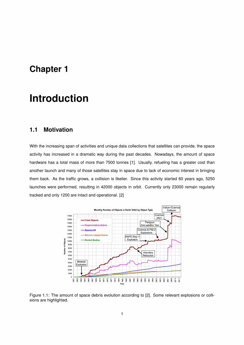
1.1 The amount of space debris evolution according to [2]. Some relevant explosions or
collisions are highlighted. . . . . . . . . . . . . . . . . . . . . . . . . . . . . . . . . . . . . 1
2.1 Representation of the typical rendezvous stages. ADR missions introduced new concepts
on capture and the idea of de-orbiting. . . . . . . . . . . . . . . . . . . . . . . . . . . . . . 10
2.2 The concept of the net-based system currently being studied by ESA. Obtained the best
score among other ideas presented in [34]. . . . . . . . . . . . . . . . . . . . . . . . . . . 11
2.3 Representation of ENVISAT [36]. . . . . . . . . . . . . . . . . . . . . . . . . . . . . . . . . 12
2.4 Structural and relevant characteristics of the adopted chaser vehicle based on net capture
mechanism for e-Deorbit mission [34]. . . . . . . . . . . . . . . . . . . . . . . . . . . . . . 13
3.2 Illustration of conjugacy. Shewchuk [55] stated that if one could strech the left figure until
the ellipsed appeared circles, then the its vector would appear orthoghonal as in the right
image. Adapted from [55]. . . . . . . . . . . . . . . . . . . . . . . . . . . . . . . . . . . . . 26
3.3 Illustration of the penalty factor concept. Increasing the penalty factor will increase the
infeasibilities penalties, until convergence. . . . . . . . . . . . . . . . . . . . . . . . . . . . 28
3.4 Overview of the implemented software using block diagrams and levels. . . . . . . . . . . 28
3.6 Fourier series approximation of pulse function (in black). Adaptation from [65] . . . . . . . 39
4.1 Representation of an Hohmann transfer procedure for orbit raising. Adapted from [10]. . . 46
4.2 Representation of a three-impulse transfer. For a r2r1> 11.94, the Hohmann transfer is no
longer the impulse-optimal orbital transfer. Adapted from [69] . . . . . . . . . . . . . . . . 47
4.3 Variation of ∆VTotal with the ratio ρ = r2r1≈ ∆x + 1 of the final and initial orbit, using the
CW equations and the Vis-viva equation . . . . . . . . . . . . . . . . . . . . . . . . . . . . 48
xv
4.4 Resulting state evolution after the Hohmann transfer simulation. For a scenario with
y0 = 5[N ] and with variables Ω = 1[rad/s] and m = 1[kg] the corresponding Hohmann
transfer of ∆x = 2.5[m] was tried. From equation 4.12, the resulting continuous force to
apply on y direction during an orbital period T = 2πΩ is Fy = 1.99× 10⁻¹[N ]. . . . . . . . . 50
4.5 Track of chaser vehicle trajectory during the Hohmann transfer (∆x = 2.5) (Hill’s Frame) . 50
4.6 Comparison between the resulting orbit trajectory of the solutions provided by SEPFOpt
and DIDO for the Earth-Venus transfer. . . . . . . . . . . . . . . . . . . . . . . . . . . . . . 54
4.7 Comparison between the resulting endpoints of the solutions provided by SEPFOpt and
DIDO for the Earth-Venus transfer. . . . . . . . . . . . . . . . . . . . . . . . . . . . . . . . 54
4.9 Comparison between the hamiltonian history of the solutions provided by SEPFOpt,
DIDO and linear values for the Earth-Venus transfer. . . . . . . . . . . . . . . . . . . . . . 55
4.10 Comparison between the resulting orbit trajectory of the solutions provided by SEPFOpt,
DIDO and linear values for the Earth-Mars transfer. . . . . . . . . . . . . . . . . . . . . . . 56
4.11 Comparison between the resulting endpoints of the solutions provided by SEPFOpt and
DIDO for the Earth-Mars transfer. . . . . . . . . . . . . . . . . . . . . . . . . . . . . . . . . 56
4.13 Comparison between the hamiltonian history of the solutions provided by SEPFOpt and
DIDO for the Earth-Mars transfer. . . . . . . . . . . . . . . . . . . . . . . . . . . . . . . . . 57
4.14 Absolute error between the the cost results from SEPFOpt and linear theory and between
SEPFOpt and DIDO. The simulation number axis is in accordance with the tables at
Appendix B. . . . . . . . . . . . . . . . . . . . . . . . . . . . . . . . . . . . . . . . . . . . . 58
4.15 Comparison between endpoint evolution for the original DIDO solution for the Earth-Mars
problem and the propagated one. The final state error for the propagated solution is∑13i=1 |Ωi(x(tf ))| = 1.6172× 10⁻⁴. . . . . . . . . . . . . . . . . . . . . . . . . . . . . . . . . 59
4.16 Variation of manouevre cost J∗SEPFOpt with tf and ρ. . . . . . . . . . . . . . . . . . . . . . 59
5.1 Illustration of a non-collision scenario. The collision test is simply verifying if R > Rc +Rt. 65
5.2 Representation of the trajectory along the z axis and the impossibility of reaching certain
values of rz(tf ). . . . . . . . . . . . . . . . . . . . . . . . . . . . . . . . . . . . . . . . . . 66
5.3 Obtained trajectory for docking manoeuvres where the initial position rz0 was perturbed
positively (in red) and negatively (in blue). Results obtained for DIDO with 100 nodes. . . 67
6.1 Plane xy view of docking manouevre performed by chaser (DIDO). . . . . . . . . . . . . . 73
6.2 Zoom of docking manoeuvre performed by the chaser (SEPFOpt). . . . . . . . . . . . . . 74
6.3 Control variables history obtained for the minimum energy docking manoeuvre (DIDO). . 75
6.4 Hamiltonian history obtained for the minimum energy docking manoeuvre (DIDO). . . . . 75
xvi
6.5 Endpoints history obtained for the minimum energy docking manoeuvre (DIDO). . . . . . 76
6.7 Hamiltonian history obtained for the minimum absolute fuel docking manoeuvre (DIDO). . 77
6.6 Control variables history obtained for the minimum absolute fuel docking manoeuvre
(DIDO). . . . . . . . . . . . . . . . . . . . . . . . . . . . . . . . . . . . . . . . . . . . . . . 77
6.8 Endpoints history obtained for the minimum absolute fuel docking manoeuvre (DIDO). . . 78
6.9 Control variables history obtained for the mixed performance index docking manoeuvre
(DIDO). . . . . . . . . . . . . . . . . . . . . . . . . . . . . . . . . . . . . . . . . . . . . . . 79
6.10 Hamiltonian history obtained for the mixed performance index docking manoeuvre (DIDO). 79
6.11 Endpoints history obtained for the mixed performance index docking manoeuvre (DIDO). 80
6.12 Control variables history obtained for the minimum energy docking manoeuvre (SEPFOpt). 81
6.13 Endpoints history and listed final values obtained for the minimum energy docking ma-
noeuvre (SEPFOpt). . . . . . . . . . . . . . . . . . . . . . . . . . . . . . . . . . . . . . . . 82
6.14 Hamiltonian history obtained for the minimum energy docking manoeuvre (SEPFOpt). . . 82
6.15 Co-states history obtained for the minimum energy docking manoeuvre (SEPFOpt). . . . 83
6.16 Comparison between the controls history and the gradient of H obtained for the minimum
energy docking manoeuvre (SEPFOpt). . . . . . . . . . . . . . . . . . . . . . . . . . . . . 83
6.18 Control variables history obtained for the mixed performance index docking manoeuvre
(SEPFOpt). . . . . . . . . . . . . . . . . . . . . . . . . . . . . . . . . . . . . . . . . . . . . 85
6.19 Hamiltonian history obtained for the mixed performance index docking manoeuvre (SEP-
FOpt). . . . . . . . . . . . . . . . . . . . . . . . . . . . . . . . . . . . . . . . . . . . . . . . 85
6.20 Endpoints history obtained for the mixed performance index docking manoeuvre (SEP-
FOpt). . . . . . . . . . . . . . . . . . . . . . . . . . . . . . . . . . . . . . . . . . . . . . . . 86
6.21 Plane xy view of capture manoeuvre performed by chaser (DIDO solution). . . . . . . . . 87
6.22 Zoom of capture manoeuvre performed by chaser (DIDO solution). . . . . . . . . . . . . . 87
6.23 Control variables history obtained for the minimum energy capture manoeuvre (DIDO). . . 88
6.24 Endpoints history obtained for the minimum energy capture manoeuvre (DIDO). . . . . . 88
6.25 Plane xy view of minimum energy capture manoeuvre performed by chaser (SEPFOpt). . 89
6.26 Zoom of minimum energy capture manoeuvre performed by chaser (SEPFOpt). . . . . . . 89
6.27 Control variables history obtained for the minimum energy capture manoeuvre (SEPFOpt). 90
6.28 Endpoints history obtained for the minimum energy capture manoeuvre (SEPFOpt). . . . 90
6.29 Comparison between the solutions for SEPFOpt and DIDO for the minimum energy dock-
ing manoeuvre. . . . . . . . . . . . . . . . . . . . . . . . . . . . . . . . . . . . . . . . . . . 92
6.30 Comparison between the endpoint histories of SEPFOpt, DIDO and the propagation of
DIDO solution for the minimum energy docking manoeuvre. . . . . . . . . . . . . . . . . . 92
xvii

6.31 Comparison between the solutions for SEPFOpt and DIDO for the minimum energy cap-
ture manoeuvre. . . . . . . . . . . . . . . . . . . . . . . . . . . . . . . . . . . . . . . . . . 93
6.32 Comparison between the endpoint histories of SEPFOpt, DIDO and the propagation of
DIDO solution for the minimum energy capture manoeuvre. . . . . . . . . . . . . . . . . . 93
xviii

.
xix

Nomenclature
CB Central Body.
Ω Targets angular rate.
µ Earths Standart Gravitacional Parameter.
a(d)(b/c) Physical quantity a of b with respect to c measured at d
~M Torque.
~ω Angular velocity
~f Thrust force.
~r Position.
~v Linear velocity.
c chaser vehicle.
d Docking point.
i, j, k Computational indexes.
t target vehicle.
x′′, y′′, z′′ Cartesian coordinates at Auxiliary frame.
x′, y′, z′ Cartesian coordinates at chaser body frame.
x, y, z Cartesian coordinates at Hill’s coordinate frame.
Acronyms
ISS International Space Station.
ADR Active Debris Removal.
xx

CW Clohessy and Wiltshire.
GNC Guidance Navigation Control.
LEO Low-Earth Orbit.
OCP Optimal Control Problems.
OCP Sequential Unconstrained Minimization Technique.
RCS Reaction Control System.
RODC Rendezvous Operations and Docking Control.
RVD Rendezvous.
xxi

xxii
Chapter 1
Introduction
1.1 Motivation
With the increasing span of activities and unique data collections that satellites can provide, the space
activity has increased in a dramatic way during the past decades. Nowadays, the amount of space
hardware has a total mass of more than 7500 tonnes [1]. Usually, refueling has a greater cost than
another launch and many of those satellites stay in space due to lack of economic interest in bringing
them back. As the traffic grows, a collision is likelier. Since this activity started 60 years ago, 5250
launches were performed, resulting in 42000 objects in orbit. Currently only 23000 remain regularly
tracked and only 1200 are intact and operational. [2]
Figure 1.1: The amount of space debris evolution according to [2]. Some relevant explosions or colli-sions are highlighted.
1
Over time, the harsh space environment can reduce the mechanical integrity of external and internal
parts, leading to leaks and mixing of fuel components, which could trigger self-ignition of the residual
fuel [1]. The resulting explosion can destroy the object and spread its mass across numerous fragments
with an enormous range of sizes and resulting velocities.
Since Low Earth orbit (LEO) environment is reaching a critical point where new launches will face
difficulties due to the amount of debris in high density zones [3] , European Space Agency (ESA)
decided to take action on this topic launching the Clean Space program [4]. A branch of this initiative,
e.Deorbit, investigates the actual task of chasing a non-operational object, capturing it and then sending
it back to Earth where it would be burnt on its atmospheric re-entry. The project includes developing a
proper chaser vehicle, equipped with new technologies that include all the control and guidance systems
required.
Moreover, other important tasks in space are dependent on a reliable technology of approach and
docking of two spacecraft. A wide range of services that could be provided such as repairing and refu-
eling could even revive some unused material in space. Currently, DARPA’s OE Advanced Technology
Demonstration Program validated the technology and techniques for on-orbit refueling [5]. It is important
to refer that the prime driver in orbit maneuvers (excluding the military ones, where the time minimization
acquires an extraordinary importance) is the fuel consumption. The cost of any propellant in Earth is not
comparable to anywhere in space mainly because of the huge additional cost per kilogram associated
to launching.
However, even with the investment in the aforementioned programs, spacecraft proximity operations
that have any dynamic tasking attributes are currently executed by humans, relying heavily on an ex-
tensive staff to plan and oversee the maneuvers [6]. As a consequence, this approach is spender with
respect to time, manpower and fuel efficiency. Therefore, there is a need for a robust and effective
autonomous close proximity control algorithm for spacecraft rendezvous.
1.2 Topic Overview
Active Debris Removal (ADR)
NASA scientist Donald J. Kessler proposed back in 1978 [7] a theory, known as the Kessler syndrome
where he stated that the environment has already reached a point where collisions among existing
debris will result in the population to increase, even if the launches stopped. It emphasized the imminent
danger of small debris in orbit and the need to reduce them. A set of measures to reduce debris is
proposed by Bonnal [8].
2
Space debris mitigation requirements have been adopted internationally, such as the French Space
Operations Act [9] where a set of several requirements and technical implementations were defined with
focus on ensuring long-term safety and sustainability for population and environment.
A number of challenges arise from the target being non-designed for rendezvous. The unfavorable
disposal of the antennas and solar panels and difficult the approach and handling from another vehicle.
The target may also be non-responding to any request of its current state. New technologies must
be capable of analyzing the target motion before taking any step. Recall that a collision would be
catastrophic. Besides not meeting the mission goal, it would turn the scenario even worst, and since
the priority targets are large and heavy ones, it would largely augment the problem that the mission was
trying to solve. These technical challenges using a chase and catch technique for debris removal have
been summarized by Fehse [10]. A more recent article [11] describes high-level variety of potential
solutions focused on the recent studies on this area and current trends.
The subject of space debris was faced by ESA with the launch of the Clean Space initiative [12]. A
branch of this study, e.Deorbit, investigates the viability of debris removal based on a development of a
chaser vehicle with all the necessary technologies. All the work is focused on removing an ESA-owned
large non-operational satellite from LEO. This is the first ADR mission that ever occured and then it
represents a great share of the knowledge and development of the field.
Four conference sessions have already taken place with several presentations from ESA and its
industrial partners that not only underlined the feasibility of this basic concept but also provided an
update on the ongoing validation of key technologies.
Rendezvous Guidance and Control
In the past half-century, major space countries performed hundreds of (Rendezvous) RVD missions.
The first rendezvous successfully accomplished was performed by astronaut Wally Schirra on Decem-
ber 15, 1965. The Gemini 6 maintained a distance of 30 cm (station-keeping) to Gemini 7 during 20
minutes.
A rendezvous takes place each time a spacecraft brings crew members or supplies to an orbiting
space station. Currently, Soyuz spacecraft is used at approximately six month intervals to transport
crew members to and from the International Space Station (ISS)[13].
Rendezvous orbital dynamics and control (RDOC) is a research subject of RDV missions, and con-
tinues to be an active research field of spacecraft dynamics and control since many new research ideas
and results on this topic are still coming out [14].
An exhaustive list of guidance, navigation and control (GNC) architecture efforts related to ren-
3
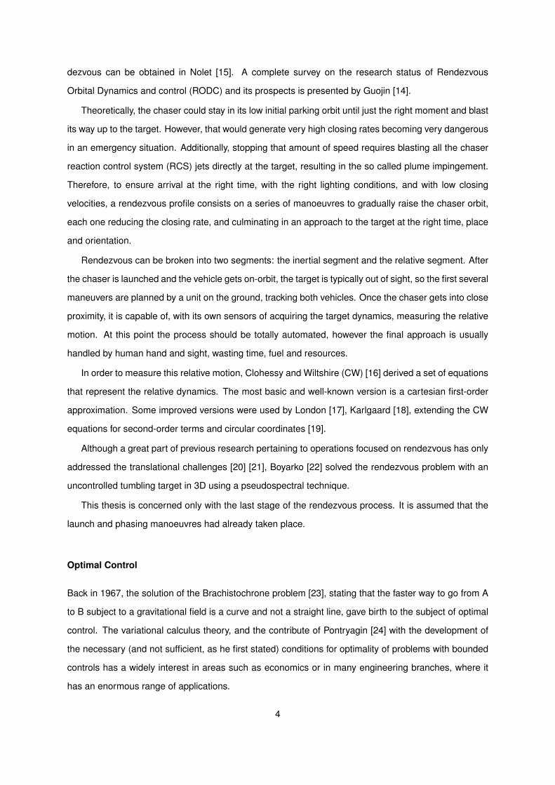
dezvous can be obtained in Nolet [15]. A complete survey on the research status of Rendezvous
Orbital Dynamics and control (RODC) and its prospects is presented by Guojin [14].
Theoretically, the chaser could stay in its low initial parking orbit until just the right moment and blast
its way up to the target. However, that would generate very high closing rates becoming very dangerous
in an emergency situation. Additionally, stopping that amount of speed requires blasting all the chaser
reaction control system (RCS) jets directly at the target, resulting in the so called plume impingement.
Therefore, to ensure arrival at the right time, with the right lighting conditions, and with low closing
velocities, a rendezvous profile consists on a series of manoeuvres to gradually raise the chaser orbit,
each one reducing the closing rate, and culminating in an approach to the target at the right time, place
and orientation.
Rendezvous can be broken into two segments: the inertial segment and the relative segment. After
the chaser is launched and the vehicle gets on-orbit, the target is typically out of sight, so the first several
maneuvers are planned by a unit on the ground, tracking both vehicles. Once the chaser gets into close
proximity, it is capable of, with its own sensors of acquiring the target dynamics, measuring the relative
motion. At this point the process should be totally automated, however the final approach is usually
handled by human hand and sight, wasting time, fuel and resources.
In order to measure this relative motion, Clohessy and Wiltshire (CW) [16] derived a set of equations
that represent the relative dynamics. The most basic and well-known version is a cartesian first-order
approximation. Some improved versions were used by London [17], Karlgaard [18], extending the CW
equations for second-order terms and circular coordinates [19].
Although a great part of previous research pertaining to operations focused on rendezvous has only
addressed the translational challenges [20] [21], Boyarko [22] solved the rendezvous problem with an
uncontrolled tumbling target in 3D using a pseudospectral technique.
This thesis is concerned only with the last stage of the rendezvous process. It is assumed that the
launch and phasing manoeuvres had already taken place.
Optimal Control
Back in 1967, the solution of the Brachistochrone problem [23], stating that the faster way to go from A
to B subject to a gravitational field is a curve and not a straight line, gave birth to the subject of optimal
control. The variational calculus theory, and the contribute of Pontryagin [24] with the development of
the necessary (and not sufficient, as he first stated) conditions for optimality of problems with bounded
controls has a widely interest in areas such as economics or in many engineering branches, where it
has an enormous range of applications.
4
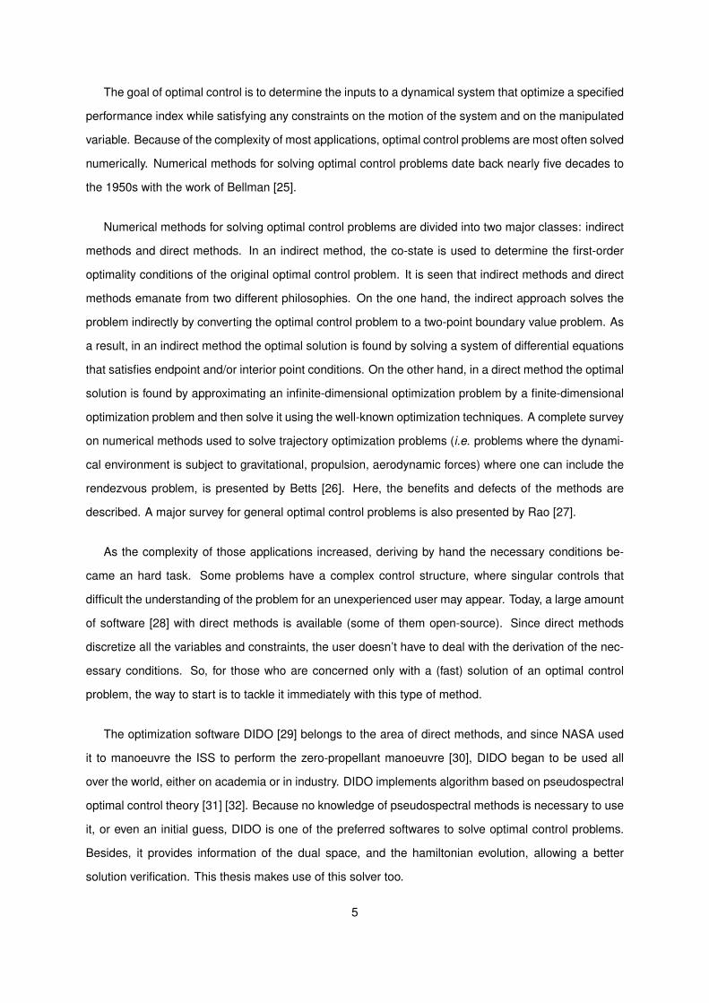
The goal of optimal control is to determine the inputs to a dynamical system that optimize a specified
performance index while satisfying any constraints on the motion of the system and on the manipulated
variable. Because of the complexity of most applications, optimal control problems are most often solved
numerically. Numerical methods for solving optimal control problems date back nearly five decades to
the 1950s with the work of Bellman [25].
Numerical methods for solving optimal control problems are divided into two major classes: indirect
methods and direct methods. In an indirect method, the co-state is used to determine the first-order
optimality conditions of the original optimal control problem. It is seen that indirect methods and direct
methods emanate from two different philosophies. On the one hand, the indirect approach solves the
problem indirectly by converting the optimal control problem to a two-point boundary value problem. As
a result, in an indirect method the optimal solution is found by solving a system of differential equations
that satisfies endpoint and/or interior point conditions. On the other hand, in a direct method the optimal
solution is found by approximating an infinite-dimensional optimization problem by a finite-dimensional
optimization problem and then solve it using the well-known optimization techniques. A complete survey
on numerical methods used to solve trajectory optimization problems (i.e. problems where the dynami-
cal environment is subject to gravitational, propulsion, aerodynamic forces) where one can include the
rendezvous problem, is presented by Betts [26]. Here, the benefits and defects of the methods are
described. A major survey for general optimal control problems is also presented by Rao [27].
As the complexity of those applications increased, deriving by hand the necessary conditions be-
came an hard task. Some problems have a complex control structure, where singular controls that
difficult the understanding of the problem for an unexperienced user may appear. Today, a large amount
of software [28] with direct methods is available (some of them open-source). Since direct methods
discretize all the variables and constraints, the user doesn’t have to deal with the derivation of the nec-
essary conditions. So, for those who are concerned only with a (fast) solution of an optimal control
problem, the way to start is to tackle it immediately with this type of method.
The optimization software DIDO [29] belongs to the area of direct methods, and since NASA used
it to manoeuvre the ISS to perform the zero-propellant manoeuvre [30], DIDO began to be used all
over the world, either on academia or in industry. DIDO implements algorithm based on pseudospectral
optimal control theory [31] [32]. Because no knowledge of pseudospectral methods is necessary to use
it, or even an initial guess, DIDO is one of the preferred softwares to solve optimal control problems.
Besides, it provides information of the dual space, and the hamiltonian evolution, allowing a better
solution verification. This thesis makes use of this solver too.
5
1.3 Objectives and contributions
The main contribution of this dissertation consists in the demonstration on how the motion planning
associated to the rendezvous of a chaser vehicle with respect to a moving target vehicle in orbit can be
formulated and solved using optimal control methods.
This thesis develops a method capable of solving the two problems posed. The first one is related
with the Clean Space initiative - a non-operational target, where the net approach is assumed. The
other problem is the docking with a operational (non-tumbling) object in space. The solutions for both
problems will be analyzed and their optimality checked and verified with DIDO.
Finally, the solvers will be compared and conclusions with respect to their performance and accuracy
will be taken.
1.4 Thesis Outline
Seeking the achievement of the stated objectives, this thesis goes from the model derivation until achiev-
ing the contextualized solutions. It is structured as follows:
• The need for developing algorithms that can reduce costs is transmitted at Chapter 1, particularly
to the under development programs of space debris mitigation and on-orbit servicing. The ap-
proaches to optimal control problems and the developments on the ADR and RDV areas are also
briefly introduced.
• The baseline chaser and target vehicles is introduced at Chapter 2, and a net-based capture
method is assumed. Moreover, it presents the three-dimensional model based on relative position,
orientation and velocities between the vehicles.
• At Chapter 3, both the indirect and direct approaches concepts are explained in higher detail,
leading to the roots of DIDO, a pseudospectral based flight-tested software and SEPFOpt, the
implemented solver, based on indirect methods.
• The capability of both solvers to reach optimal solutions was verified, at Chapter 4. Starting
by extending the Hohmann transfer optimal bi-impulsive solution to a low-thrust manoeuvre, a
simple problem of orbit raising is posed and solved by both softwares and then compared with a
linearization of the optimal solution.
• At Chapter 5, scenarios for the docking and capture manoeuvres were proposed, along with their
formulations in OCP syntax. The necessary conditions for the general rendezvous problem are
6

derived. Furthermore, the solution is studied in terms of existence, uniqueness and structure.
• The obtained results for both manoeuvres were shown at Chapter 6. Their optimality was tested,
specially for the implemented solver, whose solutions were verified with the necessary conditions.
• The final remarks and further work were shown at Chapter 7.
7

8
Chapter 2
Context
2.1 Mission Parametrization
Since 2012, ESA Clean Space initiative started to consider the entire life-cycle of space activities, from
the early stages of conceptual design to beyond the missions ending in order to reach the goal of a
cleaner and safer LEO.
Clean Space has three branches that reflect its mission to ensure the low environmental impact of
ESA programs, contributing to a more sustainable and competitive space industry.
These branches are and respective missions are:
• EcoDesign: address environmental impacts and green technologies.
• CleanSat: reduce the production of space debris
• eDeorbit: remove a large piece of space debris from orbit.
With a planned launch to 2023, e.Deorbit will be the world first ever ADR mission. The goal is to
capture an item with the highest impact possible orbiting at the range of 800to1000[km]. This region has
been identified as the focus of ADR, where the orbital lifetime of the resulting fragments is longer [33].
ADR missions follow essentially the same steps as a RDV mission (figure 2.1), with the addition of
a de-orbit stage. It is important to refer that this de-orbiting process does not imply an atmospheric
reentry. Raising the target altitude to a non-harmful orbit is also considered by future ADR missions.
9
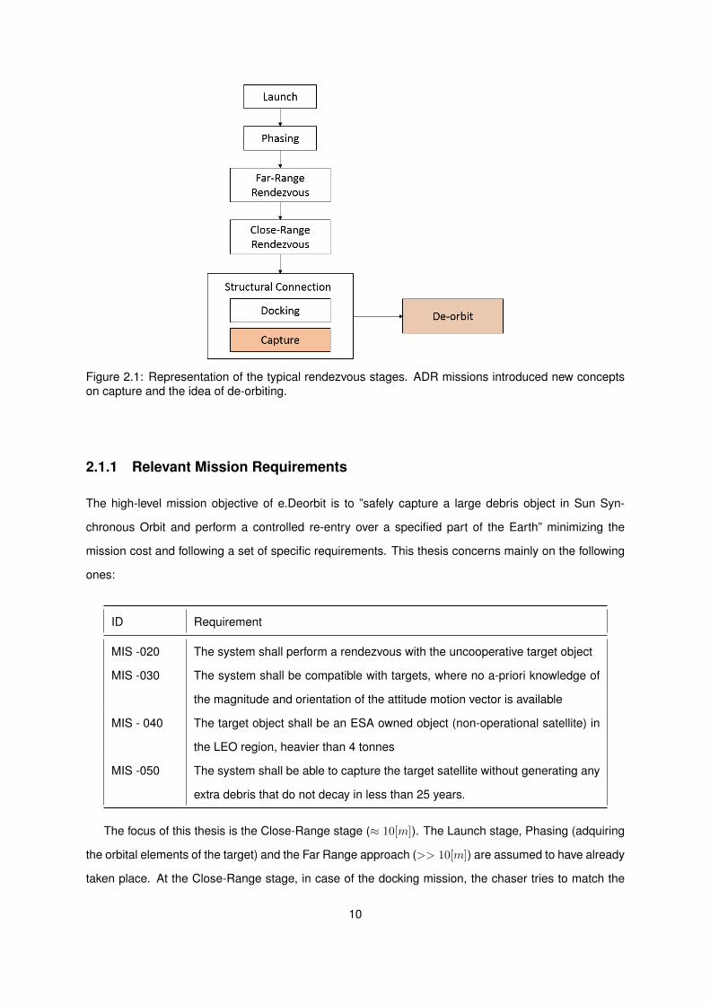
Figure 2.1: Representation of the typical rendezvous stages. ADR missions introduced new conceptson capture and the idea of de-orbiting.
2.1.1 Relevant Mission Requirements
The high-level mission objective of e.Deorbit is to ”safely capture a large debris object in Sun Syn-
chronous Orbit and perform a controlled re-entry over a specified part of the Earth” minimizing the
mission cost and following a set of specific requirements. This thesis concerns mainly on the following
ones:
ID Requirement
MIS -020 The system shall perform a rendezvous with the uncooperative target object
MIS -030 The system shall be compatible with targets, where no a-priori knowledge of
the magnitude and orientation of the attitude motion vector is available
MIS - 040 The target object shall be an ESA owned object (non-operational satellite) in
the LEO region, heavier than 4 tonnes
MIS -050 The system shall be able to capture the target satellite without generating any
extra debris that do not decay in less than 25 years.
The focus of this thesis is the Close-Range stage (≈ 10[m]). The Launch stage, Phasing (adquiring
the orbital elements of the target) and the Far Range approach (>> 10[m]) are assumed to have already
taken place. At the Close-Range stage, in case of the docking mission, the chaser tries to match the
10
target docking interface position and respective attitude. In case of a ”soft” capture, the chaser manages
to arrive to a favorable position and attitude to attack the target.
Capture Mechanism
Many ideas emerged for mechanisms that assure the structural connection between the two vehicles
were proposed, and essentially fall into two major classes. The flexible systems, such as nets or har-
poons, are capable of catching the target at a considerable distance. In the realm of the rigid mecha-
nisms, robotics arms and tentacles are studied. Although heavier than the previous ones, these robotic
devices have a greater control capacity.
The discussion between this mechanisms and its combinations is still in process. A complete study
on the trade-off between them is shown at [34]. The mechanisms were evaluated on several parameters
such as mass, volume, controllability, cost... For each parameter a degree of priority was attributed. The
mechanism that scored a higher punctuation was the tether-based net, specially given its unbeatable
versatility, lower mass and low complexity of approach and capture.
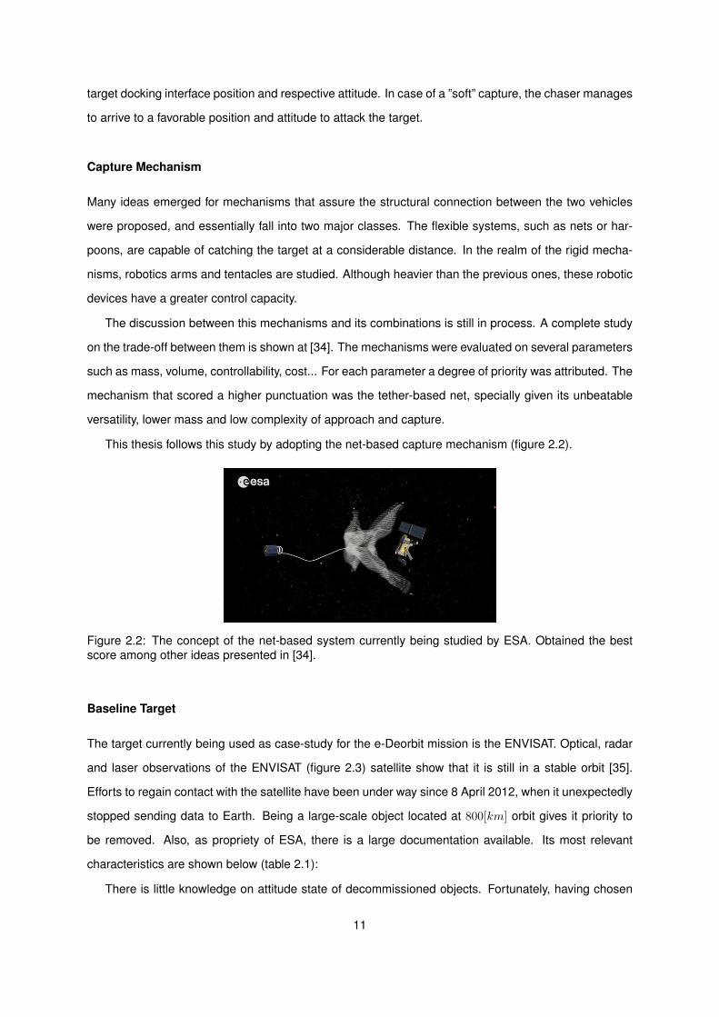
This thesis follows this study by adopting the net-based capture mechanism (figure 2.2).
Figure 2.2: The concept of the net-based system currently being studied by ESA. Obtained the bestscore among other ideas presented in [34].
Baseline Target
The target currently being used as case-study for the e-Deorbit mission is the ENVISAT. Optical, radar
and laser observations of the ENVISAT (figure 2.3) satellite show that it is still in a stable orbit [35].
Efforts to regain contact with the satellite have been under way since 8 April 2012, when it unexpectedly
stopped sending data to Earth. Being a large-scale object located at 800[km] orbit gives it priority to
be removed. Also, as propriety of ESA, there is a large documentation available. Its most relevant
characteristics are shown below (table 2.1):
There is little knowledge on attitude state of decommissioned objects. Fortunately, having chosen
11
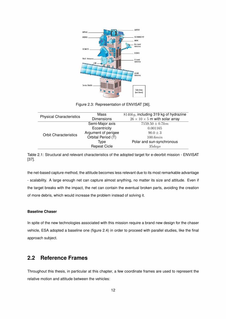
Figure 2.3: Representation of ENVISAT [36].
Physical Characteristics Mass 8140kg, including 319 kg of hydrazineDimensions 26× 10× 5 m with solar array
Orbit Characteristics
Semi-Major axis 7159.50± 0.7kmEccentricity 0.001165
Argument of perigee 90.0± 3Orbital Period (T) 100.6min
Type Polar and sun-synchronousRepeat Cicle 35days
Table 2.1: Structural and relevant characteristics of the adopted target for e-deorbit mission - ENVISAT[37].
the net-based capture method, the attitude becomes less relevant due to its most remarkable advantage
- scalability. A large enough net can capture almost anything, no matter its size and attitude. Even if
the target breaks with the impact, the net can contain the eventual broken parts, avoiding the creation
of more debris, which would increase the problem instead of solving it.
Baseline Chaser
In spite of the new technologies associated with this mission require a brand new design for the chaser
vehicle, ESA adopted a baseline one (figure 2.4) in order to proceed with parallel studies, like the final
approach subject.
2.2 Reference Frames
Throughout this thesis, in particular at this chapter, a few coordinate frames are used to represent the
relative motion and attitude between the vehicles:
12
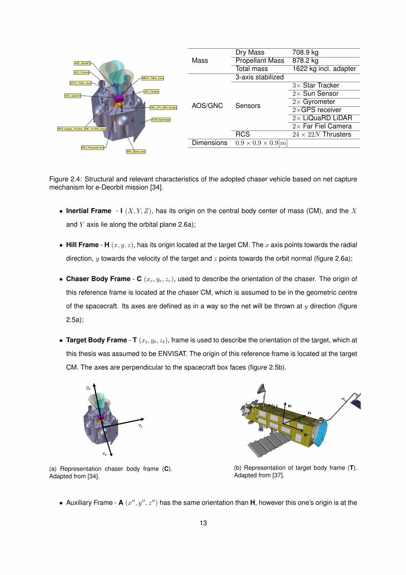
MassDry Mass 708.9 kgPropellant Mass 878.2 kgTotal mass 1622 kg incl. adapter
AOS/GNC
3-axis stabilized
Sensors
3× Star Tracker2× Sun Sensor2× Gyrometer2×GPS receiver2× LiQuaRD LiDAR2× Far Fiel Camera
RCS 24× 22N ThrustersDimensions 0.9× 0.9× 0.9[m]
Figure 2.4: Structural and relevant characteristics of the adopted chaser vehicle based on net capturemechanism for e-Deorbit mission [34].
• Inertial Frame - I (X,Y, Z), has its origin on the central body center of mass (CM), and the X
and Y axis lie along the orbital plane 2.6a);
• Hill Frame - H (x, y, z), has its origin located at the target CM. The x axis points towards the radial
direction, y towards the velocity of the target and z points towards the orbit normal (figure 2.6a);
• Chaser Body Frame - C (xc, yc, zc), used to describe the orientation of the chaser. The origin of
this reference frame is located at the chaser CM, which is assumed to be in the geometric centre
of the spacecraft. Its axes are defined as in a way so the net will be thrown at y direction (figure
2.5a);
• Target Body Frame - T (xt, yt, zt), frame is used to describe the orientation of the target, which at
this thesis was assumed to be ENVISAT. The origin of this reference frame is located at the target
CM. The axes are perpendicular to the spacecraft box faces (figure 2.5b).
(a) Representation chaser body frame (C).Adapted from [34].
(b) Representation of target body frame (T).Adapted from [37].
• Auxiliary Frame - A (x′′, y′′, z′′) has the same orientation than H, however this one’s origin is at the
13

chaser CM. It will be useful to track the chaser rotation.The figure 2.6b may represent the angle
displacement of chaser body frame with respect to the auxiliary frame.
(a) Representation of Hill’s Frame (centeredat target CM) and Inertial Frame (centered atcentral body CM).
(b) Angular displacement between the C andA frames in terms of Tait Bryan angles ψ, θ, φ(yaw, pitch, roll). Adapted from [38]
2.3 RDV Dynamics
In order to achieve a docking state between the two vehicles, it is necessary reduce to zero the distance
between the positions of both docking points, ~rdt/dc , that can be written as
~rdt/dc = ~r(dt/CGt) + ~r(CGt/dc) = ~r(dt/CGt) − ~r(dc/CGt). (2.1)
In order to expand ~r(dc/CGt) it is useful to think of chaser movement as translation and rotation
separately.
~r(dc/CGt) = ~r(CGc/CGt) + ~r(dc/CGc) (2.2)
Under the assumptions considered:
• target moving under constant circular orbit around a central body,
• spherical central body,
• chaser - target distance much lower than the target - central body distance |~r(CGt/CGc)| <<
|~r(CGt/CGCB)|,
the well-known CW equations (derivation presented at [39] and [3]) provide the linear dynamics (all
the quadratic or high-order terms of positions or velocities were ignored) that models the behavior of
relative positions and velocities between the two objects CM as (using the notation rx,ry,rz to represent
the position of the chaser relative to the target mapped at Hill’s Frame, ~r(H)(CGc/CGt)
) as
14

rx − 3Ω2rx − 2Ωry = fx
m
ry + 2Ωrx =fym
rz + Ω2rz = fzm
, (2.3)
where Ω represents the constant angular velocity of the target around the central body, depending
only on the gravitational constant parameter µCB and on the radius of that circular orbit Rorbit =
|~r(CGt/CGCB)| [40]. It is calculated as:
Ω =
õCBR3orbit
. (2.4)
Note also that the forces are applied at the chaser, but expressed at Hill’s frame, [fx, fy, fz] = ~f(H)(CGc)
.
Writing equation 2.2 at Hill’s frame,
~r(H)(dc/CGt)
= ~r(H)(CGc/CGt)
+ ~r(H)(dc/CGc)
=
rx
ry
rz
+ ~r(A)(dc/CGc)
. (2.5)
In order to successfully dock the two vehicles, it is crucial to know exactly how the chaser rotates
with is body-mounted controls.
The variation of angular momentum states
~H = ~M, (2.6)
where ~H = [I]~ω represents the angular momentum of a body with inertia tensor I about a general point
with angular velocity ~ω and ~M the torque applied at that point.
Keeping track of the motion with an inertial coordinate system and expanding 2.6, it follows [41]
~M = ~H =d
dt([I]~ω) = [I]~ω + ~ω[I]. (2.7)
In spite of the validity of this approach, keeping track of [I] is difficult, even if starting with the inertial
axis along the principal ones, the inertia tensor at this system would vary, resulting in a non-diagonal
matrix, turning the calculations harder. This issue disappears if a body frame is adopted. It is only
necessary to include the Coriolis Theorem term (~ω×) [41].
With a body-fixed axis, equation 2.7 becomes:
15
H = [I]ω + ω ×H (2.8)
Although with this approach [I] = 0 is guaranteed, it is now necessary to develop a technique to
follow the changes in axis location as the body rotates.
In order to avoid gimbal lock [42] and obtain a better computation performance [43] (sine and co-
sine functions are approximated by polynomials, slowing the process when computing Euler’s rotation
matrices), quaternions were used as alternative.
From their definition, quaternions are divided into a scalar and vector part as,
q = (r, ~v), q ∈ <4, r ∈ <, ~v ∈ <3. (2.9)
Usually they are represented in the form:
q = (q0 + q1i + q2j + q3k), (2.10)
where q0,q1,q2,q3 are real numbers and i,j,k are imaginary units. It is possible to extract the axis
of rotation ~a and the angle θ (amount of rotation performed around the axis) from these real numbers,
since
q0 = cos( θ2 )
q1 = ax sin( θ2 )
q2 = ay sin( θ2 )
q3 = az sin( θ2 )
. (2.11)
The multiplication between two quaternions, qaqb, in terms of their scalar and vector parts is defined
as [44]
qaqb = (sa, va) · (sb, vb) = (sasb − va · vb, savb + sbva + va × vb). (2.12)
A rotated point prot around an axis defined by a quaternion q is calculated by
0
prot
= q
0
p
q−1 (2.13)
where q−1 = q∗|q|2 represents the inverse of the quaternion, q∗ its conjugate and |q| its norm. It is useful
to write equation 2.13 in a more intuitive way, such as its matricial form
16
prot = R · p, (2.14)
where
R(q) =
q20 + q2
1 − q22 − q2
3 2(q1q2 − q3q0) 2(q1q3 + q2q0)
2(q1q2 + q3q0) q20 − q2
1 + q22 − q2
3 2(q2q3 − q1q0)
2(q1q3 − q2q0) 2(q2q3 + q1q0) q20 − q2
1 − q22 + q2
3
. (2.15)
Recording that the auxiliary frame is attached to the chaser CM, aligned with the Hill’s frame, if
a quaternion qc = (qc0 , qc1 , qc2 , qc3) could track the movement of the chaser body frame around this
intermediate frame, then ~r(A)(dc/CGc)
could be given as
~r(A)(dc/CGc)
= R(qc) · ~r(B)(dc/CGc)
. (2.16)
Assuming that the chaser can be modeled as a rectangular cuboid with width w, depth d and height
h, the inertial tensor from its principal axis Ic =
[Ix′x′ Iy′y′ Iz′z′
]·I3, where I3 denotes the third order
identity matrix, will be [45]
Ic =1
12m
(h2 + d2) 0 0
0 (w2 + h2) 0
0 0 (d2 + h2)
. (2.17)
Simplifying the notation ~M(B)(dc/CMc)
= [Mx′ ,My′ ,Mz′ ]T , and ~ω(B)
(dc/CMc)= [ωx′ , ωy′ , ωz′ ]
T , the equation
2.8 can be rewritten in its scalar form as:
Mx′ = Ix′x′ ωx′ − (Iy′y′ − Iz′z′)ωy′ωz′
My′ = Iy′y′ ωy′ − (Iz′z′ − Ix′x′)ωz′ωx′
Mz′ = Iz′z′ ωz′ − (Ix′x′ − Iy′y′)ωx′ωy′
. (2.18)
The components of the quaternion qc will evolve with ~ω(A)(dc/CGCB) = [ωx′′ , ωy′′ , ωz′′ ]
T as [46]
˙qc0
˙qc1
˙qc2
˙qc3
=
1
2
0 −ωx′′ −ωy′′ −ωz′′
ωx′′ 0 ωz′′ −ωy′′
ωy′′ −ωz′′ 0 ωx′′
ωz′′ ωy′′ −ωx′′ 0
qc0
qc1
qc2
qc3
. (2.19)
17
The chaser angular velocity expressed in the auxiliary frame ~ω(A)dc/CGCB
is
~ω(dc/CGCB) = ~ω(CGc/CGCB) + ~ω(dc/CGc) ⇒ ~ω(A)(dc/CGc)
= ~ω(A)(dc/CGCB) − ~ω
(A)(CGc/CGCB). (2.20)
From equation 2.13, ~ω(A)(dc/CGCB) can be obtained by the same quantity expressed at the body frame,
using the quaternion qc as:
~ω(A)(dc/CGc)
= R(qc) · ~ω(B)(dc/CGCB) − ~ω
(A)(CGc/CGCB). (2.21)
Assuming that the target circular orbit is in the same plane thanXY , then ~ω(A)(CGc/CGCB) = ~ω
(I)(CGc/CGCB).
Since the axis Z matches with the axis z, iz = iZ , thus ~ω(A)(CGc/CGCB) = [0, 0,Ω]T , resulting in
~ω(A)(dc/CGc)
= R(qc) · ~ω(B)(dc/CGCB) −
0
0
Ω
. (2.22)
In order to model the body mounted thrusters, the forces [fx, fy, fz]T = ~f
(H)(CGc)
from equation 2.3
may now be written as a function of the ones expressed at chaser body frame as:
~f(H)(CGc)
= R(qc) · ~f (B)(CGc)
. (2.23)
2.4 State Model
The state vector will be formed by x = [rx, ry, rz, vx, vy, vz, ωx′ , ωy′ , ωz′ , qc0 , qc1 , qc2 , qc3 ] and the control
u = [fx′ , fy′ , fz′ ,Mx′ ,My′ ,Mz′ ]. Note that both forces and torques have SI units and are expressed at
the chaser body frame where the vector θ = [Ω,m,w, d, h] contains the parameters required by f .
It is now possible to compile the equations 2.3,2.18,2.19 and 2.22, into the system
x = f(x,u, θ) (2.24)
,
composed by the set of equations:
vx =(q2c0 + q2
c1 − q2c2 − q
2c3)fx′ + (2qc1qc2 − 2qc3qc0)fy′ + (2qc1qc3 + 2qc2qc0)fz′
m+ 3Ω2rx + 2Ωvy (2.24a)
18
vy =(2qc1qc2 + 2qc3qc0)fx′ + (q2
c0 − q2c1 + q2
c2 − q2c3)fy′ + (2qc2qc3 − 2qc1qc0)fz′
m− 2Ωvx (2.24b)
vz =(2qc1qc3 − 2qc2qc0)fx′ + (2qc2qc3 + 2qc1qc0)fy′ + (q2
c0 − q2c1 − q
2c2 + q2
c3)fz′
m− Ω2vz (2.24c)
ωx′ =h2 − d2
h2 + d2ωz′ωx′ +
12Mx′
m(h2 + d2)(2.24d)
ωy′ =w2 − h2
w2 + h2ωz′ωx′ +
12My′
m(w2 + h2)(2.24e)
ωz′ =d2 − w2
d2 + w2ωz′ωx′ +
12Mz′
m(d2 + w2)(2.24f)
qc0 =− [(q2c0 + q2
c1 − q2c2 − q
2c3)ωx′ + (2qc1qc2 − 2qc3qc0)ωy′ + (2qc1qc3 + 2qc2qc0)ωz′ ]qc1
− [(2qc1qc2 + 2qc3qc0)ωx′ + (q2c0 − q
2c1 + q2
c2 − q2c3)ωy′ + (2qc2qc3 − 2qc1qc0)ωz′ ]qc2
− [(2qc1qc3 − 2qc2qc0)ωx′ + (2qc2qc3 + 2qc1qc0)ωy′ + (q2c0 − q
2c1 − q
2c2 + q2
c3)ωz′ ]qc3
(2.24g)
qc1 =[(q2c0 + q2
c1 − q2c2 − q
2c3)ωx′ + (2qc1qc2 − 2qc3qc0)ωy′ + (2qc1qc3 + 2qc2qc0)ωz′ ]qc0
+ [(2qc1qc3 − 2qc2qc0)ωx′ + (2qc2qc3 + 2qc1qc0)ωy′ + (q2c0 − q
2c1 − q
2c2 + q2
c3)ωz′ ]qc2
− [(2qc1qc2 + 2qc3qc0)ωx′ + (q2c0 − q
2c1 + q2
c2 − q2c3)ωy′ + (2qc2qc3 − 2qc1qc0)ωz′ ]qc3
(2.24h)
qc2 =[(q2c0 + q2
c1 − q2c2 − q
2c3)ωx′ + (2qc1qc2 − 2qc3qc0)ωy′ + (2qc1qc3 + 2qc2qc0)ωz′ ]qc0
− [(2qc1qc3 − 2qc2qc0)ωx′ + (2qc2qc3 + 2qc1qc0)ωy′ + (q2c0 − q
2c1 − q
2c2 + q2
c3)ωz′ ]qc1
+ [(2qc1qc2 + 2qc3qc0)ωx′ + (q2c0 − q
2c1 + q2
c2 − q2c3)ωy′ + (2qc2qc3 − 2qc1qc0)ωz′ ]qc3
(2.24i)
19

qc3 =[(q2c0 + q2
c1 − q2c2 − q
2c3)ωx′ + (2qc1qc2 − 2qc3qc0)ωy′ + (2qc1qc3 + 2qc2qc0)ωz′ ]qc0
+ [(2qc1qc3 − 2qc2qc0)ωx′ + (2qc2qc3 + 2qc1qc0)ωy′ + (q2c0 − q
2c1 − q
2c2 + q2
c3)ωz′ ]qc1
− [(2qc1qc2 + 2qc3qc0)ωx′ + (q2c0 − q
2c1 + q2
c2 − q2c3)ωy′ + (2qc2qc3 − 2qc1qc0)ωz′ ]qc2
(2.24j)
that model the rotational and translational dynamics of the chaser around the target.
20
Chapter 3
Numerical Methods for Optimal
Control
Optimal control is a major tool to solve a great span of problems in multiple areas of science and
engineering. In this chapter, a generalized form for the problems proposed at this thesis is firstly defined.
Then, the origins of two methods applied used are exploited. The first one, implemented at this thesis,
is from the indirect methods class and based on conjugate gradients using a penalty for infeasible
solutions. The other one, DIDO, is based on the very actual pseudospectral methods.
3.1 Formulation
Let the dynamics of the system to control be represented by the non-linear state model:
x = f(x, u), (3.1)
in which ∂f∂x is continuous to ensure an unique solution for the initial state specified.
This set of equations, starting from an initial state x(t0) = x0 generate all the possible behaviours of
a system. where x is the state taking values in Rn , u is the control input taking values in some control
set U ⊂ Rm , t is time and t0 is the initial time.
The cost functional assigns a cost to each possible behaviour. Since for a give initial point (x0, t0)
the paths are parameterized by the control function u(t), the cost functional J can be written being only
a function of u(t), and is composed by an integral term (running cost) and a final one (terminal cost)
denoted by L and K respectively.
21
J(u) :=
∫ tf
t0
L(x(t), u(t))dt+K(xf ) (3.2)
The goal of an optimal control problem is to find a control history u(t) that minimizes the above cost
functional.
Depending on the control objective, the final time and final state can be free or fixed, or can belong
to some set. Usually it is necessary to constraint the problem by applying a set of equalities
h(x(t)) = 0. (3.3)
The so called fixed-endpoint problems are settled using these equalities at the final time. In some
cases, the search span of the state or control variables may be restricted. This cases are handled by
inequality equations. These ones are common in trajectory optimization problems, often called as path
constraints, prohibiting the trajectory to cross some areas along the path. They are represented by
g(x(t), u(t)) ≤ 0. (3.4)
Optimal control problems whose cost is given by the general form (3.2) are known as problems in the
Bolza form, or collectively as the Bolza problem. The other two popular forms, Lagrange and Mayer, are
easily converted back and forth between them using simple transformations. They are simpler forms of
the Bolza problem since at the first one there is no terminal cost: K ≡ 0 and in the second one there is
no running cost: L ≡ 0 .
A problem with a given running cost L may be converted adding an equation to the systems dynam-
ics and an extra variable such as
x0 = L(t, x, u). (3.5)
Obviously it is also necessary to define its initial value
x0(t0) = 0. (3.6)
This procedure yields:
∫ tf
t0
L(t, x(t), u(t))dt = x0(tf ). (3.7)
Therefore the terminal cost K(tf , xf ) may be augmented to include the term x0(tf ). Note that there
is no difference from the cost (3.2) to this result.
22
3.2 Indirect Methods
In order to find a miminum of a function, as in one-dimensional space, searching for zeros in the deriva-
tive of the function will lead to a stationary point (first-order conditions) and then checking its curvature
(second-order conditions) will tell if the candidate is minimum or a maximum.
The so called co-state variables (or Lagrange multipliers) λ(t) are used to adjoin the dynamical
f(x, u, t) constraints to the cost function J , augmenting it:
J = J +
∫ tf
t0
λT [x− f(x, u, t)]dt (3.8)
The common idea referred in some literature [47] is that these variables lack on physical meaning,
discarding the use of indirect methods for having to deal with them, specially if it is necessary to provide
their values as a guess. Ross [48] has given an explanation on how one should think of these co-state
variables and gain sensibility to try to guess them.
Assuming that there are no restrictions to the admissible values of u, and after deriving the gradient
of the augmented cost function, ∇J , the resulting equations (Euler-Lagrange) are the necessary set to
a candidate be stationary, [49]:
∂J∂λ = 0→ x = f(x(t), u(t), t)
∂J∂x = 0→ λ = −(∂f∂x )Tλ− (∂L∂x )T
∂J∂u = 0→ (∂L∂u )T + (∂f∂u )Tλ = 0
(3.9)
Since along the optimal solution, the term∫ tft0λT [x − f(x, u, t)]dt equals zero, the value of u that
minimizes J , minimizes J too [50]. The first order conditions are usually written with respect to the
quantity H, the Hamiltonian, defined as:
H = λf + L (3.10)
resulting on a more compact set:
x = ∂H
∂λ
λ = −∂H∂x
0 = ∂H∂u
(3.11)
The differencial equations form a system of 2n equations. To solve them, 2n boundary equations
are needed.
23
x(0) = x0
λ(tf ) = ∂K∂x(tf )
(3.12)
If there are terminal contraints Ω present, they should be adjoined to the cost functional by means
of more lagrange multipliers v, as
¯J = J + vTΩ. (3.13)
This results on the following changes of the co-state final values:
λ(tf ) =∂K
∂x(tf )+ vT
∂Ω
∂x(tf ). (3.14)
Pontryagin’s Minimum Principle
The previous set of equations was stated based on the assumption that were no boundaries to the
control. If these boundaries are present, it is not guaranteed that ∂H∂u = 0, i.e. the values of u that
minimize the function cost may not be interior points and be located on the boundaries. Pontryagin’s
minimum principle [51] included those possibilities, stating that the optimal control should satisfy:
H(x∗(t), u∗(t), λ∗(t)) ≤ H(x(t), u(t), λ(t)), ∀u ∈ U , t ∈ [t0, tf ]. (3.15)
3.2.1 Gradient Methods
Pursuing the goal of finding the minimum of a function f(x) it is important to define a search direction
with information that is reasonably easy to get. A very good one would be the gradient, since it tells in
what direction the function grows (along all the dimensions of x). So, taking its opposite as the search
direction s = −∇f(x), and taking steps along it, will iteratively approach lower values of f(x).
xk+1 = xk − λsk (3.16)
The question that follows must be: What will be the step λ value?
There are several approaches to this issue. The fixed-step gradient method considers λ constant,
as the name suggests. The simplicity of this method brings some disadvantages: If the factor is chosen
too large,then the process will likely overshoot the minimum value. However, if the factor is chosen too
small, then the process will take an endless amount of time to reach the minimum value.
24

(a) Ilustration of the large stepsize problem. The char-acteristic zig-zag denotes difficulties on convergence.Adapted from [52].
(b) Illustration of small step-size problem. The smallsteps in the search direction may take a longer time toconverge. Adapted from [52].
Line search
Other intuitively option may be to choose the step size at each iteration. Steepest descent gradient
methods attempt to overcome this difficulty by optimally choosing the step at each successive iteration
of the gradient procedure by performing a one dimensional search (line-search). The first choice to a
step to perform the ”steepest” descent, is obviously:
λk = argmin(xk − λ∇f(xk)). (3.17)
This is the simplest form of line search. Although, it may seem the best choice, it converges only
linearly and is very sensitive to ill-conditioning problems [53].
For non-linear problems an exact line search is usually undesirable since it may ask for substantial
computational resources. One of the possible solutions is the backtracking line search algorithm. As
its name suggests, backtracking allows choosing a large starting step-size and iteratively decrease
it, avoiding the large amount of time to reach the minimum value as in figure 3.1b. The step-size is
iteratively shrunk by a predefined factor λi+1 = τλi, until satisfying the Armijo-Goldstein inequality [54]:
f(x+ λs) 6 f(x) + c · λ · ∇f(x) (3.18)
This condition ensures the sufficient decrease of the functional value. The amount of decrease is
controlled by the constant parameter c ∈ [0, 1].
Conjugate Gradient
Steepest Descent often finds itself taking steps in the same direction as earlier steps. It would be
desirable that for each direction, exactly only one step is taken. The idea behind this is to consider
conjugate search directions instead of local gradient to go downhill.
25
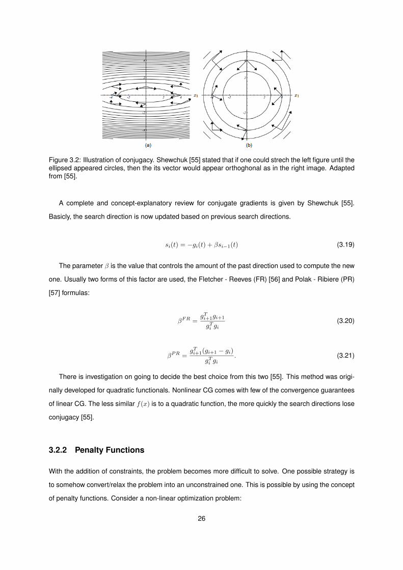
Figure 3.2: Illustration of conjugacy. Shewchuk [55] stated that if one could strech the left figure until theellipsed appeared circles, then the its vector would appear orthoghonal as in the right image. Adaptedfrom [55].
A complete and concept-explanatory review for conjugate gradients is given by Shewchuk [55].
Basicly, the search direction is now updated based on previous search directions.
si(t) = −gi(t) + βsi−1(t) (3.19)
The parameter β is the value that controls the amount of the past direction used to compute the new
one. Usually two forms of this factor are used, the Fletcher - Reeves (FR) [56] and Polak - Ribiere (PR)
[57] formulas:
βFR =gTi+1gi+1
gTi gi(3.20)
βPR =gTi+1(gi+1 − gi)
gTi gi. (3.21)
There is investigation on going to decide the best choice from this two [55]. This method was origi-
nally developed for quadratic functionals. Nonlinear CG comes with few of the convergence guarantees
of linear CG. The less similar f(x) is to a quadratic function, the more quickly the search directions lose
conjugacy [55].
3.2.2 Penalty Functions
With the addition of constraints, the problem becomes more difficult to solve. One possible strategy is
to somehow convert/relax the problem into an unconstrained one. This is possible by using the concept
of penalty functions. Consider a non-linear optimization problem:
26

Minimize f(x)
subject to: x ∈ S(3.22)
where S = x ∈ RN |gi(x) ≤ 0 ∧ hj(x) = 0 for i = 1, ...,m and j = 1, ..., l.
Unlike the direct methods presented in subsequent chapters of this thesis, the penalty function
approach is an alteration of the form of the optimal control problem itself rather than a modification of
the numerical technique used to solve it. The basic idea behind the penalty methods is to convert the
above problem to an unconstrained version, just by augmenting the functional to include a penalty term
P (x),
Minimize f(x) + P (x). (3.23)
Ideally, the infeasibilities should be penalized infinitely:
P (x) =
0, if x ∈ S,
∞, otherwise.
(3.24)
The impossibility of computing P (x), suggests a replacement for a better behaving function.
Consider that P (x) is changed to the form
P (x) = K( m∑i=1
ψ[max(0, gi(x))] +l∑
j=1
ψ[hj(x)]). (3.25)
The C0 function ψ(s) : R→ R+ has to be chosen such that ψ(s) = 0↔ s = 0. Common choices are
ψ(s) = |s| ans ψ(s) = s2.
If one chooses just one value for K, the problem may converge, but often it does not converge to a
minimum of the constrained problem. The difficulties encountered using penalty functions when solving
for one unconstrained problem can be avoided by replacing a single solution attempt by a sequence of
solutions involving increased weighting of the constraint violation (figure 3.25). Each new subproblem
is started from the solution to the previous subproblem or from an estimate derived from solutions to
the previous subproblems until satisfying the requirements of the constraint tolerances. This proce-
dure is known as sequential unconstrained minimization technique (SUMT) developed by Fiacco and
McCormick, who proved its convergence [58].
27
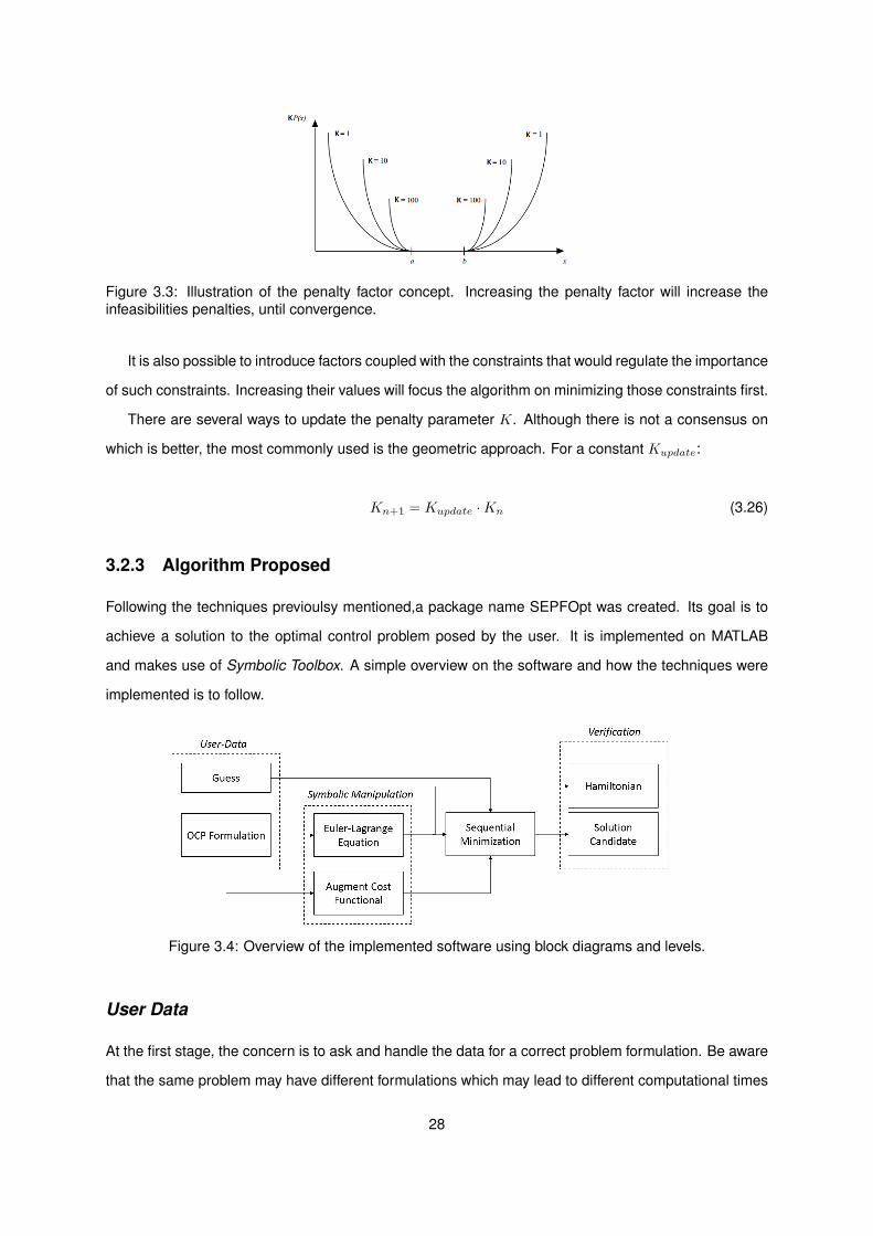
Figure 3.3: Illustration of the penalty factor concept. Increasing the penalty factor will increase theinfeasibilities penalties, until convergence.
It is also possible to introduce factors coupled with the constraints that would regulate the importance
of such constraints. Increasing their values will focus the algorithm on minimizing those constraints first.
There are several ways to update the penalty parameter K. Although there is not a consensus on
which is better, the most commonly used is the geometric approach. For a constant Kupdate:
Kn+1 = Kupdate ·Kn (3.26)
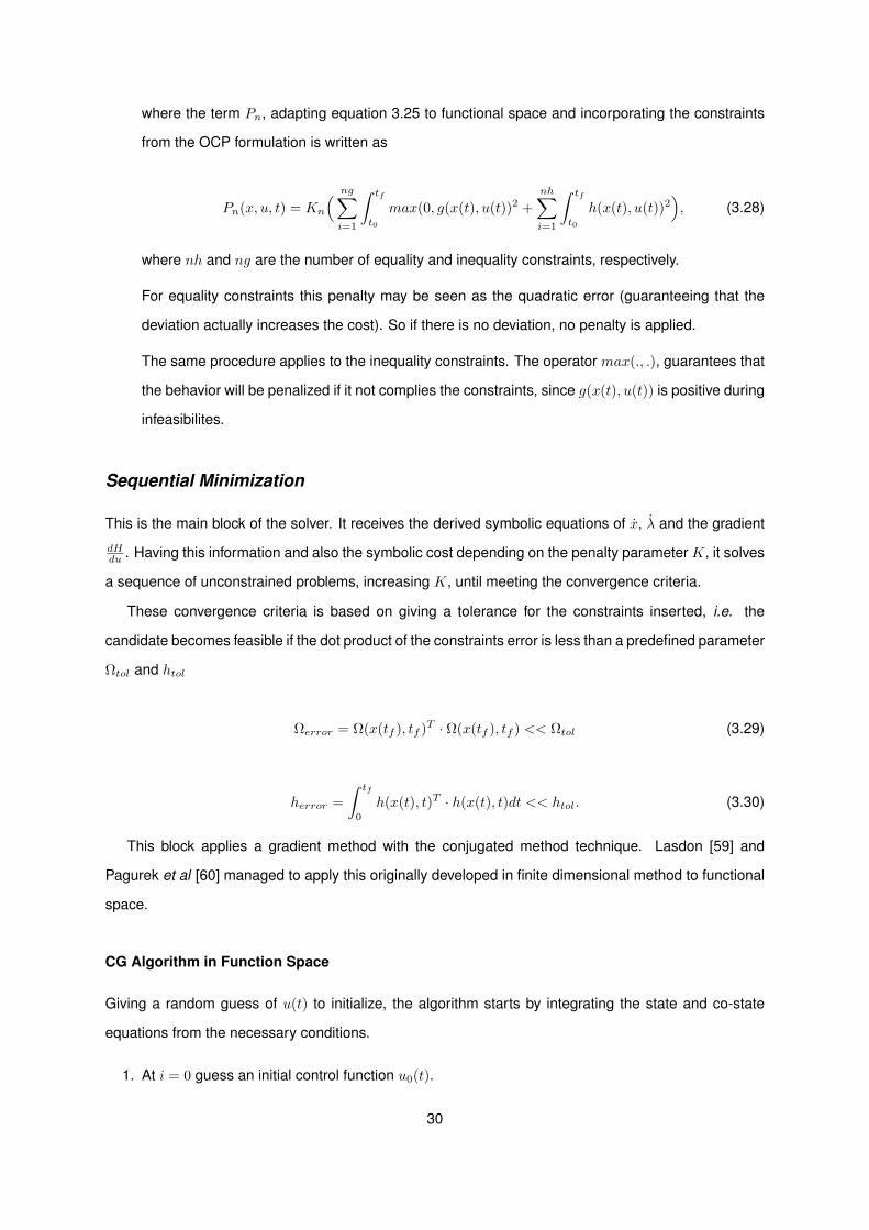
3.2.3 Algorithm Proposed
Following the techniques previoulsy mentioned,a package name SEPFOpt was created. Its goal is to
achieve a solution to the optimal control problem posed by the user. It is implemented on MATLAB
and makes use of Symbolic Toolbox. A simple overview on the software and how the techniques were
implemented is to follow.
Figure 3.4: Overview of the implemented software using block diagrams and levels.
User Data
At the first stage, the concern is to ask and handle the data for a correct problem formulation. Be aware
that the same problem may have different formulations which may lead to different computational times
28

and different solutions.
• OCP Formulation
The software starts by reading a file that stores the dynamics, cost function posed in Bolza form,
and all sort of constraints in order to formulate the optimal control problem. The final time must
also be provided.
• Guess
If the user has some sort of idea on how the control history u(t) will look like, it is recom-
mended to provide it. Although not required, (if no guess is available the software will assume
u(t) = 0 ∀t ∈ [0, tf ]), a good guess may improve dramatically the speed of the process. Also, it is
common to an OCP to have multiple local optimizers. Different guesses may lead the software to
find different solutions.
Symbolic Manipulation
The main drawback of the indirect methods are due to difficulties on deriving the necessary equations
for optimality. For complex problems, in particular the large scale ones, that task may turn out to be very
difficult. To avoid this situation, after the data is settled, the Symbolic Toolbox from MATLAB was used,
providing the handles to functions necessary at subsequent stages.
• Euler-Lagrange Equation
Here, the necessary conditions 3.11 and the transversality equation 3.14 are derived from the
problem formulation. The resulting equations are exported to the Sequential Minimization block.
Also, the hamiltonian is exported for verification purposes.
• Augment Cost Functional
This block has the functionality to augment the cost functional in the same manner as in equation
3.28, converting the OCP to an unconstrained version. It introduces the penalty parameter K
which will be updated until convergence. The augmented cost functional is
Minimize Jn = J + Pn , (3.27)
29
where the term Pn, adapting equation 3.25 to functional space and incorporating the constraints
from the OCP formulation is written as
Pn(x, u, t) = Kn
( ng∑i=1
∫ tf
t0
max(0, g(x(t), u(t))2 +
nh∑i=1
∫ tf
t0
h(x(t), u(t))2), (3.28)
where nh and ng are the number of equality and inequality constraints, respectively.
For equality constraints this penalty may be seen as the quadratic error (guaranteeing that the
deviation actually increases the cost). So if there is no deviation, no penalty is applied.
The same procedure applies to the inequality constraints. The operator max(., .), guarantees that
the behavior will be penalized if it not complies the constraints, since g(x(t), u(t)) is positive during
infeasibilites.
Sequential Minimization
This is the main block of the solver. It receives the derived symbolic equations of x, λ and the gradient
dHdu . Having this information and also the symbolic cost depending on the penalty parameter K, it solves
a sequence of unconstrained problems, increasing K, until meeting the convergence criteria.
These convergence criteria is based on giving a tolerance for the constraints inserted, i.e. the
candidate becomes feasible if the dot product of the constraints error is less than a predefined parameter
Ωtol and htol
Ωerror = Ω(x(tf ), tf )T · Ω(x(tf ), tf ) << Ωtol (3.29)
herror =
∫ tf
0
h(x(t), t)T · h(x(t), t)dt << htol. (3.30)
This block applies a gradient method with the conjugated method technique. Lasdon [59] and
Pagurek et al [60] managed to apply this originally developed in finite dimensional method to functional
space.
CG Algorithm in Function Space
Giving a random guess of u(t) to initialize, the algorithm starts by integrating the state and co-state
equations from the necessary conditions.
1. At i = 0 guess an initial control function u0(t).
30
2 Integrate x = f(x, u, t) from t0 to tf .
3. Integrate λ = −dHdx from tf to t0. Since their boundary conditions are given with respect to the
problem final time, these ones must be integrated backwards.
4. Calculate the gradient of the hamiltonian:
dH
du= gi. (3.31)
5. Calculate βi using the Fletcher and Reeves formula:
βi =
<gi,gi>
<gi−1,gi−1>, if i 6= 0
0, if i = 0
. (3.32)
6. Calculate the direction of the search si.
si(t) = −gi(t) + βsi−1(t). (3.33)
Note: In the case of steepest descent, βi = 0. This implies the search direction to be always
opposite to the gradient.
7. Let ui+1 be computed as:
ui+1 = ui + αisi. (3.34)
Perform a one-dimensional minimization (choose α) according to:
J(ui + αisi) 6 J(ui + γisi) ∀ γi ≥ 0. (3.35)
Backtracking line search
In order to perform the one dimensional minimization required at step 7, the backtracking line search
with the Armijo-Goldstein rule was chosen.
The factor c controls the ”amount” of objective function needed to be reduced at each iteration and
that the step α is updated by a factor τ defined between 0 and 1.
Converting to function space, the basic algorithm for the inexact line performed at step 7. , is now:
31
7.1 At j = 0, set c ∈ (0, 1) and α0.
7.2 Calculate the updated control law: uj+1 = uj + αjs.
7.3 Calculate J(uj+1).
7.4 Test the condition:
J(uj+1) > J(uj)αj + csTi gi. (3.36)
If true return αj as solution.
7.5 Update αj+1 = ταj .
7.6 Increment j.
7.7 Go to 7.2.
Dealing with control bounds
The presence of bounds in the control space affects the step 7.2 of the previous algorithm. For sufficient
values of αj , the calculated uj+1 may be in the infeasible domain. The approach taken was to truncate
the control values within their boundaries after this step, as
ui+1 =
ui + αisi Umin ≤ ui+1 ≤ Umax
Umin ui+1 < Umin
Umax ui+1 < Umax
. (3.37)
Verification
If the problem is feasible, it is very likely that SEPFOpt finds a solution, whatever the computational time
is. It is important to note that a solution should not be accepted as optimal without verification, whatever
the solver is. Furthermore, although the solution was calculated based on the necessary conditions,
none of the softwares currently available guarantees (this one included) the solution to be the global
minimizer of the cost functional, so the user may obtain a far to global optimal solution, finding other
local solutions. Ideally, the user should try to input a set of different guesses to each problems in order
to induce the solver to search different regions, and then compare the solutions.
Behavior of the Hamiltonian with time
The hamiltonian is a function of u, x, λ, so, following the chain rule, it derivative with respect to t will be:
32
dH(u, x, λ)
dt=∂H
∂uu+
∂H
∂xx+
∂H
∂λλ+
∂H
∂t(3.38)
Recall that from the Pontryagin Minimum Principle.
dH(u, x, λ)
dt=∂H
∂uu− λx+ xλ+
∂H
∂t(3.39)
dH(u, x, λ)
dt=∂H
∂uu+
∂H
∂t(3.40)
If the solution lies on the boundaries, then u = 0. On the other way, if it is an interior point, then
∂H∂u = 0. Thus,
dH(u, x, λ)
dt=∂H
∂t(3.41)
Therefore, since the case of an explicitly time dependent hamiltonian was not considered, then,
along the optimal trajectory, the hamiltonian of an optimal solution should be constant.
The terminal conditions and path constraints
Obviously, if constraints were imposed to the OCP, the solution must comply them in order to be feasible.
If terminal constraints are posed, the user may simply compare the final state obtained with the desired
one. Ideally, both equality and inequality constraints are strictly respected. However, different problems
may ask for different accuracies. If not satisfied, the user should re-run the software, this time reducing
the constraint tolerances Ωtol, gtol for final state and path constraints, respectively.
3.3 Direct Methods
”Discretize then optimize”
One of the primary advantages of using direct methods is that a deep understanding of optimal
control theory or the nature of the problem is not necessarily required to solve the problem. Switching
structures and adjoint variables are not a concern.
In a general way, the direct methods discretize the original optimal control problem to formulate a
nonlinear programming problem (NLP), which is then solved numerically using a sparse NLP solver to
find approximate local optimal solutions.
Since the pseudospectral methods were developed, originally for the solution of partial differential
33
equations for the subject of Fluid Dynamics [61], their techniques were implemented in important com-
putational methods for solving OCPs.
Pseudospectral methods handle relatively easily all the perks of OCPs. Differential equations are
approximated by a set of algebraic equations. The derivatives of the state functions at the discretiza-
tion nodes are easily calculated by means of a constant differentiation matrix. For differentiation, the
derivatives of the state functions at the discretization nodes are easily computed by using a constant
differentiation matrix. The method uses a Legendre or Chebyshev polynomials as basis functions to ap-
proximate another functions. One of the main appeals of pseudospectral methods is their exponential
rate of convergence [62]. The state and control constraints are converted on simply algebraic equations.
The objective of the remainder of this section is to develop an understanding of some progressively
more complicated direct methods, starting with basic collocation and moving through to pseudospectral
methods.
In spite of being unnecessary to know any theoretical background to get a solution from DIDO
(besides the problem formulation), it is important to have some notions on its numerical approach to
understand its behavior. This section summarizes the numerical tools used by DIDO. The concepts
of interpolation, orthogonality and quadrature are mixed to ultimately understand the Legendre Pseu-
dospectral method used by this solver.
3.3.1 Collocation methods and its numerical techniques
Due to their useful proprieties, such as the possibility of being represented by a finite set of coefficients,
and calculate integrals and derivatives easily by using the same coefficients, polynomial splines are
used by direct transcription methods to discretize a continuous optimization problem.
Collocation is the method by which conditions are enforced. In the discretization of the dynamical
constraints, an approximation for the time derivative is required at selected points. Therefore, the goal
is to use the discrete values of x(t) that enforce the dynamics to be satisfied. The dynamics residual is
defined as
ri = f(xi, ui, ti)− x′i (3.42)
at some evaluation point i, where x′i is an approximation of f(xi, ui, ti) in terms of the values of x
and f at that evaluation point and several neighboring points. The goal of collocation is to force ri to
zero.
This is illustrated below by using three different collocation methods: Euler, midpoint and trapezoidal.
Each one with its way of approximating x(t). In the trapezoidal method the collocation of the other
34
constraints and elements is also shown. For all these methods, assume that the discrete points are
selected at equal intervals, ∆t.
Trapezoidal Method
The trapezoidal rule [63] approximates x(t) by using the average of fi and fi+1. Explicitly,
xn+1 ≈ xn +∆t
2
(fi + fi+1
). (3.43)
This method has an order of consistency O(∆t3), thus a two degree accuracy.
The conversion process into an NLP is known as transcription and it is why some literature refers to
direct collocation methods as direct transcription methods.
Trapezoidal collocation is one of the simplest case of transcription. The conversion of a continuous-
time OCP into a non-linear program is done using trapezoid rule stated above for integration, to convert
each continuous aspect of the problem into a discrete approximation. An overview on how this method
generates a NLP from an optimal control problem is to follow. Each element of the OCP, such as
dynamics, control, constraints and cost function is treated.
1. Integrals.
With a cost functional written at the Bolza form, the integral term requires special attention in the
transcription process. The key concept here is that the summation only requires the value of the
integrand at the collocation points tk along the trajectory. This approximation is done by applying
the trapezoid rule for integration between each collocation point. Explicitly,
∫ tf
0
L(x(t), u(t)dt ≈N−1∑i=0
1
2∆t(Li + L+1). (3.44)
2. Dynamics.
For trapezoidal collocation, the dynamical constraints are constructed by writing the dynamics in
integral form. Since x = f :
x =
∫ ti+1
ti
fdt (3.45)
Now the integral is approximated with the trapezoidal rule as in equation 3.43 for every collocation
points i ∈ 0...N − 1:
xi+1 − xi =∆t
2(fi+1 + fi), (3.46)
35
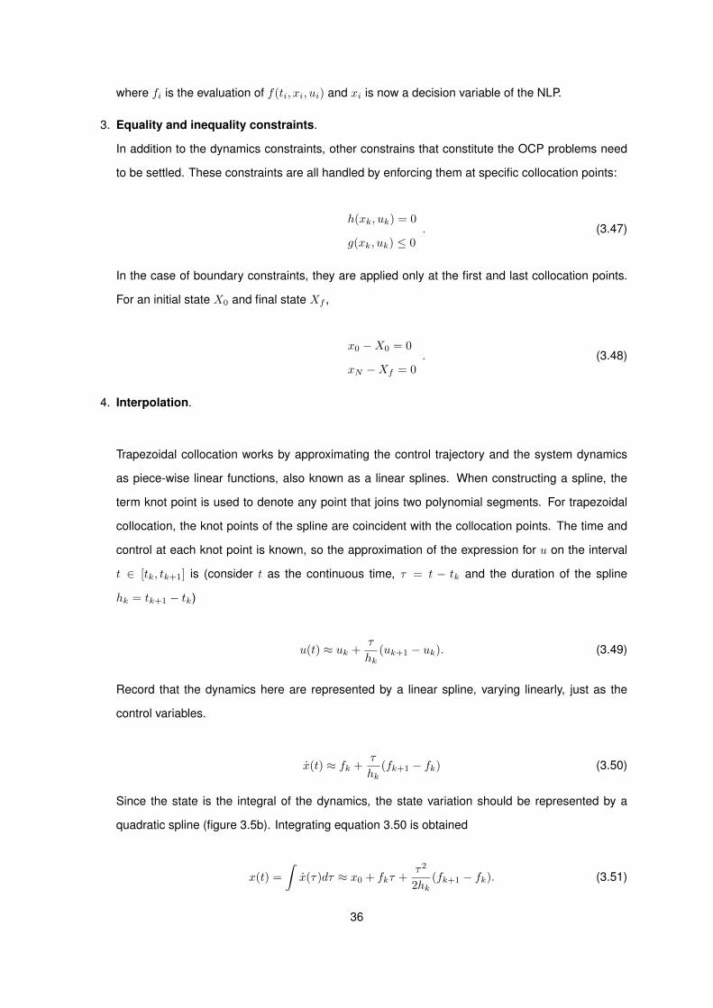
where fi is the evaluation of f(ti, xi, ui) and xi is now a decision variable of the NLP.
3. Equality and inequality constraints.
In addition to the dynamics constraints, other constrains that constitute the OCP problems need
to be settled. These constraints are all handled by enforcing them at specific collocation points:
h(xk, uk) = 0
g(xk, uk) ≤ 0. (3.47)
In the case of boundary constraints, they are applied only at the first and last collocation points.
For an initial state X0 and final state Xf ,
x0 −X0 = 0
xN −Xf = 0. (3.48)
4. Interpolation.
Trapezoidal collocation works by approximating the control trajectory and the system dynamics
as piece-wise linear functions, also known as a linear splines. When constructing a spline, the
term knot point is used to denote any point that joins two polynomial segments. For trapezoidal
collocation, the knot points of the spline are coincident with the collocation points. The time and
control at each knot point is known, so the approximation of the expression for u on the interval
t ∈ [tk, tk+1] is (consider t as the continuous time, τ = t − tk and the duration of the spline
hk = tk+1 − tk)
u(t) ≈ uk +τ
hk(uk+1 − uk). (3.49)
Record that the dynamics here are represented by a linear spline, varying linearly, just as the
control variables.
x(t) ≈ fk +τ
hk(fk+1 − fk) (3.50)
Since the state is the integral of the dynamics, the state variation should be represented by a
quadratic spline (figure 3.5b). Integrating equation 3.50 is obtained
x(t) =
∫x(τ)dτ ≈ x0 + fkτ +
τ2
2hk(fk+1 − fk). (3.51)
36
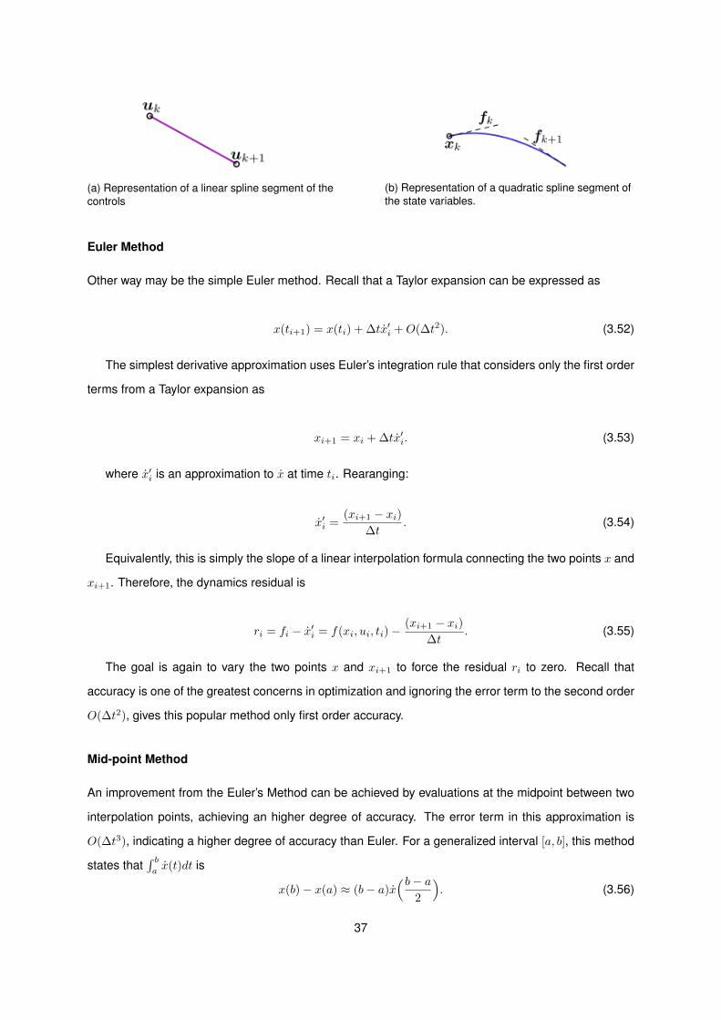
(a) Representation of a linear spline segment of thecontrols
(b) Representation of a quadratic spline segment ofthe state variables.
Euler Method
Other way may be the simple Euler method. Recall that a Taylor expansion can be expressed as
x(ti+1) = x(ti) + ∆tx′i +O(∆t2). (3.52)
The simplest derivative approximation uses Euler’s integration rule that considers only the first order
terms from a Taylor expansion as
xi+1 = xi + ∆tx′i. (3.53)
where x′i is an approximation to x at time ti. Rearanging:
x′i =(xi+1 − xi)
∆t. (3.54)
Equivalently, this is simply the slope of a linear interpolation formula connecting the two points x and
xi+1. Therefore, the dynamics residual is
ri = fi − x′i = f(xi, ui, ti)−(xi+1 − xi)
∆t. (3.55)
The goal is again to vary the two points x and xi+1 to force the residual ri to zero. Recall that
accuracy is one of the greatest concerns in optimization and ignoring the error term to the second order
O(∆t2), gives this popular method only first order accuracy.
Mid-point Method
An improvement from the Euler’s Method can be achieved by evaluations at the midpoint between two
interpolation points, achieving an higher degree of accuracy. The error term in this approximation is
O(∆t3), indicating a higher degree of accuracy than Euler. For a generalized interval [a, b], this method
states that∫ bax(t)dt is
x(b)− x(a) ≈ (b− a)x(b− a
2
). (3.56)
37
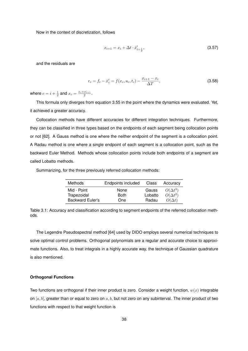
Now in the context of discretization, follows
xi+1 = xi + ∆t · x′i+ 12, (3.57)
and the residuals are
rc = fc − x′c = f(xc, uc, tc)−xi+1 − xi
∆T, (3.58)
where c = i+ 12 and xc = xi+xi+1
2 .
This formula only diverges from equation 3.55 in the point where the dynamics were evaluated. Yet,
it achieved a greater accuracy.
Collocation methods have different accuracies for different integration techniques. Furthermore,
they can be classified in three types based on the endpoints of each segment being collocation points
or not [62]. A Gauss method is one where the neither endpoint of the segment is a collocation point.
A Radau method is one where a single endpoint of each segment is a collocation point, such as the
backward Euler Method. Methods whose collocation points include both endpoints of a segment are
called Lobatto methods.
Summarizing, for the three previously referred collocation methods:
Methods Endpoints included Class Accuracy
Mid - Point None Gauss O(∆t3)Trapezoidal Both Lobatto O(∆t2)Backward Euler’s One Radau O(∆t)
Table 3.1: Accuracy and classification according to segment endpoints of the referred collocation meth-ods.
The Legendre Pseudospectral method [64] used by DIDO employs several numerical techniques to
solve optimal control problems. Orthogonal polynomials are a regular and accurate choice to approxi-
mate functions. Also, to treat integrals in a highly accurate way, the technique of Gaussian quadrature
is also mentioned.
Orthogonal Functions
Two functions are orthogonal if their inner product is zero. Consider a weight function, w(x) integrable
on [a, b], greater than or equal to zero on a, b, but not zero on any subinterval. The inner product of two
functions with respect to that weight function is
38
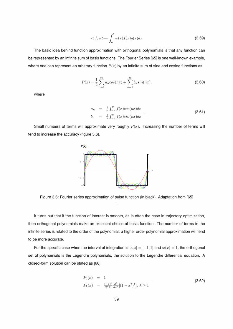
< f, g >=
∫ b
a
w(x)f(x)g(x)dx. (3.59)
The basic idea behind function approximation with orthogonal polynomials is that any function can
be represented by an infinite sum of basis functions. The Fourier Series [65] is one well-known example,
where one can represent an arbitrary function P (x) by an infinite sum of sine and cosine functions as
P (x) =1
2
∞∑n=1
ancos(nx) +
∞∑n=1
bnsin(nx), (3.60)
where
an = 1π
∫ π−π f(x)cos(nx)dx
bn = 1π
∫ π−π f(x)sin(nx)dx
. (3.61)
Small numbers of terms will approximate very roughly P (x). Increasing the number of terms will
tend to increase the accuracy (figure 3.6).
Figure 3.6: Fourier series approximation of pulse function (in black). Adaptation from [65].
It turns out that if the function of interest is smooth, as is often the case in trajectory optimization,
then orthogonal polynomials make an excellent choice of basis function. The number of terms in the
infinite series is related to the order of the polynomial: a higher order polynomial approximation will tend
to be more accurate.
For the specific case when the interval of integration is [a, b] = [−1, 1] and w(x) = 1, the orthogonal
set of polynomials is the Legendre polynomials, the solution to the Legendre differential equation. A
closed-form solution can be stated as [66]:
P0(x) = 1
Pk(x) = (−1)k
2kk!dk
dxk[(1− x2)k], k ≥ 1
. (3.62)
39
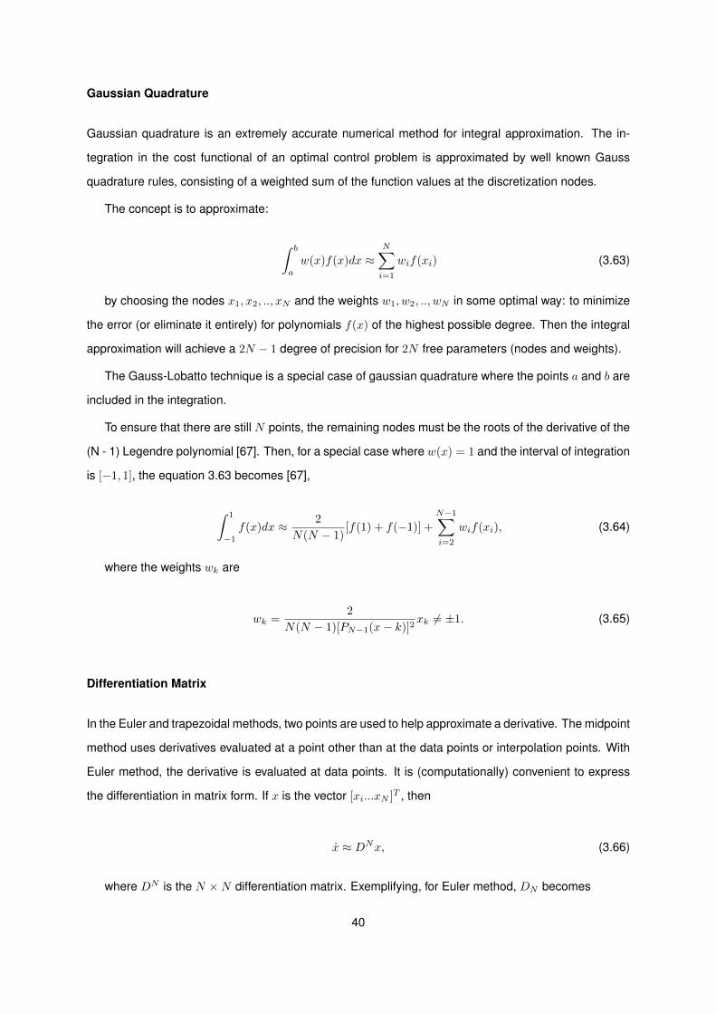
Gaussian Quadrature
Gaussian quadrature is an extremely accurate numerical method for integral approximation. The in-
tegration in the cost functional of an optimal control problem is approximated by well known Gauss
quadrature rules, consisting of a weighted sum of the function values at the discretization nodes.
The concept is to approximate:
∫ b
a
w(x)f(x)dx ≈N∑i=1
wif(xi) (3.63)
by choosing the nodes x1, x2, .., xN and the weights w1, w2, .., wN in some optimal way: to minimize
the error (or eliminate it entirely) for polynomials f(x) of the highest possible degree. Then the integral
approximation will achieve a 2N − 1 degree of precision for 2N free parameters (nodes and weights).
The Gauss-Lobatto technique is a special case of gaussian quadrature where the points a and b are
included in the integration.
To ensure that there are still N points, the remaining nodes must be the roots of the derivative of the
(N - 1) Legendre polynomial [67]. Then, for a special case where w(x) = 1 and the interval of integration
is [−1, 1], the equation 3.63 becomes [67],
∫ 1
−1
f(x)dx ≈ 2
N(N − 1)[f(1) + f(−1)] +
N−1∑i=2
wif(xi), (3.64)
where the weights wk are
wk =2
N(N − 1)[PN−1(x− k)]2xk 6= ±1. (3.65)
Differentiation Matrix
In the Euler and trapezoidal methods, two points are used to help approximate a derivative. The midpoint
method uses derivatives evaluated at a point other than at the data points or interpolation points. With
Euler method, the derivative is evaluated at data points. It is (computationally) convenient to express
the differentiation in matrix form. If x is the vector [xi...xN ]T , then
x ≈ DNx, (3.66)
where DN is the N ×N differentiation matrix. Exemplifying, for Euler method, DN becomes
40
DN =1
∆t
−1 1
−1 1
. . . . . .
1 −1
. (3.67)
3.3.2 The Legendre Pseudospectral Method
The idea to obtain the highest accuracy is, from a set of discrete data, find the global interpolating
polynomial, and evaluate the derivative of that interpolant at each point on the grid. This yields a dense
differentiation matrix, which can be used for collocation of the entire interval, driving the residual to zero
as
r = f − x′ = f −DNx→ 0. (3.68)
The Legendre pseudospectral method is based on interpolating functions on Legendre-Gauss-
Lobatto (LGL) quadrature nodes [64] as in equation 3.64. These points are distributed over the com-
putational interval [−1, 1] are given by τ0 = −1, τN = 1. In order to transform to the physical domain
t = [t0, tf ]:
t(τ) =(tf − t0)τ + (tf + t0)
2(3.69)
The state and the control functions are approximated by the Nth degree of polynomials in the form:
x(t(τ)) ≈N∑l=0
xlφl(τ) (3.70)
u(t(τ)) ≈N∑l=0
ulφl(τ) (3.71)
where, for l = 0, 1, ...N , φl are the Lagrange polynomials of degree N :
φl(τ) =1
N(N + 1)PN (τl)
(τ2 − 1)PN (τ)
τ − τl(3.72)
and PN are the Legendre polynomials of degree N (equation 3.62). The matrix D that can be used
to compute the derivative of x at each interpolation point is [64]
41
Dkj =
PN (tk)
PN (tl)1
τk−τlk 6= l
−N(N+1)4 k = l = 0
N(N+1)4 k = l = N
0 otherwise
. (3.73)
Following the steps for each element used in trapezoidal transcription the optimal control described
at equation 3.2 is in conditions to be transcribed.
1. Integrals.
The integrals such as the integral term in the cost function J are approximated using Gaussian
quadrature.
∫ tf
0
L(t, x(t), u(t)dt ≈ tf − t02
N∑i=0
L(xk, uk)wk (3.74)
with the weights:
wk :=2
N(N + 1)
1
PN (τk)2(3.75)
2. Dynamics.
The dynamics for the Legendre Pseudospectral Method are approximated as:
tf − t02
f(xk, uk)−N∑l=0
Dklxl = 0 (3.76)
3. Constraints.
The constraints are handled at the same way that were treated in trapezoidal collocation. Each
one is simply converted to an algebraic equation.
x0 −X0 = 0
xN −Xf = 0(3.77)
h(xk, uk) = 0
g(xk, uk) ≤ 0(3.78)
So the goal is to find the decision vector [XN ;UN ; tf ] that solves the following problem.
42
Minimize J = K(xN ) +tf2
∑Nk=0 L(xk, uk)wk
subject to: tf−t02 f(xk, uk)−
∑Nl=0Dklxl = 0
x0 −X0 = 0
xN −Xf = 0
h(xk, uk) = 0
g(xk, uk) ≤ 0
(3.79)
When DIDO (Legendre Pseudospectral Method) converges to a solution, it means that all the con-
straints are met to some degree of precision at the nodes. However, the risk of the solution to be
infeasible exists, since nothing guarantees the constraints are not necessarily met between the nodes.
Feasibility implies that the trajectory goes from the initial conditions through the final ones, following
the systems dynamics.
A method to approve the DIDO solution, is interpolating it an then integrate the resulting data with
a Range-Kutta integrator, following the same dynamics as in the problem formulation, obviously. If they
appear to be very similar and feasible, then one may finally trust the DIDO solution and evaluate its
accuracy.
43

44
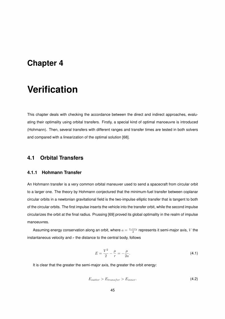
Chapter 4
Verification
This chapter deals with checking the accordance between the direct and indirect approaches, evalu-
ating their optimality using orbital transfers. Firstly, a special kind of optimal manoeuvre is introduced
(Hohmann). Then, several transfers with different ranges and transfer times are tested in both solvers
and compared with a linearization of the optimal solution [68].
4.1 Orbital Transfers
4.1.1 Hohmann Transfer
An Hohmann transfer is a very common orbital maneuver used to send a spacecraft from circular orbit
to a larger one. The theory by Hohmann conjectured that the minimum-fuel transfer between coplanar
circular orbits in a newtonian gravitational field is the two-impulse elliptic transfer that is tangent to both
of the circular orbits. The first impulse inserts the vehicle into the transfer orbit, while the second impulse
circularizes the orbit at the final radius. Prussing [69] proved its global optimality in the realm of impulse
manoeuvres.
Assuming energy conservation along an orbit, where a = r1+r22 represents it semi-major axis, V the
instantaneous velocity and r the distance to the central body, follows
E =V 2
2− µ
r= − µ
2a. (4.1)
It is clear that the greater the semi-major axis, the greater the orbit energy:
Eoutter > Etransfer > Einner. (4.2)
45
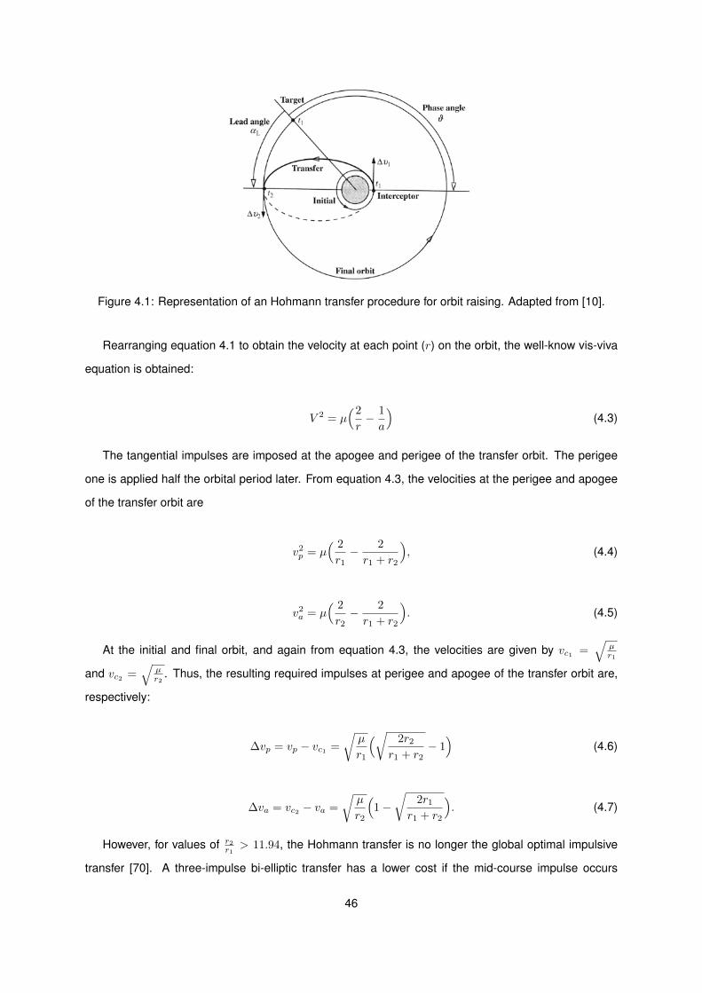
Figure 4.1: Representation of an Hohmann transfer procedure for orbit raising. Adapted from [10].
Rearranging equation 4.1 to obtain the velocity at each point (r) on the orbit, the well-know vis-viva
equation is obtained:
V 2 = µ(2
r− 1
a
)(4.3)
The tangential impulses are imposed at the apogee and perigee of the transfer orbit. The perigee
one is applied half the orbital period later. From equation 4.3, the velocities at the perigee and apogee
of the transfer orbit are
v2p = µ
( 2
r1− 2
r1 + r2
), (4.4)
v2a = µ
( 2
r2− 2
r1 + r2
). (4.5)
At the initial and final orbit, and again from equation 4.3, the velocities are given by vc1 =√
µr1
and vc2 =√
µr2
. Thus, the resulting required impulses at perigee and apogee of the transfer orbit are,
respectively:
∆vp = vp − vc1 =
õ
r1
(√ 2r2
r1 + r2− 1)
(4.6)
∆va = vc2 − va =
õ
r2
(1−
√2r1
r1 + r2
). (4.7)
However, for values of r2r1 > 11.94, the Hohmann transfer is no longer the global optimal impulsive
transfer [70]. A three-impulse bi-elliptic transfer has a lower cost if the mid-course impulse occurs
46
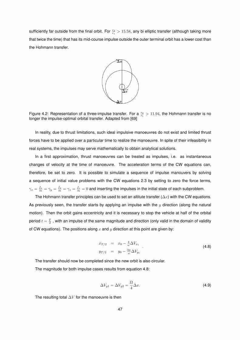
sufficiently far outside from the final orbit. For r2r1> 15.58, any bi elliptic transfer (although taking more
that twice the time) that has its mid-course impulse outside the outer terminal orbit has a lower cost than
the Hohmann transfer.
Figure 4.2: Representation of a three-impulse transfer. For a r2r1> 11.94, the Hohmann transfer is no
longer the impulse-optimal orbital transfer. Adapted from [69]
In reality, due to thrust limitations, such ideal impulsive manoeuvres do not exist and limited thrust
forces have to be applied over a particular time to realize the manoeuvre. In spite of their infeasibility in
real systems, the impulses may serve mathematically to obtain analytical solutions.
In a first approximation, thrust manoeuvres can be treated as impulses, i.e. as instantaneous
changes of velocity at the time of manoeuvre. The acceleration terms of the CW equations can,
therefore, be set to zero. It is possible to simulate a sequence of impulse manouvers by solving
a sequence of initial value problems with the CW equations 2.3 by setting to zero the force terms,
γx = fxm = γy =
fym = γz = fz
m = 0 and inserting the impulses in the initial state of each subproblem.
The Hohmann transfer principles can be used to set an altitute transfer (∆x) with the CW equations.
As previously seen, the transfer starts by applying an impulse with the y direction (along the natural
motion). Then the orbit gains eccentricity and it is necessary to stop the vehicle at half of the orbital
period t = T2 , with an impulse of the same magnitude and direction (only valid in the domain of validity
of CW equations). The positions along x and y direction at this point are given by:
xT/2 = x0 − 4ω∆Vx1
yT/2 = y0 − 3πω ∆Vy1
. (4.8)
The transfer should now be completed since the new orbit is also circular.
The magnitude for both impulse cases results from equation 4.8:
∆Vy1 = ∆Vy2 =Ω
4∆x. (4.9)
The resulting total ∆V for the manoeuvre is then
47
∆Vtotal =Ω
2∆x. (4.10)
This result, in the domain where the CW equations are valid is a very good approximation of the
results derived from the conservation of energy (equation 4.3).
Figure 4.3: Variation of ∆VTotal with the ratio ρ = r2r1≈ ∆x+ 1 of the final and initial orbit, using the CW
equations and the Vis-viva equation
In reality, all thrusters have a finite force level, thus, a constant force has to be applied over a certain
time in order to achieve a particular ∆V .
The equations of motion 2.3 during constant thrust are given by [10]:
x(t) =(
2y0ω − 3x0
)cos(ωt) + x0
ω sin(ωt)
+(
4x0 − 2y0ω
)+ 2
ω2 γy(sin(ωt)− ωt) + γxω2 (1− cos(ωt))
y(t) =(
4 y0ω − 6x0)sin(ωt)− 2 x0
ω cos(ωt) + (6ωx0 − 3y0)t+ (y′0 + 2x0
ω )
+ 2ω2 γx(ωt− sin(ωt)) + γy
(4ω2 (1− cos(ωt))− 3
2 t2)
z(t) = z0cos(ωt) + z0ω sin(ωt) + γz
ω2 (1− cos(ωt))
(4.11)
The total ∆V applied after time t = tf for a constant thrust level is simply
∆Vtotal =
∫ tf
0
γ(t)dt. (4.12)
In the extreme case, the ∆V of the Hohmann transfer can be extended to an entire orbital revolution
[10]. The change ∆x, which was achieved for a particular impulsive ∆V , is the same. This extension
can be very useful to manouevres that require special safety considerations, such as the final approach
ones.
48
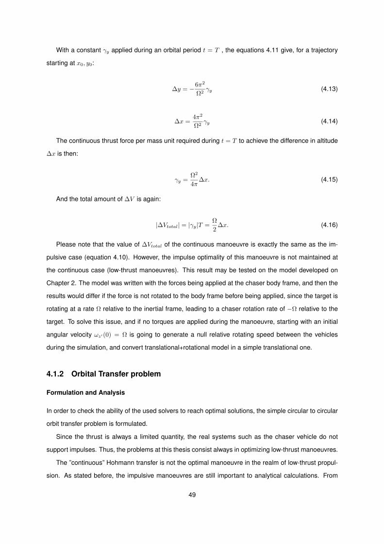
With a constant γy applied during an orbital period t = T , the equations 4.11 give, for a trajectory
starting at x0, y0:
∆y = −6π2
Ω2γy (4.13)
∆x =4π2
Ω2γy (4.14)
The continuous thrust force per mass unit required during t = T to achieve the difference in altitude
∆x is then:
γy =Ω2
4π∆x. (4.15)
And the total amount of ∆V is again:
|∆Vtotal| = |γy|T =Ω
2∆x. (4.16)
Please note that the value of ∆Vtotal of the continuous manoeuvre is exactly the same as the im-
pulsive case (equation 4.10). However, the impulse optimality of this manoeuvre is not maintained at
the continuous case (low-thrust manoeuvres). This result may be tested on the model developed on
Chapter 2. The model was written with the forces being applied at the chaser body frame, and then the
results would differ if the force is not rotated to the body frame before being applied, since the target is
rotating at a rate Ω relative to the inertial frame, leading to a chaser rotation rate of −Ω relative to the
target. To solve this issue, and if no torques are applied during the manoeuvre, starting with an initial
angular velocity ωz′(0) = Ω is going to generate a null relative rotating speed between the vehicles
during the simulation, and convert translational+rotational model in a simple translational one.
4.1.2 Orbital Transfer problem
Formulation and Analysis
In order to check the ability of the used solvers to reach optimal solutions, the simple circular to circular
orbit transfer problem is formulated.
Since the thrust is always a limited quantity, the real systems such as the chaser vehicle do not
support impulses. Thus, the problems at this thesis consist always in optimizing low-thrust manoeuvres.
The ”continuous” Hohmann transfer is not the optimal manoeuvre in the realm of low-thrust propul-
sion. As stated before, the impulsive manoeuvres are still important to analytical calculations. From
49
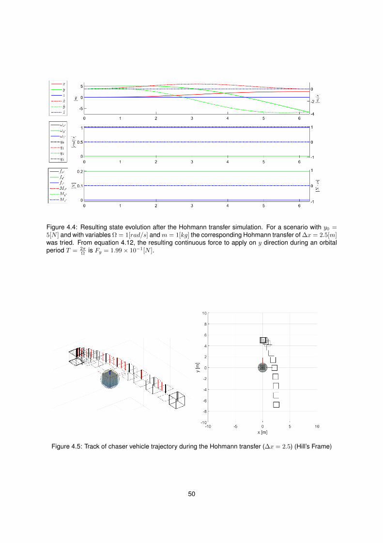
Figure 4.4: Resulting state evolution after the Hohmann transfer simulation. For a scenario with y0 =5[N ] and with variables Ω = 1[rad/s] andm = 1[kg] the corresponding Hohmann transfer of ∆x = 2.5[m]was tried. From equation 4.12, the resulting continuous force to apply on y direction during an orbitalperiod T = 2π
Ω is Fy = 1.99× 10⁻¹[N ].
Figure 4.5: Track of chaser vehicle trajectory during the Hohmann transfer (∆x = 2.5) (Hill’s Frame)
50
equation 4.16 it is possible to convert an impulse manoeuvre such as the Hohmann transfer in a low-
thrust manoeuvre. In spite of not being optimal, this value represents a feasible manoeuvre, and its cost
is close to the optimal one. This value may have an indicative role, since if a solver provides a candidate
to optimal whose cost is higher than the ”continuous” Hohmann value, then it is clear that the solver
could not reach the optimal solution.
Besides, the value of the ”continuous” Hohmann transfer can work as a reasonable guess, since it
provides an already feasible solution, which should reduce the computational time of the algorithms.
Since the assumptions of the Hohmann transfer scenario require the circularity of both the initial and
final orbit, earth-centered polar coordinates are useful to formulate the problem and to impose the start
and final conditions.
The motion of a satellite under an inverse squared gravitational field may be expressed by the fol-
lowing differential equations:
r = rθ2 − µ
r2 + ur
θ = 2θrr + 1
ruθ
. (4.17)
where the controls ur and uθ represent the thrust applied in radial and tangential directions.
This system provides 4 first order ODEs, resulting in 4 states [r, θ, r, θ]. The problem can be stated
as transfering a vehicle from an initial circular orbit r0 to an also circular final orbit rf minimizing the
energy cost functional J = 12
∫ tf0u2θ + u2
rdt. The following OCP was obtained:
Minimize J = 12
∫ tf0u2θ + u2
rdt
subject to: Equation 4.17
r(0) = R0
θ(t0) =√
µR3
0
θ(0) = r(0) = 0
r(tf ) = R0 + ∆R
θ(tf ) =√
µ(R0+∆R)3
r(tf ) = 0
(4.18)
Following the derivation process of the necessary conditions 3.11, the resulting hamiltonian is:
H =1
2(u2θ + u2
r) + λr r + λθ θ + λr
(rθ2 − µ
r2+ ur)
)+ λθ
(2θr
r+
1
ruθ
)(4.19)
51
Recalling the equations 3.11, the adjoint equations are:
λr = −λr(
2µr3 + λ2
θ
)− λθ
(λθr3 +
2λrλθr2
)λθ = 0
λr = −λr + λθ2θr
λθ = −λθ − 2λrrθ + λθ
(2rr
)(4.20)
The gradient of the hamiltonian with respect to the control variables gives
∇Hu =
ur + λr
uθ +λθr .
. (4.21)
Since no boundaries to the control were applied, the optimal control satisfies ∇Hu = 0. Then, the
optimal control histories, u∗θ and u∗r are:
u∗r = −λr (4.22)
u∗θ = −λθr
(4.23)
4.2 Results
Several circular orbit transfers were compared with a first-order solution developed by Fernandes [71][72],
based on the previous work by Edelbaum [68], where the optimal low-thrust transfer was first derived
using the Pontryagin principle, and then a first-order approximation was applied. This linear analytical
theory relevant results are described on Appendix A. These results provided a linearly calculated control
law used to compare the solutions given by the solvers used.
It should be noted that in the formulation of the optimization problem described above, the variables
are taken in a dimensionless form. Introducing the ratio ρ =rfr0
and rewriting the problem:
52
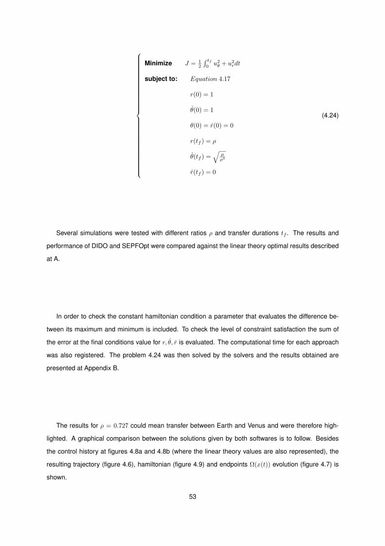
Minimize J = 12
∫ tf0u2θ + u2
rdt
subject to: Equation 4.17
r(0) = 1
θ(0) = 1
θ(0) = r(0) = 0
r(tf ) = ρ
θ(tf ) =√
µρ3
r(tf ) = 0
(4.24)
Several simulations were tested with different ratios ρ and transfer durations tf . The results and
performance of DIDO and SEPFOpt were compared against the linear theory optimal results described
at A.
In order to check the constant hamiltonian condition a parameter that evaluates the difference be-
tween its maximum and minimum is included. To check the level of constraint satisfaction the sum of
the error at the final conditions value for r, θ, r is evaluated. The computational time for each approach
was also registered. The problem 4.24 was then solved by the solvers and the results obtained are
presented at Appendix B.
The results for ρ = 0.727 could mean transfer between Earth and Venus and were therefore high-
lighted. A graphical comparison between the solutions given by both softwares is to follow. Besides
the control history at figures 4.8a and 4.8b (where the linear theory values are also represented), the
resulting trajectory (figure 4.6), hamiltonian (figure 4.9) and endpoints Ω(x(t)) evolution (figure 4.7) is
shown.
53
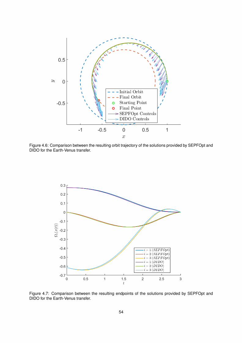
Figure 4.6: Comparison between the resulting orbit trajectory of the solutions provided by SEPFOpt andDIDO for the Earth-Venus transfer.
Figure 4.7: Comparison between the resulting endpoints of the solutions provided by SEPFOpt andDIDO for the Earth-Venus transfer.
54
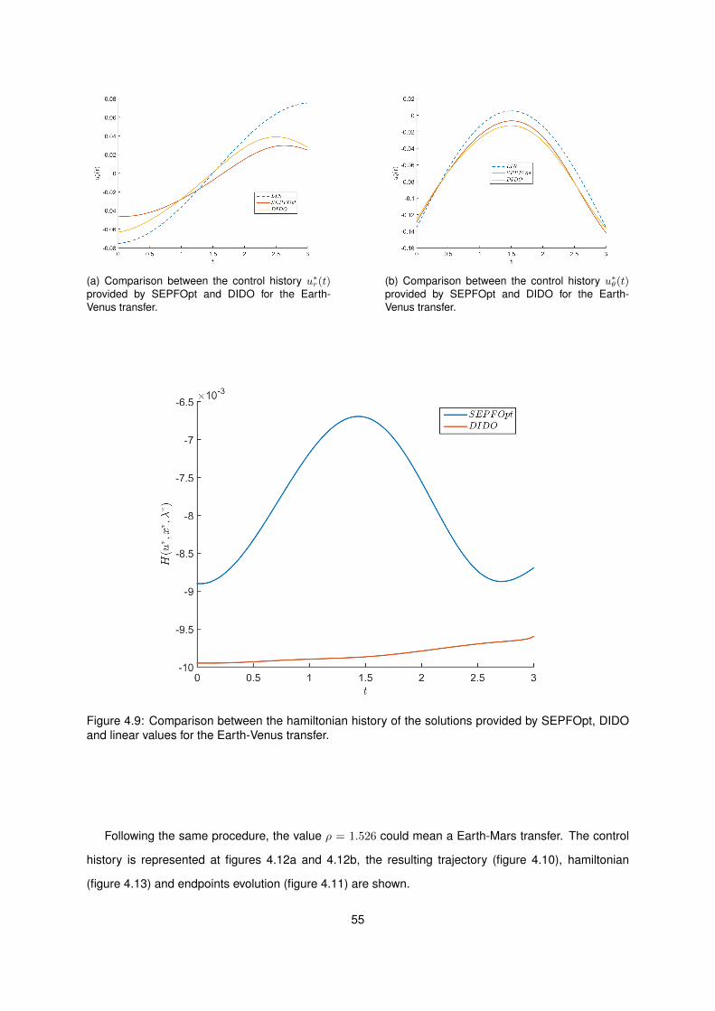
(a) Comparison between the control history u∗r(t)
provided by SEPFOpt and DIDO for the Earth-Venus transfer.
(b) Comparison between the control history u∗θ(t)
provided by SEPFOpt and DIDO for the Earth-Venus transfer.
Figure 4.9: Comparison between the hamiltonian history of the solutions provided by SEPFOpt, DIDOand linear values for the Earth-Venus transfer.
Following the same procedure, the value ρ = 1.526 could mean a Earth-Mars transfer. The control
history is represented at figures 4.12a and 4.12b, the resulting trajectory (figure 4.10), hamiltonian
(figure 4.13) and endpoints evolution (figure 4.11) are shown.
55

Figure 4.10: Comparison between the resulting orbit trajectory of the solutions provided by SEPFOpt,DIDO and linear values for the Earth-Mars transfer.
Figure 4.11: Comparison between the resulting endpoints of the solutions provided by SEPFOpt andDIDO for the Earth-Mars transfer.
56
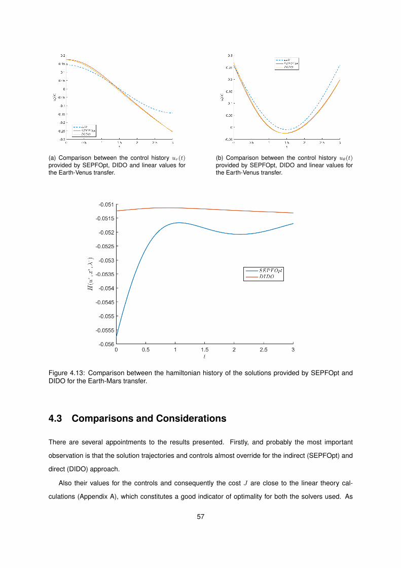
(a) Comparison between the control history ur(t)provided by SEPFOpt, DIDO and linear values forthe Earth-Venus transfer.
(b) Comparison between the control history uθ(t)provided by SEPFOpt, DIDO and linear values forthe Earth-Venus transfer.
Figure 4.13: Comparison between the hamiltonian history of the solutions provided by SEPFOpt andDIDO for the Earth-Mars transfer.
4.3 Comparisons and Considerations
There are several appointments to the results presented. Firstly, and probably the most important
observation is that the solution trajectories and controls almost override for the indirect (SEPFOpt) and
direct (DIDO) approach.
Also their values for the controls and consequently the cost J are close to the linear theory cal-
culations (Appendix A), which constitutes a good indicator of optimality for both the solvers used. As
57
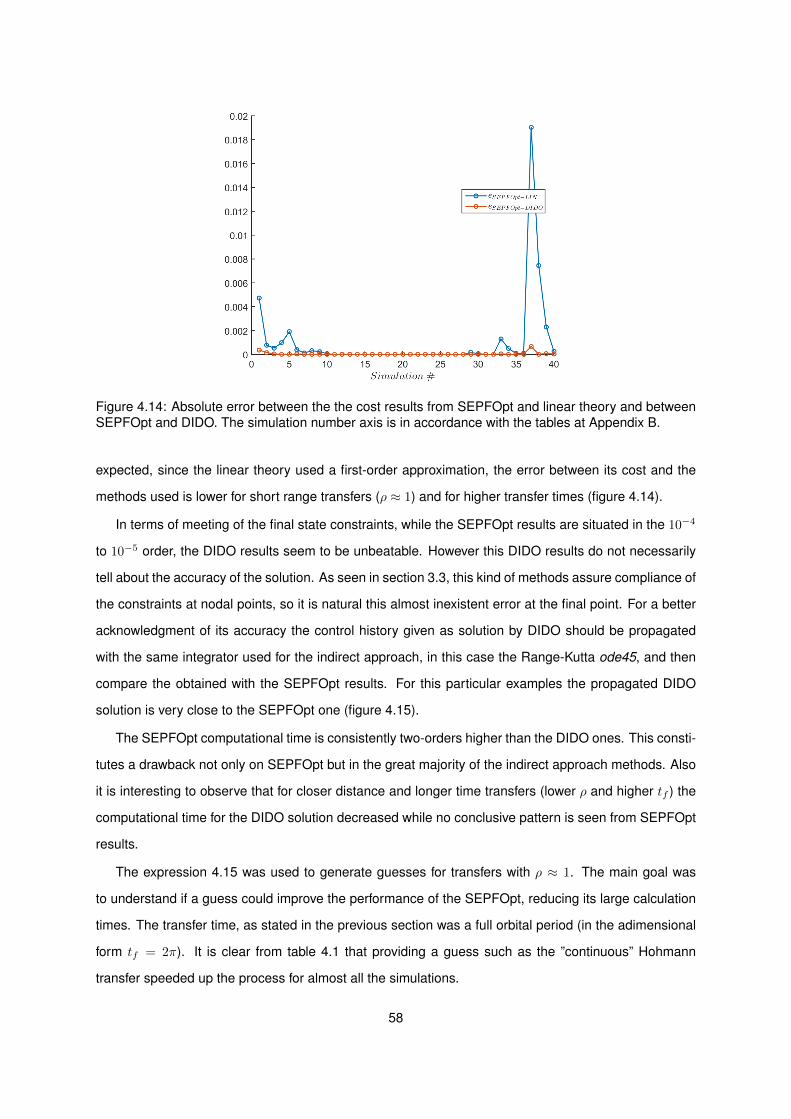
Figure 4.14: Absolute error between the the cost results from SEPFOpt and linear theory and betweenSEPFOpt and DIDO. The simulation number axis is in accordance with the tables at Appendix B.
expected, since the linear theory used a first-order approximation, the error between its cost and the
methods used is lower for short range transfers (ρ ≈ 1) and for higher transfer times (figure 4.14).
In terms of meeting of the final state constraints, while the SEPFOpt results are situated in the 10−4
to 10−5 order, the DIDO results seem to be unbeatable. However this DIDO results do not necessarily
tell about the accuracy of the solution. As seen in section 3.3, this kind of methods assure compliance of
the constraints at nodal points, so it is natural this almost inexistent error at the final point. For a better
acknowledgment of its accuracy the control history given as solution by DIDO should be propagated
with the same integrator used for the indirect approach, in this case the Range-Kutta ode45, and then
compare the obtained with the SEPFOpt results. For this particular examples the propagated DIDO
solution is very close to the SEPFOpt one (figure 4.15).
The SEPFOpt computational time is consistently two-orders higher than the DIDO ones. This consti-
tutes a drawback not only on SEPFOpt but in the great majority of the indirect approach methods. Also
it is interesting to observe that for closer distance and longer time transfers (lower ρ and higher tf ) the
computational time for the DIDO solution decreased while no conclusive pattern is seen from SEPFOpt
results.
The expression 4.15 was used to generate guesses for transfers with ρ ≈ 1. The main goal was
to understand if a guess could improve the performance of the SEPFOpt, reducing its large calculation
times. The transfer time, as stated in the previous section was a full orbital period (in the adimensional
form tf = 2π). It is clear from table 4.1 that providing a guess such as the ”continuous” Hohmann
transfer speeded up the process for almost all the simulations.
58
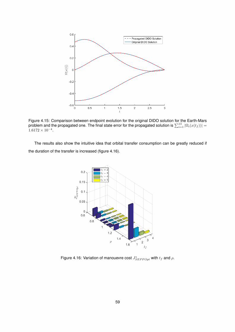
Figure 4.15: Comparison between endpoint evolution for the original DIDO solution for the Earth-Marsproblem and the propagated one. The final state error for the propagated solution is
∑13i=1 |Ωi(x(tf ))| =
1.6172× 10⁻⁴.
The results also show the intuitive idea that orbital transfer consumption can be greatly reduced if
the duration of the transfer is increased (figure 4.16).
Figure 4.16: Variation of manouevre cost J∗SEPFOpt with tf and ρ.
59
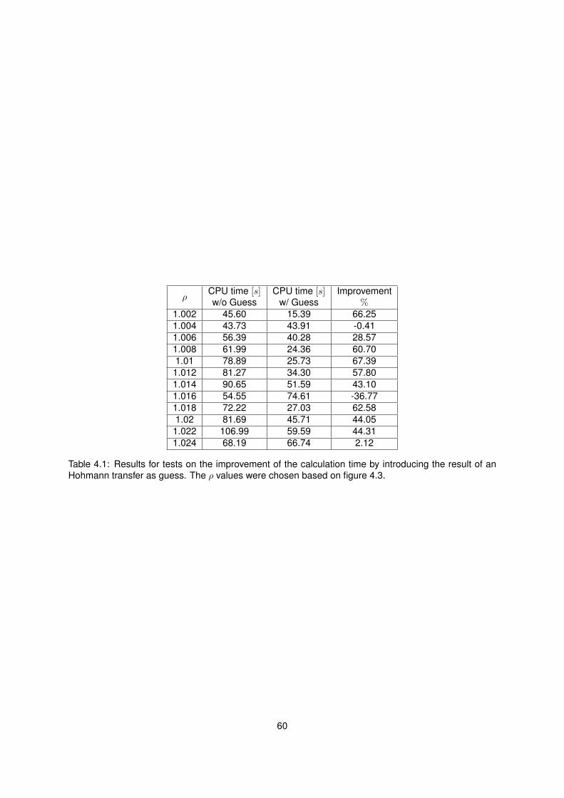
ρCPU time [s]w/o Guess
CPU time [s]w/ Guess
Improvement%
1.002 45.60 15.39 66.251.004 43.73 43.91 -0.411.006 56.39 40.28 28.571.008 61.99 24.36 60.701.01 78.89 25.73 67.391.012 81.27 34.30 57.801.014 90.65 51.59 43.101.016 54.55 74.61 -36.771.018 72.22 27.03 62.581.02 81.69 45.71 44.051.022 106.99 59.59 44.311.024 68.19 66.74 2.12
Table 4.1: Results for tests on the improvement of the calculation time by introducing the result of anHohmann transfer as guess. The ρ values were chosen based on figure 4.3.
60
Chapter 5
The Rendezvous problem
The following chapter introduces the scenarios to solve the docking and capture manoeuvres, respec-
tively. Both problems will obey to the same dynamics and cost function, thus sharing the same hamil-
tonian. The main difference between the two missions is the formulation of the final-state conditions.
While for the capture with the net concept the goal is to drive the chaser into targets proximity, the dock-
ing mission pursuits actual contact between both docking interfaces. The docking mission assumes a
non-tumbling target, while it is assumed that the net capture supports tumbling objects as the ENVISAT.
5.1 Solution Characterization
In the pursuit of an optimal solution, the necessary conditions derived at Chapter 2 are the major
tool used to attest a solution optimality. With the penalty method implemented by SEPFOpt, the cost
functional is adjoined with the square of the nc imposed final constraints, multiplied by the penalty factor
K.
J = J +K
nc∑i=1
Ω2i (5.1)
The final costates are for both manoeuvres is given by
λi(tf ) = 2K · Ωi. (5.2)
The same hamiltonian is obtained for both manoeuvres, since both obey to the same dynamics.
To determine the solution structure, only the fraction of the Hamiltonian that depends on the controls
61
H is relevant:
H = L+Hc
= λ4
(q2c0 + q2
c1 − q2c2 − q
2c3)fx′ + (2qc1qc2 − 2qc3qc0)fy′ + (2qc1qc3 + 2qc2qc0)fz′
m+
λ5
(2qc1qc2 + 2qc3qc0)fx′ + (q2c0 − q
2c1 + q2
c2 − q2c3)fy′ + (2qc2qc3 − 2qc1qc0)fz′
m+
λ6
(2qc1qc3 − 2qc2qc0)fx′ + (2qc2qc3 + 2qc1qc0)fy′ + (q2c0 − q
2c1 − q
2c2 + q2
c3)fz′ − Ω2z
m+
1
Ic1λ7Mx +
1
Ic2λ8My +
1
Ic3λ9Mz + L
(5.3)
The derivative of the hamiltonian H with respect to each control u = [fx′ , fy′ , fz′ ,Mx′ ,My′ ,Mz′ ] is
∇uH =
dHdfx′
dHdfy′
dHdfz′
dHdMx′
dHdMy′
dHdMz′
=1
m
λ4(q2c0 + q2
c1 − q2c2 − q
2c3) + λ5(2qc1qc2 + 2qc3qc0) + λ6(2qc1qc3 − 2qc2qc0)
λ4(2qc1qc2 − 2qc3qc0) + λ5(q2c0 − q
2c1 + q2
c2 − q2c3) + λ6(2qc2qc3 + 2qc1qc0)
λ4(2qc1qc3 + 2qc2qc0) + λ5(2qc2qc3 − 2qc1qc0) + λ6(q2c0 − q
2c1 − q
2c2 + q2
c3)
12λ7
h2+d2
12λ8
w2+h2
12λ9
d2+h2
+∇uL.
(5.4)
5.1.1 Minimum Energy
For a minimum energy problem, L takes the form
LME =1
2
(f2x′ + f2
y′ + f2z′ +M2
x′ +M2y′ +M2
z′
), (5.5)
Thus, the term ∇uL results simply in:
∇uLME =
[fx′ , fy′ , fz′ ,Mx′ ,My′ ,Mz′
]T(5.6)
Due to being composed by quadratic terms, the non-linearity of the cost function assures that the
control is not of the bang-bang type. Since the trust is limited, the hamiltonian minimizer may be located
at an interior point or may assume the value of a boundary of the thrust interval, i.e., u∗i (t) = Uimin and
u∗i (t) = Uimax .
62
Thus, the resulting control structure for this performance index is:
ui =
1 if ∇uHc(i) < −1
−∇uHc(i) if − 1 ≤ ∇uHc(i) ≤ 1
−1 if ∇uHc(i) > 1
(5.7)
5.1.2 Minimum Fuel
In order to solve the problem from the fuel minimization perspective, the running cost L takes the form
of the summation of the absolute value of the controls, as
LMF = ||fx′ ||+ ||fy′ ||+ ||fz′ ||+ ||Mx′ ||+ ||My′ ||+ ||Mz′ ||. (5.8)
However, this formulation would generate problems around zero, since at this value the modulus is
non-differentiable. There are two possible ways to avoid this: either smooth the data, with a differentiable
function that is approximately the modulus function, such as
||ui|| ≈ ui · tanh(uik
), (5.9)
where k is a constant, or simply by augmenting the dimension of the control variables, separating
the modulus function in two branches as
uN =
[f lx′ , f
ly′ , f
lz′ ,M
lx′ ,M
ly′ ,M
lz′ , f
rx′ , f
ry′ , f
rz′ ,M
rx′ ,M
ry′ ,M
rz′ .
](5.10)
where l represents the left branch and r the right one. Now, the new Umin must be set to zero. The
original controls written in function of the new ones are
ui
= ulNi − urNi . (5.11)
For this type of problem the gradient ∇uL results in a simple array of ones with dimension 12 .
The resulting control structure is then:
uNi =
0 if ∇uHc(i) > −1
1 if ∇uHc(i) ≤ −1
(5.12)
63

5.2 Addition of a path constraint
Neither direct or indirect methods have a clue on what is the shape of the target vehicle and sometimes
- especially if at a docking mission the chaser starts behind the target docking interface - the optimal
path implies a collision between the two vehicles. Therefore it becomes necessary to restrict the chaser
admissible path.
In order to meet the optimal control formulation stated before, it is possible to state this constraint
as an inequality constraint. The strategy goes through imposing certain regions as a ”keep-out” zone to
the chaser movement.
As assumed in Chapter 2, both vehicles are rectangular prisms, so the farthest points from the CM
are the vertexes of each vehicle:
Rc =
√depthc
2
2
+widthc
2
2
+heightc
2
2
; (5.13)
Rt =
√deptht
2
2
+widtht
2
2
+heightt
2
2
. (5.14)
Given that the chaser CM position is part of the state array, and the target CM position coincides
with the origin of the orbital frame, is possible to write the distance between the two vehicles CM as
R =√r2x + r2
y + r2z . (5.15)
An easy way to ”protect” all the points of the vehicles is to encapsulate them in a sphere, with radius
equal to the distance of a vertex to the vehicle CM. So, if the two spheres do not intersect,
R > Rc +Rt (5.16)
it is guaranteed that the vehicles avoided any collision between them. Writing it according to the
notation of an inequality constraint of an OCP:
g(x(t)) = Rc +Rt −R. (5.17)
64
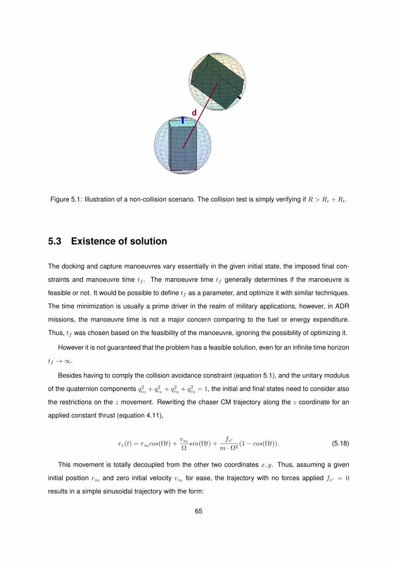
Figure 5.1: Illustration of a non-collision scenario. The collision test is simply verifying if R > Rc +Rt.
5.3 Existence of solution
The docking and capture manoeuvres vary essentially in the given initial state, the imposed final con-
straints and manoeuvre time tf . The manoeuvre time tf generally determines if the manoeuvre is
feasible or not. It would be possible to define tf as a parameter, and optimize it with similar techniques.
The time minimization is usually a prime driver in the realm of military applications, however, in ADR
missions, the manoeuvre time is not a major concern comparing to the fuel or energy expenditure.
Thus, tf was chosen based on the feasibility of the manoeuvre, ignoring the possibility of optimizing it.
However it is not guaranteed that the problem has a feasible solution, even for an infinite time horizon
tf →∞.
Besides having to comply the collision avoidance constraint (equation 5.1), and the unitary modulus
of the quaternion components q2c0 + q2
c1 + q2c2 + q2
c3 = 1, the initial and final states need to consider also
the restrictions on the z movement. Rewriting the chaser CM trajectory along the z coordinate for an
applied constant thrust (equation 4.11),
rz(t) = rz0cos(Ωt) +vz0Ωsin(Ωt) +
fz′
m · Ω2(1− cos(Ωt)). (5.18)
This movement is totally decoupled from the other two coordinates x, y. Thus, assuming a given
initial position rz0 and zero initial velocity vz0 for ease, the trajectory with no forces applied fz′ = 0
results in a simple sinusoidal trajectory with the form:
65
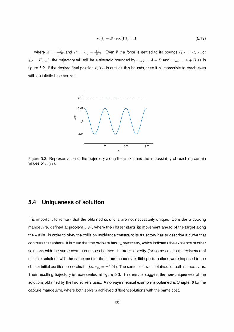
rz(t) = B · cos(Ωt) +A, (5.19)
where A = fz′mΩ2 and B = rz0 −
fz′mΩ2 . Even if the force is settled to its bounds (fz′ = Umin or
fz′ = Umax), the trajectory will still be a sinusoid bounded by zmin = A − B and zmax = A + B as in
figure 5.2. If the desired final position rz(tf ) is outside this bounds, then it is impossible to reach even
with an infinite time horizon.
Figure 5.2: Representation of the trajectory along the z axis and the impossibility of reaching certainvalues of rz(tf ).
5.4 Uniqueness of solution
It is important to remark that the obtained solutions are not necessarily unique. Consider a docking
manoeuvre, defined at problem 5.34, where the chaser starts its movement ahead of the target along
the y axis. In order to obey the collision avoidance constraint its trajectory has to describe a curve that
contours that sphere. It is clear that the problem has xy symmetry, which indicates the existence of other
solutions with the same cost than those obtained. In order to verify (for some cases) the existence of
multiple solutions with the same cost for the same manoeuvre, little perturbations were imposed to the
chaser initial position z coordinate (i.e. rz0 = ±0.01). The same cost was obtained for both manoeuvres.
Their resulting trajectory is represented at figure 5.3. This results suggest the non-uniqueness of the
solutions obtained by the two solvers used. A non-symmetrical example is obtained at Chapter 6 for the
capture manoeuvre, where both solvers achieved different solutions with the same cost.
66
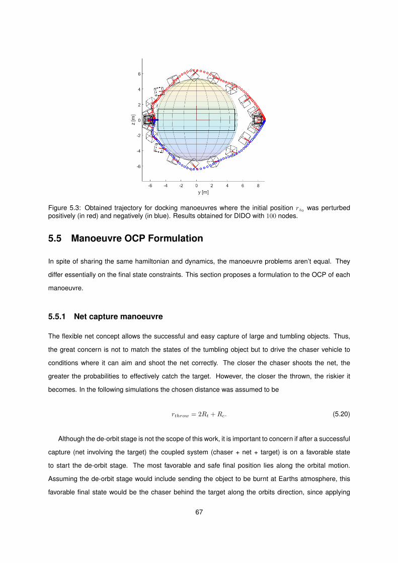
Figure 5.3: Obtained trajectory for docking manoeuvres where the initial position rz0 was perturbedpositively (in red) and negatively (in blue). Results obtained for DIDO with 100 nodes.
5.5 Manoeuvre OCP Formulation
In spite of sharing the same hamiltonian and dynamics, the manoeuvre problems aren’t equal. They
differ essentially on the final state constraints. This section proposes a formulation to the OCP of each
manoeuvre.
5.5.1 Net capture manoeuvre
The flexible net concept allows the successful and easy capture of large and tumbling objects. Thus,
the great concern is not to match the states of the tumbling object but to drive the chaser vehicle to
conditions where it can aim and shoot the net correctly. The closer the chaser shoots the net, the
greater the probabilities to effectively catch the target. However, the closer the thrown, the riskier it
becomes. In the following simulations the chosen distance was assumed to be
rthrow = 2Rt +Rc. (5.20)
Although the de-orbit stage is not the scope of this work, it is important to concern if after a successful
capture (net involving the target) the coupled system (chaser + net + target) is on a favorable state
to start the de-orbit stage. The most favorable and safe final position lies along the orbital motion.
Assuming the de-orbit stage would include sending the object to be burnt at Earths atmosphere, this
favorable final state would be the chaser behind the target along the orbits direction, since applying
67

thrust against the natural orbit motion would progressively decrease the targets energy and height in
a safe manner. Also, it offers the possibility of planning the thrown while station-keeping at zero cost.
Thus the final position of the chaser CM for this net-capture manoeuvre is
rx(tf )
ry(tf )
rz(tf )
=
0
−2Rt −Rc
0
. (5.21)
Accordingly with the baseline chaser representation and axis orientation, it is assumed that the net
is thrown along the y axis of the chaser body reference frame. Thus it is possible to write the final
orientation of this vehicle as
qc0(tf )
qc1(tf )
qc2(tf )
qc3(tf )
=
1
0
0
0
. (5.22)
The relative velocities between the two vehicles are assumed to be zero:
vx(tf )
vy(tf )
vz(tf )
= 0 (5.23)
ωx′(tf )
ωy′(tf )
ωz′(tf )
= 0 (5.24)
The final state matrix Ω(x(tf ))net compacts this 13 relations.
It is now all set to formulate this missions OCP in the usual form. The chaser thrusters are un-
der restrictions of saturation, so it is possible to define the limit the control law in an interval u(t) ∈
[Umin, Umax]. Depending on the performance index chosen, J can be the integral of LME , LMF or
other.
68
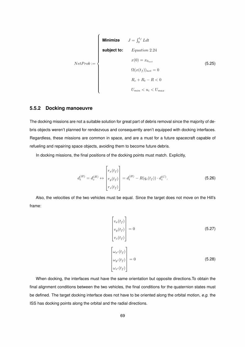
NetProb :=
Minimize J =∫ tf
0Ldt
subject to: Equation 2.24
x(0) = x0net
Ω(x(tf ))net = 0
Rc +Rt −R < 0
Umin < ui < Umax
(5.25)
5.5.2 Docking manoeuvre
The docking missions are not a suitable solution for great part of debris removal since the majority of de-
bris objects weren’t planned for rendezvous and consequently aren’t equipped with docking interfaces.
Regardless, these missions are common in space, and are a must for a future spacecraft capable of
refueling and repairing space objects, avoiding them to become future debris.
In docking missions, the final positions of the docking points must match. Explicitly,
d(H)t = d(H)
c ↔
rx(tf )
ry(tf )
rz(tf )
= d(H)t −R(qc(tf )) · d(C)
c . (5.26)
Also, the velocities of the two vehicles must be equal. Since the target does not move on the Hill’s
frame:
vx(tf )
vy(tf )
vz(tf )
= 0 (5.27)
ωx′(tf )
ωy′(tf )
ωz′(tf )
= 0 (5.28)
When docking, the interfaces must have the same orientation but opposite directions.To obtain the
final alignment conditions between the two vehicles, the final conditions for the quaternion states must
be defined. The target docking interface does not have to be oriented along the orbital motion, e.g. the
ISS has docking points along the orbital and the radial directions.
69
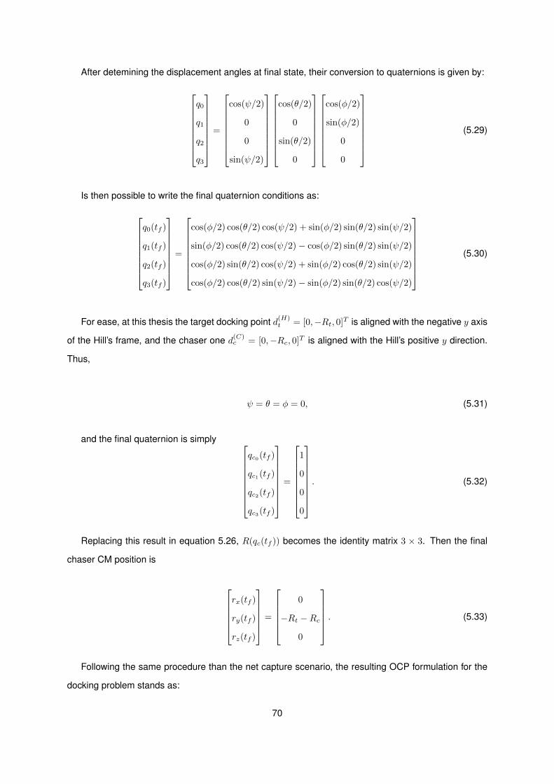
After detemining the displacement angles at final state, their conversion to quaternions is given by:
q0
q1
q2
q3
=
cos(ψ/2)
0
0
sin(ψ/2)
cos(θ/2)
0
sin(θ/2)
0
cos(φ/2)
sin(φ/2)
0
0
(5.29)
Is then possible to write the final quaternion conditions as:
q0(tf )
q1(tf )
q2(tf )
q3(tf )
=
cos(φ/2) cos(θ/2) cos(ψ/2) + sin(φ/2) sin(θ/2) sin(ψ/2)
sin(φ/2) cos(θ/2) cos(ψ/2)− cos(φ/2) sin(θ/2) sin(ψ/2)
cos(φ/2) sin(θ/2) cos(ψ/2) + sin(φ/2) cos(θ/2) sin(ψ/2)
cos(φ/2) cos(θ/2) sin(ψ/2)− sin(φ/2) sin(θ/2) cos(ψ/2)
(5.30)
For ease, at this thesis the target docking point d(H)t = [0,−Rt, 0]T is aligned with the negative y axis
of the Hill’s frame, and the chaser one d(C)c = [0,−Rc, 0]T is aligned with the Hill’s positive y direction.
Thus,
ψ = θ = φ = 0, (5.31)
and the final quaternion is simply
qc0(tf )
qc1(tf )
qc2(tf )
qc3(tf )
=
1
0
0
0
. (5.32)
Replacing this result in equation 5.26, R(qc(tf )) becomes the identity matrix 3 × 3. Then the final
chaser CM position is
rx(tf )
ry(tf )
rz(tf )
=
0
−Rt −Rc
0
. (5.33)
Following the same procedure than the net capture scenario, the resulting OCP formulation for the
docking problem stands as:
70
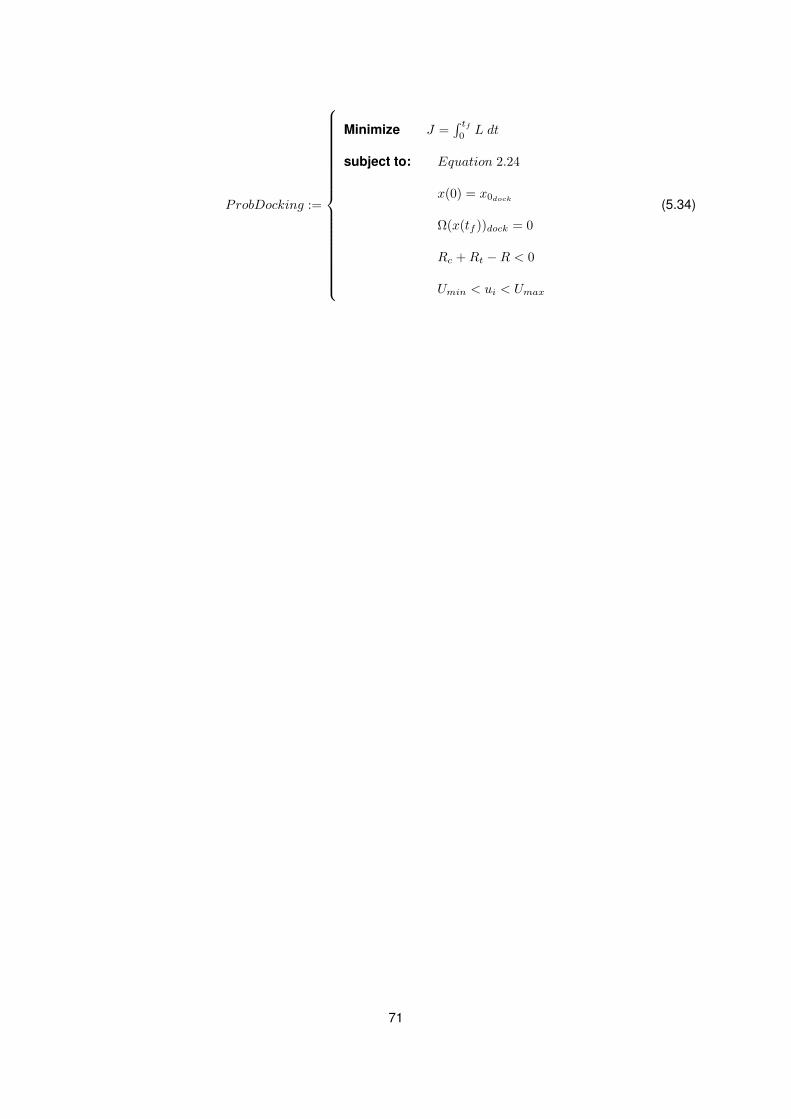
ProbDocking :=
Minimize J =∫ tf
0L dt
subject to: Equation 2.24
x(0) = x0dock
Ω(x(tf ))dock = 0
Rc +Rt −R < 0
Umin < ui < Umax
(5.34)
71
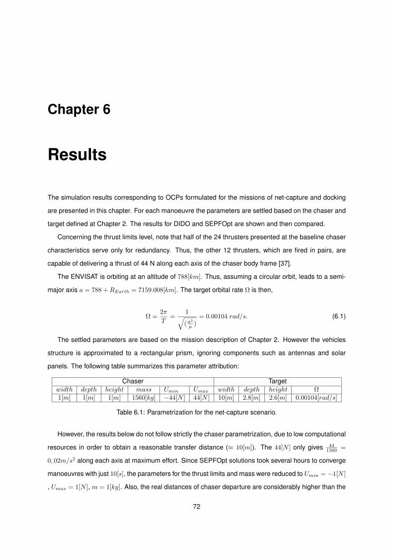
Chapter 6
Results
The simulation results corresponding to OCPs formulated for the missions of net-capture and docking
are presented in this chapter. For each manoeuvre the parameters are settled based on the chaser and
target defined at Chapter 2. The results for DIDO and SEPFOpt are shown and then compared.
Concerning the thrust limits level, note that half of the 24 thrusters presented at the baseline chaser
characteristics serve only for redundancy. Thus, the other 12 thrusters, which are fired in pairs, are
capable of delivering a thrust of 44 N along each axis of the chaser body frame [37].
The ENVISAT is orbiting at an altitude of 788[km]. Thus, assuming a circular orbit, leads to a semi-
major axis a = 788 +REarth = 7159.008[km]. The target orbital rate Ω is then,
Ω =2π
T=
1√(a
3
µ )= 0.00104 rad/s. (6.1)
The settled parameters are based on the mission description of Chapter 2. However the vehicles
structure is approximated to a rectangular prism, ignoring components such as antennas and solar
panels. The following table summarizes this parameter attribution:
Chaser Targetwidth depth height mass Umin Umax width depth height Ω1[m] 1[m] 1[m] 1560[kg] −44[N ] 44[N ] 10[m] 2.8[m] 2.6[m] 0.00104[rad/s]
Table 6.1: Parametrization for the net-capture scenario.
However, the results below do not follow strictly the chaser parametrization, due to low computational
resources in order to obtain a reasonable transfer distance (≈ 10[m]). The 44[N ] only gives 441560 =
0, 02m/s2 along each axis at maximum effort. Since SEPFOpt solutions took several hours to converge
manoeuvres with just 10[s], the parameters for the thrust limits and mass were reduced to Umin = −1[N ]
, Umax = 1[N ], m = 1[kg]. Also, the real distances of chaser departure are considerably higher than the
72
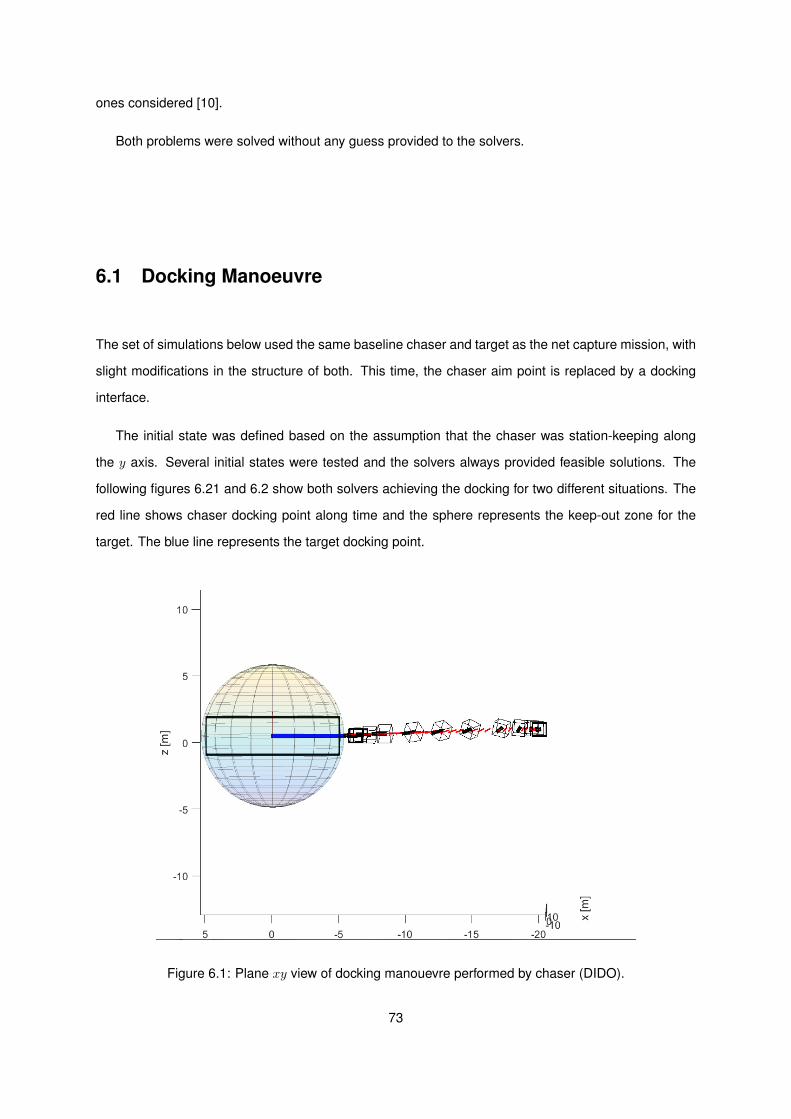
ones considered [10].
Both problems were solved without any guess provided to the solvers.
6.1 Docking Manoeuvre
The set of simulations below used the same baseline chaser and target as the net capture mission, with
slight modifications in the structure of both. This time, the chaser aim point is replaced by a docking
interface.
The initial state was defined based on the assumption that the chaser was station-keeping along
the y axis. Several initial states were tested and the solvers always provided feasible solutions. The
following figures 6.21 and 6.2 show both solvers achieving the docking for two different situations. The
red line shows chaser docking point along time and the sphere represents the keep-out zone for the
target. The blue line represents the target docking point.
Figure 6.1: Plane xy view of docking manouevre performed by chaser (DIDO).
73
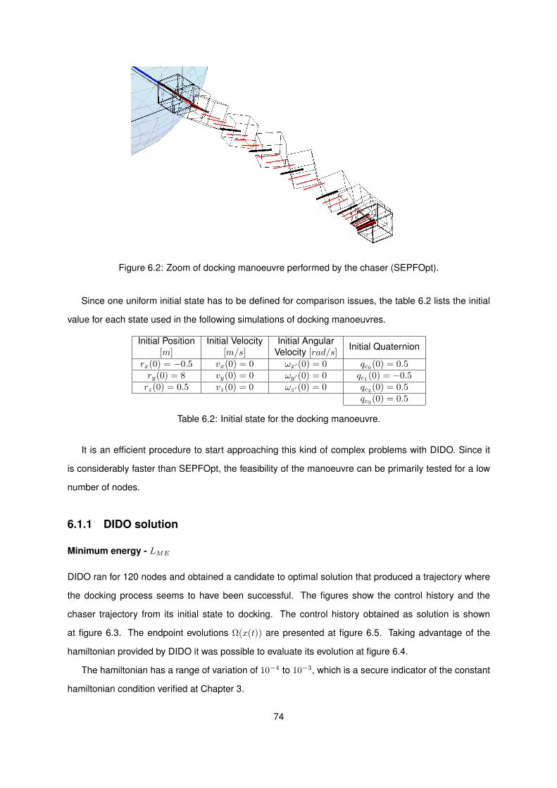
Figure 6.2: Zoom of docking manoeuvre performed by the chaser (SEPFOpt).
Since one uniform initial state has to be defined for comparison issues, the table 6.2 lists the initial
value for each state used in the following simulations of docking manoeuvres.
Initial Position[m]
Initial Velocity[m/s]
Initial AngularVelocity [rad/s]
Initial Quaternion
rx(0) = −0.5 vx(0) = 0 ωx′(0) = 0 qc0(0) = 0.5ry(0) = 8 vy(0) = 0 ωy′(0) = 0 qc1(0) = −0.5rz(0) = 0.5 vz(0) = 0 ωz′(0) = 0 qc2(0) = 0.5
qc3(0) = 0.5
Table 6.2: Initial state for the docking manoeuvre.
It is an efficient procedure to start approaching this kind of complex problems with DIDO. Since it
is considerably faster than SEPFOpt, the feasibility of the manoeuvre can be primarily tested for a low
number of nodes.
6.1.1 DIDO solution
Minimum energy - LME
DIDO ran for 120 nodes and obtained a candidate to optimal solution that produced a trajectory where
the docking process seems to have been successful. The figures show the control history and the
chaser trajectory from its initial state to docking. The control history obtained as solution is shown
at figure 6.3. The endpoint evolutions Ω(x(t)) are presented at figure 6.5. Taking advantage of the
hamiltonian provided by DIDO it was possible to evaluate its evolution at figure 6.4.
The hamiltonian has a range of variation of 10−4 to 10−3, which is a secure indicator of the constant
hamiltonian condition verified at Chapter 3.
74
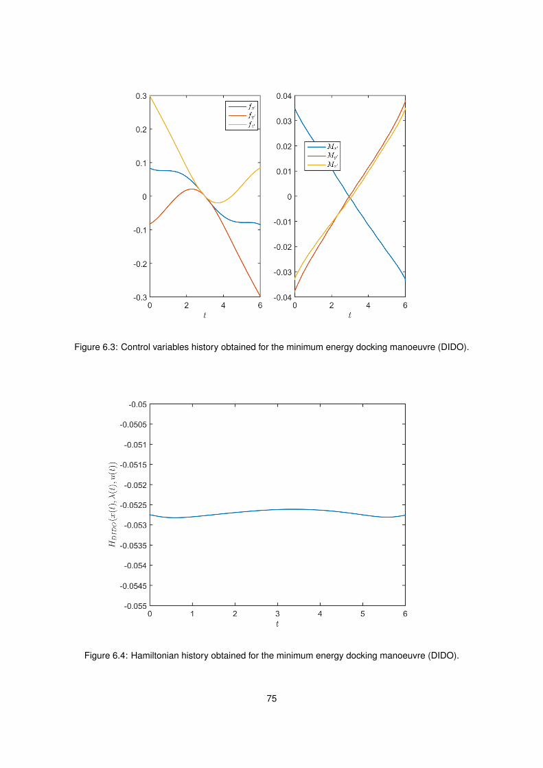
Figure 6.3: Control variables history obtained for the minimum energy docking manoeuvre (DIDO).
Figure 6.4: Hamiltonian history obtained for the minimum energy docking manoeuvre (DIDO).
75
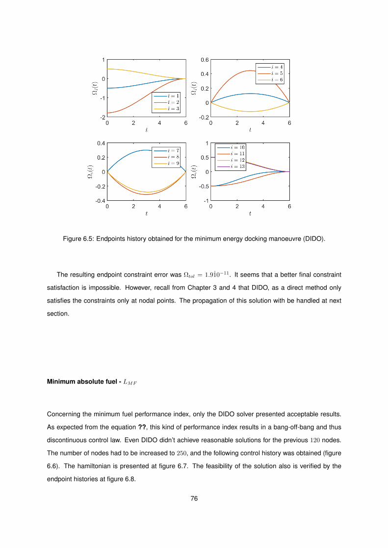
Figure 6.5: Endpoints history obtained for the minimum energy docking manoeuvre (DIDO).
The resulting endpoint constraint error was Ωtol = 1.910−11. It seems that a better final constraint
satisfaction is impossible. However, recall from Chapter 3 and 4 that DIDO, as a direct method only
satisfies the constraints only at nodal points. The propagation of this solution with be handled at next
section.
Minimum absolute fuel - LMF
Concerning the minimum fuel performance index, only the DIDO solver presented acceptable results.
As expected from the equation ??, this kind of performance index results in a bang-off-bang and thus
discontinuous control law. Even DIDO didn’t achieve reasonable solutions for the previous 120 nodes.
The number of nodes had to be increased to 250, and the following control history was obtained (figure
6.6). The hamiltonian is presented at figure 6.7. The feasibility of the solution also is verified by the
endpoint histories at figure 6.8.
76
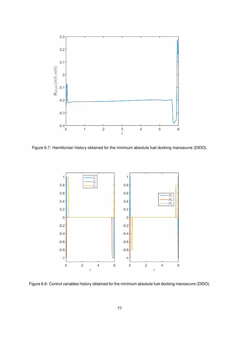
Figure 6.7: Hamiltonian history obtained for the minimum absolute fuel docking manoeuvre (DIDO).
Figure 6.6: Control variables history obtained for the minimum absolute fuel docking manoeuvre (DIDO).
77
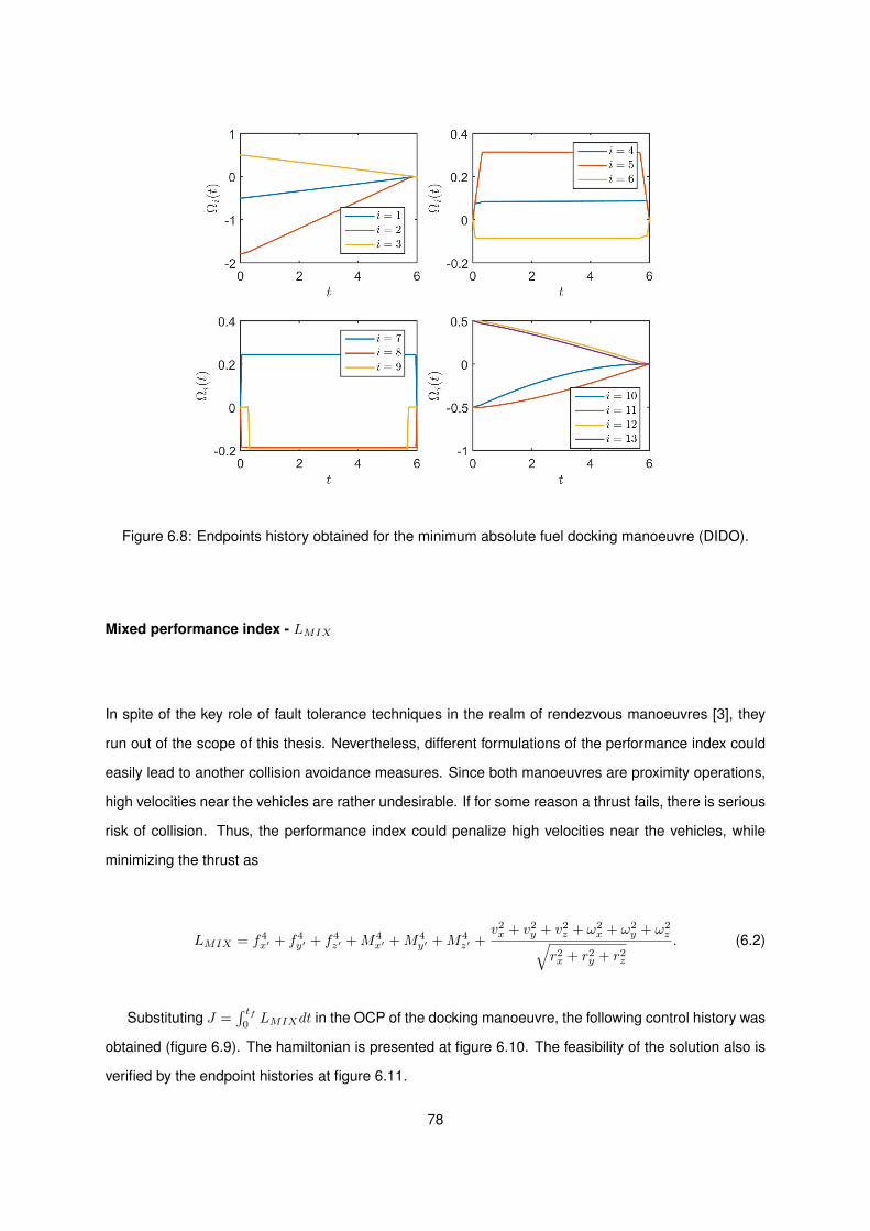
Figure 6.8: Endpoints history obtained for the minimum absolute fuel docking manoeuvre (DIDO).
Mixed performance index - LMIX
In spite of the key role of fault tolerance techniques in the realm of rendezvous manoeuvres [3], they
run out of the scope of this thesis. Nevertheless, different formulations of the performance index could
easily lead to another collision avoidance measures. Since both manoeuvres are proximity operations,
high velocities near the vehicles are rather undesirable. If for some reason a thrust fails, there is serious
risk of collision. Thus, the performance index could penalize high velocities near the vehicles, while
minimizing the thrust as
LMIX = f4x′ + f4
y′ + f4z′ +M4
x′ +M4y′ +M4
z′ +v2x + v2
y + v2z + ω2
x + ω2y + ω2
z√r2x + r2
y + r2z
. (6.2)
Substituting J =∫ tf
0LMIXdt in the OCP of the docking manoeuvre, the following control history was
obtained (figure 6.9). The hamiltonian is presented at figure 6.10. The feasibility of the solution also is
verified by the endpoint histories at figure 6.11.
78
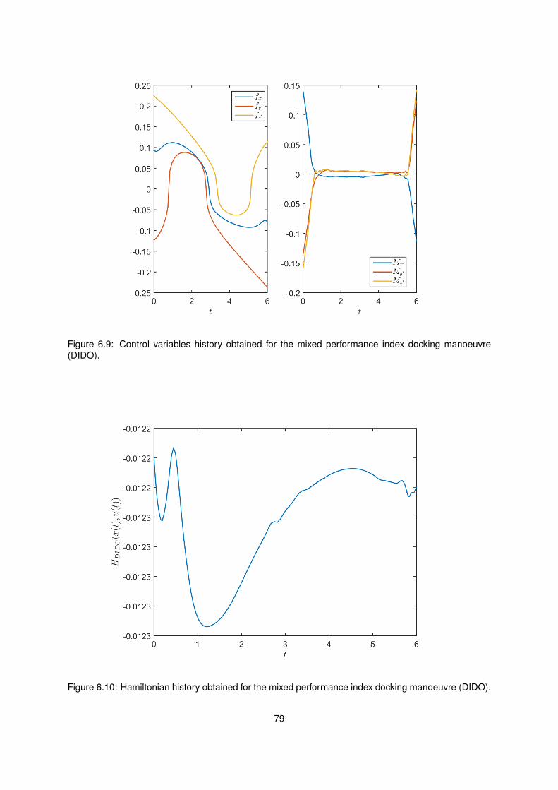
Figure 6.9: Control variables history obtained for the mixed performance index docking manoeuvre(DIDO).
Figure 6.10: Hamiltonian history obtained for the mixed performance index docking manoeuvre (DIDO).
79
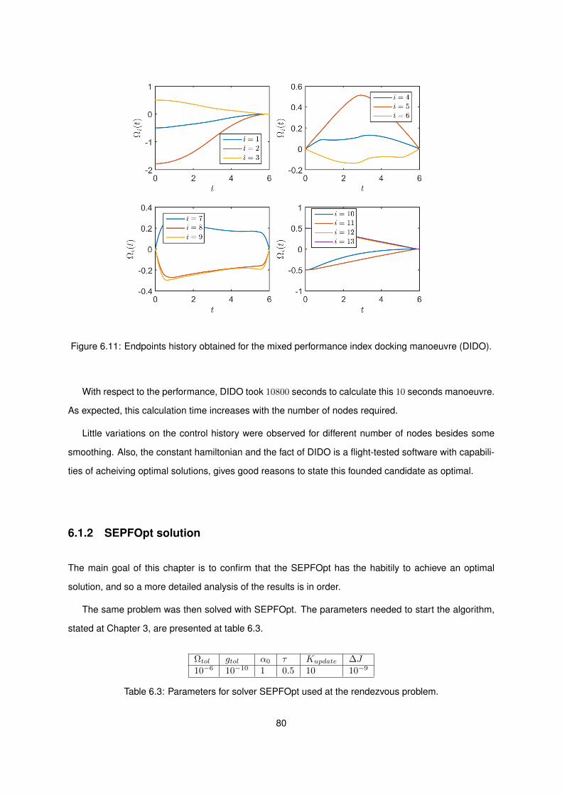
Figure 6.11: Endpoints history obtained for the mixed performance index docking manoeuvre (DIDO).
With respect to the performance, DIDO took 10800 seconds to calculate this 10 seconds manoeuvre.
As expected, this calculation time increases with the number of nodes required.
Little variations on the control history were observed for different number of nodes besides some
smoothing. Also, the constant hamiltonian and the fact of DIDO is a flight-tested software with capabili-
ties of acheiving optimal solutions, gives good reasons to state this founded candidate as optimal.
6.1.2 SEPFOpt solution
The main goal of this chapter is to confirm that the SEPFOpt has the habitily to achieve an optimal
solution, and so a more detailed analysis of the results is in order.
The same problem was then solved with SEPFOpt. The parameters needed to start the algorithm,
stated at Chapter 3, are presented at table 6.3.
Ωtol gtol α0 τ Kupdate ∆J10−6 10−10 1 0.5 10 10−9
Table 6.3: Parameters for solver SEPFOpt used at the rendezvous problem.
80
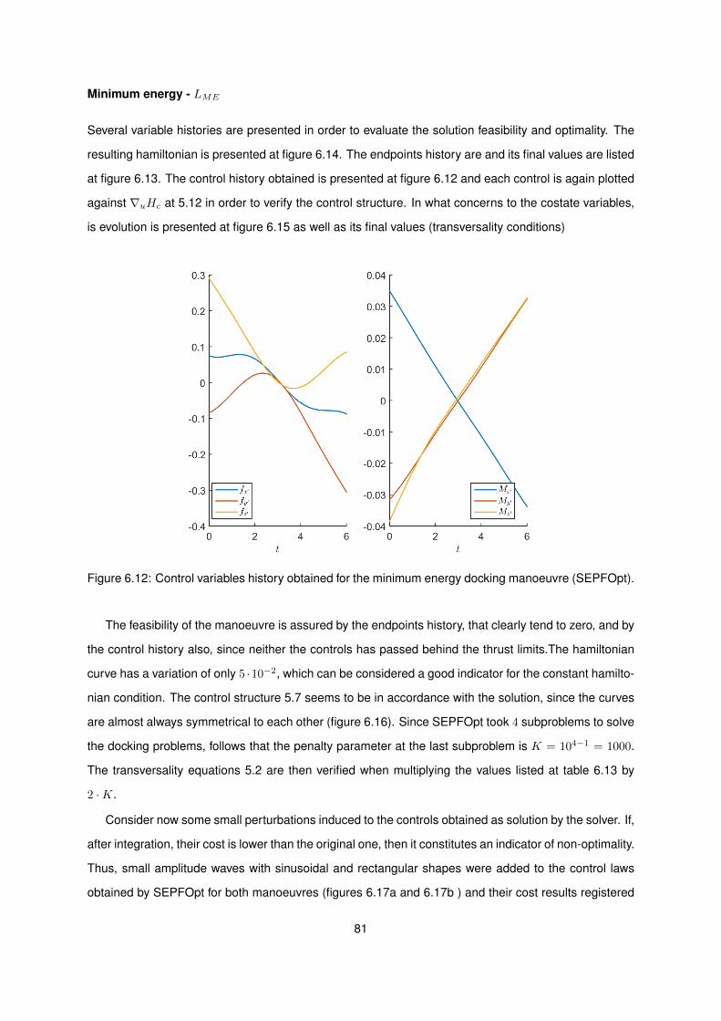
Minimum energy - LME
Several variable histories are presented in order to evaluate the solution feasibility and optimality. The
resulting hamiltonian is presented at figure 6.14. The endpoints history are and its final values are listed
at figure 6.13. The control history obtained is presented at figure 6.12 and each control is again plotted
against ∇uHc at 5.12 in order to verify the control structure. In what concerns to the costate variables,
is evolution is presented at figure 6.15 as well as its final values (transversality conditions)
Figure 6.12: Control variables history obtained for the minimum energy docking manoeuvre (SEPFOpt).
The feasibility of the manoeuvre is assured by the endpoints history, that clearly tend to zero, and by
the control history also, since neither the controls has passed behind the thrust limits.The hamiltonian
curve has a variation of only 5 ·10−2, which can be considered a good indicator for the constant hamilto-
nian condition. The control structure 5.7 seems to be in accordance with the solution, since the curves
are almost always symmetrical to each other (figure 6.16). Since SEPFOpt took 4 subproblems to solve
the docking problems, follows that the penalty parameter at the last subproblem is K = 104−1 = 1000.
The transversality equations 5.2 are then verified when multiplying the values listed at table 6.13 by
2 ·K.
Consider now some small perturbations induced to the controls obtained as solution by the solver. If,
after integration, their cost is lower than the original one, then it constitutes an indicator of non-optimality.
Thus, small amplitude waves with sinusoidal and rectangular shapes were added to the control laws
obtained by SEPFOpt for both manoeuvres (figures 6.17a and 6.17b ) and their cost results registered
81
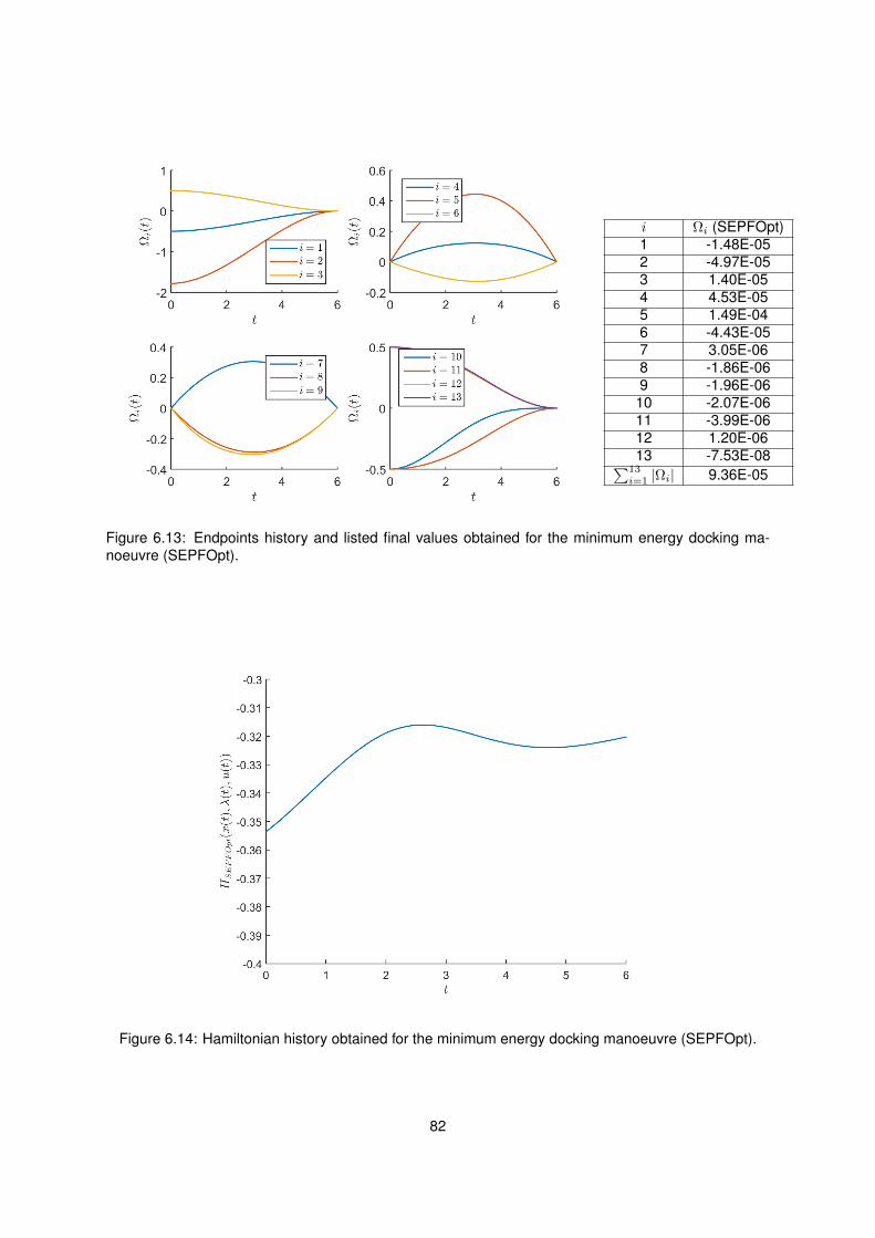
i Ωi (SEPFOpt)1 -1.48E-052 -4.97E-053 1.40E-054 4.53E-055 1.49E-046 -4.43E-057 3.05E-068 -1.86E-069 -1.96E-06
10 -2.07E-0611 -3.99E-0612 1.20E-0613 -7.53E-08∑13i=1 |Ωi| 9.36E-05
Figure 6.13: Endpoints history and listed final values obtained for the minimum energy docking ma-noeuvre (SEPFOpt).
Figure 6.14: Hamiltonian history obtained for the minimum energy docking manoeuvre (SEPFOpt).
82
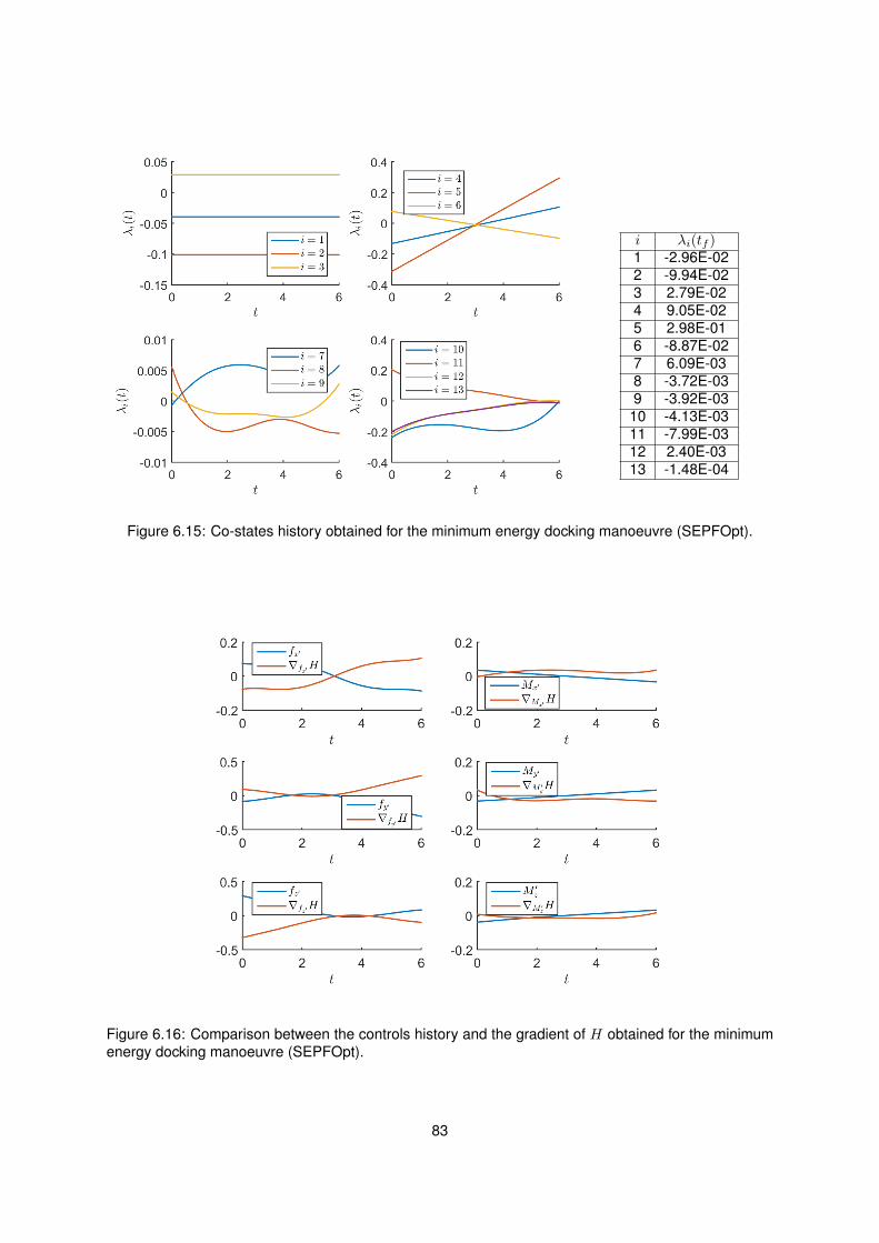
i λi(tf )1 -2.96E-022 -9.94E-023 2.79E-024 9.05E-025 2.98E-016 -8.87E-027 6.09E-038 -3.72E-039 -3.92E-03
10 -4.13E-0311 -7.99E-0312 2.40E-0313 -1.48E-04
Figure 6.15: Co-states history obtained for the minimum energy docking manoeuvre (SEPFOpt).
Figure 6.16: Comparison between the controls history and the gradient of H obtained for the minimumenergy docking manoeuvre (SEPFOpt).
83

at table 6.4. Although the results were obtained for limited values, they show that for any perturbation,
even with low amplitude, the cost obtained was higher than the claimed to be optimal by the solver.
Thus, this tests do not violate this optimality.
(a) Induced sinusoidal perturbation to the control his-tory obtained for the minimum energy docking ma-noeuvre (SEPFOpt).
(b) Induced pulsed perturbation to the control historyobtained for the minimum energy docking manoeuvre(SEPFOpt).
A Jsin Jpulse0 0.1065 0.1065
0.001 0.1816 0.10820.01 3.1744 2.55450.05 50.5767 74.3913
Table 6.4: Variation of the costs of perturbed control histories with the amplitude of perturbing wave.
Mixed performance index - LMIX
The following control history was obtained (figure 6.18). The hamiltonian is presented at figure 6.19.
The feasibility of the solution also is verified by the endpoint histories at figure 6.20.
84
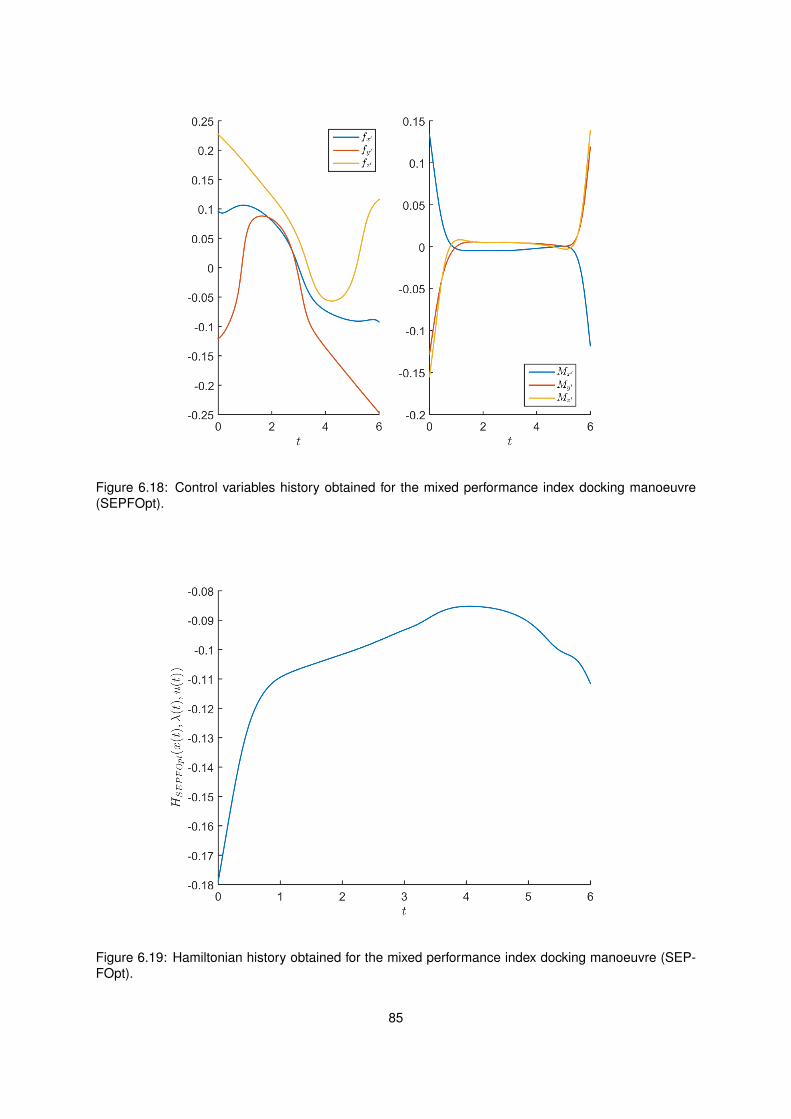
Figure 6.18: Control variables history obtained for the mixed performance index docking manoeuvre(SEPFOpt).
Figure 6.19: Hamiltonian history obtained for the mixed performance index docking manoeuvre (SEP-FOpt).
85
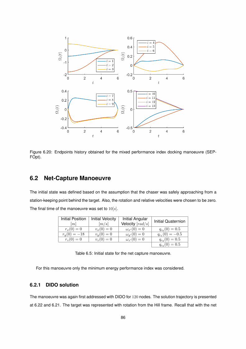
Figure 6.20: Endpoints history obtained for the mixed performance index docking manoeuvre (SEP-FOpt).
6.2 Net-Capture Manoeuvre
The initial state was defined based on the assumption that the chaser was safely approaching from a
station-keeping point behind the target. Also, the rotation and relative velocities were chosen to be zero.
The final time of the manoeuvre was set to 10[s].
Initial Position[m]
Initial Velocity[m/s]
Initial AngularVelocity [rad/s]
Initial Quaternion
rx(0) = 0 vx(0) = 0 ωx′(0) = 0 qc0(0) = 0.5ry(0) = −18 vy(0) = 0 ωy′(0) = 0 qc1(0) = −0.5rz(0) = 0 vz(0) = 0 ωz′(0) = 0 qc2(0) = 0.5
qc3(0) = 0.5
Table 6.5: Initial state for the net capture manoeuvre.
For this manoeuvre only the minimum energy performance index was considered.
6.2.1 DIDO solution
The manoeuvre was again first addressed with DIDO for 120 nodes. The solution trajectory is presented
at 6.22 and 6.21. The target was represented with rotation from the Hill frame. Recall that with the net
86
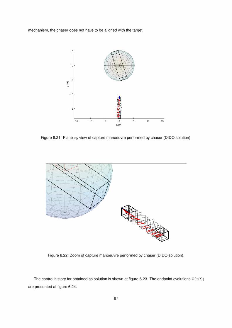
mechanism, the chaser does not have to be aligned with the target.
Figure 6.21: Plane xy view of capture manoeuvre performed by chaser (DIDO solution).
Figure 6.22: Zoom of capture manoeuvre performed by chaser (DIDO solution).
The control history for obtained as solution is shown at figure 6.23. The endpoint evolutions Ω(x(t))
are presented at figure 6.24.
87
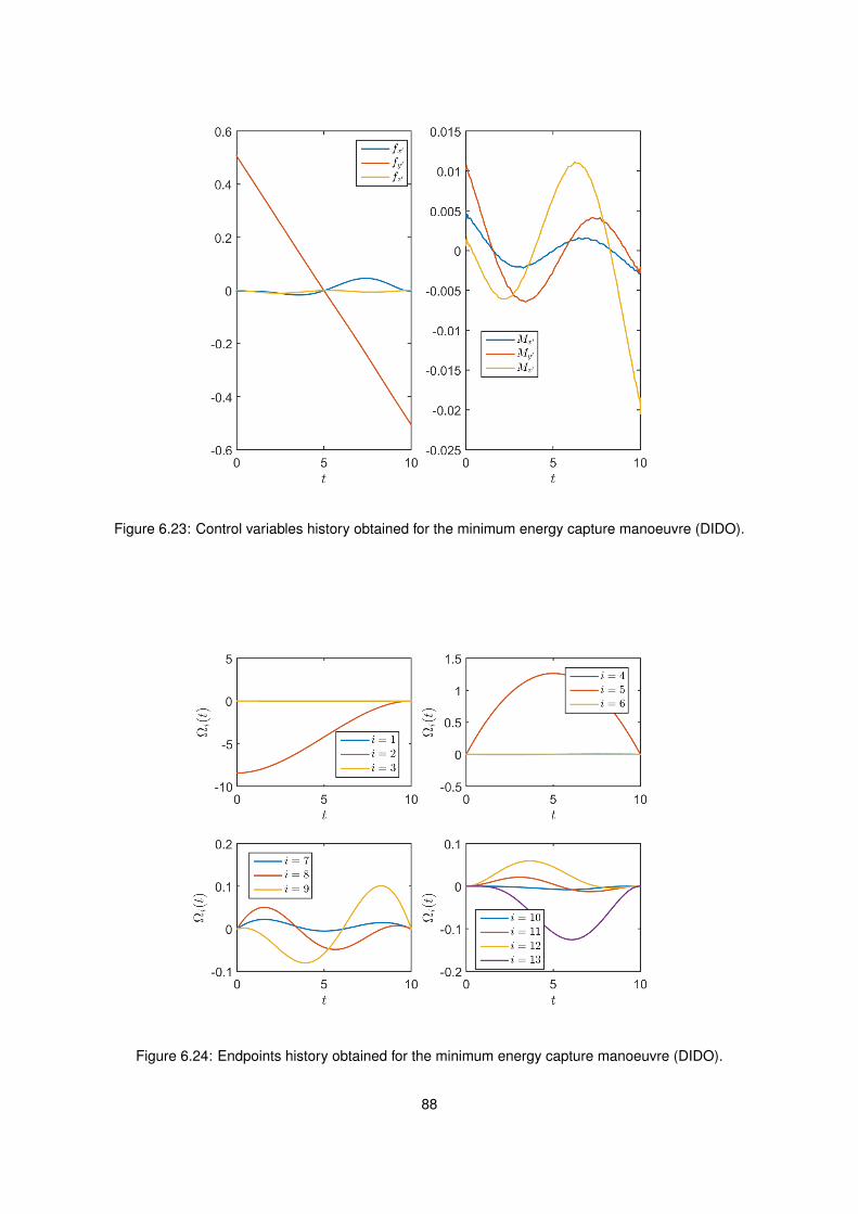
Figure 6.23: Control variables history obtained for the minimum energy capture manoeuvre (DIDO).
Figure 6.24: Endpoints history obtained for the minimum energy capture manoeuvre (DIDO).
88
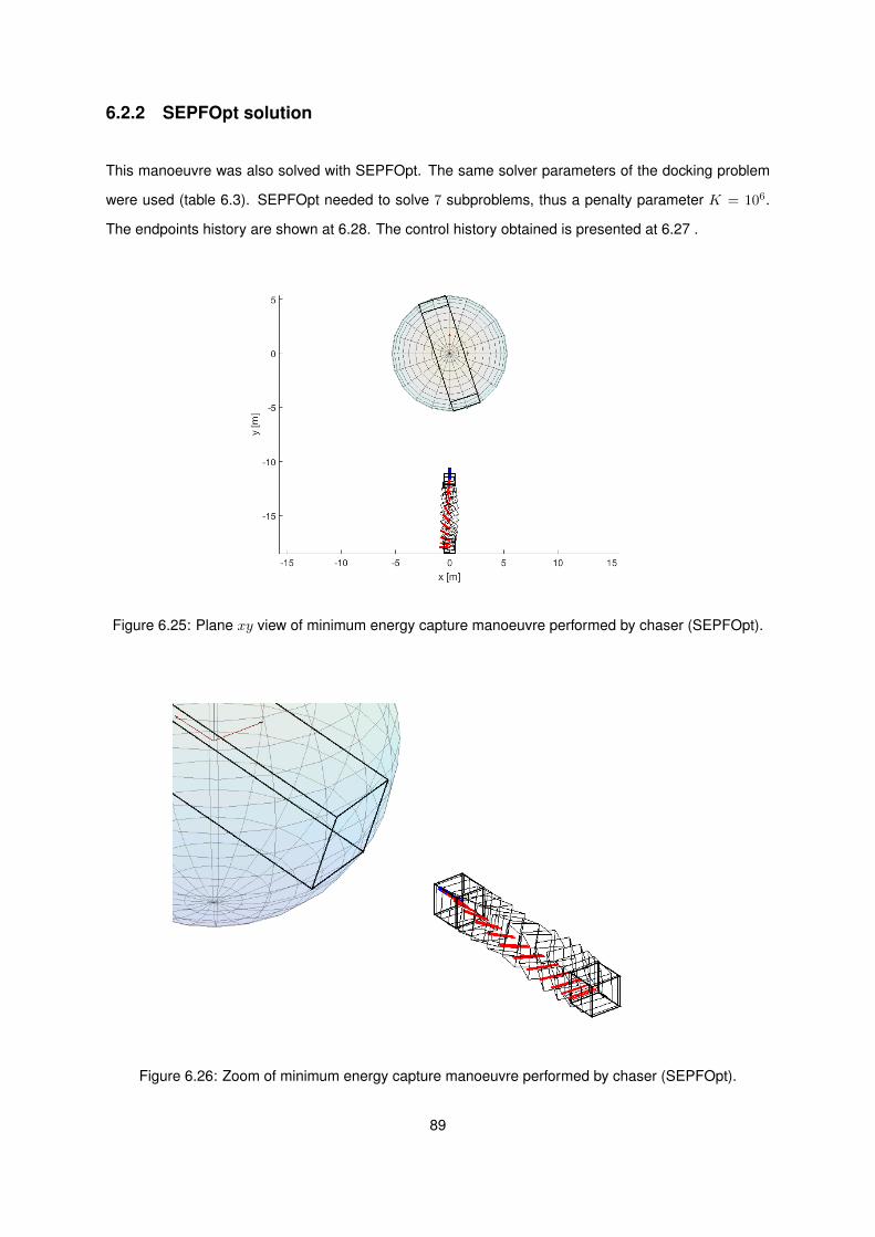
6.2.2 SEPFOpt solution
This manoeuvre was also solved with SEPFOpt. The same solver parameters of the docking problem
were used (table 6.3). SEPFOpt needed to solve 7 subproblems, thus a penalty parameter K = 106.
The endpoints history are shown at 6.28. The control history obtained is presented at 6.27 .
Figure 6.25: Plane xy view of minimum energy capture manoeuvre performed by chaser (SEPFOpt).
Figure 6.26: Zoom of minimum energy capture manoeuvre performed by chaser (SEPFOpt).
89
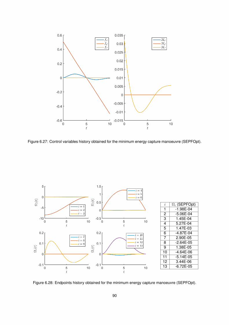
Figure 6.27: Control variables history obtained for the minimum energy capture manoeuvre (SEPFOpt).
i Ωi (SEPFOpt)1 -1.98E-042 -5.06E-043 1.45E-044 5.27E-045 1.47E-036 -4.87E-047 2.90E-058 -2.64E-059 1.38E-05
10 -4.64E-0611 -5.14E-0512 3.44E-0613 -6.72E-05
Figure 6.28: Endpoints history obtained for the minimum energy capture manoeuvre (SEPFOpt).
90
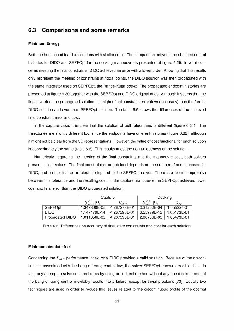
6.3 Comparisons and some remarks
Minimum Energy
Both methods found feasible solutions with similar costs. The comparison between the obtained control
histories for DIDO and SEPFOpt for the docking manoeuvre is presented at figure 6.29. In what con-
cerns meeting the final constraints, DIDO achieved an error with a lower order. Knowing that this results
only represent the meeting of constrains at nodal points, the DIDO solution was then propagated with
the same integrator used on SEPFOpt, the Range-Kutta ode45. The propagated endpoint histories are
presented at figure 6.30 together with the SEPFOpt and DIDO original ones. Although it seems that the
lines override, the propagated solution has higher final constraint error (lower accuracy) than the former
DIDO solution and even than SEPFOpt solution. The table 6.6 shows the differences of the achieved
final constraint error and cost.
In the capture case, it is clear that the solution of both algorithms is different (figure 6.31). The
trajectories are slightly different too, since the endpoints have different histories (figure 6.32), although
it might not be clear from the 3D representations. However, the value of cost functional for each solution
is approximately the same (table 6.6). This results attest the non-uniqueness of the solution.
Numericaly, regarding the meeting of the final constraints and the manoeuvre cost, both solvers
present similar values. The final constraint error obtained depends on the number of nodes chosen for
DIDO, and on the final error tolerance inputed to the SEPFOpt solver. There is a clear compromise
between this tolerance and the resulting cost. In the capture manouevre the SEPFOpt achieved lower
cost and final error than the DIDO propagated solution.
Capture Docking∑13i=1 |Ωi| L∗ME
∑13i=1 |Ωi| L∗ME
SEPFOpt 1.347800E-05 4.267278E-01 3.31202E-04 1.05522e-01DIDO 1.147479E-14 4.267395E-01 3.55979E-13 1.05473E-01Propagated DIDO 1.011056E-02 4.267395E-01 2.08786E-03 1.05473E-01
Table 6.6: Differences on accuracy of final state constraints and cost for each solution.
Minimum absolute fuel
Concerning the LMF performance index, only DIDO provided a valid solution. Because of the discon-
tinuities associated with the bang-off-bang control law, the solver SEPFOpt encounters difficulties. In
fact, any attempt to solve such problems by using an indirect method without any specific treatment of
the bang-off-bang control inevitably results into a failure, except for trivial problems [73]. Usually two
techniques are used in order to reduce this issues related to the discontinuous profile of the optimal
91
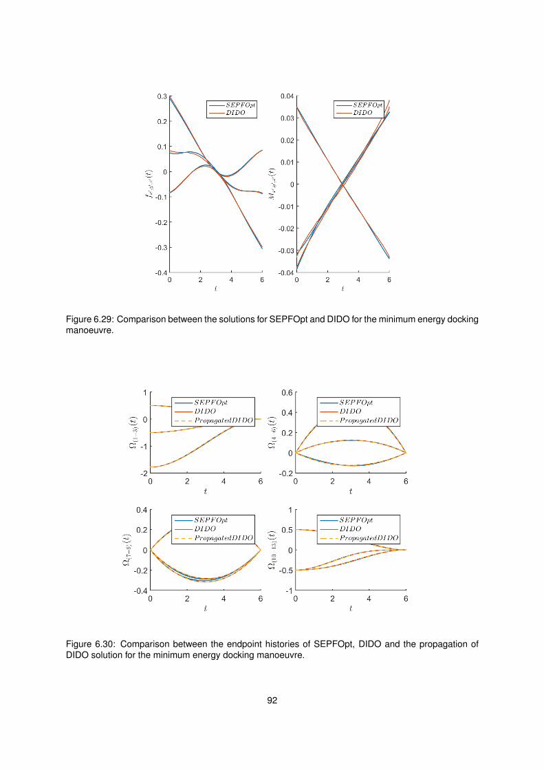
Figure 6.29: Comparison between the solutions for SEPFOpt and DIDO for the minimum energy dockingmanoeuvre.
Figure 6.30: Comparison between the endpoint histories of SEPFOpt, DIDO and the propagation ofDIDO solution for the minimum energy docking manoeuvre.
92
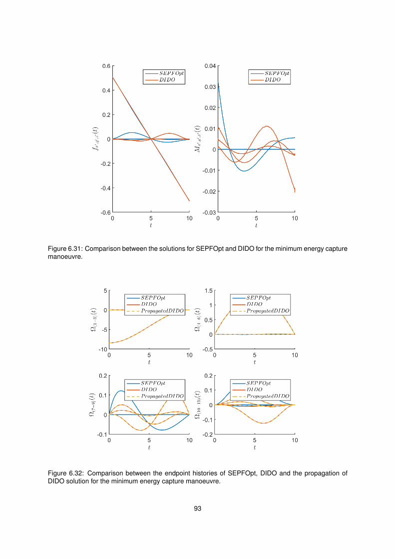
Figure 6.31: Comparison between the solutions for SEPFOpt and DIDO for the minimum energy capturemanoeuvre.
Figure 6.32: Comparison between the endpoint histories of SEPFOpt, DIDO and the propagation ofDIDO solution for the minimum energy capture manoeuvre.
93
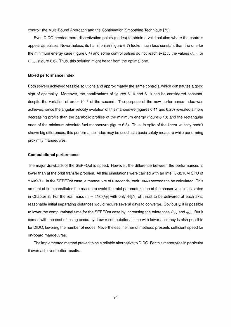
control: the Multi-Bound Approach and the Continuation-Smoothing Technique [73].
Even DIDO needed more discretization points (nodes) to obtain a valid solution where the controls
appear as pulses. Nevertheless, its hamiltonian (figure 6.7) looks much less constant than the one for
the minimum energy case (figure 6.4) and some control pulses do not reach exactly the values Umin or
Umax (figure 6.6). Thus, this solution might be far from the optimal one.
Mixed performance index
Both solvers achieved feasible solutions and approximately the same controls, which constitutes a good
sign of optimality. Moreover, the hamiltonians of figures 6.10 and 6.19 can be considered constant,
despite the variation of order 10−1 of the second. The purpose of the new performance index was
achieved, since the angular velocity evolution of this manoeuvre (figures 6.11 and 6.20) revealed a more
decreasing profile than the parabolic profiles of the minimum energy (figure 6.13) and the rectangular
ones of the minimum absolute fuel manoeuvre (figure 6.8). Thus, in spite of the linear velocity hadn’t
shown big differences, this performance index may be used as a basic safety measure while performing
proximity manoeuvres.
Computational performance
The major drawback of the SEPFOpt is speed. However, the difference between the performances is
lower than at the orbit transfer problem. All this simulations were carried with an Intel i5-3210M CPU of
2.50GHz. In the SEPFOpt case, a manoeuvre of 6 seconds, took 18650 seconds to be calculated. This
amount of time constitutes the reason to avoid the total parametrization of the chaser vehicle as stated
in Chapter 2. For the real mass m = 1580[kg] with only 44[N ] of thrust to be delivered at each axis,
reasonable initial separating distances would require several days to converge. Obviously, it is possible
to lower the computational time for the SEPFOpt case by increasing the tolerances Ωtol and gtol. But it
comes with the cost of losing accuracy. Lower computational time with lower accuracy is also possible
for DIDO, lowering the number of nodes. Nevertheless, neither of methods presents sufficient speed for
on-board manoeuvres.
The implemented method proved to be a reliable alternative to DIDO. For this manouvres in particular
it even achieved better results.
94
Chapter 7
Conclusions
The problem of space debris is adressed with the recent Clean Space initiative by ESA, where the
mission e-deorbit, responsible for capturing and de-orbiting these objects, is inserted. Also on-orbit
servicing by satelites with maintenance and refueling capabilities would decrease the number of non-
used objects in space. This issues, allied with the need of minimizing the energy expenditure of any
manouvre in space, lead to the development of optimal control algorithms, that along with collision
avoidance manouvres, were able to find feasible and optimal actuator histories.
7.1 Achievements
The thesis starts by deriving the six degree of freedom model with states representing the translational
movement at a target centered frame and also the attitude of a chaser spacecraft. The dynamics
suppose body mounted thrusters.
A comparison between the two main approaches in optimal control, focusing on the trade-offs be-
tween each other was done. The recent use of a direct approach to calculate a zero-thrust manouevre
for the ISS was adopted as the direct solver. Pursuing even better accuracy, an indirect approach
method was developed, based on an improved version of a gradient algorithm, with no need of inputing
the necessary conditions for optimality. Then, with an appropriate OCP formulation, the method can be
applied to any problem.
The validation/verification procedures were based on simple orbital transfer manoeuvres and the
solutions from both direct and indirect approaches were compared with a linearized version of the
optimal solution.
Two main manoeuvres were analyzed: in the realm of de-orbiting, capture with a still under develop-
95
ment concept of a thrown-net was assumed, allowing tumbling targets. Concerning on-orbit servicing,
docking of the interfaces for both vehicles was considered. While the docking scenario is well defined,
with the matching of relative positions, velocities and orientations between the two vehicles, a scenario
for capture was proposed, based of the correct orientation of the thrown mechanism and fuel saving
concerns. Their respective OCP formulation were stated. A collision avoidance measure was also
implemented.
In what concerns with verifying the solution optimality, the necessary conditions for optimality were
derivated, ultimately obtaining a control law structure. All this conditions were verified, along with the
constant hamiltonian condition. Also the solution feasibility was verified with the resulting control and
endpoints histories.
The solutions from the two approaches were compared, proving that is possible to achieve ma-
noeuvre with similar (and sometimes lower) cost for the implemented method. The major drawback
of the implemented algorithm is the computational time spent, where the direct approach is usually
much faster. The amount of simulation time obtained shows that is not currently possible to rely on this
methods, even the direct one, to feedback control, being only used for open-loop calculations.
Besides the common energy and fuel minimization, a new performance index was porposed, allying
the thrust minimization with the need of a safety measure based on fault-tolerance.
7.2 Future Work
From the developed model through the solutions obtained, several areas on this thesis would require
further developments before applying the results obtained on the real chaser vehicle. Several topics
were approximated or ignored, due to lack of time, information or dispersion from thesis main concerns:
• The dynamics should include effects such as the oblateness of Earth, the non-zero eccentricity,
gravity-gradients and other disturbances.
• Modeling the chaser to include the parts, such as the solar panel, described at the mission context,
which would refine the inertia matrix.
• The capture scenario was assumed to be with the net based approach, which is a feature that is
currently being submitted to a wide range of tests. If it reveals not to be the best capture method,
other scenario for the close-range rendezvous could be developed. Also, with the net based
approach it was assumed that the most favorable position to throw the net was behind the target,
along the natural motion axis. Other scenarios could be analyzed.
96

• In what concerns the implemented algorithm, several tests should be made in order to achieve
the best initial penalty parameter and the best way to update it, specifically developing several
heuristics. Instead of the exterior penalty method, the augmented Lagrangian algorithm could be
implemented. It has advantages in identification of minimal points since they must satisfy the KKT
conditions.
• After all these improvements and further work, validating these results with a chaser vehicle similar
to the baseline would constitute a big step in the ultimate goal of using these techniques in real
capture/docking manoeuvres.
97

98

Bibliography
[1] About space debris / space debris / operations / our activities / esa. http://www.esa.int/Our_
Activities/Operations/Space_Debris/About_space_debris. (Accessed on 09/27/2017).
[2] Watch 60 years of space junk accumulate around earth. https://gizmodo.com/
watch-60-years-of-space-junk-accumulate-around-earth-1749325832. (Accessed on
09/27/2017).
[3] D. Cordeiro. Fault-Tolerant Control for Terminal Rendezvous in Active Removal of Space Debris.
PhD thesis, Instituto Superior Tecnico, 2017.
[4] Clean space / space engineering & technology / our activities / esa. http://www.esa.int/Our_
Activities/Space_Engineering_Technology/Clean_Space, . (Accessed on 09/28/2017).
[5] Orbital express. http://archive.darpa.mil/orbitalexpress/index.html. (Accessed on
09/28/2017).
[6] Space station user’s guide — spaceref. http://spaceref.com/iss/operations.html. (Accessed
on 09/28/2017).
[7] D. J. Kessler and B. G. Cour-Palais. Collision frequency of artificial satellites: The creation of a
debris belt. Journal of Geophysical Research: Space Physics, 83(A6):2637–2646, 1978.
[8] C. Bonnal and F. Alby. Measures to reduce the growth or decrease the space debris population.
Acta Astronautica, 47(2):699–706, 2000.
[9] B. Lazare. The french space operations act: technical regulations.
[10] W. Fehse. Rendezvous with and capture/removal of non-cooperative bodies in orbit: The technical
challenges. The Journal of Space Safety Engineering, 1(1):17–27, 2014.
[11] C. Bonnal, J.-M. Ruault, and M.-C. Desjean. Active debris removal: Recent progress and current
trends. Acta Astronautica, 85(Supplement C):51 – 60, 2013. ISSN 0094-5765. doi: https://doi.org/
99
10.1016/j.actaastro.2012.11.009. URL http://www.sciencedirect.com/science/article/pii/
S0094576512004602.
[12] Clean space / space engineering & technology / our activities / esa. http://www.esa.int/Our_
Activities/Space_Engineering_Technology/Clean_Space, . (Accessed on 10/15/2017).
[13] Soyuz / launch vehicles / space transportation / our activities / esa. http://www.esa.int/Our_
Activities/Space_Transportation/Launch_vehicles/Soyuz2. (Accessed on 09/30/2017).
[14] L. Y. Z. J. T. Guojin. Survey of orbital dynamics and control of space rendezvous.
[15] S. Nolet. Development of a guidance, navigation and control architecture and validation process
enabling autonomous docking to a tumbling satellite. PhD thesis, Massachusetts Institute of Tech-
nology, 2007.
[16] W. Clohessy and R. Wiltshire. Terminal guidance system for satellite rendezvous. SYSTEM, 4(1),
1960.
[17] H. S. London. Second approximation to the solution of the rendezvous equations. AIAA Journal, 1
(7):1691–1693, 1963.
[18] C. D. Karlgaard and F. H. Lutze. Second-order relative motion equations. Journal of Guidance
Control and Dynamics, 26(1):41–49, 2003.
[19] F. Debruijn, E. Gill, and J. How. Comparative analysis of cartesian and curvilinear clohessy-wiltshire
equations. Journal of Aerospace Engineering, Sciences and Applications, 3(2):1–15, Jan 2011.
doi: 10.7446/jaesa.0302.01.
[20] S. Jacobsen, C. Lee, C. Zhu, and S. Dubowsky. Planning of safe kinematic trajectories for free flying
robots approaching an uncontrolled spinning satellite. In Proceedings of the ASME 27th Annual
Biennial Mechanisms and Robotics Conference, pages 1145–1151. American Soc. of Mechanical
Engineers Fairfield, NJ, 2002.
[21] S. Matsumoto, S. Jacobsen, S. Dubowsky, and Y. Ohkami. Approach planning and guidance for un-
controlled rotating satellite capture considering collision avoidance. In Pro. of the 7th International
Symposium on Artificial Intelligence and Robotics & Automation in Space: i-SAIRAS. Citeseer,
2003.
[22] G. A. Boyarko. Spacecraft Guidance Strategies for Proximity Maneuvering and Close Approach
with a Tumbling Object. PhD thesis, 2010.
100
[23] Brachistochrone problem. http://www-groups.dcs.st-and.ac.uk/history/HistTopics/
Brachistochrone.html. (Accessed on 09/14/2017).
[24] L. S. Pontryagin. Mathematical theory of optimal processes. CRC Press, 1987.
[25] R. Bellman. Dynamic programming. Courier Corporation, 2013.
[26] J. T. Betts. Survey of numerical methods for trajectory optimization. Journal of Guidance, Control,
and Dynamics, 21(2):193–207, 1998. doi: 10.2514/2.4231.
[27] A. V. Rao. A survey of numerical methods for optimal control. Advances in the Astronautical
Sciences, 135(1):497–528, 2009.
[28] H. S. Rodrigues, M. T. T. Monteiro, and D. F. Torres. Optimal control and numerical software: an
overview. arXiv preprint arXiv:1401.7279, 2014.
[29] Dido optimal control software — elissar global. http://www.elissarglobal.com/industry/
products/software-3/. (Accessed on 09/15/2017).
[30] B. Honegger. Nps professor’s software breakthrough allows zero-propellant maneuvers in space.
2007.
[31] I. M. Ross and F. Fahroo. Pseudospectral knotting methods for solving optimal control problems.
Journal of Guidance, Control, and Dynamics, 27(3):397–405, 2004.
[32] Q. Gong, F. Fahroo, I. M. Ross, et al. Spectral algorithm for pseudospectral methods in optimal
control. Journal of Guidance Control and Dynamics, 31(3):460–471, 2008.
[33] U. N. C. on the Peaceful Uses of Outer Space. Report of the Committee on the Peaceful Uses of
Outer Space. United Nations., 1968.
[34] ESA. Cdf study report: Cdf-135(c). 2012.
[35] Investigation on envisat continues / envisat / observing the earth / our activities /
esa. http://www.esa.int/Our_Activities/Observing_the_Earth/Envisat/Investigation_
on_Envisat_continues. (Accessed on 10/15/2017).
[36] Envisat information sheet wdc-rsat. http://wdc.dlr.de/sensors/sciamachy/envisat.php. (Ac-
cessed on 10/28/2017).
[37] J. Deloo. Analysis of the Rendezvous Phase of e.deorbit: Guidance, Communication and Illumina-
tion. PhD thesis, Delft University of Technology, 2014.
101
[38] Conversion between quaternions and euler angles - wikipedia. https://en.wikipedia.org/wiki/
Conversion_between_quaternions_and_Euler_angles. (Accessed on 10/14/2017).
[39] M. OpenCourseWare. The clohessy-wiltshire equations of relative motion, 2008.
[40] R. Nave. Kepler’s laws. URL http://hyperphysics.phy-astr.gsu.edu/hbase/kepler.html.
[41] S. W. J. Peraire. 3d rigid body dynamics: Equations of motion; euler’s equations, 2009.
[42] legends2k. Mathematical reason behind gimbal lock in euler an-
gles, Jan 2017. URL https://sundaram.wordpress.com/2013/03/08/
mathematical-reason-behind-gimbal-lock-in-euler-angles/.
[43] Wikipedia. Quaternions and spatial rotation, May 2017. URL https://en.wikipedia.org/wiki/
Quaternions_and_spatial_rotation.
[44] E. W. Weisstein. Quaternion. URL http://mathworld.wolfram.com/Quaternion.html.
[45] Wikipedia. List of moments of inertia, May 2017. URL https://en.wikipedia.org/wiki/List_
of_moments_of_inertia.
[46] Quaternion differentiation, Aug 2012. URL https://fgiesen.wordpress.com/2012/08/24/
quaternion-differentiation/.
[47] L. T. Biegler, T. F. Coleman, A. R. Conn, and F. N. Santosa. Large-Scale Optimization with Ap-
plications: Part II: Optimal Design and Control, volume 93. Springer Science & Business Media,
2012.
[48] I. M. Ross. A primer on Pontryagin’s principle in optimal control. Collegiate Publishers, 2015.
[49] F. Topputo. An overview of optimal control methods with applications. University Lecture, 2013.
[50] J. Lemos. Introducao ao controlo Optimo. University Lecture, 2002.
[51] M. Mardanov and Y. A. Sharifov. Pontryagin’s maximum principle for the optimal control prob-
lems with multipoint boundary conditions. In Abstract and Applied Analysis, volume 2015. Hindawi
Publishing Corporation, 2015.
[52] Gradient or steepest descent - method, example, step size selection. http://www.onmyphd.com/
?p=gradient.descent, . (Accessed on 10/16/2017).
[53] Gradient or steepest descent - method, example, step size selection. http://www.onmyphd.com/
?p=gradient.descent, . (Accessed on 09/28/2017).
102
[54] V. Torczon. On the convergence of pattern search algorithms. SIAM Journal on optimization, 7(1):
1–25, 1997.
[55] J. R. Shewchuk et al. An introduction to the conjugate gradient method without the agonizing pain,
1994.
[56] R. Fletcher and C. M. Reeves. Function minimization by conjugate gradients. The computer journal,
7(2):149–154, 1964.
[57] E. Polak and G. Ribiere. Note sur la convergence de directions conjugees. Rev. Fr. Inform. Rech.
Oper. v16, pages 35–43.
[58] A. V. Fiacco and G. P. McCormick. The sequential unconstrained minimization technique (sumt)
without parameters. Operations Research, 15(5):820–827, 1967.
[59] L. Lasdon, S. Mitter, and A. Waren. The conjugate gradient method for optimal control problems.
IEEE Transactions on Automatic Control, 12(2):132–138, 1967.
[60] B. Pagurek and C. M. Woodside. The conjugate gradient method for optimal control problems with
bounded control variables. Automatica, 4(5-6):337–349, 1968.
[61] C. Canuto, M. Y. Hussaini, A. Quarteroni, A. Thomas Jr, et al. Spectral methods in fluid dynamics.
Springer Science & Business Media, 2012.
[62] www.psopt.org/pseudospectral-methods?tmpl=%2fsystem%2fapp%2ftemplates%2fprint%2f&showprintdialog=1.
http://www.psopt.org/pseudospectral-methods?tmpl=%2Fsystem%2Fapp%2Ftemplates%
2Fprint%2F&showPrintDialog=1. (Accessed on 09/14/2017).
[63] Calculus ii - approximating definite integrals. http://tutorial.math.lamar.edu/Classes/
CalcII/ApproximatingDefIntegrals.aspx. (Accessed on 09/14/2017).
[64] I. M. Ross and F. Fahroo. Legendre pseudospectral approximations of optimal control problems.
In New trends in nonlinear dynamics and control and their applications, pages 327–342. Springer,
2003.
[65] Fourier series – from wolfram mathworld. http://mathworld.wolfram.com/FourierSeries.html.
(Accessed on 09/17/2017).
[66] Legendre polynomial – from wolfram mathworld. http://mathworld.wolfram.com/
LegendrePolynomial.html. (Accessed on 09/17/2017).
103
[67] Lobatto quadrature – from wolfram mathworld. http://mathworld.wolfram.com/
LobattoQuadrature.html. (Accessed on 09/22/2017).
[68] T. N. Edelbaum. Optimum low-thrust rendezvous and station keeping. Journal of Spacecraft and
Rockets, 40(6):960–965, 2003.
[69] J. PRUSSING. Simple proof of the global optimality of the hohmann transfer. Journal of Guidance,
Control, and Dynamics, 15(4):1037, 1992.
[70] T. Edelbaum. How many impulses. Astronautics and Aeronautics, 5(11):64–69, 1967.
[71] S. D. S. Fernandes. Optimum low-thrust limited power transfers between neighbouring elliptic non-
equatorial orbits in a non-central gravity field. Acta Astronautica, 35(12):763–770, 1995.
[72] S. Fernandes and W. Golfetto. Numerical computation of optimal low-thrust limited-power
trajectories-transfers between coplanar circular orbits. Journal of the Brazilian Society of Mechan-
ical Sciences and Engineering, 27(2):178–185, 2005.
[73] Zavioli. Indirect optimization of bang-bang control problems and applications to formation flying
missions.
104
Appendix A
Orbital Transfer Linearized Solution
A first order analytical solution for the problem of optimal simple transfer (no rendezvous) between
close quasi-circular coplanar orbits in a Newtonian central gravity fields is given by Eldebaum, Da Silva
Fernandes:
∆x = Aλ0 (A.1)
where ∆x =
[∆α ∆h ∆k
]Tdenotes the imposed changes on nonsingular orbital elements (state
variables): α = aa , h = ecos(ω), k = esin(ω), where a is the semi-major axis, e is the eccentricity and
ω is the argument of the pericenter; λ0 is the 3 × 1 vector of initial valuesof the adjoint variables, and,
A is a 3× 3 symmetric matrix. The overbar denotes the reference orbit O about which the linearization
is done. In this first order solution, the adjoint variables associated to the non-singular elements are
constant. The matrix A is given by:
A =
aαα aαh aαk
ahα ahh ahk
akα akh akk
(A.2)
where:
aαα = 4
√a5
µ3∆l (A.3)
aαh = ahα = 4
√a5
µ3(sin(lf )− sin(l0)) (A.4)
105
aαk = akα = 4
√a5
µ3(cos(lf )− cos(l0)) (A.5)
ahh = akα =
√a5
µ3(5
2∆l +
3
4(sin(2lf )− sin(2l0))) (A.6)
ahk = akh = −3
4
√a5
µ3(cos(2lf )− cos(2l0)) (A.7)
where lf = l0 + n(tf − t0) = l0 + ∆l, t0 is the initial time, tf is the final time, n =√
µa3 is the mean
motion (reference orbit O) The optimal thrust acceleration Γ∗ and the variation of the consumption
variable ∆J during the manoeuvre is expressed by
Γ∗ =1
na
(λhsin(l)− λkcos(l)
)er + 2
(λα + λhcos(l) + λksin(l)
)es. (A.8)
106
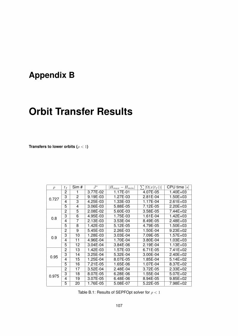
Appendix B
Orbit Transfer Results
Transfers to lower orbits (ρ < 1)
ρ tf Sim # J∗ |Hmax −Hmin|∑|Ω(x(tf ))| CPU time [s]
0.727
2 1 3.77E-02 1.17E-01 4.07E-05 1.40E+033 2 9.19E-03 1.27E-03 2.81E-04 1.50E+034 3 4.25E-03 1.33E-03 1.17E-04 2.61E+035 4 3.06E-03 5.88E-05 7.12E-05 2.20E+03
0.8
2 5 2.08E-02 5.60E-03 3.58E-05 7.44E+023 6 4.95E-03 1.75E-03 1.61E-04 1.42E+034 7 2.13E-03 3.53E-04 8.49E-05 2.48E+035 8 1.42E-03 5.12E-05 4.79E-05 1.50E+03
0.9
2 9 5.45E-03 2.26E-03 1.50E-04 9.23E+023 10 1.28E-03 3.03E-04 7.09E-05 1.57E+034 11 4.96E-04 1.70E-04 3.80E-04 1.03E+035 12 3.04E-04 3.84E-06 2.19E-04 1.13E+03
0.95
2 13 1.42E-03 1.57E-03 6.71E-05 7.41E+023 14 3.25E-04 5.32E-04 3.00E-04 2.40E+024 15 1.25E-04 8.07E-05 1.85E-04 5.14E+025 16 7.21E-05 1.65E-06 1.07E-04 8.37E+02
0.975
2 17 3.52E-04 2.48E-04 3.72E-05 2.33E+023 18 8.07E-05 6.28E-06 1.55E-04 5.07E+024 19 3.07E-05 6.48E-06 8.94E-05 9.85E+025 20 1.76E-05 5.08E-07 5.22E-05 7.98E+02
Table B.1: Results of SEPFOpt solver for ρ < 1
107
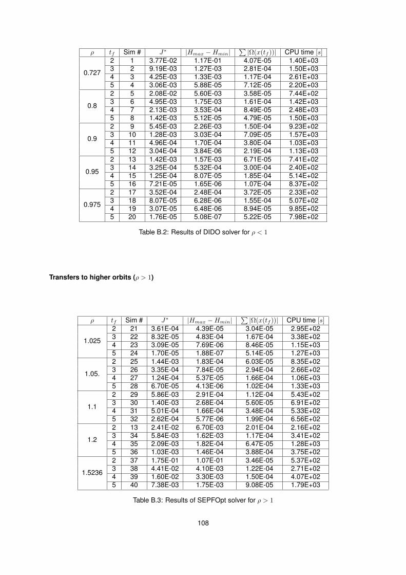
ρ tf Sim # J∗ |Hmax −Hmin|∑|Ω(x(tf ))| CPU time [s]
0.727
2 1 3.77E-02 1.17E-01 4.07E-05 1.40E+033 2 9.19E-03 1.27E-03 2.81E-04 1.50E+034 3 4.25E-03 1.33E-03 1.17E-04 2.61E+035 4 3.06E-03 5.88E-05 7.12E-05 2.20E+03
0.8
2 5 2.08E-02 5.60E-03 3.58E-05 7.44E+023 6 4.95E-03 1.75E-03 1.61E-04 1.42E+034 7 2.13E-03 3.53E-04 8.49E-05 2.48E+035 8 1.42E-03 5.12E-05 4.79E-05 1.50E+03
0.9
2 9 5.45E-03 2.26E-03 1.50E-04 9.23E+023 10 1.28E-03 3.03E-04 7.09E-05 1.57E+034 11 4.96E-04 1.70E-04 3.80E-04 1.03E+035 12 3.04E-04 3.84E-06 2.19E-04 1.13E+03
0.95
2 13 1.42E-03 1.57E-03 6.71E-05 7.41E+023 14 3.25E-04 5.32E-04 3.00E-04 2.40E+024 15 1.25E-04 8.07E-05 1.85E-04 5.14E+025 16 7.21E-05 1.65E-06 1.07E-04 8.37E+02
0.975
2 17 3.52E-04 2.48E-04 3.72E-05 2.33E+023 18 8.07E-05 6.28E-06 1.55E-04 5.07E+024 19 3.07E-05 6.48E-06 8.94E-05 9.85E+025 20 1.76E-05 5.08E-07 5.22E-05 7.98E+02
Table B.2: Results of DIDO solver for ρ < 1
Transfers to higher orbits (ρ > 1)
ρ tf Sim # J∗ |Hmax −Hmin|∑|Ω(x(tf ))| CPU time [s]
1.025
2 21 3.61E-04 4.39E-05 3.04E-05 2.95E+023 22 8.32E-05 4.83E-04 1.67E-04 3.38E+024 23 3.09E-05 7.69E-06 8.46E-05 1.15E+035 24 1.70E-05 1.88E-07 5.14E-05 1.27E+03
1.05.
2 25 1.44E-03 1.83E-04 6.03E-05 8.35E+023 26 3.35E-04 7.84E-05 2.94E-04 2.66E+024 27 1.24E-04 5.37E-05 1.66E-04 1.06E+035 28 6.70E-05 4.13E-06 1.02E-04 1.33E+03
1.1
2 29 5.86E-03 2.91E-04 1.12E-04 5.43E+023 30 1.40E-03 2.68E-04 5.60E-05 6.91E+024 31 5.01E-04 1.66E-04 3.48E-04 5.33E+025 32 2.62E-04 5.77E-06 1.99E-04 6.56E+02
1.2
2 13 2.41E-02 6.70E-03 2.01E-04 2.16E+023 34 5.84E-03 1.62E-03 1.17E-04 3.41E+024 35 2.09E-03 1.82E-04 6.47E-05 1.28E+035 36 1.03E-03 1.46E-04 3.88E-04 3.75E+02
1.5236
2 37 1.75E-01 1.07E-01 3.46E-05 5.37E+023 38 4.41E-02 4.10E-03 1.22E-04 2.71E+024 39 1.60E-02 3.30E-03 1.50E-04 4.07E+025 40 7.38E-03 1.75E-03 9.08E-05 1.79E+03
Table B.3: Results of SEPFOpt solver for ρ > 1
108
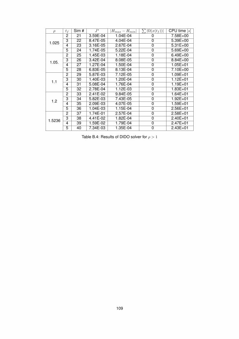
ρ tf Sim # J∗ |Hmax −Hmin|∑|Ω(x(tf ))| CPU time [s]
1.025
2 21 3.59E-04 1.04E-04 0 7.58E+003 22 8.47E-05 4.04E-04 0 5.39E+004 23 3.16E-05 2.67E-04 0 5.31E+005 24 1.74E-05 5.22E-04 0 5.69E+00
1.05.
2 25 1.45E-03 1.18E-04 0 6.49E+003 26 3.42E-04 8.08E-05 0 8.84E+004 27 1.27E-04 1.50E-04 0 1.05E+015 28 6.83E-05 8.13E-04 0 7.10E+00
1.1
2 29 5.87E-03 7.12E-05 0 1.09E+013 30 1.40E-03 1.20E-04 0 1.12E+014 31 5.08E-04 1.76E-04 0 1.19E+015 32 2.78E-04 1.12E-03 0 1.83E+01
1.2
2 33 2.41E-02 9.84E-05 0 1.64E+013 34 5.82E-03 7.43E-05 0 1.92E+014 35 2.09E-03 4.07E-05 0 1.59E+015 36 1.04E-03 1.15E-04 0 2.56E+01
1.5236
2 37 1.74E-01 2.57E-04 0 2.58E+013 38 4.41E-02 1.82E-04 0 2.40E+014 39 1.59E-02 1.79E-04 0 2.47E+015 40 7.34E-03 1.35E-04 0 2.43E+01
Table B.4: Results of DIDO solver for ρ > 1
109

110