Introduction to Algorithms
1312
Introduction to Algorithms Third Edition
Transcript of Introduction to Algorithms

Introduction to AlgorithmsThird Edition
Injector
Highlight


Thomas H. CormenCharles E. LeisersonRonald L. RivestClifford Stein
Introduction to AlgorithmsThird Edition
The MIT PressCambridge, Massachusetts London, England

c� 2009 Massachusetts Institute of Technology
All rights reserved. No part of this book may be reproduced in any form or by any electronic or mechanical means(including photocopying, recording, or information storage and retrieval) without permission in writing from thepublisher.
For information about special quantity discounts, please email special [email protected]
This book was set in Times Roman and Mathtime Pro 2 by the authors.
Printed and bound in the United States of America.
Library of Congress Cataloging-in-Publication Data
Introduction to algorithms / Thomas H. Cormen . . . [et al.].—2nd ed.p. cm.
Includes bibliographical references and index.ISBN 978-0-262-03293-3 (hc. : alk. paper, MIT Press)—978-0-262-53196-2 (pb. : alk. paper, MIT Press); 978-
0-07-013151-4 (hc. : alk. paper, McGraw-Hill)1. Computer programming. 2. Computer algorithms. I. Title:
Algorithms. II. Cormen, Thomas H.
QA76.6 I5858 2001005.1—dc21
2001031277
10 9 8 7 6 5 4 3 2 1

Contents
Preface xiii
I Foundations
Introduction 3
1 The Role of Algorithms in Computing 51.1 Algorithms 51.2 Algorithms as a technology 11
2 Getting Started 162.1 Insertion sort 162.2 Analyzing algorithms 232.3 Designing algorithms 29
3 Growth of Functions 433.1 Asymptotic notation 433.2 Standard notations and common functions 53
4 Divide-and-Conquer 654.1 The maximum-subarray problem 684.2 Strassen’s algorithm for matrix multiplication 754.3 The substitution method for solving recurrences 834.4 The recursion-tree method for solving recurrences 884.5 The master method for solving recurrences 93
? 4.6 Proof of the master theorem 97
5 Probabilistic Analysis and Randomized Algorithms 1145.1 The hiring problem 1145.2 Indicator random variables 1185.3 Randomized algorithms 122
? 5.4 Probabilistic analysis and further uses of indicator random variables130

vi Contents
II Sorting and Order Statistics
Introduction 147
6 Heapsort 1516.1 Heaps 1516.2 Maintaining the heap property 1546.3 Building a heap 1566.4 The heapsort algorithm 1596.5 Priority queues 162
7 Quicksort 1707.1 Description of quicksort 1707.2 Performance of quicksort 1747.3 A randomized version of quicksort 1797.4 Analysis of quicksort 180
8 Sorting in Linear Time 1918.1 Lower bounds for sorting 1918.2 Counting sort 1948.3 Radix sort 1978.4 Bucket sort 200
9 Medians and Order Statistics 2139.1 Minimum and maximum 2149.2 Selection in expected linear time 2159.3 Selection in worst-case linear time 220
III Data Structures
Introduction 229
10 Elementary Data Structures 23210.1 Stacks and queues 23210.2 Linked lists 23610.3 Implementing pointers and objects 24110.4 Representing rooted trees 246
11 Hash Tables 25311.1 Direct-address tables 25411.2 Hash tables 25611.3 Hash functions 26211.4 Open addressing 269
? 11.5 Perfect hashing 277

Contents vii
12 Binary Search Trees 28612.1 What is a binary search tree? 28612.2 Querying a binary search tree 28912.3 Insertion and deletion 294
? 12.4 Randomly built binary search trees 299
13 Red-Black Trees 30813.1 Properties of red-black trees 30813.2 Rotations 31213.3 Insertion 31513.4 Deletion 323
14 Augmenting Data Structures 33914.1 Dynamic order statistics 33914.2 How to augment a data structure 34514.3 Interval trees 348
IV Advanced Design and Analysis Techniques
Introduction 357
15 Dynamic Programming 35915.1 Rod cutting 36015.2 Matrix-chain multiplication 37015.3 Elements of dynamic programming 37815.4 Longest common subsequence 39015.5 Optimal binary search trees 397
16 Greedy Algorithms 41416.1 An activity-selection problem 41516.2 Elements of the greedy strategy 42316.3 Huffman codes 428
? 16.4 Matroids and greedy methods 437? 16.5 A task-scheduling problem as a matroid 443
17 Amortized Analysis 45117.1 Aggregate analysis 45217.2 The accounting method 45617.3 The potential method 45917.4 Dynamic tables 463
viii Contents
V Advanced Data Structures
Introduction 481
18 B-Trees 48418.1 Definition of B-trees 48818.2 Basic operations on B-trees 49118.3 Deleting a key from a B-tree 499
19 Fibonacci Heaps 50519.1 Structure of Fibonacci heaps 50719.2 Mergeable-heap operations 51019.3 Decreasing a key and deleting a node 51819.4 Bounding the maximum degree 523
20 van Emde Boas Trees 53120.1 Preliminary approaches 53220.2 A recursive structure 53620.3 The van Emde Boas tree 545
21 Data Structures for Disjoint Sets 56121.1 Disjoint-set operations 56121.2 Linked-list representation of disjoint sets 56421.3 Disjoint-set forests 568
? 21.4 Analysis of union by rank with path compression 573
VI Graph Algorithms
Introduction 587
22 Elementary Graph Algorithms 58922.1 Representations of graphs 58922.2 Breadth-first search 59422.3 Depth-first search 60322.4 Topological sort 61222.5 Strongly connected components 615
23 Minimum Spanning Trees 62423.1 Growing a minimum spanning tree 62523.2 The algorithms of Kruskal and Prim 631

Contents ix
24 Single-Source Shortest Paths 64324.1 The Bellman-Ford algorithm 65124.2 Single-source shortest paths in directed acyclic graphs 65524.3 Dijkstra’s algorithm 65824.4 Difference constraints and shortest paths 66424.5 Proofs of shortest-paths properties 671
25 All-Pairs Shortest Paths 68425.1 Shortest paths and matrix multiplication 68625.2 The Floyd-Warshall algorithm 69325.3 Johnson’s algorithm for sparse graphs 700
26 Maximum Flow 70826.1 Flow networks 70926.2 The Ford-Fulkerson method 71426.3 Maximum bipartite matching 732
? 26.4 Push-relabel algorithms 736? 26.5 The relabel-to-front algorithm 748
VII Selected Topics
Introduction 769
27 Multithreaded Algorithms 77227.1 The basics of dynamic multithreading 77427.2 Multithreaded matrix multiplication 79227.3 Multithreaded merge sort 797
28 Matrix Operations 81328.1 Solving systems of linear equations 81328.2 Inverting matrices 82728.3 Symmetric positive-definite matrices and least-squares approximation
832
29 Linear Programming 84329.1 Standard and slack forms 85029.2 Formulating problems as linear programs 85929.3 The simplex algorithm 86429.4 Duality 87929.5 The initial basic feasible solution 886

x Contents
30 Polynomials and the FFT 89830.1 Representing polynomials 90030.2 The DFT and FFT 90630.3 Efficient FFT implementations 915
31 Number-Theoretic Algorithms 92631.1 Elementary number-theoretic notions 92731.2 Greatest common divisor 93331.3 Modular arithmetic 93931.4 Solving modular linear equations 94631.5 The Chinese remainder theorem 95031.6 Powers of an element 95431.7 The RSA public-key cryptosystem 958
? 31.8 Primality testing 965? 31.9 Integer factorization 975
32 String Matching 98532.1 The naive string-matching algorithm 98832.2 The Rabin-Karp algorithm 99032.3 String matching with finite automata 995
? 32.4 The Knuth-Morris-Pratt algorithm 1002
33 Computational Geometry 101433.1 Line-segment properties 101533.2 Determining whether any pair of segments intersects 102133.3 Finding the convex hull 102933.4 Finding the closest pair of points 1039
34 NP-Completeness 104834.1 Polynomial time 105334.2 Polynomial-time verification 106134.3 NP-completeness and reducibility 106734.4 NP-completeness proofs 107834.5 NP-complete problems 1086
35 Approximation Algorithms 110635.1 The vertex-cover problem 110835.2 The traveling-salesman problem 111135.3 The set-covering problem 111735.4 Randomization and linear programming 112335.5 The subset-sum problem 1128

Contents xi
VIII Appendix: Mathematical Background
Introduction 1143
A Summations 1145A.1 Summation formulas and properties 1145A.2 Bounding summations 1149
B Sets, Etc. 1158B.1 Sets 1158B.2 Relations 1163B.3 Functions 1166B.4 Graphs 1168B.5 Trees 1173
C Counting and Probability 1183C.1 Counting 1183C.2 Probability 1189C.3 Discrete random variables 1196C.4 The geometric and binomial distributions 1201
? C.5 The tails of the binomial distribution 1208
D Matrices 1217D.1 Matrices and matrix operations 1217D.2 Basic matrix properties 1222
Bibliography 1231
Index 1251


Preface
Before there were computers, there were algorithms. But now that there are com-puters, there are even more algorithms, and algorithms lie at the heart of computing.
This book provides a comprehensive introduction to the modern study of com-puter algorithms. It presents many algorithms and covers them in considerabledepth, yet makes their design and analysis accessible to all levels of readers. Wehave tried to keep explanations elementary without sacrificing depth of coverageor mathematical rigor.
Each chapter presents an algorithm, a design technique, an application area, or arelated topic. Algorithms are described in English and in a pseudocode designed tobe readable by anyone who has done a little programming. The book contains 244figures—many with multiple parts—illustrating how the algorithms work. Sincewe emphasize efficiency as a design criterion, we include careful analyses of therunning times of all our algorithms.
The text is intended primarily for use in undergraduate or graduate courses inalgorithms or data structures. Because it discusses engineering issues in algorithmdesign, as well as mathematical aspects, it is equally well suited for self-study bytechnical professionals.
In this, the third edition, we have once again updated the entire book. Thechanges cover a broad spectrum, including new chapters, revised pseudocode, anda more active writing style.
To the teacher
We have designed this book to be both versatile and complete. You should find ituseful for a variety of courses, from an undergraduate course in data structures upthrough a graduate course in algorithms. Because we have provided considerablymore material than can fit in a typical one-term course, you can consider this bookto be a “buffet” or “smorgasbord” from which you can pick and choose the materialthat best supports the course you wish to teach.

xiv Preface
You should find it easy to organize your course around just the chapters youneed. We have made chapters relatively self-contained, so that you need not worryabout an unexpected and unnecessary dependence of one chapter on another. Eachchapter presents the easier material first and the more difficult material later, withsection boundaries marking natural stopping points. In an undergraduate course,you might use only the earlier sections from a chapter; in a graduate course, youmight cover the entire chapter.
We have included 957 exercises and 158 problems. Each section ends with exer-cises, and each chapter ends with problems. The exercises are generally short ques-tions that test basic mastery of the material. Some are simple self-check thoughtexercises, whereas others are more substantial and are suitable as assigned home-work. The problems are more elaborate case studies that often introduce new ma-terial; they often consist of several questions that lead the student through the stepsrequired to arrive at a solution.
Departing from our practice in previous editions of this book, we have madepublicly available solutions to some, but by no means all, of the problems and ex-ercises. Our Web site, http://mitpress.mit.edu/algorithms/, links to these solutions.You will want to check this site to make sure that it does not contain the solution toan exercise or problem that you plan to assign. We expect the set of solutions thatwe post to grow slowly over time, so you will need to check it each time you teachthe course.
We have starred (?) the sections and exercises that are more suitable for graduatestudents than for undergraduates. A starred section is not necessarily more diffi-cult than an unstarred one, but it may require an understanding of more advancedmathematics. Likewise, starred exercises may require an advanced background ormore than average creativity.
To the student
We hope that this textbook provides you with an enjoyable introduction to thefield of algorithms. We have attempted to make every algorithm accessible andinteresting. To help you when you encounter unfamiliar or difficult algorithms, wedescribe each one in a step-by-step manner. We also provide careful explanationsof the mathematics needed to understand the analysis of the algorithms. If youalready have some familiarity with a topic, you will find the chapters organized sothat you can skim introductory sections and proceed quickly to the more advancedmaterial.
This is a large book, and your class will probably cover only a portion of itsmaterial. We have tried, however, to make this a book that will be useful to younow as a course textbook and also later in your career as a mathematical deskreference or an engineering handbook.

Preface xv
What are the prerequisites for reading this book?
� You should have some programming experience. In particular, you should un-derstand recursive procedures and simple data structures such as arrays andlinked lists.
� You should have some facility with mathematical proofs, and especially proofsby mathematical induction. A few portions of the book rely on some knowledgeof elementary calculus. Beyond that, Parts I and VIII of this book teach you allthe mathematical techniques you will need.
We have heard, loud and clear, the call to supply solutions to problems andexercises. Our Web site, http://mitpress.mit.edu/algorithms/, links to solutions fora few of the problems and exercises. Feel free to check your solutions against ours.We ask, however, that you do not send your solutions to us.
To the professional
The wide range of topics in this book makes it an excellent handbook on algo-rithms. Because each chapter is relatively self-contained, you can focus in on thetopics that most interest you.
Most of the algorithms we discuss have great practical utility. We thereforeaddress implementation concerns and other engineering issues. We often providepractical alternatives to the few algorithms that are primarily of theoretical interest.
If you wish to implement any of the algorithms, you should find the transla-tion of our pseudocode into your favorite programming language to be a fairlystraightforward task. We have designed the pseudocode to present each algorithmclearly and succinctly. Consequently, we do not address error-handling and othersoftware-engineering issues that require specific assumptions about your program-ming environment. We attempt to present each algorithm simply and directly with-out allowing the idiosyncrasies of a particular programming language to obscureits essence.
We understand that if you are using this book outside of a course, then youmight be unable to check your solutions to problems and exercises against solutionsprovided by an instructor. Our Web site, http://mitpress.mit.edu/algorithms/, linksto solutions for some of the problems and exercises so that you can check yourwork. Please do not send your solutions to us.
To our colleagues
We have supplied an extensive bibliography and pointers to the current literature.Each chapter ends with a set of chapter notes that give historical details and ref-erences. The chapter notes do not provide a complete reference to the whole field

xvi Preface
of algorithms, however. Though it may be hard to believe for a book of this size,space constraints prevented us from including many interesting algorithms.
Despite myriad requests from students for solutions to problems and exercises,we have chosen as a matter of policy not to supply references for problems andexercises, to remove the temptation for students to look up a solution rather than tofind it themselves.
Changes for the third edition
What has changed between the second and third editions of this book? The mag-nitude of the changes is on a par with the changes between the first and secondeditions. As we said about the second-edition changes, depending on how youlook at it, the book changed either not much or quite a bit.
A quick look at the table of contents shows that most of the second-edition chap-ters and sections appear in the third edition. We removed two chapters and onesection, but we have added three new chapters and two new sections apart fromthese new chapters.
We kept the hybrid organization from the first two editions. Rather than organiz-ing chapters by only problem domains or according only to techniques, this bookhas elements of both. It contains technique-based chapters on divide-and-conquer,dynamic programming, greedy algorithms, amortized analysis, NP-Completeness,and approximation algorithms. But it also has entire parts on sorting, on datastructures for dynamic sets, and on algorithms for graph problems. We find thatalthough you need to know how to apply techniques for designing and analyzing al-gorithms, problems seldom announce to you which techniques are most amenableto solving them.
Here is a summary of the most significant changes for the third edition:
� We added new chapters on van Emde Boas tree and multithreaded algorithms,and we have broken out material on matrix basics into its own appendix chapter.
� We revised the chapter on recurrences to more broadly cover the divide-and-conquer technique, and its first two sections apply divide-and-conquer to solvetwo problems. The second section of this chapter presents Strassen’s algorithmfor matrix multiplication, which we have moved from the chapter on matrixoperations.
� We removed two chapters that were rarely taught: binomial heaps and sortingnetworks. One key idea in the sorting networks chapter, the 0-1 principle, ap-pears in this edition within Problem 8-7 as the 0-1 sorting lemma for compare-exchange algorithms. The treatment of Fibonacci heaps no longer relies onbinomial heaps as a precursor.
Preface xvii
� We revised our treatment of dynamic programming and greedy algorithms. Dy-namic programming now leads off with a more interesting problem, rod cutting,than the assembly-line scheduling problem from the second edition. Further-more, we emphasize memoization a bit more than we did in the second edition,and we introduce the notion of the subproblem graph as a way to understandthe running time of a dynamic-programming algorithm. In our opening exam-ple of greedy algorithms, the activity-selection problem, we get to the greedyalgorithm more directly than we did in the second edition.
� The way we delete a node from binary search trees (which includes red-blacktrees) now guarantees that the node requested for deletion is the node that isactually deleted. In the first two editions, in certain cases, some other nodewould be deleted, with its contents moving into the node passed to the deletionprocedure. With our new way to delete nodes, if other components of a programmaintain pointers to nodes in the tree, they will not mistakenly end up with stalepointers to nodes that have been deleted.
� The material on flow networks now bases flows entirely on edges. This ap-proach is more intuitive than the net flow used in the first two editions.
� With the material on matrix basics and Strassen’s algorithm moved to otherchapters, the chapter on matrix operations is smaller than in the second edition.
� We have modified our treatment of the Knuth-Morris-Pratt string-matching al-gorithm.
� We corrected several errors. Most of these errors were posted on our Web siteof second-edition errata, but a few were not.
� Based on many requests, we changed the syntax (as it were) of our pseudocode.We now use “D” to indicate assignment and “==” to test for equality, just as C,C++, Java, and Python do. Likewise, we have eliminated the keywords do andthen and adopted “//” as our comment-to-end-of-line symbol. We also now usedot-notation to indicate object attributes. Our pseudocode remains procedural,rather than object-oriented. In other words, rather than running methods onobjects, we simply call procedures, passing objects as parameters.
� We added 100 new exercises and 28 new problems. We also updated manybibligraphy entries and added several new ones.
� Finally, we went through the entire book and rewrote sentences, paragraphs,and sections to make the writing clearer and more active.

xviii Preface
Web site
You can use our Web site, http://mitpress.mit.edu/algorithms/, to obtain supple-mentary information and to communicate with us. The Web site links to a list ofknown errors, solutions to selected exercises and problems, and (of course) a listexplaining the corny professor jokes, as well as other content that we might add.The Web site also tells you how to report errors or make suggestions.
How we produced this book
Like the second edition, we produced the third edition in LATEX 2". We used theTimes font with mathematics typeset using the MathTime Pro 2 fonts. We thankMichael Spivak from Publish or Perish, Inc., Lance Carnes from Personal TeX,Inc., and Tim Tregubov from Dartmouth College for technical support. As in theprevious two editions, we compiled the index using Windex, a C program that wewrote, and the bibliography was produced with BIBTEX. The PDF files for thisbook were created on a MacBook running OS 10.5.
We drew the illustrations for the third edition using MacDraw Pro, with someof the mathematical expressions in illustrations laid in with the psfrag packagefor LATEX 2". Unfortunately, MacDraw Pro is legacy software, having not beenmarketed for over a decade now. Happily, we still have a couple of Macintoshesthat can run the Classic environment under OS 10.4, and hence they can run Mac-Draw Pro—mostly. Even under the Classic environment, we find MacDraw Pro tobe far easier to use than any other drawing software for the types of illustrationsthat accompany computer-science text, and it produces beautiful output.1 Whoknows how long our pre-Intel Macs will continue to run, so if anyone from Appleis listening: Please create an OS X-compatible version of MacDraw Pro!
Acknowledgments for the third edition
We have been working with The MIT Press for over two decades now, and what aterrific relationship it has been! We thank Ellen Faran, Bob Prior, Ada Brunstein,and Mary Reilly for their help and support.
We were geographically distributed while producing the third edition, workingin the Dartmouth College Department of Computer Science, the MIT Computer
1We investigated several drawing programs that run under Mac OS X, but all had significant short-comings compared with MacDraw Pro. We briefly attempted to produce the illustrations for thisbook with a different, well known drawing program. We found that it took at least five times as longto produce each illustration as it took with MacDraw Pro, and the resulting illustrations did not lookas good. Hence the decision to revert to MacDraw Pro running on older Macintoshes.

Preface xix
Science and Artificial Intelligence Laboratory, and the Columbia University De-partment of Industrial Engineering and Operations Research. We thank our re-spective universities and colleagues for providing such supportive and stimulatingenvironments.
Julie Sussman, P.P.A., once again bailed us out as the technical copyeditor. Timeand again, we were amazed at the errors that eluded us, but that Julie caught. Shealso helped us improve our presentation in several places. If there is a Hall ofFame for technical copyeditors, Julie is a sure-fire, first-ballot inductee. She isnothing short of phenomenal. Thank you, thank you, thank you, Julie! Any errorsthat remain (and undoubtedly, some do) are the responsibility of the authors (andprobably were inserted after Julie read the material).
The treatment for van Emde Boas trees derives from Erik Demaine’s notes,which were in turn influenced by Michael Bender. We also incorporated ideasfrom Javed Aslam, Bradley Kuszmaul, and Hui Zha into this edition.
The chapter on multithreading was based on notes originally written jointly withHarald Prokop. The material was influenced by several others working on the Cilkproject at MIT, including Bradley Kuszmaul and Matteo Frigo. The design of themultithreaded pseudocode took its inspiration from the MIT Cilk extensions to Cand by Cilk Arts’s Cilk++ extensions to C++.
We also thank the many readers of the first and second editions who reportederrors or submitted suggestions for how to improve this book. We corrected all thebona fide errors that were reported, and we incorporated as many suggestions aswe could. We rejoice that the number of such contributors has grown so great thatwe must regret that it has become impractical to list them all.
Finally, we thank our wives—Nicole Cormen, Wendy Leiserson, Gail Rivest,and Rebecca Ivry—and our children—Ricky, Will, Debby, and Katie Leiserson;Alex and Christopher Rivest; and Molly, Noah, and Benjamin Stein—for their loveand support while we prepared this book. The patience and encouragement of ourfamilies made this project possible. We affectionately dedicate this book to them.
THOMAS H. CORMEN Lebanon, New HampshireCHARLES E. LEISERSON Cambridge, MassachusettsRONALD L. RIVEST Cambridge, MassachusettsCLIFFORD STEIN New York, New York
February 2009


Introduction to AlgorithmsThird Edition

I Foundations
Introduction
This part will get you started in thinking about designing and analyzing algorithms.It is intended to be a gentle introduction to how we specify algorithms, some of thedesign strategies we will use throughout this book, and many of the fundamentalideas used in algorithm analysis. Later parts of this book will build upon this base.
Chapter 1 provides an overview of algorithms and their place in modern com-puting systems. This chapter defines what an algorithm is and lists some examples.It also makes a case that we should consider algorithms as a technology, along-side technologies such as fast hardware, graphical user interfaces, object-orientedsystems, and networks.
In Chapter 2, we see our first algorithms, which solve the problem of sortinga sequence of n numbers. They are written in a pseudocode which, although notdirectly translatable to any conventional programming language, conveys the struc-ture of the algorithm clearly enough that you should be able to implement it in thelanguage of your choice. The sorting algorithms we examine are insertion sort,which uses an incremental approach, and merge sort, which uses a recursive tech-nique known as “divide-and-conquer.” Although the time each requires increaseswith the value of n, the rate of increase differs between the two algorithms. Wedetermine these running times in Chapter 2, and we develop a useful notation toexpress them.
Chapter 3 precisely defines this notation, which we call asymptotic notation. Itstarts by defining several asymptotic notations, which we use for bounding algo-rithm running times from above and/or below. The rest of Chapter 3 is primarilya presentation of mathematical notation, more to ensure that your use of notationmatches that in this book than to teach you new mathematical concepts.

4 Part I Foundations
Chapter 4 delves further into the divide-and-conquer method introduced inChapter 2. It provides additional examples of divide-and-conquer algorithms, in-cluding Strassen’s surprising method for multiplying two square matrices. Chap-ter 4 contains methods for solving recurrences, which are useful for describingthe running times of recursive algorithms. One powerful technique is the “mas-ter method,” which we often use to solve recurrences that arise from divide-and-conquer algorithms. Although much of Chapter 4 is devoted to proving the cor-rectness of the master method, you may skip this proof yet still employ the mastermethod.
Chapter 5 introduces probabilistic analysis and randomized algorithms. We typ-ically use probabilistic analysis to determine the running time of an algorithm incases in which, due to the presence of an inherent probability distribution, therunning time may differ on different inputs of the same size. In some cases, weassume that the inputs conform to a known probability distribution, so that we areaveraging the running time over all possible inputs. In other cases, the probabilitydistribution comes not from the inputs but from random choices made during thecourse of the algorithm. An algorithm whose behavior is determined not only by itsinput but by the values produced by a random-number generator is a randomizedalgorithm. We can use randomized algorithms to enforce a probability distributionon the inputs—thereby ensuring that no particular input always causes poor perfor-mance—or even to bound the error rate of algorithms that are allowed to produceincorrect results on a limited basis.
Appendices A–D contain other mathematical material that you will find helpfulas you read this book. You are likely to have seen much of the material in theappendix chapters before having read this book (although the specific definitionsand notational conventions we use may differ in some cases from what you haveseen in the past), and so you should think of the Appendices as reference material.On the other hand, you probably have not already seen most of the material inPart I. All the chapters in Part I and the Appendices are written with a tutorialflavor.
1 The Role of Algorithms in Computing
What are algorithms? Why is the study of algorithms worthwhile? What is the roleof algorithms relative to other technologies used in computers? In this chapter, wewill answer these questions.
1.1 Algorithms
Informally, an algorithm is any well-defined computational procedure that takessome value, or set of values, as input and produces some value, or set of values, asoutput. An algorithm is thus a sequence of computational steps that transform theinput into the output.
We can also view an algorithm as a tool for solving a well-specified computa-tional problem. The statement of the problem specifies in general terms the desiredinput/output relationship. The algorithm describes a specific computational proce-dure for achieving that input/output relationship.
For example, we might need to sort a sequence of numbers into nondecreasingorder. This problem arises frequently in practice and provides fertile ground forintroducing many standard design techniques and analysis tools. Here is how weformally define the sorting problem:
Input: A sequence of n numbers ha1; a2; : : : ; ani.Output: A permutation (reordering) ha0
1; a02; : : : ; a0
ni of the input sequence suchthat a0
1 � a02 � � � � � a0
n.
For example, given the input sequence h31; 41; 59; 26; 41; 58i, a sorting algorithmreturns as output the sequence h26; 31; 41; 41; 58; 59i. Such an input sequence iscalled an instance of the sorting problem. In general, an instance of a problemconsists of the input (satisfying whatever constraints are imposed in the problemstatement) needed to compute a solution to the problem.
6 Chapter 1 The Role of Algorithms in Computing
Because many programs use it as an intermediate step, sorting is a fundamentaloperation in computer science. As a result, we have a large number of good sortingalgorithms at our disposal. Which algorithm is best for a given application dependson—among other factors—the number of items to be sorted, the extent to whichthe items are already somewhat sorted, possible restrictions on the item values,the architecture of the computer, and the kind of storage devices to be used: mainmemory, disks, or even tapes.
An algorithm is said to be correct if, for every input instance, it halts with thecorrect output. We say that a correct algorithm solves the given computationalproblem. An incorrect algorithm might not halt at all on some input instances, or itmight halt with an incorrect answer. Contrary to what you might expect, incorrectalgorithms can sometimes be useful, if we can control their error rate. We shall seean example of an algorithm with a controllable error rate in Chapter 31 when westudy algorithms for finding large prime numbers. Ordinarily, however, we shallbe concerned only with correct algorithms.
An algorithm can be specified in English, as a computer program, or even asa hardware design. The only requirement is that the specification must provide aprecise description of the computational procedure to be followed.
What kinds of problems are solved by algorithms?
Sorting is by no means the only computational problem for which algorithms havebeen developed. (You probably suspected as much when you saw the size of thisbook.) Practical applications of algorithms are ubiquitous and include the follow-ing examples:
� The Human Genome Project has made great progress toward the goals of iden-tifying all the 100,000 genes in human DNA, determining the sequences of the3 billion chemical base pairs that make up human DNA, storing this informa-tion in databases, and developing tools for data analysis. Each of these stepsrequires sophisticated algorithms. Although the solutions to the various prob-lems involved are beyond the scope of this book, many methods to solve thesebiological problems use ideas from several of the chapters in this book, therebyenabling scientists to accomplish tasks while using resources efficiently. Thesavings are in time, both human and machine, and in money, as more informa-tion can be extracted from laboratory techniques.
� The Internet enables people all around the world to quickly access and retrievelarge amounts of information. With the aid of clever algorithms, sites on theInternet are able to manage and manipulate this large volume of data. Examplesof problems that make essential use of algorithms include finding good routeson which the data will travel (techniques for solving such problems appear in

1.1 Algorithms 7
Chapter 24), and using a search engine to quickly find pages on which particularinformation resides (related techniques are in Chapters 11 and 32).
� Electronic commerce enables goods and services to be negotiated and ex-changed electronically, and it depends on the privacy of personal informa-tion such as credit card numbers, passwords, and bank statements. The coretechnologies used in electronic commerce include public-key cryptography anddigital signatures (covered in Chapter 31), which are based on numerical algo-rithms and number theory.
� Manufacturing and other commercial enterprises often need to allocate scarceresources in the most beneficial way. An oil company may wish to know whereto place its wells in order to maximize its expected profit. A political candidatemay want to determine where to spend money buying campaign advertising inorder to maximize the chances of winning an election. An airline may wishto assign crews to flights in the least expensive way possible, making sure thateach flight is covered and that government regulations regarding crew schedul-ing are met. An Internet service provider may wish to determine where to placeadditional resources in order to serve its customers more effectively. All ofthese are examples of problems that can be solved using linear programming,which we shall study in Chapter 29.
Although some of the details of these examples are beyond the scope of thisbook, we do give underlying techniques that apply to these problems and problemareas. We also show how to solve many specific problems, including the following:
� We are given a road map on which the distance between each pair of adjacentintersections is marked, and we wish to determine the shortest route from oneintersection to another. The number of possible routes can be huge, even if wedisallow routes that cross over themselves. How do we choose which of allpossible routes is the shortest? Here, we model the road map (which is itselfa model of the actual roads) as a graph (which we will meet in Part VI andAppendix B), and we wish to find the shortest path from one vertex to anotherin the graph. We shall see how to solve this problem efficiently in Chapter 24.
� We are given two ordered sequences of symbols, X D hx1; x2; : : : ; xmi andY D hy1; y2; : : : ; yni, and we wish to find a longest common subsequence ofX and Y . A subsequence of X is just X with some (or possibly all or none) ofits elements removed. For example, one subsequence of hA; B; C; D; E; F; Giwould be hB; C; E; Gi. The length of a longest common subsequence of X
and Y gives one measure of how similar these two sequences are. For example,if the two sequences are base pairs in DNA strands, then we might considerthem similar if they have a long common subsequence. If X has m symbolsand Y has n symbols, then X and Y have 2m and 2n possible subsequences,
8 Chapter 1 The Role of Algorithms in Computing
respectively. Selecting all possible subsequences of X and Y and matchingthem up could take a prohibitively long time unless m and n are very small.We shall see in Chapter 15 how to use a general technique known as dynamicprogramming to solve this problem much more efficiently.
� We are given a mechanical design in terms of a library of parts, where each partmay include instances of other parts, and we need to list the parts in order sothat each part appears before any part that uses it. If the design comprises n
parts, then there are nŠ possible orders, where nŠ denotes the factorial function.Because the factorial function grows faster than even an exponential function,we cannot feasibly generate each possible order and then verify that, withinthat order, each part appears before the parts using it (unless we have only afew parts). This problem is an instance of topological sorting, and we shall seein Chapter 22 how to solve this problem efficiently.
� We are given n points in the plane, and we wish to find the convex hull ofthese points. The convex hull is the smallest convex polygon containing thepoints. Intuitively, we can think of each point as being represented by a nailsticking out from a board. The convex hull would be represented by a tightrubber band that surrounds all the nails. Each nail around which the rubberband makes a turn is a vertex of the convex hull. (See Figure 33.6 on page 1029for an example.) Any of the 2n subsets of the points might be the verticesof the convex hull. Knowing which points are vertices of the convex hull isnot quite enough, either, since we also need to know the order in which theyappear. There are many choices, therefore, for the vertices of the convex hull.Chapter 33 gives two good methods for finding the convex hull.
These lists are far from exhaustive (as you again have probably surmised fromthis book’s heft), but exhibit two characteristics that are common to many interest-ing algorithmic problems:
1. They have many candidate solutions, the overwhelming majority of which donot solve the problem at hand. Finding one that does, or one that is “best,” canpresent quite a challenge.
2. They have practical applications. Of the problems in the above list, shortestpaths provides the easiest examples. A transportation firm, such as a truckingor railroad company, has a financial interest in finding shortest paths througha road or rail network because taking shorter paths results in lower labor andfuel costs. Or a routing node on the Internet may need to find the shortest paththrough the network in order to route a message quickly. Or a person wishingto drive from New York to Boston may want to find driving directions from anappropriate Web site, or she may use her GPS while driving.
1.1 Algorithms 9
Not every problem solved by algorithms has an easily identified set of candidatesolutions. For example, suppose we are given a set of numerical values represent-ing samples of a signal, and we want to compute the discrete Fourier transform ofthese samples. The discrete Fourier transform converts the time domain to the fre-quency domain, producing a set of numerical coefficients, so that we can determinethe strength of various frequencies in the sampled signal. In addition to lying atthe heart of signal processing, discrete Fourier transforms have applications in datacompression and multiplying large polynomials and integers. Chapter 30 givesan efficient algorithm, the fast Fourier transform (commonly called the FFT), forthis problem, and the chapter also sketches out the design of a hardware circuit tocompute the FFT.
Data structures
This book also contains several data structures. A data structure is a way to storeand organize data in order to facilitate access and modifications. No single datastructure works well for all purposes, and so it is important to know the strengthsand limitations of several of them.
Technique
Although you can use this book as a “cookbook” for algorithms, you may somedayencounter a problem for which you cannot readily find a published algorithm (manyof the exercises and problems in this book, for example). This book will teach youtechniques of algorithm design and analysis so that you can develop algorithms onyour own, show that they give the correct answer, and understand their efficiency.Different chapters address different aspects of algorithmic problem solving. Somechapters address specific problems, such as finding medians and order statistics inChapter 9, computing minimum spanning trees in Chapter 23, and determining amaximum flow in a network in Chapter 26. Other chapters address techniques,such as divide-and-conquer in Chapter 4, dynamic programming in Chapter 15,and amortized analysis in Chapter 17.
Hard problems
Most of this book is about efficient algorithms. Our usual measure of efficiencyis speed, i.e., how long an algorithm takes to produce its result. There are someproblems, however, for which no efficient solution is known. Chapter 34 studiesan interesting subset of these problems, which are known as NP-complete.
Why are NP-complete problems interesting? First, although no efficient algo-rithm for an NP-complete problem has ever been found, nobody has ever proven
10 Chapter 1 The Role of Algorithms in Computing
that an efficient algorithm for one cannot exist. In other words, no one knowswhether or not efficient algorithms exist for NP-complete problems. Second, theset of NP-complete problems has the remarkable property that if an efficient algo-rithm exists for any one of them, then efficient algorithms exist for all of them. Thisrelationship among the NP-complete problems makes the lack of efficient solutionsall the more tantalizing. Third, several NP-complete problems are similar, but notidentical, to problems for which we do know of efficient algorithms. Computerscientists are intrigued by how a small change to the problem statement can causea big change to the efficiency of the best known algorithm.
You should know about NP-complete problems because some of them arise sur-prisingly often in real applications. If you are called upon to produce an efficientalgorithm for an NP-complete problem, you are likely to spend a lot of time in afruitless search. If you can show that the problem is NP-complete, you can insteadspend your time developing an efficient algorithm that gives a good, but not thebest possible, solution.
As a concrete example, consider a delivery company with a central depot. Eachday, it loads up each delivery truck at the depot and sends it around to deliver goodsto several addresses. At the end of the day, each truck must end up back at the depotso that it is ready to be loaded for the next day. To reduce costs, the company wantsto select an order of delivery stops that yields the lowest overall distance traveledby each truck. This problem is the well-known “traveling-salesman problem,” andit is NP-complete. It has no known efficient algorithm. Under certain assumptions,however, we know of efficient algorithms that give an overall distance which isnot too far above the smallest possible. Chapter 35 discusses such “approximationalgorithms.”
Parallelism
For many years, we could count on processor clock speeds increasing at a steadyrate. Physical limitations present a fundamental roadblock to ever-increasing clockspeeds, however: because power density increases superlinearly with clock speed,chips run the risk of melting once their clock speeds become high enough. In orderto perform more computations per second, therefore, chips are being designed tocontain not just one but several processing “cores.” We can liken these multicorecomputers to several sequential computers on a single chip; in other words, they area type of “parallel computer.” In order to elicit the best performance from multicorecomputers, we need to design algorithms with parallelism in mind. Chapter 27presents a model for “multithreaded” algorithms, which take advantage of multiplecores. This model has advantages from a theoretical standpoint, and it forms thebasis of several successful computer programs, including a championship chessprogram.

1.2 Algorithms as a technology 11
Exercises
1.1-1Give a real-world example that requires sorting or a real-world example that re-quires computing a convex hull.
1.1-2Other than speed, what other measures of efficiency might one use in a real-worldsetting?
1.1-3Select a data structure that you have seen previously, and discuss its strengths andlimitations.
1.1-4How are the shortest-path and traveling-salesman problems given above similar?How are they different?
1.1-5Come up with a real-world problem in which only the best solution will do. Thencome up with one in which a solution that is “approximately” the best is goodenough.
1.2 Algorithms as a technology
Suppose computers were infinitely fast and computer memory was free. Wouldyou have any reason to study algorithms? The answer is yes, if for no other reasonthan that you would still like to demonstrate that your solution method terminatesand does so with the correct answer.
If computers were infinitely fast, any correct method for solving a problemwould do. You would probably want your implementation to be within the boundsof good software engineering practice (for example, your implementation shouldbe well designed and documented), but you would most often use whichevermethod was the easiest to implement.
Of course, computers may be fast, but they are not infinitely fast. And memorymay be inexpensive, but it is not free. Computing time is therefore a boundedresource, and so is space in memory. You should use these resources wisely, andalgorithms that are efficient in terms of time or space will help you do so.
12 Chapter 1 The Role of Algorithms in Computing
Efficiency
Different algorithms devised to solve the same problem often differ dramatically intheir efficiency. These differences can be much more significant than differencesdue to hardware and software.
As an example, in Chapter 2, we will see two algorithms for sorting. The first,known as insertion sort, takes time roughly equal to c1n2 to sort n items, where c1
is a constant that does not depend on n. That is, it takes time roughly proportionalto n2. The second, merge sort, takes time roughly equal to c2n lg n, where lg n
stands for log2 n and c2 is another constant that also does not depend on n. Inser-tion sort typically has a smaller constant factor than merge sort, so that c1 < c2.We shall see that the constant factors can have far less of an impact on the runningtime than the dependence on the input size n. Let’s write insertion sort’s runningtime as c1n � n and merge sort’s running time as c2n � lg n. Then we see that whereinsertion sort has a factor of n in its running time, merge sort has a factor of lg n,which is much smaller. (For example, when n D 1000, lg n is approximately 10,and when n equals one million, lg n is approximately only 20.) Although insertionsort usually runs faster than merge sort for small input sizes, once the input size n
becomes large enough, merge sort’s advantage of lg n vs. n will more than com-pensate for the difference in constant factors. No matter how much smaller c1 isthan c2, there will always be a crossover point beyond which merge sort is faster.
For a concrete example, let us pit a faster computer (computer A) running inser-tion sort against a slower computer (computer B) running merge sort. They eachmust sort an array of 10 million numbers. (Although 10 million numbers mightseem like a lot, if the numbers are eight-byte integers, then the input occupiesabout 80 megabytes, which fits in the memory of even an inexpensive laptop com-puter many times over.) Suppose that computer A executes 10 billion instructionsper second (faster than any single sequential computer at the time of this writing)and computer B executes only 10 million instructions per second, so that com-puter A is 1000 times faster than computer B in raw computing power. To makethe difference even more dramatic, suppose that the world’s craftiest programmercodes insertion sort in machine language for computer A, and the resulting coderequires 2n2 instructions to sort n numbers. Suppose further that just an averageprogrammer implements merge sort, using a high-level language with an inefficientcompiler, with the resulting code taking 50n lg n instructions. To sort 10 millionnumbers, computer A takes
2 � .107/2 instructions
1010 instructions/secondD 20,000 seconds (more than 5.5 hours) ;
while computer B takes

1.2 Algorithms as a technology 13
50 � 107 lg 107 instructions
107 instructions/second� 1163 seconds (less than 20 minutes) :
By using an algorithm whose running time grows more slowly, even with a poorcompiler, computer B runs more than 17 times faster than computer A! The advan-tage of merge sort is even more pronounced when we sort 100 million numbers:where insertion sort takes more than 23 days, merge sort takes under four hours.In general, as the problem size increases, so does the relative advantage of mergesort.
Algorithms and other technologies
The example above shows that we should consider algorithms, like computer hard-ware, as a technology. Total system performance depends on choosing efficientalgorithms as much as on choosing fast hardware. Just as rapid advances are beingmade in other computer technologies, they are being made in algorithms as well.
You might wonder whether algorithms are truly that important on contemporarycomputers in light of other advanced technologies, such as
� advanced computer architectures and fabrication technologies,
� easy-to-use, intuitive, graphical user interfaces (GUIs),
� object-oriented systems,
� integrated Web technologies, and
� fast networking, both wired and wireless.
The answer is yes. Although some applications do not explicitly require algorith-mic content at the application level (such as some simple, Web-based applications),many do. For example, consider a Web-based service that determines how to travelfrom one location to another. Its implementation would rely on fast hardware, agraphical user interface, wide-area networking, and also possibly on object ori-entation. However, it would also require algorithms for certain operations, suchas finding routes (probably using a shortest-path algorithm), rendering maps, andinterpolating addresses.
Moreover, even an application that does not require algorithmic content at theapplication level relies heavily upon algorithms. Does the application rely on fasthardware? The hardware design used algorithms. Does the application rely ongraphical user interfaces? The design of any GUI relies on algorithms. Does theapplication rely on networking? Routing in networks relies heavily on algorithms.Was the application written in a language other than machine code? Then it wasprocessed by a compiler, interpreter, or assembler, all of which make extensive use

14 Chapter 1 The Role of Algorithms in Computing
of algorithms. Algorithms are at the core of most technologies used in contempo-rary computers.
Furthermore, with the ever-increasing capacities of computers, we use them tosolve larger problems than ever before. As we saw in the above comparison be-tween insertion sort and merge sort, it is at larger problem sizes that the differencesin efficiency between algorithms become particularly prominent.
Having a solid base of algorithmic knowledge and technique is one characteristicthat separates the truly skilled programmers from the novices. With modern com-puting technology, you can accomplish some tasks without knowing much aboutalgorithms, but with a good background in algorithms, you can do much, muchmore.
Exercises
1.2-1Give an example of an application that requires algorithmic content at the applica-tion level, and discuss the function of the algorithms involved.
1.2-2Suppose we are comparing implementations of insertion sort and merge sort on thesame machine. For inputs of size n, insertion sort runs in 8n2 steps, while mergesort runs in 64n lg n steps. For which values of n does insertion sort beat mergesort?
1.2-3What is the smallest value of n such that an algorithm whose running time is 100n2
runs faster than an algorithm whose running time is 2n on the same machine?
Problems
1-1 Comparison of running timesFor each function f .n/ and time t in the following table, determine the largestsize n of a problem that can be solved in time t , assuming that the algorithm tosolve the problem takes f .n/ microseconds.

Notes for Chapter 1 15
1 1 1 1 1 1 1second minute hour day month year century
lg np
n
n
n lg n
n2
n3
2n
nŠ
Chapter notes
There are many excellent texts on the general topic of algorithms, including thoseby Aho, Hopcroft, and Ullman [5, 6]; Baase and Van Gelder [28]; Brassard andBratley [55]; Dasgupta, Papadimitriou, and Vazirani [83]; Goodrich and Tamassia[148]; Hofri [175]; Horowitz, Sahni, and Rajasekaran [181]; Johnsonbaugh andSchaefer [193]; Kingston [205]; Kleinberg and Tardos [208]; Knuth [209, 210,211]; Kozen [220]; Levitin [235]; Manber [242]; Mehlhorn [249, 250, 251]; Pur-dom and Brown [287]; Reingold, Nievergelt, and Deo [293]; Sedgewick [306];Sedgewick and Flajolet [307]; Skiena [318]; and Wilf [356]. Some of the morepractical aspects of algorithm design are discussed by Bentley [42, 43] and Gonnet[145]. Surveys of the field of algorithms can also be found in the Handbook ofTheoretical Computer Science, Volume A [342] and the CRC Handbook on Al-gorithms and Theory of Computation [25]. Overviews of the algorithms used incomputational biology can be found in textbooks by Gusfield [156], Pevzner [275],Setubal and Meidanis [310], and Waterman [350].
2 Getting Started
This chapter will familiarize you with the framework we shall use throughout thebook to think about the design and analysis of algorithms. It is self-contained, butit does include several references to material that we introduce in Chapters 3 and 4.(It also contains several summations, which Appendix A shows how to solve.)
We begin by examining the insertion sort algorithm to solve the sorting problemintroduced in Chapter 1. We define a “pseudocode” that should be familiar to you ifyou have done computer programming, and we use it to show how we shall specifyour algorithms. Having specified the insertion sort algorithm, we then argue that itcorrectly sorts, and we analyze its running time. The analysis introduces a notationthat focuses on how that time increases with the number of items to be sorted.Following our discussion of insertion sort, we introduce the divide-and-conquerapproach to the design of algorithms and use it to develop an algorithm calledmerge sort. We end with an analysis of merge sort’s running time.
2.1 Insertion sort
Our first algorithm, insertion sort, solves the sorting problem introduced in Chap-ter 1:
Input: A sequence of n numbers ha1; a2; : : : ; ani.Output: A permutation (reordering) ha0
1; a02; : : : ; a0
ni of the input sequence suchthat a0
1 � a02 � � � � � a0
n.
The numbers that we wish to sort are also known as the keys. Although conceptu-ally we are sorting a sequence, the input comes to us in the form of an array with n
elements.In this book, we shall typically describe algorithms as programs written in a
pseudocode that is similar in many respects to C, C++, Java, Python, or Pascal. Ifyou have been introduced to any of these languages, you should have little trouble
2.1 Insertion sort 17
2♣
♣
♣ 2♣
4♣♣ ♣
♣♣ 4♣
5♣♣ ♣
♣♣ 5♣
♣
7♣
♣♣ ♣
♣ ♣
♣♣7
♣
10♣ ♣♣ ♣♣ ♣
♣♣♣♣♣
10♣
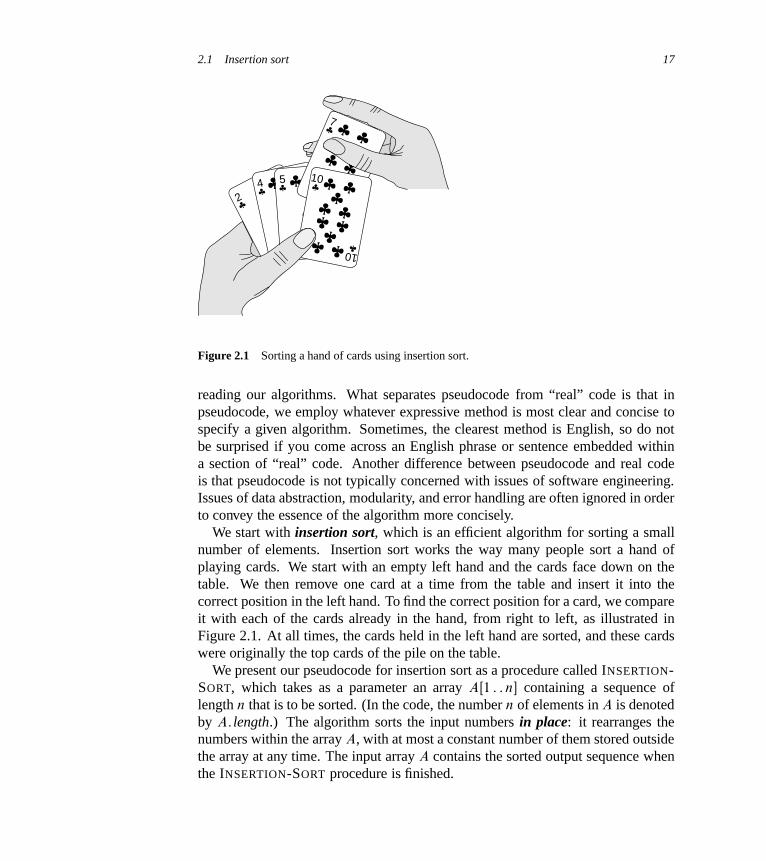
Figure 2.1 Sorting a hand of cards using insertion sort.
reading our algorithms. What separates pseudocode from “real” code is that inpseudocode, we employ whatever expressive method is most clear and concise tospecify a given algorithm. Sometimes, the clearest method is English, so do notbe surprised if you come across an English phrase or sentence embedded withina section of “real” code. Another difference between pseudocode and real codeis that pseudocode is not typically concerned with issues of software engineering.Issues of data abstraction, modularity, and error handling are often ignored in orderto convey the essence of the algorithm more concisely.
We start with insertion sort, which is an efficient algorithm for sorting a smallnumber of elements. Insertion sort works the way many people sort a hand ofplaying cards. We start with an empty left hand and the cards face down on thetable. We then remove one card at a time from the table and insert it into thecorrect position in the left hand. To find the correct position for a card, we compareit with each of the cards already in the hand, from right to left, as illustrated inFigure 2.1. At all times, the cards held in the left hand are sorted, and these cardswere originally the top cards of the pile on the table.
We present our pseudocode for insertion sort as a procedure called INSERTION-SORT, which takes as a parameter an array AŒ1 : : n� containing a sequence oflength n that is to be sorted. (In the code, the number n of elements in A is denotedby A: length.) The algorithm sorts the input numbers in place: it rearranges thenumbers within the array A, with at most a constant number of them stored outsidethe array at any time. The input array A contains the sorted output sequence whenthe INSERTION-SORT procedure is finished.
18 Chapter 2 Getting Started
1 2 3 4 5 6
5 2 4 6 1 3(a)1 2 3 4 5 6
2 5 4 6 1 3(b)1 2 3 4 5 6
2 4 5 6 1 3(c)
1 2 3 4 5 6
2 4 5 6 1 3(d)1 2 3 4 5 6
2 4 5 61 3(e)1 2 3 4 5 6
2 4 5 61 3(f)
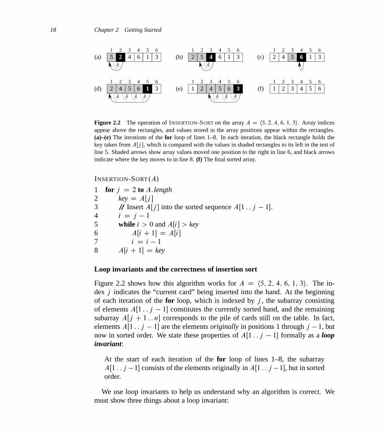
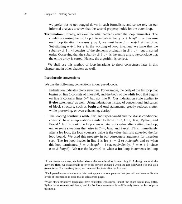
Figure 2.2 The operation of INSERTION-SORT on the array A D h5; 2; 4; 6; 1; 3i. Array indicesappear above the rectangles, and values stored in the array positions appear within the rectangles.(a)–(e) The iterations of the for loop of lines 1–8. In each iteration, the black rectangle holds thekey taken from AŒj �, which is compared with the values in shaded rectangles to its left in the test ofline 5. Shaded arrows show array values moved one position to the right in line 6, and black arrowsindicate where the key moves to in line 8. (f) The final sorted array.
INSERTION-SORT.A/
1 for j D 2 to A: length2 key D AŒj �
3 // Insert AŒj � into the sorted sequence AŒ1 : : j � 1�.4 i D j � 1
5 while i > 0 and AŒi� > key6 AŒi C 1� D AŒi�
7 i D i � 1
8 AŒi C 1� D key
Loop invariants and the correctness of insertion sort
Figure 2.2 shows how this algorithm works for A D h5; 2; 4; 6; 1; 3i. The in-dex j indicates the “current card” being inserted into the hand. At the beginningof each iteration of the for loop, which is indexed by j , the subarray consistingof elements AŒ1 : : j � 1� constitutes the currently sorted hand, and the remainingsubarray AŒj C 1 : : n� corresponds to the pile of cards still on the table. In fact,elements AŒ1 : : j � 1� are the elements originally in positions 1 through j � 1, butnow in sorted order. We state these properties of AŒ1 : : j � 1� formally as a loopinvariant:
At the start of each iteration of the for loop of lines 1–8, the subarrayAŒ1 : : j �1� consists of the elements originally in AŒ1 : : j �1�, but in sortedorder.
We use loop invariants to help us understand why an algorithm is correct. Wemust show three things about a loop invariant:

2.1 Insertion sort 19
Initialization: It is true prior to the first iteration of the loop.
Maintenance: If it is true before an iteration of the loop, it remains true before thenext iteration.
Termination: When the loop terminates, the invariant gives us a useful propertythat helps show that the algorithm is correct.
When the first two properties hold, the loop invariant is true prior to every iterationof the loop. (Of course, we are free to use established facts other than the loopinvariant itself to prove that the loop invariant remains true before each iteration.)Note the similarity to mathematical induction, where to prove that a property holds,you prove a base case and an inductive step. Here, showing that the invariant holdsbefore the first iteration corresponds to the base case, and showing that the invariantholds from iteration to iteration corresponds to the inductive step.
The third property is perhaps the most important one, since we are using the loopinvariant to show correctness. Typically, we use the loop invariant along with thecondition that caused the loop to terminate. The termination property differs fromhow we usually use mathematical induction, in which we apply the inductive stepinfinitely; here, we stop the “induction” when the loop terminates.
Let us see how these properties hold for insertion sort.
Initialization: We start by showing that the loop invariant holds before the firstloop iteration, when j D 2.1 The subarray AŒ1 : : j � 1�, therefore, consistsof just the single element AŒ1�, which is in fact the original element in AŒ1�.Moreover, this subarray is sorted (trivially, of course), which shows that theloop invariant holds prior to the first iteration of the loop.
Maintenance: Next, we tackle the second property: showing that each iterationmaintains the loop invariant. Informally, the body of the for loop works bymoving AŒj � 1�, AŒj � 2�, AŒj � 3�, and so on by one position to the rightuntil it finds the proper position for AŒj � (lines 4–7), at which point it insertsthe value of AŒj � (line 8). The subarray AŒ1 : : j � then consists of the elementsoriginally in AŒ1 : : j �, but in sorted order. Incrementing j for the next iterationof the for loop then preserves the loop invariant.
A more formal treatment of the second property would require us to state andshow a loop invariant for the while loop of lines 5–7. At this point, however,
1When the loop is a for loop, the moment at which we check the loop invariant just prior to the firstiteration is immediately after the initial assignment to the loop-counter variable and just before thefirst test in the loop header. In the case of INSERTION-SORT, this time is after assigning 2 to thevariable j but before the first test of whether j � A: length.
20 Chapter 2 Getting Started
we prefer not to get bogged down in such formalism, and so we rely on ourinformal analysis to show that the second property holds for the outer loop.
Termination: Finally, we examine what happens when the loop terminates. Thecondition causing the for loop to terminate is that j > A: length D n. Becauseeach loop iteration increases j by 1, we must have j D n C 1 at that time.Substituting n C 1 for j in the wording of loop invariant, we have that thesubarray AŒ1 : : n� consists of the elements originally in AŒ1 : : n�, but in sortedorder. Observing that the subarray AŒ1 : : n� is the entire array, we conclude thatthe entire array is sorted. Hence, the algorithm is correct.
We shall use this method of loop invariants to show correctness later in thischapter and in other chapters as well.
Pseudocode conventions
We use the following conventions in our pseudocode.
� Indentation indicates block structure. For example, the body of the for loop thatbegins on line 1 consists of lines 2–8, and the body of the while loop that beginson line 5 contains lines 6–7 but not line 8. Our indentation style applies toif-else statements2 as well. Using indentation instead of conventional indicatorsof block structure, such as begin and end statements, greatly reduces clutterwhile preserving, or even enhancing, clarity.3
� The looping constructs while, for, and repeat-until and the if-else conditionalconstruct have interpretations similar to those in C, C++, Java, Python, andPascal.4 In this book, the loop counter retains its value after exiting the loop,unlike some situations that arise in C++, Java, and Pascal. Thus, immediatelyafter a for loop, the loop counter’s value is the value that first exceeded the forloop bound. We used this property in our correctness argument for insertionsort. The for loop header in line 1 is for j D 2 to A: length, and so whenthis loop terminates, j D A: length C 1 (or, equivalently, j D n C 1, sincen D A: length). We use the keyword to when a for loop increments its loop
2In an if-else statement, we indent else at the same level as its matching if. Although we omit thekeyword then, we occasionally refer to the portion executed when the test following if is true as athen clause. For multiway tests, we use elseif for tests after the first one.
3Each pseudocode procedure in this book appears on one page so that you will not have to discernlevels of indentation in code that is split across pages.
4Most block-structured languages have equivalent constructs, though the exact syntax may differ.Python lacks repeat-until loops, and its for loops operate a little differently from the for loops inthis book.

2.1 Insertion sort 21
counter in each iteration, and we use the keyword downto when a for loopdecrements its loop counter. When the loop counter changes by an amountgreater than 1, the amount of change follows the optional keyword by.
� The symbol “//” indicates that the remainder of the line is a comment.
� A multiple assignment of the form i D j D e assigns to both variables i and j
the value of expression e; it should be treated as equivalent to the assignmentj D e followed by the assignment i D j .
� Variables (such as i , j , and key) are local to the given procedure. We shall notuse global variables without explicit indication.
� We access array elements by specifying the array name followed by the in-dex in square brackets. For example, AŒi� indicates the i th element of thearray A. The notation “: :” is used to indicate a range of values within an ar-ray. Thus, AŒ1 : : j � indicates the subarray of A consisting of the j elementsAŒ1�; AŒ2�; : : : ; AŒj �.
� We typically organize compound data into objects, which are composed of at-tributes. We access a particular attribute using the syntax found in many object-oriented programming languages: the object name, followed by a dot, followedby the attribute name. For example, we treat an array as an object with the at-tribute length indicating how many elements it contains. To specify the numberof elements in an array A, we write A: length.
We treat a variable representing an array or object as a pointer to the data rep-resenting the array or object. For all attributes f of an object x, setting y D x
causes y: f to equal x: f . Moreover, if we now set x: f D 3, then afterward notonly does x: f equal 3, but y: f equals 3 as well. In other words, x and y pointto the same object after the assignment y D x.
Our attribute notation can “cascade.” For example, suppose that the attribute f
is itself a pointer to some type of object that has an attribute g. Then the notationx: f :g is implicitly parenthesized as .x: f /:g. In other words, if we had assignedy D x: f , then x: f :g is the same as y:g.
Sometimes, a pointer will refer to no object at all. In this case, we give it thespecial value NIL.
� We pass parameters to a procedure by value: the called procedure receives itsown copy of the parameters, and if it assigns a value to a parameter, the changeis not seen by the calling procedure. When objects are passed, the pointer tothe data representing the object is copied, but the object’s attributes are not. Forexample, if x is a parameter of a called procedure, the assignment x D y withinthe called procedure is not visible to the calling procedure. The assignmentx: f D 3, however, is visible. Similarly, arrays are passed by pointer, so that

22 Chapter 2 Getting Started
a pointer to the array is passed, rather than the entire array, and changes toindividual array elements are visible to the calling procedure.
� A return statement immediately transfers control back to the point of call inthe calling procedure. Most return statements also take a value to pass back tothe caller. Our pseudocode differs from many programming languages in thatwe allow multiple values to be returned in a single return statement.
� The boolean operators “and” and “or” are short circuiting. That is, when weevaluate the expression “x and y” we first evaluate x. If x evaluates to FALSE,then the entire expression cannot evaluate to TRUE, and so we do not evaluate y.If, on the other hand, x evaluates to TRUE, we must evaluate y to determine thevalue of the entire expression. Similarly, in the expression “x or y” we eval-uate the expression y only if x evaluates to FALSE. Short-circuiting operatorsallow us to write boolean expressions such as “x ¤ NIL and x: f D y” withoutworrying about what happens when we try to evaluate x: f when x is NIL.
� The keyword error indicates that an error occurred because conditions werewrong for the procedure to have been called. The calling procedure is respon-sible for handling the error, and so we do not specify what action to take.
Exercises
2.1-1Using Figure 2.2 as a model, illustrate the operation of INSERTION-SORT on thearray A D h31; 41; 59; 26; 41; 58i.2.1-2Rewrite the INSERTION-SORT procedure to sort into nonincreasing instead of non-decreasing order.
2.1-3Consider the searching problem:
Input: A sequence of n numbers A D ha1; a2; : : : ; ani and a value �.
Output: An index i such that � D AŒi� or the special value NIL if � does notappear in A.
Write pseudocode for linear search, which scans through the sequence, lookingfor �. Using a loop invariant, prove that your algorithm is correct. Make sure thatyour loop invariant fulfills the three necessary properties.
2.1-4Consider the problem of adding two n-bit binary integers, stored in two n-elementarrays A and B . The sum of the two integers should be stored in binary form in
2.2 Analyzing algorithms 23
an .nC 1/-element array C . State the problem formally and write pseudocode foradding the two integers.
2.2 Analyzing algorithms
Analyzing an algorithm has come to mean predicting the resources that the algo-rithm requires. Occasionally, resources such as memory, communication band-width, or computer hardware are of primary concern, but most often it is compu-tational time that we want to measure. Generally, by analyzing several candidatealgorithms for a problem, we can identify a most efficient one. Such analysis mayindicate more than one viable candidate, but we can often discard several inferioralgorithms in the process.
Before we can analyze an algorithm, we must have a model of the implemen-tation technology that we will use, including a model for the resources of thattechnology and their costs. For most of this book, we shall assume a generic one-processor, random-access machine (RAM) model of computation as our imple-mentation technology and understand that our algorithms will be implemented ascomputer programs. In the RAM model, instructions are executed one after an-other, with no concurrent operations.
Strictly speaking, we should precisely define the instructions of the RAM modeland their costs. To do so, however, would be tedious and would yield little insightinto algorithm design and analysis. Yet we must be careful not to abuse the RAMmodel. For example, what if a RAM had an instruction that sorts? Then we couldsort in just one instruction. Such a RAM would be unrealistic, since real computersdo not have such instructions. Our guide, therefore, is how real computers are de-signed. The RAM model contains instructions commonly found in real computers:arithmetic (such as add, subtract, multiply, divide, remainder, floor, ceiling), datamovement (load, store, copy), and control (conditional and unconditional branch,subroutine call and return). Each such instruction takes a constant amount of time.
The data types in the RAM model are integer and floating point (for storing realnumbers). Although we typically do not concern ourselves with precision in thisbook, in some applications precision is crucial. We also assume a limit on the sizeof each word of data. For example, when working with inputs of size n, we typ-ically assume that integers are represented by c lg n bits for some constant c � 1.We require c � 1 so that each word can hold the value of n, enabling us to index theindividual input elements, and we restrict c to be a constant so that the word sizedoes not grow arbitrarily. (If the word size could grow arbitrarily, we could storehuge amounts of data in one word and operate on it all in constant time—clearlyan unrealistic scenario.)
24 Chapter 2 Getting Started
Real computers contain instructions not listed above, and such instructions rep-resent a gray area in the RAM model. For example, is exponentiation a constant-time instruction? In the general case, no; it takes several instructions to compute xy
when x and y are real numbers. In restricted situations, however, exponentiation isa constant-time operation. Many computers have a “shift left” instruction, whichin constant time shifts the bits of an integer by k positions to the left. In mostcomputers, shifting the bits of an integer by one position to the left is equivalentto multiplication by 2, so that shifting the bits by k positions to the left is equiv-alent to multiplication by 2k. Therefore, such computers can compute 2k in oneconstant-time instruction by shifting the integer 1 by k positions to the left, as longas k is no more than the number of bits in a computer word. We will endeavor toavoid such gray areas in the RAM model, but we will treat computation of 2k as aconstant-time operation when k is a small enough positive integer.
In the RAM model, we do not attempt to model the memory hierarchy that iscommon in contemporary computers. That is, we do not model caches or virtualmemory. Several computational models attempt to account for memory-hierarchyeffects, which are sometimes significant in real programs on real machines. Ahandful of problems in this book examine memory-hierarchy effects, but for themost part, the analyses in this book will not consider them. Models that includethe memory hierarchy are quite a bit more complex than the RAM model, and sothey can be difficult to work with. Moreover, RAM-model analyses are usuallyexcellent predictors of performance on actual machines.
Analyzing even a simple algorithm in the RAM model can be a challenge. Themathematical tools required may include combinatorics, probability theory, alge-braic dexterity, and the ability to identify the most significant terms in a formula.Because the behavior of an algorithm may be different for each possible input, weneed a means for summarizing that behavior in simple, easily understood formulas.
Even though we typically select only one machine model to analyze a given al-gorithm, we still face many choices in deciding how to express our analysis. Wewould like a way that is simple to write and manipulate, shows the important char-acteristics of an algorithm’s resource requirements, and suppresses tedious details.
Analysis of insertion sort
The time taken by the INSERTION-SORT procedure depends on the input: sorting athousand numbers takes longer than sorting three numbers. Moreover, INSERTION-SORT can take different amounts of time to sort two input sequences of the samesize depending on how nearly sorted they already are. In general, the time takenby an algorithm grows with the size of the input, so it is traditional to describe therunning time of a program as a function of the size of its input. To do so, we needto define the terms “running time” and “size of input” more carefully.

2.2 Analyzing algorithms 25
The best notion for input size depends on the problem being studied. For manyproblems, such as sorting or computing discrete Fourier transforms, the most nat-ural measure is the number of items in the input—for example, the array size n
for sorting. For many other problems, such as multiplying two integers, the bestmeasure of input size is the total number of bits needed to represent the input inordinary binary notation. Sometimes, it is more appropriate to describe the size ofthe input with two numbers rather than one. For instance, if the input to an algo-rithm is a graph, the input size can be described by the numbers of vertices andedges in the graph. We shall indicate which input size measure is being used witheach problem we study.
The running time of an algorithm on a particular input is the number of primitiveoperations or “steps” executed. It is convenient to define the notion of step sothat it is as machine-independent as possible. For the moment, let us adopt thefollowing view. A constant amount of time is required to execute each line of ourpseudocode. One line may take a different amount of time than another line, butwe shall assume that each execution of the i th line takes time ci , where ci is aconstant. This viewpoint is in keeping with the RAM model, and it also reflectshow the pseudocode would be implemented on most actual computers.5
In the following discussion, our expression for the running time of INSERTION-SORT will evolve from a messy formula that uses all the statement costs ci to amuch simpler notation that is more concise and more easily manipulated. Thissimpler notation will also make it easy to determine whether one algorithm is moreefficient than another.
We start by presenting the INSERTION-SORT procedure with the time “cost”of each statement and the number of times each statement is executed. For eachj D 2; 3; : : : ; n, where n D A: length, we let tj denote the number of times thewhile loop test in line 5 is executed for that value of j . When a for or while loopexits in the usual way (i.e., due to the test in the loop header), the test is executedone time more than the loop body. We assume that comments are not executablestatements, and so they take no time.
5There are some subtleties here. Computational steps that we specify in English are often variantsof a procedure that requires more than just a constant amount of time. For example, later in thisbook we might say “sort the points by x-coordinate,” which, as we shall see, takes more than aconstant amount of time. Also, note that a statement that calls a subroutine takes constant time,though the subroutine, once invoked, may take more. That is, we separate the process of calling thesubroutine—passing parameters to it, etc.—from the process of executing the subroutine.

26 Chapter 2 Getting Started
INSERTION-SORT.A/ cost times
1 for j D 2 to A: length c1 n
2 key D AŒj � c2 n � 1
3 // Insert AŒj � into the sortedsequence AŒ1 : : j � 1�. 0 n � 1
4 i D j � 1 c4 n � 1
5 while i > 0 and AŒi� > key c5
Pn
j D2 tj
6 AŒi C 1� D AŒi� c6
Pn
j D2.tj � 1/
7 i D i � 1 c7
Pn
j D2.tj � 1/
8 AŒi C 1� D key c8 n � 1
The running time of the algorithm is the sum of running times for each state-ment executed; a statement that takes ci steps to execute and executes n times willcontribute cin to the total running time.6 To compute T .n/, the running time ofINSERTION-SORT on an input of n values, we sum the products of the cost andtimes columns, obtaining
T .n/ D c1nC c2.n � 1/C c4.n � 1/C c5
nXj D2
tj C c6
nXj D2
.tj � 1/
C c7
nXj D2
.tj � 1/C c8.n � 1/ :
Even for inputs of a given size, an algorithm’s running time may depend onwhich input of that size is given. For example, in INSERTION-SORT, the bestcase occurs if the array is already sorted. For each j D 2; 3; : : : ; n, we then findthat AŒi� � key in line 5 when i has its initial value of j � 1. Thus tj D 1 forj D 2; 3; : : : ; n, and the best-case running time is
T .n/ D c1nC c2.n � 1/C c4.n � 1/C c5.n � 1/C c8.n � 1/
D .c1 C c2 C c4 C c5 C c8/n � .c2 C c4 C c5 C c8/ :
We can express this running time as anC b for constants a and b that depend onthe statement costs ci ; it is thus a linear function of n.
If the array is in reverse sorted order—that is, in decreasing order—the worstcase results. We must compare each element AŒj � with each element in the entiresorted subarray AŒ1 : : j � 1�, and so tj D j for j D 2; 3; : : : ; n. Noting that
6This characteristic does not necessarily hold for a resource such as memory. A statement thatreferences m words of memory and is executed n times does not necessarily reference mn distinctwords of memory.
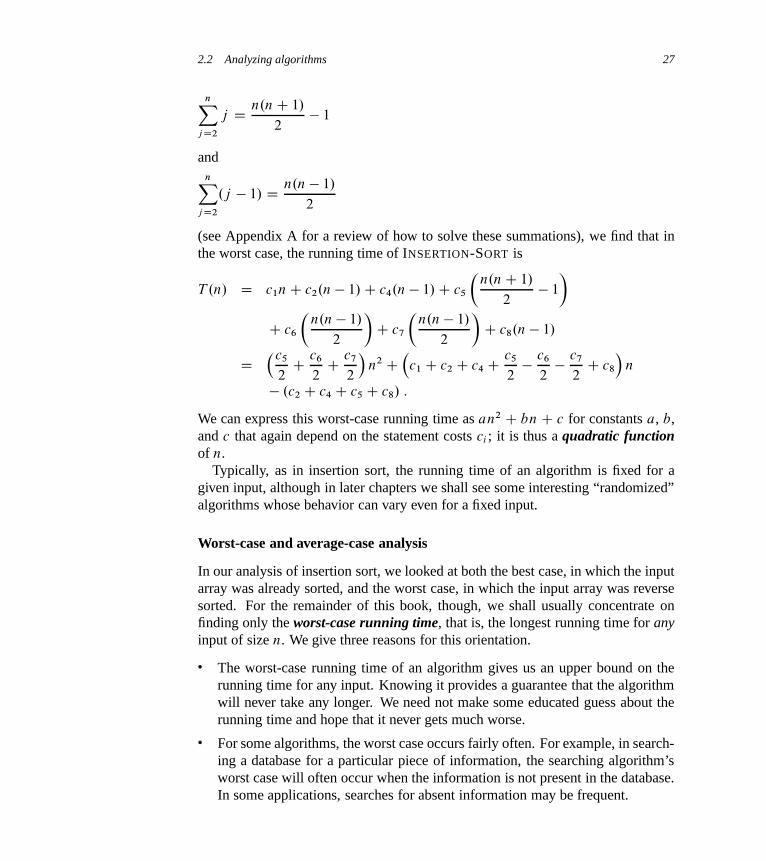
2.2 Analyzing algorithms 27
nXj D2
j D n.nC 1/
2� 1
andnX
j D2
.j � 1/ D n.n � 1/
2
(see Appendix A for a review of how to solve these summations), we find that inthe worst case, the running time of INSERTION-SORT is
T .n/ D c1nC c2.n � 1/C c4.n � 1/C c5
�n.nC 1/
2� 1
�C c6
�n.n � 1/
2
�C c7
�n.n � 1/
2
�C c8.n � 1/
D�c5
2C c6
2C c7
2
�n2 C
�c1 C c2 C c4 C
c5
2� c6
2� c7
2C c8
�n
� .c2 C c4 C c5 C c8/ :
We can express this worst-case running time as an2 C bnC c for constants a, b,and c that again depend on the statement costs ci ; it is thus a quadratic functionof n.
Typically, as in insertion sort, the running time of an algorithm is fixed for agiven input, although in later chapters we shall see some interesting “randomized”algorithms whose behavior can vary even for a fixed input.
Worst-case and average-case analysis
In our analysis of insertion sort, we looked at both the best case, in which the inputarray was already sorted, and the worst case, in which the input array was reversesorted. For the remainder of this book, though, we shall usually concentrate onfinding only the worst-case running time, that is, the longest running time for anyinput of size n. We give three reasons for this orientation.
� The worst-case running time of an algorithm gives us an upper bound on therunning time for any input. Knowing it provides a guarantee that the algorithmwill never take any longer. We need not make some educated guess about therunning time and hope that it never gets much worse.
� For some algorithms, the worst case occurs fairly often. For example, in search-ing a database for a particular piece of information, the searching algorithm’sworst case will often occur when the information is not present in the database.In some applications, searches for absent information may be frequent.

28 Chapter 2 Getting Started
� The “average case” is often roughly as bad as the worst case. Suppose that werandomly choose n numbers and apply insertion sort. How long does it take todetermine where in subarray AŒ1 : : j � 1� to insert element AŒj �? On average,half the elements in AŒ1 : : j � 1� are less than AŒj �, and half the elements aregreater. On average, therefore, we check half of the subarray AŒ1 : : j � 1�, andso tj is about j=2. The resulting average-case running time turns out to be aquadratic function of the input size, just like the worst-case running time.
In some particular cases, we shall be interested in the average-case running timeof an algorithm; we shall see the technique of probabilistic analysis applied tovarious algorithms throughout this book. The scope of average-case analysis islimited, because it may not be apparent what constitutes an “average” input fora particular problem. Often, we shall assume that all inputs of a given size areequally likely. In practice, this assumption may be violated, but we can sometimesuse a randomized algorithm, which makes random choices, to allow a probabilisticanalysis and yield an expected running time. We explore randomized algorithmsmore in Chapter 5 and in several other subsequent chapters.
Order of growth
We used some simplifying abstractions to ease our analysis of the INSERTION-SORT procedure. First, we ignored the actual cost of each statement, using theconstants ci to represent these costs. Then, we observed that even these constantsgive us more detail than we really need: we expressed the worst-case running timeas an2 C bn C c for some constants a, b, and c that depend on the statementcosts ci . We thus ignored not only the actual statement costs, but also the abstractcosts ci .
We shall now make one more simplifying abstraction: it is the rate of growth,or order of growth, of the running time that really interests us. We therefore con-sider only the leading term of a formula (e.g., an2), since the lower-order terms arerelatively insignificant for large values of n. We also ignore the leading term’s con-stant coefficient, since constant factors are less significant than the rate of growthin determining computational efficiency for large inputs. For insertion sort, whenwe ignore the lower-order terms and the leading term’s constant coefficient, we areleft with the factor of n2 from the leading term. We write that insertion sort has aworst-case running time of ‚.n2/ (pronounced “theta of n-squared”). We shall use‚-notation informally in this chapter, and we will define it precisely in Chapter 3.
We usually consider one algorithm to be more efficient than another if its worst-case running time has a lower order of growth. Due to constant factors and lower-order terms, an algorithm whose running time has a higher order of growth mighttake less time for small inputs than an algorithm whose running time has a lower

2.3 Designing algorithms 29
order of growth. But for large enough inputs, a ‚.n2/ algorithm, for example, willrun more quickly in the worst case than a ‚.n3/ algorithm.
Exercises
2.2-1Express the function n3=1000 � 100n2 � 100nC 3 in terms of ‚-notation.
2.2-2Consider sorting n numbers stored in array A by first finding the smallest elementof A and exchanging it with the element in AŒ1�. Then find the second smallestelement of A, and exchange it with AŒ2�. Continue in this manner for the first n�1
elements of A. Write pseudocode for this algorithm, which is known as selectionsort. What loop invariant does this algorithm maintain? Why does it need to runfor only the first n � 1 elements, rather than for all n elements? Give the best-caseand worst-case running times of selection sort in ‚-notation.
2.2-3Consider linear search again (see Exercise 2.1-3). How many elements of the in-put sequence need to be checked on the average, assuming that the element beingsearched for is equally likely to be any element in the array? How about in theworst case? What are the average-case and worst-case running times of linearsearch in ‚-notation? Justify your answers.
2.2-4How can we modify almost any algorithm to have a good best-case running time?
2.3 Designing algorithms
We can choose from a wide range of algorithm design techniques. For insertionsort, we used an incremental approach: having sorted the subarray AŒ1 : : j � 1�,we inserted the single element AŒj � into its proper place, yielding the sortedsubarray AŒ1 : : j �.
In this section, we examine an alternative design approach, known as “divide-and-conquer,” which we shall explore in more detail in Chapter 4. We’ll use divide-and-conquer to design a sorting algorithm whose worst-case running time is muchless than that of insertion sort. One advantage of divide-and-conquer algorithms isthat their running times are often easily determined using techniques that we willsee in Chapter 4.

30 Chapter 2 Getting Started
2.3.1 The divide-and-conquer approach
Many useful algorithms are recursive in structure: to solve a given problem, theycall themselves recursively one or more times to deal with closely related sub-problems. These algorithms typically follow a divide-and-conquer approach: theybreak the problem into several subproblems that are similar to the original prob-lem but smaller in size, solve the subproblems recursively, and then combine thesesolutions to create a solution to the original problem.
The divide-and-conquer paradigm involves three steps at each level of the recur-sion:
Divide the problem into a number of subproblems that are smaller instances of thesame problem.
Conquer the subproblems by solving them recursively. If the subproblem sizes aresmall enough, however, just solve the subproblems in a straightforward manner.
Combine the solutions to the subproblems into the solution for the original prob-lem.
The merge sort algorithm closely follows the divide-and-conquer paradigm. In-tuitively, it operates as follows.
Divide: Divide the n-element sequence to be sorted into two subsequences of n=2
elements each.
Conquer: Sort the two subsequences recursively using merge sort.
Combine: Merge the two sorted subsequences to produce the sorted answer.
The recursion “bottoms out” when the sequence to be sorted has length 1, in whichcase there is no work to be done, since every sequence of length 1 is already insorted order.
The key operation of the merge sort algorithm is the merging of two sortedsequences in the “combine” step. We merge by calling an auxiliary procedureMERGE.A; p; q; r/, where A is an array and p, q, and r are indices into the arraysuch that p � q < r . The procedure assumes that the subarrays AŒp : : q� andAŒq C 1 : : r� are in sorted order. It merges them to form a single sorted subarraythat replaces the current subarray AŒp : : r�.
Our MERGE procedure takes time ‚.n/, where n D r � p C 1 is the totalnumber of elements being merged, and it works as follows. Returning to our card-playing motif, suppose we have two piles of cards face up on a table. Each pile issorted, with the smallest cards on top. We wish to merge the two piles into a singlesorted output pile, which is to be face down on the table. Our basic step consistsof choosing the smaller of the two cards on top of the face-up piles, removing itfrom its pile (which exposes a new top card), and placing this card face down onto

2.3 Designing algorithms 31
the output pile. We repeat this step until one input pile is empty, at which timewe just take the remaining input pile and place it face down onto the output pile.Computationally, each basic step takes constant time, since we are comparing justthe two top cards. Since we perform at most n basic steps, merging takes ‚.n/
time.The following pseudocode implements the above idea, but with an additional
twist that avoids having to check whether either pile is empty in each basic step.We place on the bottom of each pile a sentinel card, which contains a special valuethat we use to simplify our code. Here, we use 1 as the sentinel value, so thatwhenever a card with1 is exposed, it cannot be the smaller card unless both pileshave their sentinel cards exposed. But once that happens, all the nonsentinel cardshave already been placed onto the output pile. Since we know in advance thatexactly r � p C 1 cards will be placed onto the output pile, we can stop once wehave performed that many basic steps.
MERGE.A; p; q; r/
1 n1 D q � p C 1
2 n2 D r � q
3 let LŒ1 : : n1 C 1� and RŒ1 : : n2 C 1� be new arrays4 for i D 1 to n1
5 LŒi� D AŒp C i � 1�
6 for j D 1 to n2
7 RŒj � D AŒq C j �
8 LŒn1 C 1� D 19 RŒn2 C 1� D 1
10 i D 1
11 j D 1
12 for k D p to r
13 if LŒi� � RŒj �
14 AŒk� D LŒi�
15 i D i C 1
16 else AŒk� D RŒj �
17 j D j C 1
In detail, the MERGE procedure works as follows. Line 1 computes the length n1
of the subarray AŒp : : q�, and line 2 computes the length n2 of the subarrayAŒq C 1 : : r�. We create arrays L and R (“left” and “right”), of lengths n1 C 1
and n2 C 1, respectively, in line 3; the extra position in each array will hold thesentinel. The for loop of lines 4–5 copies the subarray AŒp : : q� into LŒ1 : : n1�,and the for loop of lines 6–7 copies the subarray AŒq C 1 : : r� into RŒ1 : : n2�.Lines 8–9 put the sentinels at the ends of the arrays L and R. Lines 10–17, illus-
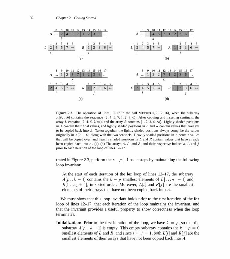
32 Chapter 2 Getting Started
A
L R1 2 3 4 1 2 3 4
i j
k
(a)
2 4 5 7 1 2 3 6
A
L R1 2 3 4 1 2 3 4
i j
k
(b)
2 4 5 7
1
2 3 61
2 4 5 7 1 2 3 6 4 5 7 1 2 3 6
A
L R
9 10 11 12 13 14 15 16
1 2 3 4 1 2 3 4
i j
k
(c)
2 4 5 7
1
2 3 61
5 7 1 2 3 62 A
L R1 2 3 4 1 2 3 4
i j
k
(d)
2 4 5 7
1
2 3 61
7 1 2 3 62 2
5∞
5∞
5∞
5∞
5∞
5∞
5∞
5∞
9 10 11 12 13 14 15 16
9 10 11 12 13 14 15 16
9 10 11 12 13 14 15 168…
17…
8…
17…
8…
17…
8…
17…
Figure 2.3 The operation of lines 10–17 in the call MERGE.A; 9; 12; 16/, when the subarrayAŒ9 : : 16� contains the sequence h2; 4; 5; 7; 1; 2; 3; 6i. After copying and inserting sentinels, thearray L contains h2; 4; 5; 7;1i, and the array R contains h1; 2; 3; 6;1i. Lightly shaded positionsin A contain their final values, and lightly shaded positions in L and R contain values that have yetto be copied back into A. Taken together, the lightly shaded positions always comprise the valuesoriginally in AŒ9 : : 16�, along with the two sentinels. Heavily shaded positions in A contain valuesthat will be copied over, and heavily shaded positions in L and R contain values that have alreadybeen copied back into A. (a)–(h) The arrays A, L, and R, and their respective indices k, i , and j
prior to each iteration of the loop of lines 12–17.
trated in Figure 2.3, perform the r�pC1 basic steps by maintaining the followingloop invariant:
At the start of each iteration of the for loop of lines 12–17, the subarrayAŒp : : k � 1� contains the k � p smallest elements of LŒ1 : : n1 C 1� andRŒ1 : : n2 C 1�, in sorted order. Moreover, LŒi� and RŒj � are the smallestelements of their arrays that have not been copied back into A.
We must show that this loop invariant holds prior to the first iteration of the forloop of lines 12–17, that each iteration of the loop maintains the invariant, andthat the invariant provides a useful property to show correctness when the loopterminates.
Initialization: Prior to the first iteration of the loop, we have k D p, so that thesubarray AŒp : : k � 1� is empty. This empty subarray contains the k � p D 0
smallest elements of L and R, and since i D j D 1, both LŒi� and RŒj � are thesmallest elements of their arrays that have not been copied back into A.
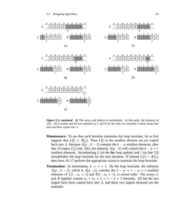
2.3 Designing algorithms 33
A
L R1 2 3 4 1 2 3 4
i j
k
(e)
2 4 5 7
1
2 3 61
1 2 3 62 2 3 A
L R1 2 3 4 1 2 3 4
i j
k
(f)
2 4 5 7
1
2 3 61
2 3 62 2 3 4
A
L R1 2 3 4 1 2 3 4
i j
k
(g)
2 4 5 7
1
2 3 61
3 62 2 3 4 5 A
L R1 2 3 4 1 2 3 4
i j
k
(h)
2 4 5 7
1
2 3 61
62 2 3 4 5
5∞
5∞
5∞
5∞
5∞
5∞
5∞
5∞
6
A
L R1 2 3 4 1 2 3 4
i j
k
(i)
2 4 5 7
1
2 3 61
72 2 3 4 5
5∞
5∞
6
9 10 11 12 13 14 15 16
9 10 11 12 13 14 15 16
9 10 11 12 13 14 15 16
9 10 11 12 13 14 15 16
9 10 11 12 13 14 15 16
8…
17…
8…
17…
8…
17…
8…
17…
8…
17…
Figure 2.3, continued (i) The arrays and indices at termination. At this point, the subarray inAŒ9 : : 16� is sorted, and the two sentinels in L and R are the only two elements in these arrays thathave not been copied into A.
Maintenance: To see that each iteration maintains the loop invariant, let us firstsuppose that LŒi� � RŒj �. Then LŒi� is the smallest element not yet copiedback into A. Because AŒp : : k � 1� contains the k � p smallest elements, afterline 14 copies LŒi� into AŒk�, the subarray AŒp : : k� will contain the k � p C 1
smallest elements. Incrementing k (in the for loop update) and i (in line 15)reestablishes the loop invariant for the next iteration. If instead LŒi� > RŒj �,then lines 16–17 perform the appropriate action to maintain the loop invariant.
Termination: At termination, k D r C 1. By the loop invariant, the subarrayAŒp : : k � 1�, which is AŒp : : r�, contains the k � p D r � p C 1 smallestelements of LŒ1 : : n1 C 1� and RŒ1 : : n2 C 1�, in sorted order. The arrays L
and R together contain n1 C n2 C 2 D r � p C 3 elements. All but the twolargest have been copied back into A, and these two largest elements are thesentinels.
34 Chapter 2 Getting Started
To see that the MERGE procedure runs in ‚.n/ time, where n D r � p C 1,observe that each of lines 1–3 and 8–11 takes constant time, the for loops oflines 4–7 take ‚.n1 C n2/ D ‚.n/ time,7 and there are n iterations of the forloop of lines 12–17, each of which takes constant time.
We can now use the MERGE procedure as a subroutine in the merge sort al-gorithm. The procedure MERGE-SORT.A; p; r/ sorts the elements in the subar-ray AŒp : : r�. If p � r , the subarray has at most one element and is thereforealready sorted. Otherwise, the divide step simply computes an index q that par-titions AŒp : : r� into two subarrays: AŒp : : q�, containing dn=2e elements, andAŒq C 1 : : r�, containing bn=2c elements.8
MERGE-SORT.A; p; r/
1 if p < r
2 q D b.p C r/=2c3 MERGE-SORT.A; p; q/
4 MERGE-SORT.A; q C 1; r/
5 MERGE.A; p; q; r/
To sort the entire sequence A D hAŒ1�; AŒ2�; : : : ; AŒn�i, we make the initial callMERGE-SORT.A; 1; A: length/, where once again A: length D n. Figure 2.4 il-lustrates the operation of the procedure bottom-up when n is a power of 2. Thealgorithm consists of merging pairs of 1-item sequences to form sorted sequencesof length 2, merging pairs of sequences of length 2 to form sorted sequences oflength 4, and so on, until two sequences of length n=2 are merged to form the finalsorted sequence of length n.
2.3.2 Analyzing divide-and-conquer algorithms
When an algorithm contains a recursive call to itself, we can often describe itsrunning time by a recurrence equation or recurrence, which describes the overallrunning time on a problem of size n in terms of the running time on smaller inputs.We can then use mathematical tools to solve the recurrence and provide bounds onthe performance of the algorithm.
7We shall see in Chapter 3 how to formally interpret equations containing ‚-notation.
8The expression dxe denotes the least integer greater than or equal to x, and bxc denotes the greatestinteger less than or equal to x. These notations are defined in Chapter 3. The easiest way to verifythat setting q to b.p C r/=2c yields subarrays AŒp : : q� and AŒq C 1 : : r� of sizes dn=2e and bn=2c,respectively, is to examine the four cases that arise depending on whether each of p and r is odd oreven.

2.3 Designing algorithms 35
5 2 4 7 1 3 2 6
2 5 4 7 1 3 2 6
2 4 5 7 1 2 3 6
1 2 2 3 4 5 6 7
merge
merge
merge
sorted sequence
initial sequence
mergemergemergemerge
Figure 2.4 The operation of merge sort on the array A D h5; 2; 4; 7; 1; 3; 2; 6i. The lengths of thesorted sequences being merged increase as the algorithm progresses from bottom to top.
A recurrence for the running time of a divide-and-conquer algorithm falls outfrom the three steps of the basic paradigm. As before, we let T .n/ be the runningtime on a problem of size n. If the problem size is small enough, say n � c
for some constant c, the straightforward solution takes constant time, which wewrite as ‚.1/. Suppose that our division of the problem yields a subproblems,each of which is 1=b the size of the original. (For merge sort, both a and b are 2,but we shall see many divide-and-conquer algorithms in which a ¤ b.) It takestime T .n=b/ to solve one subproblem of size n=b, and so it takes time aT .n=b/
to solve a of them. If we take D.n/ time to divide the problem into subproblemsand C.n/ time to combine the solutions to the subproblems into the solution to theoriginal problem, we get the recurrence
T .n/ D(
‚.1/ if n � c ;
aT .n=b/CD.n/C C.n/ otherwise :
In Chapter 4, we shall see how to solve common recurrences of this form.
Analysis of merge sort
Although the pseudocode for MERGE-SORT works correctly when the number ofelements is not even, our recurrence-based analysis is simplified if we assume that

36 Chapter 2 Getting Started
the original problem size is a power of 2. Each divide step then yields two subse-quences of size exactly n=2. In Chapter 4, we shall see that this assumption doesnot affect the order of growth of the solution to the recurrence.
We reason as follows to set up the recurrence for T .n/, the worst-case runningtime of merge sort on n numbers. Merge sort on just one element takes constanttime. When we have n > 1 elements, we break down the running time as follows.
Divide: The divide step just computes the middle of the subarray, which takesconstant time. Thus, D.n/ D ‚.1/.
Conquer: We recursively solve two subproblems, each of size n=2, which con-tributes 2T .n=2/ to the running time.
Combine: We have already noted that the MERGE procedure on an n-elementsubarray takes time ‚.n/, and so C.n/ D ‚.n/.
When we add the functions D.n/ and C.n/ for the merge sort analysis, we areadding a function that is ‚.n/ and a function that is ‚.1/. This sum is a linearfunction of n, that is, ‚.n/. Adding it to the 2T .n=2/ term from the “conquer”step gives the recurrence for the worst-case running time T .n/ of merge sort:
T .n/ D(
‚.1/ if n D 1 ;
2T .n=2/C‚.n/ if n > 1 :(2.1)
In Chapter 4, we shall see the “master theorem,” which we can use to showthat T .n/ is ‚.n lg n/, where lg n stands for log2 n. Because the logarithm func-tion grows more slowly than any linear function, for large enough inputs, mergesort, with its ‚.n lg n/ running time, outperforms insertion sort, whose runningtime is ‚.n2/, in the worst case.
We do not need the master theorem to intuitively understand why the solution tothe recurrence (2.1) is T .n/ D ‚.n lg n/. Let us rewrite recurrence (2.1) as
T .n/ D(
c if n D 1 ;
2T .n=2/C cn if n > 1 ;(2.2)
where the constant c represents the time required to solve problems of size 1 aswell as the time per array element of the divide and combine steps.9
9It is unlikely that the same constant exactly represents both the time to solve problems of size 1
and the time per array element of the divide and combine steps. We can get around this problem byletting c be the larger of these times and understanding that our recurrence gives an upper bound onthe running time, or by letting c be the lesser of these times and understanding that our recurrencegives a lower bound on the running time. Both bounds are on the order of n lg n and, taken together,give a ‚.n lg n/ running time.
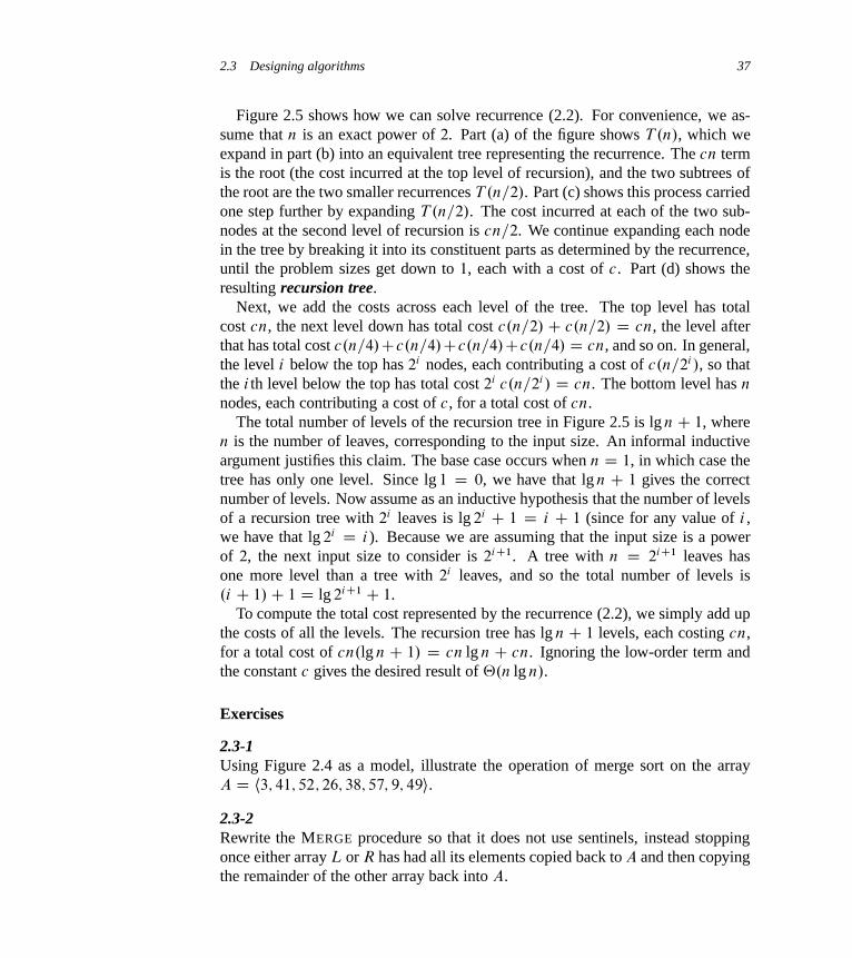
2.3 Designing algorithms 37
Figure 2.5 shows how we can solve recurrence (2.2). For convenience, we as-sume that n is an exact power of 2. Part (a) of the figure shows T .n/, which weexpand in part (b) into an equivalent tree representing the recurrence. The cn termis the root (the cost incurred at the top level of recursion), and the two subtrees ofthe root are the two smaller recurrences T .n=2/. Part (c) shows this process carriedone step further by expanding T .n=2/. The cost incurred at each of the two sub-nodes at the second level of recursion is cn=2. We continue expanding each nodein the tree by breaking it into its constituent parts as determined by the recurrence,until the problem sizes get down to 1, each with a cost of c. Part (d) shows theresulting recursion tree.
Next, we add the costs across each level of the tree. The top level has totalcost cn, the next level down has total cost c.n=2/ C c.n=2/ D cn, the level afterthat has total cost c.n=4/Cc.n=4/Cc.n=4/Cc.n=4/ D cn, and so on. In general,the level i below the top has 2i nodes, each contributing a cost of c.n=2i/, so thatthe i th level below the top has total cost 2i c.n=2i/ D cn. The bottom level has n
nodes, each contributing a cost of c, for a total cost of cn.The total number of levels of the recursion tree in Figure 2.5 is lg nC 1, where
n is the number of leaves, corresponding to the input size. An informal inductiveargument justifies this claim. The base case occurs when n D 1, in which case thetree has only one level. Since lg 1 D 0, we have that lg n C 1 gives the correctnumber of levels. Now assume as an inductive hypothesis that the number of levelsof a recursion tree with 2i leaves is lg 2i C 1 D i C 1 (since for any value of i ,we have that lg 2i D i). Because we are assuming that the input size is a powerof 2, the next input size to consider is 2iC1. A tree with n D 2iC1 leaves hasone more level than a tree with 2i leaves, and so the total number of levels is.i C 1/C 1 D lg 2iC1 C 1.
To compute the total cost represented by the recurrence (2.2), we simply add upthe costs of all the levels. The recursion tree has lg nC 1 levels, each costing cn,for a total cost of cn.lg n C 1/ D cn lg n C cn. Ignoring the low-order term andthe constant c gives the desired result of ‚.n lg n/.
Exercises
2.3-1Using Figure 2.4 as a model, illustrate the operation of merge sort on the arrayA D h3; 41; 52; 26; 38; 57; 9; 49i.2.3-2Rewrite the MERGE procedure so that it does not use sentinels, instead stoppingonce either array L or R has had all its elements copied back to A and then copyingthe remainder of the other array back into A.

38 Chapter 2 Getting Started
cn
cn
…
Total: cn lg n + cn
cn
lg n
cn
n
c c c c c c c
…
(d)
(c)
cn
T(n/2) T(n/2)
(b)
T(n)
(a)
cn
cn/2
T(n/4) T(n/4)
cn/2
T(n/4) T(n/4)
cn
cn/2
cn/4 cn/4
cn/2
cn/4 cn/4
Figure 2.5 How to construct a recursion tree for the recurrence T .n/ D 2T .n=2/ C cn.Part (a) shows T .n/, which progressively expands in (b)–(d) to form the recursion tree. The fullyexpanded tree in part (d) has lg n C 1 levels (i.e., it has height lg n, as indicated), and each levelcontributes a total cost of cn. The total cost, therefore, is cn lg nC cn, which is ‚.n lg n/.

Problems for Chapter 2 39
2.3-3Use mathematical induction to show that when n is an exact power of 2, the solu-tion of the recurrence
T .n/ D(
2 if n D 2 ;
2T .n=2/C n if n D 2k , for k > 1
is T .n/ D n lg n.
2.3-4We can express insertion sort as a recursive procedure as follows. In order to sortAŒ1 : : n�, we recursively sort AŒ1 : : n�1� and then insert AŒn� into the sorted arrayAŒ1 : : n � 1�. Write a recurrence for the running time of this recursive version ofinsertion sort.
2.3-5Referring back to the searching problem (see Exercise 2.1-3), observe that if thesequence A is sorted, we can check the midpoint of the sequence against � andeliminate half of the sequence from further consideration. The binary search al-gorithm repeats this procedure, halving the size of the remaining portion of thesequence each time. Write pseudocode, either iterative or recursive, for binarysearch. Argue that the worst-case running time of binary search is ‚.lg n/.
2.3-6Observe that the while loop of lines 5–7 of the INSERTION-SORT procedure inSection 2.1 uses a linear search to scan (backward) through the sorted subarrayAŒ1 : : j � 1�. Can we use a binary search (see Exercise 2.3-5) instead to improvethe overall worst-case running time of insertion sort to ‚.n lg n/?
2.3-7 ?
Describe a ‚.n lg n/-time algorithm that, given a set S of n integers and anotherinteger x, determines whether or not there exist two elements in S whose sum isexactly x.
Problems
2-1 Insertion sort on small arrays in merge sortAlthough merge sort runs in ‚.n lg n/ worst-case time and insertion sort runsin ‚.n2/ worst-case time, the constant factors in insertion sort can make it fasterin practice for small problem sizes on many machines. Thus, it makes sense tocoarsen the leaves of the recursion by using insertion sort within merge sort when

40 Chapter 2 Getting Started
subproblems become sufficiently small. Consider a modification to merge sort inwhich n=k sublists of length k are sorted using insertion sort and then mergedusing the standard merging mechanism, where k is a value to be determined.
a. Show that insertion sort can sort the n=k sublists, each of length k, in ‚.nk/
worst-case time.
b. Show how to merge the sublists in ‚.n lg.n=k// worst-case time.
c. Given that the modified algorithm runs in ‚.nkC n lg.n=k// worst-case time,what is the largest value of k as a function of n for which the modified algorithmhas the same running time as standard merge sort, in terms of ‚-notation?
d. How should we choose k in practice?
2-2 Correctness of bubblesortBubblesort is a popular, but inefficient, sorting algorithm. It works by repeatedlyswapping adjacent elements that are out of order.
BUBBLESORT.A/
1 for i D 1 to A: length � 1
2 for j D A: length downto i C 1
3 if AŒj � < AŒj � 1�
4 exchange AŒj � with AŒj � 1�
a. Let A0 denote the output of BUBBLESORT.A/. To prove that BUBBLESORT iscorrect, we need to prove that it terminates and that
A0Œ1� � A0Œ2� � � � � � A0Œn� ; (2.3)
where n D A: length. In order to show that BUBBLESORT actually sorts, whatelse do we need to prove?
The next two parts will prove inequality (2.3).
b. State precisely a loop invariant for the for loop in lines 2–4, and prove that thisloop invariant holds. Your proof should use the structure of the loop invariantproof presented in this chapter.
c. Using the termination condition of the loop invariant proved in part (b), statea loop invariant for the for loop in lines 1–4 that will allow you to prove in-equality (2.3). Your proof should use the structure of the loop invariant proofpresented in this chapter.
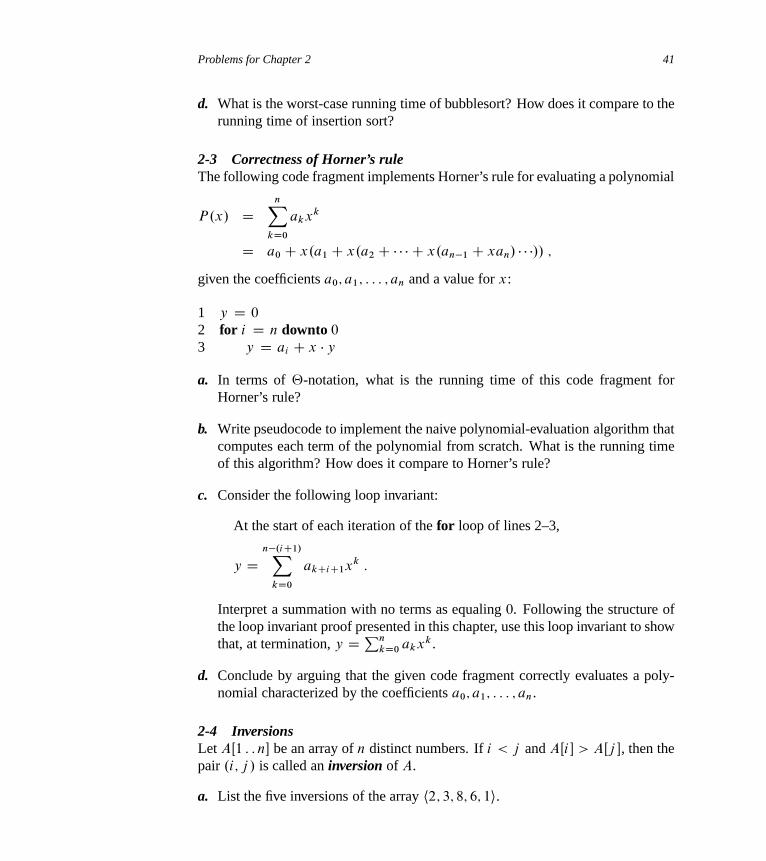
Problems for Chapter 2 41
d. What is the worst-case running time of bubblesort? How does it compare to therunning time of insertion sort?
2-3 Correctness of Horner’s ruleThe following code fragment implements Horner’s rule for evaluating a polynomial
P.x/ DnX
kD0
akxk
D a0 C x.a1 C x.a2 C � � � C x.an�1 C xan/ � � �// ;
given the coefficients a0; a1; : : : ; an and a value for x:
1 y D 0
2 for i D n downto 0
3 y D ai C x � y
a. In terms of ‚-notation, what is the running time of this code fragment forHorner’s rule?
b. Write pseudocode to implement the naive polynomial-evaluation algorithm thatcomputes each term of the polynomial from scratch. What is the running timeof this algorithm? How does it compare to Horner’s rule?
c. Consider the following loop invariant:
At the start of each iteration of the for loop of lines 2–3,
y Dn�.iC1/X
kD0
akCiC1xk :
Interpret a summation with no terms as equaling 0. Following the structure ofthe loop invariant proof presented in this chapter, use this loop invariant to showthat, at termination, y DPn
kD0 akxk.
d. Conclude by arguing that the given code fragment correctly evaluates a poly-nomial characterized by the coefficients a0; a1; : : : ; an.
2-4 InversionsLet AŒ1 : : n� be an array of n distinct numbers. If i < j and AŒi� > AŒj �, then thepair .i; j / is called an inversion of A.
a. List the five inversions of the array h2; 3; 8; 6; 1i.

42 Chapter 2 Getting Started
b. What array with elements from the set f1; 2; : : : ; ng has the most inversions?How many does it have?
c. What is the relationship between the running time of insertion sort and thenumber of inversions in the input array? Justify your answer.
d. Give an algorithm that determines the number of inversions in any permutationon n elements in ‚.n lg n/ worst-case time. (Hint: Modify merge sort.)
Chapter notes
In 1968, Knuth published the first of three volumes with the general title The Art ofComputer Programming [209, 210, 211]. The first volume ushered in the modernstudy of computer algorithms with a focus on the analysis of running time, and thefull series remains an engaging and worthwhile reference for many of the topicspresented here. According to Knuth, the word “algorithm” is derived from thename “al-Khowârizmı̂,” a ninth-century Persian mathematician.
Aho, Hopcroft, and Ullman [5] advocated the asymptotic analysis of algo-rithms—using notations that Chapter 3 introduces, including ‚-notation—as ameans of comparing relative performance. They also popularized the use of re-currence relations to describe the running times of recursive algorithms.
Knuth [211] provides an encyclopedic treatment of many sorting algorithms. Hiscomparison of sorting algorithms (page 381) includes exact step-counting analyses,like the one we performed here for insertion sort. Knuth’s discussion of insertionsort encompasses several variations of the algorithm. The most important of theseis Shell’s sort, introduced by D. L. Shell, which uses insertion sort on periodicsubsequences of the input to produce a faster sorting algorithm.
Merge sort is also described by Knuth. He mentions that a mechanical colla-tor capable of merging two decks of punched cards in a single pass was inventedin 1938. J. von Neumann, one of the pioneers of computer science, apparentlywrote a program for merge sort on the EDVAC computer in 1945.
The early history of proving programs correct is described by Gries [153], whocredits P. Naur with the first article in this field. Gries attributes loop invariants toR. W. Floyd. The textbook by Mitchell [256] describes more recent progress inproving programs correct.
3 Growth of Functions
The order of growth of the running time of an algorithm, defined in Chapter 2,gives a simple characterization of the algorithm’s efficiency and also allows us tocompare the relative performance of alternative algorithms. Once the input size n
becomes large enough, merge sort, with its ‚.n lg n/ worst-case running time,beats insertion sort, whose worst-case running time is ‚.n2/. Although we cansometimes determine the exact running time of an algorithm, as we did for insertionsort in Chapter 2, the extra precision is not usually worth the effort of computingit. For large enough inputs, the multiplicative constants and lower-order terms ofan exact running time are dominated by the effects of the input size itself.
When we look at input sizes large enough to make only the order of growth ofthe running time relevant, we are studying the asymptotic efficiency of algorithms.That is, we are concerned with how the running time of an algorithm increases withthe size of the input in the limit, as the size of the input increases without bound.Usually, an algorithm that is asymptotically more efficient will be the best choicefor all but very small inputs.
This chapter gives several standard methods for simplifying the asymptotic anal-ysis of algorithms. The next section begins by defining several types of “asymp-totic notation,” of which we have already seen an example in ‚-notation. We thenpresent several notational conventions used throughout this book, and finally wereview the behavior of functions that commonly arise in the analysis of algorithms.
3.1 Asymptotic notation
The notations we use to describe the asymptotic running time of an algorithmare defined in terms of functions whose domains are the set of natural numbersN D f0; 1; 2; : : :g. Such notations are convenient for describing the worst-caserunning-time function T .n/, which usually is defined only on integer input sizes.We sometimes find it convenient, however, to abuse asymptotic notation in a va-

44 Chapter 3 Growth of Functions
riety of ways. For example, we might extend the notation to the domain of realnumbers or, alternatively, restrict it to a subset of the natural numbers. We shouldmake sure, however, to understand the precise meaning of the notation so that whenwe abuse, we do not misuse it. This section defines the basic asymptotic notationsand also introduces some common abuses.
Asymptotic notation, functions, and running times
We will use asymptotic notation primarily to describe the running times of algo-rithms, as when we wrote that insertion sort’s worst-case running time is ‚.n2/.Asymptotic notation actually applies to functions, however. Recall that we charac-terized insertion sort’s worst-case running time as an2CbnCc, for some constantsa, b, and c. By writing that insertion sort’s running time is ‚.n2/, we abstractedaway some details of this function. Because asymptotic notation applies to func-tions, what we were writing as ‚.n2/ was the function an2 C bn C c, which inthat case happened to characterize the worst-case running time of insertion sort.
In this book, the functions to which we apply asymptotic notation will usuallycharacterize the running times of algorithms. But asymptotic notation can apply tofunctions that characterize some other aspect of algorithms (the amount of spacethey use, for example), or even to functions that have nothing whatsoever to dowith algorithms.
Even when we use asymptotic notation to apply to the running time of an al-gorithm, we need to understand which running time we mean. Sometimes we areinterested in the worst-case running time. Often, however, we wish to characterizethe running time no matter what the input. In other words, we often wish to makea blanket statement that covers all inputs, not just the worst case. We shall seeasymptotic notations that are well suited to characterizing running times no matterwhat the input.
‚-notation
In Chapter 2, we found that the worst-case running time of insertion sort isT .n/ D ‚.n2/. Let us define what this notation means. For a given function g.n/,we denote by ‚.g.n// the set of functions
‚.g.n// D ff .n/ W there exist positive constants c1, c2, and n0 such that0 � c1g.n/ � f .n/ � c2g.n/ for all n � n0g :1
1Within set notation, a colon means “such that.”
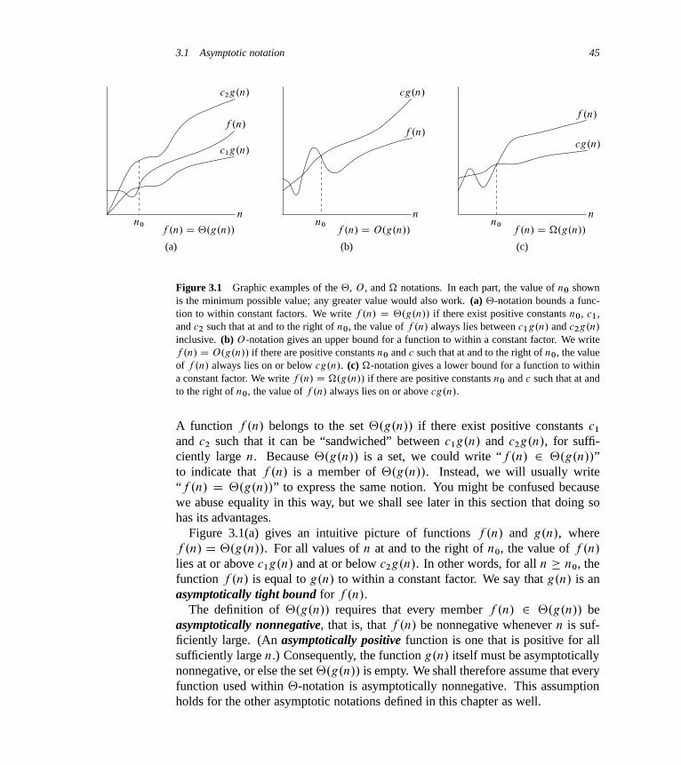
3.1 Asymptotic notation 45
(b) (c)(a)
nnnn0n0n0
f .n/ D ‚.g.n// f .n/ D O.g.n// f .n/ D �.g.n//
f .n/
f .n/f .n/
cg.n/
cg.n/
c1g.n/
c2g.n/
Figure 3.1 Graphic examples of the ‚, O , and � notations. In each part, the value of n0 shownis the minimum possible value; any greater value would also work. (a) ‚-notation bounds a func-tion to within constant factors. We write f .n/ D ‚.g.n// if there exist positive constants n0, c1,and c2 such that at and to the right of n0, the value of f .n/ always lies between c1g.n/ and c2g.n/
inclusive. (b) O-notation gives an upper bound for a function to within a constant factor. We writef .n/ D O.g.n// if there are positive constants n0 and c such that at and to the right of n0, the valueof f .n/ always lies on or below cg.n/. (c) �-notation gives a lower bound for a function to withina constant factor. We write f .n/ D �.g.n// if there are positive constants n0 and c such that at andto the right of n0, the value of f .n/ always lies on or above cg.n/.
A function f .n/ belongs to the set ‚.g.n// if there exist positive constants c1
and c2 such that it can be “sandwiched” between c1g.n/ and c2g.n/, for suffi-ciently large n. Because ‚.g.n// is a set, we could write “f .n/ 2 ‚.g.n//”to indicate that f .n/ is a member of ‚.g.n//. Instead, we will usually write“f .n/ D ‚.g.n//” to express the same notion. You might be confused becausewe abuse equality in this way, but we shall see later in this section that doing sohas its advantages.
Figure 3.1(a) gives an intuitive picture of functions f .n/ and g.n/, wheref .n/ D ‚.g.n//. For all values of n at and to the right of n0, the value of f .n/
lies at or above c1g.n/ and at or below c2g.n/. In other words, for all n � n0, thefunction f .n/ is equal to g.n/ to within a constant factor. We say that g.n/ is anasymptotically tight bound for f .n/.
The definition of ‚.g.n// requires that every member f .n/ 2 ‚.g.n// beasymptotically nonnegative, that is, that f .n/ be nonnegative whenever n is suf-ficiently large. (An asymptotically positive function is one that is positive for allsufficiently large n.) Consequently, the function g.n/ itself must be asymptoticallynonnegative, or else the set ‚.g.n// is empty. We shall therefore assume that everyfunction used within ‚-notation is asymptotically nonnegative. This assumptionholds for the other asymptotic notations defined in this chapter as well.
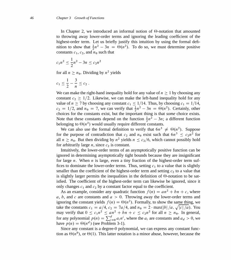
46 Chapter 3 Growth of Functions
In Chapter 2, we introduced an informal notion of ‚-notation that amountedto throwing away lower-order terms and ignoring the leading coefficient of thehighest-order term. Let us briefly justify this intuition by using the formal defi-nition to show that 1
2n2 � 3n D ‚.n2/. To do so, we must determine positive
constants c1, c2, and n0 such that
c1n2 � 1
2n2 � 3n � c2n2
for all n � n0. Dividing by n2 yields
c1 �1
2� 3
n� c2 :
We can make the right-hand inequality hold for any value of n � 1 by choosing anyconstant c2 � 1=2. Likewise, we can make the left-hand inequality hold for anyvalue of n � 7 by choosing any constant c1 � 1=14. Thus, by choosing c1 D 1=14,c2 D 1=2, and n0 D 7, we can verify that 1
2n2 � 3n D ‚.n2/. Certainly, other
choices for the constants exist, but the important thing is that some choice exists.Note that these constants depend on the function 1
2n2 � 3n; a different function
belonging to ‚.n2/ would usually require different constants.We can also use the formal definition to verify that 6n3 ¤ ‚.n2/. Suppose
for the purpose of contradiction that c2 and n0 exist such that 6n3 � c2n2 forall n � n0. But then dividing by n2 yields n � c2=6, which cannot possibly holdfor arbitrarily large n, since c2 is constant.
Intuitively, the lower-order terms of an asymptotically positive function can beignored in determining asymptotically tight bounds because they are insignificantfor large n. When n is large, even a tiny fraction of the highest-order term suf-fices to dominate the lower-order terms. Thus, setting c1 to a value that is slightlysmaller than the coefficient of the highest-order term and setting c2 to a value thatis slightly larger permits the inequalities in the definition of ‚-notation to be sat-isfied. The coefficient of the highest-order term can likewise be ignored, since itonly changes c1 and c2 by a constant factor equal to the coefficient.
As an example, consider any quadratic function f .n/ D an2 C bnC c, wherea, b, and c are constants and a > 0. Throwing away the lower-order terms andignoring the constant yields f .n/ D ‚.n2/. Formally, to show the same thing, wetake the constants c1 D a=4, c2 D 7a=4, and n0 D 2 � max.jbj =a;
pjcj =a/. You
may verify that 0 � c1n2 � an2 C bn C c � c2n2 for all n � n0. In general,for any polynomial p.n/ DPd
iD0 aini , where the ai are constants and ad > 0, we
have p.n/ D ‚.nd / (see Problem 3-1).Since any constant is a degree-0 polynomial, we can express any constant func-
tion as ‚.n0/, or ‚.1/. This latter notation is a minor abuse, however, because the
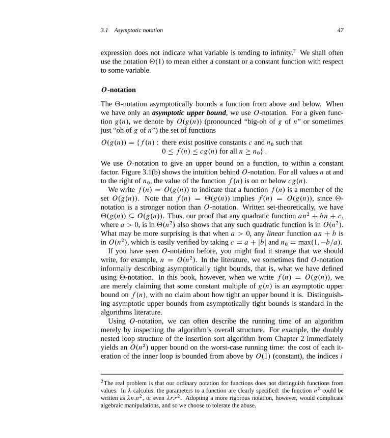
3.1 Asymptotic notation 47
expression does not indicate what variable is tending to infinity.2 We shall oftenuse the notation ‚.1/ to mean either a constant or a constant function with respectto some variable.
O-notation
The ‚-notation asymptotically bounds a function from above and below. Whenwe have only an asymptotic upper bound, we use O-notation. For a given func-tion g.n/, we denote by O.g.n// (pronounced “big-oh of g of n” or sometimesjust “oh of g of n”) the set of functions
O.g.n// D ff .n/ W there exist positive constants c and n0 such that0 � f .n/ � cg.n/ for all n � n0g :
We use O-notation to give an upper bound on a function, to within a constantfactor. Figure 3.1(b) shows the intuition behind O-notation. For all values n at andto the right of n0, the value of the function f .n/ is on or below cg.n/.
We write f .n/ D O.g.n// to indicate that a function f .n/ is a member of theset O.g.n//. Note that f .n/ D ‚.g.n// implies f .n/ D O.g.n//, since ‚-notation is a stronger notion than O-notation. Written set-theoretically, we have‚.g.n// � O.g.n//. Thus, our proof that any quadratic function an2 C bnC c,where a > 0, is in ‚.n2/ also shows that any such quadratic function is in O.n2/.What may be more surprising is that when a > 0, any linear function an C b isin O.n2/, which is easily verified by taking c D aC jbj and n0 D max.1;�b=a/.
If you have seen O-notation before, you might find it strange that we shouldwrite, for example, n D O.n2/. In the literature, we sometimes find O-notationinformally describing asymptotically tight bounds, that is, what we have definedusing ‚-notation. In this book, however, when we write f .n/ D O.g.n//, weare merely claiming that some constant multiple of g.n/ is an asymptotic upperbound on f .n/, with no claim about how tight an upper bound it is. Distinguish-ing asymptotic upper bounds from asymptotically tight bounds is standard in thealgorithms literature.
Using O-notation, we can often describe the running time of an algorithmmerely by inspecting the algorithm’s overall structure. For example, the doublynested loop structure of the insertion sort algorithm from Chapter 2 immediatelyyields an O.n2/ upper bound on the worst-case running time: the cost of each it-eration of the inner loop is bounded from above by O.1/ (constant), the indices i
2The real problem is that our ordinary notation for functions does not distinguish functions fromvalues. In �-calculus, the parameters to a function are clearly specified: the function n2 could bewritten as �n:n2, or even �r:r2. Adopting a more rigorous notation, however, would complicatealgebraic manipulations, and so we choose to tolerate the abuse.
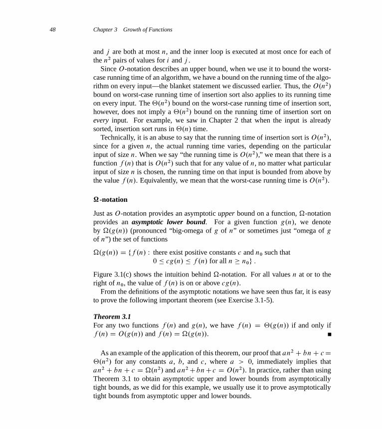
48 Chapter 3 Growth of Functions
and j are both at most n, and the inner loop is executed at most once for each ofthe n2 pairs of values for i and j .
Since O-notation describes an upper bound, when we use it to bound the worst-case running time of an algorithm, we have a bound on the running time of the algo-rithm on every input—the blanket statement we discussed earlier. Thus, the O.n2/
bound on worst-case running time of insertion sort also applies to its running timeon every input. The ‚.n2/ bound on the worst-case running time of insertion sort,however, does not imply a ‚.n2/ bound on the running time of insertion sort onevery input. For example, we saw in Chapter 2 that when the input is alreadysorted, insertion sort runs in ‚.n/ time.
Technically, it is an abuse to say that the running time of insertion sort is O.n2/,since for a given n, the actual running time varies, depending on the particularinput of size n. When we say “the running time is O.n2/,” we mean that there is afunction f .n/ that is O.n2/ such that for any value of n, no matter what particularinput of size n is chosen, the running time on that input is bounded from above bythe value f .n/. Equivalently, we mean that the worst-case running time is O.n2/.
�-notation
Just as O-notation provides an asymptotic upper bound on a function, �-notationprovides an asymptotic lower bound. For a given function g.n/, we denoteby �.g.n// (pronounced “big-omega of g of n” or sometimes just “omega of g
of n”) the set of functions
�.g.n// D ff .n/ W there exist positive constants c and n0 such that0 � cg.n/ � f .n/ for all n � n0g :
Figure 3.1(c) shows the intuition behind �-notation. For all values n at or to theright of n0, the value of f .n/ is on or above cg.n/.
From the definitions of the asymptotic notations we have seen thus far, it is easyto prove the following important theorem (see Exercise 3.1-5).
Theorem 3.1For any two functions f .n/ and g.n/, we have f .n/ D ‚.g.n// if and only iff .n/ D O.g.n// and f .n/ D �.g.n//.
As an example of the application of this theorem, our proof that an2 C bnC cD‚.n2/ for any constants a, b, and c, where a > 0, immediately implies thatan2 C bnC c D �.n2/ and an2CbnCc D O.n2/. In practice, rather than usingTheorem 3.1 to obtain asymptotic upper and lower bounds from asymptoticallytight bounds, as we did for this example, we usually use it to prove asymptoticallytight bounds from asymptotic upper and lower bounds.

3.1 Asymptotic notation 49
When we say that the running time (no modifier) of an algorithm is �.g.n//,we mean that no matter what particular input of size n is chosen for each valueof n, the running time on that input is at least a constant times g.n/, for sufficientlylarge n. Equivalently, we are giving a lower bound on the best-case running timeof an algorithm. For example, the best-case running time of insertion sort is �.n/,which implies that the running time of insertion sort is �.n/.
The running time of insertion sort therefore belongs to both �.n/ and O.n2/,since it falls anywhere between a linear function of n and a quadratic function of n.Moreover, these bounds are asymptotically as tight as possible: for instance, therunning time of insertion sort is not �.n2/, since there exists an input for whichinsertion sort runs in ‚.n/ time (e.g., when the input is already sorted). It is notcontradictory, however, to say that the worst-case running time of insertion sortis �.n2/, since there exists an input that causes the algorithm to take �.n2/ time.
Asymptotic notation in equations and inequalities
We have already seen how asymptotic notation can be used within mathematicalformulas. For example, in introducing O-notation, we wrote “n D O.n2/.” Wemight also write 2n2C3nC1 D 2n2C‚.n/. How do we interpret such formulas?
When the asymptotic notation stands alone (that is, not within a larger formula)on the right-hand side of an equation (or inequality), as in n D O.n2/, we havealready defined the equal sign to mean set membership: n 2 O.n2/. In general,however, when asymptotic notation appears in a formula, we interpret it as stand-ing for some anonymous function that we do not care to name. For example, theformula 2n2 C 3nC 1 D 2n2 C ‚.n/ means that 2n2 C 3n C 1 D 2n2 C f .n/,where f .n/ is some function in the set ‚.n/. In this case, we let f .n/ D 3nC 1,which indeed is in ‚.n/.
Using asymptotic notation in this manner can help eliminate inessential detailand clutter in an equation. For example, in Chapter 2 we expressed the worst-caserunning time of merge sort as the recurrence
T .n/ D 2T .n=2/C‚.n/ :
If we are interested only in the asymptotic behavior of T .n/, there is no point inspecifying all the lower-order terms exactly; they are all understood to be includedin the anonymous function denoted by the term ‚.n/.
The number of anonymous functions in an expression is understood to be equalto the number of times the asymptotic notation appears. For example, in the ex-pression
nXiD1
O.i/ ;
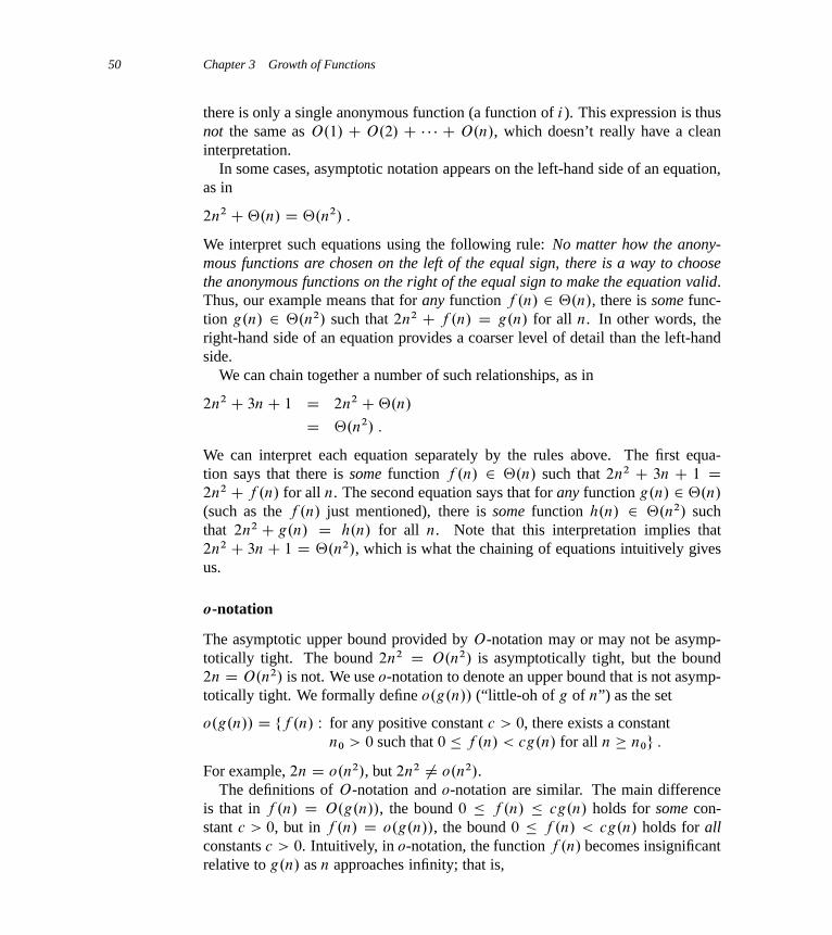
50 Chapter 3 Growth of Functions
there is only a single anonymous function (a function of i). This expression is thusnot the same as O.1/ C O.2/ C � � � C O.n/, which doesn’t really have a cleaninterpretation.
In some cases, asymptotic notation appears on the left-hand side of an equation,as in
2n2 C‚.n/ D ‚.n2/ :
We interpret such equations using the following rule: No matter how the anony-mous functions are chosen on the left of the equal sign, there is a way to choosethe anonymous functions on the right of the equal sign to make the equation valid.Thus, our example means that for any function f .n/ 2 ‚.n/, there is some func-tion g.n/ 2 ‚.n2/ such that 2n2 C f .n/ D g.n/ for all n. In other words, theright-hand side of an equation provides a coarser level of detail than the left-handside.
We can chain together a number of such relationships, as in
2n2 C 3nC 1 D 2n2 C‚.n/
D ‚.n2/ :
We can interpret each equation separately by the rules above. The first equa-tion says that there is some function f .n/ 2 ‚.n/ such that 2n2 C 3n C 1 D2n2 C f .n/ for all n. The second equation says that for any function g.n/ 2 ‚.n/
(such as the f .n/ just mentioned), there is some function h.n/ 2 ‚.n2/ suchthat 2n2 C g.n/ D h.n/ for all n. Note that this interpretation implies that2n2 C 3nC 1 D ‚.n2/, which is what the chaining of equations intuitively givesus.
o-notation
The asymptotic upper bound provided by O-notation may or may not be asymp-totically tight. The bound 2n2 D O.n2/ is asymptotically tight, but the bound2n D O.n2/ is not. We use o-notation to denote an upper bound that is not asymp-totically tight. We formally define o.g.n// (“little-oh of g of n”) as the set
o.g.n// D ff .n/ W for any positive constant c > 0, there exists a constantn0 > 0 such that 0 � f .n/ < cg.n/ for all n � n0g :
For example, 2n D o.n2/, but 2n2 ¤ o.n2/.The definitions of O-notation and o-notation are similar. The main difference
is that in f .n/ D O.g.n//, the bound 0 � f .n/ � cg.n/ holds for some con-stant c > 0, but in f .n/ D o.g.n//, the bound 0 � f .n/ < cg.n/ holds for allconstants c > 0. Intuitively, in o-notation, the function f .n/ becomes insignificantrelative to g.n/ as n approaches infinity; that is,
3.1 Asymptotic notation 51
limn!1
f .n/
g.n/D 0 : (3.1)
Some authors use this limit as a definition of the o-notation; the definition in thisbook also restricts the anonymous functions to be asymptotically nonnegative.
!-notation
By analogy, !-notation is to �-notation as o-notation is to O-notation. We use!-notation to denote a lower bound that is not asymptotically tight. One way todefine it is by
f .n/ 2 !.g.n// if and only if g.n/ 2 o.f .n// :
Formally, however, we define !.g.n// (“little-omega of g of n”) as the set
!.g.n// D ff .n/ W for any positive constant c > 0, there exists a constantn0 > 0 such that 0 � cg.n/ < f .n/ for all n � n0g :
For example, n2=2 D !.n/, but n2=2 ¤ !.n2/. The relation f .n/ D !.g.n//
implies that
limn!1
f .n/
g.n/D1 ;
if the limit exists. That is, f .n/ becomes arbitrarily large relative to g.n/ as n
approaches infinity.
Comparing functions
Many of the relational properties of real numbers apply to asymptotic comparisonsas well. For the following, assume that f .n/ and g.n/ are asymptotically positive.
Transitivity:
f .n/ D ‚.g.n// and g.n/ D ‚.h.n// imply f .n/ D ‚.h.n// ;
f .n/ D O.g.n// and g.n/ D O.h.n// imply f .n/ D O.h.n// ;
f .n/ D �.g.n// and g.n/ D �.h.n// imply f .n/ D �.h.n// ;
f .n/ D o.g.n// and g.n/ D o.h.n// imply f .n/ D o.h.n// ;
f .n/ D !.g.n// and g.n/ D !.h.n// imply f .n/ D !.h.n// :
Reflexivity:
f .n/ D ‚.f .n// ;
f .n/ D O.f .n// ;
f .n/ D �.f .n// :
52 Chapter 3 Growth of Functions
Symmetry:
f .n/ D ‚.g.n// if and only if g.n/ D ‚.f .n// :
Transpose symmetry:
f .n/ D O.g.n// if and only if g.n/ D �.f .n// ;
f .n/ D o.g.n// if and only if g.n/ D !.f .n// :
Because these properties hold for asymptotic notations, we can draw an analogybetween the asymptotic comparison of two functions f and g and the comparisonof two real numbers a and b:
f .n/ D O.g.n// is like a � b ;
f .n/ D �.g.n// is like a � b ;
f .n/ D ‚.g.n// is like a D b ;
f .n/ D o.g.n// is like a < b ;
f .n/ D !.g.n// is like a > b :
We say that f .n/ is asymptotically smaller than g.n/ if f .n/ D o.g.n//, and f .n/
is asymptotically larger than g.n/ if f .n/ D !.g.n//.One property of real numbers, however, does not carry over to asymptotic nota-
tion:
Trichotomy: For any two real numbers a and b, exactly one of the following musthold: a < b, a D b, or a > b.
Although any two real numbers can be compared, not all functions are asymptot-ically comparable. That is, for two functions f .n/ and g.n/, it may be the casethat neither f .n/ D O.g.n// nor f .n/ D �.g.n// holds. For example, we cannotcompare the functions n and n1Csin n using asymptotic notation, since the value ofthe exponent in n1Csin n oscillates between 0 and 2, taking on all values in between.
Exercises
3.1-1Let f .n/ and g.n/ be asymptotically nonnegative functions. Using the basic defi-nition of ‚-notation, prove that max.f .n/; g.n// D ‚.f .n/C g.n//.
3.1-2Show that for any real constants a and b, where b > 0,
.nC a/b D ‚.nb/ : (3.2)

3.2 Standard notations and common functions 53
3.1-3Explain why the statement, “The running time of algorithm A is at least O.n2/,” ismeaningless.
3.1-4Is 2nC1 D O.2n/? Is 22n D O.2n/?
3.1-5Prove Theorem 3.1.
3.1-6Prove that the running time of an algorithm is ‚.g.n// if and only if its worst-caserunning time is O.g.n// and its best-case running time is �.g.n//.
3.1-7Prove that o.g.n//\ !.g.n// is the empty set.
3.1-8We can extend our notation to the case of two parameters n and m that can go toinfinity independently at different rates. For a given function g.n; m/, we denoteby O.g.n; m// the set of functions
O.g.n; m// D ff .n; m/ W there exist positive constants c, n0, and m0
such that 0 � f .n; m/ � cg.n; m/
for all n � n0 or m � m0g :
Give corresponding definitions for �.g.n; m// and ‚.g.n; m//.
3.2 Standard notations and common functions
This section reviews some standard mathematical functions and notations and ex-plores the relationships among them. It also illustrates the use of the asymptoticnotations.
Monotonicity
A function f .n/ is monotonically increasing if m � n implies f .m/ � f .n/.Similarly, it is monotonically decreasing if m � n implies f .m/ � f .n/. Afunction f .n/ is strictly increasing if m < n implies f .m/ < f .n/ and strictlydecreasing if m < n implies f .m/ > f .n/.

54 Chapter 3 Growth of Functions
Floors and ceilings
For any real number x, we denote the greatest integer less than or equal to x by bxc(read “the floor of x”) and the least integer greater than or equal to x by dxe (read“the ceiling of x”). For all real x,
x � 1 < bxc � x � dxe < x C 1 : (3.3)
For any integer n,
dn=2e C bn=2c D n ;
and for any real number x � 0 and integers a; b > 0,�dx=aeb
�D
l x
ab
m; (3.4)�bx=ac
b
D
j x
ab
k; (3.5)la
b
m� aC .b � 1/
b; (3.6)ja
b
k� a � .b � 1/
b: (3.7)
The floor function f .x/ D bxc is monotonically increasing, as is the ceiling func-tion f .x/ D dxe.
Modular arithmetic
For any integer a and any positive integer n, the value a mod n is the remainder(or residue) of the quotient a=n:
a mod n D a � n ba=nc : (3.8)
It follows that
0 � a mod n < n : (3.9)
Given a well-defined notion of the remainder of one integer when divided by an-other, it is convenient to provide special notation to indicate equality of remainders.If .a mod n/ D .b mod n/, we write a � b .mod n/ and say that a is equivalentto b, modulo n. In other words, a � b .mod n/ if a and b have the same remain-der when divided by n. Equivalently, a � b .mod n/ if and only if n is a divisorof b � a. We write a 6� b .mod n/ if a is not equivalent to b, modulo n.

3.2 Standard notations and common functions 55
Polynomials
Given a nonnegative integer d , a polynomial in n of degree d is a function p.n/
of the form
p.n/ DdX
iD0
aini ;
where the constants a0; a1; : : : ; ad are the coefficients of the polynomial andad ¤ 0. A polynomial is asymptotically positive if and only if ad > 0. For anasymptotically positive polynomial p.n/ of degree d , we have p.n/ D ‚.nd /. Forany real constant a � 0, the function na is monotonically increasing, and for anyreal constant a � 0, the function na is monotonically decreasing. We say that afunction f .n/ is polynomially bounded if f .n/ D O.nk/ for some constant k.
Exponentials
For all real a > 0, m, and n, we have the following identities:
a0 D 1 ;
a1 D a ;
a�1 D 1=a ;
.am/n D amn ;
.am/n D .an/m ;
aman D amCn :
For all n and a � 1, the function an is monotonically increasing in n. Whenconvenient, we shall assume 00 D 1.
We can relate the rates of growth of polynomials and exponentials by the fol-lowing fact. For all real constants a and b such that a > 1,
limn!1
nb
anD 0 ; (3.10)
from which we can conclude that
nb D o.an/ :
Thus, any exponential function with a base strictly greater than 1 grows faster thanany polynomial function.
Using e to denote 2:71828 : : :, the base of the natural logarithm function, wehave for all real x,
ex D 1C x C x2
2ŠC x3
3ŠC � � � D
1XiD0
xi
i Š; (3.11)
56 Chapter 3 Growth of Functions
where “Š” denotes the factorial function defined later in this section. For all real x,we have the inequality
ex � 1C x ; (3.12)
where equality holds only when x D 0. When jxj � 1, we have the approximation
1C x � ex � 1C x C x2 : (3.13)
When x ! 0, the approximation of ex by 1C x is quite good:
ex D 1C x C‚.x2/ :
(In this equation, the asymptotic notation is used to describe the limiting behavioras x ! 0 rather than as x !1.) We have for all x,
limn!1
�1C x
n
�n
D ex : (3.14)
Logarithms
We shall use the following notations:
lg n D log2 n (binary logarithm) ,
ln n D loge n (natural logarithm) ,
lgk n D .lg n/k (exponentiation) ,
lg lg n D lg.lg n/ (composition) .
An important notational convention we shall adopt is that logarithm functions willapply only to the next term in the formula, so that lg n C k will mean .lg n/ C k
and not lg.nC k/. If we hold b > 1 constant, then for n > 0, the function logb n
is strictly increasing.For all real a > 0, b > 0, c > 0, and n,
a D blogb a ;
logc.ab/ D logc aC logc b ;
logb an D n logb a ;
logb a D logc a
logc b; (3.15)
logb.1=a/ D � logb a ;
logb a D 1
loga b;
alogb c D c logb a ; (3.16)
where, in each equation above, logarithm bases are not 1.

3.2 Standard notations and common functions 57
By equation (3.15), changing the base of a logarithm from one constant to an-other changes the value of the logarithm by only a constant factor, and so we shalloften use the notation “lg n” when we don’t care about constant factors, such as inO-notation. Computer scientists find 2 to be the most natural base for logarithmsbecause so many algorithms and data structures involve splitting a problem intotwo parts.
There is a simple series expansion for ln.1C x/ when jxj < 1:
ln.1C x/ D x � x2
2C x3
3� x4
4C x5
5� � � � :
We also have the following inequalities for x > �1:
x
1C x� ln.1C x/ � x ; (3.17)
where equality holds only for x D 0.We say that a function f .n/ is polylogarithmically bounded if f .n/ D O.lgk n/
for some constant k. We can relate the growth of polynomials and polylogarithmsby substituting lg n for n and 2a for a in equation (3.10), yielding
limn!1
lgb n
.2a/lg nD lim
n!1lgb n
naD 0 :
From this limit, we can conclude that
lgb n D o.na/
for any constant a > 0. Thus, any positive polynomial function grows faster thanany polylogarithmic function.
Factorials
The notation nŠ (read “n factorial”) is defined for integers n � 0 as
nŠ D(
1 if n D 0 ;
n � .n � 1/Š if n > 0 :
Thus, nŠ D 1 � 2 � 3 � � � n.A weak upper bound on the factorial function is nŠ � nn, since each of the n
terms in the factorial product is at most n. Stirling’s approximation,
nŠ Dp
2�n�n
e
�n�
1C‚
�1
n
��; (3.18)

58 Chapter 3 Growth of Functions
where e is the base of the natural logarithm, gives us a tighter upper bound, and alower bound as well. As Exercise 3.2-3 asks you to prove,
nŠ D o.nn/ ;
nŠ D !.2n/ ;
lg.nŠ/ D ‚.n lg n/ ; (3.19)
where Stirling’s approximation is helpful in proving equation (3.19). The followingequation also holds for all n � 1:
nŠ Dp
2�n�n
e
�n
e˛n (3.20)
where1
12nC 1< ˛n <
1
12n: (3.21)
Functional iteration
We use the notation f .i/.n/ to denote the function f .n/ iteratively applied i timesto an initial value of n. Formally, let f .n/ be a function over the reals. For non-negative integers i , we recursively define
f .i/.n/ D(
n if i D 0 ;
f .f .i�1/.n// if i > 0 :
For example, if f .n/ D 2n, then f .i/.n/ D 2in.
The iterated logarithm function
We use the notation lg� n (read “log star of n”) to denote the iterated logarithm, de-fined as follows. Let lg.i/ n be as defined above, with f .n/ D lg n. Because the log-arithm of a nonpositive number is undefined, lg.i/ n is defined only if lg.i�1/ n > 0.Be sure to distinguish lg.i/ n (the logarithm function applied i times in succession,starting with argument n) from lgi n (the logarithm of n raised to the i th power).Then we define the iterated logarithm function as
lg� n D min˚i � 0 W lg.i/ n � 1
:
The iterated logarithm is a very slowly growing function:
lg� 2 D 1 ;
lg� 4 D 2 ;
lg� 16 D 3 ;
lg� 65536 D 4 ;
lg�.265536/ D 5 :

3.2 Standard notations and common functions 59
Since the number of atoms in the observable universe is estimated to be about 1080,which is much less than 265536, we rarely encounter an input size n such thatlg� n > 5.
Fibonacci numbers
We define the Fibonacci numbers by the following recurrence:
F0 D 0 ;
F1 D 1 ; (3.22)
Fi D Fi�1 C Fi�2 for i � 2 :
Thus, each Fibonacci number is the sum of the two previous ones, yielding thesequence
0; 1; 1; 2; 3; 5; 8; 13; 21; 34; 55; : : : :
Fibonacci numbers are related to the golden ratio � and to its conjugate y�, whichare the two roots of the equation
x2 D x C 1 (3.23)
and are given by the following formulas (see Exercise 3.2-6):
� D 1Cp5
2(3.24)
D 1:61803 : : : ;
y� D 1�p5
2D �:61803 : : : :
Specifically, we have
Fi D �i � y�i
p5
;
which we can prove by induction (Exercise 3.2-7). Sinceˇ̌y� ˇ̌ < 1, we haveˇ̌y�i
ˇ̌p
5<
1p5
<1
2;
which implies that
60 Chapter 3 Growth of Functions
Fi D�
�i
p5C 1
2
; (3.25)
which is to say that the i th Fibonacci number Fi is equal to �i =p
5 rounded to thenearest integer. Thus, Fibonacci numbers grow exponentially.
Exercises
3.2-1Show that if f .n/ and g.n/ are monotonically increasing functions, then so arethe functions f .n/ C g.n/ and f .g.n//, and if f .n/ and g.n/ are in additionnonnegative, then f .n/ � g.n/ is monotonically increasing.
3.2-2Prove equation (3.16).
3.2-3Prove equation (3.19). Also prove that nŠ D !.2n/ and nŠ D o.nn/.
3.2-4 ?
Is the function dlg neŠ polynomially bounded? Is the function dlg lg neŠ polynomi-ally bounded?
3.2-5 ?
Which is asymptotically larger: lg.lg� n/ or lg�.lg n/?
3.2-6Show that the golden ratio � and its conjugate y� both satisfy the equationx2 D x C 1.
3.2-7Prove by induction that the i th Fibonacci number satisfies the equality
Fi D �i � y�i
p5
;
where � is the golden ratio and y� is its conjugate.
3.2-8Show that k ln k D ‚.n/ implies k D ‚.n= ln n/.
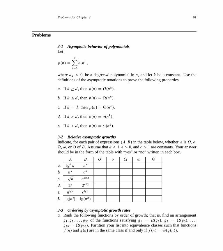
Problems for Chapter 3 61
Problems
3-1 Asymptotic behavior of polynomialsLet
p.n/ DdX
iD0
aini ;
where ad > 0, be a degree-d polynomial in n, and let k be a constant. Use thedefinitions of the asymptotic notations to prove the following properties.
a. If k � d , then p.n/ D O.nk/.
b. If k � d , then p.n/ D �.nk/.
c. If k D d , then p.n/ D ‚.nk/.
d. If k > d , then p.n/ D o.nk/.
e. If k < d , then p.n/ D !.nk/.
3-2 Relative asymptotic growthsIndicate, for each pair of expressions .A; B/ in the table below, whether A is O, o,�, !, or ‚ of B . Assume that k � 1, � > 0, and c > 1 are constants. Your answershould be in the form of the table with “yes” or “no” written in each box.
A B O o � ! ‚
a. lgk n n�
b. nk cn
c.p
n nsin n
d. 2n 2n=2
e. nlg c c lg n
f. lg.nŠ/ lg.nn/
3-3 Ordering by asymptotic growth ratesa. Rank the following functions by order of growth; that is, find an arrangement
g1; g2; : : : ; g30 of the functions satisfying g1 D �.g2/, g2 D �.g3/, . . . ,g29 D �.g30/. Partition your list into equivalence classes such that functionsf .n/ and g.n/ are in the same class if and only if f .n/ D ‚.g.n//.

62 Chapter 3 Growth of Functions
lg.lg� n/ 2lg� n .p
2/lg n n2 nŠ .lg n/Š
.32/n n3 lg2 n lg.nŠ/ 22n
n1= lg n
ln ln n lg� n n � 2n nlg lg n ln n 1
2lg n .lg n/lg n en 4lg n .nC 1/Šp
lg n
lg�.lg n/ 2p
2 lg n n 2n n lg n 22nC1
b. Give an example of a single nonnegative function f .n/ such that for all func-tions gi .n/ in part (a), f .n/ is neither O.gi .n// nor �.gi.n//.
3-4 Asymptotic notation propertiesLet f .n/ and g.n/ be asymptotically positive functions. Prove or disprove each ofthe following conjectures.
a. f .n/ D O.g.n// implies g.n/ D O.f .n//.
b. f .n/C g.n/ D ‚.min.f .n/; g.n///.
c. f .n/ D O.g.n// implies lg.f .n// D O.lg.g.n///, where lg.g.n// � 1 andf .n/ � 1 for all sufficiently large n.
d. f .n/ D O.g.n// implies 2f .n/ D O�2g.n/
�.
e. f .n/ D O ..f .n//2/.
f. f .n/ D O.g.n// implies g.n/ D �.f .n//.
g. f .n/ D ‚.f .n=2//.
h. f .n/C o.f .n// D ‚.f .n//.
3-5 Variations on O and ˝
Some authors define � in a slightly different way than we do; let’s use1� (read
“omega infinity”) for this alternative definition. We say that f .n/ D 1�.g.n// if
there exists a positive constant c such that f .n/ � cg.n/ � 0 for infinitely manyintegers n.
a. Show that for any two functions f .n/ and g.n/ that are asymptotically nonneg-ative, either f .n/ D O.g.n// or f .n/ D 1
�.g.n// or both, whereas this is nottrue if we use � in place of
1�.
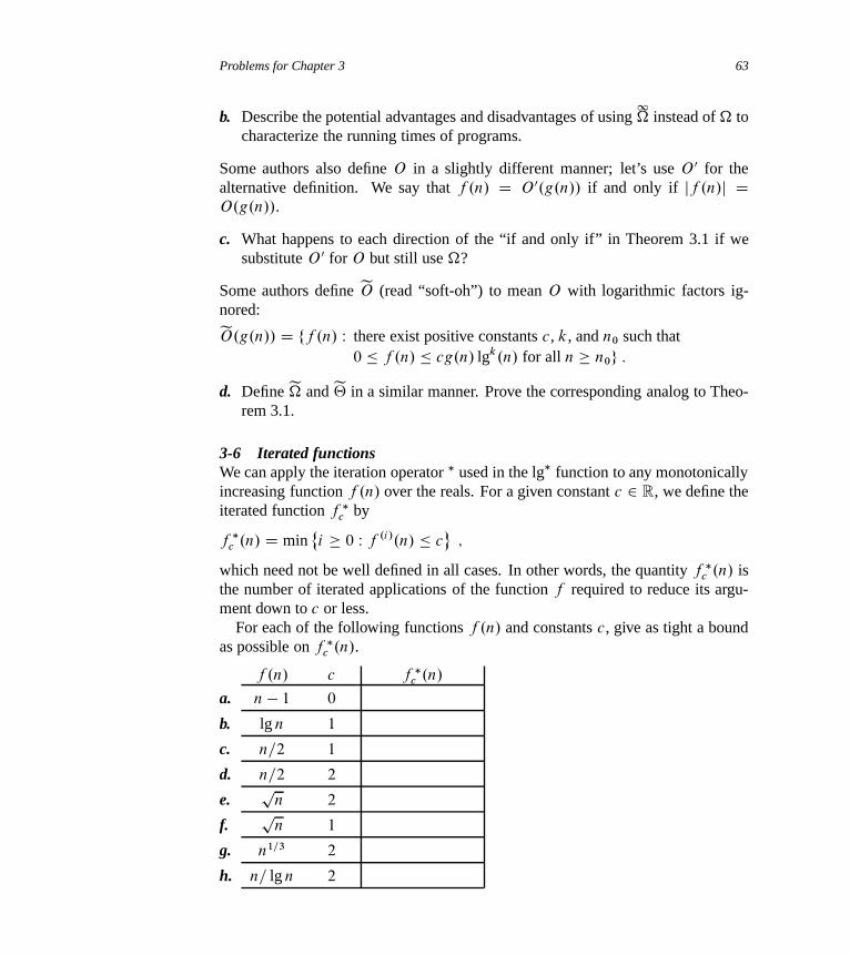
Problems for Chapter 3 63
b. Describe the potential advantages and disadvantages of using1� instead of � to
characterize the running times of programs.
Some authors also define O in a slightly different manner; let’s use O 0 for thealternative definition. We say that f .n/ D O 0.g.n// if and only if jf .n/j DO.g.n//.
c. What happens to each direction of the “if and only if” in Theorem 3.1 if wesubstitute O 0 for O but still use �?
Some authors define eO (read “soft-oh”) to mean O with logarithmic factors ig-nored:eO.g.n// D ff .n/ W there exist positive constants c, k, and n0 such that
0 � f .n/ � cg.n/ lgk.n/ for all n � n0g :
d. Define e� and e‚ in a similar manner. Prove the corresponding analog to Theo-rem 3.1.
3-6 Iterated functionsWe can apply the iteration operator � used in the lg� function to any monotonicallyincreasing function f .n/ over the reals. For a given constant c 2 R, we define theiterated function f �
c by
f �c .n/ D min
˚i � 0 W f .i/.n/ � c
;
which need not be well defined in all cases. In other words, the quantity f �c .n/ is
the number of iterated applications of the function f required to reduce its argu-ment down to c or less.
For each of the following functions f .n/ and constants c, give as tight a boundas possible on f �
c .n/.
f .n/ c f �c .n/
a. n � 1 0
b. lg n 1
c. n=2 1
d. n=2 2
e.p
n 2
f.p
n 1
g. n1=3 2
h. n= lg n 2
64 Chapter 3 Growth of Functions
Chapter notes
Knuth [209] traces the origin of the O-notation to a number-theory text by P. Bach-mann in 1892. The o-notation was invented by E. Landau in 1909 for his discussionof the distribution of prime numbers. The � and ‚ notations were advocated byKnuth [213] to correct the popular, but technically sloppy, practice in the literatureof using O-notation for both upper and lower bounds. Many people continue touse the O-notation where the ‚-notation is more technically precise. Further dis-cussion of the history and development of asymptotic notations appears in worksby Knuth [209, 213] and Brassard and Bratley [55].
Not all authors define the asymptotic notations in the same way, although thevarious definitions agree in most common situations. Some of the alternative def-initions encompass functions that are not asymptotically nonnegative, as long astheir absolute values are appropriately bounded.
Equation (3.20) is due to Robbins [297]. Other properties of elementary math-ematical functions can be found in any good mathematical reference, such asAbramowitz and Stegun [1] or Zwillinger [362], or in a calculus book, such asApostol [18] or Thomas et al. [334]. Knuth [209] and Graham, Knuth, and Patash-nik [152] contain a wealth of material on discrete mathematics as used in computerscience.

4 Divide-and-Conquer
In Section 2.3.1, we saw how merge sort serves as an example of the divide-and-conquer paradigm. Recall that in divide-and-conquer, we solve a problem recur-sively, applying three steps at each level of the recursion:
Divide the problem into a number of subproblems that are smaller instances of thesame problem.
Conquer the subproblems by solving them recursively. If the subproblem sizes aresmall enough, however, just solve the subproblems in a straightforward manner.
Combine the solutions to the subproblems into the solution for the original prob-lem.
When the subproblems are large enough to solve recursively, we call that the recur-sive case. Once the subproblems become small enough that we no longer recurse,we say that the recursion “bottoms out” and that we have gotten down to the basecase. Sometimes, in addition to subproblems that are smaller instances of the sameproblem, we have to solve subproblems that are not quite the same as the originalproblem. We consider solving such subproblems as part of the combine step.
In this chapter, we shall see more algorithms based on divide-and-conquer. Thefirst one solves the maximum-subarray problem: it takes as input an array of num-bers, and it determines the contiguous subarray whose values have the greatest sum.Then we shall see two divide-and-conquer algorithms for multiplying n n matri-ces. One runs in ‚.n3/ time, which is no better than the straightforward method ofmultiplying square matrices. But the other, Strassen’s algorithm, runs in O.n2:81/
time, which beats the straightforward method asymptotically.
Recurrences
Recurrences go hand in hand with the divide-and-conquer paradigm, because theygive us a natural way to characterize the running times of divide-and-conquer algo-rithms. A recurrence is an equation or inequality that describes a function in terms
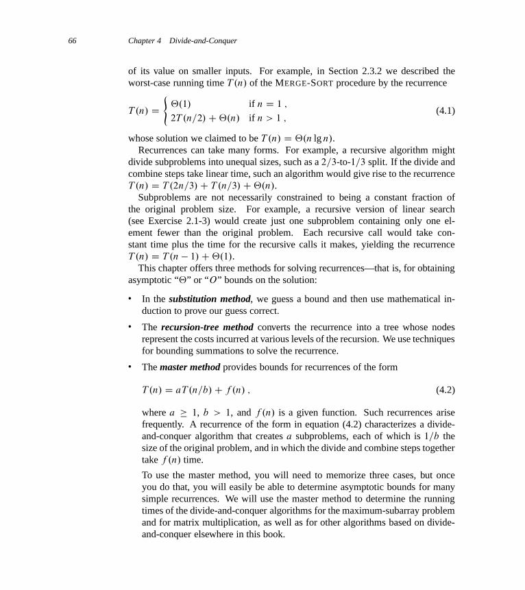
66 Chapter 4 Divide-and-Conquer
of its value on smaller inputs. For example, in Section 2.3.2 we described theworst-case running time T .n/ of the MERGE-SORT procedure by the recurrence
T .n/ D(
‚.1/ if n D 1 ;
2T .n=2/C‚.n/ if n > 1 ;(4.1)
whose solution we claimed to be T .n/ D ‚.n lg n/.Recurrences can take many forms. For example, a recursive algorithm might
divide subproblems into unequal sizes, such as a 2=3-to-1=3 split. If the divide andcombine steps take linear time, such an algorithm would give rise to the recurrenceT .n/ D T .2n=3/C T .n=3/C‚.n/.
Subproblems are not necessarily constrained to being a constant fraction ofthe original problem size. For example, a recursive version of linear search(see Exercise 2.1-3) would create just one subproblem containing only one el-ement fewer than the original problem. Each recursive call would take con-stant time plus the time for the recursive calls it makes, yielding the recurrenceT .n/ D T .n � 1/C‚.1/.
This chapter offers three methods for solving recurrences—that is, for obtainingasymptotic “‚” or “O” bounds on the solution:
� In the substitution method, we guess a bound and then use mathematical in-duction to prove our guess correct.
� The recursion-tree method converts the recurrence into a tree whose nodesrepresent the costs incurred at various levels of the recursion. We use techniquesfor bounding summations to solve the recurrence.
� The master method provides bounds for recurrences of the form
T .n/ D aT .n=b/C f .n/ ; (4.2)
where a � 1, b > 1, and f .n/ is a given function. Such recurrences arisefrequently. A recurrence of the form in equation (4.2) characterizes a divide-and-conquer algorithm that creates a subproblems, each of which is 1=b thesize of the original problem, and in which the divide and combine steps togethertake f .n/ time.
To use the master method, you will need to memorize three cases, but onceyou do that, you will easily be able to determine asymptotic bounds for manysimple recurrences. We will use the master method to determine the runningtimes of the divide-and-conquer algorithms for the maximum-subarray problemand for matrix multiplication, as well as for other algorithms based on divide-and-conquer elsewhere in this book.

Chapter 4 Divide-and-Conquer 67
Occasionally, we shall see recurrences that are not equalities but rather inequal-ities, such as T .n/ � 2T .n=2/ C ‚.n/. Because such a recurrence states onlyan upper bound on T .n/, we will couch its solution using O-notation rather than‚-notation. Similarly, if the inequality were reversed to T .n/ � 2T .n=2/C‚.n/,then because the recurrence gives only a lower bound on T .n/, we would use�-notation in its solution.
Technicalities in recurrences
In practice, we neglect certain technical details when we state and solve recur-rences. For example, if we call MERGE-SORT on n elements when n is odd, weend up with subproblems of size bn=2c and dn=2e. Neither size is actually n=2,because n=2 is not an integer when n is odd. Technically, the recurrence describingthe worst-case running time of MERGE-SORT is really
T .n/ D(
‚.1/ if n D 1 ;
T .dn=2e/C T .bn=2c/C‚.n/ if n > 1 :(4.3)
Boundary conditions represent another class of details that we typically ignore.Since the running time of an algorithm on a constant-sized input is a constant,the recurrences that arise from the running times of algorithms generally haveT .n/ D ‚.1/ for sufficiently small n. Consequently, for convenience, we shallgenerally omit statements of the boundary conditions of recurrences and assumethat T .n/ is constant for small n. For example, we normally state recurrence (4.1)as
T .n/ D 2T .n=2/C‚.n/ ; (4.4)
without explicitly giving values for small n. The reason is that although changingthe value of T .1/ changes the exact solution to the recurrence, the solution typi-cally doesn’t change by more than a constant factor, and so the order of growth isunchanged.
When we state and solve recurrences, we often omit floors, ceilings, and bound-ary conditions. We forge ahead without these details and later determine whetheror not they matter. They usually do not, but you should know when they do. Ex-perience helps, and so do some theorems stating that these details do not affect theasymptotic bounds of many recurrences characterizing divide-and-conquer algo-rithms (see Theorem 4.1). In this chapter, however, we shall address some of thesedetails and illustrate the fine points of recurrence solution methods.

68 Chapter 4 Divide-and-Conquer
4.1 The maximum-subarray problem
Suppose that you been offered the opportunity to invest in the Volatile ChemicalCorporation. Like the chemicals the company produces, the stock price of theVolatile Chemical Corporation is rather volatile. You are allowed to buy one unitof stock only one time and then sell it at a later date, buying and selling after theclose of trading for the day. To compensate for this restriction, you are allowed tolearn what the price of the stock will be in the future. Your goal is to maximizeyour profit. Figure 4.1 shows the price of the stock over a 17-day period. Youmay buy the stock at any one time, starting after day 0, when the price is $100per share. Of course, you would want to “buy low, sell high”—buy at the lowestpossible price and later on sell at the highest possible price—to maximize yourprofit. Unfortunately, you might not be able to buy at the lowest price and then sellat the highest price within a given period. In Figure 4.1, the lowest price occursafter day 7, which occurs after the highest price, after day 1.
You might think that you can always maximize profit by either buying at thelowest price or selling at the highest price. For example, in Figure 4.1, we wouldmaximize profit by buying at the lowest price, after day 7. If this strategy alwaysworked, then it would be easy determine how to maximize profit: find the highestand lowest prices, and then work left from the highest price to find the lowest priorprice, work right from the lowest price to find the highest later price, and takethe pair with the greater difference. Figure 4.2 shows a simple counterexample,
0 1 2 3 4 5 6 7 8 9 10 11 12 13 14 15 16
120
110
100
90
80
70
60
Day 0 1 2 3 4 5 6 7 8 9 10 11 12 13 14 15 16
Price 100 113 110 85 105 102 86 63 81 101 94 106 101 79 94 90 97
Change 13 �3 �25 20 �3 �16 �23 18 20 �7 12 �5 �22 15 �4 7
Figure 4.1 Information about the price of stock in the Volatile Chemical Corporation after the closeof trading over a period of 17 days. The horizontal axis of the chart indicates the day, and the verticalaxis shows the price. The bottom row of the table gives the change in price from the previous day.

4.1 The maximum-subarray problem 69
0 1 2 3 4
11
10
9
8
7
6
Day 0 1 2 3 4
Price 10 11 7 10 6
Change 1 �4 3 �4
Figure 4.2 An example showing that the maximum profit does not always start at the lowest priceor end at the highest price. Again, the horizontal axis indicates the day, and the vertical axis showsthe price. Here, the maximum profit of $3 per share would be earned by buying after day 2 andselling after day 3. The price of $7 after day 2 is not the lowest price overall, and the price of $10after day 3 is not the highest price overall.
demonstrating that the maximum profit sometimes comes neither by buying at thelowest price nor by selling at the highest price.
A brute-force solution
We can easily devise a brute-force solution to this problem: just try every possiblepair of buy and sell dates in which the buy date precedes the sell date. A period of n
days has�
n
2
�such pairs of dates. Since
�n
2
�is ‚.n2/, and the best we can hope for
is to evaluate each pair of dates in constant time, this approach would take �.n2/
time. Can we do better?
A transformation
In order to design an algorithm with an o.n2/ running time, we will look at theinput in a slightly different way. We want to find a sequence of days over whichthe net change from the first day to the last is maximum. Instead of looking at thedaily prices, let us instead consider the daily change in price, where the change onday i is the difference between the prices after day i � 1 and after day i . The tablein Figure 4.1 shows these daily changes in the bottom row. If we treat this row asan array A, shown in Figure 4.3, we now want to find the nonempty, contiguoussubarray of A whose values have the largest sum. We call this contiguous subarraythe maximum subarray. For example, in the array of Figure 4.3, the maximumsubarray of AŒ1 : : 16� is AŒ8 : : 11�, with the sum 43. Thus, you would want to buythe stock just before day 8 (that is, after day 7) and sell it after day 11, earning aprofit of $43 per share.
At first glance, this transformation does not help. We still need to check�n�1
2
� D ‚.n2/ subarrays for a period of n days. Exercise 4.1-2 asks you to show

70 Chapter 4 Divide-and-Conquer
131
–32
–253
204
–35
–166
–237 8 9 10
maximum subarray
11
1812
2013
–714
1215
716
–5 –22 15 –4A
Figure 4.3 The change in stock prices as a maximum-subarray problem. Here, the subar-ray AŒ8 : : 11�, with sum 43, has the greatest sum of any contiguous subarray of array A.
that although computing the cost of one subarray might take time proportional tothe length of the subarray, when computing all ‚.n2/ subarray sums, we can orga-nize the computation so that each subarray sum takes O.1/ time, given the valuesof previously computed subarray sums, so that the brute-force solution takes ‚.n2/
time.So let us seek a more efficient solution to the maximum-subarray problem.
When doing so, we will usually speak of “a” maximum subarray rather than “the”maximum subarray, since there could be more than one subarray that achieves themaximum sum.
The maximum-subarray problem is interesting only when the array containssome negative numbers. If all the array entries were nonnegative, then themaximum-subarray problem would present no challenge, since the entire arraywould give the greatest sum.
A solution using divide-and-conquer
Let’s think about how we might solve the maximum-subarray problem usingthe divide-and-conquer technique. Suppose we want to find a maximum subar-ray of the subarray AŒlow : : high�. Divide-and-conquer suggests that we dividethe subarray into two subarrays of as equal size as possible. That is, we findthe midpoint, say mid, of the subarray, and consider the subarrays AŒlow : : mid�
and AŒmidC 1 : : high�. As Figure 4.4(a) shows, any contiguous subarray AŒi : : j �
of AŒlow : : high� must lie in exactly one of the following places:
� entirely in the subarray AŒlow : : mid�, so that low � i � j � mid,� entirely in the subarray AŒmidC 1 : : high�, so that mid < i � j � high, or� crossing the midpoint, so that low � i � mid < j � high.
Therefore, a maximum subarray of AŒlow : : high� must lie in exactly one of theseplaces. In fact, a maximum subarray of AŒlow : : high� must have the greatestsum over all subarrays entirely in AŒlow : : mid�, entirely in AŒmid C 1 : : high�,or crossing the midpoint. We can find maximum subarrays of AŒlow : : mid� andAŒmidC1 : : high� recursively, because these two subproblems are smaller instancesof the problem of finding a maximum subarray. Thus, all that is left to do is find a
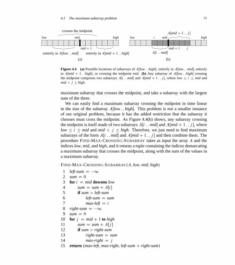
4.1 The maximum-subarray problem 71
(a) (b)
lowlow midmid highhigh
crosses the midpoint
midC 1midC 1
entirely in AŒlow : : mid� entirely in AŒmidC 1 : : high�
i
j
AŒi : : mid�
AŒmidC 1 : : j �
Figure 4.4 (a) Possible locations of subarrays of AŒlow : : high�: entirely in AŒlow : : mid�, entirelyin AŒmid C 1 : : high�, or crossing the midpoint mid. (b) Any subarray of AŒlow : : high� crossingthe midpoint comprises two subarrays AŒi : : mid� and AŒmid C 1 : : j �, where low � i � mid andmid < j � high.
maximum subarray that crosses the midpoint, and take a subarray with the largestsum of the three.
We can easily find a maximum subarray crossing the midpoint in time linearin the size of the subarray AŒlow : : high�. This problem is not a smaller instanceof our original problem, because it has the added restriction that the subarray itchooses must cross the midpoint. As Figure 4.4(b) shows, any subarray crossingthe midpoint is itself made of two subarrays AŒi : : mid� and AŒmidC 1 : : j �, wherelow � i � mid and mid < j � high. Therefore, we just need to find maximumsubarrays of the form AŒi : : mid� and AŒmidC 1 : : j � and then combine them. Theprocedure FIND-MAX-CROSSING-SUBARRAY takes as input the array A and theindices low, mid, and high, and it returns a tuple containing the indices demarcatinga maximum subarray that crosses the midpoint, along with the sum of the values ina maximum subarray.
FIND-MAX-CROSSING-SUBARRAY.A; low; mid; high/
1 left-sum D �12 sum D 0
3 for i D mid downto low4 sum D sumC AŒi�
5 if sum > left-sum6 left-sum D sum7 max-left D i
8 right-sum D �19 sum D 0
10 for j D midC 1 to high11 sum D sumC AŒj �
12 if sum > right-sum13 right-sum D sum14 max-right D j
15 return .max-left; max-right; left-sum C right-sum/

72 Chapter 4 Divide-and-Conquer
This procedure works as follows. Lines 1–7 find a maximum subarray of theleft half, AŒlow : : mid�. Since this subarray must contain AŒmid�, the for loop oflines 3–7 starts the index i at mid and works down to low, so that every subarrayit considers is of the form AŒi : : mid�. Lines 1–2 initialize the variables left-sum,which holds the greatest sum found so far, and sum, holding the sum of the entriesin AŒi : : mid�. Whenever we find, in line 5, a subarray AŒi : : mid� with a sum ofvalues greater than left-sum, we update left-sum to this subarray’s sum in line 6, andin line 7 we update the variable max-left to record this index i . Lines 8–14 workanalogously for the right half, AŒmidC1 : : high�. Here, the for loop of lines 10–14starts the index j at midC1 and works up to high, so that every subarray it considersis of the form AŒmid C 1 : : j �. Finally, line 15 returns the indices max-left andmax-right that demarcate a maximum subarray crossing the midpoint, along withthe sum left-sumCright-sum of the values in the subarray AŒmax-left : : max-right�.
If the subarray AŒlow : : high� contains n entries (so that n D high � lowC 1),we claim that the call FIND-MAX-CROSSING-SUBARRAY.A; low; mid; high/
takes ‚.n/ time. Since each iteration of each of the two for loops takes ‚.1/
time, we just need to count up how many iterations there are altogether. The forloop of lines 3–7 makes mid�lowC1 iterations, and for loop of lines 10–14 makeshigh � mid iterations, and so the total number of iterations is
.mid � lowC 1/C .high � mid/ D high � lowC 1
D n :
With a linear-time FIND-MAX-CROSSING-SUBARRAY procedure in hand, wecan write pseudocode for a divide-and-conquer algorithm to solve the maximum-subarray problem:
FIND-MAXIMUM-SUBARRAY.A; low; high/
1 if high == low2 return .low; high; AŒlow�/ // base case: only one element3 else mid D b.lowC high/=2c4 .left-low; left-high; left-sum/ D
FIND-MAXIMUM-SUBARRAY.A; low; mid/
5 .right-low; right-high; right-sum/ DFIND-MAXIMUM-SUBARRAY.A; midC 1; high/
6 .cross-low; cross-high; cross-sum/ DFIND-MAX-CROSSING-SUBARRAY.A; low; mid; high/
7 if left-sum � right-sum and left-sum � cross-sum8 return .left-low; left-high; left-sum/
9 elseif right-sum � left-sum and right-sum � cross-sum10 return .right-low; right-high; right-sum/
11 else return .cross-low; cross-high; cross-sum/

4.1 The maximum-subarray problem 73
The initial call FIND-MAXIMUM-SUBARRAY.A; 1; A: length/ will find a maxi-mum subarray of AŒ1 : : n�.
Similar to FIND-MAX-CROSSING-SUBARRAY, the recursive procedure FIND-MAXIMUM-SUBARRAY returns a tuple containing the indices that demarcate amaximum subarray, along with the sum of the values in a maximum subarray.Line 1 tests for the base case, where the subarray has just one element. A subar-ray with just one element has only one subarray—itself—and so line 2 returns atuple with the starting and ending indices of just the one element, along with itsvalue. Lines 3–11 handle the recursive case. Line 3 does the divide part, comput-ing the index mid of the midpoint. Let’s refer to the subarray AŒlow : : mid� as theleft subarray and to AŒmid C 1 : : high� as the right subarray. Because we knowthat the subarray AŒlow : : high� contains at least two elements, each of the left andright subarrays must have at least one element. Lines 4 and 5 conquer by recur-sively finding maximum subarrays within the left and right subarrays, respectively.Lines 6–11 form the combine part. Line 6 finds a maximum subarray that crossesthe midpoint. (Recall that because line 6 solves a subproblem that is not a smallerinstance of the original problem, we consider it to be in the combine part.) Line 7tests whether the left subarray contains a subarray with the maximum sum, andline 8 returns that maximum subarray. Otherwise, line 9 tests whether the rightsubarray contains a subarray with the maximum sum, and line 10 returns that max-imum subarray. If neither the left nor right subarrays contain a subarray achievingthe maximum sum, then a maximum subarray must cross the midpoint, and line 11returns it.
Analyzing the divide-and-conquer algorithm
Next we set up a recurrence that describes the running time of the recursive FIND-MAXIMUM-SUBARRAY procedure. As we did when we analyzed merge sort inSection 2.3.2, we make the simplifying assumption that the original problem sizeis a power of 2, so that all subproblem sizes are integers. We denote by T .n/ therunning time of FIND-MAXIMUM-SUBARRAY on a subarray of n elements. Forstarters, line 1 takes constant time. The base case, when n D 1, is easy: line 2takes constant time, and so
T .1/ D ‚.1/ : (4.5)
The recursive case occurs when n > 1. Lines 1 and 3 take constant time. Eachof the subproblems solved in lines 4 and 5 is on a subarray of n=2 elements (ourassumption that the original problem size is a power of 2 ensures that n=2 is aninteger), and so we spend T .n=2/ time solving each of them. Because we haveto solve two subproblems—for the left subarray and for the right subarray—thecontribution to the running time from lines 4 and 5 comes to 2T .n=2/. As we have

74 Chapter 4 Divide-and-Conquer
already seen, the call to FIND-MAX-CROSSING-SUBARRAY in line 6 takes ‚.n/
time. Lines 7–11 take only ‚.1/ time. For the recursive case, therefore, we have
T .n/ D ‚.1/C 2T .n=2/C‚.n/C‚.1/
D 2T .n=2/C‚.n/ : (4.6)
Combining equations (4.5) and (4.6) gives us a recurrence for the runningtime T .n/ of FIND-MAXIMUM-SUBARRAY:
T .n/ D(
‚.1/ if n D 1 ;
2T .n=2/C‚.n/ if n > 1 :(4.7)
This recurrence is the same as recurrence (4.1) for merge sort. As we shallsee from the master method in Section 4.5, this recurrence has the solutionT .n/ D ‚.n lg n/. You might also revisit the recursion tree in Figure 2.5 to un-derstand why the solution should be T .n/ D ‚.n lg n/.
Thus, we see that the divide-and-conquer method yields an algorithm that isasymptotically faster than the brute-force method. With merge sort and now themaximum-subarray problem, we begin to get an idea of how powerful the divide-and-conquer method can be. Sometimes it will yield the asymptotically fastestalgorithm for a problem, and other times we can do even better. As Exercise 4.1-5shows, there is in fact a linear-time algorithm for the maximum-subarray problem,and it does not use divide-and-conquer.
Exercises
4.1-1What does FIND-MAXIMUM-SUBARRAY return when all elements of A are nega-tive?
4.1-2Write pseudocode for the brute-force method of solving the maximum-subarrayproblem. Your procedure should run in ‚.n2/ time.
4.1-3Implement both the brute-force and recursive algorithms for the maximum-subarray problem on your own computer. What problem size n0 gives the crossoverpoint at which the recursive algorithm beats the brute-force algorithm? Then,change the base case of the recursive algorithm to use the brute-force algorithmwhenever the problem size is less than n0. Does that change the crossover point?
4.1-4Suppose we change the definition of the maximum-subarray problem to allow theresult to be an empty subarray, where the sum of the values of an empty subar-
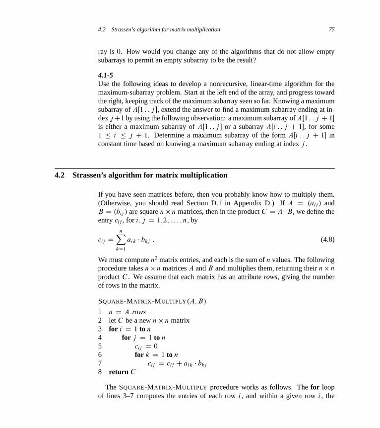
4.2 Strassen’s algorithm for matrix multiplication 75
ray is 0. How would you change any of the algorithms that do not allow emptysubarrays to permit an empty subarray to be the result?
4.1-5Use the following ideas to develop a nonrecursive, linear-time algorithm for themaximum-subarray problem. Start at the left end of the array, and progress towardthe right, keeping track of the maximum subarray seen so far. Knowing a maximumsubarray of AŒ1 : : j �, extend the answer to find a maximum subarray ending at in-dex jC1 by using the following observation: a maximum subarray of AŒ1 : : j C 1�
is either a maximum subarray of AŒ1 : : j � or a subarray AŒi : : j C 1�, for some1 � i � j C 1. Determine a maximum subarray of the form AŒi : : j C 1� inconstant time based on knowing a maximum subarray ending at index j .
4.2 Strassen’s algorithm for matrix multiplication
If you have seen matrices before, then you probably know how to multiply them.(Otherwise, you should read Section D.1 in Appendix D.) If A D .aij / andB D .bij / are square n n matrices, then in the product C D A �B , we define theentry cij , for i; j D 1; 2; : : : ; n, by
cij DnX
kD1
aik � bkj : (4.8)
We must compute n2 matrix entries, and each is the sum of n values. The followingprocedure takes n n matrices A and B and multiplies them, returning their n n
product C . We assume that each matrix has an attribute rows, giving the numberof rows in the matrix.
SQUARE-MATRIX-MULTIPLY.A; B/
1 n D A:rows2 let C be a new n n matrix3 for i D 1 to n
4 for j D 1 to n
5 cij D 0
6 for k D 1 to n
7 cij D cij C aik � bkj
8 return C
The SQUARE-MATRIX-MULTIPLY procedure works as follows. The for loopof lines 3–7 computes the entries of each row i , and within a given row i , the

76 Chapter 4 Divide-and-Conquer
for loop of lines 4–7 computes each of the entries cij , for each column j . Line 5initializes cij to 0 as we start computing the sum given in equation (4.8), and eachiteration of the for loop of lines 6–7 adds in one more term of equation (4.8).
Because each of the triply-nested for loops runs exactly n iterations, and eachexecution of line 7 takes constant time, the SQUARE-MATRIX-MULTIPLY proce-dure takes ‚.n3/ time.
You might at first think that any matrix multiplication algorithm must take �.n3/
time, since the natural definition of matrix multiplication requires that many mul-tiplications. You would be incorrect, however: we have a way to multiply matricesin o.n3/ time. In this section, we shall see Strassen’s remarkable recursive algo-rithm for multiplying n n matrices. It runs in ‚.nlg 7/ time, which we shall showin Section 4.5. Since lg 7 lies between 2:80 and 2:81, Strassen’s algorithm runs inO.n2:81/ time, which is asymptotically better than the simple SQUARE-MATRIX-MULTIPLY procedure.
A simple divide-and-conquer algorithm
To keep things simple, when we use a divide-and-conquer algorithm to computethe matrix product C D A � B , we assume that n is an exact power of 2 in each ofthe n n matrices. We make this assumption because in each divide step, we willdivide n n matrices into four n=2 n=2 matrices, and by assuming that n is anexact power of 2, we are guaranteed that as long as n � 2, the dimension n=2 is aninteger.
Suppose that we partition each of A, B , and C into four n=2 n=2 matrices
A D�
A11 A12
A21 A22
�; B D
�B11 B12
B21 B22
�; C D
�C11 C12
C21 C22
�; (4.9)
so that we rewrite the equation C D A � B as�C11 C12
C21 C22
�D�
A11 A12
A21 A22
���
B11 B12
B21 B22
�: (4.10)
Equation (4.10) corresponds to the four equations
C11 D A11 � B11 C A12 � B21 ; (4.11)
C12 D A11 � B12 C A12 � B22 ; (4.12)
C21 D A21 � B11 C A22 � B21 ; (4.13)
C22 D A21 � B12 C A22 � B22 ; (4.14)
Each of these four equations specifies two multiplications of n=2 n=2 matricesand the addition of their n=2 n=2 products. We can use these equations to createa straightforward, recursive, divide-and-conquer algorithm:
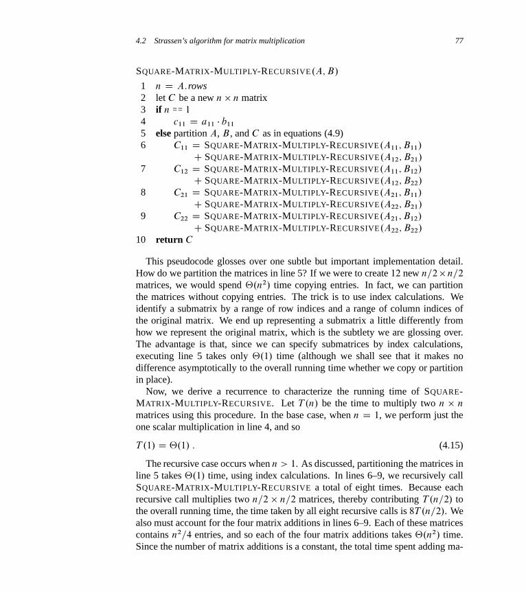
4.2 Strassen’s algorithm for matrix multiplication 77
SQUARE-MATRIX-MULTIPLY-RECURSIVE.A; B/
1 n D A:rows2 let C be a new n n matrix3 if n == 1
4 c11 D a11 � b11
5 else partition A, B , and C as in equations (4.9)6 C11 D SQUARE-MATRIX-MULTIPLY-RECURSIVE.A11; B11/
C SQUARE-MATRIX-MULTIPLY-RECURSIVE.A12; B21/
7 C12 D SQUARE-MATRIX-MULTIPLY-RECURSIVE.A11; B12/
C SQUARE-MATRIX-MULTIPLY-RECURSIVE.A12; B22/
8 C21 D SQUARE-MATRIX-MULTIPLY-RECURSIVE.A21; B11/
C SQUARE-MATRIX-MULTIPLY-RECURSIVE.A22; B21/
9 C22 D SQUARE-MATRIX-MULTIPLY-RECURSIVE.A21; B12/
C SQUARE-MATRIX-MULTIPLY-RECURSIVE.A22; B22/
10 return C
This pseudocode glosses over one subtle but important implementation detail.How do we partition the matrices in line 5? If we were to create 12 new n=2n=2
matrices, we would spend ‚.n2/ time copying entries. In fact, we can partitionthe matrices without copying entries. The trick is to use index calculations. Weidentify a submatrix by a range of row indices and a range of column indices ofthe original matrix. We end up representing a submatrix a little differently fromhow we represent the original matrix, which is the subtlety we are glossing over.The advantage is that, since we can specify submatrices by index calculations,executing line 5 takes only ‚.1/ time (although we shall see that it makes nodifference asymptotically to the overall running time whether we copy or partitionin place).
Now, we derive a recurrence to characterize the running time of SQUARE-MATRIX-MULTIPLY-RECURSIVE. Let T .n/ be the time to multiply two n n
matrices using this procedure. In the base case, when n D 1, we perform just theone scalar multiplication in line 4, and so
T .1/ D ‚.1/ : (4.15)
The recursive case occurs when n > 1. As discussed, partitioning the matrices inline 5 takes ‚.1/ time, using index calculations. In lines 6–9, we recursively callSQUARE-MATRIX-MULTIPLY-RECURSIVE a total of eight times. Because eachrecursive call multiplies two n=2 n=2 matrices, thereby contributing T .n=2/ tothe overall running time, the time taken by all eight recursive calls is 8T .n=2/. Wealso must account for the four matrix additions in lines 6–9. Each of these matricescontains n2=4 entries, and so each of the four matrix additions takes ‚.n2/ time.Since the number of matrix additions is a constant, the total time spent adding ma-
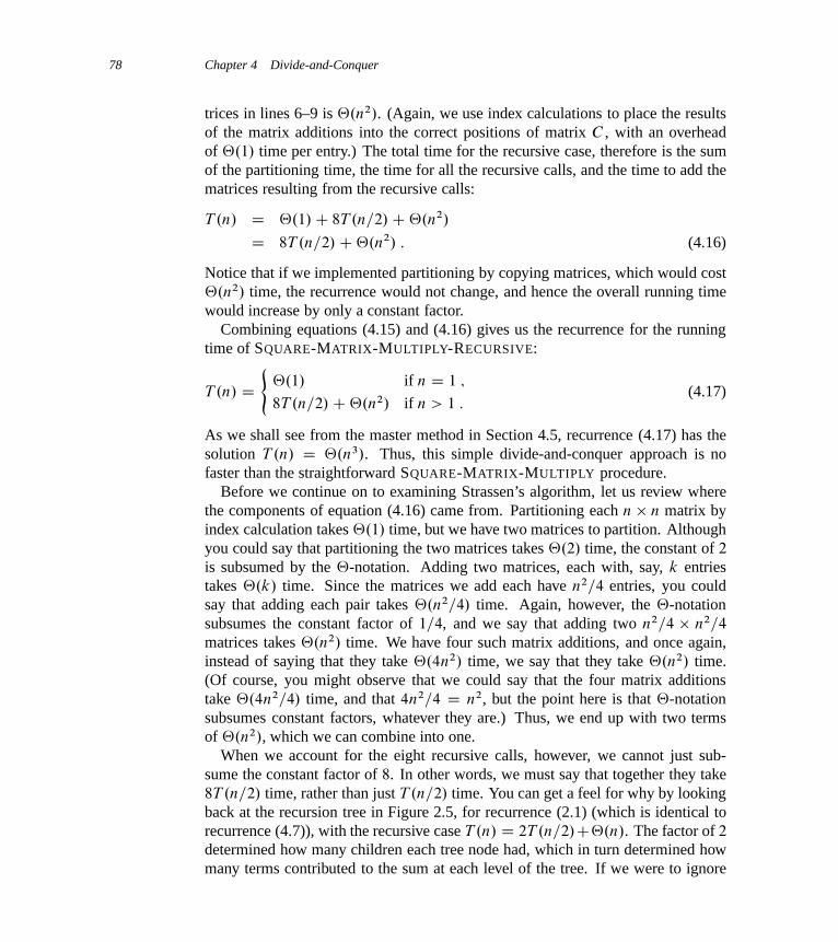
78 Chapter 4 Divide-and-Conquer
trices in lines 6–9 is ‚.n2/. (Again, we use index calculations to place the resultsof the matrix additions into the correct positions of matrix C , with an overheadof ‚.1/ time per entry.) The total time for the recursive case, therefore is the sumof the partitioning time, the time for all the recursive calls, and the time to add thematrices resulting from the recursive calls:
T .n/ D ‚.1/C 8T .n=2/C‚.n2/
D 8T .n=2/C‚.n2/ : (4.16)
Notice that if we implemented partitioning by copying matrices, which would cost‚.n2/ time, the recurrence would not change, and hence the overall running timewould increase by only a constant factor.
Combining equations (4.15) and (4.16) gives us the recurrence for the runningtime of SQUARE-MATRIX-MULTIPLY-RECURSIVE:
T .n/ D(
‚.1/ if n D 1 ;
8T .n=2/C‚.n2/ if n > 1 :(4.17)
As we shall see from the master method in Section 4.5, recurrence (4.17) has thesolution T .n/ D ‚.n3/. Thus, this simple divide-and-conquer approach is nofaster than the straightforward SQUARE-MATRIX-MULTIPLY procedure.
Before we continue on to examining Strassen’s algorithm, let us review wherethe components of equation (4.16) came from. Partitioning each n n matrix byindex calculation takes ‚.1/ time, but we have two matrices to partition. Althoughyou could say that partitioning the two matrices takes ‚.2/ time, the constant of 2
is subsumed by the ‚-notation. Adding two matrices, each with, say, k entriestakes ‚.k/ time. Since the matrices we add each have n2=4 entries, you couldsay that adding each pair takes ‚.n2=4/ time. Again, however, the ‚-notationsubsumes the constant factor of 1=4, and we say that adding two n2=4 n2=4
matrices takes ‚.n2/ time. We have four such matrix additions, and once again,instead of saying that they take ‚.4n2/ time, we say that they take ‚.n2/ time.(Of course, you might observe that we could say that the four matrix additionstake ‚.4n2=4/ time, and that 4n2=4 D n2, but the point here is that ‚-notationsubsumes constant factors, whatever they are.) Thus, we end up with two termsof ‚.n2/, which we can combine into one.
When we account for the eight recursive calls, however, we cannot just sub-sume the constant factor of 8. In other words, we must say that together they take8T .n=2/ time, rather than just T .n=2/ time. You can get a feel for why by lookingback at the recursion tree in Figure 2.5, for recurrence (2.1) (which is identical torecurrence (4.7)), with the recursive case T .n/ D 2T .n=2/C‚.n/. The factor of 2
determined how many children each tree node had, which in turn determined howmany terms contributed to the sum at each level of the tree. If we were to ignore
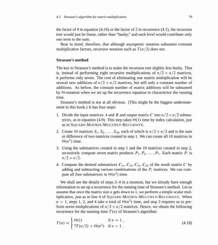
4.2 Strassen’s algorithm for matrix multiplication 79
the factor of 8 in equation (4.16) or the factor of 2 in recurrence (4.1), the recursiontree would just be linear, rather than “bushy,” and each level would contribute onlyone term to the sum.
Bear in mind, therefore, that although asymptotic notation subsumes constantmultiplicative factors, recursive notation such as T .n=2/ does not.
Strassen’s method
The key to Strassen’s method is to make the recursion tree slightly less bushy. Thatis, instead of performing eight recursive multiplications of n=2 n=2 matrices,it performs only seven. The cost of eliminating one matrix multiplication will beseveral new additions of n=2 n=2 matrices, but still only a constant number ofadditions. As before, the constant number of matrix additions will be subsumedby ‚-notation when we set up the recurrence equation to characterize the runningtime.
Strassen’s method is not at all obvious. (This might be the biggest understate-ment in this book.) It has four steps:
1. Divide the input matrices A and B and output matrix C into n=2n=2 subma-trices, as in equation (4.9). This step takes ‚.1/ time by index calculation, justas in SQUARE-MATRIX-MULTIPLY-RECURSIVE.
2. Create 10 matrices S1; S2; : : : ; S10, each of which is n=2 n=2 and is the sumor difference of two matrices created in step 1. We can create all 10 matrices in‚.n2/ time.
3. Using the submatrices created in step 1 and the 10 matrices created in step 2,recursively compute seven matrix products P1; P2; : : : ; P7. Each matrix Pi isn=2 n=2.
4. Compute the desired submatrices C11; C12; C21; C22 of the result matrix C byadding and subtracting various combinations of the Pi matrices. We can com-pute all four submatrices in ‚.n2/ time.
We shall see the details of steps 2–4 in a moment, but we already have enoughinformation to set up a recurrence for the running time of Strassen’s method. Let usassume that once the matrix size n gets down to 1, we perform a simple scalar mul-tiplication, just as in line 4 of SQUARE-MATRIX-MULTIPLY-RECURSIVE. Whenn > 1, steps 1, 2, and 4 take a total of ‚.n2/ time, and step 3 requires us to per-form seven multplications of n=2 n=2 matrices. Hence, we obtain the followingrecurrence for the running time T .n/ of Strassen’s algorithm:
T .n/ D(
‚.1/ if n D 1 ;
7T .n=2/C‚.n2/ if n > 1 :(4.18)
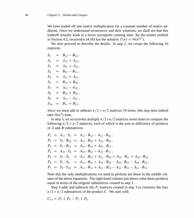
80 Chapter 4 Divide-and-Conquer
We have traded off one matrix multiplication for a constant number of matrix ad-ditions. Once we understand recurrences and their solutions, we shall see that thistradeoff actually leads to a lower asymptotic running time. By the master methodin Section 4.5, recurrence (4.18) has the solution T .n/ D ‚.nlg 7/.
We now proceed to describe the details. In step 2, we create the following 10
matrices:
S1 D B12 � B22 ;
S2 D A11 C A12 ;
S3 D A21 C A22 ;
S4 D B21 � B11 ;
S5 D A11 C A22 ;
S6 D B11 C B22 ;
S7 D A12 � A22 ;
S8 D B21 C B22 ;
S9 D A11 � A21 ;
S10 D B11 C B12 :
Since we must add or subtract n=2 n=2 matrices 10 times, this step does indeedtake ‚.n2/ time.
In step 3, we recursively multiply n=2n=2 matrices seven times to compute thefollowing n=2 n=2 matrices, each of which is the sum or difference of productsof A and B submatrices:
P1 D A11 � S1 D A11 � B12 � A11 � B22 ;
P2 D S2 � B22 D A11 � B22 C A12 � B22 ;
P3 D S3 � B11 D A21 � B11 C A22 � B11 ;
P4 D A22 � S4 D A22 � B21 � A22 � B11 ;
P5 D S5 � S6 D A11 � B11 C A11 � B22 C A22 � B11 C A22 � B22 ;
P6 D S7 � S8 D A12 � B21 C A12 � B22 � A22 � B21 � A22 � B22 ;
P7 D S9 � S10 D A11 � B11 C A11 � B12 � A21 � B11 � A21 � B12 :
Note that the only multiplications we need to perform are those in the middle col-umn of the above equations. The right-hand column just shows what these productsequal in terms of the original submatrices created in step 1.
Step 4 adds and subtracts the Pi matrices created in step 3 to construct the fourn=2 n=2 submatrices of the product C . We start with
C11 D P5 C P4 � P2 C P6 :

4.2 Strassen’s algorithm for matrix multiplication 81
Expanding out the right-hand side, with the expansion of each Pi on its own lineand vertically aligning terms that cancel out, we see that C11 equals
A11 �B11CA11 �B22CA22 �B11CA22 �B22
� A22 �B11 CA22 �B21
� A11 �B22 � A12 �B22
� A22 �B22� A22 �B21CA12 �B22CA12 �B21
A11 �B11 CA12 �B21 ;
which corresponds to equation (4.11).
Similarly, we set
C12 D P1 C P2 ;
and so C12 equals
A11 �B12 � A11 �B22
CA11 �B22CA12 �B22
A11 �B12 CA12 �B22 ;
corresponding to equation (4.12).
Setting
C21 D P3 C P4
makes C21 equal
A21 �B11CA22 �B11
� A22 �B11CA22 �B21
A21 �B11 CA22 �B21 ;
corresponding to equation (4.13).
Finally, we set
C22 D P5 C P1 � P3 � P7 ;
so that C22 equals
A11 �B11CA11 �B22CA22 �B11CA22 �B22
� A11 �B22 CA11 �B12
� A22 �B11 � A21 �B11
�A11 �B11 � A11 �B12CA21 �B11CA21 �B12
A22 �B22 CA21 �B12 ;

82 Chapter 4 Divide-and-Conquer
which corresponds to equation (4.14). Altogether, we add or subtract n=2 n=2
matrices eight times in step 4, and so this step indeed takes ‚.n2/ time.Thus, we see that Strassen’s algorithm, comprising steps 1–4, produces the cor-
rect matrix product and that recurrence (4.18) characterizes its running time. Sincewe shall see in Section 4.5 that this recurrence has the solution T .n/ D ‚.nlg 7/,Strassen’s method is asymptotically faster than the straightforward SQUARE-MATRIX-MULTIPLY procedure. The notes at the end of this chapter discuss someof the practical aspects of Strassen’s algorithm.
Exercises
Note: Although Exercises 4.2-3, 4.2-4, and 4.2-5 are about variants on Strassen’salgorithm, you should read Section 4.5 before trying to solve them.
4.2-1Use Strassen’s algorithm to compute the matrix product�
1 3
7 5
��6 8
4 2
�:
Show your work.
4.2-2Write pseudocode for Strassen’s algorithm.
4.2-3How would you modify Strassen’s algorithm to multiply nn matrices in which n
is not an exact power of 2? Show that the resulting algorithm runs in time ‚.nlg 7/.
4.2-4What is the largest k such that if you can multiply 3 3 matrices using k multi-plications (not assuming commutativity of multiplication), then you can multiplynn matrices in time o.nlg 7/? What would the running time of this algorithm be?
4.2-5V. Pan has discovered a way of multiplying 68 68 matrices using 132,464 mul-tiplications, a way of multiplying 70 70 matrices using 143,640 multiplications,and a way of multiplying 72 72 matrices using 155,424 multiplications. Whichmethod yields the best asymptotic running time when used in a divide-and-conquermatrix-multiplication algorithm? How does it compare to Strassen’s algorithm?
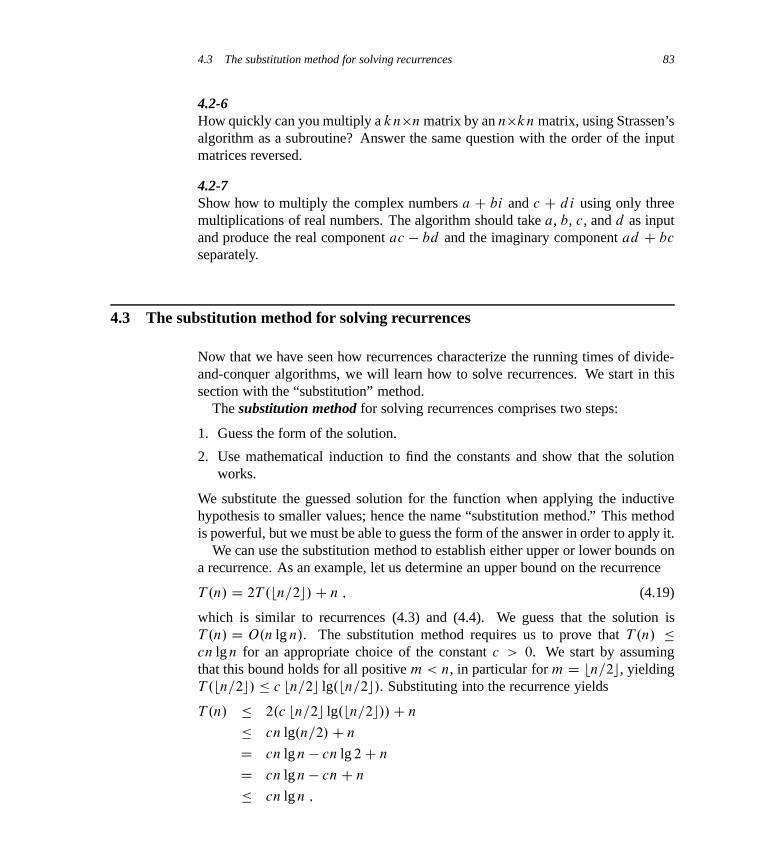
4.3 The substitution method for solving recurrences 83
4.2-6How quickly can you multiply a knn matrix by an nkn matrix, using Strassen’salgorithm as a subroutine? Answer the same question with the order of the inputmatrices reversed.
4.2-7Show how to multiply the complex numbers a C bi and c C di using only threemultiplications of real numbers. The algorithm should take a, b, c, and d as inputand produce the real component ac � bd and the imaginary component ad C bc
separately.
4.3 The substitution method for solving recurrences
Now that we have seen how recurrences characterize the running times of divide-and-conquer algorithms, we will learn how to solve recurrences. We start in thissection with the “substitution” method.
The substitution method for solving recurrences comprises two steps:
1. Guess the form of the solution.
2. Use mathematical induction to find the constants and show that the solutionworks.
We substitute the guessed solution for the function when applying the inductivehypothesis to smaller values; hence the name “substitution method.” This methodis powerful, but we must be able to guess the form of the answer in order to apply it.
We can use the substitution method to establish either upper or lower bounds ona recurrence. As an example, let us determine an upper bound on the recurrence
T .n/ D 2T .bn=2c/C n ; (4.19)
which is similar to recurrences (4.3) and (4.4). We guess that the solution isT .n/ D O.n lg n/. The substitution method requires us to prove that T .n/ �cn lg n for an appropriate choice of the constant c > 0. We start by assumingthat this bound holds for all positive m < n, in particular for m D bn=2c, yieldingT .bn=2c/ � c bn=2c lg.bn=2c/. Substituting into the recurrence yields
T .n/ � 2.c bn=2c lg.bn=2c//C n
� cn lg.n=2/C n
D cn lg n � cn lg 2C n
D cn lg n � cnC n
� cn lg n ;
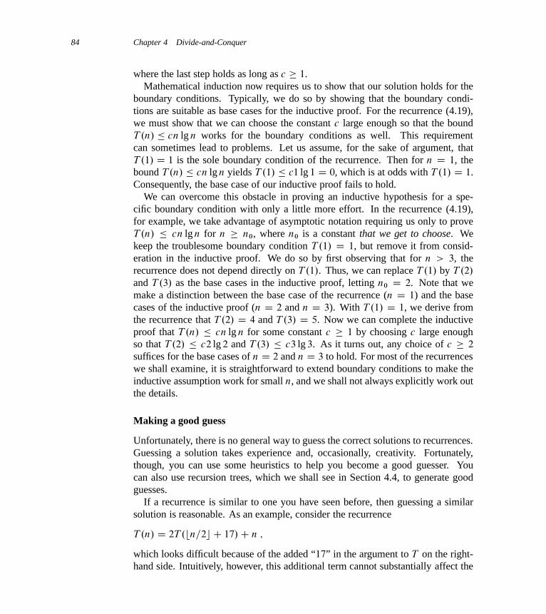
84 Chapter 4 Divide-and-Conquer
where the last step holds as long as c � 1.Mathematical induction now requires us to show that our solution holds for the
boundary conditions. Typically, we do so by showing that the boundary condi-tions are suitable as base cases for the inductive proof. For the recurrence (4.19),we must show that we can choose the constant c large enough so that the boundT .n/ � cn lg n works for the boundary conditions as well. This requirementcan sometimes lead to problems. Let us assume, for the sake of argument, thatT .1/ D 1 is the sole boundary condition of the recurrence. Then for n D 1, thebound T .n/ � cn lg n yields T .1/ � c1 lg 1 D 0, which is at odds with T .1/ D 1.Consequently, the base case of our inductive proof fails to hold.
We can overcome this obstacle in proving an inductive hypothesis for a spe-cific boundary condition with only a little more effort. In the recurrence (4.19),for example, we take advantage of asymptotic notation requiring us only to proveT .n/ � cn lg n for n � n0, where n0 is a constant that we get to choose. Wekeep the troublesome boundary condition T .1/ D 1, but remove it from consid-eration in the inductive proof. We do so by first observing that for n > 3, therecurrence does not depend directly on T .1/. Thus, we can replace T .1/ by T .2/
and T .3/ as the base cases in the inductive proof, letting n0 D 2. Note that wemake a distinction between the base case of the recurrence (n D 1) and the basecases of the inductive proof (n D 2 and n D 3). With T .1/ D 1, we derive fromthe recurrence that T .2/ D 4 and T .3/ D 5. Now we can complete the inductiveproof that T .n/ � cn lg n for some constant c � 1 by choosing c large enoughso that T .2/ � c2 lg 2 and T .3/ � c3 lg 3. As it turns out, any choice of c � 2
suffices for the base cases of n D 2 and n D 3 to hold. For most of the recurrenceswe shall examine, it is straightforward to extend boundary conditions to make theinductive assumption work for small n, and we shall not always explicitly work outthe details.
Making a good guess
Unfortunately, there is no general way to guess the correct solutions to recurrences.Guessing a solution takes experience and, occasionally, creativity. Fortunately,though, you can use some heuristics to help you become a good guesser. Youcan also use recursion trees, which we shall see in Section 4.4, to generate goodguesses.
If a recurrence is similar to one you have seen before, then guessing a similarsolution is reasonable. As an example, consider the recurrence
T .n/ D 2T .bn=2c C 17/C n ;
which looks difficult because of the added “17” in the argument to T on the right-hand side. Intuitively, however, this additional term cannot substantially affect the
4.3 The substitution method for solving recurrences 85
solution to the recurrence. When n is large, the difference between bn=2c andbn=2c C 17 is not that large: both cut n nearly evenly in half. Consequently, wemake the guess that T .n/ D O.n lg n/, which you can verify as correct by usingthe substitution method (see Exercise 4.3-6).
Another way to make a good guess is to prove loose upper and lower bounds onthe recurrence and then reduce the range of uncertainty. For example, we mightstart with a lower bound of T .n/ D �.n/ for the recurrence (4.19), since wehave the term n in the recurrence, and we can prove an initial upper bound ofT .n/ D O.n2/. Then, we can gradually lower the upper bound and raise thelower bound until we converge on the correct, asymptotically tight solution ofT .n/ D ‚.n lg n/.
Subtleties
Sometimes you might correctly guess an asymptotic bound on the solution of arecurrence, but somehow the math fails to work out in the induction. The problemfrequently turns out to be that the inductive assumption is not strong enough toprove the detailed bound. If you revise the guess by subtracting a lower-order termwhen you hit such a snag, the math often goes through.
Consider the recurrence
T .n/ D T .bn=2c/C T .dn=2e/C 1 :
We guess that the solution is T .n/ D O.n/, and we try to show that T .n/ � cn foran appropriate choice of the constant c. Substituting our guess in the recurrence,we obtain
T .n/ � c bn=2c C c dn=2e C 1
D cnC 1 ;
which does not imply T .n/ � cn for any choice of c. We might be tempted to trya larger guess, say T .n/ D O.n2/. Although we can make this larger guess work,our original guess of T .n/ D O.n/ is correct. In order to show that it is correct,however, we must make a stronger inductive hypothesis.
Intuitively, our guess is nearly right: we are off only by the constant 1, alower-order term. Nevertheless, mathematical induction does not work unless weprove the exact form of the inductive hypothesis. We overcome our difficultyby subtracting a lower-order term from our previous guess. Our new guess isT .n/ � cn � d , where d � 0 is a constant. We now have
T .n/ � .c bn=2c � d/C .c dn=2e � d/C 1
D cn� 2d C 1
� cn� d ;

86 Chapter 4 Divide-and-Conquer
as long as d � 1. As before, we must choose the constant c large enough to handlethe boundary conditions.
You might find the idea of subtracting a lower-order term counterintuitive. Af-ter all, if the math does not work out, we should increase our guess, right?Not necessarily! When proving an upper bound by induction, it may actually bemore difficult to prove that a weaker upper bound holds, because in order to provethe weaker bound, we must use the same weaker bound inductively in the proof.In our current example, when the recurrence has more than one recursive term, weget to subtract out the lower-order term of the proposed bound once per recursiveterm. In the above example, we subtracted out the constant d twice, once for theT .bn=2c/ term and once for the T .dn=2e/ term. We ended up with the inequalityT .n/ � cn� 2d C 1, and it was easy to find values of d to make cn� 2d C 1 beless than or equal to cn � d .
Avoiding pitfalls
It is easy to err in the use of asymptotic notation. For example, in the recur-rence (4.19) we can falsely “prove” T .n/ D O.n/ by guessing T .n/ � cn andthen arguing
T .n/ � 2.c bn=2c/C n
� cnC n
D O.n/ ; wrong!!
since c is a constant. The error is that we have not proved the exact form of theinductive hypothesis, that is, that T .n/ � cn. We therefore will explicitly provethat T .n/ � cn when we want to show that T .n/ D O.n/.
Changing variables
Sometimes, a little algebraic manipulation can make an unknown recurrence simi-lar to one you have seen before. As an example, consider the recurrence
T .n/ D 2T� p
n˘�C lg n ;
which looks difficult. We can simplify this recurrence, though, with a change ofvariables. For convenience, we shall not worry about rounding off values, suchasp
n, to be integers. Renaming m D lg n yields
T .2m/ D 2T .2m=2/Cm :
We can now rename S.m/ D T .2m/ to produce the new recurrence
S.m/ D 2S.m=2/Cm ;

4.3 The substitution method for solving recurrences 87
which is very much like recurrence (4.19). Indeed, this new recurrence has thesame solution: S.m/ D O.m lg m/. Changing back from S.m/ to T .n/, we obtain
T .n/ D T .2m/ D S.m/ D O.m lg m/ D O.lg n lg lg n/ :
Exercises
4.3-1Show that the solution of T .n/ D T .n � 1/C n is O.n2/.
4.3-2Show that the solution of T .n/ D T .dn=2e/C 1 is O.lg n/.
4.3-3We saw that the solution of T .n/ D 2T .bn=2c/Cn is O.n lg n/. Show that the so-lution of this recurrence is also �.n lg n/. Conclude that the solution is ‚.n lg n/.
4.3-4Show that by making a different inductive hypothesis, we can overcome the diffi-culty with the boundary condition T .1/ D 1 for recurrence (4.19) without adjustingthe boundary conditions for the inductive proof.
4.3-5Show that ‚.n lg n/ is the solution to the “exact” recurrence (4.3) for merge sort.
4.3-6Show that the solution to T .n/ D 2T .bn=2c C 17/C n is O.n lg n/.
4.3-7Using the master method in Section 4.5, you can show that the solution to therecurrence T .n/ D 4T .n=3/ C n is T .n/ D ‚.nlog3 4/. Show that a substitutionproof with the assumption T .n/ � cnlog3 4 fails. Then show how to subtract off alower-order term to make a substitution proof work.
4.3-8Using the master method in Section 4.5, you can show that the solution to therecurrence T .n/ D 4T .n=2/ C n2 is T .n/ D ‚.n2/. Show that a substitutionproof with the assumption T .n/ � cn2 fails. Then show how to subtract off alower-order term to make a substitution proof work.
88 Chapter 4 Divide-and-Conquer
4.3-9Solve the recurrence T .n/ D 3T .
pn/ C log n by making a change of variables.
Your solution should be asymptotically tight. Do not worry about whether valuesare integral.
4.4 The recursion-tree method for solving recurrences
Although you can use the substitution method to provide a succinct proof thata solution to a recurrence is correct, you might have trouble coming up with agood guess. Drawing out a recursion tree, as we did in our analysis of the mergesort recurrence in Section 2.3.2, serves as a straightforward way to devise a goodguess. In a recursion tree, each node represents the cost of a single subproblemsomewhere in the set of recursive function invocations. We sum the costs withineach level of the tree to obtain a set of per-level costs, and then we sum all theper-level costs to determine the total cost of all levels of the recursion.
A recursion tree is best used to generate a good guess, which you can then verifyby the substitution method. When using a recursion tree to generate a good guess,you can often tolerate a small amount of “sloppiness,” since you will be verifyingyour guess later on. If you are very careful when drawing out a recursion tree andsumming the costs, however, you can use a recursion tree as a direct proof of asolution to a recurrence. In this section, we will use recursion trees to generategood guesses, and in Section 4.6, we will use recursion trees directly to prove thetheorem that forms the basis of the master method.
For example, let us see how a recursion tree would provide a good guess forthe recurrence T .n/ D 3T .bn=4c/ C ‚.n2/. We start by focusing on finding anupper bound for the solution. Because we know that floors and ceilings usually donot matter when solving recurrences (here’s an example of sloppiness that we cantolerate), we create a recursion tree for the recurrence T .n/ D 3T .n=4/ C cn2,having written out the implied constant coefficient c > 0.
Figure 4.5 shows how we derive the recursion tree for T .n/ D 3T .n=4/C cn2.For convenience, we assume that n is an exact power of 4 (another example oftolerable sloppiness) so that all subproblem sizes are integers. Part (a) of the figureshows T .n/, which we expand in part (b) into an equivalent tree representing therecurrence. The cn2 term at the root represents the cost at the top level of recursion,and the three subtrees of the root represent the costs incurred by the subproblemsof size n=4. Part (c) shows this process carried one step further by expanding eachnode with cost T .n=4/ from part (b). The cost for each of the three children of theroot is c.n=4/2. We continue expanding each node in the tree by breaking it intoits constituent parts as determined by the recurrence.
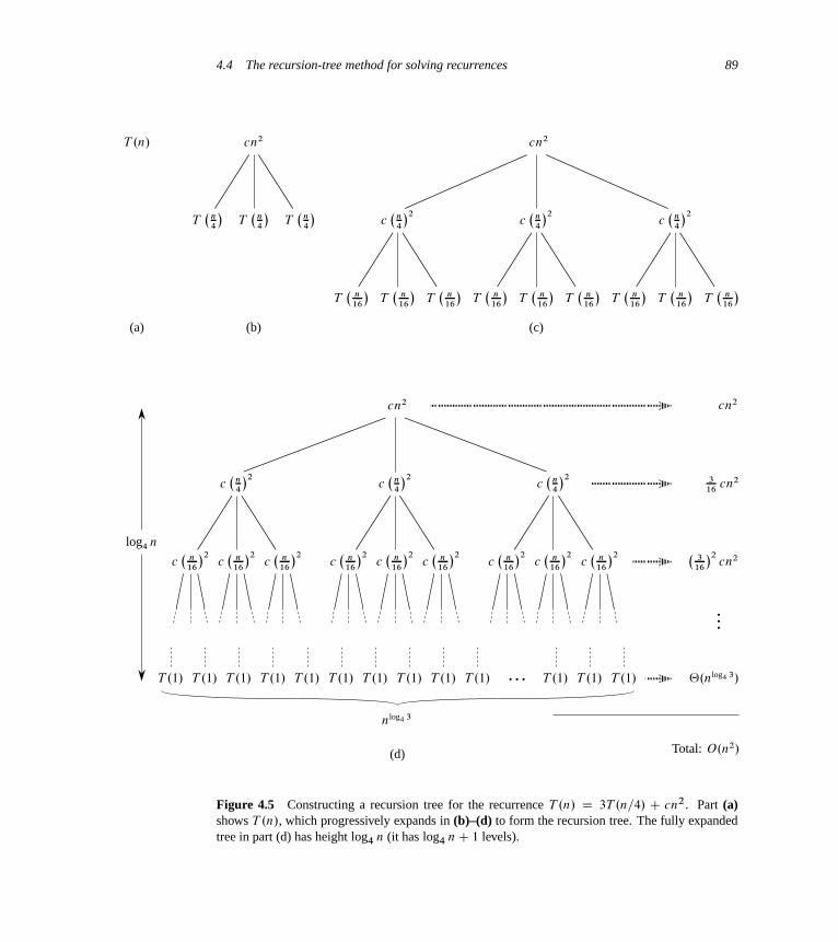
4.4 The recursion-tree method for solving recurrences 89
…
…
(d)
(c)(b)(a)
T .n/ cn2 cn2
cn2
T�
n4
�T�
n4
�T�
n4
�
T�
n16
�T�
n16
�T�
n16
�T�
n16
�T�
n16
�T�
n16
�T�
n16
�T�
n16
�T�
n16
�
cn2
c�
n4
�2c�
n4
�2c�
n4
�2
c�
n4
�2c�
n4
�2c�
n4
�2
c�
n16
�2c�
n16
�2c�
n16
�2c�
n16
�2c�
n16
�2c�
n16
�2c�
n16
�2c�
n16
�2c�
n16
�2
316
cn2
�3
16
�2cn2
log4 n
nlog4 3
T .1/T .1/T .1/T .1/T .1/T .1/T .1/T .1/T .1/T .1/T .1/T .1/T .1/ ‚.nlog4 3/
Total: O.n2/
Figure 4.5 Constructing a recursion tree for the recurrence T .n/ D 3T .n=4/ C cn2. Part (a)shows T .n/, which progressively expands in (b)–(d) to form the recursion tree. The fully expandedtree in part (d) has height log4 n (it has log4 nC 1 levels).
90 Chapter 4 Divide-and-Conquer
Because subproblem sizes decrease by a factor of 4 each time we go down onelevel, we eventually must reach a boundary condition. How far from the root dowe reach one? The subproblem size for a node at depth i is n=4i . Thus, thesubproblem size hits n D 1 when n=4i D 1 or, equivalently, when i D log4 n.Thus, the tree has log4 nC 1 levels (at depths 0; 1; 2; : : : ; log4 n).
Next we determine the cost at each level of the tree. Each level has three timesmore nodes than the level above, and so the number of nodes at depth i is 3i .Because subproblem sizes reduce by a factor of 4 for each level we go downfrom the root, each node at depth i , for i D 0; 1; 2; : : : ; log4 n � 1, has a costof c.n=4i /2. Multiplying, we see that the total cost over all nodes at depth i , fori D 0; 1; 2; : : : ; log4 n � 1, is 3ic.n=4i /2 D .3=16/i cn2. The bottom level, atdepth log4 n, has 3log4 n D nlog4 3 nodes, each contributing cost T .1/, for a totalcost of nlog4 3T .1/, which is ‚.nlog4 3/, since we assume that T .1/ is a constant.
Now we add up the costs over all levels to determine the cost for the entire tree:
T .n/ D cn2 C 3
16cn2 C
�3
16
�2
cn2 C � � � C�
3
16
�log4 n�1
cn2 C‚.nlog4 3/
Dlog4 n�1X
iD0
�3
16
�i
cn2 C‚.nlog4 3/
D .3=16/log4 n � 1
.3=16/ � 1cn2 C‚.nlog4 3/ (by equation (A.5)) :
This last formula looks somewhat messy until we realize that we can again takeadvantage of small amounts of sloppiness and use an infinite decreasing geometricseries as an upper bound. Backing up one step and applying equation (A.6), wehave
T .n/ Dlog4 n�1X
iD0
�3
16
�i
cn2 C‚.nlog4 3/
<
1XiD0
�3
16
�i
cn2 C‚.nlog4 3/
D 1
1 � .3=16/cn2 C‚.nlog4 3/
D 16
13cn2 C‚.nlog4 3/
D O.n2/ :
Thus, we have derived a guess of T .n/ D O.n2/ for our original recurrenceT .n/ D 3T .bn=4c/ C ‚.n2/. In this example, the coefficients of cn2 form adecreasing geometric series and, by equation (A.6), the sum of these coefficients
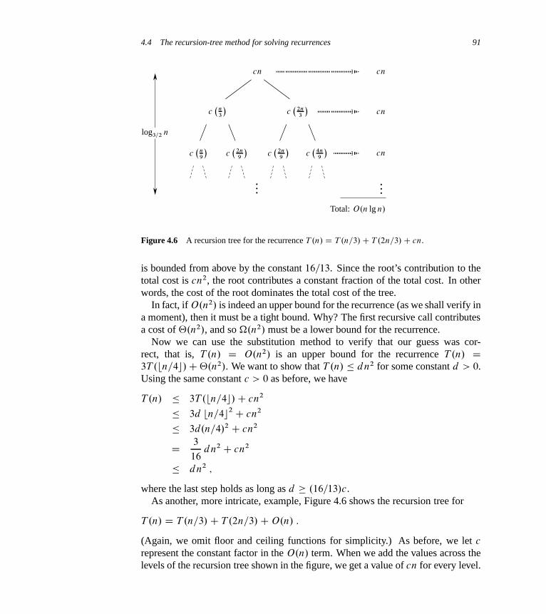
4.4 The recursion-tree method for solving recurrences 91
… …
cn
cn
cn
cn
c�
n3
�c�
2n3
�
c�
n9
�c�
2n9
�c�
2n9
�c�
4n9
�log3=2 n
Total: O.n lg n/
Figure 4.6 A recursion tree for the recurrence T .n/ D T .n=3/C T .2n=3/C cn.
is bounded from above by the constant 16=13. Since the root’s contribution to thetotal cost is cn2, the root contributes a constant fraction of the total cost. In otherwords, the cost of the root dominates the total cost of the tree.
In fact, if O.n2/ is indeed an upper bound for the recurrence (as we shall verify ina moment), then it must be a tight bound. Why? The first recursive call contributesa cost of ‚.n2/, and so �.n2/ must be a lower bound for the recurrence.
Now we can use the substitution method to verify that our guess was cor-rect, that is, T .n/ D O.n2/ is an upper bound for the recurrence T .n/ D3T .bn=4c/C‚.n2/. We want to show that T .n/ � dn2 for some constant d > 0.Using the same constant c > 0 as before, we have
T .n/ � 3T .bn=4c/C cn2
� 3d bn=4c2 C cn2
� 3d.n=4/2 C cn2
D 3
16dn2 C cn2
� dn2 ;
where the last step holds as long as d � .16=13/c.As another, more intricate, example, Figure 4.6 shows the recursion tree for
T .n/ D T .n=3/C T .2n=3/CO.n/ :
(Again, we omit floor and ceiling functions for simplicity.) As before, we let c
represent the constant factor in the O.n/ term. When we add the values across thelevels of the recursion tree shown in the figure, we get a value of cn for every level.
92 Chapter 4 Divide-and-Conquer
The longest simple path from the root to a leaf is n ! .2=3/n ! .2=3/2n !� � � ! 1. Since .2=3/kn D 1 when k D log3=2 n, the height of the tree is log3=2 n.
Intuitively, we expect the solution to the recurrence to be at most the numberof levels times the cost of each level, or O.cn log3=2 n/ D O.n lg n/. Figure 4.6shows only the top levels of the recursion tree, however, and not every level in thetree contributes a cost of cn. Consider the cost of the leaves. If this recursion treewere a complete binary tree of height log3=2 n, there would be 2log3=2 n D nlog3=2 2
leaves. Since the cost of each leaf is a constant, the total cost of all leaves wouldthen be ‚.nlog3=2 2/ which, since log3=2 2 is a constant strictly greater than 1,is !.n lg n/. This recursion tree is not a complete binary tree, however, and soit has fewer than nlog3=2 2 leaves. Moreover, as we go down from the root, moreand more internal nodes are absent. Consequently, levels toward the bottom of therecursion tree contribute less than cn to the total cost. We could work out an accu-rate accounting of all costs, but remember that we are just trying to come up with aguess to use in the substitution method. Let us tolerate the sloppiness and attemptto show that a guess of O.n lg n/ for the upper bound is correct.
Indeed, we can use the substitution method to verify that O.n lg n/ is an upperbound for the solution to the recurrence. We show that T .n/ � dn lg n, where d isa suitable positive constant. We have
T .n/ � T .n=3/C T .2n=3/C cn
� d.n=3/ lg.n=3/C d.2n=3/ lg.2n=3/C cn
D .d.n=3/ lg n � d.n=3/ lg 3/
C .d.2n=3/ lg n � d.2n=3/ lg.3=2//C cn
D dn lg n � d..n=3/ lg 3C .2n=3/ lg.3=2//C cn
D dn lg n � d..n=3/ lg 3C .2n=3/ lg 3 � .2n=3/ lg 2/C cn
D dn lg n � dn.lg 3 � 2=3/C cn
� dn lg n ;
as long as d � c=.lg 3� .2=3//. Thus, we did not need to perform a more accurateaccounting of costs in the recursion tree.
Exercises
4.4-1Use a recursion tree to determine a good asymptotic upper bound on the recurrenceT .n/ D 3T .bn=2c/C n. Use the substitution method to verify your answer.
4.4-2Use a recursion tree to determine a good asymptotic upper bound on the recurrenceT .n/ D T .n=2/C n2. Use the substitution method to verify your answer.
4.5 The master method for solving recurrences 93
4.4-3Use a recursion tree to determine a good asymptotic upper bound on the recurrenceT .n/ D 4T .n=2C 2/C n. Use the substitution method to verify your answer.
4.4-4Use a recursion tree to determine a good asymptotic upper bound on the recurrenceT .n/ D 2T .n � 1/C 1. Use the substitution method to verify your answer.
4.4-5Use a recursion tree to determine a good asymptotic upper bound on the recurrenceT .n/ D T .n�1/CT .n=2/Cn. Use the substitution method to verify your answer.
4.4-6Argue that the solution to the recurrence T .n/ D T .n=3/CT .2n=3/Ccn, where c
is a constant, is �.n lg n/ by appealing to a recursion tree.
4.4-7Draw the recursion tree for T .n/ D 4T .bn=2c/ C cn, where c is a constant, andprovide a tight asymptotic bound on its solution. Verify your bound by the substi-tution method.
4.4-8Use a recursion tree to give an asymptotically tight solution to the recurrenceT .n/ D T .n � a/C T .a/C cn, where a � 1 and c > 0 are constants.
4.4-9Use a recursion tree to give an asymptotically tight solution to the recurrenceT .n/ D T .˛n/C T ..1� ˛/n/C cn, where ˛ is a constant in the range 0 < ˛ < 1
and c > 0 is also a constant.
4.5 The master method for solving recurrences
The master method provides a “cookbook” method for solving recurrences of theform
T .n/ D aT .n=b/C f .n/ ; (4.20)
where a � 1 and b > 1 are constants and f .n/ is an asymptotically positivefunction. To use the master method, you will need to memorize three cases, butthen you will be able to solve many recurrences quite easily, often without penciland paper.

94 Chapter 4 Divide-and-Conquer
The recurrence (4.20) describes the running time of an algorithm that divides aproblem of size n into a subproblems, each of size n=b, where a and b are positiveconstants. The a subproblems are solved recursively, each in time T .n=b/. Thefunction f .n/ encompasses the cost of dividing the problem and combining theresults of the subproblems. For example, the recurrence arising from Strassen’salgorithm has a D 7, b D 2, and f .n/ D ‚.n2/.
As a matter of technical correctness, the recurrence is not actually well defined,because n=b might not be an integer. Replacing each of the a terms T .n=b/ witheither T .bn=bc/ or T .dn=be/ will not affect the asymptotic behavior of the recur-rence, however. (We will prove this assertion in the next section.) We normallyfind it convenient, therefore, to omit the floor and ceiling functions when writingdivide-and-conquer recurrences of this form.
The master theorem
The master method depends on the following theorem.
Theorem 4.1 (Master theorem)Let a � 1 and b > 1 be constants, let f .n/ be a function, and let T .n/ be definedon the nonnegative integers by the recurrence
T .n/ D aT .n=b/C f .n/ ;
where we interpret n=b to mean either bn=bc or dn=be. Then T .n/ has the follow-ing asymptotic bounds:
1. If f .n/ D O.nlogb a��/ for some constant � > 0, then T .n/ D ‚.nlogb a/.
2. If f .n/ D ‚.nlogb a/, then T .n/ D ‚.nlogb a lg n/.
3. If f .n/ D �.nlogb aC�/ for some constant � > 0, and if af .n=b/ � cf .n/ forsome constant c < 1 and all sufficiently large n, then T .n/ D ‚.f .n//.
Before applying the master theorem to some examples, let’s spend a momenttrying to understand what it says. In each of the three cases, we compare thefunction f .n/ with the function nlogb a. Intuitively, the larger of the two functionsdetermines the solution to the recurrence. If, as in case 1, the function nlogb a is thelarger, then the solution is T .n/ D ‚.nlogb a/. If, as in case 3, the function f .n/
is the larger, then the solution is T .n/ D ‚.f .n//. If, as in case 2, the two func-tions are the same size, we multiply by a logarithmic factor, and the solution isT .n/ D ‚.nlogb a lg n/ D ‚.f .n/ lg n/.
Beyond this intuition, you need to be aware of some technicalities. In the firstcase, not only must f .n/ be smaller than nlogb a, it must be polynomially smaller.

4.5 The master method for solving recurrences 95
That is, f .n/ must be asymptotically smaller than nlogb a by a factor of n� for someconstant � > 0. In the third case, not only must f .n/ be larger than nlogb a, itmust be polynomially larger and in addition satisfy the “regularity” condition thataf .n=b/ � cf .n/. This condition is satisfied by most of the polynomially boundedfunctions that we shall encounter.
Note that the three cases do not cover all the possibilities for f .n/. There isa gap between cases 1 and 2 when f .n/ is smaller than nlogb a but not polynomi-ally smaller. Similarly, there is a gap between cases 2 and 3 when f .n/ is largerthan nlogb a but not polynomially larger. If the function f .n/ falls into one of thesegaps, or if the regularity condition in case 3 fails to hold, you cannot use the mastermethod to solve the recurrence.
Using the master method
To use the master method, we simply determine which case (if any) of the mastertheorem applies and write down the answer.
As a first example, consider
T .n/ D 9T .n=3/C n :
For this recurrence, we have a D 9, b D 3, f .n/ D n, and thus we have thatnlogb a D nlog3 9 D ‚.n2). Since f .n/ D O.nlog3 9��/, where � D 1, we can applycase 1 of the master theorem and conclude that the solution is T .n/ D ‚.n2/.
Now consider
T .n/ D T .2n=3/C 1;
in which a D 1, b D 3=2, f .n/ D 1, and nlogb a D nlog3=2 1 D n0 D 1. Case 2applies, since f .n/ D ‚.nlogb a/ D ‚.1/, and thus the solution to the recurrenceis T .n/ D ‚.lg n/.
For the recurrence
T .n/ D 3T .n=4/C n lg n ;
we have a D 3, b D 4, f .n/ D n lg n, and nlogb a D nlog4 3 D O.n0:793/.Since f .n/ D �.nlog4 3C�/, where � � 0:2, case 3 applies if we can show thatthe regularity condition holds for f .n/. For sufficiently large n, we have thataf .n=b/ D 3.n=4/ lg.n=4/ � .3=4/n lg n D cf .n/ for c D 3=4. Consequently,by case 3, the solution to the recurrence is T .n/ D ‚.n lg n/.
The master method does not apply to the recurrence
T .n/ D 2T .n=2/C n lg n ;
even though it appears to have the proper form: a D 2, b D 2, f .n/ D n lg n,and nlogb a D n. You might mistakenly think that case 3 should apply, since

96 Chapter 4 Divide-and-Conquer
f .n/ D n lg n is asymptotically larger than nlogb a D n. The problem is that itis not polynomially larger. The ratio f .n/=nlogb a D .n lg n/=n D lg n is asymp-totically less than n� for any positive constant �. Consequently, the recurrence fallsinto the gap between case 2 and case 3. (See Exercise 4.6-2 for a solution.)
Let’s use the master method to solve the recurrences we saw in Sections 4.1and 4.2. Recurrence (4.7),
T .n/ D 2T .n=2/C‚.n/ ;
characterizes the running times of the divide-and-conquer algorithm for both themaximum-subarray problem and merge sort. (As is our practice, we omit statingthe base case in the recurrence.) Here, we have a D 2, b D 2, f .n/ D ‚.n/, andthus we have that nlogb a D nlog2 2 D n. Case 2 applies, since f .n/ D ‚.n/, and sowe have the solution T .n/ D ‚.n lg n/.
Recurrence (4.17),
T .n/ D 8T .n=2/C‚.n2/ ;
describes the running time of the first divide-and-conquer algorithm that we sawfor matrix multiplication. Now we have a D 8, b D 2, and f .n/ D ‚.n2/,and so nlogb a D nlog2 8 D n3. Since n3 is polynomially larger than f .n/ (that is,f .n/ D O.n3��/ for � D 1), case 1 applies, and T .n/ D ‚.n3/.
Finally, consider recurrence (4.18),
T .n/ D 7T .n=2/C‚.n2/ ;
which describes the running time of Strassen’s algorithm. Here, we have a D 7,b D 2, f .n/ D ‚.n2/, and thus nlogb a D nlog2 7. Rewriting log2 7 as lg 7 andrecalling that 2:80 < lg 7 < 2:81, we see that f .n/ D O.nlg 7��/ for � D 0:8.Again, case 1 applies, and we have the solution T .n/ D ‚.nlg 7/.
Exercises
4.5-1Use the master method to give tight asymptotic bounds for the following recur-rences.
a. T .n/ D 2T .n=4/C 1.
b. T .n/ D 2T .n=4/Cpn.
c. T .n/ D 2T .n=4/C n.
d. T .n/ D 2T .n=4/C n2.

4.6 Proof of the master theorem 97
4.5-2Professor Caesar wishes to develop a matrix-multiplication algorithm that isasymptotically faster than Strassen’s algorithm. His algorithm will use the divide-and-conquer method, dividing each matrix into pieces of size n=4 n=4, and thedivide and combine steps together will take ‚.n2/ time. He needs to determinehow many subproblems his algorithm has to create in order to beat Strassen’s algo-rithm. If his algorithm creates a subproblems, then the recurrence for the runningtime T .n/ becomes T .n/ D aT .n=4/ C ‚.n2/. What is the largest integer valueof a for which Professor Caesar’s algorithm would be asymptotically faster thanStrassen’s algorithm?
4.5-3Use the master method to show that the solution to the binary-search recurrenceT .n/ D T .n=2/C‚.1/ is T .n/ D ‚.lg n/. (See Exercise 2.3-5 for a descriptionof binary search.)
4.5-4Can the master method be applied to the recurrence T .n/ D 4T .n=2/ C n2 lg n?Why or why not? Give an asymptotic upper bound for this recurrence.
4.5-5 ?
Consider the regularity condition af .n=b/ � cf .n/ for some constant c < 1,which is part of case 3 of the master theorem. Give an example of constants a � 1
and b > 1 and a function f .n/ that satisfies all the conditions in case 3 of themaster theorem except the regularity condition.
? 4.6 Proof of the master theorem
This section contains a proof of the master theorem (Theorem 4.1). You do notneed to understand the proof in order to apply the master theorem.
The proof appears in two parts. The first part analyzes the master recur-rence (4.20), under the simplifying assumption that T .n/ is defined only on ex-act powers of b > 1, that is, for n D 1; b; b2; : : :. This part gives all the intuitionneeded to understand why the master theorem is true. The second part shows howto extend the analysis to all positive integers n; it applies mathematical techniqueto the problem of handling floors and ceilings.
In this section, we shall sometimes abuse our asymptotic notation slightly byusing it to describe the behavior of functions that are defined only over exactpowers of b. Recall that the definitions of asymptotic notations require that

98 Chapter 4 Divide-and-Conquer
bounds be proved for all sufficiently large numbers, not just those that are pow-ers of b. Since we could make new asymptotic notations that apply only to the setfbi W i D 0; 1; 2; : : :g, instead of to the nonnegative numbers, this abuse is minor.
Nevertheless, we must always be on guard when we use asymptotic notation overa limited domain lest we draw improper conclusions. For example, proving thatT .n/ D O.n/ when n is an exact power of 2 does not guarantee that T .n/ D O.n/.The function T .n/ could be defined as
T .n/ D(
n if n D 1; 2; 4; 8; : : : ;
n2 otherwise ;
in which case the best upper bound that applies to all values of n is T .n/ D O.n2/.Because of this sort of drastic consequence, we shall never use asymptotic notationover a limited domain without making it absolutely clear from the context that weare doing so.
4.6.1 The proof for exact powers
The first part of the proof of the master theorem analyzes the recurrence (4.20)
T .n/ D aT .n=b/C f .n/ ;
for the master method, under the assumption that n is an exact power of b > 1,where b need not be an integer. We break the analysis into three lemmas. The firstreduces the problem of solving the master recurrence to the problem of evaluatingan expression that contains a summation. The second determines bounds on thissummation. The third lemma puts the first two together to prove a version of themaster theorem for the case in which n is an exact power of b.
Lemma 4.2Let a � 1 and b > 1 be constants, and let f .n/ be a nonnegative function definedon exact powers of b. Define T .n/ on exact powers of b by the recurrence
T .n/ D(
‚.1/ if n D 1 ;
aT .n=b/C f .n/ if n D bi ;
where i is a positive integer. Then
T .n/ D ‚.nlogb a/Clogb n�1X
j D0
aj f .n=bj / : (4.21)
Proof We use the recursion tree in Figure 4.7. The root of the tree has cost f .n/,and it has a children, each with cost f .n=b/. (It is convenient to think of a as being
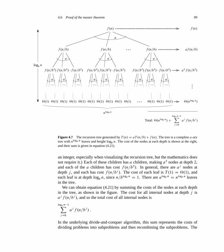
4.6 Proof of the master theorem 99
…
…
…
… … …
…
… … …
…
… … …
…
f .n/ f .n/
aaa
a
aaa
a
aaa
a
a
f .n=b/f .n=b/f .n=b/
f .n=b2/f .n=b2/f .n=b2/f .n=b2/f .n=b2/f .n=b2/f .n=b2/f .n=b2/f .n=b2/
af .n=b/
a2f .n=b2/
logb n
nlogb a
‚.1/‚.1/‚.1/‚.1/‚.1/‚.1/‚.1/‚.1/‚.1/‚.1/‚.1/‚.1/‚.1/ ‚.nlogb a/
Total: ‚.nlogb a/Clogb n�1X
j D0
aj f .n=bj /
Figure 4.7 The recursion tree generated by T .n/ D aT .n=b/Cf .n/. The tree is a complete a-arytree with nlogb a leaves and height logb n. The cost of the nodes at each depth is shown at the right,and their sum is given in equation (4.21).
an integer, especially when visualizing the recursion tree, but the mathematics doesnot require it.) Each of these children has a children, making a2 nodes at depth 2,and each of the a children has cost f .n=b2/. In general, there are aj nodes atdepth j , and each has cost f .n=bj /. The cost of each leaf is T .1/ D ‚.1/, andeach leaf is at depth logb n, since n=blogb n D 1. There are alogb n D nlogb a leavesin the tree.
We can obtain equation (4.21) by summing the costs of the nodes at each depthin the tree, as shown in the figure. The cost for all internal nodes at depth j isaj f .n=bj /, and so the total cost of all internal nodes is
logb n�1Xj D0
aj f .n=bj / :
In the underlying divide-and-conquer algorithm, this sum represents the costs ofdividing problems into subproblems and then recombining the subproblems. The
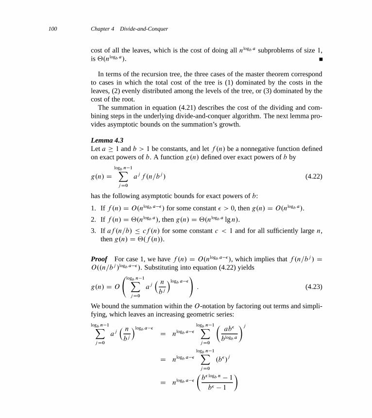
100 Chapter 4 Divide-and-Conquer
cost of all the leaves, which is the cost of doing all nlogb a subproblems of size 1,is ‚.nlogb a/.
In terms of the recursion tree, the three cases of the master theorem correspondto cases in which the total cost of the tree is (1) dominated by the costs in theleaves, (2) evenly distributed among the levels of the tree, or (3) dominated by thecost of the root.
The summation in equation (4.21) describes the cost of the dividing and com-bining steps in the underlying divide-and-conquer algorithm. The next lemma pro-vides asymptotic bounds on the summation’s growth.
Lemma 4.3Let a � 1 and b > 1 be constants, and let f .n/ be a nonnegative function definedon exact powers of b. A function g.n/ defined over exact powers of b by
g.n/ Dlogb n�1X
j D0
aj f .n=bj / (4.22)
has the following asymptotic bounds for exact powers of b:
1. If f .n/ D O.nlogb a��/ for some constant � > 0, then g.n/ D O.nlogb a/.
2. If f .n/ D ‚.nlogb a/, then g.n/ D ‚.nlogb a lg n/.
3. If af .n=b/ � cf .n/ for some constant c < 1 and for all sufficiently large n,then g.n/ D ‚.f .n//.
Proof For case 1, we have f .n/ D O.nlogb a��/, which implies that f .n=bj / DO..n=bj /logb a��/. Substituting into equation (4.22) yields
g.n/ D O
logb n�1X
j D0
aj� n
bj
�logb a��
!: (4.23)
We bound the summation within the O-notation by factoring out terms and simpli-fying, which leaves an increasing geometric series:
logb n�1Xj D0
aj� n
bj
�logb a��
D nlogb a��
logb n�1Xj D0
�ab�
blogb a
�j
D nlogb a��
logb n�1Xj D0
.b�/j
D nlogb a��
�b� logb n � 1
b� � 1
�
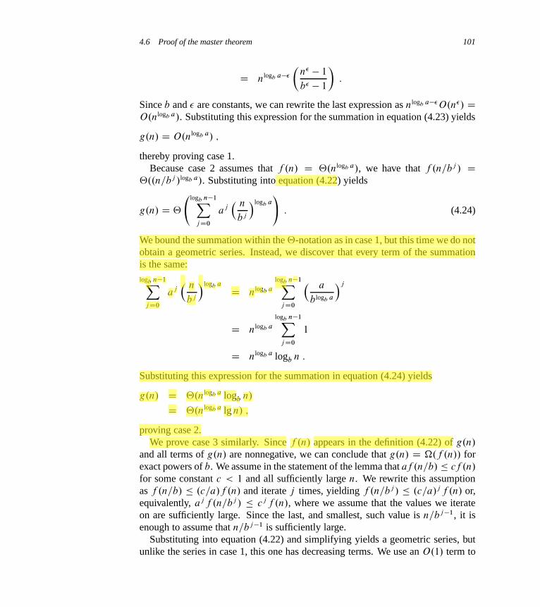
4.6 Proof of the master theorem 101
D nlogb a��
�n� � 1
b� � 1
�:
Since b and � are constants, we can rewrite the last expression as nlogb a��O.n�/ DO.nlogb a/. Substituting this expression for the summation in equation (4.23) yields
g.n/ D O.nlogb a/ ;
thereby proving case 1.Because case 2 assumes that f .n/ D ‚.nlogb a/, we have that f .n=bj / D
‚..n=bj /logb a/. Substituting into equation (4.22) yields
g.n/ D ‚
logb n�1X
j D0
aj� n
bj
�logb a
!: (4.24)
We bound the summation within the ‚-notation as in case 1, but this time we do notobtain a geometric series. Instead, we discover that every term of the summationis the same:logb n�1X
j D0
aj� n
bj
�logb a
D nlogb a
logb n�1Xj D0
� a
blogb a
�j
D nlogb a
logb n�1Xj D0
1
D nlogb a logb n :
Substituting this expression for the summation in equation (4.24) yields
g.n/ D ‚.nlogb a logb n/
D ‚.nlogb a lg n/ ;
proving case 2.We prove case 3 similarly. Since f .n/ appears in the definition (4.22) of g.n/
and all terms of g.n/ are nonnegative, we can conclude that g.n/ D �.f .n// forexact powers of b. We assume in the statement of the lemma that af .n=b/ � cf .n/
for some constant c < 1 and all sufficiently large n. We rewrite this assumptionas f .n=b/ � .c=a/f .n/ and iterate j times, yielding f .n=bj / � .c=a/j f .n/ or,equivalently, aj f .n=bj / � cj f .n/, where we assume that the values we iterateon are sufficiently large. Since the last, and smallest, such value is n=bj �1, it isenough to assume that n=bj �1 is sufficiently large.
Substituting into equation (4.22) and simplifying yields a geometric series, butunlike the series in case 1, this one has decreasing terms. We use an O.1/ term to
Injector
Highlight
Injector
Highlight
Injector
Highlight

102 Chapter 4 Divide-and-Conquer
capture the terms that are not covered by our assumption that n is sufficiently large:
g.n/ Dlogb n�1X
j D0
aj f .n=bj /
�logb n�1X
j D0
cj f .n/CO.1/
� f .n/
1Xj D0
cj CO.1/
D f .n/
�1
1 � c
�CO.1/
D O.f .n// ;
since c is a constant. Thus, we can conclude that g.n/ D ‚.f .n// for exact powersof b. With case 3 proved, the proof of the lemma is complete.
We can now prove a version of the master theorem for the case in which n is anexact power of b.
Lemma 4.4Let a � 1 and b > 1 be constants, and let f .n/ be a nonnegative function definedon exact powers of b. Define T .n/ on exact powers of b by the recurrence
T .n/ D(
‚.1/ if n D 1 ;
aT .n=b/C f .n/ if n D bi ;
where i is a positive integer. Then T .n/ has the following asymptotic bounds forexact powers of b:
1. If f .n/ D O.nlogb a��/ for some constant � > 0, then T .n/ D ‚.nlogb a/.
2. If f .n/ D ‚.nlogb a/, then T .n/ D ‚.nlogb a lg n/.
3. If f .n/ D �.nlogb aC�/ for some constant � > 0, and if af .n=b/ � cf .n/ forsome constant c < 1 and all sufficiently large n, then T .n/ D ‚.f .n//.
Proof We use the bounds in Lemma 4.3 to evaluate the summation (4.21) fromLemma 4.2. For case 1, we have
T .n/ D ‚.nlogb a/CO.nlogb a/
D ‚.nlogb a/ ;

4.6 Proof of the master theorem 103
and for case 2,
T .n/ D ‚.nlogb a/C‚.nlogb a lg n/
D ‚.nlogb a lg n/ :
For case 3,
T .n/ D ‚.nlogb a/C‚.f .n//
D ‚.f .n// ;
because f .n/ D �.nlogb aC�/.
4.6.2 Floors and ceilings
To complete the proof of the master theorem, we must now extend our analysis tothe situation in which floors and ceilings appear in the master recurrence, so thatthe recurrence is defined for all integers, not for just exact powers of b. Obtaininga lower bound on
T .n/ D aT .dn=be/C f .n/ (4.25)
and an upper bound on
T .n/ D aT .bn=bc/C f .n/ (4.26)
is routine, since we can push through the bound dn=be � n=b in the first case toyield the desired result, and we can push through the bound bn=bc � n=b in thesecond case. We use much the same technique to lower-bound the recurrence (4.26)as to upper-bound the recurrence (4.25), and so we shall present only this latterbound.
We modify the recursion tree of Figure 4.7 to produce the recursion tree in Fig-ure 4.8. As we go down in the recursion tree, we obtain a sequence of recursiveinvocations on the arguments
n ;
dn=be ;
ddn=be =be ;
dddn=be =be =be ;
:::
Let us denote the j th element in the sequence by nj , where
nj D(
n if j D 0 ;
dnj �1=be if j > 0 :(4.27)
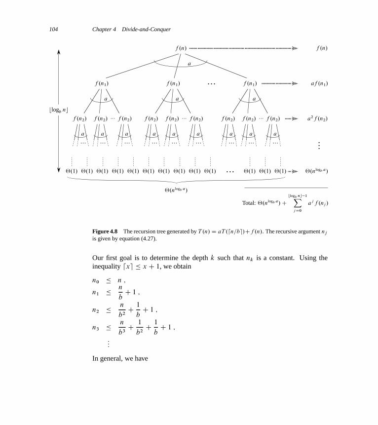
104 Chapter 4 Divide-and-Conquer
…
…
…
… … …
…
… … …
…
… … …
…
f .n/ f .n/
aaa
a
aaa
a
aaa
a
a
f .n1/f .n1/f .n1/
f .n2/f .n2/f .n2/f .n2/f .n2/f .n2/f .n2/f .n2/f .n2/
af .n1/
a2f .n2/
blogb nc
‚.nlogb a/
‚.1/‚.1/‚.1/‚.1/‚.1/‚.1/‚.1/‚.1/‚.1/‚.1/‚.1/‚.1/‚.1/ ‚.nlogb a/
Total: ‚.nlogb a/Cblogb nc�1X
j D0
aj f .nj /
Figure 4.8 The recursion tree generated by T .n/ D aT .dn=be/Cf .n/. The recursive argument nj
is given by equation (4.27).
Our first goal is to determine the depth k such that nk is a constant. Using theinequality dxe � x C 1, we obtain
n0 � n ;
n1 � n
bC 1 ;
n2 � n
b2C 1
bC 1 ;
n3 �n
b3C 1
b2C 1
bC 1 ;
:::
In general, we have

4.6 Proof of the master theorem 105
nj � n
bjC
j �1XiD0
1
bi
<n
bjC
1XiD0
1
bi
D n
bjC b
b � 1:
Letting j D blogb nc, we obtain
nblogb nc <n
bblogb nc Cb
b � 1
<n
blogb n�1C b
b � 1
D n
n=bC b
b � 1
D b C b
b � 1D O.1/ ;
and thus we see that at depth blogb nc, the problem size is at most a constant.From Figure 4.8, we see that
T .n/ D ‚.nlogb a/Cblogb nc�1X
j D0
aj f .nj / ; (4.28)
which is much the same as equation (4.21), except that n is an arbitrary integer andnot restricted to be an exact power of b.
We can now evaluate the summation
g.n/ Dblogb nc�1X
j D0
aj f .nj / (4.29)
from equation (4.28) in a manner analogous to the proof of Lemma 4.3. Beginningwith case 3, if af .dn=be/ � cf .n/ for n > bCb=.b�1/, where c < 1 is a constant,then it follows that aj f .nj / � cj f .n/. Therefore, we can evaluate the sum inequation (4.29) just as in Lemma 4.3. For case 2, we have f .n/ D ‚.nlogb a/. If wecan show that f .nj / D O.nlogb a=aj / D O..n=bj /logb a/, then the proof for case 2of Lemma 4.3 will go through. Observe that j � blogb nc implies bj =n � 1. Thebound f .n/ D O.nlogb a/ implies that there exists a constant c > 0 such that for allsufficiently large nj ,

106 Chapter 4 Divide-and-Conquer
f .nj / � c
�n
bjC b
b � 1
�logb a
D c
�n
bj
�1C bj
n� b
b � 1
��logb a
D c
�nlogb a
aj
��1C
�bj
n� b
b � 1
��logb a
� c
�nlogb a
aj
��1C b
b � 1
�logb a
D O
�nlogb a
aj
�;
since c.1C b=.b � 1//logb a is a constant. Thus, we have proved case 2. The proofof case 1 is almost identical. The key is to prove the bound f .nj / D O.nlogb a��/,which is similar to the corresponding proof of case 2, though the algebra is moreintricate.
We have now proved the upper bounds in the master theorem for all integers n.The proof of the lower bounds is similar.
Exercises
4.6-1 ?
Give a simple and exact expression for nj in equation (4.27) for the case in which b
is a positive integer instead of an arbitrary real number.
4.6-2 ?
Show that if f .n/ D ‚.nlogb a lgk n/, where k � 0, then the master recurrence hassolution T .n/ D ‚.nlogb a lgkC1 n/. For simplicity, confine your analysis to exactpowers of b.
4.6-3 ?
Show that case 3 of the master theorem is overstated, in the sense that the regularitycondition af .n=b/ � cf .n/ for some constant c < 1 implies that there exists aconstant � > 0 such that f .n/ D �.nlogb aC�/.
Problems for Chapter 4 107
Problems
4-1 Recurrence examplesGive asymptotic upper and lower bounds for T .n/ in each of the following recur-rences. Assume that T .n/ is constant for n � 2. Make your bounds as tight aspossible, and justify your answers.
a. T .n/ D 2T .n=2/C n4.
b. T .n/ D T .7n=10/C n.
c. T .n/ D 16T .n=4/C n2.
d. T .n/ D 7T .n=3/C n2.
e. T .n/ D 7T .n=2/C n2.
f. T .n/ D 2T .n=4/Cpn.
g. T .n/ D T .n � 2/C n2.
4-2 Parameter-passing costsThroughout this book, we assume that parameter passing during procedure callstakes constant time, even if an N -element array is being passed. This assumptionis valid in most systems because a pointer to the array is passed, not the array itself.This problem examines the implications of three parameter-passing strategies:
1. An array is passed by pointer. Time D ‚.1/.
2. An array is passed by copying. Time D ‚.N /, where N is the size of the array.
3. An array is passed by copying only the subrange that might be accessed by thecalled procedure. Time D ‚.q � p C 1/ if the subarray AŒp : : q� is passed.
a. Consider the recursive binary search algorithm for finding a number in a sortedarray (see Exercise 2.3-5). Give recurrences for the worst-case running timesof binary search when arrays are passed using each of the three methods above,and give good upper bounds on the solutions of the recurrences. Let N be thesize of the original problem and n be the size of a subproblem.
b. Redo part (a) for the MERGE-SORT algorithm from Section 2.3.1.
108 Chapter 4 Divide-and-Conquer
4-3 More recurrence examplesGive asymptotic upper and lower bounds for T .n/ in each of the following recur-rences. Assume that T .n/ is constant for sufficiently small n. Make your boundsas tight as possible, and justify your answers.
a. T .n/ D 4T .n=3/C n lg n.
b. T .n/ D 3T .n=3/C n= lg n.
c. T .n/ D 4T .n=2/C n2p
n.
d. T .n/ D 3T .n=3 � 2/C n=2.
e. T .n/ D 2T .n=2/C n= lg n.
f. T .n/ D T .n=2/C T .n=4/C T .n=8/C n.
g. T .n/ D T .n � 1/C 1=n.
h. T .n/ D T .n � 1/C lg n.
i. T .n/ D T .n � 2/C 1= lg n.
j. T .n/ D pnT .p
n/C n.
4-4 Fibonacci numbersThis problem develops properties of the Fibonacci numbers, which are definedby recurrence (3.22). We shall use the technique of generating functions to solvethe Fibonacci recurrence. Define the generating function (or formal power se-ries) F as
F .´/ D1X
iD0
Fi´i
D 0C ´C ´2 C 2´3 C 3´4 C 5´5 C 8´6 C 13´7 C 21´8 C � � � ;
where Fi is the i th Fibonacci number.
a. Show that F .´/ D ´C ´F .´/C ´2F .´/.

Problems for Chapter 4 109
b. Show that
F .´/ D ´
1� ´ � ´2
D ´
.1� �´/.1 � y�´/
D 1p5
�1
1� �´� 1
1� y�´
�;
where
� D 1Cp5
2D 1:61803 : : :
and
y� D 1�p5
2D �0:61803 : : : :
c. Show that
F .´/ D1X
iD0
1p5
.�i � y�i /´i :
d. Use part (c) to prove that Fi D �i =p
5 for i > 0, rounded to the nearest integer.(Hint: Observe that
ˇ̌y� ˇ̌ < 1.)
4-5 Chip testingProfessor Diogenes has n supposedly identical integrated-circuit chips that in prin-ciple are capable of testing each other. The professor’s test jig accommodates twochips at a time. When the jig is loaded, each chip tests the other and reports whetherit is good or bad. A good chip always reports accurately whether the other chip isgood or bad, but the professor cannot trust the answer of a bad chip. Thus, the fourpossible outcomes of a test are as follows:
Chip A says Chip B says ConclusionB is good A is good both are good, or both are badB is good A is bad at least one is badB is bad A is good at least one is badB is bad A is bad at least one is bad
a. Show that if more than n=2 chips are bad, the professor cannot necessarily de-termine which chips are good using any strategy based on this kind of pairwisetest. Assume that the bad chips can conspire to fool the professor.
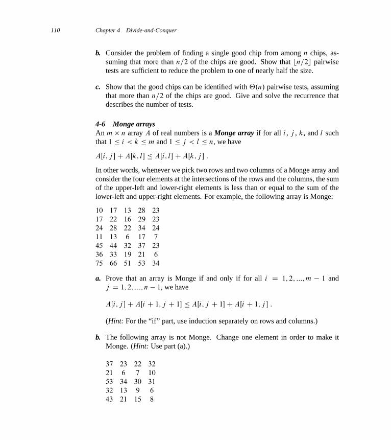
110 Chapter 4 Divide-and-Conquer
b. Consider the problem of finding a single good chip from among n chips, as-suming that more than n=2 of the chips are good. Show that bn=2c pairwisetests are sufficient to reduce the problem to one of nearly half the size.
c. Show that the good chips can be identified with ‚.n/ pairwise tests, assumingthat more than n=2 of the chips are good. Give and solve the recurrence thatdescribes the number of tests.
4-6 Monge arraysAn m n array A of real numbers is a Monge array if for all i , j , k, and l suchthat 1 � i < k � m and 1 � j < l � n, we have
AŒi; j �C AŒk; l� � AŒi; l�C AŒk; j � :
In other words, whenever we pick two rows and two columns of a Monge array andconsider the four elements at the intersections of the rows and the columns, the sumof the upper-left and lower-right elements is less than or equal to the sum of thelower-left and upper-right elements. For example, the following array is Monge:
10 17 13 28 23
17 22 16 29 23
24 28 22 34 24
11 13 6 17 7
45 44 32 37 23
36 33 19 21 6
75 66 51 53 34
a. Prove that an array is Monge if and only if for all i D 1; 2; :::; m � 1 andj D 1; 2; :::; n � 1, we have
AŒi; j �C AŒi C 1; j C 1� � AŒi; j C 1�C AŒi C 1; j � :
(Hint: For the “if” part, use induction separately on rows and columns.)
b. The following array is not Monge. Change one element in order to make itMonge. (Hint: Use part (a).)
37 23 22 32
21 6 7 10
53 34 30 31
32 13 9 6
43 21 15 8
Notes for Chapter 4 111
c. Let f .i/ be the index of the column containing the leftmost minimum elementof row i . Prove that f .1/ � f .2/ � � � � � f .m/ for any m n Monge array.
d. Here is a description of a divide-and-conquer algorithm that computes the left-most minimum element in each row of an m n Monge array A:
Construct a submatrix A0 of A consisting of the even-numbered rows of A.Recursively determine the leftmost minimum for each row of A0. Thencompute the leftmost minimum in the odd-numbered rows of A.
Explain how to compute the leftmost minimum in the odd-numbered rows of A
(given that the leftmost minimum of the even-numbered rows is known) inO.mC n/ time.
e. Write the recurrence describing the running time of the algorithm described inpart (d). Show that its solution is O.mC n log m/.
Chapter notes
Divide-and-conquer as a technique for designing algorithms dates back to at least1962 in an article by Karatsuba and Ofman [194]. It might have been used well be-fore then, however; according to Heideman, Johnson, and Burrus [163], C. F. Gaussdevised the first fast Fourier transform algorithm in 1805, and Gauss’s formulationbreaks the problem into smaller subproblems whose solutions are combined.
The maximum-subarray problem in Section 4.1 is a minor variation on a problemstudied by Bentley [43, Chapter 7].
Strassen’s algorithm [325] caused much excitement when it was publishedin 1969. Before then, few imagined the possibility of an algorithm asymptoticallyfaster than the basic SQUARE-MATRIX-MULTIPLY procedure. The asymptoticupper bound for matrix multiplication has been improved since then. The mostasymptotically efficient algorithm for multiplying n n matrices to date, due toCoppersmith and Winograd [79], has a running time of O.n2:376/. The best lowerbound known is just the obvious �.n2/ bound (obvious because we must fill in n2
elements of the product matrix).From a practical point of view, Strassen’s algorithm is often not the method of
choice for matrix multiplication, for four reasons:
1. The constant factor hidden in the ‚.nlg 7/ running time of Strassen’s algo-rithm is larger than the constant factor in the ‚.n3/-time SQUARE-MATRIX-MULTIPLY procedure.
2. When the matrices are sparse, methods tailored for sparse matrices are faster.

112 Chapter 4 Divide-and-Conquer
3. Strassen’s algorithm is not quite as numerically stable as SQUARE-MATRIX-MULTIPLY. In other words, because of the limited precision of computer arith-metic on noninteger values, larger errors accumulate in Strassen’s algorithmthan in SQUARE-MATRIX-MULTIPLY.
4. The submatrices formed at the levels of recursion consume space.
The latter two reasons were mitigated around 1990. Higham [167] demonstratedthat the difference in numerical stability had been overemphasized; althoughStrassen’s algorithm is too numerically unstable for some applications, it is withinacceptable limits for others. Bailey et al. [32] discuss techniques for reducing thememory requirements for Strassen’s algorithm.
In practice, fast matrix-multiplication implementations for dense matrices useStrassen’s algorithm for matrix sizes above a “crossover point,” and they switchto a simpler method once the subproblem size reduces to below the crossoverpoint. The exact value of the crossover point is highly system dependent. Analysesthat count operations but ignore effects from caches and pipelining have producedcrossover points as low as n D 8 (by Higham [167]) or n D 12 (by Huss-Ledermanet al. [186]). D’Alberto and Nicolau [82] developed an adaptive scheme, whichdetermines the crossover point by benchmarking when their software package isinstalled. They found crossover points on various systems ranging from n D 400
to n D 2150, and they could not find a crossover point on a couple of systems.Recurrences were studied as early as 1202 by L. Fibonacci, for whom the Fi-
bonacci numbers are named. A. De Moivre introduced the method of generatingfunctions (see Problem 4-4) for solving recurrences. The master method is adaptedfrom Bentley, Haken, and Saxe [44], which provides the extended method justifiedby Exercise 4.6-2. Knuth [209] and Liu [237] show how to solve linear recurrencesusing the method of generating functions. Purdom and Brown [287] and Graham,Knuth, and Patashnik [152] contain extended discussions of recurrence solving.
Several researchers, including Akra and Bazzi [13], Roura [299], Verma [346],and Yap [360], have given methods for solving more general divide-and-conquerrecurrences than are solved by the master method. We describe the result of Akraand Bazzi here, as modified by Leighton [228]. The Akra-Bazzi method works forrecurrences of the form
T .x/ D(
‚.1/ if 1 � x � x0 ;Pk
iD1 aiT .bix/C f .x/ if x > x0 ;(4.30)
where
� x � 1 is a real number,� x0 is a constant such that x0 � 1=bi and x0 � 1=.1 � bi / for i D 1; 2; : : : ; k,� ai is a positive constant for i D 1; 2; : : : ; k,
Notes for Chapter 4 113
� bi is a constant in the range 0 < bi < 1 for i D 1; 2; : : : ; k,
� k � 1 is an integer constant, and
� f .x/ is a nonnegative function that satisfies the polynomial-growth condi-tion: there exist positive constants c1 and c2 such that for all x � 1, fori D 1; 2; : : : ; k, and for all u such that bix � u � x, we have c1f .x/ �f .u/ � c2f .x/. (If jf 0.x/j is upper-bounded by some polynomial in x, thenf .x/ satisfies the polynomial-growth condition. For example, f .x/ D x˛ lgˇ x
satisfies this condition for any real constants ˛ and ˇ.)
Although the master method does not apply to a recurrence such as T .n/ DT .bn=3c/ C T .b2n=3c/ C O.n/, the Akra-Bazzi method does. To solve the re-currence (4.30), we first find the unique real number p such that
Pk
iD1 aibpi D 1.
(Such a p always exists.) The solution to the recurrence is then
T .n/ D ‚
�xp
�1C
Z x
1
f .u/
upC1du
��:
The Akra-Bazzi method can be somewhat difficult to use, but it serves in solvingrecurrences that model division of the problem into substantially unequally sizedsubproblems. The master method is simpler to use, but it applies only when sub-problem sizes are equal.

5 Probabilistic Analysis and RandomizedAlgorithms
This chapter introduces probabilistic analysis and randomized algorithms. If youare unfamiliar with the basics of probability theory, you should read Appendix C,which reviews this material. We shall revisit probabilistic analysis and randomizedalgorithms several times throughout this book.
5.1 The hiring problem
Suppose that you need to hire a new office assistant. Your previous attempts athiring have been unsuccessful, and you decide to use an employment agency. Theemployment agency sends you one candidate each day. You interview that personand then decide either to hire that person or not. You must pay the employmentagency a small fee to interview an applicant. To actually hire an applicant is morecostly, however, since you must fire your current office assistant and pay a substan-tial hiring fee to the employment agency. You are committed to having, at all times,the best possible person for the job. Therefore, you decide that, after interviewingeach applicant, if that applicant is better qualified than the current office assistant,you will fire the current office assistant and hire the new applicant. You are willingto pay the resulting price of this strategy, but you wish to estimate what that pricewill be.
The procedure HIRE-ASSISTANT, given below, expresses this strategy for hiringin pseudocode. It assumes that the candidates for the office assistant job are num-bered 1 through n. The procedure assumes that you are able to, after interviewingcandidate i , determine whether candidate i is the best candidate you have seen sofar. To initialize, the procedure creates a dummy candidate, numbered 0, who isless qualified than each of the other candidates.

5.1 The hiring problem 115
HIRE-ASSISTANT.n/
1 best D 0 // candidate 0 is a least-qualified dummy candidate2 for i D 1 to n
3 interview candidate i
4 if candidate i is better than candidate best5 best D i
6 hire candidate i
The cost model for this problem differs from the model described in Chapter 2.We focus not on the running time of HIRE-ASSISTANT, but instead on the costsincurred by interviewing and hiring. On the surface, analyzing the cost of this algo-rithm may seem very different from analyzing the running time of, say, merge sort.The analytical techniques used, however, are identical whether we are analyzingcost or running time. In either case, we are counting the number of times certainbasic operations are executed.
Interviewing has a low cost, say ci , whereas hiring is expensive, costing ch. Let-ting m be the number of people hired, the total cost associated with this algorithmis O.cin C chm/. No matter how many people we hire, we always interview n
candidates and thus always incur the cost cin associated with interviewing. Wetherefore concentrate on analyzing chm, the hiring cost. This quantity varies witheach run of the algorithm.
This scenario serves as a model for a common computational paradigm. We of-ten need to find the maximum or minimum value in a sequence by examining eachelement of the sequence and maintaining a current “winner.” The hiring problemmodels how often we update our notion of which element is currently winning.
Worst-case analysis
In the worst case, we actually hire every candidate that we interview. This situationoccurs if the candidates come in strictly increasing order of quality, in which casewe hire n times, for a total hiring cost of O.chn/.
Of course, the candidates do not always come in increasing order of quality. Infact, we have no idea about the order in which they arrive, nor do we have anycontrol over this order. Therefore, it is natural to ask what we expect to happen ina typical or average case.
Probabilistic analysis
Probabilistic analysis is the use of probability in the analysis of problems. Mostcommonly, we use probabilistic analysis to analyze the running time of an algo-rithm. Sometimes we use it to analyze other quantities, such as the hiring cost
116 Chapter 5 Probabilistic Analysis and Randomized Algorithms
in procedure HIRE-ASSISTANT. In order to perform a probabilistic analysis, wemust use knowledge of, or make assumptions about, the distribution of the inputs.Then we analyze our algorithm, computing an average-case running time, wherewe take the average over the distribution of the possible inputs. Thus we are, ineffect, averaging the running time over all possible inputs. When reporting such arunning time, we will refer to it as the average-case running time.
We must be very careful in deciding on the distribution of inputs. For someproblems, we may reasonably assume something about the set of all possible in-puts, and then we can use probabilistic analysis as a technique for designing anefficient algorithm and as a means for gaining insight into a problem. For otherproblems, we cannot describe a reasonable input distribution, and in these caseswe cannot use probabilistic analysis.
For the hiring problem, we can assume that the applicants come in a randomorder. What does that mean for this problem? We assume that we can compareany two candidates and decide which one is better qualified; that is, there is atotal order on the candidates. (See Appendix B for the definition of a total or-der.) Thus, we can rank each candidate with a unique number from 1 through n,using rank.i/ to denote the rank of applicant i , and adopt the convention that ahigher rank corresponds to a better qualified applicant. The ordered list hrank.1/;
rank.2/; : : : ; rank.n/i is a permutation of the list h1; 2; : : : ; ni. Saying that theapplicants come in a random order is equivalent to saying that this list of ranks isequally likely to be any one of the nŠ permutations of the numbers 1 through n.Alternatively, we say that the ranks form a uniform random permutation; that is,each of the possible nŠ permutations appears with equal probability.
Section 5.2 contains a probabilistic analysis of the hiring problem.
Randomized algorithms
In order to use probabilistic analysis, we need to know something about the distri-bution of the inputs. In many cases, we know very little about the input distribution.Even if we do know something about the distribution, we may not be able to modelthis knowledge computationally. Yet we often can use probability and randomnessas a tool for algorithm design and analysis, by making the behavior of part of thealgorithm random.
In the hiring problem, it may seem as if the candidates are being presented to usin a random order, but we have no way of knowing whether or not they really are.Thus, in order to develop a randomized algorithm for the hiring problem, we musthave greater control over the order in which we interview the candidates. We will,therefore, change the model slightly. We say that the employment agency has n
candidates, and they send us a list of the candidates in advance. On each day, wechoose, randomly, which candidate to interview. Although we know nothing about
5.1 The hiring problem 117
the candidates (besides their names), we have made a significant change. Insteadof relying on a guess that the candidates comes to us in a random order, we haveinstead gained control of the process and enforced a random order.
More generally, we call an algorithm randomized if its behavior is determinednot only by its input but also by values produced by a random-number gener-ator. We shall assume that we have at our disposal a random-number generatorRANDOM. A call to RANDOM.a; b/ returns an integer between a and b, inclu-sive, with each such integer being equally likely. For example, RANDOM.0; 1/
produces 0 with probability 1=2, and it produces 1 with probability 1=2. A call toRANDOM.3; 7/ returns either 3, 4, 5, 6, or 7, each with probability 1=5. Each inte-ger returned by RANDOM is independent of the integers returned on previous calls.You may imagine RANDOM as rolling a .b � a C 1/-sided die to obtain its out-put. (In practice, most programming environments offer a pseudorandom-numbergenerator: a deterministic algorithm returning numbers that “look” statisticallyrandom.)
When analyzing the running time of a randomized algorithm, we take the expec-tation of the running time over the distribution of values returned by the randomnumber generator. We distinguish these algorithms from those in which the inputis random by referring to the running time of a randomized algorithm as an ex-pected running time. In general, we discuss the average-case running time whenthe probability distribution is over the inputs to the algorithm, and we discuss theexpected running time when the algorithm itself makes random choices.
Exercises
5.1-1Show that the assumption that we are always able to determine which candidate isbest in line 4 of procedure HIRE-ASSISTANT implies that we know a total orderon the ranks of the candidates.
5.1-2 ?
Describe an implementation of the procedure RANDOM.a; b/ that only makes callsto RANDOM.0; 1/. What is the expected running time of your procedure, as afunction of a and b?
5.1-3 ?
Suppose that you want to output 0 with probability 1=2 and 1 with probability 1=2.At your disposal is a procedure BIASED-RANDOM, that outputs either 0 or 1. Itoutputs 1 with some probability p and 0 with probability 1� p, where 0 < p < 1,but you do not know what p is. Give an algorithm that uses BIASED-RANDOM
as a subroutine, and returns an unbiased answer, returning 0 with probability 1=2

118 Chapter 5 Probabilistic Analysis and Randomized Algorithms
and 1 with probability 1=2. What is the expected running time of your algorithmas a function of p?
5.2 Indicator random variables
In order to analyze many algorithms, including the hiring problem, we use indicatorrandom variables. Indicator random variables provide a convenient method forconverting between probabilities and expectations. Suppose we are given a samplespace S and an event A. Then the indicator random variable I fAg associated withevent A is defined as
I fAg D(
1 if A occurs ;
0 if A does not occur :(5.1)
As a simple example, let us determine the expected number of heads that weobtain when flipping a fair coin. Our sample space is S D fH; T g, with Pr fH g DPr fT g D 1=2. We can then define an indicator random variable XH , associatedwith the coin coming up heads, which is the event H . This variable counts thenumber of heads obtained in this flip, and it is 1 if the coin comes up heads and 0
otherwise. We write
XH D I fH g
D(
1 if H occurs ;
0 if T occurs :
The expected number of heads obtained in one flip of the coin is simply the ex-pected value of our indicator variable XH :
E ŒXH � D E ŒI fH g�D 1 � Pr fH g C 0 � Pr fT gD 1 � .1=2/C 0 � .1=2/
D 1=2 :
Thus the expected number of heads obtained by one flip of a fair coin is 1=2. Asthe following lemma shows, the expected value of an indicator random variableassociated with an event A is equal to the probability that A occurs.
Lemma 5.1Given a sample space S and an event A in the sample space S , let XA D I fAg.Then E ŒXA� D Pr fAg.
5.2 Indicator random variables 119
Proof By the definition of an indicator random variable from equation (5.1) andthe definition of expected value, we have
E ŒXA� D E ŒI fAg�D 1 � Pr fAg C 0 � Pr
˚A
D Pr fAg ;
where A denotes S � A, the complement of A.
Although indicator random variables may seem cumbersome for an applicationsuch as counting the expected number of heads on a flip of a single coin, they areuseful for analyzing situations in which we perform repeated random trials. Forexample, indicator random variables give us a simple way to arrive at the resultof equation (C.37). In this equation, we compute the number of heads in n coinflips by considering separately the probability of obtaining 0 heads, 1 head, 2 heads,etc. The simpler method proposed in equation (C.38) instead uses indicator randomvariables implicitly. Making this argument more explicit, we let Xi be the indicatorrandom variable associated with the event in which the i th flip comes up heads:Xi D I fthe i th flip results in the event H g. Let X be the random variable denotingthe total number of heads in the n coin flips, so that
X DnX
iD1
Xi :
We wish to compute the expected number of heads, and so we take the expectationof both sides of the above equation to obtain
E ŒX� D E
"nX
iD1
Xi
#:
The above equation gives the expectation of the sum of n indicator random vari-ables. By Lemma 5.1, we can easily compute the expectation of each of the randomvariables. By equation (C.21)—linearity of expectation—it is easy to compute theexpectation of the sum: it equals the sum of the expectations of the n randomvariables. Linearity of expectation makes the use of indicator random variables apowerful analytical technique; it applies even when there is dependence among therandom variables. We now can easily compute the expected number of heads:

120 Chapter 5 Probabilistic Analysis and Randomized Algorithms
E ŒX� D E
"nX
iD1
Xi
#
DnX
iD1
E ŒXi �
DnX
iD1
1=2
D n=2 :
Thus, compared to the method used in equation (C.37), indicator random variablesgreatly simplify the calculation. We shall use indicator random variables through-out this book.
Analysis of the hiring problem using indicator random variables
Returning to the hiring problem, we now wish to compute the expected number oftimes that we hire a new office assistant. In order to use a probabilistic analysis, weassume that the candidates arrive in a random order, as discussed in the previoussection. (We shall see in Section 5.3 how to remove this assumption.) Let X be therandom variable whose value equals the number of times we hire a new office as-sistant. We could then apply the definition of expected value from equation (C.20)to obtain
E ŒX� DnX
xD1
x Pr fX D xg ;
but this calculation would be cumbersome. We shall instead use indicator randomvariables to greatly simplify the calculation.
To use indicator random variables, instead of computing E ŒX� by defining onevariable associated with the number of times we hire a new office assistant, wedefine n variables related to whether or not each particular candidate is hired. Inparticular, we let Xi be the indicator random variable associated with the event inwhich the i th candidate is hired. Thus,
Xi D I fcandidate i is hiredg
D(
1 if candidate i is hired ;
0 if candidate i is not hired ;
and
X D X1 C X2 C � � � C Xn : (5.2)
5.2 Indicator random variables 121
By Lemma 5.1, we have that
E ŒXi � D Pr fcandidate i is hiredg ;
and we must therefore compute the probability that lines 5–6 of HIRE-ASSISTANT
are executed.Candidate i is hired, in line 6, exactly when candidate i is better than each of
candidates 1 through i � 1. Because we have assumed that the candidates arrive ina random order, the first i candidates have appeared in a random order. Any one ofthese first i candidates is equally likely to be the best-qualified so far. Candidate i
has a probability of 1=i of being better qualified than candidates 1 through i � 1
and thus a probability of 1=i of being hired. By Lemma 5.1, we conclude that
E ŒXi � D 1=i : (5.3)
Now we can compute E ŒX�:
E ŒX� D E
"nX
iD1
Xi
#(by equation (5.2)) (5.4)
DnX
iD1
E ŒXi � (by linearity of expectation)
DnX
iD1
1=i (by equation (5.3))
D ln nCO.1/ (by equation (A.7)) . (5.5)
Even though we interview n people, we actually hire only approximately ln n ofthem, on average. We summarize this result in the following lemma.
Lemma 5.2Assuming that the candidates are presented in a random order, algorithm HIRE-ASSISTANT has an average-case total hiring cost of O.ch ln n/.
Proof The bound follows immediately from our definition of the hiring costand equation (5.5), which shows that the expected number of hires is approxi-mately ln n.
The average-case hiring cost is a significant improvement over the worst-casehiring cost of O.chn/.

122 Chapter 5 Probabilistic Analysis and Randomized Algorithms
Exercises
5.2-1In HIRE-ASSISTANT, assuming that the candidates are presented in a random or-der, what is the probability that you hire exactly one time? What is the probabilitythat you hire exactly n times?
5.2-2In HIRE-ASSISTANT, assuming that the candidates are presented in a random or-der, what is the probability that you hire exactly twice?
5.2-3Use indicator random variables to compute the expected value of the sum of n dice.
5.2-4Use indicator random variables to solve the following problem, which is known asthe hat-check problem. Each of n customers gives a hat to a hat-check person at arestaurant. The hat-check person gives the hats back to the customers in a randomorder. What is the expected number of customers that get back their own hat?
5.2-5Let AŒ1 : : n� be an array of n distinct numbers. If i < j and AŒi� > AŒj �, thenthe pair .i; j / is called an inversion of A. (See Problem 2-4 for more on inver-sions.) Suppose that the elements of A form a uniform random permutation ofh1; 2; : : : ; ni. Use indicator random variables to compute the expected number ofinversions.
5.3 Randomized algorithms
In the previous section, we showed how knowing a distribution on the inputs canhelp us to analyze the average-case behavior of an algorithm. Many times, we donot have such knowledge, thus precluding an average-case analysis. As mentionedin Section 5.1, we may be able to use a randomized algorithm.
For a problem such as the hiring problem, in which it is helpful to assume thatall permutations of the input are equally likely, a probabilistic analysis can guidethe development of a randomized algorithm. Instead of assuming a distributionof inputs, we impose a distribution. In particular, before running the algorithm,we randomly permute the candidates in order to enforce the property that everypermutation is equally likely. Although we have modified the algorithm, we stillexpect to hire a new office assistant approximately ln n times. But now we expect

5.3 Randomized algorithms 123
this to be the case for any input, rather than for inputs drawn from a particulardistribution.
Let us further explore the distinction between probabilistic analysis and ran-domized algorithms. In Section 5.2, we claimed that, assuming that the candidatesarrive in a random order, the expected number of times we hire a new office assis-tant is about ln n. Note that the algorithm here is deterministic; for any particularinput, the number of times a new office assistant is hired is always be the same.Furthermore, the number of times we hire a new office assistant differs for differ-ent inputs, and it depends on the ranks of the various candidates. Since this numberdepends only on the ranks of the candidates, we can represent a particular input bylisting, in order, the ranks of the candidates, i.e., hrank.1/; rank.2/; : : : ; rank.n/i.Given the rank list A1 D h1; 2; 3; 4; 5; 6; 7; 8; 9; 10i, a new office assistant isalways hired 10 times, since each successive candidate is better than the previ-ous one, and lines 5–6 are executed in each iteration. Given the list of ranksA2 D h10; 9; 8; 7; 6; 5; 4; 3; 2; 1i, a new office assistant is hired only once, inthe first iteration. Given a list of ranks A3 D h5; 2; 1; 8; 4; 7; 10; 9; 3; 6i, a newoffice assistant is hired three times, upon interviewing the candidates with ranks 5,8, and 10. Recalling that the cost of our algorithm depends on how many timeswe hire a new office assistant, we see that there are expensive inputs such as A1,inexpensive inputs such as A2, and moderately expensive inputs such as A3.
Consider, on the other hand, the randomized algorithm that first permutes thecandidates and then determines the best candidate. In this case, we randomize inthe algorithm, not in the input distribution. Given a particular input, say A3 above,we cannot say how many times the maximum is updated, because this quantitydiffers with each run of the algorithm. The first time we run the algorithm on A3,it may produce the permutation A1 and perform 10 updates, but the second timewe run the algorithm, we may produce the permutation A2 and perform only oneupdate. The third time we run it, we may perform some other number of updates.Each time we run the algorithm, the execution depends on the random choicesmade and is likely to differ from the previous execution of the algorithm. For thisalgorithm and many other randomized algorithms, no particular input elicits itsworst-case behavior. Even your worst enemy cannot produce a bad input array,since the random permutation makes the input order irrelevant. The randomizedalgorithm performs badly only if the random-number generator produces an “un-lucky” permutation.
For the hiring problem, the only change needed in the code is to randomly per-mute the array.
124 Chapter 5 Probabilistic Analysis and Randomized Algorithms
RANDOMIZED-HIRE-ASSISTANT.n/
1 randomly permute the list of candidates2 best D 0 // candidate 0 is a least-qualified dummy candidate3 for i D 1 to n
4 interview candidate i
5 if candidate i is better than candidate best6 best D i
7 hire candidate i
With this simple change, we have created a randomized algorithm whose perfor-mance matches that obtained by assuming that the candidates were presented in arandom order.
Lemma 5.3The expected hiring cost of the procedure RANDOMIZED-HIRE-ASSISTANT isO.ch ln n/.
Proof After permuting the input array, we have achieved a situation identical tothat of the probabilistic analysis of HIRE-ASSISTANT.
Comparing Lemmas 5.2 and 5.3 highlights the difference between probabilisticanalysis and randomized algorithms. In Lemma 5.2, we make an assumption aboutthe input. In Lemma 5.3, we make no such assumption, although randomizing theinput takes some additional time. To remain consistent with our terminology, wecouched Lemma 5.2 in terms of the average-case hiring cost and Lemma 5.3 interms of the expected hiring cost. In the remainder of this section, we discuss someissues involved in randomly permuting inputs.
Randomly permuting arrays
Many randomized algorithms randomize the input by permuting the given inputarray. (There are other ways to use randomization.) Here, we shall discuss twomethods for doing so. We assume that we are given an array A which, without lossof generality, contains the elements 1 through n. Our goal is to produce a randompermutation of the array.
One common method is to assign each element AŒi� of the array a random pri-ority P Œi�, and then sort the elements of A according to these priorities. For ex-ample if our initial array is A D h1; 2; 3; 4i and we choose random prioritiesP D h36; 3; 62; 19i, we would produce an array B D h2; 4; 1; 3i, since the secondpriority is the smallest, followed by the fourth, then the first, and finally the third.We call this procedure PERMUTE-BY-SORTING:

5.3 Randomized algorithms 125
PERMUTE-BY-SORTING.A/
1 n D A: length2 let P Œ1 : : n� be a new array3 for i D 1 to n
4 P Œi� D RANDOM.1; n3/
5 sort A, using P as sort keys
Line 4 chooses a random number between 1 and n3. We use a range of 1 to n3
to make it likely that all the priorities in P are unique. (Exercise 5.3-5 asks youto prove that the probability that all entries are unique is at least 1 � 1=n, andExercise 5.3-6 asks how to implement the algorithm even if two or more prioritiesare identical.) Let us assume that all the priorities are unique.
The time-consuming step in this procedure is the sorting in line 5. As we shallsee in Chapter 8, if we use a comparison sort, sorting takes �.n lg n/ time. Wecan achieve this lower bound, since we have seen that merge sort takes ‚.n lg n/
time. (We shall see other comparison sorts that take ‚.n lg n/ time in Part II.Exercise 8.3-4 asks you to solve the very similar problem of sorting numbers in therange 0 to n3 � 1 in O.n/ time.) After sorting, if P Œi� is the j th smallest priority,then AŒi� lies in position j of the output. In this manner we obtain a permutation. Itremains to prove that the procedure produces a uniform random permutation, thatis, that the procedure is equally likely to produce every permutation of the numbers1 through n.
Lemma 5.4Procedure PERMUTE-BY-SORTING produces a uniform random permutation of theinput, assuming that all priorities are distinct.
Proof We start by considering the particular permutation in which each ele-ment AŒi� receives the i th smallest priority. We shall show that this permutationoccurs with probability exactly 1=nŠ. For i D 1; 2; : : : ; n, let Ei be the eventthat element AŒi� receives the i th smallest priority. Then we wish to compute theprobability that for all i , event Ei occurs, which is
Pr fE1 \E2 \E3 \ � � � \En�1 \Eng :
Using Exercise C.2-5, this probability is equal to
Pr fE1g � Pr fE2 j E1g � Pr fE3 j E2 \E1g � Pr fE4 j E3 \E2 \E1g� � � Pr fEi j Ei�1 \Ei�2 \ � � � \E1g � � � Pr fEn j En�1 \ � � � \E1g :
We have that Pr fE1g D 1=n because it is the probability that one prioritychosen randomly out of a set of n is the smallest priority. Next, we observe

126 Chapter 5 Probabilistic Analysis and Randomized Algorithms
that Pr fE2 j E1g D 1=.n � 1/ because given that element AŒ1� has the small-est priority, each of the remaining n � 1 elements has an equal chance of hav-ing the second smallest priority. In general, for i D 2; 3; : : : ; n, we have thatPr fEi j Ei�1 \Ei�2 \ � � � \E1g D 1=.n� i C1/, since, given that elements AŒ1�
through AŒi � 1� have the i � 1 smallest priorities (in order), each of the remainingn� .i � 1/ elements has an equal chance of having the i th smallest priority. Thus,we have
Pr fE1 \E2 \E3 \ � � � \En�1 \Eng D�
1
n
��1
n � 1
�� � ��
1
2
��1
1
�D 1
nŠ;
and we have shown that the probability of obtaining the identity permutationis 1=nŠ.
We can extend this proof to work for any permutation of priorities. Considerany fixed permutation D h.1/; .2/; : : : ; .n/i of the set f1; 2; : : : ; ng. Let usdenote by ri the rank of the priority assigned to element AŒi�, where the elementwith the j th smallest priority has rank j . If we define Ei as the event in whichelement AŒi� receives the .i/th smallest priority, or ri D .i/, the same proofstill applies. Therefore, if we calculate the probability of obtaining any particularpermutation, the calculation is identical to the one above, so that the probability ofobtaining this permutation is also 1=nŠ.
You might think that to prove that a permutation is a uniform random permuta-tion, it suffices to show that, for each element AŒi�, the probability that the elementwinds up in position j is 1=n. Exercise 5.3-4 shows that this weaker condition is,in fact, insufficient.
A better method for generating a random permutation is to permute the givenarray in place. The procedure RANDOMIZE-IN-PLACE does so in O.n/ time. Inits i th iteration, it chooses the element AŒi� randomly from among elements AŒi�
through AŒn�. Subsequent to the i th iteration, AŒi� is never altered.
RANDOMIZE-IN-PLACE.A/
1 n D A: length2 for i D 1 to n
3 swap AŒi� with AŒRANDOM.i; n/�
We shall use a loop invariant to show that procedure RANDOMIZE-IN-PLACE
produces a uniform random permutation. A k-permutation on a set of n ele-ments is a sequence containing k of the n elements, with no repetitions. (SeeAppendix C.) There are nŠ=.n � k/Š such possible k-permutations.

5.3 Randomized algorithms 127
Lemma 5.5Procedure RANDOMIZE-IN-PLACE computes a uniform random permutation.
Proof We use the following loop invariant:
Just prior to the i th iteration of the for loop of lines 2–3, for each possible.i � 1/-permutation of the n elements, the subarray AŒ1 : : i � 1� containsthis .i � 1/-permutation with probability .n � i C 1/Š=nŠ.
We need to show that this invariant is true prior to the first loop iteration, that eachiteration of the loop maintains the invariant, and that the invariant provides a usefulproperty to show correctness when the loop terminates.
Initialization: Consider the situation just before the first loop iteration, so thati D 1. The loop invariant says that for each possible 0-permutation, the sub-array AŒ1 : : 0� contains this 0-permutation with probability .n � i C 1/Š=nŠ DnŠ=nŠ D 1. The subarray AŒ1 : : 0� is an empty subarray, and a 0-permutationhas no elements. Thus, AŒ1 : : 0� contains any 0-permutation with probability 1,and the loop invariant holds prior to the first iteration.
Maintenance: We assume that just before the i th iteration, each possible.i � 1/-permutation appears in the subarray AŒ1 : : i � 1� with probability.n � i C 1/Š=nŠ, and we shall show that after the i th iteration, each possiblei-permutation appears in the subarray AŒ1 : : i � with probability .n � i/Š=nŠ.Incrementing i for the next iteration then maintains the loop invariant.
Let us examine the i th iteration. Consider a particular i-permutation, and de-note the elements in it by hx1; x2; : : : ; xii. This permutation consists of an.i � 1/-permutation hx1; : : : ; xi�1i followed by the value xi that the algorithmplaces in AŒi�. Let E1 denote the event in which the first i � 1 iterations havecreated the particular .i �1/-permutation hx1; : : : ; xi�1i in AŒ1 : : i �1�. By theloop invariant, Pr fE1g D .n� i C 1/Š=nŠ. Let E2 be the event that i th iterationputs xi in position AŒi�. The i-permutation hx1; : : : ; xi i appears in AŒ1 : : i � pre-cisely when both E1 and E2 occur, and so we wish to compute Pr fE2 \E1g.Using equation (C.14), we have
Pr fE2 \E1g D Pr fE2 j E1g Pr fE1g :
The probability Pr fE2 j E1g equals 1=.n�iC1/ because in line 3 the algorithmchooses xi randomly from the n� i C 1 values in positions AŒi : : n�. Thus, wehave

128 Chapter 5 Probabilistic Analysis and Randomized Algorithms
Pr fE2 \E1g D Pr fE2 j E1g Pr fE1gD 1
n � i C 1� .n � i C 1/Š
nŠ
D .n � i/Š
nŠ:
Termination: At termination, i D nC 1, and we have that the subarray AŒ1 : : n�
is a given n-permutation with probability .n�.nC1/C1/=nŠ D 0Š=nŠ D 1=nŠ.
Thus, RANDOMIZE-IN-PLACE produces a uniform random permutation.
A randomized algorithm is often the simplest and most efficient way to solve aproblem. We shall use randomized algorithms occasionally throughout this book.
Exercises
5.3-1Professor Marceau objects to the loop invariant used in the proof of Lemma 5.5. Hequestions whether it is true prior to the first iteration. He reasons that we could justas easily declare that an empty subarray contains no 0-permutations. Therefore,the probability that an empty subarray contains a 0-permutation should be 0, thusinvalidating the loop invariant prior to the first iteration. Rewrite the procedureRANDOMIZE-IN-PLACE so that its associated loop invariant applies to a nonemptysubarray prior to the first iteration, and modify the proof of Lemma 5.5 for yourprocedure.
5.3-2Professor Kelp decides to write a procedure that produces at random any permuta-tion besides the identity permutation. He proposes the following procedure:
PERMUTE-WITHOUT-IDENTITY.A/
1 n D A: length2 for i D 1 to n � 1
3 swap AŒi� with AŒRANDOM.i C 1; n/�
Does this code do what Professor Kelp intends?
5.3-3Suppose that instead of swapping element AŒi� with a random element from thesubarray AŒi : : n�, we swapped it with a random element from anywhere in thearray:

5.3 Randomized algorithms 129
PERMUTE-WITH-ALL.A/
1 n D A: length2 for i D 1 to n
3 swap AŒi� with AŒRANDOM.1; n/�
Does this code produce a uniform random permutation? Why or why not?
5.3-4Professor Armstrong suggests the following procedure for generating a uniformrandom permutation:
PERMUTE-BY-CYCLIC.A/
1 n D A: length2 let BŒ1 : : n� be a new array3 offset D RANDOM.1; n/
4 for i D 1 to n
5 dest D i C offset6 if dest > n
7 dest D dest � n
8 BŒdest� D AŒi�
9 return B
Show that each element AŒi� has a 1=n probability of winding up in any particularposition in B . Then show that Professor Armstrong is mistaken by showing thatthe resulting permutation is not uniformly random.
5.3-5 ?
Prove that in the array P in procedure PERMUTE-BY-SORTING, the probabilitythat all elements are unique is at least 1 � 1=n.
5.3-6Explain how to implement the algorithm PERMUTE-BY-SORTING to handle thecase in which two or more priorities are identical. That is, your algorithm shouldproduce a uniform random permutation, even if two or more priorities are identical.
5.3-7Suppose we want to create a random sample of the set f1; 2; 3; : : : ; ng, that is,an m-element subset S , where 0 � m � n, such that each m-subset is equallylikely to be created. One way would be to set AŒi� D i for i D 1; 2; 3; : : : ; n,call RANDOMIZE-IN-PLACE.A/, and then take just the first m array elements.This method would make n calls to the RANDOM procedure. If n is much largerthan m, we can create a random sample with fewer calls to RANDOM. Show that
130 Chapter 5 Probabilistic Analysis and Randomized Algorithms
the following recursive procedure returns a random m-subset S of f1; 2; 3; : : : ; ng,in which each m-subset is equally likely, while making only m calls to RANDOM:
RANDOM-SAMPLE.m; n/
1 if m == 0
2 return ;3 else S D RANDOM-SAMPLE.m � 1; n � 1/
4 i D RANDOM.1; n/
5 if i 2 S
6 S D S [ fng7 else S D S [ fig8 return S
? 5.4 Probabilistic analysis and further uses of indicator random variables
This advanced section further illustrates probabilistic analysis by way of four ex-amples. The first determines the probability that in a room of k people, two ofthem share the same birthday. The second example examines what happens whenwe randomly toss balls into bins. The third investigates “streaks” of consecutiveheads when we flip coins. The final example analyzes a variant of the hiring prob-lem in which you have to make decisions without actually interviewing all thecandidates.
5.4.1 The birthday paradox
Our first example is the birthday paradox. How many people must there be in aroom before there is a 50% chance that two of them were born on the same day ofthe year? The answer is surprisingly few. The paradox is that it is in fact far fewerthan the number of days in a year, or even half the number of days in a year, as weshall see.
To answer this question, we index the people in the room with the integers1; 2; : : : ; k, where k is the number of people in the room. We ignore the issueof leap years and assume that all years have n D 365 days. For i D 1; 2; : : : ; k,let bi be the day of the year on which person i’s birthday falls, where 1 � bi � n.We also assume that birthdays are uniformly distributed across the n days of theyear, so that Pr fbi D rg D 1=n for i D 1; 2; : : : ; k and r D 1; 2; : : : ; n.
The probability that two given people, say i and j , have matching birthdaysdepends on whether the random selection of birthdays is independent. We assumefrom now on that birthdays are independent, so that the probability that i’s birthday
5.4 Probabilistic analysis and further uses of indicator random variables 131
and j ’s birthday both fall on day r is
Pr fbi D r and bj D rg D Pr fbi D rg Pr fbj D rgD 1=n2 :
Thus, the probability that they both fall on the same day is
Pr fbi D bj g DnX
rD1
Pr fbi D r and bj D rg
DnX
rD1
.1=n2/
D 1=n : (5.6)
More intuitively, once bi is chosen, the probability that bj is chosen to be the sameday is 1=n. Thus, the probability that i and j have the same birthday is the sameas the probability that the birthday of one of them falls on a given day. Notice,however, that this coincidence depends on the assumption that the birthdays areindependent.
We can analyze the probability of at least 2 out of k people having matchingbirthdays by looking at the complementary event. The probability that at least twoof the birthdays match is 1 minus the probability that all the birthdays are different.The event that k people have distinct birthdays is
Bk Dk\
iD1
Ai ;
where Ai is the event that person i’s birthday is different from person j ’s forall j < i . Since we can write Bk D Ak \ Bk�1, we obtain from equation (C.16)the recurrence
Pr fBkg D Pr fBk�1g Pr fAk j Bk�1g ; (5.7)
where we take Pr fB1g D Pr fA1g D 1 as an initial condition. In other words,the probability that b1; b2; : : : ; bk are distinct birthdays is the probability thatb1; b2; : : : ; bk�1 are distinct birthdays times the probability that bk ¤ bi fori D 1; 2; : : : ; k � 1, given that b1; b2; : : : ; bk�1 are distinct.
If b1; b2; : : : ; bk�1 are distinct, the conditional probability that bk ¤ bi fori D 1; 2; : : : ; k � 1 is Pr fAk j Bk�1g D .n � k C 1/=n, since out of the n days,n� .k � 1/ days are not taken. We iteratively apply the recurrence (5.7) to obtain
132 Chapter 5 Probabilistic Analysis and Randomized Algorithms
Pr fBkg D Pr fBk�1g Pr fAk j Bk�1gD Pr fBk�2g Pr fAk�1 j Bk�2g Pr fAk j Bk�1g:::
D Pr fB1g Pr fA2 j B1g Pr fA3 j B2g � � � Pr fAk j Bk�1gD 1 �
�n � 1
n
��n � 2
n
�� � ��
n � k C 1
n
�D 1 �
�1� 1
n
��1 � 2
n
�� � ��
1 � k � 1
n
�:
Inequality (3.12), 1C x � ex , gives us
Pr fBkg � e�1=ne�2=n � � � e�.k�1/=n
D e�Pk�1iD1 i=n
D e�k.k�1/=2n
� 1=2
when �k.k � 1/=2n � ln.1=2/. The probability that all k birthdays are distinctis at most 1=2 when k.k � 1/ � 2n ln 2 or, solving the quadratic equation, whenk � .1 C
p1C .8 ln 2/n/=2. For n D 365, we must have k � 23. Thus, if at
least 23 people are in a room, the probability is at least 1=2 that at least two peoplehave the same birthday. On Mars, a year is 669 Martian days long; it thereforetakes 31 Martians to get the same effect.
An analysis using indicator random variables
We can use indicator random variables to provide a simpler but approximate anal-ysis of the birthday paradox. For each pair .i; j / of the k people in the room, wedefine the indicator random variable Xij , for 1 � i < j � k, by
Xij D I fperson i and person j have the same birthdayg
D(
1 if person i and person j have the same birthday ;
0 otherwise :
By equation (5.6), the probability that two people have matching birthdays is 1=n,and thus by Lemma 5.1, we have
E ŒXij � D Pr fperson i and person j have the same birthdaygD 1=n :
Letting X be the random variable that counts the number of pairs of individualshaving the same birthday, we have
5.4 Probabilistic analysis and further uses of indicator random variables 133
X DkX
iD1
kXj DiC1
Xij :
Taking expectations of both sides and applying linearity of expectation, we obtain
E ŒX� D E
"kX
iD1
kXj DiC1
Xij
#
DkX
iD1
kXj DiC1
E ŒXij �
D
k
2
!1
n
D k.k � 1/
2n:
When k.k � 1/ � 2n, therefore, the expected number of pairs of people with thesame birthday is at least 1. Thus, if we have at least
p2nC1 individuals in a room,
we can expect at least two to have the same birthday. For n D 365, if k D 28, theexpected number of pairs with the same birthday is .28 � 27/=.2 � 365/ � 1:0356.Thus, with at least 28 people, we expect to find at least one matching pair of birth-days. On Mars, where a year is 669 Martian days long, we need at least 38 Mar-tians.
The first analysis, which used only probabilities, determined the number of peo-ple required for the probability to exceed 1=2 that a matching pair of birthdaysexists, and the second analysis, which used indicator random variables, determinedthe number such that the expected number of matching birthdays is 1. Althoughthe exact numbers of people differ for the two situations, they are the same asymp-totically: ‚.
pn/.
5.4.2 Balls and bins
Consider a process in which we randomly toss identical balls into b bins, numbered1; 2; : : : ; b. The tosses are independent, and on each toss the ball is equally likelyto end up in any bin. The probability that a tossed ball lands in any given bin is 1=b.Thus, the ball-tossing process is a sequence of Bernoulli trials (see Appendix C.4)with a probability 1=b of success, where success means that the ball falls in thegiven bin. This model is particularly useful for analyzing hashing (see Chapter 11),and we can answer a variety of interesting questions about the ball-tossing process.(Problem C-1 asks additional questions about balls and bins.)
134 Chapter 5 Probabilistic Analysis and Randomized Algorithms
How many balls fall in a given bin? The number of balls that fall in a given binfollows the binomial distribution b.kIn; 1=b/. If we toss n balls, equation (C.37)tells us that the expected number of balls that fall in the given bin is n=b.
How many balls must we toss, on the average, until a given bin contains a ball?The number of tosses until the given bin receives a ball follows the geometricdistribution with probability 1=b and, by equation (C.32), the expected number oftosses until success is 1=.1=b/ D b.
How many balls must we toss until every bin contains at least one ball? Let uscall a toss in which a ball falls into an empty bin a “hit.” We want to know theexpected number n of tosses required to get b hits.
Using the hits, we can partition the n tosses into stages. The i th stage consists ofthe tosses after the .i � 1/st hit until the i th hit. The first stage consists of the firsttoss, since we are guaranteed to have a hit when all bins are empty. For each tossduring the i th stage, i � 1 bins contain balls and b � i C 1 bins are empty. Thus,for each toss in the i th stage, the probability of obtaining a hit is .b � i C 1/=b.
Let ni denote the number of tosses in the i th stage. Thus, the number of tossesrequired to get b hits is n D Pb
iD1 ni . Each random variable ni has a geometricdistribution with probability of success .b� iC1/=b and thus, by equation (C.32),we have
E Œni � Db
b � i C 1:
By linearity of expectation, we have
E Œn� D E
"bX
iD1
ni
#
DbX
iD1
E Œni �
DbX
iD1
b
b � i C 1
D b
bXiD1
1
i
D b.ln b CO.1// (by equation (A.7)) .
It therefore takes approximately b ln b tosses before we can expect that every binhas a ball. This problem is also known as the coupon collector’s problem, whichsays that a person trying to collect each of b different coupons expects to acquireapproximately b ln b randomly obtained coupons in order to succeed.
5.4 Probabilistic analysis and further uses of indicator random variables 135
5.4.3 Streaks
Suppose you flip a fair coin n times. What is the longest streak of consecutiveheads that you expect to see? The answer is ‚.lg n/, as the following analysisshows.
We first prove that the expected length of the longest streak of heads is O.lg n/.The probability that each coin flip is a head is 1=2. Let Aik be the event that astreak of heads of length at least k begins with the i th coin flip or, more precisely,the event that the k consecutive coin flips i; i C 1; : : : ; i C k � 1 yield only heads,where 1 � k � n and 1 � i � n�kC1. Since coin flips are mutually independent,for any given event Aik, the probability that all k flips are heads is
Pr fAikg D 1=2k : (5.8)
For k D 2 dlg ne,Pr fAi;2dlg neg D 1=22dlg ne
� 1=22 lg n
D 1=n2 ;
and thus the probability that a streak of heads of length at least 2 dlg ne begins inposition i is quite small. There are at most n � 2 dlg ne C 1 positions where sucha streak can begin. The probability that a streak of heads of length at least 2 dlg nebegins anywhere is therefore
Pr
(n�2dlg neC1[
iD1
Ai;2dlg ne
)�
n�2dlg neC1XiD1
1=n2
<
nXiD1
1=n2
D 1=n ; (5.9)
since by Boole’s inequality (C.19), the probability of a union of events is at mostthe sum of the probabilities of the individual events. (Note that Boole’s inequalityholds even for events such as these that are not independent.)
We now use inequality (5.9) to bound the length of the longest streak. Forj D 0; 1; 2; : : : ; n, let Lj be the event that the longest streak of heads has length ex-actly j , and let L be the length of the longest streak. By the definition of expectedvalue, we have
E ŒL� DnX
j D0
j Pr fLj g : (5.10)

136 Chapter 5 Probabilistic Analysis and Randomized Algorithms
We could try to evaluate this sum using upper bounds on each Pr fLj g similar tothose computed in inequality (5.9). Unfortunately, this method would yield weakbounds. We can use some intuition gained by the above analysis to obtain a goodbound, however. Informally, we observe that for no individual term in the sum-mation in equation (5.10) are both the factors j and Pr fLj g large. Why? Whenj � 2 dlg ne, then Pr fLj g is very small, and when j < 2 dlg ne, then j is fairlysmall. More formally, we note that the events Lj for j D 0; 1; : : : ; n are disjoint,and so the probability that a streak of heads of length at least 2 dlg ne begins any-where is
Pn
j D2dlg ne Pr fLj g. By inequality (5.9), we havePn
j D2dlg ne Pr fLj g < 1=n.
Also, noting thatPn
j D0 Pr fLj g D 1, we have thatP2dlg ne�1
j D0 Pr fLj g � 1. Thus,we obtain
E ŒL� DnX
j D0
j Pr fLj g
D2dlg ne�1X
j D0
j Pr fLj g CnX
j D2dlg nej Pr fLj g
<
2dlg ne�1Xj D0
.2 dlg ne/ Pr fLj g CnX
j D2dlg nen Pr fLj g
D 2 dlg ne2dlg ne�1X
j D0
Pr fLj g C n
nXj D2dlg ne
Pr fLj g
< 2 dlg ne � 1C n � .1=n/
D O.lg n/ :
The probability that a streak of heads exceeds r dlg ne flips diminishes quicklywith r . For r � 1, the probability that a streak of at least r dlg ne heads starts inposition i is
Pr fAi;rdlg neg D 1=2rdlg ne
� 1=nr :
Thus, the probability is at most n=nr D 1=nr�1 that the longest streak is atleast r dlg ne, or equivalently, the probability is at least 1� 1=nr�1 that the longeststreak has length less than r dlg ne.
As an example, for n D 1000 coin flips, the probability of having a streak of atleast 2 dlg ne D 20 heads is at most 1=n D 1=1000. The chance of having a streaklonger than 3 dlg ne D 30 heads is at most 1=n2 D 1=1,000,000.
We now prove a complementary lower bound: the expected length of the longeststreak of heads in n coin flips is �.lg n/. To prove this bound, we look for streaks

5.4 Probabilistic analysis and further uses of indicator random variables 137
of length s by partitioning the n flips into approximately n=s groups of s flipseach. If we choose s D b.lg n/=2c, we can show that it is likely that at least oneof these groups comes up all heads, and hence it is likely that the longest streakhas length at least s D �.lg n/. We then show that the longest streak has expectedlength �.lg n/.
We partition the n coin flips into at least bn= b.lg n/=2cc groups of b.lg n/=2cconsecutive flips, and we bound the probability that no group comes up all heads.By equation (5.8), the probability that the group starting in position i comes up allheads is
Pr fAi;b.lg n/=2cg D 1=2b.lg n/=2c
� 1=p
n :
The probability that a streak of heads of length at least b.lg n/=2c does not beginin position i is therefore at most 1 � 1=
pn. Since the bn= b.lg n/=2cc groups are
formed from mutually exclusive, independent coin flips, the probability that everyone of these groups fails to be a streak of length b.lg n/=2c is at most�1 � 1=
pn�bn=b.lg n/=2cc � �
1 � 1=p
n�n=b.lg n/=2c�1
� �1 � 1=
pn�2n= lg n�1
� e�.2n= lg n�1/=p
n
D O.e� lg n/
D O.1=n/ :
For this argument, we used inequality (3.12), 1C x � ex , and the fact, which youmight want to verify, that .2n= lg n � 1/=
pn � lg n for sufficiently large n.
Thus, the probability that the longest streak exceeds b.lg n/=2c is
nXj Db.lg n/=2cC1
Pr fLj g � 1 �O.1=n/ : (5.11)
We can now calculate a lower bound on the expected length of the longest streak,beginning with equation (5.10) and proceeding in a manner similar to our analysisof the upper bound:
138 Chapter 5 Probabilistic Analysis and Randomized Algorithms
E ŒL� DnX
j D0
j Pr fLj g
Db.lg n/=2cX
j D0
j Pr fLj g CnX
j Db.lg n/=2cC1
j Pr fLj g
�b.lg n/=2cX
j D0
0 � Pr fLj g CnX
j Db.lg n/=2cC1
b.lg n/=2c Pr fLj g
D 0 �b.lg n/=2cX
j D0
Pr fLj g C b.lg n/=2cnX
j Db.lg n/=2cC1
Pr fLj g
� 0C b.lg n/=2c .1�O.1=n// (by inequality (5.11))
D �.lg n/ :
As with the birthday paradox, we can obtain a simpler but approximate analysisusing indicator random variables. We let Xik D I fAikg be the indicator randomvariable associated with a streak of heads of length at least k beginning with thei th coin flip. To count the total number of such streaks, we define
X Dn�kC1X
iD1
Xik :
Taking expectations and using linearity of expectation, we have
E ŒX� D E
"n�kC1X
iD1
Xik
#
Dn�kC1X
iD1
E ŒXik�
Dn�kC1X
iD1
Pr fAikg
Dn�kC1X
iD1
1=2k
D n � k C 1
2k:
By plugging in various values for k, we can calculate the expected number ofstreaks of length k. If this number is large (much greater than 1), then we expectmany streaks of length k to occur and the probability that one occurs is high. If

5.4 Probabilistic analysis and further uses of indicator random variables 139
this number is small (much less than 1), then we expect few streaks of length k tooccur and the probability that one occurs is low. If k D c lg n, for some positiveconstant c, we obtain
E ŒX� D n � c lg nC 1
2c lg n
D n � c lg nC 1
nc
D 1
nc�1� .c lg n � 1/=n
nc�1
D ‚.1=nc�1/ :
If c is large, the expected number of streaks of length c lg n is small, and we con-clude that they are unlikely to occur. On the other hand, if c D 1=2, then we obtainE ŒX� D ‚.1=n1=2�1/ D ‚.n1=2/, and we expect that there are a large numberof streaks of length .1=2/ lg n. Therefore, one streak of such a length is likely tooccur. From these rough estimates alone, we can conclude that the expected lengthof the longest streak is ‚.lg n/.
5.4.4 The on-line hiring problem
As a final example, we consider a variant of the hiring problem. Suppose now thatwe do not wish to interview all the candidates in order to find the best one. Wealso do not wish to hire and fire as we find better and better applicants. Instead, weare willing to settle for a candidate who is close to the best, in exchange for hiringexactly once. We must obey one company requirement: after each interview wemust either immediately offer the position to the applicant or immediately reject theapplicant. What is the trade-off between minimizing the amount of interviewingand maximizing the quality of the candidate hired?
We can model this problem in the following way. After meeting an applicant,we are able to give each one a score; let score.i/ denote the score we give to the i thapplicant, and assume that no two applicants receive the same score. After we haveseen j applicants, we know which of the j has the highest score, but we do notknow whether any of the remaining n�j applicants will receive a higher score. Wedecide to adopt the strategy of selecting a positive integer k < n, interviewing andthen rejecting the first k applicants, and hiring the first applicant thereafter who hasa higher score than all preceding applicants. If it turns out that the best-qualifiedapplicant was among the first k interviewed, then we hire the nth applicant. Weformalize this strategy in the procedure ON-LINE-MAXIMUM.k; n/, which returnsthe index of the candidate we wish to hire.

140 Chapter 5 Probabilistic Analysis and Randomized Algorithms
ON-LINE-MAXIMUM.k; n/
1 bestscore D �12 for i D 1 to k
3 if score.i/ > bestscore4 bestscore D score.i/
5 for i D k C 1 to n
6 if score.i/ > bestscore7 return i
8 return n
We wish to determine, for each possible value of k, the probability that wehire the most qualified applicant. We then choose the best possible k, andimplement the strategy with that value. For the moment, assume that k isfixed. Let M.j / D max1�i�j fscore.i/g denote the maximum score among ap-plicants 1 through j . Let S be the event that we succeed in choosing the best-qualified applicant, and let Si be the event that we succeed when the best-qualifiedapplicant is the i th one interviewed. Since the various Si are disjoint, we havethat Pr fSg DPn
iD1 Pr fSig. Noting that we never succeed when the best-qualifiedapplicant is one of the first k, we have that Pr fSig D 0 for i D 1; 2; : : : ; k. Thus,we obtain
Pr fSg DnX
iDkC1
Pr fSig : (5.12)
We now compute Pr fSig. In order to succeed when the best-qualified applicantis the i th one, two things must happen. First, the best-qualified applicant must bein position i , an event which we denote by Bi . Second, the algorithm must notselect any of the applicants in positions kC1 through i �1, which happens only if,for each j such that kC1 � j � i�1, we find that score.j / < bestscore in line 6.(Because scores are unique, we can ignore the possibility of score.j / D bestscore.)In other words, all of the values score.k C 1/ through score.i � 1/ must be lessthan M.k/; if any are greater than M.k/, we instead return the index of the firstone that is greater. We use Oi to denote the event that none of the applicants inposition k C 1 through i � 1 are chosen. Fortunately, the two events Bi and Oi
are independent. The event Oi depends only on the relative ordering of the valuesin positions 1 through i � 1, whereas Bi depends only on whether the value inposition i is greater than the values in all other positions. The ordering of thevalues in positions 1 through i � 1 does not affect whether the value in position i
is greater than all of them, and the value in position i does not affect the orderingof the values in positions 1 through i � 1. Thus we can apply equation (C.15) toobtain
5.4 Probabilistic analysis and further uses of indicator random variables 141
Pr fSig D Pr fBi \Oig D Pr fBig Pr fOig :
The probability Pr fBig is clearly 1=n, since the maximum is equally likely tobe in any one of the n positions. For event Oi to occur, the maximum value inpositions 1 through i�1, which is equally likely to be in any of these i�1 positions,must be in one of the first k positions. Consequently, Pr fOig D k=.i � 1/ andPr fSig D k=.n.i � 1//. Using equation (5.12), we have
Pr fSg DnX
iDkC1
Pr fSig
DnX
iDkC1
k
n.i � 1/
D k
n
nXiDkC1
1
i � 1
D k
n
n�1XiDk
1
i:
We approximate by integrals to bound this summation from above and below. Bythe inequalities (A.12), we haveZ n
k
1
xdx �
n�1XiDk
1
i�Z n�1
k�1
1
xdx :
Evaluating these definite integrals gives us the bounds
k
n.ln n � ln k/ � Pr fSg � k
n.ln.n � 1/ � ln.k � 1// ;
which provide a rather tight bound for Pr fSg. Because we wish to maximize ourprobability of success, let us focus on choosing the value of k that maximizes thelower bound on Pr fSg. (Besides, the lower-bound expression is easier to maximizethan the upper-bound expression.) Differentiating the expression .k=n/.ln n�ln k/
with respect to k, we obtain
1
n.ln n � ln k � 1/ :
Setting this derivative equal to 0, we see that we maximize the lower bound on theprobability when ln k D ln n�1 D ln.n=e/ or, equivalently, when k D n=e. Thus,if we implement our strategy with k D n=e, we succeed in hiring our best-qualifiedapplicant with probability at least 1=e.
142 Chapter 5 Probabilistic Analysis and Randomized Algorithms
Exercises
5.4-1How many people must there be in a room before the probability that someonehas the same birthday as you do is at least 1=2? How many people must there bebefore the probability that at least two people have a birthday on July 4 is greaterthan 1=2?
5.4-2Suppose that we toss balls into b bins until some bin contains two balls. Each tossis independent, and each ball is equally likely to end up in any bin. What is theexpected number of ball tosses?
5.4-3 ?
For the analysis of the birthday paradox, is it important that the birthdays be mutu-ally independent, or is pairwise independence sufficient? Justify your answer.
5.4-4 ?
How many people should be invited to a party in order to make it likely that thereare three people with the same birthday?
5.4-5 ?
What is the probability that a k-string over a set of size n forms a k-permutation?How does this question relate to the birthday paradox?
5.4-6 ?
Suppose that n balls are tossed into n bins, where each toss is independent and theball is equally likely to end up in any bin. What is the expected number of emptybins? What is the expected number of bins with exactly one ball?
5.4-7 ?
Sharpen the lower bound on streak length by showing that in n flips of a fair coin,the probability is less than 1=n that no streak longer than lg n�2 lg lg n consecutiveheads occurs.

Problems for Chapter 5 143
Problems
5-1 Probabilistic countingWith a b-bit counter, we can ordinarily only count up to 2b � 1. With R. Morris’sprobabilistic counting, we can count up to a much larger value at the expense ofsome loss of precision.
We let a counter value of i represent a count of ni for i D 0; 1; : : : ; 2b�1, wherethe ni form an increasing sequence of nonnegative values. We assume that the ini-tial value of the counter is 0, representing a count of n0 D 0. The INCREMENT
operation works on a counter containing the value i in a probabilistic manner. Ifi D 2b � 1, then the operation reports an overflow error. Otherwise, the INCRE-MENT operation increases the counter by 1 with probability 1=.niC1 � ni/, and itleaves the counter unchanged with probability 1 � 1=.niC1 � ni /.
If we select ni D i for all i � 0, then the counter is an ordinary one. Moreinteresting situations arise if we select, say, ni D 2i�1 for i > 0 or ni D Fi (thei th Fibonacci number—see Section 3.2).
For this problem, assume that n2b�1 is large enough that the probability of anoverflow error is negligible.
a. Show that the expected value represented by the counter after n INCREMENT
operations have been performed is exactly n.
b. The analysis of the variance of the count represented by the counter dependson the sequence of the ni . Let us consider a simple case: ni D 100i forall i � 0. Estimate the variance in the value represented by the register after n
INCREMENT operations have been performed.
5-2 Searching an unsorted arrayThis problem examines three algorithms for searching for a value x in an unsortedarray A consisting of n elements.
Consider the following randomized strategy: pick a random index i into A. IfAŒi� D x, then we terminate; otherwise, we continue the search by picking a newrandom index into A. We continue picking random indices into A until we find anindex j such that AŒj � D x or until we have checked every element of A. Notethat we pick from the whole set of indices each time, so that we may examine agiven element more than once.
a. Write pseudocode for a procedure RANDOM-SEARCH to implement the strat-egy above. Be sure that your algorithm terminates when all indices into A havebeen picked.

144 Chapter 5 Probabilistic Analysis and Randomized Algorithms
b. Suppose that there is exactly one index i such that AŒi� D x. What is theexpected number of indices into A that we must pick before we find x andRANDOM-SEARCH terminates?
c. Generalizing your solution to part (b), suppose that there are k � 1 indices i
such that AŒi� D x. What is the expected number of indices into A that wemust pick before we find x and RANDOM-SEARCH terminates? Your answershould be a function of n and k.
d. Suppose that there are no indices i such that AŒi� D x. What is the expectednumber of indices into A that we must pick before we have checked all elementsof A and RANDOM-SEARCH terminates?
Now consider a deterministic linear search algorithm, which we refer to asDETERMINISTIC-SEARCH. Specifically, the algorithm searches A for x in order,considering AŒ1�; AŒ2�; AŒ3�; : : : ; AŒn� until either it finds AŒi� D x or it reachesthe end of the array. Assume that all possible permutations of the input array areequally likely.
e. Suppose that there is exactly one index i such that AŒi� D x. What is theaverage-case running time of DETERMINISTIC-SEARCH? What is the worst-case running time of DETERMINISTIC-SEARCH?
f. Generalizing your solution to part (e), suppose that there are k � 1 indices i
such that AŒi� D x. What is the average-case running time of DETERMINISTIC-SEARCH? What is the worst-case running time of DETERMINISTIC-SEARCH?Your answer should be a function of n and k.
g. Suppose that there are no indices i such that AŒi� D x. What is the average-caserunning time of DETERMINISTIC-SEARCH? What is the worst-case runningtime of DETERMINISTIC-SEARCH?
Finally, consider a randomized algorithm SCRAMBLE-SEARCH that works byfirst randomly permuting the input array and then running the deterministic lin-ear search given above on the resulting permuted array.
h. Letting k be the number of indices i such that AŒi� D x, give the worst-case andexpected running times of SCRAMBLE-SEARCH for the cases in which k D 0
and k D 1. Generalize your solution to handle the case in which k � 1.
i. Which of the three searching algorithms would you use? Explain your answer.

Notes for Chapter 5 145
Chapter notes
Bollobás [54], Hofri [174], and Spencer [321] contain a wealth of advanced prob-abilistic techniques. The advantages of randomized algorithms are discussed andsurveyed by Karp [200] and Rabin [288]. The textbook by Motwani and Raghavan[262] gives an extensive treatment of randomized algorithms.
Several variants of the hiring problem have been widely studied. These problemsare more commonly referred to as “secretary problems.” An example of work inthis area is the paper by Ajtai, Meggido, and Waarts [11].
II Sorting and Order Statistics
Introduction
This part presents several algorithms that solve the following sorting problem:
Input: A sequence of n numbers ha1; a2; : : : ; ani.Output: A permutation (reordering) ha0
1; a02; : : : ; a0
ni of the input sequence suchthat a0
1 � a02 � � � � � a0
n.
The input sequence is usually an n-element array, although it may be representedin some other fashion, such as a linked list.
The structure of the data
In practice, the numbers to be sorted are rarely isolated values. Each is usually partof a collection of data called a record. Each record contains a key, which is thevalue to be sorted. The remainder of the record consists of satellite data, which areusually carried around with the key. In practice, when a sorting algorithm permutesthe keys, it must permute the satellite data as well. If each record includes a largeamount of satellite data, we often permute an array of pointers to the records ratherthan the records themselves in order to minimize data movement.
In a sense, it is these implementation details that distinguish an algorithm froma full-blown program. A sorting algorithm describes the method by which wedetermine the sorted order, regardless of whether we are sorting individual numbersor large records containing many bytes of satellite data. Thus, when focusing on theproblem of sorting, we typically assume that the input consists only of numbers.Translating an algorithm for sorting numbers into a program for sorting records

148 Part II Sorting and Order Statistics
is conceptually straightforward, although in a given engineering situation othersubtleties may make the actual programming task a challenge.
Why sorting?
Many computer scientists consider sorting to be the most fundamental problem inthe study of algorithms. There are several reasons:
� Sometimes an application inherently needs to sort information. For example,in order to prepare customer statements, banks need to sort checks by checknumber.
� Algorithms often use sorting as a key subroutine. For example, a program thatrenders graphical objects which are layered on top of each other might haveto sort the objects according to an “above” relation so that it can draw theseobjects from bottom to top. We shall see numerous algorithms in this text thatuse sorting as a subroutine.
� We can draw from among a wide variety of sorting algorithms, and they em-ploy a rich set of techniques. In fact, many important techniques used through-out algorithm design appear in the body of sorting algorithms that have beendeveloped over the years. In this way, sorting is also a problem of historicalinterest.
� We can prove a nontrivial lower bound for sorting (as we shall do in Chapter 8).Our best upper bounds match the lower bound asymptotically, and so we knowthat our sorting algorithms are asymptotically optimal. Moreover, we can usethe lower bound for sorting to prove lower bounds for certain other problems.
� Many engineering issues come to the fore when implementing sorting algo-rithms. The fastest sorting program for a particular situation may depend onmany factors, such as prior knowledge about the keys and satellite data, thememory hierarchy (caches and virtual memory) of the host computer, and thesoftware environment. Many of these issues are best dealt with at the algorith-mic level, rather than by “tweaking” the code.
Sorting algorithms
We introduced two algorithms that sort n real numbers in Chapter 2. Insertion sorttakes ‚.n2/ time in the worst case. Because its inner loops are tight, however,it is a fast in-place sorting algorithm for small input sizes. (Recall that a sortingalgorithm sorts in place if only a constant number of elements of the input ar-ray are ever stored outside the array.) Merge sort has a better asymptotic runningtime, ‚.n lg n/, but the MERGE procedure it uses does not operate in place.

Part II Sorting and Order Statistics 149
In this part, we shall introduce two more algorithms that sort arbitrary real num-bers. Heapsort, presented in Chapter 6, sorts n numbers in place in O.n lg n/ time.It uses an important data structure, called a heap, with which we can also imple-ment a priority queue.
Quicksort, in Chapter 7, also sorts n numbers in place, but its worst-case runningtime is ‚.n2/. Its expected running time is ‚.n lg n/, however, and it generallyoutperforms heapsort in practice. Like insertion sort, quicksort has tight code, andso the hidden constant factor in its running time is small. It is a popular algorithmfor sorting large input arrays.
Insertion sort, merge sort, heapsort, and quicksort are all comparison sorts: theydetermine the sorted order of an input array by comparing elements. Chapter 8 be-gins by introducing the decision-tree model in order to study the performance limi-tations of comparison sorts. Using this model, we prove a lower bound of �.n lg n/
on the worst-case running time of any comparison sort on n inputs, thus showingthat heapsort and merge sort are asymptotically optimal comparison sorts.
Chapter 8 then goes on to show that we can beat this lower bound of �.n lg n/
if we can gather information about the sorted order of the input by means otherthan comparing elements. The counting sort algorithm, for example, assumes thatthe input numbers are in the set f0; 1; : : : ; kg. By using array indexing as a toolfor determining relative order, counting sort can sort n numbers in ‚.k C n/ time.Thus, when k D O.n/, counting sort runs in time that is linear in the size of theinput array. A related algorithm, radix sort, can be used to extend the range ofcounting sort. If there are n integers to sort, each integer has d digits, and eachdigit can take on up to k possible values, then radix sort can sort the numbersin ‚.d.nC k// time. When d is a constant and k is O.n/, radix sort runs inlinear time. A third algorithm, bucket sort, requires knowledge of the probabilisticdistribution of numbers in the input array. It can sort n real numbers uniformlydistributed in the half-open interval Œ0; 1/ in average-case O.n/ time.
The following table summarizes the running times of the sorting algorithms fromChapters 2 and 6–8. As usual, n denotes the number of items to sort. For countingsort, the items to sort are integers in the set f0; 1; : : : ; kg. For radix sort, each itemis a d -digit number, where each digit takes on k possible values. For bucket sort,we assume that the keys are real numbers uniformly distributed in the half-openinterval Œ0; 1/. The rightmost column gives the average-case or expected runningtime, indicating which it gives when it differs from the worst-case running time.We omit the average-case running time of heapsort because we do not analyze it inthis book.
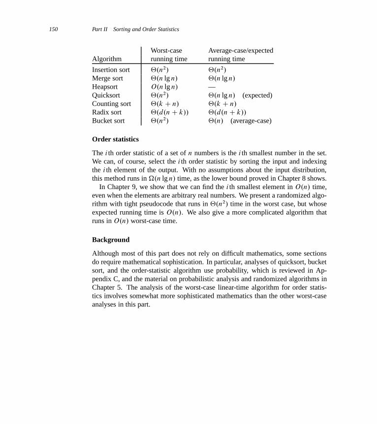
150 Part II Sorting and Order Statistics
Worst-case Average-case/expectedAlgorithm running time running time
Insertion sort ‚.n2/ ‚.n2/
Merge sort ‚.n lg n/ ‚.n lg n/
Heapsort O.n lg n/ —Quicksort ‚.n2/ ‚.n lg n/ (expected)Counting sort ‚.k C n/ ‚.k C n/
Radix sort ‚.d.nC k// ‚.d.nC k//
Bucket sort ‚.n2/ ‚.n/ (average-case)
Order statistics
The i th order statistic of a set of n numbers is the i th smallest number in the set.We can, of course, select the i th order statistic by sorting the input and indexingthe i th element of the output. With no assumptions about the input distribution,this method runs in �.n lg n/ time, as the lower bound proved in Chapter 8 shows.
In Chapter 9, we show that we can find the i th smallest element in O.n/ time,even when the elements are arbitrary real numbers. We present a randomized algo-rithm with tight pseudocode that runs in ‚.n2/ time in the worst case, but whoseexpected running time is O.n/. We also give a more complicated algorithm thatruns in O.n/ worst-case time.
Background
Although most of this part does not rely on difficult mathematics, some sectionsdo require mathematical sophistication. In particular, analyses of quicksort, bucketsort, and the order-statistic algorithm use probability, which is reviewed in Ap-pendix C, and the material on probabilistic analysis and randomized algorithms inChapter 5. The analysis of the worst-case linear-time algorithm for order statis-tics involves somewhat more sophisticated mathematics than the other worst-caseanalyses in this part.
6 Heapsort
In this chapter, we introduce another sorting algorithm: heapsort. Like merge sort,but unlike insertion sort, heapsort’s running time is O.n lg n/. Like insertion sort,but unlike merge sort, heapsort sorts in place: only a constant number of arrayelements are stored outside the input array at any time. Thus, heapsort combinesthe better attributes of the two sorting algorithms we have already discussed.
Heapsort also introduces another algorithm design technique: using a data struc-ture, in this case one we call a “heap,” to manage information. Not only is the heapdata structure useful for heapsort, but it also makes an efficient priority queue. Theheap data structure will reappear in algorithms in later chapters.
The term “heap” was originally coined in the context of heapsort, but it has sincecome to refer to “garbage-collected storage,” such as the programming languagesJava and Lisp provide. Our heap data structure is not garbage-collected storage,and whenever we refer to heaps in this book, we shall mean a data structure ratherthan an aspect of garbage collection.
6.1 Heaps
The (binary) heap data structure is an array object that we can view as anearly complete binary tree (see Section B.5.3), as shown in Figure 6.1. Eachnode of the tree corresponds to an element of the array. The tree is com-pletely filled on all levels except possibly the lowest, which is filled from theleft up to a point. An array A that represents a heap is an object with two at-tributes: A: length, which (as usual) gives the number of elements in the array, andA:heap-size, which represents how many elements in the heap are stored withinarray A. That is, although AŒ1 : : A: length� may contain numbers, only the ele-ments in AŒ1 : : A:heap-size�, where 0 � A:heap-size � A: length, are valid ele-ments of the heap. The root of the tree is AŒ1�, and given the index i of a node, wecan easily compute the indices of its parent, left child, and right child:
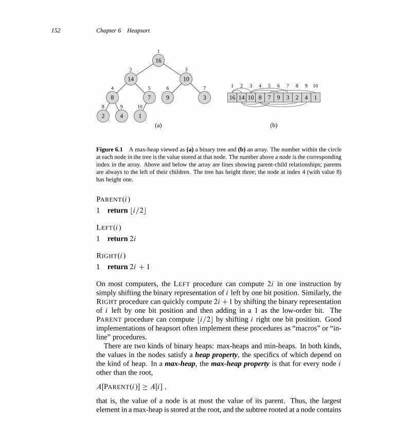
152 Chapter 6 Heapsort
(a)
16 14 10 8 7 9 3 2 4 1
1 2 3 4 5 6 7 8 9 10
(b)
1
2 3
4 5 6 7
8 9 10
16
14 10
8 7 9 3
2 4 1
Figure 6.1 A max-heap viewed as (a) a binary tree and (b) an array. The number within the circleat each node in the tree is the value stored at that node. The number above a node is the correspondingindex in the array. Above and below the array are lines showing parent-child relationships; parentsare always to the left of their children. The tree has height three; the node at index 4 (with value 8)has height one.
PARENT.i/
1 return bi=2c
LEFT.i/
1 return 2i
RIGHT.i/
1 return 2i C 1
On most computers, the LEFT procedure can compute 2i in one instruction bysimply shifting the binary representation of i left by one bit position. Similarly, theRIGHT procedure can quickly compute 2iC1 by shifting the binary representationof i left by one bit position and then adding in a 1 as the low-order bit. ThePARENT procedure can compute bi=2c by shifting i right one bit position. Goodimplementations of heapsort often implement these procedures as “macros” or “in-line” procedures.
There are two kinds of binary heaps: max-heaps and min-heaps. In both kinds,the values in the nodes satisfy a heap property, the specifics of which depend onthe kind of heap. In a max-heap, the max-heap property is that for every node i
other than the root,
AŒPARENT.i/� � AŒi� ;
that is, the value of a node is at most the value of its parent. Thus, the largestelement in a max-heap is stored at the root, and the subtree rooted at a node contains

6.1 Heaps 153
values no larger than that contained at the node itself. A min-heap is organized inthe opposite way; the min-heap property is that for every node i other than theroot,
AŒPARENT.i/� � AŒi� :
The smallest element in a min-heap is at the root.For the heapsort algorithm, we use max-heaps. Min-heaps commonly imple-
ment priority queues, which we discuss in Section 6.5. We shall be precise inspecifying whether we need a max-heap or a min-heap for any particular applica-tion, and when properties apply to either max-heaps or min-heaps, we just use theterm “heap.”
Viewing a heap as a tree, we define the height of a node in a heap to be thenumber of edges on the longest simple downward path from the node to a leaf, andwe define the height of the heap to be the height of its root. Since a heap of n ele-ments is based on a complete binary tree, its height is ‚.lg n/ (see Exercise 6.1-2).We shall see that the basic operations on heaps run in time at most proportionalto the height of the tree and thus take O.lg n/ time. The remainder of this chapterpresents some basic procedures and shows how they are used in a sorting algorithmand a priority-queue data structure.
� The MAX-HEAPIFY procedure, which runs in O.lg n/ time, is the key to main-taining the max-heap property.
� The BUILD-MAX-HEAP procedure, which runs in linear time, produces a max-heap from an unordered input array.
� The HEAPSORT procedure, which runs in O.n lg n/ time, sorts an array inplace.
� The MAX-HEAP-INSERT, HEAP-EXTRACT-MAX, HEAP-INCREASE-KEY,and HEAP-MAXIMUM procedures, which run in O.lg n/ time, allow the heapdata structure to implement a priority queue.
Exercises
6.1-1What are the minimum and maximum numbers of elements in a heap of height h?
6.1-2Show that an n-element heap has height blg nc.6.1-3Show that in any subtree of a max-heap, the root of the subtree contains the largestvalue occurring anywhere in that subtree.
154 Chapter 6 Heapsort
6.1-4Where in a max-heap might the smallest element reside, assuming that all elementsare distinct?
6.1-5Is an array that is in sorted order a min-heap?
6.1-6Is the array with values h23; 17; 14; 6; 13; 10; 1; 5; 7; 12i a max-heap?
6.1-7Show that, with the array representation for storing an n-element heap, the leavesare the nodes indexed by bn=2c C 1; bn=2c C 2; : : : ; n.
6.2 Maintaining the heap property
In order to maintain the max-heap property, we call the procedure MAX-HEAPIFY.Its inputs are an array A and an index i into the array. When it is called, MAX-HEAPIFY assumes that the binary trees rooted at LEFT.i/ and RIGHT.i/ are max-heaps, but that AŒi� might be smaller than its children, thus violating the max-heapproperty. MAX-HEAPIFY lets the value at AŒi� “float down” in the max-heap sothat the subtree rooted at index i obeys the max-heap property.
MAX-HEAPIFY.A; i/
1 l D LEFT.i/
2 r D RIGHT.i/
3 if l � A:heap-size and AŒl� > AŒi�
4 largest D l
5 else largest D i
6 if r � A:heap-size and AŒr� > AŒlargest�7 largest D r
8 if largest ¤ i
9 exchange AŒi� with AŒlargest�10 MAX-HEAPIFY.A; largest/
Figure 6.2 illustrates the action of MAX-HEAPIFY. At each step, the largest ofthe elements AŒi�, AŒLEFT.i/�, and AŒRIGHT.i/� is determined, and its index isstored in largest. If AŒi� is largest, then the subtree rooted at node i is already amax-heap and the procedure terminates. Otherwise, one of the two children has thelargest element, and AŒi� is swapped with AŒlargest�, which causes node i and its

6.2 Maintaining the heap property 155
16
4 10
14 7 9
2 8 1
(a)
16
14 10
4 7 9 3
2 8 1
(b)
16
14 10
8 7 9 3
2 4 1
(c)
3
1
3
4 5 6 7
9 10
2
8
1
3
4 5 6 7
9 10
2
8
1
3
4 5 6 7
9 10
2
8
i
i
i
Figure 6.2 The action of MAX-HEAPIFY.A; 2/, where A:heap-size D 10. (a) The initial con-figuration, with AŒ2� at node i D 2 violating the max-heap property since it is not larger thanboth children. The max-heap property is restored for node 2 in (b) by exchanging AŒ2� with AŒ4�,which destroys the max-heap property for node 4. The recursive call MAX-HEAPIFY.A; 4/ nowhas i D 4. After swapping AŒ4� with AŒ9�, as shown in (c), node 4 is fixed up, and the recursive callMAX-HEAPIFY.A; 9/ yields no further change to the data structure.
children to satisfy the max-heap property. The node indexed by largest, however,now has the original value AŒi�, and thus the subtree rooted at largest might violatethe max-heap property. Consequently, we call MAX-HEAPIFY recursively on thatsubtree.
The running time of MAX-HEAPIFY on a subtree of size n rooted at a givennode i is the ‚.1/ time to fix up the relationships among the elements AŒi�,AŒLEFT.i/�, and AŒRIGHT.i/�, plus the time to run MAX-HEAPIFY on a subtreerooted at one of the children of node i (assuming that the recursive call occurs).The children’s subtrees each have size at most 2n=3—the worst case occurs whenthe bottom level of the tree is exactly half full—and therefore we can describe therunning time of MAX-HEAPIFY by the recurrence
T .n/ � T .2n=3/C‚.1/ :
156 Chapter 6 Heapsort
The solution to this recurrence, by case 2 of the master theorem (Theorem 4.1),is T .n/ D O.lg n/. Alternatively, we can characterize the running time of MAX-HEAPIFY on a node of height h as O.h/.
Exercises
6.2-1Using Figure 6.2 as a model, illustrate the operation of MAX-HEAPIFY.A; 3/ onthe array A D h27; 17; 3; 16; 13; 10; 1; 5; 7; 12; 4; 8; 9; 0i.6.2-2Starting with the procedure MAX-HEAPIFY, write pseudocode for the procedureMIN-HEAPIFY.A; i/, which performs the corresponding manipulation on a min-heap. How does the running time of MIN-HEAPIFY compare to that of MAX-HEAPIFY?
6.2-3What is the effect of calling MAX-HEAPIFY.A; i/ when the element AŒi� is largerthan its children?
6.2-4What is the effect of calling MAX-HEAPIFY.A; i/ for i > A:heap-size=2?
6.2-5The code for MAX-HEAPIFY is quite efficient in terms of constant factors, exceptpossibly for the recursive call in line 10, which might cause some compilers toproduce inefficient code. Write an efficient MAX-HEAPIFY that uses an iterativecontrol construct (a loop) instead of recursion.
6.2-6Show that the worst-case running time of MAX-HEAPIFY on a heap of size n
is �.lg n/. (Hint: For a heap with n nodes, give node values that cause MAX-HEAPIFY to be called recursively at every node on a simple path from the rootdown to a leaf.)
6.3 Building a heap
We can use the procedure MAX-HEAPIFY in a bottom-up manner to convert anarray AŒ1 : : n�, where n D A: length, into a max-heap. By Exercise 6.1-7, theelements in the subarray AŒ.bn=2cC1/ : : n� are all leaves of the tree, and so each is
6.3 Building a heap 157
a 1-element heap to begin with. The procedure BUILD-MAX-HEAP goes throughthe remaining nodes of the tree and runs MAX-HEAPIFY on each one.
BUILD-MAX-HEAP.A/
1 A:heap-size D A: length2 for i D bA: length=2c downto 1
3 MAX-HEAPIFY.A; i/
Figure 6.3 shows an example of the action of BUILD-MAX-HEAP.To show why BUILD-MAX-HEAP works correctly, we use the following loop
invariant:
At the start of each iteration of the for loop of lines 2–3, each node i C 1;
i C 2; : : : ; n is the root of a max-heap.
We need to show that this invariant is true prior to the first loop iteration, that eachiteration of the loop maintains the invariant, and that the invariant provides a usefulproperty to show correctness when the loop terminates.
Initialization: Prior to the first iteration of the loop, i D bn=2c. Each nodebn=2cC 1; bn=2cC 2; : : : ; n is a leaf and is thus the root of a trivial max-heap.
Maintenance: To see that each iteration maintains the loop invariant, observe thatthe children of node i are numbered higher than i . By the loop invariant, there-fore, they are both roots of max-heaps. This is precisely the condition requiredfor the call MAX-HEAPIFY.A; i/ to make node i a max-heap root. Moreover,the MAX-HEAPIFY call preserves the property that nodes i C 1; i C 2; : : : ; n
are all roots of max-heaps. Decrementing i in the for loop update reestablishesthe loop invariant for the next iteration.
Termination: At termination, i D 0. By the loop invariant, each node 1; 2; : : : ; n
is the root of a max-heap. In particular, node 1 is.
We can compute a simple upper bound on the running time of BUILD-MAX-HEAP as follows. Each call to MAX-HEAPIFY costs O.lg n/ time, and BUILD-MAX-HEAP makes O.n/ such calls. Thus, the running time is O.n lg n/. Thisupper bound, though correct, is not asymptotically tight.
We can derive a tighter bound by observing that the time for MAX-HEAPIFY torun at a node varies with the height of the node in the tree, and the heights of mostnodes are small. Our tighter analysis relies on the properties that an n-element heaphas height blg nc (see Exercise 6.1-2) and at most
˙n=2hC1
�nodes of any height h
(see Exercise 6.3-3).The time required by MAX-HEAPIFY when called on a node of height h is O.h/,
and so we can express the total cost of BUILD-MAX-HEAP as being bounded fromabove by
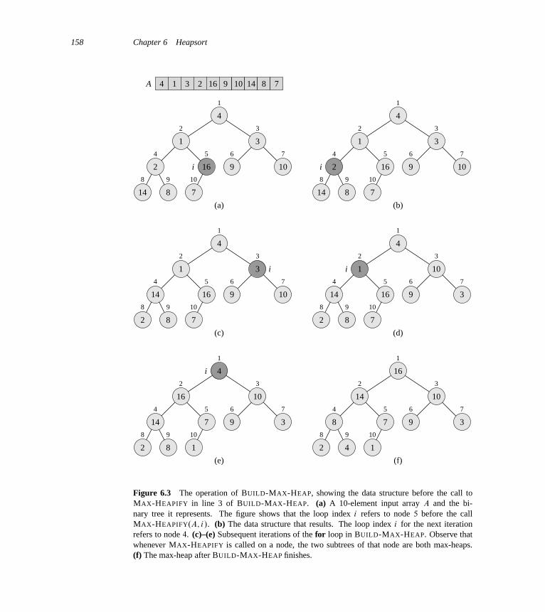
158 Chapter 6 Heapsort
1
2 3
4 5 6 7
8 9 10
1
2 3
4 5 6 7
8 9 10
1
2 3
4 5 6 7
8 9 10
1
2 3
4 5 6 7
8 9 10
1
2 3
4 5 6 7
8 9 10
1
2 3
4 5 6 7
8 9 10
4
1 3
2 9 10
14 8 7
(a)
16
4 1 23 16 9 10 14 8 7
4
1 3
2 9 10
14 8 7
(b)
16
4
1 3
14 9 10
2 8 7
(c)
16
4
1 10
14 9 3
2 8 7
(d)
16
4
16 10
14 9 3
2 8 1
(e)
7
16
14 10
8 9 3
2 4 1
(f)
7
A
i i
ii
i
Figure 6.3 The operation of BUILD-MAX-HEAP, showing the data structure before the call toMAX-HEAPIFY in line 3 of BUILD-MAX-HEAP. (a) A 10-element input array A and the bi-nary tree it represents. The figure shows that the loop index i refers to node 5 before the callMAX-HEAPIFY.A; i/. (b) The data structure that results. The loop index i for the next iterationrefers to node 4. (c)–(e) Subsequent iterations of the for loop in BUILD-MAX-HEAP. Observe thatwhenever MAX-HEAPIFY is called on a node, the two subtrees of that node are both max-heaps.(f) The max-heap after BUILD-MAX-HEAP finishes.
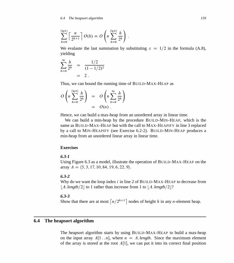
6.4 The heapsort algorithm 159
blg ncXhD0
l n
2hC1
mO.h/ D O
n
blg ncXhD0
h
2h
!:
We evalaute the last summation by substituting x D 1=2 in the formula (A.8),yielding1X
hD0
h
2hD 1=2
.1� 1=2/2
D 2 :
Thus, we can bound the running time of BUILD-MAX-HEAP as
O
n
blg ncXhD0
h
2h
!D O
n
1XhD0
h
2h
!D O.n/ :
Hence, we can build a max-heap from an unordered array in linear time.We can build a min-heap by the procedure BUILD-MIN-HEAP, which is the
same as BUILD-MAX-HEAP but with the call to MAX-HEAPIFY in line 3 replacedby a call to MIN-HEAPIFY (see Exercise 6.2-2). BUILD-MIN-HEAP produces amin-heap from an unordered linear array in linear time.
Exercises
6.3-1Using Figure 6.3 as a model, illustrate the operation of BUILD-MAX-HEAP on thearray A D h5; 3; 17; 10; 84; 19; 6; 22; 9i.6.3-2Why do we want the loop index i in line 2 of BUILD-MAX-HEAP to decrease frombA: length=2c to 1 rather than increase from 1 to bA: length=2c?6.3-3Show that there are at most
˙n=2hC1
�nodes of height h in any n-element heap.
6.4 The heapsort algorithm
The heapsort algorithm starts by using BUILD-MAX-HEAP to build a max-heapon the input array AŒ1 : : n�, where n D A: length. Since the maximum elementof the array is stored at the root AŒ1�, we can put it into its correct final position

160 Chapter 6 Heapsort
by exchanging it with AŒn�. If we now discard node n from the heap—and wecan do so by simply decrementing A:heap-size—we observe that the children ofthe root remain max-heaps, but the new root element might violate the max-heapproperty. All we need to do to restore the max-heap property, however, is callMAX-HEAPIFY.A; 1/, which leaves a max-heap in AŒ1 : : n � 1�. The heapsortalgorithm then repeats this process for the max-heap of size n � 1 down to a heapof size 2. (See Exercise 6.4-2 for a precise loop invariant.)
HEAPSORT.A/
1 BUILD-MAX-HEAP.A/
2 for i D A: length downto 23 exchange AŒ1� with AŒi�
4 A:heap-size D A:heap-size � 1
5 MAX-HEAPIFY.A; 1/
Figure 6.4 shows an example of the operation of HEAPSORT after line 1 has builtthe initial max-heap. The figure shows the max-heap before the first iteration ofthe for loop of lines 2–5 and after each iteration.
The HEAPSORT procedure takes time O.n lg n/, since the call to BUILD-MAX-HEAP takes time O.n/ and each of the n � 1 calls to MAX-HEAPIFY takestime O.lg n/.
Exercises
6.4-1Using Figure 6.4 as a model, illustrate the operation of HEAPSORT on the arrayA D h5; 13; 2; 25; 7; 17; 20; 8; 4i.6.4-2Argue the correctness of HEAPSORT using the following loop invariant:
At the start of each iteration of the for loop of lines 2–5, the subarrayAŒ1 : : i � is a max-heap containing the i smallest elements of AŒ1 : : n�, andthe subarray AŒi C 1 : : n� contains the n � i largest elements of AŒ1 : : n�,sorted.
6.4-3What is the running time of HEAPSORT on an array A of length n that is alreadysorted in increasing order? What about decreasing order?
6.4-4Show that the worst-case running time of HEAPSORT is �.n lg n/.
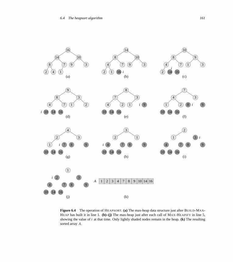
6.4 The heapsort algorithm 161
(a) (b) (c)
(d) (e) (f)
(g) (h) (i)
(j) (k)
1 2 3 4 7 8 9 10 14 16
10
2
1 3
4 7 8 9
1614
1
2 3
4 7 8 9
161410
3
2 1
9874
10 14 16
4
2 3
9871
10 14 16
8
37
4 2 1 9
161410
7
4 3
9821
10 14 16
9
8 3
2174
161410
10
8 9
3174
16142
14
8 10
3974
1612
16
14 10
3978
142
A
ii
i
i i
i i
i
i
Figure 6.4 The operation of HEAPSORT. (a) The max-heap data structure just after BUILD-MAX-HEAP has built it in line 1. (b)–(j) The max-heap just after each call of MAX-HEAPIFY in line 5,showing the value of i at that time. Only lightly shaded nodes remain in the heap. (k) The resultingsorted array A.
162 Chapter 6 Heapsort
6.4-5 ?
Show that when all elements are distinct, the best-case running time of HEAPSORT
is �.n lg n/.
6.5 Priority queues
Heapsort is an excellent algorithm, but a good implementation of quicksort, pre-sented in Chapter 7, usually beats it in practice. Nevertheless, the heap data struc-ture itself has many uses. In this section, we present one of the most popular ap-plications of a heap: as an efficient priority queue. As with heaps, priority queuescome in two forms: max-priority queues and min-priority queues. We will focushere on how to implement max-priority queues, which are in turn based on max-heaps; Exercise 6.5-3 asks you to write the procedures for min-priority queues.
A priority queue is a data structure for maintaining a set S of elements, eachwith an associated value called a key. A max-priority queue supports the followingoperations:
INSERT.S; x/ inserts the element x into the set S , which is equivalent to the oper-ation S D S [ fxg.
MAXIMUM.S/ returns the element of S with the largest key.
EXTRACT-MAX.S/ removes and returns the element of S with the largest key.
INCREASE-KEY.S; x; k/ increases the value of element x’s key to the new value k,which is assumed to be at least as large as x’s current key value.
Among their other applications, we can use max-priority queues to schedulejobs on a shared computer. The max-priority queue keeps track of the jobs tobe performed and their relative priorities. When a job is finished or interrupted,the scheduler selects the highest-priority job from among those pending by callingEXTRACT-MAX. The scheduler can add a new job to the queue at any time bycalling INSERT.
Alternatively, a min-priority queue supports the operations INSERT, MINIMUM,EXTRACT-MIN, and DECREASE-KEY. A min-priority queue can be used in anevent-driven simulator. The items in the queue are events to be simulated, eachwith an associated time of occurrence that serves as its key. The events must besimulated in order of their time of occurrence, because the simulation of an eventcan cause other events to be simulated in the future. The simulation program callsEXTRACT-MIN at each step to choose the next event to simulate. As new events areproduced, the simulator inserts them into the min-priority queue by calling INSERT.
6.5 Priority queues 163
We shall see other uses for min-priority queues, highlighting the DECREASE-KEY
operation, in Chapters 23 and 24.Not surprisingly, we can use a heap to implement a priority queue. In a given ap-
plication, such as job scheduling or event-driven simulation, elements of a priorityqueue correspond to objects in the application. We often need to determine whichapplication object corresponds to a given priority-queue element, and vice versa.When we use a heap to implement a priority queue, therefore, we often need tostore a handle to the corresponding application object in each heap element. Theexact makeup of the handle (such as a pointer or an integer) depends on the ap-plication. Similarly, we need to store a handle to the corresponding heap elementin each application object. Here, the handle would typically be an array index.Because heap elements change locations within the array during heap operations,an actual implementation, upon relocating a heap element, would also have to up-date the array index in the corresponding application object. Because the detailsof accessing application objects depend heavily on the application and its imple-mentation, we shall not pursue them here, other than noting that in practice, thesehandles do need to be correctly maintained.
Now we discuss how to implement the operations of a max-priority queue. Theprocedure HEAP-MAXIMUM implements the MAXIMUM operation in ‚.1/ time.
HEAP-MAXIMUM.A/
1 return AŒ1�
The procedure HEAP-EXTRACT-MAX implements the EXTRACT-MAX opera-tion. It is similar to the for loop body (lines 3–5) of the HEAPSORT procedure.
HEAP-EXTRACT-MAX.A/
1 if A:heap-size < 1
2 error “heap underflow”3 max D AŒ1�
4 AŒ1� D AŒA:heap-size�
5 A:heap-size D A:heap-size � 1
6 MAX-HEAPIFY.A; 1/
7 return max
The running time of HEAP-EXTRACT-MAX is O.lg n/, since it performs only aconstant amount of work on top of the O.lg n/ time for MAX-HEAPIFY.
The procedure HEAP-INCREASE-KEY implements the INCREASE-KEY opera-tion. An index i into the array identifies the priority-queue element whose key wewish to increase. The procedure first updates the key of element AŒi� to its newvalue. Because increasing the key of AŒi� might violate the max-heap property,
164 Chapter 6 Heapsort
the procedure then, in a manner reminiscent of the insertion loop (lines 5–7) ofINSERTION-SORT from Section 2.1, traverses a simple path from this node towardthe root to find a proper place for the newly increased key. As HEAP-INCREASE-KEY traverses this path, it repeatedly compares an element to its parent, exchang-ing their keys and continuing if the element’s key is larger, and terminating if the el-ement’s key is smaller, since the max-heap property now holds. (See Exercise 6.5-5for a precise loop invariant.)
HEAP-INCREASE-KEY.A; i; key/
1 if key < AŒi�
2 error “new key is smaller than current key”3 AŒi� D key4 while i > 1 and AŒPARENT.i/� < AŒi�
5 exchange AŒi� with AŒPARENT.i/�
6 i D PARENT.i/
Figure 6.5 shows an example of a HEAP-INCREASE-KEY operation. The runningtime of HEAP-INCREASE-KEY on an n-element heap is O.lg n/, since the pathtraced from the node updated in line 3 to the root has length O.lg n/.
The procedure MAX-HEAP-INSERT implements the INSERT operation. It takesas an input the key of the new element to be inserted into max-heap A. The proce-dure first expands the max-heap by adding to the tree a new leaf whose key is �1.Then it calls HEAP-INCREASE-KEY to set the key of this new node to its correctvalue and maintain the max-heap property.
MAX-HEAP-INSERT.A; key/
1 A:heap-size D A:heap-sizeC 1
2 AŒA:heap-size� D �13 HEAP-INCREASE-KEY.A; A:heap-size; key/
The running time of MAX-HEAP-INSERT on an n-element heap is O.lg n/.In summary, a heap can support any priority-queue operation on a set of size n
in O.lg n/ time.
Exercises
6.5-1Illustrate the operation of HEAP-EXTRACT-MAX on the heap A D h15; 13; 9; 5;
12; 8; 7; 4; 0; 6; 2; 1i.
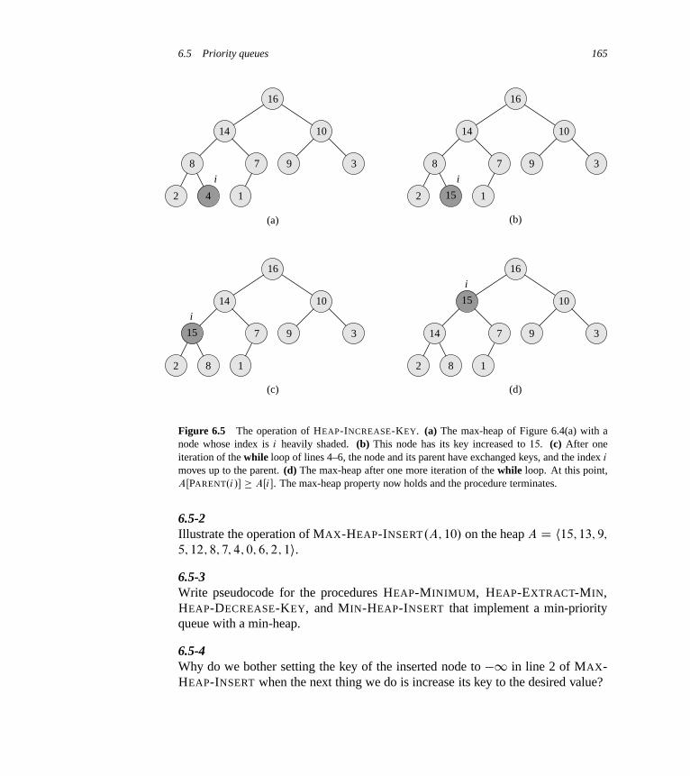
6.5 Priority queues 165
16
14 10
8 7 9 3
2 4 1
(a)
i
16
14 10
8 7 9 3
2 15 1
(b)
16
14 10
8
7 9 3
2
15
1
(c)
i
i
16
14
10
8
7 9 3
2
15
1
(d)
i
Figure 6.5 The operation of HEAP-INCREASE-KEY. (a) The max-heap of Figure 6.4(a) with anode whose index is i heavily shaded. (b) This node has its key increased to 15. (c) After oneiteration of the while loop of lines 4–6, the node and its parent have exchanged keys, and the index i
moves up to the parent. (d) The max-heap after one more iteration of the while loop. At this point,AŒPARENT.i/� � AŒi�. The max-heap property now holds and the procedure terminates.
6.5-2Illustrate the operation of MAX-HEAP-INSERT.A; 10/ on the heap A D h15; 13; 9;
5; 12; 8; 7; 4; 0; 6; 2; 1i.6.5-3Write pseudocode for the procedures HEAP-MINIMUM, HEAP-EXTRACT-MIN,HEAP-DECREASE-KEY, and MIN-HEAP-INSERT that implement a min-priorityqueue with a min-heap.
6.5-4Why do we bother setting the key of the inserted node to �1 in line 2 of MAX-HEAP-INSERT when the next thing we do is increase its key to the desired value?
166 Chapter 6 Heapsort
6.5-5Argue the correctness of HEAP-INCREASE-KEY using the following loop invari-ant:
At the start of each iteration of the while loop of lines 4–6, the subarrayAŒ1 : : A:heap-size� satisfies the max-heap property, except that there maybe one violation: AŒi� may be larger than AŒPARENT.i/�.
You may assume that the subarray AŒ1 : : A:heap-size� satisfies the max-heap prop-erty at the time HEAP-INCREASE-KEY is called.
6.5-6Each exchange operation on line 5 of HEAP-INCREASE-KEY typically requiresthree assignments. Show how to use the idea of the inner loop of INSERTION-SORT to reduce the three assignments down to just one assignment.
6.5-7Show how to implement a first-in, first-out queue with a priority queue. Showhow to implement a stack with a priority queue. (Queues and stacks are defined inSection 10.1.)
6.5-8The operation HEAP-DELETE.A; i/ deletes the item in node i from heap A. Givean implementation of HEAP-DELETE that runs in O.lg n/ time for an n-elementmax-heap.
6.5-9Give an O.n lg k/-time algorithm to merge k sorted lists into one sorted list,where n is the total number of elements in all the input lists. (Hint: Use a min-heap for k-way merging.)
Problems
6-1 Building a heap using insertionWe can build a heap by repeatedly calling MAX-HEAP-INSERT to insert the ele-ments into the heap. Consider the following variation on the BUILD-MAX-HEAP
procedure:

Problems for Chapter 6 167
BUILD-MAX-HEAP0.A/
1 A:heap-size D 1
2 for i D 2 to A: length3 MAX-HEAP-INSERT.A; AŒi �/
a. Do the procedures BUILD-MAX-HEAP and BUILD-MAX-HEAP 0 always createthe same heap when run on the same input array? Prove that they do, or providea counterexample.
b. Show that in the worst case, BUILD-MAX-HEAP 0 requires ‚.n lg n/ time tobuild an n-element heap.
6-2 Analysis of d -ary heapsA d -ary heap is like a binary heap, but (with one possible exception) non-leafnodes have d children instead of 2 children.
a. How would you represent a d -ary heap in an array?
b. What is the height of a d -ary heap of n elements in terms of n and d?
c. Give an efficient implementation of EXTRACT-MAX in a d -ary max-heap. An-alyze its running time in terms of d and n.
d. Give an efficient implementation of INSERT in a d -ary max-heap. Analyze itsrunning time in terms of d and n.
e. Give an efficient implementation of INCREASE-KEY.A; i; k/, which flags anerror if k < AŒi�, but otherwise sets AŒi� D k and then updates the d -ary max-heap structure appropriately. Analyze its running time in terms of d and n.
6-3 Young tableausAn m n Young tableau is an m n matrix such that the entries of each row arein sorted order from left to right and the entries of each column are in sorted orderfrom top to bottom. Some of the entries of a Young tableau may be1, which wetreat as nonexistent elements. Thus, a Young tableau can be used to hold r � mn
finite numbers.
a. Draw a 44 Young tableau containing the elements f9; 16; 3; 2; 4; 8; 5; 14; 12g.
b. Argue that an m n Young tableau Y is empty if Y Œ1; 1� D 1. Argue that Y
is full (contains mn elements) if Y Œm; n� <1.
168 Chapter 6 Heapsort
c. Give an algorithm to implement EXTRACT-MIN on a nonempty m n Youngtableau that runs in O.m C n/ time. Your algorithm should use a recur-sive subroutine that solves an m n problem by recursively solving eitheran .m � 1/ n or an m .n � 1/ subproblem. (Hint: Think about MAX-HEAPIFY.) Define T .p/, where p D mC n, to be the maximum running timeof EXTRACT-MIN on any m n Young tableau. Give and solve a recurrencefor T .p/ that yields the O.mC n/ time bound.
d. Show how to insert a new element into a nonfull m n Young tableau inO.mC n/ time.
e. Using no other sorting method as a subroutine, show how to use an nn Youngtableau to sort n2 numbers in O.n3/ time.
f. Give an O.m C n/-time algorithm to determine whether a given number isstored in a given m n Young tableau.
Chapter notes
The heapsort algorithm was invented by Williams [357], who also described howto implement a priority queue with a heap. The BUILD-MAX-HEAP procedurewas suggested by Floyd [106].
We use min-heaps to implement min-priority queues in Chapters 16, 23, and 24.We also give an implementation with improved time bounds for certain operationsin Chapter 19 and, assuming that the keys are drawn from a bounded set of non-negative integers, Chapter 20.
If the data are b-bit integers, and the computer memory consists of addressableb-bit words, Fredman and Willard [115] showed how to implement MINIMUM inO.1/ time and INSERT and EXTRACT-MIN in O.
plg n/ time. Thorup [337] has
improved the O.p
lg n/ bound to O.lg lg n/ time. This bound uses an amount ofspace unbounded in n, but it can be implemented in linear space by using random-ized hashing.
An important special case of priority queues occurs when the sequence ofEXTRACT-MIN operations is monotone, that is, the values returned by succes-sive EXTRACT-MIN operations are monotonically increasing over time. This casearises in several important applications, such as Dijkstra’s single-source shortest-paths algorithm, which we discuss in Chapter 24, and in discrete-event simula-tion. For Dijkstra’s algorithm it is particularly important that the DECREASE-KEY
operation be implemented efficiently. For the monotone case, if the data are in-tegers in the range 1; 2; : : : ; C , Ahuja, Mehlhorn, Orlin, and Tarjan [8] describe
Notes for Chapter 6 169
how to implement EXTRACT-MIN and INSERT in O.lg C / amortized time (seeChapter 17 for more on amortized analysis) and DECREASE-KEY in O.1/ time,using a data structure called a radix heap. The O.lg C / bound can be improvedto O.
plg C / using Fibonacci heaps (see Chapter 19) in conjunction with radix
heaps. Cherkassky, Goldberg, and Silverstein [66] further improved the bound toO.lg1=3C� C / expected time by combining the multilevel bucketing structure ofDenardo and Fox [86] with the heap of Thorup mentioned above. Raman [291]further improved these results to obtain a bound of O.min.lg1=4C� C; lg1=3C� n//,for any fixed � > 0.

7 Quicksort
The quicksort algorithm has a worst-case running time of ‚.n2/ on an input arrayof n numbers. Despite this slow worst-case running time, quicksort is often the bestpractical choice for sorting because it is remarkably efficient on the average: itsexpected running time is ‚.n lg n/, and the constant factors hidden in the ‚.n lg n/
notation are quite small. It also has the advantage of sorting in place (see page 17),and it works well even in virtual-memory environments.
Section 7.1 describes the algorithm and an important subroutine used by quick-sort for partitioning. Because the behavior of quicksort is complex, we start withan intuitive discussion of its performance in Section 7.2 and postpone its preciseanalysis to the end of the chapter. Section 7.3 presents a version of quicksort thatuses random sampling. This algorithm has a good expected running time, and noparticular input elicits its worst-case behavior. Section 7.4 analyzes the random-ized algorithm, showing that it runs in ‚.n2/ time in the worst case and, assumingdistinct elements, in expected O.n lg n/ time.
7.1 Description of quicksort
Quicksort, like merge sort, applies the divide-and-conquer paradigm introducedin Section 2.3.1. Here is the three-step divide-and-conquer process for sorting atypical subarray AŒp : : r�:
Divide: Partition (rearrange) the array AŒp : : r� into two (possibly empty) subar-rays AŒp : : q � 1� and AŒq C 1 : : r� such that each element of AŒp : : q � 1� isless than or equal to AŒq�, which is, in turn, less than or equal to each elementof AŒq C 1 : : r�. Compute the index q as part of this partitioning procedure.
Conquer: Sort the two subarrays AŒp : : q�1� and AŒqC1 : : r� by recursive callsto quicksort.
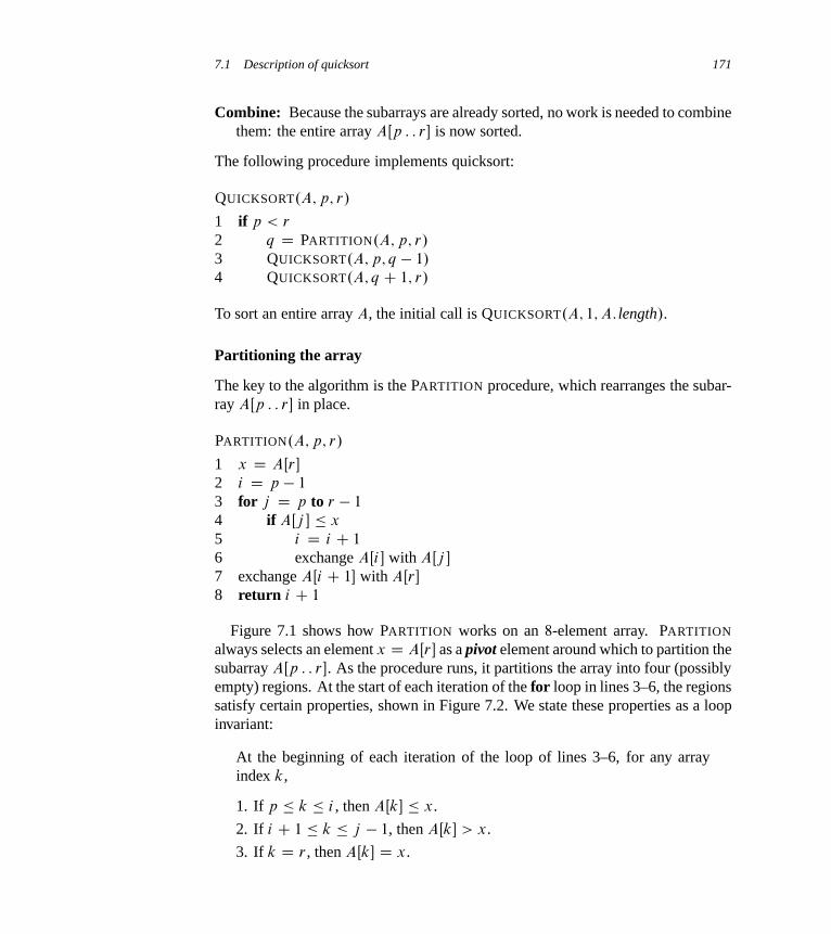
7.1 Description of quicksort 171
Combine: Because the subarrays are already sorted, no work is needed to combinethem: the entire array AŒp : : r� is now sorted.
The following procedure implements quicksort:
QUICKSORT.A; p; r/
1 if p < r
2 q D PARTITION.A; p; r/
3 QUICKSORT.A; p; q � 1/
4 QUICKSORT.A; q C 1; r/
To sort an entire array A, the initial call is QUICKSORT.A; 1; A: length/.
Partitioning the array
The key to the algorithm is the PARTITION procedure, which rearranges the subar-ray AŒp : : r� in place.
PARTITION.A; p; r/
1 x D AŒr�
2 i D p � 1
3 for j D p to r � 1
4 if AŒj � � x
5 i D i C 1
6 exchange AŒi� with AŒj �
7 exchange AŒi C 1� with AŒr�
8 return i C 1
Figure 7.1 shows how PARTITION works on an 8-element array. PARTITION
always selects an element x D AŒr� as a pivot element around which to partition thesubarray AŒp : : r�. As the procedure runs, it partitions the array into four (possiblyempty) regions. At the start of each iteration of the for loop in lines 3–6, the regionssatisfy certain properties, shown in Figure 7.2. We state these properties as a loopinvariant:
At the beginning of each iteration of the loop of lines 3–6, for any arrayindex k,
1. If p � k � i , then AŒk� � x.
2. If i C 1 � k � j � 1, then AŒk� > x.
3. If k D r , then AŒk� D x.
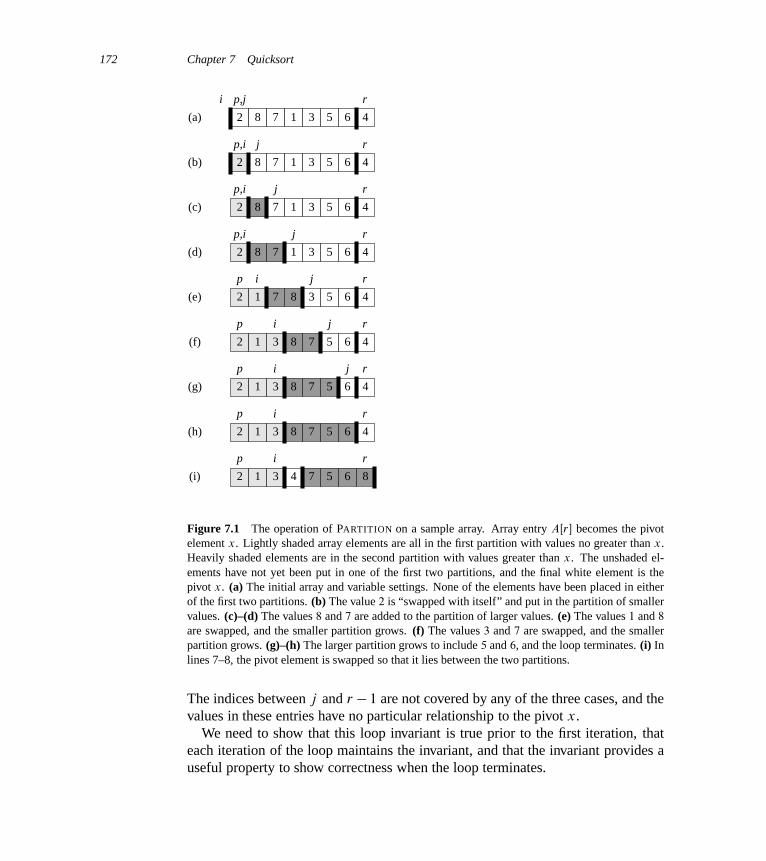
172 Chapter 7 Quicksort
2 8 7 1 3 5 6 4
p,j ri
(a)
2 8 7 1 3 5 6 4
p,i rj
(b)
2 8 7 1 3 5 6 4
p,i rj
(c)
2 8 7 1 3 5 6 4
p,i rj
(d)
2 871 3 5 6 4
p rj
(e)
i
2 8 71 3 5 6 4
p rj
(f)
i
2 8 71 3 5 6 4
p rj
(g)
i
2 8 71 3 5 6 4
p r
(h)
i
2 871 3 5 64
p r
(i)
i
Figure 7.1 The operation of PARTITION on a sample array. Array entry AŒr� becomes the pivotelement x. Lightly shaded array elements are all in the first partition with values no greater than x.Heavily shaded elements are in the second partition with values greater than x. The unshaded el-ements have not yet been put in one of the first two partitions, and the final white element is thepivot x. (a) The initial array and variable settings. None of the elements have been placed in eitherof the first two partitions. (b) The value 2 is “swapped with itself” and put in the partition of smallervalues. (c)–(d) The values 8 and 7 are added to the partition of larger values. (e) The values 1 and 8
are swapped, and the smaller partition grows. (f) The values 3 and 7 are swapped, and the smallerpartition grows. (g)–(h) The larger partition grows to include 5 and 6, and the loop terminates. (i) Inlines 7–8, the pivot element is swapped so that it lies between the two partitions.
The indices between j and r � 1 are not covered by any of the three cases, and thevalues in these entries have no particular relationship to the pivot x.
We need to show that this loop invariant is true prior to the first iteration, thateach iteration of the loop maintains the invariant, and that the invariant provides auseful property to show correctness when the loop terminates.

7.1 Description of quicksort 173
≤ x > x unrestricted
x
p i j r
Figure 7.2 The four regions maintained by the procedure PARTITION on a subarray AŒp : : r�. Thevalues in AŒp : : i � are all less than or equal to x, the values in AŒi C 1 : : j � 1� are all greater than x,and AŒr� D x. The subarray AŒj : : r � 1� can take on any values.
Initialization: Prior to the first iteration of the loop, i D p � 1 and j D p. Be-cause no values lie between p and i and no values lie between i C 1 and j � 1,the first two conditions of the loop invariant are trivially satisfied. The assign-ment in line 1 satisfies the third condition.
Maintenance: As Figure 7.3 shows, we consider two cases, depending on theoutcome of the test in line 4. Figure 7.3(a) shows what happens when AŒj � > x;the only action in the loop is to increment j . After j is incremented, condition 2holds for AŒj � 1� and all other entries remain unchanged. Figure 7.3(b) showswhat happens when AŒj � � x; the loop increments i , swaps AŒi� and AŒj �,and then increments j . Because of the swap, we now have that AŒi� � x, andcondition 1 is satisfied. Similarly, we also have that AŒj � 1� > x, since theitem that was swapped into AŒj � 1� is, by the loop invariant, greater than x.
Termination: At termination, j D r . Therefore, every entry in the array is in oneof the three sets described by the invariant, and we have partitioned the valuesin the array into three sets: those less than or equal to x, those greater than x,and a singleton set containing x.
The final two lines of PARTITION move the pivot element into its place in themiddle of the array by swapping it with the leftmost element that is greater than x.The output of PARTITION now satisfies the specifications given for the divide step.In fact, it satisfies a slightly stronger condition: after line 2 of QUICKSORT, AŒq�
is strictly less than every element of AŒq C 1 : : r�.The running time of PARTITION on the subarray AŒp : : r� is ‚.n/, where
n D r � p C 1 (see Exercise 7.1-3).
Exercises
7.1-1Using Figure 7.1 as a model, illustrate the operation of PARTITION on the arrayA D h13; 19; 9; 5; 12; 8; 7; 4; 21; 2; 6; 11i.
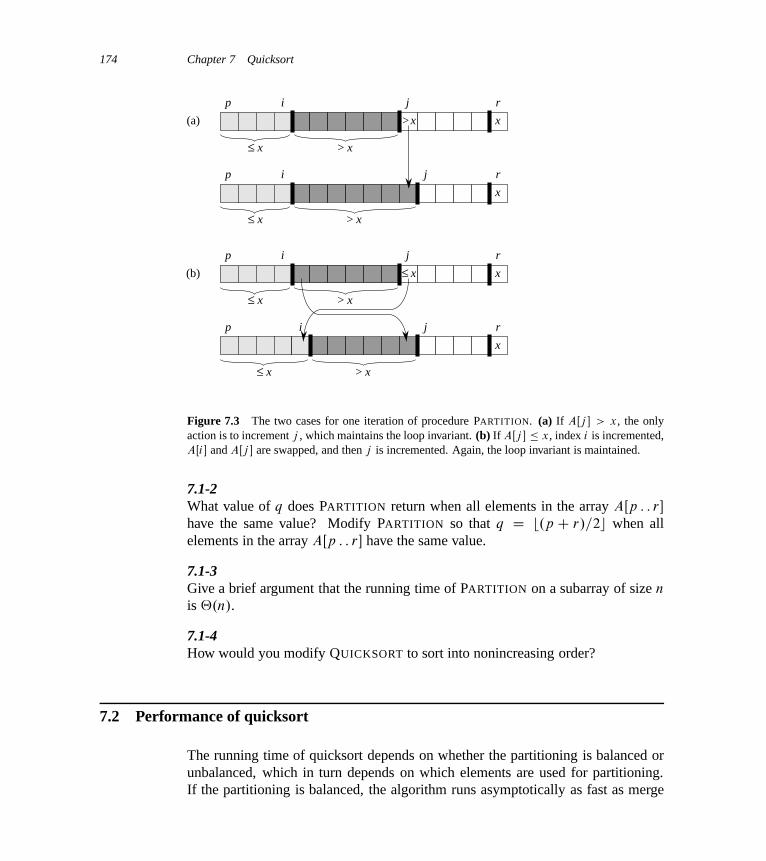
174 Chapter 7 Quicksort
≤ x > x
x
p i j r
>x(a)
≤ x > x
x
p i j r
≤ x > x
x
p i j r
≤ x(b)
≤ x > x
x
p i j r
Figure 7.3 The two cases for one iteration of procedure PARTITION. (a) If AŒj � > x, the onlyaction is to increment j , which maintains the loop invariant. (b) If AŒj � � x, index i is incremented,AŒi� and AŒj � are swapped, and then j is incremented. Again, the loop invariant is maintained.
7.1-2What value of q does PARTITION return when all elements in the array AŒp : : r�
have the same value? Modify PARTITION so that q D b.p C r/=2c when allelements in the array AŒp : : r� have the same value.
7.1-3Give a brief argument that the running time of PARTITION on a subarray of size n
is ‚.n/.
7.1-4How would you modify QUICKSORT to sort into nonincreasing order?
7.2 Performance of quicksort
The running time of quicksort depends on whether the partitioning is balanced orunbalanced, which in turn depends on which elements are used for partitioning.If the partitioning is balanced, the algorithm runs asymptotically as fast as merge
7.2 Performance of quicksort 175
sort. If the partitioning is unbalanced, however, it can run asymptotically as slowlyas insertion sort. In this section, we shall informally investigate how quicksortperforms under the assumptions of balanced versus unbalanced partitioning.
Worst-case partitioning
The worst-case behavior for quicksort occurs when the partitioning routine pro-duces one subproblem with n � 1 elements and one with 0 elements. (We provethis claim in Section 7.4.1.) Let us assume that this unbalanced partitioning arisesin each recursive call. The partitioning costs ‚.n/ time. Since the recursive callon an array of size 0 just returns, T .0/ D ‚.1/, and the recurrence for the runningtime is
T .n/ D T .n � 1/C T .0/C‚.n/
D T .n � 1/C‚.n/ :
Intuitively, if we sum the costs incurred at each level of the recursion, we getan arithmetic series (equation (A.2)), which evaluates to ‚.n2/. Indeed, it isstraightforward to use the substitution method to prove that the recurrence T .n/ DT .n � 1/C‚.n/ has the solution T .n/ D ‚.n2/. (See Exercise 7.2-1.)
Thus, if the partitioning is maximally unbalanced at every recursive level of thealgorithm, the running time is ‚.n2/. Therefore the worst-case running time ofquicksort is no better than that of insertion sort. Moreover, the ‚.n2/ running timeoccurs when the input array is already completely sorted—a common situation inwhich insertion sort runs in O.n/ time.
Best-case partitioning
In the most even possible split, PARTITION produces two subproblems, each ofsize no more than n=2, since one is of size bn=2c and one of size dn=2e�1. In thiscase, quicksort runs much faster. The recurrence for the running time is then
T .n/ D 2T .n=2/C‚.n/ ;
where we tolerate the sloppiness from ignoring the floor and ceiling and from sub-tracting 1. By case 2 of the master theorem (Theorem 4.1), this recurrence has thesolution T .n/ D ‚.n lg n/. By equally balancing the two sides of the partition atevery level of the recursion, we get an asymptotically faster algorithm.
Balanced partitioning
The average-case running time of quicksort is much closer to the best case than tothe worst case, as the analyses in Section 7.4 will show. The key to understand-
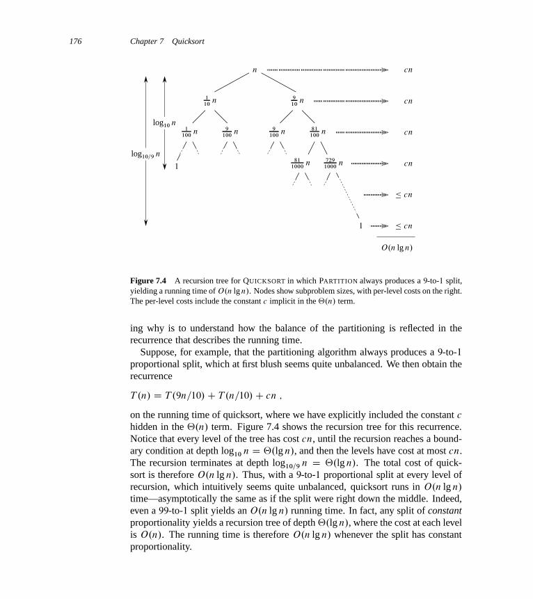
176 Chapter 7 Quicksort
n
cn
cn
cn
cn
� cn
� cn
1
1
O.n lg n/
log10 n
log10=9 n
110
n 910
n
1100
n 9100
n9100
n 81100
n
811000
n 7291000
n
Figure 7.4 A recursion tree for QUICKSORT in which PARTITION always produces a 9-to-1 split,yielding a running time of O.n lg n/. Nodes show subproblem sizes, with per-level costs on the right.The per-level costs include the constant c implicit in the ‚.n/ term.
ing why is to understand how the balance of the partitioning is reflected in therecurrence that describes the running time.
Suppose, for example, that the partitioning algorithm always produces a 9-to-1proportional split, which at first blush seems quite unbalanced. We then obtain therecurrence
T .n/ D T .9n=10/C T .n=10/C cn ;
on the running time of quicksort, where we have explicitly included the constant c
hidden in the ‚.n/ term. Figure 7.4 shows the recursion tree for this recurrence.Notice that every level of the tree has cost cn, until the recursion reaches a bound-ary condition at depth log10 n D ‚.lg n/, and then the levels have cost at most cn.The recursion terminates at depth log10=9 n D ‚.lg n/. The total cost of quick-sort is therefore O.n lg n/. Thus, with a 9-to-1 proportional split at every level ofrecursion, which intuitively seems quite unbalanced, quicksort runs in O.n lg n/
time—asymptotically the same as if the split were right down the middle. Indeed,even a 99-to-1 split yields an O.n lg n/ running time. In fact, any split of constantproportionality yields a recursion tree of depth ‚.lg n/, where the cost at each levelis O.n/. The running time is therefore O.n lg n/ whenever the split has constantproportionality.

7.2 Performance of quicksort 177
n
0 n–1
(n–1)/2 – 1 (n–1)/2
n
(n–1)/2
(a) (b)
(n–1)/2
Θ(n) Θ(n)
Figure 7.5 (a) Two levels of a recursion tree for quicksort. The partitioning at the root costs n
and produces a “bad” split: two subarrays of sizes 0 and n � 1. The partitioning of the subarray ofsize n � 1 costs n � 1 and produces a “good” split: subarrays of size .n � 1/=2 � 1 and .n � 1/=2.(b) A single level of a recursion tree that is very well balanced. In both parts, the partitioning cost forthe subproblems shown with elliptical shading is ‚.n/. Yet the subproblems remaining to be solvedin (a), shown with square shading, are no larger than the corresponding subproblems remaining to besolved in (b).
Intuition for the average case
To develop a clear notion of the randomized behavior of quicksort, we must makean assumption about how frequently we expect to encounter the various inputs.The behavior of quicksort depends on the relative ordering of the values in thearray elements given as the input, and not by the particular values in the array. Asin our probabilistic analysis of the hiring problem in Section 5.2, we will assumefor now that all permutations of the input numbers are equally likely.
When we run quicksort on a random input array, the partitioning is highly un-likely to happen in the same way at every level, as our informal analysis has as-sumed. We expect that some of the splits will be reasonably well balanced andthat some will be fairly unbalanced. For example, Exercise 7.2-6 asks you to showthat about 80 percent of the time PARTITION produces a split that is more balancedthan 9 to 1, and about 20 percent of the time it produces a split that is less balancedthan 9 to 1.
In the average case, PARTITION produces a mix of “good” and “bad” splits. In arecursion tree for an average-case execution of PARTITION, the good and bad splitsare distributed randomly throughout the tree. Suppose, for the sake of intuition,that the good and bad splits alternate levels in the tree, and that the good splitsare best-case splits and the bad splits are worst-case splits. Figure 7.5(a) showsthe splits at two consecutive levels in the recursion tree. At the root of the tree,the cost is n for partitioning, and the subarrays produced have sizes n � 1 and 0:the worst case. At the next level, the subarray of size n � 1 undergoes best-casepartitioning into subarrays of size .n � 1/=2 � 1 and .n � 1/=2. Let’s assume thatthe boundary-condition cost is 1 for the subarray of size 0.

178 Chapter 7 Quicksort
The combination of the bad split followed by the good split produces three sub-arrays of sizes 0, .n � 1/=2 � 1, and .n � 1/=2 at a combined partitioning costof ‚.n/ C ‚.n � 1/ D ‚.n/. Certainly, this situation is no worse than that inFigure 7.5(b), namely a single level of partitioning that produces two subarrays ofsize .n � 1/=2, at a cost of ‚.n/. Yet this latter situation is balanced! Intuitively,the ‚.n � 1/ cost of the bad split can be absorbed into the ‚.n/ cost of the goodsplit, and the resulting split is good. Thus, the running time of quicksort, when lev-els alternate between good and bad splits, is like the running time for good splitsalone: still O.n lg n/, but with a slightly larger constant hidden by the O-notation.We shall give a rigorous analysis of the expected running time of a randomizedversion of quicksort in Section 7.4.2.
Exercises
7.2-1Use the substitution method to prove that the recurrence T .n/ D T .n� 1/C‚.n/
has the solution T .n/ D ‚.n2/, as claimed at the beginning of Section 7.2.
7.2-2What is the running time of QUICKSORT when all elements of array A have thesame value?
7.2-3Show that the running time of QUICKSORT is ‚.n2/ when the array A containsdistinct elements and is sorted in decreasing order.
7.2-4Banks often record transactions on an account in order of the times of the transac-tions, but many people like to receive their bank statements with checks listed inorder by check number. People usually write checks in order by check number, andmerchants usually cash them with reasonable dispatch. The problem of convertingtime-of-transaction ordering to check-number ordering is therefore the problem ofsorting almost-sorted input. Argue that the procedure INSERTION-SORT wouldtend to beat the procedure QUICKSORT on this problem.
7.2-5Suppose that the splits at every level of quicksort are in the proportion 1 � ˛ to ˛,where 0 < ˛ � 1=2 is a constant. Show that the minimum depth of a leaf in the re-cursion tree is approximately � lg n= lg ˛ and the maximum depth is approximately� lg n= lg.1 � ˛/. (Don’t worry about integer round-off.)
7.3 A randomized version of quicksort 179
7.2-6 ?
Argue that for any constant 0 < ˛ � 1=2, the probability is approximately 1 � 2˛
that on a random input array, PARTITION produces a split more balanced than 1�˛
to ˛.
7.3 A randomized version of quicksort
In exploring the average-case behavior of quicksort, we have made an assumptionthat all permutations of the input numbers are equally likely. In an engineeringsituation, however, we cannot always expect this assumption to hold. (See Exer-cise 7.2-4.) As we saw in Section 5.3, we can sometimes add randomization to analgorithm in order to obtain good expected performance over all inputs. Many peo-ple regard the resulting randomized version of quicksort as the sorting algorithmof choice for large enough inputs.
In Section 5.3, we randomized our algorithm by explicitly permuting the in-put. We could do so for quicksort also, but a different randomization technique,called random sampling, yields a simpler analysis. Instead of always using AŒr�
as the pivot, we will select a randomly chosen element from the subarray AŒp : : r�.We do so by first exchanging element AŒr� with an element chosen at randomfrom AŒp : : r�. By randomly sampling the range p; : : : ; r , we ensure that the pivotelement x D AŒr� is equally likely to be any of the r � p C 1 elements in thesubarray. Because we randomly choose the pivot element, we expect the split ofthe input array to be reasonably well balanced on average.
The changes to PARTITION and QUICKSORT are small. In the new partitionprocedure, we simply implement the swap before actually partitioning:
RANDOMIZED-PARTITION.A; p; r/
1 i D RANDOM.p; r/
2 exchange AŒr� with AŒi�
3 return PARTITION.A; p; r/
The new quicksort calls RANDOMIZED-PARTITION in place of PARTITION:
RANDOMIZED-QUICKSORT.A; p; r/
1 if p < r
2 q D RANDOMIZED-PARTITION.A; p; r/
3 RANDOMIZED-QUICKSORT.A; p; q � 1/
4 RANDOMIZED-QUICKSORT.A; q C 1; r/
We analyze this algorithm in the next section.

180 Chapter 7 Quicksort
Exercises
7.3-1Why do we analyze the expected running time of a randomized algorithm and notits worst-case running time?
7.3-2When RANDOMIZED-QUICKSORT runs, how many calls are made to the random-number generator RANDOM in the worst case? How about in the best case? Giveyour answer in terms of ‚-notation.
7.4 Analysis of quicksort
Section 7.2 gave some intuition for the worst-case behavior of quicksort and forwhy we expect it to run quickly. In this section, we analyze the behavior of quick-sort more rigorously. We begin with a worst-case analysis, which applies to eitherQUICKSORT or RANDOMIZED-QUICKSORT, and conclude with an analysis of theexpected running time of RANDOMIZED-QUICKSORT.
7.4.1 Worst-case analysis
We saw in Section 7.2 that a worst-case split at every level of recursion in quicksortproduces a ‚.n2/ running time, which, intuitively, is the worst-case running timeof the algorithm. We now prove this assertion.
Using the substitution method (see Section 4.3), we can show that the runningtime of quicksort is O.n2/. Let T .n/ be the worst-case time for the procedureQUICKSORT on an input of size n. We have the recurrence
T .n/ D max0�q�n�1
.T .q/C T .n � q � 1//C‚.n/ ; (7.1)
where the parameter q ranges from 0 to n � 1 because the procedure PARTITION
produces two subproblems with total size n � 1. We guess that T .n/ � cn2 forsome constant c. Substituting this guess into recurrence (7.1), we obtain
T .n/ � max0�q�n�1
.cq2 C c.n� q � 1/2/C‚.n/
D c � max0�q�n�1
.q2 C .n � q � 1/2/C‚.n/ :
The expression q2 C .n � q � 1/2 achieves a maximum over the parameter’srange 0 � q � n � 1 at either endpoint. To verify this claim, note that the secondderivative of the expression with respect to q is positive (see Exercise 7.4-3). This
7.4 Analysis of quicksort 181
observation gives us the bound max0�q�n�1.q2 C .n � q � 1/2/ � .n � 1/2 Dn2 � 2nC 1. Continuing with our bounding of T .n/, we obtain
T .n/ � cn2 � c.2n � 1/C‚.n/
� cn2 ;
since we can pick the constant c large enough so that the c.2n � 1/ term dom-inates the ‚.n/ term. Thus, T .n/ D O.n2/. We saw in Section 7.2 a specificcase in which quicksort takes �.n2/ time: when partitioning is unbalanced. Al-ternatively, Exercise 7.4-1 asks you to show that recurrence (7.1) has a solution ofT .n/ D �.n2/. Thus, the (worst-case) running time of quicksort is ‚.n2/.
7.4.2 Expected running time
We have already seen the intuition behind why the expected running time ofRANDOMIZED-QUICKSORT is O.n lg n/: if, in each level of recursion, the splitinduced by RANDOMIZED-PARTITION puts any constant fraction of the elementson one side of the partition, then the recursion tree has depth ‚.lg n/, and O.n/
work is performed at each level. Even if we add a few new levels with the most un-balanced split possible between these levels, the total time remains O.n lg n/. Wecan analyze the expected running time of RANDOMIZED-QUICKSORT preciselyby first understanding how the partitioning procedure operates and then using thisunderstanding to derive an O.n lg n/ bound on the expected running time. Thisupper bound on the expected running time, combined with the ‚.n lg n/ best-casebound we saw in Section 7.2, yields a ‚.n lg n/ expected running time. We assumethroughout that the values of the elements being sorted are distinct.
Running time and comparisons
The QUICKSORT and RANDOMIZED-QUICKSORT procedures differ only in howthey select pivot elements; they are the same in all other respects. We can thereforecouch our analysis of RANDOMIZED-QUICKSORT by discussing the QUICKSORT
and PARTITION procedures, but with the assumption that pivot elements are se-lected randomly from the subarray passed to RANDOMIZED-PARTITION.
The running time of QUICKSORT is dominated by the time spent in the PARTI-TION procedure. Each time the PARTITION procedure is called, it selects a pivotelement, and this element is never included in any future recursive calls to QUICK-SORT and PARTITION. Thus, there can be at most n calls to PARTITION over theentire execution of the quicksort algorithm. One call to PARTITION takes O.1/
time plus an amount of time that is proportional to the number of iterations of thefor loop in lines 3–6. Each iteration of this for loop performs a comparison inline 4, comparing the pivot element to another element of the array A. Therefore,
182 Chapter 7 Quicksort
if we can count the total number of times that line 4 is executed, we can bound thetotal time spent in the for loop during the entire execution of QUICKSORT.
Lemma 7.1Let X be the number of comparisons performed in line 4 of PARTITION over theentire execution of QUICKSORT on an n-element array. Then the running time ofQUICKSORT is O.nCX/.
Proof By the discussion above, the algorithm makes at most n calls to PARTI-TION, each of which does a constant amount of work and then executes the forloop some number of times. Each iteration of the for loop executes line 4.
Our goal, therefore, is to compute X , the total number of comparisons performedin all calls to PARTITION. We will not attempt to analyze how many comparisonsare made in each call to PARTITION. Rather, we will derive an overall bound on thetotal number of comparisons. To do so, we must understand when the algorithmcompares two elements of the array and when it does not. For ease of analysis, werename the elements of the array A as ´1; ´2; : : : ; ´n, with ´i being the i th smallestelement. We also define the set Zij D f´i ; ´iC1; : : : ; j́ g to be the set of elementsbetween ´i and j́ , inclusive.
When does the algorithm compare ´i and j́ ? To answer this question, we firstobserve that each pair of elements is compared at most once. Why? Elementsare compared only to the pivot element and, after a particular call of PARTITION
finishes, the pivot element used in that call is never again compared to any otherelements.
Our analysis uses indicator random variables (see Section 5.2). We define
Xij D I f´i is compared to j́ g ;
where we are considering whether the comparison takes place at any time duringthe execution of the algorithm, not just during one iteration or one call of PARTI-TION. Since each pair is compared at most once, we can easily characterize thetotal number of comparisons performed by the algorithm:
X Dn�1XiD1
nXj DiC1
Xij :
Taking expectations of both sides, and then using linearity of expectation andLemma 5.1, we obtain
E ŒX� D E
"n�1XiD1
nXj DiC1
Xij
#

7.4 Analysis of quicksort 183
Dn�1XiD1
nXj DiC1
E ŒXij �
Dn�1XiD1
nXj DiC1
Pr f´i is compared to j́ g : (7.2)
It remains to compute Pr f´i is compared to j́ g. Our analysis assumes that theRANDOMIZED-PARTITION procedure chooses each pivot randomly and indepen-dently.
Let us think about when two items are not compared. Consider an input toquicksort of the numbers 1 through 10 (in any order), and suppose that the firstpivot element is 7. Then the first call to PARTITION separates the numbers into twosets: f1; 2; 3; 4; 5; 6g and f8; 9; 10g. In doing so, the pivot element 7 is comparedto all other elements, but no number from the first set (e.g., 2) is or ever will becompared to any number from the second set (e.g., 9).
In general, because we assume that element values are distinct, once a pivot x
is chosen with ´i < x < j́ , we know that ´i and j́ cannot be compared at anysubsequent time. If, on the other hand, ´i is chosen as a pivot before any other itemin Zij , then ´i will be compared to each item in Zij , except for itself. Similarly,if j́ is chosen as a pivot before any other item in Zij , then j́ will be compared toeach item in Zij , except for itself. In our example, the values 7 and 9 are comparedbecause 7 is the first item from Z7;9 to be chosen as a pivot. In contrast, 2 and 9 willnever be compared because the first pivot element chosen from Z2;9 is 7. Thus, ´i
and j́ are compared if and only if the first element to be chosen as a pivot from Zij
is either ´i or j́ .We now compute the probability that this event occurs. Prior to the point at
which an element from Zij has been chosen as a pivot, the whole set Zij is togetherin the same partition. Therefore, any element of Zij is equally likely to be the firstone chosen as a pivot. Because the set Zij has j�iC1 elements, and because pivotsare chosen randomly and independently, the probability that any given element isthe first one chosen as a pivot is 1=.j � i C 1/. Thus, we have
Pr f´i is compared to j́ g D Pr f´i or j́ is first pivot chosen from Zij gD Pr f´i is first pivot chosen from Zij g
C Pr f j́ is first pivot chosen from Zij gD 1
j � i C 1C 1
j � i C 1
D 2
j � i C 1: (7.3)

184 Chapter 7 Quicksort
The second line follows because the two events are mutually exclusive. Combiningequations (7.2) and (7.3), we get that
E ŒX� Dn�1XiD1
nXj DiC1
2
j � i C 1:
We can evaluate this sum using a change of variables (k D j � i) and the boundon the harmonic series in equation (A.7):
E ŒX� Dn�1XiD1
nXj DiC1
2
j � i C 1
Dn�1XiD1
n�iXkD1
2
k C 1
<
n�1XiD1
nXkD1
2
k
Dn�1XiD1
O.lg n/
D O.n lg n/ : (7.4)
Thus we conclude that, using RANDOMIZED-PARTITION, the expected runningtime of quicksort is O.n lg n/ when element values are distinct.
Exercises
7.4-1Show that in the recurrence
T .n/ D max0�q�n�1
.T .q/C T .n � q � 1//C‚.n/ ;
T .n/ D �.n2/.
7.4-2Show that quicksort’s best-case running time is �.n lg n/.
7.4-3Show that the expression q2 C .n � q � 1/2 achieves a maximum over q D0; 1; : : : ; n � 1 when q D 0 or q D n � 1.
7.4-4Show that RANDOMIZED-QUICKSORT’s expected running time is �.n lg n/.
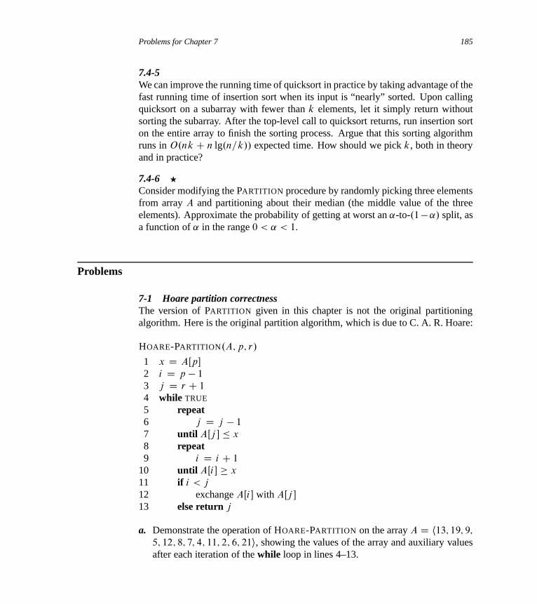
Problems for Chapter 7 185
7.4-5We can improve the running time of quicksort in practice by taking advantage of thefast running time of insertion sort when its input is “nearly” sorted. Upon callingquicksort on a subarray with fewer than k elements, let it simply return withoutsorting the subarray. After the top-level call to quicksort returns, run insertion sorton the entire array to finish the sorting process. Argue that this sorting algorithmruns in O.nk C n lg.n=k// expected time. How should we pick k, both in theoryand in practice?
7.4-6 ?
Consider modifying the PARTITION procedure by randomly picking three elementsfrom array A and partitioning about their median (the middle value of the threeelements). Approximate the probability of getting at worst an ˛-to-.1�˛/ split, asa function of ˛ in the range 0 < ˛ < 1.
Problems
7-1 Hoare partition correctnessThe version of PARTITION given in this chapter is not the original partitioningalgorithm. Here is the original partition algorithm, which is due to C. A. R. Hoare:
HOARE-PARTITION.A; p; r/
1 x D AŒp�
2 i D p � 1
3 j D r C 1
4 while TRUE
5 repeat6 j D j � 1
7 until AŒj � � x
8 repeat9 i D i C 1
10 until AŒi� � x
11 if i < j
12 exchange AŒi� with AŒj �
13 else return j
a. Demonstrate the operation of HOARE-PARTITION on the array A D h13; 19; 9;
5; 12; 8; 7; 4; 11; 2; 6; 21i, showing the values of the array and auxiliary valuesafter each iteration of the while loop in lines 4–13.
186 Chapter 7 Quicksort
The next three questions ask you to give a careful argument that the procedureHOARE-PARTITION is correct. Assuming that the subarray AŒp : : r� contains atleast two elements, prove the following:
b. The indices i and j are such that we never access an element of A outside thesubarray AŒp : : r�.
c. When HOARE-PARTITION terminates, it returns a value j such that p � j < r .
d. Every element of AŒp : : j � is less than or equal to every element of AŒjC1 : : r�
when HOARE-PARTITION terminates.
The PARTITION procedure in Section 7.1 separates the pivot value (originallyin AŒr�) from the two partitions it forms. The HOARE-PARTITION procedure, onthe other hand, always places the pivot value (originally in AŒp�) into one of thetwo partitions AŒp : : j � and AŒj C 1 : : r�. Since p � j < r , this split is alwaysnontrivial.
e. Rewrite the QUICKSORT procedure to use HOARE-PARTITION.
7-2 Quicksort with equal element valuesThe analysis of the expected running time of randomized quicksort in Section 7.4.2assumes that all element values are distinct. In this problem, we examine whathappens when they are not.
a. Suppose that all element values are equal. What would be randomized quick-sort’s running time in this case?
b. The PARTITION procedure returns an index q such that each element ofAŒp : : q � 1� is less than or equal to AŒq� and each element of AŒq C 1 : : r�
is greater than AŒq�. Modify the PARTITION procedure to produce a procedurePARTITION0.A; p; r/, which permutes the elements of AŒp : : r� and returns twoindices q and t , where p � q � t � r , such that
� all elements of AŒq : : t � are equal,� each element of AŒp : : q � 1� is less than AŒq�, and� each element of AŒt C 1 : : r� is greater than AŒq�.
Like PARTITION, your PARTITION0 procedure should take ‚.r � p/ time.
c. Modify the RANDOMIZED-QUICKSORT procedure to call PARTITION 0, andname the new procedure RANDOMIZED-QUICKSORT 0. Then modify theQUICKSORT procedure to produce a procedure QUICKSORT0.p; r/ that calls
Problems for Chapter 7 187
RANDOMIZED-PARTITION 0 and recurses only on partitions of elements notknown to be equal to each other.
d. Using QUICKSORT0, how would you adjust the analysis in Section 7.4.2 toavoid the assumption that all elements are distinct?
7-3 Alternative quicksort analysisAn alternative analysis of the running time of randomized quicksort focuses onthe expected running time of each individual recursive call to RANDOMIZED-QUICKSORT, rather than on the number of comparisons performed.
a. Argue that, given an array of size n, the probability that any particular elementis chosen as the pivot is 1=n. Use this to define indicator random variablesXi D I fi th smallest element is chosen as the pivotg. What is E ŒXi �?
b. Let T .n/ be a random variable denoting the running time of quicksort on anarray of size n. Argue that
E ŒT .n/� D E
"nX
qD1
Xq .T .q � 1/C T .n � q/C‚.n//
#: (7.5)
c. Show that we can rewrite equation (7.5) as
E ŒT .n/� D 2
n
n�1XqD2
E ŒT .q/�C‚.n/ : (7.6)
d. Show that
n�1XkD2
k lg k � 1
2n2 lg n � 1
8n2 : (7.7)
(Hint: Split the summation into two parts, one for k D 2; 3; : : : ; dn=2e � 1 andone for k D dn=2e ; : : : ; n � 1.)
e. Using the bound from equation (7.7), show that the recurrence in equation (7.6)has the solution E ŒT .n/� D ‚.n lg n/. (Hint: Show, by substitution, thatE ŒT .n/� � an lg n for sufficiently large n and for some positive constant a.)
188 Chapter 7 Quicksort
7-4 Stack depth for quicksortThe QUICKSORT algorithm of Section 7.1 contains two recursive calls to itself.After QUICKSORT calls PARTITION, it recursively sorts the left subarray and thenit recursively sorts the right subarray. The second recursive call in QUICKSORT
is not really necessary; we can avoid it by using an iterative control structure.This technique, called tail recursion, is provided automatically by good compilers.Consider the following version of quicksort, which simulates tail recursion:
TAIL-RECURSIVE-QUICKSORT.A; p; r/
1 while p < r
2 // Partition and sort left subarray.3 q D PARTITION.A; p; r/
4 TAIL-RECURSIVE-QUICKSORT.A; p; q � 1/
5 p D q C 1
a. Argue that TAIL-RECURSIVE-QUICKSORT.A; 1; A: length/ correctly sorts thearray A.
Compilers usually execute recursive procedures by using a stack that contains per-tinent information, including the parameter values, for each recursive call. Theinformation for the most recent call is at the top of the stack, and the informationfor the initial call is at the bottom. Upon calling a procedure, its information ispushed onto the stack; when it terminates, its information is popped. Since weassume that array parameters are represented by pointers, the information for eachprocedure call on the stack requires O.1/ stack space. The stack depth is the max-imum amount of stack space used at any time during a computation.
b. Describe a scenario in which TAIL-RECURSIVE-QUICKSORT’s stack depth is‚.n/ on an n-element input array.
c. Modify the code for TAIL-RECURSIVE-QUICKSORT so that the worst-casestack depth is ‚.lg n/. Maintain the O.n lg n/ expected running time of thealgorithm.
7-5 Median-of-3 partitionOne way to improve the RANDOMIZED-QUICKSORT procedure is to partitionaround a pivot that is chosen more carefully than by picking a random elementfrom the subarray. One common approach is the median-of-3 method: choosethe pivot as the median (middle element) of a set of 3 elements randomly selectedfrom the subarray. (See Exercise 7.4-6.) For this problem, let us assume that theelements in the input array AŒ1 : : n� are distinct and that n � 3. We denote the
Problems for Chapter 7 189
sorted output array by A0Œ1 : : n�. Using the median-of-3 method to choose thepivot element x, define pi D Pr fx D A0Œi �g.a. Give an exact formula for pi as a function of n and i for i D 2; 3; : : : ; n � 1.
(Note that p1 D pn D 0.)
b. By what amount have we increased the likelihood of choosing the pivot asx D A0Œb.nC 1/=2c�, the median of AŒ1 : : n�, compared with the ordinaryimplementation? Assume that n ! 1, and give the limiting ratio of theseprobabilities.
c. If we define a “good” split to mean choosing the pivot as x D A0Œi �, wheren=3 � i � 2n=3, by what amount have we increased the likelihood of gettinga good split compared with the ordinary implementation? (Hint: Approximatethe sum by an integral.)
d. Argue that in the �.n lg n/ running time of quicksort, the median-of-3 methodaffects only the constant factor.
7-6 Fuzzy sorting of intervalsConsider a sorting problem in which we do not know the numbers exactly. In-stead, for each number, we know an interval on the real line to which it belongs.That is, we are given n closed intervals of the form Œai ; bi �, where ai � bi . Wewish to fuzzy-sort these intervals, i.e., to produce a permutation hi1; i2; : : : ; ini ofthe intervals such that for j D 1; 2; : : : ; n, there exist cj 2 Œaij ; bij � satisfyingc1 � c2 � � � � � cn.
a. Design a randomized algorithm for fuzzy-sorting n intervals. Your algorithmshould have the general structure of an algorithm that quicksorts the left end-points (the ai values), but it should take advantage of overlapping intervals toimprove the running time. (As the intervals overlap more and more, the prob-lem of fuzzy-sorting the intervals becomes progressively easier. Your algorithmshould take advantage of such overlapping, to the extent that it exists.)
b. Argue that your algorithm runs in expected time ‚.n lg n/ in general, but runsin expected time ‚.n/ when all of the intervals overlap (i.e., when there exists avalue x such that x 2 Œai ; bi � for all i). Your algorithm should not be checkingfor this case explicitly; rather, its performance should naturally improve as theamount of overlap increases.
190 Chapter 7 Quicksort
Chapter notes
The quicksort procedure was invented by Hoare [170]; Hoare’s version appears inProblem 7-1. The PARTITION procedure given in Section 7.1 is due to N. Lomuto.The analysis in Section 7.4 is due to Avrim Blum. Sedgewick [305] and Bent-ley [43] provide a good reference on the details of implementation and how theymatter.
McIlroy [248] showed how to engineer a “killer adversary” that produces anarray on which virtually any implementation of quicksort takes ‚.n2/ time. If theimplementation is randomized, the adversary produces the array after seeing therandom choices of the quicksort algorithm.

8 Sorting in Linear Time
We have now introduced several algorithms that can sort n numbers in O.n lg n/
time. Merge sort and heapsort achieve this upper bound in the worst case; quicksortachieves it on average. Moreover, for each of these algorithms, we can produce asequence of n input numbers that causes the algorithm to run in �.n lg n/ time.
These algorithms share an interesting property: the sorted order they determineis based only on comparisons between the input elements. We call such sortingalgorithms comparison sorts. All the sorting algorithms introduced thus far arecomparison sorts.
In Section 8.1, we shall prove that any comparison sort must make �.n lg n/
comparisons in the worst case to sort n elements. Thus, merge sort and heapsortare asymptotically optimal, and no comparison sort exists that is faster by morethan a constant factor.
Sections 8.2, 8.3, and 8.4 examine three sorting algorithms—counting sort, radixsort, and bucket sort—that run in linear time. Of course, these algorithms useoperations other than comparisons to determine the sorted order. Consequently,the �.n lg n/ lower bound does not apply to them.
8.1 Lower bounds for sorting
In a comparison sort, we use only comparisons between elements to gain orderinformation about an input sequence ha1; a2; : : : ; ani. That is, given two elementsai and aj , we perform one of the tests ai < aj , ai � aj , ai D aj , ai � aj , orai > aj to determine their relative order. We may not inspect the values of theelements or gain order information about them in any other way.
In this section, we assume without loss of generality that all the input elementsare distinct. Given this assumption, comparisons of the form ai D aj are useless,so we can assume that no comparisons of this form are made. We also note thatthe comparisons ai � aj , ai � aj , ai > aj , and ai < aj are all equivalent in that
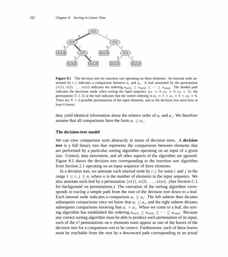
192 Chapter 8 Sorting in Linear Time
≤ >
≤ >
1:2
2:3 1:3
⟨1,2,3⟩ 1:3 ⟨2,1,3⟩ 2:3
⟨1,3,2⟩ ⟨3,1,2⟩ ⟨3,2,1⟩
≤ >
≤ >
≤ >
⟨2,3,1⟩
Figure 8.1 The decision tree for insertion sort operating on three elements. An internal node an-notated by i :j indicates a comparison between ai and aj . A leaf annotated by the permutationh�.1/; �.2/; : : : ; �.n/i indicates the ordering a�.1/ � a�.2/ � � � � � a�.n/. The shaded pathindicates the decisions made when sorting the input sequence ha1 D 6; a2 D 8; a3 D 5i; thepermutation h3; 1; 2i at the leaf indicates that the sorted ordering is a3 D 5 � a1 D 6 � a2 D 8.There are 3Š D 6 possible permutations of the input elements, and so the decision tree must have atleast 6 leaves.
they yield identical information about the relative order of ai and aj . We thereforeassume that all comparisons have the form ai � aj .
The decision-tree model
We can view comparison sorts abstractly in terms of decision trees. A decisiontree is a full binary tree that represents the comparisons between elements thatare performed by a particular sorting algorithm operating on an input of a givensize. Control, data movement, and all other aspects of the algorithm are ignored.Figure 8.1 shows the decision tree corresponding to the insertion sort algorithmfrom Section 2.1 operating on an input sequence of three elements.
In a decision tree, we annotate each internal node by i :j for some i and j in therange 1 � i; j � n, where n is the number of elements in the input sequence. Wealso annotate each leaf by a permutation h�.1/; �.2/; : : : ; �.n/i. (See Section C.1for background on permutations.) The execution of the sorting algorithm corre-sponds to tracing a simple path from the root of the decision tree down to a leaf.Each internal node indicates a comparison ai � aj . The left subtree then dictatessubsequent comparisons once we know that ai � aj , and the right subtree dictatessubsequent comparisons knowing that ai > aj . When we come to a leaf, the sort-ing algorithm has established the ordering a�.1/ � a�.2/ � � � � � a�.n/. Becauseany correct sorting algorithm must be able to produce each permutation of its input,each of the nŠ permutations on n elements must appear as one of the leaves of thedecision tree for a comparison sort to be correct. Furthermore, each of these leavesmust be reachable from the root by a downward path corresponding to an actual

8.1 Lower bounds for sorting 193
execution of the comparison sort. (We shall refer to such leaves as “reachable.”)Thus, we shall consider only decision trees in which each permutation appears asa reachable leaf.
A lower bound for the worst case
The length of the longest simple path from the root of a decision tree to any ofits reachable leaves represents the worst-case number of comparisons that the cor-responding sorting algorithm performs. Consequently, the worst-case number ofcomparisons for a given comparison sort algorithm equals the height of its decisiontree. A lower bound on the heights of all decision trees in which each permutationappears as a reachable leaf is therefore a lower bound on the running time of anycomparison sort algorithm. The following theorem establishes such a lower bound.
Theorem 8.1Any comparison sort algorithm requires �.n lg n/ comparisons in the worst case.
Proof From the preceding discussion, it suffices to determine the height of adecision tree in which each permutation appears as a reachable leaf. Consider adecision tree of height h with l reachable leaves corresponding to a comparisonsort on n elements. Because each of the nŠ permutations of the input appears assome leaf, we have nŠ � l . Since a binary tree of height h has no more than 2h
leaves, we have
nŠ � l � 2h ;
which, by taking logarithms, implies
h � lg.nŠ/ (since the lg function is monotonically increasing)
D �.n lg n/ (by equation (3.19)) .
Corollary 8.2Heapsort and merge sort are asymptotically optimal comparison sorts.
Proof The O.n lg n/ upper bounds on the running times for heapsort and mergesort match the �.n lg n/ worst-case lower bound from Theorem 8.1.
Exercises
8.1-1What is the smallest possible depth of a leaf in a decision tree for a comparisonsort?
194 Chapter 8 Sorting in Linear Time
8.1-2Obtain asymptotically tight bounds on lg.nŠ/ without using Stirling’s approxi-mation. Instead, evaluate the summation
Pn
kD1 lg k using techniques from Sec-tion A.2.
8.1-3Show that there is no comparison sort whose running time is linear for at least halfof the nŠ inputs of length n. What about a fraction of 1=n of the inputs of length n?What about a fraction 1=2n?
8.1-4Suppose that you are given a sequence of n elements to sort. The input sequenceconsists of n=k subsequences, each containing k elements. The elements in a givensubsequence are all smaller than the elements in the succeeding subsequence andlarger than the elements in the preceding subsequence. Thus, all that is needed tosort the whole sequence of length n is to sort the k elements in each of the n=k
subsequences. Show an �.n lg k/ lower bound on the number of comparisonsneeded to solve this variant of the sorting problem. (Hint: It is not rigorous tosimply combine the lower bounds for the individual subsequences.)
8.2 Counting sort
Counting sort assumes that each of the n input elements is an integer in the range0 to k, for some integer k. When k D O.n/, the sort runs in ‚.n/ time.
Counting sort determines, for each input element x, the number of elements lessthan x. It uses this information to place element x directly into its position in theoutput array. For example, if 17 elements are less than x, then x belongs in outputposition 18. We must modify this scheme slightly to handle the situation in whichseveral elements have the same value, since we do not want to put them all in thesame position.
In the code for counting sort, we assume that the input is an array AŒ1 : : n�, andthus A: length D n. We require two other arrays: the array BŒ1 : : n� holds thesorted output, and the array C Œ0 : : k� provides temporary working storage.
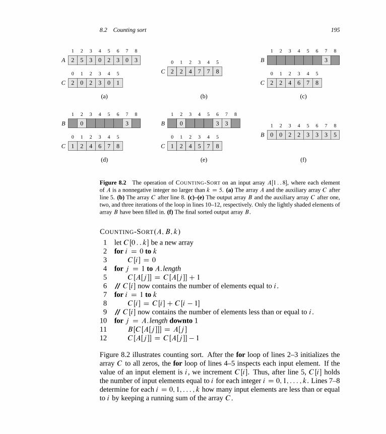
8.2 Counting sort 195
2 5 3 0 2 3 0 3
1 2 3 4 5 6 7 8
2 0 2 3 0 1
1 2 3 4 5
A
C
(a)
2 2 4 7 7 8C
(b)
3
1 2 3 4 5 6 7 8
2 2 4 6 7 8
B
C
(c)
3
1 2 3 4 5 6 7 8
1 2 4 6 7 8
B
C
(d)
0 3
1 2 3 4 5 6 7 8
1 2 4 5 7 8
B
C
(e)
0 3
3
1 2 3 4 5 6 7 8
B
(f)
0 30 2 2 3 5
0
1 2 3 4 50
1 2 3 4 50 1 2 3 4 50
1 2 3 4 50
Figure 8.2 The operation of COUNTING-SORT on an input array AŒ1 : : 8�, where each elementof A is a nonnegative integer no larger than k D 5. (a) The array A and the auxiliary array C afterline 5. (b) The array C after line 8. (c)–(e) The output array B and the auxiliary array C after one,two, and three iterations of the loop in lines 10–12, respectively. Only the lightly shaded elements ofarray B have been filled in. (f) The final sorted output array B .
COUNTING-SORT.A; B; k/
1 let C Œ0 : : k� be a new array2 for i D 0 to k
3 C Œi� D 0
4 for j D 1 to A: length5 C ŒAŒj �� D C ŒAŒj ��C 1
6 // C Œi� now contains the number of elements equal to i .7 for i D 1 to k
8 C Œi� D C Œi�C C Œi � 1�
9 // C Œi� now contains the number of elements less than or equal to i .10 for j D A: length downto 111 BŒC ŒAŒj ��� D AŒj �
12 C ŒAŒj �� D C ŒAŒj ��� 1
Figure 8.2 illustrates counting sort. After the for loop of lines 2–3 initializes thearray C to all zeros, the for loop of lines 4–5 inspects each input element. If thevalue of an input element is i , we increment C Œi�. Thus, after line 5, C Œi� holdsthe number of input elements equal to i for each integer i D 0; 1; : : : ; k. Lines 7–8determine for each i D 0; 1; : : : ; k how many input elements are less than or equalto i by keeping a running sum of the array C .

196 Chapter 8 Sorting in Linear Time
Finally, the for loop of lines 10–12 places each element AŒj � into its correctsorted position in the output array B . If all n elements are distinct, then when wefirst enter line 10, for each AŒj �, the value C ŒAŒj �� is the correct final positionof AŒj � in the output array, since there are C ŒAŒj �� elements less than or equalto AŒj �. Because the elements might not be distinct, we decrement C ŒAŒj �� eachtime we place a value AŒj � into the B array. Decrementing C ŒAŒj �� causes thenext input element with a value equal to AŒj �, if one exists, to go to the positionimmediately before AŒj � in the output array.
How much time does counting sort require? The for loop of lines 2–3 takestime ‚.k/, the for loop of lines 4–5 takes time ‚.n/, the for loop of lines 7–8 takestime ‚.k/, and the for loop of lines 10–12 takes time ‚.n/. Thus, the overall timeis ‚.kCn/. In practice, we usually use counting sort when we have k D O.n/, inwhich case the running time is ‚.n/.
Counting sort beats the lower bound of �.n lg n/ proved in Section 8.1 becauseit is not a comparison sort. In fact, no comparisons between input elements occuranywhere in the code. Instead, counting sort uses the actual values of the elementsto index into an array. The �.n lg n/ lower bound for sorting does not apply whenwe depart from the comparison-sort model.
An important property of counting sort is that it is stable: numbers with the samevalue appear in the output array in the same order as they do in the input array. Thatis, it breaks ties between two numbers by the rule that whichever number appearsfirst in the input array appears first in the output array. Normally, the property ofstability is important only when satellite data are carried around with the elementbeing sorted. Counting sort’s stability is important for another reason: countingsort is often used as a subroutine in radix sort. As we shall see in the next section,in order for radix sort to work correctly, counting sort must be stable.
Exercises
8.2-1Using Figure 8.2 as a model, illustrate the operation of COUNTING-SORT on thearray A D h6; 0; 2; 0; 1; 3; 4; 6; 1; 3; 2i.8.2-2Prove that COUNTING-SORT is stable.
8.2-3Suppose that we were to rewrite the for loop header in line 10 of the COUNTING-SORT as
10 for j D 1 to A: length
Show that the algorithm still works properly. Is the modified algorithm stable?
8.3 Radix sort 197
8.2-4Describe an algorithm that, given n integers in the range 0 to k, preprocesses itsinput and then answers any query about how many of the n integers fall into arange Œa : : b� in O.1/ time. Your algorithm should use ‚.n C k/ preprocessingtime.
8.3 Radix sort
Radix sort is the algorithm used by the card-sorting machines you now find only incomputer museums. The cards have 80 columns, and in each column a machine canpunch a hole in one of 12 places. The sorter can be mechanically “programmed”to examine a given column of each card in a deck and distribute the card into oneof 12 bins depending on which place has been punched. An operator can thengather the cards bin by bin, so that cards with the first place punched are on top ofcards with the second place punched, and so on.
For decimal digits, each column uses only 10 places. (The other two placesare reserved for encoding nonnumeric characters.) A d -digit number would thenoccupy a field of d columns. Since the card sorter can look at only one columnat a time, the problem of sorting n cards on a d -digit number requires a sortingalgorithm.
Intuitively, you might sort numbers on their most significant digit, sort each ofthe resulting bins recursively, and then combine the decks in order. Unfortunately,since the cards in 9 of the 10 bins must be put aside to sort each of the bins, thisprocedure generates many intermediate piles of cards that you would have to keeptrack of. (See Exercise 8.3-5.)
Radix sort solves the problem of card sorting—counterintuitively—by sorting onthe least significant digit first. The algorithm then combines the cards into a singledeck, with the cards in the 0 bin preceding the cards in the 1 bin preceding thecards in the 2 bin, and so on. Then it sorts the entire deck again on the second-leastsignificant digit and recombines the deck in a like manner. The process continuesuntil the cards have been sorted on all d digits. Remarkably, at that point the cardsare fully sorted on the d -digit number. Thus, only d passes through the deck arerequired to sort. Figure 8.3 shows how radix sort operates on a “deck” of seven3-digit numbers.
In order for radix sort to work correctly, the digit sorts must be stable. The sortperformed by a card sorter is stable, but the operator has to be wary about notchanging the order of the cards as they come out of a bin, even though all the cardsin a bin have the same digit in the chosen column.

198 Chapter 8 Sorting in Linear Time
329457657839436720355
329
457657
839
436
720355 329
457657
839436
720
355
329
457657
839
436
720
355
Figure 8.3 The operation of radix sort on a list of seven 3-digit numbers. The leftmost column isthe input. The remaining columns show the list after successive sorts on increasingly significant digitpositions. Shading indicates the digit position sorted on to produce each list from the previous one.
In a typical computer, which is a sequential random-access machine, we some-times use radix sort to sort records of information that are keyed by multiple fields.For example, we might wish to sort dates by three keys: year, month, and day. Wecould run a sorting algorithm with a comparison function that, given two dates,compares years, and if there is a tie, compares months, and if another tie occurs,compares days. Alternatively, we could sort the information three times with astable sort: first on day, next on month, and finally on year.
The code for radix sort is straightforward. The following procedure assumes thateach element in the n-element array A has d digits, where digit 1 is the lowest-orderdigit and digit d is the highest-order digit.
RADIX-SORT.A; d/
1 for i D 1 to d
2 use a stable sort to sort array A on digit i
Lemma 8.3Given n d -digit numbers in which each digit can take on up to k possible values,RADIX-SORT correctly sorts these numbers in ‚.d.nC k// time if the stable sortit uses takes ‚.nC k/ time.
Proof The correctness of radix sort follows by induction on the column beingsorted (see Exercise 8.3-3). The analysis of the running time depends on the stablesort used as the intermediate sorting algorithm. When each digit is in the range 0
to k�1 (so that it can take on k possible values), and k is not too large, counting sortis the obvious choice. Each pass over n d -digit numbers then takes time ‚.nCk/.There are d passes, and so the total time for radix sort is ‚.d.nC k//.
When d is constant and k D O.n/, we can make radix sort run in linear time.More generally, we have some flexibility in how to break each key into digits.
8.3 Radix sort 199
Lemma 8.4Given n b-bit numbers and any positive integer r � b, RADIX-SORT correctly sortsthese numbers in ‚..b=r/.nC 2r// time if the stable sort it uses takes ‚.nC k/
time for inputs in the range 0 to k.
Proof For a value r � b, we view each key as having d D db=re digits of r bitseach. Each digit is an integer in the range 0 to 2r � 1, so that we can use countingsort with k D 2r �1. (For example, we can view a 32-bit word as having four 8-bitdigits, so that b D 32, r D 8, k D 2r � 1 D 255, and d D b=r D 4.) Each pass ofcounting sort takes time ‚.nC k/ D ‚.nC 2r/ and there are d passes, for a totalrunning time of ‚.d.nC 2r// D ‚..b=r/.nC 2r//.
For given values of n and b, we wish to choose the value of r , with r � b,that minimizes the expression .b=r/.n C 2r/. If b < blg nc, then for any valueof r � b, we have that .nC 2r/ D ‚.n/. Thus, choosing r D b yields a runningtime of .b=b/.n C 2b/ D ‚.n/, which is asymptotically optimal. If b � blg nc,then choosing r D blg nc gives the best time to within a constant factor, whichwe can see as follows. Choosing r D blg nc yields a running time of ‚.bn= lg n/.As we increase r above blg nc, the 2r term in the numerator increases faster thanthe r term in the denominator, and so increasing r above blg nc yields a runningtime of �.bn= lg n/. If instead we were to decrease r below blg nc, then the b=r
term increases and the nC 2r term remains at ‚.n/.Is radix sort preferable to a comparison-based sorting algorithm, such as quick-
sort? If b D O.lg n/, as is often the case, and we choose r � lg n, then radix sort’srunning time is ‚.n/, which appears to be better than quicksort’s expected runningtime of ‚.n lg n/. The constant factors hidden in the ‚-notation differ, however.Although radix sort may make fewer passes than quicksort over the n keys, eachpass of radix sort may take significantly longer. Which sorting algorithm we preferdepends on the characteristics of the implementations, of the underlying machine(e.g., quicksort often uses hardware caches more effectively than radix sort), andof the input data. Moreover, the version of radix sort that uses counting sort as theintermediate stable sort does not sort in place, which many of the ‚.n lg n/-timecomparison sorts do. Thus, when primary memory storage is at a premium, wemight prefer an in-place algorithm such as quicksort.
Exercises
8.3-1Using Figure 8.3 as a model, illustrate the operation of RADIX-SORT on the fol-lowing list of English words: COW, DOG, SEA, RUG, ROW, MOB, BOX, TAB,BAR, EAR, TAR, DIG, BIG, TEA, NOW, FOX.

200 Chapter 8 Sorting in Linear Time
8.3-2Which of the following sorting algorithms are stable: insertion sort, merge sort,heapsort, and quicksort? Give a simple scheme that makes any sorting algorithmstable. How much additional time and space does your scheme entail?
8.3-3Use induction to prove that radix sort works. Where does your proof need theassumption that the intermediate sort is stable?
8.3-4Show how to sort n integers in the range 0 to n3 � 1 in O.n/ time.
8.3-5 ?
In the first card-sorting algorithm in this section, exactly how many sorting passesare needed to sort d -digit decimal numbers in the worst case? How many piles ofcards would an operator need to keep track of in the worst case?
8.4 Bucket sort
Bucket sort assumes that the input is drawn from a uniform distribution and has anaverage-case running time of O.n/. Like counting sort, bucket sort is fast becauseit assumes something about the input. Whereas counting sort assumes that the inputconsists of integers in a small range, bucket sort assumes that the input is generatedby a random process that distributes elements uniformly and independently overthe interval Œ0; 1/. (See Section C.2 for a definition of uniform distribution.)
Bucket sort divides the interval Œ0; 1/ into n equal-sized subintervals, or buckets,and then distributes the n input numbers into the buckets. Since the inputs are uni-formly and independently distributed over Œ0; 1/, we do not expect many numbersto fall into each bucket. To produce the output, we simply sort the numbers in eachbucket and then go through the buckets in order, listing the elements in each.
Our code for bucket sort assumes that the input is an n-element array A andthat each element AŒi� in the array satisfies 0 � AŒi� < 1. The code requires anauxiliary array BŒ0 : : n � 1� of linked lists (buckets) and assumes that there is amechanism for maintaining such lists. (Section 10.2 describes how to implementbasic operations on linked lists.)

8.4 Bucket sort 201
1
2
3
4
5
6
7
8
9
10
.78
.17
.39
.72
.94
.21
.12
.23
.68
A
(a)
1
2
3
4
5
6
7
8
9
B
(b)
0
.12 .17
.21 .23
.26
.26
.39
.68
.72 .78
.94
Figure 8.4 The operation of BUCKET-SORT for n D 10. (a) The input array AŒ1 : : 10�. (b) Thearray BŒ0 : : 9� of sorted lists (buckets) after line 8 of the algorithm. Bucket i holds values in thehalf-open interval Œi=10; .i C 1/=10/. The sorted output consists of a concatenation in order of thelists BŒ0�; BŒ1�; : : : ; BŒ9�.
BUCKET-SORT.A/
1 let BŒ0 : : n � 1� be a new array2 n D A: length3 for i D 0 to n � 1
4 make BŒi� an empty list5 for i D 1 to n
6 insert AŒi� into list BŒbnAŒi�c�7 for i D 0 to n � 1
8 sort list BŒi� with insertion sort9 concatenate the lists BŒ0�; BŒ1�; : : : ; BŒn � 1� together in order
Figure 8.4 shows the operation of bucket sort on an input array of 10 numbers.To see that this algorithm works, consider two elements AŒi� and AŒj �. Assume
without loss of generality that AŒi� � AŒj �. Since bnAŒi�c � bnAŒj �c, eitherelement AŒi� goes into the same bucket as AŒj � or it goes into a bucket with a lowerindex. If AŒi� and AŒj � go into the same bucket, then the for loop of lines 7–8 putsthem into the proper order. If AŒi� and AŒj � go into different buckets, then line 9puts them into the proper order. Therefore, bucket sort works correctly.
To analyze the running time, observe that all lines except line 8 take O.n/ timein the worst case. We need to analyze the total time taken by the n calls to insertionsort in line 8.

202 Chapter 8 Sorting in Linear Time
To analyze the cost of the calls to insertion sort, let ni be the random variabledenoting the number of elements placed in bucket BŒi�. Since insertion sort runsin quadratic time (see Section 2.2), the running time of bucket sort is
T .n/ D ‚.n/Cn�1XiD0
O.n2i / :
We now analyze the average-case running time of bucket sort, by computing theexpected value of the running time, where we take the expectation over the inputdistribution. Taking expectations of both sides and using linearity of expectation,we have
E ŒT .n/� D E
"‚.n/C
n�1XiD0
O.n2i /
#
D ‚.n/Cn�1XiD0
E�O.n2
i /�
(by linearity of expectation)
D ‚.n/Cn�1XiD0
O�E�n2
i
��(by equation (C.22)) . (8.1)
We claim that
E�n2
i
� D 2 � 1=n (8.2)
for i D 0; 1; : : : ; n � 1. It is no surprise that each bucket i has the same value ofE Œn2
i �, since each value in the input array A is equally likely to fall in any bucket.To prove equation (8.2), we define indicator random variables
Xij D I fAŒj � falls in bucket igfor i D 0; 1; : : : ; n � 1 and j D 1; 2; : : : ; n. Thus,
ni DnX
j D1
Xij :
To compute E Œn2i �, we expand the square and regroup terms:

8.4 Bucket sort 203
E�n2
i
� D E
" nX
j D1
Xij
!2#
D E
"nX
j D1
nXkD1
Xij Xik
#
D E
24 nXj D1
X2ij C
X1�j �n
X1�k�n
k¤j
Xij Xik
35D
nXj D1
E�X2
ij
�C X1�j �n
X1�k�n
k¤j
E ŒXij Xik� ; (8.3)
where the last line follows by linearity of expectation. We evaluate the two sum-mations separately. Indicator random variable Xij is 1 with probability 1=n and 0
otherwise, and therefore
E�X2
ij
� D 12 � 1nC 02 �
�1 � 1
n
�D 1
n:
When k ¤ j , the variables Xij and Xik are independent, and hence
E ŒXij Xik� D E ŒXij � E ŒXik�
D 1
n� 1
n
D 1
n2:
Substituting these two expected values in equation (8.3), we obtain
E�n2
i
� D nXj D1
1
nC
X1�j �n
X1�k�n
k¤j
1
n2
D n � 1nC n.n � 1/ � 1
n2
D 1C n � 1
n
D 2 � 1
n;
which proves equation (8.2).

204 Chapter 8 Sorting in Linear Time
Using this expected value in equation (8.1), we conclude that the average-caserunning time for bucket sort is ‚.n/C n �O.2 � 1=n/ D ‚.n/.
Even if the input is not drawn from a uniform distribution, bucket sort may stillrun in linear time. As long as the input has the property that the sum of the squaresof the bucket sizes is linear in the total number of elements, equation (8.1) tells usthat bucket sort will run in linear time.
Exercises
8.4-1Using Figure 8.4 as a model, illustrate the operation of BUCKET-SORT on the arrayA D h:79; :13; :16; :64; :39; :20; :89; :53; :71; :42i.8.4-2Explain why the worst-case running time for bucket sort is ‚.n2/. What simplechange to the algorithm preserves its linear average-case running time and makesits worst-case running time O.n lg n/?
8.4-3Let X be a random variable that is equal to the number of heads in two flips of afair coin. What is E ŒX2�? What is E2 ŒX�?
8.4-4 ?
We are given n points in the unit circle, pi D .xi ; yi /, such that 0 < x2i C y2
i � 1
for i D 1; 2; : : : ; n. Suppose that the points are uniformly distributed; that is, theprobability of finding a point in any region of the circle is proportional to the areaof that region. Design an algorithm with an average-case running time of ‚.n/ tosort the n points by their distances di D
px2
i C y2i from the origin. (Hint: Design
the bucket sizes in BUCKET-SORT to reflect the uniform distribution of the pointsin the unit circle.)
8.4-5 ?
A probability distribution function P.x/ for a random variable X is definedby P.x/ D Pr fX � xg. Suppose that we draw a list of n random variablesX1; X2; : : : ; Xn from a continuous probability distribution function P that is com-putable in O.1/ time. Give an algorithm that sorts these numbers in linear average-case time.

Problems for Chapter 8 205
Problems
8-1 Probabilistic lower bounds on comparison sortingIn this problem, we prove a probabilistic �.n lg n/ lower bound on the running timeof any deterministic or randomized comparison sort on n distinct input elements.We begin by examining a deterministic comparison sort A with decision tree TA.We assume that every permutation of A’s inputs is equally likely.
a. Suppose that each leaf of TA is labeled with the probability that it is reachedgiven a random input. Prove that exactly nŠ leaves are labeled 1=nŠ and that therest are labeled 0.
b. Let D.T / denote the external path length of a decision tree T ; that is, D.T /
is the sum of the depths of all the leaves of T . Let T be a decision tree withk > 1 leaves, and let LT and RT be the left and right subtrees of T . Show thatD.T / D D.LT/CD.RT/C k.
c. Let d.k/ be the minimum value of D.T / over all decision trees T with k > 1
leaves. Show that d.k/ D min1�i�k�1 fd.i/C d.k � i/C kg. (Hint: Considera decision tree T with k leaves that achieves the minimum. Let i0 be the numberof leaves in LT and k � i0 the number of leaves in RT.)
d. Prove that for a given value of k > 1 and i in the range 1 � i � k � 1, thefunction i lg i C .k � i/ lg.k � i/ is minimized at i D k=2. Conclude thatd.k/ D �.k lg k/.
e. Prove that D.TA/ D �.nŠ lg.nŠ//, and conclude that the average-case time tosort n elements is �.n lg n/.
Now, consider a randomized comparison sort B . We can extend the decision-tree model to handle randomization by incorporating two kinds of nodes: ordinarycomparison nodes and “randomization” nodes. A randomization node models arandom choice of the form RANDOM.1; r/ made by algorithm B; the node has r
children, each of which is equally likely to be chosen during an execution of thealgorithm.
f. Show that for any randomized comparison sort B , there exists a deterministiccomparison sort A whose expected number of comparisons is no more thanthose made by B .

206 Chapter 8 Sorting in Linear Time
8-2 Sorting in place in linear timeSuppose that we have an array of n data records to sort and that the key of eachrecord has the value 0 or 1. An algorithm for sorting such a set of records mightpossess some subset of the following three desirable characteristics:
1. The algorithm runs in O.n/ time.
2. The algorithm is stable.
3. The algorithm sorts in place, using no more than a constant amount of storagespace in addition to the original array.
a. Give an algorithm that satisfies criteria 1 and 2 above.
b. Give an algorithm that satisfies criteria 1 and 3 above.
c. Give an algorithm that satisfies criteria 2 and 3 above.
d. Can you use any of your sorting algorithms from parts (a)–(c) as the sortingmethod used in line 2 of RADIX-SORT, so that RADIX-SORT sorts n recordswith b-bit keys in O.bn/ time? Explain how or why not.
e. Suppose that the n records have keys in the range from 1 to k. Show how tomodify counting sort so that it sorts the records in place in O.nC k/ time. Youmay use O.k/ storage outside the input array. Is your algorithm stable? (Hint:How would you do it for k D 3?)
8-3 Sorting variable-length itemsa. You are given an array of integers, where different integers may have different
numbers of digits, but the total number of digits over all the integers in the arrayis n. Show how to sort the array in O.n/ time.
b. You are given an array of strings, where different strings may have differentnumbers of characters, but the total number of characters over all the stringsis n. Show how to sort the strings in O.n/ time.
(Note that the desired order here is the standard alphabetical order; for example,a < ab < b.)
8-4 Water jugsSuppose that you are given n red and n blue water jugs, all of different shapes andsizes. All red jugs hold different amounts of water, as do the blue ones. Moreover,for every red jug, there is a blue jug that holds the same amount of water, and viceversa.

Problems for Chapter 8 207
Your task is to find a grouping of the jugs into pairs of red and blue jugs that holdthe same amount of water. To do so, you may perform the following operation: picka pair of jugs in which one is red and one is blue, fill the red jug with water, andthen pour the water into the blue jug. This operation will tell you whether the redor the blue jug can hold more water, or that they have the same volume. Assumethat such a comparison takes one time unit. Your goal is to find an algorithm thatmakes a minimum number of comparisons to determine the grouping. Rememberthat you may not directly compare two red jugs or two blue jugs.
a. Describe a deterministic algorithm that uses ‚.n2/ comparisons to group thejugs into pairs.
b. Prove a lower bound of �.n lg n/ for the number of comparisons an algorithmsolving this problem must make.
c. Give a randomized algorithm whose expected number of comparisons isO.n lg n/, and prove that this bound is correct. What is the worst-case num-ber of comparisons for your algorithm?
8-5 Average sortingSuppose that, instead of sorting an array, we just require that the elements increaseon average. More precisely, we call an n-element array A k-sorted if, for alli D 1; 2; : : : ; n � k, the following holds:PiCk�1
j Di AŒj �
k�PiCk
j DiC1 AŒj �
k:
a. What does it mean for an array to be 1-sorted?
b. Give a permutation of the numbers 1; 2; : : : ; 10 that is 2-sorted, but not sorted.
c. Prove that an n-element array is k-sorted if and only if AŒi� � AŒi C k� for alli D 1; 2; : : : ; n � k.
d. Give an algorithm that k-sorts an n-element array in O.n lg.n=k// time.
We can also show a lower bound on the time to produce a k-sorted array, when k
is a constant.
e. Show that we can sort a k-sorted array of length n in O.n lg k/ time. (Hint:Use the solution to Exercise 6.5-9. )
f. Show that when k is a constant, k-sorting an n-element array requires �.n lg n/
time. (Hint: Use the solution to the previous part along with the lower boundon comparison sorts.)
208 Chapter 8 Sorting in Linear Time
8-6 Lower bound on merging sorted listsThe problem of merging two sorted lists arises frequently. We have seen a pro-cedure for it as the subroutine MERGE in Section 2.3.1. In this problem, we willprove a lower bound of 2n � 1 on the worst-case number of comparisons requiredto merge two sorted lists, each containing n items.
First we will show a lower bound of 2n� o.n/ comparisons by using a decisiontree.
a. Given 2n numbers, compute the number of possible ways to divide them intotwo sorted lists, each with n numbers.
b. Using a decision tree and your answer to part (a), show that any algorithm thatcorrectly merges two sorted lists must perform at least 2n� o.n/ comparisons.
Now we will show a slightly tighter 2n � 1 bound.
c. Show that if two elements are consecutive in the sorted order and from differentlists, then they must be compared.
d. Use your answer to the previous part to show a lower bound of 2n� 1 compar-isons for merging two sorted lists.
8-7 The 0-1 sorting lemma and columnsortA compare-exchange operation on two array elements AŒi� and AŒj �, where i < j ,has the form
COMPARE-EXCHANGE.A; i; j /
1 if AŒi� > AŒj �
2 exchange AŒi� with AŒj �
After the compare-exchange operation, we know that AŒi� � AŒj �.An oblivious compare-exchange algorithm operates solely by a sequence of
prespecified compare-exchange operations. The indices of the positions comparedin the sequence must be determined in advance, and although they can dependon the number of elements being sorted, they cannot depend on the values beingsorted, nor can they depend on the result of any prior compare-exchange operation.For example, here is insertion sort expressed as an oblivious compare-exchangealgorithm:
INSERTION-SORT.A/
1 for j D 2 to A: length2 for i D j � 1 downto 1
3 COMPARE-EXCHANGE.A; i; i C 1/
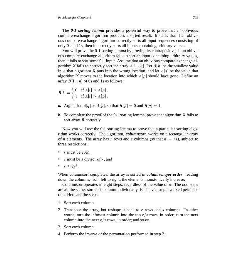
Problems for Chapter 8 209
The 0-1 sorting lemma provides a powerful way to prove that an obliviouscompare-exchange algorithm produces a sorted result. It states that if an oblivi-ous compare-exchange algorithm correctly sorts all input sequences consisting ofonly 0s and 1s, then it correctly sorts all inputs containing arbitrary values.
You will prove the 0-1 sorting lemma by proving its contrapositive: if an oblivi-ous compare-exchange algorithm fails to sort an input containing arbitrary values,then it fails to sort some 0-1 input. Assume that an oblivious compare-exchange al-gorithm X fails to correctly sort the array AŒ1 : : n�. Let AŒp� be the smallest valuein A that algorithm X puts into the wrong location, and let AŒq� be the value thatalgorithm X moves to the location into which AŒp� should have gone. Define anarray BŒ1 : : n� of 0s and 1s as follows:
BŒi� D(
0 if AŒi� � AŒp� ;
1 if AŒi� > AŒp� :
a. Argue that AŒq� > AŒp�, so that BŒp� D 0 and BŒq� D 1.
b. To complete the proof of the 0-1 sorting lemma, prove that algorithm X fails tosort array B correctly.
Now you will use the 0-1 sorting lemma to prove that a particular sorting algo-rithm works correctly. The algorithm, columnsort, works on a rectangular arrayof n elements. The array has r rows and s columns (so that n D rs), subject tothree restrictions:
� r must be even,
� s must be a divisor of r , and
� r � 2s2.
When columnsort completes, the array is sorted in column-major order: readingdown the columns, from left to right, the elements monotonically increase.
Columnsort operates in eight steps, regardless of the value of n. The odd stepsare all the same: sort each column individually. Each even step is a fixed permuta-tion. Here are the steps:
1. Sort each column.
2. Transpose the array, but reshape it back to r rows and s columns. In otherwords, turn the leftmost column into the top r=s rows, in order; turn the nextcolumn into the next r=s rows, in order; and so on.
3. Sort each column.
4. Perform the inverse of the permutation performed in step 2.
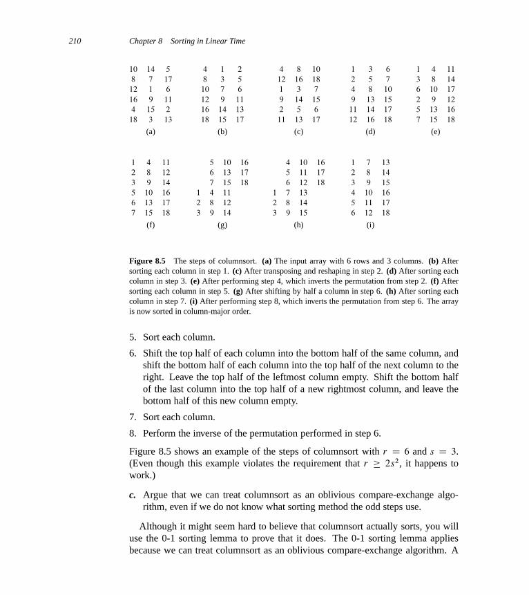
210 Chapter 8 Sorting in Linear Time
10 14 5
8 7 17
12 1 6
16 9 11
4 15 2
18 3 13
(a)
4 1 2
8 3 5
10 7 6
12 9 11
16 14 13
18 15 17
(b)
4 8 10
12 16 18
1 3 7
9 14 15
2 5 6
11 13 17
(c)
1 3 6
2 5 7
4 8 10
9 13 15
11 14 17
12 16 18
(d)
1 4 11
3 8 14
6 10 17
2 9 12
5 13 16
7 15 18
(e)
1 4 11
2 8 12
3 9 14
5 10 16
6 13 17
7 15 18
(f)
5 10 16
6 13 17
7 15 18
1 4 11
2 8 12
3 9 14
(g)
4 10 16
5 11 17
6 12 18
1 7 13
2 8 14
3 9 15
(h)
1 7 13
2 8 14
3 9 15
4 10 16
5 11 17
6 12 18
(i)
Figure 8.5 The steps of columnsort. (a) The input array with 6 rows and 3 columns. (b) Aftersorting each column in step 1. (c) After transposing and reshaping in step 2. (d) After sorting eachcolumn in step 3. (e) After performing step 4, which inverts the permutation from step 2. (f) Aftersorting each column in step 5. (g) After shifting by half a column in step 6. (h) After sorting eachcolumn in step 7. (i) After performing step 8, which inverts the permutation from step 6. The arrayis now sorted in column-major order.
5. Sort each column.
6. Shift the top half of each column into the bottom half of the same column, andshift the bottom half of each column into the top half of the next column to theright. Leave the top half of the leftmost column empty. Shift the bottom halfof the last column into the top half of a new rightmost column, and leave thebottom half of this new column empty.
7. Sort each column.
8. Perform the inverse of the permutation performed in step 6.
Figure 8.5 shows an example of the steps of columnsort with r D 6 and s D 3.(Even though this example violates the requirement that r � 2s2, it happens towork.)
c. Argue that we can treat columnsort as an oblivious compare-exchange algo-rithm, even if we do not know what sorting method the odd steps use.
Although it might seem hard to believe that columnsort actually sorts, you willuse the 0-1 sorting lemma to prove that it does. The 0-1 sorting lemma appliesbecause we can treat columnsort as an oblivious compare-exchange algorithm. A
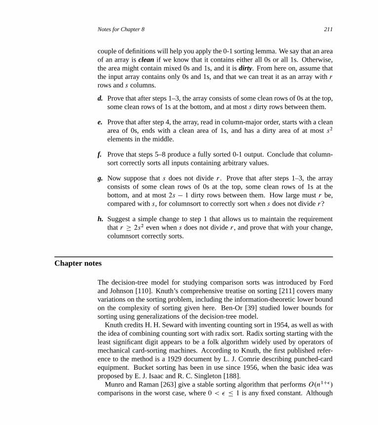
Notes for Chapter 8 211
couple of definitions will help you apply the 0-1 sorting lemma. We say that an areaof an array is clean if we know that it contains either all 0s or all 1s. Otherwise,the area might contain mixed 0s and 1s, and it is dirty. From here on, assume thatthe input array contains only 0s and 1s, and that we can treat it as an array with r
rows and s columns.
d. Prove that after steps 1–3, the array consists of some clean rows of 0s at the top,some clean rows of 1s at the bottom, and at most s dirty rows between them.
e. Prove that after step 4, the array, read in column-major order, starts with a cleanarea of 0s, ends with a clean area of 1s, and has a dirty area of at most s2
elements in the middle.
f. Prove that steps 5–8 produce a fully sorted 0-1 output. Conclude that column-sort correctly sorts all inputs containing arbitrary values.
g. Now suppose that s does not divide r . Prove that after steps 1–3, the arrayconsists of some clean rows of 0s at the top, some clean rows of 1s at thebottom, and at most 2s � 1 dirty rows between them. How large must r be,compared with s, for columnsort to correctly sort when s does not divide r?
h. Suggest a simple change to step 1 that allows us to maintain the requirementthat r � 2s2 even when s does not divide r , and prove that with your change,columnsort correctly sorts.
Chapter notes
The decision-tree model for studying comparison sorts was introduced by Fordand Johnson [110]. Knuth’s comprehensive treatise on sorting [211] covers manyvariations on the sorting problem, including the information-theoretic lower boundon the complexity of sorting given here. Ben-Or [39] studied lower bounds forsorting using generalizations of the decision-tree model.
Knuth credits H. H. Seward with inventing counting sort in 1954, as well as withthe idea of combining counting sort with radix sort. Radix sorting starting with theleast significant digit appears to be a folk algorithm widely used by operators ofmechanical card-sorting machines. According to Knuth, the first published refer-ence to the method is a 1929 document by L. J. Comrie describing punched-cardequipment. Bucket sorting has been in use since 1956, when the basic idea wasproposed by E. J. Isaac and R. C. Singleton [188].
Munro and Raman [263] give a stable sorting algorithm that performs O.n1C�/
comparisons in the worst case, where 0 < � � 1 is any fixed constant. Although
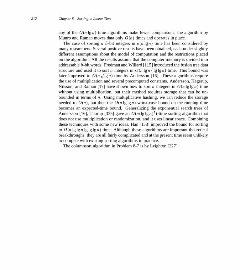
212 Chapter 8 Sorting in Linear Time
any of the O.n lg n/-time algorithms make fewer comparisons, the algorithm byMunro and Raman moves data only O.n/ times and operates in place.
The case of sorting n b-bit integers in o.n lg n/ time has been considered bymany researchers. Several positive results have been obtained, each under slightlydifferent assumptions about the model of computation and the restrictions placedon the algorithm. All the results assume that the computer memory is divided intoaddressable b-bit words. Fredman and Willard [115] introduced the fusion tree datastructure and used it to sort n integers in O.n lg n= lg lg n/ time. This bound waslater improved to O.n
plg n/ time by Andersson [16]. These algorithms require
the use of multiplication and several precomputed constants. Andersson, Hagerup,Nilsson, and Raman [17] have shown how to sort n integers in O.n lg lg n/ timewithout using multiplication, but their method requires storage that can be un-bounded in terms of n. Using multiplicative hashing, we can reduce the storageneeded to O.n/, but then the O.n lg lg n/ worst-case bound on the running timebecomes an expected-time bound. Generalizing the exponential search trees ofAndersson [16], Thorup [335] gave an O.n.lg lg n/2/-time sorting algorithm thatdoes not use multiplication or randomization, and it uses linear space. Combiningthese techniques with some new ideas, Han [158] improved the bound for sortingto O.n lg lg n lg lg lg n/ time. Although these algorithms are important theoreticalbreakthroughs, they are all fairly complicated and at the present time seem unlikelyto compete with existing sorting algorithms in practice.
The columnsort algorithm in Problem 8-7 is by Leighton [227].

9 Medians and Order Statistics
The i th order statistic of a set of n elements is the i th smallest element. Forexample, the minimum of a set of elements is the first order statistic (i D 1),and the maximum is the nth order statistic (i D n). A median, informally, isthe “halfway point” of the set. When n is odd, the median is unique, occurring ati D .nC 1/=2. When n is even, there are two medians, occurring at i D n=2 andi D n=2C1. Thus, regardless of the parity of n, medians occur at i D b.nC 1/=2c(the lower median) and i D d.nC 1/=2e (the upper median). For simplicity inthis text, however, we consistently use the phrase “the median” to refer to the lowermedian.
This chapter addresses the problem of selecting the i th order statistic from aset of n distinct numbers. We assume for convenience that the set contains dis-tinct numbers, although virtually everything that we do extends to the situation inwhich a set contains repeated values. We formally specify the selection problemas follows:
Input: A set A of n (distinct) numbers and an integer i , with 1 � i � n.
Output: The element x 2 A that is larger than exactly i � 1 other elements of A.
We can solve the selection problem in O.n lg n/ time, since we can sort the num-bers using heapsort or merge sort and then simply index the i th element in theoutput array. This chapter presents faster algorithms.
In Section 9.1, we examine the problem of selecting the minimum and maxi-mum of a set of elements. More interesting is the general selection problem, whichwe investigate in the subsequent two sections. Section 9.2 analyzes a practicalrandomized algorithm that achieves an O.n/ expected running time, assuming dis-tinct elements. Section 9.3 contains an algorithm of more theoretical interest thatachieves the O.n/ running time in the worst case.
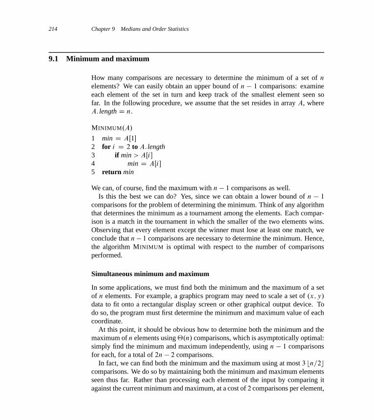
214 Chapter 9 Medians and Order Statistics
9.1 Minimum and maximum
How many comparisons are necessary to determine the minimum of a set of n
elements? We can easily obtain an upper bound of n � 1 comparisons: examineeach element of the set in turn and keep track of the smallest element seen sofar. In the following procedure, we assume that the set resides in array A, whereA: length D n.
MINIMUM.A/
1 min D AŒ1�
2 for i D 2 to A: length3 if min > AŒi�
4 min D AŒi�
5 return min
We can, of course, find the maximum with n � 1 comparisons as well.Is this the best we can do? Yes, since we can obtain a lower bound of n � 1
comparisons for the problem of determining the minimum. Think of any algorithmthat determines the minimum as a tournament among the elements. Each compar-ison is a match in the tournament in which the smaller of the two elements wins.Observing that every element except the winner must lose at least one match, weconclude that n� 1 comparisons are necessary to determine the minimum. Hence,the algorithm MINIMUM is optimal with respect to the number of comparisonsperformed.
Simultaneous minimum and maximum
In some applications, we must find both the minimum and the maximum of a setof n elements. For example, a graphics program may need to scale a set of .x; y/
data to fit onto a rectangular display screen or other graphical output device. Todo so, the program must first determine the minimum and maximum value of eachcoordinate.
At this point, it should be obvious how to determine both the minimum and themaximum of n elements using ‚.n/ comparisons, which is asymptotically optimal:simply find the minimum and maximum independently, using n � 1 comparisonsfor each, for a total of 2n � 2 comparisons.
In fact, we can find both the minimum and the maximum using at most 3 bn=2ccomparisons. We do so by maintaining both the minimum and maximum elementsseen thus far. Rather than processing each element of the input by comparing itagainst the current minimum and maximum, at a cost of 2 comparisons per element,

9.2 Selection in expected linear time 215
we process elements in pairs. We compare pairs of elements from the input firstwith each other, and then we compare the smaller with the current minimum andthe larger to the current maximum, at a cost of 3 comparisons for every 2 elements.
How we set up initial values for the current minimum and maximum dependson whether n is odd or even. If n is odd, we set both the minimum and maximumto the value of the first element, and then we process the rest of the elements inpairs. If n is even, we perform 1 comparison on the first 2 elements to determinethe initial values of the minimum and maximum, and then process the rest of theelements in pairs as in the case for odd n.
Let us analyze the total number of comparisons. If n is odd, then we perform3 bn=2c comparisons. If n is even, we perform 1 initial comparison followed by3.n � 2/=2 comparisons, for a total of 3n=2 � 2. Thus, in either case, the totalnumber of comparisons is at most 3 bn=2c.
Exercises
9.1-1Show that the second smallest of n elements can be found with n C dlg ne � 2
comparisons in the worst case. (Hint: Also find the smallest element.)
9.1-2 ?
Prove the lower bound of d3n=2e � 2 comparisons in the worst case to find boththe maximum and minimum of n numbers. (Hint: Consider how many numbersare potentially either the maximum or minimum, and investigate how a comparisonaffects these counts.)
9.2 Selection in expected linear time
The general selection problem appears more difficult than the simple problem offinding a minimum. Yet, surprisingly, the asymptotic running time for both prob-lems is the same: ‚.n/. In this section, we present a divide-and-conquer algorithmfor the selection problem. The algorithm RANDOMIZED-SELECT is modeled afterthe quicksort algorithm of Chapter 7. As in quicksort, we partition the input arrayrecursively. But unlike quicksort, which recursively processes both sides of thepartition, RANDOMIZED-SELECT works on only one side of the partition. Thisdifference shows up in the analysis: whereas quicksort has an expected runningtime of ‚.n lg n/, the expected running time of RANDOMIZED-SELECT is ‚.n/,assuming that the elements are distinct.

216 Chapter 9 Medians and Order Statistics
RANDOMIZED-SELECT uses the procedure RANDOMIZED-PARTITION intro-duced in Section 7.3. Thus, like RANDOMIZED-QUICKSORT, it is a randomized al-gorithm, since its behavior is determined in part by the output of a random-numbergenerator. The following code for RANDOMIZED-SELECT returns the i th smallestelement of the array AŒp : : r�.
RANDOMIZED-SELECT.A; p; r; i/
1 if p == r
2 return AŒp�
3 q D RANDOMIZED-PARTITION.A; p; r/
4 k D q � p C 1
5 if i == k // the pivot value is the answer6 return AŒq�
7 elseif i < k
8 return RANDOMIZED-SELECT.A; p; q � 1; i/
9 else return RANDOMIZED-SELECT.A; q C 1; r; i � k/
The RANDOMIZED-SELECT procedure works as follows. Line 1 checks for thebase case of the recursion, in which the subarray AŒp : : r� consists of just oneelement. In this case, i must equal 1, and we simply return AŒp� in line 2 as thei th smallest element. Otherwise, the call to RANDOMIZED-PARTITION in line 3partitions the array AŒp : : r� into two (possibly empty) subarrays AŒp : : q � 1�
and AŒq C 1 : : r� such that each element of AŒp : : q � 1� is less than or equalto AŒq�, which in turn is less than each element of AŒq C 1 : : r�. As in quicksort,we will refer to AŒq� as the pivot element. Line 4 computes the number k ofelements in the subarray AŒp : : q�, that is, the number of elements in the low sideof the partition, plus one for the pivot element. Line 5 then checks whether AŒq� isthe i th smallest element. If it is, then line 6 returns AŒq�. Otherwise, the algorithmdetermines in which of the two subarrays AŒp : : q � 1� and AŒq C 1 : : r� the i thsmallest element lies. If i < k, then the desired element lies on the low side ofthe partition, and line 8 recursively selects it from the subarray. If i > k, however,then the desired element lies on the high side of the partition. Since we alreadyknow k values that are smaller than the i th smallest element of AŒp : : r�—namely,the elements of AŒp : : q�—the desired element is the .i � k/th smallest elementof AŒqC1 : : r�, which line 9 finds recursively. The code appears to allow recursivecalls to subarrays with 0 elements, but Exercise 9.2-1 asks you to show that thissituation cannot happen.
The worst-case running time for RANDOMIZED-SELECT is ‚.n2/, even to findthe minimum, because we could be extremely unlucky and always partition aroundthe largest remaining element, and partitioning takes ‚.n/ time. We will see that

9.2 Selection in expected linear time 217
the algorithm has a linear expected running time, though, and because it is random-ized, no particular input elicits the worst-case behavior.
To analyze the expected running time of RANDOMIZED-SELECT, we let the run-ning time on an input array AŒp : : r� of n elements be a random variable that wedenote by T .n/, and we obtain an upper bound on E ŒT .n/� as follows. The pro-cedure RANDOMIZED-PARTITION is equally likely to return any element as thepivot. Therefore, for each k such that 1 � k � n, the subarray AŒp : : q� has k ele-ments (all less than or equal to the pivot) with probability 1=n. For k D 1; 2; : : : ; n,we define indicator random variables Xk where
Xk D I fthe subarray AŒp : : q� has exactly k elementsg ;
and so, assuming that the elements are distinct, we have
E ŒXk� D 1=n : (9.1)
When we call RANDOMIZED-SELECT and choose AŒq� as the pivot element, wedo not know, a priori, if we will terminate immediately with the correct answer,recurse on the subarray AŒp : : q � 1�, or recurse on the subarray AŒq C 1 : : r�.This decision depends on where the i th smallest element falls relative to AŒq�.Assuming that T .n/ is monotonically increasing, we can upper-bound the timeneeded for the recursive call by the time needed for the recursive call on the largestpossible input. In other words, to obtain an upper bound, we assume that the i thelement is always on the side of the partition with the greater number of elements.For a given call of RANDOMIZED-SELECT, the indicator random variable Xk hasthe value 1 for exactly one value of k, and it is 0 for all other k. When Xk D 1, thetwo subarrays on which we might recurse have sizes k � 1 and n � k. Hence, wehave the recurrence
T .n/ �nX
kD1
Xk � .T .max.k � 1; n � k//CO.n//
DnX
kD1
Xk � T .max.k � 1; n � k//CO.n/ :

218 Chapter 9 Medians and Order Statistics
Taking expected values, we have
E ŒT .n/�
� E
"nX
kD1
Xk � T .max.k � 1; n � k//CO.n/
#
DnX
kD1
E ŒXk � T .max.k � 1; n � k//�CO.n/ (by linearity of expectation)
DnX
kD1
E ŒXk� � E ŒT .max.k � 1; n � k//�CO.n/ (by equation (C.24))
DnX
kD1
1
n� E ŒT .max.k � 1; n � k//�CO.n/ (by equation (9.1)) .
In order to apply equation (C.24), we rely on Xk and T .max.k � 1; n � k// beingindependent random variables. Exercise 9.2-2 asks you to justify this assertion.
Let us consider the expression max.k � 1; n � k/. We have
max.k � 1; n � k/ D(
k � 1 if k > dn=2e ;
n � k if k � dn=2e :
If n is even, each term from T .dn=2e/ up to T .n � 1/ appears exactly twice inthe summation, and if n is odd, all these terms appear twice and T .bn=2c/ appearsonce. Thus, we have
E ŒT .n/� � 2
n
n�1XkDbn=2c
E ŒT .k/�CO.n/ :
We show that E ŒT .n/� D O.n/ by substitution. Assume that E ŒT .n/� � cn forsome constant c that satisfies the initial conditions of the recurrence. We assumethat T .n/ D O.1/ for n less than some constant; we shall pick this constant later.We also pick a constant a such that the function described by the O.n/ term above(which describes the non-recursive component of the running time of the algo-rithm) is bounded from above by an for all n > 0. Using this inductive hypothesis,we have
E ŒT .n/� � 2
n
n�1XkDbn=2c
ck C an
D 2c
n
n�1XkD1
k �bn=2c�1X
kD1
k
!C an
9.2 Selection in expected linear time 219
D 2c
n
�.n � 1/n
2� .bn=2c � 1/ bn=2c
2
�C an
� 2c
n
�.n � 1/n
2� .n=2 � 2/.n=2 � 1/
2
�C an
D 2c
n
�n2 � n
2� n2=4 � 3n=2C 2
2
�C an
D c
n
�3n2
4C n
2� 2
�C an
D c
�3n
4C 1
2� 2
n
�C an
� 3cn
4C c
2C an
D cn ��cn
4� c
2� an
�:
In order to complete the proof, we need to show that for sufficiently large n, thislast expression is at most cn or, equivalently, that cn=4 � c=2 � an � 0. If weadd c=2 to both sides and factor out n, we get n.c=4 � a/ � c=2. As long as wechoose the constant c so that c=4 � a > 0, i.e., c > 4a, we can divide both sidesby c=4 � a, giving
n � c=2
c=4� aD 2c
c � 4a:
Thus, if we assume that T .n/ D O.1/ for n < 2c=.c�4a/, then E ŒT .n/� D O.n/.We conclude that we can find any order statistic, and in particular the median, inexpected linear time, assuming that the elements are distinct.
Exercises
9.2-1Show that RANDOMIZED-SELECT never makes a recursive call to a 0-length array.
9.2-2Argue that the indicator random variable Xk and the value T .max.k � 1; n � k//
are independent.
9.2-3Write an iterative version of RANDOMIZED-SELECT.
220 Chapter 9 Medians and Order Statistics
9.2-4Suppose we use RANDOMIZED-SELECT to select the minimum element of thearray A D h3; 2; 9; 0; 7; 5; 4; 8; 6; 1i. Describe a sequence of partitions that resultsin a worst-case performance of RANDOMIZED-SELECT.
9.3 Selection in worst-case linear time
We now examine a selection algorithm whose running time is O.n/ in the worstcase. Like RANDOMIZED-SELECT, the algorithm SELECT finds the desired ele-ment by recursively partitioning the input array. Here, however, we guarantee agood split upon partitioning the array. SELECT uses the deterministic partitioningalgorithm PARTITION from quicksort (see Section 7.1), but modified to take theelement to partition around as an input parameter.
The SELECT algorithm determines the i th smallest of an input array of n > 1
distinct elements by executing the following steps. (If n D 1, then SELECT merelyreturns its only input value as the i th smallest.)
1. Divide the n elements of the input array into bn=5c groups of 5 elements eachand at most one group made up of the remaining n mod 5 elements.
2. Find the median of each of the dn=5e groups by first insertion-sorting the ele-ments of each group (of which there are at most 5) and then picking the medianfrom the sorted list of group elements.
3. Use SELECT recursively to find the median x of the dn=5e medians found instep 2. (If there are an even number of medians, then by our convention, x isthe lower median.)
4. Partition the input array around the median-of-medians x using the modifiedversion of PARTITION. Let k be one more than the number of elements on thelow side of the partition, so that x is the kth smallest element and there are n�k
elements on the high side of the partition.
5. If i D k, then return x. Otherwise, use SELECT recursively to find the i thsmallest element on the low side if i < k, or the .i � k/th smallest element onthe high side if i > k.
To analyze the running time of SELECT, we first determine a lower bound on thenumber of elements that are greater than the partitioning element x. Figure 9.1helps us to visualize this bookkeeping. At least half of the medians found in
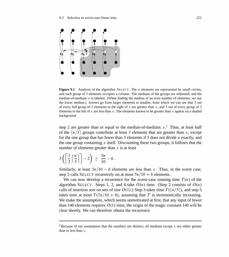
9.3 Selection in worst-case linear time 221
x
Figure 9.1 Analysis of the algorithm SELECT. The n elements are represented by small circles,and each group of 5 elements occupies a column. The medians of the groups are whitened, and themedian-of-medians x is labeled. (When finding the median of an even number of elements, we usethe lower median.) Arrows go from larger elements to smaller, from which we can see that 3 outof every full group of 5 elements to the right of x are greater than x, and 3 out of every group of 5
elements to the left of x are less than x. The elements known to be greater than x appear on a shadedbackground.
step 2 are greater than or equal to the median-of-medians x.1 Thus, at least halfof the dn=5e groups contribute at least 3 elements that are greater than x, exceptfor the one group that has fewer than 5 elements if 5 does not divide n exactly, andthe one group containing x itself. Discounting these two groups, it follows that thenumber of elements greater than x is at least
3
��1
2
ln
5
m�� 2
�� 3n
10� 6 :
Similarly, at least 3n=10 � 6 elements are less than x. Thus, in the worst case,step 5 calls SELECT recursively on at most 7n=10C 6 elements.
We can now develop a recurrence for the worst-case running time T .n/ of thealgorithm SELECT. Steps 1, 2, and 4 take O.n/ time. (Step 2 consists of O.n/
calls of insertion sort on sets of size O.1/.) Step 3 takes time T .dn=5e/, and step 5takes time at most T .7n=10 C 6/, assuming that T is monotonically increasing.We make the assumption, which seems unmotivated at first, that any input of fewerthan 140 elements requires O.1/ time; the origin of the magic constant 140 will beclear shortly. We can therefore obtain the recurrence
1Because of our assumption that the numbers are distinct, all medians except x are either greaterthan or less than x.

222 Chapter 9 Medians and Order Statistics
T .n/ �(
O.1/ if n < 140 ;
T .dn=5e/C T .7n=10C 6/CO.n/ if n � 140 :
We show that the running time is linear by substitution. More specifically, we willshow that T .n/ � cn for some suitably large constant c and all n > 0. We begin byassuming that T .n/ � cn for some suitably large constant c and all n < 140; thisassumption holds if c is large enough. We also pick a constant a such that the func-tion described by the O.n/ term above (which describes the non-recursive compo-nent of the running time of the algorithm) is bounded above by an for all n > 0.Substituting this inductive hypothesis into the right-hand side of the recurrenceyields
T .n/ � c dn=5e C c.7n=10C 6/C an
� cn=5C c C 7cn=10C 6c C an
D 9cn=10C 7c C an
D cnC .�cn=10C 7c C an/ ;
which is at most cn if
�cn=10C 7c C an � 0 : (9.2)
Inequality (9.2) is equivalent to the inequality c � 10a.n=.n� 70// when n > 70.Because we assume that n � 140, we have n=.n � 70/ � 2, and so choos-ing c � 20a will satisfy inequality (9.2). (Note that there is nothing special aboutthe constant 140; we could replace it by any integer strictly greater than 70 andthen choose c accordingly.) The worst-case running time of SELECT is thereforelinear.
As in a comparison sort (see Section 8.1), SELECT and RANDOMIZED-SELECT
determine information about the relative order of elements only by comparing ele-ments. Recall from Chapter 8 that sorting requires �.n lg n/ time in the compari-son model, even on average (see Problem 8-1). The linear-time sorting algorithmsin Chapter 8 make assumptions about the input. In contrast, the linear-time se-lection algorithms in this chapter do not require any assumptions about the input.They are not subject to the �.n lg n/ lower bound because they manage to solvethe selection problem without sorting. Thus, solving the selection problem by sort-ing and indexing, as presented in the introduction to this chapter, is asymptoticallyinefficient.
9.3 Selection in worst-case linear time 223
Exercises
9.3-1In the algorithm SELECT, the input elements are divided into groups of 5. Willthe algorithm work in linear time if they are divided into groups of 7? Argue thatSELECT does not run in linear time if groups of 3 are used.
9.3-2Analyze SELECT to show that if n � 140, then at least dn=4e elements are greaterthan the median-of-medians x and at least dn=4e elements are less than x.
9.3-3Show how quicksort can be made to run in O.n lg n/ time in the worst case, as-suming that all elements are distinct.
9.3-4 ?
Suppose that an algorithm uses only comparisons to find the i th smallest elementin a set of n elements. Show that it can also find the i � 1 smaller elements andthe n � i larger elements without performing any additional comparisons.
9.3-5Suppose that you have a “black-box” worst-case linear-time median subroutine.Give a simple, linear-time algorithm that solves the selection problem for an arbi-trary order statistic.
9.3-6The kth quantiles of an n-element set are the k � 1 order statistics that divide thesorted set into k equal-sized sets (to within 1). Give an O.n lg k/-time algorithmto list the kth quantiles of a set.
9.3-7Describe an O.n/-time algorithm that, given a set S of n distinct numbers anda positive integer k � n, determines the k numbers in S that are closest to themedian of S .
9.3-8Let XŒ1 : : n� and Y Œ1 : : n� be two arrays, each containing n numbers already insorted order. Give an O.lg n/-time algorithm to find the median of all 2n elementsin arrays X and Y .
9.3-9Professor Olay is consulting for an oil company, which is planning a large pipelinerunning east to west through an oil field of n wells. The company wants to connect
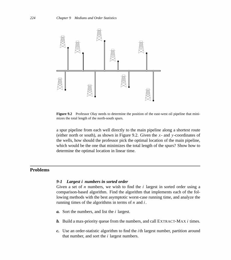
224 Chapter 9 Medians and Order Statistics
Figure 9.2 Professor Olay needs to determine the position of the east-west oil pipeline that mini-mizes the total length of the north-south spurs.
a spur pipeline from each well directly to the main pipeline along a shortest route(either north or south), as shown in Figure 9.2. Given the x- and y-coordinates ofthe wells, how should the professor pick the optimal location of the main pipeline,which would be the one that minimizes the total length of the spurs? Show how todetermine the optimal location in linear time.
Problems
9-1 Largest i numbers in sorted orderGiven a set of n numbers, we wish to find the i largest in sorted order using acomparison-based algorithm. Find the algorithm that implements each of the fol-lowing methods with the best asymptotic worst-case running time, and analyze therunning times of the algorithms in terms of n and i .
a. Sort the numbers, and list the i largest.
b. Build a max-priority queue from the numbers, and call EXTRACT-MAX i times.
c. Use an order-statistic algorithm to find the i th largest number, partition aroundthat number, and sort the i largest numbers.

Problems for Chapter 9 225
9-2 Weighted medianFor n distinct elements x1; x2; : : : ; xn with positive weights w1; w2; : : : ; wn suchthat
Pn
iD1 wi D 1, the weighted (lower) median is the element xk satisfyingXxi <xk
wi <1
2
andXxi >xk
wi � 1
2:
For example, if the elements are 0:1; 0:35; 0:05; 0:1; 0:15; 0:05; 0:2 and each ele-ment equals its weight (that is, wi D xi for i D 1; 2; : : : ; 7), then the median is 0:1,but the weighted median is 0:2.
a. Argue that the median of x1; x2; : : : ; xn is the weighted median of the xi withweights wi D 1=n for i D 1; 2; : : : ; n.
b. Show how to compute the weighted median of n elements in O.n lg n/ worst-case time using sorting.
c. Show how to compute the weighted median in ‚.n/ worst-case time using alinear-time median algorithm such as SELECT from Section 9.3.
The post-office location problem is defined as follows. We are given n pointsp1; p2; : : : ; pn with associated weights w1; w2; : : : ; wn. We wish to find a point p
(not necessarily one of the input points) that minimizes the sumPn
iD1 wi d.p; pi /,where d.a; b/ is the distance between points a and b.
d. Argue that the weighted median is a best solution for the 1-dimensional post-office location problem, in which points are simply real numbers and the dis-tance between points a and b is d.a; b/ D ja � bj.
e. Find the best solution for the 2-dimensional post-office location problem, inwhich the points are .x; y/ coordinate pairs and the distance between pointsa D .x1; y1/ and b D .x2; y2/ is the Manhattan distance given by d.a; b/ Djx1 � x2j C jy1 � y2j.
9-3 Small order statisticsWe showed that the worst-case number T .n/ of comparisons used by SELECT
to select the i th order statistic from n numbers satisfies T .n/ D ‚.n/, but theconstant hidden by the ‚-notation is rather large. When i is small relative to n, wecan implement a different procedure that uses SELECT as a subroutine but makesfewer comparisons in the worst case.
226 Chapter 9 Medians and Order Statistics
a. Describe an algorithm that uses Ui.n/ comparisons to find the i th smallest of n
elements, where
Ui.n/ D(
T .n/ if i � n=2 ;
bn=2c C Ui.dn=2e/C T .2i/ otherwise :
(Hint: Begin with bn=2c disjoint pairwise comparisons, and recurse on the setcontaining the smaller element from each pair.)
b. Show that, if i < n=2, then Ui .n/ D nCO.T .2i/ lg.n=i//.
c. Show that if i is a constant less than n=2, then Ui .n/ D nCO.lg n/.
d. Show that if i D n=k for k � 2, then Ui .n/ D nCO.T .2n=k/ lg k/.
9-4 Alternative analysis of randomized selectionIn this problem, we use indicator random variables to analyze the RANDOMIZED-SELECT procedure in a manner akin to our analysis of RANDOMIZED-QUICKSORT
in Section 7.4.2.As in the quicksort analysis, we assume that all elements are distinct, and we
rename the elements of the input array A as ´1; ´2; : : : ; ´n, where ´i is the i thsmallest element. Thus, the call RANDOMIZED-SELECT.A; 1; n; k/ returns ´k.
For 1 � i < j � n, let
Xijk D I f´i is compared with j́ sometime during the execution of the algorithmto find ´kg :
a. Give an exact expression for E ŒXijk �. (Hint: Your expression may have differ-ent values, depending on the values of i , j , and k.)
b. Let Xk denote the total number of comparisons between elements of array A
when finding ´k. Show that
E ŒXk� � 2
kX
iD1
nXj Dk
1
j � i C 1C
nXj DkC1
j � k � 1
j � k C 1C
k�2XiD1
k � i � 1
k � i C 1
!:
c. Show that E ŒXk� � 4n.
d. Conclude that, assuming all elements of array A are distinct, RANDOMIZED-SELECT runs in expected time O.n/.
Notes for Chapter 9 227
Chapter notes
The worst-case linear-time median-finding algorithm was devised by Blum, Floyd,Pratt, Rivest, and Tarjan [50]. The fast randomized version is due to Hoare [169].Floyd and Rivest [108] have developed an improved randomized version that parti-tions around an element recursively selected from a small sample of the elements.
It is still unknown exactly how many comparisons are needed to determine themedian. Bent and John [41] gave a lower bound of 2n comparisons for medianfinding, and Schönhage, Paterson, and Pippenger [302] gave an upper bound of 3n.Dor and Zwick have improved on both of these bounds. Their upper bound [94]is slightly less than 2:95n, and their lower bound [95] is .2 C �/n, for a smallpositive constant �, thereby improving slightly on related work by Dor et al. [93].Paterson [272] describes some of these results along with other related work.

III Data Structures

Introduction
Sets are as fundamental to computer science as they are to mathematics. Whereasmathematical sets are unchanging, the sets manipulated by algorithms can grow,shrink, or otherwise change over time. We call such sets dynamic. The next fivechapters present some basic techniques for representing finite dynamic sets andmanipulating them on a computer.
Algorithms may require several different types of operations to be performed onsets. For example, many algorithms need only the ability to insert elements into,delete elements from, and test membership in a set. We call a dynamic set thatsupports these operations a dictionary. Other algorithms require more complicatedoperations. For example, min-priority queues, which Chapter 6 introduced in thecontext of the heap data structure, support the operations of inserting an elementinto and extracting the smallest element from a set. The best way to implement adynamic set depends upon the operations that must be supported.
Elements of a dynamic set
In a typical implementation of a dynamic set, each element is represented by anobject whose attributes can be examined and manipulated if we have a pointer tothe object. (Section 10.3 discusses the implementation of objects and pointers inprogramming environments that do not contain them as basic data types.) Somekinds of dynamic sets assume that one of the object’s attributes is an identifyingkey. If the keys are all different, we can think of the dynamic set as being a setof key values. The object may contain satellite data, which are carried around inother object attributes but are otherwise unused by the set implementation. It may

230 Part III Data Structures
also have attributes that are manipulated by the set operations; these attributes maycontain data or pointers to other objects in the set.
Some dynamic sets presuppose that the keys are drawn from a totally orderedset, such as the real numbers, or the set of all words under the usual alphabeticordering. A total ordering allows us to define the minimum element of the set, forexample, or to speak of the next element larger than a given element in a set.
Operations on dynamic sets
Operations on a dynamic set can be grouped into two categories: queries, whichsimply return information about the set, and modifying operations, which changethe set. Here is a list of typical operations. Any specific application will usuallyrequire only a few of these to be implemented.
SEARCH.S; k/
A query that, given a set S and a key value k, returns a pointer x to an elementin S such that x:key D k, or NIL if no such element belongs to S .
INSERT.S; x/
A modifying operation that augments the set S with the element pointed toby x. We usually assume that any attributes in element x needed by the setimplementation have already been initialized.
DELETE.S; x/
A modifying operation that, given a pointer x to an element in the set S , re-moves x from S . (Note that this operation takes a pointer to an element x, nota key value.)
MINIMUM.S/
A query on a totally ordered set S that returns a pointer to the element of S
with the smallest key.
MAXIMUM.S/
A query on a totally ordered set S that returns a pointer to the element of S
with the largest key.
SUCCESSOR.S; x/
A query that, given an element x whose key is from a totally ordered set S ,returns a pointer to the next larger element in S , or NIL if x is the maximumelement.
PREDECESSOR.S; x/
A query that, given an element x whose key is from a totally ordered set S ,returns a pointer to the next smaller element in S , or NIL if x is the minimumelement.

Part III Data Structures 231
In some situations, we can extend the queries SUCCESSOR and PREDECESSOR
so that they apply to sets with nondistinct keys. For a set on n keys, the normalpresumption is that a call to MINIMUM followed by n � 1 calls to SUCCESSOR
enumerates the elements in the set in sorted order.We usually measure the time taken to execute a set operation in terms of the size
of the set. For example, Chapter 13 describes a data structure that can support anyof the operations listed above on a set of size n in time O.lg n/.
Overview of Part III
Chapters 10–14 describe several data structures that we can use to implementdynamic sets; we shall use many of these later to construct efficient algorithmsfor a variety of problems. We already saw another important data structure—theheap—in Chapter 6.
Chapter 10 presents the essentials of working with simple data structures suchas stacks, queues, linked lists, and rooted trees. It also shows how to implementobjects and pointers in programming environments that do not support them asprimitives. If you have taken an introductory programming course, then much ofthis material should be familiar to you.
Chapter 11 introduces hash tables, which support the dictionary operations IN-SERT, DELETE, and SEARCH. In the worst case, hashing requires ‚.n/ time to per-form a SEARCH operation, but the expected time for hash-table operations is O.1/.The analysis of hashing relies on probability, but most of the chapter requires nobackground in the subject.
Binary search trees, which are covered in Chapter 12, support all the dynamic-set operations listed above. In the worst case, each operation takes ‚.n/ time on atree with n elements, but on a randomly built binary search tree, the expected timefor each operation is O.lg n/. Binary search trees serve as the basis for many otherdata structures.
Chapter 13 introduces red-black trees, which are a variant of binary search trees.Unlike ordinary binary search trees, red-black trees are guaranteed to perform well:operations take O.lg n/ time in the worst case. A red-black tree is a balanced searchtree; Chapter 18 in Part V presents another kind of balanced search tree, called aB-tree. Although the mechanics of red-black trees are somewhat intricate, you canglean most of their properties from the chapter without studying the mechanics indetail. Nevertheless, you probably will find walking through the code to be quiteinstructive.
In Chapter 14, we show how to augment red-black trees to support operationsother than the basic ones listed above. First, we augment them so that we candynamically maintain order statistics for a set of keys. Then, we augment them ina different way to maintain intervals of real numbers.
10 Elementary Data Structures
In this chapter, we examine the representation of dynamic sets by simple data struc-tures that use pointers. Although we can construct many complex data structuresusing pointers, we present only the rudimentary ones: stacks, queues, linked lists,and rooted trees. We also show ways to synthesize objects and pointers from ar-rays.
10.1 Stacks and queues
Stacks and queues are dynamic sets in which the element removed from the setby the DELETE operation is prespecified. In a stack, the element deleted fromthe set is the one most recently inserted: the stack implements a last-in, first-out,or LIFO, policy. Similarly, in a queue, the element deleted is always the one thathas been in the set for the longest time: the queue implements a first-in, first-out,or FIFO, policy. There are several efficient ways to implement stacks and queueson a computer. In this section we show how to use a simple array to implementeach.
Stacks
The INSERT operation on a stack is often called PUSH, and the DELETE opera-tion, which does not take an element argument, is often called POP. These namesare allusions to physical stacks, such as the spring-loaded stacks of plates usedin cafeterias. The order in which plates are popped from the stack is the reverseof the order in which they were pushed onto the stack, since only the top plate isaccessible.
As Figure 10.1 shows, we can implement a stack of at most n elements withan array SŒ1 : : n�. The array has an attribute S: top that indexes the most recently

10.1 Stacks and queues 233
1 2 3 4 5 6 7
S 15 6 2 9
1 2 3 4 5 6 7
S 15 6 2 9 17 3
1 2 3 4 5 6 7
S 15 6 2 9 17 3
(a) (b) (c)
S: top D 4 S: top D 6 S: top D 5
Figure 10.1 An array implementation of a stack S . Stack elements appear only in the lightly shadedpositions. (a) Stack S has 4 elements. The top element is 9. (b) Stack S after the calls PUSH.S; 17/
and PUSH.S; 3/. (c) Stack S after the call POP.S/ has returned the element 3, which is the one mostrecently pushed. Although element 3 still appears in the array, it is no longer in the stack; the top iselement 17.
inserted element. The stack consists of elements SŒ1 : : S: top�, where SŒ1� is theelement at the bottom of the stack and SŒS: top� is the element at the top.
When S: top D 0, the stack contains no elements and is empty. We can test tosee whether the stack is empty by query operation STACK-EMPTY. If we attemptto pop an empty stack, we say the stack underflows, which is normally an error.If S: top exceeds n, the stack overflows. (In our pseudocode implementation, wedon’t worry about stack overflow.)
We can implement each of the stack operations with just a few lines of code:
STACK-EMPTY.S/
1 if S: top == 0
2 return TRUE
3 else return FALSE
PUSH.S; x/
1 S: top D S: topC 1
2 SŒS: top� D x
POP.S/
1 if STACK-EMPTY.S/
2 error “underflow”3 else S: top D S: top � 1
4 return SŒS: topC 1�
Figure 10.1 shows the effects of the modifying operations PUSH and POP. Each ofthe three stack operations takes O.1/ time.
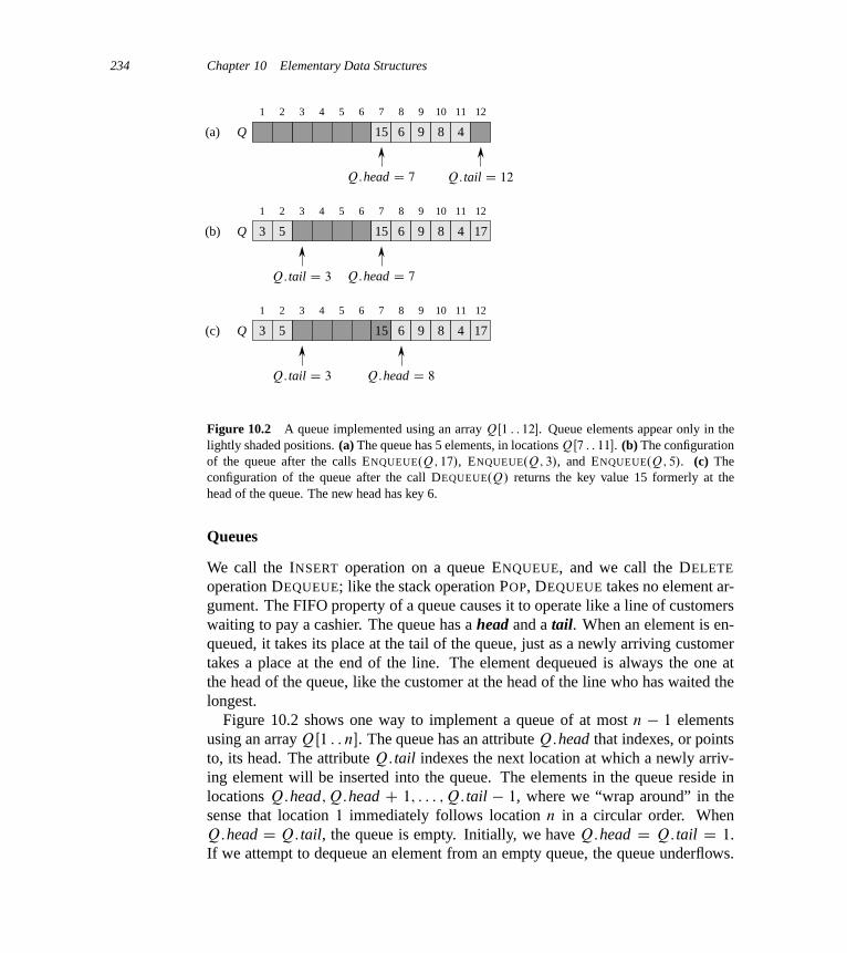
234 Chapter 10 Elementary Data Structures
1 2 3 4 5 6 7 8 9 10 11 12
Q(a) 15 6 9 8 4
1 2 3 4 5 6 7 8 9 10 11 12
Q(b) 15 6 9 8 43 5 17
1 2 3 4 5 6 7 8 9 10 11 12
Q(c) 15 6 9 8 43 5 17
Q:head D 7
Q:head D 7 Q: tail D 12
Q: tail D 3
Q: tail D 3
Q:head D 8
Figure 10.2 A queue implemented using an array QŒ1 : : 12�. Queue elements appear only in thelightly shaded positions. (a) The queue has 5 elements, in locations QŒ7 : : 11�. (b) The configurationof the queue after the calls ENQUEUE.Q; 17/, ENQUEUE.Q; 3/, and ENQUEUE.Q; 5/. (c) Theconfiguration of the queue after the call DEQUEUE.Q/ returns the key value 15 formerly at thehead of the queue. The new head has key 6.
Queues
We call the INSERT operation on a queue ENQUEUE, and we call the DELETE
operation DEQUEUE; like the stack operation POP, DEQUEUE takes no element ar-gument. The FIFO property of a queue causes it to operate like a line of customerswaiting to pay a cashier. The queue has a head and a tail. When an element is en-queued, it takes its place at the tail of the queue, just as a newly arriving customertakes a place at the end of the line. The element dequeued is always the one atthe head of the queue, like the customer at the head of the line who has waited thelongest.
Figure 10.2 shows one way to implement a queue of at most n � 1 elementsusing an array QŒ1 : : n�. The queue has an attribute Q:head that indexes, or pointsto, its head. The attribute Q: tail indexes the next location at which a newly arriv-ing element will be inserted into the queue. The elements in the queue reside inlocations Q:head; Q:head C 1; : : : ; Q: tail � 1, where we “wrap around” in thesense that location 1 immediately follows location n in a circular order. WhenQ:head D Q: tail, the queue is empty. Initially, we have Q:head D Q: tail D 1.If we attempt to dequeue an element from an empty queue, the queue underflows.
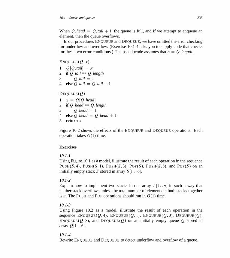
10.1 Stacks and queues 235
When Q:head D Q: tail C 1, the queue is full, and if we attempt to enqueue anelement, then the queue overflows.
In our procedures ENQUEUE and DEQUEUE, we have omitted the error checkingfor underflow and overflow. (Exercise 10.1-4 asks you to supply code that checksfor these two error conditions.) The pseudocode assumes that n D Q: length.
ENQUEUE.Q; x/
1 QŒQ: tail� D x
2 if Q: tail == Q: length3 Q: tail D 1
4 else Q: tail D Q: tailC 1
DEQUEUE.Q/
1 x D QŒQ:head�
2 if Q:head == Q: length3 Q:head D 1
4 else Q:head D Q:head C 1
5 return x
Figure 10.2 shows the effects of the ENQUEUE and DEQUEUE operations. Eachoperation takes O.1/ time.
Exercises
10.1-1Using Figure 10.1 as a model, illustrate the result of each operation in the sequencePUSH.S; 4/, PUSH.S; 1/, PUSH.S; 3/, POP.S/, PUSH.S; 8/, and POP.S/ on aninitially empty stack S stored in array SŒ1 : : 6�.
10.1-2Explain how to implement two stacks in one array AŒ1 : : n� in such a way thatneither stack overflows unless the total number of elements in both stacks togetheris n. The PUSH and POP operations should run in O.1/ time.
10.1-3Using Figure 10.2 as a model, illustrate the result of each operation in thesequence ENQUEUE.Q; 4/, ENQUEUE.Q; 1/, ENQUEUE.Q; 3/, DEQUEUE.Q/,ENQUEUE.Q; 8/, and DEQUEUE.Q/ on an initially empty queue Q stored inarray QŒ1 : : 6�.
10.1-4Rewrite ENQUEUE and DEQUEUE to detect underflow and overflow of a queue.

236 Chapter 10 Elementary Data Structures
10.1-5Whereas a stack allows insertion and deletion of elements at only one end, and aqueue allows insertion at one end and deletion at the other end, a deque (double-ended queue) allows insertion and deletion at both ends. Write four O.1/-timeprocedures to insert elements into and delete elements from both ends of a dequeimplemented by an array.
10.1-6Show how to implement a queue using two stacks. Analyze the running time of thequeue operations.
10.1-7Show how to implement a stack using two queues. Analyze the running time of thestack operations.
10.2 Linked lists
A linked list is a data structure in which the objects are arranged in a linear order.Unlike an array, however, in which the linear order is determined by the arrayindices, the order in a linked list is determined by a pointer in each object. Linkedlists provide a simple, flexible representation for dynamic sets, supporting (thoughnot necessarily efficiently) all the operations listed on page 230.
As shown in Figure 10.3, each element of a doubly linked list L is an object withan attribute key and two other pointer attributes: next and pre�. The object mayalso contain other satellite data. Given an element x in the list, x:next points to itssuccessor in the linked list, and x:pre� points to its predecessor. If x:pre� D NIL,the element x has no predecessor and is therefore the first element, or head, ofthe list. If x:next D NIL, the element x has no successor and is therefore the lastelement, or tail, of the list. An attribute L:head points to the first element of thelist. If L:head D NIL, the list is empty.
A list may have one of several forms. It may be either singly linked or doublylinked, it may be sorted or not, and it may be circular or not. If a list is singlylinked, we omit the pre� pointer in each element. If a list is sorted, the linear orderof the list corresponds to the linear order of keys stored in elements of the list; theminimum element is then the head of the list, and the maximum element is thetail. If the list is unsorted, the elements can appear in any order. In a circular list,the pre� pointer of the head of the list points to the tail, and the next pointer ofthe tail of the list points to the head. We can think of a circular list as a ring of
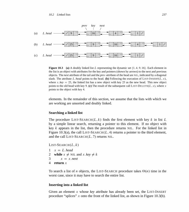
10.2 Linked lists 237
9 16 4 1
prev key next
(a)
9 16 4 1(b) 25
9 16 1(c) 25L:head
L:head
L:head
Figure 10.3 (a) A doubly linked list L representing the dynamic set f1; 4; 9; 16g. Each element inthe list is an object with attributes for the key and pointers (shown by arrows) to the next and previousobjects. The next attribute of the tail and the pre� attribute of the head are NIL, indicated by a diagonalslash. The attribute L:head points to the head. (b) Following the execution of LIST-INSERT.L; x/,where x:key D 25, the linked list has a new object with key 25 as the new head. This new objectpoints to the old head with key 9. (c) The result of the subsequent call LIST-DELETE.L; x/, where x
points to the object with key 4.
elements. In the remainder of this section, we assume that the lists with which weare working are unsorted and doubly linked.
Searching a linked list
The procedure LIST-SEARCH.L; k/ finds the first element with key k in list L
by a simple linear search, returning a pointer to this element. If no object withkey k appears in the list, then the procedure returns NIL. For the linked list inFigure 10.3(a), the call LIST-SEARCH.L; 4/ returns a pointer to the third element,and the call LIST-SEARCH.L; 7/ returns NIL.
LIST-SEARCH.L; k/
1 x D L:head2 while x ¤ NIL and x:key ¤ k
3 x D x:next4 return x
To search a list of n objects, the LIST-SEARCH procedure takes ‚.n/ time in theworst case, since it may have to search the entire list.
Inserting into a linked list
Given an element x whose key attribute has already been set, the LIST-INSERT
procedure “splices” x onto the front of the linked list, as shown in Figure 10.3(b).
238 Chapter 10 Elementary Data Structures
LIST-INSERT.L; x/
1 x:next D L:head2 if L:head ¤ NIL
3 L:head:pre� D x
4 L:head D x
5 x:pre� D NIL
(Recall that our attribute notation can cascade, so that L:head:pre� denotes thepre� attribute of the object that L:head points to.) The running time for LIST-INSERT on a list of n elements is O.1/.
Deleting from a linked list
The procedure LIST-DELETE removes an element x from a linked list L. It mustbe given a pointer to x, and it then “splices” x out of the list by updating pointers.If we wish to delete an element with a given key, we must first call LIST-SEARCH
to retrieve a pointer to the element.
LIST-DELETE.L; x/
1 if x:pre� ¤ NIL
2 x:pre�:next D x:next3 else L:head D x:next4 if x:next ¤ NIL
5 x:next:pre� D x:pre�
Figure 10.3(c) shows how an element is deleted from a linked list. LIST-DELETE
runs in O.1/ time, but if we wish to delete an element with a given key, ‚.n/ timeis required in the worst case because we must first call LIST-SEARCH to find theelement.
Sentinels
The code for LIST-DELETE would be simpler if we could ignore the boundaryconditions at the head and tail of the list:
LIST-DELETE0.L; x/
1 x:pre�:next D x:next2 x:next:pre� D x:pre�
A sentinel is a dummy object that allows us to simplify boundary conditions. Forexample, suppose that we provide with list L an object L:nil that represents NIL

10.2 Linked lists 239
9 16 4 1
9 16 4 125
9 16 425
(a)
(b)
(c)
(d) L:nil
L:nil
L:nil
L:nil
Figure 10.4 A circular, doubly linked list with a sentinel. The sentinel L:nil appears between thehead and tail. The attribute L:head is no longer needed, since we can access the head of the listby L:nil:next. (a) An empty list. (b) The linked list from Figure 10.3(a), with key 9 at the head andkey 1 at the tail. (c) The list after executing LIST-INSERT0.L; x/, where x:key D 25. The new objectbecomes the head of the list. (d) The list after deleting the object with key 1. The new tail is theobject with key 4.
but has all the attributes of the other objects in the list. Wherever we have a ref-erence to NIL in list code, we replace it by a reference to the sentinel L:nil. Asshown in Figure 10.4, this change turns a regular doubly linked list into a circu-lar, doubly linked list with a sentinel, in which the sentinel L:nil lies between thehead and tail. The attribute L:nil:next points to the head of the list, and L:nil:pre�
points to the tail. Similarly, both the next attribute of the tail and the pre� at-tribute of the head point to L:nil. Since L:nil:next points to the head, we caneliminate the attribute L:head altogether, replacing references to it by referencesto L:nil:next. Figure 10.4(a) shows that an empty list consists of just the sentinel,and both L:nil:next and L:nil:pre� point to L:nil.
The code for LIST-SEARCH remains the same as before, but with the referencesto NIL and L:head changed as specified above:
LIST-SEARCH0.L; k/
1 x D L:nil:next2 while x ¤ L:nil and x:key ¤ k
3 x D x:next4 return x
We use the two-line procedure LIST-DELETE 0 from before to delete an elementfrom the list. The following procedure inserts an element into the list:
240 Chapter 10 Elementary Data Structures
LIST-INSERT0.L; x/
1 x:next D L:nil:next2 L:nil:next:pre� D x
3 L:nil:next D x
4 x:pre� D L:nil
Figure 10.4 shows the effects of LIST-INSERT 0 and LIST-DELETE 0 on a sample list.Sentinels rarely reduce the asymptotic time bounds of data structure operations,
but they can reduce constant factors. The gain from using sentinels within loopsis usually a matter of clarity of code rather than speed; the linked list code, forexample, becomes simpler when we use sentinels, but we save only O.1/ time inthe LIST-INSERT 0 and LIST-DELETE 0 procedures. In other situations, however, theuse of sentinels helps to tighten the code in a loop, thus reducing the coefficient of,say, n or n2 in the running time.
We should use sentinels judiciously. When there are many small lists, the extrastorage used by their sentinels can represent significant wasted memory. In thisbook, we use sentinels only when they truly simplify the code.
Exercises
10.2-1Can you implement the dynamic-set operation INSERT on a singly linked listin O.1/ time? How about DELETE?
10.2-2Implement a stack using a singly linked list L. The operations PUSH and POP
should still take O.1/ time.
10.2-3Implement a queue by a singly linked list L. The operations ENQUEUE and DE-QUEUE should still take O.1/ time.
10.2-4As written, each loop iteration in the LIST-SEARCH 0 procedure requires two tests:one for x ¤ L:nil and one for x:key ¤ k. Show how to eliminate the test forx ¤ L:nil in each iteration.
10.2-5Implement the dictionary operations INSERT, DELETE, and SEARCH using singlylinked, circular lists. What are the running times of your procedures?
10.3 Implementing pointers and objects 241
10.2-6The dynamic-set operation UNION takes two disjoint sets S1 and S2 as input, andit returns a set S D S1 [ S2 consisting of all the elements of S1 and S2. Thesets S1 and S2 are usually destroyed by the operation. Show how to support UNION
in O.1/ time using a suitable list data structure.
10.2-7Give a ‚.n/-time nonrecursive procedure that reverses a singly linked list of n
elements. The procedure should use no more than constant storage beyond thatneeded for the list itself.
10.2-8 ?
Explain how to implement doubly linked lists using only one pointer value x:np peritem instead of the usual two (next and pre�). Assume that all pointer values can beinterpreted as k-bit integers, and define x:np to be x:np D x:next XOR x:pre�,the k-bit “exclusive-or” of x:next and x:pre�. (The value NIL is represented by 0.)Be sure to describe what information you need to access the head of the list. Showhow to implement the SEARCH, INSERT, and DELETE operations on such a list.Also show how to reverse such a list in O.1/ time.
10.3 Implementing pointers and objects
How do we implement pointers and objects in languages that do not provide them?In this section, we shall see two ways of implementing linked data structures with-out an explicit pointer data type. We shall synthesize objects and pointers fromarrays and array indices.
A multiple-array representation of objects
We can represent a collection of objects that have the same attributes by using anarray for each attribute. As an example, Figure 10.5 shows how we can implementthe linked list of Figure 10.3(a) with three arrays. The array key holds the valuesof the keys currently in the dynamic set, and the pointers reside in the arrays nextand pre�. For a given array index x, the array entries keyŒx�, nextŒx�, and pre�Œx�
represent an object in the linked list. Under this interpretation, a pointer x is simplya common index into the key, next, and pre� arrays.
In Figure 10.3(a), the object with key 4 follows the object with key 16 in thelinked list. In Figure 10.5, key 4 appears in keyŒ2�, and key 16 appears in keyŒ5�,and so nextŒ5� D 2 and pre�Œ2� D 5. Although the constant NIL appears in the next
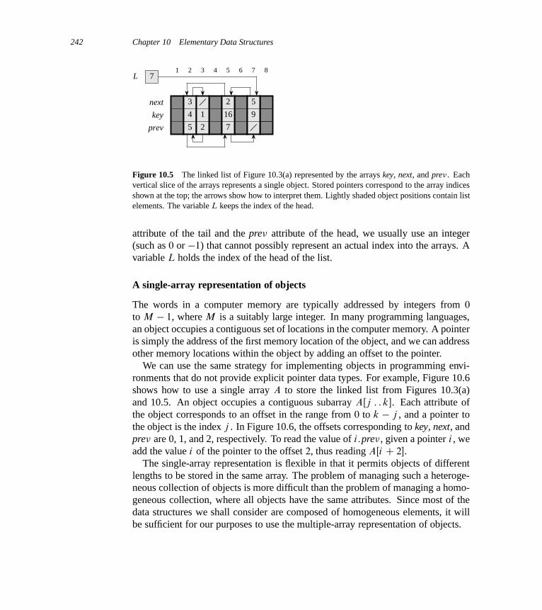
242 Chapter 10 Elementary Data Structures
1 2 3 4 5 6 7 8
key
next
prev
L 7
4 1 16 9
3 2 5
5 2 7
Figure 10.5 The linked list of Figure 10.3(a) represented by the arrays key, next, and pre�. Eachvertical slice of the arrays represents a single object. Stored pointers correspond to the array indicesshown at the top; the arrows show how to interpret them. Lightly shaded object positions contain listelements. The variable L keeps the index of the head.
attribute of the tail and the pre� attribute of the head, we usually use an integer(such as 0 or �1) that cannot possibly represent an actual index into the arrays. Avariable L holds the index of the head of the list.
A single-array representation of objects
The words in a computer memory are typically addressed by integers from 0
to M � 1, where M is a suitably large integer. In many programming languages,an object occupies a contiguous set of locations in the computer memory. A pointeris simply the address of the first memory location of the object, and we can addressother memory locations within the object by adding an offset to the pointer.
We can use the same strategy for implementing objects in programming envi-ronments that do not provide explicit pointer data types. For example, Figure 10.6shows how to use a single array A to store the linked list from Figures 10.3(a)and 10.5. An object occupies a contiguous subarray AŒj : : k�. Each attribute ofthe object corresponds to an offset in the range from 0 to k � j , and a pointer tothe object is the index j . In Figure 10.6, the offsets corresponding to key, next, andpre� are 0, 1, and 2, respectively. To read the value of i:pre�, given a pointer i , weadd the value i of the pointer to the offset 2, thus reading AŒi C 2�.
The single-array representation is flexible in that it permits objects of differentlengths to be stored in the same array. The problem of managing such a heteroge-neous collection of objects is more difficult than the problem of managing a homo-geneous collection, where all objects have the same attributes. Since most of thedata structures we shall consider are composed of homogeneous elements, it willbe sufficient for our purposes to use the multiple-array representation of objects.
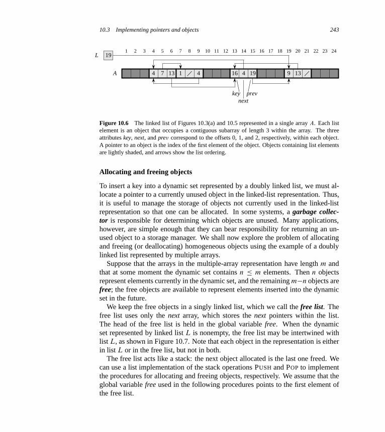
10.3 Implementing pointers and objects 243
1 2 3 4 5 6 7 8
A
L
4 1 16 97 44
9 10 11 12 13 14 15 16 17 18 19 20 21 22 23 24
prevnext
key
19
1313 19
Figure 10.6 The linked list of Figures 10.3(a) and 10.5 represented in a single array A. Each listelement is an object that occupies a contiguous subarray of length 3 within the array. The threeattributes key, next, and pre� correspond to the offsets 0, 1, and 2, respectively, within each object.A pointer to an object is the index of the first element of the object. Objects containing list elementsare lightly shaded, and arrows show the list ordering.
Allocating and freeing objects
To insert a key into a dynamic set represented by a doubly linked list, we must al-locate a pointer to a currently unused object in the linked-list representation. Thus,it is useful to manage the storage of objects not currently used in the linked-listrepresentation so that one can be allocated. In some systems, a garbage collec-tor is responsible for determining which objects are unused. Many applications,however, are simple enough that they can bear responsibility for returning an un-used object to a storage manager. We shall now explore the problem of allocatingand freeing (or deallocating) homogeneous objects using the example of a doublylinked list represented by multiple arrays.
Suppose that the arrays in the multiple-array representation have length m andthat at some moment the dynamic set contains n � m elements. Then n objectsrepresent elements currently in the dynamic set, and the remaining m�n objects arefree; the free objects are available to represent elements inserted into the dynamicset in the future.
We keep the free objects in a singly linked list, which we call the free list. Thefree list uses only the next array, which stores the next pointers within the list.The head of the free list is held in the global variable free. When the dynamicset represented by linked list L is nonempty, the free list may be intertwined withlist L, as shown in Figure 10.7. Note that each object in the representation is eitherin list L or in the free list, but not in both.
The free list acts like a stack: the next object allocated is the last one freed. Wecan use a list implementation of the stack operations PUSH and POP to implementthe procedures for allocating and freeing objects, respectively. We assume that theglobal variable free used in the following procedures points to the first element ofthe free list.
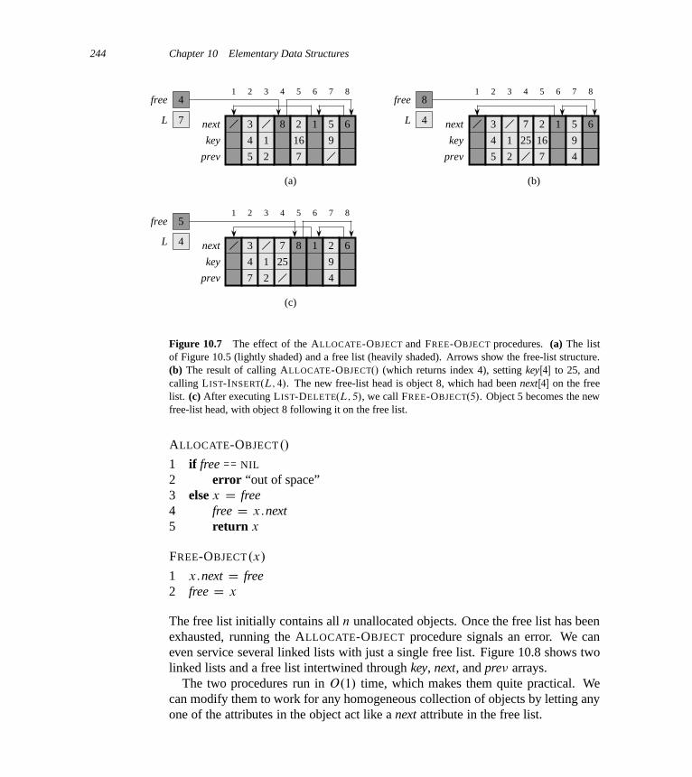
244 Chapter 10 Elementary Data Structures
1 2 3 4 5 6 7 8
key
next
prev
L 7
4 1 16 9
3 2 5
5 2 7
4
8 61
free
(a)
1 2 3 4 5 6 7 8
key
next
prev
L 4
4 1 16 9
3 2 5
5 2 7
8
7 61
free
(b)
4
25
1 2 3 4 5 6 7 8
key
next
prev
L 4
4 1 9
3 8 2
7 2
5
7 61
free
(c)
4
25
Figure 10.7 The effect of the ALLOCATE-OBJECT and FREE-OBJECT procedures. (a) The listof Figure 10.5 (lightly shaded) and a free list (heavily shaded). Arrows show the free-list structure.(b) The result of calling ALLOCATE-OBJECT./ (which returns index 4), setting keyŒ4� to 25, andcalling LIST-INSERT.L; 4/. The new free-list head is object 8, which had been nextŒ4� on the freelist. (c) After executing LIST-DELETE.L; 5/, we call FREE-OBJECT.5/. Object 5 becomes the newfree-list head, with object 8 following it on the free list.
ALLOCATE-OBJECT./
1 if free == NIL
2 error “out of space”3 else x D free4 free D x:next5 return x
FREE-OBJECT.x/
1 x:next D free2 free D x
The free list initially contains all n unallocated objects. Once the free list has beenexhausted, running the ALLOCATE-OBJECT procedure signals an error. We caneven service several linked lists with just a single free list. Figure 10.8 shows twolinked lists and a free list intertwined through key, next, and pre� arrays.
The two procedures run in O.1/ time, which makes them quite practical. Wecan modify them to work for any homogeneous collection of objects by letting anyone of the attributes in the object act like a next attribute in the free list.

10.3 Implementing pointers and objects 245
1 2 3 4 5 6 7 8 9 10
next
key
prev
free
3
6 2
6 3
715
7 9
9
10
48
1
L2
L1
k1 k2 k3 k5 k6 k7 k9
Figure 10.8 Two linked lists, L1 (lightly shaded) and L2 (heavily shaded), and a free list (dark-ened) intertwined.
Exercises
10.3-1Draw a picture of the sequence h13; 4; 8; 19; 5; 11i stored as a doubly linked listusing the multiple-array representation. Do the same for the single-array represen-tation.
10.3-2Write the procedures ALLOCATE-OBJECT and FREE-OBJECT for a homogeneouscollection of objects implemented by the single-array representation.
10.3-3Why don’t we need to set or reset the pre� attributes of objects in the implementa-tion of the ALLOCATE-OBJECT and FREE-OBJECT procedures?
10.3-4It is often desirable to keep all elements of a doubly linked list compact in storage,using, for example, the first m index locations in the multiple-array representation.(This is the case in a paged, virtual-memory computing environment.) Explainhow to implement the procedures ALLOCATE-OBJECT and FREE-OBJECT so thatthe representation is compact. Assume that there are no pointers to elements of thelinked list outside the list itself. (Hint: Use the array implementation of a stack.)
10.3-5Let L be a doubly linked list of length n stored in arrays key, pre�, and next oflength m. Suppose that these arrays are managed by ALLOCATE-OBJECT andFREE-OBJECT procedures that keep a doubly linked free list F . Suppose furtherthat of the m items, exactly n are on list L and m � n are on the free list. Writea procedure COMPACTIFY-LIST.L; F / that, given the list L and the free list F ,moves the items in L so that they occupy array positions 1; 2; : : : ; n and adjusts thefree list F so that it remains correct, occupying array positions nC1; nC2; : : : ; m.The running time of your procedure should be ‚.n/, and it should use only aconstant amount of extra space. Argue that your procedure is correct.
246 Chapter 10 Elementary Data Structures
10.4 Representing rooted trees
The methods for representing lists given in the previous section extend to any ho-mogeneous data structure. In this section, we look specifically at the problem ofrepresenting rooted trees by linked data structures. We first look at binary trees,and then we present a method for rooted trees in which nodes can have an arbitrarynumber of children.
We represent each node of a tree by an object. As with linked lists, we assumethat each node contains a key attribute. The remaining attributes of interest arepointers to other nodes, and they vary according to the type of tree.
Binary trees
Figure 10.9 shows how we use the attributes p, left, and right to store pointers tothe parent, left child, and right child of each node in a binary tree T . If x:p D NIL,then x is the root. If node x has no left child, then x: left D NIL, and similarly forthe right child. The root of the entire tree T is pointed to by the attribute T:root. IfT:root D NIL, then the tree is empty.
Rooted trees with unbounded branching
We can extend the scheme for representing a binary tree to any class of trees inwhich the number of children of each node is at most some constant k: we replacethe left and right attributes by child1; child2; : : : ; childk. This scheme no longerworks when the number of children of a node is unbounded, since we do not knowhow many attributes (arrays in the multiple-array representation) to allocate in ad-vance. Moreover, even if the number of children k is bounded by a large constantbut most nodes have a small number of children, we may waste a lot of memory.
Fortunately, there is a clever scheme to represent trees with arbitrary numbers ofchildren. It has the advantage of using only O.n/ space for any n-node rooted tree.The left-child, right-sibling representation appears in Figure 10.10. As before,each node contains a parent pointer p, and T:root points to the root of tree T .Instead of having a pointer to each of its children, however, each node x has onlytwo pointers:
1. x: left-child points to the leftmost child of node x, and
2. x:right-sibling points to the sibling of x immediately to its right.
If node x has no children, then x: left-child D NIL, and if node x is the rightmostchild of its parent, then x:right-sibling D NIL.
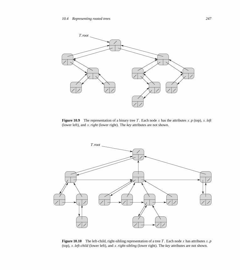
10.4 Representing rooted trees 247
T:root
Figure 10.9 The representation of a binary tree T . Each node x has the attributes x:p (top), x: left(lower left), and x:right (lower right). The key attributes are not shown.
T:root
Figure 10.10 The left-child, right-sibling representation of a tree T . Each node x has attributes x:p(top), x: left-child (lower left), and x:right-sibling (lower right). The key attributes are not shown.
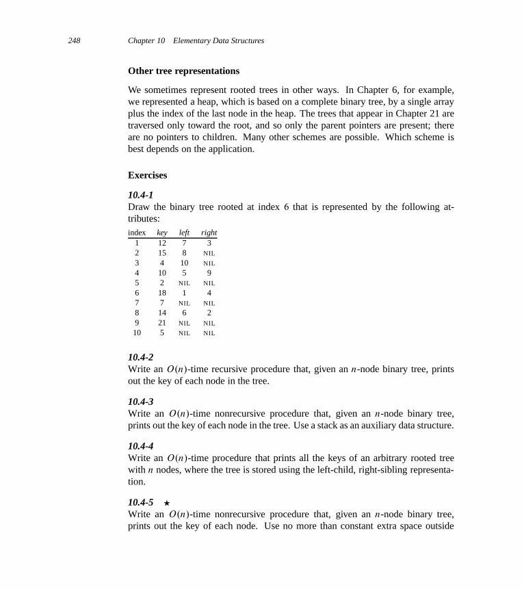
248 Chapter 10 Elementary Data Structures
Other tree representations
We sometimes represent rooted trees in other ways. In Chapter 6, for example,we represented a heap, which is based on a complete binary tree, by a single arrayplus the index of the last node in the heap. The trees that appear in Chapter 21 aretraversed only toward the root, and so only the parent pointers are present; thereare no pointers to children. Many other schemes are possible. Which scheme isbest depends on the application.
Exercises
10.4-1Draw the binary tree rooted at index 6 that is represented by the following at-tributes:index key left right
1 12 7 32 15 8 NIL
3 4 10 NIL
4 10 5 95 2 NIL NIL
6 18 1 47 7 NIL NIL
8 14 6 29 21 NIL NIL
10 5 NIL NIL
10.4-2Write an O.n/-time recursive procedure that, given an n-node binary tree, printsout the key of each node in the tree.
10.4-3Write an O.n/-time nonrecursive procedure that, given an n-node binary tree,prints out the key of each node in the tree. Use a stack as an auxiliary data structure.
10.4-4Write an O.n/-time procedure that prints all the keys of an arbitrary rooted treewith n nodes, where the tree is stored using the left-child, right-sibling representa-tion.
10.4-5 ?
Write an O.n/-time nonrecursive procedure that, given an n-node binary tree,prints out the key of each node. Use no more than constant extra space outside

Problems for Chapter 10 249
of the tree itself and do not modify the tree, even temporarily, during the proce-dure.
10.4-6 ?
The left-child, right-sibling representation of an arbitrary rooted tree uses threepointers in each node: left-child, right-sibling, and parent. From any node, itsparent can be reached and identified in constant time and all its children can bereached and identified in time linear in the number of children. Show how to useonly two pointers and one boolean value in each node so that the parent of a nodeor all of its children can be reached and identified in time linear in the number ofchildren.
Problems
10-1 Comparisons among listsFor each of the four types of lists in the following table, what is the asymptoticworst-case running time for each dynamic-set operation listed?
unsorted, sorted, unsorted, sorted,singly singly doubly doublylinked linked linked linked
SEARCH.L; k/
INSERT.L; x/
DELETE.L; x/
SUCCESSOR.L; x/
PREDECESSOR.L; x/
MINIMUM.L/
MAXIMUM.L/
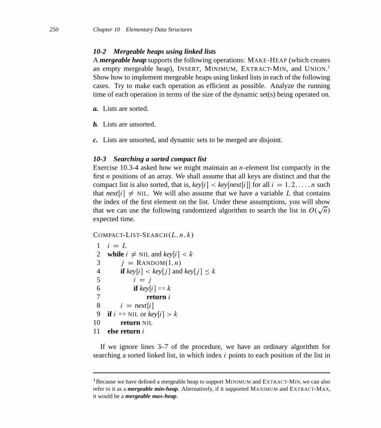
250 Chapter 10 Elementary Data Structures
10-2 Mergeable heaps using linked listsA mergeable heap supports the following operations: MAKE-HEAP (which createsan empty mergeable heap), INSERT, MINIMUM, EXTRACT-MIN, and UNION.1
Show how to implement mergeable heaps using linked lists in each of the followingcases. Try to make each operation as efficient as possible. Analyze the runningtime of each operation in terms of the size of the dynamic set(s) being operated on.
a. Lists are sorted.
b. Lists are unsorted.
c. Lists are unsorted, and dynamic sets to be merged are disjoint.
10-3 Searching a sorted compact listExercise 10.3-4 asked how we might maintain an n-element list compactly in thefirst n positions of an array. We shall assume that all keys are distinct and that thecompact list is also sorted, that is, keyŒi � < keyŒnextŒi �� for all i D 1; 2; : : : ; n suchthat nextŒi � ¤ NIL. We will also assume that we have a variable L that containsthe index of the first element on the list. Under these assumptions, you will showthat we can use the following randomized algorithm to search the list in O.
pn/
expected time.
COMPACT-LIST-SEARCH.L; n; k/
1 i D L
2 while i ¤ NIL and keyŒi � < k
3 j D RANDOM.1; n/
4 if keyŒi � < keyŒj � and keyŒj � � k
5 i D j
6 if keyŒi � == k
7 return i
8 i D nextŒi �9 if i == NIL or keyŒi � > k
10 return NIL
11 else return i
If we ignore lines 3–7 of the procedure, we have an ordinary algorithm forsearching a sorted linked list, in which index i points to each position of the list in
1Because we have defined a mergeable heap to support MINIMUM and EXTRACT-MIN, we can alsorefer to it as a mergeable min-heap. Alternatively, if it supported MAXIMUM and EXTRACT-MAX,it would be a mergeable max-heap.

Problems for Chapter 10 251
turn. The search terminates once the index i “falls off” the end of the list or oncekeyŒi � � k. In the latter case, if keyŒi � D k, clearly we have found a key with thevalue k. If, however, keyŒi � > k, then we will never find a key with the value k,and so terminating the search was the right thing to do.
Lines 3–7 attempt to skip ahead to a randomly chosen position j . Such a skipbenefits us if keyŒj � is larger than keyŒi � and no larger than k; in such a case, j
marks a position in the list that i would have to reach during an ordinary list search.Because the list is compact, we know that any choice of j between 1 and n indexessome object in the list rather than a slot on the free list.
Instead of analyzing the performance of COMPACT-LIST-SEARCH directly, weshall analyze a related algorithm, COMPACT-LIST-SEARCH 0, which executes twoseparate loops. This algorithm takes an additional parameter t which determinesan upper bound on the number of iterations of the first loop.
COMPACT-LIST-SEARCH0.L; n; k; t/
1 i D L
2 for q D 1 to t
3 j D RANDOM.1; n/
4 if keyŒi � < keyŒj � and keyŒj � � k
5 i D j
6 if keyŒi � == k
7 return i
8 while i ¤ NIL and keyŒi � < k
9 i D nextŒi �10 if i == NIL or keyŒi � > k
11 return NIL
12 else return i
To compare the execution of the algorithms COMPACT-LIST-SEARCH.L; n; k/
and COMPACT-LIST-SEARCH 0.L; n; k; t/, assume that the sequence of integers re-turned by the calls of RANDOM.1; n/ is the same for both algorithms.
a. Suppose that COMPACT-LIST-SEARCH.L; n; k/ takes t iterations of the whileloop of lines 2–8. Argue that COMPACT-LIST-SEARCH 0.L; n; k; t/ returns thesame answer and that the total number of iterations of both the for and whileloops within COMPACT-LIST-SEARCH 0 is at least t .
In the call COMPACT-LIST-SEARCH 0.L; n; k; t/, let Xt be the random variable thatdescribes the distance in the linked list (that is, through the chain of next pointers)from position i to the desired key k after t iterations of the for loop of lines 2–7have occurred.
252 Chapter 10 Elementary Data Structures
b. Argue that the expected running time of COMPACT-LIST-SEARCH 0.L; n; k; t/
is O.t C E ŒXt �/.
c. Show that E ŒXt � �Pn
rD1.1 � r=n/t . (Hint: Use equation (C.25).)
d. Show thatPn�1
rD0 r t � ntC1=.t C 1/.
e. Prove that E ŒXt � � n=.t C 1/.
f. Show that COMPACT-LIST-SEARCH 0.L; n; k; t/ runs in O.t C n=t/ expectedtime.
g. Conclude that COMPACT-LIST-SEARCH runs in O.p
n/ expected time.
h. Why do we assume that all keys are distinct in COMPACT-LIST-SEARCH? Ar-gue that random skips do not necessarily help asymptotically when the list con-tains repeated key values.
Chapter notes
Aho, Hopcroft, and Ullman [6] and Knuth [209] are excellent references for ele-mentary data structures. Many other texts cover both basic data structures and theirimplementation in a particular programming language. Examples of these types oftextbooks include Goodrich and Tamassia [147], Main [241], Shaffer [311], andWeiss [352, 353, 354]. Gonnet [145] provides experimental data on the perfor-mance of many data-structure operations.
The origin of stacks and queues as data structures in computer science is un-clear, since corresponding notions already existed in mathematics and paper-basedbusiness practices before the introduction of digital computers. Knuth [209] citesA. M. Turing for the development of stacks for subroutine linkage in 1947.
Pointer-based data structures also seem to be a folk invention. According toKnuth, pointers were apparently used in early computers with drum memories. TheA-1 language developed by G. M. Hopper in 1951 represented algebraic formulasas binary trees. Knuth credits the IPL-II language, developed in 1956 by A. Newell,J. C. Shaw, and H. A. Simon, for recognizing the importance and promoting theuse of pointers. Their IPL-III language, developed in 1957, included explicit stackoperations.

11 Hash Tables
Many applications require a dynamic set that supports only the dictionary opera-tions INSERT, SEARCH, and DELETE. For example, a compiler that translates aprogramming language maintains a symbol table, in which the keys of elementsare arbitrary character strings corresponding to identifiers in the language. A hashtable is an effective data structure for implementing dictionaries. Although search-ing for an element in a hash table can take as long as searching for an element in alinked list—‚.n/ time in the worst case—in practice, hashing performs extremelywell. Under reasonable assumptions, the average time to search for an element ina hash table is O.1/.
A hash table generalizes the simpler notion of an ordinary array. Directly ad-dressing into an ordinary array makes effective use of our ability to examine anarbitrary position in an array in O.1/ time. Section 11.1 discusses direct address-ing in more detail. We can take advantage of direct addressing when we can affordto allocate an array that has one position for every possible key.
When the number of keys actually stored is small relative to the total number ofpossible keys, hash tables become an effective alternative to directly addressing anarray, since a hash table typically uses an array of size proportional to the numberof keys actually stored. Instead of using the key as an array index directly, the arrayindex is computed from the key. Section 11.2 presents the main ideas, focusing on“chaining” as a way to handle “collisions,” in which more than one key maps to thesame array index. Section 11.3 describes how we can compute array indices fromkeys using hash functions. We present and analyze several variations on the basictheme. Section 11.4 looks at “open addressing,” which is another way to deal withcollisions. The bottom line is that hashing is an extremely effective and practicaltechnique: the basic dictionary operations require only O.1/ time on the average.Section 11.5 explains how “perfect hashing” can support searches in O.1/ worst-case time, when the set of keys being stored is static (that is, when the set of keysnever changes once stored).
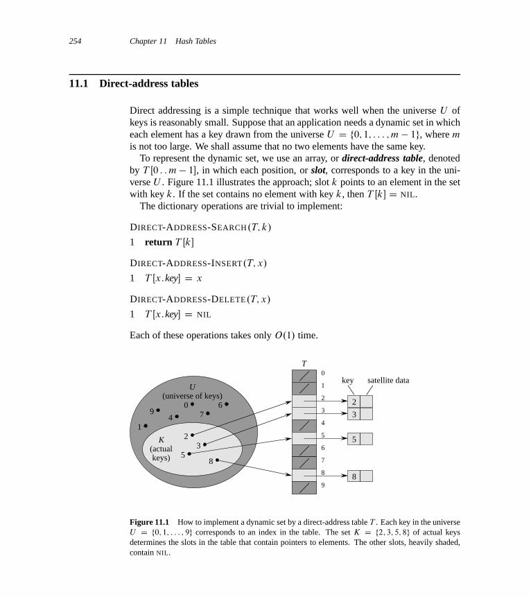
254 Chapter 11 Hash Tables
11.1 Direct-address tables
Direct addressing is a simple technique that works well when the universe U ofkeys is reasonably small. Suppose that an application needs a dynamic set in whicheach element has a key drawn from the universe U D f0; 1; : : : ; m � 1g, where m
is not too large. We shall assume that no two elements have the same key.To represent the dynamic set, we use an array, or direct-address table, denoted
by T Œ0 : : m � 1�, in which each position, or slot, corresponds to a key in the uni-verse U . Figure 11.1 illustrates the approach; slot k points to an element in the setwith key k. If the set contains no element with key k, then T Œk� D NIL.
The dictionary operations are trivial to implement:
DIRECT-ADDRESS-SEARCH.T; k/
1 return T Œk�
DIRECT-ADDRESS-INSERT.T; x/
1 T Œx:key� D x
DIRECT-ADDRESS-DELETE.T; x/
1 T Œx:key� D NIL
Each of these operations takes only O.1/ time.
T
U(universe of keys)
K(actualkeys)
23
58
1
94
07
6 2
3
5
8
key satellite data
2
0
1
3
4
5
6
7
8
9
Figure 11.1 How to implement a dynamic set by a direct-address table T . Each key in the universeU D f0; 1; : : : ; 9g corresponds to an index in the table. The set K D f2; 3; 5; 8g of actual keysdetermines the slots in the table that contain pointers to elements. The other slots, heavily shaded,contain NIL.

11.1 Direct-address tables 255
For some applications, the direct-address table itself can hold the elements in thedynamic set. That is, rather than storing an element’s key and satellite data in anobject external to the direct-address table, with a pointer from a slot in the table tothe object, we can store the object in the slot itself, thus saving space. We woulduse a special key within an object to indicate an empty slot. Moreover, it is oftenunnecessary to store the key of the object, since if we have the index of an objectin the table, we have its key. If keys are not stored, however, we must have someway to tell whether the slot is empty.
Exercises
11.1-1Suppose that a dynamic set S is represented by a direct-address table T of length m.Describe a procedure that finds the maximum element of S . What is the worst-caseperformance of your procedure?
11.1-2A bit vector is simply an array of bits (0s and 1s). A bit vector of length m takesmuch less space than an array of m pointers. Describe how to use a bit vectorto represent a dynamic set of distinct elements with no satellite data. Dictionaryoperations should run in O.1/ time.
11.1-3Suggest how to implement a direct-address table in which the keys of stored el-ements do not need to be distinct and the elements can have satellite data. Allthree dictionary operations (INSERT, DELETE, and SEARCH) should run in O.1/
time. (Don’t forget that DELETE takes as an argument a pointer to an object to bedeleted, not a key.)
11.1-4 ?
We wish to implement a dictionary by using direct addressing on a huge array. Atthe start, the array entries may contain garbage, and initializing the entire arrayis impractical because of its size. Describe a scheme for implementing a direct-address dictionary on a huge array. Each stored object should use O.1/ space;the operations SEARCH, INSERT, and DELETE should take O.1/ time each; andinitializing the data structure should take O.1/ time. (Hint: Use an additional array,treated somewhat like a stack whose size is the number of keys actually stored inthe dictionary, to help determine whether a given entry in the huge array is valid ornot.)

256 Chapter 11 Hash Tables
11.2 Hash tables
The downside of direct addressing is obvious: if the universe U is large, storinga table T of size jU j may be impractical, or even impossible, given the memoryavailable on a typical computer. Furthermore, the set K of keys actually storedmay be so small relative to U that most of the space allocated for T would bewasted.
When the set K of keys stored in a dictionary is much smaller than the uni-verse U of all possible keys, a hash table requires much less storage than a direct-address table. Specifically, we can reduce the storage requirement to ‚.jKj/ whilewe maintain the benefit that searching for an element in the hash table still requiresonly O.1/ time. The catch is that this bound is for the average-case time, whereasfor direct addressing it holds for the worst-case time.
With direct addressing, an element with key k is stored in slot k. With hashing,this element is stored in slot h.k/; that is, we use a hash function h to compute theslot from the key k. Here, h maps the universe U of keys into the slots of a hashtable T Œ0 : : m � 1�:
h W U ! f0; 1; : : : ; m � 1g ;
where the size m of the hash table is typically much less than jU j. We say that anelement with key k hashes to slot h.k/; we also say that h.k/ is the hash value ofkey k. Figure 11.2 illustrates the basic idea. The hash function reduces the rangeof array indices and hence the size of the array. Instead of a size of jU j, the arraycan have size m.
T
U(universe of keys)
K(actualkeys)
0
m–1
k1
k2 k3
k4 k5
h(k1)
h(k4)
h(k3)
h(k2) = h(k5)
Figure 11.2 Using a hash function h to map keys to hash-table slots. Because keys k2 and k5 mapto the same slot, they collide.
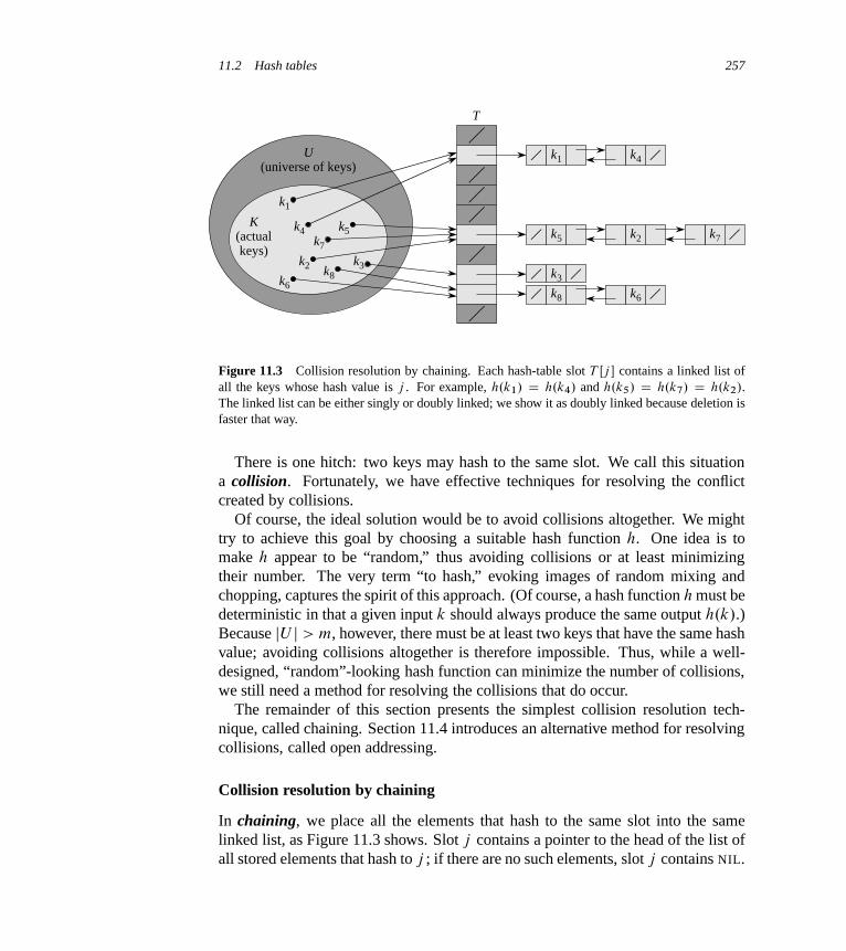
11.2 Hash tables 257
T
U(universe of keys)
K(actualkeys)
k1
k2 k3
k4 k5
k6
k7
k8
k1
k2
k3
k4
k5
k6
k7
k8
Figure 11.3 Collision resolution by chaining. Each hash-table slot T Œj � contains a linked list ofall the keys whose hash value is j . For example, h.k1/ D h.k4/ and h.k5/ D h.k7/ D h.k2/.The linked list can be either singly or doubly linked; we show it as doubly linked because deletion isfaster that way.
There is one hitch: two keys may hash to the same slot. We call this situationa collision. Fortunately, we have effective techniques for resolving the conflictcreated by collisions.
Of course, the ideal solution would be to avoid collisions altogether. We mighttry to achieve this goal by choosing a suitable hash function h. One idea is tomake h appear to be “random,” thus avoiding collisions or at least minimizingtheir number. The very term “to hash,” evoking images of random mixing andchopping, captures the spirit of this approach. (Of course, a hash function h must bedeterministic in that a given input k should always produce the same output h.k/.)Because jU j > m, however, there must be at least two keys that have the same hashvalue; avoiding collisions altogether is therefore impossible. Thus, while a well-designed, “random”-looking hash function can minimize the number of collisions,we still need a method for resolving the collisions that do occur.
The remainder of this section presents the simplest collision resolution tech-nique, called chaining. Section 11.4 introduces an alternative method for resolvingcollisions, called open addressing.
Collision resolution by chaining
In chaining, we place all the elements that hash to the same slot into the samelinked list, as Figure 11.3 shows. Slot j contains a pointer to the head of the list ofall stored elements that hash to j ; if there are no such elements, slot j contains NIL.

258 Chapter 11 Hash Tables
The dictionary operations on a hash table T are easy to implement when colli-sions are resolved by chaining:
CHAINED-HASH-INSERT.T; x/
1 insert x at the head of list T Œh.x:key/�
CHAINED-HASH-SEARCH.T; k/
1 search for an element with key k in list T Œh.k/�
CHAINED-HASH-DELETE.T; x/
1 delete x from the list T Œh.x:key/�
The worst-case running time for insertion is O.1/. The insertion procedure is fastin part because it assumes that the element x being inserted is not already present inthe table; if necessary, we can check this assumption (at additional cost) by search-ing for an element whose key is x:key before we insert. For searching, the worst-case running time is proportional to the length of the list; we shall analyze thisoperation more closely below. We can delete an element in O.1/ time if the listsare doubly linked, as Figure 11.3 depicts. (Note that CHAINED-HASH-DELETE
takes as input an element x and not its key k, so that we don’t have to search for x
first. If the hash table supports deletion, then its linked lists should be doubly linkedso that we can delete an item quickly. If the lists were only singly linked, then todelete element x, we would first have to find x in the list T Œh.x:key/� so that wecould update the next attribute of x’s predecessor. With singly linked lists, bothdeletion and seaching would have the same asymptotic running times.)
Analysis of hashing with chaining
How well does hashing with chaining perform? In particular, how long does it taketo search for an element with a given key?
Given a hash table T with m slots that stores n elements, we define the loadfactor ˛ for T as n=m, that is, the average number of elements stored in a chain.Our analysis will be in terms of ˛, which can be less than, equal to, or greaterthan 1.
The worst-case behavior of hashing with chaining is terrible: all n keys hashto the same slot, creating a list of length n. The worst-case time for searching isthus ‚.n/ plus the time to compute the hash function—no better than if we usedone linked list for all the elements. Clearly, we do not use hash tables for theirworst-case performance. (Perfect hashing, described in Section 11.5, does providegood worst-case performance when the set of keys is static, however.)
The average-case performance of hashing depends on how well the hash func-tion h distributes the set of keys to be stored among the m slots, on the average.
11.2 Hash tables 259
Section 11.3 discusses these issues, but for now we shall assume that any givenelement is equally likely to hash into any of the m slots, independently of whereany other element has hashed to. We call this the assumption of simple uniformhashing.
For j D 0; 1; : : : ; m � 1, let us denote the length of the list T Œj � by nj , so that
n D n0 C n1 C � � � C nm�1 ; (11.1)
and the expected value of nj is E Œnj � D ˛ D n=m.We assume that O.1/ time suffices to compute the hash value h.k/, so that
the time required to search for an element with key k depends linearly on thelength nh.k/ of the list T Œh.k/�. Setting aside the O.1/ time required to computethe hash function and to access slot h.k/, let us consider the expected number ofelements examined by the search algorithm, that is, the number of elements in thelist T Œh.k/� that the algorithm checks to see whether any have a key equal to k. Weshall consider two cases. In the first, the search is unsuccessful: no element in thetable has key k. In the second, the search successfully finds an element with key k.
Theorem 11.1In a hash table in which collisions are resolved by chaining, an unsuccessful searchtakes average-case time ‚.1C˛/, under the assumption of simple uniform hashing.
Proof Under the assumption of simple uniform hashing, any key k not alreadystored in the table is equally likely to hash to any of the m slots. The expected timeto search unsuccessfully for a key k is the expected time to search to the end oflist T Œh.k/�, which has expected length E Œnh.k/� D ˛. Thus, the expected numberof elements examined in an unsuccessful search is ˛, and the total time required(including the time for computing h.k/) is ‚.1C ˛/.
The situation for a successful search is slightly different, since each list is notequally likely to be searched. Instead, the probability that a list is searched is pro-portional to the number of elements it contains. Nonetheless, the expected searchtime still turns out to be ‚.1C ˛/.
Theorem 11.2In a hash table in which collisions are resolved by chaining, a successful searchtakes average-case time ‚.1C˛/, under the assumption of simple uniform hashing.
Proof We assume that the element being searched for is equally likely to be anyof the n elements stored in the table. The number of elements examined during asuccessful search for an element x is one more than the number of elements thatappear before x in x’s list. Because new elements are placed at the front of thelist, elements before x in the list were all inserted after x was inserted. To find
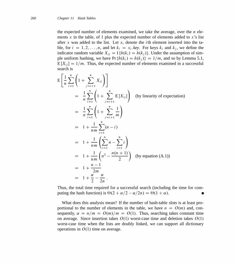
260 Chapter 11 Hash Tables
the expected number of elements examined, we take the average, over the n ele-ments x in the table, of 1 plus the expected number of elements added to x’s listafter x was added to the list. Let xi denote the i th element inserted into the ta-ble, for i D 1; 2; : : : ; n, and let ki D xi :key. For keys ki and kj , we define theindicator random variable Xij D I fh.ki / D h.kj /g. Under the assumption of sim-ple uniform hashing, we have Pr fh.ki / D h.kj /g D 1=m, and so by Lemma 5.1,E ŒXij � D 1=m. Thus, the expected number of elements examined in a successfulsearch is
E
"1
n
nXiD1
1C
nXj DiC1
Xij
!#
D 1
n
nXiD1
1C
nXj DiC1
E ŒXij �
!(by linearity of expectation)
D 1
n
nXiD1
1C
nXj DiC1
1
m
!
D 1C 1
nm
nXiD1
.n � i/
D 1C 1
nm
nX
iD1
n �nX
iD1
i
!
D 1C 1
nm
�n2 � n.nC 1/
2
�(by equation (A.1))
D 1C n � 1
2m
D 1C ˛
2� ˛
2n:
Thus, the total time required for a successful search (including the time for com-puting the hash function) is ‚.2C ˛=2� ˛=2n/ D ‚.1C ˛/.
What does this analysis mean? If the number of hash-table slots is at least pro-portional to the number of elements in the table, we have n D O.m/ and, con-sequently, ˛ D n=m D O.m/=m D O.1/. Thus, searching takes constant timeon average. Since insertion takes O.1/ worst-case time and deletion takes O.1/
worst-case time when the lists are doubly linked, we can support all dictionaryoperations in O.1/ time on average.
11.2 Hash tables 261
Exercises
11.2-1Suppose we use a hash function h to hash n distinct keys into an array T oflength m. Assuming simple uniform hashing, what is the expected number ofcollisions? More precisely, what is the expected cardinality of ffk; lg W k ¤ l andh.k/ D h.l/g?11.2-2Demonstrate what happens when we insert the keys 5; 28; 19; 15; 20; 33; 12; 17; 10
into a hash table with collisions resolved by chaining. Let the table have 9 slots,and let the hash function be h.k/ D k mod 9.
11.2-3Professor Marley hypothesizes that he can obtain substantial performance gains bymodifying the chaining scheme to keep each list in sorted order. How does the pro-fessor’s modification affect the running time for successful searches, unsuccessfulsearches, insertions, and deletions?
11.2-4Suggest how to allocate and deallocate storage for elements within the hash tableitself by linking all unused slots into a free list. Assume that one slot can storea flag and either one element plus a pointer or two pointers. All dictionary andfree-list operations should run in O.1/ expected time. Does the free list need to bedoubly linked, or does a singly linked free list suffice?
11.2-5Suppose that we are storing a set of n keys into a hash table of size m. Show that ifthe keys are drawn from a universe U with jU j > nm, then U has a subset of size n
consisting of keys that all hash to the same slot, so that the worst-case searchingtime for hashing with chaining is ‚.n/.
11.2-6Suppose we have stored n keys in a hash table of size m, with collisions resolved bychaining, and that we know the length of each chain, including the length L of thelongest chain. Describe a procedure that selects a key uniformly at random fromamong the keys in the hash table and returns it in expected time O.L � .1C 1=˛//.
262 Chapter 11 Hash Tables
11.3 Hash functions
In this section, we discuss some issues regarding the design of good hash functionsand then present three schemes for their creation. Two of the schemes, hashing bydivision and hashing by multiplication, are heuristic in nature, whereas the thirdscheme, universal hashing, uses randomization to provide provably good perfor-mance.
What makes a good hash function?
A good hash function satisfies (approximately) the assumption of simple uniformhashing: each key is equally likely to hash to any of the m slots, independently ofwhere any other key has hashed to. Unfortunately, we typically have no way tocheck this condition, since we rarely know the probability distribution from whichthe keys are drawn. Moreover, the keys might not be drawn independently.
Occasionally we do know the distribution. For example, if we know that thekeys are random real numbers k independently and uniformly distributed in therange 0 � k < 1, then the hash function
h.k/ D bkmcsatisfies the condition of simple uniform hashing.
In practice, we can often employ heuristic techniques to create a hash functionthat performs well. Qualitative information about the distribution of keys may beuseful in this design process. For example, consider a compiler’s symbol table, inwhich the keys are character strings representing identifiers in a program. Closelyrelated symbols, such as pt and pts, often occur in the same program. A goodhash function would minimize the chance that such variants hash to the same slot.
A good approach derives the hash value in a way that we expect to be indepen-dent of any patterns that might exist in the data. For example, the “division method”(discussed in Section 11.3.1) computes the hash value as the remainder when thekey is divided by a specified prime number. This method frequently gives goodresults, assuming that we choose a prime number that is unrelated to any patternsin the distribution of keys.
Finally, we note that some applications of hash functions might require strongerproperties than are provided by simple uniform hashing. For example, we mightwant keys that are “close” in some sense to yield hash values that are far apart.(This property is especially desirable when we are using linear probing, defined inSection 11.4.) Universal hashing, described in Section 11.3.3, often provides thedesired properties.

11.3 Hash functions 263
Interpreting keys as natural numbers
Most hash functions assume that the universe of keys is the set N D f0; 1; 2; : : :gof natural numbers. Thus, if the keys are not natural numbers, we find a way tointerpret them as natural numbers. For example, we can interpret a character stringas an integer expressed in suitable radix notation. Thus, we might interpret theidentifier pt as the pair of decimal integers .112; 116/, since p D 112 and t D 116
in the ASCII character set; then, expressed as a radix-128 integer, pt becomes.112 � 128/C 116 D 14452. In the context of a given application, we can usuallydevise some such method for interpreting each key as a (possibly large) naturalnumber. In what follows, we assume that the keys are natural numbers.
11.3.1 The division method
In the division method for creating hash functions, we map a key k into one of m
slots by taking the remainder of k divided by m. That is, the hash function is
h.k/ D k mod m :
For example, if the hash table has size m D 12 and the key is k D 100, thenh.k/ D 4. Since it requires only a single division operation, hashing by division isquite fast.
When using the division method, we usually avoid certain values of m. Forexample, m should not be a power of 2, since if m D 2p , then h.k/ is just the p
lowest-order bits of k. Unless we know that all low-order p-bit patterns are equallylikely, we are better off designing the hash function to depend on all the bits of thekey. As Exercise 11.3-3 asks you to show, choosing m D 2p � 1 when k is acharacter string interpreted in radix 2p may be a poor choice, because permutingthe characters of k does not change its hash value.
A prime not too close to an exact power of 2 is often a good choice for m. Forexample, suppose we wish to allocate a hash table, with collisions resolved bychaining, to hold roughly n D 2000 character strings, where a character has 8 bits.We don’t mind examining an average of 3 elements in an unsuccessful search, andso we allocate a hash table of size m D 701. We could choose m D 701 becauseit is a prime near 2000=3 but not near any power of 2. Treating each key k as aninteger, our hash function would be
h.k/ D k mod 701 :
11.3.2 The multiplication method
The multiplication method for creating hash functions operates in two steps. First,we multiply the key k by a constant A in the range 0 < A < 1 and extract the
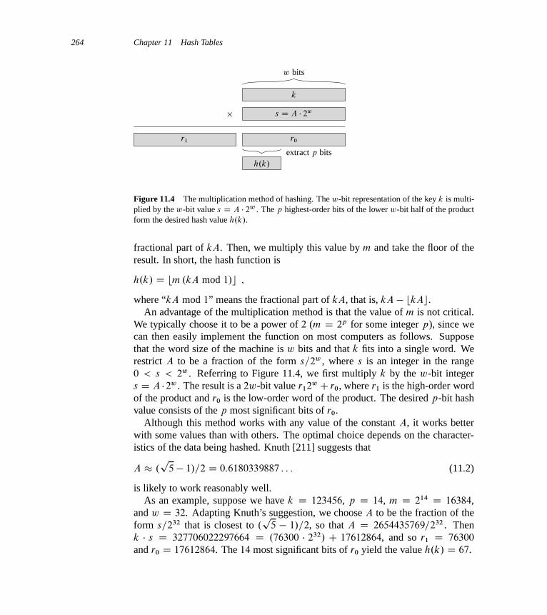
264 Chapter 11 Hash Tables
× s D A � 2w
w bits
k
r0r1
h.k/
extract p bits
Figure 11.4 The multiplication method of hashing. The w-bit representation of the key k is multi-plied by the w-bit value s D A � 2w . The p highest-order bits of the lower w-bit half of the productform the desired hash value h.k/.
fractional part of kA. Then, we multiply this value by m and take the floor of theresult. In short, the hash function is
h.k/ D bm .kA mod 1/c ;
where “kA mod 1” means the fractional part of kA, that is, kA � bkAc.An advantage of the multiplication method is that the value of m is not critical.
We typically choose it to be a power of 2 (m D 2p for some integer p), since wecan then easily implement the function on most computers as follows. Supposethat the word size of the machine is w bits and that k fits into a single word. Werestrict A to be a fraction of the form s=2w , where s is an integer in the range0 < s < 2w . Referring to Figure 11.4, we first multiply k by the w-bit integers D A �2w . The result is a 2w-bit value r12w C r0, where r1 is the high-order wordof the product and r0 is the low-order word of the product. The desired p-bit hashvalue consists of the p most significant bits of r0.
Although this method works with any value of the constant A, it works betterwith some values than with others. The optimal choice depends on the character-istics of the data being hashed. Knuth [211] suggests that
A � .p
5� 1/=2 D 0:6180339887 : : : (11.2)
is likely to work reasonably well.As an example, suppose we have k D 123456, p D 14, m D 214 D 16384,
and w D 32. Adapting Knuth’s suggestion, we choose A to be the fraction of theform s=232 that is closest to .
p5 � 1/=2, so that A D 2654435769=232 . Then
k � s D 327706022297664 D .76300 � 232/ C 17612864, and so r1 D 76300
and r0 D 17612864. The 14 most significant bits of r0 yield the value h.k/ D 67.
11.3 Hash functions 265
? 11.3.3 Universal hashing
If a malicious adversary chooses the keys to be hashed by some fixed hash function,then the adversary can choose n keys that all hash to the same slot, yielding an av-erage retrieval time of ‚.n/. Any fixed hash function is vulnerable to such terribleworst-case behavior; the only effective way to improve the situation is to choosethe hash function randomly in a way that is independent of the keys that are actuallygoing to be stored. This approach, called universal hashing, can yield provablygood performance on average, no matter which keys the adversary chooses.
In universal hashing, at the beginning of execution we select the hash functionat random from a carefully designed class of functions. As in the case of quick-sort, randomization guarantees that no single input will always evoke worst-casebehavior. Because we randomly select the hash function, the algorithm can be-have differently on each execution, even for the same input, guaranteeing goodaverage-case performance for any input. Returning to the example of a compiler’ssymbol table, we find that the programmer’s choice of identifiers cannot now causeconsistently poor hashing performance. Poor performance occurs only when thecompiler chooses a random hash function that causes the set of identifiers to hashpoorly, but the probability of this situation occurring is small and is the same forany set of identifiers of the same size.
Let H be a finite collection of hash functions that map a given universe U ofkeys into the range f0; 1; : : : ; m � 1g. Such a collection is said to be universalif for each pair of distinct keys k; l 2 U , the number of hash functions h 2 H
for which h.k/ D h.l/ is at most jH j =m. In other words, with a hash functionrandomly chosen from H , the chance of a collision between distinct keys k and l
is no more than the chance 1=m of a collision if h.k/ and h.l/ were randomly andindependently chosen from the set f0; 1; : : : ; m � 1g.
The following theorem shows that a universal class of hash functions gives goodaverage-case behavior. Recall that ni denotes the length of list T Œi �.
Theorem 11.3Suppose that a hash function h is chosen randomly from a universal collection ofhash functions and has been used to hash n keys into a table T of size m, us-ing chaining to resolve collisions. If key k is not in the table, then the expectedlength E Œnh.k/� of the list that key k hashes to is at most the load factor ˛ D n=m.If key k is in the table, then the expected length E Œnh.k/� of the list containing key k
is at most 1C ˛.
Proof We note that the expectations here are over the choice of the hash func-tion, and do not depend on any assumptions about the distribution of the keys.For each pair k and l of distinct keys, define the indicator random variable
266 Chapter 11 Hash Tables
Xkl D I fh.k/ D h.l/g. Since by the definition of a universal collection of hashfunctions, a single pair of keys collides with probability at most 1=m, we havePr fh.k/ D h.l/g � 1=m. By Lemma 5.1, therefore, we have E ŒXkl � � 1=m.
Next we define, for each key k, the random variable Yk that equals the numberof keys other than k that hash to the same slot as k, so that
Yk DXl2T
l¤k
Xkl :
Thus we have
E ŒYk� D E24X
l2Tl¤k
Xkl
35D
Xl2Tl¤k
E ŒXkl � (by linearity of expectation)
�Xl2Tl¤k
1
m:
The remainder of the proof depends on whether key k is in table T .
� If k 62 T , then nh.k/ D Yk and jfl W l 2 T and l ¤ kgj D n. Thus E Œnh.k/� DE ŒYk � � n=m D ˛.
� If k 2 T , then because key k appears in list T Œh.k/� and the count Yk does notinclude key k, we have nh.k/ D Yk C 1 and jfl W l 2 T and l ¤ kgj D n � 1.Thus E Œnh.k/� D E ŒYk �C 1 � .n � 1/=mC 1 D 1C ˛ � 1=m < 1C ˛.
The following corollary says universal hashing provides the desired payoff: ithas now become impossible for an adversary to pick a sequence of operations thatforces the worst-case running time. By cleverly randomizing the choice of hashfunction at run time, we guarantee that we can process every sequence of operationswith a good average-case running time.
Corollary 11.4Using universal hashing and collision resolution by chaining in an initially emptytable with m slots, it takes expected time ‚.n/ to handle any sequence of n INSERT,SEARCH and DELETE operations containing O.m/ INSERT operations.
Proof Since the number of insertions is O.m/, we have n D O.m/ and so˛ D O.1/. The INSERT and DELETE operations take constant time and, by The-orem 11.3, the expected time for each SEARCH operation is O.1/. By linearity of

11.3 Hash functions 267
expectation, therefore, the expected time for the entire sequence of n operationsis O.n/. Since each operation takes �.1/ time, the ‚.n/ bound follows.
Designing a universal class of hash functions
It is quite easy to design a universal class of hash functions, as a little numbertheory will help us prove. You may wish to consult Chapter 31 first if you areunfamiliar with number theory.
We begin by choosing a prime number p large enough so that every possiblekey k is in the range 0 to p � 1, inclusive. Let Zp denote the set f0; 1; : : : ; p � 1g,and let Z
�p denote the set f1; 2; : : : ; p � 1g. Since p is prime, we can solve equa-
tions modulo p with the methods given in Chapter 31. Because we assume that thesize of the universe of keys is greater than the number of slots in the hash table, wehave p > m.
We now define the hash function hab for any a 2 Z�p and any b 2 Zp using a
linear transformation followed by reductions modulo p and then modulo m:
hab.k/ D ..ak C b/ mod p/ mod m : (11.3)
For example, with p D 17 and m D 6, we have h3;4.8/ D 5. The family of allsuch hash functions is
Hpm D˚hab W a 2 Z
�p and b 2 Zp
: (11.4)
Each hash function hab maps Zp to Zm. This class of hash functions has the niceproperty that the size m of the output range is arbitrary—not necessarily prime—afeature which we shall use in Section 11.5. Since we have p � 1 choices for a
and p choices for b, the collection Hpm contains p.p � 1/ hash functions.
Theorem 11.5The class Hpm of hash functions defined by equations (11.3) and (11.4) is universal.
Proof Consider two distinct keys k and l from Zp, so that k ¤ l . For a givenhash function hab we let
r D .ak C b/ mod p ;
s D .al C b/ mod p :
We first note that r ¤ s. Why? Observe that
r � s � a.k � l/ .mod p/ :
It follows that r ¤ s because p is prime and both a and .k � l/ are nonzeromodulo p, and so their product must also be nonzero modulo p by Theorem 31.6.Therefore, when computing any hab 2 Hpm, distinct inputs k and l map to distinct
268 Chapter 11 Hash Tables
values r and s modulo p; there are no collisions yet at the “mod p level.” Moreover,each of the possible p.p�1/ choices for the pair .a; b/ with a ¤ 0 yields a differentresulting pair .r; s/ with r ¤ s, since we can solve for a and b given r and s:
a D �.r � s/..k � l/�1 mod p/
�mod p ;
b D .r � ak/ mod p ;
where ..k � l/�1 mod p/ denotes the unique multiplicative inverse, modulo p,of k � l . Since there are only p.p � 1/ possible pairs .r; s/ with r ¤ s, thereis a one-to-one correspondence between pairs .a; b/ with a ¤ 0 and pairs .r; s/
with r ¤ s. Thus, for any given pair of inputs k and l , if we pick .a; b/ uniformlyat random from Z
�p Zp, the resulting pair .r; s/ is equally likely to be any pair of
distinct values modulo p.Therefore, the probability that distinct keys k and l collide is equal to the prob-
ability that r � s .mod m/ when r and s are randomly chosen as distinct valuesmodulo p. For a given value of r , of the p � 1 possible remaining values for s, thenumber of values s such that s ¤ r and s � r .mod m/ is at most
dp=me � 1 � ..p Cm � 1/=m/ � 1 (by inequality (3.6))
D .p � 1/=m :
The probability that s collides with r when reduced modulo m is at most..p � 1/=m/=.p � 1/ D 1=m.
Therefore, for any pair of distinct values k; l 2 Zp,
Pr fhab.k/ D hab.l/g � 1=m ;
so that Hpm is indeed universal.
Exercises
11.3-1Suppose we wish to search a linked list of length n, where each element containsa key k along with a hash value h.k/. Each key is a long character string. Howmight we take advantage of the hash values when searching the list for an elementwith a given key?
11.3-2Suppose that we hash a string of r characters into m slots by treating it as aradix-128 number and then using the division method. We can easily representthe number m as a 32-bit computer word, but the string of r characters, treated asa radix-128 number, takes many words. How can we apply the division method tocompute the hash value of the character string without using more than a constantnumber of words of storage outside the string itself?
11.4 Open addressing 269
11.3-3Consider a version of the division method in which h.k/ D k mod m, wherem D 2p � 1 and k is a character string interpreted in radix 2p . Show that if wecan derive string x from string y by permuting its characters, then x and y hash tothe same value. Give an example of an application in which this property would beundesirable in a hash function.
11.3-4Consider a hash table of size m D 1000 and a corresponding hash function h.k/ Dbm .kA mod 1/c for A D .
p5 � 1/=2. Compute the locations to which the keys
61, 62, 63, 64, and 65 are mapped.
11.3-5 ?
Define a family H of hash functions from a finite set U to a finite set B to be�-universal if for all pairs of distinct elements k and l in U ,
Pr fh.k/ D h.l/g � � ;
where the probability is over the choice of the hash function h drawn at randomfrom the family H . Show that an �-universal family of hash functions must have
� � 1
jBj �1
jU j :
11.3-6 ?
Let U be the set of n-tuples of values drawn from Zp, and let B D Zp , where p
is prime. Define the hash function hb W U ! B for b 2 Zp on an input n-tupleha0; a1; : : : ; an�1i from U as
hb.ha0; a1; : : : ; an�1i/ Dn�1Xj D0
aj bj
and let H D fhb W b 2 Zpg. Argue that H is ..n � 1/=p/-universal according tothe definition of �-universal in Exercise 11.3-5. (Hint: See Exercise 31.4-4.)
11.4 Open addressing
In open addressing, all elements occupy the hash table itself. That is, each tableentry contains either an element of the dynamic set or NIL. When searching foran element, we systematically examine table slots until either we find the desiredelement or we have ascertained that the element is not in the table. No lists and

270 Chapter 11 Hash Tables
no elements are stored outside the table, unlike in chaining. Thus, in open ad-dressing, the hash table can “fill up” so that no further insertions can be made; oneconsequence is that the load factor ˛ can never exceed 1.
Of course, we could store the linked lists for chaining inside the hash table, inthe otherwise unused hash-table slots (see Exercise 11.2-4), but the advantage ofopen addressing is that it avoids pointers altogether. Instead of following pointers,we compute the sequence of slots to be examined. The extra memory freed by notstoring pointers provides the hash table with a larger number of slots for the sameamount of memory, potentially yielding fewer collisions and faster retrieval.
To perform insertion using open addressing, we successively examine, or probe,the hash table until we find an empty slot in which to put the key. Instead of beingfixed in the order 0; 1; : : : ; m � 1 (which requires ‚.n/ search time), the sequenceof positions probed depends upon the key being inserted. To determine which slotsto probe, we extend the hash function to include the probe number (starting from 0)as a second input. Thus, the hash function becomes
h W U f0; 1; : : : ; m � 1g ! f0; 1; : : : ; m � 1g :
With open addressing, we require that for every key k, the probe sequence
hh.k; 0/; h.k; 1/; : : : ; h.k; m � 1/ibe a permutation of h0;1; : : : ;m�1i, so that every hash-table position is eventuallyconsidered as a slot for a new key as the table fills up. In the following pseudocode,we assume that the elements in the hash table T are keys with no satellite infor-mation; the key k is identical to the element containing key k. Each slot containseither a key or NIL (if the slot is empty). The HASH-INSERT procedure takes asinput a hash table T and a key k. It either returns the slot number where it storeskey k or flags an error because the hash table is already full.
HASH-INSERT.T; k/
1 i D 0
2 repeat3 j D h.k; i/
4 if T Œj � == NIL
5 T Œj � D k
6 return j
7 else i D i C 1
8 until i == m
9 error “hash table overflow”
The algorithm for searching for key k probes the same sequence of slots that theinsertion algorithm examined when key k was inserted. Therefore, the search can
11.4 Open addressing 271
terminate (unsuccessfully) when it finds an empty slot, since k would have beeninserted there and not later in its probe sequence. (This argument assumes that keysare not deleted from the hash table.) The procedure HASH-SEARCH takes as inputa hash table T and a key k, returning j if it finds that slot j contains key k, or NIL
if key k is not present in table T .
HASH-SEARCH.T; k/
1 i D 0
2 repeat3 j D h.k; i/
4 if T Œj � == k
5 return j
6 i D i C 1
7 until T Œj � == NIL or i == m
8 return NIL
Deletion from an open-address hash table is difficult. When we delete a keyfrom slot i , we cannot simply mark that slot as empty by storing NIL in it. Ifwe did, we might be unable to retrieve any key k during whose insertion we hadprobed slot i and found it occupied. We can solve this problem by marking theslot, storing in it the special value DELETED instead of NIL. We would then modifythe procedure HASH-INSERT to treat such a slot as if it were empty so that we caninsert a new key there. We do not need to modify HASH-SEARCH, since it will passover DELETED values while searching. When we use the special value DELETED,however, search times no longer depend on the load factor ˛, and for this reasonchaining is more commonly selected as a collision resolution technique when keysmust be deleted.
In our analysis, we assume uniform hashing: the probe sequence of each keyis equally likely to be any of the mŠ permutations of h0; 1; : : : ; m � 1i. Uni-form hashing generalizes the notion of simple uniform hashing defined earlier to ahash function that produces not just a single number, but a whole probe sequence.True uniform hashing is difficult to implement, however, and in practice suitableapproximations (such as double hashing, defined below) are used.
We will examine three commonly used techniques to compute the probe se-quences required for open addressing: linear probing, quadratic probing, and dou-ble hashing. These techniques all guarantee that hh.k; 0/; h.k; 1/; : : : ; h.k;m� 1/iis a permutation of h0; 1; : : : ; m� 1i for each key k. None of these techniques ful-fills the assumption of uniform hashing, however, since none of them is capable ofgenerating more than m2 different probe sequences (instead of the mŠ that uniformhashing requires). Double hashing has the greatest number of probe sequences and,as one might expect, seems to give the best results.

272 Chapter 11 Hash Tables
Linear probing
Given an ordinary hash function h0 W U ! f0; 1; : : : ; m � 1g, which we refer to asan auxiliary hash function, the method of linear probing uses the hash function
h.k; i/ D .h0.k/C i/ mod m
for i D 0; 1; : : : ; m � 1. Given key k, we first probe T Œh0.k/�, i.e., the slot givenby the auxiliary hash function. We next probe slot T Œh0.k/ C 1�, and so on up toslot T Œm� 1�. Then we wrap around to slots T Œ0�; T Œ1�; : : :, until we finally probeslot T Œh0.k/ � 1�. Because the initial probe determines the entire probe sequence,there are only m distinct probe sequences.
Linear probing is easy to implement, but it suffers from a problem known asprimary clustering. Long runs of occupied slots build up, increasing the averagesearch time. Clusters arise because an empty slot preceded by i full slots gets fillednext with probability .i C 1/=m. Long runs of occupied slots tend to get longer,and the average search time increases.
Quadratic probing
Quadratic probing uses a hash function of the form
h.k; i/ D .h0.k/C c1i C c2i2/ mod m ; (11.5)
where h0 is an auxiliary hash function, c1 and c2 are positive auxiliary constants,and i D 0; 1; : : : ; m � 1. The initial position probed is T Œh0.k/�; later positionsprobed are offset by amounts that depend in a quadratic manner on the probe num-ber i . This method works much better than linear probing, but to make full use ofthe hash table, the values of c1, c2, and m are constrained. Problem 11-3 showsone way to select these parameters. Also, if two keys have the same initial probeposition, then their probe sequences are the same, since h.k1; 0/ D h.k2; 0/ im-plies h.k1; i/ D h.k2; i/. This property leads to a milder form of clustering, calledsecondary clustering. As in linear probing, the initial probe determines the entiresequence, and so only m distinct probe sequences are used.
Double hashing
Double hashing offers one of the best methods available for open addressing be-cause the permutations produced have many of the characteristics of randomlychosen permutations. Double hashing uses a hash function of the form
h.k; i/ D .h1.k/C ih2.k// mod m ;
where both h1 and h2 are auxiliary hash functions. The initial probe goes to posi-tion T Œh1.k/�; successive probe positions are offset from previous positions by the
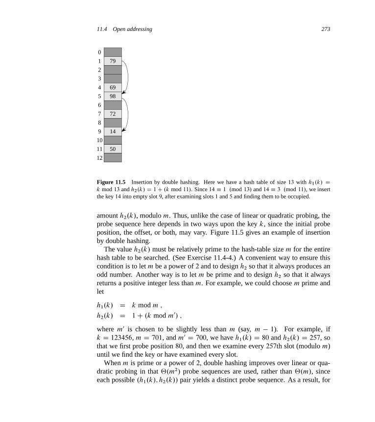
11.4 Open addressing 273
0
1
2
3
4
5
6
7
8
9
10
11
12
79
69
98
72
14
50
Figure 11.5 Insertion by double hashing. Here we have a hash table of size 13 with h1.k/ Dk mod 13 and h2.k/ D 1C .k mod 11/. Since 14 � 1 .mod 13/ and 14 � 3 .mod 11/, we insertthe key 14 into empty slot 9, after examining slots 1 and 5 and finding them to be occupied.
amount h2.k/, modulo m. Thus, unlike the case of linear or quadratic probing, theprobe sequence here depends in two ways upon the key k, since the initial probeposition, the offset, or both, may vary. Figure 11.5 gives an example of insertionby double hashing.
The value h2.k/ must be relatively prime to the hash-table size m for the entirehash table to be searched. (See Exercise 11.4-4.) A convenient way to ensure thiscondition is to let m be a power of 2 and to design h2 so that it always produces anodd number. Another way is to let m be prime and to design h2 so that it alwaysreturns a positive integer less than m. For example, we could choose m prime andlet
h1.k/ D k mod m ;
h2.k/ D 1C .k mod m0/ ;
where m0 is chosen to be slightly less than m (say, m � 1). For example, ifk D 123456, m D 701, and m0 D 700, we have h1.k/ D 80 and h2.k/ D 257, sothat we first probe position 80, and then we examine every 257th slot (modulo m)until we find the key or have examined every slot.
When m is prime or a power of 2, double hashing improves over linear or qua-dratic probing in that ‚.m2/ probe sequences are used, rather than ‚.m/, sinceeach possible .h1.k/; h2.k// pair yields a distinct probe sequence. As a result, for

274 Chapter 11 Hash Tables
such values of m, the performance of double hashing appears to be very close tothe performance of the “ideal” scheme of uniform hashing.
Although values of m other than primes or powers of 2 could in principle beused with double hashing, in practice it becomes more difficult to efficiently gen-erate h2.k/ in a way that ensures that it is relatively prime to m, in part because therelative density �.m/=m of such numbers may be small (see equation (31.24)).
Analysis of open-address hashing
As in our analysis of chaining, we express our analysis of open addressing in termsof the load factor ˛ D n=m of the hash table. Of course, with open addressing, atmost one element occupies each slot, and thus n � m, which implies ˛ � 1.
We assume that we are using uniform hashing. In this idealized scheme, theprobe sequence hh.k; 0/; h.k; 1/; : : : ; h.k; m � 1/i used to insert or search foreach key k is equally likely to be any permutation of h0; 1; : : : ; m � 1i. Of course,a given key has a unique fixed probe sequence associated with it; what we meanhere is that, considering the probability distribution on the space of keys and theoperation of the hash function on the keys, each possible probe sequence is equallylikely.
We now analyze the expected number of probes for hashing with open address-ing under the assumption of uniform hashing, beginning with an analysis of thenumber of probes made in an unsuccessful search.
Theorem 11.6Given an open-address hash table with load factor ˛ D n=m < 1, the expectednumber of probes in an unsuccessful search is at most 1=.1�˛/, assuming uniformhashing.
Proof In an unsuccessful search, every probe but the last accesses an occupiedslot that does not contain the desired key, and the last slot probed is empty. Let usdefine the random variable X to be the number of probes made in an unsuccessfulsearch, and let us also define the event Ai , for i D 1; 2; : : :, to be the event thatan i th probe occurs and it is to an occupied slot. Then the event fX � ig is theintersection of events A1\A2\� � �\Ai�1. We will bound Pr fX � ig by boundingPr fA1 \ A2 \ � � � \ Ai�1g. By Exercise C.2-5,
Pr fA1 \ A2 \ � � � \ Ai�1g D Pr fA1g � Pr fA2 j A1g � Pr fA3 j A1 \ A2g � � �Pr fAi�1 j A1 \ A2 \ � � � \ Ai�2g :
Since there are n elements and m slots, Pr fA1g D n=m. For j > 1, the probabilitythat there is a j th probe and it is to an occupied slot, given that the first j � 1
probes were to occupied slots, is .n�j C1/=.m�j C1/. This probability follows

11.4 Open addressing 275
because we would be finding one of the remaining .n � .j � 1// elements in oneof the .m� .j � 1// unexamined slots, and by the assumption of uniform hashing,the probability is the ratio of these quantities. Observing that n < m implies that.n� j /=.m� j / � n=m for all j such that 0 � j < m, we have for all i such that1 � i � m,
Pr fX � ig D n
m� n � 1
m � 1� n � 2
m � 2� � � n � i C 2
m � i C 2
�� n
m
�i�1
D ˛i�1 :
Now, we use equation (C.25) to bound the expected number of probes:
E ŒX� D1X
iD1
Pr fX � ig
�1X
iD1
˛i�1
D1X
iD0
˛i
D 1
1� ˛:
This bound of 1=.1�˛/ D 1C˛C˛2C˛3C� � � has an intuitive interpretation.We always make the first probe. With probability approximately ˛, the first probefinds an occupied slot, so that we need to probe a second time. With probabilityapproximately ˛2, the first two slots are occupied so that we make a third probe,and so on.
If ˛ is a constant, Theorem 11.6 predicts that an unsuccessful search runs in O.1/
time. For example, if the hash table is half full, the average number of probes in anunsuccessful search is at most 1=.1 � :5/ D 2. If it is 90 percent full, the averagenumber of probes is at most 1=.1 � :9/ D 10.
Theorem 11.6 gives us the performance of the HASH-INSERT procedure almostimmediately.
Corollary 11.7Inserting an element into an open-address hash table with load factor ˛ requires atmost 1=.1 � ˛/ probes on average, assuming uniform hashing.
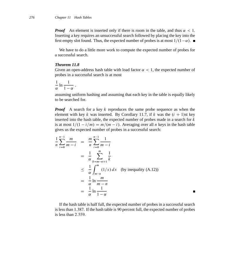
276 Chapter 11 Hash Tables
Proof An element is inserted only if there is room in the table, and thus ˛ < 1.Inserting a key requires an unsuccessful search followed by placing the key into thefirst empty slot found. Thus, the expected number of probes is at most 1=.1�˛/.
We have to do a little more work to compute the expected number of probes fora successful search.
Theorem 11.8Given an open-address hash table with load factor ˛ < 1, the expected number ofprobes in a successful search is at most
1
˛ln
1
1� ˛;
assuming uniform hashing and assuming that each key in the table is equally likelyto be searched for.
Proof A search for a key k reproduces the same probe sequence as when theelement with key k was inserted. By Corollary 11.7, if k was the .i C 1/st keyinserted into the hash table, the expected number of probes made in a search for k
is at most 1=.1 � i=m/ D m=.m � i/. Averaging over all n keys in the hash tablegives us the expected number of probes in a successful search:
1
n
n�1XiD0
m
m � iD m
n
n�1XiD0
1
m � i
D 1
˛
mXkDm�nC1
1
k
� 1
˛
Z m
m�n
.1=x/ dx (by inequality (A.12))
D 1
˛ln
m
m � n
D 1
˛ln
1
1� ˛
If the hash table is half full, the expected number of probes in a successful searchis less than 1:387. If the hash table is 90 percent full, the expected number of probesis less than 2:559.
11.5 Perfect hashing 277
Exercises
11.4-1Consider inserting the keys 10; 22; 31; 4; 15; 28; 17; 88; 59 into a hash table oflength m D 11 using open addressing with the auxiliary hash function h0.k/ D k.Illustrate the result of inserting these keys using linear probing, using quadraticprobing with c1 D 1 and c2 D 3, and using double hashing with h1.k/ D k andh2.k/ D 1C .k mod .m � 1//.
11.4-2Write pseudocode for HASH-DELETE as outlined in the text, and modify HASH-INSERT to handle the special value DELETED.
11.4-3Consider an open-address hash table with uniform hashing. Give upper boundson the expected number of probes in an unsuccessful search and on the expectednumber of probes in a successful search when the load factor is 3=4 and when itis 7=8.
11.4-4 ?
Suppose that we use double hashing to resolve collisions—that is, we use the hashfunction h.k; i/ D .h1.k/ C ih2.k// mod m. Show that if m and h2.k/ havegreatest common divisor d � 1 for some key k, then an unsuccessful search forkey k examines .1=d/th of the hash table before returning to slot h1.k/. Thus,when d D 1, so that m and h2.k/ are relatively prime, the search may examine theentire hash table. (Hint: See Chapter 31.)
11.4-5 ?
Consider an open-address hash table with a load factor ˛. Find the nonzero value ˛
for which the expected number of probes in an unsuccessful search equals twicethe expected number of probes in a successful search. Use the upper bounds givenby Theorems 11.6 and 11.8 for these expected numbers of probes.
? 11.5 Perfect hashing
Although hashing is often a good choice for its excellent average-case perfor-mance, hashing can also provide excellent worst-case performance when the set ofkeys is static: once the keys are stored in the table, the set of keys never changes.Some applications naturally have static sets of keys: consider the set of reservedwords in a programming language, or the set of file names on a CD-ROM. We

278 Chapter 11 Hash Tables
0
1
2
3
4
5
6
7
8
1 0 0 10
9 10 18 60 750 1 2 3
1 0 0 70
0
0
16 23 88 40 370 1 2 3 4 5 6 7 8
52
m2S2a2 b2
m0S0a0 b0
m5S5a5 b5
m7S7a7 b7
T
4 5 6 7 8
72
9 10 11 12 13 14 15
22
Figure 11.6 Using perfect hashing to store the set K D f10; 22; 37; 40; 52; 60; 70; 72; 75g. Theouter hash function is h.k/ D ..ak C b/ mod p/ mod m, where a D 3, b D 42, p D 101, andm D 9. For example, h.75/ D 2, and so key 75 hashes to slot 2 of table T . A secondary hashtable Sj stores all keys hashing to slot j . The size of hash table Sj is mj D n2
j , and the associatedhash function is hj .k/ D ..aj kC bj / mod p/ mod mj . Since h2.75/ D 7, key 75 is stored in slot 7of secondary hash table S2. No collisions occur in any of the secondary hash tables, and so searchingtakes constant time in the worst case.
call a hashing technique perfect hashing if O.1/ memory accesses are required toperform a search in the worst case.
To create a perfect hashing scheme, we use two levels of hashing, with universalhashing at each level. Figure 11.6 illustrates the approach.
The first level is essentially the same as for hashing with chaining: we hashthe n keys into m slots using a hash function h carefully selected from a family ofuniversal hash functions.
Instead of making a linked list of the keys hashing to slot j , however, we use asmall secondary hash table Sj with an associated hash function hj . By choosingthe hash functions hj carefully, we can guarantee that there are no collisions at thesecondary level.
In order to guarantee that there are no collisions at the secondary level, however,we will need to let the size mj of hash table Sj be the square of the number nj ofkeys hashing to slot j . Although you might think that the quadratic dependenceof mj on nj may seem likely to cause the overall storage requirement to be exces-sive, we shall show that by choosing the first-level hash function well, we can limitthe expected total amount of space used to O.n/.
We use hash functions chosen from the universal classes of hash functions ofSection 11.3.3. The first-level hash function comes from the class Hpm, where asin Section 11.3.3, p is a prime number greater than any key value. Those keys

11.5 Perfect hashing 279
hashing to slot j are re-hashed into a secondary hash table Sj of size mj using ahash function hj chosen from the class Hp;mj
.1
We shall proceed in two steps. First, we shall determine how to ensure thatthe secondary tables have no collisions. Second, we shall show that the expectedamount of memory used overall—for the primary hash table and all the secondaryhash tables—is O.n/.
Theorem 11.9Suppose that we store n keys in a hash table of size m D n2 using a hash function h
randomly chosen from a universal class of hash functions. Then, the probability isless than 1=2 that there are any collisions.
Proof There are�
n
2
�pairs of keys that may collide; each pair collides with prob-
ability 1=m if h is chosen at random from a universal family H of hash functions.Let X be a random variable that counts the number of collisions. When m D n2,the expected number of collisions is
E ŒX� D
n
2
!� 1
n2
D n2 � n
2� 1
n2
< 1=2 :
(This analysis is similar to the analysis of the birthday paradox in Section 5.4.1.)Applying Markov’s inequality (C.30), Pr fX � tg � E ŒX� =t , with t D 1, com-pletes the proof.
In the situation described in Theorem 11.9, where m D n2, it follows that a hashfunction h chosen at random from H is more likely than not to have no collisions.Given the set K of n keys to be hashed (remember that K is static), it is thus easyto find a collision-free hash function h with a few random trials.
When n is large, however, a hash table of size m D n2 is excessive. Therefore,we adopt the two-level hashing approach, and we use the approach of Theorem 11.9only to hash the entries within each slot. We use an outer, or first-level, hashfunction h to hash the keys into m D n slots. Then, if nj keys hash to slot j , weuse a secondary hash table Sj of size mj D n2
j to provide collision-free constant-time lookup.
1When nj D mj D 1, we don’t really need a hash function for slot j ; when we choose a hashfunction hab.k/ D ..ak C b/ mod p/ mod mj for such a slot, we just use a D b D 0.

280 Chapter 11 Hash Tables
We now turn to the issue of ensuring that the overall memory used is O.n/.Since the size mj of the j th secondary hash table grows quadratically with thenumber nj of keys stored, we run the risk that the overall amount of storage couldbe excessive.
If the first-level table size is m D n, then the amount of memory used is O.n/
for the primary hash table, for the storage of the sizes mj of the secondary hashtables, and for the storage of the parameters aj and bj defining the secondary hashfunctions hj drawn from the class Hp;mj
of Section 11.3.3 (except when nj D 1
and we use a D b D 0). The following theorem and a corollary provide a bound onthe expected combined sizes of all the secondary hash tables. A second corollarybounds the probability that the combined size of all the secondary hash tables issuperlinear (actually, that it equals or exceeds 4n).
Theorem 11.10Suppose that we store n keys in a hash table of size m D n using a hash function h
randomly chosen from a universal class of hash functions. Then, we have
E
"m�1Xj D0
n2j
#< 2n ;
where nj is the number of keys hashing to slot j .
Proof We start with the following identity, which holds for any nonnegative inte-ger a:
a2 D aC 2
a
2
!: (11.6)
We have
E
"m�1Xj D0
n2j
#
D E
"m�1Xj D0
nj C 2
nj
2
!!#(by equation (11.6))
D E
"m�1Xj D0
nj
#C 2 E
"m�1Xj D0
nj
2
!#(by linearity of expectation)
D E Œn�C 2 E
"m�1Xj D0
nj
2
!#(by equation (11.1))

11.5 Perfect hashing 281
D nC 2 E
"m�1Xj D0
nj
2
!#(since n is not a random variable) .
To evaluate the summationPm�1
j D0
�nj
2
�, we observe that it is just the total number
of pairs of keys in the hash table that collide. By the properties of universal hashing,the expected value of this summation is at most
n
2
!1
mD n.n� 1/
2m
D n � 1
2;
since m D n. Thus,
E
"m�1Xj D0
n2j
#� nC 2
n � 1
2
D 2n � 1
< 2n :
Corollary 11.11Suppose that we store n keys in a hash table of size m D n using a hash func-tion h randomly chosen from a universal class of hash functions, and we set thesize of each secondary hash table to mj D n2
j for j D 0; 1; : : : ; m � 1. Then,the expected amount of storage required for all secondary hash tables in a perfecthashing scheme is less than 2n.
Proof Since mj D n2j for j D 0; 1; : : : ; m � 1, Theorem 11.10 gives
E
"m�1Xj D0
mj
#D E
"m�1Xj D0
n2j
#< 2n ; (11.7)
which completes the proof.
Corollary 11.12Suppose that we store n keys in a hash table of size m D n using a hash function h
randomly chosen from a universal class of hash functions, and we set the sizeof each secondary hash table to mj D n2
j for j D 0; 1; : : : ; m � 1. Then, theprobability is less than 1=2 that the total storage used for secondary hash tablesequals or exceeds 4n.
282 Chapter 11 Hash Tables
Proof Again we apply Markov’s inequality (C.30), Pr fX � tg � E ŒX� =t , thistime to inequality (11.7), with X DPm�1
j D0 mj and t D 4n:
Pr
(m�1Xj D0
mj � 4n
)� E
�Pm�1
j D0 mj
�4n
<2n
4nD 1=2 :
From Corollary 11.12, we see that if we test a few randomly chosen hash func-tions from the universal family, we will quickly find one that uses a reasonableamount of storage.
Exercises
11.5-1 ?
Suppose that we insert n keys into a hash table of size m using open addressingand uniform hashing. Let p.n; m/ be the probability that no collisions occur. Showthat p.n; m/ � e�n.n�1/=2m. (Hint: See equation (3.12).) Argue that when n ex-ceeds
pm, the probability of avoiding collisions goes rapidly to zero.
Problems
11-1 Longest-probe bound for hashingSuppose that we use an open-addressed hash table of size m to store n � m=2
items.
a. Assuming uniform hashing, show that for i D 1; 2; : : : ; n, the probability is atmost 2�k that the i th insertion requires strictly more than k probes.
b. Show that for i D 1; 2; : : : ; n, the probability is O.1=n2/ that the i th insertionrequires more than 2 lg n probes.
Let the random variable Xi denote the number of probes required by the i th inser-tion. You have shown in part (b) that Pr fXi > 2 lg ng D O.1=n2/. Let the randomvariable X D max1�i�n Xi denote the maximum number of probes required byany of the n insertions.
c. Show that Pr fX > 2 lg ng D O.1=n/.
d. Show that the expected length E ŒX� of the longest probe sequence is O.lg n/.

Problems for Chapter 11 283
11-2 Slot-size bound for chainingSuppose that we have a hash table with n slots, with collisions resolved by chain-ing, and suppose that n keys are inserted into the table. Each key is equally likelyto be hashed to each slot. Let M be the maximum number of keys in any slot afterall the keys have been inserted. Your mission is to prove an O.lg n= lg lg n/ upperbound on E ŒM �, the expected value of M .
a. Argue that the probability Qk that exactly k keys hash to a particular slot isgiven by
Qk D�
1
n
�k�1� 1
n
�n�k
n
k
!:
b. Let Pk be the probability that M D k, that is, the probability that the slotcontaining the most keys contains k keys. Show that Pk � nQk.
c. Use Stirling’s approximation, equation (3.18), to show that Qk < ek=kk .
d. Show that there exists a constant c > 1 such that Qk0< 1=n3 for k0 D
c lg n= lg lg n. Conclude that Pk < 1=n2 for k � k0 D c lg n= lg lg n.
e. Argue that
E ŒM � � Pr
�M >
c lg n
lg lg n
�� nC Pr
�M � c lg n
lg lg n
�� c lg n
lg lg n:
Conclude that E ŒM � D O.lg n= lg lg n/.
11-3 Quadratic probingSuppose that we are given a key k to search for in a hash table with positions0; 1; : : : ; m�1, and suppose that we have a hash function h mapping the key spaceinto the set f0; 1; : : : ; m � 1g. The search scheme is as follows:
1. Compute the value j D h.k/, and set i D 0.
2. Probe in position j for the desired key k. If you find it, or if this position isempty, terminate the search.
3. Set i D i C 1. If i now equals m, the table is full, so terminate the search.Otherwise, set j D .i C j / mod m, and return to step 2.
Assume that m is a power of 2.
a. Show that this scheme is an instance of the general “quadratic probing” schemeby exhibiting the appropriate constants c1 and c2 for equation (11.5).
b. Prove that this algorithm examines every table position in the worst case.

284 Chapter 11 Hash Tables
11-4 Hashing and authenticationLet H be a class of hash functions in which each hash function h 2 H maps theuniverse U of keys to f0; 1; : : : ; m � 1g. We say that H is k-universal if, for everyfixed sequence of k distinct keys hx.1/; x.2/; : : : ; x.k/i and for any h chosen atrandom from H , the sequence hh.x.1//; h.x.2//; : : : ; h.x.k//i is equally likely to beany of the mk sequences of length k with elements drawn from f0; 1; : : : ; m � 1g.a. Show that if the family H of hash functions is 2-universal, then it is universal.
b. Suppose that the universe U is the set of n-tuples of values drawn fromZp D f0; 1; : : : ; p � 1g, where p is prime. Consider an element x Dhx0; x1; : : : ; xn�1i 2 U . For any n-tuple a D ha0; a1; : : : ; an�1i 2 U , de-fine the hash function ha by
ha.x/ D
n�1Xj D0
aj xj
!mod p :
Let H D fhag. Show that H is universal, but not 2-universal. (Hint: Find a keyfor which all hash functions in H produce the same value.)
c. Suppose that we modify H slightly from part (b): for any a 2 U and for anyb 2 Zp , define
h0ab.x/ D
n�1Xj D0
aj xj C b
!mod p
and H0 D fh0
abg. Argue that H0 is 2-universal. (Hint: Consider fixed n-tuples
x 2 U and y 2 U , with xi ¤ yi for some i . What happens to h0ab
.x/
and h0ab
.y/ as ai and b range over Zp?)
d. Suppose that Alice and Bob secretly agree on a hash function h from a2-universal family H of hash functions. Each h 2 H maps from a universe ofkeys U to Zp , where p is prime. Later, Alice sends a message m to Bob over theInternet, where m 2 U . She authenticates this message to Bob by also sendingan authentication tag t D h.m/, and Bob checks that the pair .m; t/ he receivesindeed satisfies t D h.m/. Suppose that an adversary intercepts .m; t/ en routeand tries to fool Bob by replacing the pair .m; t/ with a different pair .m0; t 0/.Argue that the probability that the adversary succeeds in fooling Bob into ac-cepting .m0; t 0/ is at most 1=p, no matter how much computing power the ad-versary has, and even if the adversary knows the family H of hash functionsused.

Notes for Chapter 11 285
Chapter notes
Knuth [211] and Gonnet [145] are excellent references for the analysis of hash-ing algorithms. Knuth credits H. P. Luhn (1953) for inventing hash tables, alongwith the chaining method for resolving collisions. At about the same time, G. M.Amdahl originated the idea of open addressing.
Carter and Wegman introduced the notion of universal classes of hash functionsin 1979 [59].
Fredman, Komlós, and Szemerédi [112] developed the perfect hashing schemefor static sets presented in Section 11.5. An extension of their method to dynamicsets, handling insertions and deletions in amortized expected time O.1/, has beengiven by Dietzfelbinger et al. [87].
12 Binary Search Trees
The search tree data structure supports many dynamic-set operations, includingSEARCH, MINIMUM, MAXIMUM, PREDECESSOR, SUCCESSOR, INSERT, andDELETE. Thus, we can use a search tree both as a dictionary and as a priorityqueue.
Basic operations on a binary search tree take time proportional to the height ofthe tree. For a complete binary tree with n nodes, such operations run in ‚.lg n/
worst-case time. If the tree is a linear chain of n nodes, however, the same oper-ations take ‚.n/ worst-case time. We shall see in Section 12.4 that the expectedheight of a randomly built binary search tree is O.lg n/, so that basic dynamic-setoperations on such a tree take ‚.lg n/ time on average.
In practice, we can’t always guarantee that binary search trees are built ran-domly, but we can design variations of binary search trees with good guaranteedworst-case performance on basic operations. Chapter 13 presents one such vari-ation, red-black trees, which have height O.lg n/. Chapter 18 introduces B-trees,which are particularly good for maintaining databases on secondary (disk) storage.
After presenting the basic properties of binary search trees, the following sec-tions show how to walk a binary search tree to print its values in sorted order, howto search for a value in a binary search tree, how to find the minimum or maximumelement, how to find the predecessor or successor of an element, and how to insertinto or delete from a binary search tree. The basic mathematical properties of treesappear in Appendix B.
12.1 What is a binary search tree?
A binary search tree is organized, as the name suggests, in a binary tree, as shownin Figure 12.1. We can represent such a tree by a linked data structure in whicheach node is an object. In addition to a key and satellite data, each node containsattributes left, right, and p that point to the nodes corresponding to its left child,
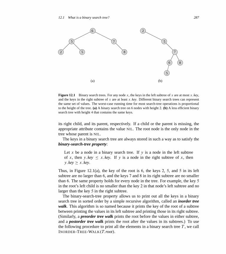
12.1 What is a binary search tree? 287
5
2 5
5
8
7
6
(a)
6 8
7
5
2
(b)
Figure 12.1 Binary search trees. For any node x, the keys in the left subtree of x are at most x:key,and the keys in the right subtree of x are at least x:key. Different binary search trees can representthe same set of values. The worst-case running time for most search-tree operations is proportionalto the height of the tree. (a) A binary search tree on 6 nodes with height 2. (b) A less efficient binarysearch tree with height 4 that contains the same keys.
its right child, and its parent, respectively. If a child or the parent is missing, theappropriate attribute contains the value NIL. The root node is the only node in thetree whose parent is NIL.
The keys in a binary search tree are always stored in such a way as to satisfy thebinary-search-tree property:
Let x be a node in a binary search tree. If y is a node in the left subtreeof x, then y:key � x:key. If y is a node in the right subtree of x, theny:key � x:key.
Thus, in Figure 12.1(a), the key of the root is 6, the keys 2, 5, and 5 in its leftsubtree are no larger than 6, and the keys 7 and 8 in its right subtree are no smallerthan 6. The same property holds for every node in the tree. For example, the key 5
in the root’s left child is no smaller than the key 2 in that node’s left subtree and nolarger than the key 5 in the right subtree.
The binary-search-tree property allows us to print out all the keys in a binarysearch tree in sorted order by a simple recursive algorithm, called an inorder treewalk. This algorithm is so named because it prints the key of the root of a subtreebetween printing the values in its left subtree and printing those in its right subtree.(Similarly, a preorder tree walk prints the root before the values in either subtree,and a postorder tree walk prints the root after the values in its subtrees.) To usethe following procedure to print all the elements in a binary search tree T , we callINORDER-TREE-WALK.T:root/.
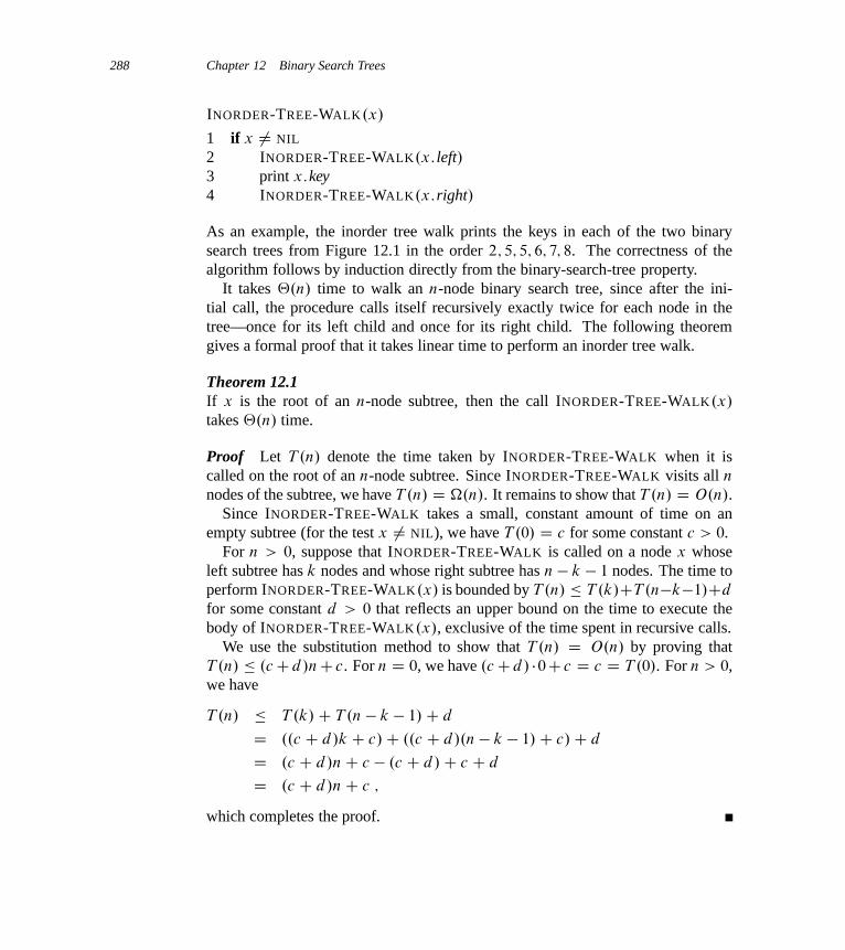
288 Chapter 12 Binary Search Trees
INORDER-TREE-WALK.x/
1 if x ¤ NIL
2 INORDER-TREE-WALK.x: left/3 print x:key4 INORDER-TREE-WALK.x:right/
As an example, the inorder tree walk prints the keys in each of the two binarysearch trees from Figure 12.1 in the order 2; 5; 5; 6; 7; 8. The correctness of thealgorithm follows by induction directly from the binary-search-tree property.
It takes ‚.n/ time to walk an n-node binary search tree, since after the ini-tial call, the procedure calls itself recursively exactly twice for each node in thetree—once for its left child and once for its right child. The following theoremgives a formal proof that it takes linear time to perform an inorder tree walk.
Theorem 12.1If x is the root of an n-node subtree, then the call INORDER-TREE-WALK.x/
takes ‚.n/ time.
Proof Let T .n/ denote the time taken by INORDER-TREE-WALK when it iscalled on the root of an n-node subtree. Since INORDER-TREE-WALK visits all n
nodes of the subtree, we have T .n/ D �.n/. It remains to show that T .n/ D O.n/.Since INORDER-TREE-WALK takes a small, constant amount of time on an
empty subtree (for the test x ¤ NIL), we have T .0/ D c for some constant c > 0.For n > 0, suppose that INORDER-TREE-WALK is called on a node x whose
left subtree has k nodes and whose right subtree has n � k � 1 nodes. The time toperform INORDER-TREE-WALK.x/ is bounded by T .n/ � T .k/CT .n�k�1/Cd
for some constant d > 0 that reflects an upper bound on the time to execute thebody of INORDER-TREE-WALK.x/, exclusive of the time spent in recursive calls.
We use the substitution method to show that T .n/ D O.n/ by proving thatT .n/ � .cCd/nC c. For n D 0, we have .cCd/ �0C c D c D T .0/. For n > 0,we have
T .n/ � T .k/C T .n � k � 1/C d
D ..c C d/k C c/C ..c C d/.n � k � 1/C c/C d
D .c C d/nC c � .c C d/C c C d
D .c C d/nC c ;
which completes the proof.
12.2 Querying a binary search tree 289
Exercises
12.1-1For the set of f1; 4; 5; 10; 16; 17; 21g of keys, draw binary search trees of heights 2,3, 4, 5, and 6.
12.1-2What is the difference between the binary-search-tree property and the min-heapproperty (see page 153)? Can the min-heap property be used to print out the keysof an n-node tree in sorted order in O.n/ time? Show how, or explain why not.
12.1-3Give a nonrecursive algorithm that performs an inorder tree walk. (Hint: An easysolution uses a stack as an auxiliary data structure. A more complicated, but ele-gant, solution uses no stack but assumes that we can test two pointers for equality.)
12.1-4Give recursive algorithms that perform preorder and postorder tree walks in ‚.n/
time on a tree of n nodes.
12.1-5Argue that since sorting n elements takes �.n lg n/ time in the worst case inthe comparison model, any comparison-based algorithm for constructing a binarysearch tree from an arbitrary list of n elements takes �.n lg n/ time in the worstcase.
12.2 Querying a binary search tree
We often need to search for a key stored in a binary search tree. Besides theSEARCH operation, binary search trees can support such queries as MINIMUM,MAXIMUM, SUCCESSOR, and PREDECESSOR. In this section, we shall examinethese operations and show how to support each one in time O.h/ on any binarysearch tree of height h.
Searching
We use the following procedure to search for a node with a given key in a binarysearch tree. Given a pointer to the root of the tree and a key k, TREE-SEARCH
returns a pointer to a node with key k if one exists; otherwise, it returns NIL.
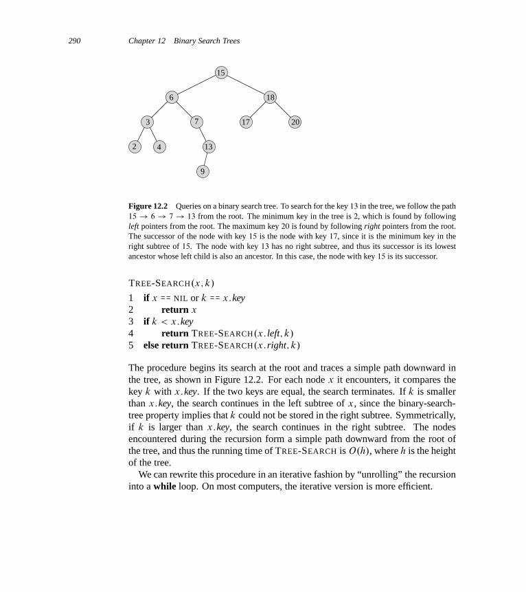
290 Chapter 12 Binary Search Trees
2 4
3
13
7
6
17 20
18
15
9
Figure 12.2 Queries on a binary search tree. To search for the key 13 in the tree, we follow the path15 ! 6 ! 7 ! 13 from the root. The minimum key in the tree is 2, which is found by followingleft pointers from the root. The maximum key 20 is found by following right pointers from the root.The successor of the node with key 15 is the node with key 17, since it is the minimum key in theright subtree of 15. The node with key 13 has no right subtree, and thus its successor is its lowestancestor whose left child is also an ancestor. In this case, the node with key 15 is its successor.
TREE-SEARCH.x; k/
1 if x == NIL or k == x:key2 return x
3 if k < x:key4 return TREE-SEARCH.x: left; k/
5 else return TREE-SEARCH.x:right; k/
The procedure begins its search at the root and traces a simple path downward inthe tree, as shown in Figure 12.2. For each node x it encounters, it compares thekey k with x:key. If the two keys are equal, the search terminates. If k is smallerthan x:key, the search continues in the left subtree of x, since the binary-search-tree property implies that k could not be stored in the right subtree. Symmetrically,if k is larger than x:key, the search continues in the right subtree. The nodesencountered during the recursion form a simple path downward from the root ofthe tree, and thus the running time of TREE-SEARCH is O.h/, where h is the heightof the tree.
We can rewrite this procedure in an iterative fashion by “unrolling” the recursioninto a while loop. On most computers, the iterative version is more efficient.
12.2 Querying a binary search tree 291
ITERATIVE-TREE-SEARCH.x; k/
1 while x ¤ NIL and k ¤ x:key2 if k < x:key3 x D x: left4 else x D x:right5 return x
Minimum and maximum
We can always find an element in a binary search tree whose key is a minimum byfollowing left child pointers from the root until we encounter a NIL, as shown inFigure 12.2. The following procedure returns a pointer to the minimum element inthe subtree rooted at a given node x, which we assume to be non-NIL:
TREE-MINIMUM.x/
1 while x: left ¤ NIL
2 x D x: left3 return x
The binary-search-tree property guarantees that TREE-MINIMUM is correct. If anode x has no left subtree, then since every key in the right subtree of x is at least aslarge as x:key, the minimum key in the subtree rooted at x is x:key. If node x hasa left subtree, then since no key in the right subtree is smaller than x:key and everykey in the left subtree is not larger than x:key, the minimum key in the subtreerooted at x resides in the subtree rooted at x: left.
The pseudocode for TREE-MAXIMUM is symmetric:
TREE-MAXIMUM.x/
1 while x:right ¤ NIL
2 x D x:right3 return x
Both of these procedures run in O.h/ time on a tree of height h since, as in TREE-SEARCH, the sequence of nodes encountered forms a simple path downward fromthe root.
Successor and predecessor
Given a node in a binary search tree, sometimes we need to find its successor inthe sorted order determined by an inorder tree walk. If all keys are distinct, the

292 Chapter 12 Binary Search Trees
successor of a node x is the node with the smallest key greater than x:key. Thestructure of a binary search tree allows us to determine the successor of a nodewithout ever comparing keys. The following procedure returns the successor of anode x in a binary search tree if it exists, and NIL if x has the largest key in thetree:
TREE-SUCCESSOR.x/
1 if x:right ¤ NIL
2 return TREE-MINIMUM.x:right/3 y D x:p4 while y ¤ NIL and x == y:right5 x D y
6 y D y:p7 return y
We break the code for TREE-SUCCESSOR into two cases. If the right subtreeof node x is nonempty, then the successor of x is just the leftmost node in x’sright subtree, which we find in line 2 by calling TREE-MINIMUM.x:right/. Forexample, the successor of the node with key 15 in Figure 12.2 is the node withkey 17.
On the other hand, as Exercise 12.2-6 asks you to show, if the right subtree ofnode x is empty and x has a successor y, then y is the lowest ancestor of x whoseleft child is also an ancestor of x. In Figure 12.2, the successor of the node withkey 13 is the node with key 15. To find y, we simply go up the tree from x until weencounter a node that is the left child of its parent; lines 3–7 of TREE-SUCCESSOR
handle this case.The running time of TREE-SUCCESSOR on a tree of height h is O.h/, since we
either follow a simple path up the tree or follow a simple path down the tree. Theprocedure TREE-PREDECESSOR, which is symmetric to TREE-SUCCESSOR, alsoruns in time O.h/.
Even if keys are not distinct, we define the successor and predecessor of anynode x as the node returned by calls made to TREE-SUCCESSOR.x/ and TREE-PREDECESSOR.x/, respectively.
In summary, we have proved the following theorem.
Theorem 12.2We can implement the dynamic-set operations SEARCH, MINIMUM, MAXIMUM,SUCCESSOR, and PREDECESSOR so that each one runs in O.h/ time on a binarysearch tree of height h.

12.2 Querying a binary search tree 293
Exercises
12.2-1Suppose that we have numbers between 1 and 1000 in a binary search tree, and wewant to search for the number 363. Which of the following sequences could not bethe sequence of nodes examined?
a. 2, 252, 401, 398, 330, 344, 397, 363.
b. 924, 220, 911, 244, 898, 258, 362, 363.
c. 925, 202, 911, 240, 912, 245, 363.
d. 2, 399, 387, 219, 266, 382, 381, 278, 363.
e. 935, 278, 347, 621, 299, 392, 358, 363.
12.2-2Write recursive versions of TREE-MINIMUM and TREE-MAXIMUM.
12.2-3Write the TREE-PREDECESSOR procedure.
12.2-4Professor Bunyan thinks he has discovered a remarkable property of binary searchtrees. Suppose that the search for key k in a binary search tree ends up in a leaf.Consider three sets: A, the keys to the left of the search path; B , the keys on thesearch path; and C , the keys to the right of the search path. Professor Bunyanclaims that any three keys a 2 A, b 2 B , and c 2 C must satisfy a � b � c. Givea smallest possible counterexample to the professor’s claim.
12.2-5Show that if a node in a binary search tree has two children, then its successor hasno left child and its predecessor has no right child.
12.2-6Consider a binary search tree T whose keys are distinct. Show that if the rightsubtree of a node x in T is empty and x has a successor y, then y is the lowestancestor of x whose left child is also an ancestor of x. (Recall that every node isits own ancestor.)
12.2-7An alternative method of performing an inorder tree walk of an n-node binarysearch tree finds the minimum element in the tree by calling TREE-MINIMUM andthen making n � 1 calls to TREE-SUCCESSOR. Prove that this algorithm runsin ‚.n/ time.
294 Chapter 12 Binary Search Trees
12.2-8Prove that no matter what node we start at in a height-h binary search tree, k
successive calls to TREE-SUCCESSOR take O.k C h/ time.
12.2-9Let T be a binary search tree whose keys are distinct, let x be a leaf node, and let y
be its parent. Show that y:key is either the smallest key in T larger than x:key orthe largest key in T smaller than x:key.
12.3 Insertion and deletion
The operations of insertion and deletion cause the dynamic set represented by abinary search tree to change. The data structure must be modified to reflect thischange, but in such a way that the binary-search-tree property continues to hold.As we shall see, modifying the tree to insert a new element is relatively straight-forward, but handling deletion is somewhat more intricate.
Insertion
To insert a new value � into a binary search tree T , we use the procedure TREE-INSERT. The procedure takes a node ´ for which ´:key D �, ´: left D NIL,and ´:right D NIL. It modifies T and some of the attributes of ´ in such a way thatit inserts ´ into an appropriate position in the tree.
TREE-INSERT.T; ´/
1 y D NIL
2 x D T:root3 while x ¤ NIL
4 y D x
5 if ´:key < x:key6 x D x: left7 else x D x:right8 ´:p D y
9 if y == NIL
10 T:root D ´ // tree T was empty11 elseif ´:key < y:key12 y: left D ´
13 else y:right D ´

12.3 Insertion and deletion 295
2 9
5
13 17
15 19
18
12
Figure 12.3 Inserting an item with key 13 into a binary search tree. Lightly shaded nodes indicatethe simple path from the root down to the position where the item is inserted. The dashed lineindicates the link in the tree that is added to insert the item.
Figure 12.3 shows how TREE-INSERT works. Just like the procedures TREE-SEARCH and ITERATIVE-TREE-SEARCH, TREE-INSERT begins at the root of thetree and the pointer x traces a simple path downward looking for a NIL to replacewith the input item ´. The procedure maintains the trailing pointer y as the parentof x. After initialization, the while loop in lines 3–7 causes these two pointersto move down the tree, going left or right depending on the comparison of ´:keywith x:key, until x becomes NIL. This NIL occupies the position where we wish toplace the input item ´. We need the trailing pointer y, because by the time we findthe NIL where ´ belongs, the search has proceeded one step beyond the node thatneeds to be changed. Lines 8–13 set the pointers that cause ´ to be inserted.
Like the other primitive operations on search trees, the procedure TREE-INSERT
runs in O.h/ time on a tree of height h.
Deletion
The overall strategy for deleting a node ´ from a binary search tree T has threebasic cases but, as we shall see, one of the cases is a bit tricky.
� If ´ has no children, then we simply remove it by modifying its parent to re-place ´ with NIL as its child.
� If ´ has just one child, then we elevate that child to take ´’s position in the treeby modifying ´’s parent to replace ´ by ´’s child.
� If ´ has two children, then we find ´’s successor y—which must be in ´’s rightsubtree—and have y take ´’s position in the tree. The rest of ´’s original rightsubtree becomes y’s new right subtree, and ´’s left subtree becomes y’s newleft subtree. This case is the tricky one because, as we shall see, it matterswhether y is ´’s right child.
296 Chapter 12 Binary Search Trees
The procedure for deleting a given node ´ from a binary search tree T takes asarguments pointers to T and ´. It organizes its cases a bit differently from the threecases outlined above by considering the four cases shown in Figure 12.4.
� If ´ has no left child (part (a) of the figure), then we replace ´ by its right child,which may or may not be NIL. When ´’s right child is NIL, this case deals withthe situation in which ´ has no children. When ´’s right child is non-NIL, thiscase handles the situation in which ´ has just one child, which is its right child.
� If ´ has just one child, which is its left child (part (b) of the figure), then wereplace ´ by its left child.
� Otherwise, ´ has both a left and a right child. We find ´’s successor y, whichlies in ´’s right subtree and has no left child (see Exercise 12.2-5). We want tosplice y out of its current location and have it replace ´ in the tree.
� If y is ´’s right child (part (c)), then we replace ´ by y, leaving y’s rightchild alone.
� Otherwise, y lies within ´’s right subtree but is not ´’s right child (part (d)).In this case, we first replace y by its own right child, and then we replace ´
by y.
In order to move subtrees around within the binary search tree, we define asubroutine TRANSPLANT, which replaces one subtree as a child of its parent withanother subtree. When TRANSPLANT replaces the subtree rooted at node u withthe subtree rooted at node �, node u’s parent becomes node �’s parent, and u’sparent ends up having � as its appropriate child.
TRANSPLANT.T; u; �/
1 if u:p == NIL
2 T:root D �
3 elseif u == u:p: left4 u:p: left D �
5 else u:p:right D �
6 if � ¤ NIL
7 �:p D u:p
Lines 1–2 handle the case in which u is the root of T . Otherwise, u is either a leftchild or a right child of its parent. Lines 3–4 take care of updating u:p: left if u
is a left child, and line 5 updates u:p:right if u is a right child. We allow � to beNIL, and lines 6–7 update �:p if � is non-NIL. Note that TRANSPLANT does notattempt to update �: left and �:right; doing so, or not doing so, is the responsibilityof TRANSPLANT’s caller.

12.3 Insertion and deletion 297
z(a) r
z
l
(b)
q
z
l
(c)
q
y
ly
q
z
l
(d)
r
q
z
l r
y
q
l r
y
r
l
x
x
xy
x
x
NIL
NIL
NIL
NIL
NIL
Figure 12.4 Deleting a node ´ from a binary search tree. Node ´ may be the root, a left child ofnode q, or a right child of q. (a) Node ´ has no left child. We replace ´ by its right child r , whichmay or may not be NIL. (b) Node ´ has a left child l but no right child. We replace ´ by l . (c) Node ´
has two children; its left child is node l , its right child is its successor y, and y’s right child is node x.We replace ´ by y, updating y’s left child to become l , but leaving x as y’s right child. (d) Node ´
has two children (left child l and right child r), and its successor y ¤ r lies within the subtree rootedat r . We replace y by its own right child x, and we set y to be r’s parent. Then, we set y to be q’schild and the parent of l .
298 Chapter 12 Binary Search Trees
With the TRANSPLANT procedure in hand, here is the procedure that deletesnode ´ from binary search tree T :
TREE-DELETE.T; ´/
1 if ´: left == NIL
2 TRANSPLANT.T; ´; ´:right/3 elseif ´:right == NIL
4 TRANSPLANT.T; ´; ´: left/5 else y D TREE-MINIMUM.´:right/6 if y:p ¤ ´
7 TRANSPLANT.T; y; y:right/8 y:right D ´:right9 y:right:p D y
10 TRANSPLANT.T; ´; y/
11 y: left D ´: left12 y: left:p D y
The TREE-DELETE procedure executes the four cases as follows. Lines 1–2handle the case in which node ´ has no left child, and lines 3–4 handle the case inwhich ´ has a left child but no right child. Lines 5–12 deal with the remaining twocases, in which ´ has two children. Line 5 finds node y, which is the successorof ´. Because ´ has a nonempty right subtree, its successor must be the node inthat subtree with the smallest key; hence the call to TREE-MINIMUM.´:right/. Aswe noted before, y has no left child. We want to splice y out of its current location,and it should replace ´ in the tree. If y is ´’s right child, then lines 10–12 replace ´
as a child of its parent by y and replace y’s left child by ´’s left child. If y isnot ´’s left child, lines 7–9 replace y as a child of its parent by y’s right child andturn ´’s right child into y’s right child, and then lines 10–12 replace ´ as a child ofits parent by y and replace y’s left child by ´’s left child.
Each line of TREE-DELETE, including the calls to TRANSPLANT, takes constanttime, except for the call to TREE-MINIMUM in line 5. Thus, TREE-DELETE runsin O.h/ time on a tree of height h.
In summary, we have proved the following theorem.
Theorem 12.3We can implement the dynamic-set operations INSERT and DELETE so that eachone runs in O.h/ time on a binary search tree of height h.
12.4 Randomly built binary search trees 299
Exercises
12.3-1Give a recursive version of the TREE-INSERT procedure.
12.3-2Suppose that we construct a binary search tree by repeatedly inserting distinct val-ues into the tree. Argue that the number of nodes examined in searching for avalue in the tree is one plus the number of nodes examined when the value wasfirst inserted into the tree.
12.3-3We can sort a given set of n numbers by first building a binary search tree contain-ing these numbers (using TREE-INSERT repeatedly to insert the numbers one byone) and then printing the numbers by an inorder tree walk. What are the worst-case and best-case running times for this sorting algorithm?
12.3-4Is the operation of deletion “commutative” in the sense that deleting x and then y
from a binary search tree leaves the same tree as deleting y and then x? Argue whyit is or give a counterexample.
12.3-5Suppose that instead of each node x keeping the attribute x:p, pointing to x’sparent, it keeps x:succ, pointing to x’s successor. Give pseudocode for SEARCH,INSERT, and DELETE on a binary search tree T using this representation. Theseprocedures should operate in time O.h/, where h is the height of the tree T . (Hint:You may wish to implement a subroutine that returns the parent of a node.)
12.3-6When node ´ in TREE-DELETE has two children, we could choose node y asits predecessor rather than its successor. What other changes to TREE-DELETE
would be necessary if we did so? Some have argued that a fair strategy, givingequal priority to predecessor and successor, yields better empirical performance.How might TREE-DELETE be changed to implement such a fair strategy?
? 12.4 Randomly built binary search trees
We have shown that each of the basic operations on a binary search tree runsin O.h/ time, where h is the height of the tree. The height of a binary search

300 Chapter 12 Binary Search Trees
tree varies, however, as items are inserted and deleted. If, for example, the n itemsare inserted in strictly increasing order, the tree will be a chain with height n � 1.On the other hand, Exercise B.5-4 shows that h � blg nc. As with quicksort, wecan show that the behavior of the average case is much closer to the best case thanto the worst case.
Unfortunately, little is known about the average height of a binary search treewhen both insertion and deletion are used to create it. When the tree is createdby insertion alone, the analysis becomes more tractable. Let us therefore define arandomly built binary search tree on n keys as one that arises from inserting thekeys in random order into an initially empty tree, where each of the nŠ permutationsof the input keys is equally likely. (Exercise 12.4-3 asks you to show that this notionis different from assuming that every binary search tree on n keys is equally likely.)In this section, we shall prove the following theorem.
Theorem 12.4The expected height of a randomly built binary search tree on n distinct keys isO.lg n/.
Proof We start by defining three random variables that help measure the heightof a randomly built binary search tree. We denote the height of a randomly builtbinary search on n keys by Xn, and we define the exponential height Yn D 2Xn .When we build a binary search tree on n keys, we choose one key as that of theroot, and we let Rn denote the random variable that holds this key’s rank withinthe set of n keys; that is, Rn holds the position that this key would occupy if theset of keys were sorted. The value of Rn is equally likely to be any element of theset f1; 2; : : : ; ng. If Rn D i , then the left subtree of the root is a randomly builtbinary search tree on i � 1 keys, and the right subtree is a randomly built binarysearch tree on n � i keys. Because the height of a binary tree is 1 more than thelarger of the heights of the two subtrees of the root, the exponential height of abinary tree is twice the larger of the exponential heights of the two subtrees of theroot. If we know that Rn D i , it follows that
Yn D 2 �max.Yi�1; Yn�i / :
As base cases, we have that Y1 D 1, because the exponential height of a tree with 1
node is 20 D 1 and, for convenience, we define Y0 D 0.Next, define indicator random variables Zn;1; Zn;2; : : : ; Zn;n, where
Zn;i D I fRn D ig :
Because Rn is equally likely to be any element of f1; 2; : : : ; ng, it follows thatPr fRn D ig D 1=n for i D 1; 2; : : : ; n, and hence, by Lemma 5.1, we have
E ŒZn;i � D 1=n ; (12.1)
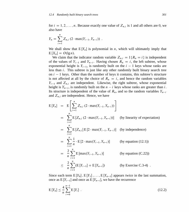
12.4 Randomly built binary search trees 301
for i D 1; 2; : : : ; n. Because exactly one value of Zn;i is 1 and all others are 0, wealso have
Yn DnX
iD1
Zn;i .2 �max.Yi�1; Yn�i // :
We shall show that E ŒYn� is polynomial in n, which will ultimately imply thatE ŒXn� D O.lg n/.
We claim that the indicator random variable Zn;i D I fRn D ig is independentof the values of Yi�1 and Yn�i . Having chosen Rn D i , the left subtree, whoseexponential height is Yi�1, is randomly built on the i � 1 keys whose ranks areless than i . This subtree is just like any other randomly built binary search treeon i � 1 keys. Other than the number of keys it contains, this subtree’s structureis not affected at all by the choice of Rn D i , and hence the random variablesYi�1 and Zn;i are independent. Likewise, the right subtree, whose exponentialheight is Yn�i , is randomly built on the n � i keys whose ranks are greater than i .Its structure is independent of the value of Rn, and so the random variables Yn�i
and Zn;i are independent. Hence, we have
E ŒYn� D E
"nX
iD1
Zn;i .2 �max.Yi�1; Yn�i //
#
DnX
iD1
E ŒZn;i .2 �max.Yi�1; Yn�i //� (by linearity of expectation)
DnX
iD1
E ŒZn;i � E Œ2 �max.Yi�1; Yn�i /� (by independence)
DnX
iD1
1
n� E Œ2 �max.Yi�1; Yn�i /� (by equation (12.1))
D 2
n
nXiD1
E Œmax.Yi�1; Yn�i /� (by equation (C.22))
� 2
n
nXiD1
.E ŒYi�1�C E ŒYn�i �/ (by Exercise C.3-4) .
Since each term E ŒY0� ; E ŒY1� ; : : : ; E ŒYn�1� appears twice in the last summation,once as E ŒYi�1� and once as E ŒYn�i �, we have the recurrence
E ŒYn� � 4
n
n�1XiD0
E ŒYi � : (12.2)
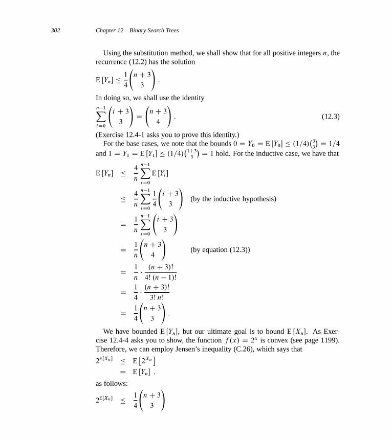
302 Chapter 12 Binary Search Trees
Using the substitution method, we shall show that for all positive integers n, therecurrence (12.2) has the solution
E ŒYn� � 1
4
nC 3
3
!:
In doing so, we shall use the identityn�1XiD0
i C 3
3
!D
nC 3
4
!: (12.3)
(Exercise 12.4-1 asks you to prove this identity.)For the base cases, we note that the bounds 0 D Y0 D E ŒY0� � .1=4/
�3
3
� D 1=4
and 1 D Y1 D E ŒY1� � .1=4/�
1C3
3
� D 1 hold. For the inductive case, we have that
E ŒYn� � 4
n
n�1XiD0
E ŒYi �
� 4
n
n�1XiD0
1
4
i C 3
3
!(by the inductive hypothesis)
D 1
n
n�1XiD0
i C 3
3
!
D 1
n
nC 3
4
!(by equation (12.3))
D 1
n� .nC 3/Š
4Š .n � 1/Š
D 1
4� .nC 3/Š
3Š nŠ
D 1
4
nC 3
3
!:
We have bounded E ŒYn�, but our ultimate goal is to bound E ŒXn�. As Exer-cise 12.4-4 asks you to show, the function f .x/ D 2x is convex (see page 1199).Therefore, we can employ Jensen’s inequality (C.26), which says that
2EŒXn� � E�2Xn
�D E ŒYn� ;
as follows:
2EŒXn� � 1
4
nC 3
3
!

Problems for Chapter 12 303
D 1
4� .nC 3/.nC 2/.nC 1/
6
D n3 C 6n2 C 11nC 6
24:
Taking logarithms of both sides gives E ŒXn� D O.lg n/.
Exercises
12.4-1Prove equation (12.3).
12.4-2Describe a binary search tree on n nodes such that the average depth of a node inthe tree is ‚.lg n/ but the height of the tree is !.lg n/. Give an asymptotic upperbound on the height of an n-node binary search tree in which the average depth ofa node is ‚.lg n/.
12.4-3Show that the notion of a randomly chosen binary search tree on n keys, whereeach binary search tree of n keys is equally likely to be chosen, is different fromthe notion of a randomly built binary search tree given in this section. (Hint: Listthe possibilities when n D 3.)
12.4-4Show that the function f .x/ D 2x is convex.
12.4-5 ?
Consider RANDOMIZED-QUICKSORT operating on a sequence of n distinct inputnumbers. Prove that for any constant k > 0, all but O.1=nk/ of the nŠ inputpermutations yield an O.n lg n/ running time.
Problems
12-1 Binary search trees with equal keysEqual keys pose a problem for the implementation of binary search trees.
a. What is the asymptotic performance of TREE-INSERT when used to insert n
items with identical keys into an initially empty binary search tree?
We propose to improve TREE-INSERT by testing before line 5 to determine whether´:key D x:key and by testing before line 11 to determine whether ´:key D y:key.
304 Chapter 12 Binary Search Trees
If equality holds, we implement one of the following strategies. For each strategy,find the asymptotic performance of inserting n items with identical keys into aninitially empty binary search tree. (The strategies are described for line 5, in whichwe compare the keys of ´ and x. Substitute y for x to arrive at the strategies forline 11.)
b. Keep a boolean flag x:b at node x, and set x to either x: left or x:right basedon the value of x:b, which alternates between FALSE and TRUE each time wevisit x while inserting a node with the same key as x.
c. Keep a list of nodes with equal keys at x, and insert ´ into the list.
d. Randomly set x to either x: left or x:right. (Give the worst-case performanceand informally derive the expected running time.)
12-2 Radix treesGiven two strings a D a0a1 : : : ap and b D b0b1 : : : bq, where each ai and each bj
is in some ordered set of characters, we say that string a is lexicographically lessthan string b if either
1. there exists an integer j , where 0 � j � min.p; q/, such that ai D bi for alli D 0; 1; : : : ; j � 1 and aj < bj , or
2. p < q and ai D bi for all i D 0; 1; : : : ; p.
For example, if a and b are bit strings, then 10100 < 10110 by rule 1 (lettingj D 3) and 10100 < 101000 by rule 2. This ordering is similar to that used inEnglish-language dictionaries.
The radix tree data structure shown in Figure 12.5 stores the bit strings 1011,10, 011, 100, and 0. When searching for a key a D a0a1 : : : ap, we go left at anode of depth i if ai D 0 and right if ai D 1. Let S be a set of distinct bit stringswhose lengths sum to n. Show how to use a radix tree to sort S lexicographicallyin ‚.n/ time. For the example in Figure 12.5, the output of the sort should be thesequence 0, 011, 10, 100, 1011.
12-3 Average node depth in a randomly built binary search treeIn this problem, we prove that the average depth of a node in a randomly builtbinary search tree with n nodes is O.lg n/. Although this result is weaker thanthat of Theorem 12.4, the technique we shall use reveals a surprising similaritybetween the building of a binary search tree and the execution of RANDOMIZED-QUICKSORT from Section 7.3.
We define the total path length P.T / of a binary tree T as the sum, over allnodes x in T , of the depth of node x, which we denote by d.x; T /.
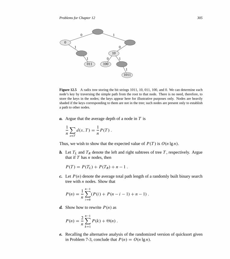
Problems for Chapter 12 305
011
0
100
10
1011
0 1
1 0
1 0 1
1
Figure 12.5 A radix tree storing the bit strings 1011, 10, 011, 100, and 0. We can determine eachnode’s key by traversing the simple path from the root to that node. There is no need, therefore, tostore the keys in the nodes; the keys appear here for illustrative purposes only. Nodes are heavilyshaded if the keys corresponding to them are not in the tree; such nodes are present only to establisha path to other nodes.
a. Argue that the average depth of a node in T is
1
n
Xx2T
d.x; T / D 1
nP.T / :
Thus, we wish to show that the expected value of P.T / is O.n lg n/.
b. Let TL and TR denote the left and right subtrees of tree T , respectively. Arguethat if T has n nodes, then
P.T / D P.TL/C P.TR/C n � 1 :
c. Let P.n/ denote the average total path length of a randomly built binary searchtree with n nodes. Show that
P.n/ D 1
n
n�1XiD0
.P.i/C P.n� i � 1/C n � 1/ :
d. Show how to rewrite P.n/ as
P.n/ D 2
n
n�1XkD1
P.k/C‚.n/ :
e. Recalling the alternative analysis of the randomized version of quicksort givenin Problem 7-3, conclude that P.n/ D O.n lg n/.
306 Chapter 12 Binary Search Trees
At each recursive invocation of quicksort, we choose a random pivot element topartition the set of elements being sorted. Each node of a binary search tree parti-tions the set of elements that fall into the subtree rooted at that node.
f. Describe an implementation of quicksort in which the comparisons to sort a setof elements are exactly the same as the comparisons to insert the elements intoa binary search tree. (The order in which comparisons are made may differ, butthe same comparisons must occur.)
12-4 Number of different binary treesLet bn denote the number of different binary trees with n nodes. In this problem,you will find a formula for bn, as well as an asymptotic estimate.
a. Show that b0 D 1 and that, for n � 1,
bn Dn�1XkD0
bkbn�1�k :
b. Referring to Problem 4-4 for the definition of a generating function, let B.x/
be the generating function
B.x/ D1X
nD0
bnxn :
Show that B.x/ D xB.x/2 C 1, and hence one way to express B.x/ in closedform is
B.x/ D 1
2x
�1 �p
1 � 4x�
:
The Taylor expansion of f .x/ around the point x D a is given by
f .x/ D1X
kD0
f .k/.a/
kŠ.x � a/k ;
where f .k/.x/ is the kth derivative of f evaluated at x.
c. Show that
bn D1
nC 1
2n
n
!

Notes for Chapter 12 307
(the nth Catalan number) by using the Taylor expansion ofp
1 � 4x aroundx D 0. (If you wish, instead of using the Taylor expansion, you may usethe generalization of the binomial expansion (C.4) to nonintegral exponents n,where for any real number n and for any integer k, we interpret
�n
k
�to be
n.n � 1/ � � � .n � k C 1/=kŠ if k � 0, and 0 otherwise.)
d. Show that
bn D 4n
p�n3=2
.1CO.1=n// :
Chapter notes
Knuth [211] contains a good discussion of simple binary search trees as well asmany variations. Binary search trees seem to have been independently discoveredby a number of people in the late 1950s. Radix trees are often called tries, whichcomes from the middle letters in the word retrieval. Knuth [211] also discussesthem.
Many texts, including the first two editions of this book, have a somewhat sim-pler method of deleting a node from a binary search tree when both of its childrenare present. Instead of replacing node ´ by its successor y, we delete node y butcopy its key and satellite data into node ´. The downside of this approach is thatthe node actually deleted might not be the node passed to the delete procedure. Ifother components of a program maintain pointers to nodes in the tree, they couldmistakenly end up with “stale” pointers to nodes that have been deleted. Althoughthe deletion method presented in this edition of this book is a bit more complicated,it guarantees that a call to delete node ´ deletes node ´ and only node ´.
Section 15.5 will show how to construct an optimal binary search tree whenwe know the search frequencies before constructing the tree. That is, given thefrequencies of searching for each key and the frequencies of searching for valuesthat fall between keys in the tree, we construct a binary search tree for which aset of searches that follows these frequencies examines the minimum number ofnodes.
The proof in Section 12.4 that bounds the expected height of a randomly builtbinary search tree is due to Aslam [24]. Martı́nez and Roura [243] give randomizedalgorithms for insertion into and deletion from binary search trees in which theresult of either operation is a random binary search tree. Their definition of arandom binary search tree differs—only slightly—from that of a randomly builtbinary search tree in this chapter, however.
13 Red-Black Trees
Chapter 12 showed that a binary search tree of height h can support any of the basicdynamic-set operations—such as SEARCH, PREDECESSOR, SUCCESSOR, MINI-MUM, MAXIMUM, INSERT, and DELETE—in O.h/ time. Thus, the set operationsare fast if the height of the search tree is small. If its height is large, however, theset operations may run no faster than with a linked list. Red-black trees are oneof many search-tree schemes that are “balanced” in order to guarantee that basicdynamic-set operations take O.lg n/ time in the worst case.
13.1 Properties of red-black trees
A red-black tree is a binary search tree with one extra bit of storage per node: itscolor, which can be either RED or BLACK. By constraining the node colors on anysimple path from the root to a leaf, red-black trees ensure that no such path is morethan twice as long as any other, so that the tree is approximately balanced.
Each node of the tree now contains the attributes color, key, left, right, and p. Ifa child or the parent of a node does not exist, the corresponding pointer attributeof the node contains the value NIL. We shall regard these NILs as being pointers toleaves (external nodes) of the binary search tree and the normal, key-bearing nodesas being internal nodes of the tree.
A red-black tree is a binary tree that satisfies the following red-black properties:
1. Every node is either red or black.
2. The root is black.
3. Every leaf (NIL) is black.
4. If a node is red, then both its children are black.
5. For each node, all simple paths from the node to descendant leaves contain thesame number of black nodes.
13.1 Properties of red-black trees 309
Figure 13.1(a) shows an example of a red-black tree.As a matter of convenience in dealing with boundary conditions in red-black
tree code, we use a single sentinel to represent NIL (see page 238). For a red-blacktree T , the sentinel T:nil is an object with the same attributes as an ordinary nodein the tree. Its color attribute is BLACK, and its other attributes—p, left, right,and key—can take on arbitrary values. As Figure 13.1(b) shows, all pointers to NIL
are replaced by pointers to the sentinel T:nil.We use the sentinel so that we can treat a NIL child of a node x as an ordinary
node whose parent is x. Although we instead could add a distinct sentinel nodefor each NIL in the tree, so that the parent of each NIL is well defined, that ap-proach would waste space. Instead, we use the one sentinel T:nil to represent allthe NILs—all leaves and the root’s parent. The values of the attributes p, left, right,and key of the sentinel are immaterial, although we may set them during the courseof a procedure for our convenience.
We generally confine our interest to the internal nodes of a red-black tree, sincethey hold the key values. In the remainder of this chapter, we omit the leaves whenwe draw red-black trees, as shown in Figure 13.1(c).
We call the number of black nodes on any simple path from, but not including, anode x down to a leaf the black-height of the node, denoted bh.x/. By property 5,the notion of black-height is well defined, since all descending simple paths fromthe node have the same number of black nodes. We define the black-height of ared-black tree to be the black-height of its root.
The following lemma shows why red-black trees make good search trees.
Lemma 13.1A red-black tree with n internal nodes has height at most 2 lg.nC 1/.
Proof We start by showing that the subtree rooted at any node x contains at least2bh.x/ � 1 internal nodes. We prove this claim by induction on the height of x. Ifthe height of x is 0, then x must be a leaf (T:nil), and the subtree rooted at x indeedcontains at least 2bh.x/ � 1 D 20 � 1 D 0 internal nodes. For the inductive step,consider a node x that has positive height and is an internal node with two children.Each child has a black-height of either bh.x/ or bh.x/ � 1, depending on whetherits color is red or black, respectively. Since the height of a child of x is less thanthe height of x itself, we can apply the inductive hypothesis to conclude that eachchild has at least 2bh.x/�1 � 1 internal nodes. Thus, the subtree rooted at x containsat least .2bh.x/�1�1/C .2bh.x/�1�1/C1 D 2bh.x/�1 internal nodes, which provesthe claim.
To complete the proof of the lemma, let h be the height of the tree. Accordingto property 4, at least half the nodes on any simple path from the root to a leaf, not
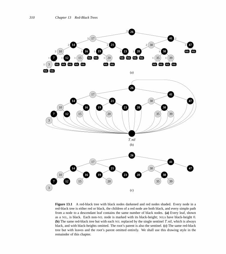
310 Chapter 13 Red-Black Trees
NIL NIL
NIL NIL NIL NILNIL
NIL NIL
NIL NIL
NIL NIL NIL NIL
NIL NIL NIL NIL
NIL NIL
26
41
4730
28 38
35 39
17
21
2319
20
14
16
15
10
127
31
1 1
2
1
1
2
1
1 1
2
3
1 1
11
2 1
2
3
(a)
26
41
4730
28 38
35 39
17
21
2319
20
14
16
15
10
127
3
(b)
26
41
4730
28 38
35 39
17
21
2319
20
14
16
15
10
127
3(c)
T:nil
Figure 13.1 A red-black tree with black nodes darkened and red nodes shaded. Every node in ared-black tree is either red or black, the children of a red node are both black, and every simple pathfrom a node to a descendant leaf contains the same number of black nodes. (a) Every leaf, shownas a NIL, is black. Each non-NIL node is marked with its black-height; NILs have black-height 0.(b) The same red-black tree but with each NIL replaced by the single sentinel T:nil, which is alwaysblack, and with black-heights omitted. The root’s parent is also the sentinel. (c) The same red-blacktree but with leaves and the root’s parent omitted entirely. We shall use this drawing style in theremainder of this chapter.
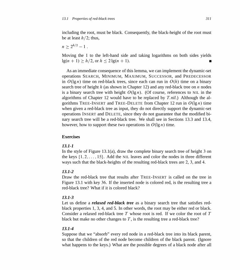
13.1 Properties of red-black trees 311
including the root, must be black. Consequently, the black-height of the root mustbe at least h=2; thus,
n � 2h=2 � 1 :
Moving the 1 to the left-hand side and taking logarithms on both sides yieldslg.nC 1/ � h=2, or h � 2 lg.nC 1/.
As an immediate consequence of this lemma, we can implement the dynamic-setoperations SEARCH, MINIMUM, MAXIMUM, SUCCESSOR, and PREDECESSOR
in O.lg n/ time on red-black trees, since each can run in O.h/ time on a binarysearch tree of height h (as shown in Chapter 12) and any red-black tree on n nodesis a binary search tree with height O.lg n/. (Of course, references to NIL in thealgorithms of Chapter 12 would have to be replaced by T:nil.) Although the al-gorithms TREE-INSERT and TREE-DELETE from Chapter 12 run in O.lg n/ timewhen given a red-black tree as input, they do not directly support the dynamic-setoperations INSERT and DELETE, since they do not guarantee that the modified bi-nary search tree will be a red-black tree. We shall see in Sections 13.3 and 13.4,however, how to support these two operations in O.lg n/ time.
Exercises
13.1-1In the style of Figure 13.1(a), draw the complete binary search tree of height 3 onthe keys f1; 2; : : : ; 15g. Add the NIL leaves and color the nodes in three differentways such that the black-heights of the resulting red-black trees are 2, 3, and 4.
13.1-2Draw the red-black tree that results after TREE-INSERT is called on the tree inFigure 13.1 with key 36. If the inserted node is colored red, is the resulting tree ared-black tree? What if it is colored black?
13.1-3Let us define a relaxed red-black tree as a binary search tree that satisfies red-black properties 1, 3, 4, and 5. In other words, the root may be either red or black.Consider a relaxed red-black tree T whose root is red. If we color the root of T
black but make no other changes to T , is the resulting tree a red-black tree?
13.1-4Suppose that we “absorb” every red node in a red-black tree into its black parent,so that the children of the red node become children of the black parent. (Ignorewhat happens to the keys.) What are the possible degrees of a black node after all
312 Chapter 13 Red-Black Trees
its red children are absorbed? What can you say about the depths of the leaves ofthe resulting tree?
13.1-5Show that the longest simple path from a node x in a red-black tree to a descendantleaf has length at most twice that of the shortest simple path from node x to adescendant leaf.
13.1-6What is the largest possible number of internal nodes in a red-black tree with black-height k? What is the smallest possible number?
13.1-7Describe a red-black tree on n keys that realizes the largest possible ratio of red in-ternal nodes to black internal nodes. What is this ratio? What tree has the smallestpossible ratio, and what is the ratio?
13.2 Rotations
The search-tree operations TREE-INSERT and TREE-DELETE, when run on a red-black tree with n keys, take O.lg n/ time. Because they modify the tree, the resultmay violate the red-black properties enumerated in Section 13.1. To restore theseproperties, we must change the colors of some of the nodes in the tree and alsochange the pointer structure.
We change the pointer structure through rotation, which is a local operation ina search tree that preserves the binary-search-tree property. Figure 13.2 shows thetwo kinds of rotations: left rotations and right rotations. When we do a left rotationon a node x, we assume that its right child y is not T:nil; x may be any node inthe tree whose right child is not T:nil. The left rotation “pivots” around the linkfrom x to y. It makes y the new root of the subtree, with x as y’s left child and y’sleft child as x’s right child.
The pseudocode for LEFT-ROTATE assumes that x:right ¤ T:nil and that theroot’s parent is T:nil.
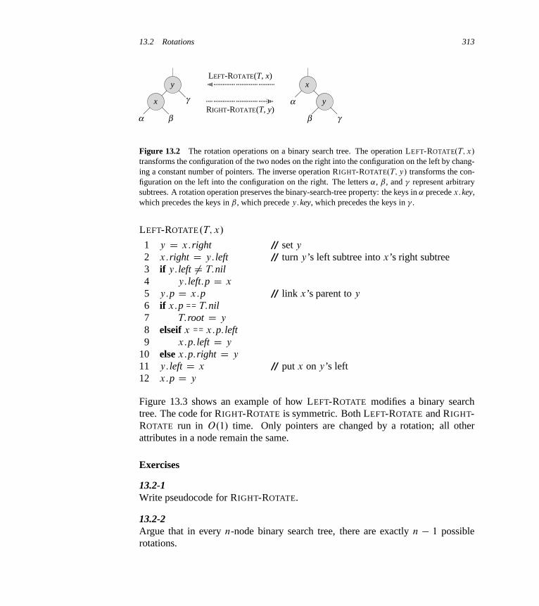
13.2 Rotations 313
y
x
α β
γ
x
yα
β γ
LEFT-ROTATE(T, x)
RIGHT-ROTATE(T, y)
Figure 13.2 The rotation operations on a binary search tree. The operation LEFT-ROTATE.T; x/
transforms the configuration of the two nodes on the right into the configuration on the left by chang-ing a constant number of pointers. The inverse operation RIGHT-ROTATE.T; y/ transforms the con-figuration on the left into the configuration on the right. The letters ˛, ˇ, and represent arbitrarysubtrees. A rotation operation preserves the binary-search-tree property: the keys in ˛ precede x:key,which precedes the keys in ˇ, which precede y:key, which precedes the keys in .
LEFT-ROTATE.T; x/
1 y D x:right // set y
2 x:right D y: left // turn y’s left subtree into x’s right subtree3 if y: left ¤ T:nil4 y: left:p D x
5 y:p D x:p // link x’s parent to y
6 if x:p == T:nil7 T:root D y
8 elseif x == x:p: left9 x:p: left D y
10 else x:p:right D y
11 y: left D x // put x on y’s left12 x:p D y
Figure 13.3 shows an example of how LEFT-ROTATE modifies a binary searchtree. The code for RIGHT-ROTATE is symmetric. Both LEFT-ROTATE and RIGHT-ROTATE run in O.1/ time. Only pointers are changed by a rotation; all otherattributes in a node remain the same.
Exercises
13.2-1Write pseudocode for RIGHT-ROTATE.
13.2-2Argue that in every n-node binary search tree, there are exactly n � 1 possiblerotations.
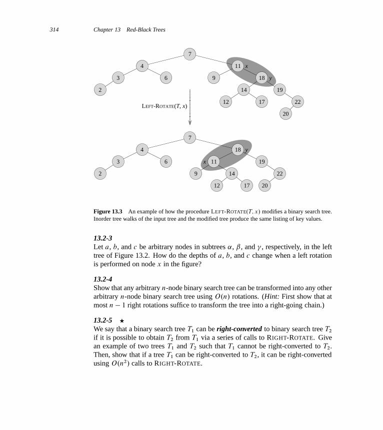
314 Chapter 13 Red-Black Trees
2
3
4
6
7
11
9 18
14
12 17
19
22
20
x
y
2
3
4
6
7
18
19
14
12 17
22
20
x
y
11
9
LEFT-ROTATE(T, x)
Figure 13.3 An example of how the procedure LEFT-ROTATE.T; x/ modifies a binary search tree.Inorder tree walks of the input tree and the modified tree produce the same listing of key values.
13.2-3Let a, b, and c be arbitrary nodes in subtrees ˛, ˇ, and , respectively, in the lefttree of Figure 13.2. How do the depths of a, b, and c change when a left rotationis performed on node x in the figure?
13.2-4Show that any arbitrary n-node binary search tree can be transformed into any otherarbitrary n-node binary search tree using O.n/ rotations. (Hint: First show that atmost n � 1 right rotations suffice to transform the tree into a right-going chain.)
13.2-5 ?
We say that a binary search tree T1 can be right-converted to binary search tree T2
if it is possible to obtain T2 from T1 via a series of calls to RIGHT-ROTATE. Givean example of two trees T1 and T2 such that T1 cannot be right-converted to T2.Then, show that if a tree T1 can be right-converted to T2, it can be right-convertedusing O.n2/ calls to RIGHT-ROTATE.

13.3 Insertion 315
13.3 Insertion
We can insert a node into an n-node red-black tree in O.lg n/ time. To do so, weuse a slightly modified version of the TREE-INSERT procedure (Section 12.3) toinsert node ´ into the tree T as if it were an ordinary binary search tree, and then wecolor ´ red. (Exercise 13.3-1 asks you to explain why we choose to make node ´
red rather than black.) To guarantee that the red-black properties are preserved, wethen call an auxiliary procedure RB-INSERT-FIXUP to recolor nodes and performrotations. The call RB-INSERT.T; ´/ inserts node ´, whose key is assumed to havealready been filled in, into the red-black tree T .
RB-INSERT.T; ´/
1 y D T:nil2 x D T:root3 while x ¤ T:nil4 y D x
5 if ´:key < x:key6 x D x: left7 else x D x:right8 ´:p D y
9 if y == T:nil10 T:root D ´
11 elseif ´:key < y:key12 y: left D ´
13 else y:right D ´
14 ´: left D T:nil15 ´:right D T:nil16 ´:color D RED
17 RB-INSERT-FIXUP.T; ´/
The procedures TREE-INSERT and RB-INSERT differ in four ways. First, allinstances of NIL in TREE-INSERT are replaced by T:nil. Second, we set ´: leftand ´:right to T:nil in lines 14–15 of RB-INSERT, in order to maintain theproper tree structure. Third, we color ´ red in line 16. Fourth, because col-oring ´ red may cause a violation of one of the red-black properties, we callRB-INSERT-FIXUP.T; ´/ in line 17 of RB-INSERT to restore the red-black prop-erties.
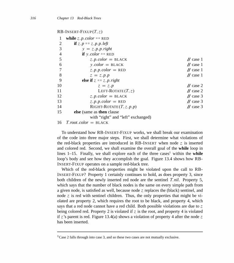
316 Chapter 13 Red-Black Trees
RB-INSERT-FIXUP.T; ´/
1 while ´:p:color == RED
2 if ´:p == ´:p:p: left3 y D ´:p:p:right4 if y:color == RED
5 ´:p:color D BLACK // case 16 y:color D BLACK // case 17 ´:p:p:color D RED // case 18 ´ D ´:p:p // case 19 else if ´ == ´:p:right
10 ´ D ´:p // case 211 LEFT-ROTATE.T; ´/ // case 212 ´:p:color D BLACK // case 313 ´:p:p:color D RED // case 314 RIGHT-ROTATE.T; ´:p:p/ // case 315 else (same as then clause
with “right” and “left” exchanged)16 T:root:color D BLACK
To understand how RB-INSERT-FIXUP works, we shall break our examinationof the code into three major steps. First, we shall determine what violations ofthe red-black properties are introduced in RB-INSERT when node ´ is insertedand colored red. Second, we shall examine the overall goal of the while loop inlines 1–15. Finally, we shall explore each of the three cases1 within the whileloop’s body and see how they accomplish the goal. Figure 13.4 shows how RB-INSERT-FIXUP operates on a sample red-black tree.
Which of the red-black properties might be violated upon the call to RB-INSERT-FIXUP? Property 1 certainly continues to hold, as does property 3, sinceboth children of the newly inserted red node are the sentinel T:nil. Property 5,which says that the number of black nodes is the same on every simple path froma given node, is satisfied as well, because node ´ replaces the (black) sentinel, andnode ´ is red with sentinel children. Thus, the only properties that might be vi-olated are property 2, which requires the root to be black, and property 4, whichsays that a red node cannot have a red child. Both possible violations are due to ´
being colored red. Property 2 is violated if ´ is the root, and property 4 is violatedif ´’s parent is red. Figure 13.4(a) shows a violation of property 4 after the node ´
has been inserted.
1Case 2 falls through into case 3, and so these two cases are not mutually exclusive.
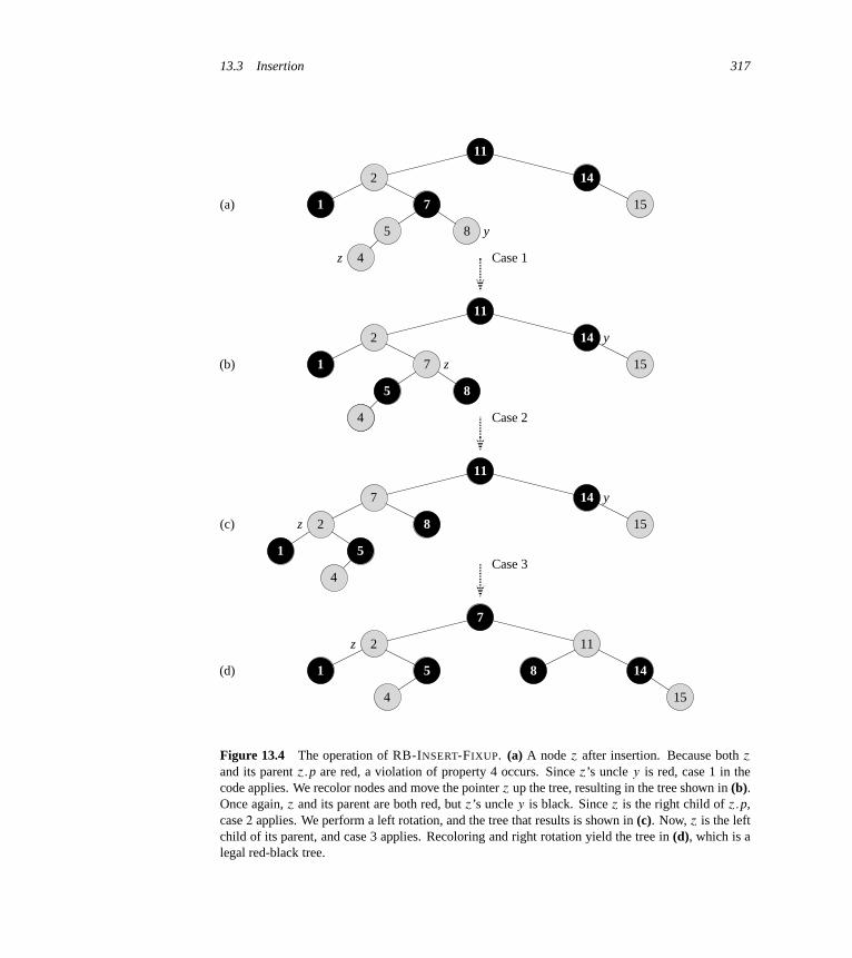
13.3 Insertion 317
z
y
11
2
1 7
5
4
8
14
15
z
y
11
2
1 7
5
4
8
14
15
(a)
(b)
Case 1
z
y
11
7
2 8
4
14
15(c)
Case 2
1 5
4
z
7
2
1 5
11
14(d)
Case 3
4
8
15
Figure 13.4 The operation of RB-INSERT-FIXUP. (a) A node ´ after insertion. Because both ´
and its parent ´:p are red, a violation of property 4 occurs. Since ´’s uncle y is red, case 1 in thecode applies. We recolor nodes and move the pointer ´ up the tree, resulting in the tree shown in (b).Once again, ´ and its parent are both red, but ´’s uncle y is black. Since ´ is the right child of ´:p,case 2 applies. We perform a left rotation, and the tree that results is shown in (c). Now, ´ is the leftchild of its parent, and case 3 applies. Recoloring and right rotation yield the tree in (d), which is alegal red-black tree.

318 Chapter 13 Red-Black Trees
The while loop in lines 1–15 maintains the following three-part invariant at thestart of each iteration of the loop:
a. Node ´ is red.
b. If ´:p is the root, then ´:p is black.
c. If the tree violates any of the red-black properties, then it violates at mostone of them, and the violation is of either property 2 or property 4. If thetree violates property 2, it is because ´ is the root and is red. If the treeviolates property 4, it is because both ´ and ´:p are red.
Part (c), which deals with violations of red-black properties, is more central toshowing that RB-INSERT-FIXUP restores the red-black properties than parts (a)and (b), which we use along the way to understand situations in the code. Becausewe’ll be focusing on node ´ and nodes near it in the tree, it helps to know frompart (a) that ´ is red. We shall use part (b) to show that the node ´:p:p exists whenwe reference it in lines 2, 3, 7, 8, 13, and 14.
Recall that we need to show that a loop invariant is true prior to the first itera-tion of the loop, that each iteration maintains the loop invariant, and that the loopinvariant gives us a useful property at loop termination.
We start with the initialization and termination arguments. Then, as we exam-ine how the body of the loop works in more detail, we shall argue that the loopmaintains the invariant upon each iteration. Along the way, we shall also demon-strate that each iteration of the loop has two possible outcomes: either the pointer ´
moves up the tree, or we perform some rotations and then the loop terminates.
Initialization: Prior to the first iteration of the loop, we started with a red-blacktree with no violations, and we added a red node ´. We show that each part ofthe invariant holds at the time RB-INSERT-FIXUP is called:
a. When RB-INSERT-FIXUP is called, ´ is the red node that was added.
b. If ´:p is the root, then ´:p started out black and did not change prior to thecall of RB-INSERT-FIXUP.
c. We have already seen that properties 1, 3, and 5 hold when RB-INSERT-FIXUP is called.If the tree violates property 2, then the red root must be the newly addednode ´, which is the only internal node in the tree. Because the parent andboth children of ´ are the sentinel, which is black, the tree does not alsoviolate property 4. Thus, this violation of property 2 is the only violation ofred-black properties in the entire tree.If the tree violates property 4, then, because the children of node ´ are blacksentinels and the tree had no other violations prior to ´ being added, the
13.3 Insertion 319
violation must be because both ´ and ´:p are red. Moreover, the tree violatesno other red-black properties.
Termination: When the loop terminates, it does so because ´:p is black. (If ´ isthe root, then ´:p is the sentinel T:nil, which is black.) Thus, the tree does notviolate property 4 at loop termination. By the loop invariant, the only propertythat might fail to hold is property 2. Line 16 restores this property, too, so thatwhen RB-INSERT-FIXUP terminates, all the red-black properties hold.
Maintenance: We actually need to consider six cases in the while loop, but threeof them are symmetric to the other three, depending on whether line 2 deter-mines ´’s parent ´:p to be a left child or a right child of ´’s grandparent ´:p:p.We have given the code only for the situation in which ´:p is a left child. Thenode ´:p:p exists, since by part (b) of the loop invariant, if ´:p is the root,then ´:p is black. Since we enter a loop iteration only if ´:p is red, we knowthat ´:p cannot be the root. Hence, ´:p:p exists.
We distinguish case 1 from cases 2 and 3 by the color of ´’s parent’s sibling,or “uncle.” Line 3 makes y point to ´’s uncle ´:p:p:right, and line 4 tests y’scolor. If y is red, then we execute case 1. Otherwise, control passes to cases 2and 3. In all three cases, ´’s grandparent ´:p:p is black, since its parent ´:p isred, and property 4 is violated only between ´ and ´:p.
Case 1: ´’s uncle y is red
Figure 13.5 shows the situation for case 1 (lines 5–8), which occurs whenboth ´:p and y are red. Because ´:p:p is black, we can color both ´:p and y
black, thereby fixing the problem of ´ and ´:p both being red, and we cancolor ´:p:p red, thereby maintaining property 5. We then repeat the while loopwith ´:p:p as the new node ´. The pointer ´ moves up two levels in the tree.
Now, we show that case 1 maintains the loop invariant at the start of the nextiteration. We use ´ to denote node ´ in the current iteration, and ´0 D ´:p:pto denote the node that will be called node ´ at the test in line 1 upon the nextiteration.
a. Because this iteration colors ´:p:p red, node ´0 is red at the start of the nextiteration.
b. The node ´0:p is ´:p:p:p in this iteration, and the color of this node does notchange. If this node is the root, it was black prior to this iteration, and itremains black at the start of the next iteration.
c. We have already argued that case 1 maintains property 5, and it does notintroduce a violation of properties 1 or 3.
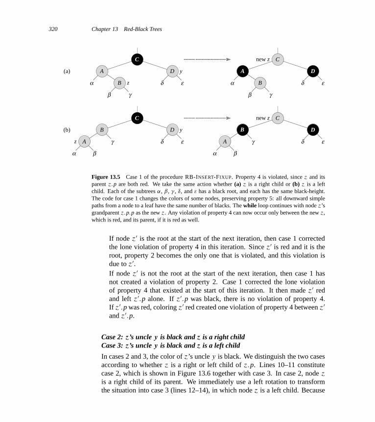
320 Chapter 13 Red-Black Trees
z
y
C
DA
Bα
β γ
δ ε
(a)
C
DA
Bα
β γ
δ ε
new z
y
C
DB
δ ε
C
DB
A
α β
γ δ ε
new z
(b)
A
α β
γz
Figure 13.5 Case 1 of the procedure RB-INSERT-FIXUP. Property 4 is violated, since ´ and itsparent ´:p are both red. We take the same action whether (a) ´ is a right child or (b) ´ is a leftchild. Each of the subtrees ˛, ˇ, , ı, and " has a black root, and each has the same black-height.The code for case 1 changes the colors of some nodes, preserving property 5: all downward simplepaths from a node to a leaf have the same number of blacks. The while loop continues with node ´’sgrandparent ´:p:p as the new ´. Any violation of property 4 can now occur only between the new ´,which is red, and its parent, if it is red as well.
If node ´0 is the root at the start of the next iteration, then case 1 correctedthe lone violation of property 4 in this iteration. Since ´0 is red and it is theroot, property 2 becomes the only one that is violated, and this violation isdue to ´0.If node ´0 is not the root at the start of the next iteration, then case 1 hasnot created a violation of property 2. Case 1 corrected the lone violationof property 4 that existed at the start of this iteration. It then made ´0 redand left ´0:p alone. If ´0:p was black, there is no violation of property 4.If ´0:p was red, coloring ´0 red created one violation of property 4 between ´0
and ´0:p.
Case 2: ´’s uncle y is black and ´ is a right childCase 3: ´’s uncle y is black and ´ is a left child
In cases 2 and 3, the color of ´’s uncle y is black. We distinguish the two casesaccording to whether ´ is a right or left child of ´:p. Lines 10–11 constitutecase 2, which is shown in Figure 13.6 together with case 3. In case 2, node ´
is a right child of its parent. We immediately use a left rotation to transformthe situation into case 3 (lines 12–14), in which node ´ is a left child. Because
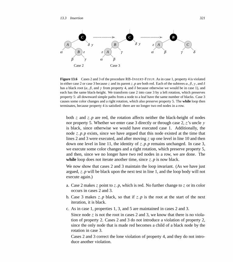
13.3 Insertion 321
C
A
Bα
β γ
δ
Case 2
z
y B
A
α β
γ
δ
Case 3
z
y z A
B
C
α β γ δ
C
Figure 13.6 Cases 2 and 3 of the procedure RB-INSERT-FIXUP. As in case 1, property 4 is violatedin either case 2 or case 3 because ´ and its parent ´:p are both red. Each of the subtrees ˛, ˇ, , and ı
has a black root (˛, ˇ, and from property 4, and ı because otherwise we would be in case 1), andeach has the same black-height. We transform case 2 into case 3 by a left rotation, which preservesproperty 5: all downward simple paths from a node to a leaf have the same number of blacks. Case 3causes some color changes and a right rotation, which also preserve property 5. The while loop thenterminates, because property 4 is satisfied: there are no longer two red nodes in a row.
both ´ and ´:p are red, the rotation affects neither the black-height of nodesnor property 5. Whether we enter case 3 directly or through case 2, ´’s uncle y
is black, since otherwise we would have executed case 1. Additionally, thenode ´:p:p exists, since we have argued that this node existed at the time thatlines 2 and 3 were executed, and after moving ´ up one level in line 10 and thendown one level in line 11, the identity of ´:p:p remains unchanged. In case 3,we execute some color changes and a right rotation, which preserve property 5,and then, since we no longer have two red nodes in a row, we are done. Thewhile loop does not iterate another time, since ´:p is now black.
We now show that cases 2 and 3 maintain the loop invariant. (As we have justargued, ´:p will be black upon the next test in line 1, and the loop body will notexecute again.)
a. Case 2 makes ´ point to ´:p, which is red. No further change to ´ or its coloroccurs in cases 2 and 3.
b. Case 3 makes ´:p black, so that if ´:p is the root at the start of the nextiteration, it is black.
c. As in case 1, properties 1, 3, and 5 are maintained in cases 2 and 3.Since node ´ is not the root in cases 2 and 3, we know that there is no viola-tion of property 2. Cases 2 and 3 do not introduce a violation of property 2,since the only node that is made red becomes a child of a black node by therotation in case 3.Cases 2 and 3 correct the lone violation of property 4, and they do not intro-duce another violation.
322 Chapter 13 Red-Black Trees
Having shown that each iteration of the loop maintains the invariant, we haveshown that RB-INSERT-FIXUP correctly restores the red-black properties.
Analysis
What is the running time of RB-INSERT? Since the height of a red-black tree on n
nodes is O.lg n/, lines 1–16 of RB-INSERT take O.lg n/ time. In RB-INSERT-FIXUP, the while loop repeats only if case 1 occurs, and then the pointer ´ movestwo levels up the tree. The total number of times the while loop can be executedis therefore O.lg n/. Thus, RB-INSERT takes a total of O.lg n/ time. Moreover, itnever performs more than two rotations, since the while loop terminates if case 2or case 3 is executed.
Exercises
13.3-1In line 16 of RB-INSERT, we set the color of the newly inserted node ´ to red.Observe that if we had chosen to set ´’s color to black, then property 4 of a red-black tree would not be violated. Why didn’t we choose to set ´’s color to black?
13.3-2Show the red-black trees that result after successively inserting the keys 41; 38; 31;
12; 19; 8 into an initially empty red-black tree.
13.3-3Suppose that the black-height of each of the subtrees ˛; ˇ; ; ı; " in Figures 13.5and 13.6 is k. Label each node in each figure with its black-height to verify thatthe indicated transformation preserves property 5.
13.3-4Professor Teach is concerned that RB-INSERT-FIXUP might set T:nil:color toRED, in which case the test in line 1 would not cause the loop to terminate when ´
is the root. Show that the professor’s concern is unfounded by arguing that RB-INSERT-FIXUP never sets T:nil:color to RED.
13.3-5Consider a red-black tree formed by inserting n nodes with RB-INSERT. Arguethat if n > 1, the tree has at least one red node.
13.3-6Suggest how to implement RB-INSERT efficiently if the representation for red-black trees includes no storage for parent pointers.
13.4 Deletion 323
13.4 Deletion
Like the other basic operations on an n-node red-black tree, deletion of a node takestime O.lg n/. Deleting a node from a red-black tree is a bit more complicated thaninserting a node.
The procedure for deleting a node from a red-black tree is based on the TREE-DELETE procedure (Section 12.3). First, we need to customize the TRANSPLANT
subroutine that TREE-DELETE calls so that it applies to a red-black tree:
RB-TRANSPLANT.T; u; �/
1 if u:p == T:nil2 T:root D �
3 elseif u == u:p: left4 u:p: left D �
5 else u:p:right D �
6 �:p D u:p
The procedure RB-TRANSPLANT differs from TRANSPLANT in two ways. First,line 1 references the sentinel T:nil instead of NIL. Second, the assignment to �:p inline 6 occurs unconditionally: we can assign to �:p even if � points to the sentinel.In fact, we shall exploit the ability to assign to �:p when � D T:nil.
The procedure RB-DELETE is like the TREE-DELETE procedure, but with ad-ditional lines of pseudocode. Some of the additional lines keep track of a node y
that might cause violations of the red-black properties. When we want to deletenode ´ and ´ has fewer than two children, then ´ is removed from the tree, and wewant y to be ´. When ´ has two children, then y should be ´’s successor, and y
moves into ´’s position in the tree. We also remember y’s color before it is re-moved from or moved within the tree, and we keep track of the node x that movesinto y’s original position in the tree, because node x might also cause violationsof the red-black properties. After deleting node ´, RB-DELETE calls an auxiliaryprocedure RB-DELETE-FIXUP, which changes colors and performs rotations torestore the red-black properties.
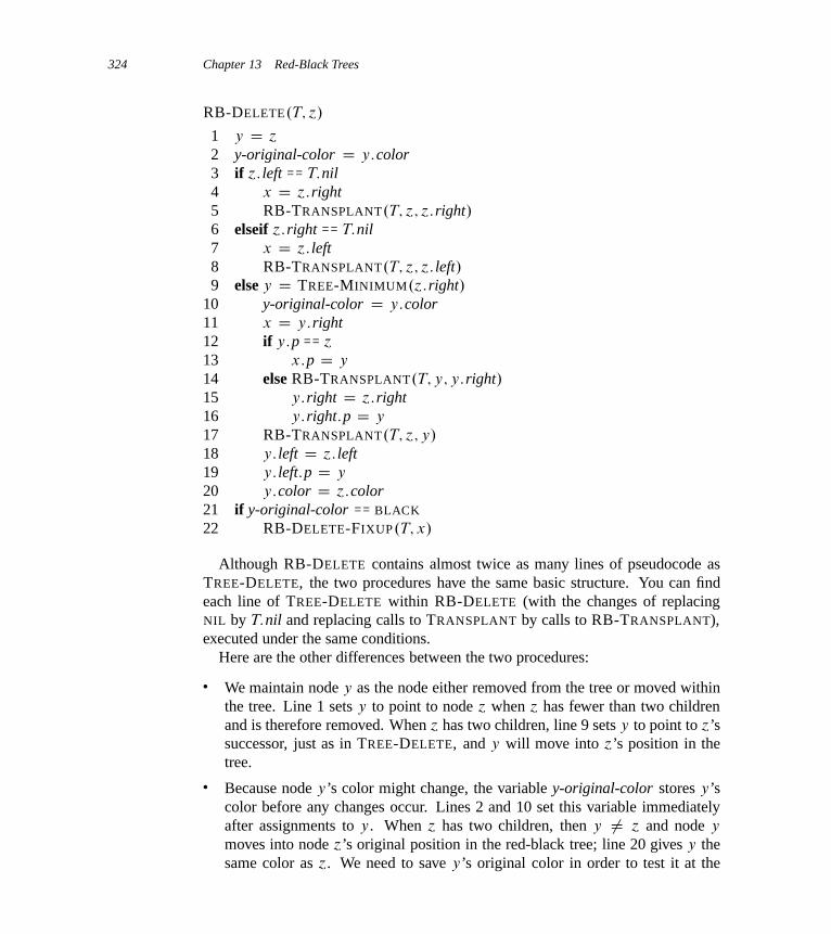
324 Chapter 13 Red-Black Trees
RB-DELETE.T; ´/
1 y D ´
2 y-original-color D y:color3 if ´: left == T:nil4 x D ´:right5 RB-TRANSPLANT.T; ´; ´:right/6 elseif ´:right == T:nil7 x D ´: left8 RB-TRANSPLANT.T; ´; ´: left/9 else y D TREE-MINIMUM.´:right/
10 y-original-color D y:color11 x D y:right12 if y:p == ´
13 x:p D y
14 else RB-TRANSPLANT.T; y; y:right/15 y:right D ´:right16 y:right:p D y
17 RB-TRANSPLANT.T; ´; y/
18 y: left D ´: left19 y: left:p D y
20 y:color D ´:color21 if y-original-color == BLACK
22 RB-DELETE-FIXUP.T; x/
Although RB-DELETE contains almost twice as many lines of pseudocode asTREE-DELETE, the two procedures have the same basic structure. You can findeach line of TREE-DELETE within RB-DELETE (with the changes of replacingNIL by T:nil and replacing calls to TRANSPLANT by calls to RB-TRANSPLANT),executed under the same conditions.
Here are the other differences between the two procedures:
� We maintain node y as the node either removed from the tree or moved withinthe tree. Line 1 sets y to point to node ´ when ´ has fewer than two childrenand is therefore removed. When ´ has two children, line 9 sets y to point to ´’ssuccessor, just as in TREE-DELETE, and y will move into ´’s position in thetree.
� Because node y’s color might change, the variable y-original-color stores y’scolor before any changes occur. Lines 2 and 10 set this variable immediatelyafter assignments to y. When ´ has two children, then y ¤ ´ and node y
moves into node ´’s original position in the red-black tree; line 20 gives y thesame color as ´. We need to save y’s original color in order to test it at the
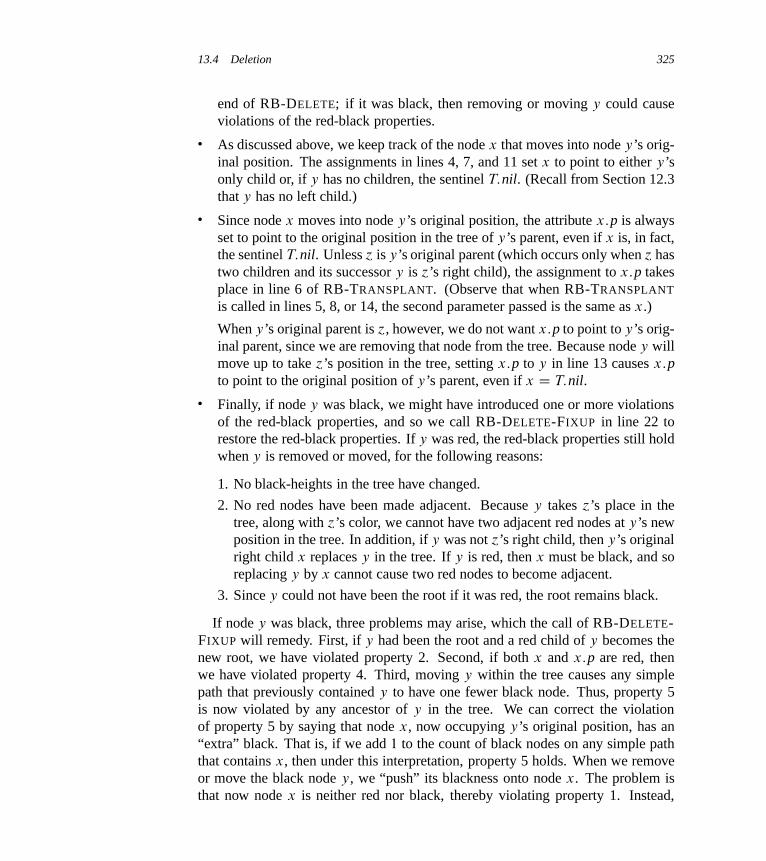
13.4 Deletion 325
end of RB-DELETE; if it was black, then removing or moving y could causeviolations of the red-black properties.
� As discussed above, we keep track of the node x that moves into node y’s orig-inal position. The assignments in lines 4, 7, and 11 set x to point to either y’sonly child or, if y has no children, the sentinel T:nil. (Recall from Section 12.3that y has no left child.)
� Since node x moves into node y’s original position, the attribute x:p is alwaysset to point to the original position in the tree of y’s parent, even if x is, in fact,the sentinel T:nil. Unless ´ is y’s original parent (which occurs only when ´ hastwo children and its successor y is ´’s right child), the assignment to x:p takesplace in line 6 of RB-TRANSPLANT. (Observe that when RB-TRANSPLANT
is called in lines 5, 8, or 14, the second parameter passed is the same as x.)
When y’s original parent is ´, however, we do not want x:p to point to y’s orig-inal parent, since we are removing that node from the tree. Because node y willmove up to take ´’s position in the tree, setting x:p to y in line 13 causes x:pto point to the original position of y’s parent, even if x D T:nil.
� Finally, if node y was black, we might have introduced one or more violationsof the red-black properties, and so we call RB-DELETE-FIXUP in line 22 torestore the red-black properties. If y was red, the red-black properties still holdwhen y is removed or moved, for the following reasons:
1. No black-heights in the tree have changed.
2. No red nodes have been made adjacent. Because y takes ´’s place in thetree, along with ´’s color, we cannot have two adjacent red nodes at y’s newposition in the tree. In addition, if y was not ´’s right child, then y’s originalright child x replaces y in the tree. If y is red, then x must be black, and soreplacing y by x cannot cause two red nodes to become adjacent.
3. Since y could not have been the root if it was red, the root remains black.
If node y was black, three problems may arise, which the call of RB-DELETE-FIXUP will remedy. First, if y had been the root and a red child of y becomes thenew root, we have violated property 2. Second, if both x and x:p are red, thenwe have violated property 4. Third, moving y within the tree causes any simplepath that previously contained y to have one fewer black node. Thus, property 5is now violated by any ancestor of y in the tree. We can correct the violationof property 5 by saying that node x, now occupying y’s original position, has an“extra” black. That is, if we add 1 to the count of black nodes on any simple paththat contains x, then under this interpretation, property 5 holds. When we removeor move the black node y, we “push” its blackness onto node x. The problem isthat now node x is neither red nor black, thereby violating property 1. Instead,
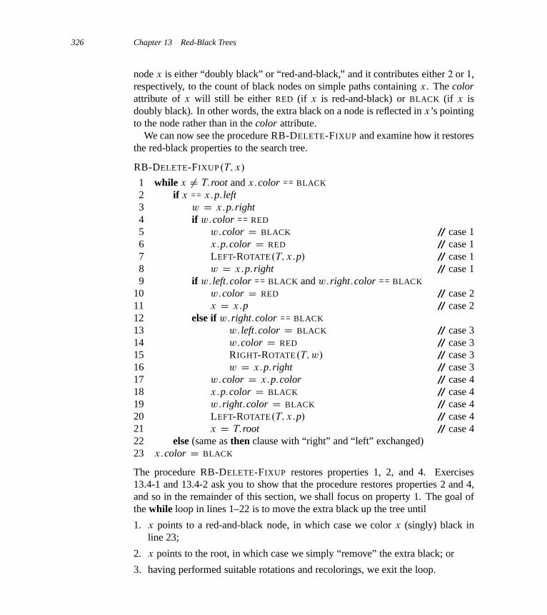
326 Chapter 13 Red-Black Trees
node x is either “doubly black” or “red-and-black,” and it contributes either 2 or 1,respectively, to the count of black nodes on simple paths containing x. The colorattribute of x will still be either RED (if x is red-and-black) or BLACK (if x isdoubly black). In other words, the extra black on a node is reflected in x’s pointingto the node rather than in the color attribute.
We can now see the procedure RB-DELETE-FIXUP and examine how it restoresthe red-black properties to the search tree.
RB-DELETE-FIXUP.T; x/
1 while x ¤ T:root and x:color == BLACK
2 if x == x:p: left3 w D x:p:right4 if w:color == RED
5 w:color D BLACK // case 16 x:p:color D RED // case 17 LEFT-ROTATE.T; x:p/ // case 18 w D x:p:right // case 19 if w: left:color == BLACK and w:right:color == BLACK
10 w:color D RED // case 211 x D x:p // case 212 else if w:right:color == BLACK
13 w: left:color D BLACK // case 314 w:color D RED // case 315 RIGHT-ROTATE.T; w/ // case 316 w D x:p:right // case 317 w:color D x:p:color // case 418 x:p:color D BLACK // case 419 w:right:color D BLACK // case 420 LEFT-ROTATE.T; x:p/ // case 421 x D T:root // case 422 else (same as then clause with “right” and “left” exchanged)23 x:color D BLACK
The procedure RB-DELETE-FIXUP restores properties 1, 2, and 4. Exercises13.4-1 and 13.4-2 ask you to show that the procedure restores properties 2 and 4,and so in the remainder of this section, we shall focus on property 1. The goal ofthe while loop in lines 1–22 is to move the extra black up the tree until
1. x points to a red-and-black node, in which case we color x (singly) black inline 23;
2. x points to the root, in which case we simply “remove” the extra black; or
3. having performed suitable rotations and recolorings, we exit the loop.

13.4 Deletion 327
Within the while loop, x always points to a nonroot doubly black node. Wedetermine in line 2 whether x is a left child or a right child of its parent x:p. (Wehave given the code for the situation in which x is a left child; the situation inwhich x is a right child—line 22—is symmetric.) We maintain a pointer w tothe sibling of x. Since node x is doubly black, node w cannot be T:nil, becauseotherwise, the number of blacks on the simple path from x:p to the (singly black)leaf w would be smaller than the number on the simple path from x:p to x.
The four cases2 in the code appear in Figure 13.7. Before examining each casein detail, let’s look more generally at how we can verify that the transformationin each of the cases preserves property 5. The key idea is that in each case, thetransformation applied preserves the number of black nodes (including x’s extrablack) from (and including) the root of the subtree shown to each of the subtrees˛; ˇ; : : : ; �. Thus, if property 5 holds prior to the transformation, it continues tohold afterward. For example, in Figure 13.7(a), which illustrates case 1, the num-ber of black nodes from the root to either subtree ˛ or ˇ is 3, both before and afterthe transformation. (Again, remember that node x adds an extra black.) Similarly,the number of black nodes from the root to any of , ı, ", and � is 2, both be-fore and after the transformation. In Figure 13.7(b), the counting must involve thevalue c of the color attribute of the root of the subtree shown, which can be eitherRED or BLACK. If we define count.RED/ D 0 and count.BLACK/ D 1, then thenumber of black nodes from the root to ˛ is 2 C count.c/, both before and afterthe transformation. In this case, after the transformation, the new node x has colorattribute c, but this node is really either red-and-black (if c D RED) or doubly black(if c D BLACK). You can verify the other cases similarly (see Exercise 13.4-5).
Case 1: x’s sibling w is redCase 1 (lines 5–8 of RB-DELETE-FIXUP and Figure 13.7(a)) occurs when node w,the sibling of node x, is red. Since w must have black children, we can switch thecolors of w and x:p and then perform a left-rotation on x:p without violating anyof the red-black properties. The new sibling of x, which is one of w’s childrenprior to the rotation, is now black, and thus we have converted case 1 into case 2,3, or 4.
Cases 2, 3, and 4 occur when node w is black; they are distinguished by thecolors of w’s children.
2As in RB-INSERT-FIXUP, the cases in RB-DELETE-FIXUP are not mutually exclusive.
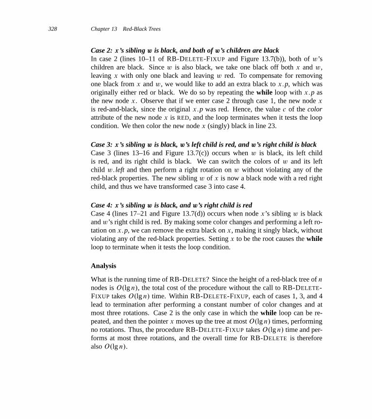
328 Chapter 13 Red-Black Trees
Case 2: x’s sibling w is black, and both of w’s children are blackIn case 2 (lines 10–11 of RB-DELETE-FIXUP and Figure 13.7(b)), both of w’schildren are black. Since w is also black, we take one black off both x and w,leaving x with only one black and leaving w red. To compensate for removingone black from x and w, we would like to add an extra black to x:p, which wasoriginally either red or black. We do so by repeating the while loop with x:p asthe new node x. Observe that if we enter case 2 through case 1, the new node x
is red-and-black, since the original x:p was red. Hence, the value c of the colorattribute of the new node x is RED, and the loop terminates when it tests the loopcondition. We then color the new node x (singly) black in line 23.
Case 3: x’s sibling w is black, w’s left child is red, and w’s right child is blackCase 3 (lines 13–16 and Figure 13.7(c)) occurs when w is black, its left childis red, and its right child is black. We can switch the colors of w and its leftchild w: left and then perform a right rotation on w without violating any of thered-black properties. The new sibling w of x is now a black node with a red rightchild, and thus we have transformed case 3 into case 4.
Case 4: x’s sibling w is black, and w’s right child is redCase 4 (lines 17–21 and Figure 13.7(d)) occurs when node x’s sibling w is blackand w’s right child is red. By making some color changes and performing a left ro-tation on x:p, we can remove the extra black on x, making it singly black, withoutviolating any of the red-black properties. Setting x to be the root causes the whileloop to terminate when it tests the loop condition.
Analysis
What is the running time of RB-DELETE? Since the height of a red-black tree of n
nodes is O.lg n/, the total cost of the procedure without the call to RB-DELETE-FIXUP takes O.lg n/ time. Within RB-DELETE-FIXUP, each of cases 1, 3, and 4lead to termination after performing a constant number of color changes and atmost three rotations. Case 2 is the only case in which the while loop can be re-peated, and then the pointer x moves up the tree at most O.lg n/ times, performingno rotations. Thus, the procedure RB-DELETE-FIXUP takes O.lg n/ time and per-forms at most three rotations, and the overall time for RB-DELETE is thereforealso O.lg n/.
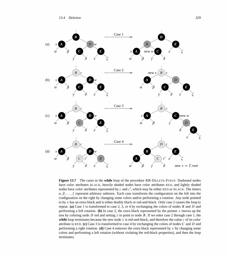
13.4 Deletion 329
A
B
D
C Eα β
γ δ ε ζ
x w
A
B
C
D
E
x new w
α β γ δ
ε ζ
A
B
D
C Eα β
γ δ ε ζ
x w
c
A
B
D
C Eα β
γ δ ε ζ
cnew x
A
B
D
C Eα β
γ δ ε ζ
x w
c
A
B
C
Dα β γ
δ
ε ζ
x
c
new w
A
B
D
C Eα β
γ δ
ε ζ
x w
c c
α β
A
B
C
D
E(d)
(c)
(b)
(a)
γ δ ε ζ
Case 4
Case 3
Case 2
Case 1
E
c′ c′
new x D T:root
Figure 13.7 The cases in the while loop of the procedure RB-DELETE-FIXUP. Darkened nodeshave color attributes BLACK, heavily shaded nodes have color attributes RED, and lightly shadednodes have color attributes represented by c and c0, which may be either RED or BLACK. The letters˛; ˇ; : : : ; � represent arbitrary subtrees. Each case transforms the configuration on the left into theconfiguration on the right by changing some colors and/or performing a rotation. Any node pointedto by x has an extra black and is either doubly black or red-and-black. Only case 2 causes the loop torepeat. (a) Case 1 is transformed to case 2, 3, or 4 by exchanging the colors of nodes B and D andperforming a left rotation. (b) In case 2, the extra black represented by the pointer x moves up thetree by coloring node D red and setting x to point to node B . If we enter case 2 through case 1, thewhile loop terminates because the new node x is red-and-black, and therefore the value c of its colorattribute is RED. (c) Case 3 is transformed to case 4 by exchanging the colors of nodes C and D andperforming a right rotation. (d) Case 4 removes the extra black represented by x by changing somecolors and performing a left rotation (without violating the red-black properties), and then the loopterminates.
330 Chapter 13 Red-Black Trees
Exercises
13.4-1Argue that after executing RB-DELETE-FIXUP, the root of the tree must be black.
13.4-2Argue that if in RB-DELETE both x and x:p are red, then property 4 is restored bythe call to RB-DELETE-FIXUP.T; x/.
13.4-3In Exercise 13.3-2, you found the red-black tree that results from successivelyinserting the keys 41; 38; 31; 12; 19; 8 into an initially empty tree. Now show thered-black trees that result from the successive deletion of the keys in the order8; 12; 19; 31; 38; 41.
13.4-4In which lines of the code for RB-DELETE-FIXUP might we examine or modifythe sentinel T:nil?
13.4-5In each of the cases of Figure 13.7, give the count of black nodes from the root ofthe subtree shown to each of the subtrees ˛; ˇ; : : : ; �, and verify that each countremains the same after the transformation. When a node has a color attribute c
or c 0, use the notation count.c/ or count.c 0/ symbolically in your count.
13.4-6Professors Skelton and Baron are concerned that at the start of case 1 of RB-DELETE-FIXUP, the node x:p might not be black. If the professors are correct,then lines 5–6 are wrong. Show that x:p must be black at the start of case 1, so thatthe professors have nothing to worry about.
13.4-7Suppose that a node x is inserted into a red-black tree with RB-INSERT and thenimmediately deleted with RB-DELETE. Is the resulting red-black tree the same asthe initial red-black tree? Justify your answer.
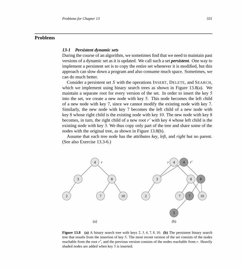
Problems for Chapter 13 331
Problems
13-1 Persistent dynamic setsDuring the course of an algorithm, we sometimes find that we need to maintain pastversions of a dynamic set as it is updated. We call such a set persistent. One way toimplement a persistent set is to copy the entire set whenever it is modified, but thisapproach can slow down a program and also consume much space. Sometimes, wecan do much better.
Consider a persistent set S with the operations INSERT, DELETE, and SEARCH,which we implement using binary search trees as shown in Figure 13.8(a). Wemaintain a separate root for every version of the set. In order to insert the key 5
into the set, we create a new node with key 5. This node becomes the left childof a new node with key 7, since we cannot modify the existing node with key 7.Similarly, the new node with key 7 becomes the left child of a new node withkey 8 whose right child is the existing node with key 10. The new node with key 8
becomes, in turn, the right child of a new root r 0 with key 4 whose left child is theexisting node with key 3. We thus copy only part of the tree and share some of thenodes with the original tree, as shown in Figure 13.8(b).
Assume that each tree node has the attributes key, left, and right but no parent.(See also Exercise 13.3-6.)
4
3
2
8
7 10
4
3
2
8
7 10
4
8
7
5
(b)(a)
r r r′
Figure 13.8 (a) A binary search tree with keys 2; 3; 4; 7; 8; 10. (b) The persistent binary searchtree that results from the insertion of key 5. The most recent version of the set consists of the nodesreachable from the root r 0, and the previous version consists of the nodes reachable from r . Heavilyshaded nodes are added when key 5 is inserted.

332 Chapter 13 Red-Black Trees
a. For a general persistent binary search tree, identify the nodes that we needchange to insert a key k or delete a node y.
b. Write a procedure PERSISTENT-TREE-INSERT that, given a persistent tree T
and a key k to insert, returns a new persistent tree T 0 that is the result of insert-ing k into T .
c. If the height of the persistent binary search tree T is h, what are the time andspace requirements of your implementation of PERSISTENT-TREE-INSERT?(The space requirement is proportional to the number of new nodes allocated.)
d. Suppose that we had included the parent attribute in each node. In this case,PERSISTENT-TREE-INSERT would need to perform additional copying. Provethat PERSISTENT-TREE-INSERT would then require �.n/ time and space,where n is the number of nodes in the tree.
e. Show how to use red-black trees to guarantee that the worst-case running timeand space are O.lg n/ per insertion or deletion.
13-2 Join operation on red-black treesThe join operation takes two dynamic sets S1 and S2 and an element x such thatfor any x1 2 S1 and x2 2 S2, we have x1:key � x:key � x2:key. It returns a setS D S1 [ fxg [ S2. In this problem, we investigate how to implement the joinoperation on red-black trees.
a. Given a red-black tree T , let us store its black-height as the new attribute T:bh.Argue that RB-INSERT and RB-DELETE can maintain the bh attribute with-out requiring extra storage in the nodes of the tree and without increasing theasymptotic running times. Show that while descending through T , we can de-termine the black-height of each node we visit in O.1/ time per node visited.
We wish to implement the operation RB-JOIN.T1; x; T2/, which destroys T1 and T2
and returns a red-black tree T D T1[fxg[T2. Let n be the total number of nodesin T1 and T2.
b. Assume that T1:bh � T2:bh. Describe an O.lg n/-time algorithm that finds ablack node y in T1 with the largest key from among those nodes whose black-height is T2:bh.
c. Let Ty be the subtree rooted at y. Describe how Ty [ fxg [ T2 can replace Ty
in O.1/ time without destroying the binary-search-tree property.
d. What color should we make x so that red-black properties 1, 3, and 5 are main-tained? Describe how to enforce properties 2 and 4 in O.lg n/ time.
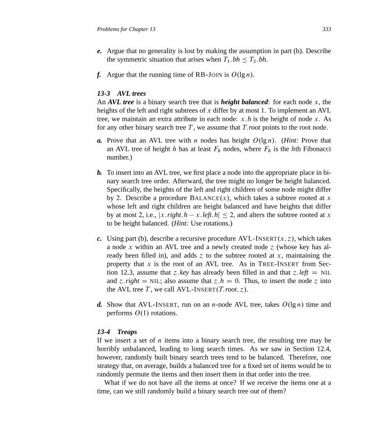
Problems for Chapter 13 333
e. Argue that no generality is lost by making the assumption in part (b). Describethe symmetric situation that arises when T1:bh � T2:bh.
f. Argue that the running time of RB-JOIN is O.lg n/.
13-3 AVL treesAn AVL tree is a binary search tree that is height balanced: for each node x, theheights of the left and right subtrees of x differ by at most 1. To implement an AVLtree, we maintain an extra attribute in each node: x:h is the height of node x. Asfor any other binary search tree T , we assume that T:root points to the root node.
a. Prove that an AVL tree with n nodes has height O.lg n/. (Hint: Prove thatan AVL tree of height h has at least Fh nodes, where Fh is the hth Fibonaccinumber.)
b. To insert into an AVL tree, we first place a node into the appropriate place in bi-nary search tree order. Afterward, the tree might no longer be height balanced.Specifically, the heights of the left and right children of some node might differby 2. Describe a procedure BALANCE.x/, which takes a subtree rooted at x
whose left and right children are height balanced and have heights that differby at most 2, i.e., jx:right:h� x: left:hj � 2, and alters the subtree rooted at x
to be height balanced. (Hint: Use rotations.)
c. Using part (b), describe a recursive procedure AVL-INSERT.x; ´/, which takesa node x within an AVL tree and a newly created node ´ (whose key has al-ready been filled in), and adds ´ to the subtree rooted at x, maintaining theproperty that x is the root of an AVL tree. As in TREE-INSERT from Sec-tion 12.3, assume that ´:key has already been filled in and that ´: left D NIL
and ´:right D NIL; also assume that ´:h D 0. Thus, to insert the node ´ intothe AVL tree T , we call AVL-INSERT.T:root; ´/.
d. Show that AVL-INSERT, run on an n-node AVL tree, takes O.lg n/ time andperforms O.1/ rotations.
13-4 TreapsIf we insert a set of n items into a binary search tree, the resulting tree may behorribly unbalanced, leading to long search times. As we saw in Section 12.4,however, randomly built binary search trees tend to be balanced. Therefore, onestrategy that, on average, builds a balanced tree for a fixed set of items would be torandomly permute the items and then insert them in that order into the tree.
What if we do not have all the items at once? If we receive the items one at atime, can we still randomly build a binary search tree out of them?

334 Chapter 13 Red-Black Trees
G: 4
B: 7 H: 5
A: 10 E: 23 K: 65
I: 73
Figure 13.9 A treap. Each node x is labeled with x:key : x:priority. For example, the root haskey G and priority 4.
We will examine a data structure that answers this question in the affirmative. Atreap is a binary search tree with a modified way of ordering the nodes. Figure 13.9shows an example. As usual, each node x in the tree has a key value x:key. Inaddition, we assign x:priority, which is a random number chosen independentlyfor each node. We assume that all priorities are distinct and also that all keys aredistinct. The nodes of the treap are ordered so that the keys obey the binary-search-tree property and the priorities obey the min-heap order property:
� If � is a left child of u, then �:key < u:key.
� If � is a right child of u, then �:key > u:key.
� If � is a child of u, then �:priority > u:priority.
(This combination of properties is why the tree is called a “treap”: it has featuresof both a binary search tree and a heap.)
It helps to think of treaps in the following way. Suppose that we insert nodesx1; x2; : : : ; xn, with associated keys, into a treap. Then the resulting treap is thetree that would have been formed if the nodes had been inserted into a normalbinary search tree in the order given by their (randomly chosen) priorities, i.e.,xi :priority < xj :priority means that we had inserted xi before xj .
a. Show that given a set of nodes x1; x2; : : : ; xn, with associated keys and priori-ties, all distinct, the treap associated with these nodes is unique.
b. Show that the expected height of a treap is ‚.lg n/, and hence the expected timeto search for a value in the treap is ‚.lg n/.
Let us see how to insert a new node into an existing treap. The first thing we dois assign to the new node a random priority. Then we call the insertion algorithm,which we call TREAP-INSERT, whose operation is illustrated in Figure 13.10.
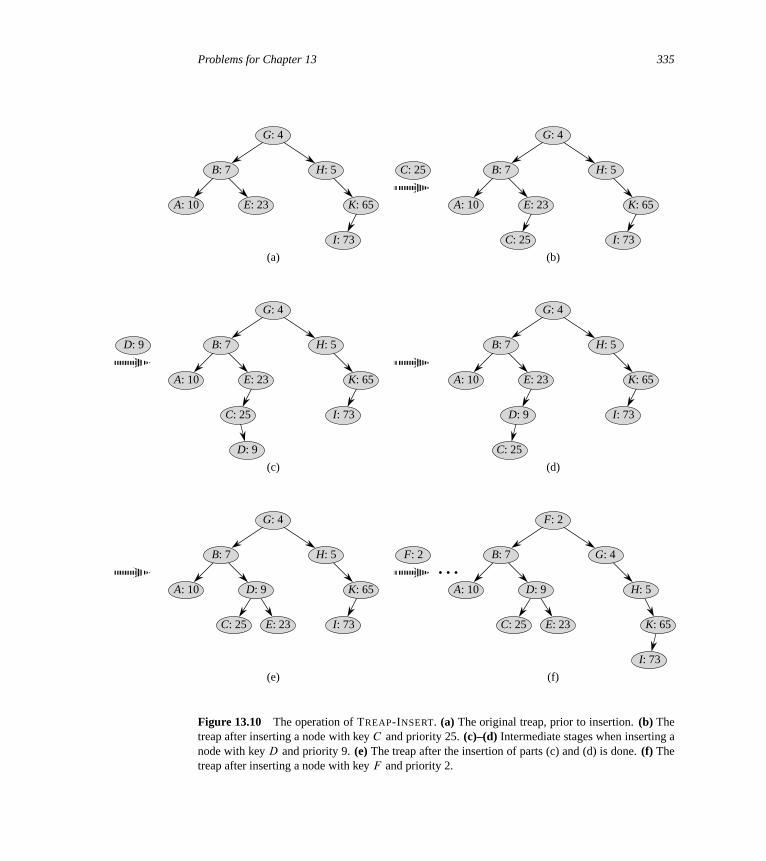
Problems for Chapter 13 335
G: 4
B: 7 H: 5
A: 10 E: 23 K: 65
I: 73
G: 4
B: 7 H: 5
A: 10 E: 23 K: 65
I: 73
C: 25
C: 25
(a) (b)
G: 4
B: 7 H: 5
A: 10 E: 23 K: 65
I: 73C: 25
(c)
D: 9
D: 9
G: 4
B: 7 H: 5
A: 10 E: 23 K: 65
I: 73
(d)
D: 9
C: 25
G: 4
B: 7 H: 5
A: 10 K: 65
I: 73
(e)
D: 9
C: 25 E: 23
B: 7
A: 10
(f)
D: 9
C: 25 E: 23
F: 2
I: 73
K: 65
H: 5
G: 4
F: 2
…
Figure 13.10 The operation of TREAP-INSERT. (a) The original treap, prior to insertion. (b) Thetreap after inserting a node with key C and priority 25. (c)–(d) Intermediate stages when inserting anode with key D and priority 9. (e) The treap after the insertion of parts (c) and (d) is done. (f) Thetreap after inserting a node with key F and priority 2.

336 Chapter 13 Red-Black Trees
15
9 18
3 12 25
216
(a)
15
9 18
3 12 25
216
(b)
Figure 13.11 Spines of a binary search tree. The left spine is shaded in (a), and the right spine isshaded in (b).
c. Explain how TREAP-INSERT works. Explain the idea in English and give pseu-docode. (Hint: Execute the usual binary-search-tree insertion procedure andthen perform rotations to restore the min-heap order property.)
d. Show that the expected running time of TREAP-INSERT is ‚.lg n/.
TREAP-INSERT performs a search and then a sequence of rotations. Althoughthese two operations have the same expected running time, they have differentcosts in practice. A search reads information from the treap without modifying it.In contrast, a rotation changes parent and child pointers within the treap. On mostcomputers, read operations are much faster than write operations. Thus we wouldlike TREAP-INSERT to perform few rotations. We will show that the expectednumber of rotations performed is bounded by a constant.
In order to do so, we will need some definitions, which Figure 13.11 depicts.The left spine of a binary search tree T is the simple path from the root to the nodewith the smallest key. In other words, the left spine is the simple path from theroot that consists of only left edges. Symmetrically, the right spine of T is thesimple path from the root consisting of only right edges. The length of a spine isthe number of nodes it contains.
e. Consider the treap T immediately after TREAP-INSERT has inserted node x.Let C be the length of the right spine of the left subtree of x. Let D be thelength of the left spine of the right subtree of x. Prove that the total number ofrotations that were performed during the insertion of x is equal to C CD.
We will now calculate the expected values of C and D. Without loss of generality,we assume that the keys are 1; 2; : : : ; n, since we are comparing them only to oneanother.
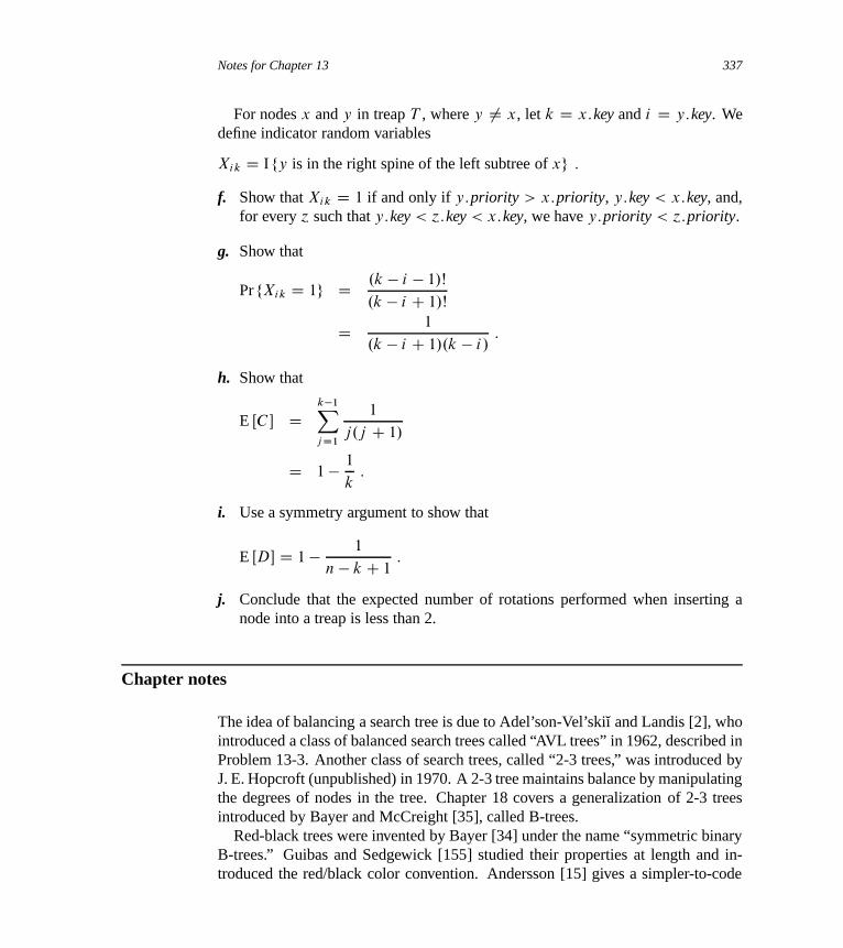
Notes for Chapter 13 337
For nodes x and y in treap T , where y ¤ x, let k D x:key and i D y:key. Wedefine indicator random variables
Xik D I fy is in the right spine of the left subtree of xg :
f. Show that Xik D 1 if and only if y:priority > x:priority, y:key < x:key, and,for every ´ such that y:key < ´:key < x:key, we have y:priority < ´:priority.
g. Show that
Pr fXik D 1g D .k � i � 1/Š
.k � i C 1/Š
D 1
.k � i C 1/.k � i/:
h. Show that
E ŒC � Dk�1Xj D1
1
j.j C 1/
D 1� 1
k:
i. Use a symmetry argument to show that
E ŒD� D 1 � 1
n � k C 1:
j. Conclude that the expected number of rotations performed when inserting anode into a treap is less than 2.
Chapter notes
The idea of balancing a search tree is due to Adel’son-Vel’skiı̆ and Landis [2], whointroduced a class of balanced search trees called “AVL trees” in 1962, described inProblem 13-3. Another class of search trees, called “2-3 trees,” was introduced byJ. E. Hopcroft (unpublished) in 1970. A 2-3 tree maintains balance by manipulatingthe degrees of nodes in the tree. Chapter 18 covers a generalization of 2-3 treesintroduced by Bayer and McCreight [35], called B-trees.
Red-black trees were invented by Bayer [34] under the name “symmetric binaryB-trees.” Guibas and Sedgewick [155] studied their properties at length and in-troduced the red/black color convention. Andersson [15] gives a simpler-to-code
338 Chapter 13 Red-Black Trees
variant of red-black trees. Weiss [351] calls this variant AA-trees. An AA-tree issimilar to a red-black tree except that left children may never be red.
Treaps, the subject of Problem 13-4, were proposed by Seidel and Aragon [309].They are the default implementation of a dictionary in LEDA [253], which is awell-implemented collection of data structures and algorithms.
There are many other variations on balanced binary trees, including weight-balanced trees [264], k-neighbor trees [245], and scapegoat trees [127]. Perhapsthe most intriguing are the “splay trees” introduced by Sleator and Tarjan [320],which are “self-adjusting.” (See Tarjan [330] for a good description of splay trees.)Splay trees maintain balance without any explicit balance condition such as color.Instead, “splay operations” (which involve rotations) are performed within the treeevery time an access is made. The amortized cost (see Chapter 17) of each opera-tion on an n-node tree is O.lg n/.
Skip lists [286] provide an alternative to balanced binary trees. A skip list is alinked list that is augmented with a number of additional pointers. Each dictionaryoperation runs in expected time O.lg n/ on a skip list of n items.
14 Augmenting Data Structures
Some engineering situations require no more than a “textbook” data struc-ture—such as a doubly linked list, a hash table, or a binary search tree—but manyothers require a dash of creativity. Only in rare situations will you need to cre-ate an entirely new type of data structure, though. More often, it will suffice toaugment a textbook data structure by storing additional information in it. You canthen program new operations for the data structure to support the desired applica-tion. Augmenting a data structure is not always straightforward, however, since theadded information must be updated and maintained by the ordinary operations onthe data structure.
This chapter discusses two data structures that we construct by augmenting red-black trees. Section 14.1 describes a data structure that supports general order-statistic operations on a dynamic set. We can then quickly find the i th smallestnumber in a set or the rank of a given element in the total ordering of the set.Section 14.2 abstracts the process of augmenting a data structure and provides atheorem that can simplify the process of augmenting red-black trees. Section 14.3uses this theorem to help design a data structure for maintaining a dynamic set ofintervals, such as time intervals. Given a query interval, we can then quickly findan interval in the set that overlaps it.
14.1 Dynamic order statistics
Chapter 9 introduced the notion of an order statistic. Specifically, the i th orderstatistic of a set of n elements, where i 2 f1; 2; : : : ; ng, is simply the element in theset with the i th smallest key. We saw how to determine any order statistic in O.n/
time from an unordered set. In this section, we shall see how to modify red-blacktrees so that we can determine any order statistic for a dynamic set in O.lg n/ time.We shall also see how to compute the rank of an element—its position in the linearorder of the set—in O.lg n/ time.
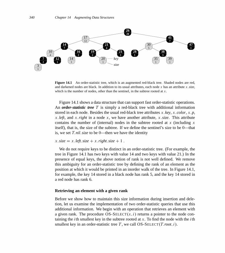
340 Chapter 14 Augmenting Data Structures
13
7 12
10
14
16
14
2 1 1
24
7
20
19 21
21
17
28
35 39
38
4730
41
26
1
2 1
4
12
1
1 1
3
5 1
7
20
key
size
Figure 14.1 An order-statistic tree, which is an augmented red-black tree. Shaded nodes are red,and darkened nodes are black. In addition to its usual attributes, each node x has an attribute x:size,which is the number of nodes, other than the sentinel, in the subtree rooted at x.
Figure 14.1 shows a data structure that can support fast order-statistic operations.An order-statistic tree T is simply a red-black tree with additional informationstored in each node. Besides the usual red-black tree attributes x:key, x:color, x:p,x: left, and x:right in a node x, we have another attribute, x:size. This attributecontains the number of (internal) nodes in the subtree rooted at x (including x
itself), that is, the size of the subtree. If we define the sentinel’s size to be 0—thatis, we set T:nil:size to be 0—then we have the identity
x:size D x: left:sizeC x:right:sizeC 1 :
We do not require keys to be distinct in an order-statistic tree. (For example, thetree in Figure 14.1 has two keys with value 14 and two keys with value 21.) In thepresence of equal keys, the above notion of rank is not well defined. We removethis ambiguity for an order-statistic tree by defining the rank of an element as theposition at which it would be printed in an inorder walk of the tree. In Figure 14.1,for example, the key 14 stored in a black node has rank 5, and the key 14 stored ina red node has rank 6.
Retrieving an element with a given rank
Before we show how to maintain this size information during insertion and dele-tion, let us examine the implementation of two order-statistic queries that use thisadditional information. We begin with an operation that retrieves an element witha given rank. The procedure OS-SELECT.x; i/ returns a pointer to the node con-taining the i th smallest key in the subtree rooted at x. To find the node with the i thsmallest key in an order-statistic tree T , we call OS-SELECT.T:root; i/.
14.1 Dynamic order statistics 341
OS-SELECT.x; i/
1 r D x: left:sizeC 1
2 if i == r
3 return x
4 elseif i < r
5 return OS-SELECT.x: left; i/
6 else return OS-SELECT.x:right; i � r/
In line 1 of OS-SELECT, we compute r , the rank of node x within the subtreerooted at x. The value of x: left:size is the number of nodes that come before x
in an inorder tree walk of the subtree rooted at x. Thus, x: left:size C 1 is therank of x within the subtree rooted at x. If i D r , then node x is the i th smallestelement, and so we return x in line 3. If i < r , then the i th smallest elementresides in x’s left subtree, and so we recurse on x: left in line 5. If i > r , thenthe i th smallest element resides in x’s right subtree. Since the subtree rooted at x
contains r elements that come before x’s right subtree in an inorder tree walk, thei th smallest element in the subtree rooted at x is the .i � r/th smallest element inthe subtree rooted at x:right. Line 6 determines this element recursively.
To see how OS-SELECT operates, consider a search for the 17th smallest ele-ment in the order-statistic tree of Figure 14.1. We begin with x as the root, whosekey is 26, and with i D 17. Since the size of 26’s left subtree is 12, its rank is 13.Thus, we know that the node with rank 17 is the 17 � 13 D 4th smallest elementin 26’s right subtree. After the recursive call, x is the node with key 41, and i D 4.Since the size of 41’s left subtree is 5, its rank within its subtree is 6. Thus, weknow that the node with rank 4 is the 4th smallest element in 41’s left subtree. Af-ter the recursive call, x is the node with key 30, and its rank within its subtree is 2.Thus, we recurse once again to find the 4�2 D 2nd smallest element in the subtreerooted at the node with key 38. We now find that its left subtree has size 1, whichmeans it is the second smallest element. Thus, the procedure returns a pointer tothe node with key 38.
Because each recursive call goes down one level in the order-statistic tree, thetotal time for OS-SELECT is at worst proportional to the height of the tree. Sincethe tree is a red-black tree, its height is O.lg n/, where n is the number of nodes.Thus, the running time of OS-SELECT is O.lg n/ for a dynamic set of n elements.
Determining the rank of an element
Given a pointer to a node x in an order-statistic tree T , the procedure OS-RANK
returns the position of x in the linear order determined by an inorder tree walkof T .

342 Chapter 14 Augmenting Data Structures
OS-RANK.T; x/
1 r D x: left:sizeC 1
2 y D x
3 while y ¤ T:root4 if y == y:p:right5 r D r C y:p: left:sizeC 1
6 y D y:p7 return r
The procedure works as follows. We can think of node x’s rank as the number ofnodes preceding x in an inorder tree walk, plus 1 for x itself. OS-RANK maintainsthe following loop invariant:
At the start of each iteration of the while loop of lines 3–6, r is the rankof x:key in the subtree rooted at node y.
We use this loop invariant to show that OS-RANK works correctly as follows:
Initialization: Prior to the first iteration, line 1 sets r to be the rank of x:key withinthe subtree rooted at x. Setting y D x in line 2 makes the invariant true thefirst time the test in line 3 executes.
Maintenance: At the end of each iteration of the while loop, we set y D y:p.Thus we must show that if r is the rank of x:key in the subtree rooted at y at thestart of the loop body, then r is the rank of x:key in the subtree rooted at y:pat the end of the loop body. In each iteration of the while loop, we considerthe subtree rooted at y:p. We have already counted the number of nodes in thesubtree rooted at node y that precede x in an inorder walk, and so we must addthe nodes in the subtree rooted at y’s sibling that precede x in an inorder walk,plus 1 for y:p if it, too, precedes x. If y is a left child, then neither y:p nor anynode in y:p’s right subtree precedes x, and so we leave r alone. Otherwise, y isa right child and all the nodes in y:p’s left subtree precede x, as does y:p itself.Thus, in line 5, we add y:p: left:sizeC 1 to the current value of r .
Termination: The loop terminates when y D T:root, so that the subtree rootedat y is the entire tree. Thus, the value of r is the rank of x:key in the entire tree.
As an example, when we run OS-RANK on the order-statistic tree of Figure 14.1to find the rank of the node with key 38, we get the following sequence of valuesof y:key and r at the top of the while loop:
iteration y:key r
1 38 22 30 43 41 44 26 17

14.1 Dynamic order statistics 343
The procedure returns the rank 17.Since each iteration of the while loop takes O.1/ time, and y goes up one level in
the tree with each iteration, the running time of OS-RANK is at worst proportionalto the height of the tree: O.lg n/ on an n-node order-statistic tree.
Maintaining subtree sizes
Given the size attribute in each node, OS-SELECT and OS-RANK can quicklycompute order-statistic information. But unless we can efficiently maintain theseattributes within the basic modifying operations on red-black trees, our work willhave been for naught. We shall now show how to maintain subtree sizes for bothinsertion and deletion without affecting the asymptotic running time of either op-eration.
We noted in Section 13.3 that insertion into a red-black tree consists of twophases. The first phase goes down the tree from the root, inserting the new nodeas a child of an existing node. The second phase goes up the tree, changing colorsand performing rotations to maintain the red-black properties.
To maintain the subtree sizes in the first phase, we simply increment x:size foreach node x on the simple path traversed from the root down toward the leaves. Thenew node added gets a size of 1. Since there are O.lg n/ nodes on the traversedpath, the additional cost of maintaining the size attributes is O.lg n/.
In the second phase, the only structural changes to the underlying red-black treeare caused by rotations, of which there are at most two. Moreover, a rotation isa local operation: only two nodes have their size attributes invalidated. The linkaround which the rotation is performed is incident on these two nodes. Referringto the code for LEFT-ROTATE.T; x/ in Section 13.2, we add the following lines:
13 y:size D x:size14 x:size D x: left:sizeC x:right:sizeC 1
Figure 14.2 illustrates how the attributes are updated. The change to RIGHT-ROTATE is symmetric.
Since at most two rotations are performed during insertion into a red-black tree,we spend only O.1/ additional time updating size attributes in the second phase.Thus, the total time for insertion into an n-node order-statistic tree is O.lg n/,which is asymptotically the same as for an ordinary red-black tree.
Deletion from a red-black tree also consists of two phases: the first operateson the underlying search tree, and the second causes at most three rotations andotherwise performs no structural changes. (See Section 13.4.) The first phaseeither removes one node y from the tree or moves upward it within the tree. Toupdate the subtree sizes, we simply traverse a simple path from node y (startingfrom its original position within the tree) up to the root, decrementing the size
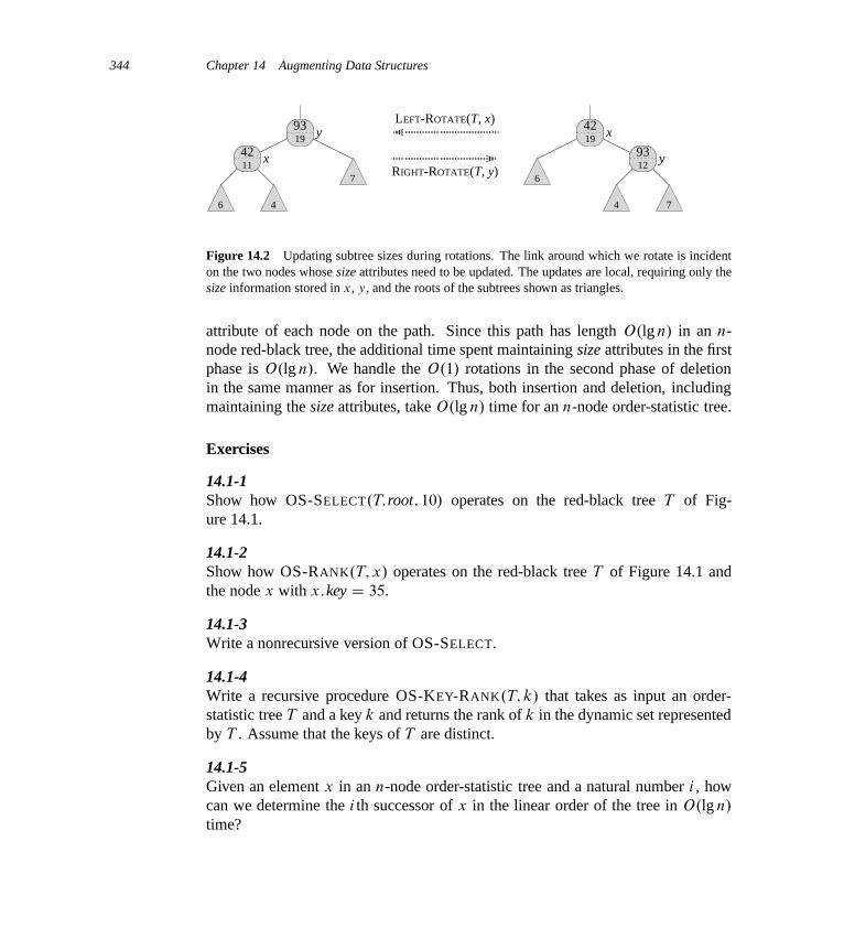
344 Chapter 14 Augmenting Data Structures
LEFT-ROTATE(T, x)
RIGHT-ROTATE(T, y)
9319
y
4211
x
6 4
7
93
4219
126
4 7
x
y
Figure 14.2 Updating subtree sizes during rotations. The link around which we rotate is incidenton the two nodes whose size attributes need to be updated. The updates are local, requiring only thesize information stored in x, y, and the roots of the subtrees shown as triangles.
attribute of each node on the path. Since this path has length O.lg n/ in an n-node red-black tree, the additional time spent maintaining size attributes in the firstphase is O.lg n/. We handle the O.1/ rotations in the second phase of deletionin the same manner as for insertion. Thus, both insertion and deletion, includingmaintaining the size attributes, take O.lg n/ time for an n-node order-statistic tree.
Exercises
14.1-1Show how OS-SELECT.T:root; 10/ operates on the red-black tree T of Fig-ure 14.1.
14.1-2Show how OS-RANK.T; x/ operates on the red-black tree T of Figure 14.1 andthe node x with x:key D 35.
14.1-3Write a nonrecursive version of OS-SELECT.
14.1-4Write a recursive procedure OS-KEY-RANK.T; k/ that takes as input an order-statistic tree T and a key k and returns the rank of k in the dynamic set representedby T . Assume that the keys of T are distinct.
14.1-5Given an element x in an n-node order-statistic tree and a natural number i , howcan we determine the i th successor of x in the linear order of the tree in O.lg n/
time?

14.2 How to augment a data structure 345
14.1-6Observe that whenever we reference the size attribute of a node in either OS-SELECT or OS-RANK, we use it only to compute a rank. Accordingly, supposewe store in each node its rank in the subtree of which it is the root. Show how tomaintain this information during insertion and deletion. (Remember that these twooperations can cause rotations.)
14.1-7Show how to use an order-statistic tree to count the number of inversions (seeProblem 2-4) in an array of size n in time O.n lg n/.
14.1-8 ?
Consider n chords on a circle, each defined by its endpoints. Describe an O.n lg n/-time algorithm to determine the number of pairs of chords that intersect inside thecircle. (For example, if the n chords are all diameters that meet at the center, thenthe correct answer is
�n
2
�.) Assume that no two chords share an endpoint.
14.2 How to augment a data structure
The process of augmenting a basic data structure to support additional functionalityoccurs quite frequently in algorithm design. We shall use it again in the next sectionto design a data structure that supports operations on intervals. In this section, weexamine the steps involved in such augmentation. We shall also prove a theoremthat allows us to augment red-black trees easily in many cases.
We can break the process of augmenting a data structure into four steps:
1. Choose an underlying data structure.
2. Determine additional information to maintain in the underlying data structure.
3. Verify that we can maintain the additional information for the basic modifyingoperations on the underlying data structure.
4. Develop new operations.
As with any prescriptive design method, you should not blindly follow the stepsin the order given. Most design work contains an element of trial and error, andprogress on all steps usually proceeds in parallel. There is no point, for example, indetermining additional information and developing new operations (steps 2 and 4)if we will not be able to maintain the additional information efficiently. Neverthe-less, this four-step method provides a good focus for your efforts in augmentinga data structure, and it is also a good way to organize the documentation of anaugmented data structure.

346 Chapter 14 Augmenting Data Structures
We followed these steps in Section 14.1 to design our order-statistic trees. Forstep 1, we chose red-black trees as the underlying data structure. A clue to thesuitability of red-black trees comes from their efficient support of other dynamic-set operations on a total order, such as MINIMUM, MAXIMUM, SUCCESSOR, andPREDECESSOR.
For step 2, we added the size attribute, in which each node x stores the size of thesubtree rooted at x. Generally, the additional information makes operations moreefficient. For example, we could have implemented OS-SELECT and OS-RANK
using just the keys stored in the tree, but they would not have run in O.lg n/ time.Sometimes, the additional information is pointer information rather than data, asin Exercise 14.2-1.
For step 3, we ensured that insertion and deletion could maintain the size at-tributes while still running in O.lg n/ time. Ideally, we should need to update onlya few elements of the data structure in order to maintain the additional information.For example, if we simply stored in each node its rank in the tree, the OS-SELECT
and OS-RANK procedures would run quickly, but inserting a new minimum ele-ment would cause a change to this information in every node of the tree. When westore subtree sizes instead, inserting a new element causes information to changein only O.lg n/ nodes.
For step 4, we developed the operations OS-SELECT and OS-RANK. After all,the need for new operations is why we bother to augment a data structure in the firstplace. Occasionally, rather than developing new operations, we use the additionalinformation to expedite existing ones, as in Exercise 14.2-1.
Augmenting red-black trees
When red-black trees underlie an augmented data structure, we can prove that in-sertion and deletion can always efficiently maintain certain kinds of additional in-formation, thereby making step 3 very easy. The proof of the following theorem issimilar to the argument from Section 14.1 that we can maintain the size attributefor order-statistic trees.
Theorem 14.1 (Augmenting a red-black tree)Let f be an attribute that augments a red-black tree T of n nodes, and suppose thatthe value of f for each node x depends on only the information in nodes x, x: left,and x:right, possibly including x: left: f and x:right: f . Then, we can maintain thevalues of f in all nodes of T during insertion and deletion without asymptoticallyaffecting the O.lg n/ performance of these operations.
Proof The main idea of the proof is that a change to an f attribute in a node x
propagates only to ancestors of x in the tree. That is, changing x: f may re-
14.2 How to augment a data structure 347
quire x:p: f to be updated, but nothing else; updating x:p: f may require x:p:p: fto be updated, but nothing else; and so on up the tree. Once we have updatedT:root: f , no other node will depend on the new value, and so the process termi-nates. Since the height of a red-black tree is O.lg n/, changing an f attribute in anode costs O.lg n/ time in updating all nodes that depend on the change.
Insertion of a node x into T consists of two phases. (See Section 13.3.) Thefirst phase inserts x as a child of an existing node x:p. We can compute the valueof x: f in O.1/ time since, by supposition, it depends only on information in theother attributes of x itself and the information in x’s children, but x’s children areboth the sentinel T:nil. Once we have computed x: f , the change propagates upthe tree. Thus, the total time for the first phase of insertion is O.lg n/. During thesecond phase, the only structural changes to the tree come from rotations. Sinceonly two nodes change in a rotation, the total time for updating the f attributesis O.lg n/ per rotation. Since the number of rotations during insertion is at mosttwo, the total time for insertion is O.lg n/.
Like insertion, deletion has two phases. (See Section 13.4.) In the first phase,changes to the tree occur when the deleted node is removed from the tree. If thedeleted node had two children at the time, then its successor moves into the positionof the deleted node. Propagating the updates to f caused by these changes costsat most O.lg n/, since the changes modify the tree locally. Fixing up the red-blacktree during the second phase requires at most three rotations, and each rotationrequires at most O.lg n/ time to propagate the updates to f . Thus, like insertion,the total time for deletion is O.lg n/.
In many cases, such as maintaining the size attributes in order-statistic trees, thecost of updating after a rotation is O.1/, rather than the O.lg n/ derived in the proofof Theorem 14.1. Exercise 14.2-3 gives an example.
Exercises
14.2-1Show, by adding pointers to the nodes, how to support each of the dynamic-setqueries MINIMUM, MAXIMUM, SUCCESSOR, and PREDECESSOR in O.1/ worst-case time on an augmented order-statistic tree. The asymptotic performance ofother operations on order-statistic trees should not be affected.
14.2-2Can we maintain the black-heights of nodes in a red-black tree as attributes in thenodes of the tree without affecting the asymptotic performance of any of the red-black tree operations? Show how, or argue why not. How about maintaining thedepths of nodes?
348 Chapter 14 Augmenting Data Structures
14.2-3 ?
Let˝ be an associative binary operator, and let a be an attribute maintained in eachnode of a red-black tree. Suppose that we want to include in each node x an addi-tional attribute f such that x: f D x1:a˝ x2:a˝ � � � ˝ xm:a, where x1; x2; : : : ; xm
is the inorder listing of nodes in the subtree rooted at x. Show how to update the f
attributes in O.1/ time after a rotation. Modify your argument slightly to apply itto the size attributes in order-statistic trees.
14.2-4 ?
We wish to augment red-black trees with an operation RB-ENUMERATE.x; a; b/
that outputs all the keys k such that a � k � b in a red-black tree rooted at x.Describe how to implement RB-ENUMERATE in ‚.mC lg n/ time, where m is thenumber of keys that are output and n is the number of internal nodes in the tree.(Hint: You do not need to add new attributes to the red-black tree.)
14.3 Interval trees
In this section, we shall augment red-black trees to support operations on dynamicsets of intervals. A closed interval is an ordered pair of real numbers Œt1; t2�, witht1 � t2. The interval Œt1; t2� represents the set ft 2 R W t1 � t � t2g. Open andhalf-open intervals omit both or one of the endpoints from the set, respectively. Inthis section, we shall assume that intervals are closed; extending the results to openand half-open intervals is conceptually straightforward.
Intervals are convenient for representing events that each occupy a continuousperiod of time. We might, for example, wish to query a database of time intervalsto find out what events occurred during a given interval. The data structure in thissection provides an efficient means for maintaining such an interval database.
We can represent an interval Œt1; t2� as an object i , with attributes i: low D t1(the low endpoint) and i:high D t2 (the high endpoint). We say that intervals i
and i 0 overlap if i \ i 0 ¤ ;, that is, if i: low � i 0:high and i 0: low � i:high. AsFigure 14.3 shows, any two intervals i and i 0 satisfy the interval trichotomy; thatis, exactly one of the following three properties holds:
a. i and i 0 overlap,
b. i is to the left of i 0 (i.e., i:high < i 0: low),
c. i is to the right of i 0 (i.e., i 0:high < i: low).
An interval tree is a red-black tree that maintains a dynamic set of elements, witheach element x containing an interval x: int. Interval trees support the followingoperations:
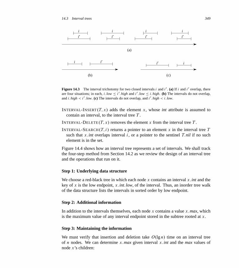
14.3 Interval trees 349
i i i i
(a)
i
(b)
i
(c)
i′ i′ i′ i′
i′i′
Figure 14.3 The interval trichotomy for two closed intervals i and i 0. (a) If i and i 0 overlap, thereare four situations; in each, i: low � i 0:high and i 0: low � i:high. (b) The intervals do not overlap,and i:high < i 0: low. (c) The intervals do not overlap, and i 0:high < i: low.
INTERVAL-INSERT.T; x/ adds the element x, whose int attribute is assumed tocontain an interval, to the interval tree T .
INTERVAL-DELETE.T; x/ removes the element x from the interval tree T .
INTERVAL-SEARCH.T; i/ returns a pointer to an element x in the interval tree T
such that x: int overlaps interval i , or a pointer to the sentinel T:nil if no suchelement is in the set.
Figure 14.4 shows how an interval tree represents a set of intervals. We shall trackthe four-step method from Section 14.2 as we review the design of an interval treeand the operations that run on it.
Step 1: Underlying data structure
We choose a red-black tree in which each node x contains an interval x: int and thekey of x is the low endpoint, x: int: low, of the interval. Thus, an inorder tree walkof the data structure lists the intervals in sorted order by low endpoint.
Step 2: Additional information
In addition to the intervals themselves, each node x contains a value x:max, whichis the maximum value of any interval endpoint stored in the subtree rooted at x.
Step 3: Maintaining the information
We must verify that insertion and deletion take O.lg n/ time on an interval treeof n nodes. We can determine x:max given interval x: int and the max values ofnode x’s children:
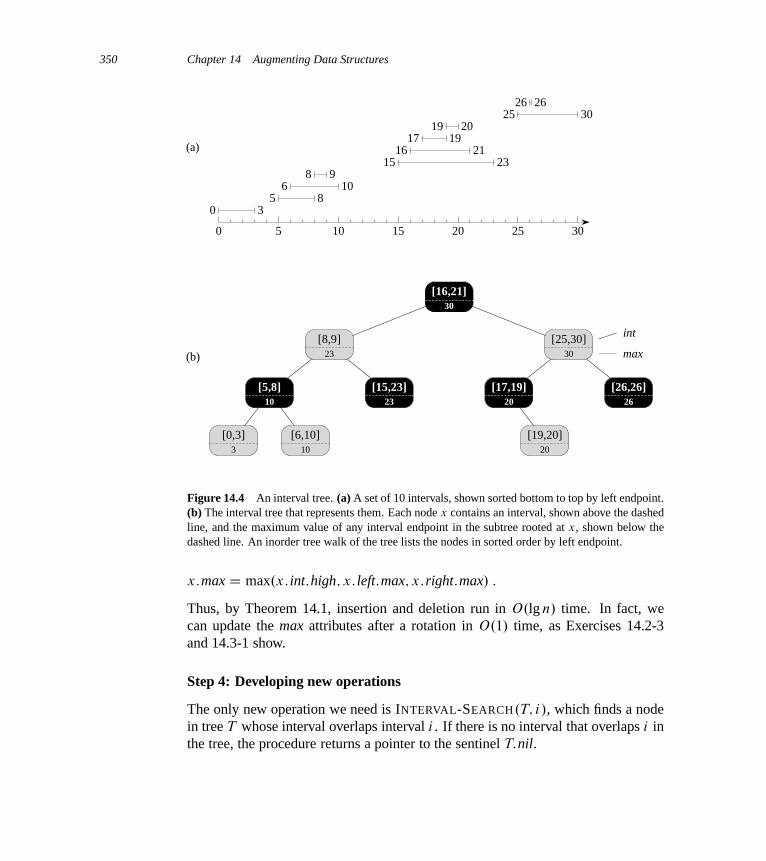
350 Chapter 14 Augmenting Data Structures
0 5 10 15 20 25 30
05
68
1516
1719
2526 26
3020
1921
239
108
3
(a)
[0,3]3
[6,10]10
[5,8]10
[8,9]23
[15,23]23
[16,21]30
[17,19]20
[26,26]26
[19,20]20
(b)
[25,30]30
int
max
Figure 14.4 An interval tree. (a) A set of 10 intervals, shown sorted bottom to top by left endpoint.(b) The interval tree that represents them. Each node x contains an interval, shown above the dashedline, and the maximum value of any interval endpoint in the subtree rooted at x, shown below thedashed line. An inorder tree walk of the tree lists the nodes in sorted order by left endpoint.
x:max D max.x: int:high; x: left:max; x:right:max/ :
Thus, by Theorem 14.1, insertion and deletion run in O.lg n/ time. In fact, wecan update the max attributes after a rotation in O.1/ time, as Exercises 14.2-3and 14.3-1 show.
Step 4: Developing new operations
The only new operation we need is INTERVAL-SEARCH.T; i/, which finds a nodein tree T whose interval overlaps interval i . If there is no interval that overlaps i inthe tree, the procedure returns a pointer to the sentinel T:nil.
14.3 Interval trees 351
INTERVAL-SEARCH.T; i/
1 x D T:root2 while x ¤ T:nil and i does not overlap x: int3 if x: left ¤ T:nil and x: left:max � i: low4 x D x: left5 else x D x:right6 return x
The search for an interval that overlaps i starts with x at the root of the tree andproceeds downward. It terminates when either it finds an overlapping interval or x
points to the sentinel T:nil. Since each iteration of the basic loop takes O.1/ time,and since the height of an n-node red-black tree is O.lg n/, the INTERVAL-SEARCH
procedure takes O.lg n/ time.Before we see why INTERVAL-SEARCH is correct, let’s examine how it works
on the interval tree in Figure 14.4. Suppose we wish to find an interval that overlapsthe interval i D Œ22; 25�. We begin with x as the root, which contains Œ16; 21� anddoes not overlap i . Since x: left:max D 23 is greater than i: low D 22, the loopcontinues with x as the left child of the root—the node containing Œ8; 9�, which alsodoes not overlap i . This time, x: left:max D 10 is less than i: low D 22, and so theloop continues with the right child of x as the new x. Because the interval Œ15; 23�
stored in this node overlaps i , the procedure returns this node.As an example of an unsuccessful search, suppose we wish to find an interval
that overlaps i D Œ11; 14� in the interval tree of Figure 14.4. We once again be-gin with x as the root. Since the root’s interval Œ16; 21� does not overlap i , andsince x: left:max D 23 is greater than i: low D 11, we go left to the node con-taining Œ8; 9�. Interval Œ8; 9� does not overlap i , and x: left:max D 10 is less thani: low D 11, and so we go right. (Note that no interval in the left subtree over-laps i .) Interval Œ15; 23� does not overlap i , and its left child is T:nil, so again wego right, the loop terminates, and we return the sentinel T:nil.
To see why INTERVAL-SEARCH is correct, we must understand why it sufficesto examine a single path from the root. The basic idea is that at any node x,if x: int does not overlap i , the search always proceeds in a safe direction: thesearch will definitely find an overlapping interval if the tree contains one. Thefollowing theorem states this property more precisely.
Theorem 14.2Any execution of INTERVAL-SEARCH.T; i/ either returns a node whose intervaloverlaps i , or it returns T:nil and the tree T contains no node whose interval over-laps i .
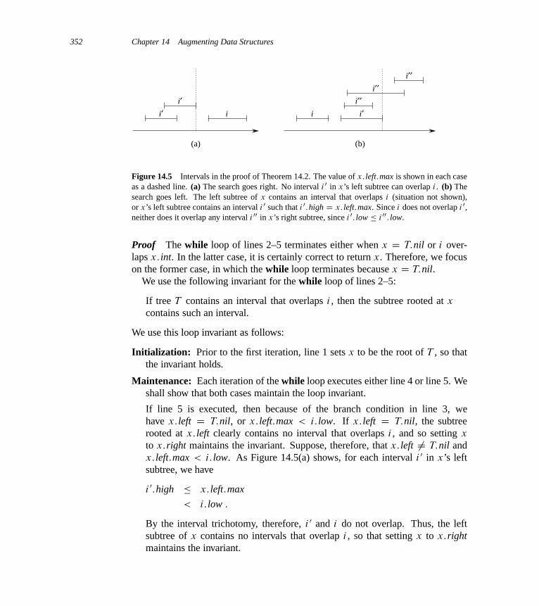
352 Chapter 14 Augmenting Data Structures
i
(a) (b)
i′i′ i i′
i′′i′′
i′′
Figure 14.5 Intervals in the proof of Theorem 14.2. The value of x: left:max is shown in each caseas a dashed line. (a) The search goes right. No interval i 0 in x’s left subtree can overlap i . (b) Thesearch goes left. The left subtree of x contains an interval that overlaps i (situation not shown),or x’s left subtree contains an interval i 0 such that i 0:high D x: left:max. Since i does not overlap i 0,neither does it overlap any interval i 00 in x’s right subtree, since i 0: low � i 00: low.
Proof The while loop of lines 2–5 terminates either when x D T:nil or i over-laps x: int. In the latter case, it is certainly correct to return x. Therefore, we focuson the former case, in which the while loop terminates because x D T:nil.
We use the following invariant for the while loop of lines 2–5:
If tree T contains an interval that overlaps i , then the subtree rooted at x
contains such an interval.
We use this loop invariant as follows:
Initialization: Prior to the first iteration, line 1 sets x to be the root of T , so thatthe invariant holds.
Maintenance: Each iteration of the while loop executes either line 4 or line 5. Weshall show that both cases maintain the loop invariant.
If line 5 is executed, then because of the branch condition in line 3, wehave x: left D T:nil, or x: left:max < i: low. If x: left D T:nil, the subtreerooted at x: left clearly contains no interval that overlaps i , and so setting x
to x:right maintains the invariant. Suppose, therefore, that x: left ¤ T:nil andx: left:max < i: low. As Figure 14.5(a) shows, for each interval i 0 in x’s leftsubtree, we have
i 0:high � x: left:max
< i: low :
By the interval trichotomy, therefore, i 0 and i do not overlap. Thus, the leftsubtree of x contains no intervals that overlap i , so that setting x to x:rightmaintains the invariant.
14.3 Interval trees 353
If, on the other hand, line 4 is executed, then we will show that the contrapos-itive of the loop invariant holds. That is, if the subtree rooted at x: left con-tains no interval overlapping i , then no interval anywhere in the tree overlaps i .Since line 4 is executed, then because of the branch condition in line 3, wehave x: left:max � i: low. Moreover, by definition of the max attribute, x’s leftsubtree must contain some interval i 0 such that
i 0:high D x: left:max
� i: low :
(Figure 14.5(b) illustrates the situation.) Since i and i 0 do not overlap, andsince it is not true that i 0:high < i: low, it follows by the interval trichotomythat i:high < i 0: low. Interval trees are keyed on the low endpoints of intervals,and thus the search-tree property implies that for any interval i 00 in x’s rightsubtree,
i:high < i 0: low
� i 00: low :
By the interval trichotomy, i and i 00 do not overlap. We conclude that whetheror not any interval in x’s left subtree overlaps i , setting x to x: left maintainsthe invariant.
Termination: If the loop terminates when x D T:nil, then the subtree rooted at x
contains no interval overlapping i . The contrapositive of the loop invariantimplies that T contains no interval that overlaps i . Hence it is correct to returnx D T:nil.
Thus, the INTERVAL-SEARCH procedure works correctly.
Exercises
14.3-1Write pseudocode for LEFT-ROTATE that operates on nodes in an interval tree andupdates the max attributes in O.1/ time.
14.3-2Rewrite the code for INTERVAL-SEARCH so that it works properly when all inter-vals are open.
14.3-3Describe an efficient algorithm that, given an interval i , returns an interval over-lapping i that has the minimum low endpoint, or T:nil if no such interval exists.
354 Chapter 14 Augmenting Data Structures
14.3-4Given an interval tree T and an interval i , describe how to list all intervals in T
that overlap i in O.min.n; k lg n// time, where k is the number of intervals in theoutput list. (Hint: One simple method makes several queries, modifying the treebetween queries. A slightly more complicated method does not modify the tree.)
14.3-5Suggest modifications to the interval-tree procedures to support the new opera-tion INTERVAL-SEARCH-EXACTLY.T; i/, where T is an interval tree and i isan interval. The operation should return a pointer to a node x in T such thatx: int: low D i: low and x: int:high D i:high, or T:nil if T contains no such node.All operations, including INTERVAL-SEARCH-EXACTLY, should run in O.lg n/
time on an n-node interval tree.
14.3-6Show how to maintain a dynamic set Q of numbers that supports the operationMIN-GAP, which gives the magnitude of the difference of the two closest num-bers in Q. For example, if Q D f1; 5; 9; 15; 18; 22g, then MIN-GAP.Q/ returns18 � 15 D 3, since 15 and 18 are the two closest numbers in Q. Make the op-erations INSERT, DELETE, SEARCH, and MIN-GAP as efficient as possible, andanalyze their running times.
14.3-7 ?
VLSI databases commonly represent an integrated circuit as a list of rectan-gles. Assume that each rectangle is rectilinearly oriented (sides parallel to thex- and y-axes), so that we represent a rectangle by its minimum and maximum x-and y-coordinates. Give an O.n lg n/-time algorithm to decide whether or not a setof n rectangles so represented contains two rectangles that overlap. Your algorithmneed not report all intersecting pairs, but it must report that an overlap exists if onerectangle entirely covers another, even if the boundary lines do not intersect. (Hint:Move a “sweep” line across the set of rectangles.)
Problems
14-1 Point of maximum overlapSuppose that we wish to keep track of a point of maximum overlap in a set ofintervals—a point with the largest number of intervals in the set that overlap it.
a. Show that there will always be a point of maximum overlap that is an endpointof one of the segments.
Notes for Chapter 14 355
b. Design a data structure that efficiently supports the operations INTERVAL-INSERT, INTERVAL-DELETE, and FIND-POM, which returns a point of max-imum overlap. (Hint: Keep a red-black tree of all the endpoints. Associatea value of C1 with each left endpoint, and associate a value of �1 with eachright endpoint. Augment each node of the tree with some extra information tomaintain the point of maximum overlap.)
14-2 Josephus permutationWe define the Josephus problem as follows. Suppose that n people form a circleand that we are given a positive integer m � n. Beginning with a designatedfirst person, we proceed around the circle, removing every mth person. After eachperson is removed, counting continues around the circle that remains. This processcontinues until we have removed all n people. The order in which the people areremoved from the circle defines the .n; m/-Josephus permutation of the integers1; 2; : : : ; n. For example, the .7; 3/-Josephus permutation is h3; 6; 2; 7; 5; 1; 4i.a. Suppose that m is a constant. Describe an O.n/-time algorithm that, given an
integer n, outputs the .n; m/-Josephus permutation.
b. Suppose that m is not a constant. Describe an O.n lg n/-time algorithm that,given integers n and m, outputs the .n; m/-Josephus permutation.
Chapter notes
In their book, Preparata and Shamos [282] describe several of the interval treesthat appear in the literature, citing work by H. Edelsbrunner (1980) and E. M.McCreight (1981). The book details an interval tree that, given a static databaseof n intervals, allows us to enumerate all k intervals that overlap a given queryinterval in O.k C lg n/ time.

IV Advanced Design and Analysis Techniques
Introduction
This part covers three important techniques used in designing and analyzing effi-cient algorithms: dynamic programming (Chapter 15), greedy algorithms (Chap-ter 16), and amortized analysis (Chapter 17). Earlier parts have presented otherwidely applicable techniques, such as divide-and-conquer, randomization, and howto solve recurrences. The techniques in this part are somewhat more sophisticated,but they help us to attack many computational problems. The themes introduced inthis part will recur later in this book.
Dynamic programming typically applies to optimization problems in which wemake a set of choices in order to arrive at an optimal solution. As we makeeach choice, subproblems of the same form often arise. Dynamic programmingis effective when a given subproblem may arise from more than one partial set ofchoices; the key technique is to store the solution to each such subproblem in case itshould reappear. Chapter 15 shows how this simple idea can sometimes transformexponential-time algorithms into polynomial-time algorithms.
Like dynamic-programming algorithms, greedy algorithms typically apply tooptimization problems in which we make a set of choices in order to arrive at anoptimal solution. The idea of a greedy algorithm is to make each choice in a locallyoptimal manner. A simple example is coin-changing: to minimize the number ofU.S. coins needed to make change for a given amount, we can repeatedly selectthe largest-denomination coin that is not larger than the amount that remains. Agreedy approach provides an optimal solution for many such problems much morequickly than would a dynamic-programming approach. We cannot always easilytell whether a greedy approach will be effective, however. Chapter 16 introduces
358 Part IV Advanced Design and Analysis Techniques
matroid theory, which provides a mathematical basis that can help us to show thata greedy algorithm yields an optimal solution.
We use amortized analysis to analyze certain algorithms that perform a sequenceof similar operations. Instead of bounding the cost of the sequence of operationsby bounding the actual cost of each operation separately, an amortized analysisprovides a bound on the actual cost of the entire sequence. One advantage of thisapproach is that although some operations might be expensive, many others mightbe cheap. In other words, many of the operations might run in well under the worst-case time. Amortized analysis is not just an analysis tool, however; it is also a wayof thinking about the design of algorithms, since the design of an algorithm and theanalysis of its running time are often closely intertwined. Chapter 17 introducesthree ways to perform an amortized analysis of an algorithm.

15 Dynamic Programming
Dynamic programming, like the divide-and-conquer method, solves problems bycombining the solutions to subproblems. (“Programming” in this context refersto a tabular method, not to writing computer code.) As we saw in Chapters 2and 4, divide-and-conquer algorithms partition the problem into disjoint subprob-lems, solve the subproblems recursively, and then combine their solutions to solvethe original problem. In contrast, dynamic programming applies when the sub-problems overlap, that is, when subproblems share subsubproblems. In this con-text, a divide-and-conquer algorithm does more work than necessary, repeatedlysolving the common subsubproblems. A dynamic-programming algorithm solveseach subsubproblem just once and then saves its answer in a table, thereby avoidingthe work of recomputing the answer every time it solves each subsubproblem.
We typically apply dynamic programming to optimization problems. Such prob-lems can have many possible solutions. Each solution has a value, and we wish tofind a solution with the optimal (minimum or maximum) value. We call such asolution an optimal solution to the problem, as opposed to the optimal solution,since there may be several solutions that achieve the optimal value.
When developing a dynamic-programming algorithm, we follow a sequence offour steps:
1. Characterize the structure of an optimal solution.
2. Recursively define the value of an optimal solution.
3. Compute the value of an optimal solution, typically in a bottom-up fashion.
4. Construct an optimal solution from computed information.
Steps 1–3 form the basis of a dynamic-programming solution to a problem. If weneed only the value of an optimal solution, and not the solution itself, then wecan omit step 4. When we do perform step 4, we sometimes maintain additionalinformation during step 3 so that we can easily construct an optimal solution.
The sections that follow use the dynamic-programming method to solve someoptimization problems. Section 15.1 examines the problem of cutting a rod into

360 Chapter 15 Dynamic Programming
rods of smaller length in way that maximizes their total value. Section 15.2 askshow we can multiply a chain of matrices while performing the fewest total scalarmultiplications. Given these examples of dynamic programming, Section 15.3 dis-cusses two key characteristics that a problem must have for dynamic programmingto be a viable solution technique. Section 15.4 then shows how to find the longestcommon subsequence of two sequences via dynamic programming. Finally, Sec-tion 15.5 uses dynamic programming to construct binary search trees that are opti-mal, given a known distribution of keys to be looked up.
15.1 Rod cutting
Our first example uses dynamic programming to solve a simple problem in decid-ing where to cut steel rods. Serling Enterprises buys long steel rods and cuts theminto shorter rods, which it then sells. Each cut is free. The management of SerlingEnterprises wants to know the best way to cut up the rods.
We assume that we know, for i D 1; 2; : : :, the price pi in dollars that SerlingEnterprises charges for a rod of length i inches. Rod lengths are always an integralnumber of inches. Figure 15.1 gives a sample price table.
The rod-cutting problem the following. Given a rod of length n inches and a ta-ble of prices pi for i D 1; 2; : : : ; n, determine the maximum revenue rn obtainableby cutting up the rod and selling the pieces. Note that if the price pn for a rod oflength n is large enough, an optimal solution may require no cutting at all.
Consider the case when n D 4. Figure 15.2 shows all the ways to cut up a rod oflength 4 inches, including the way with no cuts at all. We see that cutting a 4-inchrod into two 2-inch pieces produces revenue p2 C p2 D 5 C 5 D 10, which isoptimal.
We can cut up a rod of length n in 2n�1 different ways, since we have an in-dependent option of cutting, or not cutting, at distance i inches from the left end,
length i 1 2 3 4 5 6 7 8 9 10price pi 1 5 8 9 10 17 17 20 24 30
Figure 15.1 A sample price table for rods. Each rod of length i inches earns the company pi
dollars of revenue.

15.1 Rod cutting 361
9
(a)
1
(b)
8
(c) (d)
(e) (f) (g)
1
(h)
1 1 1
5 5 18
511 5 11 5 11
Figure 15.2 The 8 possible ways of cutting up a rod of length 4. Above each piece is thevalue of that piece, according to the sample price chart of Figure 15.1. The optimal strategy ispart (c)—cutting the rod into two pieces of length 2—which has total value 10.
for i D 1; 2; : : : ; n � 1.1 We denote a decomposition into pieces using ordinaryadditive notation, so that 7 D 2C 2C 3 indicates that a rod of length 7 is cut intothree pieces—two of length 2 and one of length 3. If an optimal solution cuts therod into k pieces, for some 1 � k � n, then an optimal decomposition
n D i1 C i2 C � � � C ik
of the rod into pieces of lengths i1, i2, . . . , ik provides maximum correspondingrevenue
rn D pi1 C pi2 C � � � C pik :
For our sample problem, we can determine the optimal revenue figures ri , fori D 1; 2; : : : ; 10, by inspection, with the corresponding optimal decompositions
1If we required the pieces to be cut in order of nondecreasing size, there would be fewer waysto consider. For n D 4, we would consider only 5 such ways: parts (a), (b), (c), (e), and (h)in Figure 15.2. The number of ways is called the partition function; it is approximately equal to
e�p
2n=3=4np
3. This quantity is less than 2n�1, but still much greater than any polynomial in n.We shall not pursue this line of inquiry further, however.

362 Chapter 15 Dynamic Programming
r1 D 1 from solution 1 D 1 (no cuts) ;
r2 D 5 from solution 2 D 2 (no cuts) ;
r3 D 8 from solution 3 D 3 (no cuts) ;
r4 D 10 from solution 4 D 2C 2 ;
r5 D 13 from solution 5 D 2C 3 ;
r6 D 17 from solution 6 D 6 (no cuts) ;
r7 D 18 from solution 7 D 1C 6 or 7 D 2C 2C 3 ;
r8 D 22 from solution 8 D 2C 6 ;
r9 D 25 from solution 9 D 3C 6 ;
r10 D 30 from solution 10 D 10 (no cuts) :
More generally, we can frame the values rn for n � 1 in terms of optimal rev-enues from shorter rods:
rn D max .pn; r1 C rn�1; r2 C rn�2; : : : ; rn�1 C r1/ : (15.1)
The first argument, pn, corresponds to making no cuts at all and selling the rod oflength n as is. The other n� 1 arguments to max correspond to the maximum rev-enue obtained by making an initial cut of the rod into two pieces of size i and n � i ,for each i D 1; 2; : : : ; n � 1, and then optimally cutting up those pieces further,obtaining revenues ri and rn�i from those two pieces. Since we don’t know aheadof time which value of i optimizes revenue, we have to consider all possible valuesfor i and pick the one that maximizes revenue. We also have the option of pickingno i at all if we can obtain more revenue by selling the rod uncut.
Note that to solve the original problem of size n, we solve smaller problems ofthe same type, but of smaller sizes. Once we make the first cut, we may considerthe two pieces as independent instances of the rod-cutting problem. The overalloptimal solution incorporates optimal solutions to the two related subproblems,maximizing revenue from each of those two pieces. We say that the rod-cuttingproblem exhibits optimal substructure: optimal solutions to a problem incorporateoptimal solutions to related subproblems, which we may solve independently.
In a related, but slightly simpler, way to arrange a recursive structure for the rod-cutting problem, we view a decomposition as consisting of a first piece of length i
cut off the left-hand end, and then a right-hand remainder of length n � i . Onlythe remainder, and not the first piece, may be further divided. We may view everydecomposition of a length-n rod in this way: as a first piece followed by somedecomposition of the remainder. When doing so, we can couch the solution withno cuts at all as saying that the first piece has size i D n and revenue pn and thatthe remainder has size 0 with corresponding revenue r0 D 0. We thus obtain thefollowing simpler version of equation (15.1):
rn D max1�i�n
.pi C rn�i / : (15.2)
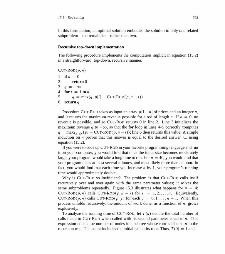
15.1 Rod cutting 363
In this formulation, an optimal solution embodies the solution to only one relatedsubproblem—the remainder—rather than two.
Recursive top-down implementation
The following procedure implements the computation implicit in equation (15.2)in a straightforward, top-down, recursive manner.
CUT-ROD.p; n/
1 if n == 0
2 return 03 q D �14 for i D 1 to n
5 q D max.q; pŒi �C CUT-ROD.p; n � i//
6 return q
Procedure CUT-ROD takes as input an array pŒ1 : : n� of prices and an integer n,and it returns the maximum revenue possible for a rod of length n. If n D 0, norevenue is possible, and so CUT-ROD returns 0 in line 2. Line 3 initializes themaximum revenue q to �1, so that the for loop in lines 4–5 correctly computesq D max1�i�n.pi C CUT-ROD.p; n� i//; line 6 then returns this value. A simpleinduction on n proves that this answer is equal to the desired answer rn, usingequation (15.2).
If you were to code up CUT-ROD in your favorite programming language and runit on your computer, you would find that once the input size becomes moderatelylarge, your program would take a long time to run. For n D 40, you would find thatyour program takes at least several minutes, and most likely more than an hour. Infact, you would find that each time you increase n by 1, your program’s runningtime would approximately double.
Why is CUT-ROD so inefficient? The problem is that CUT-ROD calls itselfrecursively over and over again with the same parameter values; it solves thesame subproblems repeatedly. Figure 15.3 illustrates what happens for n D 4:CUT-ROD.p; n/ calls CUT-ROD.p; n � i/ for i D 1; 2; : : : ; n. Equivalently,CUT-ROD.p; n/ calls CUT-ROD.p; j / for each j D 0; 1; : : : ; n � 1. When thisprocess unfolds recursively, the amount of work done, as a function of n, growsexplosively.
To analyze the running time of CUT-ROD, let T .n/ denote the total number ofcalls made to CUT-ROD when called with its second parameter equal to n. Thisexpression equals the number of nodes in a subtree whose root is labeled n in therecursion tree. The count includes the initial call at its root. Thus, T .0/ D 1 and

364 Chapter 15 Dynamic Programming
3
1 0
0
0
01
2 0
0
1
2
0
1 0
4
Figure 15.3 The recursion tree showing recursive calls resulting from a call CUT-ROD.p; n/ forn D 4. Each node label gives the size n of the corresponding subproblem, so that an edge froma parent with label s to a child with label t corresponds to cutting off an initial piece of size s � t
and leaving a remaining subproblem of size t . A path from the root to a leaf corresponds to one ofthe 2n�1 ways of cutting up a rod of length n. In general, this recursion tree has 2n nodes and 2n�1
leaves.
T .n/ D 1Cn�1Xj D0
T .j / : (15.3)
The initial 1 is for the call at the root, and the term T .j / counts the number of calls(including recursive calls) due to the call CUT-ROD.p; n � i/, where j D n � i .As Exercise 15.1-1 asks you to show,
T .n/ D 2n ; (15.4)
and so the running time of CUT-ROD is exponential in n.In retrospect, this exponential running time is not so surprising. CUT-ROD ex-
plicitly considers all the 2n�1 possible ways of cutting up a rod of length n. Thetree of recursive calls has 2n�1 leaves, one for each possible way of cutting up therod. The labels on the simple path from the root to a leaf give the sizes of eachremaining right-hand piece before making each cut. That is, the labels give thecorresponding cut points, measured from the right-hand end of the rod.
Using dynamic programming for optimal rod cutting
We now show how to convert CUT-ROD into an efficient algorithm, using dynamicprogramming.
The dynamic-programming method works as follows. Having observed that anaive recursive solution is inefficient because it solves the same subproblems re-peatedly, we arrange for each subproblem to be solved only once, saving its solu-tion. If we need to refer to this subproblem’s solution again later, we can just look it

15.1 Rod cutting 365
up, rather than recompute it. Dynamic programming thus uses additional memoryto save computation time; it serves an example of a time-memory trade-off. Thesavings may be dramatic: an exponential-time solution may be transformed into apolynomial-time solution. A dynamic-programming approach runs in polynomialtime when the number of distinct subproblems involved is polynomial in the inputsize and we can solve each such subproblem in polynomial time.
There are usually two equivalent ways to implement a dynamic-programmingapproach. We shall illustrate both of them with our rod-cutting example.
The first approach is top-down with memoization.2 In this approach, we writethe procedure recursively in a natural manner, but modified to save the result ofeach subproblem (usually in an array or hash table). The procedure now first checksto see whether it has previously solved this subproblem. If so, it returns the savedvalue, saving further computation at this level; if not, the procedure computes thevalue in the usual manner. We say that the recursive procedure has been memoized;it “remembers” what results it has computed previously.
The second approach is the bottom-up method. This approach typically dependson some natural notion of the “size” of a subproblem, such that solving any par-ticular subproblem depends only on solving “smaller” subproblems. We sort thesubproblems by size and solve them in size order, smallest first. When solving aparticular subproblem, we have already solved all of the smaller subproblems itssolution depends upon, and we have saved their solutions. We solve each sub-problem only once, and when we first see it, we have already solved all of itsprerequisite subproblems.
These two approaches yield algorithms with the same asymptotic running time,except in unusual circumstances where the top-down approach does not actuallyrecurse to examine all possible subproblems. The bottom-up approach often hasmuch better constant factors, since it has less overhead for procedure calls.
Here is the the pseudocode for the top-down CUT-ROD procedure, with memo-ization added:
MEMOIZED-CUT-ROD.p; n/
1 let rŒ0 : : n� be a new array2 for i D 0 to n
3 rŒi � D �14 return MEMOIZED-CUT-ROD-AUX.p; n; r/
2This is not a misspelling. The word really is memoization, not memorization. Memoization comesfrom memo, since the technique consists of recording a value so that we can look it up later.
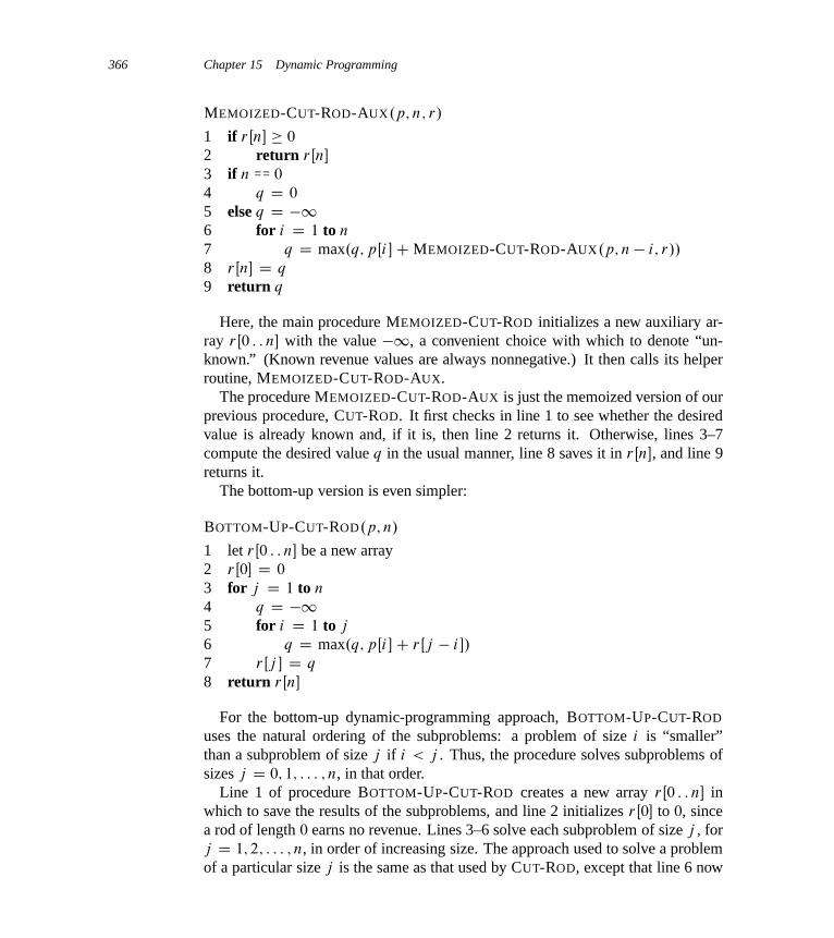
366 Chapter 15 Dynamic Programming
MEMOIZED-CUT-ROD-AUX.p; n; r/
1 if rŒn� � 0
2 return rŒn�
3 if n == 0
4 q D 0
5 else q D �16 for i D 1 to n
7 q D max.q; pŒi �CMEMOIZED-CUT-ROD-AUX.p; n � i; r//
8 rŒn� D q
9 return q
Here, the main procedure MEMOIZED-CUT-ROD initializes a new auxiliary ar-ray rŒ0 : : n� with the value �1, a convenient choice with which to denote “un-known.” (Known revenue values are always nonnegative.) It then calls its helperroutine, MEMOIZED-CUT-ROD-AUX.
The procedure MEMOIZED-CUT-ROD-AUX is just the memoized version of ourprevious procedure, CUT-ROD. It first checks in line 1 to see whether the desiredvalue is already known and, if it is, then line 2 returns it. Otherwise, lines 3–7compute the desired value q in the usual manner, line 8 saves it in rŒn�, and line 9returns it.
The bottom-up version is even simpler:
BOTTOM-UP-CUT-ROD.p; n/
1 let rŒ0 : : n� be a new array2 rŒ0� D 0
3 for j D 1 to n
4 q D �15 for i D 1 to j
6 q D max.q; pŒi �C rŒj � i �/
7 rŒj � D q
8 return rŒn�
For the bottom-up dynamic-programming approach, BOTTOM-UP-CUT-ROD
uses the natural ordering of the subproblems: a problem of size i is “smaller”than a subproblem of size j if i < j . Thus, the procedure solves subproblems ofsizes j D 0; 1; : : : ; n, in that order.
Line 1 of procedure BOTTOM-UP-CUT-ROD creates a new array rŒ0 : : n� inwhich to save the results of the subproblems, and line 2 initializes rŒ0� to 0, sincea rod of length 0 earns no revenue. Lines 3–6 solve each subproblem of size j , forj D 1; 2; : : : ; n, in order of increasing size. The approach used to solve a problemof a particular size j is the same as that used by CUT-ROD, except that line 6 now
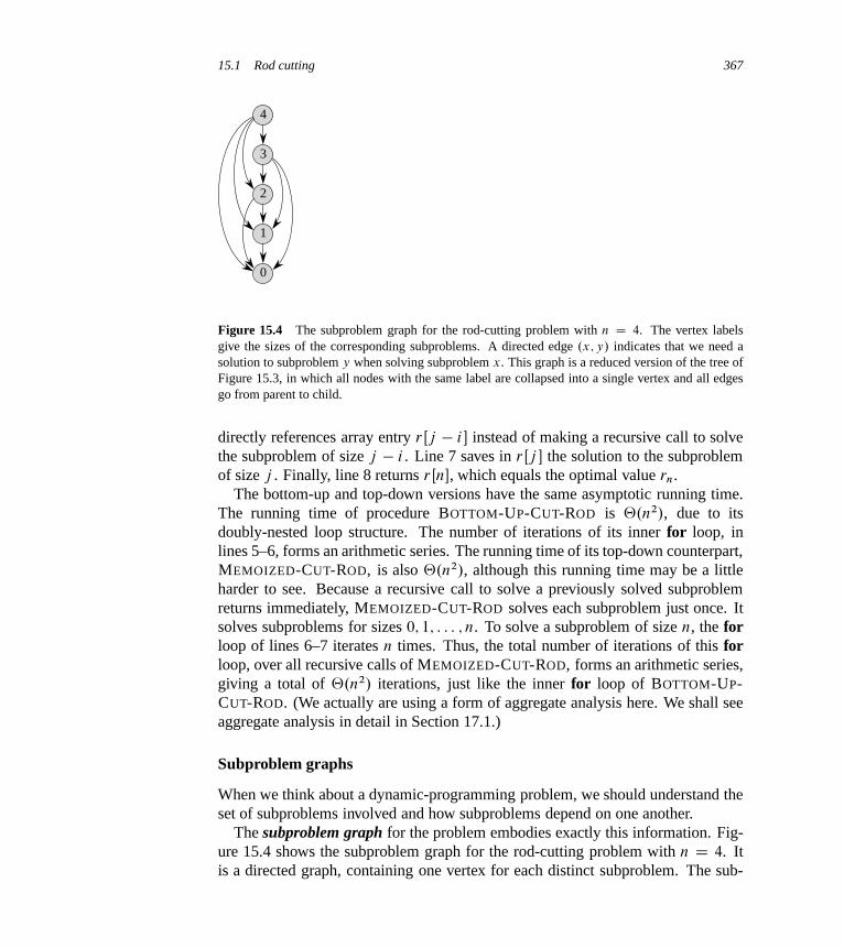
15.1 Rod cutting 367
3
0
1
2
4
Figure 15.4 The subproblem graph for the rod-cutting problem with n D 4. The vertex labelsgive the sizes of the corresponding subproblems. A directed edge .x; y/ indicates that we need asolution to subproblem y when solving subproblem x. This graph is a reduced version of the tree ofFigure 15.3, in which all nodes with the same label are collapsed into a single vertex and all edgesgo from parent to child.
directly references array entry rŒj � i � instead of making a recursive call to solvethe subproblem of size j � i . Line 7 saves in rŒj � the solution to the subproblemof size j . Finally, line 8 returns rŒn�, which equals the optimal value rn.
The bottom-up and top-down versions have the same asymptotic running time.The running time of procedure BOTTOM-UP-CUT-ROD is ‚.n2/, due to itsdoubly-nested loop structure. The number of iterations of its inner for loop, inlines 5–6, forms an arithmetic series. The running time of its top-down counterpart,MEMOIZED-CUT-ROD, is also ‚.n2/, although this running time may be a littleharder to see. Because a recursive call to solve a previously solved subproblemreturns immediately, MEMOIZED-CUT-ROD solves each subproblem just once. Itsolves subproblems for sizes 0; 1; : : : ; n. To solve a subproblem of size n, the forloop of lines 6–7 iterates n times. Thus, the total number of iterations of this forloop, over all recursive calls of MEMOIZED-CUT-ROD, forms an arithmetic series,giving a total of ‚.n2/ iterations, just like the inner for loop of BOTTOM-UP-CUT-ROD. (We actually are using a form of aggregate analysis here. We shall seeaggregate analysis in detail in Section 17.1.)
Subproblem graphs
When we think about a dynamic-programming problem, we should understand theset of subproblems involved and how subproblems depend on one another.
The subproblem graph for the problem embodies exactly this information. Fig-ure 15.4 shows the subproblem graph for the rod-cutting problem with n D 4. Itis a directed graph, containing one vertex for each distinct subproblem. The sub-
368 Chapter 15 Dynamic Programming
problem graph has a directed edge from the vertex for subproblem x to the vertexfor subproblem y if determining an optimal solution for subproblem x involvesdirectly considering an optimal solution for subproblem y. For example, the sub-problem graph contains an edge from x to y if a top-down recursive procedure forsolving x directly calls itself to solve y. We can think of the subproblem graphas a “reduced” or “collapsed” version of the recursion tree for the top-down recur-sive method, in which we coalesce all nodes for the same subproblem into a singlevertex and direct all edges from parent to child.
The bottom-up method for dynamic programming considers the vertices of thesubproblem graph in such an order that we solve the subproblems y adjacent toa given subproblem x before we solve subproblem x. (Recall from Section B.4that the adjacency relation is not necessarily symmetric.) Using the terminologyfrom Chapter 22, in a bottom-up dynamic-programming algorithm, we consider thevertices of the subproblem graph in an order that is a “reverse topological sort,” ora “topological sort of the transpose” (see Section 22.4) of the subproblem graph. Inother words, no subproblem is considered until all of the subproblems it dependsupon have been solved. Similarly, using notions from the same chapter, we canview the top-down method (with memoization) for dynamic programming as a“depth-first search” of the subproblem graph (see Section 22.3).
The size of the subproblem graph G D .V; E/ can help us determine the runningtime of the dynamic programming algorithm. Since we solve each subproblem justonce, the running time is the sum of the times needed to solve each subproblem.Typically, the time to compute the solution to a subproblem is proportional to thedegree (number of outgoing edges) of the corresponding vertex in the subproblemgraph, and the number of subproblems is equal to the number of vertices in the sub-problem graph. In this common case, the running time of dynamic programmingis linear in the number of vertices and edges.
Reconstructing a solution
Our dynamic-programming solutions to the rod-cutting problem return the value ofan optimal solution, but they do not return an actual solution: a list of piece sizes.We can extend the dynamic-programming approach to record not only the optimalvalue computed for each subproblem, but also a choice that led to the optimalvalue. With this information, we can readily print an optimal solution.
Here is an extended version of BOTTOM-UP-CUT-ROD that computes, for eachrod size j , not only the maximum revenue rj , but also sj , the optimal size of thefirst piece to cut off:
15.1 Rod cutting 369
EXTENDED-BOTTOM-UP-CUT-ROD.p; n/
1 let rŒ0 : : n� and sŒ0 : : n� be new arrays2 rŒ0� D 0
3 for j D 1 to n
4 q D �15 for i D 1 to j
6 if q < pŒi�C rŒj � i �
7 q D pŒi�C rŒj � i �
8 sŒj � D i
9 rŒj � D q
10 return r and s
This procedure is similar to BOTTOM-UP-CUT-ROD, except that it creates the ar-ray s in line 1, and it updates sŒj � in line 8 to hold the optimal size i of the firstpiece to cut off when solving a subproblem of size j .
The following procedure takes a price table p and a rod size n, and it callsEXTENDED-BOTTOM-UP-CUT-ROD to compute the array sŒ1 : : n� of optimalfirst-piece sizes and then prints out the complete list of piece sizes in an optimaldecomposition of a rod of length n:
PRINT-CUT-ROD-SOLUTION.p; n/
1 .r; s/ D EXTENDED-BOTTOM-UP-CUT-ROD.p; n/
2 while n > 0
3 print sŒn�
4 n D n � sŒn�
In our rod-cutting example, the call EXTENDED-BOTTOM-UP-CUT-ROD.p; 10/
would return the following arrays:
i 0 1 2 3 4 5 6 7 8 9 10
rŒi � 0 1 5 8 10 13 17 18 22 25 30
sŒi � 0 1 2 3 2 2 6 1 2 3 10
A call to PRINT-CUT-ROD-SOLUTION.p; 10/ would print just 10, but a call withn D 7 would print the cuts 1 and 6, corresponding to the first optimal decomposi-tion for r7 given earlier.
Exercises
15.1-1Show that equation (15.4) follows from equation (15.3) and the initial conditionT .0/ D 1.
370 Chapter 15 Dynamic Programming
15.1-2Show, by means of a counterexample, that the following “greedy” strategy doesnot always determine an optimal way to cut rods. Define the density of a rod oflength i to be pi=i , that is, its value per inch. The greedy strategy for a rod oflength n cuts off a first piece of length i , where 1 � i � n, having maximumdensity. It then continues by applying the greedy strategy to the remaining piece oflength n � i .
15.1-3Consider a modification of the rod-cutting problem in which, in addition to aprice pi for each rod, each cut incurs a fixed cost of c. The revenue associated witha solution is now the sum of the prices of the pieces minus the costs of making thecuts. Give a dynamic-programming algorithm to solve this modified problem.
15.1-4Modify MEMOIZED-CUT-ROD to return not only the value but the actual solution,too.
15.1-5The Fibonacci numbers are defined by recurrence (3.22). Give an O.n/-timedynamic-programming algorithm to compute the nth Fibonacci number. Draw thesubproblem graph. How many vertices and edges are in the graph?
15.2 Matrix-chain multiplication
Our next example of dynamic programming is an algorithm that solves the problemof matrix-chain multiplication. We are given a sequence (chain) hA1; A2; : : : ; Aniof n matrices to be multiplied, and we wish to compute the product
A1A2 � � �An : (15.5)
We can evaluate the expression (15.5) using the standard algorithm for multiply-ing pairs of matrices as a subroutine once we have parenthesized it to resolve allambiguities in how the matrices are multiplied together. Matrix multiplication isassociative, and so all parenthesizations yield the same product. A product of ma-trices is fully parenthesized if it is either a single matrix or the product of two fullyparenthesized matrix products, surrounded by parentheses. For example, if thechain of matrices is hA1; A2; A3; A4i, then we can fully parenthesize the productA1A2A3A4 in five distinct ways:
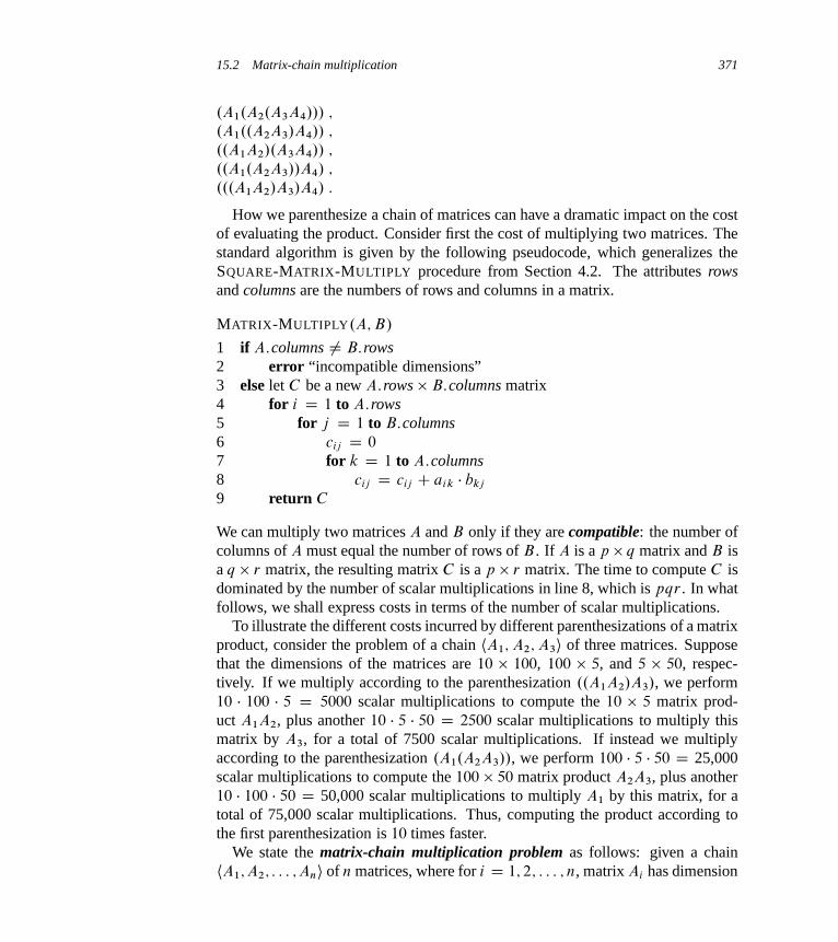
15.2 Matrix-chain multiplication 371
.A1.A2.A3A4/// ;
.A1..A2A3/A4// ;
..A1A2/.A3A4// ;
..A1.A2A3//A4/ ;
...A1A2/A3/A4/ :
How we parenthesize a chain of matrices can have a dramatic impact on the costof evaluating the product. Consider first the cost of multiplying two matrices. Thestandard algorithm is given by the following pseudocode, which generalizes theSQUARE-MATRIX-MULTIPLY procedure from Section 4.2. The attributes rowsand columns are the numbers of rows and columns in a matrix.
MATRIX-MULTIPLY.A; B/
1 if A:columns ¤ B:rows2 error “incompatible dimensions”3 else let C be a new A:rows B:columns matrix4 for i D 1 to A:rows5 for j D 1 to B:columns6 cij D 0
7 for k D 1 to A:columns8 cij D cij C aik � bkj
9 return C
We can multiply two matrices A and B only if they are compatible: the number ofcolumns of A must equal the number of rows of B . If A is a p q matrix and B isa q r matrix, the resulting matrix C is a p r matrix. The time to compute C isdominated by the number of scalar multiplications in line 8, which is pqr . In whatfollows, we shall express costs in terms of the number of scalar multiplications.
To illustrate the different costs incurred by different parenthesizations of a matrixproduct, consider the problem of a chain hA1; A2; A3i of three matrices. Supposethat the dimensions of the matrices are 10 100, 100 5, and 5 50, respec-tively. If we multiply according to the parenthesization ..A1A2/A3/, we perform10 � 100 � 5 D 5000 scalar multiplications to compute the 10 5 matrix prod-uct A1A2, plus another 10 � 5 � 50 D 2500 scalar multiplications to multiply thismatrix by A3, for a total of 7500 scalar multiplications. If instead we multiplyaccording to the parenthesization .A1.A2A3//, we perform 100 � 5 � 50 D 25,000scalar multiplications to compute the 100 50 matrix product A2A3, plus another10 � 100 � 50 D 50,000 scalar multiplications to multiply A1 by this matrix, for atotal of 75,000 scalar multiplications. Thus, computing the product according tothe first parenthesization is 10 times faster.
We state the matrix-chain multiplication problem as follows: given a chainhA1;A2; : : : ;Ani of n matrices, where for i D 1; 2; : : : ; n, matrix Ai has dimension
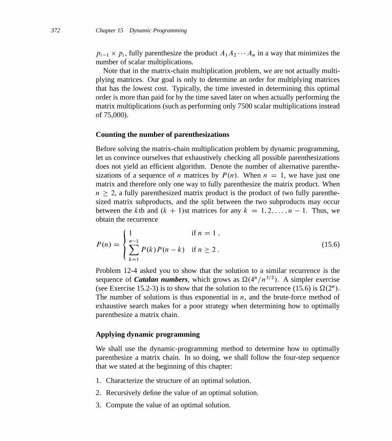
372 Chapter 15 Dynamic Programming
pi�1 pi , fully parenthesize the product A1A2 � � �An in a way that minimizes thenumber of scalar multiplications.
Note that in the matrix-chain multiplication problem, we are not actually multi-plying matrices. Our goal is only to determine an order for multiplying matricesthat has the lowest cost. Typically, the time invested in determining this optimalorder is more than paid for by the time saved later on when actually performing thematrix multiplications (such as performing only 7500 scalar multiplications insteadof 75,000).
Counting the number of parenthesizations
Before solving the matrix-chain multiplication problem by dynamic programming,let us convince ourselves that exhaustively checking all possible parenthesizationsdoes not yield an efficient algorithm. Denote the number of alternative parenthe-sizations of a sequence of n matrices by P.n/. When n D 1, we have just onematrix and therefore only one way to fully parenthesize the matrix product. Whenn � 2, a fully parenthesized matrix product is the product of two fully parenthe-sized matrix subproducts, and the split between the two subproducts may occurbetween the kth and .k C 1/st matrices for any k D 1; 2; : : : ; n � 1. Thus, weobtain the recurrence
P.n/ D
�1 if n D 1 ;n�1XkD1
P.k/P.n� k/ if n � 2 :(15.6)
Problem 12-4 asked you to show that the solution to a similar recurrence is thesequence of Catalan numbers, which grows as �.4n=n3=2/. A simpler exercise(see Exercise 15.2-3) is to show that the solution to the recurrence (15.6) is �.2n/.The number of solutions is thus exponential in n, and the brute-force method ofexhaustive search makes for a poor strategy when determining how to optimallyparenthesize a matrix chain.
Applying dynamic programming
We shall use the dynamic-programming method to determine how to optimallyparenthesize a matrix chain. In so doing, we shall follow the four-step sequencethat we stated at the beginning of this chapter:
1. Characterize the structure of an optimal solution.
2. Recursively define the value of an optimal solution.
3. Compute the value of an optimal solution.
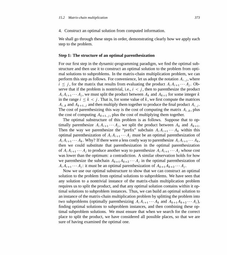
15.2 Matrix-chain multiplication 373
4. Construct an optimal solution from computed information.
We shall go through these steps in order, demonstrating clearly how we apply eachstep to the problem.
Step 1: The structure of an optimal parenthesization
For our first step in the dynamic-programming paradigm, we find the optimal sub-structure and then use it to construct an optimal solution to the problem from opti-mal solutions to subproblems. In the matrix-chain multiplication problem, we canperform this step as follows. For convenience, let us adopt the notation Ai ::j , wherei � j , for the matrix that results from evaluating the product AiAiC1 � � �Aj . Ob-serve that if the problem is nontrivial, i.e., i < j , then to parenthesize the productAiAiC1 � � �Aj , we must split the product between Ak and AkC1 for some integer k
in the range i � k < j . That is, for some value of k, we first compute the matricesAi ::k and AkC1::j and then multiply them together to produce the final product Ai ::j .The cost of parenthesizing this way is the cost of computing the matrix Ai ::k , plusthe cost of computing AkC1::j , plus the cost of multiplying them together.
The optimal substructure of this problem is as follows. Suppose that to op-timally parenthesize AiAiC1 � � �Aj , we split the product between Ak and AkC1.Then the way we parenthesize the “prefix” subchain AiAiC1 � � �Ak within thisoptimal parenthesization of AiAiC1 � � �Aj must be an optimal parenthesization ofAiAiC1 � � �Ak. Why? If there were a less costly way to parenthesize AiAiC1 � � �Ak,then we could substitute that parenthesization in the optimal parenthesizationof AiAiC1 � � �Aj to produce another way to parenthesize AiAiC1 � � �Aj whose costwas lower than the optimum: a contradiction. A similar observation holds for howwe parenthesize the subchain AkC1AkC2 � � �Aj in the optimal parenthesization ofAiAiC1 � � �Aj : it must be an optimal parenthesization of AkC1AkC2 � � �Aj .
Now we use our optimal substructure to show that we can construct an optimalsolution to the problem from optimal solutions to subproblems. We have seen thatany solution to a nontrivial instance of the matrix-chain multiplication problemrequires us to split the product, and that any optimal solution contains within it op-timal solutions to subproblem instances. Thus, we can build an optimal solution toan instance of the matrix-chain multiplication problem by splitting the problem intotwo subproblems (optimally parenthesizing AiAiC1 � � �Ak and AkC1AkC2 � � �Aj ),finding optimal solutions to subproblem instances, and then combining these op-timal subproblem solutions. We must ensure that when we search for the correctplace to split the product, we have considered all possible places, so that we aresure of having examined the optimal one.

374 Chapter 15 Dynamic Programming
Step 2: A recursive solution
Next, we define the cost of an optimal solution recursively in terms of the optimalsolutions to subproblems. For the matrix-chain multiplication problem, we pick asour subproblems the problems of determining the minimum cost of parenthesizingAiAiC1 � � �Aj for 1 � i � j � n. Let mŒi; j � be the minimum number of scalarmultiplications needed to compute the matrix Ai ::j ; for the full problem, the lowest-cost way to compute A1::n would thus be mŒ1; n�.
We can define mŒi; j � recursively as follows. If i D j , the problem is trivial;the chain consists of just one matrix Ai ::i D Ai , so that no scalar multiplicationsare necessary to compute the product. Thus, mŒi; i � D 0 for i D 1; 2; : : : ; n. Tocompute mŒi; j � when i < j , we take advantage of the structure of an optimalsolution from step 1. Let us assume that to optimally parenthesize, we split theproduct AiAiC1 � � �Aj between Ak and AkC1, where i � k < j . Then, mŒi; j �
equals the minimum cost for computing the subproducts Ai ::k and AkC1::j , plus thecost of multiplying these two matrices together. Recalling that each matrix Ai ispi�1 pi , we see that computing the matrix product Ai ::kAkC1::j takes pi�1pkpj
scalar multiplications. Thus, we obtain
mŒi; j � D mŒi; k�CmŒk C 1; j �C pi�1pkpj :
This recursive equation assumes that we know the value of k, which we do not.There are only j �i possible values for k, however, namely k D i; iC1; : : : ; j �1.Since the optimal parenthesization must use one of these values for k, we need onlycheck them all to find the best. Thus, our recursive definition for the minimum costof parenthesizing the product AiAiC1 � � �Aj becomes
mŒi; j � D(
0 if i D j ;
mini�k<j
fmŒi; k�CmŒk C 1; j �C pi�1pkpj g if i < j :(15.7)
The mŒi; j � values give the costs of optimal solutions to subproblems, but theydo not provide all the information we need to construct an optimal solution. Tohelp us do so, we define sŒi; j � to be a value of k at which we split the productAiAiC1 � � �Aj in an optimal parenthesization. That is, sŒi; j � equals a value k suchthat mŒi; j � D mŒi; k�CmŒk C 1; j �C pi�1pkpj .
Step 3: Computing the optimal costs
At this point, we could easily write a recursive algorithm based on recurrence (15.7)to compute the minimum cost mŒ1; n� for multiplying A1A2 � � �An. As we saw forthe rod-cutting problem, and as we shall see in Section 15.3, this recursive algo-rithm takes exponential time, which is no better than the brute-force method ofchecking each way of parenthesizing the product.
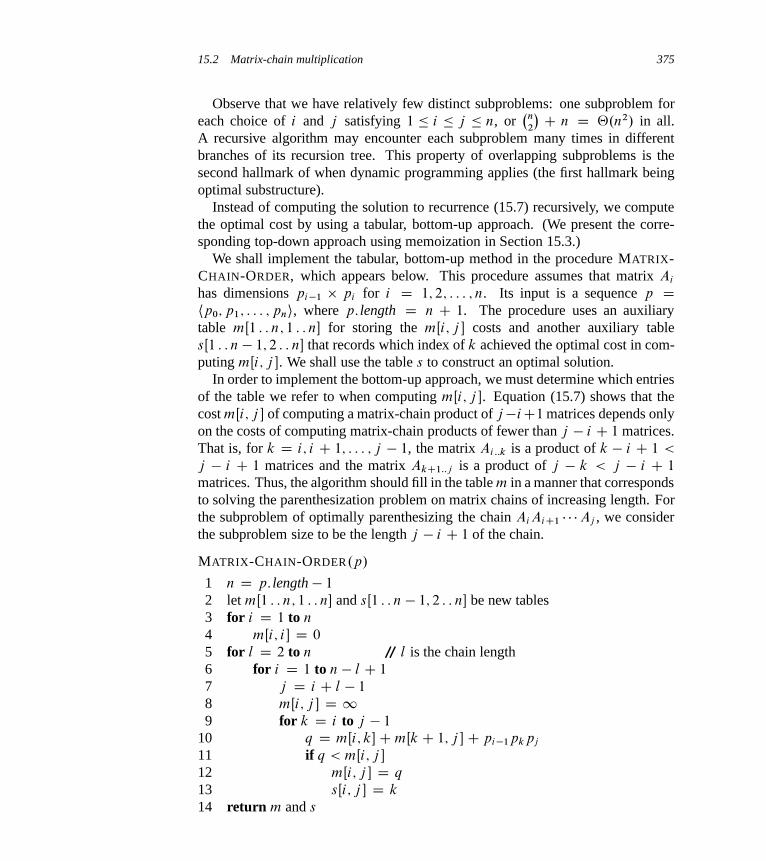
15.2 Matrix-chain multiplication 375
Observe that we have relatively few distinct subproblems: one subproblem foreach choice of i and j satisfying 1 � i � j � n, or
�n
2
� C n D ‚.n2/ in all.A recursive algorithm may encounter each subproblem many times in differentbranches of its recursion tree. This property of overlapping subproblems is thesecond hallmark of when dynamic programming applies (the first hallmark beingoptimal substructure).
Instead of computing the solution to recurrence (15.7) recursively, we computethe optimal cost by using a tabular, bottom-up approach. (We present the corre-sponding top-down approach using memoization in Section 15.3.)
We shall implement the tabular, bottom-up method in the procedure MATRIX-CHAIN-ORDER, which appears below. This procedure assumes that matrix Ai
has dimensions pi�1 pi for i D 1; 2; : : : ; n. Its input is a sequence p Dhp0; p1; : : : ; pni, where p: length D n C 1. The procedure uses an auxiliarytable mŒ1 : : n; 1 : : n� for storing the mŒi; j � costs and another auxiliary tablesŒ1 : : n � 1; 2 : : n� that records which index of k achieved the optimal cost in com-puting mŒi; j �. We shall use the table s to construct an optimal solution.
In order to implement the bottom-up approach, we must determine which entriesof the table we refer to when computing mŒi; j �. Equation (15.7) shows that thecost mŒi; j � of computing a matrix-chain product of j�iC1 matrices depends onlyon the costs of computing matrix-chain products of fewer than j � i C 1 matrices.That is, for k D i; i C 1; : : : ; j � 1, the matrix Ai ::k is a product of k � i C 1 <
j � i C 1 matrices and the matrix AkC1::j is a product of j � k < j � i C 1
matrices. Thus, the algorithm should fill in the table m in a manner that correspondsto solving the parenthesization problem on matrix chains of increasing length. Forthe subproblem of optimally parenthesizing the chain AiAiC1 � � �Aj , we considerthe subproblem size to be the length j � i C 1 of the chain.
MATRIX-CHAIN-ORDER.p/
1 n D p: length � 1
2 let mŒ1 : : n; 1 : : n� and sŒ1 : : n � 1; 2 : : n� be new tables3 for i D 1 to n
4 mŒi; i � D 0
5 for l D 2 to n // l is the chain length6 for i D 1 to n � l C 1
7 j D i C l � 1
8 mŒi; j � D 19 for k D i to j � 1
10 q D mŒi; k�CmŒk C 1; j �C pi�1pkpj
11 if q < mŒi; j �
12 mŒi; j � D q
13 sŒi; j � D k
14 return m and s
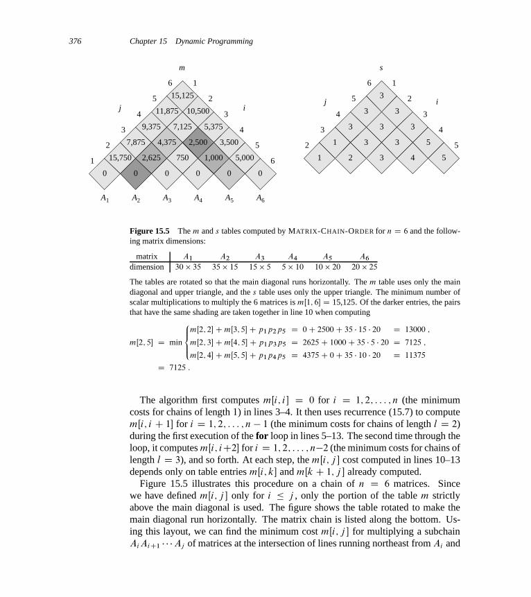
376 Chapter 15 Dynamic Programming
A6A5A4A3A2A1
0 0 0 0 0 0
15,750 2,625 750 1,000 5,000
7,875 4,375 2,500 3,500
9,375 7,125 5,375
11,875 10,500
15,125
1
2
3
4
5
6 1
2
3
4
5
6
j i
m
1 2 3 4 5
1 3 3 5
3 3 3
3 3
3
2
3
4
5
6 1
2
3
4
5
j i
s
Figure 15.5 The m and s tables computed by MATRIX-CHAIN-ORDER for n D 6 and the follow-ing matrix dimensions:
matrix A1 A2 A3 A4 A5 A6
dimension 30 35 35 15 15 5 5 10 10 20 20 25
The tables are rotated so that the main diagonal runs horizontally. The m table uses only the maindiagonal and upper triangle, and the s table uses only the upper triangle. The minimum number ofscalar multiplications to multiply the 6 matrices is mŒ1; 6� D 15,125. Of the darker entries, the pairsthat have the same shading are taken together in line 10 when computing
mŒ2; 5� D min
8̂<̂:
mŒ2; 2�CmŒ3; 5�C p1p2p5 D 0C 2500C 35 � 15 � 20 D 13000 ;
mŒ2; 3�CmŒ4; 5�C p1p3p5 D 2625C 1000C 35 � 5 � 20 D 7125 ;
mŒ2; 4�CmŒ5; 5�C p1p4p5 D 4375C 0C 35 � 10 � 20 D 11375
D 7125 :
The algorithm first computes mŒi; i � D 0 for i D 1; 2; : : : ; n (the minimumcosts for chains of length 1) in lines 3–4. It then uses recurrence (15.7) to computemŒi; i C 1� for i D 1; 2; : : : ; n � 1 (the minimum costs for chains of length l D 2)during the first execution of the for loop in lines 5–13. The second time through theloop, it computes mŒi; iC2� for i D 1; 2; : : : ; n�2 (the minimum costs for chains oflength l D 3), and so forth. At each step, the mŒi; j � cost computed in lines 10–13depends only on table entries mŒi; k� and mŒk C 1; j � already computed.
Figure 15.5 illustrates this procedure on a chain of n D 6 matrices. Sincewe have defined mŒi; j � only for i � j , only the portion of the table m strictlyabove the main diagonal is used. The figure shows the table rotated to make themain diagonal run horizontally. The matrix chain is listed along the bottom. Us-ing this layout, we can find the minimum cost mŒi; j � for multiplying a subchainAiAiC1 � � �Aj of matrices at the intersection of lines running northeast from Ai and

15.2 Matrix-chain multiplication 377
northwest from Aj . Each horizontal row in the table contains the entries for matrixchains of the same length. MATRIX-CHAIN-ORDER computes the rows from bot-tom to top and from left to right within each row. It computes each entry mŒi; j �
using the products pi�1pkpj for k D i; i C 1; : : : ; j � 1 and all entries southwestand southeast from mŒi; j �.
A simple inspection of the nested loop structure of MATRIX-CHAIN-ORDER
yields a running time of O.n3/ for the algorithm. The loops are nested three deep,and each loop index (l , i , and k) takes on at most n�1 values. Exercise 15.2-5 asksyou to show that the running time of this algorithm is in fact also �.n3/. The al-gorithm requires ‚.n2/ space to store the m and s tables. Thus, MATRIX-CHAIN-ORDER is much more efficient than the exponential-time method of enumeratingall possible parenthesizations and checking each one.
Step 4: Constructing an optimal solution
Although MATRIX-CHAIN-ORDER determines the optimal number of scalar mul-tiplications needed to compute a matrix-chain product, it does not directly showhow to multiply the matrices. The table sŒ1 : : n � 1; 2 : : n� gives us the informa-tion we need to do so. Each entry sŒi; j � records a value of k such that an op-timal parenthesization of AiAiC1 � � �Aj splits the product between Ak and AkC1.Thus, we know that the final matrix multiplication in computing A1::n optimallyis A1::sŒ1;n�AsŒ1;n�C1::n. We can determine the earlier matrix multiplications recur-sively, since sŒ1; sŒ1; n�� determines the last matrix multiplication when computingA1::sŒ1;n� and sŒsŒ1; n� C 1; n� determines the last matrix multiplication when com-puting AsŒ1;n�C1::n. The following recursive procedure prints an optimal parenthe-sization of hAi ; AiC1; : : : ; Aj i, given the s table computed by MATRIX-CHAIN-ORDER and the indices i and j . The initial call PRINT-OPTIMAL-PARENS.s; 1; n/
prints an optimal parenthesization of hA1; A2; : : : ; Ani.
PRINT-OPTIMAL-PARENS.s; i; j /
1 if i == j
2 print “A”i
3 else print “(”4 PRINT-OPTIMAL-PARENS.s; i; sŒi; j �/
5 PRINT-OPTIMAL-PARENS.s; sŒi; j � C 1; j /
6 print “)”
In the example of Figure 15.5, the call PRINT-OPTIMAL-PARENS.s; 1; 6/ printsthe parenthesization ..A1.A2A3//..A4A5/A6//.
378 Chapter 15 Dynamic Programming
Exercises
15.2-1Find an optimal parenthesization of a matrix-chain product whose sequence ofdimensions is h5; 10; 3; 12; 5; 50; 6i.15.2-2Give a recursive algorithm MATRIX-CHAIN-MULTIPLY.A; s; i; j / that actuallyperforms the optimal matrix-chain multiplication, given the sequence of matriceshA1; A2; : : : ; Ani, the s table computed by MATRIX-CHAIN-ORDER, and the in-dices i and j . (The initial call would be MATRIX-CHAIN-MULTIPLY.A; s; 1; n/.)
15.2-3Use the substitution method to show that the solution to the recurrence (15.6)is �.2n/.
15.2-4Describe the subproblem graph for matrix-chain multiplication with an input chainof length n. How many vertices does it have? How many edges does it have, andwhich edges are they?
15.2-5Let R.i; j / be the number of times that table entry mŒi; j � is referenced whilecomputing other table entries in a call of MATRIX-CHAIN-ORDER. Show that thetotal number of references for the entire table is
nXiD1
nXj Di
R.i; j / D n3 � n
3:
(Hint: You may find equation (A.3) useful.)
15.2-6Show that a full parenthesization of an n-element expression has exactly n�1 pairsof parentheses.
15.3 Elements of dynamic programming
Although we have just worked through two examples of the dynamic-programmingmethod, you might still be wondering just when the method applies. From an en-gineering perspective, when should we look for a dynamic-programming solutionto a problem? In this section, we examine the two key ingredients that an opti-

15.3 Elements of dynamic programming 379
mization problem must have in order for dynamic programming to apply: optimalsubstructure and overlapping subproblems. We also revisit and discuss more fullyhow memoization might help us take advantage of the overlapping-subproblemsproperty in a top-down recursive approach.
Optimal substructure
The first step in solving an optimization problem by dynamic programming is tocharacterize the structure of an optimal solution. Recall that a problem exhibitsoptimal substructure if an optimal solution to the problem contains within it opti-mal solutions to subproblems. Whenever a problem exhibits optimal substructure,we have a good clue that dynamic programming might apply. (As Chapter 16 dis-cusses, it also might mean that a greedy strategy applies, however.) In dynamicprogramming, we build an optimal solution to the problem from optimal solutionsto subproblems. Consequently, we must take care to ensure that the range of sub-problems we consider includes those used in an optimal solution.
We discovered optimal substructure in both of the problems we have examinedin this chapter so far. In Section 15.1, we observed that the optimal way of cut-ting up a rod of length n (if we make any cuts at all) involves optimally cuttingup the two pieces resulting from the first cut. In Section 15.2, we observed thatan optimal parenthesization of AiAiC1 � � �Aj that splits the product between Ak
and AkC1 contains within it optimal solutions to the problems of parenthesizingAiAiC1 � � �Ak and AkC1AkC2 � � �Aj .
You will find yourself following a common pattern in discovering optimal sub-structure:
1. You show that a solution to the problem consists of making a choice, such aschoosing an initial cut in a rod or choosing an index at which to split the matrixchain. Making this choice leaves one or more subproblems to be solved.
2. You suppose that for a given problem, you are given the choice that leads to anoptimal solution. You do not concern yourself yet with how to determine thischoice. You just assume that it has been given to you.
3. Given this choice, you determine which subproblems ensue and how to bestcharacterize the resulting space of subproblems.
4. You show that the solutions to the subproblems used within an optimal solutionto the problem must themselves be optimal by using a “cut-and-paste” tech-nique. You do so by supposing that each of the subproblem solutions is notoptimal and then deriving a contradiction. In particular, by “cutting out” thenonoptimal solution to each subproblem and “pasting in” the optimal one, youshow that you can get a better solution to the original problem, thus contradict-ing your supposition that you already had an optimal solution. If an optimal

380 Chapter 15 Dynamic Programming
solution gives rise to more than one subproblem, they are typically so similarthat you can modify the cut-and-paste argument for one to apply to the otherswith little effort.
To characterize the space of subproblems, a good rule of thumb says to try tokeep the space as simple as possible and then expand it as necessary. For example,the space of subproblems that we considered for the rod-cutting problem containedthe problems of optimally cutting up a rod of length i for each size i . This sub-problem space worked well, and we had no need to try a more general space ofsubproblems.
Conversely, suppose that we had tried to constrain our subproblem space formatrix-chain multiplication to matrix products of the form A1A2 � � �Aj . As before,an optimal parenthesization must split this product between Ak and AkC1 for some1 � k < j . Unless we could guarantee that k always equals j � 1, we would findthat we had subproblems of the form A1A2 � � �Ak and AkC1AkC2 � � �Aj , and thatthe latter subproblem is not of the form A1A2 � � �Aj . For this problem, we neededto allow our subproblems to vary at “both ends,” that is, to allow both i and j tovary in the subproblem AiAiC1 � � �Aj .
Optimal substructure varies across problem domains in two ways:
1. how many subproblems an optimal solution to the original problem uses, and
2. how many choices we have in determining which subproblem(s) to use in anoptimal solution.
In the rod-cutting problem, an optimal solution for cutting up a rod of size n
uses just one subproblem (of size n � i), but we must consider n choices for i
in order to determine which one yields an optimal solution. Matrix-chain mul-tiplication for the subchain AiAiC1 � � �Aj serves as an example with two sub-problems and j � i choices. For a given matrix Ak at which we split the prod-uct, we have two subproblems—parenthesizing AiAiC1 � � �Ak and parenthesizingAkC1AkC2 � � �Aj —and we must solve both of them optimally. Once we determinethe optimal solutions to subproblems, we choose from among j � i candidates forthe index k.
Informally, the running time of a dynamic-programming algorithm depends onthe product of two factors: the number of subproblems overall and how manychoices we look at for each subproblem. In rod cutting, we had ‚.n/ subproblemsoverall, and at most n choices to examine for each, yielding an O.n2/ running time.Matrix-chain multiplication had ‚.n2/ subproblems overall, and in each we had atmost n� 1 choices, giving an O.n3/ running time (actually, a ‚.n3/ running time,by Exercise 15.2-5.)
Usually, the subproblem graph gives an alternative way to perform the sameanalysis. Each vertex corresponds to a subproblem, and the choices for a sub-

15.3 Elements of dynamic programming 381
problem are the edges incident to that subproblem. Recall that in rod cutting,the subproblem graph had n vertices and at most n edges per vertex, yielding anO.n2/ running time. For matrix-chain multiplication, if we were to draw the sub-problem graph, it would have ‚.n2/ vertices and each vertex would have degree atmost n � 1, giving a total of O.n3/ vertices and edges.
Dynamic programming often uses optimal substructure in a bottom-up fashion.That is, we first find optimal solutions to subproblems and, having solved the sub-problems, we find an optimal solution to the problem. Finding an optimal solu-tion to the problem entails making a choice among subproblems as to which wewill use in solving the problem. The cost of the problem solution is usually thesubproblem costs plus a cost that is directly attributable to the choice itself. Inrod cutting, for example, first we solved the subproblems of determining optimalways to cut up rods of length i for i D 0; 1; : : : ; n � 1, and then we determinedwhich such subproblem yielded an optimal solution for a rod of length n, usingequation (15.2). The cost attributable to the choice itself is the term pi in equa-tion (15.2). In matrix-chain multiplication, we determined optimal parenthesiza-tions of subchains of AiAiC1 � � �Aj , and then we chose the matrix Ak at which tosplit the product. The cost attributable to the choice itself is the term pi�1pkpj .
In Chapter 16, we shall examine “greedy algorithms,” which have many similar-ities to dynamic programming. In particular, problems to which greedy algorithmsapply have optimal substructure. One major difference between greedy algorithmsand dynamic programming is that in greedy algorithms, instead of first findingoptimal solutions to subproblems and then making an informed choice, greedy al-gorithms first make a “greedy” choice—the choice that looks best at the time—andthen solve a resulting subproblem, without bothering to solve all possible relatedsmaller subproblems. Surprisingly, in some cases this strategy works!
SubtletiesYou should be careful not to assume that optimal substructure applies when it doesnot. Consider the following two problems in which we are given a directed graphG D .V; E/ and vertices u; � 2 V .
Unweighted shortest path:3 Find a path from u to � consisting of the fewestedges. Such a path must be simple, since removing a cycle from a path pro-duces a path with fewer edges.
3We use the term “unweighted” to distinguish this problem from that of finding shortest paths withweighted edges, which we shall see in Chapters 24 and 25. We can use the breadth-first searchtechnique of Chapter 22 to solve the unweighted problem.
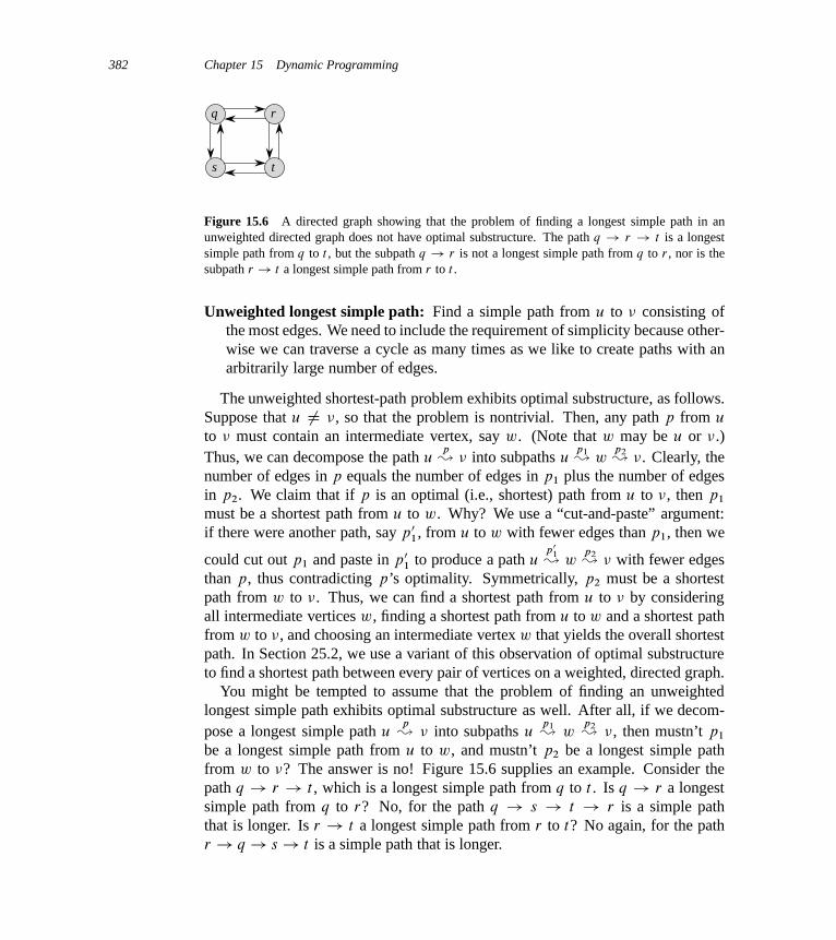
382 Chapter 15 Dynamic Programming
q r
s t
Figure 15.6 A directed graph showing that the problem of finding a longest simple path in anunweighted directed graph does not have optimal substructure. The path q ! r ! t is a longestsimple path from q to t , but the subpath q ! r is not a longest simple path from q to r , nor is thesubpath r ! t a longest simple path from r to t .
Unweighted longest simple path: Find a simple path from u to � consisting ofthe most edges. We need to include the requirement of simplicity because other-wise we can traverse a cycle as many times as we like to create paths with anarbitrarily large number of edges.
The unweighted shortest-path problem exhibits optimal substructure, as follows.Suppose that u ¤ �, so that the problem is nontrivial. Then, any path p from u
to � must contain an intermediate vertex, say w. (Note that w may be u or �.)Thus, we can decompose the path u
p� � into subpaths u
p1� w
p2� �. Clearly, the
number of edges in p equals the number of edges in p1 plus the number of edgesin p2. We claim that if p is an optimal (i.e., shortest) path from u to �, then p1
must be a shortest path from u to w. Why? We use a “cut-and-paste” argument:if there were another path, say p0
1, from u to w with fewer edges than p1, then we
could cut out p1 and paste in p01 to produce a path u
p01
� wp2� � with fewer edges
than p, thus contradicting p’s optimality. Symmetrically, p2 must be a shortestpath from w to �. Thus, we can find a shortest path from u to � by consideringall intermediate vertices w, finding a shortest path from u to w and a shortest pathfrom w to �, and choosing an intermediate vertex w that yields the overall shortestpath. In Section 25.2, we use a variant of this observation of optimal substructureto find a shortest path between every pair of vertices on a weighted, directed graph.
You might be tempted to assume that the problem of finding an unweightedlongest simple path exhibits optimal substructure as well. After all, if we decom-pose a longest simple path u
p� � into subpaths u
p1� w
p2� �, then mustn’t p1
be a longest simple path from u to w, and mustn’t p2 be a longest simple pathfrom w to �? The answer is no! Figure 15.6 supplies an example. Consider thepath q ! r ! t , which is a longest simple path from q to t . Is q ! r a longestsimple path from q to r? No, for the path q ! s ! t ! r is a simple paththat is longer. Is r ! t a longest simple path from r to t? No again, for the pathr ! q ! s ! t is a simple path that is longer.
15.3 Elements of dynamic programming 383
This example shows that for longest simple paths, not only does the problemlack optimal substructure, but we cannot necessarily assemble a “legal” solutionto the problem from solutions to subproblems. If we combine the longest simplepaths q ! s ! t ! r and r ! q ! s ! t , we get the path q ! s ! t ! r !q ! s ! t , which is not simple. Indeed, the problem of finding an unweightedlongest simple path does not appear to have any sort of optimal substructure. Noefficient dynamic-programming algorithm for this problem has ever been found. Infact, this problem is NP-complete, which—as we shall see in Chapter 34—meansthat we are unlikely to find a way to solve it in polynomial time.
Why is the substructure of a longest simple path so different from that of a short-est path? Although a solution to a problem for both longest and shortest paths usestwo subproblems, the subproblems in finding the longest simple path are not inde-pendent, whereas for shortest paths they are. What do we mean by subproblemsbeing independent? We mean that the solution to one subproblem does not affectthe solution to another subproblem of the same problem. For the example of Fig-ure 15.6, we have the problem of finding a longest simple path from q to t with twosubproblems: finding longest simple paths from q to r and from r to t . For the firstof these subproblems, we choose the path q ! s ! t ! r , and so we have alsoused the vertices s and t . We can no longer use these vertices in the second sub-problem, since the combination of the two solutions to subproblems would yield apath that is not simple. If we cannot use vertex t in the second problem, then wecannot solve it at all, since t is required to be on the path that we find, and it isnot the vertex at which we are “splicing” together the subproblem solutions (thatvertex being r). Because we use vertices s and t in one subproblem solution, wecannot use them in the other subproblem solution. We must use at least one of themto solve the other subproblem, however, and we must use both of them to solve itoptimally. Thus, we say that these subproblems are not independent. Looked atanother way, using resources in solving one subproblem (those resources beingvertices) renders them unavailable for the other subproblem.
Why, then, are the subproblems independent for finding a shortest path? Theanswer is that by nature, the subproblems do not share resources. We claim thatif a vertex w is on a shortest path p from u to �, then we can splice together anyshortest path u
p1� w and any shortest path w
p2� � to produce a shortest path from u
to �. We are assured that, other than w, no vertex can appear in both paths p1
and p2. Why? Suppose that some vertex x ¤ w appears in both p1 and p2, so thatwe can decompose p1 as u
pux� x � w and p2 as w � x
px�� �. By the optimal
substructure of this problem, path p has as many edges as p1 and p2 together; let’ssay that p has e edges. Now let us construct a path p0 D u
pux� x
px�� � from u to �.
Because we have excised the paths from x to w and from w to x, each of whichcontains at least one edge, path p0 contains at most e � 2 edges, which contradicts

384 Chapter 15 Dynamic Programming
the assumption that p is a shortest path. Thus, we are assured that the subproblemsfor the shortest-path problem are independent.
Both problems examined in Sections 15.1 and 15.2 have independent subprob-lems. In matrix-chain multiplication, the subproblems are multiplying subchainsAiAiC1 � � �Ak and AkC1AkC2 � � �Aj . These subchains are disjoint, so that no ma-trix could possibly be included in both of them. In rod cutting, to determine thebest way to cut up a rod of length n, we look at the best ways of cutting up rodsof length i for i D 0; 1; : : : ; n � 1. Because an optimal solution to the length-nproblem includes just one of these subproblem solutions (after we have cut off thefirst piece), independence of subproblems is not an issue.
Overlapping subproblems
The second ingredient that an optimization problem must have for dynamic pro-gramming to apply is that the space of subproblems must be “small” in the sensethat a recursive algorithm for the problem solves the same subproblems over andover, rather than always generating new subproblems. Typically, the total numberof distinct subproblems is a polynomial in the input size. When a recursive algo-rithm revisits the same problem repeatedly, we say that the optimization problemhas overlapping subproblems.4 In contrast, a problem for which a divide-and-conquer approach is suitable usually generates brand-new problems at each stepof the recursion. Dynamic-programming algorithms typically take advantage ofoverlapping subproblems by solving each subproblem once and then storing thesolution in a table where it can be looked up when needed, using constant time perlookup.
In Section 15.1, we briefly examined how a recursive solution to rod cut-ting makes exponentially many calls to find solutions of smaller subproblems.Our dynamic-programming solution takes an exponential-time recursive algorithmdown to quadratic time.
To illustrate the overlapping-subproblems property in greater detail, let us re-examine the matrix-chain multiplication problem. Referring back to Figure 15.5,observe that MATRIX-CHAIN-ORDER repeatedly looks up the solution to subprob-lems in lower rows when solving subproblems in higher rows. For example, itreferences entry mŒ3; 4� four times: during the computations of mŒ2; 4�, mŒ1; 4�,
4It may seem strange that dynamic programming relies on subproblems being both independentand overlapping. Although these requirements may sound contradictory, they describe two differentnotions, rather than two points on the same axis. Two subproblems of the same problem are inde-pendent if they do not share resources. Two subproblems are overlapping if they are really the samesubproblem that occurs as a subproblem of different problems.

15.3 Elements of dynamic programming 385
1..4
1..1 2..4 1..2 3..4 1..3 4..4
2..2 3..4 2..3 4..4 1..1 2..2 3..3 4..4 1..1 2..3 1..2 3..3
3..3 4..4 2..2 3..3 2..2 3..3 1..1 2..2
Figure 15.7 The recursion tree for the computation of RECURSIVE-MATRIX-CHAIN.p; 1; 4/.Each node contains the parameters i and j . The computations performed in a shaded subtree arereplaced by a single table lookup in MEMOIZED-MATRIX-CHAIN.
mŒ3; 5�, and mŒ3; 6�. If we were to recompute mŒ3; 4� each time, rather than justlooking it up, the running time would increase dramatically. To see how, considerthe following (inefficient) recursive procedure that determines mŒi; j �, the mini-mum number of scalar multiplications needed to compute the matrix-chain productAi ::j D AiAiC1 � � �Aj . The procedure is based directly on the recurrence (15.7).
RECURSIVE-MATRIX-CHAIN.p; i; j /
1 if i == j
2 return 0
3 mŒi; j � D 14 for k D i to j � 1
5 q D RECURSIVE-MATRIX-CHAIN.p; i; k/
C RECURSIVE-MATRIX-CHAIN.p; k C 1; j /
C pi�1pkpj
6 if q < mŒi; j �
7 mŒi; j � D q
8 return mŒi; j �
Figure 15.7 shows the recursion tree produced by the call RECURSIVE-MATRIX-CHAIN.p; 1; 4/. Each node is labeled by the values of the parameters i and j .Observe that some pairs of values occur many times.
In fact, we can show that the time to compute mŒ1; n� by this recursive proce-dure is at least exponential in n. Let T .n/ denote the time taken by RECURSIVE-MATRIX-CHAIN to compute an optimal parenthesization of a chain of n matrices.Because the execution of lines 1–2 and of lines 6–7 each take at least unit time, as
386 Chapter 15 Dynamic Programming
does the multiplication in line 5, inspection of the procedure yields the recurrence
T .1/ � 1 ;
T .n/ � 1Cn�1XkD1
.T .k/C T .n � k/C 1/ for n > 1 :
Noting that for i D 1; 2; : : : ; n� 1, each term T .i/ appears once as T .k/ and onceas T .n � k/, and collecting the n � 1 1s in the summation together with the 1 outfront, we can rewrite the recurrence as
T .n/ � 2
n�1XiD1
T .i/C n : (15.8)
We shall prove that T .n/ D �.2n/ using the substitution method. Specifi-cally, we shall show that T .n/ � 2n�1 for all n � 1. The basis is easy, sinceT .1/ � 1 D 20. Inductively, for n � 2 we have
T .n/ � 2
n�1XiD1
2i�1 C n
D 2
n�2XiD0
2i C n
D 2.2n�1 � 1/C n (by equation (A.5))
D 2n � 2C n
� 2n�1 ;
which completes the proof. Thus, the total amount of work performed by the callRECURSIVE-MATRIX-CHAIN.p; 1; n/ is at least exponential in n.
Compare this top-down, recursive algorithm (without memoization) with thebottom-up dynamic-programming algorithm. The latter is more efficient becauseit takes advantage of the overlapping-subproblems property. Matrix-chain mul-tiplication has only ‚.n2/ distinct subproblems, and the dynamic-programmingalgorithm solves each exactly once. The recursive algorithm, on the other hand,must again solve each subproblem every time it reappears in the recursion tree.Whenever a recursion tree for the natural recursive solution to a problem containsthe same subproblem repeatedly, and the total number of distinct subproblems issmall, dynamic programming can improve efficiency, sometimes dramatically.

15.3 Elements of dynamic programming 387
Reconstructing an optimal solution
As a practical matter, we often store which choice we made in each subproblem ina table so that we do not have to reconstruct this information from the costs that westored.
For matrix-chain multiplication, the table sŒi; j � saves us a significant amount ofwork when reconstructing an optimal solution. Suppose that we did not maintainthe sŒi; j � table, having filled in only the table mŒi; j � containing optimal subprob-lem costs. We choose from among j � i possibilities when we determine whichsubproblems to use in an optimal solution to parenthesizing AiAiC1 � � �Aj , andj � i is not a constant. Therefore, it would take ‚.j � i/ D !.1/ time to recon-struct which subproblems we chose for a solution to a given problem. By storingin sŒi; j � the index of the matrix at which we split the product AiAiC1 � � �Aj , wecan reconstruct each choice in O.1/ time.
Memoization
As we saw for the rod-cutting problem, there is an alternative approach to dy-namic programming that often offers the efficiency of the bottom-up dynamic-programming approach while maintaining a top-down strategy. The idea is tomemoize the natural, but inefficient, recursive algorithm. As in the bottom-up ap-proach, we maintain a table with subproblem solutions, but the control structurefor filling in the table is more like the recursive algorithm.
A memoized recursive algorithm maintains an entry in a table for the solution toeach subproblem. Each table entry initially contains a special value to indicate thatthe entry has yet to be filled in. When the subproblem is first encountered as therecursive algorithm unfolds, its solution is computed and then stored in the table.Each subsequent time that we encounter this subproblem, we simply look up thevalue stored in the table and return it.5
Here is a memoized version of RECURSIVE-MATRIX-CHAIN. Note where itresembles the memoized top-down method for the rod-cutting problem.
5This approach presupposes that we know the set of all possible subproblem parameters and that wehave established the relationship between table positions and subproblems. Another, more general,approach is to memoize by using hashing with the subproblem parameters as keys.
388 Chapter 15 Dynamic Programming
MEMOIZED-MATRIX-CHAIN.p/
1 n D p: length � 1
2 let mŒ1 : : n; 1 : : n� be a new table3 for i D 1 to n
4 for j D i to n
5 mŒi; j � D 16 return LOOKUP-CHAIN.m; p; 1; n/
LOOKUP-CHAIN.m; p; i; j /
1 if mŒi; j � <12 return mŒi; j �
3 if i == j
4 mŒi; j � D 0
5 else for k D i to j � 1
6 q D LOOKUP-CHAIN.m; p; i; k/
C LOOKUP-CHAIN.m; p; k C 1; j /C pi�1pkpj
7 if q < mŒi; j �
8 mŒi; j � D q
9 return mŒi; j �
The MEMOIZED-MATRIX-CHAIN procedure, like MATRIX-CHAIN-ORDER,maintains a table mŒ1 : : n; 1 : : n� of computed values of mŒi; j �, the minimum num-ber of scalar multiplications needed to compute the matrix Ai ::j . Each table entryinitially contains the value1 to indicate that the entry has yet to be filled in. Uponcalling LOOKUP-CHAIN.m; p; i; j /, if line 1 finds that mŒi; j � <1, then the pro-cedure simply returns the previously computed cost mŒi; j � in line 2. Otherwise,the cost is computed as in RECURSIVE-MATRIX-CHAIN, stored in mŒi; j �, andreturned. Thus, LOOKUP-CHAIN.m; p; i; j / always returns the value of mŒi; j �,but it computes it only upon the first call of LOOKUP-CHAIN with these specificvalues of i and j .
Figure 15.7 illustrates how MEMOIZED-MATRIX-CHAIN saves time comparedwith RECURSIVE-MATRIX-CHAIN. Shaded subtrees represent values that it looksup rather than recomputes.
Like the bottom-up dynamic-programming algorithm MATRIX-CHAIN-ORDER,the procedure MEMOIZED-MATRIX-CHAIN runs in O.n3/ time. Line 5 ofMEMOIZED-MATRIX-CHAIN executes ‚.n2/ times. We can categorize the callsof LOOKUP-CHAIN into two types:
1. calls in which mŒi; j � D1, so that lines 3–9 execute, and
2. calls in which mŒi; j � <1, so that LOOKUP-CHAIN simply returns in line 2.

15.3 Elements of dynamic programming 389
There are ‚.n2/ calls of the first type, one per table entry. All calls of the sec-ond type are made as recursive calls by calls of the first type. Whenever a givencall of LOOKUP-CHAIN makes recursive calls, it makes O.n/ of them. There-fore, there are O.n3/ calls of the second type in all. Each call of the second typetakes O.1/ time, and each call of the first type takes O.n/ time plus the time spentin its recursive calls. The total time, therefore, is O.n3/. Memoization thus turnsan �.2n/-time algorithm into an O.n3/-time algorithm.
In summary, we can solve the matrix-chain multiplication problem by either atop-down, memoized dynamic-programming algorithm or a bottom-up dynamic-programming algorithm in O.n3/ time. Both methods take advantage of theoverlapping-subproblems property. There are only ‚.n2/ distinct subproblems intotal, and either of these methods computes the solution to each subproblem onlyonce. Without memoization, the natural recursive algorithm runs in exponentialtime, since solved subproblems are repeatedly solved.
In general practice, if all subproblems must be solved at least once, a bottom-updynamic-programming algorithm usually outperforms the corresponding top-downmemoized algorithm by a constant factor, because the bottom-up algorithm has nooverhead for recursion and less overhead for maintaining the table. Moreover, forsome problems we can exploit the regular pattern of table accesses in the dynamic-programming algorithm to reduce time or space requirements even further. Alter-natively, if some subproblems in the subproblem space need not be solved at all,the memoized solution has the advantage of solving only those subproblems thatare definitely required.
Exercises
15.3-1Which is a more efficient way to determine the optimal number of multiplicationsin a matrix-chain multiplication problem: enumerating all the ways of parenthesiz-ing the product and computing the number of multiplications for each, or runningRECURSIVE-MATRIX-CHAIN? Justify your answer.
15.3-2Draw the recursion tree for the MERGE-SORT procedure from Section 2.3.1 on anarray of 16 elements. Explain why memoization fails to speed up a good divide-and-conquer algorithm such as MERGE-SORT.
15.3-3Consider a variant of the matrix-chain multiplication problem in which the goal isto parenthesize the sequence of matrices so as to maximize, rather than minimize,

390 Chapter 15 Dynamic Programming
the number of scalar multiplications. Does this problem exhibit optimal substruc-ture?
15.3-4As stated, in dynamic programming we first solve the subproblems and then choosewhich of them to use in an optimal solution to the problem. Professor Capuletclaims that we do not always need to solve all the subproblems in order to find anoptimal solution. She suggests that we can find an optimal solution to the matrix-chain multiplication problem by always choosing the matrix Ak at which to splitthe subproduct AiAiC1 � � �Aj (by selecting k to minimize the quantity pi�1pkpj )before solving the subproblems. Find an instance of the matrix-chain multiplica-tion problem for which this greedy approach yields a suboptimal solution.
15.3-5Suppose that in the rod-cutting problem of Section 15.1, we also had limit li on thenumber of pieces of length i that we are allowed to produce, for i D 1; 2; : : : ; n.Show that the optimal-substructure property described in Section 15.1 no longerholds.
15.3-6Imagine that you wish to exchange one currency for another. You realize thatinstead of directly exchanging one currency for another, you might be better offmaking a series of trades through other currencies, winding up with the currencyyou want. Suppose that you can trade n different currencies, numbered 1; 2; : : : ; n,where you start with currency 1 and wish to wind up with currency n. You aregiven, for each pair of currencies i and j , an exchange rate rij , meaning that ifyou start with d units of currency i , you can trade for drij units of currency j .A sequence of trades may entail a commission, which depends on the number oftrades you make. Let ck be the commission that you are charged when you make k
trades. Show that, if ck D 0 for all k D 1; 2; : : : ; n, then the problem of finding thebest sequence of exchanges from currency 1 to currency n exhibits optimal sub-structure. Then show that if commissions ck are arbitrary values, then the problemof finding the best sequence of exchanges from currency 1 to currency n does notnecessarily exhibit optimal substructure.
15.4 Longest common subsequence
Biological applications often need to compare the DNA of two (or more) dif-ferent organisms. A strand of DNA consists of a string of molecules called
15.4 Longest common subsequence 391
bases, where the possible bases are adenine, guanine, cytosine, and thymine.Representing each of these bases by its initial letter, we can express a strandof DNA as a string over the finite set fA; C; G; Tg. (See Appendix C forthe definition of a string.) For example, the DNA of one organism may beS1 D ACCGGTCGAGTGCGCGGAAGCCGGCCGAA, and the DNA of another organ-ism may be S2 D GTCGTTCGGAATGCCGTTGCTCTGTAAA. One reason to com-pare two strands of DNA is to determine how “similar” the two strands are, as somemeasure of how closely related the two organisms are. We can, and do, define sim-ilarity in many different ways. For example, we can say that two DNA strands aresimilar if one is a substring of the other. (Chapter 32 explores algorithms to solvethis problem.) In our example, neither S1 nor S2 is a substring of the other. Alter-natively, we could say that two strands are similar if the number of changes neededto turn one into the other is small. (Problem 15-5 looks at this notion.) Yet anotherway to measure the similarity of strands S1 and S2 is by finding a third strand S3
in which the bases in S3 appear in each of S1 and S2; these bases must appearin the same order, but not necessarily consecutively. The longer the strand S3 wecan find, the more similar S1 and S2 are. In our example, the longest strand S3 isGTCGTCGGAAGCCGGCCGAA.
We formalize this last notion of similarity as the longest-common-subsequenceproblem. A subsequence of a given sequence is just the given sequence with zero ormore elements left out. Formally, given a sequence X D hx1; x2; : : : ; xmi, anothersequence Z D h´1; ´2; : : : ; ´ki is a subsequence of X if there exists a strictlyincreasing sequence hi1; i2; : : : ; iki of indices of X such that for all j D 1; 2; : : : ; k,we have xij D j́ . For example, Z D hB; C; D; Bi is a subsequence of X DhA; B; C; B; D; A; Bi with corresponding index sequence h2; 3; 5; 7i.
Given two sequences X and Y , we say that a sequence Z is a common sub-sequence of X and Y if Z is a subsequence of both X and Y . For example, ifX D hA;B;C;B;D;A;Bi and Y D hB;D;C;A;B;Ai, the sequence hB;C;Ai isa common subsequence of both X and Y . The sequence hB; C; Ai is not a longestcommon subsequence (LCS) of X and Y , however, since it has length 3 and thesequence hB; C; B; Ai, which is also common to both X and Y , has length 4. Thesequence hB; C; B; Ai is an LCS of X and Y , as is the sequence hB; D; A; Bi,since X and Y have no common subsequence of length 5 or greater.
In the longest-common-subsequence problem, we are given two sequencesX D hx1; x2; : : : ; xmi and Y D hy1; y2; : : : ; yni and wish to find a maximum-length common subsequence of X and Y . This section shows how to efficientlysolve the LCS problem using dynamic programming.
392 Chapter 15 Dynamic Programming
Step 1: Characterizing a longest common subsequence
In a brute-force approach to solving the LCS problem, we would enumerate allsubsequences of X and check each subsequence to see whether it is also a subse-quence of Y , keeping track of the longest subsequence we find. Each subsequenceof X corresponds to a subset of the indices f1; 2; : : : ; mg of X . Because X has 2m
subsequences, this approach requires exponential time, making it impractical forlong sequences.
The LCS problem has an optimal-substructure property, however, as the follow-ing theorem shows. As we shall see, the natural classes of subproblems corre-spond to pairs of “prefixes” of the two input sequences. To be precise, given asequence X D hx1; x2; : : : ; xmi, we define the i th prefix of X , for i D 0; 1; : : : ; m,as Xi D hx1; x2; : : : ; xi i. For example, if X D hA; B; C; B; D; A; Bi, thenX4 D hA; B; C; Bi and X0 is the empty sequence.
Theorem 15.1 (Optimal substructure of an LCS)Let X D hx1; x2; : : : ; xmi and Y D hy1; y2; : : : ; yni be sequences, and let Z Dh´1; ´2; : : : ; ´ki be any LCS of X and Y .
1. If xm D yn, then ´k D xm D yn and Zk�1 is an LCS of Xm�1 and Yn�1.
2. If xm ¤ yn, then ´k ¤ xm implies that Z is an LCS of Xm�1 and Y .
3. If xm ¤ yn, then ´k ¤ yn implies that Z is an LCS of X and Yn�1.
Proof (1) If ´k ¤ xm, then we could append xm D yn to Z to obtain a commonsubsequence of X and Y of length k C 1, contradicting the supposition that Z isa longest common subsequence of X and Y . Thus, we must have ´k D xm D yn.Now, the prefix Zk�1 is a length-.k � 1/ common subsequence of Xm�1 and Yn�1.We wish to show that it is an LCS. Suppose for the purpose of contradictionthat there exists a common subsequence W of Xm�1 and Yn�1 with length greaterthan k � 1. Then, appending xm D yn to W produces a common subsequence ofX and Y whose length is greater than k, which is a contradiction.
(2) If ´k ¤ xm, then Z is a common subsequence of Xm�1 and Y . If there were acommon subsequence W of Xm�1 and Y with length greater than k, then W wouldalso be a common subsequence of Xm and Y , contradicting the assumption that Z
is an LCS of X and Y .(3) The proof is symmetric to (2).
The way that Theorem 15.1 characterizes longest common subsequences tellsus that an LCS of two sequences contains within it an LCS of prefixes of the twosequences. Thus, the LCS problem has an optimal-substructure property. A recur-
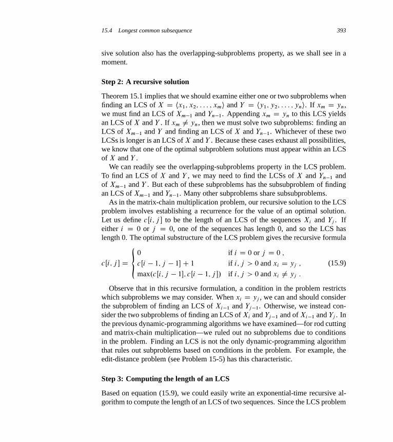
15.4 Longest common subsequence 393
sive solution also has the overlapping-subproblems property, as we shall see in amoment.
Step 2: A recursive solution
Theorem 15.1 implies that we should examine either one or two subproblems whenfinding an LCS of X D hx1; x2; : : : ; xmi and Y D hy1; y2; : : : ; yni. If xm D yn,we must find an LCS of Xm�1 and Yn�1. Appending xm D yn to this LCS yieldsan LCS of X and Y . If xm ¤ yn, then we must solve two subproblems: finding anLCS of Xm�1 and Y and finding an LCS of X and Yn�1. Whichever of these twoLCSs is longer is an LCS of X and Y . Because these cases exhaust all possibilities,we know that one of the optimal subproblem solutions must appear within an LCSof X and Y .
We can readily see the overlapping-subproblems property in the LCS problem.To find an LCS of X and Y , we may need to find the LCSs of X and Yn�1 andof Xm�1 and Y . But each of these subproblems has the subsubproblem of findingan LCS of Xm�1 and Yn�1. Many other subproblems share subsubproblems.
As in the matrix-chain multiplication problem, our recursive solution to the LCSproblem involves establishing a recurrence for the value of an optimal solution.Let us define cŒi; j � to be the length of an LCS of the sequences Xi and Yj . Ifeither i D 0 or j D 0, one of the sequences has length 0, and so the LCS haslength 0. The optimal substructure of the LCS problem gives the recursive formula
cŒi; j � D
�0 if i D 0 or j D 0 ;
cŒi � 1; j � 1�C 1 if i; j > 0 and xi D yj ;
max.cŒi; j � 1�; cŒi � 1; j �/ if i; j > 0 and xi ¤ yj :
(15.9)
Observe that in this recursive formulation, a condition in the problem restrictswhich subproblems we may consider. When xi D yj , we can and should considerthe subproblem of finding an LCS of Xi�1 and Yj �1. Otherwise, we instead con-sider the two subproblems of finding an LCS of Xi and Yj �1 and of Xi�1 and Yj . Inthe previous dynamic-programming algorithms we have examined—for rod cuttingand matrix-chain multiplication—we ruled out no subproblems due to conditionsin the problem. Finding an LCS is not the only dynamic-programming algorithmthat rules out subproblems based on conditions in the problem. For example, theedit-distance problem (see Problem 15-5) has this characteristic.
Step 3: Computing the length of an LCS
Based on equation (15.9), we could easily write an exponential-time recursive al-gorithm to compute the length of an LCS of two sequences. Since the LCS problem

394 Chapter 15 Dynamic Programming
has only ‚.mn/ distinct subproblems, however, we can use dynamic programmingto compute the solutions bottom up.
Procedure LCS-LENGTH takes two sequences X D hx1; x2; : : : ; xmi andY D hy1;y2; : : : ;yni as inputs. It stores the cŒi; j � values in a table cŒ0 : : m; 0 : : n�,and it computes the entries in row-major order. (That is, the procedure fills in thefirst row of c from left to right, then the second row, and so on.) The procedure alsomaintains the table bŒ1 : : m; 1 : : n� to help us construct an optimal solution. Intu-itively, bŒi; j � points to the table entry corresponding to the optimal subproblemsolution chosen when computing cŒi; j �. The procedure returns the b and c tables;cŒm; n� contains the length of an LCS of X and Y .
LCS-LENGTH.X; Y /
1 m D X: length2 n D Y: length3 let bŒ1 : : m; 1 : : n� and cŒ0 : : m; 0 : : n� be new tables4 for i D 1 to m
5 cŒi; 0� D 0
6 for j D 0 to n
7 cŒ0; j � D 0
8 for i D 1 to m
9 for j D 1 to n
10 if xi == yj
11 cŒi; j � D cŒi � 1; j � 1�C 1
12 bŒi; j � D “-”13 elseif cŒi � 1; j � � cŒi; j � 1�
14 cŒi; j � D cŒi � 1; j �
15 bŒi; j � D “"”16 else cŒi; j � D cŒi; j � 1�
17 bŒi; j � D “ ”18 return c and b
Figure 15.8 shows the tables produced by LCS-LENGTH on the sequences X DhA; B; C; B; D; A; Bi and Y D hB; D; C; A; B; Ai. The running time of theprocedure is ‚.mn/, since each table entry takes ‚.1/ time to compute.
Step 4: Constructing an LCS
The b table returned by LCS-LENGTH enables us to quickly construct an LCS ofX D hx1; x2; : : : ; xmi and Y D hy1; y2; : : : ; yni. We simply begin at bŒm; n� andtrace through the table by following the arrows. Whenever we encounter a “-” inentry bŒi; j �, it implies that xi D yj is an element of the LCS that LCS-LENGTH
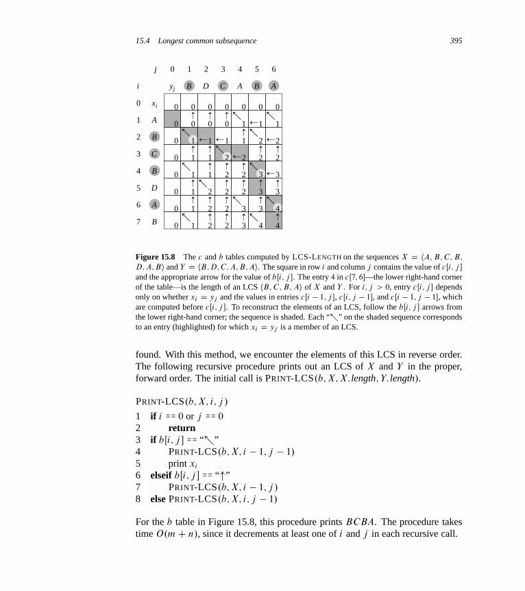
15.4 Longest common subsequence 395
0 0 0 0 0 0 0
0 0 0 0 1 1 1
0 1 1 1 2 2
0 1 1 2 2 2
0 1 1 2 2 3
0 1 2 2 2 3 3
0 1 2 2 3 3
0 1 2 2 3 4 4
1
2
3
4
B D C A B A
1 2 3 4 5 60
A
B
C
B
D
A
B
1
2
3
4
5
6
7
0
j
i
xi
yj
Figure 15.8 The c and b tables computed by LCS-LENGTH on the sequences X D hA; B; C; B;
D;A;Bi and Y D hB;D;C;A;B;Ai. The square in row i and column j contains the value of cŒi; j �
and the appropriate arrow for the value of bŒi; j �. The entry 4 in cŒ7; 6�—the lower right-hand cornerof the table—is the length of an LCS hB; C; B; Ai of X and Y . For i; j > 0, entry cŒi; j � dependsonly on whether xi D yj and the values in entries cŒi � 1; j �, cŒi; j � 1�, and cŒi � 1; j � 1�, whichare computed before cŒi; j �. To reconstruct the elements of an LCS, follow the bŒi; j � arrows fromthe lower right-hand corner; the sequence is shaded. Each “-” on the shaded sequence correspondsto an entry (highlighted) for which xi D yj is a member of an LCS.
found. With this method, we encounter the elements of this LCS in reverse order.The following recursive procedure prints out an LCS of X and Y in the proper,forward order. The initial call is PRINT-LCS.b; X; X: length; Y: length/.
PRINT-LCS.b; X; i; j /
1 if i == 0 or j == 0
2 return3 if bŒi; j � == “-”4 PRINT-LCS.b; X; i � 1; j � 1/
5 print xi
6 elseif bŒi; j � == “"”7 PRINT-LCS.b; X; i � 1; j /
8 else PRINT-LCS.b; X; i; j � 1/
For the b table in Figure 15.8, this procedure prints BCBA. The procedure takestime O.mC n/, since it decrements at least one of i and j in each recursive call.
396 Chapter 15 Dynamic Programming
Improving the code
Once you have developed an algorithm, you will often find that you can improveon the time or space it uses. Some changes can simplify the code and improveconstant factors but otherwise yield no asymptotic improvement in performance.Others can yield substantial asymptotic savings in time and space.
In the LCS algorithm, for example, we can eliminate the b table altogether. EachcŒi; j � entry depends on only three other c table entries: cŒi � 1; j � 1�, cŒi � 1; j �,and cŒi; j � 1�. Given the value of cŒi; j �, we can determine in O.1/ time which ofthese three values was used to compute cŒi; j �, without inspecting table b. Thus, wecan reconstruct an LCS in O.mCn/ time using a procedure similar to PRINT-LCS.(Exercise 15.4-2 asks you to give the pseudocode.) Although we save ‚.mn/ spaceby this method, the auxiliary space requirement for computing an LCS does notasymptotically decrease, since we need ‚.mn/ space for the c table anyway.
We can, however, reduce the asymptotic space requirements for LCS-LENGTH,since it needs only two rows of table c at a time: the row being computed and theprevious row. (In fact, as Exercise 15.4-4 asks you to show, we can use only slightlymore than the space for one row of c to compute the length of an LCS.) Thisimprovement works if we need only the length of an LCS; if we need to reconstructthe elements of an LCS, the smaller table does not keep enough information toretrace our steps in O.mC n/ time.
Exercises
15.4-1Determine an LCS of h1; 0; 0; 1; 0; 1; 0; 1i and h0; 1; 0; 1; 1; 0; 1; 1; 0i.15.4-2Give pseudocode to reconstruct an LCS from the completed c table and the originalsequences X D hx1; x2; : : : ; xmi and Y D hy1; y2; : : : ; yni in O.m C n/ time,without using the b table.
15.4-3Give a memoized version of LCS-LENGTH that runs in O.mn/ time.
15.4-4Show how to compute the length of an LCS using only 2 �min.m; n/ entries in the c
table plus O.1/ additional space. Then show how to do the same thing, but usingmin.m; n/ entries plus O.1/ additional space.
15.5 Optimal binary search trees 397
15.4-5Give an O.n2/-time algorithm to find the longest monotonically increasing subse-quence of a sequence of n numbers.
15.4-6 ?
Give an O.n lg n/-time algorithm to find the longest monotonically increasing sub-sequence of a sequence of n numbers. (Hint: Observe that the last element of acandidate subsequence of length i is at least as large as the last element of a can-didate subsequence of length i � 1. Maintain candidate subsequences by linkingthem through the input sequence.)
15.5 Optimal binary search trees
Suppose that we are designing a program to translate text from English to French.For each occurrence of each English word in the text, we need to look up its Frenchequivalent. We could perform these lookup operations by building a binary searchtree with n English words as keys and their French equivalents as satellite data.Because we will search the tree for each individual word in the text, we want thetotal time spent searching to be as low as possible. We could ensure an O.lg n/
search time per occurrence by using a red-black tree or any other balanced binarysearch tree. Words appear with different frequencies, however, and a frequentlyused word such as the may appear far from the root while a rarely used word suchas machicolation appears near the root. Such an organization would slow down thetranslation, since the number of nodes visited when searching for a key in a binarysearch tree equals one plus the depth of the node containing the key. We wantwords that occur frequently in the text to be placed nearer the root.6 Moreover,some words in the text might have no French translation,7 and such words wouldnot appear in the binary search tree at all. How do we organize a binary search treeso as to minimize the number of nodes visited in all searches, given that we knowhow often each word occurs?
What we need is known as an optimal binary search tree. Formally, we aregiven a sequence K D hk1; k2; : : : ; kni of n distinct keys in sorted order (so thatk1 < k2 < � � � < kn), and we wish to build a binary search tree from these keys.For each key ki , we have a probability pi that a search will be for ki . Somesearches may be for values not in K, and so we also have n C 1 “dummy keys”
6If the subject of the text is castle architecture, we might want machicolation to appear near the root.
7Yes, machicolation has a French counterpart: mâchicoulis.

398 Chapter 15 Dynamic Programming
k2
k1 k4
k3 k5d0 d1
d2 d3 d4 d5
(a)
k2
k1
k4
k3
k5
d0 d1
d2 d3
d4
d5
(b)
Figure 15.9 Two binary search trees for a set of n D 5 keys with the following probabilities:
i 0 1 2 3 4 5pi 0.15 0.10 0.05 0.10 0.20qi 0.05 0.10 0.05 0.05 0.05 0.10
(a) A binary search tree with expected search cost 2.80. (b) A binary search tree with expected searchcost 2.75. This tree is optimal.
d0; d1; d2; : : : ; dn representing values not in K. In particular, d0 represents all val-ues less than k1, dn represents all values greater than kn, and for i D 1; 2; : : : ; n�1,the dummy key di represents all values between ki and kiC1. For each dummykey di , we have a probability qi that a search will correspond to di . Figure 15.9shows two binary search trees for a set of n D 5 keys. Each key ki is an internalnode, and each dummy key di is a leaf. Every search is either successful (findingsome key ki ) or unsuccessful (finding some dummy key di ), and so we have
nXiD1
pi CnX
iD0
qi D 1 : (15.10)
Because we have probabilities of searches for each key and each dummy key,we can determine the expected cost of a search in a given binary search tree T . Letus assume that the actual cost of a search equals the number of nodes examined,i.e., the depth of the node found by the search in T , plus 1. Then the expected costof a search in T is
E Œsearch cost in T � DnX
iD1
.depthT .ki /C 1/ � pi CnX
iD0
.depthT .di /C 1/ � qi
D 1CnX
iD1
depthT .ki / � pi CnX
iD0
depthT .di/ � qi ; (15.11)
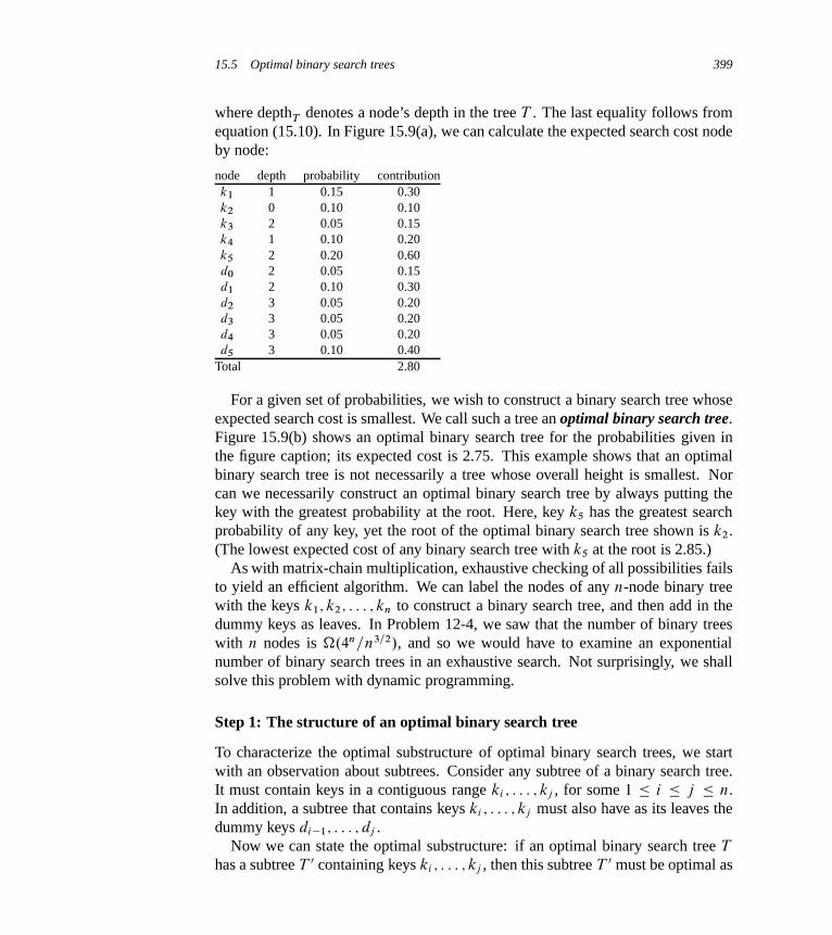
15.5 Optimal binary search trees 399
where depthT denotes a node’s depth in the tree T . The last equality follows fromequation (15.10). In Figure 15.9(a), we can calculate the expected search cost nodeby node:
node depth probability contributionk1 1 0.15 0.30k2 0 0.10 0.10k3 2 0.05 0.15k4 1 0.10 0.20k5 2 0.20 0.60d0 2 0.05 0.15d1 2 0.10 0.30d2 3 0.05 0.20d3 3 0.05 0.20d4 3 0.05 0.20d5 3 0.10 0.40
Total 2.80
For a given set of probabilities, we wish to construct a binary search tree whoseexpected search cost is smallest. We call such a tree an optimal binary search tree.Figure 15.9(b) shows an optimal binary search tree for the probabilities given inthe figure caption; its expected cost is 2.75. This example shows that an optimalbinary search tree is not necessarily a tree whose overall height is smallest. Norcan we necessarily construct an optimal binary search tree by always putting thekey with the greatest probability at the root. Here, key k5 has the greatest searchprobability of any key, yet the root of the optimal binary search tree shown is k2.(The lowest expected cost of any binary search tree with k5 at the root is 2.85.)
As with matrix-chain multiplication, exhaustive checking of all possibilities failsto yield an efficient algorithm. We can label the nodes of any n-node binary treewith the keys k1; k2; : : : ; kn to construct a binary search tree, and then add in thedummy keys as leaves. In Problem 12-4, we saw that the number of binary treeswith n nodes is �.4n=n3=2/, and so we would have to examine an exponentialnumber of binary search trees in an exhaustive search. Not surprisingly, we shallsolve this problem with dynamic programming.
Step 1: The structure of an optimal binary search tree
To characterize the optimal substructure of optimal binary search trees, we startwith an observation about subtrees. Consider any subtree of a binary search tree.It must contain keys in a contiguous range ki ; : : : ; kj , for some 1 � i � j � n.In addition, a subtree that contains keys ki ; : : : ; kj must also have as its leaves thedummy keys di�1; : : : ; dj .
Now we can state the optimal substructure: if an optimal binary search tree T
has a subtree T 0 containing keys ki ; : : : ; kj , then this subtree T 0 must be optimal as

400 Chapter 15 Dynamic Programming
well for the subproblem with keys ki ; : : : ; kj and dummy keys di�1; : : : ; dj . Theusual cut-and-paste argument applies. If there were a subtree T 00 whose expectedcost is lower than that of T 0, then we could cut T 0 out of T and paste in T 00,resulting in a binary search tree of lower expected cost than T , thus contradictingthe optimality of T .
We need to use the optimal substructure to show that we can construct an opti-mal solution to the problem from optimal solutions to subproblems. Given keyski ; : : : ; kj , one of these keys, say kr (i � r � j ), is the root of an optimalsubtree containing these keys. The left subtree of the root kr contains the keyski ; : : : ; kr�1 (and dummy keys di�1; : : : ; dr�1), and the right subtree contains thekeys krC1; : : : ; kj (and dummy keys dr ; : : : ; dj ). As long as we examine all candi-date roots kr , where i � r � j , and we determine all optimal binary search treescontaining ki ; : : : ; kr�1 and those containing krC1; : : : ; kj , we are guaranteed thatwe will find an optimal binary search tree.
There is one detail worth noting about “empty” subtrees. Suppose that in asubtree with keys ki ; : : : ; kj , we select ki as the root. By the above argument, ki ’sleft subtree contains the keys ki ; : : : ; ki�1. We interpret this sequence as containingno keys. Bear in mind, however, that subtrees also contain dummy keys. We adoptthe convention that a subtree containing keys ki ; : : : ; ki�1 has no actual keys butdoes contain the single dummy key di�1. Symmetrically, if we select kj as the root,then kj ’s right subtree contains the keys kj C1; : : : ; kj ; this right subtree containsno actual keys, but it does contain the dummy key dj .
Step 2: A recursive solution
We are ready to define the value of an optimal solution recursively. We pick oursubproblem domain as finding an optimal binary search tree containing the keyski ; : : : ; kj , where i � 1, j � n, and j � i � 1. (When j D i � 1, thereare no actual keys; we have just the dummy key di�1.) Let us define eŒi; j � asthe expected cost of searching an optimal binary search tree containing the keyski ; : : : ; kj . Ultimately, we wish to compute eŒ1; n�.
The easy case occurs when j D i � 1. Then we have just the dummy key di�1.The expected search cost is eŒi; i � 1� D qi�1.
When j � i , we need to select a root kr from among ki ; : : : ; kj and then makean optimal binary search tree with keys ki ; : : : ; kr�1 its left subtree and an optimalbinary search tree with keys krC1; : : : ; kj its right subtree. What happens to theexpected search cost of a subtree when it becomes a subtree of a node? The depthof each node in the subtree increases by 1. By equation (15.11), the expected searchcost of this subtree increases by the sum of all the probabilities in the subtree. Fora subtree with keys ki ; : : : ; kj , let us denote this sum of probabilities as

15.5 Optimal binary search trees 401
w.i; j / DjX
lDi
pl CjX
lDi�1
ql : (15.12)
Thus, if kr is the root of an optimal subtree containing keys ki ; : : : ; kj , we have
eŒi; j � D pr C .eŒi; r � 1�Cw.i; r � 1//C .eŒr C 1; j �C w.r C 1; j // :
Noting that
w.i; j / D w.i; r � 1/C pr Cw.r C 1; j / ;
we rewrite eŒi; j � as
eŒi; j � D eŒi; r � 1�C eŒr C 1; j �Cw.i; j / : (15.13)
The recursive equation (15.13) assumes that we know which node kr to use asthe root. We choose the root that gives the lowest expected search cost, giving usour final recursive formulation:
eŒi; j � D(
qi�1 if j D i � 1 ;
mini�r�j
feŒi; r � 1�C eŒr C 1; j �C w.i; j /g if i � j :(15.14)
The eŒi; j � values give the expected search costs in optimal binary search trees.To help us keep track of the structure of optimal binary search trees, we definerootŒi; j �, for 1 � i � j � n, to be the index r for which kr is the root of anoptimal binary search tree containing keys ki ; : : : ; kj . Although we will see howto compute the values of rootŒi; j �, we leave the construction of an optimal binarysearch tree from these values as Exercise 15.5-1.
Step 3: Computing the expected search cost of an optimal binary search tree
At this point, you may have noticed some similarities between our characterizationsof optimal binary search trees and matrix-chain multiplication. For both problemdomains, our subproblems consist of contiguous index subranges. A direct, recur-sive implementation of equation (15.14) would be as inefficient as a direct, recur-sive matrix-chain multiplication algorithm. Instead, we store the eŒi; j � values in atable eŒ1 : : nC1; 0 : : n�. The first index needs to run to nC1 rather than n becausein order to have a subtree containing only the dummy key dn, we need to computeand store eŒn C 1; n�. The second index needs to start from 0 because in order tohave a subtree containing only the dummy key d0, we need to compute and storeeŒ1; 0�. We use only the entries eŒi; j � for which j � i � 1. We also use a tablerootŒi; j �, for recording the root of the subtree containing keys ki ; : : : ; kj . Thistable uses only the entries for which 1 � i � j � n.
We will need one other table for efficiency. Rather than compute the valueof w.i; j / from scratch every time we are computing eŒi; j �—which would take
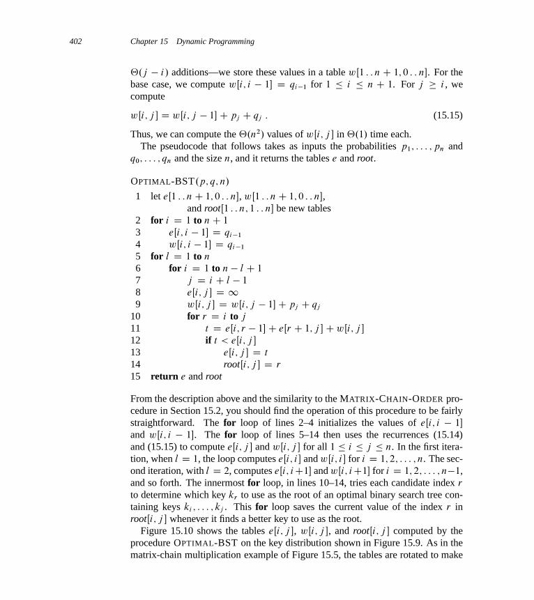
402 Chapter 15 Dynamic Programming
‚.j � i/ additions—we store these values in a table wŒ1 : : nC 1; 0 : : n�. For thebase case, we compute wŒi; i � 1� D qi�1 for 1 � i � n C 1. For j � i , wecompute
wŒi; j � D wŒi; j � 1�C pj C qj : (15.15)
Thus, we can compute the ‚.n2/ values of wŒi; j � in ‚.1/ time each.The pseudocode that follows takes as inputs the probabilities p1; : : : ; pn and
q0; : : : ; qn and the size n, and it returns the tables e and root.
OPTIMAL-BST.p; q; n/
1 let eŒ1 : : nC 1; 0 : : n�, wŒ1 : : nC 1; 0 : : n�,and rootŒ1 : : n; 1 : : n� be new tables
2 for i D 1 to nC 1
3 eŒi; i � 1� D qi�1
4 wŒi; i � 1� D qi�1
5 for l D 1 to n
6 for i D 1 to n � l C 1
7 j D i C l � 1
8 eŒi; j � D 19 wŒi; j � D wŒi; j � 1�C pj C qj
10 for r D i to j
11 t D eŒi; r � 1�C eŒr C 1; j �CwŒi; j �
12 if t < eŒi; j �
13 eŒi; j � D t
14 rootŒi; j � D r
15 return e and root
From the description above and the similarity to the MATRIX-CHAIN-ORDER pro-cedure in Section 15.2, you should find the operation of this procedure to be fairlystraightforward. The for loop of lines 2–4 initializes the values of eŒi; i � 1�
and wŒi; i � 1�. The for loop of lines 5–14 then uses the recurrences (15.14)and (15.15) to compute eŒi; j � and wŒi; j � for all 1 � i � j � n. In the first itera-tion, when l D 1, the loop computes eŒi; i � and wŒi; i � for i D 1; 2; : : : ; n. The sec-ond iteration, with l D 2, computes eŒi; iC1� and wŒi; iC1� for i D 1; 2; : : : ; n�1,and so forth. The innermost for loop, in lines 10–14, tries each candidate index r
to determine which key kr to use as the root of an optimal binary search tree con-taining keys ki ; : : : ; kj . This for loop saves the current value of the index r inrootŒi; j � whenever it finds a better key to use as the root.
Figure 15.10 shows the tables eŒi; j �, wŒi; j �, and rootŒi; j � computed by theprocedure OPTIMAL-BST on the key distribution shown in Figure 15.9. As in thematrix-chain multiplication example of Figure 15.5, the tables are rotated to make
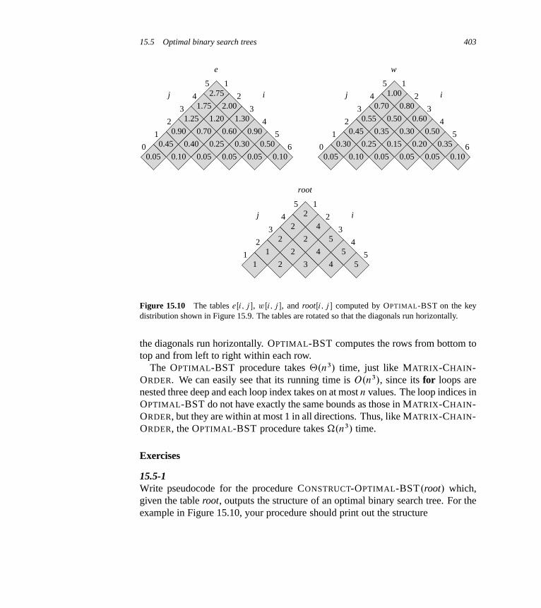
15.5 Optimal binary search trees 403
2.75
1.75
1.25
0.90
0.45
0.05
2.00
1.20
0.70
0.40
0.10
1.30
0.60
0.25
0.05
0.90
0.30
0.05
0.50
0.05 0.10
e
0
1
2
3
4
5
6
5
4
3
2
1j i 1.00
0.70
0.55
0.45
0.30
0.05
0.80
0.50
0.35
0.25
0.10
0.60
0.30
0.15
0.05
0.50
0.20
0.05
0.35
0.05 0.10
w
0
1
2
3
4
5
6
5
4
3
2
1j i
2
2
2
1
1
4
2
2
2
5
4
3
5
4 5
root
1
2
3
4
5
5
4
3
2
1j i
Figure 15.10 The tables eŒi; j �, wŒi; j �, and rootŒi; j � computed by OPTIMAL-BST on the keydistribution shown in Figure 15.9. The tables are rotated so that the diagonals run horizontally.
the diagonals run horizontally. OPTIMAL-BST computes the rows from bottom totop and from left to right within each row.
The OPTIMAL-BST procedure takes ‚.n3/ time, just like MATRIX-CHAIN-ORDER. We can easily see that its running time is O.n3/, since its for loops arenested three deep and each loop index takes on at most n values. The loop indices inOPTIMAL-BST do not have exactly the same bounds as those in MATRIX-CHAIN-ORDER, but they are within at most 1 in all directions. Thus, like MATRIX-CHAIN-ORDER, the OPTIMAL-BST procedure takes �.n3/ time.
Exercises
15.5-1Write pseudocode for the procedure CONSTRUCT-OPTIMAL-BST.root/ which,given the table root, outputs the structure of an optimal binary search tree. For theexample in Figure 15.10, your procedure should print out the structure
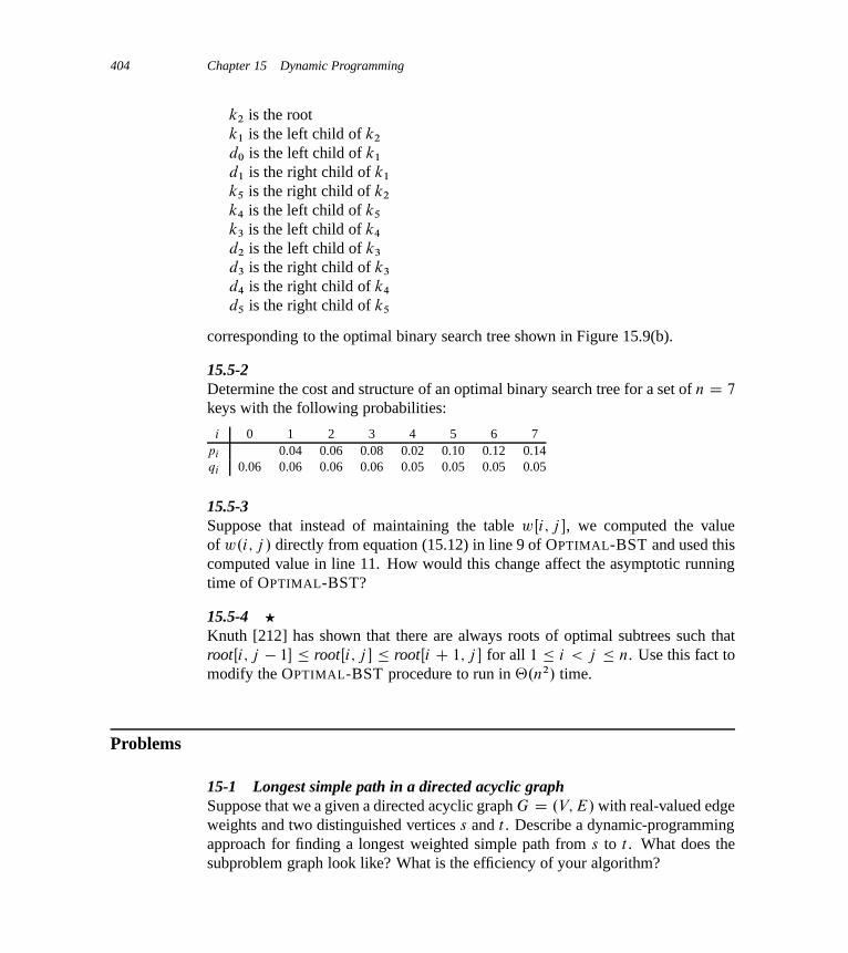
404 Chapter 15 Dynamic Programming
k2 is the rootk1 is the left child of k2
d0 is the left child of k1
d1 is the right child of k1
k5 is the right child of k2
k4 is the left child of k5
k3 is the left child of k4
d2 is the left child of k3
d3 is the right child of k3
d4 is the right child of k4
d5 is the right child of k5
corresponding to the optimal binary search tree shown in Figure 15.9(b).
15.5-2Determine the cost and structure of an optimal binary search tree for a set of n D 7
keys with the following probabilities:
i 0 1 2 3 4 5 6 7pi 0.04 0.06 0.08 0.02 0.10 0.12 0.14qi 0.06 0.06 0.06 0.06 0.05 0.05 0.05 0.05
15.5-3Suppose that instead of maintaining the table wŒi; j �, we computed the valueof w.i; j / directly from equation (15.12) in line 9 of OPTIMAL-BST and used thiscomputed value in line 11. How would this change affect the asymptotic runningtime of OPTIMAL-BST?
15.5-4 ?
Knuth [212] has shown that there are always roots of optimal subtrees such thatrootŒi; j � 1� � rootŒi; j � � rootŒi C 1; j � for all 1 � i < j � n. Use this fact tomodify the OPTIMAL-BST procedure to run in ‚.n2/ time.
Problems
15-1 Longest simple path in a directed acyclic graphSuppose that we a given a directed acyclic graph G D .V; E/ with real-valued edgeweights and two distinguished vertices s and t . Describe a dynamic-programmingapproach for finding a longest weighted simple path from s to t . What does thesubproblem graph look like? What is the efficiency of your algorithm?
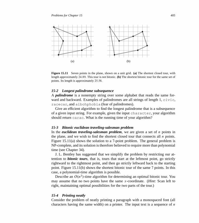
Problems for Chapter 15 405
(a) (b)
Figure 15.11 Seven points in the plane, shown on a unit grid. (a) The shortest closed tour, withlength approximately 24:89. This tour is not bitonic. (b) The shortest bitonic tour for the same set ofpoints. Its length is approximately 25:58.
15-2 Longest palindrome subsequenceA palindrome is a nonempty string over some alphabet that reads the same for-ward and backward. Examples of palindromes are all strings of length 1, civic,racecar, and aibohphobia (fear of palindromes).
Give an efficient algorithm to find the longest palindrome that is a subsequenceof a given input string. For example, given the input character, your algorithmshould return carac. What is the running time of your algorithm?
15-3 Bitonic euclidean traveling-salesman problemIn the euclidean traveling-salesman problem, we are given a set of n points inthe plane, and we wish to find the shortest closed tour that connects all n points.Figure 15.11(a) shows the solution to a 7-point problem. The general problem isNP-complete, and its solution is therefore believed to require more than polynomialtime (see Chapter 34).
J. L. Bentley has suggested that we simplify the problem by restricting our at-tention to bitonic tours, that is, tours that start at the leftmost point, go strictlyrightward to the rightmost point, and then go strictly leftward back to the startingpoint. Figure 15.11(b) shows the shortest bitonic tour of the same 7 points. In thiscase, a polynomial-time algorithm is possible.
Describe an O.n2/-time algorithm for determining an optimal bitonic tour. Youmay assume that no two points have the same x-coordinate. (Hint: Scan left toright, maintaining optimal possibilities for the two parts of the tour.)
15-4 Printing neatlyConsider the problem of neatly printing a paragraph with a monospaced font (allcharacters having the same width) on a printer. The input text is a sequence of n
406 Chapter 15 Dynamic Programming
words of lengths l1; l2; : : : ; ln, measured in characters. We want to print this para-graph neatly on a number of lines that hold a maximum of M characters each. Ourcriterion of “neatness” is as follows. If a given line contains words i through j ,where i � j , and we leave exactly one space between words, the number of extraspace characters at the end of the line is M � j C i �Pj
kDi lk, which must benonnegative so that the words fit on the line. We wish to minimize the sum, overall lines except the last, of the cubes of the numbers of extra space characters at theends of lines. Give a dynamic-programming algorithm to print a paragraph of n
words neatly on a printer. Analyze the running time and space requirements ofyour algorithm.
15-5 Edit distanceIn order to transform one source string of text xŒ1 : : m� to a target string yŒ1 : : n�,we can perform various transformation operations. Our goal is, given x and y,to produce a series of transformations that change x to y. We use an ar-ray ´—assumed to be large enough to hold all the characters it will need—to holdthe intermediate results. Initially, ´ is empty, and at termination, we should have´Œj � D yŒj � for j D 1; 2; : : : ; n. We maintain current indices i into x and j into ´,and the operations are allowed to alter ´ and these indices. Initially, i D j D 1.We are required to examine every character in x during the transformation, whichmeans that at the end of the sequence of transformation operations, we must havei D mC 1.
We may choose from among six transformation operations:
Copy a character from x to ´ by setting ´Œj � D xŒi � and then incrementing both i
and j . This operation examines xŒi �.
Replace a character from x by another character c, by setting ´Œj � D c, and thenincrementing both i and j . This operation examines xŒi �.
Delete a character from x by incrementing i but leaving j alone. This operationexamines xŒi �.
Insert the character c into ´ by setting ´Œj � D c and then incrementing j , butleaving i alone. This operation examines no characters of x.
Twiddle (i.e., exchange) the next two characters by copying them from x to ´ butin the opposite order; we do so by setting ´Œj � D xŒiC 1� and ´Œj C 1� D xŒi �
and then setting i D i C 2 and j D j C 2. This operation examines xŒi �
and xŒi C 1�.
Kill the remainder of x by setting i D m C 1. This operation examines all char-acters in x that have not yet been examined. This operation, if performed, mustbe the final operation.

Problems for Chapter 15 407
As an example, one way to transform the source string algorithm to the targetstring altruistic is to use the following sequence of operations, where theunderlined characters are xŒi � and ´Œj � after the operation:
Operation x ´
initial strings algorithmcopy algorithm acopy algorithm alreplace by t algorithm altdelete algorithm altcopy algorithm altrinsert u algorithm altruinsert i algorithm altruiinsert s algorithm altruistwiddle algorithm altruistiinsert c algorithm altruistickill algorithm altruistic
Note that there are several other sequences of transformation operations that trans-form algorithm to altruistic.
Each of the transformation operations has an associated cost. The cost of anoperation depends on the specific application, but we assume that each operation’scost is a constant that is known to us. We also assume that the individual costs ofthe copy and replace operations are less than the combined costs of the delete andinsert operations; otherwise, the copy and replace operations would not be used.The cost of a given sequence of transformation operations is the sum of the costsof the individual operations in the sequence. For the sequence above, the cost oftransforming algorithm to altruistic is
.3 � cost.copy//C cost.replace/C cost.delete/C .4 � cost.insert//
C cost.twiddle/C cost.kill/ :
a. Given two sequences xŒ1 : : m� and yŒ1 : : n� and set of transformation-operationcosts, the edit distance from x to y is the cost of the least expensive operationsequence that transforms x to y. Describe a dynamic-programming algorithmthat finds the edit distance from xŒ1 : : m� to yŒ1 : : n� and prints an optimal op-eration sequence. Analyze the running time and space requirements of youralgorithm.
The edit-distance problem generalizes the problem of aligning two DNA sequences(see, for example, Setubal and Meidanis [310, Section 3.2]). There are severalmethods for measuring the similarity of two DNA sequences by aligning them.One such method to align two sequences x and y consists of inserting spaces at

408 Chapter 15 Dynamic Programming
arbitrary locations in the two sequences (including at either end) so that the result-ing sequences x 0 and y 0 have the same length but do not have a space in the sameposition (i.e., for no position j are both x 0Œj � and y 0Œj � a space.) Then we assign a“score” to each position. Position j receives a score as follows:
� C1 if x 0Œj � D y 0Œj � and neither is a space,� �1 if x 0Œj � ¤ y 0Œj � and neither is a space,� �2 if either x 0Œj � or y 0Œj � is a space.
The score for the alignment is the sum of the scores of the individual positions. Forexample, given the sequences x D GATCGGCAT and y D CAATGTGAATC, onealignment is
G ATCG GCATCAAT GTGAATC-*++*+*+-++*
A + under a position indicates a score ofC1 for that position, a - indicates a scoreof �1, and a * indicates a score of �2, so that this alignment has a total score of6 � 1� 2 � 1 � 4 � 2 D �4.
b. Explain how to cast the problem of finding an optimal alignment as an editdistance problem using a subset of the transformation operations copy, replace,delete, insert, twiddle, and kill.
15-6 Planning a company partyProfessor Stewart is consulting for the president of a corporation that is planninga company party. The company has a hierarchical structure; that is, the supervisorrelation forms a tree rooted at the president. The personnel office has ranked eachemployee with a conviviality rating, which is a real number. In order to make theparty fun for all attendees, the president does not want both an employee and hisor her immediate supervisor to attend.
Professor Stewart is given the tree that describes the structure of the corporation,using the left-child, right-sibling representation described in Section 10.4. Eachnode of the tree holds, in addition to the pointers, the name of an employee andthat employee’s conviviality ranking. Describe an algorithm to make up a guestlist that maximizes the sum of the conviviality ratings of the guests. Analyze therunning time of your algorithm.
15-7 Viterbi algorithmWe can use dynamic programming on a directed graph G D .V; E/ for speechrecognition. Each edge .u; �/ 2 E is labeled with a sound .u; �/ from a fi-nite set † of sounds. The labeled graph is a formal model of a person speaking

Problems for Chapter 15 409
a restricted language. Each path in the graph starting from a distinguished ver-tex �0 2 V corresponds to a possible sequence of sounds produced by the model.We define the label of a directed path to be the concatenation of the labels of theedges on that path.
a. Describe an efficient algorithm that, given an edge-labeled graph G with dis-tinguished vertex �0 and a sequence s D h1; 2; : : : ; ki of sounds from †,returns a path in G that begins at �0 and has s as its label, if any such path exists.Otherwise, the algorithm should return NO-SUCH-PATH. Analyze the runningtime of your algorithm. (Hint: You may find concepts from Chapter 22 useful.)
Now, suppose that every edge .u; �/ 2 E has an associated nonnegative proba-bility p.u; �/ of traversing the edge .u; �/ from vertex u and thus producing thecorresponding sound. The sum of the probabilities of the edges leaving any vertexequals 1. The probability of a path is defined to be the product of the probabil-ities of its edges. We can view the probability of a path beginning at �0 as theprobability that a “random walk” beginning at �0 will follow the specified path,where we randomly choose which edge to take leaving a vertex u according to theprobabilities of the available edges leaving u.
b. Extend your answer to part (a) so that if a path is returned, it is a most prob-able path starting at �0 and having label s. Analyze the running time of youralgorithm.
15-8 Image compression by seam carvingWe are given a color picture consisting of an mn array AŒ1 : : m; 1 : : n� of pixels,where each pixel specifies a triple of red, green, and blue (RGB) intensities. Sup-pose that we wish to compress this picture slightly. Specifically, we wish to removeone pixel from each of the m rows, so that the whole picture becomes one pixelnarrower. To avoid disturbing visual effects, however, we require that the pixelsremoved in two adjacent rows be in the same or adjacent columns; the pixels re-moved form a “seam” from the top row to the bottom row where successive pixelsin the seam are adjacent vertically or diagonally.
a. Show that the number of such possible seams grows at least exponentially in m,assuming that n > 1.
b. Suppose now that along with each pixel AŒi; j �, we have calculated a real-valued disruption measure dŒi; j �, indicating how disruptive it would be toremove pixel AŒi; j �. Intuitively, the lower a pixel’s disruption measure, themore similar the pixel is to its neighbors. Suppose further that we define thedisruption measure of a seam to be the sum of the disruption measures of itspixels.
410 Chapter 15 Dynamic Programming
Give an algorithm to find a seam with the lowest disruption measure. Howefficient is your algorithm?
15-9 Breaking a stringA certain string-processing language allows a programmer to break a string intotwo pieces. Because this operation copies the string, it costs n time units to breaka string of n characters into two pieces. Suppose a programmer wants to breaka string into many pieces. The order in which the breaks occur can affect thetotal amount of time used. For example, suppose that the programmer wants tobreak a 20-character string after characters 2, 8, and 10 (numbering the charactersin ascending order from the left-hand end, starting from 1). If she programs thebreaks to occur in left-to-right order, then the first break costs 20 time units, thesecond break costs 18 time units (breaking the string from characters 3 to 20 atcharacter 8), and the third break costs 12 time units, totaling 50 time units. If sheprograms the breaks to occur in right-to-left order, however, then the first breakcosts 20 time units, the second break costs 10 time units, and the third break costs8 time units, totaling 38 time units. In yet another order, she could break first at 8
(costing 20), then break the left piece at 2 (costing 8), and finally the right pieceat 10 (costing 12), for a total cost of 40.
Design an algorithm that, given the numbers of characters after which to break,determines a least-cost way to sequence those breaks. More formally, given astring S with n characters and an array LŒ1 : : m� containing the break points, com-pute the lowest cost for a sequence of breaks, along with a sequence of breaks thatachieves this cost.
15-10 Planning an investment strategyYour knowledge of algorithms helps you obtain an exciting job with the AcmeComputer Company, along with a $10,000 signing bonus. You decide to investthis money with the goal of maximizing your return at the end of 10 years. Youdecide to use the Amalgamated Investment Company to manage your investments.Amalgamated Investments requires you to observe the following rules. It offers n
different investments, numbered 1 through n. In each year j , investment i providesa return rate of rij . In other words, if you invest d dollars in investment i in year j ,then at the end of year j , you have drij dollars. The return rates are guaranteed,that is, you are given all the return rates for the next 10 years for each investment.You make investment decisions only once per year. If you decide to leave yourmoney in the same set of investments in two consecutive years, you pay a fee of f1
dollars, whereas if you decide to switch your money to a different set of investmentsyou pay a fee of f2 dollars.

Problems for Chapter 15 411
a. The problem, as stated, allows you to invest your money in multiple investmentsin each year. Prove that there exists an optimal investment strategy that, ineach year, puts all the money into a single investment. (Recall that an optimalinvestment strategy maximizes the amount of money after 10 years and is notconcerned with any other objectives, such as minimizing risk.)
b. Prove that the problem of planning your optimal investment strategy exhibitsoptimal substructure.
c. Design an algorithm that plans your optimal investment strategy. What is therunning time of your algorithm?
d. Suppose that Amalgamated Investments imposed the additional restriction that,at any point, you can have no more than $15,000 in any one investment. Showthat the problem of maximizing your income at the end of 10 years no longerexhibits optimal substructure.
15-11 Inventory planningThe Rinky Dink Company makes machines that resurface ice rinks. The demandfor such products varies from month to month, and so the company needs to de-velop a strategy to plan its manufacturing given the fluctuating, but predictable,demand. The company wishes to design a plan for the next n months. For eachmonth i , the company knows the demand di , that is, the number of machines thatit will sell. Let D D Pn
iD1 di be the total demand over the next n months. Thecompany keeps a full-time staff that provides labor to manufacture up to m ma-chines per month. If the company needs to make more than m machines in a givenmonth, it can hire additional, part-time labor, at a cost that works out to c dollarsper machine. Furthermore, if, at the end of a month, the company is holding anyunsold machines, it must pay inventory costs. The cost for holding j machines isgiven as a function h.j / for j D 1; 2; : : : ; D, where h.j / � 0 for 1 � j � D andh.j / � h.j C 1/ for j � 1 � D � 1.
Give an algorithm that calculates a plan for the company that minimizes its costswhile fulfilling all the demand. The running time should be polyomial in n and D.
15-12 Signing free-agent baseball playersSuppose that you are the general manager for a major-league baseball team. Duringthe off-season, you need to sign some free-agent players for your team. The teamowner has given you a budget of $X to spend on free agents. You are allowed tospend less than $X altogether, but the owner will fire you if you spend any morethan $X .

412 Chapter 15 Dynamic Programming
You are considering N different positions, and for each position, P free-agentplayers who play that position are available.8 Because you do not want to overloadyour roster with too many players at any position, for each position you may signat most one free agent who plays that position. (If you do not sign any players at aparticular position, then you plan to stick with the players you already have at thatposition.)
To determine how valuable a player is going to be, you decide to use a sabermet-ric statistic9 known as “VORP,” or “value over replacement player.” A player witha higher VORP is more valuable than a player with a lower VORP. A player with ahigher VORP is not necessarily more expensive to sign than a player with a lowerVORP, because factors other than a player’s value determine how much it costs tosign him.
For each available free-agent player, you have three pieces of information:
� the player’s position,
� the amount of money it will cost to sign the player, and
� the player’s VORP.
Devise an algorithm that maximizes the total VORP of the players you sign whilespending no more than $X altogether. You may assume that each player signs for amultiple of $100,000. Your algorithm should output the total VORP of the playersyou sign, the total amount of money you spend, and a list of which players yousign. Analyze the running time and space requirement of your algorithm.
Chapter notes
R. Bellman began the systematic study of dynamic programming in 1955. Theword “programming,” both here and in linear programming, refers to using a tab-ular solution method. Although optimization techniques incorporating elements ofdynamic programming were known earlier, Bellman provided the area with a solidmathematical basis [37].
8Although there are nine positions on a baseball team, N is not necesarily equal to 9 because somegeneral managers have particular ways of thinking about positions. For example, a general managermight consider right-handed pitchers and left-handed pitchers to be separate “positions,” as well asstarting pitchers, long relief pitchers (relief pitchers who can pitch several innings), and short reliefpitchers (relief pitchers who normally pitch at most only one inning).
9Sabermetrics is the application of statistical analysis to baseball records. It provides several waysto compare the relative values of individual players.

Notes for Chapter 15 413
Galil and Park [125] classify dynamic-programming algorithms according to thesize of the table and the number of other table entries each entry depends on. Theycall a dynamic-programming algorithm tD=eD if its table size is O.nt / and eachentry depends on O.ne/ other entries. For example, the matrix-chain multiplicationalgorithm in Section 15.2 would be 2D=1D, and the longest-common-subsequencealgorithm in Section 15.4 would be 2D=0D.
Hu and Shing [182, 183] give an O.n lg n/-time algorithm for the matrix-chainmultiplication problem.
The O.mn/-time algorithm for the longest-common-subsequence problem ap-pears to be a folk algorithm. Knuth [71] posed the question of whether subquadraticalgorithms for the LCS problem exist. Masek and Paterson [244] answered thisquestion in the affirmative by giving an algorithm that runs in O.mn= lg n/ time,where n � m and the sequences are drawn from a set of bounded size. For thespecial case in which no element appears more than once in an input sequence,Szymanski [326] shows how to solve the problem in O..nCm/ lg.nCm// time.Many of these results extend to the problem of computing string edit distances(Problem 15-5).
An early paper on variable-length binary encodings by Gilbert and Moore [133]had applications to constructing optimal binary search trees for the case in which allprobabilities pi are 0; this paper contains an O.n3/-time algorithm. Aho, Hopcroft,and Ullman [5] present the algorithm from Section 15.5. Exercise 15.5-4 is due toKnuth [212]. Hu and Tucker [184] devised an algorithm for the case in which allprobabilities pi are 0 that uses O.n2/ time and O.n/ space; subsequently, Knuth[211] reduced the time to O.n lg n/.
Problem 15-8 is due to Avidan and Shamir [27], who have posted on the Web awonderful video illustrating this image-compression technique.

16 Greedy Algorithms
Algorithms for optimization problems typically go through a sequence of steps,with a set of choices at each step. For many optimization problems, using dynamicprogramming to determine the best choices is overkill; simpler, more efficient al-gorithms will do. A greedy algorithm always makes the choice that looks best atthe moment. That is, it makes a locally optimal choice in the hope that this choicewill lead to a globally optimal solution. This chapter explores optimization prob-lems for which greedy algorithms provide optimal solutions. Before reading thischapter, you should read about dynamic programming in Chapter 15, particularlySection 15.3.
Greedy algorithms do not always yield optimal solutions, but for many problemsthey do. We shall first examine, in Section 16.1, a simple but nontrivial problem,the activity-selection problem, for which a greedy algorithm efficiently computesan optimal solution. We shall arrive at the greedy algorithm by first consider-ing a dynamic-programming approach and then showing that we can always makegreedy choices to arrive at an optimal solution. Section 16.2 reviews the basicelements of the greedy approach, giving a direct approach for proving greedy al-gorithms correct. Section 16.3 presents an important application of greedy tech-niques: designing data-compression (Huffman) codes. In Section 16.4, we inves-tigate some of the theory underlying combinatorial structures called “matroids,”for which a greedy algorithm always produces an optimal solution. Finally, Sec-tion 16.5 applies matroids to solve a problem of scheduling unit-time tasks withdeadlines and penalties.
The greedy method is quite powerful and works well for a wide range of prob-lems. Later chapters will present many algorithms that we can view as applica-tions of the greedy method, including minimum-spanning-tree algorithms (Chap-ter 23), Dijkstra’s algorithm for shortest paths from a single source (Chapter 24),and Chvátal’s greedy set-covering heuristic (Chapter 35). Minimum-spanning-treealgorithms furnish a classic example of the greedy method. Although you can read
16.1 An activity-selection problem 415
this chapter and Chapter 23 independently of each other, you might find it usefulto read them together.
16.1 An activity-selection problem
Our first example is the problem of scheduling several competing activities that re-quire exclusive use of a common resource, with a goal of selecting a maximum-sizeset of mutually compatible activities. Suppose we have a set S D fa1; a2; : : : ; angof n proposed activities that wish to use a resource, such as a lecture hall, whichcan serve only one activity at a time. Each activity ai has a start time si and a finishtime fi , where 0 � si < fi < 1. If selected, activity ai takes place during thehalf-open time interval Œsi ; fi /. Activities ai and aj are compatible if the intervalsŒsi ; fi / and Œsj ; fj / do not overlap. That is, ai and aj are compatible if si � fj
or sj � fi . In the activity-selection problem, we wish to select a maximum-sizesubset of mutually compatible activities. We assume that the activities are sortedin monotonically increasing order of finish time:
f1 � f2 � f3 � � � � � fn�1 � fn : (16.1)
(We shall see later the advantage that this assumption provides.) For example,consider the following set S of activities:
i 1 2 3 4 5 6 7 8 9 10 11si 1 3 0 5 3 5 6 8 8 2 12fi 4 5 6 7 9 9 10 11 12 14 16
For this example, the subset fa3; a9; a11g consists of mutually compatible activities.It is not a maximum subset, however, since the subset fa1; a4; a8; a11g is larger. Infact, fa1; a4; a8; a11g is a largest subset of mutually compatible activities; anotherlargest subset is fa2; a4; a9; a11g.
We shall solve this problem in several steps. We start by thinking about adynamic-programming solution, in which we consider several choices when deter-mining which subproblems to use in an optimal solution. We shall then observe thatwe need to consider only one choice—the greedy choice—and that when we makethe greedy choice, only one subproblem remains. Based on these observations, weshall develop a recursive greedy algorithm to solve the activity-scheduling prob-lem. We shall complete the process of developing a greedy solution by convertingthe recursive algorithm to an iterative one. Although the steps we shall go throughin this section are slightly more involved than is typical when developing a greedyalgorithm, they illustrate the relationship between greedy algorithms and dynamicprogramming.
416 Chapter 16 Greedy Algorithms
The optimal substructure of the activity-selection problem
We can easily verify that the activity-selection problem exhibits optimal substruc-ture. Let us denote by Sij the set of activities that start after activity ai finishes andthat finish before activity aj starts. Suppose that we wish to find a maximum set ofmutually compatible activities in Sij , and suppose further that such a maximum setis Aij , which includes some activity ak. By including ak in an optimal solution, weare left with two subproblems: finding mutually compatible activities in the set Sik
(activities that start after activity ai finishes and that finish before activity ak starts)and finding mutually compatible activities in the set Skj (activities that start afteractivity ak finishes and that finish before activity aj starts). Let Aik D Aij \ Sik
and Akj D Aij \Skj , so that Aik contains the activities in Aij that finish before ak
starts and Akj contains the activities in Aij that start after ak finishes. Thus, wehave Aij D Aik [ fakg [ Akj , and so the maximum-size set Aij of mutually com-patible activities in Sij consists of jAij j D jAikj C jAkj j C 1 activities.
The usual cut-and-paste argument shows that the optimal solution Aij must alsoinclude optimal solutions to the two subproblems for Sik and Skj . If we couldfind a set A0
kjof mutually compatible activities in Skj where jA0
kjj > jAkj j, then
we could use A0kj
, rather than Akj , in a solution to the subproblem for Sij . Wewould have constructed a set of jAikj C jA0
kjj C 1 > jAikj C jAkj j C 1 D jAij j
mutually compatible activities, which contradicts the assumption that Aij is anoptimal solution. A symmetric argument applies to the activities in Sik.
This way of characterizing optimal substructure suggests that we might solvethe activity-selection problem by dynamic programming. If we denote the size ofan optimal solution for the set Sij by cŒi; j �, then we would have the recurrence
cŒi; j � D cŒi; k�C cŒk; j �C 1 :
Of course, if we did not know that an optimal solution for the set Sij includesactivity ak, we would have to examine all activities in Sij to find which one tochoose, so that
cŒi; j � D(
0 if Sij D ; ;
maxak2Sij
fcŒi; k�C cŒk; j �C 1g if Sij ¤ ; :(16.2)
We could then develop a recursive algorithm and memoize it, or we could workbottom-up and fill in table entries as we go along. But we would be overlookinganother important characteristic of the activity-selection problem that we can useto great advantage.

16.1 An activity-selection problem 417
Making the greedy choice
What if we could choose an activity to add to our optimal solution without havingto first solve all the subproblems? That could save us from having to consider allthe choices inherent in recurrence (16.2). In fact, for the activity-selection problem,we need consider only one choice: the greedy choice.
What do we mean by the greedy choice for the activity-selection problem? Intu-ition suggests that we should choose an activity that leaves the resource availablefor as many other activities as possible. Now, of the activities we end up choos-ing, one of them must be the first one to finish. Our intuition tells us, therefore,to choose the activity in S with the earliest finish time, since that would leave theresource available for as many of the activities that follow it as possible. (If morethan one activity in S has the earliest finish time, then we can choose any suchactivity.) In other words, since the activities are sorted in monotonically increasingorder by finish time, the greedy choice is activity a1. Choosing the first activityto finish is not the only way to think of making a greedy choice for this problem;Exercise 16.1-3 asks you to explore other possibilities.
If we make the greedy choice, we have only one remaining subproblem to solve:finding activities that start after a1 finishes. Why don’t we have to consider ac-tivities that finish before a1 starts? We have that s1 < f1, and f1 is the earliestfinish time of any activity, and therefore no activity can have a finish time less thanor equal to s1. Thus, all activities that are compatible with activity a1 must startafter a1 finishes.
Furthermore, we have already established that the activity-selection problem ex-hibits optimal substructure. Let Sk D fai 2 S W si � fkg be the set of activities thatstart after activity ak finishes. If we make the greedy choice of activity a1, then S1
remains as the only subproblem to solve.1 Optimal substructure tells us that if a1
is in the optimal solution, then an optimal solution to the original problem consistsof activity a1 and all the activities in an optimal solution to the subproblem S1.
One big question remains: is our intuition correct? Is the greedy choice—inwhich we choose the first activity to finish—always part of some optimal solution?The following theorem shows that it is.
1We sometimes refer to the sets Sk as subproblems rather than as just sets of activities. It will alwaysbe clear from the context whether we are referring to Sk as a set of activities or as a subproblemwhose input is that set.

418 Chapter 16 Greedy Algorithms
Theorem 16.1Consider any nonempty subproblem Sk, and let am be an activity in Sk with theearliest finish time. Then am is included in some maximum-size subset of mutuallycompatible activities of Sk .
Proof Let Ak be a maximum-size subset of mutually compatible activities in Sk,and let aj be the activity in Ak with the earliest finish time. If aj D am, we aredone, since we have shown that am is in some maximum-size subset of mutuallycompatible activities of Sk. If aj ¤ am, let the set A0
kD Ak�faj g[famg be Ak but
substituting am for aj . The activities in A0k
are disjoint, since the activities in Ak
are disjoint, aj is the first activity in Ak to finish, and fm � fj . Since jA0kj D jAkj,
we conclude that A0k
is a maximum-size subset of mutually compatible activitiesof Sk, and it includes am.
Thus, we see that although we might be able to solve the activity-selection prob-lem with dynamic programming, we don’t need to. (Besides, we have not yetexamined whether the activity-selection problem even has overlapping subprob-lems.) Instead, we can repeatedly choose the activity that finishes first, keep onlythe activities compatible with this activity, and repeat until no activities remain.Moreover, because we always choose the activity with the earliest finish time, thefinish times of the activities we choose must strictly increase. We can considereach activity just once overall, in monotonically increasing order of finish times.
An algorithm to solve the activity-selection problem does not need to workbottom-up, like a table-based dynamic-programming algorithm. Instead, it canwork top-down, choosing an activity to put into the optimal solution and then solv-ing the subproblem of choosing activities from those that are compatible with thosealready chosen. Greedy algorithms typically have this top-down design: make achoice and then solve a subproblem, rather than the bottom-up technique of solvingsubproblems before making a choice.
A recursive greedy algorithm
Now that we have seen how to bypass the dynamic-programming approach and in-stead use a top-down, greedy algorithm, we can write a straightforward, recursiveprocedure to solve the activity-selection problem. The procedure RECURSIVE-ACTIVITY-SELECTOR takes the start and finish times of the activities, representedas arrays s and f ,2 the index k that defines the subproblem Sk it is to solve, and
2Because the pseudocode takes s and f as arrays, it indexes into them with square brackets ratherthan subscripts.

16.1 An activity-selection problem 419
the size n of the original problem. It returns a maximum-size set of mutually com-patible activities in Sk . We assume that the n input activities are already orderedby monotonically increasing finish time, according to equation (16.1). If not, wecan sort them into this order in O.n lg n/ time, breaking ties arbitrarily. In orderto start, we add the fictitious activity a0 with f0 D 0, so that subproblem S0 isthe entire set of activities S . The initial call, which solves the entire problem, isRECURSIVE-ACTIVITY-SELECTOR.s; f; 0; n/.
RECURSIVE-ACTIVITY-SELECTOR.s; f; k; n/
1 m D k C 1
2 while m � n and sŒm� < f Œk� // find the first activity in Sk to finish3 m D mC 1
4 if m � n
5 return famg [ RECURSIVE-ACTIVITY-SELECTOR.s; f; m; n/
6 else return ;
Figure 16.1 shows the operation of the algorithm. In a given recursive callRECURSIVE-ACTIVITY-SELECTOR.s; f; k; n/, the while loop of lines 2–3 looksfor the first activity in Sk to finish. The loop examines akC1; akC2; : : : ; an, un-til it finds the first activity am that is compatible with ak; such an activity hassm � fk. If the loop terminates because it finds such an activity, line 5 returnsthe union of famg and the maximum-size subset of Sm returned by the recursivecall RECURSIVE-ACTIVITY-SELECTOR.s; f; m; n/. Alternatively, the loop mayterminate because m > n, in which case we have examined all activities in Sk
without finding one that is compatible with ak. In this case, Sk D ;, and so theprocedure returns ; in line 6.
Assuming that the activities have already been sorted by finish times, the runningtime of the call RECURSIVE-ACTIVITY-SELECTOR.s; f; 0; n/ is ‚.n/, which wecan see as follows. Over all recursive calls, each activity is examined exactly oncein the while loop test of line 2. In particular, activity ai is examined in the last callmade in which k < i .
An iterative greedy algorithm
We easily can convert our recursive procedure to an iterative one. The procedureRECURSIVE-ACTIVITY-SELECTOR is almost “tail recursive” (see Problem 7-4):it ends with a recursive call to itself followed by a union operation. It is usually astraightforward task to transform a tail-recursive procedure to an iterative form; infact, some compilers for certain programming languages perform this task automat-ically. As written, RECURSIVE-ACTIVITY-SELECTOR works for subproblems Sk ,i.e., subproblems that consist of the last activities to finish.

420 Chapter 16 Greedy Algorithms
0 1 2 3 4 5 6 7 8 9 10 11 12 13 14time
2 3 5
3 0 6
4 5 7
5 3 9
6 5 9
7 6 10
8 8 11
9 8 12
10 2 14
11 12 16
1 1 4
k sk fk
a1
a2
a1
a3
a1
a4
a1 a4
a5
a1 a4
a6
a1 a4
a7
a1 a4
a8
a1 a4 a8
a9
a1 a4 a8
a10
a1 a4 a8
a11
a1 a4 a8 a11
0 – 0
a1
a0
a0
RECURSIVE-ACTIVITY-SELECTOR(s, f, 0, 11)
RECURSIVE-ACTIVITY-SELECTOR(s, f, 1, 11)
RECURSIVE-ACTIVITY-SELECTOR(s, f, 4, 11)
RECURSIVE-ACTIVITY-SELECTOR(s, f, 8, 11)
m = 1
m = 4
m = 8
m = 11
RECURSIVE-ACTIVITY-SELECTOR(s, f, 11, 11)
15 16
Figure 16.1 The operation of RECURSIVE-ACTIVITY-SELECTOR on the 11 activities given ear-lier. Activities considered in each recursive call appear between horizontal lines. The fictitiousactivity a0 finishes at time 0, and the initial call RECURSIVE-ACTIVITY-SELECTOR.s; f; 0; 11/, se-lects activity a1. In each recursive call, the activities that have already been selected are shaded,and the activity shown in white is being considered. If the starting time of an activity occurs beforethe finish time of the most recently added activity (the arrow between them points left), it is re-jected. Otherwise (the arrow points directly up or to the right), it is selected. The last recursive call,RECURSIVE-ACTIVITY-SELECTOR.s; f; 11; 11/, returns ;. The resulting set of selected activities isfa1; a4; a8; a11g.
16.1 An activity-selection problem 421
The procedure GREEDY-ACTIVITY-SELECTOR is an iterative version of the pro-cedure RECURSIVE-ACTIVITY-SELECTOR. It also assumes that the input activi-ties are ordered by monotonically increasing finish time. It collects selected activ-ities into a set A and returns this set when it is done.
GREEDY-ACTIVITY-SELECTOR.s; f /
1 n D s: length2 A D fa1g3 k D 1
4 for m D 2 to n
5 if sŒm� � f Œk�
6 A D A [ famg7 k D m
8 return A
The procedure works as follows. The variable k indexes the most recent additionto A, corresponding to the activity ak in the recursive version. Since we considerthe activities in order of monotonically increasing finish time, fk is always themaximum finish time of any activity in A. That is,
fk D max ffi W ai 2 Ag : (16.3)
Lines 2–3 select activity a1, initialize A to contain just this activity, and initialize k
to index this activity. The for loop of lines 4–7 finds the earliest activity in Sk tofinish. The loop considers each activity am in turn and adds am to A if it is compat-ible with all previously selected activities; such an activity is the earliest in Sk tofinish. To see whether activity am is compatible with every activity currently in A,it suffices by equation (16.3) to check (in line 5) that its start time sm is not earlierthan the finish time fk of the activity most recently added to A. If activity am iscompatible, then lines 6–7 add activity am to A and set k to m. The set A returnedby the call GREEDY-ACTIVITY-SELECTOR.s; f / is precisely the set returned bythe call RECURSIVE-ACTIVITY-SELECTOR.s; f; 0; n/.
Like the recursive version, GREEDY-ACTIVITY-SELECTOR schedules a set of n
activities in ‚.n/ time, assuming that the activities were already sorted initially bytheir finish times.
Exercises
16.1-1Give a dynamic-programming algorithm for the activity-selection problem, basedon recurrence (16.2). Have your algorithm compute the sizes cŒi; j � as definedabove and also produce the maximum-size subset of mutually compatible activities.
422 Chapter 16 Greedy Algorithms
Assume that the inputs have been sorted as in equation (16.1). Compare the runningtime of your solution to the running time of GREEDY-ACTIVITY-SELECTOR.
16.1-2Suppose that instead of always selecting the first activity to finish, we instead selectthe last activity to start that is compatible with all previously selected activities. De-scribe how this approach is a greedy algorithm, and prove that it yields an optimalsolution.
16.1-3Not just any greedy approach to the activity-selection problem produces a max-imum-size set of mutually compatible activities. Give an example to show thatthe approach of selecting the activity of least duration from among those that arecompatible with previously selected activities does not work. Do the same forthe approaches of always selecting the compatible activity that overlaps the fewestother remaining activities and always selecting the compatible remaining activitywith the earliest start time.
16.1-4Suppose that we have a set of activities to schedule among a large number of lecturehalls, where any activity can take place in any lecture hall. We wish to scheduleall the activities using as few lecture halls as possible. Give an efficient greedyalgorithm to determine which activity should use which lecture hall.
(This problem is also known as the interval-graph coloring problem. We cancreate an interval graph whose vertices are the given activities and whose edgesconnect incompatible activities. The smallest number of colors required to colorevery vertex so that no two adjacent vertices have the same color corresponds tofinding the fewest lecture halls needed to schedule all of the given activities.)
16.1-5Consider a modification to the activity-selection problem in which each activity ai
has, in addition to a start and finish time, a value �i . The objective is no longerto maximize the number of activities scheduled, but instead to maximize the totalvalue of the activities scheduled. That is, we wish to choose a set A of compatibleactivities such that
Pak2A �k is maximized. Give a polynomial-time algorithm for
this problem.

16.2 Elements of the greedy strategy 423
16.2 Elements of the greedy strategy
A greedy algorithm obtains an optimal solution to a problem by making a sequenceof choices. At each decision point, the algorithm makes choice that seems best atthe moment. This heuristic strategy does not always produce an optimal solution,but as we saw in the activity-selection problem, sometimes it does. This sectiondiscusses some of the general properties of greedy methods.
The process that we followed in Section 16.1 to develop a greedy algorithm wasa bit more involved than is typical. We went through the following steps:
1. Determine the optimal substructure of the problem.
2. Develop a recursive solution. (For the activity-selection problem, we formu-lated recurrence (16.2), but we bypassed developing a recursive algorithm basedon this recurrence.)
3. Show that if we make the greedy choice, then only one subproblem remains.
4. Prove that it is always safe to make the greedy choice. (Steps 3 and 4 can occurin either order.)
5. Develop a recursive algorithm that implements the greedy strategy.
6. Convert the recursive algorithm to an iterative algorithm.
In going through these steps, we saw in great detail the dynamic-programming un-derpinnings of a greedy algorithm. For example, in the activity-selection problem,we first defined the subproblems Sij , where both i and j varied. We then foundthat if we always made the greedy choice, we could restrict the subproblems to beof the form Sk .
Alternatively, we could have fashioned our optimal substructure with a greedychoice in mind, so that the choice leaves just one subproblem to solve. In theactivity-selection problem, we could have started by dropping the second subscriptand defining subproblems of the form Sk. Then, we could have proven that a greedychoice (the first activity am to finish in Sk), combined with an optimal solution tothe remaining set Sm of compatible activities, yields an optimal solution to Sk .More generally, we design greedy algorithms according to the following sequenceof steps:
1. Cast the optimization problem as one in which we make a choice and are leftwith one subproblem to solve.
2. Prove that there is always an optimal solution to the original problem that makesthe greedy choice, so that the greedy choice is always safe.
424 Chapter 16 Greedy Algorithms
3. Demonstrate optimal substructure by showing that, having made the greedychoice, what remains is a subproblem with the property that if we combine anoptimal solution to the subproblem with the greedy choice we have made, wearrive at an optimal solution to the original problem.
We shall use this more direct process in later sections of this chapter. Neverthe-less, beneath every greedy algorithm, there is almost always a more cumbersomedynamic-programming solution.
How can we tell whether a greedy algorithm will solve a particular optimizationproblem? No way works all the time, but the greedy-choice property and optimalsubstructure are the two key ingredients. If we can demonstrate that the problemhas these properties, then we are well on the way to developing a greedy algorithmfor it.
Greedy-choice property
The first key ingredient is the greedy-choice property: we can assemble a globallyoptimal solution by making locally optimal (greedy) choices. In other words, whenwe are considering which choice to make, we make the choice that looks best inthe current problem, without considering results from subproblems.
Here is where greedy algorithms differ from dynamic programming. In dynamicprogramming, we make a choice at each step, but the choice usually depends on thesolutions to subproblems. Consequently, we typically solve dynamic-programmingproblems in a bottom-up manner, progressing from smaller subproblems to largersubproblems. (Alternatively, we can solve them top down, but memoizing. Ofcourse, even though the code works top down, we still must solve the subprob-lems before making a choice.) In a greedy algorithm, we make whatever choiceseems best at the moment and then solve the subproblem that remains. The choicemade by a greedy algorithm may depend on choices so far, but it cannot depend onany future choices or on the solutions to subproblems. Thus, unlike dynamic pro-gramming, which solves the subproblems before making the first choice, a greedyalgorithm makes its first choice before solving any subproblems. A dynamic-programming algorithm proceeds bottom up, whereas a greedy strategy usuallyprogresses in a top-down fashion, making one greedy choice after another, reduc-ing each given problem instance to a smaller one.
Of course, we must prove that a greedy choice at each step yields a globallyoptimal solution. Typically, as in the case of Theorem 16.1, the proof examinesa globally optimal solution to some subproblem. It then shows how to modifythe solution to substitute the greedy choice for some other choice, resulting in onesimilar, but smaller, subproblem.
We can usually make the greedy choice more efficiently than when we have toconsider a wider set of choices. For example, in the activity-selection problem, as-
16.2 Elements of the greedy strategy 425
suming that we had already sorted the activities in monotonically increasing orderof finish times, we needed to examine each activity just once. By preprocessing theinput or by using an appropriate data structure (often a priority queue), we oftencan make greedy choices quickly, thus yielding an efficient algorithm.
Optimal substructure
A problem exhibits optimal substructure if an optimal solution to the problemcontains within it optimal solutions to subproblems. This property is a key in-gredient of assessing the applicability of dynamic programming as well as greedyalgorithms. As an example of optimal substructure, recall how we demonstrated inSection 16.1 that if an optimal solution to subproblem Sij includes an activity ak,then it must also contain optimal solutions to the subproblems Sik and Skj . Giventhis optimal substructure, we argued that if we knew which activity to use as ak, wecould construct an optimal solution to Sij by selecting ak along with all activitiesin optimal solutions to the subproblems Sik and Skj . Based on this observation ofoptimal substructure, we were able to devise the recurrence (16.2) that describedthe value of an optimal solution.
We usually use a more direct approach regarding optimal substructure whenapplying it to greedy algorithms. As mentioned above, we have the luxury ofassuming that we arrived at a subproblem by having made the greedy choice inthe original problem. All we really need to do is argue that an optimal solution tothe subproblem, combined with the greedy choice already made, yields an optimalsolution to the original problem. This scheme implicitly uses induction on thesubproblems to prove that making the greedy choice at every step produces anoptimal solution.
Greedy versus dynamic programming
Because both the greedy and dynamic-programming strategies exploit optimal sub-structure, you might be tempted to generate a dynamic-programming solution to aproblem when a greedy solution suffices or, conversely, you might mistakenly thinkthat a greedy solution works when in fact a dynamic-programming solution is re-quired. To illustrate the subtleties between the two techniques, let us investigatetwo variants of a classical optimization problem.
The 0-1 knapsack problem is the following. A thief robbing a store finds n
items. The i th item is worth �i dollars and weighs wi pounds, where �i and wi areintegers. The thief wants to take as valuable a load as possible, but he can carry atmost W pounds in his knapsack, for some integer W . Which items should he take?(We call this the 0-1 knapsack problem because for each item, the thief must either
426 Chapter 16 Greedy Algorithms
take it or leave it behind; he cannot take a fractional amount of an item or take anitem more than once.)
In the fractional knapsack problem, the setup is the same, but the thief can takefractions of items, rather than having to make a binary (0-1) choice for each item.You can think of an item in the 0-1 knapsack problem as being like a gold ingotand an item in the fractional knapsack problem as more like gold dust.
Both knapsack problems exhibit the optimal-substructure property. For the 0-1problem, consider the most valuable load that weighs at most W pounds. If weremove item j from this load, the remaining load must be the most valuable loadweighing at most W � wj that the thief can take from the n � 1 original itemsexcluding j . For the comparable fractional problem, consider that if we removea weight w of one item j from the optimal load, the remaining load must be themost valuable load weighing at most W � w that the thief can take from the n � 1
original items plus wj � w pounds of item j .Although the problems are similar, we can solve the fractional knapsack problem
by a greedy strategy, but we cannot solve the 0-1 problem by such a strategy. Tosolve the fractional problem, we first compute the value per pound �i=wi for eachitem. Obeying a greedy strategy, the thief begins by taking as much as possible ofthe item with the greatest value per pound. If the supply of that item is exhaustedand he can still carry more, he takes as much as possible of the item with the nextgreatest value per pound, and so forth, until he reaches his weight limit W . Thus,by sorting the items by value per pound, the greedy algorithm runs in O.n lg n/
time. We leave the proof that the fractional knapsack problem has the greedy-choice property as Exercise 16.2-1.
To see that this greedy strategy does not work for the 0-1 knapsack problem,consider the problem instance illustrated in Figure 16.2(a). This example has 3
items and a knapsack that can hold 50 pounds. Item 1 weighs 10 pounds andis worth 60 dollars. Item 2 weighs 20 pounds and is worth 100 dollars. Item 3
weighs 30 pounds and is worth 120 dollars. Thus, the value per pound of item 1 is6 dollars per pound, which is greater than the value per pound of either item 2 (5dollars per pound) or item 3 (4 dollars per pound). The greedy strategy, therefore,would take item 1 first. As you can see from the case analysis in Figure 16.2(b),however, the optimal solution takes items 2 and 3, leaving item 1 behind. The twopossible solutions that take item 1 are both suboptimal.
For the comparable fractional problem, however, the greedy strategy, whichtakes item 1 first, does yield an optimal solution, as shown in Figure 16.2(c). Tak-ing item 1 doesn’t work in the 0-1 problem because the thief is unable to fill hisknapsack to capacity, and the empty space lowers the effective value per pound ofhis load. In the 0-1 problem, when we consider whether to include an item in theknapsack, we must compare the solution to the subproblem that includes the itemwith the solution to the subproblem that excludes the item before we can make the
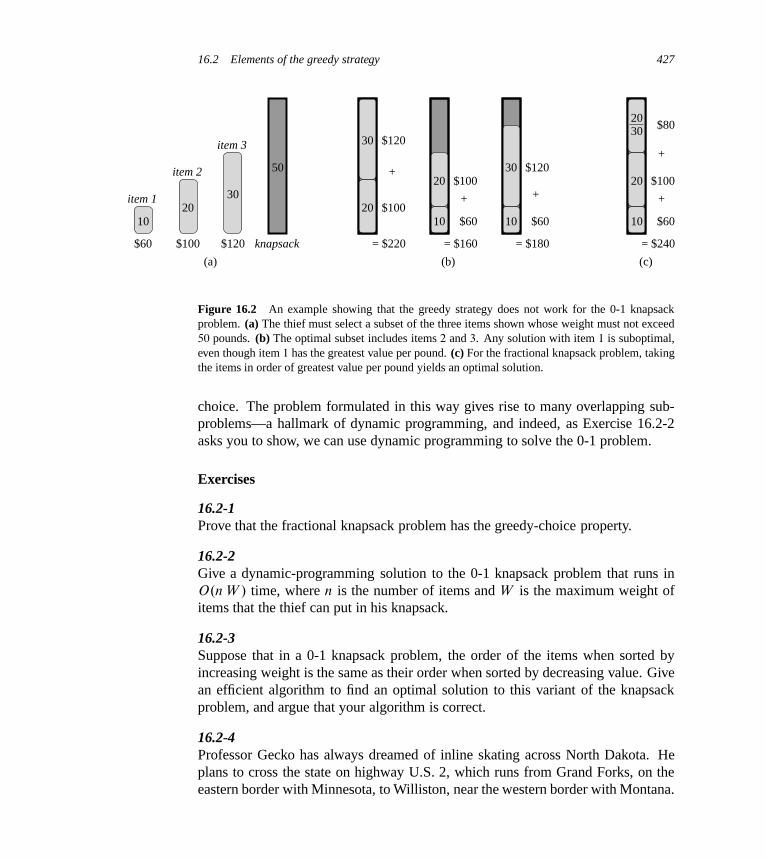
16.2 Elements of the greedy strategy 427
10
$60
item 120
$100
item 2
30
$120
item 3
50
knapsack
(a)
+
$120
$100
= $220
+
$60
$100
= $160
+
$60
$120
= $180
(b)
+
$60
$100
= $240
$80
+
(c)
20
30
10
20
10
30
10
20
2030
Figure 16.2 An example showing that the greedy strategy does not work for the 0-1 knapsackproblem. (a) The thief must select a subset of the three items shown whose weight must not exceed50 pounds. (b) The optimal subset includes items 2 and 3. Any solution with item 1 is suboptimal,even though item 1 has the greatest value per pound. (c) For the fractional knapsack problem, takingthe items in order of greatest value per pound yields an optimal solution.
choice. The problem formulated in this way gives rise to many overlapping sub-problems—a hallmark of dynamic programming, and indeed, as Exercise 16.2-2asks you to show, we can use dynamic programming to solve the 0-1 problem.
Exercises
16.2-1Prove that the fractional knapsack problem has the greedy-choice property.
16.2-2Give a dynamic-programming solution to the 0-1 knapsack problem that runs inO.n W / time, where n is the number of items and W is the maximum weight ofitems that the thief can put in his knapsack.
16.2-3Suppose that in a 0-1 knapsack problem, the order of the items when sorted byincreasing weight is the same as their order when sorted by decreasing value. Givean efficient algorithm to find an optimal solution to this variant of the knapsackproblem, and argue that your algorithm is correct.
16.2-4Professor Gecko has always dreamed of inline skating across North Dakota. Heplans to cross the state on highway U.S. 2, which runs from Grand Forks, on theeastern border with Minnesota, to Williston, near the western border with Montana.
428 Chapter 16 Greedy Algorithms
The professor can carry two liters of water, and he can skate m miles before runningout of water. (Because North Dakota is relatively flat, the professor does not haveto worry about drinking water at a greater rate on uphill sections than on flat ordownhill sections.) The professor will start in Grand Forks with two full liters ofwater. His official North Dakota state map shows all the places along U.S. 2 atwhich he can refill his water and the distances between these locations.
The professor’s goal is to minimize the number of water stops along his routeacross the state. Give an efficient method by which he can determine which waterstops he should make. Prove that your strategy yields an optimal solution, and giveits running time.
16.2-5Describe an efficient algorithm that, given a set fx1; x2; : : : ; xng of points on thereal line, determines the smallest set of unit-length closed intervals that containsall of the given points. Argue that your algorithm is correct.
16.2-6 ?
Show how to solve the fractional knapsack problem in O.n/ time.
16.2-7Suppose you are given two sets A and B , each containing n positive integers. Youcan choose to reorder each set however you like. After reordering, let ai be the i thelement of set A, and let bi be the i th element of set B . You then receive a payoffofQn
iD1 aibi . Give an algorithm that will maximize your payoff. Prove that your
algorithm maximizes the payoff, and state its running time.
16.3 Huffman codes
Huffman codes compress data very effectively: savings of 20% to 90% are typical,depending on the characteristics of the data being compressed. We consider thedata to be a sequence of characters. Huffman’s greedy algorithm uses a table givinghow often each character occurs (i.e., its frequency) to build up an optimal way ofrepresenting each character as a binary string.
Suppose we have a 100,000-character data file that we wish to store compactly.We observe that the characters in the file occur with the frequencies given by Fig-ure 16.3. That is, only 6 different characters appear, and the character a occurs45,000 times.
We have many options for how to represent such a file of information. Here,we consider the problem of designing a binary character code (or code for short)
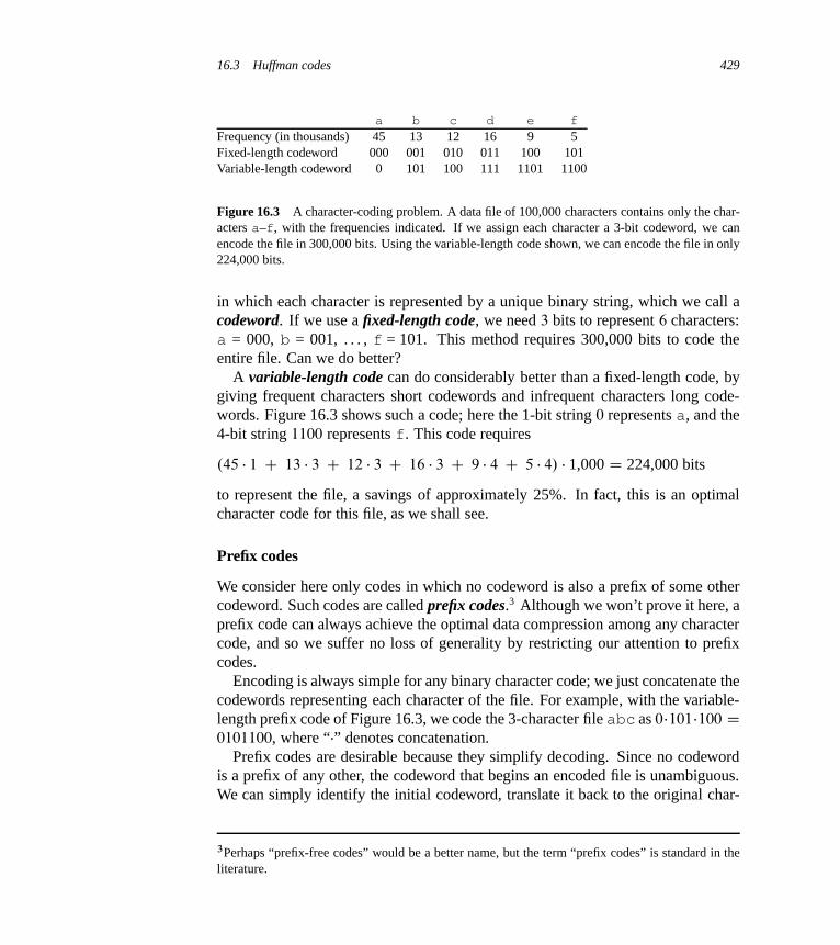
16.3 Huffman codes 429
a b c d e fFrequency (in thousands) 45 13 12 16 9 5Fixed-length codeword 000 001 010 011 100 101Variable-length codeword 0 101 100 111 1101 1100
Figure 16.3 A character-coding problem. A data file of 100,000 characters contains only the char-acters a–f, with the frequencies indicated. If we assign each character a 3-bit codeword, we canencode the file in 300,000 bits. Using the variable-length code shown, we can encode the file in only224,000 bits.
in which each character is represented by a unique binary string, which we call acodeword. If we use a fixed-length code, we need 3 bits to represent 6 characters:a = 000, b = 001, . . . , f = 101. This method requires 300,000 bits to code theentire file. Can we do better?
A variable-length code can do considerably better than a fixed-length code, bygiving frequent characters short codewords and infrequent characters long code-words. Figure 16.3 shows such a code; here the 1-bit string 0 represents a, and the4-bit string 1100 represents f. This code requires
.45 � 1 C 13 � 3 C 12 � 3 C 16 � 3 C 9 � 4 C 5 � 4/ � 1,000 D 224,000 bits
to represent the file, a savings of approximately 25%. In fact, this is an optimalcharacter code for this file, as we shall see.
Prefix codes
We consider here only codes in which no codeword is also a prefix of some othercodeword. Such codes are called prefix codes.3 Although we won’t prove it here, aprefix code can always achieve the optimal data compression among any charactercode, and so we suffer no loss of generality by restricting our attention to prefixcodes.
Encoding is always simple for any binary character code; we just concatenate thecodewords representing each character of the file. For example, with the variable-length prefix code of Figure 16.3, we code the 3-character file abc as 0�101�100 D0101100, where “�” denotes concatenation.
Prefix codes are desirable because they simplify decoding. Since no codewordis a prefix of any other, the codeword that begins an encoded file is unambiguous.We can simply identify the initial codeword, translate it back to the original char-
3Perhaps “prefix-free codes” would be a better name, but the term “prefix codes” is standard in theliterature.

430 Chapter 16 Greedy Algorithms
a:45 b:13 c:12 d:16 e:9 f:5
58 28 14
86 14
100
0 1 0 1 0 1
0 1 0
0 1
e:9f:5
14
0 1
c:12 b:13
25
0 1
d:16
30
0 1
55
0 1
a:45
100
0 1
(a) (b)
Figure 16.4 Trees corresponding to the coding schemes in Figure 16.3. Each leaf is labeled witha character and its frequency of occurrence. Each internal node is labeled with the sum of the fre-quencies of the leaves in its subtree. (a) The tree corresponding to the fixed-length code a = 000, . . . ,f = 101. (b) The tree corresponding to the optimal prefix code a = 0, b = 101, . . . , f = 1100.
acter, and repeat the decoding process on the remainder of the encoded file. In ourexample, the string 001011101 parses uniquely as 0 � 0 � 101 � 1101, which decodesto aabe.
The decoding process needs a convenient representation for the prefix code sothat we can easily pick off the initial codeword. A binary tree whose leaves arethe given characters provides one such representation. We interpret the binarycodeword for a character as the simple path from the root to that character, where 0
means “go to the left child” and 1 means “go to the right child.” Figure 16.4 showsthe trees for the two codes of our example. Note that these are not binary searchtrees, since the leaves need not appear in sorted order and internal nodes do notcontain character keys.
An optimal code for a file is always represented by a full binary tree, in whichevery nonleaf node has two children (see Exercise 16.3-2). The fixed-length codein our example is not optimal since its tree, shown in Figure 16.4(a), is not a full bi-nary tree: it contains codewords beginning 10. . . , but none beginning 11. . . . Sincewe can now restrict our attention to full binary trees, we can say that if C is thealphabet from which the characters are drawn and all character frequencies are pos-itive, then the tree for an optimal prefix code has exactly jC j leaves, one for eachletter of the alphabet, and exactly jC j � 1 internal nodes (see Exercise B.5-3).
Given a tree T corresponding to a prefix code, we can easily compute the numberof bits required to encode a file. For each character c in the alphabet C , let theattribute c: freq denote the frequency of c in the file and let dT .c/ denote the depth
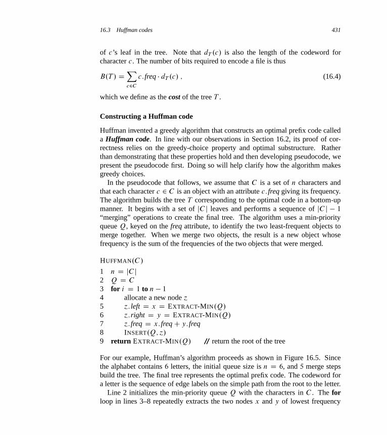
16.3 Huffman codes 431
of c’s leaf in the tree. Note that dT .c/ is also the length of the codeword forcharacter c. The number of bits required to encode a file is thus
B.T / DXc2C
c: freq � dT .c/ ; (16.4)
which we define as the cost of the tree T .
Constructing a Huffman code
Huffman invented a greedy algorithm that constructs an optimal prefix code calleda Huffman code. In line with our observations in Section 16.2, its proof of cor-rectness relies on the greedy-choice property and optimal substructure. Ratherthan demonstrating that these properties hold and then developing pseudocode, wepresent the pseudocode first. Doing so will help clarify how the algorithm makesgreedy choices.
In the pseudocode that follows, we assume that C is a set of n characters andthat each character c 2 C is an object with an attribute c: freq giving its frequency.The algorithm builds the tree T corresponding to the optimal code in a bottom-upmanner. It begins with a set of jC j leaves and performs a sequence of jC j � 1
“merging” operations to create the final tree. The algorithm uses a min-priorityqueue Q, keyed on the freq attribute, to identify the two least-frequent objects tomerge together. When we merge two objects, the result is a new object whosefrequency is the sum of the frequencies of the two objects that were merged.
HUFFMAN.C /
1 n D jC j2 Q D C
3 for i D 1 to n � 1
4 allocate a new node ´
5 ´: left D x D EXTRACT-MIN.Q/
6 ´:right D y D EXTRACT-MIN.Q/
7 ´: freq D x: freqC y: freq8 INSERT.Q; ´/
9 return EXTRACT-MIN.Q/ // return the root of the tree
For our example, Huffman’s algorithm proceeds as shown in Figure 16.5. Sincethe alphabet contains 6 letters, the initial queue size is n D 6, and 5 merge stepsbuild the tree. The final tree represents the optimal prefix code. The codeword fora letter is the sequence of edge labels on the simple path from the root to the letter.
Line 2 initializes the min-priority queue Q with the characters in C . The forloop in lines 3–8 repeatedly extracts the two nodes x and y of lowest frequency

432 Chapter 16 Greedy Algorithms
e:9f:5
14
0 1
c:12 b:13
25
0 1
d:16
30
0 1
55
0 1a:45
100
0 1
e:9f:5
14
0 1
c:12 b:13
25
0 1
d:16
30
0 1
55
0 1a:45
e:9f:5
14
0 1
c:12 b:13
25
0 1
d:16
30
0 1
a:45
e:9f:5
14
0 1
c:12 b:13
25
0 1
d:16 a:45
e:9f:5
14
0 1
c:12 b:13 d:16 a:45e:9f:5 c:12 b:13 d:16 a:45(a)
(c)
(e)
(b)
(d)
(f)
Figure 16.5 The steps of Huffman’s algorithm for the frequencies given in Figure 16.3. Each partshows the contents of the queue sorted into increasing order by frequency. At each step, the twotrees with lowest frequencies are merged. Leaves are shown as rectangles containing a characterand its frequency. Internal nodes are shown as circles containing the sum of the frequencies of theirchildren. An edge connecting an internal node with its children is labeled 0 if it is an edge to a leftchild and 1 if it is an edge to a right child. The codeword for a letter is the sequence of labels on theedges connecting the root to the leaf for that letter. (a) The initial set of n D 6 nodes, one for eachletter. (b)–(e) Intermediate stages. (f) The final tree.
from the queue, replacing them in the queue with a new node ´ representing theirmerger. The frequency of ´ is computed as the sum of the frequencies of x and y
in line 7. The node ´ has x as its left child and y as its right child. (This order isarbitrary; switching the left and right child of any node yields a different code ofthe same cost.) After n � 1 mergers, line 9 returns the one node left in the queue,which is the root of the code tree.
Although the algorithm would produce the same result if we were to excise thevariables x and y—assigning directly to ´: left and ´:right in lines 5 and 6, andchanging line 7 to ´: freq D ´: left: freq C ´:right: freq—we shall use the node

16.3 Huffman codes 433
names x and y in the proof of correctness. Therefore, we find it convenient toleave them in.
To analyze the running time of Huffman’s algorithm, we assume that Q is im-plemented as a binary min-heap (see Chapter 6). For a set C of n characters, wecan initialize Q in line 2 in O.n/ time using the BUILD-MIN-HEAP procedure dis-cussed in Section 6.3. The for loop in lines 3–8 executes exactly n � 1 times, andsince each heap operation requires time O.lg n/, the loop contributes O.n lg n/ tothe running time. Thus, the total running time of HUFFMAN on a set of n charac-ters is O.n lg n/. We can reduce the running time to O.n lg lg n/ by replacing thebinary min-heap with a van Emde Boas tree (see Chapter 20).
Correctness of Huffman’s algorithm
To prove that the greedy algorithm HUFFMAN is correct, we show that the prob-lem of determining an optimal prefix code exhibits the greedy-choice and optimal-substructure properties. The next lemma shows that the greedy-choice propertyholds.
Lemma 16.2Let C be an alphabet in which each character c 2 C has frequency c: freq. Letx and y be two characters in C having the lowest frequencies. Then there existsan optimal prefix code for C in which the codewords for x and y have the samelength and differ only in the last bit.
Proof The idea of the proof is to take the tree T representing an arbitrary optimalprefix code and modify it to make a tree representing another optimal prefix codesuch that the characters x and y appear as sibling leaves of maximum depth in thenew tree. If we can construct such a tree, then the codewords for x and y will havethe same length and differ only in the last bit.
Let a and b be two characters that are sibling leaves of maximum depth in T .Without loss of generality, we assume that a: freq � b: freq and x: freq � y: freq.Since x: freq and y: freq are the two lowest leaf frequencies, in order, and a: freqand b: freq are two arbitrary frequencies, in order, we have x: freq � a: freq andy: freq � b: freq.
In the remainder of the proof, it is possible that we could have x: freq D a: freqor y: freq D b: freq. However, if we had x: freq D b: freq, then we would also havea: freq D b: freq D x: freq D y: freq (see Exercise 16.3-1), and the lemma wouldbe trivially true. Thus, we will assume that x: freq ¤ b: freq, which means thatx ¤ b.
As Figure 16.6 shows, we exchange the positions in T of a and x to produce atree T 0, and then we exchange the positions in T 0 of b and y to produce a tree T 00

434 Chapter 16 Greedy Algorithms
x
y
a b x
y
a
b x y
a
b
T′′T T′
Figure 16.6 An illustration of the key step in the proof of Lemma 16.2. In the optimal tree T ,leaves a and b are two siblings of maximum depth. Leaves x and y are the two characters with thelowest frequencies; they appear in arbitrary positions in T . Assuming that x ¤ b, swapping leaves a
and x produces tree T 0, and then swapping leaves b and y produces tree T 00. Since each swap doesnot increase the cost, the resulting tree T 00 is also an optimal tree.
in which x and y are sibling leaves of maximum depth. (Note that if x D b buty ¤ a, then tree T 00 does not have x and y as sibling leaves of maximum depth.Because we assume that x ¤ b, this situation cannot occur.) By equation (16.4),the difference in cost between T and T 0 is
B.T / � B.T 0/
DXc2C
c: freq � dT .c/�Xc2C
c: freq � dT 0.c/
D x: freq � dT .x/C a: freq � dT .a/ � x: freq � dT 0.x/ � a: freq � dT 0.a/
D x: freq � dT .x/C a: freq � dT .a/ � x: freq � dT .a/ � a: freq � dT .x/
D .a: freq � x: freq/.dT .a/ � dT .x//
� 0 ;
because both a: freq � x: freq and dT .a/ � dT .x/ are nonnegative. More specifi-cally, a: freq � x: freq is nonnegative because x is a minimum-frequency leaf, anddT .a/�dT .x/ is nonnegative because a is a leaf of maximum depth in T . Similarly,exchanging y and b does not increase the cost, and so B.T 0/�B.T 00/ is nonnega-tive. Therefore, B.T 00/ � B.T /, and since T is optimal, we have B.T / � B.T 00/,which implies B.T 00/ D B.T /. Thus, T 00 is an optimal tree in which x and y
appear as sibling leaves of maximum depth, from which the lemma follows.
Lemma 16.2 implies that the process of building up an optimal tree by mergerscan, without loss of generality, begin with the greedy choice of merging togetherthose two characters of lowest frequency. Why is this a greedy choice? We canview the cost of a single merger as being the sum of the frequencies of the two itemsbeing merged. Exercise 16.3-4 shows that the total cost of the tree constructedequals the sum of the costs of its mergers. Of all possible mergers at each step,HUFFMAN chooses the one that incurs the least cost.
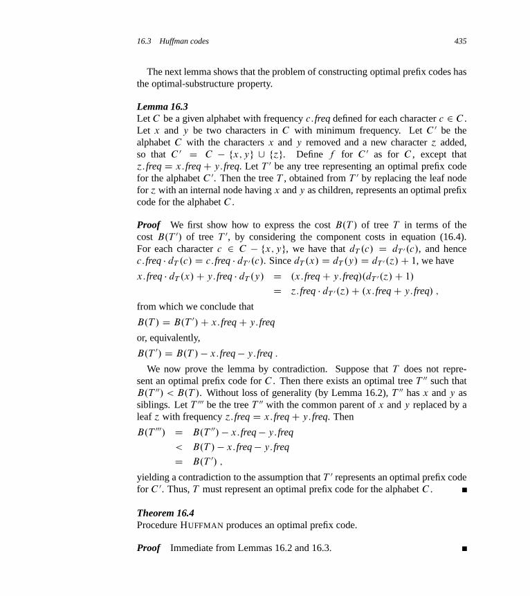
16.3 Huffman codes 435
The next lemma shows that the problem of constructing optimal prefix codes hasthe optimal-substructure property.
Lemma 16.3Let C be a given alphabet with frequency c: freq defined for each character c 2 C .Let x and y be two characters in C with minimum frequency. Let C 0 be thealphabet C with the characters x and y removed and a new character ´ added,so that C 0 D C � fx; yg [ f´g. Define f for C 0 as for C , except that´: freq D x: freqC y: freq. Let T 0 be any tree representing an optimal prefix codefor the alphabet C 0. Then the tree T , obtained from T 0 by replacing the leaf nodefor ´ with an internal node having x and y as children, represents an optimal prefixcode for the alphabet C .
Proof We first show how to express the cost B.T / of tree T in terms of thecost B.T 0/ of tree T 0, by considering the component costs in equation (16.4).For each character c 2 C � fx; yg, we have that dT .c/ D dT 0.c/, and hencec: freq � dT .c/ D c: freq � dT 0.c/. Since dT .x/ D dT .y/ D dT 0.´/C 1, we have
x: freq � dT .x/C y: freq � dT .y/ D .x: freqC y: freq/.dT 0.´/C 1/
D ´: freq � dT 0.´/C .x: freqC y: freq/ ;
from which we conclude that
B.T / D B.T 0/C x: freqC y: freq
or, equivalently,
B.T 0/ D B.T / � x: freq� y: freq :
We now prove the lemma by contradiction. Suppose that T does not repre-sent an optimal prefix code for C . Then there exists an optimal tree T 00 such thatB.T 00/ < B.T /. Without loss of generality (by Lemma 16.2), T 00 has x and y assiblings. Let T 000 be the tree T 00 with the common parent of x and y replaced by aleaf ´ with frequency ´: freq D x: freqC y: freq. Then
B.T 000/ D B.T 00/ � x: freq� y: freq
< B.T / � x: freq� y: freq
D B.T 0/ ;
yielding a contradiction to the assumption that T 0 represents an optimal prefix codefor C 0. Thus, T must represent an optimal prefix code for the alphabet C .
Theorem 16.4Procedure HUFFMAN produces an optimal prefix code.
Proof Immediate from Lemmas 16.2 and 16.3.
436 Chapter 16 Greedy Algorithms
Exercises
16.3-1Explain why, in the proof of Lemma 16.2, if x: freq D b: freq, then we must havea: freq D b: freq D x: freq D y: freq.
16.3-2Prove that a binary tree that is not full cannot correspond to an optimal prefix code.
16.3-3What is an optimal Huffman code for the following set of frequencies, based onthe first 8 Fibonacci numbers?
a:1 b:1 c:2 d:3 e:5 f:8 g:13 h:21
Can you generalize your answer to find the optimal code when the frequencies arethe first n Fibonacci numbers?
16.3-4Prove that we can also express the total cost of a tree for a code as the sum, overall internal nodes, of the combined frequencies of the two children of the node.
16.3-5Prove that if we order the characters in an alphabet so that their frequenciesare monotonically decreasing, then there exists an optimal code whose codewordlengths are monotonically increasing.
16.3-6Suppose we have an optimal prefix code on a set C D f0; 1; : : : ; n � 1g of charac-ters and we wish to transmit this code using as few bits as possible. Show how torepresent any optimal prefix code on C using only 2n � 1C n dlg ne bits. (Hint:Use 2n � 1 bits to specify the structure of the tree, as discovered by a walk of thetree.)
16.3-7Generalize Huffman’s algorithm to ternary codewords (i.e., codewords using thesymbols 0, 1, and 2), and prove that it yields optimal ternary codes.
16.3-8Suppose that a data file contains a sequence of 8-bit characters such that all 256characters are about equally common: the maximum character frequency is lessthan twice the minimum character frequency. Prove that Huffman coding in thiscase is no more efficient than using an ordinary 8-bit fixed-length code.
16.4 Matroids and greedy methods 437
16.3-9Show that no compression scheme can expect to compress a file of randomly cho-sen 8-bit characters by even a single bit. (Hint: Compare the number of possiblefiles with the number of possible encoded files.)
? 16.4 Matroids and greedy methods
In this section, we sketch a beautiful theory about greedy algorithms. This theorydescribes many situations in which the greedy method yields optimal solutions. Itinvolves combinatorial structures known as “matroids.” Although this theory doesnot cover all cases for which a greedy method applies (for example, it does notcover the activity-selection problem of Section 16.1 or the Huffman-coding prob-lem of Section 16.3), it does cover many cases of practical interest. Furthermore,this theory has been extended to cover many applications; see the notes at the endof this chapter for references.
Matroids
A matroid is an ordered pair M D .S; � / satisfying the following conditions.
1. S is a finite set.
2. � is a nonempty family of subsets of S , called the independent subsets of S ,such that if B 2 � and A � B , then A 2 � . We say that � is hereditary if itsatisfies this property. Note that the empty set ; is necessarily a member of � .
3. If A 2 � , B 2 � , and jAj < jBj, then there exists some element x 2 B � A
such that A [ fxg 2 � . We say that M satisfies the exchange property.
The word “matroid” is due to Hassler Whitney. He was studying matric ma-troids, in which the elements of S are the rows of a given matrix and a set of rows isindependent if they are linearly independent in the usual sense. As Exercise 16.4-2asks you to show, this structure defines a matroid.
As another example of matroids, consider the graphic matroid MG D .SG; �G/
defined in terms of a given undirected graph G D .V; E/ as follows:
� The set SG is defined to be E, the set of edges of G.
� If A is a subset of E, then A 2 �G if and only if A is acyclic. That is, a set ofedges A is independent if and only if the subgraph GA D .V; A/ forms a forest.
The graphic matroid MG is closely related to the minimum-spanning-tree problem,which Chapter 23 covers in detail.
438 Chapter 16 Greedy Algorithms
Theorem 16.5If G D .V; E/ is an undirected graph, then MG D .SG; �G/ is a matroid.
Proof Clearly, SG D E is a finite set. Furthermore, �G is hereditary, since asubset of a forest is a forest. Putting it another way, removing edges from anacyclic set of edges cannot create cycles.
Thus, it remains to show that MG satisfies the exchange property. Suppose thatGA D .V; A/ and GB D .V; B/ are forests of G and that jBj > jAj. That is, A
and B are acyclic sets of edges, and B contains more edges than A does.We claim that a forest F D .VF ; EF / contains exactly jVF j � jEF j trees. To
see why, suppose that F consists of t trees, where the i th tree contains �i verticesand ei edges. Then, we have
jEF j DtX
iD1
ei
DtX
iD1
.�i � 1/ (by Theorem B.2)
DtX
iD1
�i � t
D jVF j � t ;
which implies that t D jVF j � jEF j. Thus, forest GA contains jV j � jAj trees, andforest GB contains jV j � jBj trees.
Since forest GB has fewer trees than forest GA does, forest GB must containsome tree T whose vertices are in two different trees in forest GA. Moreover,since T is connected, it must contain an edge .u; �/ such that vertices u and �
are in different trees in forest GA. Since the edge .u; �/ connects vertices in twodifferent trees in forest GA, we can add the edge .u; �/ to forest GA without creatinga cycle. Therefore, MG satisfies the exchange property, completing the proof thatMG is a matroid.
Given a matroid M D .S; � /, we call an element x … A an extension of A 2 �
if we can add x to A while preserving independence; that is, x is an extensionof A if A [ fxg 2 � . As an example, consider a graphic matroid MG . If A is anindependent set of edges, then edge e is an extension of A if and only if e is notin A and the addition of e to A does not create a cycle.
If A is an independent subset in a matroid M , we say that A is maximal if it hasno extensions. That is, A is maximal if it is not contained in any larger independentsubset of M . The following property is often useful.

16.4 Matroids and greedy methods 439
Theorem 16.6All maximal independent subsets in a matroid have the same size.
Proof Suppose to the contrary that A is a maximal independent subset of M
and there exists another larger maximal independent subset B of M . Then, theexchange property implies that for some x 2 B � A, we can extend A to a largerindependent set A[ fxg, contradicting the assumption that A is maximal.
As an illustration of this theorem, consider a graphic matroid MG for a con-nected, undirected graph G. Every maximal independent subset of MG must be afree tree with exactly jV j � 1 edges that connects all the vertices of G. Such a treeis called a spanning tree of G.
We say that a matroid M D .S; � / is weighted if it is associated with a weightfunction w that assigns a strictly positive weight w.x/ to each element x 2 S . Theweight function w extends to subsets of S by summation:
w.A/ DXx2A
w.x/
for any A � S . For example, if we let w.e/ denote the weight of an edge e in agraphic matroid MG , then w.A/ is the total weight of the edges in edge set A.
Greedy algorithms on a weighted matroid
Many problems for which a greedy approach provides optimal solutions can be for-mulated in terms of finding a maximum-weight independent subset in a weightedmatroid. That is, we are given a weighted matroid M D .S; � /, and we wish tofind an independent set A 2 � such that w.A/ is maximized. We call such a sub-set that is independent and has maximum possible weight an optimal subset of thematroid. Because the weight w.x/ of any element x 2 S is positive, an optimalsubset is always a maximal independent subset—it always helps to make A as largeas possible.
For example, in the minimum-spanning-tree problem, we are given a connectedundirected graph G D .V; E/ and a length function w such that w.e/ is the (posi-tive) length of edge e. (We use the term “length” here to refer to the original edgeweights for the graph, reserving the term “weight” to refer to the weights in theassociated matroid.) We wish to find a subset of the edges that connects all ofthe vertices together and has minimum total length. To view this as a problem offinding an optimal subset of a matroid, consider the weighted matroid MG withweight function w0, where w0.e/ D w0 �w.e/ and w0 is larger than the maximumlength of any edge. In this weighted matroid, all weights are positive and an opti-mal subset is a spanning tree of minimum total length in the original graph. Morespecifically, each maximal independent subset A corresponds to a spanning tree
440 Chapter 16 Greedy Algorithms
with jV j � 1 edges, and since
w0.A/ DXe2A
w0.e/
DXe2A
.w0 � w.e//
D .jV j � 1/w0 �Xe2A
w.e/
D .jV j � 1/w0 � w.A/
for any maximal independent subset A, an independent subset that maximizes thequantity w0.A/ must minimize w.A/. Thus, any algorithm that can find an optimalsubset A in an arbitrary matroid can solve the minimum-spanning-tree problem.
Chapter 23 gives algorithms for the minimum-spanning-tree problem, but herewe give a greedy algorithm that works for any weighted matroid. The algorithmtakes as input a weighted matroid M D .S; � / with an associated positive weightfunction w, and it returns an optimal subset A. In our pseudocode, we denote thecomponents of M by M:S and M:� and the weight function by w. The algorithmis greedy because it considers in turn each element x 2 S , in order of monotoni-cally decreasing weight, and immediately adds it to the set A being accumulated ifA [ fxg is independent.
GREEDY.M; w/
1 A D ;2 sort M:S into monotonically decreasing order by weight w
3 for each x 2M:S, taken in monotonically decreasing order by weight w.x/
4 if A [ fxg 2M:�
5 A D A [ fxg6 return A
Line 4 checks whether adding each element x to A would maintain A as an inde-pendent set. If A would remain independent, then line 5 adds x to A. Otherwise, x
is discarded. Since the empty set is independent, and since each iteration of the forloop maintains A’s independence, the subset A is always independent, by induc-tion. Therefore, GREEDY always returns an independent subset A. We shall see ina moment that A is a subset of maximum possible weight, so that A is an optimalsubset.
The running time of GREEDY is easy to analyze. Let n denote jS j. The sortingphase of GREEDY takes time O.n lg n/. Line 4 executes exactly n times, once foreach element of S . Each execution of line 4 requires a check on whether or notthe set A [ fxg is independent. If each such check takes time O.f .n//, the entirealgorithm runs in time O.n lg nC nf .n//.
16.4 Matroids and greedy methods 441
We now prove that GREEDY returns an optimal subset.
Lemma 16.7 (Matroids exhibit the greedy-choice property)Suppose that M D .S; � / is a weighted matroid with weight function w and that S
is sorted into monotonically decreasing order by weight. Let x be the first elementof S such that fxg is independent, if any such x exists. If x exists, then there existsan optimal subset A of S that contains x.
Proof If no such x exists, then the only independent subset is the empty set andthe lemma is vacuously true. Otherwise, let B be any nonempty optimal subset.Assume that x … B; otherwise, letting A D B gives an optimal subset of S thatcontains x.
No element of B has weight greater than w.x/. To see why, observe that y 2 B
implies that fyg is independent, since B 2 � and � is hereditary. Our choice of x
therefore ensures that w.x/ � w.y/ for any y 2 B .Construct the set A as follows. Begin with A D fxg. By the choice of x, set A is
independent. Using the exchange property, repeatedly find a new element of B thatwe can add to A until jAj D jBj, while preserving the independence of A. At thatpoint, A and B are the same except that A has x and B has some other element y.That is, A D B � fyg [ fxg for some y 2 B , and so
w.A/ D w.B/� w.y/Cw.x/
� w.B/ :
Because set B is optimal, set A, which contains x must also be optimal.
We next show that if an element is not an option initially, then it cannot be anoption later.
Lemma 16.8Let M D .S; � / be any matroid. If x is an element of S that is an extension ofsome independent subset A of S , then x is also an extension of ;.
Proof Since x is an extension of A, we have that A[fxg is independent. Since �
is hereditary, fxg must be independent. Thus, x is an extension of ;.
Corollary 16.9Let M D .S; � / be any matroid. If x is an element of S such that x is not anextension of ;, then x is not an extension of any independent subset A of S .
Proof This corollary is simply the contrapositive of Lemma 16.8.

442 Chapter 16 Greedy Algorithms
Corollary 16.9 says that any element that cannot be used immediately can neverbe used. Therefore, GREEDY cannot make an error by passing over any initialelements in S that are not an extension of ;, since they can never be used.
Lemma 16.10 (Matroids exhibit the optimal-substructure property)Let x be the first element of S chosen by GREEDY for the weighted matroidM D .S; � /. The remaining problem of finding a maximum-weight indepen-dent subset containing x reduces to finding a maximum-weight independent subsetof the weighted matroid M 0 D .S 0; �
0/, where
S 0 D fy 2 S W fx; yg 2 � g ;
�0 D fB � S � fxg W B [ fxg 2 � g ;
and the weight function for M 0 is the weight function for M , restricted to S 0. (Wecall M 0 the contraction of M by the element x.)
Proof If A is any maximum-weight independent subset of M containing x, thenA0 D A � fxg is an independent subset of M 0. Conversely, any independent sub-set A0 of M 0 yields an independent subset A D A0 [ fxg of M . Since we have inboth cases that w.A/ D w.A0/Cw.x/, a maximum-weight solution in M contain-ing x yields a maximum-weight solution in M 0, and vice versa.
Theorem 16.11 (Correctness of the greedy algorithm on matroids)If M D .S; � / is a weighted matroid with weight function w, then GREEDY.M; w/
returns an optimal subset.
Proof By Corollary 16.9, any elements that GREEDY passes over initially be-cause they are not extensions of ; can be forgotten about, since they can neverbe useful. Once GREEDY selects the first element x, Lemma 16.7 implies thatthe algorithm does not err by adding x to A, since there exists an optimal subsetcontaining x. Finally, Lemma 16.10 implies that the remaining problem is one offinding an optimal subset in the matroid M 0 that is the contraction of M by x.After the procedure GREEDY sets A to fxg, we can interpret all of its remainingsteps as acting in the matroid M 0 D .S 0; �
0/, because B is independent in M 0 ifand only if B [fxg is independent in M , for all sets B 2 �
0. Thus, the subsequentoperation of GREEDY will find a maximum-weight independent subset for M 0, andthe overall operation of GREEDY will find a maximum-weight independent subsetfor M .
16.5 A task-scheduling problem as a matroid 443
Exercises
16.4-1Show that .S; �k/ is a matroid, where S is any finite set and �k is the set of allsubsets of S of size at most k, where k � jS j.16.4-2 ?
Given an m n matrix T over some field (such as the reals), show that .S; � / is amatroid, where S is the set of columns of T and A 2 � if and only if the columnsin A are linearly independent.
16.4-3 ?
Show that if .S; � / is a matroid, then .S; �0/ is a matroid, where
�0 D fA0 W S � A0 contains some maximal A 2 � g :
That is, the maximal independent sets of .S; �0/ are just the complements of the
maximal independent sets of .S; � /.
16.4-4 ?
Let S be a finite set and let S1; S2; : : : ; Sk be a partition of S into nonempty disjointsubsets. Define the structure .S; � / by the condition that � D fA W jA \ Si j � 1
for i D 1; 2; : : : ; kg. Show that .S; � / is a matroid. That is, the set of all sets A
that contain at most one member of each subset in the partition determines theindependent sets of a matroid.
16.4-5Show how to transform the weight function of a weighted matroid problem, wherethe desired optimal solution is a minimum-weight maximal independent subset, tomake it an standard weighted-matroid problem. Argue carefully that your transfor-mation is correct.
? 16.5 A task-scheduling problem as a matroid
An interesting problem that we can solve using matroids is the problem of op-timally scheduling unit-time tasks on a single processor, where each task has adeadline, along with a penalty paid if the task misses its deadline. The problemlooks complicated, but we can solve it in a surprisingly simple manner by castingit as a matroid and using a greedy algorithm.
A unit-time task is a job, such as a program to be run on a computer, that requiresexactly one unit of time to complete. Given a finite set S of unit-time tasks, a
444 Chapter 16 Greedy Algorithms
schedule for S is a permutation of S specifying the order in which to performthese tasks. The first task in the schedule begins at time 0 and finishes at time 1,the second task begins at time 1 and finishes at time 2, and so on.
The problem of scheduling unit-time tasks with deadlines and penalties for asingle processor has the following inputs:
� a set S D fa1; a2; : : : ; ang of n unit-time tasks;
� a set of n integer deadlines d1; d2; : : : ; dn, such that each di satisfies 1 � di � n
and task ai is supposed to finish by time di ; and
� a set of n nonnegative weights or penalties w1; w2; : : : ; wn, such that we incura penalty of wi if task ai is not finished by time di , and we incur no penalty ifa task finishes by its deadline.
We wish to find a schedule for S that minimizes the total penalty incurred formissed deadlines.
Consider a given schedule. We say that a task is late in this schedule if it finishesafter its deadline. Otherwise, the task is early in the schedule. We can always trans-form an arbitrary schedule into early-first form, in which the early tasks precedethe late tasks. To see why, note that if some early task ai follows some late task aj ,then we can switch the positions of ai and aj , and ai will still be early and aj willstill be late.
Furthermore, we claim that we can always transform an arbitrary schedule intocanonical form, in which the early tasks precede the late tasks and we schedulethe early tasks in order of monotonically increasing deadlines. To do so, we putthe schedule into early-first form. Then, as long as there exist two early tasks ai
and aj finishing at respective times k and k C 1 in the schedule such that dj < di ,we swap the positions of ai and aj . Since aj is early before the swap, k C 1 � dj .Therefore, k C 1 < di , and so ai is still early after the swap. Because task aj ismoved earlier in the schedule, it remains early after the swap.
The search for an optimal schedule thus reduces to finding a set A of tasks thatwe assign to be early in the optimal schedule. Having determined A, we can createthe actual schedule by listing the elements of A in order of monotonically increas-ing deadline, then listing the late tasks (i.e., S � A) in any order, producing acanonical ordering of the optimal schedule.
We say that a set A of tasks is independent if there exists a schedule for thesetasks such that no tasks are late. Clearly, the set of early tasks for a schedule formsan independent set of tasks. Let � denote the set of all independent sets of tasks.
Consider the problem of determining whether a given set A of tasks is indepen-dent. For t D 0; 1; 2; : : : ; n, let Nt .A/ denote the number of tasks in A whosedeadline is t or earlier. Note that N0.A/ D 0 for any set A.
16.5 A task-scheduling problem as a matroid 445
Lemma 16.12For any set of tasks A, the following statements are equivalent.
1. The set A is independent.
2. For t D 0; 1; 2; : : : ; n, we have Nt.A/ � t .
3. If the tasks in A are scheduled in order of monotonically increasing deadlines,then no task is late.
Proof To show that (1) implies (2), we prove the contrapositive: if Nt .A/ > t forsome t , then there is no way to make a schedule with no late tasks for set A, becausemore than t tasks must finish before time t . Therefore, (1) implies (2). If (2) holds,then (3) must follow: there is no way to “get stuck” when scheduling the tasks inorder of monotonically increasing deadlines, since (2) implies that the i th largestdeadline is at least i . Finally, (3) trivially implies (1).
Using property 2 of Lemma 16.12, we can easily compute whether or not a givenset of tasks is independent (see Exercise 16.5-2).
The problem of minimizing the sum of the penalties of the late tasks is the sameas the problem of maximizing the sum of the penalties of the early tasks. Thefollowing theorem thus ensures that we can use the greedy algorithm to find anindependent set A of tasks with the maximum total penalty.
Theorem 16.13If S is a set of unit-time tasks with deadlines, and � is the set of all independentsets of tasks, then the corresponding system .S; � / is a matroid.
Proof Every subset of an independent set of tasks is certainly independent. Toprove the exchange property, suppose that B and A are independent sets of tasksand that jBj > jAj. Let k be the largest t such that Nt .B/ � Nt.A/. (Such a valueof t exists, since N0.A/ D N0.B/ D 0.) Since Nn.B/ D jBj and Nn.A/ D jAj,but jBj > jAj, we must have that k < n and that Nj .B/ > Nj .A/ for all j inthe range k C 1 � j � n. Therefore, B contains more tasks with deadline k C 1
than A does. Let ai be a task in B � A with deadline k C 1. Let A0 D A [ faig.We now show that A0 must be independent by using property 2 of Lemma 16.12.
For 0 � t � k, we have Nt.A0/ D Nt .A/ � t , since A is independent. For
k < t � n, we have Nt.A0/ � Nt.B/ � t , since B is independent. Therefore, A0
is independent, completing our proof that .S; � / is a matroid.
By Theorem 16.11, we can use a greedy algorithm to find a maximum-weightindependent set of tasks A. We can then create an optimal schedule having thetasks in A as its early tasks. This method is an efficient algorithm for scheduling

446 Chapter 16 Greedy Algorithms
Taskai 1 2 3 4 5 6 7
di 4 2 4 3 1 4 6wi 70 60 50 40 30 20 10
Figure 16.7 An instance of the problem of scheduling unit-time tasks with deadlines and penaltiesfor a single processor.
unit-time tasks with deadlines and penalties for a single processor. The runningtime is O.n2/ using GREEDY, since each of the O.n/ independence checks madeby that algorithm takes time O.n/ (see Exercise 16.5-2). Problem 16-4 gives afaster implementation.
Figure 16.7 demonstrates an example of the problem of scheduling unit-timetasks with deadlines and penalties for a single processor. In this example, thegreedy algorithm selects, in order, tasks a1, a2, a3, and a4, then rejects a5 (becauseN4.fa1; a2; a3; a4; a5g/ D 5) and a6 (because N4.fa1; a2; a3; a4; a6g/ D 5), andfinally accepts a7. The final optimal schedule is
ha2; a4; a1; a3; a7; a5; a6i ;
which has a total penalty incurred of w5 Cw6 D 50.
Exercises
16.5-1Solve the instance of the scheduling problem given in Figure 16.7, but with eachpenalty wi replaced by 80 � wi .
16.5-2Show how to use property 2 of Lemma 16.12 to determine in time O.jAj/ whetheror not a given set A of tasks is independent.
Problems
16-1 Coin changingConsider the problem of making change for n cents using the fewest number ofcoins. Assume that each coin’s value is an integer.
a. Describe a greedy algorithm to make change consisting of quarters, dimes,nickels, and pennies. Prove that your algorithm yields an optimal solution.

Problems for Chapter 16 447
b. Suppose that the available coins are in the denominations that are powers of c,i.e., the denominations are c0; c1; : : : ; ck for some integers c > 1 and k � 1.Show that the greedy algorithm always yields an optimal solution.
c. Give a set of coin denominations for which the greedy algorithm does not yieldan optimal solution. Your set should include a penny so that there is a solutionfor every value of n.
d. Give an O.nk/-time algorithm that makes change for any set of k different coindenominations, assuming that one of the coins is a penny.
16-2 Scheduling to minimize average completion timeSuppose you are given a set S D fa1; a2; : : : ; ang of tasks, where task ai re-quires pi units of processing time to complete, once it has started. You have onecomputer on which to run these tasks, and the computer can run only one task at atime. Let ci be the completion time of task ai , that is, the time at which task ai com-pletes processing. Your goal is to minimize the average completion time, that is,to minimize .1=n/
Pn
iD1 ci . For example, suppose there are two tasks, a1 and a2,with p1 D 3 and p2 D 5, and consider the schedule in which a2 runs first, followedby a1. Then c2 D 5, c1 D 8, and the average completion time is .5C 8/=2 D 6:5.If task a1 runs first, however, then c1 D 3, c2 D 8, and the average completiontime is .3C 8/=2 D 5:5.
a. Give an algorithm that schedules the tasks so as to minimize the average com-pletion time. Each task must run non-preemptively, that is, once task ai starts, itmust run continuously for pi units of time. Prove that your algorithm minimizesthe average completion time, and state the running time of your algorithm.
b. Suppose now that the tasks are not all available at once. That is, each taskcannot start until its release time ri . Suppose also that we allow preemption, sothat a task can be suspended and restarted at a later time. For example, a task ai
with processing time pi D 6 and release time ri D 1 might start running attime 1 and be preempted at time 4. It might then resume at time 10 but bepreempted at time 11, and it might finally resume at time 13 and complete attime 15. Task ai has run for a total of 6 time units, but its running time has beendivided into three pieces. In this scenario, ai ’s completion time is 15. Givean algorithm that schedules the tasks so as to minimize the average completiontime in this new scenario. Prove that your algorithm minimizes the averagecompletion time, and state the running time of your algorithm.
448 Chapter 16 Greedy Algorithms
16-3 Acyclic subgraphsa. The incidence matrix for an undirected graph G D .V; E/ is a jV j jEj ma-
trix M such that M�e D 1 if edge e is incident on vertex �, and M�e D 0 other-wise. Argue that a set of columns of M is linearly independent over the fieldof integers modulo 2 if and only if the corresponding set of edges is acyclic.Then, use the result of Exercise 16.4-2 to provide an alternate proof that .E; � /
of part (a) is a matroid.
b. Suppose that we associate a nonnegative weight w.e/ with each edge in anundirected graph G D .V; E/. Give an efficient algorithm to find an acyclicsubset of E of maximum total weight.
c. Let G.V; E/ be an arbitrary directed graph, and let .E; � / be defined so thatA 2 � if and only if A does not contain any directed cycles. Give an exampleof a directed graph G such that the associated system .E; � / is not a matroid.Specify which defining condition for a matroid fails to hold.
d. The incidence matrix for a directed graph G D .V; E/ with no self-loops is ajV j jEj matrix M such that M�e D �1 if edge e leaves vertex �, M�e D 1 ifedge e enters vertex �, and M�e D 0 otherwise. Argue that if a set of columnsof M is linearly independent, then the corresponding set of edges does notcontain a directed cycle.
e. Exercise 16.4-2 tells us that the set of linearly independent sets of columns ofany matrix M forms a matroid. Explain carefully why the results of parts (d)and (e) are not contradictory. How can there fail to be a perfect correspon-dence between the notion of a set of edges being acyclic and the notion of theassociated set of columns of the incidence matrix being linearly independent?
16-4 Scheduling variationsConsider the following algorithm for the problem from Section 16.5 of schedulingunit-time tasks with deadlines and penalties. Let all n time slots be initially empty,where time slot i is the unit-length slot of time that finishes at time i . We considerthe tasks in order of monotonically decreasing penalty. When considering task aj ,if there exists a time slot at or before aj ’s deadline dj that is still empty, assign aj
to the latest such slot, filling it. If there is no such slot, assign task aj to the latestof the as yet unfilled slots.
a. Argue that this algorithm always gives an optimal answer.
b. Use the fast disjoint-set forest presented in Section 21.3 to implement the algo-rithm efficiently. Assume that the set of input tasks has already been sorted into
Problems for Chapter 16 449
monotonically decreasing order by penalty. Analyze the running time of yourimplementation.
16-5 Off-line cachingModern computers use a cache to store a small amount of data in a fast memory.Even though a program may access large amounts of data, by storing a small subsetof the main memory in the cache—a small but faster memory—overall access timecan greatly decrease. When a computer program executes, it makes a sequencehr1; r2; : : : ; rni of n memory requests, where each request is for a particular dataelement. For example, a program that accesses 4 distinct elements fa; b; c; dgmight make the sequence of requests hd; b; d; b; d; a; c; d; b; a; c; bi. Let k be thesize of the cache. When the cache contains k elements and the program requests the.k C 1/st element, the system must decide, for this and each subsequent request,which k elements to keep in the cache. More precisely, for each request ri , thecache-management algorithm checks whether element ri is already in the cache. Ifit is, then we have a cache hit; otherwise, we have a cache miss. Upon a cachemiss, the system retrieves ri from the main memory, and the cache-managementalgorithm must decide whether to keep ri in the cache. If it decides to keep ri andthe cache already holds k elements, then it must evict one element to make roomfor ri . The cache-management algorithm evicts data with the goal of minimizingthe number of cache misses over the entire sequence of requests.
Typically, caching is an on-line problem. That is, we have to make decisionsabout which data to keep in the cache without knowing the future requests. Here,however, we consider the off-line version of this problem, in which we are givenin advance the entire sequence of n requests and the cache size k, and we wish tominimize the total number of cache misses.
We can solve this off-line problem by a greedy strategy called furthest-in-future,which chooses to evict the item in the cache whose next access in the requestsequence comes furthest in the future.
a. Write pseudocode for a cache manager that uses the furthest-in-future strategy.The input should be a sequence hr1; r2; : : : ; rni of requests and a cache size k,and the output should be a sequence of decisions about which data element (ifany) to evict upon each request. What is the running time of your algorithm?
b. Show that furthest-in-future exhibits optimal substructure.
c. Prove that furthest-in-future produces the minimum possible number of cachemisses.

450 Chapter 16 Greedy Algorithms
Chapter notes
Much more material on greedy algorithms and matroids can be found in Lawler[224] and Papadimitriou and Steiglitz [271].
The greedy algorithm first appeared in the combinatorial optimization literaturein a 1971 article by Edmonds [101], though the theory of matroids dates back toa 1935 article by Whitney [355].
Our proof of the correctness of the greedy algorithm for the activity-selectionproblem is based on that of Gavril [131]. The task-scheduling problem is studiedin Lawler [224]; Horowitz, Sahni, and Rajasekaran [181]; and Brassard and Bratley[55].
Huffman codes were invented in 1952 [185]; Lelewer and Hirschberg [231] sur-veys data-compression techniques known as of 1987.
An extension of matroid theory to greedoid theory was pioneered by Korte andLovász [216, 217, 218, 219], who greatly generalize the theory presented here.
17 Amortized Analysis
In an amortized analysis, we average the time required to perform a sequence ofdata-structure operations over all the operations performed. With amortized analy-sis, we can show that the average cost of an operation is small, if we average over asequence of operations, even though a single operation within the sequence mightbe expensive. Amortized analysis differs from average-case analysis in that prob-ability is not involved; an amortized analysis guarantees the average performanceof each operation in the worst case.
The first three sections of this chapter cover the three most common techniquesused in amortized analysis. Section 17.1 starts with aggregate analysis, in whichwe determine an upper bound T .n/ on the total cost of a sequence of n operations.The average cost per operation is then T .n/=n. We take the average cost as theamortized cost of each operation, so that all operations have the same amortizedcost.
Section 17.2 covers the accounting method, in which we determine an amortizedcost of each operation. When there is more than one type of operation, each type ofoperation may have a different amortized cost. The accounting method overchargessome operations early in the sequence, storing the overcharge as “prepaid credit”on specific objects in the data structure. Later in the sequence, the credit pays foroperations that are charged less than they actually cost.
Section 17.3 discusses the potential method, which is like the accounting methodin that we determine the amortized cost of each operation and may overcharge op-erations early on to compensate for undercharges later. The potential method main-tains the credit as the “potential energy” of the data structure as a whole instead ofassociating the credit with individual objects within the data structure.
We shall use two examples to examine these three methods. One is a stackwith the additional operation MULTIPOP, which pops several objects at once. Theother is a binary counter that counts up from 0 by means of the single operationINCREMENT.
452 Chapter 17 Amortized Analysis
While reading this chapter, bear in mind that the charges assigned during anamortized analysis are for analysis purposes only. They need not—and shouldnot—appear in the code. If, for example, we assign a credit to an object x whenusing the accounting method, we have no need to assign an appropriate amount tosome attribute, such as x:credit, in the code.
When we perform an amortized analysis, we often gain insight into a particulardata structure, and this insight can help us optimize the design. In Section 17.4,for example, we shall use the potential method to analyze a dynamically expandingand contracting table.
17.1 Aggregate analysis
In aggregate analysis, we show that for all n, a sequence of n operations takesworst-case time T .n/ in total. In the worst case, the average cost, or amortizedcost, per operation is therefore T .n/=n. Note that this amortized cost applies toeach operation, even when there are several types of operations in the sequence.The other two methods we shall study in this chapter, the accounting method andthe potential method, may assign different amortized costs to different types ofoperations.
Stack operations
In our first example of aggregate analysis, we analyze stacks that have been aug-mented with a new operation. Section 10.1 presented the two fundamental stackoperations, each of which takes O.1/ time:
PUSH.S; x/ pushes object x onto stack S .
POP.S/ pops the top of stack S and returns the popped object. Calling POP on anempty stack generates an error.
Since each of these operations runs in O.1/ time, let us consider the cost of eachto be 1. The total cost of a sequence of n PUSH and POP operations is therefore n,and the actual running time for n operations is therefore ‚.n/.
Now we add the stack operation MULTIPOP.S; k/, which removes the k top ob-jects of stack S , popping the entire stack if the stack contains fewer than k objects.Of course, we assume that k is positive; otherwise the MULTIPOP operation leavesthe stack unchanged. In the following pseudocode, the operation STACK-EMPTY
returns TRUE if there are no objects currently on the stack, and FALSE otherwise.
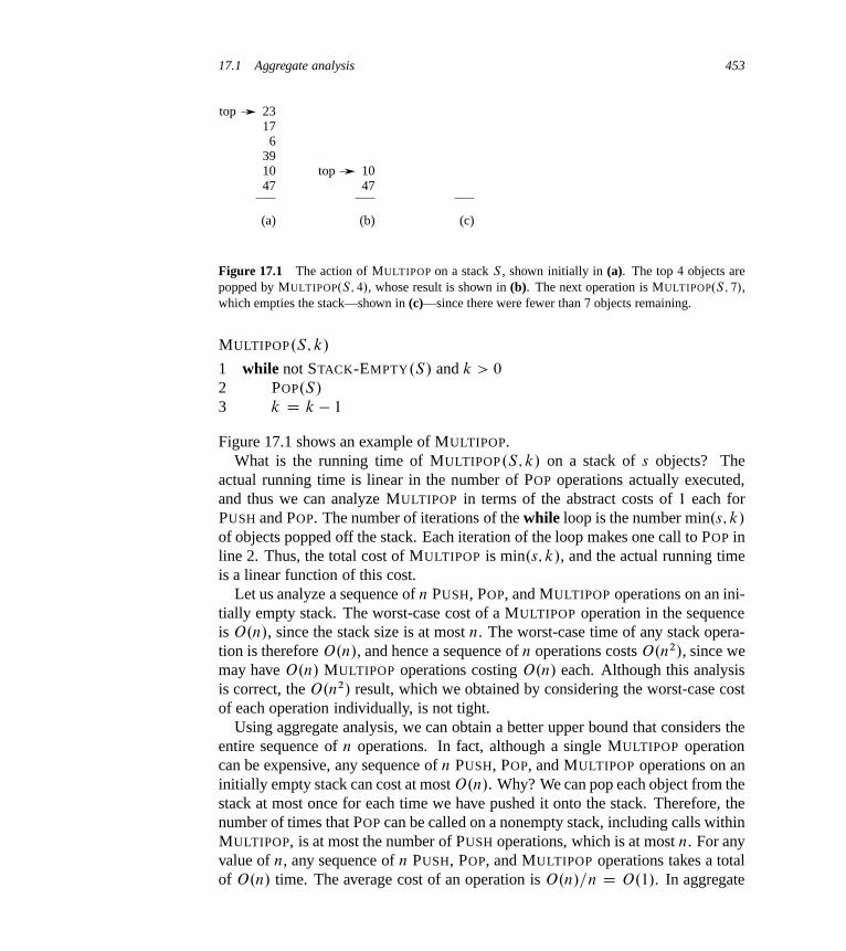
17.1 Aggregate analysis 453
23176
391047
(a)
top
1047
(b)
top
(c)
Figure 17.1 The action of MULTIPOP on a stack S , shown initially in (a). The top 4 objects arepopped by MULTIPOP.S; 4/, whose result is shown in (b). The next operation is MULTIPOP.S; 7/,which empties the stack—shown in (c)—since there were fewer than 7 objects remaining.
MULTIPOP.S; k/
1 while not STACK-EMPTY.S/ and k > 0
2 POP.S/
3 k D k � 1
Figure 17.1 shows an example of MULTIPOP.What is the running time of MULTIPOP.S; k/ on a stack of s objects? The
actual running time is linear in the number of POP operations actually executed,and thus we can analyze MULTIPOP in terms of the abstract costs of 1 each forPUSH and POP. The number of iterations of the while loop is the number min.s; k/
of objects popped off the stack. Each iteration of the loop makes one call to POP inline 2. Thus, the total cost of MULTIPOP is min.s; k/, and the actual running timeis a linear function of this cost.
Let us analyze a sequence of n PUSH, POP, and MULTIPOP operations on an ini-tially empty stack. The worst-case cost of a MULTIPOP operation in the sequenceis O.n/, since the stack size is at most n. The worst-case time of any stack opera-tion is therefore O.n/, and hence a sequence of n operations costs O.n2/, since wemay have O.n/ MULTIPOP operations costing O.n/ each. Although this analysisis correct, the O.n2/ result, which we obtained by considering the worst-case costof each operation individually, is not tight.
Using aggregate analysis, we can obtain a better upper bound that considers theentire sequence of n operations. In fact, although a single MULTIPOP operationcan be expensive, any sequence of n PUSH, POP, and MULTIPOP operations on aninitially empty stack can cost at most O.n/. Why? We can pop each object from thestack at most once for each time we have pushed it onto the stack. Therefore, thenumber of times that POP can be called on a nonempty stack, including calls withinMULTIPOP, is at most the number of PUSH operations, which is at most n. For anyvalue of n, any sequence of n PUSH, POP, and MULTIPOP operations takes a totalof O.n/ time. The average cost of an operation is O.n/=n D O.1/. In aggregate

454 Chapter 17 Amortized Analysis
analysis, we assign the amortized cost of each operation to be the average cost. Inthis example, therefore, all three stack operations have an amortized cost of O.1/.
We emphasize again that although we have just shown that the average cost, andhence the running time, of a stack operation is O.1/, we did not use probabilisticreasoning. We actually showed a worst-case bound of O.n/ on a sequence of n
operations. Dividing this total cost by n yielded the average cost per operation, orthe amortized cost.
Incrementing a binary counter
As another example of aggregate analysis, consider the problem of implementinga k-bit binary counter that counts upward from 0. We use an array AŒ0 : : k � 1� ofbits, where A: length D k, as the counter. A binary number x that is stored in thecounter has its lowest-order bit in AŒ0� and its highest-order bit in AŒk� 1�, so thatx DPk�1
iD0 AŒi� � 2i . Initially, x D 0, and thus AŒi� D 0 for i D 0; 1; : : : ; k � 1. Toadd 1 (modulo 2k) to the value in the counter, we use the following procedure.
INCREMENT.A/
1 i D 0
2 while i < A: length and AŒi� == 1
3 AŒi� D 0
4 i D i C 1
5 if i < A: length6 AŒi� D 1
Figure 17.2 shows what happens to a binary counter as we increment it 16 times,starting with the initial value 0 and ending with the value 16. At the start ofeach iteration of the while loop in lines 2–4, we wish to add a 1 into position i .If AŒi� D 1, then adding 1 flips the bit to 0 in position i and yields a carry of 1,to be added into position i C 1 on the next iteration of the loop. Otherwise, theloop ends, and then, if i < k, we know that AŒi� D 0, so that line 6 adds a 1 intoposition i , flipping the 0 to a 1. The cost of each INCREMENT operation is linearin the number of bits flipped.
As with the stack example, a cursory analysis yields a bound that is correct butnot tight. A single execution of INCREMENT takes time ‚.k/ in the worst case, inwhich array A contains all 1s. Thus, a sequence of n INCREMENT operations onan initially zero counter takes time O.nk/ in the worst case.
We can tighten our analysis to yield a worst-case cost of O.n/ for a sequence of n
INCREMENT operations by observing that not all bits flip each time INCREMENT
is called. As Figure 17.2 shows, AŒ0� does flip each time INCREMENT is called.The next bit up, AŒ1�, flips only every other time: a sequence of n INCREMENT

17.1 Aggregate analysis 455
0 0 0 0 0 0 0 000 0 0 0 0 0 0 110 0 0 0 0 0 1 020 0 0 0 0 0 1 130 0 0 0 0 1 0 040 0 0 0 0 1 0 150 0 0 0 0 1 1 060 0 0 0 0 1 1 170 0 0 0 1 0 0 080 0 0 0 1 0 0 190 0 0 0 1 0 1 0100 0 0 0 1 0 1 1110 0 0 0 1 1 0 0120 0 0 0 1 1 0 1130 0 0 0 1 1 1 0140 0 0 0 1 1 1 1150 0 0 1 0 0 0 016
A[0]
A[1]
A[2]
A[3]
A[4]
A[5]
A[6]
A[7]Counter
valueTotalcost
13478
1011151618192223252631
0
Figure 17.2 An 8-bit binary counter as its value goes from 0 to 16 by a sequence of 16 INCREMENT
operations. Bits that flip to achieve the next value are shaded. The running cost for flipping bits isshown at the right. Notice that the total cost is always less than twice the total number of INCREMENT
operations.
operations on an initially zero counter causes AŒ1� to flip bn=2c times. Similarly,bit AŒ2� flips only every fourth time, or bn=4c times in a sequence of n INCREMENT
operations. In general, for i D 0; 1; : : : ; k � 1, bit AŒi� flips bn=2ic times in asequence of n INCREMENT operations on an initially zero counter. For i � k,bit AŒi� does not exist, and so it cannot flip. The total number of flips in thesequence is thus
k�1XiD0
j n
2i
k< n
1XiD0
1
2i
D 2n ;
by equation (A.6). The worst-case time for a sequence of n INCREMENT operationson an initially zero counter is therefore O.n/. The average cost of each operation,and therefore the amortized cost per operation, is O.n/=n D O.1/.
456 Chapter 17 Amortized Analysis
Exercises
17.1-1If the set of stack operations included a MULTIPUSH operation, which pushes k
items onto the stack, would the O.1/ bound on the amortized cost of stack opera-tions continue to hold?
17.1-2Show that if a DECREMENT operation were included in the k-bit counter example,n operations could cost as much as ‚.nk/ time.
17.1-3Suppose we perform a sequence of n operations on a data structure in which the i thoperation costs i if i is an exact power of 2, and 1 otherwise. Use aggregate analysisto determine the amortized cost per operation.
17.2 The accounting method
In the accounting method of amortized analysis, we assign differing charges todifferent operations, with some operations charged more or less than they actu-ally cost. We call the amount we charge an operation its amortized cost. Whenan operation’s amortized cost exceeds its actual cost, we assign the difference tospecific objects in the data structure as credit. Credit can help pay for later oper-ations whose amortized cost is less than their actual cost. Thus, we can view theamortized cost of an operation as being split between its actual cost and credit thatis either deposited or used up. Different operations may have different amortizedcosts. This method differs from aggregate analysis, in which all operations havethe same amortized cost.
We must choose the amortized costs of operations carefully. If we want to showthat in the worst case the average cost per operation is small by analyzing withamortized costs, we must ensure that the total amortized cost of a sequence of oper-ations provides an upper bound on the total actual cost of the sequence. Moreover,as in aggregate analysis, this relationship must hold for all sequences of opera-tions. If we denote the actual cost of the i th operation by ci and the amortized costof the i th operation by yci , we require
nXiD1
yci �nX
iD1
ci (17.1)
for all sequences of n operations. The total credit stored in the data structureis the difference between the total amortized cost and the total actual cost, or
17.2 The accounting method 457
Pn
iD1 yci �Pn
iD1 ci . By inequality (17.1), the total credit associated with the datastructure must be nonnegative at all times. If we ever were to allow the total creditto become negative (the result of undercharging early operations with the promiseof repaying the account later on), then the total amortized costs incurred at thattime would be below the total actual costs incurred; for the sequence of operationsup to that time, the total amortized cost would not be an upper bound on the totalactual cost. Thus, we must take care that the total credit in the data structure neverbecomes negative.
Stack operations
To illustrate the accounting method of amortized analysis, let us return to the stackexample. Recall that the actual costs of the operations were
PUSH 1 ,POP 1 ,MULTIPOP min.k; s/ ,
where k is the argument supplied to MULTIPOP and s is the stack size when it iscalled. Let us assign the following amortized costs:
PUSH 2 ,POP 0 ,MULTIPOP 0 .
Note that the amortized cost of MULTIPOP is a constant (0), whereas the actual costis variable. Here, all three amortized costs are constant. In general, the amortizedcosts of the operations under consideration may differ from each other, and theymay even differ asymptotically.
We shall now show that we can pay for any sequence of stack operations bycharging the amortized costs. Suppose we use a dollar bill to represent each unitof cost. We start with an empty stack. Recall the analogy of Section 10.1 betweenthe stack data structure and a stack of plates in a cafeteria. When we push a plateon the stack, we use 1 dollar to pay the actual cost of the push and are left with acredit of 1 dollar (out of the 2 dollars charged), which we leave on top of the plate.At any point in time, every plate on the stack has a dollar of credit on it.
The dollar stored on the plate serves as prepayment for the cost of popping itfrom the stack. When we execute a POP operation, we charge the operation nothingand pay its actual cost using the credit stored in the stack. To pop a plate, we takethe dollar of credit off the plate and use it to pay the actual cost of the operation.Thus, by charging the PUSH operation a little bit more, we can charge the POP
operation nothing.
458 Chapter 17 Amortized Analysis
Moreover, we can also charge MULTIPOP operations nothing. To pop the firstplate, we take the dollar of credit off the plate and use it to pay the actual cost of aPOP operation. To pop a second plate, we again have a dollar of credit on the plateto pay for the POP operation, and so on. Thus, we have always charged enoughup front to pay for MULTIPOP operations. In other words, since each plate on thestack has 1 dollar of credit on it, and the stack always has a nonnegative number ofplates, we have ensured that the amount of credit is always nonnegative. Thus, forany sequence of n PUSH, POP, and MULTIPOP operations, the total amortized costis an upper bound on the total actual cost. Since the total amortized cost is O.n/,so is the total actual cost.
Incrementing a binary counter
As another illustration of the accounting method, we analyze the INCREMENT op-eration on a binary counter that starts at zero. As we observed earlier, the runningtime of this operation is proportional to the number of bits flipped, which we shalluse as our cost for this example. Let us once again use a dollar bill to representeach unit of cost (the flipping of a bit in this example).
For the amortized analysis, let us charge an amortized cost of 2 dollars to set abit to 1. When a bit is set, we use 1 dollar (out of the 2 dollars charged) to payfor the actual setting of the bit, and we place the other dollar on the bit as credit tobe used later when we flip the bit back to 0. At any point in time, every 1 in thecounter has a dollar of credit on it, and thus we can charge nothing to reset a bitto 0; we just pay for the reset with the dollar bill on the bit.
Now we can determine the amortized cost of INCREMENT. The cost of resettingthe bits within the while loop is paid for by the dollars on the bits that are reset. TheINCREMENT procedure sets at most one bit, in line 6, and therefore the amortizedcost of an INCREMENT operation is at most 2 dollars. The number of 1s in thecounter never becomes negative, and thus the amount of credit stays nonnegativeat all times. Thus, for n INCREMENT operations, the total amortized cost is O.n/,which bounds the total actual cost.
Exercises
17.2-1Suppose we perform a sequence of stack operations on a stack whose size neverexceeds k. After every k operations, we make a copy of the entire stack for backuppurposes. Show that the cost of n stack operations, including copying the stack,is O.n/ by assigning suitable amortized costs to the various stack operations.
17.3 The potential method 459
17.2-2Redo Exercise 17.1-3 using an accounting method of analysis.
17.2-3Suppose we wish not only to increment a counter but also to reset it to zero (i.e.,make all bits in it 0). Counting the time to examine or modify a bit as ‚.1/,show how to implement a counter as an array of bits so that any sequence of n
INCREMENT and RESET operations takes time O.n/ on an initially zero counter.(Hint: Keep a pointer to the high-order 1.)
17.3 The potential method
Instead of representing prepaid work as credit stored with specific objects in thedata structure, the potential method of amortized analysis represents the prepaidwork as “potential energy,” or just “potential,” which can be released to pay forfuture operations. We associate the potential with the data structure as a wholerather than with specific objects within the data structure.
The potential method works as follows. We will perform n operations, startingwith an initial data structure D0. For each i D 1; 2; : : : ; n, we let ci be the actualcost of the i th operation and Di be the data structure that results after applyingthe i th operation to data structure Di�1. A potential function ˆ maps each datastructure Di to a real number ˆ.Di /, which is the potential associated with datastructure Di . The amortized cost yci of the i th operation with respect to potentialfunction ˆ is defined by
yci D ci Cˆ.Di / �ˆ.Di�1/ : (17.2)
The amortized cost of each operation is therefore its actual cost plus the change inpotential due to the operation. By equation (17.2), the total amortized cost of the n
operations is
nXiD1
yci DnX
iD1
.ci Cˆ.Di / �ˆ.Di�1//
DnX
iD1
ci Cˆ.Dn/ �ˆ.D0/ : (17.3)
The second equality follows from equation (A.9) because the ˆ.Di / terms tele-scope.
If we can define a potential function ˆ so that ˆ.Dn/ � ˆ.D0/, then the totalamortized cost
Pn
iD1 yci gives an upper bound on the total actual costPn
iD1 ci .

460 Chapter 17 Amortized Analysis
In practice, we do not always know how many operations might be performed.Therefore, if we require that ˆ.Di / � ˆ.D0/ for all i , then we guarantee, as inthe accounting method, that we pay in advance. We usually just define ˆ.D0/ tobe 0 and then show that ˆ.Di / � 0 for all i . (See Exercise 17.3-1 for an easy wayto handle cases in which ˆ.D0/ ¤ 0.)
Intuitively, if the potential difference ˆ.Di/ � ˆ.Di�1/ of the i th operation ispositive, then the amortized cost yci represents an overcharge to the i th operation,and the potential of the data structure increases. If the potential difference is neg-ative, then the amortized cost represents an undercharge to the i th operation, andthe decrease in the potential pays for the actual cost of the operation.
The amortized costs defined by equations (17.2) and (17.3) depend on the choiceof the potential function ˆ. Different potential functions may yield different amor-tized costs yet still be upper bounds on the actual costs. We often find trade-offsthat we can make in choosing a potential function; the best potential function touse depends on the desired time bounds.
Stack operations
To illustrate the potential method, we return once again to the example of the stackoperations PUSH, POP, and MULTIPOP. We define the potential function ˆ on astack to be the number of objects in the stack. For the empty stack D0 with whichwe start, we have ˆ.D0/ D 0. Since the number of objects in the stack is nevernegative, the stack Di that results after the i th operation has nonnegative potential,and thus
ˆ.Di / � 0
D ˆ.D0/ :
The total amortized cost of n operations with respect to ˆ therefore represents anupper bound on the actual cost.
Let us now compute the amortized costs of the various stack operations. If the i thoperation on a stack containing s objects is a PUSH operation, then the potentialdifference is
ˆ.Di / �ˆ.Di�1/ D .s C 1/ � s
D 1 :
By equation (17.2), the amortized cost of this PUSH operation is
yci D ci Cˆ.Di / �ˆ.Di�1/
D 1C 1
D 2 :

17.3 The potential method 461
Suppose that the i th operation on the stack is MULTIPOP.S; k/, which causesk0 D min.k; s/ objects to be popped off the stack. The actual cost of the opera-tion is k0, and the potential difference is
ˆ.Di / �ˆ.Di�1/ D �k0 :
Thus, the amortized cost of the MULTIPOP operation is
yci D ci Cˆ.Di / �ˆ.Di�1/
D k0 � k0
D 0 :
Similarly, the amortized cost of an ordinary POP operation is 0.The amortized cost of each of the three operations is O.1/, and thus the total
amortized cost of a sequence of n operations is O.n/. Since we have already arguedthat ˆ.Di / � ˆ.D0/, the total amortized cost of n operations is an upper boundon the total actual cost. The worst-case cost of n operations is therefore O.n/.
Incrementing a binary counter
As another example of the potential method, we again look at incrementing a binarycounter. This time, we define the potential of the counter after the i th INCREMENT
operation to be bi , the number of 1s in the counter after the i th operation.Let us compute the amortized cost of an INCREMENT operation. Suppose that
the i th INCREMENT operation resets ti bits. The actual cost of the operation istherefore at most ti C 1, since in addition to resetting ti bits, it sets at most onebit to 1. If bi D 0, then the i th operation resets all k bits, and so bi�1 D ti D k.If bi > 0, then bi D bi�1 � ti C 1. In either case, bi � bi�1 � ti C 1, and thepotential difference is
ˆ.Di / �ˆ.Di�1/ � .bi�1 � ti C 1/ � bi�1
D 1� ti :
The amortized cost is therefore
yci D ci Cˆ.Di / �ˆ.Di�1/
� .ti C 1/C .1 � ti /
D 2 :
If the counter starts at zero, then ˆ.D0/ D 0. Since ˆ.Di/ � 0 for all i , the totalamortized cost of a sequence of n INCREMENT operations is an upper bound on thetotal actual cost, and so the worst-case cost of n INCREMENT operations is O.n/.
The potential method gives us an easy way to analyze the counter even whenit does not start at zero. The counter starts with b0 1s, and after n INCREMENT
462 Chapter 17 Amortized Analysis
operations it has bn 1s, where 0 � b0; bn � k. (Recall that k is the number of bitsin the counter.) We can rewrite equation (17.3) as
nXiD1
ci DnX
iD1
yci �ˆ.Dn/Cˆ.D0/ : (17.4)
We have yci � 2 for all 1 � i � n. Since ˆ.D0/ D b0 and ˆ.Dn/ D bn, the totalactual cost of n INCREMENT operations is
nXiD1
ci �nX
iD1
2 � bn C b0
D 2n � bn C b0 :
Note in particular that since b0 � k, as long as k D O.n/, the total actual costis O.n/. In other words, if we execute at least n D �.k/ INCREMENT operations,the total actual cost is O.n/, no matter what initial value the counter contains.
Exercises
17.3-1Suppose we have a potential function ˆ such that ˆ.Di / � ˆ.D0/ for all i , butˆ.D0/ ¤ 0. Show that there exists a potential function ˆ0 such that ˆ0.D0/ D 0,ˆ0.Di / � 0 for all i � 1, and the amortized costs using ˆ0 are the same as theamortized costs using ˆ.
17.3-2Redo Exercise 17.1-3 using a potential method of analysis.
17.3-3Consider an ordinary binary min-heap data structure with n elements supportingthe instructions INSERT and EXTRACT-MIN in O.lg n/ worst-case time. Give apotential function ˆ such that the amortized cost of INSERT is O.lg n/ and theamortized cost of EXTRACT-MIN is O.1/, and show that it works.
17.3-4What is the total cost of executing n of the stack operations PUSH, POP, andMULTIPOP, assuming that the stack begins with s0 objects and finishes with sn
objects?
17.3-5Suppose that a counter begins at a number with b 1s in its binary representa-tion, rather than at 0. Show that the cost of performing n INCREMENT operationsis O.n/ if n D �.b/. (Do not assume that b is constant.)
17.4 Dynamic tables 463
17.3-6Show how to implement a queue with two ordinary stacks (Exercise 10.1-6) so thatthe amortized cost of each ENQUEUE and each DEQUEUE operation is O.1/.
17.3-7Design a data structure to support the following two operations for a dynamicmultiset S of integers, which allows duplicate values:
INSERT.S; x/ inserts x into S .
DELETE-LARGER-HALF.S/ deletes the largest djS j =2e elements from S .
Explain how to implement this data structure so that any sequence of m INSERT
and DELETE-LARGER-HALF operations runs in O.m/ time. Your implementationshould also include a way to output the elements of S in O.jS j/ time.
17.4 Dynamic tables
We do not always know in advance how many objects some applications will storein a table. We might allocate space for a table, only to find out later that it is notenough. We must then reallocate the table with a larger size and copy all objectsstored in the original table over into the new, larger table. Similarly, if many objectshave been deleted from the table, it may be worthwhile to reallocate the table witha smaller size. In this section, we study this problem of dynamically expanding andcontracting a table. Using amortized analysis, we shall show that the amortized costof insertion and deletion is only O.1/, even though the actual cost of an operationis large when it triggers an expansion or a contraction. Moreover, we shall see howto guarantee that the unused space in a dynamic table never exceeds a constantfraction of the total space.
We assume that the dynamic table supports the operations TABLE-INSERT andTABLE-DELETE. TABLE-INSERT inserts into the table an item that occupies a sin-gle slot, that is, a space for one item. Likewise, TABLE-DELETE removes an itemfrom the table, thereby freeing a slot. The details of the data-structuring methodused to organize the table are unimportant; we might use a stack (Section 10.1),a heap (Chapter 6), or a hash table (Chapter 11). We might also use an array orcollection of arrays to implement object storage, as we did in Section 10.3.
We shall find it convenient to use a concept introduced in our analysis of hashing(Chapter 11). We define the load factor ˛.T / of a nonempty table T to be thenumber of items stored in the table divided by the size (number of slots) of thetable. We assign an empty table (one with no items) size 0, and we define its loadfactor to be 1. If the load factor of a dynamic table is bounded below by a constant,

464 Chapter 17 Amortized Analysis
the unused space in the table is never more than a constant fraction of the totalamount of space.
We start by analyzing a dynamic table in which we only insert items. We thenconsider the more general case in which we both insert and delete items.
17.4.1 Table expansion
Let us assume that storage for a table is allocated as an array of slots. A table fillsup when all slots have been used or, equivalently, when its load factor is 1.1 In somesoftware environments, upon attempting to insert an item into a full table, the onlyalternative is to abort with an error. We shall assume, however, that our softwareenvironment, like many modern ones, provides a memory-management system thatcan allocate and free blocks of storage on request. Thus, upon inserting an iteminto a full table, we can expand the table by allocating a new table with more slotsthan the old table had. Because we always need the table to reside in contiguousmemory, we must allocate a new array for the larger table and then copy items fromthe old table into the new table.
A common heuristic allocates a new table with twice as many slots as the oldone. If the only table operations are insertions, then the load factor of the table isalways at least 1=2, and thus the amount of wasted space never exceeds half thetotal space in the table.
In the following pseudocode, we assume that T is an object representing thetable. The attribute T: table contains a pointer to the block of storage representingthe table, T:num contains the number of items in the table, and T:size gives the totalnumber of slots in the table. Initially, the table is empty: T:num D T:size D 0.
TABLE-INSERT.T; x/
1 if T:size == 0
2 allocate T: table with 1 slot3 T:size D 1
4 if T:num == T:size5 allocate new-table with 2 � T:size slots6 insert all items in T: table into new-table7 free T: table8 T: table D new-table9 T:size D 2 � T:size
10 insert x into T: table11 T:num D T:numC 1
1In some situations, such as an open-address hash table, we may wish to consider a table to be full ifits load factor equals some constant strictly less than 1. (See Exercise 17.4-1.)
17.4 Dynamic tables 465
Notice that we have two “insertion” procedures here: the TABLE-INSERT proce-dure itself and the elementary insertion into a table in lines 6 and 10. We cananalyze the running time of TABLE-INSERT in terms of the number of elementaryinsertions by assigning a cost of 1 to each elementary insertion. We assume thatthe actual running time of TABLE-INSERT is linear in the time to insert individualitems, so that the overhead for allocating an initial table in line 2 is constant andthe overhead for allocating and freeing storage in lines 5 and 7 is dominated bythe cost of transferring items in line 6. We call the event in which lines 5–9 areexecuted an expansion.
Let us analyze a sequence of n TABLE-INSERT operations on an initially emptytable. What is the cost ci of the i th operation? If the current table has room for thenew item (or if this is the first operation), then ci D 1, since we need only performthe one elementary insertion in line 10. If the current table is full, however, and anexpansion occurs, then ci D i : the cost is 1 for the elementary insertion in line 10plus i � 1 for the items that we must copy from the old table to the new table inline 6. If we perform n operations, the worst-case cost of an operation is O.n/,which leads to an upper bound of O.n2/ on the total running time for n operations.
This bound is not tight, because we rarely expand the table in the course of n
TABLE-INSERT operations. Specifically, the i th operation causes an expansiononly when i � 1 is an exact power of 2. The amortized cost of an operation is infact O.1/, as we can show using aggregate analysis. The cost of the i th operationis
ci D(
i if i � 1 is an exact power of 2 ;
1 otherwise :
The total cost of n TABLE-INSERT operations is thereforenX
iD1
ci � nCblg ncXj D0
2j
< nC 2n
D 3n ;
because at most n operations cost 1 and the costs of the remaining operations forma geometric series. Since the total cost of n TABLE-INSERT operations is boundedby 3n, the amortized cost of a single operation is at most 3.
By using the accounting method, we can gain some feeling for why the amor-tized cost of a TABLE-INSERT operation should be 3. Intuitively, each item paysfor 3 elementary insertions: inserting itself into the current table, moving itselfwhen the table expands, and moving another item that has already been movedonce when the table expands. For example, suppose that the size of the table is m
immediately after an expansion. Then the table holds m=2 items, and it contains
466 Chapter 17 Amortized Analysis
no credit. We charge 3 dollars for each insertion. The elementary insertion thatoccurs immediately costs 1 dollar. We place another dollar as credit on the iteminserted. We place the third dollar as credit on one of the m=2 items already in thetable. The table will not fill again until we have inserted another m=2 � 1 items,and thus, by the time the table contains m items and is full, we will have placed adollar on each item to pay to reinsert it during the expansion.
We can use the potential method to analyze a sequence of n TABLE-INSERT
operations, and we shall use it in Section 17.4.2 to design a TABLE-DELETE op-eration that has an O.1/ amortized cost as well. We start by defining a potentialfunction ˆ that is 0 immediately after an expansion but builds to the table size bythe time the table is full, so that we can pay for the next expansion by the potential.The function
ˆ.T / D 2 � T:num � T:size (17.5)
is one possibility. Immediately after an expansion, we have T:num D T:size=2,and thus ˆ.T / D 0, as desired. Immediately before an expansion, we haveT:num D T:size, and thus ˆ.T / D T:num, as desired. The initial value of thepotential is 0, and since the table is always at least half full, T:num � T:size=2,which implies that ˆ.T / is always nonnegative. Thus, the sum of the amortizedcosts of n TABLE-INSERT operations gives an upper bound on the sum of the actualcosts.
To analyze the amortized cost of the i th TABLE-INSERT operation, we let numi
denote the number of items stored in the table after the i th operation, sizei denotethe total size of the table after the i th operation, and ˆi denote the potential afterthe i th operation. Initially, we have num0 D 0, size0 D 0, and ˆ0 D 0.
If the i th TABLE-INSERT operation does not trigger an expansion, then we havesizei D sizei�1 and the amortized cost of the operation is
yci D ci Cˆi �ˆi�1
D 1C .2 � numi � sizei / � .2 � numi�1 � sizei�1/
D 1C .2 � numi � sizei / � .2.numi � 1/ � sizei /
D 3 :
If the i th operation does trigger an expansion, then we have sizei D 2 � sizei�1 andsizei�1 D numi�1 D numi � 1, which implies that sizei D 2 � .numi � 1/. Thus,the amortized cost of the operation is
yci D ci Cˆi �ˆi�1
D numi C .2 � numi � sizei/ � .2 � numi�1 � sizei�1/
D numi C .2 � numi � 2 � .numi � 1// � .2.numi � 1/ � .numi � 1//
D numi C 2 � .numi � 1/
D 3 :

17.4 Dynamic tables 467
Φi
numisizei
0 8 16 24 320
8
16
24
32
i
Figure 17.3 The effect of a sequence of n TABLE-INSERT operations on the number numi of itemsin the table, the number sizei of slots in the table, and the potential ˆi D 2 � numi � sizei , eachbeing measured after the i th operation. The thin line shows numi , the dashed line shows sizei , andthe thick line shows ˆi . Notice that immediately before an expansion, the potential has built up tothe number of items in the table, and therefore it can pay for moving all the items to the new table.Afterwards, the potential drops to 0, but it is immediately increased by 2 upon inserting the item thatcaused the expansion.
Figure 17.3 plots the values of numi , sizei , and ˆi against i . Notice how thepotential builds to pay for expanding the table.
17.4.2 Table expansion and contraction
To implement a TABLE-DELETE operation, it is simple enough to remove the spec-ified item from the table. In order to limit the amount of wasted space, however,we might wish to contract the table when the load factor becomes too small. Tablecontraction is analogous to table expansion: when the number of items in the tabledrops too low, we allocate a new, smaller table and then copy the items from theold table into the new one. We can then free the storage for the old table by return-ing it to the memory-management system. Ideally, we would like to preserve twoproperties:
� the load factor of the dynamic table is bounded below by a positive constant,and
� the amortized cost of a table operation is bounded above by a constant.
468 Chapter 17 Amortized Analysis
We assume that we measure the cost in terms of elementary insertions and dele-tions.
You might think that we should double the table size upon inserting an item intoa full table and halve the size when a deleting an item would cause the table tobecome less than half full. This strategy would guarantee that the load factor ofthe table never drops below 1=2, but unfortunately, it can cause the amortized costof an operation to be quite large. Consider the following scenario. We perform n
operations on a table T , where n is an exact power of 2. The first n=2 operations areinsertions, which by our previous analysis cost a total of ‚.n/. At the end of thissequence of insertions, T:num D T:size D n=2. For the second n=2 operations,we perform the following sequence:
insert, delete, delete, insert, insert, delete, delete, insert, insert, . . . .
The first insertion causes the table to expand to size n. The two following deletionscause the table to contract back to size n=2. Two further insertions cause anotherexpansion, and so forth. The cost of each expansion and contraction is ‚.n/, andthere are ‚.n/ of them. Thus, the total cost of the n operations is ‚.n2/, makingthe amortized cost of an operation ‚.n/.
The downside of this strategy is obvious: after expanding the table, we do notdelete enough items to pay for a contraction. Likewise, after contracting the table,we do not insert enough items to pay for an expansion.
We can improve upon this strategy by allowing the load factor of the table todrop below 1=2. Specifically, we continue to double the table size upon insertingan item into a full table, but we halve the table size when deleting an item causesthe table to become less than 1=4 full, rather than 1=2 full as before. The loadfactor of the table is therefore bounded below by the constant 1=4.
Intuitively, we would consider a load factor of 1=2 to be ideal, and the table’spotential would then be 0. As the load factor deviates from 1=2, the potentialincreases so that by the time we expand or contract the table, the table has garneredsufficient potential to pay for copying all the items into the newly allocated table.Thus, we will need a potential function that has grown to T:num by the time thatthe load factor has either increased to 1 or decreased to 1=4. After either expandingor contracting the table, the load factor goes back to 1=2 and the table’s potentialreduces back to 0.
We omit the code for TABLE-DELETE, since it is analogous to TABLE-INSERT.For our analysis, we shall assume that whenever the number of items in the tabledrops to 0, we free the storage for the table. That is, if T:num D 0, then T:size D 0.
We can now use the potential method to analyze the cost of a sequence of n
TABLE-INSERT and TABLE-DELETE operations. We start by defining a poten-tial function ˆ that is 0 immediately after an expansion or contraction and buildsas the load factor increases to 1 or decreases to 1=4. Let us denote the load fac-
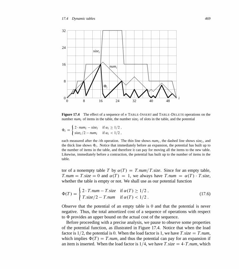
17.4 Dynamic tables 469
numi
Φi
sizei
0 8 16 24 32 40 480
8
16
24
32
i
Figure 17.4 The effect of a sequence of n TABLE-INSERT and TABLE-DELETE operations on thenumber numi of items in the table, the number sizei of slots in the table, and the potential
ˆi D�
2 � numi � sizei if ˛i � 1=2 ;
sizei =2 � numi if ˛i < 1=2 ;
each measured after the i th operation. The thin line shows numi , the dashed line shows sizei , andthe thick line shows ˆi . Notice that immediately before an expansion, the potential has built up tothe number of items in the table, and therefore it can pay for moving all the items to the new table.Likewise, immediately before a contraction, the potential has built up to the number of items in thetable.
tor of a nonempty table T by ˛.T / D T:num=T:size. Since for an empty table,T:num D T:size D 0 and ˛.T / D 1, we always have T:num D ˛.T / � T:size,whether the table is empty or not. We shall use as our potential function
ˆ.T / D(
2 � T:num � T:size if ˛.T / � 1=2 ;
T:size=2 � T:num if ˛.T / < 1=2 :(17.6)
Observe that the potential of an empty table is 0 and that the potential is nevernegative. Thus, the total amortized cost of a sequence of operations with respectto ˆ provides an upper bound on the actual cost of the sequence.
Before proceeding with a precise analysis, we pause to observe some propertiesof the potential function, as illustrated in Figure 17.4. Notice that when the loadfactor is 1=2, the potential is 0. When the load factor is 1, we have T:size D T:num,which implies ˆ.T / D T:num, and thus the potential can pay for an expansion ifan item is inserted. When the load factor is 1=4, we have T:size D 4 �T:num, which

470 Chapter 17 Amortized Analysis
implies ˆ.T / D T:num, and thus the potential can pay for a contraction if an itemis deleted.
To analyze a sequence of n TABLE-INSERT and TABLE-DELETE operations,we let ci denote the actual cost of the i th operation, yci denote its amortized costwith respect to ˆ, numi denote the number of items stored in the table after the i thoperation, sizei denote the total size of the table after the i th operation, ˛i denotethe load factor of the table after the i th operation, and ˆi denote the potential afterthe i th operation. Initially, num0 D 0, size0 D 0, ˛0 D 1, and ˆ0 D 0.
We start with the case in which the i th operation is TABLE-INSERT. The analy-sis is identical to that for table expansion in Section 17.4.1 if ˛i�1 � 1=2. Whetherthe table expands or not, the amortized cost yci of the operation is at most 3.If ˛i�1 < 1=2, the table cannot expand as a result of the operation, since the ta-ble expands only when ˛i�1 D 1. If ˛i < 1=2 as well, then the amortized cost ofthe i th operation is
yci D ci Cˆi �ˆi�1
D 1C .sizei=2 � numi/ � .sizei�1=2 � numi�1/
D 1C .sizei=2 � numi/ � .sizei=2 � .numi � 1//
D 0 :
If ˛i�1 < 1=2 but ˛i � 1=2, then
yci D ci Cˆi �ˆi�1
D 1C .2 � numi � sizei / � .sizei�1=2 � numi�1/
D 1C .2.numi�1 C 1/ � sizei�1/ � .sizei�1=2 � numi�1/
D 3 � numi�1 � 3
2sizei�1 C 3
D 3˛i�1sizei�1 � 3
2sizei�1 C 3
<3
2sizei�1 �
3
2sizei�1 C 3
D 3 :
Thus, the amortized cost of a TABLE-INSERT operation is at most 3.We now turn to the case in which the i th operation is TABLE-DELETE. In this
case, numi D numi�1 � 1. If ˛i�1 < 1=2, then we must consider whether theoperation causes the table to contract. If it does not, then sizei D sizei�1 and theamortized cost of the operation is
yci D ci Cˆi �ˆi�1
D 1C .sizei=2 � numi/ � .sizei�1=2 � numi�1/
D 1C .sizei=2 � numi/ � .sizei=2 � .numi C 1//
D 2 :

17.4 Dynamic tables 471
If ˛i�1 < 1=2 and the i th operation does trigger a contraction, then the actual costof the operation is ci D numi C 1, since we delete one item and move numi items.We have sizei=2 D sizei�1=4 D numi�1 D numi C 1, and the amortized cost ofthe operation is
yci D ci Cˆi �ˆi�1
D .numi C 1/C .sizei=2 � numi/ � .sizei�1=2 � numi�1/
D .numi C 1/C ..numi C 1/ � numi/ � ..2 � numi C 2/ � .numi C 1//
D 1 :
When the i th operation is a TABLE-DELETE and ˛i�1 � 1=2, the amortized costis also bounded above by a constant. We leave the analysis as Exercise 17.4-2.
In summary, since the amortized cost of each operation is bounded above bya constant, the actual time for any sequence of n operations on a dynamic tableis O.n/.
Exercises
17.4-1Suppose that we wish to implement a dynamic, open-address hash table. Whymight we consider the table to be full when its load factor reaches some value ˛
that is strictly less than 1? Describe briefly how to make insertion into a dynamic,open-address hash table run in such a way that the expected value of the amortizedcost per insertion is O.1/. Why is the expected value of the actual cost per insertionnot necessarily O.1/ for all insertions?
17.4-2Show that if ˛i�1 � 1=2 and the i th operation on a dynamic table is TABLE-DELETE, then the amortized cost of the operation with respect to the potentialfunction (17.6) is bounded above by a constant.
17.4-3Suppose that instead of contracting a table by halving its size when its load factordrops below 1=4, we contract it by multiplying its size by 2=3 when its load factordrops below 1=3. Using the potential function
ˆ.T / D j2 � T:num � T:sizej ;
show that the amortized cost of a TABLE-DELETE that uses this strategy is boundedabove by a constant.

472 Chapter 17 Amortized Analysis
Problems
17-1 Bit-reversed binary counterChapter 30 examines an important algorithm called the fast Fourier transform,or FFT. The first step of the FFT algorithm performs a bit-reversal permutation onan input array AŒ0 : : n�1� whose length is n D 2k for some nonnegative integer k.This permutation swaps elements whose indices have binary representations thatare the reverse of each other.
We can express each index a as a k-bit sequence hak�1; ak�2; : : : ; a0i, wherea DPk�1
iD0 ai 2i . We define
revk.hak�1; ak�2; : : : ; a0i/ D ha0; a1; : : : ; ak�1i Ithus,
revk.a/ Dk�1XiD0
ak�i�12i :
For example, if n D 16 (or, equivalently, k D 4), then revk.3/ D 12, sincethe 4-bit representation of 3 is 0011, which when reversed gives 1100, the 4-bitrepresentation of 12.
a. Given a function revk that runs in ‚.k/ time, write an algorithm to perform thebit-reversal permutation on an array of length n D 2k in O.nk/ time.
We can use an algorithm based on an amortized analysis to improve the runningtime of the bit-reversal permutation. We maintain a “bit-reversed counter” and aprocedure BIT-REVERSED-INCREMENT that, when given a bit-reversed-countervalue a, produces revk.revk.a/C 1/. If k D 4, for example, and the bit-reversedcounter starts at 0, then successive calls to BIT-REVERSED-INCREMENT producethe sequence
0000; 1000; 0100; 1100; 0010; 1010; : : : D 0; 8; 4; 12; 2; 10; : : : :
b. Assume that the words in your computer store k-bit values and that in unit time,your computer can manipulate the binary values with operations such as shiftingleft or right by arbitrary amounts, bitwise-AND, bitwise-OR, etc. Describean implementation of the BIT-REVERSED-INCREMENT procedure that allowsthe bit-reversal permutation on an n-element array to be performed in a totalof O.n/ time.
c. Suppose that you can shift a word left or right by only one bit in unit time. Is itstill possible to implement an O.n/-time bit-reversal permutation?
Problems for Chapter 17 473
17-2 Making binary search dynamicBinary search of a sorted array takes logarithmic search time, but the time to inserta new element is linear in the size of the array. We can improve the time forinsertion by keeping several sorted arrays.
Specifically, suppose that we wish to support SEARCH and INSERT on a setof n elements. Let k D dlg.nC 1/e, and let the binary representation of n
be hnk�1; nk�2; : : : ; n0i. We have k sorted arrays A0; A1; : : : ; Ak�1, where fori D 0; 1; : : : ; k � 1, the length of array Ai is 2i . Each array is either full or empty,depending on whether ni D 1 or ni D 0, respectively. The total number of ele-ments held in all k arrays is therefore
Pk�1
iD0 ni 2i D n. Although each individualarray is sorted, elements in different arrays bear no particular relationship to eachother.
a. Describe how to perform the SEARCH operation for this data structure. Analyzeits worst-case running time.
b. Describe how to perform the INSERT operation. Analyze its worst-case andamortized running times.
c. Discuss how to implement DELETE.
17-3 Amortized weight-balanced treesConsider an ordinary binary search tree augmented by adding to each node x theattribute x:size giving the number of keys stored in the subtree rooted at x. Let ˛
be a constant in the range 1=2 � ˛ < 1. We say that a given node x is ˛-balancedif x: left:size � ˛ � x:size and x:right:size � ˛ � x:size. The tree as a wholeis ˛-balanced if every node in the tree is ˛-balanced. The following amortizedapproach to maintaining weight-balanced trees was suggested by G. Varghese.
a. A 1=2-balanced tree is, in a sense, as balanced as it can be. Given a node x
in an arbitrary binary search tree, show how to rebuild the subtree rooted at x
so that it becomes 1=2-balanced. Your algorithm should run in time ‚.x:size/,and it can use O.x:size/ auxiliary storage.
b. Show that performing a search in an n-node ˛-balanced binary search treetakes O.lg n/ worst-case time.
For the remainder of this problem, assume that the constant ˛ is strictly greaterthan 1=2. Suppose that we implement INSERT and DELETE as usual for an n-nodebinary search tree, except that after every such operation, if any node in the treeis no longer ˛-balanced, then we “rebuild” the subtree rooted at the highest suchnode in the tree so that it becomes 1=2-balanced.
474 Chapter 17 Amortized Analysis
We shall analyze this rebuilding scheme using the potential method. For a node x
in a binary search tree T , we define
�.x/ D jx: left:size � x:right:sizej ;
and we define the potential of T as
ˆ.T / D cX
x2T W�.x/�2
�.x/ ;
where c is a sufficiently large constant that depends on ˛.
c. Argue that any binary search tree has nonnegative potential and that a 1=2-balanced tree has potential 0.
d. Suppose that m units of potential can pay for rebuilding an m-node subtree.How large must c be in terms of ˛ in order for it to take O.1/ amortized timeto rebuild a subtree that is not ˛-balanced?
e. Show that inserting a node into or deleting a node from an n-node ˛-balancedtree costs O.lg n/ amortized time.
17-4 The cost of restructuring red-black treesThere are four basic operations on red-black trees that perform structural modi-fications: node insertions, node deletions, rotations, and color changes. We haveseen that RB-INSERT and RB-DELETE use only O.1/ rotations, node insertions,and node deletions to maintain the red-black properties, but they may make manymore color changes.
a. Describe a legal red-black tree with n nodes such that calling RB-INSERT toadd the .n C 1/st node causes �.lg n/ color changes. Then describe a legalred-black tree with n nodes for which calling RB-DELETE on a particular nodecauses �.lg n/ color changes.
Although the worst-case number of color changes per operation can be logarithmic,we shall prove that any sequence of m RB-INSERT and RB-DELETE operations onan initially empty red-black tree causes O.m/ structural modifications in the worstcase. Note that we count each color change as a structural modification.
b. Some of the cases handled by the main loop of the code of both RB-INSERT-FIXUP and RB-DELETE-FIXUP are terminating: once encountered, they causethe loop to terminate after a constant number of additional operations. For eachof the cases of RB-INSERT-FIXUP and RB-DELETE-FIXUP, specify which areterminating and which are not. (Hint: Look at Figures 13.5, 13.6, and 13.7.)
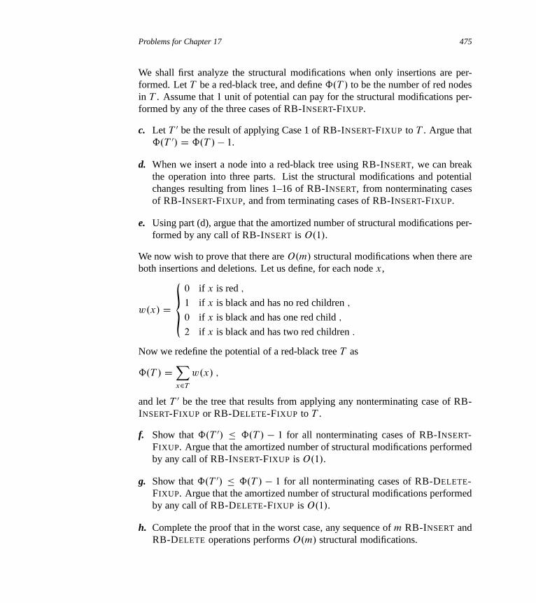
Problems for Chapter 17 475
We shall first analyze the structural modifications when only insertions are per-formed. Let T be a red-black tree, and define ˆ.T / to be the number of red nodesin T . Assume that 1 unit of potential can pay for the structural modifications per-formed by any of the three cases of RB-INSERT-FIXUP.
c. Let T 0 be the result of applying Case 1 of RB-INSERT-FIXUP to T . Argue thatˆ.T 0/ D ˆ.T / � 1.
d. When we insert a node into a red-black tree using RB-INSERT, we can breakthe operation into three parts. List the structural modifications and potentialchanges resulting from lines 1–16 of RB-INSERT, from nonterminating casesof RB-INSERT-FIXUP, and from terminating cases of RB-INSERT-FIXUP.
e. Using part (d), argue that the amortized number of structural modifications per-formed by any call of RB-INSERT is O.1/.
We now wish to prove that there are O.m/ structural modifications when there areboth insertions and deletions. Let us define, for each node x,
w.x/ D
„0 if x is red ;
1 if x is black and has no red children ;
0 if x is black and has one red child ;
2 if x is black and has two red children :
Now we redefine the potential of a red-black tree T as
ˆ.T / DXx2T
w.x/ ;
and let T 0 be the tree that results from applying any nonterminating case of RB-INSERT-FIXUP or RB-DELETE-FIXUP to T .
f. Show that ˆ.T 0/ � ˆ.T / � 1 for all nonterminating cases of RB-INSERT-FIXUP. Argue that the amortized number of structural modifications performedby any call of RB-INSERT-FIXUP is O.1/.
g. Show that ˆ.T 0/ � ˆ.T / � 1 for all nonterminating cases of RB-DELETE-FIXUP. Argue that the amortized number of structural modifications performedby any call of RB-DELETE-FIXUP is O.1/.
h. Complete the proof that in the worst case, any sequence of m RB-INSERT andRB-DELETE operations performs O.m/ structural modifications.

476 Chapter 17 Amortized Analysis
17-5 Competitive analysis of self-organizing lists with move-to-frontA self-organizing list is a linked list of n elements, in which each element has aunique key. When we search for an element in the list, we are given a key, and wewant to find an element with that key.
A self-organizing list has two important properties:
1. To find an element in the list, given its key, we must traverse the list from thebeginning until we encounter the element with the given key. If that element isthe kth element from the start of the list, then the cost to find the element is k.
2. We may reorder the list elements after any operation, according to a given rulewith a given cost. We may choose any heuristic we like to decide how to reorderthe list.
Assume that we start with a given list of n elements, and we are given an accesssequence D h1; 2; : : : ; mi of keys to find, in order. The cost of the sequenceis the sum of the costs of the individual accesses in the sequence.
Out of the various possible ways to reorder the list after an operation, this prob-lem focuses on transposing adjacent list elements—switching their positions in thelist—with a unit cost for each transpose operation. You will show, by means of apotential function, that a particular heuristic for reordering the list, move-to-front,entails a total cost no worse than 4 times that of any other heuristic for maintainingthe list order—even if the other heuristic knows the access sequence in advance!We call this type of analysis a competitive analysis.
For a heuristic H and a given initial ordering of the list, denote the access cost ofsequence by CH ./. Let m be the number of accesses in .
a. Argue that if heuristic H does not know the access sequence in advance, thenthe worst-case cost for H on an access sequence is CH ./ D �.mn/.
With the move-to-front heuristic, immediately after searching for an element x,we move x to the first position on the list (i.e., the front of the list).
Let rankL.x/ denote the rank of element x in list L, that is, the position of x inlist L. For example, if x is the fourth element in L, then rankL.x/ D 4. Let ci
denote the cost of access i using the move-to-front heuristic, which includes thecost of finding the element in the list and the cost of moving it to the front of thelist by a series of transpositions of adjacent list elements.
b. Show that if i accesses element x in list L using the move-to-front heuristic,then ci D 2 � rankL.x/� 1.
Now we compare move-to-front with any other heuristic H that processes anaccess sequence according to the two properties above. Heuristic H may transpose
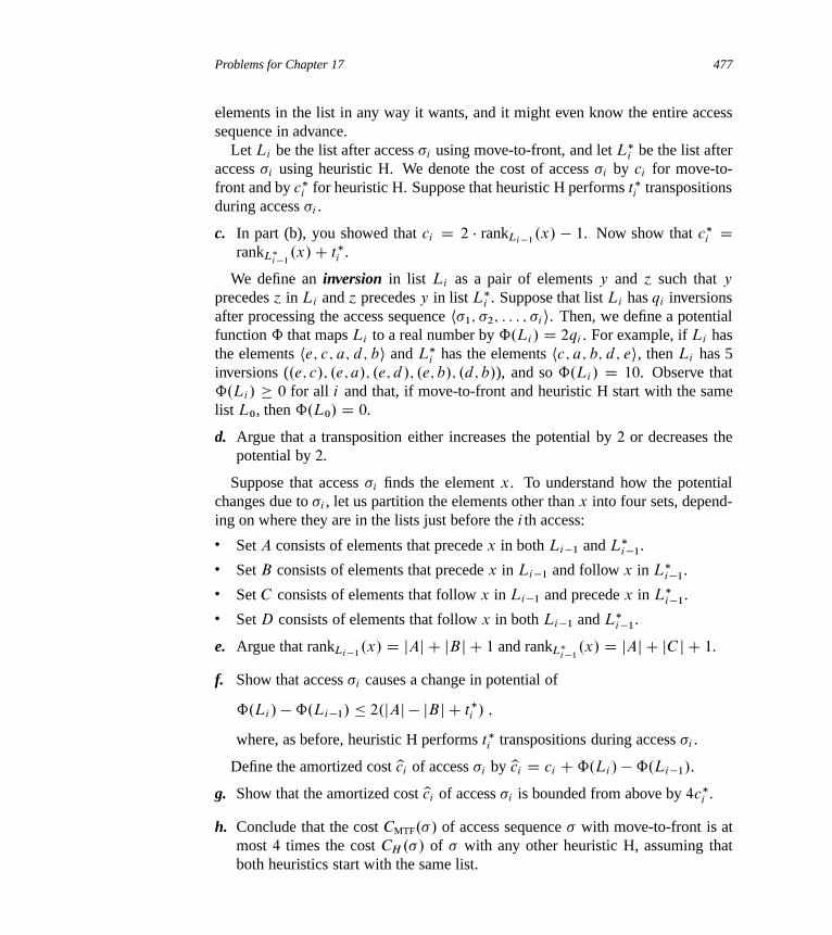
Problems for Chapter 17 477
elements in the list in any way it wants, and it might even know the entire accesssequence in advance.
Let Li be the list after access i using move-to-front, and let L�i be the list after
access i using heuristic H. We denote the cost of access i by ci for move-to-front and by c�
i for heuristic H. Suppose that heuristic H performs t�i transpositions
during access i .
c. In part (b), you showed that ci D 2 � rankLi�1.x/ � 1. Now show that c�
i DrankL�
i�1.x/C t�
i .
We define an inversion in list Li as a pair of elements y and ´ such that y
precedes ´ in Li and ´ precedes y in list L�i . Suppose that list Li has qi inversions
after processing the access sequence h1; 2; : : : ; ii. Then, we define a potentialfunction ˆ that maps Li to a real number by ˆ.Li / D 2qi . For example, if Li hasthe elements he; c; a; d; bi and L�
i has the elements hc; a; b; d; ei, then Li has 5inversions (.e; c/; .e; a/; .e; d/; .e; b/; .d; b/), and so ˆ.Li / D 10. Observe thatˆ.Li / � 0 for all i and that, if move-to-front and heuristic H start with the samelist L0, then ˆ.L0/ D 0.
d. Argue that a transposition either increases the potential by 2 or decreases thepotential by 2.
Suppose that access i finds the element x. To understand how the potentialchanges due to i , let us partition the elements other than x into four sets, depend-ing on where they are in the lists just before the i th access:� Set A consists of elements that precede x in both Li�1 and L�
i�1.� Set B consists of elements that precede x in Li�1 and follow x in L�
i�1.� Set C consists of elements that follow x in Li�1 and precede x in L�
i�1.� Set D consists of elements that follow x in both Li�1 and L�
i�1.
e. Argue that rankLi�1.x/ D jAj C jBj C 1 and rankL�
i�1.x/ D jAj C jC j C 1.
f. Show that access i causes a change in potential of
ˆ.Li / �ˆ.Li�1/ � 2.jAj � jBj C t�i / ;
where, as before, heuristic H performs t�i transpositions during access i .
Define the amortized cost yci of access i by yci D ci Cˆ.Li / �ˆ.Li�1/.
g. Show that the amortized cost yci of access i is bounded from above by 4c�i .
h. Conclude that the cost CMTF./ of access sequence with move-to-front is atmost 4 times the cost CH ./ of with any other heuristic H, assuming thatboth heuristics start with the same list.

478 Chapter 17 Amortized Analysis
Chapter notes
Aho, Hopcroft, and Ullman [5] used aggregate analysis to determine the runningtime of operations on a disjoint-set forest; we shall analyze this data structure us-ing the potential method in Chapter 21. Tarjan [331] surveys the accounting andpotential methods of amortized analysis and presents several applications. He at-tributes the accounting method to several authors, including M. R. Brown, R. E.Tarjan, S. Huddleston, and K. Mehlhorn. He attributes the potential method toD. D. Sleator. The term “amortized” is due to D. D. Sleator and R. E. Tarjan.
Potential functions are also useful for proving lower bounds for certain types ofproblems. For each configuration of the problem, we define a potential functionthat maps the configuration to a real number. Then we determine the potential ˆinit
of the initial configuration, the potential ˆfinal of the final configuration, and themaximum change in potential �ˆmax due to any step. The number of steps musttherefore be at least jˆfinal �ˆinitj = j�ˆmaxj. Examples of potential functions toprove lower bounds in I/O complexity appear in works by Cormen, Sundquist, andWisniewski [80]; Floyd [107]; and Aggarwal and Vitter [4]. Krumme, Cybenko,and Venkataraman [221] applied potential functions to prove lower bounds on gos-siping: communicating a unique item from each vertex in a graph to every othervertex.
The move-to-front heuristic from Problem 17-5 works quite well in practice.Moreover, if we recognize that when we find an element, we can splice it out of itsposition in the list and relocate it to the front of the list in constant time, we canshow that the cost of move-to-front is at most twice the cost of any other heuristicincluding, again, one that knows the entire access sequence in advance.

V Advanced Data Structures
Introduction
This part returns to studying data structures that support operations on dynamicsets, but at a more advanced level than Part III. Two of the chapters, for example,make extensive use of the amortized analysis techniques we saw in Chapter 17.
Chapter 18 presents B-trees, which are balanced search trees specifically de-signed to be stored on disks. Because disks operate much more slowly thanrandom-access memory, we measure the performance of B-trees not only by howmuch computing time the dynamic-set operations consume but also by how manydisk accesses they perform. For each B-tree operation, the number of disk accessesincreases with the height of the B-tree, but B-tree operations keep the height low.
Chapter 19 gives an implementation of a mergeable heap, which supports theoperations INSERT, MINIMUM, EXTRACT-MIN, and UNION.1 The UNION oper-ation unites, or merges, two heaps. Fibonacci heaps—the data structure in Chap-ter 19—also support the operations DELETE and DECREASE-KEY. We use amor-tized time bounds to measure the performance of Fibonacci heaps. The opera-tions INSERT, MINIMUM, and UNION take only O.1/ actual and amortized timeon Fibonacci heaps, and the operations EXTRACT-MIN and DELETE take O.lg n/
amortized time. The most significant advantage of Fibonacci heaps, however, isthat DECREASE-KEY takes only O.1/ amortized time. Because the DECREASE-
1As in Problem 10-2, we have defined a mergeable heap to support MINIMUM and EXTRACT-MIN,and so we can also refer to it as a mergeable min-heap. Alternatively, if it supported MAXIMUM
and EXTRACT-MAX, it would be a mergeable max-heap. Unless we specify otherwise, mergeableheaps will be by default mergeable min-heaps.
482 Part V Advanced Data Structures
KEY operation takes constant amortized time, Fibonacci heaps are key componentsof some of the asymptotically fastest algorithms to date for graph problems.
Noting that we can beat the �.n lg n/ lower bound for sorting when the keysare integers in a restricted range, Chapter 20 asks whether we can design a datastructure that supports the dynamic-set operations SEARCH, INSERT, DELETE,MINIMUM, MAXIMUM, SUCCESSOR, and PREDECESSOR in o.lg n/ time whenthe keys are integers in a restricted range. The answer turns out to be that we can,by using a recursive data structure known as a van Emde Boas tree. If the keys areunique integers drawn from the set f0; 1; 2; : : : ; u � 1g, where u is an exact powerof 2, then van Emde Boas trees support each of the above operations in O.lg lg u/
time.Finally, Chapter 21 presents data structures for disjoint sets. We have a universe
of n elements that are partitioned into dynamic sets. Initially, each element belongsto its own singleton set. The operation UNION unites two sets, and the query FIND-SET identifies the unique set that contains a given element at the moment. Byrepresenting each set as a simple rooted tree, we obtain surprisingly fast operations:a sequence of m operations runs in O.m ˛.n// time, where ˛.n/ is an incrediblyslowly growing function—˛.n/ is at most 4 in any conceivable application. Theamortized analysis that proves this time bound is as complex as the data structureis simple.
The topics covered in this part are by no means the only examples of “advanced”data structures. Other advanced data structures include the following:
� Dynamic trees, introduced by Sleator and Tarjan [319] and discussed by Tarjan[330], maintain a forest of disjoint rooted trees. Each edge in each tree hasa real-valued cost. Dynamic trees support queries to find parents, roots, edgecosts, and the minimum edge cost on a simple path from a node up to a root.Trees may be manipulated by cutting edges, updating all edge costs on a simplepath from a node up to a root, linking a root into another tree, and making anode the root of the tree it appears in. One implementation of dynamic treesgives an O.lg n/ amortized time bound for each operation; a more complicatedimplementation yields O.lg n/ worst-case time bounds. Dynamic trees are usedin some of the asymptotically fastest network-flow algorithms.
� Splay trees, developed by Sleator and Tarjan [320] and, again, discussed byTarjan [330], are a form of binary search tree on which the standard search-tree operations run in O.lg n/ amortized time. One application of splay treessimplifies dynamic trees.
� Persistent data structures allow queries, and sometimes updates as well, on pastversions of a data structure. Driscoll, Sarnak, Sleator, and Tarjan [98] presenttechniques for making linked data structures persistent with only a small time

Part V Advanced Data Structures 483
and space cost. Problem 13-1 gives a simple example of a persistent dynamicset.
� As in Chapter 20, several data structures allow a faster implementation of dic-tionary operations (INSERT, DELETE, and SEARCH) for a restricted universeof keys. By taking advantage of these restrictions, they are able to achieve bet-ter worst-case asymptotic running times than comparison-based data structures.Fredman and Willard introduced fusion trees [115], which were the first datastructure to allow faster dictionary operations when the universe is restricted tointegers. They showed how to implement these operations in O.lg n= lg lg n/
time. Several subsequent data structures, including exponential search trees[16], have also given improved bounds on some or all of the dictionary opera-tions and are mentioned in the chapter notes throughout this book.
� Dynamic graph data structures support various queries while allowing thestructure of a graph to change through operations that insert or delete verticesor edges. Examples of the queries that they support include vertex connectivity[166], edge connectivity, minimum spanning trees [165], biconnectivity, andtransitive closure [164].
Chapter notes throughout this book mention additional data structures.

18 B-Trees
B-trees are balanced search trees designed to work well on disks or other direct-access secondary storage devices. B-trees are similar to red-black trees (Chap-ter 13), but they are better at minimizing disk I/O operations. Many database sys-tems use B-trees, or variants of B-trees, to store information.
B-trees differ from red-black trees in that B-tree nodes may have many children,from a few to thousands. That is, the “branching factor” of a B-tree can be quitelarge, although it usually depends on characteristics of the disk unit used. B-treesare similar to red-black trees in that every n-node B-tree has height O.lg n/. Theexact height of a B-tree can be considerably less than that of a red-black tree,however, because its branching factor, and hence the base of the logarithm thatexpresses its height, can be much larger. Therefore, we can also use B-trees toimplement many dynamic-set operations in time O.lg n/.
B-trees generalize binary search trees in a natural manner. Figure 18.1 shows asimple B-tree. If an internal B-tree node x contains x:n keys, then x has x:nC 1
children. The keys in node x serve as dividing points separating the range of keyshandled by x into x:n C 1 subranges, each handled by one child of x. Whensearching for a key in a B-tree, we make an .x:n C 1/-way decision based oncomparisons with the x:n keys stored at node x. The structure of leaf nodes differsfrom that of internal nodes; we will examine these differences in Section 18.1.
Section 18.1 gives a precise definition of B-trees and proves that the height ofa B-tree grows only logarithmically with the number of nodes it contains. Sec-tion 18.2 describes how to search for a key and insert a key into a B-tree, andSection 18.3 discusses deletion. Before proceeding, however, we need to ask whywe evaluate data structures designed to work on a disk differently from data struc-tures designed to work in main random-access memory.
Data structures on secondary storage
Computer systems take advantage of various technologies that provide memorycapacity. The primary memory (or main memory) of a computer system normally

Chapter 18 B-Trees 485
B C F G J K L
D H
N P R S V W Y Z
Q T X
M
T:root
Figure 18.1 A B-tree whose keys are the consonants of English. An internal node x containingx:n keys has x:nC 1 children. All leaves are at the same depth in the tree. The lightly shaded nodesare examined in a search for the letter R.
platter track
arms
read/writehead
spindle
Figure 18.2 A typical disk drive. It comprises one or more platters (two platters are shown here)that rotate around a spindle. Each platter is read and written with a head at the end of an arm. Armsrotate around a common pivot axis. A track is the surface that passes beneath the read/write headwhen the head is stationary.
consists of silicon memory chips. This technology is typically more than an orderof magnitude more expensive per bit stored than magnetic storage technology, suchas tapes or disks. Most computer systems also have secondary storage based onmagnetic disks; the amount of such secondary storage often exceeds the amount ofprimary memory by at least two orders of magnitude.
Figure 18.2 shows a typical disk drive. The drive consists of one or more plat-ters, which rotate at a constant speed around a common spindle. A magnetizablematerial covers the surface of each platter. The drive reads and writes each platterby a head at the end of an arm. The arms can move their heads toward or away
486 Chapter 18 B-Trees
from the spindle. When a given head is stationary, the surface that passes under-neath it is called a track. Multiple platters increase only the disk drive’s capacityand not its performance.
Although disks are cheaper and have higher capacity than main memory, they aremuch, much slower because they have moving mechanical parts.1 The mechanicalmotion has two components: platter rotation and arm movement. As of this writing,commodity disks rotate at speeds of 5400–15,000 revolutions per minute (RPM).We typically see 15,000 RPM speeds in server-grade drives, 7200 RPM speedsin drives for desktops, and 5400 RPM speeds in drives for laptops. Although7200 RPM may seem fast, one rotation takes 8.33 milliseconds, which is over 5orders of magnitude longer than the 50 nanosecond access times (more or less)commonly found for silicon memory. In other words, if we have to wait a full rota-tion for a particular item to come under the read/write head, we could access mainmemory more than 100,000 times during that span. On average we have to waitfor only half a rotation, but still, the difference in access times for silicon memorycompared with disks is enormous. Moving the arms also takes some time. As ofthis writing, average access times for commodity disks are in the range of 8 to 11milliseconds.
In order to amortize the time spent waiting for mechanical movements, disksaccess not just one item but several at a time. Information is divided into a numberof equal-sized pages of bits that appear consecutively within tracks, and each diskread or write is of one or more entire pages. For a typical disk, a page might be 211
to 214 bytes in length. Once the read/write head is positioned correctly and the diskhas rotated to the beginning of the desired page, reading or writing a magnetic diskis entirely electronic (aside from the rotation of the disk), and the disk can quicklyread or write large amounts of data.
Often, accessing a page of information and reading it from a disk takes longerthan examining all the information read. For this reason, in this chapter we shalllook separately at the two principal components of the running time:
� the number of disk accesses, and
� the CPU (computing) time.
We measure the number of disk accesses in terms of the number of pages of infor-mation that need to be read from or written to the disk. We note that disk-accesstime is not constant—it depends on the distance between the current track andthe desired track and also on the initial rotational position of the disk. We shall
1As of this writing, solid-state drives have recently come onto the consumer market. Although theyare faster than mechanical disk drives, they cost more per gigabyte and have lower capacities thanmechanical disk drives.
Chapter 18 B-Trees 487
nonetheless use the number of pages read or written as a first-order approximationof the total time spent accessing the disk.
In a typical B-tree application, the amount of data handled is so large that allthe data do not fit into main memory at once. The B-tree algorithms copy selectedpages from disk into main memory as needed and write back onto disk the pagesthat have changed. B-tree algorithms keep only a constant number of pages inmain memory at any time; thus, the size of main memory does not limit the size ofB-trees that can be handled.
We model disk operations in our pseudocode as follows. Let x be a pointer to anobject. If the object is currently in the computer’s main memory, then we can referto the attributes of the object as usual: x:key, for example. If the object referred toby x resides on disk, however, then we must perform the operation DISK-READ.x/
to read object x into main memory before we can refer to its attributes. (We as-sume that if x is already in main memory, then DISK-READ.x/ requires no diskaccesses; it is a “no-op.”) Similarly, the operation DISK-WRITE.x/ is used to saveany changes that have been made to the attributes of object x. That is, the typicalpattern for working with an object is as follows:
x D a pointer to some objectDISK-READ.x/
operations that access and/or modify the attributes of x
DISK-WRITE.x/ // omitted if no attributes of x were changedother operations that access but do not modify attributes of x
The system can keep only a limited number of pages in main memory at any onetime. We shall assume that the system flushes from main memory pages no longerin use; our B-tree algorithms will ignore this issue.
Since in most systems the running time of a B-tree algorithm depends primar-ily on the number of DISK-READ and DISK-WRITE operations it performs, wetypically want each of these operations to read or write as much information aspossible. Thus, a B-tree node is usually as large as a whole disk page, and this sizelimits the number of children a B-tree node can have.
For a large B-tree stored on a disk, we often see branching factors between 50
and 2000, depending on the size of a key relative to the size of a page. A largebranching factor dramatically reduces both the height of the tree and the number ofdisk accesses required to find any key. Figure 18.3 shows a B-tree with a branchingfactor of 1001 and height 2 that can store over one billion keys; nevertheless, sincewe can keep the root node permanently in main memory, we can find any key inthis tree by making at most only two disk accesses.
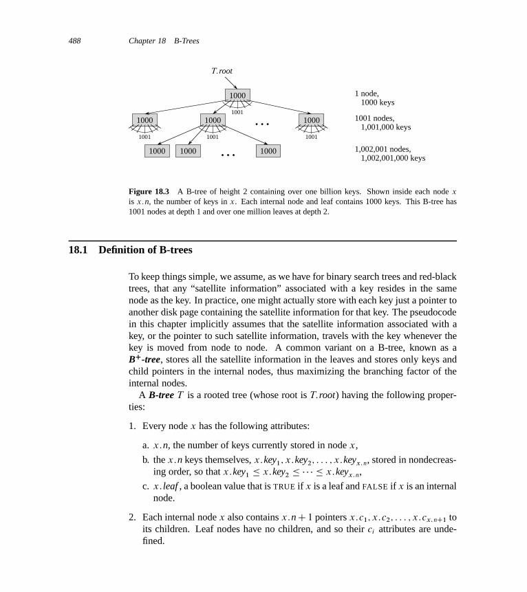
488 Chapter 18 B-Trees
1000
1001
1000
1001
1000
1001
1000
1001
100010001000
…
1 node, 1000 keys
1001 nodes, 1,001,000 keys
1,002,001 nodes, 1,002,001,000 keys
…
T:root
Figure 18.3 A B-tree of height 2 containing over one billion keys. Shown inside each node x
is x:n, the number of keys in x. Each internal node and leaf contains 1000 keys. This B-tree has1001 nodes at depth 1 and over one million leaves at depth 2.
18.1 Definition of B-trees
To keep things simple, we assume, as we have for binary search trees and red-blacktrees, that any “satellite information” associated with a key resides in the samenode as the key. In practice, one might actually store with each key just a pointer toanother disk page containing the satellite information for that key. The pseudocodein this chapter implicitly assumes that the satellite information associated with akey, or the pointer to such satellite information, travels with the key whenever thekey is moved from node to node. A common variant on a B-tree, known as aBC-tree, stores all the satellite information in the leaves and stores only keys andchild pointers in the internal nodes, thus maximizing the branching factor of theinternal nodes.
A B-tree T is a rooted tree (whose root is T:root) having the following proper-ties:
1. Every node x has the following attributes:
a. x:n, the number of keys currently stored in node x,
b. the x:n keys themselves, x:key1; x:key2; : : : ; x:keyx: n, stored in nondecreas-ing order, so that x:key1 � x:key2 � � � � � x:keyx: n,
c. x: leaf , a boolean value that is TRUE if x is a leaf and FALSE if x is an internalnode.
2. Each internal node x also contains x:nC 1 pointers x:c1; x:c2; : : : ; x:cx: nC1 toits children. Leaf nodes have no children, and so their ci attributes are unde-fined.
18.1 Definition of B-trees 489
3. The keys x:keyi separate the ranges of keys stored in each subtree: if ki is anykey stored in the subtree with root x:ci , then
k1 � x:key1 � k2 � x:key2 � � � � � x:keyx: n � kx: nC1 :
4. All leaves have the same depth, which is the tree’s height h.
5. Nodes have lower and upper bounds on the number of keys they can contain.We express these bounds in terms of a fixed integer t � 2 called the minimumdegree of the B-tree:
a. Every node other than the root must have at least t � 1 keys. Every internalnode other than the root thus has at least t children. If the tree is nonempty,the root must have at least one key.
b. Every node may contain at most 2t � 1 keys. Therefore, an internal nodemay have at most 2t children. We say that a node is full if it contains exactly2t � 1 keys.2
The simplest B-tree occurs when t D 2. Every internal node then has either 2,3, or 4 children, and we have a 2-3-4 tree. In practice, however, much larger valuesof t yield B-trees with smaller height.
The height of a B-tree
The number of disk accesses required for most operations on a B-tree is propor-tional to the height of the B-tree. We now analyze the worst-case height of a B-tree.
Theorem 18.1If n � 1, then for any n-key B-tree T of height h and minimum degree t � 2,
h � logt
nC 1
2:
Proof The root of a B-tree T contains at least one key, and all other nodes containat least t � 1 keys. Thus, T , whose height is h, has at least 2 nodes at depth 1, atleast 2t nodes at depth 2, at least 2t2 nodes at depth 3, and so on, until at depth h
it has at least 2th�1 nodes. Figure 18.4 illustrates such a tree for h D 3. Thus, the
2Another common variant on a B-tree, known as a B�-tree, requires each internal node to be atleast 2=3 full, rather than at least half full, as a B-tree requires.
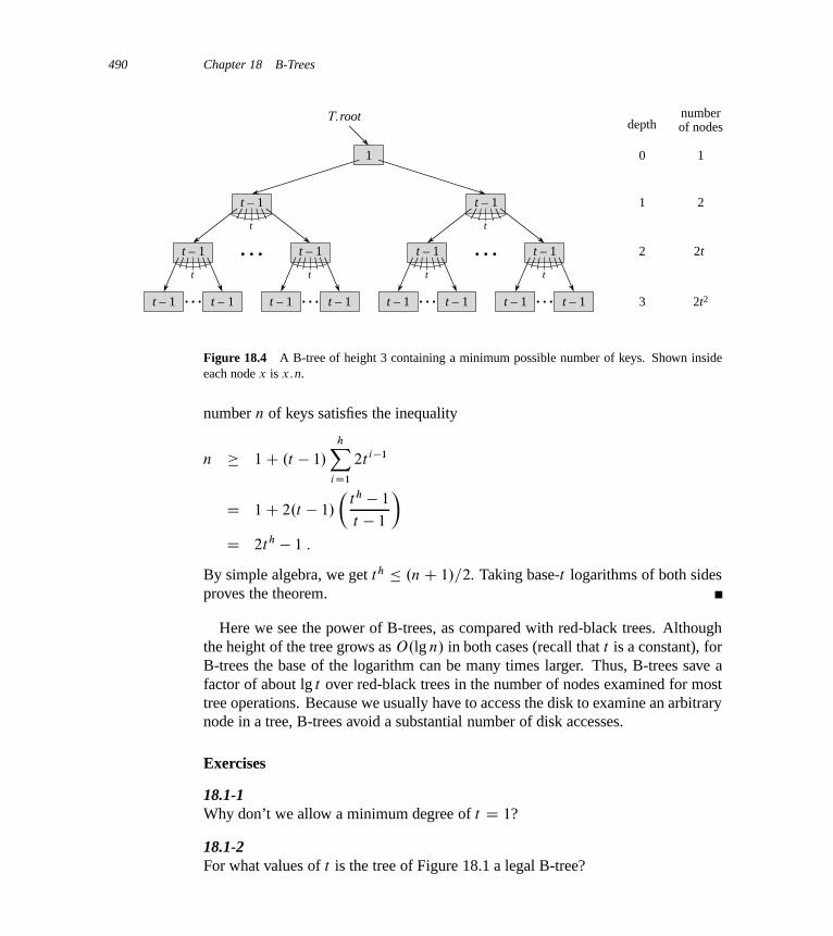
490 Chapter 18 B-Trees
t – 1
t – 1 t – 1…t
t – 1
t
…
1
t – 1
t – 1 t – 1…t
t – 1
t – 1 t – 1…t
t – 1
t
… t – 1
t – 1 t – 1…t
depthnumberof nodes
3 2t2
1
2
0 1
2
2t
T:root
Figure 18.4 A B-tree of height 3 containing a minimum possible number of keys. Shown insideeach node x is x:n.
number n of keys satisfies the inequality
n � 1C .t � 1/
hXiD1
2t i�1
D 1C 2.t � 1/
�th � 1
t � 1
�D 2th � 1 :
By simple algebra, we get th � .nC 1/=2. Taking base-t logarithms of both sidesproves the theorem.
Here we see the power of B-trees, as compared with red-black trees. Althoughthe height of the tree grows as O.lg n/ in both cases (recall that t is a constant), forB-trees the base of the logarithm can be many times larger. Thus, B-trees save afactor of about lg t over red-black trees in the number of nodes examined for mosttree operations. Because we usually have to access the disk to examine an arbitrarynode in a tree, B-trees avoid a substantial number of disk accesses.
Exercises
18.1-1Why don’t we allow a minimum degree of t D 1?
18.1-2For what values of t is the tree of Figure 18.1 a legal B-tree?

18.2 Basic operations on B-trees 491
18.1-3Show all legal B-trees of minimum degree 2 that represent f1; 2; 3; 4; 5g.18.1-4As a function of the minimum degree t , what is the maximum number of keys thatcan be stored in a B-tree of height h?
18.1-5Describe the data structure that would result if each black node in a red-black treewere to absorb its red children, incorporating their children with its own.
18.2 Basic operations on B-trees
In this section, we present the details of the operations B-TREE-SEARCH, B-TREE-CREATE, and B-TREE-INSERT. In these procedures, we adopt two con-ventions:
� The root of the B-tree is always in main memory, so that we never need toperform a DISK-READ on the root; we do have to perform a DISK-WRITE ofthe root, however, whenever the root node is changed.
� Any nodes that are passed as parameters must already have had a DISK-READ
operation performed on them.
The procedures we present are all “one-pass” algorithms that proceed downwardfrom the root of the tree, without having to back up.
Searching a B-tree
Searching a B-tree is much like searching a binary search tree, except that insteadof making a binary, or “two-way,” branching decision at each node, we make amultiway branching decision according to the number of the node’s children. Moreprecisely, at each internal node x, we make an .x:nC 1/-way branching decision.
B-TREE-SEARCH is a straightforward generalization of the TREE-SEARCH pro-cedure defined for binary search trees. B-TREE-SEARCH takes as input a pointerto the root node x of a subtree and a key k to be searched for in that subtree. Thetop-level call is thus of the form B-TREE-SEARCH.T:root; k/. If k is in the B-tree,B-TREE-SEARCH returns the ordered pair .y; i/ consisting of a node y and anindex i such that y:keyi D k. Otherwise, the procedure returns NIL.

492 Chapter 18 B-Trees
B-TREE-SEARCH.x; k/
1 i D 1
2 while i � x:n and k > x:keyi
3 i D i C 1
4 if i � x:n and k == x:keyi
5 return .x; i/
6 elseif x: leaf7 return NIL
8 else DISK-READ.x:ci/
9 return B-TREE-SEARCH.x:ci ; k/
Using a linear-search procedure, lines 1–3 find the smallest index i such thatk � x:keyi , or else they set i to x:n C 1. Lines 4–5 check to see whether wehave now discovered the key, returning if we have. Otherwise, lines 6–9 either ter-minate the search unsuccessfully (if x is a leaf) or recurse to search the appropriatesubtree of x, after performing the necessary DISK-READ on that child.
Figure 18.1 illustrates the operation of B-TREE-SEARCH. The procedure exam-ines the lightly shaded nodes during a search for the key R.
As in the TREE-SEARCH procedure for binary search trees, the nodes encoun-tered during the recursion form a simple path downward from the root of thetree. The B-TREE-SEARCH procedure therefore accesses O.h/ D O.logt n/ diskpages, where h is the height of the B-tree and n is the number of keys in the B-tree.Since x:n < 2t , the while loop of lines 2–3 takes O.t/ time within each node, andthe total CPU time is O.th/ D O.t logt n/.
Creating an empty B-tree
To build a B-tree T , we first use B-TREE-CREATE to create an empty root nodeand then call B-TREE-INSERT to add new keys. Both of these procedures use anauxiliary procedure ALLOCATE-NODE, which allocates one disk page to be usedas a new node in O.1/ time. We can assume that a node created by ALLOCATE-NODE requires no DISK-READ, since there is as yet no useful information storedon the disk for that node.
B-TREE-CREATE.T /
1 x D ALLOCATE-NODE./
2 x: leaf D TRUE
3 x:n D 0
4 DISK-WRITE.x/
5 T:root D x
B-TREE-CREATE requires O.1/ disk operations and O.1/ CPU time.
18.2 Basic operations on B-trees 493
Inserting a key into a B-tree
Inserting a key into a B-tree is significantly more complicated than inserting a keyinto a binary search tree. As with binary search trees, we search for the leaf positionat which to insert the new key. With a B-tree, however, we cannot simply createa new leaf node and insert it, as the resulting tree would fail to be a valid B-tree.Instead, we insert the new key into an existing leaf node. Since we cannot insert akey into a leaf node that is full, we introduce an operation that splits a full node y
(having 2t�1 keys) around its median key y:keyt into two nodes having only t�1
keys each. The median key moves up into y’s parent to identify the dividing pointbetween the two new trees. But if y’s parent is also full, we must split it before wecan insert the new key, and thus we could end up splitting full nodes all the way upthe tree.
As with a binary search tree, we can insert a key into a B-tree in a single passdown the tree from the root to a leaf. To do so, we do not wait to find out whetherwe will actually need to split a full node in order to do the insertion. Instead, as wetravel down the tree searching for the position where the new key belongs, we spliteach full node we come to along the way (including the leaf itself). Thus wheneverwe want to split a full node y, we are assured that its parent is not full.
Splitting a node in a B-treeThe procedure B-TREE-SPLIT-CHILD takes as input a nonfull internal node x (as-sumed to be in main memory) and an index i such that x:ci (also assumed to be inmain memory) is a full child of x. The procedure then splits this child in two andadjusts x so that it has an additional child. To split a full root, we will first make theroot a child of a new empty root node, so that we can use B-TREE-SPLIT-CHILD.The tree thus grows in height by one; splitting is the only means by which the treegrows.
Figure 18.5 illustrates this process. We split the full node y D x:ci about itsmedian key S , which moves up into y’s parent node x. Those keys in y that aregreater than the median key move into a new node ´, which becomes a new childof x.
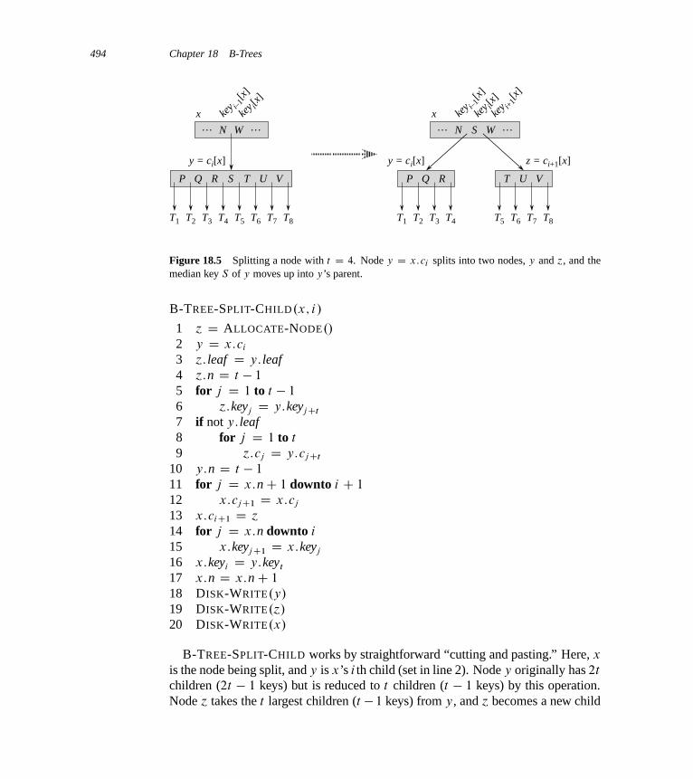
494 Chapter 18 B-Trees
T8T7T6T5T4T3T2T1T8T7T6T5T4T3T2T1
y = ci[x]
key i+
1[x]
key i[
x]
key i[
x]
key i–1
[x]
key i–1
[x]
R S TQP U V
N W
x… …
RQP T U V
N W
x
S
y = ci[x] z = ci+1[x]
… …
Figure 18.5 Splitting a node with t D 4. Node y D x:ci splits into two nodes, y and ´, and themedian key S of y moves up into y’s parent.
B-TREE-SPLIT-CHILD.x; i/
1 ´ D ALLOCATE-NODE./
2 y D x:ci
3 ´: leaf D y: leaf4 ´:n D t � 1
5 for j D 1 to t � 1
6 ´:keyj D y:keyj Ct
7 if not y: leaf8 for j D 1 to t
9 ´:cj D y:cj Ct
10 y:n D t � 1
11 for j D x:nC 1 downto i C 1
12 x:cj C1 D x:cj
13 x:ciC1 D ´
14 for j D x:n downto i
15 x:keyj C1 D x:keyj
16 x:keyi D y:keyt
17 x:n D x:nC 1
18 DISK-WRITE.y/
19 DISK-WRITE.´/
20 DISK-WRITE.x/
B-TREE-SPLIT-CHILD works by straightforward “cutting and pasting.” Here, x
is the node being split, and y is x’s i th child (set in line 2). Node y originally has 2t
children (2t � 1 keys) but is reduced to t children (t � 1 keys) by this operation.Node ´ takes the t largest children (t � 1 keys) from y, and ´ becomes a new child
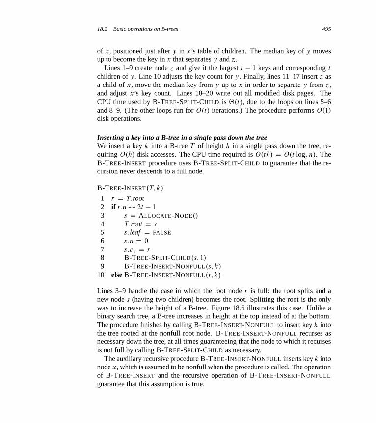
18.2 Basic operations on B-trees 495
of x, positioned just after y in x’s table of children. The median key of y movesup to become the key in x that separates y and ´.
Lines 1–9 create node ´ and give it the largest t � 1 keys and corresponding t
children of y. Line 10 adjusts the key count for y. Finally, lines 11–17 insert ´ asa child of x, move the median key from y up to x in order to separate y from ´,and adjust x’s key count. Lines 18–20 write out all modified disk pages. TheCPU time used by B-TREE-SPLIT-CHILD is ‚.t/, due to the loops on lines 5–6and 8–9. (The other loops run for O.t/ iterations.) The procedure performs O.1/
disk operations.
Inserting a key into a B-tree in a single pass down the treeWe insert a key k into a B-tree T of height h in a single pass down the tree, re-quiring O.h/ disk accesses. The CPU time required is O.th/ D O.t logt n/. TheB-TREE-INSERT procedure uses B-TREE-SPLIT-CHILD to guarantee that the re-cursion never descends to a full node.
B-TREE-INSERT.T; k/
1 r D T:root2 if r:n == 2t � 1
3 s D ALLOCATE-NODE./
4 T:root D s
5 s: leaf D FALSE
6 s:n D 0
7 s:c1 D r
8 B-TREE-SPLIT-CHILD.s; 1/
9 B-TREE-INSERT-NONFULL.s; k/
10 else B-TREE-INSERT-NONFULL.r; k/
Lines 3–9 handle the case in which the root node r is full: the root splits and anew node s (having two children) becomes the root. Splitting the root is the onlyway to increase the height of a B-tree. Figure 18.6 illustrates this case. Unlike abinary search tree, a B-tree increases in height at the top instead of at the bottom.The procedure finishes by calling B-TREE-INSERT-NONFULL to insert key k intothe tree rooted at the nonfull root node. B-TREE-INSERT-NONFULL recurses asnecessary down the tree, at all times guaranteeing that the node to which it recursesis not full by calling B-TREE-SPLIT-CHILD as necessary.
The auxiliary recursive procedure B-TREE-INSERT-NONFULL inserts key k intonode x, which is assumed to be nonfull when the procedure is called. The operationof B-TREE-INSERT and the recursive operation of B-TREE-INSERT-NONFULL
guarantee that this assumption is true.
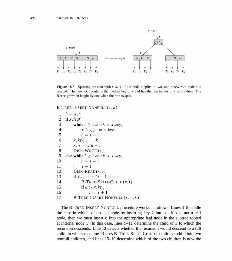
496 Chapter 18 B-Trees
T8T7T6T5T4T3T2T1T8T7T6T5T4T3T2T1
F H LDA N P FDA L N P
s
H
r r
T:root
T:root
Figure 18.6 Splitting the root with t D 4. Root node r splits in two, and a new root node s iscreated. The new root contains the median key of r and has the two halves of r as children. TheB-tree grows in height by one when the root is split.
B-TREE-INSERT-NONFULL.x; k/
1 i D x:n2 if x: leaf3 while i � 1 and k < x:keyi
4 x:keyiC1 D x:keyi
5 i D i � 1
6 x:keyiC1 D k
7 x:n D x:nC 1
8 DISK-WRITE.x/
9 else while i � 1 and k < x:keyi
10 i D i � 1
11 i D i C 1
12 DISK-READ.x:ci/
13 if x:ci :n == 2t � 1
14 B-TREE-SPLIT-CHILD.x; i/
15 if k > x:keyi
16 i D i C 1
17 B-TREE-INSERT-NONFULL.x:ci ; k/
The B-TREE-INSERT-NONFULL procedure works as follows. Lines 3–8 handlethe case in which x is a leaf node by inserting key k into x. If x is not a leafnode, then we must insert k into the appropriate leaf node in the subtree rootedat internal node x. In this case, lines 9–11 determine the child of x to which therecursion descends. Line 13 detects whether the recursion would descend to a fullchild, in which case line 14 uses B-TREE-SPLIT-CHILD to split that child into twononfull children, and lines 15–16 determine which of the two children is now the

18.2 Basic operations on B-trees 497
correct one to descend to. (Note that there is no need for a DISK-READ.x:ci/ afterline 16 increments i , since the recursion will descend in this case to a child thatwas just created by B-TREE-SPLIT-CHILD.) The net effect of lines 13–16 is thusto guarantee that the procedure never recurses to a full node. Line 17 then recursesto insert k into the appropriate subtree. Figure 18.7 illustrates the various cases ofinserting into a B-tree.
For a B-tree of height h, B-TREE-INSERT performs O.h/ disk accesses, sinceonly O.1/ DISK-READ and DISK-WRITE operations occur between calls toB-TREE-INSERT-NONFULL. The total CPU time used is O.th/ D O.t logt n/.Since B-TREE-INSERT-NONFULL is tail-recursive, we can alternatively imple-ment it as a while loop, thereby demonstrating that the number of pages that needto be in main memory at any time is O.1/.
Exercises
18.2-1Show the results of inserting the keys
F; S; Q; K; C; L; H; T; V; W; M; R; N; P; A; B; X; Y; D; Z; E
in order into an empty B-tree with minimum degree 2. Draw only the configura-tions of the tree just before some node must split, and also draw the final configu-ration.
18.2-2Explain under what circumstances, if any, redundant DISK-READ or DISK-WRITE
operations occur during the course of executing a call to B-TREE-INSERT. (Aredundant DISK-READ is a DISK-READ for a page that is already in memory.A redundant DISK-WRITE writes to disk a page of information that is identical towhat is already stored there.)
18.2-3Explain how to find the minimum key stored in a B-tree and how to find the prede-cessor of a given key stored in a B-tree.
18.2-4 ?
Suppose that we insert the keys f1; 2; : : : ; ng into an empty B-tree with minimumdegree 2. How many nodes does the final B-tree have?
18.2-5Since leaf nodes require no pointers to children, they could conceivably use a dif-ferent (larger) t value than internal nodes for the same disk page size. Show howto modify the procedures for creating and inserting into a B-tree to handle thisvariation.
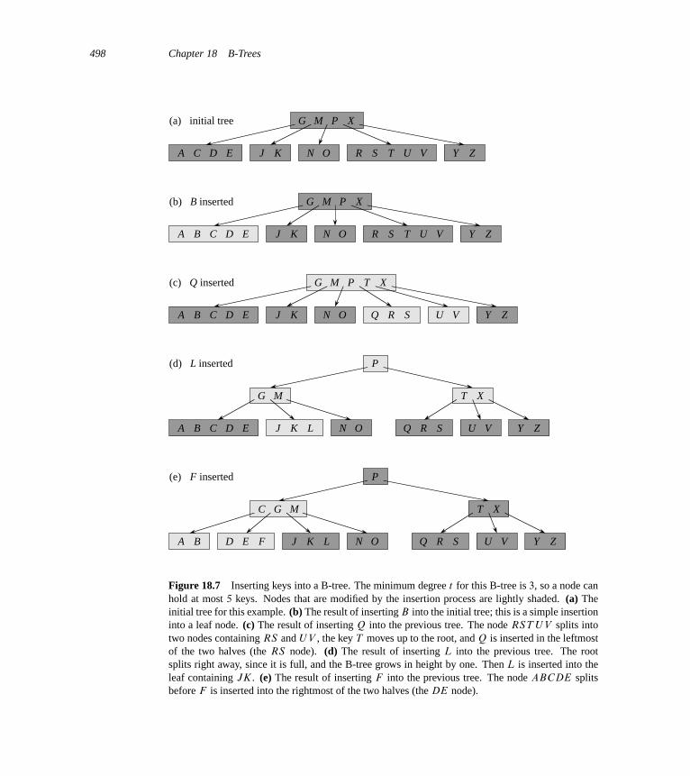
498 Chapter 18 B-Trees
J K N O R S TD ECA U V Y Z
P XMG(a)
J K N O R S TD EBA U V Y Z
P XMG(b)
C
J K N OD EBA U V Y Z
P XMG(c)
C R SQ
T
J K N OD EBA U V Y Z
MG
(d)
C R SQL
P
XT
J K N OD EBA U V Y Z
MG
(e)
C
R SQL
P
XT
F
Q inserted
L inserted
F inserted
initial tree
B inserted
Figure 18.7 Inserting keys into a B-tree. The minimum degree t for this B-tree is 3, so a node canhold at most 5 keys. Nodes that are modified by the insertion process are lightly shaded. (a) Theinitial tree for this example. (b) The result of inserting B into the initial tree; this is a simple insertioninto a leaf node. (c) The result of inserting Q into the previous tree. The node RST U V splits intotwo nodes containing RS and U V , the key T moves up to the root, and Q is inserted in the leftmostof the two halves (the RS node). (d) The result of inserting L into the previous tree. The rootsplits right away, since it is full, and the B-tree grows in height by one. Then L is inserted into theleaf containing JK. (e) The result of inserting F into the previous tree. The node ABCDE splitsbefore F is inserted into the rightmost of the two halves (the DE node).
18.3 Deleting a key from a B-tree 499
18.2-6Suppose that we were to implement B-TREE-SEARCH to use binary search ratherthan linear search within each node. Show that this change makes the CPU timerequired O.lg n/, independently of how t might be chosen as a function of n.
18.2-7Suppose that disk hardware allows us to choose the size of a disk page arbitrarily,but that the time it takes to read the disk page is aCbt , where a and b are specifiedconstants and t is the minimum degree for a B-tree using pages of the selected size.Describe how to choose t so as to minimize (approximately) the B-tree search time.Suggest an optimal value of t for the case in which a D 5 milliseconds and b D 10
microseconds.
18.3 Deleting a key from a B-tree
Deletion from a B-tree is analogous to insertion but a little more complicated, be-cause we can delete a key from any node—not just a leaf—and when we delete akey from an internal node, we will have to rearrange the node’s children. As ininsertion, we must guard against deletion producing a tree whose structure violatesthe B-tree properties. Just as we had to ensure that a node didn’t get too big due toinsertion, we must ensure that a node doesn’t get too small during deletion (exceptthat the root is allowed to have fewer than the minimum number t � 1 of keys).Just as a simple insertion algorithm might have to back up if a node on the pathto where the key was to be inserted was full, a simple approach to deletion mighthave to back up if a node (other than the root) along the path to where the key is tobe deleted has the minimum number of keys.
The procedure B-TREE-DELETE deletes the key k from the subtree rooted at x.We design this procedure to guarantee that whenever it calls itself recursively on anode x, the number of keys in x is at least the minimum degree t . Note that thiscondition requires one more key than the minimum required by the usual B-treeconditions, so that sometimes a key may have to be moved into a child node beforerecursion descends to that child. This strengthened condition allows us to deletea key from the tree in one downward pass without having to “back up” (with oneexception, which we’ll explain). You should interpret the following specificationfor deletion from a B-tree with the understanding that if the root node x ever be-comes an internal node having no keys (this situation can occur in cases 2c and 3b,below), then we delete x, and x’s only child x:c1 becomes the new root of the tree,decreasing the height of the tree by one and preserving the property that the root ofthe tree contains at least one key (unless the tree is empty).
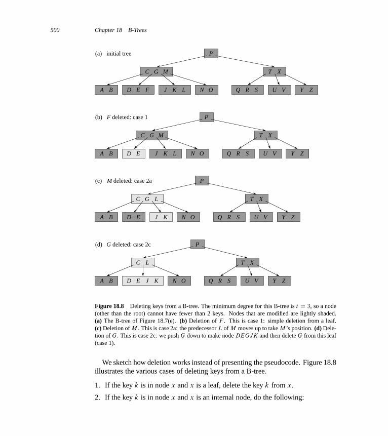
500 Chapter 18 B-Trees
J K N OD EBA U V Y Z
MG
(a)
C
R SQL
P
XT
F
initial tree
J K N OD EBA U V Y Z
MG
(b)
C
R SQL
P
XT
F deleted: case 1
J K N OD EBA U V Y Z
G
(c)
C
R SQ
L
P
XT
M deleted: case 2a
J K N OD EBA U V Y Z
(d)
C
R SQ
L
P
XT
G deleted: case 2c
Figure 18.8 Deleting keys from a B-tree. The minimum degree for this B-tree is t D 3, so a node(other than the root) cannot have fewer than 2 keys. Nodes that are modified are lightly shaded.(a) The B-tree of Figure 18.7(e). (b) Deletion of F . This is case 1: simple deletion from a leaf.(c) Deletion of M . This is case 2a: the predecessor L of M moves up to take M ’s position. (d) Dele-tion of G. This is case 2c: we push G down to make node DEGJK and then delete G from this leaf(case 1).
We sketch how deletion works instead of presenting the pseudocode. Figure 18.8illustrates the various cases of deleting keys from a B-tree.
1. If the key k is in node x and x is a leaf, delete the key k from x.
2. If the key k is in node x and x is an internal node, do the following:
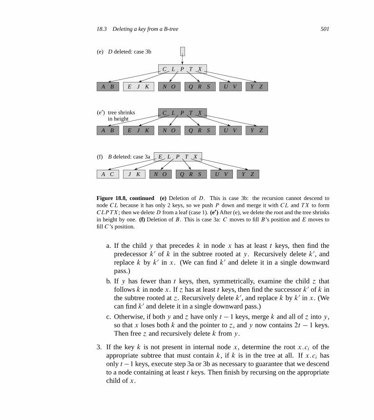
18.3 Deleting a key from a B-tree 501
J K N OEBA U V Y Z
(e)
C
R SQ
L P XT
D deleted: case 3b
J K N OEBA U V Y Z
C
R SQ
L P XT
J K N OA U V Y ZC R SQ
L P XT(f) B deleted: case 3a E
(e′) tree shrinksin height
Figure 18.8, continued (e) Deletion of D. This is case 3b: the recursion cannot descend tonode CL because it has only 2 keys, so we push P down and merge it with CL and TX to formCLP TX ; then we delete D from a leaf (case 1). (e0) After (e), we delete the root and the tree shrinksin height by one. (f) Deletion of B . This is case 3a: C moves to fill B’s position and E moves tofill C ’s position.
a. If the child y that precedes k in node x has at least t keys, then find thepredecessor k0 of k in the subtree rooted at y. Recursively delete k0, andreplace k by k0 in x. (We can find k0 and delete it in a single downwardpass.)
b. If y has fewer than t keys, then, symmetrically, examine the child ´ thatfollows k in node x. If ´ has at least t keys, then find the successor k0 of k inthe subtree rooted at ´. Recursively delete k0, and replace k by k0 in x. (Wecan find k0 and delete it in a single downward pass.)
c. Otherwise, if both y and ´ have only t � 1 keys, merge k and all of ´ into y,so that x loses both k and the pointer to ´, and y now contains 2t � 1 keys.Then free ´ and recursively delete k from y.
3. If the key k is not present in internal node x, determine the root x:ci of theappropriate subtree that must contain k, if k is in the tree at all. If x:ci hasonly t �1 keys, execute step 3a or 3b as necessary to guarantee that we descendto a node containing at least t keys. Then finish by recursing on the appropriatechild of x.
502 Chapter 18 B-Trees
a. If x:ci has only t � 1 keys but has an immediate sibling with at least t keys,give x:ci an extra key by moving a key from x down into x:ci , moving akey from x:ci ’s immediate left or right sibling up into x, and moving theappropriate child pointer from the sibling into x:ci .
b. If x:ci and both of x:ci ’s immediate siblings have t � 1 keys, merge x:ci
with one sibling, which involves moving a key from x down into the newmerged node to become the median key for that node.
Since most of the keys in a B-tree are in the leaves, we may expect that inpractice, deletion operations are most often used to delete keys from leaves. TheB-TREE-DELETE procedure then acts in one downward pass through the tree,without having to back up. When deleting a key in an internal node, however,the procedure makes a downward pass through the tree but may have to return tothe node from which the key was deleted to replace the key with its predecessor orsuccessor (cases 2a and 2b).
Although this procedure seems complicated, it involves only O.h/ disk oper-ations for a B-tree of height h, since only O.1/ calls to DISK-READ and DISK-WRITE are made between recursive invocations of the procedure. The CPU timerequired is O.th/ D O.t logt n/.
Exercises
18.3-1Show the results of deleting C , P , and V , in order, from the tree of Figure 18.8(f).
18.3-2Write pseudocode for B-TREE-DELETE.
Problems
18-1 Stacks on secondary storageConsider implementing a stack in a computer that has a relatively small amountof fast primary memory and a relatively large amount of slower disk storage. Theoperations PUSH and POP work on single-word values. The stack we wish tosupport can grow to be much larger than can fit in memory, and thus most of itmust be stored on disk.
A simple, but inefficient, stack implementation keeps the entire stack on disk.We maintain in memory a stack pointer, which is the disk address of the top elementon the stack. If the pointer has value p, the top element is the .p mod m/th wordon page bp=mc of the disk, where m is the number of words per page.

Problems for Chapter 18 503
To implement the PUSH operation, we increment the stack pointer, read the ap-propriate page into memory from disk, copy the element to be pushed to the ap-propriate word on the page, and write the page back to disk. A POP operation issimilar. We decrement the stack pointer, read in the appropriate page from disk,and return the top of the stack. We need not write back the page, since it was notmodified.
Because disk operations are relatively expensive, we count two costs for anyimplementation: the total number of disk accesses and the total CPU time. Anydisk access to a page of m words incurs charges of one disk access and ‚.m/ CPUtime.
a. Asymptotically, what is the worst-case number of disk accesses for n stackoperations using this simple implementation? What is the CPU time for n stackoperations? (Express your answer in terms of m and n for this and subsequentparts.)
Now consider a stack implementation in which we keep one page of the stack inmemory. (We also maintain a small amount of memory to keep track of which pageis currently in memory.) We can perform a stack operation only if the relevant diskpage resides in memory. If necessary, we can write the page currently in memoryto the disk and read in the new page from the disk to memory. If the relevant diskpage is already in memory, then no disk accesses are required.
b. What is the worst-case number of disk accesses required for n PUSH opera-tions? What is the CPU time?
c. What is the worst-case number of disk accesses required for n stack operations?What is the CPU time?
Suppose that we now implement the stack by keeping two pages in memory (inaddition to a small number of words for bookkeeping).
d. Describe how to manage the stack pages so that the amortized number of diskaccesses for any stack operation is O.1=m/ and the amortized CPU time forany stack operation is O.1/.
18-2 Joining and splitting 2-3-4 treesThe join operation takes two dynamic sets S 0 and S 00 and an element x such thatfor any x 0 2 S 0 and x 00 2 S 00, we have x 0:key < x:key < x 00:key. It returns a setS D S 0 [ fxg [ S 00. The split operation is like an “inverse” join: given a dynamicset S and an element x 2 S , it creates a set S 0 that consists of all elements inS � fxg whose keys are less than x:key and a set S 00 that consists of all elementsin S � fxg whose keys are greater than x:key. In this problem, we investigate

504 Chapter 18 B-Trees
how to implement these operations on 2-3-4 trees. We assume for convenience thatelements consist only of keys and that all key values are distinct.
a. Show how to maintain, for every node x of a 2-3-4 tree, the height of the subtreerooted at x as an attribute x:height. Make sure that your implementation doesnot affect the asymptotic running times of searching, insertion, and deletion.
b. Show how to implement the join operation. Given two 2-3-4 trees T 0 and T 00
and a key k, the join operation should run in O.1 C jh0 � h00j/ time, where h0
and h00 are the heights of T 0 and T 00, respectively.
c. Consider the simple path p from the root of a 2-3-4 tree T to a given key k,the set S 0 of keys in T that are less than k, and the set S 00 of keys in T that aregreater than k. Show that p breaks S 0 into a set of trees fT 0
0; T 01; : : : ; T 0
mg and aset of keys fk0
1; k02; : : : ; k0
mg, where, for i D 1; 2; : : : ; m, we have y < k0i < ´
for any keys y 2 T 0i�1 and ´ 2 T 0
i . What is the relationship between the heightsof T 0
i�1 and T 0i ? Describe how p breaks S 00 into sets of trees and keys.
d. Show how to implement the split operation on T . Use the join operation toassemble the keys in S 0 into a single 2-3-4 tree T 0 and the keys in S 00 into asingle 2-3-4 tree T 00. The running time of the split operation should be O.lg n/,where n is the number of keys in T . (Hint: The costs for joining should tele-scope.)
Chapter notes
Knuth [211], Aho, Hopcroft, and Ullman [5], and Sedgewick [306] give furtherdiscussions of balanced-tree schemes and B-trees. Comer [75] provides a compre-hensive survey of B-trees. Guibas and Sedgewick [155] discuss the relationshipsamong various kinds of balanced-tree schemes, including red-black trees and 2-3-4trees.
In 1970, J. E. Hopcroft invented 2-3 trees, a precursor to B-trees and 2-3-4trees, in which every internal node has either two or three children. Bayer andMcCreight [35] introduced B-trees in 1972; they did not explain their choice ofname.
Bender, Demaine, and Farach-Colton [40] studied how to make B-trees performwell in the presence of memory-hierarchy effects. Their cache-oblivious algo-rithms work efficiently without explicitly knowing the data transfer sizes withinthe memory hierarchy.
19 Fibonacci Heaps
The Fibonacci heap data structure serves a dual purpose. First, it supports a set ofoperations that constitutes what is known as a “mergeable heap.” Second, severalFibonacci-heap operations run in constant amortized time, which makes this datastructure well suited for applications that invoke these operations frequently.
Mergeable heaps
A mergeable heap is any data structure that supports the following five operations,in which each element has a key:
MAKE-HEAP./ creates and returns a new heap containing no elements.
INSERT.H; x/ inserts element x, whose key has already been filled in, into heap H .
MINIMUM.H/ returns a pointer to the element in heap H whose key is minimum.
EXTRACT-MIN.H/ deletes the element from heap H whose key is minimum, re-turning a pointer to the element.
UNION.H1; H2/ creates and returns a new heap that contains all the elements ofheaps H1 and H2. Heaps H1 and H2 are “destroyed” by this operation.
In addition to the mergeable-heap operations above, Fibonacci heaps also supportthe following two operations:
DECREASE-KEY.H; x; k/ assigns to element x within heap H the new keyvalue k, which we assume to be no greater than its current key value.1
DELETE.H; x/ deletes element x from heap H .
1As mentioned in the introduction to Part V, our default mergeable heaps are mergeable min-heaps, and so the operations MINIMUM, EXTRACT-MIN, and DECREASE-KEY apply. Alterna-tively, we could define a mergeable max-heap with the operations MAXIMUM, EXTRACT-MAX,and INCREASE-KEY.
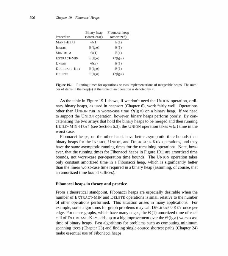
506 Chapter 19 Fibonacci Heaps
Binary heap Fibonacci heapProcedure (worst-case) (amortized)
MAKE-HEAP ‚.1/ ‚.1/
INSERT ‚.lg n/ ‚.1/
MINIMUM ‚.1/ ‚.1/
EXTRACT-MIN ‚.lg n/ O.lg n/
UNION ‚.n/ ‚.1/
DECREASE-KEY ‚.lg n/ ‚.1/
DELETE ‚.lg n/ O.lg n/
Figure 19.1 Running times for operations on two implementations of mergeable heaps. The num-ber of items in the heap(s) at the time of an operation is denoted by n.
As the table in Figure 19.1 shows, if we don’t need the UNION operation, ordi-nary binary heaps, as used in heapsort (Chapter 6), work fairly well. Operationsother than UNION run in worst-case time O.lg n/ on a binary heap. If we needto support the UNION operation, however, binary heaps perform poorly. By con-catenating the two arrays that hold the binary heaps to be merged and then runningBUILD-MIN-HEAP (see Section 6.3), the UNION operation takes ‚.n/ time in theworst case.
Fibonacci heaps, on the other hand, have better asymptotic time bounds thanbinary heaps for the INSERT, UNION, and DECREASE-KEY operations, and theyhave the same asymptotic running times for the remaining operations. Note, how-ever, that the running times for Fibonacci heaps in Figure 19.1 are amortized timebounds, not worst-case per-operation time bounds. The UNION operation takesonly constant amortized time in a Fibonacci heap, which is significantly betterthan the linear worst-case time required in a binary heap (assuming, of course, thatan amortized time bound suffices).
Fibonacci heaps in theory and practice
From a theoretical standpoint, Fibonacci heaps are especially desirable when thenumber of EXTRACT-MIN and DELETE operations is small relative to the numberof other operations performed. This situation arises in many applications. Forexample, some algorithms for graph problems may call DECREASE-KEY once peredge. For dense graphs, which have many edges, the ‚.1/ amortized time of eachcall of DECREASE-KEY adds up to a big improvement over the ‚.lg n/ worst-casetime of binary heaps. Fast algorithms for problems such as computing minimumspanning trees (Chapter 23) and finding single-source shortest paths (Chapter 24)make essential use of Fibonacci heaps.
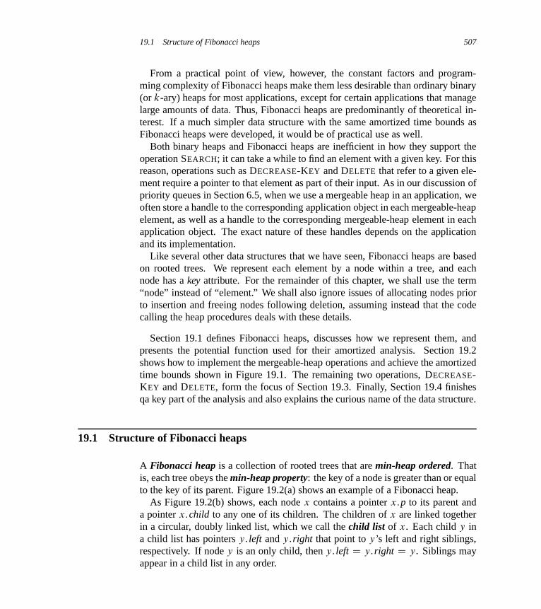
19.1 Structure of Fibonacci heaps 507
From a practical point of view, however, the constant factors and program-ming complexity of Fibonacci heaps make them less desirable than ordinary binary(or k-ary) heaps for most applications, except for certain applications that managelarge amounts of data. Thus, Fibonacci heaps are predominantly of theoretical in-terest. If a much simpler data structure with the same amortized time bounds asFibonacci heaps were developed, it would be of practical use as well.
Both binary heaps and Fibonacci heaps are inefficient in how they support theoperation SEARCH; it can take a while to find an element with a given key. For thisreason, operations such as DECREASE-KEY and DELETE that refer to a given ele-ment require a pointer to that element as part of their input. As in our discussion ofpriority queues in Section 6.5, when we use a mergeable heap in an application, weoften store a handle to the corresponding application object in each mergeable-heapelement, as well as a handle to the corresponding mergeable-heap element in eachapplication object. The exact nature of these handles depends on the applicationand its implementation.
Like several other data structures that we have seen, Fibonacci heaps are basedon rooted trees. We represent each element by a node within a tree, and eachnode has a key attribute. For the remainder of this chapter, we shall use the term“node” instead of “element.” We shall also ignore issues of allocating nodes priorto insertion and freeing nodes following deletion, assuming instead that the codecalling the heap procedures deals with these details.
Section 19.1 defines Fibonacci heaps, discusses how we represent them, andpresents the potential function used for their amortized analysis. Section 19.2shows how to implement the mergeable-heap operations and achieve the amortizedtime bounds shown in Figure 19.1. The remaining two operations, DECREASE-KEY and DELETE, form the focus of Section 19.3. Finally, Section 19.4 finishesqa key part of the analysis and also explains the curious name of the data structure.
19.1 Structure of Fibonacci heaps
A Fibonacci heap is a collection of rooted trees that are min-heap ordered. Thatis, each tree obeys the min-heap property: the key of a node is greater than or equalto the key of its parent. Figure 19.2(a) shows an example of a Fibonacci heap.
As Figure 19.2(b) shows, each node x contains a pointer x:p to its parent anda pointer x:child to any one of its children. The children of x are linked togetherin a circular, doubly linked list, which we call the child list of x. Each child y ina child list has pointers y: left and y:right that point to y’s left and right siblings,respectively. If node y is an only child, then y: left D y:right D y. Siblings mayappear in a child list in any order.
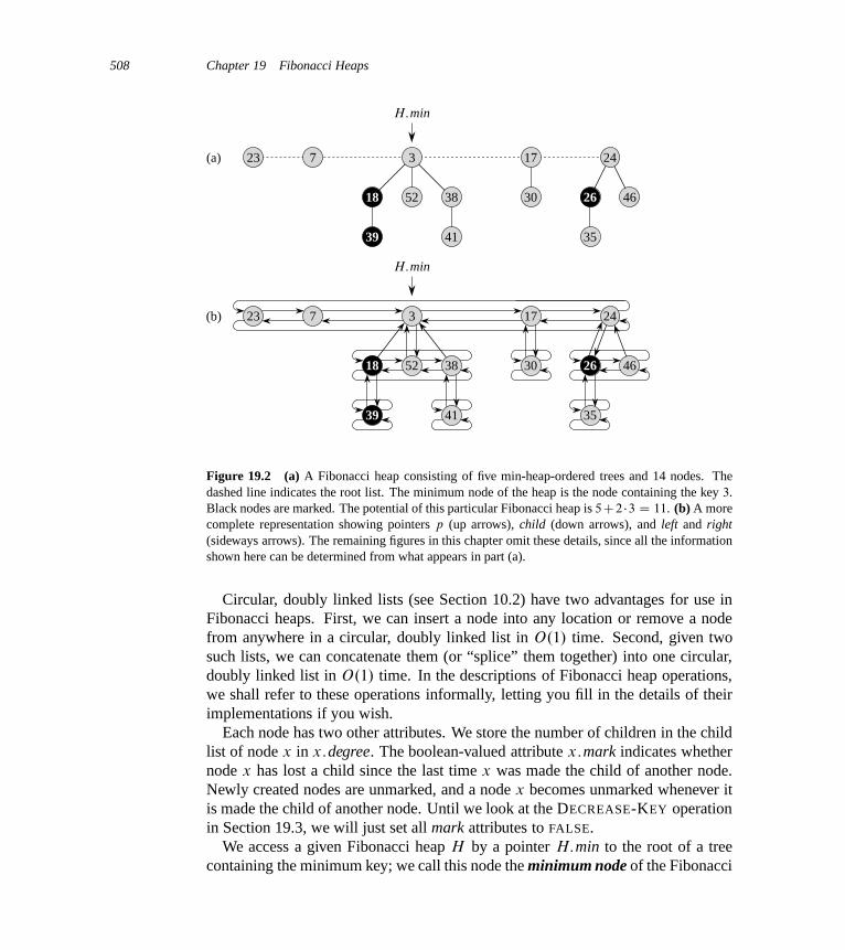
508 Chapter 19 Fibonacci Heaps
17
30 26 46
35
24
18 52 38
3
39 41
23 7
17
30 26 46
35
24
18 52 38
3
39 41
23 7
(a)
(b)
H:min
H:min
Figure 19.2 (a) A Fibonacci heap consisting of five min-heap-ordered trees and 14 nodes. Thedashed line indicates the root list. The minimum node of the heap is the node containing the key 3.Black nodes are marked. The potential of this particular Fibonacci heap is 5C2 �3 D 11. (b) A morecomplete representation showing pointers p (up arrows), child (down arrows), and left and right(sideways arrows). The remaining figures in this chapter omit these details, since all the informationshown here can be determined from what appears in part (a).
Circular, doubly linked lists (see Section 10.2) have two advantages for use inFibonacci heaps. First, we can insert a node into any location or remove a nodefrom anywhere in a circular, doubly linked list in O.1/ time. Second, given twosuch lists, we can concatenate them (or “splice” them together) into one circular,doubly linked list in O.1/ time. In the descriptions of Fibonacci heap operations,we shall refer to these operations informally, letting you fill in the details of theirimplementations if you wish.
Each node has two other attributes. We store the number of children in the childlist of node x in x:degree. The boolean-valued attribute x:mark indicates whethernode x has lost a child since the last time x was made the child of another node.Newly created nodes are unmarked, and a node x becomes unmarked whenever itis made the child of another node. Until we look at the DECREASE-KEY operationin Section 19.3, we will just set all mark attributes to FALSE.
We access a given Fibonacci heap H by a pointer H:min to the root of a treecontaining the minimum key; we call this node the minimum node of the Fibonacci

19.1 Structure of Fibonacci heaps 509
heap. If more than one root has a key with the minimum value, then any such rootmay serve as the minimum node. When a Fibonacci heap H is empty, H:minis NIL.
The roots of all the trees in a Fibonacci heap are linked together using theirleft and right pointers into a circular, doubly linked list called the root list of theFibonacci heap. The pointer H:min thus points to the node in the root list whosekey is minimum. Trees may appear in any order within a root list.
We rely on one other attribute for a Fibonacci heap H : H:n, the number ofnodes currently in H .
Potential function
As mentioned, we shall use the potential method of Section 17.3 to analyze theperformance of Fibonacci heap operations. For a given Fibonacci heap H , weindicate by t.H/ the number of trees in the root list of H and by m.H/ the numberof marked nodes in H . We then define the potential ˆ.H/ of Fibonacci heap H
by
ˆ.H/ D t.H/C 2 m.H/ : (19.1)
(We will gain some intuition for this potential function in Section 19.3.) For exam-ple, the potential of the Fibonacci heap shown in Figure 19.2 is 5C2 �3 D 11. Thepotential of a set of Fibonacci heaps is the sum of the potentials of its constituentFibonacci heaps. We shall assume that a unit of potential can pay for a constantamount of work, where the constant is sufficiently large to cover the cost of any ofthe specific constant-time pieces of work that we might encounter.
We assume that a Fibonacci heap application begins with no heaps. The initialpotential, therefore, is 0, and by equation (19.1), the potential is nonnegative atall subsequent times. From equation (17.3), an upper bound on the total amortizedcost provides an upper bound on the total actual cost for the sequence of operations.
Maximum degree
The amortized analyses we shall perform in the remaining sections of this chapterassume that we know an upper bound D.n/ on the maximum degree of any nodein an n-node Fibonacci heap. We won’t prove it, but when only the mergeable-heap operations are supported, D.n/ � blg nc. (Problem 19-2(d) asks you to provethis property.) In Sections 19.3 and 19.4, we shall show that when we supportDECREASE-KEY and DELETE as well, D.n/ D O.lg n/.
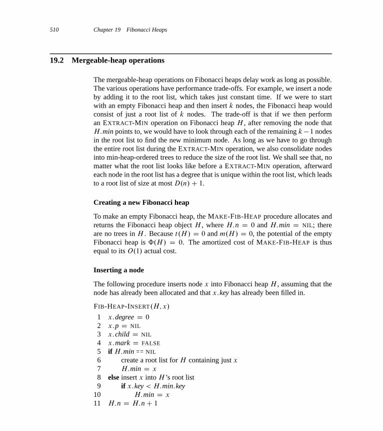
510 Chapter 19 Fibonacci Heaps
19.2 Mergeable-heap operations
The mergeable-heap operations on Fibonacci heaps delay work as long as possible.The various operations have performance trade-offs. For example, we insert a nodeby adding it to the root list, which takes just constant time. If we were to startwith an empty Fibonacci heap and then insert k nodes, the Fibonacci heap wouldconsist of just a root list of k nodes. The trade-off is that if we then performan EXTRACT-MIN operation on Fibonacci heap H , after removing the node thatH:min points to, we would have to look through each of the remaining k�1 nodesin the root list to find the new minimum node. As long as we have to go throughthe entire root list during the EXTRACT-MIN operation, we also consolidate nodesinto min-heap-ordered trees to reduce the size of the root list. We shall see that, nomatter what the root list looks like before a EXTRACT-MIN operation, afterwardeach node in the root list has a degree that is unique within the root list, which leadsto a root list of size at most D.n/C 1.
Creating a new Fibonacci heap
To make an empty Fibonacci heap, the MAKE-FIB-HEAP procedure allocates andreturns the Fibonacci heap object H , where H:n D 0 and H:min D NIL; thereare no trees in H . Because t.H/ D 0 and m.H/ D 0, the potential of the emptyFibonacci heap is ˆ.H/ D 0. The amortized cost of MAKE-FIB-HEAP is thusequal to its O.1/ actual cost.
Inserting a node
The following procedure inserts node x into Fibonacci heap H , assuming that thenode has already been allocated and that x:key has already been filled in.
FIB-HEAP-INSERT.H; x/
1 x:degree D 0
2 x:p D NIL
3 x:child D NIL
4 x:mark D FALSE
5 if H:min == NIL
6 create a root list for H containing just x
7 H:min D x
8 else insert x into H ’s root list9 if x:key < H:min:key
10 H:min D x
11 H:n D H:nC 1
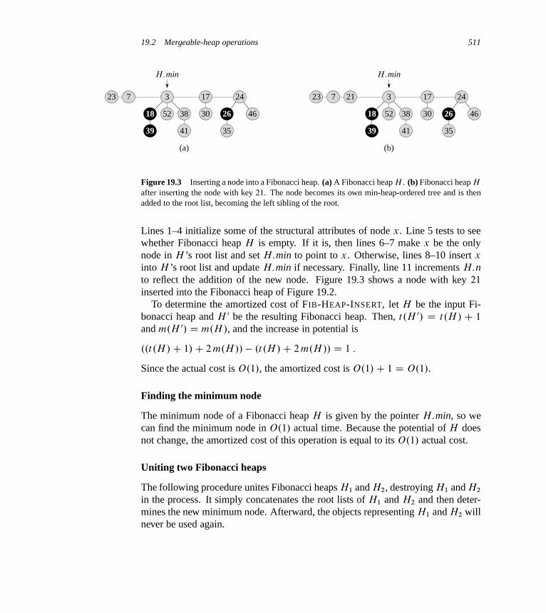
19.2 Mergeable-heap operations 511
(a) (b)
17
30
2423
26
35
46
7 21
18 52 38
39 41
317
30
2423
26
35
46
7
18 52 38
39 41
3
H:min H:min
Figure 19.3 Inserting a node into a Fibonacci heap. (a) A Fibonacci heap H . (b) Fibonacci heap H
after inserting the node with key 21. The node becomes its own min-heap-ordered tree and is thenadded to the root list, becoming the left sibling of the root.
Lines 1–4 initialize some of the structural attributes of node x. Line 5 tests to seewhether Fibonacci heap H is empty. If it is, then lines 6–7 make x be the onlynode in H ’s root list and set H:min to point to x. Otherwise, lines 8–10 insert x
into H ’s root list and update H:min if necessary. Finally, line 11 increments H:nto reflect the addition of the new node. Figure 19.3 shows a node with key 21
inserted into the Fibonacci heap of Figure 19.2.To determine the amortized cost of FIB-HEAP-INSERT, let H be the input Fi-
bonacci heap and H 0 be the resulting Fibonacci heap. Then, t.H 0/ D t.H/ C 1
and m.H 0/ D m.H/, and the increase in potential is
..t.H/C 1/C 2 m.H// � .t.H/C 2 m.H// D 1 :
Since the actual cost is O.1/, the amortized cost is O.1/C 1 D O.1/.
Finding the minimum node
The minimum node of a Fibonacci heap H is given by the pointer H:min, so wecan find the minimum node in O.1/ actual time. Because the potential of H doesnot change, the amortized cost of this operation is equal to its O.1/ actual cost.
Uniting two Fibonacci heaps
The following procedure unites Fibonacci heaps H1 and H2, destroying H1 and H2
in the process. It simply concatenates the root lists of H1 and H2 and then deter-mines the new minimum node. Afterward, the objects representing H1 and H2 willnever be used again.
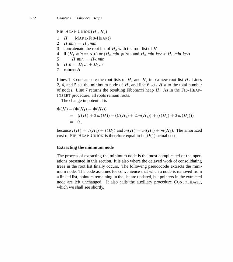
512 Chapter 19 Fibonacci Heaps
FIB-HEAP-UNION.H1; H2/
1 H D MAKE-FIB-HEAP./
2 H:min D H1:min3 concatenate the root list of H2 with the root list of H
4 if .H1:min == NIL/ or .H2:min ¤ NIL and H2:min:key < H1:min:key/
5 H:min D H2:min6 H:n D H1:nCH2:n7 return H
Lines 1–3 concatenate the root lists of H1 and H2 into a new root list H . Lines2, 4, and 5 set the minimum node of H , and line 6 sets H:n to the total numberof nodes. Line 7 returns the resulting Fibonacci heap H . As in the FIB-HEAP-INSERT procedure, all roots remain roots.
The change in potential is
ˆ.H/ � .ˆ.H1/Cˆ.H2//
D .t.H/C 2 m.H// � ..t.H1/C 2 m.H1//C .t.H2/C 2 m.H2///
D 0 ;
because t.H/ D t.H1/ C t.H2/ and m.H/ D m.H1/ C m.H2/. The amortizedcost of FIB-HEAP-UNION is therefore equal to its O.1/ actual cost.
Extracting the minimum node
The process of extracting the minimum node is the most complicated of the oper-ations presented in this section. It is also where the delayed work of consolidatingtrees in the root list finally occurs. The following pseudocode extracts the mini-mum node. The code assumes for convenience that when a node is removed froma linked list, pointers remaining in the list are updated, but pointers in the extractednode are left unchanged. It also calls the auxiliary procedure CONSOLIDATE,which we shall see shortly.

19.2 Mergeable-heap operations 513
FIB-HEAP-EXTRACT-MIN.H/
1 ´ D H:min2 if ´ ¤ NIL
3 for each child x of ´
4 add x to the root list of H
5 x:p D NIL
6 remove ´ from the root list of H
7 if ´ == ´:right8 H:min D NIL
9 else H:min D ´:right10 CONSOLIDATE.H/
11 H:n D H:n � 1
12 return ´
As Figure 19.4 illustrates, FIB-HEAP-EXTRACT-MIN works by first making a rootout of each of the minimum node’s children and removing the minimum node fromthe root list. It then consolidates the root list by linking roots of equal degree untilat most one root remains of each degree.
We start in line 1 by saving a pointer ´ to the minimum node; the procedurereturns this pointer at the end. If ´ is NIL, then Fibonacci heap H is already emptyand we are done. Otherwise, we delete node ´ from H by making all of ´’s chil-dren roots of H in lines 3–5 (putting them into the root list) and removing ´ fromthe root list in line 6. If ´ is its own right sibling after line 6, then ´ was theonly node on the root list and it had no children, so all that remains is to makethe Fibonacci heap empty in line 8 before returning ´. Otherwise, we set thepointer H:min into the root list to point to a root other than ´ (in this case, ´’sright sibling), which is not necessarily going to be the new minimum node whenFIB-HEAP-EXTRACT-MIN is done. Figure 19.4(b) shows the Fibonacci heap ofFigure 19.4(a) after executing line 9.
The next step, in which we reduce the number of trees in the Fibonacci heap, isconsolidating the root list of H , which the call CONSOLIDATE.H/ accomplishes.Consolidating the root list consists of repeatedly executing the following steps untilevery root in the root list has a distinct degree value:
1. Find two roots x and y in the root list with the same degree. Without loss ofgenerality, let x:key � y:key.
2. Link y to x: remove y from the root list, and make y a child of x by calling theFIB-HEAP-LINK procedure. This procedure increments the attribute x:degreeand clears the mark on y.
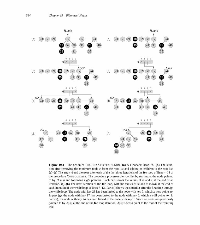
514 Chapter 19 Fibonacci Heaps
A0 1 2 3
A0 1 2 3
A0 1 2 3
A0 1 2 3
A0 1 2 3
A0 1 2 3
(c) (d)
(e)
17
30
24 23
26
35
46
7
17
30
2423
26
35
46
7 21
18 52 38
39 41
(a) 3 (b)
(f)
(g) 21 18 52 38
39 41
(h)
17
30
2423
26
35
46
7 21 18 52 38
39 41
17
30
2423
26
35
46
7 21 18 52 38
39 41
17
30
2423
26
35
46
7 21 18 52 38
39 41
17
30
2423
26
35
46
7 21 18 52 38
39 41
17
30
24
23 26
35
46
7 21 18 52 38
39 41
17
30
24
23 26
35
46
7 21 18 52 38
39 41
w,x w,x
w,x w,x
w,x w,x
H:minH:min
Figure 19.4 The action of FIB-HEAP-EXTRACT-MIN. (a) A Fibonacci heap H . (b) The situa-tion after removing the minimum node ´ from the root list and adding its children to the root list.(c)–(e) The array A and the trees after each of the first three iterations of the for loop of lines 4–14 ofthe procedure CONSOLIDATE. The procedure processes the root list by starting at the node pointedto by H:min and following right pointers. Each part shows the values of w and x at the end of aniteration. (f)–(h) The next iteration of the for loop, with the values of w and x shown at the end ofeach iteration of the while loop of lines 7–13. Part (f) shows the situation after the first time throughthe while loop. The node with key 23 has been linked to the node with key 7, which x now points to.In part (g), the node with key 17 has been linked to the node with key 7, which x still points to. Inpart (h), the node with key 24 has been linked to the node with key 7. Since no node was previouslypointed to by AŒ3�, at the end of the for loop iteration, AŒ3� is set to point to the root of the resultingtree.
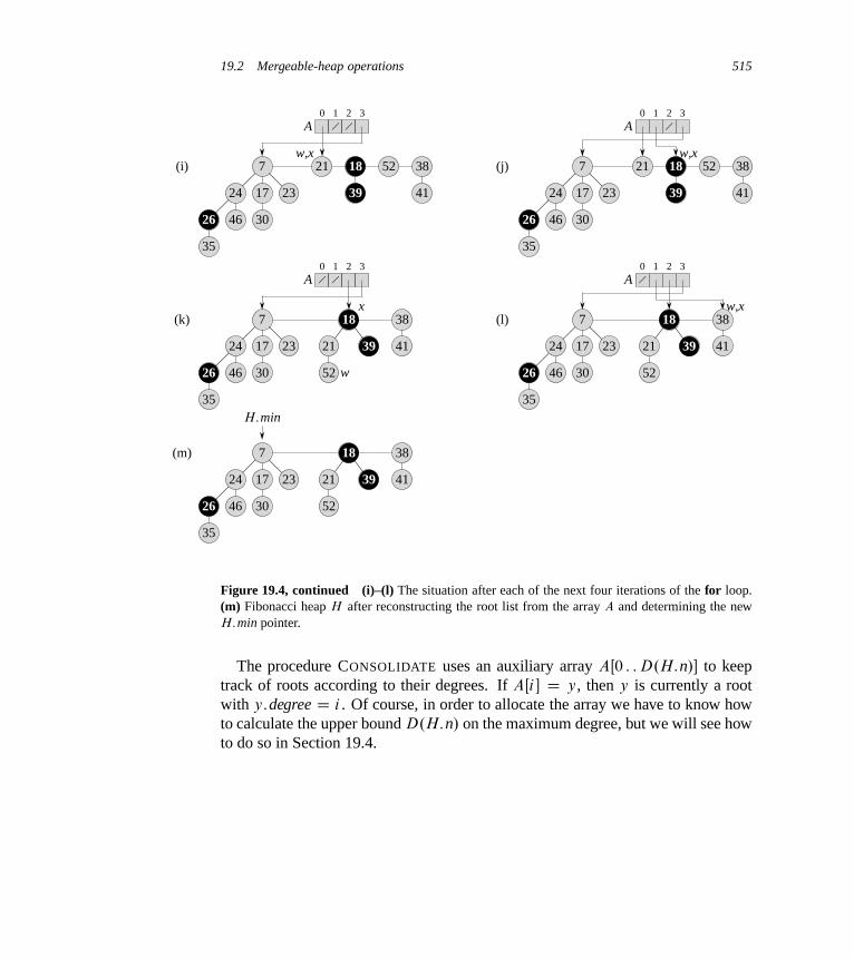
19.2 Mergeable-heap operations 515
A0 1 2 3
A0 1 2 3
A0 1 2 3
A0 1 2 3
17
30
24 23
26
35
46
7 21 18 52 38
39 41
(i)
17
30
24 23
26
35
46
7 21 18 52 38
39 41
(j)
17
30
24 23
26
35
46
7 38
41
(k)
21
18
52
39 17
30
24 23
26
35
46
7 38
41
(l)
21
18
52
39
17
30
24 23
26
35
46
7 38
41
(m)
21
18
52
39
w,x w,x
x w,x
w
H:min
Figure 19.4, continued (i)–(l) The situation after each of the next four iterations of the for loop.(m) Fibonacci heap H after reconstructing the root list from the array A and determining the newH:min pointer.
The procedure CONSOLIDATE uses an auxiliary array AŒ0 : : D.H:n/� to keeptrack of roots according to their degrees. If AŒi� D y, then y is currently a rootwith y:degree D i . Of course, in order to allocate the array we have to know howto calculate the upper bound D.H:n/ on the maximum degree, but we will see howto do so in Section 19.4.

516 Chapter 19 Fibonacci Heaps
CONSOLIDATE.H/
1 let AŒ0 : : D.H:n/� be a new array2 for i D 0 to D.H:n/
3 AŒi� D NIL
4 for each node w in the root list of H
5 x D w
6 d D x:degree7 while AŒd� ¤ NIL
8 y D AŒd� // another node with the same degree as x
9 if x:key > y:key10 exchange x with y
11 FIB-HEAP-LINK.H; y; x/
12 AŒd� D NIL
13 d D d C 1
14 AŒd� D x
15 H:min D NIL
16 for i D 0 to D.H:n/
17 if AŒi� ¤ NIL
18 if H:min == NIL
19 create a root list for H containing just AŒi�
20 H:min D AŒi�
21 else insert AŒi� into H ’s root list22 if AŒi�:key < H:min:key23 H:min D AŒi�
FIB-HEAP-LINK.H; y; x/
1 remove y from the root list of H
2 make y a child of x, incrementing x:degree3 y:mark D FALSE
In detail, the CONSOLIDATE procedure works as follows. Lines 1–3 allocateand initialize the array A by making each entry NIL. The for loop of lines 4–14processes each root w in the root list. As we link roots together, w may be linkedto some other node and no longer be a root. Nevertheless, w is always in a treerooted at some node x, which may or may not be w itself. Because we want atmost one root with each degree, we look in the array A to see whether it containsa root y with the same degree as x. If it does, then we link the roots x and y butguaranteeing that x remains a root after linking. That is, we link y to x after firstexchanging the pointers to the two roots if y’s key is smaller than x’s key. Afterwe link y to x, the degree of x has increased by 1, and so we continue this process,linking x and another root whose degree equals x’s new degree, until no other root
19.2 Mergeable-heap operations 517
that we have processed has the same degree as x. We then set the appropriate entryof A to point to x, so that as we process roots later on, we have recorded that x isthe unique root of its degree that we have already processed. When this for loopterminates, at most one root of each degree will remain, and the array A will pointto each remaining root.
The while loop of lines 7–13 repeatedly links the root x of the tree containingnode w to another tree whose root has the same degree as x, until no other root hasthe same degree. This while loop maintains the following invariant:
At the start of each iteration of the while loop, d D x:degree.
We use this loop invariant as follows:
Initialization: Line 6 ensures that the loop invariant holds the first time we enterthe loop.
Maintenance: In each iteration of the while loop, AŒd� points to some root y.Because d D x:degree D y:degree, we want to link x and y. Whichever ofx and y has the smaller key becomes the parent of the other as a result of thelink operation, and so lines 9–10 exchange the pointers to x and y if necessary.Next, we link y to x by the call FIB-HEAP-LINK.H; y; x/ in line 11. Thiscall increments x:degree but leaves y:degree as d . Node y is no longer a root,and so line 12 removes the pointer to it in array A. Because the call of FIB-HEAP-LINK increments the value of x:degree, line 13 restores the invariantthat d D x:degree.
Termination: We repeat the while loop until AŒd� D NIL, in which case there isno other root with the same degree as x.
After the while loop terminates, we set AŒd� to x in line 14 and perform the nextiteration of the for loop.
Figures 19.4(c)–(e) show the array A and the resulting trees after the first threeiterations of the for loop of lines 4–14. In the next iteration of the for loop, threelinks occur; their results are shown in Figures 19.4(f)–(h). Figures 19.4(i)–(l) showthe result of the next four iterations of the for loop.
All that remains is to clean up. Once the for loop of lines 4–14 completes,line 15 empties the root list, and lines 16–23 reconstruct it from the array A. Theresulting Fibonacci heap appears in Figure 19.4(m). After consolidating the rootlist, FIB-HEAP-EXTRACT-MIN finishes up by decrementing H:n in line 11 andreturning a pointer to the deleted node ´ in line 12.
We are now ready to show that the amortized cost of extracting the minimumnode of an n-node Fibonacci heap is O.D.n//. Let H denote the Fibonacci heapjust prior to the FIB-HEAP-EXTRACT-MIN operation.
We start by accounting for the actual cost of extracting the minimum node.An O.D.n// contribution comes from FIB-HEAP-EXTRACT-MIN processing at

518 Chapter 19 Fibonacci Heaps
most D.n/ children of the minimum node and from the work in lines 2–3 and16–23 of CONSOLIDATE. It remains to analyze the contribution from the for loopof lines 4–14 in CONSOLIDATE, for which we use an aggregate analysis. The sizeof the root list upon calling CONSOLIDATE is at most D.n/ C t.H/ � 1, since itconsists of the original t.H/ root-list nodes, minus the extracted root node, plusthe children of the extracted node, which number at most D.n/. Within a giveniteration of the for loop of lines 4–14, the number of iterations of the while loop oflines 7–13 depends on the root list. But we know that every time through the whileloop, one of the roots is linked to another, and thus the total number of iterationsof the while loop over all iterations of the for loop is at most the number of rootsin the root list. Hence, the total amount of work performed in the for loop is atmost proportional to D.n/ C t.H/. Thus, the total actual work in extracting theminimum node is O.D.n/C t.H//.
The potential before extracting the minimum node is t.H/ C 2 m.H/, and thepotential afterward is at most .D.n/C 1/C 2 m.H/, since at most D.n/C 1 rootsremain and no nodes become marked during the operation. The amortized cost isthus at most
O.D.n/C t.H//C ..D.n/C 1/C 2 m.H// � .t.H/C 2 m.H//
D O.D.n//CO.t.H// � t.H/
D O.D.n// ;
since we can scale up the units of potential to dominate the constant hiddenin O.t.H//. Intuitively, the cost of performing each link is paid for by the re-duction in potential due to the link’s reducing the number of roots by one. We shallsee in Section 19.4 that D.n/ D O.lg n/, so that the amortized cost of extractingthe minimum node is O.lg n/.
Exercises
19.2-1Show the Fibonacci heap that results from calling FIB-HEAP-EXTRACT-MIN onthe Fibonacci heap shown in Figure 19.4(m).
19.3 Decreasing a key and deleting a node
In this section, we show how to decrease the key of a node in a Fibonacci heapin O.1/ amortized time and how to delete any node from an n-node Fibonacciheap in O.D.n// amortized time. In Section 19.4, we will show that the maxi-
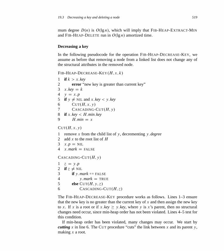
19.3 Decreasing a key and deleting a node 519
mum degree D.n/ is O.lg n/, which will imply that FIB-HEAP-EXTRACT-MIN
and FIB-HEAP-DELETE run in O.lg n/ amortized time.
Decreasing a key
In the following pseudocode for the operation FIB-HEAP-DECREASE-KEY, weassume as before that removing a node from a linked list does not change any ofthe structural attributes in the removed node.
FIB-HEAP-DECREASE-KEY.H; x; k/
1 if k > x:key2 error “new key is greater than current key”3 x:key D k
4 y D x:p5 if y ¤ NIL and x:key < y:key6 CUT.H; x; y/
7 CASCADING-CUT.H; y/
8 if x:key < H:min:key9 H:min D x
CUT.H; x; y/
1 remove x from the child list of y, decrementing y:degree2 add x to the root list of H
3 x:p D NIL
4 x:mark D FALSE
CASCADING-CUT.H; y/
1 ´ D y:p2 if ´ ¤ NIL
3 if y:mark == FALSE
4 y:mark D TRUE
5 else CUT.H; y; ´/
6 CASCADING-CUT.H; ´/
The FIB-HEAP-DECREASE-KEY procedure works as follows. Lines 1–3 ensurethat the new key is no greater than the current key of x and then assign the new keyto x. If x is a root or if x:key � y:key, where y is x’s parent, then no structuralchanges need occur, since min-heap order has not been violated. Lines 4–5 test forthis condition.
If min-heap order has been violated, many changes may occur. We start bycutting x in line 6. The CUT procedure “cuts” the link between x and its parent y,making x a root.

520 Chapter 19 Fibonacci Heaps
We use the mark attributes to obtain the desired time bounds. They record a littlepiece of the history of each node. Suppose that the following events have happenedto node x:
1. at some time, x was a root,
2. then x was linked to (made the child of) another node,
3. then two children of x were removed by cuts.
As soon as the second child has been lost, we cut x from its parent, making it a newroot. The attribute x:mark is TRUE if steps 1 and 2 have occurred and one childof x has been cut. The CUT procedure, therefore, clears x:mark in line 4, since itperforms step 1. (We can now see why line 3 of FIB-HEAP-LINK clears y:mark:node y is being linked to another node, and so step 2 is being performed. The nexttime a child of y is cut, y:mark will be set to TRUE.)
We are not yet done, because x might be the second child cut from its parent y
since the time that y was linked to another node. Therefore, line 7 of FIB-HEAP-DECREASE-KEY attempts to perform a cascading-cut operation on y. If y is aroot, then the test in line 2 of CASCADING-CUT causes the procedure to just return.If y is unmarked, the procedure marks it in line 4, since its first child has just beencut, and returns. If y is marked, however, it has just lost its second child; y is cutin line 5, and CASCADING-CUT calls itself recursively in line 6 on y’s parent ´.The CASCADING-CUT procedure recurses its way up the tree until it finds either aroot or an unmarked node.
Once all the cascading cuts have occurred, lines 8–9 of FIB-HEAP-DECREASE-KEY finish up by updating H:min if necessary. The only node whose key changedwas the node x whose key decreased. Thus, the new minimum node is either theoriginal minimum node or node x.
Figure 19.5 shows the execution of two calls of FIB-HEAP-DECREASE-KEY,starting with the Fibonacci heap shown in Figure 19.5(a). The first call, shownin Figure 19.5(b), involves no cascading cuts. The second call, shown in Fig-ures 19.5(c)–(e), invokes two cascading cuts.
We shall now show that the amortized cost of FIB-HEAP-DECREASE-KEY isonly O.1/. We start by determining its actual cost. The FIB-HEAP-DECREASE-KEY procedure takes O.1/ time, plus the time to perform the cascading cuts. Sup-pose that a given invocation of FIB-HEAP-DECREASE-KEY results in c calls ofCASCADING-CUT (the call made from line 7 of FIB-HEAP-DECREASE-KEY fol-lowed by c � 1 recursive calls of CASCADING-CUT). Each call of CASCADING-CUT takes O.1/ time exclusive of recursive calls. Thus, the actual cost of FIB-HEAP-DECREASE-KEY, including all recursive calls, is O.c/.
We next compute the change in potential. Let H denote the Fibonacci heap justprior to the FIB-HEAP-DECREASE-KEY operation. The call to CUT in line 6 of
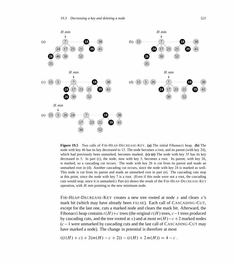
19.3 Decreasing a key and deleting a node 521
17
30
24 23
26
35
15 7
21
18
52
38
39 41
(b)
17
30
24 23
26
515 7
21
18
52
38
39 41
(c)
17
30
24 23
26515 7
21
18
52
38
39 41
(d)
17
30
24
23
26515 7
21
18
52
38
39 41
(e)
17
30
24 23
26
35
46
7
21
18
52
38
39 41
(a)
H:min
H:min
H:minH:min
H:min
Figure 19.5 Two calls of FIB-HEAP-DECREASE-KEY. (a) The initial Fibonacci heap. (b) Thenode with key 46 has its key decreased to 15. The node becomes a root, and its parent (with key 24),which had previously been unmarked, becomes marked. (c)–(e) The node with key 35 has its keydecreased to 5. In part (c), the node, now with key 5, becomes a root. Its parent, with key 26,is marked, so a cascading cut occurs. The node with key 26 is cut from its parent and made anunmarked root in (d). Another cascading cut occurs, since the node with key 24 is marked as well.This node is cut from its parent and made an unmarked root in part (e). The cascading cuts stopat this point, since the node with key 7 is a root. (Even if this node were not a root, the cascadingcuts would stop, since it is unmarked.) Part (e) shows the result of the FIB-HEAP-DECREASE-KEY
operation, with H:min pointing to the new minimum node.
FIB-HEAP-DECREASE-KEY creates a new tree rooted at node x and clears x’smark bit (which may have already been FALSE). Each call of CASCADING-CUT,except for the last one, cuts a marked node and clears the mark bit. Afterward, theFibonacci heap contains t.H/Cc trees (the original t.H/ trees, c�1 trees producedby cascading cuts, and the tree rooted at x) and at most m.H/�cC2 marked nodes(c�1 were unmarked by cascading cuts and the last call of CASCADING-CUT mayhave marked a node). The change in potential is therefore at most
..t.H/C c/C 2.m.H/ � c C 2// � .t.H/C 2 m.H// D 4 � c :
522 Chapter 19 Fibonacci Heaps
Thus, the amortized cost of FIB-HEAP-DECREASE-KEY is at most
O.c/C 4� c D O.1/ ;
since we can scale up the units of potential to dominate the constant hidden in O.c/.You can now see why we defined the potential function to include a term that is
twice the number of marked nodes. When a marked node y is cut by a cascadingcut, its mark bit is cleared, which reduces the potential by 2. One unit of potentialpays for the cut and the clearing of the mark bit, and the other unit compensatesfor the unit increase in potential due to node y becoming a root.
Deleting a node
The following pseudocode deletes a node from an n-node Fibonacci heap inO.D.n// amortized time. We assume that there is no key value of �1 currentlyin the Fibonacci heap.
FIB-HEAP-DELETE.H; x/
1 FIB-HEAP-DECREASE-KEY.H; x;�1/
2 FIB-HEAP-EXTRACT-MIN.H/
FIB-HEAP-DELETE makes x become the minimum node in the Fibonacci heap bygiving it a uniquely small key of �1. The FIB-HEAP-EXTRACT-MIN procedurethen removes node x from the Fibonacci heap. The amortized time of FIB-HEAP-DELETE is the sum of the O.1/ amortized time of FIB-HEAP-DECREASE-KEY
and the O.D.n// amortized time of FIB-HEAP-EXTRACT-MIN. Since we shall seein Section 19.4 that D.n/ D O.lg n/, the amortized time of FIB-HEAP-DELETE
is O.lg n/.
Exercises
19.3-1Suppose that a root x in a Fibonacci heap is marked. Explain how x came to bea marked root. Argue that it doesn’t matter to the analysis that x is marked, eventhough it is not a root that was first linked to another node and then lost one child.
19.3-2Justify the O.1/ amortized time of FIB-HEAP-DECREASE-KEY as an average costper operation by using aggregate analysis.
19.4 Bounding the maximum degree 523
19.4 Bounding the maximum degree
To prove that the amortized time of FIB-HEAP-EXTRACT-MIN and FIB-HEAP-DELETE is O.lg n/, we must show that the upper bound D.n/ on the degree ofany node of an n-node Fibonacci heap is O.lg n/. In particular, we shall show thatD.n/ � log� n
˘, where � is the golden ratio, defined in equation (3.24) as
� D .1Cp
5/=2 D 1:61803 : : : :
The key to the analysis is as follows. For each node x within a Fibonacci heap,define size.x/ to be the number of nodes, including x itself, in the subtree rootedat x. (Note that x need not be in the root list—it can be any node at all.) We shallshow that size.x/ is exponential in x:degree. Bear in mind that x:degree is alwaysmaintained as an accurate count of the degree of x.
Lemma 19.1Let x be any node in a Fibonacci heap, and suppose that x:degree D k. Lety1; y2; : : : ; yk denote the children of x in the order in which they were linked to x,from the earliest to the latest. Then, y1:degree � 0 and yi :degree � i � 2 fori D 2; 3; : : : ; k.
Proof Obviously, y1:degree � 0.For i � 2, we note that when yi was linked to x, all of y1; y2; : : : ; yi�1 were
children of x, and so we must have had x:degree � i � 1. Because node yi islinked to x (by CONSOLIDATE) only if x:degree D yi :degree, we must have alsohad yi :degree � i � 1 at that time. Since then, node yi has lost at most onechild, since it would have been cut from x (by CASCADING-CUT) if it had losttwo children. We conclude that yi :degree � i � 2.
We finally come to the part of the analysis that explains the name “Fibonacciheaps.” Recall from Section 3.2 that for k D 0; 1; 2; : : :, the kth Fibonacci numberis defined by the recurrence
Fk D
�0 if k D 0 ;
1 if k D 1 ;
Fk�1 C Fk�2 if k � 2 :
The following lemma gives another way to express Fk .

524 Chapter 19 Fibonacci Heaps
Lemma 19.2For all integers k � 0,
FkC2 D 1CkX
iD0
Fi :
Proof The proof is by induction on k. When k D 0,
1C0X
iD0
Fi D 1C F0
D 1C 0
D F2 :
We now assume the inductive hypothesis that FkC1 D 1 CPk�1
iD0 Fi , and wehave
FkC2 D Fk C FkC1
D Fk C
1Ck�1XiD0
Fi
!
D 1CkX
iD0
Fi :
Lemma 19.3For all integers k � 0, the .k C 2/nd Fibonacci number satisfies FkC2 � �k .
Proof The proof is by induction on k. The base cases are for k D 0 and k D 1.When k D 0 we have F2 D 1 D �0, and when k D 1 we have F3 D 2 >
1:619 > �1. The inductive step is for k � 2, and we assume that FiC2 > �i fori D 0; 1; : : : ; k�1. Recall that � is the positive root of equation (3.23), x2 D xC1.Thus, we have
FkC2 D FkC1 C Fk
� �k�1 C �k�2 (by the inductive hypothesis)
D �k�2.� C 1/
D �k�2 � �2 (by equation (3.23))
D �k :
The following lemma and its corollary complete the analysis.
19.4 Bounding the maximum degree 525
Lemma 19.4Let x be any node in a Fibonacci heap, and let k D x:degree. Then size.x/ �FkC2 � �k , where � D .1Cp5/=2.
Proof Let sk denote the minimum possible size of any node of degree k in anyFibonacci heap. Trivially, s0 D 1 and s1 D 2. The number sk is at most size.x/
and, because adding children to a node cannot decrease the node’s size, the valueof sk increases monotonically with k. Consider some node ´, in any Fibonacciheap, such that ´:degree D k and size.´/ D sk. Because sk � size.x/, wecompute a lower bound on size.x/ by computing a lower bound on sk . As inLemma 19.1, let y1; y2; : : : ; yk denote the children of ´ in the order in which theywere linked to ´. To bound sk , we count one for ´ itself and one for the first child y1
(for which size.y1/ � 1), giving
size.x/ � sk
� 2CkX
iD2
syi : degree
� 2CkX
iD2
si�2 ;
where the last line follows from Lemma 19.1 (so that yi :degree � i � 2) and themonotonicity of sk (so that syi : degree � si�2).
We now show by induction on k that sk � FkC2 for all nonnegative integers k.The bases, for k D 0 and k D 1, are trivial. For the inductive step, we assume thatk � 2 and that si � FiC2 for i D 0; 1; : : : ; k � 1. We have
sk � 2CkX
iD2
si�2
� 2CkX
iD2
Fi
D 1CkX
iD0
Fi
D FkC2 (by Lemma 19.2)
� �k (by Lemma 19.3) .
Thus, we have shown that size.x/ � sk � FkC2 � �k .
526 Chapter 19 Fibonacci Heaps
Corollary 19.5The maximum degree D.n/ of any node in an n-node Fibonacci heap is O.lg n/.
Proof Let x be any node in an n-node Fibonacci heap, and let k D x:degree.By Lemma 19.4, we have n � size.x/ � �k . Taking base-� logarithms givesus k � log� n. (In fact, because k is an integer, k � log� n
˘.) The maximum
degree D.n/ of any node is thus O.lg n/.
Exercises
19.4-1Professor Pinocchio claims that the height of an n-node Fibonacci heap is O.lg n/.Show that the professor is mistaken by exhibiting, for any positive integer n, asequence of Fibonacci-heap operations that creates a Fibonacci heap consisting ofjust one tree that is a linear chain of n nodes.
19.4-2Suppose we generalize the cascading-cut rule to cut a node x from its parent assoon as it loses its kth child, for some integer constant k. (The rule in Section 19.3uses k D 2.) For what values of k is D.n/ D O.lg n/?
Problems
19-1 Alternative implementation of deletionProfessor Pisano has proposed the following variant of the FIB-HEAP-DELETE
procedure, claiming that it runs faster when the node being deleted is not the nodepointed to by H:min.
PISANO-DELETE.H; x/
1 if x == H:min2 FIB-HEAP-EXTRACT-MIN.H/
3 else y D x:p4 if y ¤ NIL
5 CUT.H; x; y/
6 CASCADING-CUT.H; y/
7 add x’s child list to the root list of H
8 remove x from the root list of H

Problems for Chapter 19 527
a. The professor’s claim that this procedure runs faster is based partly on the as-sumption that line 7 can be performed in O.1/ actual time. What is wrong withthis assumption?
b. Give a good upper bound on the actual time of PISANO-DELETE when x isnot H:min. Your bound should be in terms of x:degree and the number c ofcalls to the CASCADING-CUT procedure.
c. Suppose that we call PISANO-DELETE.H; x/, and let H 0 be the Fibonacci heapthat results. Assuming that node x is not a root, bound the potential of H 0 interms of x:degree, c, t.H/, and m.H/.
d. Conclude that the amortized time for PISANO-DELETE is asymptotically nobetter than for FIB-HEAP-DELETE, even when x ¤ H:min.
19-2 Binomial trees and binomial heapsThe binomial tree Bk is an ordered tree (see Section B.5.2) defined recursively.As shown in Figure 19.6(a), the binomial tree B0 consists of a single node. Thebinomial tree Bk consists of two binomial trees Bk�1 that are linked together sothat the root of one is the leftmost child of the root of the other. Figure 19.6(b)shows the binomial trees B0 through B4.
a. Show that for the binomial tree Bk ,
1. there are 2k nodes,
2. the height of the tree is k,
3. there are exactly�
k
i
�nodes at depth i for i D 0; 1; : : : ; k, and
4. the root has degree k, which is greater than that of any other node; moreover,as Figure 19.6(c) shows, if we number the children of the root from left toright by k � 1; k � 2; : : : ; 0, then child i is the root of a subtree Bi .
A binomial heap H is a set of binomial trees that satisfies the following proper-ties:
1. Each node has a key (like a Fibonacci heap).
2. Each binomial tree in H obeys the min-heap property.
3. For any nonnegative integer k, there is at most one binomial tree in H whoseroot has degree k.
b. Suppose that a binomial heap H has a total of n nodes. Discuss the relationshipbetween the binomial trees that H contains and the binary representation of n.Conclude that H consists of at most blg nc C 1 binomial trees.

528 Chapter 19 Fibonacci Heaps
B4
Bk–1Bk–2
Bk
B2B1
B0
B3B2B1B0
Bk
Bk–1Bk–1
B0
(a)
depth
0
1
2
3
4
(b)
(c)
Figure 19.6 (a) The recursive definition of the binomial tree Bk . Triangles represent rooted sub-trees. (b) The binomial trees B0 through B4. Node depths in B4 are shown. (c) Another way oflooking at the binomial tree Bk .
Suppose that we represent a binomial heap as follows. The left-child, right-sibling scheme of Section 10.4 represents each binomial tree within a binomialheap. Each node contains its key; pointers to its parent, to its leftmost child, andto the sibling immediately to its right (these pointers are NIL when appropriate);and its degree (as in Fibonacci heaps, how many children it has). The roots form asingly linked root list, ordered by the degrees of the roots (from low to high), andwe access the binomial heap by a pointer to the first node on the root list.
c. Complete the description of how to represent a binomial heap (i.e., name theattributes, describe when attributes have the value NIL, and define how the rootlist is organized), and show how to implement the same seven operations onbinomial heaps as this chapter implemented on Fibonacci heaps. Each opera-tion should run in O.lg n/ worst-case time, where n is the number of nodes in
Problems for Chapter 19 529
the binomial heap (or in the case of the UNION operation, in the two binomialheaps that are being united). The MAKE-HEAP operation should take constanttime.
d. Suppose that we were to implement only the mergeable-heap operations on aFibonacci heap (i.e., we do not implement the DECREASE-KEY or DELETE op-erations). How would the trees in a Fibonacci heap resemble those in a binomialheap? How would they differ? Show that the maximum degree in an n-nodeFibonacci heap would be at most blg nc.
e. Professor McGee has devised a new data structure based on Fibonacci heaps.A McGee heap has the same structure as a Fibonacci heap and supports justthe mergeable-heap operations. The implementations of the operations are thesame as for Fibonacci heaps, except that insertion and union consolidate theroot list as their last step. What are the worst-case running times of operationson McGee heaps?
19-3 More Fibonacci-heap operationsWe wish to augment a Fibonacci heap H to support two new operations withoutchanging the amortized running time of any other Fibonacci-heap operations.
a. The operation FIB-HEAP-CHANGE-KEY.H; x; k/ changes the key of node x
to the value k. Give an efficient implementation of FIB-HEAP-CHANGE-KEY,and analyze the amortized running time of your implementation for the casesin which k is greater than, less than, or equal to x:key.
b. Give an efficient implementation of FIB-HEAP-PRUNE.H; r/, which deletesq D min.r; H:n/ nodes from H . You may choose any q nodes to delete. Ana-lyze the amortized running time of your implementation. (Hint: You may needto modify the data structure and potential function.)
19-4 2-3-4 heapsChapter 18 introduced the 2-3-4 tree, in which every internal node (other than pos-sibly the root) has two, three, or four children and all leaves have the same depth. Inthis problem, we shall implement 2-3-4 heaps, which support the mergeable-heapoperations.
The 2-3-4 heaps differ from 2-3-4 trees in the following ways. In 2-3-4 heaps,only leaves store keys, and each leaf x stores exactly one key in the attribute x:key.The keys in the leaves may appear in any order. Each internal node x containsa value x:small that is equal to the smallest key stored in any leaf in the subtreerooted at x. The root r contains an attribute r:height that gives the height of the

530 Chapter 19 Fibonacci Heaps
tree. Finally, 2-3-4 heaps are designed to be kept in main memory, so that diskreads and writes are not needed.
Implement the following 2-3-4 heap operations. In parts (a)–(e), each operationshould run in O.lg n/ time on a 2-3-4 heap with n elements. The UNION operationin part (f) should run in O.lg n/ time, where n is the number of elements in the twoinput heaps.
a. MINIMUM, which returns a pointer to the leaf with the smallest key.
b. DECREASE-KEY, which decreases the key of a given leaf x to a given valuek � x:key.
c. INSERT, which inserts leaf x with key k.
d. DELETE, which deletes a given leaf x.
e. EXTRACT-MIN, which extracts the leaf with the smallest key.
f. UNION, which unites two 2-3-4 heaps, returning a single 2-3-4 heap and de-stroying the input heaps.
Chapter notes
Fredman and Tarjan [114] introduced Fibonacci heaps. Their paper also describesthe application of Fibonacci heaps to the problems of single-source shortest paths,all-pairs shortest paths, weighted bipartite matching, and the minimum-spanning-tree problem.
Subsequently, Driscoll, Gabow, Shrairman, and Tarjan [97] developed “relaxedheaps” as an alternative to Fibonacci heaps. They devised two varieties of re-laxed heaps. One gives the same amortized time bounds as Fibonacci heaps. Theother allows DECREASE-KEY to run in O.1/ worst-case (not amortized) time andEXTRACT-MIN and DELETE to run in O.lg n/ worst-case time. Relaxed heapsalso have some advantages over Fibonacci heaps in parallel algorithms.
See also the chapter notes for Chapter 6 for other data structures that support fastDECREASE-KEY operations when the sequence of values returned by EXTRACT-MIN calls are monotonically increasing over time and the data are integers in aspecific range.
20 van Emde Boas Trees
In previous chapters, we saw data structures that support the operations of a priorityqueue—binary heaps in Chapter 6, red-black trees in Chapter 13,1 and Fibonacciheaps in Chapter 19. In each of these data structures, at least one important op-eration took O.lg n/ time, either worst case or amortized. In fact, because eachof these data structures bases its decisions on comparing keys, the �.n lg n/ lowerbound for sorting in Section 8.1 tells us that at least one operation will have totake �.lg n/ time. Why? If we could perform both the INSERT and EXTRACT-MIN
operations in o.lg n/ time, then we could sort n keys in o.n lg n/ time by first per-forming n INSERT operations, followed by n EXTRACT-MIN operations.
We saw in Chapter 8, however, that sometimes we can exploit additional infor-mation about the keys to sort in o.n lg n/ time. In particular, with counting sortwe can sort n keys, each an integer in the range 0 to k, in time ‚.n C k/, whichis ‚.n/ when k D O.n/.
Since we can circumvent the �.n lg n/ lower bound for sorting when the keys areintegers in a bounded range, you might wonder whether we can perform each of thepriority-queue operations in o.lg n/ time in a similar scenario. In this chapter, weshall see that we can: van Emde Boas trees support the priority-queue operations,and a few others, each in O.lg lg n/ worst-case time. The hitch is that the keysmust be integers in the range 0 to n � 1, with no duplicates allowed.
Specifically, van Emde Boas trees support each of the dynamic set operationslisted on page 230—SEARCH, INSERT, DELETE, MINIMUM, MAXIMUM, SUC-CESSOR, and PREDECESSOR—in O.lg lg n/ time. In this chapter, we will omitdiscussion of satellite data and focus only on storing keys. Because we concentrateon keys and disallow duplicate keys to be stored, instead of describing the SEARCH
1Chapter 13 does not explicitly discuss how to implement EXTRACT-MIN and DECREASE-KEY, butwe can easily build these operations for any data structure that supports MINIMUM, DELETE, andINSERT.
532 Chapter 20 van Emde Boas Trees
operation, we will implement the simpler operation MEMBER.S; x/, which returnsa boolean indicating whether the value x is currently in dynamic set S .
So far, we have used the parameter n for two distinct purposes: the number ofelements in the dynamic set, and the range of the possible values. To avoid anyfurther confusion, from here on we will use n to denote the number of elementscurrently in the set and u as the range of possible values, so that each van EmdeBoas tree operation runs in O.lg lg u/ time. We call the set f0; 1; 2; : : : ; u � 1gthe universe of values that can be stored and u the universe size. We assumethroughout this chapter that u is an exact power of 2, i.e., u D 2k for some integerk � 1.
Section 20.1 starts us out by examining some simple approaches that will getus going in the right direction. We enhance these approaches in Section 20.2,introducing proto van Emde Boas structures, which are recursive but do not achieveour goal of O.lg lg u/-time operations. Section 20.3 modifies proto van Emde Boasstructures to develop van Emde Boas trees, and it shows how to implement eachoperation in O.lg lg u/ time.
20.1 Preliminary approaches
In this section, we shall examine various approaches for storing a dynamic set.Although none will achieve the O.lg lg u/ time bounds that we desire, we will gaininsights that will help us understand van Emde Boas trees when we see them laterin this chapter.
Direct addressing
Direct addressing, as we saw in Section 11.1, provides the simplest approach tostoring a dynamic set. Since in this chapter we are concerned only with storingkeys, we can simplify the direct-addressing approach to store the dynamic set as abit vector, as discussed in Exercise 11.1-2. To store a dynamic set of values fromthe universe f0; 1; 2; : : : ; u � 1g, we maintain an array AŒ0 : : u � 1� of u bits. Theentry AŒx� holds a 1 if the value x is in the dynamic set, and it holds a 0 otherwise.Although we can perform each of the INSERT, DELETE, and MEMBER operationsin O.1/ time with a bit vector, the remaining operations—MINIMUM, MAXIMUM,SUCCESSOR, and PREDECESSOR—each take ‚.u/ time in the worst case because

20.1 Preliminary approaches 533
0
0
0
1
1
2
1
3
1
4
1
5
0
6
1
7
0
8
0
9
0
10
0
11
0
12
0
13
1
14
1
15
0 1 1 1 0 0 0 1
1 1 0 1
1 1
1
A
Figure 20.1 A binary tree of bits superimposed on top of a bit vector representing the setf2; 3; 4; 5; 7; 14; 15g when u D 16. Each internal node contains a 1 if and only if some leaf inits subtree contains a 1. The arrows show the path followed to determine the predecessor of 14 in theset.
we might have to scan through ‚.u/ elements.2 For example, if a set contains onlythe values 0 and u � 1, then to find the successor of 0, we would have to scanentries 1 through u � 2 before finding a 1 in AŒu � 1�.
Superimposing a binary tree structure
We can short-cut long scans in the bit vector by superimposing a binary tree of bitson top of it. Figure 20.1 shows an example. The entries of the bit vector form theleaves of the binary tree, and each internal node contains a 1 if and only if any leafin its subtree contains a 1. In other words, the bit stored in an internal node is thelogical-or of its two children.
The operations that took ‚.u/ worst-case time with an unadorned bit vector nowuse the tree structure:
� To find the minimum value in the set, start at the root and head down towardthe leaves, always taking the leftmost node containing a 1.
� To find the maximum value in the set, start at the root and head down towardthe leaves, always taking the rightmost node containing a 1.
2We assume throughout this chapter that MINIMUM and MAXIMUM return NIL if the dynamic setis empty and that SUCCESSOR and PREDECESSOR return NIL if the element they are given has nosuccessor or predecessor, respectively.

534 Chapter 20 van Emde Boas Trees
� To find the successor of x, start at the leaf indexed by x, and head up toward theroot until we enter a node from the left and this node has a 1 in its right child ´.Then head down through node ´, always taking the leftmost node containinga 1 (i.e., find the minimum value in the subtree rooted at the right child ´).
� To find the predecessor of x, start at the leaf indexed by x, and head up towardthe root until we enter a node from the right and this node has a 1 in its leftchild ´. Then head down through node ´, always taking the rightmost nodecontaining a 1 (i.e., find the maximum value in the subtree rooted at the leftchild ´).
Figure 20.1 shows the path taken to find the predecessor, 7, of the value 14.We also augment the INSERT and DELETE operations appropriately. When in-
serting a value, we store a 1 in each node on the simple path from the appropriateleaf up to the root. When deleting a value, we go from the appropriate leaf up tothe root, recomputing the bit in each internal node on the path as the logical-or ofits two children.
Since the height of the tree is lg u and each of the above operations makes atmost one pass up the tree and at most one pass down, each operation takes O.lg u/
time in the worst case.This approach is only marginally better than just using a red-black tree. We can
still perform the MEMBER operation in O.1/ time, whereas searching a red-blacktree takes O.lg n/ time. Then again, if the number n of elements stored is muchsmaller than the size u of the universe, a red-black tree would be faster for all theother operations.
Superimposing a tree of constant height
What happens if we superimpose a tree with greater degree? Let us assume thatthe size of the universe is u D 22k for some integer k, so that
pu is an integer.
Instead of superimposing a binary tree on top of the bit vector, we superimpose atree of degree
pu. Figure 20.2(a) shows such a tree for the same bit vector as in
Figure 20.1. The height of the resulting tree is always 2.As before, each internal node stores the logical-or of the bits within its sub-
tree, so that thep
u internal nodes at depth 1 summarize each group ofp
u val-ues. As Figure 20.2(b) demonstrates, we can think of these nodes as an arraysummaryŒ0 : :
pu � 1�, where summaryŒi � contains a 1 if and only if the subar-
ray AŒip
u : : .i C 1/p
u � 1� contains a 1. We call thisp
u-bit subarray of A
the i th cluster. For a given value of x, the bit AŒx� appears in cluster num-ber bx=
puc. Now INSERT becomes an O.1/-time operation: to insert x, set
both AŒx� and summaryŒbx=p
uc� to 1. We can use the summary array to perform

20.1 Preliminary approaches 535
0
0
0
1
1
2
1
3
1
4
1
5
0
6
1
7
0
8
0
9
0
10
0
11
0
12
0
13
1
14
1
15
1
1
1 0 1
(a)
0
0
0
1
1
2
1
3
1
4
1
5
0
6
1
7
0
8
0
9
0
10
0
11
0
12
0
13
1
14
1
15
(b)
1
0
1
1
0
2
1
3
AA
summary
pu bits
pu bits
Figure 20.2 (a) A tree of degreep
u superimposed on top of the same bit vector as in Figure 20.1.Each internal node stores the logical-or of the bits in its subtree. (b) A view of the same structure,but with the internal nodes at depth 1 treated as an array summaryŒ0 : :
pu� 1�, where summaryŒi � is
the logical-or of the subarray AŒip
u : : .i C 1/p
u � 1�.
each of the operations MINIMUM, MAXIMUM, SUCCESSOR, PREDECESSOR, andDELETE in O.
pu/ time:
� To find the minimum (maximum) value, find the leftmost (rightmost) entry insummary that contains a 1, say summaryŒi �, and then do a linear search withinthe i th cluster for the leftmost (rightmost) 1.
� To find the successor (predecessor) of x, first search to the right (left) within itscluster. If we find a 1, that position gives the result. Otherwise, let i D bx=
puc
and search to the right (left) within the summary array from index i . The firstposition that holds a 1 gives the index of a cluster. Search within that clusterfor the leftmost (rightmost) 1. That position holds the successor (predecessor).
� To delete the value x, let i D bx=p
uc�. Set AŒx� to 0 and then set summaryŒi �
to the logical-or of the bits in the i th cluster.
In each of the above operations, we search through at most two clusters ofp
u bitsplus the summary array, and so each operation takes O.
pu/ time.
At first glance, it seems as though we have made negative progress. Superimpos-ing a binary tree gave us O.lg u/-time operations, which are asymptotically fasterthan O.
pu/ time. Using a tree of degree
pu will turn out to be a key idea of van
Emde Boas trees, however. We continue down this path in the next section.
Exercises
20.1-1Modify the data structures in this section to support duplicate keys.
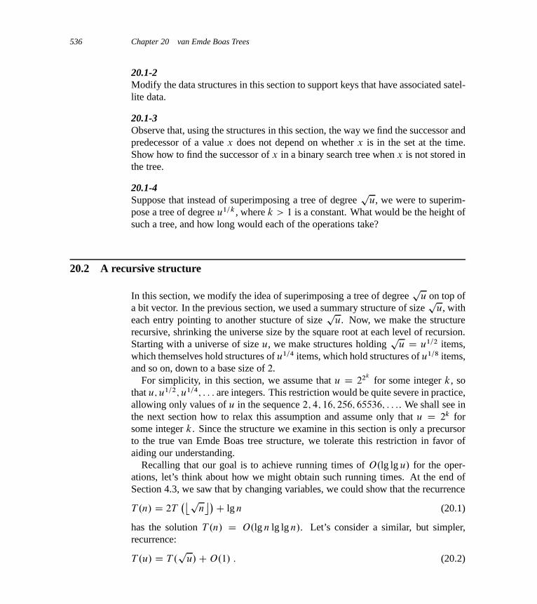
536 Chapter 20 van Emde Boas Trees
20.1-2Modify the data structures in this section to support keys that have associated satel-lite data.
20.1-3Observe that, using the structures in this section, the way we find the successor andpredecessor of a value x does not depend on whether x is in the set at the time.Show how to find the successor of x in a binary search tree when x is not stored inthe tree.
20.1-4Suppose that instead of superimposing a tree of degree
pu, we were to superim-
pose a tree of degree u1=k , where k > 1 is a constant. What would be the height ofsuch a tree, and how long would each of the operations take?
20.2 A recursive structure
In this section, we modify the idea of superimposing a tree of degreep
u on top ofa bit vector. In the previous section, we used a summary structure of size
pu, with
each entry pointing to another stucture of sizep
u. Now, we make the structurerecursive, shrinking the universe size by the square root at each level of recursion.Starting with a universe of size u, we make structures holding
pu D u1=2 items,
which themselves hold structures of u1=4 items, which hold structures of u1=8 items,and so on, down to a base size of 2.
For simplicity, in this section, we assume that u D 22k
for some integer k, sothat u; u1=2; u1=4; : : : are integers. This restriction would be quite severe in practice,allowing only values of u in the sequence 2; 4; 16; 256; 65536; : : :. We shall see inthe next section how to relax this assumption and assume only that u D 2k forsome integer k. Since the structure we examine in this section is only a precursorto the true van Emde Boas tree structure, we tolerate this restriction in favor ofaiding our understanding.
Recalling that our goal is to achieve running times of O.lg lg u/ for the oper-ations, let’s think about how we might obtain such running times. At the end ofSection 4.3, we saw that by changing variables, we could show that the recurrence
T .n/ D 2T� p
n˘�C lg n (20.1)
has the solution T .n/ D O.lg n lg lg n/. Let’s consider a similar, but simpler,recurrence:
T .u/ D T .p
u/CO.1/ : (20.2)
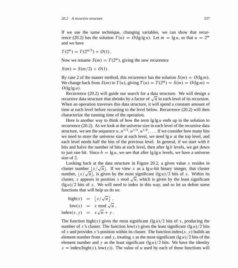
20.2 A recursive structure 537
If we use the same technique, changing variables, we can show that recur-rence (20.2) has the solution T .u/ D O.lg lg u/. Let m D lg u, so that u D 2m
and we have
T .2m/ D T .2m=2/CO.1/ :
Now we rename S.m/ D T .2m/, giving the new recurrence
S.m/ D S.m=2/CO.1/ :
By case 2 of the master method, this recurrence has the solution S.m/ D O.lg m/.We change back from S.m/ to T .u/, giving T .u/ D T .2m/ D S.m/ D O.lg m/ DO.lg lg u/.
Recurrence (20.2) will guide our search for a data structure. We will design arecursive data structure that shrinks by a factor of
pu in each level of its recursion.
When an operation traverses this data structure, it will spend a constant amount oftime at each level before recursing to the level below. Recurrence (20.2) will thencharacterize the running time of the operation.
Here is another way to think of how the term lg lg u ends up in the solution torecurrence (20.2). As we look at the universe size in each level of the recursive datastructure, we see the sequence u; u1=2; u1=4; u1=8; : : :. If we consider how many bitswe need to store the universe size at each level, we need lg u at the top level, andeach level needs half the bits of the previous level. In general, if we start with b
bits and halve the number of bits at each level, then after lg b levels, we get downto just one bit. Since b D lg u, we see that after lg lg u levels, we have a universesize of 2.
Looking back at the data structure in Figure 20.2, a given value x resides incluster number bx=
puc. If we view x as a lg u-bit binary integer, that cluster
number, bx=p
uc, is given by the most significant .lg u/=2 bits of x. Within itscluster, x appears in position x mod
pu, which is given by the least significant
.lg u/=2 bits of x. We will need to index in this way, and so let us define somefunctions that will help us do so:
high.x/ D x=p
u˘
;
low.x/ D x modp
u ;
index.x; y/ D xp
uC y :
The function high.x/ gives the most significant .lg u/=2 bits of x, producing thenumber of x’s cluster. The function low.x/ gives the least significant .lg u/=2 bitsof x and provides x’s position within its cluster. The function index.x; y/ builds anelement number from x and y, treating x as the most significant .lg u/=2 bits of theelement number and y as the least significant .lg u/=2 bits. We have the identityx D index.high.x/; low.x//. The value of u used by each of these functions will

538 Chapter 20 van Emde Boas Trees
…0 1 2 3p
u � 1proto-�EB.u/
u summary cluster
proto-�EB.p
u/ structure pu proto-�EB.
pu/ structures
Figure 20.3 The information in a proto-�EB.u/ structure when u � 4. The structure contains theuniverse size u, a pointer summary to a proto-�EB.
pu/ structure, and an array clusterŒ0 : :
pu � 1�
ofp
u pointers to proto-�EB.p
u/ structures.
always be the universe size of the data structure in which we call the function,which changes as we descend into the recursive structure.
20.2.1 Proto van Emde Boas structures
Taking our cue from recurrence (20.2), let us design a recursive data structure tosupport the operations. Although this data structure will fail to achieve our goal ofO.lg lg u/ time for some operations, it serves as a basis for the van Emde Boas treestructure that we will see in Section 20.3.
For the universe f0; 1; 2; : : : ; u � 1g, we define a proto van Emde Boas struc-ture, or proto-vEB structure, which we denote as proto-�EB.u/, recursively asfollows. Each proto-�EB.u/ structure contains an attribute u giving its universesize. In addition, it contains the following:
� If u D 2, then it is the base size, and it contains an array AŒ0 : : 1� of two bits.
� Otherwise, u D 22k
for some integer k � 1, so that u � 4. In additionto the universe size u, the data structure proto-�EB.u/ contains the followingattributes, illustrated in Figure 20.3:
� a pointer named summary to a proto-�EB.p
u/ structure and� an array clusterŒ0 : :
pu�1� of
pu pointers, each to a proto-�EB.
pu/ struc-
ture.
The element x, where 0 � x < u, is recursively stored in the cluster numberedhigh.x/ as element low.x/ within that cluster.
In the two-level structure of the previous section, each node stores a summaryarray of size
pu, in which each entry contains a bit. From the index of each
entry, we can compute the starting index of the subarray of sizep
u that the bitsummarizes. In the proto-vEB structure, we use explicit pointers rather than index
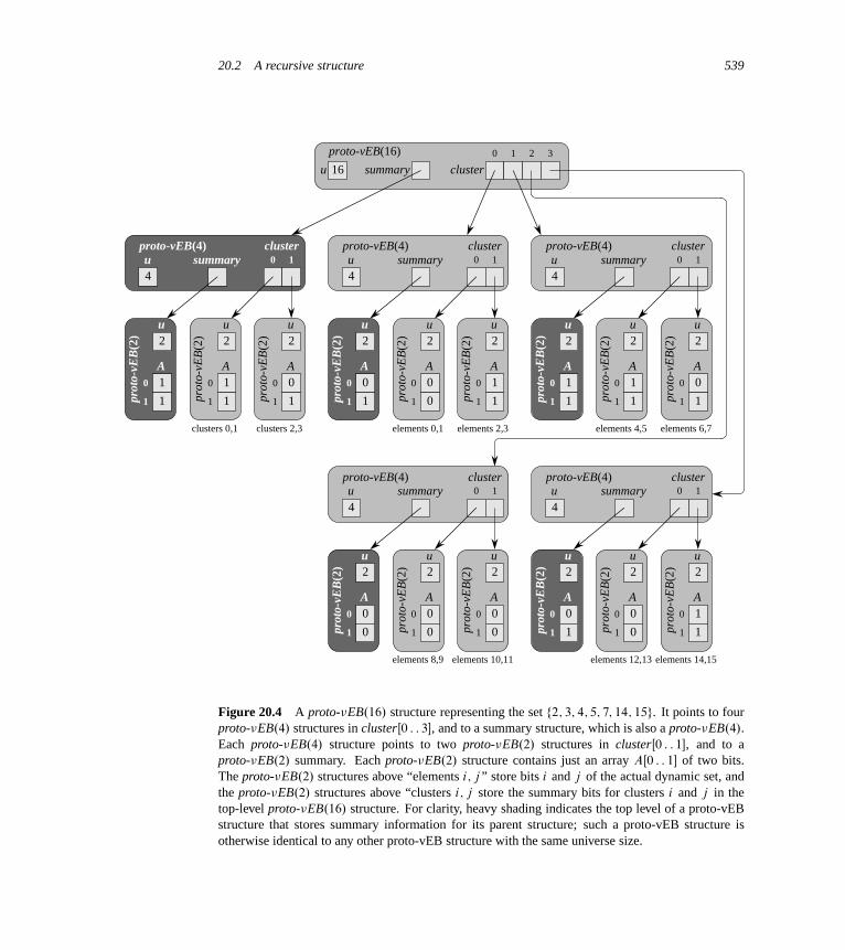
20.2 A recursive structure 539
0 1 2 3
clusteru 16 summary
proto-vEB(16)
0 1cluster
u4
summaryproto-vEB(4)
0
1
A
prot
o-vE
B(2
)
1
1
0 1cluster
u4
summaryproto-vEB(4)
0 1cluster
u4
summaryproto-vEB(4)
0 1cluster
u4
summaryproto-vEB(4)
0 1cluster
u4
summaryproto-vEB(4)
elements 0,1 elements 2,3clusters 0,1 clusters 2,3 elements 4,5 elements 6,7
elements 8,9 elements 10,11 elements 12,13 elements 14,15
u2
0
1
A
prot
o-vE
B(2
)
1
1
u2
0
1
Apr
oto-
vEB
(2)
0
0
u2
0
1
A
prot
o-vE
B(2
)
0
1
u2
0
1
A
prot
o-vE
B(2
)
0
0
u2
0
1
A
prot
o-vE
B(2
)
0
0
u2
0
1
A
prot
o-vE
B(2
)
0
0
u2
0
1
A
prot
o-vE
B(2
)
0
1
u2
0
1
A
prot
o-vE
B(2
)
1
1
u2
0
1
A
prot
o-vE
B(2
)
1
1
u2
0
1
A
prot
o-vE
B(2
)
1
1
u2
0
1
A
prot
o-vE
B(2
)
0
0
u2
0
1
A
prot
o-vE
B(2
)
0
1
u2
0
1
A
prot
o-vE
B(2
)
0
1
u2
0
1
A
prot
o-vE
B(2
)
1
1
u2
Figure 20.4 A proto-�EB.16/ structure representing the set f2; 3; 4; 5; 7; 14; 15g. It points to fourproto-�EB.4/ structures in clusterŒ0 : : 3�, and to a summary structure, which is also a proto-�EB.4/.Each proto-�EB.4/ structure points to two proto-�EB.2/ structures in clusterŒ0 : : 1�, and to aproto-�EB.2/ summary. Each proto-�EB.2/ structure contains just an array AŒ0 : : 1� of two bits.The proto-�EB.2/ structures above “elements i; j ” store bits i and j of the actual dynamic set, andthe proto-�EB.2/ structures above “clusters i; j store the summary bits for clusters i and j in thetop-level proto-�EB.16/ structure. For clarity, heavy shading indicates the top level of a proto-vEBstructure that stores summary information for its parent structure; such a proto-vEB structure isotherwise identical to any other proto-vEB structure with the same universe size.
540 Chapter 20 van Emde Boas Trees
calculations. The array summary contains the summary bits stored recursively in aproto-vEB structure, and the array cluster contains
pu pointers.
Figure 20.4 shows a fully expanded proto-�EB.16/ structure representing theset f2; 3; 4; 5; 7; 14; 15g. If the value i is in the proto-vEB structure pointed to bysummary, then the i th cluster contains some value in the set being represented.As in the tree of constant height, clusterŒi � represents the values i
pu through
.i C 1/p
u � 1, which form the i th cluster.At the base level, the elements of the actual dynamic sets are stored in some
of the proto-�EB.2/ structures, and the remaining proto-�EB.2/ structures storesummary bits. Beneath each of the non-summary base structures, the figure in-dicates which bits it stores. For example, the proto-�EB.2/ structure labeled“elements 6,7” stores bit 6 (0, since element 6 is not in the set) in its AŒ0� andbit 7 (1, since element 7 is in the set) in its AŒ1�.
Like the clusters, each summary is just a dynamic set with universe sizep
u ,and so we represent each summary as a proto-�EB.
pu/ structure. The four sum-
mary bits for the main proto-�EB.16/ structure are in the leftmost proto-�EB.4/
structure, and they ultimately appear in two proto-�EB.2/ structures. For exam-ple, the proto-�EB.2/ structure labeled “clusters 2,3” has AŒ0� D 0, indicating thatcluster 2 of the proto-�EB.16/ structure (containing elements 8; 9; 10; 11) is all 0,and AŒ1� D 1, telling us that cluster 3 (containing elements 12; 13; 14; 15) has atleast one 1. Each proto-�EB.4/ structure points to its own summary, which is itselfstored as a proto-�EB.2/ structure. For example, look at the proto-�EB.2/ struc-ture just to the left of the one labeled “elements 0,1.” Because its AŒ0� is 0, it tellsus that the “elements 0,1” structure is all 0, and because its AŒ1� is 1, we know thatthe “elements 2,3” structure contains at least one 1.
20.2.2 Operations on a proto van Emde Boas structure
We shall now describe how to perform operations on a proto-vEB structure.We first examine the query operations—MEMBER, MINIMUM, MAXIMUM, andSUCCESSOR—which do not change the proto-vEB structure. We then discussINSERT and DELETE. We leave MAXIMUM and PREDECESSOR, which are sym-metric to MINIMUM and SUCCESSOR, respectively, as Exercise 20.2-1.
Each of the MEMBER, SUCCESSOR, PREDECESSOR, INSERT, and DELETE op-erations takes a parameter x, along with a proto-vEB structure V . Each of theseoperations assumes that 0 � x < V:u.
Determining whether a value is in the set
To perform MEMBER.x/, we need to find the bit corresponding to x within theappropriate proto-�EB.2/ structure. We can do so in O.lg lg u/ time, bypassing
20.2 A recursive structure 541
the summary structures altogether. The following procedure takes a proto-�EBstructure V and a value x, and it returns a bit indicating whether x is in the dynamicset held by V .
PROTO-VEB-MEMBER.V; x/
1 if V:u == 2
2 return V:AŒx�
3 else return PROTO-VEB-MEMBER.V:clusterŒhigh.x/�; low.x//
The PROTO-VEB-MEMBER procedure works as follows. Line 1 tests whetherwe are in a base case, where V is a proto-�EB.2/ structure. Line 2 handles thebase case, simply returning the appropriate bit of array A. Line 3 deals with therecursive case, “drilling down” into the appropriate smaller proto-vEB structure.The value high.x/ says which proto-�EB.
pu/ structure we visit, and low.x/ de-
termines which element within that proto-�EB.p
u/ structure we are querying.Let’s see what happens when we call PROTO-VEB-MEMBER.V; 6/ on the
proto-�EB.16/ structure in Figure 20.4. Since high.6/ D 1 when u D 16, werecurse into the proto-�EB.4/ structure in the upper right, and we ask about ele-ment low.6/ D 2 of that structure. In this recursive call, u D 4, and so we recurseagain. With u D 4, we have high.2/ D 1 and low.2/ D 0, and so we ask aboutelement 0 of the proto-�EB.2/ structure in the upper right. This recursive call turnsout to be a base case, and so it returns AŒ0� D 0 back up through the chain of re-cursive calls. Thus, we get the result that PROTO-VEB-MEMBER.V; 6/ returns 0,indicating that 6 is not in the set.
To determine the running time of PROTO-VEB-MEMBER, let T .u/ denoteits running time on a proto-�EB.u/ structure. Each recursive call takes con-stant time, not including the time taken by the recursive calls that it makes.When PROTO-VEB-MEMBER makes a recursive call, it makes a call on aproto-�EB.
pu/ structure. Thus, we can characterize the running time by the recur-
rence T .u/ D T .p
u/CO.1/, which we have already seen as recurrence (20.2).Its solution is T .u/ D O.lg lg u/, and so we conclude that PROTO-VEB-MEMBER
runs in time O.lg lg u/.
Finding the minimum element
Now we examine how to perform the MINIMUM operation. The procedurePROTO-VEB-MINIMUM.V / returns the minimum element in the proto-vEB struc-ture V , or NIL if V represents an empty set.

542 Chapter 20 van Emde Boas Trees
PROTO-VEB-MINIMUM.V /
1 if V:u == 2
2 if V:AŒ0� == 1
3 return 0
4 elseif V:AŒ1� == 1
5 return 1
6 else return NIL
7 else min-cluster D PROTO-VEB-MINIMUM.V:summary/
8 if min-cluster == NIL
9 return NIL
10 else offset D PROTO-VEB-MINIMUM.V:clusterŒmin-cluster�/
11 return index.min-cluster; offset/
This procedure works as follows. Line 1 tests for the base case, which lines 2–6handle by brute force. Lines 7–11 handle the recursive case. First, line 7 finds thenumber of the first cluster that contains an element of the set. It does so by recur-sively calling PROTO-VEB-MINIMUM on V:summary, which is a proto-�EB.
pu/
structure. Line 7 assigns this cluster number to the variable min-cluster. If the setis empty, then the recursive call returned NIL, and line 9 returns NIL. Otherwise,the minimum element of the set is somewhere in cluster number min-cluster. Therecursive call in line 10 finds the offset within the cluster of the minimum elementin this cluster. Finally, line 11 constructs the value of the minimum element fromthe cluster number and offset, and it returns this value.
Although querying the summary information allows us to quickly find the clus-ter containing the minimum element, because this procedure makes two recursivecalls on proto-�EB.
pu/ structures, it does not run in O.lg lg u/ time in the worst
case. Letting T .u/ denote the worst-case time for PROTO-VEB-MINIMUM on aproto-�EB.u/ structure, we have the recurrence
T .u/ D 2T .p
u/CO.1/ : (20.3)
Again, we use a change of variables to solve this recurrence, letting m D lg u,which gives
T .2m/ D 2T .2m=2/CO.1/ :
Renaming S.m/ D T .2m/ gives
S.m/ D 2S.m=2/CO.1/ ;
which, by case 1 of the master method, has the solution S.m/ D ‚.m/. By chang-ing back from S.m/ to T .u/, we have that T .u/ D T .2m/ D S.m/ D ‚.m/ D‚.lg u/. Thus, we see that because of the second recursive call, PROTO-VEB-MINIMUM runs in ‚.lg u/ time rather than the desired O.lg lg u/ time.
20.2 A recursive structure 543
Finding the successor
The SUCCESSOR operation is even worse. In the worst case, it makes two recursivecalls, along with a call to PROTO-VEB-MINIMUM. The procedure PROTO-VEB-SUCCESSOR.V; x/ returns the smallest element in the proto-vEB structure V thatis greater than x, or NIL if no element in V is greater than x. It does not require x
to be a member of the set, but it does assume that 0 � x < V:u.
PROTO-VEB-SUCCESSOR.V; x/
1 if V:u == 2
2 if x == 0 and V:AŒ1� == 1
3 return 1
4 else return NIL
5 else offset D PROTO-VEB-SUCCESSOR.V:clusterŒhigh.x/�; low.x//
6 if offset ¤ NIL
7 return index.high.x/; offset/8 else succ-cluster D PROTO-VEB-SUCCESSOR.V:summary; high.x//
9 if succ-cluster == NIL
10 return NIL
11 else offset D PROTO-VEB-MINIMUM.V:clusterŒsucc-cluster�/
12 return index.succ-cluster; offset/
The PROTO-VEB-SUCCESSOR procedure works as follows. As usual, line 1tests for the base case, which lines 2–4 handle by brute force: the only way that x
can have a successor within a proto-�EB.2/ structure is when x D 0 and AŒ1�
is 1. Lines 5–12 handle the recursive case. Line 5 searches for a successor to x
within x’s cluster, assigning the result to offset. Line 6 determines whether x hasa successor within its cluster; if it does, then line 7 computes and returns the valueof this successor. Otherwise, we have to search in other clusters. Line 8 assigns tosucc-cluster the number of the next nonempty cluster, using the summary informa-tion to find it. Line 9 tests whether succ-cluster is NIL, with line 10 returning NIL
if all succeeding clusters are empty. If succ-cluster is non-NIL, line 11 assignsthe first element within that cluster to offset, and line 12 computes and returns theminimum element in that cluster.
In the worst case, PROTO-VEB-SUCCESSOR calls itself recursively twice onproto-�EB.
pu/ structures, and it makes one call to PROTO-VEB-MINIMUM on
a proto-�EB.p
u/ structure. Thus, the recurrence for the worst-case runningtime T .u/ of PROTO-VEB-SUCCESSOR is
T .u/ D 2T .p
u/C‚.lgp
u/
D 2T .p
u/C‚.lg u/ :

544 Chapter 20 van Emde Boas Trees
We can the same technique that we used for recurrence (20.1) to show thatthis recurrence has the solution T .u/ D ‚.lg u lg lg u/. Thus, PROTO-VEB-SUCCESSOR is asymptotically slower than PROTO-VEB-MINIMUM.
Inserting an element
To insert an element, we need to insert it into the appropriate cluster and also setthe summary bit for that cluster to 1. The procedure PROTO-VEB-INSERT.V; x/
inserts the value x into the proto-vEB structure V .
PROTO-VEB-INSERT.V; x/
1 if V:u == 2
2 V:AŒx� D 1
3 else PROTO-VEB-INSERT.V:clusterŒhigh.x/�; low.x//
4 PROTO-VEB-INSERT.V:summary; high.x//
In the base case, line 2 sets the appropriate bit in the array A to 1. In the recursivecase, the recursive call in line 3 inserts x into the appropriate cluster, and line 4sets the summary bit for that cluster to 1.
Because PROTO-VEB-INSERT makes two recursive calls in the worst case, re-currence (20.3) characterizes its running time. Hence, PROTO-VEB-INSERT runsin ‚.lg u/ time.
Deleting an element
The DELETE operation is more complicated than insertion. Whereas we can alwaysset a summary bit to 1 when inserting, we cannot always reset the same summarybit to 0 when deleting. We need to determine whether any bit in the appropriatecluster is 1. As we have defined proto-vEB structures, we would have to examineallp
u bits within a cluster to determine whether any of them are 1. Alternatively,we could add an attribute n to the proto-vEB structure, counting how many el-ements it has. We leave implementation of PROTO-VEB-DELETE as Exercises20.2-2 and 20.2-3.
Clearly, we need to modify the proto-vEB structure to get each operation downto making at most one recursive call. We will see in the next section how to do so.
Exercises
20.2-1Write pseudocode for the procedures PROTO-VEB-MAXIMUM and PROTO-VEB-PREDECESSOR.
20.3 The van Emde Boas tree 545
20.2-2Write pseudocode for PROTO-VEB-DELETE. It should update the appropriatesummary bit by scanning the related bits within the cluster. What is the worst-case running time of your procedure?
20.2-3Add the attribute n to each proto-vEB structure, giving the number of elementscurrently in the set it represents, and write pseudocode for PROTO-VEB-DELETE
that uses the attribute n to decide when to reset summary bits to 0. What is theworst-case running time of your procedure? What other procedures need to changebecause of the new attribute? Do these changes affect their running times?
20.2-4Modify the proto-vEB structure to support duplicate keys.
20.2-5Modify the proto-vEB structure to support keys that have associated satellite data.
20.2-6Write pseudocode for a procedure that creates a proto-�EB.u/ structure.
20.2-7Argue that if line 9 of PROTO-VEB-MINIMUM is executed, then the proto-vEBstructure is empty.
20.2-8Suppose that we designed a proto-vEB structure in which each cluster array hadonly u1=4 elements. What would the running times of each operation be?
20.3 The van Emde Boas tree
The proto-vEB structure of the previous section is close to what we need to achieveO.lg lg u/ running times. It falls short because we have to recurse too many timesin most of the operations. In this section, we shall design a data structure thatis similar to the proto-vEB structure but stores a little more information, therebyremoving the need for some of the recursion.
In Section 20.2, we observed that the assumption that we made about the uni-verse size—that u D 22k
for some integer k—is unduly restrictive, confining thepossible values of u an overly sparse set. From this point on, therefore, we willallow the universe size u to be any exact power of 2, and when
pu is not an inte-
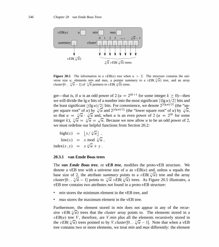
546 Chapter 20 van Emde Boas Trees
…0 1 2 3 "p
u � 1
�EB.u/ u min max
summary cluster
�EB. "p
u/"p
u �EB. #p
u/ trees
Figure 20.5 The information in a �EB.u/ tree when u > 2. The structure contains the uni-verse size u, elements min and max, a pointer summary to a �EB. "
pu/ tree, and an array
clusterŒ0 : : "p
u � 1� of "p
u pointers to �EB. #p
u/ trees.
ger—that is, if u is an odd power of 2 (u D 22kC1 for some integer k � 0)—thenwe will divide the lg u bits of a number into the most significant d.lg u/=2e bits andthe least significant b.lg u/=2c bits. For convenience, we denote 2d.lg u/=2e (the “up-per square root” of u) by "
pu and 2b.lg u/=2c (the “lower square root” of u) by #
pu,
so that u D "p
u � #p
u and, when u is an even power of 2 (u D 22k for someinteger k), "
pu D #
pu D pu. Because we now allow u to be an odd power of 2,
we must redefine our helpful functions from Section 20.2:
high.x/ D x= #p
u˘
;
low.x/ D x mod #p
u ;
index.x; y/ D x #p
uC y :
20.3.1 van Emde Boas trees
The van Emde Boas tree, or vEB tree, modifies the proto-vEB structure. Wedenote a vEB tree with a universe size of u as �EB.u/ and, unless u equals thebase size of 2, the attribute summary points to a �EB. "
pu/ tree and the array
clusterŒ0 : : "p
u � 1� points to "p
u �EB. #p
u/ trees. As Figure 20.5 illustrates, avEB tree contains two attributes not found in a proto-vEB structure:
� min stores the minimum element in the vEB tree, and
� max stores the maximum element in the vEB tree.
Furthermore, the element stored in min does not appear in any of the recur-sive �EB. #
pu/ trees that the cluster array points to. The elements stored in a
�EB.u/ tree V , therefore, are V:min plus all the elements recursively stored inthe �EB. #
pu/ trees pointed to by V:clusterŒ0 : : "
pu � 1�. Note that when a vEB
tree contains two or more elements, we treat min and max differently: the element

20.3 The van Emde Boas tree 547
stored in min does not appear in any of the clusters, but the element stored in maxdoes.
Since the base size is 2, a �EB.2/ tree does not need the array A that the cor-responding proto-�EB.2/ structure has. Instead, we can determine its elementsfrom its min and max attributes. In a vEB tree with no elements, regardless of itsuniverse size u, both min and max are NIL.
Figure 20.6 shows a �EB.16/ tree V holding the set f2; 3; 4; 5; 7; 14; 15g. Be-cause the smallest element is 2, V:min equals 2, and even though high.2/ D 0, theelement 2 does not appear in the �EB.4/ tree pointed to by V:clusterŒ0�: noticethat V:clusterŒ0�:min equals 3, and so 2 is not in this vEB tree. Similarly, sinceV:clusterŒ0�:min equals 3, and 2 and 3 are the only elements in V:clusterŒ0�, the�EB.2/ clusters within V:clusterŒ0� are empty.
The min and max attributes will turn out to be key to reducing the number ofrecursive calls within the operations on vEB trees. These attributes will help us infour ways:
1. The MINIMUM and MAXIMUM operations do not even need to recurse, for theycan just return the values of min or max.
2. The SUCCESSOR operation can avoid making a recursive call to determinewhether the successor of a value x lies within high.x/. That is because x’ssuccessor lies within its cluster if and only if x is strictly less than the maxattribute of its cluster. A symmetric argument holds for PREDECESSOR andmin.
3. We can tell whether a vEB tree has no elements, exactly one element, or at leasttwo elements in constant time from its min and max values. This ability willhelp in the INSERT and DELETE operations. If min and max are both NIL, thenthe vEB tree has no elements. If min and max are non-NIL but are equal to eachother, then the vEB tree has exactly one element. Otherwise, both min and maxare non-NIL but are unequal, and the vEB tree has two or more elements.
4. If we know that a vEB tree is empty, we can insert an element into it by updatingonly its min and max attributes. Hence, we can insert into an empty vEB tree inconstant time. Similarly, if we know that a vEB tree has only one element, wecan delete that element in constant time by updating only min and max. Theseproperties will allow us to cut short the chain of recursive calls.
Even if the universe size u is an odd power of 2, the difference in the sizesof the summary vEB tree and the clusters will not turn out to affect the asymptoticrunning times of the vEB-tree operations. The recursive procedures that implementthe vEB-tree operations will all have running times characterized by the recurrence
T .u/ � T . "p
u/CO.1/ : (20.4)

548 Chapter 20 van Emde Boas Trees
0 1 2 3
cluster
u 16
summary
vEB(16) min 2 max 15
0 1
cluster
u 4
summary
vEB(4) min 0 max 3
u 2
min 0
max 1
vEB(2)
u 2
min 1
max 1
vEB(2)
u 2
min 1
max 1
vEB(2)
0 1
clustersummary
u 2
min
max
vEB(2)
u 2
min
max
vEB(2)
u 2
min
max
vEB(2)
0 1
clustersummary
u 2
min 0
max 1
vEB(2)
u 2
min 1
max 1
vEB(2)
u 2
min 1
max 1
vEB(2)
0 1
clustersummary
u 2
min
max
vEB(2)
u 2
min
max
vEB(2)
u 2
min
max
vEB(2)
0 1
clustersummary
u 2
min 1
max 1
vEB(2)
u 2
min
max
vEB(2)
u 2
min 1
max 1
vEB(2)
u 4vEB(4) min 3 max 3 u 4vEB(4) min 0 max 3
u 4vEB(4) min max u 4vEB(4) min 2 max 3
Figure 20.6 A �EB.16/ tree corresponding to the proto-vEB tree in Figure 20.4. It stores the setf2; 3; 4; 5; 7; 14; 15g. Slashes indicate NIL values. The value stored in the min attribute of a vEB treedoes not appear in any of its clusters. Heavy shading serves the same purpose here as in Figure 20.4.

20.3 The van Emde Boas tree 549
This recurrence looks similar to recurrence (20.2), and we will solve it in a similarfashion. Letting m D lg u, we rewrite it as
T .2m/ � T .2dm=2e/CO.1/ :
Noting that dm=2e � 2m=3 for all m � 2, we have
T .2m/ � T .22m=3/CO.1/ :
Letting S.m/ D T .2m/, we rewrite this last recurrence as
S.m/ � S.2m=3/CO.1/ ;
which, by case 2 of the master method, has the solution S.m/ D O.lg m/. (Interms of the asymptotic solution, the fraction 2=3 does not make any differencecompared with the fraction 1=2, because when we apply the master method, wefind that log3=2 1 D log2 1 D 0:) Thus, we have T .u/ D T .2m/ D S.m/ DO.lg m/ D O.lg lg u/.
Before using a van Emde Boas tree, we must know the universe size u, so thatwe can create a van Emde Boas tree of the appropriate size that initially representsan empty set. As Problem 20-1 asks you to show, the total space requirement ofa van Emde Boas tree is O.u/, and it is straightforward to create an empty treein O.u/ time. In contrast, we can create an empty red-black tree in constant time.Therefore, we might not want to use a van Emde Boas tree when we perform onlya small number of operations, since the time to create the data structure wouldexceed the time saved in the individual operations. This drawback is usually notsignificant, since we typically use a simple data structure, such as an array or linkedlist, to represent a set with only a few elements.
20.3.2 Operations on a van Emde Boas tree
We are now ready to see how to perform operations on a van Emde Boas tree. Aswe did for the proto van Emde Boas structure, we will consider the querying oper-ations first, and then INSERT and DELETE. Due to the slight asymmetry betweenthe minimum and maximum elements in a vEB tree—when a vEB tree containsat least two elements, the minumum element does not appear within a cluster butthe maximum element does—we will provide pseudocode for all five querying op-erations. As in the operations on proto van Emde Boas structures, the operationshere that take parameters V and x, where V is a van Emde Boas tree and x is anelement, assume that 0 � x < V:u.
Finding the minimum and maximum elements
Because we store the minimum and maximum in the attributes min and max, twoof the operations are one-liners, taking constant time:

550 Chapter 20 van Emde Boas Trees
VEB-TREE-MINIMUM.V /
1 return V:min
VEB-TREE-MAXIMUM.V /
1 return V:max
Determining whether a value is in the set
The procedure VEB-TREE-MEMBER.V; x/ has a recursive case like that ofPROTO-VEB-MEMBER, but the base case is a little different. We also check di-rectly whether x equals the minimum or maximum element. Since a vEB treedoesn’t store bits as a proto-vEB structure does, we design VEB-TREE-MEMBER
to return TRUE or FALSE rather than 1 or 0.
VEB-TREE-MEMBER.V; x/
1 if x == V:min or x == V:max2 return TRUE
3 elseif V:u == 2
4 return FALSE
5 else return VEB-TREE-MEMBER.V:clusterŒhigh.x/�; low.x//
Line 1 checks to see whether x equals either the minimum or maximum element.If it does, line 2 returns TRUE. Otherwise, line 3 tests for the base case. Sincea �EB.2/ tree has no elements other than those in min and max, if it is the basecase, line 4 returns FALSE. The other possibility—it is not a base case and x equalsneither min nor max—is handled by the recursive call in line 5.
Recurrence (20.4) characterizes the running time of the VEB-TREE-MEMBER
procedure, and so this procedure takes O.lg lg u/ time.
Finding the successor and predecessor
Next we see how to implement the SUCCESSOR operation. Recall that the pro-cedure PROTO-VEB-SUCCESSOR.V; x/ could make two recursive calls: one todetermine whether x’s successor resides in the same cluster as x and, if it doesnot, one to find the cluster containing x’s successor. Because we can access themaximum value in a vEB tree quickly, we can avoid making two recursive calls,and instead make one recursive call on either a cluster or on the summary, but noton both.

20.3 The van Emde Boas tree 551
VEB-TREE-SUCCESSOR.V; x/
1 if V:u == 2
2 if x == 0 and V:max == 1
3 return 1
4 else return NIL
5 elseif V:min ¤ NIL and x < V:min6 return V:min7 else max-low D VEB-TREE-MAXIMUM.V:clusterŒhigh.x/�/
8 if max-low ¤ NIL and low.x/ < max-low9 offset D VEB-TREE-SUCCESSOR.V:clusterŒhigh.x/�; low.x//
10 return index.high.x/; offset/11 else succ-cluster D VEB-TREE-SUCCESSOR.V:summary; high.x//
12 if succ-cluster == NIL
13 return NIL
14 else offset D VEB-TREE-MINIMUM.V:clusterŒsucc-cluster�/
15 return index.succ-cluster; offset/
This procedure has six return statements and several cases. We start with thebase case in lines 2–4, which returns 1 in line 3 if we are trying to find the successorof 0 and 1 is in the 2-element set; otherwise, the base case returns NIL in line 4.
If we are not in the base case, we next check in line 5 whether x is strictly lessthan the minimum element. If so, then we simply return the minimum element inline 6.
If we get to line 7, then we know that we are not in a base case and that x isgreater than or equal to the minimum value in the vEB tree V . Line 7 assigns tomax-low the maximum element in x’s cluster. If x’s cluster contains some elementthat is greater than x, then we know that x’s successor lies somewhere within x’scluster. Line 8 tests for this condition. If x’s successor is within x’s cluster, thenline 9 determines where in the cluster it is, and line 10 returns the successor in thesame way as line 7 of PROTO-VEB-SUCCESSOR.
We get to line 11 if x is greater than or equal to the greatest element in itscluster. In this case, lines 11–15 find x’s successor in the same way as lines 8–12of PROTO-VEB-SUCCESSOR.
It is easy to see how recurrence (20.4) characterizes the running time of VEB-TREE-SUCCESSOR. Depending on the result of the test in line 7, the procedurecalls itself recursively in either line 9 (on a vEB tree with universe size #
pu) or
line 11 (on a vEB tree with universe size "p
u). In either case, the one recursivecall is on a vEB tree with universe size at most "
pu. The remainder of the proce-
dure, including the calls to VEB-TREE-MINIMUM and VEB-TREE-MAXIMUM,takes O.1/ time. Hence, VEB-TREE-SUCCESSOR runs in O.lg lg u/ worst-casetime.
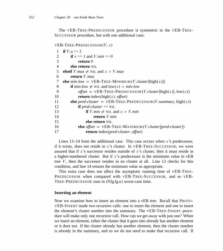
552 Chapter 20 van Emde Boas Trees
The VEB-TREE-PREDECESSOR procedure is symmetric to the VEB-TREE-SUCCESSOR procedure, but with one additional case:
VEB-TREE-PREDECESSOR.V; x/
1 if V:u == 2
2 if x == 1 and V:min == 0
3 return 0
4 else return NIL
5 elseif V:max ¤ NIL and x > V:max6 return V:max7 else min-low D VEB-TREE-MINIMUM.V:clusterŒhigh.x/�/
8 if min-low ¤ NIL and low.x/ > min-low9 offset D VEB-TREE-PREDECESSOR.V:clusterŒhigh.x/�; low.x//
10 return index.high.x/; offset/11 else pred-cluster D VEB-TREE-PREDECESSOR.V:summary; high.x//
12 if pred-cluster == NIL
13 if V:min ¤ NIL and x > V:min14 return V:min15 else return NIL
16 else offset D VEB-TREE-MAXIMUM.V:clusterŒpred-cluster�/
17 return index.pred-cluster; offset/
Lines 13–14 form the additional case. This case occurs when x’s predecessor,if it exists, does not reside in x’s cluster. In VEB-TREE-SUCCESSOR, we wereassured that if x’s successor resides outside of x’s cluster, then it must reside ina higher-numbered cluster. But if x’s predecessor is the minimum value in vEBtree V , then the successor resides in no cluster at all. Line 13 checks for thiscondition, and line 14 returns the minimum value as appropriate.
This extra case does not affect the asymptotic running time of VEB-TREE-PREDECESSOR when compared with VEB-TREE-SUCCESSOR, and so VEB-TREE-PREDECESSOR runs in O.lg lg u/ worst-case time.
Inserting an element
Now we examine how to insert an element into a vEB tree. Recall that PROTO-VEB-INSERT made two recursive calls: one to insert the element and one to insertthe element’s cluster number into the summary. The VEB-TREE-INSERT proce-dure will make only one recursive call. How can we get away with just one? Whenwe insert an element, either the cluster that it goes into already has another elementor it does not. If the cluster already has another element, then the cluster numberis already in the summary, and so we do not need to make that recursive call. If
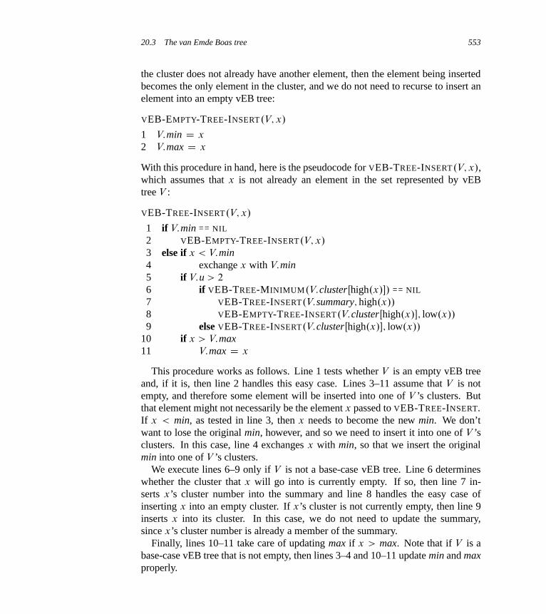
20.3 The van Emde Boas tree 553
the cluster does not already have another element, then the element being insertedbecomes the only element in the cluster, and we do not need to recurse to insert anelement into an empty vEB tree:
VEB-EMPTY-TREE-INSERT.V; x/
1 V:min D x
2 V:max D x
With this procedure in hand, here is the pseudocode for VEB-TREE-INSERT.V; x/,which assumes that x is not already an element in the set represented by vEBtree V :
VEB-TREE-INSERT.V; x/
1 if V:min == NIL
2 VEB-EMPTY-TREE-INSERT.V; x/
3 else if x < V:min4 exchange x with V:min5 if V:u > 2
6 if VEB-TREE-MINIMUM.V:clusterŒhigh.x/�/ == NIL
7 VEB-TREE-INSERT.V:summary; high.x//
8 VEB-EMPTY-TREE-INSERT.V:clusterŒhigh.x/�; low.x//
9 else VEB-TREE-INSERT.V:clusterŒhigh.x/�; low.x//
10 if x > V:max11 V:max D x
This procedure works as follows. Line 1 tests whether V is an empty vEB treeand, if it is, then line 2 handles this easy case. Lines 3–11 assume that V is notempty, and therefore some element will be inserted into one of V ’s clusters. Butthat element might not necessarily be the element x passed to VEB-TREE-INSERT.If x < min, as tested in line 3, then x needs to become the new min. We don’twant to lose the original min, however, and so we need to insert it into one of V ’sclusters. In this case, line 4 exchanges x with min, so that we insert the originalmin into one of V ’s clusters.
We execute lines 6–9 only if V is not a base-case vEB tree. Line 6 determineswhether the cluster that x will go into is currently empty. If so, then line 7 in-serts x’s cluster number into the summary and line 8 handles the easy case ofinserting x into an empty cluster. If x’s cluster is not currently empty, then line 9inserts x into its cluster. In this case, we do not need to update the summary,since x’s cluster number is already a member of the summary.
Finally, lines 10–11 take care of updating max if x > max. Note that if V is abase-case vEB tree that is not empty, then lines 3–4 and 10–11 update min and maxproperly.
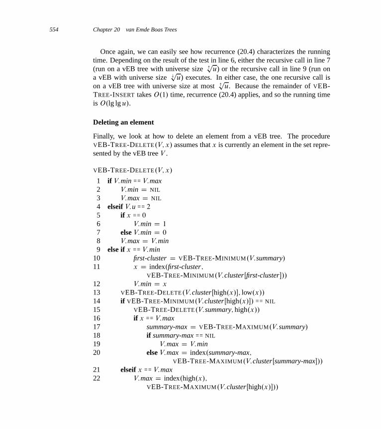
554 Chapter 20 van Emde Boas Trees
Once again, we can easily see how recurrence (20.4) characterizes the runningtime. Depending on the result of the test in line 6, either the recursive call in line 7(run on a vEB tree with universe size "
pu) or the recursive call in line 9 (run on
a vEB with universe size #p
u) executes. In either case, the one recursive call ison a vEB tree with universe size at most "
pu. Because the remainder of VEB-
TREE-INSERT takes O.1/ time, recurrence (20.4) applies, and so the running timeis O.lg lg u/.
Deleting an element
Finally, we look at how to delete an element from a vEB tree. The procedureVEB-TREE-DELETE.V; x/ assumes that x is currently an element in the set repre-sented by the vEB tree V .
VEB-TREE-DELETE.V; x/
1 if V:min == V:max2 V:min D NIL
3 V:max D NIL
4 elseif V:u == 2
5 if x == 0
6 V:min D 1
7 else V:min D 0
8 V:max D V:min9 else if x == V:min
10 first-cluster D VEB-TREE-MINIMUM.V:summary/
11 x D index.first-cluster;
VEB-TREE-MINIMUM.V:clusterŒfirst-cluster�//
12 V:min D x
13 VEB-TREE-DELETE.V:clusterŒhigh.x/�; low.x//
14 if VEB-TREE-MINIMUM.V:clusterŒhigh.x/�/ == NIL
15 VEB-TREE-DELETE.V:summary; high.x//
16 if x == V:max17 summary-max D VEB-TREE-MAXIMUM.V:summary/
18 if summary-max == NIL
19 V:max D V:min20 else V:max D index.summary-max;
VEB-TREE-MAXIMUM.V:clusterŒsummary-max�//
21 elseif x == V:max22 V:max D index.high.x/;
VEB-TREE-MAXIMUM.V:clusterŒhigh.x/�//
20.3 The van Emde Boas tree 555
The VEB-TREE-DELETE procedure works as follows. If the vEB tree V con-tains only one element, then it’s just as easy to delete it as it was to insert an elementinto an empty vEB tree: just set min and max to NIL. Lines 1–3 handle this case.Otherwise, V has at least two elements. Line 4 tests whether V is a base-case vEBtree and, if so, lines 5–8 set min and max to the one remaining element.
Lines 9–22 assume that V has two or more elements and that u � 4. In thiscase, we will have to delete an element from a cluster. The element we delete froma cluster might not be x, however, because if x equals min, then once we havedeleted x, some other element within one of V ’s clusters becomes the new min,and we have to delete that other element from its cluster. If the test in line 9 revealsthat we are in this case, then line 10 sets first-cluster to the number of the clusterthat contains the lowest element other than min, and line 11 sets x to the value ofthe lowest element in that cluster. This element becomes the new min in line 12and, because we set x to its value, it is the element that will be deleted from itscluster.
When we reach line 13, we know that we need to delete element x from itscluster, whether x was the value originally passed to VEB-TREE-DELETE or x
is the element becoming the new minimum. Line 13 deletes x from its cluster.That cluster might now become empty, which line 14 tests, and if it does, thenwe need to remove x’s cluster number from the summary, which line 15 handles.After updating the summary, we might need to update max. Line 16 checks to seewhether we are deleting the maximum element in V and, if we are, then line 17 setssummary-max to the number of the highest-numbered nonempty cluster. (The callVEB-TREE-MAXIMUM.V:summary/ works because we have already recursivelycalled VEB-TREE-DELETE on V:summary, and therefore V:summary:max has al-ready been updated as necessary.) If all of V ’s clusters are empty, then the onlyremaining element in V is min; line 18 checks for this case, and line 19 updatesmax appropriately. Otherwise, line 20 sets max to the maximum element in thehighest-numbered cluster. (If this cluster is where the element has been deleted,we again rely on the recursive call in line 13 having already corrected that cluster’smax attribute.)
Finally, we have to handle the case in which x’s cluster did not become emptydue to x being deleted. Although we do not have to update the summary in thiscase, we might have to update max. Line 21 tests for this case, and if we have toupdate max, line 22 does so (again relying on the recursive call to have correctedmax in the cluster).
Now we show that VEB-TREE-DELETE runs in O.lg lg u/ time in the worstcase. At first glance, you might think that recurrence (20.4) does not always apply,because a single call of VEB-TREE-DELETE can make two recursive calls: oneon line 13 and one on line 15. Although the procedure can make both recursivecalls, let’s think about what happens when it does. In order for the recursive call on

556 Chapter 20 van Emde Boas Trees
line 15 to occur, the test on line 14 must show that x’s cluster is empty. The onlyway that x’s cluster can be empty is if x was the only element in its cluster whenwe made the recursive call on line 13. But if x was the only element in its cluster,then that recursive call took O.1/ time, because it executed only lines 1–3. Thus,we have two mutually exclusive possibilities:
� The recursive call on line 13 took constant time.
� The recursive call on line 15 did not occur.
In either case, recurrence (20.4) characterizes the running time of VEB-TREE-DELETE, and hence its worst-case running time is O.lg lg u/.
Exercises
20.3-1Modify vEB trees to support duplicate keys.
20.3-2Modify vEB trees to support keys that have associated satellite data.
20.3-3Write pseudocode for a procedure that creates an empty van Emde Boas tree.
20.3-4What happens if you call VEB-TREE-INSERT with an element that is already inthe vEB tree? What happens if you call VEB-TREE-DELETE with an element thatis not in the vEB tree? Explain why the procedures exhibit the behavior that theydo. Show how to modify vEB trees and their operations so that we can check inconstant time whether an element is present.
20.3-5Suppose that instead of "
pu clusters, each with universe size #
pu, we constructed
vEB trees to have u1=k clusters, each with universe size u1�1=k , where k > 1 is aconstant. If we were to modify the operations appropriately, what would be theirrunning times? For the purpose of analysis, assume that u1=k and u1�1=k are alwaysintegers.
20.3-6Creating a vEB tree with universe size u requires O.u/ time. Suppose we wish toexplicitly account for that time. What is the smallest number of operations n forwhich the amortized time of each operation in a vEB tree is O.lg lg u/?

Problems for Chapter 20 557
Problems
20-1 Space requirements for van Emde Boas treesThis problem explores the space requirements for van Emde Boas trees and sug-gests a way to modify the data structure to make its space requirement depend onthe number n of elements actually stored in the tree, rather than on the universesize u. For simplicity, assume that
pu is always an integer.
a. Explain why the following recurrence characterizes the space requirement P.u/
of a van Emde Boas tree with universe size u:
P.u/ D .p
uC 1/P.p
u/C‚.p
u/ : (20.5)
b. Prove that recurrence (20.5) has the solution P.u/ D O.u/.
In order to reduce the space requirements, let us define a reduced-space van EmdeBoas tree, or RS-vEB tree, as a vEB tree V but with the following changes:� The attribute V:cluster, rather than being stored as a simple array of pointers to
vEB trees with universe sizep
u, is a hash table (see Chapter 11) stored as a dy-namic table (see Section 17.4). Corresponding to the array version of V:cluster,the hash table stores pointers to RS-vEB trees with universe size
pu. To find
the i th cluster, we look up the key i in the hash table, so that we can find thei th cluster by a single search in the hash table.
� The hash table stores only pointers to nonempty clusters. A search in the hashtable for an empty cluster returns NIL, indicating that the cluster is empty.
� The attribute V:summary is NIL if all clusters are empty. Otherwise, V:summarypoints to an RS-vEB tree with universe size
pu.
Because the hash table is implemented with a dynamic table, the space it requiresis proportional to the number of nonempty clusters.
When we need to insert an element into an empty RS-vEB tree, we create the RS-vEB tree by calling the following procedure, where the parameter u is the universesize of the RS-vEB tree:
CREATE-NEW-RS-VEB-TREE.u/
1 allocate a new vEB tree V
2 V:u D u
3 V:min D NIL
4 V:max D NIL
5 V:summary D NIL
6 create V:cluster as an empty dynamic hash table7 return V

558 Chapter 20 van Emde Boas Trees
c. Modify the VEB-TREE-INSERT procedure to produce pseudocode for the pro-cedure RS-VEB-TREE-INSERT.V; x/, which inserts x into the RS-vEB tree V ,calling CREATE-NEW-RS-VEB-TREE as appropriate.
d. Modify the VEB-TREE-SUCCESSOR procedure to produce pseudocode forthe procedure RS-VEB-TREE-SUCCESSOR.V; x/, which returns the successorof x in RS-vEB tree V , or NIL if x has no successor in V .
e. Prove that, under the assumption of simple uniform hashing, your RS-VEB-TREE-INSERT and RS-VEB-TREE-SUCCESSOR procedures run in O.lg lg u/
expected time.
f. Assuming that elements are never deleted from a vEB tree, prove that the spacerequirement for the RS-vEB tree structure is O.n/, where n is the number ofelements actually stored in the RS-vEB tree.
g. RS-vEB trees have another advantage over vEB trees: they require less time tocreate. How long does it take to create an empty RS-vEB tree?
20-2 y-fast triesThis problem investigates D. Willard’s “y-fast tries” which, like van Emde Boastrees, perform each of the operations MEMBER, MINIMUM, MAXIMUM, PRE-DECESSOR, and SUCCESSOR on elements drawn from a universe with size u inO.lg lg u/ worst-case time. The INSERT and DELETE operations take O.lg lg u/
amortized time. Like reduced-space van Emde Boas trees (see Problem 20-1), y-fast tries use only O.n/ space to store n elements. The design of y-fast tries relieson perfect hashing (see Section 11.5).
As a preliminary structure, suppose that we create a perfect hash table containingnot only every element in the dynamic set, but every prefix of the binary represen-tation of every element in the set. For example, if u D 16, so that lg u D 4, andx D 13 is in the set, then because the binary representation of 13 is 1101, theperfect hash table would contain the strings 1, 11, 110, and 1101. In addition tothe hash table, we create a doubly linked list of the elements currently in the set, inincreasing order.
a. How much space does this structure require?
b. Show how to perform the MINIMUM and MAXIMUM operations in O.1/ time,the MEMBER, PREDECESSOR, and SUCCESSOR operations in O.lg lg u/ time,and the INSERT and DELETE operations in O.lg u/ time.
To reduce the space requirement to O.n/, we make the following changes to thedata structure:

Notes for Chapter 20 559
� We cluster the n elements into n= lg u groups of size lg u. (Assume for nowthat lg u divides n.) The first group consists of the lg u smallest elements in theset, the second group consists of the next lg u smallest elements, and so on.
� We designate a “representative” value for each group. The representative ofthe i th group is at least as large as the largest element in the i th group, and it issmaller than every element of the .iC1/st group. (The representative of the lastgroup can be the maximum possible element u � 1.) Note that a representativemight be a value not currently in the set.
� We store the lg u elements of each group in a balanced binary search tree, suchas a red-black tree. Each representative points to the balanced binary searchtree for its group, and each balanced binary search tree points to its group’srepresentative.
� The perfect hash table stores only the representatives, which are also stored ina doubly linked list in increasing order.
We call this structure a y-fast trie.
c. Show that a y-fast trie requires only O.n/ space to store n elements.
d. Show how to perform the MINIMUM and MAXIMUM operations in O.lg lg u/
time with a y-fast trie.
e. Show how to perform the MEMBER operation in O.lg lg u/ time.
f. Show how to perform the PREDECESSOR and SUCCESSOR operations inO.lg lg u/ time.
g. Explain why the INSERT and DELETE operations take �.lg lg u/ time.
h. Show how to relax the requirement that each group in a y-fast trie has exactlylg u elements to allow INSERT and DELETE to run in O.lg lg u/ amortized timewithout affecting the asymptotic running times of the other operations.
Chapter notes
The data structure in this chapter is named after P. van Emde Boas, who describedan early form of the idea in 1975 [339]. Later papers by van Emde Boas [340]and van Emde Boas, Kaas, and Zijlstra [341] refined the idea and the exposition.Mehlhorn and Näher [252] subsequently extended the ideas to apply to universe
560 Chapter 20 van Emde Boas Trees
sizes that are prime. Mehlhorn’s book [249] contains a slightly different treatmentof van Emde Boas trees than the one in this chapter.
Using the ideas behind van Emde Boas trees, Dementiev et al. [84] developeda nonrecursive, three-level search tree that ran faster than van Emde Boas trees intheir own experiments.
Wang and Lin [347] designed a hardware-pipelined version of van Emde Boastrees, which achieves constant amortized time per operation and uses O.lg lg u/
stages in the pipeline.A lower bound by Pǎtraşcu and Thorup [273, 274] for finding the predecessor
shows that van Emde Boas trees are optimal for this operation, even if randomiza-tion is allowed.
21 Data Structures for Disjoint Sets
Some applications involve grouping n distinct elements into a collection of disjointsets. These applications often need to perform two operations in particular: findingthe unique set that contains a given element and uniting two sets. This chapterexplores methods for maintaining a data structure that supports these operations.
Section 21.1 describes the operations supported by a disjoint-set data structureand presents a simple application. In Section 21.2, we look at a simple linked-listimplementation for disjoint sets. Section 21.3 presents a more efficient represen-tation using rooted trees. The running time using the tree representation is theo-retically superlinear, but for all practical purposes it is linear. Section 21.4 definesand discusses a very quickly growing function and its very slowly growing inverse,which appears in the running time of operations on the tree-based implementation,and then, by a complex amortized analysis, proves an upper bound on the runningtime that is just barely superlinear.
21.1 Disjoint-set operations
A disjoint-set data structure maintains a collection S D fS1; S2; : : : ; Skg of dis-joint dynamic sets. We identify each set by a representative, which is some mem-ber of the set. In some applications, it doesn’t matter which member is used as therepresentative; we care only that if we ask for the representative of a dynamic settwice without modifying the set between the requests, we get the same answer bothtimes. Other applications may require a prespecified rule for choosing the repre-sentative, such as choosing the smallest member in the set (assuming, of course,that the elements can be ordered).
As in the other dynamic-set implementations we have studied, we represent eachelement of a set by an object. Letting x denote an object, we wish to support thefollowing operations:
562 Chapter 21 Data Structures for Disjoint Sets
MAKE-SET.x/ creates a new set whose only member (and thus representative)is x. Since the sets are disjoint, we require that x not already be in some otherset.
UNION.x; y/ unites the dynamic sets that contain x and y, say Sx and Sy , into anew set that is the union of these two sets. We assume that the two sets are dis-joint prior to the operation. The representative of the resulting set is any memberof Sx [ Sy , although many implementations of UNION specifically choose therepresentative of either Sx or Sy as the new representative. Since we requirethe sets in the collection to be disjoint, conceptually we destroy sets Sx and Sy ,removing them from the collection S . In practice, we often absorb the elementsof one of the sets into the other set.
FIND-SET.x/ returns a pointer to the representative of the (unique) set contain-ing x.
Throughout this chapter, we shall analyze the running times of disjoint-set datastructures in terms of two parameters: n, the number of MAKE-SET operations,and m, the total number of MAKE-SET, UNION, and FIND-SET operations. Sincethe sets are disjoint, each UNION operation reduces the number of sets by one.After n � 1 UNION operations, therefore, only one set remains. The number ofUNION operations is thus at most n � 1. Note also that since the MAKE-SET
operations are included in the total number of operations m, we have m � n. Weassume that the n MAKE-SET operations are the first n operations performed.
An application of disjoint-set data structures
One of the many applications of disjoint-set data structures arises in determin-ing the connected components of an undirected graph (see Section B.4). Fig-ure 21.1(a), for example, shows a graph with four connected components.
The procedure CONNECTED-COMPONENTS that follows uses the disjoint-setoperations to compute the connected components of a graph. Once CONNECTED-COMPONENTS has preprocessed the graph, the procedure SAME-COMPONENT
answers queries about whether two vertices are in the same connected component.1
(In pseudocode, we denote the set of vertices of a graph G by G:V and the set ofedges by G:E.)
1When the edges of the graph are static—not changing over time—we can compute the connectedcomponents faster by using depth-first search (Exercise 22.3-12). Sometimes, however, the edgesare added dynamically and we need to maintain the connected components as each edge is added. Inthis case, the implementation given here can be more efficient than running a new depth-first searchfor each new edge.
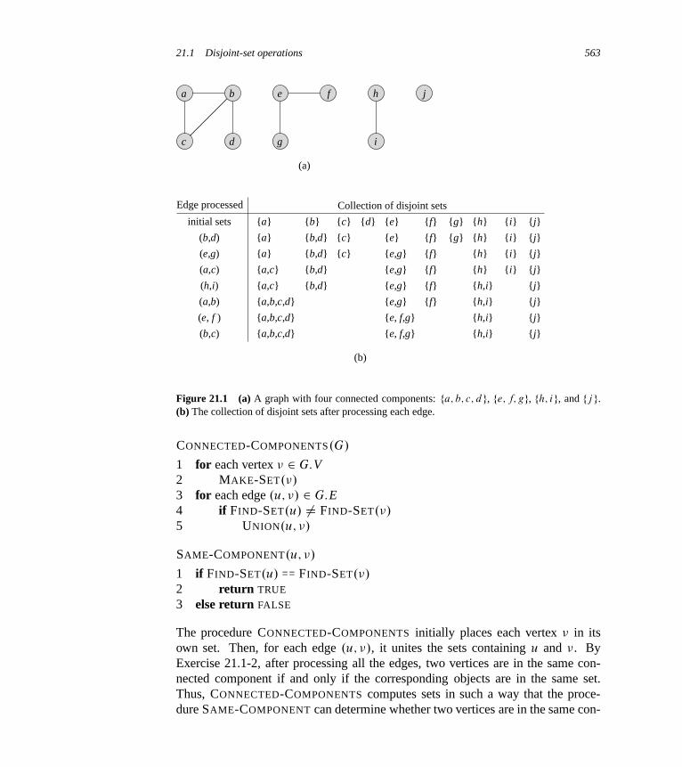
21.1 Disjoint-set operations 563
a b
c d
e f
g
h
i
j
Edge processed
initial sets
(b,d)
(e,g)
(a,c)
(h,i)
(a,b)
(e, f )
(b,c)
{a,b,c,d}
{a,b,c,d}
{a,c}
{a,c}
{a}
{a}
{a}
{a,b,c,d}
{b,d}
{b,d}
{b,d}
{b,d}
{b}
{c}
{c}
{c} {d}
{e, f,g}
{e, f,g}
{e,g}
{e,g}
{e,g}
{e,g}
{e}
{e} {f}
{f}
{f}
{f}
{f}
{f}
{g}
{g}
{h,i}
{h,i}
{h,i}
{h,i}
{h}
{h}
{h}
{h} {i}
{i}
{i}
{i}
{j}
{j}
{j}
{j}
{j}
{j}
{j}
{j}
Collection of disjoint sets
(a)
(b)
Figure 21.1 (a) A graph with four connected components: fa; b; c; dg, fe; f; gg, fh; ig, and fj g.(b) The collection of disjoint sets after processing each edge.
CONNECTED-COMPONENTS.G/
1 for each vertex � 2 G:V2 MAKE-SET.�/
3 for each edge .u; �/ 2 G:E4 if FIND-SET.u/ ¤ FIND-SET.�/
5 UNION.u; �/
SAME-COMPONENT.u; �/
1 if FIND-SET.u/ == FIND-SET.�/
2 return TRUE
3 else return FALSE
The procedure CONNECTED-COMPONENTS initially places each vertex � in itsown set. Then, for each edge .u; �/, it unites the sets containing u and �. ByExercise 21.1-2, after processing all the edges, two vertices are in the same con-nected component if and only if the corresponding objects are in the same set.Thus, CONNECTED-COMPONENTS computes sets in such a way that the proce-dure SAME-COMPONENT can determine whether two vertices are in the same con-
564 Chapter 21 Data Structures for Disjoint Sets
nected component. Figure 21.1(b) illustrates how CONNECTED-COMPONENTS
computes the disjoint sets.In an actual implementation of this connected-components algorithm, the repre-
sentations of the graph and the disjoint-set data structure would need to referenceeach other. That is, an object representing a vertex would contain a pointer tothe corresponding disjoint-set object, and vice versa. These programming detailsdepend on the implementation language, and we do not address them further here.
Exercises
21.1-1Suppose that CONNECTED-COMPONENTS is run on the undirected graph G D.V; E/, where V D fa; b; c; d; e; f; g; h; i; j; kg and the edges of E are pro-cessed in the order .d; i/; .f; k/; .g; i/; .b; g/; .a; h/; .i; j /; .d; k/; .b; j /; .d; f /;
.g; j /; .a; e/. List the vertices in each connected component after each iteration oflines 3–5.
21.1-2Show that after all edges are processed by CONNECTED-COMPONENTS, two ver-tices are in the same connected component if and only if they are in the same set.
21.1-3During the execution of CONNECTED-COMPONENTS on an undirected graph G D.V; E/ with k connected components, how many times is FIND-SET called? Howmany times is UNION called? Express your answers in terms of jV j, jEj, and k.
21.2 Linked-list representation of disjoint sets
Figure 21.2(a) shows a simple way to implement a disjoint-set data structure: eachset is represented by its own linked list. The object for each set has attributes head,pointing to the first object in the list, and tail, pointing to the last object. Eachobject in the list contains a set member, a pointer to the next object in the list, anda pointer back to the set object. Within each linked list, the objects may appear inany order. The representative is the set member in the first object in the list.
With this linked-list representation, both MAKE-SET and FIND-SET are easy,requiring O.1/ time. To carry out MAKE-SET.x/, we create a new linked listwhose only object is x. For FIND-SET.x/, we just follow the pointer from x backto its set object and then return the member in the object that head points to. Forexample, in Figure 21.2(a), the call FIND-SET.g/ would return f .
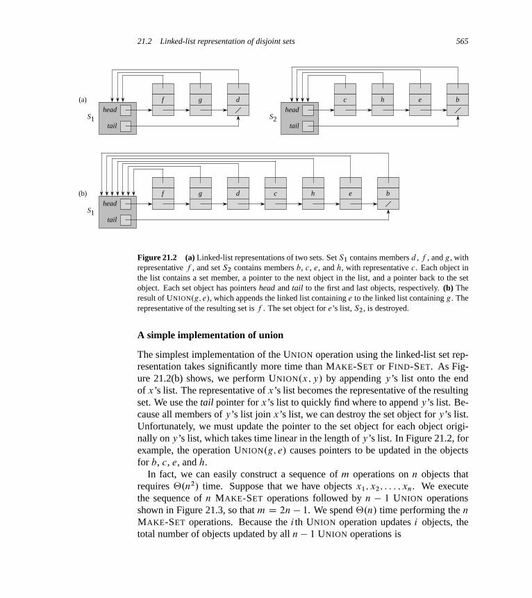
21.2 Linked-list representation of disjoint sets 565
f g d c h e b
(a)
(b)
head
tailS1
c h e
head
tailS2
bf g d
head
tailS1
Figure 21.2 (a) Linked-list representations of two sets. Set S1 contains members d , f , and g, withrepresentative f , and set S2 contains members b, c, e, and h, with representative c. Each object inthe list contains a set member, a pointer to the next object in the list, and a pointer back to the setobject. Each set object has pointers head and tail to the first and last objects, respectively. (b) Theresult of UNION.g; e/, which appends the linked list containing e to the linked list containing g. Therepresentative of the resulting set is f . The set object for e’s list, S2, is destroyed.
A simple implementation of union
The simplest implementation of the UNION operation using the linked-list set rep-resentation takes significantly more time than MAKE-SET or FIND-SET. As Fig-ure 21.2(b) shows, we perform UNION.x; y/ by appending y’s list onto the endof x’s list. The representative of x’s list becomes the representative of the resultingset. We use the tail pointer for x’s list to quickly find where to append y’s list. Be-cause all members of y’s list join x’s list, we can destroy the set object for y’s list.Unfortunately, we must update the pointer to the set object for each object origi-nally on y’s list, which takes time linear in the length of y’s list. In Figure 21.2, forexample, the operation UNION.g; e/ causes pointers to be updated in the objectsfor b, c, e, and h.
In fact, we can easily construct a sequence of m operations on n objects thatrequires ‚.n2/ time. Suppose that we have objects x1; x2; : : : ; xn. We executethe sequence of n MAKE-SET operations followed by n � 1 UNION operationsshown in Figure 21.3, so that m D 2n � 1. We spend ‚.n/ time performing the n
MAKE-SET operations. Because the i th UNION operation updates i objects, thetotal number of objects updated by all n � 1 UNION operations is

566 Chapter 21 Data Structures for Disjoint Sets
Operation Number of objects updatedMAKE-SET.x1/ 1MAKE-SET.x2/ 1
::::::
MAKE-SET.xn/ 1UNION.x2; x1/ 1UNION.x3; x2/ 2UNION.x4; x3/ 3
::::::
UNION.xn; xn�1/ n � 1
Figure 21.3 A sequence of 2n � 1 operations on n objects that takes ‚.n2/ time, or ‚.n/ timeper operation on average, using the linked-list set representation and the simple implementation ofUNION.
n�1XiD1
i D ‚.n2/ :
The total number of operations is 2n�1, and so each operation on average requires‚.n/ time. That is, the amortized time of an operation is ‚.n/.
A weighted-union heuristic
In the worst case, the above implementation of the UNION procedure requires anaverage of ‚.n/ time per call because we may be appending a longer list ontoa shorter list; we must update the pointer to the set object for each member ofthe longer list. Suppose instead that each list also includes the length of the list(which we can easily maintain) and that we always append the shorter list onto thelonger, breaking ties arbitrarily. With this simple weighted-union heuristic, a sin-gle UNION operation can still take �.n/ time if both sets have �.n/ members. Asthe following theorem shows, however, a sequence of m MAKE-SET, UNION, andFIND-SET operations, n of which are MAKE-SET operations, takes O.mC n lg n/
time.
Theorem 21.1Using the linked-list representation of disjoint sets and the weighted-union heuris-tic, a sequence of m MAKE-SET, UNION, and FIND-SET operations, n of whichare MAKE-SET operations, takes O.mC n lg n/ time.
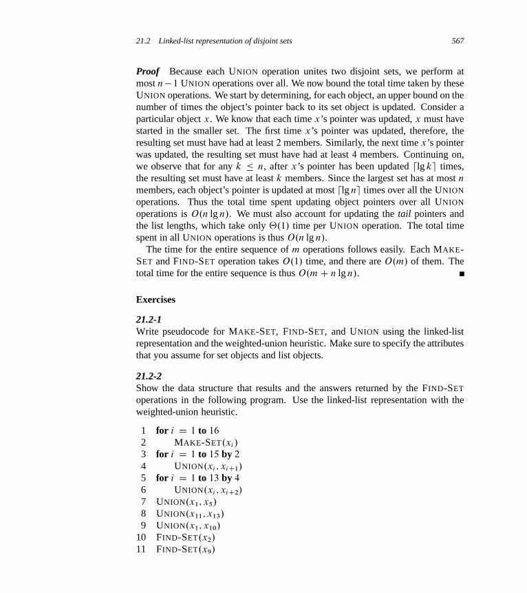
21.2 Linked-list representation of disjoint sets 567
Proof Because each UNION operation unites two disjoint sets, we perform atmost n�1 UNION operations over all. We now bound the total time taken by theseUNION operations. We start by determining, for each object, an upper bound on thenumber of times the object’s pointer back to its set object is updated. Consider aparticular object x. We know that each time x’s pointer was updated, x must havestarted in the smaller set. The first time x’s pointer was updated, therefore, theresulting set must have had at least 2 members. Similarly, the next time x’s pointerwas updated, the resulting set must have had at least 4 members. Continuing on,we observe that for any k � n, after x’s pointer has been updated dlg ke times,the resulting set must have at least k members. Since the largest set has at most n
members, each object’s pointer is updated at most dlg ne times over all the UNION
operations. Thus the total time spent updating object pointers over all UNION
operations is O.n lg n/. We must also account for updating the tail pointers andthe list lengths, which take only ‚.1/ time per UNION operation. The total timespent in all UNION operations is thus O.n lg n/.
The time for the entire sequence of m operations follows easily. Each MAKE-SET and FIND-SET operation takes O.1/ time, and there are O.m/ of them. Thetotal time for the entire sequence is thus O.mC n lg n/.
Exercises
21.2-1Write pseudocode for MAKE-SET, FIND-SET, and UNION using the linked-listrepresentation and the weighted-union heuristic. Make sure to specify the attributesthat you assume for set objects and list objects.
21.2-2Show the data structure that results and the answers returned by the FIND-SET
operations in the following program. Use the linked-list representation with theweighted-union heuristic.
1 for i D 1 to 16
2 MAKE-SET.xi/
3 for i D 1 to 15 by 2
4 UNION.xi ; xiC1/
5 for i D 1 to 13 by 4
6 UNION.xi ; xiC2/
7 UNION.x1; x5/
8 UNION.x11; x13/
9 UNION.x1; x10/
10 FIND-SET.x2/
11 FIND-SET.x9/

568 Chapter 21 Data Structures for Disjoint Sets
Assume that if the sets containing xi and xj have the same size, then the operationUNION.xi ; xj / appends xj ’s list onto xi ’s list.
21.2-3Adapt the aggregate proof of Theorem 21.1 to obtain amortized time boundsof O.1/ for MAKE-SET and FIND-SET and O.lg n/ for UNION using the linked-list representation and the weighted-union heuristic.
21.2-4Give a tight asymptotic bound on the running time of the sequence of operations inFigure 21.3 assuming the linked-list representation and the weighted-union heuris-tic.
21.2-5Professor Gompers suspects that it might be possible to keep just one pointer ineach set object, rather than two (head and tail), while keeping the number of point-ers in each list element at two. Show that the professor’s suspicion is well foundedby describing how to represent each set by a linked list such that each operationhas the same running time as the operations described in this section. Describealso how the operations work. Your scheme should allow for the weighted-unionheuristic, with the same effect as described in this section. (Hint: Use the tail of alinked list as its set’s representative.)
21.2-6Suggest a simple change to the UNION procedure for the linked-list representationthat removes the need to keep the tail pointer to the last object in each list. Whetheror not the weighted-union heuristic is used, your change should not change theasymptotic running time of the UNION procedure. (Hint: Rather than appendingone list to another, splice them together.)
21.3 Disjoint-set forests
In a faster implementation of disjoint sets, we represent sets by rooted trees, witheach node containing one member and each tree representing one set. In a disjoint-set forest, illustrated in Figure 21.4(a), each member points only to its parent. Theroot of each tree contains the representative and is its own parent. As we shallsee, although the straightforward algorithms that use this representation are nofaster than ones that use the linked-list representation, by introducing two heuris-tics—“union by rank” and “path compression”—we can achieve an asymptoticallyoptimal disjoint-set data structure.

21.3 Disjoint-set forests 569
c
h e
b
f
d
g
(a)
f
c
h e
b
d
g
(b)
Figure 21.4 A disjoint-set forest. (a) Two trees representing the two sets of Figure 21.2. Thetree on the left represents the set fb; c; e; hg, with c as the representative, and the tree on the rightrepresents the set fd; f; gg, with f as the representative. (b) The result of UNION.e; g/.
We perform the three disjoint-set operations as follows. A MAKE-SET operationsimply creates a tree with just one node. We perform a FIND-SET operation byfollowing parent pointers until we find the root of the tree. The nodes visited onthis simple path toward the root constitute the find path. A UNION operation,shown in Figure 21.4(b), causes the root of one tree to point to the root of the other.
Heuristics to improve the running time
So far, we have not improved on the linked-list implementation. A sequence ofn� 1 UNION operations may create a tree that is just a linear chain of n nodes. Byusing two heuristics, however, we can achieve a running time that is almost linearin the total number of operations m.
The first heuristic, union by rank, is similar to the weighted-union heuristic weused with the linked-list representation. The obvious approach would be to makethe root of the tree with fewer nodes point to the root of the tree with more nodes.Rather than explicitly keeping track of the size of the subtree rooted at each node,we shall use an approach that eases the analysis. For each node, we maintain arank, which is an upper bound on the height of the node. In union by rank, wemake the root with smaller rank point to the root with larger rank during a UNION
operation.The second heuristic, path compression, is also quite simple and highly effec-
tive. As shown in Figure 21.5, we use it during FIND-SET operations to make eachnode on the find path point directly to the root. Path compression does not changeany ranks.

570 Chapter 21 Data Structures for Disjoint Sets
a
b
c
d
e
f
a b c d e
f
(a) (b)
Figure 21.5 Path compression during the operation FIND-SET. Arrows and self-loops at roots areomitted. (a) A tree representing a set prior to executing FIND-SET.a/. Triangles represent subtreeswhose roots are the nodes shown. Each node has a pointer to its parent. (b) The same set afterexecuting FIND-SET.a/. Each node on the find path now points directly to the root.
Pseudocode for disjoint-set forests
To implement a disjoint-set forest with the union-by-rank heuristic, we must keeptrack of ranks. With each node x, we maintain the integer value x:rank, which isan upper bound on the height of x (the number of edges in the longest simple pathbetween x and a descendant leaf). When MAKE-SET creates a singleton set, thesingle node in the corresponding tree has an initial rank of 0. Each FIND-SET oper-ation leaves all ranks unchanged. The UNION operation has two cases, dependingon whether the roots of the trees have equal rank. If the roots have unequal rank,we make the root with higher rank the parent of the root with lower rank, but theranks themselves remain unchanged. If, instead, the roots have equal ranks, wearbitrarily choose one of the roots as the parent and increment its rank.
Let us put this method into pseudocode. We designate the parent of node x
by x:p. The LINK procedure, a subroutine called by UNION, takes pointers to tworoots as inputs.

21.3 Disjoint-set forests 571
MAKE-SET.x/
1 x:p D x
2 x:rank D 0
UNION.x; y/
1 LINK.FIND-SET.x/; FIND-SET.y//
LINK.x; y/
1 if x:rank > y:rank2 y:p D x
3 else x:p D y
4 if x:rank == y:rank5 y:rank D y:rankC 1
The FIND-SET procedure with path compression is quite simple:
FIND-SET.x/
1 if x ¤ x:p2 x:p D FIND-SET.x:p/
3 return x:p
The FIND-SET procedure is a two-pass method: as it recurses, it makes one passup the find path to find the root, and as the recursion unwinds, it makes a secondpass back down the find path to update each node to point directly to the root. Eachcall of FIND-SET.x/ returns x:p in line 3. If x is the root, then FIND-SET skipsline 2 and instead returns x:p, which is x; this is the case in which the recursionbottoms out. Otherwise, line 2 executes, and the recursive call with parameter x:preturns a pointer to the root. Line 2 updates node x to point directly to the root,and line 3 returns this pointer.
Effect of the heuristics on the running time
Separately, either union by rank or path compression improves the running time ofthe operations on disjoint-set forests, and the improvement is even greater whenwe use the two heuristics together. Alone, union by rank yields a running timeof O.m lg n/ (see Exercise 21.4-4), and this bound is tight (see Exercise 21.3-3).Although we shall not prove it here, for a sequence of n MAKE-SET opera-tions (and hence at most n � 1 UNION operations) and f FIND-SET opera-tions, the path-compression heuristic alone gives a worst-case running time of‚.nC f � .1C log2Cf=n n//.

572 Chapter 21 Data Structures for Disjoint Sets
When we use both union by rank and path compression, the worst-case runningtime is O.m ˛.n//, where ˛.n/ is a very slowly growing function, which we de-fine in Section 21.4. In any conceivable application of a disjoint-set data structure,˛.n/ � 4; thus, we can view the running time as linear in m in all practical situa-tions. Strictly speaking, however, it is superlinear. In Section 21.4, we prove thisupper bound.
Exercises
21.3-1Redo Exercise 21.2-2 using a disjoint-set forest with union by rank and path com-pression.
21.3-2Write a nonrecursive version of FIND-SET with path compression.
21.3-3Give a sequence of m MAKE-SET, UNION, and FIND-SET operations, n of whichare MAKE-SET operations, that takes �.m lg n/ time when we use union by rankonly.
21.3-4Suppose that we wish to add the operation PRINT-SET.x/, which is given a node x
and prints all the members of x’s set, in any order. Show how we can add justa single attribute to each node in a disjoint-set forest so that PRINT-SET.x/ takestime linear in the number of members of x’s set and the asymptotic running timesof the other operations are unchanged. Assume that we can print each member ofthe set in O.1/ time.
21.3-5 ?
Show that any sequence of m MAKE-SET, FIND-SET, and LINK operations, whereall the LINK operations appear before any of the FIND-SET operations, takes onlyO.m/ time if we use both path compression and union by rank. What happens inthe same situation if we use only the path-compression heuristic?
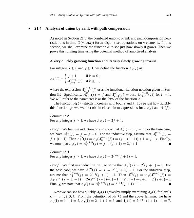
21.4 Analysis of union by rank with path compression 573
? 21.4 Analysis of union by rank with path compression
As noted in Section 21.3, the combined union-by-rank and path-compression heu-ristic runs in time O.m ˛.n// for m disjoint-set operations on n elements. In thissection, we shall examine the function ˛ to see just how slowly it grows. Then weprove this running time using the potential method of amortized analysis.
A very quickly growing function and its very slowly growing inverse
For integers k � 0 and j � 1, we define the function Ak.j / as
Ak.j / D(
j C 1 if k D 0 ;
A.j C1/
k�1.j / if k � 1 ;
where the expression A.j C1/
k�1.j / uses the functional-iteration notation given in Sec-
tion 3.2. Specifically, A.0/
k�1.j / D j and A
.i/
k�1.j / D Ak�1.A
.i�1/
k�1.j // for i � 1.
We will refer to the parameter k as the level of the function A.The function Ak.j / strictly increases with both j and k. To see just how quickly
this function grows, we first obtain closed-form expressions for A1.j / and A2.j /.
Lemma 21.2For any integer j � 1, we have A1.j / D 2j C 1.
Proof We first use induction on i to show that A.i/0 .j / D jCi . For the base case,
we have A.0/0 .j / D j D j C 0. For the inductive step, assume that A
.i�1/0 .j / D
j C .i � 1/. Then A.i/0 .j / D A0.A
.i�1/0 .j // D .j C .i � 1//C 1 D j C i . Finally,
we note that A1.j / D A.j C1/0 .j / D j C .j C 1/ D 2j C 1.
Lemma 21.3For any integer j � 1, we have A2.j / D 2j C1.j C 1/ � 1.
Proof We first use induction on i to show that A.i/1 .j / D 2i .j C 1/ � 1. For
the base case, we have A.0/1 .j / D j D 20.j C 1/ � 1. For the inductive step,
assume that A.i�1/1 .j / D 2i�1.j C 1/ � 1. Then A
.i/1 .j / D A1.A
.i�1/1 .j // D
A1.2i�1.j C 1/ � 1/ D 2�.2i�1.jC1/�1/C1 D 2i .jC1/�2C1 D 2i .jC1/�1.Finally, we note that A2.j / D A
.j C1/1 .j / D 2j C1.j C 1/ � 1.
Now we can see how quickly Ak.j / grows by simply examining Ak.1/ for levelsk D 0; 1; 2; 3; 4. From the definition of A0.k/ and the above lemmas, we haveA0.1/ D 1C 1 D 2, A1.1/ D 2 � 1C 1 D 3, and A2.1/ D 21C1 � .1C 1/ � 1 D 7.
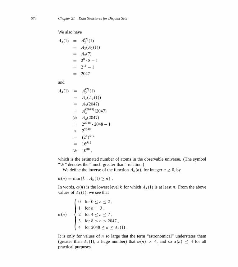
574 Chapter 21 Data Structures for Disjoint Sets
We also have
A3.1/ D A.2/2 .1/
D A2.A2.1//
D A2.7/
D 28 � 8 � 1
D 211 � 1
D 2047
and
A4.1/ D A.2/3 .1/
D A3.A3.1//
D A3.2047/
D A.2048/2 .2047/
� A2.2047/
D 22048 � 2048 � 1
> 22048
D .24/512
D 16512
� 1080 ;
which is the estimated number of atoms in the observable universe. (The symbol“�” denotes the “much-greater-than” relation.)
We define the inverse of the function Ak.n/, for integer n � 0, by
˛.n/ D min fk W Ak.1/ � ng :
In words, ˛.n/ is the lowest level k for which Ak.1/ is at least n. From the abovevalues of Ak.1/, we see that
˛.n/ D
˚0 for 0 � n � 2 ;
1 for n D 3 ;
2 for 4 � n � 7 ;
3 for 8 � n � 2047 ;
4 for 2048 � n � A4.1/ :
It is only for values of n so large that the term “astronomical” understates them(greater than A4.1/, a huge number) that ˛.n/ > 4, and so ˛.n/ � 4 for allpractical purposes.

21.4 Analysis of union by rank with path compression 575
Properties of ranks
In the remainder of this section, we prove an O.m˛.n// bound on the running timeof the disjoint-set operations with union by rank and path compression. In order toprove this bound, we first prove some simple properties of ranks.
Lemma 21.4For all nodes x, we have x:rank � x:p:rank, with strict inequality if x ¤ x:p.The value of x:rank is initially 0 and increases through time until x ¤ x:p; fromthen on, x:rank does not change. The value of x:p:rank monotonically increasesover time.
Proof The proof is a straightforward induction on the number of operations, us-ing the implementations of MAKE-SET, UNION, and FIND-SET that appear inSection 21.3. We leave it as Exercise 21.4-1.
Corollary 21.5As we follow the simple path from any node toward a root, the node ranks strictlyincrease.
Lemma 21.6Every node has rank at most n � 1.
Proof Each node’s rank starts at 0, and it increases only upon LINK operations.Because there are at most n � 1 UNION operations, there are also at most n � 1
LINK operations. Because each LINK operation either leaves all ranks alone orincreases some node’s rank by 1, all ranks are at most n � 1.
Lemma 21.6 provides a weak bound on ranks. In fact, every node has rank atmost blg nc (see Exercise 21.4-2). The looser bound of Lemma 21.6 will sufficefor our purposes, however.
Proving the time bound
We shall use the potential method of amortized analysis (see Section 17.3) to provethe O.m ˛.n// time bound. In performing the amortized analysis, we will find itconvenient to assume that we invoke the LINK operation rather than the UNION
operation. That is, since the parameters of the LINK procedure are pointers to tworoots, we act as though we perform the appropriate FIND-SET operations sepa-rately. The following lemma shows that even if we count the extra FIND-SET op-erations induced by UNION calls, the asymptotic running time remains unchanged.

576 Chapter 21 Data Structures for Disjoint Sets
Lemma 21.7Suppose we convert a sequence S 0 of m0 MAKE-SET, UNION, and FIND-SET op-erations into a sequence S of m MAKE-SET, LINK, and FIND-SET operations byturning each UNION into two FIND-SET operations followed by a LINK. Then, ifsequence S runs in O.m ˛.n// time, sequence S 0 runs in O.m0 ˛.n// time.
Proof Since each UNION operation in sequence S 0 is converted into three opera-tions in S , we have m0 � m � 3m0. Since m D O.m0/, an O.m ˛.n// time boundfor the converted sequence S implies an O.m0 ˛.n// time bound for the originalsequence S 0.
In the remainder of this section, we shall assume that the initial sequence of m0
MAKE-SET, UNION, and FIND-SET operations has been converted to a sequenceof m MAKE-SET, LINK, and FIND-SET operations. We now prove an O.m ˛.n//
time bound for the converted sequence and appeal to Lemma 21.7 to prove theO.m0 ˛.n// running time of the original sequence of m0 operations.
Potential function
The potential function we use assigns a potential �q.x/ to each node x in thedisjoint-set forest after q operations. We sum the node potentials for the poten-tial of the entire forest: ˆq D
Px �q.x/, where ˆq denotes the potential of the
forest after q operations. The forest is empty prior to the first operation, and wearbitrarily set ˆ0 D 0. No potential ˆq will ever be negative.
The value of �q.x/ depends on whether x is a tree root after the qth operation.If it is, or if x:rank D 0, then �q.x/ D ˛.n/ � x:rank.
Now suppose that after the qth operation, x is not a root and that x:rank � 1.We need to define two auxiliary functions on x before we can define �q.x/. Firstwe define
level.x/ D max fk W x:p:rank � Ak.x:rank/g :
That is, level.x/ is the greatest level k for which Ak, applied to x’s rank, is nogreater than x’s parent’s rank.
We claim that
0 � level.x/ < ˛.n/ ; (21.1)
which we see as follows. We have
x:p:rank � x:rankC 1 (by Lemma 21.4)
D A0.x:rank/ (by definition of A0.j /) ,
which implies that level.x/ � 0, and we have
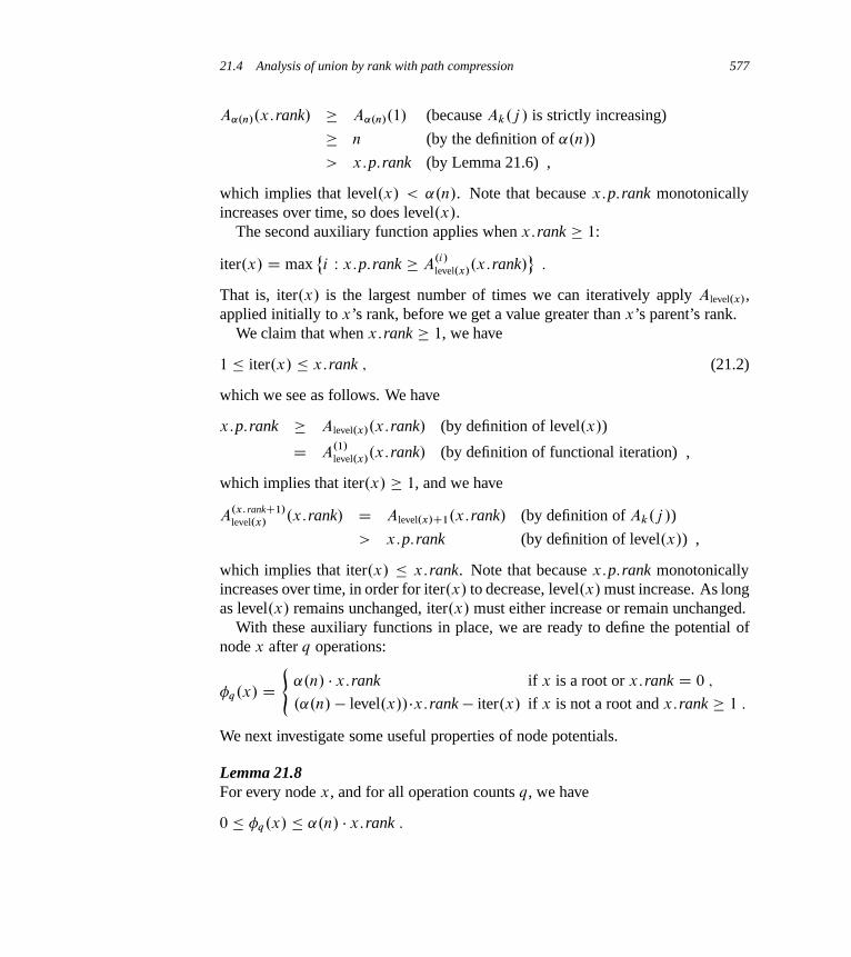
21.4 Analysis of union by rank with path compression 577
A˛.n/.x:rank/ � A˛.n/.1/ (because Ak.j / is strictly increasing)
� n (by the definition of ˛.n/)
> x:p:rank (by Lemma 21.6) ,
which implies that level.x/ < ˛.n/. Note that because x:p:rank monotonicallyincreases over time, so does level.x/.
The second auxiliary function applies when x:rank � 1:
iter.x/ D max˚i W x:p:rank � A
.i/
level.x/.x:rank/
:
That is, iter.x/ is the largest number of times we can iteratively apply Alevel.x/,applied initially to x’s rank, before we get a value greater than x’s parent’s rank.
We claim that when x:rank � 1, we have
1 � iter.x/ � x:rank ; (21.2)
which we see as follows. We have
x:p:rank � Alevel.x/.x:rank/ (by definition of level.x/)
D A.1/
level.x/.x:rank/ (by definition of functional iteration) ,
which implies that iter.x/ � 1, and we have
A.x: rankC1/
level.x/.x:rank/ D Alevel.x/C1.x:rank/ (by definition of Ak.j /)
> x:p:rank (by definition of level.x/) ,
which implies that iter.x/ � x:rank. Note that because x:p:rank monotonicallyincreases over time, in order for iter.x/ to decrease, level.x/ must increase. As longas level.x/ remains unchanged, iter.x/ must either increase or remain unchanged.
With these auxiliary functions in place, we are ready to define the potential ofnode x after q operations:
�q.x/ D(
˛.n/ � x:rank if x is a root or x:rank D 0 ;
.˛.n/ � level.x//�x:rank � iter.x/ if x is not a root and x:rank � 1 :
We next investigate some useful properties of node potentials.
Lemma 21.8For every node x, and for all operation counts q, we have
0 � �q.x/ � ˛.n/ � x:rank :
578 Chapter 21 Data Structures for Disjoint Sets
Proof If x is a root or x:rank D 0, then �q.x/ D ˛.n/�x:rank by definition. Nowsuppose that x is not a root and that x:rank � 1. We obtain a lower bound on �q.x/
by maximizing level.x/ and iter.x/. By the bound (21.1), level.x/ � ˛.n/�1, andby the bound (21.2), iter.x/ � x:rank. Thus,
�q.x/ D .˛.n/ � level.x// � x:rank � iter.x/
� .˛.n/ � .˛.n/� 1// � x:rank � x:rank
D x:rank � x:rank
D 0 :
Similarly, we obtain an upper bound on �q.x/ by minimizing level.x/ and iter.x/.By the bound (21.1), level.x/ � 0, and by the bound (21.2), iter.x/ � 1. Thus,
�q.x/ � .˛.n/ � 0/ � x:rank � 1
D ˛.n/ � x:rank � 1
< ˛.n/ � x:rank :
Corollary 21.9If node x is not a root and x:rank > 0, then �q.x/ < ˛.n/ � x:rank.
Potential changes and amortized costs of operations
We are now ready to examine how the disjoint-set operations affect node potentials.With an understanding of the change in potential due to each operation, we candetermine each operation’s amortized cost.
Lemma 21.10Let x be a node that is not a root, and suppose that the qth operation is either aLINK or FIND-SET. Then after the qth operation, �q.x/ � �q�1.x/. Moreover, ifx:rank � 1 and either level.x/ or iter.x/ changes due to the qth operation, then�q.x/ � �q�1.x/ � 1. That is, x’s potential cannot increase, and if it has positiverank and either level.x/ or iter.x/ changes, then x’s potential drops by at least 1.
Proof Because x is not a root, the qth operation does not change x:rank, andbecause n does not change after the initial n MAKE-SET operations, ˛.n/ remainsunchanged as well. Hence, these components of the formula for x’s potential re-main the same after the qth operation. If x:rank D 0, then �q.x/ D �q�1.x/ D 0.Now assume that x:rank � 1.
Recall that level.x/ monotonically increases over time. If the qth operationleaves level.x/ unchanged, then iter.x/ either increases or remains unchanged.If both level.x/ and iter.x/ are unchanged, then �q.x/ D �q�1.x/. If level.x/
21.4 Analysis of union by rank with path compression 579
is unchanged and iter.x/ increases, then it increases by at least 1, and so�q.x/ � �q�1.x/� 1.
Finally, if the qth operation increases level.x/, it increases by at least 1, so thatthe value of the term .˛.n/ � level.x// � x:rank drops by at least x:rank. Be-cause level.x/ increased, the value of iter.x/ might drop, but according to thebound (21.2), the drop is by at most x:rank � 1. Thus, the increase in poten-tial due to the change in iter.x/ is less than the decrease in potential due to thechange in level.x/, and we conclude that �q.x/ � �q�1.x/� 1.
Our final three lemmas show that the amortized cost of each MAKE-SET, LINK,and FIND-SET operation is O.˛.n//. Recall from equation (17.2) that the amor-tized cost of each operation is its actual cost plus the increase in potential due tothe operation.
Lemma 21.11The amortized cost of each MAKE-SET operation is O.1/.
Proof Suppose that the qth operation is MAKE-SET.x/. This operation createsnode x with rank 0, so that �q.x/ D 0. No other ranks or potentials change, andso ˆq D ˆq�1. Noting that the actual cost of the MAKE-SET operation is O.1/
completes the proof.
Lemma 21.12The amortized cost of each LINK operation is O.˛.n//.
Proof Suppose that the qth operation is LINK.x; y/. The actual cost of the LINK
operation is O.1/. Without loss of generality, suppose that the LINK makes y theparent of x.
To determine the change in potential due to the LINK, we note that the onlynodes whose potentials may change are x, y, and the children of y just prior to theoperation. We shall show that the only node whose potential can increase due tothe LINK is y, and that its increase is at most ˛.n/:
� By Lemma 21.10, any node that is y’s child just before the LINK cannot haveits potential increase due to the LINK.
� From the definition of �q.x/, we see that, since x was a root just before the qthoperation, �q�1.x/ D ˛.n/�x:rank. If x:rank D 0, then �q.x/ D �q�1.x/ D 0.Otherwise,
�q.x/ < ˛.n/ � x:rank (by Corollary 21.9)
D �q�1.x/ ;
and so x’s potential decreases.
580 Chapter 21 Data Structures for Disjoint Sets
� Because y is a root prior to the LINK, �q�1.y/ D ˛.n/ � y:rank. The LINK
operation leaves y as a root, and it either leaves y’s rank alone or it increases y’srank by 1. Therefore, either �q.y/ D �q�1.y/ or �q.y/ D �q�1.y/C ˛.n/.
The increase in potential due to the LINK operation, therefore, is at most ˛.n/.The amortized cost of the LINK operation is O.1/C ˛.n/ D O.˛.n//.
Lemma 21.13The amortized cost of each FIND-SET operation is O.˛.n//.
Proof Suppose that the qth operation is a FIND-SET and that the find path con-tains s nodes. The actual cost of the FIND-SET operation is O.s/. We shallshow that no node’s potential increases due to the FIND-SET and that at leastmax.0; s � .˛.n/ C 2// nodes on the find path have their potential decrease byat least 1.
To see that no node’s potential increases, we first appeal to Lemma 21.10 for allnodes other than the root. If x is the root, then its potential is ˛.n/ � x:rank, whichdoes not change.
Now we show that at least max.0; s � .˛.n/ C 2// nodes have their potentialdecrease by at least 1. Let x be a node on the find path such that x:rank > 0
and x is followed somewhere on the find path by another node y that is not a root,where level.y/ D level.x/ just before the FIND-SET operation. (Node y need notimmediately follow x on the find path.) All but at most ˛.n/C 2 nodes on the findpath satisfy these constraints on x. Those that do not satisfy them are the first nodeon the find path (if it has rank 0), the last node on the path (i.e., the root), and thelast node w on the path for which level.w/ D k, for each k D 0; 1; 2; : : : ; ˛.n/�1.
Let us fix such a node x, and we shall show that x’s potential decreases by atleast 1. Let k D level.x/ D level.y/. Just prior to the path compression caused bythe FIND-SET, we have
x:p:rank � A.iter.x//
k.x:rank/ (by definition of iter.x/) ,
y:p:rank � Ak.y:rank/ (by definition of level.y/) ,
y:rank � x:p:rank (by Corollary 21.5 and becausey follows x on the find path) .
Putting these inequalities together and letting i be the value of iter.x/ before pathcompression, we have
y:p:rank � Ak.y:rank/
� Ak.x:p:rank/ (because Ak.j / is strictly increasing)
� Ak.A.iter.x//
k.x:rank//
D A.iC1/
k.x:rank/ :

21.4 Analysis of union by rank with path compression 581
Because path compression will make x and y have the same parent, we knowthat after path compression, x:p:rank D y:p:rank and that the path compressiondoes not decrease y:p:rank. Since x:rank does not change, after path compressionwe have that x:p:rank � A
.iC1/
k.x:rank/. Thus, path compression will cause ei-
ther iter.x/ to increase (to at least i C 1) or level.x/ to increase (which occurs ifiter.x/ increases to at least x:rankC 1). In either case, by Lemma 21.10, we have�q.x/ � �q�1.x/� 1. Hence, x’s potential decreases by at least 1.
The amortized cost of the FIND-SET operation is the actual cost plus the changein potential. The actual cost is O.s/, and we have shown that the total potentialdecreases by at least max.0; s � .˛.n/C 2//. The amortized cost, therefore, is atmost O.s/ � .s � .˛.n/C 2// D O.s/ � s C O.˛.n// D O.˛.n//, since we canscale up the units of potential to dominate the constant hidden in O.s/.
Putting the preceding lemmas together yields the following theorem.
Theorem 21.14A sequence of m MAKE-SET, UNION, and FIND-SET operations, n of which areMAKE-SET operations, can be performed on a disjoint-set forest with union byrank and path compression in worst-case time O.m ˛.n//.
Proof Immediate from Lemmas 21.7, 21.11, 21.12, and 21.13.
Exercises
21.4-1Prove Lemma 21.4.
21.4-2Prove that every node has rank at most blg nc.21.4-3In light of Exercise 21.4-2, how many bits are necessary to store x:rank for eachnode x?
21.4-4Using Exercise 21.4-2, give a simple proof that operations on a disjoint-set forestwith union by rank but without path compression run in O.m lg n/ time.
21.4-5Professor Dante reasons that because node ranks increase strictly along a simplepath to the root, node levels must monotonically increase along the path. In other
582 Chapter 21 Data Structures for Disjoint Sets
words, if rank.x/ > 0 and x:p is not a root, then level.x/ � level.x:p/. Is theprofessor correct?
21.4-6 ?
Consider the function ˛0.n/ D min fk W Ak.1/ � lg.nC 1/g. Show that ˛0.n/ � 3
for all practical values of n and, using Exercise 21.4-2, show how to modify thepotential-function argument to prove that we can perform a sequence of m MAKE-SET, UNION, and FIND-SET operations, n of which are MAKE-SET operations, ona disjoint-set forest with union by rank and path compression in worst-case timeO.m ˛0.n//.
Problems
21-1 Off-line minimumThe off-line minimum problem asks us to maintain a dynamic set T of elementsfrom the domain f1; 2; : : : ; ng under the operations INSERT and EXTRACT-MIN.We are given a sequence S of n INSERT and m EXTRACT-MIN calls, where eachkey in f1; 2; : : : ; ng is inserted exactly once. We wish to determine which keyis returned by each EXTRACT-MIN call. Specifically, we wish to fill in an arrayextractedŒ1 : : m�, where for i D 1; 2; : : : ; m, extractedŒi � is the key returned bythe i th EXTRACT-MIN call. The problem is “off-line” in the sense that we areallowed to process the entire sequence S before determining any of the returnedkeys.
a. In the following instance of the off-line minimum problem, each operationINSERT.i/ is represented by the value of i and each EXTRACT-MIN is rep-resented by the letter E:
4; 8; E; 3; E; 9; 2; 6; E; E; E; 1; 7; E; 5 :
Fill in the correct values in the extracted array.
To develop an algorithm for this problem, we break the sequence S into homoge-neous subsequences. That is, we represent S by
I1; E; I2; E; I3; : : : ; Im; E; ImC1 ;
where each E represents a single EXTRACT-MIN call and each Ij represents a (pos-sibly empty) sequence of INSERT calls. For each subsequence Ij , we initially placethe keys inserted by these operations into a set Kj , which is empty if Ij is empty.We then do the following:

Problems for Chapter 21 583
OFF-LINE-MINIMUM.m; n/
1 for i D 1 to n
2 determine j such that i 2 Kj
3 if j ¤ mC 1
4 extractedŒj � D i
5 let l be the smallest value greater than j
for which set Kl exists6 Kl D Kj [Kl , destroying Kj
7 return extracted
b. Argue that the array extracted returned by OFF-LINE-MINIMUM is correct.
c. Describe how to implement OFF-LINE-MINIMUM efficiently with a disjoint-set data structure. Give a tight bound on the worst-case running time of yourimplementation.
21-2 Depth determinationIn the depth-determination problem, we maintain a forest F D fTig of rootedtrees under three operations:
MAKE-TREE.�/ creates a tree whose only node is �.
FIND-DEPTH.�/ returns the depth of node � within its tree.
GRAFT.r; �/ makes node r , which is assumed to be the root of a tree, become thechild of node �, which is assumed to be in a different tree than r but may or maynot itself be a root.
a. Suppose that we use a tree representation similar to a disjoint-set forest: �:pis the parent of node �, except that �:p D � if � is a root. Suppose furtherthat we implement GRAFT.r; �/ by setting r:p D � and FIND-DEPTH.�/ byfollowing the find path up to the root, returning a count of all nodes other than �
encountered. Show that the worst-case running time of a sequence of m MAKE-TREE, FIND-DEPTH, and GRAFT operations is ‚.m2/.
By using the union-by-rank and path-compression heuristics, we can reduce theworst-case running time. We use the disjoint-set forest S D fSig, where eachset Si (which is itself a tree) corresponds to a tree Ti in the forest F . The treestructure within a set Si , however, does not necessarily correspond to that of Ti . Infact, the implementation of Si does not record the exact parent-child relationshipsbut nevertheless allows us to determine any node’s depth in Ti .
The key idea is to maintain in each node � a “pseudodistance” �:d, which isdefined so that the sum of the pseudodistances along the simple path from � to the
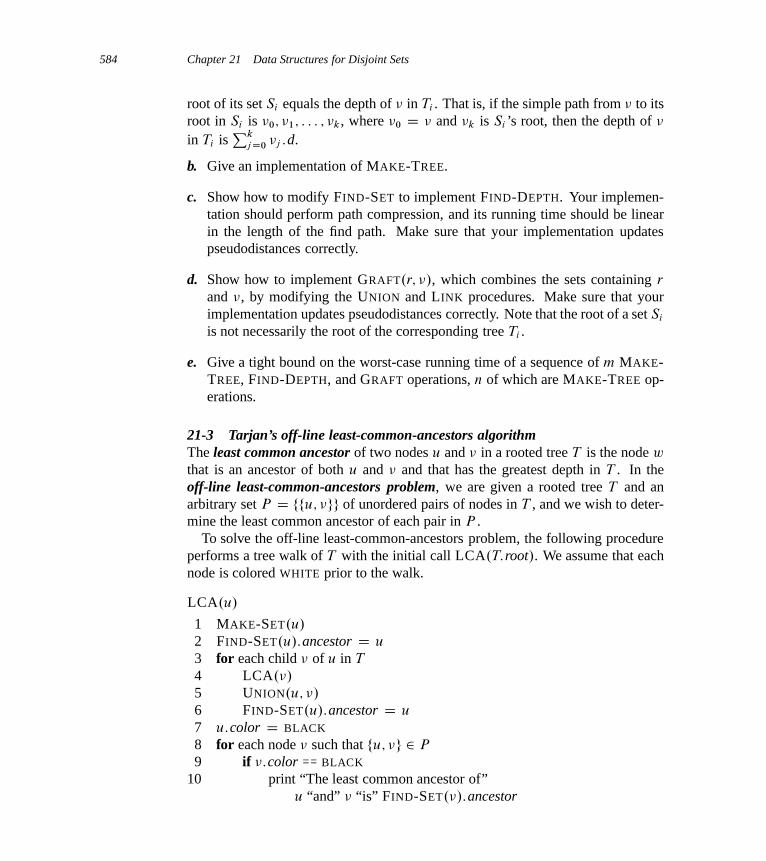
584 Chapter 21 Data Structures for Disjoint Sets
root of its set Si equals the depth of � in Ti . That is, if the simple path from � to itsroot in Si is �0; �1; : : : ; �k, where �0 D � and �k is Si ’s root, then the depth of �
in Ti isPk
j D0 �j :d.
b. Give an implementation of MAKE-TREE.
c. Show how to modify FIND-SET to implement FIND-DEPTH. Your implemen-tation should perform path compression, and its running time should be linearin the length of the find path. Make sure that your implementation updatespseudodistances correctly.
d. Show how to implement GRAFT.r; �/, which combines the sets containing r
and �, by modifying the UNION and LINK procedures. Make sure that yourimplementation updates pseudodistances correctly. Note that the root of a set Si
is not necessarily the root of the corresponding tree Ti .
e. Give a tight bound on the worst-case running time of a sequence of m MAKE-TREE, FIND-DEPTH, and GRAFT operations, n of which are MAKE-TREE op-erations.
21-3 Tarjan’s off-line least-common-ancestors algorithmThe least common ancestor of two nodes u and � in a rooted tree T is the node w
that is an ancestor of both u and � and that has the greatest depth in T . In theoff-line least-common-ancestors problem, we are given a rooted tree T and anarbitrary set P D ffu; �gg of unordered pairs of nodes in T , and we wish to deter-mine the least common ancestor of each pair in P .
To solve the off-line least-common-ancestors problem, the following procedureperforms a tree walk of T with the initial call LCA.T:root/. We assume that eachnode is colored WHITE prior to the walk.
LCA.u/
1 MAKE-SET.u/
2 FIND-SET.u/:ancestor D u
3 for each child � of u in T
4 LCA.�/
5 UNION.u; �/
6 FIND-SET.u/:ancestor D u
7 u:color D BLACK
8 for each node � such that fu; �g 2 P
9 if �:color == BLACK
10 print “The least common ancestor of”u “and” � “is” FIND-SET.�/:ancestor

Notes for Chapter 21 585
a. Argue that line 10 executes exactly once for each pair fu; �g 2 P .
b. Argue that at the time of the call LCA.u/, the number of sets in the disjoint-setdata structure equals the depth of u in T .
c. Prove that LCA correctly prints the least common ancestor of u and � for eachpair fu; �g 2 P .
d. Analyze the running time of LCA, assuming that we use the implementation ofthe disjoint-set data structure in Section 21.3.
Chapter notes
Many of the important results for disjoint-set data structures are due at least in partto R. E. Tarjan. Using aggregate analysis, Tarjan [328, 330] gave the first tightupper bound in terms of the very slowly growing inverse y̨.m; n/ of Ackermann’sfunction. (The function Ak.j / given in Section 21.4 is similar to Ackermann’sfunction, and the function ˛.n/ is similar to the inverse. Both ˛.n/ and y̨.m; n/
are at most 4 for all conceivable values of m and n.) An O.m lg� n/ upper boundwas proven earlier by Hopcroft and Ullman [5, 179]. The treatment in Section 21.4is adapted from a later analysis by Tarjan [332], which is in turn based on an anal-ysis by Kozen [220]. Harfst and Reingold [161] give a potential-based version ofTarjan’s earlier bound.
Tarjan and van Leeuwen [333] discuss variants on the path-compression heuris-tic, including “one-pass methods,” which sometimes offer better constant factorsin their performance than do two-pass methods. As with Tarjan’s earlier analysesof the basic path-compression heuristic, the analyses by Tarjan and van Leeuwenare aggregate. Harfst and Reingold [161] later showed how to make a small changeto the potential function to adapt their path-compression analysis to these one-passvariants. Gabow and Tarjan [121] show that in certain applications, the disjoint-setoperations can be made to run in O.m/ time.
Tarjan [329] showed that a lower bound of �.m y̨.m; n// time is required foroperations on any disjoint-set data structure satisfying certain technical conditions.This lower bound was later generalized by Fredman and Saks [113], who showedthat in the worst case, �.m y̨.m; n// .lg n/-bit words of memory must be accessed.
VI Graph Algorithms

Introduction
Graph problems pervade computer science, and algorithms for working with themare fundamental to the field. Hundreds of interesting computational problems arecouched in terms of graphs. In this part, we touch on a few of the more significantones.
Chapter 22 shows how we can represent a graph in a computer and then discussesalgorithms based on searching a graph using either breadth-first search or depth-first search. The chapter gives two applications of depth-first search: topologicallysorting a directed acyclic graph and decomposing a directed graph into its stronglyconnected components.
Chapter 23 describes how to compute a minimum-weight spanning tree of agraph: the least-weight way of connecting all of the vertices together when eachedge has an associated weight. The algorithms for computing minimum spanningtrees serve as good examples of greedy algorithms (see Chapter 16).
Chapters 24 and 25 consider how to compute shortest paths between verticeswhen each edge has an associated length or “weight.” Chapter 24 shows how tofind shortest paths from a given source vertex to all other vertices, and Chapter 25examines methods to compute shortest paths between every pair of vertices.
Finally, Chapter 26 shows how to compute a maximum flow of material in a flownetwork, which is a directed graph having a specified source vertex of material, aspecified sink vertex, and specified capacities for the amount of material that cantraverse each directed edge. This general problem arises in many forms, and agood algorithm for computing maximum flows can help solve a variety of relatedproblems efficiently.
588 Part VI Graph Algorithms
When we characterize the running time of a graph algorithm on a given graphG D .V; E/, we usually measure the size of the input in terms of the number ofvertices jV j and the number of edges jEj of the graph. That is, we describe thesize of the input with two parameters, not just one. We adopt a common notationalconvention for these parameters. Inside asymptotic notation (such as O-notationor ‚-notation), and only inside such notation, the symbol V denotes jV j andthe symbol E denotes jEj. For example, we might say, “the algorithm runs intime O.VE/,” meaning that the algorithm runs in time O.jV j jEj/. This conven-tion makes the running-time formulas easier to read, without risk of ambiguity.
Another convention we adopt appears in pseudocode. We denote the vertex setof a graph G by G:V and its edge set by G:E. That is, the pseudocode views vertexand edge sets as attributes of a graph.
22 Elementary Graph Algorithms
This chapter presents methods for representing a graph and for searching a graph.Searching a graph means systematically following the edges of the graph so as tovisit the vertices of the graph. A graph-searching algorithm can discover muchabout the structure of a graph. Many algorithms begin by searching their inputgraph to obtain this structural information. Several other graph algorithms elabo-rate on basic graph searching. Techniques for searching a graph lie at the heart ofthe field of graph algorithms.
Section 22.1 discusses the two most common computational representations ofgraphs: as adjacency lists and as adjacency matrices. Section 22.2 presents a sim-ple graph-searching algorithm called breadth-first search and shows how to cre-ate a breadth-first tree. Section 22.3 presents depth-first search and proves somestandard results about the order in which depth-first search visits vertices. Sec-tion 22.4 provides our first real application of depth-first search: topologically sort-ing a directed acyclic graph. A second application of depth-first search, finding thestrongly connected components of a directed graph, is the topic of Section 22.5.
22.1 Representations of graphs
We can choose between two standard ways to represent a graph G D .V; E/:as a collection of adjacency lists or as an adjacency matrix. Either way appliesto both directed and undirected graphs. Because the adjacency-list representationprovides a compact way to represent sparse graphs—those for which jEj is muchless than jV j2—it is usually the method of choice. Most of the graph algorithmspresented in this book assume that an input graph is represented in adjacency-list form. We may prefer an adjacency-matrix representation, however, when thegraph is dense—jEj is close to jV j2—or when we need to be able to tell quicklyif there is an edge connecting two given vertices. For example, two of the all-pairs

590 Chapter 22 Elementary Graph Algorithms
1 2
3
45
1
2
3
4
5
2 5
1
2
2
4 1 2
5 3
4
45 3
1 0 0 1
0 1 1 1
1 0 1 0
1 1 0 1
1 0 1 0
0
1
0
0
1
1 2 3 4 5
1
2
3
4
5
(a) (b) (c)
Figure 22.1 Two representations of an undirected graph. (a) An undirected graph G with 5 verticesand 7 edges. (b) An adjacency-list representation of G. (c) The adjacency-matrix representationof G.
1 2
54
1
2
3
4
5
2 4
5
6
2
4
6
5
1 0 1 0
0 0 0 1
0 0 0 1
1 0 0 0
0 0 1 0
0
0
0
0
0
1 2 3 4 5
1
2
3
4
5
(a) (b) (c)
3
6 6
6
6 0 0 0 0 0 1
0
0
1
0
0
Figure 22.2 Two representations of a directed graph. (a) A directed graph G with 6 vertices and 8edges. (b) An adjacency-list representation of G. (c) The adjacency-matrix representation of G.
shortest-paths algorithms presented in Chapter 25 assume that their input graphsare represented by adjacency matrices.
The adjacency-list representation of a graph G D .V; E/ consists of an ar-ray Adj of jV j lists, one for each vertex in V . For each u 2 V , the adjacency listAdjŒu� contains all the vertices � such that there is an edge .u; �/ 2 E. That is,AdjŒu� consists of all the vertices adjacent to u in G. (Alternatively, it may containpointers to these vertices.) Since the adjacency lists represent the edges of a graph,in pseudocode we treat the array Adj as an attribute of the graph, just as we treatthe edge set E. In pseudocode, therefore, we will see notation such as G:AdjŒu�.Figure 22.1(b) is an adjacency-list representation of the undirected graph in Fig-ure 22.1(a). Similarly, Figure 22.2(b) is an adjacency-list representation of thedirected graph in Figure 22.2(a).
If G is a directed graph, the sum of the lengths of all the adjacency lists is jEj,since an edge of the form .u; �/ is represented by having � appear in AdjŒu�. If G is
22.1 Representations of graphs 591
an undirected graph, the sum of the lengths of all the adjacency lists is 2 jEj, sinceif .u; �/ is an undirected edge, then u appears in �’s adjacency list and vice versa.For both directed and undirected graphs, the adjacency-list representation has thedesirable property that the amount of memory it requires is ‚.V CE/.
We can readily adapt adjacency lists to represent weighted graphs, that is, graphsfor which each edge has an associated weight, typically given by a weight functionw W E ! R. For example, let G D .V; E/ be a weighted graph with weightfunction w. We simply store the weight w.u; �/ of the edge .u; �/ 2 E withvertex � in u’s adjacency list. The adjacency-list representation is quite robust inthat we can modify it to support many other graph variants.
A potential disadvantage of the adjacency-list representation is that it providesno quicker way to determine whether a given edge .u; �/ is present in the graphthan to search for � in the adjacency list AdjŒu�. An adjacency-matrix representa-tion of the graph remedies this disadvantage, but at the cost of using asymptoticallymore memory. (See Exercise 22.1-8 for suggestions of variations on adjacency liststhat permit faster edge lookup.)
For the adjacency-matrix representation of a graph G D .V; E/, we assumethat the vertices are numbered 1; 2; : : : ; jV j in some arbitrary manner. Then theadjacency-matrix representation of a graph G consists of a jV j jV j matrixA D .aij / such that
aij D(
1 if .i; j / 2 E ;
0 otherwise :
Figures 22.1(c) and 22.2(c) are the adjacency matrices of the undirected and di-rected graphs in Figures 22.1(a) and 22.2(a), respectively. The adjacency matrix ofa graph requires ‚.V 2/ memory, independent of the number of edges in the graph.
Observe the symmetry along the main diagonal of the adjacency matrix in Fig-ure 22.1(c). Since in an undirected graph, .u; �/ and .�; u/ represent the sameedge, the adjacency matrix A of an undirected graph is its own transpose: A D AT.In some applications, it pays to store only the entries on and above the diagonal ofthe adjacency matrix, thereby cutting the memory needed to store the graph almostin half.
Like the adjacency-list representation of a graph, an adjacency matrix can repre-sent a weighted graph. For example, if G D .V; E/ is a weighted graph with edge-weight function w, we can simply store the weight w.u; �/ of the edge .u; �/ 2 E
as the entry in row u and column � of the adjacency matrix. If an edge does notexist, we can store a NIL value as its corresponding matrix entry, though for manyproblems it is convenient to use a value such as 0 or1.
Although the adjacency-list representation is asymptotically at least as space-efficient as the adjacency-matrix representation, adjacency matrices are simpler,and so we may prefer them when graphs are reasonably small. Moreover, adja-
592 Chapter 22 Elementary Graph Algorithms
cency matrices carry a further advantage for unweighted graphs: they require onlyone bit per entry.
Representing attributes
Most algorithms that operate on graphs need to maintain attributes for verticesand/or edges. We indicate these attributes using our usual notation, such as �:dfor an attribute d of a vertex �. When we indicate edges as pairs of vertices, weuse the same style of notation. For example, if edges have an attribute f , then wedenote this attribute for edge .u; �/ by .u; �/: f . For the purpose of presenting andunderstanding algorithms, our attribute notation suffices.
Implementing vertex and edge attributes in real programs can be another storyentirely. There is no one best way to store and access vertex and edge attributes.For a given situation, your decision will likely depend on the programming lan-guage you are using, the algorithm you are implementing, and how the rest of yourprogram uses the graph. If you represent a graph using adjacency lists, one designrepresents vertex attributes in additional arrays, such as an array dŒ1 : : jV j� thatparallels the Adj array. If the vertices adjacent to u are in AdjŒu�, then what we callthe attribute u:d would actually be stored in the array entry dŒu�. Many other waysof implementing attributes are possible. For example, in an object-oriented pro-gramming language, vertex attributes might be represented as instance variableswithin a subclass of a Vertex class.
Exercises
22.1-1Given an adjacency-list representation of a directed graph, how long does it taketo compute the out-degree of every vertex? How long does it take to compute thein-degrees?
22.1-2Give an adjacency-list representation for a complete binary tree on 7 vertices. Givean equivalent adjacency-matrix representation. Assume that vertices are numberedfrom 1 to 7 as in a binary heap.
22.1-3The transpose of a directed graph G D .V; E/ is the graph GT D .V; ET/, whereET D f.�; u/ 2 V V W .u; �/ 2 Eg. Thus, GT is G with all its edges reversed.Describe efficient algorithms for computing GT from G, for both the adjacency-list and adjacency-matrix representations of G. Analyze the running times of youralgorithms.

22.1 Representations of graphs 593
22.1-4Given an adjacency-list representation of a multigraph G D .V; E/, describe anO.V C E/-time algorithm to compute the adjacency-list representation of the“equivalent” undirected graph G0 D .V; E 0/, where E 0 consists of the edges in E
with all multiple edges between two vertices replaced by a single edge and with allself-loops removed.
22.1-5The square of a directed graph G D .V; E/ is the graph G2 D .V; E2/ such that.u; �/ 2 E2 if and only G contains a path with at most two edges between u and �.Describe efficient algorithms for computing G2 from G for both the adjacency-list and adjacency-matrix representations of G. Analyze the running times of youralgorithms.
22.1-6Most graph algorithms that take an adjacency-matrix representation as input re-quire time �.V 2/, but there are some exceptions. Show how to determine whethera directed graph G contains a universal sink—a vertex with in-degree jV j � 1 andout-degree 0—in time O.V /, given an adjacency matrix for G.
22.1-7The incidence matrix of a directed graph G D .V; E/ with no self-loops is ajV j jEj matrix B D .bij / such that
bij D
��1 if edge j leaves vertex i ;
1 if edge j enters vertex i ;
0 otherwise :
Describe what the entries of the matrix product BBT represent, where BT is thetranspose of B .
22.1-8Suppose that instead of a linked list, each array entry AdjŒu� is a hash table contain-ing the vertices � for which .u; �/ 2 E. If all edge lookups are equally likely, whatis the expected time to determine whether an edge is in the graph? What disadvan-tages does this scheme have? Suggest an alternate data structure for each edge listthat solves these problems. Does your alternative have disadvantages compared tothe hash table?

594 Chapter 22 Elementary Graph Algorithms
22.2 Breadth-first search
Breadth-first search is one of the simplest algorithms for searching a graph andthe archetype for many important graph algorithms. Prim’s minimum-spanning-tree algorithm (Section 23.2) and Dijkstra’s single-source shortest-paths algorithm(Section 24.3) use ideas similar to those in breadth-first search.
Given a graph G D .V; E/ and a distinguished source vertex s, breadth-firstsearch systematically explores the edges of G to “discover” every vertex that isreachable from s. It computes the distance (smallest number of edges) from s
to each reachable vertex. It also produces a “breadth-first tree” with root s thatcontains all reachable vertices. For any vertex � reachable from s, the simple pathin the breadth-first tree from s to � corresponds to a “shortest path” from s to �
in G, that is, a path containing the smallest number of edges. The algorithm workson both directed and undirected graphs.
Breadth-first search is so named because it expands the frontier between discov-ered and undiscovered vertices uniformly across the breadth of the frontier. Thatis, the algorithm discovers all vertices at distance k from s before discovering anyvertices at distance k C 1.
To keep track of progress, breadth-first search colors each vertex white, gray, orblack. All vertices start out white and may later become gray and then black. Avertex is discovered the first time it is encountered during the search, at which timeit becomes nonwhite. Gray and black vertices, therefore, have been discovered, butbreadth-first search distinguishes between them to ensure that the search proceedsin a breadth-first manner.1 If .u; �/ 2 E and vertex u is black, then vertex �
is either gray or black; that is, all vertices adjacent to black vertices have beendiscovered. Gray vertices may have some adjacent white vertices; they representthe frontier between discovered and undiscovered vertices.
Breadth-first search constructs a breadth-first tree, initially containing only itsroot, which is the source vertex s. Whenever the search discovers a white vertex �
in the course of scanning the adjacency list of an already discovered vertex u, thevertex � and the edge .u; �/ are added to the tree. We say that u is the predecessoror parent of � in the breadth-first tree. Since a vertex is discovered at most once, ithas at most one parent. Ancestor and descendant relationships in the breadth-firsttree are defined relative to the root s as usual: if u is on the simple path in the treefrom the root s to vertex �, then u is an ancestor of � and � is a descendant of u.
1We distinguish between gray and black vertices to help us understand how breadth-first search op-erates. In fact, as Exercise 22.2-3 shows, we would get the same result even if we did not distinguishbetween gray and black vertices.
22.2 Breadth-first search 595
The breadth-first-search procedure BFS below assumes that the input graphG D .V; E/ is represented using adjacency lists. It attaches several additionalattributes to each vertex in the graph. We store the color of each vertex u 2 V
in the attribute u:color and the predecessor of u in the attribute u:� . If u has nopredecessor (for example, if u D s or u has not been discovered), then u:� D NIL.The attribute u:d holds the distance from the source s to vertex u computed by thealgorithm. The algorithm also uses a first-in, first-out queue Q (see Section 10.1)to manage the set of gray vertices.
BFS.G; s/
1 for each vertex u 2 G:V � fsg2 u:color D WHITE
3 u:d D 14 u:� D NIL
5 s:color D GRAY
6 s:d D 0
7 s:� D NIL
8 Q D ;9 ENQUEUE.Q; s/
10 while Q ¤ ;11 u D DEQUEUE.Q/
12 for each � 2 G:AdjŒu�
13 if �:color == WHITE
14 �:color D GRAY
15 �:d D u:dC 1
16 �:� D u
17 ENQUEUE.Q; �/
18 u:color D BLACK
Figure 22.3 illustrates the progress of BFS on a sample graph.The procedure BFS works as follows. With the exception of the source vertex s,
lines 1–4 paint every vertex white, set u:d to be infinity for each vertex u, and setthe parent of every vertex to be NIL. Line 5 paints s gray, since we consider it to bediscovered as the procedure begins. Line 6 initializes s:d to 0, and line 7 sets thepredecessor of the source to be NIL. Lines 8–9 initialize Q to the queue containingjust the vertex s.
The while loop of lines 10–18 iterates as long as there remain gray vertices,which are discovered vertices that have not yet had their adjacency lists fully ex-amined. This while loop maintains the following invariant:
At the test in line 10, the queue Q consists of the set of gray vertices.

596 Chapter 22 Elementary Graph Algorithms
r s t u
v w x y
0∞ ∞ ∞
∞∞∞∞s
0
Q(a)
t u
v w x y
01 ∞ ∞
∞∞∞ 1
w
1
Q(b) r
1
t u
v w x y
01 2 ∞
∞2∞ 1
Q(c) r
1
t u
v w x y
01 ∞
∞Q(d)
(e) (f)
(g) (h)
Q(i)
r s
r s r s
t
2
x
2
2
212
t
2
x
2
v
2
t u
v w x y
01
∞Q
r s
2
212
x
2
v
2
u
3
3
t u
v w x y
01
3
Q
r s
2
212
v
2
u
3
3
y
3
t u
v w x y
01
3
Q
r s
2
21
u
3
3
y
32
t u
v w x y
01
3
Q
r s
2
21
3
y
32
t u
v w x y
01
r s
2
21
3
2 3
;
Figure 22.3 The operation of BFS on an undirected graph. Tree edges are shown shaded as theyare produced by BFS. The value of u:d appears within each vertex u. The queue Q is shown at thebeginning of each iteration of the while loop of lines 10–18. Vertex distances appear below verticesin the queue.
Although we won’t use this loop invariant to prove correctness, it is easy to seethat it holds prior to the first iteration and that each iteration of the loop maintainsthe invariant. Prior to the first iteration, the only gray vertex, and the only vertexin Q, is the source vertex s. Line 11 determines the gray vertex u at the head ofthe queue Q and removes it from Q. The for loop of lines 12–17 considers eachvertex � in the adjacency list of u. If � is white, then it has not yet been discovered,and the procedure discovers it by executing lines 14–17. The procedure paintsvertex � gray, sets its distance �:d to u:dC1, records u as its parent �:� , and placesit at the tail of the queue Q. Once the procedure has examined all the vertices on u’s

22.2 Breadth-first search 597
adjacency list, it blackens u in line 18. The loop invariant is maintained becausewhenever a vertex is painted gray (in line 14) it is also enqueued (in line 17), andwhenever a vertex is dequeued (in line 11) it is also painted black (in line 18).
The results of breadth-first search may depend upon the order in which the neigh-bors of a given vertex are visited in line 12: the breadth-first tree may vary, but thedistances d computed by the algorithm will not. (See Exercise 22.2-5.)
Analysis
Before proving the various properties of breadth-first search, we take on the some-what easier job of analyzing its running time on an input graph G D .V; E/. Weuse aggregate analysis, as we saw in Section 17.1. After initialization, breadth-firstsearch never whitens a vertex, and thus the test in line 13 ensures that each vertexis enqueued at most once, and hence dequeued at most once. The operations ofenqueuing and dequeuing take O.1/ time, and so the total time devoted to queueoperations is O.V /. Because the procedure scans the adjacency list of each vertexonly when the vertex is dequeued, it scans each adjacency list at most once. Sincethe sum of the lengths of all the adjacency lists is ‚.E/, the total time spent inscanning adjacency lists is O.E/. The overhead for initialization is O.V /, andthus the total running time of the BFS procedure is O.V CE/. Thus, breadth-firstsearch runs in time linear in the size of the adjacency-list representation of G.
Shortest paths
At the beginning of this section, we claimed that breadth-first search finds the dis-tance to each reachable vertex in a graph G D .V; E/ from a given source vertexs 2 V . Define the shortest-path distance ı.s; �/ from s to � as the minimum num-ber of edges in any path from vertex s to vertex �; if there is no path from s to �,then ı.s; �/ D 1. We call a path of length ı.s; �/ from s to � a shortest path2
from s to �. Before showing that breadth-first search correctly computes shortest-path distances, we investigate an important property of shortest-path distances.
2In Chapters 24 and 25, we shall generalize our study of shortest paths to weighted graphs, in whichevery edge has a real-valued weight and the weight of a path is the sum of the weights of its con-stituent edges. The graphs considered in the present chapter are unweighted or, equivalently, alledges have unit weight.
598 Chapter 22 Elementary Graph Algorithms
Lemma 22.1Let G D .V; E/ be a directed or undirected graph, and let s 2 V be an arbitraryvertex. Then, for any edge .u; �/ 2 E,
ı.s; �/ � ı.s; u/C 1 :
Proof If u is reachable from s, then so is �. In this case, the shortest path from s
to � cannot be longer than the shortest path from s to u followed by the edge .u; �/,and thus the inequality holds. If u is not reachable from s, then ı.s; u/ D 1, andthe inequality holds.
We want to show that BFS properly computes �:d D ı.s; �/ for each ver-tex � 2 V . We first show that �:d bounds ı.s; �/ from above.
Lemma 22.2Let G D .V; E/ be a directed or undirected graph, and suppose that BFS is runon G from a given source vertex s 2 V . Then upon termination, for each ver-tex � 2 V , the value �:d computed by BFS satisfies �:d � ı.s; �/.
Proof We use induction on the number of ENQUEUE operations. Our inductivehypothesis is that �:d � ı.s; �/ for all � 2 V .
The basis of the induction is the situation immediately after enqueuing s in line 9of BFS. The inductive hypothesis holds here, because s:d D 0 D ı.s; s/ and�:d D1 � ı.s; �/ for all � 2 V � fsg.
For the inductive step, consider a white vertex � that is discovered during thesearch from a vertex u. The inductive hypothesis implies that u:d � ı.s; u/. Fromthe assignment performed by line 15 and from Lemma 22.1, we obtain
�:d D u:d C 1
� ı.s; u/C 1
� ı.s; �/ :
Vertex � is then enqueued, and it is never enqueued again because it is also grayedand the then clause of lines 14–17 is executed only for white vertices. Thus, thevalue of �:d never changes again, and the inductive hypothesis is maintained.
To prove that �:d D ı.s; �/, we must first show more precisely how the queue Q
operates during the course of BFS. The next lemma shows that at all times, thequeue holds at most two distinct d values.

22.2 Breadth-first search 599
Lemma 22.3Suppose that during the execution of BFS on a graph G D .V; E/, the queue Q
contains the vertices h�1; �2; : : : ; �ri, where �1 is the head of Q and �r is the tail.Then, �r :d � �1:dC 1 and �i :d � �iC1:d for i D 1; 2; : : : ; r � 1.
Proof The proof is by induction on the number of queue operations. Initially,when the queue contains only s, the lemma certainly holds.
For the inductive step, we must prove that the lemma holds after both dequeuingand enqueuing a vertex. If the head �1 of the queue is dequeued, �2 becomes thenew head. (If the queue becomes empty, then the lemma holds vacuously.) By theinductive hypothesis, �1:d � �2:d. But then we have �r :d � �1:dC 1 � �2:dC 1,and the remaining inequalities are unaffected. Thus, the lemma follows with �2 asthe head.
In order to understand what happens upon enqueuing a vertex, we need to ex-amine the code more closely. When we enqueue a vertex � in line 17 of BFS, itbecomes �rC1. At that time, we have already removed vertex u, whose adjacencylist is currently being scanned, from the queue Q, and by the inductive hypothesis,the new head �1 has �1:d � u:d. Thus, �rC1:d D �:d D u:dC1 � �1:dC1. Fromthe inductive hypothesis, we also have �r :d � u:dC 1, and so �r :d � u:d C 1 D�:d D �rC1:d, and the remaining inequalities are unaffected. Thus, the lemmafollows when � is enqueued.
The following corollary shows that the d values at the time that vertices areenqueued are monotonically increasing over time.
Corollary 22.4Suppose that vertices �i and �j are enqueued during the execution of BFS, andthat �i is enqueued before �j . Then �i :d � �j :d at the time that �j is enqueued.
Proof Immediate from Lemma 22.3 and the property that each vertex receives afinite d value at most once during the course of BFS.
We can now prove that breadth-first search correctly finds shortest-path dis-tances.
Theorem 22.5 (Correctness of breadth-first search)Let G D .V; E/ be a directed or undirected graph, and suppose that BFS is runon G from a given source vertex s 2 V . Then, during its execution, BFS discoversevery vertex � 2 V that is reachable from the source s, and upon termination,�:d D ı.s; �/ for all � 2 V . Moreover, for any vertex � ¤ s that is reachable
600 Chapter 22 Elementary Graph Algorithms
from s, one of the shortest paths from s to � is a shortest path from s to �:�
followed by the edge .�:�; �/.
Proof Assume, for the purpose of contradiction, that some vertex receives a d
value not equal to its shortest-path distance. Let � be the vertex with min-imum ı.s; �/ that receives such an incorrect d value; clearly � ¤ s. ByLemma 22.2, �:d � ı.s; �/, and thus we have that �:d > ı.s; �/. Vertex � must bereachable from s, for if it is not, then ı.s; �/ D 1 � �:d. Let u be the vertex im-mediately preceding � on a shortest path from s to �, so that ı.s; �/ D ı.s; u/C 1.Because ı.s; u/ < ı.s; �/, and because of how we chose �, we have u:d D ı.s; u/.Putting these properties together, we have
�:d > ı.s; �/ D ı.s; u/C 1 D u:dC 1 : (22.1)
Now consider the time when BFS chooses to dequeue vertex u from Q inline 11. At this time, vertex � is either white, gray, or black. We shall showthat in each of these cases, we derive a contradiction to inequality (22.1). If � iswhite, then line 15 sets �:d D u:d C 1, contradicting inequality (22.1). If � isblack, then it was already removed from the queue and, by Corollary 22.4, we have�:d � u:d, again contradicting inequality (22.1). If � is gray, then it was paintedgray upon dequeuing some vertex w, which was removed from Q earlier than u
and for which �:d D w:dC 1. By Corollary 22.4, however, w:d � u:d, and so wehave �:d D w:dC 1 � u:dC 1, once again contradicting inequality (22.1).
Thus we conclude that �:d D ı.s; �/ for all � 2 V . All vertices � reachablefrom s must be discovered, for otherwise they would have1D �:d > ı.s; �/. Toconclude the proof of the theorem, observe that if �:� D u, then �:d D u:d C 1.Thus, we can obtain a shortest path from s to � by taking a shortest path from s
to �:� and then traversing the edge .�:�; �/.
Breadth-first trees
The procedure BFS builds a breadth-first tree as it searches the graph, as Fig-ure 22.3 illustrates. The tree corresponds to the � attributes. More formally, fora graph G D .V; E/ with source s, we define the predecessor subgraph of G asG� D .V� ; E�/, where
V� D f� 2 V W �:� ¤ NILg [ fsgand
E� D f.�:�; �/ W � 2 V� � fsgg :
The predecessor subgraph G� is a breadth-first tree if V� consists of the verticesreachable from s and, for all � 2 V� , the subgraph G� contains a unique simple

22.2 Breadth-first search 601
path from s to � that is also a shortest path from s to � in G. A breadth-first treeis in fact a tree, since it is connected and jE� j D jV� j � 1 (see Theorem B.2). Wecall the edges in E� tree edges.
The following lemma shows that the predecessor subgraph produced by the BFSprocedure is a breadth-first tree.
Lemma 22.6When applied to a directed or undirected graph G D .V; E/, procedure BFS con-structs � so that the predecessor subgraph G� D .V� ; E�/ is a breadth-first tree.
Proof Line 16 of BFS sets �:� D u if and only if .u; �/ 2 E and ı.s; �/ <1—that is, if � is reachable from s—and thus V� consists of the vertices in V reachablefrom s. Since G� forms a tree, by Theorem B.2, it contains a unique simple pathfrom s to each vertex in V� . By applying Theorem 22.5 inductively, we concludethat every such path is a shortest path in G.
The following procedure prints out the vertices on a shortest path from s to �,assuming that BFS has already computed a breadth-first tree:
PRINT-PATH.G; s; �/
1 if � == s
2 print s
3 elseif �:� == NIL
4 print “no path from” s “to” � “exists”5 else PRINT-PATH.G; s; �:�/
6 print �
This procedure runs in time linear in the number of vertices in the path printed,since each recursive call is for a path one vertex shorter.
Exercises
22.2-1Show the d and � values that result from running breadth-first search on the di-rected graph of Figure 22.2(a), using vertex 3 as the source.
22.2-2Show the d and � values that result from running breadth-first search on the undi-rected graph of Figure 22.3, using vertex u as the source.

602 Chapter 22 Elementary Graph Algorithms
22.2-3Show that using a single bit to store each vertex color suffices by arguing that theBFS procedure would produce the same result if lines 5 and 14 were removed.
22.2-4What is the running time of BFS if we represent its input graph by an adjacencymatrix and modify the algorithm to handle this form of input?
22.2-5Argue that in a breadth-first search, the value u:d assigned to a vertex u is inde-pendent of the order in which the vertices appear in each adjacency list. UsingFigure 22.3 as an example, show that the breadth-first tree computed by BFS candepend on the ordering within adjacency lists.
22.2-6Give an example of a directed graph G D .V; E/, a source vertex s 2 V , and aset of tree edges E� � E such that for each vertex � 2 V , the unique simple pathin the graph .V; E�/ from s to � is a shortest path in G, yet the set of edges E�
cannot be produced by running BFS on G, no matter how the vertices are orderedin each adjacency list.
22.2-7There are two types of professional wrestlers: “babyfaces” (“good guys”) and“heels” (“bad guys”). Between any pair of professional wrestlers, there may ormay not be a rivalry. Suppose we have n professional wrestlers and we have a listof r pairs of wrestlers for which there are rivalries. Give an O.n C r/-time algo-rithm that determines whether it is possible to designate some of the wrestlers asbabyfaces and the remainder as heels such that each rivalry is between a babyfaceand a heel. If it is possible to perform such a designation, your algorithm shouldproduce it.
22.2-8 ?
The diameter of a tree T D .V; E/ is defined as maxu;�2V ı.u; �/, that is, thelargest of all shortest-path distances in the tree. Give an efficient algorithm tocompute the diameter of a tree, and analyze the running time of your algorithm.
22.2-9Let G D .V; E/ be a connected, undirected graph. Give an O.V C E/-time algo-rithm to compute a path in G that traverses each edge in E exactly once in eachdirection. Describe how you can find your way out of a maze if you are given alarge supply of pennies.
22.3 Depth-first search 603
22.3 Depth-first search
The strategy followed by depth-first search is, as its name implies, to search“deeper” in the graph whenever possible. Depth-first search explores edges outof the most recently discovered vertex � that still has unexplored edges leaving it.Once all of �’s edges have been explored, the search “backtracks” to explore edgesleaving the vertex from which � was discovered. This process continues until wehave discovered all the vertices that are reachable from the original source vertex.If any undiscovered vertices remain, then depth-first search selects one of them asa new source, and it repeats the search from that source. The algorithm repeats thisentire process until it has discovered every vertex.3
As in breadth-first search, whenever depth-first search discovers a vertex � dur-ing a scan of the adjacency list of an already discovered vertex u, it records thisevent by setting �’s predecessor attribute �:� to u. Unlike breadth-first search,whose predecessor subgraph forms a tree, the predecessor subgraph produced bya depth-first search may be composed of several trees, because the search mayrepeat from multiple sources. Therefore, we define the predecessor subgraph ofa depth-first search slightly differently from that of a breadth-first search: we letG� D .V; E�/, where
E� D f.�:�; �/ W � 2 V and �:� ¤ NILg :
The predecessor subgraph of a depth-first search forms a depth-first forest com-prising several depth-first trees. The edges in E� are tree edges.
As in breadth-first search, depth-first search colors vertices during the search toindicate their state. Each vertex is initially white, is grayed when it is discoveredin the search, and is blackened when it is finished, that is, when its adjacency listhas been examined completely. This technique guarantees that each vertex ends upin exactly one depth-first tree, so that these trees are disjoint.
Besides creating a depth-first forest, depth-first search also timestamps each ver-tex. Each vertex � has two timestamps: the first timestamp �:d records when �
is first discovered (and grayed), and the second timestamp �: f records when thesearch finishes examining �’s adjacency list (and blackens �). These timestamps
3It may seem arbitrary that breadth-first search is limited to only one source whereas depth-firstsearch may search from multiple sources. Although conceptually, breadth-first search could proceedfrom multiple sources and depth-first search could be limited to one source, our approach reflects howthe results of these searches are typically used. Breadth-first search usually serves to find shortest-path distances (and the associated predecessor subgraph) from a given source. Depth-first search isoften a subroutine in another algorithm, as we shall see later in this chapter.
604 Chapter 22 Elementary Graph Algorithms
provide important information about the structure of the graph and are generallyhelpful in reasoning about the behavior of depth-first search.
The procedure DFS below records when it discovers vertex u in the attribute u:dand when it finishes vertex u in the attribute u: f . These timestamps are integersbetween 1 and 2 jV j, since there is one discovery event and one finishing event foreach of the jV j vertices. For every vertex u,
u:d < u: f : (22.2)
Vertex u is WHITE before time u:d, GRAY between time u:d and time u: f , andBLACK thereafter.
The following pseudocode is the basic depth-first-search algorithm. The inputgraph G may be undirected or directed. The variable time is a global variable thatwe use for timestamping.
DFS.G/
1 for each vertex u 2 G:V2 u:color D WHITE
3 u:� D NIL
4 time D 0
5 for each vertex u 2 G:V6 if u:color == WHITE
7 DFS-VISIT.G; u/
DFS-VISIT.G; u/
1 time D timeC 1 // white vertex u has just been discovered2 u:d D time3 u:color D GRAY
4 for each � 2 G:AdjŒu� // explore edge .u; �/
5 if �:color == WHITE
6 �:� D u
7 DFS-VISIT.G; �/
8 u:color D BLACK // blacken u; it is finished9 time D timeC 1
10 u: f D time
Figure 22.4 illustrates the progress of DFS on the graph shown in Figure 22.2.Procedure DFS works as follows. Lines 1–3 paint all vertices white and ini-
tialize their � attributes to NIL. Line 4 resets the global time counter. Lines 5–7check each vertex in V in turn and, when a white vertex is found, visit it usingDFS-VISIT. Every time DFS-VISIT.G; u/ is called in line 7, vertex u becomes
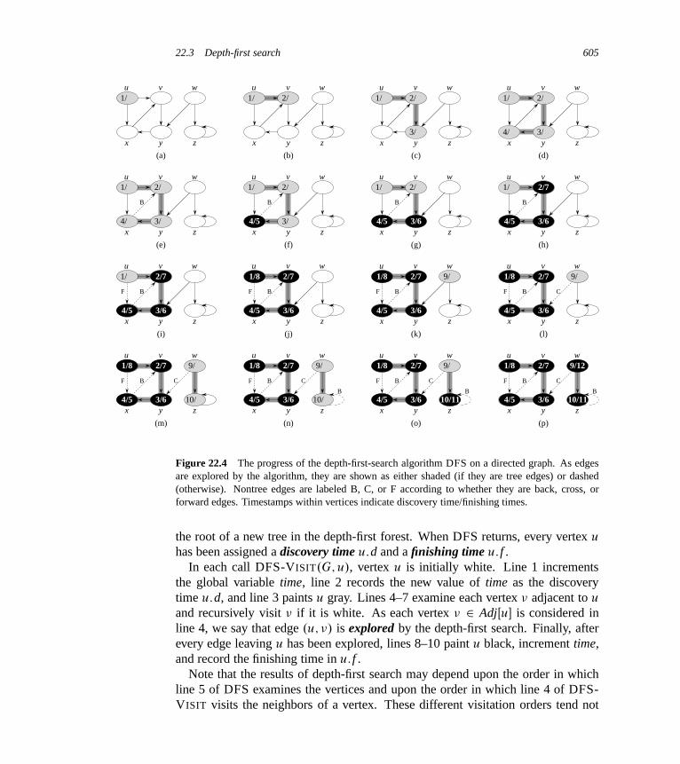
22.3 Depth-first search 605
u v w
x y z
1/ 1/ 2/ 1/ 2/
3/
1/ 2/
3/4/
1/ 2/
3/4/
B
1/ 2/
3/
B
4/5
1/ 2/
B
4/5 3/6
1/
B
4/5 3/6
2/7
1/
B
4/5 3/6
2/7
F B
4/5 3/6
2/7
F
1/8
B
4/5 3/6
2/7
F
1/8 9/
B
4/5 3/6
2/7
F
1/8 9/
C
B
4/5 3/6
2/7
F
1/8 9/
C B
4/5 3/6
2/7
F
1/8 9/
C
B
B
4/5 3/6
2/7
F
1/8 9/
C
B10/11
B
4/5 3/6
2/7
F
1/8
C
B10/11
9/12
u v w
x y z
u v w
x y z
u v w
x y z
u v w
x y z
u v w
x y z
u v w
x y z
u v w
x y z
u v w
x y z
u v w
x y z
u v w
x y z
u v w
x y z
u v w
x y z
u v w
x y z
u v w
x y z
u v w
x y z
(m) (n) (o) (p)
(i) (j) (k) (l)
(e) (f) (g) (h)
(a) (b) (c) (d)
10/10/
Figure 22.4 The progress of the depth-first-search algorithm DFS on a directed graph. As edgesare explored by the algorithm, they are shown as either shaded (if they are tree edges) or dashed(otherwise). Nontree edges are labeled B, C, or F according to whether they are back, cross, orforward edges. Timestamps within vertices indicate discovery time/finishing times.
the root of a new tree in the depth-first forest. When DFS returns, every vertex u
has been assigned a discovery time u:d and a finishing time u: f .In each call DFS-VISIT.G; u/, vertex u is initially white. Line 1 increments
the global variable time, line 2 records the new value of time as the discoverytime u:d, and line 3 paints u gray. Lines 4–7 examine each vertex � adjacent to u
and recursively visit � if it is white. As each vertex � 2 AdjŒu� is considered inline 4, we say that edge .u; �/ is explored by the depth-first search. Finally, afterevery edge leaving u has been explored, lines 8–10 paint u black, increment time,and record the finishing time in u: f .
Note that the results of depth-first search may depend upon the order in whichline 5 of DFS examines the vertices and upon the order in which line 4 of DFS-VISIT visits the neighbors of a vertex. These different visitation orders tend not
606 Chapter 22 Elementary Graph Algorithms
to cause problems in practice, as we can usually use any depth-first search resulteffectively, with essentially equivalent results.
What is the running time of DFS? The loops on lines 1–3 and lines 5–7 of DFStake time ‚.V /, exclusive of the time to execute the calls to DFS-VISIT. As we didfor breadth-first search, we use aggregate analysis. The procedure DFS-VISIT iscalled exactly once for each vertex � 2 V , since the vertex u on which DFS-VISIT
is invoked must be white and the first thing DFS-VISIT does is paint vertex u gray.During an execution of DFS-VISIT.G; �/, the loop on lines 4–7 executes jAdjŒ��jtimes. SinceX�2V
jAdjŒ��j D ‚.E/ ;
the total cost of executing lines 4–7 of DFS-VISIT is ‚.E/. The running time ofDFS is therefore ‚.V CE/.
Properties of depth-first search
Depth-first search yields valuable information about the structure of a graph. Per-haps the most basic property of depth-first search is that the predecessor sub-graph G� does indeed form a forest of trees, since the structure of the depth-first trees exactly mirrors the structure of recursive calls of DFS-VISIT. That is,u D �:� if and only if DFS-VISIT.G; �/ was called during a search of u’s ad-jacency list. Additionally, vertex � is a descendant of vertex u in the depth-firstforest if and only if � is discovered during the time in which u is gray.
Another important property of depth-first search is that discovery and finishingtimes have parenthesis structure. If we represent the discovery of vertex u witha left parenthesis “.u” and represent its finishing by a right parenthesis “u/”, thenthe history of discoveries and finishings makes a well-formed expression in thesense that the parentheses are properly nested. For example, the depth-first searchof Figure 22.5(a) corresponds to the parenthesization shown in Figure 22.5(b). Thefollowing theorem provides another way to characterize the parenthesis structure.
Theorem 22.7 (Parenthesis theorem)In any depth-first search of a (directed or undirected) graph G D .V; E/, for anytwo vertices u and �, exactly one of the following three conditions holds:� the intervals Œu:d; u: f � and Œ�:d; �: f � are entirely disjoint, and neither u nor �
is a descendant of the other in the depth-first forest,� the interval Œu:d; u: f � is contained entirely within the interval Œ�:d; �: f �, and u
is a descendant of � in a depth-first tree, or� the interval Œ�:d; �: f � is contained entirely within the interval Œu:d; u: f �, and �
is a descendant of u in a depth-first tree.

22.3 Depth-first search 607
3/6 2/9 1/10 11/16
14/1512/137/84/5
y z s t
uvwx
B
C
F
C
C
C
B
1 2 3 4 5 6 7 8 9 10 11 12 13 14 15 16
s t
z
y w
x
v u
s
z
y w
x
t
v u
C
FB
C
C
B
C
(a)
(b)
(c)
(s (z (y (x x) y) (w w) z) s) (t (v v) (u u) t)
Figure 22.5 Properties of depth-first search. (a) The result of a depth-first search of a directedgraph. Vertices are timestamped and edge types are indicated as in Figure 22.4. (b) Intervals forthe discovery time and finishing time of each vertex correspond to the parenthesization shown. Eachrectangle spans the interval given by the discovery and finishing times of the corresponding vertex.Only tree edges are shown. If two intervals overlap, then one is nested within the other, and thevertex corresponding to the smaller interval is a descendant of the vertex corresponding to the larger.(c) The graph of part (a) redrawn with all tree and forward edges going down within a depth-first treeand all back edges going up from a descendant to an ancestor.
608 Chapter 22 Elementary Graph Algorithms
Proof We begin with the case in which u:d < �:d. We consider two subcases,according to whether �:d < u: f or not. The first subcase occurs when �:d < u: f ,so � was discovered while u was still gray, which implies that � is a descendantof u. Moreover, since � was discovered more recently than u, all of its outgo-ing edges are explored, and � is finished, before the search returns to and fin-ishes u. In this case, therefore, the interval Œ�:d; �: f � is entirely contained withinthe interval Œu:d; u: f �. In the other subcase, u: f < �:d, and by inequality (22.2),u:d < u: f < �:d < �: f ; thus the intervals Œu:d; u: f � and Œ�:d; �: f � are disjoint.Because the intervals are disjoint, neither vertex was discovered while the otherwas gray, and so neither vertex is a descendant of the other.
The case in which �:d < u:d is similar, with the roles of u and � reversed in theabove argument.
Corollary 22.8 (Nesting of descendants’ intervals)Vertex � is a proper descendant of vertex u in the depth-first forest for a (directedor undirected) graph G if and only if u:d < �:d < �: f < u: f .
Proof Immediate from Theorem 22.7.
The next theorem gives another important characterization of when one vertexis a descendant of another in the depth-first forest.
Theorem 22.9 (White-path theorem)In a depth-first forest of a (directed or undirected) graph G D .V; E/, vertex � isa descendant of vertex u if and only if at the time u:d that the search discovers u,there is a path from u to � consisting entirely of white vertices.
Proof ): If � D u, then the path from u to � contains just vertex u, which is stillwhite when we set the value of u:d. Now, suppose that � is a proper descendantof u in the depth-first forest. By Corollary 22.8, u:d < �:d, and so � is white attime u:d. Since � can be any descendant of u, all vertices on the unique simplepath from u to � in the depth-first forest are white at time u:d.(: Suppose that there is a path of white vertices from u to � at time u:d, but �
does not become a descendant of u in the depth-first tree. Without loss of general-ity, assume that every vertex other than � along the path becomes a descendant of u.(Otherwise, let � be the closest vertex to u along the path that doesn’t become a de-scendant of u.) Let w be the predecessor of � in the path, so that w is a descendantof u (w and u may in fact be the same vertex). By Corollary 22.8, w: f � u: f . Be-cause � must be discovered after u is discovered, but before w is finished, we haveu:d < �:d < w: f � u: f . Theorem 22.7 then implies that the interval Œ�:d; �: f �
22.3 Depth-first search 609
is contained entirely within the interval Œu:d; u: f �. By Corollary 22.8, � must afterall be a descendant of u.
Classification of edges
Another interesting property of depth-first search is that the search can be usedto classify the edges of the input graph G D .V; E/. The type of each edge canprovide important information about a graph. For example, in the next section, weshall see that a directed graph is acyclic if and only if a depth-first search yields no“back” edges (Lemma 22.11).
We can define four edge types in terms of the depth-first forest G� produced bya depth-first search on G:
1. Tree edges are edges in the depth-first forest G� . Edge .u; �/ is a tree edge if �
was first discovered by exploring edge .u; �/.
2. Back edges are those edges .u; �/ connecting a vertex u to an ancestor � in adepth-first tree. We consider self-loops, which may occur in directed graphs, tobe back edges.
3. Forward edges are those nontree edges .u; �/ connecting a vertex u to a de-scendant � in a depth-first tree.
4. Cross edges are all other edges. They can go between vertices in the samedepth-first tree, as long as one vertex is not an ancestor of the other, or they cango between vertices in different depth-first trees.
In Figures 22.4 and 22.5, edge labels indicate edge types. Figure 22.5(c) also showshow to redraw the graph of Figure 22.5(a) so that all tree and forward edges headdownward in a depth-first tree and all back edges go up. We can redraw any graphin this fashion.
The DFS algorithm has enough information to classify some edges as it encoun-ters them. The key idea is that when we first explore an edge .u; �/, the color ofvertex � tells us something about the edge:
1. WHITE indicates a tree edge,
2. GRAY indicates a back edge, and
3. BLACK indicates a forward or cross edge.
The first case is immediate from the specification of the algorithm. For the sec-ond case, observe that the gray vertices always form a linear chain of descendantscorresponding to the stack of active DFS-VISIT invocations; the number of grayvertices is one more than the depth in the depth-first forest of the vertex most re-cently discovered. Exploration always proceeds from the deepest gray vertex, so
610 Chapter 22 Elementary Graph Algorithms
an edge that reaches another gray vertex has reached an ancestor. The third casehandles the remaining possibility; Exercise 22.3-5 asks you to show that such anedge .u; �/ is a forward edge if u:d < �:d and a cross edge if u:d > �:d.
An undirected graph may entail some ambiguity in how we classify edges,since .u; �/ and .�; u/ are really the same edge. In such a case, we classify theedge as the first type in the classification list that applies. Equivalently (see Ex-ercise 22.3-6), we classify the edge according to whichever of .u; �/ or .�; u/ thesearch encounters first.
We now show that forward and cross edges never occur in a depth-first search ofan undirected graph.
Theorem 22.10In a depth-first search of an undirected graph G, every edge of G is either a treeedge or a back edge.
Proof Let .u; �/ be an arbitrary edge of G, and suppose without loss of generalitythat u:d < �:d. Then the search must discover and finish � before it finishes u
(while u is gray), since � is on u’s adjacency list. If the first time that the searchexplores edge .u; �/, it is in the direction from u to �, then � is undiscovered(white) until that time, for otherwise the search would have explored this edgealready in the direction from � to u. Thus, .u; �/ becomes a tree edge. If thesearch explores .u; �/ first in the direction from � to u, then .u; �/ is a back edge,since u is still gray at the time the edge is first explored.
We shall see several applications of these theorems in the following sections.
Exercises
22.3-1Make a 3-by-3 chart with row and column labels WHITE, GRAY, and BLACK. Ineach cell .i; j /, indicate whether, at any point during a depth-first search of a di-rected graph, there can be an edge from a vertex of color i to a vertex of color j .For each possible edge, indicate what edge types it can be. Make a second suchchart for depth-first search of an undirected graph.
22.3-2Show how depth-first search works on the graph of Figure 22.6. Assume that thefor loop of lines 5–7 of the DFS procedure considers the vertices in alphabeticalorder, and assume that each adjacency list is ordered alphabetically. Show thediscovery and finishing times for each vertex, and show the classification of eachedge.

22.3 Depth-first search 611
q r
s t u
v w x y
z
Figure 22.6 A directed graph for use in Exercises 22.3-2 and 22.5-2.
22.3-3Show the parenthesis structure of the depth-first search of Figure 22.4.
22.3-4Show that using a single bit to store each vertex color suffices by arguing thatthe DFS procedure would produce the same result if line 3 of DFS-VISIT wasremoved.
22.3-5Show that edge .u; �/ is
a. a tree edge or forward edge if and only if u:d < �:d < �: f < u: f ,
b. a back edge if and only if �:d � u:d < u: f � �: f , and
c. a cross edge if and only if �:d < �: f < u:d < u: f .
22.3-6Show that in an undirected graph, classifying an edge .u; �/ as a tree edge or a backedge according to whether .u; �/ or .�; u/ is encountered first during the depth-firstsearch is equivalent to classifying it according to the ordering of the four types inthe classification scheme.
22.3-7Rewrite the procedure DFS, using a stack to eliminate recursion.
22.3-8Give a counterexample to the conjecture that if a directed graph G contains a pathfrom u to �, and if u:d < �:d in a depth-first search of G, then � is a descendantof u in the depth-first forest produced.
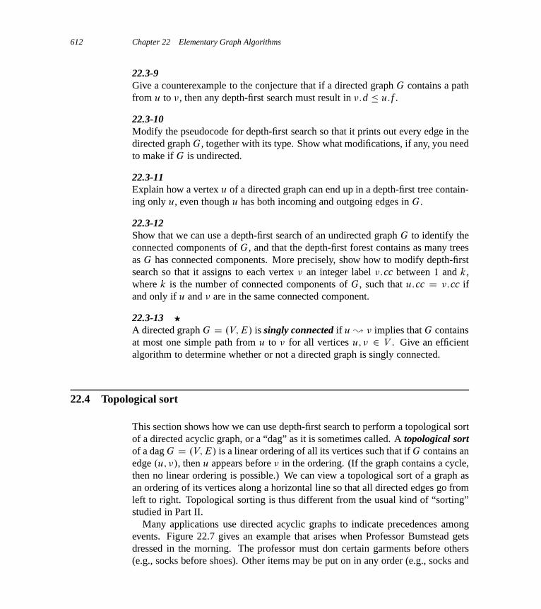
612 Chapter 22 Elementary Graph Algorithms
22.3-9Give a counterexample to the conjecture that if a directed graph G contains a pathfrom u to �, then any depth-first search must result in �:d � u: f .
22.3-10Modify the pseudocode for depth-first search so that it prints out every edge in thedirected graph G, together with its type. Show what modifications, if any, you needto make if G is undirected.
22.3-11Explain how a vertex u of a directed graph can end up in a depth-first tree contain-ing only u, even though u has both incoming and outgoing edges in G.
22.3-12Show that we can use a depth-first search of an undirected graph G to identify theconnected components of G, and that the depth-first forest contains as many treesas G has connected components. More precisely, show how to modify depth-firstsearch so that it assigns to each vertex � an integer label �:cc between 1 and k,where k is the number of connected components of G, such that u:cc D �:cc ifand only if u and � are in the same connected component.
22.3-13 ?
A directed graph G D .V; E/ is singly connected if u � � implies that G containsat most one simple path from u to � for all vertices u; � 2 V . Give an efficientalgorithm to determine whether or not a directed graph is singly connected.
22.4 Topological sort
This section shows how we can use depth-first search to perform a topological sortof a directed acyclic graph, or a “dag” as it is sometimes called. A topological sortof a dag G D .V; E/ is a linear ordering of all its vertices such that if G contains anedge .u; �/, then u appears before � in the ordering. (If the graph contains a cycle,then no linear ordering is possible.) We can view a topological sort of a graph asan ordering of its vertices along a horizontal line so that all directed edges go fromleft to right. Topological sorting is thus different from the usual kind of “sorting”studied in Part II.
Many applications use directed acyclic graphs to indicate precedences amongevents. Figure 22.7 gives an example that arises when Professor Bumstead getsdressed in the morning. The professor must don certain garments before others(e.g., socks before shoes). Other items may be put on in any order (e.g., socks and
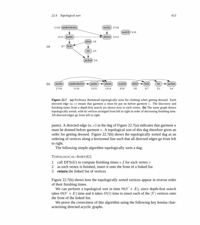
22.4 Topological sort 613
11/16
12/15
6/7
1/8
2/5
3/4
17/18
13/14
9/10
17/18 11/16 12/15 13/14 9/10 1/8 6/7 2/5 3/4
(a)
(b)
undershorts
pants
belt
shirt
tie
jacket
socks
shoes
watch
socks undershorts pants shoes watch shirt belt tie jacket
Figure 22.7 (a) Professor Bumstead topologically sorts his clothing when getting dressed. Eachdirected edge .u; �/ means that garment u must be put on before garment �. The discovery andfinishing times from a depth-first search are shown next to each vertex. (b) The same graph showntopologically sorted, with its vertices arranged from left to right in order of decreasing finishing time.All directed edges go from left to right.
pants). A directed edge .u; �/ in the dag of Figure 22.7(a) indicates that garment u
must be donned before garment �. A topological sort of this dag therefore gives anorder for getting dressed. Figure 22.7(b) shows the topologically sorted dag as anordering of vertices along a horizontal line such that all directed edges go from leftto right.
The following simple algorithm topologically sorts a dag:
TOPOLOGICAL-SORT.G/
1 call DFS.G/ to compute finishing times �: f for each vertex �
2 as each vertex is finished, insert it onto the front of a linked list3 return the linked list of vertices
Figure 22.7(b) shows how the topologically sorted vertices appear in reverse orderof their finishing times.
We can perform a topological sort in time ‚.V C E/, since depth-first searchtakes ‚.V CE/ time and it takes O.1/ time to insert each of the jV j vertices ontothe front of the linked list.
We prove the correctness of this algorithm using the following key lemma char-acterizing directed acyclic graphs.
614 Chapter 22 Elementary Graph Algorithms
Lemma 22.11A directed graph G is acyclic if and only if a depth-first search of G yields no backedges.
Proof ): Suppose that a depth-first search produces a back edge .u; �/. Thenvertex � is an ancestor of vertex u in the depth-first forest. Thus, G contains a pathfrom � to u, and the back edge .u; �/ completes a cycle.(: Suppose that G contains a cycle c. We show that a depth-first search of G
yields a back edge. Let � be the first vertex to be discovered in c, and let .u; �/ bethe preceding edge in c. At time �:d, the vertices of c form a path of white verticesfrom � to u. By the white-path theorem, vertex u becomes a descendant of � in thedepth-first forest. Therefore, .u; �/ is a back edge.
Theorem 22.12TOPOLOGICAL-SORT produces a topological sort of the directed acyclic graphprovided as its input.
Proof Suppose that DFS is run on a given dag G D .V; E/ to determine fin-ishing times for its vertices. It suffices to show that for any pair of distinct ver-tices u; � 2 V , if G contains an edge from u to �, then �: f < u: f . Consider anyedge .u; �/ explored by DFS.G/. When this edge is explored, � cannot be gray,since then � would be an ancestor of u and .u; �/ would be a back edge, contra-dicting Lemma 22.11. Therefore, � must be either white or black. If � is white,it becomes a descendant of u, and so �: f < u: f . If � is black, it has already beenfinished, so that �: f has already been set. Because we are still exploring from u, wehave yet to assign a timestamp to u: f , and so once we do, we will have �: f < u: fas well. Thus, for any edge .u; �/ in the dag, we have �: f < u: f , proving thetheorem.
Exercises
22.4-1Show the ordering of vertices produced by TOPOLOGICAL-SORT when it is run onthe dag of Figure 22.8, under the assumption of Exercise 22.3-2.
22.4-2Give a linear-time algorithm that takes as input a directed acyclic graph G D.V; E/ and two vertices s and t , and returns the number of simple paths from s
to t in G. For example, the directed acyclic graph of Figure 22.8 contains exactlyfour simple paths from vertex p to vertex �: po�, pory�, posry�, and psry�.(Your algorithm needs only to count the simple paths, not list them.)

22.5 Strongly connected components 615
zyx
wvut
srq
ponm
Figure 22.8 A dag for topological sorting.
22.4-3Give an algorithm that determines whether or not a given undirected graph G D.V; E/ contains a cycle. Your algorithm should run in O.V / time, independentof jEj.22.4-4Prove or disprove: If a directed graph G contains cycles, then TOPOLOGICAL-SORT.G/ produces a vertex ordering that minimizes the number of “bad” edgesthat are inconsistent with the ordering produced.
22.4-5Another way to perform topological sorting on a directed acyclic graph G D.V; E/ is to repeatedly find a vertex of in-degree 0, output it, and remove it andall of its outgoing edges from the graph. Explain how to implement this idea sothat it runs in time O.V CE/. What happens to this algorithm if G has cycles?
22.5 Strongly connected components
We now consider a classic application of depth-first search: decomposing a di-rected graph into its strongly connected components. This section shows how to doso using two depth-first searches. Many algorithms that work with directed graphsbegin with such a decomposition. After decomposing the graph into strongly con-nected components, such algorithms run separately on each one and then combinethe solutions according to the structure of connections among components.
Recall from Appendix B that a strongly connected component of a directedgraph G D .V; E/ is a maximal set of vertices C � V such that for every pairof vertices u and � in C , we have both u � � and � � u; that is, vertices u and �
are reachable from each other. Figure 22.9 shows an example.
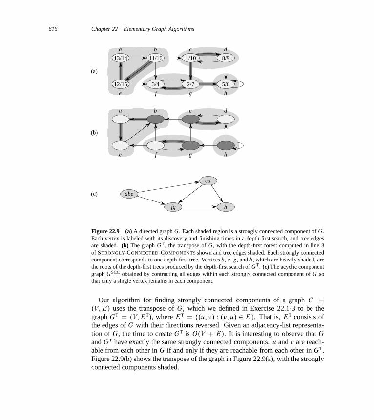
616 Chapter 22 Elementary Graph Algorithms
13/14 11/16
12/15 3/4
1/10
2/7
8/9
5/6
a b c d
e f g h
a b c d
e f g h
abe
cd
fg h
(c)
(b)
(a)
Figure 22.9 (a) A directed graph G. Each shaded region is a strongly connected component of G.Each vertex is labeled with its discovery and finishing times in a depth-first search, and tree edgesare shaded. (b) The graph GT, the transpose of G, with the depth-first forest computed in line 3of STRONGLY-CONNECTED-COMPONENTS shown and tree edges shaded. Each strongly connectedcomponent corresponds to one depth-first tree. Vertices b, c, g, and h, which are heavily shaded, arethe roots of the depth-first trees produced by the depth-first search of GT. (c) The acyclic componentgraph GSCC obtained by contracting all edges within each strongly connected component of G sothat only a single vertex remains in each component.
Our algorithm for finding strongly connected components of a graph G D.V; E/ uses the transpose of G, which we defined in Exercise 22.1-3 to be thegraph GT D .V; ET/, where ET D f.u; �/ W .�; u/ 2 Eg. That is, ET consists ofthe edges of G with their directions reversed. Given an adjacency-list representa-tion of G, the time to create GT is O.V C E/. It is interesting to observe that G
and GT have exactly the same strongly connected components: u and � are reach-able from each other in G if and only if they are reachable from each other in GT.Figure 22.9(b) shows the transpose of the graph in Figure 22.9(a), with the stronglyconnected components shaded.
22.5 Strongly connected components 617
The following linear-time (i.e., ‚.VCE/-time) algorithm computes the stronglyconnected components of a directed graph G D .V; E/ using two depth-firstsearches, one on G and one on GT.
STRONGLY-CONNECTED-COMPONENTS.G/
1 call DFS.G/ to compute finishing times u: f for each vertex u
2 compute GT
3 call DFS.GT/, but in the main loop of DFS, consider the verticesin order of decreasing u: f (as computed in line 1)
4 output the vertices of each tree in the depth-first forest formed in line 3 as aseparate strongly connected component
The idea behind this algorithm comes from a key property of the componentgraph GSCC D .V SCC; ESCC/, which we define as follows. Suppose that G
has strongly connected components C1; C2; : : : ; Ck . The vertex set V SCC isf�1; �2; : : : ; �kg, and it contains a vertex �i for each strongly connected compo-nent Ci of G. There is an edge .�i ; �j / 2 ESCC if G contains a directed edge .x; y/
for some x 2 Ci and some y 2 Cj . Looked at another way, by contracting alledges whose incident vertices are within the same strongly connected componentof G, the resulting graph is GSCC. Figure 22.9(c) shows the component graph ofthe graph in Figure 22.9(a).
The key property is that the component graph is a dag, which the followinglemma implies.
Lemma 22.13Let C and C 0 be distinct strongly connected components in directed graph G D.V; E/, let u; � 2 C , let u0; � 0 2 C 0, and suppose that G contains a path u � u0.Then G cannot also contain a path � 0
� �.
Proof If G contains a path � 0� �, then it contains paths u � u0
� � 0 and� 0
� � � u. Thus, u and � 0 are reachable from each other, thereby contradictingthe assumption that C and C 0 are distinct strongly connected components.
We shall see that by considering vertices in the second depth-first search in de-creasing order of the finishing times that were computed in the first depth-firstsearch, we are, in essence, visiting the vertices of the component graph (each ofwhich corresponds to a strongly connected component of G) in topologically sortedorder.
Because the STRONGLY-CONNECTED-COMPONENTS procedure performs twodepth-first searches, there is the potential for ambiguity when we discuss u:dor u: f . In this section, these values always refer to the discovery and finishingtimes as computed by the first call of DFS, in line 1.
618 Chapter 22 Elementary Graph Algorithms
We extend the notation for discovery and finishing times to sets of vertices.If U � V , then we define d.U / D minu2U fu:dg and f .U / D maxu2U fu: f g.That is, d.U / and f .U / are the earliest discovery time and latest finishing time,respectively, of any vertex in U .
The following lemma and its corollary give a key property relating strongly con-nected components and finishing times in the first depth-first search.
Lemma 22.14Let C and C 0 be distinct strongly connected components in directed graph G D.V; E/. Suppose that there is an edge .u; �/ 2 E, where u 2 C and � 2 C 0. Thenf .C / > f .C 0/.
Proof We consider two cases, depending on which strongly connected compo-nent, C or C 0, had the first discovered vertex during the depth-first search.
If d.C / < d.C 0/, let x be the first vertex discovered in C . At time x:d, all ver-tices in C and C 0 are white. At that time, G contains a path from x to each vertexin C consisting only of white vertices. Because .u; �/ 2 E, for any vertex w 2 C 0,there is also a path in G at time x:d from x to w consisting only of white vertices:x � u ! � � w. By the white-path theorem, all vertices in C and C 0 becomedescendants of x in the depth-first tree. By Corollary 22.8, x has the latest finishingtime of any of its descendants, and so x: f D f .C / > f .C 0/.
If instead we have d.C / > d.C 0/, let y be the first vertex discovered in C 0.At time y:d, all vertices in C 0 are white and G contains a path from y to eachvertex in C 0 consisting only of white vertices. By the white-path theorem, all ver-tices in C 0 become descendants of y in the depth-first tree, and by Corollary 22.8,y: f D f .C 0/. At time y:d, all vertices in C are white. Since there is an edge .u; �/
from C to C 0, Lemma 22.13 implies that there cannot be a path from C 0 to C .Hence, no vertex in C is reachable from y. At time y: f , therefore, all vertices in C
are still white. Thus, for any vertex w 2 C , we have w: f > y: f , which impliesthat f .C / > f .C 0/.
The following corollary tells us that each edge in GT that goes between differentstrongly connected components goes from a component with an earlier finishingtime (in the first depth-first search) to a component with a later finishing time.
Corollary 22.15Let C and C 0 be distinct strongly connected components in directed graph G D.V; E/. Suppose that there is an edge .u; �/ 2 ET, where u 2 C and � 2 C 0. Thenf .C / < f .C 0/.
22.5 Strongly connected components 619
Proof Since .u; �/ 2 ET, we have .�; u/ 2 E. Because the strongly con-nected components of G and GT are the same, Lemma 22.14 implies thatf .C / < f .C 0/.
Corollary 22.15 provides the key to understanding why the strongly connectedcomponents algorithm works. Let us examine what happens when we perform thesecond depth-first search, which is on GT. We start with the strongly connectedcomponent C whose finishing time f .C / is maximum. The search starts fromsome vertex x 2 C , and it visits all vertices in C . By Corollary 22.15, GT containsno edges from C to any other strongly connected component, and so the searchfrom x will not visit vertices in any other component. Thus, the tree rooted at x
contains exactly the vertices of C . Having completed visiting all vertices in C ,the search in line 3 selects as a root a vertex from some other strongly connectedcomponent C 0 whose finishing time f .C 0/ is maximum over all components otherthan C . Again, the search will visit all vertices in C 0, but by Corollary 22.15,the only edges in GT from C 0 to any other component must be to C , which wehave already visited. In general, when the depth-first search of GT in line 3 visitsany strongly connected component, any edges out of that component must be tocomponents that the search already visited. Each depth-first tree, therefore, will beexactly one strongly connected component. The following theorem formalizes thisargument.
Theorem 22.16The STRONGLY-CONNECTED-COMPONENTS procedure correctly computes thestrongly connected components of the directed graph G provided as its input.
Proof We argue by induction on the number of depth-first trees found in thedepth-first search of GT in line 3 that the vertices of each tree form a stronglyconnected component. The inductive hypothesis is that the first k trees producedin line 3 are strongly connected components. The basis for the induction, whenk D 0, is trivial.
In the inductive step, we assume that each of the first k depth-first trees producedin line 3 is a strongly connected component, and we consider the .k C 1/st treeproduced. Let the root of this tree be vertex u, and let u be in strongly connectedcomponent C . Because of how we choose roots in the depth-first search in line 3,u: f D f .C / > f .C 0/ for any strongly connected component C 0 other than C
that has yet to be visited. By the inductive hypothesis, at the time that the searchvisits u, all other vertices of C are white. By the white-path theorem, therefore, allother vertices of C are descendants of u in its depth-first tree. Moreover, by theinductive hypothesis and by Corollary 22.15, any edges in GT that leave C must beto strongly connected components that have already been visited. Thus, no vertex
620 Chapter 22 Elementary Graph Algorithms
in any strongly connected component other than C will be a descendant of u duringthe depth-first search of GT. Thus, the vertices of the depth-first tree in GT that isrooted at u form exactly one strongly connected component, which completes theinductive step and the proof.
Here is another way to look at how the second depth-first search operates. Con-sider the component graph .GT/SCC of GT. If we map each strongly connectedcomponent visited in the second depth-first search to a vertex of .GT/SCC, the sec-ond depth-first search visits vertices of .GT/SCC in the reverse of a topologicallysorted order. If we reverse the edges of .GT/SCC, we get the graph ..GT/SCC/T.Because ..GT/SCC/T D GSCC (see Exercise 22.5-4), the second depth-first searchvisits the vertices of GSCC in topologically sorted order.
Exercises
22.5-1How can the number of strongly connected components of a graph change if a newedge is added?
22.5-2Show how the procedure STRONGLY-CONNECTED-COMPONENTS works on thegraph of Figure 22.6. Specifically, show the finishing times computed in line 1 andthe forest produced in line 3. Assume that the loop of lines 5–7 of DFS considersvertices in alphabetical order and that the adjacency lists are in alphabetical order.
22.5-3Professor Bacon claims that the algorithm for strongly connected componentswould be simpler if it used the original (instead of the transpose) graph in thesecond depth-first search and scanned the vertices in order of increasing finishingtimes. Does this simpler algorithm always produce correct results?
22.5-4Prove that for any directed graph G, we have ..GT/SCC/T D GSCC. That is, thetranspose of the component graph of GT is the same as the component graph of G.
22.5-5Give an O.V C E/-time algorithm to compute the component graph of a directedgraph G D .V; E/. Make sure that there is at most one edge between two verticesin the component graph your algorithm produces.

Problems for Chapter 22 621
22.5-6Given a directed graph G D .V; E/, explain how to create another graph G0 D.V; E 0/ such that (a) G0 has the same strongly connected components as G, (b) G0
has the same component graph as G, and (c) E 0 is as small as possible. Describe afast algorithm to compute G0.
22.5-7A directed graph G D .V; E/ is semiconnected if, for all pairs of vertices u; � 2 V ,we have u � � or � � u. Give an efficient algorithm to determine whetheror not G is semiconnected. Prove that your algorithm is correct, and analyze itsrunning time.
Problems
22-1 Classifying edges by breadth-first searchA depth-first forest classifies the edges of a graph into tree, back, forward, andcross edges. A breadth-first tree can also be used to classify the edges reachablefrom the source of the search into the same four categories.
a. Prove that in a breadth-first search of an undirected graph, the following prop-erties hold:
1. There are no back edges and no forward edges.
2. For each tree edge .u; �/, we have �:d D u:d C 1.
3. For each cross edge .u; �/, we have �:d D u:d or �:d D u:dC 1.
b. Prove that in a breadth-first search of a directed graph, the following propertieshold:
1. There are no forward edges.
2. For each tree edge .u; �/, we have �:d D u:d C 1.
3. For each cross edge .u; �/, we have �:d � u:d C 1.
4. For each back edge .u; �/, we have 0 � �:d � u:d.
22-2 Articulation points, bridges, and biconnected componentsLet G D .V; E/ be a connected, undirected graph. An articulation point of G isa vertex whose removal disconnects G. A bridge of G is an edge whose removaldisconnects G. A biconnected component of G is a maximal set of edges suchthat any two edges in the set lie on a common simple cycle. Figure 22.10 illustrates

622 Chapter 22 Elementary Graph Algorithms
12
3
4
5
6
Figure 22.10 The articulation points, bridges, and biconnected components of a connected, undi-rected graph for use in Problem 22-2. The articulation points are the heavily shaded vertices, thebridges are the heavily shaded edges, and the biconnected components are the edges in the shadedregions, with a bcc numbering shown.
these definitions. We can determine articulation points, bridges, and biconnectedcomponents using depth-first search. Let G� D .V; E�/ be a depth-first tree of G.
a. Prove that the root of G� is an articulation point of G if and only if it has atleast two children in G� .
b. Let � be a nonroot vertex of G� . Prove that � is an articulation point of G if andonly if � has a child s such that there is no back edge from s or any descendantof s to a proper ancestor of �.
c. Let
�: low D min
(�:d ;
w:d W .u; w/ is a back edge for some descendant u of � :
Show how to compute �: low for all vertices � 2 V in O.E/ time.
d. Show how to compute all articulation points in O.E/ time.
e. Prove that an edge of G is a bridge if and only if it does not lie on any simplecycle of G.
f. Show how to compute all the bridges of G in O.E/ time.
g. Prove that the biconnected components of G partition the nonbridge edges of G.
h. Give an O.E/-time algorithm to label each edge e of G with a positive in-teger e:bcc such that e:bcc D e0:bcc if and only if e and e0 are in the samebiconnected component.
Notes for Chapter 22 623
22-3 Euler tourAn Euler tour of a strongly connected, directed graph G D .V; E/ is a cycle thattraverses each edge of G exactly once, although it may visit a vertex more thanonce.
a. Show that G has an Euler tour if and only if in-degree.�/ D out-degree.�/ foreach vertex � 2 V .
b. Describe an O.E/-time algorithm to find an Euler tour of G if one exists. (Hint:Merge edge-disjoint cycles.)
22-4 ReachabilityLet G D .V; E/ be a directed graph in which each vertex u 2 V is labeled witha unique integer L.u/ from the set f1; 2; : : : ; jV jg. For each vertex u 2 V , letR.u/ D f� 2 V W u � �g be the set of vertices that are reachable from u. Definemin.u/ to be the vertex in R.u/ whose label is minimum, i.e., min.u/ is the vertex �
such that L.�/ D min fL.w/ W w 2 R.u/g. Give an O.V CE/-time algorithm thatcomputes min.u/ for all vertices u 2 V .
Chapter notes
Even [103] and Tarjan [330] are excellent references for graph algorithms.Breadth-first search was discovered by Moore [260] in the context of finding
paths through mazes. Lee [226] independently discovered the same algorithm inthe context of routing wires on circuit boards.
Hopcroft and Tarjan [178] advocated the use of the adjacency-list representationover the adjacency-matrix representation for sparse graphs and were the first torecognize the algorithmic importance of depth-first search. Depth-first search hasbeen widely used since the late 1950s, especially in artificial intelligence programs.
Tarjan [327] gave a linear-time algorithm for finding strongly connected compo-nents. The algorithm for strongly connected components in Section 22.5 is adaptedfrom Aho, Hopcroft, and Ullman [6], who credit it to S. R. Kosaraju (unpublished)and M. Sharir [314]. Gabow [119] also developed an algorithm for strongly con-nected components that is based on contracting cycles and uses two stacks to makeit run in linear time. Knuth [209] was the first to give a linear-time algorithm fortopological sorting.
23 Minimum Spanning Trees
Electronic circuit designs often need to make the pins of several components elec-trically equivalent by wiring them together. To interconnect a set of n pins, we canuse an arrangement of n� 1 wires, each connecting two pins. Of all such arrange-ments, the one that uses the least amount of wire is usually the most desirable.
We can model this wiring problem with a connected, undirected graph G D.V; E/, where V is the set of pins, E is the set of possible interconnections betweenpairs of pins, and for each edge .u; �/ 2 E, we have a weight w.u; �/ specifyingthe cost (amount of wire needed) to connect u and �. We then wish to find anacyclic subset T � E that connects all of the vertices and whose total weight
w.T / DX
.u;�/2T
w.u; �/
is minimized. Since T is acyclic and connects all of the vertices, it must form a tree,which we call a spanning tree since it “spans” the graph G. We call the problem ofdetermining the tree T the minimum-spanning-tree problem.1 Figure 23.1 showsan example of a connected graph and a minimum spanning tree.
In this chapter, we shall examine two algorithms for solving the minimum-spanning-tree problem: Kruskal’s algorithm and Prim’s algorithm. We can easilymake each of them run in time O.E lg V / using ordinary binary heaps. By usingFibonacci heaps, Prim’s algorithm runs in time O.E C V lg V /, which improvesover the binary-heap implementation if jV j is much smaller than jEj.
The two algorithms are greedy algorithms, as described in Chapter 16. Eachstep of a greedy algorithm must make one of several possible choices. The greedystrategy advocates making the choice that is the best at the moment. Such a strat-egy does not generally guarantee that it will always find globally optimal solutions
1The phrase “minimum spanning tree” is a shortened form of the phrase “minimum-weight spanningtree.” We are not, for example, minimizing the number of edges in T , since all spanning trees haveexactly jV j � 1 edges by Theorem B.2.
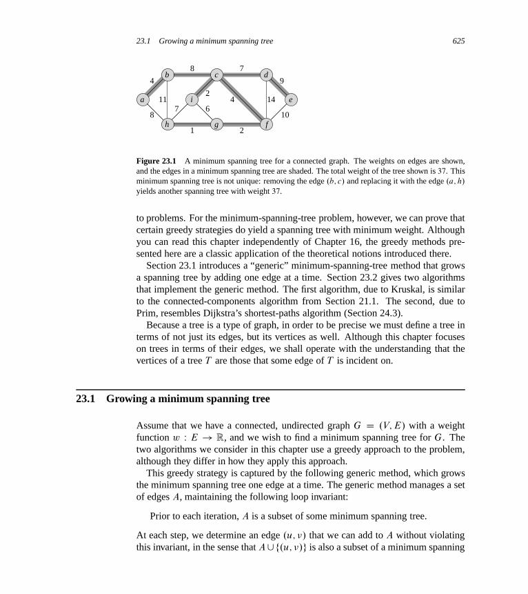
23.1 Growing a minimum spanning tree 625
b
a
h
c
g
i
d
f
e
4
8
11
8 7
9
10
144
21
2
7 6
Figure 23.1 A minimum spanning tree for a connected graph. The weights on edges are shown,and the edges in a minimum spanning tree are shaded. The total weight of the tree shown is 37. Thisminimum spanning tree is not unique: removing the edge .b; c/ and replacing it with the edge .a; h/
yields another spanning tree with weight 37.
to problems. For the minimum-spanning-tree problem, however, we can prove thatcertain greedy strategies do yield a spanning tree with minimum weight. Althoughyou can read this chapter independently of Chapter 16, the greedy methods pre-sented here are a classic application of the theoretical notions introduced there.
Section 23.1 introduces a “generic” minimum-spanning-tree method that growsa spanning tree by adding one edge at a time. Section 23.2 gives two algorithmsthat implement the generic method. The first algorithm, due to Kruskal, is similarto the connected-components algorithm from Section 21.1. The second, due toPrim, resembles Dijkstra’s shortest-paths algorithm (Section 24.3).
Because a tree is a type of graph, in order to be precise we must define a tree interms of not just its edges, but its vertices as well. Although this chapter focuseson trees in terms of their edges, we shall operate with the understanding that thevertices of a tree T are those that some edge of T is incident on.
23.1 Growing a minimum spanning tree
Assume that we have a connected, undirected graph G D .V; E/ with a weightfunction w W E ! R, and we wish to find a minimum spanning tree for G. Thetwo algorithms we consider in this chapter use a greedy approach to the problem,although they differ in how they apply this approach.
This greedy strategy is captured by the following generic method, which growsthe minimum spanning tree one edge at a time. The generic method manages a setof edges A, maintaining the following loop invariant:
Prior to each iteration, A is a subset of some minimum spanning tree.
At each step, we determine an edge .u; �/ that we can add to A without violatingthis invariant, in the sense that A[f.u; �/g is also a subset of a minimum spanning

626 Chapter 23 Minimum Spanning Trees
tree. We call such an edge a safe edge for A, since we can add it safely to A whilemaintaining the invariant.
GENERIC-MST.G; w/
1 A D ;2 while A does not form a spanning tree3 find an edge .u; �/ that is safe for A
4 A D A [ f.u; �/g5 return A
We use the loop invariant as follows:
Initialization: After line 1, the set A trivially satisfies the loop invariant.
Maintenance: The loop in lines 2–4 maintains the invariant by adding only safeedges.
Termination: All edges added to A are in a minimum spanning tree, and so theset A returned in line 5 must be a minimum spanning tree.
The tricky part is, of course, finding a safe edge in line 3. One must exist, sincewhen line 3 is executed, the invariant dictates that there is a spanning tree T suchthat A � T . Within the while loop body, A must be a proper subset of T , andtherefore there must be an edge .u; �/ 2 T such that .u; �/ 62 A and .u; �/ is safefor A.
In the remainder of this section, we provide a rule (Theorem 23.1) for recogniz-ing safe edges. The next section describes two algorithms that use this rule to findsafe edges efficiently.
We first need some definitions. A cut .S; V � S/ of an undirected graph G D.V; E/ is a partition of V . Figure 23.2 illustrates this notion. We say that an edge.u; �/ 2 E crosses the cut .S; V � S/ if one of its endpoints is in S and the otheris in V � S . We say that a cut respects a set A of edges if no edge in A crosses thecut. An edge is a light edge crossing a cut if its weight is the minimum of any edgecrossing the cut. Note that there can be more than one light edge crossing a cut inthe case of ties. More generally, we say that an edge is a light edge satisfying agiven property if its weight is the minimum of any edge satisfying the property.
Our rule for recognizing safe edges is given by the following theorem.
Theorem 23.1Let G D .V; E/ be a connected, undirected graph with a real-valued weight func-tion w defined on E. Let A be a subset of E that is included in some minimumspanning tree for G, let .S; V � S/ be any cut of G that respects A, and let .u; �/
be a light edge crossing .S; V � S/. Then, edge .u; �/ is safe for A.

23.1 Growing a minimum spanning tree 627
b
a
h
c
g
i
d
f
e
4
8
11
8 7
9
10
144
21
2
7 6
a
b
d
e
h
i
g
c
f
8
11
8
7
14
10
4
6
7
4
9
2
1
2
S
(a) (b)
V – S
S
V – S
S
V – S
Figure 23.2 Two ways of viewing a cut .S; V � S/ of the graph from Figure 23.1. (a) Blackvertices are in the set S , and white vertices are in V � S . The edges crossing the cut are thoseconnecting white vertices with black vertices. The edge .d; c/ is the unique light edge crossing thecut. A subset A of the edges is shaded; note that the cut .S; V � S/ respects A, since no edge of A
crosses the cut. (b) The same graph with the vertices in the set S on the left and the vertices in theset V � S on the right. An edge crosses the cut if it connects a vertex on the left with a vertex on theright.
Proof Let T be a minimum spanning tree that includes A, and assume that T
does not contain the light edge .u; �/, since if it does, we are done. We shallconstruct another minimum spanning tree T 0 that includes A [ f.u; �/g by using acut-and-paste technique, thereby showing that .u; �/ is a safe edge for A.
The edge .u; �/ forms a cycle with the edges on the simple path p from u
to � in T , as Figure 23.3 illustrates. Since u and � are on opposite sides of thecut .S; V � S/, at least one edge in T lies on the simple path p and also crossesthe cut. Let .x; y/ be any such edge. The edge .x; y/ is not in A, because the cutrespects A. Since .x; y/ is on the unique simple path from u to � in T , remov-ing .x; y/ breaks T into two components. Adding .u; �/ reconnects them to forma new spanning tree T 0 D T � f.x; y/g [ f.u; �/g.
We next show that T 0 is a minimum spanning tree. Since .u; �/ is a light edgecrossing .S; V �S/ and .x; y/ also crosses this cut, w.u; �/ � w.x; y/. Therefore,
w.T 0/ D w.T / � w.x; y/Cw.u; �/
� w.T / :
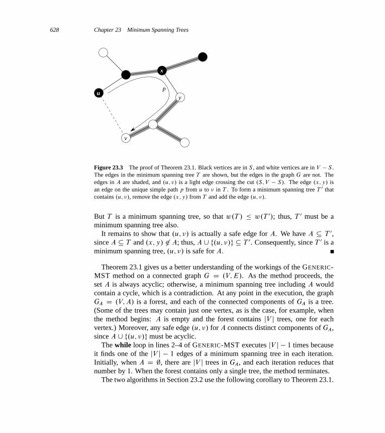
628 Chapter 23 Minimum Spanning Trees
y
v
u
x
p
Figure 23.3 The proof of Theorem 23.1. Black vertices are in S , and white vertices are in V � S .The edges in the minimum spanning tree T are shown, but the edges in the graph G are not. Theedges in A are shaded, and .u; �/ is a light edge crossing the cut .S; V � S/. The edge .x; y/ isan edge on the unique simple path p from u to � in T . To form a minimum spanning tree T 0 thatcontains .u; �/, remove the edge .x; y/ from T and add the edge .u; �/.
But T is a minimum spanning tree, so that w.T / � w.T 0/; thus, T 0 must be aminimum spanning tree also.
It remains to show that .u; �/ is actually a safe edge for A. We have A � T 0,since A � T and .x; y/ 62 A; thus, A [ f.u; �/g � T 0. Consequently, since T 0 is aminimum spanning tree, .u; �/ is safe for A.
Theorem 23.1 gives us a better understanding of the workings of the GENERIC-MST method on a connected graph G D .V; E/. As the method proceeds, theset A is always acyclic; otherwise, a minimum spanning tree including A wouldcontain a cycle, which is a contradiction. At any point in the execution, the graphGA D .V; A/ is a forest, and each of the connected components of GA is a tree.(Some of the trees may contain just one vertex, as is the case, for example, whenthe method begins: A is empty and the forest contains jV j trees, one for eachvertex.) Moreover, any safe edge .u; �/ for A connects distinct components of GA,since A [ f.u; �/g must be acyclic.
The while loop in lines 2–4 of GENERIC-MST executes jV j � 1 times becauseit finds one of the jV j � 1 edges of a minimum spanning tree in each iteration.Initially, when A D ;, there are jV j trees in GA, and each iteration reduces thatnumber by 1. When the forest contains only a single tree, the method terminates.
The two algorithms in Section 23.2 use the following corollary to Theorem 23.1.
23.1 Growing a minimum spanning tree 629
Corollary 23.2Let G D .V; E/ be a connected, undirected graph with a real-valued weight func-tion w defined on E. Let A be a subset of E that is included in some minimumspanning tree for G, and let C D .VC ; EC / be a connected component (tree) in theforest GA D .V; A/. If .u; �/ is a light edge connecting C to some other componentin GA, then .u; �/ is safe for A.
Proof The cut .VC ; V � VC / respects A, and .u; �/ is a light edge for this cut.Therefore, .u; �/ is safe for A.
Exercises
23.1-1Let .u; �/ be a minimum-weight edge in a connected graph G. Show that .u; �/
belongs to some minimum spanning tree of G.
23.1-2Professor Sabatier conjectures the following converse of Theorem 23.1. Let G D.V; E/ be a connected, undirected graph with a real-valued weight function w de-fined on E. Let A be a subset of E that is included in some minimum spanningtree for G, let .S; V � S/ be any cut of G that respects A, and let .u; �/ be a safeedge for A crossing .S; V � S/. Then, .u; �/ is a light edge for the cut. Show thatthe professor’s conjecture is incorrect by giving a counterexample.
23.1-3Show that if an edge .u; �/ is contained in some minimum spanning tree, then it isa light edge crossing some cut of the graph.
23.1-4Give a simple example of a connected graph such that the set of edges f.u; �/ Wthere exists a cut .S; V � S/ such that .u; �/ is a light edge crossing .S; V � S/gdoes not form a minimum spanning tree.
23.1-5Let e be a maximum-weight edge on some cycle of connected graph G D .V; E/.Prove that there is a minimum spanning tree of G0 D .V; E � feg/ that is also aminimum spanning tree of G. That is, there is a minimum spanning tree of G thatdoes not include e.
630 Chapter 23 Minimum Spanning Trees
23.1-6Show that a graph has a unique minimum spanning tree if, for every cut of thegraph, there is a unique light edge crossing the cut. Show that the converse is nottrue by giving a counterexample.
23.1-7Argue that if all edge weights of a graph are positive, then any subset of edges thatconnects all vertices and has minimum total weight must be a tree. Give an exampleto show that the same conclusion does not follow if we allow some weights to benonpositive.
23.1-8Let T be a minimum spanning tree of a graph G, and let L be the sorted list of theedge weights of T . Show that for any other minimum spanning tree T 0 of G, thelist L is also the sorted list of edge weights of T 0.
23.1-9Let T be a minimum spanning tree of a graph G D .V; E/, and let V 0 be a subsetof V . Let T 0 be the subgraph of T induced by V 0, and let G0 be the subgraph of G
induced by V 0. Show that if T 0 is connected, then T 0 is a minimum spanning treeof G0.
23.1-10Given a graph G and a minimum spanning tree T , suppose that we decrease theweight of one of the edges in T . Show that T is still a minimum spanning treefor G. More formally, let T be a minimum spanning tree for G with edge weightsgiven by weight function w. Choose one edge .x; y/ 2 T and a positive number k,and define the weight function w0 by
w0.u; �/ D(
w.u; �/ if .u; �/ ¤ .x; y/ ;
w.x; y/ � k if .u; �/ D .x; y/ :
Show that T is a minimum spanning tree for G with edge weights given by w0.
23.1-11 ?
Given a graph G and a minimum spanning tree T , suppose that we decrease theweight of one of the edges not in T . Give an algorithm for finding the minimumspanning tree in the modified graph.

23.2 The algorithms of Kruskal and Prim 631
23.2 The algorithms of Kruskal and Prim
The two minimum-spanning-tree algorithms described in this section elaborate onthe generic method. They each use a specific rule to determine a safe edge in line 3of GENERIC-MST. In Kruskal’s algorithm, the set A is a forest whose vertices areall those of the given graph. The safe edge added to A is always a least-weightedge in the graph that connects two distinct components. In Prim’s algorithm, theset A forms a single tree. The safe edge added to A is always a least-weight edgeconnecting the tree to a vertex not in the tree.
Kruskal’s algorithm
Kruskal’s algorithm finds a safe edge to add to the growing forest by finding, of allthe edges that connect any two trees in the forest, an edge .u; �/ of least weight.Let C1 and C2 denote the two trees that are connected by .u; �/. Since .u; �/ mustbe a light edge connecting C1 to some other tree, Corollary 23.2 implies that .u; �/
is a safe edge for C1. Kruskal’s algorithm qualifies as a greedy algorithm becauseat each step it adds to the forest an edge of least possible weight.
Our implementation of Kruskal’s algorithm is like the algorithm to computeconnected components from Section 21.1. It uses a disjoint-set data structure tomaintain several disjoint sets of elements. Each set contains the vertices in one treeof the current forest. The operation FIND-SET.u/ returns a representative elementfrom the set that contains u. Thus, we can determine whether two vertices u and �
belong to the same tree by testing whether FIND-SET.u/ equals FIND-SET.�/. Tocombine trees, Kruskal’s algorithm calls the UNION procedure.
MST-KRUSKAL.G; w/
1 A D ;2 for each vertex � 2 G:V3 MAKE-SET.�/
4 sort the edges of G:E into nondecreasing order by weight w
5 for each edge .u; �/ 2 G:E, taken in nondecreasing order by weight6 if FIND-SET.u/ ¤ FIND-SET.�/
7 A D A [ f.u; �/g8 UNION.u; �/
9 return A
Figure 23.4 shows how Kruskal’s algorithm works. Lines 1–3 initialize the set A
to the empty set and create jV j trees, one containing each vertex. The for loop inlines 5–8 examines edges in order of weight, from lowest to highest. The loop
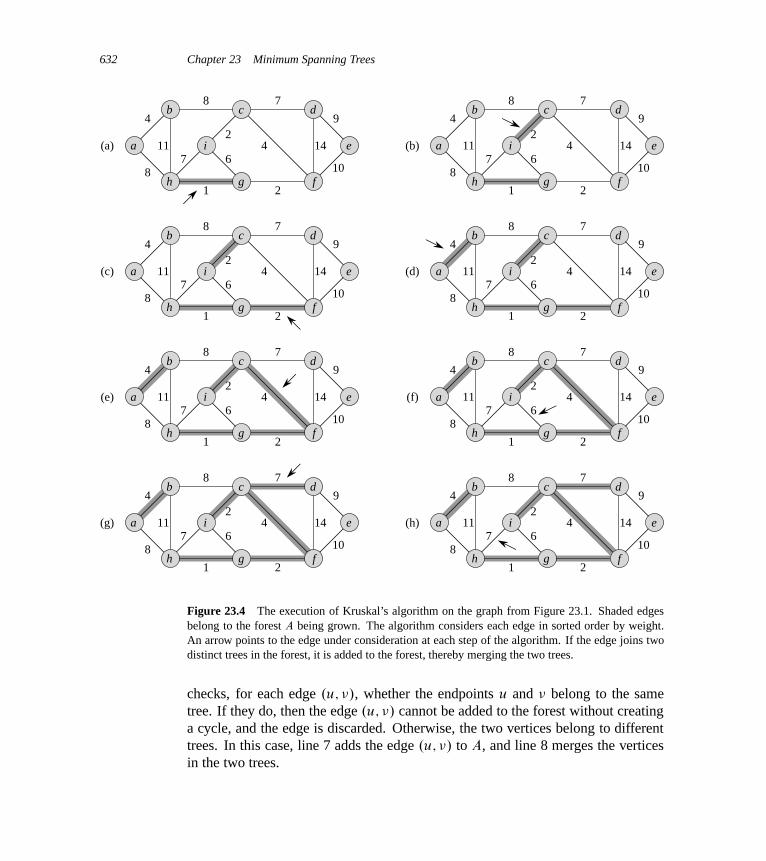
632 Chapter 23 Minimum Spanning Trees
b
a
h
c
g
i
d
f
e
4
8
11
8 7
9
10
144
21
2
7 6(a) (b)
(c) (d)
(e)
(g)
(f)
(h)
b
a
h
c
g
i
d
f
e
4
8
11
8 7
9
10
144
21
7 6
2
b
a
h
c
g
i
d
f
e
4
8
11
8 7
9
10
144
21
7 6
2
b
a
h
c
g
i
d
f
e
4
8
11
8 7
9
10
144
21
7 6
2
b
a
h
c
g
i
d
f
e
4
8
11
8 7
9
10
144
21
7 6
2
b
a
h
c
g
i
d
f
e
4
8
11
8 7
9
10
144
21
7 6
2
b
a
h
c
g
i
d
f
e
4
8
11
8 7
9
10
144
21
7 6
2
b
a
h
c
g
i
d
f
e
4
8
11
8 7
9
10
144
21
7 6
2
Figure 23.4 The execution of Kruskal’s algorithm on the graph from Figure 23.1. Shaded edgesbelong to the forest A being grown. The algorithm considers each edge in sorted order by weight.An arrow points to the edge under consideration at each step of the algorithm. If the edge joins twodistinct trees in the forest, it is added to the forest, thereby merging the two trees.
checks, for each edge .u; �/, whether the endpoints u and � belong to the sametree. If they do, then the edge .u; �/ cannot be added to the forest without creatinga cycle, and the edge is discarded. Otherwise, the two vertices belong to differenttrees. In this case, line 7 adds the edge .u; �/ to A, and line 8 merges the verticesin the two trees.
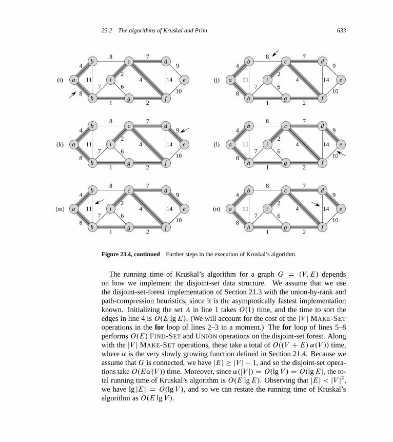
23.2 The algorithms of Kruskal and Prim 633
(i) (j)
(k) (l)
(n)(m)
b
a
h
c
g
i
d
f
e
4
8
11
8 7
9
10
144
21
7 6
b
a
h
c
g
i
d
f
e
4
8
11
8 7
9
10
144
21
7 6
22
b
a
h
c
g
i
d
f
e
4
8
11
8 7
9
10
144
21
7 6
2
b
a
h
c
g
i
d
f
e
4
8
11
8 7
9
10
144
21
7 6
b
a
h
c
g
i
d
f
e
4
8
11
8 7
9
10
144
21
7 6
b
a
h
c
g
i
d
f
e
4
8
11
8 7
9
10
144
21
7 6
2
2
2
Figure 23.4, continued Further steps in the execution of Kruskal’s algorithm.
The running time of Kruskal’s algorithm for a graph G D .V; E/ dependson how we implement the disjoint-set data structure. We assume that we usethe disjoint-set-forest implementation of Section 21.3 with the union-by-rank andpath-compression heuristics, since it is the asymptotically fastest implementationknown. Initializing the set A in line 1 takes O.1/ time, and the time to sort theedges in line 4 is O.E lg E/. (We will account for the cost of the jV j MAKE-SET
operations in the for loop of lines 2–3 in a moment.) The for loop of lines 5–8performs O.E/ FIND-SET and UNION operations on the disjoint-set forest. Alongwith the jV j MAKE-SET operations, these take a total of O..V CE/ ˛.V // time,where ˛ is the very slowly growing function defined in Section 21.4. Because weassume that G is connected, we have jEj � jV j � 1, and so the disjoint-set opera-tions take O.E˛.V // time. Moreover, since ˛.jV j/ D O.lg V / D O.lg E/, the to-tal running time of Kruskal’s algorithm is O.E lg E/. Observing that jEj < jV j2,we have lg jEj D O.lg V /, and so we can restate the running time of Kruskal’salgorithm as O.E lg V /.
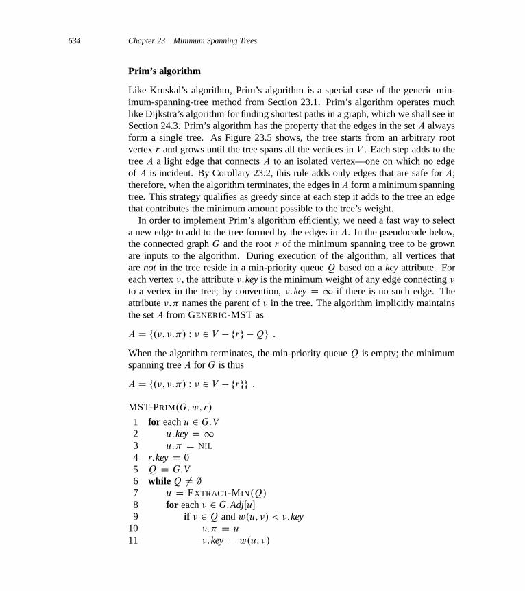
634 Chapter 23 Minimum Spanning Trees
Prim’s algorithm
Like Kruskal’s algorithm, Prim’s algorithm is a special case of the generic min-imum-spanning-tree method from Section 23.1. Prim’s algorithm operates muchlike Dijkstra’s algorithm for finding shortest paths in a graph, which we shall see inSection 24.3. Prim’s algorithm has the property that the edges in the set A alwaysform a single tree. As Figure 23.5 shows, the tree starts from an arbitrary rootvertex r and grows until the tree spans all the vertices in V . Each step adds to thetree A a light edge that connects A to an isolated vertex—one on which no edgeof A is incident. By Corollary 23.2, this rule adds only edges that are safe for A;therefore, when the algorithm terminates, the edges in A form a minimum spanningtree. This strategy qualifies as greedy since at each step it adds to the tree an edgethat contributes the minimum amount possible to the tree’s weight.
In order to implement Prim’s algorithm efficiently, we need a fast way to selecta new edge to add to the tree formed by the edges in A. In the pseudocode below,the connected graph G and the root r of the minimum spanning tree to be grownare inputs to the algorithm. During execution of the algorithm, all vertices thatare not in the tree reside in a min-priority queue Q based on a key attribute. Foreach vertex �, the attribute �:key is the minimum weight of any edge connecting �
to a vertex in the tree; by convention, �:key D 1 if there is no such edge. Theattribute �:� names the parent of � in the tree. The algorithm implicitly maintainsthe set A from GENERIC-MST as
A D f.�; �:�/ W � 2 V � frg �Qg :
When the algorithm terminates, the min-priority queue Q is empty; the minimumspanning tree A for G is thus
A D f.�; �:�/ W � 2 V � frgg :
MST-PRIM.G; w; r/
1 for each u 2 G:V2 u:key D 13 u:� D NIL
4 r:key D 0
5 Q D G:V6 while Q ¤ ;7 u D EXTRACT-MIN.Q/
8 for each � 2 G:AdjŒu�
9 if � 2 Q and w.u; �/ < �:key10 �:� D u
11 �:key D w.u; �/
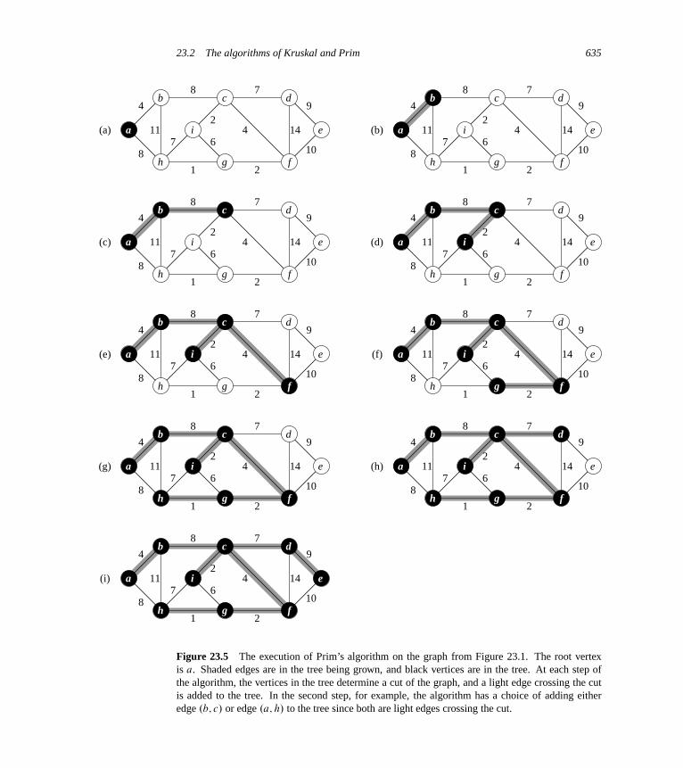
23.2 The algorithms of Kruskal and Prim 635
(a) (b)
(c) (d)
(e) (f)
(g) (h)
(i)
b
a
h
c
g
i
d
f
e
4
8
11
8 7
9
10
144
21
2
7 6
b
a
h
c
g
i
d
f
e
4
8
11
8 7
9
10
144
21
2
7 6
b
a
h
c
g
i
d
f
e
4
8
11
8 7
9
10
144
21
2
7 6
b
a
h
c
g
i
d
f
e
4
8
11
8 7
9
10
144
21
7 6
2
b
a
h
c
g
i
d
f
e
4
8
11
8 7
9
10
144
21
7 6
2
b
a
h
c
g
i
d
f
e
4
8
11
8 7
9
10
144
21
7 6
2
b
a
h
c
g
i
d
f
e
4
8
11
8 7
9
10
144
21
7 6
2
b
a
h
c
g
i
d
f
e
4
8
11
8 7
9
10
144
21
7 6
2
b
a
h
c
g
i
d
f
e
4
8
11
8 7
9
10
144
21
7 6
2
Figure 23.5 The execution of Prim’s algorithm on the graph from Figure 23.1. The root vertexis a. Shaded edges are in the tree being grown, and black vertices are in the tree. At each step ofthe algorithm, the vertices in the tree determine a cut of the graph, and a light edge crossing the cutis added to the tree. In the second step, for example, the algorithm has a choice of adding eitheredge .b; c/ or edge .a; h/ to the tree since both are light edges crossing the cut.
636 Chapter 23 Minimum Spanning Trees
Figure 23.5 shows how Prim’s algorithm works. Lines 1–5 set the key of eachvertex to 1 (except for the root r , whose key is set to 0 so that it will be thefirst vertex processed), set the parent of each vertex to NIL, and initialize the min-priority queue Q to contain all the vertices. The algorithm maintains the followingthree-part loop invariant:
Prior to each iteration of the while loop of lines 6–11,
1. A D f.�; �:�/ W � 2 V � frg �Qg.2. The vertices already placed into the minimum spanning tree are those in
V �Q.
3. For all vertices � 2 Q, if �:� ¤ NIL, then �:key < 1 and �:key isthe weight of a light edge .�; �:�/ connecting � to some vertex alreadyplaced into the minimum spanning tree.
Line 7 identifies a vertex u 2 Q incident on a light edge that crosses the cut.V �Q; Q/ (with the exception of the first iteration, in which u D r due to line 4).Removing u from the set Q adds it to the set V �Q of vertices in the tree, thusadding .u; u:�/ to A. The for loop of lines 8–11 updates the key and � attributesof every vertex � adjacent to u but not in the tree, thereby maintaining the thirdpart of the loop invariant.
The running time of Prim’s algorithm depends on how we implement the min-priority queue Q. If we implement Q as a binary min-heap (see Chapter 6), wecan use the BUILD-MIN-HEAP procedure to perform lines 1–5 in O.V / time. Thebody of the while loop executes jV j times, and since each EXTRACT-MIN opera-tion takes O.lg V / time, the total time for all calls to EXTRACT-MIN is O.V lg V /.The for loop in lines 8–11 executes O.E/ times altogether, since the sum of thelengths of all adjacency lists is 2 jEj. Within the for loop, we can implement thetest for membership in Q in line 9 in constant time by keeping a bit for each vertexthat tells whether or not it is in Q, and updating the bit when the vertex is removedfrom Q. The assignment in line 11 involves an implicit DECREASE-KEY opera-tion on the min-heap, which a binary min-heap supports in O.lg V / time. Thus,the total time for Prim’s algorithm is O.V lg V C E lg V / D O.E lg V /, which isasymptotically the same as for our implementation of Kruskal’s algorithm.
We can improve the asymptotic running time of Prim’s algorithm by using Fi-bonacci heaps. Chapter 19 shows that if a Fibonacci heap holds jV j elements, anEXTRACT-MIN operation takes O.lg V / amortized time and a DECREASE-KEY
operation (to implement line 11) takes O.1/ amortized time. Therefore, if we use aFibonacci heap to implement the min-priority queue Q, the running time of Prim’salgorithm improves to O.E C V lg V /.
23.2 The algorithms of Kruskal and Prim 637
Exercises
23.2-1Kruskal’s algorithm can return different spanning trees for the same input graph G,depending on how it breaks ties when the edges are sorted into order. Show thatfor each minimum spanning tree T of G, there is a way to sort the edges of G inKruskal’s algorithm so that the algorithm returns T .
23.2-2Suppose that we represent the graph G D .V; E/ as an adjacency matrix. Give asimple implementation of Prim’s algorithm for this case that runs in O.V 2/ time.
23.2-3For a sparse graph G D .V; E/, where jEj D ‚.V /, is the implementation ofPrim’s algorithm with a Fibonacci heap asymptotically faster than the binary-heapimplementation? What about for a dense graph, where jEj D ‚.V 2/? Howmust the sizes jEj and jV j be related for the Fibonacci-heap implementation tobe asymptotically faster than the binary-heap implementation?
23.2-4Suppose that all edge weights in a graph are integers in the range from 1 to jV j.How fast can you make Kruskal’s algorithm run? What if the edge weights areintegers in the range from 1 to W for some constant W ?
23.2-5Suppose that all edge weights in a graph are integers in the range from 1 to jV j.How fast can you make Prim’s algorithm run? What if the edge weights are integersin the range from 1 to W for some constant W ?
23.2-6 ?
Suppose that the edge weights in a graph are uniformly distributed over the half-open interval Œ0; 1/. Which algorithm, Kruskal’s or Prim’s, can you make runfaster?
23.2-7 ?
Suppose that a graph G has a minimum spanning tree already computed. Howquickly can we update the minimum spanning tree if we add a new vertex andincident edges to G?
23.2-8Professor Borden proposes a new divide-and-conquer algorithm for computingminimum spanning trees, which goes as follows. Given a graph G D .V; E/,partition the set V of vertices into two sets V1 and V2 such that jV1j and jV2j differ
638 Chapter 23 Minimum Spanning Trees
by at most 1. Let E1 be the set of edges that are incident only on vertices in V1, andlet E2 be the set of edges that are incident only on vertices in V2. Recursively solvea minimum-spanning-tree problem on each of the two subgraphs G1 D .V1; E1/
and G2 D .V2; E2/. Finally, select the minimum-weight edge in E that crosses thecut .V1; V2/, and use this edge to unite the resulting two minimum spanning treesinto a single spanning tree.
Either argue that the algorithm correctly computes a minimum spanning treeof G, or provide an example for which the algorithm fails.
Problems
23-1 Second-best minimum spanning treeLet G D .V; E/ be an undirected, connected graph whose weight function isw W E ! R, and suppose that jEj � jV j and all edge weights are distinct.
We define a second-best minimum spanning tree as follows. Let T be the setof all spanning trees of G, and let T 0 be a minimum spanning tree of G. Thena second-best minimum spanning tree is a spanning tree T such that w.T / DminT 002T �fT 0g fw.T 00/g.a. Show that the minimum spanning tree is unique, but that the second-best mini-
mum spanning tree need not be unique.
b. Let T be the minimum spanning tree of G. Prove that G contains edges.u; �/ 2 T and .x; y/ 62 T such that T � f.u; �/g [ f.x; y/g is a second-bestminimum spanning tree of G.
c. Let T be a spanning tree of G and, for any two vertices u; � 2 V , let maxŒu; ��
denote an edge of maximum weight on the unique simple path between u and �
in T . Describe an O.V 2/-time algorithm that, given T , computes maxŒu; �� forall u; � 2 V .
d. Give an efficient algorithm to compute the second-best minimum spanning treeof G.
23-2 Minimum spanning tree in sparse graphsFor a very sparse connected graph G D .V; E/, we can further improve upon theO.E C V lg V / running time of Prim’s algorithm with Fibonacci heaps by prepro-cessing G to decrease the number of vertices before running Prim’s algorithm. Inparticular, we choose, for each vertex u, the minimum-weight edge .u; �/ incidenton u, and we put .u; �/ into the minimum spanning tree under construction. We

Problems for Chapter 23 639
then contract all chosen edges (see Section B.4). Rather than contracting theseedges one at a time, we first identify sets of vertices that are united into the samenew vertex. Then we create the graph that would have resulted from contractingthese edges one at a time, but we do so by “renaming” edges according to the setsinto which their endpoints were placed. Several edges from the original graph maybe renamed the same as each other. In such a case, only one edge results, and itsweight is the minimum of the weights of the corresponding original edges.
Initially, we set the minimum spanning tree T being constructed to be empty,and for each edge .u; �/ 2 E, we initialize the attributes .u; �/:orig D .u; �/
and .u; �/:c D w.u; �/. We use the orig attribute to reference the edge from theinitial graph that is associated with an edge in the contracted graph. The c attributeholds the weight of an edge, and as edges are contracted, we update it according tothe above scheme for choosing edge weights. The procedure MST-REDUCE takesinputs G and T , and it returns a contracted graph G0 with updated attributes orig0
and c 0. The procedure also accumulates edges of G into the minimum spanningtree T .
MST-REDUCE.G; T /
1 for each � 2 G:V2 �:mark D FALSE
3 MAKE-SET.�/
4 for each u 2 G:V5 if u:mark == FALSE
6 choose � 2 G:AdjŒu� such that .u; �/:c is minimized7 UNION.u; �/
8 T D T [ f.u; �/:origg9 u:mark D �:mark D TRUE
10 G0:V D fFIND-SET.�/ W � 2 G:Vg11 G0:E D ;12 for each .x; y/ 2 G:E13 u D FIND-SET.x/
14 � D FIND-SET.y/
15 if .u; �/ 62 G0:E16 G0:E D G0:E [ f.u; �/g17 .u; �/:orig0 D .x; y/:orig18 .u; �/:c 0 D .x; y/:c19 else if .x; y/:c < .u; �/:c 0
20 .u; �/:orig0 D .x; y/:orig21 .u; �/:c 0 D .x; y/:c22 construct adjacency lists G0:Adj for G0
23 return G0 and T

640 Chapter 23 Minimum Spanning Trees
a. Let T be the set of edges returned by MST-REDUCE, and let A be the minimumspanning tree of the graph G0 formed by the call MST-PRIM.G0; c 0; r/, where c 0
is the weight attribute on the edges of G0:E and r is any vertex in G0:V . Provethat T [ f.x; y/:orig0 W .x; y/ 2 Ag is a minimum spanning tree of G.
b. Argue that jG0:Vj � jV j =2.
c. Show how to implement MST-REDUCE so that it runs in O.E/ time. (Hint:Use simple data structures.)
d. Suppose that we run k phases of MST-REDUCE, using the output G0 producedby one phase as the input G to the next phase and accumulating edges in T .Argue that the overall running time of the k phases is O.kE/.
e. Suppose that after running k phases of MST-REDUCE, as in part (d), we runPrim’s algorithm by calling MST-PRIM.G0; c 0; r/, where G0, with weight at-tribute c 0, is returned by the last phase and r is any vertex in G0:V . Show howto pick k so that the overall running time is O.E lg lg V /. Argue that yourchoice of k minimizes the overall asymptotic running time.
f. For what values of jEj (in terms of jV j) does Prim’s algorithm with preprocess-ing asymptotically beat Prim’s algorithm without preprocessing?
23-3 Bottleneck spanning treeA bottleneck spanning tree T of an undirected graph G is a spanning tree of G
whose largest edge weight is minimum over all spanning trees of G. We say thatthe value of the bottleneck spanning tree is the weight of the maximum-weightedge in T .
a. Argue that a minimum spanning tree is a bottleneck spanning tree.
Part (a) shows that finding a bottleneck spanning tree is no harder than findinga minimum spanning tree. In the remaining parts, we will show how to find abottleneck spanning tree in linear time.
b. Give a linear-time algorithm that given a graph G and an integer b, determineswhether the value of the bottleneck spanning tree is at most b.
c. Use your algorithm for part (b) as a subroutine in a linear-time algorithm forthe bottleneck-spanning-tree problem. (Hint: You may want to use a subroutinethat contracts sets of edges, as in the MST-REDUCE procedure described inProblem 23-2.)

Notes for Chapter 23 641
23-4 Alternative minimum-spanning-tree algorithmsIn this problem, we give pseudocode for three different algorithms. Each one takesa connected graph and a weight function as input and returns a set of edges T . Foreach algorithm, either prove that T is a minimum spanning tree or prove that T isnot a minimum spanning tree. Also describe the most efficient implementation ofeach algorithm, whether or not it computes a minimum spanning tree.
a. MAYBE-MST-A.G; w/
1 sort the edges into nonincreasing order of edge weights w
2 T D E
3 for each edge e, taken in nonincreasing order by weight4 if T � feg is a connected graph5 T D T � feg6 return T
b. MAYBE-MST-B.G; w/
1 T D ;2 for each edge e, taken in arbitrary order3 if T [ feg has no cycles4 T D T [ feg5 return T
c. MAYBE-MST-C.G; w/
1 T D ;2 for each edge e, taken in arbitrary order3 T D T [ feg4 if T has a cycle c
5 let e0 be a maximum-weight edge on c
6 T D T � fe0g7 return T
Chapter notes
Tarjan [330] surveys the minimum-spanning-tree problem and provides excellentadvanced material. Graham and Hell [151] compiled a history of the minimum-spanning-tree problem.
Tarjan attributes the first minimum-spanning-tree algorithm to a 1926 paper byO. Boru̇vka. Boru̇vka’s algorithm consists of running O.lg V / iterations of the

642 Chapter 23 Minimum Spanning Trees
procedure MST-REDUCE described in Problem 23-2. Kruskal’s algorithm wasreported by Kruskal [222] in 1956. The algorithm commonly known as Prim’salgorithm was indeed invented by Prim [285], but it was also invented earlier byV. Jarnı́k in 1930.
The reason underlying why greedy algorithms are effective at finding minimumspanning trees is that the set of forests of a graph forms a graphic matroid. (SeeSection 16.4.)
When jEj D �.V lg V /, Prim’s algorithm, implemented with Fibonacci heaps,runs in O.E/ time. For sparser graphs, using a combination of the ideas fromPrim’s algorithm, Kruskal’s algorithm, and Boru̇vka’s algorithm, together with ad-vanced data structures, Fredman and Tarjan [114] give an algorithm that runs inO.E lg� V / time. Gabow, Galil, Spencer, and Tarjan [120] improved this algo-rithm to run in O.E lg lg� V / time. Chazelle [61] gives an algorithm that runsin O.E y̨.E; V // time, where y̨.E; V / is the functional inverse of Ackermann’sfunction. (See the chapter notes for Chapter 21 for a brief discussion of Acker-mann’s function and its inverse.) Unlike previous minimum-spanning-tree algo-rithms, Chazelle’s algorithm does not follow the greedy method.
A related problem is spanning-tree verification, in which we are given a graphG D .V; E/ and a tree T � E, and we wish to determine whether T is a minimumspanning tree of G. King [203] gives a linear-time algorithm to verify a spanningtree, building on earlier work of Komlós [215] and Dixon, Rauch, and Tarjan [91].
The above algorithms are all deterministic and fall into the comparison-basedmodel described in Chapter 8. Karger, Klein, and Tarjan [195] give a randomizedminimum-spanning-tree algorithm that runs in O.V C E/ expected time. Thisalgorithm uses recursion in a manner similar to the linear-time selection algorithmin Section 9.3: a recursive call on an auxiliary problem identifies a subset of theedges E 0 that cannot be in any minimum spanning tree. Another recursive callon E � E 0 then finds the minimum spanning tree. The algorithm also uses ideasfrom Boru̇vka’s algorithm and King’s algorithm for spanning-tree verification.
Fredman and Willard [116] showed how to find a minimum spanning tree inO.V CE/ time using a deterministic algorithm that is not comparison based. Theiralgorithm assumes that the data are b-bit integers and that the computer memoryconsists of addressable b-bit words.

24 Single-Source Shortest Paths
Professor Patrick wishes to find the shortest possible route from Phoenix to Indi-anapolis. Given a road map of the United States on which the distance betweeneach pair of adjacent intersections is marked, how can she determine this shortestroute?
One possible way would be to enumerate all the routes from Phoenix to Indi-anapolis, add up the distances on each route, and select the shortest. It is easy tosee, however, that even disallowing routes that contain cycles, Professor Patrickwould have to examine an enormous number of possibilities, most of which aresimply not worth considering. For example, a route from Phoenix to Indianapolisthat passes through Seattle is obviously a poor choice, because Seattle is severalhundred miles out of the way.
In this chapter and in Chapter 25, we show how to solve such problems ef-ficiently. In a shortest-paths problem, we are given a weighted, directed graphG D .V; E/, with weight function w W E ! R mapping edges to real-valuedweights. The weight w.p/ of path p D h�0; �1; : : : ; �ki is the sum of the weightsof its constituent edges:
w.p/ DkX
iD1
w.�i�1; �i / :
We define the shortest-path weight ı.u; �/ from u to � by
ı.u; �/ D(
minfw.p/ W u p� �g if there is a path from u to � ;
1 otherwise :
A shortest path from vertex u to vertex � is then defined as any path p with weightw.p/ D ı.u; �/.
In the Phoenix-to-Indianapolis example, we can model the road map as a graph:vertices represent intersections, edges represent road segments between intersec-tions, and edge weights represent road distances. Our goal is to find a shortest pathfrom a given intersection in Phoenix to a given intersection in Indianapolis.
644 Chapter 24 Single-Source Shortest Paths
Edge weights can represent metrics other than distances, such as time, cost,penalties, loss, or any other quantity that accumulates linearly along a path andthat we would want to minimize.
The breadth-first-search algorithm from Section 22.2 is a shortest-paths algo-rithm that works on unweighted graphs, that is, graphs in which each edge has unitweight. Because many of the concepts from breadth-first search arise in the studyof shortest paths in weighted graphs, you might want to to review Section 22.2before proceeding.
Variants
In this chapter, we shall focus on the single-source shortest-paths problem: givena graph G D .V; E/, we want to find a shortest path from a given source vertexs 2 V to each vertex � 2 V . The algorithm for the single-source problem cansolve many other problems, including the following variants.
Single-destination shortest-paths problem: Find a shortest path to a given des-tination vertex t from each vertex �. By reversing the direction of each edge inthe graph, we can reduce this problem to a single-source problem.
Single-pair shortest-path problem: Find a shortest path from u to � for givenvertices u and �. If we solve the single-source problem with source vertex u,we solve this problem also. Moreover, all known algorithms for this problemhave the same worst-case asymptotic running time as the best single-sourcealgorithms.
All-pairs shortest-paths problem: Find a shortest path from u to � for every pairof vertices u and �. Although we can solve this problem by running a single-source algorithm once from each vertex, we usually can solve it faster. Addi-tionally, its structure is interesting in its own right. Chapter 25 addresses theall-pairs problem in detail.
Optimal substructure of a shortest path
Shortest-paths algorithms typically rely on the property that a shortest path be-tween two vertices contains other shortest paths within it. (The Edmonds-Karpmaximum-flow algorithm in Chapter 26 also relies on this property.) Recallthat optimal substructure is one of the key indicators that dynamic programming(Chapter 15) and the greedy method (Chapter 16) might apply. Dijkstra’s algo-rithm, which we shall see in Section 24.3, is a greedy algorithm, and the Floyd-Warshall algorithm, which finds shortest paths between all pairs of vertices (seeSection 25.2), is a dynamic-programming algorithm. The following lemma statesthe optimal-substructure property of shortest paths more precisely.
Chapter 24 Single-Source Shortest Paths 645
Lemma 24.1 (Subpaths of shortest paths are shortest paths)Given a weighted, directed graph G D .V; E/ with weight function w W E ! R,let p D h�0; �1; : : : ; �ki be a shortest path from vertex �0 to vertex �k and, for anyi and j such that 0 � i � j � k, let pij D h�i ; �iC1; : : : ; �j i be the subpath of p
from vertex �i to vertex �j . Then, pij is a shortest path from �i to �j .
Proof If we decompose path p into �0
p0i� �i
pij� �j
pjk� �k, then we have that
w.p/ D w.p0i/Cw.pij /Cw.pjk/. Now, assume that there is a path p0ij from �i
to �j with weight w.p0ij / < w.pij /. Then, �0
p0i� �i
p0ij
� �j
pjk� �k is a path from �0
to �k whose weight w.p0i/Cw.p0ij /Cw.pjk/ is less than w.p/, which contradicts
the assumption that p is a shortest path from �0 to �k.
Negative-weight edges
Some instances of the single-source shortest-paths problem may include edgeswhose weights are negative. If the graph G D .V; E/ contains no negative-weight cycles reachable from the source s, then for all � 2 V , the shortest-pathweight ı.s; �/ remains well defined, even if it has a negative value. If the graphcontains a negative-weight cycle reachable from s, however, shortest-path weightsare not well defined. No path from s to a vertex on the cycle can be a short-est path—we can always find a path with lower weight by following the proposed“shortest” path and then traversing the negative-weight cycle. If there is a negative-weight cycle on some path from s to �, we define ı.s; �/ D �1.
Figure 24.1 illustrates the effect of negative weights and negative-weight cy-cles on shortest-path weights. Because there is only one path from s to a (thepath hs; ai), we have ı.s; a/ D w.s; a/ D 3. Similarly, there is only one pathfrom s to b, and so ı.s; b/ D w.s; a/ C w.a; b/ D 3 C .�4/ D �1. There areinfinitely many paths from s to c: hs; ci, hs; c; d; ci, hs; c; d; c; d; ci, and so on.Because the cycle hc; d; ci has weight 6C .�3/ D 3 > 0, the shortest path from s
to c is hs; ci, with weight ı.s; c/ D w.s; c/ D 5. Similarly, the shortest path from s
to d is hs; c;d i, with weight ı.s; d/ D w.s; c/Cw.c; d/ D 11. Analogously, thereare infinitely many paths from s to e: hs; ei, hs; e; f; ei, hs; e; f; e; f; ei, and soon. Because the cycle he; f; ei has weight 3 C .�6/ D �3 < 0, however, thereis no shortest path from s to e. By traversing the negative-weight cycle he; f; eiarbitrarily many times, we can find paths from s to e with arbitrarily large negativeweights, and so ı.s; e/ D �1. Similarly, ı.s; f / D �1. Because g is reachablefrom f , we can also find paths with arbitrarily large negative weights from s to g,and so ı.s; g/ D �1. Vertices h, i , and j also form a negative-weight cycle. Theyare not reachable from s, however, and so ı.s; h/ D ı.s; i/ D ı.s; j / D1.
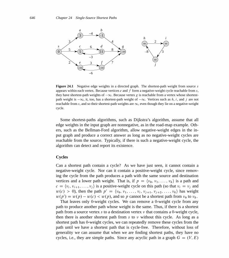
646 Chapter 24 Single-Source Shortest Paths
5
c
11
d6
–3
–∞e
–∞f3
–6
3
a
–1
b
0
s
–∞g
–4
5
3
2
8
4
7
∞h
∞i
2
∞j
–8 3
Figure 24.1 Negative edge weights in a directed graph. The shortest-path weight from source s
appears within each vertex. Because vertices e and f form a negative-weight cycle reachable from s,they have shortest-path weights of �1. Because vertex g is reachable from a vertex whose shortest-path weight is �1, it, too, has a shortest-path weight of �1. Vertices such as h, i , and j are notreachable from s, and so their shortest-path weights are1, even though they lie on a negative-weightcycle.
Some shortest-paths algorithms, such as Dijkstra’s algorithm, assume that alledge weights in the input graph are nonnegative, as in the road-map example. Oth-ers, such as the Bellman-Ford algorithm, allow negative-weight edges in the in-put graph and produce a correct answer as long as no negative-weight cycles arereachable from the source. Typically, if there is such a negative-weight cycle, thealgorithm can detect and report its existence.
Cycles
Can a shortest path contain a cycle? As we have just seen, it cannot contain anegative-weight cycle. Nor can it contain a positive-weight cycle, since remov-ing the cycle from the path produces a path with the same source and destinationvertices and a lower path weight. That is, if p D h�0; �1; : : : ; �ki is a path andc D h�i ; �iC1; : : : ; �j i is a positive-weight cycle on this path (so that �i D �j andw.c/ > 0), then the path p0 D h�0; �1; : : : ; �i ; �j C1; �j C2; : : : ; �ki has weightw.p0/ D w.p/� w.c/ < w.p/, and so p cannot be a shortest path from �0 to �k.
That leaves only 0-weight cycles. We can remove a 0-weight cycle from anypath to produce another path whose weight is the same. Thus, if there is a shortestpath from a source vertex s to a destination vertex � that contains a 0-weight cycle,then there is another shortest path from s to � without this cycle. As long as ashortest path has 0-weight cycles, we can repeatedly remove these cycles from thepath until we have a shortest path that is cycle-free. Therefore, without loss ofgenerality we can assume that when we are finding shortest paths, they have nocycles, i.e., they are simple paths. Since any acyclic path in a graph G D .V; E/
Chapter 24 Single-Source Shortest Paths 647
contains at most jV j distinct vertices, it also contains at most jV j � 1 edges. Thus,we can restrict our attention to shortest paths of at most jV j � 1 edges.
Representing shortest paths
We often wish to compute not only shortest-path weights, but the vertices on short-est paths as well. We represent shortest paths similarly to how we representedbreadth-first trees in Section 22.2. Given a graph G D .V; E/, we maintain foreach vertex � 2 V a predecessor �:� that is either another vertex or NIL. Theshortest-paths algorithms in this chapter set the � attributes so that the chain of pre-decessors originating at a vertex � runs backwards along a shortest path from s to �.Thus, given a vertex � for which �:� ¤ NIL, the procedure PRINT-PATH.G; s; �/
from Section 22.2 will print a shortest path from s to �.In the midst of executing a shortest-paths algorithm, however, the � values might
not indicate shortest paths. As in breadth-first search, we shall be interested in thepredecessor subgraph G� D .V� ; E�/ induced by the � values. Here again, wedefine the vertex set V� to be the set of vertices of G with non-NIL predecessors,plus the source s:
V� D f� 2 V W �:� ¤ NILg [ fsg :
The directed edge set E� is the set of edges induced by the � values for verticesin V� :
E� D f.�:�; �/ 2 E W � 2 V� � fsgg :
We shall prove that the � values produced by the algorithms in this chapter havethe property that at termination G� is a “shortest-paths tree”—informally, a rootedtree containing a shortest path from the source s to every vertex that is reachablefrom s. A shortest-paths tree is like the breadth-first tree from Section 22.2, but itcontains shortest paths from the source defined in terms of edge weights instead ofnumbers of edges. To be precise, let G D .V; E/ be a weighted, directed graphwith weight function w W E ! R, and assume that G contains no negative-weightcycles reachable from the source vertex s 2 V , so that shortest paths are welldefined. A shortest-paths tree rooted at s is a directed subgraph G0 D .V 0; E 0/,where V 0 � V and E 0 � E, such that
1. V 0 is the set of vertices reachable from s in G,
2. G0 forms a rooted tree with root s, and
3. for all � 2 V 0, the unique simple path from s to � in G0 is a shortest path from s
to � in G.

648 Chapter 24 Single-Source Shortest Paths
(a) (b) (c)
0
6
6
72124
3
53
s
t x
y z
3 9
5 11
0
6
6
72124
3
53
s
t x
y z
3 9
5 11
0
6
6
72124
3
53
s
t x
y z
3 9
5 11
Figure 24.2 (a) A weighted, directed graph with shortest-path weights from source s. (b) Theshaded edges form a shortest-paths tree rooted at the source s. (c) Another shortest-paths tree withthe same root.
Shortest paths are not necessarily unique, and neither are shortest-paths trees. Forexample, Figure 24.2 shows a weighted, directed graph and two shortest-paths treeswith the same root.
Relaxation
The algorithms in this chapter use the technique of relaxation. For each vertex� 2 V , we maintain an attribute �:d, which is an upper bound on the weight ofa shortest path from source s to �. We call �:d a shortest-path estimate. Weinitialize the shortest-path estimates and predecessors by the following ‚.V /-timeprocedure:
INITIALIZE-SINGLE-SOURCE.G; s/
1 for each vertex � 2 G:V2 �:d D 13 �:� D NIL
4 s:d D 0
After initialization, we have �:� D NIL for all � 2 V , s:d D 0, and �:d D 1 for� 2 V � fsg.
The process of relaxing an edge .u; �/ consists of testing whether we can im-prove the shortest path to � found so far by going through u and, if so, updat-ing �:d and �:� . A relaxation step1 may decrease the value of the shortest-path
1It may seem strange that the term “relaxation” is used for an operation that tightens an upper bound.The use of the term is historical. The outcome of a relaxation step can be viewed as a relaxationof the constraint �:d � u:d C w.u; �/, which, by the triangle inequality (Lemma 24.10), must besatisfied if u:d D ı.s; u/ and �:d D ı.s; �/. That is, if �:d � u:d C w.u; �/, there is no “pressure”to satisfy this constraint, so the constraint is “relaxed.”
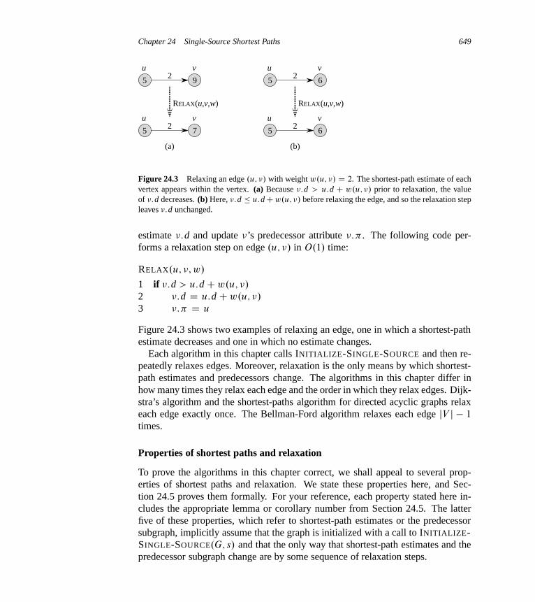
Chapter 24 Single-Source Shortest Paths 649
u v
5 92
u v
5 72
RELAX(u,v,w)
(a) (b)
u v
5 62
u v
5 62
RELAX(u,v,w)
Figure 24.3 Relaxing an edge .u; �/ with weight w.u; �/ D 2. The shortest-path estimate of eachvertex appears within the vertex. (a) Because �:d > u:d C w.u; �/ prior to relaxation, the valueof �:d decreases. (b) Here, �:d � u:dCw.u; �/ before relaxing the edge, and so the relaxation stepleaves �:d unchanged.
estimate �:d and update �’s predecessor attribute �:� . The following code per-forms a relaxation step on edge .u; �/ in O.1/ time:
RELAX.u; �; w/
1 if �:d > u:dCw.u; �/
2 �:d D u:d Cw.u; �/
3 �:� D u
Figure 24.3 shows two examples of relaxing an edge, one in which a shortest-pathestimate decreases and one in which no estimate changes.
Each algorithm in this chapter calls INITIALIZE-SINGLE-SOURCE and then re-peatedly relaxes edges. Moreover, relaxation is the only means by which shortest-path estimates and predecessors change. The algorithms in this chapter differ inhow many times they relax each edge and the order in which they relax edges. Dijk-stra’s algorithm and the shortest-paths algorithm for directed acyclic graphs relaxeach edge exactly once. The Bellman-Ford algorithm relaxes each edge jV j � 1
times.
Properties of shortest paths and relaxation
To prove the algorithms in this chapter correct, we shall appeal to several prop-erties of shortest paths and relaxation. We state these properties here, and Sec-tion 24.5 proves them formally. For your reference, each property stated here in-cludes the appropriate lemma or corollary number from Section 24.5. The latterfive of these properties, which refer to shortest-path estimates or the predecessorsubgraph, implicitly assume that the graph is initialized with a call to INITIALIZE-SINGLE-SOURCE.G; s/ and that the only way that shortest-path estimates and thepredecessor subgraph change are by some sequence of relaxation steps.
650 Chapter 24 Single-Source Shortest Paths
Triangle inequality (Lemma 24.10)For any edge .u; �/ 2 E, we have ı.s; �/ � ı.s; u/C w.u; �/.
Upper-bound property (Lemma 24.11)We always have �:d � ı.s; �/ for all vertices � 2 V , and once �:d achieves thevalue ı.s; �/, it never changes.
No-path property (Corollary 24.12)If there is no path from s to �, then we always have �:d D ı.s; �/ D1.
Convergence property (Lemma 24.14)If s � u! � is a shortest path in G for some u; � 2 V , and if u:d D ı.s; u/ atany time prior to relaxing edge .u; �/, then �:d D ı.s; �/ at all times afterward.
Path-relaxation property (Lemma 24.15)If p D h�0; �1; : : : ; �ki is a shortest path from s D �0 to �k, and we relax theedges of p in the order .�0; �1/; .�1; �2/; : : : ; .�k�1; �k/, then �k:d D ı.s; �k/.This property holds regardless of any other relaxation steps that occur, even ifthey are intermixed with relaxations of the edges of p.
Predecessor-subgraph property (Lemma 24.17)Once �:d D ı.s; �/ for all � 2 V , the predecessor subgraph is a shortest-pathstree rooted at s.
Chapter outline
Section 24.1 presents the Bellman-Ford algorithm, which solves the single-sourceshortest-paths problem in the general case in which edges can have negative weight.The Bellman-Ford algorithm is remarkably simple, and it has the further benefitof detecting whether a negative-weight cycle is reachable from the source. Sec-tion 24.2 gives a linear-time algorithm for computing shortest paths from a singlesource in a directed acyclic graph. Section 24.3 covers Dijkstra’s algorithm, whichhas a lower running time than the Bellman-Ford algorithm but requires the edgeweights to be nonnegative. Section 24.4 shows how we can use the Bellman-Fordalgorithm to solve a special case of linear programming. Finally, Section 24.5proves the properties of shortest paths and relaxation stated above.
We require some conventions for doing arithmetic with infinities. We shall as-sume that for any real number a ¤ �1, we have aC1 D1C a D1. Also, tomake our proofs hold in the presence of negative-weight cycles, we shall assumethat for any real number a ¤1, we have aC .�1/ D .�1/C a D �1.
All algorithms in this chapter assume that the directed graph G is stored in theadjacency-list representation. Additionally, stored with each edge is its weight, sothat as we traverse each adjacency list, we can determine the edge weights in O.1/
time per edge.

24.1 The Bellman-Ford algorithm 651
24.1 The Bellman-Ford algorithm
The Bellman-Ford algorithm solves the single-source shortest-paths problem inthe general case in which edge weights may be negative. Given a weighted, di-rected graph G D .V; E/ with source s and weight function w W E ! R, theBellman-Ford algorithm returns a boolean value indicating whether or not there isa negative-weight cycle that is reachable from the source. If there is such a cy-cle, the algorithm indicates that no solution exists. If there is no such cycle, thealgorithm produces the shortest paths and their weights.
The algorithm relaxes edges, progressively decreasing an estimate �:d on theweight of a shortest path from the source s to each vertex � 2 V until it achievesthe actual shortest-path weight ı.s; �/. The algorithm returns TRUE if and only ifthe graph contains no negative-weight cycles that are reachable from the source.
BELLMAN-FORD.G; w; s/
1 INITIALIZE-SINGLE-SOURCE.G; s/
2 for i D 1 to jG:Vj � 1
3 for each edge .u; �/ 2 G:E4 RELAX.u; �; w/
5 for each edge .u; �/ 2 G:E6 if �:d > u:dCw.u; �/
7 return FALSE
8 return TRUE
Figure 24.4 shows the execution of the Bellman-Ford algorithm on a graphwith 5 vertices. After initializing the d and � values of all vertices in line 1,the algorithm makes jV j � 1 passes over the edges of the graph. Each pass isone iteration of the for loop of lines 2–4 and consists of relaxing each edge of thegraph once. Figures 24.4(b)–(e) show the state of the algorithm after each of thefour passes over the edges. After making jV j � 1 passes, lines 5–8 check for anegative-weight cycle and return the appropriate boolean value. (We’ll see a littlelater why this check works.)
The Bellman-Ford algorithm runs in time O.VE/, since the initialization inline 1 takes ‚.V / time, each of the jV j � 1 passes over the edges in lines 2–4takes ‚.E/ time, and the for loop of lines 5–7 takes O.E/ time.
To prove the correctness of the Bellman-Ford algorithm, we start by showing thatif there are no negative-weight cycles, the algorithm computes correct shortest-pathweights for all vertices reachable from the source.
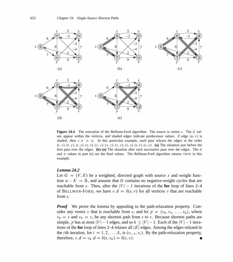
652 Chapter 24 Single-Source Shortest Paths
(a) (b) (c)
(d)
0
5
9
78
6
7
(e)
t x
s
y z
–4
–3
–22
7
4
–22
0
5
9
78
6
7
t x
s
y z
–4
–3
–22
7
4
22
0
5
9
78
6
7
t x
s
y z
–4
–3
–26
7
4
22
0
5
9
78
6
7
t x
s
y z
–4
–3
–26
7
∞
∞2
0
5
9
78
6
7
t x
s
y z
–4
–3
–2 ∞
∞2
∞
∞
Figure 24.4 The execution of the Bellman-Ford algorithm. The source is vertex s. The d val-ues appear within the vertices, and shaded edges indicate predecessor values: if edge .u; �/ isshaded, then �:� D u. In this particular example, each pass relaxes the edges in the order.t; x/; .t; y/; .t; ´/; .x; t/; .y; x/; .y; ´/; .´; x/; .´; s/; .s; t/; .s; y/. (a) The situation just before thefirst pass over the edges. (b)–(e) The situation after each successive pass over the edges. The d
and � values in part (e) are the final values. The Bellman-Ford algorithm returns TRUE in thisexample.
Lemma 24.2Let G D .V; E/ be a weighted, directed graph with source s and weight func-tion w W E ! R, and assume that G contains no negative-weight cycles that arereachable from s. Then, after the jV j � 1 iterations of the for loop of lines 2–4of BELLMAN-FORD, we have �:d D ı.s; �/ for all vertices � that are reachablefrom s.
Proof We prove the lemma by appealing to the path-relaxation property. Con-sider any vertex � that is reachable from s, and let p D h�0; �1; : : : ; �ki, where�0 D s and �k D �, be any shortest path from s to �. Because shortest paths aresimple, p has at most jV j � 1 edges, and so k � jV j � 1. Each of the jV j � 1 itera-tions of the for loop of lines 2–4 relaxes all jEj edges. Among the edges relaxed inthe i th iteration, for i D 1; 2; : : : ; k, is .�i�1; �i /. By the path-relaxation property,therefore, �:d D �k :d D ı.s; �k/ D ı.s; �/.

24.1 The Bellman-Ford algorithm 653
Corollary 24.3Let G D .V; E/ be a weighted, directed graph with source vertex s and weightfunction w W E ! R, and assume that G contains no negative-weight cycles thatare reachable from s. Then, for each vertex � 2 V , there is a path from s to � ifand only if BELLMAN-FORD terminates with �:d <1 when it is run on G.
Proof The proof is left as Exercise 24.1-2.
Theorem 24.4 (Correctness of the Bellman-Ford algorithm)Let BELLMAN-FORD be run on a weighted, directed graph G D .V; E/ withsource s and weight function w W E ! R. If G contains no negative-weight cyclesthat are reachable from s, then the algorithm returns TRUE, we have �:d D ı.s; �/
for all vertices � 2 V , and the predecessor subgraph G� is a shortest-paths treerooted at s. If G does contain a negative-weight cycle reachable from s, then thealgorithm returns FALSE.
Proof Suppose that graph G contains no negative-weight cycles that are reach-able from the source s. We first prove the claim that at termination, �:d D ı.s; �/
for all vertices � 2 V . If vertex � is reachable from s, then Lemma 24.2 proves thisclaim. If � is not reachable from s, then the claim follows from the no-path prop-erty. Thus, the claim is proven. The predecessor-subgraph property, along with theclaim, implies that G� is a shortest-paths tree. Now we use the claim to show thatBELLMAN-FORD returns TRUE. At termination, we have for all edges .u; �/ 2 E,
�:d D ı.s; �/
� ı.s; u/C w.u; �/ (by the triangle inequality)
D u:dCw.u; �/ ;
and so none of the tests in line 6 causes BELLMAN-FORD to return FALSE. There-fore, it returns TRUE.
Now, suppose that graph G contains a negative-weight cycle that is reachablefrom the source s; let this cycle be c D h�0; �1; : : : ; �ki, where �0 D �k. Then,
kXiD1
w.�i�1; �i / < 0 : (24.1)
Assume for the purpose of contradiction that the Bellman-Ford algorithm returnsTRUE. Thus, �i :d � �i�1:d C w.�i�1; �i / for i D 1; 2; : : : ; k. Summing theinequalities around cycle c gives us

654 Chapter 24 Single-Source Shortest Paths
kXiD1
�i :d �kX
iD1
.�i�1:dC w.�i�1; �i//
DkX
iD1
�i�1:dCkX
iD1
w.�i�1; �i/ :
Since �0 D �k, each vertex in c appears exactly once in each of the summationsPk
iD1 �i :d andPk
iD1 �i�1:d, and so
kXiD1
�i :d DkX
iD1
�i�1:d :
Moreover, by Corollary 24.3, �i :d is finite for i D 1; 2; : : : ; k. Thus,
0 �kX
iD1
w.�i�1; �i/ ;
which contradicts inequality (24.1). We conclude that the Bellman-Ford algorithmreturns TRUE if graph G contains no negative-weight cycles reachable from thesource, and FALSE otherwise.
Exercises
24.1-1Run the Bellman-Ford algorithm on the directed graph of Figure 24.4, using ver-tex ´ as the source. In each pass, relax edges in the same order as in the figure, andshow the d and � values after each pass. Now, change the weight of edge .´; x/
to 4 and run the algorithm again, using s as the source.
24.1-2Prove Corollary 24.3.
24.1-3Given a weighted, directed graph G D .V; E/ with no negative-weight cycles,let m be the maximum over all vertices � 2 V of the minimum number of edgesin a shortest path from the source s to �. (Here, the shortest path is by weight, notthe number of edges.) Suggest a simple change to the Bellman-Ford algorithm thatallows it to terminate in mC 1 passes, even if m is not known in advance.
24.1-4Modify the Bellman-Ford algorithm so that it sets �:d to �1 for all vertices � forwhich there is a negative-weight cycle on some path from the source to �.
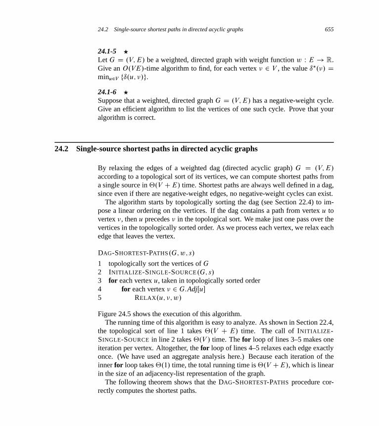
24.2 Single-source shortest paths in directed acyclic graphs 655
24.1-5 ?
Let G D .V; E/ be a weighted, directed graph with weight function w W E ! R.Give an O.VE/-time algorithm to find, for each vertex � 2 V , the value ı�.�/ Dminu2V fı.u; �/g.24.1-6 ?
Suppose that a weighted, directed graph G D .V; E/ has a negative-weight cycle.Give an efficient algorithm to list the vertices of one such cycle. Prove that youralgorithm is correct.
24.2 Single-source shortest paths in directed acyclic graphs
By relaxing the edges of a weighted dag (directed acyclic graph) G D .V; E/
according to a topological sort of its vertices, we can compute shortest paths froma single source in ‚.V CE/ time. Shortest paths are always well defined in a dag,since even if there are negative-weight edges, no negative-weight cycles can exist.
The algorithm starts by topologically sorting the dag (see Section 22.4) to im-pose a linear ordering on the vertices. If the dag contains a path from vertex u tovertex �, then u precedes � in the topological sort. We make just one pass over thevertices in the topologically sorted order. As we process each vertex, we relax eachedge that leaves the vertex.
DAG-SHORTEST-PATHS.G; w; s/
1 topologically sort the vertices of G
2 INITIALIZE-SINGLE-SOURCE.G; s/
3 for each vertex u, taken in topologically sorted order4 for each vertex � 2 G:AdjŒu�
5 RELAX.u; �; w/
Figure 24.5 shows the execution of this algorithm.The running time of this algorithm is easy to analyze. As shown in Section 22.4,
the topological sort of line 1 takes ‚.V C E/ time. The call of INITIALIZE-SINGLE-SOURCE in line 2 takes ‚.V / time. The for loop of lines 3–5 makes oneiteration per vertex. Altogether, the for loop of lines 4–5 relaxes each edge exactlyonce. (We have used an aggregate analysis here.) Because each iteration of theinner for loop takes ‚.1/ time, the total running time is ‚.V CE/, which is linearin the size of an adjacency-list representation of the graph.
The following theorem shows that the DAG-SHORTEST-PATHS procedure cor-rectly computes the shortest paths.
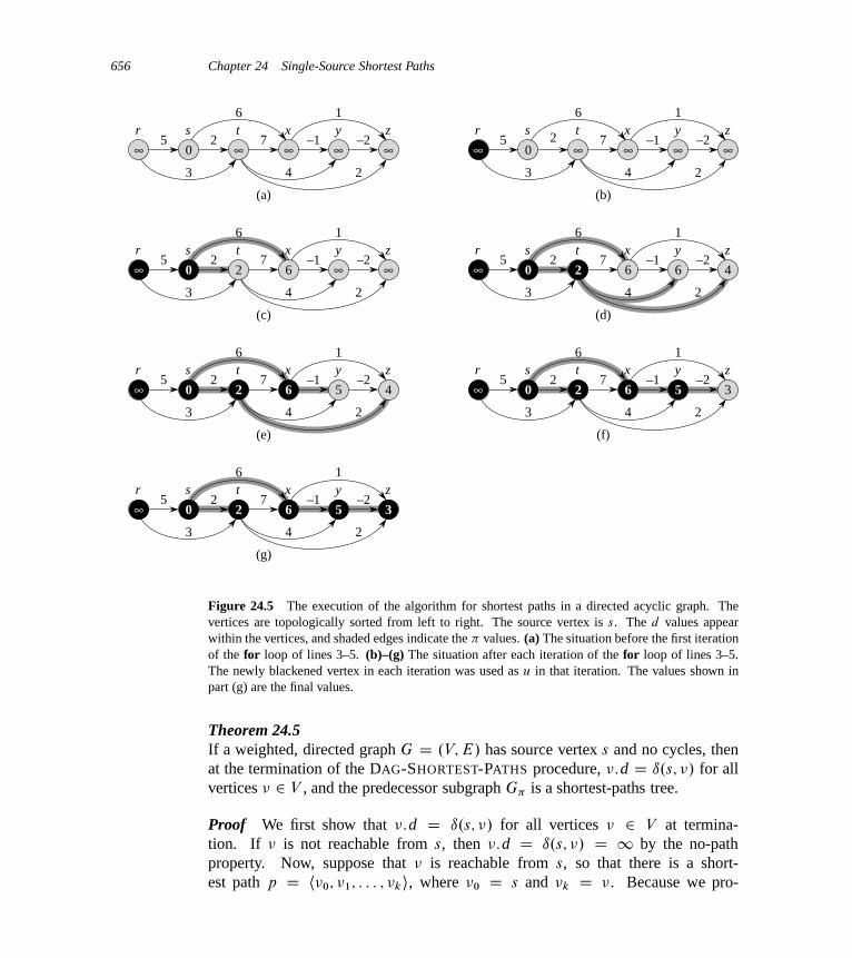
656 Chapter 24 Single-Source Shortest Paths
2∞ ∞0
5
16
3 4
∞ ∞ ∞7 –1 –2
2
(a)
xtsr y z
25
16
3 4
7 –1 –2
2
(c)
xtsr y z
25
16
3 4
7 –1 –2
2
(e)
xtsr y z
25
16
3 4
7 –1 –2
2
(g)
xtsr y z
25
16
3 4
7 –1 –2
2
(b)
xtsr y z
25
16
3 4
7 –1 –2
2
(d)
xtsr y z
25
16
3 4
7 –1 –2
2
(f)
xtsr y z
∞ 0 ∞ ∞2 6
∞ 0 2 6 5 4
∞ 0 2 6 5 3
∞ 0 2 6 5 3
∞ 0 2 6 6 4
∞ ∞0 ∞ ∞ ∞
Figure 24.5 The execution of the algorithm for shortest paths in a directed acyclic graph. Thevertices are topologically sorted from left to right. The source vertex is s. The d values appearwithin the vertices, and shaded edges indicate the � values. (a) The situation before the first iterationof the for loop of lines 3–5. (b)–(g) The situation after each iteration of the for loop of lines 3–5.The newly blackened vertex in each iteration was used as u in that iteration. The values shown inpart (g) are the final values.
Theorem 24.5If a weighted, directed graph G D .V; E/ has source vertex s and no cycles, thenat the termination of the DAG-SHORTEST-PATHS procedure, �:d D ı.s; �/ for allvertices � 2 V , and the predecessor subgraph G� is a shortest-paths tree.
Proof We first show that �:d D ı.s; �/ for all vertices � 2 V at termina-tion. If � is not reachable from s, then �:d D ı.s; �/ D 1 by the no-pathproperty. Now, suppose that � is reachable from s, so that there is a short-est path p D h�0; �1; : : : ; �ki, where �0 D s and �k D �. Because we pro-

24.2 Single-source shortest paths in directed acyclic graphs 657
cess the vertices in topologically sorted order, we relax the edges on p in theorder .�0; �1/; .�1; �2/; : : : ; .�k�1; �k/. The path-relaxation property implies that�i :d D ı.s; �i / at termination for i D 0; 1; : : : ; k. Finally, by the predecessor-subgraph property, G� is a shortest-paths tree.
An interesting application of this algorithm arises in determining critical pathsin PERT chart2 analysis. Edges represent jobs to be performed, and edge weightsrepresent the times required to perform particular jobs. If edge .u; �/ enters ver-tex � and edge .�; x/ leaves �, then job .u; �/ must be performed before job .�; x/.A path through this dag represents a sequence of jobs that must be performed in aparticular order. A critical path is a longest path through the dag, correspondingto the longest time to perform any sequence of jobs. Thus, the weight of a criticalpath provides a lower bound on the total time to perform all the jobs. We can finda critical path by either
� negating the edge weights and running DAG-SHORTEST-PATHS, or� running DAG-SHORTEST-PATHS, with the modification that we replace “1”
by “�1” in line 2 of INITIALIZE-SINGLE-SOURCE and “>” by “<” in theRELAX procedure.
Exercises
24.2-1Run DAG-SHORTEST-PATHS on the directed graph of Figure 24.5, using vertex r
as the source.
24.2-2Suppose we change line 3 of DAG-SHORTEST-PATHS to read
3 for the first jV j � 1 vertices, taken in topologically sorted order
Show that the procedure would remain correct.
24.2-3The PERT chart formulation given above is somewhat unnatural. In a more natu-ral structure, vertices would represent jobs and edges would represent sequencingconstraints; that is, edge .u; �/ would indicate that job u must be performed beforejob �. We would then assign weights to vertices, not edges. Modify the DAG-SHORTEST-PATHS procedure so that it finds a longest path in a directed acyclicgraph with weighted vertices in linear time.
2“PERT” is an acronym for “program evaluation and review technique.”
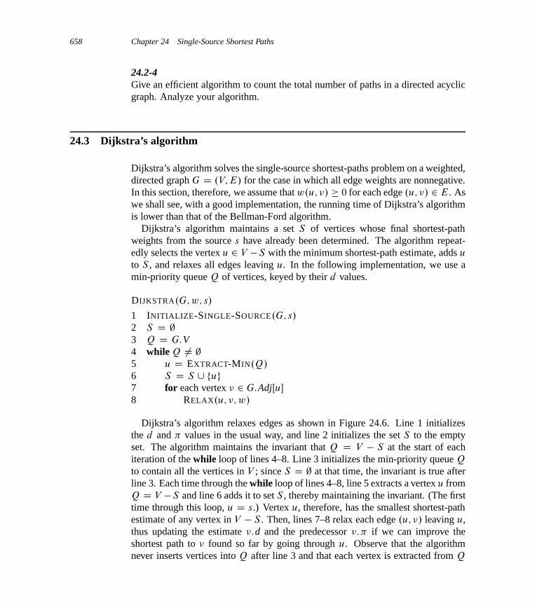
658 Chapter 24 Single-Source Shortest Paths
24.2-4Give an efficient algorithm to count the total number of paths in a directed acyclicgraph. Analyze your algorithm.
24.3 Dijkstra’s algorithm
Dijkstra’s algorithm solves the single-source shortest-paths problem on a weighted,directed graph G D .V; E/ for the case in which all edge weights are nonnegative.In this section, therefore, we assume that w.u; �/ � 0 for each edge .u; �/ 2 E. Aswe shall see, with a good implementation, the running time of Dijkstra’s algorithmis lower than that of the Bellman-Ford algorithm.
Dijkstra’s algorithm maintains a set S of vertices whose final shortest-pathweights from the source s have already been determined. The algorithm repeat-edly selects the vertex u 2 V �S with the minimum shortest-path estimate, adds u
to S , and relaxes all edges leaving u. In the following implementation, we use amin-priority queue Q of vertices, keyed by their d values.
DIJKSTRA.G; w; s/
1 INITIALIZE-SINGLE-SOURCE.G; s/
2 S D ;3 Q D G:V4 while Q ¤ ;5 u D EXTRACT-MIN.Q/
6 S D S [ fug7 for each vertex � 2 G:AdjŒu�
8 RELAX.u; �; w/
Dijkstra’s algorithm relaxes edges as shown in Figure 24.6. Line 1 initializesthe d and � values in the usual way, and line 2 initializes the set S to the emptyset. The algorithm maintains the invariant that Q D V � S at the start of eachiteration of the while loop of lines 4–8. Line 3 initializes the min-priority queue Q
to contain all the vertices in V ; since S D ; at that time, the invariant is true afterline 3. Each time through the while loop of lines 4–8, line 5 extracts a vertex u fromQ D V �S and line 6 adds it to set S , thereby maintaining the invariant. (The firsttime through this loop, u D s.) Vertex u, therefore, has the smallest shortest-pathestimate of any vertex in V � S . Then, lines 7–8 relax each edge .u; �/ leaving u,thus updating the estimate �:d and the predecessor �:� if we can improve theshortest path to � found so far by going through u. Observe that the algorithmnever inserts vertices into Q after line 3 and that each vertex is extracted from Q

24.3 Dijkstra’s algorithm 659
0
∞ ∞
∞ ∞
0
∞
∞
1
2
10
5
(c)
10
5
0
8
5
14
7
0
8
5
13
7
0
8
5
9
7
0
5
9
7
8
64329
7
s
t x
y z
1
2
10
5
(f)
64329
7
s
t x
y z
1
2
10
5
(b)
64329
7
s
t x
y z
1
2
10
5
(e)
64329
7
s
t x
y z
1
2
10
5
(a)
64329
7
s
t x
y z
1
2
10
5
(d)
64329
7
s
t x
y z
Figure 24.6 The execution of Dijkstra’s algorithm. The source s is the leftmost vertex. Theshortest-path estimates appear within the vertices, and shaded edges indicate predecessor values.Black vertices are in the set S , and white vertices are in the min-priority queue Q D V � S . (a) Thesituation just before the first iteration of the while loop of lines 4–8. The shaded vertex has the mini-mum d value and is chosen as vertex u in line 5. (b)–(f) The situation after each successive iterationof the while loop. The shaded vertex in each part is chosen as vertex u in line 5 of the next iteration.The d values and predecessors shown in part (f) are the final values.
and added to S exactly once, so that the while loop of lines 4–8 iterates exactly jV jtimes.
Because Dijkstra’s algorithm always chooses the “lightest” or “closest” vertexin V � S to add to set S , we say that it uses a greedy strategy. Chapter 16 explainsgreedy strategies in detail, but you need not have read that chapter to understandDijkstra’s algorithm. Greedy strategies do not always yield optimal results in gen-eral, but as the following theorem and its corollary show, Dijkstra’s algorithm doesindeed compute shortest paths. The key is to show that each time it adds a vertex u
to set S , we have u:d D ı.s; u/.
Theorem 24.6 (Correctness of Dijkstra’s algorithm)Dijkstra’s algorithm, run on a weighted, directed graph G D .V; E/ with non-negative weight function w and source s, terminates with u:d D ı.s; u/ for allvertices u 2 V .
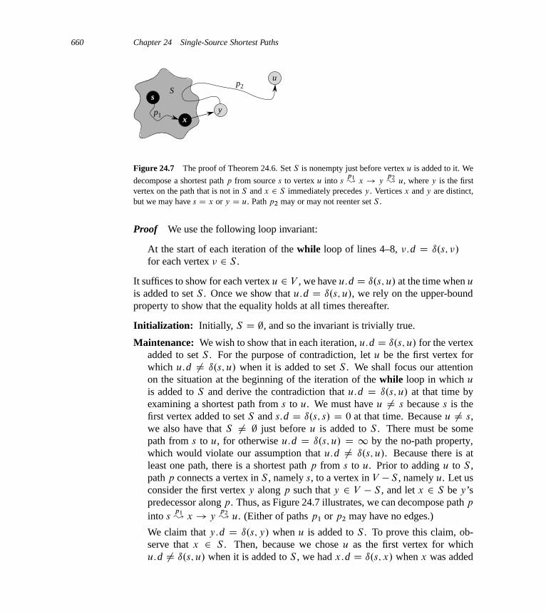
660 Chapter 24 Single-Source Shortest Paths
p1
Sp2
u
y
s
x
Figure 24.7 The proof of Theorem 24.6. Set S is nonempty just before vertex u is added to it. We
decompose a shortest path p from source s to vertex u into sp1� x ! y
p2� u, where y is the first
vertex on the path that is not in S and x 2 S immediately precedes y. Vertices x and y are distinct,but we may have s D x or y D u. Path p2 may or may not reenter set S .
Proof We use the following loop invariant:
At the start of each iteration of the while loop of lines 4–8, �:d D ı.s; �/
for each vertex � 2 S .
It suffices to show for each vertex u 2 V , we have u:d D ı.s; u/ at the time when u
is added to set S . Once we show that u:d D ı.s; u/, we rely on the upper-boundproperty to show that the equality holds at all times thereafter.
Initialization: Initially, S D ;, and so the invariant is trivially true.
Maintenance: We wish to show that in each iteration, u:d D ı.s; u/ for the vertexadded to set S . For the purpose of contradiction, let u be the first vertex forwhich u:d ¤ ı.s; u/ when it is added to set S . We shall focus our attentionon the situation at the beginning of the iteration of the while loop in which u
is added to S and derive the contradiction that u:d D ı.s; u/ at that time byexamining a shortest path from s to u. We must have u ¤ s because s is thefirst vertex added to set S and s:d D ı.s; s/ D 0 at that time. Because u ¤ s,we also have that S ¤ ; just before u is added to S . There must be somepath from s to u, for otherwise u:d D ı.s; u/ D 1 by the no-path property,which would violate our assumption that u:d ¤ ı.s; u/. Because there is atleast one path, there is a shortest path p from s to u. Prior to adding u to S ,path p connects a vertex in S , namely s, to a vertex in V �S , namely u. Let usconsider the first vertex y along p such that y 2 V � S , and let x 2 S be y’spredecessor along p. Thus, as Figure 24.7 illustrates, we can decompose path p
into sp1� x ! y
p2� u. (Either of paths p1 or p2 may have no edges.)
We claim that y:d D ı.s; y/ when u is added to S . To prove this claim, ob-serve that x 2 S . Then, because we chose u as the first vertex for whichu:d ¤ ı.s; u/ when it is added to S , we had x:d D ı.s; x/ when x was added

24.3 Dijkstra’s algorithm 661
to S . Edge .x; y/ was relaxed at that time, and the claim follows from theconvergence property.
We can now obtain a contradiction to prove that u:d D ı.s; u/. Because y
appears before u on a shortest path from s to u and all edge weights are non-negative (notably those on path p2), we have ı.s; y/ � ı.s; u/, and thus
y:d D ı.s; y/
� ı.s; u/ (24.2)
� u:d (by the upper-bound property) .
But because both vertices u and y were in V � S when u was chosen in line 5,we have u:d � y:d. Thus, the two inequalities in (24.2) are in fact equalities,giving
y:d D ı.s; y/ D ı.s; u/ D u:d :
Consequently, u:d D ı.s; u/, which contradicts our choice of u. We concludethat u:d D ı.s; u/ when u is added to S , and that this equality is maintained atall times thereafter.
Termination: At termination, Q D ; which, along with our earlier invariant thatQ D V �S , implies that S D V . Thus, u:d D ı.s; u/ for all vertices u 2 V .
Corollary 24.7If we run Dijkstra’s algorithm on a weighted, directed graph G D .V; E/ withnonnegative weight function w and source s, then at termination, the predecessorsubgraph G� is a shortest-paths tree rooted at s.
Proof Immediate from Theorem 24.6 and the predecessor-subgraph property.
Analysis
How fast is Dijkstra’s algorithm? It maintains the min-priority queue Q by call-ing three priority-queue operations: INSERT (implicit in line 3), EXTRACT-MIN
(line 5), and DECREASE-KEY (implicit in RELAX, which is called in line 8). Thealgorithm calls both INSERT and EXTRACT-MIN once per vertex. Because eachvertex u 2 V is added to set S exactly once, each edge in the adjacency list AdjŒu�
is examined in the for loop of lines 7–8 exactly once during the course of the al-gorithm. Since the total number of edges in all the adjacency lists is jEj, this forloop iterates a total of jEj times, and thus the algorithm calls DECREASE-KEY atmost jEj times overall. (Observe once again that we are using aggregate analysis.)
The running time of Dijkstra’s algorithm depends on how we implement themin-priority queue. Consider first the case in which we maintain the min-priority
662 Chapter 24 Single-Source Shortest Paths
queue by taking advantage of the vertices being numbered 1 to jV j. We simplystore �:d in the �th entry of an array. Each INSERT and DECREASE-KEY operationtakes O.1/ time, and each EXTRACT-MIN operation takes O.V / time (since wehave to search through the entire array), for a total time of O.V 2 C E/ D O.V 2/.
If the graph is sufficiently sparse—in particular, E D o.V 2= lg V /—we canimprove the algorithm by implementing the min-priority queue with a binary min-heap. (As discussed in Section 6.5, the implementation should make sure thatvertices and corresponding heap elements maintain handles to each other.) EachEXTRACT-MIN operation then takes time O.lg V /. As before, there are jV j suchoperations. The time to build the binary min-heap is O.V /. Each DECREASE-KEY
operation takes time O.lg V /, and there are still at most jEj such operations. Thetotal running time is therefore O..V CE/ lg V /, which is O.E lg V / if all verticesare reachable from the source. This running time improves upon the straightfor-ward O.V 2/-time implementation if E D o.V 2= lg V /.
We can in fact achieve a running time of O.V lg V C E/ by implementing themin-priority queue with a Fibonacci heap (see Chapter 19). The amortized costof each of the jV j EXTRACT-MIN operations is O.lg V /, and each DECREASE-KEY call, of which there are at most jEj, takes only O.1/ amortized time. His-torically, the development of Fibonacci heaps was motivated by the observationthat Dijkstra’s algorithm typically makes many more DECREASE-KEY calls thanEXTRACT-MIN calls, so that any method of reducing the amortized time of eachDECREASE-KEY operation to o.lg V / without increasing the amortized time ofEXTRACT-MIN would yield an asymptotically faster implementation than with bi-nary heaps.
Dijkstra’s algorithm resembles both breadth-first search (see Section 22.2) andPrim’s algorithm for computing minimum spanning trees (see Section 23.2). It islike breadth-first search in that set S corresponds to the set of black vertices in abreadth-first search; just as vertices in S have their final shortest-path weights, sodo black vertices in a breadth-first search have their correct breadth-first distances.Dijkstra’s algorithm is like Prim’s algorithm in that both algorithms use a min-priority queue to find the “lightest” vertex outside a given set (the set S in Dijkstra’salgorithm and the tree being grown in Prim’s algorithm), add this vertex into theset, and adjust the weights of the remaining vertices outside the set accordingly.
Exercises
24.3-1Run Dijkstra’s algorithm on the directed graph of Figure 24.2, first using vertex s
as the source and then using vertex ´ as the source. In the style of Figure 24.6,show the d and � values and the vertices in set S after each iteration of the whileloop.
24.3 Dijkstra’s algorithm 663
24.3-2Give a simple example of a directed graph with negative-weight edges for whichDijkstra’s algorithm produces incorrect answers. Why doesn’t the proof of Theo-rem 24.6 go through when negative-weight edges are allowed?
24.3-3Suppose we change line 4 of Dijkstra’s algorithm to the following.
4 while jQj > 1
This change causes the while loop to execute jV j � 1 times instead of jV j times. Isthis proposed algorithm correct?
24.3-4Professor Gaedel has written a program that he claims implements Dijkstra’s al-gorithm. The program produces �:d and �:� for each vertex � 2 V . Give anO.V CE/-time algorithm to check the output of the professor’s program. It shoulddetermine whether the d and � attributes match those of some shortest-paths tree.You may assume that all edge weights are nonnegative.
24.3-5Professor Newman thinks that he has worked out a simpler proof of correctnessfor Dijkstra’s algorithm. He claims that Dijkstra’s algorithm relaxes the edges ofevery shortest path in the graph in the order in which they appear on the path, andtherefore the path-relaxation property applies to every vertex reachable from thesource. Show that the professor is mistaken by constructing a directed graph forwhich Dijkstra’s algorithm could relax the edges of a shortest path out of order.
24.3-6We are given a directed graph G D .V; E/ on which each edge .u; �/ 2 E has anassociated value r.u; �/, which is a real number in the range 0 � r.u; �/ � 1 thatrepresents the reliability of a communication channel from vertex u to vertex �.We interpret r.u; �/ as the probability that the channel from u to � will not fail,and we assume that these probabilities are independent. Give an efficient algorithmto find the most reliable path between two given vertices.
24.3-7Let G D .V; E/ be a weighted, directed graph with positive weight functionw W E ! f1; 2; : : : ; W g for some positive integer W , and assume that no two ver-tices have the same shortest-path weights from source vertex s. Now suppose thatwe define an unweighted, directed graph G0 D .V [ V 0; E 0/ by replacing eachedge .u; �/ 2 E with w.u; �/ unit-weight edges in series. How many verticesdoes G0 have? Now suppose that we run a breadth-first search on G0. Show that

664 Chapter 24 Single-Source Shortest Paths
the order in which the breadth-first search of G0 colors vertices in V black is thesame as the order in which Dijkstra’s algorithm extracts the vertices of V from thepriority queue when it runs on G.
24.3-8Let G D .V; E/ be a weighted, directed graph with nonnegative weight functionw W E ! f0; 1; : : : ; W g for some nonnegative integer W . Modify Dijkstra’s algo-rithm to compute the shortest paths from a given source vertex s in O.W V C E/
time.
24.3-9Modify your algorithm from Exercise 24.3-8 to run in O..V C E/ lg W / time.(Hint: How many distinct shortest-path estimates can there be in V � S at anypoint in time?)
24.3-10Suppose that we are given a weighted, directed graph G D .V; E/ in which edgesthat leave the source vertex s may have negative weights, all other edge weightsare nonnegative, and there are no negative-weight cycles. Argue that Dijkstra’salgorithm correctly finds shortest paths from s in this graph.
24.4 Difference constraints and shortest paths
Chapter 29 studies the general linear-programming problem, in which we wish tooptimize a linear function subject to a set of linear inequalities. In this section, weinvestigate a special case of linear programming that we reduce to finding shortestpaths from a single source. We can then solve the single-source shortest-pathsproblem that results by running the Bellman-Ford algorithm, thereby also solvingthe linear-programming problem.
Linear programming
In the general linear-programming problem, we are given an m n matrix A,an m-vector b, and an n-vector c. We wish to find a vector x of n elements thatmaximizes the objective function
Pn
iD1 cixi subject to the m constraints given byAx � b.
Although the simplex algorithm, which is the focus of Chapter 29, does notalways run in time polynomial in the size of its input, there are other linear-programming algorithms that do run in polynomial time. We offer here two reasonsto understand the setup of linear-programming problems. First, if we know that we
24.4 Difference constraints and shortest paths 665
can cast a given problem as a polynomial-sized linear-programming problem, thenwe immediately have a polynomial-time algorithm to solve the problem. Second,faster algorithms exist for many special cases of linear programming. For exam-ple, the single-pair shortest-path problem (Exercise 24.4-4) and the maximum-flowproblem (Exercise 26.1-5) are special cases of linear programming.
Sometimes we don’t really care about the objective function; we just wish to findany feasible solution, that is, any vector x that satisfies Ax � b, or to determinethat no feasible solution exists. We shall focus on one such feasibility problem.
Systems of difference constraints
In a system of difference constraints, each row of the linear-programming matrix A
contains one 1 and one �1, and all other entries of A are 0. Thus, the constraintsgiven by Ax � b are a set of m difference constraints involving n unknowns, inwhich each constraint is a simple linear inequality of the form
xj � xi � bk ;
where 1 � i; j � n, i ¤ j , and 1 � k � m.For example, consider the problem of finding a 5-vector x D .xi/ that satisfies�
1 �1 0 0 0
1 0 0 0 �1
0 1 0 0 �1
�1 0 1 0 0
�1 0 0 1 0
0 0 �1 1 0
0 0 �1 0 1
0 0 0 �1 1
˘ˇx1
x2
x3
x4
x5
��
�0
�1
1
5
4
�1
�3
�3
˘:
This problem is equivalent to finding values for the unknowns x1; x2; x3; x4; x5,satisfying the following 8 difference constraints:
x1 � x2 � 0 , (24.3)
x1 � x5 � �1 , (24.4)
x2 � x5 � 1 , (24.5)
x3 � x1 � 5 , (24.6)
x4 � x1 � 4 , (24.7)
x4 � x3 � �1 , (24.8)
x5 � x3 � �3 , (24.9)
x5 � x4 � �3 . (24.10)

666 Chapter 24 Single-Source Shortest Paths
One solution to this problem is x D .�5;�3; 0;�1;�4/, which you can verify di-rectly by checking each inequality. In fact, this problem has more than one solution.Another is x 0 D .0; 2; 5; 4; 1/. These two solutions are related: each componentof x 0 is 5 larger than the corresponding component of x. This fact is not merecoincidence.
Lemma 24.8Let x D .x1; x2; : : : ; xn/ be a solution to a system Ax � b of difference con-straints, and let d be any constant. Then x C d D .x1 C d; x2 C d; : : : ; xn C d/
is a solution to Ax � b as well.
Proof For each xi and xj , we have .xj C d/ � .xi C d/ D xj � xi . Thus, if x
satisfies Ax � b, so does x C d .
Systems of difference constraints occur in many different applications. For ex-ample, the unknowns xi may be times at which events are to occur. Each constraintstates that at least a certain amount of time, or at most a certain amount of time,must elapse between two events. Perhaps the events are jobs to be performed dur-ing the assembly of a product. If we apply an adhesive that takes 2 hours to set attime x1 and we have to wait until it sets to install a part at time x2, then we have theconstraint that x2 � x1 C 2 or, equivalently, that x1 � x2 � �2. Alternatively, wemight require that the part be installed after the adhesive has been applied but nolater than the time that the adhesive has set halfway. In this case, we get the pair ofconstraints x2 � x1 and x2 � x1C1 or, equivalently, x1�x2 � 0 and x2�x1 � 1.
Constraint graphs
We can interpret systems of difference constraints from a graph-theoretic pointof view. In a system Ax � b of difference constraints, we view the m n
linear-programming matrix A as the transpose of an incidence matrix (see Exer-cise 22.1-7) for a graph with n vertices and m edges. Each vertex �i in the graph,for i D 1; 2; : : : ; n, corresponds to one of the n unknown variables xi . Each di-rected edge in the graph corresponds to one of the m inequalities involving twounknowns.
More formally, given a system Ax � b of difference constraints, the correspond-ing constraint graph is a weighted, directed graph G D .V; E/, where
V D f�0; �1; : : : ; �ngand
E D f.�i ; �j / W xj � xi � bk is a constraintg[ f.�0; �1/; .�0; �2/; .�0; �3/; : : : ; .�0; �n/g :

24.4 Difference constraints and shortest paths 667
0
0
0
0
0
0–1
1
54
–1
–3–30
–5
–3
0–1
–4
v3
v2
v1
v5
v0
v4
Figure 24.8 The constraint graph corresponding to the system (24.3)–(24.10) of difference con-straints. The value of ı.�0; �i / appears in each vertex �i . One feasible solution to the system isx D .�5;�3; 0;�1;�4/.
The constraint graph contains the additional vertex �0, as we shall see shortly, toguarantee that the graph has some vertex which can reach all other vertices. Thus,the vertex set V consists of a vertex �i for each unknown xi , plus an additionalvertex �0. The edge set E contains an edge for each difference constraint, plusan edge .�0; �i / for each unknown xi . If xj � xi � bk is a difference constraint,then the weight of edge .�i ; �j / is w.�i ; �j / D bk. The weight of each edge leav-ing �0 is 0. Figure 24.8 shows the constraint graph for the system (24.3)–(24.10)of difference constraints.
The following theorem shows that we can find a solution to a system of differ-ence constraints by finding shortest-path weights in the corresponding constraintgraph.
Theorem 24.9Given a system Ax � b of difference constraints, let G D .V; E/ be the corre-sponding constraint graph. If G contains no negative-weight cycles, then
x D .ı.�0; �1/; ı.�0; �2/; ı.�0; �3/; : : : ; ı.�0; �n// (24.11)
is a feasible solution for the system. If G contains a negative-weight cycle, thenthere is no feasible solution for the system.
Proof We first show that if the constraint graph contains no negative-weightcycles, then equation (24.11) gives a feasible solution. Consider any edge.�i ; �j / 2 E. By the triangle inequality, ı.�0; �j / � ı.�0; �i / C w.�i ; �j / or,equivalently, ı.�0; �j / � ı.�0; �i / � w.�i ; �j /. Thus, letting xi D ı.�0; �i / and
668 Chapter 24 Single-Source Shortest Paths
xj D ı.�0; �j / satisfies the difference constraint xj � xi � w.�i ; �j / that corre-sponds to edge .�i ; �j /.
Now we show that if the constraint graph contains a negative-weight cycle, thenthe system of difference constraints has no feasible solution. Without loss of gen-erality, let the negative-weight cycle be c D h�1; �2; : : : ; �ki, where �1 D �k.(The vertex �0 cannot be on cycle c, because it has no entering edges.) Cycle c
corresponds to the following difference constraints:
x2 � x1 � w.�1; �2/ ;
x3 � x2 � w.�2; �3/ ;
:::
xk�1 � xk�2 � w.�k�2; �k�1/ ;
xk � xk�1 � w.�k�1; �k/ :
We will assume that x has a solution satisfying each of these k inequalities and thenderive a contradiction. The solution must also satisfy the inequality that resultswhen we sum the k inequalities together. If we sum the left-hand sides, eachunknown xi is added in once and subtracted out once (remember that �1 D �k
implies x1 D xk), so that the left-hand side of the sum is 0. The right-hand sidesums to w.c/, and thus we obtain 0 � w.c/. But since c is a negative-weight cycle,w.c/ < 0, and we obtain the contradiction that 0 � w.c/ < 0.
Solving systems of difference constraints
Theorem 24.9 tells us that we can use the Bellman-Ford algorithm to solve asystem of difference constraints. Because the constraint graph contains edgesfrom the source vertex �0 to all other vertices, any negative-weight cycle in theconstraint graph is reachable from �0. If the Bellman-Ford algorithm returnsTRUE, then the shortest-path weights give a feasible solution to the system. InFigure 24.8, for example, the shortest-path weights provide the feasible solutionx D .�5;�3; 0;�1;�4/, and by Lemma 24.8, x D .d � 5; d � 3; d; d � 1; d � 4/
is also a feasible solution for any constant d . If the Bellman-Ford algorithm returnsFALSE, there is no feasible solution to the system of difference constraints.
A system of difference constraints with m constraints on n unknowns producesa graph with n C 1 vertices and n C m edges. Thus, using the Bellman-Fordalgorithm, we can solve the system in O..n C 1/.n C m// D O.n2 C nm/ time.Exercise 24.4-5 asks you to modify the algorithm to run in O.nm/ time, even if m
is much less than n.

24.4 Difference constraints and shortest paths 669
Exercises
24.4-1Find a feasible solution or determine that no feasible solution exists for the follow-ing system of difference constraints:
x1 � x2 � 1 ,
x1 � x4 � �4 ,
x2 � x3 � 2 ,
x2 � x5 � 7 ,
x2 � x6 � 5 ,
x3 � x6 � 10 ,
x4 � x2 � 2 ,
x5 � x1 � �1 ,
x5 � x4 � 3 ,
x6 � x3 � �8 .
24.4-2Find a feasible solution or determine that no feasible solution exists for the follow-ing system of difference constraints:
x1 � x2 � 4 ,
x1 � x5 � 5 ,
x2 � x4 � �6 ,
x3 � x2 � 1 ,
x4 � x1 � 3 ,
x4 � x3 � 5 ,
x4 � x5 � 10 ,
x5 � x3 � �4 ,
x5 � x4 � �8 .
24.4-3Can any shortest-path weight from the new vertex �0 in a constraint graph be posi-tive? Explain.
24.4-4Express the single-pair shortest-path problem as a linear program.
670 Chapter 24 Single-Source Shortest Paths
24.4-5Show how to modify the Bellman-Ford algorithm slightly so that when we use itto solve a system of difference constraints with m inequalities on n unknowns, therunning time is O.nm/.
24.4-6Suppose that in addition to a system of difference constraints, we want to handleequality constraints of the form xi D xj C bk. Show how to adapt the Bellman-Ford algorithm to solve this variety of constraint system.
24.4-7Show how to solve a system of difference constraints by a Bellman-Ford-like algo-rithm that runs on a constraint graph without the extra vertex �0.
24.4-8 ?
Let Ax � b be a system of m difference constraints in n unknowns. Show that theBellman-Ford algorithm, when run on the corresponding constraint graph, maxi-mizes
Pn
iD1 xi subject to Ax � b and xi � 0 for all xi .
24.4-9 ?
Show that the Bellman-Ford algorithm, when run on the constraint graph for a sys-tem Ax � b of difference constraints, minimizes the quantity .max fxig�min fxig/subject to Ax � b. Explain how this fact might come in handy if the algorithm isused to schedule construction jobs.
24.4-10Suppose that every row in the matrix A of a linear program Ax � b corresponds toa difference constraint, a single-variable constraint of the form xi � bk, or a single-variable constraint of the form �xi � bk. Show how to adapt the Bellman-Fordalgorithm to solve this variety of constraint system.
24.4-11Give an efficient algorithm to solve a system Ax � b of difference constraintswhen all of the elements of b are real-valued and all of the unknowns xi must beintegers.
24.4-12 ?
Give an efficient algorithm to solve a system Ax � b of difference constraintswhen all of the elements of b are real-valued and a specified subset of some, butnot necessarily all, of the unknowns xi must be integers.

24.5 Proofs of shortest-paths properties 671
24.5 Proofs of shortest-paths properties
Throughout this chapter, our correctness arguments have relied on the triangleinequality, upper-bound property, no-path property, convergence property, path-relaxation property, and predecessor-subgraph property. We stated these propertieswithout proof at the beginning of this chapter. In this section, we prove them.
The triangle inequality
In studying breadth-first search (Section 22.2), we proved as Lemma 22.1 a sim-ple property of shortest distances in unweighted graphs. The triangle inequalitygeneralizes the property to weighted graphs.
Lemma 24.10 (Triangle inequality)Let G D .V; E/ be a weighted, directed graph with weight function w W E ! R
and source vertex s. Then, for all edges .u; �/ 2 E, we have
ı.s; �/ � ı.s; u/Cw.u; �/ :
Proof Suppose that p is a shortest path from source s to vertex �. Then p hasno more weight than any other path from s to �. Specifically, path p has no moreweight than the particular path that takes a shortest path from source s to vertex u
and then takes edge .u; �/.Exercise 24.5-3 asks you to handle the case in which there is no shortest path
from s to �.
Effects of relaxation on shortest-path estimates
The next group of lemmas describes how shortest-path estimates are affected whenwe execute a sequence of relaxation steps on the edges of a weighted, directedgraph that has been initialized by INITIALIZE-SINGLE-SOURCE.
Lemma 24.11 (Upper-bound property)Let G D .V; E/ be a weighted, directed graph with weight function w W E ! R.Let s 2 V be the source vertex, and let the graph be initialized by INITIALIZE-SINGLE-SOURCE.G; s/. Then, �:d � ı.s; �/ for all � 2 V , and this invariant ismaintained over any sequence of relaxation steps on the edges of G. Moreover,once �:d achieves its lower bound ı.s; �/, it never changes.
672 Chapter 24 Single-Source Shortest Paths
Proof We prove the invariant �:d � ı.s; �/ for all vertices � 2 V by inductionover the number of relaxation steps.
For the basis, �:d � ı.s; �/ is certainly true after initialization, since �:d D 1implies �:d � ı.s; �/ for all � 2 V � fsg, and since s:d D 0 � ı.s; s/ (note thatı.s; s/ D �1 if s is on a negative-weight cycle and 0 otherwise).
For the inductive step, consider the relaxation of an edge .u; �/. By the inductivehypothesis, x:d � ı.s; x/ for all x 2 V prior to the relaxation. The only d valuethat may change is �:d. If it changes, we have
�:d D u:d Cw.u; �/
� ı.s; u/Cw.u; �/ (by the inductive hypothesis)
� ı.s; �/ (by the triangle inequality) .
and so the invariant is maintained.To see that the value of �:d never changes once �:d D ı.s; �/, note that having
achieved its lower bound, �:d cannot decrease because we have just shown that�:d � ı.s; �/, and it cannot increase because relaxation steps do not increase d
values.
Corollary 24.12 (No-path property)Suppose that in a weighted, directed graph G D .V; E/ with weight functionw W E ! R, no path connects a source vertex s 2 V to a given vertex � 2 V .Then, after the graph is initialized by INITIALIZE-SINGLE-SOURCE.G; s/, wehave �:d D ı.s; �/ D 1, and this equality is maintained as an invariant overany sequence of relaxation steps on the edges of G.
Proof By the upper-bound property, we always have 1 D ı.s; �/ � �:d, andthus �:d D1 D ı.s; �/.
Lemma 24.13Let G D .V; E/ be a weighted, directed graph with weight function w W E ! R,and let .u; �/ 2 E. Then, immediately after relaxing edge .u; �/ by executingRELAX.u; �; w/, we have �:d � u:dCw.u; �/.
Proof If, just prior to relaxing edge .u; �/, we have �:d > u:d C w.u; �/, then�:d D u:d C w.u; �/ afterward. If, instead, �:d � u:d C w.u; �/ just beforethe relaxation, then neither u:d nor �:d changes, and so �:d � u:d C w.u; �/
afterward.
Lemma 24.14 (Convergence property)Let G D .V; E/ be a weighted, directed graph with weight function w W E ! R,let s 2 V be a source vertex, and let s � u ! � be a shortest path in G for
24.5 Proofs of shortest-paths properties 673
some vertices u; � 2 V . Suppose that G is initialized by INITIALIZE-SINGLE-SOURCE.G; s/ and then a sequence of relaxation steps that includes the callRELAX.u; �; w/ is executed on the edges of G. If u:d D ı.s; u/ at any timeprior to the call, then �:d D ı.s; �/ at all times after the call.
Proof By the upper-bound property, if u:d D ı.s; u/ at some point prior to re-laxing edge .u; �/, then this equality holds thereafter. In particular, after relaxingedge .u; �/, we have
�:d � u:dCw.u; �/ (by Lemma 24.13)
D ı.s; u/C w.u; �/
D ı.s; �/ (by Lemma 24.1) .
By the upper-bound property, �:d � ı.s; �/, from which we conclude that�:d D ı.s; �/, and this equality is maintained thereafter.
Lemma 24.15 (Path-relaxation property)Let G D .V; E/ be a weighted, directed graph with weight function w W E ! R,and let s 2 V be a source vertex. Consider any shortest path p D h�0; �1; : : : ; �kifrom s D �0 to �k. If G is initialized by INITIALIZE-SINGLE-SOURCE.G; s/ andthen a sequence of relaxation steps occurs that includes, in order, relaxing the edges.�0; �1/; .�1; �2/; : : : ; .�k�1; �k/, then �k:d D ı.s; �k/ after these relaxations andat all times afterward. This property holds no matter what other edge relaxationsoccur, including relaxations that are intermixed with relaxations of the edges of p.
Proof We show by induction that after the i th edge of path p is relaxed, we have�i :d D ı.s; �i /. For the basis, i D 0, and before any edges of p have been relaxed,we have from the initialization that �0:d D s:d D 0 D ı.s; s/. By the upper-boundproperty, the value of s:d never changes after initialization.
For the inductive step, we assume that �i�1:d D ı.s; �i�1/, and we examinewhat happens when we relax edge .�i�1; �i/. By the convergence property, afterrelaxing this edge, we have �i :d D ı.s; �i /, and this equality is maintained at alltimes thereafter.
Relaxation and shortest-paths trees
We now show that once a sequence of relaxations has caused the shortest-path es-timates to converge to shortest-path weights, the predecessor subgraph G� inducedby the resulting � values is a shortest-paths tree for G. We start with the follow-ing lemma, which shows that the predecessor subgraph always forms a rooted treewhose root is the source.
674 Chapter 24 Single-Source Shortest Paths
Lemma 24.16Let G D .V; E/ be a weighted, directed graph with weight function w W E ! R,let s 2 V be a source vertex, and assume that G contains no negative-weightcycles that are reachable from s. Then, after the graph is initialized by INITIALIZE-SINGLE-SOURCE.G; s/, the predecessor subgraph G� forms a rooted tree withroot s, and any sequence of relaxation steps on edges of G maintains this propertyas an invariant.
Proof Initially, the only vertex in G� is the source vertex, and the lemma is triv-ially true. Consider a predecessor subgraph G� that arises after a sequence ofrelaxation steps. We shall first prove that G� is acyclic. Suppose for the sake ofcontradiction that some relaxation step creates a cycle in the graph G� . Let the cy-cle be c D h�0; �1; : : : ; �ki, where �k D �0. Then, �i :� D �i�1 for i D 1; 2; : : : ; k
and, without loss of generality, we can assume that relaxing edge .�k�1; �k/ createdthe cycle in G� .
We claim that all vertices on cycle c are reachable from the source s. Why?Each vertex on c has a non-NIL predecessor, and so each vertex on c was assigneda finite shortest-path estimate when it was assigned its non-NIL � value. By theupper-bound property, each vertex on cycle c has a finite shortest-path weight,which implies that it is reachable from s.
We shall examine the shortest-path estimates on c just prior to the callRELAX.�k�1; �k; w/ and show that c is a negative-weight cycle, thereby contra-dicting the assumption that G contains no negative-weight cycles that are reachablefrom the source. Just before the call, we have �i :� D �i�1 for i D 1; 2; : : : ; k � 1.Thus, for i D 1; 2; : : : ; k � 1, the last update to �i :d was by the assignment�i :d D �i�1:dCw.�i�1; �i /. If �i�1:d changed since then, it decreased. Therefore,just before the call RELAX.�k�1; �k ; w/, we have
�i :d � �i�1:dCw.�i�1; �i / for all i D 1; 2; : : : ; k � 1 : (24.12)
Because �k:� is changed by the call, immediately beforehand we also have thestrict inequality
�k:d > �k�1:dCw.�k�1; �k/ :
Summing this strict inequality with the k � 1 inequalities (24.12), we obtain thesum of the shortest-path estimates around cycle c:
kXiD1
�i :d >
kXiD1
.�i�1:dC w.�i�1; �i//
DkX
iD1
�i�1:dCkX
iD1
w.�i�1; �i/ :

24.5 Proofs of shortest-paths properties 675
su
x
y
zv
Figure 24.9 Showing that a simple path in G� from source s to vertex � is unique. If there are twopaths p1 (s � u � x ! ´ � �) and p2 (s � u � y ! ´ � �), where x ¤ y, then ´:� D x
and ´:� D y, a contradiction.
But
kXiD1
�i :d DkX
iD1
�i�1:d ;
since each vertex in the cycle c appears exactly once in each summation. Thisequality implies
0 >
kXiD1
w.�i�1; �i / :
Thus, the sum of weights around the cycle c is negative, which provides the desiredcontradiction.
We have now proven that G� is a directed, acyclic graph. To show that it formsa rooted tree with root s, it suffices (see Exercise B.5-2) to prove that for eachvertex � 2 V� , there is a unique simple path from s to � in G� .
We first must show that a path from s exists for each vertex in V� . The ver-tices in V� are those with non-NIL � values, plus s. The idea here is to prove byinduction that a path exists from s to all vertices in V� . We leave the details asExercise 24.5-6.
To complete the proof of the lemma, we must now show that for any vertex� 2 V� , the graph G� contains at most one simple path from s to �. Suppose other-wise. That is, suppose that, as Figure 24.9 illustrates, G� contains two simple pathsfrom s to some vertex �: p1, which we decompose into s � u � x ! ´ � �,and p2, which we decompose into s � u � y ! ´ � �, where x ¤ y (though u
could be s and ´ could be �). But then, ´:� D x and ´:� D y, which impliesthe contradiction that x D y. We conclude that G� contains a unique simple pathfrom s to �, and thus G� forms a rooted tree with root s.
We can now show that if, after we have performed a sequence of relaxation steps,all vertices have been assigned their true shortest-path weights, then the predeces-sor subgraph G� is a shortest-paths tree.
676 Chapter 24 Single-Source Shortest Paths
Lemma 24.17 (Predecessor-subgraph property)Let G D .V; E/ be a weighted, directed graph with weight function w W E ! R,let s 2 V be a source vertex, and assume that G contains no negative-weight cyclesthat are reachable from s. Let us call INITIALIZE-SINGLE-SOURCE.G; s/ and thenexecute any sequence of relaxation steps on edges of G that produces �:d D ı.s; �/
for all � 2 V . Then, the predecessor subgraph G� is a shortest-paths tree rootedat s.
Proof We must prove that the three properties of shortest-paths trees given onpage 647 hold for G� . To show the first property, we must show that V� is the setof vertices reachable from s. By definition, a shortest-path weight ı.s; �/ is finiteif and only if � is reachable from s, and thus the vertices that are reachable from s
are exactly those with finite d values. But a vertex � 2 V � fsg has been assigneda finite value for �:d if and only if �:� ¤ NIL. Thus, the vertices in V� are exactlythose reachable from s.
The second property follows directly from Lemma 24.16.It remains, therefore, to prove the last property of shortest-paths trees: for each
vertex � 2 V� , the unique simple path sp� � in G� is a shortest path from s to �
in G. Let p D h�0; �1; : : : ; �ki, where �0 D s and �k D �. For i D 1; 2; : : : ; k,we have both �i :d D ı.s; �i / and �i :d � �i�1:d C w.�i�1; �i /, from which weconclude w.�i�1; �i / � ı.s; �i / � ı.s; �i�1/. Summing the weights along path p
yields
w.p/ DkX
iD1
w.�i�1; �i /
�kX
iD1
.ı.s; �i / � ı.s; �i�1//
D ı.s; �k/ � ı.s; �0/ (because the sum telescopes)
D ı.s; �k/ (because ı.s; �0/ D ı.s; s/ D 0) .
Thus, w.p/ � ı.s; �k/. Since ı.s; �k/ is a lower bound on the weight of any pathfrom s to �k, we conclude that w.p/ D ı.s; �k/, and thus p is a shortest pathfrom s to � D �k.
Exercises
24.5-1Give two shortest-paths trees for the directed graph of Figure 24.2 (on page 648)other than the two shown.
24.5 Proofs of shortest-paths properties 677
24.5-2Give an example of a weighted, directed graph G D .V; E/ with weight functionw W E ! R and source vertex s such that G satisfies the following property: Forevery edge .u; �/ 2 E, there is a shortest-paths tree rooted at s that contains .u; �/
and another shortest-paths tree rooted at s that does not contain .u; �/.
24.5-3Embellish the proof of Lemma 24.10 to handle cases in which shortest-pathweights are1 or �1.
24.5-4Let G D .V; E/ be a weighted, directed graph with source vertex s, and let G
be initialized by INITIALIZE-SINGLE-SOURCE.G; s/. Prove that if a sequence ofrelaxation steps sets s:� to a non-NIL value, then G contains a negative-weightcycle.
24.5-5Let G D .V; E/ be a weighted, directed graph with no negative-weight edges. Lets 2 V be the source vertex, and suppose that we allow �:� to be the predecessorof � on any shortest path to � from source s if � 2 V � fsg is reachable from s,and NIL otherwise. Give an example of such a graph G and an assignment of �
values that produces a cycle in G� . (By Lemma 24.16, such an assignment cannotbe produced by a sequence of relaxation steps.)
24.5-6Let G D .V; E/ be a weighted, directed graph with weight function w W E ! R
and no negative-weight cycles. Let s 2 V be the source vertex, and let G be initial-ized by INITIALIZE-SINGLE-SOURCE.G; s/. Prove that for every vertex � 2 V� ,there exists a path from s to � in G� and that this property is maintained as aninvariant over any sequence of relaxations.
24.5-7Let G D .V; E/ be a weighted, directed graph that contains no negative-weightcycles. Let s 2 V be the source vertex, and let G be initialized by INITIALIZE-SINGLE-SOURCE.G; s/. Prove that there exists a sequence of jV j � 1 relaxationsteps that produces �:d D ı.s; �/ for all � 2 V .
24.5-8Let G be an arbitrary weighted, directed graph with a negative-weight cycle reach-able from the source vertex s. Show how to construct an infinite sequence of relax-ations of the edges of G such that every relaxation causes a shortest-path estimateto change.
678 Chapter 24 Single-Source Shortest Paths
Problems
24-1 Yen’s improvement to Bellman-FordSuppose that we order the edge relaxations in each pass of the Bellman-Ford al-gorithm as follows. Before the first pass, we assign an arbitrary linear order�1; �2; : : : ; �jV j to the vertices of the input graph G D .V; E/. Then, we parti-tion the edge set E into Ef [ Eb, where Ef D f.�i ; �j / 2 E W i < j g andEb D f.�i ; �j / 2 E W i > j g. (Assume that G contains no self-loops, so that everyedge is in either Ef or Eb.) Define Gf D .V; Ef / and Gb D .V; Eb/.
a. Prove that Gf is acyclic with topological sort h�1; �2; : : : ; �jV ji and that Gb isacyclic with topological sort h�jV j; �jV j�1; : : : ; �1i.
Suppose that we implement each pass of the Bellman-Ford algorithm in the fol-lowing way. We visit each vertex in the order �1; �2; : : : ; �jV j, relaxing edges of Ef
that leave the vertex. We then visit each vertex in the order �jV j; �jV j�1; : : : ; �1,relaxing edges of Eb that leave the vertex.
b. Prove that with this scheme, if G contains no negative-weight cycles that arereachable from the source vertex s, then after only djV j =2e passes over theedges, �:d D ı.s; �/ for all vertices � 2 V .
c. Does this scheme improve the asymptotic running time of the Bellman-Fordalgorithm?
24-2 Nesting boxesA d -dimensional box with dimensions .x1; x2; : : : ; xd / nests within another boxwith dimensions .y1; y2; : : : ; yd / if there exists a permutation � on f1; 2; : : : ; dgsuch that x�.1/ < y1, x�.2/ < y2, . . . , x�.d/ < yd .
a. Argue that the nesting relation is transitive.
b. Describe an efficient method to determine whether or not one d -dimensionalbox nests inside another.
c. Suppose that you are given a set of n d -dimensional boxes fB1; B2; : : : ; Bng.Give an efficient algorithm to find the longest sequence hBi1; Bi2 ; : : : ; Biki ofboxes such that Bij nests within Bij C1
for j D 1; 2; : : : ; k � 1. Express therunning time of your algorithm in terms of n and d .

Problems for Chapter 24 679
24-3 ArbitrageArbitrage is the use of discrepancies in currency exchange rates to transform oneunit of a currency into more than one unit of the same currency. For example,suppose that 1 U.S. dollar buys 49 Indian rupees, 1 Indian rupee buys 2 Japaneseyen, and 1 Japanese yen buys 0:0107 U.S. dollars. Then, by converting currencies,a trader can start with 1 U.S. dollar and buy 4920:0107 D 1:0486 U.S. dollars,thus turning a profit of 4:86 percent.
Suppose that we are given n currencies c1; c2; : : : ; cn and an n n table R ofexchange rates, such that one unit of currency ci buys RŒi; j � units of currency cj .
a. Give an efficient algorithm to determine whether or not there exists a sequenceof currencies hci1; ci2 ; : : : ; cik i such that
RŒi1; i2� �RŒi2; i3� � � �RŒik�1; ik � � RŒik; i1� > 1 :
Analyze the running time of your algorithm.
b. Give an efficient algorithm to print out such a sequence if one exists. Analyzethe running time of your algorithm.
24-4 Gabow’s scaling algorithm for single-source shortest pathsA scaling algorithm solves a problem by initially considering only the highest-order bit of each relevant input value (such as an edge weight). It then refines theinitial solution by looking at the two highest-order bits. It progressively looks atmore and more high-order bits, refining the solution each time, until it has exam-ined all bits and computed the correct solution.
In this problem, we examine an algorithm for computing the shortest paths froma single source by scaling edge weights. We are given a directed graph G D .V; E/
with nonnegative integer edge weights w. Let W D max.u;�/2E fw.u; �/g. Ourgoal is to develop an algorithm that runs in O.E lg W / time. We assume that allvertices are reachable from the source.
The algorithm uncovers the bits in the binary representation of the edge weightsone at a time, from the most significant bit to the least significant bit. Specifically,let k D dlg.W C 1/e be the number of bits in the binary representation of W ,and for i D 1; 2; : : : ; k, let wi.u; �/ D
w.u; �/=2k�i˘. That is, wi .u; �/ is the
“scaled-down” version of w.u; �/ given by the i most significant bits of w.u; �/.(Thus, wk.u; �/ D w.u; �/ for all .u; �/ 2 E.) For example, if k D 5 andw.u; �/ D 25, which has the binary representation h11001i, then w3.u; �/ Dh110i D 6. As another example with k D 5, if w.u; �/ D h00100i D 4, thenw3.u; �/ D h001i D 1. Let us define ıi.u; �/ as the shortest-path weight fromvertex u to vertex � using weight function wi . Thus, ık.u; �/ D ı.u; �/ for allu; � 2 V . For a given source vertex s, the scaling algorithm first computes the

680 Chapter 24 Single-Source Shortest Paths
shortest-path weights ı1.s; �/ for all � 2 V , then computes ı2.s; �/ for all � 2 V ,and so on, until it computes ık.s; �/ for all � 2 V . We assume throughout thatjEj � jV j � 1, and we shall see that computing ıi from ıi�1 takes O.E/ time, sothat the entire algorithm takes O.kE/ D O.E lg W / time.
a. Suppose that for all vertices � 2 V , we have ı.s; �/ � jEj. Show that we cancompute ı.s; �/ for all � 2 V in O.E/ time.
b. Show that we can compute ı1.s; �/ for all � 2 V in O.E/ time.
Let us now focus on computing ıi from ıi�1.
c. Prove that for i D 2; 3; : : : ; k, we have either wi.u; �/ D 2wi�1.u; �/ orwi.u; �/ D 2wi�1.u; �/C 1. Then, prove that
2ıi�1.s; �/ � ıi .s; �/ � 2ıi�1.s; �/C jV j � 1
for all � 2 V .
d. Define for i D 2; 3; : : : ; k and all .u; �/ 2 E,
ywi.u; �/ D wi.u; �/C 2ıi�1.s; u/ � 2ıi�1.s; �/ :
Prove that for i D 2; 3; : : : ; k and all u; � 2 V , the “reweighted” value ywi .u; �/
of edge .u; �/ is a nonnegative integer.
e. Now, define yıi .s; �/ as the shortest-path weight from s to � using the weightfunction ywi . Prove that for i D 2; 3; : : : ; k and all � 2 V ,
ıi.s; �/ D yıi .s; �/C 2ıi�1.s; �/
and that yıi .s; �/ � jEj.
f. Show how to compute ıi .s; �/ from ıi�1.s; �/ for all � 2 V in O.E/ time, andconclude that we can compute ı.s; �/ for all � 2 V in O.E lg W / time.
24-5 Karp’s minimum mean-weight cycle algorithmLet G D .V; E/ be a directed graph with weight function w W E ! R, and letn D jV j. We define the mean weight of a cycle c D he1; e2; : : : ; eki of edges in E
to be
.c/ D 1
k
kXiD1
w.ei/ :
Problems for Chapter 24 681
Let � D minc .c/, where c ranges over all directed cycles in G. We call a cycle c
for which .c/ D � a minimum mean-weight cycle. This problem investigatesan efficient algorithm for computing �.
Assume without loss of generality that every vertex � 2 V is reachable from asource vertex s 2 V . Let ı.s; �/ be the weight of a shortest path from s to �, and letık.s; �/ be the weight of a shortest path from s to � consisting of exactly k edges.If there is no path from s to � with exactly k edges, then ık.s; �/ D1.
a. Show that if � D 0, then G contains no negative-weight cycles and ı.s; �/ Dmin0�k�n�1 ık.s; �/ for all vertices � 2 V .
b. Show that if � D 0, then
max0�k�n�1
ın.s; �/ � ık.s; �/
n � k� 0
for all vertices � 2 V . (Hint: Use both properties from part (a).)
c. Let c be a 0-weight cycle, and let u and � be any two vertices on c. Supposethat � D 0 and that the weight of the simple path from u to � along the cycleis x. Prove that ı.s; �/ D ı.s; u/ C x. (Hint: The weight of the simple pathfrom � to u along the cycle is �x.)
d. Show that if � D 0, then on each minimum mean-weight cycle there exists avertex � such that
max0�k�n�1
ın.s; �/ � ık.s; �/
n � kD 0 :
(Hint: Show how to extend a shortest path to any vertex on a minimum mean-weight cycle along the cycle to make a shortest path to the next vertex on thecycle.)
e. Show that if � D 0, then
min�2V
max0�k�n�1
ın.s; �/ � ık.s; �/
n � kD 0 :
f. Show that if we add a constant t to the weight of each edge of G, then �
increases by t . Use this fact to show that
� D min�2V
max0�k�n�1
ın.s; �/ � ık.s; �/
n � k:
g. Give an O.VE/-time algorithm to compute �.
682 Chapter 24 Single-Source Shortest Paths
24-6 Bitonic shortest pathsA sequence is bitonic if it monotonically increases and then monotonically de-creases, or if by a circular shift it monotonically increases and then monotonicallydecreases. For example the sequences h1; 4; 6; 8; 3;�2i, h9; 2;�4;�10;�5i, andh1; 2; 3; 4i are bitonic, but h1; 3; 12; 4; 2; 10i is not bitonic. (See Problem 15-3 forthe bitonic euclidean traveling-salesman problem.)
Suppose that we are given a directed graph G D .V; E/ with weight functionw W E ! R, where all edge weights are unique, and we wish to find single-sourceshortest paths from a source vertex s. We are given one additional piece of infor-mation: for each vertex � 2 V , the weights of the edges along any shortest pathfrom s to � form a bitonic sequence.
Give the most efficient algorithm you can to solve this problem, and analyze itsrunning time.
Chapter notes
Dijkstra’s algorithm [89] appeared in 1959, but it contained no mention of a priorityqueue. The Bellman-Ford algorithm is based on separate algorithms by Bellman[38] and Ford [109]. Bellman describes the relation of shortest paths to differenceconstraints. Lawler [224] describes the linear-time algorithm for shortest paths ina dag, which he considers part of the folklore.
When edge weights are relatively small nonnegative integers, we have more ef-ficient algorithms to solve the single-source shortest-paths problem. The sequenceof values returned by the EXTRACT-MIN calls in Dijkstra’s algorithm monoton-ically increases over time. As discussed in the chapter notes for Chapter 6, inthis case several data structures can implement the various priority-queue opera-tions more efficiently than a binary heap or a Fibonacci heap. Ahuja, Mehlhorn,Orlin, and Tarjan [8] give an algorithm that runs in O.E C V
plg W / time on
graphs with nonnegative edge weights, where W is the largest weight of any edgein the graph. The best bounds are by Thorup [337], who gives an algorithm thatruns in O.E lg lg V / time, and by Raman [291], who gives an algorithm that runsin O
�E C V min
˚.lg V /1=3C�; .lg W /1=4C�
�time. These two algorithms use an
amount of space that depends on the word size of the underlying machine. Al-though the amount of space used can be unbounded in the size of the input, it canbe reduced to be linear in the size of the input using randomized hashing.
For undirected graphs with integer weights, Thorup [336] gives an O.V C E/-time algorithm for single-source shortest paths. In contrast to the algorithms men-tioned in the previous paragraph, this algorithm is not an implementation of Dijk-

Notes for Chapter 24 683
stra’s algorithm, since the sequence of values returned by EXTRACT-MIN callsdoes not monotonically increase over time.
For graphs with negative edge weights, an algorithm due to Gabow and Tar-jan [122] runs in O.
pV E lg.V W // time, and one by Goldberg [137] runs in
O.p
V E lg W / time, where W D max.u;�/2E fjw.u; �/jg.Cherkassky, Goldberg, and Radzik [65] conducted extensive experiments com-
paring various shortest-path algorithms.
25 All-Pairs Shortest Paths
In this chapter, we consider the problem of finding shortest paths between all pairsof vertices in a graph. This problem might arise in making a table of distances be-tween all pairs of cities for a road atlas. As in Chapter 24, we are given a weighted,directed graph G D .V; E/ with a weight function w W E ! R that maps edgesto real-valued weights. We wish to find, for every pair of vertices u; � 2 V , ashortest (least-weight) path from u to �, where the weight of a path is the sum ofthe weights of its constituent edges. We typically want the output in tabular form:the entry in u’s row and �’s column should be the weight of a shortest path from u
to �.We can solve an all-pairs shortest-paths problem by running a single-source
shortest-paths algorithm jV j times, once for each vertex as the source. If alledge weights are nonnegative, we can use Dijkstra’s algorithm. If we usethe linear-array implementation of the min-priority queue, the running time isO.V 3 C VE/ D O.V 3/. The binary min-heap implementation of the min-priorityqueue yields a running time of O.VE lg V /, which is an improvement if the graphis sparse. Alternatively, we can implement the min-priority queue with a Fibonacciheap, yielding a running time of O.V 2 lg V C VE/.
If the graph has negative-weight edges, we cannot use Dijkstra’s algorithm. In-stead, we must run the slower Bellman-Ford algorithm once from each vertex. Theresulting running time is O.V 2E/, which on a dense graph is O.V 4/. In this chap-ter we shall see how to do better. We also investigate the relation of the all-pairsshortest-paths problem to matrix multiplication and study its algebraic structure.
Unlike the single-source algorithms, which assume an adjacency-list represen-tation of the graph, most of the algorithms in this chapter use an adjacency-matrix representation. (Johnson’s algorithm for sparse graphs, in Section 25.3,uses adjacency lists.) For convenience, we assume that the vertices are numbered1; 2; : : : ; jV j, so that the input is an n n matrix W representing the edge weightsof an n-vertex directed graph G D .V; E/. That is, W D .wij /, where
Chapter 25 All-Pairs Shortest Paths 685
wij D
�0 if i D j ;
the weight of directed edge .i; j / if i ¤ j and .i; j / 2 E ;
1 if i ¤ j and .i; j / 62 E :
(25.1)
We allow negative-weight edges, but we assume for the time being that the inputgraph contains no negative-weight cycles.
The tabular output of the all-pairs shortest-paths algorithms presented in thischapter is an n n matrix D D .dij /, where entry dij contains the weight of ashortest path from vertex i to vertex j . That is, if we let ı.i; j / denote the shortest-path weight from vertex i to vertex j (as in Chapter 24), then dij D ı.i; j / attermination.
To solve the all-pairs shortest-paths problem on an input adjacency matrix, weneed to compute not only the shortest-path weights but also a predecessor matrix… D .�ij /, where �ij is NIL if either i D j or there is no path from i to j ,and otherwise �ij is the predecessor of j on some shortest path from i . Just asthe predecessor subgraph G� from Chapter 24 is a shortest-paths tree for a givensource vertex, the subgraph induced by the i th row of the … matrix should be ashortest-paths tree with root i . For each vertex i 2 V , we define the predecessorsubgraph of G for i as G�;i D .V�;i ; E�;i/ , where
V�;i D fj 2 V W �ij ¤ NILg [ figand
E�;i D f.�ij ; j / W j 2 V�;i � figg :
If G�;i is a shortest-paths tree, then the following procedure, which is a modifiedversion of the PRINT-PATH procedure from Chapter 22, prints a shortest path fromvertex i to vertex j .
PRINT-ALL-PAIRS-SHORTEST-PATH.…; i; j /
1 if i == j
2 print i
3 elseif �ij == NIL
4 print “no path from” i “to” j “exists”5 else PRINT-ALL-PAIRS-SHORTEST-PATH.…; i; �ij /
6 print j
In order to highlight the essential features of the all-pairs algorithms in this chapter,we won’t cover the creation and properties of predecessor matrices as extensivelyas we dealt with predecessor subgraphs in Chapter 24. Some of the exercises coverthe basics.

686 Chapter 25 All-Pairs Shortest Paths
Chapter outline
Section 25.1 presents a dynamic-programming algorithm based on matrix multi-plication to solve the all-pairs shortest-paths problem. Using the technique of “re-peated squaring,” we can achieve a running time of ‚.V 3 lg V /. Section 25.2 givesanother dynamic-programming algorithm, the Floyd-Warshall algorithm, whichruns in time ‚.V 3/. Section 25.2 also covers the problem of finding the tran-sitive closure of a directed graph, which is related to the all-pairs shortest-pathsproblem. Finally, Section 25.3 presents Johnson’s algorithm, which solves the all-pairs shortest-paths problem in O.V 2 lg V C VE/ time and is a good choice forlarge, sparse graphs.
Before proceeding, we need to establish some conventions for adjacency-matrixrepresentations. First, we shall generally assume that the input graph G D .V; E/
has n vertices, so that n D jV j. Second, we shall use the convention of denotingmatrices by uppercase letters, such as W , L, or D, and their individual elementsby subscripted lowercase letters, such as wij , lij , or dij . Some matrices will haveparenthesized superscripts, as in L.m/ D �
l.m/ij
�or D.m/ D �
d.m/ij
�, to indicate
iterates. Finally, for a given n n matrix A, we shall assume that the value of n isstored in the attribute A:rows.
25.1 Shortest paths and matrix multiplication
This section presents a dynamic-programming algorithm for the all-pairs shortest-paths problem on a directed graph G D .V; E/. Each major loop of the dynamicprogram will invoke an operation that is very similar to matrix multiplication, sothat the algorithm will look like repeated matrix multiplication. We shall start bydeveloping a ‚.V 4/-time algorithm for the all-pairs shortest-paths problem andthen improve its running time to ‚.V 3 lg V /.
Before proceeding, let us briefly recap the steps given in Chapter 15 for devel-oping a dynamic-programming algorithm.
1. Characterize the structure of an optimal solution.
2. Recursively define the value of an optimal solution.
3. Compute the value of an optimal solution in a bottom-up fashion.
We reserve the fourth step—constructing an optimal solution from computed in-formation—for the exercises.

25.1 Shortest paths and matrix multiplication 687
The structure of a shortest path
We start by characterizing the structure of an optimal solution. For the all-pairsshortest-paths problem on a graph G D .V; E/, we have proven (Lemma 24.1)that all subpaths of a shortest path are shortest paths. Suppose that we representthe graph by an adjacency matrix W D .wij /. Consider a shortest path p fromvertex i to vertex j , and suppose that p contains at most m edges. Assuming thatthere are no negative-weight cycles, m is finite. If i D j , then p has weight 0
and no edges. If vertices i and j are distinct, then we decompose path p into
ip0
� k ! j , where path p0 now contains at most m � 1 edges. By Lemma 24.1,p0 is a shortest path from i to k, and so ı.i; j / D ı.i; k/C wkj .
A recursive solution to the all-pairs shortest-paths problem
Now, let l.m/ij be the minimum weight of any path from vertex i to vertex j that
contains at most m edges. When m D 0, there is a shortest path from i to j withno edges if and only if i D j . Thus,
l.0/ij D
(0 if i D j ;
1 if i ¤ j :
For m � 1, we compute l.m/ij as the minimum of l
.m�1/ij (the weight of a shortest
path from i to j consisting of at most m�1 edges) and the minimum weight of anypath from i to j consisting of at most m edges, obtained by looking at all possiblepredecessors k of j . Thus, we recursively define
l.m/ij D min
�l
.m�1/ij ; min
1�k�n
˚l
.m�1/
ikC wkj
�D min
1�k�n
˚l
.m�1/
ikCwkj
: (25.2)
The latter equality follows since wjj D 0 for all j .What are the actual shortest-path weights ı.i; j /? If the graph contains
no negative-weight cycles, then for every pair of vertices i and j for whichı.i; j / <1, there is a shortest path from i to j that is simple and thus contains atmost n � 1 edges. A path from vertex i to vertex j with more than n � 1 edgescannot have lower weight than a shortest path from i to j . The actual shortest-pathweights are therefore given by
ı.i; j / D l.n�1/ij D l
.n/ij D l
.nC1/ij D � � � : (25.3)
688 Chapter 25 All-Pairs Shortest Paths
Computing the shortest-path weights bottom up
Taking as our input the matrix W D .wij /, we now compute a series of matricesL.1/; L.2/; : : : ; L.n�1/, where for m D 1; 2; : : : ; n � 1, we have L.m/ D �
l.m/ij
�.
The final matrix L.n�1/ contains the actual shortest-path weights. Observe thatl
.1/ij D wij for all vertices i; j 2 V , and so L.1/ D W .
The heart of the algorithm is the following procedure, which, given matricesL.m�1/ and W , returns the matrix L.m/. That is, it extends the shortest paths com-puted so far by one more edge.
EXTEND-SHORTEST-PATHS.L; W /
1 n D L:rows2 let L0 D �l 0
ij
�be a new n n matrix
3 for i D 1 to n
4 for j D 1 to n
5 l 0ij D 1
6 for k D 1 to n
7 l 0ij D min.l 0
ij ; lik C wkj /
8 return L0
The procedure computes a matrix L0 D .l 0ij /, which it returns at the end. It does so
by computing equation (25.2) for all i and j , using L for L.m�1/ and L0 for L.m/.(It is written without the superscripts to make its input and output matrices inde-pendent of m.) Its running time is ‚.n3/ due to the three nested for loops.
Now we can see the relation to matrix multiplication. Suppose we wish to com-pute the matrix product C D A � B of two n n matrices A and B . Then, fori; j D 1; 2; : : : ; n, we compute
cij DnX
kD1
aik � bkj : (25.4)
Observe that if we make the substitutions
l .m�1/ ! a ;
w ! b ;
l .m/ ! c ;
min ! C ;
C ! �in equation (25.2), we obtain equation (25.4). Thus, if we make these changes toEXTEND-SHORTEST-PATHS and also replace 1 (the identity for min) by 0 (the

25.1 Shortest paths and matrix multiplication 689
identity for C), we obtain the same ‚.n3/-time procedure for multiplying squarematrices that we saw in Section 4.2:
SQUARE-MATRIX-MULTIPLY.A; B/
1 n D A:rows2 let C be a new n n matrix3 for i D 1 to n
4 for j D 1 to n
5 cij D 0
6 for k D 1 to n
7 cij D cij C aik � bkj
8 return C
Returning to the all-pairs shortest-paths problem, we compute the shortest-pathweights by extending shortest paths edge by edge. Letting A � B denote the ma-trix “product” returned by EXTEND-SHORTEST-PATHS.A; B/, we compute the se-quence of n � 1 matrices
L.1/ D L.0/ �W D W ;
L.2/ D L.1/ �W D W 2 ;
L.3/ D L.2/ �W D W 3 ;:::
L.n�1/ D L.n�2/ �W D W n�1 :
As we argued above, the matrix L.n�1/ D W n�1 contains the shortest-path weights.The following procedure computes this sequence in ‚.n4/ time.
SLOW-ALL-PAIRS-SHORTEST-PATHS.W /
1 n D W:rows2 L.1/ D W
3 for m D 2 to n � 1
4 let L.m/ be a new n n matrix5 L.m/ D EXTEND-SHORTEST-PATHS.L.m�1/; W /
6 return L.n�1/
Figure 25.1 shows a graph and the matrices L.m/ computed by the procedureSLOW-ALL-PAIRS-SHORTEST-PATHS.
Improving the running time
Our goal, however, is not to compute all the L.m/ matrices: we are interestedonly in matrix L.n�1/. Recall that in the absence of negative-weight cycles, equa-
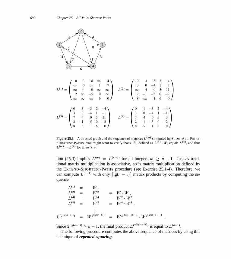
690 Chapter 25 All-Pairs Shortest Paths
2
1 3
5 4
3 4
82
6
7 1–4 –5
L.1/ D
�0 3 8 1 �4
1 0 1 1 7
1 4 0 1 12 1 �5 0 11 1 1 6 0
˘L.2/ D
�0 3 8 2 �4
3 0 �4 1 7
1 4 0 5 11
2 �1 �5 0 �2
8 1 1 6 0
˘
L.3/ D
�0 3 �3 2 �4
3 0 �4 1 �1
7 4 0 5 11
2 �1 �5 0 �2
8 5 1 6 0
˘L.4/ D
�0 1 �3 2 �4
3 0 �4 1 �1
7 4 0 5 3
2 �1 �5 0 �2
8 5 1 6 0
˘Figure 25.1 A directed graph and the sequence of matrices L.m/ computed by SLOW-ALL-PAIRS-SHORTEST-PATHS. You might want to verify that L.5/, defined as L.4/ �W , equals L.4/, and thusL.m/ D L.4/ for all m � 4.
tion (25.3) implies L.m/ D L.n�1/ for all integers m � n � 1. Just as tradi-tional matrix multiplication is associative, so is matrix multiplication defined bythe EXTEND-SHORTEST-PATHS procedure (see Exercise 25.1-4). Therefore, wecan compute L.n�1/ with only dlg.n � 1/e matrix products by computing the se-quence
L.1/ D W ;
L.2/ D W 2 D W �W ;
L.4/ D W 4 D W 2 �W 2
L.8/ D W 8 D W 4 �W 4 ;:::
L.2dlg.n�1/e/ D W 2dlg.n�1/e D W 2dlg.n�1/e�1 �W 2dlg.n�1/e�1
:
Since 2dlg.n�1/e � n � 1, the final product L.2dlg.n�1/e/ is equal to L.n�1/.The following procedure computes the above sequence of matrices by using this
technique of repeated squaring.
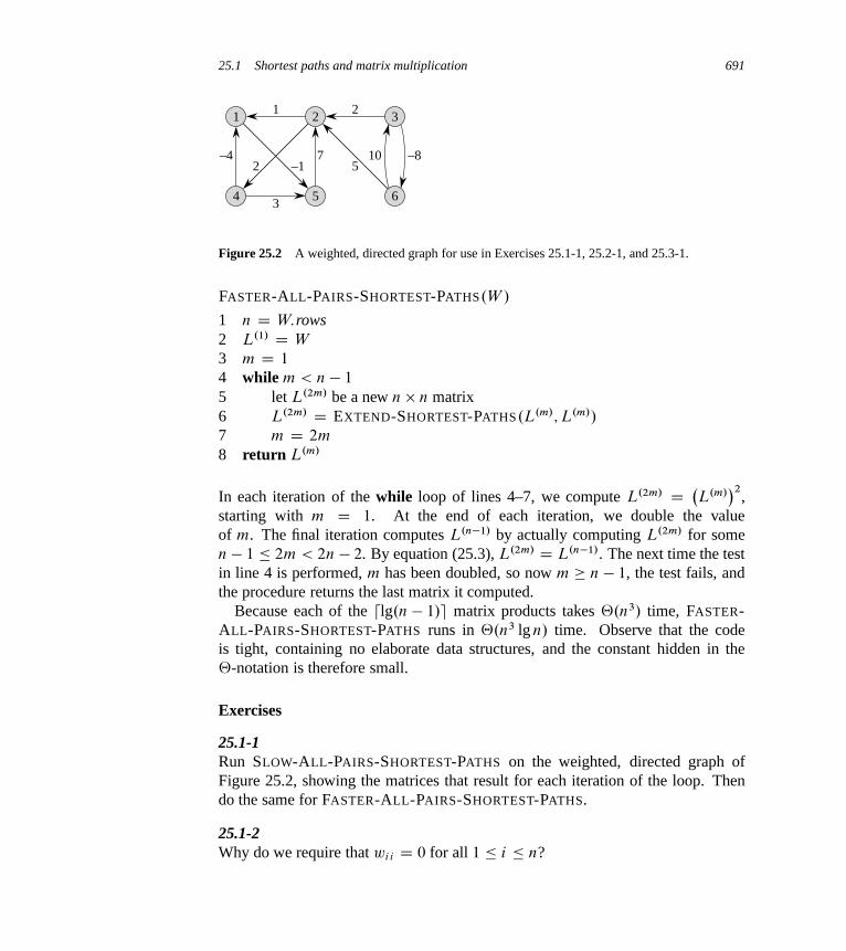
25.1 Shortest paths and matrix multiplication 691
1 2
3
5–12
1 2 3
4 5 6
–4 –8107
Figure 25.2 A weighted, directed graph for use in Exercises 25.1-1, 25.2-1, and 25.3-1.
FASTER-ALL-PAIRS-SHORTEST-PATHS.W /
1 n D W:rows2 L.1/ D W
3 m D 1
4 while m < n � 1
5 let L.2m/ be a new n n matrix6 L.2m/ D EXTEND-SHORTEST-PATHS.L.m/; L.m//
7 m D 2m
8 return L.m/
In each iteration of the while loop of lines 4–7, we compute L.2m/ D �L.m/
�2,
starting with m D 1. At the end of each iteration, we double the valueof m. The final iteration computes L.n�1/ by actually computing L.2m/ for somen � 1 � 2m < 2n � 2. By equation (25.3), L.2m/ D L.n�1/. The next time the testin line 4 is performed, m has been doubled, so now m � n � 1, the test fails, andthe procedure returns the last matrix it computed.
Because each of the dlg.n � 1/e matrix products takes ‚.n3/ time, FASTER-ALL-PAIRS-SHORTEST-PATHS runs in ‚.n3 lg n/ time. Observe that the codeis tight, containing no elaborate data structures, and the constant hidden in the‚-notation is therefore small.
Exercises
25.1-1Run SLOW-ALL-PAIRS-SHORTEST-PATHS on the weighted, directed graph ofFigure 25.2, showing the matrices that result for each iteration of the loop. Thendo the same for FASTER-ALL-PAIRS-SHORTEST-PATHS.
25.1-2Why do we require that wi i D 0 for all 1 � i � n?
692 Chapter 25 All-Pairs Shortest Paths
25.1-3What does the matrix
L.0/ D
�0 1 1 � � � 11 0 1 � � � 11 1 0 � � � 1:::
::::::
: : ::::
1 1 1 � � � 0
�used in the shortest-paths algorithms correspond to in regular matrix multiplica-tion?
25.1-4Show that matrix multiplication defined by EXTEND-SHORTEST-PATHS is asso-ciative.
25.1-5Show how to express the single-source shortest-paths problem as a product of ma-trices and a vector. Describe how evaluating this product corresponds to a Bellman-Ford-like algorithm (see Section 24.1).
25.1-6Suppose we also wish to compute the vertices on shortest paths in the algorithms ofthis section. Show how to compute the predecessor matrix … from the completedmatrix L of shortest-path weights in O.n3/ time.
25.1-7We can also compute the vertices on shortest paths as we compute the shortest-path weights. Define �
.m/ij as the predecessor of vertex j on any minimum-weight
path from i to j that contains at most m edges. Modify the EXTEND-SHORTEST-PATHS and SLOW-ALL-PAIRS-SHORTEST-PATHS procedures to compute the ma-trices ….1/; ….2/; : : : ; ….n�1/ as the matrices L.1/; L.2/; : : : ; L.n�1/ are computed.
25.1-8The FASTER-ALL-PAIRS-SHORTEST-PATHS procedure, as written, requires us tostore dlg.n � 1/e matrices, each with n2 elements, for a total space requirement of‚.n2 lg n/. Modify the procedure to require only ‚.n2/ space by using only twon n matrices.
25.1-9Modify FASTER-ALL-PAIRS-SHORTEST-PATHS so that it can determine whetherthe graph contains a negative-weight cycle.

25.2 The Floyd-Warshall algorithm 693
25.1-10Give an efficient algorithm to find the length (number of edges) of a minimum-length negative-weight cycle in a graph.
25.2 The Floyd-Warshall algorithm
In this section, we shall use a different dynamic-programming formulation to solvethe all-pairs shortest-paths problem on a directed graph G D .V; E/. The result-ing algorithm, known as the Floyd-Warshall algorithm, runs in ‚.V 3/ time. Asbefore, negative-weight edges may be present, but we assume that there are nonegative-weight cycles. As in Section 25.1, we follow the dynamic-programmingprocess to develop the algorithm. After studying the resulting algorithm, wepresent a similar method for finding the transitive closure of a directed graph.
The structure of a shortest path
In the Floyd-Warshall algorithm, we characterize the structure of a shortest pathdifferently from how we characterized it in Section 25.1. The Floyd-Warshall algo-rithm considers the intermediate vertices of a shortest path, where an intermediatevertex of a simple path p D h�1; �2; : : : ; �li is any vertex of p other than �1 or �l ,that is, any vertex in the set f�2; �3; : : : ; �l�1g.
The Floyd-Warshall algorithm relies on the following observation. Under ourassumption that the vertices of G are V D f1; 2; : : : ; ng, let us consider a subsetf1; 2; : : : ; kg of vertices for some k. For any pair of vertices i; j 2 V , consider allpaths from i to j whose intermediate vertices are all drawn from f1; 2; : : : ; kg, andlet p be a minimum-weight path from among them. (Path p is simple.) The Floyd-Warshall algorithm exploits a relationship between path p and shortest paths from i
to j with all intermediate vertices in the set f1; 2; : : : ; k � 1g. The relationshipdepends on whether or not k is an intermediate vertex of path p.
� If k is not an intermediate vertex of path p, then all intermediate vertices ofpath p are in the set f1; 2; : : : ; k � 1g. Thus, a shortest path from vertex i
to vertex j with all intermediate vertices in the set f1; 2; : : : ; k � 1g is also ashortest path from i to j with all intermediate vertices in the set f1; 2; : : : ; kg.
� If k is an intermediate vertex of path p, then we decompose p into ip1� k
p2� j ,
as Figure 25.3 illustrates. By Lemma 24.1, p1 is a shortest path from i to k
with all intermediate vertices in the set f1; 2; : : : ; kg. In fact, we can make aslightly stronger statement. Because vertex k is not an intermediate vertex ofpath p1, all intermediate vertices of p1 are in the set f1; 2; : : : ; k � 1g. There-

694 Chapter 25 All-Pairs Shortest Paths
i
k
j
p1 p2
p: all intermediate vertices in f1; 2; : : : ; kg
all intermediate vertices in f1; 2; : : : ; k � 1gall intermediate vertices in f1; 2; : : : ; k � 1g
Figure 25.3 Path p is a shortest path from vertex i to vertex j , and k is the highest-numberedintermediate vertex of p. Path p1, the portion of path p from vertex i to vertex k, has all intermediatevertices in the set f1; 2; : : : ; k � 1g. The same holds for path p2 from vertex k to vertex j .
fore, p1 is a shortest path from i to k with all intermediate vertices in the setf1; 2; : : : ; k � 1g. Similarly, p2 is a shortest path from vertex k to vertex j withall intermediate vertices in the set f1; 2; : : : ; k � 1g.
A recursive solution to the all-pairs shortest-paths problem
Based on the above observations, we define a recursive formulation of shortest-path estimates that differs from the one in Section 25.1. Let d
.k/ij be the weight
of a shortest path from vertex i to vertex j for which all intermediate verticesare in the set f1; 2; : : : ; kg. When k D 0, a path from vertex i to vertex j withno intermediate vertex numbered higher than 0 has no intermediate vertices at all.Such a path has at most one edge, and hence d
.0/ij D wij . Following the above
discussion, we define d.k/ij recursively by
d.k/ij D
(wij if k D 0 ;
min�d
.k�1/ij ; d
.k�1/
ikC d
.k�1/
kj
�if k � 1 :
(25.5)
Because for any path, all intermediate vertices are in the set f1; 2; : : : ; ng, the ma-trix D.n/ D �d .n/
ij
�gives the final answer: d
.n/ij D ı.i; j / for all i; j 2 V .
Computing the shortest-path weights bottom up
Based on recurrence (25.5), we can use the following bottom-up procedure to com-pute the values d
.k/ij in order of increasing values of k. Its input is an nn matrix W
defined as in equation (25.1). The procedure returns the matrix D.n/ of shortest-path weights.

25.2 The Floyd-Warshall algorithm 695
FLOYD-WARSHALL.W /
1 n D W:rows2 D.0/ D W
3 for k D 1 to n
4 let D.k/ D �d .k/ij
�be a new n n matrix
5 for i D 1 to n
6 for j D 1 to n
7 d.k/ij D min
�d
.k�1/ij ; d
.k�1/
ikC d
.k�1/
kj
�8 return D.n/
Figure 25.4 shows the matrices D.k/ computed by the Floyd-Warshall algorithmfor the graph in Figure 25.1.
The running time of the Floyd-Warshall algorithm is determined by the triplynested for loops of lines 3–7. Because each execution of line 7 takes O.1/ time,the algorithm runs in time ‚.n3/. As in the final algorithm in Section 25.1, thecode is tight, with no elaborate data structures, and so the constant hidden in the‚-notation is small. Thus, the Floyd-Warshall algorithm is quite practical for evenmoderate-sized input graphs.
Constructing a shortest path
There are a variety of different methods for constructing shortest paths in the Floyd-Warshall algorithm. One way is to compute the matrix D of shortest-path weightsand then construct the predecessor matrix … from the D matrix. Exercise 25.1-6asks you to implement this method so that it runs in O.n3/ time. Given the pre-decessor matrix …, the PRINT-ALL-PAIRS-SHORTEST-PATH procedure will printthe vertices on a given shortest path.
Alternatively, we can compute the predecessor matrix … while the algorithmcomputes the matrices D.k/. Specifically, we compute a sequence of matrices….0/; ….1/; : : : ; ….n/, where … D ….n/ and we define �
.k/ij as the predecessor of
vertex j on a shortest path from vertex i with all intermediate vertices in the setf1; 2; : : : ; kg.
We can give a recursive formulation of �.k/ij . When k D 0, a shortest path from i
to j has no intermediate vertices at all. Thus,
�.0/ij D
(NIL if i D j or wij D1 ;
i if i ¤ j and wij <1 :(25.6)
For k � 1, if we take the path i � k � j , where k ¤ j , then the predecessorof j we choose is the same as the predecessor of j we chose on a shortest pathfrom k with all intermediate vertices in the set f1; 2; : : : ; k � 1g. Otherwise, we

696 Chapter 25 All-Pairs Shortest Paths
D.0/ D
�0 3 8 1 �4
1 0 1 1 7
1 4 0 1 12 1 �5 0 11 1 1 6 0
˘….0/ D
�NIL 1 1 NIL 1
NIL NIL NIL 2 2
NIL 3 NIL NIL NIL
4 NIL 4 NIL NIL
NIL NIL NIL 5 NIL
˘
D.1/ D
�0 3 8 1 �4
1 0 1 1 7
1 4 0 1 12 5 �5 0 �2
1 1 1 6 0
˘….1/ D
�NIL 1 1 NIL 1
NIL NIL NIL 2 2
NIL 3 NIL NIL NIL
4 1 4 NIL 1
NIL NIL NIL 5 NIL
˘
D.2/ D
�0 3 8 4 �4
1 0 1 1 7
1 4 0 5 11
2 5 �5 0 �2
1 1 1 6 0
˘….2/ D
�NIL 1 1 2 1
NIL NIL NIL 2 2
NIL 3 NIL 2 2
4 1 4 NIL 1
NIL NIL NIL 5 NIL
˘
D.3/ D
�0 3 8 4 �4
1 0 1 1 7
1 4 0 5 11
2 �1 �5 0 �2
1 1 1 6 0
˘….3/ D
�NIL 1 1 2 1
NIL NIL NIL 2 2
NIL 3 NIL 2 2
4 3 4 NIL 1
NIL NIL NIL 5 NIL
˘
D.4/ D
�0 3 �1 4 �4
3 0 �4 1 �1
7 4 0 5 3
2 �1 �5 0 �2
8 5 1 6 0
˘….4/ D
�NIL 1 4 2 1
4 NIL 4 2 1
4 3 NIL 2 1
4 3 4 NIL 1
4 3 4 5 NIL
˘
D.5/ D
�0 1 �3 2 �4
3 0 �4 1 �1
7 4 0 5 3
2 �1 �5 0 �2
8 5 1 6 0
˘….5/ D
�NIL 3 4 5 1
4 NIL 4 2 1
4 3 NIL 2 1
4 3 4 NIL 1
4 3 4 5 NIL
˘
Figure 25.4 The sequence of matrices D.k/ and ….k/ computed by the Floyd-Warshall algorithmfor the graph in Figure 25.1.

25.2 The Floyd-Warshall algorithm 697
choose the same predecessor of j that we chose on a shortest path from i with allintermediate vertices in the set f1; 2; : : : ; k � 1g. Formally, for k � 1,
�.k/ij D
(�
.k�1/ij if d
.k�1/ij � d
.k�1/
ikC d
.k�1/
kj;
�.k�1/
kjif d
.k�1/ij > d
.k�1/
ikC d
.k�1/
kj:
(25.7)
We leave the incorporation of the ….k/ matrix computations into the FLOYD-WARSHALL procedure as Exercise 25.2-3. Figure 25.4 shows the sequence of ….k/
matrices that the resulting algorithm computes for the graph of Figure 25.1. Theexercise also asks for the more difficult task of proving that the predecessor sub-graph G�;i is a shortest-paths tree with root i . Exercise 25.2-7 asks for yet anotherway to reconstruct shortest paths.
Transitive closure of a directed graph
Given a directed graph G D .V; E/ with vertex set V D f1; 2; : : : ; ng, we mightwish to determine whether G contains a path from i to j for all vertex pairsi; j 2 V . We define the transitive closure of G as the graph G� D .V; E�/, where
E� D f.i; j / W there is a path from vertex i to vertex j in Gg :
One way to compute the transitive closure of a graph in ‚.n3/ time is to assigna weight of 1 to each edge of E and run the Floyd-Warshall algorithm. If there is apath from vertex i to vertex j , we get dij < n. Otherwise, we get dij D1.
There is another, similar way to compute the transitive closure of G in ‚.n3/
time that can save time and space in practice. This method substitutes the logicaloperations _ (logical OR) and ^ (logical AND) for the arithmetic operations minand C in the Floyd-Warshall algorithm. For i; j; k D 1; 2; : : : ; n, we define t
.k/ij to
be 1 if there exists a path in graph G from vertex i to vertex j with all intermediatevertices in the set f1; 2; : : : ; kg, and 0 otherwise. We construct the transitive closureG� D .V; E�/ by putting edge .i; j / into E� if and only if t
.n/ij D 1. A recursive
definition of t.k/ij , analogous to recurrence (25.5), is
t.0/ij D
(0 if i ¤ j and .i; j / 62 E ;
1 if i D j or .i; j / 2 E ;
and for k � 1,
t.k/ij D t
.k�1/ij _ �t .k�1/
ik^ t
.k�1/
kj
�: (25.8)
As in the Floyd-Warshall algorithm, we compute the matrices T .k/ D �t
.k/ij
�in
order of increasing k.

698 Chapter 25 All-Pairs Shortest Paths
1 2
4 3
T .0/ D
�1 0 0 0
0 1 1 1
0 1 1 0
1 0 1 1
�T .1/ D
�1 0 0 0
0 1 1 1
0 1 1 0
1 0 1 1
�T .2/ D
�1 0 0 0
0 1 1 1
0 1 1 1
1 0 1 1
�
T .3/ D
�1 0 0 0
0 1 1 1
0 1 1 1
1 1 1 1
�T .4/ D
�1 0 0 0
1 1 1 1
1 1 1 1
1 1 1 1
�Figure 25.5 A directed graph and the matrices T .k/ computed by the transitive-closure algorithm.
TRANSITIVE-CLOSURE.G/
1 n D jG:Vj2 let T .0/ D �t .0/
ij
�be a new n n matrix
3 for i D 1 to n
4 for j D 1 to n
5 if i == j or .i; j / 2 G:E6 t
.0/ij D 1
7 else t.0/ij D 0
8 for k D 1 to n
9 let T .k/ D �t .k/ij
�be a new n n matrix
10 for i D 1 to n
11 for j D 1 to n
12 t.k/ij D t
.k�1/ij _ �t .k�1/
ik^ t
.k�1/
kj
�13 return T .n/
Figure 25.5 shows the matrices T .k/ computed by the TRANSITIVE-CLOSURE
procedure on a sample graph. The TRANSITIVE-CLOSURE procedure, like theFloyd-Warshall algorithm, runs in ‚.n3/ time. On some computers, though, log-ical operations on single-bit values execute faster than arithmetic operations oninteger words of data. Moreover, because the direct transitive-closure algorithmuses only boolean values rather than integer values, its space requirement is less
25.2 The Floyd-Warshall algorithm 699
than the Floyd-Warshall algorithm’s by a factor corresponding to the size of a wordof computer storage.
Exercises
25.2-1Run the Floyd-Warshall algorithm on the weighted, directed graph of Figure 25.2.Show the matrix D.k/ that results for each iteration of the outer loop.
25.2-2Show how to compute the transitive closure using the technique of Section 25.1.
25.2-3Modify the FLOYD-WARSHALL procedure to compute the ….k/ matrices accordingto equations (25.6) and (25.7). Prove rigorously that for all i 2 V , the predecessorsubgraph G�;i is a shortest-paths tree with root i . (Hint: To show that G�;i isacyclic, first show that �
.k/ij D l implies d
.k/ij � d
.k/
ilC wlj , according to the
definition of �.k/ij . Then, adapt the proof of Lemma 24.16.)
25.2-4As it appears above, the Floyd-Warshall algorithm requires ‚.n3/ space, since wecompute d
.k/ij for i; j; k D 1; 2; : : : ; n. Show that the following procedure, which
simply drops all the superscripts, is correct, and thus only ‚.n2/ space is required.
FLOYD-WARSHALL0.W /
1 n D W:rows2 D D W
3 for k D 1 to n
4 for i D 1 to n
5 for j D 1 to n
6 dij D min .dij ; dik C dkj /
7 return D
25.2-5Suppose that we modify the way in which equation (25.7) handles equality:
�.k/ij D
(�
.k�1/ij if d
.k�1/ij < d
.k�1/
ikC d
.k�1/
kj;
�.k�1/
kjif d
.k�1/ij � d
.k�1/
ikC d
.k�1/
kj:
Is this alternative definition of the predecessor matrix … correct?
700 Chapter 25 All-Pairs Shortest Paths
25.2-6How can we use the output of the Floyd-Warshall algorithm to detect the presenceof a negative-weight cycle?
25.2-7Another way to reconstruct shortest paths in the Floyd-Warshall algorithm usesvalues �
.k/ij for i; j; k D 1; 2; : : : ; n, where �
.k/ij is the highest-numbered interme-
diate vertex of a shortest path from i to j in which all intermediate vertices arein the set f1; 2; : : : ; kg. Give a recursive formulation for �
.k/ij , modify the FLOYD-
WARSHALL procedure to compute the �.k/ij values, and rewrite the PRINT-ALL-
PAIRS-SHORTEST-PATH procedure to take the matrix ˆ D ��
.n/ij
�as an input.
How is the matrix ˆ like the s table in the matrix-chain multiplication problem ofSection 15.2?
25.2-8Give an O.VE/-time algorithm for computing the transitive closure of a directedgraph G D .V; E/.
25.2-9Suppose that we can compute the transitive closure of a directed acyclic graph inf .jV j ; jEj/ time, where f is a monotonically increasing function of jV j and jEj.Show that the time to compute the transitive closure G� D .V; E�/ of a generaldirected graph G D .V; E/ is then f .jV j ; jEj/CO.V CE�/.
25.3 Johnson’s algorithm for sparse graphs
Johnson’s algorithm finds shortest paths between all pairs in O.V 2 lg V C VE/
time. For sparse graphs, it is asymptotically faster than either repeated squaring ofmatrices or the Floyd-Warshall algorithm. The algorithm either returns a matrix ofshortest-path weights for all pairs of vertices or reports that the input graph containsa negative-weight cycle. Johnson’s algorithm uses as subroutines both Dijkstra’salgorithm and the Bellman-Ford algorithm, which Chapter 24 describes.
Johnson’s algorithm uses the technique of reweighting, which works as follows.If all edge weights w in a graph G D .V; E/ are nonnegative, we can find short-est paths between all pairs of vertices by running Dijkstra’s algorithm once fromeach vertex; with the Fibonacci-heap min-priority queue, the running time of thisall-pairs algorithm is O.V 2 lg V C VE/. If G has negative-weight edges but nonegative-weight cycles, we simply compute a new set of nonnegative edge weights

25.3 Johnson’s algorithm for sparse graphs 701
that allows us to use the same method. The new set of edge weights yw must satisfytwo important properties:
1. For all pairs of vertices u; � 2 V , a path p is a shortest path from u to � usingweight function w if and only if p is also a shortest path from u to � usingweight function yw.
2. For all edges .u; �/, the new weight yw.u; �/ is nonnegative.
As we shall see in a moment, we can preprocess G to determine the new weightfunction yw in O.VE/ time.
Preserving shortest paths by reweighting
The following lemma shows how easily we can reweight the edges to satisfy thefirst property above. We use ı to denote shortest-path weights derived from weightfunction w and yı to denote shortest-path weights derived from weight function yw.
Lemma 25.1 (Reweighting does not change shortest paths)Given a weighted, directed graph G D .V; E/ with weight function w W E ! R,let h W V ! R be any function mapping vertices to real numbers. For each edge.u; �/ 2 E, define
yw.u; �/ D w.u; �/C h.u/ � h.�/ : (25.9)
Let p D h�0; �1; : : : ; �ki be any path from vertex �0 to vertex �k. Then p is ashortest path from �0 to �k with weight function w if and only if it is a shortest pathwith weight function yw. That is, w.p/ D ı.�0; �k/ if and only if yw.p/ D yı.�0; �k/.Furthermore, G has a negative-weight cycle using weight function w if and onlyif G has a negative-weight cycle using weight function yw.
Proof We start by showing that
yw.p/ D w.p/C h.�0/ � h.�k/ : (25.10)
We have
yw.p/ DkX
iD1
yw.�i�1; �i /
DkX
iD1
.w.�i�1; �i /C h.�i�1/ � h.�i //
DkX
iD1
w.�i�1; �i /C h.�0/ � h.�k/ (because the sum telescopes)
D w.p/C h.�0/ � h.�k/ :

702 Chapter 25 All-Pairs Shortest Paths
Therefore, any path p from �0 to �k has yw.p/ D w.p/ C h.�0/ � h.�k/. Be-cause h.�0/ and h.�k/ do not depend on the path, if one path from �0 to �k isshorter than another using weight function w, then it is also shorter using yw. Thus,w.p/ D ı.�0; �k/ if and only if yw.p/ D yı.�0; �k/.
Finally, we show that G has a negative-weight cycle using weight function w ifand only if G has a negative-weight cycle using weight function yw. Consider anycycle c D h�0; �1; : : : ; �ki, where �0 D �k. By equation (25.10),
yw.c/ D w.c/C h.�0/ � h.�k/
D w.c/ ;
and thus c has negative weight using w if and only if it has negative weight us-ing yw.
Producing nonnegative weights by reweighting
Our next goal is to ensure that the second property holds: we want yw.u; �/ to benonnegative for all edges .u; �/ 2 E. Given a weighted, directed graph G D.V; E/ with weight function w W E ! R, we make a new graph G0 D .V 0; E 0/,where V 0 D V [ fsg for some new vertex s 62 V and E 0 D E [ f.s; �/ W � 2 V g.We extend the weight function w so that w.s; �/ D 0 for all � 2 V . Note thatbecause s has no edges that enter it, no shortest paths in G0, other than those withsource s, contain s. Moreover, G0 has no negative-weight cycles if and only if G
has no negative-weight cycles. Figure 25.6(a) shows the graph G0 correspondingto the graph G of Figure 25.1.
Now suppose that G and G0 have no negative-weight cycles. Let us defineh.�/ D ı.s; �/ for all � 2 V 0. By the triangle inequality (Lemma 24.10),we have h.�/ � h.u/ C w.u; �/ for all edges .u; �/ 2 E 0. Thus, if we de-fine the new weights yw by reweighting according to equation (25.9), we haveyw.u; �/ D w.u; �/C h.u/ � h.�/ � 0, and we have satisfied the second property.Figure 25.6(b) shows the graph G0 from Figure 25.6(a) with reweighted edges.
Computing all-pairs shortest paths
Johnson’s algorithm to compute all-pairs shortest paths uses the Bellman-Ford al-gorithm (Section 24.1) and Dijkstra’s algorithm (Section 24.3) as subroutines. Itassumes implicitly that the edges are stored in adjacency lists. The algorithm re-turns the usual jV j jV j matrix D D dij , where dij D ı.i; j /, or it reports thatthe input graph contains a negative-weight cycle. As is typical for an all-pairsshortest-paths algorithm, we assume that the vertices are numbered from 1 to jV j.
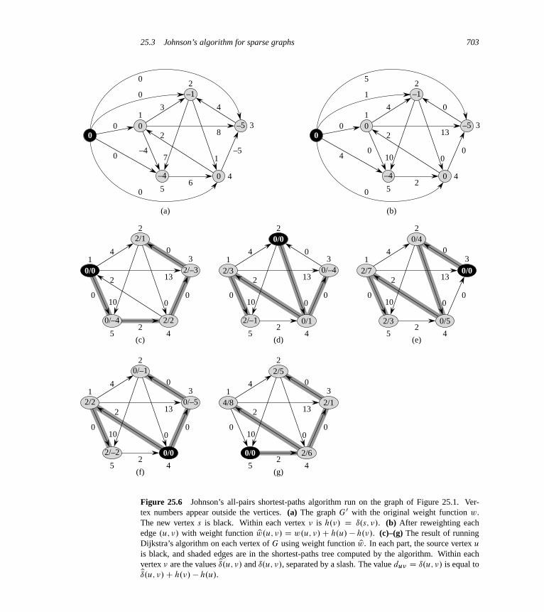
25.3 Johnson’s algorithm for sparse graphs 703
2
1
5
4
3 4
82
6
7 1
0
0
0
0
0
0
0
2/1
2/–3
2/20/–4
2/3 0/–4
0/12/–1
2/7
0/4
0/52/3
2/2
0/–1
0/–5
2/–2
4/8
2/5
2/1
2/6
(a)
(c)
(b)
–4
–4
–1
–5
–5
3
2
1
5
4
4 0
132
2
10 0
5
1
0
4
0
0
0
0
–4
–1
–5
0
3
2
1
5 4
4 0
132
2
10 00 0
3
(d)
2
1
5 4
4 0
132
2
10 00 0
3
(e)
2
1
5 4
4 0
132
2
10 00 0
3
(f)
2
1
5 4
4 0
132
2
10 00 0
3
(g)
2
1
5 4
4 0
132
2
10 00 0
3
0/00/0
0/0
0/0
0/0
00
Figure 25.6 Johnson’s all-pairs shortest-paths algorithm run on the graph of Figure 25.1. Ver-tex numbers appear outside the vertices. (a) The graph G0 with the original weight function w.The new vertex s is black. Within each vertex � is h.�/ D ı.s; �/. (b) After reweighting eachedge .u; �/ with weight function yw.u; �/ D w.u; �/C h.u/ � h.�/. (c)–(g) The result of runningDijkstra’s algorithm on each vertex of G using weight function yw. In each part, the source vertex u
is black, and shaded edges are in the shortest-paths tree computed by the algorithm. Within eachvertex � are the values yı.u; �/ and ı.u; �/, separated by a slash. The value du� D ı.u; �/ is equal toyı.u; �/C h.�/ � h.u/.

704 Chapter 25 All-Pairs Shortest Paths
JOHNSON.G/
1 compute G0, where G0:V D G:V [ fsg,G0:E D G:E [ f.s; �/ W � 2 G:Vg, andw.s; �/ D 0 for all � 2 G:V
2 if BELLMAN-FORD.G0; w; s/ == FALSE
3 print “the input graph contains a negative-weight cycle”4 else for each vertex � 2 G0:V5 set h.�/ to the value of ı.s; �/
computed by the Bellman-Ford algorithm6 for each edge .u; �/ 2 G0:E7 yw.u; �/ D w.u; �/C h.u/ � h.�/
8 let D D .du�/ be a new n n matrix9 for each vertex u 2 G:V
10 run DIJKSTRA.G; yw; u/ to compute yı.u; �/ for all � 2 G:V11 for each vertex � 2 G:V12 du� D yı.u; �/C h.�/ � h.u/
13 return D
This code simply performs the actions we specified earlier. Line 1 produces G0.Line 2 runs the Bellman-Ford algorithm on G0 with weight function w and sourcevertex s. If G0, and hence G, contains a negative-weight cycle, line 3 reports theproblem. Lines 4–12 assume that G0 contains no negative-weight cycles. Lines 4–5set h.�/ to the shortest-path weight ı.s; �/ computed by the Bellman-Ford algo-rithm for all � 2 V 0. Lines 6–7 compute the new weights yw. For each pair of ver-tices u; � 2 V , the for loop of lines 9–12 computes the shortest-path weight yı.u; �/
by calling Dijkstra’s algorithm once from each vertex in V . Line 12 stores inmatrix entry du� the correct shortest-path weight ı.u; �/, calculated using equa-tion (25.10). Finally, line 13 returns the completed D matrix. Figure 25.6 depictsthe execution of Johnson’s algorithm.
If we implement the min-priority queue in Dijkstra’s algorithm by a Fibonacciheap, Johnson’s algorithm runs in O.V 2 lg V CVE/ time. The simpler binary min-heap implementation yields a running time of O.VE lg V /, which is still asymp-totically faster than the Floyd-Warshall algorithm if the graph is sparse.
Exercises
25.3-1Use Johnson’s algorithm to find the shortest paths between all pairs of vertices inthe graph of Figure 25.2. Show the values of h and yw computed by the algorithm.
Problems for Chapter 25 705
25.3-2What is the purpose of adding the new vertex s to V , yielding V 0?
25.3-3Suppose that w.u; �/ � 0 for all edges .u; �/ 2 E. What is the relationshipbetween the weight functions w and yw?
25.3-4Professor Greenstreet claims that there is a simpler way to reweight edges thanthe method used in Johnson’s algorithm. Letting w� D min.u;�/2E fw.u; �/g, justdefine yw.u; �/ D w.u; �/ � w� for all edges .u; �/ 2 E. What is wrong with theprofessor’s method of reweighting?
25.3-5Suppose that we run Johnson’s algorithm on a directed graph G with weight func-tion w. Show that if G contains a 0-weight cycle c, then yw.u; �/ D 0 for everyedge .u; �/ in c.
25.3-6Professor Michener claims that there is no need to create a new source vertex inline 1 of JOHNSON. He claims that instead we can just use G0 D G and let s be anyvertex. Give an example of a weighted, directed graph G for which incorporatingthe professor’s idea into JOHNSON causes incorrect answers. Then show that if G
is strongly connected (every vertex is reachable from every other vertex), the resultsreturned by JOHNSON with the professor’s modification are correct.
Problems
25-1 Transitive closure of a dynamic graphSuppose that we wish to maintain the transitive closure of a directed graph G D.V; E/ as we insert edges into E. That is, after each edge has been inserted, wewant to update the transitive closure of the edges inserted so far. Assume that thegraph G has no edges initially and that we represent the transitive closure as aboolean matrix.
a. Show how to update the transitive closure G� D .V; E�/ of a graph G D .V; E/
in O.V 2/ time when a new edge is added to G.
b. Give an example of a graph G and an edge e such that �.V 2/ time is requiredto update the transitive closure after the insertion of e into G, no matter whatalgorithm is used.
706 Chapter 25 All-Pairs Shortest Paths
c. Describe an efficient algorithm for updating the transitive closure as edges areinserted into the graph. For any sequence of n insertions, your algorithm shouldrun in total time
Pn
iD1 ti D O.V 3/, where ti is the time to update the transitiveclosure upon inserting the i th edge. Prove that your algorithm attains this timebound.
25-2 Shortest paths in �-dense graphsA graph G D .V; E/ is �-dense if jEj D ‚.V 1C�/ for some constant � in therange 0 < � � 1. By using d -ary min-heaps (see Problem 6-2) in shortest-pathsalgorithms on �-dense graphs, we can match the running times of Fibonacci-heap-based algorithms without using as complicated a data structure.
a. What are the asymptotic running times for INSERT, EXTRACT-MIN, andDECREASE-KEY, as a function of d and the number n of elements in a d -arymin-heap? What are these running times if we choose d D ‚.n˛/ for someconstant 0 < ˛ � 1? Compare these running times to the amortized costs ofthese operations for a Fibonacci heap.
b. Show how to compute shortest paths from a single source on an �-dense directedgraph G D .V; E/ with no negative-weight edges in O.E/ time. (Hint: Pick d
as a function of �.)
c. Show how to solve the all-pairs shortest-paths problem on an �-dense directedgraph G D .V; E/ with no negative-weight edges in O.VE/ time.
d. Show how to solve the all-pairs shortest-paths problem in O.VE/ time on an�-dense directed graph G D .V; E/ that may have negative-weight edges buthas no negative-weight cycles.
Chapter notes
Lawler [224] has a good discussion of the all-pairs shortest-paths problem, al-though he does not analyze solutions for sparse graphs. He attributes the matrix-multiplication algorithm to the folklore. The Floyd-Warshall algorithm is due toFloyd [105], who based it on a theorem of Warshall [349] that describes how tocompute the transitive closure of boolean matrices. Johnson’s algorithm is takenfrom [192].
Several researchers have given improved algorithms for computing shortestpaths via matrix multiplication. Fredman [111] shows how to solve the all-pairs shortest paths problem using O.V 5=2/ comparisons between sums of edge

Notes for Chapter 25 707
weights and obtains an algorithm that runs in O.V 3.lg lg V= lg V /1=3/ time, whichis slightly better than the running time of the Floyd-Warshall algorithm. Han [159]reduced the running time to O.V 3.lg lg V= lg V /5=4/. Another line of researchdemonstrates that we can apply algorithms for fast matrix multiplication (see thechapter notes for Chapter 4) to the all-pairs shortest paths problem. Let O.n!/ bethe running time of the fastest algorithm for multiplying n n matrices; currently! < 2:376 [79]. Galil and Margalit [123, 124] and Seidel [308] designed algo-rithms that solve the all-pairs shortest paths problem in undirected, unweightedgraphs in .V !p.V // time, where p.n/ denotes a particular function that is poly-logarithmically bounded in n. In dense graphs, these algorithms are faster thanthe O.VE/ time needed to perform jV j breadth-first searches. Several researchershave extended these results to give algorithms for solving the all-pairs shortestpaths problem in undirected graphs in which the edge weights are integers in therange f1; 2; : : : ; W g. The asymptotically fastest such algorithm, by Shoshan andZwick [316], runs in time O.W V !p.V W //.
Karger, Koller, and Phillips [196] and independently McGeoch [247] have givena time bound that depends on E�, the set of edges in E that participate in someshortest path. Given a graph with nonnegative edge weights, their algorithms run inO.VE�CV 2 lg V / time and improve upon running Dijkstra’s algorithm jV j timeswhen jE�j D o.E/.
Baswana, Hariharan, and Sen [33] examined decremental algorithms for main-taining all-pairs shortest paths and transitive-closure information. Decremen-tal algorithms allow a sequence of intermixed edge deletions and queries; bycomparison, Problem 25-1, in which edges are inserted, asks for an incremen-tal algorithm. The algorithms by Baswana, Hariharan, and Sen are randomizedand, when a path exists, their transitive-closure algorithm can fail to report itwith probability 1=nc for an arbitrary c > 0. The query times are O.1/ withhigh probability. For transitive closure, the amortized time for each update isO.V 4=3 lg1=3 V /. For all-pairs shortest paths, the update times depend on thequeries. For queries just giving the shortest-path weights, the amortized time perupdate is O.V 3=E lg2 V /. To report the actual shortest path, the amortized up-date time is min.O.V 3=2
plg V /; O.V 3=E lg2 V //. Demetrescu and Italiano [85]
showed how to handle update and query operations when edges are both insertedand deleted, as long as each given edge has a bounded range of possible valuesdrawn from the real numbers.
Aho, Hopcroft, and Ullman [5] defined an algebraic structure known as a “closedsemiring,” which serves as a general framework for solving path problems in di-rected graphs. Both the Floyd-Warshall algorithm and the transitive-closure algo-rithm from Section 25.2 are instantiations of an all-pairs algorithm based on closedsemirings. Maggs and Plotkin [240] showed how to find minimum spanning treesusing a closed semiring.
26 Maximum Flow
Just as we can model a road map as a directed graph in order to find the shortestpath from one point to another, we can also interpret a directed graph as a “flownetwork” and use it to answer questions about material flows. Imagine a mate-rial coursing through a system from a source, where the material is produced, toa sink, where it is consumed. The source produces the material at some steadyrate, and the sink consumes the material at the same rate. The “flow” of the mate-rial at any point in the system is intuitively the rate at which the material moves.Flow networks can model many problems, including liquids flowing through pipes,parts through assembly lines, current through electrical networks, and informationthrough communication networks.
We can think of each directed edge in a flow network as a conduit for the mate-rial. Each conduit has a stated capacity, given as a maximum rate at which the ma-terial can flow through the conduit, such as 200 gallons of liquid per hour througha pipe or 20 amperes of electrical current through a wire. Vertices are conduitjunctions, and other than the source and sink, material flows through the verticeswithout collecting in them. In other words, the rate at which material enters a ver-tex must equal the rate at which it leaves the vertex. We call this property “flowconservation,” and it is equivalent to Kirchhoff’s current law when the material iselectrical current.
In the maximum-flow problem, we wish to compute the greatest rate at whichwe can ship material from the source to the sink without violating any capacityconstraints. It is one of the simplest problems concerning flow networks and, aswe shall see in this chapter, this problem can be solved by efficient algorithms.Moreover, we can adapt the basic techniques used in maximum-flow algorithms tosolve other network-flow problems.
This chapter presents two general methods for solving the maximum-flow prob-lem. Section 26.1 formalizes the notions of flow networks and flows, formallydefining the maximum-flow problem. Section 26.2 describes the classical methodof Ford and Fulkerson for finding maximum flows. An application of this method,
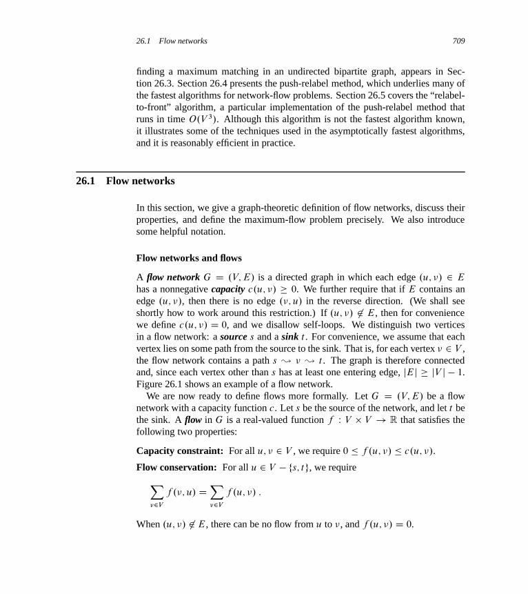
26.1 Flow networks 709
finding a maximum matching in an undirected bipartite graph, appears in Sec-tion 26.3. Section 26.4 presents the push-relabel method, which underlies many ofthe fastest algorithms for network-flow problems. Section 26.5 covers the “relabel-to-front” algorithm, a particular implementation of the push-relabel method thatruns in time O.V 3/. Although this algorithm is not the fastest algorithm known,it illustrates some of the techniques used in the asymptotically fastest algorithms,and it is reasonably efficient in practice.
26.1 Flow networks
In this section, we give a graph-theoretic definition of flow networks, discuss theirproperties, and define the maximum-flow problem precisely. We also introducesome helpful notation.
Flow networks and flows
A flow network G D .V; E/ is a directed graph in which each edge .u; �/ 2 E
has a nonnegative capacity c.u; �/ � 0. We further require that if E contains anedge .u; �/, then there is no edge .�; u/ in the reverse direction. (We shall seeshortly how to work around this restriction.) If .u; �/ 62 E, then for conveniencewe define c.u; �/ D 0, and we disallow self-loops. We distinguish two verticesin a flow network: a source s and a sink t . For convenience, we assume that eachvertex lies on some path from the source to the sink. That is, for each vertex � 2 V ,the flow network contains a path s � � � t . The graph is therefore connectedand, since each vertex other than s has at least one entering edge, jEj � jV j � 1.Figure 26.1 shows an example of a flow network.
We are now ready to define flows more formally. Let G D .V; E/ be a flownetwork with a capacity function c. Let s be the source of the network, and let t bethe sink. A flow in G is a real-valued function f W V V ! R that satisfies thefollowing two properties:
Capacity constraint: For all u; � 2 V , we require 0 � f .u; �/ � c.u; �/.
Flow conservation: For all u 2 V � fs; tg, we requireX�2V
f .�; u/ DX�2V
f .u; �/ :
When .u; �/ 62 E, there can be no flow from u to �, and f .u; �/ D 0.
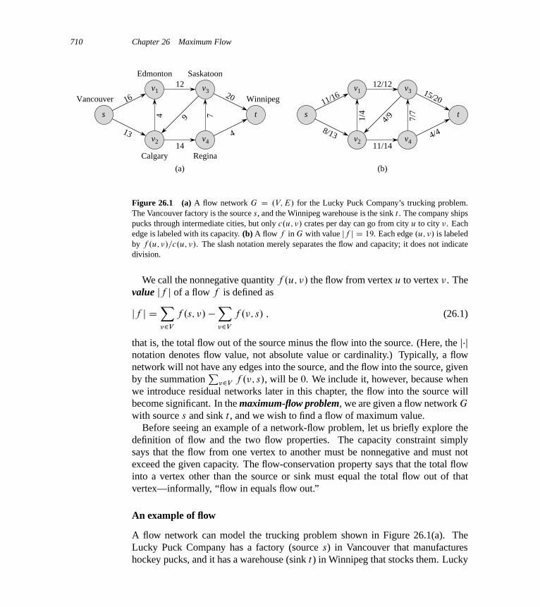
710 Chapter 26 Maximum Flow
s t
16
1220
794
13
14
4
Edmonton
Calgary
Saskatoon
Regina
Vancouver Winnipeg
s t
11/1612/12
15/20
7/7
4/91/4
8/1311/14
4/4
(a) (b)
v1 v1
v2 v2
v3 v3
v4v4
Figure 26.1 (a) A flow network G D .V; E/ for the Lucky Puck Company’s trucking problem.The Vancouver factory is the source s, and the Winnipeg warehouse is the sink t . The company shipspucks through intermediate cities, but only c.u; �/ crates per day can go from city u to city �. Eachedge is labeled with its capacity. (b) A flow f in G with value jf j D 19. Each edge .u; �/ is labeledby f .u; �/=c.u; �/. The slash notation merely separates the flow and capacity; it does not indicatedivision.
We call the nonnegative quantity f .u; �/ the flow from vertex u to vertex �. Thevalue jf j of a flow f is defined as
jf j DX�2V
f .s; �/ �X�2V
f .�; s/ ; (26.1)
that is, the total flow out of the source minus the flow into the source. (Here, the j�jnotation denotes flow value, not absolute value or cardinality.) Typically, a flownetwork will not have any edges into the source, and the flow into the source, givenby the summation
P�2V f .�; s/, will be 0. We include it, however, because when
we introduce residual networks later in this chapter, the flow into the source willbecome significant. In the maximum-flow problem, we are given a flow network G
with source s and sink t , and we wish to find a flow of maximum value.Before seeing an example of a network-flow problem, let us briefly explore the
definition of flow and the two flow properties. The capacity constraint simplysays that the flow from one vertex to another must be nonnegative and must notexceed the given capacity. The flow-conservation property says that the total flowinto a vertex other than the source or sink must equal the total flow out of thatvertex—informally, “flow in equals flow out.”
An example of flow
A flow network can model the trucking problem shown in Figure 26.1(a). TheLucky Puck Company has a factory (source s) in Vancouver that manufactureshockey pucks, and it has a warehouse (sink t) in Winnipeg that stocks them. Lucky
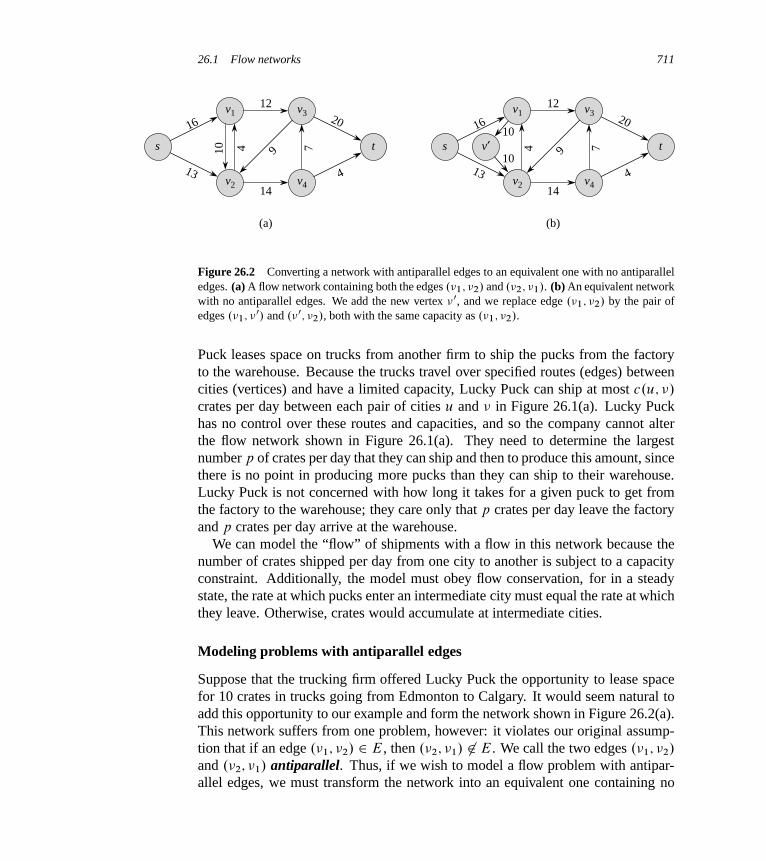
26.1 Flow networks 711
s t
16
1220
794
13
14
4
(a) (b)
v1
v2
v3
v4
10 s t
16
1220
794
13
14
4
v1
v2
v3
v4
v′10
10
Figure 26.2 Converting a network with antiparallel edges to an equivalent one with no antiparalleledges. (a) A flow network containing both the edges .�1; �2/ and .�2; �1/. (b) An equivalent networkwith no antiparallel edges. We add the new vertex �0, and we replace edge .�1; �2/ by the pair ofedges .�1; �0/ and .�0; �2/, both with the same capacity as .�1; �2/.
Puck leases space on trucks from another firm to ship the pucks from the factoryto the warehouse. Because the trucks travel over specified routes (edges) betweencities (vertices) and have a limited capacity, Lucky Puck can ship at most c.u; �/
crates per day between each pair of cities u and � in Figure 26.1(a). Lucky Puckhas no control over these routes and capacities, and so the company cannot alterthe flow network shown in Figure 26.1(a). They need to determine the largestnumber p of crates per day that they can ship and then to produce this amount, sincethere is no point in producing more pucks than they can ship to their warehouse.Lucky Puck is not concerned with how long it takes for a given puck to get fromthe factory to the warehouse; they care only that p crates per day leave the factoryand p crates per day arrive at the warehouse.
We can model the “flow” of shipments with a flow in this network because thenumber of crates shipped per day from one city to another is subject to a capacityconstraint. Additionally, the model must obey flow conservation, for in a steadystate, the rate at which pucks enter an intermediate city must equal the rate at whichthey leave. Otherwise, crates would accumulate at intermediate cities.
Modeling problems with antiparallel edges
Suppose that the trucking firm offered Lucky Puck the opportunity to lease spacefor 10 crates in trucks going from Edmonton to Calgary. It would seem natural toadd this opportunity to our example and form the network shown in Figure 26.2(a).This network suffers from one problem, however: it violates our original assump-tion that if an edge .�1; �2/ 2 E, then .�2; �1/ 62 E. We call the two edges .�1; �2/
and .�2; �1/ antiparallel. Thus, if we wish to model a flow problem with antipar-allel edges, we must transform the network into an equivalent one containing no
712 Chapter 26 Maximum Flow
antiparallel edges. Figure 26.2(b) displays this equivalent network. We chooseone of the two antiparallel edges, in this case .�1; �2/, and split it by adding a newvertex � 0 and replacing edge .�1; �2/ with the pair of edges .�1; � 0/ and .� 0; �2/.We also set the capacity of both new edges to the capacity of the original edge.The resulting network satisfies the property that if an edge is in the network, thereverse edge is not. Exercise 26.1-1 asks you to prove that the resulting network isequivalent to the original one.
Thus, we see that a real-world flow problem might be most naturally modeledby a network with antiparallel edges. It will be convenient to disallow antipar-allel edges, however, and so we have a straighforward way to convert a networkcontaining antiparallel edges into an equivalent one with no antiparallel edges.
Networks with multiple sources and sinks
A maximum-flow problem may have several sources and sinks, rather than justone of each. The Lucky Puck Company, for example, might actually have a setof m factories fs1; s2; : : : ; smg and a set of n warehouses ft1; t2; : : : ; tng, as shownin Figure 26.3(a). Fortunately, this problem is no harder than ordinary maximumflow.
We can reduce the problem of determining a maximum flow in a network withmultiple sources and multiple sinks to an ordinary maximum-flow problem. Fig-ure 26.3(b) shows how to convert the network from (a) to an ordinary flow networkwith only a single source and a single sink. We add a supersource s and add adirected edge .s; si / with capacity c.s; si / D 1 for each i D 1; 2; : : : ; m. We alsocreate a new supersink t and add a directed edge .ti ; t/ with capacity c.ti ; t/ D1for each i D 1; 2; : : : ; n. Intuitively, any flow in the network in (a) corresponds toa flow in the network in (b), and vice versa. The single source s simply providesas much flow as desired for the multiple sources si , and the single sink t likewiseconsumes as much flow as desired for the multiple sinks ti . Exercise 26.1-2 asksyou to prove formally that the two problems are equivalent.
Exercises
26.1-1Show that splitting an edge in a flow network yields an equivalent network. Moreformally, suppose that flow network G contains edge .u; �/, and we create a newflow network G0 by creating a new vertex x and replacing .u; �/ by new edges.u; x/ and .x; �/ with c.u; x/ D c.x; �/ D c.u; �/. Show that a maximum flowin G0 has the same value as a maximum flow in G.
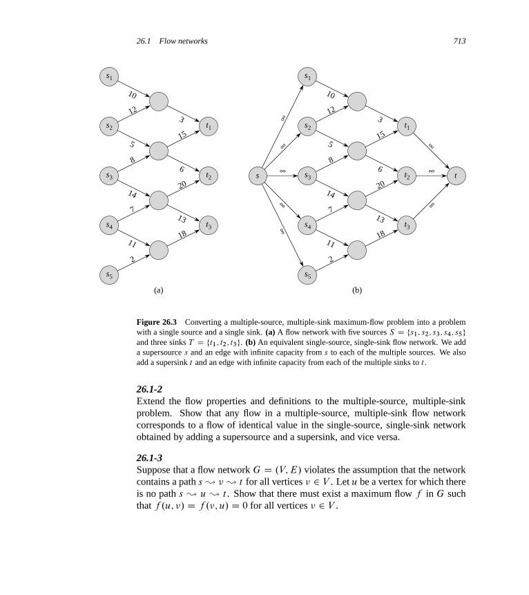
26.1 Flow networks 713
10
(a)
12
5
8
14
7
11
2
3
15
6
20
13
18
10
12
5
8
14
7
11
2
3
15
6
20
13
18
∞ ∞
∞
∞
∞
∞
∞
∞
s1 s1
s2 s2
s3s3
s4 s4
s5s5
t1 t1
t2t2
t3 t3
(b)
s t
Figure 26.3 Converting a multiple-source, multiple-sink maximum-flow problem into a problemwith a single source and a single sink. (a) A flow network with five sources S D fs1; s2; s3; s4; s5gand three sinks T D ft1; t2; t3g. (b) An equivalent single-source, single-sink flow network. We adda supersource s and an edge with infinite capacity from s to each of the multiple sources. We alsoadd a supersink t and an edge with infinite capacity from each of the multiple sinks to t .
26.1-2Extend the flow properties and definitions to the multiple-source, multiple-sinkproblem. Show that any flow in a multiple-source, multiple-sink flow networkcorresponds to a flow of identical value in the single-source, single-sink networkobtained by adding a supersource and a supersink, and vice versa.
26.1-3Suppose that a flow network G D .V; E/ violates the assumption that the networkcontains a path s � � � t for all vertices � 2 V . Let u be a vertex for which thereis no path s � u � t . Show that there must exist a maximum flow f in G suchthat f .u; �/ D f .�; u/ D 0 for all vertices � 2 V .

714 Chapter 26 Maximum Flow
26.1-4Let f be a flow in a network, and let ˛ be a real number. The scalar flow product,denoted f̨ , is a function from V V to R defined by
. f̨ /.u; �/ D ˛ � f .u; �/ :
Prove that the flows in a network form a convex set. That is, show that if f1 and f2
are flows, then so is f̨1 C .1� ˛/f2 for all ˛ in the range 0 � ˛ � 1.
26.1-5State the maximum-flow problem as a linear-programming problem.
26.1-6Professor Adam has two children who, unfortunately, dislike each other. The prob-lem is so severe that not only do they refuse to walk to school together, but in facteach one refuses to walk on any block that the other child has stepped on that day.The children have no problem with their paths crossing at a corner. Fortunatelyboth the professor’s house and the school are on corners, but beyond that he is notsure if it is going to be possible to send both of his children to the same school.The professor has a map of his town. Show how to formulate the problem of de-termining whether both his children can go to the same school as a maximum-flowproblem.
26.1-7Suppose that, in addition to edge capacities, a flow network has vertex capacities.That is each vertex � has a limit l.�/ on how much flow can pass though �. Showhow to transform a flow network G D .V; E/ with vertex capacities into an equiv-alent flow network G0 D .V 0; E 0/ without vertex capacities, such that a maximumflow in G0 has the same value as a maximum flow in G. How many vertices andedges does G0 have?
26.2 The Ford-Fulkerson method
This section presents the Ford-Fulkerson method for solving the maximum-flowproblem. We call it a “method” rather than an “algorithm” because it encompassesseveral implementations with differing running times. The Ford-Fulkerson methoddepends on three important ideas that transcend the method and are relevant tomany flow algorithms and problems: residual networks, augmenting paths, andcuts. These ideas are essential to the important max-flow min-cut theorem (The-orem 26.6), which characterizes the value of a maximum flow in terms of cuts of
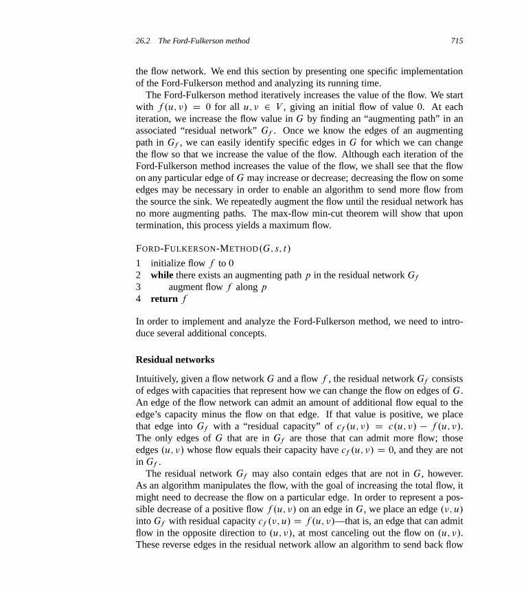
26.2 The Ford-Fulkerson method 715
the flow network. We end this section by presenting one specific implementationof the Ford-Fulkerson method and analyzing its running time.
The Ford-Fulkerson method iteratively increases the value of the flow. We startwith f .u; �/ D 0 for all u; � 2 V , giving an initial flow of value 0. At eachiteration, we increase the flow value in G by finding an “augmenting path” in anassociated “residual network” Gf . Once we know the edges of an augmentingpath in Gf , we can easily identify specific edges in G for which we can changethe flow so that we increase the value of the flow. Although each iteration of theFord-Fulkerson method increases the value of the flow, we shall see that the flowon any particular edge of G may increase or decrease; decreasing the flow on someedges may be necessary in order to enable an algorithm to send more flow fromthe source the sink. We repeatedly augment the flow until the residual network hasno more augmenting paths. The max-flow min-cut theorem will show that upontermination, this process yields a maximum flow.
FORD-FULKERSON-METHOD.G; s; t/
1 initialize flow f to 0
2 while there exists an augmenting path p in the residual network Gf
3 augment flow f along p
4 return f
In order to implement and analyze the Ford-Fulkerson method, we need to intro-duce several additional concepts.
Residual networks
Intuitively, given a flow network G and a flow f , the residual network Gf consistsof edges with capacities that represent how we can change the flow on edges of G.An edge of the flow network can admit an amount of additional flow equal to theedge’s capacity minus the flow on that edge. If that value is positive, we placethat edge into Gf with a “residual capacity” of cf .u; �/ D c.u; �/ � f .u; �/.The only edges of G that are in Gf are those that can admit more flow; thoseedges .u; �/ whose flow equals their capacity have cf .u; �/ D 0, and they are notin Gf .
The residual network Gf may also contain edges that are not in G, however.As an algorithm manipulates the flow, with the goal of increasing the total flow, itmight need to decrease the flow on a particular edge. In order to represent a pos-sible decrease of a positive flow f .u; �/ on an edge in G, we place an edge .�; u/
into Gf with residual capacity cf .�; u/ D f .u; �/—that is, an edge that can admitflow in the opposite direction to .u; �/, at most canceling out the flow on .u; �/.These reverse edges in the residual network allow an algorithm to send back flow

716 Chapter 26 Maximum Flow
it has already sent along an edge. Sending flow back along an edge is equiva-lent to decreasing the flow on the edge, which is a necessary operation in manyalgorithms.
More formally, suppose that we have a flow network G D .V; E/ with source s
and sink t . Let f be a flow in G, and consider a pair of vertices u; � 2 V . Wedefine the residual capacity cf .u; �/ by
cf .u; �/ D
�c.u; �/ � f .u; �/ if .u; �/ 2 E ;
f .�; u/ if .�; u/ 2 E ;
0 otherwise :
(26.2)
Because of our assumption that .u; �/ 2 E implies .�; u/ 62 E, exactly one case inequation (26.2) applies to each ordered pair of vertices.
As an example of equation (26.2), if c.u; �/ D 16 and f .u; �/ D 11, then wecan increase f .u; �/ by up to cf .u; �/ D 5 units before we exceed the capacityconstraint on edge .u; �/. We also wish to allow an algorithm to return up to 11
units of flow from � to u, and hence cf .�; u/ D 11.Given a flow network G D .V; E/ and a flow f , the residual network of G
induced by f is Gf D .V; Ef /, where
Ef D f.u; �/ 2 V V W cf .u; �/ > 0g : (26.3)
That is, as promised above, each edge of the residual network, or residual edge,can admit a flow that is greater than 0. Figure 26.4(a) repeats the flow network G
and flow f of Figure 26.1(b), and Figure 26.4(b) shows the corresponding residualnetwork Gf . The edges in Ef are either edges in E or their reversals, and thus
jEf j � 2 jEj :
Observe that the residual network Gf is similar to a flow network with capacitiesgiven by cf . It does not satisfy our definition of a flow network because it maycontain both an edge .u; �/ and its reversal .�; u/. Other than this difference, aresidual network has the same properties as a flow network, and we can define aflow in the residual network as one that satisfies the definition of a flow, but withrespect to capacities cf in the network Gf .
A flow in a residual network provides a roadmap for adding flow to the originalflow network. If f is a flow in G and f 0 is a flow in the corresponding residualnetwork Gf , we define f "f 0, the augmentation of flow f by f 0, to be a functionfrom V V to R, defined by
.f "f 0/.u; �/ D(
f .u; �/C f 0.u; �/ � f 0.�; u/ if .u; �/ 2 E ;
0 otherwise :(26.4)

26.2 The Ford-Fulkerson method 717
9
15s t
512
5
7
5
31
8
11
4
s t
11/1612/12
19/20
7/7
91/4
12/1311/14
4/4
(b)
(c)
115
3
4s t
11/1612/12
15/20
7/7
4/91/4
8/1311/14
4/4
(d)
19s t
512
1
731
12
11
4
111
3
v1
v1
v1
v1
v2
v2
v2
v2
v3
v3
v3
v3
v4
v4
v4
v4
(a)
Figure 26.4 (a) The flow network G and flow f of Figure 26.1(b). (b) The residual network Gf
with augmenting path p shaded; its residual capacity is cf .p/ D cf .�2; �3/ D 4. Edges withresidual capacity equal to 0, such as .�1; �3/, are not shown, a convention we follow in the remainderof this section. (c) The flow in G that results from augmenting along path p by its residual capacity 4.Edges carrying no flow, such as .�3; �2/, are labeled only by their capacity, another convention wefollow throughout. (d) The residual network induced by the flow in (c).
The intuition behind this definition follows the definition of the residual network.We increase the flow on .u; �/ by f 0.u; �/ but decrease it by f 0.�; u/ becausepushing flow on the reverse edge in the residual network signifies decreasing theflow in the original network. Pushing flow on the reverse edge in the residualnetwork is also known as cancellation. For example, if we send 5 crates of hockeypucks from u to � and send 2 crates from � to u, we could equivalently (from theperspective of the final result) just send 3 creates from u to � and none from � to u.Cancellation of this type is crucial for any maximum-flow algorithm.
Lemma 26.1Let G D .V; E/ be a flow network with source s and sink t , and let f be a flowin G. Let Gf be the residual network of G induced by f , and let f 0 be a flowin Gf . Then the function f "f 0 defined in equation (26.4) is a flow in G withvalue jf "f 0j D jf j C jf 0j.
Proof We first verify that f "f 0 obeys the capacity constraint for each edge in E
and flow conservation at each vertex in V � fs; tg.

718 Chapter 26 Maximum Flow
For the capacity constraint, first observe that if .u; �/ 2 E, then cf .�; u/ Df .u; �/. Therefore, we have f 0.�; u/ � cf .�; u/ D f .u; �/, and hence
.f "f 0/.u; �/ D f .u; �/C f 0.u; �/ � f 0.�; u/ (by equation (26.4))
� f .u; �/C f 0.u; �/ � f .u; �/ (because f 0.�; u/ � f .u; �/)
D f 0.u; �/
� 0 :
In addition,
.f "f 0/.u; �/
D f .u; �/C f 0.u; �/ � f 0.�; u/ (by equation (26.4))
� f .u; �/C f 0.u; �/ (because flows are nonnegative)
� f .u; �/C cf .u; �/ (capacity constraint)
D f .u; �/C c.u; �/ � f .u; �/ (definition of cf )
D c.u; �/ :
For flow conservation, because both f and f 0 obey flow conservation, we havethat for all u 2 V � fs; tg,X�2V
.f " f 0/.u; �/ DX�2V
.f .u; �/C f 0.u; �/ � f 0.�; u//
DX�2V
f .u; �/CX�2V
f 0.u; �/ �X�2V
f 0.�; u/
DX�2V
f .�; u/CX�2V
f 0.�; u/ �X�2V
f 0.u; �/
DX�2V
.f .�; u/C f 0.�; u/ � f 0.u; �//
DX�2V
.f "f 0/.�; u/ ;
where the third line follows from the second by flow conservation.Finally, we compute the value of f "f 0. Recall that we disallow antiparallel
edges in G (but not in Gf ), and hence for each vertex � 2 V , we know that therecan be an edge .s; �/ or .�; s/, but never both. We define V1 D f� W .s; �/ 2 Egto be the set of vertices with edges from s and V2 D f� W .�; s/ 2 Eg to be theset of vertices with edges to s. We have V1 [ V2 � V and, because we disallowantiparallel edges, V1 \ V2 D ;. We now compute
jf "f 0j DX�2V
.f "f 0/ .s; �/ �X�2V
.f " f 0/ .�; s/
DX�2V1
.f " f 0/ .s; �/ �X�2V2
.f " f 0/ .�; s/ ; (26.5)
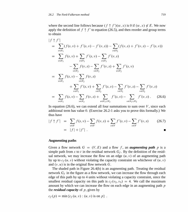
26.2 The Ford-Fulkerson method 719
where the second line follows because .f "f 0/.w; x/ is 0 if .w; x/ 62 E. We nowapply the definition of f "f 0 to equation (26.5), and then reorder and group termsto obtain
jf "f 0jD
X�2V1
.f .s; �/C f 0.s; �/ � f 0.�; s// �X�2V2
.f .�; s/C f 0.�; s/ � f 0.s; �//
DX�2V1
f .s; �/CX�2V1
f 0.s; �/ �X�2V1
f 0.�; s/
�X�2V2
f .�; s/ �X�2V2
f 0.�; s/CX�2V2
f 0.s; �/
DX�2V1
f .s; �/ �X�2V2
f .�; s/
CX�2V1
f 0.s; �/CX�2V2
f 0.s; �/ �X�2V1
f 0.�; s/ �X�2V2
f 0.�; s/
DX�2V1
f .s; �/ �X�2V2
f .�; s/CX
�2V1[V2
f 0.s; �/ �X
�2V1[V2
f 0.�; s/ : (26.6)
In equation (26.6), we can extend all four summations to sum over V , since eachadditional term has value 0. (Exercise 26.2-1 asks you to prove this formally.) Wethus have
jf "f 0j DX�2V
f .s; �/ �X�2V
f .�; s/CX�2V
f 0.s; �/ �X�2V
f 0.�; s/ (26.7)
D jf j C jf 0j :
Augmenting paths
Given a flow network G D .V; E/ and a flow f , an augmenting path p is asimple path from s to t in the residual network Gf . By the definition of the resid-ual network, we may increase the flow on an edge .u; �/ of an augmenting pathby up to cf .u; �/ without violating the capacity constraint on whichever of .u; �/
and .�; u/ is in the original flow network G.The shaded path in Figure 26.4(b) is an augmenting path. Treating the residual
network Gf in the figure as a flow network, we can increase the flow through eachedge of this path by up to 4 units without violating a capacity constraint, since thesmallest residual capacity on this path is cf .�2; �3/ D 4. We call the maximumamount by which we can increase the flow on each edge in an augmenting path p
the residual capacity of p, given by
cf .p/ D min fcf .u; �/ W .u; �/ is on pg :
720 Chapter 26 Maximum Flow
The following lemma, whose proof we leave as Exercise 26.2-7, makes the aboveargument more precise.
Lemma 26.2Let G D .V; E/ be a flow network, let f be a flow in G, and let p be an augmentingpath in Gf . Define a function fp W V V ! R by
fp.u; �/ D(
cf .p/ if .u; �/ is on p ;
0 otherwise :(26.8)
Then, fp is a flow in Gf with value jfpj D cf .p/ > 0.
The following corollary shows that if we augment f by fp, we get another flowin G whose value is closer to the maximum. Figure 26.4(c) shows the result ofaugmenting the flow f from Figure 26.4(a) by the flow fp in Figure 26.4(b), andFigure 26.4(d) shows the ensuing residual network.
Corollary 26.3Let G D .V; E/ be a flow network, let f be a flow in G, and let p be anaugmenting path in Gf . Let fp be defined as in equation (26.8), and supposethat we augment f by fp. Then the function f "fp is a flow in G with valuejf "fpj D jf j C jfpj > jf j.
Proof Immediate from Lemmas 26.1 and 26.2.
Cuts of flow networks
The Ford-Fulkerson method repeatedly augments the flow along augmenting pathsuntil it has found a maximum flow. How do we know that when the algorithmterminates, we have actually found a maximum flow? The max-flow min-cut theo-rem, which we shall prove shortly, tells us that a flow is maximum if and only if itsresidual network contains no augmenting path. To prove this theorem, though, wemust first explore the notion of a cut of a flow network.
A cut .S; T / of flow network G D .V; E/ is a partition of V into S andT D V � S such that s 2 S and t 2 T . (This definition is similar to the def-inition of “cut” that we used for minimum spanning trees in Chapter 23, exceptthat here we are cutting a directed graph rather than an undirected graph, and weinsist that s 2 S and t 2 T .) If f is a flow, then the net flow f .S; T / across thecut .S; T / is defined to be
f .S; T / DXu2S
X�2T
f .u; �/�Xu2S
X�2T
f .�; u/ : (26.9)

26.2 The Ford-Fulkerson method 721
s t
11/1612/12
15/20
7/7
4/91/4
8/1311/14
4/4
S T
v4
v3v1
v2
Figure 26.5 A cut .S; T / in the flow network of Figure 26.1(b), where S D fs; �1; �2g andT D f�3; �4; tg. The vertices in S are black, and the vertices in T are white. The net flowacross .S; T / is f .S; T / D 19, and the capacity is c.S; T / D 26.
The capacity of the cut .S; T / is
c.S; T / DXu2S
X�2T
c.u; �/ : (26.10)
A minimum cut of a network is a cut whose capacity is minimum over all cuts ofthe network.
The asymmetry between the definitions of flow and capacity of a cut is inten-tional and important. For capacity, we count only the capacities of edges goingfrom S to T , ignoring edges in the reverse direction. For flow, we consider theflow going from S to T minus the flow going in the reverse direction from T to S .The reason for this difference will become clear later in this section.
Figure 26.5 shows the cut .fs; �1; �2g ; f�3; �4; tg/ in the flow network of Fig-ure 26.1(b). The net flow across this cut is
f .�1; �3/C f .�2; �4/ � f .�3; �2/ D 12C 11 � 4
D 19 ;
and the capacity of this cut is
c.�1; �3/C c.�2; �4/ D 12C 14
D 26 :
The following lemma shows that, for a given flow f , the net flow across any cutis the same, and it equals jf j, the value of the flow.
Lemma 26.4Let f be a flow in a flow network G with source s and sink t , and let .S; T / be anycut of G. Then the net flow across .S; T / is f .S; T / D jf j.
722 Chapter 26 Maximum Flow
Proof We can rewrite the flow-conservation condition for any node u 2 V �fs; tgasX�2V
f .u; �/ �X�2V
f .�; u/ D 0 : (26.11)
Taking the definition of jf j from equation (26.1) and adding the left-hand side ofequation (26.11), which equals 0, summed over all vertices in S � fsg, gives
jf j DX�2V
f .s; �/ �X�2V
f .�; s/CX
u2S�fsg
X�2V
f .u; �/ �X�2V
f .�; u/
!:
Expanding the right-hand summation and regrouping terms yields
jf j DX�2V
f .s; �/ �X�2V
f .�; s/CX
u2S�fsg
X�2V
f .u; �/�X
u2S�fsg
X�2V
f .�; u/
DX�2V
f .s; �/C
Xu2S�fsg
f .u; �/
!�X�2V
f .�; s/C
Xu2S�fsg
f .�; u/
!D
X�2V
Xu2S
f .u; �/ �X�2V
Xu2S
f .�; u/ :
Because V D S [ T and S \ T D ;, we can split each summation over V intosummations over S and T to obtain
jf j DX�2S
Xu2S
f .u; �/CX�2T
Xu2S
f .u; �/�X�2S
Xu2S
f .�; u/�X�2T
Xu2S
f .�; u/
DX�2T
Xu2S
f .u; �/ �X�2T
Xu2S
f .�; u/
C X
�2S
Xu2S
f .u; �/ �X�2S
Xu2S
f .�; u/
!:
The two summations within the parentheses are actually the same, since for allvertices x; y 2 V , the term f .x; y/ appears once in each summation. Hence, thesesummations cancel, and we have
jf j DXu2S
X�2T
f .u; �/ �Xu2S
X�2T
f .�; u/
D f .S; T / :
A corollary to Lemma 26.4 shows how we can use cut capacities to bound thevalue of a flow.
26.2 The Ford-Fulkerson method 723
Corollary 26.5The value of any flow f in a flow network G is bounded from above by the capacityof any cut of G.
Proof Let .S; T / be any cut of G and let f be any flow. By Lemma 26.4 and thecapacity constraint,
jf j D f .S; T /
DXu2S
X�2T
f .u; �/�Xu2S
X�2T
f .�; u/
�Xu2S
X�2T
f .u; �/
�Xu2S
X�2T
c.u; �/
D c.S; T / :
Corollary 26.5 yields the immediate consequence that the value of a maximumflow in a network is bounded from above by the capacity of a minimum cut ofthe network. The important max-flow min-cut theorem, which we now state andprove, says that the value of a maximum flow is in fact equal to the capacity of aminimum cut.
Theorem 26.6 (Max-flow min-cut theorem)If f is a flow in a flow network G D .V; E/ with source s and sink t , then thefollowing conditions are equivalent:
1. f is a maximum flow in G.
2. The residual network Gf contains no augmenting paths.
3. jf j D c.S; T / for some cut .S; T / of G.
Proof .1/ ) .2/: Suppose for the sake of contradiction that f is a maximumflow in G but that Gf has an augmenting path p. Then, by Corollary 26.3, theflow found by agumenting f by fp, where fp is given by equation (26.8), is a flowin G with value strictly greater than jf j, contradicting the assumption that f is amaximum flow.
.2/ ) .3/: Suppose that Gf has no augmenting path, that is, that Gf containsno path from s to t . Define
S D f� 2 V W there exists a path from s to � in Gf gand T D V � S . The partition .S; T / is a cut: we have s 2 S trivially and t 62 S
because there is no path from s to t in Gf . Now consider a pair of vertices

724 Chapter 26 Maximum Flow
u 2 S and � 2 T . If .u; �/ 2 E, we must have f .u; �/ D c.u; �/, sinceotherwise .u; �/ 2 Ef , which would place � in set S . If .�; u/ 2 E, we musthave f .�; u/ D 0, because otherwise cf .u; �/ D f .�; u/ would be positive andwe would have .u; �/ 2 Ef , which would place � in S . Of course, if neither .u; �/
nor .�; u/ is in E, then f .u; �/ D f .�; u/ D 0. We thus have
f .S; T / DXu2S
X�2T
f .u; �/ �X�2T
Xu2S
f .�; u/
DXu2S
X�2T
c.u; �/ �X�2T
Xu2S
0
D c.S; T / :
By Lemma 26.4, therefore, jf j D f .S; T / D c.S; T /..3/) .1/: By Corollary 26.5, jf j � c.S; T / for all cuts .S; T /. The conditionjf j D c.S; T / thus implies that f is a maximum flow.
The basic Ford-Fulkerson algorithm
In each iteration of the Ford-Fulkerson method, we find some augmenting path p
and use p to modify the flow f . As Lemma 26.2 and Corollary 26.3 suggest, wereplace f by f "fp, obtaining a new flow whose value is jf j C jfpj. The follow-ing implementation of the method computes the maximum flow in a flow networkG D .V; E/ by updating the flow attribute .u; �/: f for each edge .u; �/ 2 E.1
If .u; �/ 62 E, we assume implicitly that .u; �/: f D 0. We also assume that weare given the capacities c.u; �/ along with the flow network, and c.u; �/ D 0
if .u; �/ 62 E. We compute the residual capacity cf .u; �/ in accordance with theformula (26.2). The expression cf .p/ in the code is just a temporary variable thatstores the residual capacity of the path p.
FORD-FULKERSON.G; s; t/
1 for each edge .u; �/ 2 G:E2 .u; �/: f D 0
3 while there exists a path p from s to t in the residual network Gf
4 cf .p/ D min fcf .u; �/ W .u; �/ is in pg5 for each edge .u; �/ in p
6 if .u; �/ 2 E
7 .u; �/: f D .u; �/: f C cf .p/
8 else .�; u/: f D .�; u/: f � cf .p/
1Recall from Section 22.1 that we represent an attribute f for edge .u; �/ with the same style ofnotation—.u; �/: f —that we use for an attribute of any other object.

26.2 The Ford-Fulkerson method 725
The FORD-FULKERSON algorithm simply expands on the FORD-FULKERSON-METHOD pseudocode given earlier. Figure 26.6 shows the result of each iterationin a sample run. Lines 1–2 initialize the flow f to 0. The while loop of lines 3–8repeatedly finds an augmenting path p in Gf and augments flow f along p bythe residual capacity cf .p/. Each residual edge in path p is either an edge in theoriginal network or the reversal of an edge in the original network. Lines 6–8update the flow in each case appropriately, adding flow when the residual edge isan original edge and subtracting it otherwise. When no augmenting paths exist, theflow f is a maximum flow.
Analysis of Ford-Fulkerson
The running time of FORD-FULKERSON depends on how we find the augmentingpath p in line 3. If we choose it poorly, the algorithm might not even terminate: thevalue of the flow will increase with successive augmentations, but it need not evenconverge to the maximum flow value.2 If we find the augmenting path by using abreadth-first search (which we saw in Section 22.2), however, the algorithm runs inpolynomial time. Before proving this result, we obtain a simple bound for the casein which we choose the augmenting path arbitrarily and all capacities are integers.
In practice, the maximum-flow problem often arises with integral capacities. Ifthe capacities are rational numbers, we can apply an appropriate scaling transfor-mation to make them all integral. If f � denotes a maximum flow in the transformednetwork, then a straightforward implementation of FORD-FULKERSON executesthe while loop of lines 3–8 at most jf �j times, since the flow value increases by atleast one unit in each iteration.
We can perform the work done within the while loop efficiently if we implementthe flow network G D .V; E/ with the right data structure and find an augmentingpath by a linear-time algorithm. Let us assume that we keep a data structure cor-responding to a directed graph G0 D .V; E 0/, where E 0 D f.u; �/ W .u; �/ 2 E or.�; u/ 2 Eg. Edges in the network G are also edges in G0, and therefore we caneasily maintain capacities and flows in this data structure. Given a flow f on G,the edges in the residual network Gf consist of all edges .u; �/ of G0 such thatcf .u; �/ > 0, where cf conforms to equation (26.2). The time to find a path ina residual network is therefore O.V C E 0/ D O.E/ if we use either depth-firstsearch or breadth-first search. Each iteration of the while loop thus takes O.E/
time, as does the initialization in lines 1–2, making the total running time of theFORD-FULKERSON algorithm O.E jf �j/.
2The Ford-Fulkerson method might fail to terminate only if edge capacities are irrational numbers.
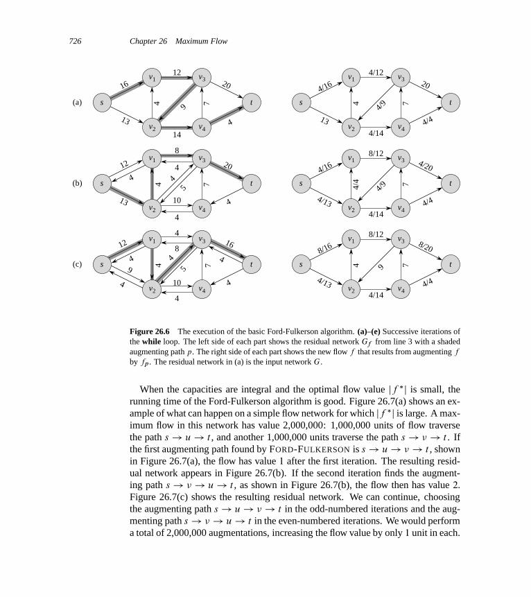
726 Chapter 26 Maximum Flow
12
4
44/
44
v1
4
16
4
10
s t
16
1220
794
13
14
4
v1
s t
4/16
4/1220
7
4/9
13
4/144/4
s t75
4
4
v1
8
4
13
20v1
s t
4/16
8/124/20
7
4/9
4/134/14
4/4
4
10
s t75
8
4
v14
9
v1
s t
8/16
8/128/20
794/13
4/144/4
v2 v2
v2v2
v2 v2
v3 v3
v3v3
v3 v3
v4 v4
v4v4
v4v4
(b)
(a)
(c)
124
4
4
4
4
Figure 26.6 The execution of the basic Ford-Fulkerson algorithm. (a)–(e) Successive iterations ofthe while loop. The left side of each part shows the residual network Gf from line 3 with a shadedaugmenting path p. The right side of each part shows the new flow f that results from augmenting f
by fp. The residual network in (a) is the input network G.
When the capacities are integral and the optimal flow value jf �j is small, therunning time of the Ford-Fulkerson algorithm is good. Figure 26.7(a) shows an ex-ample of what can happen on a simple flow network for which jf �j is large. A max-imum flow in this network has value 2,000,000: 1,000,000 units of flow traversethe path s ! u! t , and another 1,000,000 units traverse the path s ! � ! t . Ifthe first augmenting path found by FORD-FULKERSON is s ! u! � ! t , shownin Figure 26.7(a), the flow has value 1 after the first iteration. The resulting resid-ual network appears in Figure 26.7(b). If the second iteration finds the augment-ing path s ! � ! u! t , as shown in Figure 26.7(b), the flow then has value 2.Figure 26.7(c) shows the resulting residual network. We can continue, choosingthe augmenting path s ! u! � ! t in the odd-numbered iterations and the aug-menting path s ! � ! u! t in the even-numbered iterations. We would performa total of 2,000,000 augmentations, increasing the flow value by only 1 unit in each.

26.2 The Ford-Fulkerson method 727
4
1211
2
11
2
8
8
9
4
4
9
8
4
4
9
8s t
12
7
4
4
v1
s t
8/16
8/1215/20
7/7
911/13
11/144/4
v1
10
19s t
121
7
11
43
v2
v3 v3
v3
v4v4
v4
(d)
(f)
4
9
8
4
4
15s t
5
711
4
v1
s t
12/1612/12
19/20
7/7
911/13
11/144/4
v1
3v2
v3 v3
v4v4
(e) 4
v2
v2
v1
v2
8
8
Figure 26.6, continued (f) The residual network at the last while loop test. It has no augmentingpaths, and the flow f shown in (e) is therefore a maximum flow. The value of the maximum flowfound is 23.
The Edmonds-Karp algorithm
We can improve the bound on FORD-FULKERSON by finding the augmentingpath p in line 3 with a breadth-first search. That is, we choose the augmentingpath as a shortest path from s to t in the residual network, where each edge hasunit distance (weight). We call the Ford-Fulkerson method so implemented theEdmonds-Karp algorithm. We now prove that the Edmonds-Karp algorithm runsin O.VE2/ time.
The analysis depends on the distances to vertices in the residual network Gf .The following lemma uses the notation ıf .u; �/ for the shortest-path distancefrom u to � in Gf , where each edge has unit distance.
Lemma 26.7If the Edmonds-Karp algorithm is run on a flow network G D .V; E/ with source s
and sink t , then for all vertices � 2 V � fs; tg, the shortest-path distance ıf .s; �/
in the residual network Gf increases monotonically with each flow augmentation.

728 Chapter 26 Maximum Flow
1
999,999
999,999
1
s t1,000,000 1,000,000
1
1,000,000 1,000,000
999,999
1
1 999,999
u
v
s t
1,000,000
1
1,000,000
u
v
999,999
1
999,999
1s t1
u
v
(a) (b) (c)
Figure 26.7 (a) A flow network for which FORD-FULKERSON can take ‚.E jf �j/ time,where f � is a maximum flow, shown here with jf �j D 2,000,000. The shaded path is an aug-menting path with residual capacity 1. (b) The resulting residual network, with another augmentingpath whose residual capacity is 1. (c) The resulting residual network.
Proof We will suppose that for some vertex � 2 V � fs; tg, there is a flow aug-mentation that causes the shortest-path distance from s to � to decrease, and thenwe will derive a contradiction. Let f be the flow just before the first augmentationthat decreases some shortest-path distance, and let f 0 be the flow just afterward.Let � be the vertex with the minimum ıf 0.s; �/ whose distance was decreased bythe augmentation, so that ıf 0.s; �/ < ıf .s; �/. Let p D s � u ! � be a shortestpath from s to � in Gf 0 , so that .u; �/ 2 Ef 0 and
ıf 0.s; u/ D ıf 0.s; �/ � 1 : (26.12)
Because of how we chose �, we know that the distance of vertex u from the source s
did not decrease, i.e.,
ıf 0.s; u/ � ıf .s; u/ : (26.13)
We claim that .u; �/ 62 Ef . Why? If we had .u; �/ 2 Ef , then we would also have
ıf .s; �/ � ıf .s; u/C 1 (by Lemma 24.10, the triangle inequality)
� ıf 0.s; u/C 1 (by inequality (26.13))
D ıf 0.s; �/ (by equation (26.12)) ,
which contradicts our assumption that ıf 0.s; �/ < ıf .s; �/.How can we have .u; �/ 62 Ef and .u; �/ 2 Ef 0? The augmentation must
have increased the flow from � to u. The Edmonds-Karp algorithm always aug-ments flow along shortest paths, and therefore the shortest path from s to u in Gf
has .�; u/ as its last edge. Therefore,
ıf .s; �/ D ıf .s; u/ � 1
� ıf 0.s; u/ � 1 (by inequality (26.13))
D ıf 0.s; �/ � 2 (by equation (26.12)) ,

26.2 The Ford-Fulkerson method 729
which contradicts our assumption that ıf 0.s; �/ < ıf .s; �/. We conclude that ourassumption that such a vertex � exists is incorrect.
The next theorem bounds the number of iterations of the Edmonds-Karp algo-rithm.
Theorem 26.8If the Edmonds-Karp algorithm is run on a flow network G D .V; E/ with source s
and sink t , then the total number of flow augmentations performed by the algorithmis O.VE/.
Proof We say that an edge .u; �/ in a residual network Gf is critical on an aug-menting path p if the residual capacity of p is the residual capacity of .u; �/, thatis, if cf .p/ D cf .u; �/. After we have augmented flow along an augmenting path,any critical edge on the path disappears from the residual network. Moreover, atleast one edge on any augmenting path must be critical. We will show that each ofthe jEj edges can become critical at most jV j =2 times.
Let u and � be vertices in V that are connected by an edge in E. Since augment-ing paths are shortest paths, when .u; �/ is critical for the first time, we have
ıf .s; �/ D ıf .s; u/C 1 :
Once the flow is augmented, the edge .u; �/ disappears from the residual network.It cannot reappear later on another augmenting path until after the flow from u to �
is decreased, which occurs only if .�; u/ appears on an augmenting path. If f 0 isthe flow in G when this event occurs, then we have
ıf 0.s; u/ D ıf 0.s; �/C 1 :
Since ıf .s; �/ � ıf 0.s; �/ by Lemma 26.7, we have
ıf 0.s; u/ D ıf 0.s; �/C 1
� ıf .s; �/C 1
D ıf .s; u/C 2 :
Consequently, from the time .u; �/ becomes critical to the time when it nextbecomes critical, the distance of u from the source increases by at least 2. Thedistance of u from the source is initially at least 0. The intermediate vertices on ashortest path from s to u cannot contain s, u, or t (since .u; �/ on an augmentingpath implies that u ¤ t). Therefore, until u becomes unreachable from the source,if ever, its distance is at most jV j � 2. Thus, after the first time that .u; �/ becomescritical, it can become critical at most .jV j � 2/=2 D jV j =2 � 1 times more, for atotal of at most jV j =2 times. Since there are O.E/ pairs of vertices that can have anedge between them in a residual network, the total number of critical edges during

730 Chapter 26 Maximum Flow
the entire execution of the Edmonds-Karp algorithm is O.VE/. Each augmentingpath has at least one critical edge, and hence the theorem follows.
Because we can implement each iteration of FORD-FULKERSON in O.E/ timewhen we find the augmenting path by breadth-first search, the total running time ofthe Edmonds-Karp algorithm is O.VE2/. We shall see that push-relabel algorithmscan yield even better bounds. The algorithm of Section 26.4 gives a method forachieving an O.V 2E/ running time, which forms the basis for the O.V 3/-timealgorithm of Section 26.5.
Exercises
26.2-1Prove that the summations in equation (26.6) equal the summations in equa-tion (26.7).
26.2-2In Figure 26.1(b), what is the flow across the cut .fs; �2; �4g ; f�1; �3; tg/? What isthe capacity of this cut?
26.2-3Show the execution of the Edmonds-Karp algorithm on the flow network of Fig-ure 26.1(a).
26.2-4In the example of Figure 26.6, what is the minimum cut corresponding to the max-imum flow shown? Of the augmenting paths appearing in the example, which onecancels flow?
26.2-5Recall that the construction in Section 26.1 that converts a flow network with mul-tiple sources and sinks into a single-source, single-sink network adds edges withinfinite capacity. Prove that any flow in the resulting network has a finite valueif the edges of the original network with multiple sources and sinks have finitecapacity.
26.2-6Suppose that each source si in a flow network with multiple sources and sinksproduces exactly pi units of flow, so that
P�2V f .si ; �/ D pi . Suppose also
that each sink tj consumes exactly qj units, so thatP
�2V f .�; tj / D qj , wherePi pi D
Pj qj . Show how to convert the problem of finding a flow f that obeys
26.2 The Ford-Fulkerson method 731
these additional constraints into the problem of finding a maximum flow in a single-source, single-sink flow network.
26.2-7Prove Lemma 26.2.
26.2-8Suppose that we redefine the residual network to disallow edges into s. Argue thatthe procedure FORD-FULKERSON still correctly computes a maximum flow.
26.2-9Suppose that both f and f 0 are flows in a network G and we compute flow f "f 0.Does the augmented flow satisfy the flow conservation property? Does it satisfythe capacity constraint?
26.2-10Show how to find a maximum flow in a network G D .V; E/ by a sequence of atmost jEj augmenting paths. (Hint: Determine the paths after finding the maximumflow.)
26.2-11The edge connectivity of an undirected graph is the minimum number k of edgesthat must be removed to disconnect the graph. For example, the edge connectivityof a tree is 1, and the edge connectivity of a cyclic chain of vertices is 2. Showhow to determine the edge connectivity of an undirected graph G D .V; E/ byrunning a maximum-flow algorithm on at most jV j flow networks, each havingO.V / vertices and O.E/ edges.
26.2-12Suppose that you are given a flow network G, and G has edges entering thesource s. Let f be a flow in G in which one of the edges .�; s/ entering the sourcehas f .�; s/ D 1. Prove that there must exist another flow f 0 with f 0.�; s/ D 0
such that jf j D jf 0j. Give an O.E/-time algorithm to compute f 0, given f .
26.2-13Suppose that you wish to find, among all minimum cuts in a flow network G, onethat contains the smallest number of edges. Show how to modify the capacitiesof G to create a new flow network G0 in which any minimum cut in G0 is a mini-mum cut with the smallest number of edges in G.

732 Chapter 26 Maximum Flow
26.3 Maximum bipartite matching
Some combinatorial problems can easily be cast as maximum-flow problems. Themultiple-source, multiple-sink maximum-flow problem from Section 26.1 gave usone example. Some other combinatorial problems seem on the surface to have littleto do with flow networks, but can in fact be reduced to maximum-flow problems.This section presents one such problem: finding a maximum matching in a bipartitegraph. In order to solve this problem, we shall take advantage of an integralityproperty provided by the Ford-Fulkerson method. We shall also see how to usethe Ford-Fulkerson method to solve the maximum-bipartite-matching problem ona graph G D .V; E/ in O.VE/ time.
The maximum-bipartite-matching problem
Given an undirected graph G D .V; E/, a matching is a subset of edges M � E
such that for all vertices � 2 V , at most one edge of M is incident on �. Wesay that a vertex � 2 V is matched by the matching M if some edge in M isincident on �; otherwise, � is unmatched. A maximum matching is a matchingof maximum cardinality, that is, a matching M such that for any matching M 0,we have jM j � jM 0j. In this section, we shall restrict our attention to findingmaximum matchings in bipartite graphs: graphs in which the vertex set can bepartitioned into V D L [ R, where L and R are disjoint and all edges in E
go between L and R. We further assume that every vertex in V has at least oneincident edge. Figure 26.8 illustrates the notion of a matching in a bipartite graph.
The problem of finding a maximum matching in a bipartite graph has manypractical applications. As an example, we might consider matching a set L of ma-chines with a set R of tasks to be performed simultaneously. We take the presenceof edge .u; �/ in E to mean that a particular machine u 2 L is capable of per-forming a particular task � 2 R. A maximum matching provides work for as manymachines as possible.
Finding a maximum bipartite matching
We can use the Ford-Fulkerson method to find a maximum matching in an undi-rected bipartite graph G D .V; E/ in time polynomial in jV j and jEj. The trick isto construct a flow network in which flows correspond to matchings, as shown inFigure 26.8(c). We define the corresponding flow network G0 D .V 0; E 0/ for thebipartite graph G as follows. We let the source s and sink t be new vertices notin V , and we let V 0 D V [ fs; tg. If the vertex partition of G is V D L [ R, the

26.3 Maximum bipartite matching 733
L R L R
s t
(a) (c)
L R
(b)
Figure 26.8 A bipartite graph G D .V; E/ with vertex partition V D L [ R. (a) A matchingwith cardinality 2, indicated by shaded edges. (b) A maximum matching with cardinality 3. (c) Thecorresponding flow network G0 with a maximum flow shown. Each edge has unit capacity. Shadededges have a flow of 1, and all other edges carry no flow. The shaded edges from L to R correspondto those in the maximum matching from (b).
directed edges of G0 are the edges of E, directed from L to R, along with jV j newdirected edges:
E 0 D f.s; u/ W u 2 Lg [ f.u; �/ W .u; �/ 2 Eg [ f.�; t/ W � 2 Rg :
To complete the construction, we assign unit capacity to each edge in E 0. Sinceeach vertex in V has at least one incident edge, jEj � jV j =2. Thus, jEj � jE 0j DjEj C jV j � 3 jEj, and so jE 0j D ‚.E/.
The following lemma shows that a matching in G corresponds directly to a flowin G’s corresponding flow network G0. We say that a flow f on a flow networkG D .V; E/ is integer-valued if f .u; �/ is an integer for all .u; �/ 2 V V .
Lemma 26.9Let G D .V; E/ be a bipartite graph with vertex partition V D L [ R, and letG0 D .V 0; E 0/ be its corresponding flow network. If M is a matching in G, thenthere is an integer-valued flow f in G0 with value jf j D jM j. Conversely, if f
is an integer-valued flow in G0, then there is a matching M in G with cardinalityjM j D jf j.
Proof We first show that a matching M in G corresponds to an integer-valuedflow f in G0. Define f as follows. If .u; �/ 2 M , then f .s; u/ D f .u; �/ Df .�; t/ D 1. For all other edges .u; �/ 2 E 0, we define f .u; �/ D 0. It is simpleto verify that f satisfies the capacity constraint and flow conservation.

734 Chapter 26 Maximum Flow
Intuitively, each edge .u; �/ 2 M corresponds to one unit of flow in G0 thattraverses the path s ! u ! � ! t . Moreover, the paths induced by edges in M
are vertex-disjoint, except for s and t . The net flow across cut .L [ fsg ; R [ ftg/is equal to jM j; thus, by Lemma 26.4, the value of the flow is jf j D jM j.
To prove the converse, let f be an integer-valued flow in G0, and let
M D f.u; �/ W u 2 L; � 2 R; and f .u; �/ > 0g :
Each vertex u 2 L has only one entering edge, namely .s; u/, and its capacityis 1. Thus, each u 2 L has at most one unit of flow entering it, and if one unit offlow does enter, by flow conservation, one unit of flow must leave. Furthermore,since f is integer-valued, for each u 2 L, the one unit of flow can enter on at mostone edge and can leave on at most one edge. Thus, one unit of flow enters u if andonly if there is exactly one vertex � 2 R such that f .u; �/ D 1, and at most oneedge leaving each u 2 L carries positive flow. A symmetric argument applies toeach � 2 R. The set M is therefore a matching.
To see that jM j D jf j, observe that for every matched vertex u 2 L, we havef .s; u/ D 1, and for every edge .u; �/ 2 E �M , we have f .u; �/ D 0. Conse-quently, f .L [ fsg ; R [ ftg/, the net flow across cut .L [ fsg ; R [ ftg/, is equalto jM j. Applying Lemma 26.4, we have that jf j D f .L[fsg ; R[ftg/ D jM j.
Based on Lemma 26.9, we would like to conclude that a maximum matchingin a bipartite graph G corresponds to a maximum flow in its corresponding flownetwork G0, and we can therefore compute a maximum matching in G by runninga maximum-flow algorithm on G0. The only hitch in this reasoning is that themaximum-flow algorithm might return a flow in G0 for which some f .u; �/ isnot an integer, even though the flow value jf j must be an integer. The followingtheorem shows that if we use the Ford-Fulkerson method, this difficulty cannotarise.
Theorem 26.10 (Integrality theorem)If the capacity function c takes on only integral values, then the maximum flow f
produced by the Ford-Fulkerson method has the property that jf j is an integer.Moreover, for all vertices u and �, the value of f .u; �/ is an integer.
Proof The proof is by induction on the number of iterations. We leave it asExercise 26.3-2.
We can now prove the following corollary to Lemma 26.9.

26.3 Maximum bipartite matching 735
Corollary 26.11The cardinality of a maximum matching M in a bipartite graph G equals the valueof a maximum flow f in its corresponding flow network G0.
Proof We use the nomenclature from Lemma 26.9. Suppose that M is a max-imum matching in G and that the corresponding flow f in G0 is not maximum.Then there is a maximum flow f 0 in G0 such that jf 0j > jf j. Since the ca-pacities in G0 are integer-valued, by Theorem 26.10, we can assume that f 0 isinteger-valued. Thus, f 0 corresponds to a matching M 0 in G with cardinalityjM 0j D jf 0j > jf j D jM j, contradicting our assumption that M is a maximummatching. In a similar manner, we can show that if f is a maximum flow in G0, itscorresponding matching is a maximum matching on G.
Thus, given a bipartite undirected graph G, we can find a maximum matching bycreating the flow network G0, running the Ford-Fulkerson method, and directly ob-taining a maximum matching M from the integer-valued maximum flow f found.Since any matching in a bipartite graph has cardinality at most min.L; R/ D O.V /,the value of the maximum flow in G0 is O.V /. We can therefore find a maximummatching in a bipartite graph in time O.VE 0/ D O.VE/, since jE 0j D ‚.E/.
Exercises
26.3-1Run the Ford-Fulkerson algorithm on the flow network in Figure 26.8(c) and showthe residual network after each flow augmentation. Number the vertices in L topto bottom from 1 to 5 and in R top to bottom from 6 to 9. For each iteration, pickthe augmenting path that is lexicographically smallest.
26.3-2Prove Theorem 26.10.
26.3-3Let G D .V; E/ be a bipartite graph with vertex partition V D L [ R, and let G0
be its corresponding flow network. Give a good upper bound on the length of anyaugmenting path found in G0 during the execution of FORD-FULKERSON.
26.3-4 ?
A perfect matching is a matching in which every vertex is matched. Let G D.V; E/ be an undirected bipartite graph with vertex partition V D L [ R, wherejLj D jRj. For any X � V , define the neighborhood of X as
N.X/ D fy 2 V W .x; y/ 2 E for some x 2 Xg ;
736 Chapter 26 Maximum Flow
that is, the set of vertices adjacent to some member of X . Prove Hall’s theorem:there exists a perfect matching in G if and only if jAj � jN.A/j for every subsetA � L.
26.3-5 ?
We say that a bipartite graph G D .V; E/, where V D L[R, is d -regular if everyvertex � 2 V has degree exactly d . Every d -regular bipartite graph has jLj D jRj.Prove that every d -regular bipartite graph has a matching of cardinality jLj byarguing that a minimum cut of the corresponding flow network has capacity jLj.
? 26.4 Push-relabel algorithms
In this section, we present the “push-relabel” approach to computing maximumflows. To date, many of the asymptotically fastest maximum-flow algorithms arepush-relabel algorithms, and the fastest actual implementations of maximum-flowalgorithms are based on the push-relabel method. Push-relabel methods also effi-ciently solve other flow problems, such as the minimum-cost flow problem. Thissection introduces Goldberg’s “generic” maximum-flow algorithm, which has asimple implementation that runs in O.V 2E/ time, thereby improving upon theO.VE2/ bound of the Edmonds-Karp algorithm. Section 26.5 refines the genericalgorithm to obtain another push-relabel algorithm that runs in O.V 3/ time.
Push-relabel algorithms work in a more localized manner than the Ford-Fulkerson method. Rather than examine the entire residual network to find an aug-menting path, push-relabel algorithms work on one vertex at a time, looking onlyat the vertex’s neighbors in the residual network. Furthermore, unlike the Ford-Fulkerson method, push-relabel algorithms do not maintain the flow-conservationproperty throughout their execution. They do, however, maintain a preflow, whichis a function f W V V ! R that satisfies the capacity constraint and the followingrelaxation of flow conservation:X�2V
f .�; u/�X�2V
f .u; �/ � 0
for all vertices u 2 V � fsg. That is, the flow into a vertex may exceed the flowout. We call the quantity
e.u/ DX�2V
f .�; u/�X�2V
f .u; �/ (26.14)
the excess flow into vertex u. The excess at a vertex is the amount by which theflow in exceeds the flow out. We say that a vertex u 2 V � fs; tg is overflowing ife.u/ > 0.
26.4 Push-relabel algorithms 737
We shall begin this section by describing the intuition behind the push-relabelmethod. We shall then investigate the two operations employed by the method:“pushing” preflow and “relabeling” a vertex. Finally, we shall present a genericpush-relabel algorithm and analyze its correctness and running time.
Intuition
You can understand the intuition behind the push-relabel method in terms of fluidflows: we consider a flow network G D .V; E/ to be a system of interconnectedpipes of given capacities. Applying this analogy to the Ford-Fulkerson method,we might say that each augmenting path in the network gives rise to an additionalstream of fluid, with no branch points, flowing from the source to the sink. TheFord-Fulkerson method iteratively adds more streams of flow until no more can beadded.
The generic push-relabel algorithm has a rather different intuition. As before,directed edges correspond to pipes. Vertices, which are pipe junctions, have twointeresting properties. First, to accommodate excess flow, each vertex has an out-flow pipe leading to an arbitrarily large reservoir that can accumulate fluid. Second,each vertex, its reservoir, and all its pipe connections sit on a platform whose heightincreases as the algorithm progresses.
Vertex heights determine how flow is pushed: we push flow only downhill, thatis, from a higher vertex to a lower vertex. The flow from a lower vertex to a highervertex may be positive, but operations that push flow push it only downhill. Wefix the height of the source at jV j and the height of the sink at 0. All other vertexheights start at 0 and increase with time. The algorithm first sends as much flow aspossible downhill from the source toward the sink. The amount it sends is exactlyenough to fill each outgoing pipe from the source to capacity; that is, it sends thecapacity of the cut .s; V � fsg/. When flow first enters an intermediate vertex, itcollects in the vertex’s reservoir. From there, we eventually push it downhill.
We may eventually find that the only pipes that leave a vertex u and are notalready saturated with flow connect to vertices that are on the same level as u orare uphill from u. In this case, to rid an overflowing vertex u of its excess flow, wemust increase its height—an operation called “relabeling” vertex u. We increaseits height to one unit more than the height of the lowest of its neighbors to whichit has an unsaturated pipe. After a vertex is relabeled, therefore, it has at least oneoutgoing pipe through which we can push more flow.
Eventually, all the flow that can possibly get through to the sink has arrived there.No more can arrive, because the pipes obey the capacity constraints; the amount offlow across any cut is still limited by the capacity of the cut. To make the preflowa “legal” flow, the algorithm then sends the excess collected in the reservoirs ofoverflowing vertices back to the source by continuing to relabel vertices to above

738 Chapter 26 Maximum Flow
the fixed height jV j of the source. As we shall see, once we have emptied all thereservoirs, the preflow is not only a “legal” flow, it is also a maximum flow.
The basic operations
From the preceding discussion, we see that a push-relabel algorithm performs twobasic operations: pushing flow excess from a vertex to one of its neighbors andrelabeling a vertex. The situations in which these operations apply depend on theheights of vertices, which we now define precisely.
Let G D .V; E/ be a flow network with source s and sink t , and let f be apreflow in G. A function h W V ! N is a height function3 if h.s/ D jV j,h.t/ D 0, and
h.u/ � h.�/C 1
for every residual edge .u; �/ 2 Ef . We immediately obtain the following lemma.
Lemma 26.12Let G D .V; E/ be a flow network, let f be a preflow in G, and let h be a heightfunction on V . For any two vertices u; � 2 V , if h.u/ > h.�/C 1, then .u; �/ isnot an edge in the residual network.
The push operationThe basic operation PUSH.u; �/ applies if u is an overflowing vertex, cf .u; �/ > 0,and h.u/ D h.�/C1. The pseudocode below updates the preflow f and the excessflows for u and �. It assumes that we can compute residual capacity cf .u; �/ inconstant time given c and f . We maintain the excess flow stored at a vertex u asthe attribute u:e and the height of u as the attribute u:h. The expression �f .u; �/
is a temporary variable that stores the amount of flow that we can push from u to �.
3In the literature, a height function is typically called a “distance function,” and the height of a vertexis called a “distance label.” We use the term “height” because it is more suggestive of the intuitionbehind the algorithm. We retain the use of the term “relabel” to refer to the operation that increasesthe height of a vertex. The height of a vertex is related to its distance from the sink t , as would befound in a breadth-first search of the transpose GT.

26.4 Push-relabel algorithms 739
PUSH.u; �/
1 // Applies when: u is overflowing, cf .u; �/ > 0, and u:h D �:hC 1.2 // Action: Push �f .u; �/ D min.u:e; cf .u; �// units of flow from u to �.3 �f .u; �/ D min.u:e; cf .u; �//
4 if .u; �/ 2 E
5 .u; �/: f D .u; �/: f C�f .u; �/
6 else .�; u/: f D .�; u/: f ��f .u; �/
7 u:e D u:e��f .u; �/
8 �:e D �:eC�f .u; �/
The code for PUSH operates as follows. Because vertex u has a positive excess u:eand the residual capacity of .u; �/ is positive, we can increase the flow from u to �
by �f .u; �/ D min.u:e; cf .u; �// without causing u:e to become negative or thecapacity c.u; �/ to be exceeded. Line 3 computes the value �f .u; �/, and lines 4–6update f . Line 5 increases the flow on edge .u; �/, because we are pushing flowover a residual edge that is also an original edge. Line 6 decreases the flow onedge .�; u/, because the residual edge is actually the reverse of an edge in theoriginal network. Finally, lines 7–8 update the excess flows into vertices u and �.Thus, if f is a preflow before PUSH is called, it remains a preflow afterward.
Observe that nothing in the code for PUSH depends on the heights of u and �,yet we prohibit it from being invoked unless u:h D �:hC 1. Thus, we push excessflow downhill only by a height differential of 1. By Lemma 26.12, no residualedges exist between two vertices whose heights differ by more than 1, and thus,as long as the attribute h is indeed a height function, we would gain nothing byallowing flow to be pushed downhill by a height differential of more than 1.
We call the operation PUSH.u; �/ a push from u to �. If a push operation ap-plies to some edge .u; �/ leaving a vertex u, we also say that the push operationapplies to u. It is a saturating push if edge .u; �/ in the residual network becomessaturated (cf .u; �/ D 0 afterward); otherwise, it is a nonsaturating push. If anedge becomes saturated, it disappears from the residual network. A simple lemmacharacterizes one result of a nonsaturating push.
Lemma 26.13After a nonsaturating push from u to �, the vertex u is no longer overflowing.
Proof Since the push was nonsaturating, the amount of flow �f .u; �/ actuallypushed must equal u:e prior to the push. Since u:e is reduced by this amount, itbecomes 0 after the push.
740 Chapter 26 Maximum Flow
The relabel operationThe basic operation RELABEL.u/ applies if u is overflowing and if u:h � �:h forall edges .u; �/ 2 Ef . In other words, we can relabel an overflowing vertex u iffor every vertex � for which there is residual capacity from u to �, flow cannot bepushed from u to � because � is not downhill from u. (Recall that by definition,neither the source s nor the sink t can be overflowing, and so s and t are ineligiblefor relabeling.)
RELABEL.u/
1 // Applies when: u is overflowing and for all � 2 V such that .u; �/ 2 Ef ,we have u:h � �:h.
2 // Action: Increase the height of u.3 u:h D 1Cmin f�:h W .u; �/ 2 Ef gWhen we call the operation RELABEL.u/, we say that vertex u is relabeled. Notethat when u is relabeled, Ef must contain at least one edge that leaves u, so thatthe minimization in the code is over a nonempty set. This property follows fromthe assumption that u is overflowing, which in turn tell us that
u:e DX�2V
f .�; u/�X�2V
f .u; �/ > 0 :
Since all flows are nonnegative, we must therefore have at least one vertex � suchthat .�; u/: f > 0. But then, cf .u; �/ > 0, which implies that .u; �/ 2 Ef . Theoperation RELABEL.u/ thus gives u the greatest height allowed by the constraintson height functions.
The generic algorithm
The generic push-relabel algorithm uses the following subroutine to create an ini-tial preflow in the flow network.
INITIALIZE-PREFLOW.G; s/
1 for each vertex � 2 G:V2 �:h D 0
3 �:e D 0
4 for each edge .u; �/ 2 G:E5 .u; �/: f D 0
6 s:h D jG:Vj7 for each vertex � 2 s:Adj8 .s; �/: f D c.s; �/
9 �:e D c.s; �/
10 s:e D s:e � c.s; �/
26.4 Push-relabel algorithms 741
INITIALIZE-PREFLOW creates an initial preflow f defined by
.u; �/: f D(
c.u; �/ if u D s ;
0 otherwise :(26.15)
That is, we fill to capacity each edge leaving the source s, and all other edges carryno flow. For each vertex � adjacent to the source, we initially have �:e D c.s; �/,and we initialize s:e to the negative of the sum of these capacities. The genericalgorithm also begins with an initial height function h, given by
u:h D(jV j if u D s ;
0 otherwise :(26.16)
Equation (26.16) defines a height function because the only edges .u; �/ for whichu:h > �:h C 1 are those for which u D s, and those edges are saturated, whichmeans that they are not in the residual network.
Initialization, followed by a sequence of push and relabel operations, executedin no particular order, yields the GENERIC-PUSH-RELABEL algorithm:
GENERIC-PUSH-RELABEL.G/
1 INITIALIZE-PREFLOW.G; s/
2 while there exists an applicable push or relabel operation3 select an applicable push or relabel operation and perform it
The following lemma tells us that as long as an overflowing vertex exists, at leastone of the two basic operations applies.
Lemma 26.14 (An overflowing vertex can be either pushed or relabeled)Let G D .V; E/ be a flow network with source s and sink t , let f be a preflow,and let h be any height function for f . If u is any overflowing vertex, then either apush or relabel operation applies to it.
Proof For any residual edge .u; �/, we have h.u/ � h.�/ C 1 because h is aheight function. If a push operation does not apply to an overflowing vertex u,then for all residual edges .u; �/, we must have h.u/ < h.�/ C 1, which impliesh.u/ � h.�/. Thus, a relabel operation applies to u.
Correctness of the push-relabel method
To show that the generic push-relabel algorithm solves the maximum-flow prob-lem, we shall first prove that if it terminates, the preflow f is a maximum flow.We shall later prove that it terminates. We start with some observations about theheight function h.
742 Chapter 26 Maximum Flow
Lemma 26.15 (Vertex heights never decrease)During the execution of the GENERIC-PUSH-RELABEL procedure on a flow net-work G D .V; E/, for each vertex u 2 V , the height u:h never decreases. More-over, whenever a relabel operation is applied to a vertex u, its height u:h increasesby at least 1.
Proof Because vertex heights change only during relabel operations, it sufficesto prove the second statement of the lemma. If vertex u is about to be rela-beled, then for all vertices � such that .u; �/ 2 Ef , we have u:h � �:h. Thus,u:h < 1Cmin f�:h W .u; �/ 2 Ef g, and so the operation must increase u:h.
Lemma 26.16Let G D .V; E/ be a flow network with source s and sink t . Then the execution ofGENERIC-PUSH-RELABEL on G maintains the attribute h as a height function.
Proof The proof is by induction on the number of basic operations performed.Initially, h is a height function, as we have already observed.
We claim that if h is a height function, then an operation RELABEL.u/ leaves h
a height function. If we look at a residual edge .u; �/ 2 Ef that leaves u, thenthe operation RELABEL.u/ ensures that u:h � �:hC 1 afterward. Now considera residual edge .w; u/ that enters u. By Lemma 26.15, w:h � u:hC 1 before theoperation RELABEL.u/ implies w:h < u:h C 1 afterward. Thus, the operationRELABEL.u/ leaves h a height function.
Now, consider an operation PUSH.u; �/. This operation may add the edge .�; u/
to Ef , and it may remove .u; �/ from Ef . In the former case, we have�:h D u:h � 1 < u:hC 1, and so h remains a height function. In the latter case,removing .u; �/ from the residual network removes the corresponding constraint,and h again remains a height function.
The following lemma gives an important property of height functions.
Lemma 26.17Let G D .V; E/ be a flow network with source s and sink t , let f be a preflowin G, and let h be a height function on V . Then there is no path from the source s
to the sink t in the residual network Gf .
Proof Assume for the sake of contradiction that Gf contains a path p from s to t ,where p D h�0; �1; : : : ; �ki, �0 D s, and �k D t . Without loss of generality, p
is a simple path, and so k < jV j. For i D 0; 1; : : : ; k � 1, edge .�i ; �iC1/ 2 Ef .Because h is a height function, h.�i/ � h.�iC1/C 1 for i D 0; 1; : : : ; k � 1. Com-bining these inequalities over path p yields h.s/ � h.t/Ck. But because h.t/ D 0,

26.4 Push-relabel algorithms 743
we have h.s/ � k < jV j, which contradicts the requirement that h.s/ D jV j in aheight function.
We are now ready to show that if the generic push-relabel algorithm terminates,the preflow it computes is a maximum flow.
Theorem 26.18 (Correctness of the generic push-relabel algorithm)If the algorithm GENERIC-PUSH-RELABEL terminates when run on a flow net-work G D .V; E/ with source s and sink t , then the preflow f it computes is amaximum flow for G.
Proof We use the following loop invariant:
Each time the while loop test in line 2 in GENERIC-PUSH-RELABEL isexecuted, f is a preflow.
Initialization: INITIALIZE-PREFLOW makes f a preflow.
Maintenance: The only operations within the while loop of lines 2–3 are push andrelabel. Relabel operations affect only height attributes and not the flow values;hence they do not affect whether f is a preflow. As argued on page 739, if f isa preflow prior to a push operation, it remains a preflow afterward.
Termination: At termination, each vertex in V � fs; tg must have an excess of 0,because by Lemma 26.14 and the invariant that f is always a preflow, there areno overflowing vertices. Therefore, f is a flow. Lemma 26.16 shows that h isa height function at termination, and thus Lemma 26.17 tells us that there is nopath from s to t in the residual network Gf . By the max-flow min-cut theorem(Theorem 26.6), therefore, f is a maximum flow.
Analysis of the push-relabel method
To show that the generic push-relabel algorithm indeed terminates, we shall boundthe number of operations it performs. We bound separately each of the three typesof operations: relabels, saturating pushes, and nonsaturating pushes. With knowl-edge of these bounds, it is a straightforward problem to construct an algorithm thatruns in O.V 2E/ time. Before beginning the analysis, however, we prove an im-portant lemma. Recall that we allow edges into the source in the residual network.
Lemma 26.19Let G D .V; E/ be a flow network with source s and sink t , and let f be a preflowin G. Then, for any overflowing vertex x, there is a simple path from x to s in theresidual network Gf .
744 Chapter 26 Maximum Flow
Proof For an overflowing vertex x, let U D f� W there exists a simple path from x
to � in Gf g, and suppose for the sake of contradiction that s 62 U . Let U D V �U .We take the definition of excess from equation (26.14), sum over all vertices
in U , and note that V D U [ U , to obtainXu2U
e.u/
DXu2U
X�2V
f .�; u/ �X�2V
f .u; �/
!
DXu2U
X�2U
f .�; u/CX�2U
f .�; u/
!� X
�2U
f .u; �/CX�2U
f .u; �/
!!D
Xu2U
X�2U
f .�; u/CXu2U
X�2U
f .�; u/�Xu2U
X�2U
f .u; �/�Xu2U
X�2U
f .u; �/
DXu2U
X�2U
f .�; u/�Xu2U
X�2U
f .u; �/ :
We know that the quantityP
u2U e.u/ must be positive because e.x/ > 0, x 2 U ,all vertices other than s have nonnegative excess, and, by assumption, s 62 U . Thus,we haveXu2U
X�2U
f .�; u/�Xu2U
X�2U
f .u; �/ > 0 : (26.17)
All edge flows are nonnegative, and so for equation (26.17) to hold, we must havePu2U
P�2U f .�; u/ > 0. Hence, there must exist at least one pair of vertices
u0 2 U and � 0 2 U with f .� 0; u0/ > 0. But, if f .� 0; u0/ > 0, there must be aresidual edge .u0; � 0/, which means that there is a simple path from x to � 0 (thepath x � u0 ! � 0), thus contradicting the definition of U .
The next lemma bounds the heights of vertices, and its corollary bounds thenumber of relabel operations that are performed in total.
Lemma 26.20Let G D .V; E/ be a flow network with source s and sink t . At any time duringthe execution of GENERIC-PUSH-RELABEL on G, we have u:h � 2 jV j�1 for allvertices u 2 V .
Proof The heights of the source s and the sink t never change because thesevertices are by definition not overflowing. Thus, we always have s:h D jV j andt:h D 0, both of which are no greater than 2 jV j � 1.
Now consider any vertex u 2 V �fs; tg. Initially, u:h D 0 � 2 jV j�1. We shallshow that after each relabeling operation, we still have u:h � 2 jV j � 1. When u is

26.4 Push-relabel algorithms 745
relabeled, it is overflowing, and Lemma 26.19 tells us that there is a simple path p
from u to s in Gf . Let p D h�0;�1; : : : ;�ki, where �0 D u, �k D s, and k � jV j�1
because p is simple. For i D 0; 1; : : : ; k � 1, we have .�i ; �iC1/ 2 Ef , andtherefore, by Lemma 26.16, �i :h � �iC1:hC 1. Expanding these inequalities overpath p yields u:h D �0:h � �k:hC k � s:hC .jV j � 1/ D 2 jV j � 1.
Corollary 26.21 (Bound on relabel operations)Let G D .V; E/ be a flow network with source s and sink t . Then, during theexecution of GENERIC-PUSH-RELABEL on G, the number of relabel operations isat most 2 jV j � 1 per vertex and at most .2 jV j � 1/.jV j � 2/ < 2 jV j2 overall.
Proof Only the jV j�2 vertices in V �fs; tg may be relabeled. Let u 2 V �fs; tg.The operation RELABEL.u/ increases u:h. The value of u:h is initially 0 and byLemma 26.20, it grows to at most 2 jV j � 1. Thus, each vertex u 2 V � fs; tgis relabeled at most 2 jV j � 1 times, and the total number of relabel operationsperformed is at most .2 jV j � 1/.jV j � 2/ < 2 jV j2.
Lemma 26.20 also helps us to bound the number of saturating pushes.
Lemma 26.22 (Bound on saturating pushes)During the execution of GENERIC-PUSH-RELABEL on any flow network G D.V; E/, the number of saturating pushes is less than 2 jV j jEj.
Proof For any pair of vertices u; � 2 V , we will count the saturating pushesfrom u to � and from � to u together, calling them the saturating pushes between u
and �. If there are any such pushes, at least one of .u; �/ and .�; u/ is actuallyan edge in E. Now, suppose that a saturating push from u to � has occurred.At that time, �:h D u:h � 1. In order for another push from u to � to occurlater, the algorithm must first push flow from � to u, which cannot happen until�:h D u:h C 1. Since u:h never decreases, in order for �:h D u:h C 1, thevalue of �:h must increase by at least 2. Likewise, u:h must increase by at least 2
between saturating pushes from � to u. Heights start at 0 and, by Lemma 26.20,never exceed 2 jV j�1, which implies that the number of times any vertex can haveits height increase by 2 is less than jV j. Since at least one of u:h and �:h mustincrease by 2 between any two saturating pushes between u and �, there are fewerthan 2 jV j saturating pushes between u and �. Multiplying by the number of edgesgives a bound of less than 2 jV j jEj on the total number of saturating pushes.
The following lemma bounds the number of nonsaturating pushes in the genericpush-relabel algorithm.

746 Chapter 26 Maximum Flow
Lemma 26.23 (Bound on nonsaturating pushes)During the execution of GENERIC-PUSH-RELABEL on any flow network G D.V; E/, the number of nonsaturating pushes is less than 4 jV j2 .jV j C jEj/.
Proof Define a potential function ˆ D P�We.�/>0 �:h. Initially, ˆ D 0, and the
value of ˆ may change after each relabeling, saturating push, and nonsaturatingpush. We will bound the amount that saturating pushes and relabelings can con-tribute to the increase of ˆ. Then we will show that each nonsaturating push mustdecrease ˆ by at least 1, and will use these bounds to derive an upper bound on thenumber of nonsaturating pushes.
Let us examine the two ways in which ˆ might increase. First, relabeling avertex u increases ˆ by less than 2 jV j, since the set over which the sum is taken isthe same and the relabeling cannot increase u’s height by more than its maximumpossible height, which, by Lemma 26.20, is at most 2 jV j � 1. Second, a saturatingpush from a vertex u to a vertex � increases ˆ by less than 2 jV j, since no heightschange and only vertex �, whose height is at most 2 jV j � 1, can possibly becomeoverflowing.
Now we show that a nonsaturating push from u to � decreases ˆ by at least 1.Why? Before the nonsaturating push, u was overflowing, and � may or may nothave been overflowing. By Lemma 26.13, u is no longer overflowing after thepush. In addition, unless � is the source, it may or may not be overflowing afterthe push. Therefore, the potential function ˆ has decreased by exactly u:h, and ithas increased by either 0 or �:h. Since u:h � �:h D 1, the net effect is that thepotential function has decreased by at least 1.
Thus, during the course of the algorithm, the total amount of increase in ˆ isdue to relabelings and saturated pushes, and Corollary 26.21 and Lemma 26.22constrain the increase to be less than .2 jV j/.2 jV j2/ C .2 jV j/.2 jV j jEj/ D4 jV j2 .jV j C jEj/. Since ˆ � 0, the total amount of decrease, and therefore thetotal number of nonsaturating pushes, is less than 4 jV j2 .jV j C jEj/.
Having bounded the number of relabelings, saturating pushes, and nonsatu-rating push, we have set the stage for the following analysis of the GENERIC-PUSH-RELABEL procedure, and hence of any algorithm based on the push-relabelmethod.
Theorem 26.24During the execution of GENERIC-PUSH-RELABEL on any flow network G D.V; E/, the number of basic operations is O.V 2E/.
Proof Immediate from Corollary 26.21 and Lemmas 26.22 and 26.23.
26.4 Push-relabel algorithms 747
Thus, the algorithm terminates after O.V 2E/ operations. All that remains isto give an efficient method for implementing each operation and for choosing anappropriate operation to execute.
Corollary 26.25There is an implementation of the generic push-relabel algorithm that runs inO.V 2E/ time on any flow network G D .V; E/.
Proof Exercise 26.4-2 asks you to show how to implement the generic algorithmwith an overhead of O.V / per relabel operation and O.1/ per push. It also asksyou to design a data structure that allows you to pick an applicable operation inO.1/ time. The corollary then follows.
Exercises
26.4-1Prove that, after the procedure INITIALIZE-PREFLOW.G; s/ terminates, we haves:e � � jf �j, where f � is a maximum flow for G.
26.4-2Show how to implement the generic push-relabel algorithm using O.V / time perrelabel operation, O.1/ time per push, and O.1/ time to select an applicable oper-ation, for a total time of O.V 2E/.
26.4-3Prove that the generic push-relabel algorithm spends a total of only O.VE/ timein performing all the O.V 2/ relabel operations.
26.4-4Suppose that we have found a maximum flow in a flow network G D .V; E/ usinga push-relabel algorithm. Give a fast algorithm to find a minimum cut in G.
26.4-5Give an efficient push-relabel algorithm to find a maximum matching in a bipartitegraph. Analyze your algorithm.
26.4-6Suppose that all edge capacities in a flow network G D .V; E/ are in the setf1; 2; : : : ; kg. Analyze the running time of the generic push-relabel algorithm interms of jV j, jEj, and k. (Hint: How many times can each edge support a nonsat-urating push before it becomes saturated?)
748 Chapter 26 Maximum Flow
26.4-7Show that we could change line 6 of INITIALIZE-PREFLOW to
6 s:h D jG:Vj � 2
without affecting the correctness or asymptotic performance of the generic push-relabel algorithm.
26.4-8Let ıf .u; �/ be the distance (number of edges) from u to � in the residual net-work Gf . Show that the GENERIC-PUSH-RELABEL procedure maintains theproperties that u:h < jV j implies u:h � ıf .u; t/ and that u:h � jV j impliesu:h � jV j � ıf .u; s/.
26.4-9 ?
As in the previous exercise, let ıf .u; �/ be the distance from u to � in the residualnetwork Gf . Show how to modify the generic push-relabel algorithm to maintainthe property that u:h < jV j implies u:h D ıf .u; t/ and that u:h � jV j impliesu:h � jV j D ıf .u; s/. The total time that your implementation dedicates to main-taining this property should be O.VE/.
26.4-10Show that the number of nonsaturating pushes executed by the GENERIC-PUSH-RELABEL procedure on a flow network G D .V; E/ is at most 4 jV j2 jEj forjV j � 4.
? 26.5 The relabel-to-front algorithm
The push-relabel method allows us to apply the basic operations in any order atall. By choosing the order carefully and managing the network data structure effi-ciently, however, we can solve the maximum-flow problem faster than the O.V 2E/
bound given by Corollary 26.25. We shall now examine the relabel-to-front algo-rithm, a push-relabel algorithm whose running time is O.V 3/, which is asymptot-ically at least as good as O.V 2E/, and even better for dense networks.
The relabel-to-front algorithm maintains a list of the vertices in the network.Beginning at the front, the algorithm scans the list, repeatedly selecting an over-flowing vertex u and then “discharging” it, that is, performing push and relabeloperations until u no longer has a positive excess. Whenever we relabel a ver-tex, we move it to the front of the list (hence the name “relabel-to-front”) and thealgorithm begins its scan anew.

26.5 The relabel-to-front algorithm 749
The correctness and analysis of the relabel-to-front algorithm depend on thenotion of “admissible” edges: those edges in the residual network through whichflow can be pushed. After proving some properties about the network of admissibleedges, we shall investigate the discharge operation and then present and analyze therelabel-to-front algorithm itself.
Admissible edges and networks
If G D .V; E/ is a flow network with source s and sink t , f is a preflow in G, and h
is a height function, then we say that .u; �/ is an admissible edge if cf .u; �/ > 0
and h.u/ D h.�/C 1. Otherwise, .u; �/ is inadmissible. The admissible networkis Gf;h D .V; Ef;h/, where Ef;h is the set of admissible edges.
The admissible network consists of those edges through which we can push flow.The following lemma shows that this network is a directed acyclic graph (dag).
Lemma 26.26 (The admissible network is acyclic)If G D .V; E/ is a flow network, f is a preflow in G, and h is a height functionon G, then the admissible network Gf;h D .V; Ef;h/ is acyclic.
Proof The proof is by contradiction. Suppose that Gf;h contains a cycle p Dh�0; �1; : : : ; �ki, where �0 D �k and k > 0. Since each edge in p is admissible, wehave h.�i�1/ D h.�i /C 1 for i D 1; 2; : : : ; k. Summing around the cycle gives
kXiD1
h.�i�1/ DkX
iD1
.h.�i /C 1/
DkX
iD1
h.�i /C k :
Because each vertex in cycle p appears once in each of the summations, we derivethe contradiction that 0 D k.
The next two lemmas show how push and relabel operations change the admis-sible network.
Lemma 26.27Let G D .V; E/ be a flow network, let f be a preflow in G, and suppose that theattribute h is a height function. If a vertex u is overflowing and .u; �/ is an ad-missible edge, then PUSH.u; �/ applies. The operation does not create any newadmissible edges, but it may cause .u; �/ to become inadmissible.

750 Chapter 26 Maximum Flow
Proof By the definition of an admissible edge, we can push flow from u to �.Since u is overflowing, the operation PUSH.u; �/ applies. The only new residualedge that pushing flow from u to � can create is .�; u/. Since �:h D u:h � 1,edge .�; u/ cannot become admissible. If the operation is a saturating push, thencf .u; �/ D 0 afterward and .u; �/ becomes inadmissible.
Lemma 26.28Let G D .V; E/ be a flow network, let f be a preflow in G, and suppose thatthe attribute h is a height function. If a vertex u is overflowing and there are noadmissible edges leaving u, then RELABEL.u/ applies. After the relabel operation,there is at least one admissible edge leaving u, but there are no admissible edgesentering u.
Proof If u is overflowing, then by Lemma 26.14, either a push or a relabel op-eration applies to it. If there are no admissible edges leaving u, then no flowcan be pushed from u and so RELABEL.u/ applies. After the relabel operation,u:h D 1 C min f�:h W .u; �/ 2 Ef g. Thus, if � is a vertex that realizes the mini-mum in this set, the edge .u; �/ becomes admissible. Hence, after the relabel, thereis at least one admissible edge leaving u.
To show that no admissible edges enter u after a relabel operation, suppose thatthere is a vertex � such that .�; u/ is admissible. Then, �:h D u:h C 1 after therelabel, and so �:h > u:h C 1 just before the relabel. But by Lemma 26.12, noresidual edges exist between vertices whose heights differ by more than 1. More-over, relabeling a vertex does not change the residual network. Thus, .�; u/ is notin the residual network, and hence it cannot be in the admissible network.
Neighbor lists
Edges in the relabel-to-front algorithm are organized into “neighbor lists.” Givena flow network G D .V; E/, the neighbor list u:N for a vertex u 2 V is a singlylinked list of the neighbors of u in G. Thus, vertex � appears in the list u:N if.u; �/ 2 E or .�; u/ 2 E. The neighbor list u:N contains exactly those vertices �
for which there may be a residual edge .u; �/. The attribute u:N:head points tothe first vertex in u:N, and �:next-neighbor points to the vertex following � in aneighbor list; this pointer is NIL if � is the last vertex in the neighbor list.
The relabel-to-front algorithm cycles through each neighbor list in an arbitraryorder that is fixed throughout the execution of the algorithm. For each vertex u,the attribute u:current points to the vertex currently under consideration in u:N.Initially, u:current is set to u:N:head.

26.5 The relabel-to-front algorithm 751
Discharging an overflowing vertex
An overflowing vertex u is discharged by pushing all of its excess flow throughadmissible edges to neighboring vertices, relabeling u as necessary to cause edgesleaving u to become admissible. The pseudocode goes as follows.
DISCHARGE.u/
1 while u:e > 0
2 � D u:current3 if � == NIL
4 RELABEL.u/
5 u:current D u:N:head6 elseif cf .u; �/ > 0 and u:h == �:hC 1
7 PUSH.u; �/
8 else u:current D �:next-neighbor
Figure 26.9 steps through several iterations of the while loop of lines 1–8, whichexecutes as long as vertex u has positive excess. Each iteration performs exactlyone of three actions, depending on the current vertex � in the neighbor list u:N.
1. If � is NIL, then we have run off the end of u:N. Line 4 relabels vertex u,and then line 5 resets the current neighbor of u to be the first one in u:N.(Lemma 26.29 below states that the relabel operation applies in this situation.)
2. If � is non-NIL and .u; �/ is an admissible edge (determined by the test inline 6), then line 7 pushes some (or possibly all) of u’s excess to vertex �.
3. If � is non-NIL but .u; �/ is inadmissible, then line 8 advances u:current oneposition further in the neighbor list u:N.
Observe that if DISCHARGE is called on an overflowing vertex u, then the lastaction performed by DISCHARGE must be a push from u. Why? The procedureterminates only when u:e becomes zero, and neither the relabel operation nor ad-vancing the pointer u:current affects the value of u:e.
We must be sure that when PUSH or RELABEL is called by DISCHARGE, theoperation applies. The next lemma proves this fact.
Lemma 26.29If DISCHARGE calls PUSH.u; �/ in line 7, then a push operation applies to .u; �/.If DISCHARGE calls RELABEL.u/ in line 4, then a relabel operation applies to u.
Proof The tests in lines 1 and 6 ensure that a push operation occurs only if theoperation applies, which proves the first statement in the lemma.

752 Chapter 26 Maximum Flow
s–265
4
3
2
1
0
6
x0 y
19z0
5/5 8
14/14
s
x
z
s–265
4
3
2
1
0
6
x0
y19 z
0
8
14/14
s
x
z5/5
s–265
4
3
2
1
0
6
x0
y11 z
8
8/8
14/14
5/5
s
x
z
s
x
z
1 2 3
s
x
z
4
5
s
x
z
6
s
x
z
7
s
x
z
8
s
x
z
9
(a)
(b)
(c)
Figure 26.9 Discharging a vertex y. It takes 15 iterations of the while loop of DISCHARGE to pushall the excess flow from y. Only the neighbors of y and edges of the flow network that enter or leave y
are shown. In each part of the figure, the number inside each vertex is its excess at the beginning ofthe first iteration shown in the part, and each vertex is shown at its height throughout the part. Theneighbor list y:N at the beginning of each iteration appears on the right, with the iteration numberon top. The shaded neighbor is y:current. (a) Initially, there are 19 units of excess to push from y,and y:current D s. Iterations 1, 2, and 3 just advance y:current, since there are no admissible edgesleaving y. In iteration 4, y:current D NIL (shown by the shading being below the neighbor list),and so y is relabeled and y:current is reset to the head of the neighbor list. (b) After relabeling,vertex y has height 1. In iterations 5 and 6, edges .y; s/ and .y; x/ are found to be inadmissible, butiteration 7 pushes 8 units of excess flow from y to ´. Because of the push, y:current does not advancein this iteration. (c) Because the push in iteration 7 saturated edge .y; ´/, it is found inadmissible initeration 8. In iteration 9, y:current D NIL, and so vertex y is again relabeled and y:current is reset.
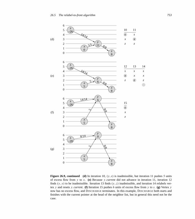
26.5 The relabel-to-front algorithm 753
s–265
4
3
2
1
0
6
x5
y6
z8
58/8
14/14
s–265
4
3
2
1
0
6
x0
y11
z8
8/8
14/14
5/5
s–265
4
3
2
1
0
6
x5
y6
z8
8/8
14/14
5
s–205
4
3
2
1
0
6
x5
y0
z8
58/8
8/14
s
x
z
10
s
x
z
11
s
x
z
12
s
x
z
13
s
x
z
14
s
x
z
15
(f)
(d)
(e)
(g)
Figure 26.9, continued (d) In iteration 10, .y; s/ is inadmissible, but iteration 11 pushes 5 unitsof excess flow from y to x. (e) Because y:current did not advance in iteration 11, iteration 12finds .y; x/ to be inadmissible. Iteration 13 finds .y; ´/ inadmissible, and iteration 14 relabels ver-tex y and resets y:current. (f) Iteration 15 pushes 6 units of excess flow from y to s. (g) Vertex y
now has no excess flow, and DISCHARGE terminates. In this example, DISCHARGE both starts andfinishes with the current pointer at the head of the neighbor list, but in general this need not be thecase.

754 Chapter 26 Maximum Flow
To prove the second statement, according to the test in line 1 and Lemma 26.28,we need only show that all edges leaving u are inadmissible. If a call toDISCHARGE.u/ starts with the pointer u:current at the head of u’s neighbor listand finishes with it off the end of the list, then all of u’s outgoing edges are in-admissible and a relabel operation applies. It is possible, however, that during acall to DISCHARGE.u/, the pointer u:current traverses only part of the list be-fore the procedure returns. Calls to DISCHARGE on other vertices may then oc-cur, but u:current will continue moving through the list during the next call toDISCHARGE.u/. We now consider what happens during a complete pass throughthe list, which begins at the head of u:N and finishes with u:current D NIL. Onceu:current reaches the end of the list, the procedure relabels u and begins a newpass. For the u:current pointer to advance past a vertex � 2 u:N during a pass, theedge .u; �/ must be deemed inadmissible by the test in line 6. Thus, by the timethe pass completes, every edge leaving u has been determined to be inadmissibleat some time during the pass. The key observation is that at the end of the pass,every edge leaving u is still inadmissible. Why? By Lemma 26.27, pushes cannotcreate any admissible edges, regardless of which vertex the flow is pushed from.Thus, any admissible edge must be created by a relabel operation. But the vertex u
is not relabeled during the pass, and by Lemma 26.28, any other vertex � that isrelabeled during the pass (resulting from a call of DISCHARGE.�/) has no enteringadmissible edges after relabeling. Thus, at the end of the pass, all edges leaving u
remain inadmissible, which completes the proof.
The relabel-to-front algorithm
In the relabel-to-front algorithm, we maintain a linked list L consisting of all ver-tices in V � fs; tg. A key property is that the vertices in L are topologically sortedaccording to the admissible network, as we shall see in the loop invariant below.(Recall from Lemma 26.26 that the admissible network is a dag.)
The pseudocode for the relabel-to-front algorithm assumes that the neighborlists u:N have already been created for each vertex u. It also assumes that u:nextpoints to the vertex that follows u in list L and that, as usual, u:next D NIL if u isthe last vertex in the list.
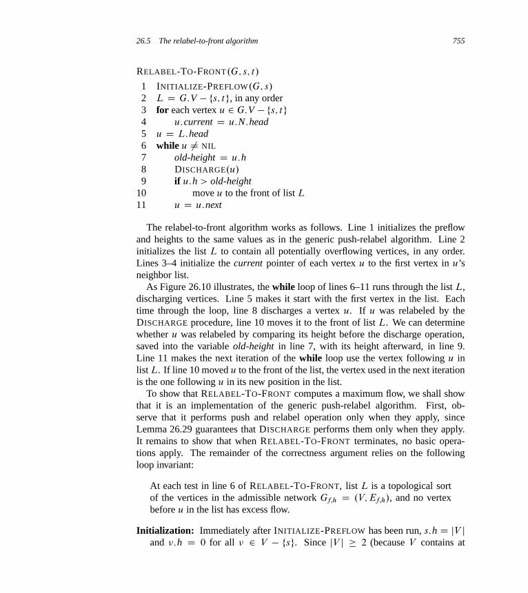
26.5 The relabel-to-front algorithm 755
RELABEL-TO-FRONT.G; s; t/
1 INITIALIZE-PREFLOW.G; s/
2 L D G:V � fs; tg, in any order3 for each vertex u 2 G:V � fs; tg4 u:current D u:N:head5 u D L:head6 while u ¤ NIL
7 old-height D u:h8 DISCHARGE.u/
9 if u:h > old-height10 move u to the front of list L
11 u D u:next
The relabel-to-front algorithm works as follows. Line 1 initializes the preflowand heights to the same values as in the generic push-relabel algorithm. Line 2initializes the list L to contain all potentially overflowing vertices, in any order.Lines 3–4 initialize the current pointer of each vertex u to the first vertex in u’sneighbor list.
As Figure 26.10 illustrates, the while loop of lines 6–11 runs through the list L,discharging vertices. Line 5 makes it start with the first vertex in the list. Eachtime through the loop, line 8 discharges a vertex u. If u was relabeled by theDISCHARGE procedure, line 10 moves it to the front of list L. We can determinewhether u was relabeled by comparing its height before the discharge operation,saved into the variable old-height in line 7, with its height afterward, in line 9.Line 11 makes the next iteration of the while loop use the vertex following u inlist L. If line 10 moved u to the front of the list, the vertex used in the next iterationis the one following u in its new position in the list.
To show that RELABEL-TO-FRONT computes a maximum flow, we shall showthat it is an implementation of the generic push-relabel algorithm. First, ob-serve that it performs push and relabel operation only when they apply, sinceLemma 26.29 guarantees that DISCHARGE performs them only when they apply.It remains to show that when RELABEL-TO-FRONT terminates, no basic opera-tions apply. The remainder of the correctness argument relies on the followingloop invariant:
At each test in line 6 of RELABEL-TO-FRONT, list L is a topological sortof the vertices in the admissible network Gf;h D .V; Ef;h/, and no vertexbefore u in the list has excess flow.
Initialization: Immediately after INITIALIZE-PREFLOW has been run, s:h D jV jand �:h D 0 for all � 2 V � fsg. Since jV j � 2 (because V contains at
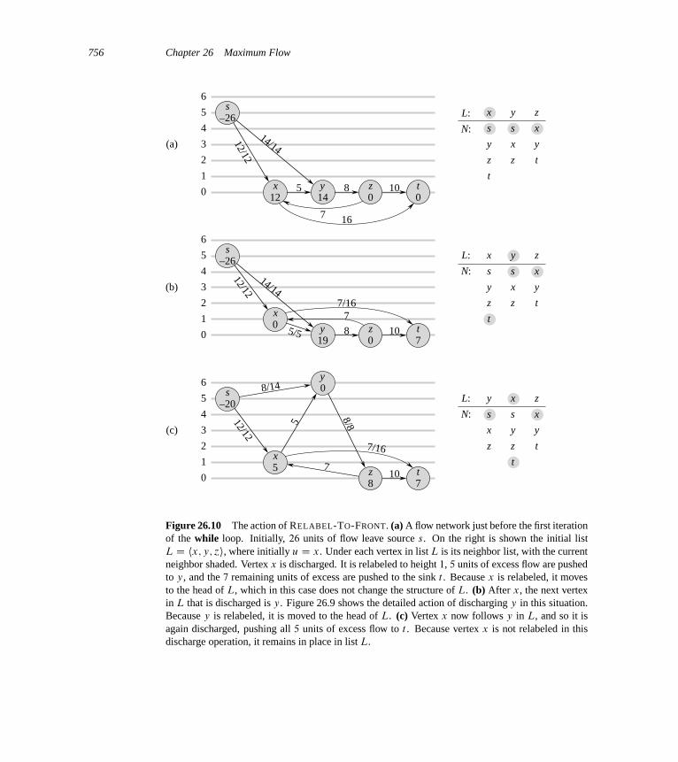
756 Chapter 26 Maximum Flow
s–265
4
3
2
1
0
6
x12
y14
z0
t0
5 8 10
7 16
14/14
12/12
L: x y z
N: s
y
z
t
s
x
z
x
y
t
(a)
s–265
4
3
2
1
0
6
x0 y
19z0
t7
5/5 8 10
14/14
12/12
L: x y z
N: s
y
z
t
s
x
z
x
y
t
(b)
77/16
s–205
4
3
2
1
0
6
x5
y0
z8
t7
5
8/8
10
8/14
12/12
L: xy z
N: s
y
z
t
s
x
z
x
y
t
(c)
7
7/16
Figure 26.10 The action of RELABEL-TO-FRONT. (a) A flow network just before the first iterationof the while loop. Initially, 26 units of flow leave source s. On the right is shown the initial listL D hx; y; ´i, where initially u D x. Under each vertex in list L is its neighbor list, with the currentneighbor shaded. Vertex x is discharged. It is relabeled to height 1, 5 units of excess flow are pushedto y, and the 7 remaining units of excess are pushed to the sink t . Because x is relabeled, it movesto the head of L, which in this case does not change the structure of L. (b) After x, the next vertexin L that is discharged is y. Figure 26.9 shows the detailed action of discharging y in this situation.Because y is relabeled, it is moved to the head of L. (c) Vertex x now follows y in L, and so it isagain discharged, pushing all 5 units of excess flow to t . Because vertex x is not relabeled in thisdischarge operation, it remains in place in list L.
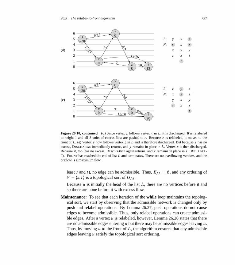
26.5 The relabel-to-front algorithm 757
s–205
4
3
2
1
0
6
x0
y0
z8
t12
5
8/8
10
8/14
12/12
L: xy z
N: s
y
z
t
s
x
z
x
y
t
(d)
7
12/16
s–205
4
3
2
1
0
6
x0
y0
z0 t
20
5
8/88/10
8/14
12/12
L: xyz
N: s
y
z
t
s
x
z
x
y
t
(e)
12/167
Figure 26.10, continued (d) Since vertex ´ follows vertex x in L, it is discharged. It is relabeledto height 1 and all 8 units of excess flow are pushed to t . Because ´ is relabeled, it moves to thefront of L. (e) Vertex y now follows vertex ´ in L and is therefore discharged. But because y has noexcess, DISCHARGE immediately returns, and y remains in place in L. Vertex x is then discharged.Because it, too, has no excess, DISCHARGE again returns, and x remains in place in L. RELABEL-TO-FRONT has reached the end of list L and terminates. There are no overflowing vertices, and thepreflow is a maximum flow.
least s and t), no edge can be admissible. Thus, Ef;h D ;, and any ordering ofV � fs; tg is a topological sort of Gf;h.
Because u is initially the head of the list L, there are no vertices before it andso there are none before it with excess flow.
Maintenance: To see that each iteration of the while loop maintains the topolog-ical sort, we start by observing that the admissible network is changed only bypush and relabel operations. By Lemma 26.27, push operations do not causeedges to become admissible. Thus, only relabel operations can create admissi-ble edges. After a vertex u is relabeled, however, Lemma 26.28 states that thereare no admissible edges entering u but there may be admissible edges leaving u.Thus, by moving u to the front of L, the algorithm ensures that any admissibleedges leaving u satisfy the topological sort ordering.

758 Chapter 26 Maximum Flow
To see that no vertex preceding u in L has excess flow, we denote the vertexthat will be u in the next iteration by u0. The vertices that will precede u0
in the next iteration include the current u (due to line 11) and either no othervertices (if u is relabeled) or the same vertices as before (if u is not relabeled).When u is discharged, it has no excess flow afterward. Thus, if u is relabeledduring the discharge, no vertices preceding u0 have excess flow. If u is notrelabeled during the discharge, no vertices before it on the list acquired excessflow during this discharge, because L remained topologically sorted at all timesduring the discharge (as pointed out just above, admissible edges are createdonly by relabeling, not pushing), and so each push operation causes excess flowto move only to vertices further down the list (or to s or t). Again, no verticespreceding u0 have excess flow.
Termination: When the loop terminates, u is just past the end of L, and so theloop invariant ensures that the excess of every vertex is 0. Thus, no basic oper-ations apply.
Analysis
We shall now show that RELABEL-TO-FRONT runs in O.V 3/ time on any flownetwork G D .V; E/. Since the algorithm is an implementation of the genericpush-relabel algorithm, we shall take advantage of Corollary 26.21, which pro-vides an O.V / bound on the number of relabel operations executed per vertex andan O.V 2/ bound on the total number of relabel operations overall. In addition, Ex-ercise 26.4-3 provides an O.VE/ bound on the total time spent performing relabeloperations, and Lemma 26.22 provides an O.VE/ bound on the total number ofsaturating push operations.
Theorem 26.30The running time of RELABEL-TO-FRONT on any flow network G D .V; E/
is O.V 3/.
Proof Let us consider a “phase” of the relabel-to-front algorithm to be the timebetween two consecutive relabel operations. There are O.V 2/ phases, since thereare O.V 2/ relabel operations. Each phase consists of at most jV j calls to DIS-CHARGE, which we can see as follows. If DISCHARGE does not perform a re-label operation, then the next call to DISCHARGE is further down the list L, andthe length of L is less than jV j. If DISCHARGE does perform a relabel, the nextcall to DISCHARGE belongs to a different phase. Since each phase contains atmost jV j calls to DISCHARGE and there are O.V 2/ phases, the number of timesDISCHARGE is called in line 8 of RELABEL-TO-FRONT is O.V 3/. Thus, the total
26.5 The relabel-to-front algorithm 759
work performed by the while loop in RELABEL-TO-FRONT, excluding the workperformed within DISCHARGE, is at most O.V 3/.
We must now bound the work performed within DISCHARGE during the ex-ecution of the algorithm. Each iteration of the while loop within DISCHARGE
performs one of three actions. We shall analyze the total amount of work involvedin performing each of these actions.
We start with relabel operations (lines 4–5). Exercise 26.4-3 provides an O.VE/
time bound on all the O.V 2/ relabels that are performed.Now, suppose that the action updates the u:current pointer in line 8. This action
occurs O.degree.u// times each time a vertex u is relabeled, and O.V �degree.u//
times overall for the vertex. For all vertices, therefore, the total amount of workdone in advancing pointers in neighbor lists is O.VE/ by the handshaking lemma(Exercise B.4-1).
The third type of action performed by DISCHARGE is a push operation (line 7).We already know that the total number of saturating push operations is O.VE/.Observe that if a nonsaturating push is executed, DISCHARGE immediately returns,since the push reduces the excess to 0. Thus, there can be at most one nonsaturatingpush per call to DISCHARGE. As we have observed, DISCHARGE is called O.V 3/
times, and thus the total time spent performing nonsaturating pushes is O.V 3/.The running time of RELABEL-TO-FRONT is therefore O.V 3 C VE/, which
is O.V 3/.
Exercises
26.5-1Illustrate the execution of RELABEL-TO-FRONT in the manner of Figure 26.10 forthe flow network in Figure 26.1(a). Assume that the initial ordering of vertices in L
is h�1; �2; �3; �4i and that the neighbor lists are
�1:N D hs; �2; �3i ;
�2:N D hs; �1; �3; �4i ;
�3:N D h�1; �2; �4; ti ;
�4:N D h�2; �3; ti :
26.5-2 ?
We would like to implement a push-relabel algorithm in which we maintain a first-in, first-out queue of overflowing vertices. The algorithm repeatedly discharges thevertex at the head of the queue, and any vertices that were not overflowing beforethe discharge but are overflowing afterward are placed at the end of the queue.After the vertex at the head of the queue is discharged, it is removed. When the

760 Chapter 26 Maximum Flow
queue is empty, the algorithm terminates. Show how to implement this algorithmto compute a maximum flow in O.V 3/ time.
26.5-3Show that the generic algorithm still works if RELABEL updates u:h by sim-ply computing u:h D u:h C 1. How would this change affect the analysis ofRELABEL-TO-FRONT?
26.5-4 ?
Show that if we always discharge a highest overflowing vertex, we can make thepush-relabel method run in O.V 3/ time.
26.5-5Suppose that at some point in the execution of a push-relabel algorithm, there existsan integer 0 < k � jV j � 1 for which no vertex has �:h D k. Show that allvertices with �:h > k are on the source side of a minimum cut. If such a k exists,the gap heuristic updates every vertex � 2 V � fsg for which �:h > k to set�:h D max.�:h; jV j C 1/. Show that the resulting attribute h is a height function.(The gap heuristic is crucial in making implementations of the push-relabel methodperform well in practice.)
Problems
26-1 Escape problemAn nn grid is an undirected graph consisting of n rows and n columns of vertices,as shown in Figure 26.11. We denote the vertex in the i th row and the j th columnby .i; j /. All vertices in a grid have exactly four neighbors, except for the boundaryvertices, which are the points .i; j / for which i D 1, i D n, j D 1, or j D n.
Given m � n2 starting points .x1; y1/; .x2; y2/; : : : ; .xm; ym/ in the grid, theescape problem is to determine whether or not there are m vertex-disjoint pathsfrom the starting points to any m different points on the boundary. For example,the grid in Figure 26.11(a) has an escape, but the grid in Figure 26.11(b) does not.
a. Consider a flow network in which vertices, as well as edges, have capacities.That is, the total positive flow entering any given vertex is subject to a capacityconstraint. Show that determining the maximum flow in a network with edgeand vertex capacities can be reduced to an ordinary maximum-flow problem ona flow network of comparable size.
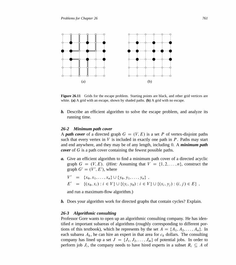
Problems for Chapter 26 761
(a) (b)
Figure 26.11 Grids for the escape problem. Starting points are black, and other grid vertices arewhite. (a) A grid with an escape, shown by shaded paths. (b) A grid with no escape.
b. Describe an efficient algorithm to solve the escape problem, and analyze itsrunning time.
26-2 Minimum path coverA path cover of a directed graph G D .V; E/ is a set P of vertex-disjoint pathssuch that every vertex in V is included in exactly one path in P . Paths may startand end anywhere, and they may be of any length, including 0. A minimum pathcover of G is a path cover containing the fewest possible paths.
a. Give an efficient algorithm to find a minimum path cover of a directed acyclicgraph G D .V; E/. (Hint: Assuming that V D f1; 2; : : : ; ng, construct thegraph G0 D .V 0; E 0/, where
V 0 D fx0; x1; : : : ; xng [ fy0; y1; : : : ; yng ;
E 0 D f.x0; xi / W i 2 V g [ f.yi ; y0/ W i 2 V g [ f.xi ; yj / W .i; j / 2 Eg ;
and run a maximum-flow algorithm.)
b. Does your algorithm work for directed graphs that contain cycles? Explain.
26-3 Algorithmic consultingProfessor Gore wants to open up an algorithmic consulting company. He has iden-tified n important subareas of algorithms (roughly corresponding to different por-tions of this textbook), which he represents by the set A D fA1; A2; : : : ; Ang. Ineach subarea Ak, he can hire an expert in that area for ck dollars. The consultingcompany has lined up a set J D fJ1; J2; : : : ; Jmg of potential jobs. In order toperform job Ji , the company needs to have hired experts in a subset Ri � A of

762 Chapter 26 Maximum Flow
subareas. Each expert can work on multiple jobs simultaneously. If the companychooses to accept job Ji , it must have hired experts in all subareas in Ri , and it willtake in revenue of pi dollars.
Professor Gore’s job is to determine which subareas to hire experts in and whichjobs to accept in order to maximize the net revenue, which is the total income fromjobs accepted minus the total cost of employing the experts.
Consider the following flow network G. It contains a source vertex s, verticesA1; A2; : : : ; An, vertices J1; J2; : : : ; Jm, and a sink vertex t . For k D 1; 2 : : : ; n,the flow network contains an edge .s; Ak/ with capacity c.s; Ak/ D ck, andfor i D 1; 2; : : : ; m, the flow network contains an edge .Ji ; t/ with capacityc.Ji ; t/ D pi . For k D 1; 2; : : : ; n and i D 1; 2; : : : ; m, if Ak 2 Ri , then G
contains an edge .Ak; Ji / with capacity c.Ak; Ji / D1.
a. Show that if Ji 2 T for a finite-capacity cut .S; T / of G, then Ak 2 T for eachAk 2 Ri .
b. Show how to determine the maximum net revenue from the capacity of a mini-mum cut of G and the given pi values.
c. Give an efficient algorithm to determine which jobs to accept and which expertsto hire. Analyze the running time of your algorithm in terms of m, n, andr DPm
iD1 jRi j.
26-4 Updating maximum flowLet G D .V; E/ be a flow network with source s, sink t , and integer capacities.Suppose that we are given a maximum flow in G.
a. Suppose that we increase the capacity of a single edge .u; �/ 2 E by 1. Givean O.V CE/-time algorithm to update the maximum flow.
b. Suppose that we decrease the capacity of a single edge .u; �/ 2 E by 1. Givean O.V CE/-time algorithm to update the maximum flow.
26-5 Maximum flow by scalingLet G D .V; E/ be a flow network with source s, sink t , and an integer capac-ity c.u; �/ on each edge .u; �/ 2 E. Let C D max.u;�/2E c.u; �/.
a. Argue that a minimum cut of G has capacity at most C jEj.
b. For a given number K, show how to find an augmenting path of capacity atleast K in O.E/ time, if such a path exists.

Problems for Chapter 26 763
We can use the following modification of FORD-FULKERSON-METHOD to com-pute a maximum flow in G:
MAX-FLOW-BY-SCALING.G; s; t/
1 C D max.u;�/2E c.u; �/
2 initialize flow f to 0
3 K D 2blg C c
4 while K � 1
5 while there exists an augmenting path p of capacity at least K
6 augment flow f along p
7 K D K=2
8 return f
c. Argue that MAX-FLOW-BY-SCALING returns a maximum flow.
d. Show that the capacity of a minimum cut of the residual network Gf is at most2K jEj each time line 4 is executed.
e. Argue that the inner while loop of lines 5–6 executes O.E/ times for each valueof K.
f. Conclude that MAX-FLOW-BY-SCALING can be implemented so that it runsin O.E2 lg C / time.
26-6 The Hopcroft-Karp bipartite matching algorithmIn this problem, we describe a faster algorithm, due to Hopcroft and Karp, forfinding a maximum matching in a bipartite graph. The algorithm runs in O.
pV E/
time. Given an undirected, bipartite graph G D .V; E/, where V D L [ R andall edges have exactly one endpoint in L, let M be a matching in G. We say thata simple path P in G is an augmenting path with respect to M if it starts at anunmatched vertex in L, ends at an unmatched vertex in R, and its edges belongalternately to M and E � M . (This definition of an augmenting path is relatedto, but different from, an augmenting path in a flow network.) In this problem,we treat a path as a sequence of edges, rather than as a sequence of vertices. Ashortest augmenting path with respect to a matching M is an augmenting pathwith a minimum number of edges.
Given two sets A and B , the symmetric difference A˚B is defined as .A�B/[.B � A/, that is, the elements that are in exactly one of the two sets.

764 Chapter 26 Maximum Flow
a. Show that if M is a matching and P is an augmenting path with respect to M ,then the symmetric difference M ˚P is a matching and jM ˚ P j D jM j C 1.Show that if P1; P2; : : : ; Pk are vertex-disjoint augmenting paths with respectto M , then the symmetric difference M ˚ .P1 [ P2 [ � � � [ Pk/ is a matchingwith cardinality jM j C k.
The general structure of our algorithm is the following:
HOPCROFT-KARP.G/
1 M D ;2 repeat3 let P D fP1; P2; : : : ; Pkg be a maximal set of vertex-disjoint
shortest augmenting paths with respect to M
4 M D M ˚ .P1 [ P2 [ � � � [ Pk/
5 until P == ;6 return M
The remainder of this problem asks you to analyze the number of iterations inthe algorithm (that is, the number of iterations in the repeat loop) and to describean implementation of line 3.
b. Given two matchings M and M � in G, show that every vertex in the graphG0 D .V; M ˚ M �/ has degree at most 2. Conclude that G0 is a disjointunion of simple paths or cycles. Argue that edges in each such simple pathor cycle belong alternately to M or M �. Prove that if jM j � jM �j, thenM ˚M � contains at least jM �j � jM j vertex-disjoint augmenting paths withrespect to M .
Let l be the length of a shortest augmenting path with respect to a matching M , andlet P1; P2; : : : ; Pk be a maximal set of vertex-disjoint augmenting paths of length l
with respect to M . Let M 0 D M˚.P1[� � �[Pk/, and suppose that P is a shortestaugmenting path with respect to M 0.
c. Show that if P is vertex-disjoint from P1; P2; : : : ; Pk, then P has more than l
edges.
d. Now suppose that P is not vertex-disjoint from P1; P2; : : : ; Pk . Let A be theset of edges .M ˚M 0/˚ P . Show that A D .P1 [ P2 [ � � � [ Pk/˚ P andthat jAj � .k C 1/l . Conclude that P has more than l edges.
e. Prove that if a shortest augmenting path with respect to M has l edges, the sizeof the maximum matching is at most jM j C jV j =.l C 1/.

Notes for Chapter 26 765
f. Show that the number of repeat loop iterations in the algorithm is at most 2p
V .(Hint: By how much can M grow after iteration number
pV ?)
g. Give an algorithm that runs in O.E/ time to find a maximal set of vertex-disjoint shortest augmenting paths P1; P2; : : : ; Pk for a given matching M .Conclude that the total running time of HOPCROFT-KARP is O.
pV E/.
Chapter notes
Ahuja, Magnanti, and Orlin [7], Even [103], Lawler [224], Papadimitriou and Stei-glitz [271], and Tarjan [330] are good references for network flow and related algo-rithms. Goldberg, Tardos, and Tarjan [139] also provide a nice survey of algorithmsfor network-flow problems, and Schrijver [304] has written an interesting reviewof historical developments in the field of network flows.
The Ford-Fulkerson method is due to Ford and Fulkerson [109], who originatedthe formal study of many of the problems in the area of network flow, includingthe maximum-flow and bipartite-matching problems. Many early implementationsof the Ford-Fulkerson method found augmenting paths using breadth-first search;Edmonds and Karp [102], and independently Dinic [90], proved that this strategyyields a polynomial-time algorithm. A related idea, that of using “blocking flows,”was also first developed by Dinic [90]. Karzanov [202] first developed the idea ofpreflows. The push-relabel method is due to Goldberg [136] and Goldberg and Tar-jan [140]. Goldberg and Tarjan gave an O.V 3/-time algorithm that uses a queue tomaintain the set of overflowing vertices, as well as an algorithm that uses dynamictrees to achieve a running time of O.VE lg.V 2=EC2//. Several other researchershave developed push-relabel maximum-flow algorithms. Ahuja and Orlin [9] andAhuja, Orlin, and Tarjan [10] gave algorithms that used scaling. Cheriyan andMaheshwari [63] proposed pushing flow from the overflowing vertex of maximumheight. Cheriyan and Hagerup [62] suggested randomly permuting the neighborlists, and several researchers [14, 204, 276] developed clever derandomizations ofthis idea, leading to a sequence of faster algorithms. The algorithm of King, Rao,and Tarjan [204] is the fastest such algorithm and runs in O.VE logE=.V lg V / V /
time.The asymptotically fastest algorithm to date for the maximum-flow problem, by
Goldberg and Rao [138], runs in time O.min.V 2=3; E1=2/E lg.V 2=E C 2/ lg C /,where C D max.u;�/2E c.u; �/. This algorithm does not use the push-relabelmethod but instead is based on finding blocking flows. All previous maximum-flow algorithms, including the ones in this chapter, use some notion of distance(the push-relabel algorithms use the analogous notion of height), with a length of 1

766 Chapter 26 Maximum Flow
assigned implicitly to each edge. This new algorithm takes a different approach andassigns a length of 0 to high-capacity edges and a length of 1 to low-capacity edges.Informally, with respect to these lengths, shortest paths from the source to the sinktend have high capacity, which means that fewer iterations need be performed.
In practice, push-relabel algorithms currently dominate augmenting-path orlinear-programming based algorithms for the maximum-flow problem. A studyby Cherkassky and Goldberg [64] underscores the importance of using two heuris-tics when implementing a push-relabel algorithm. The first heuristic is to peri-odically perform a breadth-first search of the residual network in order to obtainmore accurate height values. The second heuristic is the gap heuristic, described inExercise 26.5-5. Cherkassky and Goldberg conclude that the best choice of push-relabel variants is the one that chooses to discharge the overflowing vertex with themaximum height.
The best algorithm to date for maximum bipartite matching, discovered byHopcroft and Karp [176], runs in O.
pV E/ time and is described in Problem 26-6.
The book by Lovász and Plummer [239] is an excellent reference on matchingproblems.


VII Selected Topics
Introduction
This part contains a selection of algorithmic topics that extend and complementearlier material in this book. Some chapters introduce new models of computationsuch as circuits or parallel computers. Others cover specialized domains such ascomputational geometry or number theory. The last two chapters discuss some ofthe known limitations to the design of efficient algorithms and introduce techniquesfor coping with those limitations.
Chapter 27 presents an algorithmic model for parallel computing based on dy-namic multithreading. The chapter introduces the basics of the model, showinghow to quantify parallelism in terms of the measures of work and span. It theninvestigates several interesting multithreaded algorithms, including algorithms formatrix multiplication and merge sorting.
Chapter 28 studies efficient algorithms for operating on matrices. It presentstwo general methods—LU decomposition and LUP decomposition—for solvinglinear equations by Gaussian elimination in O.n3/ time. It also shows that matrixinversion and matrix multiplication can be performed equally fast. The chapterconcludes by showing how to compute a least-squares approximate solution whena set of linear equations has no exact solution.
Chapter 29 studies linear programming, in which we wish to maximize or mini-mize an objective, given limited resources and competing constraints. Linear pro-gramming arises in a variety of practical application areas. This chapter covers howto formulate and solve linear programs. The solution method covered is the sim-plex algorithm, which is the oldest algorithm for linear programming. In contrastto many algorithms in this book, the simplex algorithm does not run in polynomialtime in the worst case, but it is fairly efficient and widely used in practice.

770 Part VII Selected Topics
Chapter 30 studies operations on polynomials and shows how to use a well-known signal-processing technique—the fast Fourier transform (FFT)—to multi-ply two degree-n polynomials in O.n lg n/ time. It also investigates efficient im-plementations of the FFT, including a parallel circuit.
Chapter 31 presents number-theoretic algorithms. After reviewing elementarynumber theory, it presents Euclid’s algorithm for computing greatest common di-visors. Next, it studies algorithms for solving modular linear equations and forraising one number to a power modulo another number. Then, it explores an impor-tant application of number-theoretic algorithms: the RSA public-key cryptosystem.This cryptosystem can be used not only to encrypt messages so that an adversarycannot read them, but also to provide digital signatures. The chapter then presentsthe Miller-Rabin randomized primality test, with which we can find large primesefficiently—an essential requirement for the RSA system. Finally, the chapter cov-ers Pollard’s “rho” heuristic for factoring integers and discusses the state of the artof integer factorization.
Chapter 32 studies the problem of finding all occurrences of a given patternstring in a given text string, a problem that arises frequently in text-editing pro-grams. After examining the naive approach, the chapter presents an elegant ap-proach due to Rabin and Karp. Then, after showing an efficient solution basedon finite automata, the chapter presents the Knuth-Morris-Pratt algorithm, whichmodifies the automaton-based algorithm to save space by cleverly preprocessingthe pattern.
Chapter 33 considers a few problems in computational geometry. After dis-cussing basic primitives of computational geometry, the chapter shows how to usea “sweeping” method to efficiently determine whether a set of line segments con-tains any intersections. Two clever algorithms for finding the convex hull of a set ofpoints—Graham’s scan and Jarvis’s march—also illustrate the power of sweepingmethods. The chapter closes with an efficient algorithm for finding the closest pairfrom among a given set of points in the plane.
Chapter 34 concerns NP-complete problems. Many interesting computationalproblems are NP-complete, but no polynomial-time algorithm is known for solvingany of them. This chapter presents techniques for determining when a problem isNP-complete. Several classic problems are proved to be NP-complete: determiningwhether a graph has a hamiltonian cycle, determining whether a boolean formulais satisfiable, and determining whether a given set of numbers has a subset thatadds up to a given target value. The chapter also proves that the famous traveling-salesman problem is NP-complete.
Chapter 35 shows how to find approximate solutions to NP-complete problemsefficiently by using approximation algorithms. For some NP-complete problems,approximate solutions that are near optimal are quite easy to produce, but for otherseven the best approximation algorithms known work progressively more poorly as

Part VII Selected Topics 771
the problem size increases. Then, there are some problems for which we can investincreasing amounts of computation time in return for increasingly better approx-imate solutions. This chapter illustrates these possibilities with the vertex-coverproblem (unweighted and weighted versions), an optimization version of 3-CNFsatisfiability, the traveling-salesman problem, the set-covering problem, and thesubset-sum problem.
27 Multithreaded Algorithms
The vast majority of algorithms in this book are serial algorithms suitable forrunning on a uniprocessor computer in which only one instruction executes at atime. In this chapter, we shall extend our algorithmic model to encompass parallelalgorithms, which can run on a multiprocessor computer that permits multipleinstructions to execute concurrently. In particular, we shall explore the elegantmodel of dynamic multithreaded algorithms, which are amenable to algorithmicdesign and analysis, as well as to efficient implementation in practice.
Parallel computers—computers with multiple processing units—have becomeincreasingly common, and they span a wide range of prices and performance. Rela-tively inexpensive desktop and laptop chip multiprocessors contain a single multi-core integrated-circuit chip that houses multiple processing “cores,” each of whichis a full-fledged processor that can access a common memory. At an intermedi-ate price/performance point are clusters built from individual computers—oftensimple PC-class machines—with a dedicated network interconnecting them. Thehighest-priced machines are supercomputers, which often use a combination ofcustom architectures and custom networks to deliver the highest performance interms of instructions executed per second.
Multiprocessor computers have been around, in one form or another, fordecades. Although the computing community settled on the random-access ma-chine model for serial computing early on in the history of computer science, nosingle model for parallel computing has gained as wide acceptance. A major rea-son is that vendors have not agreed on a single architectural model for parallelcomputers. For example, some parallel computers feature shared memory, whereeach processor can directly access any location of memory. Other parallel com-puters employ distributed memory, where each processor’s memory is private, andan explicit message must be sent between processors in order for one processor toaccess the memory of another. With the advent of multicore technology, however,every new laptop and desktop machine is now a shared-memory parallel computer,

Chapter 27 Multithreaded Algorithms 773
and the trend appears to be toward shared-memory multiprocessing. Although timewill tell, that is the approach we shall take in this chapter.
One common means of programming chip multiprocessors and other shared-memory parallel computers is by using static threading, which provides a softwareabstraction of “virtual processors,” or threads, sharing a common memory. Eachthread maintains an associated program counter and can execute code indepen-dently of the other threads. The operating system loads a thread onto a processorfor execution and switches it out when another thread needs to run. Although theoperating system allows programmers to create and destroy threads, these opera-tions are comparatively slow. Thus, for most applications, threads persist for theduration of a computation, which is why we call them “static.”
Unfortunately, programming a shared-memory parallel computer directly usingstatic threads is difficult and error-prone. One reason is that dynamically parti-tioning the work among the threads so that each thread receives approximatelythe same load turns out to be a complicated undertaking. For any but the sim-plest of applications, the programmer must use complex communication protocolsto implement a scheduler to load-balance the work. This state of affairs has ledtoward the creation of concurrency platforms, which provide a layer of softwarethat coordinates, schedules, and manages the parallel-computing resources. Someconcurrency platforms are built as runtime libraries, but others provide full-fledgedparallel languages with compiler and runtime support.
Dynamic multithreaded programming
One important class of concurrency platform is dynamic multithreading, which isthe model we shall adopt in this chapter. Dynamic multithreading allows program-mers to specify parallelism in applications without worrying about communicationprotocols, load balancing, and other vagaries of static-thread programming. Theconcurrency platform contains a scheduler, which load-balances the computationautomatically, thereby greatly simplifying the programmer’s chore. Although thefunctionality of dynamic-multithreading environments is still evolving, almost allsupport two features: nested parallelism and parallel loops. Nested parallelismallows a subroutine to be “spawned,” allowing the caller to proceed while thespawned subroutine is computing its result. A parallel loop is like an ordinaryfor loop, except that the iterations of the loop can execute concurrently.
These two features form the basis of the model for dynamic multithreading thatwe shall study in this chapter. A key aspect of this model is that the programmerneeds to specify only the logical parallelism within a computation, and the threadswithin the underlying concurrency platform schedule and load-balance the compu-tation among themselves. We shall investigate multithreaded algorithms written for

774 Chapter 27 Multithreaded Algorithms
this model, as well how the underlying concurrency platform can schedule compu-tations efficiently.
Our model for dynamic multithreading offers several important advantages:
� It is a simple extension of our serial programming model. We can describe amultithreaded algorithm by adding to our pseudocode just three “concurrency”keywords: parallel, spawn, and sync. Moreover, if we delete these concur-rency keywords from the multithreaded pseudocode, the resulting text is serialpseudocode for the same problem, which we call the “serialization” of the mul-tithreaded algorithm.
� It provides a theoretically clean way to quantify parallelism based on the no-tions of “work” and “span.”
� Many multithreaded algorithms involving nested parallelism follow naturallyfrom the divide-and-conquer paradigm. Moreover, just as serial divide-and-conquer algorithms lend themselves to analysis by solving recurrences, so domultithreaded algorithms.
� The model is faithful to how parallel-computing practice is evolving. A grow-ing number of concurrency platforms support one variant or another of dynamicmultithreading, including Cilk [51, 118], Cilk++ [72], OpenMP [60], Task Par-allel Library [230], and Threading Building Blocks [292].
Section 27.1 introduces the dynamic multithreading model and presents the met-rics of work, span, and parallelism, which we shall use to analyze multithreadedalgorithms. Section 27.2 investigates how to multiply matrices with multithread-ing, and Section 27.3 tackles the tougher problem of multithreading merge sort.
27.1 The basics of dynamic multithreading
We shall begin our exploration of dynamic multithreading using the example ofcomputing Fibonacci numbers recursively. Recall that the Fibonacci numbers aredefined by recurrence (3.22):
F0 D 0 ;
F1 D 1 ;
Fi D Fi�1 C Fi�2 for i � 2 :
Here is a simple, recursive, serial algorithm to compute the nth Fibonacci number:
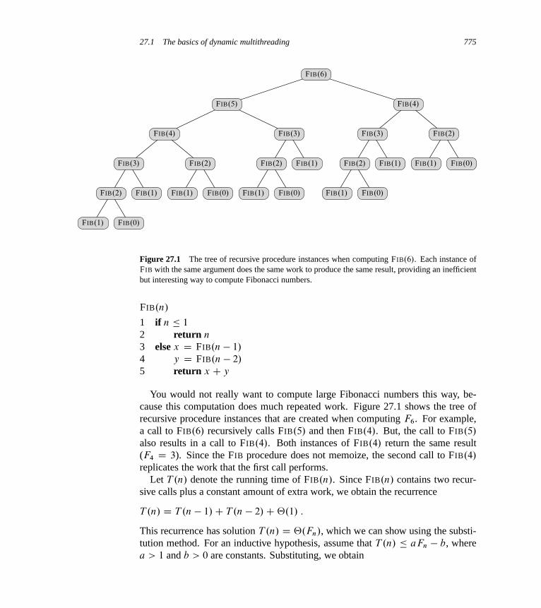
27.1 The basics of dynamic multithreading 775
FIB.0/
FIB.0/FIB.0/FIB.0/
FIB.0/
FIB.1/FIB.1/
FIB.1/
FIB.1/
FIB.1/FIB.1/FIB.1/
FIB.1/
FIB.2/
FIB.2/FIB.2/FIB.2/
FIB.2/
FIB.3/FIB.3/
FIB.3/
FIB.4/
FIB.4/
FIB.5/
FIB.6/
Figure 27.1 The tree of recursive procedure instances when computing FIB.6/. Each instance ofFIB with the same argument does the same work to produce the same result, providing an inefficientbut interesting way to compute Fibonacci numbers.
FIB.n/
1 if n � 1
2 return n
3 else x D FIB.n � 1/
4 y D FIB.n � 2/
5 return x C y
You would not really want to compute large Fibonacci numbers this way, be-cause this computation does much repeated work. Figure 27.1 shows the tree ofrecursive procedure instances that are created when computing F6. For example,a call to FIB.6/ recursively calls FIB.5/ and then FIB.4/. But, the call to FIB.5/
also results in a call to FIB.4/. Both instances of FIB.4/ return the same result(F4 D 3). Since the FIB procedure does not memoize, the second call to FIB.4/
replicates the work that the first call performs.Let T .n/ denote the running time of FIB.n/. Since FIB.n/ contains two recur-
sive calls plus a constant amount of extra work, we obtain the recurrence
T .n/ D T .n � 1/C T .n � 2/C‚.1/ :
This recurrence has solution T .n/ D ‚.Fn/, which we can show using the substi-tution method. For an inductive hypothesis, assume that T .n/ � aFn � b, wherea > 1 and b > 0 are constants. Substituting, we obtain
776 Chapter 27 Multithreaded Algorithms
T .n/ � .aFn�1 � b/C .aFn�2 � b/C‚.1/
D a.Fn�1 C Fn�2/ � 2b C‚.1/
D aFn � b � .b �‚.1//
� aFn � b
if we choose b large enough to dominate the constant in the ‚.1/. We can thenchoose a large enough to satisfy the initial condition. The analytical bound
T .n/ D ‚.�n/ ; (27.1)
where � D .1 C p5/=2 is the golden ratio, now follows from equation (3.25).Since Fn grows exponentially in n, this procedure is a particularly slow way tocompute Fibonacci numbers. (See Problem 31-3 for much faster ways.)
Although the FIB procedure is a poor way to compute Fibonacci numbers, itmakes a good example for illustrating key concepts in the analysis of multithreadedalgorithms. Observe that within FIB.n/, the two recursive calls in lines 3 and 4 toFIB.n� 1/ and FIB.n� 2/, respectively, are independent of each other: they couldbe called in either order, and the computation performed by one in no way affectsthe other. Therefore, the two recursive calls can run in parallel.
We augment our pseudocode to indicate parallelism by adding the concurrencykeywords spawn and sync. Here is how we can rewrite the FIB procedure to usedynamic multithreading:
P-FIB.n/
1 if n � 1
2 return n
3 else x D spawn P-FIB.n � 1/
4 y D P-FIB.n � 2/
5 sync6 return x C y
Notice that if we delete the concurrency keywords spawn and sync from P-FIB,the resulting pseudocode text is identical to FIB (other than renaming the procedurein the header and in the two recursive calls). We define the serialization of a mul-tithreaded algorithm to be the serial algorithm that results from deleting the multi-threaded keywords: spawn, sync, and when we examine parallel loops, parallel.Indeed, our multithreaded pseudocode has the nice property that a serialization isalways ordinary serial pseudocode to solve the same problem.
Nested parallelism occurs when the keyword spawn precedes a procedure call,as in line 3. The semantics of a spawn differs from an ordinary procedure call inthat the procedure instance that executes the spawn—the parent—may continueto execute in parallel with the spawned subroutine—its child—instead of waiting

27.1 The basics of dynamic multithreading 777
for the child to complete, as would normally happen in a serial execution. In thiscase, while the spawned child is computing P-FIB.n � 1/, the parent may go onto compute P-FIB.n � 2/ in line 4 in parallel with the spawned child. Since theP-FIB procedure is recursive, these two subroutine calls themselves create nestedparallelism, as do their children, thereby creating a potentially vast tree of subcom-putations, all executing in parallel.
The keyword spawn does not say, however, that a procedure must execute con-currently with its spawned children, only that it may. The concurrency keywordsexpress the logical parallelism of the computation, indicating which parts of thecomputation may proceed in parallel. At runtime, it is up to a scheduler to deter-mine which subcomputations actually run concurrently by assigning them to avail-able processors as the computation unfolds. We shall discuss the theory behindschedulers shortly.
A procedure cannot safely use the values returned by its spawned children untilafter it executes a sync statement, as in line 5. The keyword sync indicates thatthe procedure must wait as necessary for all its spawned children to complete be-fore proceeding to the statement after the sync. In the P-FIB procedure, a syncis required before the return statement in line 6 to avoid the anomaly that wouldoccur if x and y were summed before x was computed. In addition to explicitsynchronization provided by the sync statement, every procedure executes a syncimplicitly before it returns, thus ensuring that all its children terminate before itdoes.
A model for multithreaded execution
It helps to think of a multithreaded computation—the set of runtime instruc-tions executed by a processor on behalf of a multithreaded program—as a directedacyclic graph G D .V; E/, called a computation dag. As an example, Figure 27.2shows the computation dag that results from computing P-FIB.4/. Conceptually,the vertices in V are instructions, and the edges in E represent dependencies be-tween instructions, where .u; �/ 2 E means that instruction u must execute beforeinstruction �. For convenience, however, if a chain of instructions contains noparallel control (no spawn, sync, or return from a spawn—via either an explicitreturn statement or the return that happens implicitly upon reaching the end ofa procedure), we may group them into a single strand, each of which representsone or more instructions. Instructions involving parallel control are not includedin strands, but are represented in the structure of the dag. For example, if a strandhas two successors, one of them must have been spawned, and a strand with mul-tiple predecessors indicates the predecessors joined because of a sync statement.Thus, in the general case, the set V forms the set of strands, and the set E of di-rected edges represents dependencies between strands induced by parallel control.

778 Chapter 27 Multithreaded Algorithms
P-FIB(1) P-FIB(0)
P-FIB(3)
P-FIB(4)
P-FIB(1)
P-FIB(1)
P-FIB(0)
P-FIB(2)
P-FIB(2)
Figure 27.2 A directed acyclic graph representing the computation of P-FIB.4/. Each circle rep-resents one strand, with black circles representing either base cases or the part of the procedure(instance) up to the spawn of P-FIB.n � 1/ in line 3, shaded circles representing the part of the pro-cedure that calls P-FIB.n� 2/ in line 4 up to the sync in line 5, where it suspends until the spawn ofP-FIB.n � 1/ returns, and white circles representing the part of the procedure after the sync whereit sums x and y up to the point where it returns the result. Each group of strands belonging to thesame procedure is surrounded by a rounded rectangle, lightly shaded for spawned procedures andheavily shaded for called procedures. Spawn edges and call edges point downward, continuationedges point horizontally to the right, and return edges point upward. Assuming that each strand takesunit time, the work equals 17 time units, since there are 17 strands, and the span is 8 time units, sincethe critical path—shown with shaded edges—contains 8 strands.
If G has a directed path from strand u to strand �, we say that the two strands are(logically) in series. Otherwise, strands u and � are (logically) in parallel.
We can picture a multithreaded computation as a dag of strands embedded in atree of procedure instances. For example, Figure 27.1 shows the tree of procedureinstances for P-FIB.6/ without the detailed structure showing strands. Figure 27.2zooms in on a section of that tree, showing the strands that constitute each proce-dure. All directed edges connecting strands run either within a procedure or alongundirected edges in the procedure tree.
We can classify the edges of a computation dag to indicate the kind of dependen-cies between the various strands. A continuation edge .u; u0/, drawn horizontallyin Figure 27.2, connects a strand u to its successor u0 within the same procedureinstance. When a strand u spawns a strand �, the dag contains a spawn edge .u; �/,which points downward in the figure. Call edges, representing normal procedurecalls, also point downward. Strand u spawning strand � differs from u calling �
in that a spawn induces a horizontal continuation edge from u to the strand u0 fol-

27.1 The basics of dynamic multithreading 779
lowing u in its procedure, indicating that u0 is free to execute at the same timeas �, whereas a call induces no such edge. When a strand u returns to its callingprocedure and x is the strand immediately following the next sync in the callingprocedure, the computation dag contains return edge .u; x/, which points upward.A computation starts with a single initial strand—the black vertex in the procedurelabeled P-FIB.4/ in Figure 27.2—and ends with a single final strand—the whitevertex in the procedure labeled P-FIB.4/.
We shall study the execution of multithreaded algorithms on an ideal paral-lel computer, which consists of a set of processors and a sequentially consistentshared memory. Sequential consistency means that the shared memory, which mayin reality be performing many loads and stores from the processors at the sametime, produces the same results as if at each step, exactly one instruction from oneof the processors is executed. That is, the memory behaves as if the instructionswere executed sequentially according to some global linear order that preserves theindividual orders in which each processor issues its own instructions. For dynamicmultithreaded computations, which are scheduled onto processors automaticallyby the concurrency platform, the shared memory behaves as if the multithreadedcomputation’s instructions were interleaved to produce a linear order that preservesthe partial order of the computation dag. Depending on scheduling, the orderingcould differ from one run of the program to another, but the behavior of any exe-cution can be understood by assuming that the instructions are executed in somelinear order consistent with the computation dag.
In addition to making assumptions about semantics, the ideal-parallel-computermodel makes some performance assumptions. Specifically, it assumes that eachprocessor in the machine has equal computing power, and it ignores the cost ofscheduling. Although this last assumption may sound optimistic, it turns out thatfor algorithms with sufficient “parallelism” (a term we shall define precisely in amoment), the overhead of scheduling is generally minimal in practice.
Performance measures
We can gauge the theoretical efficiency of a multithreaded algorithm by using twometrics: “work” and “span.” The work of a multithreaded computation is the totaltime to execute the entire computation on one processor. In other words, the workis the sum of the times taken by each of the strands. For a computation dag inwhich each strand takes unit time, the work is just the number of vertices in thedag. The span is the longest time to execute the strands along any path in the dag.Again, for a dag in which each strand takes unit time, the span equals the number ofvertices on a longest or critical path in the dag. (Recall from Section 24.2 that wecan find a critical path in a dag G D .V; E/ in ‚.V C E/ time.) For example, thecomputation dag of Figure 27.2 has 17 vertices in all and 8 vertices on its critical
780 Chapter 27 Multithreaded Algorithms
path, so that if each strand takes unit time, its work is 17 time units and its spanis 8 time units.
The actual running time of a multithreaded computation depends not only onits work and its span, but also on how many processors are available and howthe scheduler allocates strands to processors. To denote the running time of amultithreaded computation on P processors, we shall subscript by P . For example,we might denote the running time of an algorithm on P processors by TP . Thework is the running time on a single processor, or T1. The span is the running timeif we could run each strand on its own processor—in other words, if we had anunlimited number of processors—and so we denote the span by T1.
The work and span provide lower bounds on the running time TP of a multi-threaded computation on P processors:
� In one step, an ideal parallel computer with P processors can do at most P
units of work, and thus in TP time, it can perform at most P TP work. Since thetotal work to do is T1, we have P TP � T1. Dividing by P yields the work law:
TP � T1=P : (27.2)
� A P -processor ideal parallel computer cannot run any faster than a machinewith an unlimited number of processors. Looked at another way, a machinewith an unlimited number of processors can emulate a P -processor machine byusing just P of its processors. Thus, the span law follows:
TP � T1 : (27.3)
We define the speedup of a computation on P processors by the ratio T1=TP ,which says how many times faster the computation is on P processors thanon 1 processor. By the work law, we have TP � T1=P which implies thatT1=TP � P . Thus, the speedup on P processors can be at most P . When thespeedup is linear in the number of processors, that is, when T1=TP D ‚.P /, thecomputation exhibits linear speedup, and when T1=TP D P , we have perfectlinear speedup.
The ratio T1=T1 of the work to the span gives the parallelism of the multi-threaded computation. We can view the parallelism from three perspectives. As aratio, the parallelism denotes the average amount of work that can be performed inparallel for each step along the critical path. As an upper bound, the parallelismgives the maximum possible speedup that can be achieved on any number of pro-cessors. Finally, and perhaps most important, the parallelism provides a limit onthe possibility of attaining perfect linear speedup. Specifically, once the number ofprocessors exceeds the parallelism, the computation cannot possibly achieve per-fect linear speedup. To see this last point, suppose that P > T1=T1, in which case

27.1 The basics of dynamic multithreading 781
the span law implies that the speedup satisfies T1=TP � T1=T1 < P . Moreover,if the number P of processors in the ideal parallel computer greatly exceeds theparallelism—that is, if P � T1=T1—then T1=TP � P , so that the speedup ismuch less than the number of processors. In other words, the more processors weuse beyond the parallelism, the less perfect the speedup.
As an example, consider the computation P-FIB.4/ in Figure 27.2, and assumethat each strand takes unit time. Since the work is T1 D 17 and the span is T1 D 8,the parallelism is T1=T1 D 17=8 D 2:125. Consequently, achieving much morethan double the speedup is impossible, no matter how many processors we em-ploy to execute the computation. For larger input sizes, however, we shall see thatP-FIB.n/ exhibits substantial parallelism.
We define the (parallel) slackness of a multithreaded computation executedon an ideal parallel computer with P processors to be the ratio .T1=T1/=P DT1=.P T1/, which is the factor by which the parallelism of the computation ex-ceeds the number of processors in the machine. Thus, if the slackness is less than 1,we cannot hope to achieve perfect linear speedup, because T1=.P T1/ < 1 and thespan law imply that the speedup on P processors satisfies T1=TP � T1=T1 < P .Indeed, as the slackness decreases from 1 toward 0, the speedup of the computationdiverges further and further from perfect linear speedup. If the slackness is greaterthan 1, however, the work per processor is the limiting constraint. As we shall see,as the slackness increases from 1, a good scheduler can achieve closer and closerto perfect linear speedup.
Scheduling
Good performance depends on more than just minimizing the work and span. Thestrands must also be scheduled efficiently onto the processors of the parallel ma-chine. Our multithreaded programming model provides no way to specify whichstrands to execute on which processors. Instead, we rely on the concurrency plat-form’s scheduler to map the dynamically unfolding computation to individual pro-cessors. In practice, the scheduler maps the strands to static threads, and the op-erating system schedules the threads on the processors themselves, but this extralevel of indirection is unnecessary for our understanding of scheduling. We canjust imagine that the concurrency platform’s scheduler maps strands to processorsdirectly.
A multithreaded scheduler must schedule the computation with no advanceknowledge of when strands will be spawned or when they will complete—it mustoperate on-line. Moreover, a good scheduler operates in a distributed fashion,where the threads implementing the scheduler cooperate to load-balance the com-putation. Provably good on-line, distributed schedulers exist, but analyzing themis complicated.
782 Chapter 27 Multithreaded Algorithms
Instead, to keep our analysis simple, we shall investigate an on-line centralizedscheduler, which knows the global state of the computation at any given time. Inparticular, we shall analyze greedy schedulers, which assign as many strands toprocessors as possible in each time step. If at least P strands are ready to executeduring a time step, we say that the step is a complete step, and a greedy schedulerassigns any P of the ready strands to processors. Otherwise, fewer than P strandsare ready to execute, in which case we say that the step is an incomplete step, andthe scheduler assigns each ready strand to its own processor.
From the work law, the best running time we can hope for on P processorsis TP D T1=P , and from the span law the best we can hope for is TP D T1.The following theorem shows that greedy scheduling is provably good in that itachieves the sum of these two lower bounds as an upper bound.
Theorem 27.1On an ideal parallel computer with P processors, a greedy scheduler executes amultithreaded computation with work TP and span T1 in time
TP � T1=P C T1 : (27.4)
Proof We start by considering the complete steps. In each complete step, theP processors together perform a total of P work. Suppose for the purpose ofcontradiction that the number of complete steps is strictly greater than bT1=P c.Then, the total work of the complete steps is at least
P � .bT1=P c C 1/ D P bT1=P c C P
D T1 � .T1 mod P /C P (by equation (3.8))
> T1 (by inequality (3.9)) .
Thus, we obtain the contradiction that the P processors would perform more workthan the computation requires, which allows us to conclude that the number ofcomplete steps is at most bT1=P c.
Now, consider an incomplete step. Let G be the dag representing the entirecomputation, and without loss of generality, assume that each strand takes unittime. (We can replace each longer strand by a chain of unit-time strands.) Let G0
be the subgraph of G that has yet to be executed at the start of the incomplete step,and let G00 be the subgraph remaining to be executed after the incomplete step. Alongest path in a dag must necessarily start at a vertex with in-degree 0. Since anincomplete step of a greedy scheduler executes all strands with in-degree 0 in G0,the length of a longest path in G00 must be 1 less than the length of a longest pathin G0. In other words, an incomplete step decreases the span of the unexecuted dagby 1. Hence, the number of incomplete steps is at most T1.
Since each step is either complete or incomplete, the theorem follows.

27.1 The basics of dynamic multithreading 783
The following corollary to Theorem 27.1 shows that a greedy scheduler alwaysperforms well.
Corollary 27.2The running time TP of any multithreaded computation scheduled by a greedyscheduler on an ideal parallel computer with P processors is within a factor of 2
of optimal.
Proof Let T �P be the running time produced by an optimal scheduler on a machine
with P processors, and let T1 and T1 be the work and span of the computation,respectively. Since the work and span laws—inequalities (27.2) and (27.3)—giveus T �
P � max.T1=P; T1/, Theorem 27.1 implies that
TP � T1=P C T1� 2 �max.T1=P; T1/
� 2T �P :
The next corollary shows that, in fact, a greedy scheduler achieves near-perfectlinear speedup on any multithreaded computation as the slackness grows.
Corollary 27.3Let TP be the running time of a multithreaded computation produced by a greedyscheduler on an ideal parallel computer with P processors, and let T1 and T1 bethe work and span of the computation, respectively. Then, if P � T1=T1, wehave TP � T1=P , or equivalently, a speedup of approximately P .
Proof If we suppose that P � T1=T1, then we also have T1 � T1=P , andhence Theorem 27.1 gives us TP � T1=P C T1 � T1=P . Since the worklaw (27.2) dictates that TP � T1=P , we conclude that TP � T1=P , or equiva-lently, that the speedup is T1=TP � P .
The� symbol denotes “much less,” but how much is “much less”? As a ruleof thumb, a slackness of at least 10—that is, 10 times more parallelism than pro-cessors—generally suffices to achieve good speedup. Then, the span term in thegreedy bound, inequality 27.4, is less than 10% of the work-per-processor term,which is good enough for most engineering situations. For example, if a computa-tion runs on only 10 or 100 processors, it doesn’t make sense to value parallelismof, say 1,000,000 over parallelism of 10,000, even with the factor of 100 differ-ence. As Problem 27-2 shows, sometimes by reducing extreme parallelism, wecan obtain algorithms that are better with respect to other concerns and which stillscale up well on reasonable numbers of processors.
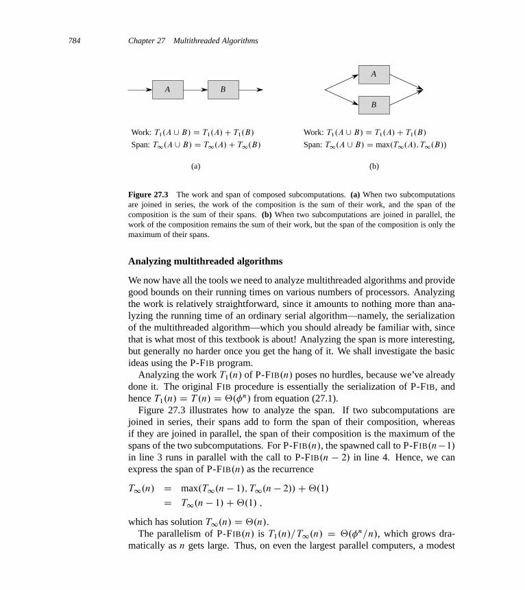
784 Chapter 27 Multithreaded Algorithms
A
(a) (b)
B
A
B
Work: T1.A [ B/ D T1.A/C T1.B/
Span: T1.A[ B/ D T1.A/C T1.B/
Work: T1.A [ B/ D T1.A/C T1.B/
Span: T1.A [ B/ D max.T1.A/; T1.B/)
Figure 27.3 The work and span of composed subcomputations. (a) When two subcomputationsare joined in series, the work of the composition is the sum of their work, and the span of thecomposition is the sum of their spans. (b) When two subcomputations are joined in parallel, thework of the composition remains the sum of their work, but the span of the composition is only themaximum of their spans.
Analyzing multithreaded algorithms
We now have all the tools we need to analyze multithreaded algorithms and providegood bounds on their running times on various numbers of processors. Analyzingthe work is relatively straightforward, since it amounts to nothing more than ana-lyzing the running time of an ordinary serial algorithm—namely, the serializationof the multithreaded algorithm—which you should already be familiar with, sincethat is what most of this textbook is about! Analyzing the span is more interesting,but generally no harder once you get the hang of it. We shall investigate the basicideas using the P-FIB program.
Analyzing the work T1.n/ of P-FIB.n/ poses no hurdles, because we’ve alreadydone it. The original FIB procedure is essentially the serialization of P-FIB, andhence T1.n/ D T .n/ D ‚.�n/ from equation (27.1).
Figure 27.3 illustrates how to analyze the span. If two subcomputations arejoined in series, their spans add to form the span of their composition, whereasif they are joined in parallel, the span of their composition is the maximum of thespans of the two subcomputations. For P-FIB.n/, the spawned call to P-FIB.n�1/
in line 3 runs in parallel with the call to P-FIB.n � 2/ in line 4. Hence, we canexpress the span of P-FIB.n/ as the recurrence
T1.n/ D max.T1.n � 1/; T1.n � 2//C‚.1/
D T1.n � 1/C‚.1/ ;
which has solution T1.n/ D ‚.n/.The parallelism of P-FIB.n/ is T1.n/=T1.n/ D ‚.�n=n/, which grows dra-
matically as n gets large. Thus, on even the largest parallel computers, a modest
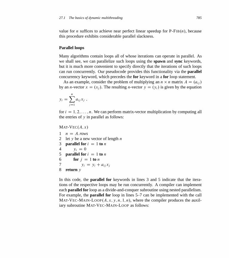
27.1 The basics of dynamic multithreading 785
value for n suffices to achieve near perfect linear speedup for P-FIB.n/, becausethis procedure exhibits considerable parallel slackness.
Parallel loops
Many algorithms contain loops all of whose iterations can operate in parallel. Aswe shall see, we can parallelize such loops using the spawn and sync keywords,but it is much more convenient to specify directly that the iterations of such loopscan run concurrently. Our pseudocode provides this functionality via the parallelconcurrency keyword, which precedes the for keyword in a for loop statement.
As an example, consider the problem of multiplying an n n matrix A D .aij /
by an n-vector x D .xj /. The resulting n-vector y D .yi/ is given by the equation
yi DnX
j D1
aij xj ;
for i D 1; 2; : : : ; n. We can perform matrix-vector multiplication by computing allthe entries of y in parallel as follows:
MAT-VEC.A; x/
1 n D A:rows2 let y be a new vector of length n
3 parallel for i D 1 to n
4 yi D 0
5 parallel for i D 1 to n
6 for j D 1 to n
7 yi D yi C aij xj
8 return y
In this code, the parallel for keywords in lines 3 and 5 indicate that the itera-tions of the respective loops may be run concurrently. A compiler can implementeach parallel for loop as a divide-and-conquer subroutine using nested parallelism.For example, the parallel for loop in lines 5–7 can be implemented with the callMAT-VEC-MAIN-LOOP.A; x; y; n; 1; n/, where the compiler produces the auxil-iary subroutine MAT-VEC-MAIN-LOOP as follows:

786 Chapter 27 Multithreaded Algorithms
1,1 2,2 3,3 4,4 5,5 6,6 7,7 8,8
1,2 3,4 5,6 7,8
1,4 5,8
1,8
Figure 27.4 A dag representing the computation of MAT-VEC-MAIN-LOOP.A; x; y; 8; 1; 8/. Thetwo numbers within each rounded rectangle give the values of the last two parameters (i and i 0 inthe procedure header) in the invocation (spawn or call) of the procedure. The black circles repre-sent strands corresponding to either the base case or the part of the procedure up to the spawn ofMAT-VEC-MAIN-LOOP in line 5; the shaded circles represent strands corresponding to the part ofthe procedure that calls MAT-VEC-MAIN-LOOP in line 6 up to the sync in line 7, where it suspendsuntil the spawned subroutine in line 5 returns; and the white circles represent strands correspondingto the (negligible) part of the procedure after the sync up to the point where it returns.
MAT-VEC-MAIN-LOOP.A; x; y; n; i; i 0/
1 if i == i 0
2 for j D 1 to n
3 yi D yi C aij xj
4 else mid D b.i C i 0/=2c5 spawn MAT-VEC-MAIN-LOOP.A; x; y; n; i; mid/
6 MAT-VEC-MAIN-LOOP.A; x; y; n; midC 1; i 0/7 sync
This code recursively spawns the first half of the iterations of the loop to executein parallel with the second half of the iterations and then executes a sync, therebycreating a binary tree of execution where the leaves are individual loop iterations,as shown in Figure 27.4.
To calculate the work T1.n/ of MAT-VEC on an nn matrix, we simply computethe running time of its serialization, which we obtain by replacing the parallel forloops with ordinary for loops. Thus, we have T1.n/ D ‚.n2/, because the qua-dratic running time of the doubly nested loops in lines 5–7 dominates. This analysis
27.1 The basics of dynamic multithreading 787
seems to ignore the overhead for recursive spawning in implementing the parallelloops, however. In fact, the overhead of recursive spawning does increase the workof a parallel loop compared with that of its serialization, but not asymptotically.To see why, observe that since the tree of recursive procedure instances is a fullbinary tree, the number of internal nodes is 1 fewer than the number of leaves (seeExercise B.5-3). Each internal node performs constant work to divide the iterationrange, and each leaf corresponds to an iteration of the loop, which takes at leastconstant time (‚.n/ time in this case). Thus, we can amortize the overhead of re-cursive spawning against the work of the iterations, contributing at most a constantfactor to the overall work.
As a practical matter, dynamic-multithreading concurrency platforms sometimescoarsen the leaves of the recursion by executing several iterations in a single leaf,either automatically or under programmer control, thereby reducing the overheadof recursive spawning. This reduced overhead comes at the expense of also reduc-ing the parallelism, however, but if the computation has sufficient parallel slack-ness, near-perfect linear speedup need not be sacrificed.
We must also account for the overhead of recursive spawning when analyzing thespan of a parallel-loop construct. Since the depth of recursive calling is logarithmicin the number of iterations, for a parallel loop with n iterations in which the i thiteration has span iter1.i/, the span is
T1.n/ D ‚.lg n/C max1�i�n
iter1.i/ :
For example, for MAT-VEC on an n n matrix, the parallel initialization loop inlines 3–4 has span ‚.lg n/, because the recursive spawning dominates the constant-time work of each iteration. The span of the doubly nested loops in lines 5–7is ‚.n/, because each iteration of the outer parallel for loop contains n iterationsof the inner (serial) for loop. The span of the remaining code in the procedureis constant, and thus the span is dominated by the doubly nested loops, yieldingan overall span of ‚.n/ for the whole procedure. Since the work is ‚.n2/, theparallelism is ‚.n2/=‚.n/ D ‚.n/. (Exercise 27.1-6 asks you to provide animplementation with even more parallelism.)
Race conditions
A multithreaded algorithm is deterministic if it always does the same thing on thesame input, no matter how the instructions are scheduled on the multicore com-puter. It is nondeterministic if its behavior might vary from run to run. Often, amultithreaded algorithm that is intended to be deterministic fails to be, because itcontains a “determinacy race.”
Race conditions are the bane of concurrency. Famous race bugs include theTherac-25 radiation therapy machine, which killed three people and injured sev-
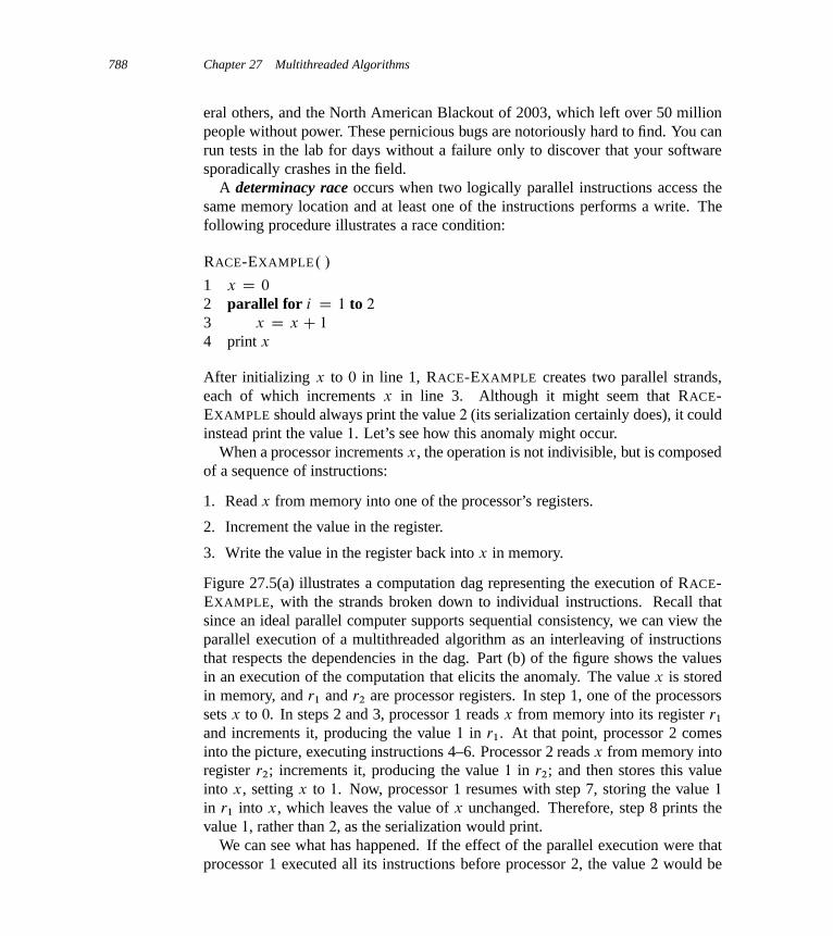
788 Chapter 27 Multithreaded Algorithms
eral others, and the North American Blackout of 2003, which left over 50 millionpeople without power. These pernicious bugs are notoriously hard to find. You canrun tests in the lab for days without a failure only to discover that your softwaresporadically crashes in the field.
A determinacy race occurs when two logically parallel instructions access thesame memory location and at least one of the instructions performs a write. Thefollowing procedure illustrates a race condition:
RACE-EXAMPLE. /
1 x D 0
2 parallel for i D 1 to 2
3 x D x C 1
4 print x
After initializing x to 0 in line 1, RACE-EXAMPLE creates two parallel strands,each of which increments x in line 3. Although it might seem that RACE-EXAMPLE should always print the value 2 (its serialization certainly does), it couldinstead print the value 1. Let’s see how this anomaly might occur.
When a processor increments x, the operation is not indivisible, but is composedof a sequence of instructions:
1. Read x from memory into one of the processor’s registers.
2. Increment the value in the register.
3. Write the value in the register back into x in memory.
Figure 27.5(a) illustrates a computation dag representing the execution of RACE-EXAMPLE, with the strands broken down to individual instructions. Recall thatsince an ideal parallel computer supports sequential consistency, we can view theparallel execution of a multithreaded algorithm as an interleaving of instructionsthat respects the dependencies in the dag. Part (b) of the figure shows the valuesin an execution of the computation that elicits the anomaly. The value x is storedin memory, and r1 and r2 are processor registers. In step 1, one of the processorssets x to 0. In steps 2 and 3, processor 1 reads x from memory into its register r1
and increments it, producing the value 1 in r1. At that point, processor 2 comesinto the picture, executing instructions 4–6. Processor 2 reads x from memory intoregister r2; increments it, producing the value 1 in r2; and then stores this valueinto x, setting x to 1. Now, processor 1 resumes with step 7, storing the value 1
in r1 into x, which leaves the value of x unchanged. Therefore, step 8 prints thevalue 1, rather than 2, as the serialization would print.
We can see what has happened. If the effect of the parallel execution were thatprocessor 1 executed all its instructions before processor 2, the value 2 would be
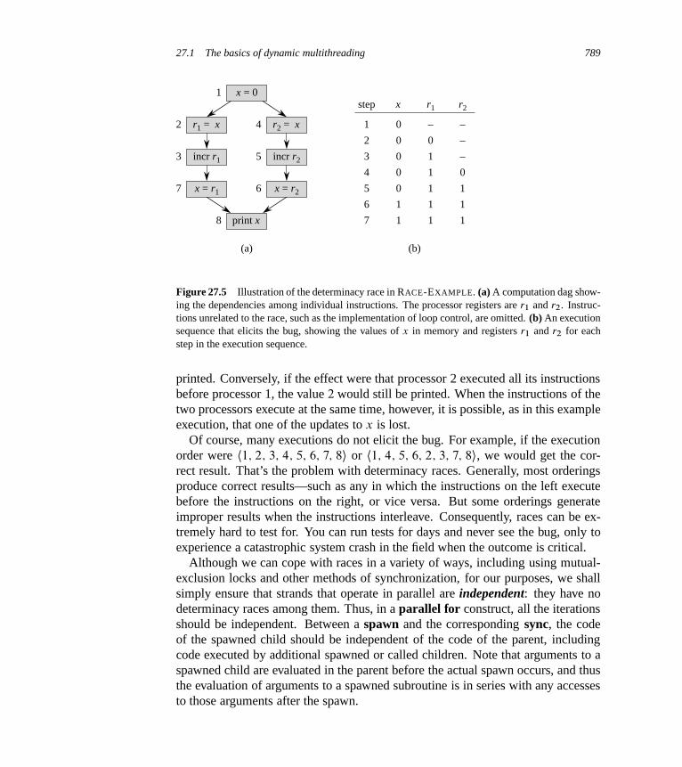
27.1 The basics of dynamic multithreading 789
incr r13
r1 = x2
x = r17
incr r25
r2 = x4
x = r26
x = 01
print x8
(a)
step x r1 r2
1
2
3
4
5
6
7
0
0
0
0
0
1
1
–
0
1
1
1
1
1
–
–
–
0
1
1
1
(b)
Figure 27.5 Illustration of the determinacy race in RACE-EXAMPLE. (a) A computation dag show-ing the dependencies among individual instructions. The processor registers are r1 and r2. Instruc-tions unrelated to the race, such as the implementation of loop control, are omitted. (b) An executionsequence that elicits the bug, showing the values of x in memory and registers r1 and r2 for eachstep in the execution sequence.
printed. Conversely, if the effect were that processor 2 executed all its instructionsbefore processor 1, the value 2 would still be printed. When the instructions of thetwo processors execute at the same time, however, it is possible, as in this exampleexecution, that one of the updates to x is lost.
Of course, many executions do not elicit the bug. For example, if the executionorder were h1; 2; 3; 4; 5; 6; 7; 8i or h1; 4; 5; 6; 2; 3; 7; 8i, we would get the cor-rect result. That’s the problem with determinacy races. Generally, most orderingsproduce correct results—such as any in which the instructions on the left executebefore the instructions on the right, or vice versa. But some orderings generateimproper results when the instructions interleave. Consequently, races can be ex-tremely hard to test for. You can run tests for days and never see the bug, only toexperience a catastrophic system crash in the field when the outcome is critical.
Although we can cope with races in a variety of ways, including using mutual-exclusion locks and other methods of synchronization, for our purposes, we shallsimply ensure that strands that operate in parallel are independent: they have nodeterminacy races among them. Thus, in a parallel for construct, all the iterationsshould be independent. Between a spawn and the corresponding sync, the codeof the spawned child should be independent of the code of the parent, includingcode executed by additional spawned or called children. Note that arguments to aspawned child are evaluated in the parent before the actual spawn occurs, and thusthe evaluation of arguments to a spawned subroutine is in series with any accessesto those arguments after the spawn.
790 Chapter 27 Multithreaded Algorithms
As an example of how easy it is to generate code with races, here is a faultyimplementation of multithreaded matrix-vector multiplication that achieves a spanof ‚.lg n/ by parallelizing the inner for loop:
MAT-VEC-WRONG.A; x/
1 n D A:rows2 let y be a new vector of length n
3 parallel for i D 1 to n
4 yi D 0
5 parallel for i D 1 to n
6 parallel for j D 1 to n
7 yi D yi C aij xj
8 return y
This procedure is, unfortunately, incorrect due to races on updating yi in line 7,which executes concurrently for all n values of j . Exercise 27.1-6 asks you to givea correct implementation with ‚.lg n/ span.
A multithreaded algorithm with races can sometimes be correct. As an exam-ple, two parallel threads might store the same value into a shared variable, and itwouldn’t matter which stored the value first. Generally, however, we shall considercode with races to be illegal.
A chess lesson
We close this section with a true story that occurred during the development ofthe world-class multithreaded chess-playing program ?Socrates [81], although thetimings below have been simplified for exposition. The program was was proto-typed on a 32-processor computer but was ultimately to run on a supercomputerwith 512 processors. At one point, the developers incorporated an optimizationinto the program that reduced its running time on an important benchmark on the32-processor machine from T32 D 65 seconds to T 0
32 D 40 seconds. Yet, the devel-opers used the work and span performance measures to conclude that the optimizedversion, which was faster on 32 processors, would actually be slower than the orig-inal version on 512 processsors. As a result, they abandoned the “optimization.”
Here is their analysis. The original version of the program had work T1 D 2048
seconds and span T1 D 1 second. If we treat inequality (27.4) as an equation,TP D T1=P C T1, and use it as an approximation to the running time on P pro-cessors, we see that indeed T32 D 2048=32 C 1 D 65. With the optimization, thework became T 0
1 D 1024 seconds and the span became T 01 D 8 seconds. Again
using our approximation, we get T 032 D 1024=32C 8 D 40.
The relative speeds of the two versions switch when we calculate the runningtimes on 512 processors, however. In particular, we have T512 D 2048=512C1 D 5
27.1 The basics of dynamic multithreading 791
seconds, and T 0512 D 1024=512 C 8 D 10 seconds. The optimization that sped up
the program on 32 processors would have made the program twice as slow on 512
processors! The optimized version’s span of 8, which was not the dominant term inthe running time on 32 processors, became the dominant term on 512 processors,nullifying the advantage from using more processors.
The moral of the story is that work and span can provide a better means ofextrapolating performance than can measured running times.
Exercises
27.1-1Suppose that we spawn P-FIB.n � 2/ in line 4 of P-FIB, rather than calling itas is done in the code. What is the impact on the asymptotic work, span, andparallelism?
27.1-2Draw the computation dag that results from executing P-FIB.5/. Assuming thateach strand in the computation takes unit time, what are the work, span, and par-allelism of the computation? Show how to schedule the dag on 3 processors usinggreedy scheduling by labeling each strand with the time step in which it is executed.
27.1-3Prove that a greedy scheduler achieves the following time bound, which is slightlystronger than the bound proven in Theorem 27.1:
TP �T1 � T1
PC T1 : (27.5)
27.1-4Construct a computation dag for which one execution of a greedy scheduler cantake nearly twice the time of another execution of a greedy scheduler on the samenumber of processors. Describe how the two executions would proceed.
27.1-5Professor Karan measures her deterministic multithreaded algorithm on 4, 10,and 64 processors of an ideal parallel computer using a greedy scheduler. Sheclaims that the three runs yielded T4 D 80 seconds, T10 D 42 seconds, andT64 D 10 seconds. Argue that the professor is either lying or incompetent. (Hint:Use the work law (27.2), the span law (27.3), and inequality (27.5) from Exer-cise 27.1-3.)

792 Chapter 27 Multithreaded Algorithms
27.1-6Give a multithreaded algorithm to multiply an n n matrix by an n-vector thatachieves ‚.n2= lg n/ parallelism while maintaining ‚.n2/ work.
27.1-7Consider the following multithreaded pseudocode for transposing an nn matrix A
in place:
P-TRANSPOSE.A/
1 n D A:rows2 parallel for j D 2 to n
3 parallel for i D 1 to j � 1
4 exchange aij with aj i
5 return y
Analyze the work, span, and parallelism of this algorithm.
27.1-8Suppose that we replace the parallel for loop in line 3 of P-TRANSPOSE (see Ex-ercise 27.1-7) with an ordinary for loop. Analyze the work, span, and parallelismof the resulting algorithm.
27.1-9For how many processors do the two versions of the chess programs run equallyfast, assuming that TP D T1=P C T1?
27.2 Multithreaded matrix multiplication
In this section, we examine how to multithread matrix multiplication, a problemwhose serial running time we studied in Section 4.2. We’ll look at multithreadedalgorithms based on the standard triply nested loop, as well as divide-and-conqueralgorithms.
Multithreaded matrix multiplication
The first algorithm we study is the straighforward algorithm based on parallelizingthe loops in the procedure SQUARE-MATRIX-MULTIPLY on page 75:
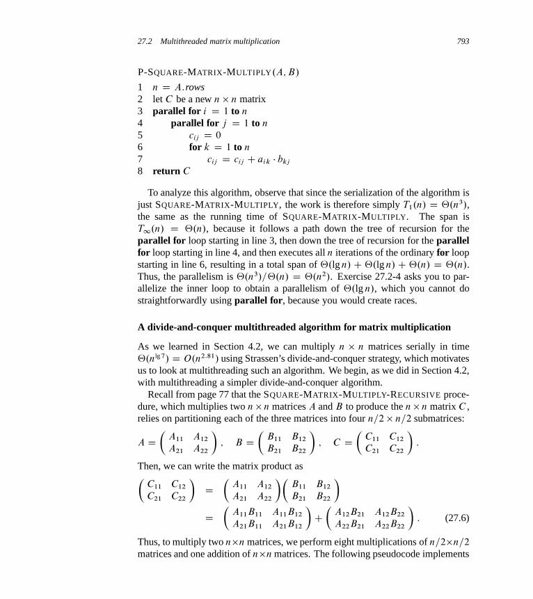
27.2 Multithreaded matrix multiplication 793
P-SQUARE-MATRIX-MULTIPLY.A; B/
1 n D A:rows2 let C be a new n n matrix3 parallel for i D 1 to n
4 parallel for j D 1 to n
5 cij D 0
6 for k D 1 to n
7 cij D cij C aik � bkj
8 return C
To analyze this algorithm, observe that since the serialization of the algorithm isjust SQUARE-MATRIX-MULTIPLY, the work is therefore simply T1.n/ D ‚.n3/,the same as the running time of SQUARE-MATRIX-MULTIPLY. The span isT1.n/ D ‚.n/, because it follows a path down the tree of recursion for theparallel for loop starting in line 3, then down the tree of recursion for the parallelfor loop starting in line 4, and then executes all n iterations of the ordinary for loopstarting in line 6, resulting in a total span of ‚.lg n/ C ‚.lg n/ C ‚.n/ D ‚.n/.Thus, the parallelism is ‚.n3/=‚.n/ D ‚.n2/. Exercise 27.2-4 asks you to par-allelize the inner loop to obtain a parallelism of ‚.lg n/, which you cannot dostraightforwardly using parallel for, because you would create races.
A divide-and-conquer multithreaded algorithm for matrix multiplication
As we learned in Section 4.2, we can multiply n n matrices serially in time‚.nlg 7/ D O.n2:81/ using Strassen’s divide-and-conquer strategy, which motivatesus to look at multithreading such an algorithm. We begin, as we did in Section 4.2,with multithreading a simpler divide-and-conquer algorithm.
Recall from page 77 that the SQUARE-MATRIX-MULTIPLY-RECURSIVE proce-dure, which multiplies two n n matrices A and B to produce the n n matrix C ,relies on partitioning each of the three matrices into four n=2 n=2 submatrices:
A D�
A11 A12
A21 A22
�; B D
�B11 B12
B21 B22
�; C D
�C11 C12
C21 C22
�:
Then, we can write the matrix product as�C11 C12
C21 C22
�D
�A11 A12
A21 A22
��B11 B12
B21 B22
�D
�A11B11 A11B12
A21B11 A21B12
�C�
A12B21 A12B22
A22B21 A22B22
�: (27.6)
Thus, to multiply two nn matrices, we perform eight multiplications of n=2n=2
matrices and one addition of nn matrices. The following pseudocode implements

794 Chapter 27 Multithreaded Algorithms
this divide-and-conquer strategy using nested parallelism. Unlike the SQUARE-MATRIX-MULTIPLY-RECURSIVE procedure on which it is based, P-MATRIX-MULTIPLY-RECURSIVE takes the output matrix as a parameter to avoid allocatingmatrices unnecessarily.
P-MATRIX-MULTIPLY-RECURSIVE.C; A; B/
1 n D A:rows2 if n == 1
3 c11 D a11b11
4 else let T be a new n n matrix5 partition A, B , C , and T into n=2 n=2 submatrices
A11; A12; A21; A22; B11; B12; B21; B22; C11; C12; C21; C22;and T11; T12; T21; T22; respectively
6 spawn P-MATRIX-MULTIPLY-RECURSIVE.C11; A11; B11/
7 spawn P-MATRIX-MULTIPLY-RECURSIVE.C12; A11; B12/
8 spawn P-MATRIX-MULTIPLY-RECURSIVE.C21; A21; B11/
9 spawn P-MATRIX-MULTIPLY-RECURSIVE.C22; A21; B12/
10 spawn P-MATRIX-MULTIPLY-RECURSIVE.T11; A12; B21/
11 spawn P-MATRIX-MULTIPLY-RECURSIVE.T12; A12; B22/
12 spawn P-MATRIX-MULTIPLY-RECURSIVE.T21; A22; B21/
13 P-MATRIX-MULTIPLY-RECURSIVE.T22; A22; B22/
14 sync15 parallel for i D 1 to n
16 parallel for j D 1 to n
17 cij D cij C tij
Line 3 handles the base case, where we are multiplying 1 1 matrices. We handlethe recursive case in lines 4–17. We allocate a temporary matrix T in line 4, andline 5 partitions each of the matrices A, B , C , and T into n=2 n=2 submatrices.(As with SQUARE-MATRIX-MULTIPLY-RECURSIVE on page 77, we gloss overthe minor issue of how to use index calculations to represent submatrix sectionsof a matrix.) The recursive call in line 6 sets the submatrix C11 to the submatrixproduct A11B11, so that C11 equals the first of the two terms that form its sum inequation (27.6). Similarly, lines 7–9 set C12, C21, and C22 to the first of the twoterms that equal their sums in equation (27.6). Line 10 sets the submatrix T11 tothe submatrix product A12B21, so that T11 equals the second of the two terms thatform C11’s sum. Lines 11–13 set T12, T21, and T22 to the second of the two termsthat form the sums of C12, C21, and C22, respectively. The first seven recursivecalls are spawned, and the last one runs in the main strand. The sync statement inline 14 ensures that all the submatrix products in lines 6–13 have been computed,

27.2 Multithreaded matrix multiplication 795
after which we add the products from T into C in using the doubly nested parallelfor loops in lines 15–17.
We first analyze the work M1.n/ of the P-MATRIX-MULTIPLY-RECURSIVE
procedure, echoing the serial running-time analysis of its progenitor SQUARE-MATRIX-MULTIPLY-RECURSIVE. In the recursive case, we partition in ‚.1/ time,perform eight recursive multiplications of n=2 n=2 matrices, and finish up withthe ‚.n2/ work from adding two n n matrices. Thus, the recurrence for thework M1.n/ is
M1.n/ D 8M1.n=2/C‚.n2/
D ‚.n3/
by case 1 of the master theorem. In other words, the work of our multithreaded al-gorithm is asymptotically the same as the running time of the procedure SQUARE-MATRIX-MULTIPLY in Section 4.2, with its triply nested loops.
To determine the span M1.n/ of P-MATRIX-MULTIPLY-RECURSIVE, we firstobserve that the span for partitioning is ‚.1/, which is dominated by the ‚.lg n/
span of the doubly nested parallel for loops in lines 15–17. Because the eightparallel recursive calls all execute on matrices of the same size, the maximum spanfor any recursive call is just the span of any one. Hence, the recurrence for thespan M1.n/ of P-MATRIX-MULTIPLY-RECURSIVE is
M1.n/ DM1.n=2/C‚.lg n/ : (27.7)
This recurrence does not fall under any of the cases of the master theorem, butit does meet the condition of Exercise 4.6-2. By Exercise 4.6-2, therefore, thesolution to recurrence (27.7) is M1.n/ D ‚.lg2 n/.
Now that we know the work and span of P-MATRIX-MULTIPLY-RECURSIVE,we can compute its parallelism as M1.n/=M1.n/ D ‚.n3= lg2 n/, which is veryhigh.
Multithreading Strassen’s method
To multithread Strassen’s algorithm, we follow the same general outline as onpage 79, only using nested parallelism:
1. Divide the input matrices A and B and output matrix C into n=2 n=2 sub-matrices, as in equation (27.6). This step takes ‚.1/ work and span by indexcalculation.
2. Create 10 matrices S1; S2; : : : ; S10, each of which is n=2 n=2 and is the sumor difference of two matrices created in step 1. We can create all 10 matriceswith ‚.n2/ work and ‚.lg n/ span by using doubly nested parallel for loops.
796 Chapter 27 Multithreaded Algorithms
3. Using the submatrices created in step 1 and the 10 matrices created instep 2, recursively spawn the computation of seven n=2 n=2 matrix productsP1; P2; : : : ; P7.
4. Compute the desired submatrices C11; C12; C21; C22 of the result matrix C byadding and subtracting various combinations of the Pi matrices, once againusing doubly nested parallel for loops. We can compute all four submatriceswith ‚.n2/ work and ‚.lg n/ span.
To analyze this algorithm, we first observe that since the serialization is thesame as the original serial algorithm, the work is just the running time of theserialization, namely, ‚.nlg 7/. As for P-MATRIX-MULTIPLY-RECURSIVE, wecan devise a recurrence for the span. In this case, seven recursive calls exe-cute in parallel, but since they all operate on matrices of the same size, we ob-tain the same recurrence (27.7) as we did for P-MATRIX-MULTIPLY-RECURSIVE,which has solution ‚.lg2 n/. Thus, the parallelism of multithreaded Strassen’smethod is ‚.nlg 7= lg2 n/, which is high, though slightly less than the parallelismof P-MATRIX-MULTIPLY-RECURSIVE.
Exercises
27.2-1Draw the computation dag for computing P-MATRIX-MULTIPLY on 22 matrices,labeling how the vertices in your diagram correspond to strands in the executionof the algorithm. Use the convention that spawn and call edges point downward,continuation edges point horizontally to the right, and return edges point upward.Assuming that each strand takes unit time, analyze the work, span, and parallelismof this computation.
27.2-2Repeat Exercise 27.2-1 for P-MATRIX-MULTIPLY-RECURSIVE.
27.2-3Give pseudocode for a multithreaded algorithm that multiplies an n n matrix A
by an n-vector x with work ‚.n2/ and span ‚.lg n/. Analyze your algorithm.
27.2-4Give pseudocode for a multithreaded algorithm that multiplies two n n matriceswith work ‚.n3/ but span only ‚.lg n/. Analyze your algorithm.
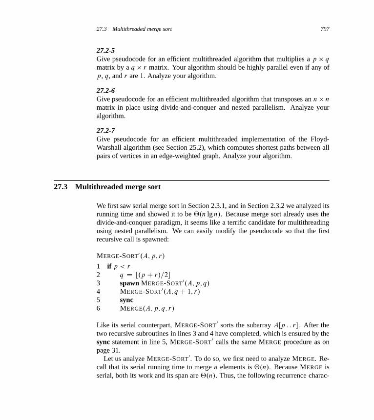
27.3 Multithreaded merge sort 797
27.2-5Give pseudocode for an efficient multithreaded algorithm that multiplies a p q
matrix by a q r matrix. Your algorithm should be highly parallel even if any ofp, q, and r are 1. Analyze your algorithm.
27.2-6Give pseudocode for an efficient multithreaded algorithm that transposes an n n
matrix in place using divide-and-conquer and nested parallelism. Analyze youralgorithm.
27.2-7Give pseudocode for an efficient multithreaded implementation of the Floyd-Warshall algorithm (see Section 25.2), which computes shortest paths between allpairs of vertices in an edge-weighted graph. Analyze your algorithm.
27.3 Multithreaded merge sort
We first saw serial merge sort in Section 2.3.1, and in Section 2.3.2 we analyzed itsrunning time and showed it to be ‚.n lg n/. Because merge sort already uses thedivide-and-conquer paradigm, it seems like a terrific candidate for multithreadingusing nested parallelism. We can easily modify the pseudocode so that the firstrecursive call is spawned:
MERGE-SORT0.A; p; r/
1 if p < r
2 q D b.p C r/=2c3 spawn MERGE-SORT 0.A; p; q/
4 MERGE-SORT 0.A; q C 1; r/
5 sync6 MERGE.A; p; q; r/
Like its serial counterpart, MERGE-SORT 0 sorts the subarray AŒp : : r�. After thetwo recursive subroutines in lines 3 and 4 have completed, which is ensured by thesync statement in line 5, MERGE-SORT 0 calls the same MERGE procedure as onpage 31.
Let us analyze MERGE-SORT 0. To do so, we first need to analyze MERGE. Re-call that its serial running time to merge n elements is ‚.n/. Because MERGE isserial, both its work and its span are ‚.n/. Thus, the following recurrence charac-

798 Chapter 27 Multithreaded Algorithms
… … …
… …merge mergecopy
p1 q1 r1 p2 q2 r2
p3 q3 r3
A
T
x
x
� x
� x < x
� x
� x � x
Figure 27.6 The idea behind the multithreaded merging of two sorted subarrays T Œp1 : : r1�
and T Œp2 : : r2� into the subarray AŒp3 : : r3�. Letting x D T Œq1� be the median of T Œp1 : : r1� and q2
be the place in T Œp2 : : r2� such that x would fall between T Œq2 � 1� and T Œq2�, every element insubarrays T Œp1 : : q1 � 1� and T Œp2 : : q2 � 1� (lightly shaded) is less than or equal to x, and everyelement in the subarrays T Œq1C 1 : : r1� and T Œq2C 1 : : r2� (heavily shaded) is at least x. To merge,we compute the index q3 where x belongs in AŒp3 : : r3�, copy x into AŒq3�, and then recursivelymerge T Œp1 : : q1 � 1� with T Œp2 : : q2� into AŒp3 : : q3 � 1� and T Œq1 C 1 : : r1� with T Œq2C 1 : : r2�
into AŒq3 C 1 : : r3�.
terizes the work MS01.n/ of MERGE-SORT0 on n elements:
MS01.n/ D 2 MS0
1.n=2/C‚.n/
D ‚.n lg n/ ;
which is the same as the serial running time of merge sort. Since the two recursivecalls of MERGE-SORT0 can run in parallel, the span MS0
1 is given by the recurrence
MS01.n/ D MS0
1.n=2/C‚.n/
D ‚.n/ :
Thus, the parallelism of MERGE-SORT0 comes to MS01.n/=MS0
1.n/ D ‚.lg n/,which is an unimpressive amount of parallelism. To sort 10 million elements, forexample, it might achieve linear speedup on a few processors, but it would notscale up effectively to hundreds of processors.
You probably have already figured out where the parallelism bottleneck is inthis multithreaded merge sort: the serial MERGE procedure. Although mergingmight initially seem to be inherently serial, we can, in fact, fashion a multithreadedversion of it by using nested parallelism.
Our divide-and-conquer strategy for multithreaded merging, which is illus-trated in Figure 27.6, operates on subarrays of an array T . Suppose that weare merging the two sorted subarrays T Œp1 : : r1� of length n1 D r1 � p1 C 1
and T Œp2 : : r2� of length n2 D r2 � p2 C 1 into another subarray AŒp3 : : r3�, oflength n3 D r3 � p3 C 1 D n1 C n2. Without loss of generality, we make the sim-plifying assumption that n1 � n2.

27.3 Multithreaded merge sort 799
We first find the middle element x D T Œq1� of the subarray T Œp1 : : r1�,where q1 D b.p1 C r1/=2c. Because the subarray is sorted, x is a medianof T Œp1 : : r1�: every element in T Œp1 : : q1 � 1� is no more than x, and every el-ement in T Œq1 C 1 : : r1� is no less than x. We then use binary search to find theindex q2 in the subarray T Œp2 : : r2� so that the subarray would still be sorted if weinserted x between T Œq2 � 1� and T Œq2�.
We next merge the original subarrays T Œp1 : : r1� and T Œp2 : : r2� into AŒp3 : : r3�
as follows:
1. Set q3 D p3 C .q1 � p1/C .q2 � p2/.
2. Copy x into AŒq3�.
3. Recursively merge T Œp1 : : q1�1� with T Œp2 : : q2�1�, and place the result intothe subarray AŒp3 : : q3 � 1�.
4. Recursively merge T Œq1 C 1 : : r1� with T Œq2 : : r2�, and place the result into thesubarray AŒq3 C 1 : : r3�.
When we compute q3, the quantity q1�p1 is the number of elements in the subarrayT Œp1 : : q1 � 1�, and the quantity q2 � p2 is the number of elements in the subarrayT Œp2 : : q2 � 1�. Thus, their sum is the number of elements that end up before x inthe subarray AŒp3 : : r3�.
The base case occurs when n1 D n2 D 0, in which case we have no workto do to merge the two empty subarrays. Since we have assumed that the sub-array T Œp1 : : r1� is at least as long as T Œp2 : : r2�, that is, n1 � n2, we can checkfor the base case by just checking whether n1 D 0. We must also ensure that therecursion properly handles the case when only one of the two subarrays is empty,which, by our assumption that n1 � n2, must be the subarray T Œp2 : : r2�.
Now, let’s put these ideas into pseudocode. We start with the binary search,which we express serially. The procedure BINARY-SEARCH.x; T; p; r/ takes akey x and a subarray T Œp : : r�, and it returns one of the following:
� If T Œp : : r� is empty (r < p), then it returns the index p.
� If x � T Œp�, and hence less than or equal to all the elements of T Œp : : r�, thenit returns the index p.
� If x > T Œp�, then it returns the largest index q in the range p < q � rC1 suchthat T Œq � 1� < x.
Here is the pseudocode:
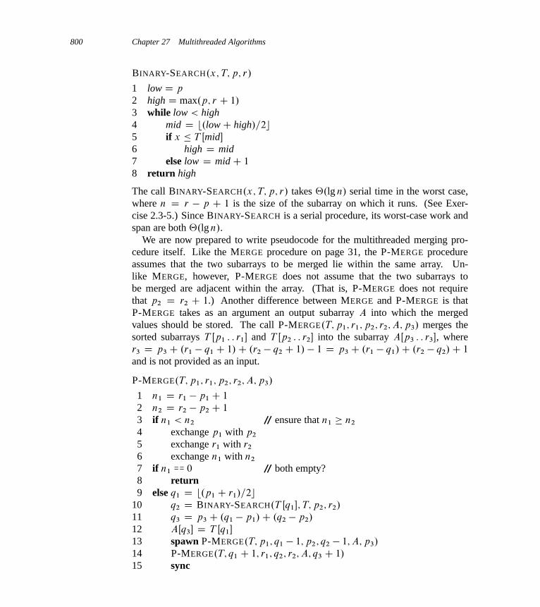
800 Chapter 27 Multithreaded Algorithms
BINARY-SEARCH.x; T; p; r/
1 low D p
2 high D max.p; r C 1/
3 while low < high4 mid D b.lowC high/=2c5 if x � T Œmid�
6 high D mid7 else low D midC 1
8 return high
The call BINARY-SEARCH.x; T; p; r/ takes ‚.lg n/ serial time in the worst case,where n D r � p C 1 is the size of the subarray on which it runs. (See Exer-cise 2.3-5.) Since BINARY-SEARCH is a serial procedure, its worst-case work andspan are both ‚.lg n/.
We are now prepared to write pseudocode for the multithreaded merging pro-cedure itself. Like the MERGE procedure on page 31, the P-MERGE procedureassumes that the two subarrays to be merged lie within the same array. Un-like MERGE, however, P-MERGE does not assume that the two subarrays tobe merged are adjacent within the array. (That is, P-MERGE does not requirethat p2 D r2 C 1.) Another difference between MERGE and P-MERGE is thatP-MERGE takes as an argument an output subarray A into which the mergedvalues should be stored. The call P-MERGE.T; p1; r1; p2; r2; A; p3/ merges thesorted subarrays T Œp1 : : r1� and T Œp2 : : r2� into the subarray AŒp3 : : r3�, wherer3 D p3 C .r1 � q1 C 1/C .r2 � q2 C 1/ � 1 D p3 C .r1 � q1/C .r2 � q2/C 1
and is not provided as an input.
P-MERGE.T; p1; r1; p2; r2; A; p3/
1 n1 D r1 � p1 C 1
2 n2 D r2 � p2 C 1
3 if n1 < n2 // ensure that n1 � n2
4 exchange p1 with p2
5 exchange r1 with r2
6 exchange n1 with n2
7 if n1 == 0 // both empty?8 return9 else q1 D b.p1 C r1/=2c
10 q2 D BINARY-SEARCH.T Œq1�; T; p2; r2/
11 q3 D p3 C .q1 � p1/C .q2 � p2/
12 AŒq3� D T Œq1�
13 spawn P-MERGE.T; p1; q1 � 1; p2; q2 � 1; A; p3/
14 P-MERGE.T; q1 C 1; r1; q2; r2; A; q3 C 1/
15 sync

27.3 Multithreaded merge sort 801
The P-MERGE procedure works as follows. Lines 1–2 compute the lengths n1
and n2 of the subarrays T Œp1 : : r1� and T Œp2 : : r2�, respectively. Lines 3–6 en-force the assumption that n1 � n2. Line 7 tests for the base case, where thesubarray T Œp1 : : r1� is empty (and hence so is T Œp2 : : r2�), in which case we sim-ply return. Lines 9–15 implement the divide-and-conquer strategy. Line 9 com-putes the midpoint of T Œp1 : : r1�, and line 10 finds the point q2 in T Œp2 : : r2� suchthat all elements in T Œp2 : : q2 � 1� are less than T Œq1� (which corresponds to x)and all the elements in T Œq2 : : p2� are at least as large as T Œq1�. Line 11 com-putes the index q3 of the element that divides the output subarray AŒp3 : : r3� intoAŒp3 : : q3 � 1� and AŒq3C1 : : r3�, and then line 12 copies T Œq1� directly into AŒq3�.
Then, we recurse using nested parallelism. Line 13 spawns the first subproblem,while line 14 calls the second subproblem in parallel. The sync statement in line 15ensures that the subproblems have completed before the procedure returns. (Sinceevery procedure implicitly executes a sync before returning, we could have omittedthe sync statement in line 15, but including it is good coding practice.) Thereis some cleverness in the coding to ensure that when the subarray T Œp2 : : r2� isempty, the code operates correctly. The way it works is that on each recursive call,a median element of T Œp1 : : r1� is placed into the output subarray, until T Œp1 : : r1�
itself finally becomes empty, triggering the base case.
Analysis of multithreaded merging
We first derive a recurrence for the span PM1.n/ of P-MERGE, where the twosubarrays contain a total of n D n1Cn2 elements. Because the spawn in line 13 andthe call in line 14 operate logically in parallel, we need examine only the costlier ofthe two calls. The key is to understand that in the worst case, the maximum numberof elements in either of the recursive calls can be at most 3n=4, which we see asfollows. Because lines 3–6 ensure that n2 � n1, it follows that n2 D 2n2=2 �.n1 C n2/=2 D n=2. In the worst case, one of the two recursive calls mergesbn1=2c elements of T Œp1 : : r1� with all n2 elements of T Œp2 : : r2�, and hence thenumber of elements involved in the call is
bn1=2c C n2 � n1=2C n2=2C n2=2
D .n1 C n2/=2C n2=2
� n=2C n=4
D 3n=4 :
Adding in the ‚.lg n/ cost of the call to BINARY-SEARCH in line 10, we obtainthe following recurrence for the worst-case span:
PM1.n/ D PM1.3n=4/C‚.lg n/ : (27.8)

802 Chapter 27 Multithreaded Algorithms
(For the base case, the span is ‚.1/, since lines 1–8 execute in constant time.)This recurrence does not fall under any of the cases of the master theorem, but itmeets the condition of Exercise 4.6-2. Therefore, the solution to recurrence (27.8)is PM1.n/ D ‚.lg2 n/.
We now analyze the work PM1.n/ of P-MERGE on n elements, which turns outto be ‚.n/. Since each of the n elements must be copied from array T to array A,we have PM1.n/ D �.n/. Thus, it remains only to show that PM1.n/ D O.n/.
We shall first derive a recurrence for the worst-case work. The binary search inline 10 costs ‚.lg n/ in the worst case, which dominates the other work outsideof the recursive calls. For the recursive calls, observe that although the recursivecalls in lines 13 and 14 might merge different numbers of elements, together thetwo recursive calls merge at most n elements (actually n� 1 elements, since T Œq1�
does not participate in either recursive call). Moreover, as we saw in analyzing thespan, a recursive call operates on at most 3n=4 elements. We therefore obtain therecurrence
PM1.n/ D PM1.˛n/C PM1..1� ˛/n/CO.lg n/ ; (27.9)
where ˛ lies in the range 1=4 � ˛ � 3=4, and where we understand that the actualvalue of ˛ may vary for each level of recursion.
We prove that recurrence (27.9) has solution PM1 D O.n/ via the substitutionmethod. Assume that PM1.n/ � c1n�c2 lg n for some positive constants c1 and c2.Substituting gives us
PM1.n/ � .c1˛n � c2 lg.˛n//C .c1.1� ˛/n � c2 lg..1� ˛/n//C‚.lg n/
D c1.˛ C .1 � ˛//n� c2.lg.˛n/C lg..1 � ˛/n//C‚.lg n/
D c1n � c2.lg ˛ C lg nC lg.1� ˛/C lg n/C‚.lg n/
D c1n � c2 lg n � .c2.lg nC lg.˛.1� ˛/// �‚.lg n//
� c1n � c2 lg n ;
since we can choose c2 large enough that c2.lg n C lg.˛.1 � ˛/// dominates the‚.lg n/ term. Furthermore, we can choose c1 large enough to satisfy the baseconditions of the recurrence. Since the work PM1.n/ of P-MERGE is both �.n/
and O.n/, we have PM1.n/ D ‚.n/.The parallelism of P-MERGE is PM1.n/=PM1.n/ D ‚.n= lg2 n/.
Multithreaded merge sort
Now that we have a nicely parallelized multithreaded merging procedure, we canincorporate it into a multithreaded merge sort. This version of merge sort is similarto the MERGE-SORT 0 procedure we saw earlier, but unlike MERGE-SORT 0, it takesas an argument an output subarray B , which will hold the sorted result. In par-

27.3 Multithreaded merge sort 803
ticular, the call P-MERGE-SORT.A; p; r; B; s/ sorts the elements in AŒp : : r� andstores them in BŒs : : s C r � p�.
P-MERGE-SORT.A; p; r; B; s/
1 n D r � p C 1
2 if n == 1
3 BŒs� D AŒp�
4 else let T Œ1 : : n� be a new array5 q D b.p C r/=2c6 q0 D q � p C 1
7 spawn P-MERGE-SORT.A; p; q; T; 1/
8 P-MERGE-SORT.A; q C 1; r; T; q0 C 1/
9 sync10 P-MERGE.T; 1; q0; q0 C 1; n; B; s/
After line 1 computes the number n of elements in the input subarray AŒp : : r�,lines 2–3 handle the base case when the array has only 1 element. Lines 4–6 setup for the recursive spawn in line 7 and call in line 8, which operate in parallel. Inparticular, line 4 allocates a temporary array T with n elements to store the resultsof the recursive merge sorting. Line 5 calculates the index q of AŒp : : r� to dividethe elements into the two subarrays AŒp : : q� and AŒq C 1 : : r� that will be sortedrecursively, and line 6 goes on to compute the number q0 of elements in the firstsubarray AŒp : : q�, which line 8 uses to determine the starting index in T of whereto store the sorted result of AŒq C 1 : : r�. At that point, the spawn and recursivecall are made, followed by the sync in line 9, which forces the procedure to waituntil the spawned procedure is done. Finally, line 10 calls P-MERGE to mergethe sorted subarrays, now in T Œ1 : : q0� and T Œq0 C 1 : : r�, into the output subarrayBŒs : : s C r � p�.
Analysis of multithreaded merge sort
We start by analyzing the work PMS1.n/ of P-MERGE-SORT, which is consider-ably easier than analyzing the work of P-MERGE. Indeed, the work is given by therecurrence
PMS1.n/ D 2 PMS1.n=2/C PM1.n/
D 2 PMS1.n=2/C‚.n/ :
This recurrence is the same as the recurrence (4.4) for ordinary MERGE-SORT
from Section 2.3.1 and has solution PMS1.n/ D ‚.n lg n/ by case 2 of the mastertheorem.
804 Chapter 27 Multithreaded Algorithms
We now derive and analyze a recurrence for the worst-case span PMS1.n/. Be-cause the two recursive calls to P-MERGE-SORT on lines 7 and 8 operate logicallyin parallel, we can ignore one of them, obtaining the recurrence
PMS1.n/ D PMS1.n=2/C PM1.n/
D PMS1.n=2/C‚.lg2 n/ : (27.10)
As for recurrence (27.8), the master theorem does not apply to recurrence (27.10),but Exercise 4.6-2 does. The solution is PMS1.n/ D ‚.lg3 n/, and so the span ofP-MERGE-SORT is ‚.lg3 n/.
Parallel merging gives P-MERGE-SORT a significant parallelism advantage overMERGE-SORT 0. Recall that the parallelism of MERGE-SORT 0, which calls the se-rial MERGE procedure, is only ‚.lg n/. For P-MERGE-SORT, the parallelism is
PMS1.n/=PMS1.n/ D ‚.n lg n/=‚.lg3 n/
D ‚.n= lg2 n/ ;
which is much better both in theory and in practice. A good implementation inpractice would sacrifice some parallelism by coarsening the base case in order toreduce the constants hidden by the asymptotic notation. The straightforward wayto coarsen the base case is to switch to an ordinary serial sort, perhaps quicksort,when the size of the array is sufficiently small.
Exercises
27.3-1Explain how to coarsen the base case of P-MERGE.
27.3-2Instead of finding a median element in the larger subarray, as P-MERGE does, con-sider a variant that finds a median element of all the elements in the two sortedsubarrays using the result of Exercise 9.3-8. Give pseudocode for an efficientmultithreaded merging procedure that uses this median-finding procedure. Ana-lyze your algorithm.
27.3-3Give an efficient multithreaded algorithm for partitioning an array around a pivot,as is done by the PARTITION procedure on page 171. You need not partition the ar-ray in place. Make your algorithm as parallel as possible. Analyze your algorithm.(Hint: You may need an auxiliary array and may need to make more than one passover the input elements.)
Problems for Chapter 27 805
27.3-4Give a multithreaded version of RECURSIVE-FFT on page 911. Make your imple-mentation as parallel as possible. Analyze your algorithm.
27.3-5 ?
Give a multithreaded version of RANDOMIZED-SELECT on page 216. Make yourimplementation as parallel as possible. Analyze your algorithm. (Hint: Use thepartitioning algorithm from Exercise 27.3-3.)
27.3-6 ?
Show how to multithread SELECT from Section 9.3. Make your implementation asparallel as possible. Analyze your algorithm.
Problems
27-1 Implementing parallel loops using nested parallelismConsider the following multithreaded algorithm for performing pairwise additionon n-element arrays AŒ1 : : n� and BŒ1 : : n�, storing the sums in C Œ1 : : n�:
SUM-ARRAYS.A; B; C /
1 parallel for i D 1 to A: length2 C Œi� D AŒi�C BŒi�
a. Rewrite the parallel loop in SUM-ARRAYS using nested parallelism (spawnand sync) in the manner of MAT-VEC-MAIN-LOOP. Analyze the parallelismof your implementation.
Consider the following alternative implementation of the parallel loop, whichcontains a value grain-size to be specified:
SUM-ARRAYS0.A; B; C /
1 n D A: length2 grain-size D ‹ // to be determined3 r D dn=grain-sizee4 for k D 0 to r � 1
5 spawn ADD-SUBARRAY.A; B; C; k � grain-sizeC 1;
min..k C 1/ � grain-size; n//
6 sync

806 Chapter 27 Multithreaded Algorithms
ADD-SUBARRAY.A; B; C; i; j /
1 for k D i to j
2 C Œk� D AŒk�C BŒk�
b. Suppose that we set grain-size D 1. What is the parallelism of this implemen-tation?
c. Give a formula for the span of SUM-ARRAYS0 in terms of n and grain-size.Derive the best value for grain-size to maximize parallelism.
27-2 Saving temporary space in matrix multiplicationThe P-MATRIX-MULTIPLY-RECURSIVE procedure has the disadvantage that itmust allocate a temporary matrix T of size n n, which can adversely affect theconstants hidden by the ‚-notation. The P-MATRIX-MULTIPLY-RECURSIVE pro-cedure does have high parallelism, however. For example, ignoring the constantsin the ‚-notation, the parallelism for multiplying 1000 1000 matrices comes toapproximately 10003=102 D 107, since lg 1000 � 10. Most parallel computershave far fewer than 10 million processors.
a. Describe a recursive multithreaded algorithm that eliminates the need for thetemporary matrix T at the cost of increasing the span to ‚.n/. (Hint: Com-pute C D C C AB following the general strategy of P-MATRIX-MULTIPLY-RECURSIVE, but initialize C in parallel and insert a sync in a judiciously cho-sen location.)
b. Give and solve recurrences for the work and span of your implementation.
c. Analyze the parallelism of your implementation. Ignoring the constants in the‚-notation, estimate the parallelism on 1000 1000 matrices. Compare withthe parallelism of P-MATRIX-MULTIPLY-RECURSIVE.
27-3 Multithreaded matrix algorithmsa. Parallelize the LU-DECOMPOSITION procedure on page 821 by giving pseu-
docode for a multithreaded version of this algorithm. Make your implementa-tion as parallel as possible, and analyze its work, span, and parallelism.
b. Do the same for LUP-DECOMPOSITION on page 824.
c. Do the same for LUP-SOLVE on page 817.
d. Do the same for a multithreaded algorithm based on equation (28.13) for in-verting a symmetric positive-definite matrix.
Problems for Chapter 27 807
27-4 Multithreading reductions and prefix computationsA ˝-reduction of an array xŒ1 : : n�, where˝ is an associative operator, is the value
y D xŒ1�˝ xŒ2�˝ � � � ˝ xŒn� :
The following procedure computes the ˝-reduction of a subarray xŒi : : j � serially.
REDUCE.x; i; j /
1 y D xŒi �
2 for k D i C 1 to n
3 y D y ˝ xŒk�
4 return y
a. Use nested parallelism to implement a multithreaded algorithm P-REDUCE,which performs the same function with ‚.n/ work and ‚.lg n/ span. Analyzeyour algorithm.
A related problem is that of computing a ˝-prefix computation, sometimescalled a ˝-scan, on an array xŒ1 : : n�, where ˝ is once again an associative op-erator. The ˝-scan produces the array yŒ1 : : n� given by
yŒ1� D xŒ1� ;
yŒ2� D xŒ1�˝ xŒ2� ;
yŒ3� D xŒ1�˝ xŒ2�˝ xŒ3� ;
:::
yŒn� D xŒ1�˝ xŒ2�˝ xŒ3�˝ � � � ˝ xŒn� ;
that is, all prefixes of the array x “summed” using the ˝ operator. The followingserial procedure SCAN performs a˝-prefix computation:
SCAN.x/
1 n D x: length2 let yŒ1 : : n� be a new array3 yŒ1� D xŒ1�
4 for i D 2 to n
5 yŒi � D yŒi � 1�˝ xŒi �
6 return y
Unfortunately, multithreading SCAN is not straightforward. For example, changingthe for loop to a parallel for loop would create races, since each iteration of theloop body depends on the previous iteration. The following procedure P-SCAN-1performs the˝-prefix computation in parallel, albeit inefficiently:
808 Chapter 27 Multithreaded Algorithms
P-SCAN-1.x/
1 n D x: length2 let yŒ1 : : n� be a new array3 P-SCAN-1-AUX.x; y; 1; n/
4 return y
P-SCAN-1-AUX.x; y; i; j /
1 parallel for l D i to j
2 yŒl� D P-REDUCE.x; 1; l/
b. Analyze the work, span, and parallelism of P-SCAN-1.
By using nested parallelism, we can obtain a more efficient ˝-prefix computa-tion:
P-SCAN-2.x/
1 n D x: length2 let yŒ1 : : n� be a new array3 P-SCAN-2-AUX.x; y; 1; n/
4 return y
P-SCAN-2-AUX.x; y; i; j /
1 if i == j
2 yŒi � D xŒi �
3 else k D b.i C j /=2c4 spawn P-SCAN-2-AUX.x; y; i; k/
5 P-SCAN-2-AUX.x; y; k C 1; j /
6 sync7 parallel for l D k C 1 to j
8 yŒl� D yŒk�˝ yŒl�
c. Argue that P-SCAN-2 is correct, and analyze its work, span, and parallelism.
We can improve on both P-SCAN-1 and P-SCAN-2 by performing the ˝-prefixcomputation in two distinct passes over the data. On the first pass, we gather theterms for various contiguous subarrays of x into a temporary array t , and on thesecond pass we use the terms in t to compute the final result y. The followingpseudocode implements this strategy, but certain expressions have been omitted:

Problems for Chapter 27 809
P-SCAN-3.x/
1 n D x: length2 let yŒ1 : : n� and t Œ1 : : n� be new arrays3 yŒ1� D xŒ1�
4 if n > 1
5 P-SCAN-UP.x; t; 2; n/
6 P-SCAN-DOWN.xŒ1�; x; t; y; 2; n/
7 return y
P-SCAN-UP.x; t; i; j /
1 if i == j
2 return xŒi �
3 else4 k D b.i C j /=2c5 t Œk� D spawn P-SCAN-UP.x; t; i; k/
6 right D P-SCAN-UP.x; t; k C 1; j /
7 sync8 return // fill in the blank
P-SCAN-DOWN.�; x; t; y; i; j /
1 if i == j
2 yŒi � D � ˝ xŒi �
3 else4 k D b.i C j /=2c5 spawn P-SCAN-DOWN. ; x; t; y; i; k/ // fill in the blank6 P-SCAN-DOWN. ; x; t; y; k C 1; j / // fill in the blank7 sync
d. Fill in the three missing expressions in line 8 of P-SCAN-UP and lines 5 and 6of P-SCAN-DOWN. Argue that with expressions you supplied, P-SCAN-3 iscorrect. (Hint: Prove that the value � passed to P-SCAN-DOWN.�; x; t; y; i; j /
satisfies � D xŒ1�˝ xŒ2�˝ � � � ˝ xŒi � 1�.)
e. Analyze the work, span, and parallelism of P-SCAN-3.
27-5 Multithreading a simple stencil calculationComputational science is replete with algorithms that require the entries of an arrayto be filled in with values that depend on the values of certain already computedneighboring entries, along with other information that does not change over thecourse of the computation. The pattern of neighboring entries does not changeduring the computation and is called a stencil. For example, Section 15.4 presents
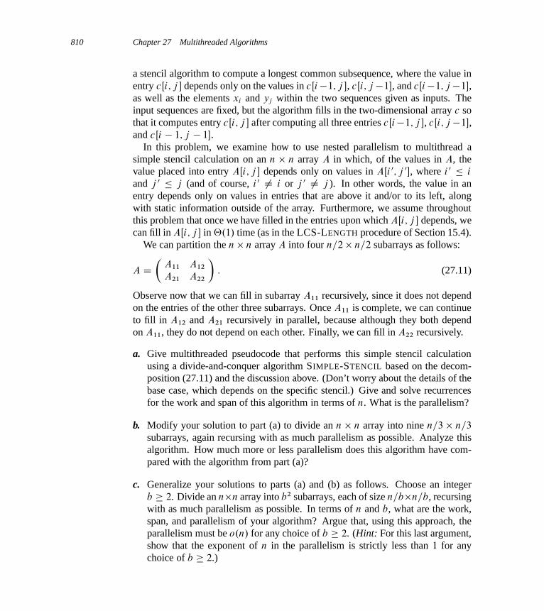
810 Chapter 27 Multithreaded Algorithms
a stencil algorithm to compute a longest common subsequence, where the value inentry cŒi; j � depends only on the values in cŒi�1; j �, cŒi; j �1�, and cŒi�1; j �1�,as well as the elements xi and yj within the two sequences given as inputs. Theinput sequences are fixed, but the algorithm fills in the two-dimensional array c sothat it computes entry cŒi; j � after computing all three entries cŒi�1; j �, cŒi; j �1�,and cŒi � 1; j � 1�.
In this problem, we examine how to use nested parallelism to multithread asimple stencil calculation on an n n array A in which, of the values in A, thevalue placed into entry AŒi; j � depends only on values in AŒi 0; j 0�, where i 0 � i
and j 0 � j (and of course, i 0 ¤ i or j 0 ¤ j ). In other words, the value in anentry depends only on values in entries that are above it and/or to its left, alongwith static information outside of the array. Furthermore, we assume throughoutthis problem that once we have filled in the entries upon which AŒi; j � depends, wecan fill in AŒi; j � in ‚.1/ time (as in the LCS-LENGTH procedure of Section 15.4).
We can partition the n n array A into four n=2 n=2 subarrays as follows:
A D�
A11 A12
A21 A22
�: (27.11)
Observe now that we can fill in subarray A11 recursively, since it does not dependon the entries of the other three subarrays. Once A11 is complete, we can continueto fill in A12 and A21 recursively in parallel, because although they both dependon A11, they do not depend on each other. Finally, we can fill in A22 recursively.
a. Give multithreaded pseudocode that performs this simple stencil calculationusing a divide-and-conquer algorithm SIMPLE-STENCIL based on the decom-position (27.11) and the discussion above. (Don’t worry about the details of thebase case, which depends on the specific stencil.) Give and solve recurrencesfor the work and span of this algorithm in terms of n. What is the parallelism?
b. Modify your solution to part (a) to divide an n n array into nine n=3 n=3
subarrays, again recursing with as much parallelism as possible. Analyze thisalgorithm. How much more or less parallelism does this algorithm have com-pared with the algorithm from part (a)?
c. Generalize your solutions to parts (a) and (b) as follows. Choose an integerb � 2. Divide an nn array into b2 subarrays, each of size n=bn=b, recursingwith as much parallelism as possible. In terms of n and b, what are the work,span, and parallelism of your algorithm? Argue that, using this approach, theparallelism must be o.n/ for any choice of b � 2. (Hint: For this last argument,show that the exponent of n in the parallelism is strictly less than 1 for anychoice of b � 2.)

Notes for Chapter 27 811
d. Give pseudocode for a multithreaded algorithm for this simple stencil calcu-lation that achieves ‚.n= lg n/ parallelism. Argue using notions of work andspan that the problem, in fact, has ‚.n/ inherent parallelism. As it turns out,the divide-and-conquer nature of our multithreaded pseudocode does not let usachieve this maximal parallelism.
27-6 Randomized multithreaded algorithmsJust as with ordinary serial algorithms, we sometimes want to implement random-ized multithreaded algorithms. This problem explores how to adapt the variousperformance measures in order to handle the expected behavior of such algorithms.It also asks you to design and analyze a multithreaded algorithm for randomizedquicksort.
a. Explain how to modify the work law (27.2), span law (27.3), and greedy sched-uler bound (27.4) to work with expectations when TP , T1, and T1 are all ran-dom variables.
b. Consider a randomized multithreaded algorithm for which 1% of the time wehave T1 D 104 and T10;000 D 1, but for 99% of the time we have T1 DT10;000 D 109. Argue that the speedup of a randomized multithreaded algo-rithm should be defined as E ŒT1� =E ŒTP �, rather than E ŒT1=TP �.
c. Argue that the parallelism of a randomized multithreaded algorithm should bedefined as the ratio E ŒT1� =E ŒT1�.
d. Multithread the RANDOMIZED-QUICKSORT algorithm on page 179 by usingnested parallelism. (Do not parallelize RANDOMIZED-PARTITION.) Give thepseudocode for your P-RANDOMIZED-QUICKSORT algorithm.
e. Analyze your multithreaded algorithm for randomized quicksort. (Hint: Re-view the analysis of RANDOMIZED-SELECT on page 216.)
Chapter notes
Parallel computers, models for parallel computers, and algorithmic models for par-allel programming have been around in various forms for years. Prior editions ofthis book included material on sorting networks and the PRAM (Parallel Random-Access Machine) model. The data-parallel model [48, 168] is another popular al-gorithmic programming model, which features operations on vectors and matricesas primitives.

812 Chapter 27 Multithreaded Algorithms
Graham [149] and Brent [56] showed that there exist schedulers achieving thebound of Theorem 27.1, and Blumofe and Leiserson [52] showed that any greedyscheduler achieves the bound. Blelloch [47] developed an algorithmic program-ming model based on work and span (which he called the “depth” of the com-putation) for data-parallel programming. Blumofe and Leiserson [53] gave a dis-tributed scheduling algorithm for dynamic multithreading based on randomized“work-stealing” and showed that it achieves the bound E ŒTP � � T1=P CO.T1/.Arora, Blumofe, and Plaxton [19] and Blelloch, Gibbons, and Matias [49] alsoprovided provably good algorithms for scheduling dynamic multithreaded compu-tations.
The multithreaded pseudocode and programming model were heavily influencedby the Cilk [51, 118] project at MIT and the Cilk++ [72] extensions to C++ dis-tributed by Cilk Arts, Inc. Many of the multithreaded algorithms in this chapterappeared in unpublished lecture notes by C. E. Leiserson and H. Prokop and havebeen implemented in Cilk or Cilk++. The multithreaded merge-sorting algorithmwas inspired by an algorithm of Akl [12].
The notion of sequential consistency is due to Lamport [223].

28 Matrix Operations
Because operations on matrices lie at the heart of scientific computing, efficient al-gorithms for working with matrices have many practical applications. This chapterfocuses on how to multiply matrices and solve sets of simultaneous linear equa-tions. Appendix D reviews the basics of matrices.
Section 28.1 shows how to solve a set of linear equations using LUP decomposi-tions. Then, Section 28.2 explores the close relationship between multiplying andinverting matrices. Finally, Section 28.3 discusses the important class of symmetricpositive-definite matrices and shows how we can use them to find a least-squaressolution to an overdetermined set of linear equations.
One important issue that arises in practice is numerical stability. Due to thelimited precision of floating-point representations in actual computers, round-offerrors in numerical computations may become amplified over the course of a com-putation, leading to incorrect results; we call such computations numerically un-stable. Although we shall briefly consider numerical stability on occasion, we donot focus on it in this chapter. We refer you to the excellent book by Golub andVan Loan [144] for a thorough discussion of stability issues.
28.1 Solving systems of linear equations
Numerous applications need to solve sets of simultaneous linear equations. Wecan formulate a linear system as a matrix equation in which each matrix or vectorelement belongs to a field, typically the real numbers R. This section discusses howto solve a system of linear equations using a method called LUP decomposition.
We start with a set of linear equations in n unknowns x1; x2; : : : ; xn:
814 Chapter 28 Matrix Operations
a11x1 C a12x2 C � � � C a1nxn D b1 ;
a21x1 C a22x2 C � � � C a2nxn D b2 ;
:::
an1x1 C an2x2 C � � � C annxn D bn :
(28.1)
A solution to the equations (28.1) is a set of values for x1; x2; : : : ; xn that satisfyall of the equations simultaneously. In this section, we treat only the case in whichthere are exactly n equations in n unknowns.
We can conveniently rewrite equations (28.1) as the matrix-vector equation˙a11 a12 � � � a1n
a21 a22 � � � a2n
::::::
: : ::::
an1 an2 � � � ann
�˙x1
x2
:::
xn
�D
˙b1
b2
:::
bn
�or, equivalently, letting A D .aij /, x D .xi /, and b D .bi /, as
Ax D b : (28.2)
If A is nonsingular, it possesses an inverse A�1, and
x D A�1b (28.3)
is the solution vector. We can prove that x is the unique solution to equation (28.2)as follows. If there are two solutions, x and x 0, then Ax D Ax 0 D b and, letting I
denote an identity matrix,
x D Ix
D .A�1A/x
D A�1.Ax/
D A�1.Ax 0/
D .A�1A/x 0
D x 0 :
In this section, we shall be concerned predominantly with the case in which A
is nonsingular or, equivalently (by Theorem D.1), the rank of A is equal to thenumber n of unknowns. There are other possibilities, however, which merit a briefdiscussion. If the number of equations is less than the number n of unknowns—or,more generally, if the rank of A is less than n—then the system is underdeter-mined. An underdetermined system typically has infinitely many solutions, al-though it may have no solutions at all if the equations are inconsistent. If thenumber of equations exceeds the number n of unknowns, the system is overdeter-mined, and there may not exist any solutions. Section 28.3 addresses the important

28.1 Solving systems of linear equations 815
problem of finding good approximate solutions to overdetermined systems of linearequations.
Let us return to our problem of solving the system Ax D b of n equations in n
unknowns. We could compute A�1 and then, using equation (28.3), multiply b
by A�1, yielding x D A�1b. This approach suffers in practice from numericalinstability. Fortunately, another approach—LUP decomposition—is numericallystable and has the further advantage of being faster in practice.
Overview of LUP decomposition
The idea behind LUP decomposition is to find three n n matrices L, U , and P
such that
PA D LU ; (28.4)
where
� L is a unit lower-triangular matrix,
� U is an upper-triangular matrix, and
� P is a permutation matrix.
We call matrices L, U , and P satisfying equation (28.4) an LUP decompositionof the matrix A. We shall show that every nonsingular matrix A possesses such adecomposition.
Computing an LUP decomposition for the matrix A has the advantage that wecan more easily solve linear systems when they are triangular, as is the case forboth matrices L and U . Once we have found an LUP decomposition for A, wecan solve equation (28.2), Ax D b, by solving only triangular linear systems, asfollows. Multiplying both sides of Ax D b by P yields the equivalent equationPAx D P b, which, by Exercise D.1-4, amounts to permuting the equations (28.1).Using our decomposition (28.4), we obtain
LUx D P b :
We can now solve this equation by solving two triangular linear systems. Let usdefine y D Ux, where x is the desired solution vector. First, we solve the lower-triangular system
Ly D P b (28.5)
for the unknown vector y by a method called “forward substitution.” Having solvedfor y, we then solve the upper-triangular system
Ux D y (28.6)
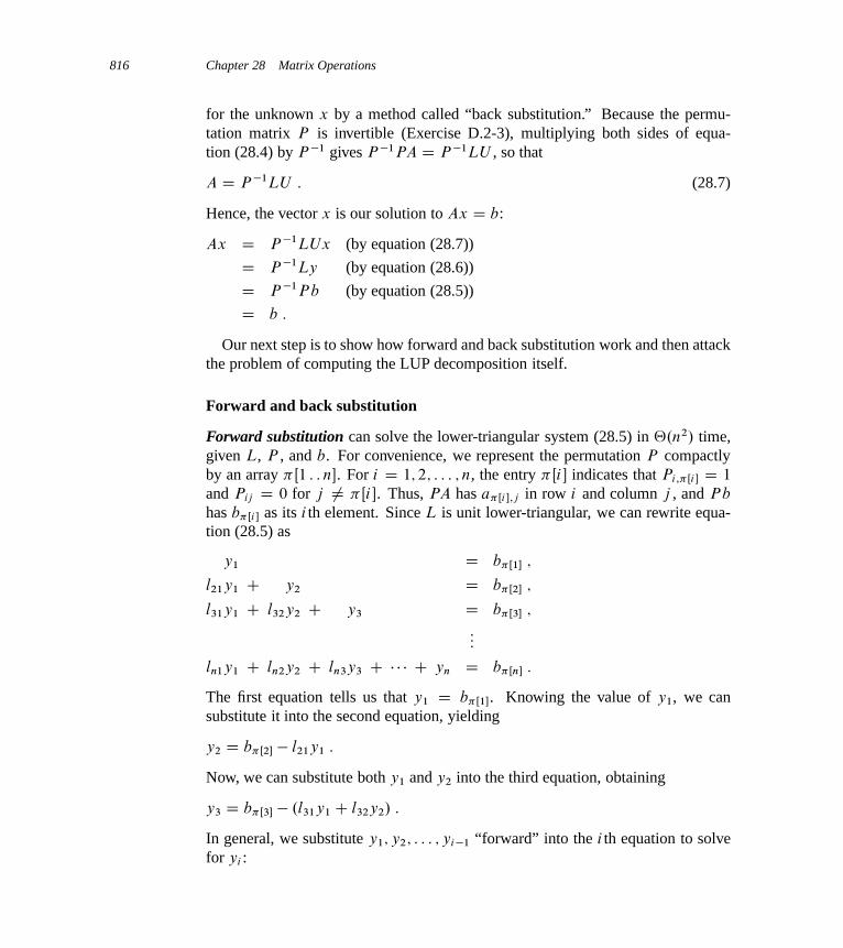
816 Chapter 28 Matrix Operations
for the unknown x by a method called “back substitution.” Because the permu-tation matrix P is invertible (Exercise D.2-3), multiplying both sides of equa-tion (28.4) by P �1 gives P �1PA D P �1LU , so that
A D P �1LU : (28.7)
Hence, the vector x is our solution to Ax D b:
Ax D P �1LUx (by equation (28.7))
D P �1Ly (by equation (28.6))
D P �1P b (by equation (28.5))
D b :
Our next step is to show how forward and back substitution work and then attackthe problem of computing the LUP decomposition itself.
Forward and back substitution
Forward substitution can solve the lower-triangular system (28.5) in ‚.n2/ time,given L, P , and b. For convenience, we represent the permutation P compactlyby an array �Œ1 : : n�. For i D 1; 2; : : : ; n, the entry �Œi� indicates that Pi;�Œi � D 1
and Pij D 0 for j ¤ �Œi�. Thus, PA has a�Œi�;j in row i and column j , and P b
has b�Œi� as its i th element. Since L is unit lower-triangular, we can rewrite equa-tion (28.5) as
y1 D b�Œ1� ;
l21y1 C y2 D b�Œ2� ;
l31y1 C l32y2 C y3 D b�Œ3� ;
:::
ln1y1 C ln2y2 C ln3y3 C � � � C yn D b�Œn� :
The first equation tells us that y1 D b�Œ1�. Knowing the value of y1, we cansubstitute it into the second equation, yielding
y2 D b�Œ2� � l21y1 :
Now, we can substitute both y1 and y2 into the third equation, obtaining
y3 D b�Œ3� � .l31y1 C l32y2/ :
In general, we substitute y1; y2; : : : ; yi�1 “forward” into the i th equation to solvefor yi :
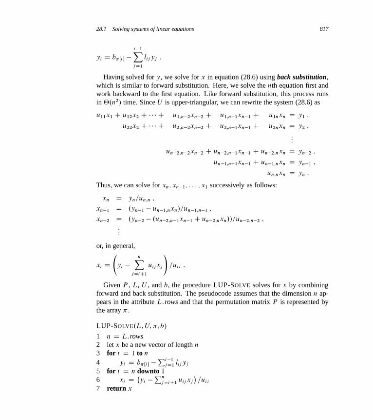
28.1 Solving systems of linear equations 817
yi D b�Œi� �i�1Xj D1
lij yj :
Having solved for y, we solve for x in equation (28.6) using back substitution,which is similar to forward substitution. Here, we solve the nth equation first andwork backward to the first equation. Like forward substitution, this process runsin ‚.n2/ time. Since U is upper-triangular, we can rewrite the system (28.6) as
u11x1 C u12x2 C � � � C u1;n�2xn�2 C u1;n�1xn�1 C u1nxn D y1 ;
u22x2 C � � � C u2;n�2xn�2 C u2;n�1xn�1 C u2nxn D y2 ;
:::
un�2;n�2xn�2 C un�2;n�1xn�1 C un�2;nxn D yn�2 ;
un�1;n�1xn�1 C un�1;nxn D yn�1 ;
un;nxn D yn :
Thus, we can solve for xn; xn�1; : : : ; x1 successively as follows:
xn D yn=un;n ;
xn�1 D .yn�1 � un�1;nxn/=un�1;n�1 ;
xn�2 D .yn�2 � .un�2;n�1xn�1 C un�2;nxn//=un�2;n�2 ;
:::
or, in general,
xi D
yi �nX
j DiC1
uij xj
!=ui i :
Given P , L, U , and b, the procedure LUP-SOLVE solves for x by combiningforward and back substitution. The pseudocode assumes that the dimension n ap-pears in the attribute L:rows and that the permutation matrix P is represented bythe array � .
LUP-SOLVE.L; U; �; b/
1 n D L:rows2 let x be a new vector of length n
3 for i D 1 to n
4 yi D b�Œi� �Pi�1
j D1 lij yj
5 for i D n downto 1
6 xi D�yi �
Pn
j DiC1 uij xj
�=ui i
7 return x

818 Chapter 28 Matrix Operations
Procedure LUP-SOLVE solves for y using forward substitution in lines 3–4, andthen it solves for x using backward substitution in lines 5–6. Since the summationwithin each of the for loops includes an implicit loop, the running time is ‚.n2/.
As an example of these methods, consider the system of linear equations definedby�
1 2 0
3 4 4
5 6 3
�x D
�3
7
8
�;
where
A D�
1 2 0
3 4 4
5 6 3
�;
b D�
3
7
8
�;
and we wish to solve for the unknown x. The LUP decomposition is
L D�
1 0 0
0:2 1 0
0:6 0:5 1
�;
U D�
5 6 3
0 0:8 �0:6
0 0 2:5
�;
P D�
0 0 1
1 0 0
0 1 0
�:
(You might want to verify that PA D LU .) Using forward substitution, we solveLy D P b for y:�
1 0 0
0:2 1 0
0:6 0:5 1
��y1
y2
y3
�D�
8
3
7
�;
obtaining
y D�
8
1:4
1:5
�by computing first y1, then y2, and finally y3. Using back substitution, we solveUx D y for x:
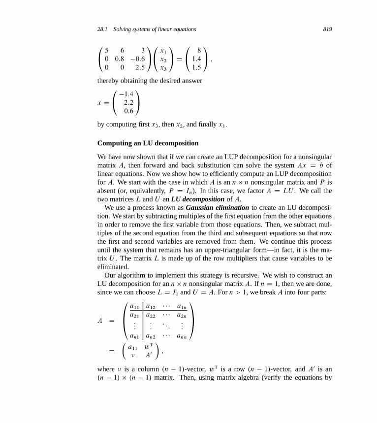
28.1 Solving systems of linear equations 819�5 6 3
0 0:8 �0:6
0 0 2:5
��x1
x2
x3
�D
�8
1:4
1:5
�;
thereby obtaining the desired answer
x D� �1:4
2:2
0:6
�by computing first x3, then x2, and finally x1.
Computing an LU decomposition
We have now shown that if we can create an LUP decomposition for a nonsingularmatrix A, then forward and back substitution can solve the system Ax D b oflinear equations. Now we show how to efficiently compute an LUP decompositionfor A. We start with the case in which A is an n n nonsingular matrix and P isabsent (or, equivalently, P D In). In this case, we factor A D LU . We call thetwo matrices L and U an LU decomposition of A.
We use a process known as Gaussian elimination to create an LU decomposi-tion. We start by subtracting multiples of the first equation from the other equationsin order to remove the first variable from those equations. Then, we subtract mul-tiples of the second equation from the third and subsequent equations so that nowthe first and second variables are removed from them. We continue this processuntil the system that remains has an upper-triangular form—in fact, it is the ma-trix U . The matrix L is made up of the row multipliers that cause variables to beeliminated.
Our algorithm to implement this strategy is recursive. We wish to construct anLU decomposition for an n n nonsingular matrix A. If n D 1, then we are done,since we can choose L D I1 and U D A. For n > 1, we break A into four parts:
A D
˙a11 a12 � � � a1n
a21 a22 � � � a2n
::::::
: : ::::
an1 an2 � � � ann
�D
�a11 wT
� A0
�;
where � is a column .n � 1/-vector, wT is a row .n � 1/-vector, and A0 is an.n � 1/ .n � 1/ matrix. Then, using matrix algebra (verify the equations by
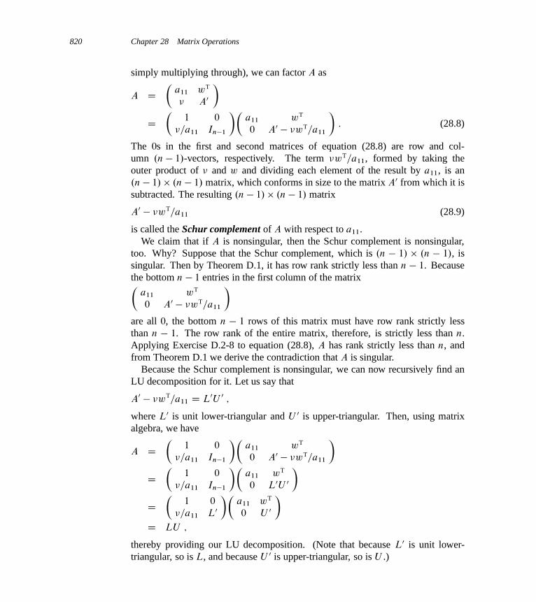
820 Chapter 28 Matrix Operations
simply multiplying through), we can factor A as
A D�
a11 wT
� A0
�D
�1 0
�=a11 In�1
��a11 wT
0 A0 � �wT=a11
�: (28.8)
The 0s in the first and second matrices of equation (28.8) are row and col-umn .n � 1/-vectors, respectively. The term �wT=a11, formed by taking theouter product of � and w and dividing each element of the result by a11, is an.n � 1/ .n � 1/ matrix, which conforms in size to the matrix A0 from which it issubtracted. The resulting .n � 1/ .n � 1/ matrix
A0 � �wT=a11 (28.9)
is called the Schur complement of A with respect to a11.We claim that if A is nonsingular, then the Schur complement is nonsingular,
too. Why? Suppose that the Schur complement, which is .n � 1/ .n � 1/, issingular. Then by Theorem D.1, it has row rank strictly less than n � 1. Becausethe bottom n � 1 entries in the first column of the matrix�
a11 wT
0 A0 � �wT=a11
�are all 0, the bottom n � 1 rows of this matrix must have row rank strictly lessthan n � 1. The row rank of the entire matrix, therefore, is strictly less than n.Applying Exercise D.2-8 to equation (28.8), A has rank strictly less than n, andfrom Theorem D.1 we derive the contradiction that A is singular.
Because the Schur complement is nonsingular, we can now recursively find anLU decomposition for it. Let us say that
A0 � �wT=a11 D L0U 0 ;
where L0 is unit lower-triangular and U 0 is upper-triangular. Then, using matrixalgebra, we have
A D�
1 0
�=a11 In�1
��a11 wT
0 A0 � �wT=a11
�D
�1 0
�=a11 In�1
��a11 wT
0 L0U 0
�D
�1 0
�=a11 L0
��a11 wT
0 U 0
�D LU ;
thereby providing our LU decomposition. (Note that because L0 is unit lower-triangular, so is L, and because U 0 is upper-triangular, so is U .)
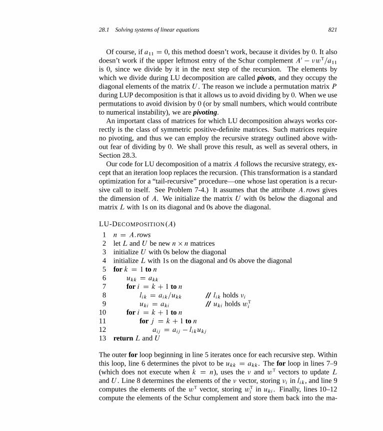
28.1 Solving systems of linear equations 821
Of course, if a11 D 0, this method doesn’t work, because it divides by 0. It alsodoesn’t work if the upper leftmost entry of the Schur complement A0 � �wT=a11
is 0, since we divide by it in the next step of the recursion. The elements bywhich we divide during LU decomposition are called pivots, and they occupy thediagonal elements of the matrix U . The reason we include a permutation matrix P
during LUP decomposition is that it allows us to avoid dividing by 0. When we usepermutations to avoid division by 0 (or by small numbers, which would contributeto numerical instability), we are pivoting.
An important class of matrices for which LU decomposition always works cor-rectly is the class of symmetric positive-definite matrices. Such matrices requireno pivoting, and thus we can employ the recursive strategy outlined above with-out fear of dividing by 0. We shall prove this result, as well as several others, inSection 28.3.
Our code for LU decomposition of a matrix A follows the recursive strategy, ex-cept that an iteration loop replaces the recursion. (This transformation is a standardoptimization for a “tail-recursive” procedure—one whose last operation is a recur-sive call to itself. See Problem 7-4.) It assumes that the attribute A:rows givesthe dimension of A. We initialize the matrix U with 0s below the diagonal andmatrix L with 1s on its diagonal and 0s above the diagonal.
LU-DECOMPOSITION.A/
1 n D A:rows2 let L and U be new n n matrices3 initialize U with 0s below the diagonal4 initialize L with 1s on the diagonal and 0s above the diagonal5 for k D 1 to n
6 ukk D akk
7 for i D k C 1 to n
8 lik D aik=ukk // lik holds �i
9 uki D aki // uki holds wTi
10 for i D k C 1 to n
11 for j D k C 1 to n
12 aij D aij � likukj
13 return L and U
The outer for loop beginning in line 5 iterates once for each recursive step. Withinthis loop, line 6 determines the pivot to be ukk D akk. The for loop in lines 7–9(which does not execute when k D n), uses the � and wT vectors to update L
and U . Line 8 determines the elements of the � vector, storing �i in lik, and line 9computes the elements of the wT vector, storing wT
i in uki . Finally, lines 10–12compute the elements of the Schur complement and store them back into the ma-

822 Chapter 28 Matrix Operations
2 3 1 5
6 13 5 19
2 19 10 23
4 10 11 31
(a)
3 1 5
3 4 2 4
1 16 9 18
2 4 9 21
(b)
2 3 1 5
3 2 4
1 4 1 2
2 1 7 17
(c)
2 3 1 5
3 4 2 4
1 4 2
2 1 7 3
(d)
(e)
2
4
1
�2 3 1 5
6 13 5 19
2 19 10 23
4 10 11 31
˘D
�1 0 0 0
3 1 0 0
1 4 1 0
2 1 7 1
˘ �2 3 1 5
0 4 2 4
0 0 1 2
0 0 0 3
˘A L U
Figure 28.1 The operation of LU-DECOMPOSITION. (a) The matrix A. (b) The element a11 D 2
in the black circle is the pivot, the shaded column is �=a11, and the shaded row is wT. The elementsof U computed thus far are above the horizontal line, and the elements of L are to the left of thevertical line. The Schur complement matrix A0 � �wT=a11 occupies the lower right. (c) We nowoperate on the Schur complement matrix produced from part (b). The element a22 D 4 in the blackcircle is the pivot, and the shaded column and row are �=a22 and wT (in the partitioning of the Schurcomplement), respectively. Lines divide the matrix into the elements of U computed so far (above),the elements of L computed so far (left), and the new Schur complement (lower right). (d) After thenext step, the matrix A is factored. (The element 3 in the new Schur complement becomes part of U
when the recursion terminates.) (e) The factorization A D LU .
trix A. (We don’t need to divide by akk in line 12 because we already did so whenwe computed lik in line 8.) Because line 12 is triply nested, LU-DECOMPOSITION
runs in time ‚.n3/.Figure 28.1 illustrates the operation of LU-DECOMPOSITION. It shows a stan-
dard optimization of the procedure in which we store the significant elements of L
and U in place in the matrix A. That is, we can set up a correspondence betweeneach element aij and either lij (if i > j ) or uij (if i � j ) and update the ma-trix A so that it holds both L and U when the procedure terminates. To obtainthe pseudocode for this optimization from the above pseudocode, just replace eachreference to l or u by a; you can easily verify that this transformation preservescorrectness.
Computing an LUP decomposition
Generally, in solving a system of linear equations Ax D b, we must pivot on off-diagonal elements of A to avoid dividing by 0. Dividing by 0 would, of course,be disastrous. But we also want to avoid dividing by a small value—even if A is
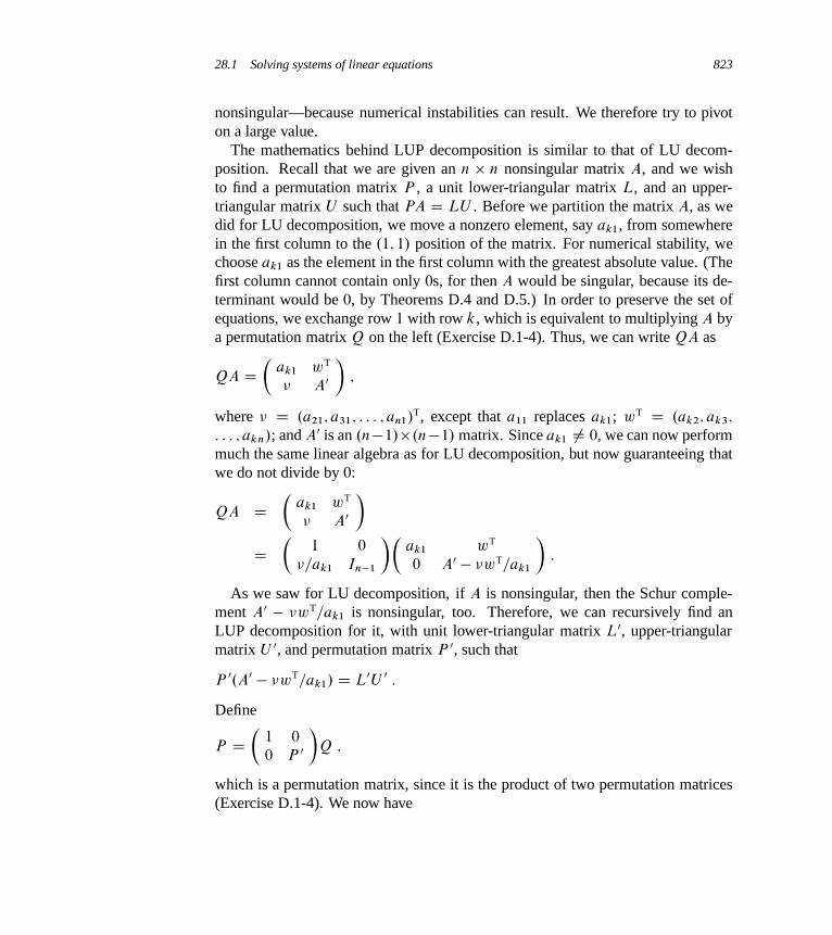
28.1 Solving systems of linear equations 823
nonsingular—because numerical instabilities can result. We therefore try to pivoton a large value.
The mathematics behind LUP decomposition is similar to that of LU decom-position. Recall that we are given an n n nonsingular matrix A, and we wishto find a permutation matrix P , a unit lower-triangular matrix L, and an upper-triangular matrix U such that PA D LU . Before we partition the matrix A, as wedid for LU decomposition, we move a nonzero element, say ak1, from somewherein the first column to the .1; 1/ position of the matrix. For numerical stability, wechoose ak1 as the element in the first column with the greatest absolute value. (Thefirst column cannot contain only 0s, for then A would be singular, because its de-terminant would be 0, by Theorems D.4 and D.5.) In order to preserve the set ofequations, we exchange row 1 with row k, which is equivalent to multiplying A bya permutation matrix Q on the left (Exercise D.1-4). Thus, we can write QA as
QA D�
ak1 wT
� A0
�;
where � D .a21; a31; : : : ; an1/T, except that a11 replaces ak1; wT D .ak2; ak3;
: : : ; akn/; and A0 is an .n�1/.n�1/ matrix. Since ak1 ¤ 0, we can now performmuch the same linear algebra as for LU decomposition, but now guaranteeing thatwe do not divide by 0:
QA D�
ak1 wT
� A0
�D
�1 0
�=ak1 In�1
��ak1 wT
0 A0 � �wT=ak1
�:
As we saw for LU decomposition, if A is nonsingular, then the Schur comple-ment A0 � �wT=ak1 is nonsingular, too. Therefore, we can recursively find anLUP decomposition for it, with unit lower-triangular matrix L0, upper-triangularmatrix U 0, and permutation matrix P 0, such that
P 0.A0 � �wT=ak1/ D L0U 0 :
Define
P D�
1 0
0 P 0
�Q ;
which is a permutation matrix, since it is the product of two permutation matrices(Exercise D.1-4). We now have
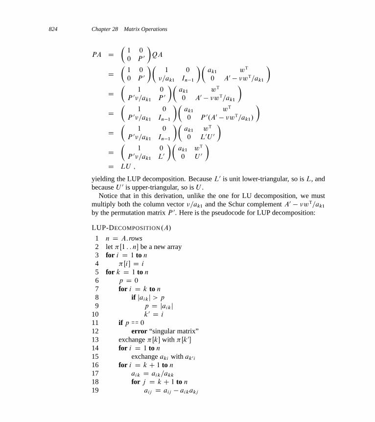
824 Chapter 28 Matrix Operations
PA D�
1 0
0 P 0
�QA
D�
1 0
0 P 0
��1 0
�=ak1 In�1
��ak1 wT
0 A0 � �wT=ak1
�D
�1 0
P 0�=ak1 P 0
��ak1 wT
0 A0 � �wT=ak1
�D
�1 0
P 0�=ak1 In�1
��ak1 wT
0 P 0.A0 � �wT=ak1/
�D
�1 0
P 0�=ak1 In�1
��ak1 wT
0 L0U 0
�D
�1 0
P 0�=ak1 L0
��ak1 wT
0 U 0
�D LU ;
yielding the LUP decomposition. Because L0 is unit lower-triangular, so is L, andbecause U 0 is upper-triangular, so is U .
Notice that in this derivation, unlike the one for LU decomposition, we mustmultiply both the column vector �=ak1 and the Schur complement A0 � �wT=ak1
by the permutation matrix P 0. Here is the pseudocode for LUP decomposition:
LUP-DECOMPOSITION.A/
1 n D A:rows2 let �Œ1 : : n� be a new array3 for i D 1 to n
4 �Œi� D i
5 for k D 1 to n
6 p D 0
7 for i D k to n
8 if jaikj > p
9 p D jaikj10 k0 D i
11 if p == 0
12 error “singular matrix”13 exchange �Œk� with �Œk0�14 for i D 1 to n
15 exchange aki with ak0i
16 for i D k C 1 to n
17 aik D aik=akk
18 for j D k C 1 to n
19 aij D aij � aikakj
28.1 Solving systems of linear equations 825
Like LU-DECOMPOSITION, our LUP-DECOMPOSITION procedure replacesthe recursion with an iteration loop. As an improvement over a direct implemen-tation of the recursion, we dynamically maintain the permutation matrix P as anarray � , where �Œi� D j means that the i th row of P contains a 1 in column j .We also implement the code to compute L and U “in place” in the matrix A. Thus,when the procedure terminates,
aij D(
lij if i > j ;
uij if i � j :
Figure 28.2 illustrates how LUP-DECOMPOSITION factors a matrix. Lines 3–4initialize the array � to represent the identity permutation. The outer for loopbeginning in line 5 implements the recursion. Each time through the outer loop,lines 6–10 determine the element ak0k with largest absolute value of those in thecurrent first column (column k) of the .n � k C 1/ .n � k C 1/ matrix whoseLUP decomposition we are finding. If all elements in the current first column arezero, lines 11–12 report that the matrix is singular. To pivot, we exchange �Œk0�with �Œk� in line 13 and exchange the kth and k0th rows of A in lines 14–15,thereby making the pivot element akk. (The entire rows are swapped because inthe derivation of the method above, not only is A0� �wT=ak1 multiplied by P 0, butso is �=ak1.) Finally, the Schur complement is computed by lines 16–19 in muchthe same way as it is computed by lines 7–12 of LU-DECOMPOSITION, except thathere the operation is written to work in place.
Because of its triply nested loop structure, LUP-DECOMPOSITION has a run-ning time of ‚.n3/, which is the same as that of LU-DECOMPOSITION. Thus,pivoting costs us at most a constant factor in time.
Exercises
28.1-1Solve the equation�
1 0 0
4 1 0
�6 5 1
��x1
x2
x3
�D
�3
14
�7
�by using forward substitution.
28.1-2Find an LU decomposition of the matrix�
4 �5 6
8 �6 7
12 �7 12
�:
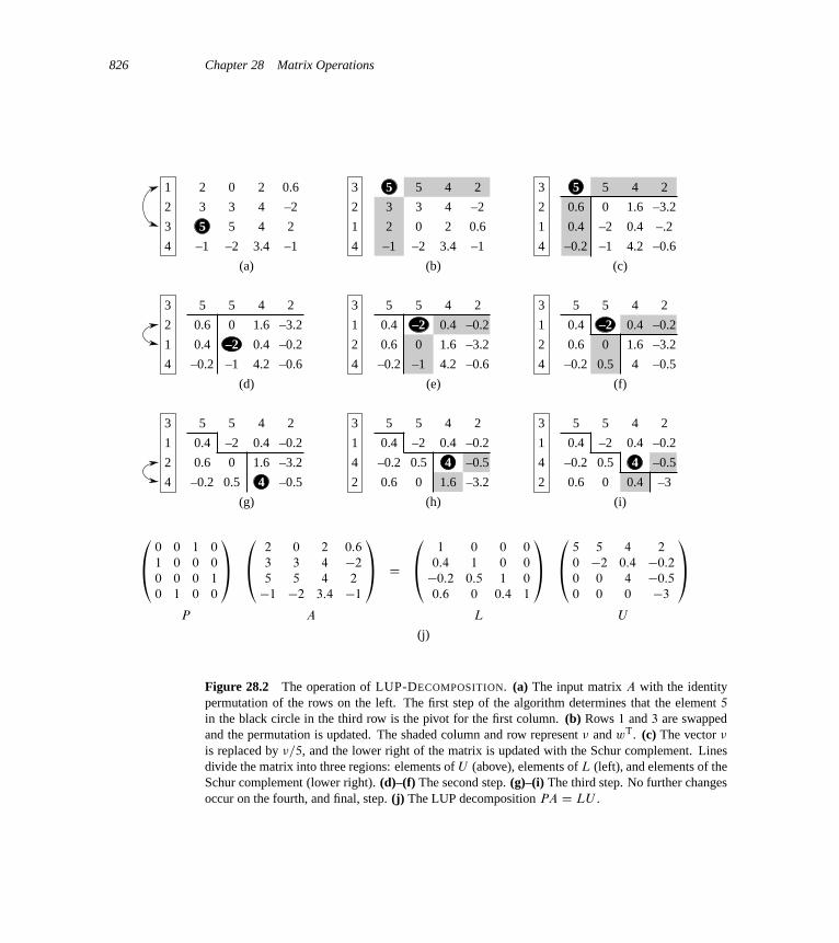
826 Chapter 28 Matrix Operations
2 0 2 0.6
3 3 4 –2
5 5 4 2
–1 –2 3.4 –1
(a)
1
2
3
4
2 0 2 0.6
3 3 4 –2
5 5 4 2
–1 –2 3.4 –1
(b)
3
2
1
4
0.4 –2 0.4 –.2
0.6 0 1.6 –3.2
5 5 4 2
–0.2 –1 4.2 –0.6
(c)
3
2
1
4
0.4 –2 0.4 –0.2
0.6 0 1.6 –3.2
5 5 4 2
–0.2 –1 4.2 –0.6
(d)
3
2
1
4
0.4 –2 0.4 –0.2
0.6 0 1.6 –3.2
5 5 4 2
–0.2 –1 4.2 –0.6
(e)
3
2
1
4
0.4 –2 0.4 –0.2
0.6 0 1.6 –3.2
5 5 4 2
–0.2 0.5 4 –0.5
(f)
3
2
1
4
0.4 –2 0.4 –0.2
0.6 0 1.6 –3.2
5 5 4 2
–0.2 0.5 4 –0.5
(g)
3
2
1
4
0.4 –2 0.4 –0.2
0.6 0 1.6 –3.2
5 5 4 2
–0.2 0.5 4 –0.5
(h)
3
2
1
4
0.4 –2 0.4 –0.2
0.6 0 0.4 –3
5 5 4 2
–0.2 0.5 4 –0.5
(i)
3
2
1
4
(j)
�0 0 1 0
1 0 0 0
0 0 0 1
0 1 0 0
˘ �2 0 2 0:6
3 3 4 �2
5 5 4 2
�1 �2 3:4 �1
˘D
�1 0 0 0
0:4 1 0 0
�0:2 0:5 1 0
0:6 0 0:4 1
˘ �5 5 4 2
0 �2 0:4 �0:2
0 0 4 �0:5
0 0 0 �3
˘P A L U
Figure 28.2 The operation of LUP-DECOMPOSITION. (a) The input matrix A with the identitypermutation of the rows on the left. The first step of the algorithm determines that the element 5
in the black circle in the third row is the pivot for the first column. (b) Rows 1 and 3 are swappedand the permutation is updated. The shaded column and row represent � and wT. (c) The vector �
is replaced by �=5, and the lower right of the matrix is updated with the Schur complement. Linesdivide the matrix into three regions: elements of U (above), elements of L (left), and elements of theSchur complement (lower right). (d)–(f) The second step. (g)–(i) The third step. No further changesoccur on the fourth, and final, step. (j) The LUP decomposition PA D LU .
28.2 Inverting matrices 827
28.1-3Solve the equation�
1 5 4
2 0 3
5 8 2
��x1
x2
x3
�D
�12
9
5
�by using an LUP decomposition.
28.1-4Describe the LUP decomposition of a diagonal matrix.
28.1-5Describe the LUP decomposition of a permutation matrix A, and prove that it isunique.
28.1-6Show that for all n � 1, there exists a singular nn matrix that has an LU decom-position.
28.1-7In LU-DECOMPOSITION, is it necessary to perform the outermost for loop itera-tion when k D n? How about in LUP-DECOMPOSITION?
28.2 Inverting matrices
Although in practice we do not generally use matrix inverses to solve systems oflinear equations, preferring instead to use more numerically stable techniques suchas LUP decomposition, sometimes we need to compute a matrix inverse. In thissection, we show how to use LUP decomposition to compute a matrix inverse.We also prove that matrix multiplication and computing the inverse of a matrixare equivalently hard problems, in that (subject to technical conditions) we canuse an algorithm for one to solve the other in the same asymptotic running time.Thus, we can use Strassen’s algorithm (see Section 4.2) for matrix multiplicationto invert a matrix. Indeed, Strassen’s original paper was motivated by the problemof showing that a set of a linear equations could be solved more quickly than bythe usual method.

828 Chapter 28 Matrix Operations
Computing a matrix inverse from an LUP decomposition
Suppose that we have an LUP decomposition of a matrix A in the form of threematrices L, U , and P such that PA D LU . Using LUP-SOLVE, we can solvean equation of the form Ax D b in time ‚.n2/. Since the LUP decompositiondepends on A but not b, we can run LUP-SOLVE on a second set of equations ofthe form Ax D b0 in additional time ‚.n2/. In general, once we have the LUPdecomposition of A, we can solve, in time ‚.kn2/, k versions of the equationAx D b that differ only in b.
We can think of the equation
AX D In ; (28.10)
which defines the matrix X , the inverse of A, as a set of n distinct equations of theform Ax D b. To be precise, let Xi denote the i th column of X , and recall that theunit vector ei is the i th column of In. We can then solve equation (28.10) for X byusing the LUP decomposition for A to solve each equation
AXi D ei
separately for Xi . Once we have the LUP decomposition, we can compute each ofthe n columns Xi in time ‚.n2/, and so we can compute X from the LUP decom-position of A in time ‚.n3/. Since we can determine the LUP decomposition of A
in time ‚.n3/, we can compute the inverse A�1 of a matrix A in time ‚.n3/.
Matrix multiplication and matrix inversion
We now show that the theoretical speedups obtained for matrix multiplicationtranslate to speedups for matrix inversion. In fact, we prove something stronger:matrix inversion is equivalent to matrix multiplication, in the following sense.If M.n/ denotes the time to multiply two n n matrices, then we can invert anonsingular n n matrix in time O.M.n//. Moreover, if I.n/ denotes the timeto invert a nonsingular n n matrix, then we can multiply two n n matrices intime O.I.n//. We prove these results as two separate theorems.
Theorem 28.1 (Multiplication is no harder than inversion)If we can invert an n n matrix in time I.n/, where I.n/ D �.n2/ and I.n/
satisfies the regularity condition I.3n/ D O.I.n//, then we can multiply two nn
matrices in time O.I.n//.
Proof Let A and B be n n matrices whose matrix product C we wish to com-pute. We define the 3n 3n matrix D by

28.2 Inverting matrices 829
D D�
In A 0
0 In B
0 0 In
�:
The inverse of D is
D�1 D�
In �A AB
0 In �B
0 0 In
�;
and thus we can compute the product AB by taking the upper right nn submatrixof D�1.
We can construct matrix D in ‚.n2/ time, which is O.I.n// because we assumethat I.n/ D �.n2/, and we can invert D in O.I.3n// D O.I.n// time, by theregularity condition on I.n/. We thus have M.n/ D O.I.n//.
Note that I.n/ satisfies the regularity condition whenever I.n/ D ‚.nc lgd n/
for any constants c > 0 and d � 0.The proof that matrix inversion is no harder than matrix multiplication relies
on some properties of symmetric positive-definite matrices that we will prove inSection 28.3.
Theorem 28.2 (Inversion is no harder than multiplication)Suppose we can multiply two n n real matrices in time M.n/, where M.n/ D�.n2/ and M.n/ satisfies the two regularity conditions M.nC k/ D O.M.n// forany k in the range 0 � k � n and M.n=2/ � cM.n/ for some constant c < 1=2.Then we can compute the inverse of any real nonsingular n n matrix in timeO.M.n//.
Proof We prove the theorem here for real matrices. Exercise 28.2-6 asks you togeneralize the proof for matrices whose entries are complex numbers.
We can assume that n is an exact power of 2, since we have�A 0
0 Ik
��1
D�
A�1 0
0 Ik
�for any k > 0. Thus, by choosing k such that n C k is a power of 2, we enlargethe matrix to a size that is the next power of 2 and obtain the desired answer A�1
from the answer to the enlarged problem. The first regularity condition on M.n/
ensures that this enlargement does not cause the running time to increase by morethan a constant factor.
For the moment, let us assume that the nn matrix A is symmetric and positive-definite. We partition each of A and its inverse A�1 into four n=2 n=2 submatri-ces:
830 Chapter 28 Matrix Operations
A D�
B C T
C D
�and A�1 D
�R T
U V
�: (28.11)
Then, if we let
S D D � CB�1C T (28.12)
be the Schur complement of A with respect to B (we shall see more about this formof Schur complement in Section 28.3), we have
A�1 D�
R T
U V
�D�
B�1 C B�1C TS�1CB�1 �B�1C TS�1
�S�1CB�1 S�1
�; (28.13)
since AA�1 D In, as you can verify by performing the matrix multiplication. Be-cause A is symmetric and positive-definite, Lemmas 28.4 and 28.5 in Section 28.3imply that B and S are both symmetric and positive-definite. By Lemma 28.3 inSection 28.3, therefore, the inverses B�1 and S�1 exist, and by Exercise D.2-6,B�1 and S�1 are symmetric, so that .B�1/T D B�1 and .S�1/T D S�1. There-fore, we can compute the submatrices R, T , U , and V of A�1 as follows, whereall matrices mentioned are n=2 n=2:
1. Form the submatrices B , C , C T, and D of A.
2. Recursively compute the inverse B�1 of B .
3. Compute the matrix product W D CB�1, and then compute its transpose W T,which equals B�1C T (by Exercise D.1-2 and .B�1/T D B�1).
4. Compute the matrix product X D W C T, which equals CB�1C T, and thencompute the matrix S D D �X D D � CB�1C T.
5. Recursively compute the inverse S�1 of S , and set V to S�1.
6. Compute the matrix product Y D S�1W , which equals S�1CB�1, andthen compute its transpose Y T, which equals B�1C TS�1 (by Exercise D.1-2,.B�1/T D B�1, and .S�1/T D S�1). Set T to �Y T and U to �Y .
7. Compute the matrix product Z D W TY , which equals B�1C TS�1CB�1, andset R to B�1 C Z.
Thus, we can invert an nn symmetric positive-definite matrix by inverting twon=2n=2 matrices in steps 2 and 5; performing four multiplications of n=2n=2
matrices in steps 3, 4, 6, and 7; plus an additional cost of O.n2/ for extractingsubmatrices from A, inserting submatrices into A�1, and performing a constantnumber of additions, subtractions, and transposes on n=2 n=2 matrices. We getthe recurrence
I.n/ � 2I.n=2/C 4M.n=2/CO.n2/
D 2I.n=2/C‚.M.n//
D O.M.n// :
28.2 Inverting matrices 831
The second line holds because the second regularity condition in the statementof the theorem implies that 4M.n=2/ < 2M.n/ and because we assume thatM.n/ D �.n2/. The third line follows because the second regularity conditionallows us to apply case 3 of the master theorem (Theorem 4.1).
It remains to prove that we can obtain the same asymptotic running time for ma-trix multiplication as for matrix inversion when A is invertible but not symmetricand positive-definite. The basic idea is that for any nonsingular matrix A, the ma-trix ATA is symmetric (by Exercise D.1-2) and positive-definite (by Theorem D.6).The trick, then, is to reduce the problem of inverting A to the problem of invert-ing ATA.
The reduction is based on the observation that when A is an n n nonsingularmatrix, we have
A�1 D .ATA/�1AT ;
since ..ATA/�1AT/A D .ATA/�1.ATA/ D In and a matrix inverse is unique.Therefore, we can compute A�1 by first multiplying AT by A to obtain ATA, theninverting the symmetric positive-definite matrix ATA using the above divide-and-conquer algorithm, and finally multiplying the result by AT. Each of these threesteps takes O.M.n// time, and thus we can invert any nonsingular matrix with realentries in O.M.n// time.
The proof of Theorem 28.2 suggests a means of solving the equation Ax D b
by using LU decomposition without pivoting, so long as A is nonsingular. Wemultiply both sides of the equation by AT, yielding .ATA/x D ATb. This trans-formation doesn’t affect the solution x, since AT is invertible, and so we can fac-tor the symmetric positive-definite matrix ATA by computing an LU decomposi-tion. We then use forward and back substitution to solve for x with the right-handside ATb. Although this method is theoretically correct, in practice the procedureLUP-DECOMPOSITION works much better. LUP decomposition requires fewerarithmetic operations by a constant factor, and it has somewhat better numericalproperties.
Exercises
28.2-1Let M.n/ be the time to multiply two n n matrices, and let S.n/ denote the timerequired to square an n n matrix. Show that multiplying and squaring matri-ces have essentially the same difficulty: an M.n/-time matrix-multiplication al-gorithm implies an O.M.n//-time squaring algorithm, and an S.n/-time squaringalgorithm implies an O.S.n//-time matrix-multiplication algorithm.

832 Chapter 28 Matrix Operations
28.2-2Let M.n/ be the time to multiply two n n matrices, and let L.n/ be the time tocompute the LUP decomposition of an n n matrix. Show that multiplying matri-ces and computing LUP decompositions of matrices have essentially the same dif-ficulty: an M.n/-time matrix-multiplication algorithm implies an O.M.n//-timeLUP-decomposition algorithm, and an L.n/-time LUP-decomposition algorithmimplies an O.L.n//-time matrix-multiplication algorithm.
28.2-3Let M.n/ be the time to multiply two n n matrices, and let D.n/ denote thetime required to find the determinant of an n n matrix. Show that multiply-ing matrices and computing the determinant have essentially the same difficulty:an M.n/-time matrix-multiplication algorithm implies an O.M.n//-time determi-nant algorithm, and a D.n/-time determinant algorithm implies an O.D.n//-timematrix-multiplication algorithm.
28.2-4Let M.n/ be the time to multiply two n n boolean matrices, and let T .n/ be thetime to find the transitive closure of an n n boolean matrix. (See Section 25.2.)Show that an M.n/-time boolean matrix-multiplication algorithm implies anO.M.n/ lg n/-time transitive-closure algorithm, and a T .n/-time transitive-closurealgorithm implies an O.T .n//-time boolean matrix-multiplication algorithm.
28.2-5Does the matrix-inversion algorithm based on Theorem 28.2 work when matrixelements are drawn from the field of integers modulo 2? Explain.
28.2-6 ?
Generalize the matrix-inversion algorithm of Theorem 28.2 to handle matrices ofcomplex numbers, and prove that your generalization works correctly. (Hint: In-stead of the transpose of A, use the conjugate transpose A�, which you obtain fromthe transpose of A by replacing every entry with its complex conjugate. Instead ofsymmetric matrices, consider Hermitian matrices, which are matrices A such thatA D A�.)
28.3 Symmetric positive-definite matrices and least-squares approximation
Symmetric positive-definite matrices have many interesting and desirable proper-ties. For example, they are nonsingular, and we can perform LU decompositionon them without having to worry about dividing by 0. In this section, we shall

28.3 Symmetric positive-definite matrices and least-squares approximation 833
prove several other important properties of symmetric positive-definite matricesand show an interesting application to curve fitting by a least-squares approxima-tion.
The first property we prove is perhaps the most basic.
Lemma 28.3Any positive-definite matrix is nonsingular.
Proof Suppose that a matrix A is singular. Then by Corollary D.3, there exists anonzero vector x such that Ax D 0. Hence, xTAx D 0, and A cannot be positive-definite.
The proof that we can perform LU decomposition on a symmetric positive-definite matrix A without dividing by 0 is more involved. We begin by provingproperties about certain submatrices of A. Define the kth leading submatrix of A
to be the matrix Ak consisting of the intersection of the first k rows and first k
columns of A.
Lemma 28.4If A is a symmetric positive-definite matrix, then every leading submatrix of A issymmetric and positive-definite.
Proof That each leading submatrix Ak is symmetric is obvious. To prove that Ak
is positive-definite, we assume that it is not and derive a contradiction. If Ak is notpositive-definite, then there exists a k-vector xk ¤ 0 such that xT
kAkxk � 0. Let A
be n n, and
A D�
Ak BT
B C
�(28.14)
for submatrices B (which is .n�k/k) and C (which is .n�k/ .n�k/). Definethe n-vector x D . xT
k 0 /T, where n � k 0s follow xk. Then we have
xTAx D . xTk 0 /
�Ak BT
B C
��xk
0
�D . xT
k 0 /
�Akxk
Bxk
�D xT
kAkxk
� 0 ;
which contradicts A being positive-definite.
834 Chapter 28 Matrix Operations
We now turn to some essential properties of the Schur complement. Let A bea symmetric positive-definite matrix, and let Ak be a leading k k submatrixof A. Partition A once again according to equation (28.14). We generalize equa-tion (28.9) to define the Schur complement S of A with respect to Ak as
S D C � BA�1k BT : (28.15)
(By Lemma 28.4, Ak is symmetric and positive-definite; therefore, A�1k
exists byLemma 28.3, and S is well defined.) Note that our earlier definition (28.9) of theSchur complement is consistent with equation (28.15), by letting k D 1.
The next lemma shows that the Schur-complement matrices of symmetric posi-tive-definite matrices are themselves symmetric and positive-definite. We used thisresult in Theorem 28.2, and we need its corollary to prove the correctness of LUdecomposition for symmetric positive-definite matrices.
Lemma 28.5 (Schur complement lemma)If A is a symmetric positive-definite matrix and Ak is a leading k k submatrixof A, then the Schur complement S of A with respect to Ak is symmetric andpositive-definite.
Proof Because A is symmetric, so is the submatrix C . By Exercise D.2-6, theproduct BA�1
kBT is symmetric, and by Exercise D.1-1, S is symmetric.
It remains to show that S is positive-definite. Consider the partition of A given inequation (28.14). For any nonzero vector x, we have xTAx > 0 by the assumptionthat A is positive-definite. Let us break x into two subvectors y and ´ compatiblewith Ak and C , respectively. Because A�1
kexists, we have
xTAx D . yT ´T /
�Ak BT
B C
��y
´
�D . yT ´T /
�Aky C BT´
By C C ´
�D yTAky C yTBT´C ´TBy C ´TC ´
D .y C A�1k BT´/TAk.y C A�1
k BT´/C ´T.C � BA�1k BT/´ ; (28.16)
by matrix magic. (Verify by multiplying through.) This last equation amounts to“completing the square” of the quadratic form. (See Exercise 28.3-2.)
Since xTAx > 0 holds for any nonzero x, let us pick any nonzero ´ and thenchoose y D �A�1
kBT´, which causes the first term in equation (28.16) to vanish,
leaving
´T.C � BA�1k BT/´ D ´TS´
as the value of the expression. For any ´ ¤ 0, we therefore have ´TS´ DxTAx > 0, and thus S is positive-definite.

28.3 Symmetric positive-definite matrices and least-squares approximation 835
Corollary 28.6LU decomposition of a symmetric positive-definite matrix never causes a divisionby 0.
Proof Let A be a symmetric positive-definite matrix. We shall prove somethingstronger than the statement of the corollary: every pivot is strictly positive. The firstpivot is a11. Let e1 be the first unit vector, from which we obtain a11 D eT
1Ae1 > 0.Since the first step of LU decomposition produces the Schur complement of A
with respect to A1 D .a11/, Lemma 28.5 implies by induction that all pivots arepositive.
Least-squares approximation
One important application of symmetric positive-definite matrices arises in fittingcurves to given sets of data points. Suppose that we are given a set of m data points
.x1; y1/; .x2; y2/; : : : ; .xm; ym/ ;
where we know that the yi are subject to measurement errors. We would like todetermine a function F.x/ such that the approximation errors
�i D F.xi/ � yi ; (28.17)
are small for i D 1; 2; : : : ; m. The form of the function F depends on the problemat hand. Here, we assume that it has the form of a linearly weighted sum,
F.x/ DnX
j D1
cj fj .x/ ;
where the number of summands n and the specific basis functions fj are chosenbased on knowledge of the problem at hand. A common choice is fj .x/ D xj �1,which means that
F.x/ D c1 C c2x C c3x2 C � � � C cnxn�1
is a polynomial of degree n � 1 in x. Thus, given m data points .x1; y1/; .x2; y2/;
: : : ; .xm; ym/, we wish to calculate n coefficients c1; c2; : : : ; cn that minimize theapproximation errors �1; �2; : : : ; �m.
By choosing n D m, we can calculate each yi exactly in equation (28.17). Sucha high-degree F “fits the noise” as well as the data, however, and generally givespoor results when used to predict y for previously unseen values of x. It is usu-ally better to choose n significantly smaller than m and hope that by choosing thecoefficients cj well, we can obtain a function F that finds the significant patternsin the data points without paying undue attention to the noise. Some theoretical
836 Chapter 28 Matrix Operations
principles exist for choosing n, but they are beyond the scope of this text. In anycase, once we choose a value of n that is less than m, we end up with an overde-termined set of equations whose solution we wish to approximate. We now showhow to do so.
Let
A D
˙f1.x1/ f2.x1/ : : : fn.x1/
f1.x2/ f2.x2/ : : : fn.x2/:::
:::: : :
:::
f1.xm/ f2.xm/ : : : fn.xm/
�denote the matrix of values of the basis functions at the given points; that is,aij D fj .xi/. Let c D .ck/ denote the desired n-vector of coefficients. Then,
Ac D
˙f1.x1/ f2.x1/ : : : fn.x1/
f1.x2/ f2.x2/ : : : fn.x2/:::
:::: : :
:::
f1.xm/ f2.xm/ : : : fn.xm/
�˙c1
c2
:::
cn
�
D
˙F.x1/
F.x2/:::
F .xm/
�
is the m-vector of “predicted values” for y. Thus,
� D Ac � y
is the m-vector of approximation errors.To minimize approximation errors, we choose to minimize the norm of the error
vector �, which gives us a least-squares solution, since
k�k D
mXiD1
�2i
!1=2
:
Because
k�k2 D kAc � yk2 DmX
iD1
nX
j D1
aij cj � yi
!2
;
we can minimize k�k by differentiating k�k2 with respect to each ck and thensetting the result to 0:
28.3 Symmetric positive-definite matrices and least-squares approximation 837
d k�k2
dck
DmX
iD1
2
nX
j D1
aij cj � yi
!aik D 0 : (28.18)
The n equations (28.18) for k D 1; 2; : : : ; n are equivalent to the single matrixequation
.Ac � y/TA D 0
or, equivalently (using Exercise D.1-2), to
AT.Ac � y/ D 0 ;
which implies
ATAc D ATy : (28.19)
In statistics, this is called the normal equation. The matrix ATA is symmetricby Exercise D.1-2, and if A has full column rank, then by Theorem D.6, ATA
is positive-definite as well. Hence, .ATA/�1 exists, and the solution to equa-tion (28.19) is
c D �.ATA/�1AT
�y
D ACy ; (28.20)
where the matrix AC D ..ATA/�1AT/ is the pseudoinverse of the matrix A. Thepseudoinverse naturally generalizes the notion of a matrix inverse to the case inwhich A is not square. (Compare equation (28.20) as the approximate solution toAc D y with the solution A�1b as the exact solution to Ax D b.)
As an example of producing a least-squares fit, suppose that we have five datapoints
.x1; y1/ D .�1; 2/ ;
.x2; y2/ D .1; 1/ ;
.x3; y3/ D .2; 1/ ;
.x4; y4/ D .3; 0/ ;
.x5; y5/ D .5; 3/ ;
shown as black dots in Figure 28.3. We wish to fit these points with a quadraticpolynomial
F.x/ D c1 C c2x C c3x2 :
We start with the matrix of basis-function values

838 Chapter 28 Matrix Operations
0.5
1.0
1.5
2.0
2.5
3.0
0.01 2 3 4 50–1–2
x
y
F(x) = 1.2 – 0.757x + 0.214x2
Figure 28.3 The least-squares fit of a quadratic polynomial to the set of five data pointsf.�1; 2/; .1; 1/; .2; 1/; .3; 0/; .5; 3/g. The black dots are the data points, and the white dots are theirestimated values predicted by the polynomial F.x/ D 1:2 � 0:757x C 0:214x2 , the quadratic poly-nomial that minimizes the sum of the squared errors. Each shaded line shows the error for one datapoint.
A D
�1 x1 x2
1
1 x2 x22
1 x3 x23
1 x4 x24
1 x5 x25
�D
�1 �1 1
1 1 1
1 2 4
1 3 9
1 5 25
�;
whose pseudoinverse is
AC D�
0:500 0:300 0:200 0:100 �0:100
�0:388 0:093 0:190 0:193 �0:088
0:060 �0:036 �0:048 �0:036 0:060
�:
Multiplying y by AC, we obtain the coefficient vector
c D�
1:200
�0:757
0:214
�;
which corresponds to the quadratic polynomial

28.3 Symmetric positive-definite matrices and least-squares approximation 839
F.x/ D 1:200 � 0:757x C 0:214x2
as the closest-fitting quadratic to the given data, in a least-squares sense.As a practical matter, we solve the normal equation (28.19) by multiplying y
by AT and then finding an LU decomposition of ATA. If A has full rank, thematrix ATA is guaranteed to be nonsingular, because it is symmetric and positive-definite. (See Exercise D.1-2 and Theorem D.6.)
Exercises
28.3-1Prove that every diagonal element of a symmetric positive-definite matrix is posi-tive.
28.3-2
Let A D�
a b
b c
�be a 2 2 symmetric positive-definite matrix. Prove that its
determinant ac � b2 is positive by “completing the square” in a manner similar tothat used in the proof of Lemma 28.5.
28.3-3Prove that the maximum element in a symmetric positive-definite matrix lies onthe diagonal.
28.3-4Prove that the determinant of each leading submatrix of a symmetric positive-definite matrix is positive.
28.3-5Let Ak denote the kth leading submatrix of a symmetric positive-definite matrix A.Prove that det.Ak/= det.Ak�1/ is the kth pivot during LU decomposition, where,by convention, det.A0/ D 1.
28.3-6Find the function of the form
F.x/ D c1 C c2x lg x C c3ex
that is the best least-squares fit to the data points
.1; 1/; .2; 1/; .3; 3/; .4; 8/ :
840 Chapter 28 Matrix Operations
28.3-7Show that the pseudoinverse AC satisfies the following four equations:
AACA D A ;
ACAAC D AC ;
.AAC/T D AAC ;
.ACA/T D ACA :
Problems
28-1 Tridiagonal systems of linear equationsConsider the tridiagonal matrix
A D
ˇ1 �1 0 0 0
�1 2 �1 0 0
0 �1 2 �1 0
0 0 �1 2 �1
0 0 0 �1 2
�:
a. Find an LU decomposition of A.
b. Solve the equation Ax D �1 1 1 1 1
�Tby using forward and back sub-
stitution.
c. Find the inverse of A.
d. Show how, for any n n symmetric positive-definite, tridiagonal matrix A andany n-vector b, to solve the equation Ax D b in O.n/ time by performing anLU decomposition. Argue that any method based on forming A�1 is asymptot-ically more expensive in the worst case.
e. Show how, for any nn nonsingular, tridiagonal matrix A and any n-vector b, tosolve the equation Ax D b in O.n/ time by performing an LUP decomposition.
28-2 SplinesA practical method for interpolating a set of points with a curve is to use cu-bic splines. We are given a set f.xi ; yi/ W i D 0; 1; : : : ; ng of n C 1 point-valuepairs, where x0 < x1 < � � � < xn. We wish to fit a piecewise-cubic curve(spline) f .x/ to the points. That is, the curve f .x/ is made up of n cubic polyno-mials fi.x/ D ai C bix C cix
2 C dix3 for i D 0; 1; : : : ; n � 1, where if x falls in

Problems for Chapter 28 841
the range xi � x � xiC1, then the value of the curve is given by f .x/ D fi.x�xi/.The points xi at which the cubic polynomials are “pasted” together are called knots.For simplicity, we shall assume that xi D i for i D 0; 1; : : : ; n.
To ensure continuity of f .x/, we require that
f .xi/ D fi.0/ D yi ;
f .xiC1/ D fi.1/ D yiC1
for i D 0; 1; : : : ; n � 1. To ensure that f .x/ is sufficiently smooth, we also insistthat the first derivative be continuous at each knot:
f 0.xiC1/ D f 0i .1/ D f 0
iC1.0/
for i D 0; 1; : : : ; n � 2.
a. Suppose that for i D 0; 1; : : : ; n, we are given not only the point-value pairsf.xi ; yi /g but also the first derivatives Di D f 0.xi/ at each knot. Express eachcoefficient ai , bi , ci , and di in terms of the values yi , yiC1, Di , and DiC1.(Remember that xi D i .) How quickly can we compute the 4n coefficientsfrom the point-value pairs and first derivatives?
The question remains of how to choose the first derivatives of f .x/ at the knots.One method is to require the second derivatives to be continuous at the knots:
f 00.xiC1/ D f 00i .1/ D f 00
iC1.0/
for i D 0; 1; : : : ; n � 2. At the first and last knots, we assume that f 00.x0/ Df 00
0 .0/ D 0 and f 00.xn/ D f 00n�1.1/ D 0; these assumptions make f .x/ a natural
cubic spline.
b. Use the continuity constraints on the second derivative to show that for i D1; 2; : : : ; n � 1,
Di�1 C 4Di CDiC1 D 3.yiC1 � yi�1/ : (28.21)
c. Show that
2D0 CD1 D 3.y1 � y0/ ; (28.22)
Dn�1 C 2Dn D 3.yn � yn�1/ : (28.23)
d. Rewrite equations (28.21)–(28.23) as a matrix equation involving the vectorD D hD0; D1; : : : ; Dni of unknowns. What attributes does the matrix in yourequation have?
e. Argue that a natural cubic spline can interpolate a set of nC 1 point-value pairsin O.n/ time (see Problem 28-1).
842 Chapter 28 Matrix Operations
f. Show how to determine a natural cubic spline that interpolates a set of n C 1
points .xi ; yi / satisfying x0 < x1 < � � � < xn, even when xi is not necessarilyequal to i . What matrix equation must your method solve, and how quicklydoes your algorithm run?
Chapter notes
Many excellent texts describe numerical and scientific computation in much greaterdetail than we have room for here. The following are especially readable: Georgeand Liu [132], Golub and Van Loan [144], Press, Teukolsky, Vetterling, and Flan-nery [283, 284], and Strang [323, 324].
Golub and Van Loan [144] discuss numerical stability. They show why det.A/
is not necessarily a good indicator of the stability of a matrix A, proposing insteadto use kAk1 kA�1k1, where kAk1 D max1�i�n
Pn
j D1 jaij j. They also addressthe question of how to compute this value without actually computing A�1.
Gaussian elimination, upon which the LU and LUP decompositions are based,was the first systematic method for solving linear systems of equations. It was alsoone of the earliest numerical algorithms. Although it was known earlier, its dis-covery is commonly attributed to C. F. Gauss (1777–1855). In his famous paper[325], Strassen showed that an nn matrix can be inverted in O.nlg 7/ time. Wino-grad [358] originally proved that matrix multiplication is no harder than matrixinversion, and the converse is due to Aho, Hopcroft, and Ullman [5].
Another important matrix decomposition is the singular value decomposition,or SVD. The SVD factors an m n matrix A into A D Q1†QT
2 , where † is anmn matrix with nonzero values only on the diagonal, Q1 is mm with mutuallyorthonormal columns, and Q2 is n n, also with mutually orthonormal columns.Two vectors are orthonormal if their inner product is 0 and each vector has a normof 1. The books by Strang [323, 324] and Golub and Van Loan [144] contain goodtreatments of the SVD.
Strang [324] has an excellent presentation of symmetric positive-definite matri-ces and of linear algebra in general.
29 Linear Programming
Many problems take the form of maximizing or minimizing an objective, givenlimited resources and competing constraints. If we can specify the objective asa linear function of certain variables, and if we can specify the constraints onresources as equalities or inequalities on those variables, then we have a linear-programming problem. Linear programs arise in a variety of practical applica-tions. We begin by studying an application in electoral politics.
A political problem
Suppose that you are a politician trying to win an election. Your district has threedifferent types of areas—urban, suburban, and rural. These areas have, respec-tively, 100,000, 200,000, and 50,000 registered voters. Although not all the reg-istered voters actually go to the polls, you decide that to govern effectively, youwould like at least half the registered voters in each of the three regions to vote foryou. You are honorable and would never consider supporting policies in which youdo not believe. You realize, however, that certain issues may be more effective inwinning votes in certain places. Your primary issues are building more roads, guncontrol, farm subsidies, and a gasoline tax dedicated to improved public transit.According to your campaign staff’s research, you can estimate how many votesyou win or lose from each population segment by spending $1,000 on advertisingon each issue. This information appears in the table of Figure 29.1. In this table,each entry indicates the number of thousands of either urban, suburban, or ruralvoters who would be won over by spending $1,000 on advertising in support of aparticular issue. Negative entries denote votes that would be lost. Your task is tofigure out the minimum amount of money that you need to spend in order to win50,000 urban votes, 100,000 suburban votes, and 25,000 rural votes.
You could, by trial and error, devise a strategy that wins the required numberof votes, but the strategy you come up with might not be the least expensive one.For example, you could devote $20,000 of advertising to building roads, $0 to guncontrol, $4,000 to farm subsidies, and $9,000 to a gasoline tax. In this case, you

844 Chapter 29 Linear Programming
policy urban suburban ruralbuild roads �2 5 3gun control 8 2 �5
farm subsidies 0 0 10gasoline tax 10 0 �2
Figure 29.1 The effects of policies on voters. Each entry describes the number of thousands ofurban, suburban, or rural voters who could be won over by spending $1,000 on advertising supportof a policy on a particular issue. Negative entries denote votes that would be lost.
would win 20.�2/C0.8/C4.0/C9.10/ D 50 thousand urban votes, 20.5/C0.2/C4.0/C9.0/ D 100 thousand suburban votes, and 20.3/C0.�5/C4.10/C9.�2/ D82 thousand rural votes. You would win the exact number of votes desired in theurban and suburban areas and more than enough votes in the rural area. (In fact,in the rural area, you would receive more votes than there are voters.) In order togarner these votes, you would have paid for 20C 0C 4C 9 D 33 thousand dollarsof advertising.
Naturally, you may wonder whether this strategy is the best possible. That is,could you achieve your goals while spending less on advertising? Additional trialand error might help you to answer this question, but wouldn’t you rather have asystematic method for answering such questions? In order to develop one, we shallformulate this question mathematically. We introduce 4 variables:
� x1 is the number of thousands of dollars spent on advertising on building roads,
� x2 is the number of thousands of dollars spent on advertising on gun control,
� x3 is the number of thousands of dollars spent on advertising on farm subsidies,and
� x4 is the number of thousands of dollars spent on advertising on a gasoline tax.
We can write the requirement that we win at least 50,000 urban votes as
�2x1 C 8x2 C 0x3 C 10x4 � 50 : (29.1)
Similarly, we can write the requirements that we win at least 100,000 suburbanvotes and 25,000 rural votes as
5x1 C 2x2 C 0x3 C 0x4 � 100 (29.2)
and
3x1 � 5x2 C 10x3 � 2x4 � 25 : (29.3)
Any setting of the variables x1; x2; x3; x4 that satisfies inequalities (29.1)–(29.3)yields a strategy that wins a sufficient number of each type of vote. In order to

Chapter 29 Linear Programming 845
keep costs as small as possible, you would like to minimize the amount spent onadvertising. That is, you want to minimize the expression
x1 C x2 C x3 C x4 : (29.4)
Although negative advertising often occurs in political campaigns, there is no suchthing as negative-cost advertising. Consequently, we require that
x1 � 0; x2 � 0; x3 � 0; and x4 � 0 : (29.5)
Combining inequalities (29.1)–(29.3) and (29.5) with the objective of minimiz-ing (29.4), we obtain what is known as a “linear program.” We format this problemas
minimize x1 C x2 C x3 C x4 (29.6)
subject to�2x1 C 8x2 C 0x3 C 10x4 � 50 (29.7)
5x1 C 2x2 C 0x3 C 0x4 � 100 (29.8)
3x1 � 5x2 C 10x3 � 2x4 � 25 (29.9)
x1; x2; x3; x4 � 0 : (29.10)
The solution of this linear program yields your optimal strategy.
General linear programs
In the general linear-programming problem, we wish to optimize a linear functionsubject to a set of linear inequalities. Given a set of real numbers a1; a2; : : : ; an anda set of variables x1; x2; : : : ; xn, we define a linear function f on those variablesby
f .x1; x2; : : : ; xn/ D a1x1 C a2x2 C � � � C anxn DnX
j D1
aj xj :
If b is a real number and f is a linear function, then the equation
f .x1; x2; : : : ; xn/ D b
is a linear equality and the inequalities
f .x1; x2; : : : ; xn/ � b
and
f .x1; x2; : : : ; xn/ � b

846 Chapter 29 Linear Programming
are linear inequalities. We use the general term linear constraints to denote eitherlinear equalities or linear inequalities. In linear programming, we do not allowstrict inequalities. Formally, a linear-programming problem is the problem ofeither minimizing or maximizing a linear function subject to a finite set of linearconstraints. If we are to minimize, then we call the linear program a minimizationlinear program, and if we are to maximize, then we call the linear program amaximization linear program.
This remainder of this chapter covers how to formulate and solve linear pro-grams. Although several polynomial-time algorithms for linear programming havebeen developed, we shall not study them in this chapter. Instead, we shall study thesimplex algorithm, which is the oldest linear-programming algorithm. The simplexalgorithm does not run in polynomial time in the worst case, but it is fairly efficientand widely used in practice.
An overview of linear programming
In order to describe properties of and algorithms for linear programs, we find itconvenient to express them in canonical forms. We shall use two forms, standardand slack, in this chapter. We shall define them precisely in Section 29.1. Infor-mally, a linear program in standard form is the maximization of a linear functionsubject to linear inequalities, whereas a linear program in slack form is the max-imization of a linear function subject to linear equalities. We shall typically usestandard form for expressing linear programs, but we find it more convenient touse slack form when we describe the details of the simplex algorithm. For now, werestrict our attention to maximizing a linear function on n variables subject to a setof m linear inequalities.
Let us first consider the following linear program with two variables:
maximize x1 C x2 (29.11)
subject to4x1 � x2 � 8 (29.12)
2x1 C x2 � 10 (29.13)
5x1 � 2x2 � �2 (29.14)
x1; x2 � 0 : (29.15)
We call any setting of the variables x1 and x2 that satisfies all the constraints(29.12)–(29.15) a feasible solution to the linear program. If we graph the con-straints in the .x1; x2/-Cartesian coordinate system, as in Figure 29.2(a), we see
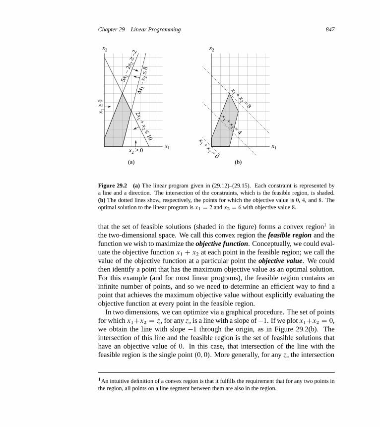
Chapter 29 Linear Programming 847
4x1 –
x2
≤ 8
2x1 + x
2 ≤ 10
x2
x1x2 ≥ 0
x 1≥
0
5x1 –
2x 2
≥ –2
(a)
x2
x1
(b)
x1 + x
2 = 0
x1 + x
2 = 4
x1 + x
2 = 8
Figure 29.2 (a) The linear program given in (29.12)–(29.15). Each constraint is represented bya line and a direction. The intersection of the constraints, which is the feasible region, is shaded.(b) The dotted lines show, respectively, the points for which the objective value is 0, 4, and 8. Theoptimal solution to the linear program is x1 D 2 and x2 D 6 with objective value 8.
that the set of feasible solutions (shaded in the figure) forms a convex region1 inthe two-dimensional space. We call this convex region the feasible region and thefunction we wish to maximize the objective function. Conceptually, we could eval-uate the objective function x1 C x2 at each point in the feasible region; we call thevalue of the objective function at a particular point the objective value. We couldthen identify a point that has the maximum objective value as an optimal solution.For this example (and for most linear programs), the feasible region contains aninfinite number of points, and so we need to determine an efficient way to find apoint that achieves the maximum objective value without explicitly evaluating theobjective function at every point in the feasible region.
In two dimensions, we can optimize via a graphical procedure. The set of pointsfor which x1Cx2 D ´, for any ´, is a line with a slope of�1. If we plot x1Cx2 D 0,we obtain the line with slope �1 through the origin, as in Figure 29.2(b). Theintersection of this line and the feasible region is the set of feasible solutions thathave an objective value of 0. In this case, that intersection of the line with thefeasible region is the single point .0; 0/. More generally, for any ´, the intersection
1An intuitive definition of a convex region is that it fulfills the requirement that for any two points inthe region, all points on a line segment between them are also in the region.

848 Chapter 29 Linear Programming
of the line x1 C x2 D ´ and the feasible region is the set of feasible solutions thathave objective value ´. Figure 29.2(b) shows the lines x1 C x2 D 0, x1 C x2 D 4,and x1 C x2 D 8. Because the feasible region in Figure 29.2 is bounded, theremust be some maximum value ´ for which the intersection of the line x1C x2 D ´
and the feasible region is nonempty. Any point at which this occurs is an optimalsolution to the linear program, which in this case is the point x1 D 2 and x2 D 6
with objective value 8.It is no accident that an optimal solution to the linear program occurs at a vertex
of the feasible region. The maximum value of ´ for which the line x1 C x2 D ´
intersects the feasible region must be on the boundary of the feasible region, andthus the intersection of this line with the boundary of the feasible region is either asingle vertex or a line segment. If the intersection is a single vertex, then there isjust one optimal solution, and it is that vertex. If the intersection is a line segment,every point on that line segment must have the same objective value; in particular,both endpoints of the line segment are optimal solutions. Since each endpoint of aline segment is a vertex, there is an optimal solution at a vertex in this case as well.
Although we cannot easily graph linear programs with more than two variables,the same intuition holds. If we have three variables, then each constraint corre-sponds to a half-space in three-dimensional space. The intersection of these half-spaces forms the feasible region. The set of points for which the objective functionobtains a given value ´ is now a plane (assuming no degenerate conditions). If allcoefficients of the objective function are nonnegative, and if the origin is a feasiblesolution to the linear program, then as we move this plane away from the origin, ina direction normal to the objective function, we find points of increasing objectivevalue. (If the origin is not feasible or if some coefficients in the objective functionare negative, the intuitive picture becomes slightly more complicated.) As in twodimensions, because the feasible region is convex, the set of points that achievethe optimal objective value must include a vertex of the feasible region. Simi-larly, if we have n variables, each constraint defines a half-space in n-dimensionalspace. We call the feasible region formed by the intersection of these half-spaces asimplex. The objective function is now a hyperplane and, because of convexity, anoptimal solution still occurs at a vertex of the simplex.
The simplex algorithm takes as input a linear program and returns an optimalsolution. It starts at some vertex of the simplex and performs a sequence of itera-tions. In each iteration, it moves along an edge of the simplex from a current vertexto a neighboring vertex whose objective value is no smaller than that of the currentvertex (and usually is larger.) The simplex algorithm terminates when it reachesa local maximum, which is a vertex from which all neighboring vertices have asmaller objective value. Because the feasible region is convex and the objectivefunction is linear, this local optimum is actually a global optimum. In Section 29.4,
Chapter 29 Linear Programming 849
we shall use a concept called “duality” to show that the solution returned by thesimplex algorithm is indeed optimal.
Although the geometric view gives a good intuitive view of the operations of thesimplex algorithm, we shall not refer to it explicitly when developing the detailsof the simplex algorithm in Section 29.3. Instead, we take an algebraic view. Wefirst write the given linear program in slack form, which is a set of linear equalities.These linear equalities express some of the variables, called “basic variables,” interms of other variables, called “nonbasic variables.” We move from one vertexto another by making a basic variable become nonbasic and making a nonbasicvariable become basic. We call this operation a “pivot” and, viewed algebraically,it is nothing more than rewriting the linear program in an equivalent slack form.
The two-variable example described above was particularly simple. We shallneed to address several more details in this chapter. These issues include iden-tifying linear programs that have no solutions, linear programs that have no finiteoptimal solution, and linear programs for which the origin is not a feasible solution.
Applications of linear programming
Linear programming has a large number of applications. Any textbook on opera-tions research is filled with examples of linear programming, and linear program-ming has become a standard tool taught to students in most business schools. Theelection scenario is one typical example. Two more examples of linear program-ming are the following:
� An airline wishes to schedule its flight crews. The Federal Aviation Adminis-tration imposes many constraints, such as limiting the number of consecutivehours that each crew member can work and insisting that a particular crew workonly on one model of aircraft during each month. The airline wants to schedulecrews on all of its flights using as few crew members as possible.
� An oil company wants to decide where to drill for oil. Siting a drill at a particu-lar location has an associated cost and, based on geological surveys, an expectedpayoff of some number of barrels of oil. The company has a limited budget forlocating new drills and wants to maximize the amount of oil it expects to find,given this budget.
With linear programs, we also model and solve graph and combinatorial prob-lems, such as those appearing in this textbook. We have already seen a specialcase of linear programming used to solve systems of difference constraints in Sec-tion 24.4. In Section 29.2, we shall study how to formulate several graph andnetwork-flow problems as linear programs. In Section 35.4, we shall use linearprogramming as a tool to find an approximate solution to another graph problem.

850 Chapter 29 Linear Programming
Algorithms for linear programming
This chapter studies the simplex algorithm. This algorithm, when implementedcarefully, often solves general linear programs quickly in practice. With somecarefully contrived inputs, however, the simplex algorithm can require exponentialtime. The first polynomial-time algorithm for linear programming was the ellipsoidalgorithm, which runs slowly in practice. A second class of polynomial-time algo-rithms are known as interior-point methods. In contrast to the simplex algorithm,which moves along the exterior of the feasible region and maintains a feasible solu-tion that is a vertex of the simplex at each iteration, these algorithms move throughthe interior of the feasible region. The intermediate solutions, while feasible, arenot necessarily vertices of the simplex, but the final solution is a vertex. For largeinputs, interior-point algorithms can run as fast as, and sometimes faster than, thesimplex algorithm. The chapter notes point you to more information about thesealgorithms.
If we add to a linear program the additional requirement that all variables takeon integer values, we have an integer linear program. Exercise 34.5-3 asks youto show that just finding a feasible solution to this problem is NP-hard; sinceno polynomial-time algorithms are known for any NP-hard problems, there is noknown polynomial-time algorithm for integer linear programming. In contrast, wecan solve a general linear-programming problem in polynomial time.
In this chapter, if we have a linear program with variables x D .x1; x2; : : : ; xn/
and wish to refer to a particular setting of the variables, we shall use the notationNx D . Nx1; Nx2; : : : ; Nxn/.
29.1 Standard and slack forms
This section describes two formats, standard form and slack form, that are use-ful when we specify and work with linear programs. In standard form, all theconstraints are inequalities, whereas in slack form, all constraints are equalities(except for those that require the variables to be nonnegative).
Standard form
In standard form, we are given n real numbers c1; c2; : : : ; cn; m real numbersb1; b2; : : : ; bm; and mn real numbers aij for i D 1; 2; : : : ; m and j D 1; 2; : : : ; n.We wish to find n real numbers x1; x2; : : : ; xn that
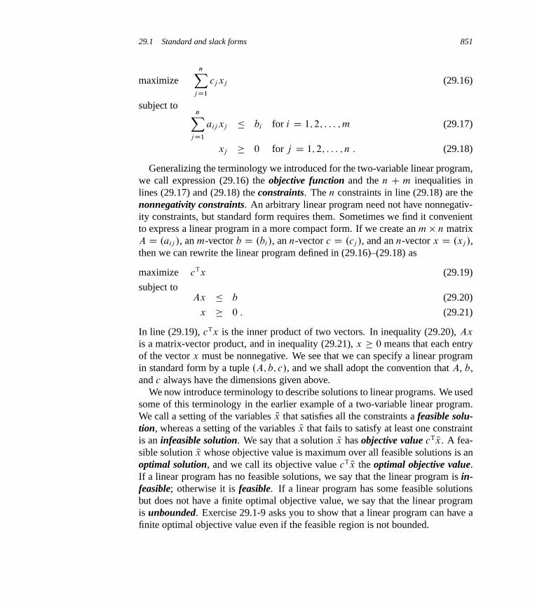
29.1 Standard and slack forms 851
maximizenX
j D1
cj xj (29.16)
subject tonX
j D1
aij xj � bi for i D 1; 2; : : : ; m (29.17)
xj � 0 for j D 1; 2; : : : ; n : (29.18)
Generalizing the terminology we introduced for the two-variable linear program,we call expression (29.16) the objective function and the n C m inequalities inlines (29.17) and (29.18) the constraints. The n constraints in line (29.18) are thenonnegativity constraints. An arbitrary linear program need not have nonnegativ-ity constraints, but standard form requires them. Sometimes we find it convenientto express a linear program in a more compact form. If we create an m n matrixA D .aij /, an m-vector b D .bi/, an n-vector c D .cj /, and an n-vector x D .xj /,then we can rewrite the linear program defined in (29.16)–(29.18) as
maximize cTx (29.19)
subject toAx � b (29.20)
x � 0 : (29.21)
In line (29.19), cTx is the inner product of two vectors. In inequality (29.20), Ax
is a matrix-vector product, and in inequality (29.21), x � 0 means that each entryof the vector x must be nonnegative. We see that we can specify a linear programin standard form by a tuple .A; b; c/, and we shall adopt the convention that A, b,and c always have the dimensions given above.
We now introduce terminology to describe solutions to linear programs. We usedsome of this terminology in the earlier example of a two-variable linear program.We call a setting of the variables Nx that satisfies all the constraints a feasible solu-tion, whereas a setting of the variables Nx that fails to satisfy at least one constraintis an infeasible solution. We say that a solution Nx has objective value cT Nx. A fea-sible solution Nx whose objective value is maximum over all feasible solutions is anoptimal solution, and we call its objective value cT Nx the optimal objective value.If a linear program has no feasible solutions, we say that the linear program is in-feasible; otherwise it is feasible. If a linear program has some feasible solutionsbut does not have a finite optimal objective value, we say that the linear programis unbounded. Exercise 29.1-9 asks you to show that a linear program can have afinite optimal objective value even if the feasible region is not bounded.

852 Chapter 29 Linear Programming
Converting linear programs into standard form
It is always possible to convert a linear program, given as minimizing or maxi-mizing a linear function subject to linear constraints, into standard form. A linearprogram might not be in standard form for any of four possible reasons:
1. The objective function might be a minimization rather than a maximization.
2. There might be variables without nonnegativity constraints.
3. There might be equality constraints, which have an equal sign rather than aless-than-or-equal-to sign.
4. There might be inequality constraints, but instead of having a less-than-or-equal-to sign, they have a greater-than-or-equal-to sign.
When converting one linear program L into another linear program L0, we wouldlike the property that an optimal solution to L0 yields an optimal solution to L. Tocapture this idea, we say that two maximization linear programs L and L0 areequivalent if for each feasible solution Nx to L with objective value ´, there isa corresponding feasible solution Nx 0 to L0 with objective value ´, and for eachfeasible solution Nx 0 to L0 with objective value ´, there is a corresponding feasiblesolution Nx to L with objective value ´. (This definition does not imply a one-to-one correspondence between feasible solutions.) A minimization linear program L
and a maximization linear program L0 are equivalent if for each feasible solution Nxto L with objective value ´, there is a corresponding feasible solution Nx 0 to L0 withobjective value �´, and for each feasible solution Nx 0 to L0 with objective value ´,there is a corresponding feasible solution Nx to L with objective value �´.
We now show how to remove, one by one, each of the possible problems in thelist above. After removing each one, we shall argue that the new linear program isequivalent to the old one.
To convert a minimization linear program L into an equivalent maximization lin-ear program L0, we simply negate the coefficients in the objective function. SinceL and L0 have identical sets of feasible solutions and, for any feasible solution, theobjective value in L is the negative of the objective value in L0, these two linearprograms are equivalent. For example, if we have the linear program
minimize �2x1 C 3x2
subject tox1 C x2 D 7
x1 � 2x2 � 4
x1 � 0 ;
and we negate the coefficients of the objective function, we obtain

29.1 Standard and slack forms 853
maximize 2x1 � 3x2
subject tox1 C x2 D 7
x1 � 2x2 � 4
x1 � 0 :
Next, we show how to convert a linear program in which some of the variablesdo not have nonnegativity constraints into one in which each variable has a non-negativity constraint. Suppose that some variable xj does not have a nonnegativityconstraint. Then, we replace each occurrence of xj by x 0
j � x 00j , and add the non-
negativity constraints x 0j � 0 and x 00
j � 0. Thus, if the objective function has aterm cj xj , we replace it by cj x 0
j � cj x 00j , and if constraint i has a term aij xj , we
replace it by aij x 0j � aij x 00
j . Any feasible solution yx to the new linear program cor-responds to a feasible solution Nx to the original linear program with Nxj D yx 0
j � yx 00j
and with the same objective value. Also, any feasible solution Nx to the originallinear program corresponds to a feasible solution yx to the new linear program withyx 0
j D Nxj and yx 00j D 0 if Nxj � 0, or with yx 00
j D Nxj and yx 0j D 0 if Nxj < 0. The two
linear programs have the same objective value regardless of the sign of Nxj . Thus,the two linear programs are equivalent. We apply this conversion scheme to eachvariable that does not have a nonnegativity constraint to yield an equivalent linearprogram in which all variables have nonnegativity constraints.
Continuing the example, we want to ensure that each variable has a correspond-ing nonnegativity constraint. Variable x1 has such a constraint, but variable x2 doesnot. Therefore, we replace x2 by two variables x 0
2 and x 002 , and we modify the linear
program to obtain
maximize 2x1 � 3x 02 C 3x 00
2
subject tox1 C x 0
2 � x 002 D 7 (29.22)
x1 � 2x 02 C 2x 00
2 � 4
x1; x 02; x 00
2 � 0 :
Next, we convert equality constraints into inequality constraints. Suppose that alinear program has an equality constraint f .x1; x2; : : : ; xn/ D b. Since x D y ifand only if both x � y and x � y, we can replace this equality constraint by thepair of inequality constraints f .x1; x2; : : : ; xn/ � b and f .x1; x2; : : : ; xn/ � b.Repeating this conversion for each equality constraint yields a linear program inwhich all constraints are inequalities.
Finally, we can convert the greater-than-or-equal-to constraints to less-than-or-equal-constraints by multiplying these constraints through by �1. That is, anyinequality of the form

854 Chapter 29 Linear Programming
nXj D1
aij xj � bi
is equivalent to
nXj D1
�aij xj � �bi :
Thus, by replacing each coefficient aij by�aij and each value bi by�bi , we obtainan equivalent less-than-or-equal-to constraint.
Finishing our example, we replace the equality in constraint (29.22) by two in-equalities, obtaining
maximize 2x1 � 3x 02 C 3x 00
2
subject tox1 C x 0
2 � x 002 � 7
x1 C x 02 � x 00
2 � 7 (29.23)
x1 � 2x 02 C 2x 00
2 � 4
x1; x 02; x 00
2 � 0 :
Finally, we negate constraint (29.23). For consistency in variable names, we re-name x 0
2 to x2 and x 002 to x3, obtaining the standard form
maximize 2x1 � 3x2 C 3x3 (29.24)
subject tox1 C x2 � x3 � 7 (29.25)
�x1 � x2 C x3 � �7 (29.26)
x1 � 2x2 C 2x3 � 4 (29.27)
x1; x2; x3 � 0 : (29.28)
Converting linear programs into slack form
To efficiently solve a linear program with the simplex algorithm, we prefer to ex-press it in a form in which some of the constraints are equality constraints. Moreprecisely, we shall convert it into a form in which the nonnegativity constraints arethe only inequality constraints, and the remaining constraints are equalities. Let
nXj D1
aij xj � bi (29.29)
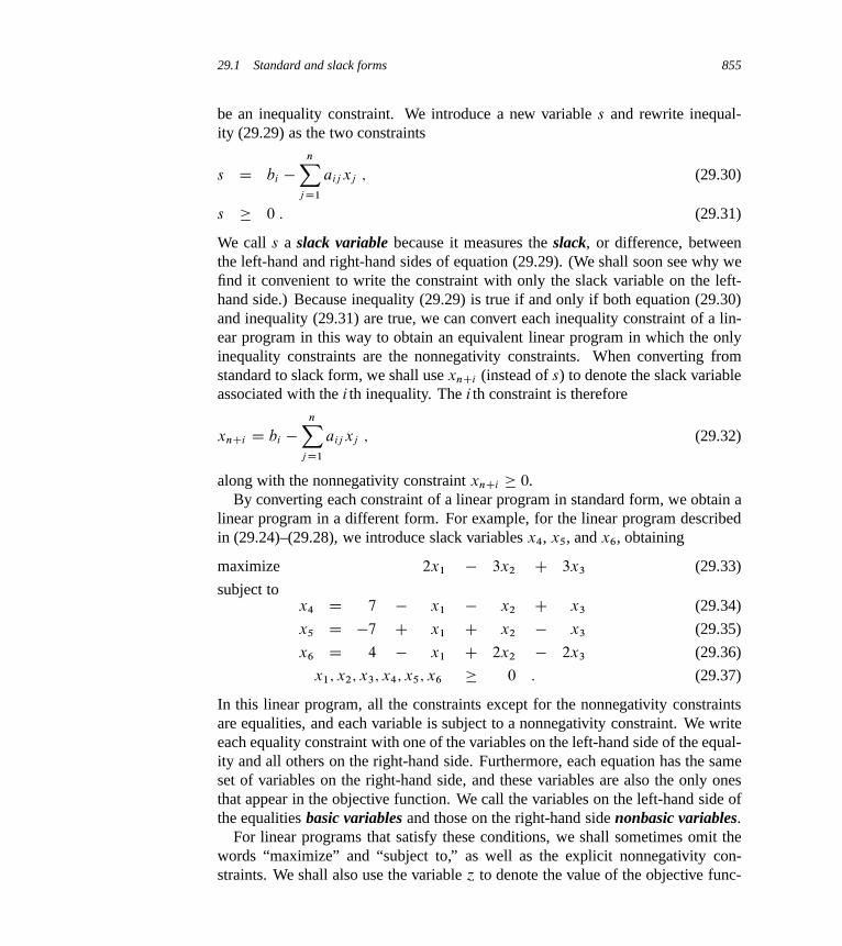
29.1 Standard and slack forms 855
be an inequality constraint. We introduce a new variable s and rewrite inequal-ity (29.29) as the two constraints
s D bi �nX
j D1
aij xj ; (29.30)
s � 0 : (29.31)
We call s a slack variable because it measures the slack, or difference, betweenthe left-hand and right-hand sides of equation (29.29). (We shall soon see why wefind it convenient to write the constraint with only the slack variable on the left-hand side.) Because inequality (29.29) is true if and only if both equation (29.30)and inequality (29.31) are true, we can convert each inequality constraint of a lin-ear program in this way to obtain an equivalent linear program in which the onlyinequality constraints are the nonnegativity constraints. When converting fromstandard to slack form, we shall use xnCi (instead of s) to denote the slack variableassociated with the i th inequality. The i th constraint is therefore
xnCi D bi �nX
j D1
aij xj ; (29.32)
along with the nonnegativity constraint xnCi � 0.By converting each constraint of a linear program in standard form, we obtain a
linear program in a different form. For example, for the linear program describedin (29.24)–(29.28), we introduce slack variables x4, x5, and x6, obtaining
maximize 2x1 � 3x2 C 3x3 (29.33)
subject tox4 D 7 � x1 � x2 C x3 (29.34)
x5 D �7 C x1 C x2 � x3 (29.35)
x6 D 4 � x1 C 2x2 � 2x3 (29.36)
x1; x2; x3; x4; x5; x6 � 0 : (29.37)
In this linear program, all the constraints except for the nonnegativity constraintsare equalities, and each variable is subject to a nonnegativity constraint. We writeeach equality constraint with one of the variables on the left-hand side of the equal-ity and all others on the right-hand side. Furthermore, each equation has the sameset of variables on the right-hand side, and these variables are also the only onesthat appear in the objective function. We call the variables on the left-hand side ofthe equalities basic variables and those on the right-hand side nonbasic variables.
For linear programs that satisfy these conditions, we shall sometimes omit thewords “maximize” and “subject to,” as well as the explicit nonnegativity con-straints. We shall also use the variable ´ to denote the value of the objective func-
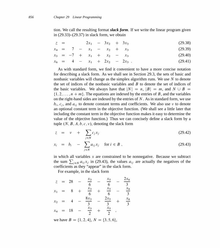
856 Chapter 29 Linear Programming
tion. We call the resulting format slack form. If we write the linear program givenin (29.33)–(29.37) in slack form, we obtain
´ D 2x1 � 3x2 C 3x3 (29.38)
x4 D 7 � x1 � x2 C x3 (29.39)
x5 D �7 C x1 C x2 � x3 (29.40)
x6 D 4 � x1 C 2x2 � 2x3 : (29.41)
As with standard form, we find it convenient to have a more concise notationfor describing a slack form. As we shall see in Section 29.3, the sets of basic andnonbasic variables will change as the simplex algorithm runs. We use N to denotethe set of indices of the nonbasic variables and B to denote the set of indices ofthe basic variables. We always have that jN j D n, jBj D m, and N [ B Df1; 2; : : : ; nCmg. The equations are indexed by the entries of B , and the variableson the right-hand sides are indexed by the entries of N . As in standard form, we usebi , cj , and aij to denote constant terms and coefficients. We also use � to denotean optional constant term in the objective function. (We shall see a little later thatincluding the constant term in the objective function makes it easy to determine thevalue of the objective function.) Thus we can concisely define a slack form by atuple .N; B; A; b; c; �/, denoting the slack form
´ D � CXj 2N
cj xj (29.42)
xi D bi �Xj 2N
aij xj for i 2 B ; (29.43)
in which all variables x are constrained to be nonnegative. Because we subtractthe sum
Pj 2N aij xj in (29.43), the values aij are actually the negatives of the
coefficients as they “appear” in the slack form.For example, in the slack form
´ D 28 � x3
6� x5
6� 2x6
3
x1 D 8 C x3
6C x5
6� x6
3
x2 D 4 � 8x3
3� 2x5
3C x6
3
x4 D 18 � x3
2C x5
2;
we have B D f1; 2; 4g, N D f3; 5; 6g,

29.1 Standard and slack forms 857
A D�
a13 a15 a16
a23 a25 a26
a43 a45 a46
�D
� �1=6 �1=6 1=3
8=3 2=3 �1=3
1=2 �1=2 0
�;
b D�
b1
b2
b4
�D
�8
4
18
�;
c D �c3 c5 c6
�T D � �1=6 �1=6 �2=3�T
, and � D 28. Note that theindices into A, b, and c are not necessarily sets of contiguous integers; they dependon the index sets B and N . As an example of the entries of A being the negativesof the coefficients as they appear in the slack form, observe that the equation for x1
includes the term x3=6, yet the coefficient a13 is actually �1=6 rather than C1=6.
Exercises
29.1-1If we express the linear program in (29.24)–(29.28) in the compact notation of(29.19)–(29.21), what are n, m, A, b, and c?
29.1-2Give three feasible solutions to the linear program in (29.24)–(29.28). What is theobjective value of each one?
29.1-3For the slack form in (29.38)–(29.41), what are N , B , A, b, c, and �?
29.1-4Convert the following linear program into standard form:
minimize 2x1 C 7x2 C x3
subject tox1 � x3 D 7
3x1 C x2 � 24
x2 � 0
x3 � 0 :

858 Chapter 29 Linear Programming
29.1-5Convert the following linear program into slack form:
maximize 2x1 � 6x3
subject tox1 C x2 � x3 � 7
3x1 � x2 � 8
�x1 C 2x2 C 2x3 � 0
x1; x2; x3 � 0 :
What are the basic and nonbasic variables?
29.1-6Show that the following linear program is infeasible:
maximize 3x1 � 2x2
subject tox1 C x2 � 2
�2x1 � 2x2 � �10
x1; x2 � 0 :
29.1-7Show that the following linear program is unbounded:
maximize x1 � x2
subject to�2x1 C x2 � �1
�x1 � 2x2 � �2
x1; x2 � 0 :
29.1-8Suppose that we have a general linear program with n variables and m constraints,and suppose that we convert it into standard form. Give an upper bound on thenumber of variables and constraints in the resulting linear program.
29.1-9Give an example of a linear program for which the feasible region is not bounded,but the optimal objective value is finite.

29.2 Formulating problems as linear programs 859
29.2 Formulating problems as linear programs
Although we shall focus on the simplex algorithm in this chapter, it is also impor-tant to be able to recognize when we can formulate a problem as a linear program.Once we cast a problem as a polynomial-sized linear program, we can solve itin polynomial time by the ellipsoid algorithm or interior-point methods. Severallinear-programming software packages can solve problems efficiently, so that oncethe problem is in the form of a linear program, such a package can solve it.
We shall look at several concrete examples of linear-programming problems. Westart with two problems that we have already studied: the single-source shortest-paths problem (see Chapter 24) and the maximum-flow problem (see Chapter 26).We then describe the minimum-cost-flow problem. Although the minimum-cost-flow problem has a polynomial-time algorithm that is not based on linear program-ming, we won’t describe the algorithm. Finally, we describe the multicommodity-flow problem, for which the only known polynomial-time algorithm is based onlinear programming.
When we solved graph problems in Part VI, we used attribute notation, suchas �:d and .u; �/: f . Linear programs typically use subscripted variables ratherthan objects with attached attributes, however. Therefore, when we express vari-ables in linear programs, we shall indicate vertices and edges through subscripts.For example, we denote the shortest-path weight for vertex � not by �:d but by d� .Similarly, we denote the flow from vertex u to vertex � not by .u; �/: f but by fu� .For quantities that are given as inputs to problems, such as edge weights or capac-ities, we shall continue to use notations such as w.u; �/ and c.u:�/.
Shortest paths
We can formulate the single-source shortest-paths problem as a linear program.In this section, we shall focus on how to formulate the single-pair shortest-pathproblem, leaving the extension to the more general single-source shortest-pathsproblem as Exercise 29.2-3.
In the single-pair shortest-path problem, we are given a weighted, directed graphG D .V; E/, with weight function w W E ! R mapping edges to real-valuedweights, a source vertex s, and destination vertex t . We wish to compute thevalue dt , which is the weight of a shortest path from s to t . To express this prob-lem as a linear program, we need to determine a set of variables and constraints thatdefine when we have a shortest path from s to t . Fortunately, the Bellman-Ford al-gorithm does exactly this. When the Bellman-Ford algorithm terminates, it hascomputed, for each vertex �, a value d� (using subscript notation here rather thanattribute notation) such that for each edge .u; �/ 2 E, we have d� � duCw.u; �/.
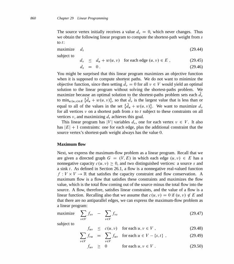
860 Chapter 29 Linear Programming
The source vertex initially receives a value ds D 0, which never changes. Thuswe obtain the following linear program to compute the shortest-path weight from s
to t :
maximize dt (29.44)
subject tod� � du Cw.u; �/ for each edge .u; �/ 2 E ; (29.45)
ds D 0 : (29.46)
You might be surprised that this linear program maximizes an objective functionwhen it is supposed to compute shortest paths. We do not want to minimize theobjective function, since then setting Nd� D 0 for all � 2 V would yield an optimalsolution to the linear program without solving the shortest-paths problem. Wemaximize because an optimal solution to the shortest-paths problem sets each Nd�
to minuW.u;�/2E
˚ Ndu C w.u; �/, so that Nd� is the largest value that is less than or
equal to all of the values in the set˚ Ndu Cw.u; �/
. We want to maximize d�
for all vertices � on a shortest path from s to t subject to these constraints on allvertices �, and maximizing dt achieves this goal.
This linear program has jV j variables d� , one for each vertex � 2 V . It alsohas jEj C 1 constraints: one for each edge, plus the additional constraint that thesource vertex’s shortest-path weight always has the value 0.
Maximum flow
Next, we express the maximum-flow problem as a linear program. Recall that weare given a directed graph G D .V; E/ in which each edge .u; �/ 2 E has anonnegative capacity c.u; �/ � 0, and two distinguished vertices: a source s anda sink t . As defined in Section 26.1, a flow is a nonnegative real-valued functionf W V V ! R that satisfies the capacity constraint and flow conservation. Amaximum flow is a flow that satisfies these constraints and maximizes the flowvalue, which is the total flow coming out of the source minus the total flow into thesource. A flow, therefore, satisfies linear constraints, and the value of a flow is alinear function. Recalling also that we assume that c.u; �/ D 0 if .u; �/ 62 E andthat there are no antiparallel edges, we can express the maximum-flow problem asa linear program:
maximizeX�2V
fs� �X�2V
f�s (29.47)
subject tofu� � c.u; �/ for each u; � 2 V ; (29.48)X
�2V
f�u DX�2V
fu� for each u 2 V � fs; tg ; (29.49)
fu� � 0 for each u; � 2 V : (29.50)
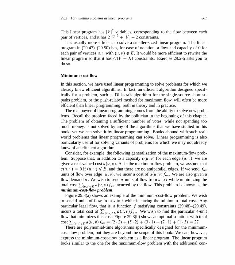
29.2 Formulating problems as linear programs 861
This linear program has jV j2 variables, corresponding to the flow between eachpair of vertices, and it has 2 jV j2 C jV j � 2 constraints.
It is usually more efficient to solve a smaller-sized linear program. The linearprogram in (29.47)–(29.50) has, for ease of notation, a flow and capacity of 0 foreach pair of vertices u; � with .u; �/ 62 E. It would be more efficient to rewrite thelinear program so that it has O.V C E/ constraints. Exercise 29.2-5 asks you todo so.
Minimum-cost flow
In this section, we have used linear programming to solve problems for which wealready knew efficient algorithms. In fact, an efficient algorithm designed specif-ically for a problem, such as Dijkstra’s algorithm for the single-source shortest-paths problem, or the push-relabel method for maximum flow, will often be moreefficient than linear programming, both in theory and in practice.
The real power of linear programming comes from the ability to solve new prob-lems. Recall the problem faced by the politician in the beginning of this chapter.The problem of obtaining a sufficient number of votes, while not spending toomuch money, is not solved by any of the algorithms that we have studied in thisbook, yet we can solve it by linear programming. Books abound with such real-world problems that linear programming can solve. Linear programming is alsoparticularly useful for solving variants of problems for which we may not alreadyknow of an efficient algorithm.
Consider, for example, the following generalization of the maximum-flow prob-lem. Suppose that, in addition to a capacity c.u; �/ for each edge .u; �/, we aregiven a real-valued cost a.u; �/. As in the maximum-flow problem, we assume thatc.u; �/ D 0 if .u; �/ 62 E, and that there are no antiparallel edges. If we send fu�
units of flow over edge .u; �/, we incur a cost of a.u; �/fu�. We are also given aflow demand d . We wish to send d units of flow from s to t while minimizing thetotal cost
P.u;�/2E a.u; �/fu� incurred by the flow. This problem is known as the
minimum-cost-flow problem.Figure 29.3(a) shows an example of the minimum-cost-flow problem. We wish
to send 4 units of flow from s to t while incurring the minimum total cost. Anyparticular legal flow, that is, a function f satisfying constraints (29.48)–(29.49),incurs a total cost of
P.u;�/2E a.u; �/fu�. We wish to find the particular 4-unit
flow that minimizes this cost. Figure 29.3(b) shows an optimal solution, with totalcost
P.u;�/2E a.u; �/fu� D .2 � 2/C .5 � 2/C .3 � 1/C .7 � 1/C .1 � 3/ D 27:
There are polynomial-time algorithms specifically designed for the minimum-cost-flow problem, but they are beyond the scope of this book. We can, however,express the minimum-cost-flow problem as a linear program. The linear programlooks similar to the one for the maximum-flow problem with the additional con-

862 Chapter 29 Linear Programming
s
x
t
y
(a)
c = 1a = 3
c = 5
a = 2
c = 4
a = 1
c = 2a = 7
c = 2a = 5
s
x
t
y
(b)
1/1a = 3
2/5
a = 2
3/4
a = 1
1/2a = 7
2/2a = 5
Figure 29.3 (a) An example of a minimum-cost-flow problem. We denote the capacities by c andthe costs by a. Vertex s is the source and vertex t is the sink, and we wish to send 4 units of flowfrom s to t . (b) A solution to the minimum-cost flow problem in which 4 units of flow are sent from s
to t . For each edge, the flow and capacity are written as flow/capacity.
straint that the value of the flow be exactly d units, and with the new objectivefunction of minimizing the cost:
minimizeX
.u;�/2E
a.u; �/fu� (29.51)
subject tofu� � c.u; �/ for each u; � 2 V ;X
�2V
f�u �X�2V
fu� D 0 for each u 2 V � fs; tg ;X�2V
fs� �X�2V
f�s D d ;
fu� � 0 for each u; � 2 V : (29.52)
Multicommodity flow
As a final example, we consider another flow problem. Suppose that the LuckyPuck company from Section 26.1 decides to diversify its product line and shipnot only hockey pucks, but also hockey sticks and hockey helmets. Each piece ofequipment is manufactured in its own factory, has its own warehouse, and mustbe shipped, each day, from factory to warehouse. The sticks are manufactured inVancouver and must be shipped to Saskatoon, and the helmets are manufactured inEdmonton and must be shipped to Regina. The capacity of the shipping networkdoes not change, however, and the different items, or commodities, must share thesame network.
This example is an instance of a multicommodity-flow problem. In this problem,we are again given a directed graph G D .V; E/ in which each edge .u; �/ 2 E hasa nonnegative capacity c.u; �/ � 0. As in the maximum-flow problem, we implic-itly assume that c.u; �/ D 0 for .u; �/ 62 E, and that the graph has no antiparallel
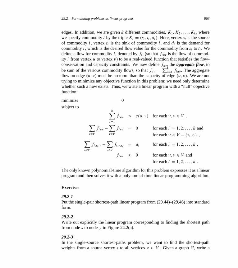
29.2 Formulating problems as linear programs 863
edges. In addition, we are given k different commodities, K1; K2; : : : ; Kk , wherewe specify commodity i by the triple Ki D .si ; ti ; di /. Here, vertex si is the sourceof commodity i , vertex ti is the sink of commodity i , and di is the demand forcommodity i , which is the desired flow value for the commodity from si to ti . Wedefine a flow for commodity i , denoted by fi , (so that fiu� is the flow of commod-ity i from vertex u to vertex �) to be a real-valued function that satisfies the flow-conservation and capacity constraints. We now define fu� , the aggregate flow, tobe sum of the various commodity flows, so that fu� D
Pk
iD1 fiu�. The aggregateflow on edge .u; �/ must be no more than the capacity of edge .u; �/. We are nottrying to minimize any objective function in this problem; we need only determinewhether such a flow exists. Thus, we write a linear program with a “null” objectivefunction:
minimize 0
subject tokX
iD1
fiu� � c.u; �/ for each u; � 2 V ;X�2V
fiu� �X�2V
fi�u D 0 for each i D 1; 2; : : : ; k and
for each u 2 V � fsi ; tig ;X�2V
fi;si ;� �X�2V
fi;�;siD di for each i D 1; 2; : : : ; k ;
fiu� � 0 for each u; � 2 V and
for each i D 1; 2; : : : ; k :
The only known polynomial-time algorithm for this problem expresses it as a linearprogram and then solves it with a polynomial-time linear-programming algorithm.
Exercises
29.2-1Put the single-pair shortest-path linear program from (29.44)–(29.46) into standardform.
29.2-2Write out explicitly the linear program corresponding to finding the shortest pathfrom node s to node y in Figure 24.2(a).
29.2-3In the single-source shortest-paths problem, we want to find the shortest-pathweights from a source vertex s to all vertices � 2 V . Given a graph G, write a

864 Chapter 29 Linear Programming
linear program for which the solution has the property that d� is the shortest-pathweight from s to � for each vertex � 2 V .
29.2-4Write out explicitly the linear program corresponding to finding the maximum flowin Figure 26.1(a).
29.2-5Rewrite the linear program for maximum flow (29.47)–(29.50) so that it uses onlyO.V CE/ constraints.
29.2-6Write a linear program that, given a bipartite graph G D .V; E/, solves the maxi-mum-bipartite-matching problem.
29.2-7In the minimum-cost multicommodity-flow problem, we are given directed graphG D .V; E/ in which each edge .u; �/ 2 E has a nonnegative capacity c.u; �/ � 0
and a cost a.u; �/. As in the multicommodity-flow problem, we are given k dif-ferent commodities, K1; K2; : : : ; Kk , where we specify commodity i by the tripleKi D .si ; ti ; di /. We define the flow fi for commodity i and the aggregate flow fu�
on edge .u; �/ as in the multicommodity-flow problem. A feasible flow is onein which the aggregate flow on each edge .u; �/ is no more than the capacity ofedge .u; �/. The cost of a flow is
Pu;�2V a.u; �/fu� , and the goal is to find the
feasible flow of minimum cost. Express this problem as a linear program.
29.3 The simplex algorithm
The simplex algorithm is the classical method for solving linear programs. In con-trast to most of the other algorithms in this book, its running time is not polynomialin the worst case. It does yield insight into linear programs, however, and is oftenremarkably fast in practice.
In addition to having a geometric interpretation, described earlier in this chap-ter, the simplex algorithm bears some similarity to Gaussian elimination, discussedin Section 28.1. Gaussian elimination begins with a system of linear equalitieswhose solution is unknown. In each iteration, we rewrite this system in a equiva-lent form that has some additional structure. After some number of iterations, wehave rewritten the system so that the solution is simple to obtain. The simplex al-gorithm proceeds in a similar manner, and we can view it as Gaussian eliminationfor inequalities.

29.3 The simplex algorithm 865
We now describe the main idea behind an iteration of the simplex algorithm.Associated with each iteration will be a “basic solution” that we can easily obtainfrom the slack form of the linear program: set each nonbasic variable to 0 andcompute the values of the basic variables from the equality constraints. An iterationconverts one slack form into an equivalent slack form. The objective value of theassociated basic feasible solution will be no less than that at the previous iteration,and usually greater. To achieve this increase in the objective value, we choose anonbasic variable such that if we were to increase that variable’s value from 0, thenthe objective value would increase, too. The amount by which we can increasethe variable is limited by the other constraints. In particular, we raise it until somebasic variable becomes 0. We then rewrite the slack form, exchanging the rolesof that basic variable and the chosen nonbasic variable. Although we have used aparticular setting of the variables to guide the algorithm, and we shall use it in ourproofs, the algorithm does not explicitly maintain this solution. It simply rewritesthe linear program until an optimal solution becomes “obvious.”
An example of the simplex algorithm
We begin with an extended example. Consider the following linear program instandard form:
maximize 3x1 C x2 C 2x3 (29.53)
subject tox1 C x2 C 3x3 � 30 (29.54)
2x1 C 2x2 C 5x3 � 24 (29.55)
4x1 C x2 C 2x3 � 36 (29.56)
x1; x2; x3 � 0 : (29.57)
In order to use the simplex algorithm, we must convert the linear program intoslack form; we saw how to do so in Section 29.1. In addition to being an algebraicmanipulation, slack is a useful algorithmic concept. Recalling from Section 29.1that each variable has a corresponding nonnegativity constraint, we say that anequality constraint is tight for a particular setting of its nonbasic variables if theycause the constraint’s basic variable to become 0. Similarly, a setting of the non-basic variables that would make a basic variable become negative violates thatconstraint. Thus, the slack variables explicitly maintain how far each constraint isfrom being tight, and so they help to determine how much we can increase valuesof nonbasic variables without violating any constraints.
Associating the slack variables x4, x5, and x6 with inequalities (29.54)–(29.56),respectively, and putting the linear program into slack form, we obtain
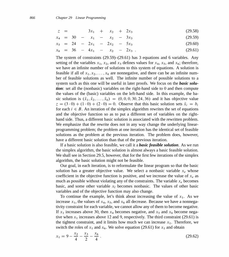
866 Chapter 29 Linear Programming
´ D 3x1 C x2 C 2x3 (29.58)
x4 D 30 � x1 � x2 � 3x3 (29.59)
x5 D 24 � 2x1 � 2x2 � 5x3 (29.60)
x6 D 36 � 4x1 � x2 � 2x3 : (29.61)
The system of constraints (29.59)–(29.61) has 3 equations and 6 variables. Anysetting of the variables x1, x2, and x3 defines values for x4, x5, and x6; therefore,we have an infinite number of solutions to this system of equations. A solution isfeasible if all of x1; x2; : : : ; x6 are nonnegative, and there can be an infinite num-ber of feasible solutions as well. The infinite number of possible solutions to asystem such as this one will be useful in later proofs. We focus on the basic solu-tion: set all the (nonbasic) variables on the right-hand side to 0 and then computethe values of the (basic) variables on the left-hand side. In this example, the ba-sic solution is . Nx1; Nx2; : : : ; Nx6/ D .0; 0; 0; 30; 24; 36/ and it has objective value´ D .3 � 0/C .1 � 0/C .2 � 0/ D 0. Observe that this basic solution sets Nxi D bi
for each i 2 B . An iteration of the simplex algorithm rewrites the set of equationsand the objective function so as to put a different set of variables on the right-hand side. Thus, a different basic solution is associated with the rewritten problem.We emphasize that the rewrite does not in any way change the underlying linear-programming problem; the problem at one iteration has the identical set of feasiblesolutions as the problem at the previous iteration. The problem does, however,have a different basic solution than that of the previous iteration.
If a basic solution is also feasible, we call it a basic feasible solution. As we runthe simplex algorithm, the basic solution is almost always a basic feasible solution.We shall see in Section 29.5, however, that for the first few iterations of the simplexalgorithm, the basic solution might not be feasible.
Our goal, in each iteration, is to reformulate the linear program so that the basicsolution has a greater objective value. We select a nonbasic variable xe whosecoefficient in the objective function is positive, and we increase the value of xe asmuch as possible without violating any of the constraints. The variable xe becomesbasic, and some other variable xl becomes nonbasic. The values of other basicvariables and of the objective function may also change.
To continue the example, let’s think about increasing the value of x1. As weincrease x1, the values of x4, x5, and x6 all decrease. Because we have a nonnega-tivity constraint for each variable, we cannot allow any of them to become negative.If x1 increases above 30, then x4 becomes negative, and x5 and x6 become nega-tive when x1 increases above 12 and 9, respectively. The third constraint (29.61) isthe tightest constraint, and it limits how much we can increase x1. Therefore, weswitch the roles of x1 and x6. We solve equation (29.61) for x1 and obtain
x1 D 9� x2
4� x3
2� x6
4: (29.62)

29.3 The simplex algorithm 867
To rewrite the other equations with x6 on the right-hand side, we substitute for x1
using equation (29.62). Doing so for equation (29.59), we obtain
x4 D 30 � x1 � x2 � 3x3
D 30 ��9 � x2
4� x3
2� x6
4
�� x2 � 3x3
D 21 � 3x2
4� 5x3
2C x6
4: (29.63)
Similarly, we combine equation (29.62) with constraint (29.60) and with objectivefunction (29.58) to rewrite our linear program in the following form:
´ D 27 C x2
4C x3
2� 3x6
4(29.64)
x1 D 9 � x2
4� x3
2� x6
4(29.65)
x4 D 21 � 3x2
4� 5x3
2C x6
4(29.66)
x5 D 6 � 3x2
2� 4x3 C x6
2: (29.67)
We call this operation a pivot. As demonstrated above, a pivot chooses a nonbasicvariable xe, called the entering variable, and a basic variable xl , called the leavingvariable, and exchanges their roles.
The linear program described in equations (29.64)–(29.67) is equivalent to thelinear program described in equations (29.58)–(29.61). We perform two operationsin the simplex algorithm: rewrite equations so that variables move between the left-hand side and the right-hand side, and substitute one equation into another. The firstoperation trivially creates an equivalent problem, and the second, by elementarylinear algebra, also creates an equivalent problem. (See Exercise 29.3-3.)
To demonstrate this equivalence, observe that our original basic solution .0; 0;
0; 30; 24; 36/ satisfies the new equations (29.65)–(29.67) and has objective value27C .1=4/ � 0C .1=2/ � 0� .3=4/ � 36 D 0. The basic solution associated with thenew linear program sets the nonbasic values to 0 and is .9; 0; 0; 21; 6; 0/, with ob-jective value ´ D 27. Simple arithmetic verifies that this solution also satisfiesequations (29.59)–(29.61) and, when plugged into objective function (29.58), hasobjective value .3 � 9/C .1 � 0/C .2 � 0/ D 27.
Continuing the example, we wish to find a new variable whose value we wish toincrease. We do not want to increase x6, since as its value increases, the objectivevalue decreases. We can attempt to increase either x2 or x3; let us choose x3. Howfar can we increase x3 without violating any of the constraints? Constraint (29.65)limits it to 18, constraint (29.66) limits it to 42=5, and constraint (29.67) limitsit to 3=2. The third constraint is again the tightest one, and therefore we rewritethe third constraint so that x3 is on the left-hand side and x5 is on the right-hand

868 Chapter 29 Linear Programming
side. We then substitute this new equation, x3 D 3=2� 3x2=8� x5=4C x6=8, intoequations (29.64)–(29.66) and obtain the new, but equivalent, system
´ D 111
4C x2
16� x5
8� 11x6
16(29.68)
x1 D33
4� x2
16C x5
8� 5x6
16(29.69)
x3 D3
2� 3x2
8� x5
4C x6
8(29.70)
x4 D 69
4C 3x2
16C 5x5
8� x6
16: (29.71)
This system has the associated basic solution .33=4; 0; 3=2; 69=4; 0; 0/, with ob-jective value 111=4. Now the only way to increase the objective value is to in-crease x2. The three constraints give upper bounds of 132, 4, and1, respectively.(We get an upper bound of1 from constraint (29.71) because, as we increase x2,the value of the basic variable x4 increases also. This constraint, therefore, placesno restriction on how much we can increase x2.) We increase x2 to 4, and it be-comes nonbasic. Then we solve equation (29.70) for x2 and substitute in the otherequations to obtain
´ D 28 � x3
6� x5
6� 2x6
3(29.72)
x1 D 8 C x3
6C x5
6� x6
3(29.73)
x2 D 4 � 8x3
3� 2x5
3C x6
3(29.74)
x4 D 18 � x3
2C x5
2: (29.75)
At this point, all coefficients in the objective function are negative. As we shall seelater in this chapter, this situation occurs only when we have rewritten the linearprogram so that the basic solution is an optimal solution. Thus, for this problem,the solution .8; 4; 0; 18; 0; 0/, with objective value 28, is optimal. We can nowreturn to our original linear program given in (29.53)–(29.57). The only variablesin the original linear program are x1, x2, and x3, and so our solution is x1 D 8,x2 D 4, and x3 D 0, with objective value .3 � 8/ C .1 � 4/ C .2 � 0/ D 28. Notethat the values of the slack variables in the final solution measure how much slackremains in each inequality. Slack variable x4 is 18, and in inequality (29.54), theleft-hand side, with value 8C 4C 0 D 12, is 18 less than the right-hand side of 30.Slack variables x5 and x6 are 0 and indeed, in inequalities (29.55) and (29.56),the left-hand and right-hand sides are equal. Observe also that even though thecoefficients in the original slack form are integral, the coefficients in the otherlinear programs are not necessarily integral, and the intermediate solutions are not

29.3 The simplex algorithm 869
necessarily integral. Furthermore, the final solution to a linear program need notbe integral; it is purely coincidental that this example has an integral solution.
Pivoting
We now formalize the procedure for pivoting. The procedure PIVOT takes as in-put a slack form, given by the tuple .N; B; A; b; c; �/, the index l of the leav-ing variable xl , and the index e of the entering variable xe. It returns the tuple. yN ; yB; yA; yb; yc; y�/ describing the new slack form. (Recall again that the entries ofthe mn matrices A and yA are actually the negatives of the coefficients that appearin the slack form.)
PIVOT.N; B; A; b; c; �; l; e/
1 // Compute the coefficients of the equation for new basic variable xe.2 let yA be a new m n matrix3 ybe D bl=ale
4 for each j 2 N � feg5 yaej D alj =ale
6 yael D 1=ale
7 // Compute the coefficients of the remaining constraints.8 for each i 2 B � flg9 ybi D bi � aie
ybe
10 for each j 2 N � feg11 yaij D aij � aieyaej
12 yai l D �aieyael
13 // Compute the objective function.14 y� D � C ce
ybe
15 for each j 2 N � feg16 ycj D cj � ceyaej
17 ycl D �ceyael
18 // Compute new sets of basic and nonbasic variables.19 yN D N � feg [ flg20 yB D B � flg [ feg21 return . yN ; yB; yA; yb; yc; y�/
PIVOT works as follows. Lines 3–6 compute the coefficients in the new equationfor xe by rewriting the equation that has xl on the left-hand side to instead have xe
on the left-hand side. Lines 8–12 update the remaining equations by substitutingthe right-hand side of this new equation for each occurrence of xe. Lines 14–17do the same substitution for the objective function, and lines 19 and 20 update the
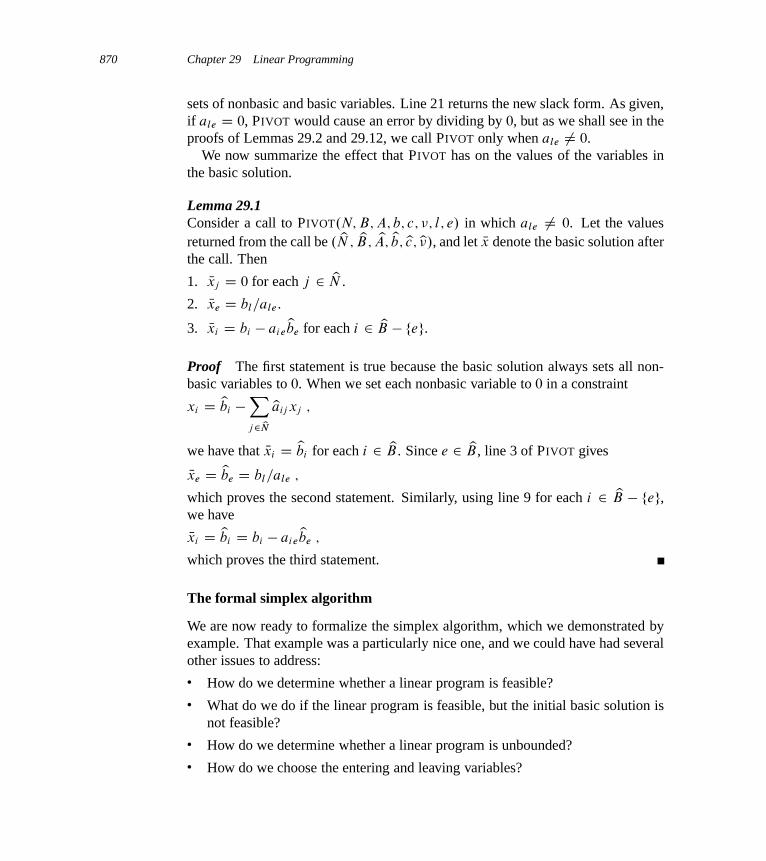
870 Chapter 29 Linear Programming
sets of nonbasic and basic variables. Line 21 returns the new slack form. As given,if ale D 0, PIVOT would cause an error by dividing by 0, but as we shall see in theproofs of Lemmas 29.2 and 29.12, we call PIVOT only when ale ¤ 0.
We now summarize the effect that PIVOT has on the values of the variables inthe basic solution.
Lemma 29.1Consider a call to PIVOT.N; B; A; b; c; �; l; e/ in which ale ¤ 0. Let the valuesreturned from the call be . yN ; yB; yA; yb; yc; y�/, and let Nx denote the basic solution afterthe call. Then
1. Nxj D 0 for each j 2 yN .
2. Nxe D bl=ale .
3. Nxi D bi � aieybe for each i 2 yB � feg.
Proof The first statement is true because the basic solution always sets all non-basic variables to 0. When we set each nonbasic variable to 0 in a constraint
xi D ybi �Xj 2 yNyaij xj ;
we have that Nxi D ybi for each i 2 yB . Since e 2 yB , line 3 of PIVOT gives
Nxe D ybe D bl=ale ;
which proves the second statement. Similarly, using line 9 for each i 2 yB � feg,we have
Nxi D ybi D bi � aieybe ;
which proves the third statement.
The formal simplex algorithm
We are now ready to formalize the simplex algorithm, which we demonstrated byexample. That example was a particularly nice one, and we could have had severalother issues to address:� How do we determine whether a linear program is feasible?� What do we do if the linear program is feasible, but the initial basic solution is
not feasible?� How do we determine whether a linear program is unbounded?� How do we choose the entering and leaving variables?

29.3 The simplex algorithm 871
In Section 29.5, we shall show how to determine whether a problem is feasible,and if so, how to find a slack form in which the initial basic solution is feasible.Therefore, let us assume that we have a procedure INITIALIZE-SIMPLEX.A; b; c/
that takes as input a linear program in standard form, that is, an m n matrixA D .aij /, an m-vector b D .bi/, and an n-vector c D .cj /. If the problem isinfeasible, the procedure returns a message that the program is infeasible and thenterminates. Otherwise, the procedure returns a slack form for which the initialbasic solution is feasible.
The procedure SIMPLEX takes as input a linear program in standard form, as justdescribed. It returns an n-vector Nx D . Nxj / that is an optimal solution to the linearprogram described in (29.19)–(29.21).
SIMPLEX.A; b; c/
1 .N; B; A; b; c; �/ D INITIALIZE-SIMPLEX.A; b; c/
2 let � be a new vector of length n
3 while some index j 2 N has cj > 0
4 choose an index e 2 N for which ce > 0
5 for each index i 2 B
6 if aie > 0
7 �i D bi=aie
8 else �i D 19 choose an index l 2 B that minimizes �i
10 if �l ==111 return “unbounded”12 else .N; B; A; b; c; �/ D PIVOT.N; B; A; b; c; �; l; e/
13 for i D 1 to n
14 if i 2 B
15 Nxi D bi
16 else Nxi D 0
17 return . Nx1; Nx2; : : : ; Nxn/
The SIMPLEX procedure works as follows. In line 1, it calls the procedureINITIALIZE-SIMPLEX.A; b; c/, described above, which either determines that thelinear program is infeasible or returns a slack form for which the basic solution isfeasible. The while loop of lines 3–12 forms the main part of the algorithm. If allcoefficients in the objective function are negative, then the while loop terminates.Otherwise, line 4 selects a variable xe, whose coefficient in the objective functionis positive, as the entering variable. Although we may choose any such variable asthe entering variable, we assume that we use some prespecified deterministic rule.Next, lines 5–9 check each constraint and pick the one that most severely limitsthe amount by which we can increase xe without violating any of the nonnegativ-
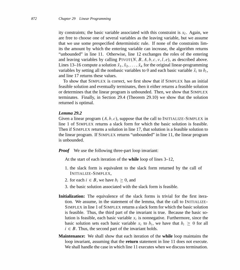
872 Chapter 29 Linear Programming
ity constraints; the basic variable associated with this constraint is xl . Again, weare free to choose one of several variables as the leaving variable, but we assumethat we use some prespecified deterministic rule. If none of the constraints lim-its the amount by which the entering variable can increase, the algorithm returns“unbounded” in line 11. Otherwise, line 12 exchanges the roles of the enteringand leaving variables by calling PIVOT.N; B; A; b; c; �; l; e/, as described above.Lines 13–16 compute a solution Nx1; Nx2; : : : ; Nxn for the original linear-programmingvariables by setting all the nonbasic variables to 0 and each basic variable Nxi to bi ,and line 17 returns these values.
To show that SIMPLEX is correct, we first show that if SIMPLEX has an initialfeasible solution and eventually terminates, then it either returns a feasible solutionor determines that the linear program is unbounded. Then, we show that SIMPLEX
terminates. Finally, in Section 29.4 (Theorem 29.10) we show that the solutionreturned is optimal.
Lemma 29.2Given a linear program .A; b; c/, suppose that the call to INITIALIZE-SIMPLEX inline 1 of SIMPLEX returns a slack form for which the basic solution is feasible.Then if SIMPLEX returns a solution in line 17, that solution is a feasible solution tothe linear program. If SIMPLEX returns “unbounded” in line 11, the linear programis unbounded.
Proof We use the following three-part loop invariant:
At the start of each iteration of the while loop of lines 3–12,
1. the slack form is equivalent to the slack form returned by the call ofINITIALIZE-SIMPLEX,
2. for each i 2 B , we have bi � 0, and
3. the basic solution associated with the slack form is feasible.
Initialization: The equivalence of the slack forms is trivial for the first itera-tion. We assume, in the statement of the lemma, that the call to INITIALIZE-SIMPLEX in line 1 of SIMPLEX returns a slack form for which the basic solutionis feasible. Thus, the third part of the invariant is true. Because the basic so-lution is feasible, each basic variable xi is nonnegative. Furthermore, since thebasic solution sets each basic variable xi to bi , we have that bi � 0 for alli 2 B . Thus, the second part of the invariant holds.
Maintenance: We shall show that each iteration of the while loop maintains theloop invariant, assuming that the return statement in line 11 does not execute.We shall handle the case in which line 11 executes when we discuss termination.
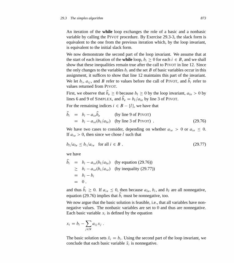
29.3 The simplex algorithm 873
An iteration of the while loop exchanges the role of a basic and a nonbasicvariable by calling the PIVOT procedure. By Exercise 29.3-3, the slack form isequivalent to the one from the previous iteration which, by the loop invariant,is equivalent to the initial slack form.
We now demonstrate the second part of the loop invariant. We assume that atthe start of each iteration of the while loop, bi � 0 for each i 2 B , and we shallshow that these inequalities remain true after the call to PIVOT in line 12. Sincethe only changes to the variables bi and the set B of basic variables occur in thisassignment, it suffices to show that line 12 maintains this part of the invariant.We let bi , aij , and B refer to values before the call of PIVOT, and ybi refer tovalues returned from PIVOT.
First, we observe that ybe � 0 because bl � 0 by the loop invariant, ale > 0 bylines 6 and 9 of SIMPLEX, and ybe D bl=ale by line 3 of PIVOT.
For the remaining indices i 2 B � flg, we have that
ybi D bi � aieybe (by line 9 of PIVOT)
D bi � aie.bl=ale/ (by line 3 of PIVOT) . (29.76)
We have two cases to consider, depending on whether aie > 0 or aie � 0.If aie > 0, then since we chose l such that
bl=ale � bi=aie for all i 2 B ; (29.77)
we have
ybi D bi � aie.bl=ale/ (by equation (29.76))
� bi � aie.bi=aie/ (by inequality (29.77))
D bi � bi
D 0 ;
and thus ybi � 0. If aie � 0, then because ale, bi , and bl are all nonnegative,equation (29.76) implies that ybi must be nonnegative, too.
We now argue that the basic solution is feasible, i.e., that all variables have non-negative values. The nonbasic variables are set to 0 and thus are nonnegative.Each basic variable xi is defined by the equation
xi D bi �Xj 2N
aij xj :
The basic solution sets Nxi D bi . Using the second part of the loop invariant, weconclude that each basic variable Nxi is nonnegative.
874 Chapter 29 Linear Programming
Termination: The while loop can terminate in one of two ways. If it terminatesbecause of the condition in line 3, then the current basic solution is feasible andline 17 returns this solution. The other way it terminates is by returning “un-bounded” in line 11. In this case, for each iteration of the for loop in lines 5–8,when line 6 is executed, we find that aie � 0. Consider the solution Nx defined as
Nxi D
�1 if i D e ;
0 if i 2 N � feg ;
bi �P
j 2N aij Nxj if i 2 B :
We now show that this solution is feasible, i.e., that all variables are nonneg-ative. The nonbasic variables other than Nxe are 0, and Nxe D 1 > 0; thus allnonbasic variables are nonnegative. For each basic variable Nxi , we have
Nxi D bi �Xj 2N
aij Nxj
D bi � aie Nxe :
The loop invariant implies that bi � 0, and we have aie � 0 and Nxe D 1 > 0.Thus, Nxi � 0.
Now we show that the objective value for the solution Nx is unbounded. Fromequation (29.42), the objective value is
´ D � CXj 2N
cj Nxj
D � C ce Nxe :
Since ce > 0 (by line 4 of SIMPLEX) and Nxe D 1, the objective value is1,and thus the linear program is unbounded.
It remains to show that SIMPLEX terminates, and when it does terminate, thesolution it returns is optimal. Section 29.4 will address optimality. We now discusstermination.
Termination
In the example given in the beginning of this section, each iteration of the simplexalgorithm increased the objective value associated with the basic solution. As Ex-ercise 29.3-2 asks you to show, no iteration of SIMPLEX can decrease the objectivevalue associated with the basic solution. Unfortunately, it is possible that an itera-tion leaves the objective value unchanged. This phenomenon is called degeneracy,and we shall now study it in greater detail.

29.3 The simplex algorithm 875
The assignment in line 14 of PIVOT, y� D �C ceybe, changes the objective value.
Since SIMPLEX calls PIVOT only when ce > 0, the only way for the objectivevalue to remain unchanged (i.e., y� D �) is for ybe to be 0. This value is assignedas ybe D bl=ale in line 3 of PIVOT. Since we always call PIVOT with ale ¤ 0, wesee that for ybe to equal 0, and hence the objective value to be unchanged, we musthave bl D 0.
Indeed, this situation can occur. Consider the linear program
´ D x1 C x2 C x3
x4 D 8 � x1 � x2
x5 D x2 � x3 :
Suppose that we choose x1 as the entering variable and x4 as the leaving variable.After pivoting, we obtain
´ D 8 C x3 � x4
x1 D 8 � x2 � x4
x5 D x2 � x3 :
At this point, our only choice is to pivot with x3 entering and x5 leaving. Sinceb5 D 0, the objective value of 8 remains unchanged after pivoting:
´ D 8 C x2 � x4 � x5
x1 D 8 � x2 � x4
x3 D x2 � x5 :
The objective value has not changed, but our slack form has. Fortunately, if wepivot again, with x2 entering and x1 leaving, the objective value increases (to 16),and the simplex algorithm can continue.
Degeneracy can prevent the simplex algorithm from terminating, because it canlead to a phenomenon known as cycling: the slack forms at two different itera-tions of SIMPLEX are identical. Because of degeneracy, SIMPLEX could choose asequence of pivot operations that leave the objective value unchanged but repeata slack form within the sequence. Since SIMPLEX is a deterministic algorithm, ifit cycles, then it will cycle through the same series of slack forms forever, neverterminating.
Cycling is the only reason that SIMPLEX might not terminate. To show this fact,we must first develop some additional machinery.
At each iteration, SIMPLEX maintains A, b, c, and � in addition to the setsN and B . Although we need to explicitly maintain A, b, c, and � in order toimplement the simplex algorithm efficiently, we can get by without maintainingthem. In other words, the sets of basic and nonbasic variables suffice to uniquelydetermine the slack form. Before proving this fact, we prove a useful algebraiclemma.

876 Chapter 29 Linear Programming
Lemma 29.3Let I be a set of indices. For each j 2 I , let j̨ and ǰ be real numbers, and let xj
be a real-valued variable. Let be any real number. Suppose that for any settingsof the xj , we haveXj 2I
j̨ xj D CXj 2I
ǰ xj : (29.78)
Then j̨ D ǰ for each j 2 I , and D 0.
Proof Since equation (29.78) holds for any values of the xj , we can use particularvalues to draw conclusions about ˛, ˇ, and . If we let xj D 0 for each j 2 I ,we conclude that D 0. Now pick an arbitrary index j 2 I , and set xj D 1 andxk D 0 for all k ¤ j . Then we must have j̨ D ǰ . Since we picked j as anyindex in I , we conclude that j̨ D ǰ for each j 2 I .
A particular linear program has many different slack forms; recall that each slackform has the same set of feasible and optimal solutions as the original linear pro-gram. We now show that the slack form of a linear program is uniquely determinedby the set of basic variables. That is, given the set of basic variables, a unique slackform (unique set of coefficients and right-hand sides) is associated with those basicvariables.
Lemma 29.4Let .A; b; c/ be a linear program in standard form. Given a set B of basic variables,the associated slack form is uniquely determined.
Proof Assume for the purpose of contradiction that there are two different slackforms with the same set B of basic variables. The slack forms must also haveidentical sets N D f1; 2; : : : ; nCmg �B of nonbasic variables. We write the firstslack form as
´ D � CXj 2N
cj xj (29.79)
xi D bi �Xj 2N
aij xj for i 2 B ; (29.80)
and the second as
´ D � 0 CXj 2N
c 0j xj (29.81)
xi D b0i �
Xj 2N
a0ij xj for i 2 B : (29.82)
29.3 The simplex algorithm 877
Consider the system of equations formed by subtracting each equation inline (29.82) from the corresponding equation in line (29.80). The resulting sys-tem is
0 D .bi � b0i/ �
Xj 2N
.aij � a0ij /xj for i 2 B
or, equivalently,Xj 2N
aij xj D .bi � b0i /C
Xj 2N
a0ij xj for i 2 B :
Now, for each i 2 B , apply Lemma 29.3 with j̨ D aij , ǰ D a0ij , D bi �b0
i , andI D N . Since ˛i D ˇi , we have that aij D a0
ij for each j 2 N , and since D 0,we have that bi D b0
i . Thus, for the two slack forms, A and b are identical to A0
and b0. Using a similar argument, Exercise 29.3-1 shows that it must also be thecase that c D c 0 and � D � 0, and hence that the slack forms must be identical.
We can now show that cycling is the only possible reason that SIMPLEX mightnot terminate.
Lemma 29.5If SIMPLEX fails to terminate in at most
�nCm
m
�iterations, then it cycles.
Proof By Lemma 29.4, the set B of basic variables uniquely determines a slackform. There are n C m variables and jBj D m, and therefore, there are at most�
nCm
m
�ways to choose B . Thus, there are only at most
�nCm
m
�unique slack forms.
Therefore, if SIMPLEX runs for more than�
nCm
m
�iterations, it must cycle.
Cycling is theoretically possible, but extremely rare. We can prevent it by choos-ing the entering and leaving variables somewhat more carefully. One option is toperturb the input slightly so that it is impossible to have two solutions with thesame objective value. Another option is to break ties by always choosing the vari-able with the smallest index, a strategy known as Bland’s rule. We omit the proofthat these strategies avoid cycling.
Lemma 29.6If lines 4 and 9 of SIMPLEX always break ties by choosing the variable with thesmallest index, then SIMPLEX must terminate.
We conclude this section with the following lemma.

878 Chapter 29 Linear Programming
Lemma 29.7Assuming that INITIALIZE-SIMPLEX returns a slack form for which the basic so-lution is feasible, SIMPLEX either reports that a linear program is unbounded, or itterminates with a feasible solution in at most
�nCm
m
�iterations.
Proof Lemmas 29.2 and 29.6 show that if INITIALIZE-SIMPLEX returns a slackform for which the basic solution is feasible, SIMPLEX either reports that a linearprogram is unbounded, or it terminates with a feasible solution. By the contra-positive of Lemma 29.5, if SIMPLEX terminates with a feasible solution, then itterminates in at most
�nCm
m
�iterations.
Exercises
29.3-1Complete the proof of Lemma 29.4 by showing that it must be the case that c D c 0
and � D � 0.
29.3-2Show that the call to PIVOT in line 12 of SIMPLEX never decreases the value of �.
29.3-3Prove that the slack form given to the PIVOT procedure and the slack form that theprocedure returns are equivalent.
29.3-4Suppose we convert a linear program .A; b; c/ in standard form to slack form.Show that the basic solution is feasible if and only if bi � 0 for i D 1; 2; : : : ; m.
29.3-5Solve the following linear program using SIMPLEX:
maximize 18x1 C 12:5x2
subject tox1 C x2 � 20
x1 � 12
x2 � 16
x1; x2 � 0 :
29.4 Duality 879
29.3-6Solve the following linear program using SIMPLEX:
maximize 5x1 � 3x2
subject tox1 � x2 � 1
2x1 C x2 � 2
x1; x2 � 0 :
29.3-7Solve the following linear program using SIMPLEX:
minimize x1 C x2 C x3
subject to2x1 C 7:5x2 C 3x3 � 10000
20x1 C 5x2 C 10x3 � 30000
x1; x2; x3 � 0 :
29.3-8In the proof of Lemma 29.5, we argued that there are at most
�mCn
n
�ways to choose
a set B of basic variables. Give an example of a linear program in which there arestrictly fewer than
�mCn
n
�ways to choose the set B .
29.4 Duality
We have proven that, under certain assumptions, SIMPLEX terminates. We have notyet shown that it actually finds an optimal solution to a linear program, however.In order to do so, we introduce a powerful concept called linear-programmingduality.
Duality enables us to prove that a solution is indeed optimal. We saw an exam-ple of duality in Chapter 26 with Theorem 26.6, the max-flow min-cut theorem.Suppose that, given an instance of a maximum-flow problem, we find a flow f
with value jf j. How do we know whether f is a maximum flow? By the max-flowmin-cut theorem, if we can find a cut whose value is also jf j, then we have ver-ified that f is indeed a maximum flow. This relationship provides an example ofduality: given a maximization problem, we define a related minimization problemsuch that the two problems have the same optimal objective values.
Given a linear program in which the objective is to maximize, we shall describehow to formulate a dual linear program in which the objective is to minimize and

880 Chapter 29 Linear Programming
whose optimal value is identical to that of the original linear program. When refer-ring to dual linear programs, we call the original linear program the primal.
Given a primal linear program in standard form, as in (29.16)–(29.18), we definethe dual linear program as
minimizemX
iD1
biyi (29.83)
subject tomX
iD1
aij yi � cj for j D 1; 2; : : : ; n ; (29.84)
yi � 0 for i D 1; 2; : : : ; m : (29.85)
To form the dual, we change the maximization to a minimization, exchange theroles of coefficients on the the right-hand sides and the objective function, andreplace each less-than-or-equal-to by a greater-than-or-equal-to. Each of the m
constraints in the primal has an associated variable yi in the dual, and each ofthe n constraints in the dual has an associated variable xj in the primal. For exam-ple, consider the linear program given in (29.53)–(29.57). The dual of this linearprogram is
minimize 30y1 C 24y2 C 36y3 (29.86)
subject toy1 C 2y2 C 4y3 � 3 (29.87)
y1 C 2y2 C y3 � 1 (29.88)
3y1 C 5y2 C 2y3 � 2 (29.89)
y1; y2; y3 � 0 : (29.90)
We shall show in Theorem 29.10 that the optimal value of the dual linear pro-gram is always equal to the optimal value of the primal linear program. Further-more, the simplex algorithm actually implicitly solves both the primal and the duallinear programs simultaneously, thereby providing a proof of optimality.
We begin by demonstrating weak duality, which states that any feasible solu-tion to the primal linear program has a value no greater than that of any feasiblesolution to the dual linear program.
Lemma 29.8 (Weak linear-programming duality)Let Nx be any feasible solution to the primal linear program in (29.16)–(29.18) andlet Ny be any feasible solution to the dual linear program in (29.83)–(29.85). Then,we have
nXj D1
cj Nxj �mX
iD1
bi Nyi :

29.4 Duality 881
Proof We havenX
j D1
cj Nxj �nX
j D1
mX
iD1
aij Nyi
!Nxj (by inequalities (29.84))
DmX
iD1
nX
j D1
aij Nxj
!Nyi
�mX
iD1
bi Nyi (by inequalities (29.17)) .
Corollary 29.9Let Nx be a feasible solution to a primal linear program .A; b; c/, and let Ny be afeasible solution to the corresponding dual linear program. If
nXj D1
cj Nxj DmX
iD1
bi Nyi ;
then Nx and Ny are optimal solutions to the primal and dual linear programs, respec-tively.
Proof By Lemma 29.8, the objective value of a feasible solution to the primalcannot exceed that of a feasible solution to the dual. The primal linear program isa maximization problem and the dual is a minimization problem. Thus, if feasiblesolutions Nx and Ny have the same objective value, neither can be improved.
Before proving that there always is a dual solution whose value is equal to thatof an optimal primal solution, we describe how to find such a solution. Whenwe ran the simplex algorithm on the linear program in (29.53)–(29.57), the finaliteration yielded the slack form (29.72)–(29.75) with objective ´ D 28 � x3=6 �x5=6�2x6=3, B D f1; 2; 4g, and N D f3; 5; 6g. As we shall show below, the basicsolution associated with the final slack form is indeed an optimal solution to thelinear program; an optimal solution to linear program (29.53)–(29.57) is therefore. Nx1; Nx2; Nx3/ D .8; 4; 0/, with objective value .3 � 8/C .1 � 4/C .2 � 0/ D 28. As weshall also show below, we can read off an optimal dual solution: the negatives ofthe coefficients of the primal objective function are the values of the dual variables.More precisely, suppose that the last slack form of the primal is
´ D � 0 CXj 2N
c 0j xj
xi D b0i �
Xj 2N
a0ij xj for i 2 B :
882 Chapter 29 Linear Programming
Then, to produce an optimal dual solution, we set
Nyi D(�c 0
nCi if .nC i/ 2 N ;
0 otherwise :(29.91)
Thus, an optimal solution to the dual linear program defined in (29.86)–(29.90)is Ny1 D 0 (since n C 1 D 4 2 B), Ny2 D �c 0
5 D 1=6, and Ny3 D �c 06 D 2=3.
Evaluating the dual objective function (29.86), we obtain an objective value of.30 � 0/C .24 � .1=6//C .36 � .2=3// D 28, which confirms that the objective valueof the primal is indeed equal to the objective value of the dual. Combining thesecalculations with Lemma 29.8 yields a proof that the optimal objective value of theprimal linear program is 28. We now show that this approach applies in general:we can find an optimal solution to the dual and simultaneously prove that a solutionto the primal is optimal.
Theorem 29.10 (Linear-programming duality)Suppose that SIMPLEX returns values Nx D . Nx1; Nx2; : : : ; Nxn/ for the primal lin-ear program .A; b; c/. Let N and B denote the nonbasic and basic variables forthe final slack form, let c 0 denote the coefficients in the final slack form, and letNy D . Ny1; Ny2; : : : ; Nym/ be defined by equation (29.91). Then Nx is an optimal so-lution to the primal linear program, Ny is an optimal solution to the dual linearprogram, and
nXj D1
cj Nxj DmX
iD1
bi Nyi : (29.92)
Proof By Corollary 29.9, if we can find feasible solutions Nx and Ny that satisfyequation (29.92), then Nx and Ny must be optimal primal and dual solutions. Weshall now show that the solutions Nx and Ny described in the statement of the theoremsatisfy equation (29.92).
Suppose that we run SIMPLEX on a primal linear program, as given in lines(29.16)–(29.18). The algorithm proceeds through a series of slack forms until itterminates with a final slack form with objective function
´ D � 0 CXj 2N
c 0j xj : (29.93)
Since SIMPLEX terminated with a solution, by the condition in line 3 we know that
c 0j � 0 for all j 2 N : (29.94)
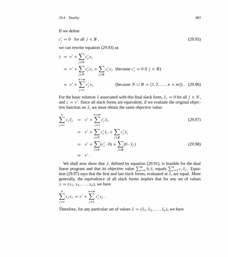
29.4 Duality 883
If we define
c 0j D 0 for all j 2 B ; (29.95)
we can rewrite equation (29.93) as
´ D � 0 CXj 2N
c 0j xj
D � 0 CXj 2N
c 0j xj C
Xj 2B
c 0j xj (because c 0
j D 0 if j 2 B)
D � 0 CnCmXj D1
c 0j xj (because N [ B D f1; 2; : : : ; nCmg) . (29.96)
For the basic solution Nx associated with this final slack form, Nxj D 0 for all j 2 N ,and ´ D � 0. Since all slack forms are equivalent, if we evaluate the original objec-tive function on Nx, we must obtain the same objective value:
nXj D1
cj Nxj D � 0 CnCmXj D1
c 0j Nxj (29.97)
D � 0 CXj 2N
c 0j Nxj C
Xj 2B
c 0j Nxj
D � 0 CXj 2N
.c 0j � 0/C
Xj 2B
.0 � Nxj / (29.98)
D � 0 :
We shall now show that Ny, defined by equation (29.91), is feasible for the duallinear program and that its objective value
Pm
iD1 bi Nyi equalsPn
j D1 cj Nxj . Equa-tion (29.97) says that the first and last slack forms, evaluated at Nx, are equal. Moregenerally, the equivalence of all slack forms implies that for any set of valuesx D .x1; x2; : : : ; xn/, we have
nXj D1
cj xj D � 0 CnCmXj D1
c 0j xj :
Therefore, for any particular set of values Nx D . Nx1; Nx2; : : : ; Nxn/, we have

884 Chapter 29 Linear Programming
nXj D1
cj Nxj
D � 0 CnCmXj D1
c 0j Nxj
D � 0 CnX
j D1
c 0j Nxj C
nCmXj DnC1
c 0j Nxj
D � 0 CnX
j D1
c 0j Nxj C
mXiD1
c 0nCi NxnCi
D � 0 CnX
j D1
c 0j Nxj C
mXiD1
.� Nyi/ NxnCi (by equations (29.91) and (29.95))
D � 0 CnX
j D1
c 0j Nxj C
mXiD1
.� Nyi/
bi �
nXj D1
aij Nxj
!(by equation (29.32))
D � 0 CnX
j D1
c 0j Nxj �
mXiD1
bi Nyi CmX
iD1
nXj D1
.aij Nxj / Nyi
D � 0 CnX
j D1
c 0j Nxj �
mXiD1
bi Nyi CnX
j D1
mXiD1
.aij Nyi/ Nxj
D
� 0 �mX
iD1
bi Nyi
!C
nXj D1
c 0
j CmX
iD1
aij Nyi
!Nxj ;
so thatnX
j D1
cj Nxj D
� 0 �mX
iD1
bi Nyi
!C
nXj D1
c 0
j CmX
iD1
aij Nyi
!Nxj : (29.99)
Applying Lemma 29.3 to equation (29.99), we obtain
� 0 �mX
iD1
bi Nyi D 0 ; (29.100)
c 0j C
mXiD1
aij Nyi D cj for j D 1; 2; : : : ; n : (29.101)
By equation (29.100), we have thatPm
iD1 bi Nyi D � 0, and hence the objective value
of the dual�Pm
iD1 bi Nyi
�is equal to that of the primal (� 0). It remains to show

29.4 Duality 885
that the solution Ny is feasible for the dual problem. From inequalities (29.94) andequations (29.95), we have that c 0
j � 0 for all j D 1; 2; : : : ; nCm. Hence, for anyj D 1; 2; : : : ; n, equations (29.101) imply that
cj D c 0j C
mXiD1
aij Nyi
�mX
iD1
aij Nyi ;
which satisfies the constraints (29.84) of the dual. Finally, since c 0j � 0 for each
j 2 N[B , when we set Ny according to equation (29.91), we have that each Nyi � 0,and so the nonnegativity constraints are satisfied as well.
We have shown that, given a feasible linear program, if INITIALIZE-SIMPLEX
returns a feasible solution, and if SIMPLEX terminates without returning “un-bounded,” then the solution returned is indeed an optimal solution. We have alsoshown how to construct an optimal solution to the dual linear program.
Exercises
29.4-1Formulate the dual of the linear program given in Exercise 29.3-5.
29.4-2Suppose that we have a linear program that is not in standard form. We couldproduce the dual by first converting it to standard form, and then taking the dual.It would be more convenient, however, to be able to produce the dual directly.Explain how we can directly take the dual of an arbitrary linear program.
29.4-3Write down the dual of the maximum-flow linear program, as given in lines(29.47)–(29.50) on page 860. Explain how to interpret this formulation as aminimum-cut problem.
29.4-4Write down the dual of the minimum-cost-flow linear program, as given in lines(29.51)–(29.52) on page 862. Explain how to interpret this problem in terms ofgraphs and flows.
29.4-5Show that the dual of the dual of a linear program is the primal linear program.

886 Chapter 29 Linear Programming
29.4-6Which result from Chapter 26 can be interpreted as weak duality for the maximum-flow problem?
29.5 The initial basic feasible solution
In this section, we first describe how to test whether a linear program is feasible,and if it is, how to produce a slack form for which the basic solution is feasible.We conclude by proving the fundamental theorem of linear programming, whichsays that the SIMPLEX procedure always produces the correct result.
Finding an initial solution
In Section 29.3, we assumed that we had a procedure INITIALIZE-SIMPLEX thatdetermines whether a linear program has any feasible solutions, and if it does, givesa slack form for which the basic solution is feasible. We describe this procedurehere.
A linear program can be feasible, yet the initial basic solution might not befeasible. Consider, for example, the following linear program:
maximize 2x1 � x2 (29.102)
subject to2x1 � x2 � 2 (29.103)
x1 � 5x2 � �4 (29.104)
x1; x2 � 0 : (29.105)
If we were to convert this linear program to slack form, the basic solution wouldset x1 D 0 and x2 D 0. This solution violates constraint (29.104), and so it is not afeasible solution. Thus, INITIALIZE-SIMPLEX cannot just return the obvious slackform. In order to determine whether a linear program has any feasible solutions,we will formulate an auxiliary linear program. For this auxiliary linear program,we can find (with a little work) a slack form for which the basic solution is feasible.Furthermore, the solution of this auxiliary linear program determines whether theinitial linear program is feasible and if so, it provides a feasible solution with whichwe can initialize SIMPLEX.
Lemma 29.11Let L be a linear program in standard form, given as in (29.16)–(29.18). Let x0 bea new variable, and let Laux be the following linear program with nC 1 variables:
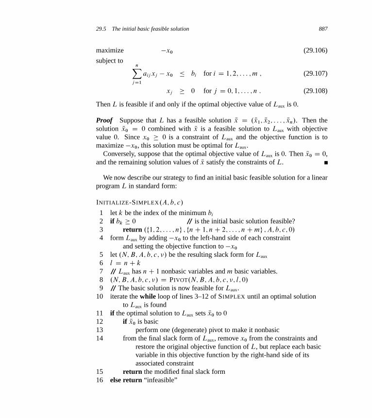
29.5 The initial basic feasible solution 887
maximize �x0 (29.106)
subject tonX
j D1
aij xj � x0 � bi for i D 1; 2; : : : ; m ; (29.107)
xj � 0 for j D 0; 1; : : : ; n : (29.108)
Then L is feasible if and only if the optimal objective value of Laux is 0.
Proof Suppose that L has a feasible solution Nx D . Nx1; Nx2; : : : ; Nxn/. Then thesolution Nx0 D 0 combined with Nx is a feasible solution to Laux with objectivevalue 0. Since x0 � 0 is a constraint of Laux and the objective function is tomaximize �x0, this solution must be optimal for Laux.
Conversely, suppose that the optimal objective value of Laux is 0. Then Nx0 D 0,and the remaining solution values of Nx satisfy the constraints of L.
We now describe our strategy to find an initial basic feasible solution for a linearprogram L in standard form:
INITIALIZE-SIMPLEX.A; b; c/
1 let k be the index of the minimum bi
2 if bk � 0 // is the initial basic solution feasible?3 return .f1; 2; : : : ; ng ; fnC 1; nC 2; : : : ; nCmg ; A; b; c; 0/
4 form Laux by adding �x0 to the left-hand side of each constraintand setting the objective function to �x0
5 let .N; B; A; b; c; �/ be the resulting slack form for Laux
6 l D nC k
7 // Laux has nC 1 nonbasic variables and m basic variables.8 .N; B; A; b; c; �/ D PIVOT.N; B; A; b; c; �; l; 0/
9 // The basic solution is now feasible for Laux.10 iterate the while loop of lines 3–12 of SIMPLEX until an optimal solution
to Laux is found11 if the optimal solution to Laux sets Nx0 to 0
12 if Nx0 is basic13 perform one (degenerate) pivot to make it nonbasic14 from the final slack form of Laux, remove x0 from the constraints and
restore the original objective function of L, but replace each basicvariable in this objective function by the right-hand side of itsassociated constraint
15 return the modified final slack form16 else return “infeasible”

888 Chapter 29 Linear Programming
INITIALIZE-SIMPLEX works as follows. In lines 1–3, we implicitly test thebasic solution to the initial slack form for L given by N D f1; 2; : : : ; ng, B DfnC 1; nC 2; : : : ; nCmg, Nxi D bi for all i 2 B , and Nxj D 0 for all j 2 N .(Creating the slack form requires no explicit effort, as the values of A, b, and c arethe same in both slack and standard forms.) If line 2 finds this basic solution to befeasible—that is, Nxi � 0 for all i 2 N [ B—then line 3 returns the slack form.Otherwise, in line 4, we form the auxiliary linear program Laux as in Lemma 29.11.Since the initial basic solution to L is not feasible, the initial basic solution to theslack form for Laux cannot be feasible either. To find a basic feasible solution, weperform a single pivot operation. Line 6 selects l D n C k as the index of thebasic variable that will be the leaving variable in the upcoming pivot operation.Since the basic variables are xnC1; xnC2; : : : ; xnCm, the leaving variable xl will bethe one with the most negative value. Line 8 performs that call of PIVOT, withx0 entering and xl leaving. We shall see shortly that the basic solution resultingfrom this call of PIVOT will be feasible. Now that we have a slack form for whichthe basic solution is feasible, we can, in line 10, repeatedly call PIVOT to fullysolve the auxiliary linear program. As the test in line 11 demonstrates, if we findan optimal solution to Laux with objective value 0, then in lines 12–14, we createa slack form for L for which the basic solution is feasible. To do so, we first,in lines 12–13, handle the degenerate case in which x0 may still be basic withvalue Nx0 D 0. In this case, we perform a pivot step to remove x0 from the basis,using any e 2 N such that a0e ¤ 0 as the entering variable. The new basicsolution remains feasible; the degenerate pivot does not change the value of anyvariable. Next we delete all x0 terms from the constraints and restore the originalobjective function for L. The original objective function may contain both basicand nonbasic variables. Therefore, in the objective function we replace each basicvariable by the right-hand side of its associated constraint. Line 15 then returnsthis modified slack form. If, on the other hand, line 11 discovers that the originallinear program L is infeasible, then line 16 returns this information.
We now demonstrate the operation of INITIALIZE-SIMPLEX on the linear pro-gram (29.102)–(29.105). This linear program is feasible if we can find nonneg-ative values for x1 and x2 that satisfy inequalities (29.103) and (29.104). UsingLemma 29.11, we formulate the auxiliary linear program
maximize �x0 (29.109)
subject to2x1 � x2 � x0 � 2 (29.110)
x1 � 5x2 � x0 � �4 (29.111)
x1; x2; x0 � 0 :
By Lemma 29.11, if the optimal objective value of this auxiliary linear programis 0, then the original linear program has a feasible solution. If the optimal objective

29.5 The initial basic feasible solution 889
value of this auxiliary linear program is negative, then the original linear programdoes not have a feasible solution.
We write this linear program in slack form, obtaining
´ D � x0
x3 D 2 � 2x1 C x2 C x0
x4 D �4 � x1 C 5x2 C x0 :
We are not out of the woods yet, because the basic solution, which would setx4 D �4, is not feasible for this auxiliary linear program. We can, however, withone call to PIVOT, convert this slack form into one in which the basic solution isfeasible. As line 8 indicates, we choose x0 to be the entering variable. In line 6, wechoose as the leaving variable x4, which is the basic variable whose value in thebasic solution is most negative. After pivoting, we have the slack form
´ D �4 � x1 C 5x2 � x4
x0 D 4 C x1 � 5x2 C x4
x3 D 6 � x1 � 4x2 C x4 :
The associated basic solution is . Nx0; Nx1; Nx2; Nx3; Nx4/ D .4; 0; 0; 6; 0/, which is feasi-ble. We now repeatedly call PIVOT until we obtain an optimal solution to Laux. Inthis case, one call to PIVOT with x2 entering and x0 leaving yields
´ D � x0
x2 D 4
5� x0
5C x1
5C x4
5
x3 D 14
5C 4x0
5� 9x1
5C x4
5:
This slack form is the final solution to the auxiliary problem. Since this solutionhas x0 D 0, we know that our initial problem was feasible. Furthermore, sincex0 D 0, we can just remove it from the set of constraints. We then restore theoriginal objective function, with appropriate substitutions made to include onlynonbasic variables. In our example, we get the objective function
2x1 � x2 D 2x1 ��
4
5� x0
5C x1
5C x4
5
�:
Setting x0 D 0 and simplifying, we get the objective function
�4
5C 9x1
5� x4
5;
and the slack form
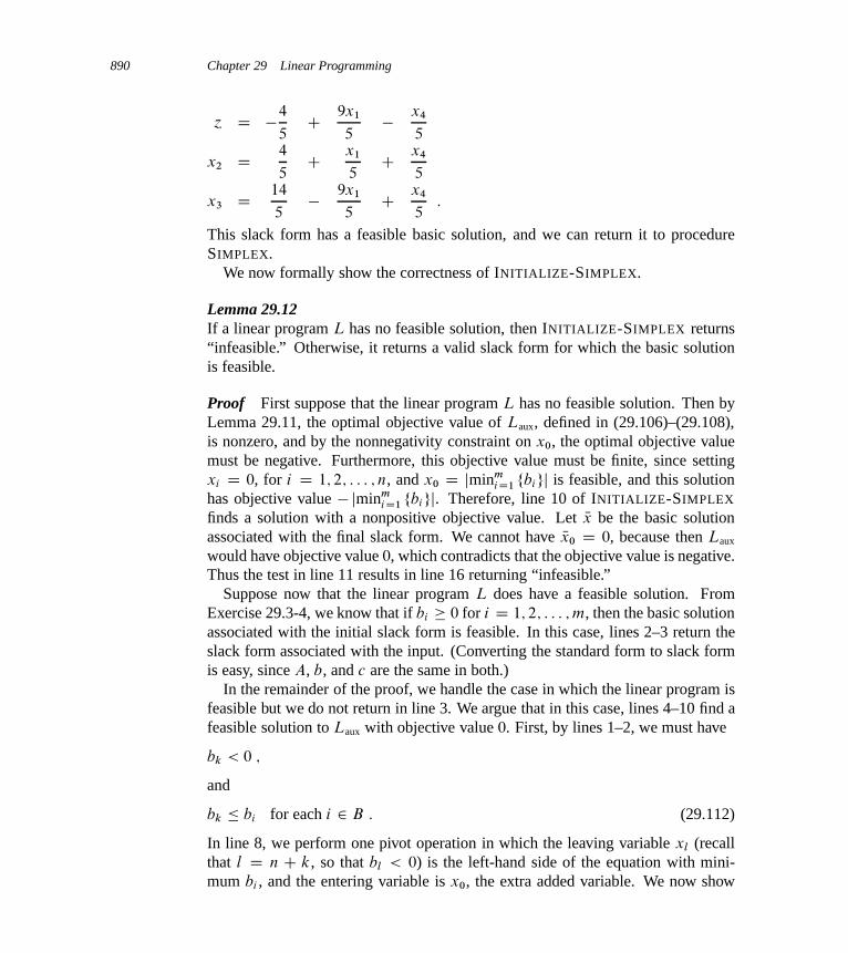
890 Chapter 29 Linear Programming
´ D �4
5C 9x1
5� x4
5
x2 D4
5C x1
5C x4
5
x3 D14
5� 9x1
5C x4
5:
This slack form has a feasible basic solution, and we can return it to procedureSIMPLEX.
We now formally show the correctness of INITIALIZE-SIMPLEX.
Lemma 29.12If a linear program L has no feasible solution, then INITIALIZE-SIMPLEX returns“infeasible.” Otherwise, it returns a valid slack form for which the basic solutionis feasible.
Proof First suppose that the linear program L has no feasible solution. Then byLemma 29.11, the optimal objective value of Laux, defined in (29.106)–(29.108),is nonzero, and by the nonnegativity constraint on x0, the optimal objective valuemust be negative. Furthermore, this objective value must be finite, since settingxi D 0, for i D 1; 2; : : : ; n, and x0 D jminm
iD1 fbigj is feasible, and this solutionhas objective value � jminm
iD1 fbigj. Therefore, line 10 of INITIALIZE-SIMPLEX
finds a solution with a nonpositive objective value. Let Nx be the basic solutionassociated with the final slack form. We cannot have Nx0 D 0, because then Laux
would have objective value 0, which contradicts that the objective value is negative.Thus the test in line 11 results in line 16 returning “infeasible.”
Suppose now that the linear program L does have a feasible solution. FromExercise 29.3-4, we know that if bi � 0 for i D 1; 2; : : : ; m, then the basic solutionassociated with the initial slack form is feasible. In this case, lines 2–3 return theslack form associated with the input. (Converting the standard form to slack formis easy, since A, b, and c are the same in both.)
In the remainder of the proof, we handle the case in which the linear program isfeasible but we do not return in line 3. We argue that in this case, lines 4–10 find afeasible solution to Laux with objective value 0. First, by lines 1–2, we must have
bk < 0 ;
and
bk � bi for each i 2 B : (29.112)
In line 8, we perform one pivot operation in which the leaving variable xl (recallthat l D n C k, so that bl < 0) is the left-hand side of the equation with mini-mum bi , and the entering variable is x0, the extra added variable. We now show
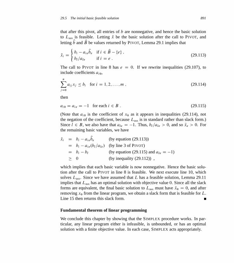
29.5 The initial basic feasible solution 891
that after this pivot, all entries of b are nonnegative, and hence the basic solutionto Laux is feasible. Letting Nx be the basic solution after the call to PIVOT, andletting yb and yB be values returned by PIVOT, Lemma 29.1 implies that
Nxi D(
bi � aieybe if i 2 yB � feg ;
bl=ale if i D e :(29.113)
The call to PIVOT in line 8 has e D 0. If we rewrite inequalities (29.107), toinclude coefficients ai0,
nXj D0
aij xj � bi for i D 1; 2; : : : ; m ; (29.114)
then
ai0 D aie D �1 for each i 2 B : (29.115)
(Note that ai0 is the coefficient of x0 as it appears in inequalities (29.114), notthe negation of the coefficient, because Laux is in standard rather than slack form.)Since l 2 B , we also have that ale D �1. Thus, bl=ale > 0, and so Nxe > 0. Forthe remaining basic variables, we have
Nxi D bi � aieybe (by equation (29.113))
D bi � aie.bl=ale/ (by line 3 of PIVOT)
D bi � bl (by equation (29.115) and ale D �1)
� 0 (by inequality (29.112)) ,
which implies that each basic variable is now nonnegative. Hence the basic solu-tion after the call to PIVOT in line 8 is feasible. We next execute line 10, whichsolves Laux. Since we have assumed that L has a feasible solution, Lemma 29.11implies that Laux has an optimal solution with objective value 0. Since all the slackforms are equivalent, the final basic solution to Laux must have Nx0 D 0, and afterremoving x0 from the linear program, we obtain a slack form that is feasible for L.Line 15 then returns this slack form.
Fundamental theorem of linear programming
We conclude this chapter by showing that the SIMPLEX procedure works. In par-ticular, any linear program either is infeasible, is unbounded, or has an optimalsolution with a finite objective value. In each case, SIMPLEX acts appropriately.

892 Chapter 29 Linear Programming
Theorem 29.13 (Fundamental theorem of linear programming)Any linear program L, given in standard form, either
1. has an optimal solution with a finite objective value,
2. is infeasible, or
3. is unbounded.
If L is infeasible, SIMPLEX returns “infeasible.” If L is unbounded, SIMPLEX
returns “unbounded.” Otherwise, SIMPLEX returns an optimal solution with a finiteobjective value.
Proof By Lemma 29.12, if linear program L is infeasible, then SIMPLEX returns“infeasible.” Now suppose that the linear program L is feasible. By Lemma 29.12,INITIALIZE-SIMPLEX returns a slack form for which the basic solution is feasible.By Lemma 29.7, therefore, SIMPLEX either returns “unbounded” or terminateswith a feasible solution. If it terminates with a finite solution, then Theorem 29.10tells us that this solution is optimal. On the other hand, if SIMPLEX returns “un-bounded,” Lemma 29.2 tells us the linear program L is indeed unbounded. SinceSIMPLEX always terminates in one of these ways, the proof is complete.
Exercises
29.5-1Give detailed pseudocode to implement lines 5 and 14 of INITIALIZE-SIMPLEX.
29.5-2Show that when the main loop of SIMPLEX is run by INITIALIZE-SIMPLEX, it cannever return “unbounded.”
29.5-3Suppose that we are given a linear program L in standard form, and suppose thatfor both L and the dual of L, the basic solutions associated with the initial slackforms are feasible. Show that the optimal objective value of L is 0.
29.5-4Suppose that we allow strict inequalities in a linear program. Show that in thiscase, the fundamental theorem of linear programming does not hold.
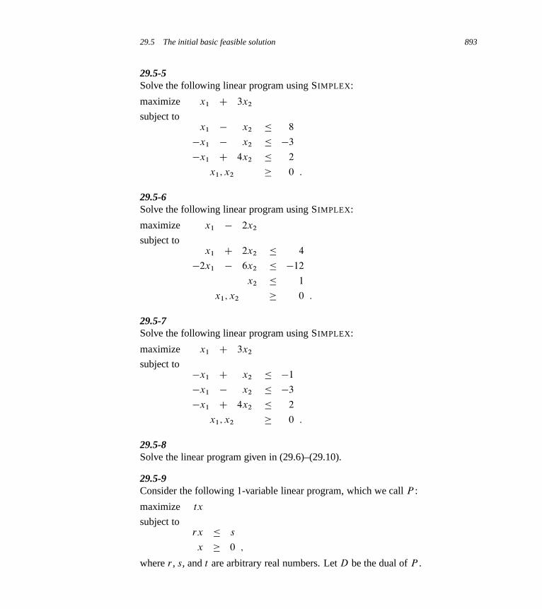
29.5 The initial basic feasible solution 893
29.5-5Solve the following linear program using SIMPLEX:
maximize x1 C 3x2
subject tox1 � x2 � 8
�x1 � x2 � �3
�x1 C 4x2 � 2
x1; x2 � 0 :
29.5-6Solve the following linear program using SIMPLEX:
maximize x1 � 2x2
subject tox1 C 2x2 � 4
�2x1 � 6x2 � �12
x2 � 1
x1; x2 � 0 :
29.5-7Solve the following linear program using SIMPLEX:
maximize x1 C 3x2
subject to�x1 C x2 � �1
�x1 � x2 � �3
�x1 C 4x2 � 2
x1; x2 � 0 :
29.5-8Solve the linear program given in (29.6)–(29.10).
29.5-9Consider the following 1-variable linear program, which we call P :
maximize tx
subject torx � s
x � 0 ;
where r , s, and t are arbitrary real numbers. Let D be the dual of P .
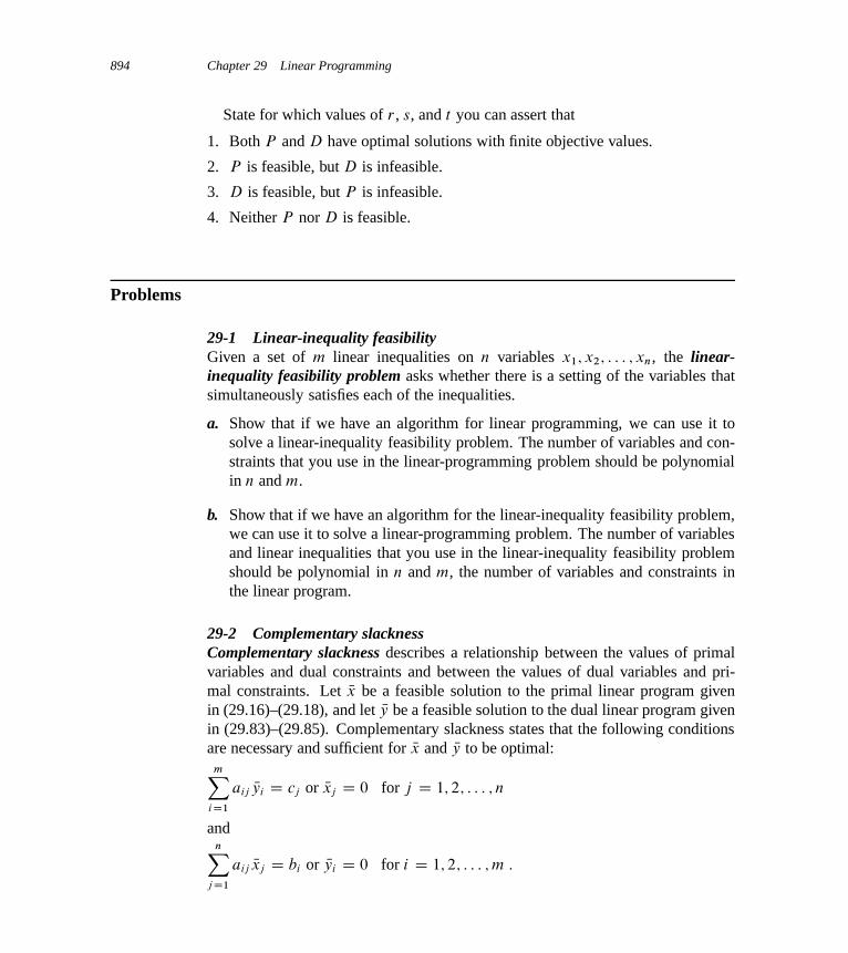
894 Chapter 29 Linear Programming
State for which values of r , s, and t you can assert that
1. Both P and D have optimal solutions with finite objective values.
2. P is feasible, but D is infeasible.
3. D is feasible, but P is infeasible.
4. Neither P nor D is feasible.
Problems
29-1 Linear-inequality feasibilityGiven a set of m linear inequalities on n variables x1; x2; : : : ; xn, the linear-inequality feasibility problem asks whether there is a setting of the variables thatsimultaneously satisfies each of the inequalities.
a. Show that if we have an algorithm for linear programming, we can use it tosolve a linear-inequality feasibility problem. The number of variables and con-straints that you use in the linear-programming problem should be polynomialin n and m.
b. Show that if we have an algorithm for the linear-inequality feasibility problem,we can use it to solve a linear-programming problem. The number of variablesand linear inequalities that you use in the linear-inequality feasibility problemshould be polynomial in n and m, the number of variables and constraints inthe linear program.
29-2 Complementary slacknessComplementary slackness describes a relationship between the values of primalvariables and dual constraints and between the values of dual variables and pri-mal constraints. Let Nx be a feasible solution to the primal linear program givenin (29.16)–(29.18), and let Ny be a feasible solution to the dual linear program givenin (29.83)–(29.85). Complementary slackness states that the following conditionsare necessary and sufficient for Nx and Ny to be optimal:
mXiD1
aij Nyi D cj or Nxj D 0 for j D 1; 2; : : : ; n
andnX
j D1
aij Nxj D bi or Nyi D 0 for i D 1; 2; : : : ; m :
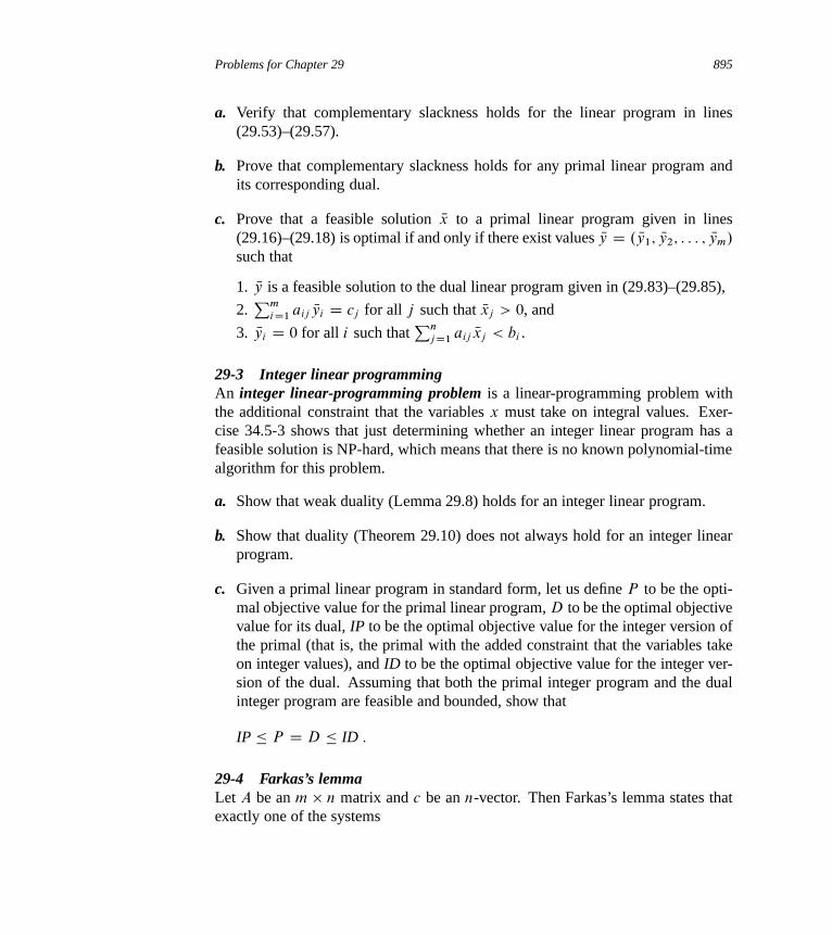
Problems for Chapter 29 895
a. Verify that complementary slackness holds for the linear program in lines(29.53)–(29.57).
b. Prove that complementary slackness holds for any primal linear program andits corresponding dual.
c. Prove that a feasible solution Nx to a primal linear program given in lines(29.16)–(29.18) is optimal if and only if there exist values Ny D . Ny1; Ny2; : : : ; Nym/
such that
1. Ny is a feasible solution to the dual linear program given in (29.83)–(29.85),
2.Pm
iD1 aij Nyi D cj for all j such that Nxj > 0, and
3. Nyi D 0 for all i such thatPn
j D1 aij Nxj < bi .
29-3 Integer linear programmingAn integer linear-programming problem is a linear-programming problem withthe additional constraint that the variables x must take on integral values. Exer-cise 34.5-3 shows that just determining whether an integer linear program has afeasible solution is NP-hard, which means that there is no known polynomial-timealgorithm for this problem.
a. Show that weak duality (Lemma 29.8) holds for an integer linear program.
b. Show that duality (Theorem 29.10) does not always hold for an integer linearprogram.
c. Given a primal linear program in standard form, let us define P to be the opti-mal objective value for the primal linear program, D to be the optimal objectivevalue for its dual, IP to be the optimal objective value for the integer version ofthe primal (that is, the primal with the added constraint that the variables takeon integer values), and ID to be the optimal objective value for the integer ver-sion of the dual. Assuming that both the primal integer program and the dualinteger program are feasible and bounded, show that
IP � P D D � ID :
29-4 Farkas’s lemmaLet A be an m n matrix and c be an n-vector. Then Farkas’s lemma states thatexactly one of the systems

896 Chapter 29 Linear Programming
Ax � 0 ;
cTx > 0
and
ATy D c ;
y � 0
is solvable, where x is an n-vector and y is an m-vector. Prove Farkas’s lemma.
29-5 Minimum-cost circulationIn this problem, we consider a variant of the minimum-cost-flow problem fromSection 29.2 in which we are not given a demand, a source, or a sink. Instead,we are given, as before, a flow network and edge costs a.u; �/. A flow is feasibleif it satisfies the capacity constraint on every edge and flow conservation at everyvertex. The goal is to find, among all feasible flows, the one of minimum cost. Wecall this problem the minimum-cost-circulation problem.
a. Formulate the minimum-cost-circulation problem as a linear program.
b. Suppose that for all edges .u; �/ 2 E, we have a.u; �/ > 0. Characterize anoptimal solution to the minimum-cost-circulation problem.
c. Formulate the maximum-flow problem as a minimum-cost-circulation problemlinear program. That is given a maximum-flow problem instance G D .V; E/
with source s, sink t and edge capacities c, create a minimum-cost-circulationproblem by giving a (possibly different) network G0 D .V 0; E 0/ with edgecapacities c 0 and edge costs a0 such that you can discern a solution to themaximum-flow problem from a solution to the minimum-cost-circulation prob-lem.
d. Formulate the single-source shortest-path problem as a minimum-cost-circu-lation problem linear program.
Chapter notes
This chapter only begins to study the wide field of linear programming. A num-ber of books are devoted exclusively to linear programming, including those byChvátal [70], Gass [130], Karloff [197], Schrijver [303], and Vanderbei [344].Many other books give a good coverage of linear programming, including thoseby Papadimitriou and Steiglitz [271] and Ahuja, Magnanti, and Orlin [7]. Thecoverage in this chapter draws on the approach taken by Chvátal.
Notes for Chapter 29 897
The simplex algorithm for linear programming was invented by G. Dantzigin 1947. Shortly after, researchers discovered how to formulate a number of prob-lems in a variety of fields as linear programs and solve them with the simplexalgorithm. As a result, applications of linear programming flourished, along withseveral algorithms. Variants of the simplex algorithm remain the most popularmethods for solving linear-programming problems. This history appears in a num-ber of places, including the notes in [70] and [197].
The ellipsoid algorithm was the first polynomial-time algorithm for linear pro-gramming and is due to L. G. Khachian in 1979; it was based on earlier work byN. Z. Shor, D. B. Judin, and A. S. Nemirovskii. Grötschel, Lovász, and Schrijver[154] describe how to use the ellipsoid algorithm to solve a variety of problems incombinatorial optimization. To date, the ellipsoid algorithm does not appear to becompetitive with the simplex algorithm in practice.
Karmarkar’s paper [198] includes a description of the first interior-point algo-rithm. Many subsequent researchers designed interior-point algorithms. Good sur-veys appear in the article of Goldfarb and Todd [141] and the book by Ye [361].
Analysis of the simplex algorithm remains an active area of research. V. Kleeand G. J. Minty constructed an example on which the simplex algorithm runsthrough 2n � 1 iterations. The simplex algorithm usually performs very well inpractice and many researchers have tried to give theoretical justification for thisempirical observation. A line of research begun by K. H. Borgwardt, and carriedon by many others, shows that under certain probabilistic assumptions on the in-put, the simplex algorithm converges in expected polynomial time. Spielman andTeng [322] made progress in this area, introducing the “smoothed analysis of algo-rithms” and applying it to the simplex algorithm.
The simplex algorithm is known to run efficiently in certain special cases. Par-ticularly noteworthy is the network-simplex algorithm, which is the simplex al-gorithm, specialized to network-flow problems. For certain network problems,including the shortest-paths, maximum-flow, and minimum-cost-flow problems,variants of the network-simplex algorithm run in polynomial time. See, for exam-ple, the article by Orlin [268] and the citations therein.

30 Polynomials and the FFT
The straightforward method of adding two polynomials of degree n takes ‚.n/
time, but the straightforward method of multiplying them takes ‚.n2/ time. In thischapter, we shall show how the fast Fourier transform, or FFT, can reduce the timeto multiply polynomials to ‚.n lg n/.
The most common use for Fourier transforms, and hence the FFT, is in signalprocessing. A signal is given in the time domain: as a function mapping time toamplitude. Fourier analysis allows us to express the signal as a weighted sum ofphase-shifted sinusoids of varying frequencies. The weights and phases associatedwith the frequencies characterize the signal in the frequency domain. Among themany everyday applications of FFT’s are compression techniques used to encodedigital video and audio information, including MP3 files. Several fine books delveinto the rich area of signal processing; the chapter notes reference a few of them.
Polynomials
A polynomial in the variable x over an algebraic field F represents a function A.x/
as a formal sum:
A.x/ Dn�1Xj D0
aj xj :
We call the values a0; a1; : : : ; an�1 the coefficients of the polynomial. The co-efficients are drawn from a field F , typically the set C of complex numbers. Apolynomial A.x/ has degree k if its highest nonzero coefficient is ak; we writethat degree.A/ D k. Any integer strictly greater than the degree of a polynomialis a degree-bound of that polynomial. Therefore, the degree of a polynomial ofdegree-bound n may be any integer between 0 and n � 1, inclusive.
We can define a variety of operations on polynomials. For polynomial addi-tion, if A.x/ and B.x/ are polynomials of degree-bound n, their sum is a polyno-
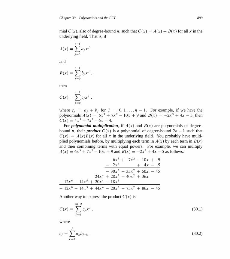
Chapter 30 Polynomials and the FFT 899
mial C.x/, also of degree-bound n, such that C.x/ D A.x/C B.x/ for all x in theunderlying field. That is, if
A.x/ Dn�1Xj D0
aj xj
and
B.x/ Dn�1Xj D0
bj xj ;
then
C.x/ Dn�1Xj D0
cj xj ;
where cj D aj C bj for j D 0; 1; : : : ; n � 1. For example, if we have thepolynomials A.x/ D 6x3 C 7x2 � 10x C 9 and B.x/ D �2x3 C 4x � 5, thenC.x/ D 4x3 C 7x2 � 6x C 4.
For polynomial multiplication, if A.x/ and B.x/ are polynomials of degree-bound n, their product C.x/ is a polynomial of degree-bound 2n � 1 such thatC.x/ D A.x/B.x/ for all x in the underlying field. You probably have multi-plied polynomials before, by multiplying each term in A.x/ by each term in B.x/
and then combining terms with equal powers. For example, we can multiplyA.x/ D 6x3 C 7x2 � 10x C 9 and B.x/ D �2x3 C 4x � 5 as follows:
6x3 C 7x2 � 10x C 9
� 2x3 C 4x � 5
� 30x3 � 35x2 C 50x � 45
24x4 C 28x3 � 40x2 C 36x
� 12x6 � 14x5 C 20x4 � 18x3
� 12x6 � 14x5 C 44x4 � 20x3 � 75x2 C 86x � 45
Another way to express the product C.x/ is
C.x/ D2n�2Xj D0
cj xj ; (30.1)
where
cj DjX
kD0
akbj �k : (30.2)

900 Chapter 30 Polynomials and the FFT
Note that degree.C / D degree.A/ C degree.B/, implying that if A is a polyno-mial of degree-bound na and B is a polynomial of degree-bound nb, then C is apolynomial of degree-bound na C nb � 1. Since a polynomial of degree-bound k
is also a polynomial of degree-bound k C 1, we will normally say that the productpolynomial C is a polynomial of degree-bound na C nb.
Chapter outline
Section 30.1 presents two ways to represent polynomials: the coefficient represen-tation and the point-value representation. The straightforward methods for multi-plying polynomials—equations (30.1) and (30.2)—take ‚.n2/ time when we rep-resent polynomials in coefficient form, but only ‚.n/ time when we represent themin point-value form. We can, however, multiply polynomials using the coefficientrepresentation in only ‚.n lg n/ time by converting between the two representa-tions. To see why this approach works, we must first study complex roots of unity,which we do in Section 30.2. Then, we use the FFT and its inverse, also describedin Section 30.2, to perform the conversions. Section 30.3 shows how to implementthe FFT quickly in both serial and parallel models.
This chapter uses complex numbers extensively, and within this chapter we usethe symbol i exclusively to denote
p�1.
30.1 Representing polynomials
The coefficient and point-value representations of polynomials are in a sense equiv-alent; that is, a polynomial in point-value form has a unique counterpart in co-efficient form. In this section, we introduce the two representations and showhow to combine them so that we can multiply two degree-bound n polynomialsin ‚.n lg n/ time.
Coefficient representation
A coefficient representation of a polynomial A.x/ D Pn�1
j D0 aj xj of degree-bound n is a vector of coefficients a D .a0; a1; : : : ; an�1/. In matrix equationsin this chapter, we shall generally treat vectors as column vectors.
The coefficient representation is convenient for certain operations on polyno-mials. For example, the operation of evaluating the polynomial A.x/ at a givenpoint x0 consists of computing the value of A.x0/. We can evaluate a polynomialin ‚.n/ time using Horner’s rule:
A.x0/ D a0 C x0.a1 C x0.a2 C � � � C x0.an�2 C x0.an�1// � � �// :
30.1 Representing polynomials 901
Similarly, adding two polynomials represented by the coefficient vectors a D.a0; a1; : : : ; an�1/ and b D .b0; b1; : : : ; bn�1/ takes ‚.n/ time: we just producethe coefficient vector c D .c0; c1; : : : ; cn�1/, where cj D aj C bj for j D0; 1; : : : ; n � 1.
Now, consider multiplying two degree-bound n polynomials A.x/ and B.x/ rep-resented in coefficient form. If we use the method described by equations (30.1)and (30.2), multiplying polynomials takes time ‚.n2/, since we must multiplyeach coefficient in the vector a by each coefficient in the vector b. The operationof multiplying polynomials in coefficient form seems to be considerably more diffi-cult than that of evaluating a polynomial or adding two polynomials. The resultingcoefficient vector c, given by equation (30.2), is also called the convolution of theinput vectors a and b, denoted c D a ˝ b. Since multiplying polynomials andcomputing convolutions are fundamental computational problems of considerablepractical importance, this chapter concentrates on efficient algorithms for them.
Point-value representation
A point-value representation of a polynomial A.x/ of degree-bound n is a set ofn point-value pairs
f.x0; y0/; .x1; y1/; : : : ; .xn�1; yn�1/gsuch that all of the xk are distinct and
yk D A.xk/ (30.3)
for k D 0; 1; : : : ; n � 1. A polynomial has many different point-value representa-tions, since we can use any set of n distinct points x0; x1; : : : ; xn�1 as a basis forthe representation.
Computing a point-value representation for a polynomial given in coefficientform is in principle straightforward, since all we have to do is select n distinctpoints x0; x1; : : : ; xn�1 and then evaluate A.xk/ for k D 0; 1; : : : ; n � 1. WithHorner’s method, evaluating a polynomial at n points takes time ‚.n2/. We shallsee later that if we choose the points xk cleverly, we can accelerate this computationto run in time ‚.n lg n/.
The inverse of evaluation—determining the coefficient form of a polynomialfrom a point-value representation—is interpolation. The following theorem showsthat interpolation is well defined when the desired interpolating polynomial musthave a degree-bound equal to the given number of point-value pairs.
Theorem 30.1 (Uniqueness of an interpolating polynomial)For any set f.x0; y0/; .x1; y1/; : : : ; .xn�1; yn�1/g of n point-value pairs such thatall the xk values are distinct, there is a unique polynomial A.x/ of degree-bound n
such that yk D A.xk/ for k D 0; 1; : : : ; n � 1.

902 Chapter 30 Polynomials and the FFT
Proof The proof relies on the existence of the inverse of a certain matrix. Equa-tion (30.3) is equivalent to the matrix equation˙
1 x0 x20 � � � xn�1
0
1 x1 x21 � � � xn�1
1:::
::::::
: : ::::
1 xn�1 x2n�1 � � � xn�1
n�1
�˙a0
a1
:::
an�1
�D
˙y0
y1
:::
yn�1
�: (30.4)
The matrix on the left is denoted V.x0; x1; : : : ; xn�1/ and is known as a Vander-monde matrix. By Problem D-1, this matrix has determinantY0�j <k�n�1
.xk � xj / ;
and therefore, by Theorem D.5, it is invertible (that is, nonsingular) if the xk aredistinct. Thus, we can solve for the coefficients aj uniquely given the point-valuerepresentation:
a D V.x0; x1; : : : ; xn�1/�1y :
The proof of Theorem 30.1 describes an algorithm for interpolation based onsolving the set (30.4) of linear equations. Using the LU decomposition algorithmsof Chapter 28, we can solve these equations in time O.n3/.
A faster algorithm for n-point interpolation is based on Lagrange’s formula:
A.x/ Dn�1XkD0
yk
Yj ¤k
.x � xj /
Yj ¤k
.xk � xj /: (30.5)
You may wish to verify that the right-hand side of equation (30.5) is a polynomialof degree-bound n that satisfies A.xk/ D yk for all k. Exercise 30.1-5 asks youhow to compute the coefficients of A using Lagrange’s formula in time ‚.n2/.
Thus, n-point evaluation and interpolation are well-defined inverse operationsthat transform between the coefficient representation of a polynomial and a point-value representation.1 The algorithms described above for these problems taketime ‚.n2/.
The point-value representation is quite convenient for many operations on poly-nomials. For addition, if C.x/ D A.x/CB.x/, then C.xk/ D A.xk/CB.xk/ forany point xk. More precisely, if we have a point-value representation for A,
1Interpolation is a notoriously tricky problem from the point of view of numerical stability. Althoughthe approaches described here are mathematically correct, small differences in the inputs or round-offerrors during computation can cause large differences in the result.
30.1 Representing polynomials 903
f.x0; y0/; .x1; y1/; : : : ; .xn�1; yn�1/g ;
and for B ,
f.x0; y 00/; .x1; y 0
1/; : : : ; .xn�1; y 0n�1/g
(note that A and B are evaluated at the same n points), then a point-value repre-sentation for C is
f.x0; y0 C y 00/; .x1; y1 C y 0
1/; : : : ; .xn�1; yn�1 C y 0n�1/g :
Thus, the time to add two polynomials of degree-bound n in point-value formis ‚.n/.
Similarly, the point-value representation is convenient for multiplying polyno-mials. If C.x/ D A.x/B.x/, then C.xk/ D A.xk/B.xk/ for any point xk, andwe can pointwise multiply a point-value representation for A by a point-value rep-resentation for B to obtain a point-value representation for C . We must face theproblem, however, that degree.C / D degree.A/ C degree.B/; if A and B are ofdegree-bound n, then C is of degree-bound 2n. A standard point-value represen-tation for A and B consists of n point-value pairs for each polynomial. When wemultiply these together, we get n point-value pairs, but we need 2n pairs to interpo-late a unique polynomial C of degree-bound 2n. (See Exercise 30.1-4.) We musttherefore begin with “extended” point-value representations for A and for B con-sisting of 2n point-value pairs each. Given an extended point-value representationfor A,
f.x0; y0/; .x1; y1/; : : : ; .x2n�1; y2n�1/g ;
and a corresponding extended point-value representation for B ,
f.x0; y 00/; .x1; y 0
1/; : : : ; .x2n�1; y 02n�1/g ;
then a point-value representation for C is
f.x0; y0y 00/; .x1; y1y 0
1/; : : : ; .x2n�1; y2n�1y 02n�1/g :
Given two input polynomials in extended point-value form, we see that the time tomultiply them to obtain the point-value form of the result is ‚.n/, much less thanthe time required to multiply polynomials in coefficient form.
Finally, we consider how to evaluate a polynomial given in point-value form at anew point. For this problem, we know of no simpler approach than converting thepolynomial to coefficient form first, and then evaluating it at the new point.
Fast multiplication of polynomials in coefficient form
Can we use the linear-time multiplication method for polynomials in point-valueform to expedite polynomial multiplication in coefficient form? The answer hinges

904 Chapter 30 Polynomials and the FFT
a0; a1; : : : ; an�1
b0; b1; : : : ; bn�1
c0; c1; : : : ; c2n�2Ordinary multiplication
Time ‚.n2/
Evaluation
Time ‚.n lg n/Time ‚.n lg n/
Interpolation
Pointwise multiplication
Time ‚.n/
A.!02n/; B.!0
2n/
A.!12n/; B.!1
2n/
A.!2n�12n /; B.!2n�1
2n /
::::::
C.!02n/
C.!12n/
C.!2n�12n /
Coefficient
Point-valuerepresentations
representations
Figure 30.1 A graphical outline of an efficient polynomial-multiplication process. Representationson the top are in coefficient form, while those on the bottom are in point-value form. The arrowsfrom left to right correspond to the multiplication operation. The !2n terms are complex .2n/th rootsof unity.
on whether we can convert a polynomial quickly from coefficient form to point-value form (evaluate) and vice versa (interpolate).
We can use any points we want as evaluation points, but by choosing the eval-uation points carefully, we can convert between representations in only ‚.n lg n/
time. As we shall see in Section 30.2, if we choose “complex roots of unity” asthe evaluation points, we can produce a point-value representation by taking thediscrete Fourier transform (or DFT) of a coefficient vector. We can perform theinverse operation, interpolation, by taking the “inverse DFT” of point-value pairs,yielding a coefficient vector. Section 30.2 will show how the FFT accomplishesthe DFT and inverse DFT operations in ‚.n lg n/ time.
Figure 30.1 shows this strategy graphically. One minor detail concerns degree-bounds. The product of two polynomials of degree-bound n is a polynomial ofdegree-bound 2n. Before evaluating the input polynomials A and B , therefore,we first double their degree-bounds to 2n by adding n high-order coefficients of 0.Because the vectors have 2n elements, we use “complex .2n/th roots of unity,”which are denoted by the !2n terms in Figure 30.1.
Given the FFT, we have the following ‚.n lg n/-time procedure for multiplyingtwo polynomials A.x/ and B.x/ of degree-bound n, where the input and outputrepresentations are in coefficient form. We assume that n is a power of 2; we canalways meet this requirement by adding high-order zero coefficients.
1. Double degree-bound: Create coefficient representations of A.x/ and B.x/ asdegree-bound 2n polynomials by adding n high-order zero coefficients to each.
30.1 Representing polynomials 905
2. Evaluate: Compute point-value representations of A.x/ and B.x/ of length 2n
by applying the FFT of order 2n on each polynomial. These representationscontain the values of the two polynomials at the .2n/th roots of unity.
3. Pointwise multiply: Compute a point-value representation for the polynomialC.x/ D A.x/B.x/ by multiplying these values together pointwise. This repre-sentation contains the value of C.x/ at each .2n/th root of unity.
4. Interpolate: Create the coefficient representation of the polynomial C.x/ byapplying the FFT on 2n point-value pairs to compute the inverse DFT.
Steps (1) and (3) take time ‚.n/, and steps (2) and (4) take time ‚.n lg n/. Thus,once we show how to use the FFT, we will have proven the following.
Theorem 30.2We can multiply two polynomials of degree-bound n in time ‚.n lg n/, with boththe input and output representations in coefficient form.
Exercises
30.1-1Multiply the polynomials A.x/ D 7x3 � x2 C x � 10 and B.x/ D 8x3 � 6x C 3
using equations (30.1) and (30.2).
30.1-2Another way to evaluate a polynomial A.x/ of degree-bound n at a given point x0
is to divide A.x/ by the polynomial .x�x0/, obtaining a quotient polynomial q.x/
of degree-bound n � 1 and a remainder r , such that
A.x/ D q.x/.x � x0/C r :
Clearly, A.x0/ D r . Show how to compute the remainder r and the coefficientsof q.x/ in time ‚.n/ from x0 and the coefficients of A.
30.1-3Derive a point-value representation for Arev.x/ D Pn�1
j D0 an�1�j xj from a point-
value representation for A.x/ DPn�1
j D0 aj xj , assuming that none of the points is 0.
30.1-4Prove that n distinct point-value pairs are necessary to uniquely specify a polyno-mial of degree-bound n, that is, if fewer than n distinct point-value pairs are given,they fail to specify a unique polynomial of degree-bound n. (Hint: Using Theo-rem 30.1, what can you say about a set of n� 1 point-value pairs to which you addone more arbitrarily-chosen point-value pair?)

906 Chapter 30 Polynomials and the FFT
30.1-5Show how to use equation (30.5) to interpolate in time ‚.n2/. (Hint: First computethe coefficient representation of the polynomial
Qj .x � xj / and then divide by
.x�xk/ as necessary for the numerator of each term; see Exercise 30.1-2. You cancompute each of the n denominators in time O.n/.)
30.1-6Explain what is wrong with the “obvious” approach to polynomial division usinga point-value representation, i.e., dividing the corresponding y values. Discussseparately the case in which the division comes out exactly and the case in whichit doesn’t.
30.1-7Consider two sets A and B , each having n integers in the range from 0 to 10n. Wewish to compute the Cartesian sum of A and B , defined by
C D fx C y W x 2 A and y 2 Bg :
Note that the integers in C are in the range from 0 to 20n. We want to find theelements of C and the number of times each element of C is realized as a sum ofelements in A and B . Show how to solve the problem in O.n lg n/ time. (Hint:Represent A and B as polynomials of degree at most 10n.)
30.2 The DFT and FFT
In Section 30.1, we claimed that if we use complex roots of unity, we can evaluateand interpolate polynomials in ‚.n lg n/ time. In this section, we define complexroots of unity and study their properties, define the DFT, and then show how theFFT computes the DFT and its inverse in ‚.n lg n/ time.
Complex roots of unity
A complex nth root of unity is a complex number ! such that
!n D 1 :
There are exactly n complex nth roots of unity: e2�ik=n for k D 0; 1; : : : ; n � 1.To interpret this formula, we use the definition of the exponential of a complexnumber:
eiu D cos.u/C i sin.u/ :
Figure 30.2 shows that the n complex roots of unity are equally spaced around thecircle of unit radius centered at the origin of the complex plane. The value
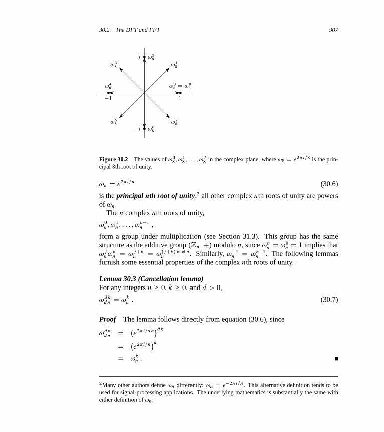
30.2 The DFT and FFT 907
1�1
i
�i
!08 D !8
8
!18
!28
!38
!48
!58
!68
!78
Figure 30.2 The values of !08 ; !1
8 ; : : : ; !78 in the complex plane, where !8 D e2�i=8 is the prin-
cipal 8th root of unity.
!n D e2�i=n (30.6)
is the principal nth root of unity;2 all other complex nth roots of unity are powersof !n.
The n complex nth roots of unity,
!0n; !1
n; : : : ; !n�1n ;
form a group under multiplication (see Section 31.3). This group has the samestructure as the additive group .Zn;C/ modulo n, since !n
n D !0n D 1 implies that
!jn!k
n D !j Ckn D !.j Ck/ mod n
n . Similarly, !�1n D !n�1
n . The following lemmasfurnish some essential properties of the complex nth roots of unity.
Lemma 30.3 (Cancellation lemma)For any integers n � 0, k � 0, and d > 0,
!dkdn D !k
n : (30.7)
Proof The lemma follows directly from equation (30.6), since
!dkdn D �
e2�i=dn�dk
D �e2�i=n
�kD !k
n :
2Many other authors define !n differently: !n D e�2�i=n. This alternative definition tends to beused for signal-processing applications. The underlying mathematics is substantially the same witheither definition of !n.

908 Chapter 30 Polynomials and the FFT
Corollary 30.4For any even integer n > 0,
!n=2n D !2 D �1 :
Proof The proof is left as Exercise 30.2-1.
Lemma 30.5 (Halving lemma)If n > 0 is even, then the squares of the n complex nth roots of unity are the n=2
complex .n=2/th roots of unity.
Proof By the cancellation lemma, we have .!kn/2 D !k
n=2, for any nonnegative
integer k. Note that if we square all of the complex nth roots of unity, then weobtain each .n=2/th root of unity exactly twice, since
.!kCn=2n /2 D !2kCn
n
D !2kn !n
n
D !2kn
D .!kn/2 :
Thus, !kn and !kCn=2
n have the same square. We could also have used Corol-lary 30.4 to prove this property, since !n=2
n D �1 implies !kCn=2n D �!k
n , andthus .!kCn=2
n /2 D .!kn/2.
As we shall see, the halving lemma is essential to our divide-and-conquer ap-proach for converting between coefficient and point-value representations of poly-nomials, since it guarantees that the recursive subproblems are only half as large.
Lemma 30.6 (Summation lemma)For any integer n � 1 and nonzero integer k not divisible by n,
n�1Xj D0
�!k
n
�j D 0 :
Proof Equation (A.5) applies to complex values as well as to reals, and so wehave
30.2 The DFT and FFT 909
n�1Xj D0
�!k
n
�j D .!kn/n � 1
!kn � 1
D .!nn/k � 1
!kn � 1
D .1/k � 1
!kn � 1
D 0 :
Because we require that k is not divisible by n, and because !kn D 1 only when k
is divisible by n, we ensure that the denominator is not 0.
The DFT
Recall that we wish to evaluate a polynomial
A.x/ Dn�1Xj D0
aj xj
of degree-bound n at !0n; !1
n; !2n; : : : ; !n�1
n (that is, at the n complex nth roots ofunity).3 We assume that A is given in coefficient form: a D .a0; a1; : : : ; an�1/. Letus define the results yk, for k D 0; 1; : : : ; n � 1, by
yk D A.!kn/
Dn�1Xj D0
aj !kjn : (30.8)
The vector y D .y0; y1; : : : ; yn�1/ is the discrete Fourier transform (DFT) of thecoefficient vector a D .a0; a1; : : : ; an�1/. We also write y D DFTn.a/.
The FFT
By using a method known as the fast Fourier transform (FFT), which takes ad-vantage of the special properties of the complex roots of unity, we can computeDFTn.a/ in time ‚.n lg n/, as opposed to the ‚.n2/ time of the straightforwardmethod. We assume throughout that n is an exact power of 2. Although strategies
3The length n is actually what we referred to as 2n in Section 30.1, since we double the degree-boundof the given polynomials prior to evaluation. In the context of polynomial multiplication, therefore,we are actually working with complex .2n/th roots of unity.
910 Chapter 30 Polynomials and the FFT
for dealing with non-power-of-2 sizes are known, they are beyond the scope of thisbook.
The FFT method employs a divide-and-conquer strategy, using the even-indexedand odd-indexed coefficients of A.x/ separately to define the two new polynomialsAŒ0�.x/ and AŒ1�.x/ of degree-bound n=2:
AŒ0�.x/ D a0 C a2x C a4x2 C � � � C an�2xn=2�1 ;
AŒ1�.x/ D a1 C a3x C a5x2 C � � � C an�1xn=2�1 :
Note that AŒ0� contains all the even-indexed coefficients of A (the binary represen-tation of the index ends in 0) and AŒ1� contains all the odd-indexed coefficients (thebinary representation of the index ends in 1). It follows that
A.x/ D AŒ0�.x2/C xAŒ1�.x2/ ; (30.9)
so that the problem of evaluating A.x/ at !0n; !1
n; : : : ; !n�1n reduces to
1. evaluating the degree-bound n=2 polynomials AŒ0�.x/ and AŒ1�.x/ at the points
.!0n/2; .!1
n/2; : : : ; .!n�1n /2 ; (30.10)
and then
2. combining the results according to equation (30.9).
By the halving lemma, the list of values (30.10) consists not of n distinct val-ues but only of the n=2 complex .n=2/th roots of unity, with each root occurringexactly twice. Therefore, we recursively evaluate the polynomials AŒ0� and AŒ1�
of degree-bound n=2 at the n=2 complex .n=2/th roots of unity. These subprob-lems have exactly the same form as the original problem, but are half the size.We have now successfully divided an n-element DFTn computation into two n=2-element DFTn=2 computations. This decomposition is the basis for the follow-ing recursive FFT algorithm, which computes the DFT of an n-element vectora D .a0; a1; : : : ; an�1/, where n is a power of 2.
30.2 The DFT and FFT 911
RECURSIVE-FFT.a/
1 n D a: length // n is a power of 2
2 if n == 1
3 return a
4 !n D e2�i=n
5 ! D 1
6 aŒ0� D .a0; a2; : : : ; an�2/
7 aŒ1� D .a1; a3; : : : ; an�1/
8 yŒ0� D RECURSIVE-FFT.aŒ0�/
9 yŒ1� D RECURSIVE-FFT.aŒ1�/
10 for k D 0 to n=2 � 1
11 yk D yŒ0�
kC ! y
Œ1�
k
12 ykC.n=2/ D yŒ0�
k� ! y
Œ1�
k
13 ! D ! !n
14 return y // y is assumed to be a column vector
The RECURSIVE-FFT procedure works as follows. Lines 2–3 represent the basisof the recursion; the DFT of one element is the element itself, since in this case
y0 D a0 !01
D a0 � 1D a0 :
Lines 6–7 define the coefficient vectors for the polynomials AŒ0� and AŒ1�. Lines4, 5, and 13 guarantee that ! is updated properly so that whenever lines 11–12are executed, we have ! D !k
n . (Keeping a running value of ! from iterationto iteration saves time over computing !k
n from scratch each time through the forloop.) Lines 8–9 perform the recursive DFTn=2 computations, setting, for k D0; 1; : : : ; n=2 � 1,
yŒ0�
kD AŒ0�.!k
n=2/ ;
yŒ1�
kD AŒ1�.!k
n=2/ ;
or, since !kn=2D !2k
n by the cancellation lemma,
yŒ0�
kD AŒ0�.!2k
n / ;
yŒ1�
kD AŒ1�.!2k
n / :
912 Chapter 30 Polynomials and the FFT
Lines 11–12 combine the results of the recursive DFTn=2 calculations. For y0; y1;
: : : ; yn=2�1, line 11 yields
yk D yŒ0�
kC !k
nyŒ1�
k
D AŒ0�.!2kn /C !k
nAŒ1�.!2kn /
D A.!kn/ (by equation (30.9)) .
For yn=2; yn=2C1; : : : ; yn�1, letting k D 0; 1; : : : ; n=2 � 1, line 12 yields
ykC.n=2/ D yŒ0�
k� !k
nyŒ1�
k
D yŒ0�
kC !kC.n=2/
n yŒ1�
k(since !kC.n=2/
n D �!kn )
D AŒ0�.!2kn /C !kC.n=2/
n AŒ1�.!2kn /
D AŒ0�.!2kCnn /C !kC.n=2/
n AŒ1�.!2kCnn / (since !2kCn
n D !2kn )
D A.!kC.n=2/n / (by equation (30.9)) .
Thus, the vector y returned by RECURSIVE-FFT is indeed the DFT of the inputvector a.
Lines 11 and 12 multiply each value yŒ1�
kby !k
n , for k D 0; 1; : : : ; n=2 � 1.Line 11 adds this product to y
Œ0�
k, and line 12 subtracts it. Because we use each
factor !kn in both its positive and negative forms, we call the factors !k
n twiddlefactors.
To determine the running time of procedure RECURSIVE-FFT, we note thatexclusive of the recursive calls, each invocation takes time ‚.n/, where n is thelength of the input vector. The recurrence for the running time is therefore
T .n/ D 2T .n=2/C‚.n/
D ‚.n lg n/ :
Thus, we can evaluate a polynomial of degree-bound n at the complex nth roots ofunity in time ‚.n lg n/ using the fast Fourier transform.
Interpolation at the complex roots of unity
We now complete the polynomial multiplication scheme by showing how to in-terpolate the complex roots of unity by a polynomial, which enables us to convertfrom point-value form back to coefficient form. We interpolate by writing the DFTas a matrix equation and then looking at the form of the matrix inverse.
From equation (30.4), we can write the DFT as the matrix product y D Vna,where Vn is a Vandermonde matrix containing the appropriate powers of !n:

30.2 The DFT and FFT 913�y0
y1
y2
y3
:::
yn�1
�D
�1 1 1 1 � � � 1
1 !n !2n !3
n � � � !n�1n
1 !2n !4
n !6n � � � !2.n�1/
n
1 !3n !6
n !9n � � � !3.n�1/
n:::
::::::
:::: : :
:::
1 !n�1n !2.n�1/
n !3.n�1/n � � � !.n�1/.n�1/
n
��a0
a1
a2
a3
:::
an�1
�:
The .k; j / entry of Vn is !kjn , for j; k D 0; 1; : : : ; n � 1. The exponents of the
entries of Vn form a multiplication table.For the inverse operation, which we write as a D DFT�1
n .y/, we proceed bymultiplying y by the matrix V �1
n , the inverse of Vn.
Theorem 30.7For j; k D 0; 1; : : : ; n � 1, the .j; k/ entry of V �1
n is !�kjn =n.
Proof We show that V �1n Vn D In, the n n identity matrix. Consider the .j; j 0/
entry of V �1n Vn:
ŒV �1n Vn�jj 0 D
n�1XkD0
.!�kjn =n/.!kj 0
n /
Dn�1XkD0
!k.j 0�j /n =n :
This summation equals 1 if j 0 D j , and it is 0 otherwise by the summation lemma(Lemma 30.6). Note that we rely on �.n � 1/ � j 0 � j � n � 1, so that j 0 � j isnot divisible by n, in order for the summation lemma to apply.
Given the inverse matrix V �1n , we have that DFT�1
n .y/ is given by
aj D 1
n
n�1XkD0
yk!�kjn (30.11)
for j D 0; 1; : : : ; n � 1. By comparing equations (30.8) and (30.11), we see thatby modifying the FFT algorithm to switch the roles of a and y, replace !n by !�1
n ,and divide each element of the result by n, we compute the inverse DFT (see Ex-ercise 30.2-4). Thus, we can compute DFT�1
n in ‚.n lg n/ time as well.We see that, by using the FFT and the inverse FFT, we can transform a poly-
nomial of degree-bound n back and forth between its coefficient representationand a point-value representation in time ‚.n lg n/. In the context of polynomialmultiplication, we have shown the following.

914 Chapter 30 Polynomials and the FFT
Theorem 30.8 (Convolution theorem)For any two vectors a and b of length n, where n is a power of 2,
a˝ b D DFT�12n .DFT2n.a/ � DFT2n.b// ;
where the vectors a and b are padded with 0s to length 2n and � denotes the com-ponentwise product of two 2n-element vectors.
Exercises
30.2-1Prove Corollary 30.4.
30.2-2Compute the DFT of the vector .0; 1; 2; 3/.
30.2-3Do Exercise 30.1-1 by using the ‚.n lg n/-time scheme.
30.2-4Write pseudocode to compute DFT�1
n in ‚.n lg n/ time.
30.2-5Describe the generalization of the FFT procedure to the case in which n is a powerof 3. Give a recurrence for the running time, and solve the recurrence.
30.2-6 ?
Suppose that instead of performing an n-element FFT over the field of complexnumbers (where n is even), we use the ring Zm of integers modulo m, wherem D 2tn=2 C 1 and t is an arbitrary positive integer. Use ! D 2t instead of !n
as a principal nth root of unity, modulo m. Prove that the DFT and the inverse DFTare well defined in this system.
30.2-7Given a list of values ´0; ´1; : : : ; ´n�1 (possibly with repetitions), show how to findthe coefficients of a polynomial P.x/ of degree-bound n C 1 that has zeros onlyat ´0; ´1; : : : ; ´n�1 (possibly with repetitions). Your procedure should run in timeO.n lg2 n/. (Hint: The polynomial P.x/ has a zero at j́ if and only if P.x/ is amultiple of .x � j́ /.)
30.2-8 ?
The chirp transform of a vector a D .a0; a1; : : : ; an�1/ is the vector y D.y0; y1; : : : ; yn�1/, where yk D
Pn�1
j D0 aj ´kj and ´ is any complex number. The
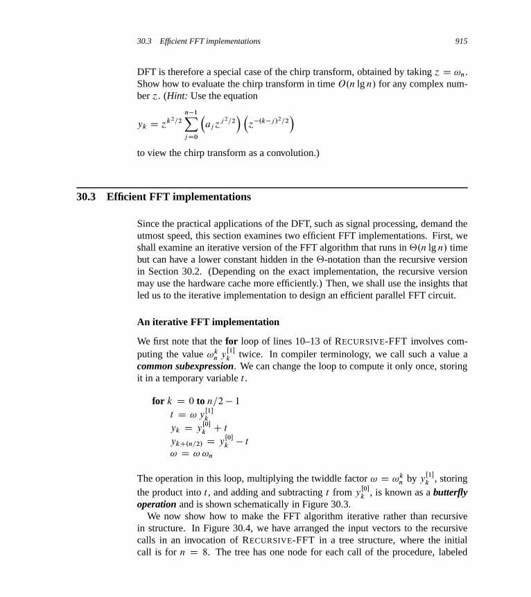
30.3 Efficient FFT implementations 915
DFT is therefore a special case of the chirp transform, obtained by taking ´ D !n.Show how to evaluate the chirp transform in time O.n lg n/ for any complex num-ber ´. (Hint: Use the equation
yk D ´k2=2
n�1Xj D0
�aj ´j 2=2
� �´�.k�j /2=2
�to view the chirp transform as a convolution.)
30.3 Efficient FFT implementations
Since the practical applications of the DFT, such as signal processing, demand theutmost speed, this section examines two efficient FFT implementations. First, weshall examine an iterative version of the FFT algorithm that runs in ‚.n lg n/ timebut can have a lower constant hidden in the ‚-notation than the recursive versionin Section 30.2. (Depending on the exact implementation, the recursive versionmay use the hardware cache more efficiently.) Then, we shall use the insights thatled us to the iterative implementation to design an efficient parallel FFT circuit.
An iterative FFT implementation
We first note that the for loop of lines 10–13 of RECURSIVE-FFT involves com-puting the value !k
n yŒ1�
ktwice. In compiler terminology, we call such a value a
common subexpression. We can change the loop to compute it only once, storingit in a temporary variable t .
for k D 0 to n=2 � 1
t D ! yŒ1�
k
yk D yŒ0�
kC t
ykC.n=2/ D yŒ0�
k� t
! D ! !n
The operation in this loop, multiplying the twiddle factor ! D !kn by y
Œ1�
k, storing
the product into t , and adding and subtracting t from yŒ0�
k, is known as a butterfly
operation and is shown schematically in Figure 30.3.We now show how to make the FFT algorithm iterative rather than recursive
in structure. In Figure 30.4, we have arranged the input vectors to the recursivecalls in an invocation of RECURSIVE-FFT in a tree structure, where the initialcall is for n D 8. The tree has one node for each call of the procedure, labeled
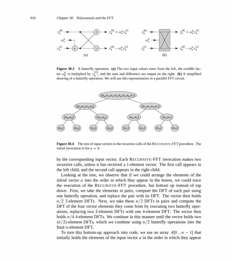
916 Chapter 30 Polynomials and the FFT
+
–•
(a) (b)
yŒ0�
ky
Œ0�
k
yŒ1�
ky
Œ1�
k
!kn!k
n
yŒ0�
kC !k
nyŒ1�
ky
Œ0�
kC !k
nyŒ1�
k
yŒ0�
k� !k
nyŒ1�
ky
Œ0�
k� !k
nyŒ1�
k
Figure 30.3 A butterfly operation. (a) The two input values enter from the left, the twiddle fac-
tor !kn is multiplied by y
Œ1�k
, and the sum and difference are output on the right. (b) A simplifieddrawing of a butterfly operation. We will use this representation in a parallel FFT circuit.
(a0,a1,a2,a3,a4,a5,a6,a7)
(a0,a2,a4,a6)
(a0,a4) (a2,a6)
(a0) (a4) (a2) (a6)
(a1,a3,a5,a7)
(a1,a5)
(a1) (a5)
(a3,a7)
(a3) (a7)
Figure 30.4 The tree of input vectors to the recursive calls of the RECURSIVE-FFT procedure. Theinitial invocation is for n D 8.
by the corresponding input vector. Each RECURSIVE-FFT invocation makes tworecursive calls, unless it has received a 1-element vector. The first call appears inthe left child, and the second call appears in the right child.
Looking at the tree, we observe that if we could arrange the elements of theinitial vector a into the order in which they appear in the leaves, we could tracethe execution of the RECURSIVE-FFT procedure, but bottom up instead of topdown. First, we take the elements in pairs, compute the DFT of each pair usingone butterfly operation, and replace the pair with its DFT. The vector then holdsn=2 2-element DFTs. Next, we take these n=2 DFTs in pairs and compute theDFT of the four vector elements they come from by executing two butterfly oper-ations, replacing two 2-element DFTs with one 4-element DFT. The vector thenholds n=4 4-element DFTs. We continue in this manner until the vector holds two.n=2/-element DFTs, which we combine using n=2 butterfly operations into thefinal n-element DFT.
To turn this bottom-up approach into code, we use an array AŒ0 : : n � 1� thatinitially holds the elements of the input vector a in the order in which they appear

30.3 Efficient FFT implementations 917
in the leaves of the tree of Figure 30.4. (We shall show later how to determine thisorder, which is known as a bit-reversal permutation.) Because we have to combineDFTs on each level of the tree, we introduce a variable s to count the levels, rangingfrom 1 (at the bottom, when we are combining pairs to form 2-element DFTs)to lg n (at the top, when we are combining two .n=2/-element DFTs to produce thefinal result). The algorithm therefore has the following structure:
1 for s D 1 to lg n
2 for k D 0 to n � 1 by 2s
3 combine the two 2s�1-element DFTs inAŒk : : k C 2s�1 � 1� and AŒk C 2s�1 : : k C 2s � 1�
into one 2s-element DFT in AŒk : : k C 2s � 1�
We can express the body of the loop (line 3) as more precise pseudocode. Wecopy the for loop from the RECURSIVE-FFT procedure, identifying yŒ0� withAŒk : : k C 2s�1 � 1� and yŒ1� with AŒk C 2s�1 : : k C 2s � 1�. The twiddle fac-tor used in each butterfly operation depends on the value of s; it is a power of !m,where m D 2s . (We introduce the variable m solely for the sake of readability.)We introduce another temporary variable u that allows us to perform the butterflyoperation in place. When we replace line 3 of the overall structure by the loopbody, we get the following pseudocode, which forms the basis of the parallel im-plementation we shall present later. The code first calls the auxiliary procedureBIT-REVERSE-COPY.a; A/ to copy vector a into array A in the initial order inwhich we need the values.
ITERATIVE-FFT.a/
1 BIT-REVERSE-COPY.a; A/
2 n D a: length // n is a power of 2
3 for s D 1 to lg n
4 m D 2s
5 !m D e2�i=m
6 for k D 0 to n � 1 by m
7 ! D 1
8 for j D 0 to m=2 � 1
9 t D ! AŒk C j Cm=2�
10 u D AŒk C j �
11 AŒk C j � D uC t
12 AŒk C j Cm=2� D u � t
13 ! D ! !m
14 return A
How does BIT-REVERSE-COPY get the elements of the input vector a into thedesired order in the array A? The order in which the leaves appear in Figure 30.4
918 Chapter 30 Polynomials and the FFT
is a bit-reversal permutation. That is, if we let rev.k/ be the lg n-bit integerformed by reversing the bits of the binary representation of k, then we want toplace vector element ak in array position AŒrev.k/�. In Figure 30.4, for exam-ple, the leaves appear in the order 0; 4; 2; 6; 1; 5; 3; 7; this sequence in binary is000; 100; 010; 110; 001; 101; 011; 111, and when we reverse the bits of each valuewe get the sequence 000; 001; 010; 011; 100; 101; 110; 111. To see that we want abit-reversal permutation in general, we note that at the top level of the tree, indiceswhose low-order bit is 0 go into the left subtree and indices whose low-order bitis 1 go into the right subtree. Stripping off the low-order bit at each level, we con-tinue this process down the tree, until we get the order given by the bit-reversalpermutation at the leaves.
Since we can easily compute the function rev.k/, the BIT-REVERSE-COPY pro-cedure is simple:
BIT-REVERSE-COPY.a; A/
1 n D a: length2 for k D 0 to n � 1
3 AŒrev.k/� D ak
The iterative FFT implementation runs in time ‚.n lg n/. The call to BIT-REVERSE-COPY.a; A/ certainly runs in O.n lg n/ time, since we iterate n timesand can reverse an integer between 0 and n � 1, with lg n bits, in O.lg n/ time.(In practice, because we usually know the initial value of n in advance, we wouldprobably code a table mapping k to rev.k/, making BIT-REVERSE-COPY run in‚.n/ time with a low hidden constant. Alternatively, we could use the clever amor-tized reverse binary counter scheme described in Problem 17-1.) To complete theproof that ITERATIVE-FFT runs in time ‚.n lg n/, we show that L.n/, the numberof times the body of the innermost loop (lines 8–13) executes, is ‚.n lg n/. Thefor loop of lines 6–13 iterates n=m D n=2s times for each value of s, and theinnermost loop of lines 8–13 iterates m=2 D 2s�1 times. Thus,
L.n/ Dlg nXsD1
n
2s� 2s�1
Dlg nXsD1
n
2
D ‚.n lg n/ :

30.3 Efficient FFT implementations 919
a0
a1
a2
a3
a4
a5
a6
a7
y0
y1
y2
y3
y4
y5
y6
y7
stage s D 1 stage s D 2 stage s D 3
!02
!02
!02
!02
!04
!04
!14
!14
!08
!18
!28
!38
Figure 30.5 A circuit that computes the FFT in parallel, here shown on n D 8 inputs. Eachbutterfly operation takes as input the values on two wires, along with a twiddle factor, and it producesas outputs the values on two wires. The stages of butterflies are labeled to correspond to iterationsof the outermost loop of the ITERATIVE-FFT procedure. Only the top and bottom wires passingthrough a butterfly interact with it; wires that pass through the middle of a butterfly do not affectthat butterfly, nor are their values changed by that butterfly. For example, the top butterfly in stage 2
has nothing to do with wire 1 (the wire whose output is labeled y1); its inputs and outputs are onlyon wires 0 and 2 (labeled y0 and y2, respectively). This circuit has depth ‚.lg n/ and performs‚.n lg n/ butterfly operations altogether.
A parallel FFT circuit
We can exploit many of the properties that allowed us to implement an efficientiterative FFT algorithm to produce an efficient parallel algorithm for the FFT. Wewill express the parallel FFT algorithm as a circuit. Figure 30.5 shows a parallelFFT circuit, which computes the FFT on n inputs, for n D 8. The circuit beginswith a bit-reverse permutation of the inputs, followed by lg n stages, each stageconsisting of n=2 butterflies executed in parallel. The depth of the circuit—themaximum number of computational elements between any output and any inputthat can reach it—is therefore ‚.lg n/.
The leftmost part of the parallel FFT circuit performs the bit-reverse permuta-tion, and the remainder mimics the iterative ITERATIVE-FFT procedure. Becauseeach iteration of the outermost for loop performs n=2 independent butterfly opera-tions, the circuit performs them in parallel. The value of s in each iteration within

920 Chapter 30 Polynomials and the FFT
ITERATIVE-FFT corresponds to a stage of butterflies shown in Figure 30.5. Fors D 1; 2; : : : ; lg n, stage s consists of n=2s groups of butterflies (corresponding toeach value of k in ITERATIVE-FFT), with 2s�1 butterflies per group (correspondingto each value of j in ITERATIVE-FFT). The butterflies shown in Figure 30.5 corre-spond to the butterfly operations of the innermost loop (lines 9–12 of ITERATIVE-FFT). Note also that the twiddle factors used in the butterflies correspond to thoseused in ITERATIVE-FFT: in stage s, we use !0
m; !1m; : : : ; !m=2�1
m , where m D 2s .
Exercises
30.3-1Show how ITERATIVE-FFT computes the DFT of the input vector .0; 2; 3;�1; 4;
5; 7; 9/.
30.3-2Show how to implement an FFT algorithm with the bit-reversal permutation occur-ring at the end, rather than at the beginning, of the computation. (Hint: Considerthe inverse DFT.)
30.3-3How many times does ITERATIVE-FFT compute twiddle factors in each stage?Rewrite ITERATIVE-FFT to compute twiddle factors only 2s�1 times in stage s.
30.3-4 ?
Suppose that the adders within the butterfly operations of the FFT circuit some-times fail in such a manner that they always produce a zero output, independentof their inputs. Suppose that exactly one adder has failed, but that you don’t knowwhich one. Describe how you can identify the failed adder by supplying inputs tothe overall FFT circuit and observing the outputs. How efficient is your method?
Problems
30-1 Divide-and-conquer multiplicationa. Show how to multiply two linear polynomials ax C b and cx C d using only
three multiplications. (Hint: One of the multiplications is .aC b/ � .c C d/.)
b. Give two divide-and-conquer algorithms for multiplying two polynomials ofdegree-bound n in ‚.nlg 3/ time. The first algorithm should divide the inputpolynomial coefficients into a high half and a low half, and the second algorithmshould divide them according to whether their index is odd or even.

Problems for Chapter 30 921
c. Show how to multiply two n-bit integers in O.nlg 3/ steps, where each stepoperates on at most a constant number of 1-bit values.
30-2 Toeplitz matricesA Toeplitz matrix is an n n matrix A D .aij / such that aij D ai�1;j �1 fori D 2; 3; : : : ; n and j D 2; 3; : : : ; n.
a. Is the sum of two Toeplitz matrices necessarily Toeplitz? What about the prod-uct?
b. Describe how to represent a Toeplitz matrix so that you can add two n n
Toeplitz matrices in O.n/ time.
c. Give an O.n lg n/-time algorithm for multiplying an nn Toeplitz matrix by avector of length n. Use your representation from part (b).
d. Give an efficient algorithm for multiplying two nn Toeplitz matrices. Analyzeits running time.
30-3 Multidimensional fast Fourier transformWe can generalize the 1-dimensional discrete Fourier transform defined by equa-tion (30.8) to d dimensions. The input is a d -dimensional array A D .aj1;j2;:::;jd
/
whose dimensions are n1; n2; : : : ; nd , where n1n2 � � � nd D n. We define thed -dimensional discrete Fourier transform by the equation
yk1;k2;:::;kdD
n1�1Xj1D0
n2�1Xj2D0
� � �nd �1Xjd D0
aj1;j2;:::;jd!j1k1
n1!j2k2
n2� � �!jd kd
nd
for 0 � k1 < n1, 0 � k2 < n2, . . . , 0 � kd < nd .
a. Show that we can compute a d -dimensional DFT by computing 1-dimensionalDFTs on each dimension in turn. That is, we first compute n=n1 separate1-dimensional DFTs along dimension 1. Then, using the result of the DFTsalong dimension 1 as the input, we compute n=n2 separate 1-dimensional DFTsalong dimension 2. Using this result as the input, we compute n=n3 separate1-dimensional DFTs along dimension 3, and so on, through dimension d .
b. Show that the ordering of dimensions does not matter, so that we can computea d -dimensional DFT by computing the 1-dimensional DFT’s in any order ofthe d dimensions.

922 Chapter 30 Polynomials and the FFT
c. Show that if we compute each 1-dimensional DFT by computing the fast Four-ier transform, the total time to compute a d -dimensional DFT is O.n lg n/,independent of d .
30-4 Evaluating all derivatives of a polynomial at a pointGiven a polynomial A.x/ of degree-bound n, we define its t th derivative by
A.t/.x/ D
„A.x/ if t D 0 ;
ddx
A.t�1/.x/ if 1 � t � n � 1 ;
0 if t � n :
From the coefficient representation .a0; a1; : : : ; an�1/ of A.x/ and a given point x0,we wish to determine A.t/.x0/ for t D 0; 1; : : : ; n � 1.
a. Given coefficients b0; b1; : : : ; bn�1 such that
A.x/ Dn�1Xj D0
bj .x � x0/j ;
show how to compute A.t/.x0/, for t D 0; 1; : : : ; n � 1, in O.n/ time.
b. Explain how to find b0; b1; : : : ; bn�1 in O.n lg n/ time, given A.x0 C !kn/ for
k D 0; 1; : : : ; n � 1.
c. Prove that
A.x0 C !kn/ D
n�1XrD0
!kr
n
rŠ
n�1Xj D0
f .j /g.r � j /
!;
where f .j / D aj � j Š and
g.l/ D(
x�l0 =.�l/Š if �.n� 1/ � l � 0 ;
0 if 1 � l � n � 1 :
d. Explain how to evaluate A.x0 C !kn/ for k D 0; 1; : : : ; n � 1 in O.n lg n/
time. Conclude that we can evaluate all nontrivial derivatives of A.x/ at x0 inO.n lg n/ time.
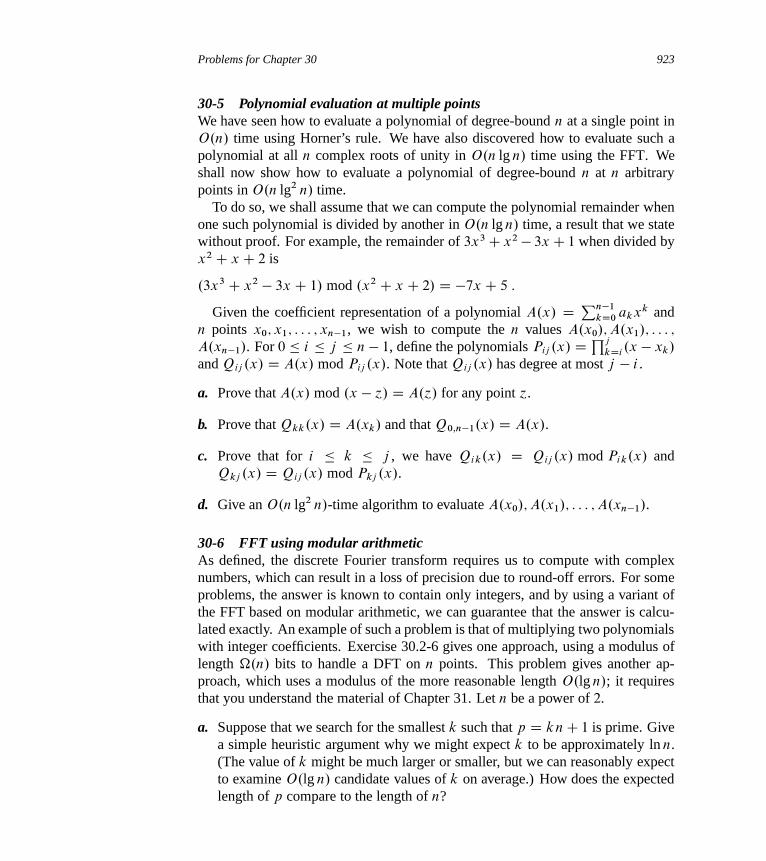
Problems for Chapter 30 923
30-5 Polynomial evaluation at multiple pointsWe have seen how to evaluate a polynomial of degree-bound n at a single point inO.n/ time using Horner’s rule. We have also discovered how to evaluate such apolynomial at all n complex roots of unity in O.n lg n/ time using the FFT. Weshall now show how to evaluate a polynomial of degree-bound n at n arbitrarypoints in O.n lg2 n/ time.
To do so, we shall assume that we can compute the polynomial remainder whenone such polynomial is divided by another in O.n lg n/ time, a result that we statewithout proof. For example, the remainder of 3x3C x2 � 3x C 1 when divided byx2 C x C 2 is
.3x3 C x2 � 3x C 1/ mod .x2 C x C 2/ D �7x C 5 :
Given the coefficient representation of a polynomial A.x/ D Pn�1
kD0 akxk andn points x0; x1; : : : ; xn�1, we wish to compute the n values A.x0/; A.x1/; : : : ;
A.xn�1/. For 0 � i � j � n � 1, define the polynomials Pij .x/ D Qj
kDi.x � xk/
and Qij .x/ D A.x/ mod Pij .x/. Note that Qij .x/ has degree at most j � i .
a. Prove that A.x/ mod .x � ´/ D A.´/ for any point ´.
b. Prove that Qkk.x/ D A.xk/ and that Q0;n�1.x/ D A.x/.
c. Prove that for i � k � j , we have Qik.x/ D Qij .x/ mod Pik.x/ andQkj .x/ D Qij .x/ mod Pkj .x/.
d. Give an O.n lg2 n/-time algorithm to evaluate A.x0/; A.x1/; : : : ; A.xn�1/.
30-6 FFT using modular arithmeticAs defined, the discrete Fourier transform requires us to compute with complexnumbers, which can result in a loss of precision due to round-off errors. For someproblems, the answer is known to contain only integers, and by using a variant ofthe FFT based on modular arithmetic, we can guarantee that the answer is calcu-lated exactly. An example of such a problem is that of multiplying two polynomialswith integer coefficients. Exercise 30.2-6 gives one approach, using a modulus oflength �.n/ bits to handle a DFT on n points. This problem gives another ap-proach, which uses a modulus of the more reasonable length O.lg n/; it requiresthat you understand the material of Chapter 31. Let n be a power of 2.
a. Suppose that we search for the smallest k such that p D knC 1 is prime. Givea simple heuristic argument why we might expect k to be approximately ln n.(The value of k might be much larger or smaller, but we can reasonably expectto examine O.lg n/ candidate values of k on average.) How does the expectedlength of p compare to the length of n?
924 Chapter 30 Polynomials and the FFT
Let g be a generator of Z�p , and let w D gk mod p.
b. Argue that the DFT and the inverse DFT are well-defined inverse operationsmodulo p, where w is used as a principal nth root of unity.
c. Show how to make the FFT and its inverse work modulo p in time O.n lg n/,where operations on words of O.lg n/ bits take unit time. Assume that thealgorithm is given p and w.
d. Compute the DFT modulo p D 17 of the vector .0; 5; 3; 7; 7; 2; 1; 6/. Note thatg D 3 is a generator of Z
�17.
Chapter notes
Van Loan’s book [343] provides an outstanding treatment of the fast Fourier trans-form. Press, Teukolsky, Vetterling, and Flannery [283, 284] have a good descrip-tion of the fast Fourier transform and its applications. For an excellent introductionto signal processing, a popular FFT application area, see the texts by Oppenheimand Schafer [266] and Oppenheim and Willsky [267]. The Oppenheim and Schaferbook also shows how to handle cases in which n is not an integer power of 2.
Fourier analysis is not limited to 1-dimensional data. It is widely used in imageprocessing to analyze data in 2 or more dimensions. The books by Gonzalez andWoods [146] and Pratt [281] discuss multidimensional Fourier transforms and theiruse in image processing, and books by Tolimieri, An, and Lu [338] and Van Loan[343] discuss the mathematics of multidimensional fast Fourier transforms.
Cooley and Tukey [77] are widely credited with devising the FFT in the 1960s.The FFT had in fact been discovered many times previously, but its importance wasnot fully realized before the advent of modern digital computers. Although Press,Teukolsky, Vetterling, and Flannery attribute the origins of the method to Rungeand König in 1924, an article by Heideman, Johnson, and Burrus [163] traces thehistory of the FFT as far back as C. F. Gauss in 1805.
Frigo and Johnson [117] developed a fast and flexible implementation of theFFT, called FFTW (“fastest Fourier transform in the West”). FFTW is designed forsituations requiring multiple DFT computations on the same problem size. Beforeactually computing the DFTs, FFTW executes a “planner,” which, by a series oftrial runs, determines how best to decompose the FFT computation for the givenproblem size on the host machine. FFTW adapts to use the hardware cache ef-ficiently, and once subproblems are small enough, FFTW solves them with opti-mized, straight-line code. Furthermore, FFTW has the unusual advantage of taking‚.n lg n/ time for any problem size n, even when n is a large prime.
Notes for Chapter 30 925
Although the standard Fourier transform assumes that the input represents pointsthat are uniformly spaced in the time domain, other techniques can approximate theFFT on “nonequispaced” data. The article by Ware [348] provides an overview.
31 Number-Theoretic Algorithms
Number theory was once viewed as a beautiful but largely useless subject in puremathematics. Today number-theoretic algorithms are used widely, due in large partto the invention of cryptographic schemes based on large prime numbers. Theseschemes are feasible because we can find large primes easily, and they are securebecause we do not know how to factor the product of large primes efficiently. Thischapter presents some of the number theory and associated algorithms that underliesuch applications.
Section 31.1 introduces basic concepts of number theory, such as divisibility,modular equivalence, and unique factorization. Section 31.2 studies one of theworld’s oldest algorithms: Euclid’s algorithm for computing the greatest commondivisor of two integers. Section 31.3 reviews concepts of modular arithmetic. Sec-tion 31.4 then studies the set of multiples of a given number a, modulo n, and showshow to find all solutions to the equation ax � b .mod n/ by using Euclid’s algo-rithm. The Chinese remainder theorem is presented in Section 31.5. Section 31.6considers powers of a given number a, modulo n, and presents a repeated-squaringalgorithm for efficiently computing ab mod n, given a, b, and n. This operation isat the heart of efficient primality testing and of much modern cryptography. Sec-tion 31.7 then describes the RSA public-key cryptosystem. Section 31.8 examinesa randomized primality test. We can use this test to find large primes efficiently,which we need to do in order to create keys for the RSA cryptosystem. Finally,Section 31.9 reviews a simple but effective heuristic for factoring small integers. Itis a curious fact that factoring is one problem people may wish to be intractable,since the security of RSA depends on the difficulty of factoring large integers.
Size of inputs and cost of arithmetic computations
Because we shall be working with large integers, we need to adjust how we thinkabout the size of an input and about the cost of elementary arithmetic operations.
In this chapter, a “large input” typically means an input containing “large in-tegers” rather than an input containing “many integers” (as for sorting). Thus,
31.1 Elementary number-theoretic notions 927
we shall measure the size of an input in terms of the number of bits required torepresent that input, not just the number of integers in the input. An algorithmwith integer inputs a1; a2; : : : ; ak is a polynomial-time algorithm if it runs in timepolynomial in lg a1; lg a2; : : : ; lg ak, that is, polynomial in the lengths of its binary-encoded inputs.
In most of this book, we have found it convenient to think of the elemen-tary arithmetic operations (multiplications, divisions, or computing remainders)as primitive operations that take one unit of time. By counting the number of sucharithmetic operations that an algorithm performs, we have a basis for making areasonable estimate of the algorithm’s actual running time on a computer. Elemen-tary operations can be time-consuming, however, when their inputs are large. Itthus becomes convenient to measure how many bit operations a number-theoreticalgorithm requires. In this model, multiplying two ˇ-bit integers by the ordinarymethod uses ‚.ˇ2/ bit operations. Similarly, we can divide a ˇ-bit integer by ashorter integer or take the remainder of a ˇ-bit integer when divided by a shorter in-teger in time ‚.ˇ2/ by simple algorithms. (See Exercise 31.1-12.) Faster methodsare known. For example, a simple divide-and-conquer method for multiplying twoˇ-bit integers has a running time of ‚.ˇlg 3/, and the fastest known method hasa running time of ‚.ˇ lg ˇ lg lg ˇ/. For practical purposes, however, the ‚.ˇ2/
algorithm is often best, and we shall use this bound as a basis for our analyses.We shall generally analyze algorithms in this chapter in terms of both the number
of arithmetic operations and the number of bit operations they require.
31.1 Elementary number-theoretic notions
This section provides a brief review of notions from elementary number theoryconcerning the set Z D f: : : ;�2;�1; 0; 1; 2; : : :g of integers and the set N Df0; 1; 2; : : :g of natural numbers.
Divisibility and divisors
The notion of one integer being divisible by another is key to the theory of numbers.The notation d j a (read “d divides a”) means that a D kd for some integer k.Every integer divides 0. If a > 0 and d j a, then jd j � jaj. If d j a, then we alsosay that a is a multiple of d . If d does not divide a, we write d − a.
If d j a and d � 0, we say that d is a divisor of a. Note that d j a if and onlyif �d j a, so that no generality is lost by defining the divisors to be nonnegative,with the understanding that the negative of any divisor of a also divides a. A
928 Chapter 31 Number-Theoretic Algorithms
divisor of a nonzero integer a is at least 1 but not greater than jaj. For example, thedivisors of 24 are 1, 2, 3, 4, 6, 8, 12, and 24.
Every positive integer a is divisible by the trivial divisors 1 and a. The nontrivialdivisors of a are the factors of a. For example, the factors of 20 are 2, 4, 5, and 10.
Prime and composite numbers
An integer a > 1 whose only divisors are the trivial divisors 1 and a is a primenumber or, more simply, a prime. Primes have many special properties and play acritical role in number theory. The first 20 primes, in order, are
2; 3; 5; 7; 11; 13; 17; 19; 23; 29; 31; 37; 41; 43; 47; 53; 59; 61; 67; 71 :
Exercise 31.1-2 asks you to prove that there are infinitely many primes. An integera > 1 that is not prime is a composite number or, more simply, a composite. Forexample, 39 is composite because 3 j 39. We call the integer 1 a unit, and it isneither prime nor composite. Similarly, the integer 0 and all negative integers areneither prime nor composite.
The division theorem, remainders, and modular equivalence
Given an integer n, we can partition the integers into those that are multiples of n
and those that are not multiples of n. Much number theory is based upon refiningthis partition by classifying the nonmultiples of n according to their remainderswhen divided by n. The following theorem provides the basis for this refinement.We omit the proof (but see, for example, Niven and Zuckerman [265]).
Theorem 31.1 (Division theorem)For any integer a and any positive integer n, there exist unique integers q and r
such that 0 � r < n and a D qnC r .
The value q D ba=nc is the quotient of the division. The value r D a mod n
is the remainder (or residue) of the division. We have that n j a if and only ifa mod n D 0.
We can partition the integers into n equivalence classes according to their re-mainders modulo n. The equivalence class modulo n containing an integer a is
Œa�n D faC kn W k 2 Zg :
For example, Œ3�7 D f: : : ;�11;�4; 3; 10; 17; : : :g; we can also denote this set byŒ�4�7 and Œ10�7. Using the notation defined on page 54, we can say that writinga 2 Œb�n is the same as writing a � b .mod n/. The set of all such equivalenceclasses is
31.1 Elementary number-theoretic notions 929
Zn D fŒa�n W 0 � a � n � 1g : (31.1)
When you see the definition
Zn D f0; 1; : : : ; n � 1g ; (31.2)
you should read it as equivalent to equation (31.1) with the understanding that 0
represents Œ0�n, 1 represents Œ1�n, and so on; each class is represented by its smallestnonnegative element. You should keep the underlying equivalence classes in mind,however. For example, if we refer to �1 as a member of Zn, we are really referringto Œn � 1�n, since �1 � n � 1 .mod n/.
Common divisors and greatest common divisors
If d is a divisor of a and d is also a divisor of b, then d is a common divisor of a
and b. For example, the divisors of 30 are 1, 2, 3, 5, 6, 10, 15, and 30, and so thecommon divisors of 24 and 30 are 1, 2, 3, and 6. Note that 1 is a common divisorof any two integers.
An important property of common divisors is that
d j a and d j b implies d j .aC b/ and d j .a � b/ : (31.3)
More generally, we have that
d j a and d j b implies d j .ax C by/ (31.4)
for any integers x and y. Also, if a j b, then either jaj � jbj or b D 0, whichimplies that
a j b and b j a implies a D ˙b : (31.5)
The greatest common divisor of two integers a and b, not both zero, is thelargest of the common divisors of a and b; we denote it by gcd.a; b/. For example,gcd.24; 30/ D 6, gcd.5; 7/ D 1, and gcd.0; 9/ D 9. If a and b are both nonzero,then gcd.a; b/ is an integer between 1 and min.jaj ; jbj/. We define gcd.0; 0/ tobe 0; this definition is necessary to make standard properties of the gcd function(such as equation (31.9) below) universally valid.
The following are elementary properties of the gcd function:
gcd.a; b/ D gcd.b; a/ ; (31.6)
gcd.a; b/ D gcd.�a; b/ ; (31.7)
gcd.a; b/ D gcd.jaj ; jbj/ ; (31.8)
gcd.a; 0/ D jaj ; (31.9)
gcd.a; ka/ D jaj for any k 2 Z : (31.10)
The following theorem provides an alternative and useful characterization ofgcd.a; b/.
930 Chapter 31 Number-Theoretic Algorithms
Theorem 31.2If a and b are any integers, not both zero, then gcd.a; b/ is the smallest positiveelement of the set fax C by W x; y 2 Zg of linear combinations of a and b.
Proof Let s be the smallest positive such linear combination of a and b, and lets D ax C by for some x; y 2 Z. Let q D ba=sc. Equation (3.8) then implies
a mod s D a � qs
D a � q.ax C by/
D a .1 � qx/C b .�qy/ ;
and so a mod s is a linear combination of a and b as well. But, since 0 �a mod s < s, we have that a mod s D 0, because s is the smallest positive such lin-ear combination. Therefore, we have that s j a and, by analogous reasoning, s j b.Thus, s is a common divisor of a and b, and so gcd.a; b/ � s. Equation (31.4)implies that gcd.a; b/ j s, since gcd.a; b/ divides both a and b and s is a linearcombination of a and b. But gcd.a; b/ j s and s > 0 imply that gcd.a; b/ � s.Combining gcd.a; b/ � s and gcd.a; b/ � s yields gcd.a; b/ D s. We concludethat s is the greatest common divisor of a and b.
Corollary 31.3For any integers a and b, if d j a and d j b, then d j gcd.a; b/.
Proof This corollary follows from equation (31.4), because gcd.a; b/ is a linearcombination of a and b by Theorem 31.2.
Corollary 31.4For all integers a and b and any nonnegative integer n,
gcd.an; bn/ D n gcd.a; b/ :
Proof If n D 0, the corollary is trivial. If n > 0, then gcd.an; bn/ is the smallestpositive element of the set fanx C bny W x; y 2 Zg, which is n times the smallestpositive element of the set fax C by W x; y 2 Zg.
Corollary 31.5For all positive integers n, a, and b, if n j ab and gcd.a; n/ D 1, then n j b.
Proof We leave the proof as Exercise 31.1-5.
31.1 Elementary number-theoretic notions 931
Relatively prime integers
Two integers a and b are relatively prime if their only common divisor is 1, thatis, if gcd.a; b/ D 1. For example, 8 and 15 are relatively prime, since the divisorsof 8 are 1, 2, 4, and 8, and the divisors of 15 are 1, 3, 5, and 15. The followingtheorem states that if two integers are each relatively prime to an integer p, thentheir product is relatively prime to p.
Theorem 31.6For any integers a, b, and p, if both gcd.a; p/ D 1 and gcd.b; p/ D 1, thengcd.ab; p/ D 1.
Proof It follows from Theorem 31.2 that there exist integers x, y, x 0, and y 0 suchthat
ax C py D 1 ;
bx 0C py 0 D 1 :
Multiplying these equations and rearranging, we have
ab.xx 0/C p.ybx 0C y 0ax C pyy 0/ D 1 :
Since 1 is thus a positive linear combination of ab and p, an appeal to Theo-rem 31.2 completes the proof.
Integers n1, n2, . . . , nk are pairwise relatively prime if, whenever i ¤ j , wehave gcd.ni ; nj / D 1.
Unique factorization
An elementary but important fact about divisibility by primes is the following.
Theorem 31.7For all primes p and all integers a and b, if p j ab, then p j a or p j b (or both).
Proof Assume for the purpose of contradiction that p j ab, but that p − a andp − b. Thus, gcd.a; p/ D 1 and gcd.b; p/ D 1, since the only divisors of p are 1
and p, and we assume that p divides neither a nor b. Theorem 31.6 then impliesthat gcd.ab; p/ D 1, contradicting our assumption that p j ab, since p j ab
implies gcd.ab; p/ D p. This contradiction completes the proof.
A consequence of Theorem 31.7 is that we can uniquely factor any compositeinteger into a product of primes.

932 Chapter 31 Number-Theoretic Algorithms
Theorem 31.8 (Unique factorization)There is exactly one way to write any composite integer a as a product of the form
a D pe1
1 pe2
2 � � �per
r ;
where the pi are prime, p1 < p2 < � � � < pr , and the ei are positive integers.
Proof We leave the proof as Exercise 31.1-11.
As an example, the number 6000 is uniquely factored into primes as 24 � 3 � 53.
Exercises
31.1-1Prove that if a > b > 0 and c D aC b, then c mod a D b.
31.1-2Prove that there are infinitely many primes. (Hint: Show that none of the primesp1; p2; : : : ; pk divide .p1p2 � � �pk/C 1.)
31.1-3Prove that if a j b and b j c, then a j c.
31.1-4Prove that if p is prime and 0 < k < p, then gcd.k; p/ D 1.
31.1-5Prove Corollary 31.5.
31.1-6Prove that if p is prime and 0 < k < p, then p j �p
k
�. Conclude that for all integers
a and b and all primes p,
.aC b/p � ap C bp .mod p/ :
31.1-7Prove that if a and b are any positive integers such that a j b, then
.x mod b/ mod a D x mod a
for any x. Prove, under the same assumptions, that
x � y .mod b/ implies x � y .mod a/
for any integers x and y.

31.2 Greatest common divisor 933
31.1-8For any integer k > 0, an integer n is a kth power if there exists an integer a suchthat ak D n. Furthermore, n > 1 is a nontrivial power if it is a kth power forsome integer k > 1. Show how to determine whether a given ˇ-bit integer n is anontrivial power in time polynomial in ˇ.
31.1-9Prove equations (31.6)–(31.10).
31.1-10Show that the gcd operator is associative. That is, prove that for all integers a, b,and c,
gcd.a; gcd.b; c// D gcd.gcd.a; b/; c/ :
31.1-11 ?
Prove Theorem 31.8.
31.1-12Give efficient algorithms for the operations of dividing a ˇ-bit integer by a shorterinteger and of taking the remainder of a ˇ-bit integer when divided by a shorterinteger. Your algorithms should run in time ‚.ˇ2/.
31.1-13Give an efficient algorithm to convert a given ˇ-bit (binary) integer to a decimalrepresentation. Argue that if multiplication or division of integers whose lengthis at most ˇ takes time M.ˇ/, then we can convert binary to decimal in time‚.M.ˇ/ lg ˇ/. (Hint: Use a divide-and-conquer approach, obtaining the top andbottom halves of the result with separate recursions.)
31.2 Greatest common divisor
In this section, we describe Euclid’s algorithm for efficiently computing the great-est common divisor of two integers. When we analyze the running time, we shallsee a surprising connection with the Fibonacci numbers, which yield a worst-caseinput for Euclid’s algorithm.
We restrict ourselves in this section to nonnegative integers. This restriction isjustified by equation (31.8), which states that gcd.a; b/ D gcd.jaj ; jbj/.
934 Chapter 31 Number-Theoretic Algorithms
In principle, we can compute gcd.a; b/ for positive integers a and b from theprime factorizations of a and b. Indeed, if
a D pe1
1 pe2
2 � � �per
r ; (31.11)
b D pf1
1 pf2
2 � � �pfr
r ; (31.12)
with zero exponents being used to make the set of primes p1; p2; : : : ; pr the samefor both a and b, then, as Exercise 31.2-1 asks you to show,
gcd.a; b/ D pmin.e1;f1/1 p
min.e2;f2/2 � � �pmin.er ;fr /
r : (31.13)
As we shall show in Section 31.9, however, the best algorithms to date for factoringdo not run in polynomial time. Thus, this approach to computing greatest commondivisors seems unlikely to yield an efficient algorithm.
Euclid’s algorithm for computing greatest common divisors relies on the follow-ing theorem.
Theorem 31.9 (GCD recursion theorem)For any nonnegative integer a and any positive integer b,
gcd.a; b/ D gcd.b; a mod b/ :
Proof We shall show that gcd.a; b/ and gcd.b; a mod b/ divide each other, sothat by equation (31.5) they must be equal (since they are both nonnegative).
We first show that gcd.a; b/ j gcd.b; a mod b/. If we let d D gcd.a; b/, thend j a and d j b. By equation (3.8), a mod b D a � qb, where q D ba=bc.Since a mod b is thus a linear combination of a and b, equation (31.4) implies thatd j .a mod b/. Therefore, since d j b and d j .a mod b/, Corollary 31.3 impliesthat d j gcd.b; a mod b/ or, equivalently, that
gcd.a; b/ j gcd.b; a mod b/: (31.14)
Showing that gcd.b; a mod b/ j gcd.a; b/ is almost the same. If we now letd D gcd.b; a mod b/, then d j b and d j .a mod b/. Since a D qb C .a mod b/,where q D ba=bc, we have that a is a linear combination of b and .a mod b/. Byequation (31.4), we conclude that d j a. Since d j b and d j a, we have thatd j gcd.a; b/ by Corollary 31.3 or, equivalently, that
gcd.b; a mod b/ j gcd.a; b/: (31.15)
Using equation (31.5) to combine equations (31.14) and (31.15) completes theproof.

31.2 Greatest common divisor 935
Euclid’s algorithm
The Elements of Euclid (circa 300 B.C.) describes the following gcd algorithm,although it may be of even earlier origin. We express Euclid’s algorithm as arecursive program based directly on Theorem 31.9. The inputs a and b are arbitrarynonnegative integers.
EUCLID.a; b/
1 if b == 0
2 return a
3 else return EUCLID.b; a mod b/
As an example of the running of EUCLID, consider the computation of gcd.30; 21/:
EUCLID.30; 21/ D EUCLID.21; 9/
D EUCLID.9; 3/
D EUCLID.3; 0/
D 3 :
This computation calls EUCLID recursively three times.The correctness of EUCLID follows from Theorem 31.9 and the property that if
the algorithm returns a in line 2, then b D 0, so that equation (31.9) implies thatgcd.a; b/ D gcd.a; 0/ D a. The algorithm cannot recurse indefinitely, since thesecond argument strictly decreases in each recursive call and is always nonnegative.Therefore, EUCLID always terminates with the correct answer.
The running time of Euclid’s algorithm
We analyze the worst-case running time of EUCLID as a function of the size ofa and b. We assume with no loss of generality that a > b � 0. To justify thisassumption, observe that if b > a � 0, then EUCLID.a; b/ immediately makes therecursive call EUCLID.b; a/. That is, if the first argument is less than the secondargument, EUCLID spends one recursive call swapping its arguments and then pro-ceeds. Similarly, if b D a > 0, the procedure terminates after one recursive call,since a mod b D 0.
The overall running time of EUCLID is proportional to the number of recursivecalls it makes. Our analysis makes use of the Fibonacci numbers Fk , defined bythe recurrence (3.22).
Lemma 31.10If a > b � 1 and the call EUCLID.a; b/ performs k � 1 recursive calls, thena � FkC2 and b � FkC1.
936 Chapter 31 Number-Theoretic Algorithms
Proof The proof proceeds by induction on k. For the basis of the induction, letk D 1. Then, b � 1 D F2, and since a > b, we must have a � 2 D F3. Sinceb > .a mod b/, in each recursive call the first argument is strictly larger than thesecond; the assumption that a > b therefore holds for each recursive call.
Assume inductively that the lemma holds if k � 1 recursive calls are made; weshall then prove that the lemma holds for k recursive calls. Since k > 0, we haveb > 0, and EUCLID.a; b/ calls EUCLID.b; a mod b/ recursively, which in turnmakes k � 1 recursive calls. The inductive hypothesis then implies that b � FkC1
(thus proving part of the lemma), and a mod b � Fk . We have
b C .a mod b/ D b C .a � b ba=bc/� a ;
since a > b > 0 implies ba=bc � 1. Thus,
a � b C .a mod b/
� FkC1 C Fk
D FkC2 :
The following theorem is an immediate corollary of this lemma.
Theorem 31.11 (Lamé’s theorem)For any integer k � 1, if a > b � 1 and b < FkC1, then the call EUCLID.a; b/
makes fewer than k recursive calls.
We can show that the upper bound of Theorem 31.11 is the best possible byshowing that the call EUCLID.FkC1; Fk/ makes exactly k � 1 recursive callswhen k � 2. We use induction on k. For the base case, k D 2, and the callEUCLID.F3; F2/ makes exactly one recursive call, to EUCLID.1; 0/. (We have tostart at k D 2, because when k D 1 we do not have F2 > F1.) For the induc-tive step, assume that EUCLID.Fk; Fk�1/ makes exactly k � 2 recursive calls. Fork > 2, we have Fk > Fk�1 > 0 and FkC1 D FkCFk�1, and so by Exercise 31.1-1,we have FkC1 mod Fk D Fk�1. Thus, we have
gcd.FkC1; Fk/ D gcd.Fk; FkC1 mod Fk/
D gcd.Fk; Fk�1/ :
Therefore, the call EUCLID.FkC1; Fk/ recurses one time more than the callEUCLID.Fk ; Fk�1/, or exactly k � 1 times, meeting the upper bound of Theo-rem 31.11.
Since Fk is approximately �k=p
5, where � is the golden ratio .1Cp5/=2 de-fined by equation (3.24), the number of recursive calls in EUCLID is O.lg b/. (See

31.2 Greatest common divisor 937
a b ba=bc d x y
99 78 1 3 �11 14
78 21 3 3 3 �11
21 15 1 3 �2 3
15 6 2 3 1 �2
6 3 2 3 0 13 0 — 3 1 0
Figure 31.1 How EXTENDED-EUCLID computes gcd.99; 78/. Each line shows one level of therecursion: the values of the inputs a and b, the computed value ba=bc, and the values d , x, and y
returned. The triple .d; x; y/ returned becomes the triple .d 0; x0; y0/ used at the next higher levelof recursion. The call EXTENDED-EUCLID.99; 78/ returns .3;�11; 14/, so that gcd.99; 78/ D 3 D99 � .�11/C 78 � 14.
Exercise 31.2-5 for a tighter bound.) Therefore, if we call EUCLID on two ˇ-bitnumbers, then it performs O.ˇ/ arithmetic operations and O.ˇ3/ bit operations(assuming that multiplication and division of ˇ-bit numbers take O.ˇ2/ bit oper-ations). Problem 31-2 asks you to show an O.ˇ2/ bound on the number of bitoperations.
The extended form of Euclid’s algorithm
We now rewrite Euclid’s algorithm to compute additional useful information.Specifically, we extend the algorithm to compute the integer coefficients x and y
such that
d D gcd.a; b/ D ax C by : (31.16)
Note that x and y may be zero or negative. We shall find these coefficients usefullater for computing modular multiplicative inverses. The procedure EXTENDED-EUCLID takes as input a pair of nonnegative integers and returns a triple of theform .d; x; y/ that satisfies equation (31.16).
EXTENDED-EUCLID.a; b/
1 if b == 0
2 return .a; 1; 0/
3 else .d 0; x 0; y 0/ D EXTENDED-EUCLID.b; a mod b/
4 .d; x; y/ D .d 0; y 0; x 0 � ba=bc y 0/5 return .d; x; y/
Figure 31.1 illustrates how EXTENDED-EUCLID computes gcd.99; 78/.The EXTENDED-EUCLID procedure is a variation of the EUCLID procedure.
Line 1 is equivalent to the test “b == 0” in line 1 of EUCLID. If b D 0, then

938 Chapter 31 Number-Theoretic Algorithms
EXTENDED-EUCLID returns not only d D a in line 2, but also the coefficientsx D 1 and y D 0, so that a D ax C by. If b ¤ 0, EXTENDED-EUCLID firstcomputes .d 0; x 0; y 0/ such that d 0 D gcd.b; a mod b/ and
d 0 D bx 0 C .a mod b/y 0 : (31.17)
As for EUCLID, we have in this case d D gcd.a; b/ D d 0 D gcd.b; a mod b/.To obtain x and y such that d D ax C by, we start by rewriting equation (31.17)using the equation d D d 0 and equation (3.8):
d D bx 0 C .a � b ba=bc/y 0
D ay 0 C b.x 0 � ba=bc y 0/ :
Thus, choosing x D y 0 and y D x 0�ba=bc y 0 satisfies the equation d D axCby,proving the correctness of EXTENDED-EUCLID.
Since the number of recursive calls made in EUCLID is equal to the numberof recursive calls made in EXTENDED-EUCLID, the running times of EUCLID
and EXTENDED-EUCLID are the same, to within a constant factor. That is, fora > b > 0, the number of recursive calls is O.lg b/.
Exercises
31.2-1Prove that equations (31.11) and (31.12) imply equation (31.13).
31.2-2Compute the values .d; x; y/ that the call EXTENDED-EUCLID.899; 493/ returns.
31.2-3Prove that for all integers a, k, and n,
gcd.a; n/ D gcd.aC kn; n/ :
31.2-4Rewrite EUCLID in an iterative form that uses only a constant amount of memory(that is, stores only a constant number of integer values).
31.2-5If a > b � 0, show that the call EUCLID.a; b/ makes at most 1C log� b recursivecalls. Improve this bound to 1C log�.b= gcd.a; b//.
31.2-6What does EXTENDED-EUCLID.FkC1; Fk/ return? Prove your answer correct.
31.3 Modular arithmetic 939
31.2-7Define the gcd function for more than two arguments by the recursive equationgcd.a0; a1; : : : ; an/ D gcd.a0; gcd.a1; a2; : : : ; an//. Show that the gcd functionreturns the same answer independent of the order in which its arguments are speci-fied. Also show how to find integers x0; x1; : : : ; xn such that gcd.a0; a1; : : : ; an/ Da0x0 C a1x1 C � � � C anxn. Show that the number of divisions performed by youralgorithm is O.nC lg.max fa0; a1; : : : ; ang//.31.2-8Define lcm.a1; a2; : : : ; an/ to be the least common multiple of the n integersa1; a2; : : : ; an, that is, the smallest nonnegative integer that is a multiple of each ai .Show how to compute lcm.a1; a2; : : : ; an/ efficiently using the (two-argument) gcdoperation as a subroutine.
31.2-9Prove that n1, n2, n3, and n4 are pairwise relatively prime if and only if
gcd.n1n2; n3n4/ D gcd.n1n3; n2n4/ D 1 :
More generally, show that n1; n2; : : : ; nk are pairwise relatively prime if and onlyif a set of dlg ke pairs of numbers derived from the ni are relatively prime.
31.3 Modular arithmetic
Informally, we can think of modular arithmetic as arithmetic as usual over theintegers, except that if we are working modulo n, then every result x is replacedby the element of f0; 1; : : : ; n � 1g that is equivalent to x, modulo n (that is, x isreplaced by x mod n). This informal model suffices if we stick to the operationsof addition, subtraction, and multiplication. A more formal model for modulararithmetic, which we now give, is best described within the framework of grouptheory.
Finite groups
A group .S;˚/ is a set S together with a binary operation ˚ defined on S forwhich the following properties hold:
1. Closure: For all a, b 2 S , we have a˚ b 2 S .
2. Identity: There exists an element e 2 S , called the identity of the group, suchthat e ˚ a D a˚ e D a for all a 2 S .
3. Associativity: For all a, b, c 2 S , we have .a˚ b/˚ c D a˚ .b ˚ c/.
940 Chapter 31 Number-Theoretic Algorithms
4. Inverses: For each a 2 S , there exists a unique element b 2 S , called theinverse of a, such that a˚ b D b ˚ a D e.
As an example, consider the familiar group .Z;C/ of the integers Z under theoperation of addition: 0 is the identity, and the inverse of a is�a. If a group .S;˚/
satisfies the commutative law a˚ b D b˚ a for all a; b 2 S , then it is an abeliangroup. If a group .S;˚/ satisfies jS j <1, then it is a finite group.
The groups defined by modular addition and multiplication
We can form two finite abelian groups by using addition and multiplication mod-ulo n, where n is a positive integer. These groups are based on the equivalenceclasses of the integers modulo n, defined in Section 31.1.
To define a group on Zn, we need to have suitable binary operations, whichwe obtain by redefining the ordinary operations of addition and multiplication.We can easily define addition and multiplication operations for Zn, because theequivalence class of two integers uniquely determines the equivalence class of theirsum or product. That is, if a � a0 .mod n/ and b � b0 .mod n/, then
aC b � a0 C b0 .mod n/ ;
ab � a0b0 .mod n/ :
Thus, we define addition and multiplication modulo n, denoted Cn and �n, by
Œa�n Cn Œb�n D ŒaC b�n ; (31.18)
Œa�n �n Œb�n D Œab�n :
(We can define subtraction similarly on Zn by Œa�n �n Œb�n D Œa � b�n, but divi-sion is more complicated, as we shall see.) These facts justify the common andconvenient practice of using the smallest nonnegative element of each equivalenceclass as its representative when performing computations in Zn. We add, subtract,and multiply as usual on the representatives, but we replace each result x by therepresentative of its class, that is, by x mod n.
Using this definition of addition modulo n, we define the additive groupmodulo n as .Zn;Cn/. The size of the additive group modulo n is jZnj D n.Figure 31.2(a) gives the operation table for the group .Z6;C6/.
Theorem 31.12The system .Zn;Cn/ is a finite abelian group.
Proof Equation (31.18) shows that .Zn;Cn/ is closed. Associativity and com-mutativity ofCn follow from the associativity and commutativity ofC:

31.3 Modular arithmetic 941
0 1 2 3 4 5
0
1
2
3
4
5
01 2 3 4 5
0 12 3 4 5
0 1 2 3 4 5
0 1 23 4 5
0 1 2 34 5
0 1 2 3 45
(a)
1 2 4 7 8 11 13 14
1
2
4
7
8
11
13
14
1 2 4 7 8 11 13 14
2 4 8 14 1 7 11 13
4 8 1 13 2 14 7 11
7 14 13 4 11 2 1 8
8 1 2 11 4 13 14 7
11 7 14 2 13 1 8 4
13 11 7 1 14 8 4 2
14 13 11 8 7 4 2 1
(b)
+6 ·15
Figure 31.2 Two finite groups. Equivalence classes are denoted by their representative elements.(a) The group .Z6;C6/. (b) The group .Z�
15; �15/.
.Œa�n Cn Œb�n/Cn Œc�n D ŒaC b�n Cn Œc�n
D Œ.aC b/C c�n
D ŒaC .b C c/�n
D Œa�n Cn Œb C c�n
D Œa�n Cn .Œb�n Cn Œc�n/ ;
Œa�n Cn Œb�n D ŒaC b�n
D Œb C a�n
D Œb�n Cn Œa�n :
The identity element of .Zn;Cn/ is 0 (that is, Œ0�n). The (additive) inverse ofan element a (that is, of Œa�n) is the element �a (that is, Œ�a�n or Œn � a�n), sinceŒa�n Cn Œ�a�n D Œa � a�n D Œ0�n.
Using the definition of multiplication modulo n, we define the multiplicativegroup modulo n as .Z�
n; �n/. The elements of this group are the set Z�n of elements
in Zn that are relatively prime to n, so that each one has a unique inverse, modulo n:
Z�n D fŒa�n 2 Zn W gcd.a; n/ D 1g :
To see that Z�n is well defined, note that for 0 � a < n, we have a � .a C kn/
.mod n/ for all integers k. By Exercise 31.2-3, therefore, gcd.a; n/ D 1 impliesgcd.aC kn; n/ D 1 for all integers k. Since Œa�n D faC kn W k 2 Zg, the set Z
�n
is well defined. An example of such a group is
Z�15 D f1; 2; 4; 7; 8; 11; 13; 14g ;

942 Chapter 31 Number-Theoretic Algorithms
where the group operation is multiplication modulo 15. (Here we denote an el-ement Œa�15 as a; for example, we denote Œ7�15 as 7.) Figure 31.2(b) shows thegroup .Z�
15; �15/. For example, 8 � 11 � 13 .mod 15/, working in Z�15. The iden-
tity for this group is 1.
Theorem 31.13The system .Z�
n; �n/ is a finite abelian group.
Proof Theorem 31.6 implies that .Z�n; �n/ is closed. Associativity and commu-
tativity can be proved for �n as they were for Cn in the proof of Theorem 31.12.The identity element is Œ1�n. To show the existence of inverses, let a be an elementof Z
�n and let .d; x; y/ be returned by EXTENDED-EUCLID.a; n/. Then, d D 1,
since a 2 Z�n, and
ax C ny D 1 (31.19)
or, equivalently,
ax � 1 .mod n/ :
Thus, Œx�n is a multiplicative inverse of Œa�n, modulo n. Furthermore, we claimthat Œx�n 2 Z
�n. To see why, equation (31.19) demonstrates that the smallest pos-
itive linear combination of x and n must be 1. Therefore, Theorem 31.2 impliesthat gcd.x; n/ D 1. We defer the proof that inverses are uniquely defined untilCorollary 31.26.
As an example of computing multiplicative inverses, suppose that a D 5 andn D 11. Then EXTENDED-EUCLID.a; n/ returns .d; x; y/ D .1;�2; 1/, so that1 D 5 � .�2/C 11 � 1. Thus, Œ�2�11 (i.e., Œ9�11) is the multiplicative inverse of Œ5�11.
When working with the groups .Zn;Cn/ and .Z�n; �n/ in the remainder of this
chapter, we follow the convenient practice of denoting equivalence classes by theirrepresentative elements and denoting the operations Cn and �n by the usual arith-metic notations C and � (or juxtaposition, so that ab D a � b) respectively. Also,equivalences modulo n may also be interpreted as equations in Zn. For example,the following two statements are equivalent:
ax � b .mod n/ ;
Œa�n �n Œx�n D Œb�n :
As a further convenience, we sometimes refer to a group .S;˚/ merely as S
when the operation ˚ is understood from context. We may thus refer to the groups.Zn;Cn/ and .Z�
n; �n/ as Zn and Z�n, respectively.
We denote the (multiplicative) inverse of an element a by .a�1 mod n/. Divisionin Z
�n is defined by the equation a=b � ab�1 .mod n/. For example, in Z
�15
31.3 Modular arithmetic 943
we have that 7�1 � 13 .mod 15/, since 7 � 13 D 91 � 1 .mod 15/, so that4=7 � 4 � 13 � 7 .mod 15/.
The size of Z�n is denoted �.n/. This function, known as Euler’s phi function,
satisfies the equation
�.n/ D nY
p W p is prime and p j n
�1 � 1
p
�; (31.20)
so that p runs over all the primes dividing n (including n itself, if n is prime).We shall not prove this formula here. Intuitively, we begin with a list of the n
remainders f0; 1; : : : ; n � 1g and then, for each prime p that divides n, cross outevery multiple of p in the list. For example, since the prime divisors of 45 are 3and 5,
�.45/ D 45
�1� 1
3
��1� 1
5
�D 45
�2
3
��4
5
�D 24 :
If p is prime, then Z�p D f1; 2; : : : ; p � 1g, and
�.p/ D p
�1� 1
p
�D p � 1 : (31.21)
If n is composite, then �.n/ < n � 1, although it can be shown that
�.n/ >n
e� ln ln nC 3ln ln n
(31.22)
for n � 3, where D 0:5772156649 : : : is Euler’s constant. A somewhat simpler(but looser) lower bound for n > 5 is
�.n/ >n
6 ln ln n: (31.23)
The lower bound (31.22) is essentially the best possible, since
lim infn!1
�.n/
n= ln ln nD e�� : (31.24)
Subgroups
If .S;˚/ is a group, S 0 � S , and .S 0;˚/ is also a group, then .S 0;˚/ is a subgroupof .S;˚/. For example, the even integers form a subgroup of the integers under theoperation of addition. The following theorem provides a useful tool for recognizingsubgroups.

944 Chapter 31 Number-Theoretic Algorithms
Theorem 31.14 (A nonempty closed subset of a finite group is a subgroup)If .S;˚/ is a finite group and S 0 is any nonempty subset of S such that a˚ b 2 S 0
for all a; b 2 S 0, then .S 0;˚/ is a subgroup of .S;˚/.
Proof We leave the proof as Exercise 31.3-3.
For example, the set f0; 2; 4; 6g forms a subgroup of Z8, since it is nonemptyand closed under the operation C (that is, it is closed under C8).
The following theorem provides an extremely useful constraint on the size of asubgroup; we omit the proof.
Theorem 31.15 (Lagrange’s theorem)If .S;˚/ is a finite group and .S 0;˚/ is a subgroup of .S;˚/, then jS 0j is a divisorof jS j.
A subgroup S 0 of a group S is a proper subgroup if S 0 ¤ S . We shall use thefollowing corollary in our analysis of the Miller-Rabin primality test procedure inSection 31.8.
Corollary 31.16If S 0 is a proper subgroup of a finite group S , then jS 0j � jS j =2.
Subgroups generated by an element
Theorem 31.14 gives us an easy way to produce a subgroup of a finite group .S;˚/:choose an element a and take all elements that can be generated from a using thegroup operation. Specifically, define a.k/ for k � 1 by
a.k/ DkM
iD1
a D a˚ a˚ � � � ˚ aœk
:
For example, if we take a D 2 in the group Z6, the sequence a.1/; a.2/; a.3/; : : : is
2; 4; 0; 2; 4; 0; 2; 4; 0; : : : :
In the group Zn, we have a.k/ D ka mod n, and in the group Z�n, we have a.k/ D
ak mod n. We define the subgroup generated by a, denoted hai or .hai;˚/, by
hai D fa.k/ W k � 1g :
We say that a generates the subgroup hai or that a is a generator of hai. Since S isfinite, hai is a finite subset of S , possibly including all of S . Since the associativityof ˚ implies

31.3 Modular arithmetic 945
a.i/ ˚ a.j / D a.iCj / ;
hai is closed and therefore, by Theorem 31.14, hai is a subgroup of S . For example,in Z6, we have
h0i D f0g ;
h1i D f0; 1; 2; 3; 4; 5g ;
h2i D f0; 2; 4g :
Similarly, in Z�7 , we have
h1i D f1g ;
h2i D f1; 2; 4g ;
h3i D f1; 2; 3; 4; 5; 6g :
The order of a (in the group S), denoted ord.a/, is defined as the smallest posi-tive integer t such that a.t/ D e.
Theorem 31.17For any finite group .S;˚/ and any a 2 S , the order of a is equal to the size of thesubgroup it generates, or ord.a/ D jhaij.
Proof Let t D ord.a/. Since a.t/ D e and a.tCk/ D a.t/ ˚ a.k/ D a.k/ fork � 1, if i > t , then a.i/ D a.j / for some j < i . Thus, as we generate ele-ments by a, we see no new elements after a.t/. Thus, hai D fa.1/; a.2/; : : : ; a.t/g,and so jhaij � t . To show that jhaij � t , we show that each element of the se-quence a.1/; a.2/; : : : ; a.t/ is distinct. Suppose for the purpose of contradiction thata.i/ D a.j / for some i and j satisfying 1 � i < j � t . Then, a.iCk/ D a.j Ck/
for k � 0. But this equality implies that a.iC.t�j // D a.j C.t�j // D e, a contradic-tion, since iC.t�j / < t but t is the least positive value such that a.t/ D e. There-fore, each element of the sequence a.1/; a.2/; : : : ; a.t/ is distinct, and jhaij � t . Weconclude that ord.a/ D jhaij.
Corollary 31.18The sequence a.1/; a.2/; : : : is periodic with period t D ord.a/; that is, a.i/ D a.j /
if and only if i � j .mod t/.
Consistent with the above corollary, we define a.0/ as e and a.i/ as a.i mod t/,where t D ord.a/, for all integers i .
Corollary 31.19If .S;˚/ is a finite group with identity e, then for all a 2 S ,
a.jS j/ D e :

946 Chapter 31 Number-Theoretic Algorithms
Proof Lagrange’s theorem (Theorem 31.15) implies that ord.a/ j jS j, and sojS j � 0 .mod t/, where t D ord.a/. Therefore, a.jS j/ D a.0/ D e.
Exercises
31.3-1Draw the group operation tables for the groups .Z4;C4/ and .Z�
5; �5/. Show thatthese groups are isomorphic by exhibiting a one-to-one correspondence ˛ betweentheir elements such that a C b � c .mod 4/ if and only if ˛.a/ � ˛.b/ � ˛.c/
.mod 5/.
31.3-2List all subgroups of Z9 and of Z
�13.
31.3-3Prove Theorem 31.14.
31.3-4Show that if p is prime and e is a positive integer, then
�.pe/ D pe�1.p � 1/ :
31.3-5Show that for any integer n > 1 and for any a 2 Z
�n, the function fa W Z�
n ! Z�n
defined by fa.x/ D ax mod n is a permutation of Z�n.
31.4 Solving modular linear equations
We now consider the problem of finding solutions to the equation
ax � b .mod n/ ; (31.25)
where a > 0 and n > 0. This problem has several applications; for example,we shall use it as part of the procedure for finding keys in the RSA public-keycryptosystem in Section 31.7. We assume that a, b, and n are given, and we wishto find all values of x, modulo n, that satisfy equation (31.25). The equation mayhave zero, one, or more than one such solution.
Let hai denote the subgroup of Zn generated by a. Since hai D fa.x/ W x > 0g Dfax mod n W x > 0g, equation (31.25) has a solution if and only if Œb� 2 hai. La-grange’s theorem (Theorem 31.15) tells us that jhaij must be a divisor of n. Thefollowing theorem gives us a precise characterization of hai.
31.4 Solving modular linear equations 947
Theorem 31.20For any positive integers a and n, if d D gcd.a; n/, then
hai D hd i D f0; d; 2d; : : : ; ..n=d/ � 1/dg ; (31.26)
in Zn, and thus
jhaij D n=d :
Proof We begin by showing that d 2 hai. Recall that EXTENDED-EUCLID.a; n/
produces integers x 0 and y 0 such that ax 0C ny 0 D d . Thus, ax 0 � d .mod n/, sothat d 2 hai. In other words, d is a multiple of a in Zn.
Since d 2 hai, it follows that every multiple of d belongs to hai, because anymultiple of a multiple of a is itself a multiple of a. Thus, hai contains every elementin f0; d; 2d; : : : ; ..n=d/ � 1/dg. That is, hd i � hai.
We now show that hai � hd i. If m 2 hai, then m D ax mod n for someinteger x, and so m D axC ny for some integer y. However, d j a and d j n, andso d j m by equation (31.4). Therefore, m 2 hd i.
Combining these results, we have that hai D hd i. To see that jhaij D n=d ,observe that there are exactly n=d multiples of d between 0 and n�1, inclusive.
Corollary 31.21The equation ax � b .mod n/ is solvable for the unknown x if and only if d j b,where d D gcd.a; n/.
Proof The equation ax � b .mod n/ is solvable if and only if Œb� 2 hai, whichis the same as saying
.b mod n/ 2 f0; d; 2d; : : : ; ..n=d/ � 1/dg ;
by Theorem 31.20. If 0 � b < n, then b 2 hai if and only if d j b, since themembers of hai are precisely the multiples of d . If b < 0 or b � n, the corollarythen follows from the observation that d j b if and only if d j .b mod n/, since b
and b mod n differ by a multiple of n, which is itself a multiple of d .
Corollary 31.22The equation ax � b .mod n/ either has d distinct solutions modulo n, whered D gcd.a; n/, or it has no solutions.
Proof If ax � b .mod n/ has a solution, then b 2 hai. By Theorem 31.17,ord.a/ D jhaij, and so Corollary 31.18 and Theorem 31.20 imply that the sequenceai mod n, for i D 0; 1; : : :, is periodic with period jhaij D n=d . If b 2 hai, then b
appears exactly d times in the sequence ai mod n, for i D 0; 1; : : : ; n � 1, since
948 Chapter 31 Number-Theoretic Algorithms
the length-.n=d/ block of values hai repeats exactly d times as i increases from 0
to n�1. The indices x of the d positions for which ax mod n D b are the solutionsof the equation ax � b .mod n/.
Theorem 31.23Let d D gcd.a; n/, and suppose that d D ax 0 C ny 0 for some integers x 0 and y 0
(for example, as computed by EXTENDED-EUCLID). If d j b, then the equationax � b .mod n/ has as one of its solutions the value x0, where
x0 D x 0.b=d/ mod n :
Proof We have
ax0 � ax 0.b=d/ .mod n/
� d.b=d/ .mod n/ (because ax 0 � d .mod n/)
� b .mod n/ ;
and thus x0 is a solution to ax � b .mod n/.
Theorem 31.24Suppose that the equation ax � b .mod n/ is solvable (that is, d j b, whered D gcd.a; n/) and that x0 is any solution to this equation. Then, this equa-tion has exactly d distinct solutions, modulo n, given by xi D x0 C i.n=d/ fori D 0; 1; : : : ; d � 1.
Proof Because n=d > 0 and 0 � i.n=d/ < n for i D 0; 1; : : : ; d � 1, thevalues x0; x1; : : : ; xd�1 are all distinct, modulo n. Since x0 is a solution of ax � b
.mod n/, we have ax0 mod n � b .mod n/. Thus, for i D 0; 1; : : : ; d � 1, wehave
axi mod n D a.x0 C in=d/ mod n
D .ax0 C ain=d/ mod n
D ax0 mod n (because d j a implies that ain=d is a multiple of n)
� b .mod n/ ;
and hence axi � b .mod n/, making xi a solution, too. By Corollary 31.22, theequation ax � b .mod n/ has exactly d solutions, so that x0; x1; : : : ; xd�1 mustbe all of them.
We have now developed the mathematics needed to solve the equation ax � b
.mod n/; the following algorithm prints all solutions to this equation. The inputsa and n are arbitrary positive integers, and b is an arbitrary integer.
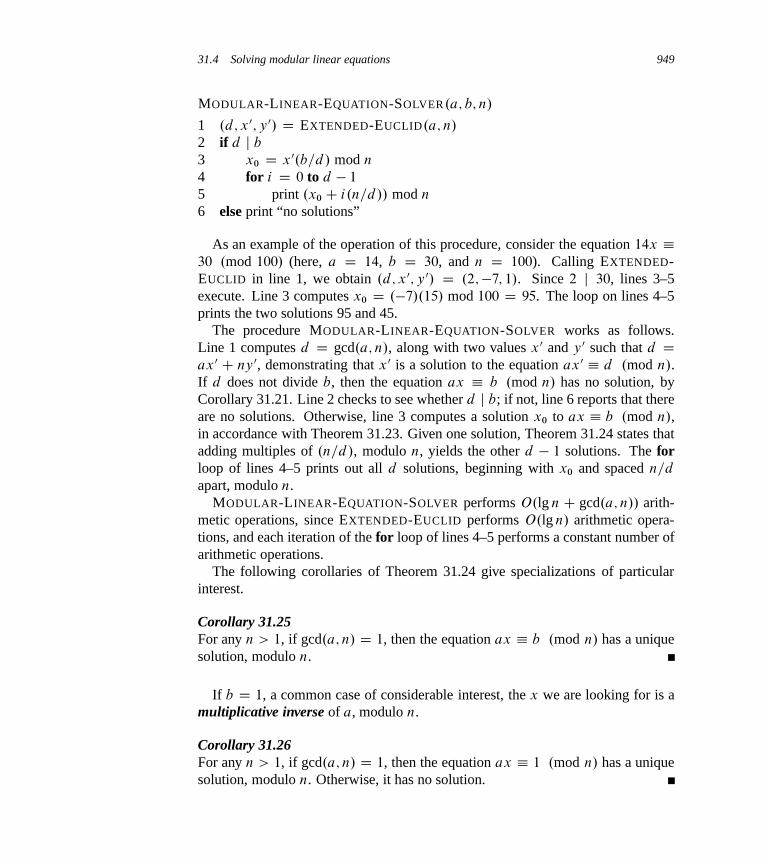
31.4 Solving modular linear equations 949
MODULAR-LINEAR-EQUATION-SOLVER.a; b; n/
1 .d; x 0; y 0/ D EXTENDED-EUCLID.a; n/
2 if d j b3 x0 D x 0.b=d/ mod n
4 for i D 0 to d � 1
5 print .x0 C i.n=d// mod n
6 else print “no solutions”
As an example of the operation of this procedure, consider the equation 14x �30 .mod 100/ (here, a D 14, b D 30, and n D 100). Calling EXTENDED-EUCLID in line 1, we obtain .d; x 0; y 0/ D .2;�7; 1/. Since 2 j 30, lines 3–5execute. Line 3 computes x0 D .�7/.15/ mod 100 D 95. The loop on lines 4–5prints the two solutions 95 and 45.
The procedure MODULAR-LINEAR-EQUATION-SOLVER works as follows.Line 1 computes d D gcd.a; n/, along with two values x 0 and y 0 such that d Dax 0 C ny 0, demonstrating that x 0 is a solution to the equation ax 0 � d .mod n/.If d does not divide b, then the equation ax � b .mod n/ has no solution, byCorollary 31.21. Line 2 checks to see whether d j b; if not, line 6 reports that thereare no solutions. Otherwise, line 3 computes a solution x0 to ax � b .mod n/,in accordance with Theorem 31.23. Given one solution, Theorem 31.24 states thatadding multiples of .n=d/, modulo n, yields the other d � 1 solutions. The forloop of lines 4–5 prints out all d solutions, beginning with x0 and spaced n=d
apart, modulo n.MODULAR-LINEAR-EQUATION-SOLVER performs O.lg n C gcd.a; n// arith-
metic operations, since EXTENDED-EUCLID performs O.lg n/ arithmetic opera-tions, and each iteration of the for loop of lines 4–5 performs a constant number ofarithmetic operations.
The following corollaries of Theorem 31.24 give specializations of particularinterest.
Corollary 31.25For any n > 1, if gcd.a; n/ D 1, then the equation ax � b .mod n/ has a uniquesolution, modulo n.
If b D 1, a common case of considerable interest, the x we are looking for is amultiplicative inverse of a, modulo n.
Corollary 31.26For any n > 1, if gcd.a; n/ D 1, then the equation ax � 1 .mod n/ has a uniquesolution, modulo n. Otherwise, it has no solution.
950 Chapter 31 Number-Theoretic Algorithms
Thanks to Corollary 31.26, we can use the notation a�1 mod n to refer to themultiplicative inverse of a, modulo n, when a and n are relatively prime. Ifgcd.a; n/ D 1, then the unique solution to the equation ax � 1 .mod n/ is theinteger x returned by EXTENDED-EUCLID, since the equation
gcd.a; n/ D 1 D ax C ny
implies ax � 1 .mod n/. Thus, we can compute a�1 mod n efficiently usingEXTENDED-EUCLID.
Exercises
31.4-1Find all solutions to the equation 35x � 10 .mod 50/.
31.4-2Prove that the equation ax � ay .mod n/ implies x � y .mod n/ whenevergcd.a; n/ D 1. Show that the condition gcd.a; n/ D 1 is necessary by supplying acounterexample with gcd.a; n/ > 1.
31.4-3Consider the following change to line 3 of the procedure MODULAR-LINEAR-EQUATION-SOLVER:
3 x0 D x 0.b=d/ mod .n=d/
Will this work? Explain why or why not.
31.4-4 ?
Let p be prime and f .x/ � f0 C f1x C � � � C ftxt .mod p/ be a polyno-
mial of degree t , with coefficients fi drawn from Zp. We say that a 2 Zp
is a zero of f if f .a/ � 0 .mod p/. Prove that if a is a zero of f , thenf .x/ � .x � a/g.x/ .mod p/ for some polynomial g.x/ of degree t � 1. Proveby induction on t that if p is prime, then a polynomial f .x/ of degree t can haveat most t distinct zeros modulo p.
31.5 The Chinese remainder theorem
Around A.D. 100, the Chinese mathematician Sun-Tsŭ solved the problem of find-ing those integers x that leave remainders 2, 3, and 2 when divided by 3, 5, and 7respectively. One such solution is x D 23; all solutions are of the form 23C 105k

31.5 The Chinese remainder theorem 951
for arbitrary integers k. The “Chinese remainder theorem” provides a correspon-dence between a system of equations modulo a set of pairwise relatively primemoduli (for example, 3, 5, and 7) and an equation modulo their product (for exam-ple, 105).
The Chinese remainder theorem has two major applications. Let the inte-ger n be factored as n D n1n2 � � � nk , where the factors ni are pairwise relativelyprime. First, the Chinese remainder theorem is a descriptive “structure theorem”that describes the structure of Zn as identical to that of the Cartesian productZn1 Zn2
� � � Znkwith componentwise addition and multiplication modulo ni
in the i th component. Second, this description helps us to design efficient algo-rithms, since working in each of the systems Zni
can be more efficient (in terms ofbit operations) than working modulo n.
Theorem 31.27 (Chinese remainder theorem)Let n D n1n2 � � � nk, where the ni are pairwise relatively prime. Consider thecorrespondence
a$ .a1; a2; : : : ; ak/ ; (31.27)
where a 2 Zn, ai 2 Zni, and
ai D a mod ni
for i D 1; 2; : : : ; k. Then, mapping (31.27) is a one-to-one correspondence (bijec-tion) between Zn and the Cartesian product Zn1
Zn2� � � Znk
. Operations per-formed on the elements of Zn can be equivalently performed on the correspondingk-tuples by performing the operations independently in each coordinate position inthe appropriate system. That is, if
a $ .a1; a2; : : : ; ak/ ;
b $ .b1; b2; : : : ; bk/ ;
then
.aC b/ mod n $ ..a1 C b1/ mod n1; : : : ; .ak C bk/ mod nk/ ; (31.28)
.a � b/ mod n $ ..a1 � b1/ mod n1; : : : ; .ak � bk/ mod nk/ ; (31.29)
.ab/ mod n $ .a1b1 mod n1; : : : ; akbk mod nk/ : (31.30)
Proof Transforming between the two representations is fairly straightforward.Going from a to .a1; a2; : : : ; ak/ is quite easy and requires only k “mod” opera-tions.
Computing a from inputs .a1; a2; : : : ; ak/ is a bit more complicated. We beginby defining mi D n=ni for i D 1; 2; : : : ; k; thus mi is the product of all of the nj ’sother than ni : mi D n1n2 � � � ni�1niC1 � � � nk. We next define
952 Chapter 31 Number-Theoretic Algorithms
ci D mi.m�1i mod ni/ (31.31)
for i D 1; 2; : : : ; k. Equation (31.31) is always well defined: since mi and ni arerelatively prime (by Theorem 31.6), Corollary 31.26 guarantees that m�1
i mod ni
exists. Finally, we can compute a as a function of a1, a2, . . . , ak as follows:
a � .a1c1 C a2c2 C � � � C akck/ .mod n/ : (31.32)
We now show that equation (31.32) ensures that a � ai .mod ni/ for i D1; 2; : : : ; k. Note that if j ¤ i , then mj � 0 .mod ni /, which implies that cj �mj � 0 .mod ni /. Note also that ci � 1 .mod ni /, from equation (31.31). Wethus have the appealing and useful correspondence
ci $ .0; 0; : : : ; 0; 1; 0; : : : ; 0/ ;
a vector that has 0s everywhere except in the i th coordinate, where it has a 1; the ci
thus form a “basis” for the representation, in a certain sense. For each i , therefore,we have
a � aici .mod ni/
� aimi .m�1i mod ni/ .mod ni/
� ai .mod ni/ ;
which is what we wished to show: our method of computing a from the ai ’s pro-duces a result a that satisfies the constraints a � ai .mod ni/ for i D 1; 2; : : : ; k.The correspondence is one-to-one, since we can transform in both directions.Finally, equations (31.28)–(31.30) follow directly from Exercise 31.1-7, sincex mod ni D .x mod n/ mod ni for any x and i D 1; 2; : : : ; k.
We shall use the following corollaries later in this chapter.
Corollary 31.28If n1; n2; : : : ; nk are pairwise relatively prime and n D n1n2 � � � nk, then for anyintegers a1; a2; : : : ; ak , the set of simultaneous equations
x � ai .mod ni/ ;
for i D 1; 2; : : : ; k, has a unique solution modulo n for the unknown x.
Corollary 31.29If n1; n2; : : : ; nk are pairwise relatively prime and n D n1n2 � � � nk, then for allintegers x and a,
x � a .mod ni /
for i D 1; 2; : : : ; k if and only if
x � a .mod n/ :
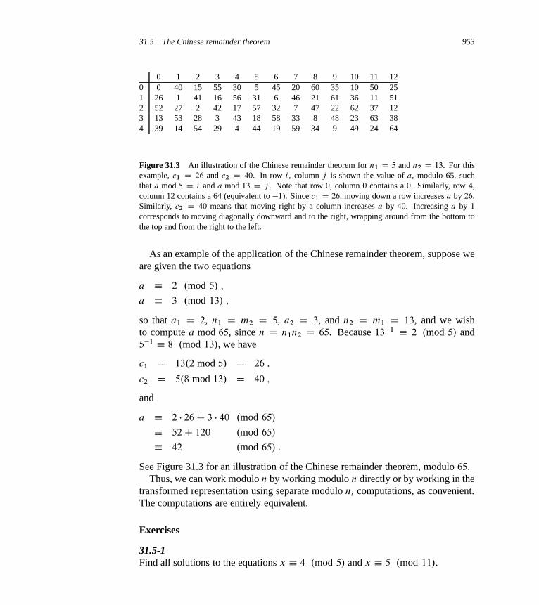
31.5 The Chinese remainder theorem 953
0 1 2 3 4 5 6 7 8 9 10 11 120 0 40 15 55 30 5 45 20 60 35 10 50 251 26 1 41 16 56 31 6 46 21 61 36 11 512 52 27 2 42 17 57 32 7 47 22 62 37 123 13 53 28 3 43 18 58 33 8 48 23 63 384 39 14 54 29 4 44 19 59 34 9 49 24 64
Figure 31.3 An illustration of the Chinese remainder theorem for n1 D 5 and n2 D 13. For thisexample, c1 D 26 and c2 D 40. In row i , column j is shown the value of a, modulo 65, suchthat a mod 5 D i and a mod 13 D j . Note that row 0, column 0 contains a 0. Similarly, row 4,column 12 contains a 64 (equivalent to �1). Since c1 D 26, moving down a row increases a by 26.Similarly, c2 D 40 means that moving right by a column increases a by 40. Increasing a by 1
corresponds to moving diagonally downward and to the right, wrapping around from the bottom tothe top and from the right to the left.
As an example of the application of the Chinese remainder theorem, suppose weare given the two equations
a � 2 .mod 5/ ;
a � 3 .mod 13/ ;
so that a1 D 2, n1 D m2 D 5, a2 D 3, and n2 D m1 D 13, and we wishto compute a mod 65, since n D n1n2 D 65. Because 13�1 � 2 .mod 5/ and5�1 � 8 .mod 13/, we have
c1 D 13.2 mod 5/ D 26 ;
c2 D 5.8 mod 13/ D 40 ;
and
a � 2 � 26C 3 � 40 .mod 65/
� 52C 120 .mod 65/
� 42 .mod 65/ :
See Figure 31.3 for an illustration of the Chinese remainder theorem, modulo 65.Thus, we can work modulo n by working modulo n directly or by working in the
transformed representation using separate modulo ni computations, as convenient.The computations are entirely equivalent.
Exercises
31.5-1Find all solutions to the equations x � 4 .mod 5/ and x � 5 .mod 11/.
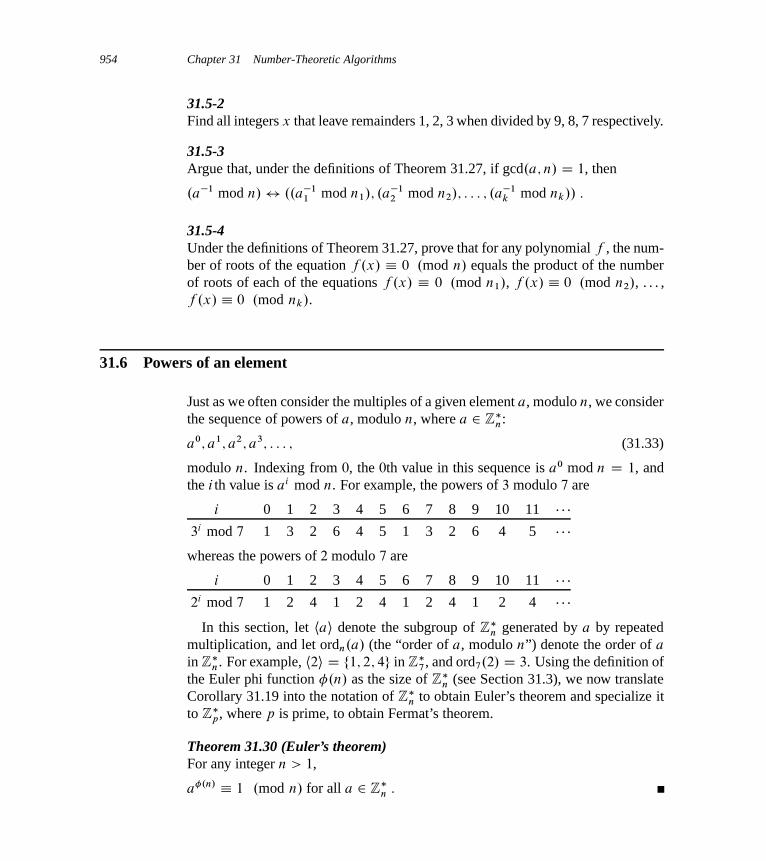
954 Chapter 31 Number-Theoretic Algorithms
31.5-2Find all integers x that leave remainders 1, 2, 3 when divided by 9, 8, 7 respectively.
31.5-3Argue that, under the definitions of Theorem 31.27, if gcd.a; n/ D 1, then
.a�1 mod n/$ ..a�11 mod n1/; .a�1
2 mod n2/; : : : ; .a�1k mod nk// :
31.5-4Under the definitions of Theorem 31.27, prove that for any polynomial f , the num-ber of roots of the equation f .x/ � 0 .mod n/ equals the product of the numberof roots of each of the equations f .x/ � 0 .mod n1/, f .x/ � 0 .mod n2/, . . . ,f .x/ � 0 .mod nk/.
31.6 Powers of an element
Just as we often consider the multiples of a given element a, modulo n, we considerthe sequence of powers of a, modulo n, where a 2 Z
�n:
a0; a1; a2; a3; : : : ; (31.33)
modulo n. Indexing from 0, the 0th value in this sequence is a0 mod n D 1, andthe i th value is ai mod n. For example, the powers of 3 modulo 7 are
i 0 1 2 3 4 5 6 7 8 9 10 11 � � �3i mod 7 1 3 2 6 4 5 1 3 2 6 4 5 � � �
whereas the powers of 2 modulo 7 are
i 0 1 2 3 4 5 6 7 8 9 10 11 � � �2i mod 7 1 2 4 1 2 4 1 2 4 1 2 4 � � �
In this section, let hai denote the subgroup of Z�n generated by a by repeated
multiplication, and let ordn.a/ (the “order of a, modulo n”) denote the order of a
in Z�n. For example, h2i D f1; 2; 4g in Z
�7 , and ord7.2/ D 3. Using the definition of
the Euler phi function �.n/ as the size of Z�n (see Section 31.3), we now translate
Corollary 31.19 into the notation of Z�n to obtain Euler’s theorem and specialize it
to Z�p, where p is prime, to obtain Fermat’s theorem.
Theorem 31.30 (Euler’s theorem)For any integer n > 1,
a�.n/ � 1 .mod n/ for all a 2 Z�n :
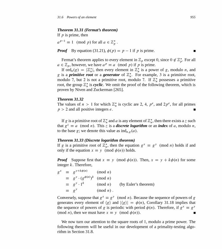
31.6 Powers of an element 955
Theorem 31.31 (Fermat’s theorem)If p is prime, then
ap�1 � 1 .mod p/ for all a 2 Z�p :
Proof By equation (31.21), �.p/ D p � 1 if p is prime.
Fermat’s theorem applies to every element in Zp except 0, since 0 62 Z�p. For all
a 2 Zp, however, we have ap � a .mod p/ if p is prime.If ordn.g/ D jZ�
nj, then every element in Z�n is a power of g, modulo n, and
g is a primitive root or a generator of Z�n. For example, 3 is a primitive root,
modulo 7, but 2 is not a primitive root, modulo 7. If Z�n possesses a primitive
root, the group Z�n is cyclic. We omit the proof of the following theorem, which is
proven by Niven and Zuckerman [265].
Theorem 31.32The values of n > 1 for which Z
�n is cyclic are 2, 4, pe, and 2pe, for all primes
p > 2 and all positive integers e.
If g is a primitive root of Z�n and a is any element of Z
�n, then there exists a ´ such
that g´ � a .mod n/. This ´ is a discrete logarithm or an index of a, modulo n,to the base g; we denote this value as indn;g.a/.
Theorem 31.33 (Discrete logarithm theorem)If g is a primitive root of Z
�n, then the equation gx � gy .mod n/ holds if and
only if the equation x � y .mod �.n// holds.
Proof Suppose first that x � y .mod �.n//. Then, x D y C k�.n/ for someinteger k. Therefore,
gx � gyCk�.n/ .mod n/
� gy � .g�.n//k .mod n/
� gy � 1k .mod n/ (by Euler’s theorem)
� gy .mod n/ :
Conversely, suppose that gx � gy .mod n/. Because the sequence of powers of g
generates every element of hgi and jhgij D �.n/, Corollary 31.18 implies thatthe sequence of powers of g is periodic with period �.n/. Therefore, if gx � gy
.mod n/, then we must have x � y .mod �.n//.
We now turn our attention to the square roots of 1, modulo a prime power. Thefollowing theorem will be useful in our development of a primality-testing algo-rithm in Section 31.8.

956 Chapter 31 Number-Theoretic Algorithms
Theorem 31.34If p is an odd prime and e � 1, then the equation
x2 � 1 .mod pe/ (31.34)
has only two solutions, namely x D 1 and x D �1.
Proof Equation (31.34) is equivalent to
pe j .x � 1/.x C 1/ :
Since p > 2, we can have p j .x � 1/ or p j .x C 1/, but not both. (Otherwise,by property (31.3), p would also divide their difference .x C 1/ � .x � 1/ D 2).If p − .x � 1/, then gcd.pe; x � 1/ D 1, and by Corollary 31.5, we would havepe j .x C 1/. That is, x � �1 .mod pe/. Symmetrically, if p − .x C 1/,then gcd.pe; x C 1/ D 1, and Corollary 31.5 implies that pe j .x � 1/, so thatx � 1 .mod pe/. Therefore, either x � �1 .mod pe/ or x � 1 .mod pe/.
A number x is a nontrivial square root of 1, modulo n, if it satisfies the equationx2 � 1 .mod n/ but x is equivalent to neither of the two “trivial” square roots: 1
or �1, modulo n. For example, 6 is a nontrivial square root of 1, modulo 35. Weshall use the following corollary to Theorem 31.34 in the correctness proof for theMiller-Rabin primality-testing procedure in Section 31.8.
Corollary 31.35If there exists a nontrivial square root of 1, modulo n, then n is composite.
Proof By the contrapositive of Theorem 31.34, if there exists a nontrivial squareroot of 1, modulo n, then n cannot be an odd prime or a power of an odd prime.If x2 � 1 .mod 2/, then x � 1 .mod 2/, and so all square roots of 1, modulo 2,are trivial. Thus, n cannot be prime. Finally, we must have n > 1 for a nontrivialsquare root of 1 to exist. Therefore, n must be composite.
Raising to powers with repeated squaring
A frequently occurring operation in number-theoretic computations is raising onenumber to a power modulo another number, also known as modular exponentia-tion. More precisely, we would like an efficient way to compute ab mod n, wherea and b are nonnegative integers and n is a positive integer. Modular exponenti-ation is an essential operation in many primality-testing routines and in the RSApublic-key cryptosystem. The method of repeated squaring solves this problemefficiently using the binary representation of b.
Let hbk; bk�1; : : : ; b1; b0i be the binary representation of b. (That is, the binaryrepresentation is k C 1 bits long, bk is the most significant bit, and b0 is the least

31.6 Powers of an element 957
i 9 8 7 6 5 4 3 2 1 0bi 1 0 0 0 1 1 0 0 0 0c 1 2 4 8 17 35 70 140 280 560d 7 49 157 526 160 241 298 166 67 1
Figure 31.4 The results of MODULAR-EXPONENTIATION when computing ab .mod n/, wherea D 7, b D 560 D h1000110000i, and n D 561. The values are shown after each execution of thefor loop. The final result is 1.
significant bit.) The following procedure computes ac mod n as c is increased bydoublings and incrementations from 0 to b.
MODULAR-EXPONENTIATION.a; b; n/
1 c D 0
2 d D 1
3 let hbk; bk�1; : : : ; b0i be the binary representation of b
4 for i D k downto 0
5 c D 2c
6 d D .d � d/ mod n
7 if bi == 1
8 c D c C 1
9 d D .d � a/ mod n
10 return d
The essential use of squaring in line 6 of each iteration explains the name “repeatedsquaring.” As an example, for a D 7, b D 560, and n D 561, the algorithmcomputes the sequence of values modulo 561 shown in Figure 31.4; the sequenceof exponents used appears in the row of the table labeled by c.
The variable c is not really needed by the algorithm but is included for the fol-lowing two-part loop invariant:
Just prior to each iteration of the for loop of lines 4–9,
1. The value of c is the same as the prefix hbk; bk�1; : : : ; biC1i of the binaryrepresentation of b, and
2. d D ac mod n.
We use this loop invariant as follows:
Initialization: Initially, i D k, so that the prefix hbk; bk�1; : : : ; biC1i is empty,which corresponds to c D 0. Moreover, d D 1 D a0 mod n.
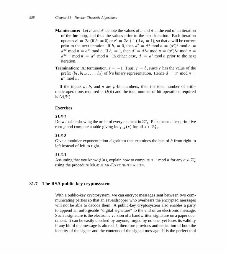
958 Chapter 31 Number-Theoretic Algorithms
Maintenance: Let c 0 and d 0 denote the values of c and d at the end of an iterationof the for loop, and thus the values prior to the next iteration. Each iterationupdates c 0 D 2c (if bi D 0) or c 0 D 2cC1 (if bi D 1), so that c will be correctprior to the next iteration. If bi D 0, then d 0 D d 2 mod n D .ac/2 mod n Da2c mod n D ac0
mod n. If bi D 1, then d 0 D d 2a mod n D .ac/2a mod n Da2cC1 mod n D ac0
mod n. In either case, d D ac mod n prior to the nextiteration.
Termination: At termination, i D �1. Thus, c D b, since c has the value of theprefix hbk; bk�1; : : : ; b0i of b’s binary representation. Hence d D ac mod n Dab mod n.
If the inputs a, b, and n are ˇ-bit numbers, then the total number of arith-metic operations required is O.ˇ/ and the total number of bit operations requiredis O.ˇ3/.
Exercises
31.6-1Draw a table showing the order of every element in Z
�11. Pick the smallest primitive
root g and compute a table giving ind11;g.x/ for all x 2 Z�11.
31.6-2Give a modular exponentiation algorithm that examines the bits of b from right toleft instead of left to right.
31.6-3Assuming that you know �.n/, explain how to compute a�1 mod n for any a 2 Z
�n
using the procedure MODULAR-EXPONENTIATION.
31.7 The RSA public-key cryptosystem
With a public-key cryptosystem, we can encrypt messages sent between two com-municating parties so that an eavesdropper who overhears the encrypted messageswill not be able to decode them. A public-key cryptosystem also enables a partyto append an unforgeable “digital signature” to the end of an electronic message.Such a signature is the electronic version of a handwritten signature on a paper doc-ument. It can be easily checked by anyone, forged by no one, yet loses its validityif any bit of the message is altered. It therefore provides authentication of both theidentity of the signer and the contents of the signed message. It is the perfect tool
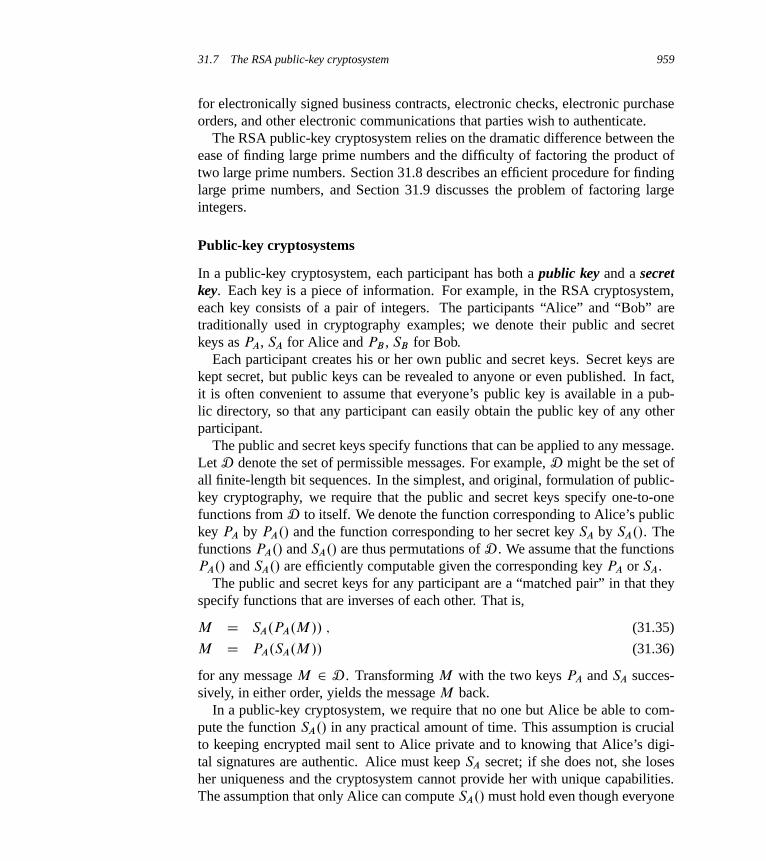
31.7 The RSA public-key cryptosystem 959
for electronically signed business contracts, electronic checks, electronic purchaseorders, and other electronic communications that parties wish to authenticate.
The RSA public-key cryptosystem relies on the dramatic difference between theease of finding large prime numbers and the difficulty of factoring the product oftwo large prime numbers. Section 31.8 describes an efficient procedure for findinglarge prime numbers, and Section 31.9 discusses the problem of factoring largeintegers.
Public-key cryptosystems
In a public-key cryptosystem, each participant has both a public key and a secretkey. Each key is a piece of information. For example, in the RSA cryptosystem,each key consists of a pair of integers. The participants “Alice” and “Bob” aretraditionally used in cryptography examples; we denote their public and secretkeys as PA, SA for Alice and PB , SB for Bob.
Each participant creates his or her own public and secret keys. Secret keys arekept secret, but public keys can be revealed to anyone or even published. In fact,it is often convenient to assume that everyone’s public key is available in a pub-lic directory, so that any participant can easily obtain the public key of any otherparticipant.
The public and secret keys specify functions that can be applied to any message.Let D denote the set of permissible messages. For example, D might be the set ofall finite-length bit sequences. In the simplest, and original, formulation of public-key cryptography, we require that the public and secret keys specify one-to-onefunctions from D to itself. We denote the function corresponding to Alice’s publickey PA by PA./ and the function corresponding to her secret key SA by SA./. Thefunctions PA./ and SA./ are thus permutations of D . We assume that the functionsPA./ and SA./ are efficiently computable given the corresponding key PA or SA.
The public and secret keys for any participant are a “matched pair” in that theyspecify functions that are inverses of each other. That is,
M D SA.PA.M // ; (31.35)
M D PA.SA.M // (31.36)
for any message M 2 D . Transforming M with the two keys PA and SA succes-sively, in either order, yields the message M back.
In a public-key cryptosystem, we require that no one but Alice be able to com-pute the function SA./ in any practical amount of time. This assumption is crucialto keeping encrypted mail sent to Alice private and to knowing that Alice’s digi-tal signatures are authentic. Alice must keep SA secret; if she does not, she losesher uniqueness and the cryptosystem cannot provide her with unique capabilities.The assumption that only Alice can compute SA./ must hold even though everyone
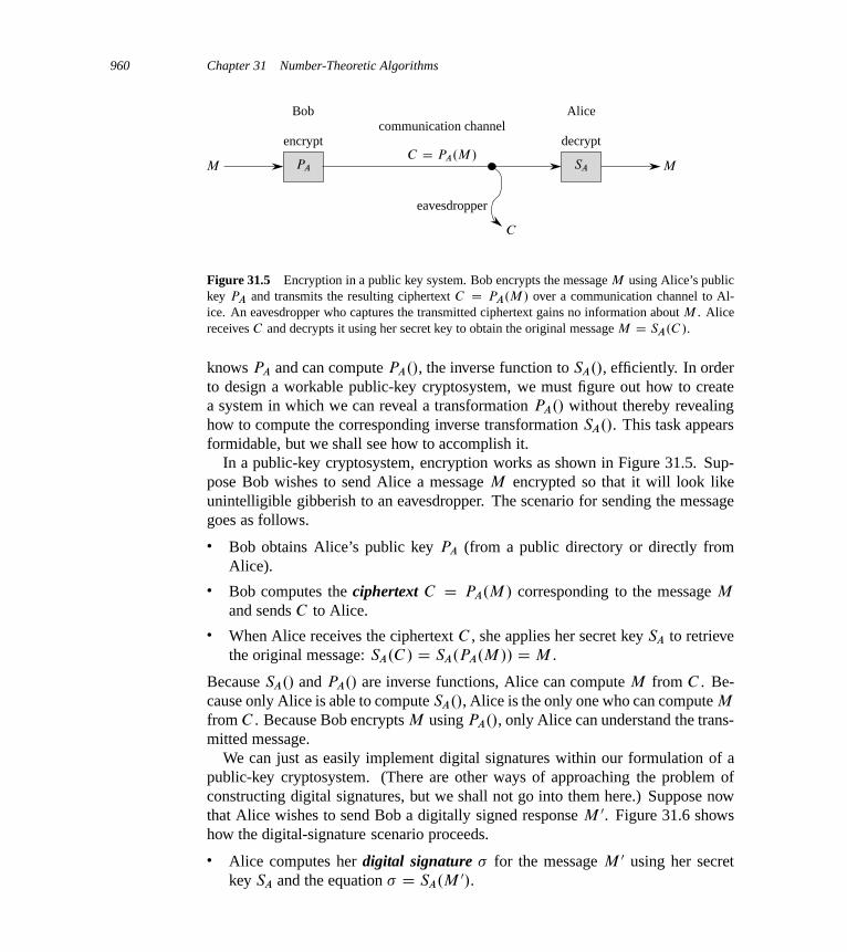
960 Chapter 31 Number-Theoretic Algorithms
decryptcommunication channel
encrypt
Bob Alice
eavesdropper
MM PA SA
C
C D PA.M /
Figure 31.5 Encryption in a public key system. Bob encrypts the message M using Alice’s publickey PA and transmits the resulting ciphertext C D PA.M/ over a communication channel to Al-ice. An eavesdropper who captures the transmitted ciphertext gains no information about M . Alicereceives C and decrypts it using her secret key to obtain the original message M D SA.C /.
knows PA and can compute PA./, the inverse function to SA./, efficiently. In orderto design a workable public-key cryptosystem, we must figure out how to createa system in which we can reveal a transformation PA./ without thereby revealinghow to compute the corresponding inverse transformation SA./. This task appearsformidable, but we shall see how to accomplish it.
In a public-key cryptosystem, encryption works as shown in Figure 31.5. Sup-pose Bob wishes to send Alice a message M encrypted so that it will look likeunintelligible gibberish to an eavesdropper. The scenario for sending the messagegoes as follows.
� Bob obtains Alice’s public key PA (from a public directory or directly fromAlice).
� Bob computes the ciphertext C D PA.M / corresponding to the message M
and sends C to Alice.� When Alice receives the ciphertext C , she applies her secret key SA to retrieve
the original message: SA.C / D SA.PA.M // DM .
Because SA./ and PA./ are inverse functions, Alice can compute M from C . Be-cause only Alice is able to compute SA./, Alice is the only one who can compute M
from C . Because Bob encrypts M using PA./, only Alice can understand the trans-mitted message.
We can just as easily implement digital signatures within our formulation of apublic-key cryptosystem. (There are other ways of approaching the problem ofconstructing digital signatures, but we shall not go into them here.) Suppose nowthat Alice wishes to send Bob a digitally signed response M 0. Figure 31.6 showshow the digital-signature scenario proceeds.
� Alice computes her digital signature for the message M 0 using her secretkey SA and the equation D SA.M 0/.
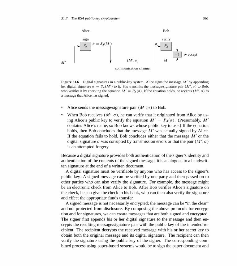
31.7 The RSA public-key cryptosystem 961
sign
communication channel
verify
=? accept
BobAlice
M 0M 0
PASA
.M 0; /
D SA.M 0/
Figure 31.6 Digital signatures in a public-key system. Alice signs the message M 0 by appendingher digital signature D SA.M 0/ to it. She transmits the message/signature pair .M 0; / to Bob,who verifies it by checking the equation M 0 D PA./. If the equation holds, he accepts .M 0; / asa message that Alice has signed.
� Alice sends the message/signature pair .M 0; / to Bob.
� When Bob receives .M 0; /, he can verify that it originated from Alice by us-ing Alice’s public key to verify the equation M 0 D PA./. (Presumably, M 0
contains Alice’s name, so Bob knows whose public key to use.) If the equationholds, then Bob concludes that the message M 0 was actually signed by Alice.If the equation fails to hold, Bob concludes either that the message M 0 or thedigital signature was corrupted by transmission errors or that the pair .M 0; /
is an attempted forgery.
Because a digital signature provides both authentication of the signer’s identity andauthentication of the contents of the signed message, it is analogous to a handwrit-ten signature at the end of a written document.
A digital signature must be verifiable by anyone who has access to the signer’spublic key. A signed message can be verified by one party and then passed on toother parties who can also verify the signature. For example, the message mightbe an electronic check from Alice to Bob. After Bob verifies Alice’s signature onthe check, he can give the check to his bank, who can then also verify the signatureand effect the appropriate funds transfer.
A signed message is not necessarily encrypted; the message can be “in the clear”and not protected from disclosure. By composing the above protocols for encryp-tion and for signatures, we can create messages that are both signed and encrypted.The signer first appends his or her digital signature to the message and then en-crypts the resulting message/signature pair with the public key of the intended re-cipient. The recipient decrypts the received message with his or her secret key toobtain both the original message and its digital signature. The recipient can thenverify the signature using the public key of the signer. The corresponding com-bined process using paper-based systems would be to sign the paper document and

962 Chapter 31 Number-Theoretic Algorithms
then seal the document inside a paper envelope that is opened only by the intendedrecipient.
The RSA cryptosystem
In the RSA public-key cryptosystem, a participant creates his or her public andsecret keys with the following procedure:
1. Select at random two large prime numbers p and q such that p ¤ q. The primesp and q might be, say, 1024 bits each.
2. Compute n D pq.
3. Select a small odd integer e that is relatively prime to �.n/, which, by equa-tion (31.20), equals .p � 1/.q � 1/.
4. Compute d as the multiplicative inverse of e, modulo �.n/. (Corollary 31.26guarantees that d exists and is uniquely defined. We can use the technique ofSection 31.4 to compute d , given e and �.n/.)
5. Publish the pair P D .e; n/ as the participant’s RSA public key.
6. Keep secret the pair S D .d; n/ as the participant’s RSA secret key.
For this scheme, the domain D is the set Zn. To transform a message M asso-ciated with a public key P D .e; n/, compute
P.M / DM e mod n : (31.37)
To transform a ciphertext C associated with a secret key S D .d; n/, compute
S.C / D C d mod n : (31.38)
These equations apply to both encryption and signatures. To create a signature, thesigner applies his or her secret key to the message to be signed, rather than to aciphertext. To verify a signature, the public key of the signer is applied to it, ratherthan to a message to be encrypted.
We can implement the public-key and secret-key operations using the procedureMODULAR-EXPONENTIATION described in Section 31.6. To analyze the runningtime of these operations, assume that the public key .e; n/ and secret key .d; n/
satisfy lg e D O.1/, lg d � ˇ, and lg n � ˇ. Then, applying a public key requiresO.1/ modular multiplications and uses O.ˇ2/ bit operations. Applying a secretkey requires O.ˇ/ modular multiplications, using O.ˇ3/ bit operations.
Theorem 31.36 (Correctness of RSA)The RSA equations (31.37) and (31.38) define inverse transformations of Zn satis-fying equations (31.35) and (31.36).

31.7 The RSA public-key cryptosystem 963
Proof From equations (31.37) and (31.38), we have that for any M 2 Zn,
P.S.M // D S.P.M // DM ed .mod n/ :
Since e and d are multiplicative inverses modulo �.n/ D .p � 1/.q � 1/,
ed D 1C k.p � 1/.q � 1/
for some integer k. But then, if M 6� 0 .mod p/, we have
M ed � M.M p�1/k.q�1/ .mod p/
� M..M mod p/p�1/k.q�1/ .mod p/
� M.1/k.q�1/ .mod p/ (by Theorem 31.31)
� M .mod p/ :
Also, M ed �M .mod p/ if M � 0 .mod p/. Thus,
M ed �M .mod p/
for all M . Similarly,
M ed �M .mod q/
for all M . Thus, by Corollary 31.29 to the Chinese remainder theorem,
M ed �M .mod n/
for all M .
The security of the RSA cryptosystem rests in large part on the difficulty of fac-toring large integers. If an adversary can factor the modulus n in a public key, thenthe adversary can derive the secret key from the public key, using the knowledgeof the factors p and q in the same way that the creator of the public key used them.Therefore, if factoring large integers is easy, then breaking the RSA cryptosystemis easy. The converse statement, that if factoring large integers is hard, then break-ing RSA is hard, is unproven. After two decades of research, however, no easiermethod has been found to break the RSA public-key cryptosystem than to factorthe modulus n. And as we shall see in Section 31.9, factoring large integers is sur-prisingly difficult. By randomly selecting and multiplying together two 1024-bitprimes, we can create a public key that cannot be “broken” in any feasible amountof time with current technology. In the absence of a fundamental breakthrough inthe design of number-theoretic algorithms, and when implemented with care fol-lowing recommended standards, the RSA cryptosystem is capable of providing ahigh degree of security in applications.
In order to achieve security with the RSA cryptosystem, however, we shoulduse integers that are quite long—hundreds or even more than one thousand bits
964 Chapter 31 Number-Theoretic Algorithms
long—to resist possible advances in the art of factoring. At the time of thiswriting (2009), RSA moduli were commonly in the range of 768 to 2048 bits.To create moduli of such sizes, we must be able to find large primes efficiently.Section 31.8 addresses this problem.
For efficiency, RSA is often used in a “hybrid” or “key-management” modewith fast non-public-key cryptosystems. With such a system, the encryption anddecryption keys are identical. If Alice wishes to send a long message M to Bobprivately, she selects a random key K for the fast non-public-key cryptosystem andencrypts M using K, obtaining ciphertext C . Here, C is as long as M , but K
is quite short. Then, she encrypts K using Bob’s public RSA key. Since K isshort, computing PB.K/ is fast (much faster than computing PB.M /). She thentransmits .C; PB.K// to Bob, who decrypts PB.K/ to obtain K and then uses K
to decrypt C , obtaining M .We can use a similar hybrid approach to make digital signatures efficiently.
This approach combines RSA with a public collision-resistant hash function h—afunction that is easy to compute but for which it is computationally infeasible tofind two messages M and M 0 such that h.M / D h.M 0/. The value h.M / isa short (say, 256-bit) “fingerprint” of the message M . If Alice wishes to sign amessage M , she first applies h to M to obtain the fingerprint h.M /, which shethen encrypts with her secret key. She sends .M; SA.h.M /// to Bob as her signedversion of M . Bob can verify the signature by computing h.M / and verifyingthat PA applied to SA.h.M // as received equals h.M /. Because no one can createtwo messages with the same fingerprint, it is computationally infeasible to alter asigned message and preserve the validity of the signature.
Finally, we note that the use of certificates makes distributing public keys mucheasier. For example, assume there is a “trusted authority” T whose public keyis known by everyone. Alice can obtain from T a signed message (her certificate)stating that “Alice’s public key is PA.” This certificate is “self-authenticating” sinceeveryone knows PT . Alice can include her certificate with her signed messages,so that the recipient has Alice’s public key immediately available in order to verifyher signature. Because her key was signed by T , the recipient knows that Alice’skey is really Alice’s.
Exercises
31.7-1Consider an RSA key set with p D 11, q D 29, n D 319, and e D 3. Whatvalue of d should be used in the secret key? What is the encryption of the messageM D 100?
31.8 Primality testing 965
31.7-2Prove that if Alice’s public exponent e is 3 and an adversary obtains Alice’s secretexponent d , where 0 < d < �.n/, then the adversary can factor Alice’s modulus n
in time polynomial in the number of bits in n. (Although you are not asked to proveit, you may be interested to know that this result remains true even if the conditione D 3 is removed. See Miller [255].)
31.7-3 ?
Prove that RSA is multiplicative in the sense that
PA.M1/PA.M2/ � PA.M1M2/ .mod n/ :
Use this fact to prove that if an adversary had a procedure that could efficientlydecrypt 1 percent of messages from Zn encrypted with PA, then he could employa probabilistic algorithm to decrypt every message encrypted with PA with highprobability.
? 31.8 Primality testing
In this section, we consider the problem of finding large primes. We begin with adiscussion of the density of primes, proceed to examine a plausible, but incomplete,approach to primality testing, and then present an effective randomized primalitytest due to Miller and Rabin.
The density of prime numbers
For many applications, such as cryptography, we need to find large “random”primes. Fortunately, large primes are not too rare, so that it is feasible to testrandom integers of the appropriate size until we find a prime. The prime distribu-tion function �.n/ specifies the number of primes that are less than or equal to n.For example, �.10/ D 4, since there are 4 prime numbers less than or equal to 10,namely, 2, 3, 5, and 7. The prime number theorem gives a useful approximationto �.n/.
Theorem 31.37 (Prime number theorem)
limn!1
�.n/
n= ln nD 1 :
The approximation n= ln n gives reasonably accurate estimates of �.n/ evenfor small n. For example, it is off by less than 6% at n D 109, where �.n/ D
966 Chapter 31 Number-Theoretic Algorithms
50,847,534 and n= ln n � 48,254,942. (To a number theorist, 109 is a small num-ber.)
We can view the process of randomly selecting an integer n and determiningwhether it is prime as a Bernoulli trial (see Section C.4). By the prime numbertheorem, the probability of a success—that is, the probability that n is prime—isapproximately 1= ln n. The geometric distribution tells us how many trials we needto obtain a success, and by equation (C.32), the expected number of trials is ap-proximately ln n. Thus, we would expect to examine approximately ln n integerschosen randomly near n in order to find a prime that is of the same length as n.For example, we expect that finding a 1024-bit prime would require testing ap-proximately ln 21024 � 710 randomly chosen 1024-bit numbers for primality. (Ofcourse, we can cut this figure in half by choosing only odd integers.)
In the remainder of this section, we consider the problem of determining whetheror not a large odd integer n is prime. For notational convenience, we assume that n
has the prime factorization
n D pe1
1 pe2
2 � � �per
r ; (31.39)
where r � 1, p1; p2; : : : ; pr are the prime factors of n, and e1; e2; : : : ; er are posi-tive integers. The integer n is prime if and only if r D 1 and e1 D 1.
One simple approach to the problem of testing for primality is trial division. Wetry dividing n by each integer 2; 3; : : : ; bpnc. (Again, we may skip even integersgreater than 2.) It is easy to see that n is prime if and only if none of the trial divi-sors divides n. Assuming that each trial division takes constant time, the worst-caserunning time is ‚.
pn/, which is exponential in the length of n. (Recall that if n
is encoded in binary using ˇ bits, then ˇ D dlg.nC 1/e, and sop
n D ‚.2ˇ=2/.)Thus, trial division works well only if n is very small or happens to have a smallprime factor. When it works, trial division has the advantage that it not only de-termines whether n is prime or composite, but also determines one of n’s primefactors if n is composite.
In this section, we are interested only in finding out whether a given number n
is prime; if n is composite, we are not concerned with finding its prime factor-ization. As we shall see in Section 31.9, computing the prime factorization of anumber is computationally expensive. It is perhaps surprising that it is much easierto tell whether or not a given number is prime than it is to determine the primefactorization of the number if it is not prime.
Pseudoprimality testing
We now consider a method for primality testing that “almost works” and in factis good enough for many practical applications. Later on, we shall present a re-
31.8 Primality testing 967
finement of this method that removes the small defect. Let ZCn denote the nonzero
elements of Zn:
ZCn D f1; 2; : : : ; n � 1g :
If n is prime, then ZCn D Z
�n.
We say that n is a base-a pseudoprime if n is composite and
an�1 � 1 .mod n/ : (31.40)
Fermat’s theorem (Theorem 31.31) implies that if n is prime, then n satisfies equa-tion (31.40) for every a in Z
Cn . Thus, if we can find any a 2 Z
Cn such that n does
not satisfy equation (31.40), then n is certainly composite. Surprisingly, the con-verse almost holds, so that this criterion forms an almost perfect test for primality.We test to see whether n satisfies equation (31.40) for a D 2. If not, we declare n
to be composite by returning COMPOSITE. Otherwise, we return PRIME, guessingthat n is prime (when, in fact, all we know is that n is either prime or a base-2pseudoprime).
The following procedure pretends in this manner to be checking the primalityof n. It uses the procedure MODULAR-EXPONENTIATION from Section 31.6. Weassume that the input n is an odd integer greater than 2.
PSEUDOPRIME.n/
1 if MODULAR-EXPONENTIATION.2; n � 1; n/ 6� 1 .mod n/
2 return COMPOSITE // definitely3 else return PRIME // we hope!
This procedure can make errors, but only of one type. That is, if it says that n
is composite, then it is always correct. If it says that n is prime, however, then itmakes an error only if n is a base-2 pseudoprime.
How often does this procedure err? Surprisingly rarely. There are only 22 valuesof n less than 10,000 for which it errs; the first four such values are 341, 561,645, and 1105. We won’t prove it, but the probability that this program makes anerror on a randomly chosen ˇ-bit number goes to zero as ˇ ! 1. Using moreprecise estimates due to Pomerance [279] of the number of base-2 pseudoprimes ofa given size, we may estimate that a randomly chosen 512-bit number that is calledprime by the above procedure has less than one chance in 1020 of being a base-2pseudoprime, and a randomly chosen 1024-bit number that is called prime has lessthan one chance in 1041 of being a base-2 pseudoprime. So if you are merelytrying to find a large prime for some application, for all practical purposes youalmost never go wrong by choosing large numbers at random until one of themcauses PSEUDOPRIME to return PRIME. But when the numbers being tested forprimality are not randomly chosen, we need a better approach for testing primality.

968 Chapter 31 Number-Theoretic Algorithms
As we shall see, a little more cleverness, and some randomization, will yield aprimality-testing routine that works well on all inputs.
Unfortunately, we cannot entirely eliminate all the errors by simply checkingequation (31.40) for a second base number, say a D 3, because there exist com-posite integers n, known as Carmichael numbers, that satisfy equation (31.40) forall a 2 Z
�n. (We note that equation (31.40) does fail when gcd.a; n/ > 1—that
is, when a 62 Z�n—but hoping to demonstrate that n is composite by finding such
an a can be difficult if n has only large prime factors.) The first three Carmichaelnumbers are 561, 1105, and 1729. Carmichael numbers are extremely rare; thereare, for example, only 255 of them less than 100,000,000. Exercise 31.8-2 helpsexplain why they are so rare.
We next show how to improve our primality test so that it won’t be fooled byCarmichael numbers.
The Miller-Rabin randomized primality test
The Miller-Rabin primality test overcomes the problems of the simple test PSEU-DOPRIME with two modifications:
� It tries several randomly chosen base values a instead of just one base value.
� While computing each modular exponentiation, it looks for a nontrivial squareroot of 1, modulo n, during the final set of squarings. If it finds one, it stopsand returns COMPOSITE. Corollary 31.35 from Section 31.6 justifies detectingcomposites in this manner.
The pseudocode for the Miller-Rabin primality test follows. The input n > 2 isthe odd number to be tested for primality, and s is the number of randomly cho-sen base values from Z
Cn to be tried. The code uses the random-number generator
RANDOM described on page 117: RANDOM.1; n � 1/ returns a randomly choseninteger a satisfying 1 � a � n�1. The code uses an auxiliary procedure WITNESS
such that WITNESS.a; n/ is TRUE if and only if a is a “witness” to the composite-ness of n—that is, if it is possible using a to prove (in a manner that we shall see)that n is composite. The test WITNESS.a; n/ is an extension of, but more effectivethan, the test
an�1 6� 1 .mod n/
that formed the basis (using a D 2) for PSEUDOPRIME. We first present andjustify the construction of WITNESS, and then we shall show how we use it in theMiller-Rabin primality test. Let n � 1 D 2tu where t � 1 and u is odd; i.e.,the binary representation of n � 1 is the binary representation of the odd integer u
followed by exactly t zeros. Therefore, an�1 � .au/2t
.mod n/, so that we can

31.8 Primality testing 969
compute an�1 mod n by first computing au mod n and then squaring the result t
times successively.
WITNESS.a; n/
1 let t and u be such that t � 1, u is odd, and n � 1 D 2tu
2 x0 D MODULAR-EXPONENTIATION.a; u; n/
3 for i D 1 to t
4 xi D x2i�1 mod n
5 if xi == 1 and xi�1 ¤ 1 and xi�1 ¤ n � 1
6 return TRUE
7 if xt ¤ 1
8 return TRUE
9 return FALSE
This pseudocode for WITNESS computes an�1 mod n by first computing thevalue x0 D au mod n in line 2 and then squaring the result t times in a row in thefor loop of lines 3–6. By induction on i , the sequence x0, x1, . . . , xt of valuescomputed satisfies the equation xi � a2i u .mod n/ for i D 0; 1; : : : ; t , so that inparticular xt � an�1 .mod n/. After line 4 performs a squaring step, however,the loop may terminate early if lines 5–6 detect that a nontrivial square root of 1
has just been discovered. (We shall explain these tests shortly.) If so, the algo-rithm stops and returns TRUE. Lines 7–8 return TRUE if the value computed forxt � an�1 .mod n/ is not equal to 1, just as the PSEUDOPRIME procedure returnsCOMPOSITE in this case. Line 9 returns FALSE if we haven’t returned TRUE inlines 6 or 8.
We now argue that if WITNESS.a; n/ returns TRUE, then we can construct aproof that n is composite using a as a witness.
If WITNESS returns TRUE from line 8, then it has discovered that xt Dan�1 mod n ¤ 1. If n is prime, however, we have by Fermat’s theorem (Theo-rem 31.31) that an�1 � 1 .mod n/ for all a 2 Z
Cn . Therefore, n cannot be prime,
and the equation an�1 mod n ¤ 1 proves this fact.If WITNESS returns TRUE from line 6, then it has discovered that xi�1 is a non-
trivial square root of 1, modulo n, since we have that xi�1 6� ˙1 .mod n/ yetxi � x2
i�1 � 1 .mod n/. Corollary 31.35 states that only if n is composite canthere exist a nontrivial square root of 1 modulo n, so that demonstrating that xi�1
is a nontrivial square root of 1 modulo n proves that n is composite.This completes our proof of the correctness of WITNESS. If we find that the call
WITNESS.a; n/ returns TRUE, then n is surely composite, and the witness a, alongwith the reason that the procedure returns TRUE (did it return from line 6 or fromline 8?), provides a proof that n is composite.
970 Chapter 31 Number-Theoretic Algorithms
At this point, we briefly present an alternative description of the behavior ofWITNESS as a function of the sequence X D hx0; x1; : : : ; xti, which we shall finduseful later on, when we analyze the efficiency of the Miller-Rabin primality test.Note that if xi D 1 for some 0 � i < t , WITNESS might not compute the restof the sequence. If it were to do so, however, each value xiC1; xiC2; : : : ; xt wouldbe 1, and we consider these positions in the sequence X as being all 1s. We havefour cases:
1. X D h: : : ; d i, where d ¤ 1: the sequence X does not end in 1. Return TRUE
in line 8; a is a witness to the compositeness of n (by Fermat’s Theorem).
2. X D h1; 1; : : : ; 1i: the sequence X is all 1s. Return FALSE; a is not a witnessto the compositeness of n.
3. X D h: : : ;�1; 1; : : : ; 1i: the sequence X ends in 1, and the last non-1 is equalto �1. Return FALSE; a is not a witness to the compositeness of n.
4. X D h: : : ; d; 1; : : : ; 1i, where d ¤ ˙1: the sequence X ends in 1, but the lastnon-1 is not �1. Return TRUE in line 6; a is a witness to the compositenessof n, since d is a nontrivial square root of 1.
We now examine the Miller-Rabin primality test based on the use of WITNESS.Again, we assume that n is an odd integer greater than 2.
MILLER-RABIN.n; s/
1 for j D 1 to s
2 a D RANDOM.1; n � 1/
3 if WITNESS.a; n/
4 return COMPOSITE // definitely5 return PRIME // almost surely
The procedure MILLER-RABIN is a probabilistic search for a proof that n iscomposite. The main loop (beginning on line 1) picks up to s random values of a
from ZCn (line 2). If one of the a’s picked is a witness to the compositeness of n,
then MILLER-RABIN returns COMPOSITE on line 4. Such a result is always cor-rect, by the correctness of WITNESS. If MILLER-RABIN finds no witness in s
trials, then the procedure assumes that this is because no witnesses exist, and there-fore it assumes that n is prime. We shall see that this result is likely to be correctif s is large enough, but that there is still a tiny chance that the procedure may beunlucky in its choice of a’s and that witnesses do exist even though none has beenfound.
To illustrate the operation of MILLER-RABIN, let n be the Carmichael num-ber 561, so that n � 1 D 560 D 24 � 35, t D 4, and u D 35. If the pro-cedure chooses a D 7 as a base, Figure 31.4 in Section 31.6 shows that WIT-NESS computes x0 � a35 � 241 .mod 561/ and thus computes the sequence

31.8 Primality testing 971
X D h241; 298; 166; 67; 1i. Thus, WITNESS discovers a nontrivial square rootof 1 in the last squaring step, since a280 � 67 .mod n/ and a560 � 1 .mod n/.Therefore, a D 7 is a witness to the compositeness of n, WITNESS.7; n/ returnsTRUE, and MILLER-RABIN returns COMPOSITE.
If n is a ˇ-bit number, MILLER-RABIN requires O.sˇ/ arithmetic operationsand O.sˇ3/ bit operations, since it requires asymptotically no more work than s
modular exponentiations.
Error rate of the Miller-Rabin primality test
If MILLER-RABIN returns PRIME, then there is a very slim chance that it has madean error. Unlike PSEUDOPRIME, however, the chance of error does not dependon n; there are no bad inputs for this procedure. Rather, it depends on the size of s
and the “luck of the draw” in choosing base values a. Moreover, since each test ismore stringent than a simple check of equation (31.40), we can expect on generalprinciples that the error rate should be small for randomly chosen integers n. Thefollowing theorem presents a more precise argument.
Theorem 31.38If n is an odd composite number, then the number of witnesses to the composite-ness of n is at least .n � 1/=2.
Proof The proof shows that the number of nonwitnesses is at most .n � 1/=2,which implies the theorem.
We start by claiming that any nonwitness must be a member of Z�n. Why?
Consider any nonwitness a. It must satisfy an�1 � 1 .mod n/ or, equivalently,a � an�2 � 1 .mod n/. Thus, the equation ax � 1 .mod n/ has a solution,namely an�2. By Corollary 31.21, gcd.a; n/ j 1, which in turn implies thatgcd.a; n/ D 1. Therefore, a is a member of Z
�n; all nonwitnesses belong to Z
�n.
To complete the proof, we show that not only are all nonwitnesses containedin Z
�n, they are all contained in a proper subgroup B of Z
�n (recall that we say B
is a proper subgroup of Z�n when B is subgroup of Z
�n but B is not equal to Z
�n).
By Corollary 31.16, we then have jBj � jZ�nj =2. Since jZ�
nj � n � 1, we obtainjBj � .n � 1/=2. Therefore, the number of nonwitnesses is at most .n � 1/=2, sothat the number of witnesses must be at least .n � 1/=2.
We now show how to find a proper subgroup B of Z�n containing all of the
nonwitnesses. We break the proof into two cases.
Case 1: There exists an x 2 Z�n such that
xn�1 6� 1 .mod n/ :
972 Chapter 31 Number-Theoretic Algorithms
In other words, n is not a Carmichael number. Because, as we noted earlier,Carmichael numbers are extremely rare, case 1 is the main case that arises “inpractice” (e.g., when n has been chosen randomly and is being tested for primal-ity).
Let B D fb 2 Z�n W bn�1 � 1 .mod n/g. Clearly, B is nonempty, since 1 2 B .
Since B is closed under multiplication modulo n, we have that B is a subgroupof Z
�n by Theorem 31.14. Note that every nonwitness belongs to B , since a non-
witness a satisfies an�1 � 1 .mod n/. Since x 2 Z�n � B , we have that B is a
proper subgroup of Z�n.
Case 2: For all x 2 Z�n,
xn�1 � 1 .mod n/ : (31.41)
In other words, n is a Carmichael number. This case is extremely rare in prac-tice. However, the Miller-Rabin test (unlike a pseudo-primality test) can efficientlydetermine that Carmichael numbers are composite, as we now show.
In this case, n cannot be a prime power. To see why, let us suppose to thecontrary that n D pe, where p is a prime and e > 1. We derive a contradictionas follows. Since we assume that n is odd, p must also be odd. Theorem 31.32implies that Z
�n is a cyclic group: it contains a generator g such that ordn.g/ D
jZ�nj D �.n/ D pe.1 � 1=p/ D .p � 1/pe�1. (The formula for �.n/ comes from
equation (31.20).) By equation (31.41), we have gn�1 � 1 .mod n/. Then thediscrete logarithm theorem (Theorem 31.33, taking y D 0) implies that n � 1 � 0
.mod �.n//, or
.p � 1/pe�1 j pe � 1 :
This is a contradiction for e > 1, since .p � 1/pe�1 is divisible by the prime p
but pe � 1 is not. Thus, n is not a prime power.Since the odd composite number n is not a prime power, we decompose it into
a product n1n2, where n1 and n2 are odd numbers greater than 1 that are relativelyprime to each other. (There may be several ways to decompose n, and it does notmatter which one we choose. For example, if n D p
e1
1 pe2
2 � � �perr , then we can
choose n1 D pe1
1 and n2 D pe2
2 pe3
3 � � �perr .)
Recall that we define t and u so that n� 1 D 2tu, where t � 1 and u is odd, andthat for an input a, the procedure WITNESS computes the sequence
X D hau; a2u; a22u; : : : ; a2t ui(all computations are performed modulo n).
Let us call a pair .�; j / of integers acceptable if � 2 Z�n, j 2 f0; 1; : : : ; tg, and
�2j u � �1 .mod n/ :

31.8 Primality testing 973
Acceptable pairs certainly exist since u is odd; we can choose � D n � 1 andj D 0, so that .n�1; 0/ is an acceptable pair. Now pick the largest possible j suchthat there exists an acceptable pair .�; j /, and fix � so that .�; j / is an acceptablepair. Let
B D fx 2 Z�n W x2j u � ˙1 .mod n/g :
Since B is closed under multiplication modulo n, it is a subgroup of Z�n. By Theo-
rem 31.15, therefore, jBj divides jZ�nj. Every nonwitness must be a member of B ,
since the sequence X produced by a nonwitness must either be all 1s or else containa�1 no later than the j th position, by the maximality of j . (If .a; j 0/ is acceptable,where a is a nonwitness, we must have j 0 � j by how we chose j .)
We now use the existence of � to demonstrate that there exists a w 2 Z�n � B ,
and hence that B is a proper subgroup of Z�n. Since �2j u � �1 .mod n/, we have
�2j u � �1 .mod n1/ by Corollary 31.29 to the Chinese remainder theorem. ByCorollary 31.28, there exists a w simultaneously satisfying the equations
w � � .mod n1/ ;
w � 1 .mod n2/ :
Therefore,
w2j u � �1 .mod n1/ ;
w2j u � 1 .mod n2/ :
By Corollary 31.29, w2j u 6� 1 .mod n1/ implies w2j u 6� 1 .mod n/, andw2j u 6� �1 .mod n2/ implies w2j u 6� �1 .mod n/. Hence, we conclude thatw2j u 6� ˙1 .mod n/, and so w 62 B .
It remains to show that w 2 Z�n, which we do by first working separately mod-
ulo n1 and modulo n2. Working modulo n1, we observe that since � 2 Z�n, we
have that gcd.�; n/ D 1, and so also gcd.�; n1/ D 1; if � does not have any com-mon divisors with n, then it certainly does not have any common divisors with n1.Since w � � .mod n1/, we see that gcd.w; n1/ D 1. Working modulo n2, weobserve that w � 1 .mod n2/ implies gcd.w; n2/ D 1. To combine these results,we use Theorem 31.6, which implies that gcd.w; n1n2/ D gcd.w; n/ D 1. That is,w 2 Z
�n.
Therefore w 2 Z�n � B , and we finish case 2 with the conclusion that B is a
proper subgroup of Z�n.
In either case, we see that the number of witnesses to the compositeness of n isat least .n � 1/=2.
Theorem 31.39For any odd integer n > 2 and positive integer s, the probability that MILLER-RABIN.n; s/ errs is at most 2�s .

974 Chapter 31 Number-Theoretic Algorithms
Proof Using Theorem 31.38, we see that if n is composite, then each execution ofthe for loop of lines 1–4 has a probability of at least 1=2 of discovering a witness x
to the compositeness of n. MILLER-RABIN makes an error only if it is so unluckyas to miss discovering a witness to the compositeness of n on each of the s iterationsof the main loop. The probability of such a sequence of misses is at most 2�s .
If n is prime, MILLER-RABIN always reports PRIME, and if n is composite, thechance that MILLER-RABIN reports PRIME is at most 2�s .
When applying MILLER-RABIN to a large randomly-chosen integer n, however,we need to consider as well the prior probability that n is prime, in order to cor-rectly interpret MILLER-RABIN’s result. Suppose that we fix a bit length ˇ andchoose at random an integer n of length ˇ bits to be tested for primality. Let A
denote the event that n is prime. By the prime number theorem (Theorem 31.37),the probability that n is prime is approximately
Pr fAg � 1= ln n
� 1:443=ˇ :
Now let B denote the event that MILLER-RABIN returns PRIME. We have thatPr˚B j A D 0 (or equivalently, that Pr fB j Ag D 1) and Pr
˚B j A � 2�s (or
equivalently, that Pr˚B j A > 1 � 2�s).
But what is Pr fA j Bg, the probability that n is prime, given that MILLER-RABIN has returned PRIME? By the alternate form of Bayes’s theorem (equa-tion (C.18)) we have
Pr fA j Bg D Pr fAg Pr fB j AgPr fAgPr fB j Ag C Pr
˚A
Pr˚B j A
� 1
1C 2�s.ln n � 1/:
This probability does not exceed 1=2 until s exceeds lg.ln n � 1/; intuitively, thatmany initial trials are needed just for the confidence derived from failing to find awitness to the compositeness of n to overcome the prior bias in favor of n beingcomposite. For a number with ˇ D 1024 bits, this initial testing requires about
lg.ln n � 1/ � lg.ˇ=1:443/
� 9
trials. In any case, choosing s D 50 should suffice for almost any imaginableapplication.
In fact, the situation is much better. If we are trying to find large primes byapplying MILLER-RABIN to large randomly chosen odd integers, then choosinga small value of s (say 3) is very unlikely to lead to erroneous results, though
31.9 Integer factorization 975
we won’t prove it here. The reason is that for a randomly chosen odd compositeinteger n, the expected number of nonwitnesses to the compositeness of n is likelyto be very much smaller than .n � 1/=2.
If the integer n is not chosen randomly, however, the best that can be proven isthat the number of nonwitnesses is at most .n � 1/=4, using an improved versionof Theorem 31.38. Furthermore, there do exist integers n for which the number ofnonwitnesses is .n � 1/=4.
Exercises
31.8-1Prove that if an odd integer n > 1 is not a prime or a prime power, then there existsa nontrivial square root of 1 modulo n.
31.8-2 ?
It is possible to strengthen Euler’s theorem slightly to the form
a.n/ � 1 .mod n/ for all a 2 Z�n ;
where n D pe1
1 � � �perr and �.n/ is defined by
�.n/ D lcm.�.pe1
1 /; : : : ; �.per
r // : (31.42)
Prove that �.n/ j �.n/. A composite number n is a Carmichael number if�.n/ j n � 1. The smallest Carmichael number is 561 D 3 � 11 � 17; here,�.n/ D lcm.2; 10; 16/ D 80, which divides 560. Prove that Carmichael num-bers must be both “square-free” (not divisible by the square of any prime) and theproduct of at least three primes. (For this reason, they are not very common.)
31.8-3Prove that if x is a nontrivial square root of 1, modulo n, then gcd.x � 1; n/ andgcd.x C 1; n/ are both nontrivial divisors of n.
? 31.9 Integer factorization
Suppose we have an integer n that we wish to factor, that is, to decompose into aproduct of primes. The primality test of the preceding section may tell us that n iscomposite, but it does not tell us the prime factors of n. Factoring a large integer n
seems to be much more difficult than simply determining whether n is prime orcomposite. Even with today’s supercomputers and the best algorithms to date, wecannot feasibly factor an arbitrary 1024-bit number.

976 Chapter 31 Number-Theoretic Algorithms
Pollard’s rho heuristic
Trial division by all integers up to R is guaranteed to factor completely any numberup to R2. For the same amount of work, the following procedure, POLLARD-RHO,factors any number up to R4 (unless we are unlucky). Since the procedure is onlya heuristic, neither its running time nor its success is guaranteed, although theprocedure is highly effective in practice. Another advantage of the POLLARD-RHO procedure is that it uses only a constant number of memory locations. (If youwanted to, you could easily implement POLLARD-RHO on a programmable pocketcalculator to find factors of small numbers.)
POLLARD-RHO.n/
1 i D 1
2 x1 D RANDOM.0; n � 1/
3 y D x1
4 k D 2
5 while TRUE
6 i D i C 1
7 xi D .x2i�1 � 1/ mod n
8 d D gcd.y � xi ; n/
9 if d ¤ 1 and d ¤ n
10 print d
11 if i == k
12 y D xi
13 k D 2k
The procedure works as follows. Lines 1–2 initialize i to 1 and x1 to a randomlychosen value in Zn. The while loop beginning on line 5 iterates forever, searchingfor factors of n. During each iteration of the while loop, line 7 uses the recurrence
xi D .x2i�1 � 1/ mod n (31.43)
to produce the next value of xi in the infinite sequence
x1; x2; x3; x4; : : : ; (31.44)
with line 6 correspondingly incrementing i . The pseudocode is written using sub-scripted variables xi for clarity, but the program works the same if all of the sub-scripts are dropped, since only the most recent value of xi needs to be maintained.With this modification, the procedure uses only a constant number of memory lo-cations.
Every so often, the program saves the most recently generated xi value in thevariable y. Specifically, the values that are saved are the ones whose subscripts arepowers of 2:
31.9 Integer factorization 977
x1; x2; x4; x8; x16; : : : :
Line 3 saves the value x1, and line 12 saves xk whenever i is equal to k. Thevariable k is initialized to 2 in line 4, and line 13 doubles it whenever line 12updates y. Therefore, k follows the sequence 1; 2; 4; 8; : : : and always gives thesubscript of the next value xk to be saved in y.
Lines 8–10 try to find a factor of n, using the saved value of y and the cur-rent value of xi . Specifically, line 8 computes the greatest common divisord D gcd.y � xi ; n/. If line 9 finds d to be a nontrivial divisor of n, then line 10prints d .
This procedure for finding a factor may seem somewhat mysterious at first.Note, however, that POLLARD-RHO never prints an incorrect answer; any num-ber it prints is a nontrivial divisor of n. POLLARD-RHO might not print anythingat all, though; it comes with no guarantee that it will print any divisors. We shallsee, however, that we have good reason to expect POLLARD-RHO to print a fac-tor p of n after ‚.
pp/ iterations of the while loop. Thus, if n is composite, we
can expect this procedure to discover enough divisors to factor n completely afterapproximately n1=4 updates, since every prime factor p of n except possibly thelargest one is less than
pn.
We begin our analysis of how this procedure behaves by studying how longit takes a random sequence modulo n to repeat a value. Since Zn is finite, andsince each value in the sequence (31.44) depends only on the previous value, thesequence (31.44) eventually repeats itself. Once we reach an xi such that xi D xj
for some j < i , we are in a cycle, since xiC1 D xj C1, xiC2 D xj C2, and so on.The reason for the name “rho heuristic” is that, as Figure 31.7 shows, we can drawthe sequence x1; x2; : : : ; xj �1 as the “tail” of the rho and the cycle xj ; xj C1; : : : ; xi
as the “body” of the rho.Let us consider the question of how long it takes for the sequence of xi to repeat.
This information is not exactly what we need, but we shall see later how to modifythe argument. For the purpose of this estimation, let us assume that the function
fn.x/ D .x2 � 1/ mod n
behaves like a “random” function. Of course, it is not really random, but this as-sumption yields results consistent with the observed behavior of POLLARD-RHO.We can then consider each xi to have been independently drawn from Zn accordingto a uniform distribution on Zn. By the birthday-paradox analysis of Section 5.4.1,we expect ‚.
pn/ steps to be taken before the sequence cycles.
Now for the required modification. Let p be a nontrivial factor of n such thatgcd.p; n=p/ D 1. For example, if n has the factorization n D p
e1
1 pe2
2 � � �perr , then
we may take p to be pe1
1 . (If e1 D 1, then p is just the smallest prime factor of n,a good example to keep in mind.)
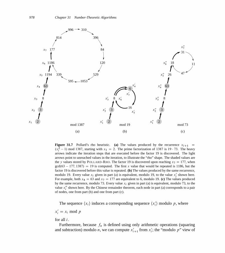
978 Chapter 31 Number-Theoretic Algorithms
996 310
396
84
120
529
1053595
339
814
1194
63
8
3
2
(b) (c)(a)
3
2
18
26
8
31
11
47
177
1186
mod 1387 mod 19 mod 73
8
6
16
63
3
2x1
x2
x3
x4
x5
x6
x7
x 01
x 02
x 03
x 04
x 05
x 06
x 07
x 001
x 002
x 003
x 004
x 005
x 006
x 007
Figure 31.7 Pollard’s rho heuristic. (a) The values produced by the recurrence xiC1 D.x2
i � 1/ mod 1387, starting with x1 D 2. The prime factorization of 1387 is 19 � 73. The heavyarrows indicate the iteration steps that are executed before the factor 19 is discovered. The lightarrows point to unreached values in the iteration, to illustrate the “rho” shape. The shaded values arethe y values stored by POLLARD-RHO. The factor 19 is discovered upon reaching x7 D 177, whengcd.63 � 177; 1387/ D 19 is computed. The first x value that would be repeated is 1186, but thefactor 19 is discovered before this value is repeated. (b) The values produced by the same recurrence,modulo 19. Every value xi given in part (a) is equivalent, modulo 19, to the value x0
i shown here.For example, both x4 D 63 and x7 D 177 are equivalent to 6, modulo 19. (c) The values producedby the same recurrence, modulo 73. Every value xi given in part (a) is equivalent, modulo 73, to thevalue x00
i shown here. By the Chinese remainder theorem, each node in part (a) corresponds to a pairof nodes, one from part (b) and one from part (c).
The sequence hxii induces a corresponding sequence hx 0ii modulo p, where
x 0i D xi mod p
for all i .Furthermore, because fn is defined using only arithmetic operations (squaring
and subtraction) modulo n, we can compute x 0iC1 from x 0
i ; the “modulo p” view of

31.9 Integer factorization 979
the sequence is a smaller version of what is happening modulo n:
x 0iC1 D xiC1 mod p
D fn.xi / mod p
D ..x2i � 1/ mod n/ mod p
D .x2i � 1/ mod p (by Exercise 31.1-7)
D ..xi mod p/2 � 1/ mod p
D ..x 0i/
2 � 1/ mod p
D fp.x 0i / :
Thus, although we are not explicitly computing the sequence hx 0ii, this sequence is
well defined and obeys the same recurrence as the sequence hxii.Reasoning as before, we find that the expected number of steps before the se-
quence hx 0ii repeats is ‚.
pp/. If p is small compared to n, the sequence hx 0
iimightrepeat much more quickly than the sequence hxii. Indeed, as parts (b) and (c) ofFigure 31.7 show, the hx 0
ii sequence repeats as soon as two elements of the se-quence hxii are merely equivalent modulo p, rather than equivalent modulo n.
Let t denote the index of the first repeated value in the hx 0ii sequence, and let
u > 0 denote the length of the cycle that has been thereby produced. That is, t
and u > 0 are the smallest values such that x 0tCi D x 0
tCuCi for all i � 0. By theabove arguments, the expected values of t and u are both ‚.
pp/. Note that if
x 0tCi D x 0
tCuCi , then p j .xtCuCi � xtCi/. Thus, gcd.xtCuCi � xtCi ; n/ > 1.Therefore, once POLLARD-RHO has saved as y any value xk such that k � t ,
then y mod p is always on the cycle modulo p. (If a new value is saved as y,that value is also on the cycle modulo p.) Eventually, k is set to a value thatis greater than u, and the procedure then makes an entire loop around the cyclemodulo p without changing the value of y. The procedure then discovers a factorof n when xi “runs into” the previously stored value of y, modulo p, that is, whenxi � y .mod p/.
Presumably, the factor found is the factor p, although it may occasionally hap-pen that a multiple of p is discovered. Since the expected values of both t and u are‚.p
p/, the expected number of steps required to produce the factor p is ‚.p
p/.This algorithm might not perform quite as expected, for two reasons. First, the
heuristic analysis of the running time is not rigorous, and it is possible that the cycleof values, modulo p, could be much larger than
pp. In this case, the algorithm
performs correctly but much more slowly than desired. In practice, this issue seemsto be moot. Second, the divisors of n produced by this algorithm might always beone of the trivial factors 1 or n. For example, suppose that n D pq, where p
and q are prime. It can happen that the values of t and u for p are identical withthe values of t and u for q, and thus the factor p is always revealed in the samegcd operation that reveals the factor q. Since both factors are revealed at the same
980 Chapter 31 Number-Theoretic Algorithms
time, the trivial factor pq D n is revealed, which is useless. Again, this problemseems to be insignificant in practice. If necessary, we can restart the heuristic witha different recurrence of the form xiC1 D .x2
i � c/ mod n. (We should avoid thevalues c D 0 and c D 2 for reasons we will not go into here, but other values arefine.)
Of course, this analysis is heuristic and not rigorous, since the recurrence isnot really “random.” Nonetheless, the procedure performs well in practice, andit seems to be as efficient as this heuristic analysis indicates. It is the method ofchoice for finding small prime factors of a large number. To factor a ˇ-bit compos-ite number n completely, we only need to find all prime factors less than bn1=2c,and so we expect POLLARD-RHO to require at most n1=4 D 2ˇ=4 arithmetic opera-tions and at most n1=4ˇ2 D 2ˇ=4ˇ2 bit operations. POLLARD-RHO’s ability to finda small factor p of n with an expected number ‚.
pp/ of arithmetic operations is
often its most appealing feature.
Exercises
31.9-1Referring to the execution history shown in Figure 31.7(a), when does POLLARD-RHO print the factor 73 of 1387?
31.9-2Suppose that we are given a function f W Zn ! Zn and an initial value x0 2 Zn.Define xi D f .xi�1/ for i D 1; 2; : : :. Let t and u > 0 be the smallest values suchthat xtCi D xtCuCi for i D 0; 1; : : :. In the terminology of Pollard’s rho algorithm,t is the length of the tail and u is the length of the cycle of the rho. Give an efficientalgorithm to determine t and u exactly, and analyze its running time.
31.9-3How many steps would you expect POLLARD-RHO to require to discover a factorof the form pe, where p is prime and e > 1?
31.9-4 ?
One disadvantage of POLLARD-RHO as written is that it requires one gcd compu-tation for each step of the recurrence. Instead, we could batch the gcd computa-tions by accumulating the product of several xi values in a row and then using thisproduct instead of xi in the gcd computation. Describe carefully how you wouldimplement this idea, why it works, and what batch size you would pick as the mosteffective when working on a ˇ-bit number n.

Problems for Chapter 31 981
Problems
31-1 Binary gcd algorithmMost computers can perform the operations of subtraction, testing the parity (oddor even) of a binary integer, and halving more quickly than computing remainders.This problem investigates the binary gcd algorithm, which avoids the remaindercomputations used in Euclid’s algorithm.
a. Prove that if a and b are both even, then gcd.a; b/ D 2 � gcd.a=2; b=2/.
b. Prove that if a is odd and b is even, then gcd.a; b/ D gcd.a; b=2/.
c. Prove that if a and b are both odd, then gcd.a; b/ D gcd..a � b/=2; b/.
d. Design an efficient binary gcd algorithm for input integers a and b, wherea � b, that runs in O.lg a/ time. Assume that each subtraction, parity test,and halving takes unit time.
31-2 Analysis of bit operations in Euclid’s algorithma. Consider the ordinary “paper and pencil” algorithm for long division: dividing
a by b, which yields a quotient q and remainder r . Show that this methodrequires O..1C lg q/ lg b/ bit operations.
b. Define .a; b/ D .1C lg a/.1C lg b/. Show that the number of bit operationsperformed by EUCLID in reducing the problem of computing gcd.a; b/ to thatof computing gcd.b; a mod b/ is at most c. .a; b/� .b; a mod b// for somesufficiently large constant c > 0.
c. Show that EUCLID.a; b/ requires O. .a; b// bit operations in general andO.ˇ2/ bit operations when applied to two ˇ-bit inputs.
31-3 Three algorithms for Fibonacci numbersThis problem compares the efficiency of three methods for computing the nth Fi-bonacci number Fn, given n. Assume that the cost of adding, subtracting, or mul-tiplying two numbers is O.1/, independent of the size of the numbers.
a. Show that the running time of the straightforward recursive method for com-puting Fn based on recurrence (3.22) is exponential in n. (See, for example, theFIB procedure on page 775.)
b. Show how to compute Fn in O.n/ time using memoization.

982 Chapter 31 Number-Theoretic Algorithms
c. Show how to compute Fn in O.lg n/ time using only integer addition and mul-tiplication. (Hint: Consider the matrix�
0 1
1 1
�and its powers.)
d. Assume now that adding two ˇ-bit numbers takes ‚.ˇ/ time and that multi-plying two ˇ-bit numbers takes ‚.ˇ2/ time. What is the running time of thesethree methods under this more reasonable cost measure for the elementary arith-metic operations?
31-4 Quadratic residuesLet p be an odd prime. A number a 2 Z�
p is a quadratic residue if the equationx2 D a .mod p/ has a solution for the unknown x.
a. Show that there are exactly .p � 1/=2 quadratic residues, modulo p.
b. If p is prime, we define the Legendre symbol . ap
/, for a 2 Z�p, to be 1 if a is a
quadratic residue modulo p and �1 otherwise. Prove that if a 2 Z�p, then�a
p
�� a.p�1/=2 .mod p/ :
Give an efficient algorithm that determines whether a given number a is a qua-dratic residue modulo p. Analyze the efficiency of your algorithm.
c. Prove that if p is a prime of the form 4kC 3 and a is a quadratic residue in Z�p,
then akC1 mod p is a square root of a, modulo p. How much time is requiredto find the square root of a quadratic residue a modulo p?
d. Describe an efficient randomized algorithm for finding a nonquadratic residue,modulo an arbitrary prime p, that is, a member of Z
�p that is not a quadratic
residue. How many arithmetic operations does your algorithm require on aver-age?
Chapter notes
Niven and Zuckerman [265] provide an excellent introduction to elementary num-ber theory. Knuth [210] contains a good discussion of algorithms for finding the
Notes for Chapter 31 983
greatest common divisor, as well as other basic number-theoretic algorithms. Bach[30] and Riesel [295] provide more recent surveys of computational number the-ory. Dixon [92] gives an overview of factorization and primality testing. Theconference proceedings edited by Pomerance [280] contains several excellent sur-vey articles. More recently, Bach and Shallit [31] have provided an exceptionaloverview of the basics of computational number theory.
Knuth [210] discusses the origin of Euclid’s algorithm. It appears in Book 7,Propositions 1 and 2, of the Greek mathematician Euclid’s Elements, which waswritten around 300 B.C. Euclid’s description may have been derived from an al-gorithm due to Eudoxus around 375 B.C. Euclid’s algorithm may hold the honorof being the oldest nontrivial algorithm; it is rivaled only by an algorithm for mul-tiplication known to the ancient Egyptians. Shallit [312] chronicles the history ofthe analysis of Euclid’s algorithm.
Knuth attributes a special case of the Chinese remainder theorem (Theo-rem 31.27) to the Chinese mathematician Sun-Tsŭ, who lived sometime between200 B.C. and A.D. 200—the date is quite uncertain. The same special case wasgiven by the Greek mathematician Nichomachus around A.D. 100. It was gener-alized by Chhin Chiu-Shao in 1247. The Chinese remainder theorem was finallystated and proved in its full generality by L. Euler in 1734.
The randomized primality-testing algorithm presented here is due to Miller [255]and Rabin [289]; it is the fastest randomized primality-testing algorithm known,to within constant factors. The proof of Theorem 31.39 is a slight adaptation ofone suggested by Bach [29]. A proof of a stronger result for MILLER-RABIN
was given by Monier [258, 259]. Randomization appears to be necessary toobtain a polynomial-time primality-testing algorithm. The fastest deterministicprimality-testing algorithm known is the Cohen-Lenstra version [74] of the pri-mality test by Adleman, Pomerance, and Rumely [3]. When testing a number n
of length dlg.nC 1/e for primality, it runs in .lg n/O.lg lg lg n/ time, which is justslightly superpolynomial.
The problem of finding large “random” primes is nicely discussed in an articleby Beauchemin, Brassard, Crépeau, Goutier, and Pomerance [36].
The concept of a public-key cryptosystem is due to Diffie and Hellman [88].The RSA cryptosystem was proposed in 1977 by Rivest, Shamir, and Adleman[296]. Since then, the field of cryptography has blossomed. Our understandingof the RSA cryptosystem has deepened, and modern implementations use signif-icant refinements of the basic techniques presented here. In addition, many newtechniques have been developed for proving cryptosystems to be secure. For ex-ample, Goldwasser and Micali [142] show that randomization can be an effectivetool in the design of secure public-key encryption schemes. For signature schemes,Goldwasser, Micali, and Rivest [143] present a digital-signature scheme for which
984 Chapter 31 Number-Theoretic Algorithms
every conceivable type of forgery is provably as difficult as factoring. Menezeset al. [254] provide an overview of applied cryptography.
The rho heuristic for integer factorization was invented by Pollard [277]. Theversion presented here is a variant proposed by Brent [57].
The best algorithms for factoring large numbers have a running time that growsroughly exponentially with the cube root of the length of the number n to be fac-tored. The general number-field sieve factoring algorithm, as developed by Buhleret al. [58] as an extension of the ideas in the number-field sieve factoring algorithmby Pollard [278] and Lenstra et al. [232] and refined by Coppersmith [78] andothers, is perhaps the most efficient such algorithm in general for large inputs. Al-though it is difficult to give a rigorous analysis of this algorithm, under reasonableassumptions we can derive a running-time estimate of L.1=3; n/1:902Co.1/, whereL.˛; n/ D e.ln n/˛.ln ln n/1�˛
.The elliptic-curve method due to Lenstra [233] may be more effective for some
inputs than the number-field sieve method, since, like Pollard’s rho method, it canfind a small prime factor p quite quickly. With this method, the time to find p isestimated to be L.1=2; p/
p2Co.1/.
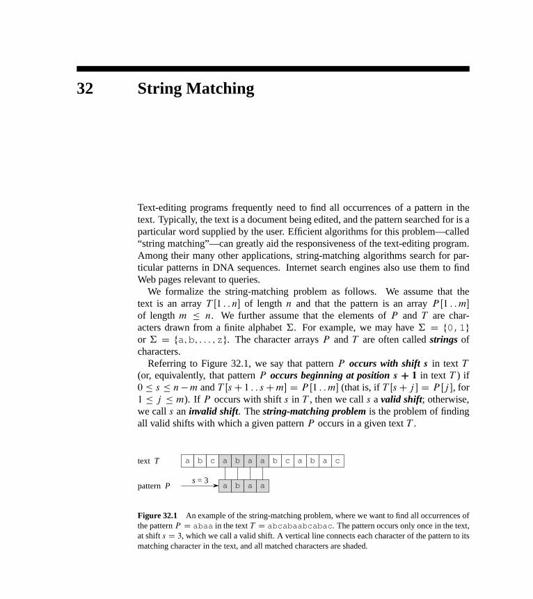
32 String Matching
Text-editing programs frequently need to find all occurrences of a pattern in thetext. Typically, the text is a document being edited, and the pattern searched for is aparticular word supplied by the user. Efficient algorithms for this problem—called“string matching”—can greatly aid the responsiveness of the text-editing program.Among their many other applications, string-matching algorithms search for par-ticular patterns in DNA sequences. Internet search engines also use them to findWeb pages relevant to queries.
We formalize the string-matching problem as follows. We assume that thetext is an array T Œ1 : : n� of length n and that the pattern is an array P Œ1 : : m�
of length m � n. We further assume that the elements of P and T are char-acters drawn from a finite alphabet †. For example, we may have † D f0,1gor † D fa; b; : : : ; zg. The character arrays P and T are often called strings ofcharacters.
Referring to Figure 32.1, we say that pattern P occurs with shift s in text T
(or, equivalently, that pattern P occurs beginning at position s C 1 in text T ) if0 � s � n�m and T ŒsC 1 : : sCm� D P Œ1 : : m� (that is, if T ŒsC j � D P Œj �, for1 � j � m). If P occurs with shift s in T , then we call s a valid shift; otherwise,we call s an invalid shift. The string-matching problem is the problem of findingall valid shifts with which a given pattern P occurs in a given text T .
a b c a b a a b c a b a c
a b a apattern P
text T
s = 3
Figure 32.1 An example of the string-matching problem, where we want to find all occurrences ofthe pattern P D abaa in the text T D abcabaabcabac. The pattern occurs only once in the text,at shift s D 3, which we call a valid shift. A vertical line connects each character of the pattern to itsmatching character in the text, and all matched characters are shaded.

986 Chapter 32 String Matching
Algorithm Preprocessing time Matching time
Naive 0 O..n �mC 1/m/
Rabin-Karp ‚.m/ O..n �mC 1/m/
Finite automaton O.m j†j/ ‚.n/
Knuth-Morris-Pratt ‚.m/ ‚.n/
Figure 32.2 The string-matching algorithms in this chapter and their preprocessing and matchingtimes.
Except for the naive brute-force algorithm, which we review in Section 32.1,each string-matching algorithm in this chapter performs some preprocessing basedon the pattern and then finds all valid shifts; we call this latter phase “matching.”Figure 32.2 shows the preprocessing and matching times for each of the algorithmsin this chapter. The total running time of each algorithm is the sum of the prepro-cessing and matching times. Section 32.2 presents an interesting string-matchingalgorithm, due to Rabin and Karp. Although the ‚..n � m C 1/m/ worst-caserunning time of this algorithm is no better than that of the naive method, it worksmuch better on average and in practice. It also generalizes nicely to other pattern-matching problems. Section 32.3 then describes a string-matching algorithm thatbegins by constructing a finite automaton specifically designed to search for occur-rences of the given pattern P in a text. This algorithm takes O.m j†j/ preprocess-ing time, but only ‚.n/ matching time. Section 32.4 presents the similar, but muchcleverer, Knuth-Morris-Pratt (or KMP) algorithm; it has the same ‚.n/ matchingtime, and it reduces the preprocessing time to only ‚.m/.
Notation and terminology
We denote by †� (read “sigma-star”) the set of all finite-length strings formedusing characters from the alphabet †. In this chapter, we consider only finite-length strings. The zero-length empty string, denoted ", also belongs to †�. Thelength of a string x is denoted jxj. The concatenation of two strings x and y,denoted xy, has length jxj C jyj and consists of the characters from x followed bythe characters from y.
We say that a string w is a prefix of a string x, denoted w � x, if x D wy forsome string y 2 †�. Note that if w � x, then jwj � jxj. Similarly, we say that astring w is a suffix of a string x, denoted w � x, if x D yw for some y 2 †�. Aswith a prefix, w � x implies jwj � jxj. For example, we have ab � abcca andcca � abcca. The empty string " is both a suffix and a prefix of every string. Forany strings x and y and any character a, we have x � y if and only if xa � ya.
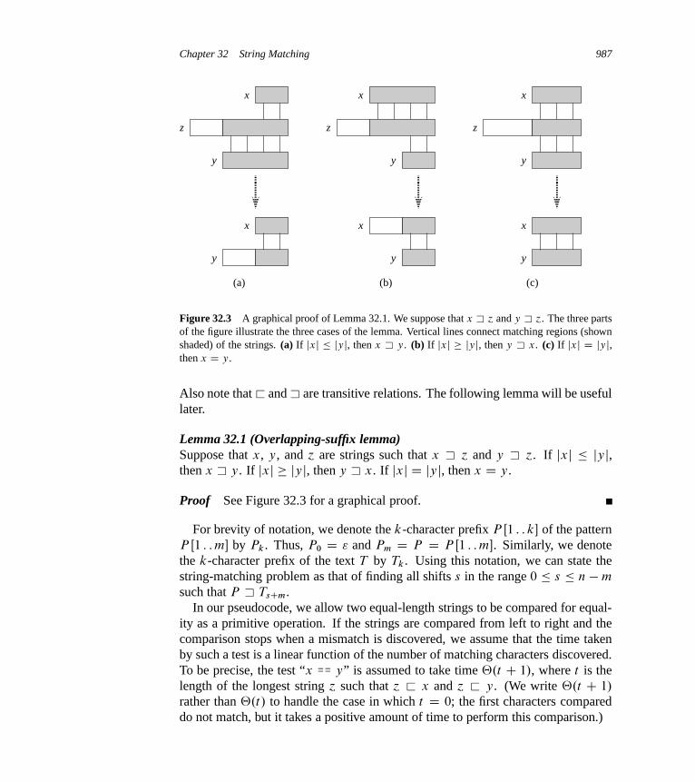
Chapter 32 String Matching 987
x
z
x
y
y
(a)
x
z
x
y
y
(b)
x
z
x
y
y
(c)
Figure 32.3 A graphical proof of Lemma 32.1. We suppose that x � ´ and y � ´. The three partsof the figure illustrate the three cases of the lemma. Vertical lines connect matching regions (shownshaded) of the strings. (a) If jxj � jyj, then x � y. (b) If jxj � jyj, then y � x. (c) If jxj D jyj,then x D y.
Also note that � and � are transitive relations. The following lemma will be usefullater.
Lemma 32.1 (Overlapping-suffix lemma)Suppose that x, y, and ´ are strings such that x � ´ and y � ´. If jxj � jyj,then x � y. If jxj � jyj, then y � x. If jxj D jyj, then x D y.
Proof See Figure 32.3 for a graphical proof.
For brevity of notation, we denote the k-character prefix P Œ1 : : k� of the patternP Œ1 : : m� by Pk. Thus, P0 D " and Pm D P D P Œ1 : : m�. Similarly, we denotethe k-character prefix of the text T by Tk. Using this notation, we can state thestring-matching problem as that of finding all shifts s in the range 0 � s � n �m
such that P � TsCm.In our pseudocode, we allow two equal-length strings to be compared for equal-
ity as a primitive operation. If the strings are compared from left to right and thecomparison stops when a mismatch is discovered, we assume that the time takenby such a test is a linear function of the number of matching characters discovered.To be precise, the test “x == y” is assumed to take time ‚.t C 1/, where t is thelength of the longest string ´ such that ´ � x and ´ � y. (We write ‚.t C 1/
rather than ‚.t/ to handle the case in which t D 0; the first characters compareddo not match, but it takes a positive amount of time to perform this comparison.)
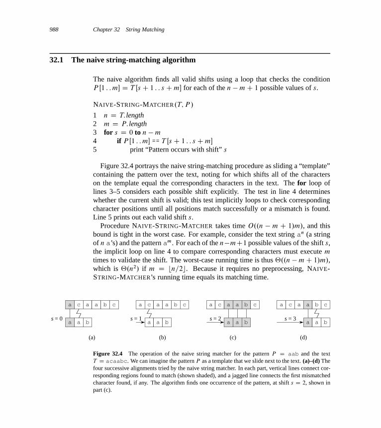
988 Chapter 32 String Matching
32.1 The naive string-matching algorithm
The naive algorithm finds all valid shifts using a loop that checks the conditionP Œ1 : : m� D T Œs C 1 : : s Cm� for each of the n �mC 1 possible values of s.
NAIVE-STRING-MATCHER.T; P /
1 n D T: length2 m D P: length3 for s D 0 to n �m
4 if P Œ1 : : m� == T Œs C 1 : : s Cm�
5 print “Pattern occurs with shift” s
Figure 32.4 portrays the naive string-matching procedure as sliding a “template”containing the pattern over the text, noting for which shifts all of the characterson the template equal the corresponding characters in the text. The for loop oflines 3–5 considers each possible shift explicitly. The test in line 4 determineswhether the current shift is valid; this test implicitly loops to check correspondingcharacter positions until all positions match successfully or a mismatch is found.Line 5 prints out each valid shift s.
Procedure NAIVE-STRING-MATCHER takes time O..n � m C 1/m/, and thisbound is tight in the worst case. For example, consider the text string an (a stringof n a’s) and the pattern am. For each of the n�mC1 possible values of the shift s,the implicit loop on line 4 to compare corresponding characters must execute m
times to validate the shift. The worst-case running time is thus ‚..n �mC 1/m/,which is ‚.n2/ if m D bn=2c. Because it requires no preprocessing, NAIVE-STRING-MATCHER’s running time equals its matching time.
a c a a b c
a a bs = 0
(a)
a c a a b c
a a bs = 1
(b)
a c a a b c
a a bs = 2
(c)
a c a a b c
a a bs = 3
(d)
Figure 32.4 The operation of the naive string matcher for the pattern P D aab and the textT D acaabc. We can imagine the pattern P as a template that we slide next to the text. (a)–(d) Thefour successive alignments tried by the naive string matcher. In each part, vertical lines connect cor-responding regions found to match (shown shaded), and a jagged line connects the first mismatchedcharacter found, if any. The algorithm finds one occurrence of the pattern, at shift s D 2, shown inpart (c).

32.1 The naive string-matching algorithm 989
As we shall see, NAIVE-STRING-MATCHER is not an optimal procedure for thisproblem. Indeed, in this chapter we shall see that the Knuth-Morris-Pratt algorithmis much better in the worst case. The naive string-matcher is inefficient becauseit entirely ignores information gained about the text for one value of s when itconsiders other values of s. Such information can be quite valuable, however. Forexample, if P D aaab and we find that s D 0 is valid, then none of the shifts 1, 2,or 3 are valid, since T Œ4� D b. In the following sections, we examine several waysto make effective use of this sort of information.
Exercises
32.1-1Show the comparisons the naive string matcher makes for the pattern P D 0001in the text T D 000010001010001.
32.1-2Suppose that all characters in the pattern P are different. Show how to accelerateNAIVE-STRING-MATCHER to run in time O.n/ on an n-character text T .
32.1-3Suppose that pattern P and text T are randomly chosen strings of length m and n,respectively, from the d -ary alphabet †d D f0; 1; : : : ; d � 1g, where d � 2. Showthat the expected number of character-to-character comparisons made by the im-plicit loop in line 4 of the naive algorithm is
.n �mC 1/1 � d �m
1 � d �1� 2.n �mC 1/
over all executions of this loop. (Assume that the naive algorithm stops comparingcharacters for a given shift once it finds a mismatch or matches the entire pattern.)Thus, for randomly chosen strings, the naive algorithm is quite efficient.
32.1-4Suppose we allow the pattern P to contain occurrences of a gap character } thatcan match an arbitrary string of characters (even one of zero length). For example,the pattern ab}ba}c occurs in the text cabccbacbacab as
c ab’ab
cc’}
ba’ba
cba“}
c’c
ab
and as
c ab’ab
ccbac—}
ba’ba
’}
c’c
ab :
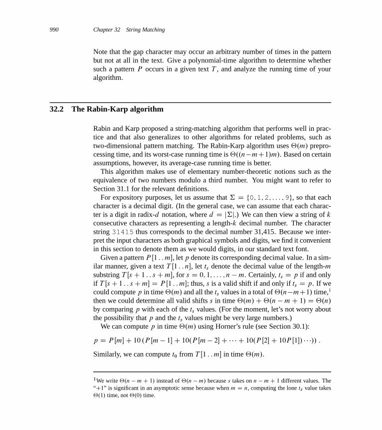
990 Chapter 32 String Matching
Note that the gap character may occur an arbitrary number of times in the patternbut not at all in the text. Give a polynomial-time algorithm to determine whethersuch a pattern P occurs in a given text T , and analyze the running time of youralgorithm.
32.2 The Rabin-Karp algorithm
Rabin and Karp proposed a string-matching algorithm that performs well in prac-tice and that also generalizes to other algorithms for related problems, such astwo-dimensional pattern matching. The Rabin-Karp algorithm uses ‚.m/ prepro-cessing time, and its worst-case running time is ‚..n�mC1/m/. Based on certainassumptions, however, its average-case running time is better.
This algorithm makes use of elementary number-theoretic notions such as theequivalence of two numbers modulo a third number. You might want to refer toSection 31.1 for the relevant definitions.
For expository purposes, let us assume that † D f0; 1; 2; : : : ; 9g, so that eachcharacter is a decimal digit. (In the general case, we can assume that each charac-ter is a digit in radix-d notation, where d D j†j.) We can then view a string of k
consecutive characters as representing a length-k decimal number. The characterstring 31415 thus corresponds to the decimal number 31,415. Because we inter-pret the input characters as both graphical symbols and digits, we find it convenientin this section to denote them as we would digits, in our standard text font.
Given a pattern P Œ1 : : m�, let p denote its corresponding decimal value. In a sim-ilar manner, given a text T Œ1 : : n�, let ts denote the decimal value of the length-msubstring T ŒsC 1 : : sCm�, for s D 0; 1; : : : ; n �m. Certainly, ts D p if and onlyif T ŒsC 1 : : sCm� D P Œ1 : : m�; thus, s is a valid shift if and only if ts D p. If wecould compute p in time ‚.m/ and all the ts values in a total of ‚.n�mC1/ time,1
then we could determine all valid shifts s in time ‚.m/C‚.n �mC 1/ D ‚.n/
by comparing p with each of the ts values. (For the moment, let’s not worry aboutthe possibility that p and the ts values might be very large numbers.)
We can compute p in time ‚.m/ using Horner’s rule (see Section 30.1):
p D P Œm�C 10 .P Œm� 1�C 10.P Œm� 2�C � � � C 10.P Œ2�C 10P Œ1�/ � � �// :
Similarly, we can compute t0 from T Œ1 : : m� in time ‚.m/.
1We write ‚.n �mC 1/ instead of ‚.n �m/ because s takes on n �mC 1 different values. The“C1” is significant in an asymptotic sense because when m D n, computing the lone ts value takes‚.1/ time, not ‚.0/ time.

32.2 The Rabin-Karp algorithm 991
To compute the remaining values t1; t2; : : : ; tn�m in time ‚.n �m/, we observethat we can compute tsC1 from ts in constant time, since
tsC1 D 10.ts � 10m�1T Œs C 1�/C T Œs CmC 1� : (32.1)
Subtracting 10m�1T Œs C 1� removes the high-order digit from ts , multiplying theresult by 10 shifts the number left by one digit position, and adding T Œs CmC 1�
brings in the appropriate low-order digit. For example, if m D 5 and ts D 31415,then we wish to remove the high-order digit T Œs C 1� D 3 and bring in the newlow-order digit (suppose it is T Œs C 5C 1� D 2) to obtain
tsC1 D 10.31415 � 10000 � 3/C 2
D 14152 :
If we precompute the constant 10m�1 (which we can do in time O.lg m/ using thetechniques of Section 31.6, although for this application a straightforward O.m/-time method suffices), then each execution of equation (32.1) takes a constant num-ber of arithmetic operations. Thus, we can compute p in time ‚.m/, and we cancompute all of t0; t1; : : : ; tn�m in time ‚.n �mC 1/. Therefore, we can find alloccurrences of the pattern P Œ1 : : m� in the text T Œ1 : : n� with ‚.m/ preprocessingtime and ‚.n �mC 1/ matching time.
Until now, we have intentionally overlooked one problem: p and ts may betoo large to work with conveniently. If P contains m characters, then we cannotreasonably assume that each arithmetic operation on p (which is m digits long)takes “constant time.” Fortunately, we can solve this problem easily, as Figure 32.5shows: compute p and the ts values modulo a suitable modulus q. We can computep modulo q in ‚.m/ time and all the ts values modulo q in ‚.n � m C 1/ time.If we choose the modulus q as a prime such that 10q just fits within one computerword, then we can perform all the necessary computations with single-precisionarithmetic. In general, with a d -ary alphabet f0; 1; : : : ; d � 1g, we choose q sothat dq fits within a computer word and adjust the recurrence equation (32.1) towork modulo q, so that it becomes
tsC1 D .d.ts � T Œs C 1�h/C T Œs CmC 1�/ mod q ; (32.2)
where h � d m�1 .mod q/ is the value of the digit “1” in the high-order positionof an m-digit text window.
The solution of working modulo q is not perfect, however: ts � p .mod q/
does not imply that ts D p. On the other hand, if ts 6� p .mod q/, then wedefinitely have that ts ¤ p, so that shift s is invalid. We can thus use the testts � p .mod q/ as a fast heuristic test to rule out invalid shifts s. Any shift s forwhich ts � p .mod q/ must be tested further to see whether s is really valid orwe just have a spurious hit. This additional test explicitly checks the condition
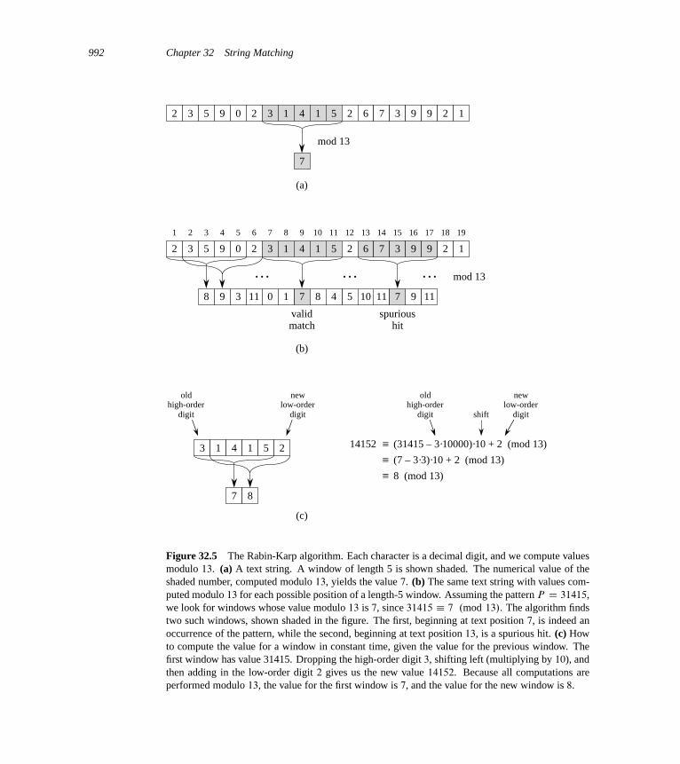
992 Chapter 32 String Matching
2 3 5 9 0 2 3 1 4 1 5 2 6 7 3 9 9 2 1
7
(a)
mod 13
2 3 5 9 0 2 3 1 4 1 5 2 6 7 3 9 9 2 1
7
(b)
mod 13
1 2 3 4 5 6 7 8 9 10 11 12 13 14 15 16 17 18 19
8 9 3 11 0 1 8 5 11 9 117104
validmatch
spurioushit
… … …
3 1 4 1 5 2
7 8
oldhigh-order
digit
newlow-order
digit
≡ (31415 – 3·10000)·10 + 2 (mod 13)
oldhigh-order
digit
newlow-order
digitshift
≡ (7 – 3·3)·10 + 2 (mod 13)
≡ 8 (mod 13)
(c)
14152
Figure 32.5 The Rabin-Karp algorithm. Each character is a decimal digit, and we compute valuesmodulo 13. (a) A text string. A window of length 5 is shown shaded. The numerical value of theshaded number, computed modulo 13, yields the value 7. (b) The same text string with values com-puted modulo 13 for each possible position of a length-5 window. Assuming the pattern P D 31415,we look for windows whose value modulo 13 is 7, since 31415 � 7 .mod 13/. The algorithm findstwo such windows, shown shaded in the figure. The first, beginning at text position 7, is indeed anoccurrence of the pattern, while the second, beginning at text position 13, is a spurious hit. (c) Howto compute the value for a window in constant time, given the value for the previous window. Thefirst window has value 31415. Dropping the high-order digit 3, shifting left (multiplying by 10), andthen adding in the low-order digit 2 gives us the new value 14152. Because all computations areperformed modulo 13, the value for the first window is 7, and the value for the new window is 8.
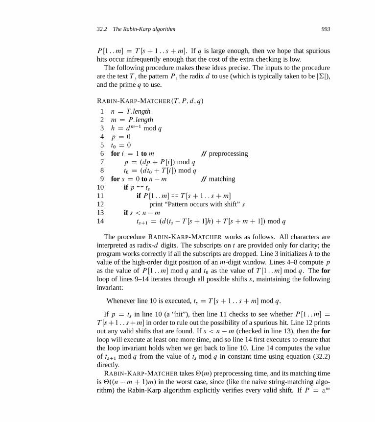
32.2 The Rabin-Karp algorithm 993
P Œ1 : : m� D T Œs C 1 : : s Cm�. If q is large enough, then we hope that spurioushits occur infrequently enough that the cost of the extra checking is low.
The following procedure makes these ideas precise. The inputs to the procedureare the text T , the pattern P , the radix d to use (which is typically taken to be j†j),and the prime q to use.
RABIN-KARP-MATCHER.T; P; d; q/
1 n D T: length2 m D P: length3 h D d m�1 mod q
4 p D 0
5 t0 D 0
6 for i D 1 to m // preprocessing7 p D .dp C P Œi�/ mod q
8 t0 D .dt0 C T Œi �/ mod q
9 for s D 0 to n �m // matching10 if p == ts11 if P Œ1 : : m� == T Œs C 1 : : s Cm�
12 print “Pattern occurs with shift” s
13 if s < n �m
14 tsC1 D .d.ts � T Œs C 1�h/C T Œs CmC 1�/ mod q
The procedure RABIN-KARP-MATCHER works as follows. All characters areinterpreted as radix-d digits. The subscripts on t are provided only for clarity; theprogram works correctly if all the subscripts are dropped. Line 3 initializes h to thevalue of the high-order digit position of an m-digit window. Lines 4–8 compute p
as the value of P Œ1 : : m� mod q and t0 as the value of T Œ1 : : m� mod q. The forloop of lines 9–14 iterates through all possible shifts s, maintaining the followinginvariant:
Whenever line 10 is executed, ts D T Œs C 1 : : s Cm� mod q.
If p D ts in line 10 (a “hit”), then line 11 checks to see whether P Œ1 : : m� DT ŒsC1 : : sCm� in order to rule out the possibility of a spurious hit. Line 12 printsout any valid shifts that are found. If s < n �m (checked in line 13), then the forloop will execute at least one more time, and so line 14 first executes to ensure thatthe loop invariant holds when we get back to line 10. Line 14 computes the valueof tsC1 mod q from the value of ts mod q in constant time using equation (32.2)directly.
RABIN-KARP-MATCHER takes ‚.m/ preprocessing time, and its matching timeis ‚..n �mC 1/m/ in the worst case, since (like the naive string-matching algo-rithm) the Rabin-Karp algorithm explicitly verifies every valid shift. If P D am

994 Chapter 32 String Matching
and T D an, then verifying takes time ‚..n�mC1/m/, since each of the n�mC1
possible shifts is valid.In many applications, we expect few valid shifts—perhaps some constant c of
them. In such applications, the expected matching time of the algorithm is onlyO..n �mC 1/C cm/ D O.n C m/, plus the time required to process spurioushits. We can base a heuristic analysis on the assumption that reducing values mod-ulo q acts like a random mapping from †� to Zq . (See the discussion on the use ofdivision for hashing in Section 11.3.1. It is difficult to formalize and prove such anassumption, although one viable approach is to assume that q is chosen randomlyfrom integers of the appropriate size. We shall not pursue this formalization here.)We can then expect that the number of spurious hits is O.n=q/, since we can es-timate the chance that an arbitrary ts will be equivalent to p, modulo q, as 1=q.Since there are O.n/ positions at which the test of line 10 fails and we spend O.m/
time for each hit, the expected matching time taken by the Rabin-Karp algorithmis
O.n/CO.m.� C n=q// ;
where � is the number of valid shifts. This running time is O.n/ if � D O.1/ andwe choose q � m. That is, if the expected number of valid shifts is small (O.1/)and we choose the prime q to be larger than the length of the pattern, then wecan expect the Rabin-Karp procedure to use only O.nCm/ matching time. Sincem � n, this expected matching time is O.n/.
Exercises
32.2-1Working modulo q D 11, how many spurious hits does the Rabin-Karp matcher en-counter in the text T D 3141592653589793 when looking for the pattern P D 26?
32.2-2How would you extend the Rabin-Karp method to the problem of searching a textstring for an occurrence of any one of a given set of k patterns? Start by assumingthat all k patterns have the same length. Then generalize your solution to allow thepatterns to have different lengths.
32.2-3Show how to extend the Rabin-Karp method to handle the problem of looking fora given m m pattern in an n n array of characters. (The pattern may be shiftedvertically and horizontally, but it may not be rotated.)
32.3 String matching with finite automata 995
32.2-4Alice has a copy of a long n-bit file A D han�1; an�2; : : : ; a0i, and Bob similarlyhas an n-bit file B D hbn�1; bn�2; : : : ; b0i. Alice and Bob wish to know if theirfiles are identical. To avoid transmitting all of A or B , they use the following fastprobabilistic check. Together, they select a prime q > 1000n and randomly selectan integer x from f0; 1; : : : ; q � 1g. Then, Alice evaluates
A.x/ D
n�1XiD0
aixi
!mod q
and Bob similarly evaluates B.x/. Prove that if A ¤ B , there is at most onechance in 1000 that A.x/ D B.x/, whereas if the two files are the same, A.x/ isnecessarily the same as B.x/. (Hint: See Exercise 31.4-4.)
32.3 String matching with finite automata
Many string-matching algorithms build a finite automaton—a simple machine forprocessing information—that scans the text string T for all occurrences of the pat-tern P . This section presents a method for building such an automaton. Thesestring-matching automata are very efficient: they examine each text character ex-actly once, taking constant time per text character. The matching time used—afterpreprocessing the pattern to build the automaton—is therefore ‚.n/. The time tobuild the automaton, however, can be large if † is large. Section 32.4 describes aclever way around this problem.
We begin this section with the definition of a finite automaton. We then examinea special string-matching automaton and show how to use it to find occurrencesof a pattern in a text. Finally, we shall show how to construct the string-matchingautomaton for a given input pattern.
Finite automata
A finite automaton M , illustrated in Figure 32.6, is a 5-tuple .Q; q0; A; †; ı/,where
� Q is a finite set of states,� q0 2 Q is the start state,� A � Q is a distinguished set of accepting states,� † is a finite input alphabet,� ı is a function from Q † into Q, called the transition function of M .
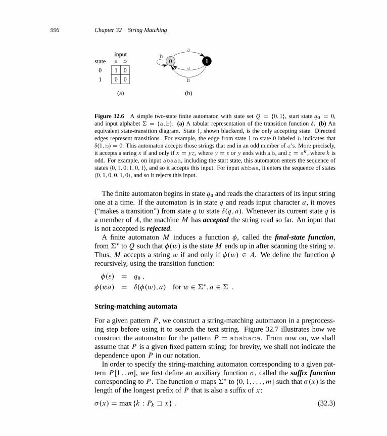
996 Chapter 32 String Matching
1 0
0 0
a binput
state
0
1
(a)
a
a
b
b
(b)
0 1
Figure 32.6 A simple two-state finite automaton with state set Q D f0; 1g, start state q0 D 0,and input alphabet † D fa; bg. (a) A tabular representation of the transition function ı. (b) Anequivalent state-transition diagram. State 1, shown blackend, is the only accepting state. Directededges represent transitions. For example, the edge from state 1 to state 0 labeled b indicates thatı.1; b/ D 0. This automaton accepts those strings that end in an odd number of a’s. More precisely,it accepts a string x if and only if x D y´, where y D " or y ends with a b, and ´ D ak , where k isodd. For example, on input abaaa, including the start state, this automaton enters the sequence ofstates h0; 1; 0; 1; 0; 1i, and so it accepts this input. For input abbaa, it enters the sequence of statesh0; 1; 0; 0; 1; 0i, and so it rejects this input.
The finite automaton begins in state q0 and reads the characters of its input stringone at a time. If the automaton is in state q and reads input character a, it moves(“makes a transition”) from state q to state ı.q; a/. Whenever its current state q isa member of A, the machine M has accepted the string read so far. An input thatis not accepted is rejected.
A finite automaton M induces a function �, called the final-state function,from †� to Q such that �.w/ is the state M ends up in after scanning the string w.Thus, M accepts a string w if and only if �.w/ 2 A. We define the function �
recursively, using the transition function:
�."/ D q0 ;
�.wa/ D ı.�.w/; a/ for w 2 †�; a 2 † .
String-matching automata
For a given pattern P , we construct a string-matching automaton in a preprocess-ing step before using it to search the text string. Figure 32.7 illustrates how weconstruct the automaton for the pattern P D ababaca. From now on, we shallassume that P is a given fixed pattern string; for brevity, we shall not indicate thedependence upon P in our notation.
In order to specify the string-matching automaton corresponding to a given pat-tern P Œ1 : : m�, we first define an auxiliary function , called the suffix functioncorresponding to P . The function maps †� to f0; 1; : : : ; mg such that .x/ is thelength of the longest prefix of P that is also a suffix of x:
.x/ D max fk W Pk � xg : (32.3)

32.3 String matching with finite automata 997
0 1 2 3 4 5 6 7a b a b a c a
b
aa
aa
b
(a)
1 0 0
1 2 0
3 0 0
1 4 0
5 0 0
1 4 6
7 0 0
1 2 0
0
1
2
3
4
5
6
7
stateinput
a b c
a
b
a
b
a
c
a
P
(b)
1 2 3 4 5 6 7 8 9 10 11
a b a b a b a c a b a
0 1 2 3 4 5 4 5 6 7 2 3
—
—
(c)
i
T Œi �
state �.Ti /
Figure 32.7 (a) A state-transition diagram for the string-matching automaton that accepts allstrings ending in the string ababaca. State 0 is the start state, and state 7 (shown blackened) isthe only accepting state. A directed edge from state i to state j labeled a represents ı.i; a/ D j . Theright-going edges forming the “spine” of the automaton, shown heavy in the figure, correspond tosuccessful matches between pattern and input characters. The left-going edges correspond to failingmatches. Some edges corresponding to failing matches are omitted; by convention, if a state i hasno outgoing edge labeled a for some a 2 †, then ı.i; a/ D 0. (b) The corresponding transitionfunction ı, and the pattern string P D ababaca. The entries corresponding to successful matchesbetween pattern and input characters are shown shaded. (c) The operation of the automaton on thetext T D abababacaba. Under each text character T Œi� appears the state �.Ti / that the automa-ton is in after processing the prefix Ti . The automaton finds one occurrence of the pattern, ending inposition 9.
The suffix function is well defined since the empty string P0 D " is a suf-fix of every string. As examples, for the pattern P D ab, we have ."/ D 0,.ccaca/ D 1, and .ccab/ D 2. For a pattern P of length m, we have.x/ D m if and only if P � x. From the definition of the suffix function,x � y implies .x/ � .y/.
We define the string-matching automaton that corresponds to a given patternP Œ1 : : m� as follows:

998 Chapter 32 String Matching
� The state set Q is f0; 1; : : : ; mg. The start state q0 is state 0, and state m is theonly accepting state.
� The transition function ı is defined by the following equation, for any state q
and character a:
ı.q; a/ D .Pqa/ : (32.4)
We define ı.q; a/ D .Pqa/ because we want to keep track of the longest prefixof the pattern P that has matched the text string T so far. We consider the mostrecently read characters of T , and in order for a substring of T —let’s say thesubstring ending at T Œi �—to match some prefix Pj of P , this prefix Pj must be asuffix of Ti . Suppose that q D �.Ti /, so that after reading Ti , the automaton is instate q. We design the transition function ı so that this state number, q, tells us thelength of the longest prefix of P that matches a suffix of Ti . That is, in state q,Pq � Ti and q D .Ti/. (Whenever q D m, all m characters of P match a suffixof Ti , and so we have found a match.) Thus, since �.Ti / and .Ti / both equal q,we shall see (in Theorem 32.4, below) that the automaton maintains the followinginvariant:
�.Ti / D .Ti / : (32.5)
If the automaton is in state q and reads the next character T Œi C 1� D a, then wewant the transition to lead to the state corresponding to the longest prefix of P thatis a suffix of Tia, and that state is .Tia/. Because Pq is the longest prefix of P
that is a suffix of Ti , the longest prefix of P that is a suffix of Tia is not only .Tia/,but also .Pqa/. (Lemma 32.3, below, proves that .Tia/ D .Pqa/.) Thus,when the automaton is in state q, we want the transition function on character a totake the automaton to state .Pqa/.
There are two cases to consider. In the first case, a D P Œq C 1�, so that thecharacter a continues to match the pattern; in this case, because ı.q; a/ D qC1, thetransition continues to go along the “spine” of the automaton (the heavy edges inFigure 32.7). In the second case, a ¤ P ŒqC1�, so that a does not continue to matchthe pattern. Here, we must find a smaller prefix of P that is also a suffix of Ti .Because the preprocessing step matches the pattern against itself when creating thestring-matching automaton, the transition function quickly identifies the longestsuch smaller prefix of P .
Let’s look at an example. The string-matching automaton of Figure 32.7 hası.5; c/ D 6, illustrating the first case, in which the match continues. To illus-trate the second case, observe that the automaton of Figure 32.7 has ı.5; b/ D 4.We make this transition because if the automaton reads a b in state q D 5, thenPqb D ababab, and the longest prefix of P that is also a suffix of ababab isP4 D abab.
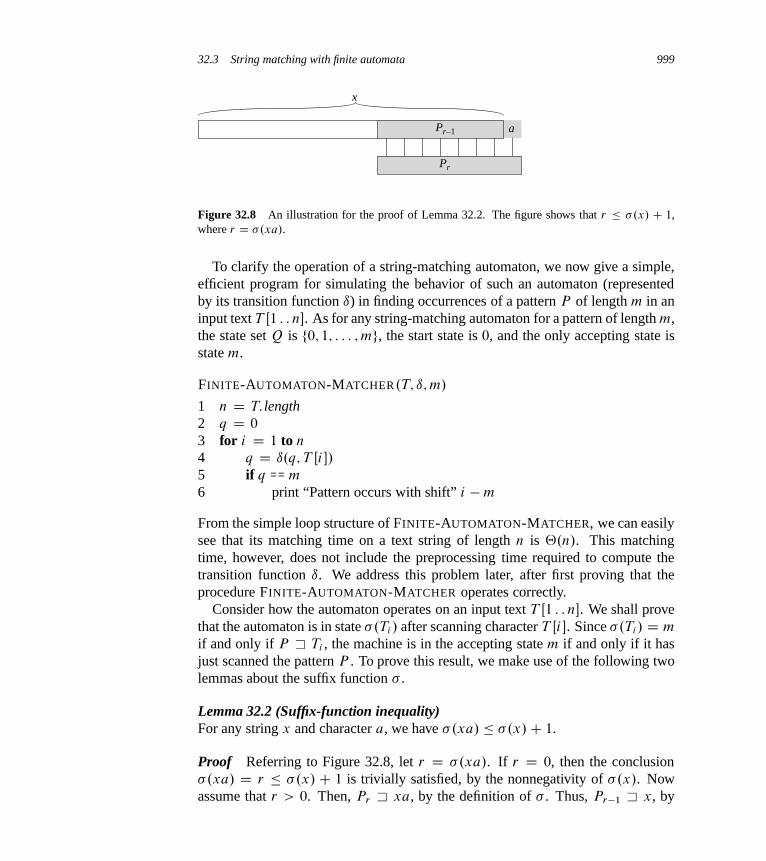
32.3 String matching with finite automata 999
x
a
Pr
Pr–1
Figure 32.8 An illustration for the proof of Lemma 32.2. The figure shows that r � .x/ C 1,where r D .xa/.
To clarify the operation of a string-matching automaton, we now give a simple,efficient program for simulating the behavior of such an automaton (representedby its transition function ı) in finding occurrences of a pattern P of length m in aninput text T Œ1 : : n�. As for any string-matching automaton for a pattern of length m,the state set Q is f0; 1; : : : ; mg, the start state is 0, and the only accepting state isstate m.
FINITE-AUTOMATON-MATCHER.T; ı; m/
1 n D T: length2 q D 0
3 for i D 1 to n
4 q D ı.q; T Œi �/
5 if q == m
6 print “Pattern occurs with shift” i �m
From the simple loop structure of FINITE-AUTOMATON-MATCHER, we can easilysee that its matching time on a text string of length n is ‚.n/. This matchingtime, however, does not include the preprocessing time required to compute thetransition function ı. We address this problem later, after first proving that theprocedure FINITE-AUTOMATON-MATCHER operates correctly.
Consider how the automaton operates on an input text T Œ1 : : n�. We shall provethat the automaton is in state .Ti / after scanning character T Œi �. Since .Ti/ D m
if and only if P � Ti , the machine is in the accepting state m if and only if it hasjust scanned the pattern P . To prove this result, we make use of the following twolemmas about the suffix function .
Lemma 32.2 (Suffix-function inequality)For any string x and character a, we have .xa/ � .x/C 1.
Proof Referring to Figure 32.8, let r D .xa/. If r D 0, then the conclusion.xa/ D r � .x/C 1 is trivially satisfied, by the nonnegativity of .x/. Nowassume that r > 0. Then, Pr � xa, by the definition of . Thus, Pr�1 � x, by
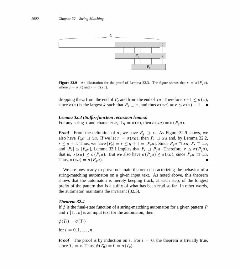
1000 Chapter 32 String Matching
x
a
aPq
Pr
Figure 32.9 An illustration for the proof of Lemma 32.3. The figure shows that r D .Pqa/,where q D .x/ and r D .xa/.
dropping the a from the end of Pr and from the end of xa. Therefore, r�1 � .x/,since .x/ is the largest k such that Pk � x, and thus .xa/ D r � .x/C 1.
Lemma 32.3 (Suffix-function recursion lemma)For any string x and character a, if q D .x/, then .xa/ D .Pqa/.
Proof From the definition of , we have Pq � x. As Figure 32.9 shows, wealso have Pqa � xa. If we let r D .xa/, then Pr � xa and, by Lemma 32.2,r � qC 1. Thus, we have jPr j D r � qC 1 D jPqaj. Since Pqa � xa, Pr � xa,and jPr j � jPqaj, Lemma 32.1 implies that Pr � Pqa. Therefore, r � .Pqa/,that is, .xa/ � .Pqa/. But we also have .Pqa/ � .xa/, since Pqa � xa.Thus, .xa/ D .Pqa/.
We are now ready to prove our main theorem characterizing the behavior of astring-matching automaton on a given input text. As noted above, this theoremshows that the automaton is merely keeping track, at each step, of the longestprefix of the pattern that is a suffix of what has been read so far. In other words,the automaton maintains the invariant (32.5).
Theorem 32.4If � is the final-state function of a string-matching automaton for a given pattern P
and T Œ1 : : n� is an input text for the automaton, then
�.Ti / D .Ti /
for i D 0; 1; : : : ; n.
Proof The proof is by induction on i . For i D 0, the theorem is trivially true,since T0 D ". Thus, �.T0/ D 0 D .T0/.
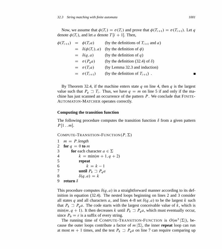
32.3 String matching with finite automata 1001
Now, we assume that �.Ti / D .Ti/ and prove that �.TiC1/ D .TiC1/. Let q
denote �.Ti /, and let a denote T Œi C 1�. Then,
�.TiC1/ D �.Tia/ (by the definitions of TiC1 and a)
D ı.�.Ti /; a/ (by the definition of �)
D ı.q; a/ (by the definition of q)
D .Pqa/ (by the definition (32.4) of ı)
D .Tia/ (by Lemma 32.3 and induction)
D .TiC1/ (by the definition of TiC1) .
By Theorem 32.4, if the machine enters state q on line 4, then q is the largestvalue such that Pq � Ti . Thus, we have q D m on line 5 if and only if the ma-chine has just scanned an occurrence of the pattern P . We conclude that FINITE-AUTOMATON-MATCHER operates correctly.
Computing the transition function
The following procedure computes the transition function ı from a given patternP Œ1 : : m�.
COMPUTE-TRANSITION-FUNCTION.P; †/
1 m D P: length2 for q D 0 to m
3 for each character a 2 †
4 k D min.mC 1; q C 2/
5 repeat6 k D k � 1
7 until Pk � Pqa
8 ı.q; a/ D k
9 return ı
This procedure computes ı.q; a/ in a straightforward manner according to its def-inition in equation (32.4). The nested loops beginning on lines 2 and 3 considerall states q and all characters a, and lines 4–8 set ı.q; a/ to be the largest k suchthat Pk � Pqa. The code starts with the largest conceivable value of k, which ismin.m; q C 1/. It then decreases k until Pk � Pqa, which must eventually occur,since P0 D " is a suffix of every string.
The running time of COMPUTE-TRANSITION-FUNCTION is O.m3 j†j/, be-cause the outer loops contribute a factor of m j†j, the inner repeat loop can runat most m C 1 times, and the test Pk � Pqa on line 7 can require comparing up

1002 Chapter 32 String Matching
to m characters. Much faster procedures exist; by utilizing some cleverly com-puted information about the pattern P (see Exercise 32.4-8), we can improve thetime required to compute ı from P to O.m j†j/. With this improved procedure forcomputing ı, we can find all occurrences of a length-m pattern in a length-n textover an alphabet † with O.m j†j/ preprocessing time and ‚.n/ matching time.
Exercises
32.3-1Construct the string-matching automaton for the pattern P D aabab and illustrateits operation on the text string T D aaababaabaababaab.
32.3-2Draw a state-transition diagram for a string-matching automaton for the patternababbabbababbababbabb over the alphabet † D fa; bg.32.3-3We call a pattern P nonoverlappable if Pk � Pq implies k D 0 or k D q. De-scribe the state-transition diagram of the string-matching automaton for a nonover-lappable pattern.
32.3-4 ?
Given two patterns P and P 0, describe how to construct a finite automaton thatdetermines all occurrences of either pattern. Try to minimize the number of statesin your automaton.
32.3-5Given a pattern P containing gap characters (see Exercise 32.1-4), show how tobuild a finite automaton that can find an occurrence of P in a text T in O.n/
matching time, where n D jT j.
? 32.4 The Knuth-Morris-Pratt algorithm
We now present a linear-time string-matching algorithm due to Knuth, Morris, andPratt. This algorithm avoids computing the transition function ı altogether, and itsmatching time is ‚.n/ using just an auxiliary function � , which we precomputefrom the pattern in time ‚.m/ and store in an array �Œ1 : : m�. The array � allowsus to compute the transition function ı efficiently (in an amortized sense) “on thefly” as needed. Loosely speaking, for any state q D 0; 1; : : : ; m and any character
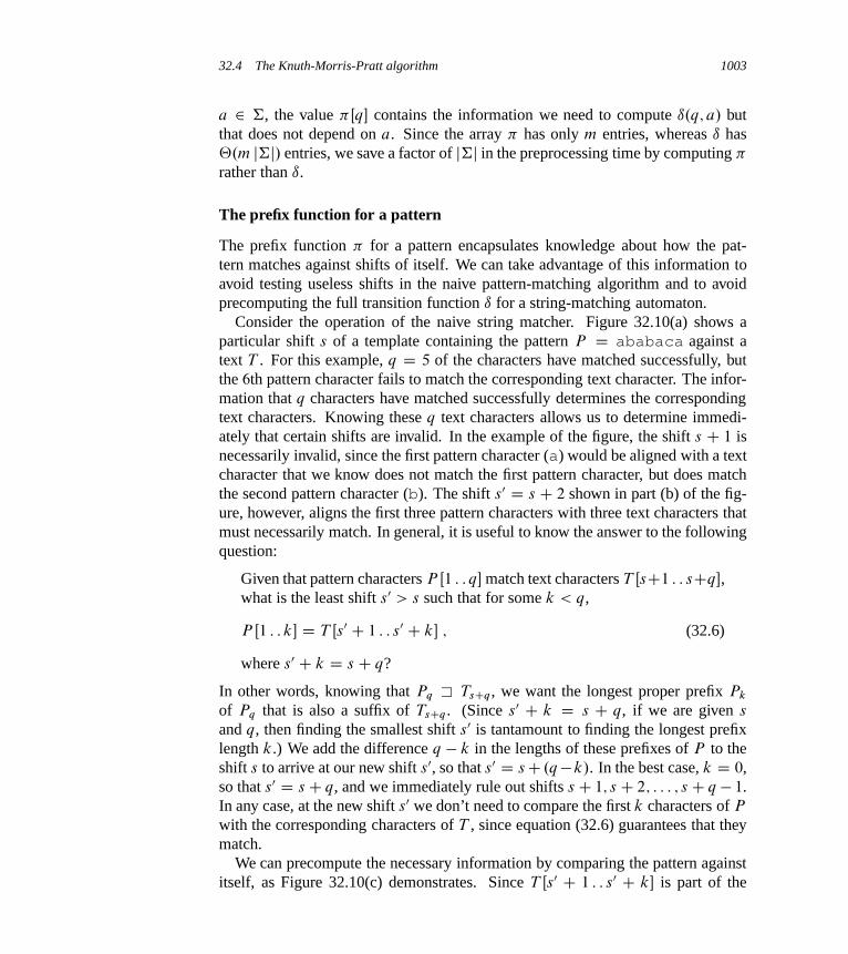
32.4 The Knuth-Morris-Pratt algorithm 1003
a 2 †, the value �Œq� contains the information we need to compute ı.q; a/ butthat does not depend on a. Since the array � has only m entries, whereas ı has‚.m j†j/ entries, we save a factor of j†j in the preprocessing time by computing �
rather than ı.
The prefix function for a pattern
The prefix function � for a pattern encapsulates knowledge about how the pat-tern matches against shifts of itself. We can take advantage of this information toavoid testing useless shifts in the naive pattern-matching algorithm and to avoidprecomputing the full transition function ı for a string-matching automaton.
Consider the operation of the naive string matcher. Figure 32.10(a) shows aparticular shift s of a template containing the pattern P D ababaca against atext T . For this example, q D 5 of the characters have matched successfully, butthe 6th pattern character fails to match the corresponding text character. The infor-mation that q characters have matched successfully determines the correspondingtext characters. Knowing these q text characters allows us to determine immedi-ately that certain shifts are invalid. In the example of the figure, the shift s C 1 isnecessarily invalid, since the first pattern character (a) would be aligned with a textcharacter that we know does not match the first pattern character, but does matchthe second pattern character (b). The shift s0 D s C 2 shown in part (b) of the fig-ure, however, aligns the first three pattern characters with three text characters thatmust necessarily match. In general, it is useful to know the answer to the followingquestion:
Given that pattern characters P Œ1 : : q� match text characters T ŒsC1 : : sCq�,what is the least shift s0 > s such that for some k < q,
P Œ1 : : k� D T Œs0 C 1 : : s0 C k� ; (32.6)
where s0 C k D s C q?
In other words, knowing that Pq � TsCq, we want the longest proper prefix Pk
of Pq that is also a suffix of TsCq. (Since s0 C k D s C q, if we are given s
and q, then finding the smallest shift s0 is tantamount to finding the longest prefixlength k.) We add the difference q � k in the lengths of these prefixes of P to theshift s to arrive at our new shift s0, so that s0 D sC .q�k/. In the best case, k D 0,so that s0 D sC q, and we immediately rule out shifts sC 1; s C 2; : : : ; sC q � 1.In any case, at the new shift s0 we don’t need to compare the first k characters of P
with the corresponding characters of T , since equation (32.6) guarantees that theymatch.
We can precompute the necessary information by comparing the pattern againstitself, as Figure 32.10(c) demonstrates. Since T Œs0 C 1 : : s0 C k� is part of the
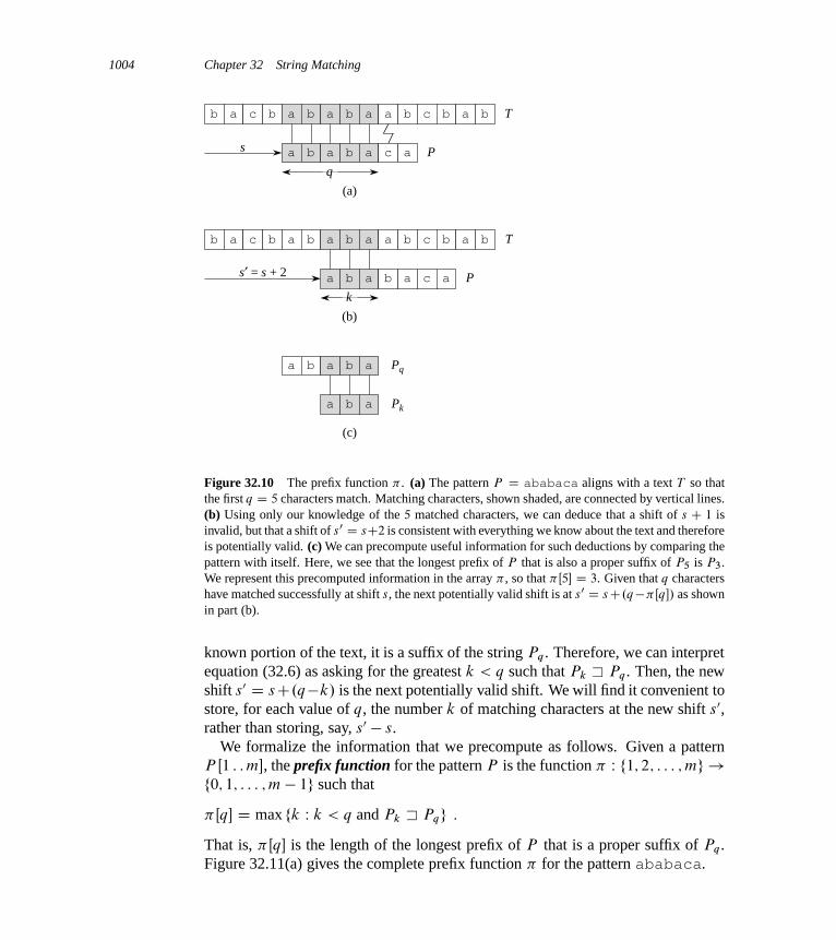
1004 Chapter 32 String Matching
b a c b a b
a b a
(a)
a b a a b c b a b
b a c as
T
P
q
b a c b a b
a b a
(b)
a b a a b c b a b
b a c as′ = s + 2
T
P
k
a b
a b a
a b a
(c)
Pq
Pk
Figure 32.10 The prefix function � . (a) The pattern P D ababaca aligns with a text T so thatthe first q D 5 characters match. Matching characters, shown shaded, are connected by vertical lines.(b) Using only our knowledge of the 5 matched characters, we can deduce that a shift of s C 1 isinvalid, but that a shift of s0 D sC2 is consistent with everything we know about the text and thereforeis potentially valid. (c) We can precompute useful information for such deductions by comparing thepattern with itself. Here, we see that the longest prefix of P that is also a proper suffix of P5 is P3.We represent this precomputed information in the array � , so that �Œ5� D 3. Given that q charactershave matched successfully at shift s, the next potentially valid shift is at s0 D sC.q��Œq�/ as shownin part (b).
known portion of the text, it is a suffix of the string Pq. Therefore, we can interpretequation (32.6) as asking for the greatest k < q such that Pk � Pq. Then, the newshift s0 D sC.q�k/ is the next potentially valid shift. We will find it convenient tostore, for each value of q, the number k of matching characters at the new shift s0,rather than storing, say, s0 � s.
We formalize the information that we precompute as follows. Given a patternP Œ1 : : m�, the prefix function for the pattern P is the function � W f1; 2; : : : ; mg !f0; 1; : : : ; m � 1g such that
�Œq� D max fk W k < q and Pk � Pqg :
That is, �Œq� is the length of the longest prefix of P that is a proper suffix of Pq.Figure 32.11(a) gives the complete prefix function � for the pattern ababaca.

32.4 The Knuth-Morris-Pratt algorithm 1005
1 2 3 4 5 6 7
0 0 1 2 3 0 1
a b a b a c a
(a)
a b a b a c a
a b a b a c a
a b a b a c a
a b a b a c a
(b)
"
i
P Œi �
�Œi �
P5
P3
P1
P0
�Œ5� D 3
�Œ3� D 1
�Œ1� D 0
Figure 32.11 An illustration of Lemma 32.5 for the pattern P D ababaca and q D 5. (a) The �
function for the given pattern. Since �Œ5� D 3, �Œ3� D 1, and �Œ1� D 0, by iterating � we obtain��Œ5� D f3; 1; 0g. (b) We slide the template containing the pattern P to the right and note when someprefix Pk of P matches up with some proper suffix of P5; we get matches when k D 3, 1, and 0. Inthe figure, the first row gives P , and the dotted vertical line is drawn just after P5. Successive rowsshow all the shifts of P that cause some prefix Pk of P to match some suffix of P5. Successfullymatched characters are shown shaded. Vertical lines connect aligned matching characters. Thus,fk W k < 5 and Pk � P5g D f3; 1; 0g. Lemma 32.5 claims that ��Œq� D fk W k < q and Pk � Pqgfor all q.
The pseudocode below gives the Knuth-Morris-Pratt matching algorithm asthe procedure KMP-MATCHER. For the most part, the procedure follows fromFINITE-AUTOMATON-MATCHER, as we shall see. KMP-MATCHER calls the aux-iliary procedure COMPUTE-PREFIX-FUNCTION to compute � .
KMP-MATCHER.T; P /
1 n D T: length2 m D P: length3 � D COMPUTE-PREFIX-FUNCTION.P /
4 q D 0 // number of characters matched5 for i D 1 to n // scan the text from left to right6 while q > 0 and P Œq C 1� ¤ T Œi �
7 q D �Œq� // next character does not match8 if P Œq C 1� == T Œi �
9 q D q C 1 // next character matches10 if q == m // is all of P matched?11 print “Pattern occurs with shift” i �m
12 q D �Œq� // look for the next match

1006 Chapter 32 String Matching
COMPUTE-PREFIX-FUNCTION.P /
1 m D P: length2 let �Œ1 : : m� be a new array3 �Œ1� D 0
4 k D 0
5 for q D 2 to m
6 while k > 0 and P Œk C 1� ¤ P Œq�
7 k D �Œk�
8 if P Œk C 1� == P Œq�
9 k D k C 1
10 �Œq� D k
11 return �
These two procedures have much in common, because both match a string againstthe pattern P : KMP-MATCHER matches the text T against P , and COMPUTE-PREFIX-FUNCTION matches P against itself.
We begin with an analysis of the running times of these procedures. Provingthese procedures correct will be more complicated.
Running-time analysis
The running time of COMPUTE-PREFIX-FUNCTION is ‚.m/, which we show byusing the aggregate method of amortized analysis (see Section 17.1). The onlytricky part is showing that the while loop of lines 6–7 executes O.m/ times alto-gether. We shall show that it makes at most m � 1 iterations. We start by makingsome observations about k. First, line 4 starts k at 0, and the only way that k
increases is by the increment operation in line 9, which executes at most once periteration of the for loop of lines 5–10. Thus, the total increase in k is at most m�1.Second, since k < q upon entering the for loop and each iteration of the loop in-crements q, we always have k < q. Therefore, the assignments in lines 3 and 10ensure that �Œq� < q for all q D 1; 2; : : : ; m, which means that each iteration ofthe while loop decreases k. Third, k never becomes negative. Putting these factstogether, we see that the total decrease in k from the while loop is bounded fromabove by the total increase in k over all iterations of the for loop, which is m � 1.Thus, the while loop iterates at most m � 1 times in all, and COMPUTE-PREFIX-FUNCTION runs in time ‚.m/.
Exercise 32.4-4 asks you to show, by a similar aggregate analysis, that the match-ing time of KMP-MATCHER is ‚.n/.
Compared with FINITE-AUTOMATON-MATCHER, by using � rather than ı, wehave reduced the time for preprocessing the pattern from O.m j†j/ to ‚.m/, whilekeeping the actual matching time bounded by ‚.n/.

32.4 The Knuth-Morris-Pratt algorithm 1007
Correctness of the prefix-function computation
We shall see a little later that the prefix function � helps us simulate the transitionfunction ı in a string-matching automaton. But first, we need to prove that theprocedure COMPUTE-PREFIX-FUNCTION does indeed compute the prefix func-tion correctly. In order to do so, we will need to find all prefixes Pk that are propersuffixes of a given prefix Pq. The value of �Œq� gives us the longest such prefix, butthe following lemma, illustrated in Figure 32.11, shows that by iterating the prefixfunction � , we can indeed enumerate all the prefixes Pk that are proper suffixesof Pq. Let
��Œq� D f�Œq�; � .2/Œq�; � .3/Œq�; : : : ; � .t/Œq�g ;
where � .i/Œq� is defined in terms of functional iteration, so that � .0/Œq� D q and� .i/Œq� D �Œ� .i�1/Œq�� for i � 1, and where the sequence in ��Œq� stops uponreaching � .t/Œq� D 0.
Lemma 32.5 (Prefix-function iteration lemma)Let P be a pattern of length m with prefix function � . Then, for q D 1; 2; : : : ; m,we have ��Œq� D fk W k < q and Pk � Pqg.
Proof We first prove that ��Œq� � fk W k < q and Pk � Pqg or, equivalently,
i 2 ��Œq� implies Pi � Pq : (32.7)
If i 2 ��Œq�, then i D � .u/Œq� for some u > 0. We prove equation (32.7) byinduction on u. For u D 1, we have i D �Œq�, and the claim follows since i < q
and P�Œq� � Pq by the definition of � . Using the relations �Œi� < i and P�Œi� � Pi
and the transitivity of < and � establishes the claim for all i in ��Œq�. Therefore,��Œq� � fk W k < q and Pk � Pqg.
We now prove that fk W k < q and Pk � Pqg � ��Œq� by contradiction. Sup-pose to the contrary that the set fk W k < q and Pk � Pqg � ��Œq� is nonempty,and let j be the largest number in the set. Because �Œq� is the largest value infk W k < q and Pk � Pqg and �Œq� 2 ��Œq�, we must have j < �Œq�, and so welet j 0 denote the smallest integer in ��Œq� that is greater than j . (We can choosej 0 D �Œq� if no other number in ��Œq� is greater than j .) We have Pj � Pq becausej 2 fk W k < q and Pk � Pqg, and from j 0 2 ��Œq� and equation (32.7), we havePj 0 � Pq. Thus, Pj � Pj 0 by Lemma 32.1, and j is the largest value less than j 0
with this property. Therefore, we must have �Œj 0� D j and, since j 0 2 ��Œq�, wemust have j 2 ��Œq� as well. This contradiction proves the lemma.
The algorithm COMPUTE-PREFIX-FUNCTION computes �Œq�, in order, for q D1; 2; : : : ; m. Setting �Œ1� to 0 in line 3 of COMPUTE-PREFIX-FUNCTION is cer-tainly correct, since �Œq� < q for all q. We shall use the following lemma and
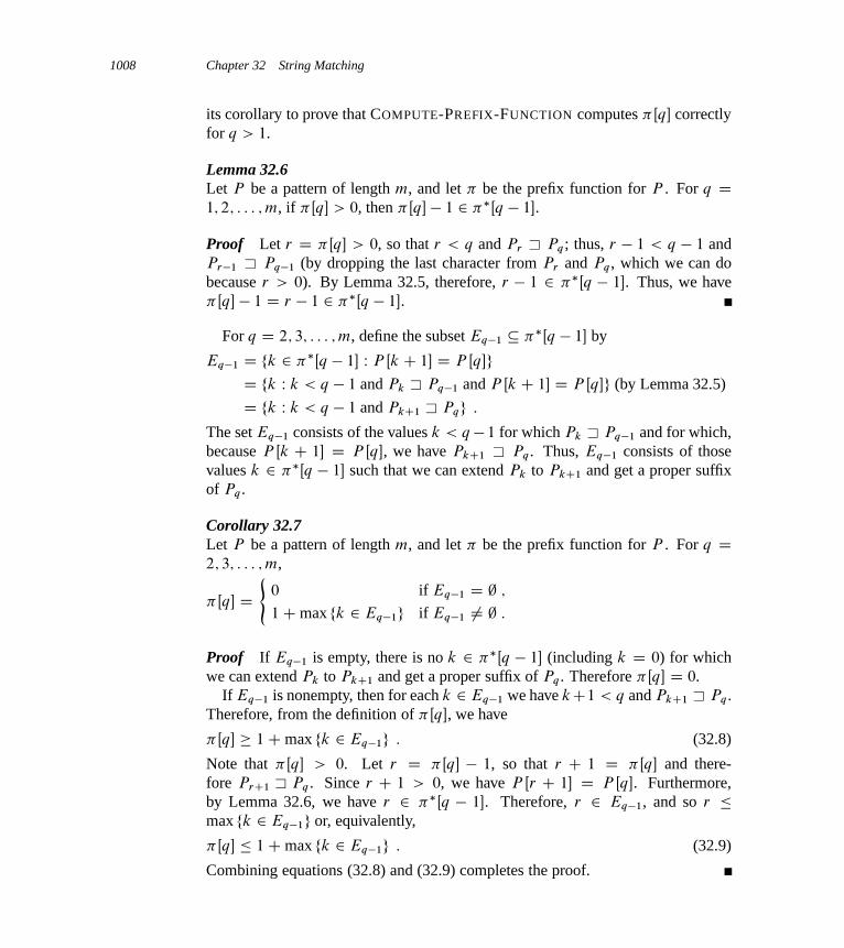
1008 Chapter 32 String Matching
its corollary to prove that COMPUTE-PREFIX-FUNCTION computes �Œq� correctlyfor q > 1.
Lemma 32.6Let P be a pattern of length m, and let � be the prefix function for P . For q D1; 2; : : : ; m, if �Œq� > 0, then �Œq� � 1 2 ��Œq � 1�.
Proof Let r D �Œq� > 0, so that r < q and Pr � Pq; thus, r � 1 < q � 1 andPr�1 � Pq�1 (by dropping the last character from Pr and Pq, which we can dobecause r > 0). By Lemma 32.5, therefore, r � 1 2 ��Œq � 1�. Thus, we have�Œq� � 1 D r � 1 2 ��Œq � 1�.
For q D 2; 3; : : : ; m, define the subset Eq�1 � ��Œq � 1� by
Eq�1 D fk 2 ��Œq � 1� W P Œk C 1� D P Œq�gD fk W k < q � 1 and Pk � Pq�1 and P Œk C 1� D P Œq�g (by Lemma 32.5)
D fk W k < q � 1 and PkC1 � Pqg :
The set Eq�1 consists of the values k < q� 1 for which Pk � Pq�1 and for which,because P Œk C 1� D P Œq�, we have PkC1 � Pq. Thus, Eq�1 consists of thosevalues k 2 ��Œq � 1� such that we can extend Pk to PkC1 and get a proper suffixof Pq.
Corollary 32.7Let P be a pattern of length m, and let � be the prefix function for P . For q D2; 3; : : : ; m,
�Œq� D(
0 if Eq�1 D ; ;
1Cmax fk 2 Eq�1g if Eq�1 ¤ ; :
Proof If Eq�1 is empty, there is no k 2 ��Œq � 1� (including k D 0) for whichwe can extend Pk to PkC1 and get a proper suffix of Pq. Therefore �Œq� D 0.
If Eq�1 is nonempty, then for each k 2 Eq�1 we have kC1 < q and PkC1 � Pq.Therefore, from the definition of �Œq�, we have
�Œq� � 1Cmax fk 2 Eq�1g : (32.8)
Note that �Œq� > 0. Let r D �Œq� � 1, so that r C 1 D �Œq� and there-fore PrC1 � Pq . Since r C 1 > 0, we have P Œr C 1� D P Œq�. Furthermore,by Lemma 32.6, we have r 2 ��Œq � 1�. Therefore, r 2 Eq�1, and so r �max fk 2 Eq�1g or, equivalently,
�Œq� � 1Cmax fk 2 Eq�1g : (32.9)
Combining equations (32.8) and (32.9) completes the proof.
32.4 The Knuth-Morris-Pratt algorithm 1009
We now finish the proof that COMPUTE-PREFIX-FUNCTION computes � cor-rectly. In the procedure COMPUTE-PREFIX-FUNCTION, at the start of each iter-ation of the for loop of lines 5–10, we have that k D �Œq � 1�. This conditionis enforced by lines 3 and 4 when the loop is first entered, and it remains true ineach successive iteration because of line 10. Lines 6–9 adjust k so that it becomesthe correct value of �Œq�. The while loop of lines 6–7 searches through all valuesk 2 ��Œq � 1� until it finds a value of k for which P Œk C 1� D P Œq�; at that point,k is the largest value in the set Eq�1, so that, by Corollary 32.7, we can set �Œq�
to kC 1. If the while loop cannot find a k 2 ��Œq� 1� such that P ŒkC 1� D P Œq�,then k equals 0 at line 8. If P Œ1� D P Œq�, then we should set both k and �Œq� to 1;otherwise we should leave k alone and set �Œq� to 0. Lines 8–10 set k and �Œq�
correctly in either case. This completes our proof of the correctness of COMPUTE-PREFIX-FUNCTION.
Correctness of the Knuth-Morris-Pratt algorithm
We can think of the procedure KMP-MATCHER as a reimplemented version ofthe procedure FINITE-AUTOMATON-MATCHER, but using the prefix function �
to compute state transitions. Specifically, we shall prove that in the i th iteration ofthe for loops of both KMP-MATCHER and FINITE-AUTOMATON-MATCHER, thestate q has the same value when we test for equality with m (at line 10 in KMP-MATCHER and at line 5 in FINITE-AUTOMATON-MATCHER). Once we haveargued that KMP-MATCHER simulates the behavior of FINITE-AUTOMATON-MATCHER, the correctness of KMP-MATCHER follows from the correctness ofFINITE-AUTOMATON-MATCHER (though we shall see a little later why line 12 inKMP-MATCHER is necessary).
Before we formally prove that KMP-MATCHER correctly simulates FINITE-AUTOMATON-MATCHER, let’s take a moment to understand how the prefix func-tion � replaces the ı transition function. Recall that when a string-matchingautomaton is in state q and it scans a character a D T Œi �, it moves to a newstate ı.q; a/. If a D P Œq C 1�, so that a continues to match the pattern, thenı.q; a/ D q C 1. Otherwise, a ¤ P Œq C 1�, so that a does not continue to matchthe pattern, and 0 � ı.q; a/ � q. In the first case, when a continues to match,KMP-MATCHER moves to state q C 1 without referring to the � function: thewhile loop test in line 6 comes up false the first time, the test in line 8 comes uptrue, and line 9 increments q.
The � function comes into play when the character a does not continue to matchthe pattern, so that the new state ı.q; a/ is either q or to the left of q along the spineof the automaton. The while loop of lines 6–7 in KMP-MATCHER iterates throughthe states in ��Œq�, stopping either when it arrives in a state, say q0, such that a
matches P Œq0 C 1� or q0 has gone all the way down to 0. If a matches P Œq0 C 1�,
1010 Chapter 32 String Matching
then line 9 sets the new state to q0C1, which should equal ı.q; a/ for the simulationto work correctly. In other words, the new state ı.q; a/ should be either state 0 orone greater than some state in ��Œq�.
Let’s look at the example in Figures 32.7 and 32.11, which are for the patternP D ababaca. Suppose that the automaton is in state q D 5; the states in��Œ5� are, in descending order, 3, 1, and 0. If the next character scanned is c, thenwe can easily see that the automaton moves to state ı.5; c/ D 6 in both FINITE-AUTOMATON-MATCHER and KMP-MATCHER. Now suppose that the next char-acter scanned is instead b, so that the automaton should move to state ı.5; b/ D 4.The while loop in KMP-MATCHER exits having executed line 7 once, and it ar-rives in state q0 D �Œ5� D 3. Since P Œq0 C 1� D P Œ4� D b, the test in line 8comes up true, and KMP-MATCHER moves to the new state q0C1 D 4 D ı.5; b/.Finally, suppose that the next character scanned is instead a, so that the automa-ton should move to state ı.5; a/ D 1. The first three times that the test in line 6executes, the test comes up true. The first time, we find that P Œ6� D c ¤ a, andKMP-MATCHER moves to state �Œ5� D 3 (the first state in ��Œ5�). The secondtime, we find that P Œ4� D b ¤ a and move to state �Œ3� D 1 (the second statein ��Œ5�). The third time, we find that P Œ2� D b ¤ a and move to state �Œ1� D 0
(the last state in ��Œ5�). The while loop exits once it arrives in state q0 D 0. Now,line 8 finds that P Œq0C1� D P Œ1� D a, and line 9 moves the automaton to the newstate q0 C 1 D 1 D ı.5; a/.
Thus, our intuition is that KMP-MATCHER iterates through the states in ��Œq� indecreasing order, stopping at some state q0 and then possibly moving to state q0C1.Although that might seem like a lot of work just to simulate computing ı.q; a/,bear in mind that asymptotically, KMP-MATCHER is no slower than FINITE-AUTOMATON-MATCHER.
We are now ready to formally prove the correctness of the Knuth-Morris-Prattalgorithm. By Theorem 32.4, we have that q D .Ti / after each time we executeline 4 of FINITE-AUTOMATON-MATCHER. Therefore, it suffices to show that thesame property holds with regard to the for loop in KMP-MATCHER. The proofproceeds by induction on the number of loop iterations. Initially, both proceduresset q to 0 as they enter their respective for loops for the first time. Consider itera-tion i of the for loop in KMP-MATCHER, and let q0 be state at the start of this loopiteration. By the inductive hypothesis, we have q0 D .Ti�1/. We need to showthat q D .Ti / at line 10. (Again, we shall handle line 12 separately.)
When we consider the character T Œi �, the longest prefix of P that is a suffix of Ti
is either Pq0C1 (if P Œq0 C 1� D T Œi �) or some prefix (not necessarily proper, andpossibly empty) of Pq0 . We consider separately the three cases in which .Ti/ D 0,.Ti / D q0 C 1, and 0 < .Ti/ � q0.
32.4 The Knuth-Morris-Pratt algorithm 1011
� If .Ti / D 0, then P0 D " is the only prefix of P that is a suffix of Ti . The whileloop of lines 6–7 iterates through the values in ��Œq0�, but although Pq � Ti forevery q 2 ��Œq0�, the loop never finds a q such that P ŒqC 1� D T Œi �. The loopterminates when q reaches 0, and of course line 9 does not execute. Therefore,q D 0 at line 10, so that q D .Ti/.
� If .Ti / D q0 C 1, then P Œq0 C 1� D T Œi �, and the while loop test in line 6fails the first time through. Line 9 executes, incrementing q so that afterwardwe have q D q0 C 1 D .Ti /.
� If 0 < .Ti/ � q0, then the while loop of lines 6–7 iterates at least once,checking in decreasing order each value q 2 ��Œq0� until it stops at some q < q0.Thus, Pq is the longest prefix of Pq0 for which P ŒqC1� D T Œi �, so that when thewhile loop terminates, q C 1 D .Pq0T Œi �/. Since q0 D .Ti�1/, Lemma 32.3implies that .Ti�1T Œi �/ D .Pq0T Œi �/. Thus, we have
q C 1 D .Pq0T Œi �/
D .Ti�1T Œi �/
D .Ti/
when the while loop terminates. After line 9 increments q, we have q D .Ti /.
Line 12 is necessary in KMP-MATCHER, because otherwise, we might refer-ence P ŒmC 1� on line 6 after finding an occurrence of P . (The argument thatq D .Ti�1/ upon the next execution of line 6 remains valid by the hint given inExercise 32.4-8: ı.m; a/ D ı.�Œm�; a/ or, equivalently, .P a/ D .P�Œm�a/ forany a 2 †.) The remaining argument for the correctness of the Knuth-Morris-Pratt algorithm follows from the correctness of FINITE-AUTOMATON-MATCHER,since we have shown that KMP-MATCHER simulates the behavior of FINITE-AUTOMATON-MATCHER.
Exercises
32.4-1Compute the prefix function � for the pattern ababbabbabbababbabb.
32.4-2Give an upper bound on the size of ��Œq� as a function of q. Give an example toshow that your bound is tight.
32.4-3Explain how to determine the occurrences of pattern P in the text T by examiningthe � function for the string P T (the string of length mCn that is the concatenationof P and T ).
1012 Chapter 32 String Matching
32.4-4Use an aggregate analysis to show that the running time of KMP-MATCHER
is ‚.n/.
32.4-5Use a potential function to show that the running time of KMP-MATCHER is ‚.n/.
32.4-6Show how to improve KMP-MATCHER by replacing the occurrence of � in line 7(but not line 12) by � 0, where � 0 is defined recursively for q D 1; 2; : : : ; m � 1 bythe equation
� 0Œq� D
�0 if �Œq� D 0 ;
� 0Œ�Œq�� if �Œq� ¤ 0 and P Œ�Œq�C 1� D P Œq C 1� ;
�Œq� if �Œq� ¤ 0 and P Œ�Œq�C 1� ¤ P Œq C 1� :
Explain why the modified algorithm is correct, and explain in what sense thischange constitutes an improvement.
32.4-7Give a linear-time algorithm to determine whether a text T is a cyclic rotation ofanother string T 0. For example, arc and car are cyclic rotations of each other.
32.4-8 ?
Give an O.m j†j/-time algorithm for computing the transition function ı for thestring-matching automaton corresponding to a given pattern P . (Hint: Prove thatı.q; a/ D ı.�Œq�; a/ if q D m or P Œq C 1� ¤ a.)
Problems
32-1 String matching based on repetition factorsLet yi denote the concatenation of string y with itself i times. For example,.ab/3 D ababab. We say that a string x 2 †� has repetition factor r if x D yr
for some string y 2 †� and some r > 0. Let �.x/ denote the largest r such that x
has repetition factor r .
a. Give an efficient algorithm that takes as input a pattern P Œ1 : : m� and computesthe value �.Pi/ for i D 1; 2; : : : ; m. What is the running time of your algo-rithm?

Notes for Chapter 32 1013
b. For any pattern P Œ1 : : m�, let ��.P / be defined as max1�i�m �.Pi/. Prove that ifthe pattern P is chosen randomly from the set of all binary strings of length m,then the expected value of ��.P / is O.1/.
c. Argue that the following string-matching algorithm correctly finds all occur-rences of pattern P in a text T Œ1 : : n� in time O.��.P /nCm/:
REPETITION-MATCHER.P; T /
1 m D P: length2 n D T: length3 k D 1C ��.P /
4 q D 0
5 s D 0
6 while s � n �m
7 if T Œs C q C 1� == P Œq C 1�
8 q D q C 1
9 if q == m
10 print “Pattern occurs with shift” s
11 if q == m or T Œs C q C 1� ¤ P Œq C 1�
12 s D s Cmax.1; dq=ke/13 q D 0
This algorithm is due to Galil and Seiferas. By extending these ideas greatly,they obtained a linear-time string-matching algorithm that uses only O.1/ stor-age beyond what is required for P and T .
Chapter notes
The relation of string matching to the theory of finite automata is discussed byAho, Hopcroft, and Ullman [5]. The Knuth-Morris-Pratt algorithm [214] wasinvented independently by Knuth and Pratt and by Morris; they published theirwork jointly. Reingold, Urban, and Gries [294] give an alternative treatment of theKnuth-Morris-Pratt algorithm. The Rabin-Karp algorithm was proposed by Rabinand Karp [201]. Galil and Seiferas [126] give an interesting deterministic linear-time string-matching algorithm that uses only O.1/ space beyond that required tostore the pattern and text.
33 Computational Geometry
Computational geometry is the branch of computer science that studies algorithmsfor solving geometric problems. In modern engineering and mathematics, com-putational geometry has applications in such diverse fields as computer graphics,robotics, VLSI design, computer-aided design, molecular modeling, metallurgy,manufacturing, textile layout, forestry, and statistics. The input to a computational-geometry problem is typically a description of a set of geometric objects, such asa set of points, a set of line segments, or the vertices of a polygon in counterclock-wise order. The output is often a response to a query about the objects, such aswhether any of the lines intersect, or perhaps a new geometric object, such as theconvex hull (smallest enclosing convex polygon) of the set of points.
In this chapter, we look at a few computational-geometry algorithms in twodimensions, that is, in the plane. We represent each input object by a set ofpoints fp1; p2; p3; : : :g, where each pi D .xi ; yi / and xi ; yi 2 R. For exam-ple, we represent an n-vertex polygon P by a sequence hp0; p1; p2; : : : ; pn�1iof its vertices in order of their appearance on the boundary of P . Computationalgeometry can also apply to three dimensions, and even higher-dimensional spaces,but such problems and their solutions can be very difficult to visualize. Even intwo dimensions, however, we can see a good sample of computational-geometrytechniques.
Section 33.1 shows how to answer basic questions about line segments effi-ciently and accurately: whether one segment is clockwise or counterclockwisefrom another that shares an endpoint, which way we turn when traversing twoadjoining line segments, and whether two line segments intersect. Section 33.2presents a technique called “sweeping” that we use to develop an O.n lg n/-timealgorithm for determining whether a set of n line segments contains any inter-sections. Section 33.3 gives two “rotational-sweep” algorithms that compute theconvex hull (smallest enclosing convex polygon) of a set of n points: Graham’sscan, which runs in time O.n lg n/, and Jarvis’s march, which takes O.nh/ time,where h is the number of vertices of the convex hull. Finally, Section 33.4 gives
33.1 Line-segment properties 1015
an O.n lg n/-time divide-and-conquer algorithm for finding the closest pair ofpoints in a set of n points in the plane.
33.1 Line-segment properties
Several of the computational-geometry algorithms in this chapter require answersto questions about the properties of line segments. A convex combination of twodistinct points p1 D .x1; y1/ and p2 D .x2; y2/ is any point p3 D .x3; y3/ suchthat for some ˛ in the range 0 � ˛ � 1, we have x3 D ˛x1 C .1 � ˛/x2 andy3 D ˛y1 C .1� ˛/y2. We also write that p3 D ˛p1 C .1 � ˛/p2. Intuitively, p3
is any point that is on the line passing through p1 and p2 and is on or between p1
and p2 on the line. Given two distinct points p1 and p2, the line segment p1p2
is the set of convex combinations of p1 and p2. We call p1 and p2 the endpointsof segment p1p2. Sometimes the ordering of p1 and p2 matters, and we speak ofthe directed segment ���!p1p2. If p1 is the origin .0; 0/, then we can treat the directedsegment ���!p1p2 as the vector p2.
In this section, we shall explore the following questions:
1. Given two directed segments ���!p0p1 and ���!p0p2, is ���!p0p1 clockwise from ���!p0p2
with respect to their common endpoint p0?
2. Given two line segments p0p1 and p1p2, if we traverse p0p1 and then p1p2,do we make a left turn at point p1?
3. Do line segments p1p2 and p3p4 intersect?
There are no restrictions on the given points.We can answer each question in O.1/ time, which should come as no surprise
since the input size of each question is O.1/. Moreover, our methods use only ad-ditions, subtractions, multiplications, and comparisons. We need neither divisionnor trigonometric functions, both of which can be computationally expensive andprone to problems with round-off error. For example, the “straightforward” methodof determining whether two segments intersect—compute the line equation of theform y D mx C b for each segment (m is the slope and b is the y-intercept),find the point of intersection of the lines, and check whether this point is on bothsegments—uses division to find the point of intersection. When the segments arenearly parallel, this method is very sensitive to the precision of the division opera-tion on real computers. The method in this section, which avoids division, is muchmore accurate.
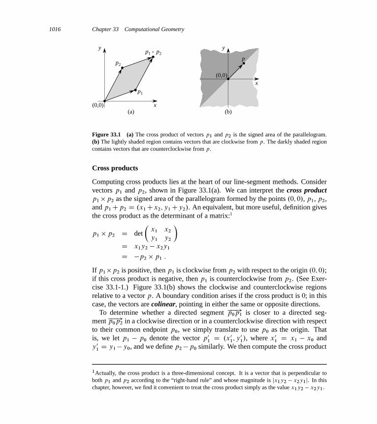
1016 Chapter 33 Computational Geometry
p2
x
y
(0,0)
p1
p1 + p2
(a) (b)
y
x(0,0)
p
Figure 33.1 (a) The cross product of vectors p1 and p2 is the signed area of the parallelogram.(b) The lightly shaded region contains vectors that are clockwise from p. The darkly shaded regioncontains vectors that are counterclockwise from p.
Cross products
Computing cross products lies at the heart of our line-segment methods. Considervectors p1 and p2, shown in Figure 33.1(a). We can interpret the cross productp1p2 as the signed area of the parallelogram formed by the points .0; 0/, p1, p2,and p1Cp2 D .x1Cx2; y1Cy2/. An equivalent, but more useful, definition givesthe cross product as the determinant of a matrix:1
p1 p2 D det
�x1 x2
y1 y2
�D x1y2 � x2y1
D �p2 p1 :
If p1p2 is positive, then p1 is clockwise from p2 with respect to the origin .0; 0/;if this cross product is negative, then p1 is counterclockwise from p2. (See Exer-cise 33.1-1.) Figure 33.1(b) shows the clockwise and counterclockwise regionsrelative to a vector p. A boundary condition arises if the cross product is 0; in thiscase, the vectors are colinear, pointing in either the same or opposite directions.
To determine whether a directed segment ���!p0p1 is closer to a directed seg-ment ���!p0p2 in a clockwise direction or in a counterclockwise direction with respectto their common endpoint p0, we simply translate to use p0 as the origin. Thatis, we let p1 � p0 denote the vector p0
1 D .x 01; y 0
1/, where x 01 D x1 � x0 and
y 01 D y1�y0, and we define p2�p0 similarly. We then compute the cross product
1Actually, the cross product is a three-dimensional concept. It is a vector that is perpendicular toboth p1 and p2 according to the “right-hand rule” and whose magnitude is jx1y2 � x2y1j. In thischapter, however, we find it convenient to treat the cross product simply as the value x1y2 � x2y1.
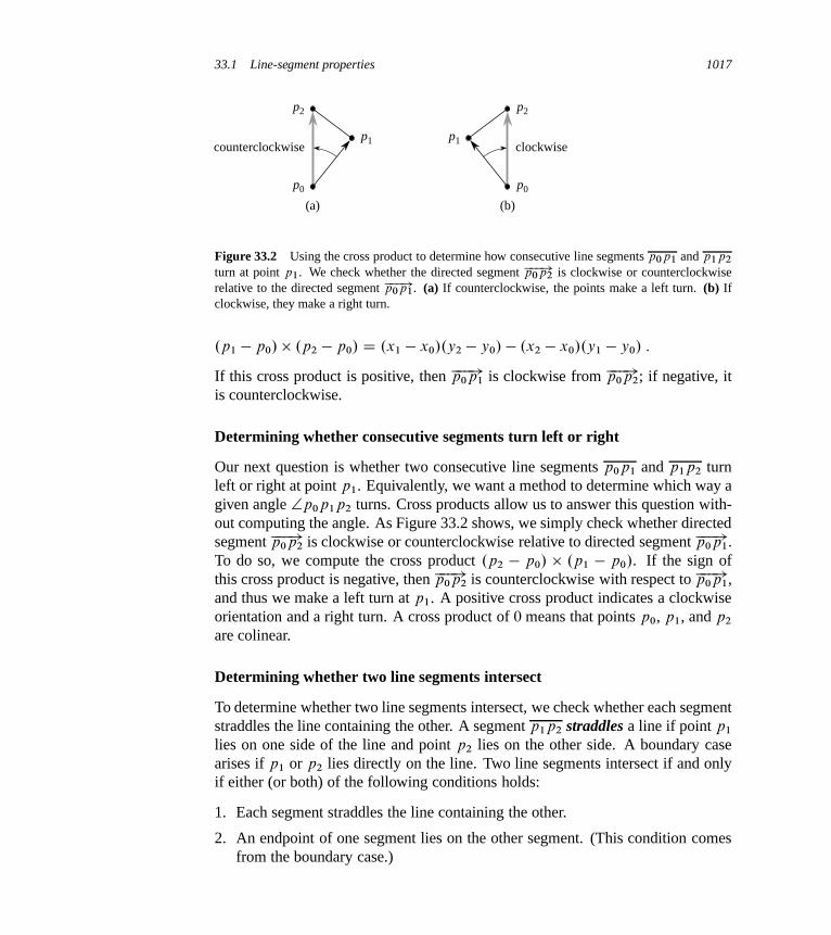
33.1 Line-segment properties 1017
p0
p1
p2
p0
p1
p2
counterclockwise
(a) (b)
clockwise
Figure 33.2 Using the cross product to determine how consecutive line segments p0p1 and p1p2
turn at point p1. We check whether the directed segment ���!p0p2 is clockwise or counterclockwiserelative to the directed segment ���!p0p1. (a) If counterclockwise, the points make a left turn. (b) Ifclockwise, they make a right turn.
.p1 � p0/ .p2 � p0/ D .x1 � x0/.y2 � y0/ � .x2 � x0/.y1 � y0/ :
If this cross product is positive, then ���!p0p1 is clockwise from ���!p0p2; if negative, itis counterclockwise.
Determining whether consecutive segments turn left or right
Our next question is whether two consecutive line segments p0p1 and p1p2 turnleft or right at point p1. Equivalently, we want a method to determine which way agiven angle †p0p1p2 turns. Cross products allow us to answer this question with-out computing the angle. As Figure 33.2 shows, we simply check whether directedsegment ���!p0p2 is clockwise or counterclockwise relative to directed segment ���!p0p1.To do so, we compute the cross product .p2 � p0/ .p1 � p0/. If the sign ofthis cross product is negative, then ���!p0p2 is counterclockwise with respect to ���!p0p1,and thus we make a left turn at p1. A positive cross product indicates a clockwiseorientation and a right turn. A cross product of 0 means that points p0, p1, and p2
are colinear.
Determining whether two line segments intersect
To determine whether two line segments intersect, we check whether each segmentstraddles the line containing the other. A segment p1p2 straddles a line if point p1
lies on one side of the line and point p2 lies on the other side. A boundary casearises if p1 or p2 lies directly on the line. Two line segments intersect if and onlyif either (or both) of the following conditions holds:
1. Each segment straddles the line containing the other.
2. An endpoint of one segment lies on the other segment. (This condition comesfrom the boundary case.)

1018 Chapter 33 Computational Geometry
The following procedures implement this idea. SEGMENTS-INTERSECT returnsTRUE if segments p1p2 and p3p4 intersect and FALSE if they do not. It callsthe subroutines DIRECTION, which computes relative orientations using the cross-product method above, and ON-SEGMENT, which determines whether a pointknown to be colinear with a segment lies on that segment.
SEGMENTS-INTERSECT.p1; p2; p3; p4/
1 d1 D DIRECTION.p3; p4; p1/
2 d2 D DIRECTION.p3; p4; p2/
3 d3 D DIRECTION.p1; p2; p3/
4 d4 D DIRECTION.p1; p2; p4/
5 if ..d1 > 0 and d2 < 0/ or .d1 < 0 and d2 > 0// and..d3 > 0 and d4 < 0/ or .d3 < 0 and d4 > 0//
6 return TRUE
7 elseif d1 == 0 and ON-SEGMENT.p3; p4; p1/
8 return TRUE
9 elseif d2 == 0 and ON-SEGMENT.p3; p4; p2/
10 return TRUE
11 elseif d3 == 0 and ON-SEGMENT.p1; p2; p3/
12 return TRUE
13 elseif d4 == 0 and ON-SEGMENT.p1; p2; p4/
14 return TRUE
15 else return FALSE
DIRECTION.pi ; pj ; pk/
1 return .pk � pi/ .pj � pi /
ON-SEGMENT.pi ; pj ; pk/
1 if min.xi ; xj / � xk � max.xi ; xj / and min.yi ; yj / � yk � max.yi ; yj /
2 return TRUE
3 else return FALSE
SEGMENTS-INTERSECT works as follows. Lines 1–4 compute the relative ori-entation di of each endpoint pi with respect to the other segment. If all the relativeorientations are nonzero, then we can easily determine whether segments p1p2
and p3p4 intersect, as follows. Segment p1p2 straddles the line containing seg-ment p3p4 if directed segments ���!p3p1 and ���!p3p2 have opposite orientations relativeto ���!p3p4. In this case, the signs of d1 and d2 differ. Similarly, p3p4 straddlesthe line containing p1p2 if the signs of d3 and d4 differ. If the test of line 5 istrue, then the segments straddle each other, and SEGMENTS-INTERSECT returnsTRUE. Figure 33.3(a) shows this case. Otherwise, the segments do not straddle
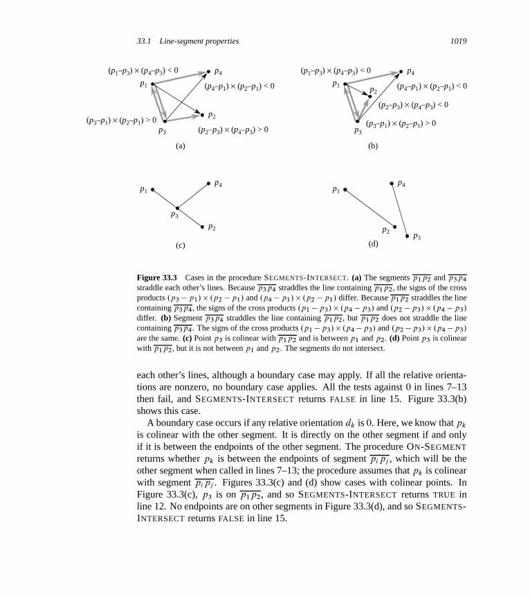
33.1 Line-segment properties 1019
p1
p2
p3
p4(p1–p3) × (p4–p3) < 0
(p4–p1) × (p2–p1) < 0
(p2–p3) × (p4–p3) > 0(p3–p1) × (p2–p1) > 0
(a)
p1 p2
p3
p4(p1–p3) × (p4–p3) < 0
(p4–p1) × (p2–p1) < 0
(p2–p3) × (p4–p3) < 0
(p3–p1) × (p2–p1) > 0
(b)
p1
p2
p3
p4
(c)
p1
p2 p3
p4
(d)
Figure 33.3 Cases in the procedure SEGMENTS-INTERSECT. (a) The segments p1p2 and p3p4
straddle each other’s lines. Because p3p4 straddles the line containing p1p2, the signs of the crossproducts .p3 �p1/ .p2 �p1/ and .p4 �p1/ .p2 �p1/ differ. Because p1p2 straddles the linecontaining p3p4, the signs of the cross products .p1 �p3/ .p4 �p3/ and .p2 �p3/ .p4 �p3/
differ. (b) Segment p3p4 straddles the line containing p1p2, but p1p2 does not straddle the linecontaining p3p4. The signs of the cross products .p1�p3/ .p4�p3/ and .p2�p3/ .p4�p3/
are the same. (c) Point p3 is colinear with p1p2 and is between p1 and p2. (d) Point p3 is colinearwith p1p2, but it is not between p1 and p2. The segments do not intersect.
each other’s lines, although a boundary case may apply. If all the relative orienta-tions are nonzero, no boundary case applies. All the tests against 0 in lines 7–13then fail, and SEGMENTS-INTERSECT returns FALSE in line 15. Figure 33.3(b)shows this case.
A boundary case occurs if any relative orientation dk is 0. Here, we know that pk
is colinear with the other segment. It is directly on the other segment if and onlyif it is between the endpoints of the other segment. The procedure ON-SEGMENT
returns whether pk is between the endpoints of segment pipj , which will be theother segment when called in lines 7–13; the procedure assumes that pk is colinearwith segment pipj . Figures 33.3(c) and (d) show cases with colinear points. InFigure 33.3(c), p3 is on p1p2, and so SEGMENTS-INTERSECT returns TRUE inline 12. No endpoints are on other segments in Figure 33.3(d), and so SEGMENTS-INTERSECT returns FALSE in line 15.
1020 Chapter 33 Computational Geometry
Other applications of cross products
Later sections of this chapter introduce additional uses for cross products. In Sec-tion 33.3, we shall need to sort a set of points according to their polar angles withrespect to a given origin. As Exercise 33.1-3 asks you to show, we can use crossproducts to perform the comparisons in the sorting procedure. In Section 33.2, weshall use red-black trees to maintain the vertical ordering of a set of line segments.Rather than keeping explicit key values which we compare to each other in thered-black tree code, we shall compute a cross-product to determine which of twosegments that intersect a given vertical line is above the other.
Exercises
33.1-1Prove that if p1 p2 is positive, then vector p1 is clockwise from vector p2 withrespect to the origin .0; 0/ and that if this cross product is negative, then p1 iscounterclockwise from p2.
33.1-2Professor van Pelt proposes that only the x-dimension needs to be tested in line 1of ON-SEGMENT. Show why the professor is wrong.
33.1-3The polar angle of a point p1 with respect to an origin point p0 is the angle of thevector p1 � p0 in the usual polar coordinate system. For example, the polar angleof .3; 5/ with respect to .2; 4/ is the angle of the vector .1; 1/, which is 45 degreesor �=4 radians. The polar angle of .3; 3/ with respect to .2; 4/ is the angle of thevector .1;�1/, which is 315 degrees or 7�=4 radians. Write pseudocode to sort asequence hp1; p2; : : : ; pni of n points according to their polar angles with respectto a given origin point p0. Your procedure should take O.n lg n/ time and use crossproducts to compare angles.
33.1-4Show how to determine in O.n2 lg n/ time whether any three points in a set of n
points are colinear.
33.1-5A polygon is a piecewise-linear, closed curve in the plane. That is, it is a curveending on itself that is formed by a sequence of straight-line segments, called thesides of the polygon. A point joining two consecutive sides is a vertex of the poly-gon. If the polygon is simple, as we shall generally assume, it does not cross itself.The set of points in the plane enclosed by a simple polygon forms the interior of
33.2 Determining whether any pair of segments intersects 1021
the polygon, the set of points on the polygon itself forms its boundary, and the setof points surrounding the polygon forms its exterior. A simple polygon is convexif, given any two points on its boundary or in its interior, all points on the linesegment drawn between them are contained in the polygon’s boundary or interior.A vertex of a convex polygon cannot be expressed as a convex combination of anytwo distinct points on the boundary or in the interior of the polygon.
Professor Amundsen proposes the following method to determine whether a se-quence hp0; p1; : : : ; pn�1i of n points forms the consecutive vertices of a convexpolygon. Output “yes” if the set f†pipiC1piC2 W i D 0; 1; : : : ; n � 1g, where sub-script addition is performed modulo n, does not contain both left turns and rightturns; otherwise, output “no.” Show that although this method runs in linear time,it does not always produce the correct answer. Modify the professor’s method sothat it always produces the correct answer in linear time.
33.1-6Given a point p0 D .x0; y0/, the right horizontal ray from p0 is the set of pointsfpi D .xi ; yi / W xi � x0 and yi D y0g, that is, it is the set of points due right of p0
along with p0 itself. Show how to determine whether a given right horizontal rayfrom p0 intersects a line segment p1p2 in O.1/ time by reducing the problem tothat of determining whether two line segments intersect.
33.1-7One way to determine whether a point p0 is in the interior of a simple, but notnecessarily convex, polygon P is to look at any ray from p0 and check that the rayintersects the boundary of P an odd number of times but that p0 itself is not onthe boundary of P . Show how to compute in ‚.n/ time whether a point p0 is inthe interior of an n-vertex polygon P . (Hint: Use Exercise 33.1-6. Make sure youralgorithm is correct when the ray intersects the polygon boundary at a vertex andwhen the ray overlaps a side of the polygon.)
33.1-8Show how to compute the area of an n-vertex simple, but not necessarily convex,polygon in ‚.n/ time. (See Exercise 33.1-5 for definitions pertaining to polygons.)
33.2 Determining whether any pair of segments intersects
This section presents an algorithm for determining whether any two line segmentsin a set of segments intersect. The algorithm uses a technique known as “sweep-ing,” which is common to many computational-geometry algorithms. Moreover, as

1022 Chapter 33 Computational Geometry
the exercises at the end of this section show, this algorithm, or simple variations ofit, can help solve other computational-geometry problems.
The algorithm runs in O.n lg n/ time, where n is the number of segments we aregiven. It determines only whether or not any intersection exists; it does not printall the intersections. (By Exercise 33.2-1, it takes �.n2/ time in the worst case tofind all the intersections in a set of n line segments.)
In sweeping, an imaginary vertical sweep line passes through the given set ofgeometric objects, usually from left to right. We treat the spatial dimension thatthe sweep line moves across, in this case the x-dimension, as a dimension oftime. Sweeping provides a method for ordering geometric objects, usually by plac-ing them into a dynamic data structure, and for taking advantage of relationshipsamong them. The line-segment-intersection algorithm in this section considers allthe line-segment endpoints in left-to-right order and checks for an intersection eachtime it encounters an endpoint.
To describe and prove correct our algorithm for determining whether any twoof n line segments intersect, we shall make two simplifying assumptions. First, weassume that no input segment is vertical. Second, we assume that no three inputsegments intersect at a single point. Exercises 33.2-8 and 33.2-9 ask you to showthat the algorithm is robust enough that it needs only a slight modification to workeven when these assumptions do not hold. Indeed, removing such simplifyingassumptions and dealing with boundary conditions often present the most difficultchallenges when programming computational-geometry algorithms and provingtheir correctness.
Ordering segments
Because we assume that there are no vertical segments, we know that any inputsegment intersecting a given vertical sweep line intersects it at a single point. Thus,we can order the segments that intersect a vertical sweep line according to the y-coordinates of the points of intersection.
To be more precise, consider two segments s1 and s2. We say that these segmentsare comparable at x if the vertical sweep line with x-coordinate x intersects both ofthem. We say that s1 is above s2 at x, written s1 <x s2, if s1 and s2 are comparableat x and the intersection of s1 with the sweep line at x is higher than the intersectionof s2 with the same sweep line, or if s1 and s2 intersect at the sweep line. InFigure 33.4(a), for example, we have the relationships a <r c, a <t b, b <t c,a <t c, and b <u c. Segment d is not comparable with any other segment.
For any given x, the relation “<x” is a total preorder (see Section B.2) for allsegments that intersect the sweep line at x. That is, the relation is transitive, andif segments s1 and s2 each intersect the sweep line at x, then either s1 <x s2
or s2 <x s1, or both (if s1 and s2 intersect at the sweep line). (The relation <x is
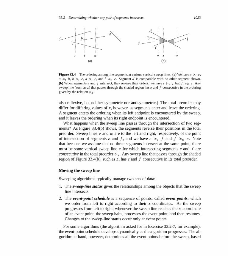
33.2 Determining whether any pair of segments intersects 1023
r t u
a
c
bd
(a) (b)
v w
e
f
gh
i
z
Figure 33.4 The ordering among line segments at various vertical sweep lines. (a) We have a <r c,a <t b, b <t c, a <t c, and b <u c. Segment d is comparable with no other segment shown.(b) When segments e and f intersect, they reverse their orders: we have e <� f but f <w e. Anysweep line (such as ´) that passes through the shaded region has e and f consecutive in the orderinggiven by the relation <´.
also reflexive, but neither symmetric nor antisymmetric.) The total preorder maydiffer for differing values of x, however, as segments enter and leave the ordering.A segment enters the ordering when its left endpoint is encountered by the sweep,and it leaves the ordering when its right endpoint is encountered.
What happens when the sweep line passes through the intersection of two seg-ments? As Figure 33.4(b) shows, the segments reverse their positions in the totalpreorder. Sweep lines � and w are to the left and right, respectively, of the pointof intersection of segments e and f , and we have e <� f and f <w e. Notethat because we assume that no three segments intersect at the same point, theremust be some vertical sweep line x for which intersecting segments e and f areconsecutive in the total preorder <x . Any sweep line that passes through the shadedregion of Figure 33.4(b), such as ´, has e and f consecutive in its total preorder.
Moving the sweep line
Sweeping algorithms typically manage two sets of data:
1. The sweep-line status gives the relationships among the objects that the sweepline intersects.
2. The event-point schedule is a sequence of points, called event points, whichwe order from left to right according to their x-coordinates. As the sweepprogresses from left to right, whenever the sweep line reaches the x-coordinateof an event point, the sweep halts, processes the event point, and then resumes.Changes to the sweep-line status occur only at event points.
For some algorithms (the algorithm asked for in Exercise 33.2-7, for example),the event-point schedule develops dynamically as the algorithm progresses. The al-gorithm at hand, however, determines all the event points before the sweep, based
1024 Chapter 33 Computational Geometry
solely on simple properties of the input data. In particular, each segment endpointis an event point. We sort the segment endpoints by increasing x-coordinate andproceed from left to right. (If two or more endpoints are covertical, i.e., they havethe same x-coordinate, we break the tie by putting all the covertical left endpointsbefore the covertical right endpoints. Within a set of covertical left endpoints, weput those with lower y-coordinates first, and we do the same within a set of cover-tical right endpoints.) When we encounter a segment’s left endpoint, we insert thesegment into the sweep-line status, and we delete the segment from the sweep-linestatus upon encountering its right endpoint. Whenever two segments first becomeconsecutive in the total preorder, we check whether they intersect.
The sweep-line status is a total preorder T , for which we require the followingoperations:
� INSERT.T; s/: insert segment s into T .
� DELETE.T; s/: delete segment s from T .
� ABOVE.T; s/: return the segment immediately above segment s in T .
� BELOW.T; s/: return the segment immediately below segment s in T .
It is possible for segments s1 and s2 to be mutually above each other in the totalpreorder T ; this situation can occur if s1 and s2 intersect at the sweep line whosetotal preorder is given by T . In this case, the two segments may appear in eitherorder in T .
If the input contains n segments, we can perform each of the operations INSERT,DELETE, ABOVE, and BELOW in O.lg n/ time using red-black trees. Recall thatthe red-black-tree operations in Chapter 13 involve comparing keys. We can re-place the key comparisons by comparisons that use cross products to determine therelative ordering of two segments (see Exercise 33.2-2).
Segment-intersection pseudocode
The following algorithm takes as input a set S of n line segments, returning theboolean value TRUE if any pair of segments in S intersects, and FALSE otherwise.A red-black tree maintains the total preorder T .
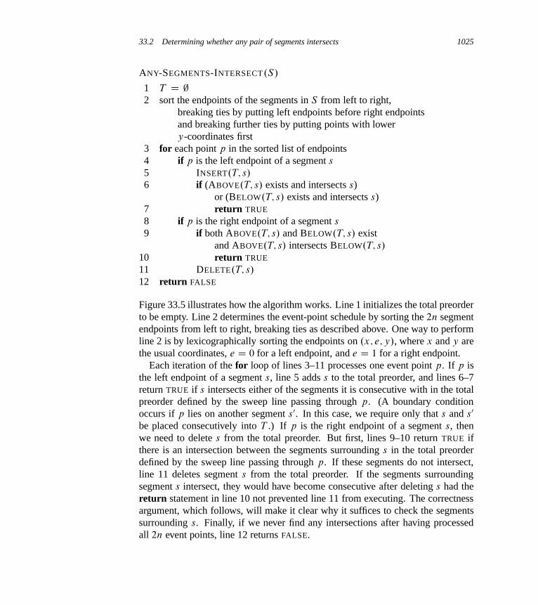
33.2 Determining whether any pair of segments intersects 1025
ANY-SEGMENTS-INTERSECT.S/
1 T D ;2 sort the endpoints of the segments in S from left to right,
breaking ties by putting left endpoints before right endpointsand breaking further ties by putting points with lowery-coordinates first
3 for each point p in the sorted list of endpoints4 if p is the left endpoint of a segment s
5 INSERT.T; s/
6 if (ABOVE.T; s/ exists and intersects s)or (BELOW.T; s/ exists and intersects s)
7 return TRUE
8 if p is the right endpoint of a segment s
9 if both ABOVE.T; s/ and BELOW.T; s/ existand ABOVE.T; s/ intersects BELOW.T; s/
10 return TRUE
11 DELETE.T; s/
12 return FALSE
Figure 33.5 illustrates how the algorithm works. Line 1 initializes the total preorderto be empty. Line 2 determines the event-point schedule by sorting the 2n segmentendpoints from left to right, breaking ties as described above. One way to performline 2 is by lexicographically sorting the endpoints on .x; e; y/, where x and y arethe usual coordinates, e D 0 for a left endpoint, and e D 1 for a right endpoint.
Each iteration of the for loop of lines 3–11 processes one event point p. If p isthe left endpoint of a segment s, line 5 adds s to the total preorder, and lines 6–7return TRUE if s intersects either of the segments it is consecutive with in the totalpreorder defined by the sweep line passing through p. (A boundary conditionoccurs if p lies on another segment s0. In this case, we require only that s and s0
be placed consecutively into T .) If p is the right endpoint of a segment s, thenwe need to delete s from the total preorder. But first, lines 9–10 return TRUE ifthere is an intersection between the segments surrounding s in the total preorderdefined by the sweep line passing through p. If these segments do not intersect,line 11 deletes segment s from the total preorder. If the segments surroundingsegment s intersect, they would have become consecutive after deleting s had thereturn statement in line 10 not prevented line 11 from executing. The correctnessargument, which follows, will make it clear why it suffices to check the segmentssurrounding s. Finally, if we never find any intersections after having processedall 2n event points, line 12 returns FALSE.

1026 Chapter 33 Computational Geometry
a ab
acb
dacb
dcb
edcb
a
b
c
de
f
time
Figure 33.5 The execution of ANY-SEGMENTS-INTERSECT. Each dashed line is the sweep line atan event point. Except for the rightmost sweep line, the ordering of segment names below each sweepline corresponds to the total preorder T at the end of the for loop processing the corresponding eventpoint. The rightmost sweep line occurs when processing the right endpoint of segment c; becausesegments d and b surround c and intersect each other, the procedure returns TRUE.
Correctness
To show that ANY-SEGMENTS-INTERSECT is correct, we will prove that the callANY-SEGMENTS-INTERSECT.S/ returns TRUE if and only if there is an intersec-tion among the segments in S .
It is easy to see that ANY-SEGMENTS-INTERSECT returns TRUE (on lines 7and 10) only if it finds an intersection between two of the input segments. Hence,if it returns TRUE, there is an intersection.
We also need to show the converse: that if there is an intersection, then ANY-SEGMENTS-INTERSECT returns TRUE. Let us suppose that there is at least oneintersection. Let p be the leftmost intersection point, breaking ties by choosing thepoint with the lowest y-coordinate, and let a and b be the segments that intersectat p. Since no intersections occur to the left of p, the order given by T is correct atall points to the left of p. Because no three segments intersect at the same point, a
and b become consecutive in the total preorder at some sweep line ´.2 Moreover,´ is to the left of p or goes through p. Some segment endpoint q on sweep line ´
2If we allow three segments to intersect at the same point, there may be an intervening segment c thatintersects both a and b at point p. That is, we may have a <w c and c <w b for all sweep lines w tothe left of p for which a <w b. Exercise 33.2-8 asks you to show that ANY-SEGMENTS-INTERSECT
is correct even if three segments do intersect at the same point.
33.2 Determining whether any pair of segments intersects 1027
is the event point at which a and b become consecutive in the total preorder. If p
is on sweep line ´, then q D p. If p is not on sweep line ´, then q is to the leftof p. In either case, the order given by T is correct just before encountering q.(Here is where we use the lexicographic order in which the algorithm processesevent points. Because p is the lowest of the leftmost intersection points, even if p
is on sweep line ´ and some other intersection point p0 is on ´, event point q D p
is processed before the other intersection p0 can interfere with the total preorder T .Moreover, even if p is the left endpoint of one segment, say a, and the right end-point of the other segment, say b, because left endpoint events occur before rightendpoint events, segment b is in T upon first encountering segment a.) Either eventpoint q is processed by ANY-SEGMENTS-INTERSECT or it is not processed.
If q is processed by ANY-SEGMENTS-INTERSECT, only two possible actionsmay occur:
1. Either a or b is inserted into T , and the other segment is above or below it inthe total preorder. Lines 4–7 detect this case.
2. Segments a and b are already in T , and a segment between them in the totalpreorder is deleted, making a and b become consecutive. Lines 8–11 detect thiscase.
In either case, we find the intersection p and ANY-SEGMENTS-INTERSECT returnsTRUE.
If event point q is not processed by ANY-SEGMENTS-INTERSECT, the proce-dure must have returned before processing all event points. This situation couldhave occurred only if ANY-SEGMENTS-INTERSECT had already found an inter-section and returned TRUE.
Thus, if there is an intersection, ANY-SEGMENTS-INTERSECT returns TRUE.As we have already seen, if ANY-SEGMENTS-INTERSECT returns TRUE, there isan intersection. Therefore, ANY-SEGMENTS-INTERSECT always returns a correctanswer.
Running time
If set S contains n segments, then ANY-SEGMENTS-INTERSECT runs in timeO.n lg n/. Line 1 takes O.1/ time. Line 2 takes O.n lg n/ time, using mergesort or heapsort. The for loop of lines 3–11 iterates at most once per event point,and so with 2n event points, the loop iterates at most 2n times. Each iteration takesO.lg n/ time, since each red-black-tree operation takes O.lg n/ time and, using themethod of Section 33.1, each intersection test takes O.1/ time. The total time isthus O.n lg n/.

1028 Chapter 33 Computational Geometry
Exercises
33.2-1Show that a set of n line segments may contain ‚.n2/ intersections.
33.2-2Given two segments a and b that are comparable at x, show how to determinein O.1/ time which of a <x b or b <x a holds. Assume that neither segmentis vertical. (Hint: If a and b do not intersect, you can just use cross products.If a and b intersect—which you can of course determine using only cross prod-ucts—you can still use only addition, subtraction, and multiplication, avoidingdivision. Of course, in the application of the <x relation used here, if a and b
intersect, we can just stop and declare that we have found an intersection.)
33.2-3Professor Mason suggests that we modify ANY-SEGMENTS-INTERSECT so thatinstead of returning upon finding an intersection, it prints the segments that inter-sect and continues on to the next iteration of the for loop. The professor calls theresulting procedure PRINT-INTERSECTING-SEGMENTS and claims that it printsall intersections, from left to right, as they occur in the set of line segments. Pro-fessor Dixon disagrees, claiming that Professor Mason’s idea is incorrect. Whichprofessor is right? Will PRINT-INTERSECTING-SEGMENTS always find the left-most intersection first? Will it always find all the intersections?
33.2-4Give an O.n lg n/-time algorithm to determine whether an n-vertex polygon issimple.
33.2-5Give an O.n lg n/-time algorithm to determine whether two simple polygons witha total of n vertices intersect.
33.2-6A disk consists of a circle plus its interior and is represented by its center point andradius. Two disks intersect if they have any point in common. Give an O.n lg n/-time algorithm to determine whether any two disks in a set of n intersect.
33.2-7Given a set of n line segments containing a total of k intersections, show how tooutput all k intersections in O..nC k/ lg n/ time.
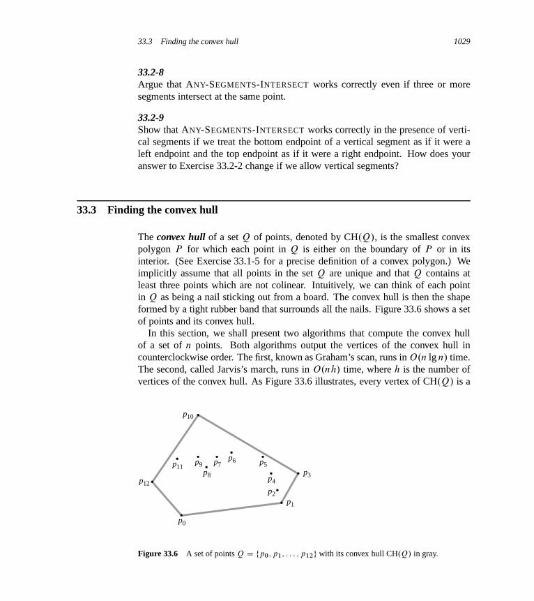
33.3 Finding the convex hull 1029
33.2-8Argue that ANY-SEGMENTS-INTERSECT works correctly even if three or moresegments intersect at the same point.
33.2-9Show that ANY-SEGMENTS-INTERSECT works correctly in the presence of verti-cal segments if we treat the bottom endpoint of a vertical segment as if it were aleft endpoint and the top endpoint as if it were a right endpoint. How does youranswer to Exercise 33.2-2 change if we allow vertical segments?
33.3 Finding the convex hull
The convex hull of a set Q of points, denoted by CH.Q/, is the smallest convexpolygon P for which each point in Q is either on the boundary of P or in itsinterior. (See Exercise 33.1-5 for a precise definition of a convex polygon.) Weimplicitly assume that all points in the set Q are unique and that Q contains atleast three points which are not colinear. Intuitively, we can think of each pointin Q as being a nail sticking out from a board. The convex hull is then the shapeformed by a tight rubber band that surrounds all the nails. Figure 33.6 shows a setof points and its convex hull.
In this section, we shall present two algorithms that compute the convex hullof a set of n points. Both algorithms output the vertices of the convex hull incounterclockwise order. The first, known as Graham’s scan, runs in O.n lg n/ time.The second, called Jarvis’s march, runs in O.nh/ time, where h is the number ofvertices of the convex hull. As Figure 33.6 illustrates, every vertex of CH.Q/ is a
p0
p1
p2
p3p4
p5p6p7
p8
p9
p10
p11
p12
Figure 33.6 A set of points Q D fp0; p1; : : : ; p12g with its convex hull CH.Q/ in gray.
1030 Chapter 33 Computational Geometry
point in Q. Both algorithms exploit this property, deciding which vertices in Q tokeep as vertices of the convex hull and which vertices in Q to reject.
We can compute convex hulls in O.n lg n/ time by any one of several methods.Both Graham’s scan and Jarvis’s march use a technique called “rotational sweep,”processing vertices in the order of the polar angles they form with a referencevertex. Other methods include the following:
� In the incremental method, we first sort the points from left to right, yielding asequence hp1; p2; : : : ; pni. At the i th stage, we update the convex hull of thei � 1 leftmost points, CH.fp1; p2; : : : ; pi�1g/, according to the i th point fromthe left, thus forming CH.fp1; p2; : : : ; pig/. Exercise 33.3-6 asks you how toimplement this method to take a total of O.n lg n/ time.
� In the divide-and-conquer method, we divide the set of n points in ‚.n/ timeinto two subsets, one containing the leftmost dn=2e points and one containingthe rightmost bn=2c points, recursively compute the convex hulls of the subsets,and then, by means of a clever method, combine the hulls in O.n/ time. Therunning time is described by the familiar recurrence T .n/ D 2T .n=2/CO.n/,and so the divide-and-conquer method runs in O.n lg n/ time.
� The prune-and-search method is similar to the worst-case linear-time medianalgorithm of Section 9.3. With this method, we find the upper portion (or “upperchain”) of the convex hull by repeatedly throwing out a constant fraction of theremaining points until only the upper chain of the convex hull remains. We thendo the same for the lower chain. This method is asymptotically the fastest: ifthe convex hull contains h vertices, it runs in only O.n lg h/ time.
Computing the convex hull of a set of points is an interesting problem in its ownright. Moreover, algorithms for some other computational-geometry problems startby computing a convex hull. Consider, for example, the two-dimensional farthest-pair problem: we are given a set of n points in the plane and wish to find thetwo points whose distance from each other is maximum. As Exercise 33.3-3 asksyou to prove, these two points must be vertices of the convex hull. Although wewon’t prove it here, we can find the farthest pair of vertices of an n-vertex convexpolygon in O.n/ time. Thus, by computing the convex hull of the n input pointsin O.n lg n/ time and then finding the farthest pair of the resulting convex-polygonvertices, we can find the farthest pair of points in any set of n points in O.n lg n/
time.
Graham’s scan
Graham’s scan solves the convex-hull problem by maintaining a stack S of can-didate points. It pushes each point of the input set Q onto the stack one time,

33.3 Finding the convex hull 1031
and it eventually pops from the stack each point that is not a vertex of CH.Q/.When the algorithm terminates, stack S contains exactly the vertices of CH.Q/, incounterclockwise order of their appearance on the boundary.
The procedure GRAHAM-SCAN takes as input a set Q of points, where jQj � 3.It calls the functions TOP.S/, which returns the point on top of stack S withoutchanging S , and NEXT-TO-TOP.S/, which returns the point one entry below thetop of stack S without changing S . As we shall prove in a moment, the stack S
returned by GRAHAM-SCAN contains, from bottom to top, exactly the verticesof CH.Q/ in counterclockwise order.
GRAHAM-SCAN.Q/
1 let p0 be the point in Q with the minimum y-coordinate,or the leftmost such point in case of a tie
2 let hp1; p2; : : : ; pmi be the remaining points in Q,sorted by polar angle in counterclockwise order around p0
(if more than one point has the same angle, remove all butthe one that is farthest from p0)
3 let S be an empty stack4 PUSH.p0; S/
5 PUSH.p1; S/
6 PUSH.p2; S/
7 for i D 3 to m
8 while the angle formed by points NEXT-TO-TOP.S/, TOP.S/,and pi makes a nonleft turn
9 POP.S/
10 PUSH.pi ; S/
11 return S
Figure 33.7 illustrates the progress of GRAHAM-SCAN. Line 1 chooses point p0
as the point with the lowest y-coordinate, picking the leftmost such point in caseof a tie. Since there is no point in Q that is below p0 and any other points withthe same y-coordinate are to its right, p0 must be a vertex of CH.Q/. Line 2sorts the remaining points of Q by polar angle relative to p0, using the samemethod—comparing cross products—as in Exercise 33.1-3. If two or more pointshave the same polar angle relative to p0, all but the farthest such point are convexcombinations of p0 and the farthest point, and so we remove them entirely fromconsideration. We let m denote the number of points other than p0 that remain.The polar angle, measured in radians, of each point in Q relative to p0 is in thehalf-open interval Œ0; �/. Since the points are sorted according to polar angles,they are sorted in counterclockwise order relative to p0. We designate this sortedsequence of points by hp1; p2; : : : ; pmi. Note that points p1 and pm are vertices

1032 Chapter 33 Computational Geometry
p12
p11
p10
p9p8
p7p6
p5p4 p3
p2
p1
p0 (a)
p12
p11
p10
p9p8
p7p6
p5p4 p3
p2
p1
p0 (b)
p12
p11
p10
p9p8
p7p6
p5
p4p3
p2
p1
p0 (c)
p12
p11
p10
p9p8
p7p6
p5
p4p3
p2
p1
p0 (d)
p12
p11
p10
p9p8
p7p6
p5p4 p3
p2
p1
p0 (e)
p12
p11
p10
p9p8
p7p6
p5p4 p3
p2
p1
p0 (f)
Figure 33.7 The execution of GRAHAM-SCAN on the set Q of Figure 33.6. The current convexhull contained in stack S is shown in gray at each step. (a) The sequence hp1; p2; : : : ; p12i of pointsnumbered in order of increasing polar angle relative to p0, and the initial stack S containing p0, p1,and p2. (b)–(k) Stack S after each iteration of the for loop of lines 7–10. Dashed lines show nonleftturns, which cause points to be popped from the stack. In part (h), for example, the right turn atangle †p7p8p9 causes p8 to be popped, and then the right turn at angle †p6p7p9 causes p7 to bepopped.

33.3 Finding the convex hull 1033
p12
p11
p10
p9
p8
p7p6
p5p4 p3
p2
p1
p0 (g)
p12
p11
p10
p9
p8
p6
p5p4 p3
p2
p1
p0 (h)
p12
p11
p10
p9p8
p7p6 p5
p3
p2
p1
p0 (i)
p12
p11
p10
p9p8
p7p6
p3
p2
p1
p0 (j)
p12
p11
p10
p9p8
p7p6
p5p4 p3
p2
p1
p0 (k)
p12
p11
p10
p9p8
p7p6
p5p4 p3
p2
p1
p0 (l)
p4 p4
p5
p7
Figure 33.7, continued (l) The convex hull returned by the procedure, which matches that ofFigure 33.6.
1034 Chapter 33 Computational Geometry
of CH.Q/ (see Exercise 33.3-1). Figure 33.7(a) shows the points of Figure 33.6sequentially numbered in order of increasing polar angle relative to p0.
The remainder of the procedure uses the stack S . Lines 3–6 initialize the stackto contain, from bottom to top, the first three points p0, p1, and p2. Figure 33.7(a)shows the initial stack S . The for loop of lines 7–10 iterates once for each pointin the subsequence hp3; p4; : : : ; pmi. We shall see that after processing point pi ,stack S contains, from bottom to top, the vertices of CH.fp0; p1; : : : ; pig/ in coun-terclockwise order. The while loop of lines 8–9 removes points from the stack ifwe find them not to be vertices of the convex hull. When we traverse the convexhull counterclockwise, we should make a left turn at each vertex. Thus, each timethe while loop finds a vertex at which we make a nonleft turn, we pop the vertexfrom the stack. (By checking for a nonleft turn, rather than just a right turn, thistest precludes the possibility of a straight angle at a vertex of the resulting convexhull. We want no straight angles, since no vertex of a convex polygon may be aconvex combination of other vertices of the polygon.) After we pop all verticesthat have nonleft turns when heading toward point pi , we push pi onto the stack.Figures 33.7(b)–(k) show the state of the stack S after each iteration of the forloop. Finally, GRAHAM-SCAN returns the stack S in line 11. Figure 33.7(l) showsthe corresponding convex hull.
The following theorem formally proves the correctness of GRAHAM-SCAN.
Theorem 33.1 (Correctness of Graham’s scan)If GRAHAM-SCAN executes on a set Q of points, where jQj � 3, then at termina-tion, the stack S consists of, from bottom to top, exactly the vertices of CH.Q/ incounterclockwise order.
Proof After line 2, we have the sequence of points hp1; p2; : : : ; pmi. Let usdefine, for i D 2; 3; : : : ; m, the subset of points Qi D fp0; p1; : : : ; pig. Thepoints in Q � Qm are those that were removed because they had the same polarangle relative to p0 as some point in Qm; these points are not in CH.Q/, andso CH.Qm/ D CH.Q/. Thus, it suffices to show that when GRAHAM-SCAN
terminates, the stack S consists of the vertices of CH.Qm/ in counterclockwiseorder, when listed from bottom to top. Note that just as p0, p1, and pm are verticesof CH.Q/, the points p0, p1, and pi are all vertices of CH.Qi /.
The proof uses the following loop invariant:
At the start of each iteration of the for loop of lines 7–10, stack S consists of,from bottom to top, exactly the vertices of CH.Qi�1/ in counterclockwiseorder.
Initialization: The invariant holds the first time we execute line 7, since at thattime, stack S consists of exactly the vertices of Q2 D Qi�1, and this set of three

33.3 Finding the convex hull 1035
p0
p1
p2
pkpj
pi
Qj
(a)
p0
p1
pj
pi
(b)
pt
pr
Figure 33.8 The proof of correctness of GRAHAM-SCAN. (a) Because pi ’s polar angle relativeto p0 is greater than pj ’s polar angle, and because the angle †pkpj pi makes a left turn, adding pi
to CH.Qj / gives exactly the vertices of CH.Qj [ fpi g/. (b) If the angle †pr pt pi makes a nonleftturn, then pt is either in the interior of the triangle formed by p0, pr , and pi or on a side of thetriangle, which means that it cannot be a vertex of CH.Qi /.
vertices forms its own convex hull. Moreover, they appear in counterclockwiseorder from bottom to top.
Maintenance: Entering an iteration of the for loop, the top point on stack S
is pi�1, which was pushed at the end of the previous iteration (or before thefirst iteration, when i D 3). Let pj be the top point on S after executing thewhile loop of lines 8–9 but before line 10 pushes pi , and let pk be the pointjust below pj on S . At the moment that pj is the top point on S and we havenot yet pushed pi , stack S contains exactly the same points it contained afteriteration j of the for loop. By the loop invariant, therefore, S contains exactlythe vertices of CH.Qj / at that moment, and they appear in counterclockwiseorder from bottom to top.
Let us continue to focus on this moment just before pushing pi . We knowthat pi ’s polar angle relative to p0 is greater than pj ’s polar angle and thatthe angle †pkpj pi makes a left turn (otherwise we would have popped pj ).Therefore, because S contains exactly the vertices of CH.Qj /, we see fromFigure 33.8(a) that once we push pi , stack S will contain exactly the verticesof CH.Qj [ fpig/, still in counterclockwise order from bottom to top.
We now show that CH.Qj[fpig/ is the same set of points as CH.Qi /. Considerany point pt that was popped during iteration i of the for loop, and let pr bethe point just below pt on stack S at the time pt was popped (pr might be pj ).The angle †prptpi makes a nonleft turn, and the polar angle of pt relativeto p0 is greater than the polar angle of pr . As Figure 33.8(b) shows, pt must
1036 Chapter 33 Computational Geometry
be either in the interior of the triangle formed by p0, pr , and pi or on a side ofthis triangle (but it is not a vertex of the triangle). Clearly, since pt is within atriangle formed by three other points of Qi , it cannot be a vertex of CH.Qi/.Since pt is not a vertex of CH.Qi /, we have that
CH.Qi � fptg/ D CH.Qi / : (33.1)
Let Pi be the set of points that were popped during iteration i of the for loop.Since the equality (33.1) applies for all points in Pi , we can apply it repeatedlyto show that CH.Qi � Pi / D CH.Qi /. But Qi � Pi D Qj [ fpig, and so weconclude that CH.Qj [ fpig/ D CH.Qi � Pi/ D CH.Qi /.
We have shown that once we push pi , stack S contains exactly the verticesof CH.Qi / in counterclockwise order from bottom to top. Incrementing i willthen cause the loop invariant to hold for the next iteration.
Termination: When the loop terminates, we have i D m C 1, and so the loopinvariant implies that stack S consists of exactly the vertices of CH.Qm/, whichis CH.Q/, in counterclockwise order from bottom to top. This completes theproof.
We now show that the running time of GRAHAM-SCAN is O.n lg n/, wheren D jQj. Line 1 takes ‚.n/ time. Line 2 takes O.n lg n/ time, using merge sortor heapsort to sort the polar angles and the cross-product method of Section 33.1to compare angles. (We can remove all but the farthest point with the same polarangle in total of O.n/ time over all n points.) Lines 3–6 take O.1/ time. Becausem � n � 1, the for loop of lines 7–10 executes at most n � 3 times. Since PUSH
takes O.1/ time, each iteration takes O.1/ time exclusive of the time spent in thewhile loop of lines 8–9, and thus overall the for loop takes O.n/ time exclusive ofthe nested while loop.
We use aggregate analysis to show that the while loop takes O.n/ time overall.For i D 0; 1; : : : ; m, we push each point pi onto stack S exactly once. As in theanalysis of the MULTIPOP procedure of Section 17.1, we observe that we can pop atmost the number of items that we push. At least three points—p0, p1, and pm—arenever popped from the stack, so that in fact at most m � 2 POP operations areperformed in total. Each iteration of the while loop performs one POP, and sothere are at most m � 2 iterations of the while loop altogether. Since the test inline 8 takes O.1/ time, each call of POP takes O.1/ time, and m � n� 1, the totaltime taken by the while loop is O.n/. Thus, the running time of GRAHAM-SCAN
is O.n lg n/.

33.3 Finding the convex hull 1037
p4 p2
p0
p1
right chainleft chain
right chainleft chain
p3
Figure 33.9 The operation of Jarvis’s march. We choose the first vertex as the lowest point p0.The next vertex, p1, has the smallest polar angle of any point with respect to p0. Then, p2 has thesmallest polar angle with respect to p1. The right chain goes as high as the highest point p3. Then,we construct the left chain by finding smallest polar angles with respect to the negative x-axis.
Jarvis’s march
Jarvis’s march computes the convex hull of a set Q of points by a technique knownas package wrapping (or gift wrapping). The algorithm runs in time O.nh/,where h is the number of vertices of CH.Q/. When h is o.lg n/, Jarvis’s march isasymptotically faster than Graham’s scan.
Intuitively, Jarvis’s march simulates wrapping a taut piece of paper around theset Q. We start by taping the end of the paper to the lowest point in the set, that is,to the same point p0 with which we start Graham’s scan. We know that this pointmust be a vertex of the convex hull. We pull the paper to the right to make it taut,and then we pull it higher until it touches a point. This point must also be a vertexof the convex hull. Keeping the paper taut, we continue in this way around the setof vertices until we come back to our original point p0.
More formally, Jarvis’s march builds a sequence H D hp0; p1; : : : ; ph�1i of thevertices of CH.Q/. We start with p0. As Figure 33.9 shows, the next vertex p1
in the convex hull has the smallest polar angle with respect to p0. (In case of ties,we choose the point farthest from p0.) Similarly, p2 has the smallest polar angle

1038 Chapter 33 Computational Geometry
with respect to p1, and so on. When we reach the highest vertex, say pk (breakingties by choosing the farthest such vertex), we have constructed, as Figure 33.9shows, the right chain of CH.Q/. To construct the left chain, we start at pk andchoose pkC1 as the point with the smallest polar angle with respect to pk, but fromthe negative x-axis. We continue on, forming the left chain by taking polar anglesfrom the negative x-axis, until we come back to our original vertex p0.
We could implement Jarvis’s march in one conceptual sweep around the convexhull, that is, without separately constructing the right and left chains. Such imple-mentations typically keep track of the angle of the last convex-hull side chosen andrequire the sequence of angles of hull sides to be strictly increasing (in the rangeof 0 to 2� radians). The advantage of constructing separate chains is that we neednot explicitly compute angles; the techniques of Section 33.1 suffice to compareangles.
If implemented properly, Jarvis’s march has a running time of O.nh/. For eachof the h vertices of CH.Q/, we find the vertex with the minimum polar angle. Eachcomparison between polar angles takes O.1/ time, using the techniques of Sec-tion 33.1. As Section 9.1 shows, we can compute the minimum of n values in O.n/
time if each comparison takes O.1/ time. Thus, Jarvis’s march takes O.nh/ time.
Exercises
33.3-1Prove that in the procedure GRAHAM-SCAN, points p1 and pm must be verticesof CH.Q/.
33.3-2Consider a model of computation that supports addition, comparison, and multipli-cation and for which there is a lower bound of �.n lg n/ to sort n numbers. Provethat �.n lg n/ is a lower bound for computing, in order, the vertices of the convexhull of a set of n points in such a model.
33.3-3Given a set of points Q, prove that the pair of points farthest from each other mustbe vertices of CH.Q/.
33.3-4For a given polygon P and a point q on its boundary, the shadow of q is the setof points r such that the segment qr is entirely on the boundary or in the interiorof P . As Figure 33.10 illustrates, a polygon P is star-shaped if there exists apoint p in the interior of P that is in the shadow of every point on the boundaryof P . The set of all such points p is called the kernel of P . Given an n-vertex,

33.4 Finding the closest pair of points 1039
p
(a) (b)
q
q′
Figure 33.10 The definition of a star-shaped polygon, for use in Exercise 33.3-4. (a) A star-shapedpolygon. The segment from point p to any point q on the boundary intersects the boundary only at q.(b) A non-star-shaped polygon. The shaded region on the left is the shadow of q, and the shadedregion on the right is the shadow of q0. Since these regions are disjoint, the kernel is empty.
star-shaped polygon P specified by its vertices in counterclockwise order, showhow to compute CH.P / in O.n/ time.
33.3-5In the on-line convex-hull problem, we are given the set Q of n points one point ata time. After receiving each point, we compute the convex hull of the points seenso far. Obviously, we could run Graham’s scan once for each point, with a totalrunning time of O.n2 lg n/. Show how to solve the on-line convex-hull problem ina total of O.n2/ time.
33.3-6 ?
Show how to implement the incremental method for computing the convex hullof n points so that it runs in O.n lg n/ time.
33.4 Finding the closest pair of points
We now consider the problem of finding the closest pair of points in a set Q ofn � 2 points. “Closest” refers to the usual euclidean distance: the distance betweenpoints p1 D .x1; y1/ and p2 D .x2; y2/ is
p.x1 � x2/2 C .y1 � y2/2. Two points
in set Q may be coincident, in which case the distance between them is zero. Thisproblem has applications in, for example, traffic-control systems. A system forcontrolling air or sea traffic might need to identify the two closest vehicles in orderto detect potential collisions.
A brute-force closest-pair algorithm simply looks at all the�
n
2
� D ‚.n2/ pairsof points. In this section, we shall describe a divide-and-conquer algorithm for
1040 Chapter 33 Computational Geometry
this problem, whose running time is described by the familiar recurrence T .n/ D2T .n=2/CO.n/. Thus, this algorithm uses only O.n lg n/ time.
The divide-and-conquer algorithm
Each recursive invocation of the algorithm takes as input a subset P � Q andarrays X and Y , each of which contains all the points of the input subset P .The points in array X are sorted so that their x-coordinates are monotonicallyincreasing. Similarly, array Y is sorted by monotonically increasing y-coordinate.Note that in order to attain the O.n lg n/ time bound, we cannot afford to sortin each recursive call; if we did, the recurrence for the running time would beT .n/ D 2T .n=2/ C O.n lg n/, whose solution is T .n/ D O.n lg2 n/. (Use theversion of the master method given in Exercise 4.6-2.) We shall see a little laterhow to use “presorting” to maintain this sorted property without actually sorting ineach recursive call.
A given recursive invocation with inputs P , X , and Y first checks whetherjP j � 3. If so, the invocation simply performs the brute-force method describedabove: try all
�jP j2
�pairs of points and return the closest pair. If jP j > 3, the
recursive invocation carries out the divide-and-conquer paradigm as follows.
Divide: Find a vertical line l that bisects the point set P into two sets PL and PR
such that jPLj D djP j =2e, jPRj D bjP j =2c, all points in PL are on or to theleft of line l , and all points in PR are on or to the right of l . Divide the array X
into arrays XL and XR, which contain the points of PL and PR respectively,sorted by monotonically increasing x-coordinate. Similarly, divide the array Y
into arrays YL and YR, which contain the points of PL and PR respectively,sorted by monotonically increasing y-coordinate.
Conquer: Having divided P into PL and PR, make two recursive calls, one to findthe closest pair of points in PL and the other to find the closest pair of pointsin PR. The inputs to the first call are the subset PL and arrays XL and YL; thesecond call receives the inputs PR, XR, and YR. Let the closest-pair distancesreturned for PL and PR be ıL and ıR, respectively, and let ı D min.ıL; ıR/.
Combine: The closest pair is either the pair with distance ı found by one of therecursive calls, or it is a pair of points with one point in PL and the other in PR.The algorithm determines whether there is a pair with one point in PL and theother point in PR and whose distance is less than ı. Observe that if a pair ofpoints has distance less than ı, both points of the pair must be within ı unitsof line l . Thus, as Figure 33.11(a) shows, they both must reside in the 2ı-widevertical strip centered at line l . To find such a pair, if one exists, we do thefollowing:

33.4 Finding the closest pair of points 1041
1. Create an array Y 0, which is the array Y with all points not in the 2ı-widevertical strip removed. The array Y 0 is sorted by y-coordinate, just as Y is.
2. For each point p in the array Y 0, try to find points in Y 0 that are within ı
units of p. As we shall see shortly, only the 7 points in Y 0 that follow p needbe considered. Compute the distance from p to each of these 7 points, andkeep track of the closest-pair distance ı0 found over all pairs of points in Y 0.
3. If ı0 < ı, then the vertical strip does indeed contain a closer pair than therecursive calls found. Return this pair and its distance ı0. Otherwise, returnthe closest pair and its distance ı found by the recursive calls.
The above description omits some implementation details that are necessary toachieve the O.n lg n/ running time. After proving the correctness of the algorithm,we shall show how to implement the algorithm to achieve the desired time bound.
Correctness
The correctness of this closest-pair algorithm is obvious, except for two aspects.First, by bottoming out the recursion when jP j � 3, we ensure that we never try tosolve a subproblem consisting of only one point. The second aspect is that we needonly check the 7 points following each point p in array Y 0; we shall now prove thisproperty.
Suppose that at some level of the recursion, the closest pair of points is pL 2 PL
and pR 2 PR. Thus, the distance ı0 between pL and pR is strictly less than ı.Point pL must be on or to the left of line l and less than ı units away. Similarly, pR
is on or to the right of l and less than ı units away. Moreover, pL and pR arewithin ı units of each other vertically. Thus, as Figure 33.11(a) shows, pL and pR
are within a ı 2ı rectangle centered at line l . (There may be other points withinthis rectangle as well.)
We next show that at most 8 points of P can reside within this ı 2ı rectangle.Consider the ı ı square forming the left half of this rectangle. Since all pointswithin PL are at least ı units apart, at most 4 points can reside within this square;Figure 33.11(b) shows how. Similarly, at most 4 points in PR can reside withinthe ı ı square forming the right half of the rectangle. Thus, at most 8 points of P
can reside within the ı 2ı rectangle. (Note that since points on line l may be ineither PL or PR, there may be up to 4 points on l . This limit is achieved if there aretwo pairs of coincident points such that each pair consists of one point from PL andone point from PR, one pair is at the intersection of l and the top of the rectangle,and the other pair is where l intersects the bottom of the rectangle.)
Having shown that at most 8 points of P can reside within the rectangle, wecan easily see why we need to check only the 7 points following each point in thearray Y 0. Still assuming that the closest pair is pL and pR, let us assume without
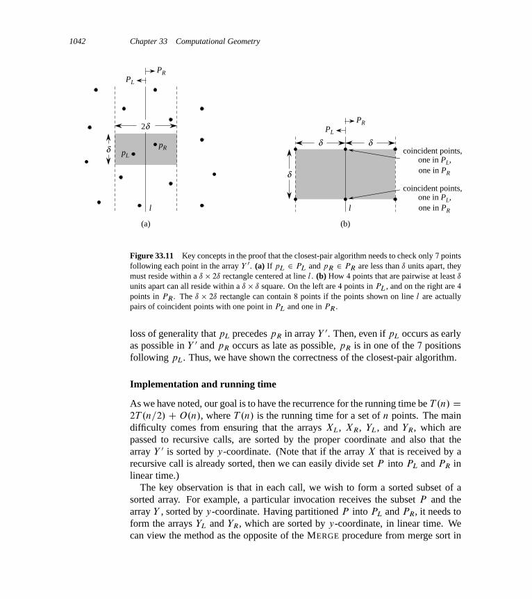
1042 Chapter 33 Computational Geometry
l
pL
pR
PL
PR
δ
2δ
(a)
PRPL
(b)
l
coincident points, one in PL, one in PR
coincident points, one in PL, one in PR
δδ
δ
Figure 33.11 Key concepts in the proof that the closest-pair algorithm needs to check only 7 pointsfollowing each point in the array Y 0. (a) If pL 2 PL and pR 2 PR are less than ı units apart, theymust reside within a ı 2ı rectangle centered at line l . (b) How 4 points that are pairwise at least ı
units apart can all reside within a ı ı square. On the left are 4 points in PL, and on the right are 4
points in PR. The ı 2ı rectangle can contain 8 points if the points shown on line l are actuallypairs of coincident points with one point in PL and one in PR.
loss of generality that pL precedes pR in array Y 0. Then, even if pL occurs as earlyas possible in Y 0 and pR occurs as late as possible, pR is in one of the 7 positionsfollowing pL. Thus, we have shown the correctness of the closest-pair algorithm.
Implementation and running time
As we have noted, our goal is to have the recurrence for the running time be T .n/ D2T .n=2/ CO.n/, where T .n/ is the running time for a set of n points. The maindifficulty comes from ensuring that the arrays XL, XR, YL, and YR, which arepassed to recursive calls, are sorted by the proper coordinate and also that thearray Y 0 is sorted by y-coordinate. (Note that if the array X that is received by arecursive call is already sorted, then we can easily divide set P into PL and PR inlinear time.)
The key observation is that in each call, we wish to form a sorted subset of asorted array. For example, a particular invocation receives the subset P and thearray Y , sorted by y-coordinate. Having partitioned P into PL and PR, it needs toform the arrays YL and YR, which are sorted by y-coordinate, in linear time. Wecan view the method as the opposite of the MERGE procedure from merge sort in

33.4 Finding the closest pair of points 1043
Section 2.3.1: we are splitting a sorted array into two sorted arrays. The followingpseudocode gives the idea.
1 let YLŒ1 : : Y: length� and YRŒ1 : : Y: length� be new arrays2 YL: length D YR: length D 0
3 for i D 1 to Y: length4 if Y Œi � 2 PL
5 YL: length D YL: lengthC 1
6 YLŒYL: length� D Y Œi �
7 else YR: length D YR: lengthC 1
8 YRŒYR: length� D Y Œi �
We simply examine the points in array Y in order. If a point Y Œi � is in PL, weappend it to the end of array YL; otherwise, we append it to the end of array YR.Similar pseudocode works for forming arrays XL, XR, and Y 0.
The only remaining question is how to get the points sorted in the first place. Wepresort them; that is, we sort them once and for all before the first recursive call.We pass these sorted arrays into the first recursive call, and from there we whittlethem down through the recursive calls as necessary. Presorting adds an additionalO.n lg n/ term to the running time, but now each step of the recursion takes lineartime exclusive of the recursive calls. Thus, if we let T .n/ be the running time ofeach recursive step and T 0.n/ be the running time of the entire algorithm, we getT 0.n/ D T .n/CO.n lg n/ and
T .n/ D(
2T .n=2/CO.n/ if n > 3 ;
O.1/ if n � 3 :
Thus, T .n/ D O.n lg n/ and T 0.n/ D O.n lg n/.
Exercises
33.4-1Professor Williams comes up with a scheme that allows the closest-pair algorithmto check only 5 points following each point in array Y 0. The idea is always to placepoints on line l into set PL. Then, there cannot be pairs of coincident points online l with one point in PL and one in PR. Thus, at most 6 points can reside inthe ı 2ı rectangle. What is the flaw in the professor’s scheme?
33.4-2Show that it actually suffices to check only the points in the 5 array positions fol-lowing each point in the array Y 0.

1044 Chapter 33 Computational Geometry
33.4-3We can define the distance between two points in ways other than euclidean. Inthe plane, the Lm-distance between points p1 and p2 is given by the expres-sion .jx1 � x2jm C jy1 � y2jm/
1=m. Euclidean distance, therefore, is L2-distance.Modify the closest-pair algorithm to use the L1-distance, which is also known asthe Manhattan distance.
33.4-4Given two points p1 and p2 in the plane, the L1-distance between them isgiven by max.jx1 � x2j ; jy1 � y2j/. Modify the closest-pair algorithm to use theL1-distance.
33.4-5Suppose that �.n/ of the points given to the closest-pair algorithm are covertical.Show how to determine the sets PL and PR and how to determine whether eachpoint of Y is in PL or PR so that the running time for the closest-pair algorithmremains O.n lg n/.
33.4-6Suggest a change to the closest-pair algorithm that avoids presorting the Y arraybut leaves the running time as O.n lg n/. (Hint: Merge sorted arrays YL and YR toform the sorted array Y .)
Problems
33-1 Convex layersGiven a set Q of points in the plane, we define the convex layers of Q inductively.The first convex layer of Q consists of those points in Q that are vertices of CH.Q/.For i > 1, define Qi to consist of the points of Q with all points in convex layers1; 2; : : : ; i �1 removed. Then, the i th convex layer of Q is CH.Qi / if Qi ¤ ; andis undefined otherwise.
a. Give an O.n2/-time algorithm to find the convex layers of a set of n points.
b. Prove that �.n lg n/ time is required to compute the convex layers of a set of n
points with any model of computation that requires �.n lg n/ time to sort n realnumbers.
Problems for Chapter 33 1045
33-2 Maximal layersLet Q be a set of n points in the plane. We say that point .x; y/ dominatespoint .x 0; y 0/ if x � x 0 and y � y 0. A point in Q that is dominated by no otherpoints in Q is said to be maximal. Note that Q may contain many maximal points,which can be organized into maximal layers as follows. The first maximal layer L1
is the set of maximal points of Q. For i > 1, the i th maximal layer Li is the set ofmaximal points in Q �Si�1
j D1 Lj .Suppose that Q has k nonempty maximal layers, and let yi be the y-coordinate
of the leftmost point in Li for i D 1; 2; : : : ; k. For now, assume that no two pointsin Q have the same x- or y-coordinate.
a. Show that y1 > y2 > � � � > yk.
Consider a point .x; y/ that is to the left of any point in Q and for which y isdistinct from the y-coordinate of any point in Q. Let Q0 D Q [ f.x; y/g.b. Let j be the minimum index such that yj < y, unless y < yk, in which case
we let j D k C 1. Show that the maximal layers of Q0 are as follows:
� If j � k, then the maximal layers of Q0 are the same as the maximal layersof Q, except that Lj also includes .x; y/ as its new leftmost point.
� If j D kC1, then the first k maximal layers of Q0 are the same as for Q, butin addition, Q0 has a nonempty .k C 1/st maximal layer: LkC1 D f.x; y/g.
c. Describe an O.n lg n/-time algorithm to compute the maximal layers of a set Q
of n points. (Hint: Move a sweep line from right to left.)
d. Do any difficulties arise if we now allow input points to have the same x- ory-coordinate? Suggest a way to resolve such problems.
33-3 Ghostbusters and ghostsA group of n Ghostbusters is battling n ghosts. Each Ghostbuster carries a protonpack, which shoots a stream at a ghost, eradicating it. A stream goes in a straightline and terminates when it hits the ghost. The Ghostbusters decide upon the fol-lowing strategy. They will pair off with the ghosts, forming n Ghostbuster-ghostpairs, and then simultaneously each Ghostbuster will shoot a stream at his cho-sen ghost. As we all know, it is very dangerous to let streams cross, and so theGhostbusters must choose pairings for which no streams will cross.
Assume that the position of each Ghostbuster and each ghost is a fixed point inthe plane and that no three positions are colinear.
a. Argue that there exists a line passing through one Ghostbuster and one ghostsuch that the number of Ghostbusters on one side of the line equals the numberof ghosts on the same side. Describe how to find such a line in O.n lg n/ time.

1046 Chapter 33 Computational Geometry
b. Give an O.n2 lg n/-time algorithm to pair Ghostbusters with ghosts in such away that no streams cross.
33-4 Picking up sticksProfessor Charon has a set of n sticks, which are piled up in some configuration.Each stick is specified by its endpoints, and each endpoint is an ordered triplegiving its .x; y; ´/ coordinates. No stick is vertical. He wishes to pick up all thesticks, one at a time, subject to the condition that he may pick up a stick only ifthere is no other stick on top of it.
a. Give a procedure that takes two sticks a and b and reports whether a is above,below, or unrelated to b.
b. Describe an efficient algorithm that determines whether it is possible to pick upall the sticks, and if so, provides a legal order in which to pick them up.
33-5 Sparse-hulled distributionsConsider the problem of computing the convex hull of a set of points in the planethat have been drawn according to some known random distribution. Sometimes,the number of points, or size, of the convex hull of n points drawn from such adistribution has expectation O.n1��/ for some constant � > 0. We call such adistribution sparse-hulled. Sparse-hulled distributions include the following:
� Points drawn uniformly from a unit-radius disk. The convex hull has expectedsize ‚.n1=3/.
� Points drawn uniformly from the interior of a convex polygon with k sides, forany constant k. The convex hull has expected size ‚.lg n/.
� Points drawn according to a two-dimensional normal distribution. The convexhull has expected size ‚.
plg n/.
a. Given two convex polygons with n1 and n2 vertices respectively, show how tocompute the convex hull of all n1Cn2 points in O.n1Cn2/ time. (The polygonsmay overlap.)
b. Show how to compute the convex hull of a set of n points drawn independentlyaccording to a sparse-hulled distribution in O.n/ average-case time. (Hint:Recursively find the convex hulls of the first n=2 points and the second n=2
points, and then combine the results.)

Notes for Chapter 33 1047
Chapter notes
This chapter barely scratches the surface of computational-geometry algorithmsand techniques. Books on computational geometry include those by Preparata andShamos [282], Edelsbrunner [99], and O’Rourke [269].
Although geometry has been studied since antiquity, the development of algo-rithms for geometric problems is relatively new. Preparata and Shamos note thatthe earliest notion of the complexity of a problem was given by E. Lemoine in 1902.He was studying euclidean constructions—those using a compass and a ruler—anddevised a set of five primitives: placing one leg of the compass on a given point,placing one leg of the compass on a given line, drawing a circle, passing the ruler’sedge through a given point, and drawing a line. Lemoine was interested in thenumber of primitives needed to effect a given construction; he called this amountthe “simplicity” of the construction.
The algorithm of Section 33.2, which determines whether any segments inter-sect, is due to Shamos and Hoey [313].
The original version of Graham’s scan is given by Graham [150]. The package-wrapping algorithm is due to Jarvis [189]. Using a decision-tree model of com-putation, Yao [359] proved a worst-case lower bound of �.n lg n/ for the runningtime of any convex-hull algorithm. When the number of vertices h of the con-vex hull is taken into account, the prune-and-search algorithm of Kirkpatrick andSeidel [206], which takes O.n lg h/ time, is asymptotically optimal.
The O.n lg n/-time divide-and-conquer algorithm for finding the closest pair ofpoints is by Shamos and appears in Preparata and Shamos [282]. Preparata andShamos also show that the algorithm is asymptotically optimal in a decision-treemodel.

34 NP-Completeness
Almost all the algorithms we have studied thus far have been polynomial-time al-gorithms: on inputs of size n, their worst-case running time is O.nk/ for some con-stant k. You might wonder whether all problems can be solved in polynomial time.The answer is no. For example, there are problems, such as Turing’s famous “Halt-ing Problem,” that cannot be solved by any computer, no matter how much time weallow. There are also problems that can be solved, but not in time O.nk/ for anyconstant k. Generally, we think of problems that are solvable by polynomial-timealgorithms as being tractable, or easy, and problems that require superpolynomialtime as being intractable, or hard.
The subject of this chapter, however, is an interesting class of problems, calledthe “NP-complete” problems, whose status is unknown. No polynomial-time al-gorithm has yet been discovered for an NP-complete problem, nor has anyone yetbeen able to prove that no polynomial-time algorithm can exist for any one of them.This so-called P ¤ NP question has been one of the deepest, most perplexing openresearch problems in theoretical computer science since it was first posed in 1971.
Several NP-complete problems are particularly tantalizing because they seemon the surface to be similar to problems that we know how to solve in polynomialtime. In each of the following pairs of problems, one is solvable in polynomialtime and the other is NP-complete, but the difference between problems appears tobe slight:
Shortest vs. longest simple paths: In Chapter 24, we saw that even with negativeedge weights, we can find shortest paths from a single source in a directedgraph G D .V; E/ in O.VE/ time. Finding a longest simple path between twovertices is difficult, however. Merely determining whether a graph contains asimple path with at least a given number of edges is NP-complete.
Euler tour vs. hamiltonian cycle: An Euler tour of a connected, directed graphG D .V; E/ is a cycle that traverses each edge of G exactly once, althoughit is allowed to visit each vertex more than once. By Problem 22-3, we candetermine whether a graph has an Euler tour in only O.E/ time and, in fact,

Chapter 34 NP-Completeness 1049
we can find the edges of the Euler tour in O.E/ time. A hamiltonian cycle ofa directed graph G D .V; E/ is a simple cycle that contains each vertex in V .Determining whether a directed graph has a hamiltonian cycle is NP-complete.(Later in this chapter, we shall prove that determining whether an undirectedgraph has a hamiltonian cycle is NP-complete.)
2-CNF satisfiability vs. 3-CNF satisfiability: A boolean formula contains vari-ables whose values are 0 or 1; boolean connectives such as ^ (AND), _ (OR),and : (NOT); and parentheses. A boolean formula is satisfiable if there existssome assignment of the values 0 and 1 to its variables that causes it to evaluateto 1. We shall define terms more formally later in this chapter, but informally, aboolean formula is in k-conjunctive normal form, or k-CNF, if it is the ANDof clauses of ORs of exactly k variables or their negations. For example, theboolean formula .x1 _ :x2/ ^ .:x1 _ x3/ ^ .:x2 _ :x3/ is in 2-CNF. (It hasthe satisfying assignment x1 D 1; x2 D 0; x3 D 1.) Although we can deter-mine in polynomial time whether a 2-CNF formula is satisfiable, we shall seelater in this chapter that determining whether a 3-CNF formula is satisfiable isNP-complete.
NP-completeness and the classes P and NP
Throughout this chapter, we shall refer to three classes of problems: P, NP, andNPC, the latter class being the NP-complete problems. We describe them infor-mally here, and we shall define them more formally later on.
The class P consists of those problems that are solvable in polynomial time.More specifically, they are problems that can be solved in time O.nk/ for someconstant k, where n is the size of the input to the problem. Most of the problemsexamined in previous chapters are in P.
The class NP consists of those problems that are “verifiable” in polynomial time.What do we mean by a problem being verifiable? If we were somehow given a“certificate” of a solution, then we could verify that the certificate is correct in timepolynomial in the size of the input to the problem. For example, in the hamiltonian-cycle problem, given a directed graph G D .V; E/, a certificate would be a se-quence h�1; �2; �3; : : : ; �jV ji of jV j vertices. We could easily check in polynomialtime that .�i ; �iC1/ 2 E for i D 1; 2; 3; : : : ; jV j�1 and that .�jV j; �1/ 2 E as well.As another example, for 3-CNF satisfiability, a certificate would be an assignmentof values to variables. We could check in polynomial time that this assignmentsatisfies the boolean formula.
Any problem in P is also in NP, since if a problem is in P then we can solve itin polynomial time without even being supplied a certificate. We shall formalizethis notion later in this chapter, but for now we can believe that P � NP. The openquestion is whether or not P is a proper subset of NP.
1050 Chapter 34 NP-Completeness
Informally, a problem is in the class NPC—and we refer to it as being NP-complete—if it is in NP and is as “hard” as any problem in NP. We shall formallydefine what it means to be as hard as any problem in NP later in this chapter.In the meantime, we will state without proof that if any NP-complete problemcan be solved in polynomial time, then every problem in NP has a polynomial-time algorithm. Most theoretical computer scientists believe that the NP-completeproblems are intractable, since given the wide range of NP-complete problemsthat have been studied to date—without anyone having discovered a polynomial-time solution to any of them—it would be truly astounding if all of them couldbe solved in polynomial time. Yet, given the effort devoted thus far to provingthat NP-complete problems are intractable—without a conclusive outcome—wecannot rule out the possibility that the NP-complete problems are in fact solvablein polynomial time.
To become a good algorithm designer, you must understand the rudiments of thetheory of NP-completeness. If you can establish a problem as NP-complete, youprovide good evidence for its intractability. As an engineer, you would then dobetter spending your time developing an approximation algorithm (see Chapter 35)or solving a tractable special case, rather than searching for a fast algorithm thatsolves the problem exactly. Moreover, many natural and interesting problems thaton the surface seem no harder than sorting, graph searching, or network flow arein fact NP-complete. Therefore, you should become familiar with this remarkableclass of problems.
Overview of showing problems to be NP-complete
The techniques we use to show that a particular problem is NP-complete differfundamentally from the techniques used throughout most of this book to designand analyze algorithms. When we demonstrate that a problem is NP-complete,we are making a statement about how hard it is (or at least how hard we think itis), rather than about how easy it is. We are not trying to prove the existence ofan efficient algorithm, but instead that no efficient algorithm is likely to exist. Inthis way, NP-completeness proofs bear some similarity to the proof in Section 8.1of an �.n lg n/-time lower bound for any comparison sort algorithm; the specifictechniques used for showing NP-completeness differ from the decision-tree methodused in Section 8.1, however.
We rely on three key concepts in showing a problem to be NP-complete:
Decision problems vs. optimization problemsMany problems of interest are optimization problems, in which each feasible (i.e.,“legal”) solution has an associated value, and we wish to find a feasible solutionwith the best value. For example, in a problem that we call SHORTEST-PATH,
Chapter 34 NP-Completeness 1051
we are given an undirected graph G and vertices u and �, and we wish to find apath from u to � that uses the fewest edges. In other words, SHORTEST-PATHis the single-pair shortest-path problem in an unweighted, undirected graph. NP-completeness applies directly not to optimization problems, however, but to deci-sion problems, in which the answer is simply “yes” or “no” (or, more formally, “1”or “0”).
Although NP-complete problems are confined to the realm of decision problems,we can take advantage of a convenient relationship between optimization problemsand decision problems. We usually can cast a given optimization problem as a re-lated decision problem by imposing a bound on the value to be optimized. Forexample, a decision problem related to SHORTEST-PATH is PATH: given a di-rected graph G, vertices u and �, and an integer k, does a path exist from u to �
consisting of at most k edges?The relationship between an optimization problem and its related decision prob-
lem works in our favor when we try to show that the optimization problem is“hard.” That is because the decision problem is in a sense “easier,” or at least “noharder.” As a specific example, we can solve PATH by solving SHORTEST-PATHand then comparing the number of edges in the shortest path found to the valueof the decision-problem parameter k. In other words, if an optimization prob-lem is easy, its related decision problem is easy as well. Stated in a way that hasmore relevance to NP-completeness, if we can provide evidence that a decisionproblem is hard, we also provide evidence that its related optimization problem ishard. Thus, even though it restricts attention to decision problems, the theory ofNP-completeness often has implications for optimization problems as well.
ReductionsThe above notion of showing that one problem is no harder or no easier than an-other applies even when both problems are decision problems. We take advantageof this idea in almost every NP-completeness proof, as follows. Let us consider adecision problem A, which we would like to solve in polynomial time. We call theinput to a particular problem an instance of that problem; for example, in PATH,an instance would be a particular graph G, particular vertices u and � of G, and aparticular integer k. Now suppose that we already know how to solve a differentdecision problem B in polynomial time. Finally, suppose that we have a procedurethat transforms any instance ˛ of A into some instance ˇ of B with the followingcharacteristics:
� The transformation takes polynomial time.
� The answers are the same. That is, the answer for ˛ is “yes” if and only if theanswer for ˇ is also “yes.”
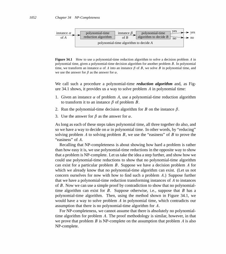
1052 Chapter 34 NP-Completeness
polynomial-timereduction algorithm
instance β polynomial-timealgorithm to decide B
yes yes
polynomial-time algorithm to decide A
nonoof Binstance α
of A
Figure 34.1 How to use a polynomial-time reduction algorithm to solve a decision problem A inpolynomial time, given a polynomial-time decision algorithm for another problem B . In polynomialtime, we transform an instance ˛ of A into an instance ˇ of B , we solve B in polynomial time, andwe use the answer for ˇ as the answer for ˛.
We call such a procedure a polynomial-time reduction algorithm and, as Fig-ure 34.1 shows, it provides us a way to solve problem A in polynomial time:
1. Given an instance ˛ of problem A, use a polynomial-time reduction algorithmto transform it to an instance ˇ of problem B .
2. Run the polynomial-time decision algorithm for B on the instance ˇ.
3. Use the answer for ˇ as the answer for ˛.
As long as each of these steps takes polynomial time, all three together do also, andso we have a way to decide on ˛ in polynomial time. In other words, by “reducing”solving problem A to solving problem B , we use the “easiness” of B to prove the“easiness” of A.
Recalling that NP-completeness is about showing how hard a problem is ratherthan how easy it is, we use polynomial-time reductions in the opposite way to showthat a problem is NP-complete. Let us take the idea a step further, and show how wecould use polynomial-time reductions to show that no polynomial-time algorithmcan exist for a particular problem B . Suppose we have a decision problem A forwhich we already know that no polynomial-time algorithm can exist. (Let us notconcern ourselves for now with how to find such a problem A.) Suppose furtherthat we have a polynomial-time reduction transforming instances of A to instancesof B . Now we can use a simple proof by contradiction to show that no polynomial-time algorithm can exist for B . Suppose otherwise, i.e., suppose that B has apolynomial-time algorithm. Then, using the method shown in Figure 34.1, wewould have a way to solve problem A in polynomial time, which contradicts ourassumption that there is no polynomial-time algorithm for A.
For NP-completeness, we cannot assume that there is absolutely no polynomial-time algorithm for problem A. The proof methodology is similar, however, in thatwe prove that problem B is NP-complete on the assumption that problem A is alsoNP-complete.

34.1 Polynomial time 1053
A first NP-complete problemBecause the technique of reduction relies on having a problem already known tobe NP-complete in order to prove a different problem NP-complete, we need a“first” NP-complete problem. The problem we shall use is the circuit-satisfiabilityproblem, in which we are given a boolean combinational circuit composed of AND,OR, and NOT gates, and we wish to know whether there exists some set of booleaninputs to this circuit that causes its output to be 1. We shall prove that this firstproblem is NP-complete in Section 34.3.
Chapter outline
This chapter studies the aspects of NP-completeness that bear most directly on theanalysis of algorithms. In Section 34.1, we formalize our notion of “problem” anddefine the complexity class P of polynomial-time solvable decision problems. Wealso see how these notions fit into the framework of formal-language theory. Sec-tion 34.2 defines the class NP of decision problems whose solutions are verifiablein polynomial time. It also formally poses the P ¤ NP question.
Section 34.3 shows we can relate problems via polynomial-time “reductions.”It defines NP-completeness and sketches a proof that one problem, called “circuitsatisfiability,” is NP-complete. Having found one NP-complete problem, we showin Section 34.4 how to prove other problems to be NP-complete much more simplyby the methodology of reductions. We illustrate this methodology by showing thattwo formula-satisfiability problems are NP-complete. With additional reductions,we show a variety of other problems to be NP-complete in Section 34.5.
34.1 Polynomial time
We begin our study of NP-completeness by formalizing our notion of polynomial-time solvable problems. We generally regard these problems as tractable, but forphilosophical, not mathematical, reasons. We can offer three supporting argu-ments.
First, although we may reasonably regard a problem that requires time ‚.n100/
to be intractable, very few practical problems require time on the order of such ahigh-degree polynomial. The polynomial-time computable problems encounteredin practice typically require much less time. Experience has shown that once thefirst polynomial-time algorithm for a problem has been discovered, more efficientalgorithms often follow. Even if the current best algorithm for a problem has arunning time of ‚.n100/, an algorithm with a much better running time will likelysoon be discovered.

1054 Chapter 34 NP-Completeness
Second, for many reasonable models of computation, a problem that can besolved in polynomial time in one model can be solved in polynomial time in an-other. For example, the class of problems solvable in polynomial time by the serialrandom-access machine used throughout most of this book is the same as the classof problems solvable in polynomial time on abstract Turing machines.1 It is alsothe same as the class of problems solvable in polynomial time on a parallel com-puter when the number of processors grows polynomially with the input size.
Third, the class of polynomial-time solvable problems has nice closure proper-ties, since polynomials are closed under addition, multiplication, and composition.For example, if the output of one polynomial-time algorithm is fed into the input ofanother, the composite algorithm is polynomial. Exercise 34.1-5 asks you to showthat if an algorithm makes a constant number of calls to polynomial-time subrou-tines and performs an additional amount of work that also takes polynomial time,then the running time of the composite algorithm is polynomial.
Abstract problems
To understand the class of polynomial-time solvable problems, we must first havea formal notion of what a “problem” is. We define an abstract problem Q to be abinary relation on a set I of problem instances and a set S of problem solutions.For example, an instance for SHORTEST-PATH is a triple consisting of a graphand two vertices. A solution is a sequence of vertices in the graph, with perhapsthe empty sequence denoting that no path exists. The problem SHORTEST-PATHitself is the relation that associates each instance of a graph and two vertices witha shortest path in the graph that connects the two vertices. Since shortest paths arenot necessarily unique, a given problem instance may have more than one solution.
This formulation of an abstract problem is more general than we need for ourpurposes. As we saw above, the theory of NP-completeness restricts attention todecision problems: those having a yes/no solution. In this case, we can view anabstract decision problem as a function that maps the instance set I to the solutionset f0; 1g. For example, a decision problem related to SHORTEST-PATH is theproblem PATH that we saw earlier. If i D hG;u; �; ki is an instance of the decisionproblem PATH, then PATH.i/ D 1 (yes) if a shortest path from u to � has atmost k edges, and PATH.i/ D 0 (no) otherwise. Many abstract problems are notdecision problems, but rather optimization problems, which require some value tobe minimized or maximized. As we saw above, however, we can usually recast anoptimization problem as a decision problem that is no harder.
1See Hopcroft and Ullman [180] or Lewis and Papadimitriou [236] for a thorough treatment of theTuring-machine model.
34.1 Polynomial time 1055
Encodings
In order for a computer program to solve an abstract problem, we must representproblem instances in a way that the program understands. An encoding of a set S
of abstract objects is a mapping e from S to the set of binary strings.2 For example,we are all familiar with encoding the natural numbers N D f0; 1; 2; 3; 4; : : :g asthe strings f0; 1; 10; 11; 100; : : :g. Using this encoding, e.17/ D 10001. If youhave looked at computer representations of keyboard characters, you probably haveseen the ASCII code, where, for example, the encoding of A is 1000001. We canencode a compound object as a binary string by combining the representations ofits constituent parts. Polygons, graphs, functions, ordered pairs, programs—all canbe encoded as binary strings.
Thus, a computer algorithm that “solves” some abstract decision problem actu-ally takes an encoding of a problem instance as input. We call a problem whoseinstance set is the set of binary strings a concrete problem. We say that an algo-rithm solves a concrete problem in time O.T .n// if, when it is provided a probleminstance i of length n D ji j, the algorithm can produce the solution in O.T .n//
time.3 A concrete problem is polynomial-time solvable, therefore, if there existsan algorithm to solve it in time O.nk/ for some constant k.
We can now formally define the complexity class P as the set of concrete deci-sion problems that are polynomial-time solvable.
We can use encodings to map abstract problems to concrete problems. Givenan abstract decision problem Q mapping an instance set I to f0; 1g, an encodinge W I ! f0; 1g� can induce a related concrete decision problem, which we denoteby e.Q/.4 If the solution to an abstract-problem instance i 2 I is Q.i/ 2 f0; 1g,then the solution to the concrete-problem instance e.i/ 2 f0; 1g� is also Q.i/. As atechnicality, some binary strings might represent no meaningful abstract-probleminstance. For convenience, we shall assume that any such string maps arbitrarilyto 0. Thus, the concrete problem produces the same solutions as the abstract prob-lem on binary-string instances that represent the encodings of abstract-probleminstances.
We would like to extend the definition of polynomial-time solvability from con-crete problems to abstract problems by using encodings as the bridge, but we would
2The codomain of e need not be binary strings; any set of strings over a finite alphabet having atleast 2 symbols will do.
3We assume that the algorithm’s output is separate from its input. Because it takes at least one timestep to produce each bit of the output and the algorithm takes O.T .n// time steps, the size of theoutput is O.T .n//.
4We denote by f0; 1g� the set of all strings composed of symbols from the set f0; 1g.
1056 Chapter 34 NP-Completeness
like the definition to be independent of any particular encoding. That is, the ef-ficiency of solving a problem should not depend on how the problem is encoded.Unfortunately, it depends quite heavily on the encoding. For example, suppose thatan integer k is to be provided as the sole input to an algorithm, and suppose thatthe running time of the algorithm is ‚.k/. If the integer k is provided in unary—astring of k 1s—then the running time of the algorithm is O.n/ on length-n inputs,which is polynomial time. If we use the more natural binary representation of theinteger k, however, then the input length is n D blg kc C 1. In this case, the run-ning time of the algorithm is ‚.k/ D ‚.2n/, which is exponential in the size of theinput. Thus, depending on the encoding, the algorithm runs in either polynomialor superpolynomial time.
How we encode an abstract problem matters quite a bit to how we understandpolynomial time. We cannot really talk about solving an abstract problem withoutfirst specifying an encoding. Nevertheless, in practice, if we rule out “expensive”encodings such as unary ones, the actual encoding of a problem makes little dif-ference to whether the problem can be solved in polynomial time. For example,representing integers in base 3 instead of binary has no effect on whether a prob-lem is solvable in polynomial time, since we can convert an integer represented inbase 3 to an integer represented in base 2 in polynomial time.
We say that a function f W f0; 1g� ! f0; 1g� is polynomial-time computableif there exists a polynomial-time algorithm A that, given any input x 2 f0; 1g�,produces as output f .x/. For some set I of problem instances, we say that two en-codings e1 and e2 are polynomially related if there exist two polynomial-time com-putable functions f12 and f21 such that for any i 2 I , we have f12.e1.i// D e2.i/
and f21.e2.i// D e1.i/.5 That is, a polynomial-time algorithm can compute the en-coding e2.i/ from the encoding e1.i/, and vice versa. If two encodings e1 and e2 ofan abstract problem are polynomially related, whether the problem is polynomial-time solvable or not is independent of which encoding we use, as the followinglemma shows.
Lemma 34.1Let Q be an abstract decision problem on an instance set I , and let e1 and e2 bepolynomially related encodings on I . Then, e1.Q/ 2 P if and only if e2.Q/ 2 P.
5Technically, we also require the functions f12 and f21 to “map noninstances to noninstances.”A noninstance of an encoding e is a string x 2 f0; 1g� such that there is no instance i for whiche.i/ D x. We require that f12.x/ D y for every noninstance x of encoding e1, where y is some non-instance of e2, and that f21.x0/ D y0 for every noninstance x0 of e2, where y0 is some noninstanceof e1.

34.1 Polynomial time 1057
Proof We need only prove the forward direction, since the backward direction issymmetric. Suppose, therefore, that e1.Q/ can be solved in time O.nk/ for someconstant k. Further, suppose that for any problem instance i , the encoding e1.i/
can be computed from the encoding e2.i/ in time O.nc/ for some constant c, wheren D je2.i/j. To solve problem e2.Q/, on input e2.i/, we first compute e1.i/ andthen run the algorithm for e1.Q/ on e1.i/. How long does this take? Convertingencodings takes time O.nc/, and therefore je1.i/j D O.nc/, since the output ofa serial computer cannot be longer than its running time. Solving the problemon e1.i/ takes time O.je1.i/jk/ D O.nck/, which is polynomial since both c and k
are constants.
Thus, whether an abstract problem has its instances encoded in binary or base 3does not affect its “complexity,” that is, whether it is polynomial-time solvable ornot, but if instances are encoded in unary, its complexity may change. In order tobe able to converse in an encoding-independent fashion, we shall generally assumethat problem instances are encoded in any reasonable, concise fashion, unless wespecifically say otherwise. To be precise, we shall assume that the encoding of aninteger is polynomially related to its binary representation, and that the encoding ofa finite set is polynomially related to its encoding as a list of its elements, enclosedin braces and separated by commas. (ASCII is one such encoding scheme.) Withsuch a “standard” encoding in hand, we can derive reasonable encodings of othermathematical objects, such as tuples, graphs, and formulas. To denote the standardencoding of an object, we shall enclose the object in angle braces. Thus, hGidenotes the standard encoding of a graph G.
As long as we implicitly use an encoding that is polynomially related to thisstandard encoding, we can talk directly about abstract problems without referenceto any particular encoding, knowing that the choice of encoding has no effect onwhether the abstract problem is polynomial-time solvable. Henceforth, we shallgenerally assume that all problem instances are binary strings encoded using thestandard encoding, unless we explicitly specify the contrary. We shall also typicallyneglect the distinction between abstract and concrete problems. You should watchout for problems that arise in practice, however, in which a standard encoding isnot obvious and the encoding does make a difference.
A formal-language framework
By focusing on decision problems, we can take advantage of the machinery offormal-language theory. Let’s review some definitions from that theory. Analphabet † is a finite set of symbols. A language L over † is any set ofstrings made up of symbols from †. For example, if † D f0; 1g, the setL D f10; 11; 101; 111; 1011; 1101; 10001; : : :g is the language of binary represen-
1058 Chapter 34 NP-Completeness
tations of prime numbers. We denote the empty string by ", the empty languageby ;, and the language of all strings over † by †�. For example, if † D f0; 1g,then †� D f"; 0; 1; 00; 01; 10; 11; 000; : : :g is the set of all binary strings. Everylanguage L over † is a subset of †�.
We can perform a variety of operations on languages. Set-theoretic operations,such as union and intersection, follow directly from the set-theoretic definitions.We define the complement of L by L D †� �L. The concatenation L1L2 of twolanguages L1 and L2 is the language
L D fx1x2 W x1 2 L1 and x2 2 L2g :
The closure or Kleene star of a language L is the language
L� D f"g [ L [ L2 [ L3 [ � � � ;
where Lk is the language obtained by concatenating L to itself k times.From the point of view of language theory, the set of instances for any decision
problem Q is simply the set †�, where † D f0; 1g. Since Q is entirely character-ized by those problem instances that produce a 1 (yes) answer, we can view Q asa language L over † D f0; 1g, where
L D fx 2 †� W Q.x/ D 1g :
For example, the decision problem PATH has the corresponding language
PATH D fhG; u; �; ki W G D .V; E/ is an undirected graph,u; � 2 V;
k � 0 is an integer, andthere exists a path from u to � in G
consisting of at most k edgesg :
(Where convenient, we shall sometimes use the same name—PATH in this case—to refer to both a decision problem and its corresponding language.)
The formal-language framework allows us to express concisely the relation be-tween decision problems and algorithms that solve them. We say that an al-gorithm A accepts a string x 2 f0; 1g� if, given input x, the algorithm’s out-put A.x/ is 1. The language accepted by an algorithm A is the set of stringsL D fx 2 f0; 1g� W A.x/ D 1g, that is, the set of strings that the algorithm accepts.An algorithm A rejects a string x if A.x/ D 0.
Even if language L is accepted by an algorithm A, the algorithm will not neces-sarily reject a string x 62 L provided as input to it. For example, the algorithm mayloop forever. A language L is decided by an algorithm A if every binary stringin L is accepted by A and every binary string not in L is rejected by A. A lan-guage L is accepted in polynomial time by an algorithm A if it is accepted by A
and if in addition there exists a constant k such that for any length-n string x 2 L,
34.1 Polynomial time 1059
algorithm A accepts x in time O.nk/. A language L is decided in polynomialtime by an algorithm A if there exists a constant k such that for any length-n stringx 2 f0; 1g�, the algorithm correctly decides whether x 2 L in time O.nk/. Thus,to accept a language, an algorithm need only produce an answer when provided astring in L, but to decide a language, it must correctly accept or reject every stringin f0; 1g�.
As an example, the language PATH can be accepted in polynomial time. Onepolynomial-time accepting algorithm verifies that G encodes an undirected graph,verifies that u and � are vertices in G, uses breadth-first search to compute a short-est path from u to � in G, and then compares the number of edges on the shortestpath obtained with k. If G encodes an undirected graph and the path found from u
to � has at most k edges, the algorithm outputs 1 and halts. Otherwise, the algo-rithm runs forever. This algorithm does not decide PATH, however, since it doesnot explicitly output 0 for instances in which a shortest path has more than k edges.A decision algorithm for PATH must explicitly reject binary strings that do not be-long to PATH. For a decision problem such as PATH, such a decision algorithm iseasy to design: instead of running forever when there is not a path from u to � withat most k edges, it outputs 0 and halts. (It must also output 0 and halt if the inputencoding is faulty.) For other problems, such as Turing’s Halting Problem, thereexists an accepting algorithm, but no decision algorithm exists.
We can informally define a complexity class as a set of languages, membershipin which is determined by a complexity measure, such as running time, of analgorithm that determines whether a given string x belongs to language L. Theactual definition of a complexity class is somewhat more technical.6
Using this language-theoretic framework, we can provide an alternative defini-tion of the complexity class P:
P D fL � f0; 1g� W there exists an algorithm A that decides L
in polynomial timeg :
In fact, P is also the class of languages that can be accepted in polynomial time.
Theorem 34.2P D fL W L is accepted by a polynomial-time algorithmg :
Proof Because the class of languages decided by polynomial-time algorithms isa subset of the class of languages accepted by polynomial-time algorithms, weneed only show that if L is accepted by a polynomial-time algorithm, it is de-cided by a polynomial-time algorithm. Let L be the language accepted by some
6For more on complexity classes, see the seminal paper by Hartmanis and Stearns [162].
1060 Chapter 34 NP-Completeness
polynomial-time algorithm A. We shall use a classic “simulation” argument toconstruct another polynomial-time algorithm A0 that decides L. Because A ac-cepts L in time O.nk/ for some constant k, there also exists a constant c suchthat A accepts L in at most cnk steps. For any input string x, the algorithm A0
simulates cnk steps of A. After simulating cnk steps, algorithm A0 inspects the be-havior of A. If A has accepted x, then A0 accepts x by outputting a 1. If A has notaccepted x, then A0 rejects x by outputting a 0. The overhead of A0 simulating A
does not increase the running time by more than a polynomial factor, and thus A0
is a polynomial-time algorithm that decides L.
Note that the proof of Theorem 34.2 is nonconstructive. For a given languageL 2 P, we may not actually know a bound on the running time for the algorithm A
that accepts L. Nevertheless, we know that such a bound exists, and therefore, thatan algorithm A0 exists that can check the bound, even though we may not be ableto find the algorithm A0 easily.
Exercises
34.1-1Define the optimization problem LONGEST-PATH-LENGTH as the relation thatassociates each instance of an undirected graph and two vertices with the num-ber of edges in a longest simple path between the two vertices. Define the de-cision problem LONGEST-PATH D fhG; u; �; ki W G D .V; E/ is an undi-rected graph, u; � 2 V , k � 0 is an integer, and there exists a simple pathfrom u to � in G consisting of at least k edgesg. Show that the optimization prob-lem LONGEST-PATH-LENGTH can be solved in polynomial time if and only ifLONGEST-PATH 2 P.
34.1-2Give a formal definition for the problem of finding the longest simple cycle in anundirected graph. Give a related decision problem. Give the language correspond-ing to the decision problem.
34.1-3Give a formal encoding of directed graphs as binary strings using an adjacency-matrix representation. Do the same using an adjacency-list representation. Arguethat the two representations are polynomially related.
34.1-4Is the dynamic-programming algorithm for the 0-1 knapsack problem that is askedfor in Exercise 16.2-2 a polynomial-time algorithm? Explain your answer.

34.2 Polynomial-time verification 1061
34.1-5Show that if an algorithm makes at most a constant number of calls to polynomial-time subroutines and performs an additional amount of work that also takes polyno-mial time, then it runs in polynomial time. Also show that a polynomial number ofcalls to polynomial-time subroutines may result in an exponential-time algorithm.
34.1-6Show that the class P, viewed as a set of languages, is closed under union, inter-section, concatenation, complement, and Kleene star. That is, if L1; L2 2 P, thenL1 [ L2 2 P, L1 \ L2 2 P, L1L2 2 P, L1 2 P, and L�
1 2 P.
34.2 Polynomial-time verification
We now look at algorithms that verify membership in languages. For example,suppose that for a given instance hG; u; �; ki of the decision problem PATH, weare also given a path p from u to �. We can easily check whether p is a path in G
and whether the length of p is at most k, and if so, we can view p as a “certificate”that the instance indeed belongs to PATH. For the decision problem PATH, thiscertificate doesn’t seem to buy us much. After all, PATH belongs to P—in fact,we can solve PATH in linear time—and so verifying membership from a givencertificate takes as long as solving the problem from scratch. We shall now examinea problem for which we know of no polynomial-time decision algorithm and yet,given a certificate, verification is easy.
Hamiltonian cycles
The problem of finding a hamiltonian cycle in an undirected graph has been stud-ied for over a hundred years. Formally, a hamiltonian cycle of an undirected graphG D .V; E/ is a simple cycle that contains each vertex in V . A graph that con-tains a hamiltonian cycle is said to be hamiltonian; otherwise, it is nonhamilto-nian. The name honors W. R. Hamilton, who described a mathematical game onthe dodecahedron (Figure 34.2(a)) in which one player sticks five pins in any fiveconsecutive vertices and the other player must complete the path to form a cycle
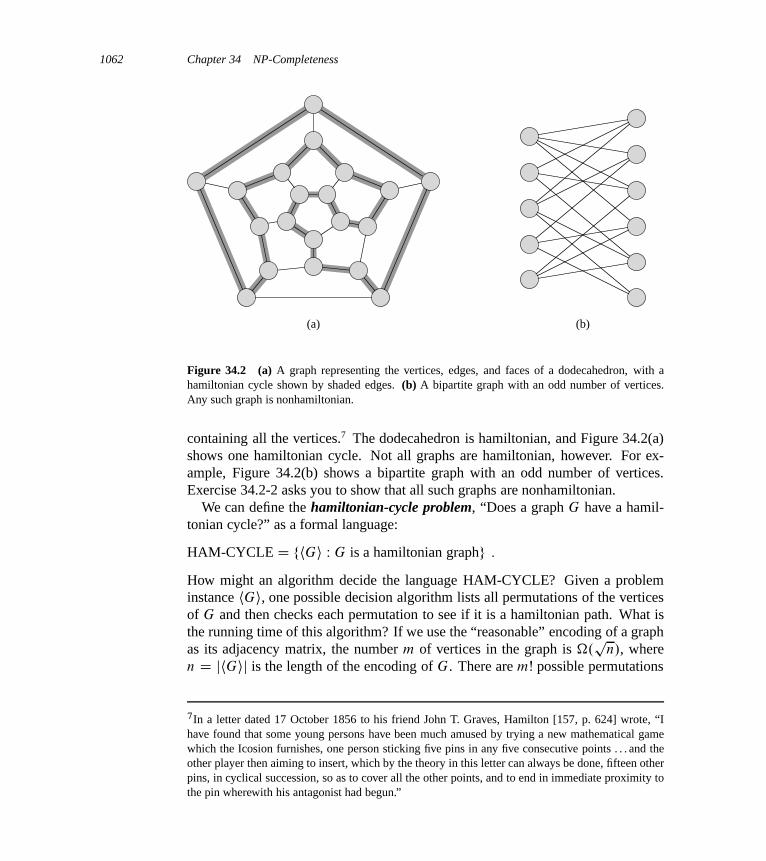
1062 Chapter 34 NP-Completeness
(a) (b)
Figure 34.2 (a) A graph representing the vertices, edges, and faces of a dodecahedron, with ahamiltonian cycle shown by shaded edges. (b) A bipartite graph with an odd number of vertices.Any such graph is nonhamiltonian.
containing all the vertices.7 The dodecahedron is hamiltonian, and Figure 34.2(a)shows one hamiltonian cycle. Not all graphs are hamiltonian, however. For ex-ample, Figure 34.2(b) shows a bipartite graph with an odd number of vertices.Exercise 34.2-2 asks you to show that all such graphs are nonhamiltonian.
We can define the hamiltonian-cycle problem, “Does a graph G have a hamil-tonian cycle?” as a formal language:
HAM-CYCLE D fhGi W G is a hamiltonian graphg :
How might an algorithm decide the language HAM-CYCLE? Given a probleminstance hGi, one possible decision algorithm lists all permutations of the verticesof G and then checks each permutation to see if it is a hamiltonian path. What isthe running time of this algorithm? If we use the “reasonable” encoding of a graphas its adjacency matrix, the number m of vertices in the graph is �.
pn/, where
n D jhGij is the length of the encoding of G. There are mŠ possible permutations
7In a letter dated 17 October 1856 to his friend John T. Graves, Hamilton [157, p. 624] wrote, “Ihave found that some young persons have been much amused by trying a new mathematical gamewhich the Icosion furnishes, one person sticking five pins in any five consecutive points . . . and theother player then aiming to insert, which by the theory in this letter can always be done, fifteen otherpins, in cyclical succession, so as to cover all the other points, and to end in immediate proximity tothe pin wherewith his antagonist had begun.”
34.2 Polynomial-time verification 1063
of the vertices, and therefore the running time is �.mŠ/ D �.p
n Š/ D �.2p
n/,which is not O.nk/ for any constant k. Thus, this naive algorithm does not runin polynomial time. In fact, the hamiltonian-cycle problem is NP-complete, as weshall prove in Section 34.5.
Verification algorithms
Consider a slightly easier problem. Suppose that a friend tells you that a givengraph G is hamiltonian, and then offers to prove it by giving you the vertices inorder along the hamiltonian cycle. It would certainly be easy enough to verify theproof: simply verify that the provided cycle is hamiltonian by checking whetherit is a permutation of the vertices of V and whether each of the consecutive edgesalong the cycle actually exists in the graph. You could certainly implement thisverification algorithm to run in O.n2/ time, where n is the length of the encodingof G. Thus, a proof that a hamiltonian cycle exists in a graph can be verified inpolynomial time.
We define a verification algorithm as being a two-argument algorithm A, whereone argument is an ordinary input string x and the other is a binary string y calleda certificate. A two-argument algorithm A verifies an input string x if there existsa certificate y such that A.x; y/ D 1. The language verified by a verificationalgorithm A is
L D fx 2 f0; 1g� W there exists y 2 f0; 1g� such that A.x; y/ D 1g :
Intuitively, an algorithm A verifies a language L if for any string x 2 L, thereexists a certificate y that A can use to prove that x 2 L. Moreover, for any stringx 62 L, there must be no certificate proving that x 2 L. For example, in thehamiltonian-cycle problem, the certificate is the list of vertices in some hamilto-nian cycle. If a graph is hamiltonian, the hamiltonian cycle itself offers enoughinformation to verify this fact. Conversely, if a graph is not hamiltonian, therecan be no list of vertices that fools the verification algorithm into believing that thegraph is hamiltonian, since the verification algorithm carefully checks the proposed“cycle” to be sure.
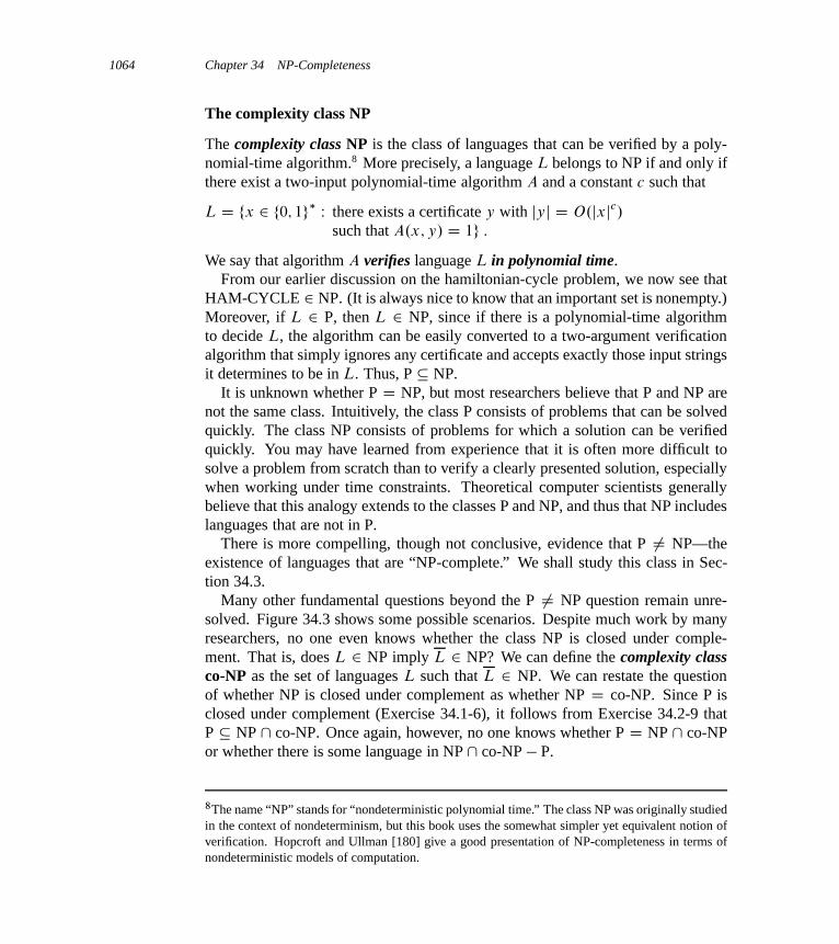
1064 Chapter 34 NP-Completeness
The complexity class NP
The complexity class NP is the class of languages that can be verified by a poly-nomial-time algorithm.8 More precisely, a language L belongs to NP if and only ifthere exist a two-input polynomial-time algorithm A and a constant c such that
L D fx 2 f0; 1g� W there exists a certificate y with jyj D O.jxjc/
such that A.x; y/ D 1g :
We say that algorithm A verifies language L in polynomial time.From our earlier discussion on the hamiltonian-cycle problem, we now see that
HAM-CYCLE 2 NP. (It is always nice to know that an important set is nonempty.)Moreover, if L 2 P, then L 2 NP, since if there is a polynomial-time algorithmto decide L, the algorithm can be easily converted to a two-argument verificationalgorithm that simply ignores any certificate and accepts exactly those input stringsit determines to be in L. Thus, P � NP.
It is unknown whether P D NP, but most researchers believe that P and NP arenot the same class. Intuitively, the class P consists of problems that can be solvedquickly. The class NP consists of problems for which a solution can be verifiedquickly. You may have learned from experience that it is often more difficult tosolve a problem from scratch than to verify a clearly presented solution, especiallywhen working under time constraints. Theoretical computer scientists generallybelieve that this analogy extends to the classes P and NP, and thus that NP includeslanguages that are not in P.
There is more compelling, though not conclusive, evidence that P ¤ NP—theexistence of languages that are “NP-complete.” We shall study this class in Sec-tion 34.3.
Many other fundamental questions beyond the P ¤ NP question remain unre-solved. Figure 34.3 shows some possible scenarios. Despite much work by manyresearchers, no one even knows whether the class NP is closed under comple-ment. That is, does L 2 NP imply L 2 NP? We can define the complexity classco-NP as the set of languages L such that L 2 NP. We can restate the questionof whether NP is closed under complement as whether NP D co-NP. Since P isclosed under complement (Exercise 34.1-6), it follows from Exercise 34.2-9 thatP � NP \ co-NP. Once again, however, no one knows whether P D NP \ co-NPor whether there is some language in NP\ co-NP � P.
8The name “NP” stands for “nondeterministic polynomial time.” The class NP was originally studiedin the context of nondeterminism, but this book uses the somewhat simpler yet equivalent notion ofverification. Hopcroft and Ullman [180] give a good presentation of NP-completeness in terms ofnondeterministic models of computation.
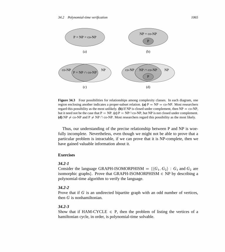
34.2 Polynomial-time verification 1065
co-NP NP
(c)
P = NP ∩ co-NPco-NP NP
(d)
P
P = NP = co-NP
(a)
NP = co-NP
(b)
P
NP ∩ co-NP
Figure 34.3 Four possibilities for relationships among complexity classes. In each diagram, oneregion enclosing another indicates a proper-subset relation. (a) P D NP D co-NP. Most researchersregard this possibility as the most unlikely. (b) If NP is closed under complement, then NP D co-NP,but it need not be the case that P D NP. (c) P D NP\co-NP, but NP is not closed under complement.(d) NP ¤ co-NP and P ¤ NP \ co-NP. Most researchers regard this possibility as the most likely.
Thus, our understanding of the precise relationship between P and NP is woe-fully incomplete. Nevertheless, even though we might not be able to prove that aparticular problem is intractable, if we can prove that it is NP-complete, then wehave gained valuable information about it.
Exercises
34.2-1Consider the language GRAPH-ISOMORPHISM D fhG1; G2i W G1 and G2 areisomorphic graphsg. Prove that GRAPH-ISOMORPHISM 2 NP by describing apolynomial-time algorithm to verify the language.
34.2-2Prove that if G is an undirected bipartite graph with an odd number of vertices,then G is nonhamiltonian.
34.2-3Show that if HAM-CYCLE 2 P, then the problem of listing the vertices of ahamiltonian cycle, in order, is polynomial-time solvable.
1066 Chapter 34 NP-Completeness
34.2-4Prove that the class NP of languages is closed under union, intersection, concate-nation, and Kleene star. Discuss the closure of NP under complement.
34.2-5Show that any language in NP can be decided by an algorithm running intime 2O.nk/ for some constant k.
34.2-6A hamiltonian path in a graph is a simple path that visits every vertex exactlyonce. Show that the language HAM-PATH D fhG; u; �i W there is a hamiltonianpath from u to � in graph Gg belongs to NP.
34.2-7Show that the hamiltonian-path problem from Exercise 34.2-6 can be solved inpolynomial time on directed acyclic graphs. Give an efficient algorithm for theproblem.
34.2-8Let � be a boolean formula constructed from the boolean input variables x1; x2;
: : : ; xk, negations (:), ANDs (^), ORs (_), and parentheses. The formula � is atautology if it evaluates to 1 for every assignment of 1 and 0 to the input variables.Define TAUTOLOGY as the language of boolean formulas that are tautologies.Show that TAUTOLOGY 2 co-NP.
34.2-9Prove that P � co-NP.
34.2-10Prove that if NP ¤ co-NP, then P ¤ NP.
34.2-11Let G be a connected, undirected graph with at least 3 vertices, and let G3 be thegraph obtained by connecting all pairs of vertices that are connected by a path in G
of length at most 3. Prove that G3 is hamiltonian. (Hint: Construct a spanning treefor G, and use an inductive argument.)

34.3 NP-completeness and reducibility 1067
34.3 NP-completeness and reducibility
Perhaps the most compelling reason why theoretical computer scientists believethat P ¤ NP comes from the existence of the class of “NP-complete” problems.This class has the intriguing property that if any NP-complete problem can besolved in polynomial time, then every problem in NP has a polynomial-time solu-tion, that is, P D NP. Despite years of study, though, no polynomial-time algorithmhas ever been discovered for any NP-complete problem.
The language HAM-CYCLE is one NP-complete problem. If we could decideHAM-CYCLE in polynomial time, then we could solve every problem in NP inpolynomial time. In fact, if NP � P should turn out to be nonempty, we could saywith certainty that HAM-CYCLE 2 NP� P.
The NP-complete languages are, in a sense, the “hardest” languages in NP. Inthis section, we shall show how to compare the relative “hardness” of languagesusing a precise notion called “polynomial-time reducibility.” Then we formallydefine the NP-complete languages, and we finish by sketching a proof that onesuch language, called CIRCUIT-SAT, is NP-complete. In Sections 34.4 and 34.5,we shall use the notion of reducibility to show that many other problems are NP-complete.
Reducibility
Intuitively, a problem Q can be reduced to another problem Q0 if any instance of Q
can be “easily rephrased” as an instance of Q0, the solution to which provides asolution to the instance of Q. For example, the problem of solving linear equationsin an indeterminate x reduces to the problem of solving quadratic equations. Givenan instance ax C b D 0, we transform it to 0x2 C ax C b D 0, whose solutionprovides a solution to ax C b D 0. Thus, if a problem Q reduces to anotherproblem Q0, then Q is, in a sense, “no harder to solve” than Q0.
Returning to our formal-language framework for decision problems, we say thata language L1 is polynomial-time reducible to a language L2, written L1 �P L2,if there exists a polynomial-time computable function f W f0; 1g� ! f0; 1g� suchthat for all x 2 f0; 1g�,
x 2 L1 if and only if f .x/ 2 L2 : (34.1)
We call the function f the reduction function, and a polynomial-time algorithm F
that computes f is a reduction algorithm.Figure 34.4 illustrates the idea of a polynomial-time reduction from a lan-
guage L1 to another language L2. Each language is a subset of f0; 1g�. Thereduction function f provides a polynomial-time mapping such that if x 2 L1,

1068 Chapter 34 NP-Completeness
L2L1
{0,1}* {0,1}*f
Figure 34.4 An illustration of a polynomial-time reduction from a language L1 to a language L2
via a reduction function f . For any input x 2 f0; 1g�, the question of whether x 2 L1 has the sameanswer as the question of whether f .x/ 2 L2.
then f .x/ 2 L2. Moreover, if x 62 L1, then f .x/ 62 L2. Thus, the reduction func-tion maps any instance x of the decision problem represented by the language L1
to an instance f .x/ of the problem represented by L2. Providing an answer towhether f .x/ 2 L2 directly provides the answer to whether x 2 L1.
Polynomial-time reductions give us a powerful tool for proving that various lan-guages belong to P.
Lemma 34.3If L1; L2 � f0; 1g� are languages such that L1 �P L2, then L2 2 P impliesL1 2 P.
Proof Let A2 be a polynomial-time algorithm that decides L2, and let F be apolynomial-time reduction algorithm that computes the reduction function f . Weshall construct a polynomial-time algorithm A1 that decides L1.
Figure 34.5 illustrates how we construct A1. For a given input x 2 f0; 1g�,algorithm A1 uses F to transform x into f .x/, and then it uses A2 to test whetherf .x/ 2 L2. Algorithm A1 takes the output from algorithm A2 and produces thatanswer as its own output.
The correctness of A1 follows from condition (34.1). The algorithm runs in poly-nomial time, since both F and A2 run in polynomial time (see Exercise 34.1-5).
NP-completeness
Polynomial-time reductions provide a formal means for showing that one prob-lem is at least as hard as another, to within a polynomial-time factor. That is, ifL1 �P L2, then L1 is not more than a polynomial factor harder than L2, which is

34.3 NP-completeness and reducibility 1069
xF
f .x/
A1
A2
yes, f .x/ 2 L2
no, f .x/ 62 L2
yes, x 2 L1
no, x 62 L1
Figure 34.5 The proof of Lemma 34.3. The algorithm F is a reduction algorithm that computes thereduction function f from L1 to L2 in polynomial time, and A2 is a polynomial-time algorithm thatdecides L2. Algorithm A1 decides whether x 2 L1 by using F to transform any input x into f .x/
and then using A2 to decide whether f .x/ 2 L2.
why the “less than or equal to” notation for reduction is mnemonic. We can nowdefine the set of NP-complete languages, which are the hardest problems in NP.
A language L � f0; 1g� is NP-complete if
1. L 2 NP, and
2. L0 �P L for every L0 2 NP.
If a language L satisfies property 2, but not necessarily property 1, we say that L
is NP-hard. We also define NPC to be the class of NP-complete languages.As the following theorem shows, NP-completeness is at the crux of deciding
whether P is in fact equal to NP.
Theorem 34.4If any NP-complete problem is polynomial-time solvable, then P D NP. Equiva-lently, if any problem in NP is not polynomial-time solvable, then no NP-completeproblem is polynomial-time solvable.
Proof Suppose that L 2 P and also that L 2 NPC. For any L0 2 NP, wehave L0 �P L by property 2 of the definition of NP-completeness. Thus, byLemma 34.3, we also have that L0 2 P, which proves the first statement of thetheorem.
To prove the second statement, note that it is the contrapositive of the first state-ment.
It is for this reason that research into the P ¤ NP question centers around theNP-complete problems. Most theoretical computer scientists believe that P ¤ NP,which leads to the relationships among P, NP, and NPC shown in Figure 34.6.But, for all we know, someone may yet come up with a polynomial-time algo-rithm for an NP-complete problem, thus proving that P D NP. Nevertheless, sinceno polynomial-time algorithm for any NP-complete problem has yet been discov-
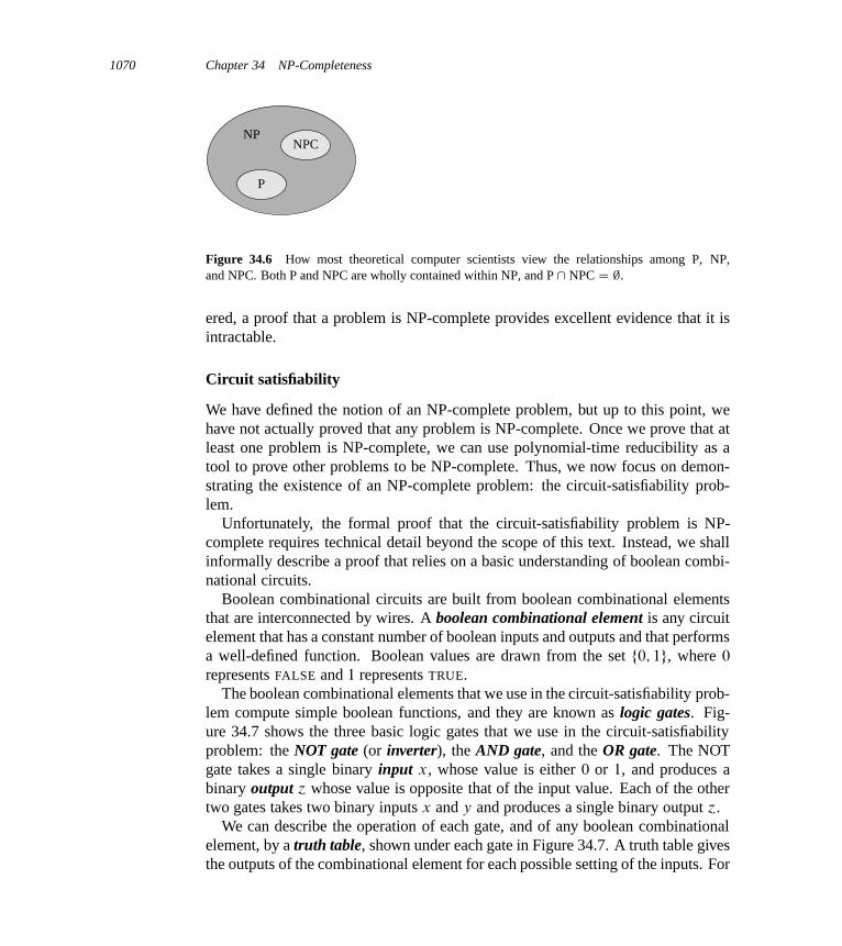
1070 Chapter 34 NP-Completeness
NPC
P
NP
Figure 34.6 How most theoretical computer scientists view the relationships among P, NP,and NPC. Both P and NPC are wholly contained within NP, and P \ NPC D ;.
ered, a proof that a problem is NP-complete provides excellent evidence that it isintractable.
Circuit satisfiability
We have defined the notion of an NP-complete problem, but up to this point, wehave not actually proved that any problem is NP-complete. Once we prove that atleast one problem is NP-complete, we can use polynomial-time reducibility as atool to prove other problems to be NP-complete. Thus, we now focus on demon-strating the existence of an NP-complete problem: the circuit-satisfiability prob-lem.
Unfortunately, the formal proof that the circuit-satisfiability problem is NP-complete requires technical detail beyond the scope of this text. Instead, we shallinformally describe a proof that relies on a basic understanding of boolean combi-national circuits.
Boolean combinational circuits are built from boolean combinational elementsthat are interconnected by wires. A boolean combinational element is any circuitelement that has a constant number of boolean inputs and outputs and that performsa well-defined function. Boolean values are drawn from the set f0; 1g, where 0
represents FALSE and 1 represents TRUE.The boolean combinational elements that we use in the circuit-satisfiability prob-
lem compute simple boolean functions, and they are known as logic gates. Fig-ure 34.7 shows the three basic logic gates that we use in the circuit-satisfiabilityproblem: the NOT gate (or inverter), the AND gate, and the OR gate. The NOTgate takes a single binary input x, whose value is either 0 or 1, and produces abinary output ´ whose value is opposite that of the input value. Each of the othertwo gates takes two binary inputs x and y and produces a single binary output ´.
We can describe the operation of each gate, and of any boolean combinationalelement, by a truth table, shown under each gate in Figure 34.7. A truth table givesthe outputs of the combinational element for each possible setting of the inputs. For
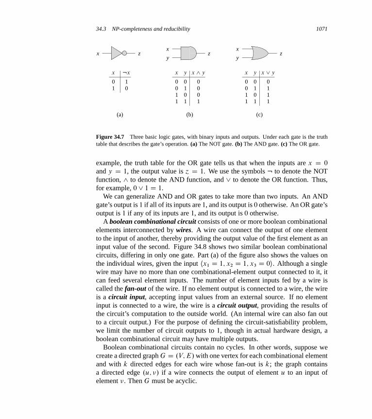
34.3 NP-completeness and reducibility 1071
x
yz
x
yz
0 0 00 1 01 0 01 1 1
0 0 00 1 11 0 11 1 1
(b) (c)
x z
0 11 0
(a)
xxx yy:x x ^ y x _ y
Figure 34.7 Three basic logic gates, with binary inputs and outputs. Under each gate is the truthtable that describes the gate’s operation. (a) The NOT gate. (b) The AND gate. (c) The OR gate.
example, the truth table for the OR gate tells us that when the inputs are x D 0
and y D 1, the output value is ´ D 1. We use the symbols : to denote the NOTfunction, ^ to denote the AND function, and _ to denote the OR function. Thus,for example, 0 _ 1 D 1.
We can generalize AND and OR gates to take more than two inputs. An ANDgate’s output is 1 if all of its inputs are 1, and its output is 0 otherwise. An OR gate’soutput is 1 if any of its inputs are 1, and its output is 0 otherwise.
A boolean combinational circuit consists of one or more boolean combinationalelements interconnected by wires. A wire can connect the output of one elementto the input of another, thereby providing the output value of the first element as aninput value of the second. Figure 34.8 shows two similar boolean combinationalcircuits, differing in only one gate. Part (a) of the figure also shows the values onthe individual wires, given the input hx1 D 1; x2 D 1; x3 D 0i. Although a singlewire may have no more than one combinational-element output connected to it, itcan feed several element inputs. The number of element inputs fed by a wire iscalled the fan-out of the wire. If no element output is connected to a wire, the wireis a circuit input, accepting input values from an external source. If no elementinput is connected to a wire, the wire is a circuit output, providing the results ofthe circuit’s computation to the outside world. (An internal wire can also fan outto a circuit output.) For the purpose of defining the circuit-satisfiability problem,we limit the number of circuit outputs to 1, though in actual hardware design, aboolean combinational circuit may have multiple outputs.
Boolean combinational circuits contain no cycles. In other words, suppose wecreate a directed graph G D .V; E/ with one vertex for each combinational elementand with k directed edges for each wire whose fan-out is k; the graph containsa directed edge .u; �/ if a wire connects the output of element u to an input ofelement �. Then G must be acyclic.

1072 Chapter 34 NP-Completeness
x3
x2
x1
(a)
1
1
0111
1
1
1
1
1
0
0
1 111
x3
x2
x1
(b)
Figure 34.8 Two instances of the circuit-satisfiability problem. (a) The assignment hx1 D 1;
x2 D 1; x3 D 0i to the inputs of this circuit causes the output of the circuit to be 1. The circuitis therefore satisfiable. (b) No assignment to the inputs of this circuit can cause the output of thecircuit to be 1. The circuit is therefore unsatisfiable.
A truth assignment for a boolean combinational circuit is a set of boolean inputvalues. We say that a one-output boolean combinational circuit is satisfiable if ithas a satisfying assignment: a truth assignment that causes the output of the circuitto be 1. For example, the circuit in Figure 34.8(a) has the satisfying assignmenthx1 D 1; x2 D 1; x3 D 0i, and so it is satisfiable. As Exercise 34.3-1 asks you toshow, no assignment of values to x1, x2, and x3 causes the circuit in Figure 34.8(b)to produce a 1 output; it always produces 0, and so it is unsatisfiable.
The circuit-satisfiability problem is, “Given a boolean combinational circuitcomposed of AND, OR, and NOT gates, is it satisfiable?” In order to pose thisquestion formally, however, we must agree on a standard encoding for circuits.The size of a boolean combinational circuit is the number of boolean combina-tional elements plus the number of wires in the circuit. We could devise a graphlikeencoding that maps any given circuit C into a binary string hC i whose length ispolynomial in the size of the circuit itself. As a formal language, we can thereforedefine
CIRCUIT-SAT D fhC i W C is a satisfiable boolean combinational circuitg :
The circuit-satisfiability problem arises in the area of computer-aided hardwareoptimization. If a subcircuit always produces 0, that subcircuit is unnecessary;the designer can replace it by a simpler subcircuit that omits all logic gates andprovides the constant 0 value as its output. You can see why we would like to havea polynomial-time algorithm for this problem.
Given a circuit C , we might attempt to determine whether it is satisfiable bysimply checking all possible assignments to the inputs. Unfortunately, if the circuithas k inputs, then we would have to check up to 2k possible assignments. When
34.3 NP-completeness and reducibility 1073
the size of C is polynomial in k, checking each one takes �.2k/ time, which issuperpolynomial in the size of the circuit.9 In fact, as we have claimed, there isstrong evidence that no polynomial-time algorithm exists that solves the circuit-satisfiability problem because circuit satisfiability is NP-complete. We break theproof of this fact into two parts, based on the two parts of the definition of NP-completeness.
Lemma 34.5The circuit-satisfiability problem belongs to the class NP.
Proof We shall provide a two-input, polynomial-time algorithm A that can verifyCIRCUIT-SAT. One of the inputs to A is (a standard encoding of) a boolean com-binational circuit C . The other input is a certificate corresponding to an assignmentof boolean values to the wires in C . (See Exercise 34.3-4 for a smaller certificate.)
We construct the algorithm A as follows. For each logic gate in the circuit, itchecks that the value provided by the certificate on the output wire is correctlycomputed as a function of the values on the input wires. Then, if the output of theentire circuit is 1, the algorithm outputs 1, since the values assigned to the inputsof C provide a satisfying assignment. Otherwise, A outputs 0.
Whenever a satisfiable circuit C is input to algorithm A, there exists a certificatewhose length is polynomial in the size of C and that causes A to output a 1. When-ever an unsatisfiable circuit is input, no certificate can fool A into believing thatthe circuit is satisfiable. Algorithm A runs in polynomial time: with a good imple-mentation, linear time suffices. Thus, we can verify CIRCUIT-SAT in polynomialtime, and CIRCUIT-SAT 2 NP.
The second part of proving that CIRCUIT-SAT is NP-complete is to show thatthe language is NP-hard. That is, we must show that every language in NP ispolynomial-time reducible to CIRCUIT-SAT. The actual proof of this fact is fullof technical intricacies, and so we shall settle for a sketch of the proof based onsome understanding of the workings of computer hardware.
A computer program is stored in the computer memory as a sequence of in-structions. A typical instruction encodes an operation to be performed, addressesof operands in memory, and an address where the result is to be stored. A spe-cial memory location, called the program counter, keeps track of which instruc-
9On the other hand, if the size of the circuit C is ‚.2k/, then an algorithm whose running timeis O.2k/ has a running time that is polynomial in the circuit size. Even if P ¤ NP, this situa-tion would not contradict the NP-completeness of the problem; the existence of a polynomial-timealgorithm for a special case does not imply that there is a polynomial-time algorithm for all cases.
1074 Chapter 34 NP-Completeness
tion is to be executed next. The program counter automatically increments uponfetching each instruction, thereby causing the computer to execute instructions se-quentially. The execution of an instruction can cause a value to be written to theprogram counter, however, which alters the normal sequential execution and allowsthe computer to loop and perform conditional branches.
At any point during the execution of a program, the computer’s memory holdsthe entire state of the computation. (We take the memory to include the programitself, the program counter, working storage, and any of the various bits of statethat a computer maintains for bookkeeping.) We call any particular state of com-puter memory a configuration. We can view the execution of an instruction asmapping one configuration to another. The computer hardware that accomplishesthis mapping can be implemented as a boolean combinational circuit, which wedenote by M in the proof of the following lemma.
Lemma 34.6The circuit-satisfiability problem is NP-hard.
Proof Let L be any language in NP. We shall describe a polynomial-time algo-rithm F computing a reduction function f that maps every binary string x to acircuit C D f .x/ such that x 2 L if and only if C 2 CIRCUIT-SAT.
Since L 2 NP, there must exist an algorithm A that verifies L in polynomialtime. The algorithm F that we shall construct uses the two-input algorithm A tocompute the reduction function f .
Let T .n/ denote the worst-case running time of algorithm A on length-n inputstrings, and let k � 1 be a constant such that T .n/ D O.nk/ and the length of thecertificate is O.nk/. (The running time of A is actually a polynomial in the totalinput size, which includes both an input string and a certificate, but since the lengthof the certificate is polynomial in the length n of the input string, the running timeis polynomial in n.)
The basic idea of the proof is to represent the computation of A as a sequenceof configurations. As Figure 34.9 illustrates, we can break each configuration intoparts consisting of the program for A, the program counter and auxiliary machinestate, the input x, the certificate y, and working storage. The combinational cir-cuit M , which implements the computer hardware, maps each configuration ci tothe next configuration ciC1, starting from the initial configuration c0. Algorithm A
writes its output—0 or 1—to some designated location by the time it finishes ex-ecuting, and if we assume that thereafter A halts, the value never changes. Thus,if the algorithm runs for at most T .n/ steps, the output appears as one of the bitsin cT .n/.
The reduction algorithm F constructs a single combinational circuit that com-putes all configurations produced by a given initial configuration. The idea is to

34.3 NP-completeness and reducibility 1075
M
A PC aux machine state x y working storage
A PC aux machine state x y working storage
M
A PC aux machine state x y working storage
M
A PC aux machine state x y
…
working storage
0/1 output
M
c0
c1
c2
cT(n)
Figure 34.9 The sequence of configurations produced by an algorithm A running on an input x andcertificate y. Each configuration represents the state of the computer for one step of the computationand, besides A, x, and y, includes the program counter (PC), auxiliary machine state, and workingstorage. Except for the certificate y, the initial configuration c0 is constant. A boolean combinationalcircuit M maps each configuration to the next configuration. The output is a distinguished bit in theworking storage.

1076 Chapter 34 NP-Completeness
paste together T .n/ copies of the circuit M . The output of the i th circuit, whichproduces configuration ci , feeds directly into the input of the .iC1/st circuit. Thus,the configurations, rather than being stored in the computer’s memory, simply re-side as values on the wires connecting copies of M .
Recall what the polynomial-time reduction algorithm F must do. Given an in-put x, it must compute a circuit C D f .x/ that is satisfiable if and only if thereexists a certificate y such that A.x; y/ D 1. When F obtains an input x, it firstcomputes n D jxj and constructs a combinational circuit C 0 consisting of T .n/
copies of M . The input to C 0 is an initial configuration corresponding to a compu-tation on A.x; y/, and the output is the configuration cT .n/.
Algorithm F modifies circuit C 0 slightly to construct the circuit C D f .x/.First, it wires the inputs to C 0 corresponding to the program for A, the initial pro-gram counter, the input x, and the initial state of memory directly to these knownvalues. Thus, the only remaining inputs to the circuit correspond to the certifi-cate y. Second, it ignores all outputs from C 0, except for the one bit of cT .n/
corresponding to the output of A. This circuit C , so constructed, computesC.y/ D A.x; y/ for any input y of length O.nk/. The reduction algorithm F ,when provided an input string x, computes such a circuit C and outputs it.
We need to prove two properties. First, we must show that F correctly computesa reduction function f . That is, we must show that C is satisfiable if and only ifthere exists a certificate y such that A.x; y/ D 1. Second, we must show that F
runs in polynomial time.To show that F correctly computes a reduction function, let us suppose that there
exists a certificate y of length O.nk/ such that A.x; y/ D 1. Then, if we apply thebits of y to the inputs of C , the output of C is C.y/ D A.x; y/ D 1. Thus, if acertificate exists, then C is satisfiable. For the other direction, suppose that C issatisfiable. Hence, there exists an input y to C such that C.y/ D 1, from whichwe conclude that A.x; y/ D 1. Thus, F correctly computes a reduction function.
To complete the proof sketch, we need only show that F runs in time polynomialin n D jxj. The first observation we make is that the number of bits required torepresent a configuration is polynomial in n. The program for A itself has constantsize, independent of the length of its input x. The length of the input x is n, andthe length of the certificate y is O.nk/. Since the algorithm runs for at most O.nk/
steps, the amount of working storage required by A is polynomial in n as well.(We assume that this memory is contiguous; Exercise 34.3-5 asks you to extendthe argument to the situation in which the locations accessed by A are scatteredacross a much larger region of memory and the particular pattern of scattering candiffer for each input x.)
The combinational circuit M implementing the computer hardware has sizepolynomial in the length of a configuration, which is O.nk/; hence, the size of M
is polynomial in n. (Most of this circuitry implements the logic of the memory
34.3 NP-completeness and reducibility 1077
system.) The circuit C consists of at most t D O.nk/ copies of M , and hence ithas size polynomial in n. The reduction algorithm F can construct C from x inpolynomial time, since each step of the construction takes polynomial time.
The language CIRCUIT-SAT is therefore at least as hard as any language in NP,and since it belongs to NP, it is NP-complete.
Theorem 34.7The circuit-satisfiability problem is NP-complete.
Proof Immediate from Lemmas 34.5 and 34.6 and from the definition of NP-completeness.
Exercises
34.3-1Verify that the circuit in Figure 34.8(b) is unsatisfiable.
34.3-2Show that the �P relation is a transitive relation on languages. That is, show that ifL1 �P L2 and L2 �P L3, then L1 �P L3.
34.3-3Prove that L �P L if and only if L �P L.
34.3-4Show that we could have used a satisfying assignment as a certificate in an alter-native proof of Lemma 34.5. Which certificate makes for an easier proof?
34.3-5The proof of Lemma 34.6 assumes that the working storage for algorithm A occu-pies a contiguous region of polynomial size. Where in the proof do we exploit thisassumption? Argue that this assumption does not involve any loss of generality.
34.3-6A language L is complete for a language class C with respect to polynomial-timereductions if L 2 C and L0 �P L for all L0 2 C . Show that ; and f0; 1g� are theonly languages in P that are not complete for P with respect to polynomial-timereductions.
1078 Chapter 34 NP-Completeness
34.3-7Show that, with respect to polynomial-time reductions (see Exercise 34.3-6), L iscomplete for NP if and only if L is complete for co-NP.
34.3-8The reduction algorithm F in the proof of Lemma 34.6 constructs the circuitC D f .x/ based on knowledge of x, A, and k. Professor Sartre observes thatthe string x is input to F , but only the existence of A, k, and the constant factorimplicit in the O.nk/ running time is known to F (since the language L belongsto NP), not their actual values. Thus, the professor concludes that F can’t possi-bly construct the circuit C and that the language CIRCUIT-SAT is not necessarilyNP-hard. Explain the flaw in the professor’s reasoning.
34.4 NP-completeness proofs
We proved that the circuit-satisfiability problem is NP-complete by a direct proofthat L �P CIRCUIT-SAT for every language L 2 NP. In this section, we shallshow how to prove that languages are NP-complete without directly reducing everylanguage in NP to the given language. We shall illustrate this methodology byproving that various formula-satisfiability problems are NP-complete. Section 34.5provides many more examples of the methodology.
The following lemma is the basis of our method for showing that a language isNP-complete.
Lemma 34.8If L is a language such that L0 �P L for some L0 2 NPC, then L is NP-hard. If, inaddition, L 2 NP, then L 2 NPC.
Proof Since L0 is NP-complete, for all L00 2 NP, we have L00 �P L0. By sup-position, L0 �P L, and thus by transitivity (Exercise 34.3-2), we have L00 �P L,which shows that L is NP-hard. If L 2 NP, we also have L 2 NPC.
In other words, by reducing a known NP-complete language L0 to L, we implic-itly reduce every language in NP to L. Thus, Lemma 34.8 gives us a method forproving that a language L is NP-complete:
1. Prove L 2 NP.
2. Select a known NP-complete language L0.
34.4 NP-completeness proofs 1079
3. Describe an algorithm that computes a function f mapping every instancex 2 f0; 1g� of L0 to an instance f .x/ of L.
4. Prove that the function f satisfies x 2 L0 if and only if f .x/ 2 L for allx 2 f0; 1g�.
5. Prove that the algorithm computing f runs in polynomial time.
(Steps 2–5 show that L is NP-hard.) This methodology of reducing from a sin-gle known NP-complete language is far simpler than the more complicated pro-cess of showing directly how to reduce from every language in NP. ProvingCIRCUIT-SAT 2 NPC has given us a “foot in the door.” Because we know that thecircuit-satisfiability problem is NP-complete, we now can prove much more easilythat other problems are NP-complete. Moreover, as we develop a catalog of knownNP-complete problems, we will have more and more choices for languages fromwhich to reduce.
Formula satisfiability
We illustrate the reduction methodology by giving an NP-completeness proof forthe problem of determining whether a boolean formula, not a circuit, is satisfiable.This problem has the historical honor of being the first problem ever shown to beNP-complete.
We formulate the (formula) satisfiability problem in terms of the language SATas follows. An instance of SAT is a boolean formula � composed of
1. n boolean variables: x1; x2; : : : ; xn;
2. m boolean connectives: any boolean function with one or two inputs and oneoutput, such as ^ (AND), _ (OR), : (NOT),! (implication), $ (if and onlyif); and
3. parentheses. (Without loss of generality, we assume that there are no redundantparentheses, i.e., a formula contains at most one pair of parentheses per booleanconnective.)
We can easily encode a boolean formula � in a length that is polynomial in nCm.As in boolean combinational circuits, a truth assignment for a boolean formula �
is a set of values for the variables of �, and a satisfying assignment is a truthassignment that causes it to evaluate to 1. A formula with a satisfying assignmentis a satisfiable formula. The satisfiability problem asks whether a given booleanformula is satisfiable; in formal-language terms,
SAT D fh�i W � is a satisfiable boolean formulag :
As an example, the formula

1080 Chapter 34 NP-Completeness
� D ..x1 ! x2/ _ :..:x1 $ x3/ _ x4// ^ :x2
has the satisfying assignment hx1 D 0; x2 D 0; x3 D 1; x4 D 1i, since
� D ..0! 0/ _ :..:0$ 1/ _ 1// ^ :0 (34.2)
D .1 _ :.1 _ 1// ^ 1
D .1 _ 0/ ^ 1
D 1 ;
and thus this formula � belongs to SAT.The naive algorithm to determine whether an arbitrary boolean formula is satis-
fiable does not run in polynomial time. A formula with n variables has 2n possibleassignments. If the length of h�i is polynomial in n, then checking every assign-ment requires �.2n/ time, which is superpolynomial in the length of h�i. As thefollowing theorem shows, a polynomial-time algorithm is unlikely to exist.
Theorem 34.9Satisfiability of boolean formulas is NP-complete.
Proof We start by arguing that SAT 2 NP. Then we prove that SAT is NP-hard byshowing that CIRCUIT-SAT �P SAT; by Lemma 34.8, this will prove the theorem.
To show that SAT belongs to NP, we show that a certificate consisting of asatisfying assignment for an input formula � can be verified in polynomial time.The verifying algorithm simply replaces each variable in the formula with its cor-responding value and then evaluates the expression, much as we did in equa-tion (34.2) above. This task is easy to do in polynomial time. If the expressionevaluates to 1, then the algorithm has verified that the formula is satisfiable. Thus,the first condition of Lemma 34.8 for NP-completeness holds.
To prove that SAT is NP-hard, we show that CIRCUIT-SAT �P SAT. In otherwords, we need to show how to reduce any instance of circuit satisfiability to aninstance of formula satisfiability in polynomial time. We can use induction toexpress any boolean combinational circuit as a boolean formula. We simply lookat the gate that produces the circuit output and inductively express each of thegate’s inputs as formulas. We then obtain the formula for the circuit by writing anexpression that applies the gate’s function to its inputs’ formulas.
Unfortunately, this straightforward method does not amount to a polynomial-time reduction. As Exercise 34.4-1 asks you to show, shared subformulas—whicharise from gates whose output wires have fan-out of 2 or more—can cause thesize of the generated formula to grow exponentially. Thus, the reduction algorithmmust be somewhat more clever.
Figure 34.10 illustrates how we overcome this problem, using as an examplethe circuit from Figure 34.8(a). For each wire xi in the circuit C , the formula �
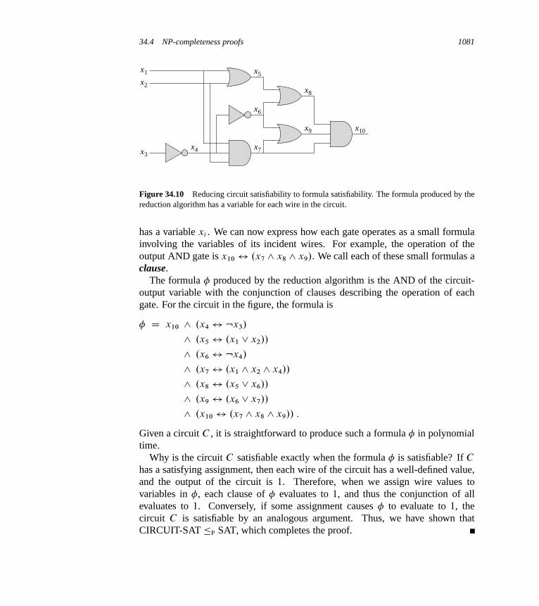
34.4 NP-completeness proofs 1081
x6
x3x4 x7
x10x9
x8
x5
x2
x1
Figure 34.10 Reducing circuit satisfiability to formula satisfiability. The formula produced by thereduction algorithm has a variable for each wire in the circuit.
has a variable xi . We can now express how each gate operates as a small formulainvolving the variables of its incident wires. For example, the operation of theoutput AND gate is x10 $ .x7 ^ x8 ^ x9/. We call each of these small formulas aclause.
The formula � produced by the reduction algorithm is the AND of the circuit-output variable with the conjunction of clauses describing the operation of eachgate. For the circuit in the figure, the formula is
� D x10 ^ .x4 $ :x3/
^ .x5 $ .x1 _ x2//
^ .x6 $ :x4/
^ .x7 $ .x1 ^ x2 ^ x4//
^ .x8 $ .x5 _ x6//
^ .x9 $ .x6 _ x7//
^ .x10 $ .x7 ^ x8 ^ x9// :
Given a circuit C , it is straightforward to produce such a formula � in polynomialtime.
Why is the circuit C satisfiable exactly when the formula � is satisfiable? If C
has a satisfying assignment, then each wire of the circuit has a well-defined value,and the output of the circuit is 1. Therefore, when we assign wire values tovariables in �, each clause of � evaluates to 1, and thus the conjunction of allevaluates to 1. Conversely, if some assignment causes � to evaluate to 1, thecircuit C is satisfiable by an analogous argument. Thus, we have shown thatCIRCUIT-SAT �P SAT, which completes the proof.

1082 Chapter 34 NP-Completeness
3-CNF satisfiability
We can prove many problems NP-complete by reducing from formula satisfiability.The reduction algorithm must handle any input formula, though, and this require-ment can lead to a huge number of cases that we must consider. We often preferto reduce from a restricted language of boolean formulas, so that we need to con-sider fewer cases. Of course, we must not restrict the language so much that itbecomes polynomial-time solvable. One convenient language is 3-CNF satisfiabil-ity, or 3-CNF-SAT.
We define 3-CNF satisfiability using the following terms. A literal in a booleanformula is an occurrence of a variable or its negation. A boolean formula is inconjunctive normal form, or CNF, if it is expressed as an AND of clauses, eachof which is the OR of one or more literals. A boolean formula is in 3-conjunctivenormal form, or 3-CNF, if each clause has exactly three distinct literals.
For example, the boolean formula
.x1 _ :x1 _ :x2/ ^ .x3 _ x2 _ x4/ ^ .:x1 _ :x3 _ :x4/
is in 3-CNF. The first of its three clauses is .x1 _ :x1 _ :x2/, which contains thethree literals x1, :x1, and :x2.
In 3-CNF-SAT, we are asked whether a given boolean formula � in 3-CNF issatisfiable. The following theorem shows that a polynomial-time algorithm thatcan determine the satisfiability of boolean formulas is unlikely to exist, even whenthey are expressed in this simple normal form.
Theorem 34.10Satisfiability of boolean formulas in 3-conjunctive normal form is NP-complete.
Proof The argument we used in the proof of Theorem 34.9 to show that SAT 2NP applies equally well here to show that 3-CNF-SAT 2 NP. By Lemma 34.8,therefore, we need only show that SAT �P 3-CNF-SAT.
We break the reduction algorithm into three basic steps. Each step progressivelytransforms the input formula � closer to the desired 3-conjunctive normal form.
The first step is similar to the one used to prove CIRCUIT-SAT �P SAT inTheorem 34.9. First, we construct a binary “parse” tree for the input formula �,with literals as leaves and connectives as internal nodes. Figure 34.11 shows sucha parse tree for the formula
� D ..x1 ! x2/ _ :..:x1 $ x3/ _ x4// ^ :x2 : (34.3)
Should the input formula contain a clause such as the OR of several literals, we useassociativity to parenthesize the expression fully so that every internal node in theresulting tree has 1 or 2 children. We can now think of the binary parse tree as acircuit for computing the function.
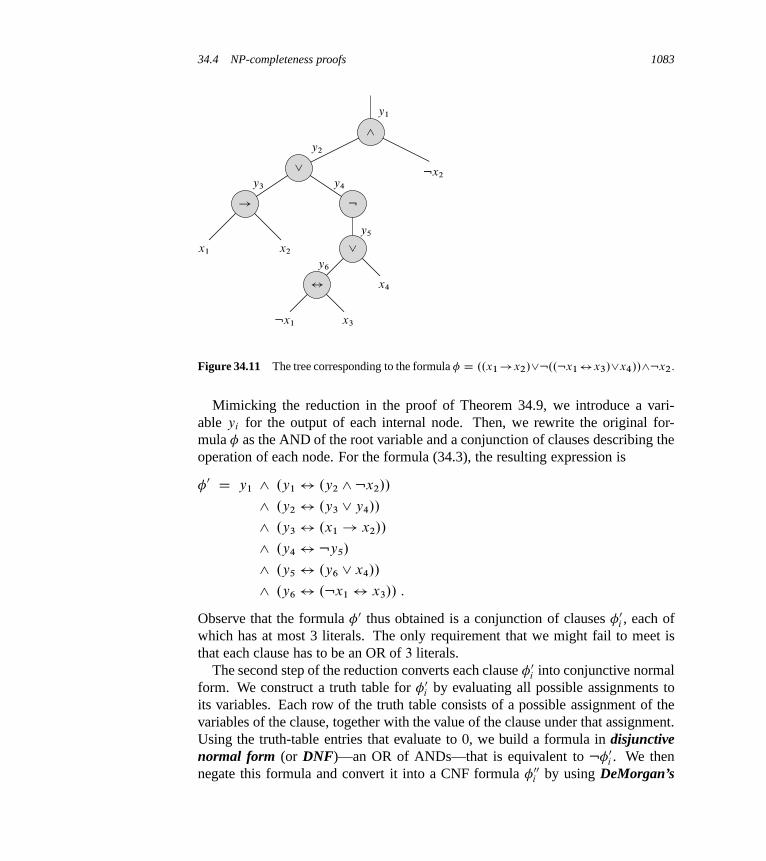
34.4 NP-completeness proofs 1083
:x1
x1
:x2
x2
x3
x4
y1
y2
y3 y4
y5
y6
^
$
_
_
:!
Figure 34.11 The tree corresponding to the formula � D ..x1!x2/_:..:x1$x3/_x4//^:x2:
Mimicking the reduction in the proof of Theorem 34.9, we introduce a vari-able yi for the output of each internal node. Then, we rewrite the original for-mula � as the AND of the root variable and a conjunction of clauses describing theoperation of each node. For the formula (34.3), the resulting expression is
�0 D y1 ^ .y1 $ .y2 ^:x2//
^ .y2 $ .y3 _ y4//
^ .y3 $ .x1 ! x2//
^ .y4 $ :y5/
^ .y5 $ .y6 _ x4//
^ .y6 $ .:x1 $ x3// :
Observe that the formula �0 thus obtained is a conjunction of clauses �0i , each of
which has at most 3 literals. The only requirement that we might fail to meet isthat each clause has to be an OR of 3 literals.
The second step of the reduction converts each clause �0i into conjunctive normal
form. We construct a truth table for �0i by evaluating all possible assignments to
its variables. Each row of the truth table consists of a possible assignment of thevariables of the clause, together with the value of the clause under that assignment.Using the truth-table entries that evaluate to 0, we build a formula in disjunctivenormal form (or DNF)—an OR of ANDs—that is equivalent to :�0
i . We thennegate this formula and convert it into a CNF formula �00
i by using DeMorgan’s
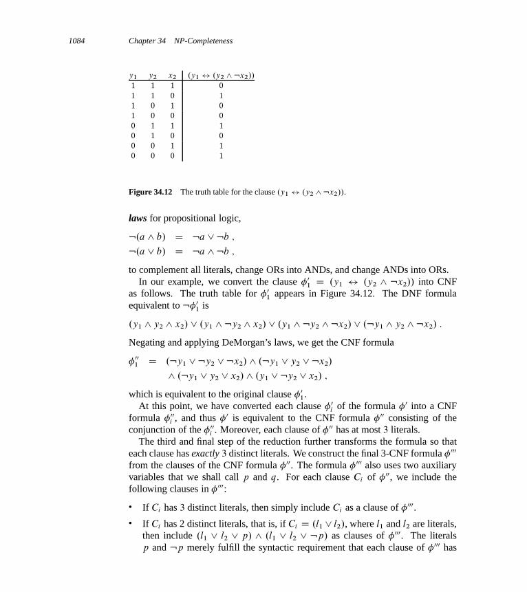
1084 Chapter 34 NP-Completeness
y1 y2 x2 .y1 $ .y2 ^ :x2//
1 1 1 01 1 0 11 0 1 01 0 0 00 1 1 10 1 0 00 0 1 10 0 0 1
Figure 34.12 The truth table for the clause .y1 $ .y2 ^ :x2//.
laws for propositional logic,
:.a ^ b/ D :a _:b ;
:.a _ b/ D :a ^:b ;
to complement all literals, change ORs into ANDs, and change ANDs into ORs.In our example, we convert the clause �0
1 D .y1 $ .y2 ^ :x2// into CNFas follows. The truth table for �0
1 appears in Figure 34.12. The DNF formulaequivalent to :�0
1 is
.y1 ^ y2 ^ x2/ _ .y1 ^ :y2 ^ x2/ _ .y1 ^ :y2 ^:x2/ _ .:y1 ^ y2 ^ :x2/ :
Negating and applying DeMorgan’s laws, we get the CNF formula
�001 D .:y1 _:y2 _ :x2/ ^ .:y1 _ y2 _ :x2/
^ .:y1 _ y2 _ x2/ ^ .y1 _ :y2 _ x2/ ;
which is equivalent to the original clause �01.
At this point, we have converted each clause �0i of the formula �0 into a CNF
formula �00i , and thus �0 is equivalent to the CNF formula �00 consisting of the
conjunction of the �00i . Moreover, each clause of �00 has at most 3 literals.
The third and final step of the reduction further transforms the formula so thateach clause has exactly 3 distinct literals. We construct the final 3-CNF formula �000
from the clauses of the CNF formula �00. The formula �000 also uses two auxiliaryvariables that we shall call p and q. For each clause Ci of �00, we include thefollowing clauses in �000:
� If Ci has 3 distinct literals, then simply include Ci as a clause of �000.� If Ci has 2 distinct literals, that is, if Ci D .l1 _ l2/, where l1 and l2 are literals,
then include .l1 _ l2 _ p/ ^ .l1 _ l2 _ :p/ as clauses of �000. The literalsp and :p merely fulfill the syntactic requirement that each clause of �000 has

34.4 NP-completeness proofs 1085
exactly 3 distinct literals. Whether p D 0 or p D 1, one of the clauses isequivalent to l1_ l2, and the other evaluates to 1, which is the identity for AND.
� If Ci has just 1 distinct literal l , then include .l _ p _ q/ ^ .l _ p _ :q/ ^.l _:p _ q/ ^ .l _:p _:q/ as clauses of �000. Regardless of the values of p
and q, one of the four clauses is equivalent to l , and the other 3 evaluate to 1.
We can see that the 3-CNF formula �000 is satisfiable if and only if � is satisfiableby inspecting each of the three steps. Like the reduction from CIRCUIT-SAT toSAT, the construction of �0 from � in the first step preserves satisfiability. Thesecond step produces a CNF formula �00 that is algebraically equivalent to �0. Thethird step produces a 3-CNF formula �000 that is effectively equivalent to �00, sinceany assignment to the variables p and q produces a formula that is algebraicallyequivalent to �00.
We must also show that the reduction can be computed in polynomial time. Con-structing �0 from � introduces at most 1 variable and 1 clause per connective in �.Constructing �00 from �0 can introduce at most 8 clauses into �00 for each clausefrom �0, since each clause of �0 has at most 3 variables, and the truth table foreach clause has at most 23 D 8 rows. The construction of �000 from �00 introducesat most 4 clauses into �000 for each clause of �00. Thus, the size of the resultingformula �000 is polynomial in the length of the original formula. Each of the con-structions can easily be accomplished in polynomial time.
Exercises
34.4-1Consider the straightforward (nonpolynomial-time) reduction in the proof of The-orem 34.9. Describe a circuit of size n that, when converted to a formula by thismethod, yields a formula whose size is exponential in n.
34.4-2Show the 3-CNF formula that results when we use the method of Theorem 34.10on the formula (34.3).
34.4-3Professor Jagger proposes to show that SAT �P 3-CNF-SAT by using only thetruth-table technique in the proof of Theorem 34.10, and not the other steps. Thatis, the professor proposes to take the boolean formula �, form a truth table forits variables, derive from the truth table a formula in 3-DNF that is equivalentto :�, and then negate and apply DeMorgan’s laws to produce a 3-CNF formulaequivalent to �. Show that this strategy does not yield a polynomial-time reduction.

1086 Chapter 34 NP-Completeness
34.4-4Show that the problem of determining whether a boolean formula is a tautology iscomplete for co-NP. (Hint: See Exercise 34.3-7.)
34.4-5Show that the problem of determining the satisfiability of boolean formulas in dis-junctive normal form is polynomial-time solvable.
34.4-6Suppose that someone gives you a polynomial-time algorithm to decide formulasatisfiability. Describe how to use this algorithm to find satisfying assignments inpolynomial time.
34.4-7Let 2-CNF-SAT be the set of satisfiable boolean formulas in CNF with exactly 2literals per clause. Show that 2-CNF-SAT 2 P. Make your algorithm as efficient aspossible. (Hint: Observe that x _ y is equivalent to :x ! y. Reduce 2-CNF-SATto an efficiently solvable problem on a directed graph.)
34.5 NP-complete problems
NP-complete problems arise in diverse domains: boolean logic, graphs, arithmetic,network design, sets and partitions, storage and retrieval, sequencing and schedul-ing, mathematical programming, algebra and number theory, games and puzzles,automata and language theory, program optimization, biology, chemistry, physics,and more. In this section, we shall use the reduction methodology to provide NP-completeness proofs for a variety of problems drawn from graph theory and setpartitioning.
Figure 34.13 outlines the structure of the NP-completeness proofs in this sectionand Section 34.4. We prove each language in the figure to be NP-complete byreduction from the language that points to it. At the root is CIRCUIT-SAT, whichwe proved NP-complete in Theorem 34.7.
34.5.1 The clique problem
A clique in an undirected graph G D .V; E/ is a subset V 0 � V of vertices, eachpair of which is connected by an edge in E. In other words, a clique is a completesubgraph of G. The size of a clique is the number of vertices it contains. Theclique problem is the optimization problem of finding a clique of maximum size in

34.5 NP-complete problems 1087
CIRCUIT-SAT
SAT
3-CNF-SAT
CLIQUE
VERTEX-COVER
SUBSET-SUM
HAM-CYCLE
TSP
Figure 34.13 The structure of NP-completeness proofs in Sections 34.4 and 34.5. All proofs ulti-mately follow by reduction from the NP-completeness of CIRCUIT-SAT.
a graph. As a decision problem, we ask simply whether a clique of a given size k
exists in the graph. The formal definition is
CLIQUE D fhG; ki W G is a graph containing a clique of size kg :
A naive algorithm for determining whether a graph G D .V; E/ with jV j ver-tices has a clique of size k is to list all k-subsets of V , and check each one tosee whether it forms a clique. The running time of this algorithm is �.k2
�jV jk
�/,
which is polynomial if k is a constant. In general, however, k could be near jV j =2,in which case the algorithm runs in superpolynomial time. Indeed, an efficientalgorithm for the clique problem is unlikely to exist.
Theorem 34.11The clique problem is NP-complete.
Proof To show that CLIQUE 2 NP, for a given graph G D .V; E/, we use theset V 0 � V of vertices in the clique as a certificate for G. We can check whether V 0
is a clique in polynomial time by checking whether, for each pair u; � 2 V 0, theedge .u; �/ belongs to E.
We next prove that 3-CNF-SAT �P CLIQUE, which shows that the clique prob-lem is NP-hard. You might be surprised that we should be able to prove such aresult, since on the surface logical formulas seem to have little to do with graphs.
The reduction algorithm begins with an instance of 3-CNF-SAT. Let � DC1 ^ C2 ^ � � � ^ Ck be a boolean formula in 3-CNF with k clauses. For r D
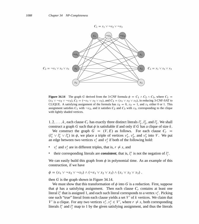
1088 Chapter 34 NP-Completeness
x1
x1
x2x2
x3x3
:x1
:x2 :x3
C1 D x1 _ :x2 _:x3
C2 D :x1 _ x2 _ x3 C3 D x1 _ x2 _ x3
Figure 34.14 The graph G derived from the 3-CNF formula � D C1 ^ C2 ^ C3, where C1 D.x1 _ :x2 _ :x3/, C2 D .:x1 _ x2 _ x3/, and C3 D .x1 _ x2 _ x3/, in reducing 3-CNF-SAT toCLIQUE. A satisfying assignment of the formula has x2 D 0, x3 D 1, and x1 either 0 or 1. Thisassignment satisfies C1 with :x2, and it satisfies C2 and C3 with x3, corresponding to the cliquewith lightly shaded vertices.
1; 2; : : : ; k, each clause Cr has exactly three distinct literals lr1 , lr
2 , and lr3 . We shall
construct a graph G such that � is satisfiable if and only if G has a clique of size k.We construct the graph G D .V; E/ as follows. For each clause Cr D
.lr1 _ lr
2 _ lr3 / in �, we place a triple of vertices �r
1 , �r2 , and �r
3 into V . We putan edge between two vertices �r
i and �sj if both of the following hold:
� �ri and �s
j are in different triples, that is, r ¤ s, and
� their corresponding literals are consistent, that is, lri is not the negation of ls
j .
We can easily build this graph from � in polynomial time. As an example of thisconstruction, if we have
� D .x1 _ :x2 _ :x3/ ^ .:x1 _ x2 _ x3/ ^ .x1 _ x2 _ x3/ ;
then G is the graph shown in Figure 34.14.We must show that this transformation of � into G is a reduction. First, suppose
that � has a satisfying assignment. Then each clause Cr contains at least oneliteral lr
i that is assigned 1, and each such literal corresponds to a vertex �ri . Picking
one such “true” literal from each clause yields a set V 0 of k vertices. We claim thatV 0 is a clique. For any two vertices �r
i ; �sj 2 V 0, where r ¤ s, both corresponding
literals lri and ls
j map to 1 by the given satisfying assignment, and thus the literals

34.5 NP-complete problems 1089
cannot be complements. Thus, by the construction of G, the edge .�ri ; �s
j / belongsto E.
Conversely, suppose that G has a clique V 0 of size k. No edges in G connectvertices in the same triple, and so V 0 contains exactly one vertex per triple. We canassign 1 to each literal lr
i such that �ri 2 V 0 without fear of assigning 1 to both a
literal and its complement, since G contains no edges between inconsistent literals.Each clause is satisfied, and so � is satisfied. (Any variables that do not correspondto a vertex in the clique may be set arbitrarily.)
In the example of Figure 34.14, a satisfying assignment of � has x2 D 0 andx3 D 1. A corresponding clique of size k D 3 consists of the vertices correspond-ing to :x2 from the first clause, x3 from the second clause, and x3 from the thirdclause. Because the clique contains no vertices corresponding to either x1 or :x1,we can set x1 to either 0 or 1 in this satisfying assignment.
Observe that in the proof of Theorem 34.11, we reduced an arbitrary instanceof 3-CNF-SAT to an instance of CLIQUE with a particular structure. You mightthink that we have shown only that CLIQUE is NP-hard in graphs in which thevertices are restricted to occur in triples and in which there are no edges betweenvertices in the same triple. Indeed, we have shown that CLIQUE is NP-hard onlyin this restricted case, but this proof suffices to show that CLIQUE is NP-hard ingeneral graphs. Why? If we had a polynomial-time algorithm that solved CLIQUEon general graphs, it would also solve CLIQUE on restricted graphs.
The opposite approach—reducing instances of 3-CNF-SAT with a special struc-ture to general instances of CLIQUE—would not have sufficed, however. Whynot? Perhaps the instances of 3-CNF-SAT that we chose to reduce from were“easy,” and so we would not have reduced an NP-hard problem to CLIQUE.
Observe also that the reduction used the instance of 3-CNF-SAT, but not thesolution. We would have erred if the polynomial-time reduction had relied onknowing whether the formula � is satisfiable, since we do not know how to decidewhether � is satisfiable in polynomial time.
34.5.2 The vertex-cover problem
A vertex cover of an undirected graph G D .V; E/ is a subset V 0 � V such thatif .u; �/ 2 E, then u 2 V 0 or � 2 V 0 (or both). That is, each vertex “covers” itsincident edges, and a vertex cover for G is a set of vertices that covers all the edgesin E. The size of a vertex cover is the number of vertices in it. For example, thegraph in Figure 34.15(b) has a vertex cover fw; ´g of size 2.
The vertex-cover problem is to find a vertex cover of minimum size in a givengraph. Restating this optimization problem as a decision problem, we wish to

1090 Chapter 34 NP-Completeness
u v
y x
z w
(a)
u v
y x
z w
(b)
Figure 34.15 Reducing CLIQUE to VERTEX-COVER. (a) An undirected graph G D .V; E/ withclique V 0 D fu; �; x; yg. (b) The graph G produced by the reduction algorithm that has vertex coverV � V 0 D fw; ´g.
determine whether a graph has a vertex cover of a given size k. As a language, wedefine
VERTEX-COVERD fhG; ki W graph G has a vertex cover of size kg :
The following theorem shows that this problem is NP-complete.
Theorem 34.12The vertex-cover problem is NP-complete.
Proof We first show that VERTEX-COVER 2 NP. Suppose we are given a graphG D .V; E/ and an integer k. The certificate we choose is the vertex cover V 0 � V
itself. The verification algorithm affirms that jV 0j D k, and then it checks, for eachedge .u; �/ 2 E, that u 2 V 0 or � 2 V 0. We can easily verify the certificate inpolynomial time.
We prove that the vertex-cover problem is NP-hard by showing that CLIQUE �P
VERTEX-COVER. This reduction relies on the notion of the “complement” of agraph. Given an undirected graph G D .V; E/, we define the complement of G
as G D .V; E/, where E D f.u; �/ W u; � 2 V; u ¤ �; and .u; �/ 62 Eg. In otherwords, G is the graph containing exactly those edges that are not in G. Figure 34.15shows a graph and its complement and illustrates the reduction from CLIQUE toVERTEX-COVER.
The reduction algorithm takes as input an instance hG; ki of the clique problem.It computes the complement G, which we can easily do in polynomial time. Theoutput of the reduction algorithm is the instance hG; jV j � ki of the vertex-coverproblem. To complete the proof, we show that this transformation is indeed a
34.5 NP-complete problems 1091
reduction: the graph G has a clique of size k if and only if the graph G has a vertexcover of size jV j � k.
Suppose that G has a clique V 0 � V with jV 0j D k. We claim that V � V 0 is avertex cover in G. Let .u; �/ be any edge in E. Then, .u; �/ 62 E, which impliesthat at least one of u or � does not belong to V 0, since every pair of vertices in V 0 isconnected by an edge of E. Equivalently, at least one of u or � is in V �V 0, whichmeans that edge .u; �/ is covered by V � V 0. Since .u; �/ was chosen arbitrarilyfrom E, every edge of E is covered by a vertex in V � V 0. Hence, the set V � V 0,which has size jV j � k, forms a vertex cover for G.
Conversely, suppose that G has a vertex cover V 0 � V , where jV 0j D jV j � k.Then, for all u; � 2 V , if .u; �/ 2 E, then u 2 V 0 or � 2 V 0 or both. Thecontrapositive of this implication is that for all u; � 2 V , if u 62 V 0 and � 62 V 0,then .u; �/ 2 E. In other words, V �V 0 is a clique, and it has size jV j�jV 0j D k.
Since VERTEX-COVER is NP-complete, we don’t expect to find a polynomial-time algorithm for finding a minimum-size vertex cover. Section 35.1 presents apolynomial-time “approximation algorithm,” however, which produces “approxi-mate” solutions for the vertex-cover problem. The size of a vertex cover producedby the algorithm is at most twice the minimum size of a vertex cover.
Thus, we shouldn’t give up hope just because a problem is NP-complete. Wemay be able to design a polynomial-time approximation algorithm that obtainsnear-optimal solutions, even though finding an optimal solution is NP-complete.Chapter 35 gives several approximation algorithms for NP-complete problems.
34.5.3 The hamiltonian-cycle problem
We now return to the hamiltonian-cycle problem defined in Section 34.2.
Theorem 34.13The hamiltonian cycle problem is NP-complete.
Proof We first show that HAM-CYCLE belongs to NP. Given a graph G D.V; E/, our certificate is the sequence of jV j vertices that makes up the hamiltoniancycle. The verification algorithm checks that this sequence contains each vertexin V exactly once and that with the first vertex repeated at the end, it forms a cyclein G. That is, it checks that there is an edge between each pair of consecutivevertices and between the first and last vertices. We can verify the certificate inpolynomial time.
We now prove that VERTEX-COVER �P HAM-CYCLE, which shows thatHAM-CYCLE is NP-complete. Given an undirected graph G D .V; E/ and an
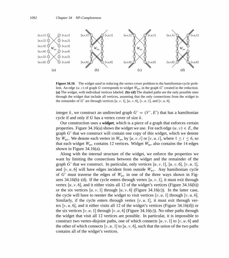
1092 Chapter 34 NP-Completeness
[u,v,1]
[u,v,2]
[u,v,3]
[u,v,4]
[u,v,5]
[u,v,6]
[v,u,1]
[v,u,2]
[v,u,3]
[v,u,4]
[v,u,5]
[v,u,6]
Wuv
(a)
Wuv
(b)
[u,v,1]
[u,v,6]
[v,u,1]
[v,u,6]
Wuv
(c)
[u,v,1]
[u,v,6]
[v,u,1]
[v,u,6]
Wuv
(d)
[u,v,1]
[u,v,6]
[v,u,1]
[v,u,6]
Figure 34.16 The widget used in reducing the vertex-cover problem to the hamiltonian-cycle prob-lem. An edge .u; �/ of graph G corresponds to widget Wu� in the graph G0 created in the reduction.(a) The widget, with individual vertices labeled. (b)–(d) The shaded paths are the only possible onesthrough the widget that include all vertices, assuming that the only connections from the widget tothe remainder of G0 are through vertices Œu; �; 1�, Œu; �; 6�, Œ�; u; 1�, and Œ�; u; 6�.
integer k, we construct an undirected graph G0 D .V 0; E 0/ that has a hamiltoniancycle if and only if G has a vertex cover of size k.
Our construction uses a widget, which is a piece of a graph that enforces certainproperties. Figure 34.16(a) shows the widget we use. For each edge .u; �/ 2 E, thegraph G0 that we construct will contain one copy of this widget, which we denoteby Wu� . We denote each vertex in Wu� by Œu; �; i � or Œ�; u; i �, where 1 � i � 6, sothat each widget Wu� contains 12 vertices. Widget Wu� also contains the 14 edgesshown in Figure 34.16(a).
Along with the internal structure of the widget, we enforce the properties wewant by limiting the connections between the widget and the remainder of thegraph G0 that we construct. In particular, only vertices Œu; �; 1�, Œu; �; 6�, Œ�; u; 1�,and Œ�; u; 6� will have edges incident from outside Wu� . Any hamiltonian cycleof G0 must traverse the edges of Wu� in one of the three ways shown in Fig-ures 34.16(b)–(d). If the cycle enters through vertex Œu; �; 1�, it must exit throughvertex Œu; �; 6�, and it either visits all 12 of the widget’s vertices (Figure 34.16(b))or the six vertices Œu; �; 1� through Œu; �; 6� (Figure 34.16(c)). In the latter case,the cycle will have to reenter the widget to visit vertices Œ�; u; 1� through Œ�; u; 6�.Similarly, if the cycle enters through vertex Œ�; u; 1�, it must exit through ver-tex Œ�; u; 6�, and it either visits all 12 of the widget’s vertices (Figure 34.16(d)) orthe six vertices Œ�; u; 1� through Œ�; u; 6� (Figure 34.16(c)). No other paths throughthe widget that visit all 12 vertices are possible. In particular, it is impossible toconstruct two vertex-disjoint paths, one of which connects Œu; �; 1� to Œ�; u; 6� andthe other of which connects Œ�; u; 1� to Œu; �; 6�, such that the union of the two pathscontains all of the widget’s vertices.
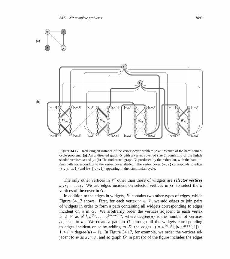
34.5 NP-complete problems 1093
[w,x,1]
[w,x,6]
[x,w,1]
[x,w,6]
Wwx
(b)
[x,y,1]
[x,y,6]
[y,x,1]
[y,x,6]
Wxy
[w,y,1]
[w,y,6]
[y,w,1]
[y,w,6]
Wwy
[w,z,1]
[w,z,6]
[z,w,1]
[z,w,6]
Wwz
s1
s2
w x
z y
(a)
Figure 34.17 Reducing an instance of the vertex-cover problem to an instance of the hamiltonian-cycle problem. (a) An undirected graph G with a vertex cover of size 2, consisting of the lightlyshaded vertices w and y. (b) The undirected graph G0 produced by the reduction, with the hamilto-nian path corresponding to the vertex cover shaded. The vertex cover fw; yg corresponds to edges.s1; Œw; x; 1�/ and .s2; Œy; x; 1�/ appearing in the hamiltonian cycle.
The only other vertices in V 0 other than those of widgets are selector verticess1; s2; : : : ; sk . We use edges incident on selector vertices in G0 to select the k
vertices of the cover in G.In addition to the edges in widgets, E 0 contains two other types of edges, which
Figure 34.17 shows. First, for each vertex u 2 V , we add edges to join pairsof widgets in order to form a path containing all widgets corresponding to edgesincident on u in G. We arbitrarily order the vertices adjacent to each vertexu 2 V as u.1/; u.2/; : : : ; u.degree.u//, where degree.u/ is the number of verticesadjacent to u. We create a path in G0 through all the widgets correspondingto edges incident on u by adding to E 0 the edges f.Œu; u.i/; 6�; Œu; u.iC1/; 1�/ W1 � i � degree.u/ � 1g. In Figure 34.17, for example, we order the vertices ad-jacent to w as x; y; ´, and so graph G0 in part (b) of the figure includes the edges

1094 Chapter 34 NP-Completeness
.Œw; x; 6�; Œw; y; 1�/ and .Œw; y; 6�; Œw; ´; 1�/. For each vertex u 2 V , these edgesin G0 fill in a path containing all widgets corresponding to edges incident on u
in G.The intuition behind these edges is that if we choose a vertex u 2 V in the vertex
cover of G, we can construct a path from Œu; u.1/; 1� to Œu; u.degree.u//; 6� in G0 that“covers” all widgets corresponding to edges incident on u. That is, for each of thesewidgets, say Wu;u.i/ , the path either includes all 12 vertices (if u is in the vertexcover but u.i/ is not) or just the six vertices Œu; u.i/; 1�; Œu; u.i/; 2�; : : : ; Œu; u.i/; 6� (ifboth u and u.i/ are in the vertex cover).
The final type of edge in E 0 joins the first vertex Œu; u.1/; 1� and the last vertexŒu; u.degree.u//; 6� of each of these paths to each of the selector vertices. That is, weinclude the edges
f.sj ; Œu; u.1/; 1�/ W u 2 V and 1 � j � kg[ f.sj ; Œu; u.degree.u//; 6�/ W u 2 V and 1 � j � kg :
Next, we show that the size of G0 is polynomial in the size of G, and hence wecan construct G0 in time polynomial in the size of G. The vertices of G0 are thosein the widgets, plus the selector vertices. With 12 vertices per widget, plus k � jV jselector vertices, we have a total of
jV 0j D 12 jEj C k
� 12 jEj C jV jvertices. The edges of G0 are those in the widgets, those that go between widgets,and those connecting selector vertices to widgets. Each widget contains 14 edges,totaling 14 jEj in all widgets. For each vertex u 2 V , graph G0 has degree.u/ � 1
edges going between widgets, so that summed over all vertices in V ,Xu2V
.degree.u/ � 1/ D 2 jEj � jV j
edges go between widgets. Finally, G0 has two edges for each pair consisting of aselector vertex and a vertex of V , totaling 2k jV j such edges. The total number ofedges of G0 is therefore
jE 0j D .14 jEj/C .2 jEj � jV j/C .2k jV j/D 16 jEj C .2k � 1/ jV j� 16 jEj C .2 jV j � 1/ jV j :
Now we show that the transformation from graph G to G0 is a reduction. That is,we must show that G has a vertex cover of size k if and only if G0 has a hamiltoniancycle.
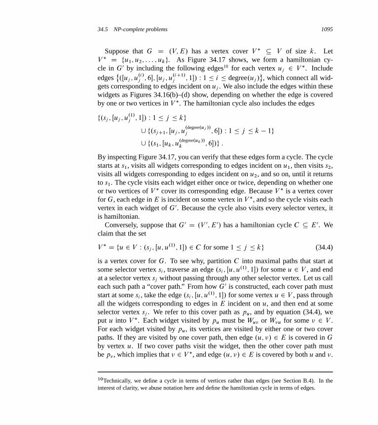
34.5 NP-complete problems 1095
Suppose that G D .V; E/ has a vertex cover V � � V of size k. LetV � D fu1; u2; : : : ; ukg. As Figure 34.17 shows, we form a hamiltonian cy-cle in G0 by including the following edges10 for each vertex uj 2 V �. Includeedges
˚.Œuj ; u
.i/j ; 6�; Œuj ; u
.iC1/j ; 1�/ W 1 � i � degree.uj /
, which connect all wid-
gets corresponding to edges incident on uj . We also include the edges within thesewidgets as Figures 34.16(b)–(d) show, depending on whether the edge is coveredby one or two vertices in V �. The hamiltonian cycle also includes the edges
f.sj ; Œuj ; u.1/j ; 1�/ W 1 � j � kg[ f.sj C1; Œuj ; u
.degree.uj //
j ; 6�/ W 1 � j � k � 1g[ f.s1; Œuk ; u
.degree.uk//
k; 6�/g :
By inspecting Figure 34.17, you can verify that these edges form a cycle. The cyclestarts at s1, visits all widgets corresponding to edges incident on u1, then visits s2,visits all widgets corresponding to edges incident on u2, and so on, until it returnsto s1. The cycle visits each widget either once or twice, depending on whether oneor two vertices of V � cover its corresponding edge. Because V � is a vertex coverfor G, each edge in E is incident on some vertex in V �, and so the cycle visits eachvertex in each widget of G0. Because the cycle also visits every selector vertex, itis hamiltonian.
Conversely, suppose that G0 D .V 0; E 0/ has a hamiltonian cycle C � E 0. Weclaim that the set
V � D fu 2 V W .sj ; Œu; u.1/; 1�/ 2 C for some 1 � j � kg (34.4)
is a vertex cover for G. To see why, partition C into maximal paths that start atsome selector vertex si , traverse an edge .si ; Œu; u.1/; 1�/ for some u 2 V , and endat a selector vertex sj without passing through any other selector vertex. Let us calleach such path a “cover path.” From how G0 is constructed, each cover path muststart at some si , take the edge .si ; Œu; u.1/; 1�/ for some vertex u 2 V , pass throughall the widgets corresponding to edges in E incident on u, and then end at someselector vertex sj . We refer to this cover path as pu, and by equation (34.4), weput u into V �. Each widget visited by pu must be Wu� or W�u for some � 2 V .For each widget visited by pu, its vertices are visited by either one or two coverpaths. If they are visited by one cover path, then edge .u; �/ 2 E is covered in G
by vertex u. If two cover paths visit the widget, then the other cover path mustbe p� , which implies that � 2 V �, and edge .u; �/ 2 E is covered by both u and �.
10Technically, we define a cycle in terms of vertices rather than edges (see Section B.4). In theinterest of clarity, we abuse notation here and define the hamiltonian cycle in terms of edges.
1096 Chapter 34 NP-Completeness
u v
x w
4
23
5
1
1
Figure 34.18 An instance of the traveling-salesman problem. Shaded edges represent a minimum-cost tour, with cost 7.
Because each vertex in each widget is visited by some cover path, we see that eachedge in E is covered by some vertex in V �.
34.5.4 The traveling-salesman problem
In the traveling-salesman problem, which is closely related to the hamiltonian-cycle problem, a salesman must visit n cities. Modeling the problem as a completegraph with n vertices, we can say that the salesman wishes to make a tour, orhamiltonian cycle, visiting each city exactly once and finishing at the city he startsfrom. The salesman incurs a nonnegative integer cost c.i; j / to travel from city i
to city j , and the salesman wishes to make the tour whose total cost is minimum,where the total cost is the sum of the individual costs along the edges of the tour.For example, in Figure 34.18, a minimum-cost tour is hu; w; �; x; ui, with cost 7.The formal language for the corresponding decision problem is
TSP D fhG; c; ki W G D .V; E/ is a complete graph;
c is a function from V V ! Z;
k 2 Z, andG has a traveling-salesman tour with cost at most kg :
The following theorem shows that a fast algorithm for the traveling-salesmanproblem is unlikely to exist.
Theorem 34.14The traveling-salesman problem is NP-complete.
Proof We first show that TSP belongs to NP. Given an instance of the problem,we use as a certificate the sequence of n vertices in the tour. The verificationalgorithm checks that this sequence contains each vertex exactly once, sums up theedge costs, and checks whether the sum is at most k. This process can certainly bedone in polynomial time.
34.5 NP-complete problems 1097
To prove that TSP is NP-hard, we show that HAM-CYCLE �P TSP. LetG D .V; E/ be an instance of HAM-CYCLE. We construct an instance of TSP asfollows. We form the complete graph G0 D .V; E 0/, where E 0 D f.i; j / W i; j 2 V
and i ¤ j g, and we define the cost function c by
c.i; j / D(
0 if .i; j / 2 E ;
1 if .i; j / 62 E :
(Note that because G is undirected, it has no self-loops, and so c.�; �/ D 1 for allvertices � 2 V .) The instance of TSP is then hG0; c; 0i, which we can easily createin polynomial time.
We now show that graph G has a hamiltonian cycle if and only if graph G0 has atour of cost at most 0. Suppose that graph G has a hamiltonian cycle h. Each edgein h belongs to E and thus has cost 0 in G0. Thus, h is a tour in G0 with cost 0.Conversely, suppose that graph G0 has a tour h0 of cost at most 0. Since the costsof the edges in E 0 are 0 and 1, the cost of tour h0 is exactly 0 and each edge on thetour must have cost 0. Therefore, h0 contains only edges in E. We conclude that h0
is a hamiltonian cycle in graph G.
34.5.5 The subset-sum problem
We next consider an arithmetic NP-complete problem. In the subset-sum problem,we are given a finite set S of positive integers and an integer target t > 0. We askwhether there exists a subset S 0 � S whose elements sum to t . For example,if S D f1; 2; 7; 14; 49; 98; 343; 686; 2409; 2793; 16808; 17206; 117705; 117993gand t D 138457, then the subset S 0 D f1; 2; 7; 98; 343; 686; 2409; 17206; 117705gis a solution.
As usual, we define the problem as a language:
SUBSET-SUMD fhS; ti W there exists a subset S 0 � S such that t DPs2S 0 sg :
As with any arithmetic problem, it is important to recall that our standard encodingassumes that the input integers are coded in binary. With this assumption in mind,we can show that the subset-sum problem is unlikely to have a fast algorithm.
Theorem 34.15The subset-sum problem is NP-complete.
Proof To show that SUBSET-SUM is in NP, for an instance hS; ti of the problem,we let the subset S 0 be the certificate. A verification algorithm can check whethert DPs2S 0 s in polynomial time.
We now show that 3-CNF-SAT �P SUBSET-SUM. Given a 3-CNF formula �
over variables x1; x2; : : : ; xn with clauses C1; C2; : : : ; Ck , each containing exactly
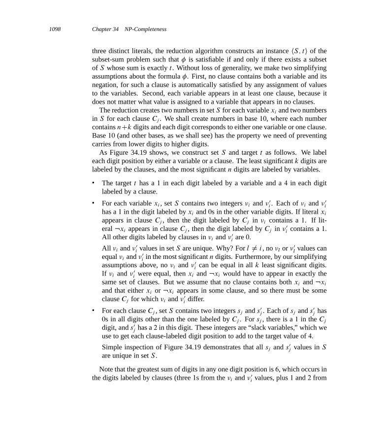
1098 Chapter 34 NP-Completeness
three distinct literals, the reduction algorithm constructs an instance hS; ti of thesubset-sum problem such that � is satisfiable if and only if there exists a subsetof S whose sum is exactly t . Without loss of generality, we make two simplifyingassumptions about the formula �. First, no clause contains both a variable and itsnegation, for such a clause is automatically satisfied by any assignment of valuesto the variables. Second, each variable appears in at least one clause, because itdoes not matter what value is assigned to a variable that appears in no clauses.
The reduction creates two numbers in set S for each variable xi and two numbersin S for each clause Cj . We shall create numbers in base 10, where each numbercontains nCk digits and each digit corresponds to either one variable or one clause.Base 10 (and other bases, as we shall see) has the property we need of preventingcarries from lower digits to higher digits.
As Figure 34.19 shows, we construct set S and target t as follows. We labeleach digit position by either a variable or a clause. The least significant k digits arelabeled by the clauses, and the most significant n digits are labeled by variables.
� The target t has a 1 in each digit labeled by a variable and a 4 in each digitlabeled by a clause.
� For each variable xi , set S contains two integers �i and � 0i . Each of �i and � 0
i
has a 1 in the digit labeled by xi and 0s in the other variable digits. If literal xi
appears in clause Cj , then the digit labeled by Cj in �i contains a 1. If lit-eral :xi appears in clause Cj , then the digit labeled by Cj in � 0
i contains a 1.All other digits labeled by clauses in �i and � 0
i are 0.
All �i and � 0i values in set S are unique. Why? For l ¤ i , no �l or � 0
lvalues can
equal �i and � 0i in the most significant n digits. Furthermore, by our simplifying
assumptions above, no �i and � 0i can be equal in all k least significant digits.
If �i and � 0i were equal, then xi and :xi would have to appear in exactly the
same set of clauses. But we assume that no clause contains both xi and :xi
and that either xi or :xi appears in some clause, and so there must be someclause Cj for which �i and � 0
i differ.
� For each clause Cj , set S contains two integers sj and s0j . Each of sj and s0
j has0s in all digits other than the one labeled by Cj . For sj , there is a 1 in the Cj
digit, and s0j has a 2 in this digit. These integers are “slack variables,” which we
use to get each clause-labeled digit position to add to the target value of 4.
Simple inspection of Figure 34.19 demonstrates that all sj and s0j values in S
are unique in set S .
Note that the greatest sum of digits in any one digit position is 6, which occurs inthe digits labeled by clauses (three 1s from the �i and � 0
i values, plus 1 and 2 from

34.5 NP-complete problems 1099
= 1 0 0 1 0 0 1
= 1 0 0 0 1 1 0
= 0 1 0 0 0 0 1
= 0 1 0 1 1 1 0
= 0 0 1 0 0 1 1
= 0 0 1 1 1 0 0
= 0 0 0 1 0 0 0
= 0 0 0 2 0 0 0
= 0 0 0 0 1 0 0
= 0 0 0 0 2 0 0
= 0 0 0 0 0 1 0
= 0 0 0 0 0 2 0
= 0 0 0 0 0 0 1
= 0 0 0 0 0 0 2
= 1 1 1 4 4 4 4
x1 x2 x3 C1 C2 C3 C4
�1
� 01
�2
� 02
�3
� 03
s1
s01
s2
s02
s3
s03
s4
s04
t
Figure 34.19 The reduction of 3-CNF-SAT to SUBSET-SUM. The formula in 3-CNF is � DC1^C2^C3^C4, where C1 D .x1_:x2_:x3/, C2 D .:x1_:x2_:x3/, C3 D .:x1_:x2_x3/,and C4 D .x1 _ x2 _ x3/. A satisfying assignment of � is hx1 D 0; x2 D 0; x3 D 1i. The set S
produced by the reduction consists of the base-10 numbers shown; reading from top to bottom, S Df1001001; 1000110; 100001; 101110; 10011; 11100; 1000; 2000; 100; 200; 10; 20; 1; 2g. The target t
is 1114444. The subset S 0 � S is lightly shaded, and it contains �01, �0
2, and �3, corresponding to thesatisfying assignment. It also contains slack variables s1, s0
1, s02, s3, s4, and s0
4 to achieve the targetvalue of 4 in the digits labeled by C1 through C4.
the sj and s0j values). Interpreting these numbers in base 10, therefore, no carries
can occur from lower digits to higher digits.11
We can perform the reduction in polynomial time. The set S contains 2nC 2k
values, each of which has nC k digits, and the time to produce each digit is poly-nomial in nC k. The target t has nC k digits, and the reduction produces each inconstant time.
We now show that the 3-CNF formula � is satisfiable if and only if there existsa subset S 0 � S whose sum is t . First, suppose that � has a satisfying assignment.For i D 1; 2; : : : ; n, if xi D 1 in this assignment, then include �i in S 0. Otherwise,include � 0
i . In other words, we include in S 0 exactly the �i and � 0i values that cor-
11In fact, any base b, where b � 7, would work. The instance at the beginning of this subsection isthe set S and target t in Figure 34.19 interpreted in base 7, with S listed in sorted order.
1100 Chapter 34 NP-Completeness
respond to literals with the value 1 in the satisfying assignment. Having includedeither �i or � 0
i , but not both, for all i , and having put 0 in the digits labeled byvariables in all sj and s0
j , we see that for each variable-labeled digit, the sum of thevalues of S 0 must be 1, which matches those digits of the target t . Because eachclause is satisfied, the clause contains some literal with the value 1. Therefore,each digit labeled by a clause has at least one 1 contributed to its sum by a �i or � 0
i
value in S 0. In fact, 1, 2, or 3 literals may be 1 in each clause, and so each clause-labeled digit has a sum of 1, 2, or 3 from the �i and � 0
i values in S 0. In Figure 34.19for example, literals :x1, :x2, and x3 have the value 1 in a satisfying assignment.Each of clauses C1 and C4 contains exactly one of these literals, and so together � 0
1,� 0
2, and �3 contribute 1 to the sum in the digits for C1 and C4. Clause C2 containstwo of these literals, and � 0
1, � 02, and �3 contribute 2 to the sum in the digit for C2.
Clause C3 contains all three of these literals, and � 01, � 0
2, and �3 contribute 3 to thesum in the digit for C3. We achieve the target of 4 in each digit labeled by clause Cj
by including in S 0 the appropriate nonempty subset of slack variables fsj ; s0j g. In
Figure 34.19, S 0 includes s1, s01, s0
2, s3, s4, and s04. Since we have matched the target
in all digits of the sum, and no carries can occur, the values of S 0 sum to t .Now, suppose that there is a subset S 0 � S that sums to t . The subset S 0 must
include exactly one of �i and � 0i for each i D 1; 2; : : : ; n, for otherwise the digits
labeled by variables would not sum to 1. If �i 2 S 0, we set xi D 1. Otherwise,� 0
i 2 S 0, and we set xi D 0. We claim that every clause Cj , for j D 1; 2; : : : ; k, issatisfied by this assignment. To prove this claim, note that to achieve a sum of 4 inthe digit labeled by Cj , the subset S 0 must include at least one �i or � 0
i value thathas a 1 in the digit labeled by Cj , since the contributions of the slack variables sj
and s0j together sum to at most 3. If S 0 includes a �i that has a 1 in Cj ’s position,
then the literal xi appears in clause Cj . Since we have set xi D 1 when �i 2 S 0,clause Cj is satisfied. If S 0 includes a � 0
i that has a 1 in that position, then theliteral :xi appears in Cj . Since we have set xi D 0 when � 0
i 2 S 0, clause Cj isagain satisfied. Thus, all clauses of � are satisfied, which completes the proof.
Exercises
34.5-1The subgraph-isomorphism problem takes two undirected graphs G1 and G2, andit asks whether G1 is isomorphic to a subgraph of G2. Show that the subgraph-isomorphism problem is NP-complete.
34.5-2Given an integer m n matrix A and an integer m-vector b, the 0-1 integer-programming problem asks whether there exists an integer n-vector x with ele-

Problems for Chapter 34 1101
ments in the set f0; 1g such that Ax � b. Prove that 0-1 integer programming isNP-complete. (Hint: Reduce from 3-CNF-SAT.)
34.5-3The integer linear-programming problem is like the 0-1 integer-programmingproblem given in Exercise 34.5-2, except that the values of the vector x may beany integers rather than just 0 or 1. Assuming that the 0-1 integer-programmingproblem is NP-hard, show that the integer linear-programming problem is NP-complete.
34.5-4Show how to solve the subset-sum problem in polynomial time if the target value t
is expressed in unary.
34.5-5The set-partition problem takes as input a set S of numbers. The question iswhether the numbers can be partitioned into two sets A and A D S � A suchthat
Px2A x DPx2A x. Show that the set-partition problem is NP-complete.
34.5-6Show that the hamiltonian-path problem is NP-complete.
34.5-7The longest-simple-cycle problem is the problem of determining a simple cycle(no repeated vertices) of maximum length in a graph. Formulate a related decisionproblem, and show that the decision problem is NP-complete.
34.5-8In the half 3-CNF satisfiability problem, we are given a 3-CNF formula � with n
variables and m clauses, where m is even. We wish to determine whether thereexists a truth assignment to the variables of � such that exactly half the clausesevaluate to 0 and exactly half the clauses evaluate to 1. Prove that the half 3-CNFsatisfiability problem is NP-complete.
Problems
34-1 Independent setAn independent set of a graph G D .V; E/ is a subset V 0 � V of vertices suchthat each edge in E is incident on at most one vertex in V 0. The independent-setproblem is to find a maximum-size independent set in G.

1102 Chapter 34 NP-Completeness
a. Formulate a related decision problem for the independent-set problem, andprove that it is NP-complete. (Hint: Reduce from the clique problem.)
b. Suppose that you are given a “black-box” subroutine to solve the decision prob-lem you defined in part (a). Give an algorithm to find an independent set of max-imum size. The running time of your algorithm should be polynomial in jV jand jEj, counting queries to the black box as a single step.
Although the independent-set decision problem is NP-complete, certain specialcases are polynomial-time solvable.
c. Give an efficient algorithm to solve the independent-set problem when each ver-tex in G has degree 2. Analyze the running time, and prove that your algorithmworks correctly.
d. Give an efficient algorithm to solve the independent-set problem when G isbipartite. Analyze the running time, and prove that your algorithm works cor-rectly. (Hint: Use the results of Section 26.3.)
34-2 Bonnie and ClydeBonnie and Clyde have just robbed a bank. They have a bag of money and wantto divide it up. For each of the following scenarios, either give a polynomial-timealgorithm, or prove that the problem is NP-complete. The input in each case is alist of the n items in the bag, along with the value of each.
a. The bag contains n coins, but only 2 different denominations: some coins areworth x dollars, and some are worth y dollars. Bonnie and Clyde wish to dividethe money exactly evenly.
b. The bag contains n coins, with an arbitrary number of different denominations,but each denomination is a nonnegative integer power of 2, i.e., the possibledenominations are 1 dollar, 2 dollars, 4 dollars, etc. Bonnie and Clyde wish todivide the money exactly evenly.
c. The bag contains n checks, which are, in an amazing coincidence, made out to“Bonnie or Clyde.” They wish to divide the checks so that they each get theexact same amount of money.
d. The bag contains n checks as in part (c), but this time Bonnie and Clyde arewilling to accept a split in which the difference is no larger than 100 dollars.

Problems for Chapter 34 1103
34-3 Graph coloringMapmakers try to use as few colors as possible when coloring countries on a map,as long as no two countries that share a border have the same color. We can modelthis problem with an undirected graph G D .V; E/ in which each vertex repre-sents a country and vertices whose respective countries share a border are adjacent.Then, a k-coloring is a function c W V ! f1; 2; : : : ; kg such that c.u/ ¤ c.�/ forevery edge .u; �/ 2 E. In other words, the numbers 1; 2; : : : ; k represent the k col-ors, and adjacent vertices must have different colors. The graph-coloring problemis to determine the minimum number of colors needed to color a given graph.
a. Give an efficient algorithm to determine a 2-coloring of a graph, if one exists.
b. Cast the graph-coloring problem as a decision problem. Show that your deci-sion problem is solvable in polynomial time if and only if the graph-coloringproblem is solvable in polynomial time.
c. Let the language 3-COLOR be the set of graphs that can be 3-colored. Showthat if 3-COLOR is NP-complete, then your decision problem from part (b) isNP-complete.
To prove that 3-COLOR is NP-complete, we use a reduction from 3-CNF-SAT.Given a formula � of m clauses on n variables x1, x2, . . . , xn, we construct a graphG D .V; E/ as follows. The set V consists of a vertex for each variable, a vertexfor the negation of each variable, 5 vertices for each clause, and 3 special vertices:TRUE, FALSE, and RED. The edges of the graph are of two types: “literal” edgesthat are independent of the clauses and “clause” edges that depend on the clauses.The literal edges form a triangle on the special vertices and also form a triangle onxi , :xi , and RED for i D 1; 2; : : : ; n.
d. Argue that in any 3-coloring c of a graph containing the literal edges, exactlyone of a variable and its negation is colored c.TRUE/ and the other is coloredc.FALSE/. Argue that for any truth assignment for �, there exists a 3-coloringof the graph containing just the literal edges.
The widget shown in Figure 34.20 helps to enforce the condition corresponding toa clause .x _ y _ ´/. Each clause requires a unique copy of the 5 vertices that areheavily shaded in the figure; they connect as shown to the literals of the clause andthe special vertex TRUE.
e. Argue that if each of x, y, and ´ is colored c.TRUE/ or c.FALSE/, then thewidget is 3-colorable if and only if at least one of x, y, or ´ is colored c.TRUE/.
f. Complete the proof that 3-COLOR is NP-complete.

1104 Chapter 34 NP-Completeness
x
y
z
TRUE
Figure 34.20 The widget corresponding to a clause .x _ y _ ´/, used in Problem 34-3.
34-4 Scheduling with profits and deadlinesSuppose that we have one machine and a set of n tasks a1; a2; : : : ; an, each ofwhich requires time on the machine. Each task aj requires tj time units on themachine (its processing time), yields a profit of pj , and has a deadline dj . Themachine can process only one task at a time, and task aj must run without inter-ruption for tj consecutive time units. If we complete task aj by its deadline dj , wereceive a profit pj , but if we complete it after its deadline, we receive no profit. Asan optimization problem, we are given the processing times, profits, and deadlinesfor a set of n tasks, and we wish to find a schedule that completes all the tasks andreturns the greatest amount of profit. The processing times, profits, and deadlinesare all nonnegative numbers.
a. State this problem as a decision problem.
b. Show that the decision problem is NP-complete.
c. Give a polynomial-time algorithm for the decision problem, assuming that allprocessing times are integers from 1 to n. (Hint: Use dynamic programming.)
d. Give a polynomial-time algorithm for the optimization problem, assuming thatall processing times are integers from 1 to n.
Chapter notes
The book by Garey and Johnson [129] provides a wonderful guide to NP-complete-ness, discussing the theory at length and providing a catalogue of many problemsthat were known to be NP-complete in 1979. The proof of Theorem 34.13 isadapted from their book, and the list of NP-complete problem domains at the begin-ning of Section 34.5 is drawn from their table of contents. Johnson wrote a series
Notes for Chapter 34 1105
of 23 columns in the Journal of Algorithms between 1981 and 1992 reporting newdevelopments in NP-completeness. Hopcroft, Motwani, and Ullman [177], Lewisand Papadimitriou [236], Papadimitriou [270], and Sipser [317] have good treat-ments of NP-completeness in the context of complexity theory. NP-completenessand several reductions also appear in books by Aho, Hopcroft, and Ullman [5];Dasgupta, Papadimitriou, and Vazirani [83]; Johnsonbaugh and Schaefer [193];and Kleinberg and Tardos [208].
The class P was introduced in 1964 by Cobham [73] and, independently, in 1965by Edmonds [100], who also introduced the class NP and conjectured that P ¤ NP.The notion of NP-completeness was proposed in 1971 by Cook [76], who gavethe first NP-completeness proofs for formula satisfiability and 3-CNF satisfiabil-ity. Levin [234] independently discovered the notion, giving an NP-completenessproof for a tiling problem. Karp [199] introduced the methodology of reductionsin 1972 and demonstrated the rich variety of NP-complete problems. Karp’s pa-per included the original NP-completeness proofs of the clique, vertex-cover, andhamiltonian-cycle problems. Since then, thousands of problems have been provento be NP-complete by many researchers. In a talk at a meeting celebrating Karp’s60th birthday in 1995, Papadimitriou remarked, “about 6000 papers each year havethe term ‘NP-complete’ on their title, abstract, or list of keywords. This is morethan each of the terms ‘compiler,’ ‘database,’ ‘expert,’ ‘neural network,’ or ‘oper-ating system.’ ”
Recent work in complexity theory has shed light on the complexity of computingapproximate solutions. This work gives a new definition of NP using “probabilis-tically checkable proofs.” This new definition implies that for problems such asclique, vertex cover, traveling-salesman problem with the triangle inequality, andmany others, computing good approximate solutions is NP-hard and hence no eas-ier than computing optimal solutions. An introduction to this area can be foundin Arora’s thesis [20]; a chapter by Arora and Lund in [172]; a survey article byArora [21]; a book edited by Mayr, Promel, and Steger [246]; and a survey articleby Johnson [191].
35 Approximation Algorithms
Many problems of practical significance are NP-complete, yet they are too impor-tant to abandon merely because we don’t know how to find an optimal solution inpolynomial time. Even if a problem is NP-complete, there may be hope. We have atleast three ways to get around NP-completeness. First, if the actual inputs are small,an algorithm with exponential running time may be perfectly satisfactory. Second,we may be able to isolate important special cases that we can solve in polynomialtime. Third, we might come up with approaches to find near-optimal solutions inpolynomial time (either in the worst case or the expected case). In practice, near-optimality is often good enough. We call an algorithm that returns near-optimalsolutions an approximation algorithm. This chapter presents polynomial-time ap-proximation algorithms for several NP-complete problems.
Performance ratios for approximation algorithms
Suppose that we are working on an optimization problem in which each potentialsolution has a positive cost, and we wish to find a near-optimal solution. Dependingon the problem, we may define an optimal solution as one with maximum possi-ble cost or one with minimum possible cost; that is, the problem may be either amaximization or a minimization problem.
We say that an algorithm for a problem has an approximation ratio of �.n/ if,for any input of size n, the cost C of the solution produced by the algorithm iswithin a factor of �.n/ of the cost C � of an optimal solution:
max
�C
C � ;C �
C
�� �.n/ : (35.1)
If an algorithm achieves an approximation ratio of �.n/, we call it a �.n/-approx-imation algorithm. The definitions of the approximation ratio and of a �.n/-approximation algorithm apply to both minimization and maximization problems.For a maximization problem, 0 < C � C �, and the ratio C �=C gives the factorby which the cost of an optimal solution is larger than the cost of the approximate
Chapter 35 Approximation Algorithms 1107
solution. Similarly, for a minimization problem, 0 < C � � C , and the ratio C=C �
gives the factor by which the cost of the approximate solution is larger than thecost of an optimal solution. Because we assume that all solutions have positivecost, these ratios are always well defined. The approximation ratio of an approx-imation algorithm is never less than 1, since C=C � � 1 implies C �=C � 1.Therefore, a 1-approximation algorithm1 produces an optimal solution, and an ap-proximation algorithm with a large approximation ratio may return a solution thatis much worse than optimal.
For many problems, we have polynomial-time approximation algorithms withsmall constant approximation ratios, although for other problems, the best knownpolynomial-time approximation algorithms have approximation ratios that growas functions of the input size n. An example of such a problem is the set-coverproblem presented in Section 35.3.
Some NP-complete problems allow polynomial-time approximation algorithmsthat can achieve increasingly better approximation ratios by using more and morecomputation time. That is, we can trade computation time for the quality of theapproximation. An example is the subset-sum problem studied in Section 35.5.This situation is important enough to deserve a name of its own.
An approximation scheme for an optimization problem is an approximation al-gorithm that takes as input not only an instance of the problem, but also a value� > 0 such that for any fixed �, the scheme is a .1C �/-approximation algorithm.We say that an approximation scheme is a polynomial-time approximation schemeif for any fixed � > 0, the scheme runs in time polynomial in the size n of its inputinstance.
The running time of a polynomial-time approximation scheme can increase veryrapidly as � decreases. For example, the running time of a polynomial-time ap-proximation scheme might be O.n2=�/. Ideally, if � decreases by a constant factor,the running time to achieve the desired approximation should not increase by morethan a constant factor (though not necessarily the same constant factor by which �
decreased).We say that an approximation scheme is a fully polynomial-time approximation
scheme if it is an approximation scheme and its running time is polynomial inboth 1=� and the size n of the input instance. For example, the scheme might havea running time of O..1=�/2n3/. With such a scheme, any constant-factor decreasein � comes with a corresponding constant-factor increase in the running time.
1When the approximation ratio is independent of n, we use the terms approximation ratio of � and�-approximation algorithm, indicating no dependence on n.
1108 Chapter 35 Approximation Algorithms
Chapter outline
The first four sections of this chapter present some examples of polynomial-timeapproximation algorithms for NP-complete problems, and the fifth section presentsa fully polynomial-time approximation scheme. Section 35.1 begins with a studyof the vertex-cover problem, an NP-complete minimization problem that has anapproximation algorithm with an approximation ratio of 2. Section 35.2 presentsan approximation algorithm with an approximation ratio of 2 for the case of thetraveling-salesman problem in which the cost function satisfies the triangle in-equality. It also shows that without the triangle inequality, for any constant � � 1,a �-approximation algorithm cannot exist unless P D NP. In Section 35.3, weshow how to use a greedy method as an effective approximation algorithm for theset-covering problem, obtaining a covering whose cost is at worst a logarithmicfactor larger than the optimal cost. Section 35.4 presents two more approximationalgorithms. First we study the optimization version of 3-CNF satisfiability andgive a simple randomized algorithm that produces a solution with an expected ap-proximation ratio of 8=7. Then we examine a weighted variant of the vertex-coverproblem and show how to use linear programming to develop a 2-approximationalgorithm. Finally, Section 35.5 presents a fully polynomial-time approximationscheme for the subset-sum problem.
35.1 The vertex-cover problem
Section 34.5.2 defined the vertex-cover problem and proved it NP-complete. Recallthat a vertex cover of an undirected graph G D .V; E/ is a subset V 0 � V suchthat if .u; �/ is an edge of G, then either u 2 V 0 or � 2 V 0 (or both). The size of avertex cover is the number of vertices in it.
The vertex-cover problem is to find a vertex cover of minimum size in a givenundirected graph. We call such a vertex cover an optimal vertex cover. This prob-lem is the optimization version of an NP-complete decision problem.
Even though we don’t know how to find an optimal vertex cover in a graph G
in polynomial time, we can efficiently find a vertex cover that is near-optimal.The following approximation algorithm takes as input an undirected graph G andreturns a vertex cover whose size is guaranteed to be no more than twice the sizeof an optimal vertex cover.
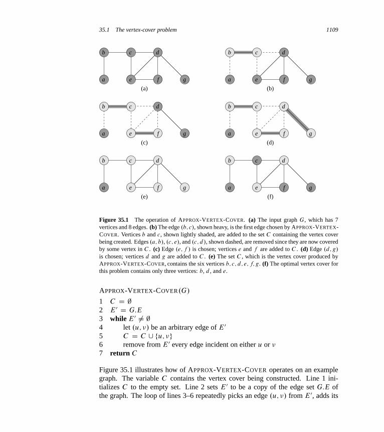
35.1 The vertex-cover problem 1109
b c d
a e f g
(a)
b c d
a e f g
(b)
b c d
a e f g
(c)
b c d
a e f g
(d)
b c d
a e f g
(e)
b c d
a e f g
(f)
Figure 35.1 The operation of APPROX-VERTEX-COVER. (a) The input graph G, which has 7vertices and 8 edges. (b) The edge .b; c/, shown heavy, is the first edge chosen by APPROX-VERTEX-COVER. Vertices b and c, shown lightly shaded, are added to the set C containing the vertex coverbeing created. Edges .a; b/, .c; e/, and .c; d/, shown dashed, are removed since they are now coveredby some vertex in C . (c) Edge .e; f / is chosen; vertices e and f are added to C . (d) Edge .d; g/
is chosen; vertices d and g are added to C . (e) The set C , which is the vertex cover produced byAPPROX-VERTEX-COVER, contains the six vertices b; c; d; e; f; g. (f) The optimal vertex cover forthis problem contains only three vertices: b, d , and e.
APPROX-VERTEX-COVER.G/
1 C D ;2 E 0 D G:E3 while E 0 ¤ ;4 let .u; �/ be an arbitrary edge of E 0
5 C D C [ fu; �g6 remove from E 0 every edge incident on either u or �
7 return C
Figure 35.1 illustrates how of APPROX-VERTEX-COVER operates on an examplegraph. The variable C contains the vertex cover being constructed. Line 1 ini-tializes C to the empty set. Line 2 sets E 0 to be a copy of the edge set G:E ofthe graph. The loop of lines 3–6 repeatedly picks an edge .u; �/ from E 0, adds its
1110 Chapter 35 Approximation Algorithms
endpoints u and � to C , and deletes all edges in E 0 that are covered by either u
or �. Finally, line 7 returns the vertex cover C . The running time of this algorithmis O.V C E/, using adjacency lists to represent E 0.
Theorem 35.1APPROX-VERTEX-COVER is a polynomial-time 2-approximation algorithm.
Proof We have already shown that APPROX-VERTEX-COVER runs in polyno-mial time.
The set C of vertices that is returned by APPROX-VERTEX-COVER is a vertexcover, since the algorithm loops until every edge in G:E has been covered by somevertex in C .
To see that APPROX-VERTEX-COVER returns a vertex cover that is at most twicethe size of an optimal cover, let A denote the set of edges that line 4 of APPROX-VERTEX-COVER picked. In order to cover the edges in A, any vertex cover—inparticular, an optimal cover C �—must include at least one endpoint of each edgein A. No two edges in A share an endpoint, since once an edge is picked in line 4,all other edges that are incident on its endpoints are deleted from E 0 in line 6. Thus,no two edges in A are covered by the same vertex from C �, and we have the lowerbound
jC �j � jAj (35.2)
on the size of an optimal vertex cover. Each execution of line 4 picks an edge forwhich neither of its endpoints is already in C , yielding an upper bound (an exactupper bound, in fact) on the size of the vertex cover returned:
jC j D 2 jAj : (35.3)
Combining equations (35.2) and (35.3), we obtain
jC j D 2 jAj� 2 jC �j ;
thereby proving the theorem.
Let us reflect on this proof. At first, you might wonder how we can possiblyprove that the size of the vertex cover returned by APPROX-VERTEX-COVER is atmost twice the size of an optimal vertex cover, when we do not even know the sizeof an optimal vertex cover. Instead of requiring that we know the exact size of anoptimal vertex cover, we rely on a lower bound on the size. As Exercise 35.1-2 asksyou to show, the set A of edges that line 4 of APPROX-VERTEX-COVER selects isactually a maximal matching in the graph G. (A maximal matching is a matchingthat is not a proper subset of any other matching.) The size of a maximal matching
35.2 The traveling-salesman problem 1111
is, as we argued in the proof of Theorem 35.1, a lower bound on the size of anoptimal vertex cover. The algorithm returns a vertex cover whose size is at mosttwice the size of the maximal matching A. By relating the size of the solutionreturned to the lower bound, we obtain our approximation ratio. We will use thismethodology in later sections as well.
Exercises
35.1-1Give an example of a graph for which APPROX-VERTEX-COVER always yields asuboptimal solution.
35.1-2Prove that the set of edges picked in line 4 of APPROX-VERTEX-COVER forms amaximal matching in the graph G.
35.1-3 ?
Professor Bündchen proposes the following heuristic to solve the vertex-coverproblem. Repeatedly select a vertex of highest degree, and remove all of its in-cident edges. Give an example to show that the professor’s heuristic does not havean approximation ratio of 2. (Hint: Try a bipartite graph with vertices of uniformdegree on the left and vertices of varying degree on the right.)
35.1-4Give an efficient greedy algorithm that finds an optimal vertex cover for a tree inlinear time.
35.1-5From the proof of Theorem 34.12, we know that the vertex-cover problem and theNP-complete clique problem are complementary in the sense that an optimal vertexcover is the complement of a maximum-size clique in the complement graph. Doesthis relationship imply that there is a polynomial-time approximation algorithmwith a constant approximation ratio for the clique problem? Justify your answer.
35.2 The traveling-salesman problem
In the traveling-salesman problem introduced in Section 34.5.4, we are given acomplete undirected graph G D .V; E/ that has a nonnegative integer cost c.u; �/
associated with each edge .u; �/ 2 E, and we must find a hamiltonian cycle (atour) of G with minimum cost. As an extension of our notation, let c.A/ denotethe total cost of the edges in the subset A � E:
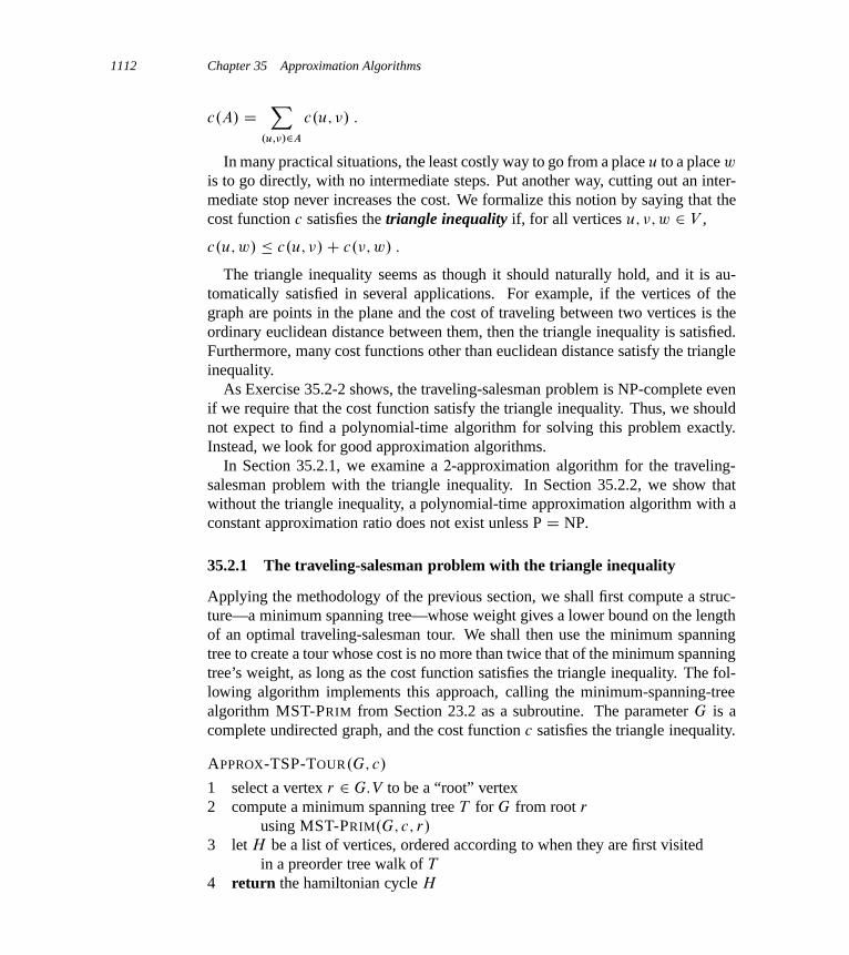
1112 Chapter 35 Approximation Algorithms
c.A/ DX
.u;�/2A
c.u; �/ :
In many practical situations, the least costly way to go from a place u to a place w
is to go directly, with no intermediate steps. Put another way, cutting out an inter-mediate stop never increases the cost. We formalize this notion by saying that thecost function c satisfies the triangle inequality if, for all vertices u; �; w 2 V ,
c.u; w/ � c.u; �/C c.�; w/ :
The triangle inequality seems as though it should naturally hold, and it is au-tomatically satisfied in several applications. For example, if the vertices of thegraph are points in the plane and the cost of traveling between two vertices is theordinary euclidean distance between them, then the triangle inequality is satisfied.Furthermore, many cost functions other than euclidean distance satisfy the triangleinequality.
As Exercise 35.2-2 shows, the traveling-salesman problem is NP-complete evenif we require that the cost function satisfy the triangle inequality. Thus, we shouldnot expect to find a polynomial-time algorithm for solving this problem exactly.Instead, we look for good approximation algorithms.
In Section 35.2.1, we examine a 2-approximation algorithm for the traveling-salesman problem with the triangle inequality. In Section 35.2.2, we show thatwithout the triangle inequality, a polynomial-time approximation algorithm with aconstant approximation ratio does not exist unless P D NP.
35.2.1 The traveling-salesman problem with the triangle inequality
Applying the methodology of the previous section, we shall first compute a struc-ture—a minimum spanning tree—whose weight gives a lower bound on the lengthof an optimal traveling-salesman tour. We shall then use the minimum spanningtree to create a tour whose cost is no more than twice that of the minimum spanningtree’s weight, as long as the cost function satisfies the triangle inequality. The fol-lowing algorithm implements this approach, calling the minimum-spanning-treealgorithm MST-PRIM from Section 23.2 as a subroutine. The parameter G is acomplete undirected graph, and the cost function c satisfies the triangle inequality.
APPROX-TSP-TOUR.G; c/
1 select a vertex r 2 G:V to be a “root” vertex2 compute a minimum spanning tree T for G from root r
using MST-PRIM.G; c; r/
3 let H be a list of vertices, ordered according to when they are first visitedin a preorder tree walk of T
4 return the hamiltonian cycle H

35.2 The traveling-salesman problem 1113
(a)
a d
b f
e
g
c
h
(b)
a d
b f
e
g
c
h
(c)
a d
e
c
h
(d)
a d
b f
e
g
c
h
(e)
b f g
e
h
c
a
b f g
d
Figure 35.2 The operation of APPROX-TSP-TOUR. (a) A complete undirected graph. Vertices lieon intersections of integer grid lines. For example, f is one unit to the right and two units up from h.The cost function between two points is the ordinary euclidean distance. (b) A minimum spanningtree T of the complete graph, as computed by MST-PRIM. Vertex a is the root vertex. Only edgesin the minimum spanning tree are shown. The vertices happen to be labeled in such a way that theyare added to the main tree by MST-PRIM in alphabetical order. (c) A walk of T , starting at a. Afull walk of the tree visits the vertices in the order a; b; c; b; h; b; a; d; e; f; e; g; e; d; a. A preorderwalk of T lists a vertex just when it is first encountered, as indicated by the dot next to each vertex,yielding the ordering a; b; c; h; d; e; f; g. (d) A tour obtained by visiting the vertices in the ordergiven by the preorder walk, which is the tour H returned by APPROX-TSP-TOUR. Its total costis approximately 19:074. (e) An optimal tour H � for the original complete graph. Its total cost isapproximately 14:715.
Recall from Section 12.1 that a preorder tree walk recursively visits every vertexin the tree, listing a vertex when it is first encountered, before visiting any of itschildren.
Figure 35.2 illustrates the operation of APPROX-TSP-TOUR. Part (a) of the fig-ure shows a complete undirected graph, and part (b) shows the minimum spanningtree T grown from root vertex a by MST-PRIM. Part (c) shows how a preorderwalk of T visits the vertices, and part (d) displays the corresponding tour, which isthe tour returned by APPROX-TSP-TOUR. Part (e) displays an optimal tour, whichis about 23% shorter.
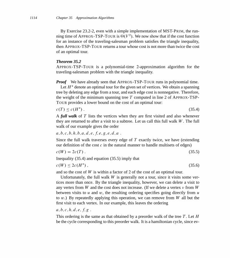
1114 Chapter 35 Approximation Algorithms
By Exercise 23.2-2, even with a simple implementation of MST-PRIM, the run-ning time of APPROX-TSP-TOUR is ‚.V 2/. We now show that if the cost functionfor an instance of the traveling-salesman problem satisfies the triangle inequality,then APPROX-TSP-TOUR returns a tour whose cost is not more than twice the costof an optimal tour.
Theorem 35.2APPROX-TSP-TOUR is a polynomial-time 2-approximation algorithm for thetraveling-salesman problem with the triangle inequality.
Proof We have already seen that APPROX-TSP-TOUR runs in polynomial time.Let H � denote an optimal tour for the given set of vertices. We obtain a spanning
tree by deleting any edge from a tour, and each edge cost is nonnegative. Therefore,the weight of the minimum spanning tree T computed in line 2 of APPROX-TSP-TOUR provides a lower bound on the cost of an optimal tour:
c.T / � c.H �/ : (35.4)
A full walk of T lists the vertices when they are first visited and also wheneverthey are returned to after a visit to a subtree. Let us call this full walk W . The fullwalk of our example gives the order
a; b; c; b; h; b; a; d; e; f; e; g; e; d; a :
Since the full walk traverses every edge of T exactly twice, we have (extendingour definition of the cost c in the natural manner to handle multisets of edges)
c.W / D 2c.T / : (35.5)
Inequality (35.4) and equation (35.5) imply that
c.W / � 2c.H �/ ; (35.6)
and so the cost of W is within a factor of 2 of the cost of an optimal tour.Unfortunately, the full walk W is generally not a tour, since it visits some ver-
tices more than once. By the triangle inequality, however, we can delete a visit toany vertex from W and the cost does not increase. (If we delete a vertex � from W
between visits to u and w, the resulting ordering specifies going directly from u
to w.) By repeatedly applying this operation, we can remove from W all but thefirst visit to each vertex. In our example, this leaves the ordering
a; b; c; h; d; e; f; g :
This ordering is the same as that obtained by a preorder walk of the tree T . Let H
be the cycle corresponding to this preorder walk. It is a hamiltonian cycle, since ev-

35.2 The traveling-salesman problem 1115
ery vertex is visited exactly once, and in fact it is the cycle computed by APPROX-TSP-TOUR. Since H is obtained by deleting vertices from the full walk W , wehave
c.H/ � c.W / : (35.7)
Combining inequalities (35.6) and (35.7) gives c.H/ � 2c.H �/, which completesthe proof.
In spite of the nice approximation ratio provided by Theorem 35.2, APPROX-TSP-TOUR is usually not the best practical choice for this problem. There areother approximation algorithms that typically perform much better in practice. Seethe references at the end of this chapter.
35.2.2 The general traveling-salesman problem
If we drop the assumption that the cost function c satisfies the triangle inequality,then we cannot find good approximate tours in polynomial time unless P D NP.
Theorem 35.3If P ¤ NP, then for any constant � � 1, there is no polynomial-time approximationalgorithm with approximation ratio � for the general traveling-salesman problem.
Proof The proof is by contradiction. Suppose to the contrary that for some num-ber � � 1, there is a polynomial-time approximation algorithm A with approx-imation ratio �. Without loss of generality, we assume that � is an integer, byrounding it up if necessary. We shall then show how to use A to solve instancesof the hamiltonian-cycle problem (defined in Section 34.2) in polynomial time.Since Theorem 34.13 tells us that the hamiltonian-cycle problem is NP-complete,Theorem 34.4 implies that if we can solve it in polynomial time, then P D NP.
Let G D .V; E/ be an instance of the hamiltonian-cycle problem. We wish todetermine efficiently whether G contains a hamiltonian cycle by making use ofthe hypothesized approximation algorithm A. We turn G into an instance of thetraveling-salesman problem as follows. Let G0 D .V; E 0/ be the complete graphon V ; that is,
E 0 D f.u; �/ W u; � 2 V and u ¤ �g :
Assign an integer cost to each edge in E 0 as follows:
c.u; �/ D(
1 if .u; �/ 2 E ;
� jV j C 1 otherwise :
We can create representations of G0 and c from a representation of G in time poly-nomial in jV j and jEj.
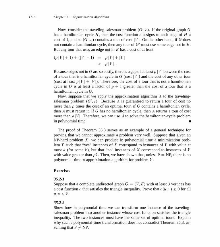
1116 Chapter 35 Approximation Algorithms
Now, consider the traveling-salesman problem .G0; c/. If the original graph G
has a hamiltonian cycle H , then the cost function c assigns to each edge of H acost of 1, and so .G0; c/ contains a tour of cost jV j. On the other hand, if G doesnot contain a hamiltonian cycle, then any tour of G0 must use some edge not in E.But any tour that uses an edge not in E has a cost of at least
.� jV j C 1/C .jV j � 1/ D � jV j C jV j> � jV j :
Because edges not in G are so costly, there is a gap of at least � jV j between the costof a tour that is a hamiltonian cycle in G (cost jV j) and the cost of any other tour(cost at least � jV j C jV j). Therefore, the cost of a tour that is not a hamiltoniancycle in G is at least a factor of � C 1 greater than the cost of a tour that is ahamiltonian cycle in G.
Now, suppose that we apply the approximation algorithm A to the traveling-salesman problem .G0; c/. Because A is guaranteed to return a tour of cost nomore than � times the cost of an optimal tour, if G contains a hamiltonian cycle,then A must return it. If G has no hamiltonian cycle, then A returns a tour of costmore than � jV j. Therefore, we can use A to solve the hamiltonian-cycle problemin polynomial time.
The proof of Theorem 35.3 serves as an example of a general technique forproving that we cannot approximate a problem very well. Suppose that given anNP-hard problem X , we can produce in polynomial time a minimization prob-lem Y such that “yes” instances of X correspond to instances of Y with value atmost k (for some k), but that “no” instances of X correspond to instances of Y
with value greater than �k. Then, we have shown that, unless P D NP, there is nopolynomial-time �-approximation algorithm for problem Y .
Exercises
35.2-1Suppose that a complete undirected graph G D .V; E/ with at least 3 vertices hasa cost function c that satisfies the triangle inequality. Prove that c.u; �/ � 0 for allu; � 2 V .
35.2-2Show how in polynomial time we can transform one instance of the traveling-salesman problem into another instance whose cost function satisfies the triangleinequality. The two instances must have the same set of optimal tours. Explainwhy such a polynomial-time transformation does not contradict Theorem 35.3, as-suming that P ¤ NP.

35.3 The set-covering problem 1117
35.2-3Consider the following closest-point heuristic for building an approximate trav-eling-salesman tour whose cost function satisfies the triangle inequality. Beginwith a trivial cycle consisting of a single arbitrarily chosen vertex. At each step,identify the vertex u that is not on the cycle but whose distance to any vertex on thecycle is minimum. Suppose that the vertex on the cycle that is nearest u is vertex �.Extend the cycle to include u by inserting u just after �. Repeat until all verticesare on the cycle. Prove that this heuristic returns a tour whose total cost is not morethan twice the cost of an optimal tour.
35.2-4In the bottleneck traveling-salesman problem, we wish to find the hamiltonian cy-cle that minimizes the cost of the most costly edge in the cycle. Assuming that thecost function satisfies the triangle inequality, show that there exists a polynomial-time approximation algorithm with approximation ratio 3 for this problem. (Hint:Show recursively that we can visit all the nodes in a bottleneck spanning tree, asdiscussed in Problem 23-3, exactly once by taking a full walk of the tree and skip-ping nodes, but without skipping more than two consecutive intermediate nodes.Show that the costliest edge in a bottleneck spanning tree has a cost that is at mostthe cost of the costliest edge in a bottleneck hamiltonian cycle.)
35.2-5Suppose that the vertices for an instance of the traveling-salesman problem arepoints in the plane and that the cost c.u; �/ is the euclidean distance betweenpoints u and �. Show that an optimal tour never crosses itself.
35.3 The set-covering problem
The set-covering problem is an optimization problem that models many problemsthat require resources to be allocated. Its corresponding decision problem general-izes the NP-complete vertex-cover problem and is therefore also NP-hard. The ap-proximation algorithm developed to handle the vertex-cover problem doesn’t applyhere, however, and so we need to try other approaches. We shall examine a simplegreedy heuristic with a logarithmic approximation ratio. That is, as the size of theinstance gets larger, the size of the approximate solution may grow, relative to thesize of an optimal solution. Because the logarithm function grows rather slowly,however, this approximation algorithm may nonetheless give useful results.

1118 Chapter 35 Approximation Algorithms
S3
S6
S4 S5
S2
S1
Figure 35.3 An instance .X; F / of the set-covering problem, where X consists of the 12 blackpoints and F D fS1; S2; S3; S4; S5; S6g. A minimum-size set cover is C D fS3; S4; S5g, withsize 3. The greedy algorithm produces a cover of size 4 by selecting either the sets S1, S4, S5,and S3 or the sets S1, S4, S5, and S6, in order.
An instance .X; F / of the set-covering problem consists of a finite set X anda family F of subsets of X , such that every element of X belongs to at least onesubset in F :
X D[
S2F
S :
We say that a subset S 2 F covers its elements. The problem is to find a minimum-size subset C � F whose members cover all of X :
X D[S2C
S : (35.8)
We say that any C satisfying equation (35.8) covers X . Figure 35.3 illustrates theset-covering problem. The size of C is the number of sets it contains, rather thanthe number of individual elements in these sets, since every subset C that covers X
must contain all jX j individual elements. In Figure 35.3, the minimum set coverhas size 3.
The set-covering problem abstracts many commonly arising combinatorial prob-lems. As a simple example, suppose that X represents a set of skills that are neededto solve a problem and that we have a given set of people available to work on theproblem. We wish to form a committee, containing as few people as possible,such that for every requisite skill in X , at least one member of the committee hasthat skill. In the decision version of the set-covering problem, we ask whether acovering exists with size at most k, where k is an additional parameter specifiedin the problem instance. The decision version of the problem is NP-complete, asExercise 35.3-2 asks you to show.

35.3 The set-covering problem 1119
A greedy approximation algorithm
The greedy method works by picking, at each stage, the set S that covers the great-est number of remaining elements that are uncovered.
GREEDY-SET-COVER.X; F /
1 U D X
2 C D ;3 while U ¤ ;4 select an S 2 F that maximizes jS \ U j5 U D U � S
6 C D C [ fSg7 return C
In the example of Figure 35.3, GREEDY-SET-COVER adds to C , in order, the setsS1, S4, and S5, followed by either S3 or S6.
The algorithm works as follows. The set U contains, at each stage, the set ofremaining uncovered elements. The set C contains the cover being constructed.Line 4 is the greedy decision-making step, choosing a subset S that covers as manyuncovered elements as possible (breaking ties arbitrarily). After S is selected,line 5 removes its elements from U , and line 6 places S into C . When the algorithmterminates, the set C contains a subfamily of F that covers X .
We can easily implement GREEDY-SET-COVER to run in time polynomial in jX jand jF j. Since the number of iterations of the loop on lines 3–6 is bounded fromabove by min.jX j ; jF j/, and we can implement the loop body to run in timeO.jX j jF j/, a simple implementation runs in time O.jX j jF jmin.jX j ; jF j//. Ex-ercise 35.3-3 asks for a linear-time algorithm.
Analysis
We now show that the greedy algorithm returns a set cover that is not too muchlarger than an optimal set cover. For convenience, in this chapter we denote the d thharmonic number Hd D
Pd
iD1 1=i (see Section A.1) by H.d/. As a boundarycondition, we define H.0/ D 0.
Theorem 35.4GREEDY-SET-COVER is a polynomial-time �.n/-approximation algorithm, where
�.n/ D H.max fjS j W S 2 F g/ :
Proof We have already shown that GREEDY-SET-COVER runs in polynomialtime.
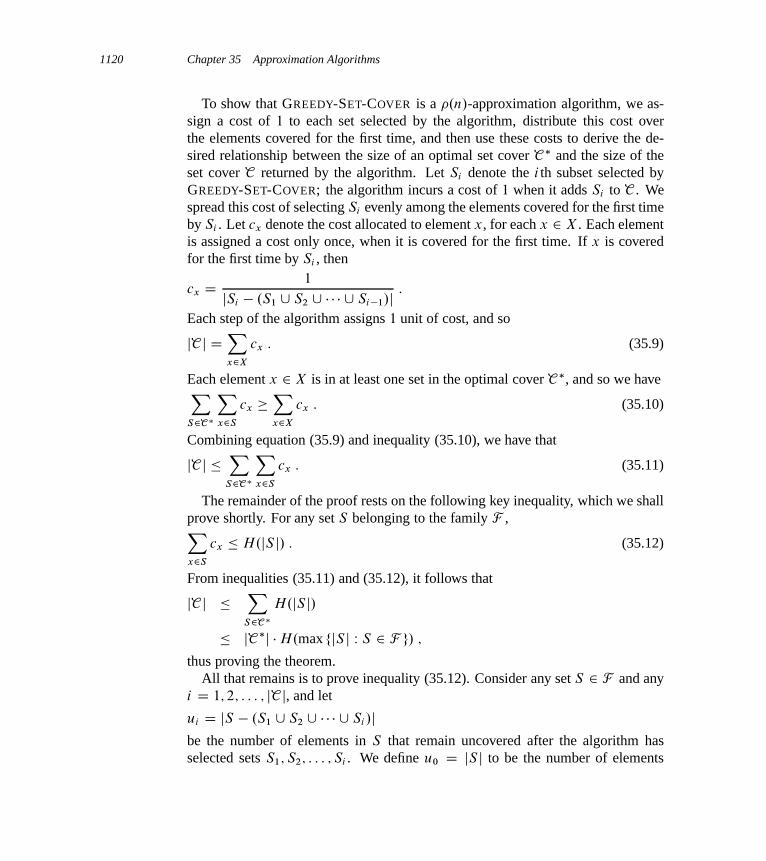
1120 Chapter 35 Approximation Algorithms
To show that GREEDY-SET-COVER is a �.n/-approximation algorithm, we as-sign a cost of 1 to each set selected by the algorithm, distribute this cost overthe elements covered for the first time, and then use these costs to derive the de-sired relationship between the size of an optimal set cover C
� and the size of theset cover C returned by the algorithm. Let Si denote the i th subset selected byGREEDY-SET-COVER; the algorithm incurs a cost of 1 when it adds Si to C . Wespread this cost of selecting Si evenly among the elements covered for the first timeby Si . Let cx denote the cost allocated to element x, for each x 2 X . Each elementis assigned a cost only once, when it is covered for the first time. If x is coveredfor the first time by Si , then
cx D1
jSi � .S1 [ S2 [ � � � [ Si�1/j :
Each step of the algorithm assigns 1 unit of cost, and so
jC j DXx2X
cx : (35.9)
Each element x 2 X is in at least one set in the optimal cover C�, and so we haveX
S2C�
Xx2S
cx �Xx2X
cx : (35.10)
Combining equation (35.9) and inequality (35.10), we have that
jC j �X
S2C�
Xx2S
cx : (35.11)
The remainder of the proof rests on the following key inequality, which we shallprove shortly. For any set S belonging to the family F ,Xx2S
cx � H.jS j/ : (35.12)
From inequalities (35.11) and (35.12), it follows that
jC j �X
S2C�
H.jS j/
� jC�j �H.max fjS j W S 2 F g/ ;
thus proving the theorem.All that remains is to prove inequality (35.12). Consider any set S 2 F and any
i D 1; 2; : : : ; jC j, and let
ui D jS � .S1 [ S2 [ � � � [ Si /jbe the number of elements in S that remain uncovered after the algorithm hasselected sets S1; S2; : : : ; Si . We define u0 D jS j to be the number of elements
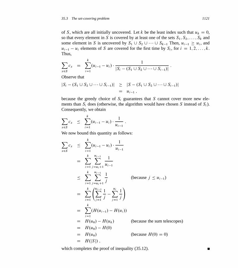
35.3 The set-covering problem 1121
of S , which are all initially uncovered. Let k be the least index such that uk D 0,so that every element in S is covered by at least one of the sets S1; S2; : : : ; Sk andsome element in S is uncovered by S1 [ S2 [ � � � [ Sk�1 Then, ui�1 � ui , andui�1 � ui elements of S are covered for the first time by Si , for i D 1; 2; : : : ; k.Thus,Xx2S
cx DkX
iD1
.ui�1 � ui / �1
jSi � .S1 [ S2 [ � � � [ Si�1/j :
Observe that
jSi � .S1 [ S2 [ � � � [ Si�1/j � jS � .S1 [ S2 [ � � � [ Si�1/jD ui�1 ;
because the greedy choice of Si guarantees that S cannot cover more new ele-ments than Si does (otherwise, the algorithm would have chosen S instead of Si ).Consequently, we obtainXx2S
cx �kX
iD1
.ui�1 � ui/ �1
ui�1
:
We now bound this quantity as follows:Xx2S
cx �kX
iD1
.ui�1 � ui / �1
ui�1
DkX
iD1
ui�1Xj Dui C1
1
ui�1
�kX
iD1
ui�1Xj Dui C1
1
j(because j � ui�1)
DkX
iD1
ui�1Xj D1
1
j�
uiXj D1
1
j
!
DkX
iD1
.H.ui�1/ �H.ui //
D H.u0/ �H.uk/ (because the sum telescopes)
D H.u0/ �H.0/
D H.u0/ (because H.0/ D 0)
D H.jS j/ ;
which completes the proof of inequality (35.12).
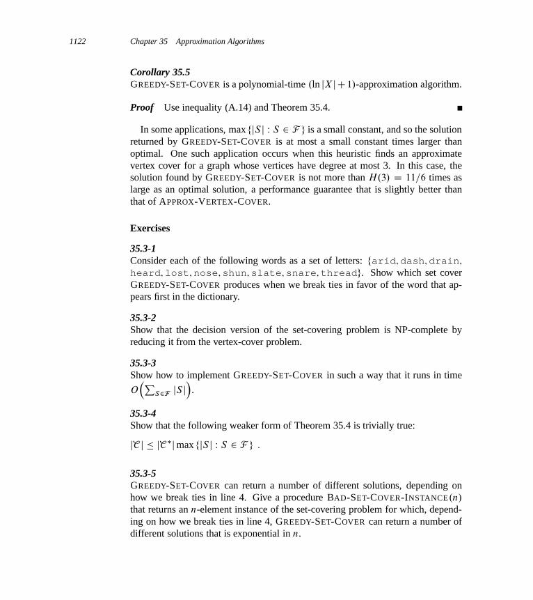
1122 Chapter 35 Approximation Algorithms
Corollary 35.5GREEDY-SET-COVER is a polynomial-time .ln jX jC1/-approximation algorithm.
Proof Use inequality (A.14) and Theorem 35.4.
In some applications, max fjS j W S 2 F g is a small constant, and so the solutionreturned by GREEDY-SET-COVER is at most a small constant times larger thanoptimal. One such application occurs when this heuristic finds an approximatevertex cover for a graph whose vertices have degree at most 3. In this case, thesolution found by GREEDY-SET-COVER is not more than H.3/ D 11=6 times aslarge as an optimal solution, a performance guarantee that is slightly better thanthat of APPROX-VERTEX-COVER.
Exercises
35.3-1Consider each of the following words as a set of letters: farid; dash; drain;
heard; lost; nose; shun; slate; snare; threadg. Show which set coverGREEDY-SET-COVER produces when we break ties in favor of the word that ap-pears first in the dictionary.
35.3-2Show that the decision version of the set-covering problem is NP-complete byreducing it from the vertex-cover problem.
35.3-3Show how to implement GREEDY-SET-COVER in such a way that it runs in time
O�P
S2FjS j�
.
35.3-4Show that the following weaker form of Theorem 35.4 is trivially true:
jC j � jC�jmax fjS j W S 2 F g :
35.3-5GREEDY-SET-COVER can return a number of different solutions, depending onhow we break ties in line 4. Give a procedure BAD-SET-COVER-INSTANCE.n/
that returns an n-element instance of the set-covering problem for which, depend-ing on how we break ties in line 4, GREEDY-SET-COVER can return a number ofdifferent solutions that is exponential in n.

35.4 Randomization and linear programming 1123
35.4 Randomization and linear programming
In this section, we study two useful techniques for designing approximation algo-rithms: randomization and linear programming. We shall give a simple randomizedalgorithm for an optimization version of 3-CNF satisfiability, and then we shall uselinear programming to help design an approximation algorithm for a weighted ver-sion of the vertex-cover problem. This section only scratches the surface of thesetwo powerful techniques. The chapter notes give references for further study ofthese areas.
A randomized approximation algorithm for MAX-3-CNF satisfiability
Just as some randomized algorithms compute exact solutions, some randomizedalgorithms compute approximate solutions. We say that a randomized algorithmfor a problem has an approximation ratio of �.n/ if, for any input of size n, theexpected cost C of the solution produced by the randomized algorithm is within afactor of �.n/ of the cost C � of an optimal solution:
max
�C
C � ;C �
C
�� �.n/ : (35.13)
We call a randomized algorithm that achieves an approximation ratio of �.n/ arandomized �.n/-approximation algorithm. In other words, a randomized ap-proximation algorithm is like a deterministic approximation algorithm, except thatthe approximation ratio is for an expected cost.
A particular instance of 3-CNF satisfiability, as defined in Section 34.4, may ormay not be satisfiable. In order to be satisfiable, there must exist an assignment ofthe variables so that every clause evaluates to 1. If an instance is not satisfiable, wemay want to compute how “close” to satisfiable it is, that is, we may wish to find anassignment of the variables that satisfies as many clauses as possible. We call theresulting maximization problem MAX-3-CNF satisfiability. The input to MAX-3-CNF satisfiability is the same as for 3-CNF satisfiability, and the goal is to returnan assignment of the variables that maximizes the number of clauses evaluatingto 1. We now show that randomly setting each variable to 1 with probability 1=2
and to 0 with probability 1=2 yields a randomized 8=7-approximation algorithm.According to the definition of 3-CNF satisfiability from Section 34.4, we requireeach clause to consist of exactly three distinct literals. We further assume thatno clause contains both a variable and its negation. (Exercise 35.4-1 asks you toremove this last assumption.)

1124 Chapter 35 Approximation Algorithms
Theorem 35.6Given an instance of MAX-3-CNF satisfiability with n variables x1; x2; : : : ; xn
and m clauses, the randomized algorithm that independently sets each vari-able to 1 with probability 1=2 and to 0 with probability 1=2 is a randomized8=7-approximation algorithm.
Proof Suppose that we have independently set each variable to 1 with probabil-ity 1=2 and to 0 with probability 1=2. For i D 1; 2; : : : ; m, we define the indicatorrandom variable
Yi D I fclause i is satisfiedg ;
so that Yi D 1 as long as we have set at least one of the literals in the i th clauseto 1. Since no literal appears more than once in the same clause, and since we haveassumed that no variable and its negation appear in the same clause, the settings ofthe three literals in each clause are independent. A clause is not satisfied only if allthree of its literals are set to 0, and so Pr fclause i is not satisfiedg D .1=2/3 D 1=8.Thus, we have Pr fclause i is satisfiedg D 1 � 1=8 D 7=8, and by Lemma 5.1,we have E ŒYi � D 7=8. Let Y be the number of satisfied clauses overall, so thatY D Y1 C Y2 C � � � C Ym. Then, we have
E ŒY � D E
"mX
iD1
Yi
#
DmX
iD1
E ŒYi � (by linearity of expectation)
DmX
iD1
7=8
D 7m=8 :
Clearly, m is an upper bound on the number of satisfied clauses, and hence theapproximation ratio is at most m=.7m=8/ D 8=7.
Approximating weighted vertex cover using linear programming
In the minimum-weight vertex-cover problem, we are given an undirected graphG D .V; E/ in which each vertex � 2 V has an associated positive weight w.�/.For any vertex cover V 0 � V , we define the weight of the vertex cover w.V 0/ DP
�2V 0 w.�/. The goal is to find a vertex cover of minimum weight.We cannot apply the algorithm used for unweighted vertex cover, nor can we use
a random solution; both methods may return solutions that are far from optimal.We shall, however, compute a lower bound on the weight of the minimum-weight
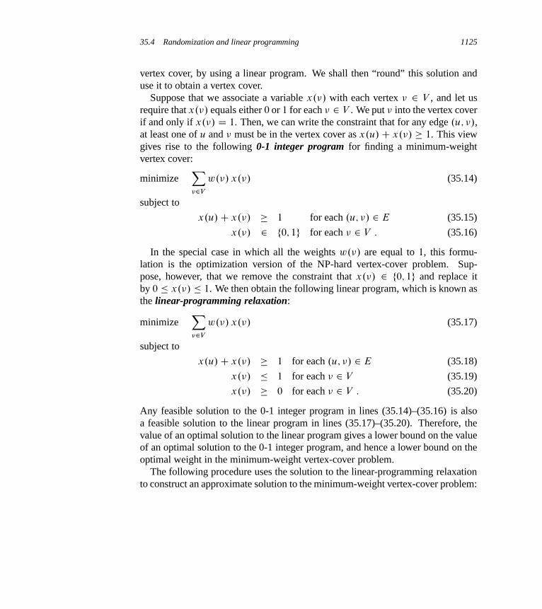
35.4 Randomization and linear programming 1125
vertex cover, by using a linear program. We shall then “round” this solution anduse it to obtain a vertex cover.
Suppose that we associate a variable x.�/ with each vertex � 2 V , and let usrequire that x.�/ equals either 0 or 1 for each � 2 V . We put � into the vertex coverif and only if x.�/ D 1. Then, we can write the constraint that for any edge .u; �/,at least one of u and � must be in the vertex cover as x.u/C x.�/ � 1. This viewgives rise to the following 0-1 integer program for finding a minimum-weightvertex cover:
minimizeX�2V
w.�/ x.�/ (35.14)
subject to
x.u/C x.�/ � 1 for each .u; �/ 2 E (35.15)
x.�/ 2 f0; 1g for each � 2 V : (35.16)
In the special case in which all the weights w.�/ are equal to 1, this formu-lation is the optimization version of the NP-hard vertex-cover problem. Sup-pose, however, that we remove the constraint that x.�/ 2 f0; 1g and replace itby 0 � x.�/ � 1. We then obtain the following linear program, which is known asthe linear-programming relaxation:
minimizeX�2V
w.�/ x.�/ (35.17)
subject to
x.u/C x.�/ � 1 for each .u; �/ 2 E (35.18)
x.�/ � 1 for each � 2 V (35.19)
x.�/ � 0 for each � 2 V : (35.20)
Any feasible solution to the 0-1 integer program in lines (35.14)–(35.16) is alsoa feasible solution to the linear program in lines (35.17)–(35.20). Therefore, thevalue of an optimal solution to the linear program gives a lower bound on the valueof an optimal solution to the 0-1 integer program, and hence a lower bound on theoptimal weight in the minimum-weight vertex-cover problem.
The following procedure uses the solution to the linear-programming relaxationto construct an approximate solution to the minimum-weight vertex-cover problem:

1126 Chapter 35 Approximation Algorithms
APPROX-MIN-WEIGHT-VC.G; w/
1 C D ;2 compute Nx, an optimal solution to the linear program in lines (35.17)–(35.20)3 for each � 2 V
4 if Nx.�/ � 1=2
5 C D C [ f�g6 return C
The APPROX-MIN-WEIGHT-VC procedure works as follows. Line 1 initial-izes the vertex cover to be empty. Line 2 formulates the linear program inlines (35.17)–(35.20) and then solves this linear program. An optimal solutiongives each vertex � an associated value Nx.�/, where 0 � Nx.�/ � 1. We use thisvalue to guide the choice of which vertices to add to the vertex cover C in lines 3–5.If Nx.�/ � 1=2, we add � to C ; otherwise we do not. In effect, we are “rounding”each fractional variable in the solution to the linear program to 0 or 1 in order toobtain a solution to the 0-1 integer program in lines (35.14)–(35.16). Finally, line 6returns the vertex cover C .
Theorem 35.7Algorithm APPROX-MIN-WEIGHT-VC is a polynomial-time 2-approximation al-gorithm for the minimum-weight vertex-cover problem.
Proof Because there is a polynomial-time algorithm to solve the linear programin line 2, and because the for loop of lines 3–5 runs in polynomial time, APPROX-MIN-WEIGHT-VC is a polynomial-time algorithm.
Now we show that APPROX-MIN-WEIGHT-VC is a 2-approximation algo-rithm. Let C � be an optimal solution to the minimum-weight vertex-cover prob-lem, and let ´� be the value of an optimal solution to the linear program inlines (35.17)–(35.20). Since an optimal vertex cover is a feasible solution to thelinear program, ´� must be a lower bound on w.C �/, that is,
´� � w.C �/ : (35.21)
Next, we claim that by rounding the fractional values of the variables Nx.�/, weproduce a set C that is a vertex cover and satisfies w.C / � 2´�. To see that C isa vertex cover, consider any edge .u; �/ 2 E. By constraint (35.18), we know thatx.u/C x.�/ � 1, which implies that at least one of Nx.u/ and Nx.�/ is at least 1=2.Therefore, at least one of u and � is included in the vertex cover, and so every edgeis covered.
Now, we consider the weight of the cover. We have
35.4 Randomization and linear programming 1127
´� DX�2V
w.�/ Nx.�/
�X
�2V W Nx.�/�1=2
w.�/ Nx.�/
�X
�2V W Nx.�/�1=2
w.�/ � 12
DX�2C
w.�/ � 12
D 1
2
X�2C
w.�/
D 1
2w.C / : (35.22)
Combining inequalities (35.21) and (35.22) gives
w.C / � 2´� � 2w.C �/ ;
and hence APPROX-MIN-WEIGHT-VC is a 2-approximation algorithm.
Exercises
35.4-1Show that even if we allow a clause to contain both a variable and its negation, ran-domly setting each variable to 1 with probability 1=2 and to 0 with probability 1=2
still yields a randomized 8=7-approximation algorithm.
35.4-2The MAX-CNF satisfiability problem is like the MAX-3-CNF satisfiability prob-lem, except that it does not restrict each clause to have exactly 3 literals. Give arandomized 2-approximation algorithm for the MAX-CNF satisfiability problem.
35.4-3In the MAX-CUT problem, we are given an unweighted undirected graph G D.V; E/. We define a cut .S; V � S/ as in Chapter 23 and the weight of a cut as thenumber of edges crossing the cut. The goal is to find a cut of maximum weight.Suppose that for each vertex �, we randomly and independently place � in S withprobability 1=2 and in V � S with probability 1=2. Show that this algorithm is arandomized 2-approximation algorithm.

1128 Chapter 35 Approximation Algorithms
35.4-4Show that the constraints in line (35.19) are redundant in the sense that if we re-move them from the linear program in lines (35.17)–(35.20), any optimal solutionto the resulting linear program must satisfy x.�/ � 1 for each � 2 V .
35.5 The subset-sum problem
Recall from Section 34.5.5 that an instance of the subset-sum problem is apair .S; t/, where S is a set fx1; x2; : : : ; xng of positive integers and t is a posi-tive integer. This decision problem asks whether there exists a subset of S thatadds up exactly to the target value t . As we saw in Section 34.5.5, this problem isNP-complete.
The optimization problem associated with this decision problem arises in prac-tical applications. In the optimization problem, we wish to find a subset offx1; x2; : : : ; xng whose sum is as large as possible but not larger than t . For ex-ample, we may have a truck that can carry no more than t pounds, and n differentboxes to ship, the i th of which weighs xi pounds. We wish to fill the truck with asheavy a load as possible without exceeding the given weight limit.
In this section, we present an exponential-time algorithm that computes the op-timal value for this optimization problem, and then we show how to modify thealgorithm so that it becomes a fully polynomial-time approximation scheme. (Re-call that a fully polynomial-time approximation scheme has a running time that ispolynomial in 1=� as well as in the size of the input.)
An exponential-time exact algorithm
Suppose that we computed, for each subset S 0 of S , the sum of the elementsin S 0, and then we selected, among the subsets whose sum does not exceed t ,the one whose sum was closest to t . Clearly this algorithm would return the op-timal solution, but it could take exponential time. To implement this algorithm,we could use an iterative procedure that, in iteration i , computes the sums ofall subsets of fx1; x2; : : : ; xig, using as a starting point the sums of all subsetsof fx1; x2; : : : ; xi�1g. In doing so, we would realize that once a particular subset S 0
had a sum exceeding t , there would be no reason to maintain it, since no super-set of S 0 could be the optimal solution. We now give an implementation of thisstrategy.
The procedure EXACT-SUBSET-SUM takes an input set S D fx1; x2; : : : ; xngand a target value t ; we’ll see its pseudocode in a moment. This procedure it-
35.5 The subset-sum problem 1129
eratively computes Li , the list of sums of all subsets of fx1; : : : ; xig that do notexceed t , and then it returns the maximum value in Ln.
If L is a list of positive integers and x is another positive integer, then we letLC x denote the list of integers derived from L by increasing each element of L
by x. For example, if L D h1; 2; 3; 5; 9i, then LC 2 D h3; 4; 5; 7; 11i. We also usethis notation for sets, so that
S C x D fs C x W s 2 Sg :
We also use an auxiliary procedure MERGE-LISTS.L; L0/, which returns thesorted list that is the merge of its two sorted input lists L and L0 with duplicatevalues removed. Like the MERGE procedure we used in merge sort (Section 2.3.1),MERGE-LISTS runs in time O.jLj C jL0j/. We omit the pseudocode for MERGE-LISTS.
EXACT-SUBSET-SUM.S; t/
1 n D jS j2 L0 D h0i3 for i D 1 to n
4 Li D MERGE-LISTS.Li�1; Li�1 C xi /
5 remove from Li every element that is greater than t
6 return the largest element in Ln
To see how EXACT-SUBSET-SUM works, let Pi denote the set of all valuesobtained by selecting a (possibly empty) subset of fx1; x2; : : : ; xig and summingits members. For example, if S D f1; 4; 5g, then
P1 D f0; 1g ;
P2 D f0; 1; 4; 5g ;
P3 D f0; 1; 4; 5; 6; 9; 10g :
Given the identity
Pi D Pi�1 [ .Pi�1 C xi/ ; (35.23)
we can prove by induction on i (see Exercise 35.5-1) that the list Li is a sorted listcontaining every element of Pi whose value is not more than t . Since the lengthof Li can be as much as 2i , EXACT-SUBSET-SUM is an exponential-time algorithmin general, although it is a polynomial-time algorithm in the special cases in which t
is polynomial in jS j or all the numbers in S are bounded by a polynomial in jS j.
A fully polynomial-time approximation scheme
We can derive a fully polynomial-time approximation scheme for the subset-sumproblem by “trimming” each list Li after it is created. The idea behind trimming is
1130 Chapter 35 Approximation Algorithms
that if two values in L are close to each other, then since we want just an approxi-mate solution, we do not need to maintain both of them explicitly. More precisely,we use a trimming parameter ı such that 0 < ı < 1. When we trim a list L by ı,we remove as many elements from L as possible, in such a way that if L0 is theresult of trimming L, then for every element y that was removed from L, there isan element ´ still in L0 that approximates y, that is,
y
1C ı� ´ � y : (35.24)
We can think of such a ´ as “representing” y in the new list L0. Each removedelement y is represented by a remaining element ´ satisfying inequality (35.24).For example, if ı D 0:1 and
L D h10; 11; 12; 15; 20; 21; 22; 23; 24; 29i ;
then we can trim L to obtain
L0 D h10; 12; 15; 20; 23; 29i ;
where the deleted value 11 is represented by 10, the deleted values 21 and 22
are represented by 20, and the deleted value 24 is represented by 23. Becauseevery element of the trimmed version of the list is also an element of the originalversion of the list, trimming can dramatically decrease the number of elements keptwhile keeping a close (and slightly smaller) representative value in the list for eachdeleted element.
The following procedure trims list L D hy1; y2; : : : ; ymi in time ‚.m/, given L
and ı, and assuming that L is sorted into monotonically increasing order. Theoutput of the procedure is a trimmed, sorted list.
TRIM.L; ı/
1 let m be the length of L
2 L0 D hy1i3 last D y1
4 for i D 2 to m
5 if yi > last � .1C ı/ // yi � last because L is sorted6 append yi onto the end of L0
7 last D yi
8 return L0
The procedure scans the elements of L in monotonically increasing order. A num-ber is appended onto the returned list L0 only if it is the first element of L or if itcannot be represented by the most recent number placed into L0.
Given the procedure TRIM, we can construct our approximation scheme as fol-lows. This procedure takes as input a set S D fx1; x2; : : : ; xng of n integers (inarbitrary order), a target integer t , and an “approximation parameter” �, where
35.5 The subset-sum problem 1131
0 < � < 1 : (35.25)
It returns a value ´ whose value is within a 1C � factor of the optimal solution.
APPROX-SUBSET-SUM.S; t; �/
1 n D jS j2 L0 D h0i3 for i D 1 to n
4 Li D MERGE-LISTS.Li�1; Li�1 C xi /
5 Li D TRIM.Li ; �=2n/
6 remove from Li every element that is greater than t
7 let ´� be the largest value in Ln
8 return ´�
Line 2 initializes the list L0 to be the list containing just the element 0. The forloop in lines 3–6 computes Li as a sorted list containing a suitably trimmed ver-sion of the set Pi , with all elements larger than t removed. Since we create Li
from Li�1, we must ensure that the repeated trimming doesn’t introduce too muchcompounded inaccuracy. In a moment, we shall see that APPROX-SUBSET-SUM
returns a correct approximation if one exists.As an example, suppose we have the instance
S D h104; 102; 201; 101iwith t D 308 and � D 0:40. The trimming parameter ı is �=8 D 0:05. APPROX-SUBSET-SUM computes the following values on the indicated lines:
line 2: L0 D h0i ;
line 4: L1 D h0; 104i ;
line 5: L1 D h0; 104i ;
line 6: L1 D h0; 104i ;
line 4: L2 D h0; 102; 104; 206i ;
line 5: L2 D h0; 102; 206i ;
line 6: L2 D h0; 102; 206i ;
line 4: L3 D h0; 102; 201; 206; 303; 407i ;
line 5: L3 D h0; 102; 201; 303; 407i ;
line 6: L3 D h0; 102; 201; 303i ;
line 4: L4 D h0; 101; 102; 201; 203; 302; 303; 404i ;
line 5: L4 D h0; 101; 201; 302; 404i ;
line 6: L4 D h0; 101; 201; 302i :

1132 Chapter 35 Approximation Algorithms
The algorithm returns ´� D 302 as its answer, which is well within � D 40% ofthe optimal answer 307 D 104C 102C 101; in fact, it is within 2%.
Theorem 35.8APPROX-SUBSET-SUM is a fully polynomial-time approximation scheme for thesubset-sum problem.
Proof The operations of trimming Li in line 5 and removing from Li every ele-ment that is greater than t maintain the property that every element of Li is also amember of Pi . Therefore, the value ´� returned in line 8 is indeed the sum of somesubset of S . Let y� 2 Pn denote an optimal solution to the subset-sum problem.Then, from line 6, we know that ´� � y�. By inequality (35.1), we need to showthat y�=´� � 1C �. We must also show that the running time of this algorithm ispolynomial in both 1=� and the size of the input.
As Exercise 35.5-2 asks you to show, for every element y in Pi that is at most t ,there exists an element ´ 2 Li such that
y
.1C �=2n/i� ´ � y (35.26)
Inequality (35.26) must hold for y� 2 Pn, and therefore there exists an element´ 2 Ln such that
y�
.1C �=2n/n� ´ � y� ;
and thus
y�
´��1C �
2n
�n
: (35.27)
Since there exists an element ´ 2 Ln fulfilling inequality (35.27), the inequalitymust hold for ´�, which is the largest value in Ln; that is,
y�
´� ��1C �
2n
�n
: (35.28)
Now, we show that y�=´� � 1C �. We do so by showing that .1C �=2n/n �
1C �. By equation (3.14), we have limn!1.1C �=2n/n D e�=2. Exercise 35.5-3asks you to show that
d
dn
�1C �
2n
�n
> 0 : (35.29)
Therefore, the function .1C �=2n/n increases with n as it approaches its limit
of e�=2, and we have
35.5 The subset-sum problem 1133
�1C �
2n
�n
� e�=2
� 1C �=2C .�=2/2 (by inequality (3.13))
� 1C � (by inequality (35.25)) . (35.30)
Combining inequalities (35.28) and (35.30) completes the analysis of the approxi-mation ratio.
To show that APPROX-SUBSET-SUM is a fully polynomial-time approximationscheme, we derive a bound on the length of Li . After trimming, successive ele-ments ´ and ´0 of Li must have the relationship ´0=´ > 1C�=2n. That is, they mustdiffer by a factor of at least 1 C �=2n. Each list, therefore, contains the value 0,possibly the value 1, and up to
log1C�=2n t
˘additional values. The number of
elements in each list Li is at most
log1C�=2n t C 2 D ln t
ln.1C �=2n/C 2
� 2n.1C �=2n/ ln t
�C 2 (by inequality (3.17))
<3n ln t
�C 2 (by inequality (35.25)) .
This bound is polynomial in the size of the input—which is the number of bits lg t
needed to represent t plus the number of bits needed to represent the set S , which isin turn polynomial in n—and in 1=�. Since the running time of APPROX-SUBSET-SUM is polynomial in the lengths of the Li , we conclude that APPROX-SUBSET-SUM is a fully polynomial-time approximation scheme.
Exercises
35.5-1Prove equation (35.23). Then show that after executing line 5 of EXACT-SUBSET-SUM, Li is a sorted list containing every element of Pi whose value is not morethan t .
35.5-2Using induction on i , prove inequality (35.26).
35.5-3Prove inequality (35.29).

1134 Chapter 35 Approximation Algorithms
35.5-4How would you modify the approximation scheme presented in this section to finda good approximation to the smallest value not less than t that is a sum of somesubset of the given input list?
35.5-5Modify the APPROX-SUBSET-SUM procedure to also return the subset of S thatsums to the value ´�.
Problems
35-1 Bin packingSuppose that we are given a set of n objects, where the size si of the i th objectsatisfies 0 < si < 1. We wish to pack all the objects into the minimum number ofunit-size bins. Each bin can hold any subset of the objects whose total size doesnot exceed 1.
a. Prove that the problem of determining the minimum number of bins required isNP-hard. (Hint: Reduce from the subset-sum problem.)
The first-fit heuristic takes each object in turn and places it into the first bin thatcan accommodate it. Let S DPn
iD1 si .
b. Argue that the optimal number of bins required is at least dSe.
c. Argue that the first-fit heuristic leaves at most one bin less than half full.
d. Prove that the number of bins used by the first-fit heuristic is never morethan d2Se.
e. Prove an approximation ratio of 2 for the first-fit heuristic.
f. Give an efficient implementation of the first-fit heuristic, and analyze its runningtime.
35-2 Approximating the size of a maximum cliqueLet G D .V; E/ be an undirected graph. For any k � 1, define G.k/ to be the undi-rected graph .V .k/; E.k//, where V .k/ is the set of all ordered k-tuples of verticesfrom V and E.k/ is defined so that .�1; �2; : : : ; �k/ is adjacent to .w1; w2; : : : ; wk/
if and only if for each i , 1 � i � k either vertex �i is adjacent to wi in G, or else�i D wi .
Problems for Chapter 35 1135
a. Prove that the size of the maximum clique in G.k/ is equal to the kth power ofthe size of the maximum clique in G.
b. Argue that if there is an approximation algorithm that has a constant approxi-mation ratio for finding a maximum-size clique, then there is a polynomial-timeapproximation scheme for the problem.
35-3 Weighted set-covering problemSuppose that we generalize the set-covering problem so that each set Si in thefamily F has an associated weight wi and the weight of a cover C is
PSi 2C
wi .We wish to determine a minimum-weight cover. (Section 35.3 handles the case inwhich wi D 1 for all i .)
Show how to generalize the greedy set-covering heuristic in a natural mannerto provide an approximate solution for any instance of the weighted set-coveringproblem. Show that your heuristic has an approximation ratio of H.d/, where d isthe maximum size of any set Si .
35-4 Maximum matchingRecall that for an undirected graph G, a matching is a set of edges such that notwo edges in the set are incident on the same vertex. In Section 26.3, we saw howto find a maximum matching in a bipartite graph. In this problem, we will look atmatchings in undirected graphs in general (i.e., the graphs are not required to bebipartite).
a. A maximal matching is a matching that is not a proper subset of any othermatching. Show that a maximal matching need not be a maximum matching byexhibiting an undirected graph G and a maximal matching M in G that is not amaximum matching. (Hint: You can find such a graph with only four vertices.)
b. Consider an undirected graph G D .V; E/. Give an O.E/-time greedy algo-rithm to find a maximal matching in G.
In this problem, we shall concentrate on a polynomial-time approximation algo-rithm for maximum matching. Whereas the fastest known algorithm for maximummatching takes superlinear (but polynomial) time, the approximation algorithmhere will run in linear time. You will show that the linear-time greedy algorithmfor maximal matching in part (b) is a 2-approximation algorithm for maximummatching.
c. Show that the size of a maximum matching in G is a lower bound on the sizeof any vertex cover for G.
1136 Chapter 35 Approximation Algorithms
d. Consider a maximal matching M in G D .V; E/. Let
T D f� 2 V W some edge in M is incident on �g :
What can you say about the subgraph of G induced by the vertices of G thatare not in T ?
e. Conclude from part (d) that 2 jM j is the size of a vertex cover for G.
f. Using parts (c) and (e), prove that the greedy algorithm in part (b) is a 2-approx-imation algorithm for maximum matching.
35-5 Parallel machine schedulingIn the parallel-machine-scheduling problem, we are given n jobs, J1; J2; : : : ; Jn,where each job Jk has an associated nonnegative processing time of pk. We arealso given m identical machines, M1; M2; : : : ; Mm. Any job can run on any ma-chine. A schedule specifies, for each job Jk, the machine on which it runs andthe time period during which it runs. Each job Jk must run on some machine Mi
for pk consecutive time units, and during that time period no other job may runon Mi . Let Ck denote the completion time of job Jk, that is, the time at whichjob Jk completes processing. Given a schedule, we define Cmax D max1�j �n Cj tobe the makespan of the schedule. The goal is to find a schedule whose makespanis minimum.
For example, suppose that we have two machines M1 and M2 and that we havefour jobs J1; J2; J3; J4, with p1 D 2, p2 D 12, p3 D 4, and p4 D 5. Then onepossible schedule runs, on machine M1, job J1 followed by job J2, and on ma-chine M2, it runs job J4 followed by job J3. For this schedule, C1 D 2, C2 D 14,C3 D 9, C4 D 5, and Cmax D 14. An optimal schedule runs J2 on machine M1, andit runs jobs J1, J3, and J4 on machine M2. For this schedule, C1 D 2, C2 D 12,C3 D 6, C4 D 11, and Cmax D 12.
Given a parallel-machine-scheduling problem, we let C �max denote the makespan
of an optimal schedule.
a. Show that the optimal makespan is at least as large as the greatest processingtime, that is,
C �max � max
1�k�npk :
b. Show that the optimal makespan is at least as large as the average machine load,that is,
C �max �
1
m
X1�k�n
pk :
Problems for Chapter 35 1137
Suppose that we use the following greedy algorithm for parallel machine schedul-ing: whenever a machine is idle, schedule any job that has not yet been scheduled.
c. Write pseudocode to implement this greedy algorithm. What is the runningtime of your algorithm?
d. For the schedule returned by the greedy algorithm, show that
Cmax �1
m
X1�k�n
pk C max1�k�n
pk :
Conclude that this algorithm is a polynomial-time 2-approximation algorithm.
35-6 Approximating a maximum spanning treeLet G D .V; E/ be an undirected graph with distinct edge weights w.u; �/ on eachedge .u; �/ 2 E. For each vertex � 2 V , let max.�/ D max.u;�/2E fw.u; �/g bethe maximum-weight edge incident on that vertex. Let SG D fmax.�/ W � 2 V gbe the set of maximum-weight edges incident on each vertex, and let TG be themaximum-weight spanning tree of G, that is, the spanning tree of maximum totalweight. For any subset of edges E 0 � E, define w.E 0/ DP.u;�/2E 0 w.u; �/.
a. Give an example of a graph with at least 4 vertices for which SG D TG .
b. Give an example of a graph with at least 4 vertices for which SG ¤ TG .
c. Prove that SG � TG for any graph G.
d. Prove that w.TG/ � w.SG/=2 for any graph G.
e. Give an O.V CE/-time algorithm to compute a 2-approximation to the maxi-mum spanning tree.
35-7 An approximation algorithm for the 0-1 knapsack problemRecall the knapsack problem from Section 16.2. There are n items, where the i thitem is worth �i dollars and weighs wi pounds. We are also given a knapsackthat can hold at most W pounds. Here, we add the further assumptions that eachweight wi is at most W and that the items are indexed in monotonically decreasingorder of their values: �1 � �2 � � � � � �n.
In the 0-1 knapsack problem, we wish to find a subset of the items whose totalweight is at most W and whose total value is maximum. The fractional knapsackproblem is like the 0-1 knapsack problem, except that we are allowed to take afraction of each item, rather than being restricted to taking either all or none of
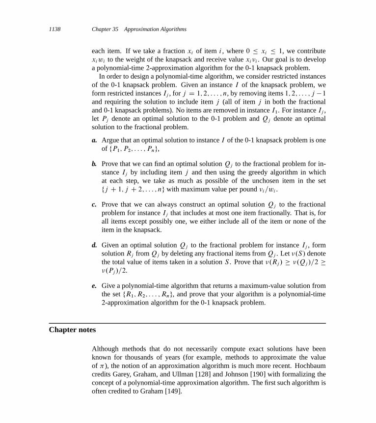
1138 Chapter 35 Approximation Algorithms
each item. If we take a fraction xi of item i , where 0 � xi � 1, we contributexiwi to the weight of the knapsack and receive value xi�i . Our goal is to developa polynomial-time 2-approximation algorithm for the 0-1 knapsack problem.
In order to design a polynomial-time algorithm, we consider restricted instancesof the 0-1 knapsack problem. Given an instance I of the knapsack problem, weform restricted instances Ij , for j D 1; 2; : : : ; n, by removing items 1; 2; : : : ; j �1
and requiring the solution to include item j (all of item j in both the fractionaland 0-1 knapsack problems). No items are removed in instance I1. For instance Ij ,let Pj denote an optimal solution to the 0-1 problem and Qj denote an optimalsolution to the fractional problem.
a. Argue that an optimal solution to instance I of the 0-1 knapsack problem is oneof fP1; P2; : : : ; Png,
b. Prove that we can find an optimal solution Qj to the fractional problem for in-stance Ij by including item j and then using the greedy algorithm in whichat each step, we take as much as possible of the unchosen item in the setfj C 1; j C 2; : : : ; ng with maximum value per pound �i=wi .
c. Prove that we can always construct an optimal solution Qj to the fractionalproblem for instance Ij that includes at most one item fractionally. That is, forall items except possibly one, we either include all of the item or none of theitem in the knapsack.
d. Given an optimal solution Qj to the fractional problem for instance Ij , formsolution Rj from Qj by deleting any fractional items from Qj . Let �.S/ denotethe total value of items taken in a solution S . Prove that �.Rj / � �.Qj /=2 ��.Pj /=2.
e. Give a polynomial-time algorithm that returns a maximum-value solution fromthe set fR1; R2; : : : ; Rng, and prove that your algorithm is a polynomial-time2-approximation algorithm for the 0-1 knapsack problem.
Chapter notes
Although methods that do not necessarily compute exact solutions have beenknown for thousands of years (for example, methods to approximate the valueof �), the notion of an approximation algorithm is much more recent. Hochbaumcredits Garey, Graham, and Ullman [128] and Johnson [190] with formalizing theconcept of a polynomial-time approximation algorithm. The first such algorithm isoften credited to Graham [149].

Notes for Chapter 35 1139
Since this early work, thousands of approximation algorithms have been de-signed for a wide range of problems, and there is a wealth of literature on thisfield. Recent texts by Ausiello et al. [26], Hochbaum [172], and Vazirani [345]deal exclusively with approximation algorithms, as do surveys by Shmoys [315]and Klein and Young [207]. Several other texts, such as Garey and Johnson [129]and Papadimitriou and Steiglitz [271], have significant coverage of approximationalgorithms as well. Lawler, Lenstra, Rinnooy Kan, and Shmoys [225] provide anextensive treatment of approximation algorithms for the traveling-salesman prob-lem.
Papadimitriou and Steiglitz attribute the algorithm APPROX-VERTEX-COVER
to F. Gavril and M. Yannakakis. The vertex-cover problem has been studied exten-sively (Hochbaum [172] lists 16 different approximation algorithms for this prob-lem), but all the approximation ratios are at least 2� o.1/.
The algorithm APPROX-TSP-TOUR appears in a paper by Rosenkrantz, Stearns,and Lewis [298]. Christofides improved on this algorithm and gave a 3=2-approx-imation algorithm for the traveling-salesman problem with the triangle inequality.Arora [22] and Mitchell [257] have shown that if the points are in the euclideanplane, there is a polynomial-time approximation scheme. Theorem 35.3 is due toSahni and Gonzalez [301].
The analysis of the greedy heuristic for the set-covering problem is modeledafter the proof published by Chvátal [69] of a more general result; the basic resultas presented here is due to Johnson [190] and Lovász [238].
The algorithm APPROX-SUBSET-SUM and its analysis are loosely modeled afterrelated approximation algorithms for the knapsack and subset-sum problems byIbarra and Kim [187].
Problem 35-7 is a combinatorial version of a more general result on approximat-ing knapsack-type integer programs by Bienstock and McClosky [45].
The randomized algorithm for MAX-3-CNF satisfiability is implicit in the workof Johnson [190]. The weighted vertex-cover algorithm is by Hochbaum [171].Section 35.4 only touches on the power of randomization and linear programmingin the design of approximation algorithms. A combination of these two ideas yieldsa technique called “randomized rounding,” which formulates a problem as an in-teger linear program, solves the linear-programming relaxation, and interprets thevariables in the solution as probabilities. These probabilities then help guide thesolution of the original problem. This technique was first used by Raghavan andThompson [290], and it has had many subsequent uses. (See Motwani, Naor, andRaghavan [261] for a survey.) Several other notable recent ideas in the field ofapproximation algorithms include the primal-dual method (see [135] for a survey),finding sparse cuts for use in divide-and-conquer algorithms [229], and the use ofsemidefinite programming [134].

1140 Chapter 35 Approximation Algorithms
As mentioned in the chapter notes for Chapter 34, recent results in probabilisti-cally checkable proofs have led to lower bounds on the approximability of manyproblems, including several in this chapter. In addition to the references there,the chapter by Arora and Lund [23] contains a good description of the relation-ship between probabilistically checkable proofs and the hardness of approximatingvarious problems.

VIII Appendix: Mathematical Background

Introduction
When we analyze algorithms, we often need to draw upon a body of mathematicaltools. Some of these tools are as simple as high-school algebra, but others may benew to you. In Part I, we saw how to manipulate asymptotic notations and solverecurrences. This appendix comprises a compendium of several other concepts andmethods we use to analyze algorithms. As noted in the introduction to Part I, youmay have seen much of the material in this appendix before having read this book(although the specific notational conventions we use might occasionally differ fromthose you have seen elsewhere). Hence, you should treat this appendix as referencematerial. As in the rest of this book, however, we have included exercises andproblems, in order for you to improve your skills in these areas.
Appendix A offers methods for evaluating and bounding summations, whichoccur frequently in the analysis of algorithms. Many of the formulas here appearin any calculus text, but you will find it convenient to have these methods compiledin one place.
Appendix B contains basic definitions and notations for sets, relations, functions,graphs, and trees. It also gives some basic properties of these mathematical objects.
Appendix C begins with elementary principles of counting: permutations, com-binations, and the like. The remainder contains definitions and properties of basicprobability. Most of the algorithms in this book require no probability for theiranalysis, and thus you can easily omit the latter sections of the chapter on a firstreading, even without skimming them. Later, when you encounter a probabilisticanalysis that you want to understand better, you will find Appendix C well orga-nized for reference purposes.

1144 Part VIII Appendix: Mathematical Background
Appendix D defines matrices, their operations, and some of their basic prop-erties. You have probably seen most of this material already if you have taken acourse in linear algebra, but you might find it helpful to have one place to look forour notation and definitions.
A Summations
When an algorithm contains an iterative control construct such as a while or forloop, we can express its running time as the sum of the times spent on each exe-cution of the body of the loop. For example, we found in Section 2.2 that the j thiteration of insertion sort took time proportional to j in the worst case. By addingup the time spent on each iteration, we obtained the summation (or series)
nXj D2
j :
When we evaluated this summation, we attained a bound of ‚.n2/ on the worst-case running time of the algorithm. This example illustrates why you should knowhow to manipulate and bound summations.
Section A.1 lists several basic formulas involving summations. Section A.2 of-fers useful techniques for bounding summations. We present the formulas in Sec-tion A.1 without proof, though proofs for some of them appear in Section A.2 toillustrate the methods of that section. You can find most of the other proofs in anycalculus text.
A.1 Summation formulas and properties
Given a sequence a1; a2; : : : ; an of numbers, where n is a nonnegative integer, wecan write the finite sum a1 C a2 C � � � C an as
nXkD1
ak :
If n D 0, the value of the summation is defined to be 0. The value of a finite seriesis always well defined, and we can add its terms in any order.
Given an infinite sequence a1; a2; : : : of numbers, we can write the infinite suma1 C a2 C � � � as
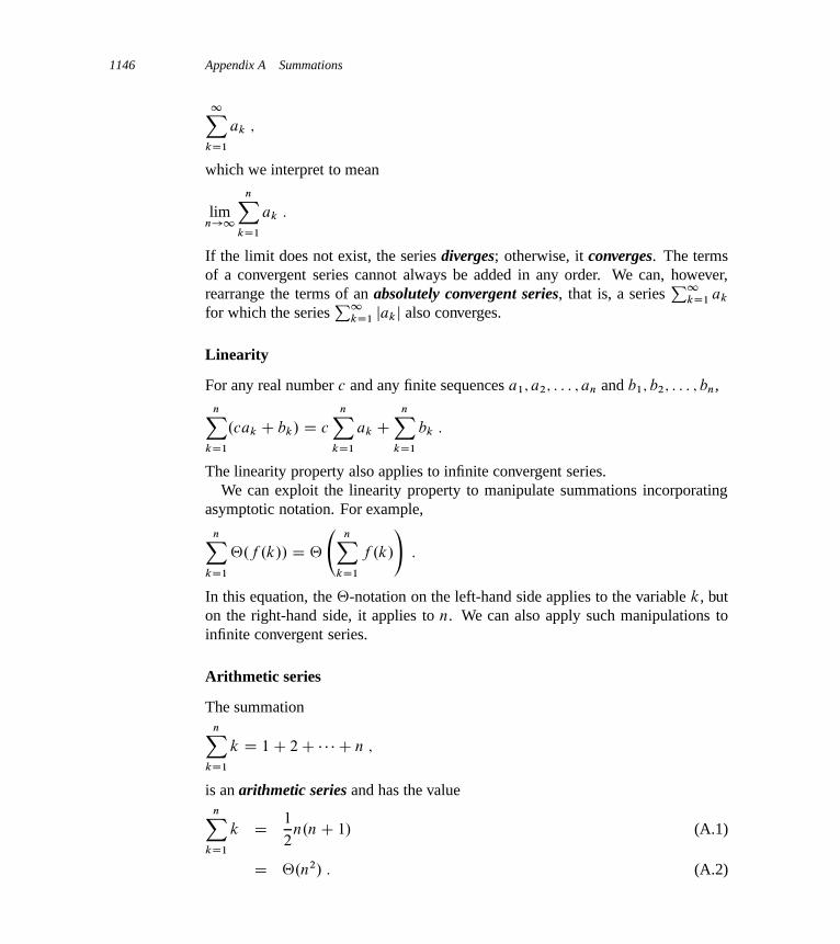
1146 Appendix A Summations
1XkD1
ak ;
which we interpret to mean
limn!1
nXkD1
ak :
If the limit does not exist, the series diverges; otherwise, it converges. The termsof a convergent series cannot always be added in any order. We can, however,rearrange the terms of an absolutely convergent series, that is, a series
P1kD1 ak
for which the seriesP1
kD1 jakj also converges.
Linearity
For any real number c and any finite sequences a1; a2; : : : ; an and b1; b2; : : : ; bn,nX
kD1
.cak C bk/ D c
nXkD1
ak CnX
kD1
bk :
The linearity property also applies to infinite convergent series.We can exploit the linearity property to manipulate summations incorporating
asymptotic notation. For example,
nXkD1
‚.f .k// D ‚
nX
kD1
f .k/
!:
In this equation, the ‚-notation on the left-hand side applies to the variable k, buton the right-hand side, it applies to n. We can also apply such manipulations toinfinite convergent series.
Arithmetic series
The summationnX
kD1
k D 1C 2C � � � C n ;
is an arithmetic series and has the valuenX
kD1
k D 1
2n.nC 1/ (A.1)
D ‚.n2/ : (A.2)

A.1 Summation formulas and properties 1147
Sums of squares and cubes
We have the following summations of squares and cubes:nX
kD0
k2 D n.nC 1/.2nC 1/
6; (A.3)
nXkD0
k3 D n2.nC 1/2
4: (A.4)
Geometric series
For real x ¤ 1, the summationnX
kD0
xk D 1C x C x2 C � � � C xn
is a geometric or exponential series and has the valuenX
kD0
xk D xnC1 � 1
x � 1: (A.5)
When the summation is infinite and jxj < 1, we have the infinite decreasing geo-metric series1X
kD0
xk D 1
1� x: (A.6)
Harmonic series
For positive integers n, the nth harmonic number is
Hn D 1C 1
2C 1
3C 1
4C � � � C 1
n
DnX
kD1
1
k
D ln nCO.1/ : (A.7)
(We shall prove a related bound in Section A.2.)
Integrating and differentiating series
By integrating or differentiating the formulas above, additional formulas arise. Forexample, by differentiating both sides of the infinite geometric series (A.6) andmultiplying by x, we get

1148 Appendix A Summations
1XkD0
kxk D x
.1 � x/2(A.8)
for jxj < 1.
Telescoping series
For any sequence a0; a1; : : : ; an,nX
kD1
.ak � ak�1/ D an � a0 ; (A.9)
since each of the terms a1; a2; : : : ; an�1 is added in exactly once and subtracted outexactly once. We say that the sum telescopes. Similarly,n�1XkD0
.ak � akC1/ D a0 � an :
As an example of a telescoping sum, consider the seriesn�1XkD1
1
k.k C 1/:
Since we can rewrite each term as1
k.k C 1/D 1
k� 1
k C 1;
we getn�1XkD1
1
k.k C 1/D
n�1XkD1
�1
k� 1
k C 1
�D 1� 1
n:
Products
We can write the finite product a1a2 � � � an asnY
kD1
ak :
If n D 0, the value of the product is defined to be 1. We can convert a formula witha product to a formula with a summation by using the identity
lg
nY
kD1
ak
!D
nXkD1
lg ak :
A.2 Bounding summations 1149
Exercises
A.1-1Find a simple formula for
Pn
kD1.2k � 1/.
A.1-2 ?
Show thatPn
kD1 1=.2k � 1/ D ln.p
n/ C O.1/ by manipulating the harmonicseries.
A.1-3Show that
P1kD0 k2xk D x.1C x/=.1� x/3 for 0 < jxj < 1.
A.1-4 ?
Show thatP1
kD0.k � 1/=2k D 0.
A.1-5 ?
Evaluate the sumP1
kD1.2k C 1/x2k.
A.1-6Prove that
Pn
kD1 O.fk.i// D O�Pn
kD1 fk.i/�
by using the linearity property ofsummations.
A.1-7Evaluate the product
Qn
kD1 2 � 4k.
A.1-8 ?
Evaluate the productQn
kD2.1 � 1=k2/.
A.2 Bounding summations
We have many techniques at our disposal for bounding the summations that de-scribe the running times of algorithms. Here are some of the most frequently usedmethods.
Mathematical induction
The most basic way to evaluate a series is to use mathematical induction. As anexample, let us prove that the arithmetic series
Pn
kD1 k evaluates to 12n.nC1/. We
can easily verify this assertion for n D 1. We make the inductive assumption that

1150 Appendix A Summations
it holds for n, and we prove that it holds for nC 1. We have
nC1XkD1
k DnX
kD1
k C .nC 1/
D 1
2n.nC 1/C .nC 1/
D 1
2.nC 1/.nC 2/ :
You don’t always need to guess the exact value of a summation in order to usemathematical induction. Instead, you can use induction to prove a bound on a sum-mation. As an example, let us prove that the geometric series
Pn
kD0 3k is O.3n/.More specifically, let us prove that
Pn
kD0 3k � c3n for some constant c. For theinitial condition n D 0, we have
P0
kD0 3k D 1 � c � 1 as long as c � 1. Assumingthat the bound holds for n, let us prove that it holds for nC 1. We have
nC1XkD0
3k DnX
kD0
3k C 3nC1
� c3n C 3nC1 (by the inductive hypothesis)
D�
1
3C 1
c
�c3nC1
� c3nC1
as long as .1=3 C 1=c/ � 1 or, equivalently, c � 3=2. Thus,Pn
kD0 3k D O.3n/,as we wished to show.
We have to be careful when we use asymptotic notation to prove bounds by in-duction. Consider the following fallacious proof that
Pn
kD1 k D O.n/. Certainly,P1
kD1 k D O.1/. Assuming that the bound holds for n, we now prove it for nC 1:
nC1XkD1
k DnX
kD1
k C .nC 1/
D O.n/C .nC 1/ wrong!!
D O.nC 1/ :
The bug in the argument is that the “constant” hidden by the “big-oh” grows with n
and thus is not constant. We have not shown that the same constant works for all n.
Bounding the terms
We can sometimes obtain a good upper bound on a series by bounding each termof the series, and it often suffices to use the largest term to bound the others. For

A.2 Bounding summations 1151
example, a quick upper bound on the arithmetic series (A.1) is
nXkD1
k �nX
kD1
n
D n2 :
In general, for a seriesPn
kD1 ak, if we let amax D max1�k�n ak, then
nXkD1
ak � n � amax :
The technique of bounding each term in a series by the largest term is a weakmethod when the series can in fact be bounded by a geometric series. Given theseries
Pn
kD0 ak, suppose that akC1=ak � r for all k � 0, where 0 < r < 1 is aconstant. We can bound the sum by an infinite decreasing geometric series, sinceak � a0rk, and thus
nXkD0
ak �1X
kD0
a0rk
D a0
1XkD0
rk
D a0
1
1 � r:
We can apply this method to bound the summationP1
kD1.k=3k/. In order tostart the summation at k D 0, we rewrite it as
P1kD0..k C 1/=3kC1/. The first
term (a0) is 1=3, and the ratio (r) of consecutive terms is
.k C 2/=3kC2
.k C 1/=3kC1D 1
3� k C 2
k C 1
� 2
3
for all k � 0. Thus, we have1X
kD1
k
3kD
1XkD0
k C 1
3kC1
� 1
3� 1
1 � 2=3
D 1 :
1152 Appendix A Summations
A common bug in applying this method is to show that the ratio of consecu-tive terms is less than 1 and then to assume that the summation is bounded by ageometric series. An example is the infinite harmonic series, which diverges since
1XkD1
1
kD lim
n!1
nXkD1
1
k
D limn!1
‚.lg n/
D 1 :
The ratio of the .kC1/st and kth terms in this series is k=.kC1/ < 1, but the seriesis not bounded by a decreasing geometric series. To bound a series by a geometricseries, we must show that there is an r < 1, which is a constant, such that the ratioof all pairs of consecutive terms never exceeds r . In the harmonic series, no such r
exists because the ratio becomes arbitrarily close to 1.
Splitting summations
One way to obtain bounds on a difficult summation is to express the series as thesum of two or more series by partitioning the range of the index and then to boundeach of the resulting series. For example, suppose we try to find a lower boundon the arithmetic series
Pn
kD1 k, which we have already seen has an upper boundof n2. We might attempt to bound each term in the summation by the smallest term,but since that term is 1, we get a lower bound of n for the summation—far off fromour upper bound of n2.
We can obtain a better lower bound by first splitting the summation. Assume forconvenience that n is even. We have
nXkD1
k Dn=2XkD1
k CnX
kDn=2C1
k
�n=2XkD1
0CnX
kDn=2C1
.n=2/
D .n=2/2
D �.n2/ ;
which is an asymptotically tight bound, sincePn
kD1 k D O.n2/.For a summation arising from the analysis of an algorithm, we can often split
the summation and ignore a constant number of the initial terms. Generally, thistechnique applies when each term ak in a summation
Pn
kD0 ak is independent of n.
A.2 Bounding summations 1153
Then for any constant k0 > 0, we can write
nXkD0
ak Dk0�1XkD0
ak CnX
kDk0
ak
D ‚.1/CnX
kDk0
ak ;
since the initial terms of the summation are all constant and there are a constantnumber of them. We can then use other methods to bound
Pn
kDk0ak. This tech-
nique applies to infinite summations as well. For example, to find an asymptoticupper bound on
1XkD0
k2
2k;
we observe that the ratio of consecutive terms is
.k C 1/2=2kC1
k2=2kD .k C 1/2
2k2
� 8
9
if k � 3. Thus, the summation can be split into
1XkD0
k2
2kD
2XkD0
k2
2kC
1XkD3
k2
2k
�2X
kD0
k2
2kC 9
8
1XkD0
�8
9
�k
D O.1/ ;
since the first summation has a constant number of terms and the second summationis a decreasing geometric series.
The technique of splitting summations can help us determine asymptotic boundsin much more difficult situations. For example, we can obtain a bound of O.lg n/
on the harmonic series (A.7):
Hn DnX
kD1
1
k:
We do so by splitting the range 1 to n into blg nc C 1 pieces and upper-boundingthe contribution of each piece by 1. For i D 0; 1; : : : ; blg nc, the i th piece consists

1154 Appendix A Summations
of the terms starting at 1=2i and going up to but not including 1=2iC1. The lastpiece might contain terms not in the original harmonic series, and thus we have
nXkD1
1
k�
blg ncXiD0
2i �1Xj D0
1
2i C j
�blg ncXiD0
2i �1Xj D0
1
2i
Dblg ncXiD0
1
� lg nC 1 : (A.10)
Approximation by integrals
When a summation has the formPn
kDm f .k/, where f .k/ is a monotonically in-creasing function, we can approximate it by integrals:Z n
m�1
f .x/ dx �nX
kDm
f .k/ �Z nC1
m
f .x/ dx : (A.11)
Figure A.1 justifies this approximation. The summation is represented as the areaof the rectangles in the figure, and the integral is the shaded region under the curve.When f .k/ is a monotonically decreasing function, we can use a similar methodto provide the boundsZ nC1
m
f .x/ dx �nX
kDm
f .k/ �Z n
m�1
f .x/ dx : (A.12)
The integral approximation (A.12) gives a tight estimate for the nth harmonicnumber. For a lower bound, we obtain
nXkD1
1
k�
Z nC1
1
dx
x
D ln.nC 1/ : (A.13)
For the upper bound, we derive the inequalitynX
kD2
1
k�
Z n
1
dx
x
D ln n ;
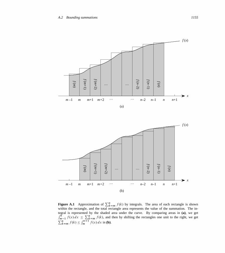
A.2 Bounding summations 1155
n+1n–1n–2m+2mm –1
f (m)
f (m+
1)
f (m+
2)
f (n–2)
f (n–1)
f (n)
f (x)
x… … n
… …
(a)
m+1
n+1n–1n–2m+2mm –1
f (m)
f (m+
1)
f (m+
2)
f (n–2)
f (n–1)
f (n)
f (x)
x… … n
… …
(b)
m+1
Figure A.1 Approximation ofPn
kDm f .k/ by integrals. The area of each rectangle is shownwithin the rectangle, and the total rectangle area represents the value of the summation. The in-tegral is represented by the shaded area under the curve. By comparing areas in (a), we getR n
m�1 f .x/ dx � PnkDm f .k/, and then by shifting the rectangles one unit to the right, we getPn
kDm f .k/ � R nC1m f .x/ dx in (b).

1156 Appendix A Summations
which yields the bound
nXkD1
1
k� ln nC 1 : (A.14)
Exercises
A.2-1Show that
Pn
kD1 1=k2 is bounded above by a constant.
A.2-2Find an asymptotic upper bound on the summation
blg ncXkD0
˙n=2k
�:
A.2-3Show that the nth harmonic number is �.lg n/ by splitting the summation.
A.2-4Approximate
Pn
kD1 k3 with an integral.
A.2-5Why didn’t we use the integral approximation (A.12) directly on
Pn
kD1 1=k toobtain an upper bound on the nth harmonic number?
Problems
A-1 Bounding summationsGive asymptotically tight bounds on the following summations. Assume that r � 0
and s � 0 are constants.
a.nX
kD1
kr .
b.nX
kD1
lgs k.
Notes for Appendix A 1157
c.nX
kD1
kr lgs k.
Chapter notes
Knuth [209] provides an excellent reference for the material presented here. Youcan find basic properties of series in any good calculus book, such as Apostol [18]or Thomas et al. [334].

B Sets, Etc.
Many chapters of this book touch on the elements of discrete mathematics. Thischapter reviews more completely the notations, definitions, and elementary prop-erties of sets, relations, functions, graphs, and trees. If you are already well versedin this material, you can probably just skim this chapter.
B.1 Sets
A set is a collection of distinguishable objects, called its members or elements. Ifan object x is a member of a set S , we write x 2 S (read “x is a member of S”or, more briefly, “x is in S”). If x is not a member of S , we write x 62 S . Wecan describe a set by explicitly listing its members as a list inside braces. Forexample, we can define a set S to contain precisely the numbers 1, 2, and 3 bywriting S D f1; 2; 3g. Since 2 is a member of the set S , we can write 2 2 S , andsince 4 is not a member, we have 4 … S . A set cannot contain the same object morethan once,1 and its elements are not ordered. Two sets A and B are equal, writtenA D B , if they contain the same elements. For example, f1; 2; 3; 1g D f1; 2; 3g Df3; 2; 1g.
We adopt special notations for frequently encountered sets:� ; denotes the empty set, that is, the set containing no members.� Z denotes the set of integers, that is, the set f: : : ;�2;�1; 0; 1; 2; : : :g.� R denotes the set of real numbers.� N denotes the set of natural numbers, that is, the set f0; 1; 2; : : :g.2
1A variation of a set, which can contain the same object more than once, is called a multiset.
2Some authors start the natural numbers with 1 instead of 0. The modern trend seems to be to startwith 0.
B.1 Sets 1159
If all the elements of a set A are contained in a set B , that is, if x 2 A impliesx 2 B , then we write A � B and say that A is a subset of B . A set A is aproper subset of B , written A B , if A � B but A ¤ B . (Some authors use thesymbol “ ” to denote the ordinary subset relation, rather than the proper-subsetrelation.) For any set A, we have A � A. For two sets A and B , we have A D B
if and only if A � B and B � A. For any three sets A, B , and C , if A � B
and B � C , then A � C . For any set A, we have ; � A.We sometimes define sets in terms of other sets. Given a set A, we can define a
set B � A by stating a property that distinguishes the elements of B . For example,we can define the set of even integers by fx W x 2 Z and x=2 is an integerg. Thecolon in this notation is read “such that.” (Some authors use a vertical bar in placeof the colon.)
Given two sets A and B , we can also define new sets by applying set operations:
� The intersection of sets A and B is the set
A \ B D fx W x 2 A and x 2 Bg :
� The union of sets A and B is the set
A [ B D fx W x 2 A or x 2 Bg :
� The difference between two sets A and B is the set
A � B D fx W x 2 A and x … Bg :
Set operations obey the following laws:
Empty set laws:
A \ ; D ; ;
A [ ; D A :
Idempotency laws:
A \ A D A ;
A [ A D A :
Commutative laws:
A \ B D B \ A ;
A [ B D B [ A :

1160 Appendix B Sets, Etc.
AAAAA
A
BBBBB
�
�
.B \ C / [
[
DD
DD
A � .B \ C / .A � B/ .A � C /
CCCCC
Figure B.1 A Venn diagram illustrating the first of DeMorgan’s laws (B.2). Each of the sets A, B ,and C is represented as a circle.
Associative laws:
A \ .B \ C / D .A \ B/ \ C ;
A [ .B [ C / D .A [ B/ [ C :
Distributive laws:
A \ .B [ C / D .A \ B/ [ .A \ C / ;
A [ .B \ C / D .A [ B/ \ .A [ C / :(B.1)
Absorption laws:
A \ .A [ B/ D A ;
A [ .A \ B/ D A :
DeMorgan’s laws:
A � .B \ C / D .A � B/ [ .A � C / ;
A � .B [ C / D .A � B/ \ .A � C / :(B.2)
Figure B.1 illustrates the first of DeMorgan’s laws, using a Venn diagram: a graph-ical picture in which sets are represented as regions of the plane.
Often, all the sets under consideration are subsets of some larger set U called theuniverse. For example, if we are considering various sets made up only of integers,the set Z of integers is an appropriate universe. Given a universe U , we define thecomplement of a set A as A D U � A D fx W x 2 U and x 62 Ag. For any setA � U , we have the following laws:
A D A ;
A \ A D ; ;
A [ A D U :
B.1 Sets 1161
We can rewrite DeMorgan’s laws (B.2) with set complements. For any two setsB; C � U , we have
B \ C D B [ C ;
B [ C D B \ C :
Two sets A and B are disjoint if they have no elements in common, that is, ifA\B D ;. A collection S D fSig of nonempty sets forms a partition of a set S if
� the sets are pairwise disjoint, that is, Si ; Sj 2 S and i ¤ j imply Si \ Sj D ;,and
� their union is S , that is,
S D[
Si 2S
Si :
In other words, S forms a partition of S if each element of S appears in exactlyone Si 2 S .
The number of elements in a set is the cardinality (or size) of the set, denoted jS j.Two sets have the same cardinality if their elements can be put into a one-to-onecorrespondence. The cardinality of the empty set is j;j D 0. If the cardinality of aset is a natural number, we say the set is finite; otherwise, it is infinite. An infiniteset that can be put into a one-to-one correspondence with the natural numbers N iscountably infinite; otherwise, it is uncountable. For example, the integers Z arecountable, but the reals R are uncountable.
For any two finite sets A and B , we have the identity
jA [ Bj D jAj C jBj � jA \ Bj ; (B.3)
from which we can conclude that
jA [ Bj � jAj C jBj :
If A and B are disjoint, then jA \ Bj D 0 and thus jA [ Bj D jAj C jBj. IfA � B , then jAj � jBj.
A finite set of n elements is sometimes called an n-set. A 1-set is called asingleton. A subset of k elements of a set is sometimes called a k-subset.
We denote the set of all subsets of a set S , including the empty set and S itself,by 2S ; we call 2S the power set of S . For example, 2fa;bg D f;; fag ; fbg ; fa; bgg.The power set of a finite set S has cardinality 2jS j (see Exercise B.1-5).
We sometimes care about setlike structures in which the elements are ordered.An ordered pair of two elements a and b is denoted .a; b/ and is defined formallyas the set .a; b/ D fa; fa; bgg. Thus, the ordered pair .a; b/ is not the same as theordered pair .b; a/.

1162 Appendix B Sets, Etc.
The Cartesian product of two sets A and B , denoted A B , is the set of allordered pairs such that the first element of the pair is an element of A and thesecond is an element of B . More formally,
A B D f.a; b/ W a 2 A and b 2 Bg :
For example, fa; bgfa; b; cg D f.a; a/; .a; b/; .a; c/; .b; a/; .b; b/; .b; c/g. WhenA and B are finite sets, the cardinality of their Cartesian product is
jA Bj D jAj � jBj : (B.4)
The Cartesian product of n sets A1; A2; : : : ; An is the set of n-tuples
A1 A2 � � � An D f.a1; a2; : : : ; an/ W ai 2 Ai for i D 1; 2; : : : ; ng ;
whose cardinality is
jA1 A2 � � � Anj D jA1j � jA2j � � � jAnjif all sets are finite. We denote an n-fold Cartesian product over a single set A bythe set
An D A A � � � A ;
whose cardinality is jAnj D jAjn if A is finite. We can also view an n-tuple as afinite sequence of length n (see page 1166).
Exercises
B.1-1Draw Venn diagrams that illustrate the first of the distributive laws (B.1).
B.1-2Prove the generalization of DeMorgan’s laws to any finite collection of sets:
A1 \ A2 \ � � � \ An D A1 [ A2 [ � � � [ An ;
A1 [ A2 [ � � � [ An D A1 \ A2 \ � � � \ An :

B.2 Relations 1163
B.1-3 ?
Prove the generalization of equation (B.3), which is called the principle of inclu-sion and exclusion:
jA1 [ A2 [ � � � [ Anj DjA1j C jA2j C � � � C jAnj� jA1 \ A2j � jA1 \ A3j � � � � (all pairs)
C jA1 \ A2 \ A3j C � � � (all triples):::
C .�1/n�1 jA1 \ A2 \ � � � \ Anj :
B.1-4Show that the set of odd natural numbers is countable.
B.1-5Show that for any finite set S , the power set 2S has 2jS j elements (that is, thereare 2jS j distinct subsets of S).
B.1-6Give an inductive definition for an n-tuple by extending the set-theoretic definitionfor an ordered pair.
B.2 Relations
A binary relation R on two sets A and B is a subset of the Cartesian product AB .If .a; b/ 2 R, we sometimes write a R b. When we say that R is a binary relationon a set A, we mean that R is a subset of A A. For example, the “less than”relation on the natural numbers is the set f.a; b/ W a; b 2 N and a < bg. An n-aryrelation on sets A1; A2; : : : ; An is a subset of A1 A2 � � � An.
A binary relation R � A A is reflexive if
a R a
for all a 2 A. For example, “D” and “�” are reflexive relations on N, but “<” isnot. The relation R is symmetric if
a R b implies b R a
for all a; b 2 A. For example, “D” is symmetric, but “<” and “�” are not. Therelation R is transitive if
a R b and b R c imply a R c

1164 Appendix B Sets, Etc.
for all a; b; c 2 A. For example, the relations “<,” “�,” and “D” are transitive, butthe relation R D f.a; b/ W a; b 2 N and a D b � 1g is not, since 3 R 4 and 4 R 5
do not imply 3 R 5.A relation that is reflexive, symmetric, and transitive is an equivalence relation.
For example, “D” is an equivalence relation on the natural numbers, but “<” is not.If R is an equivalence relation on a set A, then for a 2 A, the equivalence classof a is the set Œa� D fb 2 A W a R bg, that is, the set of all elements equivalent to a.For example, if we define R D f.a; b/ W a; b 2 N and aC b is an even numberg,then R is an equivalence relation, since a C a is even (reflexive), a C b is evenimplies b C a is even (symmetric), and a C b is even and b C c is even implya C c is even (transitive). The equivalence class of 4 is Œ4� D f0; 2; 4; 6; : : :g, andthe equivalence class of 3 is Œ3� D f1; 3; 5; 7; : : :g. A basic theorem of equivalenceclasses is the following.
Theorem B.1 (An equivalence relation is the same as a partition)The equivalence classes of any equivalence relation R on a set A form a partitionof A, and any partition of A determines an equivalence relation on A for which thesets in the partition are the equivalence classes.
Proof For the first part of the proof, we must show that the equivalence classesof R are nonempty, pairwise-disjoint sets whose union is A. Because R is reflex-ive, a 2 Œa�, and so the equivalence classes are nonempty; moreover, since everyelement a 2 A belongs to the equivalence class Œa�, the union of the equivalenceclasses is A. It remains to show that the equivalence classes are pairwise disjoint,that is, if two equivalence classes Œa� and Œb� have an element c in common, thenthey are in fact the same set. Suppose that a R c and b R c. By symmetry, c R b,and by transitivity, a R b. Thus, for any arbitrary element x 2 Œa�, we have x R a
and, by transitivity, x R b, and thus Œa� � Œb�. Similarly, Œb� � Œa�, and thusŒa� D Œb�.
For the second part of the proof, let A D fAig be a partition of A, and defineR D f.a; b/ W there exists i such that a 2 Ai and b 2 Aig. We claim that R is anequivalence relation on A. Reflexivity holds, since a 2 Ai implies a R a. Symme-try holds, because if a R b, then a and b are in the same set Ai , and hence b R a.If a R b and b R c, then all three elements are in the same set Ai , and thus a R c
and transitivity holds. To see that the sets in the partition are the equivalenceclasses of R, observe that if a 2 Ai , then x 2 Œa� implies x 2 Ai , and x 2 Ai
implies x 2 Œa�.
A binary relation R on a set A is antisymmetric if
a R b and b R a imply a D b :
B.2 Relations 1165
For example, the “�” relation on the natural numbers is antisymmetric, since a � b
and b � a imply a D b. A relation that is reflexive, antisymmetric, and transitiveis a partial order, and we call a set on which a partial order is defined a partiallyordered set. For example, the relation “is a descendant of” is a partial order on theset of all people (if we view individuals as being their own descendants).
In a partially ordered set A, there may be no single “maximum” element a suchthat b R a for all b 2 A. Instead, the set may contain several maximal elements a
such that for no b 2 A, where b ¤ a, is it the case that a R b. For example, acollection of different-sized boxes may contain several maximal boxes that don’tfit inside any other box, yet it has no single “maximum” box into which any otherbox will fit.3
A relation R on a set A is a total relation if for all a; b 2 A, we have a R b
or b R a (or both), that is, if every pairing of elements of A is related by R. Apartial order that is also a total relation is a total order or linear order. For example,the relation “�” is a total order on the natural numbers, but the “is a descendantof” relation is not a total order on the set of all people, since there are individualsneither of whom is descended from the other. A total relation that is transitive, butnot necessarily reflexive and antisymmetric, is a total preorder.
Exercises
B.2-1Prove that the subset relation “�” on all subsets of Z is a partial order but not atotal order.
B.2-2Show that for any positive integer n, the relation “equivalent modulo n” is an equiv-alence relation on the integers. (We say that a � b .mod n/ if there exists aninteger q such that a � b D qn.) Into what equivalence classes does this relationpartition the integers?
B.2-3Give examples of relations that are
a. reflexive and symmetric but not transitive,
b. reflexive and transitive but not symmetric,
c. symmetric and transitive but not reflexive.
3To be precise, in order for the “fit inside” relation to be a partial order, we need to view a box asfitting inside itself.

1166 Appendix B Sets, Etc.
B.2-4Let S be a finite set, and let R be an equivalence relation on S S . Show that ifin addition R is antisymmetric, then the equivalence classes of S with respect to R
are singletons.
B.2-5Professor Narcissus claims that if a relation R is symmetric and transitive, then it isalso reflexive. He offers the following proof. By symmetry, a R b implies b R a.Transitivity, therefore, implies a R a. Is the professor correct?
B.3 Functions
Given two sets A and B , a function f is a binary relation on AB such that for alla 2 A, there exists precisely one b 2 B such that .a; b/ 2 f . The set A is calledthe domain of f , and the set B is called the codomain of f . We sometimes writef W A! B; and if .a; b/ 2 f , we write b D f .a/, since b is uniquely determinedby the choice of a.
Intuitively, the function f assigns an element of B to each element of A. Noelement of A is assigned two different elements of B , but the same element of B
can be assigned to two different elements of A. For example, the binary relation
f D f.a; b/ W a; b 2 N and b D a mod 2gis a function f W N ! f0; 1g, since for each natural number a, there is exactly onevalue b in f0; 1g such that b D a mod 2. For this example, 0 D f .0/, 1 D f .1/,0 D f .2/, etc. In contrast, the binary relation
g D f.a; b/ W a; b 2 N and aC b is evengis not a function, since .1; 3/ and .1; 5/ are both in g, and thus for the choice a D 1,there is not precisely one b such that .a; b/ 2 g.
Given a function f W A! B , if b D f .a/, we say that a is the argument of f
and that b is the value of f at a. We can define a function by stating its value forevery element of its domain. For example, we might define f .n/ D 2n for n 2 N,which means f D f.n; 2n/ W n 2 Ng. Two functions f and g are equal if theyhave the same domain and codomain and if, for all a in the domain, f .a/ D g.a/.
A finite sequence of length n is a function f whose domain is the set of n
integers f0; 1; : : : ; n � 1g. We often denote a finite sequence by listing its values:hf .0/; f .1/; : : : ; f .n � 1/i. An infinite sequence is a function whose domain isthe set N of natural numbers. For example, the Fibonacci sequence, defined byrecurrence (3.22), is the infinite sequence h0; 1; 1; 2; 3; 5; 8; 13; 21; : : :i.

B.3 Functions 1167
When the domain of a function f is a Cartesian product, we often omit the extraparentheses surrounding the argument of f . For example, if we had a functionf W A1 A2 � � � An ! B , we would write b D f .a1; a2; : : : ; an/ insteadof b D f ..a1; a2; : : : ; an//. We also call each ai an argument to the function f ,though technically the (single) argument to f is the n-tuple .a1; a2; : : : ; an/.
If f W A! B is a function and b D f .a/, then we sometimes say that b is theimage of a under f . The image of a set A0 � A under f is defined by
f .A0/ D fb 2 B W b D f .a/ for some a 2 A0g :
The range of f is the image of its domain, that is, f .A/. For example, the rangeof the function f W N ! N defined by f .n/ D 2n is f .N/ D fm W m D 2n forsome n 2 Ng, in other words, the set of nonnegative even integers.
A function is a surjection if its range is its codomain. For example, the functionf .n/ D bn=2c is a surjective function from N to N, since every element in N
appears as the value of f for some argument. In contrast, the function f .n/ D 2n
is not a surjective function from N to N, since no argument to f can produce 3 as avalue. The function f .n/ D 2n is, however, a surjective function from the naturalnumbers to the even numbers. A surjection f W A! B is sometimes described asmapping A onto B . When we say that f is onto, we mean that it is surjective.
A function f W A ! B is an injection if distinct arguments to f producedistinct values, that is, if a ¤ a0 implies f .a/ ¤ f .a0/. For example, the functionf .n/ D 2n is an injective function from N to N, since each even number b is theimage under f of at most one element of the domain, namely b=2. The functionf .n/ D bn=2c is not injective, since the value 1 is produced by two arguments: 2
and 3. An injection is sometimes called a one-to-one function.A function f W A! B is a bijection if it is injective and surjective. For example,
the function f .n/ D .�1/n dn=2e is a bijection from N to Z:
0 ! 0 ;
1 ! �1 ;
2 ! 1 ;
3 ! �2 ;
4 ! 2 ;:::
The function is injective, since no element of Z is the image of more than oneelement of N. It is surjective, since every element of Z appears as the image ofsome element of N. Hence, the function is bijective. A bijection is sometimescalled a one-to-one correspondence, since it pairs elements in the domain andcodomain. A bijection from a set A to itself is sometimes called a permutation.
When a function f is bijective, we define its inverse f �1 as
f �1.b/ D a if and only if f .a/ D b :

1168 Appendix B Sets, Etc.
For example, the inverse of the function f .n/ D .�1/n dn=2e is
f �1.m/ D(
2m if m � 0 ;
�2m � 1 if m < 0 :
Exercises
B.3-1Let A and B be finite sets, and let f W A! B be a function. Show that
a. if f is injective, then jAj � jBj;b. if f is surjective, then jAj � jBj.
B.3-2Is the function f .x/ D xC 1 bijective when the domain and the codomain are N?Is it bijective when the domain and the codomain are Z?
B.3-3Give a natural definition for the inverse of a binary relation such that if a relationis in fact a bijective function, its relational inverse is its functional inverse.
B.3-4 ?
Give a bijection from Z to Z Z.
B.4 Graphs
This section presents two kinds of graphs: directed and undirected. Certain def-initions in the literature differ from those given here, but for the most part, thedifferences are slight. Section 22.1 shows how we can represent graphs in com-puter memory.
A directed graph (or digraph) G is a pair .V; E/, where V is a finite set and E
is a binary relation on V . The set V is called the vertex set of G, and its elementsare called vertices (singular: vertex). The set E is called the edge set of G, and itselements are called edges. Figure B.2(a) is a pictorial representation of a directedgraph on the vertex set f1; 2; 3; 4; 5; 6g. Vertices are represented by circles in thefigure, and edges are represented by arrows. Note that self-loops—edges from avertex to itself—are possible.
In an undirected graph G D .V; E/, the edge set E consists of unorderedpairs of vertices, rather than ordered pairs. That is, an edge is a set fu; �g, where
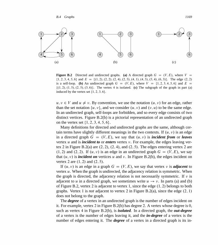
B.4 Graphs 1169
1 2 3
4 5 6
(a)
1 2 3
4 5 6
(b)
1 2 3
6
(c)
Figure B.2 Directed and undirected graphs. (a) A directed graph G D .V; E/, where V Df1; 2; 3; 4; 5; 6g and E D f.1; 2/; .2; 2/; .2; 4/; .2; 5/; .4; 1/; .4; 5/; .5; 4/; .6; 3/g. The edge .2; 2/
is a self-loop. (b) An undirected graph G D .V; E/, where V D f1; 2; 3; 4; 5; 6g and E Df.1; 2/; .1; 5/; .2; 5/; .3; 6/g. The vertex 4 is isolated. (c) The subgraph of the graph in part (a)induced by the vertex set f1; 2; 3; 6g.
u; � 2 V and u ¤ �. By convention, we use the notation .u; �/ for an edge, ratherthan the set notation fu; �g, and we consider .u; �/ and .�; u/ to be the same edge.In an undirected graph, self-loops are forbidden, and so every edge consists of twodistinct vertices. Figure B.2(b) is a pictorial representation of an undirected graphon the vertex set f1; 2; 3; 4; 5; 6g.
Many definitions for directed and undirected graphs are the same, although cer-tain terms have slightly different meanings in the two contexts. If .u; �/ is an edgein a directed graph G D .V; E/, we say that .u; �/ is incident from or leavesvertex u and is incident to or enters vertex �. For example, the edges leaving ver-tex 2 in Figure B.2(a) are .2; 2/, .2; 4/, and .2; 5/. The edges entering vertex 2 are.1; 2/ and .2; 2/. If .u; �/ is an edge in an undirected graph G D .V; E/, we saythat .u; �/ is incident on vertices u and �. In Figure B.2(b), the edges incident onvertex 2 are .1; 2/ and .2; 5/.
If .u; �/ is an edge in a graph G D .V; E/, we say that vertex � is adjacent tovertex u. When the graph is undirected, the adjacency relation is symmetric. Whenthe graph is directed, the adjacency relation is not necessarily symmetric. If � isadjacent to u in a directed graph, we sometimes write u ! �. In parts (a) and (b)of Figure B.2, vertex 2 is adjacent to vertex 1, since the edge .1; 2/ belongs to bothgraphs. Vertex 1 is not adjacent to vertex 2 in Figure B.2(a), since the edge .2; 1/
does not belong to the graph.The degree of a vertex in an undirected graph is the number of edges incident on
it. For example, vertex 2 in Figure B.2(b) has degree 2. A vertex whose degree is 0,such as vertex 4 in Figure B.2(b), is isolated. In a directed graph, the out-degreeof a vertex is the number of edges leaving it, and the in-degree of a vertex is thenumber of edges entering it. The degree of a vertex in a directed graph is its in-
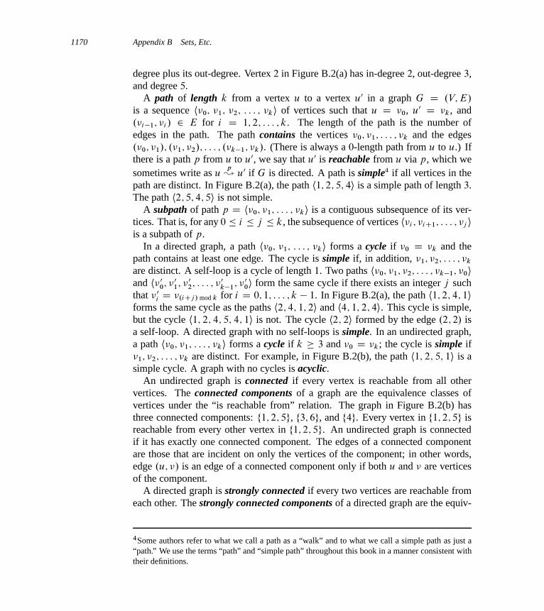
1170 Appendix B Sets, Etc.
degree plus its out-degree. Vertex 2 in Figure B.2(a) has in-degree 2, out-degree 3,and degree 5.
A path of length k from a vertex u to a vertex u0 in a graph G D .V; E/
is a sequence h�0; �1; �2; : : : ; �ki of vertices such that u D �0, u0 D �k, and.�i�1; �i / 2 E for i D 1; 2; : : : ; k. The length of the path is the number ofedges in the path. The path contains the vertices �0; �1; : : : ; �k and the edges.�0; �1/; .�1; �2/; : : : ; .�k�1; �k/. (There is always a 0-length path from u to u.) Ifthere is a path p from u to u0, we say that u0 is reachable from u via p, which wesometimes write as u
p� u0 if G is directed. A path is simple4 if all vertices in the
path are distinct. In Figure B.2(a), the path h1; 2; 5; 4i is a simple path of length 3.The path h2; 5; 4; 5i is not simple.
A subpath of path p D h�0; �1; : : : ; �ki is a contiguous subsequence of its ver-tices. That is, for any 0 � i � j � k, the subsequence of vertices h�i ; �iC1; : : : ; �j iis a subpath of p.
In a directed graph, a path h�0; �1; : : : ; �ki forms a cycle if �0 D �k and thepath contains at least one edge. The cycle is simple if, in addition, �1; �2; : : : ; �k
are distinct. A self-loop is a cycle of length 1. Two paths h�0; �1; �2; : : : ; �k�1; �0iand h� 0
0; � 01; � 0
2; : : : ; � 0k�1
; � 00i form the same cycle if there exists an integer j such
that � 0i D �.iCj / mod k for i D 0; 1; : : : ; k � 1. In Figure B.2(a), the path h1; 2; 4; 1i
forms the same cycle as the paths h2; 4; 1; 2i and h4; 1; 2; 4i. This cycle is simple,but the cycle h1; 2; 4; 5; 4; 1i is not. The cycle h2; 2i formed by the edge .2; 2/ isa self-loop. A directed graph with no self-loops is simple. In an undirected graph,a path h�0; �1; : : : ; �ki forms a cycle if k � 3 and �0 D �k; the cycle is simple if�1; �2; : : : ; �k are distinct. For example, in Figure B.2(b), the path h1; 2; 5; 1i is asimple cycle. A graph with no cycles is acyclic.
An undirected graph is connected if every vertex is reachable from all othervertices. The connected components of a graph are the equivalence classes ofvertices under the “is reachable from” relation. The graph in Figure B.2(b) hasthree connected components: f1; 2; 5g, f3; 6g, and f4g. Every vertex in f1; 2; 5g isreachable from every other vertex in f1; 2; 5g. An undirected graph is connectedif it has exactly one connected component. The edges of a connected componentare those that are incident on only the vertices of the component; in other words,edge .u; �/ is an edge of a connected component only if both u and � are verticesof the component.
A directed graph is strongly connected if every two vertices are reachable fromeach other. The strongly connected components of a directed graph are the equiv-
4Some authors refer to what we call a path as a “walk” and to what we call a simple path as just a“path.” We use the terms “path” and “simple path” throughout this book in a manner consistent withtheir definitions.
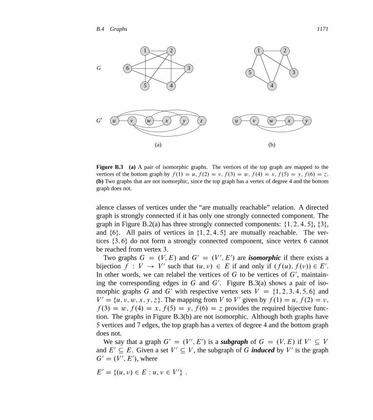
B.4 Graphs 1171
1 2
3
45
6
u v w x y z
(a)
1 2
3
4
5
u v w x y
(b)
G
G′
Figure B.3 (a) A pair of isomorphic graphs. The vertices of the top graph are mapped to thevertices of the bottom graph by f .1/ D u; f .2/ D �; f .3/ D w; f .4/ D x; f .5/ D y; f .6/ D ´.(b) Two graphs that are not isomorphic, since the top graph has a vertex of degree 4 and the bottomgraph does not.
alence classes of vertices under the “are mutually reachable” relation. A directedgraph is strongly connected if it has only one strongly connected component. Thegraph in Figure B.2(a) has three strongly connected components: f1; 2; 4; 5g, f3g,and f6g. All pairs of vertices in f1; 2; 4; 5g are mutually reachable. The ver-tices f3; 6g do not form a strongly connected component, since vertex 6 cannotbe reached from vertex 3.
Two graphs G D .V; E/ and G0 D .V 0; E 0/ are isomorphic if there exists abijection f W V ! V 0 such that .u; �/ 2 E if and only if .f .u/; f .�// 2 E 0.In other words, we can relabel the vertices of G to be vertices of G0, maintain-ing the corresponding edges in G and G0. Figure B.3(a) shows a pair of iso-morphic graphs G and G0 with respective vertex sets V D f1; 2; 3; 4; 5; 6g andV 0 D fu; �; w; x; y; ´g. The mapping from V to V 0 given by f .1/ D u; f .2/ D �;
f .3/ D w; f .4/ D x; f .5/ D y; f .6/ D ´ provides the required bijective func-tion. The graphs in Figure B.3(b) are not isomorphic. Although both graphs have5 vertices and 7 edges, the top graph has a vertex of degree 4 and the bottom graphdoes not.
We say that a graph G0 D .V 0; E 0/ is a subgraph of G D .V; E/ if V 0 � V
and E 0 � E. Given a set V 0 � V , the subgraph of G induced by V 0 is the graphG0 D .V 0; E 0/, where
E 0 D f.u; �/ 2 E W u; � 2 V 0g :
1172 Appendix B Sets, Etc.
The subgraph induced by the vertex set f1; 2; 3; 6g in Figure B.2(a) appears inFigure B.2(c) and has the edge set f.1; 2/; .2; 2/; .6; 3/g.
Given an undirected graph G D .V; E/, the directed version of G is the directedgraph G0 D .V; E 0/, where .u; �/ 2 E 0 if and only if .u; �/ 2 E. That is, wereplace each undirected edge .u; �/ in G by the two directed edges .u; �/ and .�; u/
in the directed version. Given a directed graph G D .V; E/, the undirected versionof G is the undirected graph G0 D .V; E 0/, where .u; �/ 2 E 0 if and only if u ¤ �
and .u; �/ 2 E. That is, the undirected version contains the edges of G “withtheir directions removed” and with self-loops eliminated. (Since .u; �/ and .�; u/
are the same edge in an undirected graph, the undirected version of a directedgraph contains it only once, even if the directed graph contains both edges .u; �/
and .�; u/.) In a directed graph G D .V; E/, a neighbor of a vertex u is any vertexthat is adjacent to u in the undirected version of G. That is, � is a neighbor of u ifu ¤ � and either .u; �/ 2 E or .�; u/ 2 E. In an undirected graph, u and � areneighbors if they are adjacent.
Several kinds of graphs have special names. A complete graph is an undirectedgraph in which every pair of vertices is adjacent. A bipartite graph is an undirectedgraph G D .V; E/ in which V can be partitioned into two sets V1 and V2 such that.u; �/ 2 E implies either u 2 V1 and � 2 V2 or u 2 V2 and � 2 V1. That is, alledges go between the two sets V1 and V2. An acyclic, undirected graph is a forest,and a connected, acyclic, undirected graph is a (free) tree (see Section B.5). Weoften take the first letters of “directed acyclic graph” and call such a graph a dag.
There are two variants of graphs that you may occasionally encounter. A multi-graph is like an undirected graph, but it can have both multiple edges between ver-tices and self-loops. A hypergraph is like an undirected graph, but each hyperedge,rather than connecting two vertices, connects an arbitrary subset of vertices. Manyalgorithms written for ordinary directed and undirected graphs can be adapted torun on these graphlike structures.
The contraction of an undirected graph G D .V; E/ by an edge e D .u; �/ is agraph G0 D .V 0; E 0/, where V 0 D V � fu; �g [ fxg and x is a new vertex. The setof edges E 0 is formed from E by deleting the edge .u; �/ and, for each vertex w
incident on u or �, deleting whichever of .u; w/ and .�; w/ is in E and adding thenew edge .x; w/. In effect, u and � are “contracted” into a single vertex.
Exercises
B.4-1Attendees of a faculty party shake hands to greet each other, and each professorremembers how many times he or she shook hands. At the end of the party, thedepartment head adds up the number of times that each professor shook hands.
B.5 Trees 1173
Show that the result is even by proving the handshaking lemma: if G D .V; E/ isan undirected graph, thenX�2V
degree.�/ D 2 jEj :
B.4-2Show that if a directed or undirected graph contains a path between two vertices u
and �, then it contains a simple path between u and �. Show that if a directed graphcontains a cycle, then it contains a simple cycle.
B.4-3Show that any connected, undirected graph G D .V; E/ satisfies jEj � jV j � 1.
B.4-4Verify that in an undirected graph, the “is reachable from” relation is an equiv-alence relation on the vertices of the graph. Which of the three properties of anequivalence relation hold in general for the “is reachable from” relation on thevertices of a directed graph?
B.4-5What is the undirected version of the directed graph in Figure B.2(a)? What is thedirected version of the undirected graph in Figure B.2(b)?
B.4-6 ?
Show that we can represent a hypergraph by a bipartite graph if we let incidence inthe hypergraph correspond to adjacency in the bipartite graph. (Hint: Let one setof vertices in the bipartite graph correspond to vertices of the hypergraph, and letthe other set of vertices of the bipartite graph correspond to hyperedges.)
B.5 Trees
As with graphs, there are many related, but slightly different, notions of trees. Thissection presents definitions and mathematical properties of several kinds of trees.Sections 10.4 and 22.1 describe how we can represent trees in computer memory.
B.5.1 Free trees
As defined in Section B.4, a free tree is a connected, acyclic, undirected graph. Weoften omit the adjective “free” when we say that a graph is a tree. If an undirectedgraph is acyclic but possibly disconnected, it is a forest. Many algorithms that work

1174 Appendix B Sets, Etc.
(a) (b) (c)
Figure B.4 (a) A free tree. (b) A forest. (c) A graph that contains a cycle and is therefore neithera tree nor a forest.
for trees also work for forests. Figure B.4(a) shows a free tree, and Figure B.4(b)shows a forest. The forest in Figure B.4(b) is not a tree because it is not connected.The graph in Figure B.4(c) is connected but neither a tree nor a forest, because itcontains a cycle.
The following theorem captures many important facts about free trees.
Theorem B.2 (Properties of free trees)Let G D .V; E/ be an undirected graph. The following statements are equivalent.
1. G is a free tree.
2. Any two vertices in G are connected by a unique simple path.
3. G is connected, but if any edge is removed from E, the resulting graph is dis-connected.
4. G is connected, and jEj D jV j � 1.
5. G is acyclic, and jEj D jV j � 1.
6. G is acyclic, but if any edge is added to E, the resulting graph contains a cycle.
Proof (1)) (2): Since a tree is connected, any two vertices in G are connectedby at least one simple path. Suppose, for the sake of contradiction, that vertices u
and � are connected by two distinct simple paths p1 and p2, as shown in Figure B.5.Let w be the vertex at which the paths first diverge; that is, w is the first vertexon both p1 and p2 whose successor on p1 is x and whose successor on p2 is y,where x ¤ y. Let ´ be the first vertex at which the paths reconverge; that is, ´ isthe first vertex following w on p1 that is also on p2. Let p0 be the subpath of p1
from w through x to ´, and let p00 be the subpath of p2 from w through y to ´.Paths p0 and p00 share no vertices except their endpoints. Thus, the path obtained byconcatenating p0 and the reverse of p00 is a cycle, which contradicts our assumption
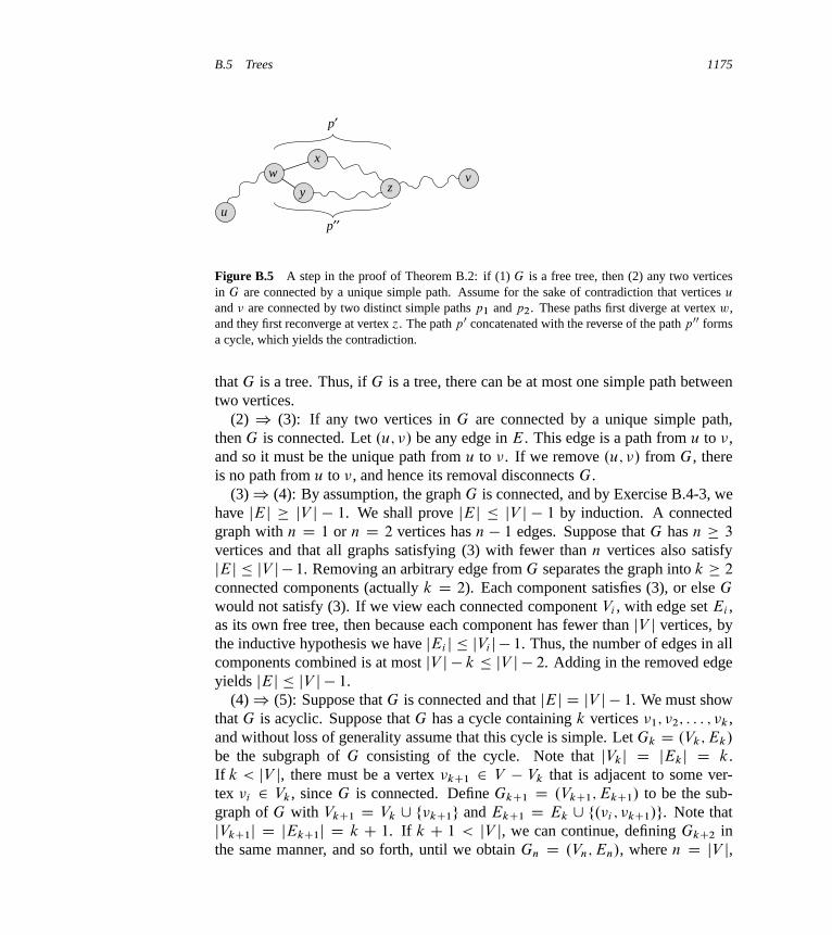
B.5 Trees 1175
u
wz
v
x
y
p′
p′′
Figure B.5 A step in the proof of Theorem B.2: if (1) G is a free tree, then (2) any two verticesin G are connected by a unique simple path. Assume for the sake of contradiction that vertices u
and � are connected by two distinct simple paths p1 and p2. These paths first diverge at vertex w,and they first reconverge at vertex ´. The path p0 concatenated with the reverse of the path p00 formsa cycle, which yields the contradiction.
that G is a tree. Thus, if G is a tree, there can be at most one simple path betweentwo vertices.
(2) ) (3): If any two vertices in G are connected by a unique simple path,then G is connected. Let .u; �/ be any edge in E. This edge is a path from u to �,and so it must be the unique path from u to �. If we remove .u; �/ from G, thereis no path from u to �, and hence its removal disconnects G.
(3)) (4): By assumption, the graph G is connected, and by Exercise B.4-3, wehave jEj � jV j � 1. We shall prove jEj � jV j � 1 by induction. A connectedgraph with n D 1 or n D 2 vertices has n � 1 edges. Suppose that G has n � 3
vertices and that all graphs satisfying (3) with fewer than n vertices also satisfyjEj � jV j � 1. Removing an arbitrary edge from G separates the graph into k � 2
connected components (actually k D 2). Each component satisfies (3), or else G
would not satisfy (3). If we view each connected component Vi , with edge set Ei ,as its own free tree, then because each component has fewer than jV j vertices, bythe inductive hypothesis we have jEi j � jVi j � 1. Thus, the number of edges in allcomponents combined is at most jV j � k � jV j � 2. Adding in the removed edgeyields jEj � jV j � 1.
(4)) (5): Suppose that G is connected and that jEj D jV j � 1. We must showthat G is acyclic. Suppose that G has a cycle containing k vertices �1; �2; : : : ; �k ,and without loss of generality assume that this cycle is simple. Let Gk D .Vk; Ek/
be the subgraph of G consisting of the cycle. Note that jVkj D jEkj D k.If k < jV j, there must be a vertex �kC1 2 V � Vk that is adjacent to some ver-tex �i 2 Vk, since G is connected. Define GkC1 D .VkC1; EkC1/ to be the sub-graph of G with VkC1 D Vk [ f�kC1g and EkC1 D Ek [ f.�i ; �kC1/g. Note thatjVkC1j D jEkC1j D k C 1. If k C 1 < jV j, we can continue, defining GkC2 inthe same manner, and so forth, until we obtain Gn D .Vn; En/, where n D jV j,
1176 Appendix B Sets, Etc.
Vn D V , and jEnj D jVnj D jV j. Since Gn is a subgraph of G, we have En � E,and hence jEj � jV j, which contradicts the assumption that jEj D jV j � 1. Thus,G is acyclic.
(5) ) (6): Suppose that G is acyclic and that jEj D jV j � 1. Let k be thenumber of connected components of G. Each connected component is a free treeby definition, and since (1) implies (5), the sum of all edges in all connected com-ponents of G is jV j � k. Consequently, we must have k D 1, and G is in fact atree. Since (1) implies (2), any two vertices in G are connected by a unique simplepath. Thus, adding any edge to G creates a cycle.
(6) ) (1): Suppose that G is acyclic but that adding any edge to E creates acycle. We must show that G is connected. Let u and � be arbitrary vertices in G.If u and � are not already adjacent, adding the edge .u; �/ creates a cycle in whichall edges but .u; �/ belong to G. Thus, the cycle minus edge .u; �/ must contain apath from u to �, and since u and � were chosen arbitrarily, G is connected.
B.5.2 Rooted and ordered trees
A rooted tree is a free tree in which one of the vertices is distinguished from theothers. We call the distinguished vertex the root of the tree. We often refer to avertex of a rooted tree as a node5 of the tree. Figure B.6(a) shows a rooted tree ona set of 12 nodes with root 7.
Consider a node x in a rooted tree T with root r . We call any node y on theunique simple path from r to x an ancestor of x. If y is an ancestor of x, then x isa descendant of y. (Every node is both an ancestor and a descendant of itself.) If y
is an ancestor of x and x ¤ y, then y is a proper ancestor of x and x is a properdescendant of y. The subtree rooted at x is the tree induced by descendants of x,rooted at x. For example, the subtree rooted at node 8 in Figure B.6(a) containsnodes 8, 6, 5, and 9.
If the last edge on the simple path from the root r of a tree T to a node x is .y; x/,then y is the parent of x, and x is a child of y. The root is the only node in T withno parent. If two nodes have the same parent, they are siblings. A node with nochildren is a leaf or external node. A nonleaf node is an internal node.
5The term “node” is often used in the graph theory literature as a synonym for “vertex.” We reservethe term “node” to mean a vertex of a rooted tree.
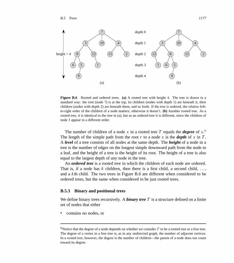
B.5 Trees 1177
9
6 5
8
1
12
3 10
7
11 2
4
height = 4
depth 0
depth 1
depth 2
depth 3
depth 4
(a)
9
6 5
812
3 10
7
11 2
4
(b)
1
Figure B.6 Rooted and ordered trees. (a) A rooted tree with height 4. The tree is drawn in astandard way: the root (node 7) is at the top, its children (nodes with depth 1) are beneath it, theirchildren (nodes with depth 2) are beneath them, and so forth. If the tree is ordered, the relative left-to-right order of the children of a node matters; otherwise it doesn’t. (b) Another rooted tree. As arooted tree, it is identical to the tree in (a), but as an ordered tree it is different, since the children ofnode 3 appear in a different order.
The number of children of a node x in a rooted tree T equals the degree of x.6
The length of the simple path from the root r to a node x is the depth of x in T .A level of a tree consists of all nodes at the same depth. The height of a node in atree is the number of edges on the longest simple downward path from the node toa leaf, and the height of a tree is the height of its root. The height of a tree is alsoequal to the largest depth of any node in the tree.
An ordered tree is a rooted tree in which the children of each node are ordered.That is, if a node has k children, then there is a first child, a second child, . . . ,and a kth child. The two trees in Figure B.6 are different when considered to beordered trees, but the same when considered to be just rooted trees.
B.5.3 Binary and positional trees
We define binary trees recursively. A binary tree T is a structure defined on a finiteset of nodes that either
� contains no nodes, or
6Notice that the degree of a node depends on whether we consider T to be a rooted tree or a free tree.The degree of a vertex in a free tree is, as in any undirected graph, the number of adjacent vertices.In a rooted tree, however, the degree is the number of children—the parent of a node does not counttoward its degree.
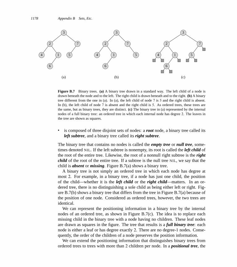
1178 Appendix B Sets, Etc.
3
2
4 1
6
7
5
(a)
3
2
4 1
6
7
5
(b)
3
2
4 1
6
7
5
(c)
Figure B.7 Binary trees. (a) A binary tree drawn in a standard way. The left child of a node isdrawn beneath the node and to the left. The right child is drawn beneath and to the right. (b) A binarytree different from the one in (a). In (a), the left child of node 7 is 5 and the right child is absent.In (b), the left child of node 7 is absent and the right child is 5. As ordered trees, these trees arethe same, but as binary trees, they are distinct. (c) The binary tree in (a) represented by the internalnodes of a full binary tree: an ordered tree in which each internal node has degree 2. The leaves inthe tree are shown as squares.
� is composed of three disjoint sets of nodes: a root node, a binary tree called itsleft subtree, and a binary tree called its right subtree.
The binary tree that contains no nodes is called the empty tree or null tree, some-times denoted NIL. If the left subtree is nonempty, its root is called the left child ofthe root of the entire tree. Likewise, the root of a nonnull right subtree is the rightchild of the root of the entire tree. If a subtree is the null tree NIL, we say that thechild is absent or missing. Figure B.7(a) shows a binary tree.
A binary tree is not simply an ordered tree in which each node has degree atmost 2. For example, in a binary tree, if a node has just one child, the positionof the child—whether it is the left child or the right child—matters. In an or-dered tree, there is no distinguishing a sole child as being either left or right. Fig-ure B.7(b) shows a binary tree that differs from the tree in Figure B.7(a) because ofthe position of one node. Considered as ordered trees, however, the two trees areidentical.
We can represent the positioning information in a binary tree by the internalnodes of an ordered tree, as shown in Figure B.7(c). The idea is to replace eachmissing child in the binary tree with a node having no children. These leaf nodesare drawn as squares in the figure. The tree that results is a full binary tree: eachnode is either a leaf or has degree exactly 2. There are no degree-1 nodes. Conse-quently, the order of the children of a node preserves the position information.
We can extend the positioning information that distinguishes binary trees fromordered trees to trees with more than 2 children per node. In a positional tree, the

B.5 Trees 1179
height = 3
depth 0
depth 1
depth 2
depth 3
Figure B.8 A complete binary tree of height 3 with 8 leaves and 7 internal nodes.
children of a node are labeled with distinct positive integers. The i th child of anode is absent if no child is labeled with integer i . A k-ary tree is a positional treein which for every node, all children with labels greater than k are missing. Thus,a binary tree is a k-ary tree with k D 2.
A complete k-ary tree is a k-ary tree in which all leaves have the same depthand all internal nodes have degree k. Figure B.8 shows a complete binary tree ofheight 3. How many leaves does a complete k-ary tree of height h have? The roothas k children at depth 1, each of which has k children at depth 2, etc. Thus, thenumber of leaves at depth h is kh. Consequently, the height of a complete k-arytree with n leaves is logk n. The number of internal nodes of a complete k-ary treeof height h is
1C k C k2 C � � � C kh�1 Dh�1XiD0
ki
D kh � 1
k � 1
by equation (A.5). Thus, a complete binary tree has 2h � 1 internal nodes.
Exercises
B.5-1Draw all the free trees composed of the three vertices x, y, and ´. Draw all therooted trees with nodes x, y, and ´ with x as the root. Draw all the ordered treeswith nodes x, y, and ´ with x as the root. Draw all the binary trees with nodes x,y, and ´ with x as the root.

1180 Appendix B Sets, Etc.
B.5-2Let G D .V; E/ be a directed acyclic graph in which there is a vertex �0 2 V
such that there exists a unique path from �0 to every vertex � 2 V . Prove that theundirected version of G forms a tree.
B.5-3Show by induction that the number of degree-2 nodes in any nonempty binary treeis 1 fewer than the number of leaves. Conclude that the number of internal nodesin a full binary tree is 1 fewer than the number of leaves.
B.5-4Use induction to show that a nonempty binary tree with n nodes has height atleast blg nc.B.5-5 ?
The internal path length of a full binary tree is the sum, taken over all internalnodes of the tree, of the depth of each node. Likewise, the external path length isthe sum, taken over all leaves of the tree, of the depth of each leaf. Consider a fullbinary tree with n internal nodes, internal path length i , and external path length e.Prove that e D i C 2n.
B.5-6 ?
Let us associate a “weight” w.x/ D 2�d with each leaf x of depth d in a binarytree T , and let L be the set of leaves of T . Prove that
Px2L w.x/ � 1. (This is
known as the Kraft inequality.)
B.5-7 ?
Show that if L � 2, then every binary tree with L leaves contains a subtree havingbetween L=3 and 2L=3 leaves, inclusive.
Problems
B-1 Graph coloringGiven an undirected graph G D .V; E/, a k-coloring of G is a function c W V !f0; 1; : : : ; k � 1g such that c.u/ ¤ c.�/ for every edge .u; �/ 2 E. In other words,the numbers 0; 1; : : : ; k� 1 represent the k colors, and adjacent vertices must havedifferent colors.
a. Show that any tree is 2-colorable.

Problems for Appendix B 1181
b. Show that the following are equivalent:
1. G is bipartite.
2. G is 2-colorable.
3. G has no cycles of odd length.
c. Let d be the maximum degree of any vertex in a graph G. Prove that we cancolor G with d C 1 colors.
d. Show that if G has O.jV j/ edges, then we can color G with O.pjV j/ colors.
B-2 Friendly graphsReword each of the following statements as a theorem about undirected graphs,and then prove it. Assume that friendship is symmetric but not reflexive.
a. Any group of at least two people contains at least two people with the samenumber of friends in the group.
b. Every group of six people contains either at least three mutual friends or at leastthree mutual strangers.
c. Any group of people can be partitioned into two subgroups such that at leasthalf the friends of each person belong to the subgroup of which that person isnot a member.
d. If everyone in a group is the friend of at least half the people in the group, thenthe group can be seated around a table in such a way that everyone is seatedbetween two friends.
B-3 Bisecting treesMany divide-and-conquer algorithms that operate on graphs require that the graphbe bisected into two nearly equal-sized subgraphs, which are induced by a partitionof the vertices. This problem investigates bisections of trees formed by removing asmall number of edges. We require that whenever two vertices end up in the samesubtree after removing edges, then they must be in the same partition.
a. Show that we can partition the vertices of any n-vertex binary tree into twosets A and B , such that jAj � 3n=4 and jBj � 3n=4, by removing a singleedge.
b. Show that the constant 3=4 in part (a) is optimal in the worst case by givingan example of a simple binary tree whose most evenly balanced partition uponremoval of a single edge has jAj D 3n=4.
1182 Appendix B Sets, Etc.
c. Show that by removing at most O.lg n/ edges, we can partition the verticesof any n-vertex binary tree into two sets A and B such that jAj D bn=2cand jBj D dn=2e.
Chapter notes
G. Boole pioneered the development of symbolic logic, and he introduced many ofthe basic set notations in a book published in 1854. Modern set theory was createdby G. Cantor during the period 1874–1895. Cantor focused primarily on sets ofinfinite cardinality. The term “function” is attributed to G. W. Leibniz, who used itto refer to several kinds of mathematical formulas. His limited definition has beengeneralized many times. Graph theory originated in 1736, when L. Euler provedthat it was impossible to cross each of the seven bridges in the city of Königsbergexactly once and return to the starting point.
The book by Harary [160] provides a useful compendium of many definitionsand results from graph theory.

C Counting and Probability
This chapter reviews elementary combinatorics and probability theory. If you havea good background in these areas, you may want to skim the beginning of thechapter lightly and concentrate on the later sections. Most of this book’s chaptersdo not require probability, but for some chapters it is essential.
Section C.1 reviews elementary results in counting theory, including standardformulas for counting permutations and combinations. The axioms of probabilityand basic facts concerning probability distributions form Section C.2. Randomvariables are introduced in Section C.3, along with the properties of expectationand variance. Section C.4 investigates the geometric and binomial distributionsthat arise from studying Bernoulli trials. The study of the binomial distributioncontinues in Section C.5, an advanced discussion of the “tails” of the distribution.
C.1 Counting
Counting theory tries to answer the question “How many?” without actually enu-merating all the choices. For example, we might ask, “How many different n-bitnumbers are there?” or “How many orderings of n distinct elements are there?” Inthis section, we review the elements of counting theory. Since some of the materialassumes a basic understanding of sets, you might wish to start by reviewing thematerial in Section B.1.
Rules of sum and product
We can sometimes express a set of items that we wish to count as a union of disjointsets or as a Cartesian product of sets.
The rule of sum says that the number of ways to choose one element from oneof two disjoint sets is the sum of the cardinalities of the sets. That is, if A and B
are two finite sets with no members in common, then jA [ Bj D jAj C jBj, which
1184 Appendix C Counting and Probability
follows from equation (B.3). For example, each position on a car’s license plateis a letter or a digit. The number of possibilities for each position is therefore26 C 10 D 36, since there are 26 choices if it is a letter and 10 choices if it is adigit.
The rule of product says that the number of ways to choose an ordered pair is thenumber of ways to choose the first element times the number of ways to choose thesecond element. That is, if A and B are two finite sets, then jA Bj D jAj � jBj,which is simply equation (B.4). For example, if an ice-cream parlor offers 28flavors of ice cream and 4 toppings, the number of possible sundaes with one scoopof ice cream and one topping is 28 � 4 D 112.
Strings
A string over a finite set S is a sequence of elements of S . For example, there are 8binary strings of length 3:
000; 001; 010; 011; 100; 101; 110; 111 :
We sometimes call a string of length k a k-string. A substring s0 of a string s
is an ordered sequence of consecutive elements of s. A k-substring of a stringis a substring of length k. For example, 010 is a 3-substring of 01101001 (the3-substring that begins in position 4), but 111 is not a substring of 01101001.
We can view a k-string over a set S as an element of the Cartesian product Sk
of k-tuples; thus, there are jS jk strings of length k. For example, the number ofbinary k-strings is 2k . Intuitively, to construct a k-string over an n-set, we have n
ways to pick the first element; for each of these choices, we have n ways to pick thesecond element; and so forth k times. This construction leads to the k-fold productn � n � � � n D nk as the number of k-strings.
Permutations
A permutation of a finite set S is an ordered sequence of all the elements of S ,with each element appearing exactly once. For example, if S D fa; b; cg, then S
has 6 permutations:
abc; acb; bac; bca; cab; cba :
There are nŠ permutations of a set of n elements, since we can choose the firstelement of the sequence in n ways, the second in n � 1 ways, the third in n � 2
ways, and so on.A k-permutation of S is an ordered sequence of k elements of S , with no ele-
ment appearing more than once in the sequence. (Thus, an ordinary permutation isan n-permutation of an n-set.) The twelve 2-permutations of the set fa; b; c; dg are

C.1 Counting 1185
ab; ac; ad; ba; bc; bd; ca; cb; cd; da; db; dc :
The number of k-permutations of an n-set is
n.n � 1/.n � 2/ � � � .n � k C 1/ D nŠ
.n � k/Š; (C.1)
since we have n ways to choose the first element, n� 1 ways to choose the secondelement, and so on, until we have selected k elements, the last being a selectionfrom the remaining n � k C 1 elements.
Combinations
A k-combination of an n-set S is simply a k-subset of S . For example, the 4-setfa; b; c; dg has six 2-combinations:
ab; ac; ad; bc; bd; cd :
(Here we use the shorthand of denoting the 2-subset fa; bg by ab, and so on.)We can construct a k-combination of an n-set by choosing k distinct (different)elements from the n-set. The order in which we select the elements does not matter.
We can express the number of k-combinations of an n-set in terms of the numberof k-permutations of an n-set. Every k-combination has exactly kŠ permutationsof its elements, each of which is a distinct k-permutation of the n-set. Thus, thenumber of k-combinations of an n-set is the number of k-permutations dividedby kŠ; from equation (C.1), this quantity is
nŠ
kŠ .n � k/Š: (C.2)
For k D 0, this formula tells us that the number of ways to choose 0 elements froman n-set is 1 (not 0), since 0Š D 1.
Binomial coefficients
The notation�
n
k
�(read “n choose k”) denotes the number of k-combinations of
an n-set. From equation (C.2), we have n
k
!D nŠ
kŠ .n � k/Š:
This formula is symmetric in k and n � k: n
k
!D
n
n � k
!: (C.3)

1186 Appendix C Counting and Probability
These numbers are also known as binomial coefficients, due to their appearance inthe binomial expansion:
.x C y/n DnX
kD0
n
k
!xkyn�k : (C.4)
A special case of the binomial expansion occurs when x D y D 1:
2n DnX
kD0
n
k
!:
This formula corresponds to counting the 2n binary n-strings by the number of 1sthey contain:
�n
k
�binary n-strings contain exactly k 1s, since we have
�n
k
�ways to
choose k out of the n positions in which to place the 1s.Many identities involve binomial coefficients. The exercises at the end of this
section give you the opportunity to prove a few.
Binomial bounds
We sometimes need to bound the size of a binomial coefficient. For 1 � k � n,we have the lower bound
n
k
!D n.n � 1/ � � � .n � k C 1/
k.k � 1/ � � � 1
D�n
k
��n � 1
k � 1
�� � ��
n � k C 1
1
��
�n
k
�k
:
Taking advantage of the inequality kŠ � .k=e/k derived from Stirling’s approxi-mation (3.18), we obtain the upper bounds
n
k
!D n.n � 1/ � � � .n � k C 1/
k.k � 1/ � � � 1
� nk
kŠ
��en
k
�k
: (C.5)
For all integers k such that 0 � k � n, we can use induction (see Exercise C.1-12)to prove the bound
C.1 Counting 1187
n
k
!� nn
kk.n � k/n�k; (C.6)
where for convenience we assume that 00 D 1. For k D �n, where 0 � � � 1, wecan rewrite this bound as
n
�n
!� nn
.�n/n..1 � �/n/.1�/n
D �
1
�
� �1
1 � �
�1�!n
D 2n H./ ;
where
H.�/ D �� lg � � .1 � �/ lg.1 � �/ (C.7)
is the (binary) entropy function and where, for convenience, we assume that0 lg 0 D 0, so that H.0/ D H.1/ D 0.
Exercises
C.1-1How many k-substrings does an n-string have? (Consider identical k-substrings atdifferent positions to be different.) How many substrings does an n-string have intotal?
C.1-2An n-input, m-output boolean function is a function from fTRUE; FALSEgn tofTRUE; FALSEgm. How many n-input, 1-output boolean functions are there? Howmany n-input, m-output boolean functions are there?
C.1-3In how many ways can n professors sit around a circular conference table? Con-sider two seatings to be the same if one can be rotated to form the other.
C.1-4In how many ways can we choose three distinct numbers from the set f1; 2; : : : ; 99gso that their sum is even?

1188 Appendix C Counting and Probability
C.1-5Prove the identity
n
k
!D n
k
n � 1
k � 1
!(C.8)
for 0 < k � n.
C.1-6Prove the identity
n
k
!D n
n � k
n � 1
k
!for 0 � k < n.
C.1-7To choose k objects from n, you can make one of the objects distinguished andconsider whether the distinguished object is chosen. Use this approach to provethat
n
k
!D
n � 1
k
!C
n � 1
k � 1
!:
C.1-8Using the result of Exercise C.1-7, make a table for n D 0; 1; : : : ; 6 and 0 � k � n
of the binomial coefficients�
n
k
�with
�0
0
�at the top,
�1
0
�and
�1
1
�on the next line, and
so forth. Such a table of binomial coefficients is called Pascal’s triangle.
C.1-9Prove that
nXiD1
i D
nC 1
2
!:
C.1-10Show that for any integers n � 0 and 0 � k � n, the expression
�n
k
�achieves its
maximum value when k D bn=2c or k D dn=2e.C.1-11 ?
Argue that for any integers n � 0, j � 0, k � 0, and j C k � n, n
j C k
!�
n
j
! n � j
k
!: (C.9)
C.2 Probability 1189
Provide both an algebraic proof and an argument based on a method for choosingj C k items out of n. Give an example in which equality does not hold.
C.1-12 ?
Use induction on all integers k such that 0 � k � n=2 to prove inequality (C.6),and use equation (C.3) to extend it to all integers k such that 0 � k � n.
C.1-13 ?
Use Stirling’s approximation to prove that 2n
n
!D 22n
p�n
.1CO.1=n// : (C.10)
C.1-14 ?
By differentiating the entropy function H.�/, show that it achieves its maximumvalue at � D 1=2. What is H.1=2/?
C.1-15 ?
Show that for any integer n � 0,
nXkD0
n
k
!k D n2n�1 : (C.11)
C.2 Probability
Probability is an essential tool for the design and analysis of probabilistic and ran-domized algorithms. This section reviews basic probability theory.
We define probability in terms of a sample space S , which is a set whose ele-ments are called elementary events. We can think of each elementary event as apossible outcome of an experiment. For the experiment of flipping two distinguish-able coins, with each individual flip resulting in a head (H) or a tail (T), we can viewthe sample space as consisting of the set of all possible 2-strings over fH; Tg:S D fHH; HT; TH; TTg :
1190 Appendix C Counting and Probability
An event is a subset1 of the sample space S . For example, in the experiment offlipping two coins, the event of obtaining one head and one tail is fHT; THg. Theevent S is called the certain event, and the event ; is called the null event. We saythat two events A and B are mutually exclusive if A\B D ;. We sometimes treatan elementary event s 2 S as the event fsg. By definition, all elementary eventsare mutually exclusive.
Axioms of probability
A probability distribution Pr fg on a sample space S is a mapping from events of S
to real numbers satisfying the following probability axioms:
1. Pr fAg � 0 for any event A.
2. Pr fSg D 1.
3. Pr fA[ Bg D Pr fAg C Pr fBg for any two mutually exclusive events A
and B . More generally, for any (finite or countably infinite) sequence of eventsA1; A2; : : : that are pairwise mutually exclusive,
Pr
([i
Ai
)DX
i
Pr fAig :
We call Pr fAg the probability of the event A. We note here that axiom 2 is anormalization requirement: there is really nothing fundamental about choosing 1
as the probability of the certain event, except that it is natural and convenient.Several results follow immediately from these axioms and basic set theory (see
Section B.1). The null event ; has probability Pr f;g D 0. If A � B , thenPr fAg � Pr fBg. Using A to denote the event S � A (the complement of A),we have Pr
˚A D 1 � Pr fAg. For any two events A and B ,
Pr fA [ Bg D Pr fAg C Pr fBg � Pr fA \ Bg (C.12)
� Pr fAg C Pr fBg : (C.13)
1For a general probability distribution, there may be some subsets of the sample space S that are notconsidered to be events. This situation usually arises when the sample space is uncountably infinite.The main requirement for what subsets are events is that the set of events of a sample space be closedunder the operations of taking the complement of an event, forming the union of a finite or countablenumber of events, and taking the intersection of a finite or countable number of events. Most ofthe probability distributions we shall see are over finite or countable sample spaces, and we shallgenerally consider all subsets of a sample space to be events. A notable exception is the continuousuniform probability distribution, which we shall see shortly.

C.2 Probability 1191
In our coin-flipping example, suppose that each of the four elementary eventshas probability 1=4. Then the probability of getting at least one head is
Pr fHH; HT; THg D Pr fHHg C Pr fHTg C Pr fTHgD 3=4 :
Alternatively, since the probability of getting strictly less than one head isPr fTTg D 1=4, the probability of getting at least one head is 1 � 1=4 D 3=4.
Discrete probability distributions
A probability distribution is discrete if it is defined over a finite or countably infinitesample space. Let S be the sample space. Then for any event A,
Pr fAg DXs2A
Pr fsg ;
since elementary events, specifically those in A, are mutually exclusive. If S isfinite and every elementary event s 2 S has probability
Pr fsg D 1= jS j ;
then we have the uniform probability distribution on S . In such a case the experi-ment is often described as “picking an element of S at random.”
As an example, consider the process of flipping a fair coin, one for which theprobability of obtaining a head is the same as the probability of obtaining a tail, thatis, 1=2. If we flip the coin n times, we have the uniform probability distributiondefined on the sample space S D fH; Tgn, a set of size 2n. We can represent eachelementary event in S as a string of length n over fH; Tg, each string occurring withprobability 1=2n. The event
A D fexactly k heads and exactly n � k tails occurgis a subset of S of size jAj D �
n
k
�, since
�n
k
�strings of length n over fH; Tg contain
exactly k H’s. The probability of event A is thus Pr fAg D �n
k
�=2n.
Continuous uniform probability distribution
The continuous uniform probability distribution is an example of a probabilitydistribution in which not all subsets of the sample space are considered to beevents. The continuous uniform probability distribution is defined over a closedinterval Œa; b� of the reals, where a < b. Our intuition is that each point in the in-terval Œa; b� should be “equally likely.” There are an uncountable number of points,however, so if we give all points the same finite, positive probability, we cannot si-multaneously satisfy axioms 2 and 3. For this reason, we would like to associate a
1192 Appendix C Counting and Probability
probability only with some of the subsets of S , in such a way that the axioms aresatisfied for these events.
For any closed interval Œc; d �, where a � c � d � b, the continuous uniformprobability distribution defines the probability of the event Œc; d � to be
Pr fŒc; d �g D d � c
b � a:
Note that for any point x D Œx; x�, the probability of x is 0. If we removethe endpoints of an interval Œc; d �, we obtain the open interval .c; d/. SinceŒc; d � D Œc; c� [ .c; d/ [ Œd; d �, axiom 3 gives us Pr fŒc; d �g D Pr f.c; d/g. Gen-erally, the set of events for the continuous uniform probability distribution containsany subset of the sample space Œa; b� that can be obtained by a finite or countableunion of open and closed intervals, as well as certain more complicated sets.
Conditional probability and independence
Sometimes we have some prior partial knowledge about the outcome of an exper-iment. For example, suppose that a friend has flipped two fair coins and has toldyou that at least one of the coins showed a head. What is the probability that bothcoins are heads? The information given eliminates the possibility of two tails. Thethree remaining elementary events are equally likely, so we infer that each occurswith probability 1=3. Since only one of these elementary events shows two heads,the answer to our question is 1=3.
Conditional probability formalizes the notion of having prior partial knowledgeof the outcome of an experiment. The conditional probability of an event A giventhat another event B occurs is defined to be
Pr fA j Bg D Pr fA \ BgPr fBg (C.14)
whenever Pr fBg ¤ 0. (We read “Pr fA j Bg” as “the probability of A given B .”)Intuitively, since we are given that event B occurs, the event that A also occursis A \ B . That is, A \ B is the set of outcomes in which both A and B occur.Because the outcome is one of the elementary events in B , we normalize the prob-abilities of all the elementary events in B by dividing them by Pr fBg, so that theysum to 1. The conditional probability of A given B is, therefore, the ratio of theprobability of event A \ B to the probability of event B . In the example above, A
is the event that both coins are heads, and B is the event that at least one coin is ahead. Thus, Pr fA j Bg D .1=4/=.3=4/ D 1=3.
Two events are independent if
Pr fA \ Bg D Pr fAg Pr fBg ; (C.15)
which is equivalent, if Pr fBg ¤ 0, to the condition
C.2 Probability 1193
Pr fA j Bg D Pr fAg :
For example, suppose that we flip two fair coins and that the outcomes are inde-pendent. Then the probability of two heads is .1=2/.1=2/ D 1=4. Now supposethat one event is that the first coin comes up heads and the other event is that thecoins come up differently. Each of these events occurs with probability 1=2, andthe probability that both events occur is 1=4; thus, according to the definition ofindependence, the events are independent—even though you might think that bothevents depend on the first coin. Finally, suppose that the coins are welded to-gether so that they both fall heads or both fall tails and that the two possibilities areequally likely. Then the probability that each coin comes up heads is 1=2, but theprobability that they both come up heads is 1=2 ¤ .1=2/.1=2/. Consequently, theevent that one comes up heads and the event that the other comes up heads are notindependent.
A collection A1; A2; : : : ; An of events is said to be pairwise independent if
Pr fAi \ Aj g D Pr fAigPr fAj gfor all 1 � i < j � n. We say that the events of the collection are (mutually)independent if every k-subset Ai1 ; Ai2 ; : : : ; Aik of the collection, where 2 � k � n
and 1 � i1 < i2 < � � � < ik � n, satisfies
Pr fAi1 \ Ai2 \ � � � \ Aikg D Pr fAi1g Pr fAi2g � � � Pr fAikg :
For example, suppose we flip two fair coins. Let A1 be the event that the first coinis heads, let A2 be the event that the second coin is heads, and let A3 be the eventthat the two coins are different. We have
Pr fA1g D 1=2 ;
Pr fA2g D 1=2 ;
Pr fA3g D 1=2 ;
Pr fA1 \ A2g D 1=4 ;
Pr fA1 \ A3g D 1=4 ;
Pr fA2 \ A3g D 1=4 ;
Pr fA1 \ A2 \ A3g D 0 :
Since for 1 � i < j � 3, we have Pr fAi \ Aj g D Pr fAig Pr fAj g D 1=4, theevents A1, A2, and A3 are pairwise independent. The events are not mutually inde-pendent, however, because Pr fA1 \ A2 \ A3g D 0 and Pr fA1g Pr fA2g Pr fA3g D1=8 ¤ 0.

1194 Appendix C Counting and Probability
Bayes’s theorem
From the definition of conditional probability (C.14) and the commutative lawA \ B D B \ A, it follows that for two events A and B , each with nonzeroprobability,
Pr fA \ Bg D Pr fBg Pr fA j Bg (C.16)
D Pr fAgPr fB j Ag :
Solving for Pr fA j Bg, we obtain
Pr fA j Bg D Pr fAg Pr fB j AgPr fBg ; (C.17)
which is known as Bayes’s theorem. The denominator Pr fBg is a normalizingconstant, which we can reformulate as follows. Since B D .B \ A/ [ .B \ A/,and since B \ A and B \ A are mutually exclusive events,
Pr fBg D Pr fB \ Ag C Pr˚B \ A
D Pr fAgPr fB j Ag C Pr
˚A
Pr˚B j A :
Substituting into equation (C.17), we obtain an equivalent form of Bayes’s theo-rem:
Pr fA j Bg D Pr fAg Pr fB j AgPr fAg Pr fB j Ag C Pr
˚A
Pr˚B j A : (C.18)
Bayes’s theorem can simplify the computing of conditional probabilities. Forexample, suppose that we have a fair coin and a biased coin that always comes upheads. We run an experiment consisting of three independent events: we chooseone of the two coins at random, we flip that coin once, and then we flip it again.Suppose that the coin we have chosen comes up heads both times. What is theprobability that it is biased?
We solve this problem using Bayes’s theorem. Let A be the event that we choosethe biased coin, and let B be the event that the chosen coin comes up heads bothtimes. We wish to determine Pr fA j Bg. We have Pr fAg D 1=2, Pr fB j Ag D 1,Pr˚A D 1=2, and Pr
˚B j A D 1=4; hence,
Pr fA j Bg D .1=2/ � 1.1=2/ � 1C .1=2/ � .1=4/
D 4=5 :
Exercises
C.2-1Professor Rosencrantz flips a fair coin once. Professor Guildenstern flips a faircoin twice. What is the probability that Professor Rosencrantz obtains more headsthan Professor Guildenstern?

C.2 Probability 1195
C.2-2Prove Boole’s inequality: For any finite or countably infinite sequence of eventsA1; A2; : : :,
Pr fA1 [ A2 [ � � �g � Pr fA1g C Pr fA2g C � � � : (C.19)
C.2-3Suppose we shuffle a deck of 10 cards, each bearing a distinct number from 1 to 10,to mix the cards thoroughly. We then remove three cards, one at a time, from thedeck. What is the probability that we select the three cards in sorted (increasing)order?
C.2-4Prove that
Pr fA j Bg C Pr˚A j B D 1 :
C.2-5Prove that for any collection of events A1; A2; : : : ; An,
Pr fA1 \ A2 \ � � � \ Ang D Pr fA1g � Pr fA2 j A1g � Pr fA3 j A1 \ A2g � � �Pr fAn j A1 \ A2 \ � � � \ An�1g :
C.2-6 ?
Describe a procedure that takes as input two integers a and b such that 0 < a < b
and, using fair coin flips, produces as output heads with probability a=b and tailswith probability .b � a/=b. Give a bound on the expected number of coin flips,which should be O.1/. (Hint: Represent a=b in binary.)
C.2-7 ?
Show how to construct a set of n events that are pairwise independent but such thatno subset of k > 2 of them is mutually independent.
C.2-8 ?
Two events A and B are conditionally independent, given C , if
Pr fA \ B j C g D Pr fA j C g � Pr fB j C g :
Give a simple but nontrivial example of two events that are not independent but areconditionally independent given a third event.
C.2-9 ?
You are a contestant in a game show in which a prize is hidden behind one ofthree curtains. You will win the prize if you select the correct curtain. After you

1196 Appendix C Counting and Probability
have picked one curtain but before the curtain is lifted, the emcee lifts one of theother curtains, knowing that it will reveal an empty stage, and asks if you wouldlike to switch from your current selection to the remaining curtain. How wouldyour chances change if you switch? (This question is the celebrated Monty Hallproblem, named after a game-show host who often presented contestants with justthis dilemma.)
C.2-10 ?
A prison warden has randomly picked one prisoner among three to go free. Theother two will be executed. The guard knows which one will go free but is forbid-den to give any prisoner information regarding his status. Let us call the prisonersX , Y , and Z. Prisoner X asks the guard privately which of Y or Z will be exe-cuted, arguing that since he already knows that at least one of them must die, theguard won’t be revealing any information about his own status. The guard tells X
that Y is to be executed. Prisoner X feels happier now, since he figures that eitherhe or prisoner Z will go free, which means that his probability of going free isnow 1=2. Is he right, or are his chances still 1=3? Explain.
C.3 Discrete random variables
A (discrete) random variable X is a function from a finite or countably infinitesample space S to the real numbers. It associates a real number with each possibleoutcome of an experiment, which allows us to work with the probability distribu-tion induced on the resulting set of numbers. Random variables can also be definedfor uncountably infinite sample spaces, but they raise technical issues that are un-necessary to address for our purposes. Henceforth, we shall assume that randomvariables are discrete.
For a random variable X and a real number x, we define the event X D x to befs 2 S W X.s/ D xg; thus,
Pr fX D xg DX
s2S WX.s/Dx
Pr fsg :
The function
f .x/ D Pr fX D xgis the probability density function of the random variable X . From the probabilityaxioms, Pr fX D xg � 0 and
Px Pr fX D xg D 1.
As an example, consider the experiment of rolling a pair of ordinary, 6-sideddice. There are 36 possible elementary events in the sample space. We assume

C.3 Discrete random variables 1197
that the probability distribution is uniform, so that each elementary event s 2 S isequally likely: Pr fsg D 1=36. Define the random variable X to be the maximum ofthe two values showing on the dice. We have Pr fX D 3g D 5=36, since X assignsa value of 3 to 5 of the 36 possible elementary events, namely, .1; 3/, .2; 3/, .3; 3/,.3; 2/, and .3; 1/.
We often define several random variables on the same sample space. If X and Y
are random variables, the function
f .x; y/ D Pr fX D x and Y D ygis the joint probability density function of X and Y . For a fixed value y,
Pr fY D yg DX
x
Pr fX D x and Y D yg ;
and similarly, for a fixed value x,
Pr fX D xg DX
y
Pr fX D x and Y D yg :
Using the definition (C.14) of conditional probability, we have
Pr fX D x j Y D yg D Pr fX D x and Y D ygPr fY D yg :
We define two random variables X and Y to be independent if for all x and y, theevents X D x and Y D y are independent or, equivalently, if for all x and y, wehave Pr fX D x and Y D yg D Pr fX D xgPr fY D yg.
Given a set of random variables defined over the same sample space, we candefine new random variables as sums, products, or other functions of the originalvariables.
Expected value of a random variable
The simplest and most useful summary of the distribution of a random variable isthe “average” of the values it takes on. The expected value (or, synonymously,expectation or mean) of a discrete random variable X is
E ŒX� DX
x
x � Pr fX D xg ; (C.20)
which is well defined if the sum is finite or converges absolutely. Sometimes theexpectation of X is denoted by X or, when the random variable is apparent fromcontext, simply by .
Consider a game in which you flip two fair coins. You earn $3 for each head butlose $2 for each tail. The expected value of the random variable X representing

1198 Appendix C Counting and Probability
your earnings is
E ŒX� D 6 � Pr f2 H’sg C 1 � Pr f1 H, 1 Tg � 4 � Pr f2 T’sgD 6.1=4/C 1.1=2/ � 4.1=4/
D 1 :
The expectation of the sum of two random variables is the sum of their expecta-tions, that is,
E ŒX C Y � D E ŒX�C E ŒY � ; (C.21)
whenever E ŒX� and E ŒY � are defined. We call this property linearity of expecta-tion, and it holds even if X and Y are not independent. It also extends to finite andabsolutely convergent summations of expectations. Linearity of expectation is thekey property that enables us to perform probabilistic analyses by using indicatorrandom variables (see Section 5.2).
If X is any random variable, any function g.x/ defines a new random vari-able g.X/. If the expectation of g.X/ is defined, then
E Œg.X/� DX
x
g.x/ � Pr fX D xg :
Letting g.x/ D ax, we have for any constant a,
E ŒaX� D aE ŒX� : (C.22)
Consequently, expectations are linear: for any two random variables X and Y andany constant a,
E ŒaX C Y � D aE ŒX�C E ŒY � : (C.23)
When two random variables X and Y are independent and each has a definedexpectation,
E ŒXY � DX
x
Xy
xy � Pr fX D x and Y D yg
DX
x
Xy
xy � Pr fX D xg Pr fY D yg
D X
x
x � Pr fX D xg! X
y
y � Pr fY D yg!
D E ŒX� E ŒY � :
In general, when n random variables X1; X2; : : : ; Xn are mutually independent,
E ŒX1X2 � � �Xn� D E ŒX1� E ŒX2� � � �E ŒXn� : (C.24)
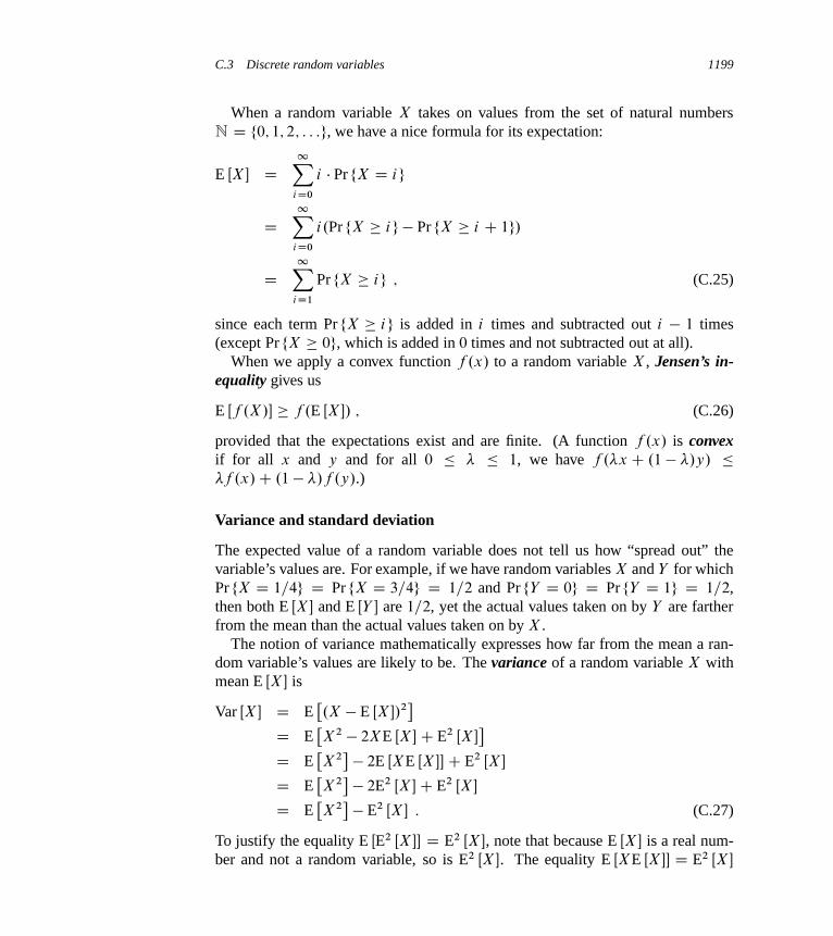
C.3 Discrete random variables 1199
When a random variable X takes on values from the set of natural numbersN D f0; 1; 2; : : :g, we have a nice formula for its expectation:
E ŒX� D1X
iD0
i � Pr fX D ig
D1X
iD0
i.Pr fX � ig � Pr fX � i C 1g/
D1X
iD1
Pr fX � ig ; (C.25)
since each term Pr fX � ig is added in i times and subtracted out i � 1 times(except Pr fX � 0g, which is added in 0 times and not subtracted out at all).
When we apply a convex function f .x/ to a random variable X , Jensen’s in-equality gives us
E Œf .X/� � f .E ŒX�/ ; (C.26)
provided that the expectations exist and are finite. (A function f .x/ is convexif for all x and y and for all 0 � � � 1, we have f .�x C .1 � �/y/ ��f .x/C .1� �/f .y/.)
Variance and standard deviation
The expected value of a random variable does not tell us how “spread out” thevariable’s values are. For example, if we have random variables X and Y for whichPr fX D 1=4g D Pr fX D 3=4g D 1=2 and Pr fY D 0g D Pr fY D 1g D 1=2,then both E ŒX� and E ŒY � are 1=2, yet the actual values taken on by Y are fartherfrom the mean than the actual values taken on by X .
The notion of variance mathematically expresses how far from the mean a ran-dom variable’s values are likely to be. The variance of a random variable X withmean E ŒX� is
Var ŒX� D E�.X � E ŒX�/2
�D E
�X2 � 2XE ŒX�C E2 ŒX�
�D E
�X2� � 2E ŒXE ŒX��C E2 ŒX�
D E�X2� � 2E2 ŒX�C E2 ŒX�
D E�X2� � E2 ŒX� : (C.27)
To justify the equality E ŒE2 ŒX�� D E2 ŒX�, note that because E ŒX� is a real num-ber and not a random variable, so is E2 ŒX�. The equality E ŒXE ŒX�� D E2 ŒX�

1200 Appendix C Counting and Probability
follows from equation (C.22), with a D E ŒX�. Rewriting equation (C.27) yieldsan expression for the expectation of the square of a random variable:
E�X2� D Var ŒX�C E2 ŒX� : (C.28)
The variance of a random variable X and the variance of aX are related (seeExercise C.3-10):
Var ŒaX� D a2Var ŒX� :
When X and Y are independent random variables,
Var ŒX C Y � D Var ŒX�C Var ŒY � :
In general, if n random variables X1; X2; : : : ; Xn are pairwise independent, then
Var
"nX
iD1
Xi
#D
nXiD1
Var ŒXi � : (C.29)
The standard deviation of a random variable X is the nonnegative square rootof the variance of X . The standard deviation of a random variable X is sometimesdenoted X or simply when the random variable X is understood from context.With this notation, the variance of X is denoted 2.
Exercises
C.3-1Suppose we roll two ordinary, 6-sided dice. What is the expectation of the sumof the two values showing? What is the expectation of the maximum of the twovalues showing?
C.3-2An array AŒ1 : : n� contains n distinct numbers that are randomly ordered, with eachpermutation of the n numbers being equally likely. What is the expectation of theindex of the maximum element in the array? What is the expectation of the indexof the minimum element in the array?
C.3-3A carnival game consists of three dice in a cage. A player can bet a dollar on anyof the numbers 1 through 6. The cage is shaken, and the payoff is as follows. If theplayer’s number doesn’t appear on any of the dice, he loses his dollar. Otherwise,if his number appears on exactly k of the three dice, for k D 1; 2; 3, he keeps hisdollar and wins k more dollars. What is his expected gain from playing the carnivalgame once?

C.4 The geometric and binomial distributions 1201
C.3-4Argue that if X and Y are nonnegative random variables, then
E Œmax.X; Y /� � E ŒX�C E ŒY � :
C.3-5 ?
Let X and Y be independent random variables. Prove that f .X/ and g.Y / areindependent for any choice of functions f and g.
C.3-6 ?
Let X be a nonnegative random variable, and suppose that E ŒX� is well defined.Prove Markov’s inequality:
Pr fX � tg � E ŒX� =t (C.30)
for all t > 0.
C.3-7 ?
Let S be a sample space, and let X and X 0 be random variables such thatX.s/ � X 0.s/ for all s 2 S . Prove that for any real constant t ,
Pr fX � tg � Pr fX 0 � tg :
C.3-8Which is larger: the expectation of the square of a random variable, or the squareof its expectation?
C.3-9Show that for any random variable X that takes on only the values 0 and 1, we haveVar ŒX� D E ŒX� E Œ1 �X�.
C.3-10Prove that Var ŒaX� D a2Var ŒX� from the definition (C.27) of variance.
C.4 The geometric and binomial distributions
We can think of a coin flip as an instance of a Bernoulli trial, which is an experi-ment with only two possible outcomes: success, which occurs with probability p,and failure, which occurs with probability q D 1�p. When we speak of Bernoullitrials collectively, we mean that the trials are mutually independent and, unless wespecifically say otherwise, that each has the same probability p for success. Two

1202 Appendix C Counting and Probability
0.05
0.10
0.15
0.20
0.25
1 2 3 4 5 6 7 8 9 10 11 12 13 14 15
0.30
0.35
k
�2
3
�k�1 �1
3
�
Figure C.1 A geometric distribution with probability p D 1=3 of success and a probabilityq D 1 � p of failure. The expectation of the distribution is 1=p D 3.
important distributions arise from Bernoulli trials: the geometric distribution andthe binomial distribution.
The geometric distribution
Suppose we have a sequence of Bernoulli trials, each with a probability p of suc-cess and a probability q D 1�p of failure. How many trials occur before we obtaina success? Let us define the random variable X be the number of trials needed toobtain a success. Then X has values in the range f1; 2; : : :g, and for k � 1,
Pr fX D kg D qk�1p ; (C.31)
since we have k � 1 failures before the one success. A probability distribution sat-isfying equation (C.31) is said to be a geometric distribution. Figure C.1 illustratessuch a distribution.

C.4 The geometric and binomial distributions 1203
Assuming that q < 1, we can calculate the expectation of a geometric distribu-tion using identity (A.8):
E ŒX� D1X
kD1
kqk�1p
D p
q
1XkD0
kqk
D p
q� q
.1� q/2
D p
q� q
p2
D 1=p : (C.32)
Thus, on average, it takes 1=p trials before we obtain a success, an intuitive result.The variance, which can be calculated similarly, but using Exercise A.1-3, is
Var ŒX� D q=p2 : (C.33)
As an example, suppose we repeatedly roll two dice until we obtain either aseven or an eleven. Of the 36 possible outcomes, 6 yield a seven and 2 yield aneleven. Thus, the probability of success is p D 8=36 D 2=9, and we must roll1=p D 9=2 D 4:5 times on average to obtain a seven or eleven.
The binomial distribution
How many successes occur during n Bernoulli trials, where a success occurs withprobability p and a failure with probability q D 1 � p? Define the random vari-able X to be the number of successes in n trials. Then X has values in the rangef0; 1; : : : ; ng, and for k D 0; 1; : : : ; n,
Pr fX D kg D
n
k
!pkqn�k ; (C.34)
since there are�
n
k
�ways to pick which k of the n trials are successes, and the
probability that each occurs is pkqn�k . A probability distribution satisfying equa-tion (C.34) is said to be a binomial distribution. For convenience, we define thefamily of binomial distributions using the notation
b.kIn; p/ D
n
k
!pk.1� p/n�k : (C.35)
Figure C.2 illustrates a binomial distribution. The name “binomial” comes from theright-hand side of equation (C.34) being the kth term of the expansion of .pCq/n.Consequently, since p C q D 1,

1204 Appendix C Counting and Probability
0.05
0.10
0.15
0.20
0.25
k0 1 2 3 4 5 6 7 8 9 10 11 12 13 14 15
b (k; 15, 1/3)
Figure C.2 The binomial distribution b.kI 15; 1=3/ resulting from n D 15 Bernoulli trials, eachwith probability p D 1=3 of success. The expectation of the distribution is np D 5.
nXkD0
b.kIn; p/ D 1 ; (C.36)
as axiom 2 of the probability axioms requires.We can compute the expectation of a random variable having a binomial distri-
bution from equations (C.8) and (C.36). Let X be a random variable that followsthe binomial distribution b.kIn; p/, and let q D 1�p. By the definition of expec-tation, we have
E ŒX� DnX
kD0
k � Pr fX D kg
DnX
kD0
k � b.kIn; p/
DnX
kD1
k
n
k
!pkqn�k
D np
nXkD1
n � 1
k � 1
!pk�1qn�k (by equation (C.8))
D np
n�1XkD0
n � 1
k
!pkq.n�1/�k

C.4 The geometric and binomial distributions 1205
D np
n�1XkD0
b.kIn � 1; p/
D np (by equation (C.36)) . (C.37)
By using the linearity of expectation, we can obtain the same result with sub-stantially less algebra. Let Xi be the random variable describing the number ofsuccesses in the i th trial. Then E ŒXi � D p � 1 C q � 0 D p, and by linearity ofexpectation (equation (C.21)), the expected number of successes for n trials is
E ŒX� D E
"nX
iD1
Xi
#
DnX
iD1
E ŒXi �
DnX
iD1
p
D np : (C.38)
We can use the same approach to calculate the variance of the distribution. Usingequation (C.27), we have Var ŒXi � D E ŒX2
i � � E2 ŒXi �. Since Xi only takes on thevalues 0 and 1, we have X2
i D Xi , which implies E ŒX2i � D E ŒXi � D p. Hence,
Var ŒXi � D p � p2 D p.1� p/ D pq : (C.39)
To compute the variance of X , we take advantage of the independence of the n
trials; thus, by equation (C.29),
Var ŒX� D Var
"nX
iD1
Xi
#
DnX
iD1
Var ŒXi �
DnX
iD1
pq
D npq : (C.40)
As Figure C.2 shows, the binomial distribution b.kIn; p/ increases with k untilit reaches the mean np, and then it decreases. We can prove that the distributionalways behaves in this manner by looking at the ratio of successive terms:

1206 Appendix C Counting and Probability
b.kIn; p/
b.k � 1In; p/D
�n
k
�pkqn�k�
n
k�1
�pk�1qn�kC1
D nŠ.k � 1/Š.n � k C 1/Šp
kŠ.n � k/ŠnŠq
D .n � k C 1/p
kq(C.41)
D 1C .nC 1/p � k
kq:
This ratio is greater than 1 precisely when .n C 1/p � k is positive. Conse-quently, b.kIn; p/ > b.k � 1In; p/ for k < .nC 1/p (the distribution increases),and b.kIn; p/ < b.k � 1In; p/ for k > .n C 1/p (the distribution decreases).If k D .nC 1/p is an integer, then b.kIn; p/ D b.k � 1In; p/, and so the distri-bution then has two maxima: at k D .nC1/p and at k�1 D .nC1/p�1 D np � q.Otherwise, it attains a maximum at the unique integer k that lies in the rangenp � q < k < .nC 1/p.
The following lemma provides an upper bound on the binomial distribution.
Lemma C.1Let n � 0, let 0 < p < 1, let q D 1 � p, and let 0 � k � n. Then
b.kIn; p/ ��np
k
�k � nq
n � k
�n�k
:
Proof Using equation (C.6), we have
b.kIn; p/ D
n
k
!pkqn�k
��n
k
�k � n
n � k
�n�k
pkqn�k
D�np
k
�k � nq
n � k
�n�k
:
Exercises
C.4-1Verify axiom 2 of the probability axioms for the geometric distribution.
C.4-2How many times on average must we flip 6 fair coins before we obtain 3 headsand 3 tails?

C.4 The geometric and binomial distributions 1207
C.4-3Show that b.kIn; p/ D b.n � kIn; q/, where q D 1 � p.
C.4-4Show that value of the maximum of the binomial distribution b.kIn; p/ is approx-imately 1=
p2�npq, where q D 1 � p.
C.4-5 ?
Show that the probability of no successes in n Bernoulli trials, each with probabilityp D 1=n, is approximately 1=e. Show that the probability of exactly one successis also approximately 1=e.
C.4-6 ?
Professor Rosencrantz flips a fair coin n times, and so does Professor Guildenstern.Show that the probability that they get the same number of heads is
�2n
n
�=4n. (Hint:
For Professor Rosencrantz, call a head a success; for Professor Guildenstern, calla tail a success.) Use your argument to verify the identity
nXkD0
n
k
!2
D
2n
n
!:
C.4-7 ?
Show that for 0 � k � n,
b.kIn; 1=2/ � 2n H.k=n/�n ;
where H.x/ is the entropy function (C.7).
C.4-8 ?
Consider n Bernoulli trials, where for i D 1; 2; : : : ; n, the i th trial has probabil-ity pi of success, and let X be the random variable denoting the total number ofsuccesses. Let p � pi for all i D 1; 2; : : : ; n. Prove that for 1 � k � n,
Pr fX < kg �k�1XiD0
b.i In; p/ :
C.4-9 ?
Let X be the random variable for the total number of successes in a set A of n
Bernoulli trials, where the i th trial has a probability pi of success, and let X 0
be the random variable for the total number of successes in a second set A0 of n
Bernoulli trials, where the i th trial has a probability p0i � pi of success. Prove that
for 0 � k � n,

1208 Appendix C Counting and Probability
Pr fX 0 � kg � Pr fX � kg :
(Hint: Show how to obtain the Bernoulli trials in A0 by an experiment involvingthe trials of A, and use the result of Exercise C.3-7.)
? C.5 The tails of the binomial distribution
The probability of having at least, or at most, k successes in n Bernoulli trials,each with probability p of success, is often of more interest than the probability ofhaving exactly k successes. In this section, we investigate the tails of the binomialdistribution: the two regions of the distribution b.kIn; p/ that are far from themean np. We shall prove several important bounds on (the sum of all terms in) atail.
We first provide a bound on the right tail of the distribution b.kIn; p/. We candetermine bounds on the left tail by inverting the roles of successes and failures.
Theorem C.2Consider a sequence of n Bernoulli trials, where success occurs with probability p.Let X be the random variable denoting the total number of successes. Then for0 � k � n, the probability of at least k successes is
Pr fX � kg DnX
iDk
b.i In; p/
�
n
k
!pk :
Proof For S � f1; 2; : : : ; ng, we let AS denote the event that the i th trial is asuccess for every i 2 S . Clearly Pr fASg D pk if jS j D k. We have
Pr fX � kg D Pr fthere exists S � f1; 2; : : : ; ng W jS j D k and ASgD Pr
� [S�f1;2;:::;ngWjS jDk
AS
��
XS�f1;2;:::;ngWjS jDk
Pr fASg (by inequality (C.19))
D
n
k
!pk :

C.5 The tails of the binomial distribution 1209
The following corollary restates the theorem for the left tail of the binomialdistribution. In general, we shall leave it to you to adapt the proofs from one tail tothe other.
Corollary C.3Consider a sequence of n Bernoulli trials, where success occurs with probabil-ity p. If X is the random variable denoting the total number of successes, then for0 � k � n, the probability of at most k successes is
Pr fX � kg DkX
iD0
b.i In; p/
�
n
n � k
!.1� p/n�k
D
n
k
!.1� p/n�k :
Our next bound concerns the left tail of the binomial distribution. Its corollaryshows that, far from the mean, the left tail diminishes exponentially.
Theorem C.4Consider a sequence of n Bernoulli trials, where success occurs with probability p
and failure with probability q D 1�p. Let X be the random variable denoting thetotal number of successes. Then for 0 < k < np, the probability of fewer than k
successes is
Pr fX < kg Dk�1XiD0
b.i In; p/
<kq
np � kb.kIn; p/ :
Proof We bound the seriesPk�1
iD0 b.i In; p/ by a geometric series using the tech-nique from Section A.2, page 1151. For i D 1; 2; : : : ; k, we have from equa-tion (C.41),b.i � 1In; p/
b.i In; p/D iq
.n � i C 1/p
<iq
.n � i/p
� kq
.n � k/p:
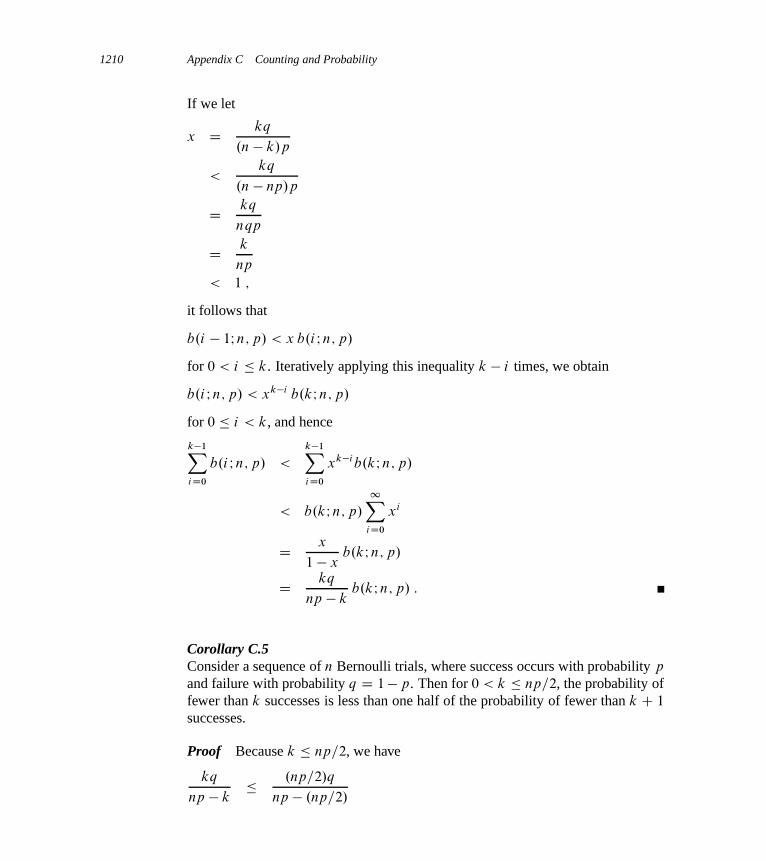
1210 Appendix C Counting and Probability
If we let
x D kq
.n � k/p
<kq
.n � np/p
D kq
nqp
D k
np
< 1 ;
it follows that
b.i � 1In; p/ < x b.i In; p/
for 0 < i � k. Iteratively applying this inequality k � i times, we obtain
b.i In; p/ < xk�i b.kIn; p/
for 0 � i < k, and hence
k�1XiD0
b.i In; p/ <
k�1XiD0
xk�ib.kIn; p/
< b.kIn; p/
1XiD0
xi
D x
1 � xb.kIn; p/
D kq
np � kb.kIn; p/ :
Corollary C.5Consider a sequence of n Bernoulli trials, where success occurs with probability p
and failure with probability q D 1�p. Then for 0 < k � np=2, the probability offewer than k successes is less than one half of the probability of fewer than k C 1
successes.
Proof Because k � np=2, we have
kq
np � k� .np=2/q
np � .np=2/

C.5 The tails of the binomial distribution 1211
D .np=2/q
np=2
� 1 ; (C.42)
since q � 1. Letting X be the random variable denoting the number of successes,Theorem C.4 and inequality (C.42) imply that the probability of fewer than k suc-cesses is
Pr fX < kg Dk�1XiD0
b.i In; p/ < b.kIn; p/ :
Thus we have
Pr fX < kgPr fX < k C 1g D
Pk�1
iD0 b.i In; p/Pk
iD0 b.i In; p/
DPk�1
iD0 b.i In; p/Pk�1
iD0 b.i In; p/C b.kIn; p/
< 1=2 ;
sincePk�1
iD0 b.i In; p/ < b.kIn; p/.
Bounds on the right tail follow similarly. Exercise C.5-2 asks you to prove them.
Corollary C.6Consider a sequence of n Bernoulli trials, where success occurs with probability p.Let X be the random variable denoting the total number of successes. Then fornp < k < n, the probability of more than k successes is
Pr fX > kg DnX
iDkC1
b.i In; p/
<.n � k/p
k � npb.kIn; p/ :
Corollary C.7Consider a sequence of n Bernoulli trials, where success occurs with probability p
and failure with probability q D 1 � p. Then for .np C n/=2 < k < n, theprobability of more than k successes is less than one half of the probability ofmore than k � 1 successes.
The next theorem considers n Bernoulli trials, each with a probability pi ofsuccess, for i D 1; 2; : : : ; n. As the subsequent corollary shows, we can use the
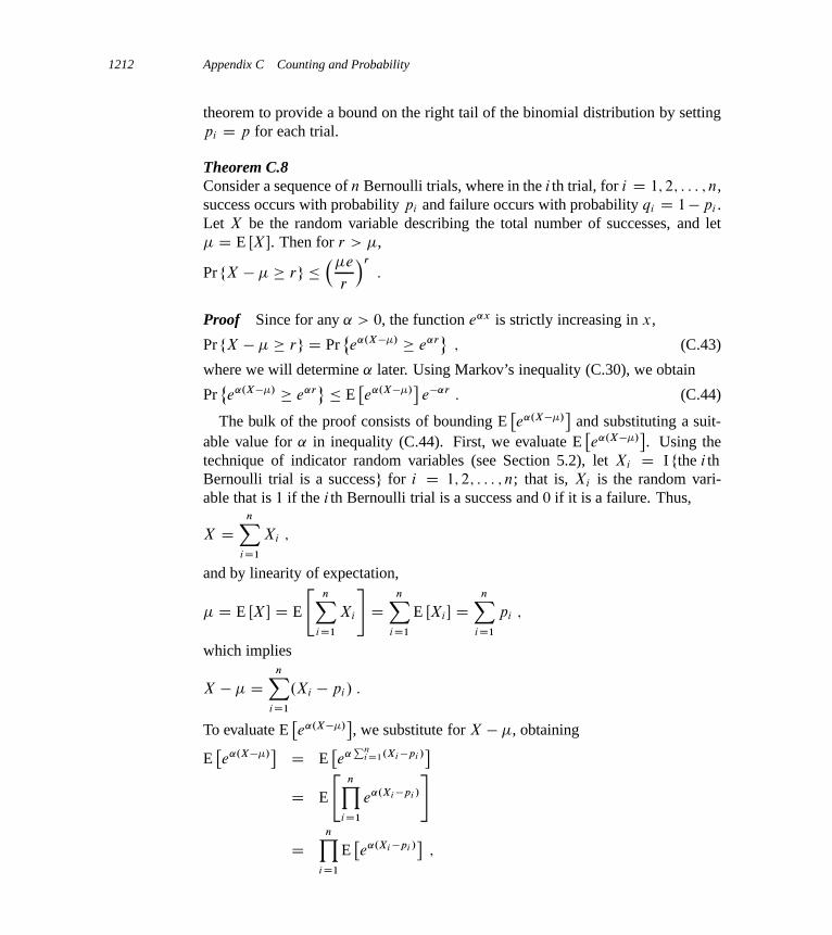
1212 Appendix C Counting and Probability
theorem to provide a bound on the right tail of the binomial distribution by settingpi D p for each trial.
Theorem C.8Consider a sequence of n Bernoulli trials, where in the i th trial, for i D 1; 2; : : : ; n,success occurs with probability pi and failure occurs with probability qi D 1�pi .Let X be the random variable describing the total number of successes, and let D E ŒX�. Then for r > ,
Pr fX � � rg �� e
r
�r
:
Proof Since for any ˛ > 0, the function e˛x is strictly increasing in x,
Pr fX � � rg D Pr˚e˛.X�/ � e˛r
; (C.43)
where we will determine ˛ later. Using Markov’s inequality (C.30), we obtain
Pr˚e˛.X�/ � e˛r
� E�e˛.X�/
�e�˛r : (C.44)
The bulk of the proof consists of bounding E�e˛.X�/
�and substituting a suit-
able value for ˛ in inequality (C.44). First, we evaluate E�e˛.X�/
�. Using the
technique of indicator random variables (see Section 5.2), let Xi D I fthe i thBernoulli trial is a successg for i D 1; 2; : : : ; n; that is, Xi is the random vari-able that is 1 if the i th Bernoulli trial is a success and 0 if it is a failure. Thus,
X DnX
iD1
Xi ;
and by linearity of expectation,
D E ŒX� D E
"nX
iD1
Xi
#D
nXiD1
E ŒXi � DnX
iD1
pi ;
which implies
X � DnX
iD1
.Xi � pi / :
To evaluate E�e˛.X�/
�, we substitute for X � , obtaining
E�e˛.X�/
� D E�e˛
PniD1.Xi �pi /
�D E
"nY
iD1
e˛.Xi �pi /
#
DnY
iD1
E�e˛.Xi �pi /
�;
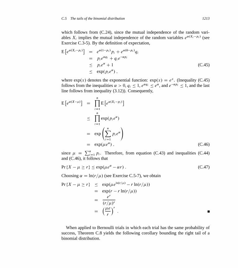
C.5 The tails of the binomial distribution 1213
which follows from (C.24), since the mutual independence of the random vari-ables Xi implies the mutual independence of the random variables e˛.Xi �pi / (seeExercise C.3-5). By the definition of expectation,
E�e˛.Xi �pi /
� D e˛.1�pi /pi C e˛.0�pi /qi
D pie˛qi C qie
�˛pi
� pie˛ C 1 (C.45)
� exp.pie˛/ ;
where exp.x/ denotes the exponential function: exp.x/ D ex . (Inequality (C.45)follows from the inequalities ˛ > 0, qi � 1, e˛qi � e˛, and e�˛pi � 1, and the lastline follows from inequality (3.12)). Consequently,
E�e˛.X�/
� D nYiD1
E�e˛.Xi �pi /
��
nYiD1
exp.pie˛/
D exp
nX
iD1
pie˛
!D exp. e˛/ ; (C.46)
since D Pn
iD1 pi . Therefore, from equation (C.43) and inequalities (C.44)and (C.46), it follows that
Pr fX � � rg � exp. e˛ � ˛r/ : (C.47)
Choosing ˛ D ln.r= / (see Exercise C.5-7), we obtain
Pr fX � � rg � exp. eln.r=/ � r ln.r= //
D exp.r � r ln.r= //
D er
.r= /r
D� e
r
�r
:
When applied to Bernoulli trials in which each trial has the same probability ofsuccess, Theorem C.8 yields the following corollary bounding the right tail of abinomial distribution.

1214 Appendix C Counting and Probability
Corollary C.9Consider a sequence of n Bernoulli trials, where in each trial success occurs withprobability p and failure occurs with probability q D 1 � p. Then for r > np,
Pr fX � np � rg DnX
kDdnpCreb.kIn; p/
��npe
r
�r
:
Proof By equation (C.37), we have D E ŒX� D np.
Exercises
C.5-1 ?
Which is less likely: obtaining no heads when you flip a fair coin n times, orobtaining fewer than n heads when you flip the coin 4n times?
C.5-2 ?
Prove Corollaries C.6 and C.7.
C.5-3 ?
Show thatk�1XiD0
n
i
!ai < .aC 1/n k
na � k.aC 1/b.kIn; a=.aC 1//
for all a > 0 and all k such that 0 < k < na=.aC 1/.
C.5-4 ?
Prove that if 0 < k < np, where 0 < p < 1 and q D 1� p, then
k�1XiD0
piqn�i <kq
np � k
�np
k
�k � nq
n � k
�n�k
:
C.5-5 ?
Show that the conditions of Theorem C.8 imply that
Pr f �X � rg ��
.n � /e
r
�r
:
Similarly, show that the conditions of Corollary C.9 imply that
Pr fnp �X � rg ��nqe
r
�r
:

Problems for Appendix C 1215
C.5-6 ?
Consider a sequence of n Bernoulli trials, where in the i th trial, for i D 1; 2; : : : ; n,success occurs with probability pi and failure occurs with probability qi D 1�pi .Let X be the random variable describing the total number of successes, and let D E ŒX�. Show that for r � 0,
Pr fX � � rg � e�r2=2n :
(Hint: Prove that pie˛qi C qie
�˛pi � e˛2=2. Then follow the outline of the proofof Theorem C.8, using this inequality in place of inequality (C.45).)
C.5-7 ?
Show that choosing ˛ D ln.r= / minimizes the right-hand side of inequal-ity (C.47).
Problems
C-1 Balls and binsIn this problem, we investigate the effect of various assumptions on the number ofways of placing n balls into b distinct bins.
a. Suppose that the n balls are distinct and that their order within a bin does notmatter. Argue that the number of ways of placing the balls in the bins is bn.
b. Suppose that the balls are distinct and that the balls in each bin are ordered.Prove that there are exactly .bC n� 1/Š=.b � 1/Š ways to place the balls in thebins. (Hint: Consider the number of ways of arranging n distinct balls and b�1
indistinguishable sticks in a row.)
c. Suppose that the balls are identical, and hence their order within a bin does notmatter. Show that the number of ways of placing the balls in the bins is
�bCn�1
n
�.
(Hint: Of the arrangements in part (b), how many are repeated if the balls aremade identical?)
d. Suppose that the balls are identical and that no bin may contain more than oneball, so that n � b. Show that the number of ways of placing the balls is
�b
n
�.
e. Suppose that the balls are identical and that no bin may be left empty. Assumingthat n � b, show that the number of ways of placing the balls is
�n�1
b�1
�.
1216 Appendix C Counting and Probability
Chapter notes
The first general methods for solving probability problems were discussed in afamous correspondence between B. Pascal and P. de Fermat, which began in 1654,and in a book by C. Huygens in 1657. Rigorous probability theory began with thework of J. Bernoulli in 1713 and A. De Moivre in 1730. Further developments ofthe theory were provided by P.-S. Laplace, S.-D. Poisson, and C. F. Gauss.
Sums of random variables were originally studied by P. L. Chebyshev and A. A.Markov. A. N. Kolmogorov axiomatized probability theory in 1933. Chernoff [67]and Hoeffding [173] provided bounds on the tails of distributions. Seminal workin random combinatorial structures was done by P. Erdös.
Knuth [209] and Liu [237] are good references for elementary combinatoricsand counting. Standard textbooks such as Billingsley [46], Chung [68], Drake [96],Feller [104], and Rozanov [300] offer comprehensive introductions to probability.

D Matrices
Matrices arise in numerous applications, including, but by no means limited to,scientific computing. If you have seen matrices before, much of the material in thischapter will be familiar to you, but some of it might be new. Section D.1 coversbasic matrix definitions and operations, and Section D.2 presents some basic matrixproperties.
D.1 Matrices and matrix operations
In this section, we review some basic concepts of matrix theory and some funda-mental properties of matrices.
Matrices and vectors
A matrix is a rectangular array of numbers. For example,
A D�
a11 a12 a13
a21 a22 a23
�D
�1 2 3
4 5 6
�(D.1)
is a 2 3 matrix A D .aij /, where for i D 1; 2 and j D 1; 2; 3, we denote theelement of the matrix in row i and column j by aij . We use uppercase lettersto denote matrices and corresponding subscripted lowercase letters to denote theirelements. We denote the set of all mn matrices with real-valued entries by R
m�n
and, in general, the set of mn matrices with entries drawn from a set S by Sm�n.The transpose of a matrix A is the matrix AT obtained by exchanging the rows
and columns of A. For the matrix A of equation (D.1),

1218 Appendix D Matrices
AT D�
1 4
2 5
3 6
�:
A vector is a one-dimensional array of numbers. For example,
x D�
2
3
5
�is a vector of size 3. We sometimes call a vector of length n an n-vector. Weuse lowercase letters to denote vectors, and we denote the i th element of a size-nvector x by xi , for i D 1; 2; : : : ; n. We take the standard form of a vector to beas a column vector equivalent to an n 1 matrix; the corresponding row vector isobtained by taking the transpose:
xT D . 2 3 5 / :
The unit vector ei is the vector whose i th element is 1 and all of whose otherelements are 0. Usually, the size of a unit vector is clear from the context.
A zero matrix is a matrix all of whose entries are 0. Such a matrix is oftendenoted 0, since the ambiguity between the number 0 and a matrix of 0s is usuallyeasily resolved from context. If a matrix of 0s is intended, then the size of thematrix also needs to be derived from the context.
Square matrices
Square n n matrices arise frequently. Several special cases of square matricesare of particular interest:
1. A diagonal matrix has aij D 0 whenever i ¤ j . Because all of the off-diagonalelements are zero, we can specify the matrix by listing the elements along thediagonal:
diag.a11; a22; : : : ; ann/ D
˙a11 0 : : : 0
0 a22 : : : 0:::
:::: : :
:::
0 0 : : : ann
�:
2. The n n identity matrix In is a diagonal matrix with 1s along the diagonal:
In D diag.1; 1; : : : ; 1/
D
˙1 0 : : : 0
0 1 : : : 0:::
:::: : :
:::
0 0 : : : 1
�:
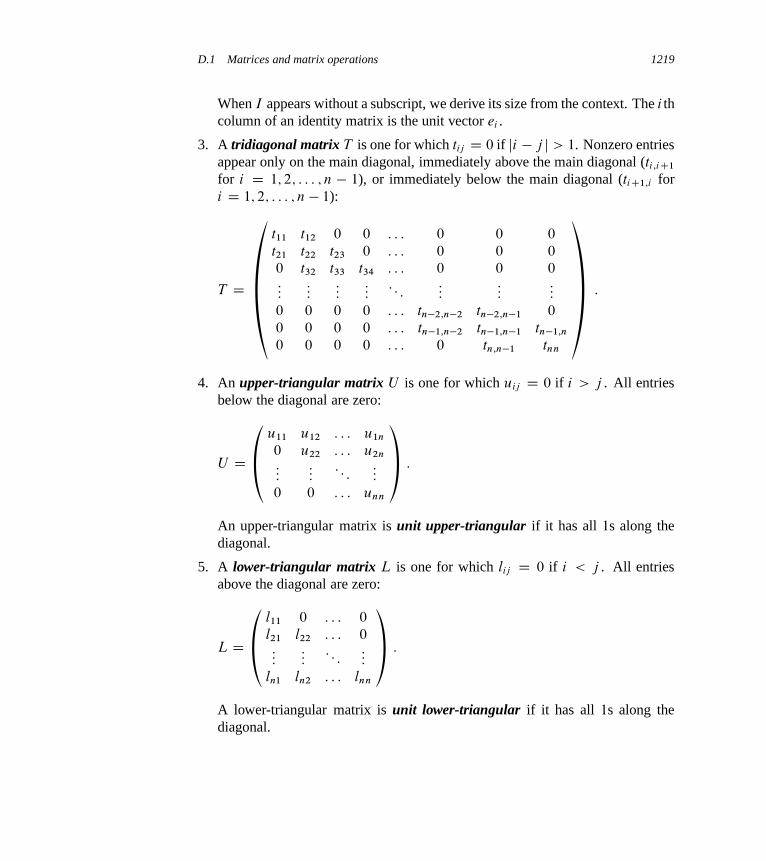
D.1 Matrices and matrix operations 1219
When I appears without a subscript, we derive its size from the context. The i thcolumn of an identity matrix is the unit vector ei .
3. A tridiagonal matrix T is one for which tij D 0 if ji � j j > 1. Nonzero entriesappear only on the main diagonal, immediately above the main diagonal (ti;iC1
for i D 1; 2; : : : ; n � 1), or immediately below the main diagonal (tiC1;i fori D 1; 2; : : : ; n � 1):
T D
�t11 t12 0 0 : : : 0 0 0
t21 t22 t23 0 : : : 0 0 0
0 t32 t33 t34 : : : 0 0 0:::
::::::
:::: : :
::::::
:::
0 0 0 0 : : : tn�2;n�2 tn�2;n�1 0
0 0 0 0 : : : tn�1;n�2 tn�1;n�1 tn�1;n
0 0 0 0 : : : 0 tn;n�1 tnn
˘:
4. An upper-triangular matrix U is one for which uij D 0 if i > j . All entriesbelow the diagonal are zero:
U D
˙u11 u12 : : : u1n
0 u22 : : : u2n
::::::
: : ::::
0 0 : : : unn
�:
An upper-triangular matrix is unit upper-triangular if it has all 1s along thediagonal.
5. A lower-triangular matrix L is one for which lij D 0 if i < j . All entriesabove the diagonal are zero:
L D
˙l11 0 : : : 0
l21 l22 : : : 0:::
:::: : :
:::
ln1 ln2 : : : lnn
�:
A lower-triangular matrix is unit lower-triangular if it has all 1s along thediagonal.
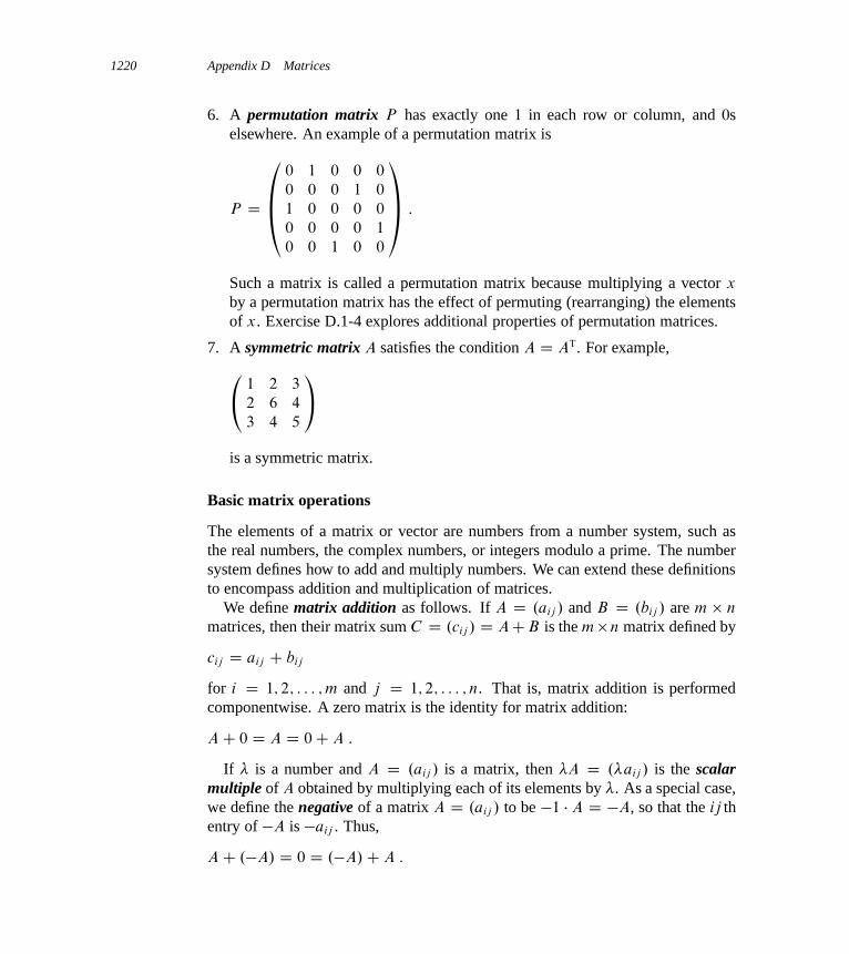
1220 Appendix D Matrices
6. A permutation matrix P has exactly one 1 in each row or column, and 0selsewhere. An example of a permutation matrix is
P D
ˇ0 1 0 0 0
0 0 0 1 0
1 0 0 0 0
0 0 0 0 1
0 0 1 0 0
�:
Such a matrix is called a permutation matrix because multiplying a vector x
by a permutation matrix has the effect of permuting (rearranging) the elementsof x. Exercise D.1-4 explores additional properties of permutation matrices.
7. A symmetric matrix A satisfies the condition A D AT. For example,�1 2 3
2 6 4
3 4 5
�is a symmetric matrix.
Basic matrix operations
The elements of a matrix or vector are numbers from a number system, such asthe real numbers, the complex numbers, or integers modulo a prime. The numbersystem defines how to add and multiply numbers. We can extend these definitionsto encompass addition and multiplication of matrices.
We define matrix addition as follows. If A D .aij / and B D .bij / are m n
matrices, then their matrix sum C D .cij / D ACB is the mn matrix defined by
cij D aij C bij
for i D 1; 2; : : : ; m and j D 1; 2; : : : ; n. That is, matrix addition is performedcomponentwise. A zero matrix is the identity for matrix addition:
AC 0 D A D 0C A :
If � is a number and A D .aij / is a matrix, then �A D .�aij / is the scalarmultiple of A obtained by multiplying each of its elements by �. As a special case,we define the negative of a matrix A D .aij / to be �1 � A D �A, so that the ij thentry of �A is �aij . Thus,
AC .�A/ D 0 D .�A/C A :
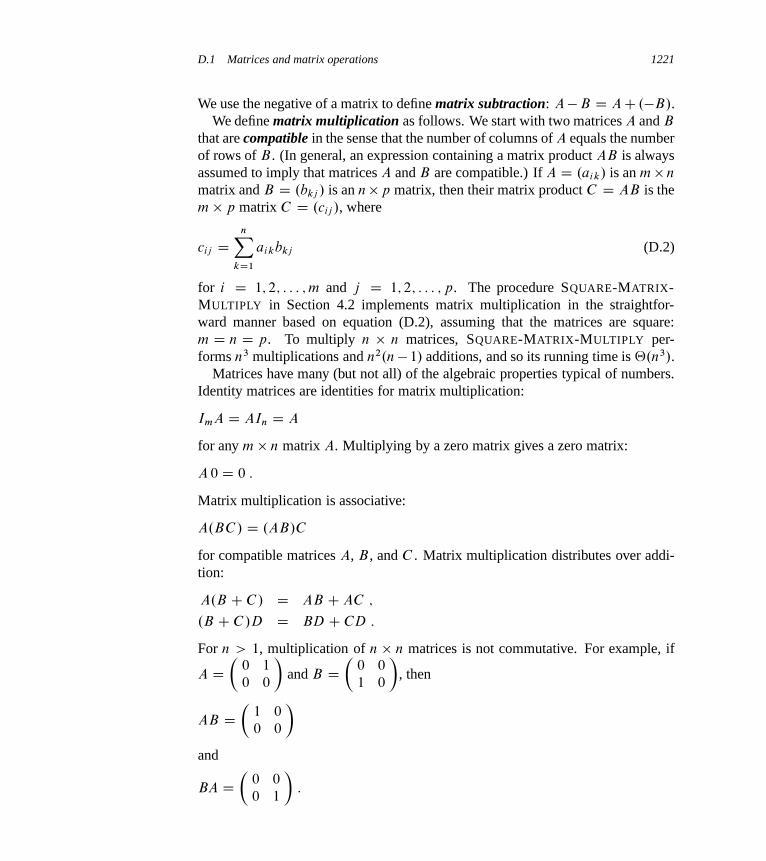
D.1 Matrices and matrix operations 1221
We use the negative of a matrix to define matrix subtraction: A�B D AC .�B/.We define matrix multiplication as follows. We start with two matrices A and B
that are compatible in the sense that the number of columns of A equals the numberof rows of B . (In general, an expression containing a matrix product AB is alwaysassumed to imply that matrices A and B are compatible.) If A D .aik/ is an m n
matrix and B D .bkj / is an np matrix, then their matrix product C D AB is them p matrix C D .cij /, where
cij DnX
kD1
aikbkj (D.2)
for i D 1; 2; : : : ; m and j D 1; 2; : : : ; p. The procedure SQUARE-MATRIX-MULTIPLY in Section 4.2 implements matrix multiplication in the straightfor-ward manner based on equation (D.2), assuming that the matrices are square:m D n D p. To multiply n n matrices, SQUARE-MATRIX-MULTIPLY per-forms n3 multiplications and n2.n� 1/ additions, and so its running time is ‚.n3/.
Matrices have many (but not all) of the algebraic properties typical of numbers.Identity matrices are identities for matrix multiplication:
ImA D AIn D A
for any m n matrix A. Multiplying by a zero matrix gives a zero matrix:
A 0 D 0 :
Matrix multiplication is associative:
A.BC / D .AB/C
for compatible matrices A, B , and C . Matrix multiplication distributes over addi-tion:
A.B C C / D AB C AC ;
.B C C /D D BD C CD :
For n > 1, multiplication of n n matrices is not commutative. For example, if
A D�
0 1
0 0
�and B D
�0 0
1 0
�, then
AB D�
1 0
0 0
�and
BA D�
0 0
0 1
�:
1222 Appendix D Matrices
We define matrix-vector products or vector-vector products as if the vector werethe equivalent n 1 matrix (or a 1 n matrix, in the case of a row vector). Thus,if A is an m n matrix and x is an n-vector, then Ax is an m-vector. If x and y
are n-vectors, then
xTy DnX
iD1
xiyi
is a number (actually a 1 1 matrix) called the inner product of x and y. The ma-trix xyT is an nn matrix Z called the outer product of x and y, with ´ij D xiyj .The (euclidean) norm kxk of an n-vector x is defined by
kxk D .x21 C x2
2 C � � � C x2n/1=2
D .xTx/1=2 :
Thus, the norm of x is its length in n-dimensional euclidean space.
Exercises
D.1-1Show that if A and B are symmetric nn matrices, then so are ACB and A�B .
D.1-2Prove that .AB/T D BTAT and that ATA is always a symmetric matrix.
D.1-3Prove that the product of two lower-triangular matrices is lower-triangular.
D.1-4Prove that if P is an n n permutation matrix and A is an n n matrix, then thematrix product PA is A with its rows permuted, and the matrix product AP is A
with its columns permuted. Prove that the product of two permutation matrices isa permutation matrix.
D.2 Basic matrix properties
In this section, we define some basic properties pertaining to matrices: inverses,linear dependence and independence, rank, and determinants. We also define theclass of positive-definite matrices.

D.2 Basic matrix properties 1223
Matrix inverses, ranks, and determinants
We define the inverse of an n n matrix A to be the n n matrix, denoted A�1 (ifit exists), such that AA�1 D In D A�1A. For example,�
1 1
1 0
��1
D�
0 1
1 �1
�:
Many nonzero n n matrices do not have inverses. A matrix without an inverse iscalled noninvertible, or singular. An example of a nonzero singular matrix is�
1 0
1 0
�:
If a matrix has an inverse, it is called invertible, or nonsingular. Matrix inverses,when they exist, are unique. (See Exercise D.2-1.) If A and B are nonsingularn n matrices, then
.BA/�1 D A�1B�1 :
The inverse operation commutes with the transpose operation:
.A�1/T D .AT/�1 :
The vectors x1; x2; : : : ; xn are linearly dependent if there exist coefficientsc1; c2; : : : ; cn, not all of which are zero, such that c1x1 C c2x2 C � � � C cnxn D 0.The row vectors x1 D . 1 2 3 /, x2 D . 2 6 4 /, and x3 D . 4 11 9 / arelinearly dependent, for example, since 2x1 C 3x2 � 2x3 D 0. If vectors are notlinearly dependent, they are linearly independent. For example, the columns of anidentity matrix are linearly independent.
The column rank of a nonzero m n matrix A is the size of the largest setof linearly independent columns of A. Similarly, the row rank of A is the sizeof the largest set of linearly independent rows of A. A fundamental property ofany matrix A is that its row rank always equals its column rank, so that we cansimply refer to the rank of A. The rank of an m n matrix is an integer between 0
and min.m; n/, inclusive. (The rank of a zero matrix is 0, and the rank of an n n
identity matrix is n.) An alternate, but equivalent and often more useful, definitionis that the rank of a nonzero m n matrix A is the smallest number r such thatthere exist matrices B and C of respective sizes m r and r n such that
A D BC :
A square n n matrix has full rank if its rank is n. An m n matrix has fullcolumn rank if its rank is n. The following theorem gives a fundamental propertyof ranks.
1224 Appendix D Matrices
Theorem D.1A square matrix has full rank if and only if it is nonsingular.
A null vector for a matrix A is a nonzero vector x such that Ax D 0. Thefollowing theorem (whose proof is left as Exercise D.2-7) and its corollary relatethe notions of column rank and singularity to null vectors.
Theorem D.2A matrix A has full column rank if and only if it does not have a null vector.
Corollary D.3A square matrix A is singular if and only if it has a null vector.
The ij th minor of an nn matrix A, for n > 1, is the .n�1/.n�1/ matrix AŒij �
obtained by deleting the i th row and j th column of A. We define the determinantof an n n matrix A recursively in terms of its minors by
det.A/ D
‚a11 if n D 1 ;
nXj D1
.�1/1Cj a1j det.AŒ1j �/ if n > 1 :
The term .�1/iCj det.AŒij �/ is known as the cofactor of the element aij .The following theorems, whose proofs are omitted here, express fundamental
properties of the determinant.
Theorem D.4 (Determinant properties)The determinant of a square matrix A has the following properties:
� If any row or any column of A is zero, then det.A/ D 0.� The determinant of A is multiplied by � if the entries of any one row (or any
one column) of A are all multiplied by �.� The determinant of A is unchanged if the entries in one row (respectively, col-
umn) are added to those in another row (respectively, column).� The determinant of A equals the determinant of AT.� The determinant of A is multiplied by �1 if any two rows (or any two columns)
are exchanged.
Also, for any square matrices A and B , we have det.AB/ D det.A/ det.B/.

D.2 Basic matrix properties 1225
Theorem D.5An n n matrix A is singular if and only if det.A/ D 0.
Positive-definite matrices
Positive-definite matrices play an important role in many applications. An n n
matrix A is positive-definite if xTAx > 0 for all n-vectors x ¤ 0. Forexample, the identity matrix is positive-definite, since for any nonzero vectorx D . x1 x2 � � � xn /T,
xTInx D xTx
DnX
iD1
x2i
> 0 :
Matrices that arise in applications are often positive-definite due to the followingtheorem.
Theorem D.6For any matrix A with full column rank, the matrix ATA is positive-definite.
Proof We must show that xT.ATA/x > 0 for any nonzero vector x. For anyvector x,
xT.ATA/x D .Ax/T.Ax/ (by Exercise D.1-2)
D kAxk2 :
Note that kAxk2 is just the sum of the squares of the elements of the vector Ax.Therefore, kAxk2 � 0. If kAxk2 D 0, every element of Ax is 0, which is to sayAx D 0. Since A has full column rank, Ax D 0 implies x D 0, by Theorem D.2.Hence, ATA is positive-definite.
Section 28.3 explores other properties of positive-definite matrices.
Exercises
D.2-1Prove that matrix inverses are unique, that is, if B and C are inverses of A, thenB D C .
D.2-2Prove that the determinant of a lower-triangular or upper-triangular matrix is equalto the product of its diagonal elements. Prove that the inverse of a lower-triangularmatrix, if it exists, is lower-triangular.
1226 Appendix D Matrices
D.2-3Prove that if P is a permutation matrix, then P is invertible, its inverse is P T,and P T is a permutation matrix.
D.2-4Let A and B be n n matrices such that AB D I . Prove that if A0 is obtainedfrom A by adding row j into row i , then subtracting column i from column j of B
yields the inverse B 0 of A0.
D.2-5Let A be a nonsingular n n matrix with complex entries. Show that every entryof A�1 is real if and only if every entry of A is real.
D.2-6Show that if A is a nonsingular, symmetric, n n matrix, then A�1 is symmetric.Show that if B is an arbitrary m n matrix, then the m m matrix given by theproduct BABT is symmetric.
D.2-7Prove Theorem D.2. That is, show that a matrix A has full column rank if and onlyif Ax D 0 implies x D 0. (Hint: Express the linear dependence of one column onthe others as a matrix-vector equation.)
D.2-8Prove that for any two compatible matrices A and B ,
rank.AB/ � min.rank.A/; rank.B// ;
where equality holds if either A or B is a nonsingular square matrix. (Hint: Usethe alternate definition of the rank of a matrix.)
Problems
D-1 Vandermonde matrixGiven numbers x0; x1; : : : ; xn�1, prove that the determinant of the Vandermondematrix
V.x0; x1; : : : ; xn�1/ D
˙1 x0 x2
0 � � � xn�10
1 x1 x21 � � � xn�1
1:::
::::::
: : ::::
1 xn�1 x2n�1 � � � xn�1
n�1
�
Problems for Appendix D 1227
is
det.V .x0; x1; : : : ; xn�1// DY
0�j <k�n�1
.xk � xj / :
(Hint: Multiply column i by �x0 and add it to column i C 1 for i D n � 1;
n � 2; : : : ; 1, and then use induction.)
D-2 Permutations defined by matrix-vector multiplication over GF.2/
One class of permutations of the integers in the set Sn D f0; 1; 2; : : : ; 2n � 1g isdefined by matrix multiplication over GF.2/. For each integer x in Sn, we view itsbinary representation as an n-bit vector�
x0
x1
x2
:::
xn�1
�;
where x D Pn�1
iD0 xi2i . If A is an n n matrix in which each entry is either 0
or 1, then we can define a permutation mapping each value x in Sn to the numberwhose binary representation is the matrix-vector product Ax. Here, we performall arithmetic over GF.2/: all values are either 0 or 1, and with one exception theusual rules of addition and multiplication apply. The exception is that 1C 1 D 0.You can think of arithmetic over GF.2/ as being just like regular integer arithmetic,except that you use only the least significant bit.
As an example, for S2 D f0; 1; 2; 3g, the matrix
A D�
1 0
1 1
�defines the following permutation �A: �A.0/ D 0, �A.1/ D 3, �A.2/ D 2,�A.3/ D 1. To see why �A.3/ D 1, observe that, working in GF.2/,
�A.3/ D�
1 0
1 1
��1
1
�D
�1 � 1C 0 � 11 � 1C 1 � 1
�D
�1
0
�;
which is the binary representation of 1.

1228 Appendix D Matrices
For the remainder of this problem, we work over GF.2/, and all matrix andvector entries are 0 or 1. We define the rank of a 0-1 matrix (a matrix for whicheach entry is either 0 or 1) over GF.2/ the same as for a regular matrix, but with allarithmetic that determines linear independence performed over GF.2/. We definethe range of an n n 0-1 matrix A by
R.A/ D fy W y D Ax for some x 2 Sng ;
so that R.A/ is the set of numbers in Sn that we can produce by multiplying eachvalue x in Sn by A.
a. If r is the rank of matrix A, prove that jR.A/j D 2r . Conclude that A defines apermutation on Sn only if A has full rank.
For a given nn matrix A and a given value y 2 R.A/, we define the preimageof y by
P .A; y/ D fx W Ax D yg ;
so that P .A; y/ is the set of values in Sn that map to y when multiplied by A.
b. If r is the rank of n n matrix A and y 2 R.A/, prove that jP .A; y/j D 2n�r .
Let 0 � m � n, and suppose we partition the set Sn into blocks of consec-utive numbers, where the i th block consists of the 2m numbers i2m; i2m C 1;
i2m C 2; : : : ; .i C 1/2m � 1. For any subset S � Sn, define B.S; m/ to be theset of size-2m blocks of Sn containing some element of S . As an example, whenn D 3, m D 1, and S D f1; 4; 5g, then B.S; m/ consists of blocks 0 (since 1 is inthe 0th block) and 2 (since both 4 and 5 are in block 2).
c. Let r be the rank of the lower left .n � m/ m submatrix of A, that is, thematrix formed by taking the intersection of the bottom n � m rows and theleftmost m columns of A. Let S be any size-2m block of Sn, and let S 0 Dfy W y D Ax for some x 2 Sg. Prove that jB.S 0; m/j D 2r and that for eachblock in B.S 0; m/, exactly 2m�r numbers in S map to that block.
Because multiplying the zero vector by any matrix yields a zero vector, the setof permutations of Sn defined by multiplying by n n 0-1 matrices with full rankover GF.2/ cannot include all permutations of Sn. Let us extend the class of per-mutations defined by matrix-vector multiplication to include an additive term, sothat x 2 Sn maps to Ax C c, where c is an n-bit vector and addition is performedover GF.2/. For example, when
A D�
1 0
1 1
�

Notes for Appendix D 1229
and
c D�
0
1
�;
we get the following permutation �A;c: �A;c.0/ D 2, �A;c.1/ D 1, �A;c.2/ D 0,�A;c.3/ D 3. We call any permutation that maps x 2 Sn to AxC c, for some n n
0-1 matrix A with full rank and some n-bit vector c, a linear permutation.
d. Use a counting argument to show that the number of linear permutations of Sn
is much less than the number of permutations of Sn.
e. Give an example of a value of n and a permutation of Sn that cannot be achievedby any linear permutation. (Hint: For a given permutation, think about howmultiplying a matrix by a unit vector relates to the columns of the matrix.)
Chapter notes
Linear-algebra textbooks provide plenty of background information on matrices.The books by Strang [323, 324] are particularly good.

Bibliography
[1] Milton Abramowitz and Irene A. Stegun, editors. Handbook of Mathematical Functions.Dover, 1965.
[2] G. M. Adel’son-Vel’skiı̆ and E. M. Landis. An algorithm for the organization of information.Soviet Mathematics Doklady, 3(5):1259–1263, 1962.
[3] Leonard M. Adleman, Carl Pomerance, and Robert S. Rumely. On distinguishing primenumbers from composite numbers. Annals of Mathematics, 117:173–206, 1983.
[4] Alok Aggarwal and Jeffrey Scott Vitter. The input/output complexity of sorting and relatedproblems. Communications of the ACM, 31(9):1116–1127, 1988.
[5] Alfred V. Aho, John E. Hopcroft, and Jeffrey D. Ullman. The Design and Analysis ofComputer Algorithms. Addison-Wesley, 1974.
[6] Alfred V. Aho, John E. Hopcroft, and Jeffrey D. Ullman. Data Structures and Algorithms.Addison-Wesley, 1983.
[7] Ravindra K. Ahuja, Thomas L. Magnanti, and James B. Orlin. Network Flows: Theory,Algorithms, and Applications. Prentice Hall, 1993.
[8] Ravindra K. Ahuja, Kurt Mehlhorn, James B. Orlin, and Robert E. Tarjan. Faster algorithmsfor the shortest path problem. Journal of the ACM, 37:213–223, 1990.
[9] Ravindra K. Ahuja and James B. Orlin. A fast and simple algorithm for the maximum flowproblem. Operations Research, 37(5):748–759, 1989.
[10] Ravindra K. Ahuja, James B. Orlin, and Robert E. Tarjan. Improved time bounds for themaximum flow problem. SIAM Journal on Computing, 18(5):939–954, 1989.
[11] Miklós Ajtai, Nimrod Megiddo, and Orli Waarts. Improved algorithms and analysis forsecretary problems and generalizations. In Proceedings of the 36th Annual Symposium onFoundations of Computer Science, pages 473–482, 1995.
[12] Selim G. Akl. The Design and Analysis of Parallel Algorithms. Prentice Hall, 1989.
[13] Mohamad Akra and Louay Bazzi. On the solution of linear recurrence equations. Compu-tational Optimization and Applications, 10(2):195–210, 1998.
[14] Noga Alon. Generating pseudo-random permutations and maximum flow algorithms. In-formation Processing Letters, 35:201–204, 1990.
1232 Bibliography
[15] Arne Andersson. Balanced search trees made simple. In Proceedings of the Third Workshopon Algorithms and Data Structures, volume 709 of Lecture Notes in Computer Science,pages 60–71. Springer, 1993.
[16] Arne Andersson. Faster deterministic sorting and searching in linear space. In Proceedingsof the 37th Annual Symposium on Foundations of Computer Science, pages 135–141, 1996.
[17] Arne Andersson, Torben Hagerup, Stefan Nilsson, and Rajeev Raman. Sorting in lineartime? Journal of Computer and System Sciences, 57:74–93, 1998.
[18] Tom M. Apostol. Calculus, volume 1. Blaisdell Publishing Company, second edition, 1967.
[19] Nimar S. Arora, Robert D. Blumofe, and C. Greg Plaxton. Thread scheduling for multipro-grammed multiprocessors. In Proceedings of the 10th Annual ACM Symposium on ParallelAlgorithms and Architectures, pages 119–129, 1998.
[20] Sanjeev Arora. Probabilistic checking of proofs and the hardness of approximation prob-lems. PhD thesis, University of California, Berkeley, 1994.
[21] Sanjeev Arora. The approximability of NP-hard problems. In Proceedings of the 30thAnnual ACM Symposium on Theory of Computing, pages 337–348, 1998.
[22] Sanjeev Arora. Polynomial time approximation schemes for euclidean traveling salesmanand other geometric problems. Journal of the ACM, 45(5):753–782, 1998.
[23] Sanjeev Arora and Carsten Lund. Hardness of approximations. In Dorit S. Hochbaum,editor, Approximation Algorithms for NP-Hard Problems, pages 399–446. PWS PublishingCompany, 1997.
[24] Javed A. Aslam. A simple bound on the expected height of a randomly built binary searchtree. Technical Report TR2001-387, Dartmouth College Department of Computer Science,2001.
[25] Mikhail J. Atallah, editor. Algorithms and Theory of Computation Handbook. CRC Press,1999.
[26] G. Ausiello, P. Crescenzi, G. Gambosi, V. Kann, A. Marchetti-Spaccamela, and M. Protasi.Complexity and Approximation: Combinatorial Optimization Problems and Their Approx-imability Properties. Springer, 1999.
[27] Shai Avidan and Ariel Shamir. Seam carving for content-aware image resizing. ACM Trans-actions on Graphics, 26(3), article 10, 2007.
[28] Sara Baase and Alan Van Gelder. Computer Algorithms: Introduction to Design and Anal-ysis. Addison-Wesley, third edition, 2000.
[29] Eric Bach. Private communication, 1989.
[30] Eric Bach. Number-theoretic algorithms. In Annual Review of Computer Science, volume 4,pages 119–172. Annual Reviews, Inc., 1990.
[31] Eric Bach and Jeffrey Shallit. Algorithmic Number Theory—Volume I: Efficient Algorithms.The MIT Press, 1996.
[32] David H. Bailey, King Lee, and Horst D. Simon. Using Strassen’s algorithm to acceleratethe solution of linear systems. The Journal of Supercomputing, 4(4):357–371, 1990.
Bibliography 1233
[33] Surender Baswana, Ramesh Hariharan, and Sandeep Sen. Improved decremental algo-rithms for maintaining transitive closure and all-pairs shortest paths. Journal of Algorithms,62(2):74–92, 2007.
[34] R. Bayer. Symmetric binary B-trees: Data structure and maintenance algorithms. ActaInformatica, 1(4):290–306, 1972.
[35] R. Bayer and E. M. McCreight. Organization and maintenance of large ordered indexes.Acta Informatica, 1(3):173–189, 1972.
[36] Pierre Beauchemin, Gilles Brassard, Claude Crépeau, Claude Goutier, and Carl Pomerance.The generation of random numbers that are probably prime. Journal of Cryptology, 1(1):53–64, 1988.
[37] Richard Bellman. Dynamic Programming. Princeton University Press, 1957.
[38] Richard Bellman. On a routing problem. Quarterly of Applied Mathematics, 16(1):87–90,1958.
[39] Michael Ben-Or. Lower bounds for algebraic computation trees. In Proceedings of theFifteenth Annual ACM Symposium on Theory of Computing, pages 80–86, 1983.
[40] Michael A. Bender, Erik D. Demaine, and Martin Farach-Colton. Cache-oblivious B-trees.In Proceedings of the 41st Annual Symposium on Foundations of Computer Science, pages399–409, 2000.
[41] Samuel W. Bent and John W. John. Finding the median requires 2n comparisons. In Pro-ceedings of the Seventeenth Annual ACM Symposium on Theory of Computing, pages 213–216, 1985.
[42] Jon L. Bentley. Writing Efficient Programs. Prentice Hall, 1982.
[43] Jon L. Bentley. Programming Pearls. Addison-Wesley, 1986.
[44] Jon L. Bentley, Dorothea Haken, and James B. Saxe. A general method for solving divide-and-conquer recurrences. SIGACT News, 12(3):36–44, 1980.
[45] Daniel Bienstock and Benjamin McClosky. Tightening simplex mixed-integer sets withguaranteed bounds. Optimization Online, July 2008.
[46] Patrick Billingsley. Probability and Measure. John Wiley & Sons, second edition, 1986.
[47] Guy E. Blelloch. Scan Primitives and Parallel Vector Models. PhD thesis, Department ofElectrical Engineering and Computer Science, MIT, 1989. Available as MIT Laboratory forComputer Science Technical Report MIT/LCS/TR-463.
[48] Guy E. Blelloch. Programming parallel algorithms. Communications of the ACM,39(3):85–97, 1996.
[49] Guy E. Blelloch, Phillip B. Gibbons, and Yossi Matias. Provably efficient scheduling forlanguages with fine-grained parallelism. In Proceedings of the 7th Annual ACM Symposiumon Parallel Algorithms and Architectures, pages 1–12, 1995.
[50] Manuel Blum, Robert W. Floyd, Vaughan Pratt, Ronald L. Rivest, and Robert E. Tarjan.Time bounds for selection. Journal of Computer and System Sciences, 7(4):448–461, 1973.
[51] Robert D. Blumofe, Christopher F. Joerg, Bradley C. Kuszmaul, Charles E. Leiserson,Keith H. Randall, and Yuli Zhou. Cilk: An efficient multithreaded runtime system. Journalof Parallel and Distributed Computing, 37(1):55–69, 1996.
1234 Bibliography
[52] Robert D. Blumofe and Charles E. Leiserson. Space-efficient scheduling of multithreadedcomputations. SIAM Journal on Computing, 27(1):202–229, 1998.
[53] Robert D. Blumofe and Charles E. Leiserson. Scheduling multithreaded computations bywork stealing. Journal of the ACM, 46(5):720–748, 1999.
[54] Béla Bollobás. Random Graphs. Academic Press, 1985.
[55] Gilles Brassard and Paul Bratley. Fundamentals of Algorithmics. Prentice Hall, 1996.
[56] Richard P. Brent. The parallel evaluation of general arithmetic expressions. Journal of theACM, 21(2):201–206, 1974.
[57] Richard P. Brent. An improved Monte Carlo factorization algorithm. BIT, 20(2):176–184,1980.
[58] J. P. Buhler, H. W. Lenstra, Jr., and Carl Pomerance. Factoring integers with the numberfield sieve. In A. K. Lenstra and H. W. Lenstra, Jr., editors, The Development of the NumberField Sieve, volume 1554 of Lecture Notes in Mathematics, pages 50–94. Springer, 1993.
[59] J. Lawrence Carter and Mark N. Wegman. Universal classes of hash functions. Journal ofComputer and System Sciences, 18(2):143–154, 1979.
[60] Barbara Chapman, Gabriele Jost, and Ruud van der Pas. Using OpenMP: Portable SharedMemory Parallel Programming. The MIT Press, 2007.
[61] Bernard Chazelle. A minimum spanning tree algorithm with inverse-Ackermann type com-plexity. Journal of the ACM, 47(6):1028–1047, 2000.
[62] Joseph Cheriyan and Torben Hagerup. A randomized maximum-flow algorithm. SIAMJournal on Computing, 24(2):203–226, 1995.
[63] Joseph Cheriyan and S. N. Maheshwari. Analysis of preflow push algorithms for maximumnetwork flow. SIAM Journal on Computing, 18(6):1057–1086, 1989.
[64] Boris V. Cherkassky and Andrew V. Goldberg. On implementing the push-relabel methodfor the maximum flow problem. Algorithmica, 19(4):390–410, 1997.
[65] Boris V. Cherkassky, Andrew V. Goldberg, and Tomasz Radzik. Shortest paths algorithms:Theory and experimental evaluation. Mathematical Programming, 73(2):129–174, 1996.
[66] Boris V. Cherkassky, Andrew V. Goldberg, and Craig Silverstein. Buckets, heaps, lists andmonotone priority queues. SIAM Journal on Computing, 28(4):1326–1346, 1999.
[67] H. Chernoff. A measure of asymptotic efficiency for tests of a hypothesis based on the sumof observations. Annals of Mathematical Statistics, 23(4):493–507, 1952.
[68] Kai Lai Chung. Elementary Probability Theory with Stochastic Processes. Springer, 1974.
[69] V. Chvátal. A greedy heuristic for the set-covering problem. Mathematics of OperationsResearch, 4(3):233–235, 1979.
[70] V. Chvátal. Linear Programming. W. H. Freeman and Company, 1983.
[71] V. Chvátal, D. A. Klarner, and D. E. Knuth. Selected combinatorial research problems.Technical Report STAN-CS-72-292, Computer Science Department, Stanford University,1972.
[72] Cilk Arts, Inc., Burlington, Massachusetts. Cilk++ Programmer’s Guide, 2008. Availableat http://www.cilk.com/archive/docs/cilk1guide.
Bibliography 1235
[73] Alan Cobham. The intrinsic computational difficulty of functions. In Proceedings of the1964 Congress for Logic, Methodology, and the Philosophy of Science, pages 24–30. North-Holland, 1964.
[74] H. Cohen and H. W. Lenstra, Jr. Primality testing and Jacobi sums. Mathematics of Com-putation, 42(165):297–330, 1984.
[75] D. Comer. The ubiquitous B-tree. ACM Computing Surveys, 11(2):121–137, 1979.
[76] Stephen Cook. The complexity of theorem proving procedures. In Proceedings of the ThirdAnnual ACM Symposium on Theory of Computing, pages 151–158, 1971.
[77] James W. Cooley and John W. Tukey. An algorithm for the machine calculation of complexFourier series. Mathematics of Computation, 19(90):297–301, 1965.
[78] Don Coppersmith. Modifications to the number field sieve. Journal of Cryptology,6(3):169–180, 1993.
[79] Don Coppersmith and Shmuel Winograd. Matrix multiplication via arithmetic progression.Journal of Symbolic Computation, 9(3):251–280, 1990.
[80] Thomas H. Cormen, Thomas Sundquist, and Leonard F. Wisniewski. Asymptotically tightbounds for performing BMMC permutations on parallel disk systems. SIAM Journal onComputing, 28(1):105–136, 1998.
[81] Don Dailey and Charles E. Leiserson. Using Cilk to write multiprocessor chess programs.In H. J. van den Herik and B. Monien, editors, Advances in Computer Games, volume 9,pages 25–52. University of Maastricht, Netherlands, 2001.
[82] Paolo D’Alberto and Alexandru Nicolau. Adaptive Strassen’s matrix multiplication. InProceedings of the 21st Annual International Conference on Supercomputing, pages 284–292, June 2007.
[83] Sanjoy Dasgupta, Christos Papadimitriou, and Umesh Vazirani. Algorithms. McGraw-Hill,2008.
[84] Roman Dementiev, Lutz Kettner, Jens Mehnert, and Peter Sanders. Engineering a sorted listdata structure for 32 bit keys. In Proceedings of the Sixth Workshop on Algorithm Engineer-ing and Experiments and the First Workshop on Analytic Algorithmics and Combinatorics,pages 142–151, January 2004.
[85] Camil Demetrescu and Giuseppe F. Italiano. Fully dynamic all pairs shortest paths with realedge weights. Journal of Computer and System Sciences, 72(5):813–837, 2006.
[86] Eric V. Denardo and Bennett L. Fox. Shortest-route methods: 1. Reaching, pruning, andbuckets. Operations Research, 27(1):161–186, 1979.
[87] Martin Dietzfelbinger, Anna Karlin, Kurt Mehlhorn, Friedhelm Meyer auf der Heide, HansRohnert, and Robert E. Tarjan. Dynamic perfect hashing: Upper and lower bounds. SIAMJournal on Computing, 23(4):738–761, 1994.
[88] Whitfield Diffie and Martin E. Hellman. New directions in cryptography. IEEE Transac-tions on Information Theory, IT-22(6):644–654, 1976.
[89] E. W. Dijkstra. A note on two problems in connexion with graphs. Numerische Mathematik,1(1):269–271, 1959.
1236 Bibliography
[90] E. A. Dinic. Algorithm for solution of a problem of maximum flow in a network with powerestimation. Soviet Mathematics Doklady, 11(5):1277–1280, 1970.
[91] Brandon Dixon, Monika Rauch, and Robert E. Tarjan. Verification and sensitivity analysisof minimum spanning trees in linear time. SIAM Journal on Computing, 21(6):1184–1192,1992.
[92] John D. Dixon. Factorization and primality tests. The American Mathematical Monthly,91(6):333–352, 1984.
[93] Dorit Dor, Johan Håstad, Staffan Ulfberg, and Uri Zwick. On lower bounds for selectingthe median. SIAM Journal on Discrete Mathematics, 14(3):299–311, 2001.
[94] Dorit Dor and Uri Zwick. Selecting the median. SIAM Journal on Computing, 28(5):1722–1758, 1999.
[95] Dorit Dor and Uri Zwick. Median selection requires .2C �/n comparisons. SIAM Journalon Discrete Mathematics, 14(3):312–325, 2001.
[96] Alvin W. Drake. Fundamentals of Applied Probability Theory. McGraw-Hill, 1967.
[97] James R. Driscoll, Harold N. Gabow, Ruth Shrairman, and Robert E. Tarjan. Relaxed heaps:An alternative to Fibonacci heaps with applications to parallel computation. Communica-tions of the ACM, 31(11):1343–1354, 1988.
[98] James R. Driscoll, Neil Sarnak, Daniel D. Sleator, and Robert E. Tarjan. Making datastructures persistent. Journal of Computer and System Sciences, 38(1):86–124, 1989.
[99] Herbert Edelsbrunner. Algorithms in Combinatorial Geometry, volume 10 of EATCS Mono-graphs on Theoretical Computer Science. Springer, 1987.
[100] Jack Edmonds. Paths, trees, and flowers. Canadian Journal of Mathematics, 17:449–467,1965.
[101] Jack Edmonds. Matroids and the greedy algorithm. Mathematical Programming, 1(1):127–136, 1971.
[102] Jack Edmonds and Richard M. Karp. Theoretical improvements in the algorithmic effi-ciency for network flow problems. Journal of the ACM, 19(2):248–264, 1972.
[103] Shimon Even. Graph Algorithms. Computer Science Press, 1979.
[104] William Feller. An Introduction to Probability Theory and Its Applications. John Wiley &Sons, third edition, 1968.
[105] Robert W. Floyd. Algorithm 97 (SHORTEST PATH). Communications of the ACM,5(6):345, 1962.
[106] Robert W. Floyd. Algorithm 245 (TREESORT). Communications of the ACM, 7(12):701,1964.
[107] Robert W. Floyd. Permuting information in idealized two-level storage. In Raymond E.Miller and James W. Thatcher, editors, Complexity of Computer Computations, pages 105–109. Plenum Press, 1972.
[108] Robert W. Floyd and Ronald L. Rivest. Expected time bounds for selection. Communica-tions of the ACM, 18(3):165–172, 1975.

Bibliography 1237
[109] Lestor R. Ford, Jr. and D. R. Fulkerson. Flows in Networks. Princeton University Press,1962.
[110] Lestor R. Ford, Jr. and Selmer M. Johnson. A tournament problem. The American Mathe-matical Monthly, 66(5):387–389, 1959.
[111] Michael L. Fredman. New bounds on the complexity of the shortest path problem. SIAMJournal on Computing, 5(1):83–89, 1976.
[112] Michael L. Fredman, János Komlós, and Endre Szemerédi. Storing a sparse table with O.1/
worst case access time. Journal of the ACM, 31(3):538–544, 1984.
[113] Michael L. Fredman and Michael E. Saks. The cell probe complexity of dynamic data struc-tures. In Proceedings of the Twenty First Annual ACM Symposium on Theory of Computing,pages 345–354, 1989.
[114] Michael L. Fredman and Robert E. Tarjan. Fibonacci heaps and their uses in improvednetwork optimization algorithms. Journal of the ACM, 34(3):596–615, 1987.
[115] Michael L. Fredman and Dan E. Willard. Surpassing the information theoretic bound withfusion trees. Journal of Computer and System Sciences, 47(3):424–436, 1993.
[116] Michael L. Fredman and Dan E. Willard. Trans-dichotomous algorithms for minimum span-ning trees and shortest paths. Journal of Computer and System Sciences, 48(3):533–551,1994.
[117] Matteo Frigo and Steven G. Johnson. The design and implementation of FFTW3. Proceed-ings of the IEEE, 93(2):216–231, 2005.
[118] Matteo Frigo, Charles E. Leiserson, and Keith H. Randall. The implementation of the Cilk-5multithreaded language. In Proceedings of the 1998 ACM SIGPLAN Conference on Pro-gramming Language Design and Implementation, pages 212–223, 1998.
[119] Harold N. Gabow. Path-based depth-first search for strong and biconnected components.Information Processing Letters, 74(3–4):107–114, 2000.
[120] Harold N. Gabow, Z. Galil, T. Spencer, and Robert E. Tarjan. Efficient algorithms for find-ing minimum spanning trees in undirected and directed graphs. Combinatorica, 6(2):109–122, 1986.
[121] Harold N. Gabow and Robert E. Tarjan. A linear-time algorithm for a special case of disjointset union. Journal of Computer and System Sciences, 30(2):209–221, 1985.
[122] Harold N. Gabow and Robert E. Tarjan. Faster scaling algorithms for network problems.SIAM Journal on Computing, 18(5):1013–1036, 1989.
[123] Zvi Galil and Oded Margalit. All pairs shortest distances for graphs with small integerlength edges. Information and Computation, 134(2):103–139, 1997.
[124] Zvi Galil and Oded Margalit. All pairs shortest paths for graphs with small integer lengthedges. Journal of Computer and System Sciences, 54(2):243–254, 1997.
[125] Zvi Galil and Kunsoo Park. Dynamic programming with convexity, concavity and sparsity.Theoretical Computer Science, 92(1):49–76, 1992.
[126] Zvi Galil and Joel Seiferas. Time-space-optimal string matching. Journal of Computer andSystem Sciences, 26(3):280–294, 1983.
1238 Bibliography
[127] Igal Galperin and Ronald L. Rivest. Scapegoat trees. In Proceedings of the 4th ACM-SIAMSymposium on Discrete Algorithms, pages 165–174, 1993.
[128] Michael R. Garey, R. L. Graham, and J. D. Ullman. Worst-case analyis of memory al-location algorithms. In Proceedings of the Fourth Annual ACM Symposium on Theory ofComputing, pages 143–150, 1972.
[129] Michael R. Garey and David S. Johnson. Computers and Intractability: A Guide to theTheory of NP-Completeness. W. H. Freeman, 1979.
[130] Saul Gass. Linear Programming: Methods and Applications. International Thomson Pub-lishing, fourth edition, 1975.
[131] Fănică Gavril. Algorithms for minimum coloring, maximum clique, minimum covering bycliques, and maximum independent set of a chordal graph. SIAM Journal on Computing,1(2):180–187, 1972.
[132] Alan George and Joseph W-H Liu. Computer Solution of Large Sparse Positive DefiniteSystems. Prentice Hall, 1981.
[133] E. N. Gilbert and E. F. Moore. Variable-length binary encodings. Bell System TechnicalJournal, 38(4):933–967, 1959.
[134] Michel X. Goemans and David P. Williamson. Improved approximation algorithms formaximum cut and satisfiability problems using semidefinite programming. Journal of theACM, 42(6):1115–1145, 1995.
[135] Michel X. Goemans and David P. Williamson. The primal-dual method for approximationalgorithms and its application to network design problems. In Dorit S. Hochbaum, editor,Approximation Algorithms for NP-Hard Problems, pages 144–191. PWS Publishing Com-pany, 1997.
[136] Andrew V. Goldberg. Efficient Graph Algorithms for Sequential and Parallel Computers.PhD thesis, Department of Electrical Engineering and Computer Science, MIT, 1987.
[137] Andrew V. Goldberg. Scaling algorithms for the shortest paths problem. SIAM Journal onComputing, 24(3):494–504, 1995.
[138] Andrew V. Goldberg and Satish Rao. Beyond the flow decomposition barrier. Journal ofthe ACM, 45(5):783–797, 1998.
[139] Andrew V. Goldberg, Éva Tardos, and Robert E. Tarjan. Network flow algorithms. In Bern-hard Korte, László Lovász, Hans Jürgen Prömel, and Alexander Schrijver, editors, Paths,Flows, and VLSI-Layout, pages 101–164. Springer, 1990.
[140] Andrew V. Goldberg and Robert E. Tarjan. A new approach to the maximum flow problem.Journal of the ACM, 35(4):921–940, 1988.
[141] D. Goldfarb and M. J. Todd. Linear programming. In G. L. Nemhauser, A. H. G. Rinnooy-Kan, and M. J. Todd, editors, Handbook in Operations Research and Management Science,Vol. 1, Optimization, pages 73–170. Elsevier Science Publishers, 1989.
[142] Shafi Goldwasser and Silvio Micali. Probabilistic encryption. Journal of Computer andSystem Sciences, 28(2):270–299, 1984.
[143] Shafi Goldwasser, Silvio Micali, and Ronald L. Rivest. A digital signature scheme secureagainst adaptive chosen-message attacks. SIAM Journal on Computing, 17(2):281–308,1988.

Bibliography 1239
[144] Gene H. Golub and Charles F. Van Loan. Matrix Computations. The Johns Hopkins Uni-versity Press, third edition, 1996.
[145] G. H. Gonnet. Handbook of Algorithms and Data Structures. Addison-Wesley, 1984.
[146] Rafael C. Gonzalez and Richard E. Woods. Digital Image Processing. Addison-Wesley,1992.
[147] Michael T. Goodrich and Roberto Tamassia. Data Structures and Algorithms in Java. JohnWiley & Sons, 1998.
[148] Michael T. Goodrich and Roberto Tamassia. Algorithm Design: Foundations, Analysis, andInternet Examples. John Wiley & Sons, 2001.
[149] Ronald L. Graham. Bounds for certain multiprocessor anomalies. Bell System TechnicalJournal, 45(9):1563–1581, 1966.
[150] Ronald L. Graham. An efficient algorithm for determining the convex hull of a finite planarset. Information Processing Letters, 1(4):132–133, 1972.
[151] Ronald L. Graham and Pavol Hell. On the history of the minimum spanning tree problem.Annals of the History of Computing, 7(1):43–57, 1985.
[152] Ronald L. Graham, Donald E. Knuth, and Oren Patashnik. Concrete Mathematics.Addison-Wesley, second edition, 1994.
[153] David Gries. The Science of Programming. Springer, 1981.
[154] M. Grötschel, László Lovász, and Alexander Schrijver. Geometric Algorithms and Combi-natorial Optimization. Springer, 1988.
[155] Leo J. Guibas and Robert Sedgewick. A dichromatic framework for balanced trees. InProceedings of the 19th Annual Symposium on Foundations of Computer Science, pages8–21, 1978.
[156] Dan Gusfield. Algorithms on Strings, Trees, and Sequences: Computer Science and Com-putational Biology. Cambridge University Press, 1997.
[157] H. Halberstam and R. E. Ingram, editors. The Mathematical Papers of Sir William RowanHamilton, volume III (Algebra). Cambridge University Press, 1967.
[158] Yijie Han. Improved fast integer sorting in linear space. In Proceedings of the 12th ACM-SIAM Symposium on Discrete Algorithms, pages 793–796, 2001.
[159] Yijie Han. An O.n3.log log n= log n/5=4/ time algorithm for all pairs shortest path. Algo-rithmica, 51(4):428–434, 2008.
[160] Frank Harary. Graph Theory. Addison-Wesley, 1969.
[161] Gregory C. Harfst and Edward M. Reingold. A potential-based amortized analysis of theunion-find data structure. SIGACT News, 31(3):86–95, 2000.
[162] J. Hartmanis and R. E. Stearns. On the computational complexity of algorithms. Transac-tions of the American Mathematical Society, 117:285–306, May 1965.
[163] Michael T. Heideman, Don H. Johnson, and C. Sidney Burrus. Gauss and the history of theFast Fourier Transform. IEEE ASSP Magazine, 1(4):14–21, 1984.
1240 Bibliography
[164] Monika R. Henzinger and Valerie King. Fully dynamic biconnectivity and transitive clo-sure. In Proceedings of the 36th Annual Symposium on Foundations of Computer Science,pages 664–672, 1995.
[165] Monika R. Henzinger and Valerie King. Randomized fully dynamic graph algorithms withpolylogarithmic time per operation. Journal of the ACM, 46(4):502–516, 1999.
[166] Monika R. Henzinger, Satish Rao, and Harold N. Gabow. Computing vertex connectivity:New bounds from old techniques. Journal of Algorithms, 34(2):222–250, 2000.
[167] Nicholas J. Higham. Exploiting fast matrix multiplication within the level 3 BLAS. ACMTransactions on Mathematical Software, 16(4):352–368, 1990.
[168] W. Daniel Hillis and Jr. Guy L. Steele. Data parallel algorithms. Communications of theACM, 29(12):1170–1183, 1986.
[169] C. A. R. Hoare. Algorithm 63 (PARTITION) and algorithm 65 (FIND). Communicationsof the ACM, 4(7):321–322, 1961.
[170] C. A. R. Hoare. Quicksort. Computer Journal, 5(1):10–15, 1962.
[171] Dorit S. Hochbaum. Efficient bounds for the stable set, vertex cover and set packing prob-lems. Discrete Applied Mathematics, 6(3):243–254, 1983.
[172] Dorit S. Hochbaum, editor. Approximation Algorithms for NP-Hard Problems. PWS Pub-lishing Company, 1997.
[173] W. Hoeffding. On the distribution of the number of successes in independent trials. Annalsof Mathematical Statistics, 27(3):713–721, 1956.
[174] Micha Hofri. Probabilistic Analysis of Algorithms. Springer, 1987.
[175] Micha Hofri. Analysis of Algorithms. Oxford University Press, 1995.
[176] John E. Hopcroft and Richard M. Karp. An n5=2 algorithm for maximum matchings inbipartite graphs. SIAM Journal on Computing, 2(4):225–231, 1973.
[177] John E. Hopcroft, Rajeev Motwani, and Jeffrey D. Ullman. Introduction to Automata The-ory, Languages, and Computation. Addison Wesley, third edition, 2006.
[178] John E. Hopcroft and Robert E. Tarjan. Efficient algorithms for graph manipulation. Com-munications of the ACM, 16(6):372–378, 1973.
[179] John E. Hopcroft and Jeffrey D. Ullman. Set merging algorithms. SIAM Journal on Com-puting, 2(4):294–303, 1973.
[180] John E. Hopcroft and Jeffrey D. Ullman. Introduction to Automata Theory, Languages, andComputation. Addison-Wesley, 1979.
[181] Ellis Horowitz, Sartaj Sahni, and Sanguthevar Rajasekaran. Computer Algorithms. Com-puter Science Press, 1998.
[182] T. C. Hu and M. T. Shing. Computation of matrix chain products. Part I. SIAM Journal onComputing, 11(2):362–373, 1982.
[183] T. C. Hu and M. T. Shing. Computation of matrix chain products. Part II. SIAM Journal onComputing, 13(2):228–251, 1984.
[184] T. C. Hu and A. C. Tucker. Optimal computer search trees and variable-length alphabeticcodes. SIAM Journal on Applied Mathematics, 21(4):514–532, 1971.
Bibliography 1241
[185] David A. Huffman. A method for the construction of minimum-redundancy codes. Pro-ceedings of the IRE, 40(9):1098–1101, 1952.
[186] Steven Huss-Lederman, Elaine M. Jacobson, Jeremy R. Johnson, Anna Tsao, and ThomasTurnbull. Implementation of Strassen’s algorithm for matrix multiplication. In Proceedingsof the 1996 ACM/IEEE Conference on Supercomputing, article 32, 1996.
[187] Oscar H. Ibarra and Chul E. Kim. Fast approximation algorithms for the knapsack and sumof subset problems. Journal of the ACM, 22(4):463–468, 1975.
[188] E. J. Isaac and R. C. Singleton. Sorting by address calculation. Journal of the ACM,3(3):169–174, 1956.
[189] R. A. Jarvis. On the identification of the convex hull of a finite set of points in the plane.Information Processing Letters, 2(1):18–21, 1973.
[190] David S. Johnson. Approximation algorithms for combinatorial problems. Journal of Com-puter and System Sciences, 9(3):256–278, 1974.
[191] David S. Johnson. The NP-completeness column: An ongoing guide—the tale of the secondprover. Journal of Algorithms, 13(3):502–524, 1992.
[192] Donald B. Johnson. Efficient algorithms for shortest paths in sparse networks. Journal ofthe ACM, 24(1):1–13, 1977.
[193] Richard Johnsonbaugh and Marcus Schaefer. Algorithms. Pearson Prentice Hall, 2004.
[194] A. Karatsuba and Yu. Ofman. Multiplication of multidigit numbers on automata. SovietPhysics—Doklady, 7(7):595–596, 1963. Translation of an article in Doklady Akademii NaukSSR, 145(2), 1962.
[195] David R. Karger, Philip N. Klein, and Robert E. Tarjan. A randomized linear-time algorithmto find minimum spanning trees. Journal of the ACM, 42(2):321–328, 1995.
[196] David R. Karger, Daphne Koller, and Steven J. Phillips. Finding the hidden path: timebounds for all-pairs shortest paths. SIAM Journal on Computing, 22(6):1199–1217, 1993.
[197] Howard Karloff. Linear Programming. Birkhäuser, 1991.
[198] N. Karmarkar. A new polynomial-time algorithm for linear programming. Combinatorica,4(4):373–395, 1984.
[199] Richard M. Karp. Reducibility among combinatorial problems. In Raymond E. Miller andJames W. Thatcher, editors, Complexity of Computer Computations, pages 85–103. PlenumPress, 1972.
[200] Richard M. Karp. An introduction to randomized algorithms. Discrete Applied Mathemat-ics, 34(1–3):165–201, 1991.
[201] Richard M. Karp and Michael O. Rabin. Efficient randomized pattern-matching algorithms.IBM Journal of Research and Development, 31(2):249–260, 1987.
[202] A. V. Karzanov. Determining the maximal flow in a network by the method of preflows.Soviet Mathematics Doklady, 15(2):434–437, 1974.
[203] Valerie King. A simpler minimum spanning tree verification algorithm. Algorithmica,18(2):263–270, 1997.
1242 Bibliography
[204] Valerie King, Satish Rao, and Robert E. Tarjan. A faster deterministic maximum flow algo-rithm. Journal of Algorithms, 17(3):447–474, 1994.
[205] Jeffrey H. Kingston. Algorithms and Data Structures: Design, Correctness, Analysis.Addison-Wesley, second edition, 1997.
[206] D. G. Kirkpatrick and R. Seidel. The ultimate planar convex hull algorithm? SIAM Journalon Computing, 15(2):287–299, 1986.
[207] Philip N. Klein and Neal E. Young. Approximation algorithms for NP-hard optimizationproblems. In CRC Handbook on Algorithms, pages 34-1–34-19. CRC Press, 1999.
[208] Jon Kleinberg and Éva Tardos. Algorithm Design. Addison-Wesley, 2006.
[209] Donald E. Knuth. Fundamental Algorithms, volume 1 of The Art of Computer Program-ming. Addison-Wesley, 1968. Third edition, 1997.
[210] Donald E. Knuth. Seminumerical Algorithms, volume 2 of The Art of Computer Program-ming. Addison-Wesley, 1969. Third edition, 1997.
[211] Donald E. Knuth. Sorting and Searching, volume 3 of The Art of Computer Programming.Addison-Wesley, 1973. Second edition, 1998.
[212] Donald E. Knuth. Optimum binary search trees. Acta Informatica, 1(1):14–25, 1971.
[213] Donald E. Knuth. Big omicron and big omega and big theta. SIGACT News, 8(2):18–23,1976.
[214] Donald E. Knuth, James H. Morris, Jr., and Vaughan R. Pratt. Fast pattern matching instrings. SIAM Journal on Computing, 6(2):323–350, 1977.
[215] J. Komlós. Linear verification for spanning trees. Combinatorica, 5(1):57–65, 1985.
[216] Bernhard Korte and László Lovász. Mathematical structures underlying greedy algorithms.In F. Gecseg, editor, Fundamentals of Computation Theory, volume 117 of Lecture Notes inComputer Science, pages 205–209. Springer, 1981.
[217] Bernhard Korte and László Lovász. Structural properties of greedoids. Combinatorica,3(3–4):359–374, 1983.
[218] Bernhard Korte and László Lovász. Greedoids—a structural framework for the greedy algo-rithm. In W. Pulleybank, editor, Progress in Combinatorial Optimization, pages 221–243.Academic Press, 1984.
[219] Bernhard Korte and László Lovász. Greedoids and linear objective functions. SIAM Journalon Algebraic and Discrete Methods, 5(2):229–238, 1984.
[220] Dexter C. Kozen. The Design and Analysis of Algorithms. Springer, 1992.
[221] David W. Krumme, George Cybenko, and K. N. Venkataraman. Gossiping in minimal time.SIAM Journal on Computing, 21(1):111–139, 1992.
[222] Joseph B. Kruskal, Jr. On the shortest spanning subtree of a graph and the traveling salesmanproblem. Proceedings of the American Mathematical Society, 7(1):48–50, 1956.
[223] Leslie Lamport. How to make a multiprocessor computer that correctly executes multipro-cess programs. IEEE Transactions on Computers, C-28(9):690–691, 1979.
[224] Eugene L. Lawler. Combinatorial Optimization: Networks and Matroids. Holt, Rinehart,and Winston, 1976.
Bibliography 1243
[225] Eugene L. Lawler, J. K. Lenstra, A. H. G. Rinnooy Kan, and D. B. Shmoys, editors. TheTraveling Salesman Problem. John Wiley & Sons, 1985.
[226] C. Y. Lee. An algorithm for path connection and its applications. IRE Transactions onElectronic Computers, EC-10(3):346–365, 1961.
[227] Tom Leighton. Tight bounds on the complexity of parallel sorting. IEEE Transactions onComputers, C-34(4):344–354, 1985.
[228] Tom Leighton. Notes on better master theorems for divide-and-conquer recurrences. Classnotes. Available at http://citeseer.ist.psu.edu/252350.html, October 1996.
[229] Tom Leighton and Satish Rao. Multicommodity max-flow min-cut theorems and their usein designing approximation algorithms. Journal of the ACM, 46(6):787–832, 1999.
[230] Daan Leijen and Judd Hall. Optimize managed code for multi-core machines. MSDNMagazine, October 2007.
[231] Debra A. Lelewer and Daniel S. Hirschberg. Data compression. ACM Computing Surveys,19(3):261–296, 1987.
[232] A. K. Lenstra, H. W. Lenstra, Jr., M. S. Manasse, and J. M. Pollard. The number field sieve.In A. K. Lenstra and H. W. Lenstra, Jr., editors, The Development of the Number Field Sieve,volume 1554 of Lecture Notes in Mathematics, pages 11–42. Springer, 1993.
[233] H. W. Lenstra, Jr. Factoring integers with elliptic curves. Annals of Mathematics,126(3):649–673, 1987.
[234] L. A. Levin. Universal sorting problems. Problemy Peredachi Informatsii, 9(3):265–266,1973. In Russian.
[235] Anany Levitin. Introduction to the Design & Analysis of Algorithms. Addison-Wesley,2007.
[236] Harry R. Lewis and Christos H. Papadimitriou. Elements of the Theory of Computation.Prentice Hall, second edition, 1998.
[237] C. L. Liu. Introduction to Combinatorial Mathematics. McGraw-Hill, 1968.
[238] László Lovász. On the ratio of optimal integral and fractional covers. Discrete Mathemat-ics, 13(4):383–390, 1975.
[239] László Lovász and M. D. Plummer. Matching Theory, volume 121 of Annals of DiscreteMathematics. North Holland, 1986.
[240] Bruce M. Maggs and Serge A. Plotkin. Minimum-cost spanning tree as a path-findingproblem. Information Processing Letters, 26(6):291–293, 1988.
[241] Michael Main. Data Structures and Other Objects Using Java. Addison-Wesley, 1999.
[242] Udi Manber. Introduction to Algorithms: A Creative Approach. Addison-Wesley, 1989.
[243] Conrado Martı́nez and Salvador Roura. Randomized binary search trees. Journal of theACM, 45(2):288–323, 1998.
[244] William J. Masek and Michael S. Paterson. A faster algorithm computing string edit dis-tances. Journal of Computer and System Sciences, 20(1):18–31, 1980.
[245] H. A. Maurer, Th. Ottmann, and H.-W. Six. Implementing dictionaries using binary trees ofvery small height. Information Processing Letters, 5(1):11–14, 1976.

1244 Bibliography
[246] Ernst W. Mayr, Hans Jürgen Prömel, and Angelika Steger, editors. Lectures on Proof Verifi-cation and Approximation Algorithms, volume 1367 of Lecture Notes in Computer Science.Springer, 1998.
[247] C. C. McGeoch. All pairs shortest paths and the essential subgraph. Algorithmica,13(5):426–441, 1995.
[248] M. D. McIlroy. A killer adversary for quicksort. Software—Practice and Experience,29(4):341–344, 1999.
[249] Kurt Mehlhorn. Sorting and Searching, volume 1 of Data Structures and Algorithms.Springer, 1984.
[250] Kurt Mehlhorn. Graph Algorithms and NP-Completeness, volume 2 of Data Structures andAlgorithms. Springer, 1984.
[251] Kurt Mehlhorn. Multidimensional Searching and Computational Geometry, volume 3 ofData Structures and Algorithms. Springer, 1984.
[252] Kurt Mehlhorn and Stefan Näher. Bounded ordered dictionaries in O.log log N / time andO.n/ space. Information Processing Letters, 35(4):183–189, 1990.
[253] Kurt Mehlhorn and Stefan Näher. LEDA: A Platform for Combinatorial and GeometricComputing. Cambridge University Press, 1999.
[254] Alfred J. Menezes, Paul C. van Oorschot, and Scott A. Vanstone. Handbook of AppliedCryptography. CRC Press, 1997.
[255] Gary L. Miller. Riemann’s hypothesis and tests for primality. Journal of Computer andSystem Sciences, 13(3):300–317, 1976.
[256] John C. Mitchell. Foundations for Programming Languages. The MIT Press, 1996.
[257] Joseph S. B. Mitchell. Guillotine subdivisions approximate polygonal subdivisions: A sim-ple polynomial-time approximation scheme for geometric TSP, k-MST, and related prob-lems. SIAM Journal on Computing, 28(4):1298–1309, 1999.
[258] Louis Monier. Algorithmes de Factorisation D’Entiers. PhD thesis, L’Université Paris-Sud,1980.
[259] Louis Monier. Evaluation and comparison of two efficient probabilistic primality testingalgorithms. Theoretical Computer Science, 12(1):97–108, 1980.
[260] Edward F. Moore. The shortest path through a maze. In Proceedings of the InternationalSymposium on the Theory of Switching, pages 285–292. Harvard University Press, 1959.
[261] Rajeev Motwani, Joseph (Seffi) Naor, and Prabakhar Raghavan. Randomized approxima-tion algorithms in combinatorial optimization. In Dorit Hochbaum, editor, ApproximationAlgorithms for NP-Hard Problems, chapter 11, pages 447–481. PWS Publishing Company,1997.
[262] Rajeev Motwani and Prabhakar Raghavan. Randomized Algorithms. Cambridge UniversityPress, 1995.
[263] J. I. Munro and V. Raman. Fast stable in-place sorting with O.n/ data moves. Algorithmica,16(2):151–160, 1996.
[264] J. Nievergelt and E. M. Reingold. Binary search trees of bounded balance. SIAM Journalon Computing, 2(1):33–43, 1973.

Bibliography 1245
[265] Ivan Niven and Herbert S. Zuckerman. An Introduction to the Theory of Numbers. JohnWiley & Sons, fourth edition, 1980.
[266] Alan V. Oppenheim and Ronald W. Schafer, with John R. Buck. Discrete-Time SignalProcessing. Prentice Hall, second edition, 1998.
[267] Alan V. Oppenheim and Alan S. Willsky, with S. Hamid Nawab. Signals and Systems.Prentice Hall, second edition, 1997.
[268] James B. Orlin. A polynomial time primal network simplex algorithm for minimum costflows. Mathematical Programming, 78(1):109–129, 1997.
[269] Joseph O’Rourke. Computational Geometry in C. Cambridge University Press, secondedition, 1998.
[270] Christos H. Papadimitriou. Computational Complexity. Addison-Wesley, 1994.
[271] Christos H. Papadimitriou and Kenneth Steiglitz. Combinatorial Optimization: Algorithmsand Complexity. Prentice Hall, 1982.
[272] Michael S. Paterson. Progress in selection. In Proceedings of the Fifth Scandinavian Work-shop on Algorithm Theory, pages 368–379, 1996.
[273] Mihai Pǎtraşcu and Mikkel Thorup. Time-space trade-offs for predecessor search. In Pro-ceedings of the 38th Annual ACM Symposium on Theory of Computing, pages 232–240,2006.
[274] Mihai Pǎtraşcu and Mikkel Thorup. Randomization does not help searching predecessors.In Proceedings of the 18th ACM-SIAM Symposium on Discrete Algorithms, pages 555–564,2007.
[275] Pavel A. Pevzner. Computational Molecular Biology: An Algorithmic Approach. The MITPress, 2000.
[276] Steven Phillips and Jeffery Westbrook. Online load balancing and network flow. In Pro-ceedings of the 25th Annual ACM Symposium on Theory of Computing, pages 402–411,1993.
[277] J. M. Pollard. A Monte Carlo method for factorization. BIT, 15(3):331–334, 1975.
[278] J. M. Pollard. Factoring with cubic integers. In A. K. Lenstra and H. W. Lenstra, Jr., editors,The Development of the Number Field Sieve, volume 1554 of Lecture Notes in Mathematics,pages 4–10. Springer, 1993.
[279] Carl Pomerance. On the distribution of pseudoprimes. Mathematics of Computation,37(156):587–593, 1981.
[280] Carl Pomerance, editor. Proceedings of the AMS Symposia in Applied Mathematics: Com-putational Number Theory and Cryptography. American Mathematical Society, 1990.
[281] William K. Pratt. Digital Image Processing. John Wiley & Sons, fourth edition, 2007.
[282] Franco P. Preparata and Michael Ian Shamos. Computational Geometry: An Introduction.Springer, 1985.
[283] William H. Press, Saul A. Teukolsky, William T. Vetterling, and Brian P. Flannery. Numer-ical Recipes in C++: The Art of Scientific Computing. Cambridge University Press, secondedition, 2002.
1246 Bibliography
[284] William H. Press, Saul A. Teukolsky, William T. Vetterling, and Brian P. Flannery. Numer-ical Recipes: The Art of Scientific Computing. Cambridge University Press, third edition,2007.
[285] R. C. Prim. Shortest connection networks and some generalizations. Bell System TechnicalJournal, 36(6):1389–1401, 1957.
[286] William Pugh. Skip lists: A probabilistic alternative to balanced trees. Communications ofthe ACM, 33(6):668–676, 1990.
[287] Paul W. Purdom, Jr. and Cynthia A. Brown. The Analysis of Algorithms. Holt, Rinehart,and Winston, 1985.
[288] Michael O. Rabin. Probabilistic algorithms. In J. F. Traub, editor, Algorithms and Com-plexity: New Directions and Recent Results, pages 21–39. Academic Press, 1976.
[289] Michael O. Rabin. Probabilistic algorithm for testing primality. Journal of Number Theory,12(1):128–138, 1980.
[290] P. Raghavan and C. D. Thompson. Randomized rounding: A technique for provably goodalgorithms and algorithmic proofs. Combinatorica, 7(4):365–374, 1987.
[291] Rajeev Raman. Recent results on the single-source shortest paths problem. SIGACT News,28(2):81–87, 1997.
[292] James Reinders. Intel Threading Building Blocks: Outfitting C++ for Multi-core ProcessorParallelism. O’Reilly Media, Inc., 2007.
[293] Edward M. Reingold, Jürg Nievergelt, and Narsingh Deo. Combinatorial Algorithms: The-ory and Practice. Prentice Hall, 1977.
[294] Edward M. Reingold, Kenneth J. Urban, and David Gries. K-M-P string matching revisited.Information Processing Letters, 64(5):217–223, 1997.
[295] Hans Riesel. Prime Numbers and Computer Methods for Factorization, volume 126 ofProgress in Mathematics. Birkhäuser, second edition, 1994.
[296] Ronald L. Rivest, Adi Shamir, and Leonard M. Adleman. A method for obtaining digitalsignatures and public-key cryptosystems. Communications of the ACM, 21(2):120–126,1978. See also U.S. Patent 4,405,829.
[297] Herbert Robbins. A remark on Stirling’s formula. American Mathematical Monthly,62(1):26–29, 1955.
[298] D. J. Rosenkrantz, R. E. Stearns, and P. M. Lewis. An analysis of several heuristics for thetraveling salesman problem. SIAM Journal on Computing, 6(3):563–581, 1977.
[299] Salvador Roura. An improved master theorem for divide-and-conquer recurrences. InProceedings of Automata, Languages and Programming, 24th International Colloquium,ICALP’97, volume 1256 of Lecture Notes in Computer Science, pages 449–459. Springer,1997.
[300] Y. A. Rozanov. Probability Theory: A Concise Course. Dover, 1969.
[301] S. Sahni and T. Gonzalez. P-complete approximation problems. Journal of the ACM,23(3):555–565, 1976.
[302] A. Schönhage, M. Paterson, and N. Pippenger. Finding the median. Journal of Computerand System Sciences, 13(2):184–199, 1976.

Bibliography 1247
[303] Alexander Schrijver. Theory of Linear and Integer Programming. John Wiley & Sons,1986.
[304] Alexander Schrijver. Paths and flows—a historical survey. CWI Quarterly, 6(3):169–183,1993.
[305] Robert Sedgewick. Implementing quicksort programs. Communications of the ACM,21(10):847–857, 1978.
[306] Robert Sedgewick. Algorithms. Addison-Wesley, second edition, 1988.
[307] Robert Sedgewick and Philippe Flajolet. An Introduction to the Analysis of Algorithms.Addison-Wesley, 1996.
[308] Raimund Seidel. On the all-pairs-shortest-path problem in unweighted undirected graphs.Journal of Computer and System Sciences, 51(3):400–403, 1995.
[309] Raimund Seidel and C. R. Aragon. Randomized search trees. Algorithmica, 16(4–5):464–497, 1996.
[310] João Setubal and João Meidanis. Introduction to Computational Molecular Biology. PWSPublishing Company, 1997.
[311] Clifford A. Shaffer. A Practical Introduction to Data Structures and Algorithm Analysis.Prentice Hall, second edition, 2001.
[312] Jeffrey Shallit. Origins of the analysis of the Euclidean algorithm. Historia Mathematica,21(4):401–419, 1994.
[313] Michael I. Shamos and Dan Hoey. Geometric intersection problems. In Proceedings of the17th Annual Symposium on Foundations of Computer Science, pages 208–215, 1976.
[314] M. Sharir. A strong-connectivity algorithm and its applications in data flow analysis. Com-puters and Mathematics with Applications, 7(1):67–72, 1981.
[315] David B. Shmoys. Computing near-optimal solutions to combinatorial optimization prob-lems. In William Cook, László Lovász, and Paul Seymour, editors, Combinatorial Opti-mization, volume 20 of DIMACS Series in Discrete Mathematics and Theoretical ComputerScience. American Mathematical Society, 1995.
[316] Avi Shoshan and Uri Zwick. All pairs shortest paths in undirected graphs with integerweights. In Proceedings of the 40th Annual Symposium on Foundations of Computer Sci-ence, pages 605–614, 1999.
[317] Michael Sipser. Introduction to the Theory of Computation. Thomson Course Technology,second edition, 2006.
[318] Steven S. Skiena. The Algorithm Design Manual. Springer, second edition, 1998.
[319] Daniel D. Sleator and Robert E. Tarjan. A data structure for dynamic trees. Journal ofComputer and System Sciences, 26(3):362–391, 1983.
[320] Daniel D. Sleator and Robert E. Tarjan. Self-adjusting binary search trees. Journal of theACM, 32(3):652–686, 1985.
[321] Joel Spencer. Ten Lectures on the Probabilistic Method, volume 64 of CBMS-NSF RegionalConference Series in Applied Mathematics. Society for Industrial and Applied Mathematics,1993.

1248 Bibliography
[322] Daniel A. Spielman and Shang-Hua Teng. Smoothed analysis of algorithms: Why the sim-plex algorithm usually takes polynomial time. Journal of the ACM, 51(3):385–463, 2004.
[323] Gilbert Strang. Introduction to Applied Mathematics. Wellesley-Cambridge Press, 1986.
[324] Gilbert Strang. Linear Algebra and Its Applications. Thomson Brooks/Cole, fourth edition,2006.
[325] Volker Strassen. Gaussian elimination is not optimal. Numerische Mathematik, 14(3):354–356, 1969.
[326] T. G. Szymanski. A special case of the maximal common subsequence problem. TechnicalReport TR-170, Computer Science Laboratory, Princeton University, 1975.
[327] Robert E. Tarjan. Depth first search and linear graph algorithms. SIAM Journal on Com-puting, 1(2):146–160, 1972.
[328] Robert E. Tarjan. Efficiency of a good but not linear set union algorithm. Journal of theACM, 22(2):215–225, 1975.
[329] Robert E. Tarjan. A class of algorithms which require nonlinear time to maintain disjointsets. Journal of Computer and System Sciences, 18(2):110–127, 1979.
[330] Robert E. Tarjan. Data Structures and Network Algorithms. Society for Industrial andApplied Mathematics, 1983.
[331] Robert E. Tarjan. Amortized computational complexity. SIAM Journal on Algebraic andDiscrete Methods, 6(2):306–318, 1985.
[332] Robert E. Tarjan. Class notes: Disjoint set union. COS 423, Princeton University, 1999.
[333] Robert E. Tarjan and Jan van Leeuwen. Worst-case analysis of set union algorithms. Jour-nal of the ACM, 31(2):245–281, 1984.
[334] George B. Thomas, Jr., Maurice D. Weir, Joel Hass, and Frank R. Giordano. Thomas’Calculus. Addison-Wesley, eleventh edition, 2005.
[335] Mikkel Thorup. Faster determinstic sorting and priority queues in linear space. In Proceed-ings of the 9th ACM-SIAM Symposium on Discrete Algorithms, pages 550–555, 1998.
[336] Mikkel Thorup. Undirected single-source shortest paths with positive integer weights inlinear time. Journal of the ACM, 46(3):362–394, 1999.
[337] Mikkel Thorup. On RAM priority queues. SIAM Journal on Computing, 30(1):86–109,2000.
[338] Richard Tolimieri, Myoung An, and Chao Lu. Mathematics of Multidimensional FourierTransform Algorithms. Springer, second edition, 1997.
[339] P. van Emde Boas. Preserving order in a forest in less than logarithmic time. In Proceedingsof the 16th Annual Symposium on Foundations of Computer Science, pages 75–84, 1975.
[340] P. van Emde Boas. Preserving order in a forest in less than logarithmic time and linearspace. Information Processing Letters, 6(3):80–82, 1977.
[341] P. van Emde Boas, R. Kaas, and E. Zijlstra. Design and implementation of an efficientpriority queue. Mathematical Systems Theory, 10(1):99–127, 1976.
[342] Jan van Leeuwen, editor. Handbook of Theoretical Computer Science, Volume A: Algo-rithms and Complexity. Elsevier Science Publishers and The MIT Press, 1990.

Bibliography 1249
[343] Charles Van Loan. Computational Frameworks for the Fast Fourier Transform. Society forIndustrial and Applied Mathematics, 1992.
[344] Robert J. Vanderbei. Linear Programming: Foundations and Extensions. Kluwer AcademicPublishers, 1996.
[345] Vijay V. Vazirani. Approximation Algorithms. Springer, 2001.
[346] Rakesh M. Verma. General techniques for analyzing recursive algorithms with applications.SIAM Journal on Computing, 26(2):568–581, 1997.
[347] Hao Wang and Bill Lin. Pipelined van Emde Boas tree: Algorithms, analysis, and ap-plications. In 26th IEEE International Conference on Computer Communications, pages2471–2475, 2007.
[348] Antony F. Ware. Fast approximate Fourier transforms for irregularly spaced data. SIAMReview, 40(4):838–856, 1998.
[349] Stephen Warshall. A theorem on boolean matrices. Journal of the ACM, 9(1):11–12, 1962.
[350] Michael S. Waterman. Introduction to Computational Biology, Maps, Sequences andGenomes. Chapman & Hall, 1995.
[351] Mark Allen Weiss. Data Structures and Problem Solving Using C++. Addison-Wesley,second edition, 2000.
[352] Mark Allen Weiss. Data Structures and Problem Solving Using Java. Addison-Wesley,third edition, 2006.
[353] Mark Allen Weiss. Data Structures and Algorithm Analysis in C++. Addison-Wesley, thirdedition, 2007.
[354] Mark Allen Weiss. Data Structures and Algorithm Analysis in Java. Addison-Wesley,second edition, 2007.
[355] Hassler Whitney. On the abstract properties of linear dependence. American Journal ofMathematics, 57(3):509–533, 1935.
[356] Herbert S. Wilf. Algorithms and Complexity. A K Peters, second edition, 2002.
[357] J. W. J. Williams. Algorithm 232 (HEAPSORT). Communications of the ACM, 7(6):347–348, 1964.
[358] Shmuel Winograd. On the algebraic complexity of functions. In Actes du Congrès Interna-tional des Mathématiciens, volume 3, pages 283–288, 1970.
[359] Andrew C.-C. Yao. A lower bound to finding convex hulls. Journal of the ACM, 28(4):780–787, 1981.
[360] Chee Yap. A real elementary approach to the master recurrence and generalizations. Un-published manuscript. Available at http://cs.nyu.edu/yap/papers/, July 2008.
[361] Yinyu Ye. Interior Point Algorithms: Theory and Analysis. John Wiley & Sons, 1997.
[362] Daniel Zwillinger, editor. CRC Standard Mathematical Tables and Formulae. Chapman &Hall/CRC Press, 31st edition, 2003.

Index
This index uses the following conventions. Numbers are alphabetized as if spelledout; for example, “2-3-4 tree” is indexed as if it were “two-three-four tree.” Whenan entry refers to a place other than the main text, the page number is followed bya tag: ex. for exercise, pr. for problem, fig. for figure, and n. for footnote. A taggedpage number often indicates the first page of an exercise or problem, which is notnecessarily the page on which the reference actually appears.
˛.n/, 574� (golden ratio), 59, 108 pr.y� (conjugate of the golden ratio), 59�.n/ (Euler’s phi function), 943�.n/-approximation algorithm, 1106, 1123o-notation, 50–51, 64O-notation, 45 fig., 47–48, 64O 0-notation, 62 pr.eO-notation, 62 pr.!-notation, 51�-notation, 45 fig., 48–49, 641�-notation, 62 pr.e�-notation, 62 pr.‚-notation, 44–47, 45 fig., 64e‚-notation, 62 pr.f g (set), 11582 (set member), 115862 (not a set member), 1158;
(empty language), 1058(empty set), 1158� (subset), 1159 (proper subset), 1159W (such that), 1159\ (set intersection), 1159[ (set union), 1159
� (set difference), 1159j j
(flow value), 710(length of a string), 986(set cardinality), 1161
(Cartesian product), 1162(cross product), 1016h i
(sequence), 1166(standard encoding), 1057�n
k
�(choose), 1185
k k (euclidean norm), 1222Š (factorial), 57d e (ceiling), 54b c (floor), 54#p (lower square root), 546"p (upper square root), 546P
(sum), 1145Q(product), 1148
! (adjacency relation), 1169� (reachability relation), 1170^ (AND), 697, 1071: (NOT), 1071_ (OR), 697, 1071˚ (group operator), 939˝ (convolution operator), 901

1252 Index
� (closure operator), 1058j (divides relation), 927− (does-not-divide relation), 927� (equivalent modulo n), 54, 1165 ex.6� (not equivalent modulo n), 54Œa�n (equivalence class modulo n), 928Cn (addition modulo n), 940�n (multiplication modulo n), 940. a
p / (Legendre symbol), 982 pr." (empty string), 986, 1058� (prefix relation), 986� (suffix relation), 986<x (above relation), 1022// (comment symbol), 21� (much-greater-than relation), 574� (much-less-than relation), 783�P (polynomial-time reducibility relation),
1067, 1077 ex.
AA-tree, 338abelian group, 940ABOVE, 1024above relation (<x), 1022absent child, 1178absolutely convergent series, 1146absorption laws for sets, 1160abstract problem, 1054acceptable pair of integers, 972acceptance
by an algorithm, 1058by a finite automaton, 996
accepting state, 995accounting method, 456–459
for binary counters, 458for dynamic tables, 465–466for stack operations, 457–458, 458 ex.
Ackermann’s function, 585activity-selection problem, 415–422, 450acyclic graph, 1170
relation to matroids, 448 pr.add instruction, 23addition
of binary integers, 22 ex.of matrices, 1220modulo n (Cn), 940of polynomials, 898
additive group modulo n, 940addressing, open, see open address hash table
ADD-SUBARRAY, 806 pr.adjacency-list representation, 590
replaced by a hash table, 593 ex.adjacency-matrix representation, 591adjacency relation (!), 1169adjacent vertices, 1169admissible edge, 749admissible network, 749–750adversary, 190aggregate analysis, 452–456
for binary counters, 454–455for breadth-first search, 597for depth-first search, 606for Dijkstra’s algorithm, 661for disjoint-set data structures, 566–567,
568 ex.for dynamic tables, 465for Fibonacci heaps, 518, 522 ex.for Graham’s scan, 1036for the Knuth-Morris-Pratt algorithm, 1006for Prim’s algorithm, 636for rod-cutting, 367for shortest paths in a dag, 655for stack operations, 452–454
aggregate flow, 863Akra-Bazzi method for solving a recurrence,
112–113algorithm, 5
correctness of, 6origin of word, 42running time of, 25as a technology, 13
Alice, 959ALLOCATE-NODE, 492ALLOCATE-OBJECT, 244allocation of objects, 243–244all-pairs shortest paths, 644, 684–707
in dynamic graphs, 707in �-dense graphs, 706 pr.Floyd-Warshall algorithm for, 693–697, 706Johnson’s algorithm for, 700–706by matrix multiplication, 686–693, 706–707by repeated squaring, 689–691
alphabet, 995, 1057˛.n/, 574amortized analysis, 451–478
accounting method of, 456–459aggregate analysis, 367, 452–456

Index 1253
for bit-reversal permutation, 472 pr.for breadth-first search, 597for depth-first search, 606for Dijkstra’s algorithm, 661for disjoint-set data structures, 566–567,
568 ex., 572 ex., 575–581, 581–582 ex.for dynamic tables, 463–471for Fibonacci heaps, 509–512, 517–518,
520–522, 522 ex.for the generic push-relabel algorithm, 746for Graham’s scan, 1036for the Knuth-Morris-Pratt algorithm, 1006for making binary search dynamic, 473 pr.potential method of, 459–463for restructuring red-black trees, 474 pr.for self-organizing lists with move-to-front,
476 pr.for shortest paths in a dag, 655for stacks on secondary storage, 502 pr.for weight-balanced trees, 473 pr.
amortized costin the accounting method, 456in aggregate analysis, 452in the potential method, 459
ancestor, 1176least common, 584 pr.
AND function (^), 697, 1071AND gate, 1070and, in pseudocode, 22antiparallel edges, 711–712antisymmetric relation, 1164ANY-SEGMENTS-INTERSECT, 1025approximation
by least squares, 835–839of summation by integrals, 1154–1156
approximation algorithm, 10, 1105–1140for bin packing, 1134 pr.for MAX-CNF satisfiability, 1127 ex.for maximum clique, 1111 ex., 1134 pr.for maximum matching, 1135 pr.for maximum spanning tree, 1137 pr.for maximum-weight cut, 1127 ex.for MAX-3-CNF satisfiability, 1123–1124,
1139for minimum-weight vertex cover,
1124–1127, 1139for parallel machine scheduling, 1136 pr.randomized, 1123
for set cover, 1117–1122, 1139for subset sum, 1128–1134, 1139for traveling-salesman problem, 1111–1117,
1139for vertex cover, 1108–1111, 1139for weighted set cover, 1135 pr.for 0-1 knapsack problem, 1137 pr., 1139
approximation error, 836approximation ratio, 1106, 1123approximation scheme, 1107APPROX-MIN-WEIGHT-VC, 1126APPROX-SUBSET-SUM, 1131APPROX-TSP-TOUR, 1112APPROX-VERTEX-COVER, 1109arbitrage, 679 pr.arc, see edgeargument of a function, 1166–1167arithmetic instructions, 23arithmetic, modular, 54, 939–946arithmetic series, 1146arithmetic with infinities, 650arm, 485array, 21
Monge, 110 pr.passing as a parameter, 21
articulation point, 621 pr.assignment
multiple, 21satisfying, 1072, 1079truth, 1072, 1079
associative laws for sets, 1160associative operation, 939asymptotically larger, 52asymptotically nonnegative, 45asymptotically positive, 45asymptotically smaller, 52asymptotically tight bound, 45asymptotic efficiency, 43asymptotic lower bound, 48asymptotic notation, 43–53, 62 pr.
and graph algorithms, 588and linearity of summations, 1146
asymptotic upper bound, 47attribute of an object, 21augmentation of a flow, 716augmenting data structures, 339–355augmenting path, 719–720, 763 pr.authentication, 284 pr., 960–961, 964
1254 Index
automatonfinite, 995string-matching, 996–1002
auxiliary hash function, 272auxiliary linear program, 886average-case running time, 28, 116AVL-INSERT, 333 pr.AVL tree, 333 pr., 337axioms, for probability, 1190
babyface, 602 ex.back edge, 609, 613back substitution, 817BAD-SET-COVER-INSTANCE, 1122 ex.BALANCE, 333 pr.balanced search tree
AA-trees, 338AVL trees, 333 pr., 337B-trees, 484–504k-neighbor trees, 338red-black trees, 308–338scapegoat trees, 338splay trees, 338, 482treaps, 333 pr., 3382-3-4 trees, 489, 503 pr.2-3 trees, 337, 504weight-balanced trees, 338, 473 pr.
balls and bins, 133–134, 1215 pr.base-a pseudoprime, 967base case, 65, 84base, in DNA, 391basic feasible solution, 866basic solution, 866basic variable, 855basis function, 835Bayes’s theorem, 1194BELLMAN-FORD, 651Bellman-Ford algorithm, 651–655, 682
for all-pairs shortest paths, 684in Johnson’s algorithm, 702–704and objective functions, 670 ex.to solve systems of difference constraints,
668Yen’s improvement to, 678 pr.
BELOW, 1024Bernoulli trial, 1201
and balls and bins, 133–134and streaks, 135–139
best-case running time, 29 ex., 49BFS, 595BIASED-RANDOM, 117 ex.biconnected component, 621 pr.big-oh notation, 45 fig., 47–48, 64big-omega notation, 45 fig., 48–49, 64bijective function, 1167binary character code, 428binary counter
analyzed by accounting method, 458analyzed by aggregate analysis, 454–455analyzed by potential method, 461–462bit-reversed, 472 pr.
binary entropy function, 1187binary gcd algorithm, 981 pr.binary heap, see heapbinary relation, 1163binary search, 39 ex.
with fast insertion, 473 pr.in insertion sort, 39 ex.in multithreaded merging, 799–800in searching B-trees, 499 ex.
BINARY-SEARCH, 800binary search tree, 286–307
AA-trees, 338AVL trees, 333 pr., 337deletion from, 295–298, 299 ex.with equal keys, 303 pr.insertion into, 294–295k-neighbor trees, 338maximum key of, 291minimum key of, 291optimal, 397–404, 413predecessor in, 291–292querying, 289–294randomly built, 299–303, 304 pr.right-converting of, 314 ex.scapegoat trees, 338searching, 289–291for sorting, 299 ex.splay trees, 338successor in, 291–292and treaps, 333 pr.weight-balanced trees, 338see also red-black tree
binary-search-tree property, 287in treaps, 333 pr.vs. min-heap property, 289 ex.
Index 1255
binary tree, 1177full, 1178number of different ones, 306 pr.representation of, 246superimposed upon a bit vector, 533–534see also binary search tree
binomial coefficient, 1186–1187binomial distribution, 1203–1206
and balls and bins, 133maximum value of, 1207 ex.tails of, 1208–1215
binomial expansion, 1186binomial heap, 527 pr.binomial tree, 527 pr.bin packing, 1134 pr.bipartite graph, 1172
corresponding flow network of, 732d -regular, 736 ex.and hypergraphs, 1173 ex.
bipartite matching, 530, 732–736, 747 ex., 766Hopcroft-Karp algorithm for, 763 pr.
birthday paradox, 130–133, 142 ex.bisection of a tree, 1181 pr.bitonic euclidean traveling-salesman problem,
405 pr.bitonic sequence, 682 pr.bitonic tour, 405 pr.bit operation, 927
in Euclid’s algorithm, 981 pr.bit-reversal permutation, 472 pr., 918BIT-REVERSE-COPY, 918bit-reversed binary counter, 472 pr.BIT-REVERSED-INCREMENT, 472 pr.bit vector, 255 ex., 532–536black-height, 309black vertex, 594, 603blocking flow, 765block structure in pseudocode, 20Bob, 959Boole’s inequality, 1195 ex.boolean combinational circuit, 1071boolean combinational element, 1070boolean connective, 1079boolean formula, 1049, 1066 ex., 1079,
1086 ex.boolean function, 1187 ex.boolean matrix multiplication, 832 ex.Boru̇vka’s algorithm, 641
bottleneck spanning tree, 640 pr.bottleneck traveling-salesman problem,
1117 ex.bottom of a stack, 233BOTTOM-UP-CUT-ROD, 366bottom-up method, for dynamic programming,
365bound
asymptotically tight, 45asymptotic lower, 48asymptotic upper, 47on binomial coefficients, 1186–1187on binomial distributions, 1206polylogarithmic, 57on the tails of a binomial distribution,
1208–1215see also lower bounds
boundary condition, in a recurrence, 67, 84boundary of a polygon, 1020 ex.bounding a summation, 1149–1156box, nesting, 678 pr.BC-tree, 488branching factor, in B-trees, 487branch instructions, 23breadth-first search, 594–602, 623
in maximum flow, 727–730, 766and shortest paths, 597–600, 644similarity to Dijkstra’s algorithm, 662,
663 ex.breadth-first tree, 594, 600bridge, 621 pr.B�-tree, 489 n.B-tree, 484–504
compared with red-black trees, 484, 490creating, 492deletion from, 499–502full node in, 489height of, 489–490insertion into, 493–497minimum degree of, 489minimum key of, 497 ex.properties of, 488–491searching, 491–492splitting a node in, 493–4952-3-4 trees, 489
B-TREE-CREATE, 492B-TREE-DELETE, 499B-TREE-INSERT, 495
1256 Index
B-TREE-INSERT-NONFULL, 496B-TREE-SEARCH, 492, 499 ex.B-TREE-SPLIT-CHILD, 494BUBBLESORT, 40 pr.bucket, 200bucket sort, 200–204BUCKET-SORT, 201BUILD-MAX-HEAP, 157BUILD-MAX-HEAP0, 167 pr.BUILD-MIN-HEAP, 159butterfly operation, 915by, in pseudocode, 21
cache, 24, 449 pr.cache hit, 449 pr.cache miss, 449 pr.cache obliviousness, 504caching, off-line, 449 pr.call
in a multithreaded computation, 776of a subroutine, 23, 25 n.by value, 21
call edge, 778cancellation lemma, 907cancellation of flow, 717canonical form for task scheduling, 444capacity
of a cut, 721of an edge, 709residual, 716, 719of a vertex, 714 ex.
capacity constraint, 709–710cardinality of a set (j j), 1161Carmichael number, 968, 975 ex.Cartesian product (), 1162Cartesian sum, 906 ex.cascading cut, 520CASCADING-CUT, 519Catalan numbers, 306 pr., 372ceiling function (d e), 54
in master theorem, 103–106ceiling instruction, 23certain event, 1190certificate
in a cryptosystem, 964for verification algorithms, 1063
CHAINED-HASH-DELETE, 258CHAINED-HASH-INSERT, 258
CHAINED-HASH-SEARCH, 258chaining, 257–260, 283 pr.chain of a convex hull, 1038changing a key, in a Fibonacci heap, 529 pr.changing variables, in the substitution method,
86–87character code, 428chess-playing program, 790–791child
in a binary tree, 1178in a multithreaded computation, 776in a rooted tree, 1176
child list in a Fibonacci heap, 507Chinese remainder theorem, 950–954, 983chip multiprocessor, 772chirp transform, 914 ex.choose
�nk
�, 1185
chord, 345 ex.Cilk, 774, 812Cilk++, 774, 812ciphertext, 960circuit
boolean combinational, 1071depth of, 919for fast Fourier transform, 919–920
CIRCUIT-SAT, 1072circuit satisfiability, 1070–1077circular, doubly linked list with a sentinel, 239circular linked list, 236
see also linked listclass
complexity, 1059equivalence, 1164
classification of edgesin breadth-first search, 621 pr.in depth-first search, 609–610, 611 ex.in a multithreaded dag, 778–779
clause, 1081–1082clean area, 208 pr.clique, 1086–1089, 1105
approximation algorithm for, 1111 ex.,1134 pr.
CLIQUE, 1087closed interval, 348closed semiring, 707closest pair, finding, 1039–1044, 1047closest-point heuristic, 1117 ex.closure

Index 1257
group property, 939of a language, 1058operator (�), 1058transitive, see transitive closure
clusterin a bit vector with a superimposed tree of
constant height, 534for parallel computing, 772in proto van Emde Boas structures, 538in van Emde Boas trees, 546
clustering, 272CNF (conjunctive normal form), 1049, 1082CNF satisfiability, 1127 ex.coarsening leaves of recursion
in merge sort, 39 pr.when recursively spawning, 787
code, 428–429Huffman, 428–437, 450
codeword, 429codomain, 1166coefficient
binomial, 1186of a polynomial, 55, 898in slack form, 856
coefficient representation, 900and fast multiplication, 903–905
cofactor, 1224coin changing, 446 pr.colinearity, 1016collision, 257
resolution by chaining, 257–260resolution by open addressing, 269–277
collision-resistant hash function, 964coloring, 1103 pr., 1180 pr.color, of a red-black-tree node, 308column-major order, 208 pr.column rank, 1223columnsort, 208 pr.column vector, 1218combination, 1185combinational circuit, 1071combinational element, 1070combine step, in divide-and-conquer, 30, 65comment, in pseudocode (//), 21commodity, 862common divisor, 929
greatest, see greatest common divisorcommon multiple, 939 ex.
common subexpression, 915common subsequence, 7, 391
longest, 7, 390–397, 413commutative laws for sets, 1159commutative operation, 940COMPACTIFY-LIST, 245 ex.compact list, 250 pr.COMPACT-LIST-SEARCH, 250 pr.COMPACT-LIST-SEARCH0, 251 pr.comparable line segments, 1022COMPARE-EXCHANGE, 208 pr.compare-exchange operation, 208 pr.comparison sort, 191
and binary search trees, 289 ex.randomized, 205 pr.and selection, 222
compatible activities, 415compatible matrices, 371, 1221competitive analysis, 476 pr.complement
of an event, 1190of a graph, 1090of a language, 1058Schur, 820, 834of a set, 1160
complementary slackness, 894 pr.complete graph, 1172complete k-ary tree, 1179
see also heapcompleteness of a language, 1077 ex.complete step, 782completion time, 447 pr., 1136 pr.complexity class, 1059
co-NP, 1064NP, 1049, 1064NPC, 1050, 1069P, 1049, 1055
complexity measure, 1059complex numbers
inverting matrices of, 832 ex.multiplication of, 83 ex.
complex root of unity, 906interpolation at, 912–913
componentbiconnected, 621 pr.connected, 1170strongly connected, 1170
component graph, 617

1258 Index
composite number, 928witness to, 968
composition, of multithreaded computations,784 fig.
computational depth, 812computational geometry, 1014–1047computational problem, 5–6computation dag, 777computation, multithreaded, 777COMPUTE-PREFIX-FUNCTION, 1006COMPUTE-TRANSITION-FUNCTION, 1001concatenation
of languages, 1058of strings, 986
concrete problem, 1055concurrency keywords, 774, 776, 785concurrency platform, 773conditional branch instruction, 23conditional independence, 1195 ex.conditional probability, 1192, 1194configuration, 1074conjugate of the golden ratio (y�), 59conjugate transpose, 832 ex.conjunctive normal form, 1049, 1082connected component, 1170
identified using depth-first search, 612 ex.identified using disjoint-set data structures,
562–564CONNECTED-COMPONENTS, 563connected graph, 1170connective, 1079co-NP (complexity class), 1064conquer step, in divide-and-conquer, 30, 65conservation of flow, 709–710consistency
of literals, 1088sequential, 779, 812
CONSOLIDATE, 516consolidating a Fibonacci-heap root list,
513–517constraint, 851
difference, 665equality, 670 ex., 852–853inequality, 852–853linear, 846nonnegativity, 851, 853tight, 865violation of, 865
constraint graph, 666–668contain, in a path, 1170continuation edge, 778continuous uniform probability distribution,
1192contraction
of a dynamic table, 467–471of a matroid, 442of an undirected graph by an edge, 1172
control instructions, 23convergence property, 650, 672–673convergent series, 1146converting binary to decimal, 933 ex.convex combination of points, 1015convex function, 1199convex hull, 8, 1029–1039, 1046 pr.convex layers, 1044 pr.convex polygon, 1020 ex.convex set, 714 ex.convolution (˝), 901convolution theorem, 913copy instruction, 23correctness of an algorithm, 6corresponding flow network for bipartite
matching, 732countably infinite set, 1161counter, see binary countercounting, 1183–1189
probabilistic, 143 pr.counting sort, 194–197
in radix sort, 198COUNTING-SORT, 195coupon collector’s problem, 134cover
path, 761 pr.by a subset, 1118vertex, 1089, 1108, 1124–1127, 1139
covertical, 1024CREATE-NEW-RS-VEB-TREE, 557 pr.credit, 456critical edge, 729critical path
of a dag, 657of a multithreaded computation, 779
cross a cut, 626cross edge, 609cross product (), 1016cryptosystem, 958–965, 983
Index 1259
cubic spline, 840 pr.currency exchange, 390 ex., 679 pr.curve fitting, 835–839cut
capacity of, 721cascading, 520of a flow network, 720–724minimum, 721, 731 ex.net flow across, 720of an undirected graph, 626weight of, 1127 ex.
CUT, 519CUT-ROD, 363cutting, in a Fibonacci heap, 519cycle of a graph, 1170
hamiltonian, 1049, 1061minimum mean-weight, 680 pr.negative-weight, see negative-weight cycleand shortest paths, 646–647
cyclic group, 955cyclic rotation, 1012 ex.cycling, of simplex algorithm, 875
dag, see directed acyclic graphDAG-SHORTEST-PATHS, 655d -ary heap, 167 pr.
in shortest-paths algorithms, 706 pr.data-movement instructions, 23data-parallel model, 811data structure, 9, 229–355, 481–585
AA-trees, 338augmentation of, 339–355AVL trees, 333 pr., 337binary search trees, 286–307binomial heaps, 527 pr.bit vectors, 255 ex., 532–536B-trees, 484–504deques, 236 ex.dictionaries, 229direct-address tables, 254–255for disjoint sets, 561–585for dynamic graphs, 483dynamic sets, 229–231dynamic trees, 482exponential search trees, 212, 483Fibonacci heaps, 505–530fusion trees, 212, 483hash tables, 256–261
heaps, 151–169interval trees, 348–354k-neighbor trees, 338linked lists, 236–241mergeable heap, 505order-statistic trees, 339–345persistent, 331 pr., 482potential of, 459priority queues, 162–166proto van Emde Boas structures, 538–545queues, 232, 234–235radix trees, 304 pr.red-black trees, 308–338relaxed heaps, 530rooted trees, 246–249scapegoat trees, 338on secondary storage, 484–487skip lists, 338splay trees, 338, 482stacks, 232–233treaps, 333 pr., 3382-3-4 heaps, 529 pr.2-3-4 trees, 489, 503 pr.2-3 trees, 337, 504van Emde Boas trees, 531–560weight-balanced trees, 338
data type, 23deadline, 444deallocation of objects, 243–244decision by an algorithm, 1058–1059decision problem, 1051, 1054
and optimization problems, 1051decision tree, 192–193DECREASE-KEY, 162, 505decreasing a key
in Fibonacci heaps, 519–522in 2-3-4 heaps, 529 pr.
DECREMENT, 456 ex.degeneracy, 874degree
of a binomial-tree root, 527 pr.maximum, of a Fibonacci heap, 509,
523–526minimum, of a B-tree, 489of a node, 1177of a polynomial, 55, 898of a vertex, 1169
degree-bound, 898
1260 Index
DELETE, 230, 505DELETE-LARGER-HALF, 463 ex.deletion
from binary search trees, 295–298, 299 ex.from a bit vector with a superimposed binary
tree, 534from a bit vector with a superimposed tree of
constant height, 535from B-trees, 499–502from chained hash tables, 258from direct-address tables, 254from dynamic tables, 467–471from Fibonacci heaps, 522, 526 pr.from heaps, 166 ex.from interval trees, 349from linked lists, 238from open-address hash tables, 271from order-statistic trees, 343–344from proto van Emde Boas structures, 544from queues, 234from red-black trees, 323–330from stacks, 232from sweep-line statuses, 1024from 2-3-4 heaps, 529 pr.from van Emde Boas trees, 554–556
DeMorgan’s lawsfor propositional logic, 1083for sets, 1160, 1162 ex.
dense graph, 589�-dense, 706 pr.
densityof prime numbers, 965–966of a rod, 370 ex.
dependenceand indicator random variables, 119linear, 1223see also independence
depthaverage, of a node in a randomly built binary
search tree, 304 pr.of a circuit, 919of a node in a rooted tree, 1177of quicksort recursion tree, 178 ex.of a stack, 188 pr.
depth-determination problem, 583 pr.depth-first forest, 603depth-first search, 603–612, 623
in finding articulation points, bridges, andbiconnected components, 621 pr.
in finding strongly connected components,615–621, 623
in topological sorting, 612–615depth-first tree, 603deque, 236 ex.DEQUEUE, 235derivative of a series, 1147descendant, 1176destination vertex, 644det, see determinantdeterminacy race, 788determinant, 1224–1225
and matrix multiplication, 832 ex.deterministic algorithm, 123
multithreaded, 787DETERMINISTIC-SEARCH, 143 pr.DFS, 604DFS-VISIT, 604DFT (discrete Fourier transform), 9, 909diagonal matrix, 1218
LUP decomposition of, 827 ex.diameter of a tree, 602 ex.dictionary, 229difference constraints, 664–670difference equation, see recurrencedifference of sets (�), 1159
symmetric, 763 pr.differentiation of a series, 1147digital signature, 960digraph, see directed graphDIJKSTRA, 658Dijkstra’s algorithm, 658–664, 682
for all-pairs shortest paths, 684, 704implemented with a Fibonacci heap, 662implemented with a min-heap, 662with integer edge weights, 664 ex.in Johnson’s algorithm, 702similarity to breadth-first search, 662,
663 ex.similarity to Prim’s algorithm, 634, 662
DIRECT-ADDRESS-DELETE, 254direct addressing, 254–255, 532–536DIRECT-ADDRESS-INSERT, 254DIRECT-ADDRESS-SEARCH, 254direct-address table, 254–255directed acyclic graph (dag), 1172
Index 1261
and back edges, 613and component graphs, 617and hamiltonian paths, 1066 ex.longest simple path in, 404 pr.for representing a multithreaded
computation, 777single-source shortest-paths algorithm for,
655–658topological sort of, 612–615, 623
directed graph, 1168all-pairs shortest paths in, 684–707constraint graph, 666Euler tour of, 623 pr., 1048hamiltonian cycle of, 1049and longest paths, 1048path cover of, 761 pr.PERT chart, 657, 657 ex.semiconnected, 621 ex.shortest path in, 643single-source shortest paths in, 643–683singly connected, 612 ex.square of, 593 ex.transitive closure of, 697transpose of, 592 ex.universal sink in, 593 ex.see also directed acyclic graph, graph,
networkdirected segment, 1015–1017directed version of an undirected graph, 1172DIRECTION, 1018dirty area, 208 pr.DISCHARGE, 751discharge of an overflowing vertex, 751discovered vertex, 594, 603discovery time, in depth-first search, 605discrete Fourier transform, 9, 909discrete logarithm, 955discrete logarithm theorem, 955discrete probability distribution, 1191discrete random variable, 1196–1201disjoint-set data structure, 561–585
analysis of, 575–581, 581 ex.in connected components, 562–564in depth determination, 583 pr.disjoint-set-forest implementation of,
568–572in Kruskal’s algorithm, 631linear-time special case of, 585
linked-list implementation of, 564–568in off-line least common ancestors, 584 pr.in off-line minimum, 582 pr.in task scheduling, 448 pr.
disjoint-set forest, 568–572analysis of, 575–581, 581 ex.rank properties of, 575, 581 ex.see also disjoint-set data structure
disjoint sets, 1161disjunctive normal form, 1083disk, 1028 ex.disk drive, 485–487
see also secondary storageDISK-READ, 487DISK-WRITE, 487distance
edit, 406 pr.euclidean, 1039Lm, 1044 ex.Manhattan, 225 pr., 1044 ex.of a shortest path, 597
distributed memory, 772distribution
binomial, 1203–1206continuous uniform, 1192discrete, 1191geometric, 1202–1203of inputs, 116, 122of prime numbers, 965probability, 1190sparse-hulled, 1046 pr.uniform, 1191
distributive laws for sets, 1160divergent series, 1146divide-and-conquer method, 30–35, 65
analysis of, 34–35for binary search, 39 ex.for conversion of binary to decimal, 933 ex.for fast Fourier transform, 909–912for finding the closest pair of points,
1040–1043for finding the convex hull, 1030for matrix inversion, 829–831for matrix multiplication, 76–83, 792–797for maximum-subarray problem, 68–75for merge sort, 30–37, 797–805for multiplication, 920 pr.

1262 Index
for multithreaded matrix multiplication,792–797
for multithreaded merge sort, 797–805for quicksort, 170–190relation to dynamic programming, 359for selection, 215–224solving recurrences for, 83–106, 112–113for Strassen’s algorithm, 79–83
divide instruction, 23divides relation (j), 927divide step, in divide-and-conquer, 30, 65division method, 263, 268–269 ex.division theorem, 928divisor, 927–928
common, 929see also greatest common divisor
DNA, 6–7, 390–391, 406 pr.DNF (disjunctive normal form), 1083does-not-divide relation (−), 927domain, 1166dominates relation, 1045 pr.double hashing, 272–274, 277 ex.doubly linked list, 236
see also linked listdownto, in pseudocode, 21d -regular graph, 736 ex.duality, 879–886, 895 pr.
weak, 880–881, 886 ex.dual linear program, 879dummy key, 397dynamic graph, 562 n.
all-pairs shortest paths algorithms for, 707data structures for, 483minimum-spanning-tree algorithm for,
637 ex.transitive closure of, 705 pr., 707
dynamic multithreaded algorithm, seemultithreaded algorithm
dynamic multithreading, 773dynamic order statistics, 339–345dynamic-programming method, 359–413
for activity selection, 421 ex.for all-pairs shortest paths, 686–697for bitonic euclidean traveling-salesman
problem, 405 pr.bottom-up, 365for breaking a string, 410 pr.
compared with greedy algorithms, 381,390 ex., 418, 423–427
for edit distance, 406 pr.elements of, 378–390for Floyd-Warshall algorithm, 693–697for inventory planning, 411 pr.for longest common subsequence, 390–397for longest palindrome subsequence, 405 pr.for longest simple path in a weighted
directed acyclic graph, 404 pr.for matrix-chain multiplication, 370–378and memoization, 387–389for optimal binary search trees, 397–404optimal substructure in, 379–384overlapping subproblems in, 384–386for printing neatly, 405 pr.reconstructing an optimal solution in, 387relation to divide-and-conquer, 359for rod-cutting, 360–370for seam carving, 409 pr.for signing free agents, 411 pr.top-down with memoization, 365for transitive closure, 697–699for Viterbi algorithm, 408 pr.for 0-1 knapsack problem, 427 ex.
dynamic set, 229–231see also data structure
dynamic table, 463–471analyzed by accounting method, 465–466analyzed by aggregate analysis, 465analyzed by potential method, 466–471load factor of, 463
dynamic tree, 482
e, 55E Œ � (expected value), 1197early-first form, 444early task, 444edge, 1168
admissible, 749antiparallel, 711–712attributes of, 592back, 609bridge, 621 pr.call, 778capacity of, 709classification in breadth-first search, 621 pr.classification in depth-first search, 609–610
Index 1263
continuation, 778critical, 729cross, 609forward, 609inadmissible, 749light, 626negative-weight, 645–646residual, 716return, 779safe, 626saturated, 739spawn, 778tree, 601, 603, 609weight of, 591
edge connectivity, 731 ex.edge set, 1168edit distance, 406 pr.Edmonds-Karp algorithm, 727–730elementary event, 1189elementary insertion, 465element of a set (2), 1158ellipsoid algorithm, 850, 897elliptic-curve factorization method, 984elseif, in pseudocode, 20 n.else, in pseudocode, 20empty language (;), 1058empty set (;), 1158empty set laws, 1159empty stack, 233empty string ("), 986, 1058empty tree, 1178encoding of problem instances, 1055–1057endpoint
of an interval, 348of a line segment, 1015
ENQUEUE, 235entering a vertex, 1169entering variable, 867entropy function, 1187�-dense graph, 706 pr.equality
of functions, 1166linear, 845of sets, 1158
equality constraint, 670 ex., 852and inequality constraints, 853tight, 865violation of, 865
equationand asymptotic notation, 49–50normal, 837recurrence, see recurrence
equivalence class, 1164modulo n (Œa�n), 928
equivalence, modular (�), 54, 1165 ex.equivalence relation, 1164
and modular equivalence, 1165 ex.equivalent linear programs, 852error, in pseudocode, 22escape problem, 760 pr.EUCLID, 935Euclid’s algorithm, 933–939, 981 pr., 983euclidean distance, 1039euclidean norm (k k), 1222Euler’s constant, 943Euler’s phi function, 943Euler’s theorem, 954, 975 ex.Euler tour, 623 pr., 1048
and hamiltonian cycles, 1048�-universal hash function, 269 ex.evaluation of a polynomial, 41 pr., 900, 905 ex.
derivatives of, 922 pr.at multiple points, 923 pr.
event, 1190event point, 1023event-point schedule, 1023EXACT-SUBSET-SUM, 1129excess flow, 736exchange property, 437exclusion and inclusion, 1163 ex.execute a subroutine, 25 n.expansion of a dynamic table, 464–467expectation, see expected valueexpected running time, 28, 117expected value, 1197–1199
of a binomial distribution, 1204of a geometric distribution, 1202of an indicator random variable, 118
explored vertex, 605exponential function, 55–56exponential height, 300exponential search tree, 212, 483exponential series, 1147exponentiation instruction, 24exponentiation, modular, 956EXTENDED-BOTTOM-UP-CUT-ROD, 369
1264 Index
EXTENDED-EUCLID, 937EXTEND-SHORTEST-PATHS, 688extension of a set, 438exterior of a polygon, 1020 ex.external node, 1176external path length, 1180 ex.extracting the maximum key
from d -ary heaps, 167 pr.from max-heaps, 163
extracting the minimum keyfrom Fibonacci heaps, 512–518from 2-3-4 heaps, 529 pr.from Young tableaus, 167 pr.
EXTRACT-MAX, 162–163EXTRACT-MIN, 162, 505
factor, 928twiddle, 912
factorial function (Š), 57–58factorization, 975–980, 984
unique, 931failure, in a Bernoulli trial, 1201fair coin, 1191fan-out, 1071Farkas’s lemma, 895 pr.farthest-pair problem, 1030FASTER-ALL-PAIRS-SHORTEST-PATHS, 691,
692 ex.fast Fourier transform (FFT), 898–925
circuit for, 919–920iterative implementation of, 915–918multidimensional, 921 pr.multithreaded algorithm for, 805 ex.recursive implementation of, 909–912using modular arithmetic, 923 pr.
feasibility problem, 665, 894 pr.feasible linear program, 851feasible region, 847feasible solution, 665, 846, 851Fermat’s theorem, 954FFT, see fast Fourier transformFFTW, 924FIB, 775FIB-HEAP-CHANGE-KEY, 529 pr.FIB-HEAP-DECREASE-KEY, 519FIB-HEAP-DELETE, 522FIB-HEAP-EXTRACT-MIN, 513FIB-HEAP-INSERT, 510
FIB-HEAP-LINK, 516FIB-HEAP-PRUNE, 529 pr.FIB-HEAP-UNION, 512Fibonacci heap, 505–530
changing a key in, 529 pr.compared with binary heaps, 506–507creating, 510decreasing a key in, 519–522deletion from, 522, 526 pr.in Dijkstra’s algorithm, 662extracting the minimum key from, 512–518insertion into, 510–511in Johnson’s algorithm, 704maximum degree of, 509, 523–526minimum key of, 511potential function for, 509in Prim’s algorithm, 636pruning, 529 pr.running times of operations on, 506 fig.uniting, 511–512
Fibonacci numbers, 59–60, 108 pr., 523computation of, 774–780, 981 pr.
FIFO (first-in, first-out), 232see also queue
final-state function, 996final strand, 779FIND-DEPTH, 583 pr.FIND-MAX-CROSSING-SUBARRAY, 71FIND-MAXIMUM-SUBARRAY, 72find path, 569FIND-SET, 562
disjoint-set-forest implementation of, 571,585
linked-list implementation of, 564finished vertex, 603finishing time, in depth-first search, 605
and strongly connected components, 618finish time, in activity selection, 415finite automaton, 995
for string matching, 996–1002FINITE-AUTOMATON-MATCHER, 999finite group, 940finite sequence, 1166finite set, 1161first-fit heuristic, 1134 pr.first-in, first-out, 232
see also queuefixed-length code, 429

Index 1265
floating-point data type, 23floor function (b c), 54
in master theorem, 103–106floor instruction, 23flow, 709–714
aggregate, 863augmentation of, 716blocking, 765cancellation of, 717excess, 736integer-valued, 733net, across a cut, 720value of, 710
flow conservation, 709–710flow network, 709–714
corresponding to a bipartite graph, 732cut of, 720–724with multiple sources and sinks, 712
FLOYD-WARSHALL, 695FLOYD-WARSHALL0, 699 ex.Floyd-Warshall algorithm, 693–697,
699–700 ex., 706multithreaded, 797 ex.
FORD-FULKERSON, 724Ford-Fulkerson method, 714–731, 765FORD-FULKERSON-METHOD, 715forest, 1172–1173
depth-first, 603disjoint-set, 568–572
for, in pseudocode, 20–21and loop invariants, 19 n.
formal power series, 108 pr.formula satisfiability, 1079–1081, 1105forward edge, 609forward substitution, 816–817Fourier transform, see discrete Fourier
transform, fast Fourier transformfractional knapsack problem, 426, 428 ex.free agent, 411 pr.freeing of objects, 243–244free list, 243FREE-OBJECT, 244free tree, 1172–1176frequency domain, 898full binary tree, 1178, 1180 ex.
relation to optimal code, 430full node, 489full rank, 1223
full walk of a tree, 1114fully parenthesized matrix-chain product, 370fully polynomial-time approximation scheme,
1107for subset sum, 1128–1134, 1139
function, 1166–1168Ackermann’s, 585basis, 835convex, 1199final-state, 996hash, see hash functionlinear, 26, 845objective, 664, 847, 851potential, 459prefix, 1003–1004quadratic, 27reduction, 1067suffix, 996transition, 995, 1001–1002, 1012 ex.
functional iteration, 58fundamental theorem of linear programming,
892furthest-in-future strategy, 449 pr.fusion tree, 212, 483fuzzy sorting, 189 pr.
Gabow’s scaling algorithm for single-sourceshortest paths, 679 pr.
gap character, 989 ex., 1002 ex.gap heuristic, 760 ex., 766garbage collection, 151, 243gate, 1070Gaussian elimination, 819, 842gcd, see greatest common divisorgeneral number-field sieve, 984generating function, 108 pr.generator
of a subgroup, 944of Z
�n, 955
GENERIC-MST, 626GENERIC-PUSH-RELABEL, 741generic push-relabel algorithm, 740–748geometric distribution, 1202–1203
and balls and bins, 134geometric series, 1147geometry, computational, 1014–1047GF.2/, 1227 pr.gift wrapping, 1037, 1047

1266 Index
global variable, 21Goldberg’s algorithm, see push-relabel
algorithmgolden ratio (�), 59, 108 pr.gossiping, 478GRAFT, 583 pr.Graham’s scan, 1030–1036, 1047GRAHAM-SCAN, 1031graph, 1168–1173
adjacency-list representation of, 590adjacency-matrix representation of, 591algorithms for, 587–766and asymptotic notation, 588attributes of, 588, 592breadth-first search of, 594–602, 623coloring of, 1103 pr.complement of, 1090component, 617constraint, 666–668dense, 589depth-first search of, 603–612, 623dynamic, 562 n.�-dense, 706 pr.hamiltonian, 1061incidence matrix of, 448 pr., 593 ex.interval, 422 ex.nonhamiltonian, 1061shortest path in, 597singly connected, 612 ex.sparse, 589static, 562 n.subproblem, 367–368tour of, 1096weighted, 591see also directed acyclic graph, directed
graph, flow network, undirected graph,tree
graphic matroid, 437–438, 642GRAPH-ISOMORPHISM, 1065 ex.gray vertex, 594, 603greatest common divisor (gcd), 929–930,
933 ex.binary gcd algorithm for, 981 pr.Euclid’s algorithm for, 933–939, 981 pr., 983with more than two arguments, 939 ex.recursion theorem for, 934
greedoid, 450GREEDY, 440
GREEDY-ACTIVITY-SELECTOR, 421greedy algorithm, 414–450
for activity selection, 415–422for coin changing, 446 pr.compared with dynamic programming, 381,
390 ex., 418, 423–427Dijkstra’s algorithm, 658–664elements of, 423–428for fractional knapsack problem, 426greedy-choice property in, 424–425for Huffman code, 428–437Kruskal’s algorithm, 631–633and matroids, 437–443for minimum spanning tree, 631–638for multithreaded scheduling, 781–783for off-line caching, 449 pr.optimal substructure in, 425Prim’s algorithm, 634–636for set cover, 1117–1122, 1139for task scheduling, 443–446, 447–448 pr.on a weighted matroid, 439–442for weighted set cover, 1135 pr.
greedy-choice property, 424–425of activity selection, 417–418of Huffman codes, 433–434of a weighted matroid, 441
greedy scheduler, 782GREEDY-SET-COVER, 1119grid, 760 pr.group, 939–946
cyclic, 955operator (˚), 939
guessing the solution, in the substitutionmethod, 84–85
half 3-CNF satisfiability, 1101 ex.half-open interval, 348Hall’s theorem, 735 ex.halting problem, 1048halving lemma, 908HAM-CYCLE, 1062hamiltonian cycle, 1049, 1061, 1091–1096,
1105hamiltonian graph, 1061hamiltonian path, 1066 ex., 1101 ex.HAM-PATH, 1066 ex.handle, 163, 507handshaking lemma, 1172 ex.

Index 1267
harmonic number, 1147, 1153–1154harmonic series, 1147, 1153–1154HASH-DELETE, 277 ex.hash function, 256, 262–269
auxiliary, 272collision-resistant, 964division method for, 263, 268–269 ex.�-universal, 269 ex.multiplication method for, 263–264universal, 265–268
hashing, 253–285with chaining, 257–260, 283 pr.double, 272–274, 277 ex.k-universal, 284 pr.in memoization, 365, 387with open addressing, 269–277perfect, 277–282, 285to replace adjacency lists, 593 ex.universal, 265–268
HASH-INSERT, 270, 277 ex.HASH-SEARCH, 271, 277 ex.hash table, 256–261
dynamic, 471 ex.secondary, 278see also hashing
hash value, 256hat-check problem, 122 ex.head
in a disk drive, 485of a linked list, 236of a queue, 234
heap, 151–169analyzed by potential method, 462 ex.binomial, 527 pr.building, 156–159, 166 pr.compared with Fibonacci heaps, 506–507d -ary, 167 pr., 706 pr.deletion from, 166 ex.in Dijkstra’s algorithm, 662extracting the maximum key from, 163Fibonacci, see Fibonacci heapas garbage-collected storage, 151height of, 153in Huffman’s algorithm, 433to implement a mergeable heap, 506increasing a key in, 163–164insertion into, 164in Johnson’s algorithm, 704
max-heap, 152maximum key of, 163mergeable, see mergeable heapmin-heap, 153in Prim’s algorithm, 636as a priority queue, 162–166relaxed, 530running times of operations on, 506 fig.and treaps, 333 pr.2-3-4, 529 pr.
HEAP-DECREASE-KEY, 165 ex.HEAP-DELETE, 166 ex.HEAP-EXTRACT-MAX, 163HEAP-EXTRACT-MIN, 165 ex.HEAP-INCREASE-KEY, 164HEAP-MAXIMUM, 163HEAP-MINIMUM, 165 ex.heap property, 152
maintenance of, 154–156vs. binary-search-tree property, 289 ex.
heapsort, 151–169HEAPSORT, 160heel, 602 ex.height
of a binomial tree, 527 pr.black-, 309of a B-tree, 489–490of a d -ary heap, 167 pr.of a decision tree, 193exponential, 300of a heap, 153of a node in a heap, 153, 159 ex.of a node in a tree, 1177of a red-black tree, 309of a tree, 1177
height-balanced tree, 333 pr.height function, in push-relabel algorithms, 738hereditary family of subsets, 437Hermitian matrix, 832 ex.high endpoint of an interval, 348high function, 537, 546HIRE-ASSISTANT, 115hiring problem, 114–115, 123–124, 145
on-line, 139–141probabilistic analysis of, 120–121
hitcache, 449 pr.spurious, 991

1268 Index
HOARE-PARTITION, 185 pr.HOPCROFT-KARP, 764 pr.Hopcroft-Karp bipartite matching algorithm,
763 pr.horizontal ray, 1021 ex.Horner’s rule, 41 pr., 900
in the Rabin-Karp algorithm, 990HUFFMAN, 431Huffman code, 428–437, 450hull, convex, 8, 1029–1039, 1046 pr.Human Genome Project, 6hyperedge, 1172hypergraph, 1172
and bipartite graphs, 1173 ex.
ideal parallel computer, 779idempotency laws for sets, 1159identity, 939identity matrix, 1218if, in pseudocode, 20image, 1167image compression, 409 pr., 413inadmissible edge, 749incidence, 1169incidence matrix
and difference constraints, 666of a directed graph, 448 pr., 593 ex.of an undirected graph, 448 pr.
inclusion and exclusion, 1163 ex.incomplete step, 782INCREASE-KEY, 162increasing a key, in a max-heap, 163–164INCREMENT, 454incremental design method, 29
for finding the convex hull, 1030in-degree, 1169indentation in pseudocode, 20independence
of events, 1192–1193, 1195 ex.of random variables, 1197of subproblems in dynamic programming,
383–384independent family of subsets, 437independent set, 1101 pr.
of tasks, 444independent strands, 789index function, 537, 546index of an element of Z
�n, 955
indicator random variable, 118–121in analysis of expected height of a randomly
built binary search tree, 300–303in analysis of inserting into a treap, 333 pr.in analysis of streaks, 138–139in analysis of the birthday paradox, 132–133in approximation algorithm for
MAX-3-CNF satisfiability, 1124in bounding the right tail of the binomial
distribution, 1212–1213in bucket sort analysis, 202–204expected value of, 118in hashing analysis, 259–260in hiring-problem analysis, 120–121and linearity of expectation, 119in quicksort analysis, 182–184, 187 pr.in randomized-selection analysis, 217–219,
226 pr.in universal-hashing analysis, 265–266
induced subgraph, 1171inequality constraint, 852
and equality constraints, 853inequality, linear, 846infeasible linear program, 851infeasible solution, 851infinite sequence, 1166infinite set, 1161infinite sum, 1145infinity, arithmetic with, 650INITIALIZE-PREFLOW, 740INITIALIZE-SIMPLEX, 871, 887INITIALIZE-SINGLE-SOURCE, 648initial strand, 779injective function, 1167inner product, 1222inorder tree walk, 287, 293 ex., 342INORDER-TREE-WALK, 288in-place sorting, 17, 148, 206 pr.input
to an algorithm, 5to a combinational circuit, 1071distribution of, 116, 122to a logic gate, 1070size of, 25
input alphabet, 995INSERT, 162, 230, 463 ex., 505insertion
into binary search trees, 294–295
Index 1269
into a bit vector with a superimposed binarytree, 534
into a bit vector with a superimposed tree ofconstant height, 534
into B-trees, 493–497into chained hash tables, 258into d -ary heaps, 167 pr.into direct-address tables, 254into dynamic tables, 464–467elementary, 465into Fibonacci heaps, 510–511into heaps, 164into interval trees, 349into linked lists, 237–238into open-address hash tables, 270into order-statistic trees, 343into proto van Emde Boas structures, 544into queues, 234into red-black trees, 315–323into stacks, 232into sweep-line statuses, 1024into treaps, 333 pr.into 2-3-4 heaps, 529 pr.into van Emde Boas trees, 552–554into Young tableaus, 167 pr.
insertion sort, 12, 16–20, 25–27in bucket sort, 201–204compared with merge sort, 14 ex.compared with quicksort, 178 ex.decision tree for, 192 fig.in merge sort, 39 pr.in quicksort, 185 ex.using binary search, 39 ex.
INSERTION-SORT, 18, 26, 208 pr.instance
of an abstract problem, 1051, 1054of a problem, 5
instructions of the RAM model, 23integer data type, 23integer linear programming, 850, 895 pr.,
1101 ex.integers (Z), 1158integer-valued flow, 733integrality theorem, 734integral, to approximate summations,
1154–1156integration of a series, 1147interior of a polygon, 1020 ex.
interior-point method, 850, 897intermediate vertex, 693internal node, 1176internal path length, 1180 ex.interpolation by a cubic spline, 840 pr.interpolation by a polynomial, 901, 906 ex.
at complex roots of unity, 912–913intersection
of chords, 345 ex.determining, for a set of line segments,
1021–1029, 1047determining, for two line segments,
1017–1019of languages, 1058of sets (\), 1159
interval, 348fuzzy sorting of, 189 pr.
INTERVAL-DELETE, 349interval graph, 422 ex.INTERVAL-INSERT, 349INTERVAL-SEARCH, 349, 351INTERVAL-SEARCH-EXACTLY, 354 ex.interval tree, 348–354interval trichotomy, 348intractability, 1048invalid shift, 985inventory planning, 411 pr.inverse
of a bijective function, 1167in a group, 940of a matrix, 827–831, 842, 1223, 1225 ex.multiplicative, modulo n, 949
inversionin a self-organizing list, 476 pr.in a sequence, 41 pr., 122 ex., 345 ex.
inverter, 1070invertible matrix, 1223isolated vertex, 1169isomorphic graphs, 1171iterated function, 63 pr.iterated logarithm function, 58–59ITERATIVE-FFT, 917ITERATIVE-TREE-SEARCH, 291iter function, 577
Jarvis’s march, 1037–1038, 1047Jensen’s inequality, 1199JOHNSON, 704

1270 Index
Johnson’s algorithm, 700–706joining
of red-black trees, 332 pr.of 2-3-4 trees, 503 pr.
joint probability density function, 1197Josephus permutation, 355 pr.
Karmarkar’s algorithm, 897Karp’s minimum mean-weight cycle algorithm,
680 pr.k-ary tree, 1179k-CNF, 1049k-coloring, 1103 pr., 1180 pr.k-combination, 1185k-conjunctive normal form, 1049kernel of a polygon, 1038 ex.key, 16, 147, 162, 229
dummy, 397interpreted as a natural number, 263median, of a B-tree node, 493public, 959, 962secret, 959, 962static, 277
keywords, in pseudocode, 20–22multithreaded, 774, 776–777, 785–786
“killer adversary” for quicksort, 190Kirchhoff’s current law, 708Kleene star (�), 1058KMP algorithm, 1002–1013KMP-MATCHER, 1005knapsack problem
fractional, 426, 428 ex.0-1, 425, 427 ex., 1137 pr., 1139
k-neighbor tree, 338knot, of a spline, 840 pr.Knuth-Morris-Pratt algorithm, 1002–1013k-permutation, 126, 1184Kraft inequality, 1180 ex.Kruskal’s algorithm, 631–633, 642
with integer edge weights, 637 ex.k-sorted, 207 pr.k-string, 1184k-subset, 1161k-substring, 1184kth power, 933 ex.k-universal hashing, 284 pr.
Lagrange’s formula, 902
Lagrange’s theorem, 944Lamé’s theorem, 936language, 1057
completeness of, 1077 ex.proving NP-completeness of, 1078–1079verification of, 1063
last-in, first-out, 232see also stack
late task, 444layers
convex, 1044 pr.maximal, 1045 pr.
LCA, 584 pr.lcm (least common multiple), 939 ex.LCS, 7, 390–397, 413LCS-LENGTH, 394leading submatrix, 833, 839 ex.leaf, 1176least common ancestor, 584 pr.least common multiple, 939 ex.least-squares approximation, 835–839leaving a vertex, 1169leaving variable, 867LEFT, 152left child, 1178left-child, right-sibling representation, 246,
249 ex.LEFT-ROTATE, 313, 353 ex.left rotation, 312left spine, 333 pr.left subtree, 1178Legendre symbol . a
p /, 982 pr.length
of a path, 1170of a sequence, 1166of a spine, 333 pr.of a string, 986, 1184
levelof a function, 573of a tree, 1177
level function, 576lexicographically less than, 304 pr.lexicographic sorting, 304 pr.lg (binary logarithm), 56lg� (iterated logarithm function), 58–59lgk (exponentiation of logarithms), 56lg lg (composition of logarithms), 56LIFO (last-in, first-out), 232

Index 1271
see also stacklight edge, 626linear constraint, 846linear dependence, 1223linear equality, 845linear equations
solving modular, 946–950solving systems of, 813–827solving tridiagonal systems of, 840 pr.
linear function, 26, 845linear independence, 1223linear inequality, 846linear-inequality feasibility problem, 894 pr.linearity of expectation, 1198
and indicator random variables, 119linearity of summations, 1146linear order, 1165linear permutation, 1229 pr.linear probing, 272linear programming, 7, 843–897
algorithms for, 850applications of, 849duality in, 879–886ellipsoid algorithm for, 850, 897finding an initial solution in, 886–891fundamental theorem of, 892interior-point methods for, 850, 897Karmarkar’s algorithm for, 897and maximum flow, 860–861and minimum-cost circulation, 896 pr.and minimum-cost flow, 861–862and minimum-cost multicommodity flow,
864 ex.and multicommodity flow, 862–863simplex algorithm for, 864–879, 896and single-pair shortest path, 859–860and single-source shortest paths, 664–670,
863 ex.slack form for, 854–857standard form for, 850–854see also integer linear programming, 0-1
integer programminglinear-programming relaxation, 1125linear search, 22 ex.linear speedup, 780line segment, 1015
comparable, 1022determining turn of, 1017
determining whether any intersect,1021–1029, 1047
determining whether two intersect,1017–1019
linkof binomial trees, 527 pr.of Fibonacci-heap roots, 513of trees in a disjoint-set forest, 570–571
LINK, 571linked list, 236–241
compact, 245 ex., 250 pr.deletion from, 238to implement disjoint sets, 564–568insertion into, 237–238neighbor list, 750searching, 237, 268 ex.self-organizing, 476 pr.
list, see linked listLIST-DELETE, 238LIST-DELETE0, 238LIST-INSERT, 238LIST-INSERT0, 240LIST-SEARCH, 237LIST-SEARCH0, 239literal, 1082little-oh notation, 50–51, 64little-omega notation, 51Lm-distance, 1044 ex.ln (natural logarithm), 56load factor
of a dynamic table, 463of a hash table, 258
load instruction, 23local variable, 21logarithm function (log), 56–57
discrete, 955iterated (lg�), 58–59
logical parallelism, 777logic gate, 1070longest common subsequence, 7, 390–397, 413longest palindrome subsequence, 405 pr.LONGEST-PATH, 1060 ex.LONGEST-PATH-LENGTH, 1060 ex.longest simple cycle, 1101 ex.longest simple path, 1048
in an unweighted graph, 382in a weighted directed acyclic graph, 404 pr.
LOOKUP-CHAIN, 388
1272 Index
loop, in pseudocode, 20parallel, 785–787
loop invariant, 18–19for breadth-first search, 595for building a heap, 157for consolidating the root list of a Fibonacci
heap, 517for determining the rank of an element in an
order-statistic tree, 342for Dijkstra’s algorithm, 660for the generic minimum-spanning-tree
method, 625for the generic push-relabel algorithm, 743for Graham’s scan, 1034for heapsort, 160 ex.for Horner’s rule, 41 pr.for increasing a key in a heap, 166 ex.initialization of, 19for insertion sort, 18and for loops, 19 n.maintenance of, 19for merging, 32for modular exponentiation, 957origin of, 42for partitioning, 171for Prim’s algorithm, 636for the Rabin-Karp algorithm, 993for randomly permuting an array, 127,
128 ex.for red-black tree insertion, 318for the relabel-to-front algorithm, 755for searching an interval tree, 352for the simplex algorithm, 872for string-matching automata, 998, 1000and termination, 19
low endpoint of an interval, 348lower bounds
on approximations, 1140asymptotic, 48for average sorting, 207 pr.on binomial coefficients, 1186for comparting water jugs, 206 pr.for convex hull, 1038 ex., 1047for disjoint-set data structures, 585for finding the minimum, 214for finding the predecessor, 560for length of an optimal traveling-salesman
tour, 1112–1115
for median finding, 227for merging, 208 pr.for minimum-weight vertex cover,
1124–1126for multithreaded computations, 780and potential functions, 478for priority-queue operations, 531and recurrences, 67for simultaneous minimum and maximum,
215 ex.for size of an optimal vertex cover, 1110,
1135 pr.for sorting, 191–194, 205 pr., 211, 531for streaks, 136–138, 142 ex.on summations, 1152, 1154
lower median, 213lower square root
�#p �
, 546lower-triangular matrix, 1219, 1222 ex.,
1225 ex.low function, 537, 546LU decomposition, 806 pr., 819–822LU-DECOMPOSITION, 821LUP decomposition, 806 pr., 815
computation of, 822–825of a diagonal matrix, 827 ex.in matrix inversion, 828and matrix multiplication, 832 ex.of a permutation matrix, 827 ex.use of, 815–819
LUP-DECOMPOSITION, 824LUP-SOLVE, 817
main memory, 484MAKE-HEAP, 505MAKE-SET, 561
disjoint-set-forest implementation of, 571linked-list implementation of, 564
makespan, 1136 pr.MAKE-TREE, 583 pr.Manhattan distance, 225 pr., 1044 ex.marked node, 508, 519–520Markov’s inequality, 1201 ex.master method for solving a recurrence, 93–97master theorem, 94
proof of, 97–106matched vertex, 732matching
bipartite, 732, 763 pr.
Index 1273
maximal, 1110, 1135 pr.maximum, 1135 pr.and maximum flow, 732–736, 747 ex.perfect, 735 ex.of strings, 985–1013weighted bipartite, 530
matric matroid, 437matrix, 1217–1229
addition of, 1220adjacency, 591conjugate transpose of, 832 ex.determinant of, 1224–1225diagonal, 1218Hermitian, 832 ex.identity, 1218incidence, 448 pr., 593 ex.inversion of, 806 pr., 827–831, 842lower-triangular, 1219, 1222 ex., 1225 ex.multiplication of, see matrix multiplicationnegative of, 1220permutation, 1220, 1222 ex.predecessor, 685product of, with a vector, 785–787, 789–790,
796 ex.pseudoinverse of, 837scalar multiple of, 1220subtraction of, 1221symmetric, 1220symmetric positive-definite, 832–835, 842Toeplitz, 921 pr.transpose of, 797 ex., 1217tridiagonal, 1219unit lower-triangular, 1219unit upper-triangular, 1219upper-triangular, 1219, 1225 ex.Vandermonde, 902, 1226 pr.
matrix-chain multiplication, 370–378MATRIX-CHAIN-MULTIPLY
MATRIX-CHAIN-ORDER, 375matrix multiplication, 75–83, 1221
for all-pairs shortest paths, 686–693,706–707
boolean, 832 ex.and computing the determinant, 832 ex.divide-and-conquer method for, 76–83and LUP decomposition, 832 ex.and matrix inversion, 828–831, 842
multithreaded algorithm for, 792–797,806 pr.
Pan’s method for, 82 ex.Strassen’s algorithm for, 79–83, 111–112
MATRIX-MULTIPLY, 371matrix-vector multiplication, multithreaded,
785–787, 796 ex.with race, 789–790
matroid, 437–443, 448 pr., 450, 642for task scheduling, 443–446
MAT-VEC, 785MAT-VEC-MAIN-LOOP, 786MAT-VEC-WRONG, 790MAX-CNF satisfiability, 1127 ex.MAX-CUT problem, 1127 ex.MAX-FLOW-BY-SCALING, 763 pr.max-flow min-cut theorem, 723max-heap, 152
building, 156–159d -ary, 167 pr.deletion from, 166 ex.extracting the maximum key from, 163in heapsort, 159–162increasing a key in, 163–164insertion into, 164maximum key of, 163as a max-priority queue, 162–166mergeable, 250 n., 481 n., 505 n.
MAX-HEAPIFY, 154MAX-HEAP-INSERT, 164
building a heap with, 166 pr.max-heap property, 152
maintenance of, 154–156maximal element, of a partially ordered set,
1165maximal layers, 1045 pr.maximal matching, 1110, 1135 pr.maximal point, 1045 pr.maximal subset, in a matroid, 438maximization linear program, 846
and minimization linear programs, 852maximum, 213
in binary search trees, 291of a binomial distribution, 1207 ex.in a bit vector with a superimposed binary
tree, 533in a bit vector with a superimposed tree of
constant height, 535
1274 Index
finding, 214–215in heaps, 163in order-statistic trees, 347 ex.in proto van Emde Boas structures, 544 ex.in red-black trees, 311in van Emde Boas trees, 550
MAXIMUM, 162–163, 230maximum bipartite matching, 732–736,
747 ex., 766Hopcroft-Karp algorithm for, 763 pr.
maximum degree, in a Fibonacci heap, 509,523–526
maximum flow, 708–766Edmonds-Karp algorithm for, 727–730Ford-Fulkerson method for, 714–731, 765as a linear program, 860–861and maximum bipartite matching, 732–736,
747 ex.push-relabel algorithms for, 736–760, 765relabel-to-front algorithm for, 748–760scaling algorithm for, 762 pr., 765updating, 762 pr.
maximum matching, 1135 pr.maximum spanning tree, 1137 pr.maximum-subarray problem, 68–75, 111max-priority queue, 162MAX-3-CNF satisfiability, 1123–1124, 1139MAYBE-MST-A, 641 pr.MAYBE-MST-B, 641 pr.MAYBE-MST-C, 641 pr.mean, see expected valuemean weight of a cycle, 680 pr.median, 213–227
multithreaded algorithm for, 805 ex.of sorted lists, 223 ex.of two sorted lists, 804 ex.weighted, 225 pr.
median key, of a B-tree node, 493median-of-3 method, 188 pr.member of a set (2), 1158membership
in proto van Emde Boas structures, 540–541in Van Emde Boas trees, 550
memoization, 365, 387–389MEMOIZED-CUT-ROD, 365MEMOIZED-CUT-ROD-AUX, 366MEMOIZED-MATRIX-CHAIN, 388memory, 484
memory hierarchy, 24MERGE, 31mergeable heap, 481, 505
binomial heaps, 527 pr.linked-list implementation of, 250 pr.relaxed heaps, 530running times of operations on, 506 fig.2-3-4 heaps, 529 pr.see also Fibonacci heap
mergeable max-heap, 250 n., 481 n., 505 n.mergeable min-heap, 250 n., 481 n., 505MERGE-LISTS, 1129merge sort, 12, 30–37
compared with insertion sort, 14 ex.multithreaded algorithm for, 797–805, 812use of insertion sort in, 39 pr.
MERGE-SORT, 34MERGE-SORT0, 797merging
of k sorted lists, 166 ex.lower bounds for, 208 pr.multithreaded algorithm for, 798–801of two sorted arrays, 30
MILLER-RABIN, 970Miller-Rabin primality test, 968–975, 983MIN-GAP, 354 ex.min-heap, 153
analyzed by potential method, 462 ex.building, 156–159d -ary, 706 pr.in Dijkstra’s algorithm, 662in Huffman’s algorithm, 433in Johnson’s algorithm, 704mergeable, 250 n., 481 n., 505as a min-priority queue, 165 ex.in Prim’s algorithm, 636
MIN-HEAPIFY, 156 ex.MIN-HEAP-INSERT, 165 ex.min-heap ordering, 507min-heap property, 153, 507
maintenance of, 156 ex.in treaps, 333 pr.vs. binary-search-tree property, 289 ex.
minimization linear program, 846and maximization linear programs, 852
minimum, 213in binary search trees, 291
Index 1275
in a bit vector with a superimposed binarytree, 533
in a bit vector with a superimposed tree ofconstant height, 535
in B-trees, 497 ex.in Fibonacci heaps, 511finding, 214–215off-line, 582 pr.in order-statistic trees, 347 ex.in proto van Emde Boas structures, 541–542in red-black trees, 311in 2-3-4 heaps, 529 pr.in van Emde Boas trees, 550
MINIMUM, 162, 214, 230, 505minimum-cost circulation, 896 pr.minimum-cost flow, 861–862minimum-cost multicommodity flow, 864 ex.minimum-cost spanning tree, see minimum
spanning treeminimum cut, 721, 731 ex.minimum degree, of a B-tree, 489minimum mean-weight cycle, 680 pr.minimum node, of a Fibonacci heap, 508minimum path cover, 761 pr.minimum spanning tree, 624–642
in approximation algorithm fortraveling-salesman problem, 1112
Boru̇vka’s algorithm for, 641on dynamic graphs, 637 ex.generic method for, 625–630Kruskal’s algorithm for, 631–633Prim’s algorithm for, 634–636relation to matroids, 437, 439–440second-best, 638 pr.
minimum-weight spanning tree, see minimumspanning tree
minimum-weight vertex cover, 1124–1127,1139
minor of a matrix, 1224min-priority queue, 162
in constructing Huffman codes, 431in Dijkstra’s algorithm, 661in Prim’s algorithm, 634, 636
miss, 449 pr.missing child, 1178mod, 54, 928modifying operation, 230modular arithmetic, 54, 923 pr., 939–946
modular equivalence, 54, 1165 ex.modular exponentiation, 956MODULAR-EXPONENTIATION, 957modular linear equations, 946–950MODULAR-LINEAR-EQUATION-SOLVER,
949modulo, 54, 928Monge array, 110 pr.monotone sequence, 168monotonically decreasing, 53monotonically increasing, 53Monty Hall problem, 1195 ex.move-to-front heuristic, 476 pr., 478MST-KRUSKAL, 631MST-PRIM, 634MST-REDUCE, 639 pr.much-greater-than (�), 574much-less-than (�), 783multicommodity flow, 862–863
minimum-cost, 864 ex.multicore computer, 772multidimensional fast Fourier transform,
921 pr.multigraph, 1172
converting to equivalent undirected graph,593 ex.
multiple, 927of an element modulo n, 946–950least common, 939 ex.scalar, 1220
multiple assignment, 21multiple sources and sinks, 712multiplication
of complex numbers, 83 ex.divide-and-conquer method for, 920 pr.of matrices, see matrix multiplicationof a matrix chain, 370–378matrix-vector, multithreaded, 785–787,
789–790, 796 ex.modulo n (�n), 940of polynomials, 899
multiplication method, 263–264multiplicative group modulo n, 941multiplicative inverse, modulo n, 949multiply instruction, 23MULTIPOP, 453multiprocessor, 772MULTIPUSH, 456 ex.
1276 Index
multiset, 1158 n.multithreaded algorithm, 10, 772–812
for computing Fibonacci numbers, 774–780for fast Fourier transform, 805 ex.Floyd-Warshall algorithm, 797 ex.for LU decomposition, 806 pr.for LUP decomposition, 806 pr.for matrix inversion, 806 pr.for matrix multiplication, 792–797, 806 pr.for matrix transpose, 797 ex.for matrix-vector product, 785–787,
789–790, 796 ex.for median, 805 ex.for merge sorting, 797–805, 812for merging, 798–801for order statistics, 805 ex.for partitioning, 804 ex.for prefix computation, 807 pr.for quicksort, 811 pr.for reduction, 807 pr.for simple stencil calculation, 809 pr.for solving systems of linear equations,
806 pr.Strassen’s algorithm, 795–796
multithreaded composition, 784 fig.multithreaded computation, 777multithreaded scheduling, 781–783mutually exclusive events, 1190mutually independent events, 1193
N (set of natural numbers), 1158naive algorithm, for string matching, 988–990NAIVE-STRING-MATCHER, 988natural cubic spline, 840 pr.natural numbers (N), 1158
keys interpreted as, 263negative of a matrix, 1220negative-weight cycle
and difference constraints, 667and relaxation, 677 ex.and shortest paths, 645, 653–654, 692 ex.,
700 ex.negative-weight edges, 645–646neighbor, 1172neighborhood, 735 ex.neighbor list, 750nested parallelism, 776, 805 pr.nesting boxes, 678 pr.
net flow across a cut, 720network
admissible, 749–750flow, see flow networkresidual, 715–719for sorting, 811
NEXT-TO-TOP, 1031NIL, 21node, 1176
see also vertexnonbasic variable, 855nondeterministic multithreaded algorithm, 787nondeterministic polynomial time, 1064 n.
see also NPnonhamiltonian graph, 1061noninstance, 1056 n.noninvertible matrix, 1223nonnegativity constraint, 851, 853nonoverlappable string pattern, 1002 ex.nonsaturating push, 739, 745nonsingular matrix, 1223nontrivial power, 933 ex.nontrivial square root of 1, modulo n, 956no-path property, 650, 672normal equation, 837norm of a vector, 1222NOT function (:), 1071not a set member ( 62), 1158not equivalent ( 6�), 54NOT gate, 1070NP (complexity class), 1049, 1064, 1066 ex.,
1105NPC (complexity class), 1050, 1069NP-complete, 1050, 1069NP-completeness, 9–10, 1048–1105
of the circuit-satisfiability problem,1070–1077
of the clique problem, 1086–1089, 1105of determining whether a boolean formula is
a tautology, 1086 ex.of the formula-satisfiability problem,
1079–1081, 1105of the graph-coloring problem, 1103 pr.of the half 3-CNF satisfiability problem,
1101 ex.of the hamiltonian-cycle problem,
1091–1096, 1105of the hamiltonian-path problem, 1101 ex.
Index 1277
of the independent-set problem, 1101 pr.of integer linear programming, 1101 ex.of the longest-simple-cycle problem,
1101 ex.proving, of a language, 1078–1079of scheduling with profits and deadlines,
1104 pr.of the set-covering problem, 1122 ex.of the set-partition problem, 1101 ex.of the subgraph-isomorphism problem,
1100 ex.of the subset-sum problem, 1097–1100of the 3-CNF-satisfiability problem,
1082–1085, 1105of the traveling-salesman problem,
1096–1097of the vertex-cover problem, 1089–1091,
1105of 0-1 integer programming, 1100 ex.
NP-hard, 1069n-set, 1161n-tuple, 1162null event, 1190null tree, 1178null vector, 1224number-field sieve, 984numerical stability, 813, 815, 842n-vector, 1218
o-notation, 50–51, 64O-notation, 45 fig., 47–48, 64O 0-notation, 62 pr.eO-notation, 62 pr.object, 21
allocation and freeing of, 243–244array implementation of, 241–246passing as parameter, 21
objective function, 664, 847, 851objective value, 847, 851oblivious compare-exchange algorithm, 208 pr.occurrence of a pattern, 985OFF-LINE-MINIMUM, 583 pr.off-line problem
caching, 449 pr.least common ancestors, 584 pr.minimum, 582 pr.
Omega-notation, 45 fig., 48–49, 641-approximation algorithm, 1107
one-pass method, 585one-to-one correspondence, 1167one-to-one function, 1167on-line convex-hull problem, 1039 ex.on-line hiring problem, 139–141ON-LINE-MAXIMUM, 140on-line multithreaded scheduler, 781ON-SEGMENT, 1018onto function, 1167open-address hash table, 269–277
with double hashing, 272–274, 277 ex.with linear probing, 272with quadratic probing, 272, 283 pr.
open interval, 348OpenMP, 774optimal binary search tree, 397–404, 413OPTIMAL-BST, 402optimal objective value, 851optimal solution, 851optimal subset, of a matroid, 439optimal substructure
of activity selection, 416of binary search trees, 399–400in dynamic programming, 379–384of the fractional knapsack problem, 426in greedy algorithms, 425of Huffman codes, 435of longest common subsequences, 392–393of matrix-chain multiplication, 373of rod-cutting, 362of shortest paths, 644–645, 687, 693–694of unweighted shortest paths, 382of weighted matroids, 442of the 0-1 knapsack problem, 426
optimal vertex cover, 1108optimization problem, 359, 1050, 1054
approximation algorithms for, 10,1106–1140
and decision problems, 1051OR function (_), 697, 1071order
of a group, 945linear, 1165partial, 1165total, 1165
ordered pair, 1161ordered tree, 1177order of growth, 28

1278 Index
order statistics, 213–227dynamic, 339–345multithreaded algorithm for, 805 ex.
order-statistic tree, 339–345querying, 347 ex.
OR gate, 1070origin, 1015or, in pseudocode, 22orthonormal, 842OS-KEY-RANK, 344 ex.OS-RANK, 342OS-SELECT, 341out-degree, 1169outer product, 1222output
of an algorithm, 5of a combinational circuit, 1071of a logic gate, 1070
overdetermined system of linear equations, 814overflow
of a queue, 235of a stack, 233
overflowing vertex, 736discharge of, 751
overlapping intervals, 348finding all, 354 ex.point of maximum overlap, 354 pr.
overlapping rectangles, 354 ex.overlapping subproblems, 384–386overlapping-suffix lemma, 987
P (complexity class), 1049, 1055, 1059,1061 ex., 1105
package wrapping, 1037, 1047page on a disk, 486, 499 ex., 502 pr.pair, ordered, 1161pairwise disjoint sets, 1161pairwise independence, 1193pairwise relatively prime, 931palindrome, 405 pr.Pan’s method for matrix multiplication, 82 ex.parallel algorithm, 10, 772
see also multithreaded algorithmparallel computer, 772
ideal, 779parallel for, in pseudocode, 785–786parallelism
logical, 777
of a multithreaded computation, 780nested, 776of a randomized multithreaded algorithm,
811 pr.parallel loop, 785–787, 805 pr.parallel-machine-scheduling problem, 1136 pr.parallel prefix, 807 pr.parallel random-access machine, 811parallel slackness, 781
rule of thumb, 783parallel, strands being logically in, 778parameter, 21
costs of passing, 107 pr.parent
in a breadth-first tree, 594in a multithreaded computation, 776in a rooted tree, 1176
PARENT, 152parenthesis structure of depth-first search, 606parenthesis theorem, 606parenthesization of a matrix-chain product, 370parse tree, 1082partially ordered set, 1165partial order, 1165PARTITION, 171PARTITION0, 186 pr.partition function, 361 n.partitioning, 171–173
around median of 3 elements, 185 ex.Hoare’s method for, 185 pr.multithreaded algorithm for, 804 ex.randomized, 179
partition of a set, 1161, 1164Pascal’s triangle, 1188 ex.path, 1170
augmenting, 719–720, 763 pr.critical, 657find, 569hamiltonian, 1066 ex.longest, 382, 1048shortest, see shortest pathssimple, 1170weight of, 643
PATH, 1051, 1058path compression, 569path cover, 761 pr.path length, of a tree, 304 pr., 1180 ex.path-relaxation property, 650, 673

Index 1279
pattern, in string matching, 985nonoverlappable, 1002 ex.
pattern matching, see string matchingpenalty, 444perfect hashing, 277–282, 285perfect linear speedup, 780perfect matching, 735 ex.permutation, 1167
bit-reversal, 472 pr., 918Josephus, 355 pr.k-permutation, 126, 1184linear, 1229 pr.in place, 126random, 124–128of a set, 1184uniform random, 116, 125
permutation matrix, 1220, 1222 ex., 1226 ex.LUP decomposition of, 827 ex.
PERMUTE-BY-CYCLIC, 129 ex.PERMUTE-BY-SORTING, 125PERMUTE-WITH-ALL, 129 ex.PERMUTE-WITHOUT-IDENTITY, 128 ex.persistent data structure, 331 pr., 482PERSISTENT-TREE-INSERT, 331 pr.PERT chart, 657, 657 ex.P-FIB, 776phase, of the relabel-to-front algorithm, 758phi function (�.n/), 943PISANO-DELETE, 526 pr.pivot
in linear programming, 867, 869–870,878 ex.
in LU decomposition, 821in quicksort, 171
PIVOT, 869platter, 485P-MATRIX-MULTIPLY-RECURSIVE, 794P-MERGE, 800P-MERGE-SORT, 803pointer, 21
array implementation of, 241–246trailing, 295
point-value representation, 901polar angle, 1020 ex.Pollard’s rho heuristic, 976–980, 980 ex., 984POLLARD-RHO, 976polygon, 1020 ex.
kernel of, 1038 ex.
star-shaped, 1038 ex.polylogarithmically bounded, 57polynomial, 55, 898
addition of, 898asymptotic behavior of, 61 pr.coefficient representation of, 900derivatives of, 922 pr.evaluation of, 41 pr., 900, 905 ex., 923 pr.interpolation by, 901, 906 ex.multiplication of, 899, 903–905, 920 pr.point-value representation of, 901
polynomial-growth condition, 113polynomially bounded, 55polynomially related, 1056polynomial-time acceptance, 1058polynomial-time algorithm, 927, 1048polynomial-time approximation scheme, 1107
for maximum clique, 1134 pr.polynomial-time computability, 1056polynomial-time decision, 1059polynomial-time reducibility (�P), 1067,
1077 ex.polynomial-time solvability, 1055polynomial-time verification, 1061–1066POP, 233, 452pop from a run-time stack, 188 pr.positional tree, 1178positive-definite matrix, 1225post-office location problem, 225 pr.postorder tree walk, 287potential function, 459
for lower bounds, 478potential method, 459–463
for binary counters, 461–462for disjoint-set data structures, 575–581,
582 ex.for dynamic tables, 466–471for Fibonacci heaps, 509–512, 517–518,
520–522for the generic push-relabel algorithm, 746for min-heaps, 462 ex.for restructuring red-black trees, 474 pr.for self-organizing lists with move-to-front,
476 pr.for stack operations, 460–461
potential, of a data structure, 459power
of an element, modulo n, 954–958

1280 Index
kth, 933 ex.nontrivial, 933 ex.
power series, 108 pr.power set, 1161Pr f g (probability distribution), 1190PRAM, 811predecessor
in binary search trees, 291–292in a bit vector with a superimposed binary
tree, 534in a bit vector with a superimposed tree of
constant height, 535in breadth-first trees, 594in B-trees, 497 ex.in linked lists, 236in order-statistic trees, 347 ex.in proto van Emde Boas structures, 544 ex.in red-black trees, 311in shortest-paths trees, 647in Van Emde Boas trees, 551–552
PREDECESSOR, 230predecessor matrix, 685predecessor subgraph
in all-pairs shortest paths, 685in breadth-first search, 600in depth-first search, 603in single-source shortest paths, 647
predecessor-subgraph property, 650, 676preemption, 447 pr.prefix
of a sequence, 392of a string (�), 986
prefix code, 429prefix computation, 807 pr.prefix function, 1003–1004prefix-function iteration lemma, 1007preflow, 736, 765preimage of a matrix, 1228 pr.preorder, total, 1165preorder tree walk, 287presorting, 1043Prim’s algorithm, 634–636, 642
with an adjacency matrix, 637 ex.in approximation algorithm for
traveling-salesman problem, 1112implemented with a Fibonacci heap, 636implemented with a min-heap, 636with integer edge weights, 637 ex.
similarity to Dijkstra’s algorithm, 634, 662for sparse graphs, 638 pr.
primality testing, 965–975, 983Miller-Rabin test, 968–975, 983pseudoprimality testing, 966–968
primal linear program, 880primary clustering, 272primary memory, 484prime distribution function, 965prime number, 928
density of, 965–966prime number theorem, 965primitive root of Z
�n, 955
principal root of unity, 907principle of inclusion and exclusion, 1163 ex.PRINT-ALL-PAIRS-SHORTEST-PATH, 685PRINT-CUT-ROD-SOLUTION, 369PRINT-INTERSECTING-SEGMENTS, 1028 ex.PRINT-LCS, 395PRINT-OPTIMAL-PARENS, 377PRINT-PATH, 601PRINT-SET, 572 ex.priority queue, 162–166
in constructing Huffman codes, 431in Dijkstra’s algorithm, 661heap implementation of, 162–166lower bounds for, 531max-priority queue, 162min-priority queue, 162, 165 ex.with monotone extractions, 168in Prim’s algorithm, 634, 636proto van Emde Boas structure
implementation of, 538–545van Emde Boas tree implementation of,
531–560see also binary search tree, binomial heap,
Fibonacci heapprobabilistically checkable proof, 1105, 1140probabilistic analysis, 115–116, 130–142
of approximation algorithm forMAX-3-CNF satisfiability, 1124
and average inputs, 28of average node depth in a randomly built
binary search tree, 304 pr.of balls and bins, 133–134of birthday paradox, 130–133of bucket sort, 201–204, 204 ex.of collisions, 261 ex., 282 ex.
Index 1281
of convex hull over a sparse-hulleddistribution, 1046 pr.
of file comparison, 995 ex.of fuzzy sorting of intervals, 189 pr.of hashing with chaining, 258–260of height of a randomly built binary search
tree, 299–303of hiring problem, 120–121, 139–141of insertion into a binary search tree with
equal keys, 303 pr.of longest-probe bound for hashing, 282 pr.of lower bound for sorting, 205 pr.of Miller-Rabin primality test, 971–975and multithreaded algorithms, 811 pr.of on-line hiring problem, 139–141of open-address hashing, 274–276, 277 ex.of partitioning, 179 ex., 185 ex., 187–188 pr.of perfect hashing, 279–282of Pollard’s rho heuristic, 977–980of probabilistic counting, 143 pr.of quicksort, 181–184, 187–188 pr., 303 ex.of Rabin-Karp algorithm, 994and randomized algorithms, 123–124of randomized selection, 217–219, 226 pr.of searching a compact list, 250 pr.of slot-size bound for chaining, 283 pr.of sorting points by distance from origin,
204 ex.of streaks, 135–139of universal hashing, 265–268
probabilistic counting, 143 pr.probability, 1189–1196probability density function, 1196probability distribution, 1190probability distribution function, 204 ex.probe sequence, 270probing, 270, 282 pr.
see also linear probing, quadratic probing,double hashing
problemabstract, 1054computational, 5–6concrete, 1055decision, 1051, 1054intractable, 1048optimization, 359, 1050, 1054solution to, 6, 1054–1055tractable, 1048
procedure, 6, 16–17product .
Q/, 1148
Cartesian, 1162cross, 1016inner, 1222of matrices, 1221, 1226 ex.outer, 1222of polynomials, 899rule of, 1184scalar flow, 714 ex.
professional wrestler, 602 ex.program counter, 1073programming, see dynamic programming,
linear programmingproper ancestor, 1176proper descendant, 1176proper subgroup, 944proper subset ( ), 1159proto van Emde Boas structure, 538–545
cluster in, 538compared with van Emde Boas trees, 547deletion from, 544insertion into, 544maximum in, 544 ex.membership in, 540–541minimum in, 541–542predecessor in, 544 ex.successor in, 543–544summary in, 540
PROTO-VEB-INSERT, 544PROTO-VEB-MEMBER, 541PROTO-VEB-MINIMUM, 542proto-vEB structure, see proto van Emde Boas
structurePROTO-VEB-SUCCESSOR, 543prune-and-search method, 1030pruning a Fibonacci heap, 529 pr.P-SCAN-1, 808 pr.P-SCAN-2, 808 pr.P-SCAN-3, 809 pr.P-SCAN-DOWN, 809 pr.P-SCAN-UP, 809 pr.pseudocode, 16, 20–22pseudoinverse, 837pseudoprime, 966–968PSEUDOPRIME, 967pseudorandom-number generator, 117P-SQUARE-MATRIX-MULTIPLY, 793

1282 Index
P-TRANSPOSE, 792 ex.public key, 959, 962public-key cryptosystem, 958–965, 983PUSH
push-relabel operation, 739stack operation, 233, 452
push onto a run-time stack, 188 pr.push operation (in push-relabel algorithms),
738–739nonsaturating, 739, 745saturating, 739, 745
push-relabel algorithm, 736–760, 765basic operations in, 738–740by discharging an overflowing vertex of
maximum height, 760 ex.to find a maximum bipartite matching,
747 ex.gap heuristic for, 760 ex., 766generic algorithm, 740–748with a queue of overflowing vertices, 759 ex.relabel-to-front algorithm, 748–760
quadratic function, 27quadratic probing, 272, 283 pr.quadratic residue, 982 pr.quantile, 223 ex.query, 230queue, 232, 234–235
in breadth-first search, 595implemented by stacks, 236 ex.linked-list implementation of, 240 ex.priority, see priority queuein push-relabel algorithms, 759 ex.
quicksort, 170–190analysis of, 174–185average-case analysis of, 181–184compared with insertion sort, 178 ex.compared with radix sort, 199with equal element values, 186 pr.good worst-case implementation of, 223 ex.“killer adversary” for, 190with median-of-3 method, 188 pr.multithreaded algorithm for, 811 pr.randomized version of, 179–180, 187 pr.stack depth of, 188 pr.tail-recursive version of, 188 pr.use of insertion sort in, 185 ex.worst-case analysis of, 180–181
QUICKSORT, 171QUICKSORT0, 186 pr.quotient, 928
R (set of real numbers), 1158Rabin-Karp algorithm, 990–995, 1013RABIN-KARP-MATCHER, 993race, 787–790RACE-EXAMPLE, 788radix sort, 197–200
compared with quicksort, 199RADIX-SORT, 198radix tree, 304 pr.RAM, 23–24RANDOM, 117random-access machine, 23–24
parallel, 811randomized algorithm, 116–117, 122–130
and average inputs, 28comparison sort, 205 pr.for fuzzy sorting of intervals, 189 pr.for hiring problem, 123–124for insertion into a binary search tree with
equal keys, 303 pr.for MAX-3-CNF satisfiability, 1123–1124,
1139Miller-Rabin primality test, 968–975, 983multithreaded, 811 pr.for partitioning, 179, 185 ex., 187–188 pr.for permuting an array, 124–128Pollard’s rho heuristic, 976–980, 980 ex.,
984and probabilistic analysis, 123–124quicksort, 179–180, 185 ex., 187–188 pr.randomized rounding, 1139for searching a compact list, 250 pr.for selection, 215–220universal hashing, 265–268worst-case performance of, 180 ex.
RANDOMIZED-HIRE-ASSISTANT, 124RANDOMIZED-PARTITION, 179RANDOMIZED-QUICKSORT, 179, 303 ex.
relation to randomly built binary searchtrees, 304 pr.
randomized rounding, 1139RANDOMIZED-SELECT, 216RANDOMIZE-IN-PLACE, 126
Index 1283
randomly built binary search tree, 299–303,304 pr.
random-number generator, 117random permutation, 124–128
uniform, 116, 125RANDOM-SAMPLE, 130 ex.random sampling, 129 ex., 179RANDOM-SEARCH, 143 pr.random variable, 1196–1201
indicator, see indicator random variablerange, 1167
of a matrix, 1228 pr.rank
column, 1223full, 1223of a matrix, 1223, 1226 ex.of a node in a disjoint-set forest, 569, 575,
581 ex.of a number in an ordered set, 300, 339in order-statistic trees, 341–343, 344–345 ex.row, 1223
rate of growth, 28ray, 1021 ex.RB-DELETE, 324RB-DELETE-FIXUP, 326RB-ENUMERATE, 348 ex.RB-INSERT, 315RB-INSERT-FIXUP, 316RB-JOIN, 332 pr.RB-TRANSPLANT, 323reachability in a graph (�), 1170real numbers (R), 1158reconstructing an optimal solution, in dynamic
programming, 387record, 147rectangle, 354 ex.recurrence, 34, 65–67, 83–113
solution by Akra-Bazzi method, 112–113solution by master method, 93–97solution by recursion-tree method, 88–93solution by substitution method, 83–88
recurrence equation, see recurrencerecursion, 30recursion tree, 37, 88–93
in proof of master theorem, 98–100and the substitution method, 91–92
RECURSIVE-ACTIVITY-SELECTOR, 419recursive case, 65
RECURSIVE-FFT, 911RECURSIVE-MATRIX-CHAIN, 385red-black tree, 308–338
augmentation of, 346–347compared with B-trees, 484, 490deletion from, 323–330in determining whether any line segments
intersect, 1024for enumerating keys in a range, 348 ex.height of, 309insertion into, 315–323joining of, 332 pr.maximum key of, 311minimum key of, 311predecessor in, 311properties of, 308–312relaxed, 311 ex.restructuring, 474 pr.rotation in, 312–314searching in, 311successor in, 311see also interval tree, order-statistic tree
REDUCE, 807 pr.reduced-space van Emde Boas tree, 557 pr.reducibility, 1067–1068reduction algorithm, 1052, 1067reduction function, 1067reduction, of an array, 807 pr.reflexive relation, 1163reflexivity of asymptotic notation, 51region, feasible, 847regularity condition, 95rejection
by an algorithm, 1058by a finite automaton, 996
RELABEL, 740relabeled vertex, 740relabel operation, in push-relabel algorithms,
740, 745RELABEL-TO-FRONT, 755relabel-to-front algorithm, 748–760
phase of, 758relation, 1163–1166relatively prime, 931RELAX, 649relaxation
of an edge, 648–650linear programming, 1125
1284 Index
relaxed heap, 530relaxed red-black tree, 311 ex.release time, 447 pr.remainder, 54, 928remainder instruction, 23repeated squaring
for all-pairs shortest paths, 689–691for raising a number to a power, 956
repeat, in pseudocode, 20repetition factor, of a string, 1012 pr.REPETITION-MATCHER, 1013 pr.representative of a set, 561RESET, 459 ex.residual capacity, 716, 719residual edge, 716residual network, 715–719residue, 54, 928, 982 pr.respecting a set of edges, 626return edge, 779return, in pseudocode, 22return instruction, 23reweighting
in all-pairs shortest paths, 700–702in single-source shortest paths, 679 pr.
rho heuristic, 976–980, 980 ex., 984�.n/-approximation algorithm, 1106, 1123RIGHT, 152right child, 1178right-conversion, 314 ex.right horizontal ray, 1021 ex.RIGHT-ROTATE, 313right rotation, 312right spine, 333 pr.right subtree, 1178rod-cutting, 360–370, 390 ex.root
of a tree, 1176of unity, 906–907of Z
�n, 955
rooted tree, 1176representation of, 246–249
root list, of a Fibonacci heap, 509rotation
cyclic, 1012 ex.in a red-black tree, 312–314
rotational sweep, 1030–1038rounding, 1126
randomized, 1139
row-major order, 394row rank, 1223row vector, 1218RSA public-key cryptosystem, 958–965, 983RS-vEB tree, 557 pr.rule of product, 1184rule of sum, 1183running time, 25
average-case, 28, 116best-case, 29 ex., 49expected, 28, 117of a graph algorithm, 588and multithreaded computation, 779–780order of growth, 28rate of growth, 28worst-case, 27, 49
sabermetrics, 412 n.safe edge, 626SAME-COMPONENT, 563sample space, 1189sampling, 129 ex., 179SAT, 1079satellite data, 147, 229satisfiability, 1072, 1079–1081, 1105,
1123–1124, 1127 ex., 1139satisfiable formula, 1049, 1079satisfying assignment, 1072, 1079saturated edge, 739saturating push, 739, 745scalar flow product, 714 ex.scalar multiple, 1220scaling
in maximum flow, 762 pr., 765in single-source shortest paths, 679 pr.
scan, 807 pr.SCAN, 807 pr.scapegoat tree, 338schedule, 444, 1136 pr.
event-point, 1023scheduler, for multithreaded computations,
777, 781–783, 812centralized, 782greedy, 782work-stealing algorithm for, 812
scheduling, 443–446, 447 pr., 450, 1104 pr.,1136 pr.
Schur complement, 820, 834
Index 1285
Schur complement lemma, 834SCRAMBLE-SEARCH, 143 pr.seam carving, 409 pr., 413SEARCH, 230searching, 22 ex.
binary search, 39 ex., 799–800in binary search trees, 289–291in B-trees, 491–492in chained hash tables, 258in compact lists, 250 pr.in direct-address tables, 254for an exact interval, 354 ex.in interval trees, 350–353linear search, 22 ex.in linked lists, 237in open-address hash tables, 270–271in proto van Emde Boas structures, 540–541in red-black trees, 311in an unsorted array, 143 pr.in Van Emde Boas trees, 550
search tree, see balanced search tree, binarysearch tree, B-tree, exponential searchtree, interval tree, optimal binary searchtree, order-statistic tree, red-black tree,splay tree, 2-3 tree, 2-3-4 tree
secondary clustering, 272secondary hash table, 278secondary storage
search tree for, 484–504stacks on, 502 pr.
second-best minimum spanning tree, 638 pr.secret key, 959, 962segment, see directed segment, line segmentSEGMENTS-INTERSECT, 1018SELECT, 220selection, 213
of activities, 415–422, 450and comparison sorts, 222in expected linear time, 215–220multithreaded, 805 ex.in order-statistic trees, 340–341in worst-case linear time, 220–224
selection sort, 29 ex.selector vertex, 1093self-loop, 1168self-organizing list, 476 pr., 478semiconnected graph, 621 ex.sentinel, 31, 238–240, 309
sequence (h i)bitonic, 682 pr.finite, 1166infinite, 1166inversion in, 41 pr., 122 ex., 345 ex.probe, 270
sequential consistency, 779, 812serial algorithm versus parallel algorithm, 772serialization, of a multithreaded algorithm,
774, 776series, 108 pr., 1146–1148
strands being logically in, 778set (f g), 1158–1163
cardinality (j j), 1161convex, 714 ex.difference (�), 1159independent, 1101 pr.intersection (\), 1159member (2), 1158not a member ( 62), 1158union ([), 1159
set-covering problem, 1117–1122, 1139weighted, 1135 pr.
set-partition problem, 1101 ex.shadow of a point, 1038 ex.shared memory, 772Shell’s sort, 42shift, in string matching, 985shift instruction, 24short-circuiting operator, 22SHORTEST-PATH, 1050shortest paths, 7, 643–707
all-pairs, 644, 684–707Bellman-Ford algorithm for, 651–655with bitonic paths, 682 pr.and breadth-first search, 597–600, 644convergence property of, 650, 672–673and difference constraints, 664–670Dijkstra’s algorithm for, 658–664in a directed acyclic graph, 655–658in �-dense graphs, 706 pr.estimate of, 648Floyd-Warshall algorithm for, 693–697,
700 ex., 706Gabow’s scaling algorithm for, 679 pr.Johnson’s algorithm for, 700–706as a linear program, 859–860and longest paths, 1048

1286 Index
by matrix multiplication, 686–693, 706–707and negative-weight cycles, 645, 653–654,
692 ex., 700 ex.with negative-weight edges, 645–646no-path property of, 650, 672optimal substructure of, 644–645, 687,
693–694path-relaxation property of, 650, 673predecessor-subgraph property of, 650, 676problem variants, 644and relaxation, 648–650by repeated squaring, 689–691single-destination, 644single-pair, 381, 644single-source, 643–683tree of, 647–648, 673–676triangle inequality of, 650, 671in an unweighted graph, 381, 597upper-bound property of, 650, 671–672in a weighted graph, 643
sibling, 1176side of a polygon, 1020 ex.signature, 960simple cycle, 1170simple graph, 1170simple path, 1170
longest, 382, 1048simple polygon, 1020 ex.simple stencil calculation, 809 pr.simple uniform hashing, 259simplex, 848SIMPLEX, 871simplex algorithm, 848, 864–879, 896–897single-destination shortest paths, 644single-pair shortest path, 381, 644
as a linear program, 859–860single-source shortest paths, 643–683
Bellman-Ford algorithm for, 651–655with bitonic paths, 682 pr.and difference constraints, 664–670Dijkstra’s algorithm for, 658–664in a directed acyclic graph, 655–658in �-dense graphs, 706 pr.Gabow’s scaling algorithm for, 679 pr.as a linear program, 863 ex.and longest paths, 1048
singleton, 1161singly connected graph, 612 ex.
singly linked list, 236see also linked list
singular matrix, 1223singular value decomposition, 842sink vertex, 593 ex., 709, 712size
of an algorithm’s input, 25, 926–927,1055–1057
of a binomial tree, 527 pr.of a boolean combinational circuit, 1072of a clique, 1086of a set, 1161of a subtree in a Fibonacci heap, 524of a vertex cover, 1089, 1108
skip list, 338slack, 855slack form, 846, 854–857
uniqueness of, 876slackness
complementary, 894 pr.parallel, 781
slack variable, 855slot
of a direct-access table, 254of a hash table, 256
SLOW-ALL-PAIRS-SHORTEST-PATHS, 689smoothed analysis, 897?Socrates, 790solution
to an abstract problem, 1054basic, 866to a computational problem, 6to a concrete problem, 1055feasible, 665, 846, 851infeasible, 851optimal, 851to a system of linear equations, 814
sorted linked list, 236see also linked list
sorting, 5, 16–20, 30–37, 147–212, 797–805bubblesort, 40 pr.bucket sort, 200–204columnsort, 208 pr.comparison sort, 191counting sort, 194–197fuzzy, 189 pr.heapsort, 151–169insertion sort, 12, 16–20

Index 1287
k-sorting, 207 pr.lexicographic, 304 pr.in linear time, 194–204, 206 pr.lower bounds for, 191–194, 211, 531merge sort, 12, 30–37, 797–805by oblivious compare-exchange algorithms,
208 pr.in place, 17, 148, 206 pr.of points by polar angle, 1020 ex.probabilistic lower bound for, 205 pr.quicksort, 170–190radix sort, 197–200selection sort, 29 ex.Shell’s sort, 42stable, 196table of running times, 149topological, 8, 612–615, 623using a binary search tree, 299 ex.with variable-length items, 206 pr.0-1 sorting lemma, 208 pr.
sorting network, 811source vertex, 594, 644, 709, 712span law, 780spanning tree, 439, 624
bottleneck, 640 pr.maximum, 1137 pr.verification of, 642see also minimum spanning tree
span, of a multithreaded computation, 779sparse graph, 589
all-pairs shortest paths for, 700–705and Prim’s algorithm, 638 pr.
sparse-hulled distribution, 1046 pr.spawn, in pseudocode, 776–777spawn edge, 778speedup, 780
of a randomized multithreaded algorithm,811 pr.
spindle, 485spine
of a string-matching automaton, 997 fig.of a treap, 333 pr.
splay tree, 338, 482spline, 840 pr.splitting
of B-tree nodes, 493–495of 2-3-4 trees, 503 pr.
splitting summations, 1152–1154
spurious hit, 991square matrix, 1218SQUARE-MATRIX-MULTIPLY, 75, 689SQUARE-MATRIX-MULTIPLY-RECURSIVE,
77square of a directed graph, 593 ex.square root, modulo a prime, 982 pr.squaring, repeated
for all-pairs shortest paths, 689–691for raising a number to a power, 956
stabilitynumerical, 813, 815, 842of sorting algorithms, 196, 200 ex.
stack, 232–233in Graham’s scan, 1030implemented by queues, 236 ex.linked-list implementation of, 240 ex.operations analyzed by accounting method,
457–458operations analyzed by aggregate analysis,
452–454operations analyzed by potential method,
460–461for procedure execution, 188 pr.on secondary storage, 502 pr.
STACK-EMPTY, 233standard deviation, 1200standard encoding (h i), 1057standard form, 846, 850–854star-shaped polygon, 1038 ex.start state, 995start time, 415state of a finite automaton, 995static graph, 562 n.static set of keys, 277static threading, 773stencil, 809 pr.stencil calculation, 809 pr.Stirling’s approximation, 57storage management, 151, 243–244, 245 ex.,
261 ex.store instruction, 23straddle, 1017strand, 777
final, 779independent, 789initial, 779logically in parallel, 778

1288 Index
logically in series, 778Strassen’s algorithm, 79–83, 111–112
multithreaded, 795–796streaks, 135–139strictly decreasing, 53strictly increasing, 53string, 985, 1184string matching, 985–1013
based on repetition factors, 1012 pr.by finite automata, 995–1002with gap characters, 989 ex., 1002 ex.Knuth-Morris-Pratt algorithm for,
1002–1013naive algorithm for, 988–990Rabin-Karp algorithm for, 990–995, 1013
string-matching automaton, 996–1002,1002 ex.
strongly connected component, 1170decomposition into, 615–621, 623
STRONGLY-CONNECTED-COMPONENTS, 617strongly connected graph, 1170subgraph, 1171
predecessor, see predecessor subgraphsubgraph-isomorphism problem, 1100 ex.subgroup, 943–946subpath, 1170subproblem graph, 367–368subroutine
calling, 21, 23, 25 n.executing, 25 n.
subsequence, 391subset (�), 1159, 1161
hereditary family of, 437independent family of, 437
SUBSET-SUM, 1097subset-sum problem
approximation algorithm for, 1128–1134,1139
NP-completeness of, 1097–1100with unary target, 1101 ex.
substitution method, 83–88and recursion trees, 91–92
substring, 1184subtract instruction, 23subtraction of matrices, 1221subtree, 1176
maintaining sizes of, in order-statistic trees,343–344
success, in a Bernoulli trial, 1201successor
in binary search trees, 291–292in a bit vector with a superimposed binary
tree, 533in a bit vector with a superimposed tree of
constant height, 535finding i th, of a node in an order-statistic
tree, 344 ex.in linked lists, 236in order-statistic trees, 347 ex.in proto van Emde Boas structures, 543–544in red-black trees, 311in Van Emde Boas trees, 550–551
SUCCESSOR, 230such that (W), 1159suffix (�), 986suffix function, 996suffix-function inequality, 999suffix-function recursion lemma, 1000sum .
P/, 1145
Cartesian, 906 ex.infinite, 1145of matrices, 1220of polynomials, 898rule of, 1183telescoping, 1148
SUM-ARRAYS, 805 pr.SUM-ARRAYS0, 805 pr.summary
in a bit vector with a superimposed tree ofconstant height, 534
in proto van Emde Boas structures, 540in van Emde Boas trees, 546
summation, 1145–1157in asymptotic notation, 49–50, 1146bounding, 1149–1156formulas and properties of, 1145–1149linearity of, 1146
summation lemma, 908supercomputer, 772superpolynomial time, 1048supersink, 712supersource, 712surjection, 1167SVD, 842sweeping, 1021–1029, 1045 pr.
rotational, 1030–1038
Index 1289
sweep line, 1022sweep-line status, 1023–1024symbol table, 253, 262, 265symmetric difference, 763 pr.symmetric matrix, 1220, 1222 ex., 1226 ex.symmetric positive-definite matrix, 832–835,
842symmetric relation, 1163symmetry of ‚-notation, 52sync, in pseudocode, 776–777system of difference constraints, 664–670system of linear equations, 806 pr., 813–827,
840 pr.
TABLE-DELETE, 468TABLE-INSERT, 464tail
of a binomial distribution, 1208–1215of a linked list, 236of a queue, 234
tail recursion, 188 pr., 419TAIL-RECURSIVE-QUICKSORT, 188 pr.target, 1097Tarjan’s off-line least-common-ancestors
algorithm, 584 pr.task, 443Task Parallel Library, 774task scheduling, 443–446, 448 pr., 450tautology, 1066 ex., 1086 ex.Taylor series, 306 pr.telescoping series, 1148telescoping sum, 1148testing
of primality, 965–975, 983of pseudoprimality, 966–968
text, in string matching, 985then clause, 20 n.Theta-notation, 44–47, 64thread, 773Threading Building Blocks, 7743-CNF, 10823-CNF-SAT, 10823-CNF satisfiability, 1082–1085, 1105
approximation algorithm for, 1123–1124,1139
and 2-CNF satisfiability, 10493-COLOR, 1103 pr.3-conjunctive normal form, 1082
tight constraint, 865time, see running timetime domain, 898time-memory trade-off, 365timestamp, 603, 611 ex.Toeplitz matrix, 921 pr.to, in pseudocode, 20TOP, 1031top-down method, for dynamic programming,
365top of a stack, 232topological sort, 8, 612–615, 623
in computing single-source shortest paths ina dag, 655
TOPOLOGICAL-SORT, 613total order, 1165total path length, 304 pr.total preorder, 1165total relation, 1165tour
bitonic, 405 pr.Euler, 623 pr., 1048of a graph, 1096
track, 486tractability, 1048trailing pointer, 295transition function, 995, 1001–1002, 1012 ex.transitive closure, 697–699
and boolean matrix multiplication, 832 ex.of dynamic graphs, 705 pr., 707
TRANSITIVE-CLOSURE, 698transitive relation, 1163transitivity of asymptotic notation, 51TRANSPLANT, 296, 323transpose
conjugate, 832 ex.of a directed graph, 592 ex.of a matrix, 1217
transpose symmetry of asymptotic notation, 52traveling-salesman problem
approximation algorithm for, 1111–1117,1139
bitonic euclidean, 405 pr.bottleneck, 1117 ex.NP-completeness of, 1096–1097with the triangle inequality, 1112–1115without the triangle inequality, 1115–1116
traversal of a tree, 287, 293 ex., 342, 1114

1290 Index
treap, 333 pr., 338TREAP-INSERT, 333 pr.tree, 1173–1180
AA-trees, 338AVL, 333 pr., 337binary, see binary treebinomial, 527 pr.bisection of, 1181 pr.breadth-first, 594, 600B-trees, 484–504decision, 192–193depth-first, 603diameter of, 602 ex.dynamic, 482free, 1172–1176full walk of, 1114fusion, 212, 483heap, 151–169height-balanced, 333 pr.height of, 1177interval, 348–354k-neighbor, 338minimum spanning, see minimum spanning
treeoptimal binary search, 397–404, 413order-statistic, 339–345parse, 1082recursion, 37, 88–93red-black, see red-black treerooted, 246–249, 1176scapegoat, 338search, see search treeshortest-paths, 647–648, 673–676spanning, see minimum spanning tree,
spanning treesplay, 338, 482treap, 333 pr., 3382-3, 337, 5042-3-4, 489, 503 pr.van Emde Boas, 531–560walk of, 287, 293 ex., 342, 1114weight-balanced trees, 338
TREE-DELETE, 298, 299 ex., 323–324tree edge, 601, 603, 609TREE-INSERT, 294, 315TREE-MAXIMUM, 291TREE-MINIMUM, 291TREE-PREDECESSOR, 292
TREE-SEARCH, 290TREE-SUCCESSOR, 292tree walk, 287, 293 ex., 342, 1114trial, Bernoulli, 1201trial division, 966triangle inequality, 1112
for shortest paths, 650, 671triangular matrix, 1219, 1222 ex., 1225 ex.trichotomy, interval, 348trichotomy property of real numbers, 52tridiagonal linear systems, 840 pr.tridiagonal matrix, 1219trie (radix tree), 304 pr.
y-fast, 558 pr.TRIM, 1130trimming a list, 1130trivial divisor, 928truth assignment, 1072, 1079truth table, 1070TSP, 1096tuple, 1162twiddle factor, 9122-CNF-SAT, 1086 ex.2-CNF satisfiability, 1086 ex.
and 3-CNF satisfiability, 1049two-pass method, 5712-3-4 heap, 529 pr.2-3-4 tree, 489
joining, 503 pr.splitting, 503 pr.
2-3 tree, 337, 504
unary, 1056unbounded linear program, 851unconditional branch instruction, 23uncountable set, 1161underdetermined system of linear equations,
814underflow
of a queue, 234of a stack, 233
undirected graph, 1168articulation point of, 621 pr.biconnected component of, 621 pr.bridge of, 621 pr.clique in, 1086coloring of, 1103 pr., 1180 pr.
Index 1291
computing a minimum spanning tree in,624–642
converting to, from a multigraph, 593 ex.d -regular, 736 ex.grid, 760 pr.hamiltonian, 1061independent set of, 1101 pr.matching of, 732nonhamiltonian, 1061vertex cover of, 1089, 1108see also graph
undirected version of a directed graph, 1172uniform hashing, 271uniform probability distribution, 1191–1192uniform random permutation, 116, 125union
of dynamic sets, see unitingof languages, 1058of sets ([), 1159
UNION, 505, 562disjoint-set-forest implementation of, 571linked-list implementation of, 565–567,
568 ex.union by rank, 569unique factorization of integers, 931unit (1), 928uniting
of Fibonacci heaps, 511–512of heaps, 506of linked lists, 241 ex.of 2-3-4 heaps, 529 pr.
unit lower-triangular matrix, 1219unit-time task, 443unit upper-triangular matrix, 1219unit vector, 1218universal collection of hash functions, 265universal hashing, 265–268universal sink, 593 ex.universe, 1160
of keys in van Emde Boas trees, 532universe size, 532unmatched vertex, 732unsorted linked list, 236
see also linked listuntil, in pseudocode, 20unweighted longest simple paths, 382unweighted shortest paths, 381upper bound, 47
upper-bound property, 650, 671–672upper median, 213upper square root
�"p �
, 546upper-triangular matrix, 1219, 1225 ex.
valid shift, 985value
of a flow, 710of a function, 1166objective, 847, 851
value over replacement player, 411 pr.Vandermonde matrix, 902, 1226 pr.van Emde Boas tree, 531–560
cluster in, 546compared with proto van Emde Boas
structures, 547deletion from, 554–556insertion into, 552–554maximum in, 550membership in, 550minimum in, 550predecessor in, 551–552with reduced space, 557 pr.successor in, 550–551summary in, 546
Var Œ � (variance), 1199variable
basic, 855entering, 867leaving, 867nonbasic, 855in pseudocode, 21random, 1196–1201slack, 855see also indicator random variable
variable-length code, 429variance, 1199
of a binomial distribution, 1205of a geometric distribution, 1203
VEB-EMPTY-TREE-INSERT, 553vEB tree, see van Emde Boas treeVEB-TREE-DELETE, 554VEB-TREE-INSERT, 553VEB-TREE-MAXIMUM, 550VEB-TREE-MEMBER, 550VEB-TREE-MINIMUM, 550VEB-TREE-PREDECESSOR, 552VEB-TREE-SUCCESSOR, 551
1292 Index
vector, 1218, 1222–1224convolution of, 901cross product of, 1016orthonormal, 842in the plane, 1015
Venn diagram, 1160verification, 1061–1066
of spanning trees, 642verification algorithm, 1063vertex
articulation point, 621 pr.attributes of, 592capacity of, 714 ex.in a graph, 1168intermediate, 693isolated, 1169overflowing, 736of a polygon, 1020 ex.relabeled, 740selector, 1093
vertex cover, 1089, 1108, 1124–1127, 1139VERTEX-COVER, 1090vertex-cover problem
approximation algorithm for, 1108–1111,1139
NP-completeness of, 1089–1091, 1105vertex set, 1168violation, of an equality constraint, 865virtual memory, 24Viterbi algorithm, 408 pr.VORP, 411 pr.
walk of a tree, 287, 293 ex., 342, 1114weak duality, 880–881, 886 ex., 895 pr.weight
of a cut, 1127 ex.of an edge, 591mean, 680 pr.of a path, 643
weight-balanced tree, 338, 473 pr.weighted bipartite matching, 530weighted matroid, 439–442weighted median, 225 pr.weighted set-covering problem, 1135 pr.weighted-union heuristic, 566weighted vertex cover, 1124–1127, 1139weight function
for a graph, 591
in a weighted matroid, 439while, in pseudocode, 20white-path theorem, 608white vertex, 594, 603widget, 1092wire, 1071WITNESS, 969witness, to the compositeness of a number, 968work law, 780work, of a multithreaded computation, 779work-stealing scheduling algorithm, 812worst-case running time, 27, 49
Yen’s improvement to the Bellman-Fordalgorithm, 678 pr.
y-fast trie, 558 pr.Young tableau, 167 pr.
Z (set of integers), 1158Zn (equivalence classes modulo n), 928Z
�n (elements of multiplicative group
modulo n), 941Z
Cn (nonzero elements of Zn), 967
zero matrix, 1218zero of a polynomial modulo a prime, 950 ex.0-1 integer programming, 1100 ex., 11250-1 knapsack problem, 425, 427 ex., 1137 pr.,
11390-1 sorting lemma, 208 pr.zonkmobile, 1195 ex.