Multi-Grid Genetic Algorithms For OptimalRadiation Shield Design

by

Stephen T. Asbury

A dissertation submitted in partial fulfillmentof the requirements for the degree of

Doctor of Philosophy(Nuclear Engineering and Radiation Sciences)

in The University of Michigan2012

Doctoral Committee:

Professor James Paul Holloway, ChairProfessor Ronald F. FlemingProfessor Alec D. GallimoreProfessor William R. Martin

c© Stephen T. Asbury 2012

All Rights Reserved

For My Beloved Wife Cheryl

ii

ACKNOWLEDGEMENTS

I cannot thank my wife Cheryl enough for supporting me when I decided to return

graduate school, when I was working late and when I traveled to Michigan to complete

this dissertation. Without her support I would never have had the courage to return

to school or the energy to finish. After Cheryl, Doctor Holloway deserves my unending

appreciation. I know that he was hesitant to take me on a student when I wanted to

return to the University after a hiatus, and I know he probably still wonders about

that decision. But despite being a less than optimal situation, he has supported,

educated, mentored and helped me every step of the way.

There have been four department heads during my time at the University: Dr.

Knoll, Dr. Martin, Dr. Lee and Dr. Gilgenbach. I thank all of them for supporting

me despite my unusual situation. If not for Peggy Jo Gramer I would probably not

have considered returning to Michigan. Her warm welcome when I brought up the

idea, as well as Dr. Martin’s support, were central to my return. I owe a deep debt of

gratitude to my original advisor, Dr. Kammash, for his help when I started graduate

school and support in obtaining funding.

Finally I want to thank my friends and family who supported me. Most especially

I appreciate everyone backing off from the ”how is the PhD going?” question when I

waved my hands in frustration.

This work was supported in part by DTRA grant number HDTRA1-08-1-0043.

iii

TABLE OF CONTENTS

DEDICATION . . . . . . . . . . . . . . . . . . . . . . . . . . . . . . . . . . ii

ACKNOWLEDGEMENTS . . . . . . . . . . . . . . . . . . . . . . . . . . iii

LIST OF FIGURES . . . . . . . . . . . . . . . . . . . . . . . . . . . . . . . viii

LIST OF TABLES . . . . . . . . . . . . . . . . . . . . . . . . . . . . . . . . xv

LIST OF APPENDICES . . . . . . . . . . . . . . . . . . . . . . . . . . . . xviii

ABSTRACT . . . . . . . . . . . . . . . . . . . . . . . . . . . . . . . . . . . xix

CHAPTER

I. Introduction . . . . . . . . . . . . . . . . . . . . . . . . . . . . . . 1

1.1 The Scenarios . . . . . . . . . . . . . . . . . . . . . . . . . . 21.2 The Toolbox . . . . . . . . . . . . . . . . . . . . . . . . . . . 41.3 Does It Work? . . . . . . . . . . . . . . . . . . . . . . . . . . 6

II. Genetic Algorithms . . . . . . . . . . . . . . . . . . . . . . . . . . 7

2.1 Introduction . . . . . . . . . . . . . . . . . . . . . . . . . . . 72.2 A Sample Problem: The Shortest Path . . . . . . . . . . . . . 82.3 The Genetic Algorithm . . . . . . . . . . . . . . . . . . . . . 11

2.3.1 Diversity . . . . . . . . . . . . . . . . . . . . . . . . 132.4 Selection Mechanisms . . . . . . . . . . . . . . . . . . . . . . 14

2.4.1 Random Selection . . . . . . . . . . . . . . . . . . . 142.4.2 Top Selection . . . . . . . . . . . . . . . . . . . . . 142.4.3 Truncation Selection . . . . . . . . . . . . . . . . . 142.4.4 Roulette, or Fitness Proportional Selection . . . . . 152.4.5 Rank Selection . . . . . . . . . . . . . . . . . . . . . 162.4.6 Tournament Selection . . . . . . . . . . . . . . . . . 172.4.7 Selection and Fitness Function Requirements . . . . 18

2.5 GA Operations . . . . . . . . . . . . . . . . . . . . . . . . . . 19

iv

2.5.1 Mutation . . . . . . . . . . . . . . . . . . . . . . . . 192.5.2 Crossover . . . . . . . . . . . . . . . . . . . . . . . . 202.5.3 Copy . . . . . . . . . . . . . . . . . . . . . . . . . . 23

2.6 Results for the Shortest Path Problem . . . . . . . . . . . . . 232.6.1 The Shortest Path Problem with ψ = 8 . . . . . . . 232.6.2 The Shortest Path Problem with ψ = 16 . . . . . . 25

2.7 Population Sizing and the Number of Generations . . . . . . 312.8 GA For Hard Problems . . . . . . . . . . . . . . . . . . . . . 34

2.8.1 Simple Distributed Genetic Algorithms . . . . . . . 352.8.2 Island Model Genetic Algorithms . . . . . . . . . . 352.8.3 Pyramidal Genetic Algorithms . . . . . . . . . . . . 362.8.4 Multiscale Genetic Algorithms . . . . . . . . . . . . 362.8.5 Hierarchical Genetic Algorithms . . . . . . . . . . . 372.8.6 Messy Genetic Algorithms . . . . . . . . . . . . . . 37

2.9 Genetic Algorithms on an Off-The-Shelf Cluster Scheduler . . 382.9.1 Generational GA As Jobs . . . . . . . . . . . . . . . 392.9.2 Dealing with Dependency Limits . . . . . . . . . . . 402.9.3 Dealing with Errors . . . . . . . . . . . . . . . . . . 412.9.4 Processing . . . . . . . . . . . . . . . . . . . . . . . 412.9.5 Genetik On A Proprietary Cluster . . . . . . . . . . 422.9.6 Optimizing GA . . . . . . . . . . . . . . . . . . . . 42

2.10 Summary . . . . . . . . . . . . . . . . . . . . . . . . . . . . . 43

III. Multi-Grid Genetic Algorithms . . . . . . . . . . . . . . . . . . 45

3.1 Introduction . . . . . . . . . . . . . . . . . . . . . . . . . . . 453.2 Translation . . . . . . . . . . . . . . . . . . . . . . . . . . . . 48

3.2.1 Translation and Population Size . . . . . . . . . . . 483.2.2 Translation between Encodings . . . . . . . . . . . . 48

3.3 GA for the Shortest Path Problem with ψ = 128 . . . . . . . 493.4 MGGA for the Shortest Path Problem with ψ = 128 . . . . . 533.5 Uniform Crossover for the Shortest Path Problem . . . . . . . 573.6 Miscellaneous Thoughts On MGGA . . . . . . . . . . . . . . 583.7 Conclusions . . . . . . . . . . . . . . . . . . . . . . . . . . . . 60

IV. A Short Introduction to Radiation Shielding . . . . . . . . . . 62

4.1 Introduction . . . . . . . . . . . . . . . . . . . . . . . . . . . 624.2 Radiation Basics . . . . . . . . . . . . . . . . . . . . . . . . . 624.3 Interaction Quantities . . . . . . . . . . . . . . . . . . . . . . 644.4 Shielding Basics and Radiation Interactions with Matter . . . 66

4.4.1 Interactions in Gamma Shields . . . . . . . . . . . . 674.4.2 Interactions in Neutron Shields . . . . . . . . . . . . 69

4.5 Health Physics Basics . . . . . . . . . . . . . . . . . . . . . . 714.6 Summary . . . . . . . . . . . . . . . . . . . . . . . . . . . . . 72

v

V. Designing a Shadow Shield . . . . . . . . . . . . . . . . . . . . . 73

5.1 Introduction . . . . . . . . . . . . . . . . . . . . . . . . . . . 735.2 The Shadow Shield Problem . . . . . . . . . . . . . . . . . . 74

5.2.1 Modeling the Shield . . . . . . . . . . . . . . . . . . 745.2.2 The Theoretical Shield Material . . . . . . . . . . . 775.2.3 Simulating Radiation to Score the Shield . . . . . . 785.2.4 Designing a Fitness Function for the Shadow Shield 785.2.5 Applying MGGA to the Space Shield Problem . . . 80

5.3 Results with a 16×16 Grid Using the MaxFlux Fitness Function 825.3.1 The Best of GA Versus MGGA . . . . . . . . . . . 855.3.2 GA Versus Manually Designed Shields . . . . . . . . 875.3.3 Conclusions from the MaxFlux Fitness Function . . 91

5.4 Results with a 32× 32 Grid using the MaxFlux Fitness Function 915.4.1 Conclusions from the 32× 32 Grid for MGGA . . . 94

5.5 Results with a 16 × 16 Grid Using the ByLocation FitnessFunction . . . . . . . . . . . . . . . . . . . . . . . . . . . . . 95

5.5.1 MaxFlux vs. ByLocation Results . . . . . . . . . . . 975.5.2 Conclusions from the ByLocation Fitness Function . 99

5.6 Results with Single Point Crossover . . . . . . . . . . . . . . 995.7 Results with Non-Equal Mass Rings on a 16× 16 Grid . . . 100

5.7.1 Comparing Equal and Non-Equal Mass Rings . . . . 1045.7.2 Conclusions from the Non-Equal Mass Rings . . . . 106

5.8 Diversity and MGGA . . . . . . . . . . . . . . . . . . . . . . 1065.8.1 Measuring Diversity . . . . . . . . . . . . . . . . . . 1095.8.2 An Investigation Into the Best Starting Phase . . . 1105.8.3 Adding Diversity During Translations . . . . . . . . 113

5.9 The Effect of MGGA on Time to Solution . . . . . . . . . . . 1165.10 Designing a Real Shield . . . . . . . . . . . . . . . . . . . . . 1175.11 Conclusions on the Shadow Shield Results . . . . . . . . . . . 119

VI. Designing A Gamma Shield . . . . . . . . . . . . . . . . . . . . . 121

6.1 Introduction . . . . . . . . . . . . . . . . . . . . . . . . . . . 1216.2 Initial Exploration . . . . . . . . . . . . . . . . . . . . . . . . 124

6.2.1 High Z - Low Z . . . . . . . . . . . . . . . . . . . . 1256.3 Designing a Gamma Shield with MGGA . . . . . . . . . . . . 129

6.3.1 Defining a Fitness Function . . . . . . . . . . . . . . 1296.3.2 Fitness and Error . . . . . . . . . . . . . . . . . . . 1306.3.3 Defining the Genetic Algorithm . . . . . . . . . . . 1316.3.4 Results for a 1 mm Shield Compared to 0.5 mm of

Lead . . . . . . . . . . . . . . . . . . . . . . . . . . 1326.3.5 Changing the MGGA . . . . . . . . . . . . . . . . . 1376.3.6 Results for a 1 cm Shield Compared to 0.5 cm of Lead141

vi

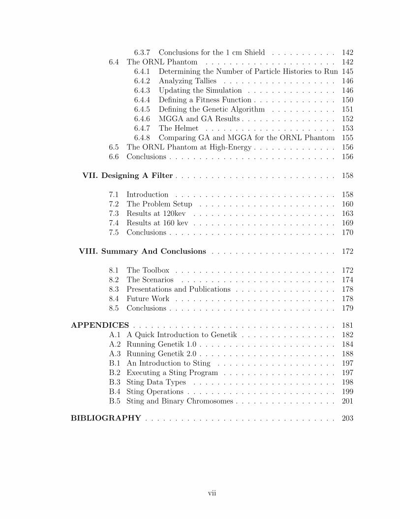
6.3.7 Conclusions for the 1 cm Shield . . . . . . . . . . . 1426.4 The ORNL Phantom . . . . . . . . . . . . . . . . . . . . . . 142

6.4.1 Determining the Number of Particle Histories to Run 1456.4.2 Analyzing Tallies . . . . . . . . . . . . . . . . . . . 1466.4.3 Updating the Simulation . . . . . . . . . . . . . . . 1466.4.4 Defining a Fitness Function . . . . . . . . . . . . . . 1506.4.5 Defining the Genetic Algorithm . . . . . . . . . . . 1516.4.6 MGGA and GA Results . . . . . . . . . . . . . . . . 1526.4.7 The Helmet . . . . . . . . . . . . . . . . . . . . . . 1536.4.8 Comparing GA and MGGA for the ORNL Phantom 155

6.5 The ORNL Phantom at High-Energy . . . . . . . . . . . . . . 1566.6 Conclusions . . . . . . . . . . . . . . . . . . . . . . . . . . . . 156

VII. Designing A Filter . . . . . . . . . . . . . . . . . . . . . . . . . . . 158

7.1 Introduction . . . . . . . . . . . . . . . . . . . . . . . . . . . 1587.2 The Problem Setup . . . . . . . . . . . . . . . . . . . . . . . 1607.3 Results at 120kev . . . . . . . . . . . . . . . . . . . . . . . . 1637.4 Results at 160 kev . . . . . . . . . . . . . . . . . . . . . . . . 1697.5 Conclusions . . . . . . . . . . . . . . . . . . . . . . . . . . . . 170

VIII. Summary And Conclusions . . . . . . . . . . . . . . . . . . . . . 172

8.1 The Toolbox . . . . . . . . . . . . . . . . . . . . . . . . . . . 1728.2 The Scenarios . . . . . . . . . . . . . . . . . . . . . . . . . . 1748.3 Presentations and Publications . . . . . . . . . . . . . . . . . 1788.4 Future Work . . . . . . . . . . . . . . . . . . . . . . . . . . . 1788.5 Conclusions . . . . . . . . . . . . . . . . . . . . . . . . . . . . 179

APPENDICES . . . . . . . . . . . . . . . . . . . . . . . . . . . . . . . . . . 181A.1 A Quick Introduction to Genetik . . . . . . . . . . . . . . . . 182A.2 Running Genetik 1.0 . . . . . . . . . . . . . . . . . . . . . . . 184A.3 Running Genetik 2.0 . . . . . . . . . . . . . . . . . . . . . . . 188B.1 An Introduction to Sting . . . . . . . . . . . . . . . . . . . . 197B.2 Executing a Sting Program . . . . . . . . . . . . . . . . . . . 197B.3 Sting Data Types . . . . . . . . . . . . . . . . . . . . . . . . 198B.4 Sting Operations . . . . . . . . . . . . . . . . . . . . . . . . . 199B.5 Sting and Binary Chromosomes . . . . . . . . . . . . . . . . . 201

BIBLIOGRAPHY . . . . . . . . . . . . . . . . . . . . . . . . . . . . . . . . 203

vii

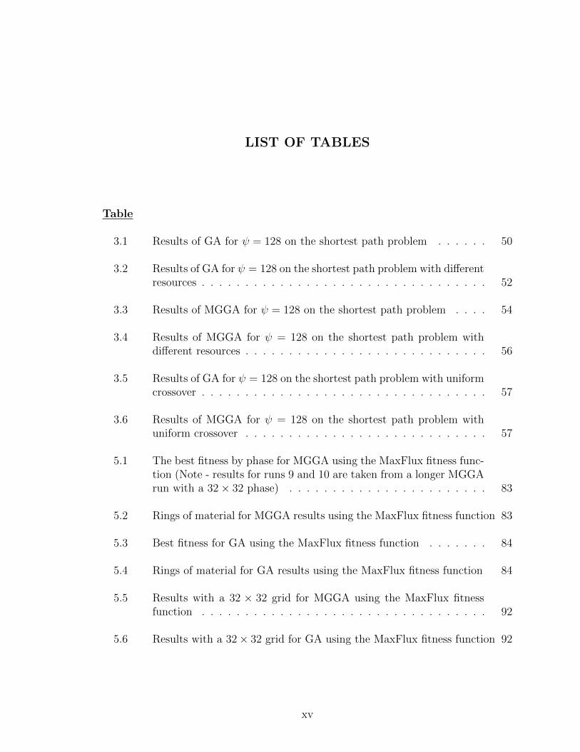
LIST OF FIGURES

Figure

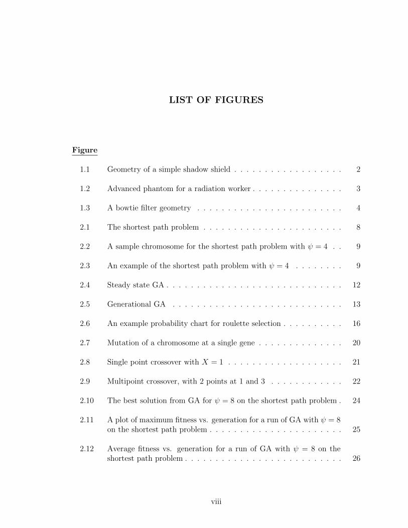
1.1 Geometry of a simple shadow shield . . . . . . . . . . . . . . . . . . 2

1.2 Advanced phantom for a radiation worker . . . . . . . . . . . . . . . 3

1.3 A bowtie filter geometry . . . . . . . . . . . . . . . . . . . . . . . . 4

2.1 The shortest path problem . . . . . . . . . . . . . . . . . . . . . . . 8

2.2 A sample chromosome for the shortest path problem with ψ = 4 . . 9

2.3 An example of the shortest path problem with ψ = 4 . . . . . . . . 9

2.4 Steady state GA . . . . . . . . . . . . . . . . . . . . . . . . . . . . . 12

2.5 Generational GA . . . . . . . . . . . . . . . . . . . . . . . . . . . . 13

2.6 An example probability chart for roulette selection . . . . . . . . . . 16

2.7 Mutation of a chromosome at a single gene . . . . . . . . . . . . . . 20

2.8 Single point crossover with X = 1 . . . . . . . . . . . . . . . . . . . 21

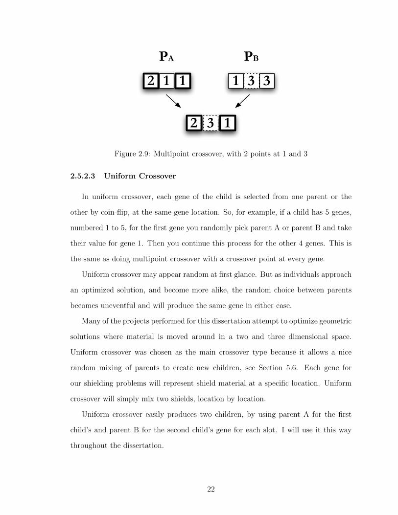
2.9 Multipoint crossover, with 2 points at 1 and 3 . . . . . . . . . . . . 22

2.10 The best solution from GA for ψ = 8 on the shortest path problem . 24

2.11 A plot of maximum fitness vs. generation for a run of GA with ψ = 8on the shortest path problem . . . . . . . . . . . . . . . . . . . . . . 25

2.12 Average fitness vs. generation for a run of GA with ψ = 8 on theshortest path problem . . . . . . . . . . . . . . . . . . . . . . . . . . 26

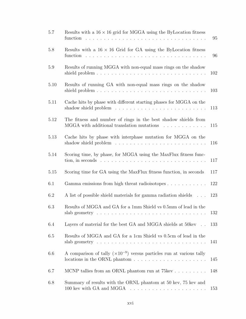
viii

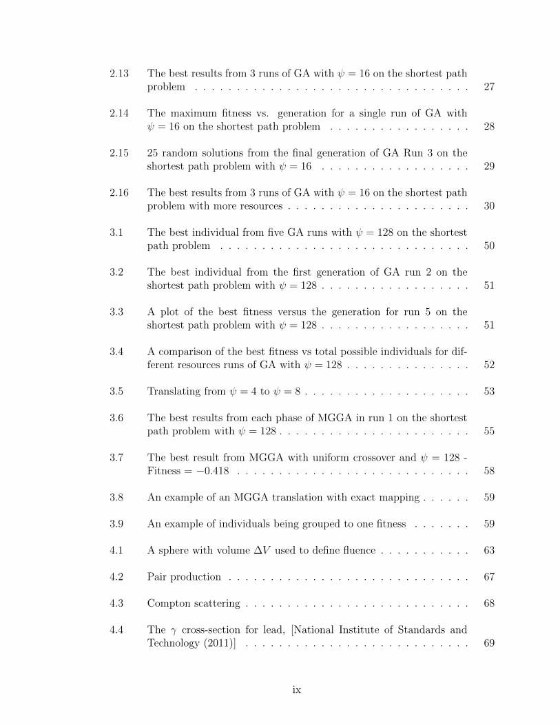
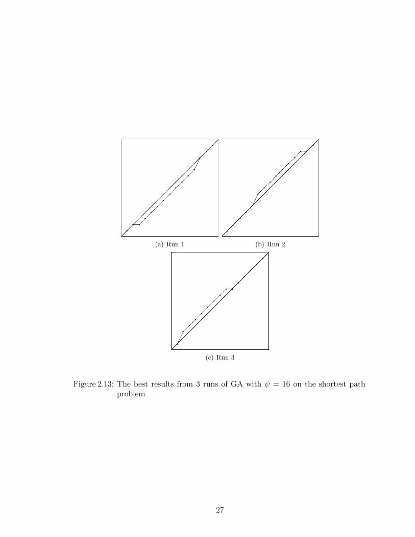
2.13 The best results from 3 runs of GA with ψ = 16 on the shortest pathproblem . . . . . . . . . . . . . . . . . . . . . . . . . . . . . . . . . 27

2.14 The maximum fitness vs. generation for a single run of GA withψ = 16 on the shortest path problem . . . . . . . . . . . . . . . . . 28

2.15 25 random solutions from the final generation of GA Run 3 on theshortest path problem with ψ = 16 . . . . . . . . . . . . . . . . . . 29

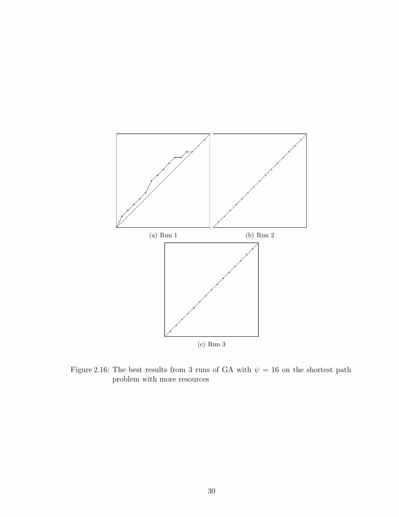
2.16 The best results from 3 runs of GA with ψ = 16 on the shortest pathproblem with more resources . . . . . . . . . . . . . . . . . . . . . . 30

3.1 The best individual from five GA runs with ψ = 128 on the shortestpath problem . . . . . . . . . . . . . . . . . . . . . . . . . . . . . . 50

3.2 The best individual from the first generation of GA run 2 on theshortest path problem with ψ = 128 . . . . . . . . . . . . . . . . . . 51

3.3 A plot of the best fitness versus the generation for run 5 on theshortest path problem with ψ = 128 . . . . . . . . . . . . . . . . . . 51

3.4 A comparison of the best fitness vs total possible individuals for dif-ferent resources runs of GA with ψ = 128 . . . . . . . . . . . . . . . 52

3.5 Translating from ψ = 4 to ψ = 8 . . . . . . . . . . . . . . . . . . . . 53

3.6 The best results from each phase of MGGA in run 1 on the shortestpath problem with ψ = 128 . . . . . . . . . . . . . . . . . . . . . . . 55

3.7 The best result from MGGA with uniform crossover and ψ = 128 -Fitness = −0.418 . . . . . . . . . . . . . . . . . . . . . . . . . . . . 58

3.8 An example of an MGGA translation with exact mapping . . . . . . 59

3.9 An example of individuals being grouped to one fitness . . . . . . . 59

4.1 A sphere with volume ∆V used to define fluence . . . . . . . . . . . 63

4.2 Pair production . . . . . . . . . . . . . . . . . . . . . . . . . . . . . 67

4.3 Compton scattering . . . . . . . . . . . . . . . . . . . . . . . . . . . 68

4.4 The γ cross-section for lead, [National Institute of Standards andTechnology (2011)] . . . . . . . . . . . . . . . . . . . . . . . . . . . 69

ix

4.5 The γ cross-sections for lead and antimony, National Institute ofStandards and Technology (2011) . . . . . . . . . . . . . . . . . . . 70

5.1 The geometry of a simple shadow shield . . . . . . . . . . . . . . . . 74

5.2 The geometry for the shadow shield problem. The r-z plane with adisk source to the left and a detector plane to the right. The goal isto place material in the intervening vacuum to reduce the flux at thedetector plane. . . . . . . . . . . . . . . . . . . . . . . . . . . . . . . 75

5.3 The shadow shield translation operator . . . . . . . . . . . . . . . . 82

5.4 The best MGGA shadow shield on a 16× 16 grid - Fitness = 0.96 . 85

5.5 The best GA shadow shield on a 16× 16 grid - Fitness = 0.75 . . . 86

5.6 Average fitness -vs- generation for GA run with the MaxFlux fitnessfunction . . . . . . . . . . . . . . . . . . . . . . . . . . . . . . . . . 87

5.7 Flux vs. Radius - For the best MGGA shield, the full shield, and acone with mass equal to the MGGA solution for the MaxFlux shadowshield problem . . . . . . . . . . . . . . . . . . . . . . . . . . . . . . 88

5.8 Flux vs. Radius - For the best GA shield, the full shield, and a conewith mass equal to the GA solution for the MaxFlux shadow shieldproblem . . . . . . . . . . . . . . . . . . . . . . . . . . . . . . . . . 88

5.9 An equal mass cone for the best MGGA shadow shield - Fitness =−19.038 . . . . . . . . . . . . . . . . . . . . . . . . . . . . . . . . . 90

5.10 An equal mass cone for the best GA shadow shield - Fitness = −3.54 90

5.11 An clean version of the best GA shadow shield - Fitness = 0.875 . . 91

5.12 The best MGGA shadow shield for a 32× 32 grid - Fitness = 0.967 93

5.13 The best GA shadow shield for a 32× 32 grid - Fitness = 0.495 . . 93

5.14 The best 16× 16 MGGA shadow shield (Fitness = 0.96) vs. the best32× 32 MGGA shadow shield (Fitness = 0.967) . . . . . . . . . . . 94

5.15 The best shield produced by MGGA for the ByLocation fitness func-tion - Fitness = 0.82 . . . . . . . . . . . . . . . . . . . . . . . . . . 96

x

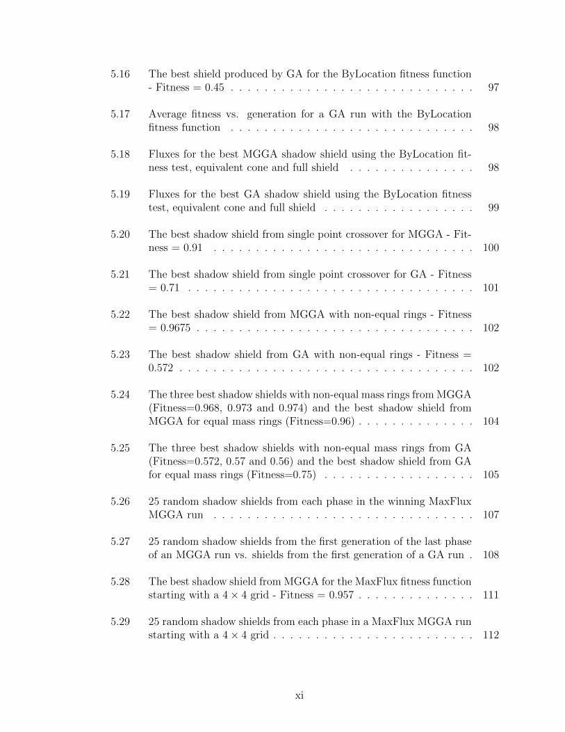
5.16 The best shield produced by GA for the ByLocation fitness function- Fitness = 0.45 . . . . . . . . . . . . . . . . . . . . . . . . . . . . . 97

5.17 Average fitness vs. generation for a GA run with the ByLocationfitness function . . . . . . . . . . . . . . . . . . . . . . . . . . . . . 98

5.18 Fluxes for the best MGGA shadow shield using the ByLocation fit-ness test, equivalent cone and full shield . . . . . . . . . . . . . . . 98

5.19 Fluxes for the best GA shadow shield using the ByLocation fitnesstest, equivalent cone and full shield . . . . . . . . . . . . . . . . . . 99

5.20 The best shadow shield from single point crossover for MGGA - Fit-ness = 0.91 . . . . . . . . . . . . . . . . . . . . . . . . . . . . . . . 100

5.21 The best shadow shield from single point crossover for GA - Fitness= 0.71 . . . . . . . . . . . . . . . . . . . . . . . . . . . . . . . . . . 101

5.22 The best shadow shield from MGGA with non-equal rings - Fitness= 0.9675 . . . . . . . . . . . . . . . . . . . . . . . . . . . . . . . . . 102

5.23 The best shadow shield from GA with non-equal rings - Fitness =0.572 . . . . . . . . . . . . . . . . . . . . . . . . . . . . . . . . . . . 102

5.24 The three best shadow shields with non-equal mass rings from MGGA(Fitness=0.968, 0.973 and 0.974) and the best shadow shield fromMGGA for equal mass rings (Fitness=0.96) . . . . . . . . . . . . . . 104

5.25 The three best shadow shields with non-equal mass rings from GA(Fitness=0.572, 0.57 and 0.56) and the best shadow shield from GAfor equal mass rings (Fitness=0.75) . . . . . . . . . . . . . . . . . . 105

5.26 25 random shadow shields from each phase in the winning MaxFluxMGGA run . . . . . . . . . . . . . . . . . . . . . . . . . . . . . . . 107

5.27 25 random shadow shields from the first generation of the last phaseof an MGGA run vs. shields from the first generation of a GA run . 108

5.28 The best shadow shield from MGGA for the MaxFlux fitness functionstarting with a 4× 4 grid - Fitness = 0.957 . . . . . . . . . . . . . . 111

5.29 25 random shadow shields from each phase in a MaxFlux MGGA runstarting with a 4× 4 grid . . . . . . . . . . . . . . . . . . . . . . . . 112

xi

5.30 The best shadow shield from MGGA for the MaxFlux fitness functionstarting with a 8× 8 grid - Fitness = 0.95 . . . . . . . . . . . . . . 113

5.31 25 random shadow shields from each phase in a MaxFlux MGGA runstarting with an 8× 8 grid . . . . . . . . . . . . . . . . . . . . . . . 114

6.1 A slab geometry for gamma shield simulations . . . . . . . . . . . . 124

6.2 The vacuum tally vs. depth for various energies of gamma radiationin the slab geometry . . . . . . . . . . . . . . . . . . . . . . . . . . 125

6.3 The dose for single material shields at a tally depth of 5 cm . . . . . 126

6.4 The dose for single material shields with energies under 100 kev . . 126

6.5 γ radiation cross-sections for Tungsten (gray) & Antimony (black),[National Institute of Standards and Technology (2011)] . . . . . . . 127

6.6 A comparison of tungsten and antimony layered shields at 50kev . . 128

6.7 A comparison of tungsten and antimony layered shields at100kev . . 128

6.8 The best GA and MGGA gamma shields at 50 kev . . . . . . . . . 133

6.9 Dose as an F6 tally for GA and MGGA at 50 kev . . . . . . . . . . 134

6.10 The best gamma shields at 50 kev for MGGA by phase . . . . . . . 135

6.11 Diversity for GA and MGGA runs at 50 kev . . . . . . . . . . . . . 136

6.12 The best GA and MGGA shields at 75 kev . . . . . . . . . . . . . . 137

6.13 The best gamma shields at 75 kev for MGGA by phase . . . . . . . 138

6.14 The best gamma shields at 100 kev . . . . . . . . . . . . . . . . . . 138

6.15 The best gamma shields at 150 kev . . . . . . . . . . . . . . . . . . 139

6.16 50kev MGGA shield with 32 layers . . . . . . . . . . . . . . . . . . 140

6.17 The best gamma shields at 200 kev with 1 cm shields . . . . . . . . 142

6.18 The best gamma shields at 200 kev for MGGA by phase, at 1 cm . 143

6.19 The ORNL phantom . . . . . . . . . . . . . . . . . . . . . . . . . . 144

xii

6.20 The shield cross section for the ORNL phantom layered shield . . . 144

6.21 Plots for 3 tallies in the ORNL phantom: dose equivalent vs. particlecount . . . . . . . . . . . . . . . . . . . . . . . . . . . . . . . . . . . 147

6.22 ORNL-based geometry before and after optimizations . . . . . . . . 149

6.23 Dose on the ORNL phantom as a function of the XY reflective wallpositions . . . . . . . . . . . . . . . . . . . . . . . . . . . . . . . . . 150

6.24 The best gamma shields for ORNL with MGGA . . . . . . . . . . . 154

6.25 The helmet (without a top) for the ORNL phantom . . . . . . . . . 154

6.26 A comparison of MGGA and GA gamma shields for the ORNL phan-tom at 100 kev . . . . . . . . . . . . . . . . . . . . . . . . . . . . . 155

7.1 The total flux vs. detector radius at 120 kev . . . . . . . . . . . . . 159

7.2 The scatter/total fluence ratio vs. detector radius at 120 kev . . . . 159

7.3 Representative bowtie filter cross-section . . . . . . . . . . . . . . . 160

7.4 Geometry for a bowtie filter with a spherical phantom . . . . . . . . 161

7.5 The best aluminum MGGA filter at 120kev (source at the top) - 0.981163

7.6 The scatter-to-total fluence ratio for the aluminum MGGA filter at120kev . . . . . . . . . . . . . . . . . . . . . . . . . . . . . . . . . . 164

7.7 γ radiation cross-sections for Titanium (gray) & Aluminum (black),[National Institute of Standards and Technology (2011)] . . . . . . . 165

7.8 The best MGGA filter at 120kev (source at the top) - 0.997 . . . . . 166

7.9 The best GA filter at 120kev (source at the top) - 0.996 . . . . . . . 166

7.10 The scatter-to-total fluence ratio for the best MGGA filter at 120kev 167

7.11 The scatter, primary and total tallies with and without the bestMGGA filter at 120kev . . . . . . . . . . . . . . . . . . . . . . . . . 167

7.12 The scatter-to-total ratio for the best GA filter at 120kev . . . . . . 168

xiii

7.13 The best MGGA filter at 160kev (source at the top) - 0.994 . . . . . 169

7.14 The best GA filter at 160 kev (source at the top) - 0.993 . . . . . . 169

7.15 The scatter-to-total ratio for the best MGGA filter at 160kev . . . . 170

7.16 The scatter-to-total ratio for the best GA filter at 160kev . . . . . . 170

7.17 The scatter and total tallies for the best MGGA filter at 160kev . . 171

8.1 Geometry of a shadow shield problem . . . . . . . . . . . . . . . . . 174

8.2 MGGA built shadow shield . . . . . . . . . . . . . . . . . . . . . . . 175

8.3 Advanced phantom for a radiation worker . . . . . . . . . . . . . . . 176

8.4 MGGA designed shield For 75KeV gamma rays . . . . . . . . . . . 176

8.5 The best MGGA filter at 120kev (source at the top) . . . . . . . . . 177

8.6 The scatter-to-primary ratio for the best MGGA filter at 120kev . . 177

xiv

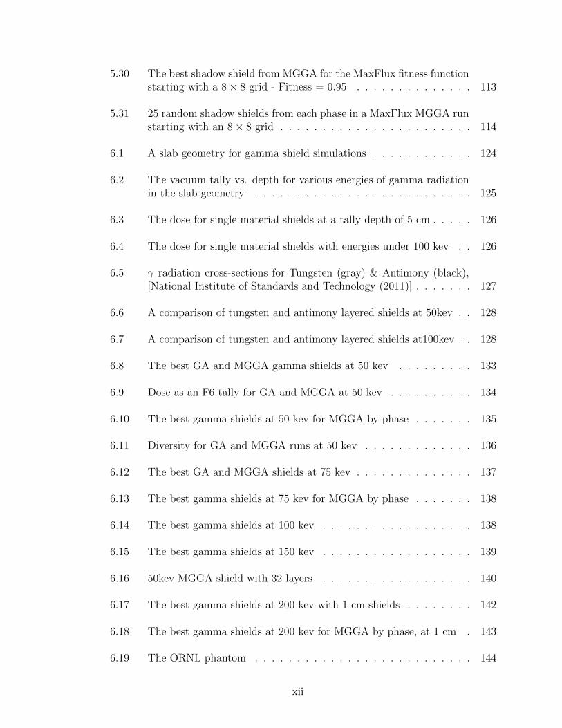
LIST OF TABLES

Table

3.1 Results of GA for ψ = 128 on the shortest path problem . . . . . . 50

3.2 Results of GA for ψ = 128 on the shortest path problem with differentresources . . . . . . . . . . . . . . . . . . . . . . . . . . . . . . . . . 52

3.3 Results of MGGA for ψ = 128 on the shortest path problem . . . . 54

3.4 Results of MGGA for ψ = 128 on the shortest path problem withdifferent resources . . . . . . . . . . . . . . . . . . . . . . . . . . . . 56

3.5 Results of GA for ψ = 128 on the shortest path problem with uniformcrossover . . . . . . . . . . . . . . . . . . . . . . . . . . . . . . . . . 57

3.6 Results of MGGA for ψ = 128 on the shortest path problem withuniform crossover . . . . . . . . . . . . . . . . . . . . . . . . . . . . 57

5.1 The best fitness by phase for MGGA using the MaxFlux fitness func-tion (Note - results for runs 9 and 10 are taken from a longer MGGArun with a 32× 32 phase) . . . . . . . . . . . . . . . . . . . . . . . 83

5.2 Rings of material for MGGA results using the MaxFlux fitness function 83

5.3 Best fitness for GA using the MaxFlux fitness function . . . . . . . 84

5.4 Rings of material for GA results using the MaxFlux fitness function 84

5.5 Results with a 32 × 32 grid for MGGA using the MaxFlux fitnessfunction . . . . . . . . . . . . . . . . . . . . . . . . . . . . . . . . . 92

5.6 Results with a 32× 32 grid for GA using the MaxFlux fitness function 92

xv

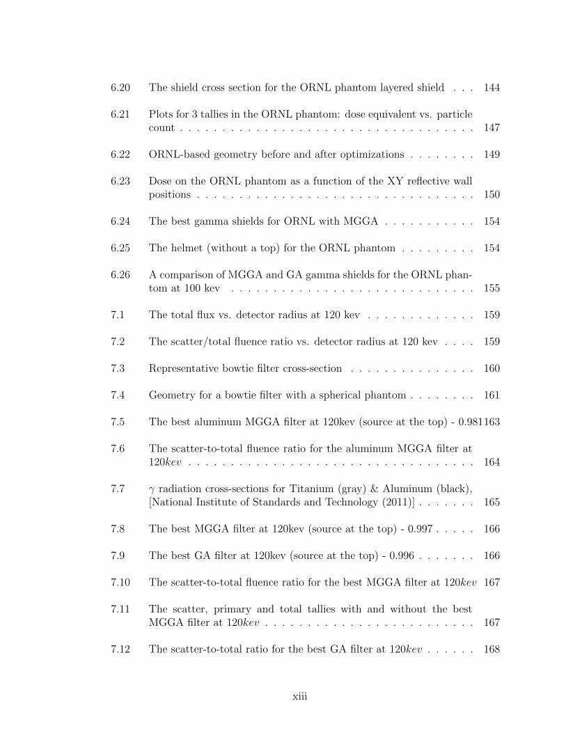
5.7 Results with a 16× 16 grid for MGGA using the ByLocation fitnessfunction . . . . . . . . . . . . . . . . . . . . . . . . . . . . . . . . . 95

5.8 Results with a 16 × 16 Grid for GA using the ByLocation fitnessfunction . . . . . . . . . . . . . . . . . . . . . . . . . . . . . . . . . 96

5.9 Results of running MGGA with non-equal mass rings on the shadowshield problem . . . . . . . . . . . . . . . . . . . . . . . . . . . . . . 102

5.10 Results of running GA with non-equal mass rings on the shadowshield problem . . . . . . . . . . . . . . . . . . . . . . . . . . . . . . 103

5.11 Cache hits by phase with different starting phases for MGGA on theshadow shield problem . . . . . . . . . . . . . . . . . . . . . . . . . 113

5.12 The fitness and number of rings in the best shadow shields fromMGGA with additional translation mutations . . . . . . . . . . . . 115

5.13 Cache hits by phase with interphase mutation for MGGA on theshadow shield problem . . . . . . . . . . . . . . . . . . . . . . . . . 116

5.14 Scoring time, by phase, for MGGA using the MaxFlux fitness func-tion, in seconds . . . . . . . . . . . . . . . . . . . . . . . . . . . . . 117

5.15 Scoring time for GA using the MaxFlux fitness function, in seconds 117

6.1 Gamma emissions from high threat radioisotopes . . . . . . . . . . . 122

6.2 A list of possible shield materials for gamma radiation shields . . . 123

6.3 Results of MGGA and GA for a 1mm Shield vs 0.5mm of lead in theslab geometry . . . . . . . . . . . . . . . . . . . . . . . . . . . . . . 132

6.4 Layers of material for the best GA and MGGA shields at 50kev . . 133

6.5 Results of MGGA and GA for a 1cm Shield vs 0.5cm of lead in theslab geometry . . . . . . . . . . . . . . . . . . . . . . . . . . . . . . 141

6.6 A comparison of tally (×10−9) versus particles run at various tallylocations in the ORNL phantom . . . . . . . . . . . . . . . . . . . . 145

6.7 MCNP tallies from an ORNL phantom run at 75kev . . . . . . . . . 148

6.8 Summary of results with the ORNL phantom at 50 kev, 75 kev and100 kev with GA and MGGA . . . . . . . . . . . . . . . . . . . . . 153

xvi

7.1 Results for GA and MGGA on the bowtie filter problem at 120kev . 165

7.2 Results for GA and MGGA on the bowtie filter problem at 160 kev 169

xvii

LIST OF APPENDICES

Appendix

A. Genetik . . . . . . . . . . . . . . . . . . . . . . . . . . . . . . . . . . . 182

B. Sting . . . . . . . . . . . . . . . . . . . . . . . . . . . . . . . . . . . . 197

xviii

ABSTRACT

Multi-Grid Genetic Algorithms For Optimal Radiation Shield Design

by

Stephen T. Asbury

Chair: James Paul Holloway

Genetic Algorithms (GA) are a powerful search and optimization technique that can

be applied to numerous problems. Unfortunately, GA relies on large numbers of fitness

evaluations to determine the relative merits of various solutions to a problem. For

problems requiring computationally intensive fitness evaluations this can make GA

too expensive to use. We describe a hierarchical technique that we have created called

Multi-Grid Genetic Algorithms (MGGA). MGGA leverages the geometry of a problem

space to build a hierarchy of increasingly smaller problem spaces. Optimizations over

these smaller spaces are used to seed a population of solutions in a larger space. We

explore how MGGA can be applied to several radiation shielding problems.

xix

CHAPTER I

Introduction

The first thing most people would think of when asked, “how do you protect

someone from radiation,” is the single word lead. Lead is used to shield us when we

go to the dentist for an X-Ray, or at least that is what we think is in that heavy

blanket they put on us. Lead is in the travel pouches for high speed film, and many

people would think incorrectly that nuclear reactors are surrounded by lead, when in

fact they generally use concrete and water to shield against neutron radiation because

hydrogen is a good material for shielding neutrons.

Protecting something or someone from radiation is more complex than stacking

lead bricks. The real world is a multi-objective function. It isn’t usually sufficient

to just build a shield. You also have to build a shield that meets numerous criteria.

Perhaps the shield must be as light as possible, or as cheap as possible. Maybe the

shield needs to be thin or made from specific materials for another reason. As we

will see in Chapter IV the type of radiation you are shielding against affects the type

of materials that will make a good shield. All of these objectives can play a role in

designing a good shield. Knights couldn’t carry a castle around with them, so they

carried a metal shield to stop their opponent’s sword. It wasn’t the best way to stop

the sword, but it was lighter and more maneuverable than a large stone structure.

Designing a shield can be hard. Moreover, the best solution can sometimes chal-

1

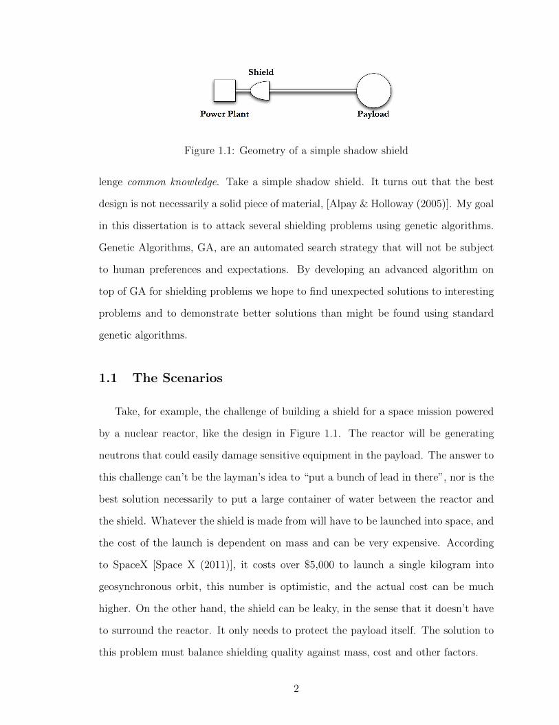
Figure 1.1: Geometry of a simple shadow shield

lenge common knowledge. Take a simple shadow shield. It turns out that the best

design is not necessarily a solid piece of material, [Alpay & Holloway (2005)]. My goal

in this dissertation is to attack several shielding problems using genetic algorithms.

Genetic Algorithms, GA, are an automated search strategy that will not be subject

to human preferences and expectations. By developing an advanced algorithm on

top of GA for shielding problems we hope to find unexpected solutions to interesting

problems and to demonstrate better solutions than might be found using standard

genetic algorithms.

1.1 The Scenarios

Take, for example, the challenge of building a shield for a space mission powered

by a nuclear reactor, like the design in Figure 1.1. The reactor will be generating

neutrons that could easily damage sensitive equipment in the payload. The answer to

this challenge can’t be the layman’s idea to “put a bunch of lead in there”, nor is the

best solution necessarily to put a large container of water between the reactor and

the shield. Whatever the shield is made from will have to be launched into space, and

the cost of the launch is dependent on mass and can be very expensive. According

to SpaceX [Space X (2011)], it costs over $5,000 to launch a single kilogram into

geosynchronous orbit, this number is optimistic, and the actual cost can be much

higher. On the other hand, the shield can be leaky, in the sense that it doesn’t have

to surround the reactor. It only needs to protect the payload itself. The solution to

this problem must balance shielding quality against mass, cost and other factors.

2

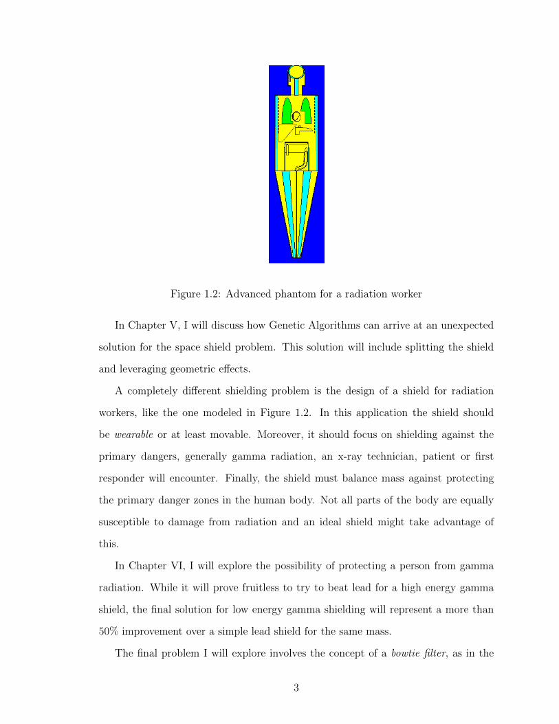
Horizontal cross-section showing heart, lungs, spine, and arms

Figure 1.2: Advanced phantom for a radiation worker

In Chapter V, I will discuss how Genetic Algorithms can arrive at an unexpected

solution for the space shield problem. This solution will include splitting the shield

and leveraging geometric effects.

A completely different shielding problem is the design of a shield for radiation

workers, like the one modeled in Figure 1.2. In this application the shield should

be wearable or at least movable. Moreover, it should focus on shielding against the

primary dangers, generally gamma radiation, an x-ray technician, patient or first

responder will encounter. Finally, the shield must balance mass against protecting

the primary danger zones in the human body. Not all parts of the body are equally

susceptible to damage from radiation and an ideal shield might take advantage of

this.

In Chapter VI, I will explore the possibility of protecting a person from gamma

radiation. While it will prove fruitless to try to beat lead for a high energy gamma

shield, the final solution for low energy gamma shielding will represent a more than

50% improvement over a simple lead shield for the same mass.

The final problem I will explore involves the concept of a bowtie filter, as in the

3

Figure 1.3: A bowtie filter geometry

geometry from Figure 1.3. These filters are used in CT scanners and other devices

to control the intensity of radiation incident on the detector plane. This problem

doesn’t suffer from mass restrictions but does present a different type of challenge.

Rather than trying to shield the target from all radiation, we are trying to shape the

incident radiation field. In Chapter VII, I will show how Genetic Algorithms can help

design a good bowtie filter with very few constraints.

By addressing these different scenarios I will show how our new Genetic Algorithm

provides a powerful tool to the shield designers toolbox.

1.2 The Toolbox

The primary tool discussed in this dissertation is a new Genetic Algorithm which

we call Multigrid Genetic Algorithms (MGGA). Chapter II discusses Genetic Algo-

rithms in a generic way, and provides a basic idea of how they solve problems. I

will introduce GA’s configuration parameters in Chapter II and discuss my choices

throughout the dissertation. A very important part of GA is the concept of a fit-

4

ness function. This fitness function is used to score possible solutions to a problem.

The goal of a Genetic Algorithm is ultimately to find a solution that has the best

score from the fitness function. In each chapter I will describe what fitness function

we are using, and why. Moreover, I will be discussing how that function captures

and balances different objectives for each shielding scenario. For example, the fitness

function for the space shield looks for a low mass solution as well as a good shield.

One disadvantage of Genetic Algorithms is that they must evaluate the fitness

function numerous times. It is common to design GAs where the fitness function

could be run millions of times, although we will generally stay to below one hundred

thousand invocations in this dissertation. In the case of radiation shielding, the fitness

function will always involve performing a radiation transport simulation with a code

like MCNP. These codes can take minutes, hours or even days to run. As a result,

the fitness function evaluation becomes a time constraint.

To help address this time constraint I pursued several avenues of research. First,

I created a Genetic Algorithm library that would allow me to scavenge time on a

computing cluster. Over the course of my research I moved through several cluster

implementations, each move altered the optimal design for the Genetic Algorithm

code. This evolution is described in Section 2.9.

Second, my GA library implements a number of smart algorithms to minimize

work. Caching is used eliminate retesting of individuals where their score is known.

An algorithm called pre-calculation was tested to see if we could eliminate fitness

function evaluations in cases where selection wouldn’t pick an individual, independent

of their fitness.

Third, we created a new form of Genetic Algorithm called the Multi-Grid Genetic

Algorithm (MGGA) which leverages geometric considerations to move the algorithm

to a good solution more quickly, using fewer calls to the fitness function. MGGA

is described in Chapter III and used for each problem I describe in this disserta-

5

tion. MGGA and its application to radiation shielding design is the most significant

contribution of this work.

1.3 Does It Work?

Ultimately the question that must be asked is, “does GA and MGGA help design

better shields?” Based on the results in this dissertation I will show that the answer

is yes. GA, and specifically MGGA, helps design shields. For the space shield, the

MGGA was able to find a non-obvious solution that allowed neutrons to scatter away

from the shield while reducing shield mass. MGGA was also able to reduce the total

dose on a realistic human phantom by over 50% for 75 kev gammas compared to a

lead shield of equal mass.

Perhaps equally as important, in most cases, MGGA is able to produce a better

result than GA with the same or fewer computing resources. MGGA is a new way of

exploring a problem space that leverages the geometric features of shielding problems

to reduce the computing resources required to explore them.

6

CHAPTER II

Genetic Algorithms

2.1 Introduction

As early as the 1950s scientists were looking at how evolution could be used to op-

timize solutions in engineering and scientific problems [Mitchel (1998)]. John Holland

at the University of Michigan [Holland (1992,1975)] began working and publishing on

the idea of Genetic Algorithms in particular over 30 years ago. Genetic Algorithms,

GA, are a way to automate the optimization process based on techniques used in

biological evolution. GA can be compared to other optimization techniques like hill

climbing or simulated annealing, in that these techniques all try to find optimal solu-

tions to problems in a generic enough way that they can be applied to a large range

of problem types.

GA is generally implemented using the following high level steps:

1. Determine a way to encode solutions to your problem, the encoding will be used

to define the chromosomes for your Genetic Algorithm.

2. Determine a way to score your solutions. We will call this scoring mechanism

the fitness function.

3. Run the Genetic Algorithm using your encoding and scoring to find a “best”

7

solution. In the next few sections we will see how GA generates new individuals

to score.

The individual elements of a chromosome will be called genes to match the bio-

logical terminology.

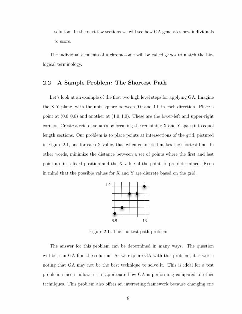
2.2 A Sample Problem: The Shortest Path

Let’s look at an example of the first two high level steps for applying GA. Imagine

the X-Y plane, with the unit square between 0.0 and 1.0 in each direction. Place a

point at (0.0, 0.0) and another at (1.0, 1.0). These are the lower-left and upper-right

corners. Create a grid of squares by breaking the remaining X and Y space into equal

length sections. Our problem is to place points at intersections of the grid, pictured

in Figure 2.1, one for each X value, that when connected makes the shortest line. In

other words, minimize the distance between a set of points where the first and last

point are in a fixed position and the X value of the points is pre-determined. Keep

in mind that the possible values for X and Y are discrete based on the grid.

0.0 1.0

1.0

Figure 2.1: The shortest path problem

The answer for this problem can be determined in many ways. The question

will be, can GA find the solution. As we explore GA with this problem, it is worth

noting that GA may not be the best technique to solve it. This is ideal for a test

problem, since it allows us to appreciate how GA is performing compared to other

techniques. This problem also offers an interesting framework because changing one

8

point at a time, as hill climbing or a steepest descent technique would try to do, won’t

necessarily work; moving one point might create a longer section between it and its

neighbors. For an algorithm to optimize the solution, it may be necessary for all of

the values in the encoding to move toward the best answer at the same time. The

solution space is non-trivial.

2.2.0.1 Encoding the Shortest Path Problem

We will encode the shortest path problem onto a discrete grid using a constant

called ψ, and the following steps:

1. Break the X-axis and Y-axis from 0 to 1.0 into ψ sections.

2. Store the Y-value at each X point, excluding the two ends, as a single integer

from 0 to ψ

The first point is always (0.0, 0.0) and last point is always (1.0, 1.0) and are not

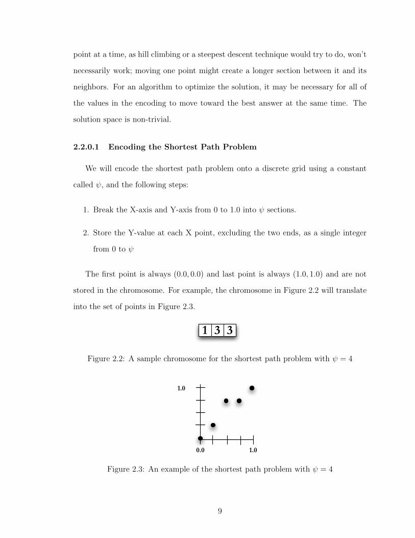
stored in the chromosome. For example, the chromosome in Figure 2.2 will translate

into the set of points in Figure 2.3.

1 3 3

Figure 2.2: A sample chromosome for the shortest path problem with ψ = 4

0.0 1.0

1.0

Figure 2.3: An example of the shortest path problem with ψ = 4

9

Because we are going to fix the first and last point to the two corners, we will

have a total of ψ − 1 integers for each chromosome. This insures that we can scale

this problem for MGGA by splitting each X value in half. The value of ψ is also used

to split the X and Y axis equally so that scaling during MGGA, discussed in the next

section, will be equal in both directions.

This is a pretty simple problem and encoding. But imagine that we use ψ = 128

This would result in a problem space with 127 X’s, each with 129 possible values, or

129127 = 1.1× 10268 possible encodings. That is a huge search space.

2.2.0.2 Scoring the Shortest Path Problem

To score each individual we use a fitness function that performs the following

steps:

1. Calculate the X value for each point by dividing the X axis into ψ parts, keeping

in mind that the first element of the chromosome is at 0.0 and the last at 1.0.

In Figure 2.3 with ψ = 4 the X values will be 0, 0.25, 0.5, 0.75 and 1.0.

2. Treat the value for each X location as ψ units that add up to a height of 1.0, so

if ψ = 4 the Y values will range from 0 to 4, corresponding to values of 0, 0.25,

0.5, 0.75 and 1.0.

3. Calculate the length of the line connecting all of the points by adding up the

distance between the points defined by consecutive genes, looping and summing

until all of the gene pairs are mapped onto line segments and included.

4. Subtract the result from 1.0 to make 1.0 the best fitness and all others less

than 1.0. The value of 1.0 is not achievable, since the distance is always greater

than 0. However, I use this convention throughout this dissertation to provide

a consistent value for the best possible fitness.

10

Put simply the fitness for a chromosome is:

F (x) = 1− sum of length of line segments

= 1−ψ∑i=0

2√

(xi+1 − xi)2 + (yi+1 − yi)2

(2.1)

Given a problem encoding and fitness function, lets look at the Genetic Algorithm

itself.

2.3 The Genetic Algorithm

Genetic algorithms are generally run in one of two modes: steady state or gener-

ational, [Langon & Poli (2002) page 9]. In steady state GA the program will perform

the following steps, pictured in Fig. 2.4.

1. Generate a number of possible solutions to the problem. Encode these solu-

tions using an appropriate format. This group of encoded solutions is called a

population.

2. Score the individuals in the population using the fitness function.

3. Use some sort of selection mechanism, see Section 2.4, to pull out good individ-

uals, call these individuals parents.

4. Build new solutions from the parents using GA operations, see Section 2.5. Call

these new individuals children, and this process reproduction.

5. Insert the children into the population, either by replacing their parents, by

growing the population or by replacing some other set of individuals chosen

using a selection mechanism.

11

6. Return to step 2. (In steady state GA, the population remains basically the

same, or steady, we just replace or add to it.)

Parent

Child

Selection

Insertion

Reproduction

Figure 2.4: Steady state GA

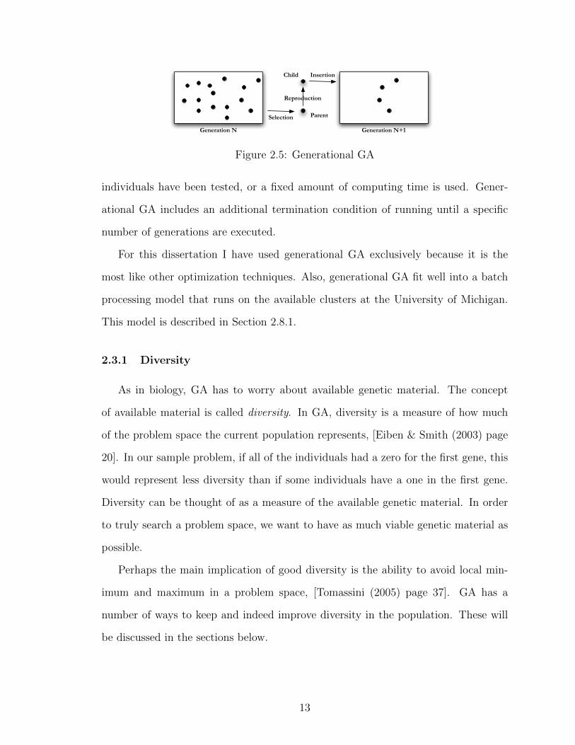
Generational GA changes the last step in this algorithm. In generational GA the

algorithm will perform the following steps, pictured in Fig. 2.5.

1. Generate a number of possible solutions to the problem, encode these solutions

using an appropriate format. This group of solutions is called a population or

generation.

2. Score the individuals in the population using the fitness function.

3. Use some sort of selection mechanism, see Section 2.4, to pull out good individ-

uals, we will use these as parents.

4. Build new solutions from the parents using GA operations, see Section 2.5. Call

these new individuals the children and this process reproduction.

5. Insert the children into a new population. (Note - in generational GA we make a

new population each time, in steady state GA we reused the same population.)

6. Repeat generating children until the new population is full.

7. Return to step 2, with the new population as the current population.

The genetic algorithm will loop until it meets some termination condition. Ter-

mination conditions include: a sufficiently good individual is found, some number of

12

Parent

Child

Selection

Insertion

Reproduction

Generation N Generation N+1

Figure 2.5: Generational GA

individuals have been tested, or a fixed amount of computing time is used. Gener-

ational GA includes an additional termination condition of running until a specific

number of generations are executed.

For this dissertation I have used generational GA exclusively because it is the

most like other optimization techniques. Also, generational GA fit well into a batch

processing model that runs on the available clusters at the University of Michigan.

This model is described in Section 2.8.1.

2.3.1 Diversity

As in biology, GA has to worry about available genetic material. The concept

of available material is called diversity. In GA, diversity is a measure of how much

of the problem space the current population represents, [Eiben & Smith (2003) page

20]. In our sample problem, if all of the individuals had a zero for the first gene, this

would represent less diversity than if some individuals have a one in the first gene.

Diversity can be thought of as a measure of the available genetic material. In order

to truly search a problem space, we want to have as much viable genetic material as

possible.

Perhaps the main implication of good diversity is the ability to avoid local min-

imum and maximum in a problem space, [Tomassini (2005) page 37]. GA has a

number of ways to keep and indeed improve diversity in the population. These will

be discussed in the sections below.

13

2.4 Selection Mechanisms

One of the key steps in the “Genetic Algorithm” is selecting parents for the next

generation. Selection is one of the main ways to maintain diversity in a population.

The selection process can be handled a number of ways.

2.4.1 Random Selection

Random selection is the process of picking individuals from the population with

no concern for their fitness. This selection scheme keeps a lot of diversity, but doesn’t

help move the algorithm toward a solution. Random selection can suffer from the

side effect that it loses good individuals to bad luck, simply because they are not

randomly picked.

2.4.2 Top Selection

Top selection takes the fitness for every individual in a population and ranks them.

Then the highest scoring individual is used as the parent for every child. Always

selecting the top individual makes very little sense in generational GA, but can make

some sense in steady state GA. If we use top section for generational GA we would

be creating a new population with a single parent. As we will see in the next few

sections, the only way to change that parent will be mutation. So with top selection

we would essentially be performing an inefficient hill climbing optimization. With

steady state GA, we would still be essentially hill climbing, but without completely

replacing the population each time.

2.4.3 Truncation Selection

Truncation selection also ranks the individuals by fitness, but instead of always

picking the top scoring individual, truncation selection randomly picks individuals

14

from the top N% of individuals. If N is small, only the very top individuals are

picked. If N = 100%, truncation selection becomes random selection.

Truncation selection has a small cost in the ranking process. Depending on pop-

ulation size this can be an issue. But the more important issue with truncation

selection is that it removes “bad” individuals from the population. This is a concern

because sometimes, the bad individuals are holding useful genetic material. In our

shortest path sample problem, a bad individual might be the only one with a one

in the first gene. By always killing lower fitness individuals, truncation selection can

hurt the long term success of the population.

2.4.4 Roulette, or Fitness Proportional Selection

Roulette selection tries to solve the problem of reduced diversity associated with

losing bad individuals by randomly choosing from all individuals, [Banzhal et al.

(1998) page 130]. However, unlike random selection where every individual has an

equal chance to be picked, roulette selection uses the fitness of each individual to give

more fit individuals a higher probability of being picked. To achieve this, roulette

assigns a selection probability for each individual based on its fitness, as follows:

1. Calculates the sum across all fitness scores.

S =∑i=0

fi, where fi is the fitness for individual i (2.2)

2. Assign each individual a probability based on its fitness divided by the sum of

all fitness scores, see Fig. 2.6.

pi = fi/S (2.3)

3. Spin the wheel to get a number r between 0 and 1.

4. Walk the list of individuals, from the first one in the population to the last,

15

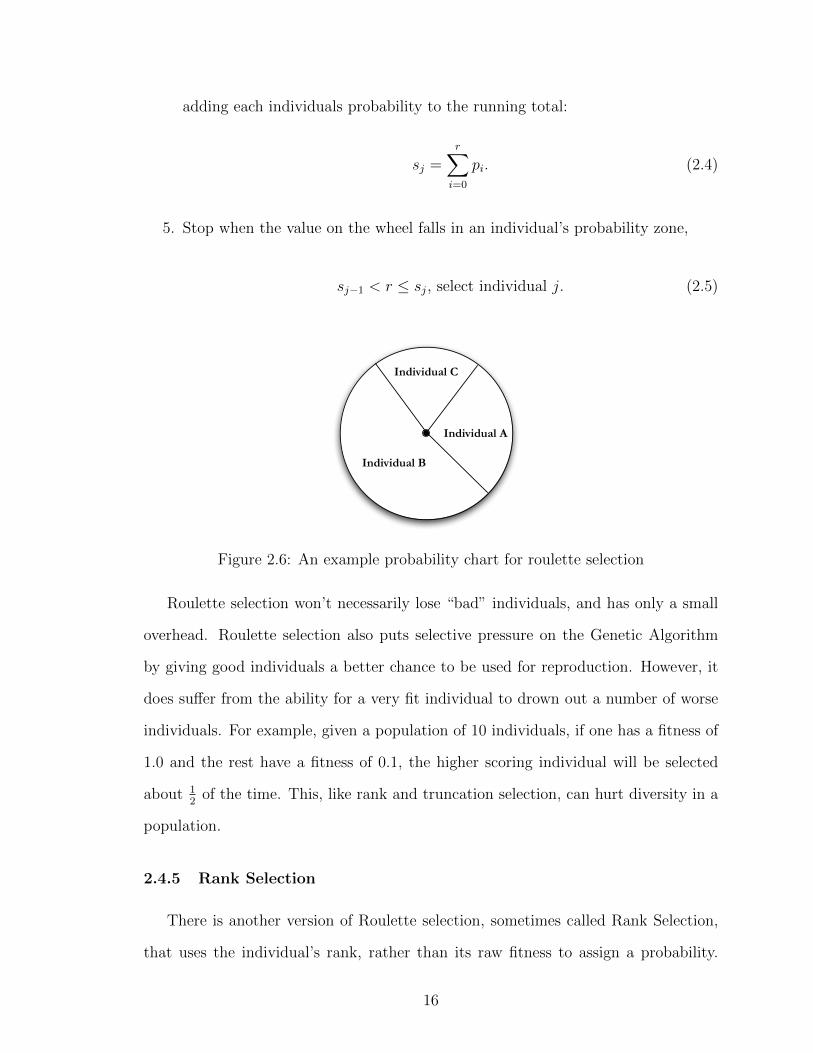
adding each individuals probability to the running total:

sj =r∑i=0

pi. (2.4)

5. Stop when the value on the wheel falls in an individual’s probability zone,

sj−1 < r ≤ sj, select individual j. (2.5)

Individual A

Individual C

Individual B

Figure 2.6: An example probability chart for roulette selection

Roulette selection won’t necessarily lose “bad” individuals, and has only a small

overhead. Roulette selection also puts selective pressure on the Genetic Algorithm

by giving good individuals a better chance to be used for reproduction. However, it

does suffer from the ability for a very fit individual to drown out a number of worse

individuals. For example, given a population of 10 individuals, if one has a fitness of

1.0 and the rest have a fitness of 0.1, the higher scoring individual will be selected

about 12

of the time. This, like rank and truncation selection, can hurt diversity in a

population.

2.4.5 Rank Selection

There is another version of Roulette selection, sometimes called Rank Selection,

that uses the individual’s rank, rather than its raw fitness to assign a probability.

16

This selection method removes the chance for a single individual, or small group of

individuals, to dominate the fitness wheel, [Eiben & Smith (2003) page 60]. Rank

selection reduces the chance of keeping a “bad” individual with “good” genes.

2.4.6 Tournament Selection

Tournament selection [Eiben & Smith (2003) page 63] tries to solve the problem

of choosing good individuals at the cost of diversity in a novel way. In tournament

selection we chose a tournament size, call it TS. In its simple form, each time an

individual needs to be selected for reproduction, a small tournament is run by:

1. Randomly pick TS individuals

2. Take the highest scoring individual from this group

This algorithm uses random selection to get the members of the tournament, so

good and bad scoring individuals are equally likely to make it into a tournament.

Unfortunately, in this simple form, tournament selection will leave zero chance for

the worst individual to be used for reproduction, since it can’t win a tournament.

This leads to a modified algorithm:

1. Pick a percentage of times we want the worst individual to win the tournament.

This value, PW , can be tuned. A low value of PW will keep bad individuals

out, while a high value can increase diversity by allowing more bad individuals

in.

2. Pick TS individuals

3. Randomly pick a number between 0 and 100.

4. If the number is greater than PW take the highest scoring individual from this

group, otherwise take the lowest scoring individual in the group

17

A useful feature of tournament selection for GA users is that it has two tuning

mechanisms, the size of the tournament and the chance that bad individuals win.

Tournament selection is good for diversity, since it allows bad individuals to win in a

controllable way. By changing tournament size it is possible to make tournament se-

lection more like random selection, using a small tournament, or more like truncation

selection, by using a large tournament.

Because of these nice features, all of the GA done in later chapters will use tourna-

ment selection. The tournament sizes will be 4 or 5 individuals. Based on experiments

these values allow close to 98% of each population to participate in at least one tour-

nament. The PW for my runs will generally be 25%. The value of 25% was based

on an initial desire to allow lower scoring individuals to win tournaments without

overwhelming good individuals. In places where my runs suffer from diversity issues,

a possible direction for future work will be to try different values for this tuning

parameter.

2.4.7 Selection and Fitness Function Requirements

The choice of fitness function and selection mechanism are connected. Suppose

that you have the choice of two fitness functions. Both rank properly, in that the bet-

ter individuals have higher fitnesses. But one is smooth and the other is discontinuous

or lumpy. What I mean by lumpy is that the fitness function likes to group individuals

around certain scores, and if individuals improve they might jump to another group

of scores.

Given these two choices of fitness function, which is best? To answer that re-

ally depends on the selection algorithm. If you use roulette selection, then lumpy or

discontinuous fitness functions could be bad because they would give larger probabil-

ities to an individual that is near a discontinuity in the fitness function, even if the

difference between that individual and one on the other side of the discontinuity is

18

ultimately minimal. On the other hand, rank selection or tournament selection won’t

have this problem because they use the ordering of fitness scores rather than the raw

fitness scores to make decisions.

For the tournament selection used throughout this dissertation, our goal is to

make sure that two individuals raking by score is correct, regardless of their absolute

difference in score. In other words, if A has a higher fitness than B then A is better

than B. But it doesn’t matter if there are gaps in the possible fitness values. Put

simply, it doesn’t matter how much better A scores than B.

2.5 GA Operations

Once individuals are selected for reproduction the children are created using op-

erations. There are three operations in particular that have come to define GA:

mutation, crossover and copy. Other operations can be created for specific problems.

GA is normally implemented to chose a single operation, from a fixed set of choices,

to generate each child. The available operations and the chance for each operation

to be chosen will effect the performance of the GA for a specific problem, [Eiben &

Smith (2003); Jong (2006); Mitchel (1998)]. I will discuss these choices more with

regards to each operation in the sections below.

2.5.1 Mutation

Mutation is the process of changing an individual in a random way, Fig. 2.7.

For the shortest path problem, all of the genes are an integer between 0 and ψ,

so mutation might change a randomly selected Y-value, or gene, from 3 to 2 or

vice-versa. As implemented for this dissertation, mutation works on a single gene,

picked randomly, and changes it to another appropriate random value. Mutation is a

powerful operator because it can add diversity into a population. This can allow GA

to move a population away from a local minimum in search of a global one.

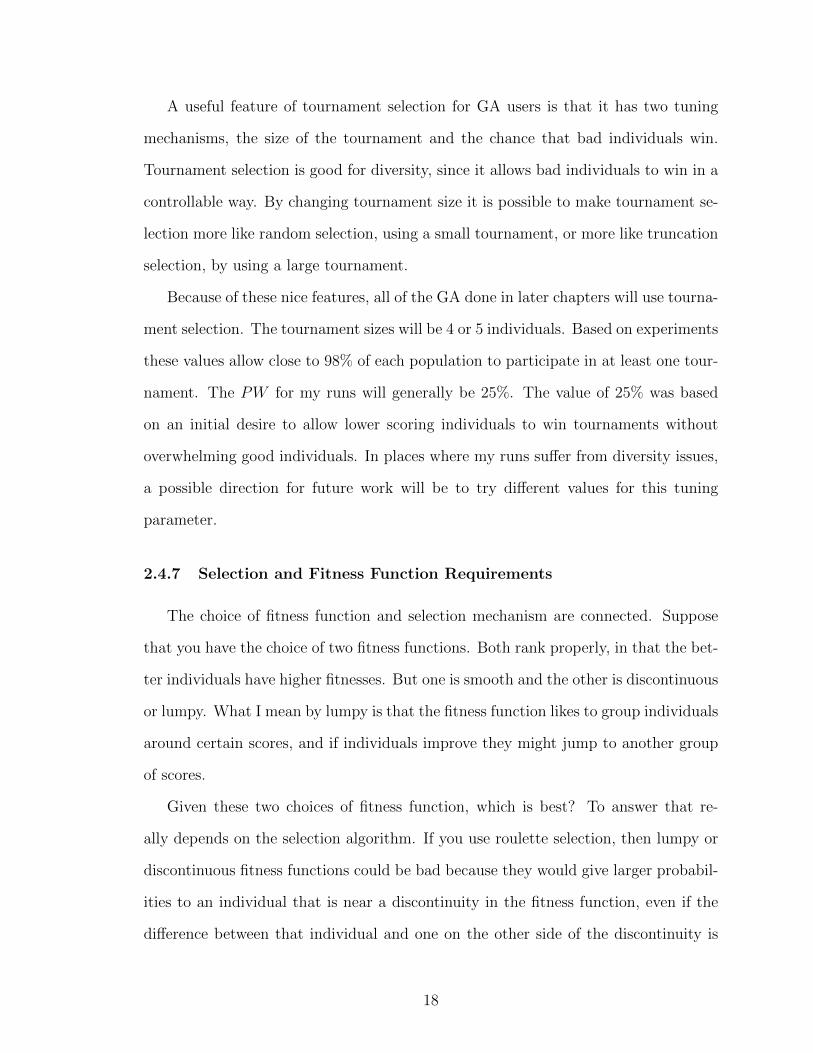
19

1 3 3 1 2 3

Figure 2.7: Mutation of a chromosome at a single gene

If mutation is used too heavily the user will move from the genetic algorithm

to a random search, on the other hand, using mutation too sparingly can allow a

population to stagnate. For most of the runs discussed in this dissertation, mutation

will be the chosen operation 20% of the time. This value is common in the literature,

and showed reasonable diversity growth for GA in all of my simulations.

2.5.2 Crossover

In crossover, two parents are chosen to create a new child by combining their

genetic material, [Eiben & Smith (2003)]. Often crossover treats the two parents

differently, like a vector cross product crossing parent A with parent B may be dif-

ferent than crossing parent B with parent A. Many implementations will actually do

crossover twice, creating two children instead of one, allowing each of the two parents

to be parent A for one of the offspring.

When diversity is high, crossover can work like mutation to keep the population

from stagnating. However, as a population loses diversity, crossover can start to

become a process of combining very similar individuals. In this case, crossover can’t

always add back diversity, while mutation can.

Several crossover operations are defined in the following subsections. Most of

the GA runs described in this dissertation use uniform crossover as the reproduction

operator 70% of the time. Unless noted, all of the runs produce two children from

each crossover.

20

2.5.2.1 Single Point Crossover

The simplest form of crossover is single point crossover. Think of the encoded

individual as a chromosome of length L. Pick a random number between 0 and L,

call it X. Take all of the encoded information to the left of X from one parent, and

to the right of X, inclusive, from the other parent. Concatenate these together to get

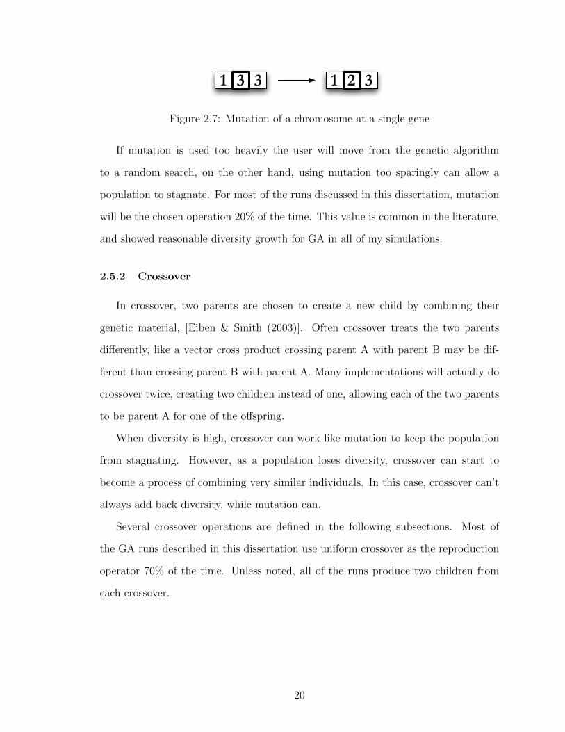
a new child. This is single point crossover as pictured in Fig. 2.8.

1 3 32 1 1

2 3 3

PA PB

Figure 2.8: Single point crossover with X = 1

Single point crossover can be restricted by the encoding scheme. For example, if

individuals can only be a fixed size, single point cross over has to use the same value

for X for both parents. However, if children can have a longer encoding than their

parents we can choose different values of X for each parent. If the encoding requires

specific groupings of genes, the crossover scheme can be customized to respect these

groupings when picking X.

2.5.2.2 Multipoint Crossover

Multi-point crossover, pictured in Fig. 2.9, is similar to single point crossover,

except that more than one crossover point X is selected. Like single-point crossover,

there are variations that allow the genes to grow or shrink. The number of points

used for crossover can range from 1, which is just single point crossover, to the total

number of elements in an individual. This limit is called uniform crossover.

21

1 3 32 1 1

2 3 1

PA PB

Figure 2.9: Multipoint crossover, with 2 points at 1 and 3

2.5.2.3 Uniform Crossover

In uniform crossover, each gene of the child is selected from one parent or the

other by coin-flip, at the same gene location. So, for example, if a child has 5 genes,

numbered 1 to 5, for the first gene you randomly pick parent A or parent B and take

their value for gene 1. Then you continue this process for the other 4 genes. This is

the same as doing multipoint crossover with a crossover point at every gene.

Uniform crossover may appear random at first glance. But as individuals approach

an optimized solution, and become more alike, the random choice between parents

becomes uneventful and will produce the same gene in either case.

Many of the projects performed for this dissertation attempt to optimize geometric

solutions where material is moved around in a two and three dimensional space.

Uniform crossover was chosen as the main crossover type because it allows a nice

random mixing of parents to create new children, see Section 5.6. Each gene for

our shielding problems will represent shield material at a specific location. Uniform

crossover will simply mix two shields, location by location.

Uniform crossover easily produces two children, by using parent A for the first

child’s and parent B for the second child’s gene for each slot. I will use it this way

throughout the dissertation.

22

2.5.3 Copy

The simplest operation in GA is copying. A parent is copied, or cloned, to create a

child. Copying is especially valuable in generational GA since it allows good individ-

uals, or bad individuals with some good genetic material, to stick around unchanged

between generations. Keep in mind that this idea of keeping good genetic material is

abstract, the GA itself has no concept of good versus bad material, only fitness scores

to judge individuals on. Most of the optimizations discussed in this dissertation have

a 10% chance of copy forward as the reproductive operator. This results in a stan-

dard break down for this dissertation of 10% copy forward, 70% crossover and 20%

mutation when an operation is required.

2.6 Results for the Shortest Path Problem

Now that we have a basic understanding of what a genetic algorithm is and the

standard operations, let’s take a look at how GA performs on the sample problem

from Section 2.2. We will look at the problem with two values of ψ to see how GA

deals with increasing the size of the search space.

2.6.1 The Shortest Path Problem with ψ = 8

To start, I will set ψ = 8. This means there will be 7 elements in the chromosome,

and each element can be an integer from 0 to 8. This results in a problem space of

size 97 = 4.78× 106, or about 5 million possible individuals.

The GA will use tournament selection with a tournament size of 5. There will

be a 25% chance of the worst individual being selected in a tournament. Each new

individual will be created using the following operational breakdown:

• 70% chance of single point crossover on reproduction

• 20% chance of mutation on reproduction

23

• 10% chance of copy on reproduction

GA will run for 40 generations with 2,500 individuals per generation. As a result,

the GA will test a total of 100,000 individuals. These individuals will not necessarily

be unique, so this is an upper bound. The GA will test less than 2% of the possible

solutions that use this encoding.

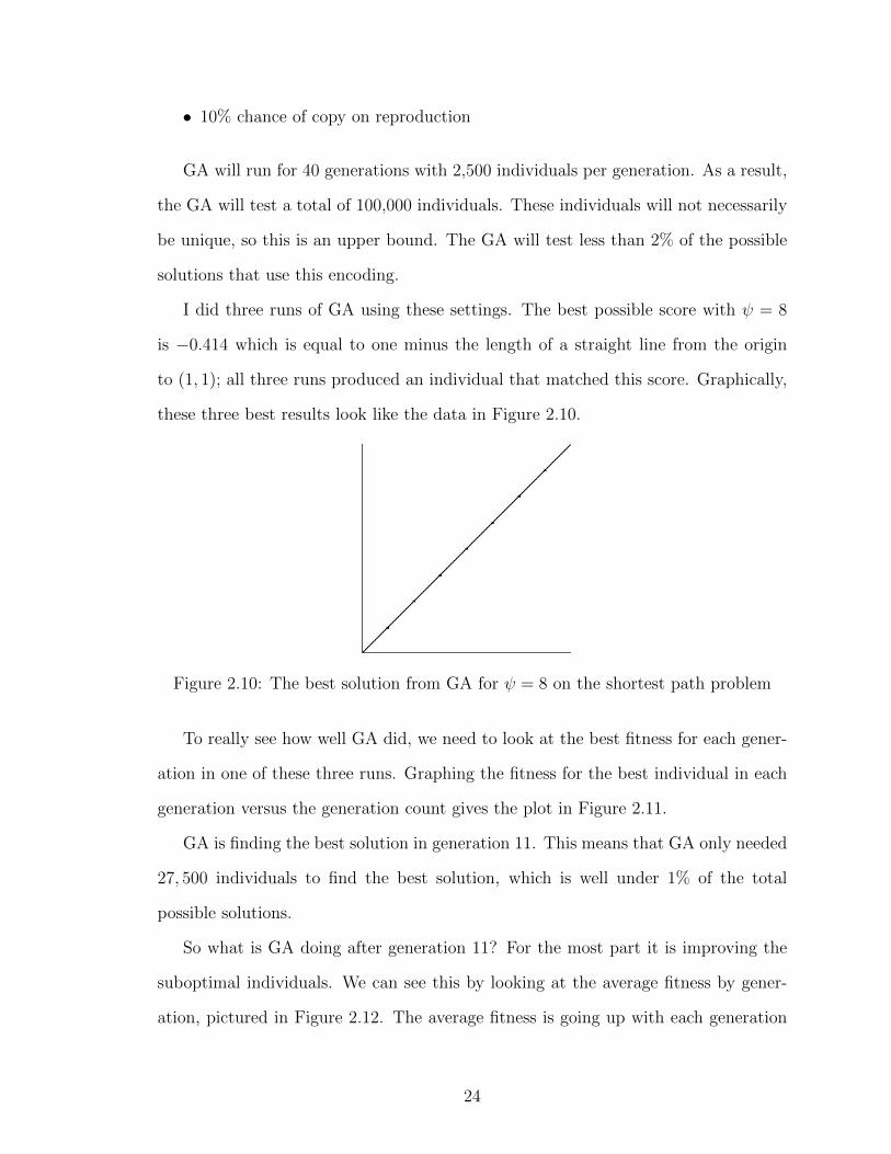
I did three runs of GA using these settings. The best possible score with ψ = 8

is −0.414 which is equal to one minus the length of a straight line from the origin

to (1, 1); all three runs produced an individual that matched this score. Graphically,

these three best results look like the data in Figure 2.10.

Figure 2.10: The best solution from GA for ψ = 8 on the shortest path problem

To really see how well GA did, we need to look at the best fitness for each gener-

ation in one of these three runs. Graphing the fitness for the best individual in each

generation versus the generation count gives the plot in Figure 2.11.

GA is finding the best solution in generation 11. This means that GA only needed

27, 500 individuals to find the best solution, which is well under 1% of the total

possible solutions.

So what is GA doing after generation 11? For the most part it is improving the

suboptimal individuals. We can see this by looking at the average fitness by gener-

ation, pictured in Figure 2.12. The average fitness is going up with each generation

24

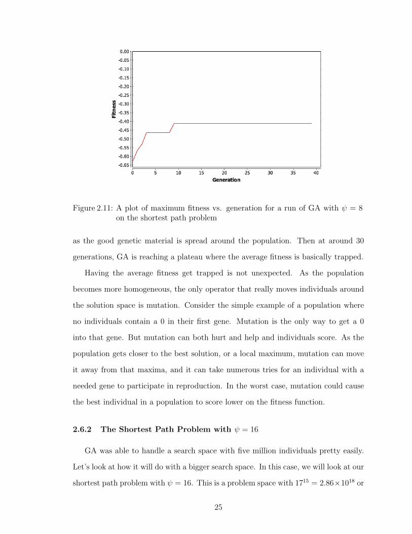
Figure 2.11: A plot of maximum fitness vs. generation for a run of GA with ψ = 8on the shortest path problem

as the good genetic material is spread around the population. Then at around 30

generations, GA is reaching a plateau where the average fitness is basically trapped.

Having the average fitness get trapped is not unexpected. As the population

becomes more homogeneous, the only operator that really moves individuals around

the solution space is mutation. Consider the simple example of a population where

no individuals contain a 0 in their first gene. Mutation is the only way to get a 0

into that gene. But mutation can both hurt and help and individuals score. As the

population gets closer to the best solution, or a local maximum, mutation can move

it away from that maxima, and it can take numerous tries for an individual with a

needed gene to participate in reproduction. In the worst case, mutation could cause

the best individual in a population to score lower on the fitness function.

2.6.2 The Shortest Path Problem with ψ = 16

GA was able to handle a search space with five million individuals pretty easily.

Let’s look at how it will do with a bigger search space. In this case, we will look at our

shortest path problem with ψ = 16. This is a problem space with 1715 = 2.86×1018 or

25

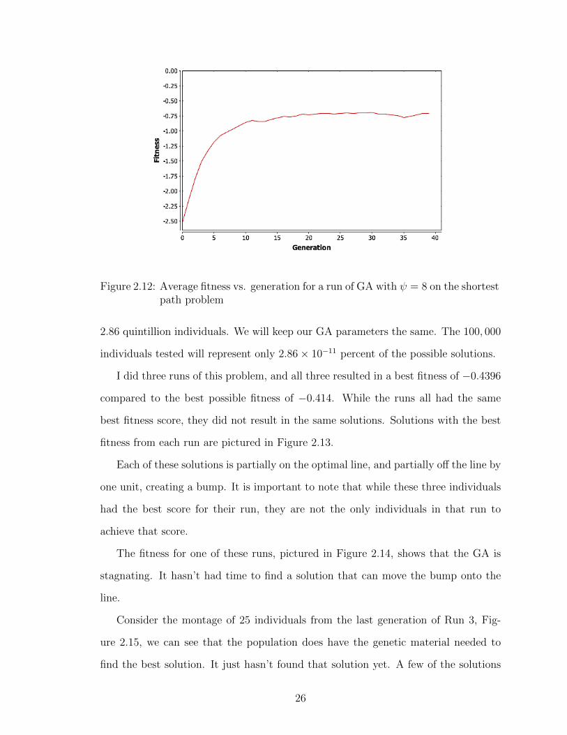
Figure 2.12: Average fitness vs. generation for a run of GA with ψ = 8 on the shortestpath problem

2.86 quintillion individuals. We will keep our GA parameters the same. The 100, 000

individuals tested will represent only 2.86× 10−11 percent of the possible solutions.

I did three runs of this problem, and all three resulted in a best fitness of −0.4396

compared to the best possible fitness of −0.414. While the runs all had the same

best fitness score, they did not result in the same solutions. Solutions with the best

fitness from each run are pictured in Figure 2.13.

Each of these solutions is partially on the optimal line, and partially off the line by

one unit, creating a bump. It is important to note that while these three individuals

had the best score for their run, they are not the only individuals in that run to

achieve that score.

The fitness for one of these runs, pictured in Figure 2.14, shows that the GA is

stagnating. It hasn’t had time to find a solution that can move the bump onto the

line.

Consider the montage of 25 individuals from the last generation of Run 3, Fig-

ure 2.15, we can see that the population does have the genetic material needed to

find the best solution. It just hasn’t found that solution yet. A few of the solutions

26

(a) Run 1 (b) Run 2

(c) Run 3

Figure 2.13: The best results from 3 runs of GA with ψ = 16 on the shortest pathproblem

27

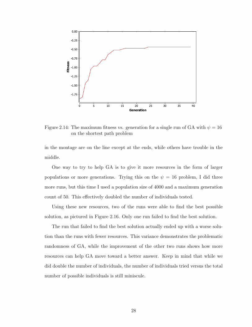
Figure 2.14: The maximum fitness vs. generation for a single run of GA with ψ = 16on the shortest path problem

in the montage are on the line except at the ends, while others have trouble in the

middle.

One way to try to help GA is to give it more resources in the form of larger

populations or more generations. Trying this on the ψ = 16 problem, I did three

more runs, but this time I used a population size of 4000 and a maximum generation

count of 50. This effectively doubled the number of individuals tested.

Using these new resources, two of the runs were able to find the best possible

solution, as pictured in Figure 2.16. Only one run failed to find the best solution.

The run that failed to find the best solution actually ended up with a worse solu-

tion than the runs with fewer resources. This variance demonstrates the problematic

randomness of GA, while the improvement of the other two runs shows how more

resources can help GA move toward a better answer. Keep in mind that while we

did double the number of individuals, the number of individuals tried versus the total

number of possible individuals is still miniscule.

28

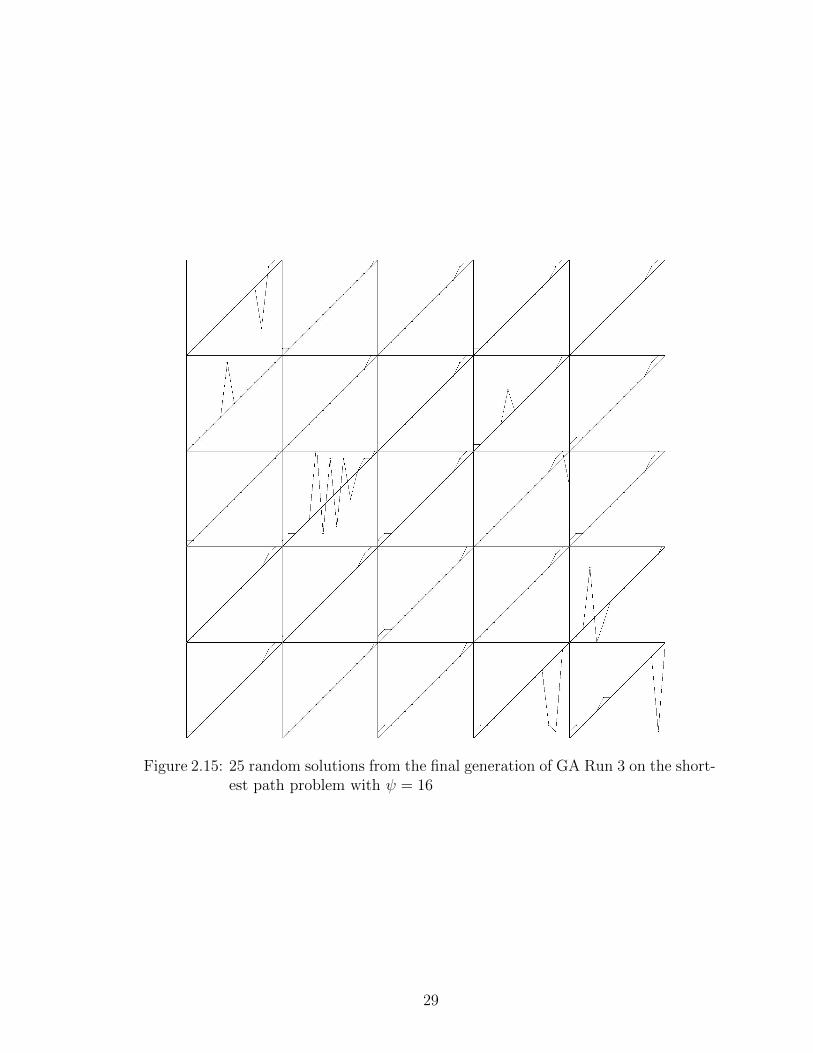
Figure 2.15: 25 random solutions from the final generation of GA Run 3 on the short-est path problem with ψ = 16

29

(a) Run 1 (b) Run 2

(c) Run 3

Figure 2.16: The best results from 3 runs of GA with ψ = 16 on the shortest pathproblem with more resources

30

2.7 Population Sizing and the Number of Generations

The test problem has lead us to an interesting question. How big should a popu-

lation be for a given problem?

At the lower end, GA needs a population that is big enough to have sufficient

diversity. For example, if we use ψ = 4 and a population of 2 there will not be

enough diversity to try to solve the problem. In order to formalize this idea of

sufficient information, researchers have decomposed the Genetic Algorithm into a set

of requirements. One decomposition that has been proposed, [Goldberg (1989)] , and

used extensively relies on the concept of building blocks. Building blocks, [Goldberg

et al. (1991)], are the elements that can be used to make solutions. In our sample

problem the building blocks would simply be the individual points, or possibly chains

of values that fall on the line that makes the best solution. Building blocks are a

very abstract idea that tries to provide a concept for the useful information chunks

encoded in a chromosome. In biology a building block might be the set of genes that

create the heart or lungs.

The building block decomposition works like this:

1. Know what the GA is processing: building blocks

2. Ensure an adequate supply of building blocks, either initially or temporarily

3. Ensure the growth of necessary building blocks

4. Ensure the mixing of necessary building blocks

5. Encode problems that are building block tractable or can be recoded so that

they are

6. Decide well among competing building blocks

31

The population size question address the second item of this decomposition: en-

suring an adequate supply. The genetic operators like crossover and mutation ensure

the growth of necessary blocks. Selection, along with the operators, ensures proper

mixing. The chromosome encoding and fitness function address the last two pieces

of this decomposition. We could re-write this decomposition using the terms we have

been using to say:

1. Encode problems in a way that works well with mutation and crossover

2. Ensure an adequate and diverse population

3. Ensure that mutation and crossover can reach all of the genes

4. Define a good fitness function

If we consider that the initial population for GA is usually generated randomly,

it is easy to see that a very small population size could prevent GA from having all

of the necessary building blocks in the initial population. If this were the case, GA

would have to try to use mutation to create these building blocks, which could be

quite inefficient. As a result, we can theorize that given limited resources there is a

population size that is too small for GA to build a solution in a reasonable amount

of time.

Population sizing is bounded from above based on computing resources. While

there are no papers saying that an infinite population is bad, it would require infinite

resources. So as GA is applied to a problem, researchers want to find the smallest

population that will still allow GA to work. Moreover, because a small population

provides more opportunity for two specific individuals to crossover, small populations

have the potential to evolve faster during the initial generations. Large populations,

on the other hand, will have a harder time putting two specific individuals together,

which can result in slower evolution.

32

One attack on the population sizing problem is given by Harik [Harik et al.

(1997)]. In this paper the building blocks that represent parts of a good solution

are treated as individuals that might be removed from the population via standard

operators and selection, a form of gambler’s ruin. Using this concept Harik et.al.

show that problems that require more building blocks are more susceptible to noise

and thus more susceptible to failure. They were also able to show that while this

semi-obvious connection exists it is not a scary one. The required population size for

a problem is shown to grow with the square root of the size of the problem, as defined

as the number of building blocks in a chromosome.

Another look at the sizing problem was done by [Goldberg et al. (1991)]. Goldberg

et.al. used an analysis of noise in the GA to show that the required population size

is O(l) where l is the length of a chromosome, or encoding. The multiplier for this

equation can depend on χ, the number of possible values for each element in the

chromosome, which is a fixed value for the problem.

These two analysis used different techniques to arrive at a scaling, and resulted

in different values. Harik’s analysis says that the required population goes with the

square root of the number of building blocks, while Goldberg’s analysis says that it

increases linearly. While both analysis rely on assumptions that make them inexact,

we can at least see that GA does not appear to require a population size that grows

exponentially or with some power of the problem size.

On the other side of the table is the question of how many generations we should

run. [Goldberg & Deb (1991)] have analyzed this problem as well to show that

using standard selection mechanisms GA should converge in O(log(n)) or O(n log(n))

generations, where n is the population size. While this equation doesn’t give us an

exact value for the number of generations to use, it does tell us that adding generations

is not going to give us exponential improvement. It also explains the shape of the

fitness graphs in Figures 2.11 and 2.14, where we could see the slope of the fitness

33

improvements going down with each generation.

In all of the experiments presented in this dissertation, the population sizes and

generation counts have been arrived at primarily through resources constraints. I

have tried to find a compromise between computing resources and reasonable results

from the GA.

2.8 GA For Hard Problems

As we saw in Section 2.6, even a simple problem description can result in a huge

problem space. As the problem spaces get bigger, the problems get harder to solve.

Hard problems can also be defined by the amount of resources they require to calcu-

late a fitness function. In this dissertation I will be discussing problems that require

radiation transport simulations to calculate a fitness score. These problems can run

for minutes or hours, as opposed to the microsecond test times of the shortest path

problem. As people have tried to apply GA to harder problems, they have reached

a point where a single computer cannot provide sufficient resources for their prob-

lem. When this happens, the Genetic Algorithm has to be distributed to multiple

computers.

Luckily, GA has an inherent parallelism. The most expensive part of GA is gen-

erally the scoring step and the process of scoring individuals can be distributed quite

easily. In this section I will discuss a number of the techniques used to distribute GA

onto multiple processors and machines.

Hard problems can also introduce other issues into standard GA. Sometimes di-

versity becomes an issue in a very large problem space. Populations can converge

too quickly, or not quickly enough due to resource constraints. Some of the following

techniques have been created to help change the diversity from the standard algorithm

or distribute on a network, or both. These techniques are important to understand

so that they can be contrasted with our new approach, MGGA.

34

2.8.1 Simple Distributed Genetic Algorithms

Perhaps the simplest way to distribute GA is to distribute the scoring phase using

some form of messaging passing technology like MPI. Distributing GA using messag-

ing passing involves running numerous agents. Most of the agents score individuals

in the genetic run. A central, or master, agent performs the initial population cre-

ation, hands out scoring work, coalesces scoring results and performs reproduction.

By scaling the number of agents, the scoring work can be scaled to any number of

machines.

Distributed GA relies on data sharing to pass scores from the scoring workers

to the scaling worker. Some form of synchronization must be provided to keep each

agent doing work at the right time, and waiting while new work is created. Simple GA

codes will generally use memory to hold populations, but by leveraging a shared file

system, database or distributed cache, these techniques can support gigantic problems

[SQLite (2011)].

Ironically, the biggest drawback of these distributed GA is that it doesn’t change

the underlying algorithm. If diversity is a problem for a specific application, distribut-

ing it won’t increase the diversity. Distribution simply adds processing power. The

next few sections discuss techniques that have been used to alter the fundamental

algorithm. These can be combined with simple distributed Genetic Algorithms, or

be distributed themselves.

2.8.2 Island Model Genetic Algorithms

The island model of GA, [Eby et al. (1999); Tomassini (2005)], breaks a single

Genetic Algorithm run into a set of runs. Each run uses the standard iterative

approach discussed in 2.3. What makes the island model different than running

a bunch of separate GAs, is that individuals from each population, or island, are

traded with other islands. So individuals from one run will migrate to, or be injected

35

into, another run. This immigration model allows the sharing of genetic material and

can add diversity by adding variety to a stagnating population.

The island model is the basis for most of the distributed algorithms used for GA

by other researchers. It can be altered to allow things like different fitness functions

for each island, or different GA parameters for each island. In Chapter III we will see

how MGGA is similar to the island model, except that we will not be performing im-

migration every generation or two, rather we will be using a hierarchy of populations,

that could be thought of as islands.

2.8.3 Pyramidal Genetic Algorithms

In pyramidal GA, [Aickelin (2002)], a number of islands or agents are used to

perform separate Genetic Algorithms. Each agent uses a different fitness function to

score individuals. These individuals are then combined, or injected into a different

agent that uses a higher order fitness function. For example, one agent might score

a shield on mass, while another scores it on shielding quality. The final population

is generated from shields that are good for mass, combined with those that are good

for shielding, and GA is performed on this combination population. The final agent

would use a fitness that scales for both mass and shielding.

2.8.4 Multiscale Genetic Algorithms

Multi-scale GA, [M Babbar (2002)], is a version of the island model where the

fitness functions for each island leverage some sort of scaling in the fitness function.

For example, one island might use a coarse grid, while another uses a fine grid, to score

individuals, [Babbar & Minsker (2003)]. This technique is one of the motivators for

MGGA. Multi-scale GA allows some of the islands to perform quick fitness tests using

low resolution models, while other islands use higher resolution models to determine

higher quality fitness values.

36

2.8.5 Hierarchical Genetic Algorithms

Hierarchical GA, [De Jong (2011)], is a term used for a version of the island model

that is similar to Multiscale GA and Pyramidal GA. Essentially the islands form a

hierarchy, where each looks for individuals based on a subset of the total criteria, and

those individuals are used to feed islands looking at more criteria. Hierarchical GA

has primarily been implemented as part of Genetic Programming to protect functions

or other modules that have been found in the lower level islands.

2.8.6 Messy Genetic Algorithms

Another technique used to apply GA to hard problems is called Messy Genetic

Algorithms, [Goldberg et al. (1993)]. Messy Genetic Algorithms use genes to encode

name-value pairs so they can change size without breaking the standard operator

semantics. The MessyGA uses a series of phases, [Merkle et al. (1998)], just like

generational GA, but the phases are slightly different. First, there is an initialization

phase. This phase is used to create all of the fundamental building blocks, but not

all of the possible individuals. In our sample problem this would mean making sure

that at least one individual had each of the appropriate points, but not necessarily all

of the appropriate points. In a shielding problem, this might mean making sure that

we have at least one individual with each part of the shield geometry included. For

very large problem spaces, this rule can be reduced to simply try to create as many

as the resources support.

After initialization, MessyGA uses a primordial phase composed of alternating

tournament selection and building block filtering (BBF). The tournament selection

finds fit individuals, and BBF deletes genes. Individuals that can have genes deleted

and are still highly fit are passed into the next phase. The next phase is called

juxtaposition. In this phase, individuals are recombined to build better individuals.

These phases are often distributed across multiple machines.

37

Messy GA focuses on the building block concept by trying to ensure that all of

the good building blocks are available and that these building blocks are highlighted

and combined into highly fit individuals. Messy GA has been written in a highly

parallel fashion to support hard problems and its building block nature helps it focus

on preserving good building blocks even in limited populations.

2.9 Genetic Algorithms on an Off-The-Shelf Cluster Sched-

uler

The problems discussed later in this dissertation are “hard problems.” They have

large solution spaces, and they require a lot of computing resources to score. Luckily

a large cluster is available at the University of Michigan. This section discusses why

I developed a genetic algorithm library to execute GA on the U of M cluster.

The U of M cluster uses the Portable Batch System (PBS) scheduler, see [pbs

(2011)]. This is a very standard, open source, cluster job scheduler. In order to put

GA onto the Michigan cluster and scheduler I had to stay within a set of restrictions.

1. All jobs for a genetic run must be scheduled in advance.

2. Jobs must be assigned an estimated time.

3. Jobs are only given their estimated time to complete, plus a margin for error.

4. Jobs that run over their time, plus the margin, are treated as failed and killed.

5. The longer the estimated time for a job, the lower priority it has.

6. Jobs can depend on one or more other jobs, in a flexible manner.

7. There is a line length associated with listing dependencies.

8. My jobs running on another user’s nodes can be interrupted.

38

9. Jobs have access to a shared file system.

Estimating time, dealing with errors for fault tolerance and working around line

length limits are the main issues with leveraging the existing cluster. Moreover, in

order to scavenge the most resources, my code had to be resilient to interruptions.

The PBS scheduler doesn’t like to schedule many long running jobs for a single user on

shared computers. Having long running jobs reduced our resource usage by reducing

our priority. Finally, the cluster administrators didn’t want my jobs to schedule other

jobs to solve this problem.

Considering these restrictions I decided to leverage the PBS scheduler as the

master node and use the job running nodes as the scoring slaves in a distributed GA.

In order meet the restrictions I also replaced the message passing design with a batch

design. Instead of agents running all of the time, a series of jobs is scheduled for each

phase in the GA process. For example, a job builds the initial population, a set of

jobs score the population, a job processes the scores, a job performs reproduction,

etc.. As with the message passing design, batch distributed GA can be scaled to

fill available computing resources. Unfortunately, there are no GA libraries, that I

could find, that support the concept of the batch-oriented distributed GA on this

type of job scheduler, with my resource restrictions. As a result, I implemented batch

distributed GA in a custom library called Genetik, discussed in Appendix A.

I was unable to find any reference to this style of distributed GA in the literature

and as a result, this implementation of batch GA in the context of a job scheduler

appears to be a new technique.

2.9.1 Generational GA As Jobs

Genetik uses the following basic job types to do the actual work:

Build Build a population, either randomly or from a previous one.

39

Score Score a sub-set of a population.

Collect And Scale Join the scored sub-sets and perform any fitness score scaling

we want to do.

The input file for Genetik includes how many individuals should be included in

each generation and how many generations to increment over. Genetik uses this

information to schedule one build job for each generation and one collect and scale

job for each generation. The input file also contains the size of the scoring populations.

Genetik uses this information to schedule enough scoring jobs to cover the population.

The build job uses a cache of all previously scored individuals to ensure that no

individual is scored in two different generations. It is possible that the same individual

is scored by 2 scoring jobs, but it will not be scored again in a later generation.

The genetik input file also contains time estimates for each job type. These are

included in the PBS job description files.

2.9.2 Dealing with Dependency Limits

PBS has a line length limit for describing dependencies. This restriction is at

odds with our desire to scavenge as many computing resources as possible. In order

to scavenge all possible resources we want to run a lot of short running jobs, rather

than a few long running jobs. Having a lot of scoring jobs for each generation places

a long dependency list on the Collect and Scale job that follows them. In order to

coalesce these dependencies into reasonable line lengths, I use no-op jobs called Joins.

These jobs do nothing, but do have dependencies. Using a 5-to-1 scaling I can quickly

reduce a large number of scoring jobs into a small number of Join jobs that can be

depended on by the Collect job.

40

2.9.3 Dealing with Errors

Scoring jobs can fail; the easiest way this can happen is if we underestimate the

time it takes to score an individual. I have built in some resilience against scoring jobs

failing. This resilience comes in the form of a repair step in the collection process.

Repairs simply replace an individual that couldn’t be scored with a random, scored,

individual.1

2.9.4 Processing

The final step in my implementation of GA on the PBS scheduler was to add

pre-processing and post-processing jobs. These jobs allow different runs to initialize

data sets, and to build reports. Also, the standard post processing step cleans up the

PBS job descriptions.

These two new jobs, along with the others I have described result in the following

mapping of GA onto the PBS scheduler.

Pre-Process Perform any initialization.

Build Build a population, either randomly or from a previous one.

Score Score a sub-set of a population by running a radiation transport code multiple

times.

Join Join scoring jobs, treated as dependency lists, into 4 or fewer dependencies.

Collect And Scale Make sure that the scoring jobs worked, and if not replace indi-

viduals that didn’t get scored with random copies from their parent generation.

Join the scored sub-sets and perform any scaling we want to do.

Post-Process Build a report of the results and clean up unneeded files.

1I only take scored individuals for repairs, to insure that failed scoring jobs aren’t propagated tothe next generation.

41

To iterate over generations, I unroll the loops associated with generational GA.

This design has been tested with numerous runs on the Michigan cluster called NYX

and provides good cluster usage, some runs used over 40 machines across several

hundred jobs.

2.9.5 Genetik On A Proprietary Cluster

For parts of this dissertation, funded by a grant, I was able to reserve time on

the U of M cluster. This allowed me to move to a single job that ran GA and used

an MPI version of MNCP to leverage the clusters computing resources. This single

job model is not unique and is very powerful, but was only available after I obtained

reserved computing resources, so that my single jobs could run for days. This type of

long running job would not work when I was scavenging resources. The single large

job with MPI-based MCNP performed similarly to the batch model, but was easier

for the cluster administrators to support.

2.9.6 Optimizing GA

The Genetik library included two mechanisms to try to reduce fitness function

executions, caching and pre-calculating. These two methods optimize the time spent

on the cluster.

Caching involves remembering or at least checking the scores of individuals against

the fitness functions that have already been run before executing their fitness function.

On a very fast problem, like the shortest path, this is not very useful. But for the

problems discussed in this dissertation where a fitness evaluation can take more than

ten minutes, the time spent building and checking a cache becomes a very good

investment. Genetik builds a cache from previous generations before scoring the

next generation. This cache maps the chromosome for an individual to a score. By

caching in this way, GA can save scoring time even if an individual disappears from

42

the population and reappears in a later generation.

When Genetik was being written I had a novel idea that we could pre-determine all

of the work we would have to do before we start running. Using this information, we

could eliminate fitness function executions by finding individuals that never reproduce

and not scoring them. I implemented this concept, called pre-calculation, by building

a plan for each generation that included which individuals would be chosen with

selection, which were mutated, which were copied and which participated in crossover

to create the next generation. By finding which individuals were never chosen I was

able to avoid scoring them. This method does not actually know which individuals

will exist, it depends on indices into the population. So the plan might say, perform

a tournament on 1,5,20,54 and 100 and create a child by mutating the winner. We

don’t know which will win, but we do know that we need to score the individuals at

those five indices in the population to run the tournament.

The first version of Genetik implemented pre-calculation, but it turned out that

very few individuals were skipped. This is a good thing. Tournament selection does

a very good job of allowing almost every individual to participate in tournaments.

So almost every individual at least has a chance to reproduce. While pre-calculation

appears to be a novel idea, and I was unable to find it in any prior work, it doesn’t

appear to be an incredibly useful idea, so I removed it from the second version of

Genetik, greatly simplifying the code.

2.10 Summary

Genetic Algorithms are a very powerful technique for finding solutions to hard

problems. Using a few standard operators, GA is able to find solutions in huge search

spaces without examining the entire space. Solutions are assigned a value using a

fitness function. Execution of the fitness functions can be distributed allowing GA to

work in parallel, making it even more powerful. Using the cluster at the University

43

of Michigan I was able to build an implementation of GA that would run in a batch

mode and take advantage of free computing resources.

In the next chapter I will discuss a novel technique for dealing with a hard problems

that allowed me to find solutions to three hard radiation shielding design problems

despite their complexity and the large run time of their fitness tests. This new

technique, called MGGA, is a powerful tool for driving GA to good solutions quickly.

44

CHAPTER III

Multi-Grid Genetic Algorithms

3.1 Introduction

Radiation transport problems are often modeled using Monte Carlo simulations,

[Fishman (2006)]. These simulations can take a very long time to run, often on the

order of hours. If we put these simulations in the context of Genetic Algorithms a

problem emerges. The generation and population sizes required by GA go up with the

problem complexity. As a result, GA wants to do thousands or even millions of fitness

function computations for a large problem space. If we are running Monte Carlo, say

MCNP [Monte Carlo Codes Group - Los Alamos National Laboratory (2011)], for

each fitness function and that MCNP run takes 10 minutes to complete, we are

talking about hundreds of thousands of minutes, or potentially tens of thousands of

computing hours to complete a simple GA run. Had I been working at a national

lab, this type of computing time may have been easy to acquire. But as a graduate

student I was faced with a conundrum. How can I use GA on expensive problems?

There are a number of existing models of parallel GA, [Cant-paz (1998)]. My first

thought was to use some kind of island model, [Skolicki (2005)]. This model generally

relies on at least one job per island executing for the duration of the run. Other

master-slave models I looked at including [Berntsson & Tang (2005)] and [Sullivan

et al. (2008)] also rely on a master node. This master node is a single long running

45

process to manage the GA work. In all of the architectures I found at least one job

was expected to run for a long time. Moreover, this job was often responsible for

scheduling work. The best computing resources available to me were in the form of

a cluster that used an existing scheduler, discussed in Section 2.9. In this context, it

would be hard for me to execute numerous GA runs if it meant many long running

jobs.

Luckily, from constraints grows creative solutions, [Heath & Heath (2007)], and

from limited computing resources with a desire to look at GA for radiation shielding

applications comes Multi-Grid Genetic Algorithms and a library for running them on

an existing scheduler.

Multi-Grid Genetic Algorithms are a new class of GA in which we leverage geo-

metric features in a problem space to build a hierarchy of problem spaces and reduce

the number of fitness function evaluations required to reach a good solution. Nor-

mally GA starts with a random population. This can create a lot of diversity, which

is good. It also requires GA to work through a lot of potentially bad genetic material,

which is bad. The question is, can we create a better starting population without

losing good diversity. MGGA is a mechanism for exploring this question.

In MGGA we start with a complex problem space. Take the example from Sec-

tion 2.2 where each element of the chromosome is an integer from 0 to ψ. If we start

with ψ = 32, there are 31 integers per chromosome, with each integer ranging from 0

to 32. This is equivalent to a search space with 3331 individuals. However, if we start

with ψ = 4, we have a search space with only 53 individuals. By running GA on the

ψ = 4 problem space, we can get some reasonable solutions for that space. Then we

can tranlate these solutions to a ψ = 8 version of the problem space, run GA again

and get new solutions that are closer to what we want in the final ψ = 32 problem

space.

We will call the different executions of GA for our MGGA phases. So in this

46

example, phase one is a GA with ψ = 4, phase two is a GA with ψ = 8 and phase

three is a GA with ψ = 32. The individuals in the final generation of phase one are

used to generate the initial population for phase two. The individuals in the final

generation of phase two are used to generate the initial population for phase three.

The process of moving individuals between phases is called translation.

MGGA works in problems where the solutions can be mapped between phases.

For example, the solutions in the ψ = 4 space can be mapped to the final ψ = 32

problem space by adding points, as will be described in Section 3.2 below. This

means that the fitness function can be written in such a way that the fitness of

this individual remains the same in both the lower resolution space and the higher

resolution space. Unlike hierarchical GA, [De Jong (2011)], pyramidal GA, [Aickelin

(2002)], or multiscale GA, [Babbar & Minsker (2003)], which build on different fitness

functions to lead to a final result, MGGA uses a single fitness function across a range

of problem spaces. In essence, the early phases of the MGGA are constraining the

possible solutions to try.

MGGA works by creating good building blocks over a restricted, coarsened, ver-

sion of the search space. Then MGGA uses these building blocks to seed the initial

population on a finer version of the search space. This process is applied recursively

so that a fine search space can be explored rapidly at successively coarser levels. In

order for MGGA to work, there must be a reasonable hierarchy in the search space.

Moreover, as we will see in the next section, the problem must have building blocks

that make sense across the hierarchy. When this precondition is met, MGGA is

able to create larger building blocks more quickly than GA because it does so in the

coarser, restricted, search space while GA has to build all of its building blocks in the

finest space where there are more non-optimal solutions to weed out.

47

3.2 Translation

MGGA is run as a set of Genetic Algorithms performed in serial. These phases

each perform a complete generational Genetic Algorithm run. Between phases a

translator is used to move the encoding for each individual from one problem space

to the next. As a result of this translation phase, MGGA introduces a number of

new parameters to Genetic Algorithms, including the method for translation and the

method for picking individuals to translate when moving between phases.

3.2.1 Translation and Population Size

Each phase in an MGGA can use a completely different set of the standard GA

parameters. This means that you could use a different type of crossover in each

phase, or a different percentage of crossover, versus mutation. For the experiments

performed for this dissertation, I have tried to minimize the changes from one phase

to the next. The only real change is in the size of the populations and the number

of generations tested for each phase. By using a small number of generations and

a small population for earlier stages, we can scale the total resources used, and also

focus them on the more complex problem spaces in later phases.

In order to move between a smaller population and a larger one I use the stan-

dard selection mechanisms, see Section 2.4. In particular, I use tournament selection

throughout this dissertation. By using selection to get individuals from one phase

to the next we can think of the translation process as just another, albeit special,

genetic operation like the ones discussed in Section 2.5.

3.2.2 Translation between Encodings

The translation operation is basically a recoding of the genome. Each individ-

ual from one phase is mapped to the equivalent individual for the next phase. For

geometric problems we can make this mapping exact if we use an appropriate scale.

48

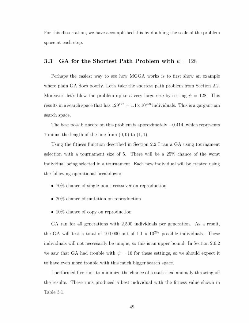
For this dissertation, we have accomplished this by doubling the scale of the problem

space at each step.

3.3 GA for the Shortest Path Problem with ψ = 128

Perhaps the easiest way to see how MGGA works is to first show an example

where plain GA does poorly. Let’s take the shortest path problem from Section 2.2.

Moreover, let’s blow the problem up to a very large size by setting ψ = 128. This

results in a search space that has 129127 = 1.1×10268 individuals. This is a gargantuan

search space.

The best possible score on this problem is approximately −0.414, which represents

1 minus the length of the line from (0, 0) to (1, 1).

Using the fitness function described in Section 2.2 I ran a GA using tournament

selection with a tournament size of 5. There will be a 25% chance of the worst

individual being selected in a tournament. Each new individual will be created using

the following operational breakdown:

• 70% chance of single point crossover on reproduction

• 20% chance of mutation on reproduction

• 10% chance of copy on reproduction

GA ran for 40 generations with 2,500 individuals per generation. As a result,

the GA will test a total of 100,000 out of 1.1 × 10268 possible individuals. These

individuals will not necessarily be unique, so this is an upper bound. In Section 2.6.2

we saw that GA had trouble with ψ = 16 for these settings, so we should expect it

to have even more trouble with this much bigger search space.

I performed five runs to minimize the chance of a statistical anomaly throwing off

the results. These runs produced a best individual with the fitness value shown in

Table 3.1.

49

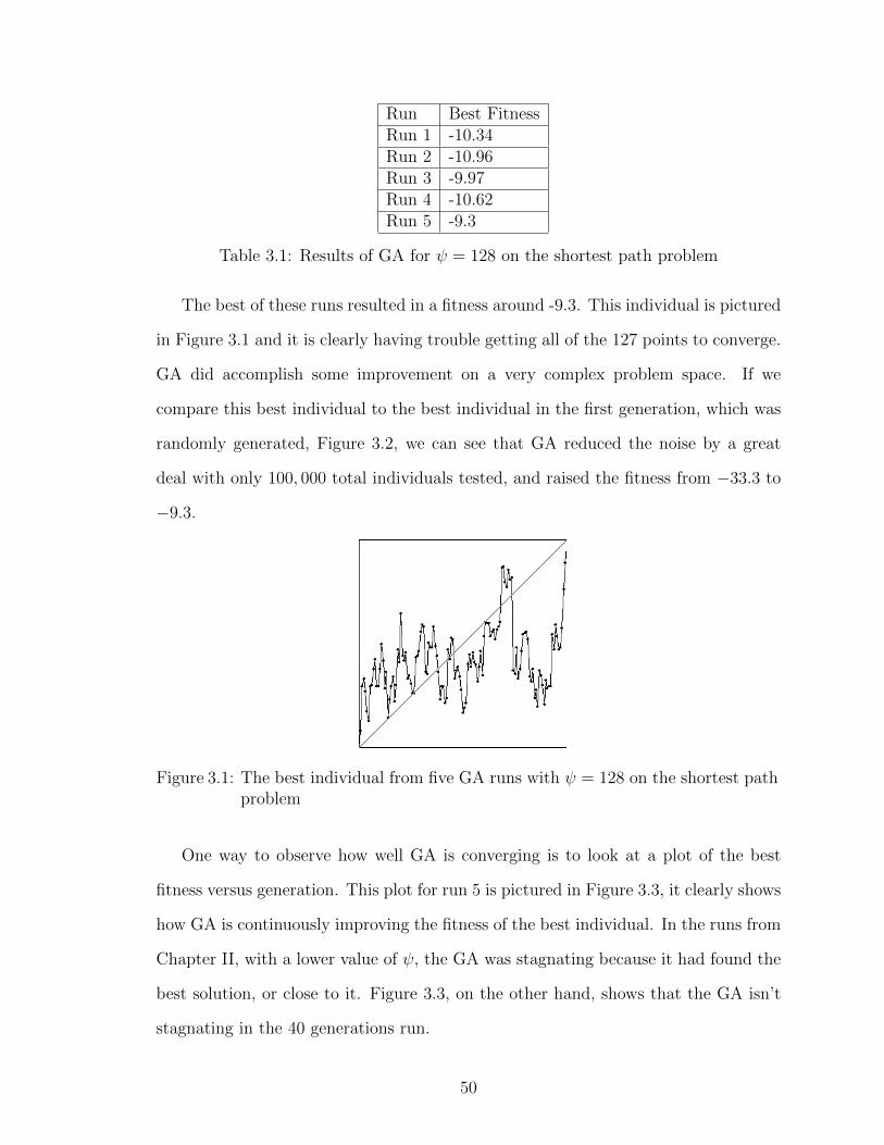
Run Best FitnessRun 1 -10.34Run 2 -10.96Run 3 -9.97Run 4 -10.62Run 5 -9.3

Table 3.1: Results of GA for ψ = 128 on the shortest path problem

The best of these runs resulted in a fitness around -9.3. This individual is pictured

in Figure 3.1 and it is clearly having trouble getting all of the 127 points to converge.

GA did accomplish some improvement on a very complex problem space. If we

compare this best individual to the best individual in the first generation, which was

randomly generated, Figure 3.2, we can see that GA reduced the noise by a great

deal with only 100, 000 total individuals tested, and raised the fitness from −33.3 to

−9.3.

Figure 3.1: The best individual from five GA runs with ψ = 128 on the shortest pathproblem

One way to observe how well GA is converging is to look at a plot of the best

fitness versus generation. This plot for run 5 is pictured in Figure 3.3, it clearly shows

how GA is continuously improving the fitness of the best individual. In the runs from

Chapter II, with a lower value of ψ, the GA was stagnating because it had found the

best solution, or close to it. Figure 3.3, on the other hand, shows that the GA isn’t

stagnating in the 40 generations run.

50

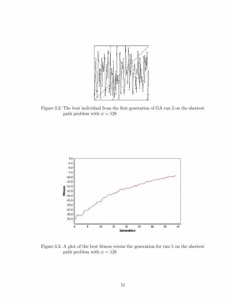
Figure 3.2: The best individual from the first generation of GA run 2 on the shortestpath problem with ψ = 128

Figure 3.3: A plot of the best fitness versus the generation for run 5 on the shortestpath problem with ψ = 128

51

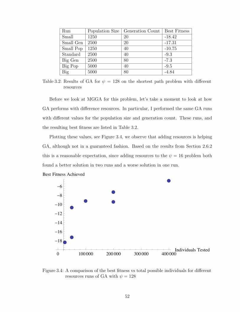
Run Population Size Generation Count Best FitnessSmall 1250 20 -18.42Small Gen 2500 20 -17.31Small Pop 1250 40 -10.75Standard 2500 40 -9.3Big Gen 2500 80 -7.3Big Pop 5000 40 -9.5Big 5000 80 -4.84

Table 3.2: Results of GA for ψ = 128 on the shortest path problem with differentresources

Before we look at MGGA for this problem, let’s take a moment to look at how

GA performs with difference resources. In particular, I performed the same GA runs

with different values for the population size and generation count. These runs, and

the resulting best fitness are listed in Table 3.2.

Plotting these values, see Figure 3.4, we observe that adding resources is helping

GA, although not in a guaranteed fashion. Based on the results from Section 2.6.2

this is a reasonable expectation, since adding resources to the ψ = 16 problem both

found a better solution in two runs and a worse solution in one run.

ÊÊ

ÊÊ Ê

Ê

Ê

0 100000 200000 300000 400000Individuals Tested

-18

-16

-14

-12

-10

-8

-6

Best Fitness Achieved

Figure 3.4: A comparison of the best fitness vs total possible individuals for differentresources runs of GA with ψ = 128

52

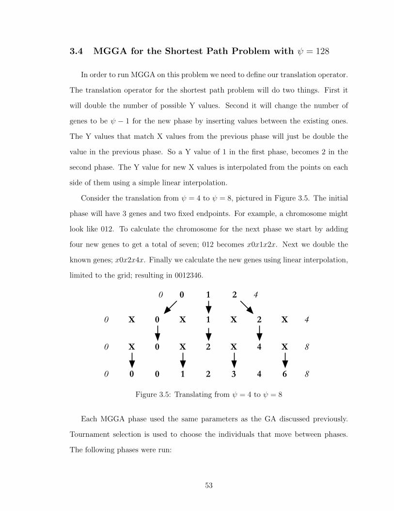
3.4 MGGA for the Shortest Path Problem with ψ = 128

In order to run MGGA on this problem we need to define our translation operator.

The translation operator for the shortest path problem will do two things. First it

will double the number of possible Y values. Second it will change the number of

genes to be ψ − 1 for the new phase by inserting values between the existing ones.

The Y values that match X values from the previous phase will just be double the

value in the previous phase. So a Y value of 1 in the first phase, becomes 2 in the

second phase. The Y value for new X values is interpolated from the points on each

side of them using a simple linear interpolation.

Consider the translation from ψ = 4 to ψ = 8, pictured in Figure 3.5. The initial

phase will have 3 genes and two fixed endpoints. For example, a chromosome might

look like 012. To calculate the chromosome for the next phase we start by adding

four new genes to get a total of seven; 012 becomes x0x1x2x. Next we double the

known genes; x0x2x4x. Finally we calculate the new genes using linear interpolation,

limited to the grid; resulting in 0012346.

0 1 2

0 X 1 X 2

0 X 2 X 4

0 1 2 3 4

X X

X X

0 6

40

0 4

8

8

0

0

Figure 3.5: Translating from ψ = 4 to ψ = 8

Each MGGA phase used the same parameters as the GA discussed previously.

Tournament selection is used to choose the individuals that move between phases.

The following phases were run:

53

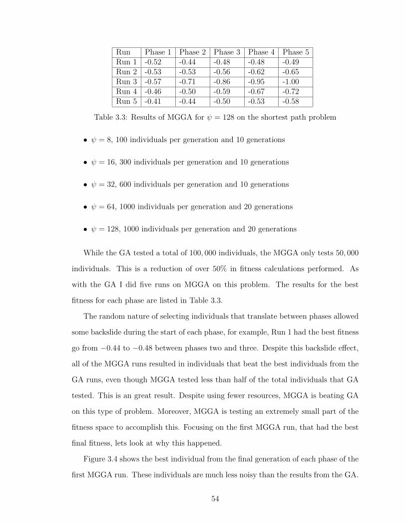
Run Phase 1 Phase 2 Phase 3 Phase 4 Phase 5Run 1 -0.52 -0.44 -0.48 -0.48 -0.49Run 2 -0.53 -0.53 -0.56 -0.62 -0.65Run 3 -0.57 -0.71 -0.86 -0.95 -1.00Run 4 -0.46 -0.50 -0.59 -0.67 -0.72Run 5 -0.41 -0.44 -0.50 -0.53 -0.58

Table 3.3: Results of MGGA for ψ = 128 on the shortest path problem

• ψ = 8, 100 individuals per generation and 10 generations

• ψ = 16, 300 individuals per generation and 10 generations

• ψ = 32, 600 individuals per generation and 10 generations

• ψ = 64, 1000 individuals per generation and 20 generations

• ψ = 128, 1000 individuals per generation and 20 generations

While the GA tested a total of 100, 000 individuals, the MGGA only tests 50, 000

individuals. This is a reduction of over 50% in fitness calculations performed. As

with the GA I did five runs on MGGA on this problem. The results for the best

fitness for each phase are listed in Table 3.3.

The random nature of selecting individuals that translate between phases allowed

some backslide during the start of each phase, for example, Run 1 had the best fitness

go from −0.44 to −0.48 between phases two and three. Despite this backslide effect,

all of the MGGA runs resulted in individuals that beat the best individuals from the

GA runs, even though MGGA tested less than half of the total individuals that GA

tested. This is an great result. Despite using fewer resources, MGGA is beating GA

on this type of problem. Moreover, MGGA is testing an extremely small part of the

fitness space to accomplish this. Focusing on the first MGGA run, that had the best

final fitness, lets look at why this happened.

Figure 3.4 shows the best individual from the final generation of each phase of the

first MGGA run. These individuals are much less noisy than the results from the GA.

54

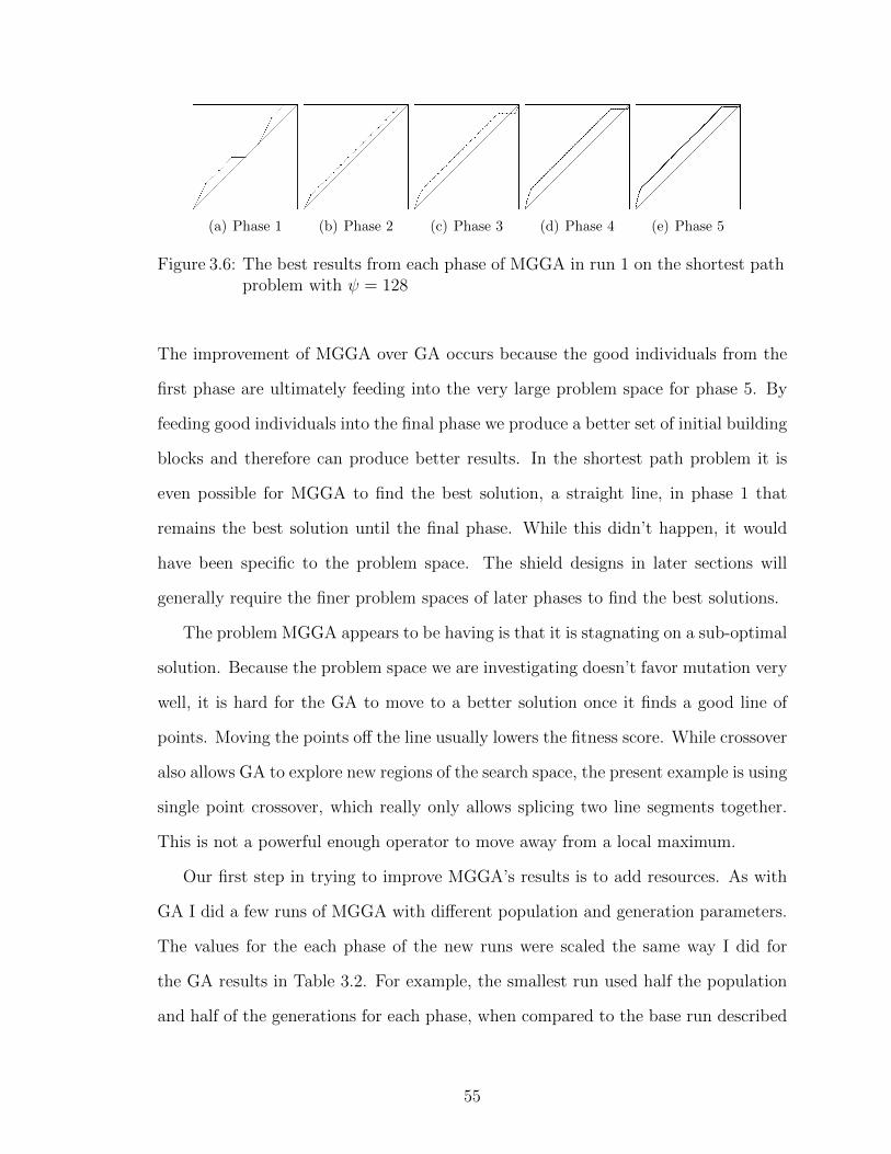
(a) Phase 1 (b) Phase 2 (c) Phase 3 (d) Phase 4 (e) Phase 5

Figure 3.6: The best results from each phase of MGGA in run 1 on the shortest pathproblem with ψ = 128

The improvement of MGGA over GA occurs because the good individuals from the

first phase are ultimately feeding into the very large problem space for phase 5. By

feeding good individuals into the final phase we produce a better set of initial building

blocks and therefore can produce better results. In the shortest path problem it is

even possible for MGGA to find the best solution, a straight line, in phase 1 that

remains the best solution until the final phase. While this didn’t happen, it would

have been specific to the problem space. The shield designs in later sections will

generally require the finer problem spaces of later phases to find the best solutions.

The problem MGGA appears to be having is that it is stagnating on a sub-optimal

solution. Because the problem space we are investigating doesn’t favor mutation very

well, it is hard for the GA to move to a better solution once it finds a good line of

points. Moving the points off the line usually lowers the fitness score. While crossover

also allows GA to explore new regions of the search space, the present example is using

single point crossover, which really only allows splicing two line segments together.

This is not a powerful enough operator to move away from a local maximum.

Our first step in trying to improve MGGA’s results is to add resources. As with

GA I did a few runs of MGGA with different population and generation parameters.

The values for the each phase of the new runs were scaled the same way I did for

the GA results in Table 3.2. For example, the smallest run used half the population

and half of the generations for each phase, when compared to the base run described

55

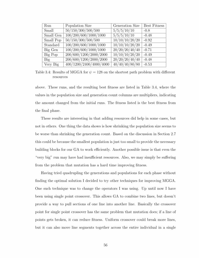
Run Population Size Generation Size Best FitnessSmall 50/150/300/500/500 5/5/5/10/10 -0.8Small Gen 100/200/600/1000/1000 5/5/5/10/10 -0.48Small Pop 50/150/300/500/500 10/10/10/20/20 -0.92Standard 100/200/600/1000/1000 10/10/10/20/20 -0.49Big Gen 100/200/600/1000/1000 20/20/20/40/40 -0.71Big Pop 200/600/1200/2000/2000 10/10/10/20/20 -0.49Big 200/600/1200/2000/2000 20/20/20/40/40 -0.48Very Big 400/1200/2400/4000/4000 40/40/40/80/80 -0.53

Table 3.4: Results of MGGA for ψ = 128 on the shortest path problem with differentresources

above. These runs, and the resulting best fitness are listed in Table 3.4, where the

values in the population size and generation count columns are multipliers, indicating

the amount changed from the initial runs. The fitness listed is the best fitness from

the final phase.

These results are interesting in that adding resources did help in some cases, but

not in others. One thing the data shows is how shrinking the population size seems to

be worse than shrinking the generation count. Based on the discussion in Section 2.7

this could be because the smallest population is just too small to provide the necessary

building blocks for our GA to work efficiently. Another possible issue is that even the

“very big” run may have had insufficient resources. Also, we may simply be suffering

from the problem that mutation has a hard time improving fitness.

Having tried quadrupling the generations and populations for each phase without

finding the optimal solution I decided to try other techniques for improving MGGA.

One such technique was to change the operators I was using. Up until now I have

been using single point crossover. This allows GA to combine two lines, but doesn’t

provide a way to pull sections of one line into another line. Basically the crossover

point for single point crossover has the same problem that mutation does; if a line of

points gets broken, it can reduce fitness. Uniform crossover could break more lines,

but it can also move line segments together across the entire individual in a single

56

Run Best FitnessRun 1 -10.66Run 2 -10.56Run 3 -10.26

Table 3.5: Results of GA for ψ = 128 on the shortest path problem with uniformcrossover

Run Best FitnessRun 1 -0.418Run 2 -0.795Run 3 -0.485

Table 3.6: Results of MGGA for ψ = 128 on the shortest path problem with uniformcrossover

step. Ultimately uniform crossover provides a very strong way to change individuals,

and will help if these major changes result in better populations as a whole.

3.5 Uniform Crossover for the Shortest Path Problem

To see if changing the GA operations would help GA and MGGA solve the shortest

path problem I did three runs of each with uniform crossover, getting the results listed

in Table 3.5. These results, for GA, are no better than the results with single point

crossover. This is not too surprising since both sets of runs are incredibly resource

starved when we consider the size of the search space.

Running MGGA with uniform crossover had a very different effect. The runs listed

in Table 3.6 produced an individual that is only a few points away from the perfect

solution, which would score −0.414. The best individual, pictured in Figure 3.7, is

the result of MGGA with only 50, 000 total individuals tried from a search space of

1.1× 10268 individuals and is a wonderful result.

MGGA is able to take advantage of uniform crossover in the early phases, where

there are fewer possible values on the grid. Later, these better solutions work together

through uniform crossover, to create even better results. Because uniform crossover

touches more of the genes, it is helping avoid the artificial plateaus that MGGA

57

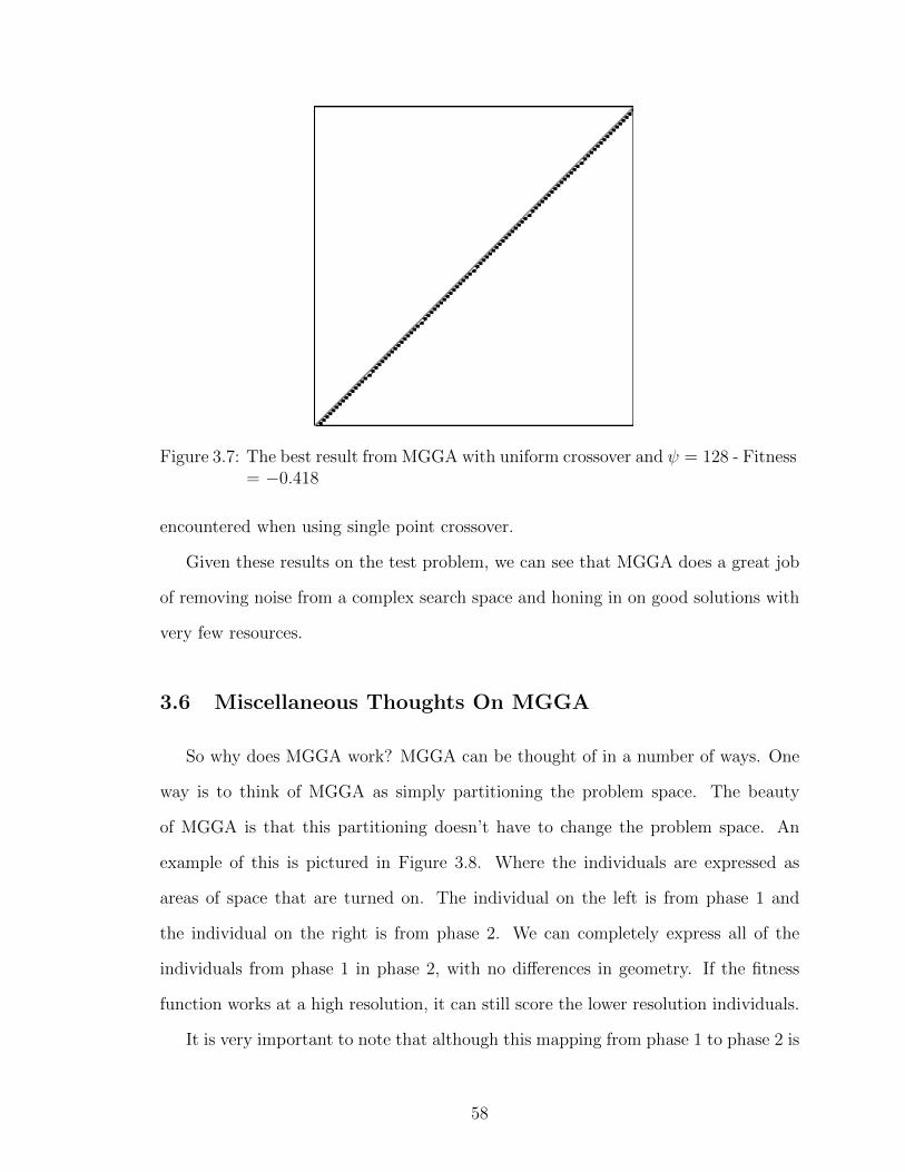
Figure 3.7: The best result from MGGA with uniform crossover and ψ = 128 - Fitness= −0.418

encountered when using single point crossover.

Given these results on the test problem, we can see that MGGA does a great job

of removing noise from a complex search space and honing in on good solutions with

very few resources.

3.6 Miscellaneous Thoughts On MGGA

So why does MGGA work? MGGA can be thought of in a number of ways. One

way is to think of MGGA as simply partitioning the problem space. The beauty

of MGGA is that this partitioning doesn’t have to change the problem space. An

example of this is pictured in Figure 3.8. Where the individuals are expressed as

areas of space that are turned on. The individual on the left is from phase 1 and

the individual on the right is from phase 2. We can completely express all of the

individuals from phase 1 in phase 2, with no differences in geometry. If the fitness

function works at a high resolution, it can still score the lower resolution individuals.

It is very important to note that although this mapping from phase 1 to phase 2 is

58

exact, there is not an equivalent reverse mapping. While you can map from phase 2

to phase 1, you will potentially be adding material to a shield, or area to a geometry

problem.

Figure 3.8: An example of an MGGA translation with exact mapping

In problem spaces where an exact mapping from one phase to the next is possible

we can think of MGGA another way. MGGA is treating a group of individuals as

having the same fitness in the early phases, while they may have a different fitness in

the higher phases. Using the concept of building blocks, MGGA is saying that a set

of building blocks from the final problem may be equivalent in earlier phases.

In Figure 3.9 we see three individuals. All three of these are impossible to map

onto the 2× 2 grid exactly. If we say that moving from 4× 4 to 2× 2 involves looking

at the material in the finer grid and if any material would appear in the coarser grid,

fill in the coarser grid. So in this example, we would fill in the upper-left square for all

three individuals. In other words, those three individuals are the same in one phase

and different in another phase.

Figure 3.9: An example of individuals being grouped to one fitness

As long as the exact mapping holds between phases, we can extend this thinking.

At the highest level MGGA on the early phases is just creating a grouping of fitness

scores for individuals in the later phases.

59

Based on these ideas, we can conclude that MGGA uses early phases to identify

the best groups of building blocks to use in later phases by filtering out groups that

don’t work well in the earlier phases. In our shortest path sample, MGGA is using

early phases to remove groups of points that aren’t near the line, then using later

phases to refine those groups to ones that are actually on the line.

One of my concerns with MGGA is what happens if we start with a very small

problem space in the first few phases? If the early GA creates a homogeneous pop-

ulation then the later phases may be hindered by a lack of diversity. There are two

obvious ways to battle this problem. First we can simply start at a phase where

the GA doesn’t produce a homogenous population. I studied this technique with the

shadow shield and have discussed the results in section 5.8.2. The second option is

to try to force some diversity into the population during the translation phase. An

easy way to do this is to perform some mutations on each individual going through

translation. An investigation of this technique is discussed in Section 5.8.3.

A final question about MGGA is whether or not it limits the possible solutions

found? The answer to this is, unfortunately, it depends. Given limited resources,

early phases of MGGA could block out good solutions from later phases. However,

the last phase of MGGA is just a normal GA, with non-random inputs. The last

phase should be able to find anything that GA can find. Therefore, given unlimited

resources there is no reason to think that MGGA can’t find all possible solutions. But

this does mean that tuning the parameters for early phases of MGGA is important to

insure that later phases are not locked out of important parts of the problem space.

3.7 Conclusions

The shortest path problem shows that MGGA is able to beat GA with fewer

resources for at least one very large problem space. The question is, can MGGA

help reduce resource usage for more real-world problems. The remainder of this

60

dissertation is focused on answering that question. I will look at three real world

problems, a shadow shield, a wearable shield and a bow tie filter. The shadow shield

problem will be fairly simplified, while the wearable shield and bow tie filter will

use more realistic physics. The goal of these three problems is to see how MGGA

holds up as the problem space grows in complexity and the actual cost of the fitness

calculation increases.

61

CHAPTER IV

A Short Introduction to Radiation Shielding

4.1 Introduction

Before diving in to my first application of MGGA, let’s take a step back and

look at the larger context of the applications we will be looking at. Each of the

three applications of MGGA presented in this dissertation are related to radiation

shielding. At the highest level, each application looks at designing a shield or filter

to alter the effects of a radiation source on a target area. Before we talk about how

MGGA can help, let’s look at what the MGGA will try to do.

4.2 Radiation Basics

Radiation is particles traveling through space, or interacting with other materials.

There are several categories of radiation based on the particles involved:

Alpha

Alpha radiation is associated with the travel of alpha particles. Alpha parti-

cles are essentially helium ions, with 2 neutrons and 2 protons. There are no

electrons in an alpha particle.

Beta

Beta radiation is transmitted via electrons, or beta particles. In some cases

62

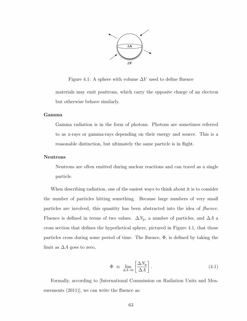
!A

!V

Figure 4.1: A sphere with volume ∆V used to define fluence

materials may emit positrons, which carry the opposite charge of an electron

but otherwise behave similarly.

Gamma

Gamma radiation is in the form of photons. Photons are sometimes referred

to as x-rays or gamma-rays depending on their energy and source. This is a

reasonable distinction, but ultimately the same particle is in flight.

Neutrons

Neutrons are often emitted during nuclear reactions and can travel as a single

particle.

When describing radiation, one of the easiest ways to think about it is to consider

the number of particles hitting something. Because large numbers of very small

particles are involved, this quantity has been abstracted into the idea of fluence.

Fluence is defined in terms of two values. ∆Np, a number of particles, and ∆A a

cross section that defines the hypothetical sphere, pictured in Figure 4.1, that those

particles cross during some period of time. The fluence, Φ, is defined by taking the

limit as ∆A goes to zero,

Φ ≡ lim∆A→0

[∆Np

∆A

]. (4.1)

Formally, according to [International Commission on Radiation Units and Mea-

surements (2011)], we can write the fluence as:

63

Φ =dN

dA(4.2)

where N is the number of particles and A is the cross section of the sphere. In many

of our simulations we will rely on MCNP to calculate the value of fluence. This is

usually done by using the equivalent definition in 4.3 where we use the length of the

tracks, dl, crossing the sphere of volume dV , and

Φ =dl

dV. (4.3)

Another way to think about radiation is to think in terms of time. Fluence rate

is the change of fluence over time. This quantity is sometimes called the particle flux

density, or flux,

Φ̇ =dΦ

dt. (4.4)

4.3 Interaction Quantities

When particles encounter matter there is a possibility that they interact. The

chance of an interaction occurring depends on the type of particle coming in, the type

of material it is encountering, the energy of the particle, the energy of the material,

and the possible interactions. The concept of a linear attenuation coefficient, µ, is used

to capture this chance of interaction into a single measurable quantity, [International

Commission on Radiation Units and Measurements (2011)]. µ is defined as:

µ =1

dl

dN

N(4.5)

where dN/N is the fraction of particles that have an interaction with the material in

a distance dl.

64

Because µ depends on the density of the target material, this definition can be

written in terms of the mass attenuation coefficient µ/ρ:

µ

ρ=

1

ρdl

dN

N(4.6)

By writing the mass coefficient in this way, we can also get to another quantity

called the microscopic cross section, σ. The units for the microscopic cross section

is m−2, which are sometimes written using barns, where one barn is 10−24cm2. The

mass coefficient is linked to the cross section by replacing the density by Avagadro’s

number, NA, times the molar mass of the target material, A.

µ

ρ=NA

Aσ (4.7)

The intensity, I, of a beam of radiation at depth t is described by

I

I0

= e−σNt (4.8)

where N is the number of atoms per cm3 and I0 is the initial intensity of the beam.

So the intensity goes down by a factor of e when the thickness is 1µ. This is also the

average distance that a particle moves from the point of its birth to its first interaction

and is called the mean free path.

In the case where there are multiple mutually exclusive interactions the cross

section is often thought of as:

σ =∑j

σj (4.9)

where σj is the cross section for a particular interaction. Also, for homogeneous

mixtures or compounds we can think of the total value for µ as a sum:

65

µ =∑j

µj =∑j

Njσj (4.10)

where Nj is the atomic density of the j-th element.

The cross section is also energy dependent, which will have an important effect

on our ability to shield various particles.

4.4 Shielding Basics and Radiation Interactions with Matter

Shielding at its most basic is the process of stopping radiation from hitting some-

thing. The basic question is how much of something is needed and what is the best

something to put in the way.

Because alpha particles are charged they are relatively easy to shield against and

can be stopped by even a thin sheet of material. A Po-210 nucleus can produce alphas

with an energy of 5.3 MeV, but these will only travel 4cm in air at 1 atmosphere, and

less than a few millimeters in human skin or aluminum. However, their charge also

allows them to transfer a great deal of energy and if allowed to hit sensitive materials

alpha particles can be devastating. Alphas had a small burst of fame in the mid-2000s

when Polonium was used to kill an ex-K.G.B. spy. But in this case, the material had

to be ingested to do real damage [Cowall (2006)].

Beta particles are charged so they interact with the electrons and nuclei of mate-

rials, making them relatively easy to shield against. For example an incoming beam

of 4 MeV beta particles only needs a centimeter or so of aluminum to stop it [Cember

& Johnson (2009)].

Gamma particles will interact with the electron clouds around atoms, allowing

them to be shielded against. However, unlike alpha and beta particles, gammas

should not be thought of as stoppable, and are better treated as something you

attenuate with a shield or filter. This process is described in 4.4.1.

66

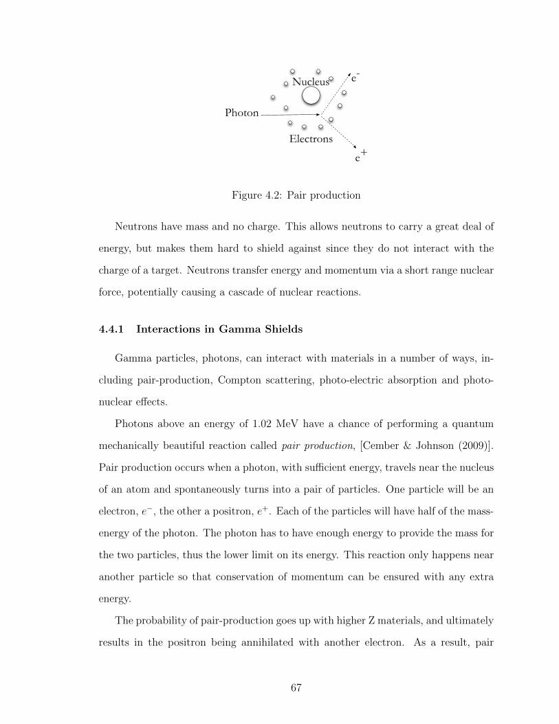
Nucleus

Electrons

Photon

e-

e+

Figure 4.2: Pair production

Neutrons have mass and no charge. This allows neutrons to carry a great deal of

energy, but makes them hard to shield against since they do not interact with the

charge of a target. Neutrons transfer energy and momentum via a short range nuclear

force, potentially causing a cascade of nuclear reactions.

4.4.1 Interactions in Gamma Shields

Gamma particles, photons, can interact with materials in a number of ways, in-

cluding pair-production, Compton scattering, photo-electric absorption and photo-

nuclear effects.

Photons above an energy of 1.02 MeV have a chance of performing a quantum

mechanically beautiful reaction called pair production, [Cember & Johnson (2009)].

Pair production occurs when a photon, with sufficient energy, travels near the nucleus

of an atom and spontaneously turns into a pair of particles. One particle will be an

electron, e−, the other a positron, e+. Each of the particles will have half of the mass-

energy of the photon. The photon has to have enough energy to provide the mass for

the two particles, thus the lower limit on its energy. This reaction only happens near

another particle so that conservation of momentum can be ensured with any extra

energy.

The probability of pair-production goes up with higher Z materials, and ultimately

results in the positron being annihilated with another electron. As a result, pair

67

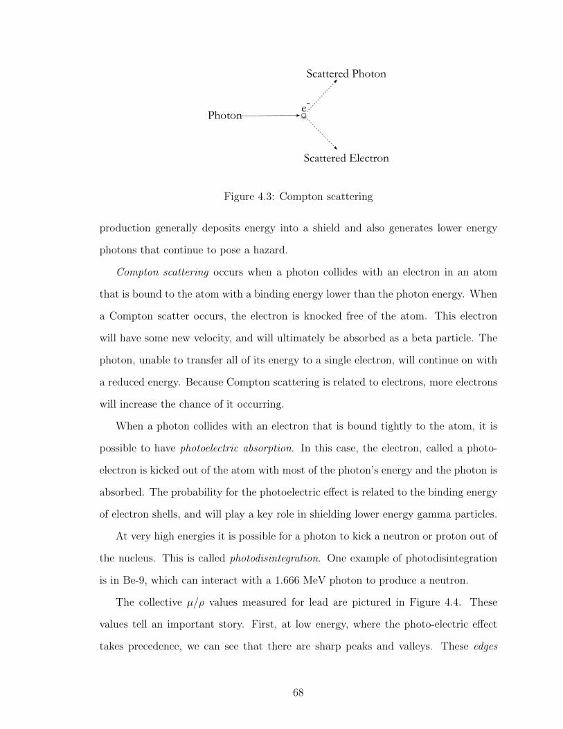
Photone-

Scattered Photon

Scattered Electron

Figure 4.3: Compton scattering

production generally deposits energy into a shield and also generates lower energy

photons that continue to pose a hazard.

Compton scattering occurs when a photon collides with an electron in an atom

that is bound to the atom with a binding energy lower than the photon energy. When

a Compton scatter occurs, the electron is knocked free of the atom. This electron

will have some new velocity, and will ultimately be absorbed as a beta particle. The

photon, unable to transfer all of its energy to a single electron, will continue on with

a reduced energy. Because Compton scattering is related to electrons, more electrons

will increase the chance of it occurring.

When a photon collides with an electron that is bound tightly to the atom, it is

possible to have photoelectric absorption. In this case, the electron, called a photo-

electron is kicked out of the atom with most of the photon’s energy and the photon is

absorbed. The probability for the photoelectric effect is related to the binding energy

of electron shells, and will play a key role in shielding lower energy gamma particles.

At very high energies it is possible for a photon to kick a neutron or proton out of

the nucleus. This is called photodisintegration. One example of photodisintegration

is in Be-9, which can interact with a 1.666 MeV photon to produce a neutron.

The collective µ/ρ values measured for lead are pictured in Figure 4.4. These

values tell an important story. First, at low energy, where the photo-electric effect

takes precedence, we can see that there are sharp peaks and valleys. These edges

68

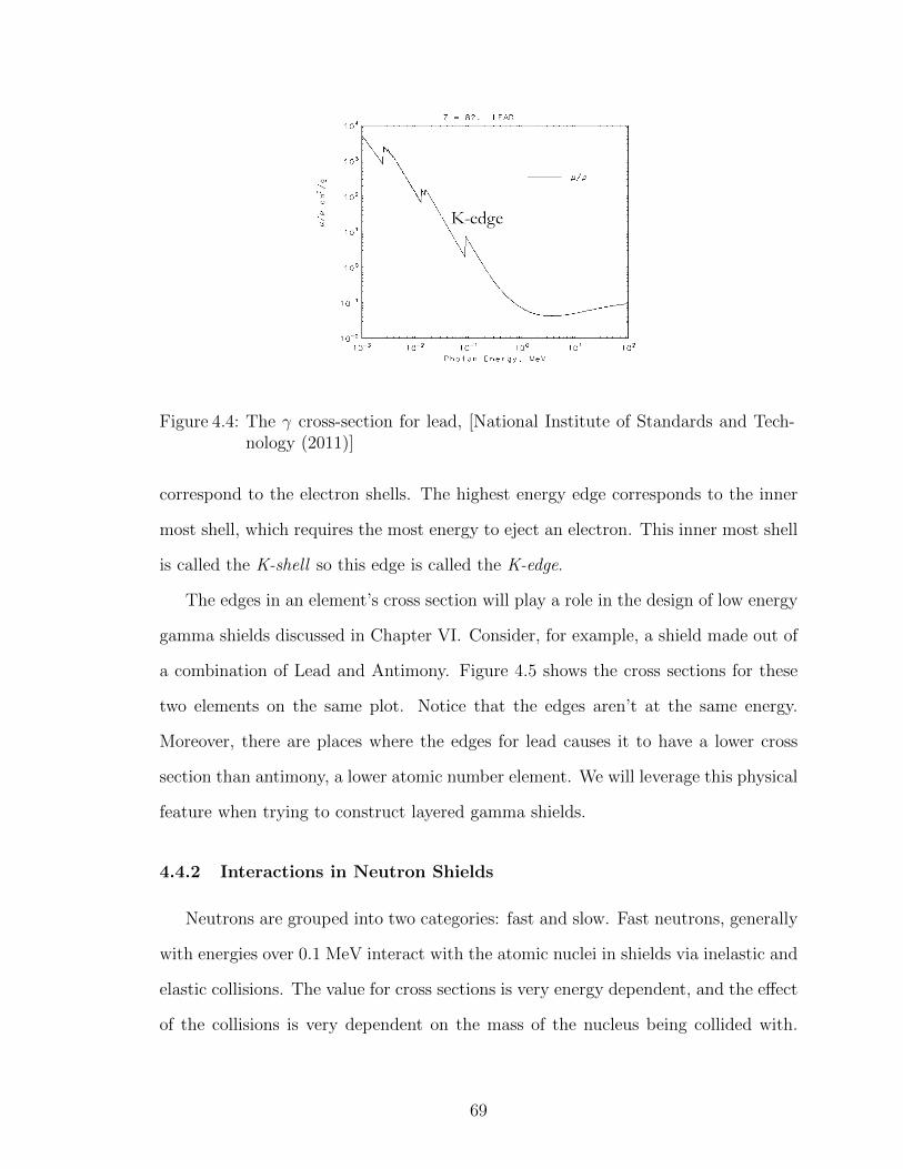
Figure 4.4: The γ cross-section for lead, [National Institute of Standards and Tech-nology (2011)]

correspond to the electron shells. The highest energy edge corresponds to the inner

most shell, which requires the most energy to eject an electron. This inner most shell

is called the K-shell so this edge is called the K-edge.

The edges in an element’s cross section will play a role in the design of low energy

gamma shields discussed in Chapter VI. Consider, for example, a shield made out of

a combination of Lead and Antimony. Figure 4.5 shows the cross sections for these

two elements on the same plot. Notice that the edges aren’t at the same energy.

Moreover, there are places where the edges for lead causes it to have a lower cross

section than antimony, a lower atomic number element. We will leverage this physical

feature when trying to construct layered gamma shields.

4.4.2 Interactions in Neutron Shields

Neutrons are grouped into two categories: fast and slow. Fast neutrons, generally

with energies over 0.1 MeV interact with the atomic nuclei in shields via inelastic and

elastic collisions. The value for cross sections is very energy dependent, and the effect

of the collisions is very dependent on the mass of the nucleus being collided with.

69

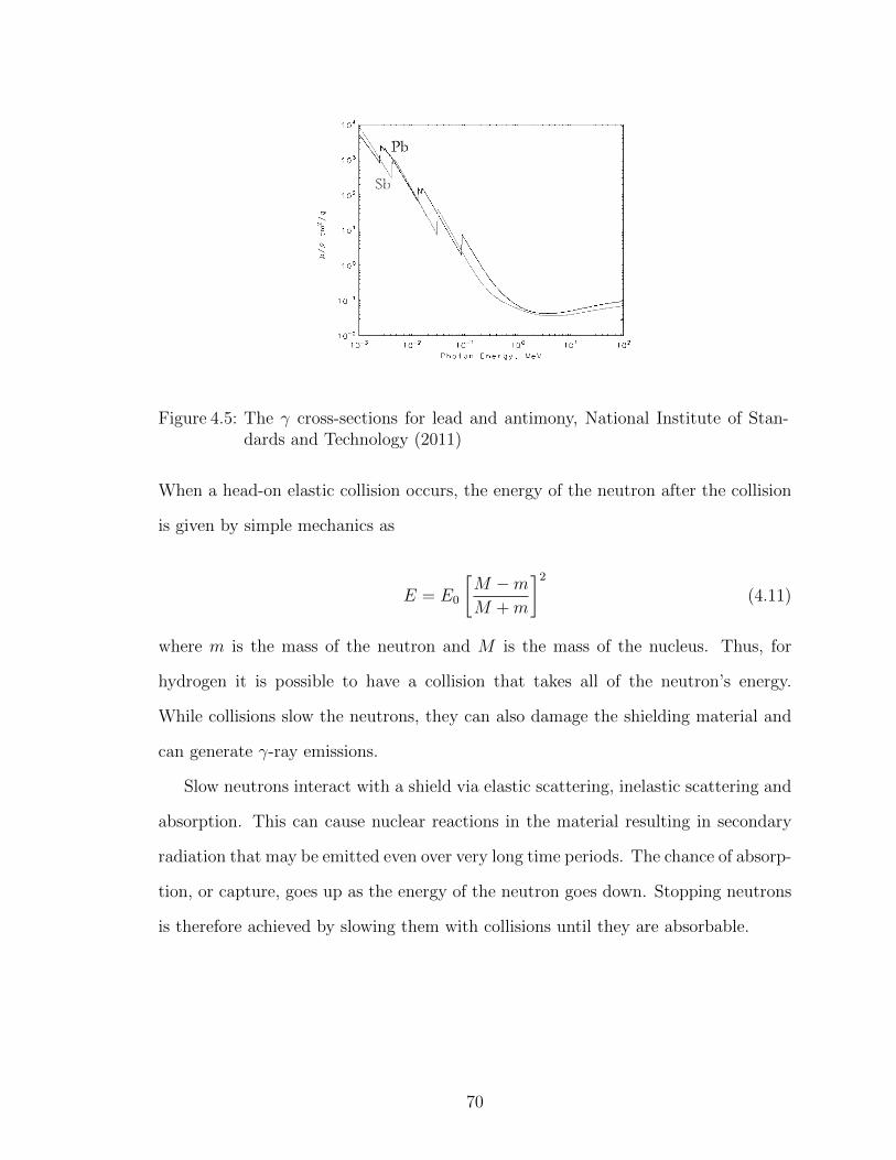
Figure 4.5: The γ cross-sections for lead and antimony, National Institute of Stan-dards and Technology (2011)

When a head-on elastic collision occurs, the energy of the neutron after the collision

is given by simple mechanics as

E = E0

[M −mM +m

]2

(4.11)

where m is the mass of the neutron and M is the mass of the nucleus. Thus, for

hydrogen it is possible to have a collision that takes all of the neutron’s energy.

While collisions slow the neutrons, they can also damage the shielding material and

can generate γ-ray emissions.

Slow neutrons interact with a shield via elastic scattering, inelastic scattering and

absorption. This can cause nuclear reactions in the material resulting in secondary

radiation that may be emitted even over very long time periods. The chance of absorp-

tion, or capture, goes up as the energy of the neutron goes down. Stopping neutrons

is therefore achieved by slowing them with collisions until they are absorbable.

70

4.5 Health Physics Basics

Interactions in the body follow the same physics as interactions in a shield. The

trick with radiation in people is figuring out the biological effects of the radiation.

With a shield, we might worry about cracking or long-term radioactivity, but with a

person we have to worry about numerous biological effects ranging from cell mutations

to death. Quantifying radiation on the body is therefore harder than in a single

material. We will use the quantity called absorbed dose to measure radiation in a

body. Absorbed dose is defined as

D =dε

dm(4.12)

where dε is the mean energy deposited to the infinitesimal volume with mass dm.

The unit for absorbed does is the Gray, which is equivalent to J/kg, or m2s−2.

When we deal with a person, we are dealing with a very complex set of interactions

between radiation and a number of materials. The human body contains different

organs that perform different biological functions. Often the health physicist will

be concerned with the whole body dose, or the dose to the entire body. There are

also concerns for specific organs, and in this case it is not enough to say how much

radiation hit that organ. We will also have to take into account a weighting that

indicates how sensitive that organ is to radiation. These weights can be used to

calculate something called the effective dose, defined as:

ε =∑T

wTHT =∑T

wT∑R

wRDT,R (4.13)

where HT is the equivalent dose in organ or tissue T , DT,R is the mean absorbed dose

in the organ or tissue T , wR is a radiation weighting factor for radiation R and wT is

a tissue weight factor. wR is independent of the tissue or organ and can range from

1 for gamma radiation to 20 for some energies of neutrons. wT is independent of the

71

radiation, and can range from 0.01 for skin to 0.2 for the gonads.

4.6 Summary

Radiation is categorized into four main forms. Alpha radiation, made up of 2

neutrons and 2 protons, is easily shielded against. Beta radiation, generally electrons

but also positrons, can be shielded against with rather thin layers because it interacts

easily with atoms. Gamma radiation is composed of photons and interacts with

matter through the electrons circling the nucleus. Gamma radiation can interact in a

number of ways based on energy and provides a more challenging shielding problem.

Neutrons are perhaps the hardest type of radiation to shield against. Neutrons don’t

interact with the electron shells around an atom. Rather they interact with the

nucleus. At high energies neutrons are basically billiard balls, slamming into nuclei

and often weakening shielding materials. At low energies neutrons can be absorbed

causing potentially long term radiological effects.

Chapter V discusses how MGGA can be used to build a neutron shield, and will

focus on scattering interactions. Chapter VI discusses building a shield for gamma

radiation and Chapter VII discusses using MGGA to design a filter for gamma radia-

tion. The two chapters will focus more on Compton scattering and the photo-electric

effect. Chapter VI is focused on shielding a human and will rely on the some of

the health physics concepts discussed here, especially the weighting factors for each

organ.

72

CHAPTER V

Designing a Shadow Shield

5.1 Introduction

Minimization of mass is critical for space applications and naturally raises the

question of what is the optimal shield shape for a space reactor shield? In the vacuum

of space a shadow shield is sufficient; it need cover only a small solid-angle while

allowing radiation to stream away from the spacecraft payload in other directions.

The obvious shield shape is therefore a frustum of a cone, but this obvious solution

has been shown to be a suboptimal design, [Alpay & Holloway (2005)]. Splitting a

frustum into two parts can open up radial streaming paths that can reduce the payload

dose for a fixed shield mass. There is no reason to believe that the split design in

[Alpay & Holloway (2005)] is the best. Moreover that result required a large number

of MCNP runs to find a good strategy for splitting the shield. The combination of

flexible geometry and mass constraints makes the problem of designing a shield for

space applications a complex and interesting one, dominated by a large search space,

a perfect testing ground for MGGA.

73

Figure 5.1: The geometry of a simple shadow shield

5.2 The Shadow Shield Problem

In this chapter I will discuss MGGA in the context of a single test problem: a

space shield based on the design pictured in Fig. 5.1. In this problem I am designing

a shield that needs to protect a payload from a particle source. I will use a geometry

pictured in Fig. 5.2 that is a very simple model of the problem pictured in Fig. 5.1

where I have removed the intervening space and placed the source and detectors next

to the shield itself. This simplification is reasonable for comparing shields, but a

more accurate geometry would be required to estimate the actual flux on a payload

through one of the shields discussed here. The source emits evenly from a disk of

radius 90 cm at the origin of the z-axis. This disk is represented by the rectangle on

the left of Fig. 5.2.

The shield is cylindrical. GA’s task is to place annular rings of material into the

vacuum along the z-axis between 10 and 160 cm from the source, with the largest

ring extending radially to 300 cm.

5.2.1 Modeling the Shield

There are two key aspects in modeling this shield for GA. First, we need to model

the shield’s geometry and second we need to model the materials that make up the

shield. For most of my work, I will model the shield’s geometry as annular rings of

equal mass (hence having larger radial extent near the axis). Two shields with the

same number of filled rings will weigh the same amount, regardless of where the rings

are. In Section 5.7 I will discuss several simulations that use non-equal mass rings.

74

Figure 5.2: The geometry for the shadow shield problem. The r-z plane with a disksource to the left and a detector plane to the right. The goal is to placematerial in the intervening vacuum to reduce the flux at the detectorplane.

In that case, the rings will have an equal radial delta, and the outside rings will be

much heavier than the inside rings.

The rings are separated along the z axis into disks. In all simulations these disks

have an equal size. Figure 5.2 pictures a shield with 16 rings and 16 disks all with

equal mass.

I chose equal mass rings for the majority of these simulations in an attempt to

reduce preferential treatment of each ring. If the inside rings are lighter than the

outside rings, then they will be preferred on the basis of mass. While physically this

may be appropriate for reducing radiation at the ship, I would rather have the GA

figure that out, than build a preference into the initial model.

The material for the shield is modeled as a binary value. A value of 0 represents

no shield material and a value of 1 represents shield material. Given the simplified

physics used, this material is not real, but is loosely based on Lithium-Hydride. I

75

picked Lithium-Hydride for several reasons. In a real-world space shield scenario the

shield material is going to have to meet a number of criteria including:

• Reduce the flux of high energy neutrons

• Reduce the flux of low energy neutrons

• Reduce the flux of gamma rays

• Be as light as possible

• Be manufacturable

• Last the life of the mission

For simplification I am focusing my design on high energy neutron shielding, so

my first goal is to scatter neutrons. The best way to do this is with hydrogen, [Chilton

et al. (1984)], which will reduce the energy of the neutrons by an average of 50% in

each scatter. Hydrogen also has a high scatter cross section. Unfortunately hydrogen

doesn’t do a good job of absorbing the thermal neutrons, so in a real shield we would

want to put it in some kind of compound, [R.K. et al. (2001)]. The question is, what

compound to use.

As far back as the 1970s engineers have been looking into shielding for space appli-

cations, [Radiobiological Advisory Panel (1970)]. These investigations have focused

on the entire set of criteria, including gamma rays and low energy neutrons. The

results of the early work was to use LiH [Lee (1987)]. LiH has a low density, so it

is lightweight. It contains a lot of hydrogen, so it slows down high energy neutrons

quickly. The LiH helps capture thermal neutrons and does so without generating a

lot of gamma rays, [Pheil (2006); Bell et al. (2010)].

Despite having significant production and durability issues, including hydrogen

disassociation and thermal swelling, LiH has historically been considered a prime

76

shielding candidate. Various packaging ideas have been proposed to deal with LiH’s

issues including storing it in containers. Other designs, [Lee (1987)], have suggested

layering LiH with something like tungsten to reduce gamma rays as well. We will only

be looking at high energy neutrons for this simulation and will ignore the potential

use of tungsten. I ignore the infrastructure of the shield in this problem, focusing

instead on designing a shadow shield that has a good material for scattering high

energy neutrons.

5.2.2 The Theoretical Shield Material

I model radiation transport for the shadow shield as a one-speed problem, using a

purely scattering material with total cross section of 0.275 per cm. This is characteris-

tic of neutron interactions in LiH at 2 MeV, with isotropic scattering, except that LiH

scatters somewhat forward. To calculate this simplified cross section I started with

the total cross-section for Li at 2 MeV, [Los Alamos National Lab (2011)], which is

1.725 barns. For hydrogen the total cross section at this energy is 2.914 barns. Next

I determined the number of Li and H atoms in a cubic centimeter. The molar mass of

LiH is 7.95 and its density is 0.78 gm cm−3, [webelements.com (2011)]. This results

in an N of 5.9 × 1022. So to determine the macroscopic total cross section of LiH I

used Equation 4.10 to calculate:

ΣT = 5.9× 1022 × (1.72 + 2.91)× 10−24 (5.1)

or 0.275 cm−1. The equivalent calculation for the radiation capture cross section at

this energy results in

ΣA = 5.9× 1022 × (5× 10−6 + 3.42× 10−5)× 10−24 ≈ 2.313× 10−6cm−1 (5.2)

77

a negligible value, indicating that LiH will primarily scatter neutrons at this energy,

as we would expect. Note that this is a natural Li, not enriched in Li-6

So, everywhere there is shield material, or a 1 in a shield’s chromosome, the fitness

test will use this 0.275 cm−1 cross section for scattering our neutrons.

5.2.3 Simulating Radiation to Score the Shield

PARTISN is used to model neutron transport through the shield. PARTISN uses

two grids to perform calculations, a coarse grid models the problem space, while a

fine grid is used for discretizing space for physics calculations. I match the PARTISN

coarse grid to the available ring locations as pictured in Fig. 5.2, with the exception

that the grid extends to the edges of the system. I set the fine grid to half the size

of the coarse grid in the highest resolution case, resulting in a 32× 32 fine grid when

the finest coarse grid is 16× 16. The fine grid’s size is kept constant regardless of the

size of the coarse grid. Angles are defined using the Rectangular Chebychev-Legendre

built-in set, with an ISN value of 24. The flux at each fine grid point located on the

detector plane at z = 170 cm from the source is used in the fitness functions described

below. This detector disk is the dark box on the right side of Fig. 5.2.

Of course I am ignoring much of the structure that would arise in a space reactor

application, but our goal is to explore the concept of MGGA, rather than to design

the final shield.

5.2.4 Designing a Fitness Function for the Shadow Shield

The ultimate goal of the space shield design problem is to create a shield that

reduces radiation on the ship while being as light as possible. Weight represents cost

for space applications, so we may be willing to trade shielding for weight above some

acceptable shielding value. However, if the shield doesn’t protect the ship sufficiently,

then the mission will fail. Our fitness function needs to take this balance between

78

weight and shielding into account.

The first task is to decide how much of a reduction in radiation is sufficient.

I compare candidate shields against the heaviest shield that the chromosome can

encode. This heaviest shield would place material in every grid location in Figure 5.2.

We know, based on [Alpay & Holloway (2005)], that the heaviest shield isn’t the best

shield. But it is a reasonable comparison for an automated search algorithm. Running

PARTISN with the heaviest shield will get a set of fluxes on the detector plane. I

compare these to each individual in the shield population, and score the candidate

shields by how well it does against the heaviest, or full, shield. Ideally, the MGGA

will either duplicate the split shield idea, or create something better.

Using the heaviest shield, called S, as a comparison for flux, I created two different

fitness functions. The first compares the flux at all places on the detector plane to the

“worst” flux for the heaviest shield. If the heaviest shield had a neutron flux ranging

from 1 to 100, we would only compare our candidate shields to the value of 100, since

that is the worst job that the heaviest shield does. Even without running a simulation

we can guess that the worst flux value will be on the z axis due to geometry, but we

won’t require that. Let’s call this fitness function, that compares to the worst flux

from the heaviest shield, the MaxFlux fitness function. We also need to factor mass

into the fitness function. We will do this by comparing the mass of a shield to the

mass of the heaviest shield.

To compute the MaxFlux fitness of a shield, s, I run PARTISN to get scalar flux

values φi(s) at the detector plane for shield s at each of the detector cells i. Let m(s)

denote the mass of shield s. The fitness of shield s is

F (s) =

mini

(1− φi

φi(S)

)if maxk(φk(S)) < φi(s) for any i

1− m(s)m(S)

otherwise.

(5.3)

This fitness function essentially looks for shields that better the full shield’s flux at

79

its worst, and then tries to find the lightest shields that meet this goal. The function

is defined in such a way that the following two facts are true: First, any shield that

doesn’t beat the heaviest shield’s “worst” flux, i.e. pass the flux criteria, will have a

negative fitness. Second, any shield that does pass the flux criteria will have a fitness

between zero and one where the best fitness a shield could aspire to is a value of one.

The second way to compare to the heaviest shield’s flux, is to try and beat it

at every detector. This means that at every grid location on the detector plan a

candidate shields flux has to be lower than the heaviest shield’s flux at that same

detector. Let’s call this fitness function the ByLocation fitness function. To compute

the ByLocation fitness of a shield, s, I run PARTISN to get scalar flux values φi(s)

at the detector plane for shield s at each of the detector cells i. Let m(s) denote the

mass of shield s. The fitness of shield s is

F (s) =

mini

(1− φi

φi(S)

)if φi(S) < φi(s) for any i

1− m(s)m(S)

otherwise.

(5.4)

This fitness function essentially looks for shields that better the full shield’s flux

at each detector, and then tries to find the lightest shields that meet this goal. Like

the MaxFlux function, the ByLocation function will result in a negative value for

shields that fail the flux criteria, and will result in a value from zero to one for shields

being graded on mass.

5.2.5 Applying MGGA to the Space Shield Problem

In order to test the concept of MGGA I did several types of runs for the shield

problem. Unless otherwise noted, these runs all used the same underlying Genetic

Algorithm and MGGA settings. For most of these runs, the finest grid we will look

at is a 16 × 16 r-z grid. This maps onto a binary chromosome with 256 elements

indicating if an individual ring is filled with material or is empty. The first type

80

of run uses a standard GA to search the resulting space of 2256 possible solutions.

This run was performed using a population of 531 individuals, and was run for 20

generations, resulting in a total of 10,620 possible shield candidates. The GA used

for these runs is fairly standard [Haupt & Haupt (1998); Mitchel (1998)]; it uses

tournament selection with a tournament size of 4, uniform crossover with a chance

of 70%, random mutation with a chance of 20% and copy forward with a chance of

10%.

The MGGA runs consisted of the following set of 4 phases:

• 2× 2 grid with 10 individuals for 20 generations (200 candidates)

• 4× 4 grid with 200 individuals for 20 generations (4000 candidates)

• 8× 8 grid with 200 individuals for 20 generations (4000 candidates)

• 16× 16 grid with 120 individuals for 20 generations (2400 candidates)

This is a total of 10, 600 shield candidates, just 20 candidates shy of the GA run.

The translation phase for MGGA on the shadow shield is similar to the one used

to translation the shortest path problem described in Section 3.4. The grid sizes were

chosen so that each phase uses a grid that cuts the other grid in half in both directions.

This effectively quarters the size of a grid element at each phase step. Translations

from one phase to the next simply look at a grid element in the early phase and if

they have shield material, the translation operator turns on the corresponding grid

elements in the later phase, see Figure 5.3. As long as the grid halves in size in both

directions this mapping is exact and the shield should maintain its flux and mass

score across translations.

I performed both GA and MGGA runs with the MaxFlux and ByLocation fitness

functions and have performed multiple runs of each type where possible to develop

statistics and check the results for random errors or successes.

81

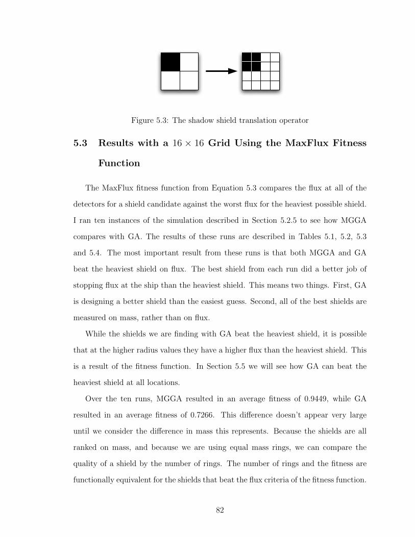
Figure 5.3: The shadow shield translation operator

5.3 Results with a 16 × 16 Grid Using the MaxFlux Fitness

Function

The MaxFlux fitness function from Equation 5.3 compares the flux at all of the

detectors for a shield candidate against the worst flux for the heaviest possible shield.

I ran ten instances of the simulation described in Section 5.2.5 to see how MGGA

compares with GA. The results of these runs are described in Tables 5.1, 5.2, 5.3

and 5.4. The most important result from these runs is that both MGGA and GA

beat the heaviest shield on flux. The best shield from each run did a better job of

stopping flux at the ship than the heaviest shield. This means two things. First, GA

is designing a better shield than the easiest guess. Second, all of the best shields are

measured on mass, rather than on flux.

While the shields we are finding with GA beat the heaviest shield, it is possible

that at the higher radius values they have a higher flux than the heaviest shield. This

is a result of the fitness function. In Section 5.5 we will see how GA can beat the

heaviest shield at all locations.

Over the ten runs, MGGA resulted in an average fitness of 0.9449, while GA

resulted in an average fitness of 0.7266. This difference doesn’t appear very large

until we consider the difference in mass this represents. Because the shields are all

ranked on mass, and because we are using equal mass rings, we can compare the

quality of a shield by the number of rings. The number of rings and the fitness are

functionally equivalent for the shields that beat the flux criteria of the fitness function.

82

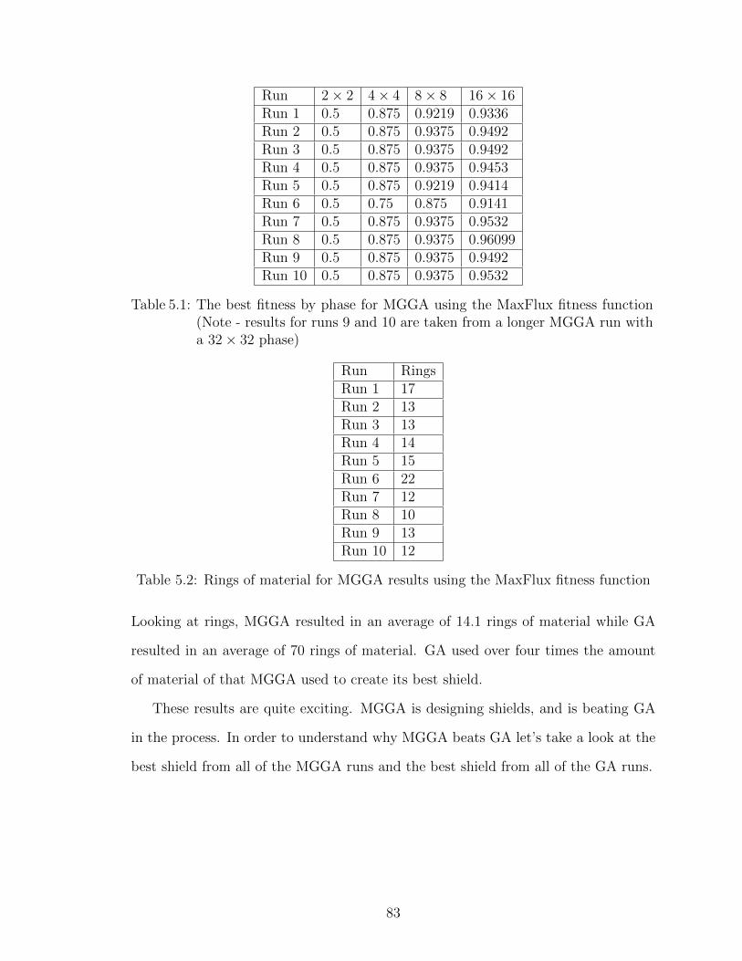
Run 2× 2 4× 4 8× 8 16× 16Run 1 0.5 0.875 0.9219 0.9336Run 2 0.5 0.875 0.9375 0.9492Run 3 0.5 0.875 0.9375 0.9492Run 4 0.5 0.875 0.9375 0.9453Run 5 0.5 0.875 0.9219 0.9414Run 6 0.5 0.75 0.875 0.9141Run 7 0.5 0.875 0.9375 0.9532Run 8 0.5 0.875 0.9375 0.96099Run 9 0.5 0.875 0.9375 0.9492Run 10 0.5 0.875 0.9375 0.9532

Table 5.1: The best fitness by phase for MGGA using the MaxFlux fitness function(Note - results for runs 9 and 10 are taken from a longer MGGA run witha 32× 32 phase)

Run RingsRun 1 17Run 2 13Run 3 13Run 4 14Run 5 15Run 6 22Run 7 12Run 8 10Run 9 13Run 10 12

Table 5.2: Rings of material for MGGA results using the MaxFlux fitness function

Looking at rings, MGGA resulted in an average of 14.1 rings of material while GA

resulted in an average of 70 rings of material. GA used over four times the amount

of material of that MGGA used to create its best shield.

These results are quite exciting. MGGA is designing shields, and is beating GA

in the process. In order to understand why MGGA beats GA let’s take a look at the

best shield from all of the MGGA runs and the best shield from all of the GA runs.

83

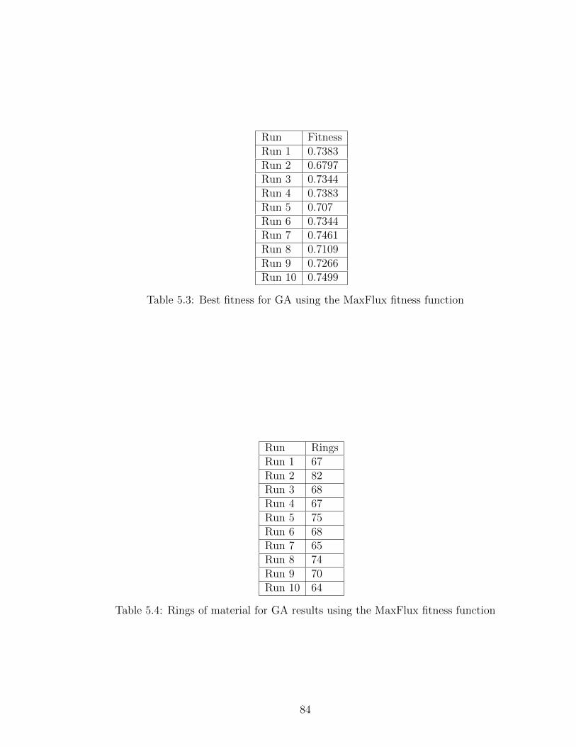
Run FitnessRun 1 0.7383Run 2 0.6797Run 3 0.7344Run 4 0.7383Run 5 0.707Run 6 0.7344Run 7 0.7461Run 8 0.7109Run 9 0.7266Run 10 0.7499

Table 5.3: Best fitness for GA using the MaxFlux fitness function

Run RingsRun 1 67Run 2 82Run 3 68Run 4 67Run 5 75Run 6 68Run 7 65Run 8 74Run 9 70Run 10 64

Table 5.4: Rings of material for GA results using the MaxFlux fitness function

84

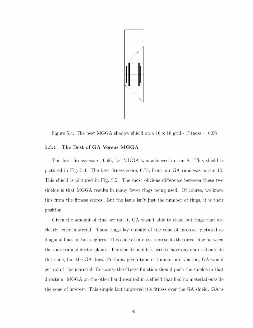
Figure 5.4: The best MGGA shadow shield on a 16× 16 grid - Fitness = 0.96

5.3.1 The Best of GA Versus MGGA

The best fitness score, 0.96, for MGGA was achieved in run 8. This shield is

pictured in Fig. 5.4. The best fitness score, 0.75, from our GA runs was in run 10.

This shield is pictured in Fig. 5.5. The most obvious difference between these two

shields is that MGGA results in many fewer rings being used. Of course, we knew

this from the fitness scores. But the issue isn’t just the number of rings, it is their

position.

Given the amount of time we ran it, GA wasn’t able to clean out rings that are

clearly extra material. These rings lay outside of the cone of interest, pictured as

diagonal lines on both figures. This cone of interest represents the direct line between

the source and detector planes. The shield shouldn’t need to have any material outside

this cone, but the GA does. Perhaps, given time or human intervention, GA would

get rid of this material. Certainly the fitness function should push the shields in that

direction. MGGA on the other hand resulted in a shield that had no material outside

the cone of interest. This simple fact improved it’s fitness over the GA shield. GA is

85

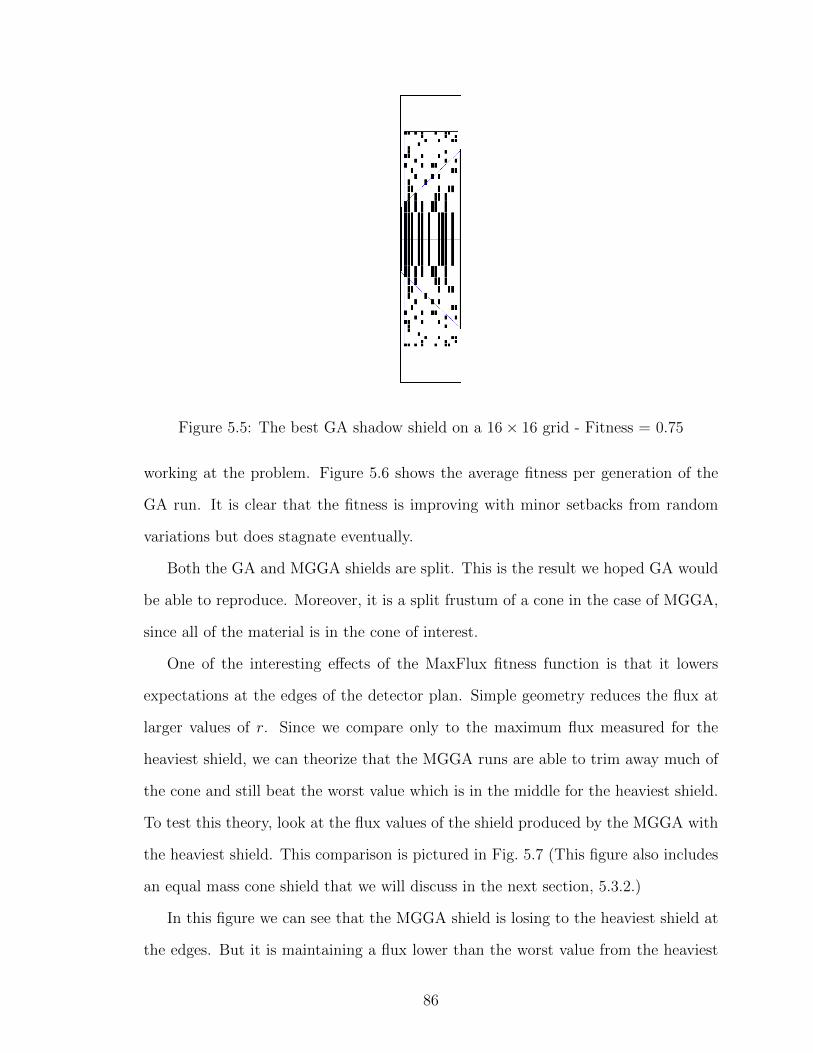
Figure 5.5: The best GA shadow shield on a 16× 16 grid - Fitness = 0.75

working at the problem. Figure 5.6 shows the average fitness per generation of the

GA run. It is clear that the fitness is improving with minor setbacks from random

variations but does stagnate eventually.

Both the GA and MGGA shields are split. This is the result we hoped GA would

be able to reproduce. Moreover, it is a split frustum of a cone in the case of MGGA,

since all of the material is in the cone of interest.

One of the interesting effects of the MaxFlux fitness function is that it lowers

expectations at the edges of the detector plan. Simple geometry reduces the flux at

larger values of r. Since we compare only to the maximum flux measured for the

heaviest shield, we can theorize that the MGGA runs are able to trim away much of

the cone and still beat the worst value which is in the middle for the heaviest shield.

To test this theory, look at the flux values of the shield produced by the MGGA with

the heaviest shield. This comparison is pictured in Fig. 5.7 (This figure also includes

an equal mass cone shield that we will discuss in the next section, 5.3.2.)

In this figure we can see that the MGGA shield is losing to the heaviest shield at

the edges. But it is maintaining a flux lower than the worst value from the heaviest

86

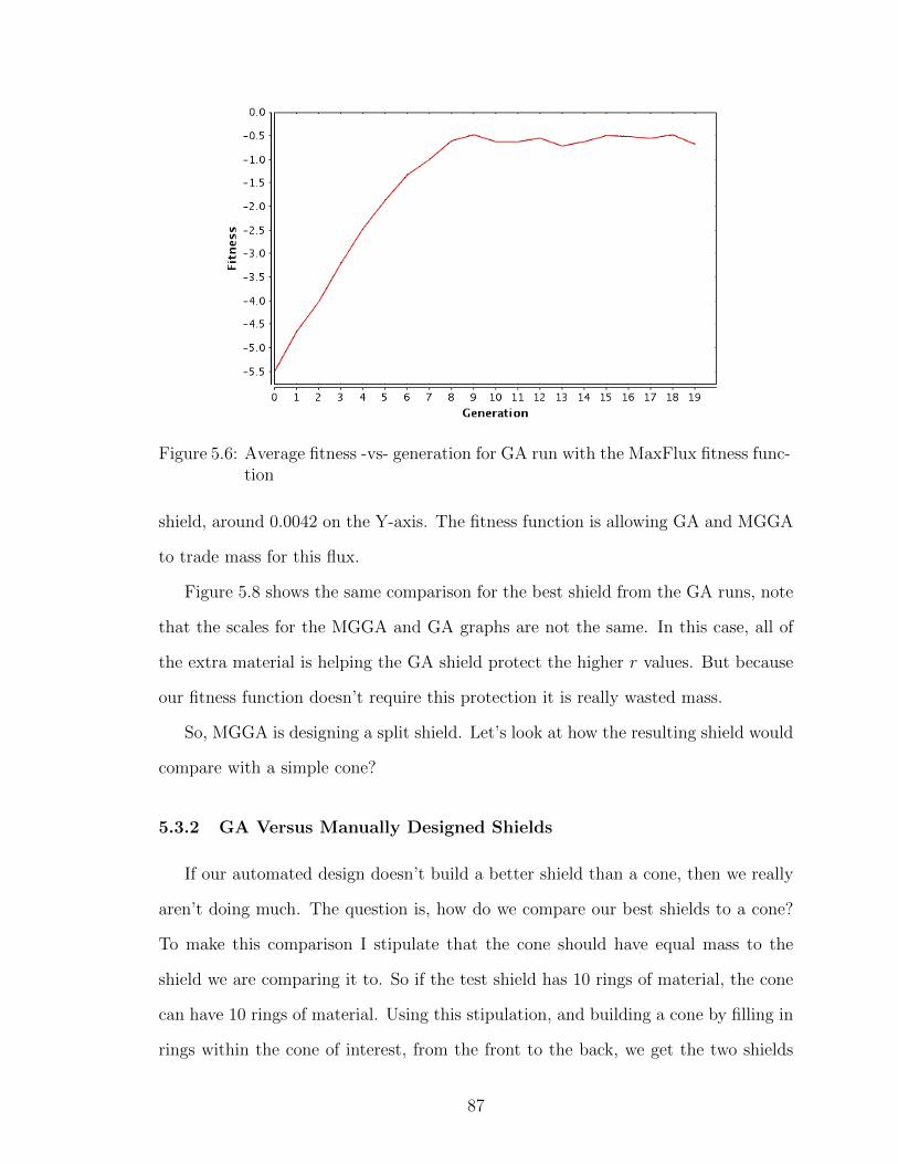
Figure 5.6: Average fitness -vs- generation for GA run with the MaxFlux fitness func-tion

shield, around 0.0042 on the Y-axis. The fitness function is allowing GA and MGGA

to trade mass for this flux.

Figure 5.8 shows the same comparison for the best shield from the GA runs, note

that the scales for the MGGA and GA graphs are not the same. In this case, all of

the extra material is helping the GA shield protect the higher r values. But because

our fitness function doesn’t require this protection it is really wasted mass.

So, MGGA is designing a split shield. Let’s look at how the resulting shield would

compare with a simple cone?

5.3.2 GA Versus Manually Designed Shields

If our automated design doesn’t build a better shield than a cone, then we really

aren’t doing much. The question is, how do we compare our best shields to a cone?

To make this comparison I stipulate that the cone should have equal mass to the

shield we are comparing it to. So if the test shield has 10 rings of material, the cone

can have 10 rings of material. Using this stipulation, and building a cone by filling in

rings within the cone of interest, from the front to the back, we get the two shields

87

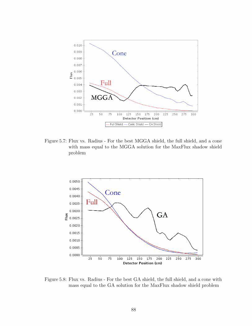
Figure 5.7: Flux vs. Radius - For the best MGGA shield, the full shield, and a conewith mass equal to the MGGA solution for the MaxFlux shadow shieldproblem

Figure 5.8: Flux vs. Radius - For the best GA shield, the full shield, and a cone withmass equal to the GA solution for the MaxFlux shadow shield problem

88

pictured in Fig. 5.9 and Fig. 5.10.

The algorithm used to make the cone shields uses the starting radius to determine

if a ring is inside of the cone of interest. In the pictures you may see a ring that

appears to go outside of the cone of interest. This is because the outer radius goes

beyond the cone, while the inner radius, at some value of z, is inside of the cone.

The first thing that really jumps out of these graphics is the difference in mass

between the MGGA version and the GA version. The GA version is a massive cone

and fills most of the cone of interest with material. These extra rings are coming from

the “noise” that was outside of the cone of interest in the generated shield. Even more

interesting, the cone version of the GA shield actually fails the flux criteria of the

fitness test and ends up with a fitness of −3.54. We can see this failure on the flux

graph in Fig. 5.8 where the center of the cone’s flux is higher than the heaviest shield.

Most likely this failure is due to scattering particles that stay in the shield and come

back to the detector plane rather than escaping as they might from a split shield.

The cone version of the MGGA shield appears small compared to its GA counter-

part. As we might expect, this conic shield also fails the flux criteria and only scores

a fitness of −19.038. Looking at the flux graph in Fig. 5.7 we can see that this cone

doesn’t even come close to matching the heaviest shield at low values of r.

Another important question about the shields coming from GA is, how would

they perform if all of the noise was removed? In the case of the best MGGA shield,

there is no noise. But for the best GA shield there is a lot of noise. I cleaned up this

noise by removing any rings that lie completely outside of the cone of interest, which

represents the line of sight between the source and detector planes. This cleaned

shield is pictured in Fig. 5.11. By removing the extra material, this shield’s fitness

jumped from 0.75 to 0.875, but still doesn’t beat the MGGA result.

89

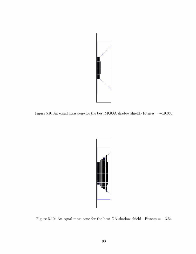
Figure 5.9: An equal mass cone for the best MGGA shadow shield - Fitness =−19.038

Figure 5.10: An equal mass cone for the best GA shadow shield - Fitness = −3.54

90

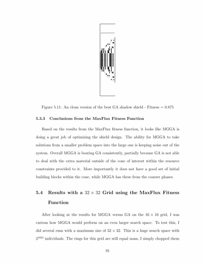
Figure 5.11: An clean version of the best GA shadow shield - Fitness = 0.875

5.3.3 Conclusions from the MaxFlux Fitness Function

Based on the results from the MaxFlux fitness function, it looks like MGGA is

doing a great job of optimizing the shield design. The ability for MGGA to take

solutions from a smaller problem space into the large one is keeping noise out of the

system. Overall MGGA is beating GA consistently, partially because GA is not able

to deal with the extra material outside of the cone of interest within the resource

constraints provided to it. More importantly it does not have a good set of initial

building blocks within the cone, while MGGA has these from the coarser phases.

5.4 Results with a 32 × 32 Grid using the MaxFlux Fitness

Function

After looking at the results for MGGA versus GA on the 16 × 16 grid, I was

curious how MGGA would perform on an even larger search space. To test this, I

did several runs with a maximum size of 32 × 32. This is a huge search space with

21024 individuals. The rings for this grid are still equal mass, I simply chopped them

91

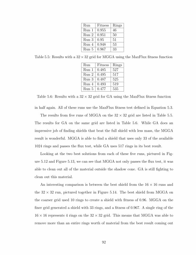
Run Fitness RingsRun 1 0.955 46Run 2 0.951 50Run 3 0.95 51Run 4 0.948 53Run 5 0.967 33

Table 5.5: Results with a 32× 32 grid for MGGA using the MaxFlux fitness function

Run Fitness RingsRun 1 0.485 527Run 2 0.495 517Run 3 0.487 525Run 4 0.493 519Run 5 0.477 535

Table 5.6: Results with a 32× 32 grid for GA using the MaxFlux fitness function

in half again. All of these runs use the MaxFlux fitness test defined in Equation 5.3.

The results from five runs of MGGA on the 32 × 32 grid are listed in Table 5.5.

The results for GA on the same grid are listed in Table 5.6. While GA does an

impressive job of finding shields that beat the full shield with less mass, the MGGA

result is wonderful. MGGA is able to find a shield that uses only 33 of the available

1024 rings and passes the flux test, while GA uses 517 rings in its best result.

Looking at the two best solutions from each of these five runs, pictured in Fig-

ure 5.12 and Figure 5.13, we can see that MGGA not only passes the flux test, it was

able to clean out all of the material outside the shadow cone. GA is still fighting to

clean out this material.

An interesting comparison is between the best shield from the 16 × 16 runs and

the 32 × 32 run, pictured together in Figure 5.14. The best shield from MGGA on

the coarser grid used 10 rings to create a shield with fitness of 0.96. MGGA on the

finer grid generated a shield with 33 rings, and a fitness of 0.967. A single ring of the

16× 16 represents 4 rings on the 32× 32 grid. This means that MGGA was able to

remove more than an entire rings worth of material from the best result coming out

92

Figure 5.12: The best MGGA shadow shield for a 32× 32 grid - Fitness = 0.967

Figure 5.13: The best GA shadow shield for a 32× 32 grid - Fitness = 0.495

93

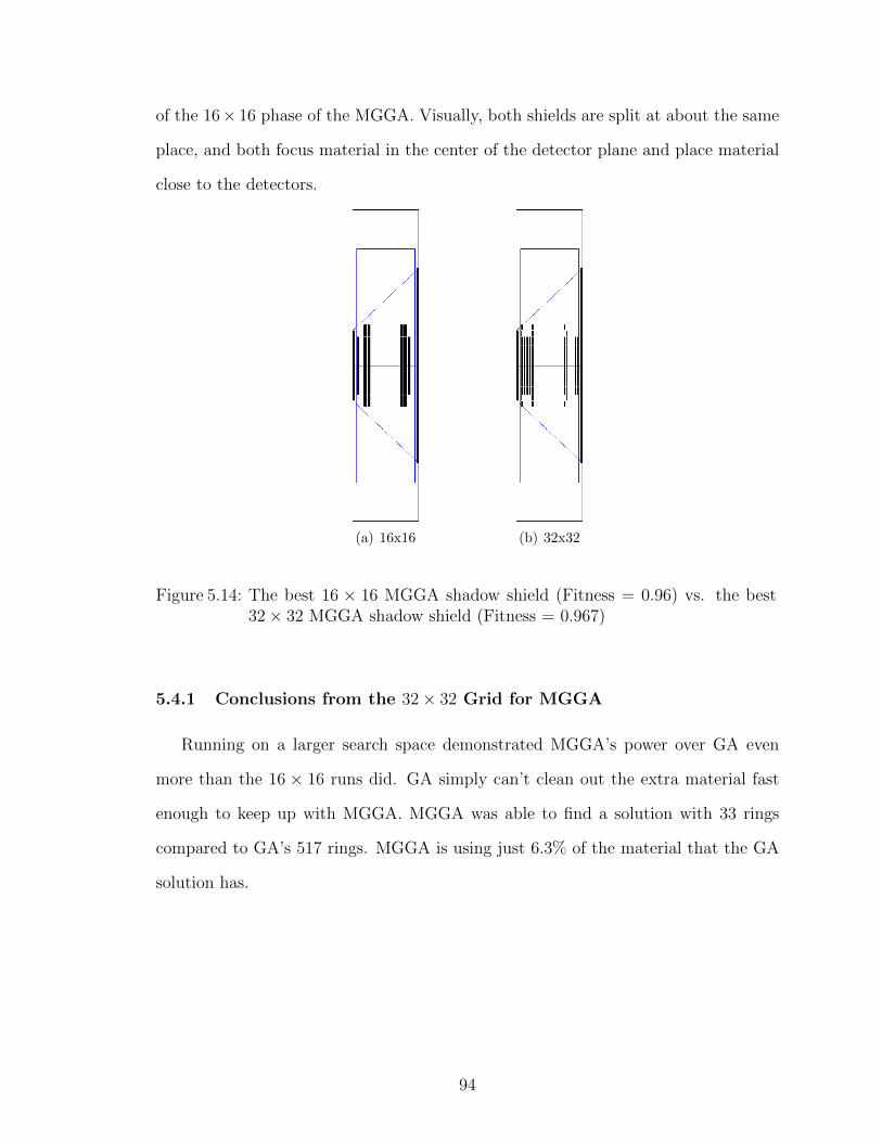
of the 16× 16 phase of the MGGA. Visually, both shields are split at about the same

place, and both focus material in the center of the detector plane and place material

close to the detectors.

(a) 16x16 (b) 32x32

Figure 5.14: The best 16 × 16 MGGA shadow shield (Fitness = 0.96) vs. the best32× 32 MGGA shadow shield (Fitness = 0.967)

5.4.1 Conclusions from the 32× 32 Grid for MGGA

Running on a larger search space demonstrated MGGA’s power over GA even

more than the 16 × 16 runs did. GA simply can’t clean out the extra material fast

enough to keep up with MGGA. MGGA was able to find a solution with 33 rings

compared to GA’s 517 rings. MGGA is using just 6.3% of the material that the GA

solution has.

94

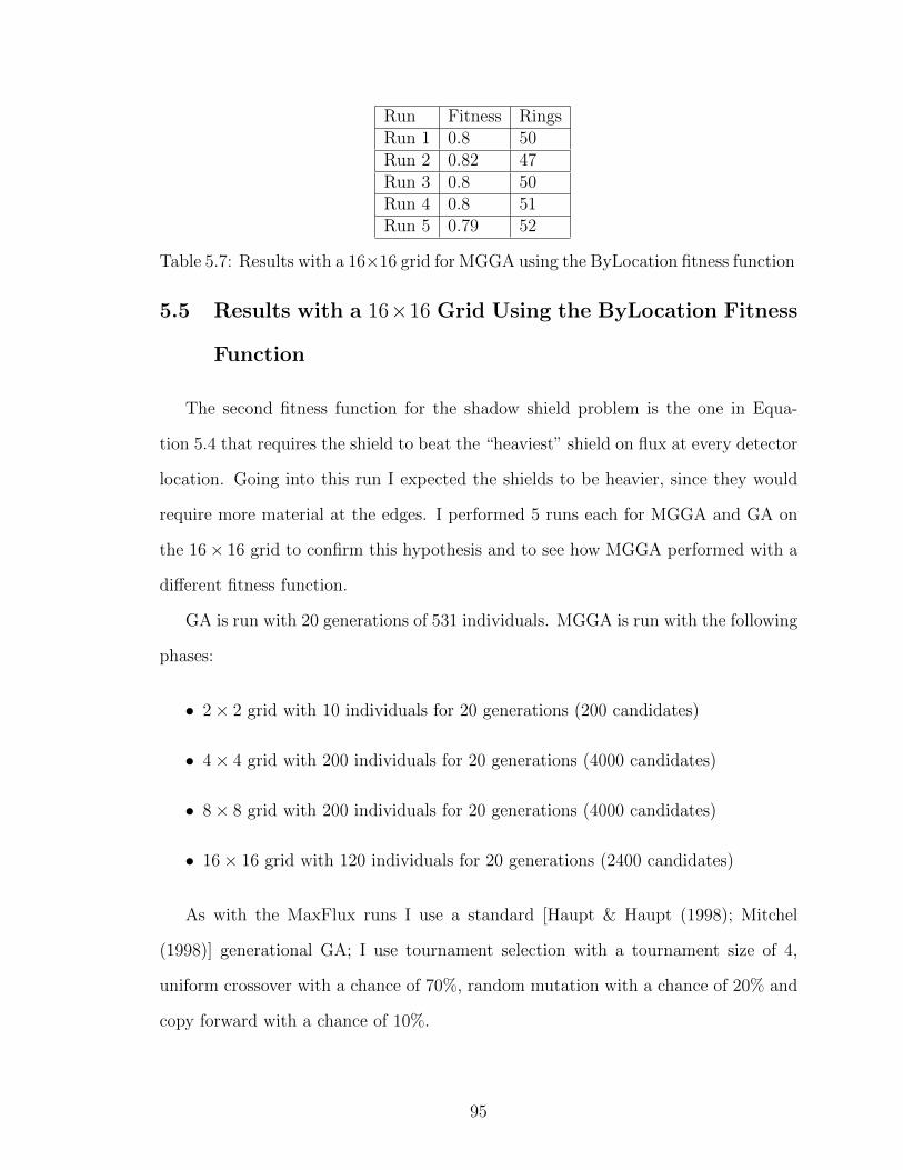
Run Fitness RingsRun 1 0.8 50Run 2 0.82 47Run 3 0.8 50Run 4 0.8 51Run 5 0.79 52

Table 5.7: Results with a 16×16 grid for MGGA using the ByLocation fitness function

5.5 Results with a 16×16 Grid Using the ByLocation Fitness

Function

The second fitness function for the shadow shield problem is the one in Equa-

tion 5.4 that requires the shield to beat the “heaviest” shield on flux at every detector

location. Going into this run I expected the shields to be heavier, since they would

require more material at the edges. I performed 5 runs each for MGGA and GA on

the 16× 16 grid to confirm this hypothesis and to see how MGGA performed with a

different fitness function.

GA is run with 20 generations of 531 individuals. MGGA is run with the following

phases:

• 2× 2 grid with 10 individuals for 20 generations (200 candidates)

• 4× 4 grid with 200 individuals for 20 generations (4000 candidates)

• 8× 8 grid with 200 individuals for 20 generations (4000 candidates)

• 16× 16 grid with 120 individuals for 20 generations (2400 candidates)

As with the MaxFlux runs I use a standard [Haupt & Haupt (1998); Mitchel

(1998)] generational GA; I use tournament selection with a tournament size of 4,

uniform crossover with a chance of 70%, random mutation with a chance of 20% and

copy forward with a chance of 10%.

95

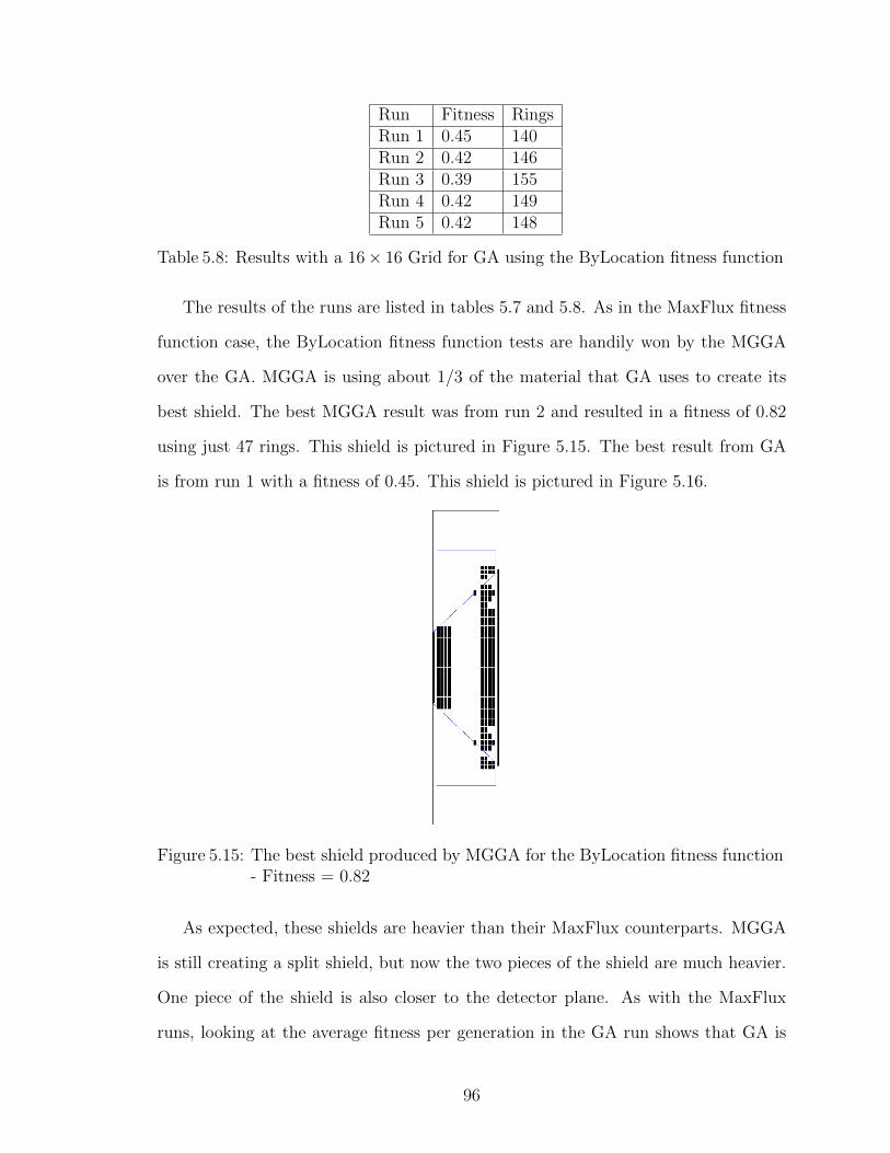
Run Fitness RingsRun 1 0.45 140Run 2 0.42 146Run 3 0.39 155Run 4 0.42 149Run 5 0.42 148

Table 5.8: Results with a 16× 16 Grid for GA using the ByLocation fitness function

The results of the runs are listed in tables 5.7 and 5.8. As in the MaxFlux fitness

function case, the ByLocation fitness function tests are handily won by the MGGA

over the GA. MGGA is using about 1/3 of the material that GA uses to create its

best shield. The best MGGA result was from run 2 and resulted in a fitness of 0.82

using just 47 rings. This shield is pictured in Figure 5.15. The best result from GA

is from run 1 with a fitness of 0.45. This shield is pictured in Figure 5.16.

Figure 5.15: The best shield produced by MGGA for the ByLocation fitness function- Fitness = 0.82

As expected, these shields are heavier than their MaxFlux counterparts. MGGA

is still creating a split shield, but now the two pieces of the shield are much heavier.

One piece of the shield is also closer to the detector plane. As with the MaxFlux

runs, looking at the average fitness per generation in the GA run shows that GA is

96

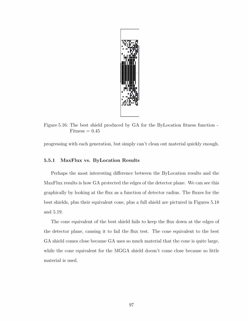
Figure 5.16: The best shield produced by GA for the ByLocation fitness function -Fitness = 0.45

progressing with each generation, but simply can’t clean out material quickly enough.

5.5.1 MaxFlux vs. ByLocation Results

Perhaps the most interesting difference between the ByLocation results and the

MaxFlux results is how GA protected the edges of the detector plane. We can see this

graphically by looking at the flux as a function of detector radius. The fluxes for the

best shields, plus their equivalent cone, plus a full shield are pictured in Figures 5.18

and 5.19.

The cone equivalent of the best shield fails to keep the flux down at the edges of

the detector plane, causing it to fail the flux test. The cone equivalent to the best

GA shield comes close because GA uses so much material that the cone is quite large,

while the cone equivalent for the MGGA shield doesn’t come close because so little

material is used.

97

Figure 5.17: Average fitness vs. generation for a GA run with the ByLocation fitnessfunction

Figure 5.18: Fluxes for the best MGGA shadow shield using the ByLocation fitnesstest, equivalent cone and full shield

98

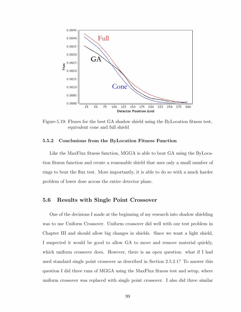
Figure 5.19: Fluxes for the best GA shadow shield using the ByLocation fitness test,equivalent cone and full shield

5.5.2 Conclusions from the ByLocation Fitness Function

Like the MaxFlux fitness function, MGGA is able to beat GA using the ByLoca-

tion fitness function and create a reasonable shield that uses only a small number of

rings to beat the flux test. More importantly, it is able to do so with a much harder

problem of lower dose across the entire detector plane.

5.6 Results with Single Point Crossover

One of the decisions I made at the beginning of my research into shadow shielding

was to use Uniform Crossover. Uniform crossover did well with our test problem in

Chapter III and should allow big changes in shields. Since we want a light shield,

I suspected it would be good to allow GA to move and remove material quickly,

which uniform crossover does. However, there is an open question: what if I had

used standard single point crossover as described in Section 2.5.2.1? To answer this

question I did three runs of MGGA using the MaxFlux fitness test and setup, where

uniform crossover was replaced with single point crossover. I also did three similar

99

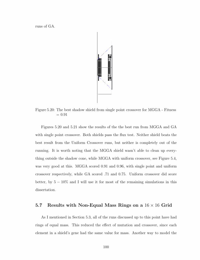
runs of GA.

Figure 5.20: The best shadow shield from single point crossover for MGGA - Fitness= 0.91

Figures 5.20 and 5.21 show the results of the the best run from MGGA and GA

with single point crossover. Both shields pass the flux test. Neither shield beats the

best result from the Uniform Crossover runs, but neither is completely out of the

running. It is worth noting that the MGGA shield wasn’t able to clean up every-

thing outside the shadow cone, while MGGA with uniform crossover, see Figure 5.4,

was very good at this. MGGA scored 0.91 and 0.96, with single point and uniform

crossover respectively, while GA scored .71 and 0.75. Uniform crossover did score

better, by 5 − 10% and I will use it for most of the remaining simulations in this

dissertation.

5.7 Results with Non-Equal Mass Rings on a 16× 16 Grid

As I mentioned in Section 5.3, all of the runs discussed up to this point have had

rings of equal mass. This reduced the effect of mutation and crossover, since each

element in a shield’s gene had the same value for mass. Another way to model the

100

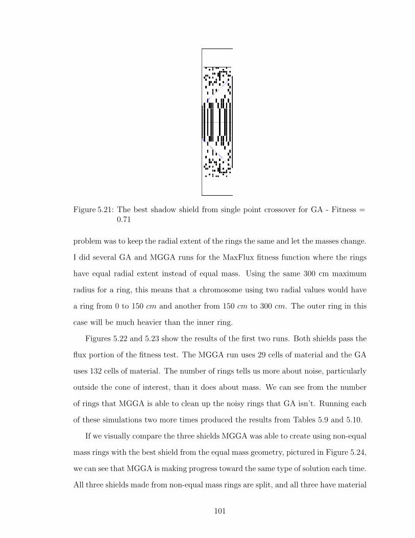
Figure 5.21: The best shadow shield from single point crossover for GA - Fitness =0.71

problem was to keep the radial extent of the rings the same and let the masses change.

I did several GA and MGGA runs for the MaxFlux fitness function where the rings

have equal radial extent instead of equal mass. Using the same 300 cm maximum

radius for a ring, this means that a chromosome using two radial values would have

a ring from 0 to 150 cm and another from 150 cm to 300 cm. The outer ring in this

case will be much heavier than the inner ring.

Figures 5.22 and 5.23 show the results of the first two runs. Both shields pass the

flux portion of the fitness test. The MGGA run uses 29 cells of material and the GA

uses 132 cells of material. The number of rings tells us more about noise, particularly

outside the cone of interest, than it does about mass. We can see from the number

of rings that MGGA is able to clean up the noisy rings that GA isn’t. Running each

of these simulations two more times produced the results from Tables 5.9 and 5.10.

If we visually compare the three shields MGGA was able to create using non-equal

mass rings with the best shield from the equal mass geometry, pictured in Figure 5.24,

we can see that MGGA is making progress toward the same type of solution each time.

All three shields made from non-equal mass rings are split, and all three have material

101

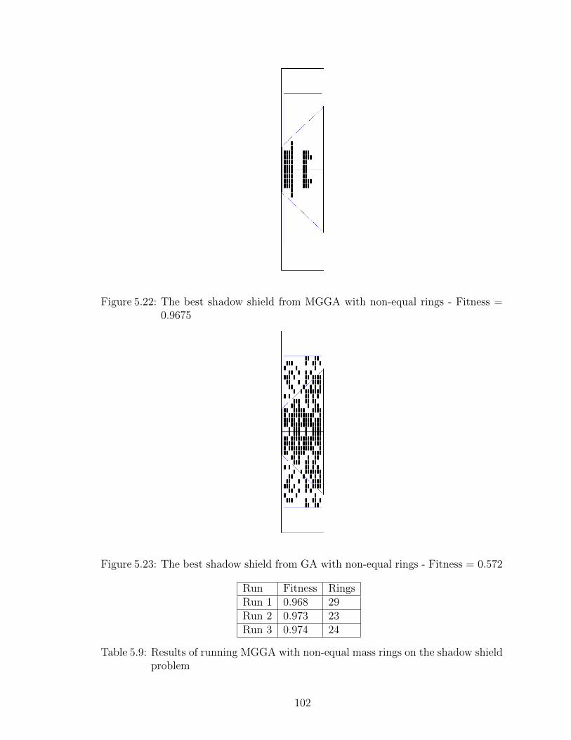
Figure 5.22: The best shadow shield from MGGA with non-equal rings - Fitness =0.9675

Figure 5.23: The best shadow shield from GA with non-equal rings - Fitness = 0.572

Run Fitness RingsRun 1 0.968 29Run 2 0.973 23Run 3 0.974 24

Table 5.9: Results of running MGGA with non-equal mass rings on the shadow shieldproblem

102

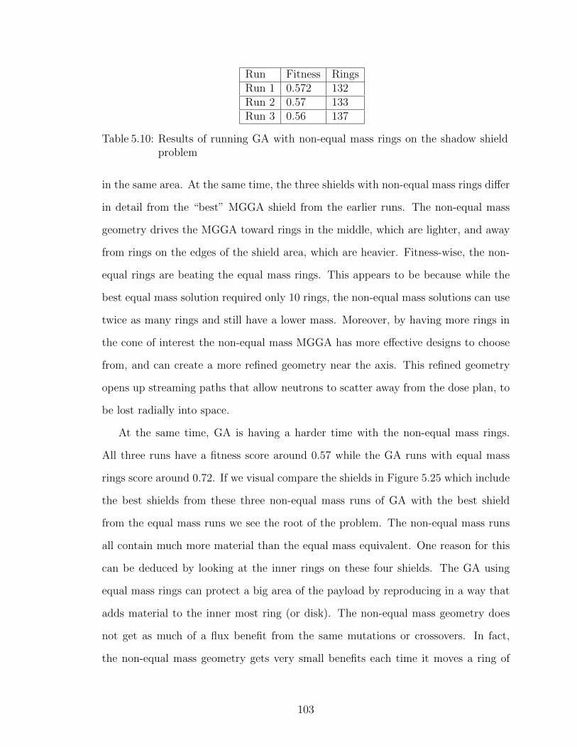
Run Fitness RingsRun 1 0.572 132Run 2 0.57 133Run 3 0.56 137

Table 5.10: Results of running GA with non-equal mass rings on the shadow shieldproblem

in the same area. At the same time, the three shields with non-equal mass rings differ

in detail from the “best” MGGA shield from the earlier runs. The non-equal mass

geometry drives the MGGA toward rings in the middle, which are lighter, and away

from rings on the edges of the shield area, which are heavier. Fitness-wise, the non-

equal rings are beating the equal mass rings. This appears to be because while the

best equal mass solution required only 10 rings, the non-equal mass solutions can use

twice as many rings and still have a lower mass. Moreover, by having more rings in

the cone of interest the non-equal mass MGGA has more effective designs to choose

from, and can create a more refined geometry near the axis. This refined geometry

opens up streaming paths that allow neutrons to scatter away from the dose plan, to

be lost radially into space.

At the same time, GA is having a harder time with the non-equal mass rings.

All three runs have a fitness score around 0.57 while the GA runs with equal mass

rings score around 0.72. If we visual compare the shields in Figure 5.25 which include

the best shields from these three non-equal mass runs of GA with the best shield

from the equal mass runs we see the root of the problem. The non-equal mass runs

all contain much more material than the equal mass equivalent. One reason for this

can be deduced by looking at the inner rings on these four shields. The GA using

equal mass rings can protect a big area of the payload by reproducing in a way that

adds material to the inner most ring (or disk). The non-equal mass geometry does

not get as much of a flux benefit from the same mutations or crossovers. In fact,

the non-equal mass geometry gets very small benefits each time it moves a ring of

103

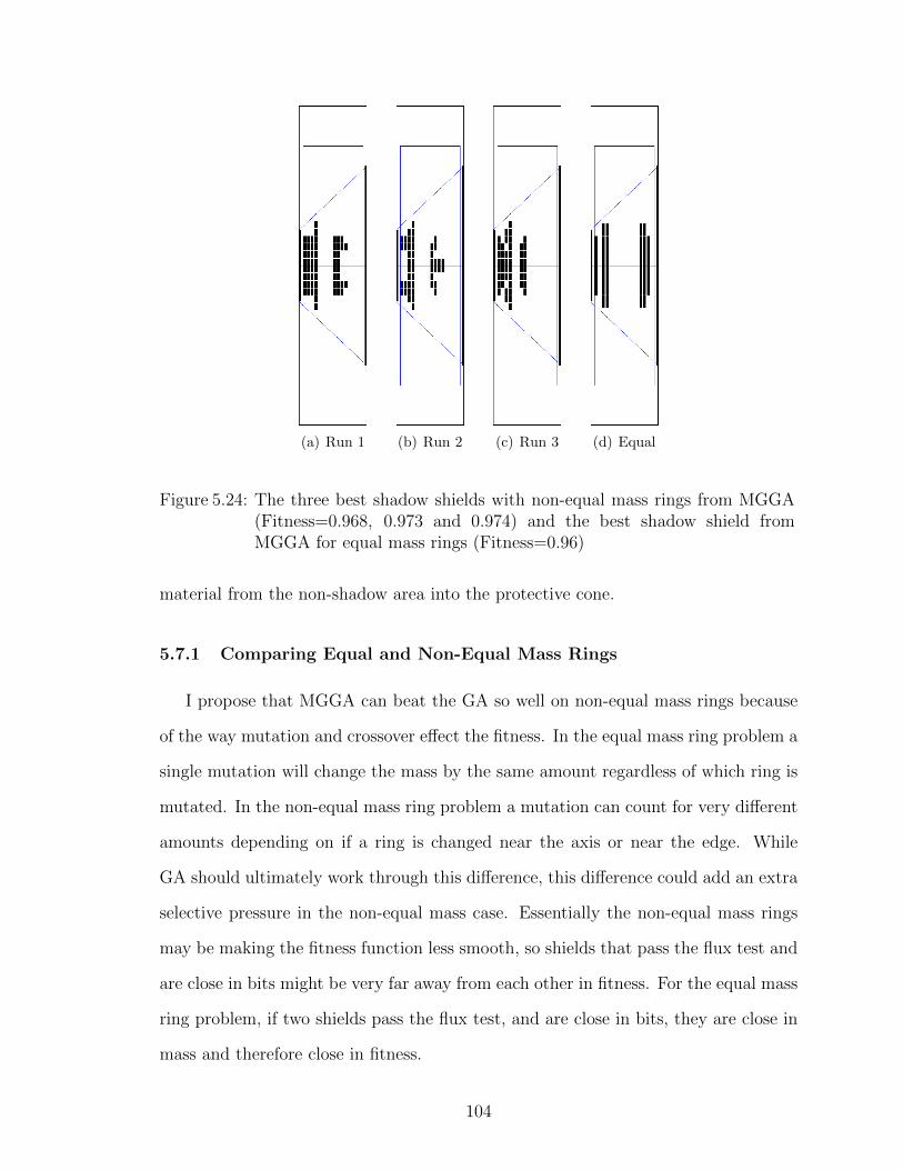
(a) Run 1 (b) Run 2 (c) Run 3 (d) Equal

Figure 5.24: The three best shadow shields with non-equal mass rings from MGGA(Fitness=0.968, 0.973 and 0.974) and the best shadow shield fromMGGA for equal mass rings (Fitness=0.96)

material from the non-shadow area into the protective cone.

5.7.1 Comparing Equal and Non-Equal Mass Rings

I propose that MGGA can beat the GA so well on non-equal mass rings because

of the way mutation and crossover effect the fitness. In the equal mass ring problem a

single mutation will change the mass by the same amount regardless of which ring is

mutated. In the non-equal mass ring problem a mutation can count for very different

amounts depending on if a ring is changed near the axis or near the edge. While

GA should ultimately work through this difference, this difference could add an extra

selective pressure in the non-equal mass case. Essentially the non-equal mass rings

may be making the fitness function less smooth, so shields that pass the flux test and

are close in bits might be very far away from each other in fitness. For the equal mass

ring problem, if two shields pass the flux test, and are close in bits, they are close in

mass and therefore close in fitness.

104

(a) Run 1 (b) Run 2 (c) Run 3 (d) Equal

Figure 5.25: The three best shadow shields with non-equal mass rings from GA (Fit-ness=0.572, 0.57 and 0.56) and the best shadow shield from GA for equalmass rings (Fitness=0.75)

To test this theory I wrote a tool to extract fitness difference for single mutations

on shields where both the parent and child pass the flux test. By insuring that both

parent and child pass the flux test, I am only looking at mutations effecting the mass

part of the fitness test. Executing this tool on several runs from the non-equal mass

and equal mass simulations I found that the non-equal mass rings do allow a larger

maximum fitness change due to mutation, but that the average effect of this is about

the same as for the equal mass ring case.

The biggest change due to mutation for the equal mass runs was 0.0039 compared

to a best fitness of 0.96, while the biggest change for the non-equal mass runs was

0.0075 compared to a best fitness of 0.968. For the non-equal mass function this

difference would be sufficient to move an individual from 0.968 to 0.975 which would

beat the best shield from any of our non-equal mass MGGA runs.

Looking back at Figure 5.24 this effect makes sense. The non-equal mass rings

result in very small rings near the axis, where most of the shielding needs to occur.

105

The MGGA is able to create more intricate designs that can allow for more scattering

paths to let the neutrons out of the system. While the non-equal mass MGGA can

find these small details in the primary shielding zone, the equal mass MGGA only

has a very large ring to manipulate in the radial area.

In the end, it isn’t obvious why GA is having a harder time with the non-equal

mass ring geometry. One reasonable explanation for why GA is struggling relates

to building blocks. When using equal mass rings, GA has to find building blocks

containing the central ring in order to pass the flux test. This is a single gene and

easy to find through mutation, crossover or randomly in the initial population. The

non-equal mass scenario requires many more genes to be active at the core to pass

the flux test. This makes creating the required building blocks more complex in the

non-equal mass case. MGGA is able to overcome this complexity by finding good

building blocks on the coarser grid and passing these building blocks into the higher

resolution problem space. As a result, MGGA can generate a number of interesting

and effective shields more easily than GA can.

5.7.2 Conclusions from the Non-Equal Mass Rings

As with the other fitness tests in this chapter, MGGA is doing a great job of

finding solutions to the shadow shield problem. Despite the fact that GA has a

harder time with the non-equal mass case, MGGA is still able to build good shields

with no obvious design flaws.

5.8 Diversity and MGGA

As I suggested earlier, there is a question about how MGGA is effecting diversity.

We can visually investigate this concern by looking at shields from the first generation

of each phase in an MGGA run. Twenty-Five random shields, organized into five rows

and five columns, from the first generation of each phase of the best run discussed in

106

Section 5.3 are pictured in Figure 5.26. Notice that randomly picking shields from the

2× 2 phase resulted in only 6 different shields, of the 16 available shield encodings.

(a) 2× 2 (b) 4× 4 (c) 8× 8 (d) 16× 16

Figure 5.26: 25 random shadow shields from each phase in the winning MaxFluxMGGA run

It is easy to see that the later phases are not starting with a lot of diversity.

The lack of diversity in the last phase is especially telling if we compare the starting

population for the first generation of the 16×16 phase in the MGGA run with twenty-

107

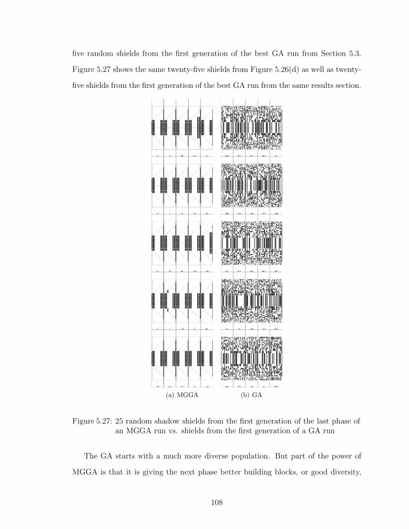
five random shields from the first generation of the best GA run from Section 5.3.

Figure 5.27 shows the same twenty-five shields from Figure 5.26(d) as well as twenty-

five shields from the first generation of the best GA run from the same results section.

(a) MGGA (b) GA

Figure 5.27: 25 random shadow shields from the first generation of the last phase ofan MGGA run vs. shields from the first generation of a GA run

The GA starts with a much more diverse population. But part of the power of

MGGA is that it is giving the next phase better building blocks, or good diversity,

108

rather than simply feeding each phase with random diversity. MGGA is providing the

final phase with a more limited set of good choices to optimize on, and thus reduces

the amount of work the final GA phase has to perform to find a good solution. The

question is, does it mean anything that we have low diversity going into the later

phases? It doesn’t seem to be hurting the results for the shadow shield problem.

But in a problem with a large search space and many local maximum it could be a

problem.

5.8.1 Measuring Diversity

We need an objective way to measure diversity. For the shadow shield problem I

use a very simple diversity measure. Later, in Section 6.3.4.1, I will discuss a more

statistical measure of diversity on a different problem.

Genetik caches the score of each unique chromosome, or individual. This cache

knows the scores from all chromosomes in previous generations. When a new chro-

mosome is scored, it checks to see if that same chromosome was used before, and if

so, takes the score from the cache. Cache hits are inversely proportional to diversity,

since zero cache hits would mean that all of the shields tested are unique in every gen-

eration, and a very high number of cache hits means that there are few unique shields

to test. This simple method of measuring diversity as cache hits will overestimate

diversity in most of our runs because we distribute the work of scoring to multiple ma-

chines. These machines do not communicate, so it is possible that within a generation

the same individual’s fitness score is tested more than once. Even with this leakage,

measuring cache hits is a simple way to see how we are doing with diversity. Lots

of cache hits means we are keeping the same individuals around across generations.

Few cache hits means we are making new individuals to test. The cache is reset for

each phase of an MGGA, so measuring diversity in MGGA will be a phase-by-phase

process.

109

Using cache hits to measure diversity I looked at two possible techniques for

improving diversity in MGGA. The first technique I investigated was to change the

grid on which I initialized the MGGA for the shadow shield problem with the MaxFlux

fitness function. The second technique was to inject diversity into the population

during a translation phase using mutation.

5.8.2 An Investigation Into the Best Starting Phase

Analyzing Figure 5.26, it is clear that the 2× 2 phase does not have a very large

search space. There just aren’t that many shields for GA to optimize toward. This

means that coming out of that first phase with only a 2 × 2 grid might be starting

with too simple a problem. We can investigate this idea by trying out MGGA with

a later starting phase.

I did a MGGA run using the MaxFlux fitness function and the standard GA

settings from Section 5.3, starting with the 4 × 4 grid instead of the coarser 2 × 2

one. The best solution from this run, pictured in Figure 5.28, was a shield with a

fitness score of 0.957 using just 11 cells of material. This is only 1 cell more than the

best run from the four phase MGGA run that started with a 2× 2 grid. Figure 5.29

shows the same type of montage of twenty five random shields we looked at in the last

section. Like the MGGA with four phases, the population appears to be converging

quickly.

The next step was to do a run with only two phases of MGGA. The first phase

used an 8×8 grid and the the last used the standard 16×16 grid. The other settings

were the same as the other MaxFlux fitness function runs. This run produced a

shield, pictured in Figure 5.30, with a fitness of 0.95 that used 12 cells of material.

Figure 5.31 shows of twenty five random shields from the first generation of each

phase.

Both of these limited phase runs tell us a lot about MGGA and GA in general.

110

Figure 5.28: The best shadow shield from MGGA for the MaxFlux fitness functionstarting with a 4× 4 grid - Fitness = 0.957

First, the run starting with an 8 × 8 grid shows how well GA was able to clean out

the extra material. If we compare this to the GA starting with a 16× 16 pictured in

Figure 5.5 it is easy to see that our population size and generation count gave GA

plenty of time to work on the smaller grid, but not quite enough on the larger grid.

The results from the run starting with a 4 × 4 grid also shows that there may be a

lower bound below which point MGGA doesn’t gain value from coarser phases. In all

cases we achieved a much better result with MGGA than with GA.

While changing the starting phase didn’t have an effect on the result, it did have

an effect on the diversity as measured by cache hits. Table 5.11 shows the cache hits

by phase for these runs. The runs that started at a later phase had fewer cache hits in

most cases. The run starting with the 8× 8 grid had very few hits in the 8× 8 phase.

This is completely expected, and does show that in a problem where diversity is an

issue, starting later could be a valid technique for keeping more diversity. One could

conclude that diversity has no value, but I think that what we have really shown is

that a lack of diversity was not a big problem for the shadow shield simulations. The

111

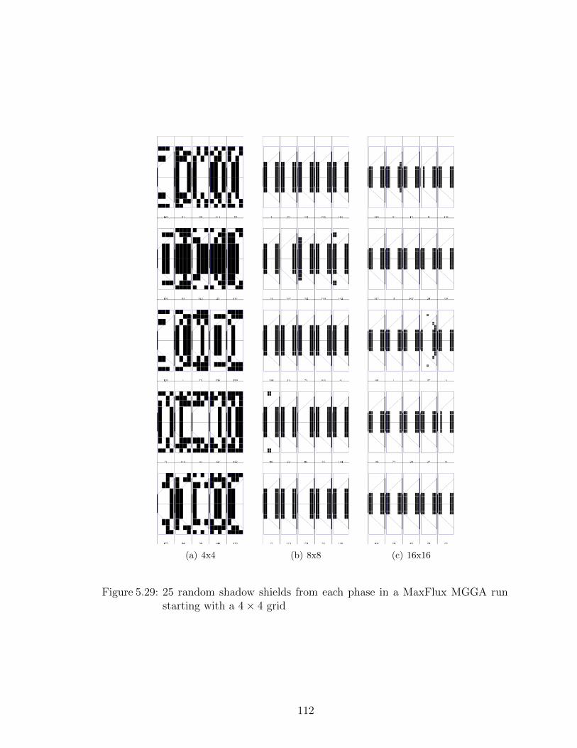
(a) 4x4 (b) 8x8 (c) 16x16

Figure 5.29: 25 random shadow shields from each phase in a MaxFlux MGGA runstarting with a 4× 4 grid

112

Figure 5.30: The best shadow shield from MGGA for the MaxFlux fitness functionstarting with a 8× 8 grid - Fitness = 0.95

Grids 2× 2 4× 4 8× 8 16× 16Four Grids 185 3422 3386 1815Three Grids N/A 2755 3392 1970Two Grids N/A N/A 536 1613

Table 5.11: Cache hits by phase with different starting phases for MGGA on theshadow shield problem

MGGA was given sufficient resources and diversity, in the form of building blocks, to

find good shields. In other words, we have shown that MGGA had sufficient diversity

to do a good job. In the next section we will see what happens if we force more

diversity into the MGGA.

5.8.3 Adding Diversity During Translations

Another idea for improving diversity in later phases is to create it artificially. GA

uses mutation to add diversity into a stagnating population. Crossover can create

diversity in populations that have enough diversity to drive it, but mutation can add

diversity to even the most homogenous population. In this section I look at adding

113

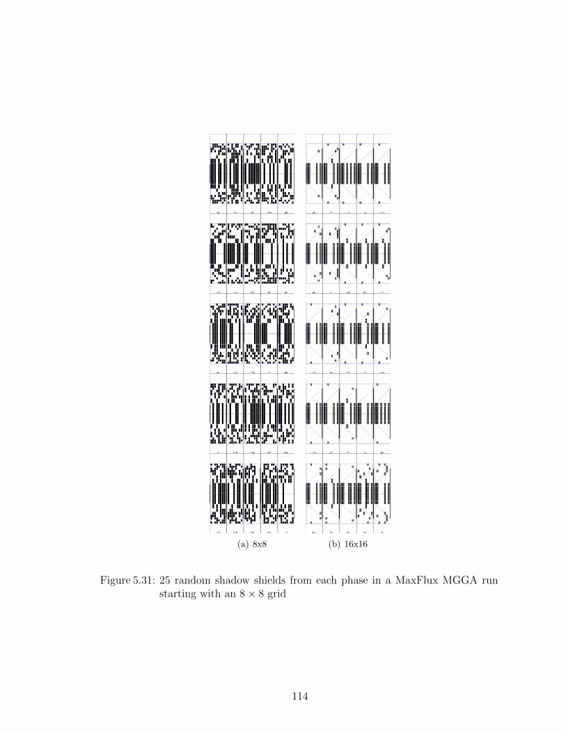
(a) 8x8 (b) 16x16

Figure 5.31: 25 random shadow shields from each phase in a MaxFlux MGGA runstarting with an 8× 8 grid

114

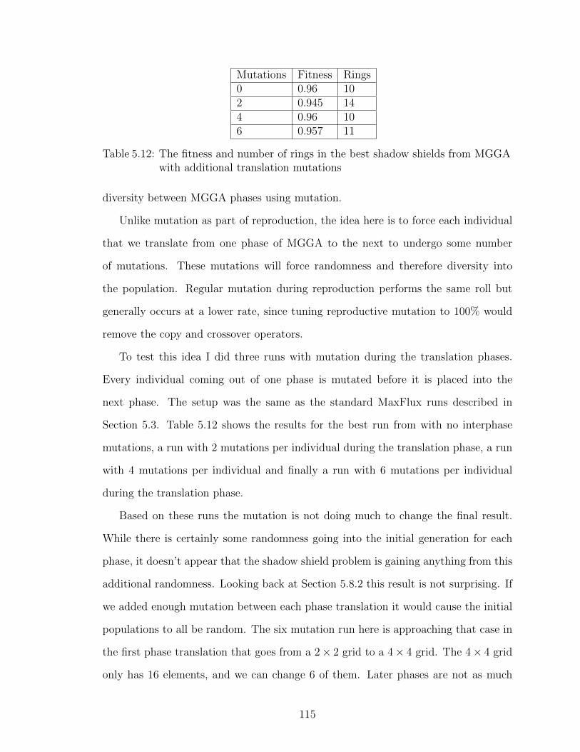
Mutations Fitness Rings0 0.96 102 0.945 144 0.96 106 0.957 11

Table 5.12: The fitness and number of rings in the best shadow shields from MGGAwith additional translation mutations

diversity between MGGA phases using mutation.

Unlike mutation as part of reproduction, the idea here is to force each individual

that we translate from one phase of MGGA to the next to undergo some number

of mutations. These mutations will force randomness and therefore diversity into

the population. Regular mutation during reproduction performs the same roll but

generally occurs at a lower rate, since tuning reproductive mutation to 100% would

remove the copy and crossover operators.

To test this idea I did three runs with mutation during the translation phases.

Every individual coming out of one phase is mutated before it is placed into the

next phase. The setup was the same as the standard MaxFlux runs described in

Section 5.3. Table 5.12 shows the results for the best run from with no interphase

mutations, a run with 2 mutations per individual during the translation phase, a run

with 4 mutations per individual and finally a run with 6 mutations per individual

during the translation phase.

Based on these runs the mutation is not doing much to change the final result.

While there is certainly some randomness going into the initial generation for each

phase, it doesn’t appear that the shadow shield problem is gaining anything from this

additional randomness. Looking back at Section 5.8.2 this result is not surprising. If

we added enough mutation between each phase translation it would cause the initial

populations to all be random. The six mutation run here is approaching that case in

the first phase translation that goes from a 2× 2 grid to a 4× 4 grid. The 4× 4 grid

only has 16 elements, and we can change 6 of them. Later phases are not as much

115

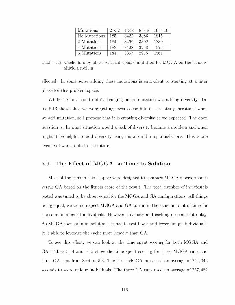
Mutations 2× 2 4× 4 8× 8 16× 16No Mutations 185 3422 3386 18152 Mutations 184 3469 3392 18304 Mutations 183 3428 3258 15756 Mutations 184 3367 2915 1561

Table 5.13: Cache hits by phase with interphase mutation for MGGA on the shadowshield problem

effected. In some sense adding these mutations is equivalent to starting at a later

phase for this problem space.

While the final result didn’t changing much, mutation was adding diversity. Ta-

ble 5.13 shows that we were getting fewer cache hits in the later generations when

we add mutation, so I propose that it is creating diversity as we expected. The open

question is: In what situation would a lack of diversity become a problem and when

might it be helpful to add diversity using mutation during translations. This is one

avenue of work to do in the future.

5.9 The Effect of MGGA on Time to Solution

Most of the runs in this chapter were designed to compare MGGA’s performance

versus GA based on the fitness score of the result. The total number of individuals

tested was tuned to be about equal for the MGGA and GA configurations. All things

being equal, we would expect MGGA and GA to run in the same amount of time for

the same number of individuals. However, diversity and caching do come into play.

As MGGA focuses in on solutions, it has to test fewer and fewer unique individuals.

It is able to leverage the cache more heavily than GA.

To see this effect, we can look at the time spent scoring for both MGGA and

GA. Tables 5.14 and 5.15 show the time spent scoring for three MGGA runs and

three GA runs from Section 5.3. The three MGGA runs used an average of 244, 042

seconds to score unique individuals. The three GA runs used an average of 757, 482

116

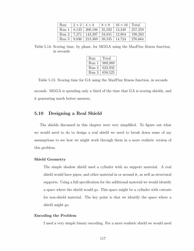
Run 2× 2 4× 4 8× 8 16× 16 TotalRun 1 8,133 200,186 35,592 13,348 257,259Run 2 7,271 143,297 34,831 12,804 198,203Run 3 9,036 213,369 39,535 14,724 276,664

Table 5.14: Scoring time, by phase, for MGGA using the MaxFlux fitness function,in seconds

Run TotalRun 1 989,989Run 2 623,932Run 3 658,525

Table 5.15: Scoring time for GA using the MaxFlux fitness function, in seconds

seconds. MGGA is spending only a third of the time that GA is scoring shields, and

it generating much better answers.

5.10 Designing a Real Shield

The shields discussed in this chapter were very simplified. To figure out what

we would need to do to design a real shield we need to break down some of my

assumptions to see how we might work through them in a more realistic version of

this problem.

Shield Geometry

The simple shadow shield used a cylinder with no support material. A real

shield would have pipes, and other material in or around it, as well as structural

supports. Using a full specification for the additional material we would identify

a space where the shield would go. This space might be a cylinder with cutouts

for non-shield material. The key point is that we identify the space where a

shield might go.

Encoding the Problem

I used a very simple binary encoding. For a more realistic shield we would need

117

to take the potential shield space and spit it into cells. For each cell we would

define a material for that cell. If we want to model gamma and neutron radiation

we could allow gamma shielding materials like tungsten as well as our LiH and

other materials for neutrons. The GA could then use a string of integers for

each chromosome, where the order of integers mapped to cell numbers and the

values of the integers mapped to materials. By choosing the size and shape of

the cells we could control how fine-grained a shield GA could produce.

Modeling the Physics

PARTISN provided good physics for our simplified shield. For a more realistic

model we would probably need to use MCNP or another Monte Carlo code. As

we will see in the next chapter, MCNP works fine with GA. Fitness functions

don’t really have restrictions in that way. Rather the GA user is limited by their

computing resources. So while I used PARTISN and a simple model, someone

with more computing time could use MCNP and a complex geometry.

Applying MGGA

While building a realistic fitness function is the first step, the MGGA user

would also need to work out population sizes for this more accurate run. As

with the physics question, sizing is mostly a question of computing resources.

If the chromosomes encode hundreds of cells, then the population size will need

to be in the thousands, at least. This will require significant computing time,

potentially spread across a large cluster.

Each of the steps for applying MGGA to a more realistic shield scenario is ad-

dressable. The fundamental question would be one of computing resources. I think

it is important to recognize that while MGGA provides a great way to explore the

potential shield designs, it probably shouldn’t be used to design the final shield at a

production scale. A real shield will be constructed using standard milling machines

118

which may not allow pieces to be added or removed as easily as they are in the sim-

ulation. I would posit that MGGA could be one step in the design process. MGGA

would be used clarify the basic shield design. An engineering team would use that

design and standard CAD/CAM tools to design the actual shield. This final design

could be simulated to a very high resolution to confirm the MGGA results before

construction.

5.11 Conclusions on the Shadow Shield Results

I performed a number of runs using both GA and MGGA to try and build a good

solution to the shadow shield problem described in Section 5.2. Using the idea that

we can score shields by how they compare to a “heaviest” shield, I built two fitness

functions. The first scored shields on flux if they were unable to do at least as well

as the heaviest shield did at its worst. This same function scored shields on their

mass if they could beat a simple flux comparison with the heaviest shield. Using

this MaxFlux fitness function, defined in Equation 5.3, MGGA was able to produce

a number of excellent shield candidates. All of these shields demonstrated the value

of splitting a shadow shield to allow particles to flow out of the system, supporting

the conclusions in [Alpay & Holloway (2005)].

The second fitness function scored shields by trying to beat the heaviest shield at

every detector location. Again, MGGA was up to the task and generated a number of

shield candidates that passed the flux portion of this fitness test, given in Equation 5.4.

In both sets of trials, MGGA created a superior shield to GA using approximately

the same number of fitness calculations and it did so in one third the time. This type

of problem space seems to fit MGGA perfectly and MGGA should be considered a

useful method for exploring possible shield designs in this type of geometry.

Exploring the value of MGGA further with a finer resolution and using the

MaxFlux fitness function I was able to show that MGGA can handle a very large

119

problem space, on the order of 21024 shield candidates, and still produce reasonable

results.

Altering the problem space by changing the shield rings from equal mass to non-

equal mass, I showed that MGGA again finds better solutions than GA, and was even

better at doing so in this problem space than the original one. MGGA appears to be

fairly resilient to changes in the fitness function as long as the geometric scaling and

translation phases are viable, which they all were for the shadow shield.

Finally, I explored a number of possible mechanisms for improving diversity in

MGGA. The conclusions from these simulations indicate that diversity was not a

problem and that having good building blocks going into the last phase of MGGA

is what is important. If MGGA is not as sensitive to diversity issues as initially

assumed it will make it an even more powerful tool for large problem spaces that can

be organized into hierarchies.

Overall, MGGA did a great job building shadow shields. It surpassed GA with

fewer computing resources in all cases. In the next two chapters I will see how MGGA

performs when designing a shield and a filter using a more detailed physical simulation

in the fitness test.

120

CHAPTER VI

Designing A Gamma Shield

6.1 Introduction

The goal of this chapter is to investigate MGGA in the context of designing a

gamma radiation shield. Rather than look at simply blocking gamma rays, I also

consider the concept of a wearable shield. Creating a shield that can be moved

around is similar to the shadow shield problem in the last chapter. Movable or

wearable shields have to balance shielding effectiveness versus mass. In the case of

a wearable shield, the mass has a reasonable maximum on the order of 50kg for

an unassisted human and something like 100kg for a human using an exoskeleton,

[Robotics (2011)]. Given this tight mass constraint, GA may be a useful tool for

finding novel shield designs. GA doesn’t have any pre-conceived notions about good

versus bad and may drive through unreasonable solutions to get to something better

than a human might design.

The initial steps in designing a gamma shield is to look at what types of radiation

we would need to worry about. There is a wide range of applications for gamma

shields, ranging from x-ray technicians, to patients receiving radiation treatment, to

a first responder dealing with a radiation dispersal device (RRD). Of these three, the

first responder has perhaps broadest range of energies to shield against. In order to

get a handle on this range of energies a first responder might encounter I looked at

121

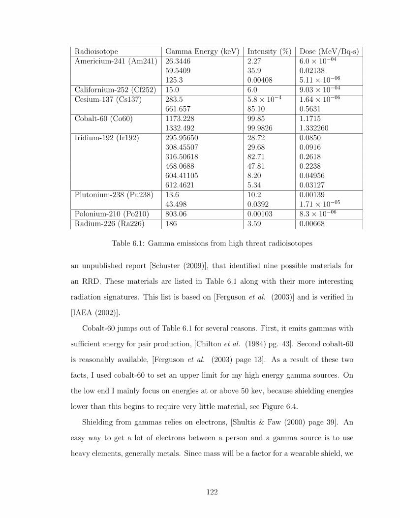
Radioisotope Gamma Energy (keV) Intensity (%) Dose (MeV/Bq-s)Americium-241 (Am241) 26.3446 2.27 6.0× 10−04

59.5409 35.9 0.02138125.3 0.00408 5.11× 10−06

Californium-252 (Cf252) 15.0 6.0 9.03× 10−04

Cesium-137 (Cs137) 283.5 5.8× 10−4 1.64× 10−06

661.657 85.10 0.5631Cobalt-60 (Co60) 1173.228 99.85 1.1715

1332.492 99.9826 1.332260Iridium-192 (Ir192) 295.95650 28.72 0.0850

308.45507 29.68 0.0916316.50618 82.71 0.2618468.0688 47.81 0.2238604.41105 8.20 0.04956612.4621 5.34 0.03127

Plutonium-238 (Pu238) 13.6 10.2 0.0013943.498 0.0392 1.71× 10−05

Polonium-210 (Po210) 803.06 0.00103 8.3× 10−06

Radium-226 (Ra226) 186 3.59 0.00668

Table 6.1: Gamma emissions from high threat radioisotopes

an unpublished report [Schuster (2009)], that identified nine possible materials for

an RRD. These materials are listed in Table 6.1 along with their more interesting

radiation signatures. This list is based on [Ferguson et al. (2003)] and is verified in

[IAEA (2002)].

Cobalt-60 jumps out of Table 6.1 for several reasons. First, it emits gammas with

sufficient energy for pair production, [Chilton et al. (1984) pg. 43]. Second cobalt-60

is reasonably available, [Ferguson et al. (2003) page 13]. As a result of these two

facts, I used cobalt-60 to set an upper limit for my high energy gamma sources. On

the low end I mainly focus on energies at or above 50 kev, because shielding energies

lower than this begins to require very little material, see Figure 6.4.

Shielding from gammas relies on electrons, [Shultis & Faw (2000) page 39]. An

easy way to get a lot of electrons between a person and a gamma source is to use

heavy elements, generally metals. Since mass will be a factor for a wearable shield, we

122

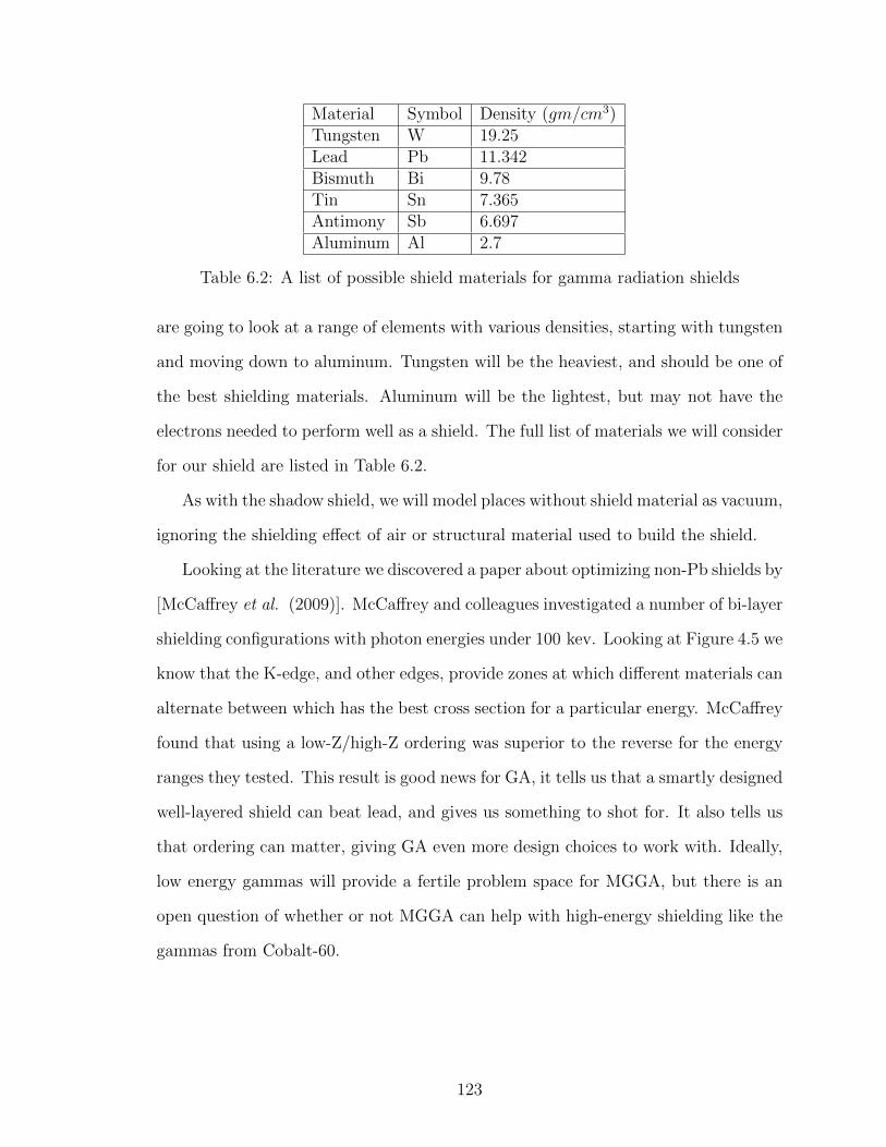
Material Symbol Density (gm/cm3)Tungsten W 19.25Lead Pb 11.342Bismuth Bi 9.78Tin Sn 7.365Antimony Sb 6.697Aluminum Al 2.7

Table 6.2: A list of possible shield materials for gamma radiation shields

are going to look at a range of elements with various densities, starting with tungsten

and moving down to aluminum. Tungsten will be the heaviest, and should be one of

the best shielding materials. Aluminum will be the lightest, but may not have the

electrons needed to perform well as a shield. The full list of materials we will consider

for our shield are listed in Table 6.2.

As with the shadow shield, we will model places without shield material as vacuum,

ignoring the shielding effect of air or structural material used to build the shield.

Looking at the literature we discovered a paper about optimizing non-Pb shields by

[McCaffrey et al. (2009)]. McCaffrey and colleagues investigated a number of bi-layer

shielding configurations with photon energies under 100 kev. Looking at Figure 4.5 we

know that the K-edge, and other edges, provide zones at which different materials can

alternate between which has the best cross section for a particular energy. McCaffrey

found that using a low-Z/high-Z ordering was superior to the reverse for the energy

ranges they tested. This result is good news for GA, it tells us that a smartly designed

well-layered shield can beat lead, and gives us something to shot for. It also tells us

that ordering can matter, giving GA even more design choices to work with. Ideally,

low energy gammas will provide a fertile problem space for MGGA, but there is an

open question of whether or not MGGA can help with high-energy shielding like the

gammas from Cobalt-60.

123

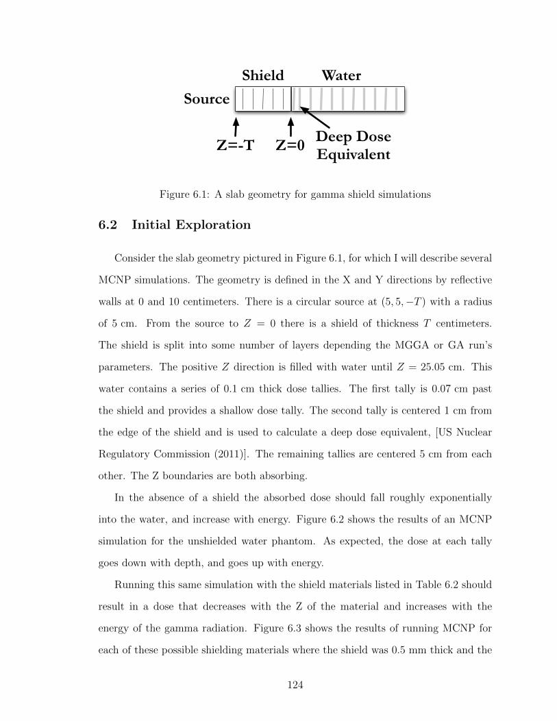
Shield Water

Z=0Z=-T

Source

Deep DoseEquivalent

Figure 6.1: A slab geometry for gamma shield simulations

6.2 Initial Exploration

Consider the slab geometry pictured in Figure 6.1, for which I will describe several

MCNP simulations. The geometry is defined in the X and Y directions by reflective

walls at 0 and 10 centimeters. There is a circular source at (5, 5,−T ) with a radius

of 5 cm. From the source to Z = 0 there is a shield of thickness T centimeters.

The shield is split into some number of layers depending the MGGA or GA run’s

parameters. The positive Z direction is filled with water until Z = 25.05 cm. This

water contains a series of 0.1 cm thick dose tallies. The first tally is 0.07 cm past

the shield and provides a shallow dose tally. The second tally is centered 1 cm from

the edge of the shield and is used to calculate a deep dose equivalent, [US Nuclear

Regulatory Commission (2011)]. The remaining tallies are centered 5 cm from each

other. The Z boundaries are both absorbing.

In the absence of a shield the absorbed dose should fall roughly exponentially

into the water, and increase with energy. Figure 6.2 shows the results of an MCNP

simulation for the unshielded water phantom. As expected, the dose at each tally

goes down with depth, and goes up with energy.

Running this same simulation with the shield materials listed in Table 6.2 should

result in a dose that decreases with the Z of the material and increases with the

energy of the gamma radiation. Figure 6.3 shows the results of running MCNP for

each of these possible shielding materials where the shield was 0.5 mm thick and the

124

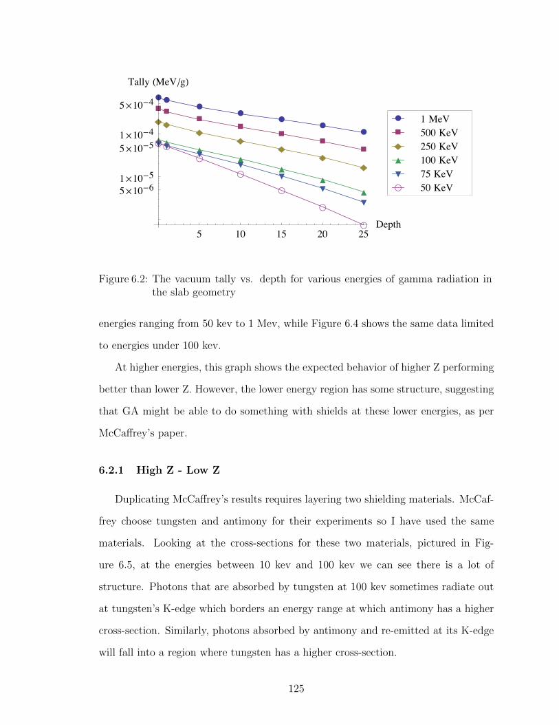
ÊÊÊ

ÊÊ

ÊÊ

‡ ‡‡

‡‡

‡‡

ÏÏÏ

ÏÏ

ÏÏ

ÚÚÚ

ÚÚ

ÚÚ

ÙÙÙ

ÙÙ

ÙÙ

ÁÁÁ

Á

Á

Á

Á5 10 15 20 25

Depth

5¥10-61¥10-5

5¥10-51¥10-4

5¥10-4

Tally HMeVêgL

Á 50 KeVÙ 75 KeVÚ 100 KeVÏ 250 KeV‡ 500 KeVÊ 1 MeV

Figure 6.2: The vacuum tally vs. depth for various energies of gamma radiation inthe slab geometry

energies ranging from 50 kev to 1 Mev, while Figure 6.4 shows the same data limited

to energies under 100 kev.

At higher energies, this graph shows the expected behavior of higher Z performing

better than lower Z. However, the lower energy region has some structure, suggesting

that GA might be able to do something with shields at these lower energies, as per

McCaffrey’s paper.

6.2.1 High Z - Low Z

Duplicating McCaffrey’s results requires layering two shielding materials. McCaf-

frey choose tungsten and antimony for their experiments so I have used the same

materials. Looking at the cross-sections for these two materials, pictured in Fig-

ure 6.5, at the energies between 10 kev and 100 kev we can see there is a lot of

structure. Photons that are absorbed by tungsten at 100 kev sometimes radiate out

at tungsten’s K-edge which borders an energy range at which antimony has a higher

cross-section. Similarly, photons absorbed by antimony and re-emitted at its K-edge

will fall into a region where tungsten has a higher cross-section.

125

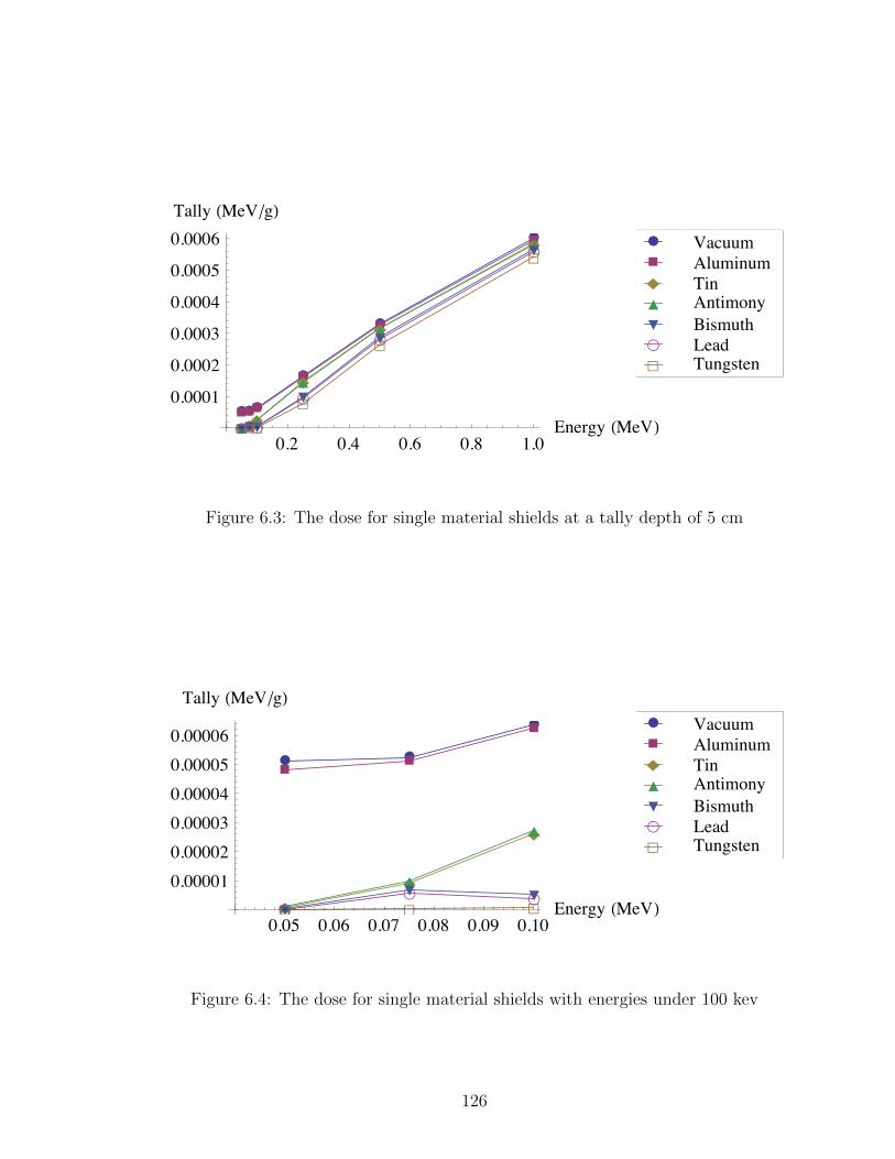
ÊÊÊ

Ê

Ê

Ê

‡‡‡

‡

‡

‡

ÏÏÏ

Ï

Ï

Ï

ÚÚÚ

Ú

Ú

Ú

ÙÙÙ

Ù

Ù

Ù

ÁÁÁ

Á

Á

Á

····

·

·

0.2 0.4 0.6 0.8 1.0Energy HMeVL

0.0001

0.0002

0.0003

0.0004

0.0005

0.0006Tally HMeVêgL

· TungstenÁ LeadÙ BismuthÚ AntimonyÏ Tin‡ AluminumÊ Vacuum

Figure 6.3: The dose for single material shields at a tally depth of 5 cm

Ê Ê

Ê

‡ ‡

‡

ÏÏ

Ï

ÚÚ

Ú

ÙÙ Ù

ÁÁ Á

· · ·0.05 0.06 0.07 0.08 0.09 0.10

Energy HMeVL0.000010.000020.000030.000040.000050.00006

Tally HMeVêgL

· TungstenÁ LeadÙ BismuthÚ AntimonyÏ Tin‡ AluminumÊ Vacuum

Figure 6.4: The dose for single material shields with energies under 100 kev

126

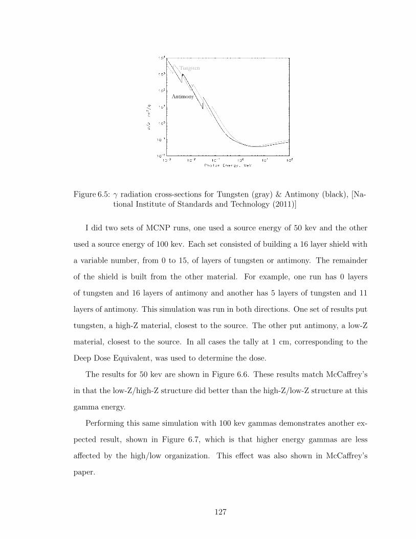
Figure 6.5: γ radiation cross-sections for Tungsten (gray) & Antimony (black), [Na-tional Institute of Standards and Technology (2011)]

I did two sets of MCNP runs, one used a source energy of 50 kev and the other

used a source energy of 100 kev. Each set consisted of building a 16 layer shield with

a variable number, from 0 to 15, of layers of tungsten or antimony. The remainder

of the shield is built from the other material. For example, one run has 0 layers

of tungsten and 16 layers of antimony and another has 5 layers of tungsten and 11

layers of antimony. This simulation was run in both directions. One set of results put

tungsten, a high-Z material, closest to the source. The other put antimony, a low-Z

material, closest to the source. In all cases the tally at 1 cm, corresponding to the

Deep Dose Equivalent, was used to determine the dose.

The results for 50 kev are shown in Figure 6.6. These results match McCaffrey’s

in that the low-Z/high-Z structure did better than the high-Z/low-Z structure at this

gamma energy.

Performing this same simulation with 100 kev gammas demonstrates another ex-

pected result, shown in Figure 6.7, which is that higher energy gammas are less

affected by the high/low organization. This effect was also shown in McCaffrey’s

paper.

127

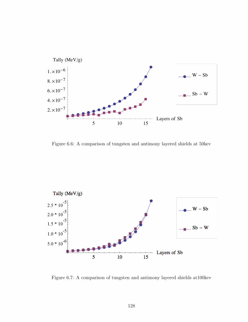
Ê

Ê

ÊÊ

ÊÊ

ÊÊÊÊÊÊÊÊÊʇ ‡ ‡ ‡ ‡ ‡ ‡

‡ ‡ ‡ ‡‡ ‡

‡ ‡‡

5 10 15Layers of Sb

2.¥10-74.¥10-76.¥10-78.¥10-71.¥10-6

Tally HMeVêgL

‡ Sb -W

Ê W - Sb

Figure 6.6: A comparison of tungsten and antimony layered shields at 50kev

Figure 6.7: A comparison of tungsten and antimony layered shields at100kev

128

6.3 Designing a Gamma Shield with MGGA

Given that layering does effect the dose, what is the best shield we can construct

from the materials in Table 6.2. MGGA and GA can help explore this problem and

work toward building good shield. But first we have to create a fitness function that

defines what good means.

6.3.1 Defining a Fitness Function

McCaffrey’s paper compared the shields they tested against a fixed amount of lead

on mass and dose. I copied this approach by defining a fitness function that tries to

find a shield with a lower mass than one made from 0.5 mm of lead and then reduce

the dose. Basically, the fitness function is trying to weigh less than a standard shield

and then try to beat it on dose. The fitness of each shield, s, will be determined as

follows:

1. Calculate the mass of a 0.5 mm shield made of lead, m(S)

2. Calculate the deep dose equivalent, D(s), with shield s

3. Compare the mass with of shield s, m(s) to the mass of the lead shield, m(S):

• If the shield is heavier than the lead shield, the fitness is −(m(s)/m(S))

• Otherwise the fitness is 1− (D(s)× 1000)

In other words, the fitness of shield s is

F (s) =

1− (D(s)× 1000) if m(s) < m(S)

−m(s)m(S)

otherwise.

(6.1)

I am multiplying the tally, in MeV/g, by 1000 to make the fitness scores more

human readable. Moreover, I am assuming that D(s) is always less than 1/1000 so

129

that a shield measured on dose is never assigned a score less than zero, and the scaling

will not effect the ranking of two light shields, where m(s) < m(S). This assumption

was not violated in the runs described here.

While the fitness compares the deep dose after running a simulation using a shield

s to the lead shield S, it is not always obvious what a particular fitness score means.

To help understand the values of the shields better I calculate another value called

Dose Reduction Percentage. Dose reduction of a shield s, compared to the lead shield

S is defined as:

DoseReductionPercentage(s) = 100 ∗[1− D(s)

D(S)

](6.2)

Basically this is the percentage reduction in dose that the shield has over the lead

shield.

6.3.2 Fitness and Error

When dealing with MCNP or any other physical simulation there will be error

in the results. While I have tried to reduce the error to a small percentage of the

total dose for these calculations, there is of course always a finite error. This means

that running a stochastic simulation like MCNP on the same shield multiple times can

result in different fitness scores (if independent random numbers are used). Moreover,

it means that two shields with very close fitness scores may be equivalent within the

error in the dose calculation. When running tournament selection, this equivalence

is ignored. So one shield may have an advantage simply because the random number

generator was kind to it in MCNP; in these cases we are effectively randomly selecting

one of the shields. In the context of this dissertation, which is focussed on showing the

value of MGGA versus GA for these types of problems, this potential inconsistency

in the fitness functions is acceptable, but it does represent a possible area of research

in the future.

130

6.3.3 Defining the Genetic Algorithm

Using the fitness function in Equation 6.1 I ran several simulations for GA and

MGGA. The final geometry had a total of 16 layers, with seven possible materi-

als in each layer, or 716 = 3.32 × 1013, or approximately 33 trillion possible shield

configurations.

The GA was run with a population of 1000 for 20 generations. The MGGA was

run with the following phases:

• 4 layers - 250 individuals per generation with 10 generations

• 8 layers - 500 individuals per generation with 15 generations

• 16 layers - 500 individuals per generation with 15 generations

Thus MGGA used 17,500 individuals while GA used 20,000.

To move between phases each layer was cut into two pieces for the next phase.

From a shielding standpoint the shields were identical as they move between phases.

The encoding for each shield was a string of integers, one for each layer. The integers

were the numbers 0-6 indicating an index into the list of available materials: vacuum,

tungsten, lead, bismuth, tin, antimony, and aluminum.

All GA was performed using tournament selection with a tournament size of 5.

There was a 25% chance that the worst individual in a tournament would win to

help preserve diversity. Reproduction relied on uniform crossover 70% of the time,

mutation of a single layer 20% of the time and copying 10% of the time. Uniform

crossover allowed each child to use the materials for any layer from either parent,

however, I created two children for each crossover reproduction, these two children

were the result of reversing the coin flip for each gene in uniform crossover.

131

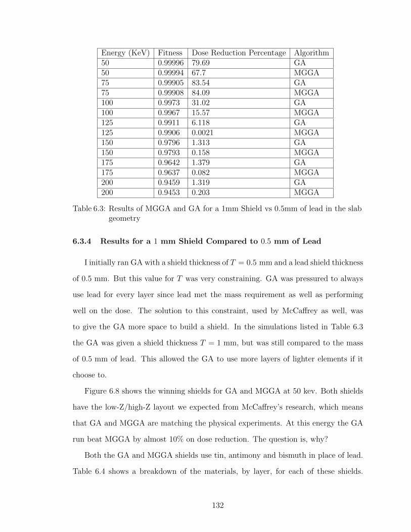
Energy (KeV) Fitness Dose Reduction Percentage Algorithm50 0.99996 79.69 GA50 0.99994 67.7 MGGA75 0.99905 83.54 GA75 0.99908 84.09 MGGA100 0.9973 31.02 GA100 0.9967 15.57 MGGA125 0.9911 6.118 GA125 0.9906 0.0021 MGGA150 0.9796 1.313 GA150 0.9793 0.158 MGGA175 0.9642 1.379 GA175 0.9637 0.082 MGGA200 0.9459 1.319 GA200 0.9453 0.203 MGGA

Table 6.3: Results of MGGA and GA for a 1mm Shield vs 0.5mm of lead in the slabgeometry

6.3.4 Results for a 1 mm Shield Compared to 0.5 mm of Lead

I initially ran GA with a shield thickness of T = 0.5 mm and a lead shield thickness

of 0.5 mm. But this value for T was very constraining. GA was pressured to always

use lead for every layer since lead met the mass requirement as well as performing

well on the dose. The solution to this constraint, used by McCaffrey as well, was

to give the GA more space to build a shield. In the simulations listed in Table 6.3

the GA was given a shield thickness T = 1 mm, but was still compared to the mass

of 0.5 mm of lead. This allowed the GA to use more layers of lighter elements if it

choose to.

Figure 6.8 shows the winning shields for GA and MGGA at 50 kev. Both shields

have the low-Z/high-Z layout we expected from McCaffrey’s research, which means

that GA and MGGA are matching the physical experiments. At this energy the GA

run beat MGGA by almost 10% on dose reduction. The question is, why?

Both the GA and MGGA shields use tin, antimony and bismuth in place of lead.

Table 6.4 shows a breakdown of the materials, by layer, for each of these shields.

132

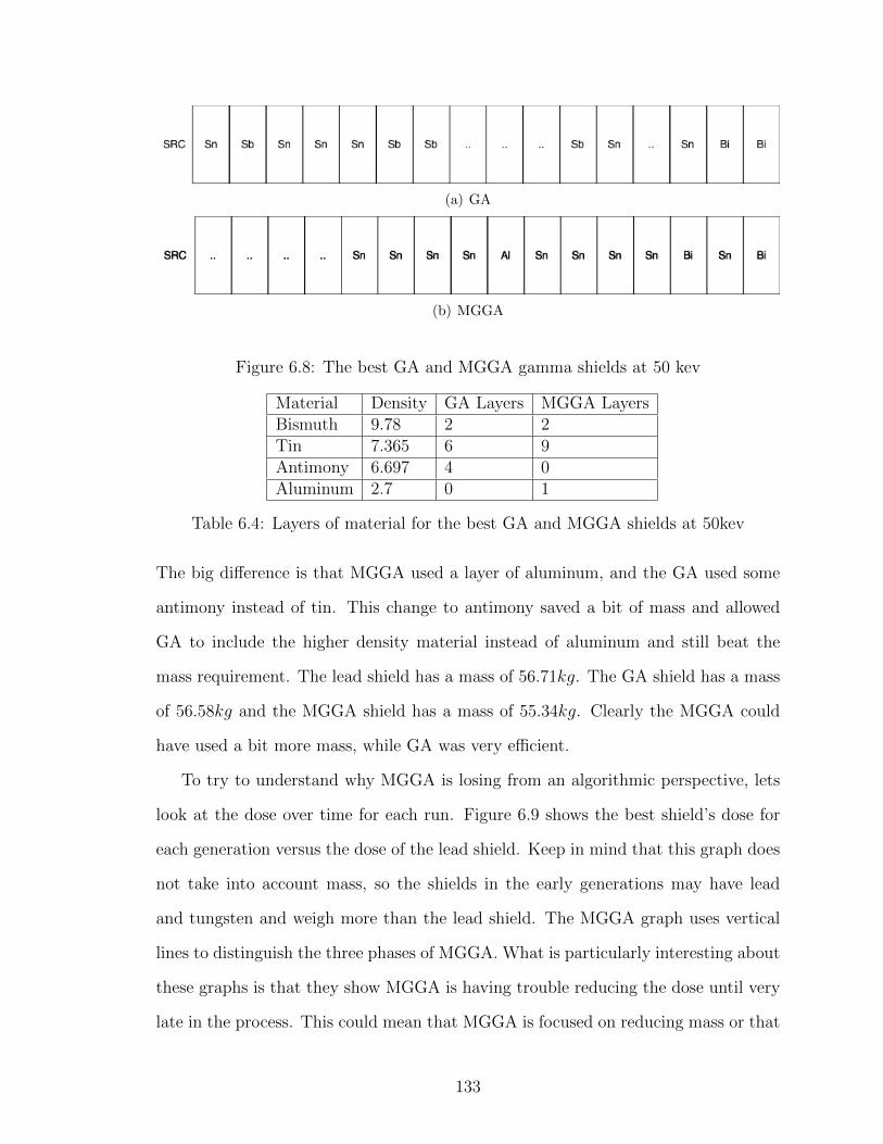
(a) GA

(b) MGGA

Figure 6.8: The best GA and MGGA gamma shields at 50 kev

Material Density GA Layers MGGA LayersBismuth 9.78 2 2Tin 7.365 6 9Antimony 6.697 4 0Aluminum 2.7 0 1

Table 6.4: Layers of material for the best GA and MGGA shields at 50kev

The big difference is that MGGA used a layer of aluminum, and the GA used some

antimony instead of tin. This change to antimony saved a bit of mass and allowed

GA to include the higher density material instead of aluminum and still beat the

mass requirement. The lead shield has a mass of 56.71kg. The GA shield has a mass

of 56.58kg and the MGGA shield has a mass of 55.34kg. Clearly the MGGA could

have used a bit more mass, while GA was very efficient.

To try to understand why MGGA is losing from an algorithmic perspective, lets

look at the dose over time for each run. Figure 6.9 shows the best shield’s dose for

each generation versus the dose of the lead shield. Keep in mind that this graph does

not take into account mass, so the shields in the early generations may have lead

and tungsten and weigh more than the lead shield. The MGGA graph uses vertical

lines to distinguish the three phases of MGGA. What is particularly interesting about

these graphs is that they show MGGA is having trouble reducing the dose until very

late in the process. This could mean that MGGA is focused on reducing mass or that

133

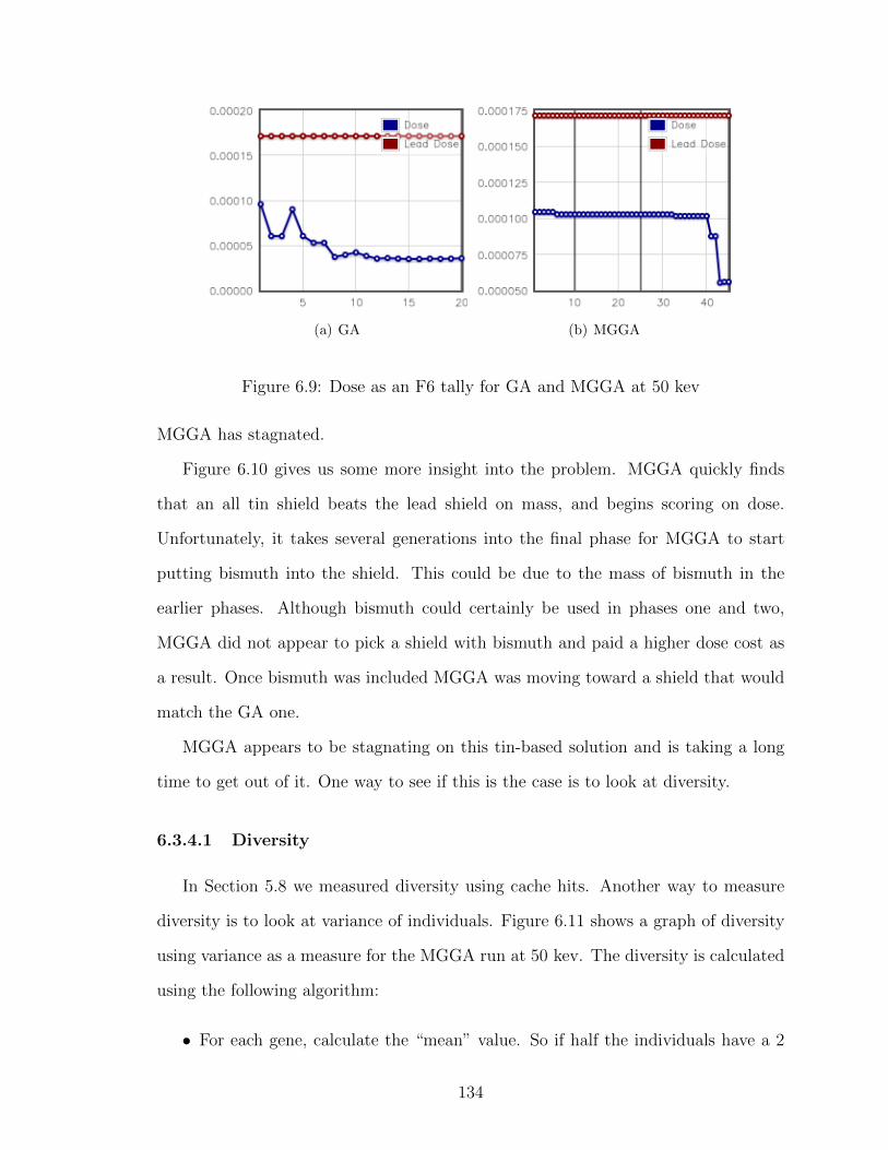
(a) GA (b) MGGA

Figure 6.9: Dose as an F6 tally for GA and MGGA at 50 kev

MGGA has stagnated.

Figure 6.10 gives us some more insight into the problem. MGGA quickly finds

that an all tin shield beats the lead shield on mass, and begins scoring on dose.

Unfortunately, it takes several generations into the final phase for MGGA to start

putting bismuth into the shield. This could be due to the mass of bismuth in the

earlier phases. Although bismuth could certainly be used in phases one and two,

MGGA did not appear to pick a shield with bismuth and paid a higher dose cost as

a result. Once bismuth was included MGGA was moving toward a shield that would

match the GA one.

MGGA appears to be stagnating on this tin-based solution and is taking a long

time to get out of it. One way to see if this is the case is to look at diversity.

6.3.4.1 Diversity

In Section 5.8 we measured diversity using cache hits. Another way to measure

diversity is to look at variance of individuals. Figure 6.11 shows a graph of diversity

using variance as a measure for the MGGA run at 50 kev. The diversity is calculated

using the following algorithm:

• For each gene, calculate the “mean” value. So if half the individuals have a 2

134

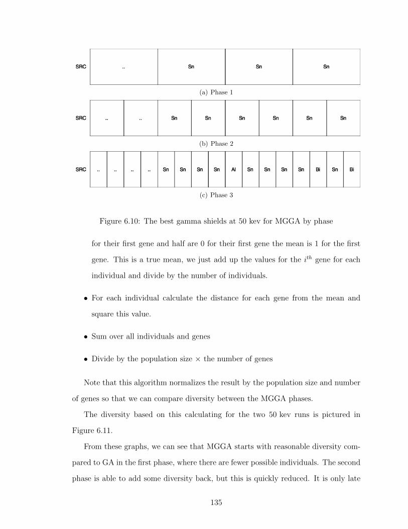
(a) Phase 1

(b) Phase 2

(c) Phase 3

Figure 6.10: The best gamma shields at 50 kev for MGGA by phase

for their first gene and half are 0 for their first gene the mean is 1 for the first

gene. This is a true mean, we just add up the values for the ith gene for each

individual and divide by the number of individuals.

• For each individual calculate the distance for each gene from the mean and

square this value.

• Sum over all individuals and genes

• Divide by the population size × the number of genes

Note that this algorithm normalizes the result by the population size and number

of genes so that we can compare diversity between the MGGA phases.

The diversity based on this calculating for the two 50 kev runs is pictured in

Figure 6.11.

From these graphs, we can see that MGGA starts with reasonable diversity com-

pared to GA in the first phase, where there are fewer possible individuals. The second

phase is able to add some diversity back, but this is quickly reduced. It is only late

135

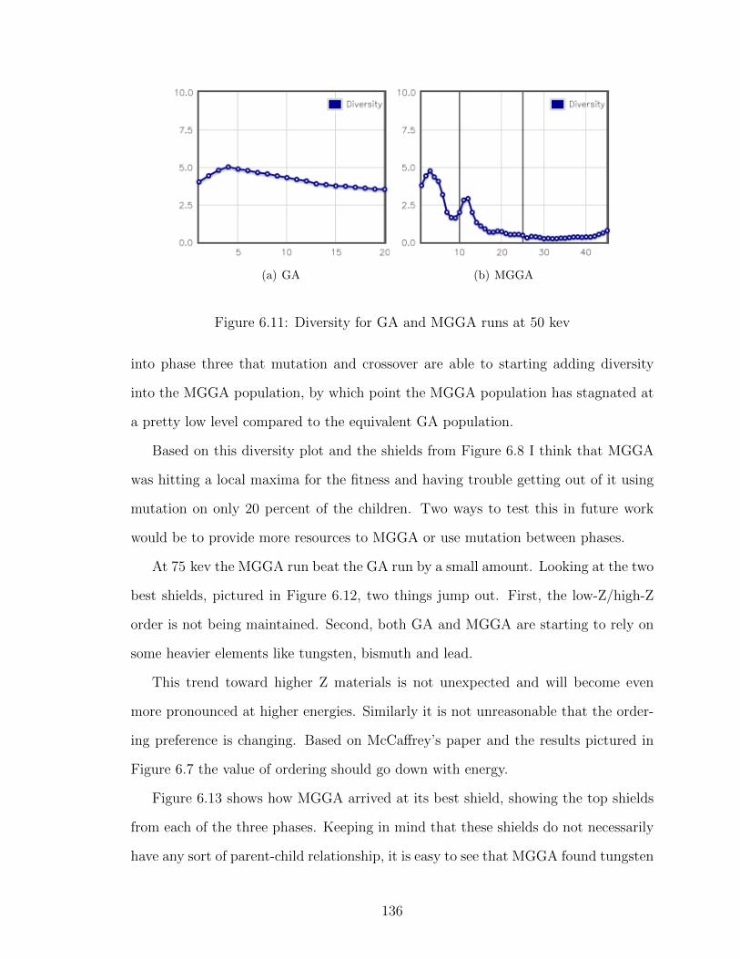
(a) GA (b) MGGA

Figure 6.11: Diversity for GA and MGGA runs at 50 kev

into phase three that mutation and crossover are able to starting adding diversity

into the MGGA population, by which point the MGGA population has stagnated at

a pretty low level compared to the equivalent GA population.

Based on this diversity plot and the shields from Figure 6.8 I think that MGGA

was hitting a local maxima for the fitness and having trouble getting out of it using

mutation on only 20 percent of the children. Two ways to test this in future work

would be to provide more resources to MGGA or use mutation between phases.

At 75 kev the MGGA run beat the GA run by a small amount. Looking at the two

best shields, pictured in Figure 6.12, two things jump out. First, the low-Z/high-Z

order is not being maintained. Second, both GA and MGGA are starting to rely on

some heavier elements like tungsten, bismuth and lead.

This trend toward higher Z materials is not unexpected and will become even

more pronounced at higher energies. Similarly it is not unreasonable that the order-

ing preference is changing. Based on McCaffrey’s paper and the results pictured in

Figure 6.7 the value of ordering should go down with energy.

Figure 6.13 shows how MGGA arrived at its best shield, showing the top shields

from each of the three phases. Keeping in mind that these shields do not necessarily

have any sort of parent-child relationship, it is easy to see that MGGA found tungsten

136

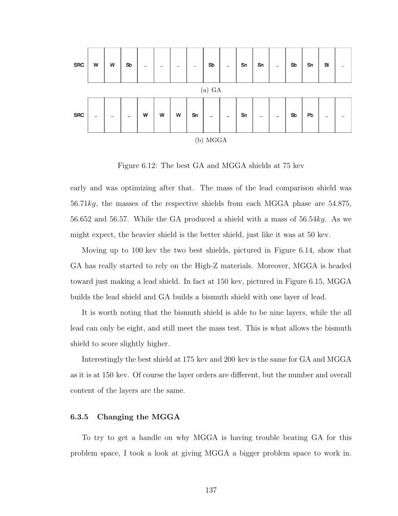
(a) GA

(b) MGGA

Figure 6.12: The best GA and MGGA shields at 75 kev

early and was optimizing after that. The mass of the lead comparison shield was

56.71kg, the masses of the respective shields from each MGGA phase are 54.875,

56.652 and 56.57. While the GA produced a shield with a mass of 56.54kg. As we

might expect, the heavier shield is the better shield, just like it was at 50 kev.

Moving up to 100 kev the two best shields, pictured in Figure 6.14, show that

GA has really started to rely on the High-Z materials. Moreover, MGGA is headed

toward just making a lead shield. In fact at 150 kev, pictured in Figure 6.15, MGGA

builds the lead shield and GA builds a bismuth shield with one layer of lead.

It is worth noting that the bismuth shield is able to be nine layers, while the all

lead can only be eight, and still meet the mass test. This is what allows the bismuth

shield to score slightly higher.

Interestingly the best shield at 175 kev and 200 kev is the same for GA and MGGA

as it is at 150 kev. Of course the layer orders are different, but the number and overall

content of the layers are the same.

6.3.5 Changing the MGGA

To try to get a handle on why MGGA is having trouble beating GA for this

problem space, I took a look at giving MGGA a bigger problem space to work in.

137

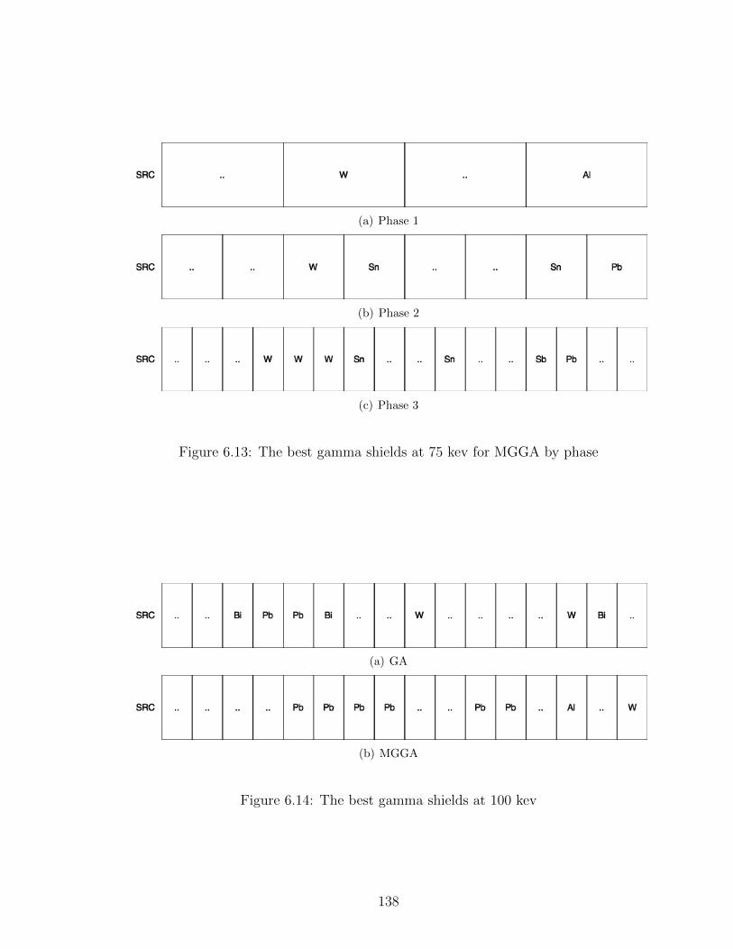
(a) Phase 1

(b) Phase 2

(c) Phase 3

Figure 6.13: The best gamma shields at 75 kev for MGGA by phase

(a) GA

(b) MGGA

Figure 6.14: The best gamma shields at 100 kev

138

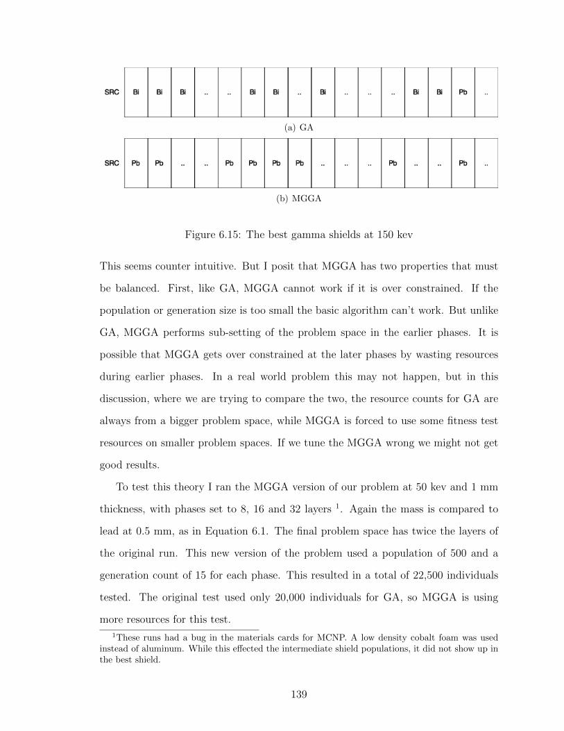
(a) GA

(b) MGGA

Figure 6.15: The best gamma shields at 150 kev

This seems counter intuitive. But I posit that MGGA has two properties that must

be balanced. First, like GA, MGGA cannot work if it is over constrained. If the

population or generation size is too small the basic algorithm can’t work. But unlike

GA, MGGA performs sub-setting of the problem space in the earlier phases. It is

possible that MGGA gets over constrained at the later phases by wasting resources

during earlier phases. In a real world problem this may not happen, but in this

discussion, where we are trying to compare the two, the resource counts for GA are

always from a bigger problem space, while MGGA is forced to use some fitness test

resources on smaller problem spaces. If we tune the MGGA wrong we might not get

good results.

To test this theory I ran the MGGA version of our problem at 50 kev and 1 mm

thickness, with phases set to 8, 16 and 32 layers 1. Again the mass is compared to

lead at 0.5 mm, as in Equation 6.1. The final problem space has twice the layers of

the original run. This new version of the problem used a population of 500 and a

generation count of 15 for each phase. This resulted in a total of 22,500 individuals

tested. The original test used only 20,000 individuals for GA, so MGGA is using

more resources for this test.

1These runs had a bug in the materials cards for MCNP. A low density cobalt foam was usedinstead of aluminum. While this effected the intermediate shield populations, it did not show up inthe best shield.

139

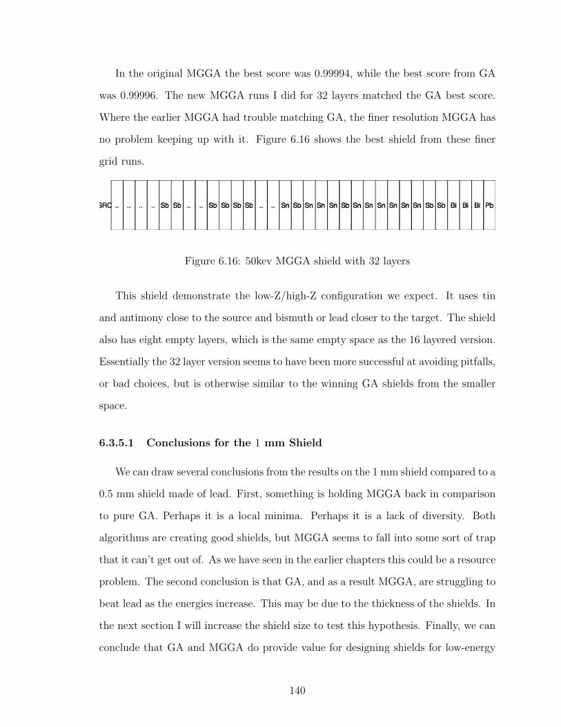
In the original MGGA the best score was 0.99994, while the best score from GA

was 0.99996. The new MGGA runs I did for 32 layers matched the GA best score.

Where the earlier MGGA had trouble matching GA, the finer resolution MGGA has

no problem keeping up with it. Figure 6.16 shows the best shield from these finer

grid runs.

Figure 6.16: 50kev MGGA shield with 32 layers

This shield demonstrate the low-Z/high-Z configuration we expect. It uses tin

and antimony close to the source and bismuth or lead closer to the target. The shield

also has eight empty layers, which is the same empty space as the 16 layered version.

Essentially the 32 layer version seems to have been more successful at avoiding pitfalls,

or bad choices, but is otherwise similar to the winning GA shields from the smaller

space.

6.3.5.1 Conclusions for the 1 mm Shield

We can draw several conclusions from the results on the 1 mm shield compared to a

0.5 mm shield made of lead. First, something is holding MGGA back in comparison

to pure GA. Perhaps it is a local minima. Perhaps it is a lack of diversity. Both

algorithms are creating good shields, but MGGA seems to fall into some sort of trap

that it can’t get out of. As we have seen in the earlier chapters this could be a resource

problem. The second conclusion is that GA, and as a result MGGA, are struggling to

beat lead as the energies increase. This may be due to the thickness of the shields. In

the next section I will increase the shield size to test this hypothesis. Finally, we can

conclude that GA and MGGA do provide value for designing shields for low-energy

140

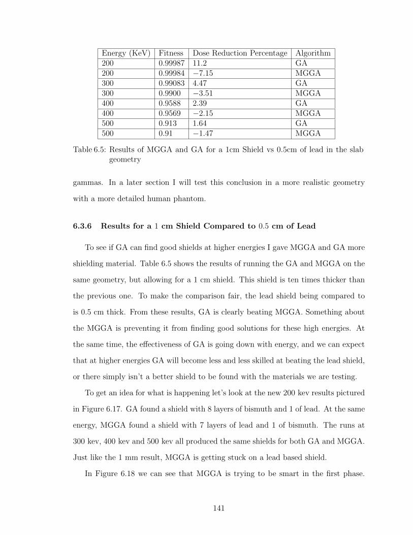
Energy (KeV) Fitness Dose Reduction Percentage Algorithm200 0.99987 11.2 GA200 0.99984 −7.15 MGGA300 0.99083 4.47 GA300 0.9900 −3.51 MGGA400 0.9588 2.39 GA400 0.9569 −2.15 MGGA500 0.913 1.64 GA500 0.91 −1.47 MGGA

Table 6.5: Results of MGGA and GA for a 1cm Shield vs 0.5cm of lead in the slabgeometry

gammas. In a later section I will test this conclusion in a more realistic geometry

with a more detailed human phantom.

6.3.6 Results for a 1 cm Shield Compared to 0.5 cm of Lead

To see if GA can find good shields at higher energies I gave MGGA and GA more

shielding material. Table 6.5 shows the results of running the GA and MGGA on the

same geometry, but allowing for a 1 cm shield. This shield is ten times thicker than

the previous one. To make the comparison fair, the lead shield being compared to

is 0.5 cm thick. From these results, GA is clearly beating MGGA. Something about

the MGGA is preventing it from finding good solutions for these high energies. At

the same time, the effectiveness of GA is going down with energy, and we can expect

that at higher energies GA will become less and less skilled at beating the lead shield,

or there simply isn’t a better shield to be found with the materials we are testing.

To get an idea for what is happening let’s look at the new 200 kev results pictured

in Figure 6.17. GA found a shield with 8 layers of bismuth and 1 of lead. At the same

energy, MGGA found a shield with 7 layers of lead and 1 of bismuth. The runs at

300 kev, 400 kev and 500 kev all produced the same shields for both GA and MGGA.

Just like the 1 mm result, MGGA is getting stuck on a lead based shield.

In Figure 6.18 we can see that MGGA is trying to be smart in the first phase.

141

(a) GA

(b) MGGA

Figure 6.17: The best gamma shields at 200 kev with 1 cm shields

It finds a shield with lead and bismuth, which meets the mass goal and has lots of

electrons to reduce dose. In phase two, the MGGA tries to continue this process and

again picks lots of lead and a little bismuth. Again this will meet the mass goal. The

problem is that MGGA doesn’t seem to figure out that switching to mostly bismuth

is ok for the mass goal and the dose. Perhaps this switch doesn’t get propagated into

later generations because switching to bismuth could, depending on the total shield,

create a higher dose. A higher dose would lead to a lower fitness and reduces the

chance that the shield will win a tournament and reproduce.

6.3.7 Conclusions for the 1 cm Shield

GA is able to beat a lead shield at moderate energies, between 200 kev and 500 kev

using a thicker shield. MGGA is getting stuck at these energies. Future work might

look into why MGGA is getting stuck and how we might force it to move forward,

perhaps by injecting diversity using interphase mutation.

6.4 The ORNL Phantom

The ORNL phantom, [Oak Ridge National Laboratory (2011)], defines a man, pic-

tured in Figure 6.19, with two legs, numerous internal organs, a neck and a head. The

142

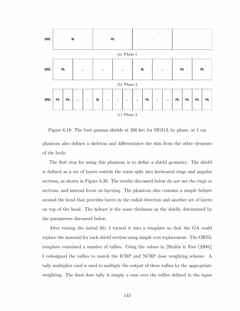
(a) Phase 1

(b) Phase 2

(c) Phase 3

Figure 6.18: The best gamma shields at 200 kev for MGGA by phase, at 1 cm

phantom also defines a skeleton and differentiates the skin from the other elements

of the body.

The first step for using this phantom is to define a shield geometry. The shield

is defined as a set of layers outside the torso split into horizontal rings and angular

sections, as shown in Figure 6.20. The results discussed below do not use the rings or

sections, and instead focus on layering. The phantom also contains a simple helmet

around the head that provides layers in the radial direction and another set of layers

on top of the head. The helmet is the same thickness as the shield, determined by

the parameters discussed below.

After testing the initial file, I turned it into a template so that the GA could

replace the material for each shield section using simple text replacement. The ORNL

template contained a number of tallies. Using the values in [Shultis & Faw (2000)]

I redesigned the tallies to match the ICRP and NCRP dose weighting scheme. A

tally multiplier card is used to multiply the output of these tallies by the appropriate

weighting. The final dose tally is simply a sum over the tallies defined in the input

143

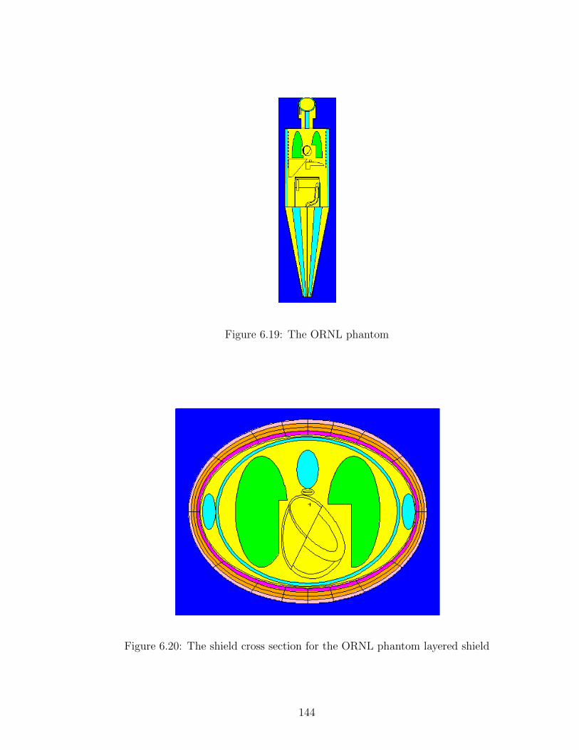
Horizontal cross-section showing heart, lungs, spine, and arms

Figure 6.19: The ORNL phantom

Figure 6.20: The shield cross section for the ORNL phantom layered shield

144

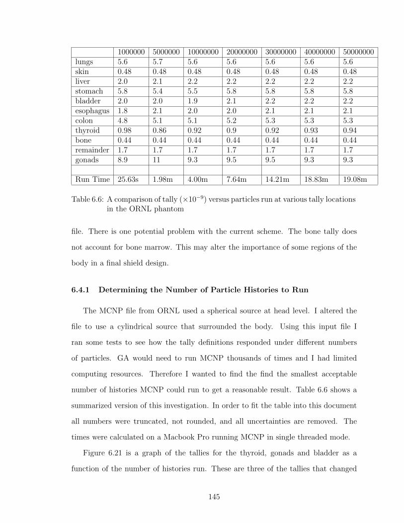
1000000 5000000 10000000 20000000 30000000 40000000 50000000lungs 5.6 5.7 5.6 5.6 5.6 5.6 5.6skin 0.48 0.48 0.48 0.48 0.48 0.48 0.48liver 2.0 2.1 2.2 2.2 2.2 2.2 2.2stomach 5.8 5.4 5.5 5.8 5.8 5.8 5.8bladder 2.0 2.0 1.9 2.1 2.2 2.2 2.2esophagus 1.8 2.1 2.0 2.0 2.1 2.1 2.1colon 4.8 5.1 5.1 5.2 5.3 5.3 5.3thyroid 0.98 0.86 0.92 0.9 0.92 0.93 0.94bone 0.44 0.44 0.44 0.44 0.44 0.44 0.44remainder 1.7 1.7 1.7 1.7 1.7 1.7 1.7gonads 8.9 11 9.3 9.5 9.5 9.3 9.3

Run Time 25.63s 1.98m 4.00m 7.64m 14.21m 18.83m 19.08m

Table 6.6: A comparison of tally (×10−9) versus particles run at various tally locationsin the ORNL phantom

file. There is one potential problem with the current scheme. The bone tally does

not account for bone marrow. This may alter the importance of some regions of the

body in a final shield design.

6.4.1 Determining the Number of Particle Histories to Run

The MCNP file from ORNL used a spherical source at head level. I altered the

file to use a cylindrical source that surrounded the body. Using this input file I

ran some tests to see how the tally definitions responded under different numbers

of particles. GA would need to run MCNP thousands of times and I had limited

computing resources. Therefore I wanted to find the find the smallest acceptable

number of histories MCNP could run to get a reasonable result. Table 6.6 shows a

summarized version of this investigation. In order to fit the table into this document

all numbers were truncated, not rounded, and all uncertainties are removed. The

times were calculated on a Macbook Pro running MCNP in single threaded mode.

Figure 6.21 is a graph of the tallies for the thyroid, gonads and bladder as a

function of the number of histories run. These are three of the tallies that changed

145

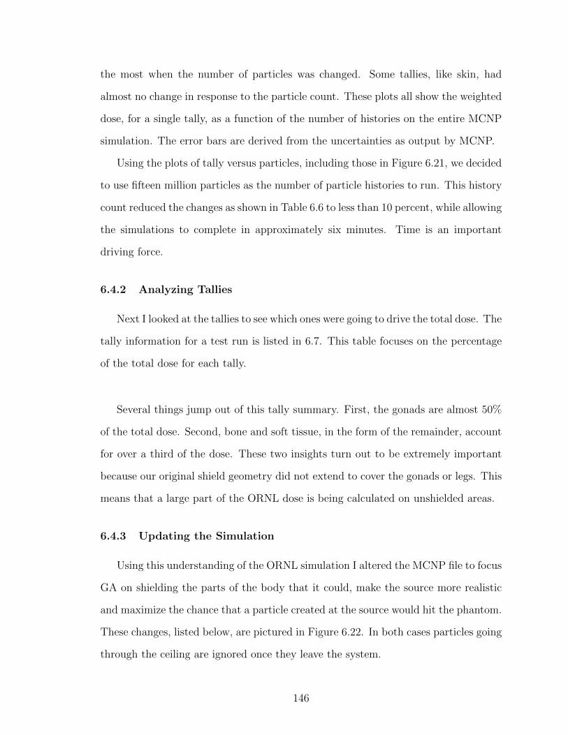
the most when the number of particles was changed. Some tallies, like skin, had

almost no change in response to the particle count. These plots all show the weighted

dose, for a single tally, as a function of the number of histories on the entire MCNP

simulation. The error bars are derived from the uncertainties as output by MCNP.

Using the plots of tally versus particles, including those in Figure 6.21, we decided

to use fifteen million particles as the number of particle histories to run. This history

count reduced the changes as shown in Table 6.6 to less than 10 percent, while allowing

the simulations to complete in approximately six minutes. Time is an important

driving force.

6.4.2 Analyzing Tallies

Next I looked at the tallies to see which ones were going to drive the total dose. The

tally information for a test run is listed in 6.7. This table focuses on the percentage

of the total dose for each tally.

Several things jump out of this tally summary. First, the gonads are almost 50%

of the total dose. Second, bone and soft tissue, in the form of the remainder, account

for over a third of the dose. These two insights turn out to be extremely important

because our original shield geometry did not extend to cover the gonads or legs. This

means that a large part of the ORNL dose is being calculated on unshielded areas.

6.4.3 Updating the Simulation

Using this understanding of the ORNL simulation I altered the MCNP file to focus

GA on shielding the parts of the body that it could, make the source more realistic

and maximize the chance that a particle created at the source would hit the phantom.

These changes, listed below, are pictured in Figure 6.22. In both cases particles going

through the ceiling are ignored once they leave the system.

146

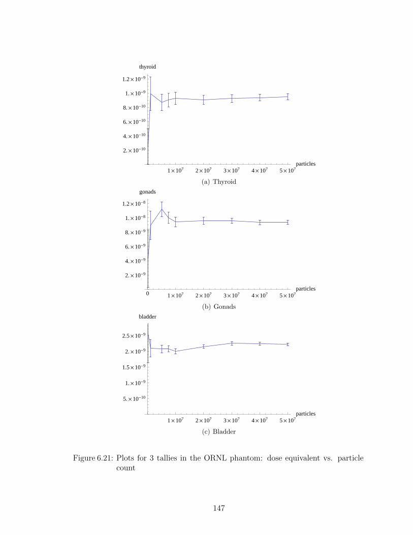
1 ´ 107 2 ´ 107 3 ´ 107 4 ´ 107 5 ´ 107particles

2. ´ 10-10

4. ´ 10-10

6. ´ 10-10

8. ´ 10-10

1. ´ 10-9

1.2 ´ 10-9

thyroid

(a) Thyroid

0 1 ´ 107 2 ´ 107 3 ´ 107 4 ´ 107 5 ´ 107particles

2. ´ 10-9

4. ´ 10-9

6. ´ 10-9

8. ´ 10-9

1. ´ 10-8

1.2 ´ 10-8

gonads

(b) Gonads

1 ´ 107 2 ´ 107 3 ´ 107 4 ´ 107 5 ´ 107particles

5. ´ 10-10

1. ´ 10-9

1.5 ´ 10-9

2. ´ 10-9

2.5 ´ 10-9

bladder

(c) Bladder

Figure 6.21: Plots for 3 tallies in the ORNL phantom: dose equivalent vs. particlecount

147

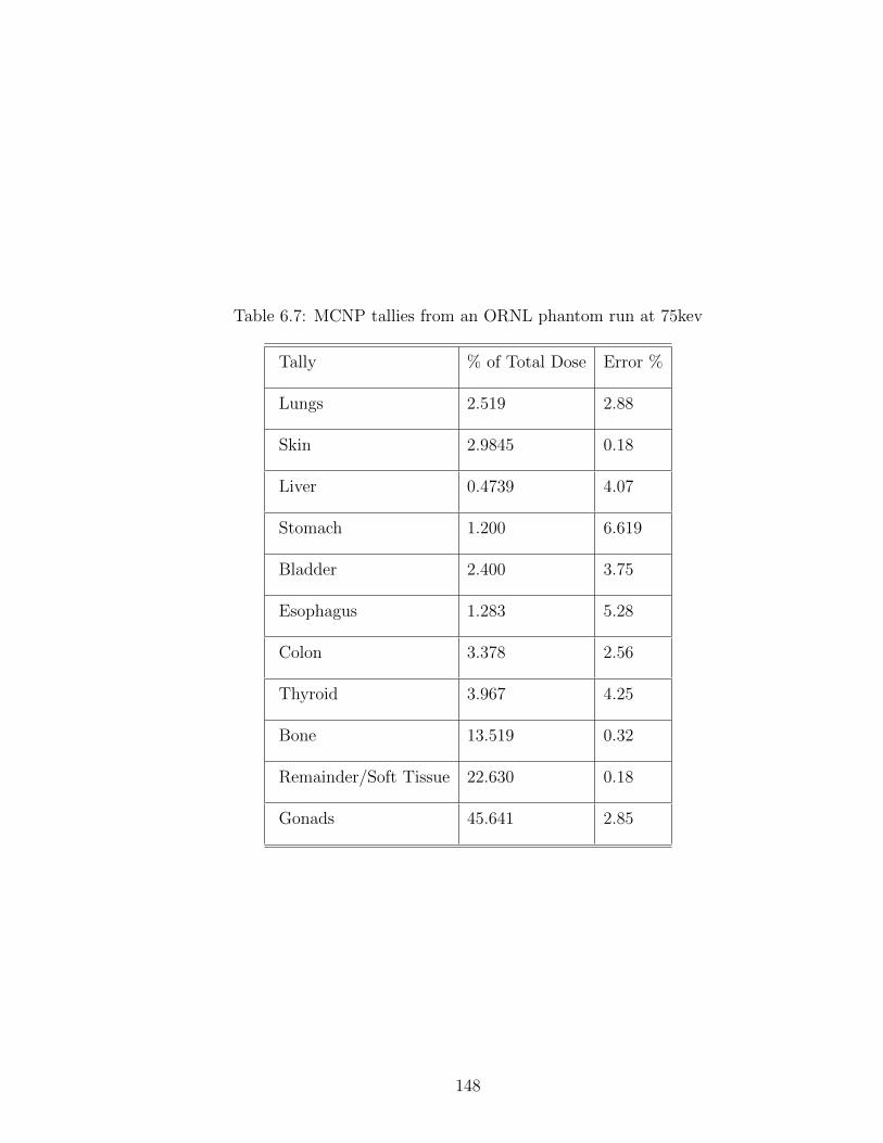
Table 6.7: MCNP tallies from an ORNL phantom run at 75kev

Tally % of Total Dose Error %

Lungs 2.519 2.88

Skin 2.9845 0.18

Liver 0.4739 4.07

Stomach 1.200 6.619

Bladder 2.400 3.75

Esophagus 1.283 5.28

Colon 3.378 2.56

Thyroid 3.967 4.25

Bone 13.519 0.32

Remainder/Soft Tissue 22.630 0.18

Gonads 45.641 2.85

148

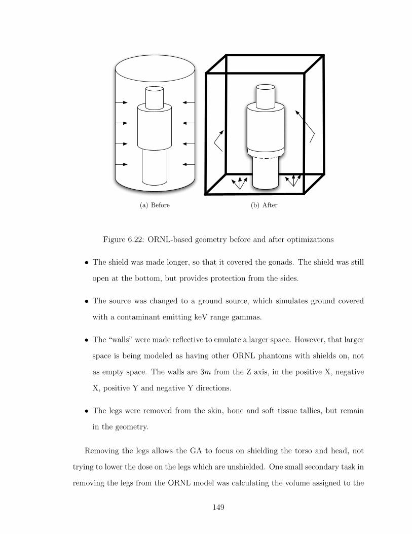
(a) Before (b) After

Figure 6.22: ORNL-based geometry before and after optimizations

• The shield was made longer, so that it covered the gonads. The shield was still

open at the bottom, but provides protection from the sides.

• The source was changed to a ground source, which simulates ground covered

with a contaminant emitting keV range gammas.

• The “walls” were made reflective to emulate a larger space. However, that larger

space is being modeled as having other ORNL phantoms with shields on, not

as empty space. The walls are 3m from the Z axis, in the positive X, negative

X, positive Y and negative Y directions.

• The legs were removed from the skin, bone and soft tissue tallies, but remain

in the geometry.

Removing the legs allows the GA to focus on shielding the torso and head, not

trying to lower the dose on the legs which are unshielded. One small secondary task in

removing the legs from the ORNL model was calculating the volume assigned to the

149

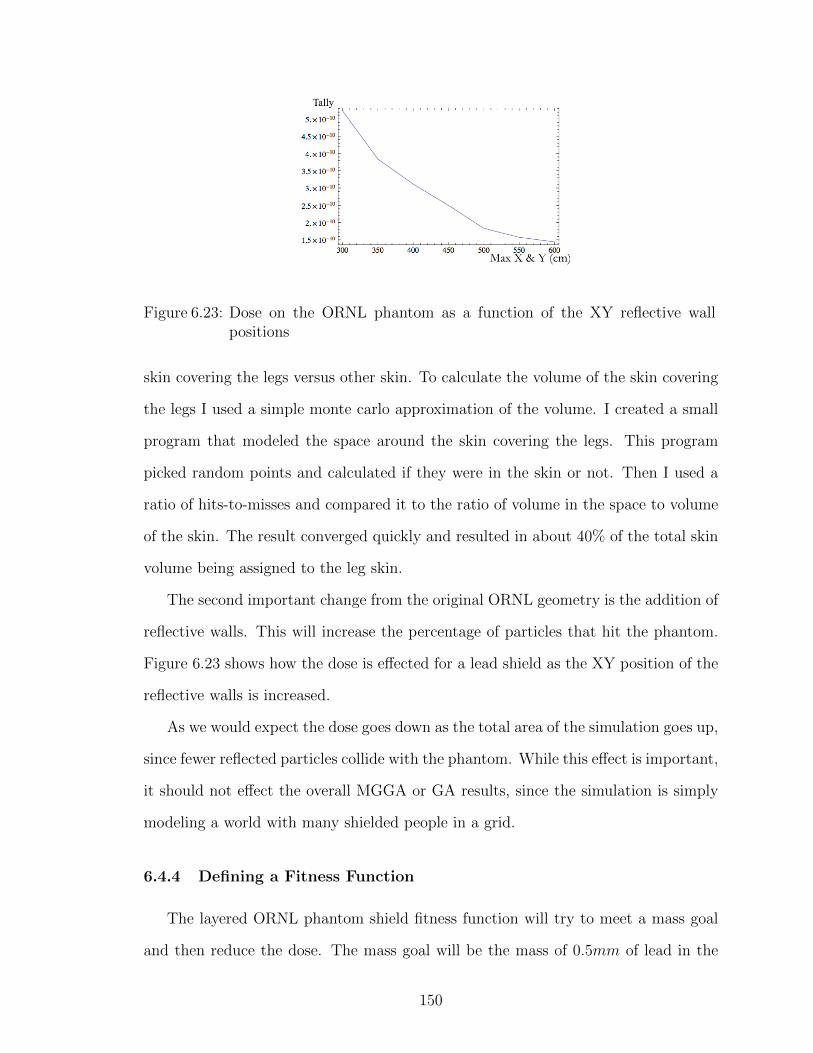
Figure 6.23: Dose on the ORNL phantom as a function of the XY reflective wallpositions

skin covering the legs versus other skin. To calculate the volume of the skin covering

the legs I used a simple monte carlo approximation of the volume. I created a small

program that modeled the space around the skin covering the legs. This program

picked random points and calculated if they were in the skin or not. Then I used a

ratio of hits-to-misses and compared it to the ratio of volume in the space to volume

of the skin. The result converged quickly and resulted in about 40% of the total skin

volume being assigned to the leg skin.

The second important change from the original ORNL geometry is the addition of

reflective walls. This will increase the percentage of particles that hit the phantom.

Figure 6.23 shows how the dose is effected for a lead shield as the XY position of the

reflective walls is increased.

As we would expect the dose goes down as the total area of the simulation goes up,

since fewer reflected particles collide with the phantom. While this effect is important,

it should not effect the overall MGGA or GA results, since the simulation is simply

modeling a world with many shielded people in a grid.

6.4.4 Defining a Fitness Function

The layered ORNL phantom shield fitness function will try to meet a mass goal

and then reduce the dose. The mass goal will be the mass of 0.5mm of lead in the

150

shield area. This is a standard shield material, so we are basically trying to weigh

less than a standard shield and then try to beat it on dose. The fitness of each shield

will be determined as follows:

1. Calculate the mass of the shield made of lead, m(S)

2. Calculate the mass of the shield based on the MCNP output file volume infor-

mation, m(s)

3. Calculate the dose with the shield, D(s) by summing up all of the weighted

tallies from the MCNP output

4. Compare the mass with the shield to the mass of the lead shield

• If the shield is heavier than the lead shield, the fitness is −(m(s)/m(S))

• Otherwise the fitness is 1−D(s)

In other words, the fitness of shield s is

F (s) =

1−D(s) if m(s) < m(S)

−m(s)m(S)

otherwise

(6.3)

6.4.5 Defining the Genetic Algorithm

Using this fitness function I ran several simulations for GA and MGGA. The final

geometry had a total of 2 helmet layers on the side, 2 helmet layers on the top, and

32 torso layers. There are seven possible materials, listed in Table 6.2, in each layer.

The total number of possible shields is therefore, 736 = 2.65 × 1030, where 7 is the

number of materials and their are 32 + 2 + 2 volumes to fill in.

The GA runs had 20 generations of 1000 individuals. The MGGA was run with

the following phases:

151

• 8 layers - 500 individuals per generation with 15 generations

• 16 layers - 500 individuals per generation with 15 generations

• 32 layers - 500 individuals per generation with 15 generations

To move between phases, each layer was cut into two pieces. From a shielding

standpoint the shields were identical as they move between phases. All of the runs

used two helmet layers for all phases.

All GA was performed using tournament selection with a tournament size of 5.

There was a 25% chance that the worst individual in a tournament will win to help

preserve diversity. Reproduction relied on uniform crossover 70% of the time, muta-

tion 20% of the time and copying 10% of the time. Uniform selection allowed each

child to use the materials for any layer from either parent, however, I created two

children for each uniform crossover reproduction, as discussed previously.

6.4.6 MGGA and GA Results

I ran several MGGA simulations, two each for 50 kev, 75 kev and 100 kev. The

best results are listed in 6.8. The 75 kev run is reminiscent of the results from the

simple geometry in 6.3. Looking at the three best shields, pictured in 6.24, keep in

mind that the source is on the right, and the phantom on the left. The helmet is

not pictured here, but contained very little material in all 3 cases. The helmet is

discussed in detail in Section 6.4.7.

At 50 kev we see the expected low-Z/high-Z organization with bismuth near the

torso and tin or antimony closer to the source. The 75 kev shield uses more high-Z

material, tungsten in particular, compared to the lower energy shield. We saw this

same behavior in the simple geometry. The 100 kev shield piles on even more high-Z

material, including lead, but still beats the lead mass, by using bismuth as a lighter

152

Table 6.8: Summary of results with the ORNL phantom at 50 kev, 75 kev and 100 kevwith GA and MGGA

Energy Shield Thickness Dose Reduction Percentage Lead Thickness Algorithm

50 keV 1 mm 11.368 0.5 mm MGGA

50 keV 1 mm 10.98 0.5 mm GA

75 keV 1 mm 66.894 0.5 mm MGGA

75 keV 1 mm 65.4 0.5 mm GA

100 keV 1 mm 27.622 0.5 mm MGGA

100 keV 1 mm 22.65 0.5 mm GA

alternative. The 100 kev shield only saves 0.097 percent in mass, so the MGGA is

doing a great job of balancing mass versus dose to get a 27% dose reduction. Some

of this savings is coming from the helmet.

6.4.7 The Helmet

The ORNL phantom includes a two layer helmet in two pieces. There is a cylin-

drical section around the head with a cutout for the face, and a round top, as pictured

as Figure 6.25. If designed by a person, the helmet would probably contain material

on the sides and the top. But, since the top should receive little, if any radiation,

the GA should remove the top. This is almost exactly what happened. The 50 kev

solution used a single layer of lead on the sides of the helmet and a single layer of tin

on the top. The 75 kev solution used a single layer of antimony on the side and had

no top. The 100 kev solution used a single layer of lead on the side, and had no top.

By removing the top, GA was able to save mass that could be used to shield the

torso. The volume for the top of the helmet is approximately 65 cm3, the volume of

the sides of the helmet is approximately 88 cm3 and the volume of the torso shield

153

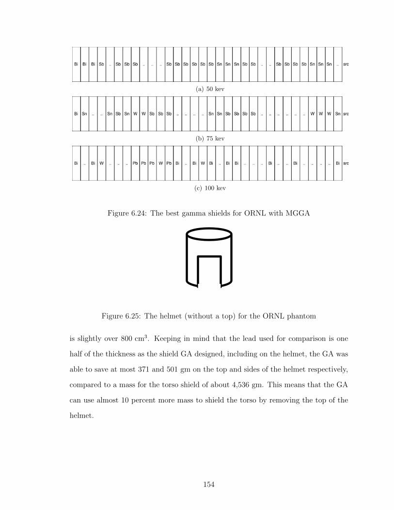
(a) 50 kev

(b) 75 kev

(c) 100 kev

Figure 6.24: The best gamma shields for ORNL with MGGA

Figure 6.25: The helmet (without a top) for the ORNL phantom

is slightly over 800 cm3. Keeping in mind that the lead used for comparison is one

half of the thickness as the shield GA designed, including on the helmet, the GA was

able to save at most 371 and 501 gm on the top and sides of the helmet respectively,

compared to a mass for the torso shield of about 4,536 gm. This means that the GA

can use almost 10 percent more mass to shield the torso by removing the top of the

helmet.

154

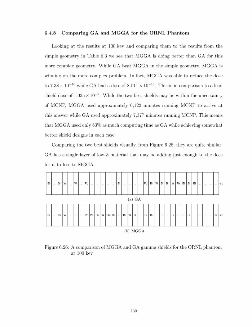
6.4.8 Comparing GA and MGGA for the ORNL Phantom

Looking at the results at 100 kev and comparing them to the results from the

simple geometry in Table 6.3 we see that MGGA is doing better than GA for this

more complex geometry. While GA beat MGGA in the simple geometry, MGGA is

winning on the more complex problem. In fact, MGGA was able to reduce the dose

to 7.38× 10−10 while GA had a dose of 8.011× 10−10. This is in comparison to a lead

shield dose of 1.035×10−9. While the two best shields may be within the uncertainty

of MCNP, MGGA used approximately 6,122 minutes running MCNP to arrive at

this answer while GA used approximately 7,377 minutes running MCNP. This means

that MGGA used only 83% as much computing time as GA while achieving somewhat

better shield designs in each case.

Comparing the two best shields visually, from Figure 6.26, they are quite similar.

GA has a single layer of low-Z material that may be adding just enough to the dose

for it to lose to MGGA.

(a) GA

(b) MGGA

Figure 6.26: A comparison of MGGA and GA gamma shields for the ORNL phantomat 100 kev

155

6.5 The ORNL Phantom at High-Energy

Prior to looking at low energy gamma shielding, I did a fairly extensive look at

high energy gamma shielding, [Asbury & Holloway (2011)]. This exploration started

with a simple geometry, moved to a minimal human phantom and ended with running

MGGA and GA on the ORNL phantom with greater than 1MeV photons. The fitness

function for these simulations was different than the one used in this chapter. It set

a dose goal based on a heavy shield and then tried to reduce mass once the goal was

met.

The results from these simulations were not interesting. Essentially GA and

MGGA used high-Z materials to lower the dose, and then would remove what they

could to reduce mass. The shields were generally tungsten or lead, leading to the

conclusion that while GA and MGGA are a useful tool at low energies where opti-

mally layering can do better than lead, they are less useful at higher energies where

pair-production and Compton scattering dominate the photon shield interactions.

6.6 Conclusions

I performed several MGGA and GA runs with both a simple geometry and a

human-like phantom. Simulations at low energies showed that there is value in cre-

ating layered shields, while simulations at higher energies showed little value for lay-

ering. As we would hope, MGGA and GA are able to create good shields for gamma

radiation as they did for the shadow shield. Moreover, MGGA and GA perform well

with a complex geometry. Both algorithms were able to create shields in a complex

geometry that were similar to shields in a simple geometry.

These results are a good indicator that GA and MGGA can work on this type

of problem, despite the severe resource constraints we were working under. MGGA

struggled with high energy gamma problems, where there may not be a good solution,

156

but it was able to do a great job on a very complex geometry using the ORNL

phantom. While GA beat MGGA on a simple geometry, MGGA surpassed GA as the

problem space grew. Moreover, MGGA saved more than 10 percent of the computing

resources used by GA. MGGA is able to provide good ideas for shield designs.

In the next chapter I will discuss how MGGA performs when designing a gamma

radiation filter.

157

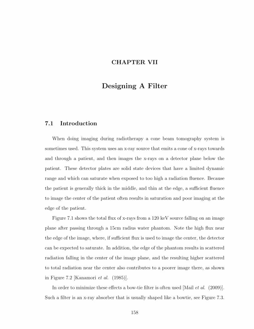
CHAPTER VII

Designing A Filter

7.1 Introduction

When doing imaging during radiotherapy a cone beam tomography system is

sometimes used. This system uses an x-ray source that emits a cone of x-rays towards

and through a patient, and then images the x-rays on a detector plane below the

patient. These detector plates are solid state devices that have a limited dynamic

range and which can saturate when exposed to too high a radiation fluence. Because

the patient is generally thick in the middle, and thin at the edge, a sufficient fluence

to image the center of the patient often results in saturation and poor imaging at the

edge of the patient.

Figure 7.1 shows the total flux of x-rays from a 120 keV source falling on an image

plane after passing through a 15cm radius water phantom. Note the high flux near

the edge of the image, where, if sufficient flux is used to image the center, the detector

can be expected to saturate. In addition, the edge of the phantom results in scattered

radiation falling in the center of the image plane, and the resulting higher scattered

to total radiation near the center also contributes to a poorer image there, as shown

in Figure 7.2 [Kanamori et al. (1985)].

In order to minimize these effects a bow-tie filter is often used [Mail et al. (2009)].

Such a filter is an x-ray absorber that is usually shaped like a bowtie, see Figure 7.3.

158

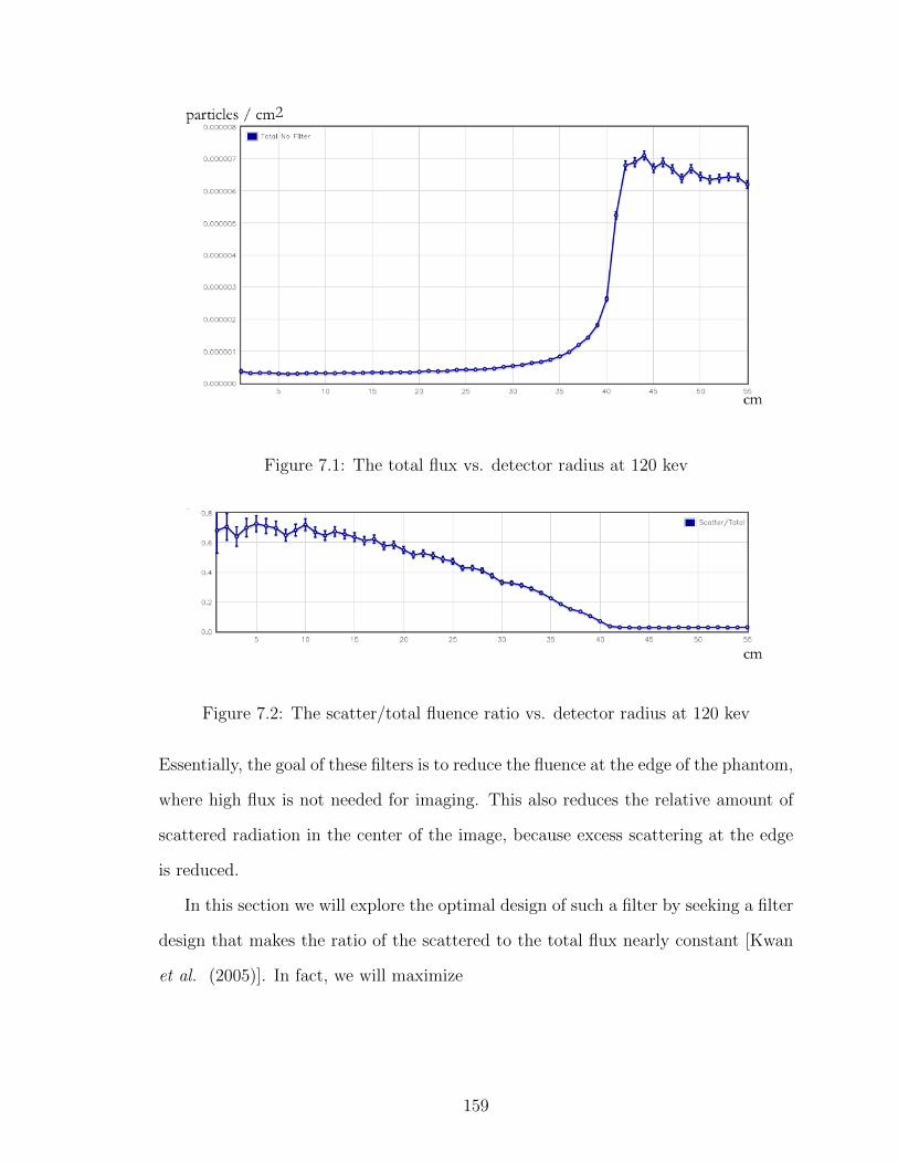
Figure 7.1: The total flux vs. detector radius at 120 kev

Figure 7.2: The scatter/total fluence ratio vs. detector radius at 120 kev

Essentially, the goal of these filters is to reduce the fluence at the edge of the phantom,

where high flux is not needed for imaging. This also reduces the relative amount of

scattered radiation in the center of the image, because excess scattering at the edge

is reduced.

In this section we will explore the optimal design of such a filter by seeking a filter

design that makes the ratio of the scattered to the total flux nearly constant [Kwan

et al. (2005)]. In fact, we will maximize

159

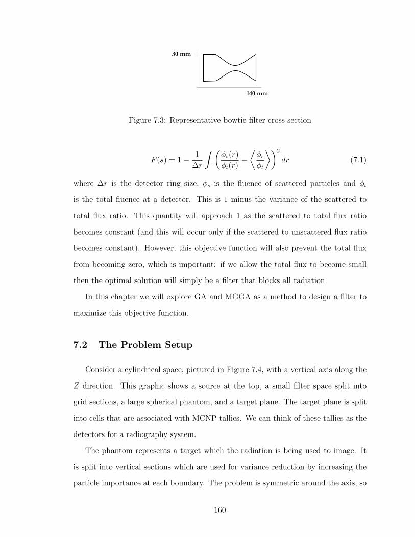
30 mm

140 mm

Figure 7.3: Representative bowtie filter cross-section

F (s) = 1− 1

∆r

∫ (φs(r)

φt(r)−⟨φsφt

⟩)2

dr (7.1)

where ∆r is the detector ring size, φs is the fluence of scattered particles and φt

is the total fluence at a detector. This is 1 minus the variance of the scattered to

total flux ratio. This quantity will approach 1 as the scattered to total flux ratio

becomes constant (and this will occur only if the scattered to unscattered flux ratio

becomes constant). However, this objective function will also prevent the total flux

from becoming zero, which is important: if we allow the total flux to become small

then the optimal solution will simply be a filter that blocks all radiation.

In this chapter we will explore GA and MGGA as a method to design a filter to

maximize this objective function.

7.2 The Problem Setup

Consider a cylindrical space, pictured in Figure 7.4, with a vertical axis along the

Z direction. This graphic shows a source at the top, a small filter space split into

grid sections, a large spherical phantom, and a target plane. The target plane is split

into cells that are associated with MCNP tallies. We can think of these tallies as the

detectors for a radiography system.

The phantom represents a target which the radiation is being used to image. It

is split into vertical sections which are used for variance reduction by increasing the

particle importance at each boundary. The problem is symmetric around the axis, so

160

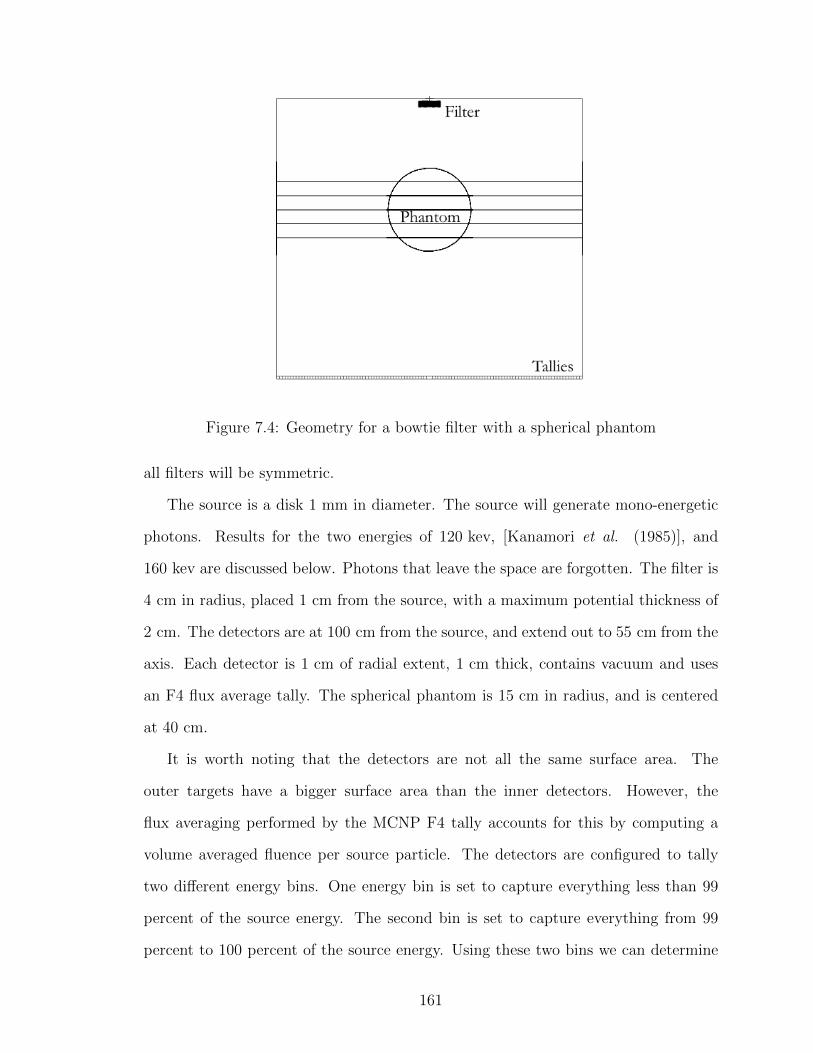
Figure 7.4: Geometry for a bowtie filter with a spherical phantom

all filters will be symmetric.

The source is a disk 1 mm in diameter. The source will generate mono-energetic

photons. Results for the two energies of 120 kev, [Kanamori et al. (1985)], and

160 kev are discussed below. Photons that leave the space are forgotten. The filter is

4 cm in radius, placed 1 cm from the source, with a maximum potential thickness of

2 cm. The detectors are at 100 cm from the source, and extend out to 55 cm from the

axis. Each detector is 1 cm of radial extent, 1 cm thick, contains vacuum and uses

an F4 flux average tally. The spherical phantom is 15 cm in radius, and is centered

at 40 cm.

It is worth noting that the detectors are not all the same surface area. The

outer targets have a bigger surface area than the inner detectors. However, the

flux averaging performed by the MCNP F4 tally accounts for this by computing a

volume averaged fluence per source particle. The detectors are configured to tally

two different energy bins. One energy bin is set to capture everything less than 99

percent of the source energy. The second bin is set to capture everything from 99

percent to 100 percent of the source energy. Using these two bins we can determine

161

scattered, primary and total fluence at each detector.

Our goal, from Equation 7.1 and expressed in the following fitness algorithm, will

be to minimize the variance of the scattered fluence to total fluence ratio across the

detector plan. This goal, loosely taken from [Mail et al. (2009)], will reduce the dose

to the patient by minimizing the impact of scattered (noisy) photons.

1. Determine the total flux for each detector using the MCNP tally

2. Determine the scattered flux at each detector, using the energy bin related to

all energies less than 99 percent of the source energy

3. If there is no flux at a detector, give the filter a fitness score of 1 minus 1000

times the number of detectors with no flux

4. Calculate the scatter to total ratio at each detector, and include it in a variance

calculation

5. Score the filter as one minus the variance squared, better filters approach a

score of 1 from below

In other words, the fitness of shield s is

F (s) =

1− 1000× count of zero tallies if any tallies are zero

1− 1N

∑Ni=0

(φs(i)φt(i)− 〈φs

φt〉)2

otherwise

(7.2)

I performed several GA simulations with this fitness function with the filter split

into 16 layers and 16 bands, for a total of 256 elements. Each GA run had a population

of 1125 individuals, and executed for 20 generations. A total of 22, 500 individuals

are tested for each GA run. The MGGA used three phases:

• 4× 4 - 500 individuals per generation with 15 generations

• 8× 8 - 500 individuals per generation with 15 generations

162

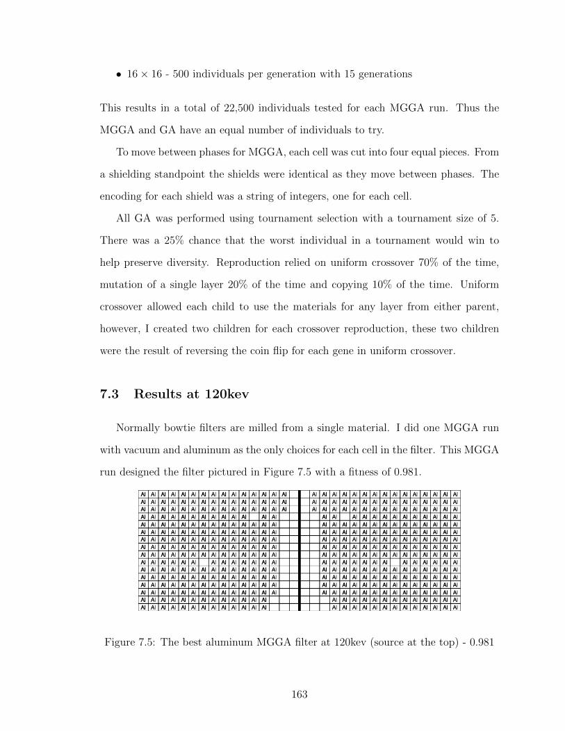
• 16× 16 - 500 individuals per generation with 15 generations

This results in a total of 22,500 individuals tested for each MGGA run. Thus the

MGGA and GA have an equal number of individuals to try.

To move between phases for MGGA, each cell was cut into four equal pieces. From

a shielding standpoint the shields were identical as they move between phases. The

encoding for each shield was a string of integers, one for each cell.

All GA was performed using tournament selection with a tournament size of 5.

There was a 25% chance that the worst individual in a tournament would win to

help preserve diversity. Reproduction relied on uniform crossover 70% of the time,

mutation of a single layer 20% of the time and copying 10% of the time. Uniform

crossover allowed each child to use the materials for any layer from either parent,

however, I created two children for each crossover reproduction, these two children

were the result of reversing the coin flip for each gene in uniform crossover.

7.3 Results at 120kev

Normally bowtie filters are milled from a single material. I did one MGGA run

with vacuum and aluminum as the only choices for each cell in the filter. This MGGA

run designed the filter pictured in Figure 7.5 with a fitness of 0.981.

Figure 7.5: The best aluminum MGGA filter at 120kev (source at the top) - 0.981

163

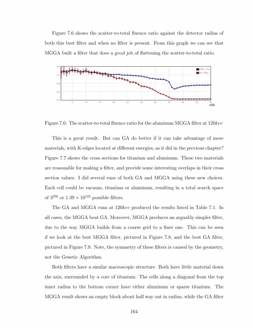
Figure 7.6 shows the scatter-to-total fluence ratio against the detector radius of

both this best filter and when no filter is present. From this graph we can see that

MGGA built a filter that does a good job of flattening the scatter-to-total ratio.

Figure 7.6: The scatter-to-total fluence ratio for the aluminum MGGA filter at 120kev

This is a great result. But can GA do better if it can take advantage of more

materials, with K-edges located at different energies, as it did in the previous chapter?

Figure 7.7 shows the cross sections for titanium and aluminum. These two materials

are reasonable for making a filter, and provide some interesting overlaps in their cross

section values. I did several runs of both GA and MGGA using these new choices.

Each cell could be vacuum, titanium or aluminum, resulting in a total search space

of 3256 or 1.39× 10122 possible filters.

The GA and MGGA runs at 120kev produced the results listed in Table 7.1. In

all cases, the MGGA beat GA. Moreover, MGGA produces an arguably simpler filter,

due to the way MGGA builds from a coarse grid to a finer one. This can be seen

if we look at the best MGGA filter, pictured in Figure 7.8, and the best GA filter,

pictured in Figure 7.9. Note, the symmetry of these filters is caused by the geometry,

not the Genetic Algorithm.

Both filters have a similar macroscopic structure. Both have little material down

the axis, surrounded by a core of titanium. The cells along a diagonal from the top

inner radius to the bottom corner have either aluminum or sparse titanium. The

MGGA result shows an empty block about half way out in radius, while the GA filter

164

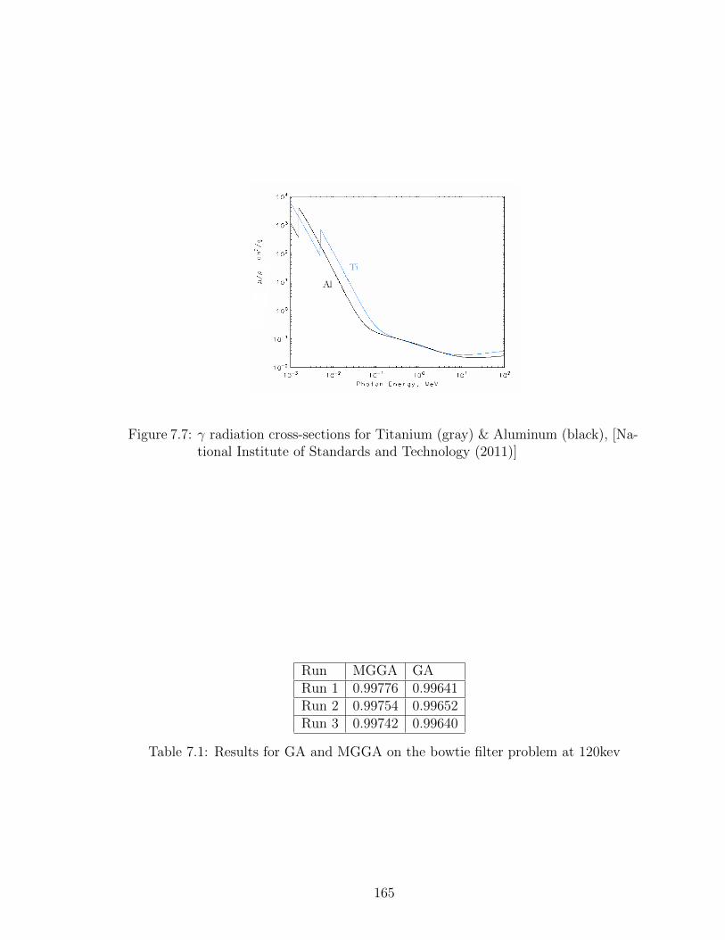
Figure 7.7: γ radiation cross-sections for Titanium (gray) & Aluminum (black), [Na-tional Institute of Standards and Technology (2011)]

Run MGGA GARun 1 0.99776 0.99641Run 2 0.99754 0.99652Run 3 0.99742 0.99640

Table 7.1: Results for GA and MGGA on the bowtie filter problem at 120kev

165

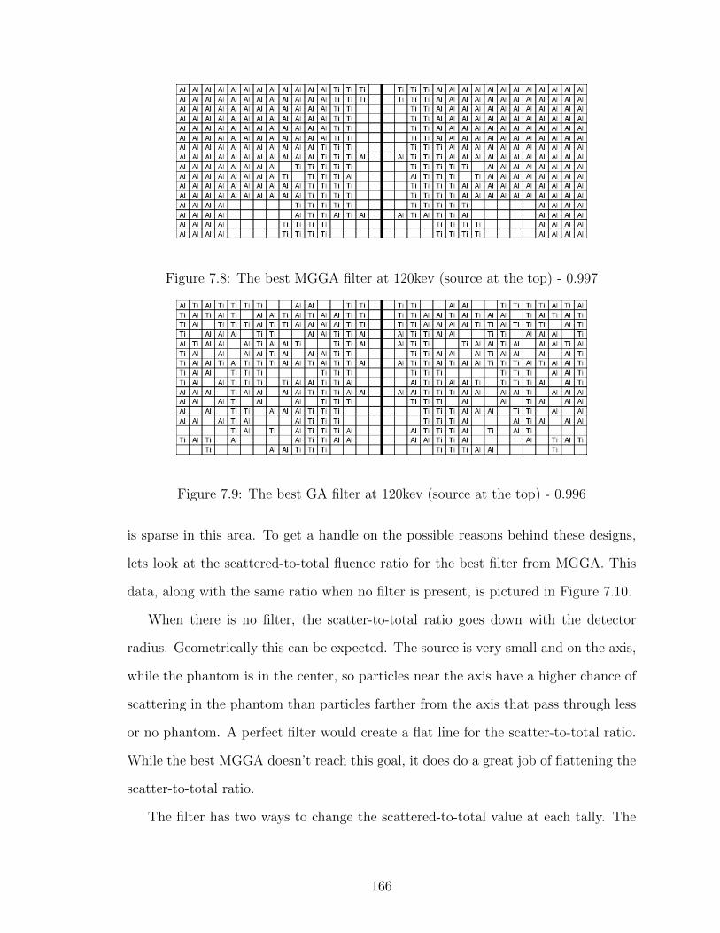
Figure 7.8: The best MGGA filter at 120kev (source at the top) - 0.997

Figure 7.9: The best GA filter at 120kev (source at the top) - 0.996

is sparse in this area. To get a handle on the possible reasons behind these designs,

lets look at the scattered-to-total fluence ratio for the best filter from MGGA. This

data, along with the same ratio when no filter is present, is pictured in Figure 7.10.

When there is no filter, the scatter-to-total ratio goes down with the detector

radius. Geometrically this can be expected. The source is very small and on the axis,

while the phantom is in the center, so particles near the axis have a higher chance of

scattering in the phantom than particles farther from the axis that pass through less

or no phantom. A perfect filter would create a flat line for the scatter-to-total ratio.

While the best MGGA doesn’t reach this goal, it does do a great job of flattening the

scatter-to-total ratio.

The filter has two ways to change the scattered-to-total value at each tally. The

166

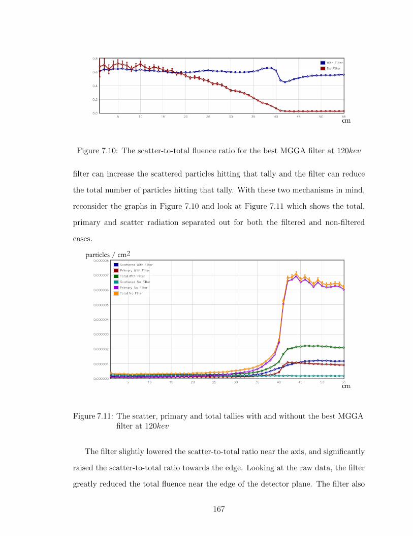
Figure 7.10: The scatter-to-total fluence ratio for the best MGGA filter at 120kev

filter can increase the scattered particles hitting that tally and the filter can reduce

the total number of particles hitting that tally. With these two mechanisms in mind,

reconsider the graphs in Figure 7.10 and look at Figure 7.11 which shows the total,

primary and scatter radiation separated out for both the filtered and non-filtered

cases.

Figure 7.11: The scatter, primary and total tallies with and without the best MGGAfilter at 120kev

The filter slightly lowered the scatter-to-total ratio near the axis, and significantly

raised the scatter-to-total ratio towards the edge. Looking at the raw data, the filter

greatly reduced the total fluence near the edge of the detector plane. The filter also

167

raised the scattered fluence near the edge of the detector plane. Together, these two

changes altered the ratio enough to bring it closer to the ratio at the center.

There is an interesting feature of the plot of scatter-to-total ratio that looks a bit

like a bump followed by a valley. This feature occurs at the same radius, around 40

cm, as the large change in total fluence in the unfiltered case. This is the image of the

edge of the phantom. A ray leaving the source, would hit the phantom tangentially

at (13.9054,34.375). Taking this point, and using similar triangles, I determined that

the source starts hitting the detector plane directly, without hitting the phantom, at

40.45 centimeters. This radius exactly matches the big drop in scatter-to-total ratio,

and leads to a conclusion that the edge of the phantom is causing this bump. The GA

filter shows the same type of feature at the same place, as pictured in Figure 7.12.

Figure 7.12: The scatter-to-total ratio for the best GA filter at 120kev

Both GA and MGGA were able to beat the pure aluminum filter designed by

MGGA using titanium and aluminum. Despite the gigantic nature of the search

space, MGGA is constructing interesting well-scoring filters. Moreover, MGGA is

using approximately 3,143 minutes to find its best filter compared to approximately

6,183 minutes for GA. MGGA is using almost half of the computing resources as GA

to find a better, more manufacturable filter.

168

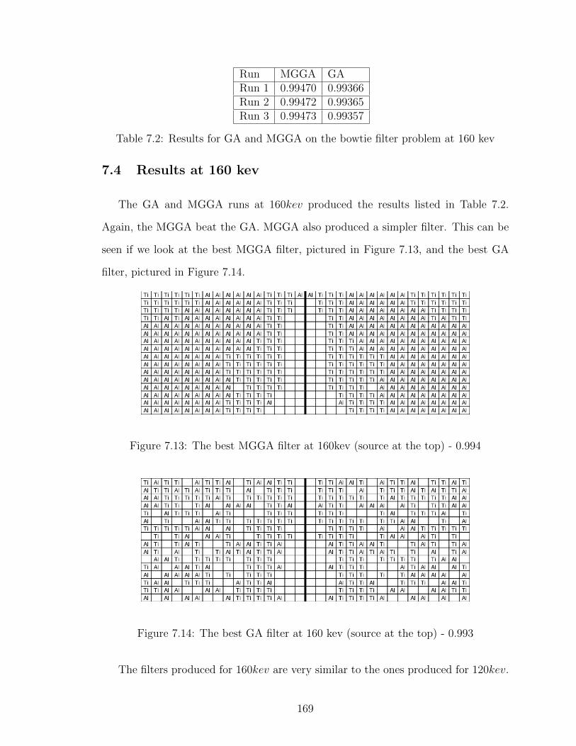
Run MGGA GARun 1 0.99470 0.99366Run 2 0.99472 0.99365Run 3 0.99473 0.99357

Table 7.2: Results for GA and MGGA on the bowtie filter problem at 160 kev

7.4 Results at 160 kev

The GA and MGGA runs at 160kev produced the results listed in Table 7.2.

Again, the MGGA beat the GA. MGGA also produced a simpler filter. This can be

seen if we look at the best MGGA filter, pictured in Figure 7.13, and the best GA

filter, pictured in Figure 7.14.

Figure 7.13: The best MGGA filter at 160kev (source at the top) - 0.994

Figure 7.14: The best GA filter at 160 kev (source at the top) - 0.993

The filters produced for 160kev are very similar to the ones produced for 120kev.

169

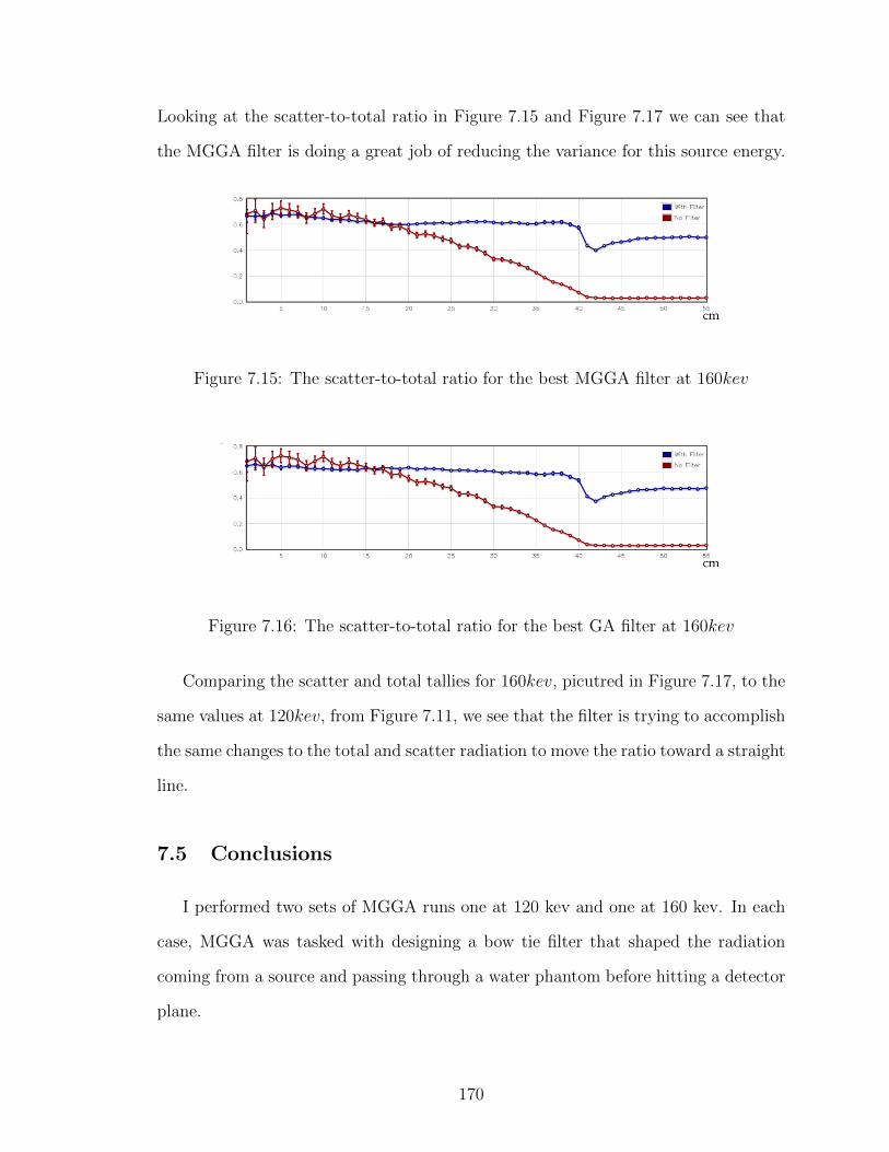
Looking at the scatter-to-total ratio in Figure 7.15 and Figure 7.17 we can see that

the MGGA filter is doing a great job of reducing the variance for this source energy.

Figure 7.15: The scatter-to-total ratio for the best MGGA filter at 160kev

Figure 7.16: The scatter-to-total ratio for the best GA filter at 160kev

Comparing the scatter and total tallies for 160kev, picutred in Figure 7.17, to the

same values at 120kev, from Figure 7.11, we see that the filter is trying to accomplish

the same changes to the total and scatter radiation to move the ratio toward a straight

line.

7.5 Conclusions

I performed two sets of MGGA runs one at 120 kev and one at 160 kev. In each

case, MGGA was tasked with designing a bow tie filter that shaped the radiation

coming from a source and passing through a water phantom before hitting a detector

plane.

170

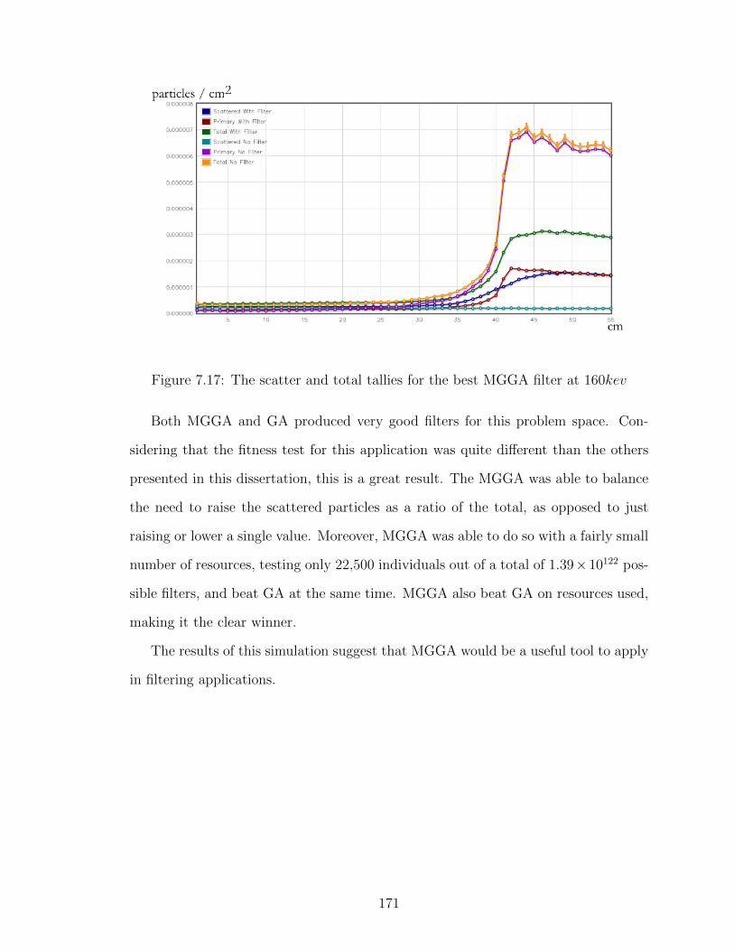
Figure 7.17: The scatter and total tallies for the best MGGA filter at 160kev

Both MGGA and GA produced very good filters for this problem space. Con-

sidering that the fitness test for this application was quite different than the others

presented in this dissertation, this is a great result. The MGGA was able to balance

the need to raise the scattered particles as a ratio of the total, as opposed to just

raising or lower a single value. Moreover, MGGA was able to do so with a fairly small

number of resources, testing only 22,500 individuals out of a total of 1.39×10122 pos-

sible filters, and beat GA at the same time. MGGA also beat GA on resources used,

making it the clear winner.

The results of this simulation suggest that MGGA would be a useful tool to apply

in filtering applications.

171

CHAPTER VIII

Summary And Conclusions

As I stated in the introduction, shielding is a simple concept. Something bad is

moving toward something good and we want to protect the good from the bad. Unfor-

tunately, shielding against radiation is often a problem that involves more than just

stopping the bad stuff, we also have to think about mass, cost, secondary radiation

effects and other factors.

This dissertation is a study in how a new form of genetic algorithms, called Multi-

Grid Genetic Algorithms, can be used to explore the space of possible shields and help

engineers design better shields. More importantly, MGGA is about helping engineers

find unexpected solutions, solutions that a human may not have considered.

8.1 The Toolbox

The primary tool discussed in this dissertation are genetic algorithms. Chapter II

discussed what genetic algorithms are, and provides a basic idea of how they solve

problems. Using GA required configuring numerous parameters and defining fitness

functions. The goal of a Genetic Algorithm is ultimately to find a solution that has

the best score from the fitness function. One disadvantage of genetic algorithms is

that they want to run the fitness function numerous times. The fitness functions in

this dissertation all involved performing a radiation transport simulation with a code

172

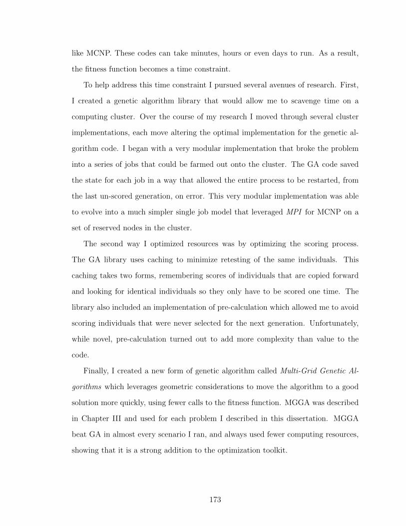
like MCNP. These codes can take minutes, hours or even days to run. As a result,

the fitness function becomes a time constraint.

To help address this time constraint I pursued several avenues of research. First,

I created a genetic algorithm library that would allow me to scavenge time on a

computing cluster. Over the course of my research I moved through several cluster

implementations, each move altering the optimal implementation for the genetic al-

gorithm code. I began with a very modular implementation that broke the problem

into a series of jobs that could be farmed out onto the cluster. The GA code saved

the state for each job in a way that allowed the entire process to be restarted, from

the last un-scored generation, on error. This very modular implementation was able

to evolve into a much simpler single job model that leveraged MPI for MCNP on a

set of reserved nodes in the cluster.

The second way I optimized resources was by optimizing the scoring process.

The GA library uses caching to minimize retesting of the same individuals. This

caching takes two forms, remembering scores of individuals that are copied forward

and looking for identical individuals so they only have to be scored one time. The

library also included an implementation of pre-calculation which allowed me to avoid

scoring individuals that were never selected for the next generation. Unfortunately,

while novel, pre-calculation turned out to add more complexity than value to the

code.

Finally, I created a new form of genetic algorithm called Multi-Grid Genetic Al-

gorithms which leverages geometric considerations to move the algorithm to a good

solution more quickly, using fewer calls to the fitness function. MGGA was described

in Chapter III and used for each problem I described in this dissertation. MGGA

beat GA in almost every scenario I ran, and always used fewer computing resources,

showing that it is a strong addition to the optimization toolkit.

173

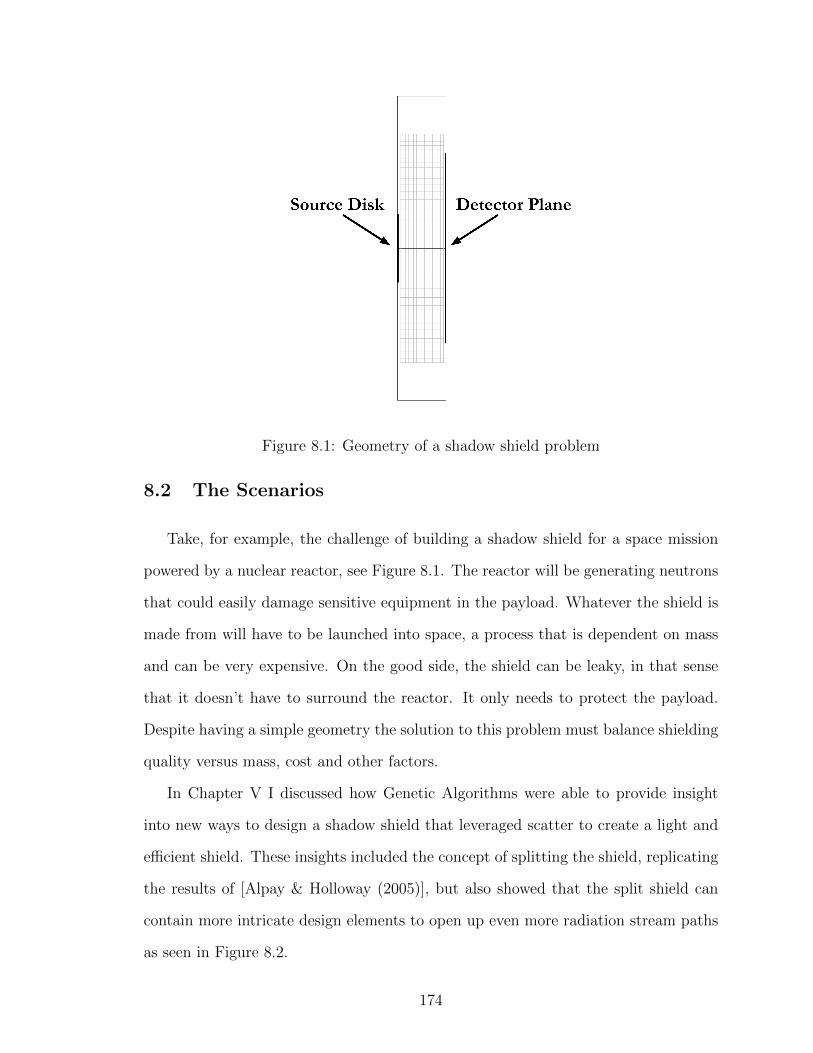
Figure 8.1: Geometry of a shadow shield problem

8.2 The Scenarios

Take, for example, the challenge of building a shadow shield for a space mission

powered by a nuclear reactor, see Figure 8.1. The reactor will be generating neutrons

that could easily damage sensitive equipment in the payload. Whatever the shield is

made from will have to be launched into space, a process that is dependent on mass

and can be very expensive. On the good side, the shield can be leaky, in that sense

that it doesn’t have to surround the reactor. It only needs to protect the payload.

Despite having a simple geometry the solution to this problem must balance shielding

quality versus mass, cost and other factors.

In Chapter V I discussed how Genetic Algorithms were able to provide insight

into new ways to design a shadow shield that leveraged scatter to create a light and

efficient shield. These insights included the concept of splitting the shield, replicating

the results of [Alpay & Holloway (2005)], but also showed that the split shield can

contain more intricate design elements to open up even more radiation stream paths

as seen in Figure 8.2.

174

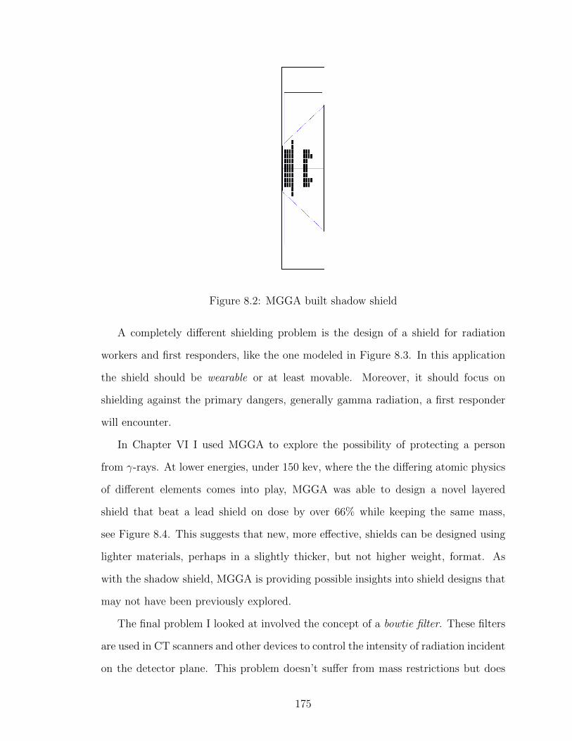
Figure 8.2: MGGA built shadow shield

A completely different shielding problem is the design of a shield for radiation

workers and first responders, like the one modeled in Figure 8.3. In this application

the shield should be wearable or at least movable. Moreover, it should focus on

shielding against the primary dangers, generally gamma radiation, a first responder

will encounter.

In Chapter VI I used MGGA to explore the possibility of protecting a person

from γ-rays. At lower energies, under 150 kev, where the the differing atomic physics

of different elements comes into play, MGGA was able to design a novel layered

shield that beat a lead shield on dose by over 66% while keeping the same mass,

see Figure 8.4. This suggests that new, more effective, shields can be designed using

lighter materials, perhaps in a slightly thicker, but not higher weight, format. As

with the shadow shield, MGGA is providing possible insights into shield designs that

may not have been previously explored.

The final problem I looked at involved the concept of a bowtie filter. These filters

are used in CT scanners and other devices to control the intensity of radiation incident

on the detector plane. This problem doesn’t suffer from mass restrictions but does

175

Horizontal cross-section showing heart, lungs, spine, and arms

Figure 8.3: Advanced phantom for a radiation worker

Figure 8.4: MGGA designed shield For 75KeV gamma rays

176

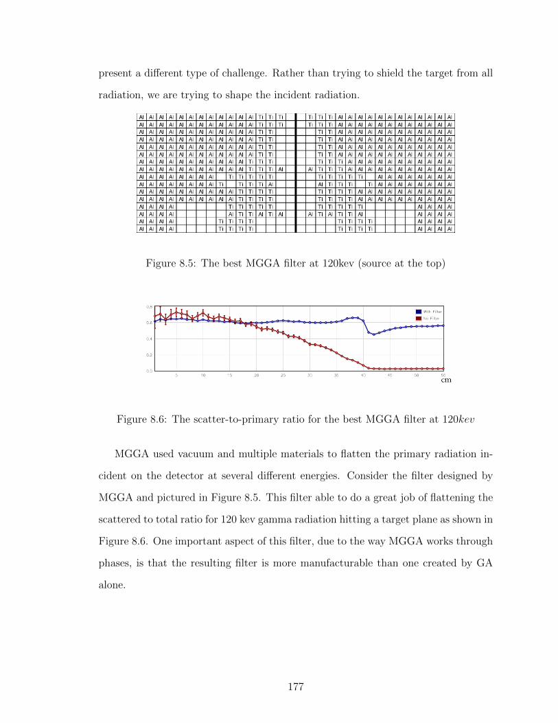
present a different type of challenge. Rather than trying to shield the target from all

radiation, we are trying to shape the incident radiation.

Figure 8.5: The best MGGA filter at 120kev (source at the top)

Figure 8.6: The scatter-to-primary ratio for the best MGGA filter at 120kev

MGGA used vacuum and multiple materials to flatten the primary radiation in-

cident on the detector at several different energies. Consider the filter designed by

MGGA and pictured in Figure 8.5. This filter able to do a great job of flattening the

scattered to total ratio for 120 kev gamma radiation hitting a target plane as shown in

Figure 8.6. One important aspect of this filter, due to the way MGGA works through

phases, is that the resulting filter is more manufacturable than one created by GA

alone.

177

8.3 Presentations and Publications

During the process of writing this dissertation I participated in a number of con-

ferences and smaller opportunities to present my work. Early on I presented an hour

long talk to students in the NERS department on biologically inspired optimization

algorithms. This presentation was a good start and provided me with some initial

thoughts on which algorithms would be worth trying on the shielding problems. I

tried ant colony and particle swarm optimization on several simple problems and

presented those concepts and results at this talk. While these techniques are both

very interesting and powerful, they didn’t seem to be a good fit for the shielding

applications, so I focused on genetic algorithms.

In 2009 I presented the work Dr Holloway and I did on shadow shields to the In-

ternational Conference on Mathematics, Computational Methods & Reactor Physics

in a talk entitled Multi-Grid Genetic Algorithms for Space Shield Design, [Asbury

& Holloway (2009a)]. The same year I presented our initial work on the wearable

shield to the Chemical and Biological Defense Science and Technology Conference in

a paper entitled Optimization of Gamma Radiation Shielding by Genetic Algorithms,

[Asbury & Holloway (2009b)].

In 2011 I presented my results on low energy gamma rays to the International

Conference on Mathematics, Computational Methods & Reactor Physics, in a paper

entitled Designing Shields for KeV Photons with Genetic Algorithms, [Asbury & Hol-

loway (2011)]. This paper included the initial results, but did not include my final

revised ORNL geometry results.

8.4 Future Work

There is still work to be done on MGGA. First, there is more research to do in

terms of how we can tune MGGA. In particular, the gamma shield problem was able

178

to stymie MGGA at some energies. It would be interesting to see if this is related to

diversity and if adding mutations between phases would help. This question of when

diversity matters and how is a generally important one.

I ignored error when using the results from PARTISN and MCNP to produce

fitness scores. There is an interesting line of research here, that could look at how

error could be used or propagated into the fitness calculation to create more fair

tournaments, or reproductive choices. For example, given two shields with very close

fitness scores, if the error is not taken into account the one with the higher fitness

would win a tournament. But if the error in the transport computation is taken into

account we might more fairly select between the shields, or we might automatically

refine the computation of fitness in these cases.

The applications I looked at could continue to be extended. The shadow shield

geometry can be expanded to include support material and the simulations could

add secondary radiation, in particular gamma rays. The fitness function for this

shield could be altered to penalize free standing rings, making the shield more man-

ufacturable. The gamma shield problem offers a wide variety of research paths in

extending the ORNL geometry and looking at more types of radiation, while the

filter problem could be extended to more closely mimic a CT scanner.

8.5 Conclusions

The MGGA results from this dissertation are very positive. The split shadow

shield was validated and expanded to include more intricate paths for scattered neu-

trons to escape the shield. A simple lead shield was defeated for low energy gamma

radiation, providing insight into the possibility of using layered materials to create

lighter and more protective shields for radiation workers. Finally, MGGA was able

to build a manufacturable bow-tie filter with two materials.

More importantly, in almost every case MGGA created a better scoring individual

179

than GA with fewer computing resources. In some cases, MGGA was able to use half

the resources as GA to create a superior result. By leveraging the hierarchical nature

of a problem, MGGA was also able to create more structured and subjectively cleaner

solutions. The shadow shield was less noisy than its GA equivalent. The bow-tie filter

created by MGGA was more manufacturable than the one created by GA. For these

three problems, and likely for similar ones, MGGA is a powerful complement for plain

GA.

Ultimately, MGGA is a great new tool for shield designers. GA and MGGA

are constrained by computing resources, limiting the “realism” that can be included

in their fitness functions. But this limitation does not make them useless. Rather it

places them earlier in the design process where MGGA is able to explore a huge prob-

lem space and suggest counter intuitive solutions with a reasonable computing cost.

These ideas can then be pursued using standard design and simulation techniques to

create better radiation shields.

180

APPENDICES

181

APPENDIX A

Genetik

A.1 A Quick Introduction to Genetik

This appendix describes the high level design and features of Genetik, a set of

Java libraries I wrote to explore optimization techniques for this dissertation. The

primary goal of Genetik was to provide an extensible library for exploring optimiza-

tion routines, especially GA, for nuclear engineering problems. Genetik is in some

ways over-engineered for the problems discussed in this dissertation, but the flexi-

bility provided by Genetik’s design was fundamental in implementing MGGA and

supporting batch GA on a cluster.

To allow for the greatest range of topics, Genetik was originally designed to sup-

port both genetic algorithms and genetic programming, where the chromosomes rep-

resent runnable computer programs. To make GP simple and consistent with GA I

wrote a small stack-based language called Sting. Sting is interpreted, with an inter-

mediate format designed for use in genetic programming. Sting is based on languages

like Forth, Postscript and Push. All of the chromosomes for Genetik 1.0 were defined

as Sting programs. Sting allows data constants, so for a chromosome containing bi-

182

nary data the Sting program might be something like “0 0 1 0”. However, this format

can be confusing since it reverses constants due to Sting’s nature as a stack language.

In order to make Genetik more usable by others, I created an updated version, 2.0,

that replaced the Sting syntax with a pluggable chromosome type. This simplified

the process of reading chromosomes as text.

The Genetik library contains a number of sub-packages that define major features.

Some of these include:

crossover Classes that define GA crossover operators, renamed to operations in 2.0

generator Classes that define different ways to generate a population, including

phase-based generation used for MGGA

insertion Classes that define different ways to insert individuals into a population

driver Utility classes for running Genetik, including on a cluster

optimize Core optimization algorithm implementations

population Classes that define population holders

precalc Implementation of the pre-calculation routines (1.0 only)

reporting Classes to help build reports from Genetik Runs

scaling Classes that can be used to scale raw scores before the fitness is calculated

selection Classes that define the various GA selection schemes

terminate Classes that define termination conditions for runs

Combined these packages represent numerous options for running GA or other op-

timization algorithms. Genetik library includes optimizers that use GA, HillClimbing,

Random Change, Particle Swarm and Simulated Annealing to find the best solution

183

in a generational context. The crossover package includes single point and uniform

crossover. Finally, Genetik supports random, rank, roulette, tournament, truncation

and stochastic selection.

A.2 Running Genetik 1.0

Genetik 1.0 uses two XML configuration files to define what it will do. These files

define the concept of a run group and the optimization to perform. For legacy reasons

the run group file is generally called run.xml and the the optimization description is

called evdesc.xml.

The following XML describes the basic format for a run.xml file.

<genetik>

<run_desc>

.. parameters for the run ..

.. an array of run definitions ..

<run>

.. parameters for a single run ..

</run>

.. other runs ..

</run_desc>

</genetik>

Basically a run group is a collection of runs. The group has some configuration,

including a name used to create the folder where results are stored. Each run can

also have parameters. However, these parameters are expressed as substitutions into

the evdesc.xml file. By default, all settings for a run are in the associated evdesc.xml

file.

184

The runs in a run group can be in one of two styles. In the most simple case a run

group has a collection of unrelated runs. This feature is used to run multiple copies

of the same run, or to perform multiple runs with slightly different parameters.

The second case for a run group is to have a collection of runs that form an

MGGA. In this case, each run represents a phase of the MGGA.

The evdesc.xml file contains all of the parameters for a run. When a run group is

executed, the substitutions for that run are performed in the default evdesc.xml file

and the new file is saved for that run. This insures that we have the evdesc.xml file

used to actually run each phase of an MGGA or each run in a multi-run simulation.

The following is an example evdesc.xml file, and shows how the various GA pa-

rameters are set.

<genetik>

<evolution_desc>

<initial_operations>256</initial_operations>

<max_operations>256</max_operations>

<generationpop>4000</generationpop>

<maxgenerations>40</maxgenerations>

<optimize_raw_score_calculations>false</optimize_raw_score_calculations>

<break_if_solution_found>false</break_if_solution_found>

<max_terminal_fitness>10000000</max_terminal_fitness>

<max_terminal_fitness>10000000</max_terminal_fitness>

<save_generations>true</save_generations>

<backup_stack>false</backup_stack>

<clone_on_push>false</clone_on_push>

185

<is_binary_problem>true</is_binary_problem>

<topntosave>5</topntosave>

<tournamentsize>5</tournamentsize>

<reproductionprob>.1</reproductionprob>

<crossoverprob>.7</crossoverprob>

<mutationprob>.2</mutationprob>

<crossovertries>5</crossovertries>

<crossover_class_name>com.sasbury.genetik.crossover.UniformCrossover</crossover_class_name>

<optimizer_class_name>com.sasbury.genetik.optimize.GenetikEvolver</optimizer_class_name>

<available_operations>

<op>%</op>

</available_operations>

<wildcardmin>0</wildcardmin>

<wildcardmax>256</wildcardmax>

<available_fitness_tests>

<fitnesstest_desc>

<classname>CurveFitTest</classname>

</fitnesstest_desc>

186

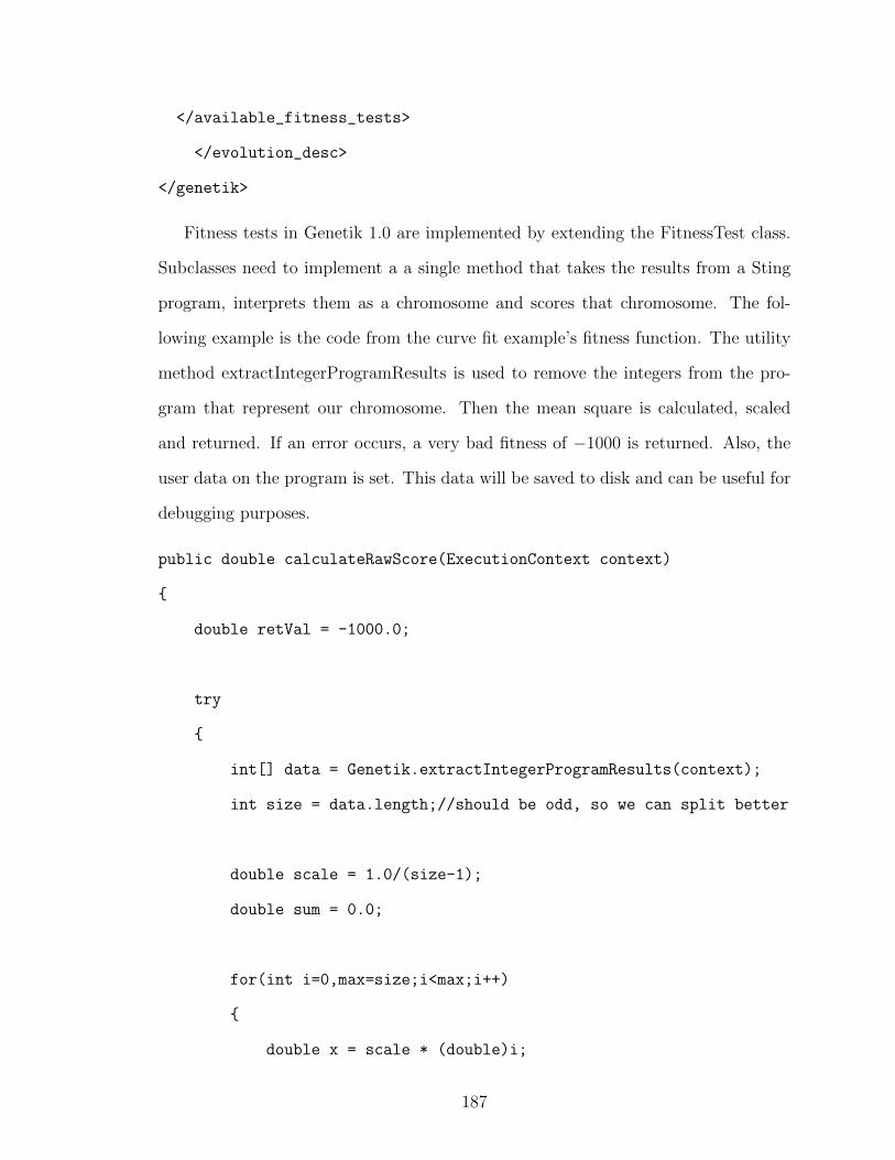
</available_fitness_tests>

</evolution_desc>

</genetik>

Fitness tests in Genetik 1.0 are implemented by extending the FitnessTest class.

Subclasses need to implement a a single method that takes the results from a Sting

program, interprets them as a chromosome and scores that chromosome. The fol-

lowing example is the code from the curve fit example’s fitness function. The utility

method extractIntegerProgramResults is used to remove the integers from the pro-

gram that represent our chromosome. Then the mean square is calculated, scaled

and returned. If an error occurs, a very bad fitness of −1000 is returned. Also, the

user data on the program is set. This data will be saved to disk and can be useful for

debugging purposes.

public double calculateRawScore(ExecutionContext context)

{

double retVal = -1000.0;

try

{

int[] data = Genetik.extractIntegerProgramResults(context);

int size = data.length;//should be odd, so we can split better

double scale = 1.0/(size-1);

double sum = 0.0;

for(int i=0,max=size;i<max;i++)

{

double x = scale * (double)i;

187

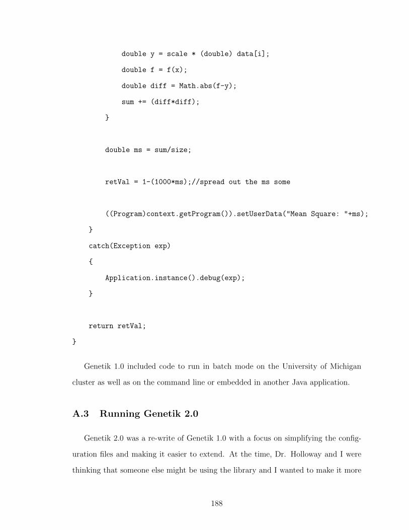
double y = scale * (double) data[i];

double f = f(x);

double diff = Math.abs(f-y);

sum += (diff*diff);

}

double ms = sum/size;

retVal = 1-(1000*ms);//spread out the ms some

((Program)context.getProgram()).setUserData("Mean Square: "+ms);

}

catch(Exception exp)

{

Application.instance().debug(exp);

}

return retVal;

}

Genetik 1.0 included code to run in batch mode on the University of Michigan

cluster as well as on the command line or embedded in another Java application.

A.3 Running Genetik 2.0

Genetik 2.0 was a re-write of Genetik 1.0 with a focus on simplifying the config-

uration files and making it easier to extend. At the time, Dr. Holloway and I were

thinking that someone else might be using the library and I wanted to make it more

188

accessible.

One of the key changes was moving from XML to the Java properties file format.

This is a key-value format. Genetik uses a simple rule to handle array like values. One

key will contain a comma separated list of values. These values are used to construct

other keys. This construct is exemplified with the runs key in the properties list below.

This example is an actual description file, combining the run.xml and evdesc.xml roles,

for a gamma shield simulation.

#

#

# Core settings

#

runs=4_bands,8_bands,16_bands

chromosome=com.sasbury.genetik.chromosomes.IntegerChromosome

minimum_gene=0

maximum_gene=6

phase_translator=com.sasbury.experiment.xraylayers.FixedLayersFitnessTest

phase_selection=com.sasbury.genetik.selection.TournamentSelection

#

# 4 band run settings

#

4_bands.population=250

4_bands.generations=10

4_bands.genes=4

4_bands.shield_layers=4

#

# 8 band run settings

#

189

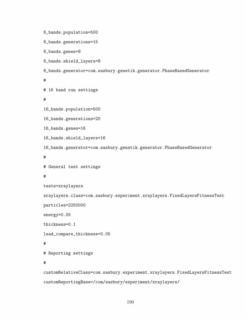
8_bands.population=500

8_bands.generations=15

8_bands.genes=8

8_bands.shield_layers=8

8_bands.generator=com.sasbury.genetik.generator.PhaseBasedGenerator

#

# 16 band run settings

#

16_bands.population=500

16_bands.generations=20

16_bands.genes=16

16_bands.shield_layers=16

16_bands.generator=com.sasbury.genetik.generator.PhaseBasedGenerator

#

# General test settings

#

tests=xraylayers

xraylayers.class=com.sasbury.experiment.xraylayers.FixedLayersFitnessTest

particles=2250000

energy=0.05

thickness=0.1

lead_compare_thickness=0.05

#

# Reporting settings

#

customRelativeClass=com.sasbury.experiment.xraylayers.FixedLayersFitnessTest

customReportingBase=/com/sasbury/experiment/xraylayers/

190

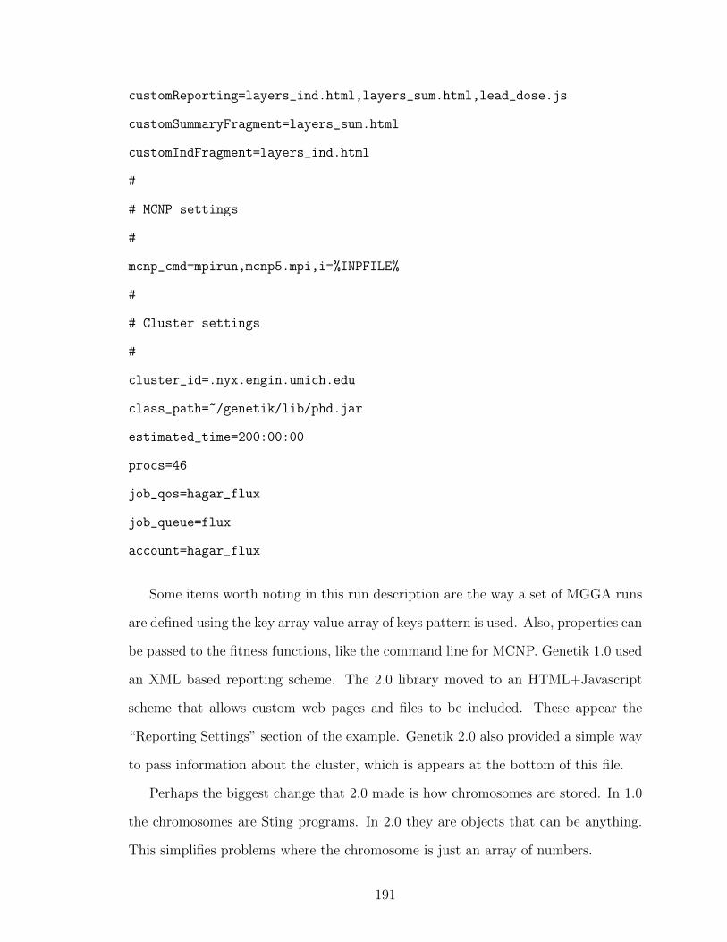
customReporting=layers_ind.html,layers_sum.html,lead_dose.js

customSummaryFragment=layers_sum.html

customIndFragment=layers_ind.html

#

# MCNP settings

#

mcnp_cmd=mpirun,mcnp5.mpi,i=%INPFILE%

#

# Cluster settings

#

cluster_id=.nyx.engin.umich.edu

class_path=~/genetik/lib/phd.jar

estimated_time=200:00:00

procs=46

job_qos=hagar_flux

job_queue=flux

account=hagar_flux

Some items worth noting in this run description are the way a set of MGGA runs

are defined using the key array value array of keys pattern is used. Also, properties can

be passed to the fitness functions, like the command line for MCNP. Genetik 1.0 used

an XML based reporting scheme. The 2.0 library moved to an HTML+Javascript

scheme that allows custom web pages and files to be included. These appear the

“Reporting Settings” section of the example. Genetik 2.0 also provided a simple way

to pass information about the cluster, which is appears at the bottom of this file.

Perhaps the biggest change that 2.0 made is how chromosomes are stored. In 1.0

the chromosomes are Sting programs. In 2.0 they are objects that can be anything.

This simplifies problems where the chromosome is just an array of numbers.

191

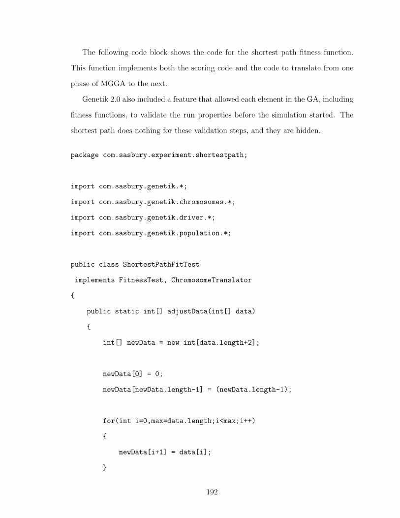
The following code block shows the code for the shortest path fitness function.

This function implements both the scoring code and the code to translate from one

phase of MGGA to the next.

Genetik 2.0 also included a feature that allowed each element in the GA, including

fitness functions, to validate the run properties before the simulation started. The

shortest path does nothing for these validation steps, and they are hidden.

package com.sasbury.experiment.shortestpath;

import com.sasbury.genetik.*;

import com.sasbury.genetik.chromosomes.*;

import com.sasbury.genetik.driver.*;

import com.sasbury.genetik.population.*;

public class ShortestPathFitTest

implements FitnessTest, ChromosomeTranslator

{

public static int[] adjustData(int[] data)

{

int[] newData = new int[data.length+2];

newData[0] = 0;

newData[newData.length-1] = (newData.length-1);

for(int i=0,max=data.length;i<max;i++)

{

newData[i+1] = data[i];

}

192

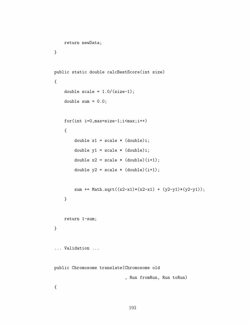
return newData;

}

public static double calcBestScore(int size)

{

double scale = 1.0/(size-1);

double sum = 0.0;

for(int i=0,max=size-1;i<max;i++)

{

double x1 = scale * (double)i;

double y1 = scale * (double)i;

double x2 = scale * (double)(i+1);

double y2 = scale * (double)(i+1);

sum += Math.sqrt((x2-x1)*(x2-x1) + (y2-y1)*(y2-y1));

}

return 1-sum;

}

... Validation ...

public Chromosome translate(Chromosome old

, Run fromRun, Run toRun)

{

193

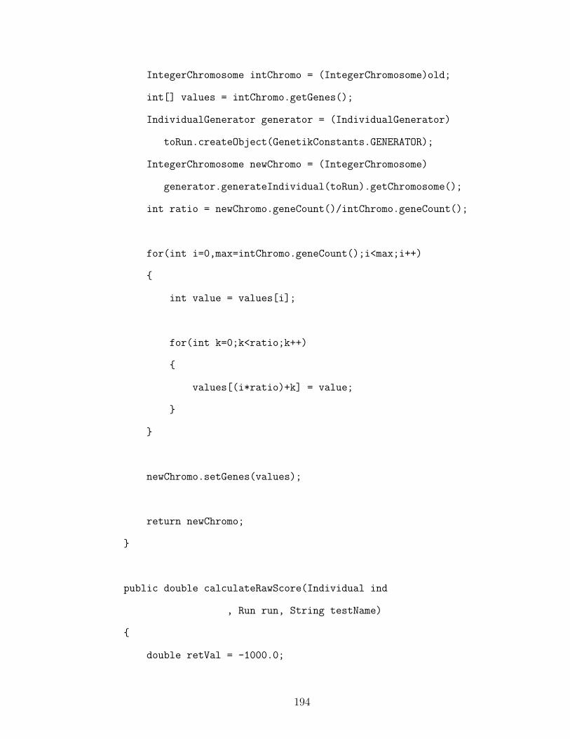
IntegerChromosome intChromo = (IntegerChromosome)old;

int[] values = intChromo.getGenes();

IndividualGenerator generator = (IndividualGenerator)

toRun.createObject(GenetikConstants.GENERATOR);

IntegerChromosome newChromo = (IntegerChromosome)

generator.generateIndividual(toRun).getChromosome();

int ratio = newChromo.geneCount()/intChromo.geneCount();

for(int i=0,max=intChromo.geneCount();i<max;i++)

{

int value = values[i];

for(int k=0;k<ratio;k++)

{

values[(i*ratio)+k] = value;

}

}

newChromo.setGenes(values);

return newChromo;

}

public double calculateRawScore(Individual ind

, Run run, String testName)

{

double retVal = -1000.0;

194

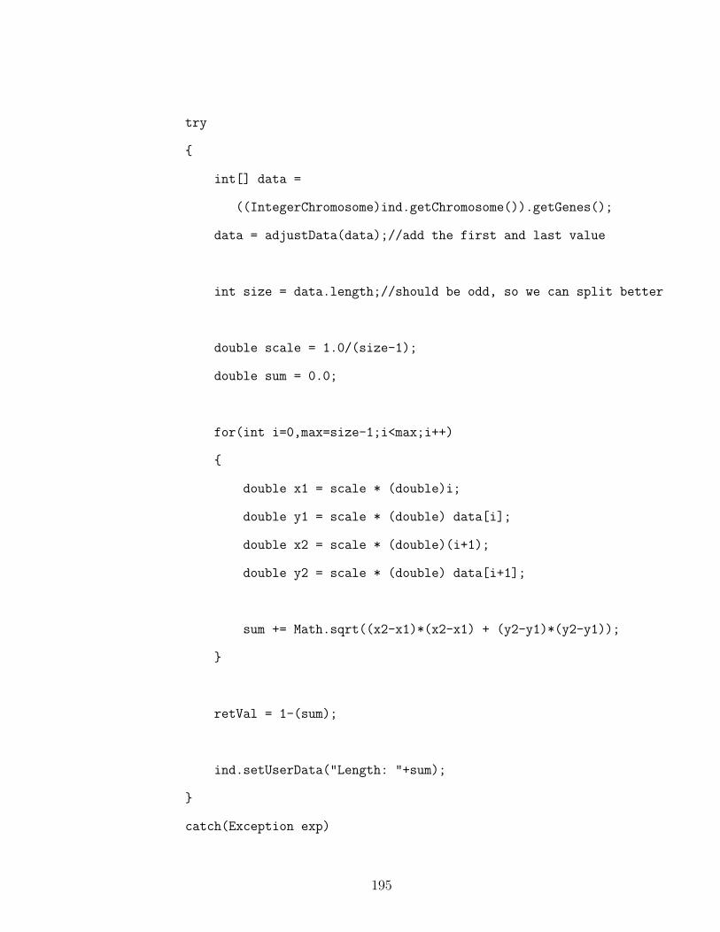
try

{

int[] data =

((IntegerChromosome)ind.getChromosome()).getGenes();

data = adjustData(data);//add the first and last value

int size = data.length;//should be odd, so we can split better

double scale = 1.0/(size-1);

double sum = 0.0;

for(int i=0,max=size-1;i<max;i++)

{

double x1 = scale * (double)i;

double y1 = scale * (double) data[i];

double x2 = scale * (double)(i+1);

double y2 = scale * (double) data[i+1];

sum += Math.sqrt((x2-x1)*(x2-x1) + (y2-y1)*(y2-y1));

}

retVal = 1-(sum);

ind.setUserData("Length: "+sum);

}

catch(Exception exp)

195

{

exp.printStackTrace();

}

return retVal;

}

}

Like Genetik 1.0, the 2.0 version of the library includes code to run on the Uni-

versity of Michigan cluster as well as from the command line.

196

APPENDIX B

Sting

B.1 An Introduction to Sting

Sting programs consist of a serious of operations that manipulate the data stack

or one of the built in data dictionaries. Internally, the Sting interpreter uses two

stacks. The data stack which is manipulated by the operations and the execution

stack which is manipulated by the interpreter to execute a program.

Because GP can create “bad” programs, all operations that cannot complete do

to an inappropriate stack are treated as a no-op. All operations that access indexed

memory will be floor’ed and modulo’ed to fit the available choices.

B.2 Executing a Sting Program

Before execution a program is compiled or created as an array of integers. Each

integer encodes two pieces of information, an operation index and a depth. The

operation indexes are created during compile time by assigning a unique index for

each operation in the program. Terminals - or constants - are implemented as a simple

push operation, so they two are indexed in this way.

197

Procedures are compiled in-line but have a depth setting 1 greater than the level

they are defined in. So,

1 1 add { 1 1 minus } 1 1 times

is compiled to 3 operations, two that push the value of 1 onto the stack and one

that subtracts. These all have a depth of 1. The other operations, 6 of them, have a

depth of 0.

This intermediate format is designed to make it easy to perform genetic program-

ming on a Sting program.

When asked to interpret a compiled program, the interpreter pushes the array of

integers onto the execution stack. Then the interpreter begins taking a single element

from the stack and executing it. The interpreter performs this operation at a specified

depth, 0 for the main program. When integers at a “deeper” depth are encountered,

they are collecting into an array, converted to a Procedure object and pushed on

the data stack. When a procedure is executed, the interpreter is set to its depth so

procedures can contain other procedures.

Sting uses white space to separate operations and values, but does not care about

the white space specifically.

Procedures in Sting are distinguished by { and } as in Postscript and other lan-

guages. Arrays are indicated by [ and ].

B.3 Sting Data Types

Sting provides the following built in data types:

• Number - a single precision floating point number

• String - a string of characters

198

• Array - an array of arrays, strings or floating point numbers, to be used as a

vector or matrix

• Procedure - a collection of statements used in a loop or conditional

• IndexedMemory - number slots that can contain the other data types, pre-

defined memory maps are provided for the programs input and output

B.4 Sting Operations

Sting provides the following extensible set of operations:

• dup - duplicate the top item on the stack

• swap - swap the top two items on the stack

• pop - pop the top item off the stack

• roll - (... n i roll) - rolls the previous n items on the stack i times, so (a b c 3 1

roll) becomes (c a b)

• copy - (... n copy) - copies the last N items on the stack, (a b c 2 copy) becomes

(a b c b c)

• mark - creates a mark for the current stack size

• cleartomark - clears the stack up to the last mark

• plus - (a b plus) - adds two numbers, a+b

• minus - (a b minus) - subtracts two numbers, a-b

• times - (a b times) - multiplies two numbers, a*b

• divide - (a b divide) - divides two numbers, a/b

199

• modulo - (a b modulo) - takes the modulo of two numbers, a

• floor - (a floor) - takes one number and finds the closest integer smaller than it

• ceil - (a ceil) - takes one number and finds the closest integer bigger than it

• abs - (a abs) - takes the absolute value of a number

• neg - (a neg) - pops a number and pushes the negative of it

• and - (a b and) - takes two numbers and returns 1 if they are both greater than

0 and -1 if not (optimized)

• or - (a b or) - takes two numbers and returns 1 if they either or both are greater

than 0 and -1 if not

• xor - (a b xor) - takes two numbers and returns 1 if they either but not both is

greater than 0 and -1 if not

• not - (a not) - takes one number and returns 1 if it is less than or equal to 0

and -1 if not

• input - puts the input indexed memory on the stack

• output - puts the output indexed memory on the stack

• working - puts the working indexed memory on the stack

• read - (i mem read) - reads the i’th element in indexed memory or array instance

mem and puts it on the stack

• write - (b i mem read) - buts b in the i’th slot in an indexed memory or array

• add - (b mem read) - adds b to the a new slot at the end of memory or array

• clear - (i mem clear) - clear the i’th slot in memory or an array

200

• size - (mem size) - pushes the number of slots in mem onto the stack

• lock - (mem lock) - locks mem- fixing the size

• unlock - (mem unlock) - unlocks mem

• null - (null) - places a null value on the stack, generally for adding to indexed

memory

• ifeq - (a proc1 proc2 ifeq) - if a is equal to zero then proc1 is executed, otherwise

proc2 is executed

• ifgt - (a proc1 proc2 ifgt) - if a is greater than zero then proc1 is executed,

otherwise proc2 is executed

• loop - (a b proc loop) - loops over an index starting at a and ending at b

(inclusive), executing proc for each loop

• forall - (array proc forall) - loops over array pushing each element in turn onto

the stack and executing proc, if proc is a noop, elements accumulate on the

stack, for index memory the key and value are pushed onto the stack

• index - push the current index for a loop on the stack, pushes 0 if not in a loop

• noop - places a noop procedure on the stack

• exec - (proc exec) - executes a procedure

B.5 Sting and Binary Chromosomes

While Sting supports a wide range of features, I have primarily used it just to

create a stack of numbers, often zero and one. Sting is very fast to compile and

interpret programs of this form.

201

1 0 1 0 0 0 1

However, programmatically it is important to keep one thing in mind. Sting is

stack based, so depending when you see the string of 1s and 0s it may be reversed

from the intended value.

202

BIBLIOGRAPHY

203

BIBLIOGRAPHY

2011. PBS User Guide. http://www.doesciencegrid.org/public/pbs/.

Aickelin, Uwe. 2002. Partnering strategies for fitness evaluation in a pyramidal evo-lutionary algorithm. Pages 263–270 of: Proc. Genetic and Evolutionary Comput.Conf. GECCO02.

Alpay, Bulent, & Holloway, James Paul. 2005. Segmenting Space Shields. Pages 563–567 of: Proceedings of the Space Nuclear Conference. American Nuclear Society.

Asbury, Stephen, & Holloway, James Paul. 2009a. Multi-Grid Genetic Algorithms forSpace Shield Design. In: International Conference on Mathematics, ComputationalMethods & Reactor Physics (M&C 2009). American Nuclear Society.

Asbury, Stephen, & Holloway, James Paul. 2009b. Optimization of Gamma RadiationShielding by Genetic Algorithms. In: Checmical and Biological Defense Science andTechnology Conference. Defense Threat Reduction Agency.

Asbury, Stephen, & Holloway, James Paul. 2011. Designing Shields for KeV Photonswith Genetic Algorithms. In: International Conference on Mathematics, Compu-tational Methods & Reactor Physics (M&C 2011). American Nuclear Society.

Babbar, Meghna, & Minsker, Barbara. 2003. Multiscale Strategies for Solving Wa-ter Resources Management Problems with Genetic Algorithms. In: Environmen-tal Water Resources Institute (EWRI) World Water Environmental ResourcesCongress 2003 Related Symposia.

Banzhal, Wolfgang, Nordin, Peter, Keller, Robert E., & Francone, Frank D. 1998.Genetic Programming - An Introduction. Morgan Kauffman.

Bell, J., Lail, D., Martin, C., & Nguyen, P. 2010. Radiation Shield for a Lunar Base.http://cmie.lsu.edu/NASA/Teams/Radiation

Berntsson, J., & Tang, Maolin. 2005. Adaptive Sizing of Populations and Number ofIslands in Distributed Genetic Algorithms. Pages 1575–1576 of: GECCO. Ameri-can Computing Society.

Cant-paz, Erick. 1998. A survey of parallel Genetic Algorithms. Calculateurs Paral-leles, 10.

204

Cember, Herman, & Johnson, Thomas E. 2009. Introduction to Health Physics, FourthEdition. McGraw-Hill Companies, Inc.

Chilton, Arthur B., Shultis, J. K., & Faw, Richard E. 1984. Principles of radiationshielding / Arthur B. Chilton, J. Kenneth Shultis, and Richard E. Faw. Prentice-Hall, Englewood Cliffs, NJ :.

Cowall, Alan. 2006. Radiation Poisoning Killed Ex-Russian Spy. New York Times.http://www.nytimes.com/2006/11/24/world/europe/25spycnd.html.

De Jong, E. 2011. Hierarchical Genetic Algorithms.http://citeseer.ist.psu.edu/705095.html.

Eby, David, Averill, R. C., Punch, III, William F., & Goodman, Erik D. 1999. Optimaldesign of flywheels using an injection island Genetic Algorithm. Artif. Intell. Eng.Des. Anal. Manuf., 13(5), 327–340.

Eiben, A.E., & Smith, J.E. 2003. An Introduction to Evolutionary Computing.Springer-Verlag.

Ferguson, Charles D., Kazi, Tahseen, & Perera, Judith. 2003. Commercial RadioactiveSources: Surveying the Security Risks. Occasional Paper No. 11.

Fishman, George S. 2006. A First Course in Monte Carlo. Thomson Brooks/Cole.

Goldberg, David E. 1989. Genetic Algorithms in Search, Optimization and MachineLearning. Boston, MA, USA: Addison-Wesley Longman Publishing Co., Inc.

Goldberg, David E., & Deb, Kalyanmoy. 1991. A comparative analysis of selectionschemes used in Genetic Algorithms. Pages 69–93 of: Foundations of GeneticAlgorithms. Morgan Kaufmann.

Goldberg, David E., Deb, Kalyanmoy, & Clark, James H. 1991. Genetic Algorithms,Noise, and the Sizing of Populations. COMPLEX SYSTEMS, 6, 333–362.

Goldberg, David E., Deb, Kalyanmoy, Kargupta, Hillol, & Harik, Georges. 1993.Rapid, Accurate Optimization of Difficult Problems Using Fast Messy GeneticAlgorithms. Pages 56–64 of: Proceedings of the Fifth International Conference onGenetic Algorithms. Morgan Kaufmann.

Harik, George, Goldberg, David E., Cantu-Paz, Erick, & Miller, Brad L. 1997. TheGambler’s Ruin Problem, Genetic Algorithms, and the Sizing of Populations. Pages7–12 of: Evolutionary Computation. IEEE Press.

Haupt, Randy L., & Haupt, Sue Ellen. 1998. Practical Genetic Algorithms. JohnWiley and Sons.

Heath, D., & Heath, C. 2007. Get Back In the Box. Fast Company (December 2007/ January 2008) p. 74.

205

Holland, John H. 1992,1975. Adaptation in Natural and Artifical Systems. MIT Press.

IAEA. 2002. Inadequate Control of Worlds Radioactive Sources.http://www.iaea.org/NewsCenter/PressReleases/2002/prn0209.shtml.

International Commission on Radiation Units and Measurements. 2011. FundamentalQuantities and Units for Ionizing Radiation. 11(1).

Jong, Kenneth A. De. 2006. Evolutionary Computation. MIT Press.

Kanamori, H., Nakamori, N., Inoue, K., & Takenaka, E. 1985. Effects of scatteredx-rays on CT images. Physics in Medicine and Biology, 3.

Kwan, A., Boone, J., & Shah, N. 2005. Evaluation of x-ray scatter properties in adedicated cone-beam breast CT scanner. Medical Physics, 32.

Langon, William B., & Poli, Riccardo. 2002. Foundations of Genetic Programming.Springer-Verlag.

Lee, L.W. 1987. Shielding Analysis of a Compact Space Nuclear Reactor.

Los Alamos National Lab. 2011. LANL Cross Section Data. http://t2.lanl.gov/.

M Babbar, B Minsker, D E Goldberg. 2002. A multiscale island injection geneticalgorithm for optimal groundwater remediation design. In: Proceedings of the Con-ference on Water Resources Planning and Management, (CWRPM02). AmericanSociety of Civil Engineers (ASCE) Environmental and Water Resources Institute(EWRI.

Mail, N., Moseley, D.J., Slewerdsen, J.H., & Jaffray, D.A. 2009. The influence ofbowtie filtration on cone-beam CT image quality. Medical Physics, 36.

McCaffrey, J. P., Mainegra-Hing, E., & Shen, H. 2009. Optimizing non-Pb radiationshielding materials using bilayers. Medical Physics, 36.

Merkle, Laurence D., Gates Jr., George H., & Lamont, Gary B. 1998. Scalability of anMPI-based fast messy Genetic Algorithm. Pages 386–393 of: SAC ’98: Proceedingsof the 1998 ACM symposium on Applied Computing. New York, NY, USA: ACM.

Mitchel, Melanie. 1998. An Introduction to Genetic Algorithms. MIT Press.

Monte Carlo Codes Group - Los Alamos National Laboratory. 2011. MCNP - AGeneral Monte Carlo N-Particle Transport Code. http://mcnp-green.lanl.gov/.

National Institute of Standards and Technology. 2011. Lead Cross Section Data.http://physics.nist.gov/PhysRefData/XrayMassCoef/ElemTab/z82.html.

Oak Ridge National Laboratory. 2011. ORNL Phantom. http://mcnp-green.lanl.gov/resources.html.

206

Pheil, EC. 2006. Space Reactor Radiation Shield Design Summary. Lockheed MartinLetter SPP-67210-0011.

Radiobiological Advisory Panel. 1970. Radiation Protection Guides and Con-straints for Space-Mission and Vehicle-Design Involving Nuclear Systems. NationalAcademy of Sciences.

R.K., Tripathi, J.W., Wilson, F.A., Cucinotta, J.E., Nealy, M.S., Clowdsley, &M.H.Y., Kim. 2001. Deep Space Mession Radiation Shielding Optimization. Societyof Automotive Engineers, 01ICES-2326.

Robotics, Berkeley. 2011. Berkeley Lower Extremity Exoskeleton.http://bleex.me.berkeley.edu/bleex.htm.

Schuster, Patricia. 2009. Synopsis: Dirty Bombs. Undergraduate Research Project.

Shultis, J. Kenneth, & Faw, Richard E. 2000. Radiation Shielding. American NuclearSociety Inc.

Skolicki, Zbigniew. 2005. An analysis of island models in evolutionary computation.Pages 386–389 of: GECCO ’05: Proceedings of the 2005 workshops on Genetic andevolutionary computation. New York, NY, USA: ACM.

Space X. 2011. Falcon 9 Users Guide. http://www.spacex.com/falcon9.php.

SQLite. 2011. Limits in SQLite. http://www.sqlite.org/limits.html.

Sullivan, Keith, Luke, Sean, Larock, Curt, Cier, Sean, & Armentrout, Steven. 2008.Opportunistic evolution: efficient evolutionary computation on large-scale compu-tational grids. Pages 2227–2232 of: GECCO ’08: Proceedings of the 2008 GECCOconference companion on Genetic and evolutionary computation. New York, NY,USA: ACM.

Tomassini, Marco. 2005. Spatially Structured Evolutionary Algorithms. Springer-Verlag.

US Nuclear Regulatory Commission. 2011. US-NRC Deep Dose Equiv-alent. http://www.nrc.gov/reading-rm/basic-ref/glossary/deep-dose-equivalent-dde.html.

webelements.com. 2011. Web Elements Data. http://www.webelements.com/.

207