Algorithms I
239
Algorithms I Markus Lohrey Universit¨ at Siegen Wintersemester 2017/2018 Markus Lohrey (Universit¨ at Siegen) Algorithms WS 2016/2017 1 / 168
-
Upload
khangminh22 -
Category
Documents
-
view
8 -
download
0
Transcript of Algorithms I

Algorithms I
Markus Lohrey
Universitat Siegen
Wintersemester 2017/2018
Markus Lohrey (Universitat Siegen) Algorithms WS 2016/2017 1 / 168

Overview, Literature
Overview:
1 Basics
2 Divide & Conquer
3 Sorting
4 Greedy algorithms
5 Dynamic programming
6 Graph algorithms
Literature:
Cormen, Leiserson Rivest, Stein. Introduction to Algorithms (3.Auflage); MIT Press 2009
Schoning, Algorithmik. Spektrum Akademischer Verlag 2001
Markus Lohrey (Universitat Siegen) Algorithms WS 2016/2017 2 / 168

Basics
Landau Symbols
Let f , g : N → N be functions.
g ∈ O(f ) if
∃c > 0 ∃n0 ∀n ≥ n0 : g(n) ≤ c · f (n).In other words: g is not growing faster than f .
g ∈ o(f ) if
∀c > 0 ∃n0 ∀n ≥ n0 : g(n) ≤ c · f (n).In other words: g is growing strictly slower than f .
g ∈ Ω(f ) ⇔ f ∈ O(g)In other words: g is growing at least as fast than f .
g ∈ ω(f ) ⇔ f ∈ o(g)In other words: g is growing strictly faster than f .
g ∈ Θ(f ) ⇔ (f ∈ O(g) ∧ g ∈ O(f ))In other words: g and f have the same asymptotic growth.
Markus Lohrey (Universitat Siegen) Algorithms WS 2016/2017 3 / 168

Basics
Jensen’s Inequality
Let f : D → R be a function, where D ⊆ R is an interval.
f is convex if for all x , y ∈ D and all 0 ≤ λ ≤ 1,f (λx + (1− λ)y) ≤ λf (x) + (1− λ)f (y).
f is concave if for all x , y ∈ D and all 0 ≤ λ ≤ 1,f (λx + (1− λ)y) ≥ λf (x) + (1− λ)f (y).
Jensen’s inequality
If f is concave, then for all x1, . . . , xn ∈ D and all λ1, . . . , λn ≥ 0 withλ1 + · · · + λn = 1:
f
( n∑
i=1
λi · xi)
≥n∑
i=1
λi · f (xi ).
If f is convex, then for all x1, . . . , xn ∈ D and all λ1, . . . , λn ≥ 0 withλ1 + · · · + λn = 1:
f
( n∑
i=1
λi · xi)
≤n∑
i=1
λi · f (xi ).
Markus Lohrey (Universitat Siegen) Algorithms WS 2016/2017 4 / 168

Basics
Complexity measures
We describe the running time of an algorithm A as a function in the inputlength n.
Standard: Worst case complexity
Maximal running time on all inputs of length n:
tA,worst(n) = maxtA(x) | x ∈ Xn,
where Xn = x | |x | = n.Criticism: Unrealistic, since in practise worst-case inputs might not arise.
Markus Lohrey (Universitat Siegen) Algorithms WS 2016/2017 5 / 168

Basics
Complexity measures
Alternative: average case complexity.
Needs a probability distribution on Xn.
Standard: uniform distribution, i.e., Prob(x) = 1|Xn|
.
Average running time:
tA,∅(n) =∑
x∈Xn
Prob(x) · tA(x)
=1
|Xn|∑
x∈Xn
tA(x) (for uniform distribution)
Problem: Difficult to analyse
Example: quicksort
Worst case number of comparisons of quicksort: tQ(n) ∈ Θ(n2).
Average number of comparisons: tQ,∅(n) = 1.38n log n
Markus Lohrey (Universitat Siegen) Algorithms WS 2016/2017 6 / 168

Basics
Machine models: Turing machines
The Turing machine (TM) is a very simple and mathematically easy todefine model of computation.
But: memory access (i.e., moving head to a certain symbol on the tape) isvery time-consuming on a Turing machine and not realistic.
Markus Lohrey (Universitat Siegen) Algorithms WS 2016/2017 7 / 168

Basics
Machine models: Register machine (RAM)
RAM
IC Program
Storage
0 = Akku
1 = 1.Reg
2 = 2.Reg
3 = 3.Reg
4 = 4.Reg
.
.
.
x1 x2 x3 x4 x5 x6 x7 x8 x9 . . .Input READ ONLY
y1 y2 y3 y4 y5 y6 y7 y8 y9 . . .Output WRITE ONLY
Assumption: Elementary operations (e.g., the arithmetic operations+,×,−, DIV, comparison, bitwise AND and OR) need a singlecomputation step.
Markus Lohrey (Universitat Siegen) Algorithms WS 2016/2017 8 / 168

Divide & Conquer
Overview
Solving recursive equations
Mergesort
Fast multiplication of integers
Matrix multiplication a la Strassen
Markus Lohrey (Universitat Siegen) Algorithms WS 2016/2017 9 / 168

Divide & Conquer
Divide & Conquer: basic idea
As a first major design principle for algorithms, we will see Divide &Conquer:
Basic idea:
Divide the input into several parts (usually of roughly equal size)
Solve the problem on each part separately (recursion).
Construct the overall solution from the sub-solutions.
Markus Lohrey (Universitat Siegen) Algorithms WS 2016/2017 10 / 168

Divide & Conquer
Recursive equations
Divide & Conquer leads in a very natural way to recursive equations.
Assumptions:
Input of length n will be split into a many parts of size n/b.
Dividing the input and merging the sub-solutions takes time g(n).
For an input of length 1 the computation time is g(1).
This leads to the following recursive equation for the computation time:
t(1) = g(1)
t(n) = a · t(n/b) + g(n)
Technical probem: What happens, if n is not divisible by b?
Solution 1: Replace n/b by ⌈n/b⌉.Solution 2: Assume that n = bk for some k ≥ 0.
If this does not hold: Stretch the input (for every n there exists ak ≥ 0 with n ≤ bk < bn).
Markus Lohrey (Universitat Siegen) Algorithms WS 2016/2017 11 / 168

Divide & Conquer
Solving simple recursive equations
Theorem 1
Let a, b ∈ N and b > 1, g : N −→ N and assume the following equations:
t(1) = g(1)
t(n) = a · t(n/b) + g(n)
Then for all n = bk (i.e., k = logb(n)):
t(n) =
k∑
i=0
ai · g( n
bi
)
.
Proof: Induction over k .
k = 0 : We have n = b0 = 1 and t(1) = g(1).
Markus Lohrey (Universitat Siegen) Algorithms WS 2016/2017 12 / 168

Divide & Conquer
Solving simple recursive equations
k > 0 : By induction we have
t(n
b
)
=
k−1∑
i=0
ai · g( n
bi+1
)
.
Hence:
t(n) = a · t(n
b
)
+ g(n)
= a
(
k−1∑
i=0
ai · g( n
bi+1
)
)
+ g(n)
=
k∑
i=1
ai · g( n
bi
)
+ a0g( n
b0
)
=k∑
i=0
ai · g( n
bi
)
.
Markus Lohrey (Universitat Siegen) Algorithms WS 2016/2017 13 / 168

Divide & Conquer
Master theorem I
Theorem 2 (Master theorem I)
Let a, b, c , d ∈ N with b > 1 and assume that
t(1) = d
t(n) = a · t(n/b) + d · nc
Then, for all n of the form bk with k ≥ 0 we have:
t(n) ∈
Θ(nc) if a < bc
Θ(nc log n) if a = bc
Θ(nlog alog b ) if a > bc
Remark: log alog b = logb a. If a > bc , then logb a > c .
Markus Lohrey (Universitat Siegen) Algorithms WS 2016/2017 14 / 168

Divide & Conquer
Proof of the master theorem I
Let g(n) = dnc . By Theorem 1 we have the following for k = logb n:
t(n) = d · nc ·k∑
i=0
( a
bc
)i
.
Case 1: a < bc
t(n) ≤ d · nc ·∞∑
i=0
( a
bc
)i
= d · nc · 1
1− abc
∈ O(nc).
Moreover, t(n) ∈ Ω(nc), which implies t(n) ∈ Θ(nc).
Case 2: a = bc
t(n) = (k + 1) · d · nc ∈ Θ(nc log n).
Markus Lohrey (Universitat Siegen) Algorithms WS 2016/2017 15 / 168

Divide & Conquer
Proof of the master theorem I
Case 3: a > bc
t(n) = d · nc ·k∑
i=0
( a
bc
)i
= d · nc · (abc)k+1 − 1abc
− 1
∈ Θ
(
nc ·( a
bc
)logb(n))
= Θ
(
nc · alogb(n)bc logb(n)
)
= Θ(
alogb(n))
= Θ(
blogb(a)·logb(n))
= Θ(
nlogb(a))
Markus Lohrey (Universitat Siegen) Algorithms WS 2016/2017 16 / 168

Divide & Conquer
Stretching the input is ok
Stretching the input length to a b-power does not change the statement ofthe master theorem I.
Formally: Assume that the function t satisfies the following recursiveequation
t(1) = d
t(n) = a · t(n/b) + d · nc
for all b-powers n.
Define the function s : N → N by s(n) = t(m), where m is the smallestb-power with m ≥ n ( n ≤ m ≤ bn).
With the master theorem I we get
s(n) = t(m) ∈
Θ(mc) = Θ(nc) if a < bc
Θ(mc logm) = Θ(nc log n) if a = bc
Θ(mlog alog b ) = Θ(n
log alog b ) if a > bc
Markus Lohrey (Universitat Siegen) Algorithms WS 2016/2017 17 / 168

Divide & Conquer
Master theorem II
Theorem 3 (Master theorem II)
Let r > 0,∑r
i=0 αi < 1 and assume that for a constant c,
t(n) ≤(
r∑
i=0
t(⌈αin⌉))
+ c · n.
Then we have t(n) ∈ O(n).
Markus Lohrey (Universitat Siegen) Algorithms WS 2016/2017 18 / 168

Divide & Conquer
Proof of the master theorem II
Choose ε > 0 and n0 > 0 such thatr∑
i=0
⌈αin⌉ ≤ (r∑
i=0
αi) · n + (r + 1) ≤ (1− ε)n
for all n ≥ n0.
Choose γ such that c ≤ γε and t(n) ≤ γn for all n < n0.
By induction we get for all n ≥ n0:
t(n) ≤(
r∑
i=0
t(⌈αin⌉))
+ cn
≤(
r∑
i=0
γ⌈αin⌉)
+ cn (induction)
≤ (γ(1 − ε) + c)n
≤ γn
Markus Lohrey (Universitat Siegen) Algorithms WS 2016/2017 19 / 168

Divide & Conquer Mergesort
Mergesort
We want to sort an array A of length n, where n = 2k for some k ≥ 0.
Algorithm mergesort
procedure mergesort(l , r)var m : integer;begin
if (l < r) thenm := (r + l) div 2;mergesort(l ,m);mergesort(m + 1, r);merge(l ,m, r);
endifendprocedure
Markus Lohrey (Universitat Siegen) Algorithms WS 2016/2017 20 / 168

Divide & Conquer Mergesort
Mergesort
Algorithm merge
procedure merge(l ,m, r)var i , j , k : integer;begin
i = l ; j := m + 1;for k := 1 to r − l + 1 do
if i = m + 1 or (i ≤ m and j ≤ r and A[j] ≤ A[i ]) thenB [k] := A[j]; j := j + 1
elseB [k] := A[i ]; i := i + 1
endifendforfor k := 0 to r − l do
A[l + k] := B [k + 1]endfor
endprocedureMarkus Lohrey (Universitat Siegen) Algorithms WS 2016/2017 21 / 168

Divide & Conquer Mergesort
Mergesort
Note: merge(l ,m, r) works in time O(r − l + 1).
Running time: tms(n) = 2 · tms(n/2) + d · n for a constant d .
Master theorem I: tms(n) ∈ Θ(n log n).
We will see later that O(n log n) is asymptotically optimal for sortingalgorithms that are only based on the comparison of elements.
Drawback of Mergesort: no in-place sorting algorithm
A sorting algorithm works in-place, if at every time instant only a constantnumber of elements from the input array A is stored outside of A.
We will see in-place sorting algorithms with a running of O(n log n).
Markus Lohrey (Universitat Siegen) Algorithms WS 2016/2017 22 / 168

Divide & Conquer Multiplication of natural numbers
Multiplication of natural numbers
We want to multiply two n-bit natural numbers, where n = 2k for somek ≥ 0.
School method: Θ(n2) bit operations.
Alternative approach:
r = A B
s = C D
Here, A (C ) are the first n/2 bits and B (D) are the last n/2 bits of r (s),i.e.,
r = A 2n/2 + B ; s = C 2n/2 + D
r s = AC 2n + (AD + B C ) 2n/2 + B D
Master theorem I: tmult(n) = 4 · tmult(n/2) + Θ(n) ∈ Θ(n2)No improvement!Markus Lohrey (Universitat Siegen) Algorithms WS 2016/2017 23 / 168

Divide & Conquer Multiplication of natural numbers
Fast multiplication by A. Karatsuba, 1960
Compute recursively AC , (A − B)(D − C ) and BD.
Then, we get
rs = AC 2n + (A− B) (D − C ) 2n/2 + (B D + AC ) 2n/2 + B D
By the master theorem I, the total number of bit operations is:
tmult(n) = 3 · tmult(n/2) + Θ(n) ∈ Θ(nlog 3log 2 ) = Θ(n1.58496...).
Using divide & conquer we reduced the exponent from 2 (school method)to 1.58496... .
Markus Lohrey (Universitat Siegen) Algorithms WS 2016/2017 24 / 168

Divide & Conquer Multiplication of natural numbers
How fast can we multiply?
In 1971, Arnold Schonhage and Volker Strassen presented an algorithmwhich multiplies two n-bit number in time O(n log n log log n) on amultitape Turing-machine.
The Schonhage-Strassen algorithm uses the so-called fast Fouriertransformation (FFT); see Algorithms II.
In practice, the Schonhage-Strassen algorithm beats Karatsuba’s algorithmfor numbers with approx. 10.000 digits.
In 2007, Martin Furer came up with an algorithm that beats theSchonhage-Strassen algorithm. His algorithm has a running time ofO(n log n 2log
∗ n), where log∗ n is the first number k such that log2(·)k-times applied to n yields a number ≤ 1.
Markus Lohrey (Universitat Siegen) Algorithms WS 2016/2017 25 / 168

Divide & Conquer Matrix multiplication
Matrix multiplication using naive divide & conquer
Let A = (ai ,j)1≤i ,j≤n and B = (bi ,j)1≤i ,j≤n be two (n × n)-matrices.
For the product matrix AB = (ci ,j)1≤i ,j≤n = C we have
ci ,j =n∑
k=1
ai ,kbk,j
Θ(n3) scalar multiplications.
Divide & conquer: A,B are divided in 4 submatrices of roughly equal size.Then, the product AB = C can be computed as follows:
(
A11
A21
A12
A22
) (
B11
B21
B12
B22
)
=
(
C11
C21
C12
C22
)
Markus Lohrey (Universitat Siegen) Algorithms WS 2016/2017 26 / 168

Divide & Conquer Matrix multiplication
Matrix multiplication using naive divide-and-conquer
(
A11
A21
A12
A22
) (
B11
B21
B12
B22
)
=
(
C11
C21
C12
C22
)
where
C11 = A11B11 + A12B21
C12 = A11B12 + A12B22
C21 = A21B11 + A22B21
C22 = A21B12 + A22B22
We get
t(n) = 8 · t(n/2) + Θ(n2) ∈ Θ(n3).
No improvement!
Markus Lohrey (Universitat Siegen) Algorithms WS 2016/2017 27 / 168

Divide & Conquer Matrix multiplication
Matrix multiplication by Volker Strassen (1969)
Compute the product of two 2× 2 matrices with 7 multiplications:
M1 := (A12 − A22)(B21 + B22)
M2 := (A11 + A22)(B11 + B22)
M3 := (A11 − A21)(B11 + B12)
M4 := (A11 + A12)B22
M5 := A11(B12 − B22)
M6 := A22(B21 − B11)
M7 := (A21 + A22)B11
C11 = M1 +M2 −M4 +M6
C12 = M4 +M5
C21 = M6 +M7
C22 = M2 −M3 +M5 −M7
Running time: t(n) = 7 · t(n/2) + Θ(n2).
Master theorem I (a = 7, b = 2, c = 2):
t(n) ∈ Θ(nlog2 7) = Θ(n2,81...) .
Markus Lohrey (Universitat Siegen) Algorithms WS 2016/2017 28 / 168

Divide & Conquer Matrix multiplication
The story of fast matrix multiplication
Strassen 1969: n2,81...
Pan 1979: n2,796...
Bini, Capovani, Romani, Lotti 1979: n2,78...
Schonhage 1981: n2,522...
Romani 1982: n2,517...
Coppersmith, Winograd 1981: n2.496...
Strassen 1986: n2,479...
Coppersmith, Winograd 1987: n2.376...
Stothers 2010: n2,374...
Williams 2014: n2,372873...
Markus Lohrey (Universitat Siegen) Algorithms WS 2016/2017 29 / 168

Sorting
Overview
Lower bounds for comparison-based sorting algorithms
Quicksort
Heapsort
Sorting in linearer time
Median computation
Markus Lohrey (Universitat Siegen) Algorithms WS 2016/2017 30 / 168

Sorting Lower bound for comparison-based sorting algorithms
Comparison-based sorting algorithms
A sorting algorithm is comparison-based if the elements of the input arraybelong to a data type that only supports the comparison of two elements.
We assume in the following considerations that the input array A[1, . . . , n]has the following properties:
A[i ] ∈ 1, . . . , n for all 1 ≤ i ≤ n.
A[i ] 6= A[j] for i 6= j
In other words: The input is a permutation of the list [1, 2, . . . , n].
The sorting algorithm has to sort this list.
Another point of view: The sorting algorithm has to compute thepermutation [i1, i2, . . . , in] such that A[ik ] = k for all 1 ≤ k ≤ n.
Example: On input [2, 3, 1] the output should be [3, 1, 2].
Markus Lohrey (Universitat Siegen) Algorithms WS 2016/2017 31 / 168

Sorting Lower bound for comparison-based sorting algorithms
Lower bound for the worst case
Theorem 4
For every comparison-based sorting algorithm and every n there exists anarray of length n, on which the algorithm makes at least
n log2(n)− log2(e)n ≥ n log2(n)− 1, 443n
many comparisons.
Proof: We execute the algorithm on an array A[1, . . . , n] without knowingthe concrete values A[i ].
This yields a decision tree that can be constructed as follows:
Assume that the algorithm compares A[i ] and A[j] in the first step.
We label the root of the decision tree with i : j .
The left (right) subtree is obtained by continuing the algorithm under theassumption that A[i ] < A[j] (A[i ] > A[j]).Markus Lohrey (Universitat Siegen) Algorithms WS 2016/2017 32 / 168

Sorting Lower bound for comparison-based sorting algorithms
Lower bound for the worst case
This yields a binary tree with n! many leaves because every inputpermutation must lead to a different leaf.
Example: Here is a decision tree for sorting an array of length 3.
2 : 3
1 : 2 1 : 3
1, 2, 3 1 : 3
2, 1, 3 2, 3, 1
1, 3, 2 1 : 2
3, 1, 2 3, 2, 1
Markus Lohrey (Universitat Siegen) Algorithms WS 2016/2017 33 / 168

Sorting Lower bound for comparison-based sorting algorithms
Lower bound for the worst case
Note: The depth (= max. number of edges on a path from the root to aleaf) of the decision tree is the maximal number of comparisons of thealgorithm on an input array of length n.
A binary tree with N leaves has depth ≥ log2(N).
Stirling’s formula (we only need n! >√2πn(n/e)n) implies
log2(n!) ≥ n log2(n)− log2(e)n +Ω(log n) ≥ n log2(n)− 1, 443n.
Thus, there exists an input array for which the algorithm makes at leastn log2(n)− 1, 443n many comparisons.
Markus Lohrey (Universitat Siegen) Algorithms WS 2016/2017 34 / 168

Sorting Lower bound for comparison-based sorting algorithms
Lower bound for the average case
A comparison-based sorting algorithm even makes n log2(n)− 2, 443nmany comparisons on almost all input permutations:
Theorem 5
For every comparison-based sorting algorithm the following holds: Theportion of all permutations on which the algorithm makes at least
log2(n!)− n ≥ n log2(n)− 2, 443n
many comparisons is at least 1− 2−n+1.
For the proof we need a simple lemma:
Lemma 6
Let A ⊆ 0, 1∗ with |A| = N, and let 1 ≤ n < log2(N). Then, at least(1− 2−n+1)N many words in A have length ≥ log2(N) − n.
Markus Lohrey (Universitat Siegen) Algorithms WS 2016/2017 35 / 168

Sorting Lower bound for comparison-based sorting algorithms
Lower bound for the average case
Consider again the decision tree. It has n! leaves, and every leafcorresponds to a permutation of the numbers 1, . . . , n.Thus, each of the n! many permutations can be represented by a wordover the alphabet 0, 1:
0 means: go in the decision tree to the left child.
1 means: go in the decision tree to the right child.
Lemma 6 the decision tree has at least (1− 2−n+1)n! many root-leafpaths of length ≥ log2(n!)− n ≥ n log2(n)− 2, 443n.
Markus Lohrey (Universitat Siegen) Algorithms WS 2016/2017 36 / 168

Sorting Lower bound for comparison-based sorting algorithms
Lower bound for the average case
Corollary
Every comparison-based sorting algorithm makes on average at leastn log2(n)− 2, 443n many comparisons when sorting an array of length n(for n large enough).
Proof: Due to Theorem 5 at least
(1− 2−n+1) · (log2(n!)− n) + 2−n+1 =
log2(n!)− n − log2(n!)− n − 1
2n−1≥
n log2(n)− 2, 443n +Ω(log2 n)−log2(n!)− n − 1
2n−1≥
n log2(n)− 2, 443n
many comparisons are done in the average.
Markus Lohrey (Universitat Siegen) Algorithms WS 2016/2017 37 / 168

Sorting Quicksort
Quicksort
The Quicksort-algorithm (Tony Hoare, 1962):
Choose an array-element p = A[i ] (the pivot element).
Partitioning: Permute the array such that on the left (resp., right) ofthe pivot element p all elements are ≤ p (resp., > p) (needs n− 1comparisons).
Apply the algorithm recursively to the subarrays to the left and rightof the pivot element.
Critical: choice of the pivot elements.
Running time is optimal, if the pivot element is the middle element ofthe array (median).
Good choice in practice: median-out-of-three
Markus Lohrey (Universitat Siegen) Algorithms WS 2016/2017 38 / 168

Sorting Quicksort
Partitioning
First, we present a procedure for partitioning a subarray A[ℓ, . . . , r ] withrespect to a pivot element P = A[p], where ℓ < r and ℓ ≤ p ≤ r .
The procedure returns an index m ∈ ℓ, . . . , r with the followingproperties:
A[m] = P
A[k] ≤ P for all ℓ ≤ k ≤ m − 1
A[k] > P for all m + 1 ≤ k ≤ r
Markus Lohrey (Universitat Siegen) Algorithms WS 2016/2017 39 / 168

Sorting Quicksort
Partitioning
Algorithm Partition
function partition(A[ℓ . . . r ] : array of integer, p : integer) : integerbegin
swap(p, r);P := A[r ];i := ℓ− 1;for j := ℓ to r − 1 do
if A[j] ≤ P theni := i + 1;swap(i , j)
endifendforswap(i + 1, r)return i + 1
endfunction
Markus Lohrey (Universitat Siegen) Algorithms WS 2016/2017 40 / 168

Sorting Quicksort
Partitioning
The following invariants hold before every iteration of the for-loop:
A[r ] = P
A[k] ≤ P for all ℓ ≤ k ≤ i
A[k] > P for all i + 1 ≤ k ≤ j − 1
Thus, the following holds before the return-statement:
A[k] ≤ P for all ℓ ≤ k ≤ i + 1
A[k] > P for all i + 2 ≤ k ≤ r
A[i + 1] = P
Note: partition(A[ℓ . . . r ]) makes r − ℓ many comparisons.
Markus Lohrey (Universitat Siegen) Algorithms WS 2016/2017 41 / 168

Sorting Quicksort
Quicksort
Algorithm Quicksort
procedure quicksort(A[ℓ . . . r ] : array of integer)begin
if ℓ < r thenp := index of the median of A[ℓ], A[(ℓ+ r) div 2], A[r ];m := partition(A[ℓ . . . r ], p);quicksort(A[ℓ . . .m − 1]);quicksort(A[m + 1 . . . r ]);
endifendprocedure
Worst-case running time: O(n2).
The worst-case arises when after each call of partition(A[ℓ . . . r ], p), one ofthe subarrays (A[ℓ . . .m − 1] or A[m + 1 . . . r ]) is empty.Markus Lohrey (Universitat Siegen) Algorithms WS 2016/2017 42 / 168

Sorting Quicksort
Quicksort: average case analysis
Average case analysis under the assumption that the pivot element ischosen randomly.
Alternatively: Input array is chosen randomly.
Let Q(n) be the avergage number of comparisons for an input array oflength n.
Theorem 7
We have Q(n) = 2(n + 1)H(n) − 4n, where
H(n) :=n∑
k=1
1
k
is the n-th harmonic number.
Markus Lohrey (Universitat Siegen) Algorithms WS 2016/2017 43 / 168

Sorting Quicksort
Quicksort: average case analysis
Proof: for n = 1 we have Q(1) = 0 = 2 · 2 · 1− 4 · 1.For n ≥ 2 we have:
Q(n) = (n − 1) +1
n
n∑
i=1
[Q(i − 1) +Q(n − i)]
= (n − 1) +2
n
n∑
i=1
Q(i − 1)
Note:
(n − 1) = number of comparisons for partitioning.
Q(i − 1) +Q(n − i) = average number of comparisons for therecursive sorting of the two subarrays.
The factor 1/n comes from the fact that every pivot element is chosenwith probability 1/n.
Markus Lohrey (Universitat Siegen) Algorithms WS 2016/2017 44 / 168

Sorting Quicksort
Quicksort: average case analysis
We get:
nQ(n) = n(n− 1) + 2n∑
i=1
Q(i − 1)
Hence:
nQ(n)− (n − 1)Q(n − 1) = n(n − 1) + 2n∑
i=1
Q(i − 1)
−(n − 1)(n − 2)− 2
n−1∑
i=1
Q(i − 1)
= n(n − 1)− (n − 2)(n − 1) + 2Q(n − 1)
= 2(n − 1) + 2Q(n − 1)
We obtain:
nQ(n) = 2(n − 1) + 2Q(n − 1) + (n − 1)Q(n − 1)
= 2(n − 1) + (n + 1)Q(n − 1)Markus Lohrey (Universitat Siegen) Algorithms WS 2016/2017 45 / 168

Sorting Quicksort
Quicksort: average case analysis
Dividing both sides by n(n + 1) gives:
Q(n)
n + 1=
2(n − 1)
n(n + 1)+
Q(n − 1)
n
Using induction on n we get:
Q(n)
n+ 1=
n∑
k=1
2(k − 1)
k(k + 1)
= 2n∑
k=1
(k − 1)
k(k + 1)
= 2(
n∑
k=1
k
k(k + 1)−
n∑
k=1
1
k(k + 1)
)
Markus Lohrey (Universitat Siegen) Algorithms WS 2016/2017 46 / 168

Sorting Quicksort
Quicksort: average case analysis
Q(n)
n+ 1= 2
[
n∑
k=1
1
k + 1−
n∑
k=1
1
k(k + 1)
]
= 2
[
n∑
k=1
2
k + 1−
n∑
k=1
1
k
]
= 2
[
2
(
1
n+ 1+ H(n)− 1
)
− H(n)
]
= 2H(n) +4
n + 1− 4.
Markus Lohrey (Universitat Siegen) Algorithms WS 2016/2017 47 / 168
Sorting Quicksort
Quicksort: average case analysis
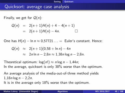
Finally, we get for Q(n):
Q(n) = 2(n + 1)H(n) + 4− 4(n + 1)
= 2(n + 1)H(n) − 4n.
One has H(n) − ln n ≈ 0,57721 . . . = Euler’s constant. Hence:
Q(n) ≈ 2(n + 1)(0,58 + ln n)− 4n
≈ 2n ln n− 2,8n ≈ 1,38n log n− 2,8n.
Theoretical optimum: log(n!) ≈ n log n − 1,44n;In the average, quicksort is only 38% worse than the optimum.
An average analysis of the media-out-of-three method yields1,18n log n − 2,2n.It is in the average only 18% worse than the optimum.
Markus Lohrey (Universitat Siegen) Algorithms WS 2016/2017 48 / 168

Sorting Heapsort
Heaps
Definition 8
A (max-)heap is an array a[1 . . . n] with the following properties:
a[i ] ≥ a[2i ] for all i ≥ 1 with 2i ≤ n
a[i ] ≥ a[2i + 1] for all i ≥ 1 with 2i + 1 ≤ n
Markus Lohrey (Universitat Siegen) Algorithms WS 2016/2017 49 / 168

Sorting Heapsort
Heaps
Example:
16 14 10 8 7 9 3 2 4 1
1 2 3 4 5 6 7 8 9 10
16
14 10
8 7 9 3
2 4 1
1
2 3
4 5 6 7
8 9 10
Markus Lohrey (Universitat Siegen) Algorithms WS 2016/2017 50 / 168

Sorting Heapsort
Sinking process
In a first step we will permute the entries of the array a[1, . . . , n] such thatthe heap condition is satisfied.
Assume that the subarray a[i + 1, . . . , n] already satisfies the heapcondition.
In order to enforce the heap condition also for i we let a[i ] sink:
x
y z
i
2i 2i + 1
With 2 comparisons one can compute maxx , y , z.
Markus Lohrey (Universitat Siegen) Algorithms WS 2016/2017 51 / 168

Sorting Heapsort
Sinking process
In a first step we will permute the entries of the array a[1, . . . , n] such thatthe heap condition is satisfied.
Assume that the subarray a[i + 1, . . . , n] already satisfies the heapcondition.
In order to enforce the heap condition also for i we let a[i ] sink:
x
y z
i
2i 2i + 1
With 2 comparisons one can compute maxx , y , z.If x is the max., then the sinking process stops.
Markus Lohrey (Universitat Siegen) Algorithms WS 2016/2017 51 / 168

Sorting Heapsort
Sinking process
In a first step we will permute the entries of the array a[1, . . . , n] such thatthe heap condition is satisfied.
Assume that the subarray a[i + 1, . . . , n] already satisfies the heapcondition.
In order to enforce the heap condition also for i we let a[i ] sink:
x
y z
i
2i 2i + 1
With 2 comparisons one can compute maxx , y , z.If y is the max., then x and y are swapped and we continue at 2i .
y
x z
i
2i 2i + 1
Markus Lohrey (Universitat Siegen) Algorithms WS 2016/2017 51 / 168

Sorting Heapsort
Sinking process
In a first step we will permute the entries of the array a[1, . . . , n] such thatthe heap condition is satisfied.
Assume that the subarray a[i + 1, . . . , n] already satisfies the heapcondition.
In order to enforce the heap condition also for i we let a[i ] sink:
x
y z
i
2i 2i + 1
With 2 comparisons one can compute maxx , y , z.If z is the max., then x and z are swapped and we continue at 2i + 1.
z
y x
i
2i 2i + 1
Markus Lohrey (Universitat Siegen) Algorithms WS 2016/2017 51 / 168

Sorting Heapsort
Reheap
Algorithm Reheap
procedure reheap(i , n: integer) (∗ i is the root ∗)var m: integer;begin
if i ≤ n/2 thenm := maxa[i ], a[2i ], a[2i + 1]; (∗ 2 comparisons! ∗)if (m 6= a[i ]) ∧ (m = a[2i ]) then
swap(i , 2i); (∗ swap x , y ∗)reheap(2i , n)
elsif (m 6= a[i ]) ∧ (m = a[2i + 1]) thenswap(i , 2i + 1); (∗ swap x , z ∗)reheap(2i + 1, n)
endifendif
endprocedure
Markus Lohrey (Universitat Siegen) Algorithms WS 2016/2017 52 / 168

Sorting Heapsort
Building the heap
Algorithm Build Heap
procedure build-heap(n: integer)begin
for i :=⌊
n2
⌋
downto 1 doreheap(i , n)
endforendprocedure
Invariant: Before the call of reheap(i , n) the subarray a[i + 1, . . . , n]satisfies the heap condition.
Clearly, this hods for i =⌊
n2
⌋
.
Assume that the invariant holds for i .
Thus, the heap condition can only fail for i .
After the sinking process for a[i ], the heap condition also holds for i .Markus Lohrey (Universitat Siegen) Algorithms WS 2016/2017 53 / 168

Sorting Heapsort
Time analysis for building the heap
Theorem 9
Built-heap runs in time O(n).
Proof: Sinking of a[i ] needs 2 · (height of the subtree under a[i ]) manycomparisons.
We carry out the computation for n = 2k − 1.
Then we have a complete binary tree of height k − 1.
There are
20 trees of height k − 1,
21 trees of height k − 2,...
2i trees of height k − 1− i ,...
2k−1 trees of height 0.Markus Lohrey (Universitat Siegen) Algorithms WS 2016/2017 54 / 168

Sorting Heapsort
Time analysis for building the heap
Hence, building the heap needs at most
2 ·k−1∑
i=0
2i (k − 1− i) = 2 ·k−1∑
i=0
2k−1−i i
= 2k ·k−1∑
i=0
i · 2−i
≤ (n + 1) ·∑
i≥0
i · 2−i
many comparisons.
Claim:∑
j≥0 j · 2−j = 2
Proof of the claim: For every |z | < 1 we have
∑
j≥0
z j =1
1− z.
Markus Lohrey (Universitat Siegen) Algorithms WS 2016/2017 55 / 168

Sorting Heapsort
Time analysis for building the heap
Taking derivations yields
∑
j≥0
j · z j−1 =1
(1− z)2,
and hence
∑
j≥0
j · z j = z
(1− z)2.
Setting z = 1/2 yields∑
j≥0
j · 2−j = 2.
Markus Lohrey (Universitat Siegen) Algorithms WS 2016/2017 56 / 168

Sorting Heapsort
Standard Heapsort (W. J. Williams, 1964)
Algorithm Heapsort
procedure heapsort(n: integer)begin
build-heap(n)for i := n downto 2 do
swap(1, i);reheap(1, i − 1)
endforendprocedure
Theorem 10
Standard Heapsort sorts an array with n elements and needs2n log2 n+O(n) comparisons.
Markus Lohrey (Universitat Siegen) Algorithms WS 2016/2017 57 / 168

Sorting Heapsort
Standard Heapsort
Proof:
Correctness: After build-heap(n), a[1] is the maximal element of the array.
This element will be moved with swap(1, n) to its correct position (n).
By induction, the subarray a[1, . . . , n − 1] will be sorted in the remainingsteps.
Running time: Building the heap needs O(n) comparison. Each of theremaining n− 1 many reheap-calls needs at most 2 log2 n comparisons.
Markus Lohrey (Universitat Siegen) Algorithms WS 2016/2017 58 / 168

Sorting Heapsort
Example for Standard Heapsort
1 2 3 4 5 6 7 8 9 10
10
9 8
6 5 7 3
2 4 1
1
2 3
4 5 6 7
8 9 10
Markus Lohrey (Universitat Siegen) Algorithms WS 2016/2017 59 / 168

Sorting Heapsort
Example for Standard Heapsort
10
1 2 3 4 5 6 7 8 9 10
1
9 8
6 5 7 3
2 4
1
2 3
4 5 6 7
8 9
Markus Lohrey (Universitat Siegen) Algorithms WS 2016/2017 59 / 168

Sorting Heapsort
Example for Standard Heapsort
10
1 2 3 4 5 6 7 8 9 10
9
1 8
6 5 7 3
2 4
1
2 3
4 5 6 7
8 9
Markus Lohrey (Universitat Siegen) Algorithms WS 2016/2017 59 / 168

Sorting Heapsort
Example for Standard Heapsort
10
1 2 3 4 5 6 7 8 9 10
9
6 8
1 5 7 3
2 4
1
2 3
4 5 6 7
8 9
Markus Lohrey (Universitat Siegen) Algorithms WS 2016/2017 59 / 168

Sorting Heapsort
Example for Standard Heapsort
10
1 2 3 4 5 6 7 8 9 10
9
6 8
4 5 7 3
2 1
1
2 3
4 5 6 7
8 9
Markus Lohrey (Universitat Siegen) Algorithms WS 2016/2017 59 / 168

Sorting Heapsort
Example for Standard Heapsort
9 10
1 2 3 4 5 6 7 8 9 10
1
6 8
4 5 7 3
2
1
2 3
4 5 6 7
8
Markus Lohrey (Universitat Siegen) Algorithms WS 2016/2017 59 / 168

Sorting Heapsort
Example for Standard Heapsort
9 10
1 2 3 4 5 6 7 8 9 10
8
6 1
4 5 7 3
2
1
2 3
4 5 6 7
8
Markus Lohrey (Universitat Siegen) Algorithms WS 2016/2017 59 / 168

Sorting Heapsort
Example for Standard Heapsort
9 10
1 2 3 4 5 6 7 8 9 10
8
6 7
4 5 1 3
2
1
2 3
4 5 6 7
8
Markus Lohrey (Universitat Siegen) Algorithms WS 2016/2017 59 / 168

Sorting Heapsort
Example for Standard Heapsort
8 9 10
1 2 3 4 5 6 7 8 9 10
2
6 7
4 5 1 3
1
2 3
4 5 6 7
Markus Lohrey (Universitat Siegen) Algorithms WS 2016/2017 59 / 168

Sorting Heapsort
Example for Standard Heapsort
8 9 10
1 2 3 4 5 6 7 8 9 10
7
6 2
4 5 1 3
1
2 3
4 5 6 7
Markus Lohrey (Universitat Siegen) Algorithms WS 2016/2017 59 / 168

Sorting Heapsort
Example for Standard Heapsort
8 9 10
1 2 3 4 5 6 7 8 9 10
7
6 3
4 5 1 2
1
2 3
4 5 6 7
Markus Lohrey (Universitat Siegen) Algorithms WS 2016/2017 59 / 168

Sorting Heapsort
Example for Standard Heapsort
7 8 9 10
1 2 3 4 5 6 7 8 9 10
2
6 3
4 5 1
1
2 3
4 5 6
Markus Lohrey (Universitat Siegen) Algorithms WS 2016/2017 59 / 168

Sorting Heapsort
Example for Standard Heapsort
7 8 9 10
1 2 3 4 5 6 7 8 9 10
6
2 3
4 5 1
1
2 3
4 5 6
Markus Lohrey (Universitat Siegen) Algorithms WS 2016/2017 59 / 168

Sorting Heapsort
Example for Standard Heapsort
7 8 9 10
1 2 3 4 5 6 7 8 9 10
6
5 3
4 2 1
1
2 3
4 5 6
Markus Lohrey (Universitat Siegen) Algorithms WS 2016/2017 59 / 168

Sorting Heapsort
Example for Standard Heapsort
6 7 8 9 10
1 2 3 4 5 6 7 8 9 10
1
5 3
4 2
1
2 3
4 5
Markus Lohrey (Universitat Siegen) Algorithms WS 2016/2017 59 / 168

Sorting Heapsort
Example for Standard Heapsort
6 7 8 9 10
1 2 3 4 5 6 7 8 9 10
5
1 3
4 2
1
2 3
4 5
Markus Lohrey (Universitat Siegen) Algorithms WS 2016/2017 59 / 168

Sorting Heapsort
Example for Standard Heapsort
6 7 8 9 10
1 2 3 4 5 6 7 8 9 10
5
4 3
1 2
1
2 3
4 5
Markus Lohrey (Universitat Siegen) Algorithms WS 2016/2017 59 / 168

Sorting Heapsort
Example for Standard Heapsort
5 6 7 8 9 10
1 2 3 4 5 6 7 8 9 10
2
4 3
1
1
2 3
4
Markus Lohrey (Universitat Siegen) Algorithms WS 2016/2017 59 / 168

Sorting Heapsort
Example for Standard Heapsort
5 6 7 8 9 10
1 2 3 4 5 6 7 8 9 10
4
2 3
1
1
2 3
4
Markus Lohrey (Universitat Siegen) Algorithms WS 2016/2017 59 / 168

Sorting Heapsort
Example for Standard Heapsort
5 6 7 8 9 10
1 2 3 4 5 6 7 8 9 10
4
2 3
1
1
2 3
4
Markus Lohrey (Universitat Siegen) Algorithms WS 2016/2017 59 / 168

Sorting Heapsort
Example for Standard Heapsort
4 5 6 7 8 9 10
1 2 3 4 5 6 7 8 9 10
1
2 3
1
2 3
Markus Lohrey (Universitat Siegen) Algorithms WS 2016/2017 59 / 168

Sorting Heapsort
Example for Standard Heapsort
4 5 6 7 8 9 10
1 2 3 4 5 6 7 8 9 10
3
2 1
1
2 3
Markus Lohrey (Universitat Siegen) Algorithms WS 2016/2017 59 / 168

Sorting Heapsort
Example for Standard Heapsort
3 4 5 6 7 8 9 10
1 2 3 4 5 6 7 8 9 10
1
2
1
2
Markus Lohrey (Universitat Siegen) Algorithms WS 2016/2017 59 / 168

Sorting Heapsort
Example for Standard Heapsort
3 4 5 6 7 8 9 10
1 2 3 4 5 6 7 8 9 10
2
1
1
2
Markus Lohrey (Universitat Siegen) Algorithms WS 2016/2017 59 / 168

Sorting Heapsort
Example for Standard Heapsort
2 3 4 5 6 7 8 9 10
1 2 3 4 5 6 7 8 9 10
11
Markus Lohrey (Universitat Siegen) Algorithms WS 2016/2017 59 / 168

Sorting Heapsort
Example for Standard Heapsort
1 2 3 4 5 6 7 8 9 10
1 2 3 4 5 6 7 8 9 10
Markus Lohrey (Universitat Siegen) Algorithms WS 2016/2017 59 / 168

Sorting Heapsort
Bottom-Up Heapsort
Remark: An analysis of the average case complexity of Heapsort yields2n log2 n many comparisons in the average. Hence, standard Heapsortcannot compete with Quicksort.
Bottom-up Heapsort needs significantly fewer comparisons.
After swap(1, i) one first determines the potential path from the root to aleaf along which the elemente a[i ] will sink; the sink path.
For this, one follows the path that always goes to the larger child. Thisneeds at most log n instead of 2 log2 n comparisons.
In most cases, a[i ] will sink deep into the heap. It is therefore moreefficient to compute the actual position of a[i ] on the sink path bottom-up.
The hope is that the bottom-up computations need in total only O(n)comparisons.
Markus Lohrey (Universitat Siegen) Algorithms WS 2016/2017 60 / 168
Sorting Heapsort
The sink path
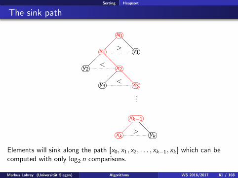
x0
x1 y1>
y2 x2<
y3 x3<
...
xk−1
xk yk>
Elements will sink along the path [x0, x1, x2, . . . , xk−1, xk ] which can becomputed with only log2 n comparisons.
Markus Lohrey (Universitat Siegen) Algorithms WS 2016/2017 61 / 168

Sorting Heapsort
Finding the right position on the sink path
We now compute the right position p on the sink path starting from theleaf and going up.
If this position p is found, then all elements x0, . . . , xp have to be rotatedcyclically (x0 goes to the position of xp, and every x1, . . . , xp moves up oneposition).
Markus Lohrey (Universitat Siegen) Algorithms WS 2016/2017 62 / 168

Sorting Heapsort
Finding the right position on the sink path
We now compute the right position p on the sink path starting from theleaf and going up.
If this position p is found, then all elements x0, . . . , xp have to be rotatedcyclically (x0 goes to the position of xp, and every x1, . . . , xp moves up oneposition).
3
9 8
6 5 7 4
1 2
1
2 3
4 5 6 7
8 9
Markus Lohrey (Universitat Siegen) Algorithms WS 2016/2017 62 / 168

Sorting Heapsort
Finding the right position on the sink path
We now compute the right position p on the sink path starting from theleaf and going up.
If this position p is found, then all elements x0, . . . , xp have to be rotatedcyclically (x0 goes to the position of xp, and every x1, . . . , xp moves up oneposition).
9 8
6 5 7 4
1 2
1
2 3
4 5 6 7
8 9
> 3?
Markus Lohrey (Universitat Siegen) Algorithms WS 2016/2017 62 / 168

Sorting Heapsort
Finding the right position on the sink path
We now compute the right position p on the sink path starting from theleaf and going up.
If this position p is found, then all elements x0, . . . , xp have to be rotatedcyclically (x0 goes to the position of xp, and every x1, . . . , xp moves up oneposition).
9
6 8
3 5 7 4
1 2
1
2 3
4 5 6 7
8 9
Markus Lohrey (Universitat Siegen) Algorithms WS 2016/2017 62 / 168

Sorting Heapsort
Average Analyse of Heapsort
Theorem 11
Standard heapsort makes on a portion of at least 1− 2−(n−1) many inputpermutations at least 2n log2(n)−O(n) many comparisons.Bottom-up heapsort makes on a portion of at least 1− 2−(n−1) manyinput permutations at most n log2(n) +O(n) many comparisons.
Proof: information-theoretic argument
A sorting algorithm computes from a permutation of [1, . . . , n] the sortedlist [1, . . . , n].
One can specify (or encode) the input permutation by running thealgorithm and in addition output information in form of a 0, 1-stringthat allows us to run the algorithm backwards starting with the outputpermutation [1, . . . , n].
Markus Lohrey (Universitat Siegen) Algorithms WS 2016/2017 63 / 168

Sorting Heapsort
Average Analyse of Heapsort
In the case of standard heapsort: we output the sink paths, i.e., every timean element is swapped with the left (resp., right) child, we output a 0(resp., 1). This makes heapsort reversible.
But: We have to know when one sink paths (a 0, 1-string) stops and thenext sink path starts.
Alternative 1: We encode a string w = a1a2 · · · at−1at ∈ 0, 1∗ by
c1(w) = a10a20 · · · at−10at1.
Note: |c1(w)| = 2|w |.Alternative 2: We encode a string w = a1a2 · · · at−1at ∈ 0, 1∗ by
c2(w) = c1(binary representation of t)a1 · · · at
Thus, |c2(w)| = |w |+ 2 log2(|w |).Markus Lohrey (Universitat Siegen) Algorithms WS 2016/2017 64 / 168

Sorting Heapsort
Average Analyse of Heapsort
Note: c2(ε) = 01, since 0 = binary representation of the number 0.
We encode the sink path w = a1a2 · · · at ∈ 0, 1∗ by
c ′2(w) = c1(binary representation of log2(n)− t)a1 · · · at .
Note: t ≤ log2(n), because every sink path has length ≤ log2 n.
Our proof showing that building the heap only needs O(n) manycomparisons also shows: In phase 1, we will output a 0, 1-string oflength O(n).
We now analyse the 0, 1-string produced in phase 2.
Markus Lohrey (Universitat Siegen) Algorithms WS 2016/2017 65 / 168

Sorting Heapsort
Average Analyse of Heapsort
Let t1, . . . , tn be the lengths of the sink paths during phase 2.
Hence, we produce in phase 2 a 0, 1-string of length
n∑
i=1
(ti + 2 log2(log2(n)− ti)) =
n∑
i=1
ti + 2
n∑
i=1
log2(log2(n)− ti )).
Define the average
t =
∑ni=1 tin
.
The function f with f (x) = log2(log2(n)− x) is concave on (−∞, log2(n)).
Jensen’s inequality (slide 4) implies:
log2(log2(n)− t) ≥n∑
i=1
1
n· log2(log2(n)− ti )).
Markus Lohrey (Universitat Siegen) Algorithms WS 2016/2017 66 / 168

Sorting Heapsort
Average Analyse of Heapsort
Therefore:n∑
i=1
ti + 2
n∑
i=1
log2(log2(n)− ti)) ≤ nt + 2n log2(log2(n)− t).
To sum up: The input permutation σ on [1, . . . , n] can be encoded by a0, 1-string of length
I (σ) ≤ cn + nt + 2n log2(log2(n)− t),
where c is a constant (for phase 1).
Lemma 6 implies
cn+ nt + 2n log2(log2(n)− t) ≥ I (σ) ≥ log2(n!)− n ≥ n log2(n)− 2, 443n
for at least (1− 2−n+1)n! many input permutations.
With d = 2, 443 + c we get:
t ≥ log2(n)− 2 log2(log2(n)− t)− d . (1)
Markus Lohrey (Universitat Siegen) Algorithms WS 2016/2017 67 / 168

Sorting Heapsort
Average Analyse von Heapsort
Since t ≥ 0 we obtain
t ≥ log2(n)− 2 log2(log2(n))− d . (2)
From (1) and (2) we get the better estimate
t ≥ log2(n)− 2 log2(2 log2(log2(n)) + d)− d . (3)
This estimate can be again applied to (1), and so on.
In general, we get for all i ≥ 1:
t ≥ log2(n)− αi − d ,
where α1 = 2 log2(log2(n)) and αi+1 = 2 log2(αi + d).
(proof by induction on i ≥ 1)
Markus Lohrey (Universitat Siegen) Algorithms WS 2016/2017 68 / 168

Sorting Heapsort
Average Analyse von Heapsort
For all x ≥ max10, d we have:
2 log2(x + d) ≤ 2 log2(2x) = 2 log2(x) + 2 ≤ 0, 9 · x .
Hence, as long as αi ≥ max10, d holds, we have αi+1 ≤ 0, 9 · αi .
Therefore, there exists a constant α with
t ≥ log2(n)− α− d . (4)
Thus, for at least (1− 2−n+1)n! many input permutations we have
n∑
i=1
ti ≥ n log2 n −O(n).
Markus Lohrey (Universitat Siegen) Algorithms WS 2016/2017 69 / 168

Sorting Heapsort
Average Analyse of Heapsort
The statement of Theorem 11 for standard Heapsort follows easily:
In phase 2, standard Heapsort makes 2∑n
i=1 ti many comparisons.
Hence, standard-Heapsort makes for at least (1− 2−n+1)n! many inputpermutations at least 2n log2 n −O(n) many comparisons.
Bottom-up heapsort makes in phase 2 at most
n log2(n) +n∑
i=1
(log2(n)− ti ) = 2n log2(n)−n∑
i=1
ti
many comparisons.
Hence, bottom-up Heapsort makes for at least (1− 2−n+1)n! many inputpermutations at most
O(n) + 2n log2(n)−n∑
i=1
ti ≤ n log2(n) +O(n)
many comparisons.Markus Lohrey (Universitat Siegen) Algorithms WS 2016/2017 70 / 168

Sorting Heapsort
Variant by Svante Carlsson, 1986
One can show that bottom-up Heapsort makes in the worst case at most1.5n log n +O(n) many comparisons.
Carlsson proposed to determine the correct position on the sink path usingbinary search.
This yields a worst-case bound of n log n+O(n log log n) many comparison.
On the other hand, in practice binary search on the sink path does notseem to pay off.
Markus Lohrey (Universitat Siegen) Algorithms WS 2016/2017 71 / 168

Sorting Sorting in linearer time
Counting-Sort
Recall: The lower bound of Ω(n log n) only holds for comparison-basedsorting algorithms.
If we make further assumptions on the array elements, we can sort in timeO(n).
Assumption: The array elements A[1], . . . ,A[n] are natural numbers inthe range [0, k].
Counting sort (see next slide) sorts under this assumption in timeO(k + n).
Hence, if k ∈ O(n), then counting sort works in linear time.
Markus Lohrey (Universitat Siegen) Algorithms WS 2016/2017 72 / 168

Sorting Sorting in linearer time
Counting Sort
Algorithm Counting-Sort
procedure counting-sort(array A[1, n] with A[1], . . .A[n] ∈ [0, k])begin
var Arrays C [0, k], B [1, n]for i := 0 to k do
C [i ] := 0for i := 1 to n do
C [A[i ]] := C [A[i ]] + 1for i := 1 to k do
C [i ] := C [i ] + C [i − 1]for n downto 1 do
B [C [A[i ]]] := A[i ];C [A[i ]] := C [A[i ]]− 1
endprocedure
Markus Lohrey (Universitat Siegen) Algorithms WS 2016/2017 73 / 168

Sorting Sorting in linearer time
Counting Sort
After the first three for-loops, C [i ] is the number of array entries that are≤ i .
The statement B [C [A[i ]]] := A[i ] puts the array element A[i ] at the rightposition C [A[i ]].
Remark: Counting sort is a stable sorting algorithm.
This means: If A[i ] = A[j] for i < j , then in the sorted array B the arrayentry A[i ] is to the left of A[j].
This is relevant if the array entries consist of (i) keys that are used forsorting and (ii) additional informations.
Stability of counting sort will be needed for radix sort on the next slide.
Markus Lohrey (Universitat Siegen) Algorithms WS 2016/2017 74 / 168

Sorting Sorting in linearer time
Radix Sort
We use counting sort to sort an array A[1, n], where A[1], . . . ,A[n] ared -ary numbers in base k (where the least significant digit is the left mostdigit).
Radix sort sorts such an array in time O(d(n + k)).
If in addition d ∈ O(1) and k ∈ O(n) (which means that we can representnumber of size O(nd)), then radix sort works in linear time.
Algorithm Radix Sort
procedure radix sort(array A[1, n] with A[1], . . .A[n])begin
for i := 1 to d dosort the array A with counting sort with respect to the i -th digit.
endforendprocedure
Markus Lohrey (Universitat Siegen) Algorithms WS 2016/2017 75 / 168

Sorting Computation of the Median
Computation of the Media
Input: array a[1, . . . , n] of numbers and 1 ≤ k ≤ n.
Output: k-th smallest element, i.e., the number m ∈ a[i ] | 1 ≤ i ≤ nsuch that
|i | a[i ] < m| ≤ k − 1 and |i | a[i ] > m| ≤ n − k
Special case: k = ⌈n/2⌉ median
Naive approach:
sort the array a in time O(n log n),
output the k-th element of the sorted array.
Markus Lohrey (Universitat Siegen) Algorithms WS 2016/2017 76 / 168

Sorting Computation of the Median
Median of the medians
Goal: Compute the k-th smallest element in linear time.
Idea: Compute a pivot element (as in quick sort) as the median of themedians of blocks of length 5.
We split the array in blocks of length 5.
For each block we compute the median (6 comparisons are sufficient).
Compute recursively the median p of the array of medians and take pas the pivot element.
Number of comparisons: T (n5 ).
Markus Lohrey (Universitat Siegen) Algorithms WS 2016/2017 77 / 168

Sorting Computation of the Median
Quick sort step
Partition the array with the pivot element p such that for suitablepositions m1 < m2 we have:
a[i ] < p for 1 ≤ i ≤ m1
a[i ] = p for m1 < i ≤ m2
a[i ] > p fur m2 < i ≤ n
Number of comparisons: ≤ n.
Case distinction:
1 k ≤ m1: Search for the k-th element recursively in a[1], . . . , a[m1].
2 m1 < k ≤ m2: Return p.
3 k > m2: Search for the (k −m2)-th element in a[m2 + 1], . . . , a[n].
Markus Lohrey (Universitat Siegen) Algorithms WS 2016/2017 78 / 168

Sorting Computation of the Median
30 – 70 splitting
The choice of the pivot element as the median of the medians (of blocksof length 5) ensures the following inequalites for m1,m2:
3
10n ≤ m2 and m1 ≤
7
10n
Therefore, the recursive step needs at most T (7n10 ) comparisons.
Markus Lohrey (Universitat Siegen) Algorithms WS 2016/2017 79 / 168

Sorting Computation of the Median
Total time
T (n) is the totoal number of comparisons comparisons for an array oflength n.
We get the following recurrence for T (n):
T (n) ≤ T(
⌈n5⌉)
+ T
(
⌈7n10
⌉)
+O(n)
The master theorem II gives T (n) ∈ O(n).
Markus Lohrey (Universitat Siegen) Algorithms WS 2016/2017 80 / 168

Sorting Computation of the Median
More precise analysis
T (n) = T(n
5
)
+ T
(
7n
10
)
+6n
5+
2n
5,
where:
6n5 is the number of comparisons to compute the medians of theblocks of length 5.2n5 is the number of comparisons for the partitioning step.
This yields the bound T (n) ≤ 16n:
With 15 +
710 = 9
10 we get T (n) ≤ T (9n10 ) +8n5 and hence
T (n) ≤ 10 · 8n5 = 16n.
Markus Lohrey (Universitat Siegen) Algorithms WS 2016/2017 81 / 168

Sorting Computation of the Median
Quick select
Quick select is a randomized algorithm for computing the median:
Algorithm
function quickselect(A[ℓ . . . r ] : array of integer, k : integer) : integerbegin
if ℓ = r then return A[ℓ]else
p := random(ℓ, r);m := partition(A[ℓ . . . r ], p);k ′ := (m − ℓ+ 1);if k = k ′ then return A[m]elsif k < k ′ then return quickselect(A[ℓ . . .m − 1], k)else return quickselect(A[m + 1 . . . r ], k − k ′)endif
endifendfunctionMarkus Lohrey (Universitat Siegen) Algorithms WS 2016/2017 82 / 168

Sorting Computation of the Median
Analysis of quick select
Let Q(n) be the average number of comparisons that quick select is doingfor an array with n elements.
We have:
Q(n) ≤ (n − 1) +1
n
n∑
i=1
Q(maxi − 1, n − i),
where:
(n − 1) is the number of comparisons for partitioning the array, and
Q(maxi − 1, n − i) is the (maximal) average number ofcomparisons for a recursive call on one of the two subarrays.
Here, we make the pessimistic assumption that we continue searching inthe larger subarray.
Markus Lohrey (Universitat Siegen) Algorithms WS 2016/2017 83 / 168

Sorting Computation of the Median
Analysis of quick select
We have
Q(n) ≤ (n − 1) +1
n
n∑
i=1
Q(maxi − 1, n − i)
= (n − 1) +1
n
n−1∑
i=⌈ n2⌉
Q(i) +
n−1∑
i=⌊ n2⌋
Q(i)
Claim: Q(n) ≤ 4 · n:Proof by induction on n: OK for n = 1.
Let n ≥ 2 and let Q(i) ≤ 4 · i for all i < n.
Markus Lohrey (Universitat Siegen) Algorithms WS 2016/2017 84 / 168

Sorting Computation of the Median
Analysis of quick select
Case 1: n is even.
Q(n) ≤ (n − 1) +2
n
n−1∑
i= n2
Q(i)
≤ (n − 1) +8
n
n−1∑
i= n2
i
= (n − 1) +8
n
(
(n − 1)n
2− (n2 − 1)n2
2
)
= (n − 1) + 4(n − 1)− n + 2
= 4n − 3 ≤ 4n
Markus Lohrey (Universitat Siegen) Algorithms WS 2016/2017 85 / 168

Sorting Computation of the Median
Analyse von Quickselect
Case 2: n is odd.
Q(n) ≤ (n − 1) +2
n
n−1∑
i=⌈ n2⌉
Q(i) +1
nQ(⌊n
2
⌋)
≤ (n − 1) +8
n
n−1∑
i=⌈ n2⌉
i + 2
= (n − 1) +8
n·(
(n − 1)n
2− (⌈
n2
⌉
− 1)⌈
n2
⌉
2
)
+ 2
≤ (n − 1) + 4(n − 1)− n − 2 + 2
= 4n − 5 ≤ 4 · n.
Markus Lohrey (Universitat Siegen) Algorithms WS 2016/2017 86 / 168

Greedy algorithms
Overview
Matroids
Kruskal’s algorithm for spanning trees
Dijkstra’s algorithm for shortest paths
Markus Lohrey (Universitat Siegen) Algorithms WS 2016/2017 87 / 168

Greedy algorithms
Greedy algorithms
Algorithms that take in each step the locally best optimal choice are calledgreedy.
For some problems this yields a globally optimal solution.
Problems where greedy algorithms always find an optimal solution can becharacterized via the notion of a matroid.
Markus Lohrey (Universitat Siegen) Algorithms WS 2016/2017 88 / 168

Greedy algorithms Matroids
Optimization problems
Let E be a finite set and U ⊆ 2E a set of subsets of E .
A pair (E ,U) is a subset system, if the following holds:
∅ ∈ U
If A ⊆ B ∈ U then A ∈ U as well.
A set A ∈ U is maximal (with respect to ⊆) if for all B ∈ U the followingholds: if A ⊆ B , then A = B .
The optimization problems associated with (E ,U) is:
Input: A weight function w : E → R
Output: A maximal set A ∈ U with w(A) ≥ w(B) for all maximal setsB ∈ U, where
w(C ) =∑
a∈C
w(a)
We call A an optimal solution.
Markus Lohrey (Universitat Siegen) Algorithms WS 2016/2017 89 / 168

Greedy algorithms Matroids
Optimization problems
In order to solve such optimization problems, one can try to use thefollowing generic greedy algorithm:
Algorithm generic greedy algorithm
procedure find-optimal (subset system (E ,U), w : E → R)begin
order set E by descending weights as e1, e2, . . . , en withw(e1) ≥ w(e2) ≥ · · · ≥ w(en)T := ∅for k := 1 to n do
if T ∪ ek ∈ U then T := T ∪ ekendforreturn (T )
endprocedure
Markus Lohrey (Universitat Siegen) Algorithms WS 2016/2017 90 / 168

Greedy algorithms Matroids
Matroids
Note: The solution computed by the generic greedy algorithm is always amaximal subset.
Unfortunately there exist subset systems for which the generic greedyalgorithm does not find an optimal solution (will be shown later).
A subset system (E ,U) is a matroid, if the following property (exchangeproperty) holds:
∀A,B ∈ U : |A| < |B | =⇒ ∃x ∈ B \ A : A ∪ x ∈ U
Remark: If (E ,U) is a matroid, then all maximal sets in U have the samecardinality.
Example: Let E be a finite set and k ≤ |E |. Then
(E , A ⊆ E | |A| ≤ k)
is a matroid.Markus Lohrey (Universitat Siegen) Algorithms WS 2016/2017 91 / 168

Greedy algorithms Matroids
Matroids
Theorem 12
Let (E ,U) be a subset system. The generic greedy algorithm computes forevery weight function w : E → R an optimal solution if and only if (E ,U)is a matroid.
Proof: First assume that (E ,U) is a matroid.
Let w : E → R be a weight function and let E = e1, e2, . . . , en with
w(e1) ≥ w(e2) ≥ · · · ≥ w(en).
Let T = ei1 , . . . , eik with i1 < i2 < · · · < ik the solution computed bythe generic greedy algorithm.
Assumption: There exists a maximal set S = ej1 , . . . , ejl ∈ U withw(S) > w(T ), where j1 < j2 < · · · < jl .
Since (E ,U) is a matroid, we have k = l .
Markus Lohrey (Universitat Siegen) Algorithms WS 2016/2017 92 / 168

Greedy algorithms Matroids
Matroids
Since w(S) > w(T ), there exists 1 ≤ p ≤ k with w(ejp ) > w(eip ).
Since the weights where sorted in descending order, we must have jp < ip.
We now apply the exchange property to the sets
A = ei1 , . . . , eip−1 ∈ U and B = ej1 , . . . , ejp ∈ U.
Since |A| < |B |, there exists an element ejq ∈ B \ A with A ∪ ejq ∈ U.
We get jq ≤ jp < ip.
But then, the generic greedy algorithm would have put ejq into thesolution, which is a contradiction.
Markus Lohrey (Universitat Siegen) Algorithms WS 2016/2017 93 / 168

Greedy algorithms Matroids
Matroids
Now assume that (E ,U) is not a matroid, i.e., the exchange property doesnot hold.
Let A,B ∈ U with |A| < |B | such that for all b ∈ B \ A: A ∪ b 6∈ U.
Let r = |B | and hence |A| ≤ r − 1.
Define the weight function w : E → R as follows:
w(x) =
r + 1 for x ∈ A
r for x ∈ B \ A0 otherwise
The generic greedy algorithm must compute a solution T with A ⊆ T andT ∩ (B \ A) = ∅.We get w(T ) = (r + 1) · |A| ≤ (r + 1)(r − 1) = r2 − 1.
Let S ∈ U be a maximal subset with B ⊆ S .
We get w(S) ≥ w(B) ≥ r2.Markus Lohrey (Universitat Siegen) Algorithms WS 2016/2017 94 / 168

Greedy algorithms Kruskal’s algorithm for spanning trees
Spanning subtrees
Let G = (V ,E ) be a finite undirected graph.
A path from u ∈ V to v ∈ V is a sequence of nodes (u1, u2, . . . , un) withu1 = u, un = v and (ui , ui+1) ∈ E for all 1 ≤ i ≤ n− 1.
G is connected, if for all u, v ∈ V with u 6= v there exists a path from u tov .
A circuit is a path (u1, u2, . . . , un) with n ≥ 3, ui 6= uj for all 1 ≤ i < j ≤ nand (un, u1) ∈ E .
G is a tree, if it is connected and has no circuits.
Excercise: for every tree T = (V ,E ) we have |E | = |V | − 1.
Let G = (V ,E ) be connected. A spanning subtree of G is a subset F ⊆ Eof edges such that (V ,F ) is a tree.
Excercise: every connected graph has a spanning subtree.
Markus Lohrey (Universitat Siegen) Algorithms WS 2016/2017 95 / 168

Greedy algorithms Kruskal’s algorithm for spanning trees
Spanning subtrees
Example:
Markus Lohrey (Universitat Siegen) Algorithms WS 2016/2017 96 / 168

Greedy algorithms Kruskal’s algorithm for spanning trees
Spanning subtrees
Example:
Markus Lohrey (Universitat Siegen) Algorithms WS 2016/2017 96 / 168

Greedy algorithms Kruskal’s algorithm for spanning trees
Matroid of circuit-free edge sets
Let G = (V ,E ) be again connected, and let w : E → R be a weightfunction.
The weight of a spanning subtree F ⊆ E is
w(F ) =∑
e∈F
w(e).
Goal: Compute a spanning subtree of maximal weight.
The following lemma allows us to use the canonical greedy algorithm:
Lemma 13
The subset system (E , A ⊆ E | (V ,A) has no circuit) is a matroid.
Markus Lohrey (Universitat Siegen) Algorithms WS 2016/2017 97 / 168

Greedy algorithms Kruskal’s algorithm for spanning trees
Matroid of circuit-free edge sets
Proof: Let A,B ⊆ E be edge sets without circuits such that |A| < |B |.Let V1,V2 . . . ,Vn be the connected components of the (V ,A).
We have |A| =∑ni=1(|Vi | − 1), because the subtree of (V ,A) induced by
Vi is a tree and therefore has |Vi | − 1 many edges.
For every edge e = (u, v) ∈ B one of the following two cases holds:
1 There is 1 ≤ i ≤ n with u, v ∈ Vi .
2 There are i 6= j with u ∈ Vi and v ∈ Vj .
But in B there can exist at most∑n
i=1(|Vi | − 1) = |A| many edges of type1 (otherwise B would contain a circuit in one of the sets Vi).
Hence, there exists an edge e ∈ B , which connects two connectedcomponents of (V ,A).
Thus, A ∪ e contains no circuit.
Markus Lohrey (Universitat Siegen) Algorithms WS 2016/2017 98 / 168

Greedy algorithms Kruskal’s algorithm for spanning trees
Kruskals algorithm
Algorithm Kruskals algorithm
procedure kruskal (edge-weighted connected graph (V ,E ,w))begin
sort E by decreasing weights e1, e2, . . . , en withw(e1) ≥ w(e2) ≥ · · · ≥ w(en)F := ∅for k := 1 to n do
if ek connects two different connected components of (V ,F ) thenF := F ∪ ek
endforreturn (F )
endprocedure
Markus Lohrey (Universitat Siegen) Algorithms WS 2016/2017 99 / 168

Greedy algorithms Kruskal’s algorithm for spanning trees
Kruskal’s algorithm
Example for Kruskal’s algorithm:
2 3
4
5 32
4
6 7
Markus Lohrey (Universitat Siegen) Algorithms WS 2016/2017 100 / 168

Greedy algorithms Kruskal’s algorithm for spanning trees
Kruskal’s algorithm
Example for Kruskal’s algorithm:
2 3
4
5 32
4
6 7
Markus Lohrey (Universitat Siegen) Algorithms WS 2016/2017 100 / 168

Greedy algorithms Kruskal’s algorithm for spanning trees
Kruskal’s algorithm
Example for Kruskal’s algorithm:
2 3
4
5 32
4
6 7
Markus Lohrey (Universitat Siegen) Algorithms WS 2016/2017 100 / 168

Greedy algorithms Kruskal’s algorithm for spanning trees
Kruskal’s algorithm
Example for Kruskal’s algorithm:
2 3
4
5 32
4
6 7
Markus Lohrey (Universitat Siegen) Algorithms WS 2016/2017 100 / 168

Greedy algorithms Kruskal’s algorithm for spanning trees
Kruskal’s algorithm
Example for Kruskal’s algorithm:
2 3
4
5 32
4
6 7
Markus Lohrey (Universitat Siegen) Algorithms WS 2016/2017 100 / 168

Greedy algorithms Kruskal’s algorithm for spanning trees
Kruskal’s algorithm
Example for Kruskal’s algorithm:
2 3
4
5 32
4
6 7
Markus Lohrey (Universitat Siegen) Algorithms WS 2016/2017 100 / 168

Greedy algorithms Kruskal’s algorithm for spanning trees
Kruskal’s algorithm
Example for Kruskal’s algorithm:
2 3
4
5 32
4
6 7
Markus Lohrey (Universitat Siegen) Algorithms WS 2016/2017 100 / 168

Greedy algorithms Kruskal’s algorithm for spanning trees
Kruskal’s algorithm
Example for Kruskal’s algorithm:
2 3
4
5 32
4
6 7
Markus Lohrey (Universitat Siegen) Algorithms WS 2016/2017 100 / 168

Greedy algorithms Kruskal’s algorithm for spanning trees
Kruskal’s algorithm
Example for Kruskal’s algorithm:
2 3
4
5 32
4
6 7
Markus Lohrey (Universitat Siegen) Algorithms WS 2016/2017 100 / 168

Greedy algorithms Kruskal’s algorithm for spanning trees
Kruskal’s algorithm
Example for Kruskal’s algorithm:
2 3
4
5 32
4
6 7
Markus Lohrey (Universitat Siegen) Algorithms WS 2016/2017 100 / 168

Greedy algorithms Kruskal’s algorithm for spanning trees
Running time of Kruskal’s algorithm
Note: Since G is connected, we have |V | − 1 ≤ |E | ≤ |V |2.Sorting the edges by weight needs time O(|E | log |E |) = O(|E | log |V |).The connected components of (V ,F ) can be maintained by a partition ofthe node set V .
We start with the partition v | v ∈ V .In every iteration of the for-loop (|E | many) we test whether the endpoints of the edge ek belong to different sets A, B of the partition.
If this holds, then we replace in the partition the sets A and B by the setA ∪ B .
For this, we will later develop a so-called union-find data structure, whichrealizes the above operations in total time O(α(|V |) · |E |) for an extremelyslow-growing function α.
This gives the running time O(|E | log |V |) for Kruskal’s algorithm.
Markus Lohrey (Universitat Siegen) Algorithms WS 2016/2017 101 / 168

Greedy algorithms Shortest paths and Dijkstra’s algorithm
Shortest paths
Another example for a greedy strategy: Computation of shortest paths inan edge-weighted directed graph G = (V ,E , γ).
V is the set of nodes
E ⊆ V × V is the set of edges, where (x , x) 6∈ E for all x ∈ V .
γ : E → N is the weight function.
Weight of a path (v0, v1, v2, . . . , vn):
n−1∑
i=0
γ(vi , vi+1)
For u, v ∈ V , d(u, v) denotes the minimum of the weight of all paths fromu to v (d(u, v) = ∞ if such a path does not exist, and d(u, u) = 0).
Goal: Given G = (V ,E , γ) and a source node u ∈ V , compute for everyv ∈ V a path u = v0, v1, v2, . . . , vn−1, vn = v with minimal weight d(u, v).
Markus Lohrey (Universitat Siegen) Algorithms WS 2016/2017 102 / 168

Greedy algorithms Shortest paths and Dijkstra’s algorithm
Dijkstra’s algorithm
B := ∅ (tree nodes); R := u (boundary); U := V \ u (unknown nodes);p(u) := nil; D(u) := 0;while R 6= ∅ dox := nil; α := ∞;forall y ∈ R doif D(y) < α thenx := y ; α := D(y)
endifendforB := B ∪ x; R := R \ xforall (x , y) ∈ E doif y ∈ U thenD(y) := D(x) + γ(x , y); p(y) := x ; U := U \ y; R := R ∪ y
elsif y ∈ R and D(x) + γ(x , y) < D(y) thenD(y) := D(x) + γ(x , y); p(y) := x
endifendfor
endwhile
Markus Lohrey (Universitat Siegen) Algorithms WS 2016/2017 103 / 168

Greedy algorithms Shortest paths and Dijkstra’s algorithm
Example for Dijkstra’s algorithm
tree nodes
boundary
unknown nodes
source node
0
1 3∞
∞ ∞
∞
3
42
3 6
1
6
13
8
Markus Lohrey (Universitat Siegen) Algorithms WS 2016/2017 104 / 168

Greedy algorithms Shortest paths and Dijkstra’s algorithm
Example for Dijkstra’s algorithm
tree nodes
boundary
unknown nodes
initial node
0
1 37
∞ ∞
14
3
42
3 6
1
6
13
8
Markus Lohrey (Universitat Siegen) Algorithms WS 2016/2017 104 / 168

Greedy algorithms Shortest paths and Dijkstra’s algorithm
Example for Dijkstra’s algorithm
tree nodes
boundary
unknown nodes
initial node
0
1 37
11 7
14
3
42
3 6
1
6
13
8
Markus Lohrey (Universitat Siegen) Algorithms WS 2016/2017 104 / 168

Greedy algorithms Shortest paths and Dijkstra’s algorithm
Example for Dijkstra’s algorithm
tree nodes
boundary
unknown nodes
initial node
0
1 37
11 7
13
3
42
3 6
1
6
13
8
Markus Lohrey (Universitat Siegen) Algorithms WS 2016/2017 104 / 168

Greedy algorithms Shortest paths and Dijkstra’s algorithm
Example for Dijkstra’s algorithm
tree nodes
boundary
unknown nodes
initial node
0
1 37
9 7
13
3
42
3 6
1
6
13
8
Markus Lohrey (Universitat Siegen) Algorithms WS 2016/2017 104 / 168

Greedy algorithms Shortest paths and Dijkstra’s algorithm
Example for Dijkstra’s algorithm
tree nodes
boundary
unknown nodes
initial node
0
1 37
9 7
12
3
42
3 6
1
6
13
8
Markus Lohrey (Universitat Siegen) Algorithms WS 2016/2017 104 / 168

Greedy algorithms Shortest paths and Dijkstra’s algorithm
Example for Dijkstra’s algorithm
tree nodes
boundary
unknown nodes
initial node
0
1 37
9 7
12
3
42
3 6
1
6
13
8
Markus Lohrey (Universitat Siegen) Algorithms WS 2016/2017 104 / 168

Greedy algorithms Shortest paths and Dijkstra’s algorithm
Correctness of Dijkstra’s algorithm
Theorem 14 (Correctness of Dijkstra’s algorithm)
Dijkstra’s algorithm computes shortest paths from the source node to allother nodes.
Proof: We show that the following invariants are preserved by theloop-body of the while-loop:
1 The sets B , R , and U form a partition of the node set V .
2 R = y | ∃x ∈ B : (x , y) ∈ E \ B3 for all x ∈ B , D(x) = d(u, x)
4 for all y ∈ R , D(y) = minD(x) + γ(x , y) | x ∈ B , (x , y) ∈ EConsider an execution of the body of the while-Schleife, where the node xis moved from R to B .
(1)–(4) hold before the execution of the loop-body.
It is clear that (1) and (2) are preserved.Markus Lohrey (Universitat Siegen) Algorithms WS 2016/2017 105 / 168

Greedy algorithms Shortest paths and Dijkstra’s algorithm
Correctness of Dijkstra’s algorithm
(3): Because of (3) and (4) there exists a node z ∈ B with
D(x) = D(z) + γ(z , x) = d(u, z) + γ(z , x).
Hence, there is path from u to x with weight D(x).
Assume that there is a path from u to x with weight < D(x).
Let w ∈ R be the first node on this path, which does not belong to B(must exist since x 6∈ B) and let v ∈ B be the predecessor of w on thepath (exists, since u ∈ B).
Since the whole path has weight < D(x), we get
D(w) = minD(w ′) + γ(w ′,w) | w ′ ∈ B , (w ′,w) ∈ E≤ D(v) + γ(v ,w) < D(x),
which contradicts the choice of x ∈ R .
Hence, we must have d(u, x) = D(x).Markus Lohrey (Universitat Siegen) Algorithms WS 2016/2017 106 / 168

Greedy algorithms Shortest paths and Dijkstra’s algorithm
Correctness of Dijkstra’s algorithm
(4): Let B ′,R ′,U ′,D ′ be the values of the variables B ,R ,U,D after theexecution of the loop-body.
Note: B ′ = B ∪ x, D(z) = D ′(z) for all z ∈ B and D(x) = D ′(x).
Let y ∈ R ′.
Case 1: y ∈ R \ x and (x , y) ∈ E . We have
D ′(y) = minD(y),D(x) + γ(x , y)= minminD(z) + γ(z , y) | z ∈ B , (z , y) ∈ E,D(x) + γ(x , y)= minminD ′(z) + γ(z , y) | z ∈ B , (z , y) ∈ E,D ′(x) + γ(x , y)= minD ′(z) + γ(z , y) | z ∈ B ′, (z , y) ∈ E
Case 2: y ∈ R \ x and (x , y) 6∈ E . We have
D ′(y) = D(y)
= minD(z) + γ(z , y) | z ∈ B , (z , y) ∈ E= minD ′(z) + γ(z , y) | z ∈ B ′, (z , y) ∈ E.
Markus Lohrey (Universitat Siegen) Algorithms WS 2016/2017 107 / 168

Greedy algorithms Shortest paths and Dijkstra’s algorithm
Correctness of Dijkstra’s algorithm
Case 3: y 6∈ R . We have (x , y) ∈ E , but there is no edge (z , y) ∈ E withz ∈ B (by (2)).
Hence, we have
D ′(y) = D(x) + γ(x , y)
= D ′(x) + γ(y , x)
= minD ′(z) + γ(z , y) | z ∈ B ′, (z , y) ∈ E.
Remark: Dijkstra’s algorithm in general does not produce a correct resultif negative edge weights are allowed.
Markus Lohrey (Universitat Siegen) Algorithms WS 2016/2017 108 / 168

Greedy algorithms Shortest paths and Dijkstra’s algorithm
Dijkstra with abstract data types for the boundary
In order to analyze the running time of Dijkstra’s algorithm, it is uselful toreformulate the algorithm with an abstract data type for the boundary R .
The following operations are needed for the boundary R :
insert insert a new element into R .decrease-key decrease the key value of an element of R .delete-min find the element from R with the smallest key value
and remove it from R .
Markus Lohrey (Universitat Siegen) Algorithms WS 2016/2017 109 / 168

Greedy algorithms Shortest paths and Dijkstra’s algorithm
Dijkstra with abstract data types for the boundary
B := ∅; R := u; U := V \ u; p(u) := nil; D(u) := 0;while (R 6= ∅) do
x := delete-min(R);B := B ∪ x;forall (x , y) ∈ E do
if y ∈ U thenU := U \ y; p(y) := x ; D(y) := D(x) + γ(x , y);insert(R , y , D(y));
elsif y ∈ R and D(x) + γ(x , y) < D(y) thenp(y) := x ; D(y) := D(x) + γ(x , y);decrease-key(R , y , D(y));
endifendfor
endwhile
Markus Lohrey (Universitat Siegen) Algorithms WS 2016/2017 110 / 168

Greedy algorithms Shortest paths and Dijkstra’s algorithm
Running time of Dijkstra’s algorithm
Number of operations (n = number of nodes, e = number of edges):
insert ndecrease-key edelete-min n
The total running time depends of the data structure that is used for theboundary:
1 Array of size n:single insert/decrease-key: O(1)single delete-min: O(n)total running time: O(n + e + n2) = O(n2)
2 Heap (balanced binary tree of depth O(log(n)):single insert/decrease-key/delete-min: O(log(n))total running time: O(n log(n) + e log(n)) = O(e log(n)).
If O(e) ⊆ o(n2/ log n), then the heap beats the array.For instance, for planar graphs one has e ≤ 3n − 6 for n ≥ 3.
Markus Lohrey (Universitat Siegen) Algorithms WS 2016/2017 111 / 168

Data structures Fibonacci heaps
Fibonacci heaps (Fredman & Tarjan 1984)
Fibonacci heaps beat arrays as well as heaps: O(e + n log n)
Ein Fibonacci heap H is a list of rooted trees, i.e., a forest.
V is the set of nodes
Every node v ∈ V has a key key (v) ∈ N.
Heap condition: ∀x ∈ V : y is a child of x ⇒ key (x) ≤ key (y)
Some of nodes of V are marked. The root of a tree is never marked.
Markus Lohrey (Universitat Siegen) Algorithms WS 2016/2017 112 / 168

Data structures Fibonacci heaps
Example for a Fibonacci heap
(key values are in the circles, marked nodes are grey)
23 7 21 3 17 24
18 52 38 30 26 46
39 41 35
Markus Lohrey (Universitat Siegen) Algorithms WS 2016/2017 113 / 168

Data structures Fibonacci heaps
Fibonacci heaps
The parent-child relation has to be realized by pointers, since thetrees in a Fibonacci heap are not necessarily balanced.
That means that pointer manipulations (expensive!) replace the indexmanipulations (cheap!) in standard heaps.
Operations:1 merge2 insert3 delete-min4 decrease-key
Markus Lohrey (Universitat Siegen) Algorithms WS 2016/2017 114 / 168

Data structures Fibonacci heaps
Implementation of merge and insert
merge: Concatenation of two lists — constant time
insert: Special case of merge — constant time
merge and insert produce long lists of one-element trees.
Every such list is a Fibonacci heap.
Markus Lohrey (Universitat Siegen) Algorithms WS 2016/2017 115 / 168

Data structures Fibonacci heaps
Implementation of delete-min
Let H be a Fibonacci heap consisting of T trees and n nodes.
for a nodes x ∈ V let rank(x) be the number of children of x .
for a tree B in H let rank(B) be the rank of the root of B .
Let rmax(n) be the maximal rank that can appear in a Fibonacci heapwith n nodes.
Clearly, rmax(n) ≤ n. Later, we will show that rmax(n) ∈ O(log n).
Markus Lohrey (Universitat Siegen) Algorithms WS 2016/2017 116 / 168

Data structures Fibonacci heaps
Implementation of delete-min
1 Search for the root x with minimal key. Time: O(T )
2 Remove x and replace the subtree rooted in x by its rank(x) manysubtrees. Remove possible markings from the new roots.Time: O(rank(x)) ⊆ O(rmax(n)).
3 Define an array L[0, . . . , rmax(n)], where L[i ] is a list of all trees ofrank i .Time: O(T + rmax(n)).
4 for i := 0 to rmax(n)− 1 dowhile |L[i ]| ≥ 2 doremove two trees from L[i ]make the root with the larger key to a child of the other rootadd the resulting tree to L[i + 1]
endwhile endfor
Time: O(T + rmax(n))
Markus Lohrey (Universitat Siegen) Algorithms WS 2016/2017 117 / 168

Data structures Fibonacci heaps
Example for delete-min
23 7 21 3 17 24
18 52 38 30 26 46
39 41 35
Markus Lohrey (Universitat Siegen) Algorithms WS 2016/2017 118 / 168

Data structures Fibonacci heaps
Example for delete-min
23 7 21 18 52 38 17 24
39 41 30 26 46
35
Markus Lohrey (Universitat Siegen) Algorithms WS 2016/2017 118 / 168

Data structures Fibonacci heaps
Example for delete-min
7 21 18 52 38 17 24
23 39 41 30 26 46
35
Markus Lohrey (Universitat Siegen) Algorithms WS 2016/2017 118 / 168

Data structures Fibonacci heaps
Example for delete-min
7 21 18 38 17 24
23 52 39 41 30 26 46
35
Markus Lohrey (Universitat Siegen) Algorithms WS 2016/2017 118 / 168

Data structures Fibonacci heaps
Example for delete-min
7 18 38 17 24
23 21 39 41 30 26 46
52 35
Markus Lohrey (Universitat Siegen) Algorithms WS 2016/2017 118 / 168

Data structures Fibonacci heaps
Example for delete-min
7 18 17 24
23 21 39 38 30 26 46
52 41 35
Markus Lohrey (Universitat Siegen) Algorithms WS 2016/2017 118 / 168

Data structures Fibonacci heaps
Example for delete-min
7
18
17 24
23 21
39 38
30 26 46
52
41
35
Markus Lohrey (Universitat Siegen) Algorithms WS 2016/2017 118 / 168

Data structures Fibonacci heaps
Remarks for delete-min
delete-min needs time O(T + rmax(n)), where T is the number oftrees before the operation.
After the execution delete-min, there exists for every i ≤ rmax(n) atmost one tree of rank i .
Hence, the number of trees after delete-min is bounded by rmax(n).
Markus Lohrey (Universitat Siegen) Algorithms WS 2016/2017 119 / 168

Data structures Fibonacci heaps
Implementation of decrease-key
Let x be the node for which the key is reduced.
1 If x is a root, then we can reduced key (x) without any othermodifications.
Now assume that x is not a root and let x = y0, y1, . . . , ym be thepath from x to the root ym (m ≥ 1).
Let yk (1 ≤ k ≤ m) be the first node on this path, which is not x andwhich is not marked (note: ym is not marked).
2 For all 0 ≤ i < k , we cut off yi from its parent node yi+1 and removethe marking from yi (y0 = x can be marked).
yi (0 ≤ i < k) is now a unmarked root of a new tree.
3 If yk is not a root, then we mark yk (this tells us later that yk lost achild).
Markus Lohrey (Universitat Siegen) Algorithms WS 2016/2017 120 / 168

Data structures Fibonacci heaps
Example for decrease-key
7
18
17 24
23 21
39 38
30 26 46
52
41
35
Markus Lohrey (Universitat Siegen) Algorithms WS 2016/2017 121 / 168

Data structures Fibonacci heaps
Example for decrease-key
decrease-key(node with key 39, 6)
7
18
17 24
23 21
39 38
30 26 46
52
41
35
Markus Lohrey (Universitat Siegen) Algorithms WS 2016/2017 121 / 168

Data structures Fibonacci heaps
Example for decrease-key
decrease-key(node with key 39, 6)
7 6 17 24
23 21 18
38
30 26 46
52
41
35
Markus Lohrey (Universitat Siegen) Algorithms WS 2016/2017 121 / 168

Data structures Fibonacci heaps
Example for decrease-key
decrease-key(node with key 38, 29)
7 6 17 24
23 21 18
38
30 26 46
52
41
35
Markus Lohrey (Universitat Siegen) Algorithms WS 2016/2017 121 / 168

Data structures Fibonacci heaps
Example for decrease-key
decrease-key(node with key 38, 29)
7 29 6 17 24
23 21 18 41 30 26 46
52 35
Markus Lohrey (Universitat Siegen) Algorithms WS 2016/2017 121 / 168

Data structures Fibonacci heaps
Example for decrease-key
decrease-key(node with key 38, 29)
7 18 29 6 17 24
23 21 41 30 26 46
52 35
Markus Lohrey (Universitat Siegen) Algorithms WS 2016/2017 121 / 168

Data structures Fibonacci heaps
Remarks for decrease-key
Time: O(k) +O(1)
decrease-key reduces the number of marked nodes by at least k − 2(k ≥ 1).
decrease-key increases the number of trees by k .
Markus Lohrey (Universitat Siegen) Algorithms WS 2016/2017 122 / 168

Data structures Fibonacci heaps
Definition of Fibonacci heaps
Definition 15
A Fibonacci heap is eine list of rooted trees as described before, which canbe obtained from the empty list be an arbitrary sequence of merge,insert, delete-min, and decrease-key operations
Lemma 16 (Fibonacci heap lemma)
Let x be a node of a Fibonacci heap with rank(x) = k.
1 If c1, . . . , ck are the children of x, and ci became a child of x beforeci+1 became a child of x, then rank(ci ) ≥ i − 2.
2 The subtree rooted in x contains at least Fk+1 many nodes. Here,Fk+1 is the (k + 1)-th Fibonacci number(F0 = F1 = 1,Fk+1 = Fk + Fk−1 for k ≥ 1).
Markus Lohrey (Universitat Siegen) Algorithms WS 2016/2017 123 / 168

Data structures Fibonacci heaps
Proof of the Fibonacci heap lemma
Part 1:
At the time instant t, where ci became a child of x , the nodes c1, . . . , ci−1
were already children of x , i.e., the rank of x at time t was at least i − 1.
Since only trees with equal rank are merged to a single tree (indelete-min), that rank of ci at time t was at least i − 1 as well.
In the meantime (i.e. after time t), ci can loose at most one child: If cilooses one child due to a decrease-key, then ci will be marked, and afterloosing second child, ci will be cut off from the parent node x .
Hence, rank(ci ) ≥ i − 2.
Markus Lohrey (Universitat Siegen) Algorithms WS 2016/2017 124 / 168

Data structures Fibonacci heaps
Proof of the Fibonacci heap lemma
Part 2:
Proof by induction on the height of the subtree rooted at x .
If x is a leaf, then k = 0 and the subtree rooted in x contains 1 = F1 node.
If x is not a leaf then we can count the number of nodes in the subtreerooted at x as follows:
1 2 (for x and c1) plus
2 the number of nodes in the subtree rooted at ci (for 2 ≤ i ≤ k),which has rank ci−2 (by part 1) and therefore contains by inductionat least Fi−1 many nodes.
Hence the subtree rooted in x contains at least
2 +k∑
i=2
Fi−1 = 2 +k−1∑
i=1
Fi = Fk+1
many nodes.Markus Lohrey (Universitat Siegen) Algorithms WS 2016/2017 125 / 168

Data structures Fibonacci heaps
Growth of the Fibonacci numbers
Theorem 17
For all k ≥ 0 we have:
Fk =1√5
(
1 +√5
2
)k+1
− 1√5
(
1−√5
2
)k+1
The Fibonacci numbers grow exponentially.
Consequence: rmax(n) ∈ O(log n).
Markus Lohrey (Universitat Siegen) Algorithms WS 2016/2017 126 / 168

Data structures Fibonacci heaps
Summary of the running times
merge, insert: constant time
delete-min: O(T + rmax(n)) ⊆ O(T + log n), where T is the currentnumber of trees.
decrease-key: O(1) +O(k) (k ≥ 1), where at least k − 2 markingsare removed from the Fibonacci heap.
Markus Lohrey (Universitat Siegen) Algorithms WS 2016/2017 127 / 168

Data structures Fibonacci heaps
Amortized time
Definition 18
For a Fibonacci heap H we define its potential pot (H) aspot (H) := T + 2M, where T is its number of trees and M is the numberof marked nodes.For an operation op let ∆pot (op ) be the difference of the potential afterand before the execution of the operation.
∆pot (op ) = pot (heap after op )− pot (heap before op ) .
The amortized time of the operation is op is
tamort(op ) = t(op ) + ∆pot (op ) .
Markus Lohrey (Universitat Siegen) Algorithms WS 2016/2017 128 / 168

Data structures Fibonacci heaps
Amortized time
The potential has the following properties:
pot (H) ≥ 0
pot (H) ∈ O(|H|)pot (nil) = 0
Let op 1, op 2, op 3, . . . , opm be sequence of m operations, and assume thatthe initial Fibonacci heap is empty.
We have
m∑
i=1
t(op i) ≤m∑
i=1
tamort(op i) .
Remark: The difference between these two sums is the potential of thegenerated Fibonacci heap.
Hence, it suffices to bound tamort(op ).
Markus Lohrey (Universitat Siegen) Algorithms WS 2016/2017 129 / 168

Data structures Fibonacci heaps
Amortized time
Convention: By multiplying all terms in the following computations witha suitable constant, we can assume that
merge and insert need one time step,
that delete-min needs T + log n time steps, and
that decrease-key needs k + 1 time steps.
This allows to omit the O-notation.
Markus Lohrey (Universitat Siegen) Algorithms WS 2016/2017 130 / 168

Data structures Fibonacci heaps
Amortized time
tamort(merge) = t(merge) = 1, because the potential of theconcatenation of two lists is the sum of the potentials of the two lists.
tamort(insert) = t(insert)+∆pot (op ) = 1 + 1 = 2.
For delete-min we have t(delete-min) ≤ T + log n, where T is thenumber of trees before the execution of delete-min.
After delete-min is the number of trees bounded by rmax(n).
The number of marked nodes can only get smaller.
Hence, we have ∆pot (op ) ≤ rmax(n)− T andtamort(delete-min) ≤ T + log n − T + rmax(n) ∈ O(log n) .
Markus Lohrey (Universitat Siegen) Algorithms WS 2016/2017 131 / 168
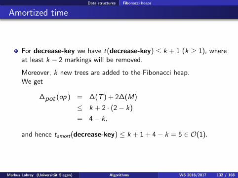
Data structures Fibonacci heaps
Amortized time
For decrease-key we have t(decrease-key) ≤ k + 1 (k ≥ 1), whereat least k − 2 markings will be removed.
Moreover, k new trees are added to the Fibonacci heap.We get
∆pot (op ) = ∆(T ) + 2∆(M)
≤ k + 2 · (2− k)
= 4− k ,
and hence tamort(decrease-key) ≤ k + 1 + 4− k = 5 ∈ O(1).
Markus Lohrey (Universitat Siegen) Algorithms WS 2016/2017 132 / 168

Data structures Fibonacci heaps
Amortized time
Theorem 19
The following amortized time bounds hold for a Fibonacci heap:
tamort(merge) ∈ O(1)
tamort(insert) ∈ O(1)
tamort(delete-min) ∈ O(log n)
tamort(decrease-key) ∈ O(1)
Markus Lohrey (Universitat Siegen) Algorithms WS 2016/2017 133 / 168

Data structures Fibonacci heaps
Fibonacci heaps for Dijkstra
Back to Dijkstra’s algorithm:
For Dijkstra’s algorithm let V be the boundary and let key (v) be thecurrent estimate for d(u, v).
Let n be the number of nodes and e be the number of edges of the inputgraph.
Dijkstra’s algorithm will execute at most n insert-, e decrease-key- and ndelete-min-operations.
Markus Lohrey (Universitat Siegen) Algorithms WS 2016/2017 134 / 168

Data structures Fibonacci heaps
Fibonacci heaps for Dijkstra
tDijkstra ≤ n · tamort(insert)
+ e · tamort(decrease-key)
+ n · tamort(delete-min)
∈ O(n + e + n log n)
= O(e + n log n)
Remember that:
with arrays we got tDijkstra ∈ O(n2), and
with standard heaps we got tDijkstra ∈ O(e log(n)).
Markus Lohrey (Universitat Siegen) Algorithms WS 2016/2017 135 / 168

Dynamic Programming
Idea of dynamic programming
Compute a table of all subsolutions of a problem, until the overall solutionis computed.
Every subsolutions is computed using the already existing entries in thetable.
Dynamic programming is tightly related to backtracking.
In contrast to backtracking, dynamic programming used iteration insteadof recursion. By storing computed subsolutions in table we avoid to solvethe same subproblem several times.
Markus Lohrey (Universitat Siegen) Algorithms WS 2016/2017 136 / 168

Dynamic Programming Computing a long product of matrices
Example: Computing a long product of matrices
Multiplication from left to right:
(10 × 1) (1× 10) (10× 1) (1× 10) (10× 1)
Markus Lohrey (Universitat Siegen) Algorithms WS 2016/2017 137 / 168

Dynamic Programming Computing a long product of matrices
Example: Computing a long product of matrices
Multiplication from left to right:
(10 × 1) (1× 10) (10× 1) (1× 10) (10× 1)
(10 × 10) (10× 1) (1× 10) (10× 1)
100 multiplications
(10× 1) (1× 10) (10× 1)
100 multiplications
(10× 10) (10× 1)
100 multiplications
(10× 1)
100 multiplications
In total: 400 multiplicationsMarkus Lohrey (Universitat Siegen) Algorithms WS 2016/2017 137 / 168

Dynamic Programming Computing a long product of matrices
Example: Computing a long product of matrices
Multiplication from right to left:
(10 × 1) (1× 10) (10× 1) (1× 10) (10× 1)
Markus Lohrey (Universitat Siegen) Algorithms WS 2016/2017 138 / 168

Dynamic Programming Computing a long product of matrices
Example: Computing a long product of matrices
Multiplication from right to left:
(10 × 1) (1× 10) (10× 1) (1× 10) (10× 1)
(10 × 1) (1× 10) (10× 1) (1× 1)
10 multiplications
Markus Lohrey (Universitat Siegen) Algorithms WS 2016/2017 138 / 168

Dynamic Programming Computing a long product of matrices
Example: Computing a long product of matrices
Multiplication from right to left:
(10 × 1) (1× 10) (10× 1) (1× 10) (10× 1)
(10 × 1) (1× 10) (10× 1) (1× 1)
10 multiplications
(10 × 1) (1× 10) (10 × 1)
10 multiplications
(10 × 1) (1× 1)
10 multiplications
(10× 1)
10 multiplications
In total: 40 multiplicationsMarkus Lohrey (Universitat Siegen) Algorithms WS 2016/2017 138 / 168

Dynamic Programming Computing a long product of matrices
Example: Computing a long product of matrices
Multiplication in optimal order
(10 × 1) (1× 10) (10× 1) (1× 10) (10× 1)
Markus Lohrey (Universitat Siegen) Algorithms WS 2016/2017 139 / 168

Dynamic Programming Computing a long product of matrices
Example: Computing a long product of matrices
Multiplication in optimal order
(10 × 1) (1× 10) (10× 1) (1× 10) (10× 1)
(10 × 1) (1× 10) (10× 1) (1× 1)
10 multiplications
Markus Lohrey (Universitat Siegen) Algorithms WS 2016/2017 139 / 168

Dynamic Programming Computing a long product of matrices
Example: Computing a long product of matrices
Multiplication in optimal order
(10 × 1) (1× 10) (10× 1) (1× 10) (10× 1)
(10 × 1) (1× 10) (10× 1) (1× 1)
10 multiplications
(10 × 1) (1× 1) (1× 1)
10 multiplications
(10 × 1) (1× 1)
1 Multiplikation
(10× 1)
10 multiplications
In total: 31 multiplicationsMarkus Lohrey (Universitat Siegen) Algorithms WS 2016/2017 139 / 168

Dynamic Programming Computing a long product of matrices
Computing a long product of matrices
Let A(n,m) be a matrix with n rows and m columns.
Assumption: Computing A(n,m) := B(n,q) · C(q,m) needs n · q ·m scalarmultiplications.
Input: sequence of matrices M1(n0,n1)
,M2(n1,n2)
,M3(n2,n3)
, . . . ,MN(nN−1,nN )
.
cost(M1, . . . ,MN) := minimal number of scalar multiplications in order tocompute M1 · · ·MN (minimum is taken over all possible bracketings).
Dynamic programming approach:
cost(M i , . . . ,M j) =
minkcost(M i , . . . ,Mk) + cost(Mk+1, . . . ,M j) + ni−1 · nk · nj
Markus Lohrey (Universitat Siegen) Algorithms WS 2016/2017 140 / 168

Dynamic Programming Computing a long product of matrices
Computing a long product of matrices
for i := 1 to N docost[i , i ] := 0;for j := i + 1 to N docost[i , j ] := ∞;
endforendforfor d := 1 to N − 1 dofor i := 1 to N − d doj := i + d ;for k := i to j − 1 dot := cost[i , k ] + cost[k + 1, j ] + n[i − 1] · n[k ] · n[j ];if t < cost[i , j ] thencost[i , j ] := t;best[i , j ] := k ;
endifendfor
endforendfor
return bestMarkus Lohrey (Universitat Siegen) Algorithms WS 2016/2017 141 / 168

Dynamic Programming Optimal binary search trees
Optimal search trees
We will see a straightforward dynamic programming algorithm forcomputing optimal search trees with a running time of of Θ(n3).
An algorithm of Donald E. Knuth reduces the time to Θ(n2)(→ Algorithms II).
Markus Lohrey (Universitat Siegen) Algorithms WS 2016/2017 142 / 168

Dynamic Programming Optimal binary search trees
Optimal search trees
Let V = v1, . . . , vn be linearly ordered set of keys, v1 < v2 < · · · < vn.
For every key v ∈ V we have given an access probability (also called theweight) γ(v).
The idea is that with every key some additional information is associated(think about personnel numbers, and additional informations like name,birthday, salary, etc). Then γ(vi ) is the probability that the informationassociated with key vi is accessed.
A binary search tree for v1 < v2 < · · · < vn is a binary tree with node setv1, v2, . . . , vn, such that:For every node v with left (resp., right) subtree L (resp. R) and all u ∈ L(resp. w ∈ R) we have: u < v (v < w).
Markus Lohrey (Universitat Siegen) Algorithms WS 2016/2017 143 / 168

Dynamic Programming Optimal binary search trees
Optimal search trees
Every node v of a search tree B has a level ℓB(v):ℓB(v) := 1+ distance (in number of edges) from v to root.
Finding a node at level ℓ requires ℓ comparisons (start in root and thenwalk down the path to the node).
Problem: Find a binary search tree B with minimal weighted inner pathlength
P(B) :=∑
v∈V
ℓB(v) · γ(v).
The weighted inner path length is the average cost for accessing a node.
Dynamic programming works because subtrees of optimal binary searchtrees have to be optimal again.
Markus Lohrey (Universitat Siegen) Algorithms WS 2016/2017 144 / 168

Dynamic Programming Optimal binary search trees
Optimal search trees
Notation:
node set = 1, . . . , n, i.e., we identify node vi with i .
P [i , j]: weighted inner path length of an optimal search tree for thenode set i , . . . , j.R [i , j]: root of an optimal search tree for i , . . . , j.Since there might be several optimal search trees we take for R [i , j]for the largest root among all optimal search trees.
Γ[i , j] :=∑j
k=i γ(k): total weight of the node set i , . . . , j.
Markus Lohrey (Universitat Siegen) Algorithms WS 2016/2017 145 / 168

Dynamic Programming Optimal binary search trees
Computing optimal search trees in time O(n3)
Using dynamic programming we can compute all values P [i , j] and R [i , j].
For a binary search tree B with left subtree B0, right subtree B1, and totalweight Γ(B) we have
P(B) := P(B0) + P(B1) + Γ(B).
We realize this idea with a cubic algorithm:
P [i , j] = Γ[i , j] + minP [i , k − 1] + P [k + 1, j] | k ∈ i , . . . , jR [i , j] = largest key among all k for which P [i , k − 1] + P [k + 1, j] isminimal.
Markus Lohrey (Universitat Siegen) Algorithms WS 2016/2017 146 / 168

Dynamic Programming Optimal binary search trees
Optimal search trees
for i := 1 to n doP[i , i − 1] := 0;P[i , i ] := γ(i);Γ[i , i ] := γ(i);R [i , i ] := i ;
endfor
for d := 1 to n− 1 dofor i := 1 to n − d doj := i + d ;root := i ;t := ∞;for k := i to j doif P[i , k − 1] + P[k + 1, j ] ≤ t thent := P[i , k − 1] + P[k + 1, j ];root := k ;
endifendforΓ[i , j ] := Γ[i , j − 1] + γ(j);P[i , j ] := t + Γ[i , j ];R [i , j ] := root;
endforendfor
Markus Lohrey (Universitat Siegen) Algorithms WS 2016/2017 147 / 168

Dynamic Programming Computation of regular expressions
Computation of regular expressions
Recall from GTI: Computation of regular expressions by Kleene.
A nondeterministic finite automaton (NFA) is a tuple
A = (Q,Σ, δ ⊆ Q × Σ× Q, I ,F ) (w.l.o.g. Q = 1, . . . , n).
Let Lk [i , j] be the set of all words that label a path in A, which
leads from i to j and
thereby only visits intermediate states from 1, . . . , k (i and j do notnecessarily belong to 1, . . . , k).
Goal: Regular expressions for all Ln[i , j] with i ∈ I and j ∈ F .
We have
L0[i , j] =
a ∈ Σ | (i , a, j) ∈ δ if i 6= j
a ∈ Σ | (i , a, j) ∈ δ ∪ ε if i = j
Lk [i , j] = Lk−1[i , j] + Lk−1[i , k] · Lk−1[k , k]∗ · Lk−1[k , j]
Markus Lohrey (Universitat Siegen) Algorithms WS 2016/2017 148 / 168

Dynamic Programming Computation of regular expressions
Computation of regular expressions
Algorithm Regular from an NFA
procedure NFA2REGEXPInput : NEA A = (Q,Σ, δ ⊆ Q × Σ× Q, I ,F )(Initialize: L[i , j] := a | (i , a, j) ∈ δ ∨ a = ε ∧ i = j)begin
for k := 1 to n dofor i := 1 to n do
for j := 1 to n doL[i , j] := L[i , j] + L[i , k] · L[k , k]∗ · L[k , j]
endforendfor
endforend
Markus Lohrey (Universitat Siegen) Algorithms WS 2016/2017 149 / 168

Dynamic Programming Warshall’s algorithm
Computing the transitiv closure
Algorithm Warshall-algorithm: computation of the transitive closure
procedure Warshall (var A : adjacency matrix)Input : graph given by its adjacency matrix (A[i , j]) ∈ Booln×n
beginfor k := 1 to n do
for i := 1 to n dofor j := 1 to n do
if (A[i , k] = 1) and (A[k , j] = 1) thenA[i , j] := 1
endifendfor
endforendfor
end
Markus Lohrey (Universitat Siegen) Algorithms WS 2016/2017 150 / 168

Dynamic Programming Warshall’s algorithm
Transitiv closure?
Algorithm Is this algorithm correct?
procedure Warshall (var A : adjacency matrix)Input : graph given by its adjacency matrix (A[i , j]) ∈ Booln×n
beginfor i := 1 to n do
for j := 1 to n dofor k := 1 to n do
if (A[i , k] = 1) and (A[k , j] = 1) thenA[i , j] := 1
endifendfor
endforendfor
end
Markus Lohrey (Universitat Siegen) Algorithms WS 2016/2017 151 / 168

Dynamic Programming Warshall’s algorithm
Correctness of Warshall
Correctness of Warshall’s algorithm follows from the following invariant:
1 After the k-th excecution of the body of the for-loop, we have:A[i , j] = 1, if there is a path from i to j with intermediate nodes from1, . . . , k .
Important: the outermost loop runs over k!
2 If A[i , j] is set to 1, then there exists a path from i to j .
If the 0/1-entries in the adjacency matrix are replaced from edge weights,one obtains Floyd’s algorithm for computing shortest paths:
Markus Lohrey (Universitat Siegen) Algorithms WS 2016/2017 152 / 168

Dynamic Programming Floyd’s algorithm
Floyd-algorithm
Algorithm Floyd: all shortest paths in a graph
procedure Floyd (var A : adjacency matrix)Input : edge-weighted graph given by its adjacency matrix A[i , j] ∈
(N ∪∞)n×n, where A[i , j] = ∞ means that there is no edge from i to j .begin
for k := 1 to n dofor i := 1 to n do
for j := 1 to n doA[i , j] := minA[i , j],A[i , k] + A[k , j];
endforendfor
endforend
Markus Lohrey (Universitat Siegen) Algorithms WS 2016/2017 153 / 168

Dynamic Programming Floyd’s algorithm
Floyd-algorithm
Floyd’s algorithm computes correct results also for graphs with negativeweights provide that there do not exist cycles with negative total weight.
Running time of Warshall and Floyd: Θ(n3).
”Improvement“ by testing before the j-loop, whether A[i , k] = 1 (resp.,A[i , k] < ∞) holds.
This yields a running time of O(n3):
Markus Lohrey (Universitat Siegen) Algorithms WS 2016/2017 154 / 168

Dynamic Programming Floyd’s algorithm
Floyd’s algorithm
Algorithm Floyd’s algorithm in O(n3)
procedure Floyd (var A : adjacency matrix)Input : adjacency matrix A[i , j] ∈ (N ∪∞)n×n
beginfor k := 1 to n do
for i := 1 to n doif A[i , k] < ∞ then
for j := 1 to n doA[i , j] := minA[i , j],A[i , k] + A[k , j];
endforendif
endforendfor
end
Markus Lohrey (Universitat Siegen) Algorithms WS 2016/2017 155 / 168

Dynamic Programming Floyd’s algorithm
Floyd’s algorithm
Algorithm Floyd’s algorithm for negative cycles
procedure Floyd (var A : adjacency matrix)Input : adjacency matrix A[i , j] ∈ (Z ∪ ∞,−∞)n×n
beginfor k := 1 to n do
for i := 1 to n doif A[i , k] < ∞ then
for j := 1 to n doif A[k , j] < ∞ then
if A[k , k] < 0 then A[i , j] := −∞else A[i , j] := minA[i , j],A[i , k] + A[k , j]
endifendif
endfor endif endfor endforend
Markus Lohrey (Universitat Siegen) Algorithms WS 2016/2017 156 / 168

Dynamic Programming Transitiv closure and matrix multiplication
Transitiv closure and matrix multiplication
Let A = (ai ,j)1≤i ,j≤n be the adjacency matrix of a directed graph withnode set 1, . . . , n, i.e.,
ai ,j =
1 if there is an edge from i to j
0 otherwise
Warshall’s algorithm computes the reflexive and transitive closure A∗ intime O(n3).
Here, A∗ =∑
k≥0 Ak , where A0 = In is the identity matrix and ∨ (boolean
or) is taken for the addition of boolean matrices .
We add as follows: 0 + 0 = 0, 0 + 1 = 1 + 0 = 1 + 1 = 1.
By induction we get: Ak(i , j) = 1 ⇐⇒ ∃ path of length k from i to j .
This yields A∗ =∑n−1
k=0 Ak .
Markus Lohrey (Universitat Siegen) Algorithms WS 2016/2017 157 / 168

Dynamic Programming Transitiv closure and matrix multiplication
Transitiv closure and matrix multiplication
Let B = In + A. We get A∗ = Bm for all m ≥ n − 1.
It therefore suffices to square the matrix ⌈log2(n − 1)⌉ times in order tocompute A∗.
Let M(n) be the time needed to multiply two boolean n × n-matrices andlet T (n) be the time needed to compute the reflexive and transitiveclosure.
We have
T (n) ∈ O(M(n) · log n).
Using Strassen’s algorithm, we get for all ε > 0:
T (n) ∈ O(nlog2(7)+ε).
Markus Lohrey (Universitat Siegen) Algorithms WS 2016/2017 158 / 168

Dynamic Programming Transitiv closure and matrix multiplication
Matrix multiplication ≤ transitiv closure
Under the plausible assumption that T (3n) ∈ O(T (n)) we getM(n) ∈ O(T (n)):
For all boolean matrices A and B we have:
0 A 00 0 B0 0 0
∗
=
In A AB0 In B0 0 In
.
Under the also plausible assumption that M(2n) ≥ (2 + ε)M(n) for anε > 0, we can show that also T (n) ∈ O(M(n)).
Hence: The computation of the reflexive and transitive closure is up toconstant factors equally expensive as matrix multiplication.
Markus Lohrey (Universitat Siegen) Algorithms WS 2016/2017 159 / 168

Dynamic Programming Transitiv closure and matrix multiplication
Computation of the transitiv closure
Input: E ∈ Bool(n × n)
Divide E into 4 submatrices A,B ,C ,D such that A and D are squarematrices and each of the 4 matrices has size roughly n/2× n/2:
E =
(
A BC D
)
.
Compute recursively D∗:Time: T (n/2).
Compute F = A+ BD∗C :Time: O(M(n/2)) ≤ O(M(n)).
Compute recursively F ∗:Time: T (n/2).
Set
E ∗ =
(
F ∗ F ∗BD∗
D∗CF ∗ D∗ + D∗CF ∗BD∗
)
.
Markus Lohrey (Universitat Siegen) Algorithms WS 2016/2017 160 / 168

Dynamic Programming Transitiv closure and matrix multiplication
Computation of the transitiv closure
We obtain the recurrence
T (n) ≤ 2T (n/2) + c ·M(n) for some c > 0.
This yields
T (n) ≤ c ·(
∑
i≥0 2i ·M(n/2i )
)
(by induction)
≤ c ·∑i≥0
(
22+ε
)i
·M(n) (da M(n/2) ≤ 12+εM(n))
∈ O(M(n)).
Markus Lohrey (Universitat Siegen) Algorithms WS 2016/2017 161 / 168

Dynamic Programming A · B = C?
How can we test whether A · B = C?
The best current algorithm for multiplying two (n × n)-matrices needsapprox. Θ(n2,372873...) many arithmetic operations (Virginia VassilevskaWilliams 2014).
Conjecture
For every ǫ > 0 there exists an algorithm for multiplying two(n × n)-matrices in time O(n2+ε).
Assume now that we have three (n × n)-matrices A, B and C .
How many arithmetic operations are needed to test whether A · B = Cholds?
Trivial answer: O(n2,372873...)
But there is a better method!
Markus Lohrey (Universitat Siegen) Algorithms WS 2016/2017 162 / 168

Dynamic Programming A · B = C?
How can we test whether A · B = C?
Satz 20 (Korec, Wiedermann 2014)
Let A,B ,C be (n × n)-matrices with entries from Z. Using O(n2) manyoperations we can check whether A · B = C holds.
Proof: Let
A = (ai ,j)1≤i ,j≤n,
B = (bi ,j)1≤i ,j≤n,
C = (ci ,j)1≤i ,j≤n and
D = (di ,j)1≤i ,j≤n = A · B − C .
Thus, we have A · B = C if and only if D is the zero-matrix.
Let x be real-valued variable and consider the column-vector
v = (1, x , x2, . . . , xn−1)T .
Markus Lohrey (Universitat Siegen) Algorithms WS 2016/2017 163 / 168

Dynamic Programming A · B = C?
How can we test whether A · B = C?
Hence, D · v = A · B · v − C · v is a column-vector whose i -th entry is thepolynomial
pi(x) = di ,1 + di ,2x + di ,3x2 + · · ·+ di ,nx
n−1.
We therefore have A · B = C if and only if pi(x) is the zero polynomial forall 1 ≤ i ≤ n.
We use the following theorem:
Cauchy bound
Let p(x) = anxn + an−1x
n−1 + · · ·+ a1x + a0 ∈ R[x ] be not thezero-polynomial and an 6= 0. For every α with p(α) = 0 we have
|α| < 1 +max|ai | | 0 ≤ i ≤ n − 1
|an|.
Markus Lohrey (Universitat Siegen) Algorithms WS 2016/2017 164 / 168

Dynamic Programming A · B = C?
How can we test whether A · B = C?
Proof of the Cauchy bound:
By replacing p(x) by the polynomial xn + an−1
anxn−1 + · · ·+ a1
anx + a0
an, it
suffices to prove the Cauchy bound for the case an = 1.
Let p(x) = xn + an−1xn−1 + · · ·+ a1x + a0 and
h = max|ai | | 0 ≤ i ≤ n − 1.
Assume that p(α) = αn + an−1αn−1 + · · ·+ a1α+ a0 = 0, i.e.,
αn = −an−1αn−1 − · · · − a1α− a0.
We show that |α| < 1 + h.
If |α| ≤ 1, we have |α| < 1 + h (if h = 0 then we must have α = 0).
Now assume that |α| > 1.Markus Lohrey (Universitat Siegen) Algorithms WS 2016/2017 165 / 168

Dynamic Programming A · B = C?
How can we test whether A · B = C?
We get
|α|n ≤ |an−1| · |α|n−1 + · · ·+ |a1| · |α| + |a0|≤ h · (|α|n−1 + · · ·+ |α|+ 1)
= h · |α|n − 1
|α| − 1.
Since |α| > 1, we obtain:
|α| − 1 ≤ h · |α|n − 1
|α|n < h
Markus Lohrey (Universitat Siegen) Algorithms WS 2016/2017 166 / 168

Dynamic Programming A · B = C?
How can we test whether A · B = C?
Let a = max|ai ,j | | 1 ≤ i , j ≤ n, b = max|bi ,j | | 1 ≤ i , j ≤ n andc = max|ci ,j | | 1 ≤ i , j ≤ n.
The absolute values of the coefficients of the polynomials pi (x) can bebounded as follows:
|di ,j | = |n∑
k=1
ai ,kbk,j − ci ,j | ≤n∑
k=1
|ai ,k | · |bk,j |+ |ci ,j | ≤ n · a · b + c .
Let d = n · a · b + c and r = 1 + d .
The Cauchy bound yields for all 1 ≤ i ≤ n:
pi (x) = 0 ⇔ pi (r) = 0
Note: It is easy to get an upper bound d for the absolute values of theentries of D, but it is not so clear how to get a lower bound.Markus Lohrey (Universitat Siegen) Algorithms WS 2016/2017 167 / 168

Dynamic Programming A · B = C?
How can we test whether A · B = C?
But: Since A,B ,C are matrices over Z, we have pi (x) ∈ Z[x ].
Therefore, the absolute value of the leading coefficient of pi (x) is at least1, if pi(x) is not the zero-polynomial.
We can therefore check with the following algorithm, whether A · B = C :
1 Compute a = max|ai ,j |, b = max|bi ,j |, c = max|ci ,j | andr = 1 + n · a · b + c(3n2 many comparisons, 2 additions, 2 multiplications)
2 Compute the column vector u = (1, r , r2, . . . , rn−1)T .(n − 2 multiplications)
3 Compute p := B · u, s := A · p and t := C · u(O(n2) many arithmetic operations)
4 A · B = C if and only if s = t.
Markus Lohrey (Universitat Siegen) Algorithms WS 2016/2017 168 / 168