978-1-4244-5550-8/10/$26.00 ©2010 IEEE

North Atlantic Right Whale Acoustic Signal Processing:

Part I. Comparison of Machine Learning Recognition Algorithms

Peter J. Dugan*, Aaron N. Rice, Ildar R. Urazghildiiev and Christopher W. Clark Bioacoustics Research Program, Cornell Laboratory of Ornithology,

Cornell University Ithaca, NY 14850 USA

*e-mail: pjd78@cornell.edu

Abstract— This paper compares three different approaches currently used in recognizing contact calls made from the North Atlantic Right Whale (NRW), Eubalaena glacialis. We present two new approaches consisting of machine learning algorithms based on artificial neural networks (NET) and the classification and regression tree classifiers (CART), and compare their performance with earlier work that employs multi-Stage feature vector testing (FVT) approach. A combined total of over 100,000 noise and NRW up-call events were used in the study. Calls were primarily recorded from two areas, Cape Cod Bay and Great South Channel. Of the three classifiers, the CART had the highest assignment rates, overall 86.45% with highest false positive rates (<100 per hour). The FVT Method had exceptionally low false positive rates, with <50 per hour. However, it had an overall assignment rate less than the NET. The CART had statistically the same false positive rate as the NET with the highest assignment rates, 2.2% higher than the NET and 11.75% greater than the FVT Method. Details of the results are shown and extensions to the research are discussed.

Keywords--Right Whale; Acoustic Monitoring; Automated Detection; Artifical Neural Network; Classfication Regression Tree

I. INTRODUCTION In recent years, passive acoustic monitoring (PAM) has

proven to be one of the most effective methods for monitoring the presence and movement of marine mammals [e.g., 1, 2], due to the fact that cetaceans are difficult to locate visually from the surface, but acoustic communication is a fundamental component of their behavior. PAM methods have been able to successfully detect most baleen whale species in North American waters [1]. Of these taxa, the North Atlantic Right Whale (NRW, Eubalaena glacialis) is one of the most critically endangered marine mammal species (with approximately only 400 individuals remaining) [3], and considerable effort has been invested in understanding these animals’ movements and behavior on the basis of their vocalizations [4].

There are several challenges to using PAM. First, understanding migratory patterns and seasonal behaviors

requires long-term acoustic recording intervals. Second, ambient noise levels can vary significantly throughout the data collection period, increasing the difficulty of sound analysis. Together, variable noise and enormous quantities of acoustic data offer a formidable challenge for detecting NRW contact calls. To optimize this process, automated signal processing, or data mining methods, have been created to accurately and precisely detect whales while accounting for variability in signal structure and background noise. In most cases, sound recognition algorithms analyze sound data after the recording devices are recovered from the water [e.g., 4]. New technologies have begun to incorporate signal recognition algorithms to be used in real-time system while devices are recording [5]. In these different archival and real-time applications, signal processing methods used to detect sounds of interest present critical tools for successful PAM: maximizing the number of true whale detections while minimizing missed whale sounds and false positives. However, temporal and geographical fluctuations in ambient and anthropogenic noise levels, can bias the detection process [6].

Significant research has been done on the design and construction for automated detection of NRW vocalizations. Several methods have been considered, these include time-based convolution [7], edge-based detection [8], a multi-stage feature vector testing (FVT) algorithm [6] and neural net detection using mini-grams [9]. The summary of these approaches have shown that multi-stage hypothesis testing and the neural net technologies perform well under varying noise conditions, outperforming edge detection and convolution methods. Currently, the multi-stage FVT-method [6] is the most accurate and readily available technology compatible with acoustic analysis software [6].

The FVT method is built using multiple stages: these involve detection Stage 1, filter bank feature extraction (Table I) Stage 2, and classification Stage 3 [6]. Performance of the FVT method varies significantly over an ensemble of data sets [6]. Variation in ambient noise levels and call variability are suspected cause for the FVT performance discrepancy. The goal of this study is to utilize Stage 1 and Stage 2 from the FVT method and focus on considering the NET and CART as possible alternatives to the zero-one approach currently used for Stage 3.

Authorized licensed use limited to: Cornell University. Downloaded on June 15,2010 at 13:02:37 UTC from IEEE Xplore. Restrictions apply.

TABLE I. FEATURES USED FOR CLASSIFICATION OF NORTH ATLANTIC RIGHT WHALE UP-CALLS [FROM 6].

II. DATA COLLECTION, ARRAY CONFIGURATION, SAMPLING CALLS

The signal processing methods discussed here were evaluated in the context of detecting NRW “up-calls.” The up-call is a frequency modulated signal (prominent harmonics at close range, though appearing tonal at farther distances) with significant energy between 50-250 Hz, lasting approximately 0.5–2 seconds (Fig. 1) and is used as a contact call for animals to find conspecifics [10, 11]. Sounds were recorded using arrays of Marine Autonomous Recording Units [12], deployed in three locations in the Northwest Atlantic Ocean along the NRW's annual migration route: the Great South Channel (GSC) in the Gulf of Maine (recorded August 2000-August 2007; Fig. 1A), Cape Cod Bay (CCB), Massachusetts (recorded May 2001-February 2008; Fig. 1B), and offshore of Brunswick, GA (recorded December 2006- February 2007; Fig. 1C). Signals recorded in the field were processed and uploaded to servers using standard audio file formats for processing. The open source acoustic software, xBAT (eXtensible Bioacoustic Tool, http://xbat.org), was used as an interface to visually represent sounds as spectrograms, and analyze sound recordings whereby detector modules (referred to as extensions) are created for processing sounds. The detector extensions serve as automated routines for creating data-logs of specific sound types. NRW contact calls were extracted from multi-channel, long-term recordings by using the human browsed tag indices; resulting audio was a condensed series of clip libraries (Table II). Human operators browsed each of the recordings marking the NRW up-calls, providing a complete, verified record of sound occurrences.

III. DETECTION AND FEATURE EXTRACTION Three classifiers are the focus of this work: multi-stage

FVT algorithm [6], artificial neural network (NET) and the classification regression tree (CART). The basic detection/recognition architecture for these detector extensions is shown in Fig. 2. For each of these three methods, Stage 1 and Stage 2 are identical: Stage 1 incorporates signal detection, or

TABLE II. NUMBER OF NRW UP-CALLS AND NOISE CLIPS USED IN THE TRAINING AND VALIDATION SET.

Figure 1. Representative spectrograms of North Atlantic right whale up-calls, from three different localities– Great South Channel (GSC), Cape Cod

Bay (CCB), and offshore Brunswick, GA– showing variability in up call properties and background noise. Spectrograms are shown with a Hann

window of 512 samples and overlap of 50%. Vertical dashed white lines show the separation in between different clips used in data libraries.

described in other terms as signal segmentation. The goal of this stage is to identify areas of high energy. A wide range of segmentation approaches exist, some of which include time-frequency templates [7], energy based detection [13] and contour morphology [14]. The spectrogram-correlation method is used for this analysis, and is described briefly below. For detailed analysis, please refer to [13].

A. Stage 1 Processing Signals of interest have energy between 50-250 Hz. This

will be considered the frequency surveillance zone (FSZ). In the FSZ, noise conditions can change dramatically throughout the course of the monitoring period. For short durations, tens of seconds, ambient noise is considered stationary. Signal intervals, or sample page (SP), of 32 seconds are input, and converted to time-frequency using a spectrogram algorithm with 50% overlap, 512 frequency bins, with a rectangular window. Consider the sample page as a discrete sequence X[n,k]. Let the expected value over time be noted as ˜ X [k]. The FSZ bins are normalized by X[n,k]/ ˜ X [k], where Y[n,k] is the resulting sequence. Decisions are made on the sequence Y[n,k] using two steps. First, values of statistic are determined, whereby 1 second intervals of Y[n,k] that fall below the statistical threshold are discarded as noise, all others are passed to the Stage 2 for further filtering and feature extraction.

B. Stage 2 Processing The second step for making decisions occurs by using a

complex filter bank consisting of four unique filters that separate candidate segments from Stage 1 using various shapes. Sample intervals for Y[n,k] that do not meet the NRW criterion

Authorized licensed use limited to: Cornell University. Downloaded on June 15,2010 at 13:02:37 UTC from IEEE Xplore. Restrictions apply.

Figure 2. Architecture of system used to measure sensor reports using three different classifier methods in Stage 3 (indicated by dashed box). Sounds from

the library are processed through Stages 1-3 and result in a sensor report, whereby their performance is evaluated by comparison with a truth report

(generated by human observers). Metrics of performance include the probability of detection (pd), missed detections (emd), and number of false

alarms (efar).

are accepted according to features extracted in preparation for recognition Stage 3. Let ˆ f represent the N dimensional feature vector given by ˆ f = f 1… fN. A total of 11 features are extracted and summarized in Table I. A more detailed description for Stage 1 and Stage 2, including feature extraction processing, is provided in [6, 15].

IV. CLASSIFICATION/RECOGNITION

A. Stage 3 Processing A multi-stage detector using FVT with 11 features out-

performs a single stage approach [6]. Other work has been done by using artificial neural nets for recognizing NRW up-calls [9]. However, this work used a different feature set consisting of individual samples from the spectrogram, or “mini-grams,” and used a relatively small data set compared to [6]. The physical origin of the feature data has a large impact on assignment rates [16]. In this section, details are provided to explain the overall approach for classification Stages for three different NRW research efforts that consist of detection studies using FVT, NET and CART topologies. The mechanics of each technology is well documented in the literature, and we briefly describe these methods below.

B. FVT Method FVT recognition Stage 3 is based on a linear distance

measure [6], which is similar to a zero-one loss metric as described in [17]. All feature values are normalized, values further from the mean are penalized toward zero, values closer to the mean are rewarded toward 1. For each sensor report, a zero-one value is obtained and compared against a threshold, while the threshold is selected through a minimum error procedure. Training includes evaluating a large number or data samples, with replacement, and selecting a decision point that minimizes recognition error. For this study, the FVT was run as a detector extension module through xBAT, using a Stage 1 threshold setting of 0.35.

C. Artificial Neural Net A standard back propagation artificial neural net (NET) is

used in the analysis. Deciding on the best architecture is a difficult problem in NET technology. Regularization implies that many different configurations exist that vary in complexity, where each provide an acceptable performance

level. Training the NET organizes a series of random weights to achieve a minimum error condition. However, one could train the NET using identical architectures, but resulting in different weight tables that meet similar error conditions. Furthermore, optimization could be done on the configuration of the architecture. In prior work [e.g., 9], optimization procedures have often been used to determine a limited set of parameters. However, these consisted of smaller data sets. Other research presents a systems approach to optimizing parameters for the NET [16, 17]. For this study, the amount of data is significant and a limited optimization is performed. Training the NETs used the Levenberg-Marquardt back-propagation algorithm (MatLab 2009a, The Mathworks, Inc., Natick, MA). The trainer executed several times, using fewer than 5000 epochs, running in batch data mode. Both the number of hidden layers, Nlayer and the number of nodes per hidden layer, Nnode, were varied. Since the data set was significantly large, both parameters were limited Nlayer = [1, 2] and Nnode = [10, 20, 40, 80]. Several architectures were tried, and the final configuration consisted of a completely connected feed forward net with Nlayer = 2 and Nnode = [80, 20] for layer one and two respectively. Hyperbolic tangent was used for the activation function for both hidden layers. Biases were used along with linear activation for the output layer. Training data consisted of three different combinations, using sounds from various geographic data sets (Table II). Training and validation consisted of using each combination with 10% of the data from specific data sets; samples were randomly selected with replacement, these include geographies for CCB, GSC and Generic. The Generic dataset combined the training data incorporating both CCB and GSC. Final recognition is deduced from the output layer, using linear activation. Values were selected based on observed heuristic minimum error. For this study, the NET was run as a detector extension module through xBAT, using a Stage 1 threshold setting of 0.35, with a Generic geography; a Stage 3 lower threshold of 0.2 with no upper limit.

D. Classification Regression Trees Classification regression trees (CART) are a popular data-

mining tool. They have the ability to handle mixed feature sets which contain numeric and non-numeric data [18], making them ideal for a variety of applications. The CART uses a decision process driven by a series of rules, which can be viewed as a series of logical decisions to determine class labels. Given a binary class problem, rules select a split point for each of the feature values, such as fN ≤ fsplit, where fsplit is selected based on several factors which include numeric and non-numeric data. Since splitting decisions can be qualitative in nature, the CART does not rely on feature distance, and is referred to as a non-metric classifier. Although multi-class trees are realizable, this study only considers a binary tree configuration. Trees are constructed by first creating a root node followed by a series of branches, or test points. The split point for each branch is determined by using a series of decisions based on the purity of the input data. The first step, starting at the root node, analyzes the training data, selecting one of fN features as the root. A split point is established using a probabilistic measure called a purity metric; one popular measure is entropy impurity [17]. For each split, the value of

Authorized licensed use limited to: Cornell University. Downloaded on June 15,2010 at 13:02:37 UTC from IEEE Xplore. Restrictions apply.

the feature is determined whereby either side of the decision boundary, the purity measure, is driven toward 0. This provides homogeneous class on either extreme. The process of splitting continues until either the stopping criterion or minimum validation error is reached. Each end point in the tree forms a leaf node, or termination node. If too many leafs are created, the tree will over-fit; too few, the tree will provide poor classification.

For this study, CART classifiers were constructed based on a population of NRW up-calls and noise samples taken from CCB and GSC (Table II). Extracted features from Stage 1 and Stage 2 were used as N dimensional input feature data, ˆ f = f1...fN. For each geographical dataset, training and validation set were randomly sampled with replacement from the original data (Table II). In all, three trees were created, CCB, GSC and a combination of both geographies referred to as Generic. Resulting tree sizes were as follows, CCB with 178 leaf nodes, GSC with 52 leaf nodes, and Generic with 71 leaf nodes. For this study, the CART was run as a detector extension module through xBAT, using a threshold setting of 0.35 and Generic geography.

E. Performance Analysis Both noise and signal are considered for class assignment.

The recognizer must assign sn or ss for the noise and signal class label, respectively. Three performance measures are summarized, hourly false alarm rate ehfar, probability of missed detections emd and the detection probability pd. For this study ehfar is the number of incorrectly detected noise signals per hour. Conventions for the missed detection emd and detection probability pd, are explained in [19]. The value for emd is the total number of missed NRW calls divided by the total number present which is the same as one minus probability pd. The value for pd is the total number of NRW calls correctly detected divided by the total present.

F. Study Objectives For this study, various geographies (CCB, GSC, and

Brunswick) were individually trained along with a classifier that contained all three geographies referred to as Generic. The goal is to consider whether we can improve the overall recognition performance, with minimal impact on system error, by introducing the CART or NET to the FVT method. To establish a baseline with earlier results published in [6], the FVT method was run and pd, emd and ehfar were recorded and reproduced for this work. For simplicity, classifiers with Generic training and validation data were selected for the CART and NET topology, where pd, emd and ehfar were also recorded. Statistical analyses of performance metrics (pd, emd, ehfar) were performed using the JMP 5.0.1.2 software package (SAS Institute, Cary, NC).

V. RESULTS The combined dataset of sounds from the three localities

consisted of signal and noise snippets (clips), 58,624 North Atlantic right whale up-calls and 81,880 noise examples. For

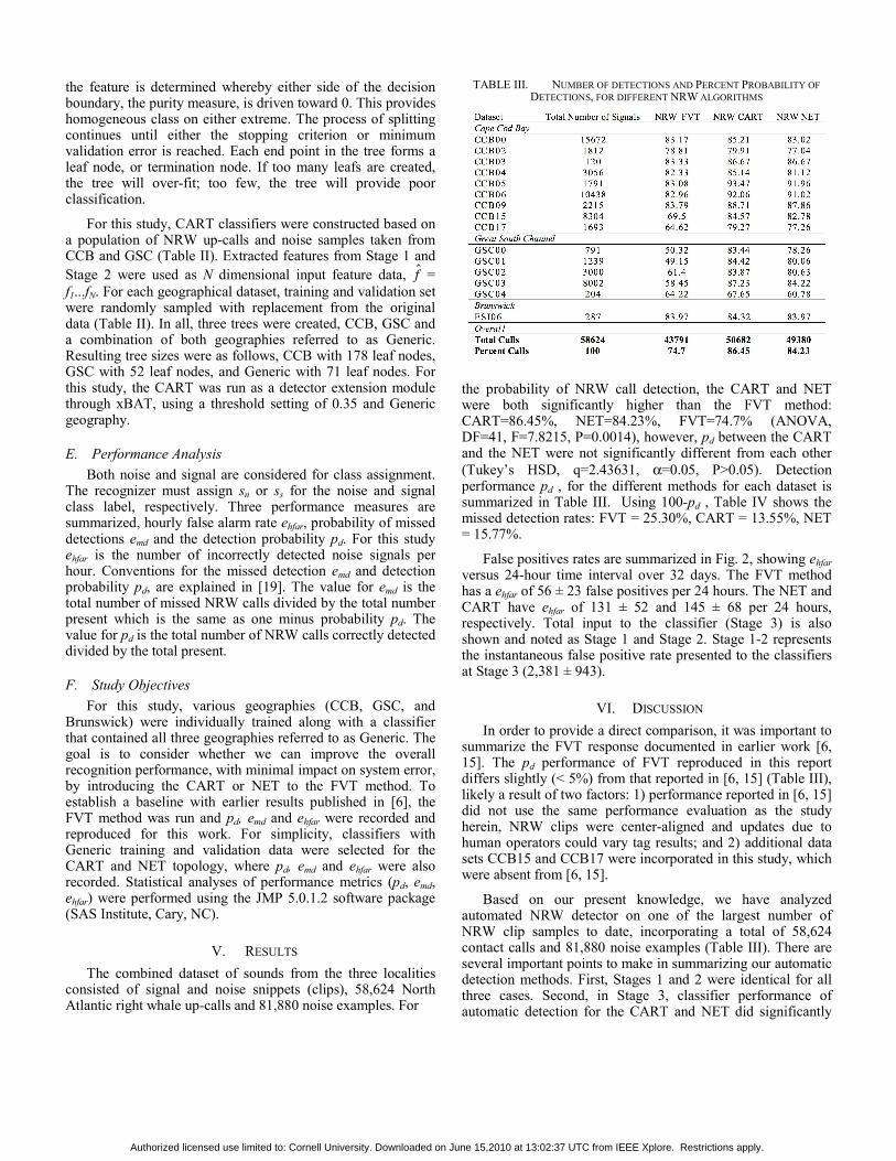
TABLE III. NUMBER OF DETECTIONS AND PERCENT PROBABILITY OF DETECTIONS, FOR DIFFERENT NRW ALGORITHMS

the probability of NRW call detection, the CART and NET were both significantly higher than the FVT method: CART=86.45%, NET=84.23%, FVT=74.7% (ANOVA, DF=41, F=7.8215, P=0.0014), however, pd between the CART and the NET were not significantly different from each other (Tukey’s HSD, q=2.43631, α=0.05, P>0.05). Detection performance pd , for the different methods for each dataset is summarized in Table III. Using 100-pd , Table IV shows the missed detection rates: FVT = 25.30%, CART = 13.55%, NET = 15.77%.

False positives rates are summarized in Fig. 2, showing ehfar versus 24-hour time interval over 32 days. The FVT method has a ehfar of 56 ± 23 false positives per 24 hours. The NET and CART have ehfar of 131 ± 52 and 145 ± 68 per 24 hours, respectively. Total input to the classifier (Stage 3) is also shown and noted as Stage 1 and Stage 2. Stage 1-2 represents the instantaneous false positive rate presented to the classifiers at Stage 3 (2,381 ± 943).

VI. DISCUSSION In order to provide a direct comparison, it was important to

summarize the FVT response documented in earlier work [6, 15]. The pd performance of FVT reproduced in this report differs slightly (< 5%) from that reported in [6, 15] (Table III), likely a result of two factors: 1) performance reported in [6, 15] did not use the same performance evaluation as the study herein, NRW clips were center-aligned and updates due to human operators could vary tag results; and 2) additional data sets CCB15 and CCB17 were incorporated in this study, which were absent from [6, 15].

Based on our present knowledge, we have analyzed automated NRW detector on one of the largest number of NRW clip samples to date, incorporating a total of 58,624 contact calls and 81,880 noise examples (Table III). There are several important points to make in summarizing our automatic detection methods. First, Stages 1 and 2 were identical for all three cases. Second, in Stage 3, classifier performance of automatic detection for the CART and NET did significantly __

Authorized licensed use limited to: Cornell University. Downloaded on June 15,2010 at 13:02:37 UTC from IEEE Xplore. Restrictions apply.

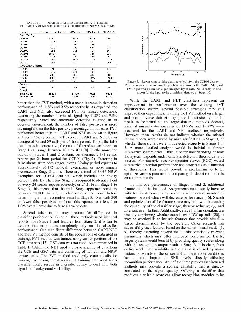
TABLE IV. NUMBER OF MISSED DETECTIONS AND PERCENT PROBABILITY OF MISSED DETECTIONS FOR DIFFERENT NRW ALGORITHMS

better than the FVT method, with a mean increase in detection performance of 11.8% and 9.5% respectively. As expected, the CART and NET also exceeded FVT for missed detections, decreasing the number of missed signals by 11.8% and 9.5% respectively. Since the automatic detection is used in an operator environment, the number of false positives is more meaningful than the false positive percentage. In this case, FVT performed better than the CART and NET as shown in figure 2. Over a 32-day period, FVT exceeded CART and NET by an average of 75 and 89 calls per 24-hour period. To put the false alarm rates in perspective, the ratio of filtered sensor reports at Stage 1 can range between 10:1 to 30:1 [8]. Furthermore, the output of Stages 1 and 2 contain, on average, 2,381 sensor reports per 24-hour period for CCB04 (Fig. 2). Factoring in false alarms from both stages, over a 32-day period equates to approximately 76,192 non-call exemplars, or noise signals presented to Stage 3 alone. There are a total of 3,056 NRW exemplars for CCB04 data set, which includes the 32-day period (Table II). Therefore Stage 3 is required to identify 1 out of every 24 sensor reports correctly, or 24:1. From Stage 1 to Stage 3, this means that the multi-Stage approach considers between 20,000 to 70,000 observations per hour, before determining a final recognition result at Stage 3. Even with 200 or fewer false positives per hour, this equates to a less than 1.0% overall error due to false alarm reports.

Several other factors may account for differences in classifier performance. Since all three methods used identical reports from Stage 1 and features from Stage 2, it is fair to assume that error rates completely rely on the classifier performance. One significant difference between CART/NET and the FVT method consists of the populations of data used in training. FVT method was trained using earlier portions of the CCB data sets [13], GSC data was not used. As summarized in Table I, CART and NET used a cross-sampling of data from the CCB and GSC data sets consisting of non-call and NRW contact calls. The FVT method used only contact calls for training. Increasing the diversity of training data used for a classifier likely results in a greater ability to deal with both signal and background variability.

Figure 3. Representative false alarm rate (efar) from the CCB04 data set. Relative number of noise samples per hour is shown for the CART, NET, and

FVT right whale detection algorithms per day of data. Noise samples also shown for the input to the classifiers, denoted as Stage 1-2.

While the CART and NET classifiers represent an improvement in performance over the existing FVT classification system, several possible strategies may still improve their capabilities. Training the FVT method on a larger and more diverse dataset may provide statistically similar results to the neural net and regression tree methods. Second, minimal missed detection rates of 13.55% and 15.77% were measured for the CART and NET methods respectively. However, these results do not indicate whether the missed sensor reports were caused by misclassification in Stage 3, or whether these signals were not detected properly in Stages 1 or 2. A more detailed analysis would be helpful to further summarize system error. Third, a better understanding of how the system responds under different detection thresholds is of interest. For example, receiver operator curves (ROC) would summarize detection performance and error rates as a function of thresholds. This would provide a mechanism to better optimize various parameters, comparing all detection methods on a common axis.

To improve performance of Stages 1 and 2, additional features could be included. Assignments rates usually increase with feature dimensionality, reaching a maximum number of features, beyond which will decrease performance [16]. Search and optimization of the feature space may help with increasing the capability of the classifier stage, thereby reducing ehfar and pd errors even further. Additionally, since human operators are visually confirming whether sounds are NRW up-calls [20], it may be worthwhile to include features that provide visually-based discrimination by the operator. Other research has successfully used features based on the human visual model [1, 9], thereby extending beyond the 11 bioacoustically relevant parameters which may offer improved performance. Lastly, larger systems could benefit by providing quality scores along with the recognition output result at Stage 3. It is clear, from earlier work that variability in the signal is caused by many factors. Proximity to the sensor and ambient noise conditions has a major impact on SNR levels, directly effecting recognition performance. Any of the three previously discussed methods may provide a scoring capability that is directly correlated to the signal quality. Offering a classifier that produces a reliable score can allow recognition modules to be

Authorized licensed use limited to: Cornell University. Downloaded on June 15,2010 at 13:02:37 UTC from IEEE Xplore. Restrictions apply.

incorporated in larger systems, or even combined with other recognition systems.

In a general sense, the goal of this study was not to claim that one classifier technology is better than another. Rather, the CART and NET appear to be acceptable technologies for Stage 3 FVT recognition. Furthermore, CART and NET are standard classifier technologies suited to train on varying sizes of data and may prove useful for similar bioacoustic recognition problems.

ACKNOWLEDGEMENT Research was supported through funding provided by the

National Oceanographic Partnership Program, Excelerate Energy, Suez Energy, and the Massachusetts Division of Marine Fisheries.

We would like to thank I. Biedron, T. Calupca, W. Kroska, and C. Tremblay for collecting field data; M. Fowler, C. McCarthy, J. Morano, C. Muirhead, A. Murray, D. Ponirakis, E. Rowland, and A. Warde for providing verified libraries of right whale sounds. Also like to thank R. Charif, T. Krein, M. Robbins, E. Spaulding and A. Warde for thoughtful insight and suggestions.

REFERENCES [1] D. K. Mellinger, K. M. Stafford, S. E. Moore, R. P. Dziak, and H.

Matsumoto, "An overview of fixed passive acoustic observation methods for cetaceans," Oceanography, vol. 20, pp. 36-45, 2007.

[2] S. M. Van Parijs, C. W. Clark, R. S. Sousa-Lima, S. E. Parks, S. Rankin, D. Risch, and I. C. Van Opzeeland, "Management and research applications of real-time and archival passive acoustic sensors over varying temporal and spatial scales," Mar. Ecol. Prog. Ser., vol. 395, pp. 21-36, 2009.

[3] S. D. Kraus, M. W. Brown, H. Caswell, C. W. Clark, M. Fujiwara, P. K. Hamilton, R. D. Kenney, A. R. Knowlton, S. Landry, C. A. Mayo, W. A. McLellan, M. J. Moore, D. P. Nowacek, D. A. Pabst, A. J. Read, and R. M. Rolland, "North Atlantic right whales in crisis," Science, vol. 309, pp. 561-562, 2005.

[4] C. W. Clark, D. Gillespie, D. P. Nowacek, and S. E. Parks, "Listening to their world: acoustics for monitoring and protecting right whales in an urbanized ocean," in The Urban Whale: North Atlantic Right Whales at the Crossroads, S. D. Kraus and R. M. Rolland, Eds. Cambridge, MA: Harvard University Press, 2007, pp. 333-357.

[5] C. W. Clark, T. Calupca, D. Gillespie, K. Von der Heydt, and J. Kemp, "A near-real-time acoustic detection and reporting system for endangered species in critical habitats," J. Acoust. Soc. Am., vol. 117, pp. 2525, 2005.

[6] I. R. Urazghildiiev, C. W. Clark, T. P. Krein, and S. E. Parks, "Detection and recognition of North Atlantic right whale contact calls in the presence of ambient noise," IEEE J. Ocean. Eng., vol. 34, pp. 358-368, 2009.

[7] D. K. Mellinger and C. W. Clark, "A method for filtering bioacoustic transients by spectrogram image convolution," Proc. IEEE: OCEANS '93, vol. 3, pp. 122-127, 1993.

[8] D. Gillespie, "Detection and classification of right whale calls using an ‘edge’ detector operating on a smoothed spectrogram," Can. Acoust., vol. 32, pp. 39-47, 2004.

[9] D. K. Mellinger, "A comparison of methods for detecting right whale calls," Can. Acoust., vol. 32, pp. 55-65, 2004.

[10] C. W. Clark, "The acoustic repertoire of the Southern right whale, a quantitative analysis," Anim. Behav., vol. 30, pp. 1060-1071, 1982.

[11] S. E. Parks and P. L. Tyack, "Sound production by North Atlantic right whales (Eubalaena glacialis) in surface active groups," J. Acoust. Soc. Am., vol. 117, pp. 3297-3306, 2005.

[12] T. A. Calupca, K. M. Fristrup, and C. W. Clark, "A compact digital recording system for autonomous bioacoustic monitoring," J. Acoust. Soc. Am., vol. 108, pp. 2582, 2000.

[13] I. R. Urazghildiiev and C. W. Clark, "Acoustic detection of North Atlantic right whale contact calls using spectrogram-based statistics," J. Acoust. Soc. Am., vol. 122, pp. 769-776, 2007.

[14] D. Mathias, A. Thode, S. B. Blackwell, and C. Greene, "Computer-aided classification of bowhead whale call categories for mitigation monitoring," presented at Proc. IEEE: New Trends for Environmental Monitoring Using Passive Systems, 2008.

[15] I. R. Urazghildiiev, C. W. Clark, and T. P. Krein, "Detection and recognition of North Atlantic right whale contact calls in the presence of ambient noise," Can. Acoust., vol. 36, pp. 111–117, 2008.

[16] D. H. Kil and F. B. Shin, Pattern Recognition and Prediction with Applications to Signal Characterization. New York: American Institute of Physics, 1996.

[17] R. O. Duda, P. E. Hart, and D. G. Stork, Pattern Classification, 2nd ed. New York: John Wiley and Sons, Inc., 2001.

[18] L. Breiman, J. H. Friedman, R. A. Olsen, and C. J. Stone, Classification and Regression Trees. Belmont, CA: Chapman & Hall, 1984.

[19] R. J. Urick, Principles of Underwater Sound for Engineers. New York: McGraw-Hill Book Company, 1967.

[20] I. R. Urazghildiiev and C. W. Clark, "Detection performances of experienced human operators compared to a likelihood ratio based detector," J. Acoust. Soc. Am., vol. 122, pp. 200-204, 2007.

Authorized licensed use limited to: Cornell University. Downloaded on June 15,2010 at 13:02:37 UTC from IEEE Xplore. Restrictions apply.