Directional Metropolis–Hastings algorithms on hyperplanes

Hugo Hammer and Håkon Tjelmeland

Department of Mathematical Sciences

Norwegian University of Science and Technology

Trondheim, Norway

Abstract

In this paper we define and study new directional Metropolis–Hastings algorithms

that propose states in hyperplanes. Each iteration in directional Metropolis–Hastings

algorithms consist of three steps. First a direction is sampled by an auxiliary variable.

Then a potential new state is proposed in the subspace defined by this direction and the

current state. Lastly, the potential new state is accepted or rejected according to the

Metropolis–Hastings acceptance probability. Traditional directional Metropolis–Hastings

algorithms define the direction by one vector and so the corresponding subspace in which

the potential new state is sampled is a line. In this paper we let the direction be defined

by two or more vectors and so the corresponding subspace becomes a hyperplane.

We compare the performance of directional Metropolis–Hastings algorithms defined

on hyperplanes with other frequently used Metropolis–Hastings schemes. The experience

is that hyperplane algorithms on average produce larger jumps in the sample space and

thereby have better mixing properties per iteration. However, with our implementations

the hyperplane algorithms is more computation intensive per iteration and so the simpler

algorithms in most cases are better when run for the same amount of computer time.

An interesting area for future research is therefore to find variants of our directional

Metropolis–Hastings algorithms that require less computation time per iteration.

Keywords: Angular Gaussian distribution, Directional Metropolis–Hastings, Markov chainMonte Carlo, Hyperplane algorithms, Subspace.

1 Introduction

We are often interested in calculating the mean of some function f(x) for x distributed ac-cording to a target probability distribution π(·). If x is of high dimension and π(·) is complex,stochastic simulation is the only viable alternative. There exists a wide range of simulationalgorithms for this. If the target distribution π(·) is sufficiently complex, the Metropolis–Hastings (MH) algorithm (Metropolis et al., 1953; Hastings, 1970) is the standard choice. InMH algorithms we run a Markov chain which has π(·) as its limiting probability distribution.Each new state of the chain is generated in two steps. Letting x denote the current stateof the Markov chain, first a potential new state, y, is proposed and second the proposal y isaccepted with a certain probability, otherwise retaining x as the current state.

In directional MH algorithms the proposal step is done in two parts. First, a directionis sampled via an auxiliary variable. Next, the potential new state is sampled in the sub-space defined by the sampled direction and the current state of the Markov chain. Severaldirectional MH algorithms are discussed in the literature: Chen and Schmeiser (1993) gen-erate the direction from an uniform distribution, Roberts and Rosenthal (1998) present analgorithm that moves along a direction centered at the gradient direction evaluated in thecurrent point. Also Eidsvik and Tjelmeland (2006) let the direction depend on the currentstate of the Markov chain. Gilks et al. (1994), Roberts and Gilks (1994) and Liu and Sabatti(2000) use information from parallel chains to generate proposals along favourable directions.

Goodman and Sokal (1989) and Liu and Sabatti (2000) find what proposal distribution to usein the chosen subspace to obtain unit MH acceptance rate. Eidsvik and Tjelmeland (2006)also study this, but for direction distributions that depend on the current state of the Markovchain.

In all the articles discussed above, the directional MH algorithms use directions that aredefined by one vector, and so the corresponding subspace is a line. The focus of this paperis when the direction is defined by two or more vectors, so that the resulting subspace is a(hyper) plane. By allowing ourselves to generate the potential new states in a hyperplaneinstead of just a line, the setup becomes more flexible and thereby there should be a potentialfor obtaining algorithms with better mixing properties. We implement this idea by generalisingthe setup in Eidsvik and Tjelmeland (2006). Similar to what is done in that article our focus ison proposal distributions that give unit MH acceptance rates. We compare the performance ofour new directional MH schemes with other frequently used MH algorithms. Our experience isthat the hyperplane algorithms on average produce larger jumps in each iteration and therebyhave better mixing properties per iteration. In some cases our new algorithms even givenegative one iteration correlations, which we were not able to obtain by either the directionalMH algorithms using only one vector to define the direction, or the simple random walk andLangevin proposal algorithms. However, with our implementations the hyperplane algorithmsrequire more computation time per iteration and in most cases therefore is outperformed bythe simpler algorithms when run for the same amount of computer time. An interesting areafor future research is therefore to define variants of the hyperplane algorithms that requireless computation time per iteration.

The paper is organised as follows. In Section 2 we give a short introduction to directionalMH algorithms and in Section 3 we present details for directional MH algorithms generatingproposals in hyperplanes. In Section 4 we study how to define the proposal distributions toobtain unit acceptance rate. In section 5 we present a simulation example comparing theperformance of our new directional MH algorithm with other frequently used MH schemes.

2 Metropolis–Hastings algorithms

A MH algorithm simulate from a specified target distribution, π(·), by simulating a Markovchain for a large number of iterations, where the Markov chain is constructed to have thetarget distribution π(·) as its limiting distribution. In this paper we restrict the attentionto continuous target distribution on R

n and let π(·) denote its density with respect to theLebesgue measure on R

n. We let x ∈ Rn denote the current state of the Markov chain.

2.1 Parametric Metropolis–Hastings

Parametric MH is a subclass of the MH algorithm where a parametric form is used to gen-erate potential new states (Green, 1995; Waagepetersen and Sørensen, 2001), also known asreversible jump algorithms. The algorithms are originally developed for target distributionsdefined on sample spaces of varying dimension, but they are equally valid when the dimensionof the state vector x is fixed. In the following we describe the procedure for this latter case.

To generate a potential new state y one first samples a t ∈ Rm from a distribution q(t|x)

2

and secondly generates the proposal y using the one-to-one transformation

y = w1(x, t)s = w2(x, t)

}⇔

{x = w1(y, s)t = w2(y, s),

(1)

where w1 : Rn+m → R

n and w2 : Rn+m → R

m. The proposal y should thereafter be acceptedwith probability

α(y|x) = min

{1,

π(y)q(s|y)

π(x)q(t|x)|J |

}, (2)

where

J =

∣∣∣∣∣∣

∂w1(x,t)∂x

∂w1(x,t)∂t

∂w2(x,t)∂x

∂w2(x,t)∂t

∣∣∣∣∣∣(3)

is the Jacobian determinant for the one-to-one relation (1).In the following we also use an auxiliary stochastic variable in the parametric MH setup.

Letting ϕ ∈ Φ denote the auxiliary variable, the procedure is then as follows. First wegenerate ϕ from some distribution h(ϕ|x). As indicated in the notation the distribution forϕ may depend on the current state vector x. Next we generate t from a distribution q(t|x, ϕ)that also may depend on the auxiliary variable. From t and ϕ we compute the proposal y usingthe one-to-one relation (1), where now w1 and w2 may be functions also of ϕ. Note, however,that the one-to-one relation is still between (x, t) and (y, s), the auxiliary variable ϕ shouldhere be considered as a fixed parameter. Lastly, we accept the proposal y with probability

α(y|ϕ, x) = min

{1,

π(y)h(ϕ|y)q(s|ϕ, y)

π(x)h(ϕ|x)q(t|ϕ, y)|Jϕ|

}, (4)

where, as indicated in the notation, the Jacobian determinant may be a function of ϕ.

2.2 Directional Metropolis–Hastings

The class of directional MH algorithms is an important subclass of parametric MH algorithms.In directional MH algorithms potential new states are traditionally generated along a line inthe sample space defined by the current state x and an auxiliary variable ϕ, where ϕ iseither a point or a directional vector in R

n. This situation is considered in Eidsvik andTjelmeland (2006) and in the following we introduce this setup and discuss the most importantexperiences for this situation. In the next section we generalise the scheme to allow proposalsin a hyperplane.

Following Eidsvik and Tjelmeland (2006), we use z to denote the auxiliary variable when-ever it represents a point in R

n, and use u when it represents a direction vector. First considerthe case that the line is defined by x and an auxiliary point z. An iteration of the MH al-gorithm then starts by generating z from a distribution p(z|x). Next, we generate a scalar t

from some distribution q(t|z, x) and compute the proposal y through the one-to-one relation

y = x + t(z − x)s = − t

1−t

}⇔

{x = y + s(z − y)t = − s

1−s.

(5)

Using (4), the acceptance probability becomes

α(y|z, x) = min

{1,

π(y)p(z|y)q(s|z, y)

π(x)p(z|x)q(t|z, y)|Jz|

}, (6)

3

where the Jacobian determinant is

Jz =

∣∣∣∣∣∣

∂y(x,t)∂x

∂y(x,t)∂t

∂s(x,t)∂x

∂s(x,t)∂t

∣∣∣∣∣∣=

∣∣∣∣(1 − t) · In z − x

0 −(1 − t)−2

∣∣∣∣ = −(1 − t)n−2, (7)

where In is the n-dimensional identity matrix and 0 is a matrix with only zero entries.Consider next the situation when we use a direction vector u to define the line. To obtain

a unique vector u for a given line, Eidsvik and Tjelmeland (2006) require

u ∈ Sn = {u ∈ Rn \ {0} : ‖u‖ = 1 and ul > 0 for l = min{j;uj 6= 0}, }. (8)

Each iteration of the algorithm then starts by generating a direction u from a distributiong(u|x). Next, a scalar t is proposed from a distribution q(t|u, x) and the proposal y is foundby the one-to-one relation

y = x + tu

s = −t

}⇔

{x = y + su

t = −s.(9)

The acceptance probability now becomes

α(y|u, x) = min

{1,

π(y)g(u|y)q(s|u, y)

π(x)g(u|x)q(t|u, y)|Ju|

}, (10)

where

Ju =

∣∣∣∣∣∣

∂y(x,t)∂x

∂y(x,t)∂t

∂s(x,t)∂x

∂s(x,t)∂t

∣∣∣∣∣∣=

∣∣∣∣In u

0 −1

∣∣∣∣ = −1. (11)

A critical choice in the two MH algorithms defined above is the distribution for the aux-iliary variable, p(z|x) or g(u|x). For p(z|x) Eidsvik and Tjelmeland (2006) propose to use aGaussian approximation to the target distribution. For g(u|x) a uniform distribution in Sn isclearly a possible choice. However, a better choice would be one that is adapted to the targetdistribution in question and the current state x. This can be achieved by first sampling apoint z from a p(z|x) and let u be the direction vector that define the same line, i.e.

u =

{z−x

||z−x|| if z−x||z−x|| ∈ Sn,

− z−x||z−x|| otherwise.

(12)

The resulting g(u|x) is then given as

g(u|x) =

∫ ∞

−∞|r|n−1p(x + ru|x)dr. (13)

To be able to compute the corresponding acceptance probability g(u|x) must be analyticallyavailable. In general this is not be the case, but when p(z|x) is Gaussian the correspondingg(u|x) is called the angular Gaussian distribution and can easily be evaluated, see e.g. Watson(1983) and Pukkila and Rao (1988).

One should note that the acceptance probabilities in the two above directional MH algo-rithms differ. They become different even if the proposal mechanisms are chosen identical bydefining g(u|x) indirectly via p(z|x) as discussed above and the proposal distributions along

4

the line are chosen to be the same. The experience reported in Eidsvik and Tjelmeland (2006)is that the algorithm based on u results in longer jumps and better mixing. Intuitively thatcan be understood as the acceptance probabilities are conditional on the sampled values ofthe auxiliary variable and a direction u contains less information than a point z. When gen-eralising the above scheme to a situation where the auxiliary variable defines a hyperplaneinstead of a line our focus is therefore on direction vectors.

2.3 Hyperplane directional MH algorithms

We now consider a directional MH algorithm where the potential new state is proposed ina hyperplane of a dimension k < n. Thus, k = 1 corresponds to the algorithm discussedabove. Each iteration of the algorithm then starts by generating k vectors u1, . . . , uk accordingto a distribution g(u|x), where u = (u1, . . . , uk). Next we propose a k-dimensional vectort = (t1, . . . , tk)

T ∈ Rk from a distribution q(t|x, u) and compute the proposal y through the

one-to-one relation

y = x +∑k

i=1 tiui

s = −t

}⇔

{x = y +

∑ki=1 siui

t = −s,(14)

where s = (s1, . . . , sk)T ∈ R

k. The corresponding acceptance probability becomes

α(y|u, x) = min

{1,

π(y)g(u|y)q(s|u, y)

π(x)g(u|x)q(t|u, y)|Ju|

}, (15)

where the Jacobian determinant is given by

Ju =

∣∣∣∣∣∣

∂y(x,t)∂x

∂y(x,t)∂t

∂s(x,t)∂x

∂s(x,t)∂t

∣∣∣∣∣∣=

∣∣∣∣In u1 · · · uk

0 −Ik

∣∣∣∣ = (−1)k. (16)

To fully define the simulation algorithm it remains to specify the distribution of the auxiliaryvariables, g(u|x), and the proposal distribution q(t|u, x). In the following we first discuss howq(t|u, x) should be chosen to give unit acceptance probability.

2.3.1 Proposal q with unit acceptance rate

Following the strategy used in Eidsvik and Tjelmeland (2006) one can easily identify a proposaldistribution q(t|x, u) that gives unit acceptance probability, namely

q(t|u, x) = c(x, u) π

(

x +

k∑

i=1

tiui

)

g

(

u

∣∣∣∣∣x +

k∑

i=1

tiui

)

, (17)

where c(x, u) is a normalising constant given by

c(x, u) =

[∫

Rkπ

(x +

k∑

i=1

tiui

)g

(u

∣∣∣∣∣x +k∑

i=1

tiui

)dt

]−1

. (18)

To see that the resulting acceptance probability is equal to one, insert the above expressionfor q(t|u, x) in (15),

α(y|u, x) = min

π(y) g(u|y) c(y, u) π

(y +

∑ki+1 siui

)g(u

∣∣∣y +∑k

i=1 siui

)

π(x) g(u|x) c(x, u) π(x +

∑ki=1 tiui

)g(u|x +

∑ki=1 tiui

)

. (19)

5

Using the one-to-one relation between (x, t) and (y, s) in (14) and noting that c(x, u) = c(y, u)we see that everything in the fraction cancels and we get α(y|u, x) = 1.

It should be noted that in most cases we will in practice not be able to use the q(t|u, x)defined above because the integral in (17) is not analytically available. However, the aboveexpressions are still of interest as we may construct analytically available approximations to(17) and thereby get acceptance rates close to one. In practice how to do this depend on theproperties of the q(t|u, x) in (17), which in turn depends on the choice of g(u|x). Next wetherefore discuss the choice of g(u|x).

3 Choice of g(u|x)

The goal is to choose g(u|x) so that the resulting hyperplanes with high probability goesthrough high density areas of the target distribution. To obtain this it seems reasonable todraw auxiliary points, z1, . . . , zk, from a distribution that resembles the target density anduse direction vectors that span the same hyperplane. In the following we discuss two waysto define direction vectors u1, . . . , uk from z1, . . . , zk. The first set of direction vectors we

denote by u(1)1 , . . . , u

(1)k and the resulting distribution by g1(u

(1)|x) and use u(2)1 , . . . , u

(2)k and

g2(u(2)|x) for the corresponding quantities for the second set of direction vectors.Assume we have available a Gaussian approximation to the target distribution π(·), and

denote this by π(·). Thus, letting z1, . . . , zk be independent realisations from π(·), we may

define corresponding direction vectors u(1)1 , . . . , u

(1)k by applying (12) to each zi separately.

Referring to our discussion in Section 2.2, the resulting g1(u(1)|x) clearly becomes a product

of angular Gaussian densities.

Notice that even though each u(1)i is uniquely defined by the corresponding zi, the set

u(1)1 , . . . , u

(1)k is not uniquely defined from the set z1, . . . , zk. Other direction vectors spanning

the same hyperplane may be defined by taking linear combinations of u(1)1 , . . . , u

(1)k . Thus, as

we discuss in the last paragraph of Section 2.2, we should expect to get an algorithm with

better mixing properties by in stead using a set of direction vectors, u(2)1 , . . . , u

(2)k , that is

uniquely defined from z1, . . . , zk. We obtain this by setting

u(2)1 = [1, 0, . . . , 0, u1,k+1, . . . , u1,n]T

u(2)2 = [0, 1, . . . , 0, u2,k+1, . . . , u2,n]T

...

u(2)k = [0, 0, . . . , 1, uk,k+1, . . . , uk,n]T .

(20)

Thus, u(2)1 , . . . , u

(2)k are defined by k(n − k) variables and these can by found from z1, . . . , zk

by solving

zi = x +k∑

j=1

ciju(2)j for i = 1, . . . , k, (21)

with respect to u(2) = {uij , i = 1, . . . , k, j = k + 1, . . . , n} and c = {cij , i, j = 1, . . . , k}. Theresulting distribution for u(2), g2(u

(2)|x), is found by first finding the joint distribution for u(2)

and c, g2(u(2), c|x), and thereafter marginalise this over c,

g2

(u(2)|x

)=

∫g2

(u(2), c

∣∣∣ x)

dc. (22)

6

For n = 2 and k = 1 this integral can be solved analytically and u1,2, which is then the onlyvariable in u(2), has a Cauchy distribution. For n > 2 we have not been able to solve theintegral analytically, but simulations show that g2(u

(2)|x) has heavy tails also for n > 2. Asg2(u

(2)|x) is not analytically available for n > 2 it can not be used, but an approximationto it may be used. To construct such an approximation we note that both the conditionalmarginal distribution for c given x, and the conditional distribution for u(2) given c and x areGaussians. Thus, it is natural to factorize the integrand in (22) as a product of these twodistributions,

g2(u(2), c|x) = g2(u

(2)|c, x)g2(c|x). (23)

Note, however, that u(2) and c given x are not jointly Gaussian. Inserting this in (22) andperforming a linear substitution for c so that the new variable, denoted by c, gets a k2-variatestandard Gaussian distribution, we have

g2(u(2)|x) =

∫g2(u

(2)|c, x)N(c)dc, (24)

where N(·) is the density of a standard Gaussian distribution. A natural approximation istherefore to sample c1, . . . , cN independently from the standard Gaussian distribution and use

g2(u(2)|x) =

1

N

N∑

i=1

g2(u(2)|ci, x). (25)

Clearly, g2(u(2)|x) is easy to sample from and it is straight forward to evaluate the corre-

sponding density. We will therefore use this as our second distribution for u. We note inpassing that taking N = 1 corresponds to using z1, . . . , zk to define the hyperplane. Clearly,in practice one should use a value for N much larger than this.

4 Appearance of the unit acceptance rate proposal distribution

For k = 1 Eidsvik and Tjelmeland (2006) show that the proposal distribution that gives unitacceptance rate, equation (17), typically becomes a bi-modal distribution with one mode closeto x and one far away from x. Thus, using this proposal distribution enables large jumpsin the sample space by proposing values to the mode away from the current state x. In thissection we study how this generalises for k > 1. As discussed in Section 2.3.1 we can notactually use (17) as our proposal distribution, but this is still of interest for two reasons. Itshows what the potential is for using a proposal distribution that is an approximation to (17)and it may generate ideas for how to construct good approximations to (17).

To study the appearance of (17) for k > 1 we consider a simplified variant of a Bayesianmodel that in Rabben et al. (2008) is used for non-linear inversion of seismic data. Thevariable of interest, x ∈ R

n, is assumed to have a Gaussian prior distribution with meanm and covariance matrix S. Given x, the data d is assumed Gaussian with mean valueax � x + bx and covariance matrix Σ, where a and b are scalar (known) parameters and �

denotes elementwise multiplication. Thus, the posterior distribution for x given d becomesnon-Gaussian for a 6= 0. Our simplification relative to the model used in Rabben et al. (2008)is that we here consider n = 10, and in Section 5 n = 30, whereas in the seismic inversionapplication much larger values of n are of interest.

7

Our target distribution of interest is the posterior distribution π(x|d) ∝ π(d|x)π(x). Oursimulation algorithm requires that we have available a Gaussian approximation to π(x|d) andthis is easily obtained by approximating the likelihood mean in each dimension, ax2

i + bxi

by the corresponding linear Taylor approximation around the prior mean, mi. We let π(x|d)denote the resulting Gaussian posterior approximation. In the following we use b = 1, m =d = (1, . . . , 1)T , Sij = exp {−(i − j)2} and Σij = exp {−|i − j|}, and consider three differentvalues for a, 0, 0.1 and 0.3. Clearly, for a = 0 the two posterior distributions π and π areidentical.

The appearance of the proposal distribution (17) that gives unit acceptance probabilitydepends on our choice of distribution for the auxiliary variable u. We consider the two alter-natives defined in Section 3, g1(u

(1)|x) and g2(u(2)|x). As discussed in Section 3, the g2(u

(2)|x)is not analytically available, so here we use the approximation in (25) with a very large valuefor N so that the result is indistinguishable from g2(u

(2)|x). To map the appearance of (17)we first run until convergence a directional MH algorithm with g1(u

(1)|x) as distribution forthe auxiliary variable. At an arbitrary iteration after convergence we stop the simulation,generate a u(1) and the corresponding u(2) and map the resulting two proposal distributions,

qj

(t|u(j), x

)= c

(x, u(j)

)π

(x +

k∑

i=1

tiu(j)i

)gj

(u(j)

∣∣∣∣∣x +k∑

i=1

tiu(j)i

)(26)

for j = 1, 2. The two q1(t|u(1), x) and q2(t|u

(2), x) are not directly comparable as the samevector t give different proposed values y. To fix this we in stead choose an orthonormal basis forthe hyperplane spanned by x and u(1) (or u(2)), v1, . . . , vk and consider the two distributionsrelative to this basis, i.e.

rj

(t

∣∣∣u(j), v1, . . . , vk, x)∝ π

(

x +

k∑

i=1

tivi

)

g1

(

u(j)

∣∣∣∣∣x +

k∑

i=1

tivi

)

(27)

for j = 1, 2. It should be noted that by transforming to an orthonormal basis gives that theEuclidean norm ‖t‖ is equal to the Euclidean distance between x and the proposed value y

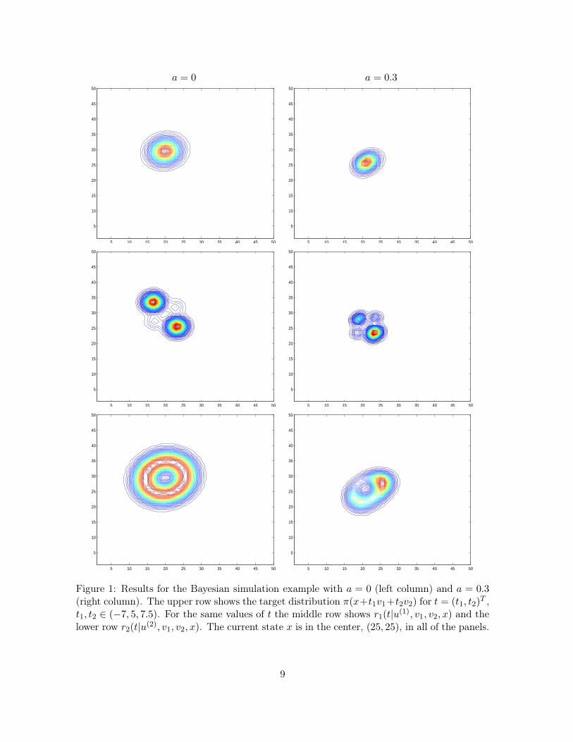
in Rn. In Figure 1 we show results for k = 2 when a = 0 (left column) and a = 0.3 (right

column). Thus, the target distribution is Gaussian in the left column and non-Gaussian in theright column. The upper row shows the target distribution π(x+ t1v1 + t2v2) for t = (t1, t2)

T ,t1, t2 ∈ (−7, 5, 7.5). For the same values of t the middle row shows r1(t|u

(1), v1, v2, x) andthe lower row r2(t|u

(2), v1, v2, x). The current state x is located in the center in all six plots.We see that in the lower row we get an O-shaped distribution. Comparing the upper andlower rows for a = 0 we observe that r2(t|u

(2), v1, v2, x) seem to follow the contours of thetarget distribution. Intuitively it seems reasonable that proposals to other parts of the targetdistribution with almost the same density as x should often be accepted with high probability.We observe this property also for a = 0.3, but here r2(t|u

(2), v1, v2, x) is not symmetrical.Note that the results in the lower row is in accordance with the observation made in Eidsvikand Tjelmeland (2006), namely that the proposal distributions for k = 1 typically have twomodes, one on each side of a high density area of the target distribution. Here we have ahigh density area of the target distribution in the center of the O-shaped distribution. Fora = 0, middle row, we see that the two largest modes are placed on each side of a high densityarea of the target distribution, one close to x and one on the other side of the high densityarea of the target distribution. Again this is accordance with Eidsvik and Tjelmeland (2006).

8

a = 0 a = 0.3

5 10 15 20 25 30 35 40 45 50

5

10

15

20

25

30

35

40

45

50

5 10 15 20 25 30 35 40 45 50

5

10

15

20

25

30

35

40

45

50

5 10 15 20 25 30 35 40 45 50

5

10

15

20

25

30

35

40

45

50

5 10 15 20 25 30 35 40 45 50

5

10

15

20

25

30

35

40

45

50

5 10 15 20 25 30 35 40 45 50

5

10

15

20

25

30

35

40

45

50

5 10 15 20 25 30 35 40 45 50

5

10

15

20

25

30

35

40

45

50

Figure 1: Results for the Bayesian simulation example with a = 0 (left column) and a = 0.3(right column). The upper row shows the target distribution π(x+t1v1+t2v2) for t = (t1, t2)

T ,t1, t2 ∈ (−7, 5, 7.5). For the same values of t the middle row shows r1(t|u

(1), v1, v2, x) and thelower row r2(t|u

(2), v1, v2, x). The current state x is in the center, (25, 25), in all of the panels.

9

Comparing the middle and lower rows for a = 0, we observe that the two largest modes in themiddle row are parts of the O-shaped distribution. This seem to be a general behaviour. Weobserve the same for a = 0.3. Thus, long jumps are possible with both g1(u|x) and g2(u|x),but we are loosing something in where we are able to propose potential new states by usingu(1) based on a non-unique basis relative to using u(2) that is based on a unique basis.

5 Bayesian simulation example

In this Section we analyse the behaviour of the algorithm based on g1(u(1)|x) introduced

above and compare the results with simpler MH algorithms. In turns out that the simulationsnecessary to calculate a satisfying approximation to (22) by using (25) is too expensive to beof any practical use. We again consider the Bayesian model for non-linear seismic inversiondefined in Section 5, but now let n = 30.

5.1 Approximating the unit acceptance rate proposal distribution

As the proposal distribution (17) is not analytically available we need to construct an approx-imation to it and use this as our proposal distribution. From the discussion in Section 4 weknow that the proposal distribution (17) typically contains two large modes, one close to t = 0and one further away from t = 0. Our strategy is to approximate (17) by a mixture of twoGaussian distributions.

To locate the large mode close to t = 0 we start a deterministic minimisation algorithm att = 0, searching for a local minimum for V (t) = − ln{q1(t|u

(1), x)}. Let µ0 denote the locationof local minimum found and let Σ0 = (∇2V (µ0))

−1 denote the inverse of the Hessian matrixevaluated at µ0. We use µ0 and Σ0 as the mean vector and covariance matrix, respectively, inthe first mixture component. We want to use a similar procedure to approximate the secondlarge mode in (17), but then need to use another starting value for t in the minimisationalgorithm. From the results discussed in Section 4 we know that the maximal value forπ(x +

∑ki=1 tiui) (as function of t) is located close to the line going through the two larger

local maxima of q1(t|u(1), x). Moreover, the maximal value for π(x +

∑ki=1 tiui) is located

between the two large local maxima of q1(t|u(1), x). A natural initial value for the second

minimisation run is therefore t = µ0 + 2(µπ − µ0), where µπ is the location of the localmaximum of π(x +

∑ki=1 tiui). Letting µ1 denote the location of the resulting second local

minimum found for V (t), and letting Σ1 = (∇2V (µ1))−1 denote the corresponding inverse

Hessian matrix, our approximation to q1(t|u(1), x) is

q1(t|u(1), x) =

q1(µ0|u(1), x)N(t;µ0,Σ0) + R · q1(µ1|u

(1), x)N(t;µ1,Σ1)

q1(µ0|u(1), x) + R · q1(µ1|u(1), x)(28)

where N(t;µ,Σ) is the density of the Gaussian distribution with mean vector µ and covariancematrix Σ evaluated at t, and R is a scalar constant that can make proposals to the mode faraway from the current state more or less likely. The results in Roberts et al. (1997) andRoberts and Rosenthal (1998) indicate that a value of R > 1 should be preferable. For a = 0simulations show that the acceptance rate is close to one for all choices of R. In this case it istherefore best always to propose the mode away from the current state, i.e. use a large valuefor R. For a 6= 0 the situation is more complicated. In all the simulations of the directionalMH algorithm we have tuned the parameter R to the optimal value in terms of mean jump

10

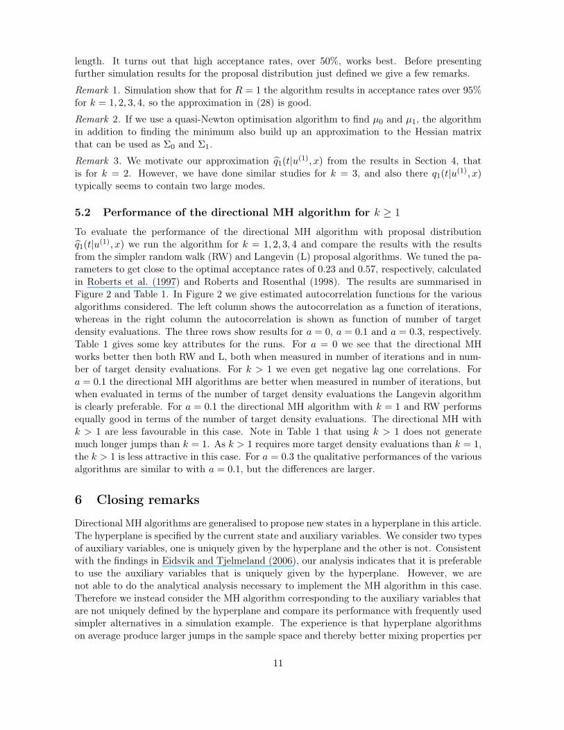
length. It turns out that high acceptance rates, over 50%, works best. Before presentingfurther simulation results for the proposal distribution just defined we give a few remarks.

Remark 1. Simulation show that for R = 1 the algorithm results in acceptance rates over 95%for k = 1, 2, 3, 4, so the approximation in (28) is good.

Remark 2. If we use a quasi-Newton optimisation algorithm to find µ0 and µ1, the algorithmin addition to finding the minimum also build up an approximation to the Hessian matrixthat can be used as Σ0 and Σ1.

Remark 3. We motivate our approximation q1(t|u(1), x) from the results in Section 4, that

is for k = 2. However, we have done similar studies for k = 3, and also there q1(t|u(1), x)

typically seems to contain two large modes.

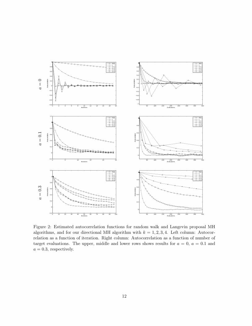
5.2 Performance of the directional MH algorithm for k ≥ 1

To evaluate the performance of the directional MH algorithm with proposal distributionq1(t|u

(1), x) we run the algorithm for k = 1, 2, 3, 4 and compare the results with the resultsfrom the simpler random walk (RW) and Langevin (L) proposal algorithms. We tuned the pa-rameters to get close to the optimal acceptance rates of 0.23 and 0.57, respectively, calculatedin Roberts et al. (1997) and Roberts and Rosenthal (1998). The results are summarised inFigure 2 and Table 1. In Figure 2 we give estimated autocorrelation functions for the variousalgorithms considered. The left column shows the autocorrelation as a function of iterations,whereas in the right column the autocorrelation is shown as function of number of targetdensity evaluations. The three rows show results for a = 0, a = 0.1 and a = 0.3, respectively.Table 1 gives some key attributes for the runs. For a = 0 we see that the directional MHworks better then both RW and L, both when measured in number of iterations and in num-ber of target density evaluations. For k > 1 we even get negative lag one correlations. Fora = 0.1 the directional MH algorithms are better when measured in number of iterations, butwhen evaluated in terms of the number of target density evaluations the Langevin algorithmis clearly preferable. For a = 0.1 the directional MH algorithm with k = 1 and RW performsequally good in terms of the number of target density evaluations. The directional MH withk > 1 are less favourable in this case. Note in Table 1 that using k > 1 does not generatemuch longer jumps than k = 1. As k > 1 requires more target density evaluations than k = 1,the k > 1 is less attractive in this case. For a = 0.3 the qualitative performances of the variousalgorithms are similar to with a = 0.1, but the differences are larger.

6 Closing remarks

Directional MH algorithms are generalised to propose new states in a hyperplane in this article.The hyperplane is specified by the current state and auxiliary variables. We consider two typesof auxiliary variables, one is uniquely given by the hyperplane and the other is not. Consistentwith the findings in Eidsvik and Tjelmeland (2006), our analysis indicates that it is preferableto use the auxiliary variables that is uniquely given by the hyperplane. However, we arenot able to do the analytical analysis necessary to implement the MH algorithm in this case.Therefore we instead consider the MH algorithm corresponding to the auxiliary variables thatare not uniquely defined by the hyperplane and compare its performance with frequently usedsimpler alternatives in a simulation example. The experience is that hyperplane algorithmson average produce larger jumps in the sample space and thereby better mixing properties per

11

a=

0

0 2 4 6 8 10 12 14 16 18 20−0.8

−0.6

−0.4

−0.2

0

0.2

0.4

0.6

0.8

1

Iterations

Auto

corre

latio

n

RWLk=1k=2k=3k=4

50 100 150 200 250 300 350 400

−1

−0.8

−0.6

−0.4

−0.2

0

0.2

0.4

0.6

0.8

1

Evaluations

Auto

corre

latio

n

RWLk=1k=2k=3k=4

a=

0.1

0 5 10 15 20 25−0.2

0

0.2

0.4

0.6

0.8

1

1.2

Iterations

Auto

corre

latio

n

RWLk=1k=2k=3k=4

50 100 150 200 250 300 350 400

0

0.2

0.4

0.6

0.8

1

Evaluations

Auto

corre

latio

n

RWLk=1k=2k=3k=4

a=

0.3

0 10 20 30 40 50 60 70 80 90 100−0.2

0

0.2

0.4

0.6

0.8

1

1.2

Iterations

Auto

corre

latio

n

RWLk=1k=2k=3k=4

50 100 150 200 250 300 350 400

0

0.2

0.4

0.6

0.8

1

Evaluations

Auto

corre

latio

n

RWLk=1k=2k=3k=4

Figure 2: Estimated autocorrelation functions for random walk and Langevin proposal MHalgorithms, and for our directional MH algorithm with k = 1, 2, 3, 4. Left column: Autocor-relation as a function of iteration. Right column: Autocorrelation as a function of number oftarget evaluations. The upper, middle and lower rows shows results for a = 0, a = 0.1 anda = 0.3, respectively.

12

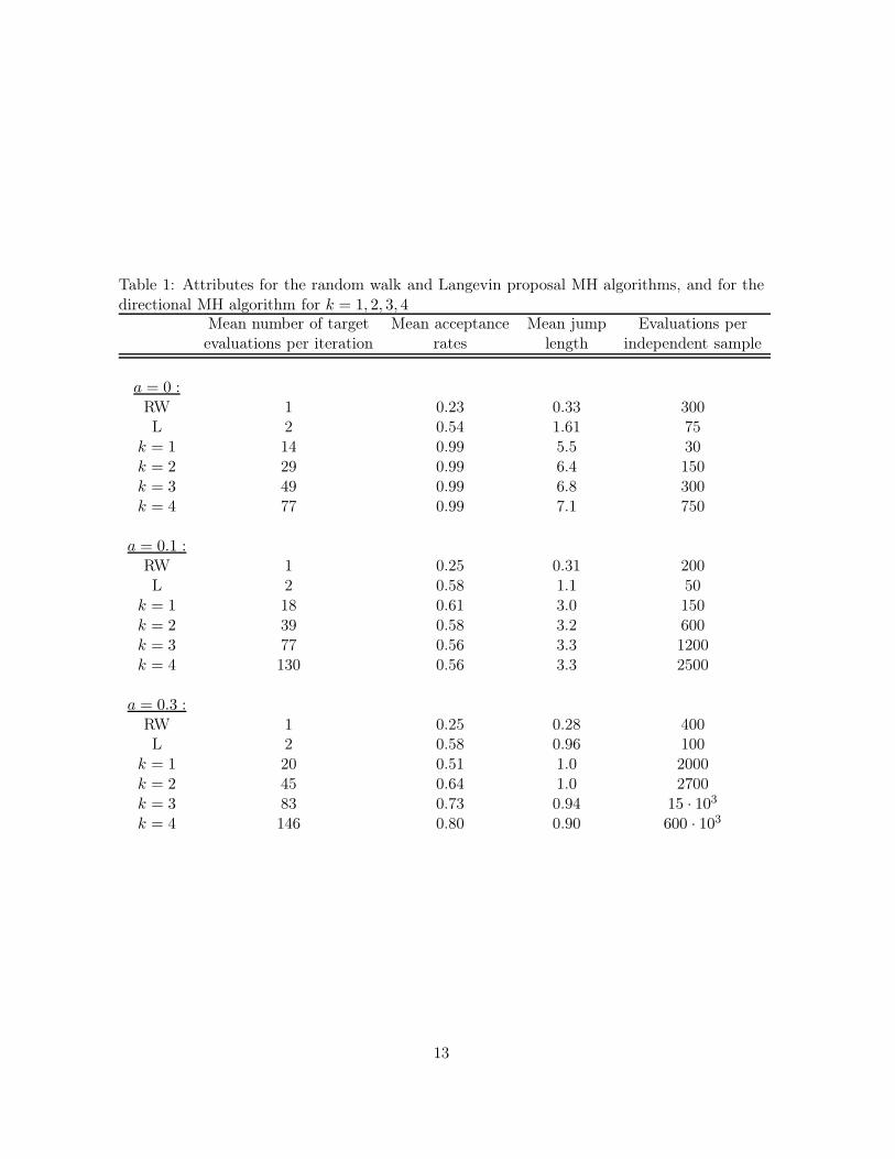
Table 1: Attributes for the random walk and Langevin proposal MH algorithms, and for thedirectional MH algorithm for k = 1, 2, 3, 4

Mean number of target Mean acceptance Mean jump Evaluations perevaluations per iteration rates length independent sample

a = 0 :RW 1 0.23 0.33 300L 2 0.54 1.61 75

k = 1 14 0.99 5.5 30k = 2 29 0.99 6.4 150k = 3 49 0.99 6.8 300k = 4 77 0.99 7.1 750

a = 0.1 :RW 1 0.25 0.31 200L 2 0.58 1.1 50

k = 1 18 0.61 3.0 150k = 2 39 0.58 3.2 600k = 3 77 0.56 3.3 1200k = 4 130 0.56 3.3 2500

a = 0.3 :RW 1 0.25 0.28 400L 2 0.58 0.96 100

k = 1 20 0.51 1.0 2000k = 2 45 0.64 1.0 2700k = 3 83 0.73 0.94 15 · 103

k = 4 146 0.80 0.90 600 · 103

13

iteration. However, in our implementation the hyperplane algorithms is more computationintensive per iteration and so the simpler algorithms in most cases are preferable when run forthe same amount of computation time. An interesting area for future research is therefore tofind variants of our directional Metropolis–Hastings algorithm that require less computationtime per iteration.

14

References

Chen, M. and Schmeiser, B. (1993). Performance of the Gibbs, hit-and-run and Metropolissamplers, Journal of computational and graphical statistics 2: 251–272.

Eidsvik, J. and Tjelmeland, H. (2006). On directional Metropolis–Hastings algorithms, Statis-

tics and Computing 16: 93–106.

Gilks, W. R., Roberts, G. O. and George, E. I. (1994). Adaptive directional sampling, The

Statistician 43: 179–189.

Goodman, J. and Sokal, A. D. (1989). Multigrid Monte Carlo method. Conceptual foundations,Physical Review D 40: 2035–2072.

Green, P. (1995). Reversible jump Markov chain Monte Carlo computations and Bayesianmodel determination, Biometrica 57: 97–109.

Hastings, W. (1970). Monte Carlo sampling using Markov chains and their applications,Biometrica 57: 97–109.

Liu, J. S. and Sabatti, C. (2000). Generalized Gibbs sampler and multigrid Monte Carlo forBayesian computation, Biometrika 87: 353–369.

Metropolis, N., Rosenbluth, A. W., Rosenbluth, M. N., Teller, A. H. and Teller, E. (1953).Equation of state calculations by fast computing machines, Journal of Chemical Physics

21: 1087–1092.

Pukkila, T. M. and Rao, C. R. (1988). Pattern recognition based on scale invariant discrimi-nant functions, Information sciences 45: 379–389.

Rabben, T. E., Tjelmeland, H. and Ursin, B. (2008). Nonlinear Bayesian joint inversion ofseismic reflection coefficients, Geophysical Journal International p. To appear.

Roberts, G. O., Gelman, A. and Gilks, W. R. (1997). Weak convergence and optimal scalingof random walk Metropolis algorithms, Annals of Applied Probability 7: 110–120.

Roberts, G. O. and Gilks, W. R. (1994). Convergence of adaptive directional sampling, Journal

of multivariate analysis 49: 287–298.

Roberts, G. O. and Rosenthal, J. S. (1998). Optimal scaling of discrete approximations toLangevin diffusions, Journal of the Royal Statistical Society. Series B 60: 255–268.

Waagepetersen, R. and Sørensen, D. (2001). A tutorial on reversible jump MCMC with aview toward application in QTL-mapping, International Statistical Review 69: 49–61.

Watson, G. S. (1983). Statistics on spheres, Wiley-Interscience.

15