COMPUTER PROGRAM FOR DIRECTIONAL DRILLING ...
120
ن الرحيم الرحم بسمUniversity of Khartoum Faculty of Engineering Department of Petroleum and Natural Gas This project is submitted as a partial requirement for the degree of B.Sc. in Petroleum Engineering Presented by: Supervised by: Mojahid Abualgasim Musa (108012) Eng. Mohammed Ahmed Hamid Mosab Mohammed Ahmed (108020) Co-Supervised by: Mohammed Ahmed Yusuf (108013) Prof. Hassan Bashir Nimir July 2015 COMPUTER PROGRAM FOR DIRECTIONAL DRILLING DESIGN
-
Upload
khangminh22 -
Category
Documents
-
view
0 -
download
0
Transcript of COMPUTER PROGRAM FOR DIRECTIONAL DRILLING ...
بسم هللا الرحمن الرحيم
University of Khartoum
Faculty of Engineering
Department of Petroleum and Natural Gas
This project is submitted as a partial requirement for
the degree of B.Sc. in Petroleum Engineering
Presented by: Supervised by:
Mojahid Abualgasim Musa (108012) Eng. Mohammed Ahmed Hamid
Mosab Mohammed Ahmed (108020) Co-Supervised by:
Mohammed Ahmed Yusuf (108013) Prof. Hassan Bashir Nimir
July 2015
COMPUTER PROGRAM FOR
DIRECTIONAL DRILLING DESIGN

I
Dedication
This project is dedicated to
our families
teachers
colleagues
and all who helped us to achieve this work.
Thanks to you all.

II
Acknowledgement
Our first thanks is be to Allah who has given us enough knowledge, intelligence and strength to produce
this work and contribute to a better understanding of Directional Drilling.
Thanks to our parents who used to support us.
Thanks are also conducted to:-
Eng. MOHAMMED AHMED, our supervisor
Prof. HASSAN BASHIR NIMIR for his advice and assistance.
Mr. QUOSAY AWAD AHMAD.
Eng. BASHAR MAGZOUB (GNPOC).
Eng. AYMEN MOHAMMED (GNPOC).
Staff of Petroleum engineering department.
And any one helped us to finish this project.

III
Abstract
Directional drilling is a very costly and complicated operation and so every step during this operation
must be well planned and designed accurately , because any mistakes will lead to a great loss of time , money
and effort , and by designing this software we are trying to avoid these mistakes.
The objective of this project is to achieve all necessary survey calculations of the well trajectory design
for all the directional drilling well profiles, in addition to give the user a clear visualization of the well trajectory
through plotting of chart in top view and side view as well as 3D chart for survey and plan purposes.
A software called CDD (Computerized Directional Drilling) employing the minimum curvature method
was developed to achieve these calculations and therefore minimize the uncertainty and risks related to hitting a
predetermined target.
Then a case study was made to determine the accuracy of the software, and then economic analysis was
made to show the effect of directional drilling on the drilling economics.
IV
Table of Contents
Dedication ................................................................................................................................................... I
Acknowledgement .................................................................................................................................... II
Abstract .................................................................................................................................................... III
Table of Contents .................................................................................................................................... IV
Table of Tables ...................................................................................................................................... VII
Table of Figures.................................................................................................................................... VIII
Chapter 1 : Introduction:- ..................................................................................................................... 2
Chapter 2 : literature Review ................................................................................................................ 6
2.1- Introduction:-................................................................................................................................... 6
2.2- History:-........................................................................................................................................... 6
2.3- Application:- .................................................................................................................................... 7
2.4- Well Planning:-................................................................................................................................ 7
2.4.1- Well trajectory planning:- ......................................................................................................... 7
2.4.2- Features of a Directional Well Profile:- ................................................................................. 12
2.4.3- CONSIDERATIONS WHEN PLANNING THE DIRECTIONAL WELL PATH:- ............ 18
2.5- Deflection Tools ............................................................................................................................. 18
2.6- Survey tools:- ................................................................................................................................. 20
2.7- SURVEY CALCULATIONS:- ........................................................................................................ 21
2.7.1- Tangential :- ............................................................................................................................ 22
2.7.2- Balanced Tangential :- ............................................................................................................ 22
2.7.3- Average angle ......................................................................................................................... 23
2.7.4- Radius of curvature :- ............................................................................................................. 24
2.7.5- Minimum curvature ................................................................................................................ 26

V
2.8- Dogleg severity :- .......................................................................................................................... 27
Chapter 3 : Methodology ..................................................................................................................... 29
3.1- Introduction:-................................................................................................................................. 29
3.2- The steps:-...................................................................................................................................... 29
3.2.1- The first step :- ........................................................................................................................ 29
3.2.2- Step two:- ................................................................................................................................ 30
3.2.3- Step three:- .............................................................................................................................. 31
3.2.4- Step four:- ............................................................................................................................... 31
3.3- The Program:- ............................................................................................................................... 32
3.3.1- The loading screen:- ............................................................................................................... 32
3.3.2- The main menu ....................................................................................................................... 33
3.3.3- The New line Feature:- ........................................................................................................... 59
Chapter 4 : Results and discussions.................................................................................................... 63
4.1- Introduction :-................................................................................................................................ 63
4.2- Case Studies:- ................................................................................................................................ 63
4.2.1- Well OCS-G-31376:- .............................................................................................................. 63
4.2.2- Well Waldock Federal 14-4-3XH:- ........................................................................................ 70
4.2.3- Well OCS-G 25994 Well #2:- ................................................................................................ 77
4.2.4- Well N024 ICS-G-016 in Gulf of Mexico USA:- .................................................................. 84
Chapter 5 : Economic Analysis ........................................................................................................... 92
5.1- Introduction:-................................................................................................................................. 92
5.2- Cost and risk associated with directional drilling : ...................................................................... 92
5.2.1- Field Economic Cumulative Production: ............................................................................... 93
5.3- Considerations during Surveying:- ............................................................................................... 94
Chapter 6 : Conclusion and recommendation ................................................................................... 97

VI
6.1- Conclusion:- .................................................................................................................................. 97
6.2- Recommendation:- ......................................................................................................................... 98
References:- ............................................................................................................................................. 99
APPENDIX -A- ..................................................................................................................................... 100

VII
Table of Tables
Table 3-1(Comparison of accuracy of five methods) ................................................................................................................ 30 Table 4-1(Sample of Wellbore Trajectory Results from OCS-G-31376 well) .......................................................................... 64 Table 4-2(Sample of Wellbore Trajectory Results from CDD) ................................................................................................. 66 Table 4-3(A Comparative Results between the (OCS-G-31376) well and the CDD Program) ................................................. 68 Table 4-4(Wellbore Trajectory Results from Waldock Federal 14-4-3XH well) ...................................................................... 71 Table 4-5(Wellbore Trajectory Results from CDD) .................................................................................................................. 73 Table 4-6(A Comparative Results between the Waldock Federal well and the CDD Program) ............................................... 75 Table 4-7(Sample of Wellbore Trajectory Results from OCS-G 25994 Well #2 well) ............................................................. 78 Table 4-8(Sample of Wellbore Trajectory Results from CDD) ................................................................................................. 80 Table 4-9(A Comparative Results between the Waldock Federal well and the CDD Program) ............................................... 82 Table 4-10(Well N024 ICS-G-016 survey data) ........................................................................................................................ 85 Table 4-11(Input given data into well type data section) ........................................................................................................... 86 Table 4-12(Wellbore Trajectory Results from CDD) ................................................................................................................ 87 Table 4-13(A Comparative Results between the Waldock Federal well and the CDD Program) ............................................. 89 Table 5-1(production simulation for the vertical and horizontal well cases) ............................................................................. 94
VIII
Table of Figures
Figure 2-1 (Applications of Directional Drilling) ........................................................................................................................ 7 Figure 2-2(Build and Hold) ......................................................................................................................................................... 8 Figure 2-3((Build, Hold, partial Drop and Hold (modified S-shape)) ......................................................................................... 9 Figure 2-4(Build, Hold and Drop (S-shape)) ............................................................................................................................. 10 Figure 2-5(Continues Build) ...................................................................................................................................................... 11 Figure 2-6(Horizontal Drilling) ................................................................................................................................................. 11 Figure 2-7 (kick Off Point) ........................................................................................................................................................ 12 Figure 2-8 (Well Inclination) ..................................................................................................................................................... 13 Figure 2-9 (End of Buildup) ...................................................................................................................................................... 13 Figure 2-10 (Hole Angle) .......................................................................................................................................................... 14 Figure 2-11 (Tangent Section) ................................................................................................................................................... 14 Figure 2-12 (Start of Drop) ........................................................................................................................................................ 15 Figure 2-13 (End of Drop) ......................................................................................................................................................... 15 Figure 2-14 (Target Displacement)............................................................................................................................................ 16 Figure 2-15(survey features) ...................................................................................................................................................... 17 Figure 2-16(Whipstocks) Figure 2-17(Bent sub) ............................................................. 19 Figure 2-18(Jetting action) Figure 2-19(Steerable Positive Displacement Motor) ...................................................... 19 Figure 2-20(Directional Bottom Hole Assemblies) ................................................................................................................... 20 Figure 2-21 (Magnetic single – shot) Figure 2-22 (Magnetic multi –shots) ...................................................... 20 Figure 2-23 (Measurement while drilling) Figure 2-24 (Gyro survey tool) ............................................................ 21 Figure 2-25(Tangential method) ................................................................................................................................................ 22 Figure 2-26 (Balanced Tangential method) ............................................................................................................................... 23 Figure 2-27 (Average Angle method) ........................................................................................................................................ 24 Figure 2-28 (Radius of curvature method) ................................................................................................................................ 25 Figure 2-29(Minimum curvature method) ................................................................................................................................. 26 Figure 3-1(Program flow diagram) ............................................................................................................................................ 29 Figure 3-2 (Loading screen) ...................................................................................................................................................... 32 Figure 3-3 (Main menu) ............................................................................................................................................................ 33 Figure 3-4 (Manage Wells) ........................................................................................................................................................ 34 Figure 3-5 (Data section) ........................................................................................................................................................... 35 Figure 3-6 (Well mode) ............................................................................................................................................................. 36 Figure 3-7 (Well type data section) ........................................................................................................................................... 37 Figure 3-8 (Complex type) ........................................................................................................................................................ 39 Figure 3-9 (Table section) ......................................................................................................................................................... 40 Figure 3-10(Export Excel) ......................................................................................................................................................... 41 Figure 3-11 (Export to PDF)...................................................................................................................................................... 42 Figure 3-12(Print preview) ........................................................................................................................................................ 43 Figure 3-13(Table Printed as PDF) ............................................................................................................................................ 44 Figure 3-14(Chart section) ......................................................................................................................................................... 45 Figure 3-15(The side view chart) .............................................................................................................................................. 46 Figure 3-16(Export side view chart to picture) .......................................................................................................................... 47 Figure 3-17 (Top view chart) ..................................................................................................................................................... 48 Figure 3-18(Export top view chart to picture) ........................................................................................................................... 49 Figure 3-19(Tool box) ............................................................................................................................................................... 49 Figure 3-20(3D Graph of well trajectory) .................................................................................................................................. 50 Figure 3-21(More detailed side view chart)............................................................................................................................... 51 Figure 3-22(More detailed top view chart) ................................................................................................................................ 52 Figure 3-23(The header) ............................................................................................................................................................ 52 Figure 3-24(Tool menu) ............................................................................................................................................................ 54
IX
Figure 3-25 (Tips activated) ...................................................................................................................................................... 54 Figure 3-26(Help menu) ............................................................................................................................................................ 54 Figure 3-27(Content help window)............................................................................................................................................ 55 Figure 3-28(Index window) ....................................................................................................................................................... 55 Figure 3-29(The about window) ................................................................................................................................................ 56 Figure 3-30 (The footer) ............................................................................................................................................................ 57 Figure 3-31 (Free model) ........................................................................................................................................................... 58 Figure 3-32(New line not activated) .......................................................................................................................................... 59 Figure 3-33(New line activated) ................................................................................................................................................ 59 Figure 3-34 (Different well trajectories are plotted in the same side and top view chart) ......................................................... 60 Figure 3-35(different well trajectories are plotted in the same 3D Graph) ................................................................................ 60 Figure 3-36(different well trajectories are plotted in the same detailed side view chart) .......................................................... 61 Figure 3-37(different well trajectories are plotted in the same detailed top view chart) ........................................................... 61 Figure 4-1(Survey Data from Walter Gas and Oil Corporation) ............................................................................................... 63 Figure 4-2(Data input into well type data section) .................................................................................................................... 65 Figure 4-3(The output results from the data input) .................................................................................................................... 65 Figure 4-4(Top view chart of the well trajectory) ..................................................................................................................... 67 Figure 4-5(Side view chart of the well trajectory) ..................................................................................................................... 67 Figure 4-6(3D view chart of the well trajectory) ....................................................................................................................... 68 Figure 4-7(EXCEL comparison between CDD results and the well data in side view) ............................................................ 69 Figure 4-8(EXCEL comparison between CDD results and the well data in top view) .............................................................. 69 Figure 4-9(Survey Data from Whiting Oil and Gas Corporation) ............................................................................................. 70 Figure 4-10(Data input into well type data section) .................................................................................................................. 72 Figure 4-11(The output results from the data input) .................................................................................................................. 72 Figure 4-12(Top view chart of well trajectory) ......................................................................................................................... 74 Figure 4-13(Side view chart of the well trajectory) ................................................................................................................... 74 Figure 4-14(3D view chart of the well trajectory) ..................................................................................................................... 75 Figure 4-15(EXCEL comparison between CDD results and the well data in side view) .......................................................... 76 Figure 4-16 (EXCEL comparison between CDD results and the well data in top view) ........................................................... 76 Figure 4-17(Survey Data from Energy Partners Ltd) ................................................................................................................ 77 Figure 4-18(Data input into well type data section) .................................................................................................................. 79 Figure 4-19(The output results from the data input) .................................................................................................................. 79 Figure 4-20(Top view chart of the well trajectory) ................................................................................................................... 81 Figure 4-21(Side view chart of the well trajectory) ................................................................................................................... 81 Figure 4-22(3D view chart of the well trajectory) ..................................................................................................................... 82 Figure 4-23(EXCEL comparison between CDD results and the well data in side view) .......................................................... 83 Figure 4-24(EXCEL comparison between CDD results and the well data in top view) ............................................................ 83 Figure 4-25 (Survey Data from EXXONMOBIL company) ..................................................................................................... 84 Figure 4-26(Top view chart of well trajectory) ......................................................................................................................... 88 Figure 4-27(side view chart of well trajectory) ......................................................................................................................... 88 Figure 4-28(3D view chart of well trajectory) ........................................................................................................................... 89 Figure 4-29(EXCEL comparison between CDD results and the well data in side view) .......................................................... 90 Figure 4-30(EXCEL comparison between CDD results and the well data in top view) ............................................................ 90 Figure 5-1(Vertical, directional and horizontal drilling costs) .................................................................................................. 93

1
Chapter one:
Introduction

2
Chapter 1 : Introduction:-
Directional drilling has become a commonly very important technology in petroleum industry, with
large reservoir contact area. Directional wells can greatly improve well productivity and effectiveness to deal
with problems. It will cost more to drill and complete directional well than a vertical well, but smaller numbers
of wells are necessary to develop a field with positive effects both on the global costs and on the environment.
The calculations can be done manually, but in reality; many different trajectories may have to be
inspected in order to minimize potential drilling problems. These problems may contain excessive torque and
drag, differential sticking and borehole instability. Each time KOP or build-up rate are changed, this will require
calculating and plotting a new trajectory.
The best way to handle these repetitive calculations is by using computers, which are becoming more
common and essential part in drilling operations. When planning wells from large offshore platforms, such
computer techniques are necessary to deal with the large amount of data and plan the wells efficiently.
several operating companies have their own private programs, and many computer packages are
available from directional drilling service companies, these programs save a lot of time and can offer many
useful features :-
(a) The computer package is capable of calculating the well plans quickly and accurately for different
combinations of kick-off point, build-up rates...etc. The actual coordinates along the planned trajectory can be
calculated at fixed intervals (e.g. 100 ft.). It can also plot large-scale of each trajectory which can be used to
compare the different options.
(b) The computer comes with a big memory that can be used to save the survey data from existing wells,
the future trajectories of the wells to be drilled can also be saved in the computer. By displaying the related data
files, the specific well being planned can be viewed in relation to other nearby wells. Plots displaying specific
well overlaying another in both top and side view can be generated.
3
(c) While the well is being drilled, the survey data from the well can be analyzed by the computer,
which will thereafter compare the planned trajectory with the calculated actual trajectory. In addition to that the
dog-leg severity can also be calculated to evaluate the bends in the trajectory.
(d) After calculating the actual location of the well being drilled, the computer can also determine the
distance and direction from that point to any nearby wells, then plots can be made to give a visual representation
of how close adjacent wellbores are to the specific well . These plots can be used during the well is drilled or at
the planning stage, to prevent any probable intersections.
Objectives :-
The objectives of this project are to design computer software that is capable of:-
1- Calculate the survey data of the well trajectory for all directional drilling well types.
2- Compute the actual coordinates along the planned trajectory at regular intervals.
3- Design plots to show the well trajectory in 2D charts in both top view and side view.
4- Design 3D graph for more visual representation of the well trajectory.
5- The capability to compare different well trajectories, and show them side by side in the same charts.
6- The ability to save the well input data in the database section in order to later retrieval.
7- Export the calculated data into various formats e.g. (Excel, PDF …)
Thesis layouts:-
Chapter one is introduction about the project and the objectives to be accomplished.
Chapter two is a literature review about directional drilling including a brief history about directional
drilling, its applications and survey calculations.
Chapter three includes the steps and the methods used to achieve the objectives of the project which
were discussed. And a detailed description about the program and all its features and sections.

4
Chapter four discusses the results obtained from the program using real field data by making four case
studies and then compares the results from the program and the field data.
Chapter five is economic analysis to show the benefits of the program in relation to the directional
drilling economics.
Chapter six includes conclusion and recommendations for future work to be done in order to enhance
this project.

5
Chapter Two:
Literature Review
6
Chapter 2 : literature Review
2.1- Introduction:-
Directional drilling is the science and art of deviating a wellbore along a planned course to a subsurface
target whose location is a given lateral distance and direction from the vertical [1]. Drilling a directional well
basically involves drilling a hole from one point in space (the surface location) to another point in space (the
target) in such a way that the hole can then be used for its intended purpose.
Directional and horizontal drilling are high-risk drilling operations compared to vertical drilling and
efficient drilling programs must be designed carefully. [2]
2.2- History:-
In the early days of land drilling most wells were drilled vertically, straight down into the reservoir.
Although these wells were considered to be vertical, they rarely were.
Some deviation in a wellbore will always occur, due to formation effects and bending of the drill string.
The first recorded instance of a well being deliberately drilled along a deviated course was in California in
1930. This well was drilled to exploit a reservoir which was beyond the shoreline underneath the Pacific Ocean.
It had been the practice to build jetties out into the ocean and build the drilling rig on the jetty. However, this
became prohibitively expensive and the technique of drilling deviated wells was developed. Since then many
new techniques and special tools have been introduced to control the path of the wellbore. [3]
7
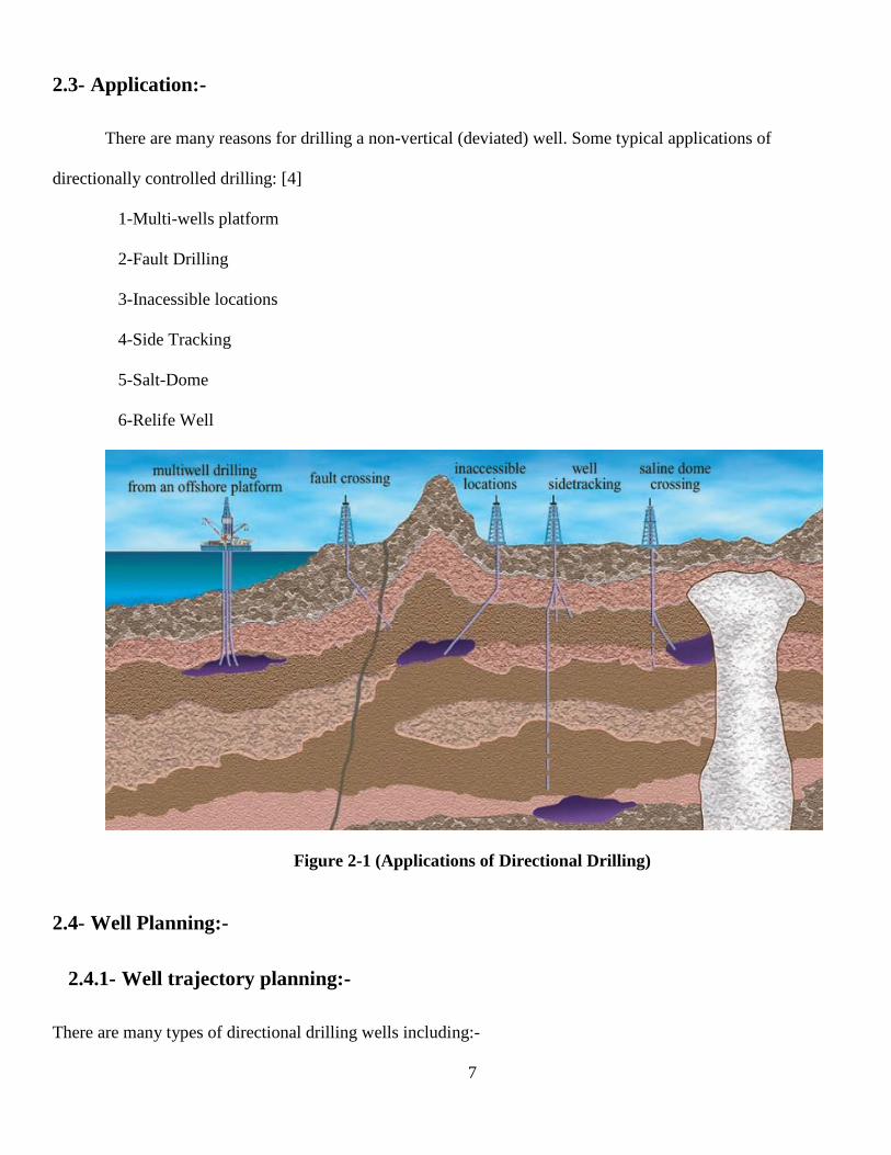
2.3- Application:-
There are many reasons for drilling a non-vertical (deviated) well. Some typical applications of
directionally controlled drilling: [4]
1-Multi-wells platform
2-Fault Drilling
3-Inacessible locations
4-Side Tracking
5-Salt-Dome
6-Relife Well
Figure 2-1 (Applications of Directional Drilling)
2.4- Well Planning:-
2.4.1- Well trajectory planning:-
There are many types of directional drilling wells including:-
8
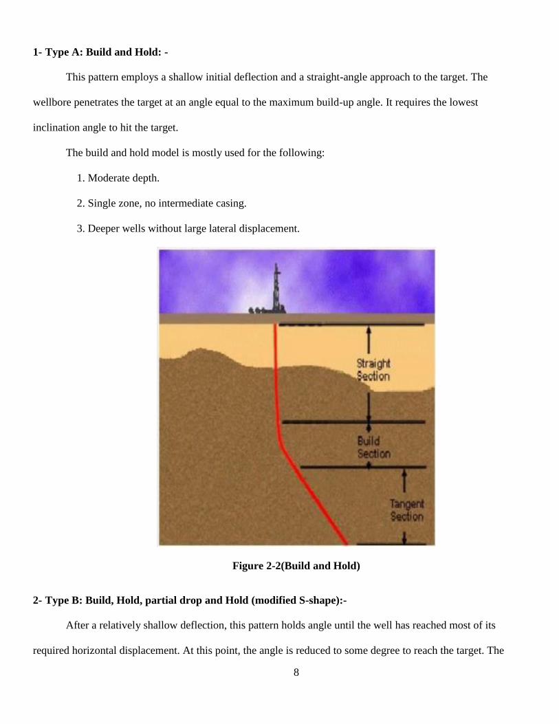
1- Type A: Build and Hold: -
This pattern employs a shallow initial deflection and a straight-angle approach to the target. The
wellbore penetrates the target at an angle equal to the maximum build-up angle. It requires the lowest
inclination angle to hit the target.
The build and hold model is mostly used for the following:
1. Moderate depth.
2. Single zone, no intermediate casing.
3. Deeper wells without large lateral displacement.
Figure 2-2(Build and Hold)
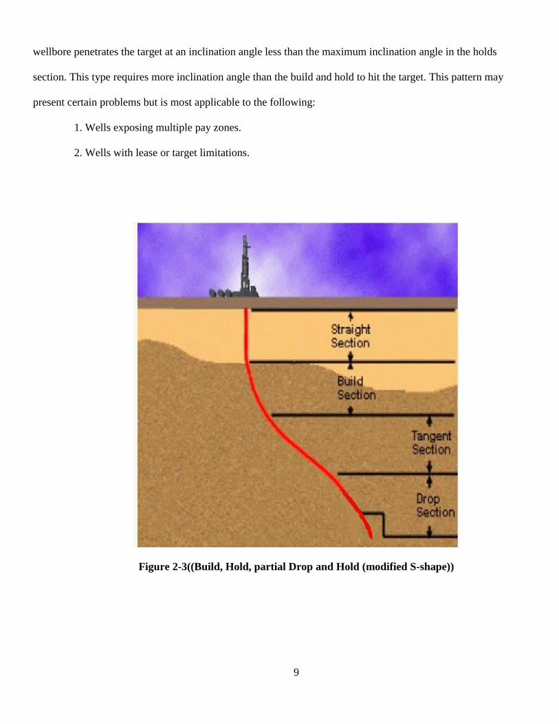
2- Type B: Build, Hold, partial drop and Hold (modified S-shape):-
After a relatively shallow deflection, this pattern holds angle until the well has reached most of its
required horizontal displacement. At this point, the angle is reduced to some degree to reach the target. The
9
wellbore penetrates the target at an inclination angle less than the maximum inclination angle in the holds
section. This type requires more inclination angle than the build and hold to hit the target. This pattern may
present certain problems but is most applicable to the following:
1. Wells exposing multiple pay zones.
2. Wells with lease or target limitations.
Figure 2-3((Build, Hold, partial Drop and Hold (modified S-shape))
10
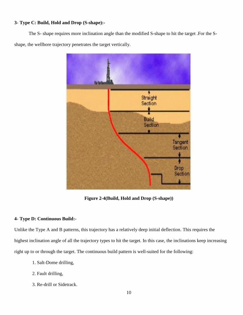
3- Type C: Build, Hold and Drop (S-shape):-
The S- shape requires more inclination angle than the modified S-shape to hit the target .For the S-
shape, the wellbore trajectory penetrates the target vertically.
Figure 2-4(Build, Hold and Drop (S-shape))
4- Type D: Continuous Build:-
Unlike the Type A and B patterns, this trajectory has a relatively deep initial deflection. This requires the
highest inclination angle of all the trajectory types to hit the target. In this case, the inclinations keep increasing
right up to or through the target. The continuous build pattern is well-suited for the following:
1. Salt-Dome drilling,
2. Fault drilling,
3. Re-drill or Sidetrack.
11
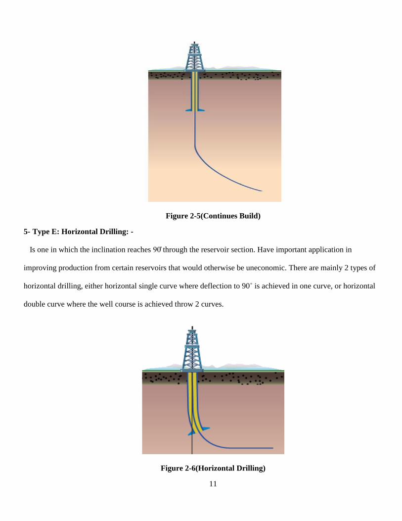
Figure 2-5(Continues Build)
5- Type E: Horizontal Drilling: -
Is one in which the inclination reaches 90̊ through the reservoir section. Have important application in
improving production from certain reservoirs that would otherwise be uneconomic. There are mainly 2 types of
horizontal drilling, either horizontal single curve where deflection to 90˚ is achieved in one curve, or horizontal
double curve where the well course is achieved throw 2 curves.
Figure 2-6(Horizontal Drilling)

12
There are some directional well designs that do not fit any of the above types. A term that is frequently
used is “Designer Wells”. Designer/Complex wells are wells that with several targets and the targets are widely
spaced. They require significant changes in azimuth along with changes in inclination and have a highly
engineered well plan.
2.4.2- Features of a Directional Well Profile:-
A directional well profile is the planned well trajectory from the surface to the final drilling depth by
projecting the wellbore onto two plotted planes. In order to determine the best geometric well profile from the
surface to the bottom hole target, the following information must be known: [5]
The position of the surface location.
The position of the target location.
The True Vertical Depth (TVD).
1- Kickoff Point (KOP):-
The kickoff point is the location at a given depth below the surface where the wellbore is deviated in a
given direction.
Figure 2-7 (kick Off Point)
13
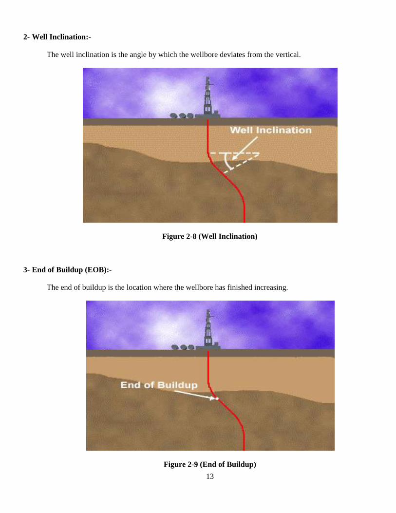
2- Well Inclination:-
The well inclination is the angle by which the wellbore deviates from the vertical.
Figure 2-8 (Well Inclination)
3- End of Buildup (EOB):-
The end of buildup is the location where the wellbore has finished increasing.
Figure 2-9 (End of Buildup)
14
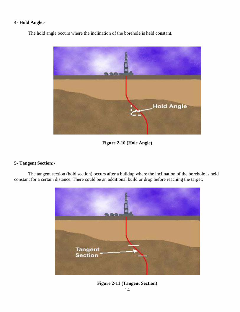
4- Hold Angle:-
The hold angle occurs where the inclination of the borehole is held constant.
Figure 2-10 (Hole Angle)
5- Tangent Section:-
The tangent section (hold section) occurs after a buildup where the inclination of the borehole is held
constant for a certain distance. There could be an additional build or drop before reaching the target.
Figure 2-11 (Tangent Section)
15
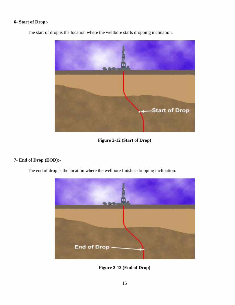
6- Start of Drop:-
The start of drop is the location where the wellbore starts dropping inclination.
Figure 2-12 (Start of Drop)
7- End of Drop (EOD):-
The end of drop is the location where the wellbore finishes dropping inclination.
Figure 2-13 (End of Drop)
16
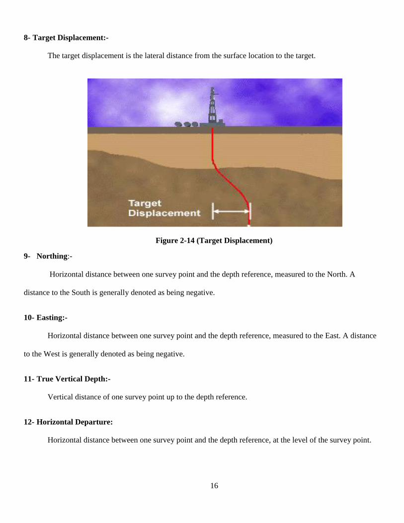
8- Target Displacement:-
The target displacement is the lateral distance from the surface location to the target.
Figure 2-14 (Target Displacement)
9- Northing:-
Horizontal distance between one survey point and the depth reference, measured to the North. A
distance to the South is generally denoted as being negative.
10- Easting:-
Horizontal distance between one survey point and the depth reference, measured to the East. A distance
to the West is generally denoted as being negative.
11- True Vertical Depth:-
Vertical distance of one survey point up to the depth reference.
12- Horizontal Departure:
Horizontal distance between one survey point and the depth reference, at the level of the survey point.
17
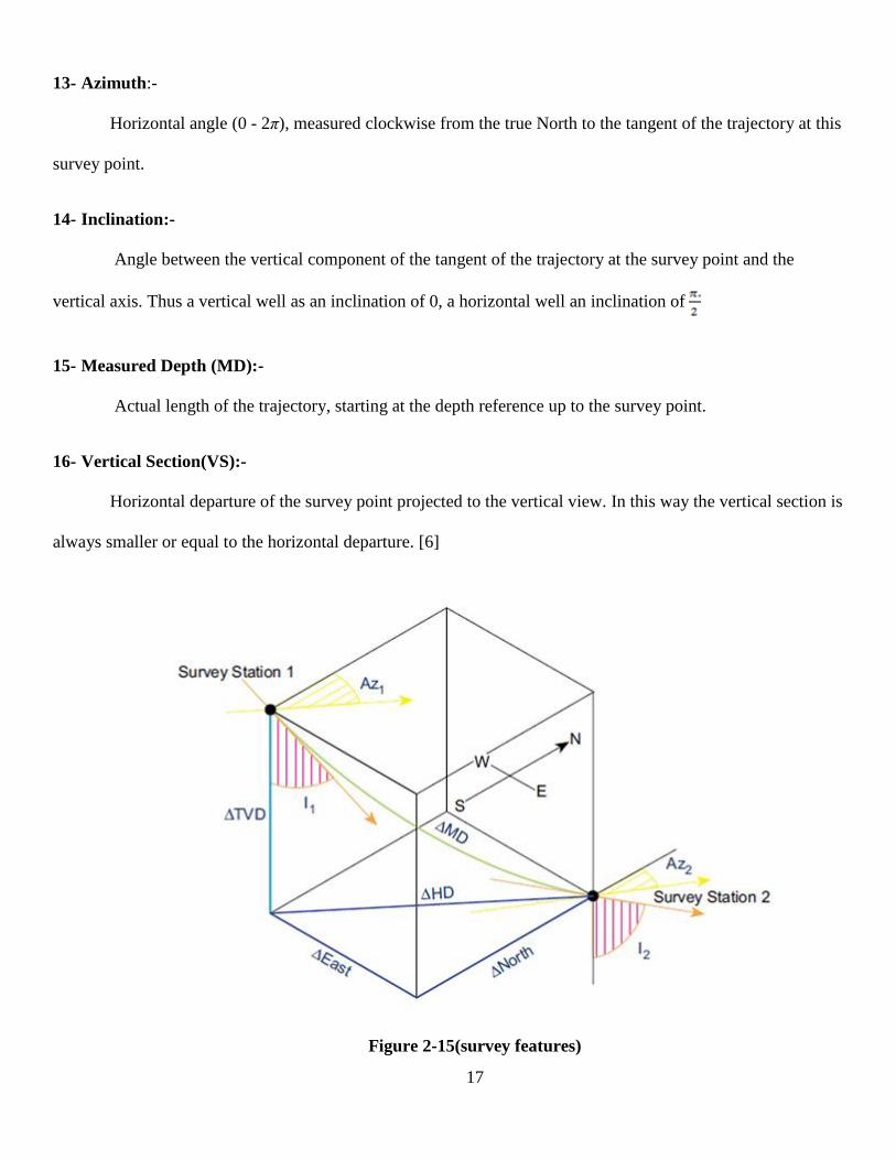
13- Azimuth:-
Horizontal angle (0 - 2π), measured clockwise from the true North to the tangent of the trajectory at this
survey point.
14- Inclination:-
Angle between the vertical component of the tangent of the trajectory at the survey point and the
vertical axis. Thus a vertical well as an inclination of 0, a horizontal well an inclination of
15- Measured Depth (MD):-
Actual length of the trajectory, starting at the depth reference up to the survey point.
16- Vertical Section(VS):-
Horizontal departure of the survey point projected to the vertical view. In this way the vertical section is
always smaller or equal to the horizontal departure. [6]
Figure 2-15(survey features)
18
2.4.3- CONSIDERATIONS WHEN PLANNING THE DIRECTIONAL WELL PATH:-
When planning a directional well a number of technical constraints and issues will have to be
considered. These will include the:-
Target location.
Target size and shape.
Surface location (rig location).
Subsurface obstacles (adjacent wells, faults etc.).
In conjunction with the above constraints the following factors must be considered in the geometrical
design of the well:-
• Casing and mud programmes.
• Geological section.
2.5- Deflection Tools
When the well trajectory has been designed, a deflection tool, which can be used to achieve that
trajectory, must be selected. There are a number of such tools available to the engineer but they all work on
basically the same principal.
These are that the bit will only depart from its trajectory - change direction - if either, a force is applied
to the side of the bit (known as a side force) or the bit is inclined with respect to the axis of the drillstring
(known as bit tilt angle).
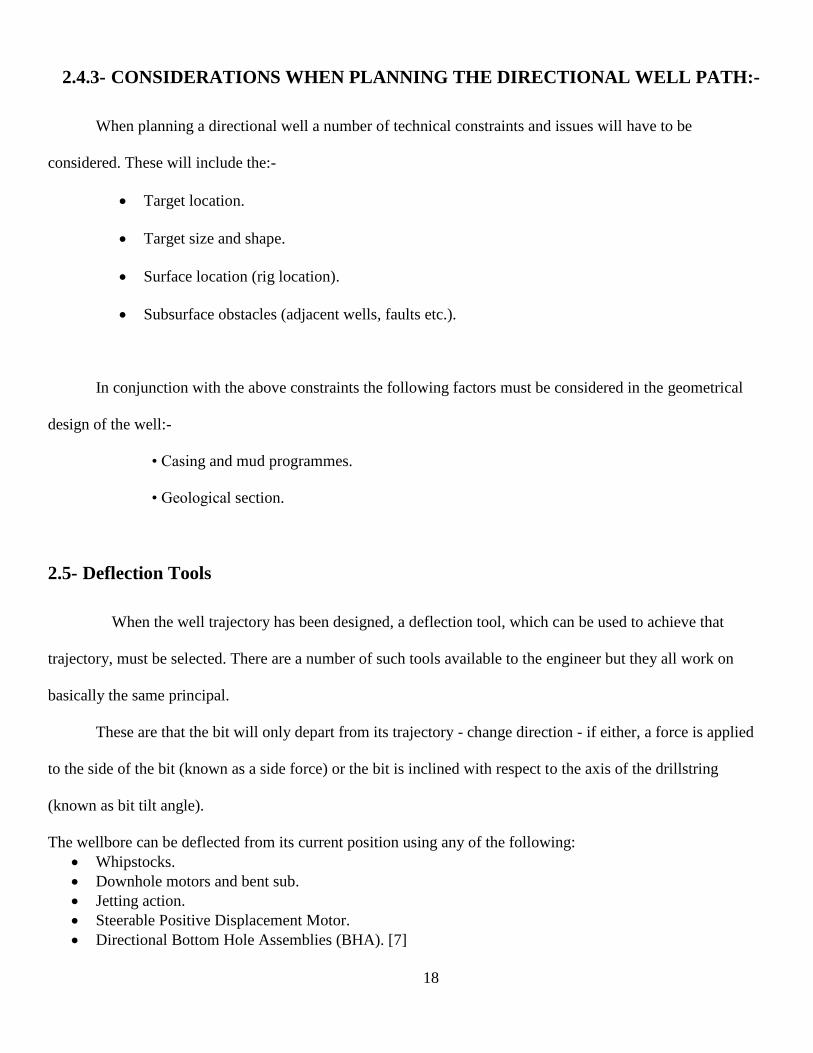
The wellbore can be deflected from its current position using any of the following:
Whipstocks.
Downhole motors and bent sub.
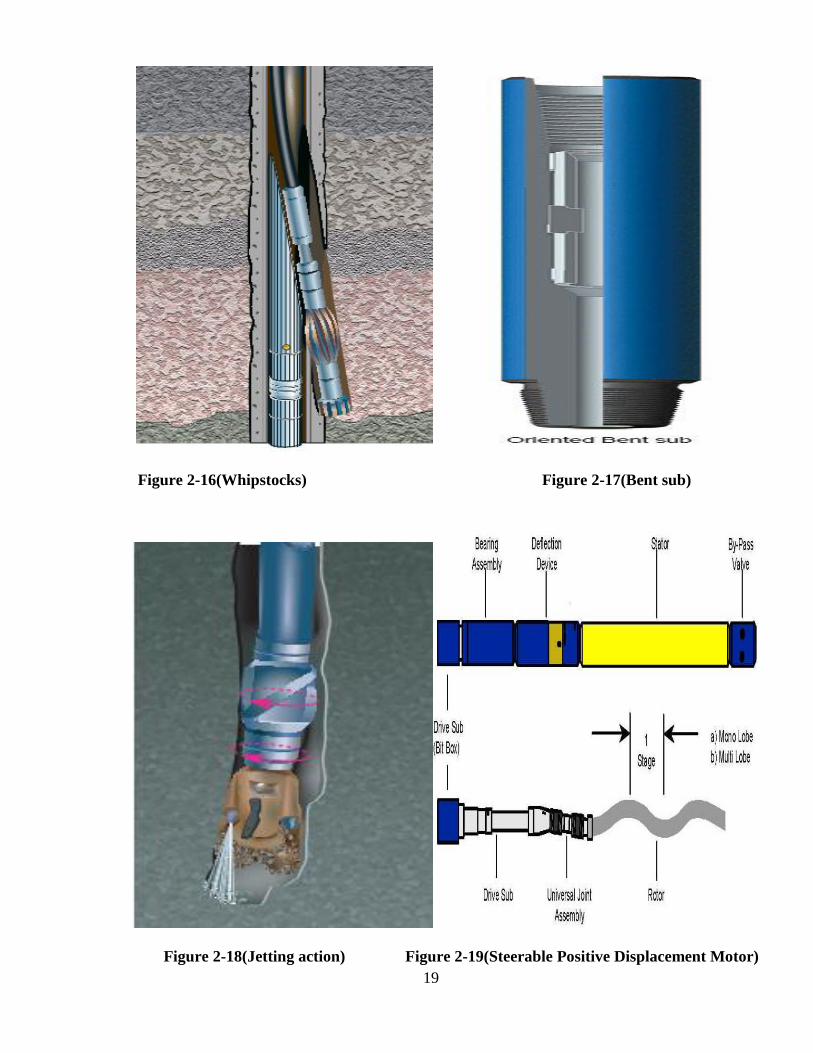
Jetting action.
Steerable Positive Displacement Motor.
Directional Bottom Hole Assemblies (BHA). [7]
19
Figure 2-16(Whipstocks) Figure 2-17(Bent sub)
Figure 2-18(Jetting action) Figure 2-19(Steerable Positive Displacement Motor)

20
Figure 2-20(Directional Bottom Hole Assemblies)
2.6- Survey tools:-
Inclination Angel Tools.
Non-Magnetic Drill Collars.
Magnetic Single-Shot.
Magnetic Multi-Shots.
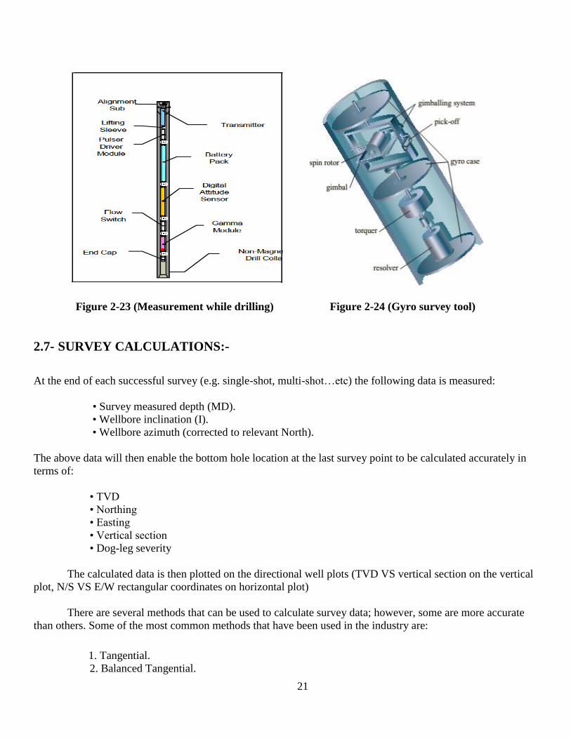
Measurements While Drilling.
The GYRO Survey Tool.[7]
Figure 2-21 (Magnetic single – shot) Figure 2-22 (Magnetic multi –shots)
21
Figure 2-23 (Measurement while drilling) Figure 2-24 (Gyro survey tool)
2.7- SURVEY CALCULATIONS:-
At the end of each successful survey (e.g. single-shot, multi-shot…etc) the following data is measured:
• Survey measured depth (MD).
• Wellbore inclination (I).
• Wellbore azimuth (corrected to relevant North).
The above data will then enable the bottom hole location at the last survey point to be calculated accurately in
terms of:
• TVD
• Northing
• Easting
• Vertical section
• Dog-leg severity
The calculated data is then plotted on the directional well plots (TVD VS vertical section on the vertical
plot, N/S VS E/W rectangular coordinates on horizontal plot)
There are several methods that can be used to calculate survey data; however, some are more accurate
than others. Some of the most common methods that have been used in the industry are:
1. Tangential.
2. Balanced Tangential.
22
3. Average Angle.
4. Radius of Curvature.
5. Minimum Curvature.
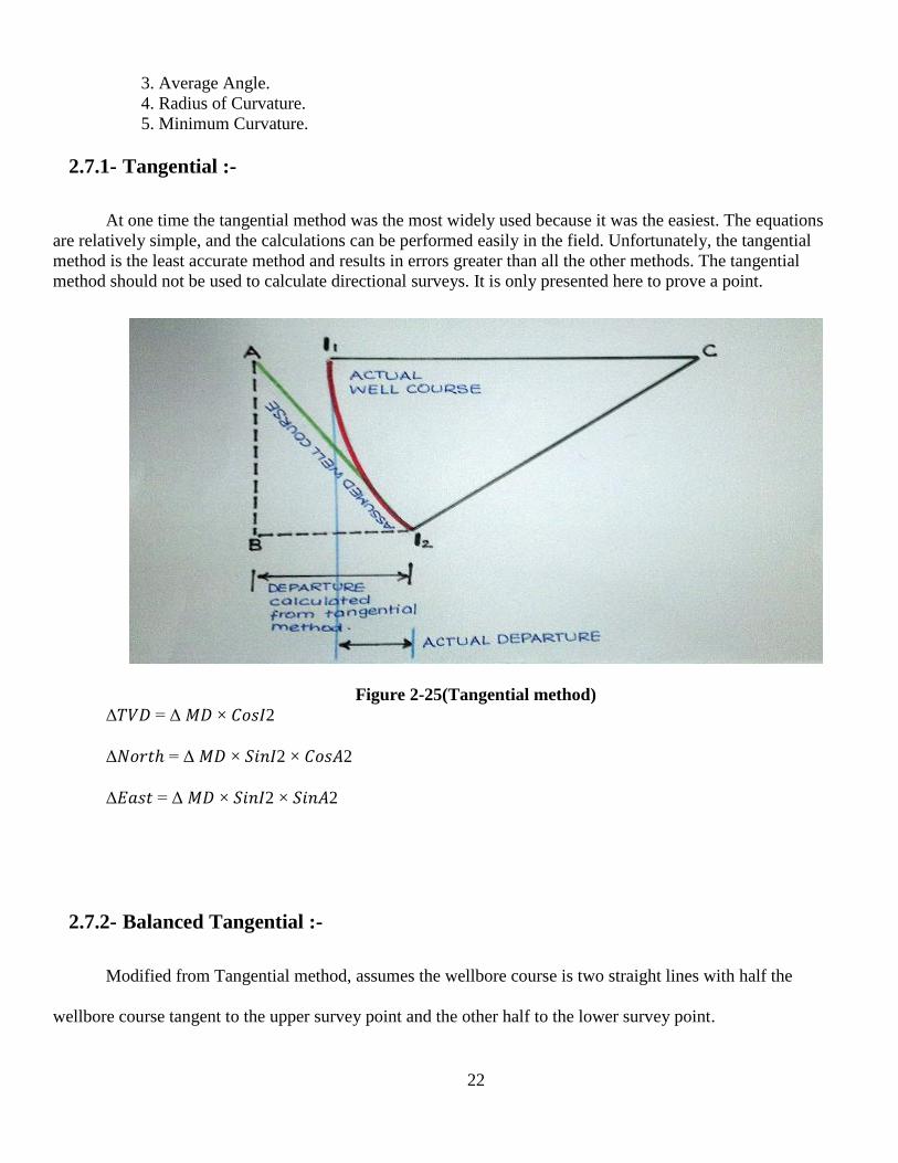
2.7.1- Tangential :-
At one time the tangential method was the most widely used because it was the easiest. The equations
are relatively simple, and the calculations can be performed easily in the field. Unfortunately, the tangential
method is the least accurate method and results in errors greater than all the other methods. The tangential
method should not be used to calculate directional surveys. It is only presented here to prove a point.
Figure 2-25(Tangential method)
Δ𝑇𝑉𝐷 = Δ 𝑀𝐷 × 𝐶𝑜𝑠𝐼2
Δ𝑁𝑜𝑟𝑡ℎ = Δ 𝑀𝐷 × 𝑆𝑖𝑛𝐼2 × 𝐶𝑜𝑠𝐴2
Δ𝐸𝑎𝑠𝑡 = Δ 𝑀𝐷 × 𝑆𝑖𝑛𝐼2 × 𝑆𝑖𝑛𝐴2
2.7.2- Balanced Tangential :-
Modified from Tangential method, assumes the wellbore course is two straight lines with half the
wellbore course tangent to the upper survey point and the other half to the lower survey point.
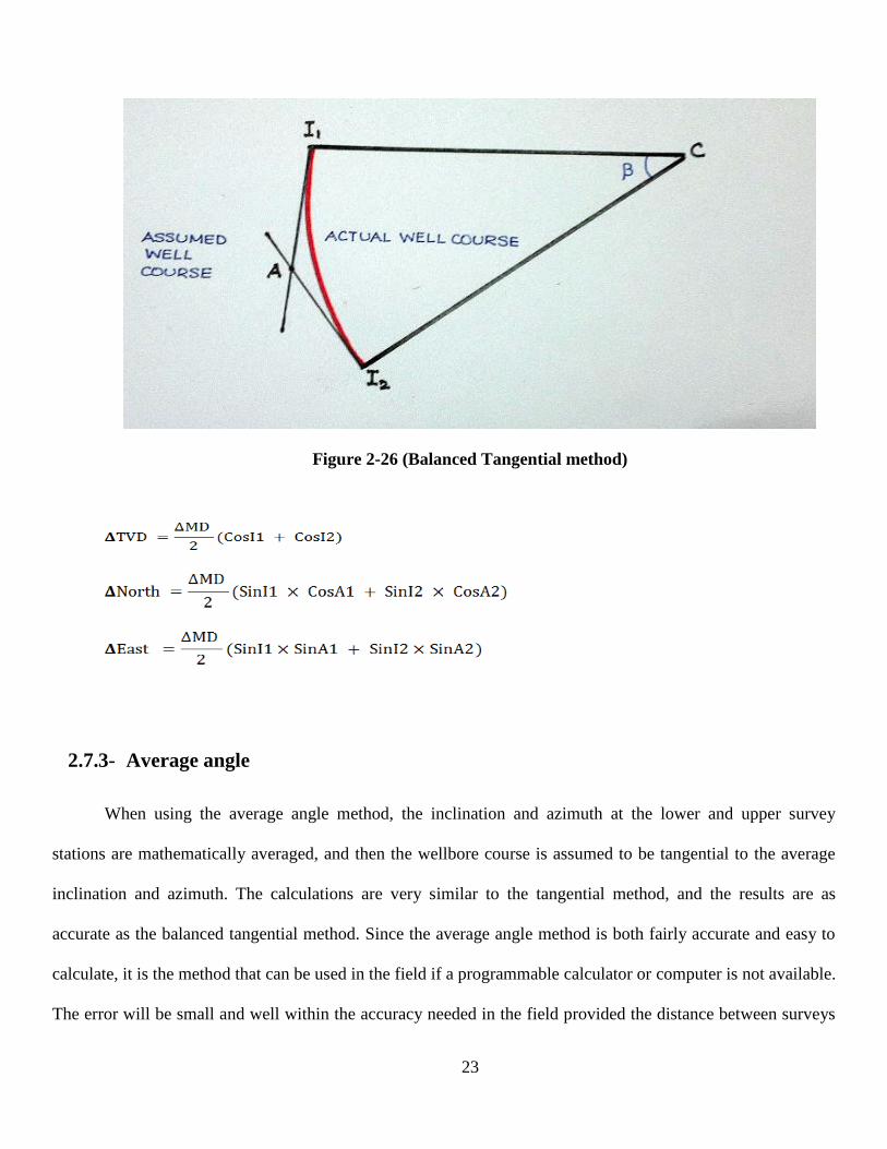
23
Figure 2-26 (Balanced Tangential method)
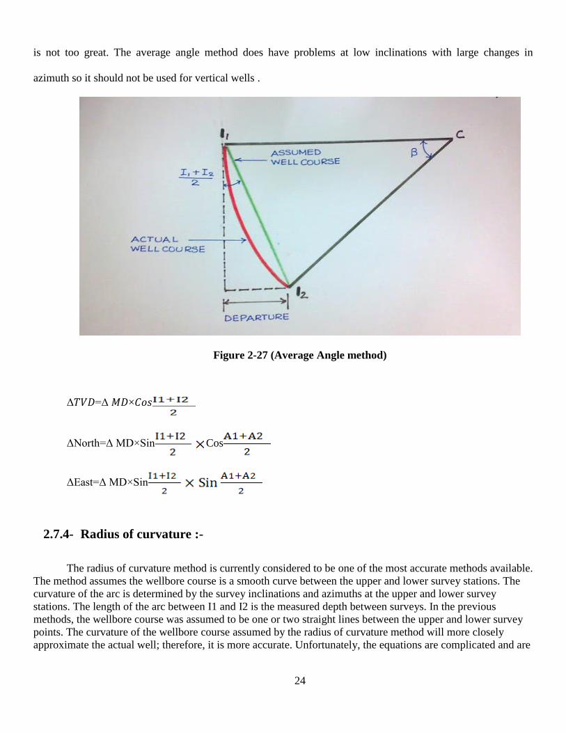
2.7.3- Average angle
When using the average angle method, the inclination and azimuth at the lower and upper survey
stations are mathematically averaged, and then the wellbore course is assumed to be tangential to the average
inclination and azimuth. The calculations are very similar to the tangential method, and the results are as
accurate as the balanced tangential method. Since the average angle method is both fairly accurate and easy to
calculate, it is the method that can be used in the field if a programmable calculator or computer is not available.
The error will be small and well within the accuracy needed in the field provided the distance between surveys
24
is not too great. The average angle method does have problems at low inclinations with large changes in
azimuth so it should not be used for vertical wells .
Figure 2-27 (Average Angle method)
Δ𝑇𝑉𝐷=Δ 𝑀𝐷×𝐶𝑜𝑠
ΔNorth=Δ MD×Sin Cos
ΔEast=Δ MD×Sin
2.7.4- Radius of curvature :-
The radius of curvature method is currently considered to be one of the most accurate methods available.
The method assumes the wellbore course is a smooth curve between the upper and lower survey stations. The
curvature of the arc is determined by the survey inclinations and azimuths at the upper and lower survey
stations. The length of the arc between I1 and I2 is the measured depth between surveys. In the previous
methods, the wellbore course was assumed to be one or two straight lines between the upper and lower survey
points. The curvature of the wellbore course assumed by the radius of curvature method will more closely
approximate the actual well; therefore, it is more accurate. Unfortunately, the equations are complicated and are

25
not easily calculated in the field without a programmable calculator or computer. In the equations, the
inclination and azimuth are entered as degrees.
Figure 2-28 (Radius of curvature method)
ΔTVD=
ΔNorth=
ΔEast=
26
ΔDEP=
r =
ΔMD=
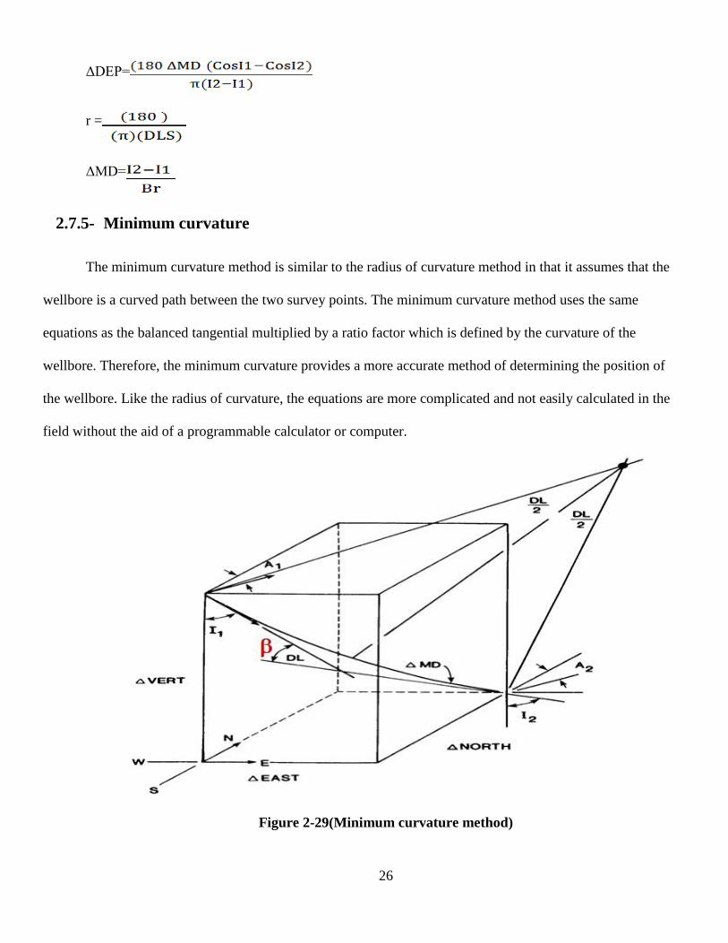
2.7.5- Minimum curvature
The minimum curvature method is similar to the radius of curvature method in that it assumes that the
wellbore is a curved path between the two survey points. The minimum curvature method uses the same
equations as the balanced tangential multiplied by a ratio factor which is defined by the curvature of the
wellbore. Therefore, the minimum curvature provides a more accurate method of determining the position of
the wellbore. Like the radius of curvature, the equations are more complicated and not easily calculated in the
field without the aid of a programmable calculator or computer.
Figure 2-29(Minimum curvature method)
27
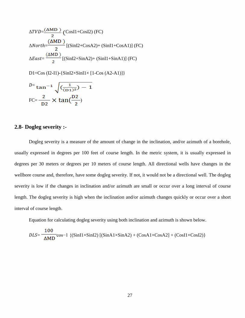
Δ𝑇𝑉𝐷= CosI1+CosI2) (FC)
Δ𝑁𝑜𝑟𝑡ℎ= [(SinI2+CosA2)+ (SinI1+CosA1)] (FC)
Δ𝐸𝑎𝑠𝑡= [(SinI2+SinA2)+ (SinI1+SinA1)] (FC)
D1=Cos (I2-I1)-{SinI2×SinI1× [1-Cos (A2-A1)]}
𝐷=
FC= )
2.8- Dogleg severity :-
Dogleg severity is a measure of the amount of change in the inclination, and/or azimuth of a borehole,
usually expressed in degrees per 100 feet of course length. In the metric system, it is usually expressed in
degrees per 30 meters or degrees per 10 meters of course length. All directional wells have changes in the
wellbore course and, therefore, have some dogleg severity. If not, it would not be a directional well. The dogleg
severity is low if the changes in inclination and/or azimuth are small or occur over a long interval of course
length. The dogleg severity is high when the inclination and/or azimuth changes quickly or occur over a short
interval of course length.
Equation for calculating dogleg severity using both inclination and azimuth is shown below.
𝐷𝐿𝑆= cos−1 {(SinI1×SinI2) [(SinA1×SinA2) + (CosA1×CosA2] + (CosI1×CosI2)}

28
Chapter three:
Methodology
29
Chapter 3 : Methodology
3.1- Introduction:-
In this chapter the discussion will be about the steps used in constructing the program , the choices
made and then demonstrate in details all the program features and aeries .
3.2- The steps:-
3.2.1- The first step :-
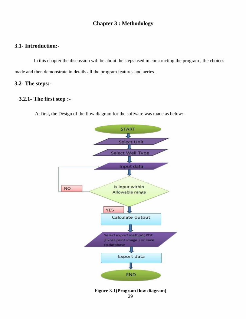
At first, the Design of the flow diagram for the software was made as below:-
Figure 3-1(Program flow diagram)
30
3.2.2- Step two:-
This step includes choosing the suitable equations to make accurate calculations in the program.
Previously in the literature review the different types of survey calculations methods were mentioned
and some of the most common methods that have been used in the industry are:
1. Tangential.
2. Balanced Tangential.
3. Average Angle.
4. Radius of Curvature.
5. Minimum Curvature.
Each method assumes that the survey trajectory has a specific shape as discussed in literature review
chapter, which result some degree of error and accuracy from the actual survey data.
In this software the minimum curvature method was used in the calculations, because it shows more
accurate results in determining the position of the wellbore and also because the equations are more complicated
and can’t be calculated easily without using computer.
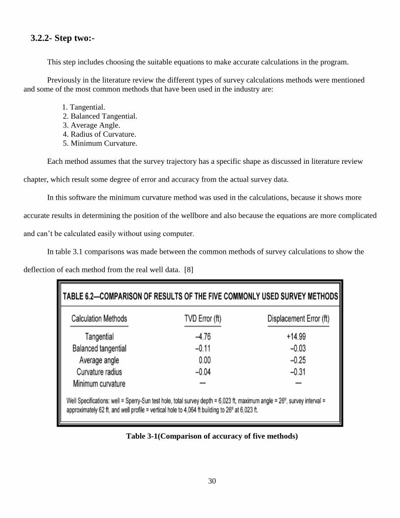
In table 3.1 comparisons was made between the common methods of survey calculations to show the
deflection of each method from the real well data. [8]
Table 3-1(Comparison of accuracy of five methods)
31
As seen from the table, the tangential method has much error for TVD and displacement, the other
methods has very small differences and any of them can be used for the calculation of the trajectory, but the
minimum curvature method shows the most accurate result and so it’s the most widely preferred method in the
oil industry.
3.2.3- Step three:-
This step starts from choosing the programming language until the program was published.
Firstly, the choice for visual basic (VB.NET) programming language was made because it’s suitable,
easy to learn and very powerful as programming language.
The learning of this language took about month through books and videos, and the (2013) version of
visual studio was used as software environment.
Secondly, the design of the software took about 2 month to finish. The programming began by designing
the user interface (UI), then the code for the program was written and the equations were entered.
After coding the equations many features were added to ease the data import and export and plots were
added for more understanding of the well trajectory, in addition to that a 3D library used to plot 3D graph
representing the trajectory in three dimensions.
The software contains more than 4000 lines of code and utilizes more than 70 equations and will be
explained in more details in the next section.
3.2.4- Step four:-
Four different case studies were made to determine the accuracy of the program as shown in chapter 4
and then economic analysis were made in chapter 5.
32
3.3- The Program:-
In this section there will be a full description about the program and all its features, the discussion will
be about the:-
1- The loading screen.
2- The main menu.
3- The manage wells window.
4- The Well mode window.
5- The Free mode window.
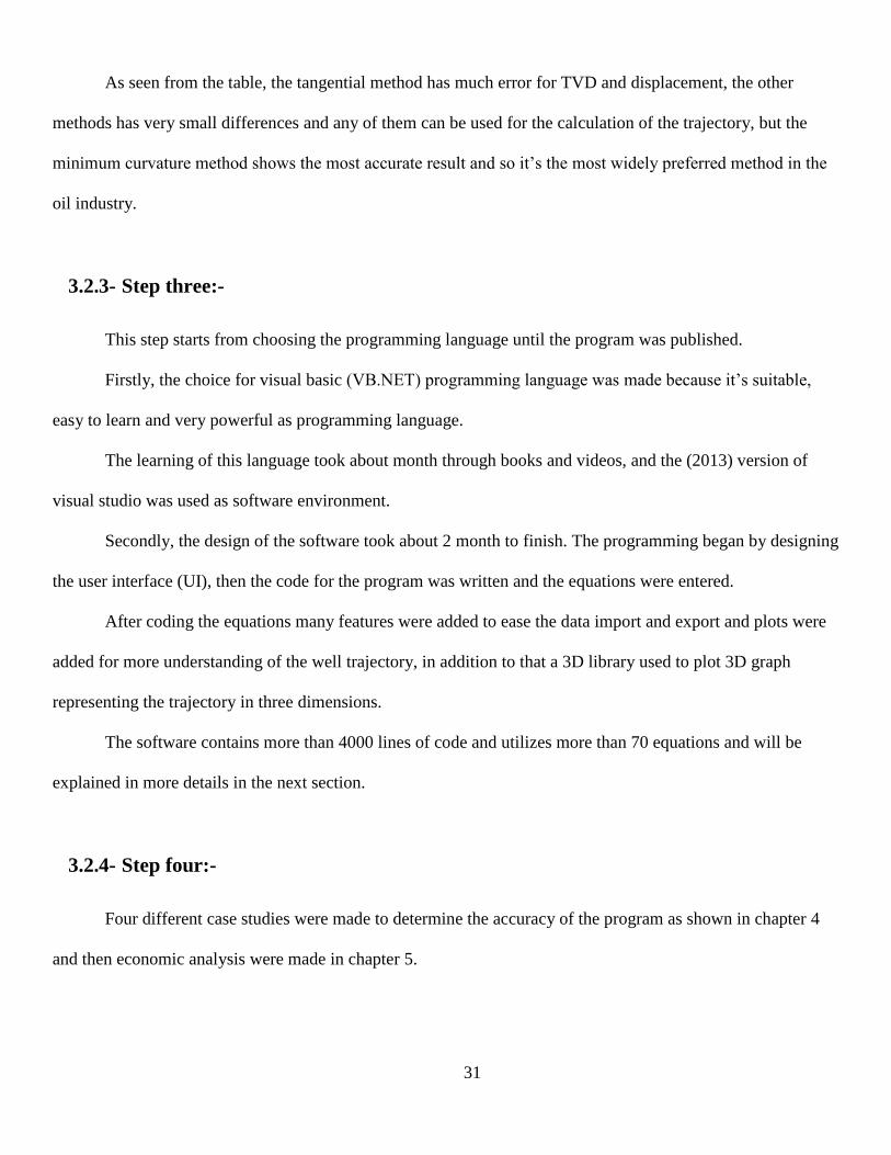
3.3.1- The loading screen:-
The first screen when starting the program, takes about 5 seconds to load, after which the main menu
appears, as shown in the figure below.
Figure 3-2 (Loading screen)
33
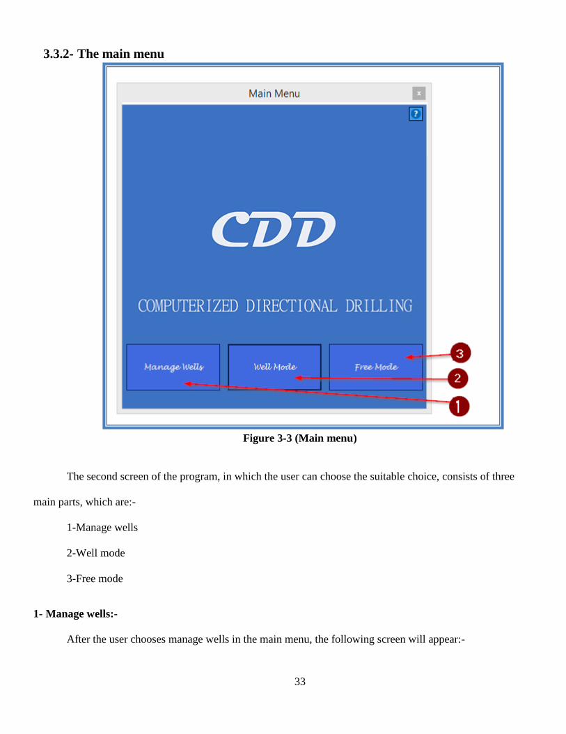
3.3.2- The main menu
Figure 3-3 (Main menu)
The second screen of the program, in which the user can choose the suitable choice, consists of three
main parts, which are:-
1-Manage wells
2-Well mode
3-Free mode
1- Manage wells:-
After the user chooses manage wells in the main menu, the following screen will appear:-
34
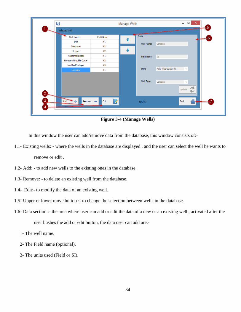
Figure 3-4 (Manage Wells)
In this window the user can add/remove data from the database, this window consists of:-
1.1- Existing wells: - where the wells in the database are displayed , and the user can select the well he wants to
remove or edit .
1.2- Add: - to add new wells to the existing ones in the database.
1.3- Remove: - to delete an existing well from the database.
1.4- Edit:- to modify the data of an existing well.
1.5- Upper or lower move button :- to change the selection between wells in the database.
1.6- Data section :- the area where user can add or edit the data of a new or an existing well , activated after the
user bushes the add or edit button, the data user can add are:-
1- The well name.
2- The Field name (optional).
3- The units used (Field or SI).

35
4- The well Type (Build and hold , Continues Build , Horizontal one curve , Horizontal double
curve , S-shape, Modified S-shape , Complex ).
Figure 3-5 (Data section)
Notice:-The number after word (total) indicates the total number of wells in the database.
1.7- Back :-to return from the manage wells window to the main menu window.
2- Well mode:-
After the user chooses well mode in the main menu, the screen in figure (4-5) will appear, this window
consists of five main parts:-
1) Well type data section.
2) Table section.
3) Chart section.
4) Program header.
5) Program footer.
36
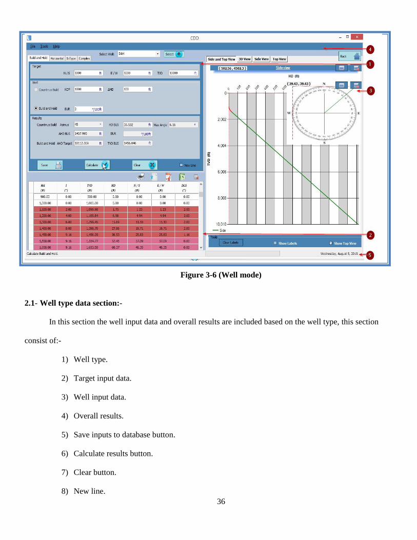
Figure 3-6 (Well mode)
2.1- Well type data section:-
In this section the well input data and overall results are included based on the well type, this section
consist of:-
1) Well type.
2) Target input data.
3) Well input data.
4) Overall results.
5) Save inputs to database button.
6) Calculate results button.
7) Clear button.
8) New line.
37
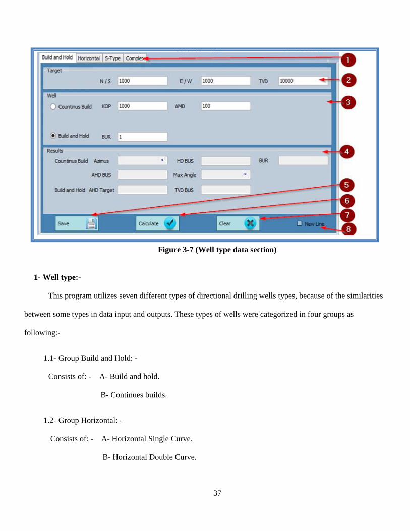
Figure 3-7 (Well type data section)
1- Well type:-
This program utilizes seven different types of directional drilling wells types, because of the similarities
between some types in data input and outputs. These types of wells were categorized in four groups as
following:-
1.1- Group Build and Hold: -
Consists of: - A- Build and hold.
B- Continues builds.
1.2- Group Horizontal: -
Consists of: - A- Horizontal Single Curve.
B- Horizontal Double Curve.

38
1.3- Group S-Type: -
Consists of: - A- S-shape.
B- Modified S-shape.
1.4- Group Complex: -
Include wells with various drilling directions .will be explained in more details in the next section.
2- Target input data:-the data to be entered are (TVD, North or South, East or West)
3- Well input data:-the data to be entered are different from one well type to another, e.g. (KOP, Delta MD,
BUR…etc.)
4- The output results: - are different based on the well type, e.g.(Azimuth , max angle , TVD BUS …etc.)
5- Save Button: - to save the input data to the database, for later recall if needed.
6- Calculate Button: - to get the output results from the data input using the equations as well as calculate the
table data and the charts .
7- Clear Button: - to delete the input and output data in order to enter new ones.
8- New line:- to draw a new chart line beside the old one for comparison purposes or for multilateral well
type, (will be discussed in more details at the section (3.3.3)
39
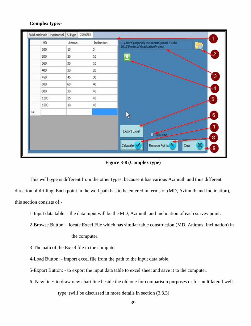
Complex type:-
Figure 3-8 (Complex type)
This well type is different from the other types, because it has various Azimuth and thus different
direction of drilling. Each point in the well path has to be entered in terms of (MD, Azimuth and Inclination),
this section consists of:-
1-Input data table: - the data input will be the MD, Azimuth and Inclination of each survey point.
2-Browse Button: - locate Excel File which has similar table construction (MD, Animus, Inclination) in
the computer.
3-The path of the Excel file in the computer
4-Load Button: - import excel file from the path to the input data table.
5-Export Button: - to export the input data table to excel sheet and save it to the computer.
6- New line:-to draw new chart line beside the old one for comparison purposes or for multilateral well
type, (will be discussed in more details in section (3.3.3)
40
7-Calculate Button: - to get the output results from the data input using the equations as well as
calculate the data table and the charts .
8-Remove Points Button:- to remove the specific points from input data table .
9- Clear Button: - to delete the data in the input data table in order to add new one.
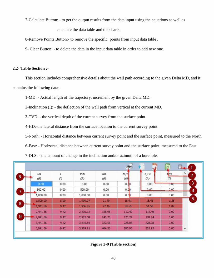
2.2- Table Section :-
This section includes comprehensive details about the well path according to the given Delta MD, and it
contains the following data:-
1-MD: - Actual length of the trajectory, increment by the given Delta MD.
2-Inclination (I): - the deflection of the well path from vertical at the current MD.
3-TVD: - the vertical depth of the current survey from the surface point.
4-HD:-the lateral distance from the surface location to the current survey point.
5-North: - Horizontal distance between current survey point and the surface point, measured to the North
6-East: - Horizontal distance between current survey point and the surface point, measured to the East.
7-DLS: - the amount of change in the inclination and/or azimuth of a borehole.
Figure 3-9 (Table section)
41
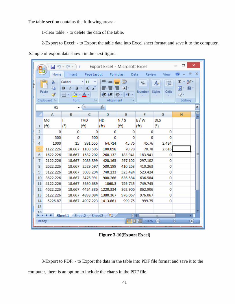
The table section contains the following areas:-
1-clear table: - to delete the data of the table.
2-Export to Excel: - to Export the table data into Excel sheet format and save it to the computer.
Sample of export data shown in the next figure.
Figure 3-10(Export Excel)
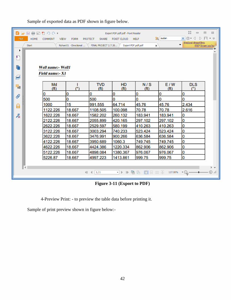
3-Export to PDF: - to Export the data in the table into PDF file format and save it to the
computer, there is an option to include the charts in the PDF file.
42
Sample of exported data as PDF shown in figure below.
Figure 3-11 (Export to PDF)
4-Preview Print: - to preview the table data before printing it.
Sample of print preview shown in figure below:-
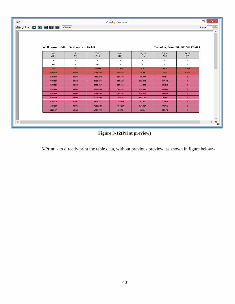
43
Figure 3-12(Print preview)
5-Print: - to directly print the table data, without previous preview, as shown in figure below:-
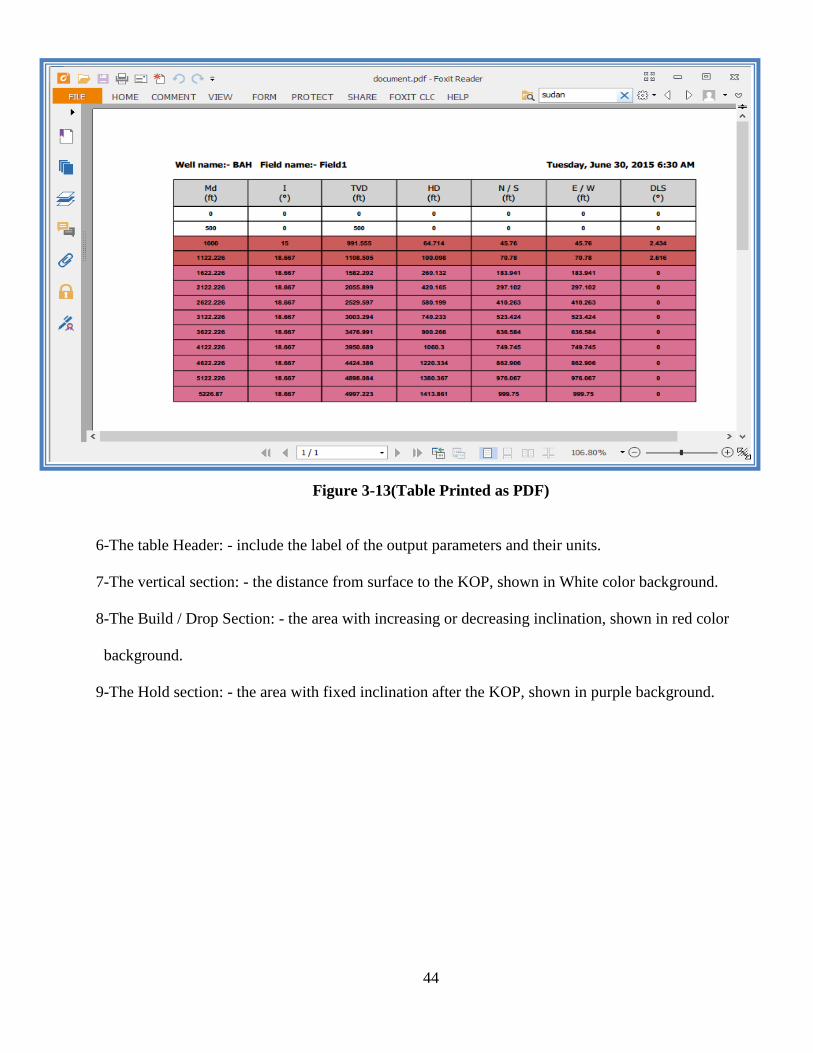
44
Figure 3-13(Table Printed as PDF)
6-The table Header: - include the label of the output parameters and their units.
7-The vertical section: - the distance from surface to the KOP, shown in White color background.
8-The Build / Drop Section: - the area with increasing or decreasing inclination, shown in red color
background.
9-The Hold section: - the area with fixed inclination after the KOP, shown in purple background.
45
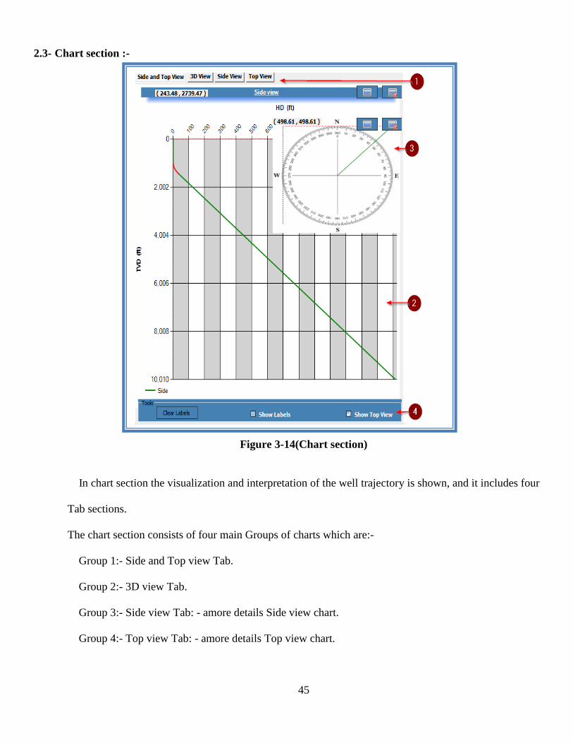
2.3- Chart section :-
Figure 3-14(Chart section)
In chart section the visualization and interpretation of the well trajectory is shown, and it includes four
Tab sections.
The chart section consists of four main Groups of charts which are:-
Group 1:- Side and Top view Tab.
Group 2:- 3D view Tab.
Group 3:- Side view Tab: - amore details Side view chart.
Group 4:- Top view Tab: - amore details Top view chart.
46
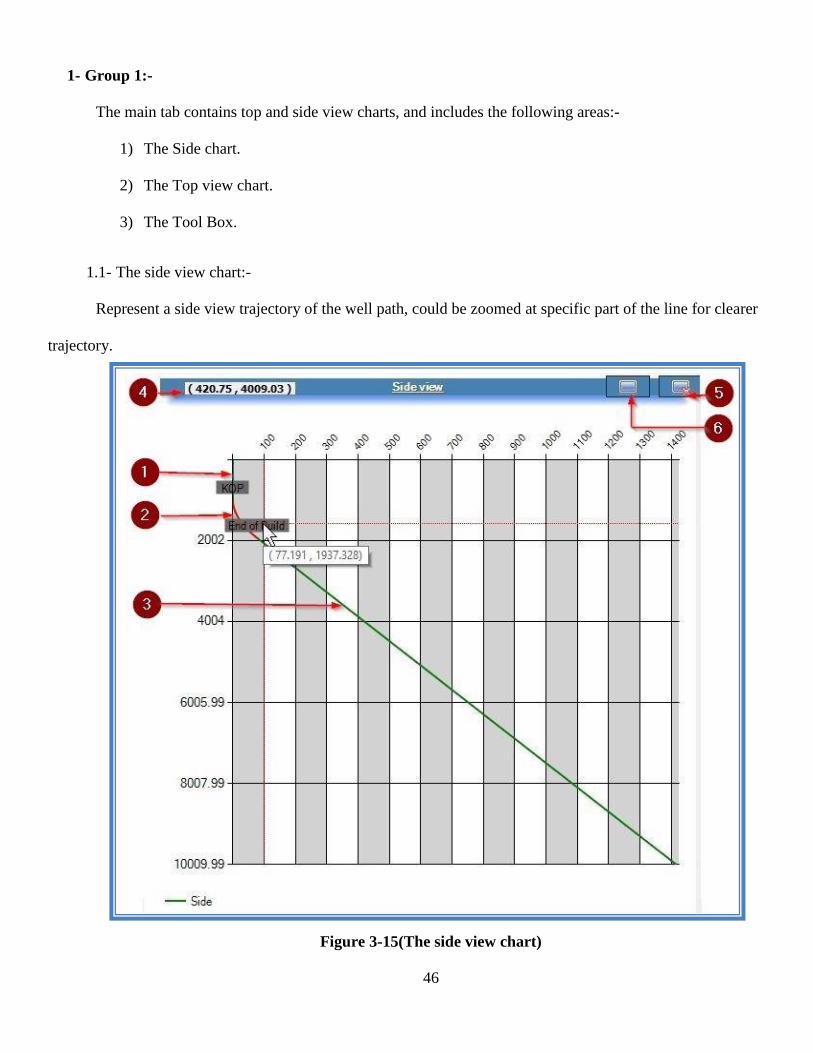
1- Group 1:-
The main tab contains top and side view charts, and includes the following areas:-
1) The Side chart.
2) The Top view chart.
3) The Tool Box.
1.1- The side view chart:-
Represent a side view trajectory of the well path, could be zoomed at specific part of the line for clearer
trajectory.
Figure 3-15(The side view chart)
47
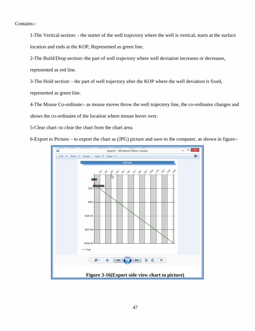
Contains:-
1-The Vertical section: - the starter of the well trajectory where the well is vertical, starts at the surface
location and ends at the KOP, Represented as green line.
2-The Build/Drop section:-the part of well trajectory where well deviation increases or decreases,
represented as red line.
3-The Hold section: - the part of well trajectory after the KOP where the well deviation is fixed,
represented as green line.
4-The Mouse Co-ordinate:- as mouse moves throw the well trajectory line, the co-ordinates changes and
shows the co-ordinates of the location where mouse hover over.
5-Clear chart:-to clear the chart from the chart area.
6-Export to Picture: - to export the chart as (JPG) picture and save to the computer, as shown in figure:-
Figure 3-16(Export side view chart to picture)
48
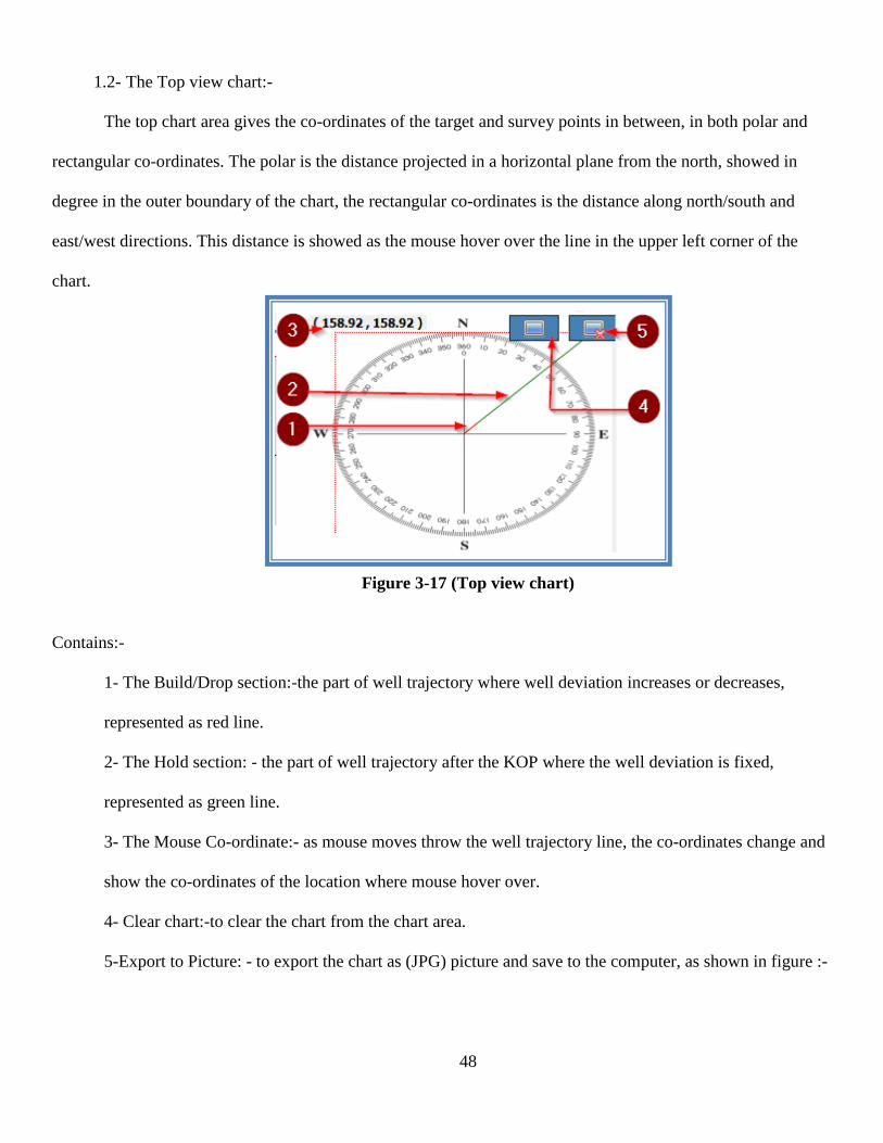
1.2- The Top view chart:-
The top chart area gives the co-ordinates of the target and survey points in between, in both polar and
rectangular co-ordinates. The polar is the distance projected in a horizontal plane from the north, showed in
degree in the outer boundary of the chart, the rectangular co-ordinates is the distance along north/south and
east/west directions. This distance is showed as the mouse hover over the line in the upper left corner of the
chart.
Figure 3-17 (Top view chart)
Contains:-
1- The Build/Drop section:-the part of well trajectory where well deviation increases or decreases,
represented as red line.
2- The Hold section: - the part of well trajectory after the KOP where the well deviation is fixed,
represented as green line.
3- The Mouse Co-ordinate:- as mouse moves throw the well trajectory line, the co-ordinates change and
show the co-ordinates of the location where mouse hover over.
4- Clear chart:-to clear the chart from the chart area.
5-Export to Picture: - to export the chart as (JPG) picture and save to the computer, as shown in figure :-
49
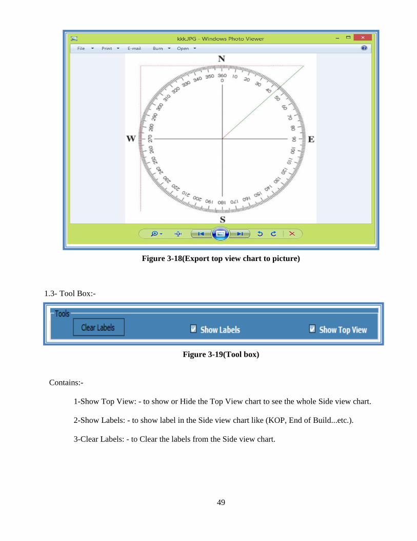
Figure 3-18(Export top view chart to picture)
1.3- Tool Box:-
Figure 3-19(Tool box)
Contains:-
1-Show Top View: - to show or Hide the Top View chart to see the whole Side view chart.
2-Show Labels: - to show label in the Side view chart like (KOP, End of Build...etc.).
3-Clear Labels: - to Clear the labels from the Side view chart.
50
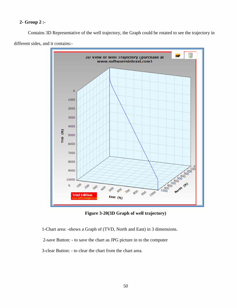
2- Group 2 :-
Contains 3D Representative of the well trajectory, the Graph could be rotated to see the trajectory in
different sides, and it contains:-
Figure 3-20(3D Graph of well trajectory)
1-Chart area: -shows a Graph of (TVD, North and East) in 3 dimensions.
2-save Button: - to save the chart as JPG picture in to the computer
3-clear Button: - to clear the chart from the chart area.
51
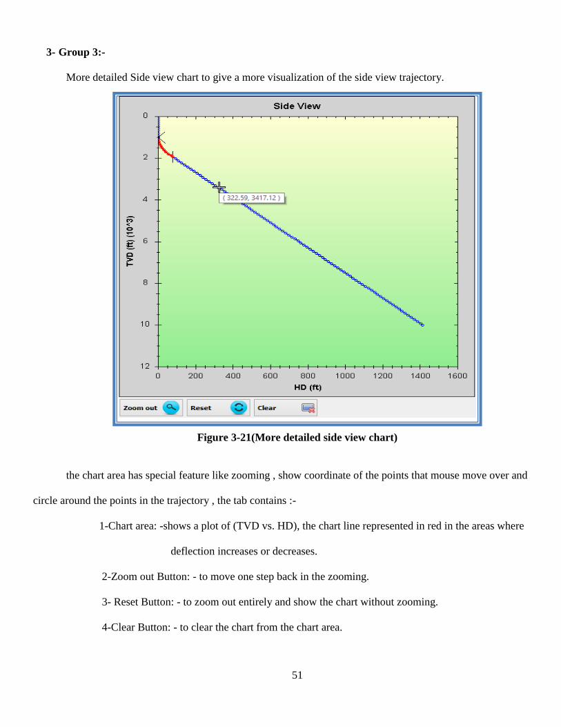
3- Group 3:-
More detailed Side view chart to give a more visualization of the side view trajectory.
Figure 3-21(More detailed side view chart)
the chart area has special feature like zooming , show coordinate of the points that mouse move over and
circle around the points in the trajectory , the tab contains :-
1-Chart area: -shows a plot of (TVD vs. HD), the chart line represented in red in the areas where
deflection increases or decreases.
2-Zoom out Button: - to move one step back in the zooming.
3- Reset Button: - to zoom out entirely and show the chart without zooming.
4-Clear Button: - to clear the chart from the chart area.
52
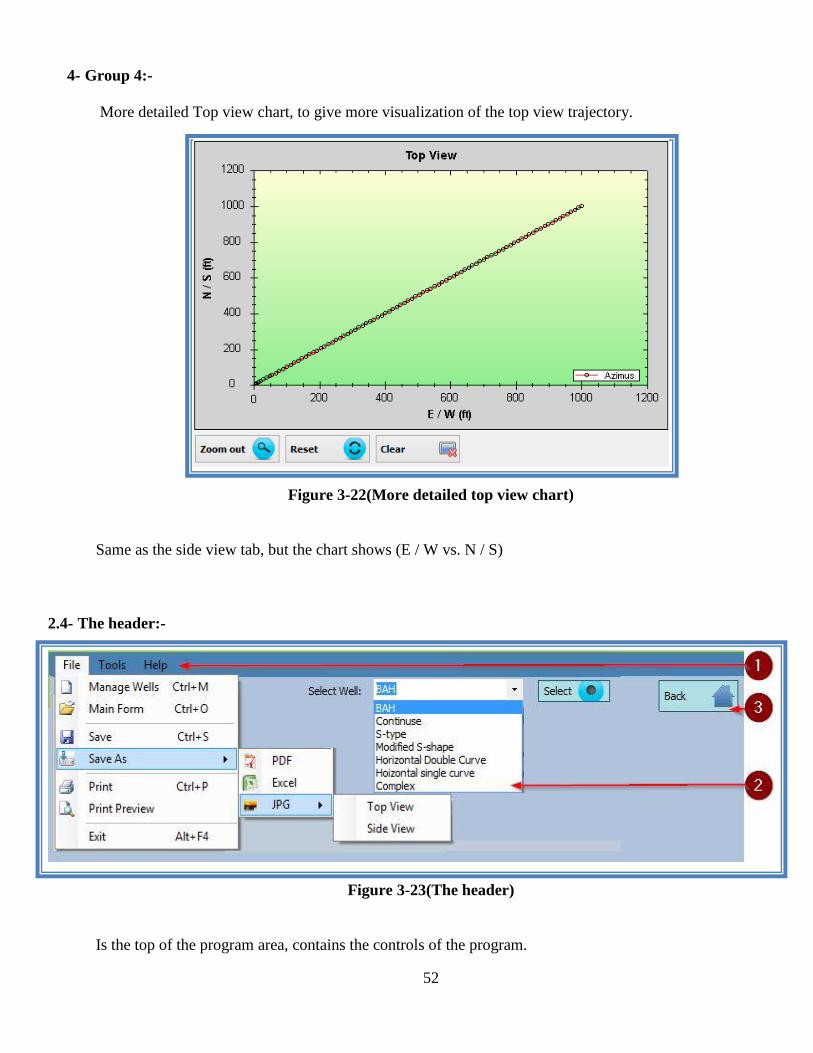
4- Group 4:-
More detailed Top view chart, to give more visualization of the top view trajectory.
Figure 3-22(More detailed top view chart)
Same as the side view tab, but the chart shows (E / W vs. N / S)
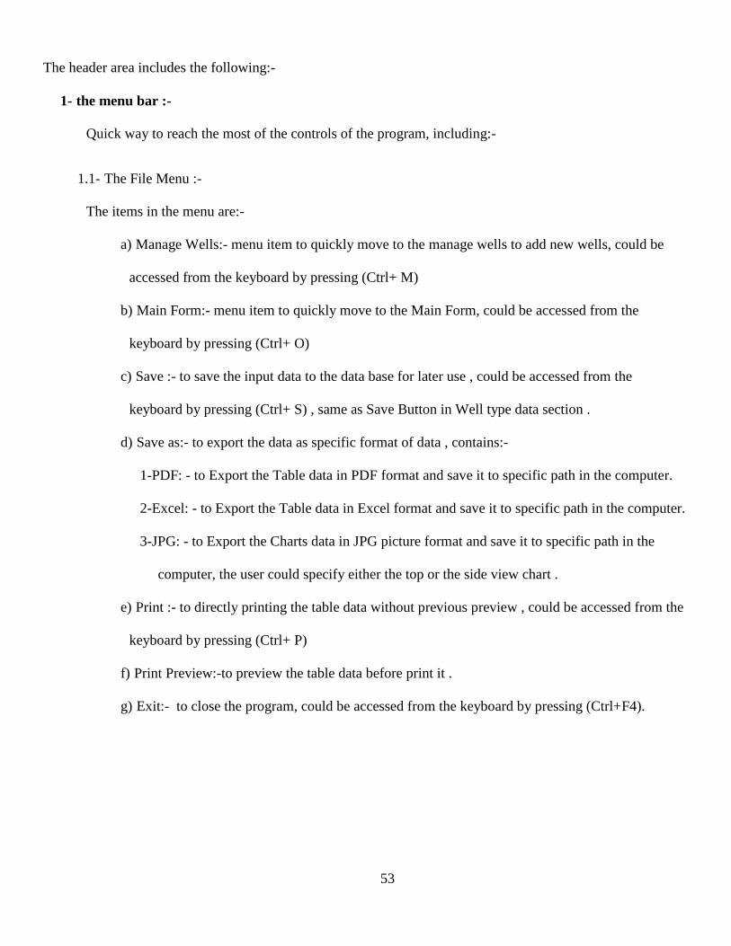
2.4- The header:-
Figure 3-23(The header)
Is the top of the program area, contains the controls of the program.
53
The header area includes the following:-
1- the menu bar :-
Quick way to reach the most of the controls of the program, including:-
1.1- The File Menu :-
The items in the menu are:-
a) Manage Wells:- menu item to quickly move to the manage wells to add new wells, could be
accessed from the keyboard by pressing (Ctrl+ M)
b) Main Form:- menu item to quickly move to the Main Form, could be accessed from the
keyboard by pressing (Ctrl+ O)
c) Save :- to save the input data to the data base for later use , could be accessed from the
keyboard by pressing (Ctrl+ S) , same as Save Button in Well type data section .
d) Save as:- to export the data as specific format of data , contains:-
1-PDF: - to Export the Table data in PDF format and save it to specific path in the computer.
2-Excel: - to Export the Table data in Excel format and save it to specific path in the computer.
3-JPG: - to Export the Charts data in JPG picture format and save it to specific path in the
computer, the user could specify either the top or the side view chart .
e) Print :- to directly printing the table data without previous preview , could be accessed from the
keyboard by pressing (Ctrl+ P)
f) Print Preview:-to preview the table data before print it .
g) Exit:- to close the program, could be accessed from the keyboard by pressing (Ctrl+F4).
54
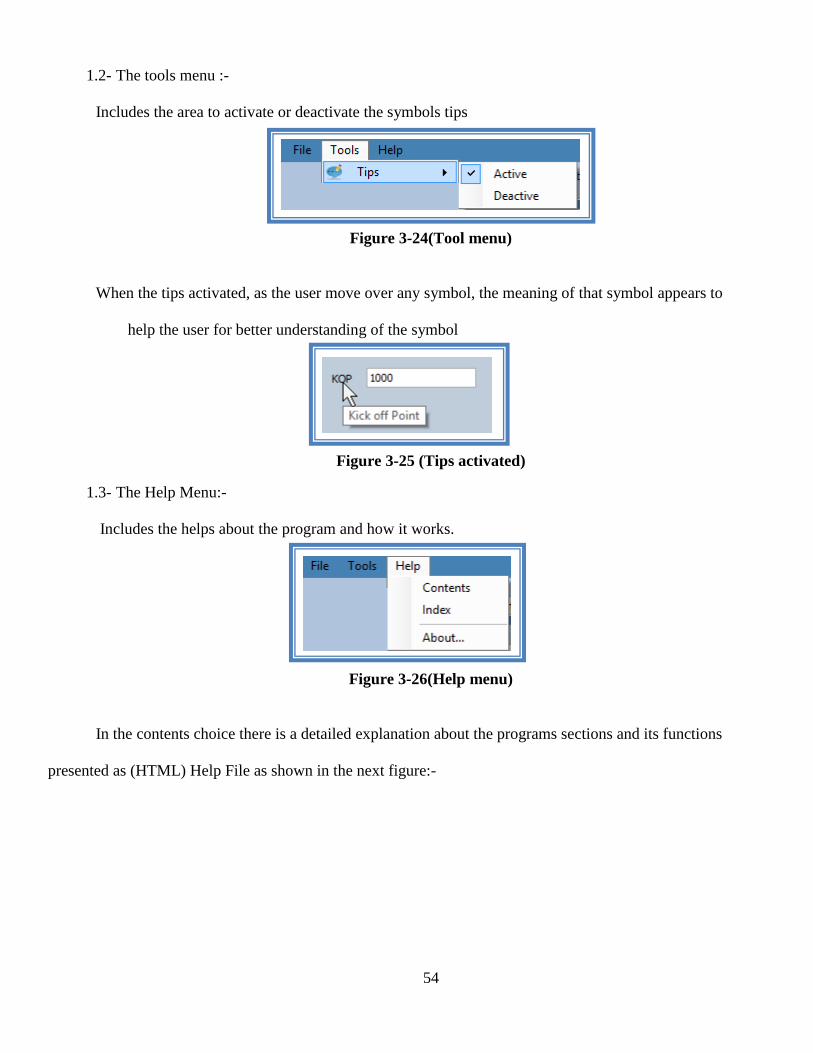
1.2- The tools menu :-
Includes the area to activate or deactivate the symbols tips
Figure 3-24(Tool menu)
When the tips activated, as the user move over any symbol, the meaning of that symbol appears to
help the user for better understanding of the symbol
Figure 3-25 (Tips activated)
1.3- The Help Menu:-
Includes the helps about the program and how it works.
Figure 3-26(Help menu)
In the contents choice there is a detailed explanation about the programs sections and its functions
presented as (HTML) Help File as shown in the next figure:-

55
Figure 3-27(Content help window)
Under the Index choice there is a quick access to the meaning of the abbreviations used in the program
as shown in figure below:-
Figure 3-28(Index window)
56
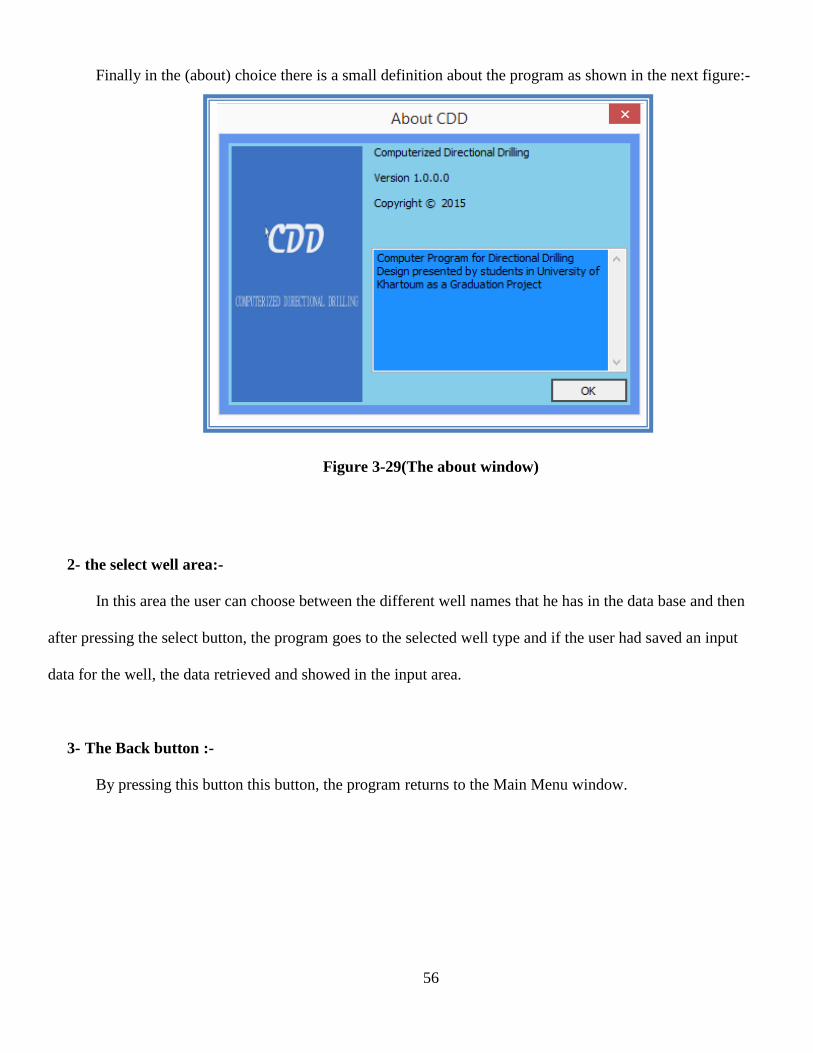
Finally in the (about) choice there is a small definition about the program as shown in the next figure:-
Figure 3-29(The about window)
2- the select well area:-
In this area the user can choose between the different well names that he has in the data base and then
after pressing the select button, the program goes to the selected well type and if the user had saved an input
data for the well, the data retrieved and showed in the input area.
3- The Back button :-
By pressing this button this button, the program returns to the Main Menu window.

57
2.5- The Footer:-
Figure 3-30 (The footer)
Is the area at the bottom of the program, and it shows details about what is going on in the program,
including:-
1-The last activity: - demonstration about the last activity in the program, including (when the
selection of the well is changed, when the export is selected, when the chart is changed….etc.).
2-The progress bar: - appears when the user exports or imports data, to show the progress made
by the program in regard to what is being processed.
3-Date: - the current date when the program is being used.
3- Free Mode:-
In free mode, the user can access to the different area of the program without previously entering the
well name or type in Manage Wells area , the only thing the user must enter is the Units used(Field units or SI
units) .
The free mode showed in the next figure:-
58
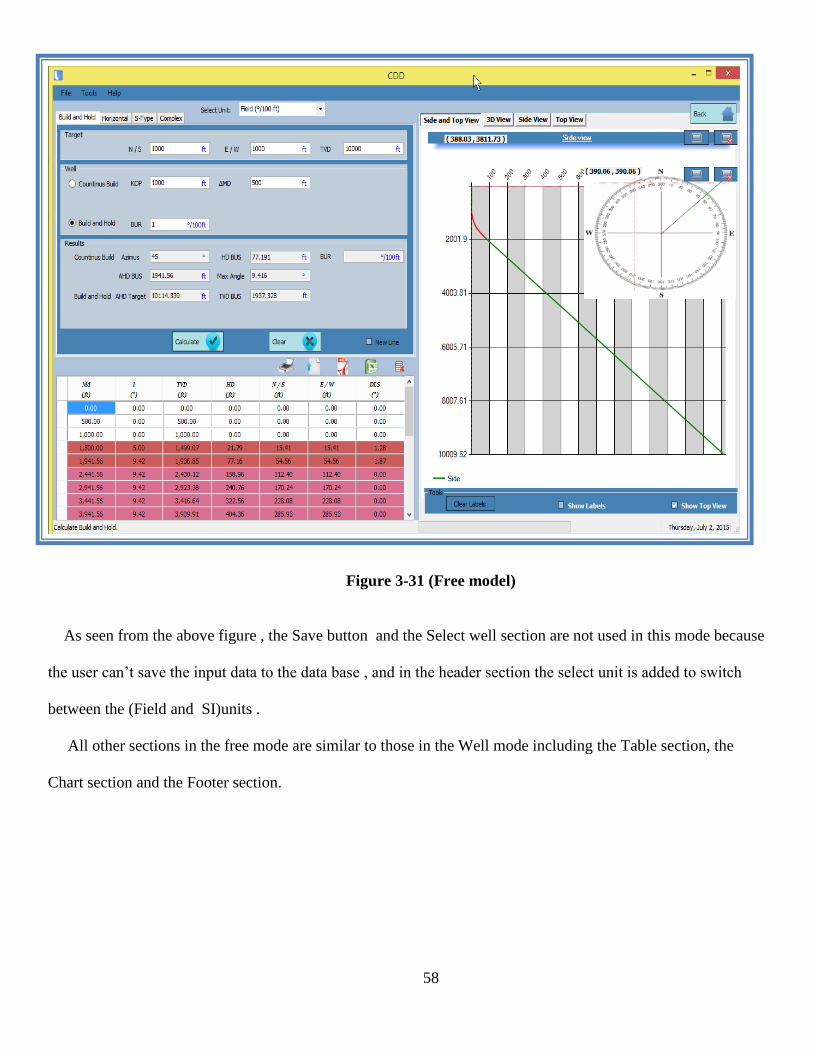
Figure 3-31 (Free model)
As seen from the above figure , the Save button and the Select well section are not used in this mode because
the user can’t save the input data to the data base , and in the header section the select unit is added to switch
between the (Field and SI)units .
All other sections in the free mode are similar to those in the Well mode including the Table section, the
Chart section and the Footer section.
59
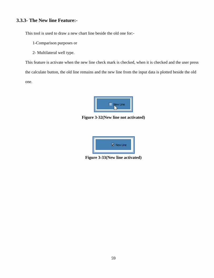
3.3.3- The New line Feature:-
This tool is used to draw a new chart line beside the old one for:-
1-Comparison purposes or
2- Multilateral well type.
This feature is activate when the new line check mark is checked, when it is checked and the user press
the calculate button, the old line remains and the new line from the input data is plotted beside the old
one.
Figure 3-32(New line not activated)
Figure 3-33(New line activated)
60
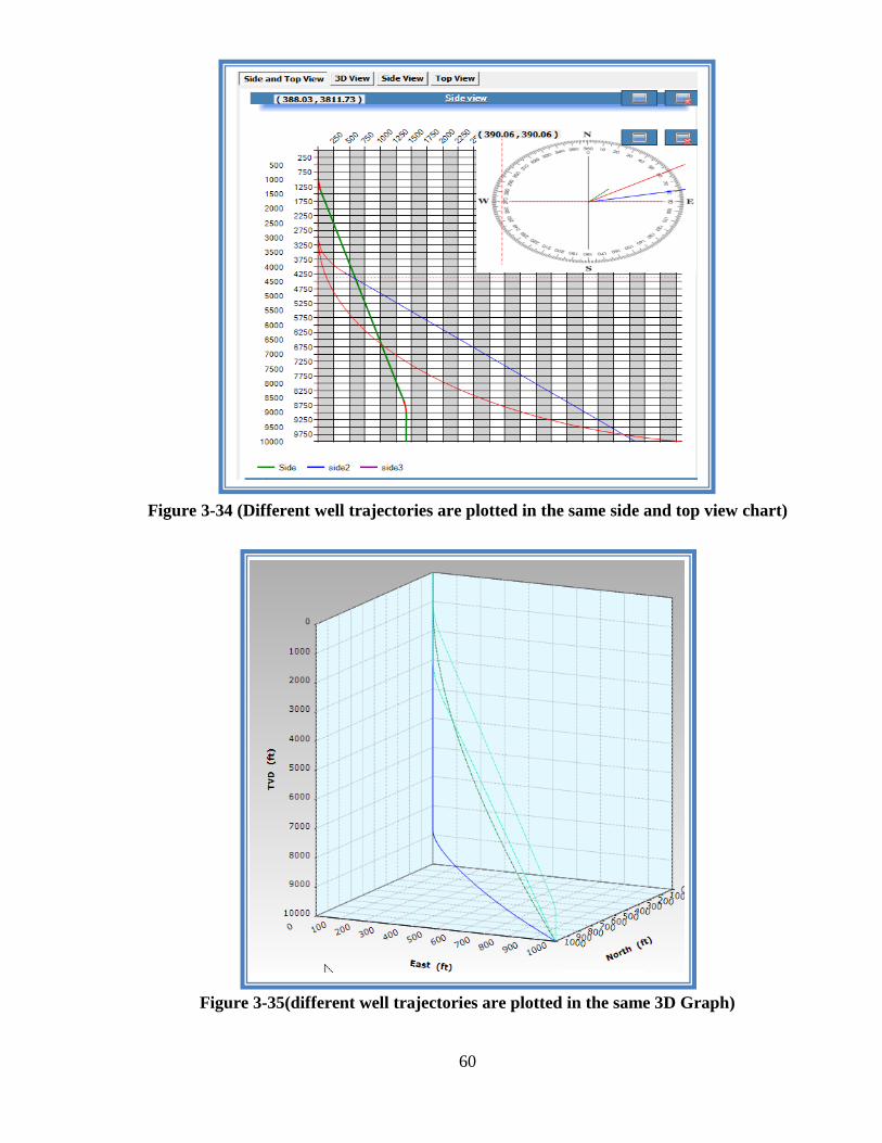
Figure 3-34 (Different well trajectories are plotted in the same side and top view chart)
Figure 3-35(different well trajectories are plotted in the same 3D Graph)
61
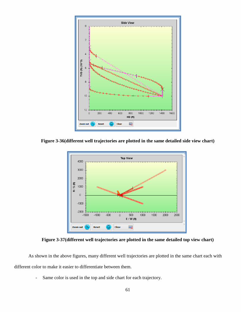
Figure 3-36(different well trajectories are plotted in the same detailed side view chart)
Figure 3-37(different well trajectories are plotted in the same detailed top view chart)
As shown in the above figures, many different well trajectories are plotted in the same chart each with
different color to make it easier to differentiate between them.
- Same color is used in the top and side chart for each trajectory.

62
Chapter Four:
Results and Discussions

63
Chapter 4 : Results and discussions
4.1- Introduction :-
The objective of this project is to develop software that is able to make the computations of the well
trajectory parameters faster and accurate.
Three wells data were used in validating the program. The first is the data used by Walter Gas and Oil
Corporation which is build and hold well, the second is from Whiting Oil and Gas Corporation which is
horizontal well and the last one is from Energy Partners Ltd and represent s-type well.
In these case studies, the software will be used to compare the obtained data with actual ones obtained
from the real wells.
4.2- Case Studies:-
4.2.1- Well OCS-G-31376:-
1- Case Statement:
Survey Data from Walter Gas and Oil Corporation represents case for build and hold well type:
Figure 4-1(Survey Data from Walter Gas and Oil Corporation)
64
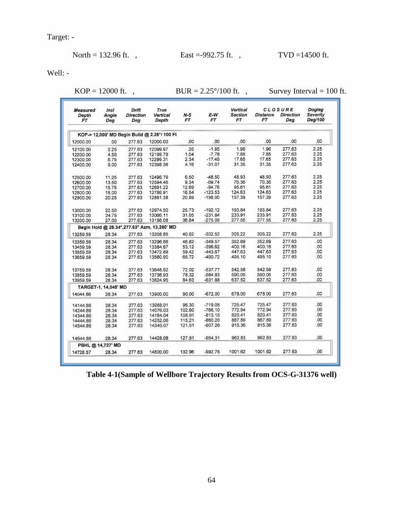
Target: -
North = 132.96 ft. , East =-992.75 ft. , TVD =14500 ft.
Well: -
KOP = 12000 ft. , BUR = 2.25°/100 ft. , Survey Interval = 100 ft.
Table 4-1(Sample of Wellbore Trajectory Results from OCS-G-31376 well)
65
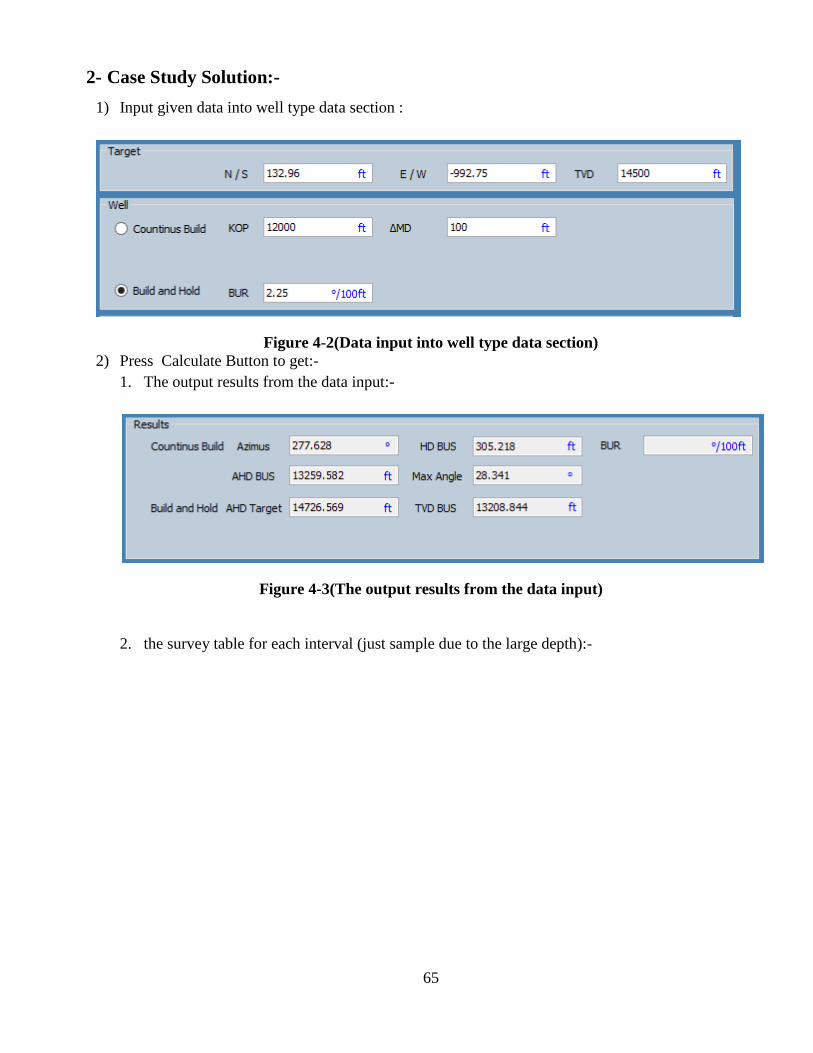
2- Case Study Solution:-
1) Input given data into well type data section :
Figure 4-2(Data input into well type data section)
2) Press Calculate Button to get:-
1. The output results from the data input:-
Figure 4-3(The output results from the data input)
2. the survey table for each interval (just sample due to the large depth):-

66
Table 4-2(Sample of Wellbore Trajectory Results from CDD)
67
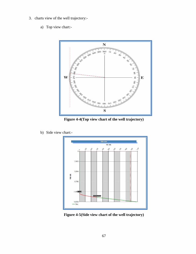
3. charts view of the well trajectory:-
a) Top view chart:-
Figure 4-4(Top view chart of the well trajectory)
b) Side view chart:-
Figure 4-5(Side view chart of the well trajectory)
68
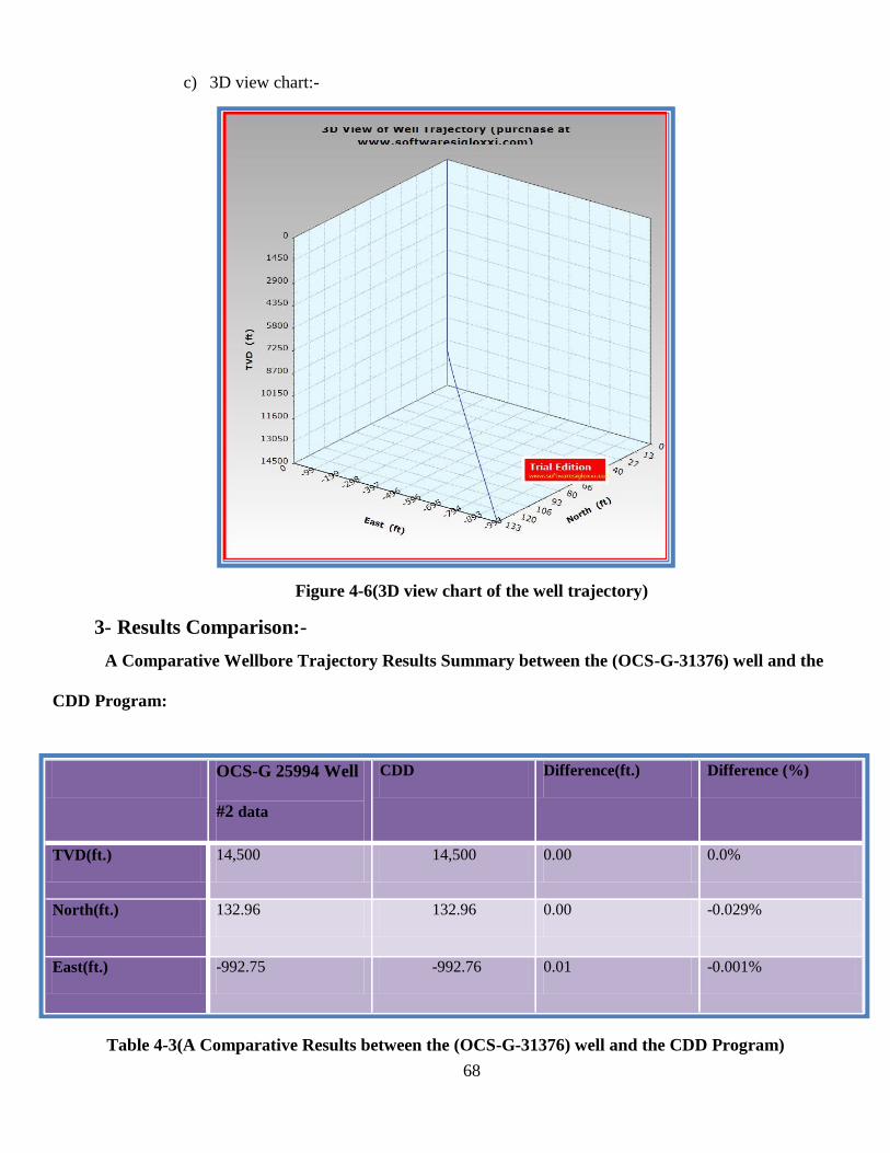
c) 3D view chart:-
Figure 4-6(3D view chart of the well trajectory)
3- Results Comparison:-
A Comparative Wellbore Trajectory Results Summary between the (OCS-G-31376) well and the
CDD Program:
Table 4-3(A Comparative Results between the (OCS-G-31376) well and the CDD Program)
OCS-G 25994 Well
#2 data
CDD Difference(ft.) Difference (%)
TVD(ft.) 14,500 14,500 0.00 0.0%
North(ft.) 132.96 132.96 0.00 -0.029%
East(ft.) -992.75 -992.76 0.01 -0.001%

69
Figure 4-7(EXCEL comparison between CDD results and the well data in side view)
Figure 4-8(EXCEL comparison between CDD results and the well data in top view)
70
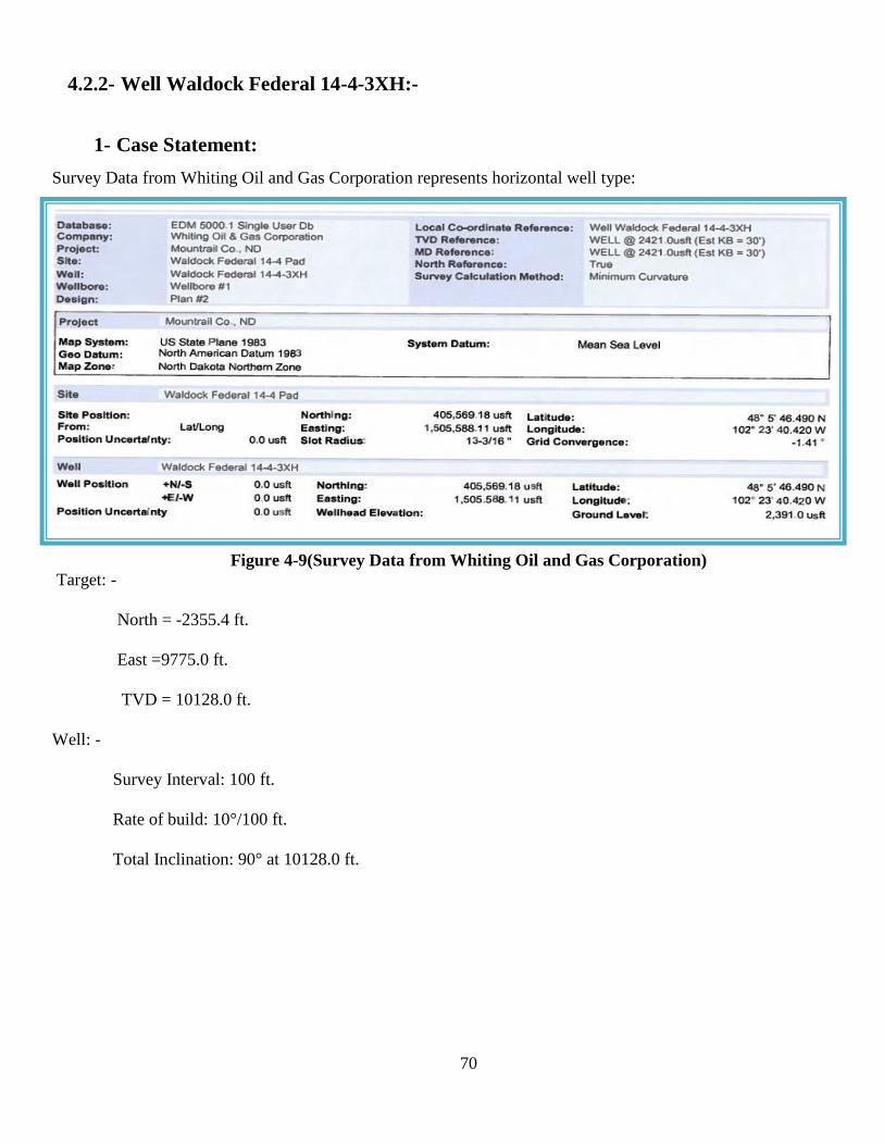
4.2.2- Well Waldock Federal 14-4-3XH:-
1- Case Statement:
Survey Data from Whiting Oil and Gas Corporation represents horizontal well type:
Figure 4-9(Survey Data from Whiting Oil and Gas Corporation)
Target: -
North = -2355.4 ft.
East =9775.0 ft.
TVD = 10128.0 ft.
Well: -
Survey Interval: 100 ft.
Rate of build: 10°/100 ft.
Total Inclination: 90° at 10128.0 ft.
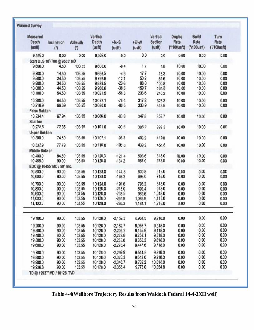
71
Table 4-4(Wellbore Trajectory Results from Waldock Federal 14-4-3XH well)

72
2- Case Study Solution:-
1) Input given data into well type data section :
Figure 4-10(Data input into well type data section)
2) Press Calculate Button to get:-
1- The output results from the data input:-
Figure 4-11(The output results from the data input)
2- the survey table for each interval:-
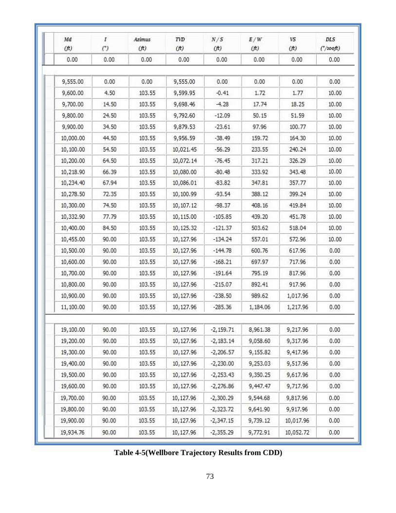
73
Table 4-5(Wellbore Trajectory Results from CDD)
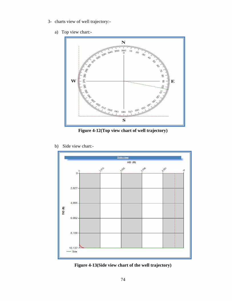
74
3- charts view of well trajectory:-
a) Top view chart:-
Figure 4-12(Top view chart of well trajectory)
b) Side view chart:-
Figure 4-13(Side view chart of the well trajectory)
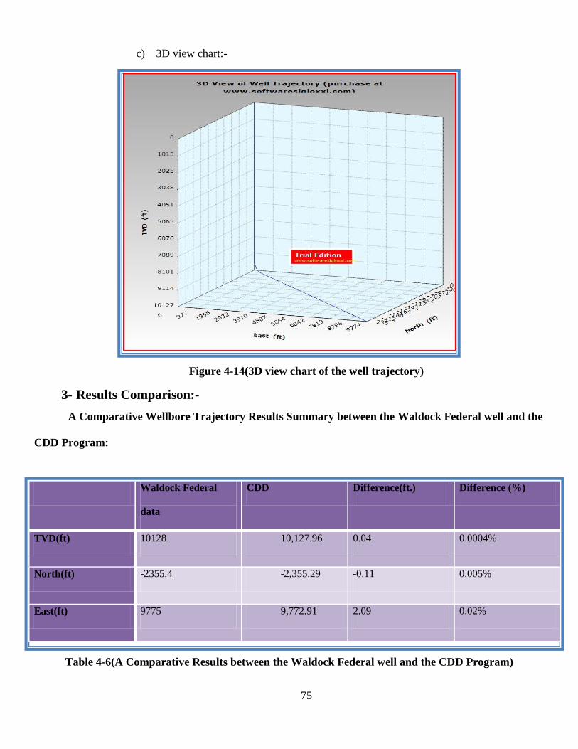
75
c) 3D view chart:-
Figure 4-14(3D view chart of the well trajectory)
3- Results Comparison:-
A Comparative Wellbore Trajectory Results Summary between the Waldock Federal well and the
CDD Program:
Table 4-6(A Comparative Results between the Waldock Federal well and the CDD Program)
Waldock Federal
data
CDD Difference(ft.) Difference (%)
TVD(ft) 10128 10,127.96 0.04 0.0004%
North(ft) -2355.4 -2,355.29 -0.11 0.005%
East(ft) 9775 9,772.91 2.09 0.02%
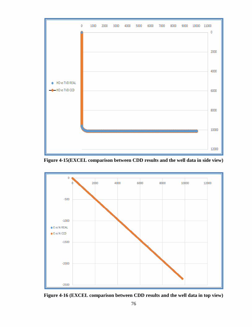
76
Figure 4-15(EXCEL comparison between CDD results and the well data in side view)
Figure 4-16 (EXCEL comparison between CDD results and the well data in top view)
77
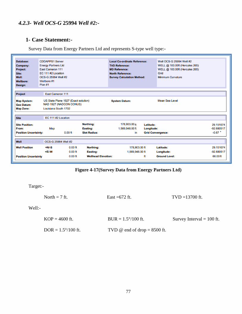
4.2.3- Well OCS-G 25994 Well #2:-
1- Case Statement:-
Survey Data from Energy Partners Ltd and represents S-type well type:-
Figure 4-17(Survey Data from Energy Partners Ltd)
Target:-
North = 7 ft. East =672 ft. TVD =13700 ft.
Well:-
KOP = 4600 ft. BUR = 1.5°/100 ft. Survey Interval = 100 ft.
DOR = 1.5°/100 ft. TVD @ end of drop = 8500 ft.
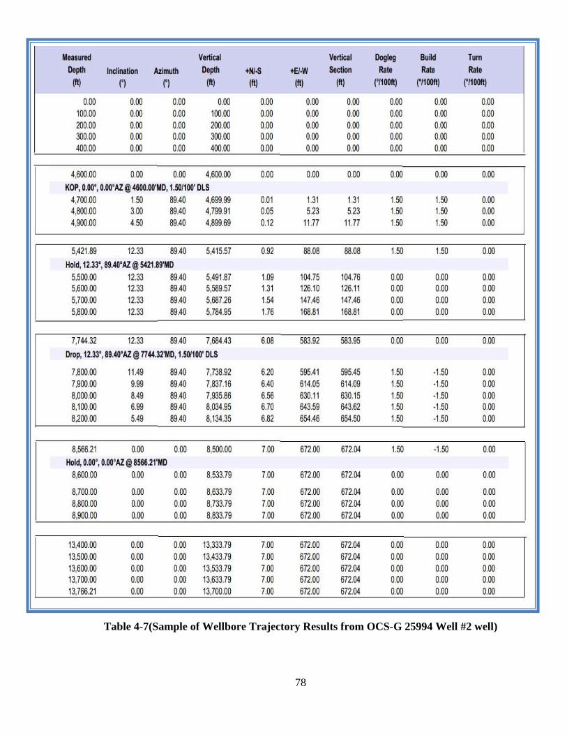
78
Table 4-7(Sample of Wellbore Trajectory Results from OCS-G 25994 Well #2 well)
79
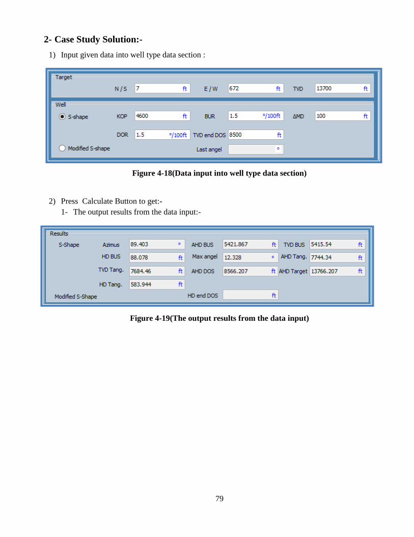
2- Case Study Solution:-
1) Input given data into well type data section :
Figure 4-18(Data input into well type data section)
2) Press Calculate Button to get:-
1- The output results from the data input:-
Figure 4-19(The output results from the data input)
80
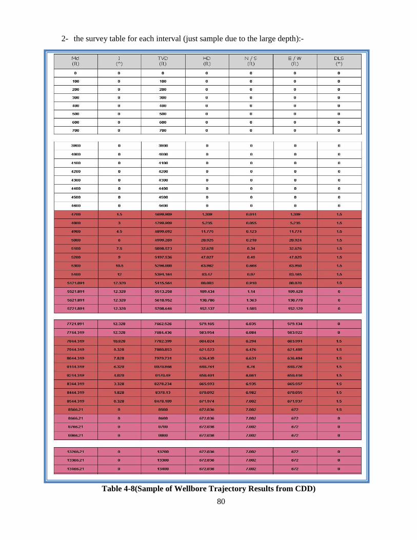
2- the survey table for each interval (just sample due to the large depth):-
Table 4-8(Sample of Wellbore Trajectory Results from CDD)
81
3-charts view of well trajectory:-
a) Top view chart:-
Figure 4-20(Top view chart of the well trajectory)
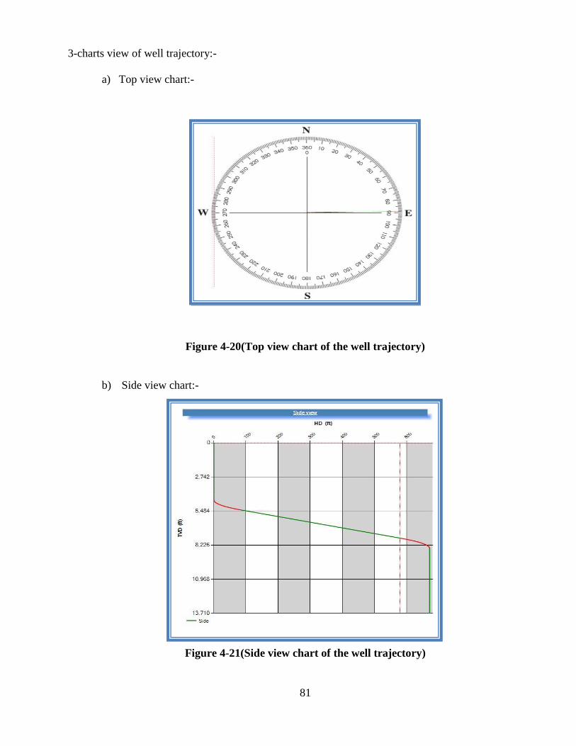
b) Side view chart:-
Figure 4-21(Side view chart of the well trajectory)

82
c) 3D view chart:-
Figure 4-22(3D view chart of the well trajectory)
3- Results Comparison:-
A Comparative Wellbore Trajectory Results Summary between the (OCS-G 25994 well#2) well and the
CDD Program:-
Table 4-9(A Comparative Results between the Waldock Federal well and the CDD Program)
OCS-G 25994 Well
#2 data
CDD Difference(ft.) Difference (%)
TVD(ft.) 13,700 13,700 0.00 0.0%
North(ft.) 7 7.002 -0.002 -0.029%
East(ft.) 672 672.036 -0.036 -0.005%
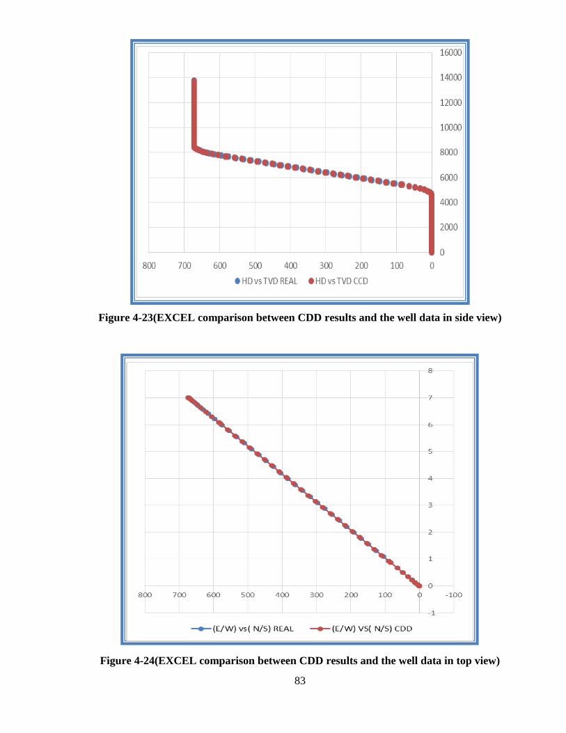
83
Figure 4-23(EXCEL comparison between CDD results and the well data in side view)
Figure 4-24(EXCEL comparison between CDD results and the well data in top view)
84
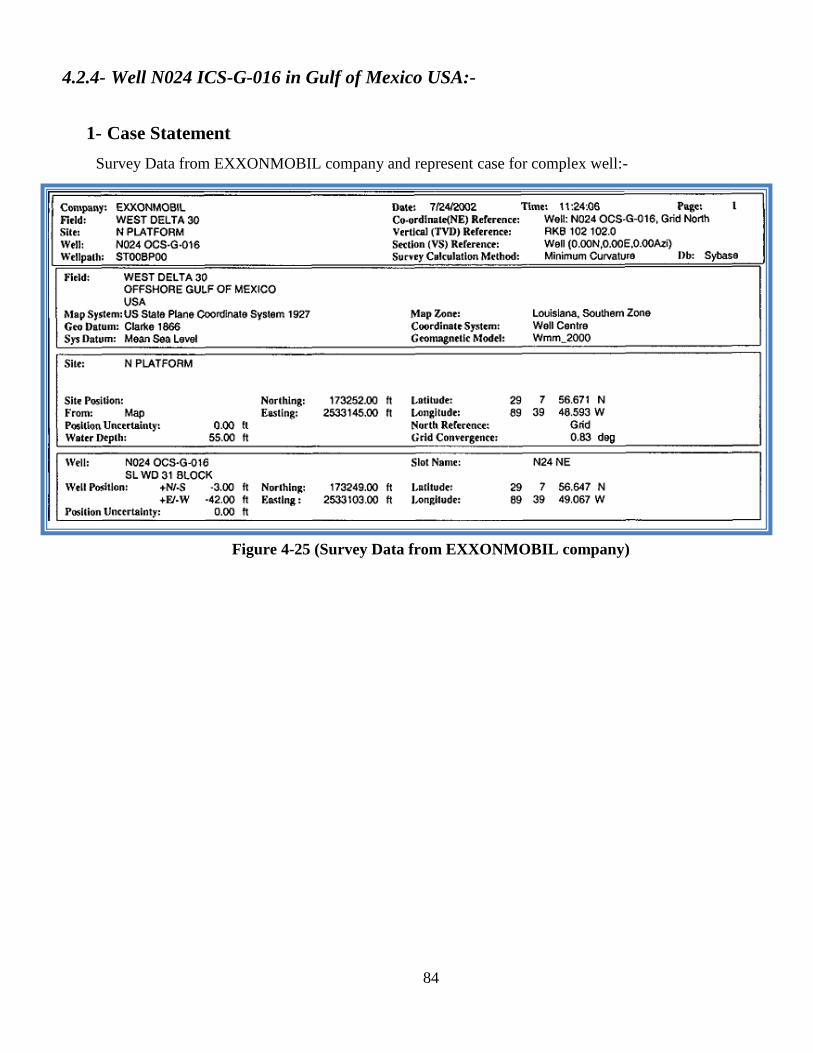
4.2.4- Well N024 ICS-G-016 in Gulf of Mexico USA:-
1- Case Statement
Survey Data from EXXONMOBIL company and represent case for complex well:-
Figure 4-25 (Survey Data from EXXONMOBIL company)
85
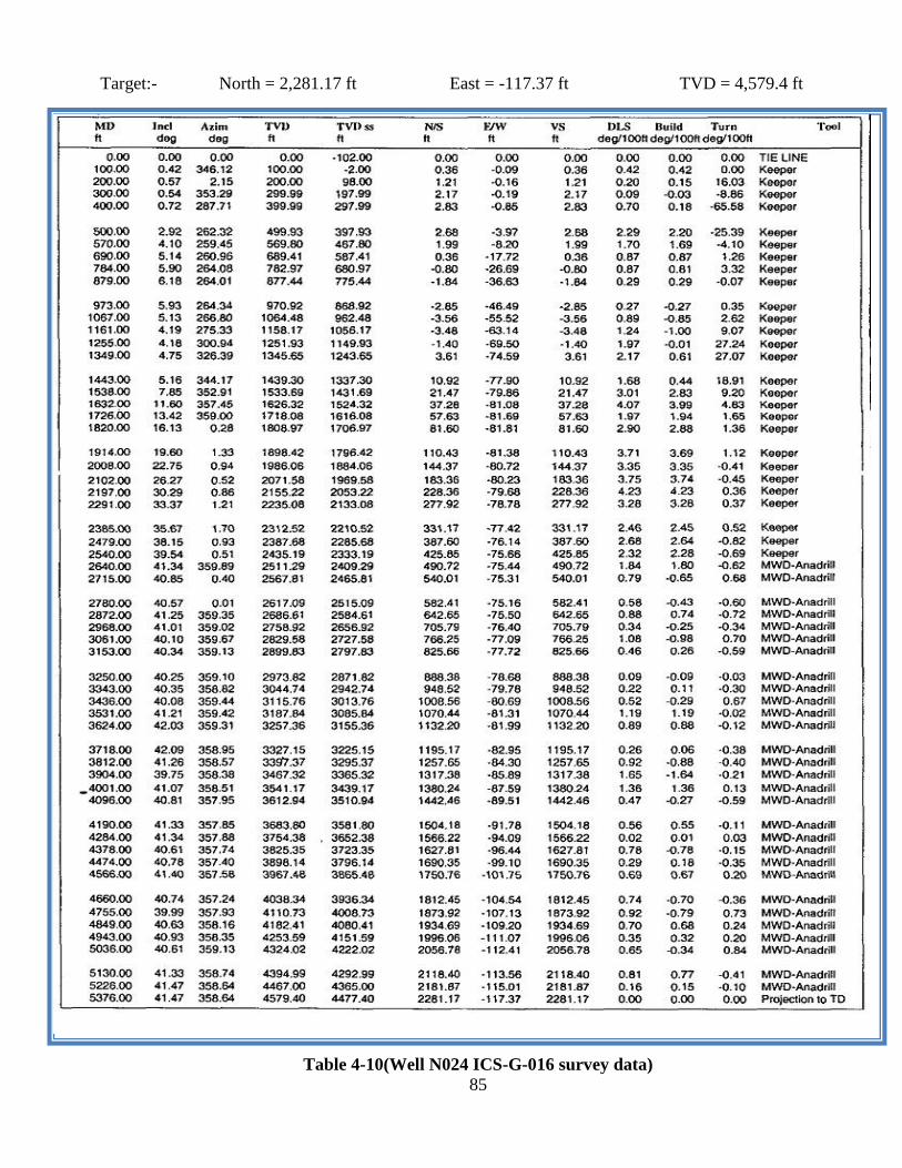
Target:- North = 2,281.17 ft East = -117.37 ft TVD = 4,579.4 ft
Table 4-10(Well N024 ICS-G-016 survey data)
86
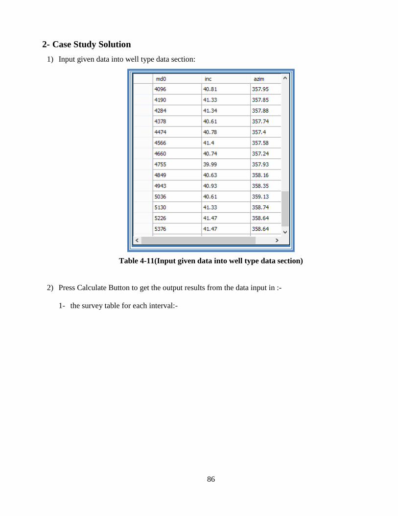
2- Case Study Solution
1) Input given data into well type data section:
Table 4-11(Input given data into well type data section)
2) Press Calculate Button to get the output results from the data input in :-
1- the survey table for each interval:-
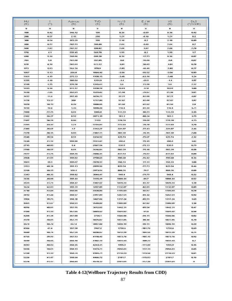
87
Table 4-12(Wellbore Trajectory Results from CDD)
88
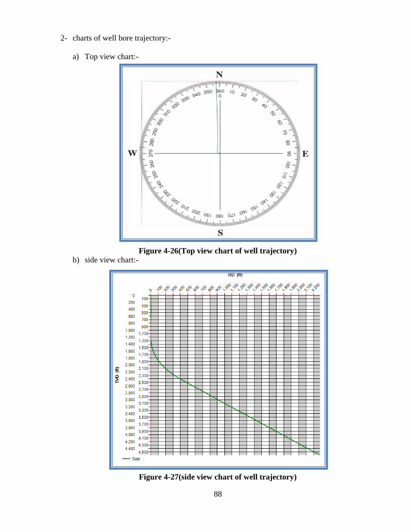
2- charts of well bore trajectory:-
a) Top view chart:-
Figure 4-26(Top view chart of well trajectory)
b) side view chart:-
Figure 4-27(side view chart of well trajectory)
89
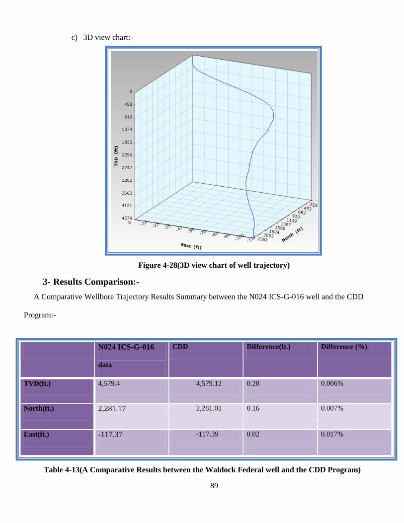
c) 3D view chart:-
Figure 4-28(3D view chart of well trajectory)
3- Results Comparison:-
A Comparative Wellbore Trajectory Results Summary between the N024 ICS-G-016 well and the CDD
Program:-
Table 4-13(A Comparative Results between the Waldock Federal well and the CDD Program)
N024 ICS-G-016
data
CDD Difference(ft.) Difference (%)
TVD(ft.) 4,579.4 4,579.12 0.28 0.006%
North(ft.) 2,281.17 2,281.01 0.16 0.007%
East(ft.) -117.37 -117.39 0.02 0.017%
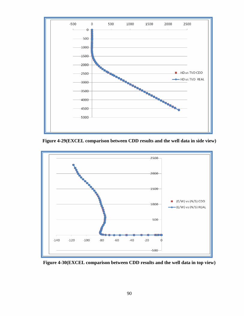
90
Figure 4-29(EXCEL comparison between CDD results and the well data in side view)
Figure 4-30(EXCEL comparison between CDD results and the well data in top view)

91
Chapter Five:
Economic Analysis

92
Chapter 5 : Economic Analysis
5.1- Introduction:-
The decision to employ directional drilling is primarily an economic one. Horizontal wells costs are
generally 20% to 25% higher than vertical well costs; because of this they must produce proportionately more
to compete economically.
5.2- Cost and risk associated with directional drilling :
The cost of directional drilling is greater than the cost of conventional drilling. This is due to the longer
time and additional equipment needed to drill and complete wells. Higher costs are also expected in the project
area due to the increased depth, the potentially higher pressure, and the increased chance of lost circulation
zones. An s-shape wellbore if required is also more costly than other types of deviated holes. Intermediate
casing, if required, would also be an additional cost.
If mechanical problems are encountered during the directional drilling, cost can rise dramatically.
Mechanical problems may include key seating, stuck pipe, fishing problems, and logging problems due to hole
deviation. The projected costs of drilling directional wells do not consider problems that may occur due to
increased risk of mechanical problems.
On an even move case-specific basis, directional wells have been found to be economically successful in
the following types of reservoirs:
1. Naturally fractured reservoir.
2. Oil reservoir with water or gas conning characteristics.
3. Sized reservoir.
4. Heavy oil reservoir.
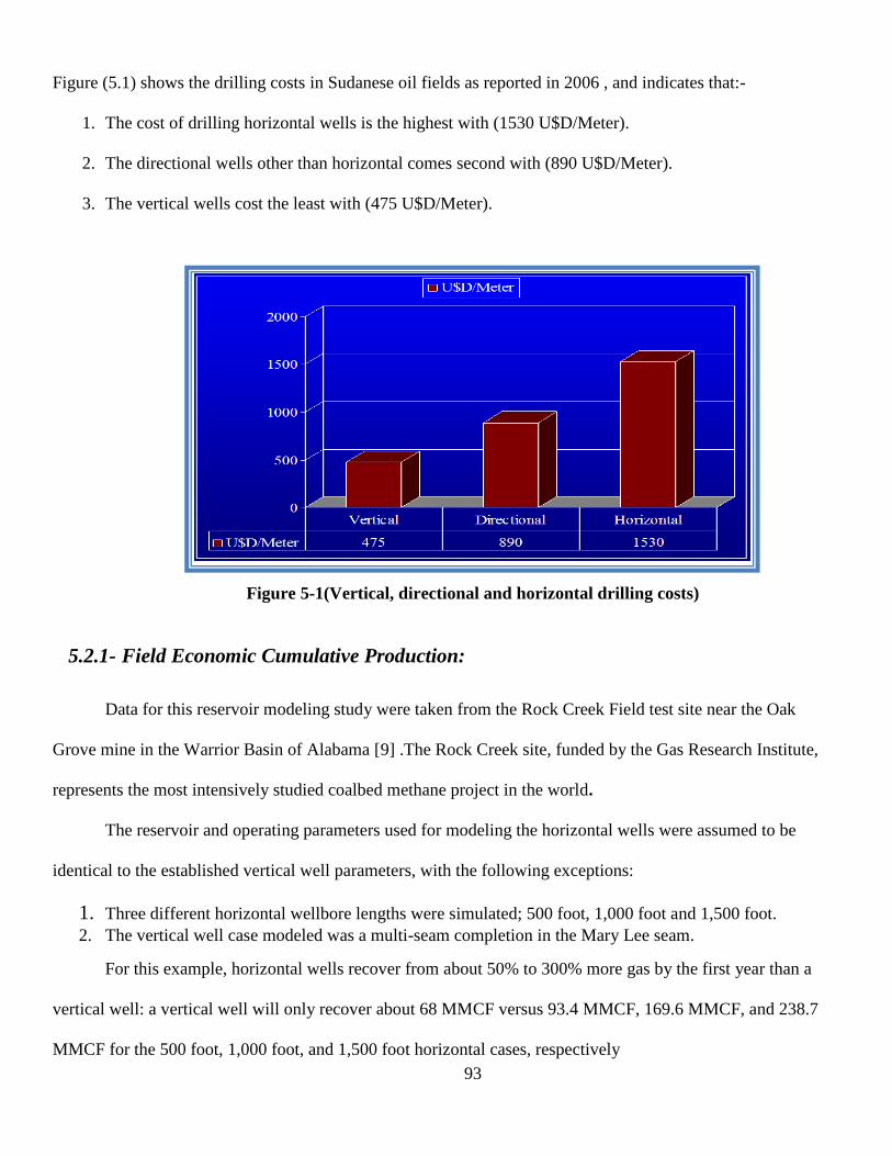
93
Figure (5.1) shows the drilling costs in Sudanese oil fields as reported in 2006 , and indicates that:-
1. The cost of drilling horizontal wells is the highest with (1530 U$D/Meter).
2. The directional wells other than horizontal comes second with (890 U$D/Meter).
3. The vertical wells cost the least with (475 U$D/Meter).
Figure 5-1(Vertical, directional and horizontal drilling costs)
5.2.1- Field Economic Cumulative Production:
Data for this reservoir modeling study were taken from the Rock Creek Field test site near the Oak
Grove mine in the Warrior Basin of Alabama [9] .The Rock Creek site, funded by the Gas Research Institute,
represents the most intensively studied coalbed methane project in the world.
The reservoir and operating parameters used for modeling the horizontal wells were assumed to be
identical to the established vertical well parameters, with the following exceptions:
1. Three different horizontal wellbore lengths were simulated; 500 foot, 1,000 foot and 1,500 foot. 2. The vertical well case modeled was a multi-seam completion in the Mary Lee seam.
For this example, horizontal wells recover from about 50% to 300% more gas by the first year than a
vertical well: a vertical well will only recover about 68 MMCF versus 93.4 MMCF, 169.6 MMCF, and 238.7
MMCF for the 500 foot, 1,000 foot, and 1,500 foot horizontal cases, respectively
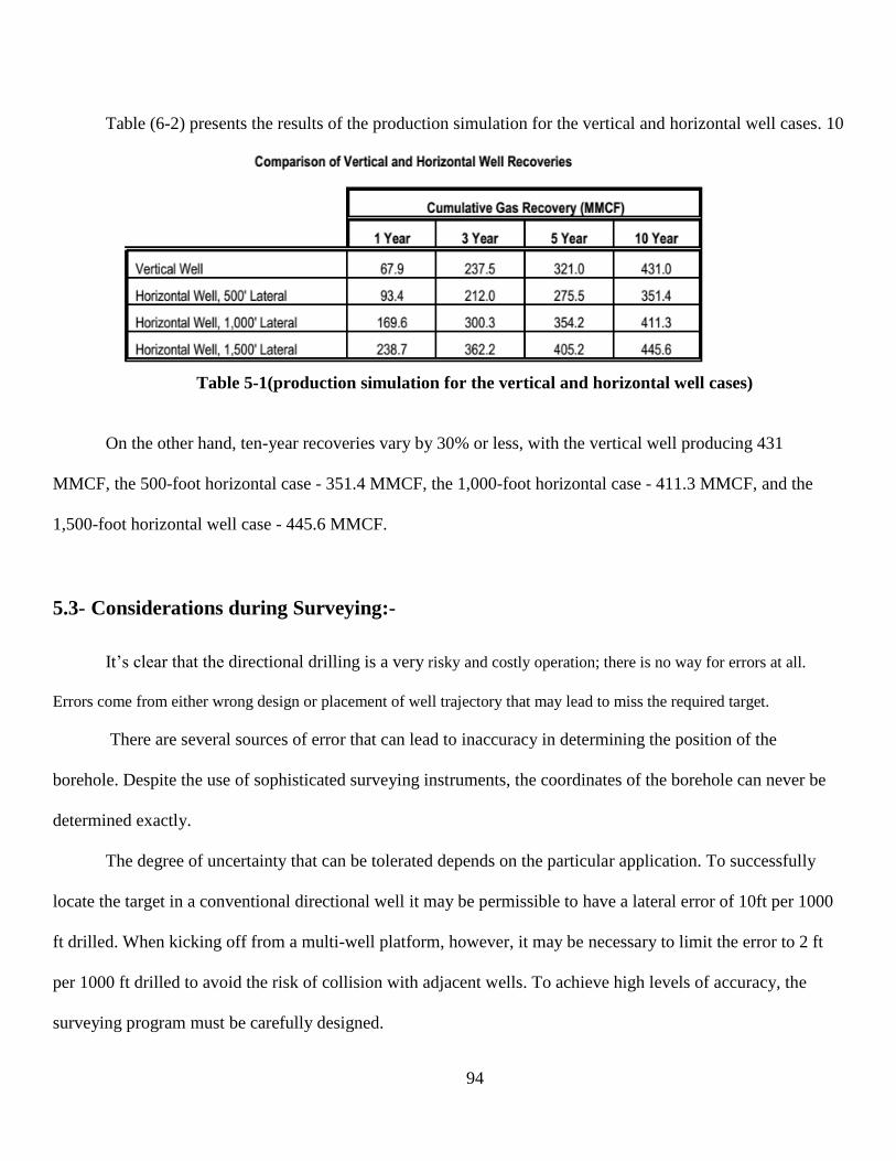
94
Table (6-2) presents the results of the production simulation for the vertical and horizontal well cases. 10
Table 5-1(production simulation for the vertical and horizontal well cases)
On the other hand, ten-year recoveries vary by 30% or less, with the vertical well producing 431
MMCF, the 500-foot horizontal case - 351.4 MMCF, the 1,000-foot horizontal case - 411.3 MMCF, and the
1,500-foot horizontal well case - 445.6 MMCF.
5.3- Considerations during Surveying:-
It’s clear that the directional drilling is a very risky and costly operation; there is no way for errors at all.
Errors come from either wrong design or placement of well trajectory that may lead to miss the required target.
There are several sources of error that can lead to inaccuracy in determining the position of the
borehole. Despite the use of sophisticated surveying instruments, the coordinates of the borehole can never be
determined exactly.
The degree of uncertainty that can be tolerated depends on the particular application. To successfully
locate the target in a conventional directional well it may be permissible to have a lateral error of 10ft per 1000
ft drilled. When kicking off from a multi-well platform, however, it may be necessary to limit the error to 2 ft
per 1000 ft drilled to avoid the risk of collision with adjacent wells. To achieve high levels of accuracy, the
surveying program must be carefully designed.

95
The source of error could be from the choice of calculation method used to calculate position of well
trajectory, the minimum curvature method is very accurate and that’s why it has been used at the designing of
this computer program.
The well must be surveyed at certain intervals to ensure it is following the planned well path. The survey
interval will vary depending on which part of the trajectory is being drilled. During kick-off, surveys should be
taken at least every 30 ft. In the tangential section when inclination is not changing so rapidly a survey interval
of 90 ft. or 120 ft. may be sufficient. The use of computer program is both money and time efficient choice
because it makes it easier to compare the results from survey instrument with the results obtained from the
program in the required interval based on the part of the trajectory that has been drilled.

96
Chapter Six:
Conclusion and
Recommendations
97
Chapter 6 : Conclusion and recommendation
6.1- Conclusion:-
1- Visual Basic software program was created to calculate the seven different types of directional
drilling trajectories based on minimum curvature method.
2- The program (Computerized Directional Drilling) is simple, friendly and easy to learn.
3- The program provides graphical views in both side and top view as well as 3D view of the well
trajectory, this helps the user to visualize and understand the path that the well will follow at.
4- This program gives very accurate results and can be used in the planning for the drilling
operations with probability of a very small error to occur.
5- Major advantages of this program is that it doesn’t need high computer requirements to install,
and doesn’t require large computer space or speed to run.
6- The case studies show that the program can produce same results as the ones obtained from the
field data. Thus it can be used for directional drilling in real fields.
7- The Economic analysis demonstrate that directional drilling costs more during the drilling phase
, but it can be more economic in long cumulative production time periods .

98
6.2- Recommendation:-
1) Directional drilling is both risky and costly process, thus the use computer programs is recommended in
planning and surveying rather than using manual methods of calculations.
2) This program took a lot of effort and time to make and optimized and hopefully it will find its way in the
petroleum industry.
3) Future development can be made in the program to add new features and take new considerations such
As (TVD boundaries, Geological Formations tops grid data …etc.).
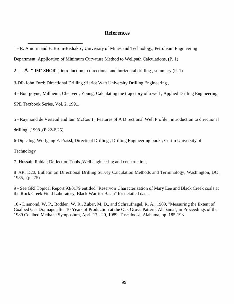
99
References
1 - R. Amorin and E. Broni-Bediako ; University of Mines and Technology, Petroleum Engineering
Department, Application of Minimum Curvature Method to Wellpath Calculations, (P. 1)
2 - J. A. "JIM" SHORT; introduction to directional and horizontal drilling , summary (P. 1)
3-DR-John Ford; Directional Drilling ;Heriot Watt University Drilling Engineering ,
4 - Bourgoyne, Millheim, Chenvert, Young; Calculating the trajectory of a well , Applied Drilling Engineering,
SPE Textbook Series, Vol. 2, 1991.
5 - Raymond de Verteuil and Iain McCourt ; Features of A Directional Well Profile , introduction to directional
drilling ,1998 ,(P.22-P.25)
6-Dipl.-Ing. Wolfgang F. Prassl,;Directinal Drilling , Drilling Engineering book ; Curtin University of
Technology
7 -Hussain Rabia ; Deflection Tools ,Well engineering and construction,
8 -API D20, Bulletin on Directional Drilling Survey Calculation Methods and Terminology, Washington, DC ,
1985, (p 275)
9 - See GRI Topical Report 93/0179 entitled "Reservoir Characterization of Mary Lee and Black Creek coals at
the Rock Creek Field Laboratory, Black Warrior Basin" for detailed data.
10 - Diamond, W. P., Bodden, W. R., Zuber, M. D., and Schraufnagel, R. A., 1989, "Measuring the Extent of
Coalbed Gas Drainage after 10 Years of Production at the Oak Grove Pattern, Alabama", in Proceedings of the
1989 Coalbed Methane Symposium, April 17 - 20, 1989, Tuscaloosa, Alabama, pp. 185-193
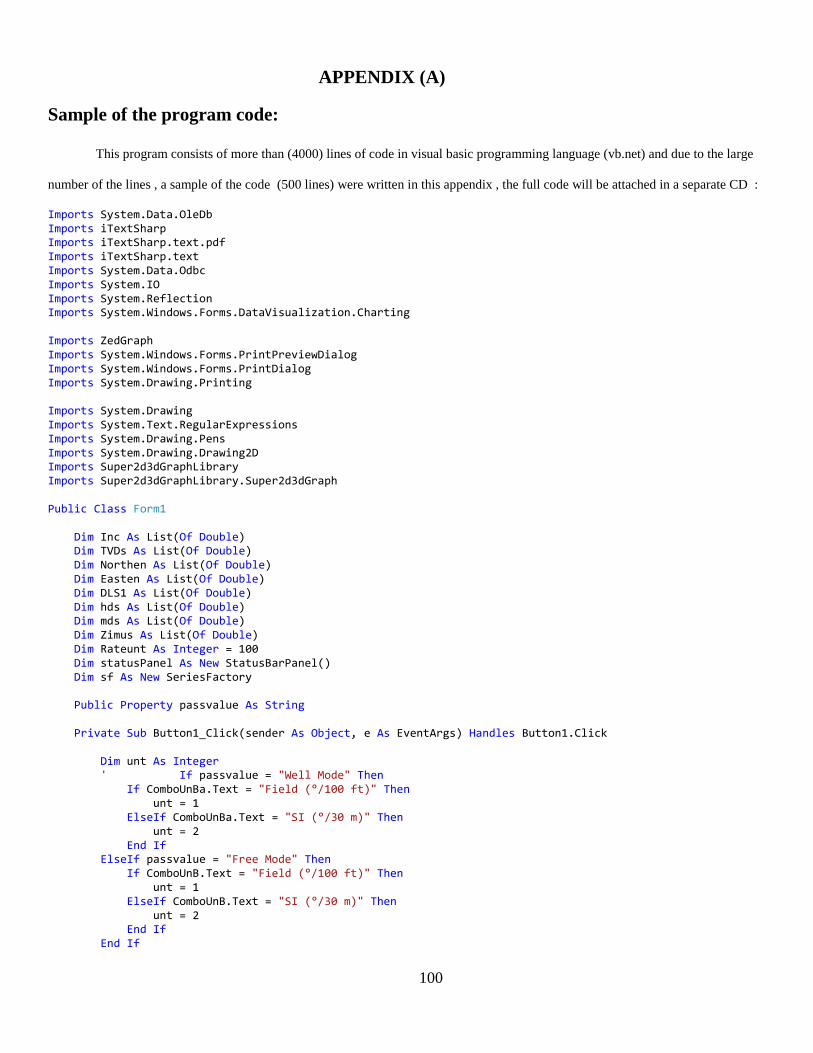
100
APPENDIX (A)
Sample of the program code:
This program consists of more than (4000) lines of code in visual basic programming language (vb.net) and due to the large
number of the lines , a sample of the code (500 lines) were written in this appendix , the full code will be attached in a separate CD :
Imports System.Data.OleDb Imports iTextSharp Imports iTextSharp.text.pdf Imports iTextSharp.text Imports System.Data.Odbc Imports System.IO Imports System.Reflection Imports System.Windows.Forms.DataVisualization.Charting Imports ZedGraph Imports System.Windows.Forms.PrintPreviewDialog Imports System.Windows.Forms.PrintDialog Imports System.Drawing.Printing Imports System.Drawing Imports System.Text.RegularExpressions Imports System.Drawing.Pens Imports System.Drawing.Drawing2D Imports Super2d3dGraphLibrary Imports Super2d3dGraphLibrary.Super2d3dGraph Public Class Form1 Dim Inc As List(Of Double) Dim TVDs As List(Of Double) Dim Northen As List(Of Double) Dim Easten As List(Of Double) Dim DLS1 As List(Of Double) Dim hds As List(Of Double) Dim mds As List(Of Double) Dim Zimus As List(Of Double) Dim Rateunt As Integer = 100 Dim statusPanel As New StatusBarPanel() Dim sf As New SeriesFactory Public Property passvalue As String Private Sub Button1_Click(sender As Object, e As EventArgs) Handles Button1.Click Dim unt As Integer ' If passvalue = "Well Mode" Then If ComboUnBa.Text = "Field (°/100 ft)" Then unt = 1 ElseIf ComboUnBa.Text = "SI (°/30 m)" Then unt = 2 End If ElseIf passvalue = "Free Mode" Then If ComboUnB.Text = "Field (°/100 ft)" Then unt = 1 ElseIf ComboUnB.Text = "SI (°/30 m)" Then unt = 2 End If End If
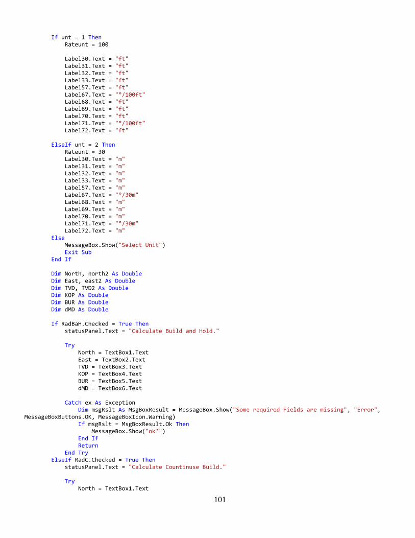
101
If unt = 1 Then Rateunt = 100 Label30.Text = "ft" Label31.Text = "ft" Label32.Text = "ft" Label33.Text = "ft" Label57.Text = "ft" Label67.Text = "°/100ft" Label68.Text = "ft" Label69.Text = "ft" Label70.Text = "ft" Label71.Text = "°/100ft" Label72.Text = "ft" ElseIf unt = 2 Then Rateunt = 30 Label30.Text = "m" Label31.Text = "m" Label32.Text = "m" Label33.Text = "m" Label57.Text = "m" Label67.Text = "°/30m" Label68.Text = "m" Label69.Text = "m" Label70.Text = "m" Label71.Text = "°/30m" Label72.Text = "m" Else MessageBox.Show("Select Unit") Exit Sub End If Dim North, north2 As Double Dim East, east2 As Double Dim TVD, TVD2 As Double Dim KOP As Double Dim BUR As Double Dim dMD As Double If RadBaH.Checked = True Then statusPanel.Text = "Calculate Build and Hold." Try North = TextBox1.Text East = TextBox2.Text TVD = TextBox3.Text KOP = TextBox4.Text BUR = TextBox5.Text dMD = TextBox6.Text Catch ex As Exception Dim msgRslt As MsgBoxResult = MessageBox.Show("Some required Fields are missing", "Error", MessageBoxButtons.OK, MessageBoxIcon.Warning) If msgRslt = MsgBoxResult.Ok Then MessageBox.Show("ok?") End If Return End Try ElseIf RadC.Checked = True Then statusPanel.Text = "Calculate Countinuse Build." Try North = TextBox1.Text
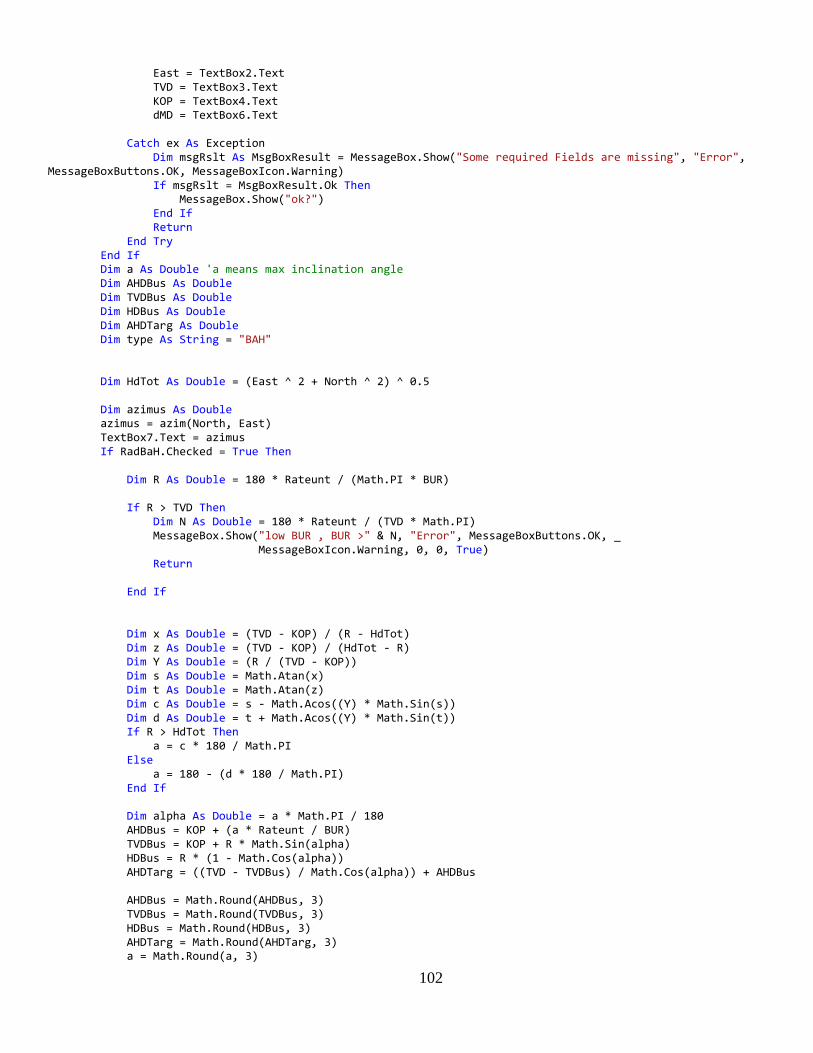
102
East = TextBox2.Text TVD = TextBox3.Text KOP = TextBox4.Text dMD = TextBox6.Text Catch ex As Exception Dim msgRslt As MsgBoxResult = MessageBox.Show("Some required Fields are missing", "Error", MessageBoxButtons.OK, MessageBoxIcon.Warning) If msgRslt = MsgBoxResult.Ok Then MessageBox.Show("ok?") End If Return End Try End If Dim a As Double 'a means max inclination angle Dim AHDBus As Double Dim TVDBus As Double Dim HDBus As Double Dim AHDTarg As Double Dim type As String = "BAH" Dim HdTot As Double = (East ^ 2 + North ^ 2) ^ 0.5 Dim azimus As Double azimus = azim(North, East) TextBox7.Text = azimus If RadBaH.Checked = True Then Dim R As Double = 180 * Rateunt / (Math.PI * BUR) If R > TVD Then Dim N As Double = 180 * Rateunt / (TVD * Math.PI) MessageBox.Show("low BUR , BUR >" & N, "Error", MessageBoxButtons.OK, _ MessageBoxIcon.Warning, 0, 0, True) Return End If Dim x As Double = (TVD - KOP) / (R - HdTot) Dim z As Double = (TVD - KOP) / (HdTot - R) Dim Y As Double = (R / (TVD - KOP)) Dim s As Double = Math.Atan(x) Dim t As Double = Math.Atan(z) Dim c As Double = s - Math.Acos((Y) * Math.Sin(s)) Dim d As Double = t + Math.Acos((Y) * Math.Sin(t)) If R > HdTot Then a = c * 180 / Math.PI Else a = 180 - (d * 180 / Math.PI) End If Dim alpha As Double = a * Math.PI / 180 AHDBus = KOP + (a * Rateunt / BUR) TVDBus = KOP + R * Math.Sin(alpha) HDBus = R * (1 - Math.Cos(alpha)) AHDTarg = ((TVD - TVDBus) / Math.Cos(alpha)) + AHDBus AHDBus = Math.Round(AHDBus, 3) TVDBus = Math.Round(TVDBus, 3) HDBus = Math.Round(HDBus, 3) AHDTarg = Math.Round(AHDTarg, 3) a = Math.Round(a, 3)
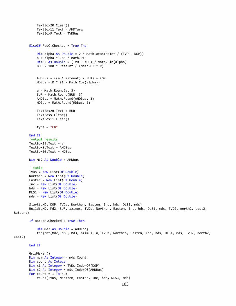
103
TextBox20.Clear() TextBox11.Text = AHDTarg TextBox9.Text = TVDBus ElseIf RadC.Checked = True Then Dim alpha As Double = 2 * Math.Atan(HdTot / (TVD - KOP)) a = alpha * 180 / Math.PI Dim R As Double = (TVD - KOP) / Math.Sin(alpha) BUR = 180 * Rateunt / (Math.PI * R) AHDBus = ((a * Rateunt) / BUR) + KOP HDBus = R * (1 - Math.Cos(alpha)) a = Math.Round(a, 3) BUR = Math.Round(BUR, 3) AHDBus = Math.Round(AHDBus, 3) HDBus = Math.Round(HDBus, 3) TextBox20.Text = BUR TextBox9.Clear() TextBox11.Clear() type = "CB" End If 'output results TextBox12.Text = a TextBox8.Text = AHDBus TextBox10.Text = HDBus Dim Md2 As Double = AHDBus ' table TVDs = New List(Of Double) Northen = New List(Of Double) Easten = New List(Of Double) Inc = New List(Of Double) hds = New List(Of Double) DLS1 = New List(Of Double) mds = New List(Of Double) Start(dMD, KOP, TVDs, Northen, Easten, Inc, hds, DLS1, mds) Build(dMD, Md2, BUR, azimus, TVDs, Northen, Easten, Inc, hds, DLS1, mds, TVD2, north2, east2, Rateunt) If RadBaH.Checked = True Then Dim Md3 As Double = AHDTarg tangent(Md2, dMD, Md3, azimus, a, TVDs, Northen, Easten, Inc, hds, DLS1, mds, TVD2, north2, east2) End If GridMaker() Dim num As Integer = mds.Count Dim count As Integer Dim x1 As Integer = TVDs.IndexOf(KOP) Dim x2 As Integer = mds.IndexOf(AHDBus) For count = 1 To num round(TVDs, Northen, Easten, Inc, hds, DLS1, mds)
104
Next For count = 1 To x1 + 1 DataGridView1.Rows.Add(mds(count - 1), Inc(count - 1), TVDs(count - 1), hds(count - 1), Northen(count - 1), Easten(count - 1), DLS1(count - 1)) Next For count = x1 + 2 To x2 + 1 DataGridView1.Rows.Add(mds(count - 1), Inc(count - 1), TVDs(count - 1), hds(count - 1), Northen(count - 1), Easten(count - 1), DLS1(count - 1)) DataGridView1.Rows(count - 1).DefaultCellStyle.BackColor = Color.IndianRed Next For count = x2 + 2 To num DataGridView1.Rows.Add(mds(count - 1), Inc(count - 1), TVDs(count - 1), hds(count - 1), Northen(count - 1), Easten(count - 1), DLS1(count - 1)) DataGridView1.Rows(count - 1).DefaultCellStyle.BackColor = Color.PaleVioletRed Next Dim x3, x4 As Integer If ChkNewLine.Checked = True Then chart(TVDs, hds, Northen, Easten, x1, x2, x3, x4, type) Else chartSec(TVDs, hds, Northen, Easten, x1, x2, x3, x4, type) End If End Sub Private Sub round(ByRef tvds As List(Of Double), ByRef northen As List(Of Double), ByRef easten As List(Of Double), ByRef inc As List(Of Double), _ ByRef hds As List(Of Double), ByRef dls1 As List(Of Double), ByRef mds As List(Of Double)) For I As Integer = 1 To tvds.Count mds(I - 1) = Math.Round(mds(I - 1), 3) tvds(I - 1) = Math.Round(tvds(I - 1), 3) northen(I - 1) = Math.Round(northen(I - 1), 3) easten(I - 1) = Math.Round(easten(I - 1), 3) hds(I - 1) = Math.Round(hds(I - 1), 3) inc(I - 1) = Math.Round(inc(I - 1), 3) dls1(I - 1) = Math.Round(dls1(I - 1), 3) Next End Sub Private Sub Button2_Click(sender As Object, e As EventArgs) Handles Button2.Click statusPanel.Text = "Clear Inputs and Outputs." TextBox1.Clear() TextBox2.Clear() TextBox3.Clear() TextBox4.Clear() TextBox5.Clear() TextBox6.Clear() TextBox7.Clear() TextBox8.Clear() TextBox9.Clear() TextBox10.Clear() TextBox11.Clear() TextBox12.Clear() TextBox20.Clear() DataGridView1.Rows.Clear() End Sub Private Sub GridMaker() With DataGridView1 .Columns.Clear() Dim unt As Integer
105
If passvalue = "Well Mode" Then If ComboUnBa.Text = "Field (°/100 ft)" Then unt = 1 ElseIf ComboUnBa.Text = "SI (°/30 m)" Then unt = 2 End If ElseIf passvalue = "Free Mode" Then If ComboUnB.Text = "Field (°/100 ft)" Then unt = 1 ElseIf ComboUnB.Text = "SI (°/30 m)" Then unt = 2 End If End If If unt = 1 Then .Columns.Add("MD", "Md" & vbCrLf & "(ft)") .Columns.Add("I", "I" & vbCrLf & "(°)") .Columns.Add("TVD", "TVD" & vbCrLf & "(ft)") .Columns.Add("HD", "HD" & vbCrLf & "(ft)") .Columns.Add("N / S", "N / S" & vbCrLf & "(ft)") .Columns.Add("E / W", "E / W" & vbCrLf & "(ft)") .Columns.Add("DLS", "DLS" & vbCrLf & "(°)") ElseIf unt = 2 Then .Columns.Add("MD", "MD" & vbCrLf & "(m)") .Columns.Add("I", "I" & vbCrLf & "(°)") .Columns.Add("TVD", "TVD" & vbCrLf & "(m)") .Columns.Add("HD", "HD" & vbCrLf & "(m)") .Columns.Add("N / S", "N / S" & vbCrLf & "(m)") .Columns.Add("E / W", "E / W" & vbCrLf & "(m)") .Columns.Add("DLS", "DLS" & vbCrLf & "(°)") End If End With End Sub Private Function azim(ByVal north As Double, ByVal east As Double) As Double Dim q As Double = (east / north) Dim t As Double = Math.Abs(q) Dim azimus As Double = Math.Atan(t) * 180 / Math.PI t = azimus If (east > 0) Then If (north < 0) Then t = 180 - t End If Else If (north > 0) Then t = 360 - t Else t = 180 + t End If End If azimus = Math.Round(t, 3) Return azimus End Function Private Sub Start(ByVal dmd As Double, ByVal kop As Double, ByRef tvds As List(Of Double), _ ByRef northen As List(Of Double), ByRef easten As List(Of Double), ByRef inc As List(Of Double), _ ByRef hds As List(Of Double), ByRef dls1 As List(Of Double), ByRef mds As List(Of Double)) Dim md As Double = 0 While md <= kop mds.Add(md) inc.Add(0) tvds.Add(md) hds.Add(0)

106
northen.Add(0) easten.Add(0) dls1.Add(0) md = md + dmd End While If md > kop Then md = md - dmd Dim difmd As Double = kop - md If difmd = 0 Then Exit Sub End If md = kop mds.Add(md) inc.Add(0) tvds.Add(md) hds.Add(0) northen.Add(0) easten.Add(0) dls1.Add(0) End If End Sub Private Sub Build(ByVal dmd As Double, ByVal md2 As Double, ByVal BUR As Double, _ ByVal azimus As Double, ByRef tvds As List(Of Double), ByRef northen As List(Of Double), _ ByRef easten As List(Of Double), ByRef inc As List(Of Double), ByRef hds As List(Of Double), _ ByRef dls1 As List(Of Double), ByRef mds As List(Of Double), ByRef tvd As Double, ByRef north As Double _ , ByRef east As Double, ByVal Rateunt As Integer) Dim num As Integer = tvds.Count Dim md As Double = mds(num - 1) + dmd tvd = tvds(num - 1) Dim dI As Double = BUR * dmd / Rateunt Dim I1, I2, dls, Rf, dTVD, dNorth, dEast, hd As Double Dim Inc1 As Double = inc(num - 1) Dim Inc2 As Double = inc(num - 1) + dI Dim az0, D, DLS2 As Double If Inc1 = 0 Then az0 = 0 Else az0 = azimus * Math.PI / 180 End If azimus = azimus * Math.PI / 180 If md = md2 Then Exit Sub End If While md <= md2 dls = Math.Acos(Math.Cos(Inc2 - Inc1)) DLS2 = dls * Math.PI / 180 Rf = 2 / DLS2 * Math.Tan(DLS2 / 2) I1 = Inc1 * Math.PI / 180 I2 = Inc2 * Math.PI / 180 dTVD = dmd * (Math.Cos(I1) + Math.Cos(I2)) * Rf / 2
107
dNorth = dmd * Rf * ((Math.Sin(I1) * Math.Cos(az0)) + (Math.Sin(I2) * Math.Cos(azimus))) / 2 dEast = dmd * Rf * ((Math.Sin(I1) * Math.Sin(az0)) + (Math.Sin(I2) * Math.Sin(azimus))) / 2 tvd = tvd + dTVD north = north + dNorth east = east + dEast hd = (east ^ 2 + north ^ 2) ^ 0.5 dls = 100 * dls / dmd mds.Add(md) inc.Add(Inc2) tvds.Add(tvd) hds.Add(hd) northen.Add(north) easten.Add(east) dls1.Add(dls) md = md + dmd Inc1 = Inc1 + dI Inc2 = Inc2 + dI az0 = azimus End While If md > md2 Then md = md - dmd Inc2 = Inc2 - dI Dim DifMd As Double = md2 - md If DifMd = 0 Then Exit Sub End If md = md2 dI = BUR * DifMd / Rateunt Inc2 = Inc2 + dI dls = Math.Acos(Math.Cos(Inc2 - Inc1)) DLS2 = dls * Math.PI / 180 Rf = 2 / DLS2 * Math.Tan(DLS2 / 2) I1 = Inc1 * Math.PI / 180 I2 = Inc2 * Math.PI / 180 dTVD = DifMd * (Math.Cos(I1) + Math.Cos(I2)) * Rf / 2 dNorth = DifMd * Rf * ((Math.Sin(I1) * Math.Cos(azimus)) + (Math.Sin(I2) * Math.Cos(azimus))) / 2 dEast = DifMd * Rf * ((Math.Sin(I1) * Math.Sin(azimus)) + (Math.Sin(I2) * Math.Sin(azimus))) / 2 tvd = tvd + dTVD north = north + dNorth east = east + dEast hd = (east ^ 2 + north ^ 2) ^ 0.5 'dls = 100 * dls / DifMd mds.Add(md) inc.Add(Inc2) tvds.Add(tvd) hds.Add(hd) northen.Add(north) easten.Add(east) dls1.Add(dls) End If End Sub
108
Private Sub tangent(ByVal md2 As Double, ByVal dmd As Double, ByVal md3 As Double, ByVal azimus As Double, _ ByVal a As Double, ByRef tvds As List(Of Double), ByRef northen As List(Of Double), _ ByRef easten As List(Of Double), ByRef inc As List(Of Double), ByRef hds As List(Of Double), _ ByRef dls1 As List(Of Double), ByRef mds As List(Of Double), ByRef tvd As Double, ByRef north As Double, _ ByRef east As Double) Dim num As Integer = mds.Count Dim md As Double = mds(num - 1) + dmd tvd = tvds(num - 1) Dim HD As Double Dim I As Double = a Dim I1 As Double = I * Math.PI / 180 azimus = azimus * Math.PI / 180 Dim DLS As Double = 0 If md2 = md3 Then Exit Sub End If While md <= md3 tvd = tvd + (dmd * Math.Cos(I1)) north = north + (dmd * Math.Sin(I1) * Math.Cos(azimus)) east = east + (dmd * Math.Sin(I1) * Math.Sin(azimus)) HD = (north ^ 2 + east ^ 2) ^ 0.5 mds.Add(md) inc.Add(I) tvds.Add(tvd) hds.Add(HD) northen.Add(north) easten.Add(east) dls1.Add(DLS) md = md + dmd End While If md > md3 Then md = md - dmd Dim DifMd As Double = md3 - md If DifMd = 0 Then Exit Sub End If md = md3 tvd = tvd + (DifMd * Math.Cos(I1)) north = north + (DifMd * Math.Sin(I1) * Math.Cos(azimus)) east = east + (DifMd * Math.Sin(I1) * Math.Sin(azimus)) HD = (north ^ 2 + east ^ 2) ^ 0.5 mds.Add(md) inc.Add(I) tvds.Add(tvd) hds.Add(HD) northen.Add(north) easten.Add(east) dls1.Add(DLS) End If End Sub Private Sub Drop(ByVal MD3 As Double, ByVal dmd As Double, ByVal md4 As Double, ByVal DOR As Double, _ ByVal azimus As Double, ByVal a As Double, ByRef tvds As List(Of Double), ByRef northen As List(Of Double), _ ByRef easten As List(Of Double), ByRef inc As List(Of Double), ByRef hds As List(Of Double), _ ByRef dls1 As List(Of Double), ByRef mds As List(Of Double), ByRef tvd As Double, ByRef north As Double _
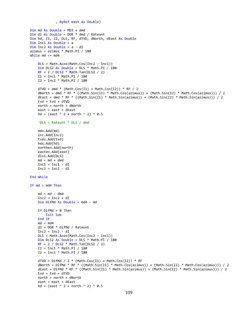
109
, ByRef east As Double) Dim md As Double = MD3 + dmd Dim dI As Double = DOR * dmd / Rateunt Dim hd, I1, I2, DLS, RF, dTVD, dNorth, dEast As Double Dim Inc1 As Double = a Dim Inc2 As Double = a - dI azimus = azimus * Math.PI / 180 While md <= md4 DLS = Math.Acos(Math.Cos(Inc2 - Inc1)) Dim DLS2 As Double = DLS * Math.PI / 180 RF = 2 / DLS2 * Math.Tan(DLS2 / 2) I1 = Inc1 * Math.PI / 180 I2 = Inc2 * Math.PI / 180 dTVD = dmd * (Math.Cos(I1) + Math.Cos(I2)) * RF / 2 dNorth = dmd * RF * ((Math.Sin(I1) * Math.Cos(azimus)) + (Math.Sin(I2) * Math.Cos(azimus))) / 2 dEast = dmd * RF * ((Math.Sin(I1) * Math.Sin(azimus)) + (Math.Sin(I2) * Math.Sin(azimus))) / 2 tvd = tvd + dTVD north = north + dNorth east = east + dEast hd = (east ^ 2 + north ^ 2) ^ 0.5 'DLS = Rateunt * DLS / dmd mds.Add(md) inc.Add(Inc2) tvds.Add(tvd) hds.Add(hd) northen.Add(north) easten.Add(east) dls1.Add(DLS) md = md + dmd Inc1 = Inc1 - dI Inc2 = Inc2 - dI End While If md > md4 Then md = md - dmd Inc2 = Inc2 + dI Dim DifMd As Double = md4 - md If DifMd = 0 Then Exit Sub End If md = md4 dI = DOR * DifMd / Rateunt Inc2 = Inc2 - dI DLS = Math.Acos(Math.Cos(Inc2 - Inc1)) Dim DLS2 As Double = DLS * Math.PI / 180 RF = 2 / DLS2 * Math.Tan(DLS2 / 2) I1 = Inc1 * Math.PI / 180 I2 = Inc2 * Math.PI / 180 dTVD = DifMd / 2 * (Math.Cos(I1) + Math.Cos(I2)) * RF dNorth = DifMd * RF * ((Math.Sin(I1) * Math.Cos(azimus)) + (Math.Sin(I2) * Math.Cos(azimus))) / 2 dEast = DifMd * RF * ((Math.Sin(I1) * Math.Sin(azimus)) + (Math.Sin(I2) * Math.Sin(azimus))) / 2 tvd = tvd + dTVD north = north + dNorth east = east + dEast hd = (east ^ 2 + north ^ 2) ^ 0.5
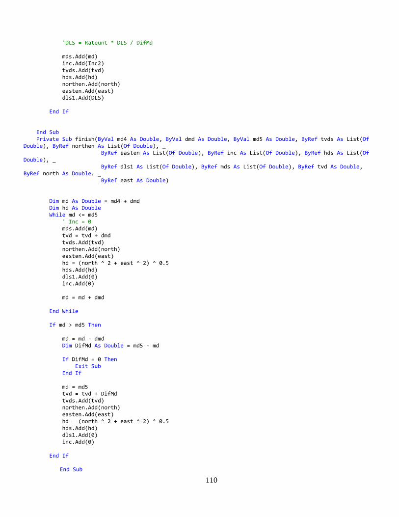
110
'DLS = Rateunt * DLS / DifMd mds.Add(md) inc.Add(Inc2) tvds.Add(tvd) hds.Add(hd) northen.Add(north) easten.Add(east) dls1.Add(DLS) End If End Sub Private Sub finish(ByVal md4 As Double, ByVal dmd As Double, ByVal md5 As Double, ByRef tvds As List(Of Double), ByRef northen As List(Of Double), _ ByRef easten As List(Of Double), ByRef inc As List(Of Double), ByRef hds As List(Of Double), _ ByRef dls1 As List(Of Double), ByRef mds As List(Of Double), ByRef tvd As Double, ByRef north As Double, _ ByRef east As Double) Dim md As Double = md4 + dmd Dim hd As Double While md <= md5 ' Inc = 0 mds.Add(md) tvd = tvd + dmd tvds.Add(tvd) northen.Add(north) easten.Add(east) hd = (north ^ 2 + east ^ 2) ^ 0.5 hds.Add(hd) dls1.Add(0) inc.Add(0) md = md + dmd End While If md > md5 Then md = md - dmd Dim DifMd As Double = md5 - md If DifMd = 0 Then Exit Sub End If md = md5 tvd = tvd + DifMd tvds.Add(tvd) northen.Add(north) easten.Add(east) hd = (north ^ 2 + east ^ 2) ^ 0.5 hds.Add(hd) dls1.Add(0) inc.Add(0) End If
End Sub