I/O-Efficient Algorithms for Problems on Grid-Based Terrains

I/O-E�cient Algorithms for Problems

on Grid-based Terrains(Extended Abstract)

Lars Arge� Laura Tomay Je�rey Scott Vitterz

Center for Geometric Computing

Department of Computer Science

Duke University

Durham, NC 27708{0129

Abstract

The potential and use of Geographic Information Systems (GIS) is rapidly increasing due to theincreasing availability of massive amounts of geospatial data from projects like NASA's Mission toPlanet Earth. However, the use of these massive datasets also exposes scalability problems withexisting GIS algorithms. These scalability problems are mainly due to the fact that most GISalgorithms have been designed to minimize internal computation time, while I/O communicationoften is the bottleneck when processing massive amounts of data.

In this paper, we consider I/O-e�cient algorithms for problems on grid-based terrains. Detailedgrid-based terrain data is rapidly becoming available for much of the earth's surface. We describeO(N

BlogM=B

NB) I/O algorithms for several problems on

pN by

pN grids for which only O(N)

algorithms were previously known. Here M denotes the size of the main memory and B the size ofa disk block.

We demonstrate the practical merits of our work by comparing the empirical performance ofour new algorithm for the ow accumulation problem with that of the previously best knownalgorithm. Flow accumulation, which models ow of water through a terrain, is one of the mostbasic hydrologic attributes of a terrain. We present the results of an extensive set of experiments onreal-life terrain datasets of di�erent sizes and characteristics. Our experiments show that while ournew algorithm scales nicely with dataset size, the previously known algorithm \breaks down" oncethe size of the dataset becomes bigger than the available main memory. For example, while ouralgorithm computes the ow accumulation for the Appalachian Mountains in about three hours,the previously known algorithm takes several weeks.

�Supported in part by the National Science Foundation through ESS grant EIA{9870734. Email: [email protected] in part by the U.S. Army Research O�ce through MURI grant DAAH04{96{1{0013 and by the National

Science Foundation through ESS grant EIA{9870734. Email: [email protected] in part by the U.S. Army Research O�ce through MURI grant DAAH04{96{1{0013 and by the National

Science Foundation through grants CCR{9522047 and EIA{9870734. Email: [email protected].

1

1 Introduction

Geographic Information Systems (GIS) is emerging as a powerful management and analysis tool in

science and engineering, environmental and medical research, and government administration. The

potential and use of GIS is rapidly increasing due to the increasing availability of massive amount of

new remote sensing data from projects like NASA's Mission to Planet Earth [1]. For example, very

detailed terrain data for much of the earth's surface is becoming publicly available in the form of a

regular spaced grid with an elevation associated with each grid point. Data at 5 minute resolution

(approximately 10 kilometers between grid points) and 30 arc second resolution (approx. 1 kilometer) is

available through projects like ETOPO5 [3] and GTOPO30 [4], while data at a few seconds resolution

(approx. 10 or 30 meters) is available from USGS [5]. Data at 1 meter resolution exists but is not

yet publicly available. Also new projects are aimed at collecting larger amounts of terrain data. For

example, NASA's Shuttle Radar Topography Mission [2] (SRTM) to be launched with the space shuttle

this year, will acquire 30 meter resolution data for 80% of the earth's land mass (home to about 95%

of the world's population). SRTM will collect around 10 terabytes of data!

While the availability of geospatial data at large resolutions increases the potential of GIS, it also

exposes scalability problems with existing GIS algorithms. Consider for example a (moderately large)

terrain of size 500 kilometers � 500 kilometers sampled at 10 meter resolution; such a terrain consists

of 2.5 billion data points. When sampled at 1 meter resolution, it consists of 250 billion data points.

Even if every data point is represented by only one word (4 bytes), such a terrain would be at least

1 terabyte in size. When processing such large amounts of data (bigger than main memory of the

machine being used) the Input/Output (or I/O) communication between fast internal memory and

slow external storage such as disks, rather than internal computation time, becomes the bottleneck

in the computation. Unfortunately, most GIS algorithms, including the ones in commercial GIS

packages, are designed to minimize internal computation time and consequently they often do not

scale to datasets just moderately larger than the available main memory. In fact, the work presented

in this paper started when environmental researchers at Duke approached us with the problem of

computing the so-called topographic convergence index for the Appalachian Mountains. Their dataset

contained about 64 million data points (approximately 800 km. � 785 km. at 100 meter resolution)

with 8 bytes per point, totaling approximately 500 megabytes, and even on a fast machine with 512MB

of main memory the computation took several weeks!

In this paper, we consider I/O-e�cient algorithms for problems on grid-based terrains. We describe

theoretically optimal algorithms for several such problems and present experimental results that show

that our algorithm for the topographic convergence index problem scales very well with problem size

and greatly outperforms the previously known algorithm on large problem instances. Our algorithm

solves the problem on the Appalachian dataset in about three hours.

1.1 Digital Elevation Models and GIS algorithms on grid-based terrains

A Digital Elevation Model (DEM) is a discretization of a continuous function of two variables. Typ-

ically it represents the spatial distribution of elevations in a terrain, but in general it can represent

any of a number of attributes. There are three principal ways of representing a DEM, namely, in

a grid-based way as described above, using a so-called triangulated irregular network (TIN), or in a

contour-based way [28]. Grid-based DEMs are most commonly used in practice, mainly because data

are readily available in grid form from remote sensing devices and because the regular grid facilitates

the development of very simple algorithms for many problems. On the other hand, TINs often use

less space than grid-based DEMs|see e.g [28, 24] for a discussion of advantages and disadvantages of

the di�erent representations.

Grid-based DEMs are used in many areas, like topographic and hydrologic analysis, landscape

ecology, and wildlife habitat analysis, to compute terrain indices which model processes like suscep-

tibility of terrain to erosion, rainfall in�ltration, drainage characteristics, solar radiation distribution,

forest and vegetation structure, and species diversity [28]. One of the most basic hydrologic attributes

1

Figure 1: Terrain, its grid-based DEM, and a representation of its topographic convergence index.

of a terrain is ow accumulation which models ow of water through the terrain. To compute the ow

accumulation of a terrain, one assumes that every grid point initially has one unit of ow (water) and

that the ow (initial as well as incoming) at a grid point is distributed to downslope neighbor points

proportional to the height di�erence between the point and the neighbors. The ow accumulation is

the total amount of ow through each grid point of the terrain [32, 36].1 Once ow accumulation has

been computed for a terrain, some of the most important hydrologic attributes can be deduced from

it. For example, the drainage network consists of all grid points for which the ow accumulation is

higher than a certain threshold, and the topographic convergence index, which quanti�es the likelihood

of saturation, is de�ned as the (logarithm of the) ratio of the ow accumulation and the local slope in a

point. Figure 1 shows a terrain, its grid-based DEM, and a graphical representation of its topographic

convergence index.

There is a natural correspondence between a grid-based DEM and a grid graph where each vertex

is labeled with a height. Here we de�ne a grid graph as a graph with vertices on apN by

pN regular

grid and where each vertex can only have edges to its eight neighbors. Note that a grid graph is

not necessarily planar. The ow accumulation problem can naturally be described as a problem on

a directed acyclic grid graph with edges directed from a vertex to its downslope neighbors. It turns

out that many other common GIS problems on grid-based terrains correspond to standard, or minor

variations of, graph theoretic problems on grid graphs. For example, Arc/Info [9], the most commonly

used GIS package, contains functions that correspond to computing depth-�rst, breadth-�rst, and

minimum spanning trees, as well as shortest paths and connected components on grid graphs.

1.2 Memory model and previous results on I/O-e�cient algorithms

We will be working in the standard model for external memory with one (logical) disk [8, 23]:

N = number of vertices=edges in the problem instance;

M = number of vertices=edges that can �t into internal memory;

B = number of vertices=edges per disk block;

where M < N and2 1 � B �pM . An Input/Output (or simply I/O) involves reading (or writing)

a block from disk into (from) internal memory. Our measure of performance of an algorithm is the

number of I/Os it performs.

At least NB

I/Os are needed to read N items, and thus the term NB, and not N , corresponds

to linear complexity in the I/O model. Aggarwal and Vitter [8] show that external sorting requires

�(NBlogM=B

NB) = �(sort(N)) I/Os. Note that in practice the di�erence between an algorithm doing

N I/Os and one doing sort(N) I/Os can be very signi�cant: Consider for example a problem involving

N = 256�106 four-byte items (1 GB), and a typical system with block size B = 8�103 items (approx.

32 KB) and internal memory size M = 64�106 items (approx. 256 MB). Thus MB = 8000 blocks �t in

memory and logM=BNB< 3, and the speedup is more than three orders of magnitude. If the external

1Several de�nitions of ow accumulation on grids have been proposed; see e.g. [19, 29, 27, 36]. We use the de�nition

proposed by Callaghan and Mark [32] and re�ned by Wolock [36], which seems to be the most appropriate and widely

used de�nition. Some work has been done on extending the ow accumulation concept to TINs; see e.g. [24, 21, 37].2Often it is only assumed that B �M=2 but sometimes, as in this paper, the very realistic assumption that the main

memory is capable of holding B2 elements is made.

2

memory algorithm takes 10 minutes to complete, the internal memory algorithm could use more than

150 hours, or equivalently, about 6 days!

I/O-e�cient graph algorithms have been considered by a number of authors [10, 11, 17, 33, 25,

20, 31, 7, 6, 30, 22, 26]. If V is the number of vertices and E the number of edges in a graph, the

best known algorithms for depth-�rst search, depending on the exact relationship between V and E,

use O( VMEB +V ) [17] or O

�(V + E

B ) logVB + sort(E)

�[25, 16] I/Os. For breadth-�rst search an O(V +

sort(E)) algorithm has been developed for the undirected case [30], while the best known algorithm

for the directed case uses O�(V + E

B ) logVB + sort(E)

�[16]. The best known algorithms for connected

components, minimum spanning tree, and single-source shortest path all work on undirected graphs

and use O�sort(E) log log V B

E

�[30], O (sort(E) logB + scan(E) log V ) [25], and O

�V + E

B log2VB

�[25]

I/Os, respectively. For the special case of grid graphs the connected component and minimum spanning

tree algorithms of [17] use O(sort(N)) I/Os. For the other three problems the best known algorithms,

even for grid graphs, all use (N) I/Os. See recent surveys for a complete reference on the �eld [12, 35].

1.3 Our results

In the �rst part of this paper (Sections 2 and 3), we develop I/O-e�cient algorithms for several

standard graph theoretic problems on grid graphs, and thus for many common GIS problems on grid-

based terrains, as well as for the problem of computing ow accumulation on a grid-based terrain.

Our new algorithms for breadth-�rst search, single source shortest path, and ow accumulation use

O(sort(N)) I/Os. For all of these problems the previously best known algorithm use O(N) I/Os. We

also develop a new algorithm for connected components that uses O(NB + sort(N)=pM ) I/Os. The

previously best know algorithm for this problem uses O(sort(N)) I/Os.

In the second part of the paper (Section 4), we demonstrate the practical merits of our work

by comparing the empirical performance of our new ow accumulation algorithm with that of the

previously best known algorithm. We present the results of an extensive set of experiments on real-

life terrain data set of di�erent sizes and characteristics. Our experiments show that while our new

algorithm scales nicely with dataset size, the previously know algorithm \breaks down" once the size

of the dataset becomes bigger than the available main memory.

2 Computing ow accumulation on grids

Recall the de�nition of ow accumulation; initially one unit of ow is placed on every grid point and

then ow is continuously distributed to downslope neighbor points proportional to the height di�erence.

The ow accumulation of a grid point is the total amount of ow through that point [32, 36].

Assume that the grid points are given in apN by

pN elevation matrix H and let Hij denote the

height of point (i; j). Let A be a similar matrix such that the after the ow accumulation computation,

Aij contains the ow accumulation of grid point (i; j). The standard ow accumulation algorithm

works as follows [36]: First a list L is produced by sorting the elevations in H in decreasing order,

and every entry in A is initialized to one unit of ow. Then the points are visited in decreasing order

of elevation by scanning through L, while ow is distributed to downslope neighbors by updating

entries in A. It is easy to see that when point (i; j) is processed, Aij contains the correct �nal ow

accumulation value for (i; j), since all other points (if any) pushing ow into (i; j) have already been

processed. Note that conceptually the algorithm corresponds to sweeping the terrain top-down with

a horizontal plane, \pushing" ow down the terrain in front of the plane.

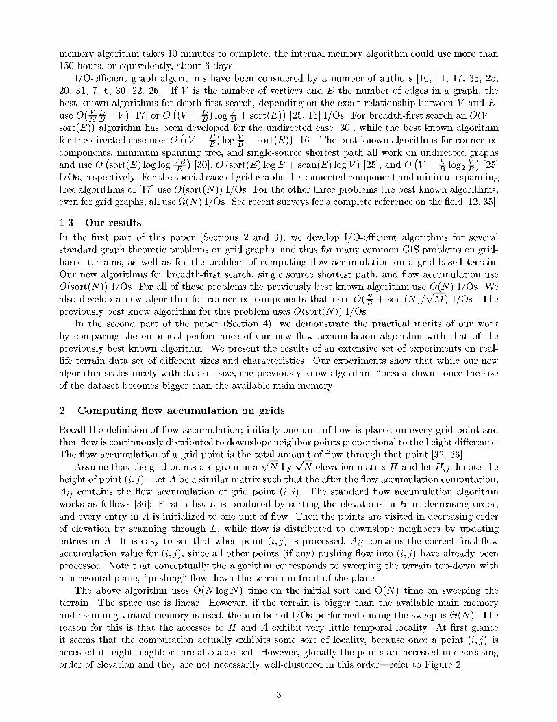
The above algorithm uses �(N logN) time on the initial sort and �(N) time on sweeping the

terrain. The space use is linear. However, if the terrain is bigger than the available main memory

and assuming virtual memory is used, the number of I/Os performed during the sweep is �(N). The

reason for this is that the accesses to H and A exhibit very little temporal locality. At �rst glance

it seems that the computation actually exhibits some sort of locality, because once a point (i; j) is

accessed its eight neighbors are also accessed. However, globally the points are accessed in decreasing

order of elevation and they are not necessarily well-clustered in this order|refer to Figure 2.

3

2.1 I/O-E�cient algorithm

The inferior I/O behavior of the standard ow accumulation algorithm is a result of two types of

scattered disk access; accesses to A to obtain the ow of the grid point being processed and to update

the ow of the neighbor points to which this point distributes ow, and accesses to H to obtain

the elevations of the neighbors in order to decide how to distribute ow. The latter accesses can be

eliminated simply by augmenting each point in L with the elevations of its eight neighbors. Using

external sorting, L can be produced in O(sort(N)) I/Os. Note that we have to sort a dataset which

is 9 times bigger than the original set.

The key observation that allows us to eliminate the scattered access to A is that when point

(i; j) is processed and we want to update the ow of its neighbors, we already know at what \time"

the neighbors are going to be processed, that is, when we will need to know how much ow (i; j)

distributed to them. This happens when the sweep-plane reaches their elevation and we know their

elevation from the information in L. The key idea is therefore to send the needed information ( ow)

\forward in time" by inserting it in an I/O-e�cient priority queue. This idea is similar to time forward

processing [17, 10].

Our new sweep algorithm works as follows. We maintain an external priority queue [10, 15] on

grid points (i; j), with primary key equal to the elevation Hij and secondary key equal to (i; j). Each

priority queue element also contains a ow value (the ow \sent forward" to (i; j) from one of its

neighbors). When we process a grid point (i; j) during the sweep (scan of L), its ow is distributed

to downslope neighbors by inserting an element for each of them into the queue. The accumulated

ow of (i; j) is found by performing extract max operations on the priority queue. As a grid point can

receive ow from multiple neighbors, we may need to perform extract max operations several times

to obtain its total ow. Flow sent to (i; j) from its upslope neighbors will be returned by consecutive

extract max operations as they all have the same key. If extract max does not return ow for (i; j)

(an element with key (Hij ; i; j)), it means that (i; j) does not have any upslope neighbors and we only

distribute its initial one unit of ow. The processing of a grid point is illustrated in Figure 3. As the

total number of priority queue operations performed is O(N), and as external priority queues with

O( 1B logM=BNB ) I/O bound per operation exist [10, 15], the sweep uses O(sort(N)) I/Os.

The above sweep algorithm does not directly output the ow accumulation matrix A. Instead, the

ow accumulation of grid points are written to a list as they are calculated during the sweep. After

the sweep, A can then be obtained by sorting this list in an appropriate way. We have the following.

Theorem 1 The ow accumulation of a terrain stored as apN by

pN grid can be computed using

O(sort(N)) I/Os, O(N logN) time, and linear space.

��

��

��

��

��

��

��

��

��

��

��

��

��

��

��

��

��

��

��

��

��

��

��

��

��

��

��

��

��

��

��

��

��

��

��

��

��

��

��

��

��

��

��

��

��

��

��

��

��

��

��

��

��

��

��

��

��

��

��

��

��

��

��

��

��

��

��

��

��

��

��

��

��

��

��

��

��

��

��

��

��

��

��

��

��

��

��

��

��

��

��

��

��

��

��

��

��

��

��

��

��

��

��

��

��

��

��

��

��

��

��

��

��

��

��

��

��

��

��

��

��

��

��

��

��

��

��

��

��

86

5

<105,i,j>90

115

100

90 6580

105

PQ

120110

Figure 2: Points with the same height (black

circles) are distributed over the terrain:

Processing them after each other might re-

sult in loading most of the disk blocks stor-

ing the terrain.

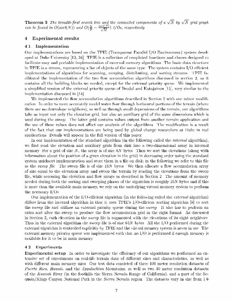
Figure 3: Point (i; j) receives ow 5 + 6 +

8 = 19 from its three upslope neighbors and

distributes it to its 5 downslope neighbors

using a priority queue. (Point with height

90 gets 105�90

100� 20 units of ow).

4

3 I/O-E�cient algorithms on grid graphs

In the previous section we designed an O(sort(N)) algorithm for the ow accumulation problem. In

this section we develop O(sort(N)) algorithms for breadth-�rst search (BFS) and single source shortest

path (SSSP) on grid graphs. The previous best known algorithms use (N) I/Os. We also develop

an O(NB+

sort(N)pM

) algorithm for computing connected components on a grid graphs, compared to the

previous O(sort(N)) algorithm. As discussed in the introduction, all these problems correspond to

important GIS problems on grids.

In Section 3.1 we describe our new SSSP algorithm in detail. In Section 3.2 we then brie y discuss

the two other algorithms. Further details will appear in the full paper.

3.1 Single Source Shortest Paths

Consider a grid of sizepN by

pN divided into O(N=M) subgrids of size

pM by

pM each. Our

algorithm will rely on the following key lemma (proof omitted)|refer to Figure 4.

Lemma 1 Consider a shortest path �(s; t) between two vertices s and t in the grid. Let fs =

A0; A1; A2; :::; Ak�1; Ak = tg denote the intersections of the path with the boundaries of the subgrids.

Then the paths Ai ! Ai+1 induced by �(s; t) in a subgrid is the shortest paths between Ai and Ai+1 in

that subgrid.

Using lemma 1, our �rst idea for improving the general O�V + E

B log2VB

�= O

�N + N

B log2NB

�

SSSP algorithm [25] in the case of a grid graph is via sparci�cation: We �rst replace eachpM �

pM

subgrid with a full graph on the \boundary vertices". The resulting graph R has �(N=pM) vertices

and �(N) edges. The weight of an edge in R is the shortest path between the corresponding two

boundary vertices, among all the paths within the subgrid|refer to Figure 4. The new edges and

weights of R can easily be computed in O(N=B) I/Os, simply by loading each subgraph in turn and

use an internal memory all-pair-shortest-paths (APSP) algorithm to compute the weights of the new

edges. Next we use the general SSSP algorithm on R to compute the length of the shortest paths

from the source vertex s to all the boundary vertices. Using Lemma 1, we know that these paths

are identical to the shortest paths in the original grid graph. Finally, we compute the shortest paths

from s to all the vertices we removed, simply by loading each subgraph in turn (together with the

shortest path lengths we found for the corresponding boundary vertices) and use an internal memory

algorithm to compute for each vertex t in the subgrid the shortest path from s using the formula

�(s; t) = minvf�(s; v)+ �subgrid(v; t)g; where v ranges over all the boundary vertices in t's subgrid, and

where �subgrid denotes the shortest path within a subgrid.

It is easy to see that the above algorithm uses O(NB ) + O( Np

M+ N

B log2NpMB

) + O(NB ) =

O(NB log2NpMB

) I/Os. We would like to improve this bound to O(sort(N)) = O(NB logM=BNB ), that is,

the base of the logarithm should beM=B instead of 2. The binary logarithm in our bound comes from

the general SSSP algorithm by Kumar and Schwabe [25]. Their algorithm is a variant of Dijkstra's

A i

A i +1

S

T

s

Figure 4: Dividing a grid in subgrids which �t in memory

5

algorithm [18], modi�ed so that when processing a vertex v, no lookup is needed in order to determine

the length of the currently known shortest path to neighbors of v (used to determine if a new shorter

path has been found and thus if a decrease key operation should be performed on the priority queue

that controls the order in which vertices are processed). Such lookups would result in an E-term in

the I/O bound. The priority queue used in their algorithm is an external version of a tournament

tree, which supports insert , delete min , and decrease key in O( 1B log2VB ) I/Os amortized.

The idea in the improvement of our algorithm is to avoid using decrease key operations and thus to

be able to use one of the O( 1B logM=BNB )-I/O-per-operation priority queues discussed earlier [10, 15].

In order to do so, we use Dijkstra's algorithm directly, instead of the algorithm by Kumar and Schwabe,

and take advantage of the special structure of R to avoid the E term Kumar and Schwabe avoids using

the external tournament tree. The main idea is to store R so that when we process a vertex we can

access its �(pM) neighbors in O(

pM=B) I/Os. To see how to do so, recall that the �(N=

pM)

vertices of R consist of everypMth column and

pMth row of the original grid graph. We store

all �(N=M) \corner vertices" (vertices which are both on one of the columns and one of the rows)

consecutively in �(N=(MB)) blocks. Then we store the remaining vertices row by row and column by

column, such that consecutive vertices are consecutive on disk. To obtain the neighbors of a vertex in

R, we then just need to access six corner vertices and access the disk in �ve di�erent places, reading

�(pM=B) blocks in each of these places, using O(

pM=B + 11) = O(

pM=B) I/Os in total.

Our SSSP algorithm on R now works as follows: Together with each vertex in the above repre-

sentation we store a distance, which we initially set to 1. We then use a slightly modi�ed version of

Dijkstra's algorithm where we maintain the invariant that for every vertex the distance in the above

representation is identical to the distance stored in the priority queue controlling the algorithm (the

shortest distance seen so far). We repeatedly perform a delete min on the priority queue to obtain

the next vertex v to process, and then we load all �(pM) edges incident to v and all the �(

pM)

neighbor vertices (and their current distances) into main memory using O(pM=B) I/Os. Without

any further I/O, we then compute which vertices need to have their distance updated. Finally, we

write the updated distances back to disk and perform the corresponding updates (decrease key) on the

priority queue. One decrease key operation is performed using a delete and an insert operation|we

can do so since we now know the key (distance) of the vertex that we update. In total we perform

O(E) = O(N) operations on the queue and use O(pM=B) on each of the �(N

pM) vertices, and

thus our algorithm uses O(sort(N)) I/Os.

Theorem 2 The single source shortest path problem on apN by

pN grid graph can be solved in

O(sort(N)) I/Os.

So far we have only described how to compute the lengths of the shortest paths. By adding an

extra step to our algorithm, we can also produce the shortest path tree. Using a recent result due to

Hutchinson, Maheshwari and Zeh [22], we can then construct a structure such that for any vertex t,

the actual shortest path between s and t can be returned in `=B I/Os, where ` is the length (number

of vertices) of the path.

3.2 Other problems

Given our O(sort(N)) SSSP algorithm, we can also develop an O(sort(N)) BFS algorithm. We simply

use the SSSP algorithm on the graph where all edges have weight one. The BFS numbering of the

vertices can then be found in a few sorting steps. Details will appear in the full paper.

The problem of �nding connected components (CC) of a grid graph can be solved e�ciently in a

way similar to the way we solved SSSP; we divide the grid into subgrids of sizepM by

pM and �nd

connected components in each of them. We then replace each subgraph with a graph on the boundary

vertices, where we connect boundary edges in the same connected component in a way such that l� 1

edges are used to connect l vertices. The graph constructed in this way has size N 0 = O( NpM) and

because of its special structure we can �nd connected components in it in O(sort(N 0)) I/Os. Using

this information we can easily solve CC. Details will appear in the full paper.

6

Theorem 3 The breadth-�rst search tree and the connected components of apN by

pN grid graph

can be found in O(sort(N)) and O(NB+

sort(N)pM

) I/Os, respectively.

4 Experimental results

4.1 Implementation

Our implementations are based on the TPIE (Transparent Parallel I/O Environment) system devel-

oped at Duke University [13, 34]. TPIE is a collection of templated functions and classes designed to

facilitate easy and portable implementation of external memory algorithms. The basic data structure

in TPIE is a stream, representing a list of objects of the same type. The system contains I/O-e�cient

implementations of algorithms for scanning, merging, distributing, and sorting streams. TPIE fa-

cilitated the implementation of the two ow accumulation algorithms discussed in section 2, as it

contains all the building blocks we needed, except for the external priority queue. We implemented

a simpli�ed version of the external priority queue of Brodal and Katajainen [15], very similar to the

implementation discussed in [14].

We implemented the ow accumulation algorithms described in Section 2 with one minor modi�-

cation. In order to more accurately model water ow through horizontal portions of the terrain (where

there are no downslope neighbors), as well as through small depressions of the terrain, our algorithms

take as input not only the elevation grid, but also an auxiliary grid of the same dimensions which is

used during the sweep. The latter grid contains values output from another terrain application and

the use of these values does not a�ect our analysis of the algorithms. The modi�cation is a result

of the fact that our implementations are being used by global change researchers at Duke in real

applications. Details will appear in the full version of this paper.

In our implementation of the standard algorithm (in the following called the internal algorithm),

we �rst read the elevation and auxiliary grids from disk into a two-dimensional array in internal

memory. For a grid of size N , the array is of size 8N bytes. Then we sort the elevations (along with

information about the position of a given elevation in the grid) in decreasing order using the standard

system quicksort implementation and store them in a �le on disk; in the following we refer to this �le

as the sweep �le. The sweep �le is of size 16N bytes. We then allocate a ow accumulation array

of size equal to the elevation array and sweep the terrain by reading the elevations from the sweep

�le, while accessing the elevation and ow arrays as described in Section 2. The amount of memory

needed during both the sorting and sweeping phases of the algorithm is roughly 16N bytes and if this

is more than the available main memory, we rely on the underlying virtual memory system to perform

the necessary I/Os.

Our implementation of the I/O-e�cient algorithm (in the following called the external algorithm)

di�ers from the internal algorithm in that it uses TPIE's I/O-e�cient sorting algorithm [8] to sort

the sweep �le and utilizes an external priority queue during the sweep. It also has to perform an

extra sort after the sweep to produce the ow accumulation grid in the right format. As discussed

in Section 2, each elevation in the sweep �le is augmented with the elevations of its eight neighbors.

Thus in the external algorithm the sweep �le is of size 64N bytes. All the I/O performed during the

external algorithm is controlled explicitly by TPIE and the virtual memory system is never in use. The

external memory priority queue was implemented such that no I/O is performed if enough memory is

available for it to be in main memory.

4.2 Experiments

Experimental setup. In order to investigate the e�ciency of our algorithms we performed an ex-

tensive set of experiments on real-life terrain data of di�erent sizes and characteristics, as well as

with di�erent main memory sizes. Our test data consisted of three 100 meter resolution datasets of

Puerto Rico, Hawaii, and the Appalachian Mountains, as well as two 30 meter resolution datasets

of the Kaweah River (in the foothills the Sierra Nevada Range of California), and a part of the Se-

quoia/Kings Canyon National Park in the Sierra Nevada region. The datasets vary in size from 1.6

7

million points or 12.8 MB (Kaweah) to 63.5 million points or 508 MB (Appalachian), and they also

vary greatly in terms of elevation distribution. Intuitively, the latter should a�ect the performance of

the sweep phase of both the internal and the external algorithms; especially of the external memory

algorithm, because the size of the priority queue is determined by the elevation distribution. The

characteristics of the �ve terrains are summarized in Table 1, which also contains the maximal size

of the priority queue during the sweep. We performed experiments with main memory sizes of 512,

256, 128, 96, and 64 MB. We performed experiments with relatively low main memory sizes, as well

as with more realistic sizes, in order to simulate ow accumulation computations on terrains of much

larger size than the ones that were available to us. Such much bigger datasets will soon be available.

If for example the Appalachian dataset was sampled at 30 instead of 100 meter resolution, it would be

of size 5.5 gigabytes. Sampled at 10 meter it would be 50 gigabytes, and at 1 meter a mind-blowing

5 terabytes.

Dataset Surface Grid size Approx. size Priority queue

Coverage size

Kaweah 34 x 42 kilometers 1163 x 1424 1.6 �106, 13MB 2 �104, 0.4MBPuerto Rico 445 x 137 kilometers 4452 x 1378 5.9 �106, 47MB 14 �104, 2.8MBSierra 112 x 80 kilometers 3750 x 2672 9.5 �106, 76MB 19 �104, 3.8MBHawaii 678 x 4369 kilometers 6784 x 4369 28.2 �106, 225MB 9 �104, 1.8MBAppalachian 847 x 785 kilometers 8479 x 7850 63.5 �106, 508MB 2.8 �106, 56MB

Table 1: Characteristics of terrain data sets.

We performed our experiments on a 450MHz Xeon Intel PII with 512 MB of main memory running

FreeBSD 4.0, and with an external local (striped) disk array composed of 4 17GB Maxtor 91728D8

IDE drives. For each experiment the machine was rebooted with the indicated amount of main

memory. In the case of the external algorithm, the TPIE limit on main memory use was set (somewhat

conservatively) to 25, 50, 95, 200, and 350MB, in the experiments with 64, 96, 128, 256, and 512MB

of main memory. The rest of the memory was reserved for the operating system.

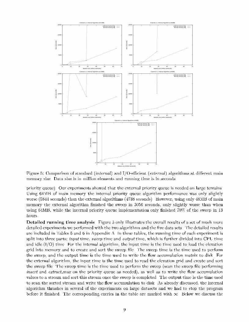
Experimental results. The main results of our experiments are shown in Figure 5. As it can be

seen, the external algorithm scales nicely for all main memory sizes. The internal algorithm on the

other hand \breaks down" (or thrashes) when the memory use exceeds the main memory size; At

512MB the internal algorithm can handle all datasets except Appalachian. At 256MB the picture is

the same, but the algorithm starts thrashing on the Hawaii dataset. At 96MB the algorithm thrashes

on the Sierra dataset, while Hawaii slows down further. The algorithm can still handle Hawaii because

of the \nice" distribution of elevations in that dataset (part of the grid is over water). At 64MB

the algorithm can only handle the relatively small Kaweah and Puerto Rico datasets. It should be

noted that on the small datasets the internal algorithm is slightly faster than the external algorithm.

However, the external algorithm could easily be made \adaptive" so that it runs the internal algorithm

if enough memory is available. This would result in the external algorithm always being at least as

fast as the internal.

An interesting observation one can make from Table 1 is that in most of the experiments discussed

so far, the priority queue used in the external algorithm actually �ts in main memory. External

memory is only really needed when processing the Appalachian dataset using only 64MB of main

memory. This suggests that in most cases one could greatly simplify the implementation by just using

an internal memory priority queue. One could even suspect that in practice an internal priority queue

implementation would perform reasonably well, since the memory accesses incurred when operating

on the queue are relatively local. In order to investigate this we performed experiments with the

external algorithm modi�ed to use an internal priority queue in the sweep while letting the OS handle

the I/O. We ran the algorithm on the Appalachian dataset using 64 and 48MB of main memory and

compared its performance to that of the unmodi�ed external algorithm (that is, using the external

8

0

5000

10000

15000

20000

0 10 20 30 40 50 60 70

time

(sec

onds

)

dataset size (million elements)

External v.s. Internal Algorithm at 512MB

external memory alg.internal memory alg.

0

5000

10000

15000

20000

0 10 20 30 40 50 60 70

time

(sec

onds

)




0

5000

10000

15000

20000

0 10 20 30 40 50 60 70

time

(sec

onds

)




0

5000

10000

15000

20000

0 10 20 30 40 50 60 70

time

(sec

onds

)




0

5000

10000

15000

20000

0 10 20 30 40 50 60 70

time

(sec

onds

)




Figure 5: Comparison of standard (internal) and I/O-e�cient (external) algorithms at di�erent main

memory size. Data size is in million elements and running time is in seconds.

priority queue). Our experiments showed that the external priority queue is needed on large terrains.

Using 64MB of main memory the internal priority queue algorithm performance was only slightly

worse (5844 seconds) than the external algorithms (4738 seconds). However, using only 48MB of main

memory the external algorithm �nished the sweep in 5056 seconds, only slightly worse than when

using 64MB, while the internal priority queue implementation only �nished 70% of the sweep in 13

hours.

Detailed running time analysis. Figure 5 only illustrates the overall results of a set of much more

detailed experiments we performed with the two algorithms and the �ve data sets. The detailed results

are included in Tables 5 and 6 in Appendix A. In these tables, the running time of each experiment is

split into three parts; input time, sweep time and output time, which is further divided into CPU time

and idle (I/O) time. For the internal algorithm, the input time is the time used to load the elevation

grid into memory and to create and sort the sweep �le. The sweep time is the time used to perform

the sweep, and the output time is the time used to write the ow accumulation matrix to disk. For

the external algorithm, the input time is the time used to read the elevation grid and create and sort

the sweep �le. The sweep time is the time used to perform the sweep (scan the sweep �le performing

insert and extract max on the priority queue as needed), as well as to write the ow accumulation

values to a stream and sort this stream once the sweep is completed. The output time is the time used

to scan the sorted stream and write the ow accumulation to disk. As already discussed, the internal

algorithm thrashes in several of the experiments on large datasets and we had to stop the program

before it �nished. The corresponding entries in the table are marked with 1. Below we discuss the

9

results in a little more detail.

First consider the internal algorithm (Table 5). The Kaweah dataset is small enough to �t in

internal memory at all memory sizes and the algorithm consistently takes 60 seconds to complete. Its

CPU utilization is around 85%. The Puerto Rico dataset �ts in memory at 512MB and 256MB and

completes in 100 seconds. When memory is reduced to 64MB, the CPU utilization drops from 87%

to 19% and the performance is 5 times slower (480 seconds). Similarly, the Sierra Nevada dataset

completes in 4 (5) minutes and 79% (66%) CPU utilization using 512MB (256MB) internal memory

where it �ts in memory. At 128MB, the running time jumps from 4 minutes to 4 hours, and the

algorithm spends 98% of the time waiting for I/O. When the memory is reduced even more the

algorithm thrashes|after 13 hours only half of the sweep had been completed. The Hawaii dataset

�ts in memory only at 512MB. As main memory gets smaller, the CPU utilization falls from 49%

at 512MB to 2% at 64MB, and the running time increases from 15 minutes at 512MB to almost 8

hours at 64MB. The Appalachian dataset is beyond the limits of the internal algorithm|with 512MB

of main memory we let it run for 4 days without �nishing. Note that the thrashing of the internal

algorithm is mainly due to sweeping. For instance, sorting the 425MB in the Hawaii dataset sweep

�le using 512MB of main memory takes 462 seconds (64% CPU), while at 64MB memory it takes

2668 seconds (7% CPU). Sweeping the same �le takes 299 seconds using 512MB of main memory, but

24347 seconds using 64MB of main memory. The sorting performance is better due to the relatively

good locality of quicksort.

Unlike the internal algorithm, the external algorithm scales (almost) linearly with memory decrease

and maintains its CPU utilization constant (Table 6). For instance, the ow accumulation computation

for the Appalachian dataset (which the internal algorithm thrashes on) takes 2 hours in total (79%

CPU) using 512MB of main memory. Using 64MB of main memory is uses only 40 minutes more (68%

CPU).

Finally, as already discussed brie y, it should be noted how the sweeping time depends not only

on the size of the dataset but also on intrinsic terrain properties (quanti�ed by the size of the priority

queue in the external algorithm). Consider for example the performance of the internal algorithm on

the Sierra and Hawaii dataset. With 512 and 256MB of main memory, both datasets �t in memory

but the sweep of the Sierra dataset is signi�cantly faster than the sweep of the Hawaii dataset, the

reason being that the Hawaii sweep �le is around six times bigger than the sierra sweep �le. Using

128MB of main memory the algorithm thrashes on the Sierra dataset even though it is smaller than

the Hawaii dataset. The reason for this is that that the Hawaii dataset is relatively easy to sweep

(small priority queue size). This can also be seen from the CPU utilization during sweeping in the

external algorithm.

5 Conclusions and open problems

In this paper we have developed I/O-e�cient algorithms for several graph problems on grid graphs

with applications to GIS problems on grid-based terrains. We have also shown that while the standard

algorithm for the ow accumulation problem is severely I/O bound when the datasets get larger than

the available main memory, our new I/O-e�cient algorithm scales very well.

A number of interesting problems on grid graphs remain open. For example, if it is possible to

develop an O(sort(N)) depth-�rst search algorithm and if connected components can be computed in

O(N=B) I/Os. For general graphs it remains an intriguing open problem if any graph problem on a

general graph can be solved in O(sort(E)) I/Os.

In terms of computing ow accumulation, it would be interesting to develop more realistic models

of ow of water over a terrain than the one used in current algorithms. Other interesting problems

include developing models and algorithms for ow accumulation on DEMs stored as TINs.

10

Acknowledgments

We would like to thank Pat Halpin and Dean Urban at Duke's Nicholas School of the Environment

for introducing us to the ow accumulation problem, as well as for answering our many questions

about the use of grid-based terrains in environmental research. We would also like to thank them

for providing the Kaweah, Sierra, and Appalachian datasets. Finally, we thank Je� Chase, Andrew

Gallatin, and Rajiv Wickremesinghe for help with the numerous system problems encountered when

working with gigabytes of data.

References

[1] NASA Earth Observing System (EOS) project. http://eos.nasa.gov/.

[2] NASA Shuttle Radar Topography Mission (SRTM). http://www-radar.jpl.nasa.gov/srtm/.

[3] U.S. Geological Survey: 5 minute Gridded Earth Topography Data (ETOPO5).http://edcwww.cr.usgs.gov/Webglis/glisbin/guide.pl /glis/hyper/guide/etopo5.

[4] U.S. Geological Survey: Global 30 arc second Elevation Dataset (GTOPO30).http://edcwww.cr.usgs.gov/landdaac/gtopo30/ gtopo30.html.

[5] U.S. Geological Survey (USGS) digital elevation models. http://mcmcweb.er.usgs.gov/status/dem stat.html.

[6] J. Abello, A. L. Buchsbaum, and J. R. Westbrook. A functional approach to external graph algorithms.In Proc. Annual European Symposium on Algorithms, LNCS 1461, pages 332{343, 1998.

[7] P. K. Agarwal, L. Arge, T. M. Murali, K. Varadarajan, and J. S. Vitter. I/O-e�cient algorithms forcontour line extraction and planar graph blocking. In Proc. ACM-SIAM Symp. on Discrete Algorithms,pages 117{126, 1998.

[8] A. Aggarwal and J. S. Vitter. The Input/Output complexity of sorting and related problems. Communi-cations of the ACM, 31(9):1116{1127, 1988.

[9] ARC/INFO. Understanding GIS|the ARC/INFO method. ARC/INFO, 1993. Rev. 6 for workstations.

[10] L. Arge. The bu�er tree: A new technique for optimal I/O-algorithms. In Proc. Workshop on Algorithms

and Data Structures, LNCS 955, pages 334{345, 1995. A complete version appears as BRICS technicalreport RS-96-28, University of Aarhus.

[11] L. Arge. The I/O-complexity of ordered binary-decision diagram manipulation. In Proc. Int. Symp. on

Algorithms and Computation, LNCS 1004, pages 82{91, 1995. A complete version appears as BRICStechnical report RS-96-29, University of Aarhus.

[12] L. Arge. E�cient External-Memory Data Structures and Applications. PhD thesis, University of Aarhus,February/August 1996.

[13] L. Arge, R. Barve, O. Procopiuc, L. Toma, D. E. Vengro�, and R. Wickeremesinghe. TPIE User Manual

and Reference (edition 0.9.01a). Duke University, 1999. The manual and software distribution are availableon the web at http://www.cs.duke.edu/TPIE/.

[14] K. Brengel, A. Crauser, P. Ferragina, and U. Meyer. An experimental study of priority queues in externalmemory. In Proc. Workshop on Algorithm Engineering, LNCS 1668, pages 345{358, 1999.

[15] G. S. Brodal and J. Katajainen. Worst-case e�cient external-memory priority queues. In Proc. Scandina-

vian Workshop on Algorithms Theory, LNCS 1432, pages 107{118, 1998.

[16] A. L. Buchsbaum, M. Goldwasser, S. Venkatasubramanian, and J. R. Westbrook. On external memorygraph traversal. In Proc. ACM-SIAM Symp. on Discrete Algorithms, 2000. (to appear).

[17] Y.-J. Chiang, M. T. Goodrich, E. F. Grove, R. Tamassia, D. E. Vengro�, and J. S. Vitter. External-memorygraph algorithms. In Proc. ACM-SIAM Symp. on Discrete Algorithms, pages 139{149, 1995.

[18] E. W. Dijkstra. A note on two problems in connection with graphs. Numerische Mathematik, 1969.

[19] J. Fair�eld and P. Leymarie. Drainage network from grid digital elevation model. Water Resource Research,27:709{717, 1991.

11

[20] E. Feuerstein and A. Marchetti-Spaccamela. Memory paging for connectivity and path problems in graphs.In Proc. Int. Symp. on Algorithms and Computation, 1993.

[21] A. U. Frank, B. Palmer, and V. B. Robinson. Formal methods for the accurate de�nition of some funda-mental terms in physical geography. In Proc. 2nd Int. Symp. on Spatial Data Handling, pages 583{599,1986.

[22] D. Hutchinson, A. Maheshwari, and N. Zeh. An external-memory data structure for shortest path queries.Proc. Int. Symp. on Algorithms and Computation, 1999 (To appear).

[23] D. E. Knuth. Sorting and Searching, volume 3 of The Art of Computer Programming. Addison-Wesley,Reading MA, second edition, 1998.

[24] M. V. Kreveld. Digital elevation models: overview and selected TIN algorithms. In M. van Kreveld,J. Nievergelt, T. Roos, and P. Widmayer, editors, Algorithmic Foundations of GIS. Springer-Verlag, LectureNotes in Computer Science 1340, 1997.

[25] V. Kumar and E. Schwabe. Improved algorithms and data structures for solving graph problems in externalmemory. In Proc. IEEE Symp. on Parallel and Distributed Processing, pages 169{177, 1996.

[26] A. Maheshwari and N. Zeh. External memory algorithms for outerplanar graphs. Submitted for publication,1999.

[27] I. D. Moore. Hydrologic Modeling and GIS, chapter 26, pages 143{148. GIS World Books. Boulder, 1996.

[28] I. D. Moore, R. B. Grayson, and A. R. Ladson. Digital terrain modelling: a review of hydrological,geomorphological and biological aplications. Hydrological Processes, 5:3{30, 1991.

[29] I. D. Moore, A. K. Turner, J. P. Wilson, S. K. Jenson, and L. E. Band. GIS and Environmental Modelling.Oxford University Press, 1993.

[30] K. Munagala and A. Ranade. I/O-complexity of graph algorithm. In Proc. ACM-SIAM Symp. on Discrete

Algorithms, pages 687{694, 1999.

[31] M. H. Nodine, M. T. Goodrich, and J. S. Vitter. Blocking for external graph searching. Algorithmica,16(2):181{214, 1996.

[32] J. F. O'Callaghan and D. M. Mark. The extraction of drainage networks from digital elevation data.Computer Vision, Graphics and Image Processing, 28, 1984.

[33] J. D. Ullman and M. Yannakakis. The input/output complexity of transitive closure. Annals of Mathematics

and Arti�cial Intellegence, 3:331{360, 1991.

[34] D. E. Vengro�. A transparent parallel I/O environment. In Proc. DAGS Symposium on Parallel Compu-

tation, 1994.

[35] J. S. Vitter. External memory algorithms (invited tutorial). In Proc. of the 1998 ACM Symposium on

Principles of Database Systems, pages 119{128, 1998.

[36] D. Wolock. Simulating the variable-source-area of stream ow generation with the watershed model top-model. Technical report, U.S. Department of the Interior, 1993.

[37] S. Yu, M. van Kreveld, and J. Snoeyink. Drainage queries on TINs: from local to global and back again.In Proc. 7th Int. Symp. on Spatial Data Handling, pages 13A.1{13A.14, 1996.

12

Appendix A

Mem

Time

Kaweah

PuertoRico

SierraNevada

Hawaii

Appalachian

MB

secs

cpu

idle

total

cpu

idle

total

cpu

idle

total

cpu

idle

total

cpu

idle

total

input

34

3

37

155

60

215

257

199

456

786

580

1366

1778

1289

3067

512

sweep

76

1

77

97

10

107

872

14

886

303

45

348

3513

215

3728

output

5

1

6

22

1

23

31

1

32

111

3

114

231

4

235

TOTAL

115

5

120

274

71

345

1160

214

1374

1200

628

1828

5522

1508

7030

%

96

4

79

21

84

16

66

34

79

21

input

35

2

37

156

134

290

256

240

496

803

637

1440

1825

1344

3174

256

sweep

77

11

88

98

14

112

870

17

887

324

97

421

3517

266

3783

output

5

0

5

22

1

23

31

1

32

111

2

113

231

4

235

TOTAL

117

13

130

276

149

425

1157

258

1415

1238

736

1974

5573

1619

7192

%

90

10

65

35

82

18

63

37

77

23

input

42

18

60

159

209

368

263

280

543

829

752

1581

1888

1337

3225

128

sweep

77

11

88

98

15

113

882

25

907

329

120

449

3531

267

3798

output

5

0

5

22

1

23

32

1

33

111

3

114

231

4

235

TOTAL

124

29

153

279

225

504

1177

306

1483

1269

875

2144

5650

1608

7258

%

81

19

55

45

79

21

59

41

78

22

input

41

28

69

164

151

315

468

87

555

845

924

1769

1917

2185

4102

96

sweep

77

10

87

104

14

118

885

35

920

331

131

462

3784

292

4076

output

5

1

6

22

1

23

32

1

33

111

2

113

232

5

237

TOTAL

123

39

162

290

166

456

1385

123

1508

1287

1057

2344

5933

2482

8415

%

76

24

64

36

92

8

55

45

71

29

input

43

32

75

169

226

395

277

293

570

873

950

1823

1978

2561

4539

64

sweep

77

14

91

105

19

124

887

64

951

339

143

482

4228

510

4738

output

5

1

6

22

1

23

32

1

33

111

2

113

231

5

236

TOTAL

125

47

172

296

246

542

1196

358

1554

1323

1095

2418

6437

3076

9513

%

73

27

55

45

77

23

55

45

68

32

Figure 6: External memory algorithm experiments.

13

Mem

Time

Kaweah

PuertoRico

SierraNevada

Hawaii

Apallachian

MB

secs

cpu

idle

total

cpu

idle

total

cpu

idle

total

cpu

idle

total

cpu

idle

total

input

35

4

39

57

7

64

99

24

123

296

166

462

1

1

512

sweep

7

6

13

9

6

15

78

32

110

24

275

299

1

1

output

5

0

5

21

0

21

29

0

29

103

4

107

TOTAL

47

10

57

87

13

100

206

56

262

423

445

868

1

1

%

82

18

87

13

79

21

49

51

input

35

1

36

57

5

62

101

9

110

306

1527

1833

256

sweep

6

3

9

8

2

10

71

94

165

25

424

449

1

1

output

5

0

5

21

0

21

29

1

30

104

81

185

TOTAL

46

4

50

86

7

93

201

104

305

435

2032

2467

1

1

%

92

8

92

8

66

34

18

82

input

35

4

39

60

50

110

103

323

426

307

2076

2383

128

sweep

7

3

10

8

5

13

124

11949

12073

27

343

370

1

1

output

5

1

6

21

2

23

29

131

160

104

208

312

TOTAL

47

8

55

89

57

146

256

12403

12659

438

2627

3065

1

1

%

85

15

61

39

2

98

14

86

input

35

3

38

58

129

187

107

413

520

325

2052

2377

96

sweep

7

4

11

9

20

29

1

1

30

1268

1298

1

1

output

5

0

5

21

12

33

104

181

285

TOTAL

47

7

54

88

161

249

1

1

459

3501

3960

1

1

%

87

13

35

65

1

99

12

88

input

36

6

42

62

234

296

109

493

602

199

2469

2668

64

sweep

7

3

10

9

101

110

1

1

101

24246

24347

1

1

output

5

1

6

21

53

74

110

138

248

TOTAL

48

10

58

92

388

480

1

1

410

26853

27263

1

1

%

83

17

19

81

2

98

Figure 7: Internal memory algorithm experiments.

14

I/O-Efficient Algorithms for Problems on Grid-Based Terrains

Documents

Transcript of I/O-Efficient Algorithms for Problems on Grid-Based Terrains