
Algorithms for programmers
220
Algorithms for programmers ideas and source code This document is work in progress: read the ”important remarks” near the beginning J¨orgArndt [email protected] This document 1 was L A T E X’d at September 26, 2002 1 This document is online at http://www.jjj.de/fxt/. It will stay available online for free.
-
Upload
khangminh22 -
Category
Documents
-
view
3 -
download
0
Transcript of Algorithms for programmers
Algorithms for programmersideas and source code
This document is work in progress: read the ”important remarks” near the beginning
Jorg [email protected]
This document1 was LATEX’d at September 26, 2002
1This document is online at http://www.jjj.de/fxt/. It will stay available online for free.
Contents
Some important remarks about this document 6
List of important symbols 7
1 The Fourier transform 8
1.1 The discrete Fourier transform . . . . . . . . . . . . . . . . . . . . . . . . . . . . . . . . . 8
1.2 Symmetries of the Fourier transform . . . . . . . . . . . . . . . . . . . . . . . . . . . . . . 9
1.3 Radix 2 FFT algorithms . . . . . . . . . . . . . . . . . . . . . . . . . . . . . . . . . . . . . 10
1.3.1 A little bit of notation . . . . . . . . . . . . . . . . . . . . . . . . . . . . . . . . . . 10
1.3.2 Decimation in time (DIT) FFT . . . . . . . . . . . . . . . . . . . . . . . . . . . . . 10
1.3.3 Decimation in frequency (DIF) FFT . . . . . . . . . . . . . . . . . . . . . . . . . . 13
1.4 Saving trigonometric computations . . . . . . . . . . . . . . . . . . . . . . . . . . . . . . . 15
1.4.1 Using lookup tables . . . . . . . . . . . . . . . . . . . . . . . . . . . . . . . . . . . 16
1.4.2 Recursive generation of the sin/cos-values . . . . . . . . . . . . . . . . . . . . . . . 16
1.4.3 Using higher radix algorithms . . . . . . . . . . . . . . . . . . . . . . . . . . . . . . 17
1.5 Higher radix DIT and DIF algorithms . . . . . . . . . . . . . . . . . . . . . . . . . . . . . 17
1.5.1 More notation . . . . . . . . . . . . . . . . . . . . . . . . . . . . . . . . . . . . . . 17
1.5.2 Decimation in time . . . . . . . . . . . . . . . . . . . . . . . . . . . . . . . . . . . . 17
1.5.3 Decimation in frequency . . . . . . . . . . . . . . . . . . . . . . . . . . . . . . . . . 18
1.5.4 Implementation of radix r = px DIF/DIT FFTs . . . . . . . . . . . . . . . . . . . . 19
1.6 Split radix Fourier transforms (SRFT) . . . . . . . . . . . . . . . . . . . . . . . . . . . . . 22
1.7 Inverse FFT for free . . . . . . . . . . . . . . . . . . . . . . . . . . . . . . . . . . . . . . . 23
1.8 Real valued Fourier transforms . . . . . . . . . . . . . . . . . . . . . . . . . . . . . . . . . 24
1.8.1 Real valued FT via wrapper routines . . . . . . . . . . . . . . . . . . . . . . . . . . 25
1.8.2 Real valued split radix Fourier transforms . . . . . . . . . . . . . . . . . . . . . . . 27
1.9 Multidimensional FTs . . . . . . . . . . . . . . . . . . . . . . . . . . . . . . . . . . . . . . 31
1.9.1 Definition . . . . . . . . . . . . . . . . . . . . . . . . . . . . . . . . . . . . . . . . . 31
1.9.2 The row column algorithm . . . . . . . . . . . . . . . . . . . . . . . . . . . . . . . 31
1.10 The matrix Fourier algorithm (MFA) . . . . . . . . . . . . . . . . . . . . . . . . . . . . . . 32
1.11 Automatic generation of FFT codes . . . . . . . . . . . . . . . . . . . . . . . . . . . . . . 33
1
CONTENTS 2
2 Convolutions 36
2.1 Definition and computation via FFT . . . . . . . . . . . . . . . . . . . . . . . . . . . . . . 36
2.2 Mass storage convolution using the MFA . . . . . . . . . . . . . . . . . . . . . . . . . . . . 40
2.3 Weighted Fourier transforms . . . . . . . . . . . . . . . . . . . . . . . . . . . . . . . . . . 42
2.4 Half cyclic convolution for half the price ? . . . . . . . . . . . . . . . . . . . . . . . . . . . 44
2.5 Convolution using the MFA . . . . . . . . . . . . . . . . . . . . . . . . . . . . . . . . . . . 44
2.5.1 The case R = 2 . . . . . . . . . . . . . . . . . . . . . . . . . . . . . . . . . . . . . . 45
2.5.2 The case R = 3 . . . . . . . . . . . . . . . . . . . . . . . . . . . . . . . . . . . . . . 45
2.6 Convolution of real valued data using the MFA . . . . . . . . . . . . . . . . . . . . . . . . 46
2.7 Convolution without transposition using the MFA . . . . . . . . . . . . . . . . . . . . . . 46
2.8 The z-transform (ZT) . . . . . . . . . . . . . . . . . . . . . . . . . . . . . . . . . . . . . . 47
2.8.1 Definition of the ZT . . . . . . . . . . . . . . . . . . . . . . . . . . . . . . . . . . . 47
2.8.2 Computation of the ZT via convolution . . . . . . . . . . . . . . . . . . . . . . . . 48
2.8.3 Arbitrary length FFT by ZT . . . . . . . . . . . . . . . . . . . . . . . . . . . . . . 48
2.8.4 Fractional Fourier transform by ZT . . . . . . . . . . . . . . . . . . . . . . . . . . . 48
3 The Hartley transform (HT) 49
3.1 Definition of the HT . . . . . . . . . . . . . . . . . . . . . . . . . . . . . . . . . . . . . . . 49
3.2 radix 2 FHT algorithms . . . . . . . . . . . . . . . . . . . . . . . . . . . . . . . . . . . . . 49
3.2.1 Decimation in time (DIT) FHT . . . . . . . . . . . . . . . . . . . . . . . . . . . . . 49
3.2.2 Decimation in frequency (DIF) FHT . . . . . . . . . . . . . . . . . . . . . . . . . . 52
3.3 Complex FT by HT . . . . . . . . . . . . . . . . . . . . . . . . . . . . . . . . . . . . . . . 55
3.4 Complex FT by complex HT and vice versa . . . . . . . . . . . . . . . . . . . . . . . . . . 56
3.5 Real FT by HT and vice versa . . . . . . . . . . . . . . . . . . . . . . . . . . . . . . . . . 57
3.6 Discrete cosine transform (DCT) by HT . . . . . . . . . . . . . . . . . . . . . . . . . . . . 58
3.7 Discrete sine transform (DST) by DCT . . . . . . . . . . . . . . . . . . . . . . . . . . . . 59
3.8 Convolution via FHT . . . . . . . . . . . . . . . . . . . . . . . . . . . . . . . . . . . . . . . 60
3.9 Negacyclic convolution via FHT . . . . . . . . . . . . . . . . . . . . . . . . . . . . . . . . . 62
4 Numbertheoretic transforms (NTTs) 63
4.1 Prime modulus: Z/pZ = Fp . . . . . . . . . . . . . . . . . . . . . . . . . . . . . . . . . . . 63
4.2 Composite modulus: Z/mZ . . . . . . . . . . . . . . . . . . . . . . . . . . . . . . . . . . . 64
4.3 Pseudocode for NTTs . . . . . . . . . . . . . . . . . . . . . . . . . . . . . . . . . . . . . . 67
4.3.1 Radix 2 DIT NTT . . . . . . . . . . . . . . . . . . . . . . . . . . . . . . . . . . . . 67
4.3.2 Radix 2 DIF NTT . . . . . . . . . . . . . . . . . . . . . . . . . . . . . . . . . . . . 68
4.4 Convolution with NTTs . . . . . . . . . . . . . . . . . . . . . . . . . . . . . . . . . . . . . 69
4.5 The Chinese Remainder Theorem (CRT) . . . . . . . . . . . . . . . . . . . . . . . . . . . . 69
4.6 A modular multiplication technique . . . . . . . . . . . . . . . . . . . . . . . . . . . . . . . 71
4.7 Numbertheoretic Hartley transform . . . . . . . . . . . . . . . . . . . . . . . . . . . . . . . 72
5 Walsh transforms 73
CONTENTS 3
5.1 Basis functions of the Walsh transforms . . . . . . . . . . . . . . . . . . . . . . . . . . . . 77
5.2 Dyadic convolution . . . . . . . . . . . . . . . . . . . . . . . . . . . . . . . . . . . . . . . . 78
5.3 The slant transform . . . . . . . . . . . . . . . . . . . . . . . . . . . . . . . . . . . . . . . 80
6 The Haar transform 82
6.1 Inplace Haar transform . . . . . . . . . . . . . . . . . . . . . . . . . . . . . . . . . . . . . 83
6.2 Integer to integer Haar transform . . . . . . . . . . . . . . . . . . . . . . . . . . . . . . . . 86
7 Some bit wizardry 88
7.1 Trivia . . . . . . . . . . . . . . . . . . . . . . . . . . . . . . . . . . . . . . . . . . . . . . . 88
7.2 Operations on low bits/blocks in a word . . . . . . . . . . . . . . . . . . . . . . . . . . . . 89
7.3 Operations on high bits/blocks in a word . . . . . . . . . . . . . . . . . . . . . . . . . . . 91
7.4 Functions related to the base-2 logarithm . . . . . . . . . . . . . . . . . . . . . . . . . . . 94
7.5 Counting the bits in a word . . . . . . . . . . . . . . . . . . . . . . . . . . . . . . . . . . . 95
7.6 Swapping bits/blocks of a word . . . . . . . . . . . . . . . . . . . . . . . . . . . . . . . . . 96
7.7 Reversing the bits of a word . . . . . . . . . . . . . . . . . . . . . . . . . . . . . . . . . . . 98
7.8 Generating bit combinations . . . . . . . . . . . . . . . . . . . . . . . . . . . . . . . . . . . 99
7.9 Generating bit subsets . . . . . . . . . . . . . . . . . . . . . . . . . . . . . . . . . . . . . . 101
7.10 Bit set lookup . . . . . . . . . . . . . . . . . . . . . . . . . . . . . . . . . . . . . . . . . . . 101
7.11 The Gray code of a word . . . . . . . . . . . . . . . . . . . . . . . . . . . . . . . . . . . . 102
7.12 Generating minimal-change bit combinations . . . . . . . . . . . . . . . . . . . . . . . . . 104
7.13 Bitwise rotation of a word . . . . . . . . . . . . . . . . . . . . . . . . . . . . . . . . . . . . 106
7.14 Bitwise zip . . . . . . . . . . . . . . . . . . . . . . . . . . . . . . . . . . . . . . . . . . . . 108
7.15 Bit sequency . . . . . . . . . . . . . . . . . . . . . . . . . . . . . . . . . . . . . . . . . . . 109
7.16 Misc . . . . . . . . . . . . . . . . . . . . . . . . . . . . . . . . . . . . . . . . . . . . . . . . 110
7.17 The bitarray class . . . . . . . . . . . . . . . . . . . . . . . . . . . . . . . . . . . . . . . . 112
7.18 Manipulation of colors . . . . . . . . . . . . . . . . . . . . . . . . . . . . . . . . . . . . . . 113
8 Permutations 115
8.1 The revbin permutation . . . . . . . . . . . . . . . . . . . . . . . . . . . . . . . . . . . . . 115
8.1.1 A naive version . . . . . . . . . . . . . . . . . . . . . . . . . . . . . . . . . . . . . . 115
8.1.2 A fast version . . . . . . . . . . . . . . . . . . . . . . . . . . . . . . . . . . . . . . . 116
8.1.3 How many swaps? . . . . . . . . . . . . . . . . . . . . . . . . . . . . . . . . . . . . 116
8.1.4 A still faster version . . . . . . . . . . . . . . . . . . . . . . . . . . . . . . . . . . . 117
8.1.5 The real world version . . . . . . . . . . . . . . . . . . . . . . . . . . . . . . . . . . 119
8.2 The radix permutation . . . . . . . . . . . . . . . . . . . . . . . . . . . . . . . . . . . . . . 120
8.3 Inplace matrix transposition . . . . . . . . . . . . . . . . . . . . . . . . . . . . . . . . . . . 121
8.4 Revbin permutation vs. transposition . . . . . . . . . . . . . . . . . . . . . . . . . . . . . 122
8.4.1 Rotate and reverse . . . . . . . . . . . . . . . . . . . . . . . . . . . . . . . . . . . . 122
8.4.2 Zip and unzip . . . . . . . . . . . . . . . . . . . . . . . . . . . . . . . . . . . . . . . 123
8.5 The Gray code permutation . . . . . . . . . . . . . . . . . . . . . . . . . . . . . . . . . . . 124
CONTENTS 4
8.6 General permutations . . . . . . . . . . . . . . . . . . . . . . . . . . . . . . . . . . . . . . 127
8.6.1 Basic definitions . . . . . . . . . . . . . . . . . . . . . . . . . . . . . . . . . . . . . 127
8.6.2 Compositions of permutations . . . . . . . . . . . . . . . . . . . . . . . . . . . . . . 128
8.6.3 Applying permutations to data . . . . . . . . . . . . . . . . . . . . . . . . . . . . . 131
8.7 Generating all Permutations . . . . . . . . . . . . . . . . . . . . . . . . . . . . . . . . . . . 132
8.7.1 Lexicographic order . . . . . . . . . . . . . . . . . . . . . . . . . . . . . . . . . . . 132
8.7.2 Minimal-change order . . . . . . . . . . . . . . . . . . . . . . . . . . . . . . . . . . 134
8.7.3 Derangement order . . . . . . . . . . . . . . . . . . . . . . . . . . . . . . . . . . . . 136
8.7.4 Star-transposition order . . . . . . . . . . . . . . . . . . . . . . . . . . . . . . . . . 137
8.7.5 Yet another order . . . . . . . . . . . . . . . . . . . . . . . . . . . . . . . . . . . . 138
9 Sorting and searching 140
9.1 Sorting . . . . . . . . . . . . . . . . . . . . . . . . . . . . . . . . . . . . . . . . . . . . . . . 140
9.2 Searching . . . . . . . . . . . . . . . . . . . . . . . . . . . . . . . . . . . . . . . . . . . . . 142
9.3 Index sorting . . . . . . . . . . . . . . . . . . . . . . . . . . . . . . . . . . . . . . . . . . . 143
9.4 Pointer sorting . . . . . . . . . . . . . . . . . . . . . . . . . . . . . . . . . . . . . . . . . . 144
9.5 Sorting by a supplied comparison function . . . . . . . . . . . . . . . . . . . . . . . . . . . 145
9.6 Unique . . . . . . . . . . . . . . . . . . . . . . . . . . . . . . . . . . . . . . . . . . . . . . . 146
9.7 Misc . . . . . . . . . . . . . . . . . . . . . . . . . . . . . . . . . . . . . . . . . . . . . . . . 148
10 Selected combinatorical algorithms 152
10.1 Offline functions: funcemu . . . . . . . . . . . . . . . . . . . . . . . . . . . . . . . . . . . . 152
10.2 Combinations in lexicographic order . . . . . . . . . . . . . . . . . . . . . . . . . . . . . . 155
10.3 Combinations in co-lexicographic order . . . . . . . . . . . . . . . . . . . . . . . . . . . . . 157
10.4 Combinations in minimal-change order . . . . . . . . . . . . . . . . . . . . . . . . . . . . . 158
10.5 Combinations in alternative minimal-change order . . . . . . . . . . . . . . . . . . . . . . 160
10.6 Subsets in lexicographic order . . . . . . . . . . . . . . . . . . . . . . . . . . . . . . . . . . 161
10.7 Subsets in minimal-change order . . . . . . . . . . . . . . . . . . . . . . . . . . . . . . . . 163
10.8 Subsets ordered by number of elements . . . . . . . . . . . . . . . . . . . . . . . . . . . . . 165
10.9 Subsets ordered with shift register sequences . . . . . . . . . . . . . . . . . . . . . . . . . 166
10.10Partitions . . . . . . . . . . . . . . . . . . . . . . . . . . . . . . . . . . . . . . . . . . . . . 167
11 Arithmetical algorithms 170
11.1 Asymptotics of algorithms . . . . . . . . . . . . . . . . . . . . . . . . . . . . . . . . . . . . 170
11.2 Multiplication of large numbers . . . . . . . . . . . . . . . . . . . . . . . . . . . . . . . . . 170
11.2.1 The Karatsuba algorithm . . . . . . . . . . . . . . . . . . . . . . . . . . . . . . . . 171
11.2.2 Fast multiplication via FFT . . . . . . . . . . . . . . . . . . . . . . . . . . . . . . . 171
11.2.3 Radix/precision considerations with FFT multiplication . . . . . . . . . . . . . . . 173
11.3 Division, square root and cube root . . . . . . . . . . . . . . . . . . . . . . . . . . . . . . . 174
11.3.1 Division . . . . . . . . . . . . . . . . . . . . . . . . . . . . . . . . . . . . . . . . . . 174
11.3.2 Square root extraction . . . . . . . . . . . . . . . . . . . . . . . . . . . . . . . . . . 175
CONTENTS 5
11.3.3 Cube root extraction . . . . . . . . . . . . . . . . . . . . . . . . . . . . . . . . . . . 176
11.4 Square root extraction for rationals . . . . . . . . . . . . . . . . . . . . . . . . . . . . . . . 176
11.5 A general procedure for the inverse n-th root . . . . . . . . . . . . . . . . . . . . . . . . . 178
11.6 Re-orthogonalization of matrices . . . . . . . . . . . . . . . . . . . . . . . . . . . . . . . . 180
11.7 n-th root by Goldschmidt’s algorithm . . . . . . . . . . . . . . . . . . . . . . . . . . . . . 181
11.8 Iterations for the inversion of a function . . . . . . . . . . . . . . . . . . . . . . . . . . . . 182
11.8.1 Householder’s formula . . . . . . . . . . . . . . . . . . . . . . . . . . . . . . . . . . 183
11.8.2 Schroder’s formula . . . . . . . . . . . . . . . . . . . . . . . . . . . . . . . . . . . . 184
11.8.3 Dealing with multiple roots . . . . . . . . . . . . . . . . . . . . . . . . . . . . . . . 185
11.8.4 A general scheme . . . . . . . . . . . . . . . . . . . . . . . . . . . . . . . . . . . . . 186
11.8.5 Improvements by the delta squared process . . . . . . . . . . . . . . . . . . . . . . 188
11.9 Trancendental functions & the AGM . . . . . . . . . . . . . . . . . . . . . . . . . . . . . . 189
11.9.1 The AGM . . . . . . . . . . . . . . . . . . . . . . . . . . . . . . . . . . . . . . . . . 189
11.9.2 log . . . . . . . . . . . . . . . . . . . . . . . . . . . . . . . . . . . . . . . . . . . . . 191
11.9.3 exp . . . . . . . . . . . . . . . . . . . . . . . . . . . . . . . . . . . . . . . . . . . . . 192
11.9.4 sin, cos, tan . . . . . . . . . . . . . . . . . . . . . . . . . . . . . . . . . . . . . . . . 193
11.9.5 Elliptic K . . . . . . . . . . . . . . . . . . . . . . . . . . . . . . . . . . . . . . . . . 193
11.9.6 Elliptic E . . . . . . . . . . . . . . . . . . . . . . . . . . . . . . . . . . . . . . . . . 193
11.10Computation of π/ log(q) . . . . . . . . . . . . . . . . . . . . . . . . . . . . . . . . . . . . 194
11.11Iterations for high precison computations of π . . . . . . . . . . . . . . . . . . . . . . . . . 195
11.12The binary splitting algorithm for rational series . . . . . . . . . . . . . . . . . . . . . . . 200
11.13The magic sumalt algorithm . . . . . . . . . . . . . . . . . . . . . . . . . . . . . . . . . . . 202
11.14Continued fractions . . . . . . . . . . . . . . . . . . . . . . . . . . . . . . . . . . . . . . . . 204
A Summary of definitions of FTs 206
B The pseudo language Sprache 208
C Optimisation considerations for fast transforms 211
D Properties of the ZT 212
E Eigenvectors of the Fourier transform 214
Bibliography 214
Index 218
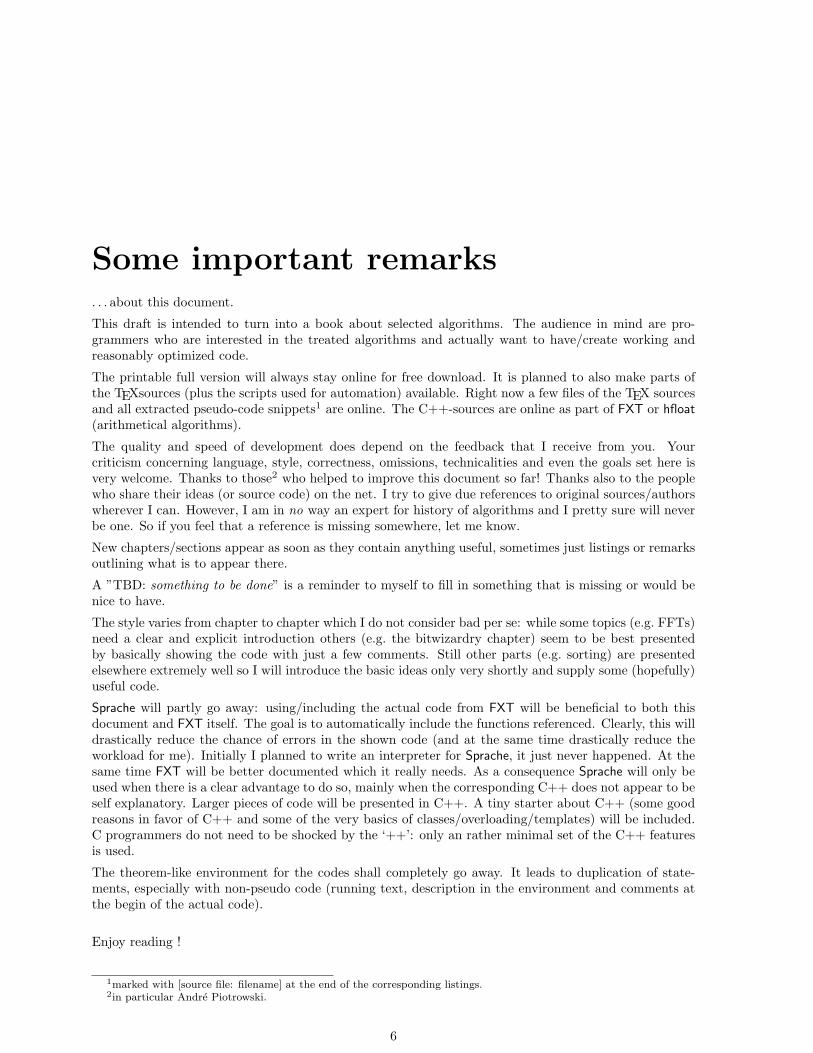
Some important remarks. . . about this document.
This draft is intended to turn into a book about selected algorithms. The audience in mind are pro-grammers who are interested in the treated algorithms and actually want to have/create working andreasonably optimized code.
The printable full version will always stay online for free download. It is planned to also make parts ofthe TEXsources (plus the scripts used for automation) available. Right now a few files of the TEX sourcesand all extracted pseudo-code snippets1 are online. The C++-sources are online as part of FXT or hfloat(arithmetical algorithms).
The quality and speed of development does depend on the feedback that I receive from you. Yourcriticism concerning language, style, correctness, omissions, technicalities and even the goals set here isvery welcome. Thanks to those2 who helped to improve this document so far! Thanks also to the peoplewho share their ideas (or source code) on the net. I try to give due references to original sources/authorswherever I can. However, I am in no way an expert for history of algorithms and I pretty sure will neverbe one. So if you feel that a reference is missing somewhere, let me know.
New chapters/sections appear as soon as they contain anything useful, sometimes just listings or remarksoutlining what is to appear there.
A ”TBD: something to be done” is a reminder to myself to fill in something that is missing or would benice to have.
The style varies from chapter to chapter which I do not consider bad per se: while some topics (e.g. FFTs)need a clear and explicit introduction others (e.g. the bitwizardry chapter) seem to be best presentedby basically showing the code with just a few comments. Still other parts (e.g. sorting) are presentedelsewhere extremely well so I will introduce the basic ideas only very shortly and supply some (hopefully)useful code.
Sprache will partly go away: using/including the actual code from FXT will be beneficial to both thisdocument and FXT itself. The goal is to automatically include the functions referenced. Clearly, this willdrastically reduce the chance of errors in the shown code (and at the same time drastically reduce theworkload for me). Initially I planned to write an interpreter for Sprache, it just never happened. At thesame time FXT will be better documented which it really needs. As a consequence Sprache will only beused when there is a clear advantage to do so, mainly when the corresponding C++ does not appear to beself explanatory. Larger pieces of code will be presented in C++. A tiny starter about C++ (some goodreasons in favor of C++ and some of the very basics of classes/overloading/templates) will be included.C programmers do not need to be shocked by the ‘++’: only an rather minimal set of the C++ featuresis used.
The theorem-like environment for the codes shall completely go away. It leads to duplication of state-ments, especially with non-pseudo code (running text, description in the environment and comments atthe begin of the actual code).
Enjoy reading !
1marked with [source file: filename] at the end of the corresponding listings.2in particular Andre Piotrowski.
6
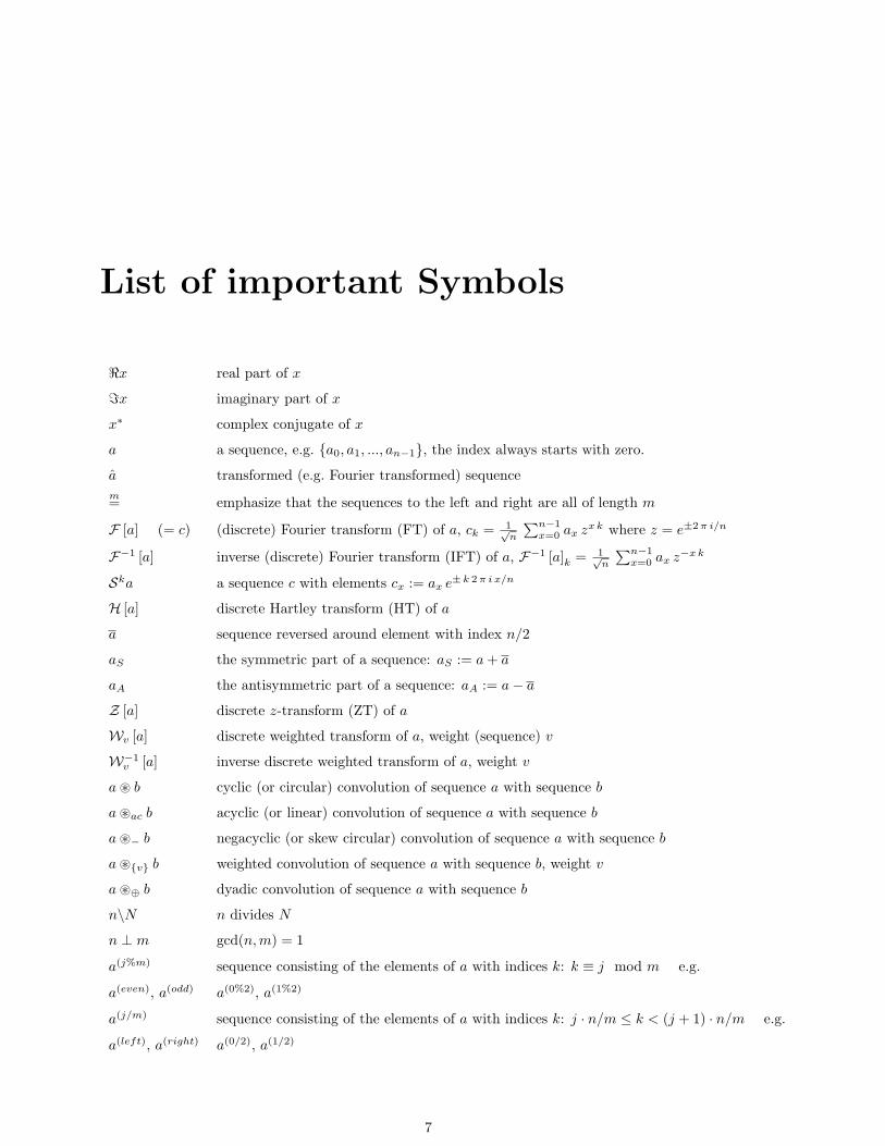
List of important Symbols
<x real part of x
=x imaginary part of x
x∗ complex conjugate of x
a a sequence, e.g. a0, a1, ..., an−1, the index always starts with zero.
a transformed (e.g. Fourier transformed) sequencem= emphasize that the sequences to the left and right are all of length m
F [a] (= c) (discrete) Fourier transform (FT) of a, ck = 1√n
∑n−1x=0 ax zx k where z = e±2 π i/n
F−1 [a] inverse (discrete) Fourier transform (IFT) of a, F−1 [a]k = 1√n
∑n−1x=0 ax z−x k
Ska a sequence c with elements cx := ax e± k 2 π i x/n
H [a] discrete Hartley transform (HT) of a
a sequence reversed around element with index n/2
aS the symmetric part of a sequence: aS := a + a
aA the antisymmetric part of a sequence: aA := a− a
Z [a] discrete z-transform (ZT) of a
Wv [a] discrete weighted transform of a, weight (sequence) v
W−1v [a] inverse discrete weighted transform of a, weight v
a ~ b cyclic (or circular) convolution of sequence a with sequence b
a ~ac b acyclic (or linear) convolution of sequence a with sequence b
a ~− b negacyclic (or skew circular) convolution of sequence a with sequence b
a ~v b weighted convolution of sequence a with sequence b, weight v
a ~⊕ b dyadic convolution of sequence a with sequence b
n\N n divides N
n ⊥ m gcd(n, m) = 1
a(j%m) sequence consisting of the elements of a with indices k: k ≡ j mod m e.g.
a(even), a(odd) a(0%2), a(1%2)
a(j/m) sequence consisting of the elements of a with indices k: j · n/m ≤ k < (j + 1) · n/m e.g.
a(left), a(right) a(0/2), a(1/2)
7
Chapter 1
The Fourier transform
1.1 The discrete Fourier transform
The discrete Fourier transform (DFT or simply FT) of a complex sequence a of length n is defined as
c = F [a] (1.1)
ck :=1√n
n−1∑x=0
ax z+x k where z = e± 2 π i/n (1.2)
z is an n-th root of unity: zn = 1.
Backtransform (or inverse discrete Fourier transform IDFT or simply IFT) is then
a = F−1 [c] (1.3)
ax =1√n
n−1∑
k=0
ck z−x k (1.4)
To see this, consider element y of the IFT of the FT of a:
F−1 [F [a]]y =1√n
n−1∑
k=0
1√n
n−1∑x=0
(ax zx k) z−y k (1.5)
=1n
∑x
ax
∑
k
(zx−y)k (1.6)
As∑
k (zx−y)k = n for x = y and zero else (because z is an n-th root of unity). Therefore the wholeexpression is equal to
1n
n∑
x
ax δx,y = ay (1.7)
where
δx,y =
1 (x = y)0 (x 6= y) (1.8)
Here we will call the FT with the plus in the exponent the forward transform. The choice is actuallyarbitrary1.
1Electrical engineers prefer the minus for the forward transform, mathematicians the plus.
8

CHAPTER 1. THE FOURIER TRANSFORM 9
The FT is a linear transform, i.e. for α, β ∈ CF [α a + β b] = αF [a] + β F [b] (1.9)
For the FT Parseval’s equation holds, let c = F [a], thenn−1∑x=0
a2x =
n−1∑
k=0
c2k (1.10)
The normalization factor 1√n
in front of the FT sums is sometimes replaced by a single 1n in front of the
inverse FT sum which is often convenient in computation. Then, of course, Parseval’s equation has to bemodified accordingly.A straight forward implementation of the discrete Fourier transform, i.e. the computation of n sums eachof length n requires ∼ n2 operations:
void slow_ft(Complex *f, long n, int is)
Complex h[n];const double ph0 = is*2.0*M_PI/n;for (long w=0; w<n; ++w)
Complex t = 0.0;for (long k=0; k<n; ++k)
t += f[k] * SinCos(ph0*k*w);h[w] = t;
copy(h, f, n);
[FXT: slow ft in slow/slowft.cc] is must be +1 (forward transform) or −1 (backward transform),SinCos(x) returns a Complex(cos(x), sin(x)).
A fast Fourier transform (FFT) algorithm is an algorithm that improves the operation count to propor-tional n
∑mk=1(pk − 1), where n = p1p2 · · · pm is a factorization of n. In case of a power n = pm the
value computes to n (p− 1) logp(n). In the special case p = 2 even n/2 log2(n) (complex) multiplicationssuffice. There are several different FFT algorithms with many variants.
1.2 Symmetries of the Fourier transform
A bit of notation turns out to be useful:Let a be the sequence a (length n) reversed around element with index n/2:
a0 := a0 (1.11)an/2 := an/2 if n even (1.12)
ak := an−k (1.13)
Let aS , aA be the symmetric, antisymmetric part of the sequence a, respectively:
aS := a + a (1.14)aA := a− a (1.15)
(The elements with indices 0 and n/2 of aA are zero). Now let a ∈ R (meaning that each element of a is∈ R), then
F [aS ] ∈ R (1.16)F [aS ] = F [aS ] (1.17)F [aA] ∈ iR (1.18)F [aA] = −F [aA] (1.19)
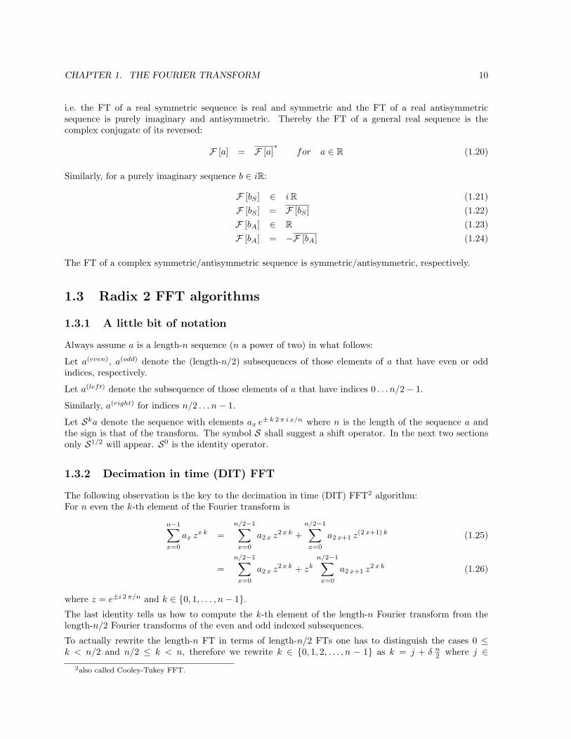
CHAPTER 1. THE FOURIER TRANSFORM 10
i.e. the FT of a real symmetric sequence is real and symmetric and the FT of a real antisymmetricsequence is purely imaginary and antisymmetric. Thereby the FT of a general real sequence is thecomplex conjugate of its reversed:
F [a] = F [a]∗
for a ∈ R (1.20)
Similarly, for a purely imaginary sequence b ∈ iR:
F [bS ] ∈ iR (1.21)F [bS ] = F [bS ] (1.22)F [bA] ∈ R (1.23)F [bA] = −F [bA] (1.24)
The FT of a complex symmetric/antisymmetric sequence is symmetric/antisymmetric, respectively.
1.3 Radix 2 FFT algorithms
1.3.1 A little bit of notation
Always assume a is a length-n sequence (n a power of two) in what follows:
Let a(even), a(odd) denote the (length-n/2) subsequences of those elements of a that have even or oddindices, respectively.
Let a(left) denote the subsequence of those elements of a that have indices 0 . . . n/2− 1.
Similarly, a(right) for indices n/2 . . . n− 1.
Let Ska denote the sequence with elements ax e± k 2 π i x/n where n is the length of the sequence a andthe sign is that of the transform. The symbol S shall suggest a shift operator. In the next two sectionsonly S1/2 will appear. S0 is the identity operator.
1.3.2 Decimation in time (DIT) FFT
The following observation is the key to the decimation in time (DIT) FFT2 algorithm:For n even the k-th element of the Fourier transform is
n−1∑x=0
ax zx k =n/2−1∑x=0
a2 x z2 x k +n/2−1∑x=0
a2 x+1 z(2 x+1) k (1.25)
=n/2−1∑x=0
a2 x z2 x k + zk
n/2−1∑x=0
a2 x+1 z2 x k (1.26)
where z = e±i 2 π/n and k ∈ 0, 1, . . . , n− 1.The last identity tells us how to compute the k-th element of the length-n Fourier transform from thelength-n/2 Fourier transforms of the even and odd indexed subsequences.
To actually rewrite the length-n FT in terms of length-n/2 FTs one has to distinguish the cases 0 ≤k < n/2 and n/2 ≤ k < n, therefore we rewrite k ∈ 0, 1, 2, . . . , n − 1 as k = j + δ n
2 where j ∈2also called Cooley-Tukey FFT.
CHAPTER 1. THE FOURIER TRANSFORM 11
0, 1, . . . , n/2− 1, δ ∈ 0, 1.n−1∑x=0
ax zx (j+δ n2 ) =
n/2−1∑x=0
a(even)x z2 x (j+δ n
2 ) + zj+δ n2
n/2−1∑x=0
a(odd)x z2 x (j+δ n
2 ) (1.27)
=
n/2−1∑x=0
a(even)x z2 x j + zj
n/2−1∑x=0
a(odd)x z2 x j for δ = 0
n/2−1∑x=0
a(even)x z2 x j − zj
n/2−1∑x=0
a(odd)x z2 x j for δ = 1
(1.28)
Noting that z2 is just the root of unity that appears in a length-n/2 FT one can rewrite the last twoequations as the
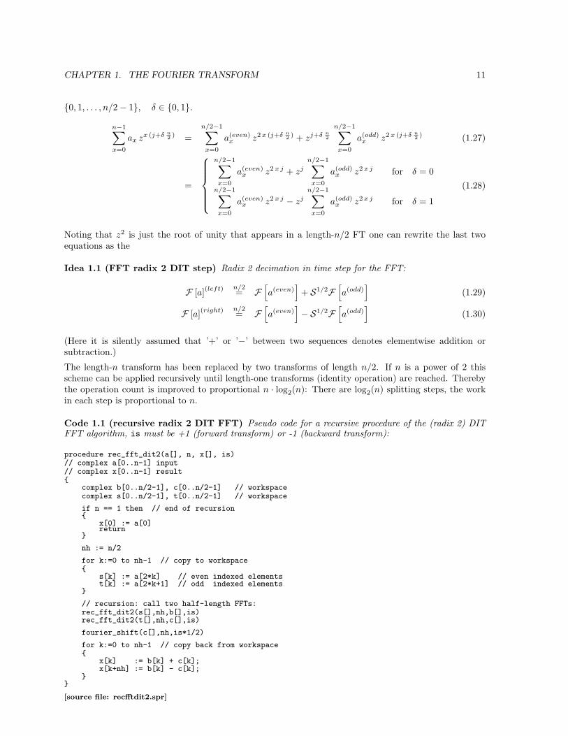
Idea 1.1 (FFT radix 2 DIT step) Radix 2 decimation in time step for the FFT:
F [a](left) n/2= F
[a(even)
]+ S1/2F
[a(odd)
](1.29)
F [a](right) n/2= F
[a(even)
]− S1/2F
[a(odd)
](1.30)
(Here it is silently assumed that ’+’ or ’−’ between two sequences denotes elementwise addition orsubtraction.)
The length-n transform has been replaced by two transforms of length n/2. If n is a power of 2 thisscheme can be applied recursively until length-one transforms (identity operation) are reached. Therebythe operation count is improved to proportional n · log2(n): There are log2(n) splitting steps, the workin each step is proportional to n.
Code 1.1 (recursive radix 2 DIT FFT) Pseudo code for a recursive procedure of the (radix 2) DITFFT algorithm, is must be +1 (forward transform) or -1 (backward transform):
procedure rec_fft_dit2(a[], n, x[], is)// complex a[0..n-1] input// complex x[0..n-1] result
complex b[0..n/2-1], c[0..n/2-1] // workspacecomplex s[0..n/2-1], t[0..n/2-1] // workspace
if n == 1 then // end of recursion
x[0] := a[0]return
nh := n/2
for k:=0 to nh-1 // copy to workspace
s[k] := a[2*k] // even indexed elementst[k] := a[2*k+1] // odd indexed elements
// recursion: call two half-length FFTs:rec_fft_dit2(s[],nh,b[],is)rec_fft_dit2(t[],nh,c[],is)
fourier_shift(c[],nh,is*1/2)
for k:=0 to nh-1 // copy back from workspace
x[k] := b[k] + c[k];x[k+nh] := b[k] - c[k];
[source file: recfftdit2.spr]
CHAPTER 1. THE FOURIER TRANSFORM 12
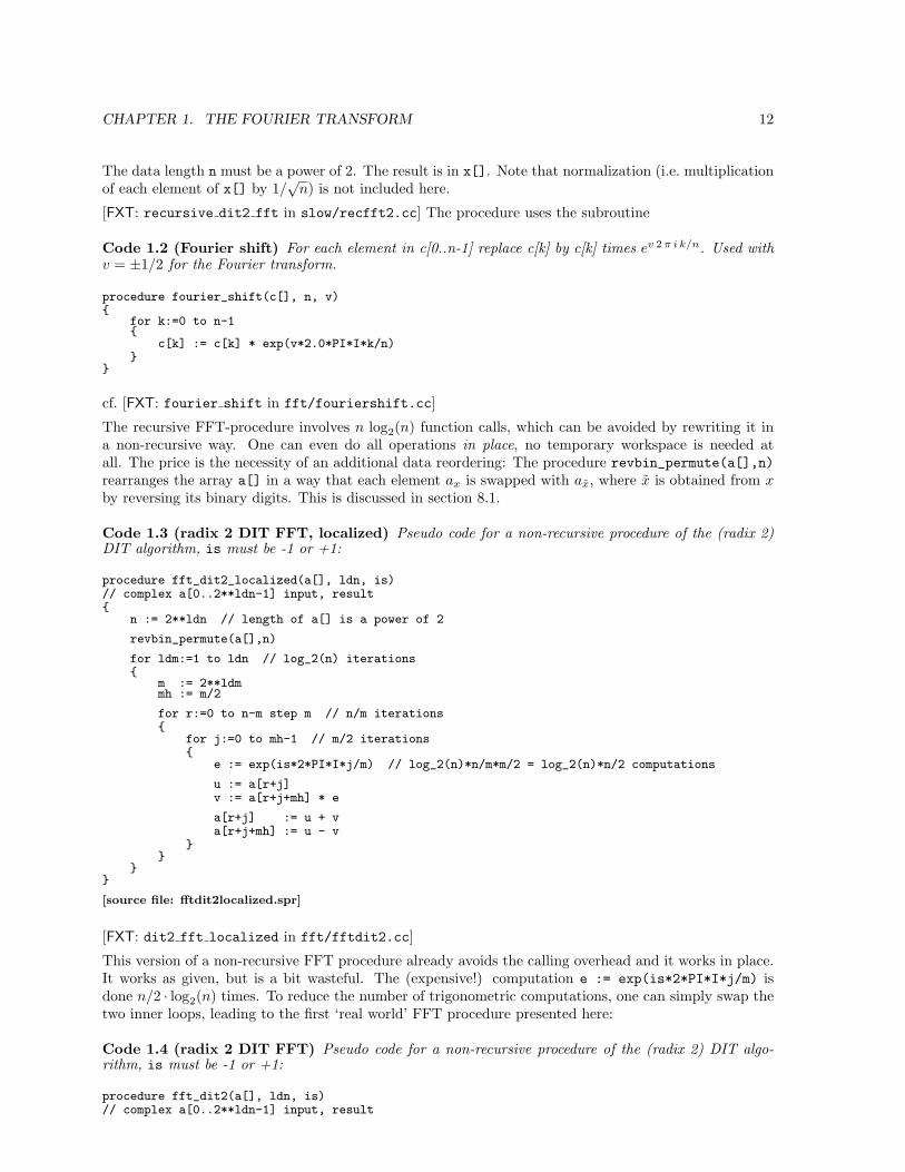
The data length n must be a power of 2. The result is in x[]. Note that normalization (i.e. multiplicationof each element of x[] by 1/
√n) is not included here.
[FXT: recursive dit2 fft in slow/recfft2.cc] The procedure uses the subroutine
Code 1.2 (Fourier shift) For each element in c[0..n-1] replace c[k] by c[k] times ev 2 π i k/n. Used withv = ±1/2 for the Fourier transform.
procedure fourier_shift(c[], n, v)
for k:=0 to n-1
c[k] := c[k] * exp(v*2.0*PI*I*k/n)
cf. [FXT: fourier shift in fft/fouriershift.cc]
The recursive FFT-procedure involves n log2(n) function calls, which can be avoided by rewriting it ina non-recursive way. One can even do all operations in place, no temporary workspace is needed atall. The price is the necessity of an additional data reordering: The procedure revbin_permute(a[],n)rearranges the array a[] in a way that each element ax is swapped with ax, where x is obtained from xby reversing its binary digits. This is discussed in section 8.1.
Code 1.3 (radix 2 DIT FFT, localized) Pseudo code for a non-recursive procedure of the (radix 2)DIT algorithm, is must be -1 or +1:
procedure fft_dit2_localized(a[], ldn, is)// complex a[0..2**ldn-1] input, result
n := 2**ldn // length of a[] is a power of 2
revbin_permute(a[],n)
for ldm:=1 to ldn // log_2(n) iterations
m := 2**ldmmh := m/2
for r:=0 to n-m step m // n/m iterations
for j:=0 to mh-1 // m/2 iterations
e := exp(is*2*PI*I*j/m) // log_2(n)*n/m*m/2 = log_2(n)*n/2 computations
u := a[r+j]v := a[r+j+mh] * e
a[r+j] := u + va[r+j+mh] := u - v
[source file: fftdit2localized.spr]
[FXT: dit2 fft localized in fft/fftdit2.cc]
This version of a non-recursive FFT procedure already avoids the calling overhead and it works in place.It works as given, but is a bit wasteful. The (expensive!) computation e := exp(is*2*PI*I*j/m) isdone n/2 · log2(n) times. To reduce the number of trigonometric computations, one can simply swap thetwo inner loops, leading to the first ‘real world’ FFT procedure presented here:
Code 1.4 (radix 2 DIT FFT) Pseudo code for a non-recursive procedure of the (radix 2) DIT algo-rithm, is must be -1 or +1:
procedure fft_dit2(a[], ldn, is)// complex a[0..2**ldn-1] input, result
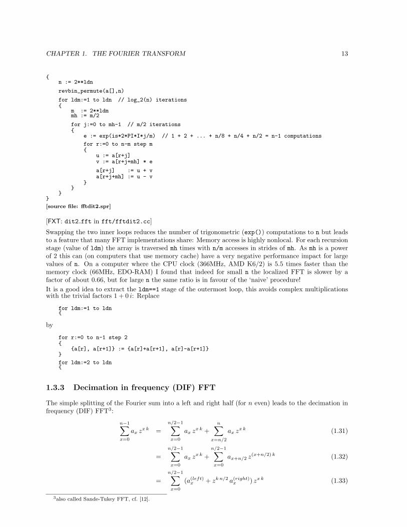
CHAPTER 1. THE FOURIER TRANSFORM 13
n := 2**ldn
revbin_permute(a[],n)
for ldm:=1 to ldn // log_2(n) iterations
m := 2**ldmmh := m/2
for j:=0 to mh-1 // m/2 iterations
e := exp(is*2*PI*I*j/m) // 1 + 2 + ... + n/8 + n/4 + n/2 = n-1 computations
for r:=0 to n-m step m
u := a[r+j]v := a[r+j+mh] * e
a[r+j] := u + va[r+j+mh] := u - v
[source file: fftdit2.spr]
[FXT: dit2 fft in fft/fftdit2.cc]
Swapping the two inner loops reduces the number of trigonometric (exp()) computations to n but leadsto a feature that many FFT implementations share: Memory access is highly nonlocal. For each recursionstage (value of ldm) the array is traversed mh times with n/m accesses in strides of mh. As mh is a powerof 2 this can (on computers that use memory cache) have a very negative performance impact for largevalues of n. On a computer where the CPU clock (366MHz, AMD K6/2) is 5.5 times faster than thememory clock (66MHz, EDO-RAM) I found that indeed for small n the localized FFT is slower by afactor of about 0.66, but for large n the same ratio is in favour of the ‘naive’ procedure!It is a good idea to extract the ldm==1 stage of the outermost loop, this avoids complex multiplicationswith the trivial factors 1 + 0 i: Replace
for ldm:=1 to ldn
by
for r:=0 to n-1 step 2
a[r], a[r+1] := a[r]+a[r+1], a[r]-a[r+1]
for ldm:=2 to ldn
1.3.3 Decimation in frequency (DIF) FFT
The simple splitting of the Fourier sum into a left and right half (for n even) leads to the decimation infrequency (DIF) FFT3:
n−1∑x=0
ax zx k =n/2−1∑x=0
ax zx k +n∑
x=n/2
ax zx k (1.31)
=n/2−1∑x=0
ax zx k +n/2−1∑x=0
ax+n/2 z(x+n/2) k (1.32)
=n/2−1∑x=0
(a(left)x + zk n/2 a(right)
x ) zx k (1.33)
3also called Sande-Tukey FFT, cf. [12].
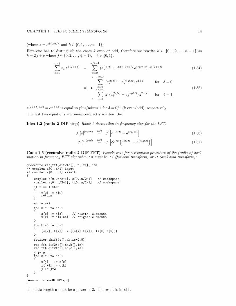
CHAPTER 1. THE FOURIER TRANSFORM 14
(where z = e±i 2 π/n and k ∈ 0, 1, . . . , n− 1)Here one has to distinguish the cases k even or odd, therefore we rewrite k ∈ 0, 1, 2, . . . , n − 1 ask = 2 j + δ where j ∈ 0, 2, . . . , n
2 − 1, δ ∈ 0, 1.n−1∑x=0
ax zx (2 j+δ) =n/2−1∑x=0
(a(left)x + z(2 j+δ) n/2 a(right)
x ) zx (2 j+δ) (1.34)
=
n/2−1∑x=0
(a(left)x + a(right)
x ) z2 x j for δ = 0
n/2−1∑x=0
zx(a(left)x − a(right)
x ) z2 x j for δ = 1
(1.35)
z(2 j+δ) n/2 = e±π i δ is equal to plus/minus 1 for δ = 0/1 (k even/odd), respectively.
The last two equations are, more compactly written, the
Idea 1.2 (radix 2 DIF step) Radix 2 decimation in frequency step for the FFT:
F [a](even) n/2= F
[a(left) + a(right)
](1.36)
F [a](odd) n/2= F
[S1/2
(a(left) − a(right)
)](1.37)
Code 1.5 (recursive radix 2 DIF FFT) Pseudo code for a recursive procedure of the (radix 2) deci-mation in frequency FFT algorithm, is must be +1 (forward transform) or -1 (backward transform):
procedure rec_fft_dif2(a[], n, x[], is)// complex a[0..n-1] input// complex x[0..n-1] result
complex b[0..n/2-1], c[0..n/2-1] // workspacecomplex s[0..n/2-1], t[0..n/2-1] // workspace
if n == 1 then
x[0] := a[0]return
nh := n/2
for k:=0 to nh-1
s[k] := a[k] // ’left’ elementst[k] := a[k+nh] // ’right’ elements
for k:=0 to nh-1
s[k], t[k] := (s[k]+t[k]), (s[k]-t[k])
fourier_shift(t[],nh,is*0.5)
rec_fft_dif2(s[],nh,b[],is)rec_fft_dif2(t[],nh,c[],is)
j := 0for k:=0 to nh-1
x[j] := b[k]x[j+1] := c[k]j := j+2
[source file: recfftdif2.spr]
The data length n must be a power of 2. The result is in x[].
CHAPTER 1. THE FOURIER TRANSFORM 15
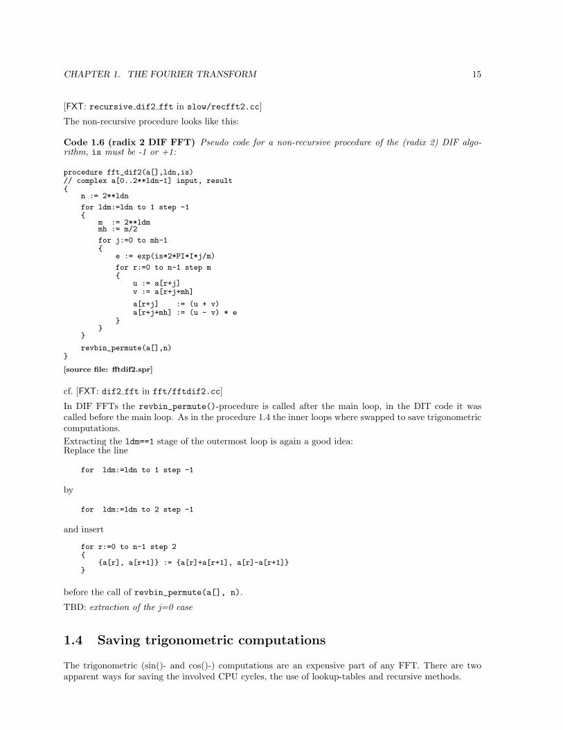
[FXT: recursive dif2 fft in slow/recfft2.cc]
The non-recursive procedure looks like this:
Code 1.6 (radix 2 DIF FFT) Pseudo code for a non-recursive procedure of the (radix 2) DIF algo-rithm, is must be -1 or +1:
procedure fft_dif2(a[],ldn,is)// complex a[0..2**ldn-1] input, result
n := 2**ldn
for ldm:=ldn to 1 step -1
m := 2**ldmmh := m/2
for j:=0 to mh-1
e := exp(is*2*PI*I*j/m)
for r:=0 to n-1 step m
u := a[r+j]v := a[r+j+mh]
a[r+j] := (u + v)a[r+j+mh] := (u - v) * e
revbin_permute(a[],n)
[source file: fftdif2.spr]
cf. [FXT: dif2 fft in fft/fftdif2.cc]
In DIF FFTs the revbin_permute()-procedure is called after the main loop, in the DIT code it wascalled before the main loop. As in the procedure 1.4 the inner loops where swapped to save trigonometriccomputations.Extracting the ldm==1 stage of the outermost loop is again a good idea:Replace the line
for ldm:=ldn to 1 step -1
by
for ldm:=ldn to 2 step -1
and insert
for r:=0 to n-1 step 2
a[r], a[r+1] := a[r]+a[r+1], a[r]-a[r+1]
before the call of revbin_permute(a[], n).
TBD: extraction of the j=0 case
1.4 Saving trigonometric computations
The trigonometric (sin()- and cos()-) computations are an expensive part of any FFT. There are twoapparent ways for saving the involved CPU cycles, the use of lookup-tables and recursive methods.
CHAPTER 1. THE FOURIER TRANSFORM 16
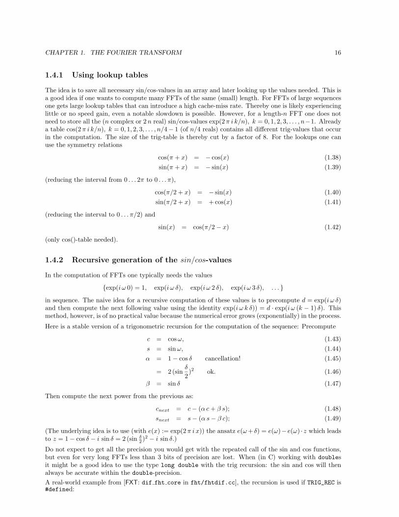
1.4.1 Using lookup tables
The idea is to save all necessary sin/cos-values in an array and later looking up the values needed. This isa good idea if one wants to compute many FFTs of the same (small) length. For FFTs of large sequencesone gets large lookup tables that can introduce a high cache-miss rate. Thereby one is likely experiencinglittle or no speed gain, even a notable slowdown is possible. However, for a length-n FFT one does notneed to store all the (n complex or 2 n real) sin/cos-values exp(2 π i k/n), k = 0, 1, 2, 3, . . . , n−1. Alreadya table cos(2 π i k/n), k = 0, 1, 2, 3, . . . , n/4− 1 (of n/4 reals) contains all different trig-values that occurin the computation. The size of the trig-table is thereby cut by a factor of 8. For the lookups one canuse the symmetry relations
cos(π + x) = − cos(x) (1.38)sin(π + x) = − sin(x) (1.39)
(reducing the interval from 0 . . . 2π to 0 . . . π),
cos(π/2 + x) = − sin(x) (1.40)sin(π/2 + x) = + cos(x) (1.41)
(reducing the interval to 0 . . . π/2) and
sin(x) = cos(π/2− x) (1.42)
(only cos()-table needed).
1.4.2 Recursive generation of the sin/cos-values
In the computation of FFTs one typically needs the values
exp(i ω 0) = 1, exp(i ω δ), exp(i ω 2 δ), exp(i ω 3 δ), . . . in sequence. The naive idea for a recursive computation of these values is to precompute d = exp(i ω δ)and then compute the next following value using the identity exp(i ω k δ)) = d · exp(i ω (k − 1) δ). Thismethod, however, is of no practical value because the numerical error grows (exponentially) in the process.
Here is a stable version of a trigonometric recursion for the computation of the sequence: Precompute
c = cos ω, (1.43)s = sin ω, (1.44)α = 1− cos δ cancellation! (1.45)
= 2 (sinδ
2)2 ok. (1.46)
β = sin δ (1.47)
Then compute the next power from the previous as:
cnext = c− (α c + β s); (1.48)snext = s− (α s− β c); (1.49)
(The underlying idea is to use (with e(x) := exp(2 π i x)) the ansatz e(ω + δ) = e(ω)−e(ω) ·z which leadsto z = 1− cos δ − i sin δ = 2 (sin δ
2 )2 − i sin δ.)
Do not expect to get all the precision you would get with the repeated call of the sin and cos functions,but even for very long FFTs less than 3 bits of precision are lost. When (in C) working with doublesit might be a good idea to use the type long double with the trig recursion: the sin and cos will thenalways be accurate within the double-precision.A real-world example from [FXT: dif fht core in fht/fhtdif.cc], the recursion is used if TRIG_REC is#defined:
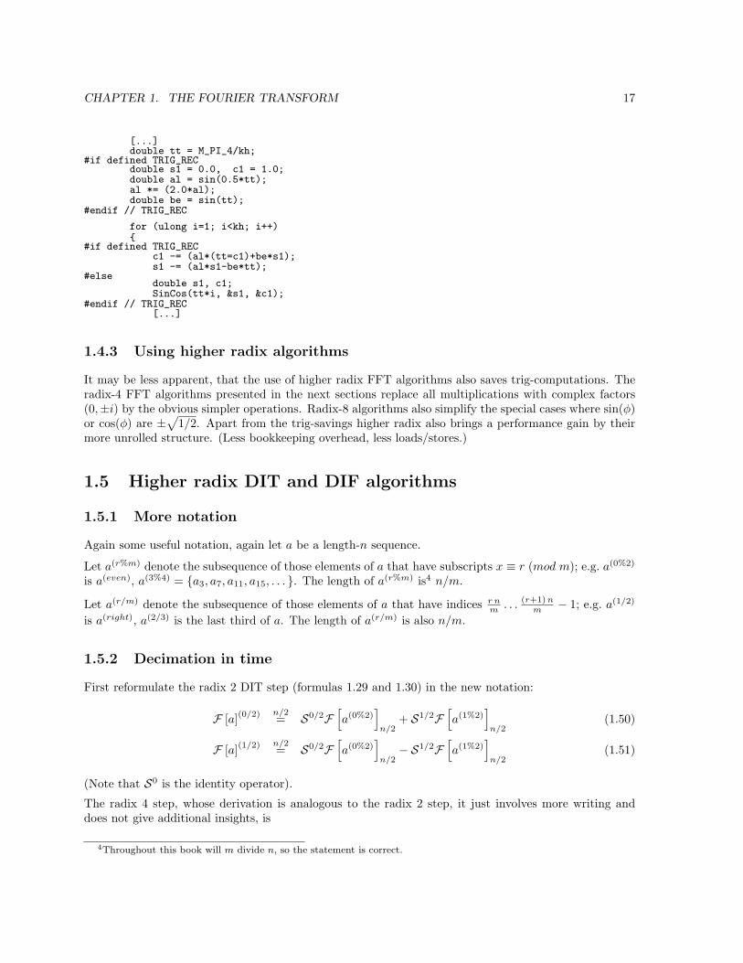
CHAPTER 1. THE FOURIER TRANSFORM 17
[...]double tt = M_PI_4/kh;
#if defined TRIG_RECdouble s1 = 0.0, c1 = 1.0;double al = sin(0.5*tt);al *= (2.0*al);double be = sin(tt);
#endif // TRIG_REC
for (ulong i=1; i<kh; i++)
#if defined TRIG_RECc1 -= (al*(tt=c1)+be*s1);s1 -= (al*s1-be*tt);
#elsedouble s1, c1;SinCos(tt*i, &s1, &c1);
#endif // TRIG_REC[...]
1.4.3 Using higher radix algorithms
It may be less apparent, that the use of higher radix FFT algorithms also saves trig-computations. Theradix-4 FFT algorithms presented in the next sections replace all multiplications with complex factors(0,±i) by the obvious simpler operations. Radix-8 algorithms also simplify the special cases where sin(φ)or cos(φ) are ±
√1/2. Apart from the trig-savings higher radix also brings a performance gain by their
more unrolled structure. (Less bookkeeping overhead, less loads/stores.)
1.5 Higher radix DIT and DIF algorithms
1.5.1 More notation
Again some useful notation, again let a be a length-n sequence.
Let a(r%m) denote the subsequence of those elements of a that have subscripts x ≡ r (mod m); e.g. a(0%2)
is a(even), a(3%4) = a3, a7, a11, a15, . . . . The length of a(r%m) is4 n/m.
Let a(r/m) denote the subsequence of those elements of a that have indices r nm . . . (r+1) n
m − 1; e.g. a(1/2)
is a(right), a(2/3) is the last third of a. The length of a(r/m) is also n/m.
1.5.2 Decimation in time
First reformulate the radix 2 DIT step (formulas 1.29 and 1.30) in the new notation:
F [a](0/2) n/2= S0/2F
[a(0%2)
]n/2
+ S1/2F[a(1%2)
]n/2
(1.50)
F [a](1/2) n/2= S0/2F
[a(0%2)
]n/2
− S1/2F[a(1%2)
]n/2
(1.51)
(Note that S0 is the identity operator).
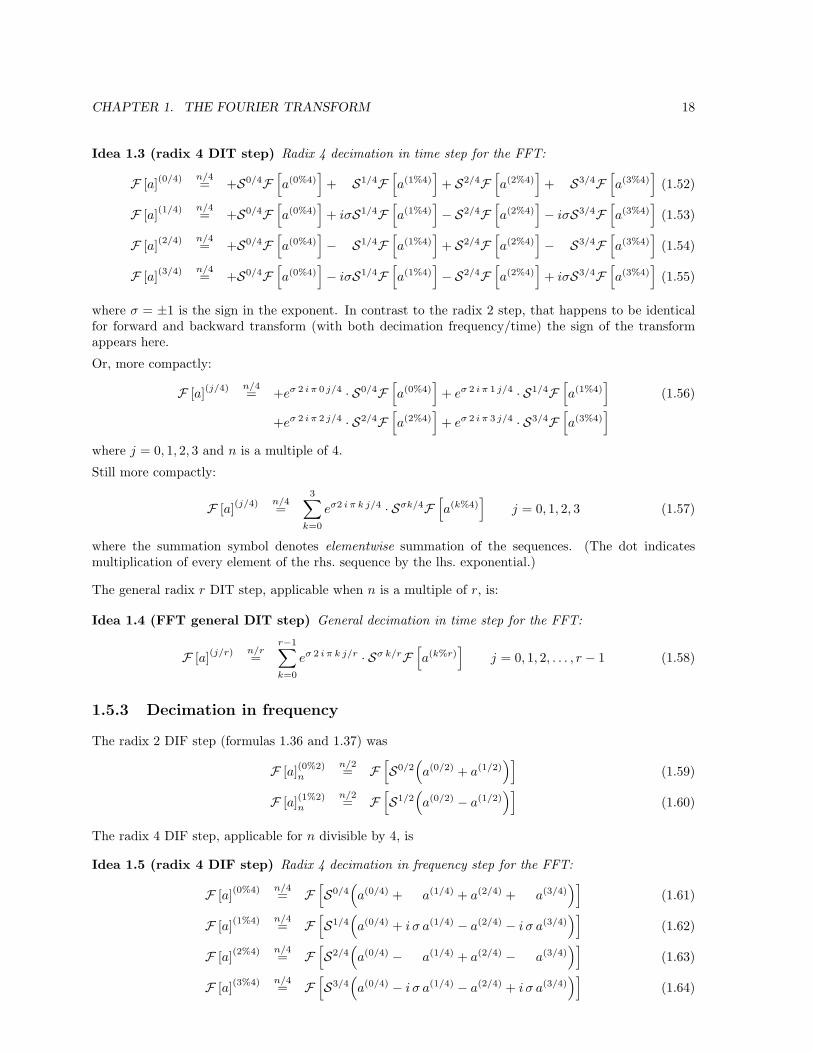
The radix 4 step, whose derivation is analogous to the radix 2 step, it just involves more writing anddoes not give additional insights, is
4Throughout this book will m divide n, so the statement is correct.
CHAPTER 1. THE FOURIER TRANSFORM 18
Idea 1.3 (radix 4 DIT step) Radix 4 decimation in time step for the FFT:
F [a](0/4) n/4= +S0/4F
[a(0%4)
]+ S1/4F
[a(1%4)
]+ S2/4F
[a(2%4)
]+ S3/4F
[a(3%4)
](1.52)
F [a](1/4) n/4= +S0/4F
[a(0%4)
]+ iσS1/4F
[a(1%4)
]− S2/4F
[a(2%4)
]− iσS3/4F
[a(3%4)
](1.53)
F [a](2/4) n/4= +S0/4F
[a(0%4)
]− S1/4F
[a(1%4)
]+ S2/4F
[a(2%4)
]− S3/4F
[a(3%4)
](1.54)
F [a](3/4) n/4= +S0/4F
[a(0%4)
]− iσS1/4F
[a(1%4)
]− S2/4F
[a(2%4)
]+ iσS3/4F
[a(3%4)
](1.55)
where σ = ±1 is the sign in the exponent. In contrast to the radix 2 step, that happens to be identicalfor forward and backward transform (with both decimation frequency/time) the sign of the transformappears here.
Or, more compactly:
F [a](j/4) n/4= +eσ 2 i π 0 j/4 · S0/4F
[a(0%4)
]+ eσ 2 i π 1 j/4 · S1/4F
[a(1%4)
](1.56)
+eσ 2 i π 2 j/4 · S2/4F[a(2%4)
]+ eσ 2 i π 3 j/4 · S3/4F
[a(3%4)
]
where j = 0, 1, 2, 3 and n is a multiple of 4.
Still more compactly:
F [a](j/4) n/4=
3∑
k=0
eσ2 i π k j/4 · Sσk/4F[a(k%4)
]j = 0, 1, 2, 3 (1.57)
where the summation symbol denotes elementwise summation of the sequences. (The dot indicatesmultiplication of every element of the rhs. sequence by the lhs. exponential.)
The general radix r DIT step, applicable when n is a multiple of r, is:
Idea 1.4 (FFT general DIT step) General decimation in time step for the FFT:
F [a](j/r) n/r=
r−1∑
k=0
eσ 2 i π k j/r · Sσ k/rF[a(k%r)
]j = 0, 1, 2, . . . , r − 1 (1.58)
1.5.3 Decimation in frequency
The radix 2 DIF step (formulas 1.36 and 1.37) was
F [a](0%2)n
n/2= F
[S0/2
(a(0/2) + a(1/2)
)](1.59)
F [a](1%2)n
n/2= F
[S1/2
(a(0/2) − a(1/2)
)](1.60)
The radix 4 DIF step, applicable for n divisible by 4, is
Idea 1.5 (radix 4 DIF step) Radix 4 decimation in frequency step for the FFT:
F [a](0%4) n/4= F
[S0/4
(a(0/4) + a(1/4) + a(2/4) + a(3/4)
)](1.61)
F [a](1%4) n/4= F
[S1/4
(a(0/4) + i σ a(1/4) − a(2/4) − i σ a(3/4)
)](1.62)
F [a](2%4) n/4= F
[S2/4
(a(0/4) − a(1/4) + a(2/4) − a(3/4)
)](1.63)
F [a](3%4) n/4= F
[S3/4
(a(0/4) − i σ a(1/4) − a(2/4) + i σ a(3/4)
)](1.64)
CHAPTER 1. THE FOURIER TRANSFORM 19
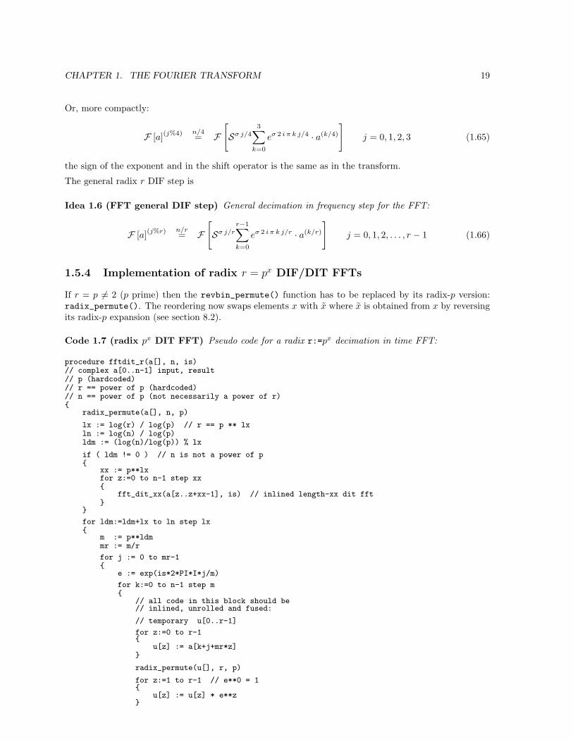
Or, more compactly:
F [a](j%4) n/4= F
[Sσ j/4
3∑
k=0
eσ 2 i π k j/4 · a(k/4)
]j = 0, 1, 2, 3 (1.65)
the sign of the exponent and in the shift operator is the same as in the transform.
The general radix r DIF step is
Idea 1.6 (FFT general DIF step) General decimation in frequency step for the FFT:
F [a](j%r) n/r= F
[Sσ j/r
r−1∑
k=0
eσ 2 i π k j/r · a(k/r)
]j = 0, 1, 2, . . . , r − 1 (1.66)
1.5.4 Implementation of radix r = px DIF/DIT FFTs
If r = p 6= 2 (p prime) then the revbin_permute() function has to be replaced by its radix-p version:radix_permute(). The reordering now swaps elements x with x where x is obtained from x by reversingits radix-p expansion (see section 8.2).
Code 1.7 (radix px DIT FFT) Pseudo code for a radix r:=px decimation in time FFT:
procedure fftdit_r(a[], n, is)// complex a[0..n-1] input, result// p (hardcoded)// r == power of p (hardcoded)// n == power of p (not necessarily a power of r)
radix_permute(a[], n, p)
lx := log(r) / log(p) // r == p ** lxln := log(n) / log(p)ldm := (log(n)/log(p)) % lx
if ( ldm != 0 ) // n is not a power of p
xx := p**lxfor z:=0 to n-1 step xx
fft_dit_xx(a[z..z+xx-1], is) // inlined length-xx dit fft
for ldm:=ldm+lx to ln step lx
m := p**ldmmr := m/r
for j := 0 to mr-1
e := exp(is*2*PI*I*j/m)
for k:=0 to n-1 step m
// all code in this block should be// inlined, unrolled and fused:
// temporary u[0..r-1]
for z:=0 to r-1
u[z] := a[k+j+mr*z]
radix_permute(u[], r, p)
for z:=1 to r-1 // e**0 = 1
u[z] := u[z] * e**z
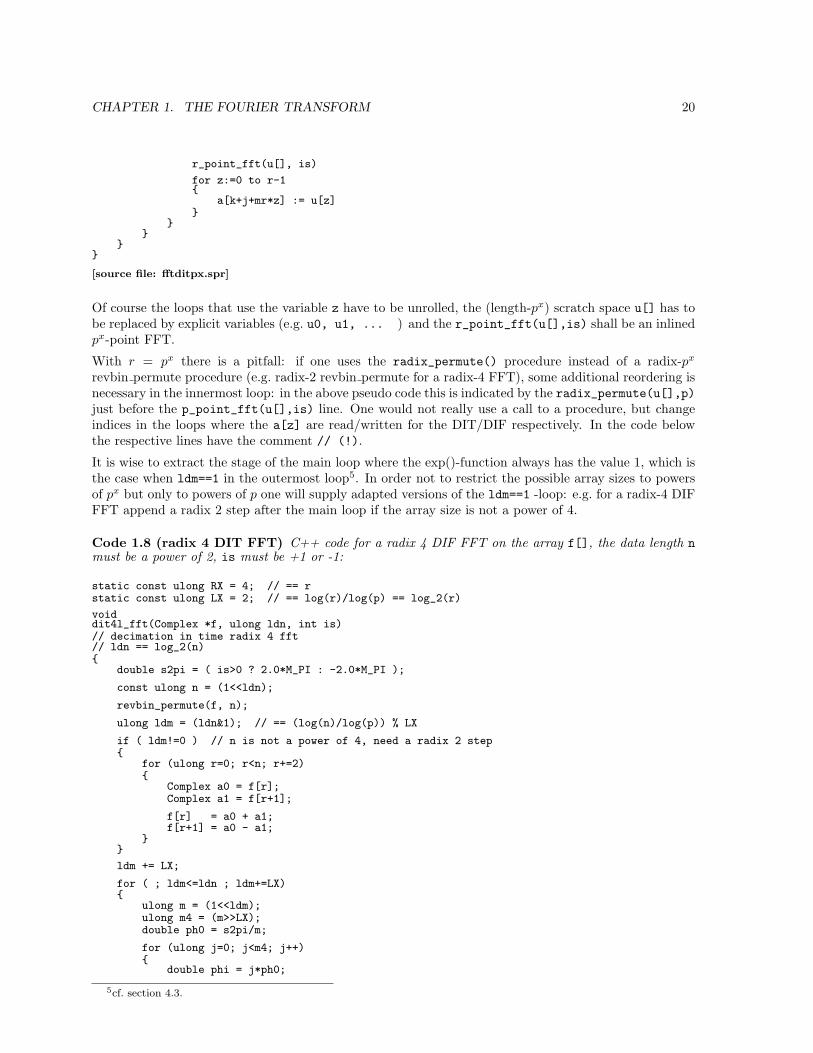
CHAPTER 1. THE FOURIER TRANSFORM 20
r_point_fft(u[], is)
for z:=0 to r-1
a[k+j+mr*z] := u[z]
[source file: fftditpx.spr]
Of course the loops that use the variable z have to be unrolled, the (length-px) scratch space u[] has tobe replaced by explicit variables (e.g. u0, u1, ... ) and the r_point_fft(u[],is) shall be an inlinedpx-point FFT.
With r = px there is a pitfall: if one uses the radix_permute() procedure instead of a radix-px
revbin permute procedure (e.g. radix-2 revbin permute for a radix-4 FFT), some additional reordering isnecessary in the innermost loop: in the above pseudo code this is indicated by the radix_permute(u[],p)just before the p_point_fft(u[],is) line. One would not really use a call to a procedure, but changeindices in the loops where the a[z] are read/written for the DIT/DIF respectively. In the code belowthe respective lines have the comment // (!).
It is wise to extract the stage of the main loop where the exp()-function always has the value 1, which isthe case when ldm==1 in the outermost loop5. In order not to restrict the possible array sizes to powersof px but only to powers of p one will supply adapted versions of the ldm==1 -loop: e.g. for a radix-4 DIFFFT append a radix 2 step after the main loop if the array size is not a power of 4.
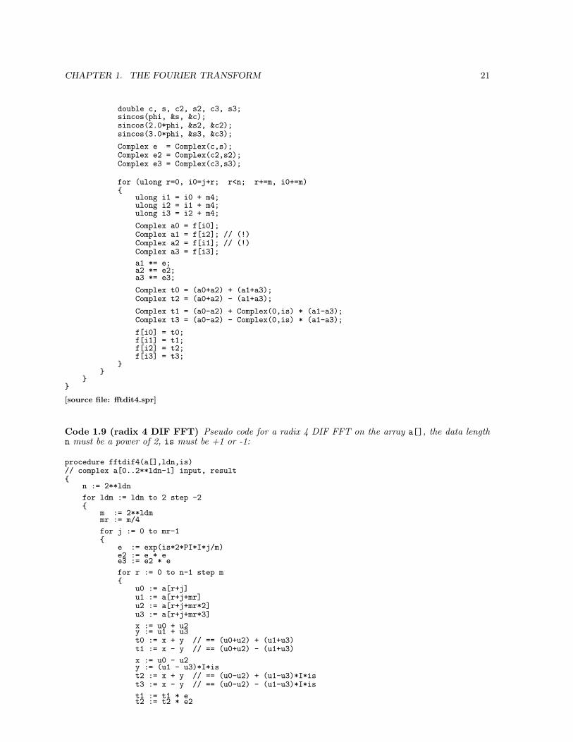
Code 1.8 (radix 4 DIT FFT) C++ code for a radix 4 DIF FFT on the array f[], the data length nmust be a power of 2, is must be +1 or -1:
static const ulong RX = 4; // == rstatic const ulong LX = 2; // == log(r)/log(p) == log_2(r)
voiddit4l_fft(Complex *f, ulong ldn, int is)// decimation in time radix 4 fft// ldn == log_2(n)
double s2pi = ( is>0 ? 2.0*M_PI : -2.0*M_PI );
const ulong n = (1<<ldn);
revbin_permute(f, n);
ulong ldm = (ldn&1); // == (log(n)/log(p)) % LX
if ( ldm!=0 ) // n is not a power of 4, need a radix 2 step
for (ulong r=0; r<n; r+=2)
Complex a0 = f[r];Complex a1 = f[r+1];
f[r] = a0 + a1;f[r+1] = a0 - a1;
ldm += LX;
for ( ; ldm<=ldn ; ldm+=LX)
ulong m = (1<<ldm);ulong m4 = (m>>LX);double ph0 = s2pi/m;
for (ulong j=0; j<m4; j++)
double phi = j*ph0;
5cf. section 4.3.
CHAPTER 1. THE FOURIER TRANSFORM 21
double c, s, c2, s2, c3, s3;sincos(phi, &s, &c);sincos(2.0*phi, &s2, &c2);sincos(3.0*phi, &s3, &c3);
Complex e = Complex(c,s);Complex e2 = Complex(c2,s2);Complex e3 = Complex(c3,s3);
for (ulong r=0, i0=j+r; r<n; r+=m, i0+=m)
ulong i1 = i0 + m4;ulong i2 = i1 + m4;ulong i3 = i2 + m4;
Complex a0 = f[i0];Complex a1 = f[i2]; // (!)Complex a2 = f[i1]; // (!)Complex a3 = f[i3];
a1 *= e;a2 *= e2;a3 *= e3;
Complex t0 = (a0+a2) + (a1+a3);Complex t2 = (a0+a2) - (a1+a3);
Complex t1 = (a0-a2) + Complex(0,is) * (a1-a3);Complex t3 = (a0-a2) - Complex(0,is) * (a1-a3);
f[i0] = t0;f[i1] = t1;f[i2] = t2;f[i3] = t3;
[source file: fftdit4.spr]
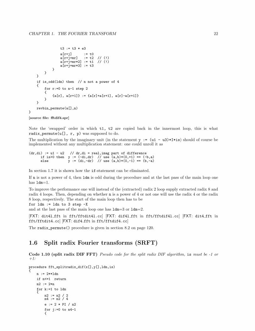
Code 1.9 (radix 4 DIF FFT) Pseudo code for a radix 4 DIF FFT on the array a[], the data lengthn must be a power of 2, is must be +1 or -1:
procedure fftdif4(a[],ldn,is)// complex a[0..2**ldn-1] input, result
n := 2**ldn
for ldm := ldn to 2 step -2
m := 2**ldmmr := m/4
for j := 0 to mr-1
e := exp(is*2*PI*I*j/m)e2 := e * ee3 := e2 * e
for r := 0 to n-1 step m
u0 := a[r+j]u1 := a[r+j+mr]u2 := a[r+j+mr*2]u3 := a[r+j+mr*3]
x := u0 + u2y := u1 + u3t0 := x + y // == (u0+u2) + (u1+u3)t1 := x - y // == (u0+u2) - (u1+u3)
x := u0 - u2y := (u1 - u3)*I*ist2 := x + y // == (u0-u2) + (u1-u3)*I*ist3 := x - y // == (u0-u2) - (u1-u3)*I*is
t1 := t1 * et2 := t2 * e2
CHAPTER 1. THE FOURIER TRANSFORM 22
t3 := t3 * e3
a[r+j] := t0a[r+j+mr] := t2 // (!)a[r+j+mr*2] := t1 // (!)a[r+j+mr*3] := t3
if is_odd(ldn) then // n not a power of 4
for r:=0 to n-1 step 2
a[r], a[r+1] := a[r]+a[r+1], a[r]-a[r+1]
revbin_permute(a[],n)
[source file: fftdif4.spr]
Note the ‘swapped’ order in which t1, t2 are copied back in the innermost loop, this is whatradix_permute(u[], r, p) was supposed to do.The multiplication by the imaginary unit (in the statement y := (u1 - u3)*I*is) should of course beimplemented without any multiplication statement: one could unroll it as
(dr,di) := u1 - u2 // dr,di = real,imag part of differenceif is>0 then y := (-di,dr) // use (a,b)*(0,+1) == (-b,a)else y := (di,-dr) // use (a,b)*(0,-1) == (b,-a)
In section 1.7 it is shown how the if-statement can be eliminated.
If n is not a power of 4, then ldm is odd during the procedure and at the last pass of the main loop onehas ldm=1.
To improve the performance one will instead of the (extracted) radix 2 loop supply extracted radix 8 andradix 4 loops. Then, depending on whether n is a power of 4 or not one will use the radix 4 or the radix8 loop, respectively. The start of the main loop then has to befor ldm := ldn to 3 step -Xand at the last pass of the main loop one has ldm=3 or ldm=2.
[FXT: dit4l fft in fft/fftdit4l.cc] [FXT: dif4l fft in fft/fftdif4l.cc] [FXT: dit4 fft infft/fftdit4.cc] [FXT: dif4 fft in fft/fftdif4.cc]
The radix_permute() procedure is given in section 8.2 on page 120.
1.6 Split radix Fourier transforms (SRFT)
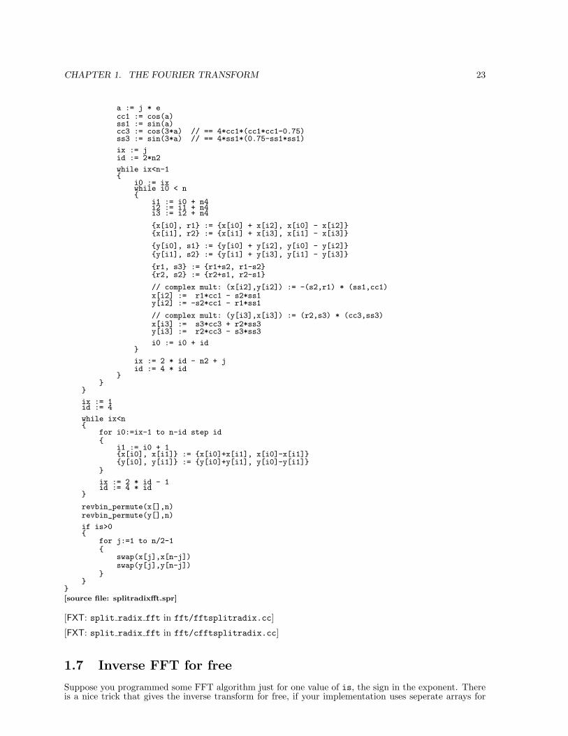
Code 1.10 (split radix DIF FFT) Pseudo code for the split radix DIF algorithm, is must be -1 or+1:
procedure fft_splitradix_dif(x[],y[],ldn,is)
n := 2**ldn
if n<=1 return
n2 := 2*n
for k:=1 to ldn
n2 := n2 / 2n4 := n2 / 4
e := 2 * PI / n2
for j:=0 to n4-1
CHAPTER 1. THE FOURIER TRANSFORM 23
a := j * ecc1 := cos(a)ss1 := sin(a)cc3 := cos(3*a) // == 4*cc1*(cc1*cc1-0.75)ss3 := sin(3*a) // == 4*ss1*(0.75-ss1*ss1)
ix := jid := 2*n2
while ix<n-1
i0 := ixwhile i0 < n
i1 := i0 + n4i2 := i1 + n4i3 := i2 + n4
x[i0], r1 := x[i0] + x[i2], x[i0] - x[i2]x[i1], r2 := x[i1] + x[i3], x[i1] - x[i3]
y[i0], s1 := y[i0] + y[i2], y[i0] - y[i2]y[i1], s2 := y[i1] + y[i3], y[i1] - y[i3]
r1, s3 := r1+s2, r1-s2r2, s2 := r2+s1, r2-s1
// complex mult: (x[i2],y[i2]) := -(s2,r1) * (ss1,cc1)x[i2] := r1*cc1 - s2*ss1y[i2] := -s2*cc1 - r1*ss1
// complex mult: (y[i3],x[i3]) := (r2,s3) * (cc3,ss3)x[i3] := s3*cc3 + r2*ss3y[i3] := r2*cc3 - s3*ss3
i0 := i0 + id
ix := 2 * id - n2 + jid := 4 * id
ix := 1id := 4
while ix<n
for i0:=ix-1 to n-id step id
i1 := i0 + 1x[i0], x[i1] := x[i0]+x[i1], x[i0]-x[i1]y[i0], y[i1] := y[i0]+y[i1], y[i0]-y[i1]
ix := 2 * id - 1id := 4 * id
revbin_permute(x[],n)revbin_permute(y[],n)
if is>0
for j:=1 to n/2-1
swap(x[j],x[n-j])swap(y[j],y[n-j])
[source file: splitradixfft.spr]
[FXT: split radix fft in fft/fftsplitradix.cc]
[FXT: split radix fft in fft/cfftsplitradix.cc]
1.7 Inverse FFT for free
Suppose you programmed some FFT algorithm just for one value of is, the sign in the exponent. Thereis a nice trick that gives the inverse transform for free, if your implementation uses seperate arrays for
CHAPTER 1. THE FOURIER TRANSFORM 24
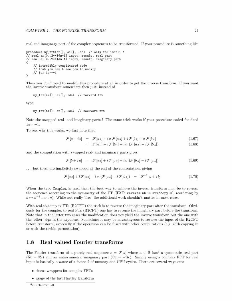
real and imaginary part of the complex sequences to be transformed. If your procedure is something like
procedure my_fft(ar[], ai[], ldn) // only for is==+1 !// real ar[0..2**ldn-1] input, result, real part// real ai[0..2**ldn-1] input, result, imaginary part
// incredibly complicated code// that you can’t see how to modify// for is==-1
Then you don’t need to modify this procedure at all in order to get the inverse transform. If you wantthe inverse transform somewhere then just, instead of
my_fft(ar[], ai[], ldn) // forward fft
type
my_fft(ai[], ar[], ldn) // backward fft
Note the swapped real- and imaginary parts ! The same trick works if your procedure coded for fixedis= −1.
To see, why this works, we first note that
F [a + i b] = F [aS ] + i σF [aA] + iF [bS ] + σF [bA] (1.67)= F [aS ] + iF [bS ] + i σ (F [aA]− iF [bA]) (1.68)
and the computation with swapped real- and imaginary parts gives
F [b + i a] = F [bS ] + iF [aS ] + i σ (F [bA]− iF [aA]) (1.69)
. . . but these are implicitely swapped at the end of the computation, giving
F [aS ] + iF [bS ]− i σ (F [aA]− iF [bA]) = F−1 [a + i b] (1.70)
When the type Complex is used then the best way to achieve the inverse transform may be to reversethe sequence according to the symmetry of the FT ([FXT: reverse nh in aux/copy.h], reordering byk 7→ k−1 mod n). While not really ‘free’ the additional work shouldn’t matter in most cases.
With real-to-complex FTs (R2CFT) the trick is to reverse the imaginary part after the transform. Obvi-ously for the complex-to-real FTs (R2CFT) one has to reverse the imaginary part before the transform.Note that in the latter two cases the modification does not yield the inverse transform but the one withthe ‘other’ sign in the exponent. Sometimes it may be advantageous to reverse the input of the R2CFTbefore transform, especially if the operation can be fused with other computations (e.g. with copying inor with the revbin-permutation).
1.8 Real valued Fourier transforms
The Fourier transform of a purely real sequence c = F [a] where a ∈ R has6 a symmetric real part(<c = <c) and an antisymmetric imaginary part (=c = −=c). Simply using a complex FFT for realinput is basically a waste of a factor 2 of memory and CPU cycles. There are several ways out:
• sincos wrappers for complex FFTs
• usage of the fast Hartley transform6cf. relation 1.20
CHAPTER 1. THE FOURIER TRANSFORM 25
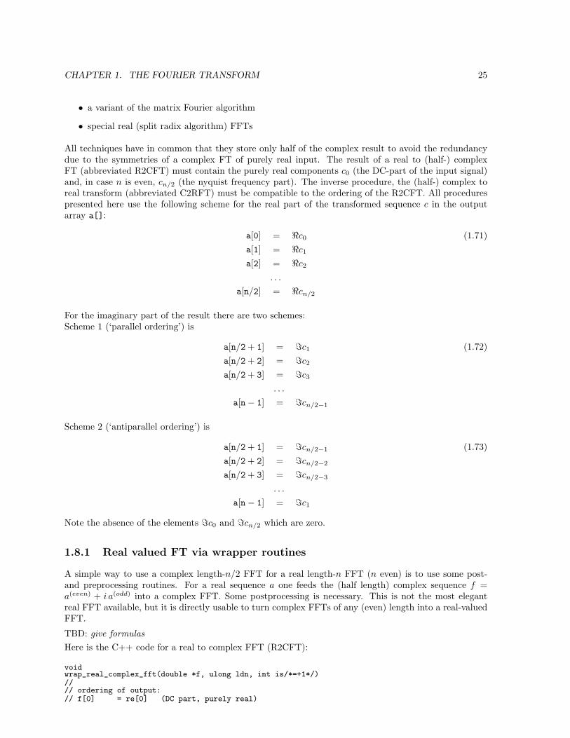
• a variant of the matrix Fourier algorithm
• special real (split radix algorithm) FFTs
All techniques have in common that they store only half of the complex result to avoid the redundancydue to the symmetries of a complex FT of purely real input. The result of a real to (half-) complexFT (abbreviated R2CFT) must contain the purely real components c0 (the DC-part of the input signal)and, in case n is even, cn/2 (the nyquist frequency part). The inverse procedure, the (half-) complex toreal transform (abbreviated C2RFT) must be compatible to the ordering of the R2CFT. All procedurespresented here use the following scheme for the real part of the transformed sequence c in the outputarray a[]:
a[0] = <c0 (1.71)a[1] = <c1
a[2] = <c2
. . .
a[n/2] = <cn/2
For the imaginary part of the result there are two schemes:Scheme 1 (‘parallel ordering’) is
a[n/2 + 1] = =c1 (1.72)a[n/2 + 2] = =c2
a[n/2 + 3] = =c3
. . .
a[n− 1] = =cn/2−1
Scheme 2 (‘antiparallel ordering’) is
a[n/2 + 1] = =cn/2−1 (1.73)a[n/2 + 2] = =cn/2−2
a[n/2 + 3] = =cn/2−3
. . .
a[n− 1] = =c1
Note the absence of the elements =c0 and =cn/2 which are zero.
1.8.1 Real valued FT via wrapper routines
A simple way to use a complex length-n/2 FFT for a real length-n FFT (n even) is to use some post-and preprocessing routines. For a real sequence a one feeds the (half length) complex sequence f =a(even) + i a(odd) into a complex FFT. Some postprocessing is necessary. This is not the most elegantreal FFT available, but it is directly usable to turn complex FFTs of any (even) length into a real-valuedFFT.
TBD: give formulasHere is the C++ code for a real to complex FFT (R2CFT):
voidwrap_real_complex_fft(double *f, ulong ldn, int is/*=+1*/)//// ordering of output:// f[0] = re[0] (DC part, purely real)
CHAPTER 1. THE FOURIER TRANSFORM 26
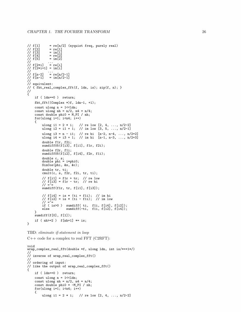
// f[1] = re[n/2] (nyquist freq, purely real)// f[2] = re[1]// f[3] = im[1]// f[4] = re[2]// f[5] = im[2]// ...// f[2*i] = re[i]// f[2*i+1] = im[i]// ...// f[n-2] = re[n/2-1]// f[n-1] = im[n/2-1]//// equivalent:// fht_real_complex_fft(f, ldn, is); zip(f, n); //
if ( ldn==0 ) return;
fht_fft((Complex *)f, ldn-1, +1);
const ulong n = 1<<ldn;const ulong nh = n/2, n4 = n/4;const double phi0 = M_PI / nh;for(ulong i=1; i<n4; i++)
ulong i1 = 2 * i; // re low [2, 4, ..., n/2-2]ulong i2 = i1 + 1; // im low [3, 5, ..., n/2-1]
ulong i3 = n - i1; // re hi [n-2, n-4, ..., n/2+2]ulong i4 = i3 + 1; // im hi [n-1, n-3, ..., n/2+3]
double f1r, f2i;sumdiff05(f[i3], f[i1], f1r, f2i);
double f2r, f1i;sumdiff05(f[i2], f[i4], f2r, f1i);
double c, s;double phi = i*phi0;SinCos(phi, &s, &c);
double tr, ti;cmult(c, s, f2r, f2i, tr, ti);
// f[i1] = f1r + tr; // re low// f[i3] = f1r - tr; // re hi// =^=sumdiff(f1r, tr, f[i1], f[i3]);
// f[i4] = is * (ti + f1i); // im hi// f[i2] = is * (ti - f1i); // im low// =^=if ( is>0 ) sumdiff( ti, f1i, f[i4], f[i2]);else sumdiff(-ti, f1i, f[i2], f[i4]);
sumdiff(f[0], f[1]);
if ( nh>=2 ) f[nh+1] *= is;
TBD: eliminate if-statement in loopC++ code for a complex to real FFT (C2RFT):
voidwrap_complex_real_fft(double *f, ulong ldn, int is/*=+1*/)//// inverse of wrap_real_complex_fft()//// ordering of input:// like the output of wrap_real_complex_fft()
if ( ldn==0 ) return;
const ulong n = 1<<ldn;const ulong nh = n/2, n4 = n/4;const double phi0 = -M_PI / nh;for(ulong i=1; i<n4; i++)
ulong i1 = 2 * i; // re low [2, 4, ..., n/2-2]
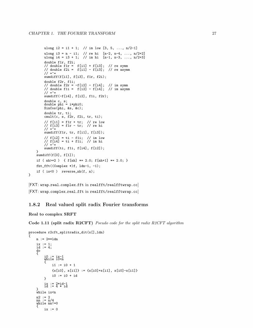
CHAPTER 1. THE FOURIER TRANSFORM 27
ulong i2 = i1 + 1; // im low [3, 5, ..., n/2-1]
ulong i3 = n - i1; // re hi [n-2, n-4, ..., n/2+2]ulong i4 = i3 + 1; // im hi [n-1, n-3, ..., n/2+3]
double f1r, f2i;// double f1r = f[i1] + f[i3]; // re symm// double f2i = f[i1] - f[i3]; // re asymm// =^=sumdiff(f[i1], f[i3], f1r, f2i);
double f2r, f1i;// double f2r = -f[i2] - f[i4]; // im symm// double f1i = f[i2] - f[i4]; // im asymm// =^=sumdiff(-f[i4], f[i2], f1i, f2r);
double c, s;double phi = i*phi0;SinCos(phi, &s, &c);
double tr, ti;cmult(c, s, f2r, f2i, tr, ti);
// f[i1] = f1r + tr; // re low// f[i3] = f1r - tr; // re hi// =^=sumdiff(f1r, tr, f[i1], f[i3]);
// f[i2] = ti - f1i; // im low// f[i4] = ti + f1i; // im hi// =^=sumdiff(ti, f1i, f[i4], f[i2]);
sumdiff(f[0], f[1]);
if ( nh>=2 ) f[nh] *= 2.0; f[nh+1] *= 2.0;
fht_fft((Complex *)f, ldn-1, -1);
if ( is<0 ) reverse_nh(f, n);
[FXT: wrap real complex fft in realfft/realfftwrap.cc]
[FXT: wrap complex real fft in realfft/realfftwrap.cc]
1.8.2 Real valued split radix Fourier transforms
Real to complex SRFT
Code 1.11 (split radix R2CFT) Pseudo code for the split radix R2CFT algorithm
procedure r2cft_splitradix_dit(x[],ldn)
n := 2**ldn
ix := 1;id := 4;do
i0 := ix-1while i0<n
i1 := i0 + 1
x[i0], x[i1] := x[i0]+x[i1], x[i0]-x[i1]
i0 := i0 + id
ix := 2*id-1id := 4 * id
while ix<n
n2 := 2nn := n/4while nn!=0
ix := 0
CHAPTER 1. THE FOURIER TRANSFORM 28
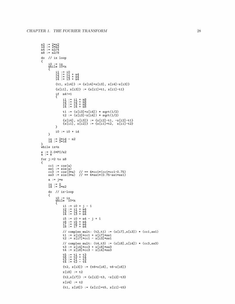
n2 := 2*n2id := 2*n2n4 := n2/4n8 := n2/8
do // ix loop
i0 := ixwhile i0<n
i1 := i0i2 := i1 + n4i3 := i2 + n4i4 := i3 + n4
t1, x[i4] := x[i4]+x[i3], x[i4]-x[i3]
x[i1], x[i3] := x[i1]+t1, x[i1]-t1
if n4!=1
i1 := i1 + n8i2 := i2 + n8i3 := i3 + n8i4 := i4 + n8
t1 := (x[i3]+x[i4]) * sqrt(1/2)t2 := (x[i3]-x[i4]) * sqrt(1/2)
x[i4], x[i3] := x[i2]-t1, -x[i2]-t1x[i1], x[i2] := x[i1]+t2, x[i1]-t2
i0 := i0 + id
ix := 2*id - n2id := 2*id
while ix<n
e := 2.0*PI/n2a := e
for j:=2 to n8
cc1 := cos(a)ss1 := sin(a)cc3 := cos(3*a) // == 4*cc1*(cc1*cc1-0.75)ss3 := sin(3*a) // == 4*ss1*(0.75-ss1*ss1)
a := j*e
ix := 0id := 2*n2
do // ix-loop
i0 := ixwhile i0<n
i1 := i0 + j - 1i2 := i1 + n4i3 := i2 + n4i4 := i3 + n4
i5 := i0 + n4 - j + 1i6 := i5 + n4i7 := i6 + n4i8 := i7 + n4
// complex mult: (t2,t1) := (x[i7],x[i3]) * (cc1,ss1)t1 := x[i3]*cc1 + x[i7]*ss1t2 := x[i7]*cc1 - x[i3]*ss1
// complex mult: (t4,t3) := (x[i8],x[i4]) * (cc3,ss3)t3 := x[i4]*cc3 + x[i8]*ss3t4 := x[i8]*cc3 - x[i4]*ss3
t5 := t1 + t3t6 := t2 + t4t3 := t1 - t3t4 := t2 - t4
t2, x[i3] := t6+x[i6], t6-x[i6]
x[i8] := t2
t2,x[i7] := x[i2]-t3, -x[i2]-t3
x[i4] := t2
t1, x[i6] := x[i1]+t5, x[i1]-t5
CHAPTER 1. THE FOURIER TRANSFORM 29
x[i1] := t1
t1, x[i5] := x[i5]+t4, x[i5]-t4
x[i2] := t1
i0 := i0 + id
ix := 2*id - n2id := 2*id
while ix<n
nn := nn/2
[source file: r2csplitradixfft.spr]
[FXT: split radix real complex fft in realfft/realfftsplitradix.cc]
Complex to real SRFT
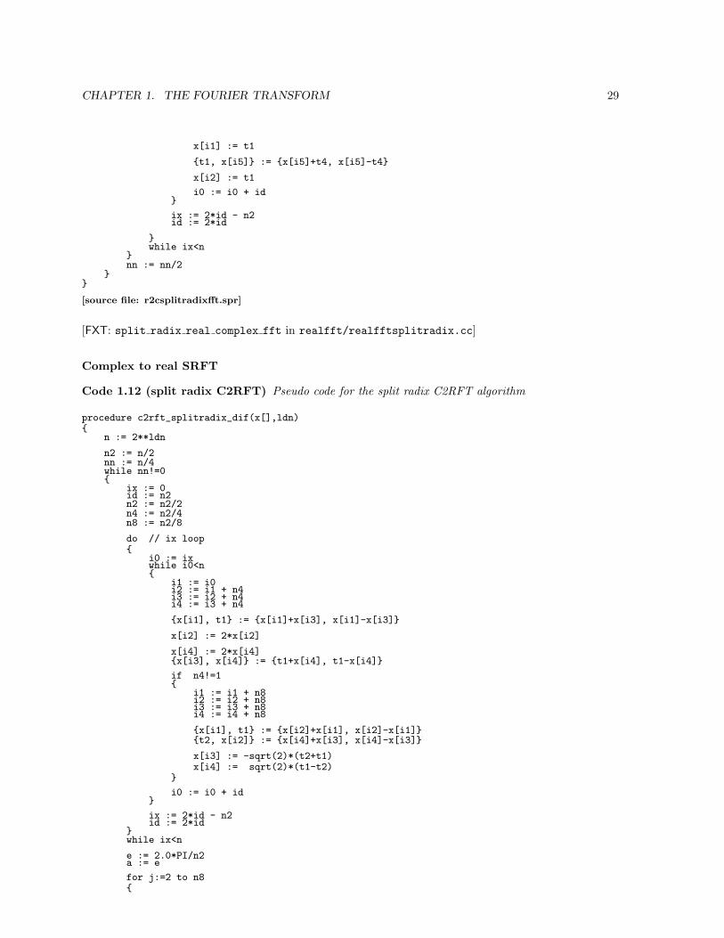
Code 1.12 (split radix C2RFT) Pseudo code for the split radix C2RFT algorithm
procedure c2rft_splitradix_dif(x[],ldn)
n := 2**ldn
n2 := n/2nn := n/4while nn!=0
ix := 0id := n2n2 := n2/2n4 := n2/4n8 := n2/8
do // ix loop
i0 := ixwhile i0<n
i1 := i0i2 := i1 + n4i3 := i2 + n4i4 := i3 + n4
x[i1], t1 := x[i1]+x[i3], x[i1]-x[i3]
x[i2] := 2*x[i2]
x[i4] := 2*x[i4]x[i3], x[i4] := t1+x[i4], t1-x[i4]
if n4!=1
i1 := i1 + n8i2 := i2 + n8i3 := i3 + n8i4 := i4 + n8
x[i1], t1 := x[i2]+x[i1], x[i2]-x[i1]t2, x[i2] := x[i4]+x[i3], x[i4]-x[i3]
x[i3] := -sqrt(2)*(t2+t1)x[i4] := sqrt(2)*(t1-t2)
i0 := i0 + id
ix := 2*id - n2id := 2*id
while ix<n
e := 2.0*PI/n2a := e
for j:=2 to n8
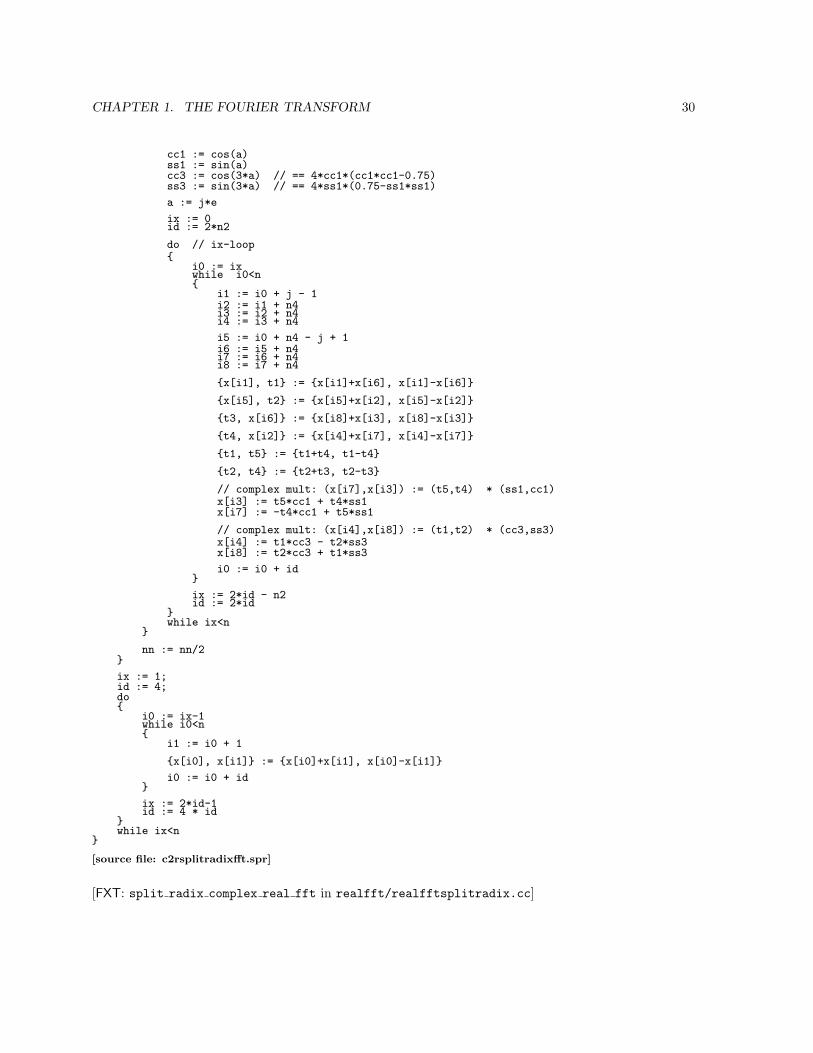
CHAPTER 1. THE FOURIER TRANSFORM 30
cc1 := cos(a)ss1 := sin(a)cc3 := cos(3*a) // == 4*cc1*(cc1*cc1-0.75)ss3 := sin(3*a) // == 4*ss1*(0.75-ss1*ss1)
a := j*e
ix := 0id := 2*n2
do // ix-loop
i0 := ixwhile i0<n
i1 := i0 + j - 1i2 := i1 + n4i3 := i2 + n4i4 := i3 + n4
i5 := i0 + n4 - j + 1i6 := i5 + n4i7 := i6 + n4i8 := i7 + n4
x[i1], t1 := x[i1]+x[i6], x[i1]-x[i6]
x[i5], t2 := x[i5]+x[i2], x[i5]-x[i2]
t3, x[i6] := x[i8]+x[i3], x[i8]-x[i3]
t4, x[i2] := x[i4]+x[i7], x[i4]-x[i7]
t1, t5 := t1+t4, t1-t4
t2, t4 := t2+t3, t2-t3
// complex mult: (x[i7],x[i3]) := (t5,t4) * (ss1,cc1)x[i3] := t5*cc1 + t4*ss1x[i7] := -t4*cc1 + t5*ss1
// complex mult: (x[i4],x[i8]) := (t1,t2) * (cc3,ss3)x[i4] := t1*cc3 - t2*ss3x[i8] := t2*cc3 + t1*ss3
i0 := i0 + id
ix := 2*id - n2id := 2*id
while ix<n
nn := nn/2
ix := 1;id := 4;do
i0 := ix-1while i0<n
i1 := i0 + 1
x[i0], x[i1] := x[i0]+x[i1], x[i0]-x[i1]
i0 := i0 + id
ix := 2*id-1id := 4 * id
while ix<n
[source file: c2rsplitradixfft.spr]
[FXT: split radix complex real fft in realfft/realfftsplitradix.cc]
CHAPTER 1. THE FOURIER TRANSFORM 31
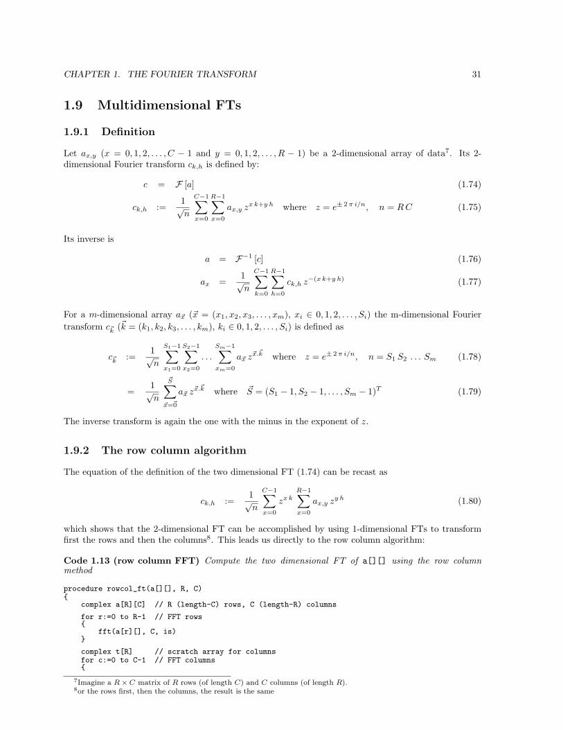
1.9 Multidimensional FTs
1.9.1 Definition
Let ax,y (x = 0, 1, 2, . . . , C − 1 and y = 0, 1, 2, . . . , R − 1) be a 2-dimensional array of data7. Its 2-dimensional Fourier transform ck,h is defined by:
c = F [a] (1.74)
ck,h :=1√n
C−1∑x=0
R−1∑x=0
ax,y zx k+y h where z = e± 2 π i/n, n = R C (1.75)
Its inverse is
a = F−1 [c] (1.76)
ax =1√n
C−1∑
k=0
R−1∑
h=0
ck,h z−(x k+y h) (1.77)
For a m-dimensional array a~x (~x = (x1, x2, x3, . . . , xm), xi ∈ 0, 1, 2, . . . , Si) the m-dimensional Fouriertransform c~k (~k = (k1, k2, k3, . . . , km), ki ∈ 0, 1, 2, . . . , Si) is defined as
c~k :=1√n
S1−1∑x1=0
S2−1∑x2=0
. . .
Sm−1∑xm=0
a~x z~x.~k where z = e± 2 π i/n, n = S1 S2 . . . Sm (1.78)
=1√n
~S∑
~x=~0
a~x z~x.~k where ~S = (S1 − 1, S2 − 1, . . . , Sm − 1)T (1.79)
The inverse transform is again the one with the minus in the exponent of z.
1.9.2 The row column algorithm
The equation of the definition of the two dimensional FT (1.74) can be recast as
ck,h :=1√n
C−1∑x=0
zx kR−1∑x=0
ax,y zy h (1.80)
which shows that the 2-dimensional FT can be accomplished by using 1-dimensional FTs to transformfirst the rows and then the columns8. This leads us directly to the row column algorithm:
Code 1.13 (row column FFT) Compute the two dimensional FT of a[][] using the row columnmethod
procedure rowcol_ft(a[][], R, C)
complex a[R][C] // R (length-C) rows, C (length-R) columns
for r:=0 to R-1 // FFT rows
fft(a[r][], C, is)
complex t[R] // scratch array for columnsfor c:=0 to C-1 // FFT columns
7Imagine a R× C matrix of R rows (of length C) and C columns (of length R).8or the rows first, then the columns, the result is the same
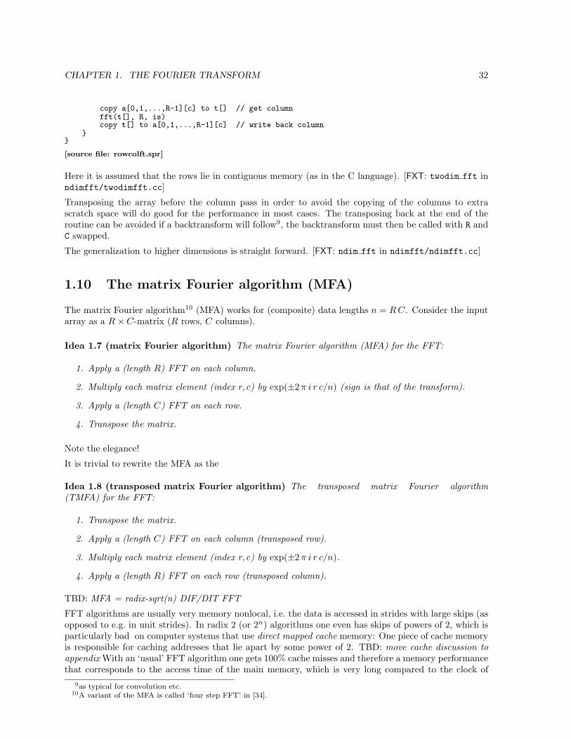
CHAPTER 1. THE FOURIER TRANSFORM 32
copy a[0,1,...,R-1][c] to t[] // get columnfft(t[], R, is)copy t[] to a[0,1,...,R-1][c] // write back column
[source file: rowcolft.spr]
Here it is assumed that the rows lie in contiguous memory (as in the C language). [FXT: twodim fft inndimfft/twodimfft.cc]
Transposing the array before the column pass in order to avoid the copying of the columns to extrascratch space will do good for the performance in most cases. The transposing back at the end of theroutine can be avoided if a backtransform will follow9, the backtransform must then be called with R andC swapped.
The generalization to higher dimensions is straight forward. [FXT: ndim fft in ndimfft/ndimfft.cc]
1.10 The matrix Fourier algorithm (MFA)
The matrix Fourier algorithm10 (MFA) works for (composite) data lengths n = R C. Consider the inputarray as a R× C-matrix (R rows, C columns).
Idea 1.7 (matrix Fourier algorithm) The matrix Fourier algorithm (MFA) for the FFT:
1. Apply a (length R) FFT on each column.
2. Multiply each matrix element (index r, c) by exp(±2 π i r c/n) (sign is that of the transform).
3. Apply a (length C) FFT on each row.
4. Transpose the matrix.
Note the elegance!
It is trivial to rewrite the MFA as the
Idea 1.8 (transposed matrix Fourier algorithm) The transposed matrix Fourier algorithm(TMFA) for the FFT:
1. Transpose the matrix.
2. Apply a (length C) FFT on each column (transposed row).
3. Multiply each matrix element (index r, c) by exp(±2 π i r c/n).
4. Apply a (length R) FFT on each row (transposed column).
TBD: MFA = radix-sqrt(n) DIF/DIT FFT
FFT algorithms are usually very memory nonlocal, i.e. the data is accessed in strides with large skips (asopposed to e.g. in unit strides). In radix 2 (or 2n) algorithms one even has skips of powers of 2, which isparticularly bad on computer systems that use direct mapped cache memory: One piece of cache memoryis responsible for caching addresses that lie apart by some power of 2. TBD: move cache discussion toappendix With an ‘usual’ FFT algorithm one gets 100% cache misses and therefore a memory performancethat corresponds to the access time of the main memory, which is very long compared to the clock of
9as typical for convolution etc.10A variant of the MFA is called ‘four step FFT’ in [34].
CHAPTER 1. THE FOURIER TRANSFORM 33
modern CPUs. The matrix Fourier algorithm has a much better memory locality (cf. [34]), because thework is done in the short FFTs over the rows and columns.
For the reason given above the computation of the column FFTs should not be done in place. One caninsert additional transpositions in the algorithm to have the columns lie in contiguous memory when theyare worked upon. The easy way is to use an additional scratch space for the column FFTs, then only thecopying from and to the scratch space will be slow. If one interleaves the copying back with the exp()-multiplications (to let the CPU do some work during the wait for the memory access) the performanceshould be ok. Moreover, one can insert small offsets (a few unused memory words) at the end of each rowin order to avoid the cache miss problem almost completely. Then one should also program a procedurethat does a ‘mass production’ variant of the column FFTs, i.e. for doing computation for all rows at once.
It is usually a good idea to use factors of the data length n that are close to√
n. Of course one canapply the same algorithm for the row (or column) FFTs again: It can be a good idea to split n into 3factors (as close to n1/3 as possible) if a length-n1/3 FFT fits completely into the second level cache (oreven the first level cache) of the computer used. Especially for systems where CPU clock is much higherthan memory clock the performance may increase drastically, a performance factor of two (even whencompared to else very good optimized FFTs) can be observed.
1.11 Automatic generation of FFT codes
FFT generators are programs that output FFT routines, usually for fixed (short) lengths. In fact thethoughts here a not at all restricted to FFT codes, but FFTs and several unrollable routines like matrixmultiplications and convolutions are prime candidates for automated generation. Writing such a programis easy: Take an existing FFT and change all computations into print statements that emit the necesarycode. The process, however, is less than delightful and errorprone.
It would be much better to have another program that takes the existing FFT code as input and emit thecode for the generator. Let us call this a metagenerator. Implementing such a metagenerator of courseis highly nontrivial. It actually is equivalent to writing an interpreter for the language used plus thenecessary data flow analysis11.
A practical compromise is to write a program that, while theoretically not even close to a metagenerator,creates output that, after a little hand editing, is a usable generator code. The implemented perl script[FXT: file scripts/metagen.pl] is capable of converting a (highly pedantically formatted) piece of C++code12 into something that is reasonable close to a generator.
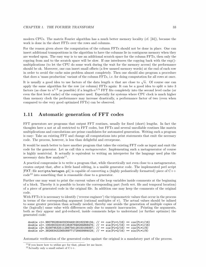
Further one may want to print the current values of the loop variables inside comments at the beginningof a block. Thereby it is possible to locate the corresponding part (both wrt. file and temporal location)of a piece of generated code in the original file. In addition one may keep the comments of the originalcode.With FFTs it is necessary to identify (‘reverse engineer’) the trigonometric values that occur in the processin terms of the corresponding argument (rational multiples of π). The actual values should be inlinedto some greater precision than actually needed, thereby one avoids the generation of multiple copies ofthe (logically) same value with differences only due to numeric inaccuracies. Printing the arguments,both as they appear and gcd-reduced, inside comments helps to understand (or further optimize) thegenerated code:
double c1=.980785280403230449126182236134; // == cos(Pi*1/16) == cos(Pi*1/16)double s1=.195090322016128267848284868476; // == sin(Pi*1/16) == sin(Pi*1/16)double c2=.923879532511286756128183189397; // == cos(Pi*2/16) == cos(Pi*1/8)double s2=.382683432365089771728459984029; // == sin(Pi*2/16) == sin(Pi*1/8)
Automatic verification of the generated codes against the original is a mandatory part of the process.11If you know how to utilize gcc for that, please let me know.12Actually only a small subset of C++.
CHAPTER 1. THE FOURIER TRANSFORM 34
A level of abstraction for the array indices is of great use: When the print statements in the generatoremit some function of the index instead of its plain value it is easy to generate modified versions of thecode for permuted input. That is, instead of
cout<<"sumdiff(f0, f2, g["<<k0<<"], g["<<k2<<"]);" <<endl;cout<<"sumdiff(f1, f3, g["<<k1<<"], g["<<k3<<"]);" <<endl;
use
cout<<"sumdiff(f0, f2, "<<idxf(g,k0)<<", "<<idxf(g,k2)<<");" <<endl;cout<<"sumdiff(f1, f3, "<<idxf(g,k1)<<", "<<idxf(g,k3)<<");" <<endl;
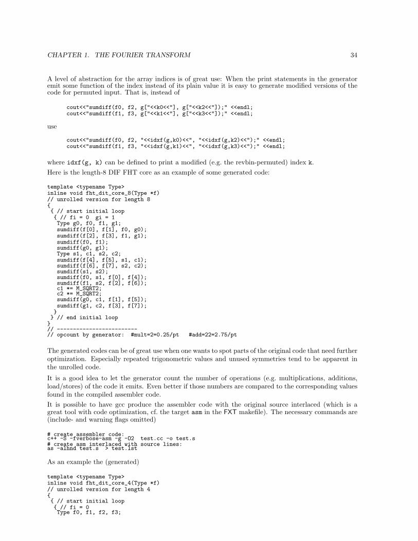
where idxf(g, k) can be defined to print a modified (e.g. the revbin-permuted) index k.Here is the length-8 DIF FHT core as an example of some generated code:
template <typename Type>inline void fht_dit_core_8(Type *f)// unrolled version for length 8 // start initial loop // fi = 0 gi = 1Type g0, f0, f1, g1;sumdiff(f[0], f[1], f0, g0);sumdiff(f[2], f[3], f1, g1);sumdiff(f0, f1);sumdiff(g0, g1);Type s1, c1, s2, c2;sumdiff(f[4], f[5], s1, c1);sumdiff(f[6], f[7], s2, c2);sumdiff(s1, s2);sumdiff(f0, s1, f[0], f[4]);sumdiff(f1, s2, f[2], f[6]);c1 *= M_SQRT2;c2 *= M_SQRT2;sumdiff(g0, c1, f[1], f[5]);sumdiff(g1, c2, f[3], f[7]);
// end initial loop
// -------------------------// opcount by generator: #mult=2=0.25/pt #add=22=2.75/pt
The generated codes can be of great use when one wants to spot parts of the original code that need furtheroptimization. Especially repeated trigonometric values and unused symmetries tend to be apparent inthe unrolled code.
It is a good idea to let the generator count the number of operations (e.g. multiplications, additions,load/stores) of the code it emits. Even better if those numbers are compared to the corresponding valuesfound in the compiled assembler code.It is possible to have gcc produce the assembler code with the original source interlaced (which is agreat tool with code optimization, cf. the target asm in the FXT makefile). The necessary commands are(include- and warning flags omitted)
# create assembler code:c++ -S -fverbose-asm -g -O2 test.cc -o test.s# create asm interlaced with source lines:as -alhnd test.s > test.lst
As an example the (generated)
template <typename Type>inline void fht_dit_core_4(Type *f)// unrolled version for length 4 // start initial loop // fi = 0Type f0, f1, f2, f3;
CHAPTER 1. THE FOURIER TRANSFORM 35
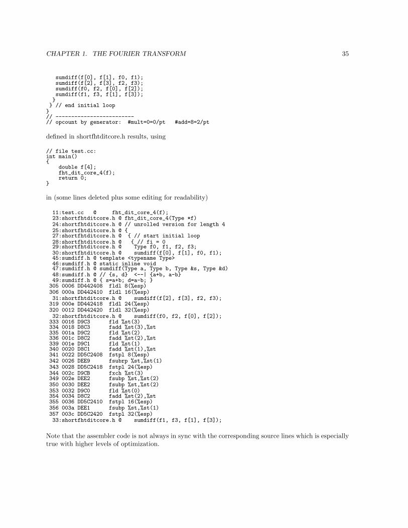
sumdiff(f[0], f[1], f0, f1);sumdiff(f[2], f[3], f2, f3);sumdiff(f0, f2, f[0], f[2]);sumdiff(f1, f3, f[1], f[3]);
// end initial loop
// -------------------------// opcount by generator: #mult=0=0/pt #add=8=2/pt
defined in shortfhtditcore.h results, using
// file test.cc:int main()
double f[4];fht_dit_core_4(f);return 0;
in (some lines deleted plus some editing for readability)
11:test.cc @ fht_dit_core_4(f);23:shortfhtditcore.h @ fht_dit_core_4(Type *f)24:shortfhtditcore.h @ // unrolled version for length 425:shortfhtditcore.h @ 27:shortfhtditcore.h @ // start initial loop28:shortfhtditcore.h @ // fi = 029:shortfhtditcore.h @ Type f0, f1, f2, f3;30:shortfhtditcore.h @ sumdiff(f[0], f[1], f0, f1);45:sumdiff.h @ template <typename Type>46:sumdiff.h @ static inline void47:sumdiff.h @ sumdiff(Type a, Type b, Type &s, Type &d)48:sumdiff.h @ // s, d <--| a+b, a-b49:sumdiff.h @ s=a+b; d=a-b; 305 0006 DD442408 fldl 8(%esp)306 000a DD442410 fldl 16(%esp)31:shortfhtditcore.h @ sumdiff(f[2], f[3], f2, f3);319 000e DD442418 fldl 24(%esp)320 0012 DD442420 fldl 32(%esp)32:shortfhtditcore.h @ sumdiff(f0, f2, f[0], f[2]);333 0016 D9C3 fld %st(3)334 0018 D8C3 fadd %st(3),%st335 001a D9C2 fld %st(2)336 001c D8C2 fadd %st(2),%st339 001e D9C1 fld %st(1)340 0020 D8C1 fadd %st(1),%st341 0022 DD5C2408 fstpl 8(%esp)342 0026 DEE9 fsubrp %st,%st(1)343 0028 DD5C2418 fstpl 24(%esp)344 002c D9CB fxch %st(3)349 002e DEE2 fsubp %st,%st(2)350 0030 DEE2 fsubp %st,%st(2)353 0032 D9C0 fld %st(0)354 0034 D8C2 fadd %st(2),%st355 0036 DD5C2410 fstpl 16(%esp)356 003a DEE1 fsubp %st,%st(1)357 003c DD5C2420 fstpl 32(%esp)33:shortfhtditcore.h @ sumdiff(f1, f3, f[1], f[3]);
Note that the assembler code is not always in sync with the corresponding source lines which is especiallytrue with higher levels of optimization.
Chapter 2
Convolutions
2.1 Definition and computation via FFT
The cyclic convolution of two sequences a and b is defined as the sequence h with elements hτ as follows:
h = a ~ b (2.1)
hτ :=∑
x+y≡τ(mod n)
ax by
The last equation may be rewritten as
hτ :=n−1∑x=0
ax bτ−x (2.2)
where negative indices τ − x must be understood as n + τ − x, it’s a cyclic convolution.
Code 2.1 (cyclic convolution by definition) Compute the cyclic convolution of a[] with b[] usingthe definition, result is returned in c[]
procedure convolution(a[],b[],c[],n)
for tau:=0 to n-1
s := 0for x:=0 to n-1
tx := tau - x
if tx<0 then tx := tx + n
s := s + a[x] * b[tx]c[tau] := s
This procedure uses (for length-n sequences a, b) proportional n2 operations, therefore it is slow for largevalues of n. The Fourier transform provides us with a more efficient way to compute convolutions thatonly uses proportional n log(n) operations. First we have to establish the convolution property of theFourier transform:
F [a ~ b] = F [a]F [b] (2.3)
i.e. convolution in original space is ordinary (elementwise) multiplication in Fourier space.
36
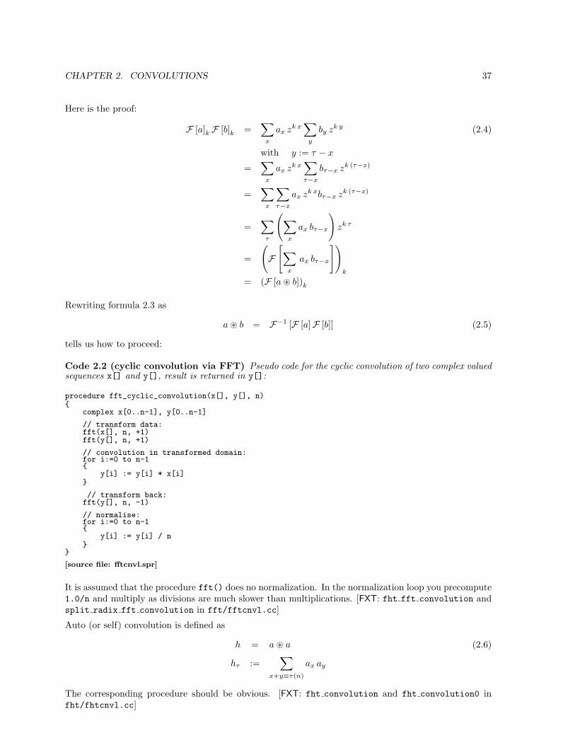
CHAPTER 2. CONVOLUTIONS 37
Here is the proof:
F [a]k F [b]k =∑
x
ax zk x∑
y
by zk y (2.4)
with y := τ − x
=∑
x
ax zk x∑τ−x
bτ−x zk (τ−x)
=∑
x
∑τ−x
ax zk xbτ−x zk (τ−x)
=∑
τ
(∑x
ax bτ−x
)zk τ
=
(F
[∑x
ax bτ−x
])
k
= (F [a ~ b])k
Rewriting formula 2.3 as
a ~ b = F−1 [F [a]F [b]] (2.5)
tells us how to proceed:
Code 2.2 (cyclic convolution via FFT) Pseudo code for the cyclic convolution of two complex valuedsequences x[] and y[], result is returned in y[]:
procedure fft_cyclic_convolution(x[], y[], n)
complex x[0..n-1], y[0..n-1]
// transform data:fft(x[], n, +1)fft(y[], n, +1)
// convolution in transformed domain:for i:=0 to n-1
y[i] := y[i] * x[i]
// transform back:fft(y[], n, -1)
// normalise:for i:=0 to n-1
y[i] := y[i] / n
[source file: fftcnvl.spr]
It is assumed that the procedure fft() does no normalization. In the normalization loop you precompute1.0/n and multiply as divisions are much slower than multiplications. [FXT: fht fft convolution andsplit radix fft convolution in fft/fftcnvl.cc]
Auto (or self) convolution is defined as
h = a ~ a (2.6)
hτ :=∑
x+y≡τ(n)
ax ay
The corresponding procedure should be obvious. [FXT: fht convolution and fht convolution0 infht/fhtcnvl.cc]
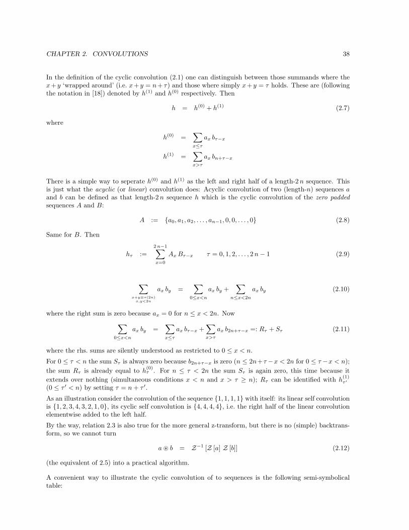
CHAPTER 2. CONVOLUTIONS 38
In the definition of the cyclic convolution (2.1) one can distinguish between those summands where thex+ y ‘wrapped around’ (i.e. x+ y = n+ τ) and those where simply x+ y = τ holds. These are (followingthe notation in [18]) denoted by h(1) and h(0) respectively. Then
h = h(0) + h(1) (2.7)
where
h(0) =∑
x≤τ
ax bτ−x
h(1) =∑x>τ
ax bn+τ−x
There is a simple way to seperate h(0) and h(1) as the left and right half of a length-2n sequence. Thisis just what the acyclic (or linear) convolution does: Acyclic convolution of two (length-n) sequences aand b can be defined as that length-2 n sequence h which is the cyclic convolution of the zero paddedsequences A and B:
A := a0, a1, a2, . . . , an−1, 0, 0, . . . , 0 (2.8)
Same for B. Then
hτ :=2 n−1∑x=0
Ax Bτ−x τ = 0, 1, 2, . . . , 2 n− 1 (2.9)
∑x+y≡τ(2n)
x,y<2n
ax by =∑
0≤x<n
ax by +∑
n≤x<2n
ax by (2.10)
where the right sum is zero because ax = 0 for n ≤ x < 2n. Now∑
0≤x<n
ax by =∑
x≤τ
ax bτ−x +∑x>τ
ax b2n+τ−x =: Rτ + Sτ (2.11)
where the rhs. sums are silently understood as restricted to 0 ≤ x < n.
For 0 ≤ τ < n the sum Sτ is always zero because b2n+τ−x is zero (n ≤ 2n+τ −x < 2n for 0 ≤ τ −x < n);the sum Rτ is already equal to h
(0)τ . For n ≤ τ < 2n the sum Sτ is again zero, this time because it
extends over nothing (simultaneous conditions x < n and x > τ ≥ n); Rτ can be identified with h(1)τ ′
(0 ≤ τ ′ < n) by setting τ = n + τ ′.
As an illustration consider the convolution of the sequence 1, 1, 1, 1 with itself: its linear self convolutionis 1, 2, 3, 4, 3, 2, 1, 0, its cyclic self convolution is 4, 4, 4, 4, i.e. the right half of the linear convolutionelementwise added to the left half.
By the way, relation 2.3 is also true for the more general z-transform, but there is no (simple) backtrans-form, so we cannot turn
a ~ b = Z−1 [Z [a] Z [b]] (2.12)
(the equivalent of 2.5) into a practical algorithm.
A convenient way to illustrate the cyclic convolution of to sequences is the following semi-symbolicaltable:

CHAPTER 2. CONVOLUTIONS 39
+-- 0 1 2 3 4 5 6 7 8 9 10 11 12 13 14 15|0: 0 1 2 3 4 5 6 7 8 9 10 11 12 13 14 151: 1 2 3 4 5 6 7 8 9 10 11 12 13 14 15 02: 2 3 4 5 6 7 8 9 10 11 12 13 14 15 0 13: 3 4 5 6 7 8 9 10 11 12 13 14 15 0 1 24: 4 5 6 7 8 9 10 11 12 13 14 15 0 1 2 35: 5 6 7 8 9 10 11 12 13 14 15 0 1 2 3 46: 6 7 8 9 10 11 12 13 14 15 0 1 2 3 4 57: 7 8 9 10 11 12 13 14 15 0 1 2 3 4 5 68: 8 9 10 11 12 13 14 15 0 1 2 3 4 5 6 79: 9 10 11 12 13 14 15 0 1 2 3 4 5 6 7 8
10: 10 11 12 13 14 15 0 1 2 3 4 5 6 7 8 911: 11 12 13 14 15 0 1 2 3 4 5 6 7 8 9 1012: 12 13 14 15 0 1 2 3 4 5 6 7 8 9 10 1113: 13 14 15 0 1 2 3 4 5 6 7 8 9 10 11 1214: 14 15 0 1 2 3 4 5 6 7 8 9 10 11 12 1315: 15 0 1 2 3 4 5 6 7 8 9 10 11 12 13 14
The entries denote where in the convolution the products of the input elements can be found:
+-- 0 1 2 3 ...|0: 0 1 2 3 ...1: 1 2 3 <--= h[3] contains a[1]*b[2]2: ...
Acyclic convolution (where there are 32 buckets 0..31) looks like:
+-- 0 1 2 3 4 5 6 7 8 9 10 11 12 13 14 15|0: 0 1 2 3 4 5 6 7 8 9 10 11 12 13 14 151: 1 2 3 4 5 6 7 8 9 10 11 12 13 14 15 162: 2 3 4 5 6 7 8 9 10 11 12 13 14 15 16 173: 3 4 5 6 7 8 9 10 11 12 13 14 15 16 17 184: 4 5 6 7 8 9 10 11 12 13 14 15 16 17 18 195: 5 6 7 8 9 10 11 12 13 14 15 16 17 18 19 206: 6 7 8 9 10 11 12 13 14 15 16 17 18 19 20 217: 7 8 9 10 11 12 13 14 15 16 17 18 19 20 21 228: 8 9 10 11 12 13 14 15 16 17 18 19 20 21 22 239: 9 10 11 12 13 14 15 16 17 18 19 20 21 22 23 24
10: 10 11 12 13 14 15 16 17 18 19 20 21 22 23 24 2511: 11 12 13 14 15 16 17 18 19 20 21 22 23 24 25 2612: 12 13 14 15 16 17 18 19 20 21 22 23 24 25 26 2713: 13 14 15 16 17 18 19 20 21 22 23 24 25 26 27 2814: 14 15 16 17 18 19 20 21 22 23 24 25 26 27 28 2915: 15 16 17 18 19 20 21 22 23 24 25 26 27 28 29 30
. . . the elements in the lower right triangle do not ‘wrap around’ anymore, they go to extra buckets.Note that bucket 31 does not appear, it is always zero.
The equivalent table for a (cyclic) correlation is
+-- 0 1 2 3 4 5 6 7 8 9 10 11 12 13 14 15|
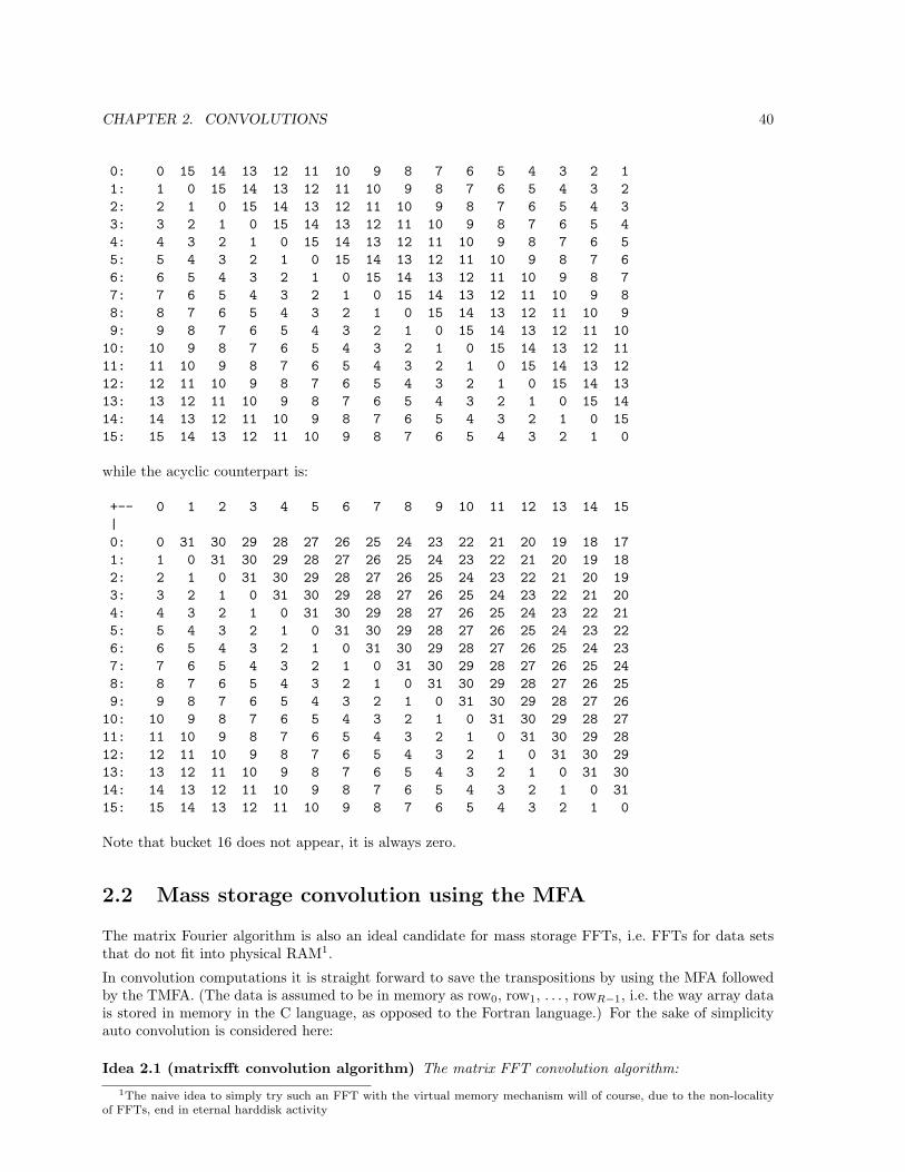
CHAPTER 2. CONVOLUTIONS 40
0: 0 15 14 13 12 11 10 9 8 7 6 5 4 3 2 11: 1 0 15 14 13 12 11 10 9 8 7 6 5 4 3 22: 2 1 0 15 14 13 12 11 10 9 8 7 6 5 4 33: 3 2 1 0 15 14 13 12 11 10 9 8 7 6 5 44: 4 3 2 1 0 15 14 13 12 11 10 9 8 7 6 55: 5 4 3 2 1 0 15 14 13 12 11 10 9 8 7 66: 6 5 4 3 2 1 0 15 14 13 12 11 10 9 8 77: 7 6 5 4 3 2 1 0 15 14 13 12 11 10 9 88: 8 7 6 5 4 3 2 1 0 15 14 13 12 11 10 99: 9 8 7 6 5 4 3 2 1 0 15 14 13 12 11 10
10: 10 9 8 7 6 5 4 3 2 1 0 15 14 13 12 1111: 11 10 9 8 7 6 5 4 3 2 1 0 15 14 13 1212: 12 11 10 9 8 7 6 5 4 3 2 1 0 15 14 1313: 13 12 11 10 9 8 7 6 5 4 3 2 1 0 15 1414: 14 13 12 11 10 9 8 7 6 5 4 3 2 1 0 1515: 15 14 13 12 11 10 9 8 7 6 5 4 3 2 1 0
while the acyclic counterpart is:
+-- 0 1 2 3 4 5 6 7 8 9 10 11 12 13 14 15|0: 0 31 30 29 28 27 26 25 24 23 22 21 20 19 18 171: 1 0 31 30 29 28 27 26 25 24 23 22 21 20 19 182: 2 1 0 31 30 29 28 27 26 25 24 23 22 21 20 193: 3 2 1 0 31 30 29 28 27 26 25 24 23 22 21 204: 4 3 2 1 0 31 30 29 28 27 26 25 24 23 22 215: 5 4 3 2 1 0 31 30 29 28 27 26 25 24 23 226: 6 5 4 3 2 1 0 31 30 29 28 27 26 25 24 237: 7 6 5 4 3 2 1 0 31 30 29 28 27 26 25 248: 8 7 6 5 4 3 2 1 0 31 30 29 28 27 26 259: 9 8 7 6 5 4 3 2 1 0 31 30 29 28 27 26
10: 10 9 8 7 6 5 4 3 2 1 0 31 30 29 28 2711: 11 10 9 8 7 6 5 4 3 2 1 0 31 30 29 2812: 12 11 10 9 8 7 6 5 4 3 2 1 0 31 30 2913: 13 12 11 10 9 8 7 6 5 4 3 2 1 0 31 3014: 14 13 12 11 10 9 8 7 6 5 4 3 2 1 0 3115: 15 14 13 12 11 10 9 8 7 6 5 4 3 2 1 0
Note that bucket 16 does not appear, it is always zero.
2.2 Mass storage convolution using the MFA
The matrix Fourier algorithm is also an ideal candidate for mass storage FFTs, i.e. FFTs for data setsthat do not fit into physical RAM1.
In convolution computations it is straight forward to save the transpositions by using the MFA followedby the TMFA. (The data is assumed to be in memory as row0, row1, . . . , rowR−1, i.e. the way array datais stored in memory in the C language, as opposed to the Fortran language.) For the sake of simplicityauto convolution is considered here:
Idea 2.1 (matrixfft convolution algorithm) The matrix FFT convolution algorithm:1The naive idea to simply try such an FFT with the virtual memory mechanism will of course, due to the non-locality
of FFTs, end in eternal harddisk activity
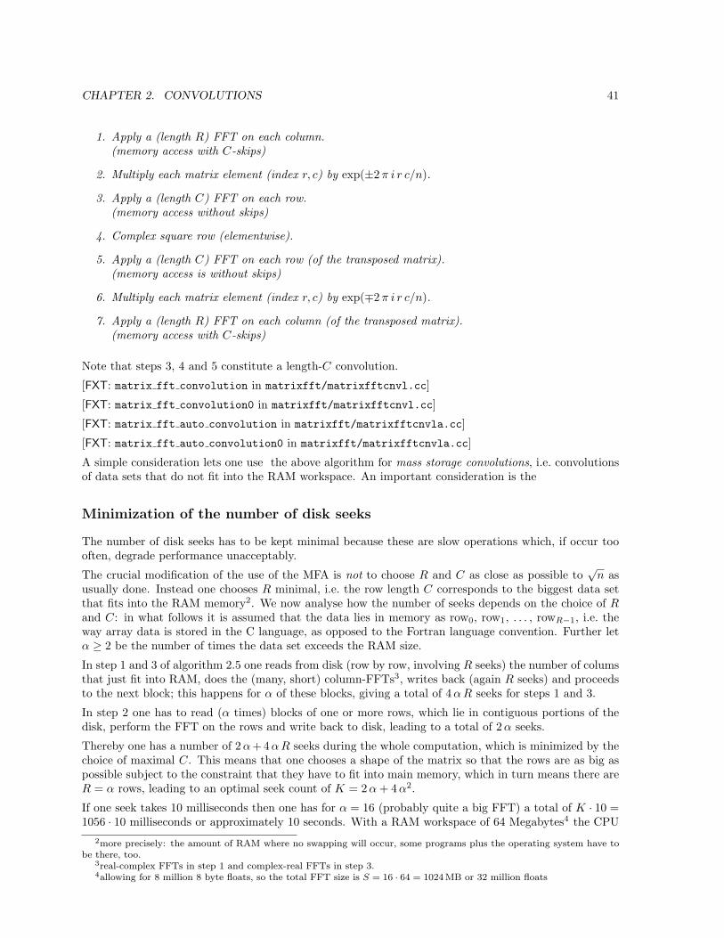
CHAPTER 2. CONVOLUTIONS 41
1. Apply a (length R) FFT on each column.(memory access with C-skips)
2. Multiply each matrix element (index r, c) by exp(±2 π i r c/n).
3. Apply a (length C) FFT on each row.(memory access without skips)
4. Complex square row (elementwise).
5. Apply a (length C) FFT on each row (of the transposed matrix).(memory access is without skips)
6. Multiply each matrix element (index r, c) by exp(∓2 π i r c/n).
7. Apply a (length R) FFT on each column (of the transposed matrix).(memory access with C-skips)
Note that steps 3, 4 and 5 constitute a length-C convolution.
[FXT: matrix fft convolution in matrixfft/matrixfftcnvl.cc]
[FXT: matrix fft convolution0 in matrixfft/matrixfftcnvl.cc]
[FXT: matrix fft auto convolution in matrixfft/matrixfftcnvla.cc]
[FXT: matrix fft auto convolution0 in matrixfft/matrixfftcnvla.cc]
A simple consideration lets one use the above algorithm for mass storage convolutions, i.e. convolutionsof data sets that do not fit into the RAM workspace. An important consideration is the
Minimization of the number of disk seeks
The number of disk seeks has to be kept minimal because these are slow operations which, if occur toooften, degrade performance unacceptably.
The crucial modification of the use of the MFA is not to choose R and C as close as possible to√
n asusually done. Instead one chooses R minimal, i.e. the row length C corresponds to the biggest data setthat fits into the RAM memory2. We now analyse how the number of seeks depends on the choice of Rand C: in what follows it is assumed that the data lies in memory as row0, row1, . . . , rowR−1, i.e. theway array data is stored in the C language, as opposed to the Fortran language convention. Further letα ≥ 2 be the number of times the data set exceeds the RAM size.
In step 1 and 3 of algorithm 2.5 one reads from disk (row by row, involving R seeks) the number of columsthat just fit into RAM, does the (many, short) column-FFTs3, writes back (again R seeks) and proceedsto the next block; this happens for α of these blocks, giving a total of 4 α R seeks for steps 1 and 3.
In step 2 one has to read (α times) blocks of one or more rows, which lie in contiguous portions of thedisk, perform the FFT on the rows and write back to disk, leading to a total of 2α seeks.
Thereby one has a number of 2α+4 α R seeks during the whole computation, which is minimized by thechoice of maximal C. This means that one chooses a shape of the matrix so that the rows are as big aspossible subject to the constraint that they have to fit into main memory, which in turn means there areR = α rows, leading to an optimal seek count of K = 2 α + 4 α2.
If one seek takes 10 milliseconds then one has for α = 16 (probably quite a big FFT) a total of K · 10 =1056 · 10 milliseconds or approximately 10 seconds. With a RAM workspace of 64 Megabytes4 the CPU
2more precisely: the amount of RAM where no swapping will occur, some programs plus the operating system have tobe there, too.
3real-complex FFTs in step 1 and complex-real FFTs in step 3.4allowing for 8 million 8 byte floats, so the total FFT size is S = 16 · 64 = 1024MB or 32 million floats
CHAPTER 2. CONVOLUTIONS 42
time alone might be in the order of several minutes. The overhead for the (linear) read and write wouldbe (throughput of 10MB/sec assumed) 6 · 1024MB/(10MB/sec) ≈ 600sec or approximately 10 minutes.
With a multithreading OS one may want to produce a ‘double buffer’ variant: choose the row length sothat it fits twice into the RAM workspace; then let always one (CPU-intensive) thread do the FFTs inone of the scratch spaces and another (hard disk intensive) thread write back the data from the otherscratch-space and read the next data to be processed. With not too small main memory (and not tooslow hard disk) and some fine tuning this should allow to keep the CPU busy during much of the harddisk operations.
Using a mass storage convolution as described the calculation of the number 999 ≈ 0.4281247 ·10369,693,100
could be done on a 32 bit machine in 1999. The computation used two files of size 2GigaBytes each andtook less than eight hours on a system with a AMD K6/2 CPU at 366MHz with 66MHz memory.Cf. [hfloat: examples/run1-pow999.txt]
2.3 Weighted Fourier transforms
Let us define a new kind of transform by slightly modifying the definition of the FT (cf. formula 1.1):
c = Wv [a] (2.13)
ck :=n−1∑x=0
vx ax zx k vx 6= 0 ∀x
where z := e± 2 π i/n. The sequence c shall be called weighted (discrete) transform of the sequence a withthe weight (sequence) v. Note the vx that entered: the weighted transform with vx = 1√
n∀x is just the
usual Fourier transform. The inverse transform is
a = W−1v [c] (2.14)
ax =1
n vx
n−1∑
k=0
ck z−x k
This can be easily seen:
W−1v [Wv [a]]y =
1n vy
n−1∑
k=0
n−1∑x=0
vx ax zx k z−y k
=1n
n−1∑
k=0
n−1∑x=0
vx1vy
ax zx k z−y k
=1n
n−1∑x=0
vx1vy
ax δx,y n
= ay
(cf. section 1.1). That Wv
[W−1v [a]
]is also identity is apparent from the definitions.
Given an implemented FFT it is trivial to set up a weighted Fourier transform:
Code 2.3 (weighted transform) Pseudo code for the discrete weighted Fourier transform
procedure weighted_ft(a[], v[], n, is)
for x:=0 to n-1
a[x] := a[x] * v[x]
fft(a[],n,is)
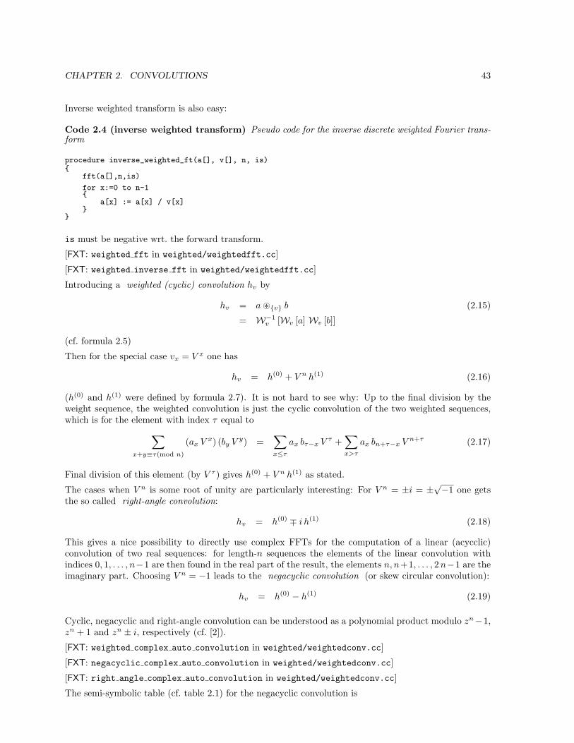
CHAPTER 2. CONVOLUTIONS 43
Inverse weighted transform is also easy:
Code 2.4 (inverse weighted transform) Pseudo code for the inverse discrete weighted Fourier trans-form
procedure inverse_weighted_ft(a[], v[], n, is)
fft(a[],n,is)
for x:=0 to n-1
a[x] := a[x] / v[x]
is must be negative wrt. the forward transform.
[FXT: weighted fft in weighted/weightedfft.cc]
[FXT: weighted inverse fft in weighted/weightedfft.cc]
Introducing a weighted (cyclic) convolution hv by
hv = a ~v b (2.15)
= W−1v [Wv [a] Wv [b]]
(cf. formula 2.5)
Then for the special case vx = V x one has
hv = h(0) + V n h(1) (2.16)
(h(0) and h(1) were defined by formula 2.7). It is not hard to see why: Up to the final division by theweight sequence, the weighted convolution is just the cyclic convolution of the two weighted sequences,which is for the element with index τ equal to
∑
x+y≡τ(mod n)
(ax V x) (by V y) =∑
x≤τ
ax bτ−x V τ +∑x>τ
ax bn+τ−x V n+τ (2.17)
Final division of this element (by V τ ) gives h(0) + V n h(1) as stated.
The cases when V n is some root of unity are particularly interesting: For V n = ±i = ±√−1 one getsthe so called right-angle convolution:
hv = h(0) ∓ i h(1) (2.18)
This gives a nice possibility to directly use complex FFTs for the computation of a linear (acycclic)convolution of two real sequences: for length-n sequences the elements of the linear convolution withindices 0, 1, . . . , n−1 are then found in the real part of the result, the elements n, n+1, . . . , 2 n−1 are theimaginary part. Choosing V n = −1 leads to the negacyclic convolution (or skew circular convolution):
hv = h(0) − h(1) (2.19)
Cyclic, negacyclic and right-angle convolution can be understood as a polynomial product modulo zn−1,zn + 1 and zn ± i, respectively (cf. [2]).
[FXT: weighted complex auto convolution in weighted/weightedconv.cc]
[FXT: negacyclic complex auto convolution in weighted/weightedconv.cc]
[FXT: right angle complex auto convolution in weighted/weightedconv.cc]
The semi-symbolic table (cf. table 2.1) for the negacyclic convolution is
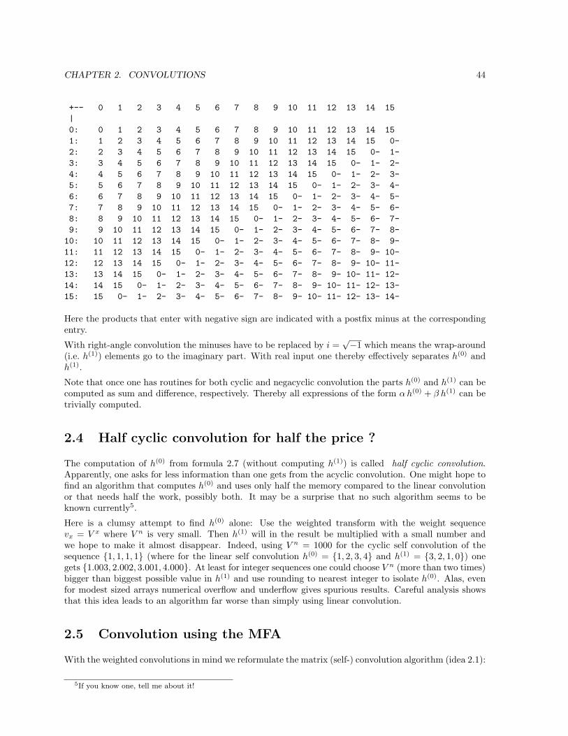
CHAPTER 2. CONVOLUTIONS 44
+-- 0 1 2 3 4 5 6 7 8 9 10 11 12 13 14 15|0: 0 1 2 3 4 5 6 7 8 9 10 11 12 13 14 151: 1 2 3 4 5 6 7 8 9 10 11 12 13 14 15 0-2: 2 3 4 5 6 7 8 9 10 11 12 13 14 15 0- 1-3: 3 4 5 6 7 8 9 10 11 12 13 14 15 0- 1- 2-4: 4 5 6 7 8 9 10 11 12 13 14 15 0- 1- 2- 3-5: 5 6 7 8 9 10 11 12 13 14 15 0- 1- 2- 3- 4-6: 6 7 8 9 10 11 12 13 14 15 0- 1- 2- 3- 4- 5-7: 7 8 9 10 11 12 13 14 15 0- 1- 2- 3- 4- 5- 6-8: 8 9 10 11 12 13 14 15 0- 1- 2- 3- 4- 5- 6- 7-9: 9 10 11 12 13 14 15 0- 1- 2- 3- 4- 5- 6- 7- 8-
10: 10 11 12 13 14 15 0- 1- 2- 3- 4- 5- 6- 7- 8- 9-11: 11 12 13 14 15 0- 1- 2- 3- 4- 5- 6- 7- 8- 9- 10-12: 12 13 14 15 0- 1- 2- 3- 4- 5- 6- 7- 8- 9- 10- 11-13: 13 14 15 0- 1- 2- 3- 4- 5- 6- 7- 8- 9- 10- 11- 12-14: 14 15 0- 1- 2- 3- 4- 5- 6- 7- 8- 9- 10- 11- 12- 13-15: 15 0- 1- 2- 3- 4- 5- 6- 7- 8- 9- 10- 11- 12- 13- 14-
Here the products that enter with negative sign are indicated with a postfix minus at the correspondingentry.
With right-angle convolution the minuses have to be replaced by i =√−1 which means the wrap-around
(i.e. h(1)) elements go to the imaginary part. With real input one thereby effectively separates h(0) andh(1).
Note that once one has routines for both cyclic and negacyclic convolution the parts h(0) and h(1) can becomputed as sum and difference, respectively. Thereby all expressions of the form α h(0) + β h(1) can betrivially computed.
2.4 Half cyclic convolution for half the price ?
The computation of h(0) from formula 2.7 (without computing h(1)) is called half cyclic convolution.Apparently, one asks for less information than one gets from the acyclic convolution. One might hope tofind an algorithm that computes h(0) and uses only half the memory compared to the linear convolutionor that needs half the work, possibly both. It may be a surprise that no such algorithm seems to beknown currently5.
Here is a clumsy attempt to find h(0) alone: Use the weighted transform with the weight sequencevx = V x where V n is very small. Then h(1) will in the result be multiplied with a small number andwe hope to make it almost disappear. Indeed, using V n = 1000 for the cyclic self convolution of thesequence 1, 1, 1, 1 (where for the linear self convolution h(0) = 1, 2, 3, 4 and h(1) = 3, 2, 1, 0) onegets 1.003, 2.002, 3.001, 4.000. At least for integer sequences one could choose V n (more than two times)bigger than biggest possible value in h(1) and use rounding to nearest integer to isolate h(0). Alas, evenfor modest sized arrays numerical overflow and underflow gives spurious results. Careful analysis showsthat this idea leads to an algorithm far worse than simply using linear convolution.
2.5 Convolution using the MFA
With the weighted convolutions in mind we reformulate the matrix (self-) convolution algorithm (idea 2.1):
5If you know one, tell me about it!
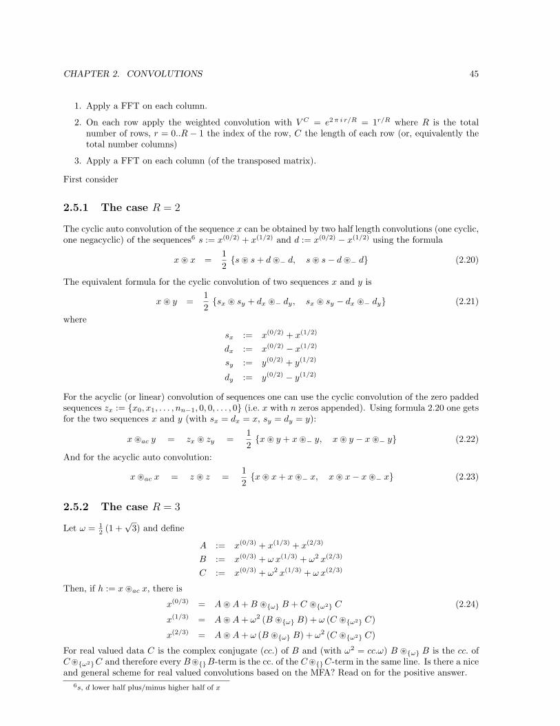
CHAPTER 2. CONVOLUTIONS 45
1. Apply a FFT on each column.
2. On each row apply the weighted convolution with V C = e2 π i r/R = 1r/R where R is the totalnumber of rows, r = 0..R − 1 the index of the row, C the length of each row (or, equivalently thetotal number columns)
3. Apply a FFT on each column (of the transposed matrix).
First consider
2.5.1 The case R = 2
The cyclic auto convolution of the sequence x can be obtained by two half length convolutions (one cyclic,one negacyclic) of the sequences6 s := x(0/2) + x(1/2) and d := x(0/2) − x(1/2) using the formula
x ~ x =12s ~ s + d ~− d, s ~ s− d ~− d (2.20)
The equivalent formula for the cyclic convolution of two sequences x and y is
x ~ y =12sx ~ sy + dx ~− dy, sx ~ sy − dx ~− dy (2.21)
where
sx := x(0/2) + x(1/2)
dx := x(0/2) − x(1/2)
sy := y(0/2) + y(1/2)
dy := y(0/2) − y(1/2)
For the acyclic (or linear) convolution of sequences one can use the cyclic convolution of the zero paddedsequences zx := x0, x1, . . . , nn−1, 0, 0, . . . , 0 (i.e. x with n zeros appended). Using formula 2.20 one getsfor the two sequences x and y (with sx = dx = x, sy = dy = y):
x ~ac y = zx ~ zy =12x ~ y + x ~− y, x ~ y − x ~− y (2.22)
And for the acyclic auto convolution:
x ~ac x = z ~ z =12x ~ x + x ~− x, x ~ x− x ~− x (2.23)
2.5.2 The case R = 3
Let ω = 12 (1 +
√3) and define
A := x(0/3) + x(1/3) + x(2/3)
B := x(0/3) + ω x(1/3) + ω2 x(2/3)
C := x(0/3) + ω2 x(1/3) + ω x(2/3)
Then, if h := x ~ac x, there is
x(0/3) = A ~ A + B ~ω B + C ~ω2 C (2.24)
x(1/3) = A ~ A + ω2 (B ~ω B) + ω (C ~ω2 C)
x(2/3) = A ~ A + ω (B ~ω B) + ω2 (C ~ω2 C)
For real valued data C is the complex conjugate (cc.) of B and (with ω2 = cc.ω) B ~ω B is the cc. ofC~ω2C and therefore every B~B-term is the cc. of the C~C-term in the same line. Is there a niceand general scheme for real valued convolutions based on the MFA? Read on for the positive answer.
6s, d lower half plus/minus higher half of x

CHAPTER 2. CONVOLUTIONS 46
2.6 Convolution of real valued data using the MFA
For row 0 (which is real after the column FFTs) one needs to compute the (usual) cyclic convolution; forrow R/2 (also real after the column FFTs) a negacyclic convolution is needed7, the code for that task isgiven on page 62.
All other weighted convolutions involve complex computations, but it is easy to see how to reduce thework by 50 percent: As the result must be real the data in row number R − r must, because of thesymmetries of the real and imaginary part of the (inverse) Fourier transform of real data, be the complexconjugate of the data in row r. Therefore one can use real FFTs (R2CFTs) for all column-transforms forstep 1 and half-complex to real FFTs (C2RFTs) for step 3.
Let the computational cost of a cyclic (real) convolution be q, then
For R even one must perform 1 cyclic (row 0), 1 negacyclic (row R/2) and R/2− 2 complex (weighted)convolutions (rows 1, 2, . . . , R/2− 1)
For R odd one must perform 1 cyclic (row 0) and (R − 1)/2 complex (weighted) convolutions (rows1, 2, . . . , (R− 1)/2)
Now assume, slightly simplifying, that the cyclic and the negacyclic real convolution involve the samenumber of computations and that the cost of a weighted complex convolution is twice as high. Then inboth cases above the total work is exactly half of that for the complex case, which is about what onewould expect from a real world real valued convolution algorithm.
For acyclic convolution one may want to use the right angle convolution (and complex FFTs in the columnpasses).
2.7 Convolution without transposition using the MFA
Section 8.4 explained the connection between revbin-permutation and transposition. Equipped with thatknowledge an algorithm for convolution using the MFA that uses revbin_permute instead of transposeis almost straight forward:
rows=8 columns=4
input data (symbolic format: R00C):
0: 0 1 2 3
1: 1000 1001 1002 1003
2: 2000 2001 2002 2003
3: 3000 3001 3002 3003
4: 4000 4001 4002 4003
5: 5000 5001 5002 5003
6: 6000 6001 6002 6003
7: 7000 7001 7002 7003
FULL REVBIN_PERMUTE for transposition:
0: 0 4000 2000 6000 1000 5000 3000 7000
1: 2 4002 2002 6002 1002 5002 3002 7002
2: 1 4001 2001 6001 1001 5001 3001 7001
3: 3 4003 2003 6003 1003 5003 3003 7003
DIT FFTs on revbin_permuted rows (in revbin_permuted sequence), i.e. unrevbin_permute rows:
(apply weight after each FFT)
0: 0 1000 2000 3000 4000 5000 6000 7000
1: 2 1002 2002 3002 4002 5002 6002 7002
2: 1 1001 2001 3001 4001 5001 6001 7001
7For R odd there is no such row and no negacyclic convolution is needed.
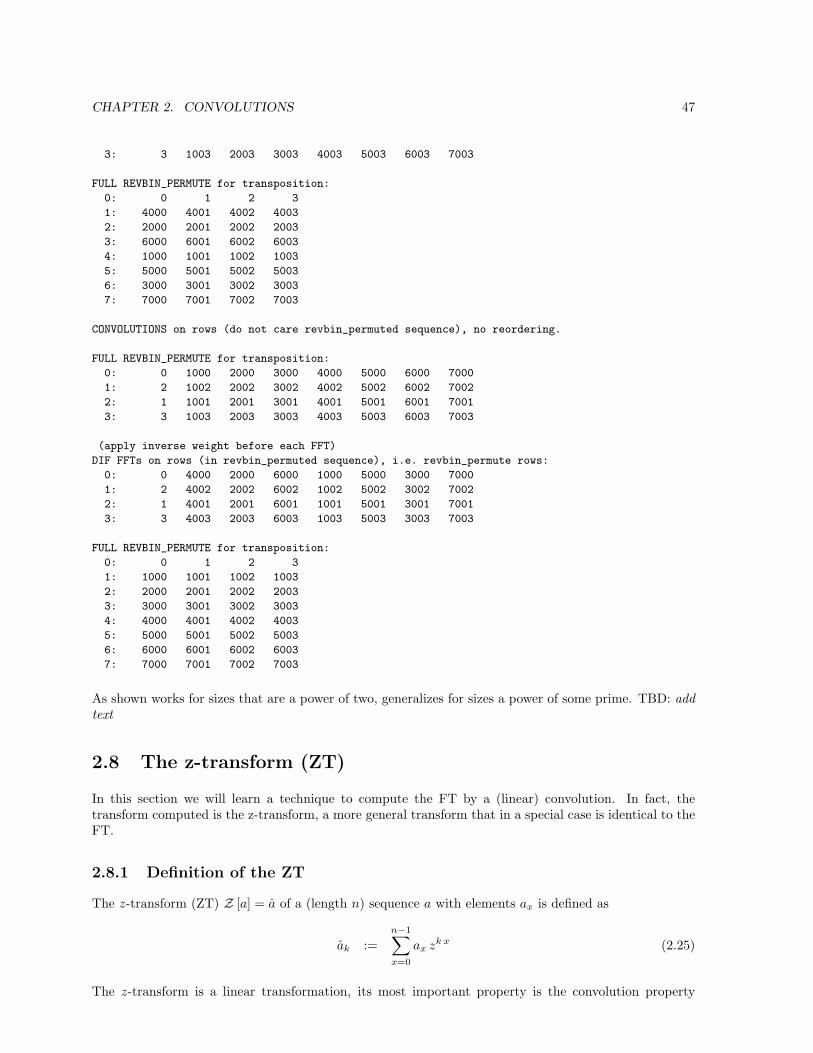
CHAPTER 2. CONVOLUTIONS 47
3: 3 1003 2003 3003 4003 5003 6003 7003
FULL REVBIN_PERMUTE for transposition:
0: 0 1 2 3
1: 4000 4001 4002 4003
2: 2000 2001 2002 2003
3: 6000 6001 6002 6003
4: 1000 1001 1002 1003
5: 5000 5001 5002 5003
6: 3000 3001 3002 3003
7: 7000 7001 7002 7003
CONVOLUTIONS on rows (do not care revbin_permuted sequence), no reordering.
FULL REVBIN_PERMUTE for transposition:
0: 0 1000 2000 3000 4000 5000 6000 7000
1: 2 1002 2002 3002 4002 5002 6002 7002
2: 1 1001 2001 3001 4001 5001 6001 7001
3: 3 1003 2003 3003 4003 5003 6003 7003
(apply inverse weight before each FFT)
DIF FFTs on rows (in revbin_permuted sequence), i.e. revbin_permute rows:
0: 0 4000 2000 6000 1000 5000 3000 7000
1: 2 4002 2002 6002 1002 5002 3002 7002
2: 1 4001 2001 6001 1001 5001 3001 7001
3: 3 4003 2003 6003 1003 5003 3003 7003
FULL REVBIN_PERMUTE for transposition:
0: 0 1 2 3
1: 1000 1001 1002 1003
2: 2000 2001 2002 2003
3: 3000 3001 3002 3003
4: 4000 4001 4002 4003
5: 5000 5001 5002 5003
6: 6000 6001 6002 6003
7: 7000 7001 7002 7003
As shown works for sizes that are a power of two, generalizes for sizes a power of some prime. TBD: addtext
2.8 The z-transform (ZT)
In this section we will learn a technique to compute the FT by a (linear) convolution. In fact, thetransform computed is the z-transform, a more general transform that in a special case is identical to theFT.
2.8.1 Definition of the ZT
The z-transform (ZT) Z [a] = a of a (length n) sequence a with elements ax is defined as
ak :=n−1∑x=0
ax zk x (2.25)
The z-transform is a linear transformation, its most important property is the convolution property

CHAPTER 2. CONVOLUTIONS 48
(formula 2.3): Convolution in original space corresponds to ordinary (elementwise) multiplication inz-space. (See [10] and [11].)
Note that the special case z = e±2 π i/n is the discrete Fourier transform.
2.8.2 Computation of the ZT via convolution
In the definition of the (discrete) z-transform we rewrite8 the product x k as
x k =12
(x2 + k2 − (k − x)2
)(2.26)
fk =n−1∑x=0
fx zx k = zk2/2n−1∑x=0
(fx zx2/2
)z−(k−x)2/2 (2.27)
This leads to the following
Idea 2.2 (chirp z-transform) Algorithm for the chirp z-transform:
1. Multiply f elementwise with zx2/2.
2. Convolve (acyclically) the resulting sequence with the sequence z−x2/2, zero padding of the sequencesis required here.
3. Multiply elementwise with the sequence zk2/2.
The above algorithm constitutes a ‘fast’ (∼ n log(n)) algorithm for the ZT because fast convolution ispossible via FFT.
2.8.3 Arbitrary length FFT by ZT
We first note that the length n of the input sequence a for the fast z-transform is not limited to highlycomposite values (especially n prime is allowed): For values of n where a FFT is not feasible pad thesequence with zeros up to a length L with L >= 2 n and a length L FFT becomes feasible (e.g. L is apower of 2).
Second remember that the FT is the special case z = e±2 π i/n of the ZT: With the chirp ZT algorithmone also has an (arbitrary length) FFT algorithm
The transform takes a few times more than an optimal transform (by direct FFT) would take. The worstcase (if only FFTs for n a power of 2 are available) is n = 2p + 1: One must perform 3 FFTs of length2p+2 ≈ 4 n for the computation of the convolution. So the total work amounts to about 12 times thework a FFT of length n = 2p would cost. It is of course possible to lower this ‘worst case factor’ to 6 byusing highly composite L slightly greater than 2n.
[FXT: fft arblen in chirp/fftarblen.cc]
TBD: show shortcuts for n even/odd
2.8.4 Fractional Fourier transform by ZT
The z-transform with z = eα 2 π i/n and α 6= 1 is called the fractional Fourier transform (FRFT). Uses ofthe FRFT are e.g. the computation of the DFT for data sets that have only few nonzero elements and thedetection of frequencies that are not integer multiples of the lowest frequency of the DFT. A thoroughdiscussion can be found in [35].
[FXT: fft fract in chirp/fftfract.cc]8cf. [2]
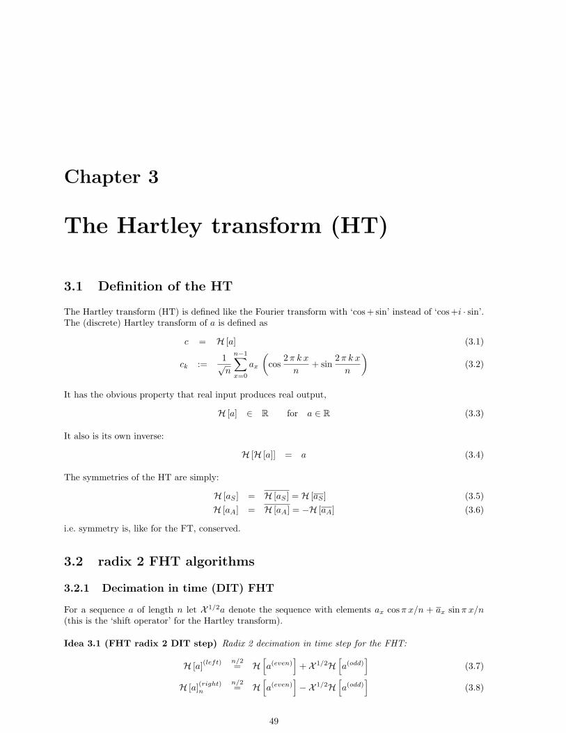
Chapter 3
The Hartley transform (HT)
3.1 Definition of the HT
The Hartley transform (HT) is defined like the Fourier transform with ‘cos + sin’ instead of ‘cos+i · sin’.The (discrete) Hartley transform of a is defined as
c = H [a] (3.1)
ck :=1√n
n−1∑x=0
ax
(cos
2 π k x
n+ sin
2 π k x
n
)(3.2)
It has the obvious property that real input produces real output,
H [a] ∈ R for a ∈ R (3.3)
It also is its own inverse:
H [H [a]] = a (3.4)
The symmetries of the HT are simply:
H [aS ] = H [aS ] = H [aS ] (3.5)H [aA] = H [aA] = −H [aA] (3.6)
i.e. symmetry is, like for the FT, conserved.
3.2 radix 2 FHT algorithms
3.2.1 Decimation in time (DIT) FHT
For a sequence a of length n let X 1/2a denote the sequence with elements ax cos π x/n + ax sinπ x/n(this is the ‘shift operator’ for the Hartley transform).
Idea 3.1 (FHT radix 2 DIT step) Radix 2 decimation in time step for the FHT:
H [a](left) n/2= H
[a(even)
]+ X 1/2H
[a(odd)
](3.7)
H [a](right)n
n/2= H
[a(even)
]−X 1/2H
[a(odd)
](3.8)
49

CHAPTER 3. THE HARTLEY TRANSFORM (HT) 50
Code 3.1 (recursive radix 2 DIT FHT) Pseudo code for a recursive procedure of the (radix 2) DITFHT algorithm:
procedure rec_fht_dit2(a[], n, x[])// real a[0..n-1] input// real x[0..n-1] result
real b[0..n/2-1], c[0..n/2-1] // workspacereal s[0..n/2-1], t[0..n/2-1] // workspace
if n == 1 then
x[0] := a[0]return
nh := n/2;
for k:=0 to nh-1
s[k] := a[2*k] // even indexed elementst[k] := a[2*k+1] // odd indexed elements
rec_fht_dit2(s[], nh, b[])rec_fht_dit2(t[], nh, c[])
hartley_shift(c[], nh, 1/2)
for k:=0 to nh-1
x[k] := b[k] + c[k];x[k+nh] := b[k] - c[k];
[source file: recfhtdit2.spr]
[FXT: recursive dit2 fht in slow/recfht2.cc]
The procedure hartley_shift replaces element ck of the input sequence c by ck cos(π k/n) +cn−k sin(π k/n). Here is the pseudo code:
Code 3.2 (Hartley shift) procedure hartley_shift_05(c[], n)// real c[0..n-1] input, result
nh := n/2j := n-1for k:=1 to nh-1
c := cos( PI*k/n )s := sin( PI*k/n )
c[k], c[j] := c[k]*c+c[j]*s, c[k]*s-c[j]*c
j := j-1
[source file: hartleyshift.spr]
[FXT: hartley shift 05 in fht/hartleyshift.cc]
Code 3.3 (radix 2 DIT FHT, localized) Pseudo code for a non-recursive procedure of the (radix 2)DIT FHT algorithm:
procedure fht_dit2(a[], ldn)// real a[0..n-1] input,result
n := 2**ldn // length of a[] is a power of 2
revbin_permute(a[], n)
for ldm:=1 to ldn
m := 2**ldmmh := m/2m4 := m/4
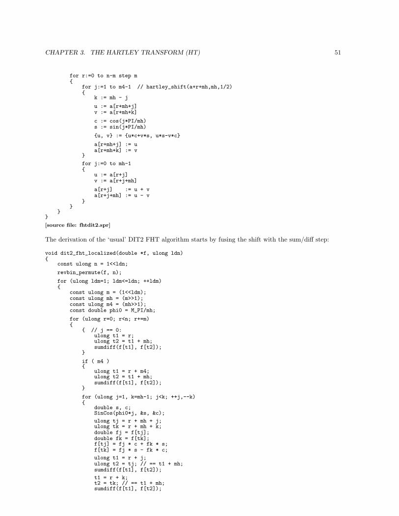
CHAPTER 3. THE HARTLEY TRANSFORM (HT) 51
for r:=0 to n-m step m
for j:=1 to m4-1 // hartley_shift(a+r+mh,mh,1/2)
k := mh - j
u := a[r+mh+j]v := a[r+mh+k]
c := cos(j*PI/mh)s := sin(j*PI/mh)
u, v := u*c+v*s, u*s-v*c
a[r+mh+j] := ua[r+mh+k] := v
for j:=0 to mh-1
u := a[r+j]v := a[r+j+mh]
a[r+j] := u + va[r+j+mh] := u - v
[source file: fhtdit2.spr]
The derivation of the ‘usual’ DIT2 FHT algorithm starts by fusing the shift with the sum/diff step:
void dit2_fht_localized(double *f, ulong ldn)
const ulong n = 1<<ldn;
revbin_permute(f, n);
for (ulong ldm=1; ldm<=ldn; ++ldm)
const ulong m = (1<<ldm);const ulong mh = (m>>1);const ulong m4 = (mh>>1);const double phi0 = M_PI/mh;
for (ulong r=0; r<n; r+=m)
// j == 0:ulong t1 = r;ulong t2 = t1 + mh;sumdiff(f[t1], f[t2]);
if ( m4 )
ulong t1 = r + m4;ulong t2 = t1 + mh;sumdiff(f[t1], f[t2]);
for (ulong j=1, k=mh-1; j<k; ++j,--k)
double s, c;SinCos(phi0*j, &s, &c);
ulong tj = r + mh + j;ulong tk = r + mh + k;double fj = f[tj];double fk = f[tk];f[tj] = fj * c + fk * s;f[tk] = fj * s - fk * c;
ulong t1 = r + j;ulong t2 = tj; // == t1 + mh;sumdiff(f[t1], f[t2]);
t1 = r + k;t2 = tk; // == t1 + mh;sumdiff(f[t1], f[t2]);

CHAPTER 3. THE HARTLEY TRANSFORM (HT) 52
[FXT: dit2 fht localized in fht/fhtdit2.cc] Swapping the innermost loops then yields (considerationsas for DIT FFT, page 13, hold)
void dit2_fht(double *f, ulong ldn)// decimation in time radix 2 fht
const ulong n = 1<<ldn;
revbin_permute(f, n);
for (ulong ldm=1; ldm<=ldn; ++ldm)
const ulong m = (1<<ldm);const ulong mh = (m>>1);const ulong m4 = (mh>>1);const double phi0 = M_PI/mh;
for (ulong r=0; r<n; r+=m)
// j == 0:ulong t1 = r;ulong t2 = t1 + mh;sumdiff(f[t1], f[t2]);
if ( m4 )
ulong t1 = r + m4;ulong t2 = t1 + mh;sumdiff(f[t1], f[t2]);
for (ulong j=1, k=mh-1; j<k; ++j,--k)
double s, c;SinCos(phi0*j, &s, &c);
for (ulong r=0; r<n; r+=m)
ulong tj = r + mh + j;ulong tk = r + mh + k;double fj = f[tj];double fk = f[tk];f[tj] = fj * c + fk * s;f[tk] = fj * s - fk * c;
ulong t1 = r + j;ulong t2 = tj; // == t1 + mh;sumdiff(f[t1], f[t2]);
t1 = r + k;t2 = tk; // == t1 + mh;sumdiff(f[t1], f[t2]);
[FXT: dit2 fht in fht/fhtdit2.cc]
3.2.2 Decimation in frequency (DIF) FHT
Idea 3.2 (FHT radix 2 DIF step) Radix 2 decimation in frequency step for the FHT:
H [a](even) n/2= H
[a(left) + a(right)
](3.9)
H [a](odd) n/2= H
[X 1/2
(a(left) − a(right)
)](3.10)
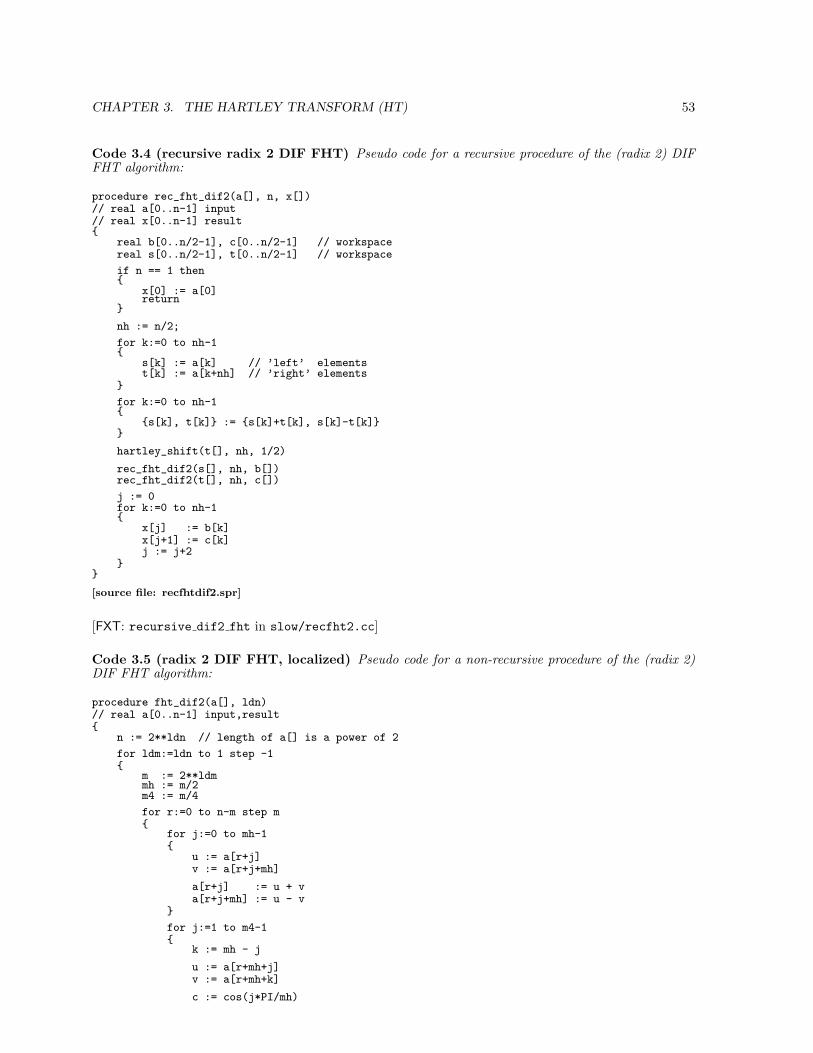
CHAPTER 3. THE HARTLEY TRANSFORM (HT) 53
Code 3.4 (recursive radix 2 DIF FHT) Pseudo code for a recursive procedure of the (radix 2) DIFFHT algorithm:
procedure rec_fht_dif2(a[], n, x[])// real a[0..n-1] input// real x[0..n-1] result
real b[0..n/2-1], c[0..n/2-1] // workspacereal s[0..n/2-1], t[0..n/2-1] // workspace
if n == 1 then
x[0] := a[0]return
nh := n/2;
for k:=0 to nh-1
s[k] := a[k] // ’left’ elementst[k] := a[k+nh] // ’right’ elements
for k:=0 to nh-1
s[k], t[k] := s[k]+t[k], s[k]-t[k]
hartley_shift(t[], nh, 1/2)
rec_fht_dif2(s[], nh, b[])rec_fht_dif2(t[], nh, c[])
j := 0for k:=0 to nh-1
x[j] := b[k]x[j+1] := c[k]j := j+2
[source file: recfhtdif2.spr]
[FXT: recursive dif2 fht in slow/recfht2.cc]
Code 3.5 (radix 2 DIF FHT, localized) Pseudo code for a non-recursive procedure of the (radix 2)DIF FHT algorithm:
procedure fht_dif2(a[], ldn)// real a[0..n-1] input,result
n := 2**ldn // length of a[] is a power of 2
for ldm:=ldn to 1 step -1
m := 2**ldmmh := m/2m4 := m/4
for r:=0 to n-m step m
for j:=0 to mh-1
u := a[r+j]v := a[r+j+mh]
a[r+j] := u + va[r+j+mh] := u - v
for j:=1 to m4-1
k := mh - j
u := a[r+mh+j]v := a[r+mh+k]
c := cos(j*PI/mh)
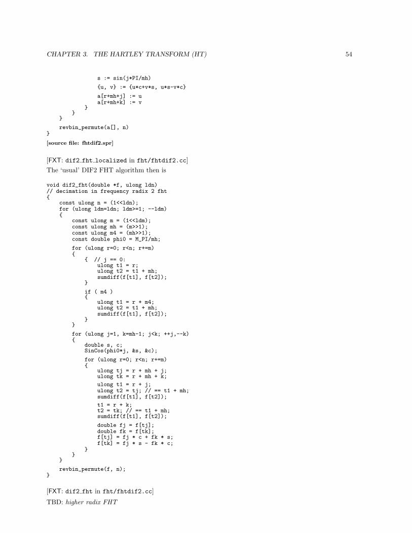
CHAPTER 3. THE HARTLEY TRANSFORM (HT) 54
s := sin(j*PI/mh)
u, v := u*c+v*s, u*s-v*c
a[r+mh+j] := ua[r+mh+k] := v
revbin_permute(a[], n)
[source file: fhtdif2.spr]
[FXT: dif2 fht localized in fht/fhtdif2.cc]The ‘usual’ DIF2 FHT algorithm then is
void dif2_fht(double *f, ulong ldn)// decimation in frequency radix 2 fht
const ulong n = (1<<ldn);for (ulong ldm=ldn; ldm>=1; --ldm)
const ulong m = (1<<ldm);const ulong mh = (m>>1);const ulong m4 = (mh>>1);const double phi0 = M_PI/mh;
for (ulong r=0; r<n; r+=m)
// j == 0:ulong t1 = r;ulong t2 = t1 + mh;sumdiff(f[t1], f[t2]);
if ( m4 )
ulong t1 = r + m4;ulong t2 = t1 + mh;sumdiff(f[t1], f[t2]);
for (ulong j=1, k=mh-1; j<k; ++j,--k)
double s, c;SinCos(phi0*j, &s, &c);
for (ulong r=0; r<n; r+=m)
ulong tj = r + mh + j;ulong tk = r + mh + k;
ulong t1 = r + j;ulong t2 = tj; // == t1 + mh;sumdiff(f[t1], f[t2]);
t1 = r + k;t2 = tk; // == t1 + mh;sumdiff(f[t1], f[t2]);
double fj = f[tj];double fk = f[tk];f[tj] = fj * c + fk * s;f[tk] = fj * s - fk * c;
revbin_permute(f, n);
[FXT: dif2 fht in fht/fhtdif2.cc]
TBD: higher radix FHT
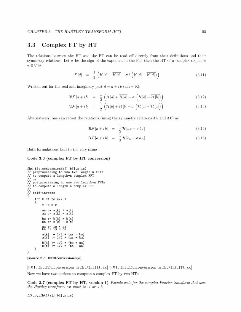
CHAPTER 3. THE HARTLEY TRANSFORM (HT) 55
3.3 Complex FT by HT
The relations between the HT and the FT can be read off directly from their definitions and theirsymmetry relations. Let σ be the sign of the exponent in the FT, then the HT of a complex sequenced ∈ C is:
F [d] =12
(H [d] +H [d] + σ i
(H [d]−H [d]
))(3.11)
Written out for the real and imaginary part d = a + i b (a, b ∈ R):
<F [a + i b] =12
(H [a] +H [a]− σ
(H [b]−H [b]
))(3.12)
=F [a + i b] =12
(H [b] +H [b] + σ
(H [a]−H [a]
))(3.13)
Alternatively, one can recast the relations (using the symmetry relations 3.5 and 3.6) as
<F [a + i b] =12H [aS − σ bA] (3.14)
=F [a + i b] =12H [bS + σ aA] (3.15)
Both formulations lead to the very same
Code 3.6 (complex FT by HT conversion)
fht_fft_conversion(a[],b[],n,is)// preprocessing to use two length-n FHTs// to compute a length-n complex FFT// or// postprocessing to use two length-n FHTs// to compute a length-n complex FFT//// self-inverse
for k:=1 to n/2-1
t := n-k
as := a[k] + a[t]aa := a[k] - a[t]
bs := b[k] + b[t]ba := b[k] - b[t]
aa := is * aaba := is * ba
a[k] := 1/2 * (as - ba)a[t] := 1/2 * (as + ba)
b[k] := 1/2 * (bs + aa)b[t] := 1/2 * (bs - aa)
[source file: fhtfftconversion.spr]
[FXT: fht fft conversion in fht/fhtfft.cc] [FXT: fht fft conversion in fht/fhtcfft.cc]
Now we have two options to compute a complex FT by two HTs:
Code 3.7 (complex FT by HT, version 1) Pseudo code for the complex Fourier transform that usesthe Hartley transform, is must be -1 or +1:
fft_by_fht1(a[],b[],n,is)
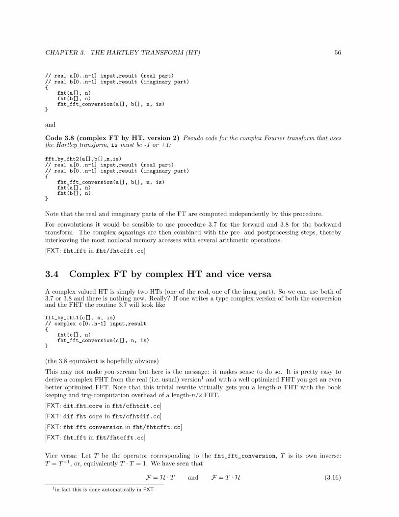
CHAPTER 3. THE HARTLEY TRANSFORM (HT) 56
// real a[0..n-1] input,result (real part)// real b[0..n-1] input,result (imaginary part)
fht(a[], n)fht(b[], n)fht_fft_conversion(a[], b[], n, is)
and
Code 3.8 (complex FT by HT, version 2) Pseudo code for the complex Fourier transform that usesthe Hartley transform, is must be -1 or +1:
fft_by_fht2(a[],b[],n,is)// real a[0..n-1] input,result (real part)// real b[0..n-1] input,result (imaginary part)
fht_fft_conversion(a[], b[], n, is)fht(a[], n)fht(b[], n)
Note that the real and imaginary parts of the FT are computed independently by this procedure.
For convolutions it would be sensible to use procedure 3.7 for the forward and 3.8 for the backwardtransform. The complex squarings are then combined with the pre- and postprocessing steps, therebyinterleaving the most nonlocal memory accesses with several arithmetic operations.
[FXT: fht fft in fht/fhtcfft.cc]
3.4 Complex FT by complex HT and vice versa
A complex valued HT is simply two HTs (one of the real, one of the imag part). So we can use both of3.7 or 3.8 and there is nothing new. Really? If one writes a type complex version of both the conversionand the FHT the routine 3.7 will look like
fft_by_fht1(c[], n, is)// complex c[0..n-1] input,result
fht(c[], n)fht_fft_conversion(c[], n, is)
(the 3.8 equivalent is hopefully obvious)
This may not make you scream but here is the message: it makes sense to do so. It is pretty easy toderive a complex FHT from the real (i.e. usual) version1 and with a well optimized FHT you get an evenbetter optimized FFT. Note that this trivial rewrite virtually gets you a length-n FHT with the bookkeeping and trig-computation overhead of a length-n/2 FHT.
[FXT: dit fht core in fht/cfhtdit.cc]
[FXT: dif fht core in fht/cfhtdif.cc]
[FXT: fht fft conversion in fht/fhtcfft.cc]
[FXT: fht fft in fht/fhtcfft.cc]
Vice versa: Let T be the operator corresponding to the fht_fft_conversion, T is its own inverse:T = T−1, or, equivalently T · T = 1. We have seen that
F = H · T and F = T · H (3.16)1in fact this is done automatically in FXT
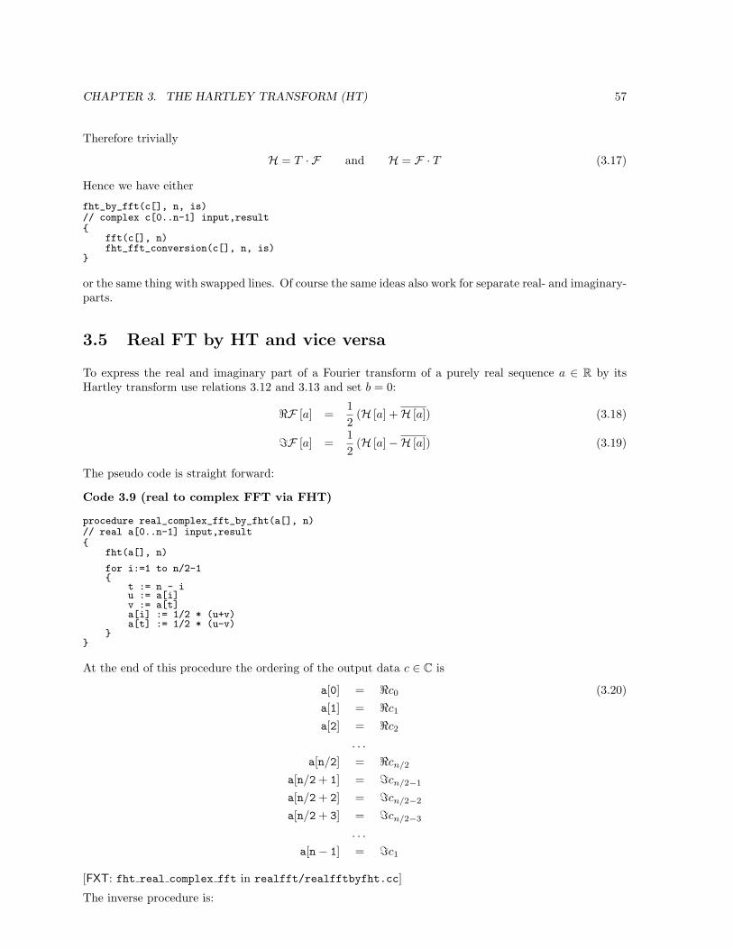
CHAPTER 3. THE HARTLEY TRANSFORM (HT) 57
Therefore trivially
H = T · F and H = F · T (3.17)
Hence we have either
fht_by_fft(c[], n, is)// complex c[0..n-1] input,result
fft(c[], n)fht_fft_conversion(c[], n, is)
or the same thing with swapped lines. Of course the same ideas also work for separate real- and imaginary-parts.
3.5 Real FT by HT and vice versa
To express the real and imaginary part of a Fourier transform of a purely real sequence a ∈ R by itsHartley transform use relations 3.12 and 3.13 and set b = 0:
<F [a] =12
(H [a] +H [a]) (3.18)
=F [a] =12
(H [a]−H [a]) (3.19)
The pseudo code is straight forward:
Code 3.9 (real to complex FFT via FHT)
procedure real_complex_fft_by_fht(a[], n)// real a[0..n-1] input,result
fht(a[], n)
for i:=1 to n/2-1
t := n - iu := a[i]v := a[t]a[i] := 1/2 * (u+v)a[t] := 1/2 * (u-v)
At the end of this procedure the ordering of the output data c ∈ C is
a[0] = <c0 (3.20)a[1] = <c1
a[2] = <c2
. . .
a[n/2] = <cn/2
a[n/2 + 1] = =cn/2−1
a[n/2 + 2] = =cn/2−2
a[n/2 + 3] = =cn/2−3
. . .
a[n− 1] = =c1
[FXT: fht real complex fft in realfft/realfftbyfht.cc]
The inverse procedure is:
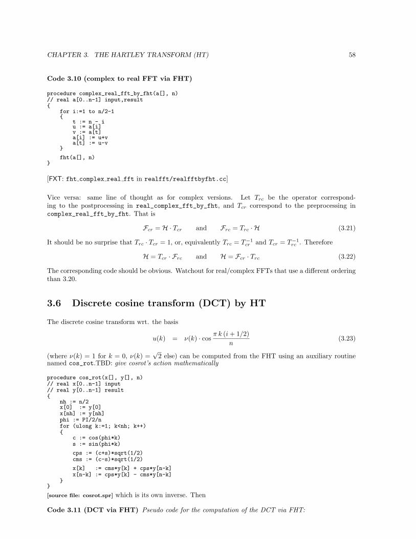
CHAPTER 3. THE HARTLEY TRANSFORM (HT) 58
Code 3.10 (complex to real FFT via FHT)
procedure complex_real_fft_by_fht(a[], n)// real a[0..n-1] input,result
for i:=1 to n/2-1
t := n - iu := a[i]v := a[t]a[i] := u+va[t] := u-v
fht(a[], n)
[FXT: fht complex real fft in realfft/realfftbyfht.cc]
Vice versa: same line of thought as for complex versions. Let Trc be the operator correspond-ing to the postprocessing in real_complex_fft_by_fht, and Tcr correspond to the preprocessing incomplex_real_fft_by_fht. That is
Fcr = H · Tcr and Frc = Trc · H (3.21)
It should be no surprise that Trc · Tcr = 1, or, equivalently Trc = T−1cr and Tcr = T−1
rc . Therefore
H = Tcr · Frc and H = Fcr · Trc (3.22)
The corresponding code should be obvious. Watchout for real/complex FFTs that use a different orderingthan 3.20.
3.6 Discrete cosine transform (DCT) by HT
The discrete cosine transform wrt. the basis
u(k) = ν(k) · cosπ k (i + 1/2)
n(3.23)
(where ν(k) = 1 for k = 0, ν(k) =√
2 else) can be computed from the FHT using an auxiliary routinenamed cos_rot.TBD: give cosrot’s action mathematically
procedure cos_rot(x[], y[], n)// real x[0..n-1] input// real y[0..n-1] result
nh := n/2x[0] := y[0]x[nh] := y[nh]phi := PI/2/nfor (ulong k:=1; k<nh; k++)
c := cos(phi*k)s := sin(phi*k)
cps := (c+s)*sqrt(1/2)cms := (c-s)*sqrt(1/2)
x[k] := cms*y[k] + cps*y[n-k]x[n-k] := cps*y[k] - cms*y[n-k]
[source file: cosrot.spr] which is its own inverse. Then
Code 3.11 (DCT via FHT) Pseudo code for the computation of the DCT via FHT:
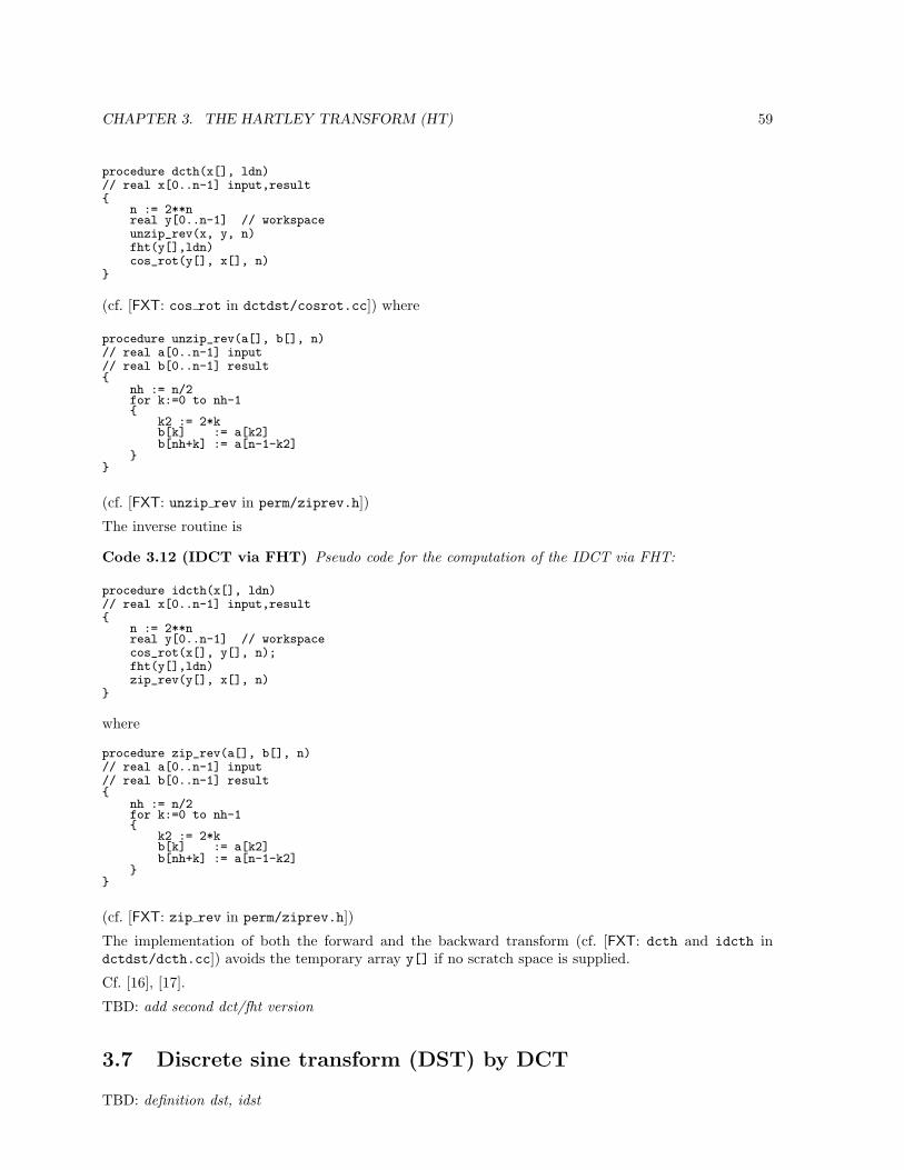
CHAPTER 3. THE HARTLEY TRANSFORM (HT) 59
procedure dcth(x[], ldn)// real x[0..n-1] input,result
n := 2**nreal y[0..n-1] // workspaceunzip_rev(x, y, n)fht(y[],ldn)cos_rot(y[], x[], n)
(cf. [FXT: cos rot in dctdst/cosrot.cc]) where
procedure unzip_rev(a[], b[], n)// real a[0..n-1] input// real b[0..n-1] result
nh := n/2for k:=0 to nh-1
k2 := 2*kb[k] := a[k2]b[nh+k] := a[n-1-k2]
(cf. [FXT: unzip rev in perm/ziprev.h])
The inverse routine is
Code 3.12 (IDCT via FHT) Pseudo code for the computation of the IDCT via FHT:
procedure idcth(x[], ldn)// real x[0..n-1] input,result
n := 2**nreal y[0..n-1] // workspacecos_rot(x[], y[], n);fht(y[],ldn)zip_rev(y[], x[], n)
where
procedure zip_rev(a[], b[], n)// real a[0..n-1] input// real b[0..n-1] result
nh := n/2for k:=0 to nh-1
k2 := 2*kb[k] := a[k2]b[nh+k] := a[n-1-k2]
(cf. [FXT: zip rev in perm/ziprev.h])
The implementation of both the forward and the backward transform (cf. [FXT: dcth and idcth indctdst/dcth.cc]) avoids the temporary array y[] if no scratch space is supplied.
Cf. [16], [17].
TBD: add second dct/fht version
3.7 Discrete sine transform (DST) by DCT
TBD: definition dst, idst
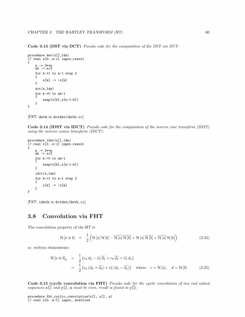
CHAPTER 3. THE HARTLEY TRANSFORM (HT) 60
Code 3.13 (DST via DCT) Pseudo code for the computation of the DST via DCT:
procedure dst(x[],ldn)// real x[0..n-1] input,result
n := 2**nnh := n/2
for k:=1 to n-1 step 2
x[k] := -x[k]
dct(x,ldn)
for k:=0 to nh-1
swap(x[k],x[n-1-k])
[FXT: dsth in dctdst/dsth.cc]
Code 3.14 (IDST via IDCT) Pseudo code for the computation of the inverse sine transform (IDST)using the inverse cosine transform (IDCT):
procedure idst(x[],ldn)// real x[0..n-1] input,result
n := 2**nnh := n/2
for k:=0 to nh-1
swap(x[k],x[n-1-k])
idct(x,ldn)
for k:=1 to n-1 step 2
x[k] := -x[k]
[FXT: idsth in dctdst/dsth.cc]
3.8 Convolution via FHT
The convolution property of the HT is
H [a ~ b] =12
(H [a]H [b]−H [a]H [b] +H [a]H [b] +H [a]H [b]
)(3.24)
or, written elementwise:
H [a ~ b]k =12
(ck dk − ck dk + ck dk + ck dk
)
=12
(ck (dk + dk) + ck (dk − dk)
)where c = H [a], d = H [b] (3.25)
Code 3.15 (cyclic convolution via FHT) Pseudo code for the cyclic convolution of two real valuedsequences x[] and y[], n must be even, result is found in y[]:
procedure fht_cyclic_convolution(x[], y[], n)// real x[0..n-1] input, modified
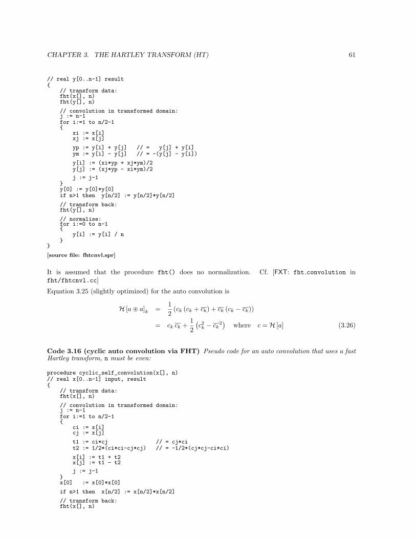
CHAPTER 3. THE HARTLEY TRANSFORM (HT) 61
// real y[0..n-1] result
// transform data:fht(x[], n)fht(y[], n)
// convolution in transformed domain:j := n-1for i:=1 to n/2-1
xi := x[i]xj := x[j]
yp := y[i] + y[j] // = y[j] + y[i]ym := y[i] - y[j] // = -(y[j] - y[i])
y[i] := (xi*yp + xj*ym)/2y[j] := (xj*yp - xi*ym)/2
j := j-1y[0] := y[0]*y[0]if n>1 then y[n/2] := y[n/2]*y[n/2]
// transform back:fht(y[], n)
// normalise:for i:=0 to n-1
y[i] := y[i] / n
[source file: fhtcnvl.spr]
It is assumed that the procedure fht() does no normalization. Cf. [FXT: fht convolution infht/fhtcnvl.cc]
Equation 3.25 (slightly optimized) for the auto convolution is
H [a ~ a]k =12
(ck (ck + ck) + ck (ck − ck))
= ck ck +12
(c2k − ck
2)
where c = H [a] (3.26)
Code 3.16 (cyclic auto convolution via FHT) Pseudo code for an auto convolution that uses a fastHartley transform, n must be even:
procedure cyclic_self_convolution(x[], n)// real x[0..n-1] input, result
// transform data:fht(x[], n)
// convolution in transformed domain:j := n-1for i:=1 to n/2-1
ci := x[i]cj := x[j]
t1 := ci*cj // = cj*cit2 := 1/2*(ci*ci-cj*cj) // = -1/2*(cj*cj-ci*ci)
x[i] := t1 + t2x[j] := t1 - t2
j := j-1x[0] := x[0]*x[0]
if n>1 then x[n/2] := x[n/2]*x[n/2]
// transform back:fht(x[], n)
CHAPTER 3. THE HARTLEY TRANSFORM (HT) 62
// normalise:for i:=0 to n-1
x[i] := x[i] / n
[source file: fhtcnvla.spr]
For odd n replace the line
for i:=1 to n/2-1
by
for i:=1 to (n-1)/2
and omit the line
if n>1 then x[n/2] := x[n/2]*x[n/2]
in both procedures above. Cf. [FXT: fht auto convolution in fht/fhtcnvla.cc]
3.9 Negacyclic convolution via FHT
Code 3.17 (negacyclic auto convolution via FHT) Code for the computation of the negacyclic(auto-) convolution:
procedure negacyclic_self_convolution(x[], n)// real x[0..n-1] input, result
// preprocessing:hartley_shift(x, n, 1/2)
// transform data:fht(x, n)
// convolution in transformed domain:j := n-1for i:=0 to n/2-1 // here i starts from zero
a := x[i]b := x[j]
x[i] := a*b+(a*a-b*b)/2x[j] := a*b-(a*a-b*b)/2j := j-1
// transform back:fht(x, n)
// postprocessing:hartley_shift(x, n, 1/2)
[source file: fhtnegacycliccnvla.spr]
(The code for hartley_shift() was given on page 50.)
Cf. [FXT: fht negacyclic auto convolution in fht/fhtnegacnvla.cc]
Code for the negacyclic convolution (without the ’self’):
[FXT: fht negacyclic convolution in fht/fhtnegacnvl.cc]
The underlying idea can be derived by closely looking at the convolution of real sequences by the radix-2FHT.
The FHT-based negacyclic convolution turns out to be extremely useful for the computation of weightedtransforms, e.g. in the MFA-based convolution for real input.
Chapter 4
Numbertheoretic transforms (NTTs)
How to make a numbertheoretic transform out of your FFT:‘Replace exp(± 2 π i/n) by a primitive n-th root of unity, done.’
We want to do FFTs in Z/mZ (the ring of integers modulo some integer m) instead of C, the (field ofthe) complex numbers. These FFTs are called numbertheoretic transforms (NTTs), mod m FFTs or (ifm is a prime) prime modulus transforms.
There is a restriction for the choice of m: For a length n FFT we need a primitive n-th root of unity. Anumber r is called an n-th root of unity if rn = 1. It is called a primitive n-th root if rk 6= 1 ∀ k < n.
In C matters are simple: e± 2 π i/n is a primitive n-th root of unity for arbitrary n. e2 π i/21 is a 21-th rootof unity. r = e2 π i/3 is also 21-th root of unity but not a primitive root, because r3 = 1. A primitive n-throot of 1 in Z/mZ is also called an element of order n. The ‘cyclic’ property of the elements r of ordern lies in the heart of all FFT algorithms: rn+k = rk.
In Z/mZ things are not that simple since primitive roots of unity do not exist for arbitrary n, they existfor some maximal order R only. Roots of unity of an order different from R are available only for thedivisors di of R: rR/di is a di-th root of unity because (rR/di)di = rR = 1.
Therefore n must divide R, the first condition for NTTs:
n\R ⇐⇒ ∃ n√
1 (4.1)
The operations needed in FFTs are addition, subtraction and multiplication. Division is not needed,except for division by n for the final normalization after transform and backtransform. Division by n ismultiplication by the inverse of n. Hence n must be invertible in Z/mZ: n must be coprime1 to m, thesecond condition for NTTs:
n ⊥ m ⇐⇒ ∃n−1 in Z/mZ (4.2)
Cf. [1], [3], [14] or [2] and books on number theory.
4.1 Prime modulus: Z/pZ = Fp
If the modulus is a prime p then Z/pZ is the field Fp: All elements except 0 have inverses and ‘division ispossible’ in Z/pZ. Thereby the second condition is trivially fulfilled for all FFT lengthes n < p: a primep is coprime to all integers n < p.
1n coprime to m ⇐⇒ gcd(n, m) = 1
63

CHAPTER 4. NUMBERTHEORETIC TRANSFORMS (NTTS) 64
Roots of unity are available for the maximal order R = p−1 and its divisors: Therefore the first conditionon n for a length-n mod p FFT being possible is that n divides p − 1. This restricts the choice for p toprimes of the form p = v n + 1: For length-n = 2k FFTs one will use primes like p = 3 · 5 · 227 + 1 (31bits), p = 13 · 228 + 1 (32 bits), p = 3 · 29 · 256 + 1 (63 bits) or p = 27 · 259 + 1 (64 bits)2. The elementsof maximal order in Z/pZ are called primitive elements, generators or primitive roots modulo p. If r is agenerator, then every element in Fp different from 0 is equal to some power re (1 ≤ e < p) of r and itsorder is R/e. To test whether r is a primitive n-th root of unity in Fp one does not need to check rk 6= 1for all k < n. It suffices to do the check for exponents k that are prime factors of n. This is because theorder of any element divides the maximal order. To find a primitive root in Fp proceed as indicated bythe following pseudo code:
Code 4.1 (Primitive root modulo p) Return a primitive root in Fp
function primroot(p)
if p==2 then return 1
f[] := distinct_prime_factors(p-1)
for r:=2 to p-1
x := TRUE
foreach q in f[]
if r**((p-1)/q)==1 then x:=FALSE
if x==TRUE then return r
error("no primitive root found") // p cannot be prime !
An element of order n is returned by this function:
Code 4.2 (Find element of order n) Return an element of order n in Fp:
function element_of_order(n,p)
R := p-1 // maxorderif (R/n)*n != R then error("order n must divide maxorder p-1")r := primroot(p)x := r**(R/n)return x
4.2 Composite modulus: Z/mZ
In what follows we will need the function ϕ(), the so-called ‘totient’ function. ϕ(m) counts the numberof integers prime to and less than m. For m = p prime ϕ(p) = p − 1. For m composite ϕ(m) is alwaysless than m− 1. For m = pk a prime power
ϕ(pk) = pk − pk−1 (4.3)
e.g. ϕ(2k) = 2k−1. ϕ(1) = 1. For coprime p1, p2 (p1, p2 not necessarily primes) ϕ(p1 p2) = ϕ(p1)ϕ(p2),ϕ() is a so-called multiplicative function.
For the computation of ϕ(m) for m a prime power one can use this simple piece of code
Code 4.3 (Compute phi(m) for m a prime power) Return ϕ(px)
2Primes of that form are not ‘exceptional’, cf. Lipson [3]
CHAPTER 4. NUMBERTHEORETIC TRANSFORMS (NTTS) 65
function phi_pp(p,x)
if x==1 then return p - 1else return p**x - p**(x-1)
Pseudo code to compute ϕ(m) for general m:
Code 4.4 (Compute phi(m)) Return ϕ(m)
function phi(m)
n, p[], x[] := factorization(m) // m==product(i=0..n-1,p[i]**x[i])
ph := 1for i:=0 to n-1
ph := ph * phi_pp(p[i],x[i])
Further we need the notion of Z/mZ∗, the ring of units in Z/mZ. Z/mZ∗ contains all invertible elements(‘units’) of Z/mZ, i.e. those which are coprime to m. Evidently the total number of units is given byϕ(m):
|Z/mZ∗| = ϕ(m) (4.4)
If m factorizes as m = 2k0 · pk11 · . . . · pkq
q then
|Z/mZ∗| = ϕ(2k0) · ϕ(pk11 ) · . . . · ϕ(pkq
q ) (4.5)
It turns out that the maximal order R of an element can be equal to or less than |Z/mZ∗|, the ringZ/mZ∗ is then called cyclic or noncyclic, respectively. For m a power of an odd prime p the maximalorder R in Z/mZ∗ (and also in Z/mZ) is
R(pk) = ϕ(pk) (4.6)
while for m a power of two a tiny irregularity enters:
R(2k) =
1 for k = 12 for k = 22k−2 for k ≥ 3
(4.7)
i.e. for powers of two greater than 4 the maximal order deviates from ϕ(2k) = 2k−1 by a factor of 2. Forthe general modulus m = 2k0 · pk1
1 · . . . · pkqq the maximal order is
R(m) = lcm(R(2k0), R(pk11 ), . . . , R(pkq
q )) (4.8)
where lcm() denotes the least common multiple.
Pseudo code to compute R(m):
Code 4.5 (Maximal order modulo m) Return R(m), the maximal order in Z/mZ
function maxorder(m)
n, p[], k[] := factorization(m) // m==product(i=0..n-1,p[i]**k[i])
R := 1for i:=0 to n-1
t := phi_pp(p[i],k[i])if p[i]==2 AND k[i]>=3 then t := t / 2R := lcm(R,t)
return R
CHAPTER 4. NUMBERTHEORETIC TRANSFORMS (NTTS) 66
Now we can see for which m the ring Z/mZ∗ will be cyclic:
Z/mZ∗ cyclic for m = 2, 4, pk, 2 · pk (4.9)
where p is an odd prime. If m contains two different odd primes pa, pb then R(m) =lcm(. . . , ϕ(pa), ϕ(pb), . . . ) is at least by a factor of two smaller than ϕ(m) = . . . · ϕ(pa) · ϕ(pb) · . . .because both ϕ(pa) and ϕ(pb) are even, so Z/mZ∗ can’t be cyclic in that case. The same argument holdsfor m = 2k0 · pk if k0 > 1. For m = 2k Z/mZ∗ is cyclic only for k = 1 and k = 2 because of the abovementioned irregularity of R(2k).
Pseudo code (following [14]) for a function that returns the order of some element x in Z/mZ:
Code 4.6 (Order of an element in Z/mZ) Return the order of an element x in Z/mZ
function order(x,m)
if gcd(x,m)!=1 then return 0 // x not a unith := phi(m) // number of elements of ring of unitse := hn, p[], k[] := factorization(h) // h==product(i=0..n-1,p[i]**k[i])
for i:=0 to n-1
f := p[i]**k[i]e := e / fg1 := x**e mod mwhile g1!=1
g1 := g1**p[i] mod me := e * p[i]p[i] := p[i] - 1
return e
Pseudo code for a function that returns some element x in Z/mZ of maximal order:
Code 4.7 (Element of maximal order in Z/mZ) Return an element that has maximal order inZ/mZ
function maxorder_element(m)
R := maxorder(m)for x:=1 to m-1
if order(x,m)==R then return x// never reached
For prime m the function returns a primitive root. It is a good idea to have a table of small primes stored(which will also be useful in the factorization routine) and restrict the search to small primes and only ifthe modulus is greater than the largest prime of the table proceed with a loop as above:
Code 4.8 (Element of maximal order in Z/mZ) Return an element that has maximal order inZ/mZ, use a precomputed table of primes
function maxorder_element(m,pt[],np)// pt[0..np-1] = 2,3,5,7,11,13,17,...
if m==2 then return 1
R := maxorder(m)
for i:=0 to np-1
if order(pt[i],m)==R then return x
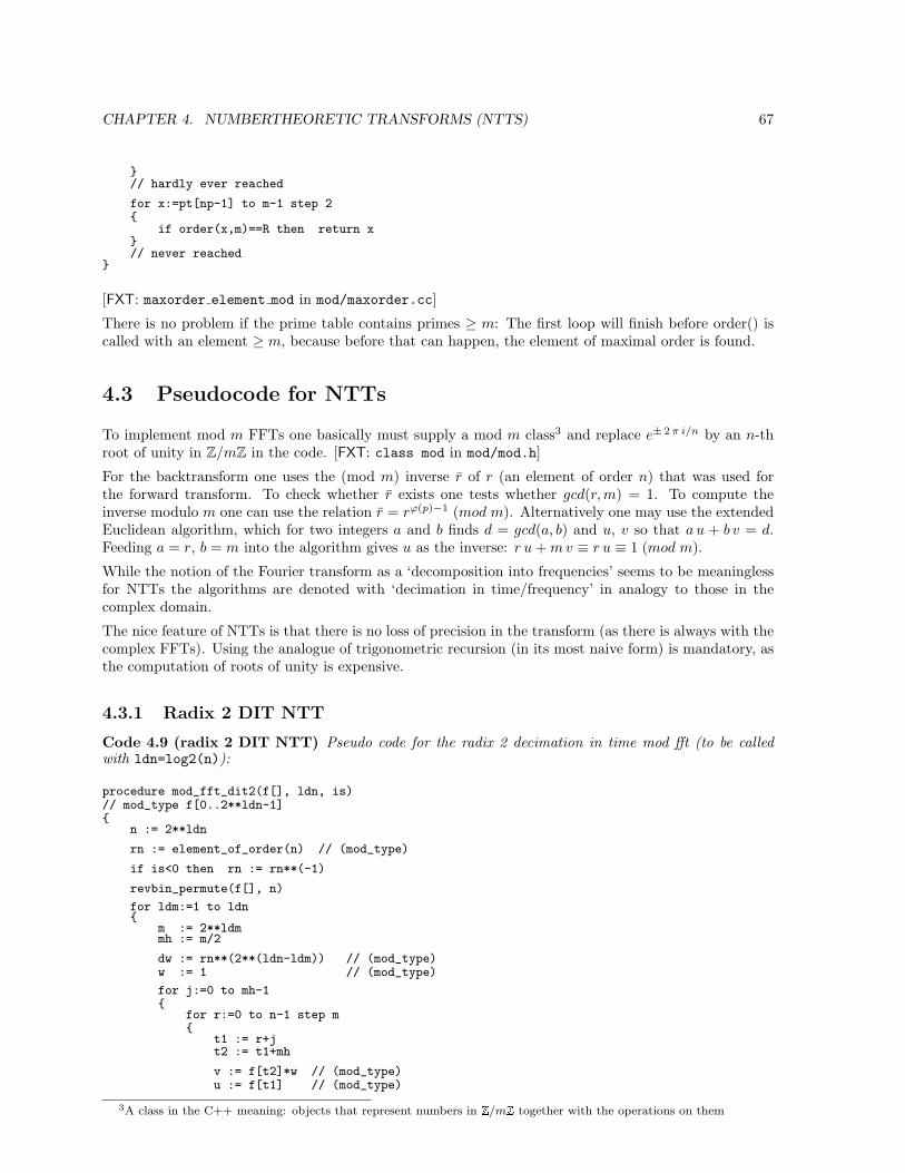
CHAPTER 4. NUMBERTHEORETIC TRANSFORMS (NTTS) 67
// hardly ever reached
for x:=pt[np-1] to m-1 step 2
if order(x,m)==R then return x// never reached
[FXT: maxorder element mod in mod/maxorder.cc]
There is no problem if the prime table contains primes ≥ m: The first loop will finish before order() iscalled with an element ≥ m, because before that can happen, the element of maximal order is found.
4.3 Pseudocode for NTTs
To implement mod m FFTs one basically must supply a mod m class3 and replace e± 2 π i/n by an n-throot of unity in Z/mZ in the code. [FXT: class mod in mod/mod.h]
For the backtransform one uses the (mod m) inverse r of r (an element of order n) that was used forthe forward transform. To check whether r exists one tests whether gcd(r,m) = 1. To compute theinverse modulo m one can use the relation r = rϕ(p)−1 (mod m). Alternatively one may use the extendedEuclidean algorithm, which for two integers a and b finds d = gcd(a, b) and u, v so that a u + b v = d.Feeding a = r, b = m into the algorithm gives u as the inverse: r u + mv ≡ r u ≡ 1 (mod m).
While the notion of the Fourier transform as a ‘decomposition into frequencies’ seems to be meaninglessfor NTTs the algorithms are denoted with ‘decimation in time/frequency’ in analogy to those in thecomplex domain.
The nice feature of NTTs is that there is no loss of precision in the transform (as there is always with thecomplex FFTs). Using the analogue of trigonometric recursion (in its most naive form) is mandatory, asthe computation of roots of unity is expensive.
4.3.1 Radix 2 DIT NTT
Code 4.9 (radix 2 DIT NTT) Pseudo code for the radix 2 decimation in time mod fft (to be calledwith ldn=log2(n)):
procedure mod_fft_dit2(f[], ldn, is)// mod_type f[0..2**ldn-1]
n := 2**ldn
rn := element_of_order(n) // (mod_type)
if is<0 then rn := rn**(-1)
revbin_permute(f[], n)
for ldm:=1 to ldn
m := 2**ldmmh := m/2
dw := rn**(2**(ldn-ldm)) // (mod_type)w := 1 // (mod_type)
for j:=0 to mh-1
for r:=0 to n-1 step m
t1 := r+jt2 := t1+mh
v := f[t2]*w // (mod_type)u := f[t1] // (mod_type)
3A class in the C++ meaning: objects that represent numbers in Z/mZ together with the operations on them
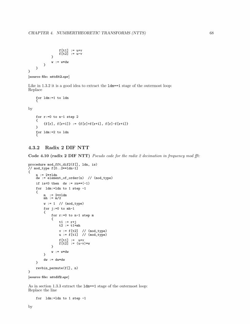
CHAPTER 4. NUMBERTHEORETIC TRANSFORMS (NTTS) 68
f[t1] := u+vf[t2] := u-v
w := w*dw
[source file: nttdit2.spr]
Like in 1.3.2 it is a good idea to extract the ldm==1 stage of the outermost loop:Replace
for ldm:=1 to ldn
by
for r:=0 to n-1 step 2
f[r], f[r+1] := f[r]+f[r+1], f[r]-f[r+1]
for ldm:=2 to ldn
4.3.2 Radix 2 DIF NTT
Code 4.10 (radix 2 DIF NTT) Pseudo code for the radix 2 decimation in frequency mod fft:
procedure mod_fft_dif2(f[], ldn, is)// mod_type f[0..2**ldn-1]
n := 2**ldndw := element_of_order(n) // (mod_type)
if is<0 then dw := rn**(-1)
for ldm:=ldn to 1 step -1
m := 2**ldmmh := m/2
w := 1 // (mod_type)
for j:=0 to mh-1
for r:=0 to n-1 step m
t1 := r+jt2 := t1+mh
v := f[t2] // (mod_type)u := f[t1] // (mod_type)
f[t1] := u+vf[t2] := (u-v)*w
w := w*dw
dw := dw*dw
revbin_permute(f[], n)
[source file: nttdif2.spr]
As in section 1.3.3 extract the ldm==1 stage of the outermost loop:Replace the line
for ldm:=ldn to 1 step -1
by
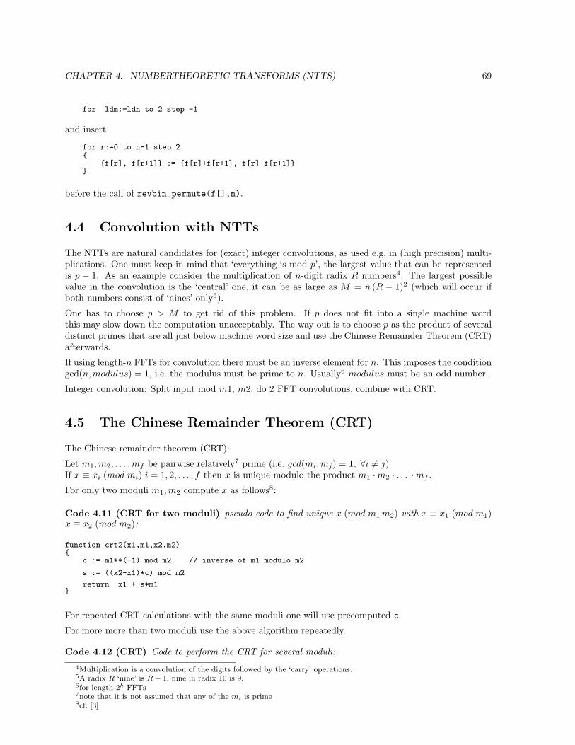
CHAPTER 4. NUMBERTHEORETIC TRANSFORMS (NTTS) 69
for ldm:=ldn to 2 step -1
and insert
for r:=0 to n-1 step 2
f[r], f[r+1] := f[r]+f[r+1], f[r]-f[r+1]
before the call of revbin_permute(f[],n).
4.4 Convolution with NTTs
The NTTs are natural candidates for (exact) integer convolutions, as used e.g. in (high precision) multi-plications. One must keep in mind that ‘everything is mod p’, the largest value that can be representedis p − 1. As an example consider the multiplication of n-digit radix R numbers4. The largest possiblevalue in the convolution is the ‘central’ one, it can be as large as M = n (R − 1)2 (which will occur ifboth numbers consist of ‘nines’ only5).
One has to choose p > M to get rid of this problem. If p does not fit into a single machine wordthis may slow down the computation unacceptably. The way out is to choose p as the product of severaldistinct primes that are all just below machine word size and use the Chinese Remainder Theorem (CRT)afterwards.
If using length-n FFTs for convolution there must be an inverse element for n. This imposes the conditiongcd(n, modulus) = 1, i.e. the modulus must be prime to n. Usually6 modulus must be an odd number.
Integer convolution: Split input mod m1, m2, do 2 FFT convolutions, combine with CRT.
4.5 The Chinese Remainder Theorem (CRT)
The Chinese remainder theorem (CRT):
Let m1,m2, . . . , mf be pairwise relatively7 prime (i.e. gcd(mi,mj) = 1, ∀i 6= j)If x ≡ xi (mod mi) i = 1, 2, . . . , f then x is unique modulo the product m1 ·m2 · . . . ·mf .
For only two moduli m1,m2 compute x as follows8:
Code 4.11 (CRT for two moduli) pseudo code to find unique x (mod m1 m2) with x ≡ x1 (mod m1)x ≡ x2 (mod m2):
function crt2(x1,m1,x2,m2)
c := m1**(-1) mod m2 // inverse of m1 modulo m2
s := ((x2-x1)*c) mod m2
return x1 + s*m1
For repeated CRT calculations with the same moduli one will use precomputed c.
For more more than two moduli use the above algorithm repeatedly.
Code 4.12 (CRT) Code to perform the CRT for several moduli:
4Multiplication is a convolution of the digits followed by the ‘carry’ operations.5A radix R ‘nine’ is R− 1, nine in radix 10 is 9.6for length-2k FFTs7note that it is not assumed that any of the mi is prime8cf. [3]
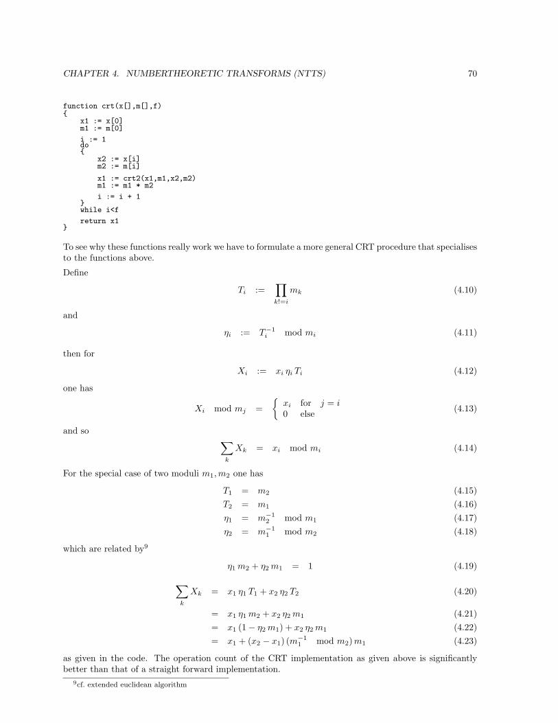
CHAPTER 4. NUMBERTHEORETIC TRANSFORMS (NTTS) 70
function crt(x[],m[],f)
x1 := x[0]m1 := m[0]
i := 1do
x2 := x[i]m2 := m[i]
x1 := crt2(x1,m1,x2,m2)m1 := m1 * m2
i := i + 1while i<f
return x1
To see why these functions really work we have to formulate a more general CRT procedure that specialisesto the functions above.
Define
Ti :=∏
k!=i
mk (4.10)
and
ηi := T−1i mod mi (4.11)
then for
Xi := xi ηi Ti (4.12)
one has
Xi mod mj =
xi for j = i0 else (4.13)
and so∑
k
Xk = xi mod mi (4.14)
For the special case of two moduli m1,m2 one has
T1 = m2 (4.15)T2 = m1 (4.16)η1 = m−1
2 mod m1 (4.17)η2 = m−1
1 mod m2 (4.18)
which are related by9
η1 m2 + η2 m1 = 1 (4.19)
∑
k
Xk = x1 η1 T1 + x2 η2 T2 (4.20)
= x1 η1 m2 + x2 η2 m1 (4.21)= x1 (1− η2 m1) + x2 η2 m1 (4.22)= x1 + (x2 − x1) (m−1
1 mod m2) m1 (4.23)
as given in the code. The operation count of the CRT implementation as given above is significantlybetter than that of a straight forward implementation.
9cf. extended euclidean algorithm
CHAPTER 4. NUMBERTHEORETIC TRANSFORMS (NTTS) 71
4.6 A modular multiplication technique
When implementing a mod class on a 32 bit machine the following trick can be useful: It allows easymultiplication of two integers a, b modulo m even if the product a · b does not fit into a machine integer(that is assumed to have some maximal value z − 1, z = 2k).
Let 〈x〉y denote x modulo y, bxc denote the integer part of x. For 0 ≤ a, b < m:
a · b =⌊
a · bm
⌋·m + 〈a · b〉m (4.24)
rearranging and taking both sides modulo z > m:⟨
a · b−⌊
a · bm
⌋·m
⟩
z
= 〈〈a · b〉m〉z (4.25)
where the rhs. equals 〈a · b〉m because m < z.
〈a · b〉m =⟨〈a · b〉z −
⟨⌊a · bm
⌋·m
⟩
z
⟩
z
(4.26)
the expression on the rhs. can be translated into a few lines fo C-code. The code given here assumes thatone has 64 bit integer types int64 (signed) and uint64 (unsigned) and a floating point type with 64 bitmantissa, float64 (typically long double).
uint64 mul_mod(uint64 a, uint64 b, uint64 m)
uint64 y = (uint64)((float64)a*(float64)b/m+(float64)1/2); // floor(a*b/m)y = y * m; // m*floor(a*b/m) mod zuint64 x = a * b; // a*b mod zuint64 r = x - y; // a*b mod z - m*floor(a*b/m) mod zif ( (int64)r < 0 ) // normalization needed ?
r = r + m;y = y - 1; // (a*b)/m quotient, omit line if not needed
return r; // (a*b)%m remnant
It uses the fact that integer multiplication computes the least significant bits of the result 〈a · b〉z whereasfloat multiplication computes the most significant bits of the result. The above routine works if 0 <=a, b < m < 263 = z
2 . The normalization isn’t necessary if m < 262 = z4 .
When working with a fixed modulus the division by p may be replaced by a multiplication with theinverse modulus, that only needs to be computed once:
Precompute: float64 i = (float64)1/m;
and replace the line uint64 y = (uint64)((float64)a*(float64)b/m+(float64)1/2);
by uint64 y = (uint64)((float64)a*(float64)b*i+(float64)1/2);
so any division inside the routine avoided. But beware, the routine then cannot be used for m >= 262:it very rarely fails for moduli of more than 62 bits. This is due to the additional error when invertingand multiplying as compared to dividing alone.
This trick is ascribed to Peter Montgomery.
TBD: montgomery mult.
CHAPTER 4. NUMBERTHEORETIC TRANSFORMS (NTTS) 72
4.7 Numbertheoretic Hartley transform
Let r be an element of order n, i.e. rn = 1 (but there is no k < n so that rk = 1) we like to identify rwith exp(2 i π/n).
Then one can set
cos2 π
n≡ r2 + 1
2 r(4.27)
i sin2 π
n≡ r2 − 1
2 r(4.28)
For This choice of sin and cos the relations exp() = cos() + i sin() and sin()2 + cos()2 = 1 should hold.The first check is trivial: x2+1
2 x + x2−12 x = x. The second is also easy if we allow to write i for some element
that is the square root of −1: (x2+12 x )2 +(x2−1
2 x i )2 = (x2+1)1−(x2−1)2
4 x2 = 1. Ok, but what is i in the modularring? Simply rn/4, then we have i2 = −1 and i4 = 1 as we are used to. This is only true in cyclic rings.
TBD: give a nice mod fht
Chapter 5
Walsh transforms
How to make a Walsh transform out of your FFT:‘Replace exp(something) by 1, done.’
Very simple, so we are ready for
Code 5.1 (radix 2 DIT Walsh transform, first trial) Pseudo code for a radix 2 decimation in timeWalsh transform: (has a flaw)
procedure walsh_wak_dit2(a[], ldn)
n := 2**ldn
for ldm := 1 to ldn
m := 2**ldmmh := m/2
for j := 0 to mh-1
for r := 0 to n-1 step m
t1 := r + jt2 := t1 + mhu := a[t1]v := a[t2]
a[t1] := u + va[t2] := u - v
[source file: walshwakdit2.spr]
The transform involves proportional n log2(n) additions (and subtractions) and no multiplication at all.Note the absence of any permute(a[],n) function call. The transform is its own inverse, so there isnothing like the is in the FFT procedures here. Let’s make a slight improvement: Here we just tookthe code 1.4 and threw away all trig computations.But the swapping of the inner loops, that caused thenonlocality of the memory access is now of no advantage, so we try this piece of
Code 5.2 (radix 2 DIT Walsh transform) Pseudo code for a radix 2 decimation in time Walshtransform:
procedure walsh_wak_dit2(a[],ldn)
n := 2**ldn
for ldm := 1 to ldn
m := 2**ldm
73
CHAPTER 5. WALSH TRANSFORMS 74
mh := m/2
for r := 0 to n-1 step m
t1 = rt2 = r + mhfor j := 0 to mh-1
u := a[t1]v := a[t2]
a[t1] := u + va[t2] := u - v
t1 := t1 + 1t2 := t2 + 1
[source file: walshwakdit2localized.spr]
Which performance impact can this innocent change in the code have? For large n it gave a speedup bya factor of more than three when run on a computer with a main memory clock of 66 Megahertz and a5.5 times higher CPU clock of 366 Megahertz.
The equivalent code for the decimation in frequency algorithm looks like this:
Code 5.3 (radix 2 DIF Walsh transform) Pseudo code for a radix 2 decimation in frequency Walshtransform:
procedure walsh_wak_dif2(a[], ldn)
n := 2**ldn
for ldm := ldn to 1 step -1
m := 2**ldmmh := m/2
for r := 0 to n-1 step m
t1 = rt2 = r + mhfor j := 0 to mh-1
u := a[t1]v := a[t2]
a[t1] := u + va[t2] := u - v
t1 := t1 + 1t2 := t2 + 1
[source file: walshwakdif2localized.spr]
The basis functions look like this (for n = 16):
TBD: definition and formulas for walsh basis
A term analogue to the frequency of the Fourier basis functions is the so called ‘sequency’ of the Walshfunctions, the number of the changes of sign of the individual functions. If one wants the basis functionsordered with respect to sequency one can use a procedure like this:
Code 5.4 (sequency ordered Walsh transform (wal))
procedure walsh_wal_dif2(a[],n)
gray_permute(a[],n)permute(a[],n)walsh_wak_dif2(a[],n)
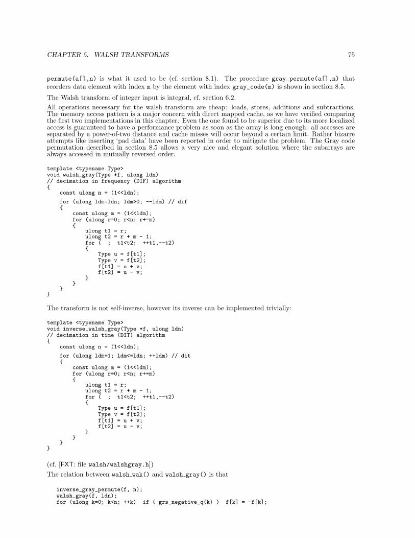
CHAPTER 5. WALSH TRANSFORMS 75
permute(a[],n) is what it used to be (cf. section 8.1). The procedure gray_permute(a[],n) thatreorders data element with index m by the element with index gray_code(m) is shown in section 8.5.
The Walsh transform of integer input is integral, cf. section 6.2.All operations necessary for the walsh transform are cheap: loads, stores, additions and subtractions.The memory access pattern is a major concern with direct mapped cache, as we have verified comparingthe first two implementations in this chapter. Even the one found to be superior due to its more localizedaccess is guaranteed to have a performance problem as soon as the array is long enough: all accesses areseparated by a power-of-two distance and cache misses will occur beyond a certain limit. Rather bizarreattempts like inserting ‘pad data’ have been reported in order to mitigate the problem. The Gray codepermutation described in section 8.5 allows a very nice and elegant solution where the subarrays arealways accessed in mutually reversed order.
template <typename Type>void walsh_gray(Type *f, ulong ldn)// decimation in frequency (DIF) algorithm
const ulong n = (1<<ldn);
for (ulong ldm=ldn; ldm>0; --ldm) // dif
const ulong m = (1<<ldm);for (ulong r=0; r<n; r+=m)
ulong t1 = r;ulong t2 = r + m - 1;for ( ; t1<t2; ++t1,--t2)
Type u = f[t1];Type v = f[t2];f[t1] = u + v;f[t2] = u - v;
The transform is not self-inverse, however its inverse can be implemented trivially:
template <typename Type>void inverse_walsh_gray(Type *f, ulong ldn)// decimation in time (DIT) algorithm
const ulong n = (1<<ldn);
for (ulong ldm=1; ldm<=ldn; ++ldm) // dit
const ulong m = (1<<ldm);for (ulong r=0; r<n; r+=m)
ulong t1 = r;ulong t2 = r + m - 1;for ( ; t1<t2; ++t1,--t2)
Type u = f[t1];Type v = f[t2];f[t1] = u + v;f[t2] = u - v;
(cf. [FXT: file walsh/walshgray.h])The relation between walsh wak() and walsh gray() is that
inverse_gray_permute(f, n);walsh_gray(f, ldn);for (ulong k=0; k<n; ++k) if ( grs_negative_q(k) ) f[k] = -f[k];
CHAPTER 5. WALSH TRANSFORMS 76
is equivalent to the call walsh wak(f, ldn). The third line is a necessary fixup for certain elements thathave the wrong sign if uncorrected. grs negative q() is described in section 7.11.Btw. walsh wal(f, ldn) is equivalent to
walsh_gray(f, ldn);for (ulong k=0; k<n; ++k) if ( grs_negative_q(k) ) f[k] = -f[k];revbin_permute(f, n);
The same idea can be used with the Fast Fourier Transform. However, the advantage of the improvedaccess pattern is usually more than compensated by the increased number of sin/cos-computations (thetwiddle factors appear reordered so n · log n instead of n computations are necessary) cf. [FXT: file
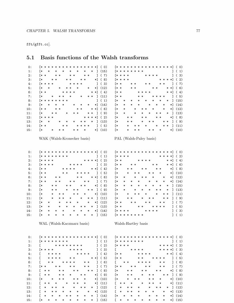
CHAPTER 5. WALSH TRANSFORMS 77
fft/gfft.cc].
5.1 Basis functions of the Walsh transforms
0: [* * * * * * * * * * * * * * * *] ( 0) [* * * * * * * * * * * * * * * *] ( 0)
1: [* * * * * * * * ] (15) [* * * * * * * * ] ( 1)
2: [* * * * * * * * ] ( 7) [* * * * * * * * ] ( 3)
3: [* * * * * * * *] ( 8) [* * * * * * * *] ( 2)
4: [* * * * * * * * ] ( 3) [* * * * * * * * ] ( 7)
5: [* * * * * * * *] (12) [* * * * * * * *] ( 6)
6: [* * * * * * * *] ( 4) [* * * * * * * *] ( 4)
7: [* * * * * * * * ] (11) [* * * * * * * * ] ( 5)
8: [* * * * * * * * ] ( 1) [* * * * * * * * ] (15)
9: [* * * * * * * *] (14) [* * * * * * * *] (14)
10: [* * * * * * * *] ( 6) [* * * * * * * *] (12)
11: [* * * * * * * * ] ( 9) [* * * * * * * * ] (13)
12: [* * * * * * * *] ( 2) [* * * * * * * *] ( 8)
13: [* * * * * * * * ] (13) [* * * * * * * * ] ( 9)
14: [* * * * * * * * ] ( 5) [* * * * * * * * ] (11)
15: [* * * * * * * *] (10) [* * * * * * * *] (10)
WAK (Walsh-Kronecker basis) PAL (Walsh-Paley basis)
0: [* * * * * * * * * * * * * * * *] ( 0) [* * * * * * * * * * * * * * * *] ( 0)
1: [* * * * * * * * ] ( 1) [* * * * * * * *] ( 2)
2: [* * * * * * * *] ( 2) [* * * * * * * *] ( 4)
3: [* * * * * * * * ] ( 3) [* * * * * * * *] ( 6)
4: [* * * * * * * *] ( 4) [* * * * * * * *] ( 8)
5: [* * * * * * * * ] ( 5) [* * * * * * * *] (10)
6: [* * * * * * * *] ( 6) [* * * * * * * *] (12)
7: [* * * * * * * * ] ( 7) [* * * * * * * *] (14)
8: [* * * * * * * *] ( 8) [* * * * * * * * ] (15)
9: [* * * * * * * * ] ( 9) [* * * * * * * * ] (13)
10: [* * * * * * * *] (10) [* * * * * * * * ] (11)
11: [* * * * * * * * ] (11) [* * * * * * * * ] ( 9)
12: [* * * * * * * *] (12) [* * * * * * * * ] ( 7)
13: [* * * * * * * * ] (13) [* * * * * * * * ] ( 5)
14: [* * * * * * * *] (14) [* * * * * * * * ] ( 3)
15: [* * * * * * * * ] (15) [* * * * * * * * ] ( 1)
WAL (Walsh-Kaczmarz basis) Walsh-Hartley basis
0: [* * * * * * * * * * * * * * * *] ( 0) [* * * * * * * * * * * * * * * *] ( 0)
1: [* * * * * * * * ] ( 1) [* * * * * * * * ] ( 1)
2: [ * * * * * * * * ] ( 2) [* * * * * * * *] ( 2)
3: [* * * * * * * * ] ( 3) [ * * * * * * * *] ( 3)
4: [ * * * * * * * * ] ( 4) [* * * * * * * *] ( 4)
5: [ * * * * * * * *] ( 5) [* * * * * * * * ] ( 5)
6: [ * * * * * * * * ] ( 6) [ * * * * * * * * ] ( 6)
7: [* * * * * * * * ] ( 7) [* * * * * * * * ] ( 7)
8: [ * * * * * * * * ] ( 8) [* * * * * * * *] ( 8)
9: [ * * * * * * * *] ( 9) [* * * * * * * * ] ( 9)
10: [* * * * * * * *] (10) [* * * * * * * *] (10)
11: [ * * * * * * * *] (11) [ * * * * * * * *] (11)
12: [ * * * * * * * * ] (12) [ * * * * * * * * ] (12)
13: [ * * * * * * * *] (13) [ * * * * * * * *] (13)
14: [ * * * * * * * * ] (14) [* * * * * * * *] (14)
15: [* * * * * * * * ] (15) [ * * * * * * * *] (15)
SEQ SEQ2
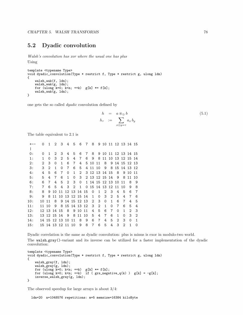
CHAPTER 5. WALSH TRANSFORMS 78
5.2 Dyadic convolution
Walsh’s convolution has xor where the usual one has plusUsing
template <typename Type>void dyadic_convolution(Type * restrict f, Type * restrict g, ulong ldn)
walsh_wak(f, ldn);walsh_wak(g, ldn);for (ulong k=0; k<n; ++k) g[k] *= f[k];walsh_wak(g, ldn);
one gets the so called dyadic convolution defined by
h = a ~⊕ b (5.1)
hτ :=∑
x⊕y=τ
ax by
The table equivalent to 2.1 is
+-- 0 1 2 3 4 5 6 7 8 9 10 11 12 13 14 15|0: 0 1 2 3 4 5 6 7 8 9 10 11 12 13 14 151: 1 0 3 2 5 4 7 6 9 8 11 10 13 12 15 142: 2 3 0 1 6 7 4 5 10 11 8 9 14 15 12 133: 3 2 1 0 7 6 5 4 11 10 9 8 15 14 13 124: 4 5 6 7 0 1 2 3 12 13 14 15 8 9 10 115: 5 4 7 6 1 0 3 2 13 12 15 14 9 8 11 106: 6 7 4 5 2 3 0 1 14 15 12 13 10 11 8 97: 7 6 5 4 3 2 1 0 15 14 13 12 11 10 9 88: 8 9 10 11 12 13 14 15 0 1 2 3 4 5 6 79: 9 8 11 10 13 12 15 14 1 0 3 2 5 4 7 6
10: 10 11 8 9 14 15 12 13 2 3 0 1 6 7 4 511: 11 10 9 8 15 14 13 12 3 2 1 0 7 6 5 412: 12 13 14 15 8 9 10 11 4 5 6 7 0 1 2 313: 13 12 15 14 9 8 11 10 5 4 7 6 1 0 3 214: 14 15 12 13 10 11 8 9 6 7 4 5 2 3 0 115: 15 14 13 12 11 10 9 8 7 6 5 4 3 2 1 0
Dyadic correlation is the same as dyadic convolution: plus is minus is exor in modulo-two world.The walsh gray()-variant and its inverse can be utilized for a faster implementation of the dyadicconvolution:
template <typename Type>void dyadic_convolution(Type * restrict f, Type * restrict g, ulong ldn)
walsh_gray(f, ldn);walsh_gray(g, ldn);for (ulong k=0; k<n; ++k) g[k] *= f[k];for (ulong k=0; k<n; ++k) if ( grs_negative_q(k) ) g[k] = -g[k];inverse_walsh_gray(g, ldn);
The observed speedup for large arrays is about 3/4:
ldn=20 n=1048576 repetitions: m=5 memsize=16384 kiloByte
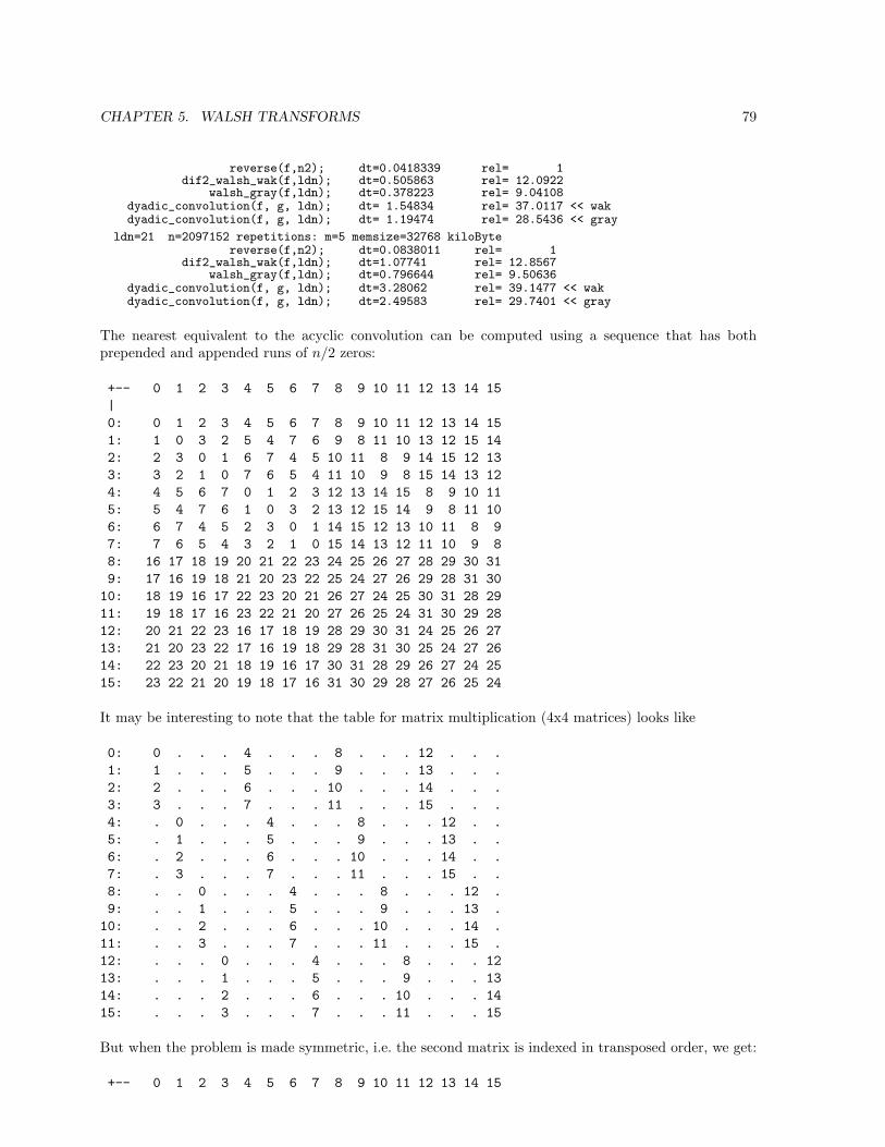
CHAPTER 5. WALSH TRANSFORMS 79
reverse(f,n2); dt=0.0418339 rel= 1dif2_walsh_wak(f,ldn); dt=0.505863 rel= 12.0922
walsh_gray(f,ldn); dt=0.378223 rel= 9.04108dyadic_convolution(f, g, ldn); dt= 1.54834 rel= 37.0117 << wakdyadic_convolution(f, g, ldn); dt= 1.19474 rel= 28.5436 << gray
ldn=21 n=2097152 repetitions: m=5 memsize=32768 kiloBytereverse(f,n2); dt=0.0838011 rel= 1
dif2_walsh_wak(f,ldn); dt=1.07741 rel= 12.8567walsh_gray(f,ldn); dt=0.796644 rel= 9.50636
dyadic_convolution(f, g, ldn); dt=3.28062 rel= 39.1477 << wakdyadic_convolution(f, g, ldn); dt=2.49583 rel= 29.7401 << gray
The nearest equivalent to the acyclic convolution can be computed using a sequence that has bothprepended and appended runs of n/2 zeros:
+-- 0 1 2 3 4 5 6 7 8 9 10 11 12 13 14 15|0: 0 1 2 3 4 5 6 7 8 9 10 11 12 13 14 151: 1 0 3 2 5 4 7 6 9 8 11 10 13 12 15 142: 2 3 0 1 6 7 4 5 10 11 8 9 14 15 12 133: 3 2 1 0 7 6 5 4 11 10 9 8 15 14 13 124: 4 5 6 7 0 1 2 3 12 13 14 15 8 9 10 115: 5 4 7 6 1 0 3 2 13 12 15 14 9 8 11 106: 6 7 4 5 2 3 0 1 14 15 12 13 10 11 8 97: 7 6 5 4 3 2 1 0 15 14 13 12 11 10 9 88: 16 17 18 19 20 21 22 23 24 25 26 27 28 29 30 319: 17 16 19 18 21 20 23 22 25 24 27 26 29 28 31 30
10: 18 19 16 17 22 23 20 21 26 27 24 25 30 31 28 2911: 19 18 17 16 23 22 21 20 27 26 25 24 31 30 29 2812: 20 21 22 23 16 17 18 19 28 29 30 31 24 25 26 2713: 21 20 23 22 17 16 19 18 29 28 31 30 25 24 27 2614: 22 23 20 21 18 19 16 17 30 31 28 29 26 27 24 2515: 23 22 21 20 19 18 17 16 31 30 29 28 27 26 25 24
It may be interesting to note that the table for matrix multiplication (4x4 matrices) looks like
0: 0 . . . 4 . . . 8 . . . 12 . . .1: 1 . . . 5 . . . 9 . . . 13 . . .2: 2 . . . 6 . . . 10 . . . 14 . . .3: 3 . . . 7 . . . 11 . . . 15 . . .4: . 0 . . . 4 . . . 8 . . . 12 . .5: . 1 . . . 5 . . . 9 . . . 13 . .6: . 2 . . . 6 . . . 10 . . . 14 . .7: . 3 . . . 7 . . . 11 . . . 15 . .8: . . 0 . . . 4 . . . 8 . . . 12 .9: . . 1 . . . 5 . . . 9 . . . 13 .
10: . . 2 . . . 6 . . . 10 . . . 14 .11: . . 3 . . . 7 . . . 11 . . . 15 .12: . . . 0 . . . 4 . . . 8 . . . 1213: . . . 1 . . . 5 . . . 9 . . . 1314: . . . 2 . . . 6 . . . 10 . . . 1415: . . . 3 . . . 7 . . . 11 . . . 15
But when the problem is made symmetric, i.e. the second matrix is indexed in transposed order, we get:
+-- 0 1 2 3 4 5 6 7 8 9 10 11 12 13 14 15

CHAPTER 5. WALSH TRANSFORMS 80
|0: 0 . . . 4 . . . 8 . . . 12 . . .1: . 0 . . . 4 . . . 8 . . . 12 . .2: . . 0 . . . 4 . . . 8 . . . 12 .3: . . . 0 . . . 4 . . . 8 . . . 124: 1 . . . 5 . . . 9 . . . 13 . . .5: . 1 . . . 5 . . . 9 . . . 13 . .6: . . 1 . . . 5 . . . 9 . . . 13 .7: . . . 1 . . . 5 . . . 9 . . . 138: 2 . . . 6 . . . 10 . . . 14 . . .9: . 2 . . . 6 . . . 10 . . . 14 . .
10: . . 2 . . . 6 . . . 10 . . . 14 .11: . . . 2 . . . 6 . . . 10 . . . 1412: 3 . . . 7 . . . 11 . . . 15 . . .13: . 3 . . . 7 . . . 11 . . . 15 . .14: . . 3 . . . 7 . . . 11 . . . 15 .15: . . . 3 . . . 7 . . . 11 . . . 15
Thereby dyadic convolution can be used to compute matrix products. The ‘unpolished’ algorithm is∼ n3 · log n as with the FT (-based correlation).
5.3 The slant transform
The slant transform (SLT) can be implemented using a Walsh Transform and just a little pre/post-processing:
void slant(double *f, ulong ldn)// slant transform
walsh_wak(f, ldn);
ulong n = 1<<ldn;for (ulong ldm=0; ldm<ldn-1; ++ldm)
ulong m = 1<<ldm; // m = 1, 2, 4, 8, ..., n/4double N = m*2, N2 = N*N;double a = sqrt(3.0*N2/(4.0*N2-1.0));double b = sqrt(1.0-a*a); // == sqrt((N2-1)/(4*N2-1));for (ulong j=m; j<n-1; j+=4*m)
ulong t1 = j;ulong t2 = j + m;double f1 = f[t1], f2 = f[t2];f[t1] = a * f1 - b * f2;f[t2] = b * f1 + a * f2;
The ldm-loop executes ldn−1 times, the inner loop is executed is n/2 − 1 times. That is, apart fromthe Walsh transform only an amount of work linear with the array size has to be done. [FXT: slant inwalsh/slant.cc]The inverse transform is:
void inverse_slant(double *f, ulong ldn)// inverse of slant()
ulong n = 1<<ldn;ulong ldm=ldn-2;do
ulong m = 1<<ldm; // m = n/4, n/2, ..., 4, 2, 1
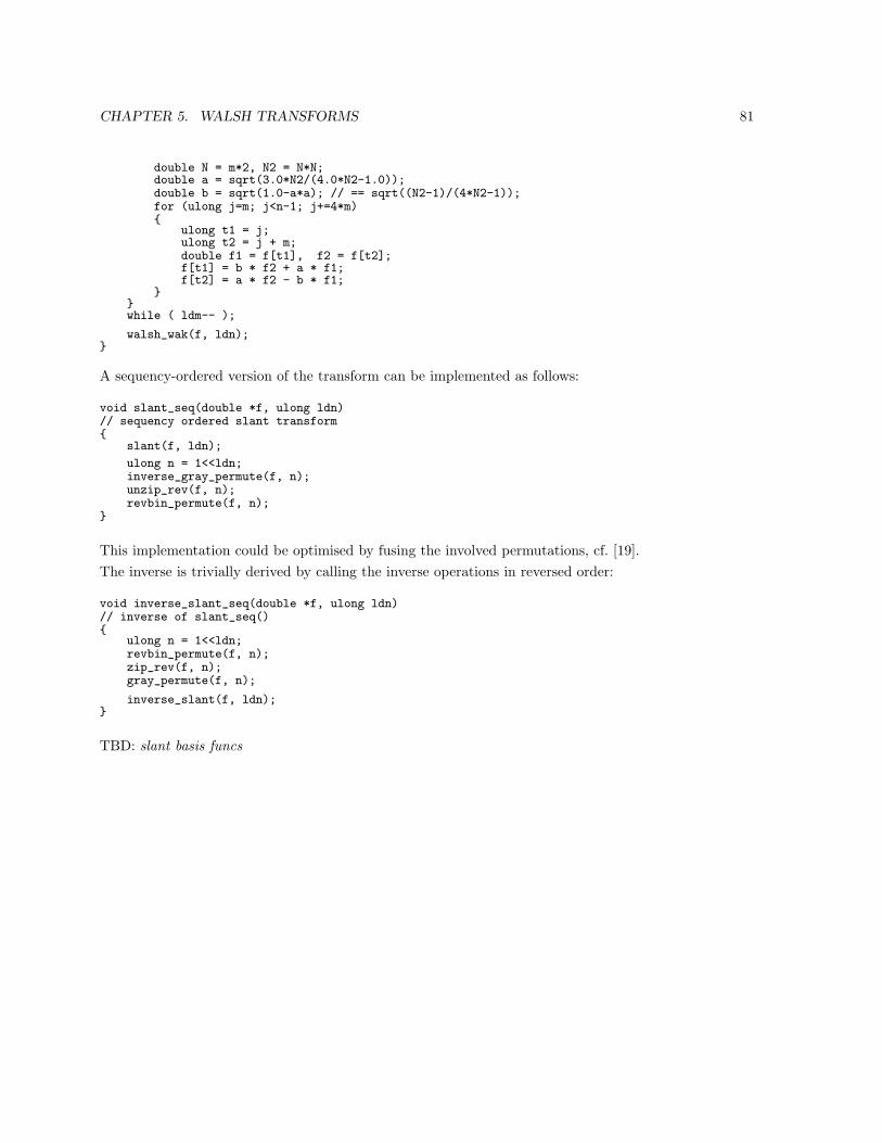
CHAPTER 5. WALSH TRANSFORMS 81
double N = m*2, N2 = N*N;double a = sqrt(3.0*N2/(4.0*N2-1.0));double b = sqrt(1.0-a*a); // == sqrt((N2-1)/(4*N2-1));for (ulong j=m; j<n-1; j+=4*m)
ulong t1 = j;ulong t2 = j + m;double f1 = f[t1], f2 = f[t2];f[t1] = b * f2 + a * f1;f[t2] = a * f2 - b * f1;
while ( ldm-- );
walsh_wak(f, ldn);
A sequency-ordered version of the transform can be implemented as follows:
void slant_seq(double *f, ulong ldn)// sequency ordered slant transform
slant(f, ldn);
ulong n = 1<<ldn;inverse_gray_permute(f, n);unzip_rev(f, n);revbin_permute(f, n);
This implementation could be optimised by fusing the involved permutations, cf. [19].The inverse is trivially derived by calling the inverse operations in reversed order:
void inverse_slant_seq(double *f, ulong ldn)// inverse of slant_seq()
ulong n = 1<<ldn;revbin_permute(f, n);zip_rev(f, n);gray_permute(f, n);
inverse_slant(f, ldn);
TBD: slant basis funcs
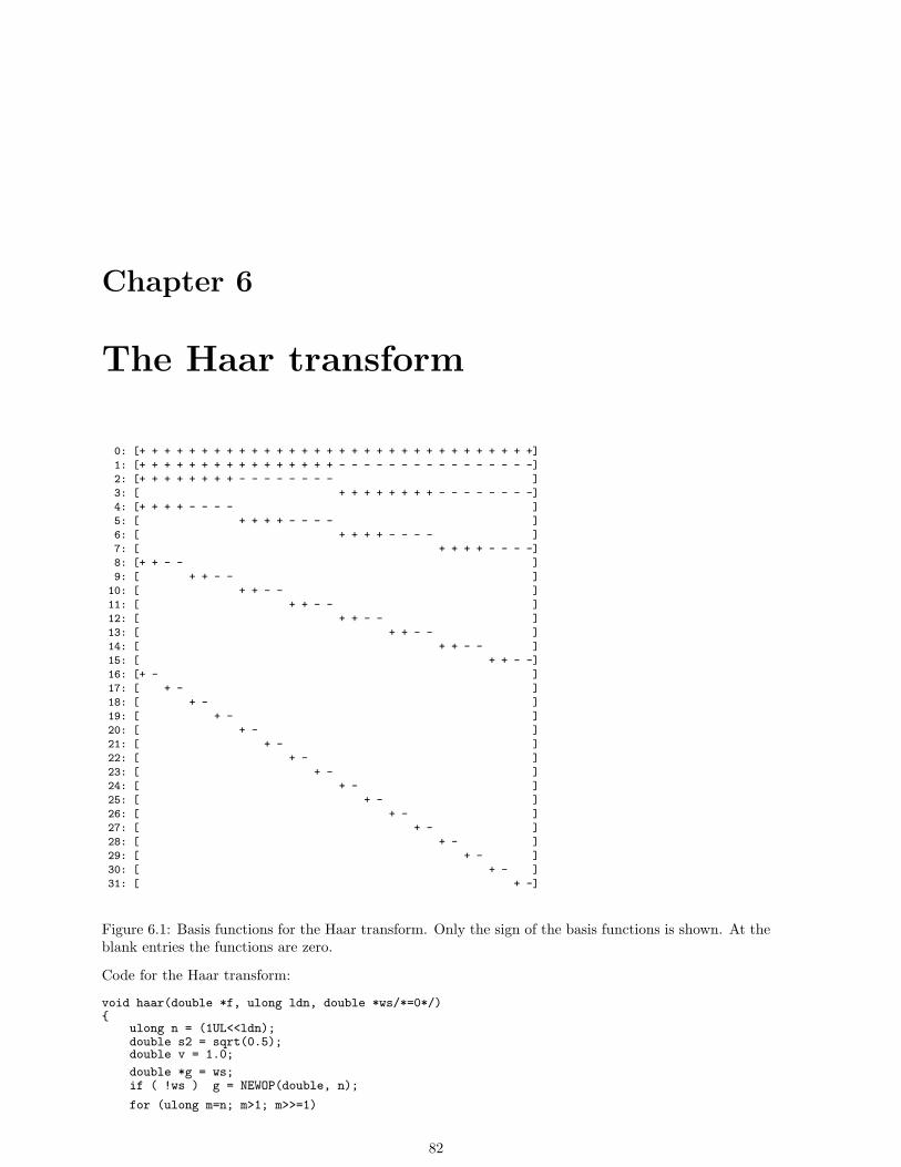
Chapter 6
The Haar transform
0: [+ + + + + + + + + + + + + + + + + + + + + + + + + + + + + + + +]
1: [+ + + + + + + + + + + + + + + + - - - - - - - - - - - - - - - -]
2: [+ + + + + + + + - - - - - - - - ]
3: [ + + + + + + + + - - - - - - - -]
4: [+ + + + - - - - ]
5: [ + + + + - - - - ]
6: [ + + + + - - - - ]
7: [ + + + + - - - -]
8: [+ + - - ]
9: [ + + - - ]
10: [ + + - - ]
11: [ + + - - ]
12: [ + + - - ]
13: [ + + - - ]
14: [ + + - - ]
15: [ + + - -]
16: [+ - ]
17: [ + - ]
18: [ + - ]
19: [ + - ]
20: [ + - ]
21: [ + - ]
22: [ + - ]
23: [ + - ]
24: [ + - ]
25: [ + - ]
26: [ + - ]
27: [ + - ]
28: [ + - ]
29: [ + - ]
30: [ + - ]
31: [ + -]
Figure 6.1: Basis functions for the Haar transform. Only the sign of the basis functions is shown. At theblank entries the functions are zero.
Code for the Haar transform:
void haar(double *f, ulong ldn, double *ws/*=0*/)
ulong n = (1UL<<ldn);double s2 = sqrt(0.5);double v = 1.0;
double *g = ws;if ( !ws ) g = NEWOP(double, n);
for (ulong m=n; m>1; m>>=1)
82
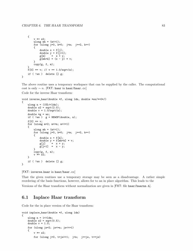
CHAPTER 6. THE HAAR TRANSFORM 83
v *= s2;ulong mh = (m>>1);for (ulong j=0, k=0; j<m; j+=2, k++)
double x = f[j];double y = f[j+1];g[k] = x + y;g[mh+k] = (x - y) * v;
copy(g, f, m);
f[0] *= v; // v == 1.0/sqrt(n);
if ( !ws ) delete [] g;
The above routine uses a temporary workspace that can be supplied by the caller. The computationalcost is only ∼ n. [FXT: haar in haar/haar.cc]Code for the inverse Haar transform:
void inverse_haar(double *f, ulong ldn, double *ws/*=0*/)
ulong n = (1UL<<ldn);double s2 = sqrt(2.0);double v = 1.0/sqrt(n);
double *g = ws;if ( !ws ) g = NEWOP(double, n);
f[0] *= v;for (ulong m=2; m<=n; m<<=1)
ulong mh = (m>>1);for (ulong j=0, k=0; j<m; j+=2, k++)
double x = f[k];double y = f[mh+k] * v;g[j] = x + y;g[j+1] = x - y;
copy(g, f, m);v *= s2;
if ( !ws ) delete [] g;
[FXT: inverse haar in haar/haar.cc]
That the given routines use a temporary storage may be seen as a disadvantage. A rather simplereordering of the basis functions, however, allows for to an in place algorithm. This leads to the
Versions of the Haar transform without normalization are given in [FXT: file haar/haarnn.h].
6.1 Inplace Haar transform
Code for the in place version of the Haar transform:
void inplace_haar(double *f, ulong ldn)
ulong n = 1<<ldn;double s2 = sqrt(0.5);double v = 1.0;
for (ulong js=2; js<=n; js<<=1)
v *= s2;
for (ulong j=0, t=js>>1; j<n; j+=js, t+=js)
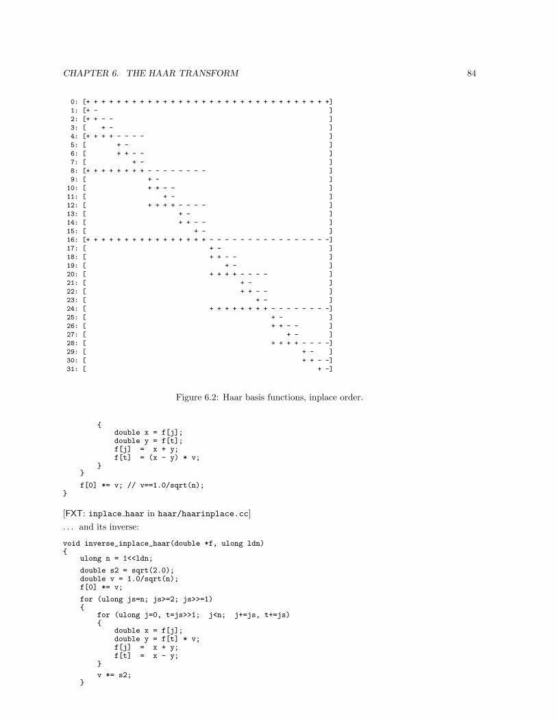
CHAPTER 6. THE HAAR TRANSFORM 84
0: [+ + + + + + + + + + + + + + + + + + + + + + + + + + + + + + + +]
1: [+ - ]
2: [+ + - - ]
3: [ + - ]
4: [+ + + + - - - - ]
5: [ + - ]
6: [ + + - - ]
7: [ + - ]
8: [+ + + + + + + + - - - - - - - - ]
9: [ + - ]
10: [ + + - - ]
11: [ + - ]
12: [ + + + + - - - - ]
13: [ + - ]
14: [ + + - - ]
15: [ + - ]
16: [+ + + + + + + + + + + + + + + + - - - - - - - - - - - - - - - -]
17: [ + - ]
18: [ + + - - ]
19: [ + - ]
20: [ + + + + - - - - ]
21: [ + - ]
22: [ + + - - ]
23: [ + - ]
24: [ + + + + + + + + - - - - - - - -]
25: [ + - ]
26: [ + + - - ]
27: [ + - ]
28: [ + + + + - - - -]
29: [ + - ]
30: [ + + - -]
31: [ + -]
Figure 6.2: Haar basis functions, inplace order.
double x = f[j];double y = f[t];f[j] = x + y;f[t] = (x - y) * v;
f[0] *= v; // v==1.0/sqrt(n);
[FXT: inplace haar in haar/haarinplace.cc]. . . and its inverse:
void inverse_inplace_haar(double *f, ulong ldn)
ulong n = 1<<ldn;
double s2 = sqrt(2.0);double v = 1.0/sqrt(n);f[0] *= v;
for (ulong js=n; js>=2; js>>=1)
for (ulong j=0, t=js>>1; j<n; j+=js, t+=js)
double x = f[j];double y = f[t] * v;f[j] = x + y;f[t] = x - y;
v *= s2;
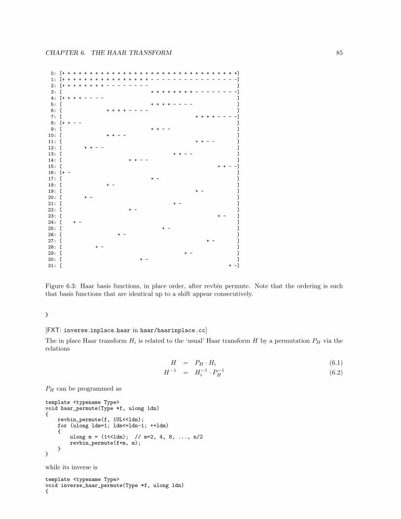
CHAPTER 6. THE HAAR TRANSFORM 85
0: [+ + + + + + + + + + + + + + + + + + + + + + + + + + + + + + + +]
1: [+ + + + + + + + + + + + + + + + - - - - - - - - - - - - - - - -]
2: [+ + + + + + + + - - - - - - - - ]
3: [ + + + + + + + + - - - - - - - -]
4: [+ + + + - - - - ]
5: [ + + + + - - - - ]
6: [ + + + + - - - - ]
7: [ + + + + - - - -]
8: [+ + - - ]
9: [ + + - - ]
10: [ + + - - ]
11: [ + + - - ]
12: [ + + - - ]
13: [ + + - - ]
14: [ + + - - ]
15: [ + + - -]
16: [+ - ]
17: [ + - ]
18: [ + - ]
19: [ + - ]
20: [ + - ]
21: [ + - ]
22: [ + - ]
23: [ + - ]
24: [ + - ]
25: [ + - ]
26: [ + - ]
27: [ + - ]
28: [ + - ]
29: [ + - ]
30: [ + - ]
31: [ + -]
Figure 6.3: Haar basis functions, in place order, after revbin permute. Note that the ordering is suchthat basis functions that are identical up to a shift appear consecutively.
[FXT: inverse inplace haar in haar/haarinplace.cc]
The in place Haar transform Hi is related to the ‘usual’ Haar transform H by a permutation PH via therelations
H = PH ·Hi (6.1)H−1 = H−1
i · P−1H (6.2)
PH can be programmed as
template <typename Type>void haar_permute(Type *f, ulong ldn)
revbin_permute(f, 1UL<<ldn);for (ulong ldm=1; ldm<=ldn-1; ++ldm)
ulong m = (1<<ldm); // m=2, 4, 8, ..., n/2revbin_permute(f+m, m);
while its inverse is
template <typename Type>void inverse_haar_permute(Type *f, ulong ldn)
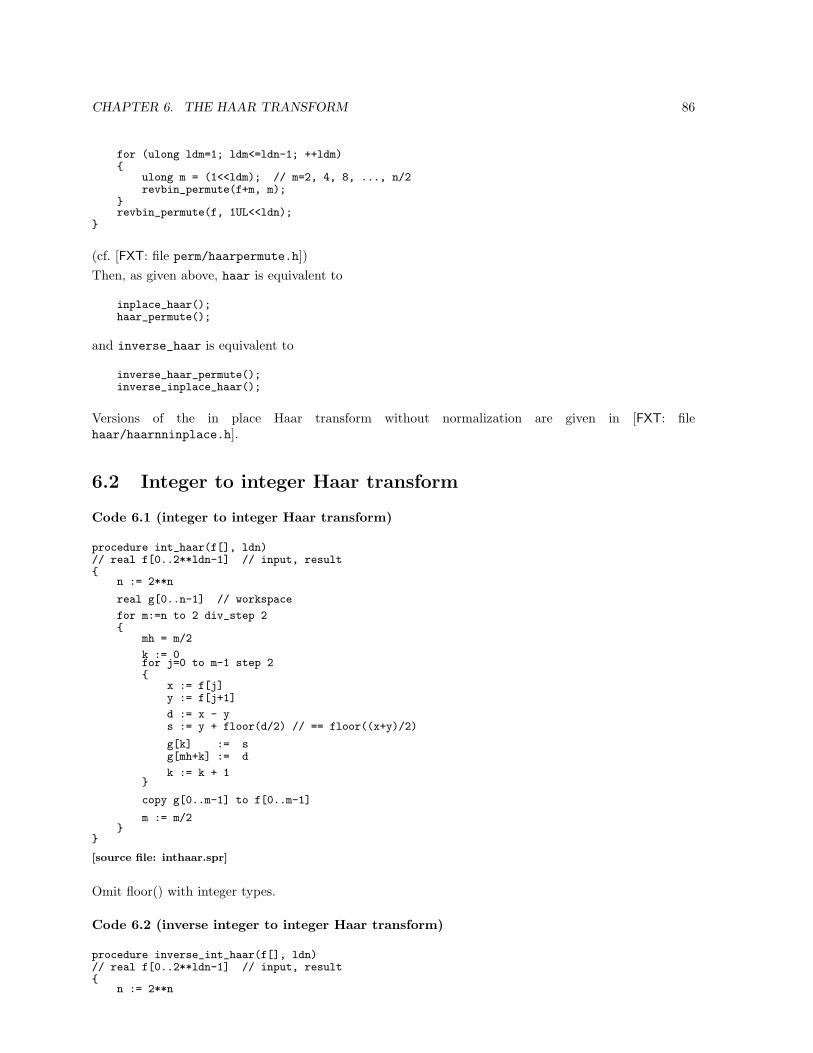
CHAPTER 6. THE HAAR TRANSFORM 86
for (ulong ldm=1; ldm<=ldn-1; ++ldm)
ulong m = (1<<ldm); // m=2, 4, 8, ..., n/2revbin_permute(f+m, m);
revbin_permute(f, 1UL<<ldn);
(cf. [FXT: file perm/haarpermute.h])Then, as given above, haar is equivalent to
inplace_haar();haar_permute();
and inverse_haar is equivalent to
inverse_haar_permute();inverse_inplace_haar();
Versions of the in place Haar transform without normalization are given in [FXT: filehaar/haarnninplace.h].
6.2 Integer to integer Haar transform
Code 6.1 (integer to integer Haar transform)
procedure int_haar(f[], ldn)// real f[0..2**ldn-1] // input, result
n := 2**n
real g[0..n-1] // workspace
for m:=n to 2 div_step 2
mh = m/2
k := 0for j=0 to m-1 step 2
x := f[j]y := f[j+1]
d := x - ys := y + floor(d/2) // == floor((x+y)/2)
g[k] := sg[mh+k] := d
k := k + 1
copy g[0..m-1] to f[0..m-1]
m := m/2
[source file: inthaar.spr]
Omit floor() with integer types.
Code 6.2 (inverse integer to integer Haar transform)
procedure inverse_int_haar(f[], ldn)// real f[0..2**ldn-1] // input, result
n := 2**n
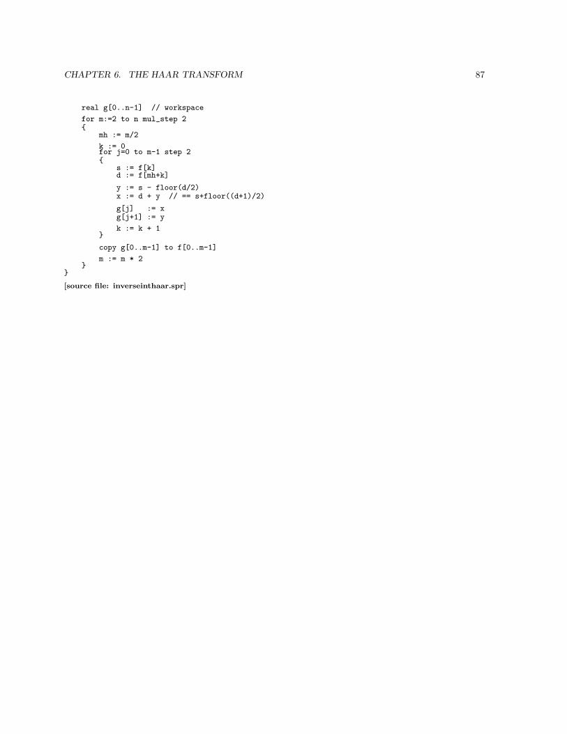
CHAPTER 6. THE HAAR TRANSFORM 87
real g[0..n-1] // workspace
for m:=2 to n mul_step 2
mh := m/2
k := 0for j=0 to m-1 step 2
s := f[k]d := f[mh+k]
y := s - floor(d/2)x := d + y // == s+floor((d+1)/2)
g[j] := xg[j+1] := y
k := k + 1
copy g[0..m-1] to f[0..m-1]
m := m * 2
[source file: inverseinthaar.spr]
Chapter 7
Some bit wizardry
In this chapter low-level functions are presented that operate on the bits of a given input word. It is oftennot obvious what these are good for and I do not attempt much to motivate why particular functionsare here. However, if you happen to have a use for a given routine you will love that it is there: Theprogram using it may run significantly faster.
Throughout this chapter it is assumed that BITS_PER_LONG (and BYTES_PER_LONG) reflect the size of thetype unsigned long which usually is 32 (and 4) on 32 bit architectures, 64 (and 8) on 64 bit machines.[FXT: file auxbit/bitsperlong.h]
Further the type unsigned long is abbreviated as ulong. [FXT: file include/fxttypes.h]
The examples of assembler code are generally for the x86-architecture. They should be simple enough tobe understood also by readers that only know the assembler-mnomics of other CPUs. The listings weregenerated from C-code using gcc’s feature described on page 34.
7.1 Trivia
With twos complement arithmetic (that is: on likely every computer you’ll ever touch) division andmultiplication by powers of two is right and left shift, respectively. This is true for unsigned types andfor multiplication (left shift) with signed types. Division with signed types rounds toward zero, as onewould expect, but right shift is a division (by a power of two) that rounds to minus infinity:
int a = -1;int s = a >> 1; // c == -1int d = a / 2; // d == 0
The compiler still uses a shift instruction for the division, but a ‘fix’ for negative values:
9:test.cc @ int foo(int a)10:test.cc @ 285 0003 8B442410 movl 16(%esp),%eax11:test.cc @ int s = a >> 1;289 0007 89C1 movl %eax,%ecx290 0009 D1F9 sarl $1,%ecx12:test.cc @ int d = a / 2;293 000b 89C2 movl %eax,%edx294 000d C1EA1F shrl $31,%edx // fix: %edx=(%edx<0?1:0)295 0010 01D0 addl %edx,%eax // fix: add one if a<0296 0012 D1F8 sarl $1,%eax
For unsigned types the shift would suffice. One more reason to use unsigned types whenever possible.There are two types of right shifts: a so called logical and an arithmetical shift. The logical version (shrlin the above fragment) always fills the higher bits with zeros, corresponding to division1 of unsigned
1So you can think of it as ‘unsigned arithmetical’ shift.
88

CHAPTER 7. SOME BIT WIZARDRY 89
types. The arithmetical shift (sarl in the above fragment) fills in ones or zeros, according to the mostsignificant bit of the original word. C uses the arithmetical or logical shift according to the operandtypes: This is used in
static inline long min0(long x)// return min(0, x), i.e. return zero for positive input// no restriction on input range
return x & (x >> (BITS_PER_LONG-1));
The trick is that the expression to the right of the “&” is 0 or 111. . . 11 for positive or negative x,respectively (i.e. arithmetical shift is used). With unsigned type the same expression would be 0 or 1according to whether the leftmost bit of x is set.Computing residues modulo a power of two with unsigned types is equivalent to a bit-and using a mask:
ulong a = b % 32; // == b & (32-1)
All of the above is done by the compiler’s optimization wherever possible.Division by constants can be replaced by multiplications and shift. The magic machinery inside thecompiler does it for you:
5:test.cc @ ulong foo(ulong a)6:test.cc @ 7:test.cc @ ulong b = a / 10;
290 0000 8B442404 movl 4(%esp),%eax291 0004 F7250000 mull .LC33 // == 0xcccccccd292 000a 89D0 movl %edx,%eax293 000c C1E803 shrl $3,%eax
Sometimes a good reason to have separate code branches with explicit special values. Similar for modulocomputations with a constant modulus:
8:test.cc @ ulong foo(ulong a)9:test.cc @
53 0000 8B4C2404 movl 4(%esp),%ecx10:test.cc @ ulong b = a % 10000;57 0004 89C8 movl %ecx,%eax58 0006 F7250000 mull .LC0 // == 0xd1b7175959 000c 89D0 movl %edx,%eax60 000e C1E80D shrl $13,%eax61 0011 69C01027 imull $10000,%eax,%eax62 0017 29C1 subl %eax,%ecx63 0019 89C8 movl %ecx,%eax
In order to toggle an integer x between two values a and b do:
precalculate: t = a ^ b;toggle: x ^= t; // a <--> b
the equivalent trick for floats is
precalculate: t = a + b;toggle: x = t - x;
7.2 Operations on low bits/blocks in a word
The following functions are taken from [FXT: file auxbit/bitlow.h].
The underlying idea is that addition/subtraction of 1 always changes a burst of bits at the lower end ofthe word.Isolation of the lowest set bit is achieved via
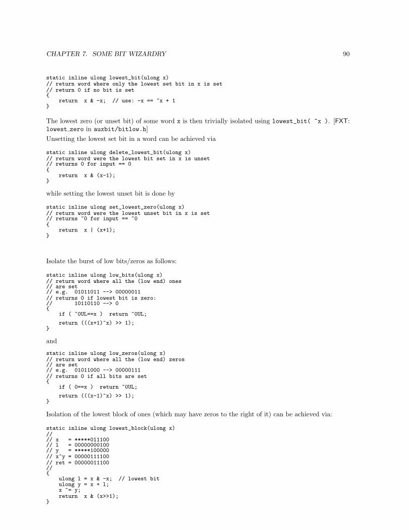
CHAPTER 7. SOME BIT WIZARDRY 90
static inline ulong lowest_bit(ulong x)// return word where only the lowest set bit in x is set// return 0 if no bit is set
return x & -x; // use: -x == ~x + 1
The lowest zero (or unset bit) of some word x is then trivially isolated using lowest_bit( ~x ). [FXT:lowest zero in auxbit/bitlow.h]Unsetting the lowest set bit in a word can be achieved via
static inline ulong delete_lowest_bit(ulong x)// return word were the lowest bit set in x is unset// returns 0 for input == 0
return x & (x-1);
while setting the lowest unset bit is done by
static inline ulong set_lowest_zero(ulong x)// return word were the lowest unset bit in x is set// returns ~0 for input == ~0
return x | (x+1);
Isolate the burst of low bits/zeros as follows:
static inline ulong low_bits(ulong x)// return word where all the (low end) ones// are set// e.g. 01011011 --> 00000011// returns 0 if lowest bit is zero:// 10110110 --> 0
if ( ~0UL==x ) return ~0UL;
return (((x+1)^x) >> 1);
and
static inline ulong low_zeros(ulong x)// return word where all the (low end) zeros// are set// e.g. 01011000 --> 00000111// returns 0 if all bits are set
if ( 0==x ) return ~0UL;
return (((x-1)^x) >> 1);
Isolation of the lowest block of ones (which may have zeros to the right of it) can be achieved via:
static inline ulong lowest_block(ulong x)//// x = *****011100// l = 00000000100// y = *****100000// x^y = 00000111100// ret = 00000011100//
ulong l = x & -x; // lowest bitulong y = x + l;x ^= y;return x & (x>>1);
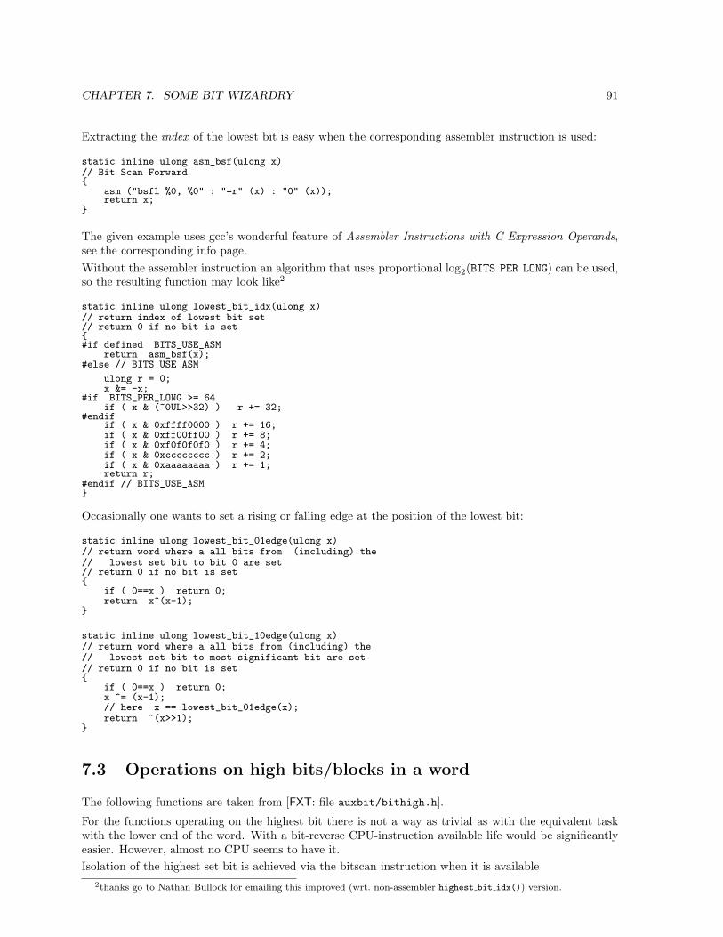
CHAPTER 7. SOME BIT WIZARDRY 91
Extracting the index of the lowest bit is easy when the corresponding assembler instruction is used:
static inline ulong asm_bsf(ulong x)// Bit Scan Forward
asm ("bsfl %0, %0" : "=r" (x) : "0" (x));return x;
The given example uses gcc’s wonderful feature of Assembler Instructions with C Expression Operands,see the corresponding info page.Without the assembler instruction an algorithm that uses proportional log2(BITS PER LONG) can be used,so the resulting function may look like2
static inline ulong lowest_bit_idx(ulong x)// return index of lowest bit set// return 0 if no bit is set#if defined BITS_USE_ASM
return asm_bsf(x);#else // BITS_USE_ASM
ulong r = 0;x &= -x;
#if BITS_PER_LONG >= 64if ( x & (~0UL>>32) ) r += 32;
#endifif ( x & 0xffff0000 ) r += 16;if ( x & 0xff00ff00 ) r += 8;if ( x & 0xf0f0f0f0 ) r += 4;if ( x & 0xcccccccc ) r += 2;if ( x & 0xaaaaaaaa ) r += 1;return r;
#endif // BITS_USE_ASM
Occasionally one wants to set a rising or falling edge at the position of the lowest bit:
static inline ulong lowest_bit_01edge(ulong x)// return word where a all bits from (including) the// lowest set bit to bit 0 are set// return 0 if no bit is set
if ( 0==x ) return 0;return x^(x-1);
static inline ulong lowest_bit_10edge(ulong x)// return word where a all bits from (including) the// lowest set bit to most significant bit are set// return 0 if no bit is set
if ( 0==x ) return 0;x ^= (x-1);// here x == lowest_bit_01edge(x);return ~(x>>1);
7.3 Operations on high bits/blocks in a word
The following functions are taken from [FXT: file auxbit/bithigh.h].
For the functions operating on the highest bit there is not a way as trivial as with the equivalent taskwith the lower end of the word. With a bit-reverse CPU-instruction available life would be significantlyeasier. However, almost no CPU seems to have it.Isolation of the highest set bit is achieved via the bitscan instruction when it is available
2thanks go to Nathan Bullock for emailing this improved (wrt. non-assembler highest bit idx()) version.
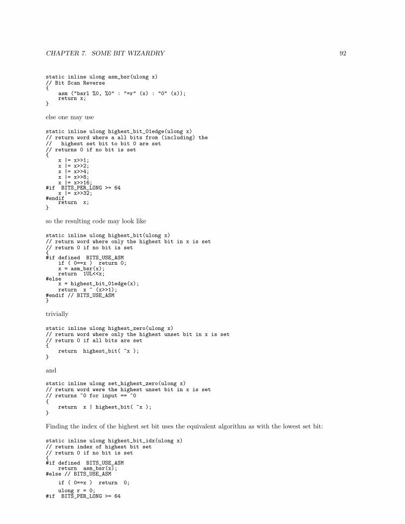
CHAPTER 7. SOME BIT WIZARDRY 92
static inline ulong asm_bsr(ulong x)// Bit Scan Reverse
asm ("bsrl %0, %0" : "=r" (x) : "0" (x));return x;
else one may use
static inline ulong highest_bit_01edge(ulong x)// return word where a all bits from (including) the// highest set bit to bit 0 are set// returns 0 if no bit is set
x |= x>>1;x |= x>>2;x |= x>>4;x |= x>>8;x |= x>>16;
#if BITS_PER_LONG >= 64x |= x>>32;
#endifreturn x;
so the resulting code may look like
static inline ulong highest_bit(ulong x)// return word where only the highest bit in x is set// return 0 if no bit is set#if defined BITS_USE_ASM
if ( 0==x ) return 0;x = asm_bsr(x);return 1UL<<x;
#elsex = highest_bit_01edge(x);return x ^ (x>>1);
#endif // BITS_USE_ASM
trivially
static inline ulong highest_zero(ulong x)// return word where only the highest unset bit in x is set// return 0 if all bits are set
return highest_bit( ~x );
and
static inline ulong set_highest_zero(ulong x)// return word were the highest unset bit in x is set// returns ~0 for input == ~0
return x | highest_bit( ~x );
Finding the index of the highest set bit uses the equivalent algorithm as with the lowest set bit:
static inline ulong highest_bit_idx(ulong x)// return index of highest bit set// return 0 if no bit is set#if defined BITS_USE_ASM
return asm_bsr(x);#else // BITS_USE_ASM
if ( 0==x ) return 0;
ulong r = 0;#if BITS_PER_LONG >= 64
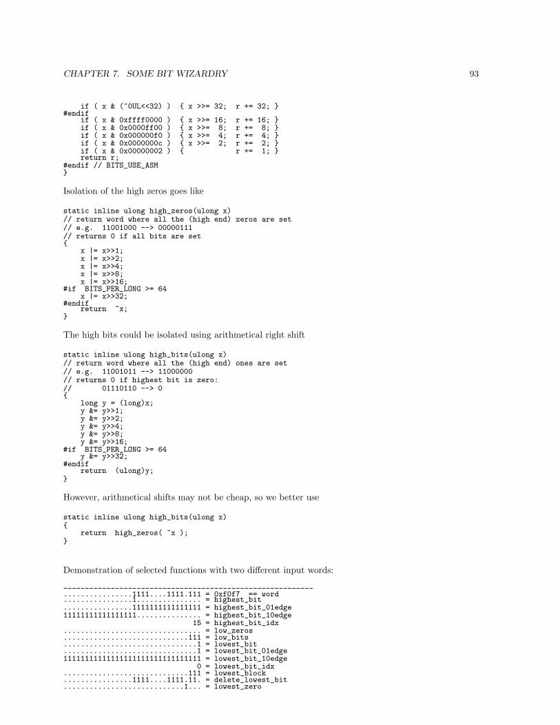
CHAPTER 7. SOME BIT WIZARDRY 93
if ( x & (~0UL<<32) ) x >>= 32; r += 32; #endif
if ( x & 0xffff0000 ) x >>= 16; r += 16; if ( x & 0x0000ff00 ) x >>= 8; r += 8; if ( x & 0x000000f0 ) x >>= 4; r += 4; if ( x & 0x0000000c ) x >>= 2; r += 2; if ( x & 0x00000002 ) r += 1; return r;
#endif // BITS_USE_ASM
Isolation of the high zeros goes like
static inline ulong high_zeros(ulong x)// return word where all the (high end) zeros are set// e.g. 11001000 --> 00000111// returns 0 if all bits are set
x |= x>>1;x |= x>>2;x |= x>>4;x |= x>>8;x |= x>>16;
#if BITS_PER_LONG >= 64x |= x>>32;
#endifreturn ~x;
The high bits could be isolated using arithmetical right shift
static inline ulong high_bits(ulong x)// return word where all the (high end) ones are set// e.g. 11001011 --> 11000000// returns 0 if highest bit is zero:// 01110110 --> 0
long y = (long)x;y &= y>>1;y &= y>>2;y &= y>>4;y &= y>>8;y &= y>>16;
#if BITS_PER_LONG >= 64y &= y>>32;
#endifreturn (ulong)y;
However, arithmetical shifts may not be cheap, so we better use
static inline ulong high_bits(ulong x)
return high_zeros( ~x );
Demonstration of selected functions with two different input words:
----------------------------------------------------------................1111....1111.111 = 0xf0f7 == word................1............... = highest_bit................1111111111111111 = highest_bit_01edge11111111111111111............... = highest_bit_10edge
15 = highest_bit_idx................................ = low_zeros.............................111 = low_bits...............................1 = lowest_bit...............................1 = lowest_bit_01edge11111111111111111111111111111111 = lowest_bit_10edge
0 = lowest_bit_idx.............................111 = lowest_block................1111....1111.11. = delete_lowest_bit............................1... = lowest_zero
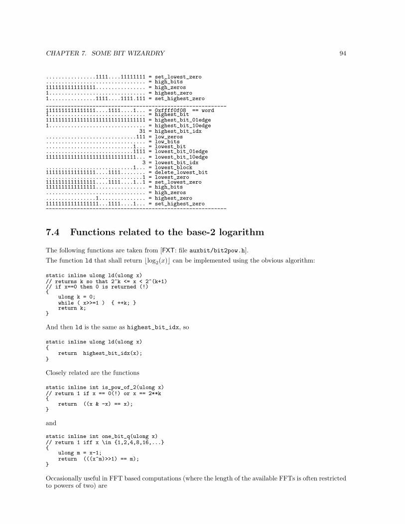
CHAPTER 7. SOME BIT WIZARDRY 94
................1111....11111111 = set_lowest_zero
................................ = high_bits1111111111111111................ = high_zeros1............................... = highest_zero1...............1111....1111.111 = set_highest_zero
----------------------------------------------------------1111111111111111....1111....1... = 0xffff0f08 == word1............................... = highest_bit11111111111111111111111111111111 = highest_bit_01edge1............................... = highest_bit_10edge
31 = highest_bit_idx.............................111 = low_zeros................................ = low_bits............................1... = lowest_bit............................1111 = lowest_bit_01edge11111111111111111111111111111... = lowest_bit_10edge
3 = lowest_bit_idx............................1... = lowest_block1111111111111111....1111........ = delete_lowest_bit...............................1 = lowest_zero1111111111111111....1111....1..1 = set_lowest_zero1111111111111111................ = high_bits................................ = high_zeros................1............... = highest_zero11111111111111111...1111....1... = set_highest_zero----------------------------------------------------------
7.4 Functions related to the base-2 logarithm
The following functions are taken from [FXT: file auxbit/bit2pow.h].
The function ld that shall return blog2(x)c can be implemented using the obvious algorithm:
static inline ulong ld(ulong x)// returns k so that 2^k <= x < 2^(k+1)// if x==0 then 0 is returned (!)
ulong k = 0;while ( x>>=1 ) ++k; return k;
And then ld is the same as highest_bit_idx, so
static inline ulong ld(ulong x)
return highest_bit_idx(x);
Closely related are the functions
static inline int is_pow_of_2(ulong x)// return 1 if x == 0(!) or x == 2**k
return ((x & -x) == x);
and
static inline int one_bit_q(ulong x)// return 1 iff x \in 1,2,4,8,16,...
ulong m = x-1;return (((x^m)>>1) == m);
Occasionally useful in FFT based computations (where the length of the available FFTs is often restrictedto powers of two) are
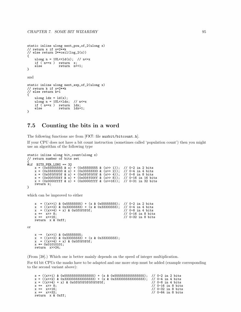
CHAPTER 7. SOME BIT WIZARDRY 95
static inline ulong next_pow_of_2(ulong x)// return x if x=2**k// else return 2**ceil(log_2(x))
ulong n = 1UL<<ld(x); // n<=xif ( n==x ) return x;else return n<<1;
and
static inline ulong next_exp_of_2(ulong x)// return k if x=2**k// else return k+1
ulong ldx = ld(x);ulong n = 1UL<<ldx; // n<=xif ( n==x ) return ldx;else return ldx+1;
7.5 Counting the bits in a word
The following functions are from [FXT: file auxbit/bitcount.h].
If your CPU does not have a bit count instruction (sometimes called ‘population count’) then you mightuse an algorithm of the following type
static inline ulong bit_count(ulong x)// return number of bits set#if BITS_PER_LONG == 32
x = (0x55555555 & x) + (0x55555555 & (x>> 1)); // 0-2 in 2 bitsx = (0x33333333 & x) + (0x33333333 & (x>> 2)); // 0-4 in 4 bitsx = (0x0f0f0f0f & x) + (0x0f0f0f0f & (x>> 4)); // 0-8 in 8 bitsx = (0x00ff00ff & x) + (0x00ff00ff & (x>> 8)); // 0-16 in 16 bitsx = (0x0000ffff & x) + (0x0000ffff & (x>>16)); // 0-31 in 32 bitsreturn x;
which can be improved to either
x = ((x>>1) & 0x55555555) + (x & 0x55555555); // 0-2 in 2 bitsx = ((x>>2) & 0x33333333) + (x & 0x33333333); // 0-4 in 4 bitsx = ((x>>4) + x) & 0x0f0f0f0f; // 0-8 in 4 bitsx += x>> 8; // 0-16 in 8 bitsx += x>>16; // 0-32 in 8 bitsreturn x & 0xff;
or
x -= (x>>1) & 0x55555555;x = ((x>>2) & 0x33333333) + (x & 0x33333333);x = ((x>>4) + x) & 0x0f0f0f0f;x *= 0x01010101;return x>>24;
(From [38].) Which one is better mainly depends on the speed of integer multiplication.
For 64 bit CPUs the masks have to be adapted and one more step must be added (example correspondingto the second variant above):
x = ((x>>1) & 0x5555555555555555) + (x & 0x5555555555555555); // 0-2 in 2 bitsx = ((x>>2) & 0x3333333333333333) + (x & 0x3333333333333333); // 0-4 in 4 bitsx = ((x>>4) + x) & 0x0f0f0f0f0f0f0f0f; // 0-8 in 4 bitsx += x>> 8; // 0-16 in 8 bitsx += x>>16; // 0-32 in 8 bitsx += x>>32; // 0-64 in 8 bitsreturn x & 0xff;
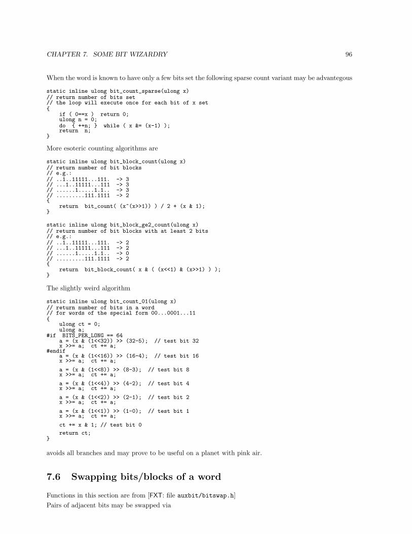
CHAPTER 7. SOME BIT WIZARDRY 96
When the word is known to have only a few bits set the following sparse count variant may be advantegous
static inline ulong bit_count_sparse(ulong x)// return number of bits set// the loop will execute once for each bit of x set
if ( 0==x ) return 0;ulong n = 0;do ++n; while ( x &= (x-1) );return n;
More esoteric counting algorithms are
static inline ulong bit_block_count(ulong x)// return number of bit blocks// e.g.:// ..1..11111...111. -> 3// ...1..11111...111 -> 3// ......1.....1.1.. -> 3// .........111.1111 -> 2
return bit_count( (x^(x>>1)) ) / 2 + (x & 1);
static inline ulong bit_block_ge2_count(ulong x)// return number of bit blocks with at least 2 bits// e.g.:// ..1..11111...111. -> 2// ...1..11111...111 -> 2// ......1.....1.1.. -> 0// .........111.1111 -> 2
return bit_block_count( x & ( (x<<1) & (x>>1) ) );
The slightly weird algorithm
static inline ulong bit_count_01(ulong x)// return number of bits in a word// for words of the special form 00...0001...11
ulong ct = 0;ulong a;
#if BITS_PER_LONG == 64a = (x & (1<<32)) >> (32-5); // test bit 32x >>= a; ct += a;
#endifa = (x & (1<<16)) >> (16-4); // test bit 16x >>= a; ct += a;
a = (x & (1<<8)) >> (8-3); // test bit 8x >>= a; ct += a;
a = (x & (1<<4)) >> (4-2); // test bit 4x >>= a; ct += a;
a = (x & (1<<2)) >> (2-1); // test bit 2x >>= a; ct += a;
a = (x & (1<<1)) >> (1-0); // test bit 1x >>= a; ct += a;
ct += x & 1; // test bit 0
return ct;
avoids all branches and may prove to be useful on a planet with pink air.
7.6 Swapping bits/blocks of a word
Functions in this section are from [FXT: file auxbit/bitswap.h]Pairs of adjacent bits may be swapped via
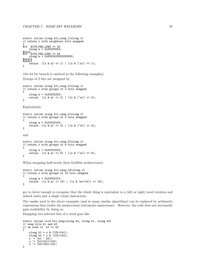
CHAPTER 7. SOME BIT WIZARDRY 97
static inline ulong bit_swap_1(ulong x)// return x with neighbour bits swapped#if BITS_PER_LONG == 32
ulong m = 0x55555555;#else#if BITS_PER_LONG == 64
ulong m = 0x5555555555555555;#endif#endif
return ((x & m) << 1) | ((x & (~m)) >> 1);
(the 64 bit branch is omitted in the following examples).Groups of 2 bits are swapped by
static inline ulong bit_swap_2(ulong x)// return x with groups of 2 bits swapped
ulong m = 0x33333333;return ((x & m) << 2) | ((x & (~m)) >> 2);
Equivalently,
static inline ulong bit_swap_4(ulong x)// return x with groups of 4 bits swapped
ulong m = 0x0f0f0f0f;return ((x & m) << 4) | ((x & (~m)) >> 4);
and
static inline ulong bit_swap_8(ulong x)// return x with groups of 8 bits swapped
ulong m = 0x00ff00ff;return ((x & m) << 8) | ((x & (~m)) >> 8);
When swapping half-words (here for32bit architectures)
static inline ulong bit_swap_16(ulong x)// return x with groups of 16 bits swapped
ulong m = 0x0000ffff;return ((x & m) << 16) | ((x & (m<<16)) >> 16);
gcc is clever enough to recognize that the whole thing is equivalent to a (left or right) word rotation andindeed emits just a single rotate instruction.
The masks used in the above examples (and in many similar algorithms) can be replaced by arithmeticexpressions that render the preprocessor statements unnecessary. However, the code does not necessarilygain readability by doing so.Swapping two selected bits of a word goes like
static inline void bit_swap(ulong &x, ulong k1, ulong k2)// swap bits k1 and k2// ok even if k1 == k2
ulong b1 = x & (1UL<<k1);ulong b2 = x & (1UL<<k2);x ^= (b1 ^ b2);x ^= (b1>>k1)<<k2;x ^= (b2>>k2)<<k1;
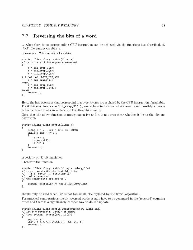
CHAPTER 7. SOME BIT WIZARDRY 98
7.7 Reversing the bits of a word
. . . when there is no corresponding CPU instruction can be achieved via the functions just described, cf.[FXT: file auxbit/revbin.h]Shown is a 32 bit version of revbin:
static inline ulong revbin(ulong x)// return x with bitsequence reversed
x = bit_swap_1(x);x = bit_swap_2(x);x = bit_swap_4(x);
#if defined BITS_USE_ASMx = asm_bswap(x);
#elsex = bit_swap_8(x);x = bit_swap_16(x);
#endifreturn x;
Here, the last two steps that correspond to a byte-reverse are replaced by the CPU instruction if available.For 64 bit machines a x = bit_swap_32(x); would have to be inserted at the end (and possibly a bswap-branch entered that can replace the last three bit_swaps).Note that the above function is pretty expensive and it is not even clear whether it beats the obviousalgorithm,
static inline ulong revbin(ulong x)
ulong r = 0, ldn = BITS_PER_LONG;while ( ldn-- != 0 )
r <<= 1;r += (x&1);x >>= 1;
return r;
especially on 32 bit machines.Therefore the function
static inline ulong revbin(ulong x, ulong ldn)// return word with the last ldn bits// (i.e. bit_0 ... bit_ldn-1)// of x reversed// the other bits are set to 0
return revbin(x) >> (BITS_PER_LONG-ldn);
should only be used when ldn is not too small, else replaced by the trivial algorithm.For practical computations the bit-reversed words usually have to be generated in the (reversed) countingorder and there is a significantly cheaper way to do the update:
static inline ulong revbin_update(ulong r, ulong ldn)// let r = revbin(x, ld(n)) at entry// then return revbin(x+1, ld(n))
ldn >>= 1;while ( !((r^=ldn)&ldn) ) ldn >>= 1;return r;
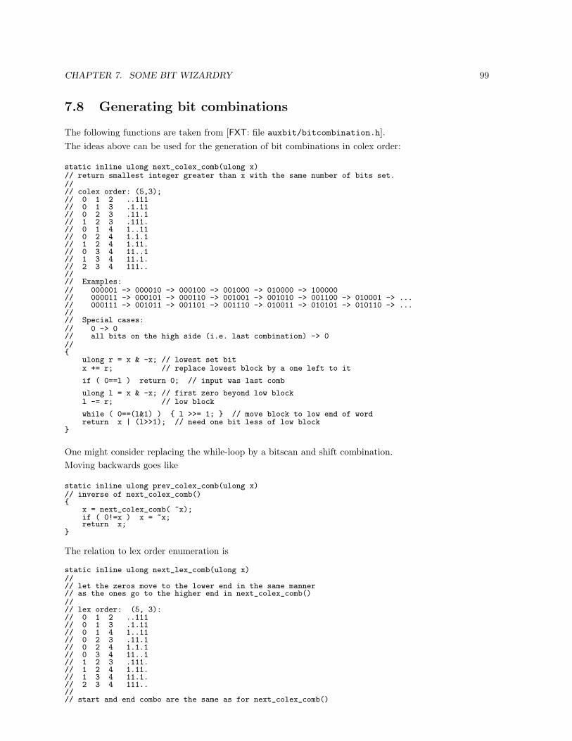
CHAPTER 7. SOME BIT WIZARDRY 99
7.8 Generating bit combinations
The following functions are taken from [FXT: file auxbit/bitcombination.h].The ideas above can be used for the generation of bit combinations in colex order:
static inline ulong next_colex_comb(ulong x)// return smallest integer greater than x with the same number of bits set.//// colex order: (5,3);// 0 1 2 ..111// 0 1 3 .1.11// 0 2 3 .11.1// 1 2 3 .111.// 0 1 4 1..11// 0 2 4 1.1.1// 1 2 4 1.11.// 0 3 4 11..1// 1 3 4 11.1.// 2 3 4 111..//// Examples:// 000001 -> 000010 -> 000100 -> 001000 -> 010000 -> 100000// 000011 -> 000101 -> 000110 -> 001001 -> 001010 -> 001100 -> 010001 -> ...// 000111 -> 001011 -> 001101 -> 001110 -> 010011 -> 010101 -> 010110 -> ...//// Special cases:// 0 -> 0// all bits on the high side (i.e. last combination) -> 0//
ulong r = x & -x; // lowest set bitx += r; // replace lowest block by a one left to it
if ( 0==l ) return 0; // input was last comb
ulong l = x & -x; // first zero beyond low blockl -= r; // low block
while ( 0==(l&1) ) l >>= 1; // move block to low end of wordreturn x | (l>>1); // need one bit less of low block
One might consider replacing the while-loop by a bitscan and shift combination.Moving backwards goes like
static inline ulong prev_colex_comb(ulong x)// inverse of next_colex_comb()
x = next_colex_comb( ~x);if ( 0!=x ) x = ~x;return x;
The relation to lex order enumeration is
static inline ulong next_lex_comb(ulong x)//// let the zeros move to the lower end in the same manner// as the ones go to the higher end in next_colex_comb()//// lex order: (5, 3):// 0 1 2 ..111// 0 1 3 .1.11// 0 1 4 1..11// 0 2 3 .11.1// 0 2 4 1.1.1// 0 3 4 11..1// 1 2 3 .111.// 1 2 4 1.11.// 1 3 4 11.1.// 2 3 4 111..//// start and end combo are the same as for next_colex_comb()
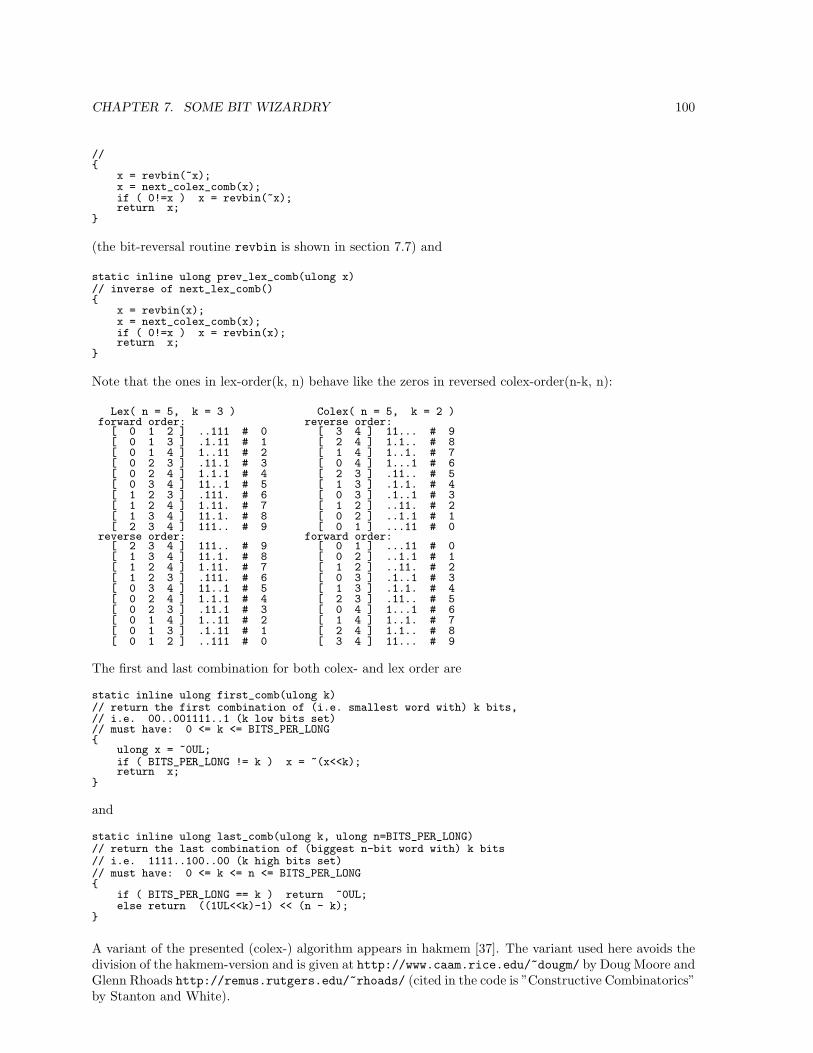
CHAPTER 7. SOME BIT WIZARDRY 100
//
x = revbin(~x);x = next_colex_comb(x);if ( 0!=x ) x = revbin(~x);return x;
(the bit-reversal routine revbin is shown in section 7.7) and
static inline ulong prev_lex_comb(ulong x)// inverse of next_lex_comb()
x = revbin(x);x = next_colex_comb(x);if ( 0!=x ) x = revbin(x);return x;
Note that the ones in lex-order(k, n) behave like the zeros in reversed colex-order(n-k, n):
Lex( n = 5, k = 3 ) Colex( n = 5, k = 2 )forward order: reverse order:
[ 0 1 2 ] ..111 # 0 [ 3 4 ] 11... # 9[ 0 1 3 ] .1.11 # 1 [ 2 4 ] 1.1.. # 8[ 0 1 4 ] 1..11 # 2 [ 1 4 ] 1..1. # 7[ 0 2 3 ] .11.1 # 3 [ 0 4 ] 1...1 # 6[ 0 2 4 ] 1.1.1 # 4 [ 2 3 ] .11.. # 5[ 0 3 4 ] 11..1 # 5 [ 1 3 ] .1.1. # 4[ 1 2 3 ] .111. # 6 [ 0 3 ] .1..1 # 3[ 1 2 4 ] 1.11. # 7 [ 1 2 ] ..11. # 2[ 1 3 4 ] 11.1. # 8 [ 0 2 ] ..1.1 # 1[ 2 3 4 ] 111.. # 9 [ 0 1 ] ...11 # 0
reverse order: forward order:[ 2 3 4 ] 111.. # 9 [ 0 1 ] ...11 # 0[ 1 3 4 ] 11.1. # 8 [ 0 2 ] ..1.1 # 1[ 1 2 4 ] 1.11. # 7 [ 1 2 ] ..11. # 2[ 1 2 3 ] .111. # 6 [ 0 3 ] .1..1 # 3[ 0 3 4 ] 11..1 # 5 [ 1 3 ] .1.1. # 4[ 0 2 4 ] 1.1.1 # 4 [ 2 3 ] .11.. # 5[ 0 2 3 ] .11.1 # 3 [ 0 4 ] 1...1 # 6[ 0 1 4 ] 1..11 # 2 [ 1 4 ] 1..1. # 7[ 0 1 3 ] .1.11 # 1 [ 2 4 ] 1.1.. # 8[ 0 1 2 ] ..111 # 0 [ 3 4 ] 11... # 9
The first and last combination for both colex- and lex order are
static inline ulong first_comb(ulong k)// return the first combination of (i.e. smallest word with) k bits,// i.e. 00..001111..1 (k low bits set)// must have: 0 <= k <= BITS_PER_LONG
ulong x = ~0UL;if ( BITS_PER_LONG != k ) x = ~(x<<k);return x;
and
static inline ulong last_comb(ulong k, ulong n=BITS_PER_LONG)// return the last combination of (biggest n-bit word with) k bits// i.e. 1111..100..00 (k high bits set)// must have: 0 <= k <= n <= BITS_PER_LONG
if ( BITS_PER_LONG == k ) return ~0UL;else return ((1UL<<k)-1) << (n - k);
A variant of the presented (colex-) algorithm appears in hakmem [37]. The variant used here avoids thedivision of the hakmem-version and is given at http://www.caam.rice.edu/~dougm/ by Doug Moore andGlenn Rhoads http://remus.rutgers.edu/~rhoads/ (cited in the code is ”Constructive Combinatorics”by Stanton and White).
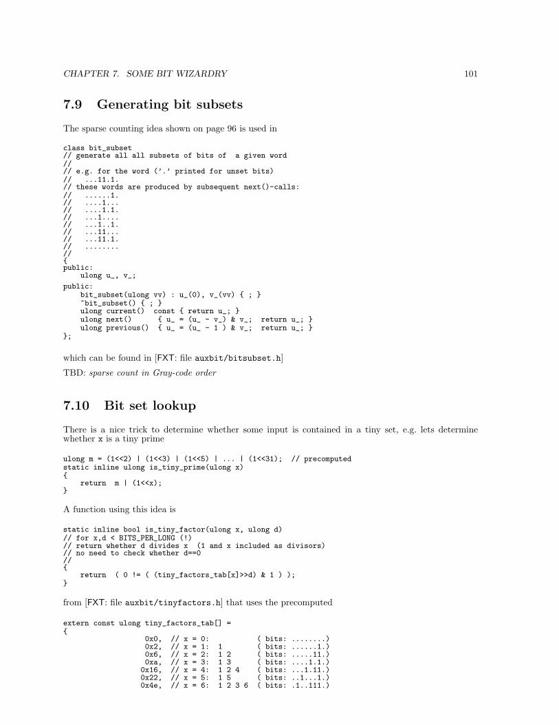
CHAPTER 7. SOME BIT WIZARDRY 101
7.9 Generating bit subsets
The sparse counting idea shown on page 96 is used in
class bit_subset// generate all all subsets of bits of a given word//// e.g. for the word (’.’ printed for unset bits)// ...11.1.// these words are produced by subsequent next()-calls:// ......1.// ....1...// ....1.1.// ...1....// ...1..1.// ...11...// ...11.1.// ........//public:
ulong u_, v_;
public:bit_subset(ulong vv) : u_(0), v_(vv) ; ~bit_subset() ; ulong current() const return u_; ulong next() u_ = (u_ - v_) & v_; return u_; ulong previous() u_ = (u_ - 1 ) & v_; return u_;
;
which can be found in [FXT: file auxbit/bitsubset.h]
TBD: sparse count in Gray-code order
7.10 Bit set lookup
There is a nice trick to determine whether some input is contained in a tiny set, e.g. lets determinewhether x is a tiny prime
ulong m = (1<<2) | (1<<3) | (1<<5) | ... | (1<<31); // precomputedstatic inline ulong is_tiny_prime(ulong x)
return m | (1<<x);
A function using this idea is
static inline bool is_tiny_factor(ulong x, ulong d)// for x,d < BITS_PER_LONG (!)// return whether d divides x (1 and x included as divisors)// no need to check whether d==0//
return ( 0 != ( (tiny_factors_tab[x]>>d) & 1 ) );
from [FXT: file auxbit/tinyfactors.h] that uses the precomputed
extern const ulong tiny_factors_tab[] =
0x0, // x = 0: ( bits: ........)0x2, // x = 1: 1 ( bits: ......1.)0x6, // x = 2: 1 2 ( bits: .....11.)0xa, // x = 3: 1 3 ( bits: ....1.1.)
0x16, // x = 4: 1 2 4 ( bits: ...1.11.)0x22, // x = 5: 1 5 ( bits: ..1...1.)0x4e, // x = 6: 1 2 3 6 ( bits: .1..111.)
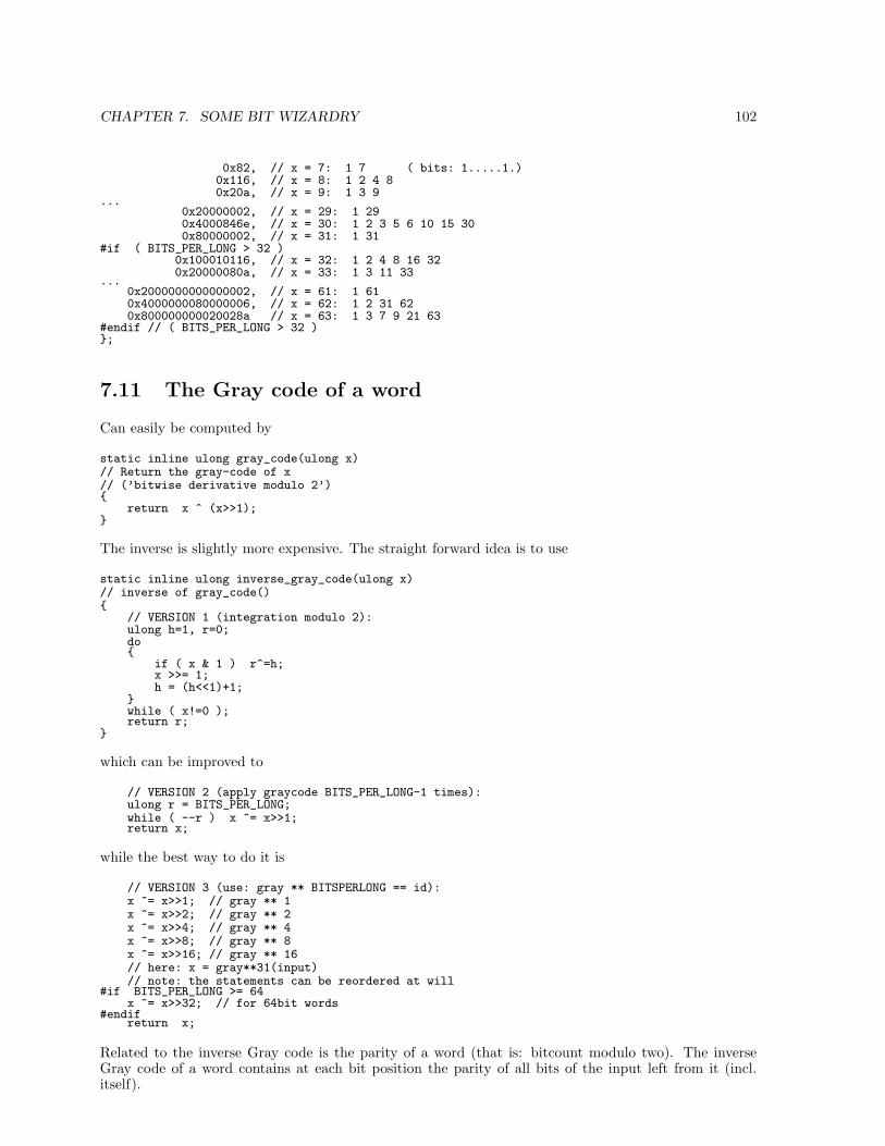
CHAPTER 7. SOME BIT WIZARDRY 102
0x82, // x = 7: 1 7 ( bits: 1.....1.)0x116, // x = 8: 1 2 4 80x20a, // x = 9: 1 3 9
...0x20000002, // x = 29: 1 290x4000846e, // x = 30: 1 2 3 5 6 10 15 300x80000002, // x = 31: 1 31
#if ( BITS_PER_LONG > 32 )0x100010116, // x = 32: 1 2 4 8 16 320x20000080a, // x = 33: 1 3 11 33
...0x2000000000000002, // x = 61: 1 610x4000000080000006, // x = 62: 1 2 31 620x800000000020028a // x = 63: 1 3 7 9 21 63
#endif // ( BITS_PER_LONG > 32 );
7.11 The Gray code of a word
Can easily be computed by
static inline ulong gray_code(ulong x)// Return the gray-code of x// (’bitwise derivative modulo 2’)
return x ^ (x>>1);
The inverse is slightly more expensive. The straight forward idea is to use
static inline ulong inverse_gray_code(ulong x)// inverse of gray_code()
// VERSION 1 (integration modulo 2):ulong h=1, r=0;do
if ( x & 1 ) r^=h;x >>= 1;h = (h<<1)+1;
while ( x!=0 );return r;
which can be improved to
// VERSION 2 (apply graycode BITS_PER_LONG-1 times):ulong r = BITS_PER_LONG;while ( --r ) x ^= x>>1;return x;
while the best way to do it is
// VERSION 3 (use: gray ** BITSPERLONG == id):x ^= x>>1; // gray ** 1x ^= x>>2; // gray ** 2x ^= x>>4; // gray ** 4x ^= x>>8; // gray ** 8x ^= x>>16; // gray ** 16// here: x = gray**31(input)// note: the statements can be reordered at will
#if BITS_PER_LONG >= 64x ^= x>>32; // for 64bit words
#endifreturn x;
Related to the inverse Gray code is the parity of a word (that is: bitcount modulo two). The inverseGray code of a word contains at each bit position the parity of all bits of the input left from it (incl.itself).
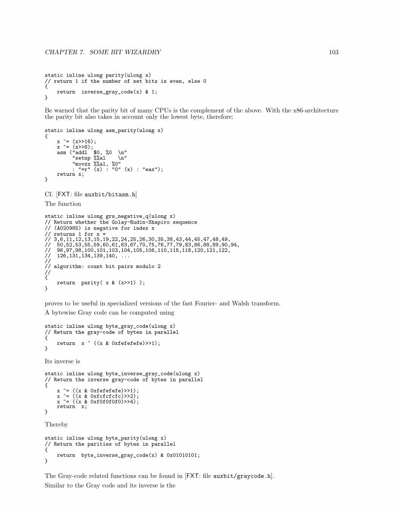
CHAPTER 7. SOME BIT WIZARDRY 103
static inline ulong parity(ulong x)// return 1 if the number of set bits is even, else 0
return inverse_gray_code(x) & 1;
Be warned that the parity bit of many CPUs is the complement of the above. With the x86-architecturethe parity bit also takes in account only the lowest byte, therefore:
static inline ulong asm_parity(ulong x)
x ^= (x>>16);x ^= (x>>8);asm ("addl $0, %0 \n"
"setnp %%al \n""movzx %%al, %0": "=r" (x) : "0" (x) : "eax");
return x;
Cf. [FXT: file auxbit/bitasm.h]The function
static inline ulong grs_negative_q(ulong x)// Return whether the Golay-Rudin-Shapiro sequence// (A020985) is negative for index x// returns 1 for x =// 3,6,11,12,13,15,19,22,24,25,26,30,35,38,43,44,45,47,48,49,// 50,52,53,55,59,60,61,63,67,70,75,76,77,79,83,86,88,89,90,94,// 96,97,98,100,101,103,104,105,106,110,115,118,120,121,122,// 126,131,134,139,140, ...//// algorithm: count bit pairs modulo 2//
return parity( x & (x>>1) );
proves to be useful in specialized versions of the fast Fourier- and Walsh transform.A bytewise Gray code can be computed using
static inline ulong byte_gray_code(ulong x)// Return the gray-code of bytes in parallel
return x ^ ((x & 0xfefefefe)>>1);
Its inverse is
static inline ulong byte_inverse_gray_code(ulong x)// Return the inverse gray-code of bytes in parallel
x ^= ((x & 0xfefefefe)>>1);x ^= ((x & 0xfcfcfcfc)>>2);x ^= ((x & 0xf0f0f0f0)>>4);return x;
Thereby
static inline ulong byte_parity(ulong x)// Return the parities of bytes in parallel
return byte_inverse_gray_code(x) & 0x01010101;
The Gray-code related functions can be found in [FXT: file auxbit/graycode.h].Similar to the Gray code and its inverse is the
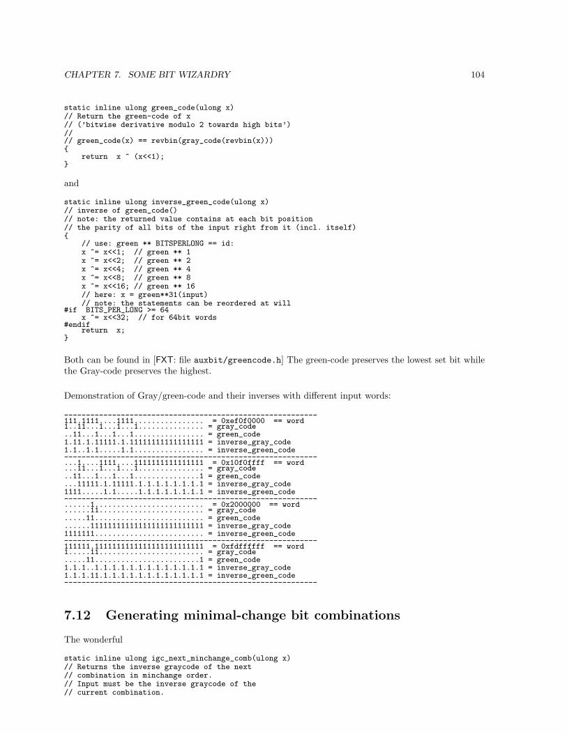
CHAPTER 7. SOME BIT WIZARDRY 104
static inline ulong green_code(ulong x)// Return the green-code of x// (’bitwise derivative modulo 2 towards high bits’)//// green_code(x) == revbin(gray_code(revbin(x)))
return x ^ (x<<1);
and
static inline ulong inverse_green_code(ulong x)// inverse of green_code()// note: the returned value contains at each bit position// the parity of all bits of the input right from it (incl. itself)
// use: green ** BITSPERLONG == id:x ^= x<<1; // green ** 1x ^= x<<2; // green ** 2x ^= x<<4; // green ** 4x ^= x<<8; // green ** 8x ^= x<<16; // green ** 16// here: x = green**31(input)// note: the statements can be reordered at will
#if BITS_PER_LONG >= 64x ^= x<<32; // for 64bit words
#endifreturn x;
Both can be found in [FXT: file auxbit/greencode.h] The green-code preserves the lowest set bit whilethe Gray-code preserves the highest.
Demonstration of Gray/green-code and their inverses with different input words:
----------------------------------------------------------111.1111....1111................ = 0xef0f0000 == word1..11...1...1...1............... = gray_code..11...1...1...1................ = green_code1.11.1.11111.1.11111111111111111 = inverse_gray_code1.1..1.1.....1.1................ = inverse_green_code----------------------------------------------------------...1....1111....1111111111111111 = 0x10f0ffff == word...11...1...1...1............... = gray_code..11...1...1...1...............1 = green_code...11111.1.11111.1.1.1.1.1.1.1.1 = inverse_gray_code1111.....1.1.....1.1.1.1.1.1.1.1 = inverse_green_code----------------------------------------------------------......1......................... = 0x2000000 == word......11........................ = gray_code.....11......................... = green_code......11111111111111111111111111 = inverse_gray_code1111111......................... = inverse_green_code----------------------------------------------------------111111.1111111111111111111111111 = 0xfdffffff == word1.....11........................ = gray_code.....11........................1 = green_code1.1.1..1.1.1.1.1.1.1.1.1.1.1.1.1 = inverse_gray_code1.1.1.11.1.1.1.1.1.1.1.1.1.1.1.1 = inverse_green_code----------------------------------------------------------
7.12 Generating minimal-change bit combinations
The wonderful
static inline ulong igc_next_minchange_comb(ulong x)// Returns the inverse graycode of the next// combination in minchange order.// Input must be the inverse graycode of the// current combination.
CHAPTER 7. SOME BIT WIZARDRY 105
ulong g = green_code(x);ulong i = 2;ulong cb; // ==candidateBits;do
ulong y = (x & ~(i-1)) + i;ulong j = lowest_bit(y) << 1;ulong h = !!(y & j);cb = ((j-h) ^ g) & (j-i);i = j;
while ( 0==cb );
return x + lowest_bit(cb);
together with
static inline ulong igc_last_comb(ulong k, ulong n)// return the (inverse graycode of the) last combination// as in igc_next_minchange_comb()
if ( 0==k ) return 0;else return ((1UL<<n) - 1) ^ (((1UL<<k) - 1) / 3);
could be used as demonstrated in
static inline ulong next_minchange_comb(ulong x, ulong last)// not efficient, just to explain the usage// of igc_next_minchange_comb()// Must have: last==igc_last_comb(k, n)//// Example with k==3, n==5:// x inverse_gray_code(x)// ..111 ..1.1 == first_sequency(k)// .11.1 .1..1// .111. .1.11// .1.11 .11.1// 11..1 1...1// 11.1. 1..11// 111.. 1.111// 1.1.1 11..1// 1.11. 11.11// 1..11 111.1 == igc_last_comb(k, n)
x = inverse_gray_code(x);if ( x==last ) return 0;x = igc_next_minchange_comb(x);return gray_code(x);
Each combination is different from the preceding one in exactly two positions. The same run of bitcom-binations could be obtained by going through the Gray codes and omitting all words where the bitcountis 6= k. The algorithm shown here, however, is much more efficient.For reasons of efficiency one may prefer code as
ulong last = igc_last_comb(k, n);ulong c, nc = first_sequency(k);do
c = nc;nc = igc_next_minchange_comb(c);ulong g = gray_code(c);// Here g contains the bitcombination
while ( c!=last );
which avoids the repeated computation of the inverse Gray code.
CHAPTER 7. SOME BIT WIZARDRY 106
As Doug Moore explains [priv.comm.], the algorithm in igc next minchange comb uses the fact that thedifference of two (inverse gray codes of) successive combinations is always a power of two. Using thisobservation one can derive a different version that checks the pattern of the change:
static inline ulong igc_next_minchange_comb(ulong x)// Alternative version.// Amortized time = O(1).
ulong gx = gray_code( x );ulong y, i = 2;do
y = x + i;ulong gy = gray_code( y );ulong r = gx ^ gy;
// Check that change consists of exactly one bit// of the new and one bit of the old pattern:if ( is_pow_of_2( r & gy ) && is_pow_of_2( r & gx ) ) break;// is_pow_of_2(x):=((x & -x) == x) returns 1 also for x==0.// But this cannot happen for both tests at the same time
i <<= 1;while ( 1 );return y;
Still another version which needs k, the number of set bits, as a second parameter:
static inline ulong igc_next_minchange_comb(ulong x, ulong k)// Alternative version, uses the fact that the difference// of two successive x is the smallest possible power of 2.// Should be fast if the CPU has a bitcount instruction.// Amortized time = O(1).
ulong y, i = 2;do
y = x + i;i <<= 1;
while ( bit_count( gray_code(y) ) != k );return y;
The necessary modification for the generation of the previous combination is minimal:
static inline ulong igc_prev_minchange_comb(ulong x, ulong k)// Returns the inverse graycode of the previous combination in minchange order.// Input must be the inverse graycode of the current combination.// Amortized time = O(1).// With input==first the output is the last for n=BITS_PER_LONG
ulong y, i = 2;do
y = x - i;i <<= 1;
while ( bit_count( gray_code(y) ) != k );return y;
7.13 Bitwise rotation of a word
Neither C nor C++ have a statement for bitwise rotation3. The operations can be ‘emulated’ like this
static inline ulong bit_rotate_left(ulong x, ulong r)
3which I consider a missing feature.
CHAPTER 7. SOME BIT WIZARDRY 107
// return word rotated r bits// to the left (i.e. toward the most significant bit)
return (x<<r) | (x>>(BITS_PER_LONG-r));
As already mentioned, gcc emits exactly the one CPU instruction that is meant here, even with non-constant r. Well done, gcc folks!Of course the explicit use of the corresponding assembler instruction cannot do any harm:
static inline ulong bit_rotate_right(ulong x, ulong r)// return word rotated r bits// to the right (i.e. toward the least significant bit)//// gcc 2.95.2 optimizes the function to asm ’rorl %cl,%ebx’#if defined BITS_USE_ASM // use x86 asm code
return asm_ror(x, r);#else
return (x>>r) | (x<<(BITS_PER_LONG-r));#endif
where (see [FXT: file auxbit/bitasm.h]):
static inline ulong asm_ror(ulong x, ulong r)
asm ("rorl %%cl, %0" : "=r" (x) : "0" (x), "c" (r));return x;
Rotations using only a part of the word length are achieved by
static inline ulong bit_rotate_left(ulong x, ulong r, ulong ldn)// return ldn-bit word rotated r bits// to the left (i.e. toward the most significant bit)// r must be <= ldn
x = (x<<r) | (x>>(ldn-r));if ( 0!=(ldn % BITS_PER_LONG) ) x &= ((1UL<<(ldn))-1);return x;
and
static inline ulong bit_rotate_right(ulong x, ulong r, ulong ldn)// return ldn-bit word rotated r bits// to the right (i.e. toward the least significant bit)// r must be <= ldn
x = (x>>r) | (x<<(ldn-r));if ( 0!=(ldn % BITS_PER_LONG) ) x &= ((1UL<<(ldn))-1);return x;
Some related functions like
static inline ulong cyclic_match(ulong x, ulong y)// return r if x==rotate_right(y, r)// else return ~0UL// in other words: returns, how often// the right arg must be rotated right (to match the left)// or, equivalently: how often// the left arg must be rotated left (to match the right)
ulong r = 0;do
if ( x==y ) return r;y = bit_rotate_right(y, 1);
CHAPTER 7. SOME BIT WIZARDRY 108
while ( ++r < BITS_PER_LONG );
return ~0UL;
or
static inline ulong cyclic_min(ulong x)// return minimum of all rotations of x
ulong r = 1;ulong m = x;do
x = bit_rotate_right(x, 1);if ( x<m ) m = x;
while ( ++r < BITS_PER_LONG );
return m;
can be found in [FXT: file auxbit/bitcyclic.h]
7.14 Bitwise zip
The bitwise zip operation, when straight forward implemented, is
ulong bit_zip(ulong a, ulong b)// put lower half bits to even indexes, higher half to odd
ulong x = 0;ulong m = 1, s = 0;for (ulong k=0; k<(BITS_PER_LONG/2); ++k)
x |= (a & m) << s;++s;x |= (b & m) << s;m <<= 1;
return x;
Its inverse is
void bit_unzip(ulong x, ulong &a, ulong &b)// put even indexed bits to lower hald, odd indexed to higher half
a = 0; b = 0;ulong m = 1, s = 0;for (ulong k=0; k<(BITS_PER_LONG/2); ++k)
a |= (x & m) >> s;++s;m <<= 1;b |= (x & m) >> s;m <<= 1;
The optimized versions (cf. [FXT: file auxbit/bitzip.h]), using ideas similar to those in revbin andbit_count, are
static inline ulong bit_zip(ulong x)#if BITS_PER_LONG == 64
x = butterfly_16(x);#endif
x = butterfly_8(x);x = butterfly_4(x);x = butterfly_2(x);x = butterfly_1(x);return x;
CHAPTER 7. SOME BIT WIZARDRY 109
and
static inline ulong bit_unzip(ulong x)
x = butterfly_1(x);x = butterfly_2(x);x = butterfly_4(x);x = butterfly_8(x);
#if BITS_PER_LONG == 64x = butterfly_16(x);
#endifreturn x;
Both use the butterfly_*()-functions which look like
static inline ulong butterfly_4(ulong x)
ulong t, ml, mr, s;#if BITS_PER_LONG == 64
ml = 0x0f000f000f000f00;#else
ml = 0x0f000f00;#endif
s = 4;mr = ml >> s;t = ((x & ml) >> s ) | ((x & mr) << s );x = (x & ~(ml | mr)) | t;return x;
The version given by Torsten Sillke (cf. http://www.mathematik.uni-bielefeld.de/~sillke/)
static inline ulong Butterfly4(ulong x)
ulong m = 0x00f000f0;return ((x & m) << 4) | ((x >> 4) & m) | (x & ~(0x11*m));
looks much nicer, but seems to use one more register (4 instead of 3) when compiled.
7.15 Bit sequency
Some doubtful functions of questionable usefulness can be found in [FXT: file auxbit/bitsequency.h]:
static inline ulong bit_sequency(ulong x)// return the number of zero-one (or one-zero)// transitions (sequency) of x.
return bit_count( gray_code(x) );
static inline ulong first_sequency(ulong k)// return the first (i.e. smallest) word with sequency k,// e.g. 00..00010101010 (seq 8)// e.g. 00..00101010101 (seq 9)// must be: 1 <= k <= BITS_PER_LONG
return inverse_gray_code( first_comb(k) );
static inline ulong last_sequency(ulong k)// return the lasst (i.e. biggest) word with sequency k,
return inverse_gray_code( last_comb(k) );
CHAPTER 7. SOME BIT WIZARDRY 110
static inline ulong next_sequency(ulong x)// return smallest integer with highest bit at greater or equal// position than the highest bit of x that has the same number// of zero-one transitions (sequency) as x.// The value of the lowest bit is conserved.//// Zero is returned when there is no further sequence.//// e.g.:// ...1.1.1 ->// ..11.1.1 ->// ..1..1.1 ->// ..1.11.1 ->// ..1.1..1 ->// ..1.1.11 ->// .111.1.1 ->// .11..1.1 ->// .11.11.1 ->// .11.1..1 ->// .11.1.11 -> ...//
x = gray_code(x);x = next_colex_comb(x);x = inverse_gray_code(x);return x;
7.16 Misc
. . . there is always some stuff that does not fit into any conceivable category. That goes to [FXT: fileauxbit/bitmisc.h], e.g. the occasionally useful
static inline ulong bit_block(ulong p, ulong n)// Return word with length-n bit block starting at bit p set.// Both p and n are effectively taken modulo BITS_PER_LONG.
ulong x = (1<<n) - 1;return x << p;
and
static inline ulong cyclic_bit_block(ulong p, ulong n)// Return word with length-n bit block starting at bit p set.// The result is possibly wrapped around the word boundary.// Both p and n are effectively taken modulo BITS_PER_LONG.
ulong x = (1<<n) - 1;return (x<<p) | (x>>(BITS_PER_LONG-p));
Rather weird functions like
static inline ulong single_bits(ulong x)// Return word were only the single bits from x are set
return x & ~( (x<<1) | (x>>1) );
or
static inline ulong single_values(ulong x)// Return word were only the single bits and the// single zeros from x are set
return (x ^ (x<<1)) & (x ^ (x>>1));
CHAPTER 7. SOME BIT WIZARDRY 111
or
static inline ulong border_values(ulong x)// Return word were those bits/zeros from x are set// that lie next to a zero/bit
ulong g = x ^ (x>>1);g |= (g<<1);return g | (x & 1);
or
static inline ulong block_bits(ulong x)// Return word were only those bits from x are set// that are part of a block of at least 2 bits
return x & ( (x<<1) | (x>>1) );
or
static inline ulong interior_bits(ulong x)// Return word were only those bits from x are set// that do not have a zero to their left or right
return x & ( (x<<1) & (x>>1) );
might not be the most often needed functions on this planet, but if you can use them you will love them.
[FXT: file auxbit/branchless.h] contains functions that avoid branches. With modern CPUs and theirconditional move instructions these are not necessarily optimal:
static inline long max0(long x)// Return max(0, x), i.e. return zero for negative input// No restriction on input range
return x & ~(x >> (BITS_PER_LONG-1));
or
static inline ulong upos_abs_diff(ulong a, ulong b)// Return abs(a-b)// Both a and b must not have the most significant bit set
long d1 = b - a;long d2 = (d1 & (d1>>(BITS_PER_LONG-1)))<<1;return d1 - d2; // == (b - d) - (a + d);
The ideas used are sometimes interesting on their own:
static inline ulong average(ulong x, ulong y)// Return (x+y)/2// Result is correct even if (x+y) wouldn’t fit into a ulong// Use the fact that x+y == ((x&y)<<1) + (x^y)// that is: sum == carries + sum_without_carries
return (x & y) + ((x ^ y) >> 1);
or
static inline void upos_sort2(ulong &a, ulong &b)// Set a, b := minimum(a, b), maximum(a,b)
CHAPTER 7. SOME BIT WIZARDRY 112
// Both a and b must not have the most significant bit set
long d = b - a;d &= (d>>(BITS_PER_LONG-1));a += d;b -= d;
Note that the upos_*() functions only work for a limited range (highest bit must not be set) in order tohave the highest bit emulate the carry flag.
static inline ulong contains_zero_byte(ulong x)// Determine if any sub-byte of x is zero.// Returns zero when x contains no zero byte and nonzero when it does.// The idea is to subtract 1 from each of the bytes and then look for bytes// where the borrow propagated all the way to the most significant bit.// To scan for other values than zero (e.g. 0xa5) use:// contains_zero_byte( x ^ 0xa5a5a5a5UL )#if BITS_PER_LONG == 32
return ((x-0x01010101UL)^x) & (~x) & 0x80808080UL;
// return ((x-0x01010101UL) ^ x) & 0x80808080UL;// ... gives false alarms when a byte of x is 0x80:// hex: 80-01 = 7f, 7f^80 = ff, ff & 80 = 80
#endif
#if BITS_PER_LONG == 64return ((x-0x0101010101010101UL) ^ x) & (~x) & 0x8080808080808080UL;
#endif
from [FXT: file auxbit/zerobyte.h] may only be a gain for ≥128 bit words (cf. [FXT: long strlen andlong memchr in aux/bytescan.cc]), however, the underlying idea is nice enough to be documented here.
7.17 The bitarray class
The bitarray class ([FXT: file auxbit/bitarray.h]) can be used as an array of tag values which is usefulin many algorithms such as operations on permutations(cf. 8.6). The public methods are
// operations on bit n:ulong test(ulong n) constvoid set(ulong n)void clear(ulong n)void change(ulong n)ulong test_set(ulong n)ulong test_clear(ulong n)ulong test_change(ulong n)
// operations on all bits:void clear_all()void set_all()int all_set_q() const; // return whether all bits are setint all_clear_q() const; // return whether all bits are clear
// scanning the array:ulong next_set_idx(ulong n) const // return next set or one beyond endulong next_clear_idx(ulong n) const // return next clear or one beyond end
On the x86 architecture the corresponding CPU instructions as
static inline ulong asm_bts(ulong *f, ulong i)// Bit Test and Set
ulong ret;asm ( "btsl %2, %1 \n"
"sbbl %0, %0"
CHAPTER 7. SOME BIT WIZARDRY 113
: "=r" (ret): "m" (*f), "r" (i) );
return ret;
(cf. [FXT: file auxbit/bitasm.h]) are used. If no specialized CPU instructions are available macros as
#define DIVMOD_TEST(n, d, bm) \ulong d = n / BITS_PER_LONG; \ulong bm = 1UL << (n % BITS_PER_LONG); \ulong t = bm & f_[d];
are used, performance is still good with these (the compiler of course replaces the ‘%’ by the correspondingbit-and with BITS_PER_LONG-1 and the ‘/’ by a right shift by log2(BITS_PER_LONG) bits).
7.18 Manipulation of colors
In the following it is assumed that the type uint (unsigned integer) contains at least 32 bit. In thissection This data type is exclusively used as a container for three color channels that are assumed to be8 bit each and lie at the lower end of the word. The functions do not depend on how the channels areordered (e.g. RGB or BGR).
The following functions are obviously candidates for your CPUs SIMD-extensions (if it has any). However,having the functionality in a platform independant manner that is sufficiently fast for most practicalpurposes4 is reason enough to include this section.Scaling a color by an integer value:
static inline uint color01(uint c, ulong v)// return color with each channel scaled by v// 0 <= v <= (1<<16) corresponding to 0.0 ... 1.0
uint t;t = c & 0xff00ff00; // must include alpha channel bits ...c ^= t; // ... because they must be removed heret *= v;t >>= 24; t <<= 8;v >>= 8;c *= v;c >>= 8;c &= 0xff00ff;return c | t;
. . . used in the computation of the weighted average of colors:
static inline uint color_mix(uint c1, uint c2, ulong v)// return channelwise average of colors// (1.0-v)*c1 and v*c2//// 0 <= v <= (1<<16) corresponding to 0.0 ... 1.0// c1 ... c2
ulong w = ((ulong)1<<16)-v;c1 = color01(c1, w);c2 = color01(c2, v);return c1 + c2; // no overflow in color channels
Channelwise average of two colors:
static inline uint color_mix_50(uint c1, uint c2)// return channelwise average of colors c1 and c2
4The software rendering program that uses these functions operates at a not too small fraction of memory bandwidthwhen all of environment mapping, texture mapping and translucent objects are shown with (very) simple scenes.
CHAPTER 7. SOME BIT WIZARDRY 114
//// shortcut for the special case (50% tranparency)// of color_mix(c1, c2, "0.5")//// least significant bits are ignored
return ((c1 & 0xfefefe) + (c2 & 0xfefefe)) >> 1; // 50% c1
. . . and with higher weight of the first color:
static inline uint color_mix_75(uint c1, uint c2)// least significant bits are ignored
return color_mix_50(c1, color_mix_50(c1, c2)); // 75% c1
Saturated addition of color channels:
static inline uint color_sum(uint c1, uint c2)// least significant bits are ignored
uint s = color_mix_50(c1, c2);return color_sum_adjust(s);
which uses:
static inline uint color_sum_adjust(uint s)// set color channel to max (0xff) iff an overflow occured// (that is, leftmost bit in channel is set)
uint m = s & 0x808080; // 1000 0000 // overflow bitss ^= m;m >>= 7; // 0000 0001m *= 0xff; // 1111 1111 // optimized to (m<<8)-m by gccreturn (s << 1) | m;
Channelwise product of two colors:
static inline uint color_mult(uint c1, uint c2)// corresponding to an object of color c1// illuminated by a light of color c2
uint t = ((c1 & 0xff) * (c2 & 0xff)) >> 8;c1 >>= 8; c2 >>= 8;t |= ((c1 & 0xff) * (c2 & 0xff)) & 0xff00;c1 &= 0xff00; c2 >>= 8;t |= ((c1 * c2) & 0xff0000);return t;
When one does not want to discard the lowest channel bits (e.g. because numerous such operations appearin a row) a more ‘perfect’ version is required:
static inline uint perfect_color_mix_50(uint c1, uint c2)// return channelwise average of colors c1 and c2
uint t = (c1 & c2) & 0x010101; // lowest channels bits in both argsreturn color_mix_50(c1, c2) + t;
. . . which is used in:
static inline uint perfect_color_sum(uint c1, uint c2)
uint s = perfect_color_mix_50(c1, c2);return color_sum_adjust(s);
Note that the last two functions are overkill for most practical purposes.
Chapter 8
Permutations
8.1 The revbin permutation
The procedure revbin_permute(a[], n) used in the DIF and DIT FFT algorithms rearranges the arraya[] in a way that each element ax is swapped with ax, where x is obtained from x by reversing its binarydigits. For example if n = 256 and x = 4310 = 001010112 then x = 110101002 = 21210. Note that xdepends on both x and on n.
8.1.1 A naive version
A first implementation might look like
procedure revbin_permute(a[], n)// a[0..n-1] input,result
for x:=0 to n-1
r := revbin(x, n)if r>x then swap(a[x], a[r])
The condition r>x before the swap() statement makes sure that the swapping isn’t undone later whenthe loop variable x has the value of the present r. The function revbin(x, n) shall return the reversedbits of x:
function revbin(x, n)
j := 0ldn := log2(n) // is an integerwhile ldn>0
j := j << 1j := j + (x & 1)x := x >> 1ldn := ldn - 1
return j
This version of the revbin_permute-routine is pretty inefficient (even if revbin() is inlined and ldn isonly computed once). Each execution of revbin() costs proportional ldn operations, giving a total ofproportional n
2 log2(n) operations (neglecting the swaps for the moment). One can do better by solvinga slightly different problem.
115

CHAPTER 8. PERMUTATIONS 116
8.1.2 A fast version
The key idea is to update the value x from the value x− 1. As x is one added to x−1, x is one ‘reversed’added to x− 1. If one finds a routine for that ‘reversed add’ update much of the computation can besaved.A routine to update r, that must be the same as the the result of revbin(x-1, n) to what would be theresult of revbin(x, n)
function revbin_update(r, n)
do
n := n >> 1r := r^n // bitwise exor
while ((r&n) == 0)return r
In C this can be cryptified to an efficient piece of code:
inline unsigned revbin_update(unsigned r, unsigned n)
for (unsigned m=n>>1; (!((r^=m)&m)); m>>=1);return r;
[FXT: revbin update in auxbit/revbin.h]Now we are ready for a fast revbin-permute routine:
procedure revbin_permute(a[], n)// a[0..n-1] input,result
if n<=2 returnr := 0 // the reversed 0for x:=1 to n-1
r := revbin_update(r, n) // inline meif r>x then swap(a[x],a[r])
This routine is several times faster than the naive version. revbin_update() needs for half of the callsjust one iteration because in half of the updates just the leftmost bit changes1, in half of the remainingupdates it needs two iterations, in half of the still remaining updates it needs three and so on. The totalnumber of operations done by revbin_update() is therefore proportional to n ( 1
2 + 24 + 3
8 + 416 +· · ·+ log2(n)
n )= n
∑log2(n)j=1
j2j . For n large this sum is close to 2n. Thereby the asymptotics of revbin_permute() is
improved from proportional n log(n) to proportional n.
8.1.3 How many swaps?
How many swap()-statements will be executed in total for different n? About n−√n, as there are onlyfew numbers with symmetric bit patterns: for even log2(n) =: 2 b the left half of the bit pattern must bethe reversed of the right half. There are 2b =
√22b such numbers. For odd log2(n) =: 2 b + 1 there are
twice as much symmetric patterns: the bit in the middle does not matter and can be 0 or 1.1corresponding to the change in only the rightmost bit if one is added to an even number

CHAPTER 8. PERMUTATIONS 117
n 2 # swaps # symm. pairs2 0 24 2 28 4 4
16 12 432 24 864 56 8
210 992 32220 0.999 · 220 210
∞ n−√n√
n
Summarizing: almost all ‘revbin-pairs’ will be swapped by revbin_permute().
8.1.4 A still faster version
The following table lists indices versus their revbin-counterpart. The subscript 2 indicates printing inbase 2, ∆ := x − x− 1 and an ‘y’ in the last column marks index pairs where revbin_permute() willswap elements.
x x2 x2 x ∆ x > x?
0 00000 00000 0 -311 00001 10000 16 16 y2 00010 01000 8 -8 y3 00011 11000 24 16 y4 00100 00100 4 -205 00101 10100 20 16 y6 00110 01100 12 -8 y7 00111 11100 28 16 y8 01000 00010 2 -269 01001 10010 18 16 y
10 01010 01010 10 -811 01011 11010 26 16 y12 01100 00110 6 -2013 01101 10110 22 16 y14 01110 01110 14 -815 01111 11110 30 16 y16 10000 00001 1 -2917 10001 10001 17 1618 10010 01001 9 -819 10011 11001 25 16 y20 10100 00101 5 -2021 10101 10101 21 1622 10110 01101 13 -823 10111 11101 29 16 y24 11000 00011 3 -2625 11001 10011 19 1626 11010 01011 11 -827 11011 11011 27 1628 11100 00111 7 -2029 11101 10111 23 1630 11110 01111 15 -831 11111 11111 31 16
Observation one: ∆ = n2 for all odd x.
Observation two: if for even x < n2 there is a swap (for the pair x, x) then there is also a swap for the
pair n− 1− x, n− 1− x. As x < n2 and x < n
2 one has n− 1− x > n2 and n− 1− x > n
2 , i.e. the swaps
CHAPTER 8. PERMUTATIONS 118
are independent.There should be no difficulties to cast these observations into a routine to put data into revbin order:
procedure revbin_permute(a[], n)
if n<=2 returnnh := n/2r := 0 // the reversed 0x := 1while x<nh
// x odd:r := r + nhswap(a[x], a[r])x := x + 1
// x even:r := revbin_update(r,n) // inline meif r>x then
swap(a[x], a[r])swap(a[n-1-x], a[n-1-r])
x := x + 1
[source file: revbinpermute.spr]
The revbin_update() would be in C, inlined and the first stage of the loop extracted
r^=nh; for (unsigned m=(nh>>1); !((r^=m)&m); m>>=1)
The code above is an ideal candidate to derive an optimized version for zero padded data:
procedure revbin_permute0(a[], n)
if n<=2 returnnh := n/2r := 0 // the reversed 0x := 1while x<nh
// x odd:r := r + nha[r] := a[x]a[x] := 0x := x + 1
// x even:r := revbin_update(r, n) // inline meif r>x then swap(a[x], a[r])// both a[n-1-x] and a[n-1-r] are zerox := x + 1
[source file: revbinpermute0.spr]
One could carry the scheme that lead to the ‘faster’ revbin permute procedures further, e.g. using 3hardcoded constants ∆1, ∆2, ∆3 depending on whether x mod 4 = 1, 2, 3 only calling revbin_update()for x mod 4 = 0. However, the code quickly gets quite complicated and there seems to be no measurablegain in speed, even for very large sequences.
If, for complex data, one works with seperate arrays for real and imaginary part2 one might be tempted todo away with half of the bookkeeping as follows: write a special procedure revbin_permute(a[],b[],n)that shall replace the two successive calls revbin_permute(a[],n) and revbin_permute(b[],n) andafter each statement swap(a[x],a[r]) has inserted a swap(b[x],b[r]). If you do so, be prepared fordisaster! Very likely the real and imaginary element for the same index lie apart in memory by a powerof two, leading to one hundred percent cache miss for the typical computer. Even in the most favourablecase the cache miss rate will be increased. Do expect to hardly ever win anything noticable but in mostcases to lose big. Think about it, whisper “direct mapped cache” and forget it.
2as opposed to: using a data type ‘complex’ with real and imaginary part of each number in consecutive places
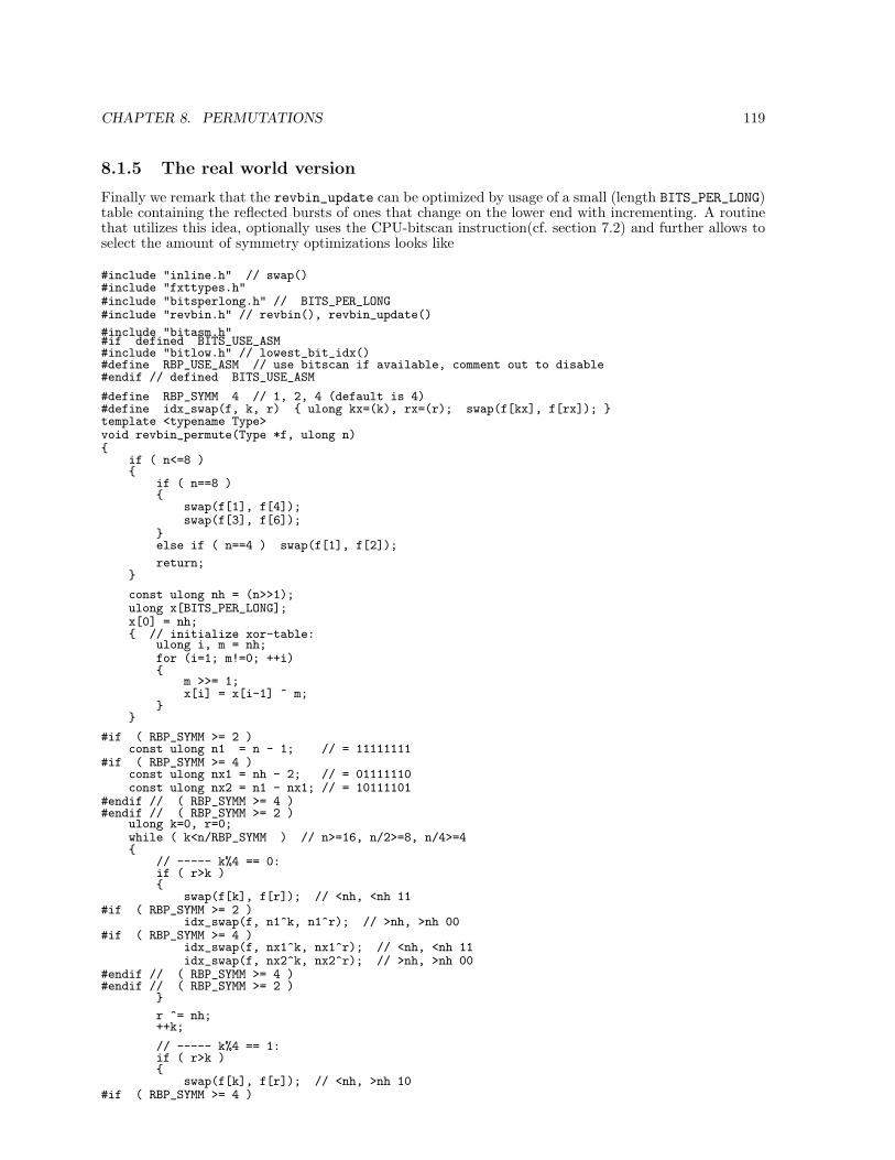
CHAPTER 8. PERMUTATIONS 119
8.1.5 The real world version
Finally we remark that the revbin_update can be optimized by usage of a small (length BITS_PER_LONG)table containing the reflected bursts of ones that change on the lower end with incrementing. A routinethat utilizes this idea, optionally uses the CPU-bitscan instruction(cf. section 7.2) and further allows toselect the amount of symmetry optimizations looks like
#include "inline.h" // swap()#include "fxttypes.h"#include "bitsperlong.h" // BITS_PER_LONG#include "revbin.h" // revbin(), revbin_update()
#include "bitasm.h"#if defined BITS_USE_ASM#include "bitlow.h" // lowest_bit_idx()#define RBP_USE_ASM // use bitscan if available, comment out to disable#endif // defined BITS_USE_ASM
#define RBP_SYMM 4 // 1, 2, 4 (default is 4)#define idx_swap(f, k, r) ulong kx=(k), rx=(r); swap(f[kx], f[rx]); template <typename Type>void revbin_permute(Type *f, ulong n)
if ( n<=8 )
if ( n==8 )
swap(f[1], f[4]);swap(f[3], f[6]);
else if ( n==4 ) swap(f[1], f[2]);
return;
const ulong nh = (n>>1);ulong x[BITS_PER_LONG];x[0] = nh; // initialize xor-table:
ulong i, m = nh;for (i=1; m!=0; ++i)
m >>= 1;x[i] = x[i-1] ^ m;
#if ( RBP_SYMM >= 2 )const ulong n1 = n - 1; // = 11111111
#if ( RBP_SYMM >= 4 )const ulong nx1 = nh - 2; // = 01111110const ulong nx2 = n1 - nx1; // = 10111101
#endif // ( RBP_SYMM >= 4 )#endif // ( RBP_SYMM >= 2 )
ulong k=0, r=0;while ( k<n/RBP_SYMM ) // n>=16, n/2>=8, n/4>=4
// ----- k%4 == 0:if ( r>k )
swap(f[k], f[r]); // <nh, <nh 11#if ( RBP_SYMM >= 2 )
idx_swap(f, n1^k, n1^r); // >nh, >nh 00#if ( RBP_SYMM >= 4 )
idx_swap(f, nx1^k, nx1^r); // <nh, <nh 11idx_swap(f, nx2^k, nx2^r); // >nh, >nh 00
#endif // ( RBP_SYMM >= 4 )#endif // ( RBP_SYMM >= 2 )
r ^= nh;++k;
// ----- k%4 == 1:if ( r>k )
swap(f[k], f[r]); // <nh, >nh 10#if ( RBP_SYMM >= 4 )

CHAPTER 8. PERMUTATIONS 120
idx_swap(f, n1^k, n1^r); // >nh, <nh 01#endif // ( RBP_SYMM >= 4 )
// scan for lowest unset bit of k:#ifdef RBP_USE_ASM
ulong i = lowest_bit_idx(~k);#else
ulong m = 2, i = 1;while ( m & k ) m <<= 1; ++i;
#endif // RBP_USE_ASMr ^= x[i];
++k;
// ----- k%4 == 2:if ( r>k )
swap(f[k], f[r]); // <nh, <nh 11#if ( RBP_SYMM >= 2 )
idx_swap(f, n1^k, n1^r); // >nh, >nh 00#endif // ( RBP_SYMM >= 2 )
r ^= nh;++k;
// ----- k%4 == 3:if ( r>k )
swap(f[k], f[r]); // <nh, >nh 10#if ( RBP_SYMM >= 4 )
idx_swap(f, nx1^k, nx1^r); // <nh, >nh 10#endif // ( RBP_SYMM >= 4 )
// scan for lowest unset bit of k:#ifdef RBP_USE_ASM
ulong i = lowest_bit_idx(~k);#else
ulong m = 4, i = 2;while ( m & k ) m <<= 1; ++i;
#endif // RBP_USE_ASMr ^= x[i];
++k;
. . . not the most readable piece of code but a nice example for a real-world optimized routine.
This is [FXT: revbin permute in perm/revbinpermute.h], see [FXT: revbin permute0 inperm/revbinpermute0.h] for the respective version for zero padded data.
8.2 The radix permutation
The radix-permutation is the generalization of the revbin-permutation (corresponding to radix 2) toarbitrary radices.C++ code for the radix-r permutation of the array f[]:
extern ulong nt[]; // nt[] = 9, 90, 900 for r=10, x=3extern ulong kt[]; // kt[] = 1, 10, 100 for r=10, x=3
template <typename Type>void radix_permute(Type *f, ulong n, ulong r)//// swap elements with index pairs i, j were the// radix-r representation of i and j are mutually// digit-reversed (e.g. 436 <--> 634)//// This is a radix-r generalization of revbin_permute()// revbin_permute(f, n) =^= radix_permute(f, n, 2)//
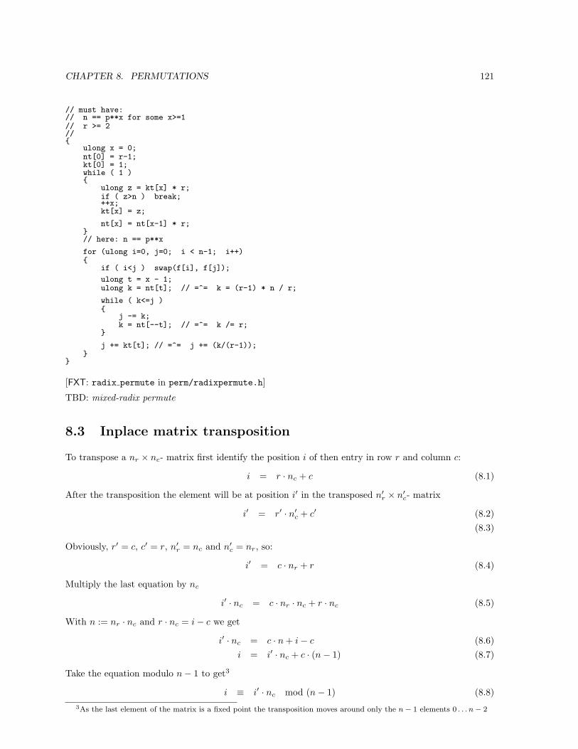
CHAPTER 8. PERMUTATIONS 121
// must have:// n == p**x for some x>=1// r >= 2//
ulong x = 0;nt[0] = r-1;kt[0] = 1;while ( 1 )
ulong z = kt[x] * r;if ( z>n ) break;++x;kt[x] = z;
nt[x] = nt[x-1] * r;// here: n == p**x
for (ulong i=0, j=0; i < n-1; i++)
if ( i<j ) swap(f[i], f[j]);
ulong t = x - 1;ulong k = nt[t]; // =^= k = (r-1) * n / r;
while ( k<=j )
j -= k;k = nt[--t]; // =^= k /= r;
j += kt[t]; // =^= j += (k/(r-1));
[FXT: radix permute in perm/radixpermute.h]
TBD: mixed-radix permute
8.3 Inplace matrix transposition
To transpose a nr × nc- matrix first identify the position i of then entry in row r and column c:
i = r · nc + c (8.1)
After the transposition the element will be at position i′ in the transposed n′r × n′c- matrix
i′ = r′ · n′c + c′ (8.2)(8.3)
Obviously, r′ = c, c′ = r, n′r = nc and n′c = nr, so:
i′ = c · nr + r (8.4)
Multiply the last equation by nc
i′ · nc = c · nr · nc + r · nc (8.5)
With n := nr · nc and r · nc = i− c we get
i′ · nc = c · n + i− c (8.6)i = i′ · nc + c · (n− 1) (8.7)
Take the equation modulo n− 1 to get3
i ≡ i′ · nc mod (n− 1) (8.8)3As the last element of the matrix is a fixed point the transposition moves around only the n− 1 elements 0 . . . n− 2
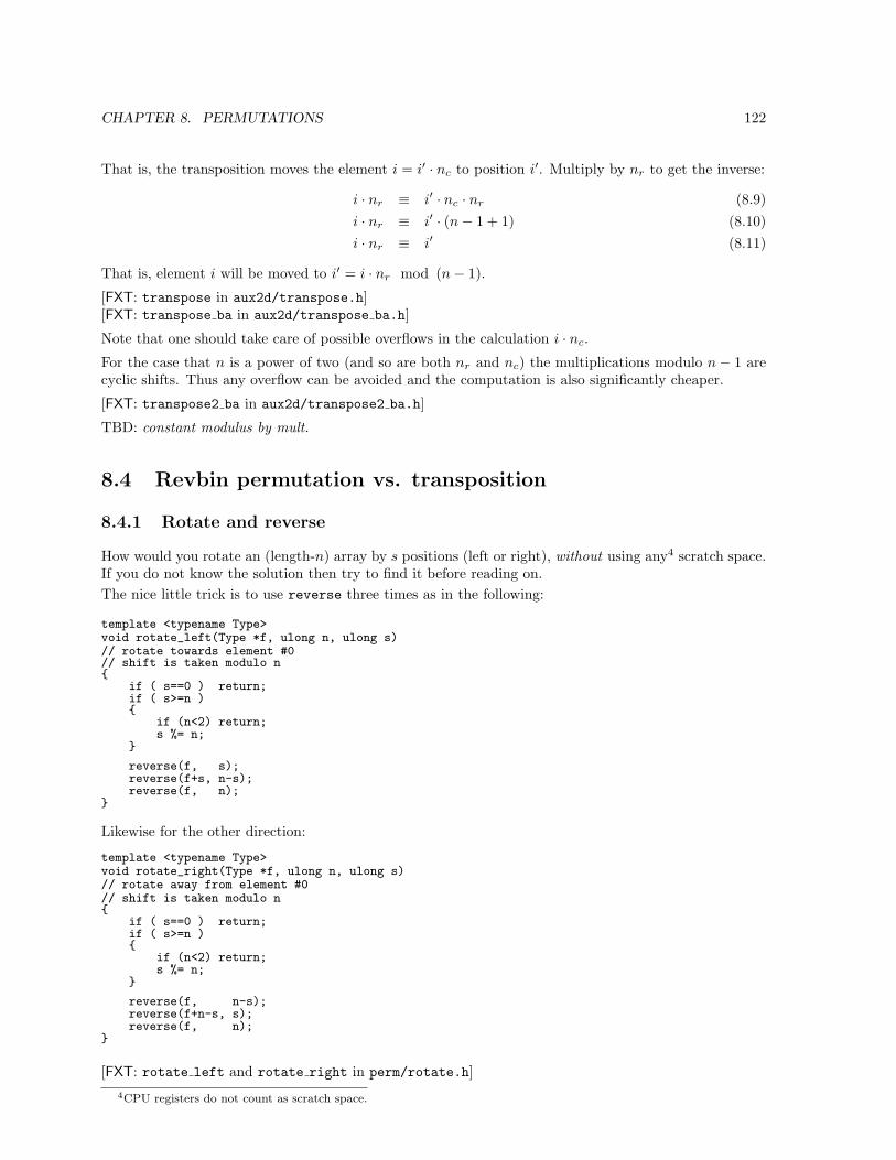
CHAPTER 8. PERMUTATIONS 122
That is, the transposition moves the element i = i′ · nc to position i′. Multiply by nr to get the inverse:
i · nr ≡ i′ · nc · nr (8.9)i · nr ≡ i′ · (n− 1 + 1) (8.10)i · nr ≡ i′ (8.11)
That is, element i will be moved to i′ = i · nr mod (n− 1).
[FXT: transpose in aux2d/transpose.h][FXT: transpose ba in aux2d/transpose ba.h]
Note that one should take care of possible overflows in the calculation i · nc.
For the case that n is a power of two (and so are both nr and nc) the multiplications modulo n− 1 arecyclic shifts. Thus any overflow can be avoided and the computation is also significantly cheaper.
[FXT: transpose2 ba in aux2d/transpose2 ba.h]
TBD: constant modulus by mult.
8.4 Revbin permutation vs. transposition
8.4.1 Rotate and reverse
How would you rotate an (length-n) array by s positions (left or right), without using any4 scratch space.If you do not know the solution then try to find it before reading on.The nice little trick is to use reverse three times as in the following:
template <typename Type>void rotate_left(Type *f, ulong n, ulong s)// rotate towards element #0// shift is taken modulo n
if ( s==0 ) return;if ( s>=n )
if (n<2) return;s %= n;
reverse(f, s);reverse(f+s, n-s);reverse(f, n);
Likewise for the other direction:
template <typename Type>void rotate_right(Type *f, ulong n, ulong s)// rotate away from element #0// shift is taken modulo n
if ( s==0 ) return;if ( s>=n )
if (n<2) return;s %= n;
reverse(f, n-s);reverse(f+n-s, s);reverse(f, n);
[FXT: rotate left and rotate right in perm/rotate.h]4CPU registers do not count as scratch space.

CHAPTER 8. PERMUTATIONS 123
What this has to do with our subject? When transposing an nr ×nc matrix whose size is a power of two(thereby both nr and nc are also powers of two) the above mentioned rotation is done with the indices(written in base two) of the elements. We know how to do a permutation that reverses the completeindices and reversing a few bits at the least significant end is not any harder:
template <typename Type>void revbin_permute_rows(Type *f, ulong ldn, ulong ldnc)// revbin_permute the length 2**ldnc rows of f[0..2**ldn-1]// (f[] considered as an 2**(ldn-ldnc) x 2**ldnc matrix)
ulong n = 1<<ldn;ulong nc = 1<<ldnc;for (ulong k=0; k<n; k+=nc) revbin_permute(f+k, nc);
And there we go:
template <typename Type>void transpose_by_rbp(Type *f, ulong ldn, ulong ldnc)// transpose f[] considered as an 2**(ldn-ldnc) x 2**ldnc matrix
revbin_permute_rows(f, ldn, ldnc);
ulong n = 1<<ldn;revbin_permute(f, n);
revbin_permute_rows(f, ldn, ldn-ldnc); // ... that is, columns
8.4.2 Zip and unzip
An important special case of the above is
template <typename Type>void zip(Type *f, ulong n)//// lower half --> even indices// higher half --> odd indices//// same as transposing the array as 2 x n/2 - matrix//// useful to combine real/imag part into a Complex array//// n must be a power of two
ulong nh = n/2;revbin_permute(f, nh); revbin_permute(f+nh, nh);revbin_permute(f, n);
[FXT: zip in perm/zip.h] which can5 for the type double be optimized as
void zip(double *f, long n)
revbin_permute(f, n);revbin_permute((Complex *)f, n/2);
[FXT: zip in perm/zip.cc]The inverse of zip is unzip:
template <typename Type>void unzip(Type *f, ulong n)//// inverse of zip():
5Assuming that type Complex consists of two doubles lying contiguous in memory.
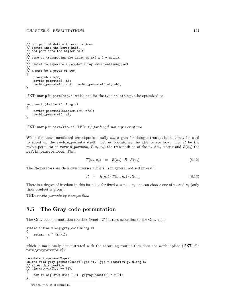
CHAPTER 8. PERMUTATIONS 124
// put part of data with even indices// sorted into the lower half,// odd part into the higher half//// same as transposing the array as n/2 x 2 - matrix//// useful to separate a Complex array into real/imag part//// n must be a power of two
ulong nh = n/2;revbin_permute(f, n);revbin_permute(f, nh); revbin_permute(f+nh, nh);
[FXT: unzip in perm/zip.h] which can for the type double again be optimized as
void unzip(double *f, long n)
revbin_permute((Complex *)f, n/2);revbin_permute(f, n);
[FXT: unzip in perm/zip.cc] TBD: zip for length not a power of two
While the above mentioned technique is usually not a gain for doing a transposition it may be usedto speed up the revbin_permute itself. Let us operatorize the idea to see how. Let R be therevbin-permutation revbin_permute, T (nr, nc) the transposition of the nr × nc matrix and R(nc) therevbin_permute_rows. Then
T (nr, nc) = R(nr) ·R ·R(nc) (8.12)
The R-operators are their own inverses while T is in general not self inverse6.
R = R(nr) · T (nr, nc) ·R(nc) (8.13)
There is a degree of freedom in this formula: for fixed n = nr ×nc one can choose one of nr and nc (onlytheir product is given).
TBD: revbin-permute by transposition
8.5 The Gray code permutation
The Gray code permutation reorders (length-2n) arrays according to the Gray code
static inline ulong gray_code(ulong x)
return x ^ (x>>1);
which is most easily demonstrated with the according routine that does not work inplace ([FXT: fileperm/graypermute.h]):
template <typename Type>inline void gray_permute(const Type *f, Type * restrict g, ulong n)// after this routine// g[gray_code(k)] == f[k]
for (ulong k=0; k<n; ++k) g[gray_code(k)] = f[k];
6For nr = nc it of course is.
CHAPTER 8. PERMUTATIONS 125
Its inverse is
template <typename Type>inline void inverse_gray_permute(const Type *f, Type * restrict g, ulong n)// after this routine// g[k] == f[gray_code(k)]// (same as: g[inverse_gray_code(k)] == f[k])
for (ulong k=0; k<n; ++k) g[k] = f[gray_code(k)];
It also uses calls to gray_code() because they are cheaper than the computation ofinverse_gray_code(), cf. 7.11.
It is actually possible7 to write an inplace version of the above routines that offers extremely goodperformance. The underlying observation is that the cycle leaders (cf. 8.6) have an easy pattern and canbe efficiently generated using the ideas from 7.4 (detection of perfect powers of two) and 7.9 (enumerationof bit subsets).
template <typename Type>void gray_permute(Type *f, ulong n)// inplace version
ulong z = 1; // mask for cycle maximaulong v = 0; // ~zulong cl = 1; // cycle lengthfor (ulong ldm=1, m=2; m<n; ++ldm, m<<=1)
z <<= 1;v <<= 1;if ( is_pow_of_2(ldm) )
++z;cl <<= 1;
else ++v;
bit_subset b(v);do
// --- do cycle: ---ulong i = z | b.next(); // start of cycleType t = f[i]; // save start valueulong g = gray_code(i); // next in cyclefor (ulong k=cl-1; k!=0; --k)
Type tt = f[g];f[g] = t;t = tt;g = gray_code(g);
f[g] = t;// --- end (do cycle) ---
while ( b.current() );
The inverse looks similar, the only actual difference is the do cycle block:
template <typename Type>void inverse_gray_permute(Type *f, ulong n)// inplace version
ulong z = 1;ulong v = 0;ulong cl = 1;for (ulong ldm=1, m=2; m<n; ++ldm, m<<=1)
7To both my delight and shock I noticed that the underlying ideas of this routine appeared in Knuths online pre-fascicle(2A) of Vol.4 where this is exercise 30 (sigh!). Yes, I wrote him a letter as requested in the preface.
CHAPTER 8. PERMUTATIONS 126
z <<= 1;v <<= 1;if ( is_pow_of_2(ldm) )
++z;cl <<= 1;
else ++v;
bit_subset b(v);do
// --- do cycle: ---ulong i = z | b.next(); // start of cycleType t = f[i]; // save start valueulong g = gray_code(i); // next in cyclefor (ulong k=cl-1; k!=0; --k)
f[i] = f[g];i = g;g = gray_code(i);
f[i] = t;// --- end (do cycle) ---
while ( b.current() );
How fast is it? We use the convention that the speed of the trivial (and completely cachefriendly, thereforerunning at memory bandwidth) reverse is 1.0, our hereby declared time unit for comparison. A littlebenchmark looks like:
CLOCK defined as 1000 MHz // AMD Athlon 1000MHz with 100MHz DDR RAMmemsize=32768 kiloByte // permuting that much memory (in chunks of doubles)
reverse(fr,n2); dt= 0.0997416 rel= 1 // set to onerevbin_permute(fr,n2); dt= 0.594105 rel= 5.95644
reverse(fr,n2); dt= 0.0997483 rel= 1.00007gray_permute(fr,n2); dt= 0.119014 rel= 1.19323
reverse(fr,n2); dt= 0.0997618 rel= 1.0002inverse_gray_permute(fr,n2); dt= 0.11028 rel= 1.10566
reverse(fr,n2); dt= 0.0997424 rel= 1.00001
We repeatedly timed reverse to get an impression how much we can trust the observed numbers. Thebandwidth of the reverse is about 320MByte/sec which should be compared to the output of a specialmemory testing program, revealing that it actually runs at about 83% of the bandwidth one can getwithout using streaming instructions:
avg: 33554432 [ 0]"memcpy" 305.869 MB/savg: 33554432 [ 1]"char *" 154.713 MB/savg: 33554432 [ 2]"short *" 187.943 MB/savg: 33554432 [ 3]"int *" 300.720 MB/savg: 33554432 [ 4]"long *" 300.584 MB/savg: 33554432 [ 5]"long * (4x unrolled)" 306.135 MB/savg: 33554432 [ 6]"int64 *" 305.372 MB/savg: 33554432 [ 7]"double *" 388.695 MB/s // <--=avg: 33554432 [ 8]"double * (4x unrolled)" 374.271 MB/savg: 33554432 [ 9]"streaming K7" 902.171 MB/savg: 33554432 [10]"streaming K7 prefetch" 1082.868 MB/savg: 33554432 [11]"streaming K7 clear" 1318.875 MB/savg: 33554432 [12]"long * clear" 341.456 MB/s
While the revbin_permute takes about 6 units (due to its memory access pattern that is very problematicwrt. cache usage) the gray_permute only uses 1.20 units, the inverse_gray_permute even8 only 1.10!This is pretty amazing for such a nontrivial permutation.
The described permutation can be used to significantly speed up fast transforms of lengths a power oftwo, notably the Walsh transform, see chapter 5.
8The observed difference between the forward- and backward version is in fact systematic.
CHAPTER 8. PERMUTATIONS 127
8.6 General permutations
So far we treated special permutations that occured as part of other algorithms. It is instructive to studypermutations in general with the operations (as composition and inverse) on them.
8.6.1 Basic definitions
A straight forward way to describe a permutation is to consider the array of indices that for the original(unpermuted) data would be the length-n canonical sequence 0, 1, 2, . . . , n − 1. The mentioned trivialsequence describes the ‘do-nothing’ permutation or identity (wrt. composition of permutations). Theconcept is best described by the routine that applies a given permutation x on an array of data f : afterthe routine has finished the array g will contain the elements of f reordered according to x
template <typename Type>void apply(const ulong *x, const Type *f, Type * restrict g, ulong n)// apply x[] on f[]// i.e. g[k] <-- f[x[k]] \forall k
for (ulong k=0; k<n; ++k) g[k] = f[x[k]];
[FXT: apply in perm/permapply.h] An example using strings (arrays of characters): The permutationdescribed by x = 7, 6, 3, 2, 5, 1, 0, 4 and the input dataf ="ABadCafe" would produceg ="efdaaBAC"
All routines in this and the following section are declared in [FXT: file perm/permutation.h]Trivially
int is_identity(const ulong *f, ulong n)// check whether f[] is the identical permutation,// i.e. whether f[k]==k for all k= 0...n-1
for (ulong k=0; k<n; ++k) if ( f[k] != k ) return 0;return 1;
A fixed point of a permutation is an index where the element isn’t moved:
ulong count_fixed_points(const ulong *f, ulong n)// return number of fixed points in f[]
ulong ct = 0;for (ulong k=0; k<n; ++k) if ( f[k] == k ) ++ct;return ct;
A derangement is a permutation that has no fixed points (i.e. that moved every element to anotherposition so count_fixed_points() returns zero). To check whether a permutation is the derangementof another permutation one can use:
int is_derangement(const ulong *f, const ulong *g, ulong n)// check whether f[] is a derangement of g[],// i.e. whether f[k]!=g[k] for all k
for (ulong k=0; k<n; ++k) if ( f[k] == g[k] ) return 0;return 1;
To check whether a given array really describes a valid permutation one has to verify that each indexappears exactly once. The bitarray class described in 7.17 allows us to do the job without modificationof the input (like e.g. sorting):
CHAPTER 8. PERMUTATIONS 128
int is_valid_permutation(const ulong *f, ulong n, bitarray *bp/*=0*/)// check whether all values 0...n-1 appear exactly once
// check whether any element is out of range:for (ulong k=0; k<n; ++k) if ( f[k]>=n ) return 0;
// check whether values are unique:bitarray *tp = bp;if ( 0==bp ) tp = new bitarray(n); // tagstp->clear_all();
ulong k;for (k=0; k<n; ++k)
if ( tp->test_set(f[k]) ) break;
if ( 0==bp ) delete tp;
return (k==n);
8.6.2 Compositions of permutations
One can apply arbitrary many permutations to an array, one by one. The resulting permutation is calledthe composition of the applied permutations. As an example, the check whether some permutation g isequal to f applied twice, or f · f , or f squared use:
int is_square(const ulong *f, const ulong *g, ulong n)// whether f * f == g as a permutation
for (ulong k=0; k<n; ++k) if ( g[k] != f[f[k]] ) return 0;return 1;
A permutation f is said to be the inverse of another permutation g if it undoes its effect, that is f ·g = id(likewise g · f = id):
int is_inverse(const ulong *f, const ulong *g, ulong n)// check whether f[] is inverse of g[]
for (ulong k=0; k<n; ++k) if ( f[g[k]] != k ) return 0;return 1;
A permutation that is its own inverse (like the revbin-permutation) is called an involution. Checkingthat is easy:
int is_involution(const ulong *f, ulong n)// check whether max cycle length is <= 2
for (ulong k=0; k<n; ++k) if ( f[f[k]] != k ) return 0;return 1;
Finding the inverse of a given permutation is trivial:
void make_inverse(const ulong *f, ulong * restrict g, ulong n)// set g[] to the inverse of f[]
for (ulong k=0; k<n; ++k) g[f[k]] = k;
However, if one wants to do the operation inplace a little bit of thought is required. The idea underlyingall subsequent routines working inplace is that every permutation entirely consists of disjoint cycles. Acycle (of a permutation) is a subset of the indices that is rotated (by one) by the permutation. The termdisjoint means that the cycles do not ‘cross’ each other. While this observation is pretty trivial it allowsus to do many operations by following the cycles of the permutation, one by one, and doing the necessaryoperation on each of them. As an example consider the following permutation of an array originallyconsisting of the (canonical) sequence 0, 1, . . . , 15 (extra spaces inserted for readability):

CHAPTER 8. PERMUTATIONS 129
0, 1, 3, 2, 7, 6, 4, 5, 15, 14, 12, 13, 8, 9, 11, 10
There are two fixed points (0 and 1) and these cycles:
( 2 <-- 3 )( 4 <-- 7 <-- 5 <-- 6 )( 8 <-- 15 <-- 10 <-- 12 )( 9 <-- 14 <-- 11 <-- 13 )
The cycles do ‘wrap around’, e.g. the initial 4 of the second cycle goes to position 6, the last element ofthe second cycle.Note that the inverse permutation could formally be described by reversing every arrow in each cycle:
( 2 --> 3 )( 4 --> 7 --> 5 --> 6 )( 8 --> 15 --> 10 --> 12 )( 9 --> 14 --> 11 --> 13 )
Equivalently, one can reverse the order of the elements in each cycle:
( 3 <-- 2 )( 6 <-- 5 <-- 7 <-- 4 )(12 <-- 10 <-- 15 <-- 8 )(13 <-- 11 <-- 14 <-- 9 )
If we begin each cycle with its smallest element the inverse permutation looks like:
( 2 <-- 3 )( 4 <-- 6 <-- 5 <-- 7 )( 8 <-- 12 <-- 10 <-- 15 )( 9 <-- 13 <-- 11 <-- 14 )
The last three sets of cycles all describe the same permutation:
0, 1, 3, 2, 6, 7, 5, 4, 12, 13, 15, 14, 10, 11, 9, 8
The maximal cycle-length of an involution is 2, that means it completely consists of fixed points and2-cycles (swapped pairs of indices).
As a warm-up look at the code used to print the cycles of the above example (which by the way is theGray-permutation of the canonical length-16 array):
ulong print_cycles(const ulong *f, ulong n, bitarray *bp=0)// print the cycles of the permutation// return number of fixed points
bitarray *tp = bp;if ( 0==bp ) tp = new bitarray(n); // tagstp->clear_all();
ulong ct = 0; // # of fixed pointsfor (ulong k=0; k<n; ++k)
if ( tp->test_clear(k) ) continue; // already processedtp->set(k);
// follow a cycle:ulong i = k;ulong g = f[i]; // next indexif ( g==i ) // fixed point ?
++ct;continue;
cout << "(" << setw(3) << i;while ( 0==(tp->test_set(g)) )
cout << " <-- " << setw(3) << g;

CHAPTER 8. PERMUTATIONS 130
g = f[g];cout << " )" << endl;
if ( 0==bp ) delete tp;
return ct;
The bitarray is used to keep track of the elements already processed.For the computation of the inverse we have to reverse each cycle:
void make_inverse(ulong *f, ulong n, bitarray *bp/*=0*/)// set f[] to its own inverse
bitarray *tp = bp;if ( 0==bp ) tp = new bitarray(n); // tagstp->clear_all();
for (ulong k=0; k<n; ++k)
if ( tp->test_clear(k) ) continue; // already processedtp->set(k);
// invert a cycle:ulong i = k;ulong g = f[i]; // next indexwhile ( 0==(tp->test_set(g)) )
ulong t = f[g];f[g] = i;i = g;g = t;
f[g] = i;
if ( 0==bp ) delete tp;
Similarly for the straighforward
void make_square(const ulong *f, ulong * restrict g, ulong n)// set g[] = f[] * f[]
for (ulong k=0; k<n; ++k) g[k] = f[f[k]];
whose inplace version is
void make_square(ulong *f, ulong n, bitarray *bp/*=0*/)// set f[] to f[] * f[]
bitarray *tp = bp;if ( 0==bp ) tp = new bitarray(n); // tagstp->clear_all();
for (ulong k=0; k<n; ++k)
if ( tp->test_clear(k) ) continue; // already processedtp->set(k);
// square a cycle:ulong i = k;ulong t = f[i]; // saveulong g = f[i]; // next indexwhile ( 0==(tp->test_set(g)) )
f[i] = f[g];i = g;g = f[g];
f[i] = t;
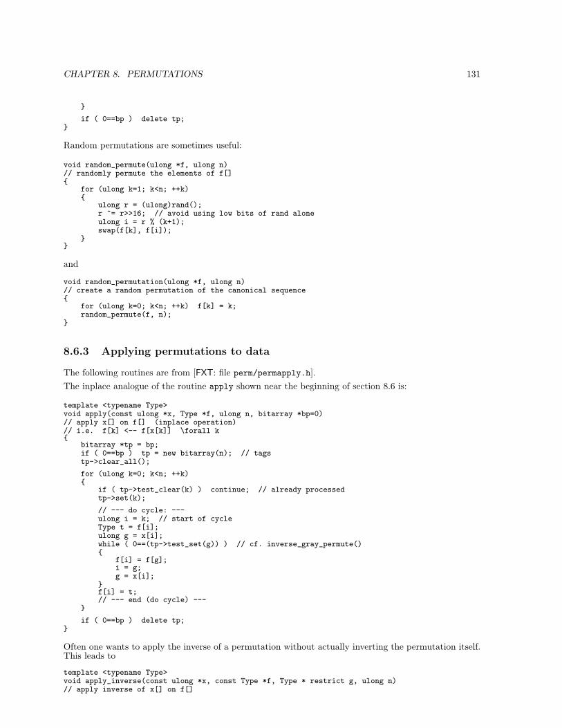
CHAPTER 8. PERMUTATIONS 131
if ( 0==bp ) delete tp;
Random permutations are sometimes useful:
void random_permute(ulong *f, ulong n)// randomly permute the elements of f[]
for (ulong k=1; k<n; ++k)
ulong r = (ulong)rand();r ^= r>>16; // avoid using low bits of rand aloneulong i = r % (k+1);swap(f[k], f[i]);
and
void random_permutation(ulong *f, ulong n)// create a random permutation of the canonical sequence
for (ulong k=0; k<n; ++k) f[k] = k;random_permute(f, n);
8.6.3 Applying permutations to data
The following routines are from [FXT: file perm/permapply.h].The inplace analogue of the routine apply shown near the beginning of section 8.6 is:
template <typename Type>void apply(const ulong *x, Type *f, ulong n, bitarray *bp=0)// apply x[] on f[] (inplace operation)// i.e. f[k] <-- f[x[k]] \forall k
bitarray *tp = bp;if ( 0==bp ) tp = new bitarray(n); // tagstp->clear_all();
for (ulong k=0; k<n; ++k)
if ( tp->test_clear(k) ) continue; // already processedtp->set(k);
// --- do cycle: ---ulong i = k; // start of cycleType t = f[i];ulong g = x[i];while ( 0==(tp->test_set(g)) ) // cf. inverse_gray_permute()
f[i] = f[g];i = g;g = x[i];
f[i] = t;// --- end (do cycle) ---
if ( 0==bp ) delete tp;
Often one wants to apply the inverse of a permutation without actually inverting the permutation itself.This leads to
template <typename Type>void apply_inverse(const ulong *x, const Type *f, Type * restrict g, ulong n)// apply inverse of x[] on f[]
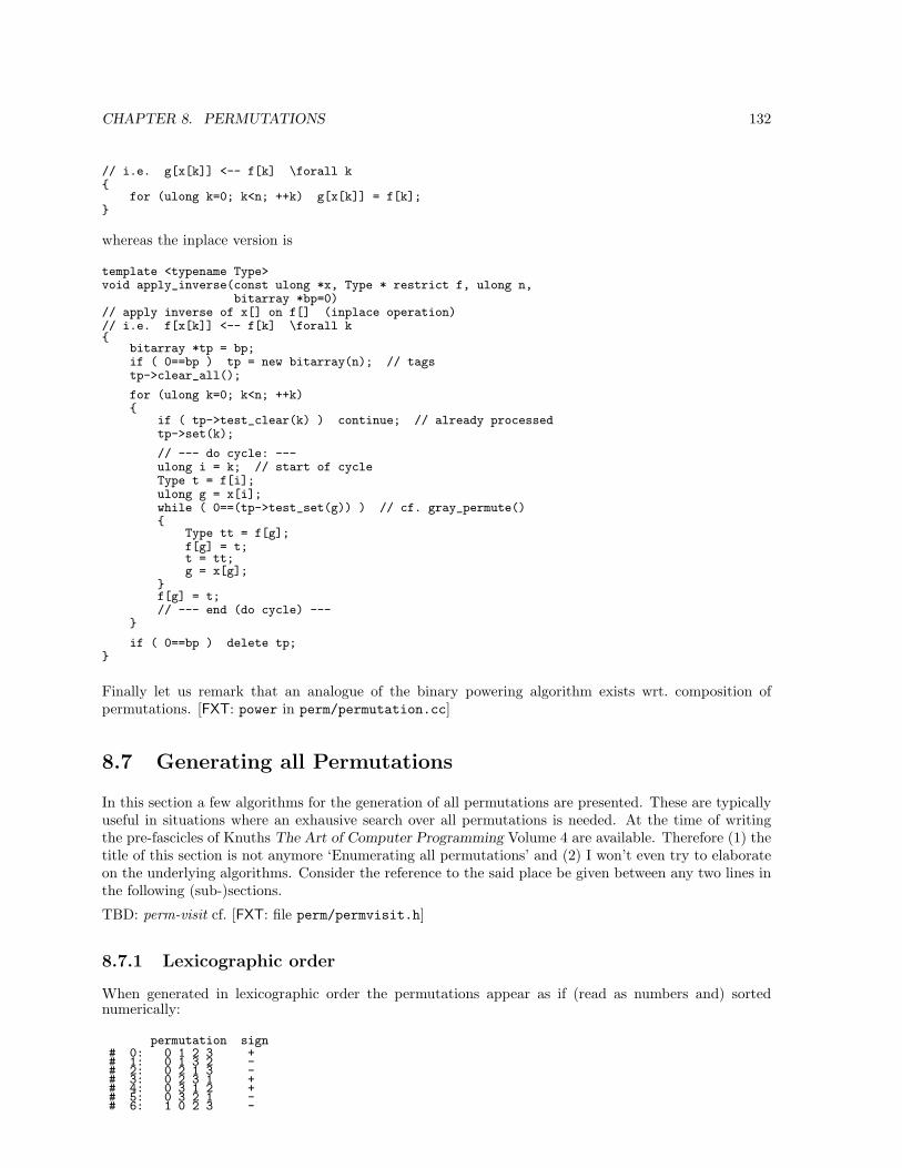
CHAPTER 8. PERMUTATIONS 132
// i.e. g[x[k]] <-- f[k] \forall k
for (ulong k=0; k<n; ++k) g[x[k]] = f[k];
whereas the inplace version is
template <typename Type>void apply_inverse(const ulong *x, Type * restrict f, ulong n,
bitarray *bp=0)// apply inverse of x[] on f[] (inplace operation)// i.e. f[x[k]] <-- f[k] \forall k
bitarray *tp = bp;if ( 0==bp ) tp = new bitarray(n); // tagstp->clear_all();
for (ulong k=0; k<n; ++k)
if ( tp->test_clear(k) ) continue; // already processedtp->set(k);
// --- do cycle: ---ulong i = k; // start of cycleType t = f[i];ulong g = x[i];while ( 0==(tp->test_set(g)) ) // cf. gray_permute()
Type tt = f[g];f[g] = t;t = tt;g = x[g];
f[g] = t;// --- end (do cycle) ---
if ( 0==bp ) delete tp;
Finally let us remark that an analogue of the binary powering algorithm exists wrt. composition ofpermutations. [FXT: power in perm/permutation.cc]
8.7 Generating all Permutations
In this section a few algorithms for the generation of all permutations are presented. These are typicallyuseful in situations where an exhausive search over all permutations is needed. At the time of writingthe pre-fascicles of Knuths The Art of Computer Programming Volume 4 are available. Therefore (1) thetitle of this section is not anymore ‘Enumerating all permutations’ and (2) I won’t even try to elaborateon the underlying algorithms. Consider the reference to the said place be given between any two lines inthe following (sub-)sections.
TBD: perm-visit cf. [FXT: file perm/permvisit.h]
8.7.1 Lexicographic order
When generated in lexicographic order the permutations appear as if (read as numbers and) sortednumerically:
permutation sign# 0: 0 1 2 3 +# 1: 0 1 3 2 -# 2: 0 2 1 3 -# 3: 0 2 3 1 +# 4: 0 3 1 2 +# 5: 0 3 2 1 -# 6: 1 0 2 3 -
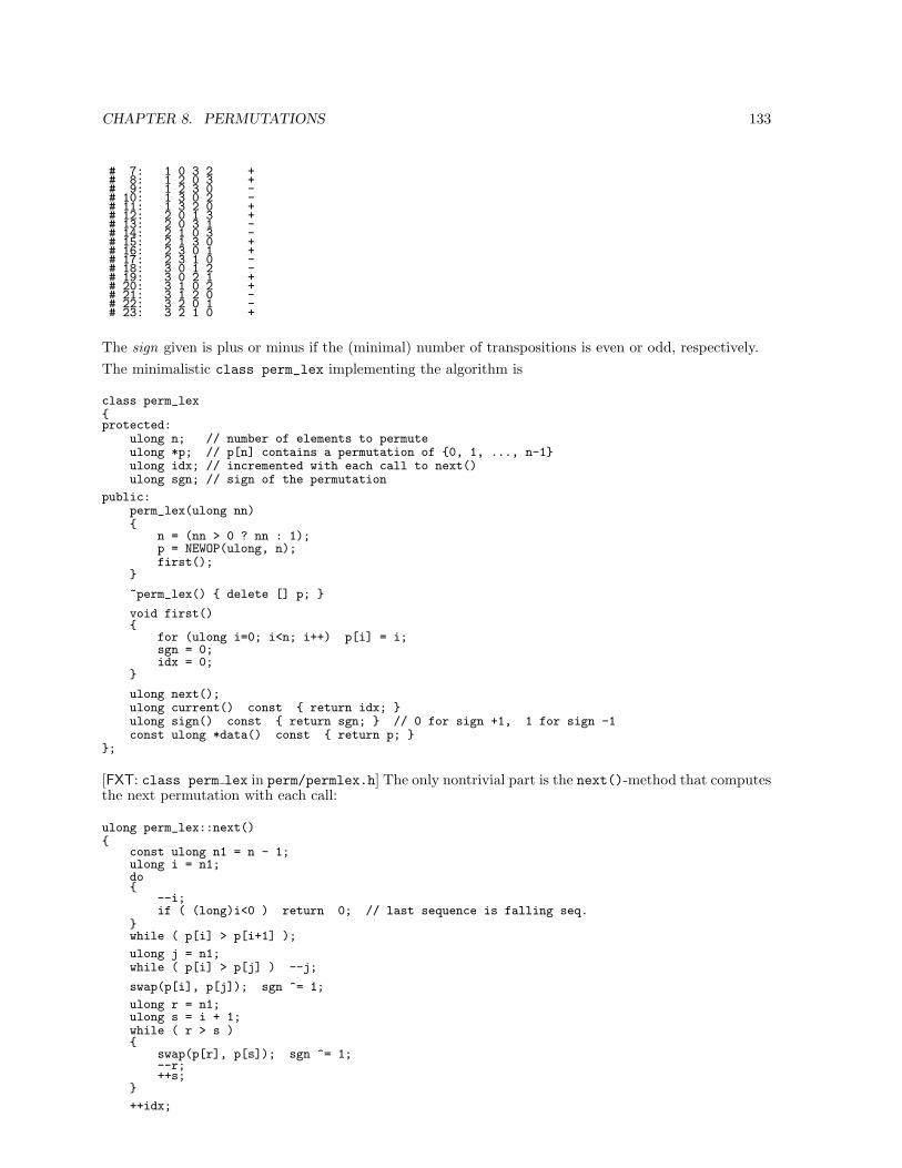
CHAPTER 8. PERMUTATIONS 133
# 7: 1 0 3 2 +# 8: 1 2 0 3 +# 9: 1 2 3 0 -# 10: 1 3 0 2 -# 11: 1 3 2 0 +# 12: 2 0 1 3 +# 13: 2 0 3 1 -# 14: 2 1 0 3 -# 15: 2 1 3 0 +# 16: 2 3 0 1 +# 17: 2 3 1 0 -# 18: 3 0 1 2 -# 19: 3 0 2 1 +# 20: 3 1 0 2 +# 21: 3 1 2 0 -# 22: 3 2 0 1 -# 23: 3 2 1 0 +
The sign given is plus or minus if the (minimal) number of transpositions is even or odd, respectively.The minimalistic class perm_lex implementing the algorithm is
class perm_lexprotected:
ulong n; // number of elements to permuteulong *p; // p[n] contains a permutation of 0, 1, ..., n-1ulong idx; // incremented with each call to next()ulong sgn; // sign of the permutation
public:perm_lex(ulong nn)
n = (nn > 0 ? nn : 1);p = NEWOP(ulong, n);first();
~perm_lex() delete [] p;
void first()
for (ulong i=0; i<n; i++) p[i] = i;sgn = 0;idx = 0;
ulong next();ulong current() const return idx; ulong sign() const return sgn; // 0 for sign +1, 1 for sign -1const ulong *data() const return p;
;
[FXT: class perm lex in perm/permlex.h] The only nontrivial part is the next()-method that computesthe next permutation with each call:
ulong perm_lex::next()
const ulong n1 = n - 1;ulong i = n1;do
--i;if ( (long)i<0 ) return 0; // last sequence is falling seq.
while ( p[i] > p[i+1] );
ulong j = n1;while ( p[i] > p[j] ) --j;
swap(p[i], p[j]); sgn ^= 1;
ulong r = n1;ulong s = i + 1;while ( r > s )
swap(p[r], p[s]); sgn ^= 1;--r;++s;
++idx;
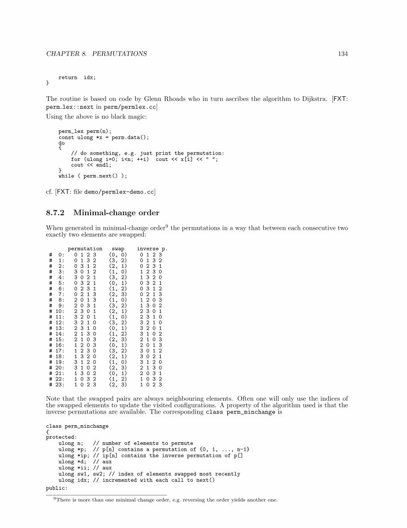
CHAPTER 8. PERMUTATIONS 134
return idx;
The routine is based on code by Glenn Rhoads who in turn ascribes the algorithm to Dijkstra. [FXT:perm lex::next in perm/permlex.cc]Using the above is no black magic:
perm_lex perm(n);const ulong *x = perm.data();do
// do something, e.g. just print the permutation:for (ulong i=0; i<n; ++i) cout << x[i] << " ";cout << endl;
while ( perm.next() );
cf. [FXT: file demo/permlex-demo.cc]
8.7.2 Minimal-change order
When generated in minimal-change order9 the permutations in a way that between each consecutive twoexactly two elements are swapped:
permutation swap inverse p.# 0: 0 1 2 3 (0, 0) 0 1 2 3# 1: 0 1 3 2 (3, 2) 0 1 3 2# 2: 0 3 1 2 (2, 1) 0 2 3 1# 3: 3 0 1 2 (1, 0) 1 2 3 0# 4: 3 0 2 1 (3, 2) 1 3 2 0# 5: 0 3 2 1 (0, 1) 0 3 2 1# 6: 0 2 3 1 (1, 2) 0 3 1 2# 7: 0 2 1 3 (2, 3) 0 2 1 3# 8: 2 0 1 3 (1, 0) 1 2 0 3# 9: 2 0 3 1 (3, 2) 1 3 0 2# 10: 2 3 0 1 (2, 1) 2 3 0 1# 11: 3 2 0 1 (1, 0) 2 3 1 0# 12: 3 2 1 0 (3, 2) 3 2 1 0# 13: 2 3 1 0 (0, 1) 3 2 0 1# 14: 2 1 3 0 (1, 2) 3 1 0 2# 15: 2 1 0 3 (2, 3) 2 1 0 3# 16: 1 2 0 3 (0, 1) 2 0 1 3# 17: 1 2 3 0 (3, 2) 3 0 1 2# 18: 1 3 2 0 (2, 1) 3 0 2 1# 19: 3 1 2 0 (1, 0) 3 1 2 0# 20: 3 1 0 2 (2, 3) 2 1 3 0# 21: 1 3 0 2 (0, 1) 2 0 3 1# 22: 1 0 3 2 (1, 2) 1 0 3 2# 23: 1 0 2 3 (2, 3) 1 0 2 3
Note that the swapped pairs are always neighbouring elements. Often one will only use the indices ofthe swapped elements to update the visited configurations. A property of the algorithm used is that theinverse permutations are available. The corresponding class perm_minchange is
class perm_minchangeprotected:
ulong n; // number of elements to permuteulong *p; // p[n] contains a permutation of 0, 1, ..., n-1ulong *ip; // ip[n] contains the inverse permutation of p[]ulong *d; // auxulong *ii; // auxulong sw1, sw2; // index of elements swapped most recentlyulong idx; // incremented with each call to next()
public:
9There is more than one minimal change order, e.g. reversing the order yields another one.
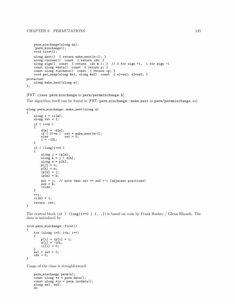
CHAPTER 8. PERMUTATIONS 135
perm_minchange(ulong nn);~perm_minchange();void first();
ulong next() return make_next(n-1); ulong current() const return idx; ulong sign() const return idx & 1; // 0 for sign +1, 1 for sign -1const ulong *data() const return p; const ulong *invdata() const return ip; void get_swap(ulong &s1, ulong &s2) const s1=sw1; s2=sw2;
protected:ulong make_next(ulong m);
;
[FXT: class perm minchange in perm/permminchange.h]
The algorithm itself can be found in [FXT: perm minchange::make next in perm/permminchange.cc]
ulong perm_minchange::make_next(ulong m)
ulong i = ii[m];ulong ret = 1;
if ( i==m )
d[m] = -d[m];if ( 0!=m ) ret = make_next(m-1);else ret = 0;i = -1UL;
if ( (long)i>=0 )
ulong j = ip[m];ulong k = j + d[m];ulong z = p[k];p[j] = z;p[k] = m;ip[z] = j;ip[m] = k;
sw1 = j; // note that sw1 == sw2 +-1 (adjacent positions)sw2 = k;++idx;
++i;ii[m] = i;
return ret;
The central block (if ( (long)i>=0 ) ...) is based on code by Frank Ruskey / Glenn Rhoads. Thedata is initialized by
void perm_minchange::first()
for (ulong i=0; i<n; i++)
p[i] = ip[i] = i;d[i] = -1UL;ii[i] = 0;
sw1 = sw2 = 0;idx = 0;
Usage of the class is straighforward:
perm_minchange perm(n);const ulong *x = perm.data();const ulong *ix = perm.invdata();ulong sw1, sw2;do
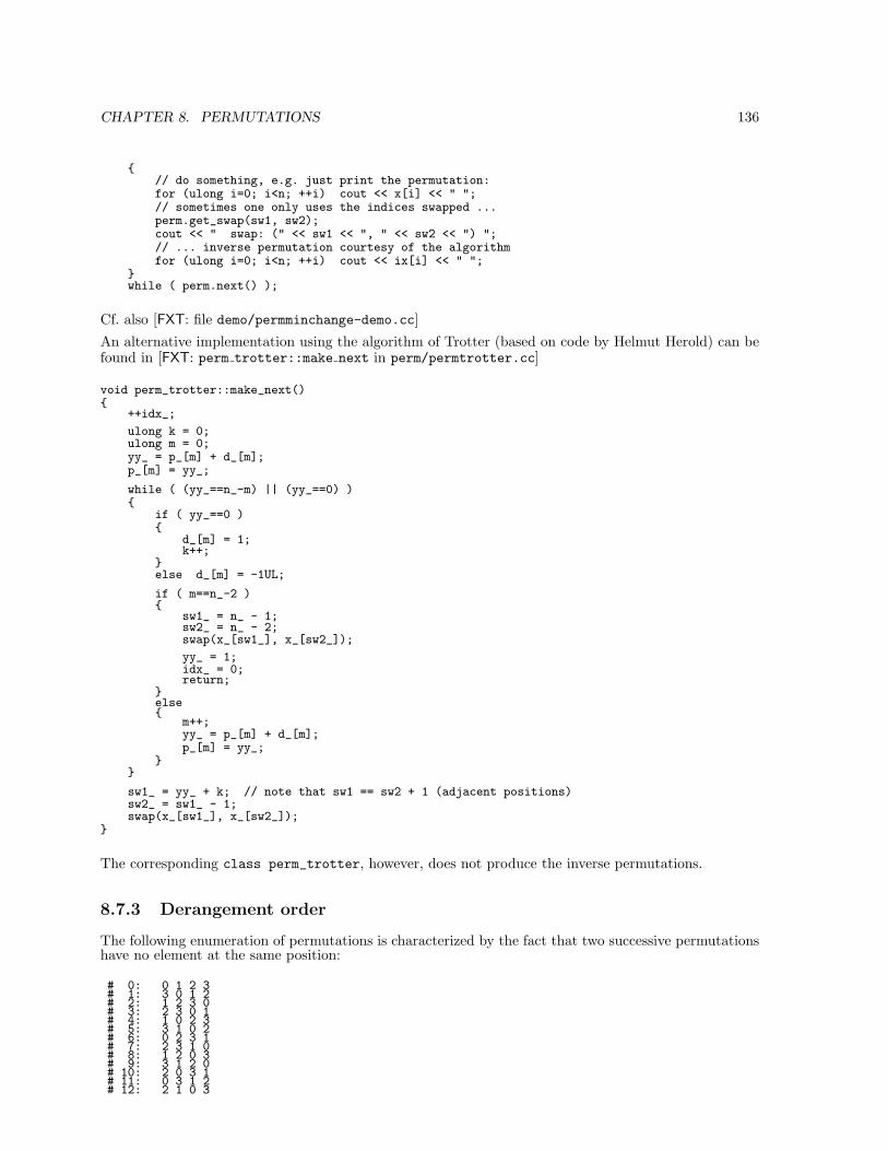
CHAPTER 8. PERMUTATIONS 136
// do something, e.g. just print the permutation:for (ulong i=0; i<n; ++i) cout << x[i] << " ";// sometimes one only uses the indices swapped ...perm.get_swap(sw1, sw2);cout << " swap: (" << sw1 << ", " << sw2 << ") ";// ... inverse permutation courtesy of the algorithmfor (ulong i=0; i<n; ++i) cout << ix[i] << " ";
while ( perm.next() );
Cf. also [FXT: file demo/permminchange-demo.cc]
An alternative implementation using the algorithm of Trotter (based on code by Helmut Herold) can befound in [FXT: perm trotter::make next in perm/permtrotter.cc]
void perm_trotter::make_next()
++idx_;
ulong k = 0;ulong m = 0;yy_ = p_[m] + d_[m];p_[m] = yy_;
while ( (yy_==n_-m) || (yy_==0) )
if ( yy_==0 )
d_[m] = 1;k++;
else d_[m] = -1UL;
if ( m==n_-2 )
sw1_ = n_ - 1;sw2_ = n_ - 2;swap(x_[sw1_], x_[sw2_]);
yy_ = 1;idx_ = 0;return;
else
m++;yy_ = p_[m] + d_[m];p_[m] = yy_;
sw1_ = yy_ + k; // note that sw1 == sw2 + 1 (adjacent positions)sw2_ = sw1_ - 1;swap(x_[sw1_], x_[sw2_]);
The corresponding class perm_trotter, however, does not produce the inverse permutations.
8.7.3 Derangement order
The following enumeration of permutations is characterized by the fact that two successive permutationshave no element at the same position:
# 0: 0 1 2 3# 1: 3 0 1 2# 2: 1 2 3 0# 3: 2 3 0 1# 4: 1 0 2 3# 5: 3 1 0 2# 6: 0 2 3 1# 7: 2 3 1 0# 8: 1 2 0 3# 9: 3 1 2 0# 10: 2 0 3 1# 11: 0 3 1 2# 12: 2 1 0 3
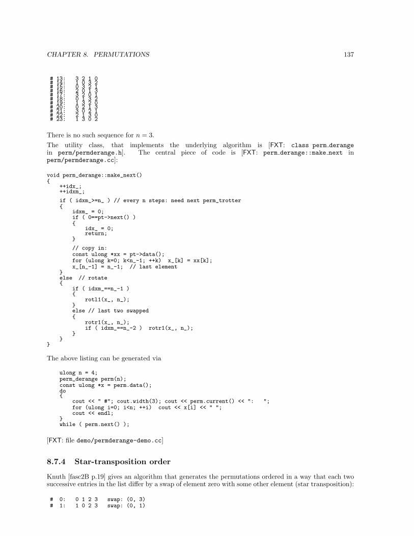
CHAPTER 8. PERMUTATIONS 137
# 13: 3 2 1 0# 14: 1 0 3 2# 15: 0 3 2 1# 16: 2 0 1 3# 17: 3 2 0 1# 18: 0 1 3 2# 19: 1 3 2 0# 20: 0 2 1 3# 21: 3 0 2 1# 22: 2 1 3 0# 23: 1 3 0 2
There is no such sequence for n = 3.The utility class, that implements the underlying algorithm is [FXT: class perm derangein perm/permderange.h]. The central piece of code is [FXT: perm derange::make next inperm/permderange.cc]:
void perm_derange::make_next()
++idx_;++idxm_;
if ( idxm_>=n_ ) // every n steps: need next perm_trotter
idxm_ = 0;if ( 0==pt->next() )
idx_ = 0;return;
// copy in:const ulong *xx = pt->data();for (ulong k=0; k<n_-1; ++k) x_[k] = xx[k];x_[n_-1] = n_-1; // last element
else // rotate
if ( idxm_==n_-1 )
rotl1(x_, n_);else // last two swapped
rotr1(x_, n_);if ( idxm_==n_-2 ) rotr1(x_, n_);
The above listing can be generated via
ulong n = 4;perm_derange perm(n);const ulong *x = perm.data();do
cout << " #"; cout.width(3); cout << perm.current() << ": ";for (ulong i=0; i<n; ++i) cout << x[i] << " ";cout << endl;
while ( perm.next() );
[FXT: file demo/permderange-demo.cc]
8.7.4 Star-transposition order
Knuth [fasc2B p.19] gives an algorithm that generates the permutations ordered in a way that each twosuccessive entries in the list differ by a swap of element zero with some other element (star transposition):
# 0: 0 1 2 3 swap: (0, 3)# 1: 1 0 2 3 swap: (0, 1)
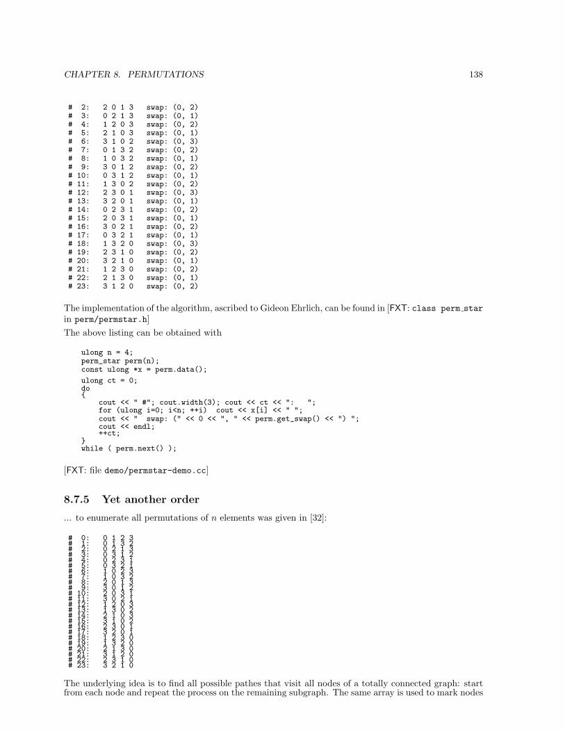
CHAPTER 8. PERMUTATIONS 138
# 2: 2 0 1 3 swap: (0, 2)# 3: 0 2 1 3 swap: (0, 1)# 4: 1 2 0 3 swap: (0, 2)# 5: 2 1 0 3 swap: (0, 1)# 6: 3 1 0 2 swap: (0, 3)# 7: 0 1 3 2 swap: (0, 2)# 8: 1 0 3 2 swap: (0, 1)# 9: 3 0 1 2 swap: (0, 2)# 10: 0 3 1 2 swap: (0, 1)# 11: 1 3 0 2 swap: (0, 2)# 12: 2 3 0 1 swap: (0, 3)# 13: 3 2 0 1 swap: (0, 1)# 14: 0 2 3 1 swap: (0, 2)# 15: 2 0 3 1 swap: (0, 1)# 16: 3 0 2 1 swap: (0, 2)# 17: 0 3 2 1 swap: (0, 1)# 18: 1 3 2 0 swap: (0, 3)# 19: 2 3 1 0 swap: (0, 2)# 20: 3 2 1 0 swap: (0, 1)# 21: 1 2 3 0 swap: (0, 2)# 22: 2 1 3 0 swap: (0, 1)# 23: 3 1 2 0 swap: (0, 2)
The implementation of the algorithm, ascribed to Gideon Ehrlich, can be found in [FXT: class perm starin perm/permstar.h]The above listing can be obtained with
ulong n = 4;perm_star perm(n);const ulong *x = perm.data();
ulong ct = 0;do
cout << " #"; cout.width(3); cout << ct << ": ";for (ulong i=0; i<n; ++i) cout << x[i] << " ";cout << " swap: (" << 0 << ", " << perm.get_swap() << ") ";cout << endl;++ct;
while ( perm.next() );
[FXT: file demo/permstar-demo.cc]
8.7.5 Yet another order
... to enumerate all permutations of n elements was given in [32]:
# 0: 0 1 2 3# 1: 0 1 3 2# 2: 0 2 1 3# 3: 0 3 1 2# 4: 0 2 3 1# 5: 0 3 2 1# 6: 1 0 2 3# 7: 1 0 3 2# 8: 2 0 1 3# 9: 3 0 1 2# 10: 2 0 3 1# 11: 3 0 2 1# 12: 1 2 0 3# 13: 1 3 0 2# 14: 2 1 0 3# 15: 3 1 0 2# 16: 2 3 0 1# 17: 3 2 0 1# 18: 1 2 3 0# 19: 1 3 2 0# 20: 2 1 3 0# 21: 3 1 2 0# 22: 2 3 1 0# 23: 3 2 1 0
The underlying idea is to find all possible pathes that visit all nodes of a totally connected graph: startfrom each node and repeat the process on the remaining subgraph. The same array is used to mark nodes
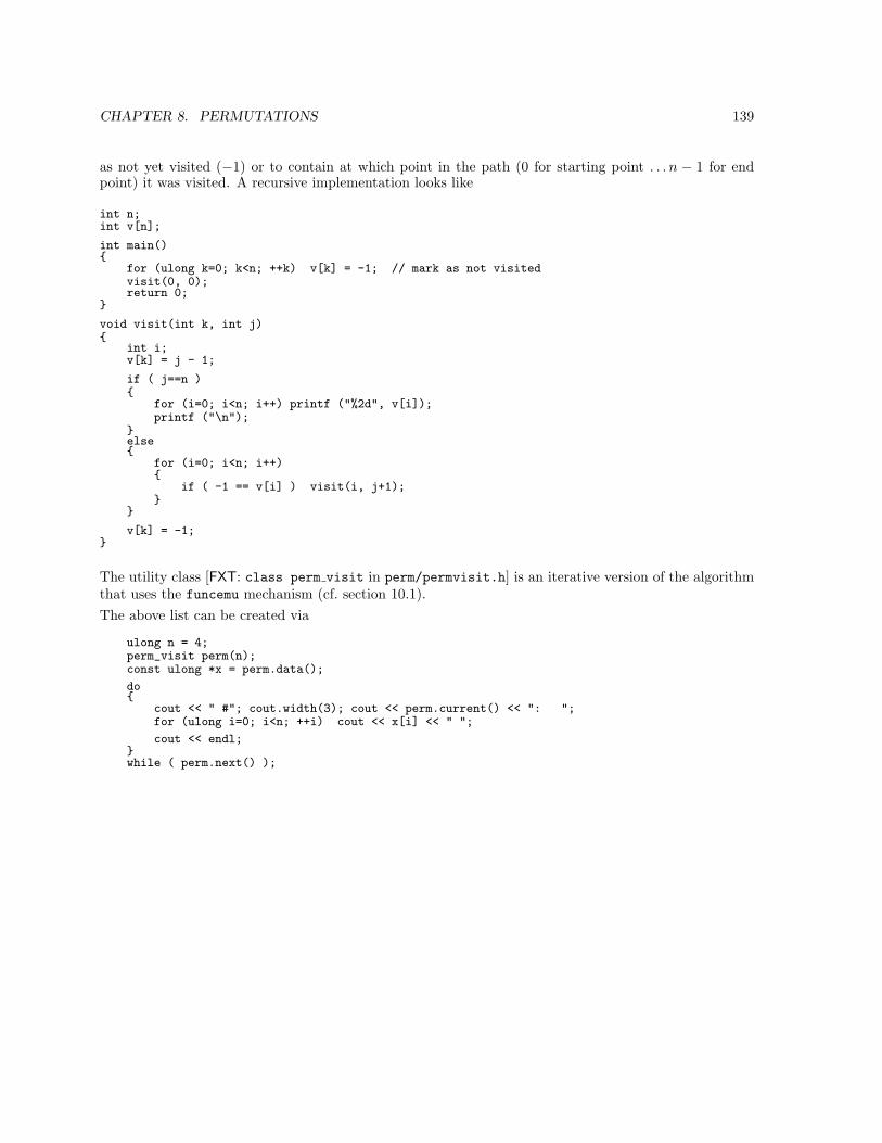
CHAPTER 8. PERMUTATIONS 139
as not yet visited (−1) or to contain at which point in the path (0 for starting point . . .n − 1 for endpoint) it was visited. A recursive implementation looks like
int n;int v[n];
int main()
for (ulong k=0; k<n; ++k) v[k] = -1; // mark as not visitedvisit(0, 0);return 0;
void visit(int k, int j)
int i;v[k] = j - 1;
if ( j==n )
for (i=0; i<n; i++) printf ("%2d", v[i]);printf ("\n");
else
for (i=0; i<n; i++)
if ( -1 == v[i] ) visit(i, j+1);
v[k] = -1;
The utility class [FXT: class perm visit in perm/permvisit.h] is an iterative version of the algorithmthat uses the funcemu mechanism (cf. section 10.1).The above list can be created via
ulong n = 4;perm_visit perm(n);const ulong *x = perm.data();
do
cout << " #"; cout.width(3); cout << perm.current() << ": ";for (ulong i=0; i<n; ++i) cout << x[i] << " ";
cout << endl;while ( perm.next() );
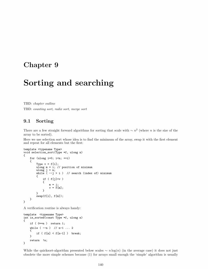
Chapter 9
Sorting and searching
TBD: chapter outline
TBD: counting sort, radix sort, merge sort
9.1 Sorting
There are a few straight forward algorithms for sorting that scale with ∼ n2 (where n is the size of thearray to be sorted).Here we use selection sort whose idea is to find the minimum of the array, swap it with the first elementand repeat for all elements but the first:
template <typename Type>void selection_sort(Type *f, ulong n)
for (ulong i=0; i<n; ++i)
Type v = f[i];ulong m = i; // position of minimumulong j = n;while ( --j > i ) // search (index of) minimum
if ( f[j]<v )
m = j;v = f[m];
swap(f[i], f[m]);
A verification routine is always handy:
template <typename Type>int is_sorted(const Type *f, ulong n)
if ( 0==n ) return 1;
while ( --n ) // n-1 ... 2
if ( f[n] < f[n-1] ) break;
return !n;
While the quicksort-algorithm presented below scales ∼ n log(n) (in the average case) it does not justobsolete the more simple schemes because (1) for arrays small enough the ‘simple’ algorithm is usually
140
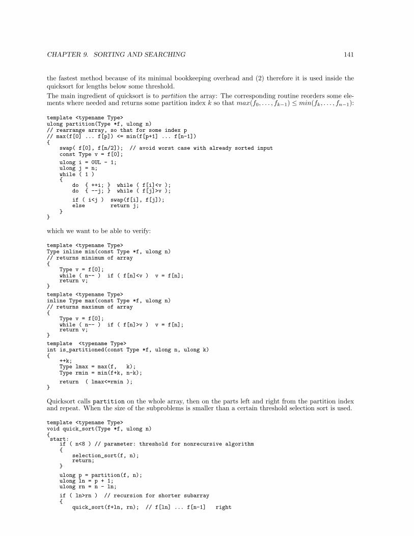
CHAPTER 9. SORTING AND SEARCHING 141
the fastest method because of its minimal bookkeeping overhead and (2) therefore it is used inside thequicksort for lengths below some threshold.The main ingredient of quicksort is to partition the array: The corresponding routine reorders some ele-ments where needed and returns some partition index k so that max(f0, . . . , fk−1) ≤ min(fk, . . . , fn−1):
template <typename Type>ulong partition(Type *f, ulong n)// rearrange array, so that for some index p// max(f[0] ... f[p]) <= min(f[p+1] ... f[n-1])
swap( f[0], f[n/2]); // avoid worst case with already sorted inputconst Type v = f[0];
ulong i = 0UL - 1;ulong j = n;while ( 1 )
do ++i; while ( f[i]<v );do --j; while ( f[j]>v );
if ( i<j ) swap(f[i], f[j]);else return j;
which we want to be able to verify:
template <typename Type>Type inline min(const Type *f, ulong n)// returns minimum of array
Type v = f[0];while ( n-- ) if ( f[n]<v ) v = f[n];return v;
template <typename Type>inline Type max(const Type *f, ulong n)// returns maximum of array
Type v = f[0];while ( n-- ) if ( f[n]>v ) v = f[n];return v;
template <typename Type>int is_partitioned(const Type *f, ulong n, ulong k)
++k;Type lmax = max(f, k);Type rmin = min(f+k, n-k);
return ( lmax<=rmin );
Quicksort calls partition on the whole array, then on the parts left and right from the partition indexand repeat. When the size of the subproblems is smaller than a certain threshold selection sort is used.
template <typename Type>void quick_sort(Type *f, ulong n)start:
if ( n<8 ) // parameter: threshold for nonrecursive algorithm
selection_sort(f, n);return;
ulong p = partition(f, n);ulong ln = p + 1;ulong rn = n - ln;
if ( ln>rn ) // recursion for shorter subarray
quick_sort(f+ln, rn); // f[ln] ... f[n-1] right
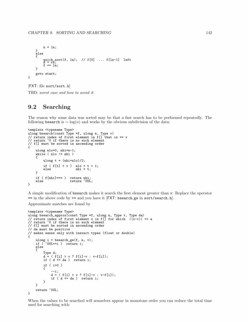
CHAPTER 9. SORTING AND SEARCHING 142
n = ln;else
quick_sort(f, ln); // f[0] ... f[ln-1] leftn = rn;f += ln;
goto start;
[FXT: file sort/sort.h]
TBD: worst case and how to avoid it
9.2 Searching
The reason why some data was sorted may be that a fast search has to be performed repeatedly. Thefollowing bsearch is ∼ log(n) and works by the obvious subdivision of the data:
template <typename Type>ulong bsearch(const Type *f, ulong n, Type v)// return index of first element in f[] that is == v// return ~0 if there is no such element// f[] must be sorted in ascending order
ulong nlo=0, nhi=n-1;while ( nlo != nhi )
ulong t = (nhi+nlo)/2;
if ( f[t] < v ) nlo = t + 1;else nhi = t;
if ( f[nhi]==v ) return nhi;else return ~0UL;
A simple modification of bsearch makes it search the first element greater than v: Replace the operator== in the above code by >= and you have it [FXT: bsearch ge in sort/search.h].Approximate matches are found by
template <typename Type>ulong bsearch_approx(const Type *f, ulong n, Type v, Type da)// return index of first element x in f[] for which |(x-v)| <= a// return ~0 if there is no such element// f[] must be sorted in ascending order// da must be positive// makes sense only with inexact types (float or double)
ulong i = bsearch_ge(f, n, v);if ( ~0UL==i ) return i;else
Type d;d = ( f[i] > v ? f[i]-v : v-f[i]);if ( d <= da ) return i;
if ( i>0 )
--i;d = ( f[i] > v ? f[i]-v : v-f[i]);if ( d <= da ) return i;
return ~0UL;
When the values to be searched will semselves appear in monotone order you can reduce the total timeused for searching with:
CHAPTER 9. SORTING AND SEARCHING 143
template <typename Type>inline long search_down(const Type *f, Type v, ulong &i)// search v in f[], starting at i (so i must be < length)// f[i] must be greater or equal v// f[] must be sorted in ascending order// returns index k if f[k]==v or ~0 if no such k is found// i is updated so that it can be used for a following// search for an element u where u < v
while ( (f[i]>v) && (i>0) ) --i;
if ( f[i]==v ) return i;else return ~0UL;
[FXT: file sort/search.h]
9.3 Index sorting
While the ‘plain’ sorting reorders an array f so that, after it has finished, fk ≤ fk+1 the following routinessort an array of indices without modifying the actual data:
template <typename Type>void idx_selection_sort(const Type *f, ulong n, ulong *x)
for (ulong i=0; i<n; ++i)
Type v = f[x[i]];ulong m = i; // position-ptr of minimumulong j = n;while ( --j > i ) // search (index of) minimum
if ( f[x[j]]<v )
m = j;v = f[x[m]];
swap(x[i], x[m]);
Apart from the ‘read only’-feature the index-sort routines have the nice property to perfectly work onnon-contiguous data.The verification code looks like:
template <typename Type>int is_idx_sorted(const Type *f, ulong n, const ulong *x)
if ( 0==n ) return 1;
while ( --n ) // n-1 ... 1
if ( f[x[n]] < f[x[n-1]] ) break;
return !n;
The index-sort routines reorder the indices in x such that x applied to f as a permutation (in the senseof section 8.6.3) will render f a sorted array.While the transformation of partition is straight forward:
template <typename Type>ulong idx_partition(const Type *f, ulong n, ulong *x)// rearrange index array, so that for some index p// max(f[x[0]] ... f[x[p]]) <= min(f[x[p+1]] ... f[x[n-1]])
CHAPTER 9. SORTING AND SEARCHING 144
swap( x[0], x[n/2]);const Type v = f[x[0]];
ulong i = 0UL - 1;ulong j = n;while ( 1 )
do ++i;while ( f[x[i]]<v );
do --j;while ( f[x[j]]>v );
if ( i<j ) swap(x[i], x[j]);else return j;
The index-quicksort itself deserves a minute of contemplation comparing it to the plain version:
template <typename Type>void idx_quick_sort(const Type *f, ulong n, ulong *x)start:
if ( n<8 ) // parameter: threshold for nonrecursive algorithm
idx_selection_sort(f, n, x);return;
ulong p = idx_partition(f, n, x);ulong ln = p + 1;ulong rn = n - ln;
if ( ln>rn ) // recursion for shorter subarray
idx_quick_sort(f, rn, x+ln); // f[x[ln]] ... f[x[n-1]] rightn = ln;
else
idx_quick_sort(f, ln, x); // f[x[0]] ... f[x[ln-1]] leftn = rn;x += ln;
goto start;
[FXT: file sort/sortidx.h]
The index-analogues of bsearch etc. are again straight forward, they can be found in [FXT: filesort/searchidx.h].
9.4 Pointer sorting
Pointer sorting is an idea similar to index sorting which is even less restricted than index sort: The datamay be unaligned in memory. And overlapping. Or no data at all but port addresses controlling somehighly dangerous machinery.
Thereby pointer sort is the perfect way to highly cryptic and powerful programs that segfault when youleast expect it. Admittedly, all the ‘dangerous’ features of pointer sort except the unaligned one are alsothere in index sort. However, with index sort you will not so often use them by accident.Just to make the idea clear, the array of indices is replaced by an array of pointers:
template <typename Type>void ptr_selection_sort(const Type *f, ulong n, Type **x)
for (ulong i=0; i<n; ++i)
Type v = *x[i];
CHAPTER 9. SORTING AND SEARCHING 145
ulong m = i; // position-ptr of minimumulong j = n;while ( --j > i ) // search (index of) minimum
if ( *x[j]<v )
m = j;v = *x[m];
swap(x[i], x[m]);
Find the pointer sorting code in [FXT: file sort/sortptr.h] and the pointer search routines in [FXT: filesort/searchptr.h].
9.5 Sorting by a supplied comparison function
The routines in [FXT: file sort/sortfunc.h] are similar to the C-quicksort qsort that is part of thestandard library. A comparison function cmp has to be supplied by the called so that compound datatypes can be sorted with respect to some key contained. Citing the manual page for qsort:
The comparison function must return an integer less than, equal to, or greater thanzero if the first argument is considered to be respectively less than, equal to, orgreater than the second. If two members compare as equal, their order in thesorted array is undefined.
Note that the numerous calls to cmp do have a negative impact on the performance. And then with C++you can provide a comparision ‘function’ for compound data by overloading the operators <, <, <= and >=and use the plain version. Back in performance land. Isn’t C++ nice? TBD: add a compile-time inlinedversion?As a prototypical example here the version of selection sort:
template <typename Type>void selection_sort(Type *f, ulong n, int (*cmp)(const Type &, const Type &))
for (ulong i=0; i<n; ++i)
Type v = f[i];ulong m = i; // position of minimumulong j = n;while ( --j > i ) // search (index of) minimum
if ( cmp(f[j],v) < 0 )
m = j;v = f[m];
swap(f[i], f[m]);
The rest of the supplied routines a rather straight forward translation of the (plain-) sort analogues, thefunction one will most likely use being
template <typename Type>void quick_sort(Type *f, ulong n, int (*cmp)(const Type &, const Type &))

CHAPTER 9. SORTING AND SEARCHING 146
Sorting complex numbers
You want to sort complex numbers? Fine for me, but don’t tell your local mathematician. To see themathematical problem we ask whether i is smaller or greater than zero. Assume i > 0: follows i · i > 0(we multiplied with a positive value) which is −1 > 0 and that is false. So, is i < 0? Then i · i > 0(multiplication with a negative value, as assumed). So −1 > 0, oops! The lesson is that there is no wayto impose an arrangement on the complex numbers that would justify the usage of the symbols < and >in the mathematical sense.
Nevertheless we can invent a relation that allows us to sort: arranging (sorting) the complex numbersaccording to their absolute value (modulus) leaves infinitely many numbers in one ‘bucket’, namely allthose that have the same distance to zero. However, one could use the modulus as the major orderingparameter, the angle as the minor. Or the real part as the major and the imaginary part as the minor.The latter is realized in
static inline intcmp_complex(const Complex &f, const Complex &g)
int ret = 0;double fr = f.real();double gr = g.real();if ( fr==gr )
double fi = f.imag();double gi = g.imag();if ( fi!=gi ) ret = (fi>gi ? +1 : -1);
else ret = (fr>gr ? +1 : -1);
return ret;
which, when used as comparison with the above function-sort as in
void complex_sort(Complex *f, ulong n)// major order wrt. real part// minor order wrt. imag part
quick_sort(f, n, cmp_complex);
can indeed be the practical tool you had in mind.
9.6 Unique
This section presents a few utility functions that revolve around whether values in a (sorted) array arerepeated or unique.Testing whether all values are unique:
template <typename Type>int test_unique(const Type *f, ulong n)// for a sorted array test whether all values are unique// (i.e. whether no value is repeated)//// returns 0 if all values are unique// else returns index of the second element in the first pair found//// this function is not called "is_unique()" because it// returns 0 (=="false") for a positive answer
for (ulong k=1; k<n; ++k)
if ( f[k] == f[k-1] ) return k; // k != 0
CHAPTER 9. SORTING AND SEARCHING 147
return 0;
The same thing, but for inexact types (floats): the maximal (absolute) difference within which twocontiguous elements will still be considered equal can be provided as additional parameter. One subtlepoint is that the values can slowly ‘drift away’ unnoticed by this implementation: Consider a long arraywhere each difference computed has the same sign and is just smaller than da, say it is d = 0.6·da. Thedifference of the first and last value then is 0.6 · (n− 1) · d which is greater than da for n ≥ 3.
template <typename Type>int test_unique_approx(const Type *f, ulong n, Type da)// for a sorted array test whether all values are// unique within some tolerance// (i.e. whether no value is repeated)//// returns 0 if all values are unique// else returns index of the second element in the first pair found//// makes mostly sense with inexact types (float or double)
if ( da<=0 ) da = -da; // want positive tolerance
for (ulong k=1; k<n; ++k)
Type d = (f[k] - f[k-1]);if ( d<=0 ) d = -d;
if ( d < da ) return k; // k != 0
return 0;
An alternative way to deal with inexact types is to apply
template <typename Type>void quantise(Type *f, ulong n, double q)//// in f[] set each element x to q*floor(1/q*(x+q/2))// e.g.: q=1 ==> round to nearest integer// q=1/1000 ==> round to nearest multiple of 1/1000// For inexact types (float or double)
Type qh = q * 0.5;Type q1 = 1.0 / q;while ( n-- )
f[n] = q * floor( q1 * (f[n]+qh) );
[FXT: quantise in aux/quantise.h] before using test_unique_approx. One should use a quantizationparameter q that is greater than the value used for da.Minimalistic demo:
Random values:0: 0.97277502431: 0.29251678452: 0.77135769823: 0.52674497954: 0.76991383665: 0.4002286223
Quantization with q=0.01
Quantised & sorted :0: 0.29000000001: 0.40000000002: 0.53000000003: 0.77000000004: 0.77000000005: 0.9700000000
First REPEATED value at index 4 (and 3)
Unique’d array:0: 0.2900000000
CHAPTER 9. SORTING AND SEARCHING 148
1: 0.40000000002: 0.53000000003: 0.77000000004: 0.9700000000
quantise() turns out to be also useful in another context, cf. [FXT: symbolify by size andsymbolify by order in aux/symbolify.h].Counting the elements that appear just once:
template <typename Type>int unique_count(const Type *f, ulong n)// for a sorted array return the number of unique values// the number of (not necessarily distinct) repeated// values is n - unique_count(f, n);
if ( 1>=n ) return n;
ulong ct = 1;for (ulong k=1; k<n; ++k)
if ( f[k] != f[k-1] ) ++ct;
return ct;
Removing repeated elements:
template <typename Type>ulong unique(Type *f, ulong n)// for a sorted array squeeze all repeated values// and return the number of unique values// e.g.: [1, 3, 3, 4, 5, 8, 8] --> [1, 3, 4, 5, 8]// the routine also works for unsorted arrays as long// as identical elements only appear in contiguous blocks// e.g. [4, 4, 3, 7, 7] --> [4, 3, 7]// the order is preserved
ulong u = unique_count(f, n);
if ( u == n ) return n; // nothing to do
Type v = f[0];for (ulong j=1, k=1; j<u; ++j)
while ( f[k] == v ) ++k; // search next different element
v = f[j] = f[k];
return u;
9.7 Misc
A sequence is called monotone if it is either purely ascending or purely descending. This includes the casewhere subsequent elements are equal. Whether a constant sequence is considered ascending or descendingin this context is a matter of convention.
template <typename Type>int is_monotone(const Type *f, ulong n)// return// +1 for ascending order// -1 for descending order// else 0
if ( 1>=n ) return +1;
ulong k;for (k=1; k<n; ++k) // skip constant start
if ( f[k] != f[k-1] ) break;
CHAPTER 9. SORTING AND SEARCHING 149
if ( k==n ) return +1; // constant is considered ascending here
int s = ( f[k] > f[k-1] ? +1 : -1 );
if ( s>0 ) // was: ascending
// scan for descending pair:for ( ; k<n; ++k) if ( f[k] < f[k-1] ) return 0;
else // was: descending
// scan for ascending pair:for ( ; k<n; ++k) if ( f[k] > f[k-1] ) return 0;
return s;
A strictly monotone sequence is a monotone sequence that has no identical pairs of elements. The testturns out to be slightly easier:
template <typename Type>int is_strictly_monotone(const Type *f, ulong n)// return// +1 for strictly ascending order// -1 for strictly descending order// else 0
if ( 1>=n ) return +1;
ulong k = 1;if ( f[k] == f[k-1] ) return 0;
int s = ( f[k] > f[k-1] ? +1 : -1 );
if ( s>0 ) // was: ascending
// scan for descending pair:for ( ; k<n; ++k) if ( f[k] <= f[k-1] ) return 0;
else // was: descending
// scan for ascending pair:for ( ; k<n; ++k) if ( f[k] >= f[k-1] ) return 0;
return s;
[FXT: file sort/monotone.h]A sequence is called convex if it starts with an ascending part and ends with a descending part. A concavesequence starts with a descending and ends with an ascending part. Whether a monotone sequence isconsidered convex or concave again is a matter of convention (i.e. you have the choice to consider the firstor the last element as extremum). Lacking a term that contains both convex and concave the followingroutine is called is_convex:
template <typename Type>long is_convex(Type *f, ulong n)//// return// +val for convex sequence (first rising then falling)// -val for concave sequence (first falling then rising)// else 0//// val is the (second) index of the first pair at the point// where the ordering changes; val>=n iff seq. is monotone.//// note: a constant sequence is considered any of rising/falling//
if ( 1>=n ) return +1;
ulong k = 1;for (k=1; k<n; ++k) // skip constant start

CHAPTER 9. SORTING AND SEARCHING 150
if ( f[k] != f[k-1] ) break;
if ( k==n ) return +n; // constant is considered convex here
int s = ( f[k] > f[k-1] ? +1 : -1 );
if ( s>0 ) // was: ascending
// scan for strictly descending pair:for ( ; k<n; ++k) if ( f[k] < f[k-1] ) break;s = +k;
else // was: descending
// scan for strictly ascending pair:for ( ; k<n; ++k) if ( f[k] > f[k-1] ) break;s = -k;
if ( k==n ) return s; // sequence is monotone
// check that the ordering does not change again:if ( s>0 ) // was: ascending --> descending
// scan for strictly ascending pair:for ( ; k<n; ++k) if ( f[k] > f[k-1] ) return 0;
else // was: descending
// scan for strictly descending pair:for ( ; k<n; ++k) if ( f[k] < f[k-1] ) return 0;
return s;
The test for strictly convex (or concave) sequences is:
template <typename Type>long is_strictly_convex(Type *f, ulong n)//// return// +val for strictly convex sequence// (i.e. first strictly rising then strictly falling)// -val for strictly concave sequence// (i.e. first strictly falling then strictly rising)// else 0//// val is the (second) index of the first pair at the point// where the ordering changes; val>=n iff seq. is strictly monotone.//
if ( 1>=n ) return +1;
ulong k = 1;if ( f[k] == f[k-1] ) return 0;
int s = ( f[k] > f[k-1] ? +1 : -1 );
if ( s>0 ) // was: ascending
// scan for descending pair:for ( ; k<n; ++k) if ( f[k] <= f[k-1] ) break;s = +k;
else // was: descending
// scan for ascending pair:for ( ; k<n; ++k) if ( f[k] >= f[k-1] ) break;s = -k;
if ( k==n ) return s; // sequence is monotoneelse if ( f[k] == f[k-1] ) return 0;
// check that the ordering does not change again:if ( s>0 ) // was: ascending --> descending
CHAPTER 9. SORTING AND SEARCHING 151
// scan for ascending pair:for ( ; k<n; ++k) if ( f[k] >= f[k-1] ) return 0;
else // was: descending
// scan for descending pair:for ( ; k<n; ++k) if ( f[k] <= f[k-1] ) return 0;
return s;
[FXT: file sort/convex.h]
The tests given are mostly useful as assertions used inside more complex algorithms.
Chapter 10
Selected combinatorical algorithms
This chapter presents selected combinatorical algorithms. The generation of combinations, subsets, par-titions, and pairings of parentheses (as example for the use of ‘funcemu’) are treated here. Permutationsare treated in a seperate chapter because of the not so combinatorical viewpoint taken with most of thematerial (especially the specific examples like the revbin-permutation) there.
TBD: debruijn sequences via primitive polys possibly using bitengine
10.1 Offline functions: funcemu
Sometimes it is possible to find recursive algorithm for solving some problem that is not easily solvediteratively. However the recursive implementations might produce the results in midst of its calling graph.When a utility class providing a the results one by one with some next call is required there is an apparentproblem: There is only one stack available for function calls1. We do not have offline functions.
As an example consider the following recursive code2
int n = 4;int v[n];
int main()
paren(0, 0);return 0;
void paren(long i, long s)
long k, t;if ( i<n )
for (k=0; k<=i-s; ++k)
a[i-1] = k;t = s + a[i-1];q[t + i] = ’(’;paren(i + 1, t); // recursionq[t + i] = ’)’;
else
a[i-1] = n - s;Visit(); // next set of parens available
1True for the majority of the programming languages.2given by Glenn Rhoads
152

CHAPTER 10. SELECTED COMBINATORICAL ALGORITHMS 153
that generates following output:
(((())))((()()))((())())((()))()(()(()))(()()())(()())()(())(())(())()()()((()))()(()())()(())()()()(())()()()()
A reasonable way to create offline functions3 is to rewrite the function as a state engine and utilize aclass [FXT: class funcemu in aux/funcemu.h] that provides two stacks, one for local variables and onefor the state of the function:
template <typename Type>class funcemupublic:
ulong tp_; // sTate stack Pointerulong dp_; // Data stack Pointerulong *t_; // sTate stackType *d_; // Data stack
public:funcemu(ulong maxdepth, ulong ndata)
t_ = new ulong[maxdepth];d_ = new Type[ndata];init();
~funcemu()
delete [] d_;delete [] t_;
void init() dp_=0; tp_=0;
void stpush(ulong x) t_[tp_++] = x; ulong stpeek() const return t_[tp_-1]; void stpeek(ulong &x) x = t_[tp_-1]; void stpoke(ulong x) t_[tp_-1] = x; void stpop() --tp_; void stpop(ulong ct) tp_-=ct;
void stnext() ++t_[tp_-1]; void stnext(ulong x) t_[tp_-1] = x; bool more() const return (0!=dp_);
void push(Type x) d_[dp_++] = x; void push(Type x, Type y) push(x); push(y); void push(Type x, Type y, Type z) push(x); push(y); push(z); void push(Type x, Type y, Type z, Type u) push(x); push(y); push(z); push(u);
void peek(Type &x) x = d_[dp_-1]; void peek(Type &x, Type &y) y = d_[dp_-1]; x = d_[dp_-2]; void peek(Type &x, Type &y, Type &z) z = d_[dp_-1]; y = d_[dp_-2]; x = d_[dp_-3]; void peek(Type &x, Type &y, Type &z, Type &u) u = d_[dp_-1]; z = d_[dp_-2]; y = d_[dp_-3]; x = d_[dp_-4];
void poke(Type x) d_[dp_-1] = x;
3A similar mechanism is called coroutines in languages that offer it.
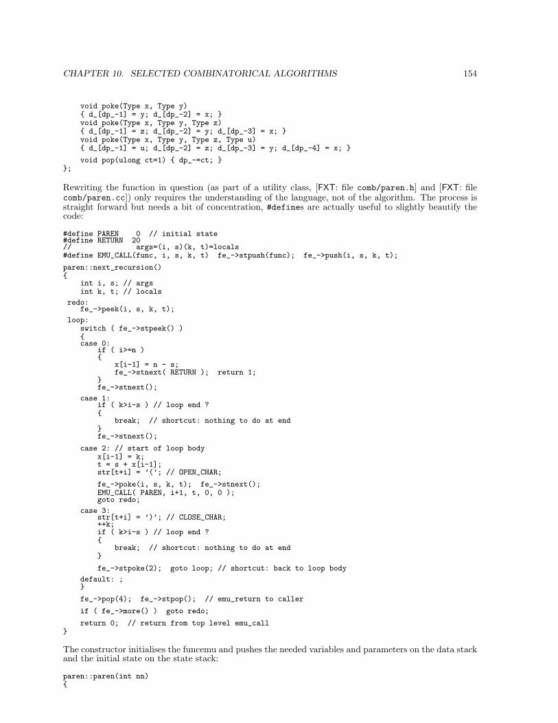
CHAPTER 10. SELECTED COMBINATORICAL ALGORITHMS 154
void poke(Type x, Type y) d_[dp_-1] = y; d_[dp_-2] = x; void poke(Type x, Type y, Type z) d_[dp_-1] = z; d_[dp_-2] = y; d_[dp_-3] = x; void poke(Type x, Type y, Type z, Type u) d_[dp_-1] = u; d_[dp_-2] = z; d_[dp_-3] = y; d_[dp_-4] = x;
void pop(ulong ct=1) dp_-=ct; ;
Rewriting the function in question (as part of a utility class, [FXT: file comb/paren.h] and [FXT: filecomb/paren.cc]) only requires the understanding of the language, not of the algorithm. The process isstraight forward but needs a bit of concentration, #defines are actually useful to slightly beautify thecode:
#define PAREN 0 // initial state#define RETURN 20// args=(i, s)(k, t)=locals#define EMU_CALL(func, i, s, k, t) fe_->stpush(func); fe_->push(i, s, k, t);
paren::next_recursion()
int i, s; // argsint k, t; // locals
redo:fe_->peek(i, s, k, t);
loop:switch ( fe_->stpeek() )case 0:
if ( i>=n )
x[i-1] = n - s;fe_->stnext( RETURN ); return 1;
fe_->stnext();
case 1:if ( k>i-s ) // loop end ?
break; // shortcut: nothing to do at endfe_->stnext();
case 2: // start of loop bodyx[i-1] = k;t = s + x[i-1];str[t+i] = ’(’; // OPEN_CHAR;
fe_->poke(i, s, k, t); fe_->stnext();EMU_CALL( PAREN, i+1, t, 0, 0 );goto redo;
case 3:str[t+i] = ’)’; // CLOSE_CHAR;++k;if ( k>i-s ) // loop end ?
break; // shortcut: nothing to do at end
fe_->stpoke(2); goto loop; // shortcut: back to loop body
default: ;
fe_->pop(4); fe_->stpop(); // emu_return to caller
if ( fe_->more() ) goto redo;
return 0; // return from top level emu_call
The constructor initialises the funcemu and pushes the needed variables and parameters on the data stackand the initial state on the state stack:
paren::paren(int nn)
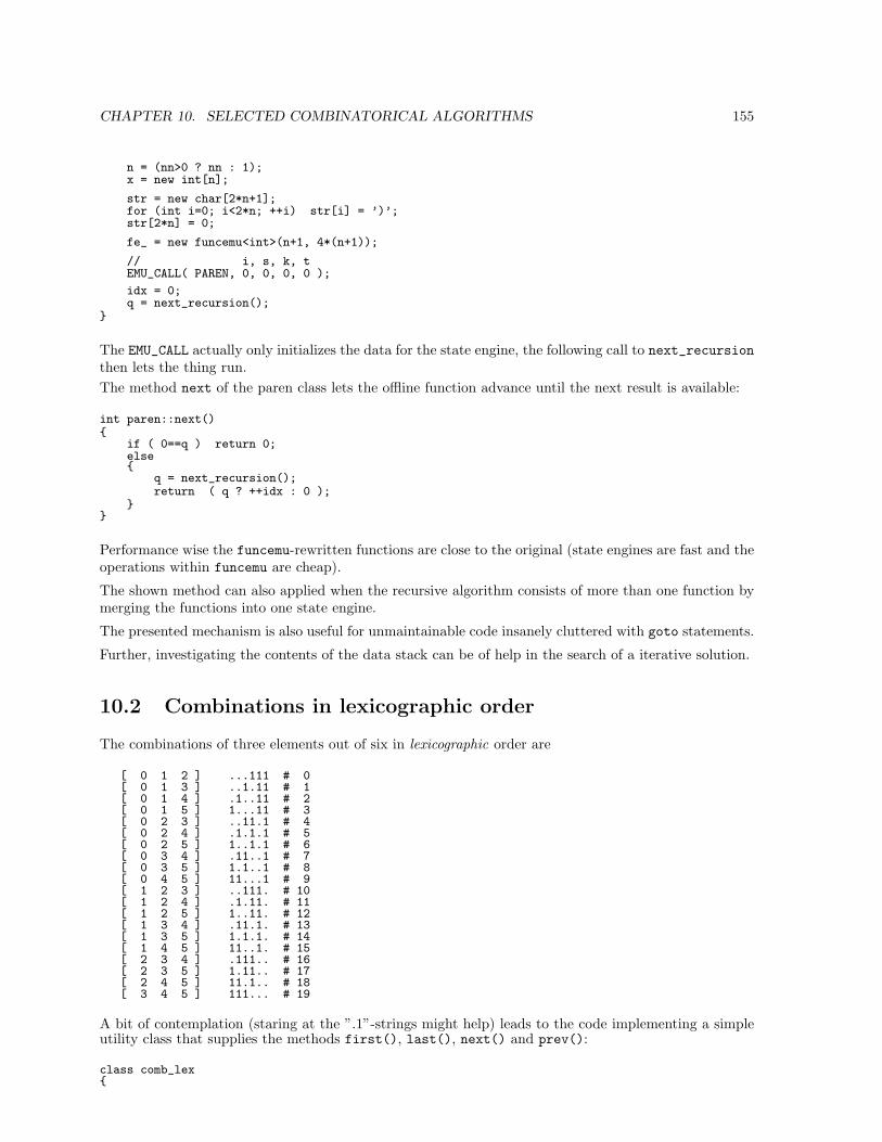
CHAPTER 10. SELECTED COMBINATORICAL ALGORITHMS 155
n = (nn>0 ? nn : 1);x = new int[n];
str = new char[2*n+1];for (int i=0; i<2*n; ++i) str[i] = ’)’;str[2*n] = 0;
fe_ = new funcemu<int>(n+1, 4*(n+1));
// i, s, k, tEMU_CALL( PAREN, 0, 0, 0, 0 );
idx = 0;q = next_recursion();
The EMU_CALL actually only initializes the data for the state engine, the following call to next_recursionthen lets the thing run.The method next of the paren class lets the offline function advance until the next result is available:
int paren::next()
if ( 0==q ) return 0;else
q = next_recursion();return ( q ? ++idx : 0 );
Performance wise the funcemu-rewritten functions are close to the original (state engines are fast and theoperations within funcemu are cheap).
The shown method can also applied when the recursive algorithm consists of more than one function bymerging the functions into one state engine.
The presented mechanism is also useful for unmaintainable code insanely cluttered with goto statements.
Further, investigating the contents of the data stack can be of help in the search of a iterative solution.
10.2 Combinations in lexicographic order
The combinations of three elements out of six in lexicographic order are
[ 0 1 2 ] ...111 # 0[ 0 1 3 ] ..1.11 # 1[ 0 1 4 ] .1..11 # 2[ 0 1 5 ] 1...11 # 3[ 0 2 3 ] ..11.1 # 4[ 0 2 4 ] .1.1.1 # 5[ 0 2 5 ] 1..1.1 # 6[ 0 3 4 ] .11..1 # 7[ 0 3 5 ] 1.1..1 # 8[ 0 4 5 ] 11...1 # 9[ 1 2 3 ] ..111. # 10[ 1 2 4 ] .1.11. # 11[ 1 2 5 ] 1..11. # 12[ 1 3 4 ] .11.1. # 13[ 1 3 5 ] 1.1.1. # 14[ 1 4 5 ] 11..1. # 15[ 2 3 4 ] .111.. # 16[ 2 3 5 ] 1.11.. # 17[ 2 4 5 ] 11.1.. # 18[ 3 4 5 ] 111... # 19
A bit of contemplation (staring at the ”.1”-strings might help) leads to the code implementing a simpleutility class that supplies the methods first(), last(), next() and prev():
class comb_lex

CHAPTER 10. SELECTED COMBINATORICAL ALGORITHMS 156
public:ulong n_;ulong k_;ulong *x_;
public:comb_lex(ulong n, ulong k)
n_ = (n ? n : 1); // not zerok_ = (k ? k : 1); // not zerox_ = NEWOP(ulong, k_ + 1);first();
~comb_lex() delete [] x_;
ulong first()
for (ulong k=0; k<k_; ++k) x_[k] = k;x_[k_] = k_; // sentinelreturn 1;
ulong last()
for (ulong i=0; i<k_; ++i) x_[i] = n_ - k_ + i;return 1;
ulong next() // return zero if previous comb was the last
if ( x_[0] == n_ - k_ ) first(); return 0;
ulong j = k_ - 1;// trivial if highest element != highest possible value:if ( x_[j] < (n_-1) ) ++x_[j]; return 1;
// find highest falling edge:while ( 1 == (x_[j] - x_[j-1]) ) --j;
// move lowest element of highest block up:ulong z = ++x_[j-1];
// ... and attach rest of block:while ( j < k_ ) x_[j] = ++z; ++j;
return 1;
ulong prev() // return zero if current comb is the first
if ( x_[k_-1] == k_-1 ) last(); return 0;
// find highest falling edge:ulong j = k_ - 1;while ( 1 == (x_[j] - x_[j-1]) ) --j;
--x_[j]; // move down edge element
// ... and move rest of block to high end:while ( ++j < k_ ) x_[j] = n_ - k_ + j;
return 1;
const ulong * data() return x_;
friend ostream & operator << (ostream &os, const comb_lex &x);;
[FXT: class comb lex in comb/comblex.h]The listing at the beginning of this section can then be produced by a simple fragment like
ulong ct = 0, n = 6, k = 3;comb_lex comb(n, k);do
cout << endl;cout << " [ " << comb << " ] ";print_set_as_bitset("", comb.data(), k, n );cout << " #" << setw(3) << ct;
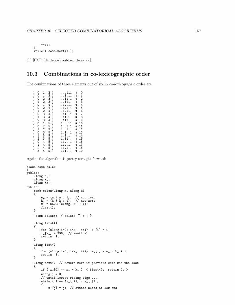
CHAPTER 10. SELECTED COMBINATORICAL ALGORITHMS 157
++ct;while ( comb.next() );
Cf. [FXT: file demo/comblex-demo.cc].
10.3 Combinations in co-lexicographic order
The combinations of three elements out of six in co-lexicographic order are
[ 0 1 2 ] ...111 # 0[ 0 1 3 ] ..1.11 # 1[ 0 2 3 ] ..11.1 # 2[ 1 2 3 ] ..111. # 3[ 0 1 4 ] .1..11 # 4[ 0 2 4 ] .1.1.1 # 5[ 1 2 4 ] .1.11. # 6[ 0 3 4 ] .11..1 # 7[ 1 3 4 ] .11.1. # 8[ 2 3 4 ] .111.. # 9[ 0 1 5 ] 1...11 # 10[ 0 2 5 ] 1..1.1 # 11[ 1 2 5 ] 1..11. # 12[ 0 3 5 ] 1.1..1 # 13[ 1 3 5 ] 1.1.1. # 14[ 2 3 5 ] 1.11.. # 15[ 0 4 5 ] 11...1 # 16[ 1 4 5 ] 11..1. # 17[ 2 4 5 ] 11.1.. # 18[ 3 4 5 ] 111... # 19
Again, the algorithm is pretty straight forward:
class comb_colexpublic:
ulong n_;ulong k_;ulong *x_;
public:comb_colex(ulong n, ulong k)
n_ = (n ? n : 1); // not zerok_ = (k ? k : 1); // not zerox_ = NEWOP(ulong, k_ + 1);first();
~comb_colex() delete [] x_;
ulong first()
for (ulong i=0; i<k_; ++i) x_[i] = i;x_[k_] = 999; // sentinelreturn 1;
ulong last()
for (ulong i=0; i<k_; ++i) x_[i] = n_ - k_ + i;return 1;
ulong next() // return zero if previous comb was the last
if ( x_[0] == n_ - k_ ) first(); return 0;
ulong j = 0;// until lowest rising edge ...while ( 1 == (x_[j+1] - x_[j]) )
x_[j] = j; // attach block at low end
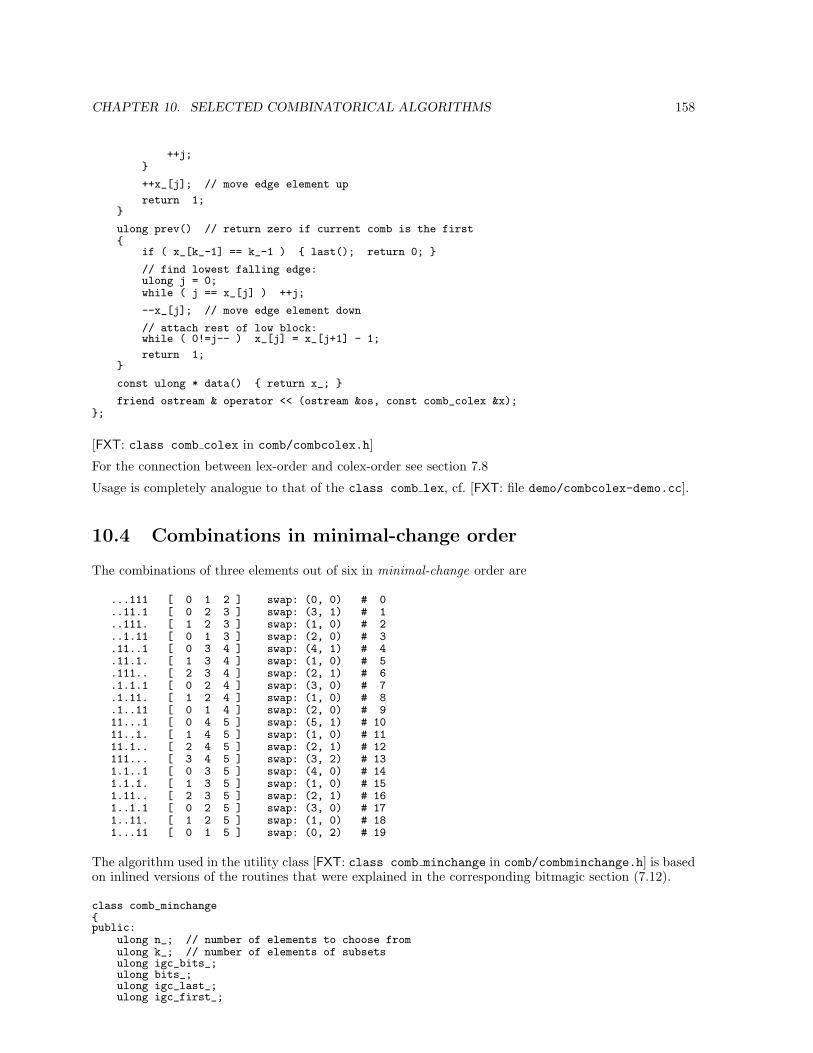
CHAPTER 10. SELECTED COMBINATORICAL ALGORITHMS 158
++j;
++x_[j]; // move edge element up
return 1;
ulong prev() // return zero if current comb is the first
if ( x_[k_-1] == k_-1 ) last(); return 0;
// find lowest falling edge:ulong j = 0;while ( j == x_[j] ) ++j;
--x_[j]; // move edge element down
// attach rest of low block:while ( 0!=j-- ) x_[j] = x_[j+1] - 1;
return 1;
const ulong * data() return x_;
friend ostream & operator << (ostream &os, const comb_colex &x);;
[FXT: class comb colex in comb/combcolex.h]
For the connection between lex-order and colex-order see section 7.8
Usage is completely analogue to that of the class comb lex, cf. [FXT: file demo/combcolex-demo.cc].
10.4 Combinations in minimal-change order
The combinations of three elements out of six in minimal-change order are
...111 [ 0 1 2 ] swap: (0, 0) # 0
..11.1 [ 0 2 3 ] swap: (3, 1) # 1
..111. [ 1 2 3 ] swap: (1, 0) # 2
..1.11 [ 0 1 3 ] swap: (2, 0) # 3
.11..1 [ 0 3 4 ] swap: (4, 1) # 4
.11.1. [ 1 3 4 ] swap: (1, 0) # 5
.111.. [ 2 3 4 ] swap: (2, 1) # 6
.1.1.1 [ 0 2 4 ] swap: (3, 0) # 7
.1.11. [ 1 2 4 ] swap: (1, 0) # 8
.1..11 [ 0 1 4 ] swap: (2, 0) # 911...1 [ 0 4 5 ] swap: (5, 1) # 1011..1. [ 1 4 5 ] swap: (1, 0) # 1111.1.. [ 2 4 5 ] swap: (2, 1) # 12111... [ 3 4 5 ] swap: (3, 2) # 131.1..1 [ 0 3 5 ] swap: (4, 0) # 141.1.1. [ 1 3 5 ] swap: (1, 0) # 151.11.. [ 2 3 5 ] swap: (2, 1) # 161..1.1 [ 0 2 5 ] swap: (3, 0) # 171..11. [ 1 2 5 ] swap: (1, 0) # 181...11 [ 0 1 5 ] swap: (0, 2) # 19
The algorithm used in the utility class [FXT: class comb minchange in comb/combminchange.h] is basedon inlined versions of the routines that were explained in the corresponding bitmagic section (7.12).
class comb_minchangepublic:
ulong n_; // number of elements to choose fromulong k_; // number of elements of subsetsulong igc_bits_;ulong bits_;ulong igc_last_;ulong igc_first_;
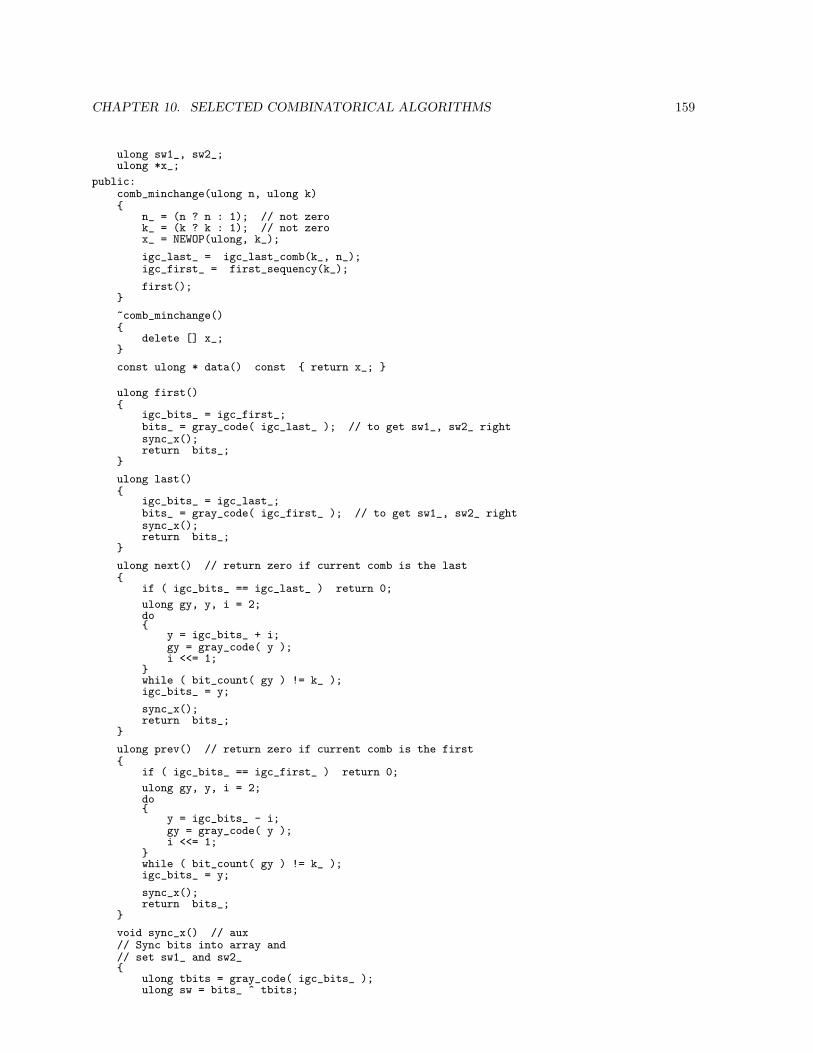
CHAPTER 10. SELECTED COMBINATORICAL ALGORITHMS 159
ulong sw1_, sw2_;ulong *x_;
public:comb_minchange(ulong n, ulong k)
n_ = (n ? n : 1); // not zerok_ = (k ? k : 1); // not zerox_ = NEWOP(ulong, k_);
igc_last_ = igc_last_comb(k_, n_);igc_first_ = first_sequency(k_);
first();
~comb_minchange()
delete [] x_;
const ulong * data() const return x_;
ulong first()
igc_bits_ = igc_first_;bits_ = gray_code( igc_last_ ); // to get sw1_, sw2_ rightsync_x();return bits_;
ulong last()
igc_bits_ = igc_last_;bits_ = gray_code( igc_first_ ); // to get sw1_, sw2_ rightsync_x();return bits_;
ulong next() // return zero if current comb is the last
if ( igc_bits_ == igc_last_ ) return 0;
ulong gy, y, i = 2;do
y = igc_bits_ + i;gy = gray_code( y );i <<= 1;
while ( bit_count( gy ) != k_ );igc_bits_ = y;
sync_x();return bits_;
ulong prev() // return zero if current comb is the first
if ( igc_bits_ == igc_first_ ) return 0;
ulong gy, y, i = 2;do
y = igc_bits_ - i;gy = gray_code( y );i <<= 1;
while ( bit_count( gy ) != k_ );igc_bits_ = y;
sync_x();return bits_;
void sync_x() // aux// Sync bits into array and// set sw1_ and sw2_
ulong tbits = gray_code( igc_bits_ );ulong sw = bits_ ^ tbits;
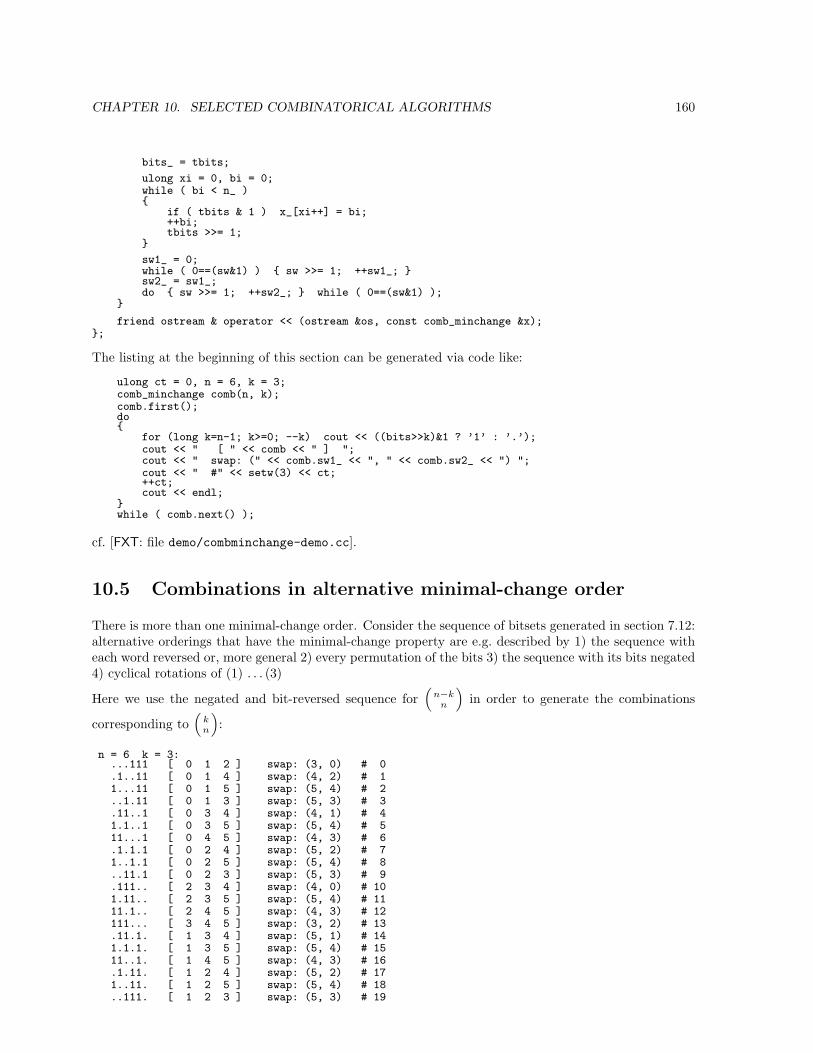
CHAPTER 10. SELECTED COMBINATORICAL ALGORITHMS 160
bits_ = tbits;
ulong xi = 0, bi = 0;while ( bi < n_ )
if ( tbits & 1 ) x_[xi++] = bi;++bi;tbits >>= 1;
sw1_ = 0;while ( 0==(sw&1) ) sw >>= 1; ++sw1_; sw2_ = sw1_;do sw >>= 1; ++sw2_; while ( 0==(sw&1) );
friend ostream & operator << (ostream &os, const comb_minchange &x);;
The listing at the beginning of this section can be generated via code like:
ulong ct = 0, n = 6, k = 3;comb_minchange comb(n, k);comb.first();do
for (long k=n-1; k>=0; --k) cout << ((bits>>k)&1 ? ’1’ : ’.’);cout << " [ " << comb << " ] ";cout << " swap: (" << comb.sw1_ << ", " << comb.sw2_ << ") ";cout << " #" << setw(3) << ct;++ct;cout << endl;
while ( comb.next() );
cf. [FXT: file demo/combminchange-demo.cc].
10.5 Combinations in alternative minimal-change order
There is more than one minimal-change order. Consider the sequence of bitsets generated in section 7.12:alternative orderings that have the minimal-change property are e.g. described by 1) the sequence witheach word reversed or, more general 2) every permutation of the bits 3) the sequence with its bits negated4) cyclical rotations of (1) . . . (3)
Here we use the negated and bit-reversed sequence for(
n−kn
)in order to generate the combinations
corresponding to(
kn
):
n = 6 k = 3:...111 [ 0 1 2 ] swap: (3, 0) # 0.1..11 [ 0 1 4 ] swap: (4, 2) # 11...11 [ 0 1 5 ] swap: (5, 4) # 2..1.11 [ 0 1 3 ] swap: (5, 3) # 3.11..1 [ 0 3 4 ] swap: (4, 1) # 41.1..1 [ 0 3 5 ] swap: (5, 4) # 511...1 [ 0 4 5 ] swap: (4, 3) # 6.1.1.1 [ 0 2 4 ] swap: (5, 2) # 71..1.1 [ 0 2 5 ] swap: (5, 4) # 8..11.1 [ 0 2 3 ] swap: (5, 3) # 9.111.. [ 2 3 4 ] swap: (4, 0) # 101.11.. [ 2 3 5 ] swap: (5, 4) # 1111.1.. [ 2 4 5 ] swap: (4, 3) # 12111... [ 3 4 5 ] swap: (3, 2) # 13.11.1. [ 1 3 4 ] swap: (5, 1) # 141.1.1. [ 1 3 5 ] swap: (5, 4) # 1511..1. [ 1 4 5 ] swap: (4, 3) # 16.1.11. [ 1 2 4 ] swap: (5, 2) # 171..11. [ 1 2 5 ] swap: (5, 4) # 18..111. [ 1 2 3 ] swap: (5, 3) # 19
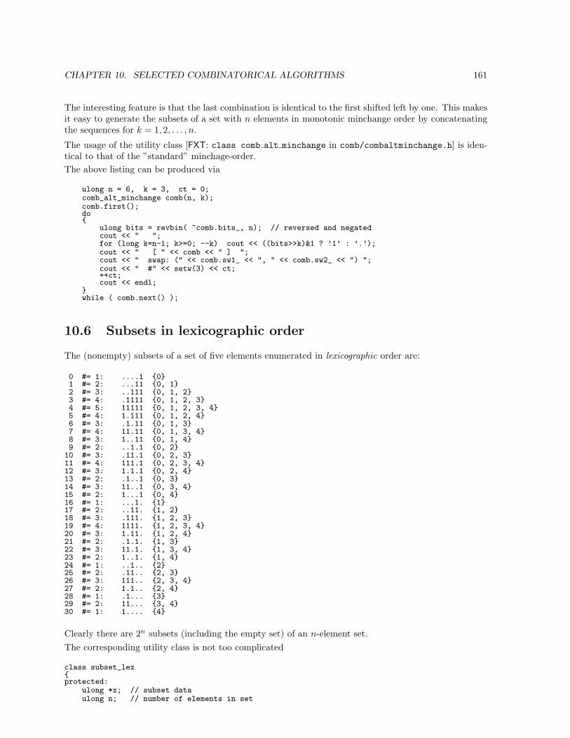
CHAPTER 10. SELECTED COMBINATORICAL ALGORITHMS 161
The interesting feature is that the last combination is identical to the first shifted left by one. This makesit easy to generate the subsets of a set with n elements in monotonic minchange order by concatenatingthe sequences for k = 1, 2, . . . , n.
The usage of the utility class [FXT: class comb alt minchange in comb/combaltminchange.h] is iden-tical to that of the ”standard” minchage-order.The above listing can be produced via
ulong n = 6, k = 3, ct = 0;comb_alt_minchange comb(n, k);comb.first();do
ulong bits = revbin( ~comb.bits_, n); // reversed and negatedcout << " ";for (long k=n-1; k>=0; --k) cout << ((bits>>k)&1 ? ’1’ : ’.’);cout << " [ " << comb << " ] ";cout << " swap: (" << comb.sw1_ << ", " << comb.sw2_ << ") ";cout << " #" << setw(3) << ct;++ct;cout << endl;
while ( comb.next() );
10.6 Subsets in lexicographic order
The (nonempty) subsets of a set of five elements enumerated in lexicographic order are:
0 #= 1: ....1 01 #= 2: ...11 0, 12 #= 3: ..111 0, 1, 23 #= 4: .1111 0, 1, 2, 34 #= 5: 11111 0, 1, 2, 3, 45 #= 4: 1.111 0, 1, 2, 46 #= 3: .1.11 0, 1, 37 #= 4: 11.11 0, 1, 3, 48 #= 3: 1..11 0, 1, 49 #= 2: ..1.1 0, 2
10 #= 3: .11.1 0, 2, 311 #= 4: 111.1 0, 2, 3, 412 #= 3: 1.1.1 0, 2, 413 #= 2: .1..1 0, 314 #= 3: 11..1 0, 3, 415 #= 2: 1...1 0, 416 #= 1: ...1. 117 #= 2: ..11. 1, 218 #= 3: .111. 1, 2, 319 #= 4: 1111. 1, 2, 3, 420 #= 3: 1.11. 1, 2, 421 #= 2: .1.1. 1, 322 #= 3: 11.1. 1, 3, 423 #= 2: 1..1. 1, 424 #= 1: ..1.. 225 #= 2: .11.. 2, 326 #= 3: 111.. 2, 3, 427 #= 2: 1.1.. 2, 428 #= 1: .1... 329 #= 2: 11... 3, 430 #= 1: 1.... 4
Clearly there are 2n subsets (including the empty set) of an n-element set.The corresponding utility class is not too complicated
class subset_lexprotected:
ulong *x; // subset dataulong n; // number of elements in set
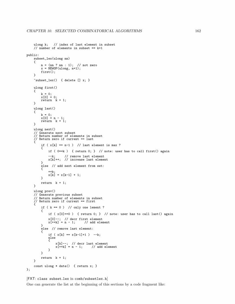
CHAPTER 10. SELECTED COMBINATORICAL ALGORITHMS 162
ulong k; // index of last element in subset// number of elements in subset == k+1
public:subset_lex(ulong nn)
n = (nn ? nn : 1); // not zerox = NEWOP(ulong, n+1);first();
~subset_lex() delete [] x;
ulong first()
k = 0;x[0] = 0;return k + 1;
ulong last()
k = 0;x[0] = n - 1;return k + 1;
ulong next()// Generate next subset// Return number of elements in subset// Return zero if current == last
if ( x[k] == n-1 ) // last element is max ?
if ( 0==k ) return 0; // note: user has to call first() again
--k; // remove last elementx[k]++; // increase last element
else // add next element from set:
++k;x[k] = x[k-1] + 1;
return k + 1;
ulong prev()// Generate previous subset// Return number of elements in subset// Return zero if current == first
if ( k == 0 ) // only one lement ?
if ( x[0]==0 ) return 0; // note: user has to call last() again
x[0]--; // decr first elementx[++k] = n - 1; // add element
else // remove last element:
if ( x[k] == x[k-1]+1 ) --k;else
x[k]--; // decr last elementx[++k] = n - 1; // add element
return k + 1;
const ulong * data() return x; ;
[FXT: class subset lex in comb/subsetlex.h]One can generate the list at the beginning of this sections by a code fragment like:
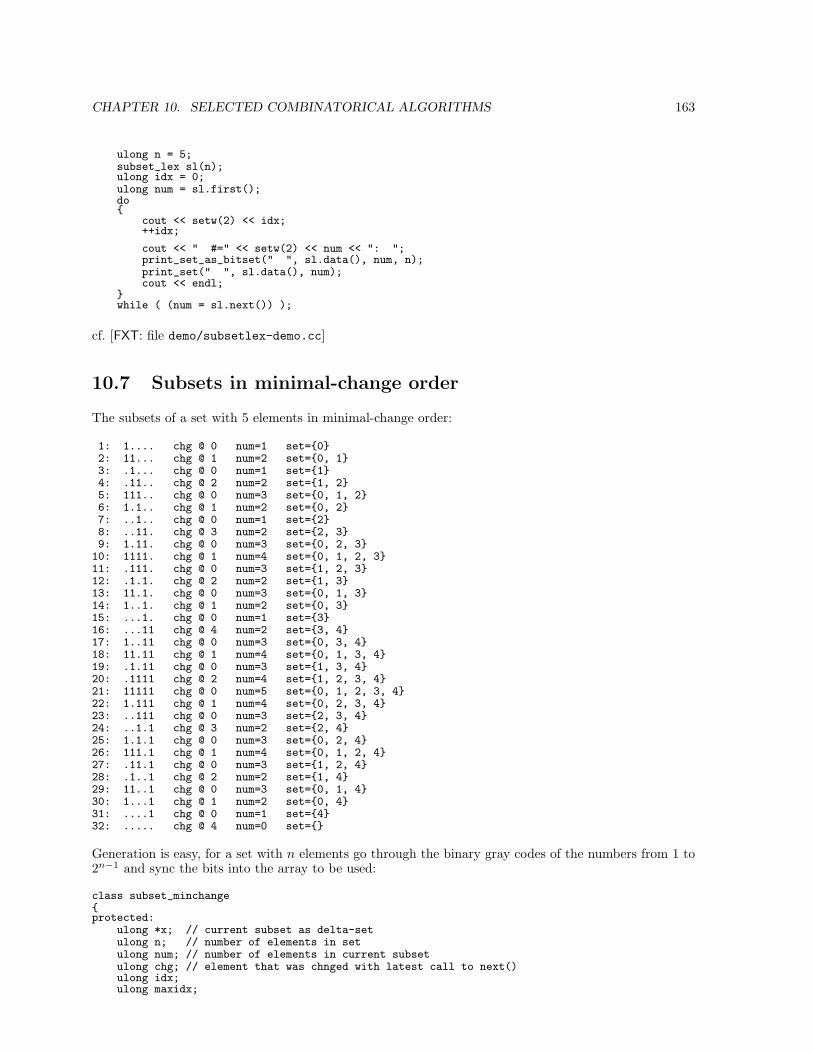
CHAPTER 10. SELECTED COMBINATORICAL ALGORITHMS 163
ulong n = 5;subset_lex sl(n);ulong idx = 0;ulong num = sl.first();do
cout << setw(2) << idx;++idx;
cout << " #=" << setw(2) << num << ": ";print_set_as_bitset(" ", sl.data(), num, n);print_set(" ", sl.data(), num);cout << endl;
while ( (num = sl.next()) );
cf. [FXT: file demo/subsetlex-demo.cc]
10.7 Subsets in minimal-change order
The subsets of a set with 5 elements in minimal-change order:
1: 1.... chg @ 0 num=1 set=02: 11... chg @ 1 num=2 set=0, 13: .1... chg @ 0 num=1 set=14: .11.. chg @ 2 num=2 set=1, 25: 111.. chg @ 0 num=3 set=0, 1, 26: 1.1.. chg @ 1 num=2 set=0, 27: ..1.. chg @ 0 num=1 set=28: ..11. chg @ 3 num=2 set=2, 39: 1.11. chg @ 0 num=3 set=0, 2, 3
10: 1111. chg @ 1 num=4 set=0, 1, 2, 311: .111. chg @ 0 num=3 set=1, 2, 312: .1.1. chg @ 2 num=2 set=1, 313: 11.1. chg @ 0 num=3 set=0, 1, 314: 1..1. chg @ 1 num=2 set=0, 315: ...1. chg @ 0 num=1 set=316: ...11 chg @ 4 num=2 set=3, 417: 1..11 chg @ 0 num=3 set=0, 3, 418: 11.11 chg @ 1 num=4 set=0, 1, 3, 419: .1.11 chg @ 0 num=3 set=1, 3, 420: .1111 chg @ 2 num=4 set=1, 2, 3, 421: 11111 chg @ 0 num=5 set=0, 1, 2, 3, 422: 1.111 chg @ 1 num=4 set=0, 2, 3, 423: ..111 chg @ 0 num=3 set=2, 3, 424: ..1.1 chg @ 3 num=2 set=2, 425: 1.1.1 chg @ 0 num=3 set=0, 2, 426: 111.1 chg @ 1 num=4 set=0, 1, 2, 427: .11.1 chg @ 0 num=3 set=1, 2, 428: .1..1 chg @ 2 num=2 set=1, 429: 11..1 chg @ 0 num=3 set=0, 1, 430: 1...1 chg @ 1 num=2 set=0, 431: ....1 chg @ 0 num=1 set=432: ..... chg @ 4 num=0 set=
Generation is easy, for a set with n elements go through the binary gray codes of the numbers from 1 to2n−1 and sync the bits into the array to be used:
class subset_minchangeprotected:
ulong *x; // current subset as delta-setulong n; // number of elements in setulong num; // number of elements in current subsetulong chg; // element that was chnged with latest call to next()ulong idx;ulong maxidx;
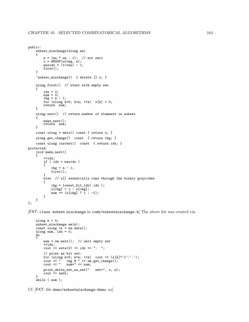
CHAPTER 10. SELECTED COMBINATORICAL ALGORITHMS 164
public:subset_minchange(ulong nn)
n = (nn ? nn : 1); // not zerox = NEWOP(ulong, n);maxidx = (1<<nn) - 1;first();
~subset_minchange() delete [] x;
ulong first() // start with empty set
idx = 0;num = 0;chg = n - 1;for (ulong k=0; k<n; ++k) x[k] = 0;return num;
ulong next() // return number of elements in subset
make_next();return num;
const ulong * data() const return x;
ulong get_change() const return chg;
const ulong current() const return idx;
protected:void make_next()
++idx;if ( idx > maxidx )
chg = n - 1;first();
else // x[] essentially runs through the binary graycodes
chg = lowest_bit_idx( idx );x[chg] = 1 - x[chg];num += (x[chg] ? 1 : -1);
;
[FXT: class subset minchange in comb/subsetminchange.h] The above list was created via
ulong n = 5;subset_minchange sm(n);const ulong *x = sm.data();ulong num, idx = 0;do
num = sm.next(); // omit empty set++idx;cout << setw(2) << idx << ": ";
// print as bit set:for (ulong k=0; k<n; ++k) cout << (x[k]?’1’:’.’);cout << " chg @ " << sm.get_change();cout << " num=" << num;
print_delta_set_as_set(" set=", x, n);cout << endl;
while ( num );
Cf. [FXT: file demo/subsetminchange-demo.cc]
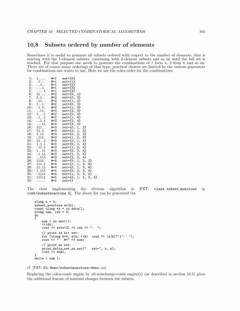
CHAPTER 10. SELECTED COMBINATORICAL ALGORITHMS 165
10.8 Subsets ordered by number of elements
Sometimes it is useful to generate all subsets ordered with respect to the number of elements, that isstarting with the 1-element subsets, continuing with 2-element subsets and so on until the full set isreached. For that purpose one needs to generate the combinations of 1 form n, 2 from n and so on.There are of course many orderings of that type, practical choices are limited by the various generatorsfor combinations one wants to use. Here we use the colex-order for the combinations:
1: 1.... #=1 set=02: .1... #=1 set=13: ..1.. #=1 set=24: ...1. #=1 set=35: ....1 #=1 set=46: 11... #=2 set=0, 17: 1.1.. #=2 set=0, 28: .11.. #=2 set=1, 29: 1..1. #=2 set=0, 3
10: .1.1. #=2 set=1, 311: ..11. #=2 set=2, 312: 1...1 #=2 set=0, 413: .1..1 #=2 set=1, 414: ..1.1 #=2 set=2, 415: ...11 #=2 set=3, 416: 111.. #=3 set=0, 1, 217: 11.1. #=3 set=0, 1, 318: 1.11. #=3 set=0, 2, 319: .111. #=3 set=1, 2, 320: 11..1 #=3 set=0, 1, 421: 1.1.1 #=3 set=0, 2, 422: .11.1 #=3 set=1, 2, 423: 1..11 #=3 set=0, 3, 424: .1.11 #=3 set=1, 3, 425: ..111 #=3 set=2, 3, 426: 1111. #=4 set=0, 1, 2, 327: 111.1 #=4 set=0, 1, 2, 428: 11.11 #=4 set=0, 1, 3, 429: 1.111 #=4 set=0, 2, 3, 430: .1111 #=4 set=1, 2, 3, 431: 11111 #=5 set=0, 1, 2, 3, 432: ..... #=0 set=
The class implementing the obvious algorithm is [FXT: class subset monotone incomb/subsetmonotone.h]. The above list can be generated via
ulong n = 5;subset_monotone so(n);const ulong *x = so.data();ulong num, idx = 0;do
num = so.next();++idx;cout << setw(2) << idx << ": ";
// print as bit set:for (ulong k=0; k<n; ++k) cout << (x[k]?’1’:’.’);cout << " #=" << num;
// print as set:print_delta_set_as_set(" set=", x, n);cout << endl;
while ( num );
cf. [FXT: file demo/subsetmonotone-demo.cc]
Replacing the colex-comb engine by alt-minchange-comb engine(s) (as described in section 10.5) givesthe additional feature of minimal changes between the subsets.
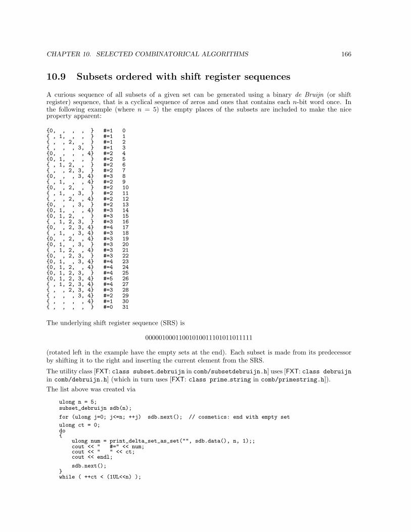
CHAPTER 10. SELECTED COMBINATORICAL ALGORITHMS 166
10.9 Subsets ordered with shift register sequences
A curious sequence of all subsets of a given set can be generated using a binary de Bruijn (or shiftregister) sequence, that is a cyclical sequence of zeros and ones that contains each n-bit word once. Inthe following example (where n = 5) the empty places of the subsets are included to make the niceproperty apparent:
0, , , , #=1 0 , 1, , , #=1 1 , , 2, , #=1 2 , , , 3, #=1 30, , , , 4 #=2 40, 1, , , #=2 5 , 1, 2, , #=2 6 , , 2, 3, #=2 70, , , 3, 4 #=3 8 , 1, , , 4 #=2 90, , 2, , #=2 10 , 1, , 3, #=2 11 , , 2, , 4 #=2 120, , , 3, #=2 130, 1, , , 4 #=3 140, 1, 2, , #=3 15 , 1, 2, 3, #=3 160, , 2, 3, 4 #=4 17 , 1, , 3, 4 #=3 180, , 2, , 4 #=3 190, 1, , 3, #=3 20 , 1, 2, , 4 #=3 210, , 2, 3, #=3 220, 1, , 3, 4 #=4 230, 1, 2, , 4 #=4 240, 1, 2, 3, #=4 250, 1, 2, 3, 4 #=5 26 , 1, 2, 3, 4 #=4 27 , , 2, 3, 4 #=3 28 , , , 3, 4 #=2 29 , , , , 4 #=1 30 , , , , #=0 31
The underlying shift register sequence (SRS) is
00000100011001010011101011011111
(rotated left in the example have the empty sets at the end). Each subset is made from its predecessorby shifting it to the right and inserting the current element from the SRS.
The utility class [FXT: class subset debruijn in comb/subsetdebruijn.h] uses [FXT: class debruijnin comb/debruijn.h] (which in turn uses [FXT: class prime string in comb/primestring.h]).The list above was created via
ulong n = 5;subset_debruijn sdb(n);
for (ulong j=0; j<=n; ++j) sdb.next(); // cosmetics: end with empty set
ulong ct = 0;do
ulong num = print_delta_set_as_set("", sdb.data(), n, 1);;cout << " #=" << num;cout << " " << ct;cout << endl;
sdb.next();while ( ++ct < (1UL<<n) );
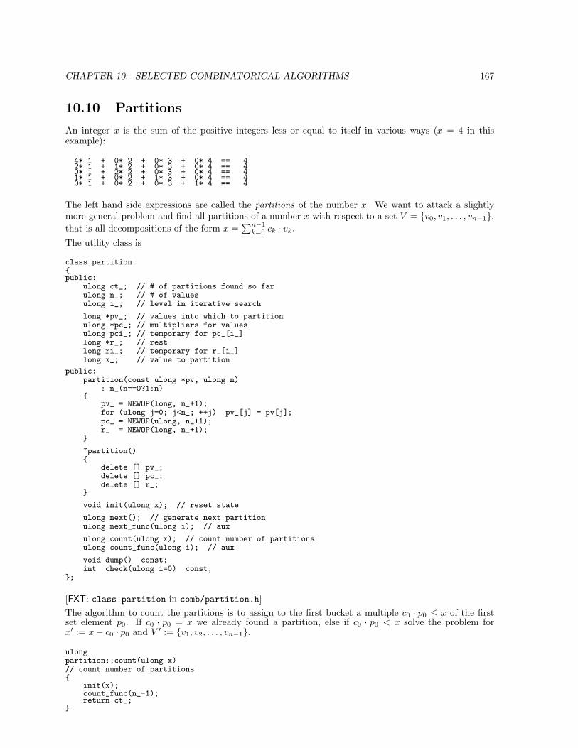
CHAPTER 10. SELECTED COMBINATORICAL ALGORITHMS 167
10.10 Partitions
An integer x is the sum of the positive integers less or equal to itself in various ways (x = 4 in thisexample):
4* 1 + 0* 2 + 0* 3 + 0* 4 == 42* 1 + 1* 2 + 0* 3 + 0* 4 == 40* 1 + 2* 2 + 0* 3 + 0* 4 == 41* 1 + 0* 2 + 1* 3 + 0* 4 == 40* 1 + 0* 2 + 0* 3 + 1* 4 == 4
The left hand side expressions are called the partitions of the number x. We want to attack a slightlymore general problem and find all partitions of a number x with respect to a set V = v0, v1, . . . , vn−1,that is all decompositions of the form x =
∑n−1k=0 ck · vk.
The utility class is
class partitionpublic:
ulong ct_; // # of partitions found so farulong n_; // # of valuesulong i_; // level in iterative search
long *pv_; // values into which to partitionulong *pc_; // multipliers for valuesulong pci_; // temporary for pc_[i_]long *r_; // restlong ri_; // temporary for r_[i_]long x_; // value to partition
public:partition(const ulong *pv, ulong n)
: n_(n==0?1:n)
pv_ = NEWOP(long, n_+1);for (ulong j=0; j<n_; ++j) pv_[j] = pv[j];pc_ = NEWOP(ulong, n_+1);r_ = NEWOP(long, n_+1);
~partition()
delete [] pv_;delete [] pc_;delete [] r_;
void init(ulong x); // reset state
ulong next(); // generate next partitionulong next_func(ulong i); // aux
ulong count(ulong x); // count number of partitionsulong count_func(ulong i); // aux
void dump() const;int check(ulong i=0) const;
;
[FXT: class partition in comb/partition.h]The algorithm to count the partitions is to assign to the first bucket a multiple c0 · p0 ≤ x of the firstset element p0. If c0 · p0 = x we already found a partition, else if c0 · p0 < x solve the problem forx′ := x− c0 · p0 and V ′ := v1, v2, . . . , vn−1.ulongpartition::count(ulong x)// count number of partitions
init(x);count_func(n_-1);return ct_;
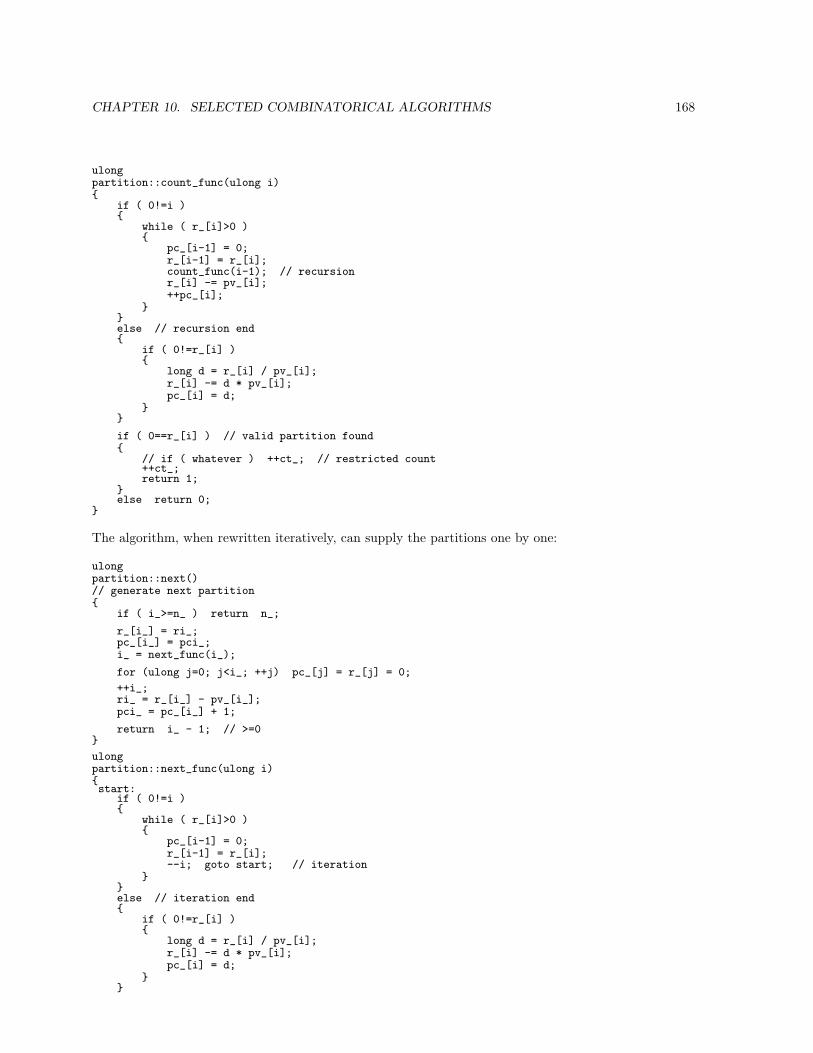
CHAPTER 10. SELECTED COMBINATORICAL ALGORITHMS 168
ulongpartition::count_func(ulong i)
if ( 0!=i )
while ( r_[i]>0 )
pc_[i-1] = 0;r_[i-1] = r_[i];count_func(i-1); // recursionr_[i] -= pv_[i];++pc_[i];
else // recursion end
if ( 0!=r_[i] )
long d = r_[i] / pv_[i];r_[i] -= d * pv_[i];pc_[i] = d;
if ( 0==r_[i] ) // valid partition found
// if ( whatever ) ++ct_; // restricted count++ct_;return 1;
else return 0;
The algorithm, when rewritten iteratively, can supply the partitions one by one:
ulongpartition::next()// generate next partition
if ( i_>=n_ ) return n_;
r_[i_] = ri_;pc_[i_] = pci_;i_ = next_func(i_);
for (ulong j=0; j<i_; ++j) pc_[j] = r_[j] = 0;
++i_;ri_ = r_[i_] - pv_[i_];pci_ = pc_[i_] + 1;
return i_ - 1; // >=0
ulongpartition::next_func(ulong i)start:
if ( 0!=i )
while ( r_[i]>0 )
pc_[i-1] = 0;r_[i-1] = r_[i];--i; goto start; // iteration
else // iteration end
if ( 0!=r_[i] )
long d = r_[i] / pv_[i];r_[i] -= d * pv_[i];pc_[i] = d;
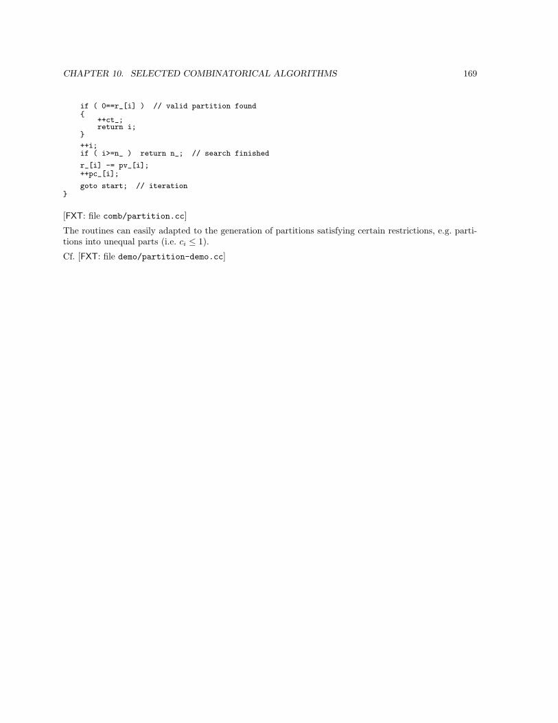
CHAPTER 10. SELECTED COMBINATORICAL ALGORITHMS 169
if ( 0==r_[i] ) // valid partition found
++ct_;return i;
++i;if ( i>=n_ ) return n_; // search finished
r_[i] -= pv_[i];++pc_[i];
goto start; // iteration
[FXT: file comb/partition.cc]
The routines can easily adapted to the generation of partitions satisfying certain restrictions, e.g. parti-tions into unequal parts (i.e. ci ≤ 1).
Cf. [FXT: file demo/partition-demo.cc]
Chapter 11
Arithmetical algorithms
11.1 Asymptotics of algorithms
An important feature of an algorithm is the number of operations that must be performed for thecompletion of a task of a certain size N . The quantity N should be some reasonable quantity that growsstrictly with the size of the task. For high precision computations one will take the length of the numberscounted in decimal digits or bits. For computations with square matrices one may take for N the numberof rows. An operation is typically a (machine word) multiplication plus an addition, one could also simplycount machine instructions.
An algorithm is said to have some asymptotics f(N) if it needs proportional f(N) operations for a taskof size N .
Examples:
• Addition of an N -digit number needs proportional N operations (here: machine word addition plussome carry operation).
• Ordinary multiplication needs ∼ N2 operations.
• The Fast Fourier Transform (FFT) needs ∼ N log(N) operations (a straight forward implementa-tion of the Fourier Transform, i.e. computing N sums each of length N would be ∼ N2).
• Matrix multiplication (by the obvious algorithm) is ∼ N3 (N2 sums each of N products).
The algorithm with the ‘best’ asymptotics wins for some, possibly huge, N . For smaller N anotheralgorithm will be superior. For the exact break-even point the constants omitted elsewhere are of courseimportant.
Example: Let the algorithm mult1 take 1.0 ·N2 operations, mult2 take 8.0 ·N log2(N) operations. Then,for N < 64 mult1 is faster and for N > 64 mult2 is faster. Completely different algorithms may beoptimal for the same task at different problem sizes.
11.2 Multiplication of large numbers
Ordinary multiplication is ∼ N2. Computing the product of two million-digit numbers would require≈ 1012 operations, taking about 1 day on a machine that does 10 million operations per second. Butthere are better ways . . .
170
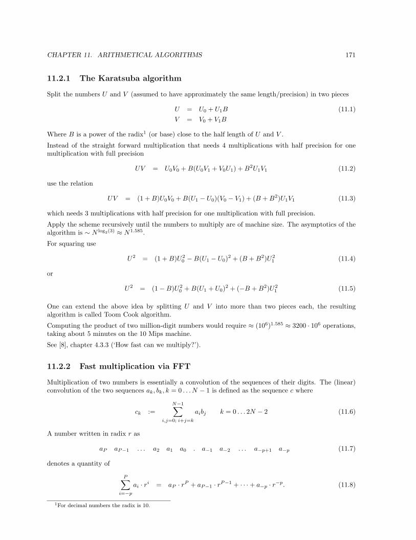
CHAPTER 11. ARITHMETICAL ALGORITHMS 171
11.2.1 The Karatsuba algorithm
Split the numbers U and V (assumed to have approximately the same length/precision) in two pieces
U = U0 + U1B (11.1)V = V0 + V1B
Where B is a power of the radix1 (or base) close to the half length of U and V .
Instead of the straight forward multiplication that needs 4 multiplications with half precision for onemultiplication with full precision
UV = U0V0 + B(U0V1 + V0U1) + B2U1V1 (11.2)
use the relation
UV = (1 + B)U0V0 + B(U1 − U0)(V0 − V1) + (B + B2)U1V1 (11.3)
which needs 3 multiplications with half precision for one multiplication with full precision.
Apply the scheme recursively until the numbers to multiply are of machine size. The asymptotics of thealgorithm is ∼ N log2(3) ≈ N1.585.
For squaring use
U2 = (1 + B)U20 −B(U1 − U0)2 + (B + B2)U2
1 (11.4)
or
U2 = (1−B)U20 + B(U1 + U0)2 + (−B + B2)U2
1 (11.5)
One can extend the above idea by splitting U and V into more than two pieces each, the resultingalgorithm is called Toom Cook algorithm.
Computing the product of two million-digit numbers would require ≈ (106)1.585 ≈ 3200 · 106 operations,taking about 5 minutes on the 10 Mips machine.
See [8], chapter 4.3.3 (‘How fast can we multiply?’).
11.2.2 Fast multiplication via FFT
Multiplication of two numbers is essentially a convolution of the sequences of their digits. The (linear)convolution of the two sequences ak, bk, k = 0 . . . N − 1 is defined as the sequence c where
ck :=N−1∑
i,j=0; i+j=k
aibj k = 0 . . . 2N − 2 (11.6)
A number written in radix r as
aP aP−1 . . . a2 a1 a0 . a−1 a−2 . . . a−p+1 a−p (11.7)
denotes a quantity of
P∑
i=−p
ai · ri = aP · rP + aP−1 · rP−1 + · · ·+ a−p · r−p. (11.8)
1For decimal numbers the radix is 10.
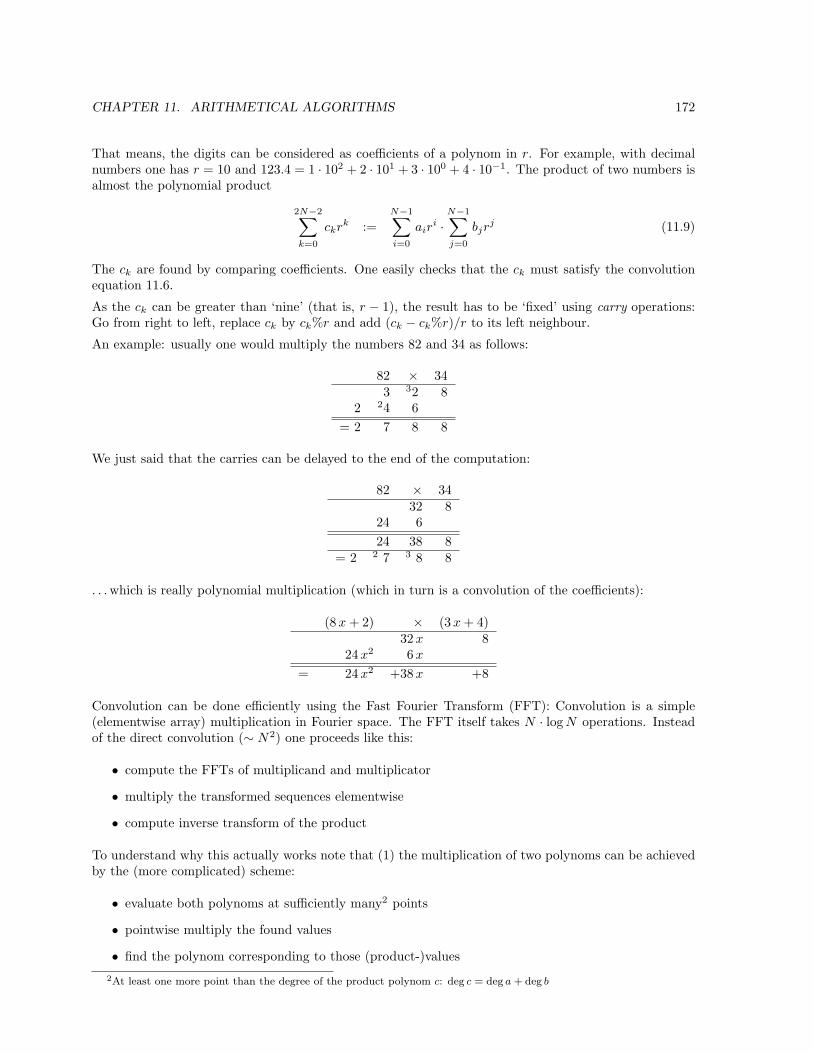
CHAPTER 11. ARITHMETICAL ALGORITHMS 172
That means, the digits can be considered as coefficients of a polynom in r. For example, with decimalnumbers one has r = 10 and 123.4 = 1 · 102 + 2 · 101 + 3 · 100 + 4 · 10−1. The product of two numbers isalmost the polynomial product
2N−2∑
k=0
ckrk :=N−1∑
i=0
airi ·
N−1∑
j=0
bjrj (11.9)
The ck are found by comparing coefficients. One easily checks that the ck must satisfy the convolutionequation 11.6.
As the ck can be greater than ‘nine’ (that is, r − 1), the result has to be ‘fixed’ using carry operations:Go from right to left, replace ck by ck%r and add (ck − ck%r)/r to its left neighbour.
An example: usually one would multiply the numbers 82 and 34 as follows:
82 × 343 32 8
2 24 6= 2 7 8 8
We just said that the carries can be delayed to the end of the computation:
82 × 3432 8
24 624 38 8
= 2 2 7 3 8 8
. . . which is really polynomial multiplication (which in turn is a convolution of the coefficients):
(8x + 2) × (3x + 4)32 x 8
24 x2 6 x
= 24 x2 +38 x +8
Convolution can be done efficiently using the Fast Fourier Transform (FFT): Convolution is a simple(elementwise array) multiplication in Fourier space. The FFT itself takes N · log N operations. Insteadof the direct convolution (∼ N2) one proceeds like this:
• compute the FFTs of multiplicand and multiplicator
• multiply the transformed sequences elementwise
• compute inverse transform of the product
To understand why this actually works note that (1) the multiplication of two polynoms can be achievedby the (more complicated) scheme:
• evaluate both polynoms at sufficiently many2 points
• pointwise multiply the found values
• find the polynom corresponding to those (product-)values
2At least one more point than the degree of the product polynom c: deg c = deg a + deg b
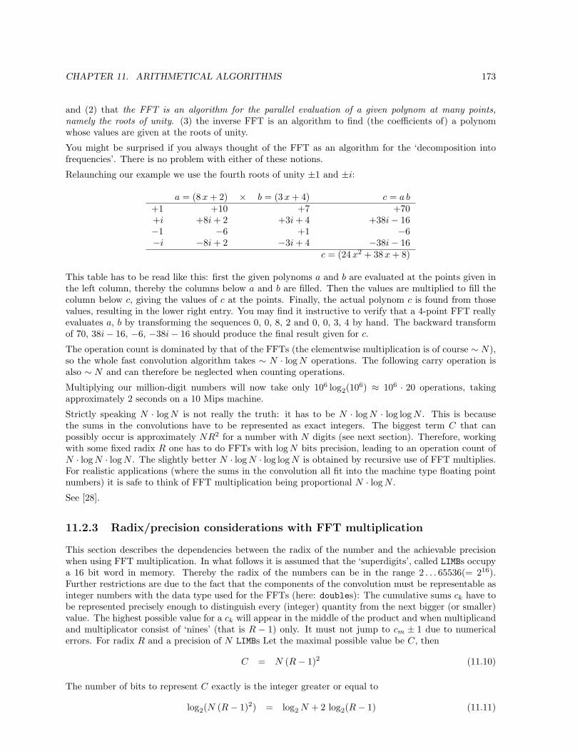
CHAPTER 11. ARITHMETICAL ALGORITHMS 173
and (2) that the FFT is an algorithm for the parallel evaluation of a given polynom at many points,namely the roots of unity. (3) the inverse FFT is an algorithm to find (the coefficients of) a polynomwhose values are given at the roots of unity.
You might be surprised if you always thought of the FFT as an algorithm for the ‘decomposition intofrequencies’. There is no problem with either of these notions.
Relaunching our example we use the fourth roots of unity ±1 and ±i:
a = (8 x + 2) × b = (3 x + 4) c = a b+1 +10 +7 +70+i +8i + 2 +3i + 4 +38i− 16−1 −6 +1 −6−i −8i + 2 −3i + 4 −38i− 16
c = (24 x2 + 38 x + 8)
This table has to be read like this: first the given polynoms a and b are evaluated at the points given inthe left column, thereby the columns below a and b are filled. Then the values are multiplied to fill thecolumn below c, giving the values of c at the points. Finally, the actual polynom c is found from thosevalues, resulting in the lower right entry. You may find it instructive to verify that a 4-point FFT reallyevaluates a, b by transforming the sequences 0, 0, 8, 2 and 0, 0, 3, 4 by hand. The backward transformof 70, 38i− 16, −6, −38i− 16 should produce the final result given for c.
The operation count is dominated by that of the FFTs (the elementwise multiplication is of course ∼ N),so the whole fast convolution algorithm takes ∼ N · log N operations. The following carry operation isalso ∼ N and can therefore be neglected when counting operations.
Multiplying our million-digit numbers will now take only 106 log2(106) ≈ 106 · 20 operations, takingapproximately 2 seconds on a 10 Mips machine.
Strictly speaking N · log N is not really the truth: it has to be N · log N · log log N . This is becausethe sums in the convolutions have to be represented as exact integers. The biggest term C that canpossibly occur is approximately NR2 for a number with N digits (see next section). Therefore, workingwith some fixed radix R one has to do FFTs with log N bits precision, leading to an operation count ofN · log N · log N . The slightly better N · log N · log log N is obtained by recursive use of FFT multiplies.For realistic applications (where the sums in the convolution all fit into the machine type floating pointnumbers) it is safe to think of FFT multiplication being proportional N · log N .
See [28].
11.2.3 Radix/precision considerations with FFT multiplication
This section describes the dependencies between the radix of the number and the achievable precisionwhen using FFT multiplication. In what follows it is assumed that the ‘superdigits’, called LIMBs occupya 16 bit word in memory. Thereby the radix of the numbers can be in the range 2 . . . 65536(= 216).Further restrictions are due to the fact that the components of the convolution must be representable asinteger numbers with the data type used for the FFTs (here: doubles): The cumulative sums ck have tobe represented precisely enough to distinguish every (integer) quantity from the next bigger (or smaller)value. The highest possible value for a ck will appear in the middle of the product and when multiplicandand multiplicator consist of ‘nines’ (that is R − 1) only. It must not jump to cm ± 1 due to numericalerrors. For radix R and a precision of N LIMBs Let the maximal possible value be C, then
C = N (R− 1)2 (11.10)
The number of bits to represent C exactly is the integer greater or equal to
log2(N (R− 1)2) = log2 N + 2 log2(R− 1) (11.11)
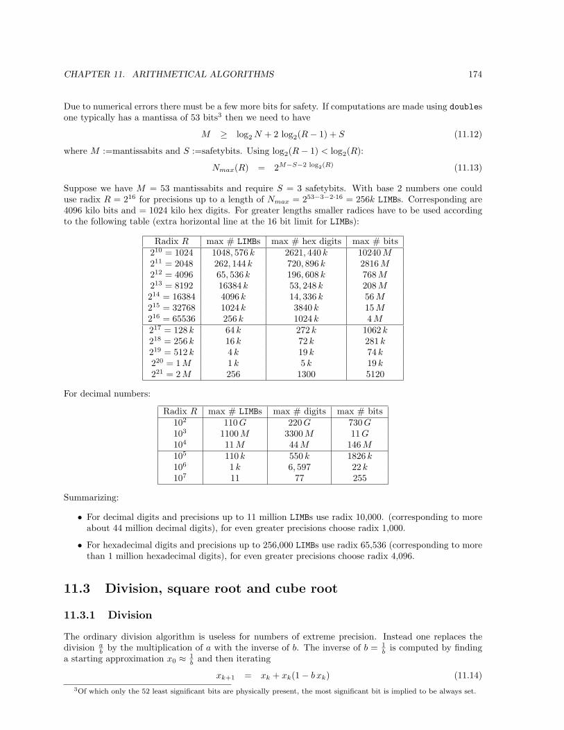
CHAPTER 11. ARITHMETICAL ALGORITHMS 174
Due to numerical errors there must be a few more bits for safety. If computations are made using doublesone typically has a mantissa of 53 bits3 then we need to have
M ≥ log2 N + 2 log2(R− 1) + S (11.12)
where M :=mantissabits and S :=safetybits. Using log2(R− 1) < log2(R):
Nmax(R) = 2M−S−2 log2(R) (11.13)
Suppose we have M = 53 mantissabits and require S = 3 safetybits. With base 2 numbers one coulduse radix R = 216 for precisions up to a length of Nmax = 253−3−2·16 = 256k LIMBs. Corresponding are4096 kilo bits and = 1024 kilo hex digits. For greater lengths smaller radices have to be used accordingto the following table (extra horizontal line at the 16 bit limit for LIMBs):
Radix R max # LIMBs max # hex digits max # bits210 = 1024 1048, 576 k 2621, 440 k 10240 M211 = 2048 262, 144 k 720, 896 k 2816 M212 = 4096 65, 536 k 196, 608 k 768 M213 = 8192 16384 k 53, 248 k 208 M214 = 16384 4096 k 14, 336 k 56 M215 = 32768 1024 k 3840 k 15 M216 = 65536 256 k 1024 k 4 M217 = 128 k 64 k 272 k 1062 k218 = 256 k 16 k 72 k 281 k219 = 512 k 4 k 19 k 74 k220 = 1 M 1 k 5 k 19 k221 = 2 M 256 1300 5120
For decimal numbers:
Radix R max # LIMBs max # digits max # bits102 110 G 220 G 730 G103 1100 M 3300 M 11 G104 11 M 44 M 146 M105 110 k 550 k 1826 k106 1 k 6, 597 22 k107 11 77 255
Summarizing:
• For decimal digits and precisions up to 11 million LIMBs use radix 10,000. (corresponding to moreabout 44 million decimal digits), for even greater precisions choose radix 1,000.
• For hexadecimal digits and precisions up to 256,000 LIMBs use radix 65,536 (corresponding to morethan 1 million hexadecimal digits), for even greater precisions choose radix 4,096.
11.3 Division, square root and cube root
11.3.1 Division
The ordinary division algorithm is useless for numbers of extreme precision. Instead one replaces thedivision a
b by the multiplication of a with the inverse of b. The inverse of b = 1b is computed by finding
a starting approximation x0 ≈ 1b and then iterating
xk+1 = xk + xk(1− b xk) (11.14)3Of which only the 52 least significant bits are physically present, the most significant bit is implied to be always set.
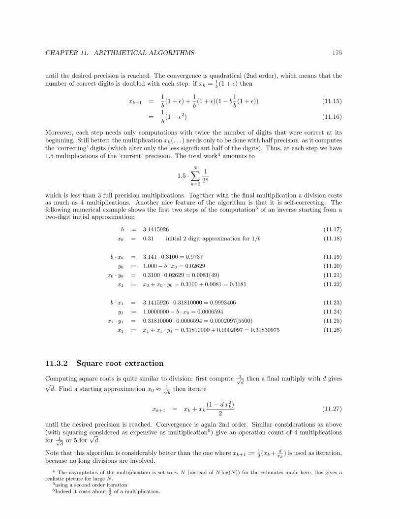
CHAPTER 11. ARITHMETICAL ALGORITHMS 175
until the desired precision is reached. The convergence is quadratical (2nd order), which means that thenumber of correct digits is doubled with each step: if xk = 1
b (1 + ε) then
xk+1 =1b(1 + ε) +
1b(1 + ε)(1− b
1b(1 + ε)) (11.15)
=1b(1− ε2) (11.16)
Moreover, each step needs only computations with twice the number of digits that were correct at itsbeginning. Still better: the multiplication xk(. . . ) needs only to be done with half precision as it computesthe ‘correcting’ digits (which alter only the less significant half of the digits). Thus, at each step we have1.5 multiplications of the ‘current’ precision. The total work4 amounts to
1.5 ·N∑
n=0
12n
which is less than 3 full precision multiplications. Together with the final multiplication a division costsas much as 4 multiplications. Another nice feature of the algorithm is that it is self-correcting. Thefollowing numerical example shows the first two steps of the computation5 of an inverse starting from atwo-digit initial approximation:
b := 3.1415926 (11.17)
x0 = 0.31 initial 2 digit approximation for 1/b (11.18)
b · x0 = 3.141 · 0.3100 = 0.9737 (11.19)
y0 := 1.000− b · x0 = 0.02629 (11.20)
x0 · y0 = 0.3100 · 0.02629 = 0.0081(49) (11.21)
x1 := x0 + x0 · y0 = 0.3100 + 0.0081 = 0.3181 (11.22)
b · x1 = 3.1415926 · 0.31810000 = 0.9993406 (11.23)
y1 := 1.0000000− b · x0 = 0.0006594 (11.24)
x1 · y1 = 0.31810000 · 0.0006594 = 0.0002097(5500) (11.25)
x2 := x1 + x1 · y1 = 0.31810000 + 0.0002097 = 0.31830975 (11.26)
11.3.2 Square root extraction
Computing square roots is quite similar to division: first compute 1√d
then a final multiply with d gives√d. Find a starting approximation x0 ≈ 1√
bthen iterate
xk+1 = xk + xk(1− d x2
k)2
(11.27)
until the desired precision is reached. Convergence is again 2nd order. Similar considerations as above(with squaring considered as expensive as multiplication6) give an operation count of 4 multiplicationsfor 1√
dor 5 for
√d.
Note that this algorithm is considerably better than the one where xk+1 := 12 (xk+ d
xk) is used as iteration,
because no long divisions are involved.4 The asymptotics of the multiplication is set to ∼ N (instead of N log(N)) for the estimates made here, this gives a
realistic picture for large N .5using a second order iteration6Indeed it costs about 2
3of a multiplication.
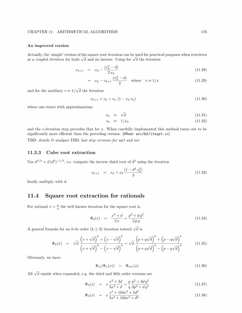
CHAPTER 11. ARITHMETICAL ALGORITHMS 176
An improved version
Actually, the ‘simple’ version of the square root iteration can be used for practical purposes when rewrittenas a coupled iteration for both
√d and its inverse. Using for
√d the iteration
xk+1 = xk − (x2k − d)2 xk
(11.28)
= xk − vk+1(x2
k − d)2
where v ≈ 1/x (11.29)
and for the auxiliary v ≈ 1/√
d the iteration
vk+1 = vk + vk (1− xk vk) (11.30)
where one starts with approximations
x0 ≈√
d (11.31)v0 ≈ 1/x0 (11.32)
and the v-iteration step precedes that for x. When carefully implemented this method turns out to besignificantly more efficient than the preceding version. [hfloat: src/hf/itsqrt.cc]
TBD: details & analysis TBD: last step versions for sqrt and inv
11.3.3 Cube root extraction
Use d1/3 = d (d2)−1/3, i.e. compute the inverse third root of d2 using the iteration
xk+1 = xk + xk(1− d2 x3
k)3
(11.33)
finally multiply with d.
11.4 Square root extraction for rationals
For rational x = pq the well known iteration for the square root is
Φ2(x) =x2 + d
2 x=
p2 + d q2
2 p q(11.34)
A general formula for an k-th order (k ≥ 2) iteration toward√
d is
Φk(x) =√
d
(x +
√d)k
+(x−
√d)k
(x +
√d)k
−(x−
√d)k
=√
d
(p + q
√d)k
+(p− q
√d)k
(p + q
√d)k
−(p− q
√d)k
(11.35)
Obviously, we have:
Φm(Φn(x)) = Φmn(x) (11.36)
All√
d vanish when expanded, e.g. the third and fifth order versions are
Φ3(x) = xx2 + 3d
3x2 + d=
p
q
p2 + 3d q2
3p2 + d q2(11.37)
Φ5(x) = xx4 + 10dx2 + 5d2
5x4 + 10dx2 + d2(11.38)
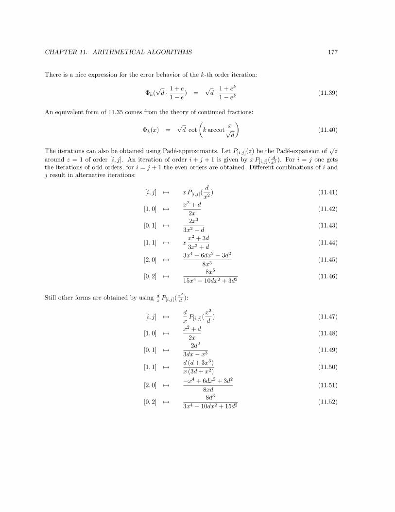
CHAPTER 11. ARITHMETICAL ALGORITHMS 177
There is a nice expression for the error behavior of the k-th order iteration:
Φk(√
d · 1 + e
1− e) =
√d · 1 + ek
1− ek(11.39)
An equivalent form of 11.35 comes from the theory of continued fractions:
Φk(x) =√
d cot(
k arccotx√d
)(11.40)
The iterations can also be obtained using Pade-approximants. Let P[i,j](z) be the Pade-expansion of√
z
around z = 1 of order [i, j]. An iteration of order i + j + 1 is given by xP[i,j]( dx2 ). For i = j one gets
the iterations of odd orders, for i = j + 1 the even orders are obtained. Different combinations of i andj result in alternative iterations:
[i, j] 7→ xP[i,j](d
x2) (11.41)
[1, 0] 7→ x2 + d
2x(11.42)
[0, 1] 7→ 2x3
3x2 − d(11.43)
[1, 1] 7→ xx2 + 3d
3x2 + d(11.44)
[2, 0] 7→ 3x4 + 6dx2 − 3d2
8x3(11.45)
[0, 2] 7→ 8x5
15x4 − 10dx2 + 3d2(11.46)
Still other forms are obtained by using dx P[i,j](x2
d ):
[i, j] 7→ d
xP[i,j](
x2
d) (11.47)
[1, 0] 7→ x2 + d
2x(11.48)
[0, 1] 7→ 2d2
3dx− x3(11.49)
[1, 1] 7→ d (d + 3x3)x (3d + x2)
(11.50)
[2, 0] 7→ −x4 + 6dx2 + 3d2
8xd(11.51)
[0, 2] 7→ 8d3
3x4 − 10dx2 + 15d2(11.52)
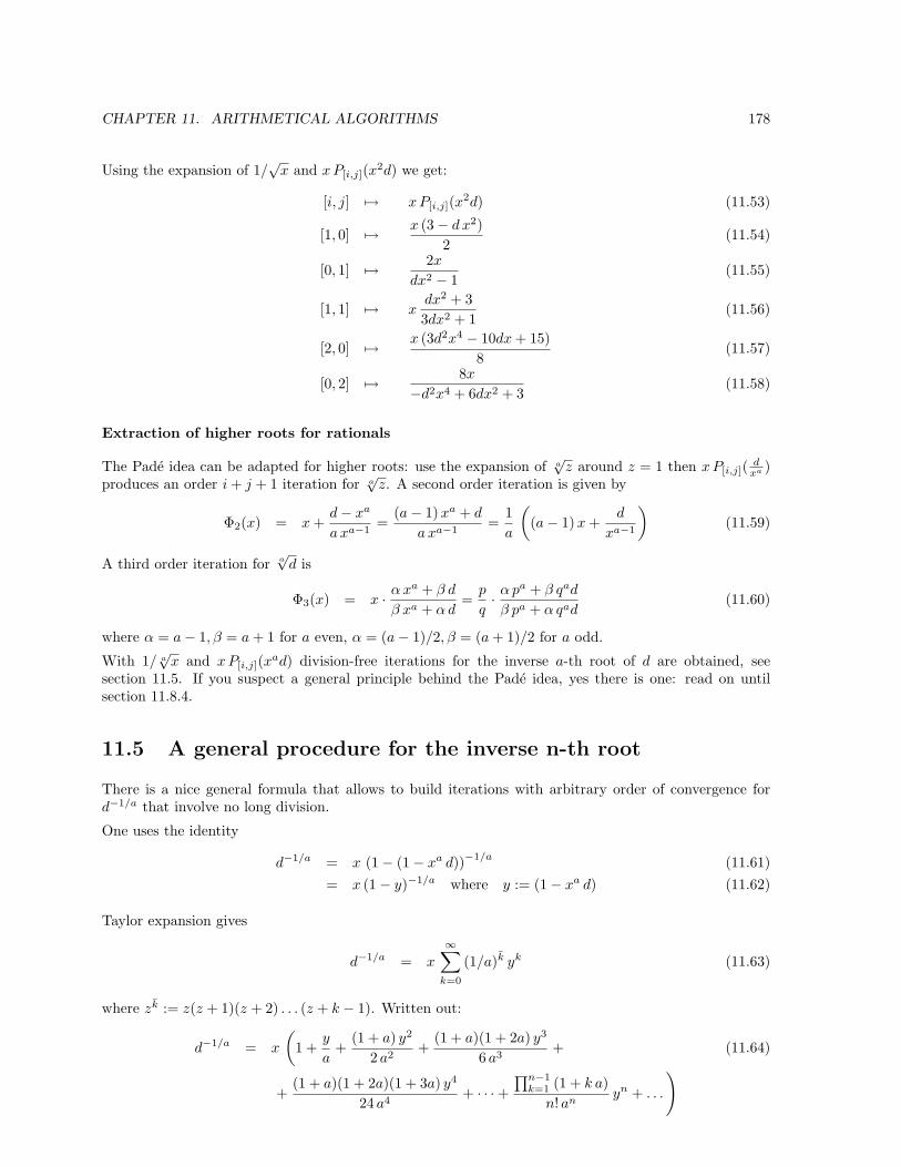
CHAPTER 11. ARITHMETICAL ALGORITHMS 178
Using the expansion of 1/√
x and xP[i,j](x2d) we get:
[i, j] 7→ xP[i,j](x2d) (11.53)
[1, 0] 7→ x (3− d x2)2
(11.54)
[0, 1] 7→ 2x
dx2 − 1(11.55)
[1, 1] 7→ xdx2 + 33dx2 + 1
(11.56)
[2, 0] 7→ x (3d2x4 − 10dx + 15)8
(11.57)
[0, 2] 7→ 8x
−d2x4 + 6dx2 + 3(11.58)
Extraction of higher roots for rationals
The Pade idea can be adapted for higher roots: use the expansion of a√
z around z = 1 then x P[i,j]( dxa )
produces an order i + j + 1 iteration for a√
z. A second order iteration is given by
Φ2(x) = x +d− xa
a xa−1=
(a− 1)xa + d
a xa−1=
1a
((a− 1)x +
d
xa−1
)(11.59)
A third order iteration for a√
d is
Φ3(x) = x · α xa + β d
β xa + α d=
p
q· α pa + β qad
β pa + α qad(11.60)
where α = a− 1, β = a + 1 for a even, α = (a− 1)/2, β = (a + 1)/2 for a odd.
With 1/ a√
x and xP[i,j](xad) division-free iterations for the inverse a-th root of d are obtained, seesection 11.5. If you suspect a general principle behind the Pade idea, yes there is one: read on untilsection 11.8.4.
11.5 A general procedure for the inverse n-th root
There is a nice general formula that allows to build iterations with arbitrary order of convergence ford−1/a that involve no long division.
One uses the identity
d−1/a = x (1− (1− xa d))−1/a (11.61)= x (1− y)−1/a where y := (1− xa d) (11.62)
Taylor expansion gives
d−1/a = x
∞∑
k=0
(1/a)k yk (11.63)
where zk := z(z + 1)(z + 2) . . . (z + k − 1). Written out:
d−1/a = x
(1 +
y
a+
(1 + a) y2
2 a2+
(1 + a)(1 + 2a) y3
6 a3+ (11.64)
+(1 + a)(1 + 2a)(1 + 3a) y4
24 a4+ · · ·+
∏n−1k=1 (1 + k a)
n! anyn + . . .
)
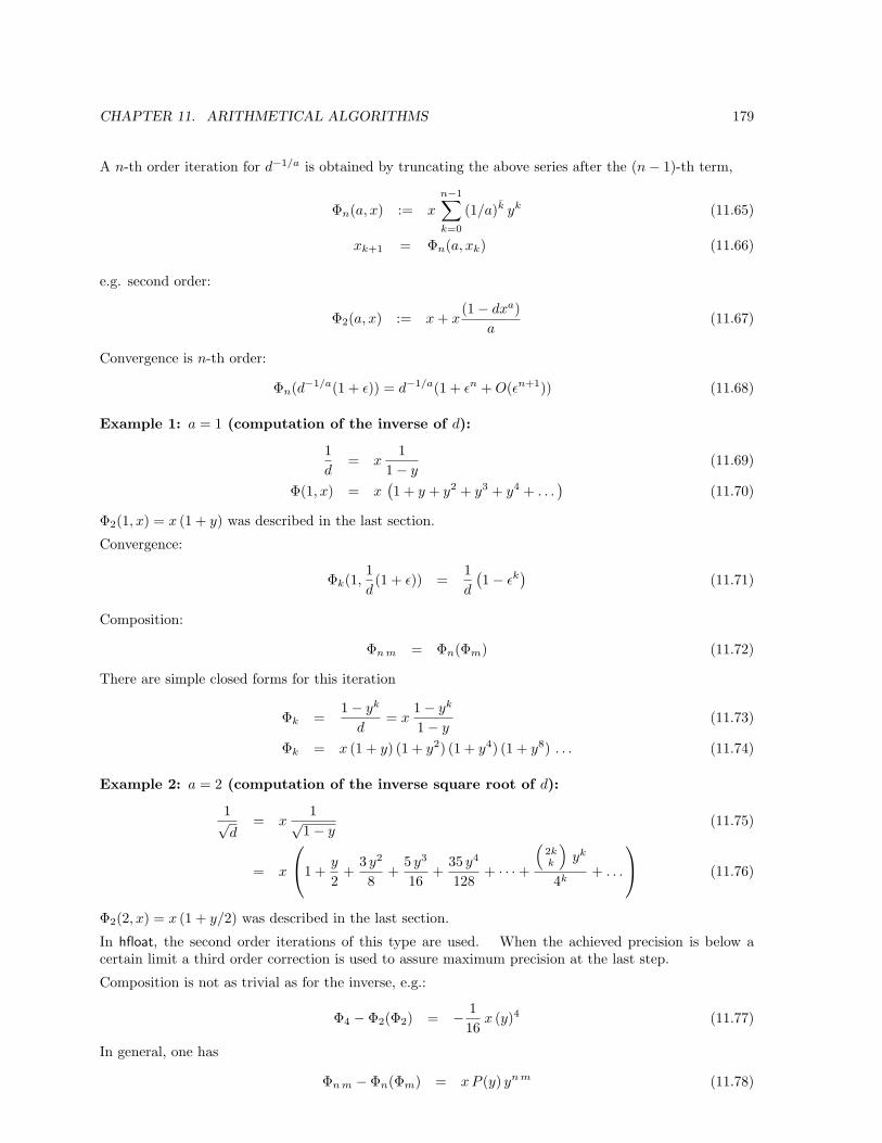
CHAPTER 11. ARITHMETICAL ALGORITHMS 179
A n-th order iteration for d−1/a is obtained by truncating the above series after the (n− 1)-th term,
Φn(a, x) := x
n−1∑
k=0
(1/a)k yk (11.65)
xk+1 = Φn(a, xk) (11.66)
e.g. second order:
Φ2(a, x) := x + x(1− dxa)
a(11.67)
Convergence is n-th order:
Φn(d−1/a(1 + ε)) = d−1/a(1 + εn + O(εn+1)) (11.68)
Example 1: a = 1 (computation of the inverse of d):
1d
= x1
1− y(11.69)
Φ(1, x) = x(1 + y + y2 + y3 + y4 + . . .
)(11.70)
Φ2(1, x) = x (1 + y) was described in the last section.
Convergence:
Φk(1,1d(1 + ε)) =
1d
(1− εk
)(11.71)
Composition:
Φn m = Φn(Φm) (11.72)
There are simple closed forms for this iteration
Φk =1− yk
d= x
1− yk
1− y(11.73)
Φk = x (1 + y) (1 + y2) (1 + y4) (1 + y8) . . . (11.74)
Example 2: a = 2 (computation of the inverse square root of d):
1√d
= x1√
1− y(11.75)
= x
1 +
y
2+
3 y2
8+
5 y3
16+
35 y4
128+ · · ·+
(2kk
)yk
4k+ . . .
(11.76)
Φ2(2, x) = x (1 + y/2) was described in the last section.
In hfloat, the second order iterations of this type are used. When the achieved precision is below acertain limit a third order correction is used to assure maximum precision at the last step.
Composition is not as trivial as for the inverse, e.g.:
Φ4 − Φ2(Φ2) = − 116
x (y)4 (11.77)
In general, one has
Φn m − Φn(Φm) = xP (y) yn m (11.78)
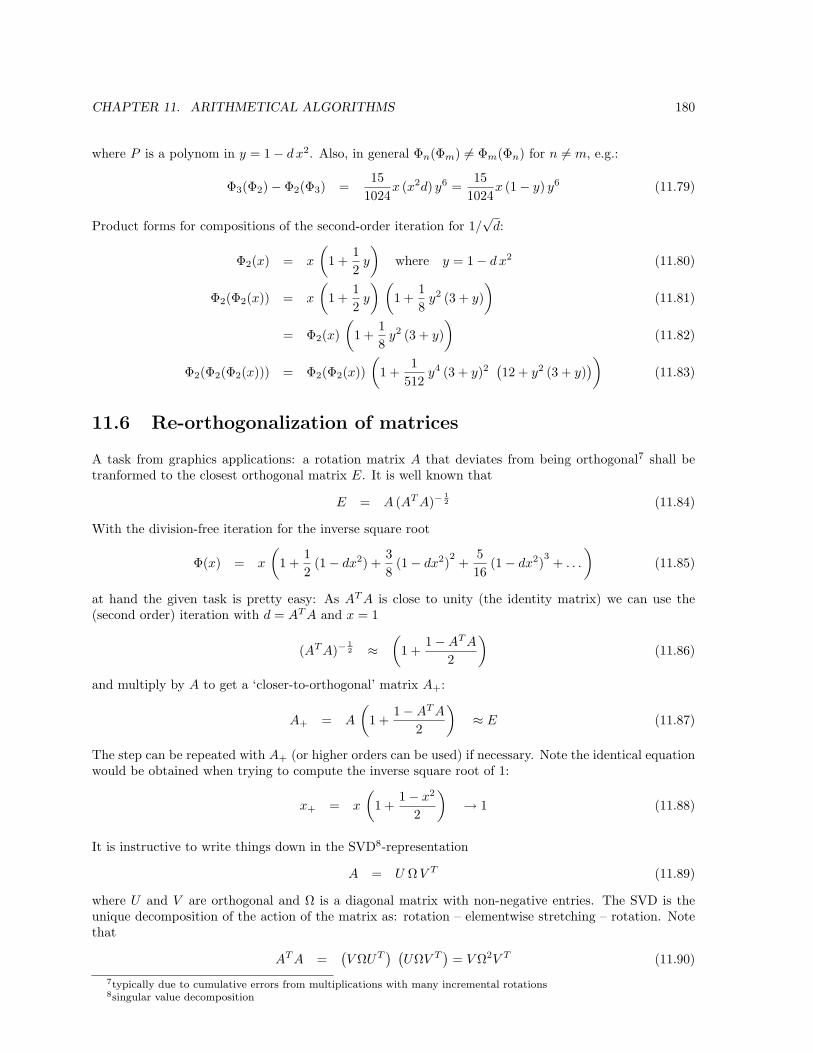
CHAPTER 11. ARITHMETICAL ALGORITHMS 180
where P is a polynom in y = 1− d x2. Also, in general Φn(Φm) 6= Φm(Φn) for n 6= m, e.g.:
Φ3(Φ2)− Φ2(Φ3) =15
1024x (x2d) y6 =
151024
x (1− y) y6 (11.79)
Product forms for compositions of the second-order iteration for 1/√
d:
Φ2(x) = x
(1 +
12
y
)where y = 1− d x2 (11.80)
Φ2(Φ2(x)) = x
(1 +
12
y
) (1 +
18
y2 (3 + y))
(11.81)
= Φ2(x)(
1 +18
y2 (3 + y))
(11.82)
Φ2(Φ2(Φ2(x))) = Φ2(Φ2(x))(
1 +1
512y4 (3 + y)2
(12 + y2 (3 + y)
))(11.83)
11.6 Re-orthogonalization of matrices
A task from graphics applications: a rotation matrix A that deviates from being orthogonal7 shall betranformed to the closest orthogonal matrix E. It is well known that
E = A (AT A)−12 (11.84)
With the division-free iteration for the inverse square root
Φ(x) = x
(1 +
12
(1− dx2) +38
(1− dx2)2
+516
(1− dx2)3
+ . . .
)(11.85)
at hand the given task is pretty easy: As AT A is close to unity (the identity matrix) we can use the(second order) iteration with d = AT A and x = 1
(AT A)−12 ≈
(1 +
1−AT A
2
)(11.86)
and multiply by A to get a ‘closer-to-orthogonal’ matrix A+:
A+ = A
(1 +
1−AT A
2
)≈ E (11.87)
The step can be repeated with A+ (or higher orders can be used) if necessary. Note the identical equationwould be obtained when trying to compute the inverse square root of 1:
x+ = x
(1 +
1− x2
2
)→ 1 (11.88)
It is instructive to write things down in the SVD8-representation
A = U ΩV T (11.89)
where U and V are orthogonal and Ω is a diagonal matrix with non-negative entries. The SVD is theunique decomposition of the action of the matrix as: rotation – elementwise stretching – rotation. Notethat
AT A =(V ΩUT
) (UΩV T
)= V Ω2V T (11.90)
7typically due to cumulative errors from multiplications with many incremental rotations8singular value decomposition
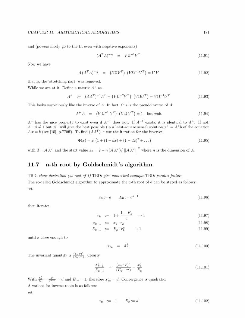
CHAPTER 11. ARITHMETICAL ALGORITHMS 181
and (powers nicely go to the Ω, even with negative exponents)
(AT A)−12 = V Ω−1V T (11.91)
Now we have
A (AT A)−12 =
(UΩV T
) (V Ω−1V T
)= U V (11.92)
that is, the ‘stretching part’ was removed.
While we are at it: Define a matrix A+ as
A+ := (AAT )−1AT =(V Ω−2V T
) (V ΩUT
)= V Ω−1UT (11.93)
This looks suspiciously like the inverse of A. In fact, this is the pseudoinverse of A:
A+ A =(V Ω−1 UT
) (U Ω V T
)= 1 but wait (11.94)
A+ has the nice property to exist even if A−1 does not. If A−1 exists, it is identical to A+. If not,A+ A 6= 1 but A+ will give the best possible (in a least-square sense) solution x+ = A+b of the equationAx = b (see [15], p.770ff). To find (AAT )−1 use the iteration for the inverse:
Φ(x) = x(1 + (1− dx) + (1− dx)2 + . . .
)(11.95)
with d = AAT and the start value x0 = 2− n (AAT )/ ||AAT ||2 where n is the dimension of A.
11.7 n-th root by Goldschmidt’s algorithm
TBD: show derivation (as root of 1) TBD: give numerical example TBD: parallel feature
The so-called Goldschmidt algorithm to approximate the a-th root of d can be stated as follows:
set
x0 := d E0 := da−1 (11.96)
then iterate:
rk := 1 +1− Ek
a→ 1 (11.97)
xk+1 := xk · rk (11.98)Ek+1 := Ek · ra
k → 1 (11.99)
until x close enough to
x∞ = d1a . (11.100)
The invariant quantity is (xk·r)a
(Ek·ra) . Clearly
xak+1
Ek+1=
(xk · r)a
(Ek · ra)=
xak
Ek(11.101)
With xa0
E0= da
da−1 = d and E∞ = 1, therefore xa∞ = d. Convergence is quadratic.
A variant for inverse roots is as follows:
set
x0 := 1 E0 := d (11.102)
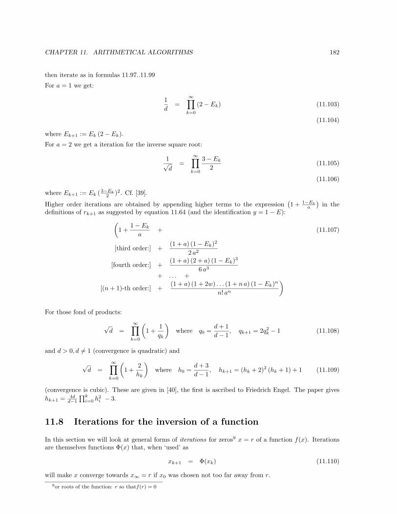
CHAPTER 11. ARITHMETICAL ALGORITHMS 182
then iterate as in formulas 11.97..11.99
For a = 1 we get:
1d
=∞∏
k=0
(2− Ek) (11.103)
(11.104)
where Ek+1 := Ek (2− Ek).
For a = 2 we get a iteration for the inverse square root:
1√d
=∞∏
k=0
3− Ek
2(11.105)
(11.106)
where Ek+1 := Ek ( 3−Ek
2 )2. Cf. [39].
Higher order iterations are obtained by appending higher terms to the expression(1 + 1−Ek
a
)in the
definitions of rk+1 as suggested by equation 11.64 (and the identification y = 1− E):(
1 +1− Ek
a+ (11.107)
[third order:] +(1 + a) (1− Ek)2
2 a2
[fourth order:] +(1 + a) (2 + a) (1− Ek)3
6 a3
+ . . . +
[(n + 1)-th order:] +(1 + a) (1 + 2w) . . . (1 + na) (1− Ek)n
n! an
)
For those fond of products:
√d =
∞∏
k=0
(1 +
1qk
)where q0 =
d + 1d− 1
, qk+1 = 2q2k − 1 (11.108)
and d > 0, d 6= 1 (convergence is quadratic) and
√d =
∞∏
k=0
(1 +
2hk
)where h0 =
d + 3d− 1
, hk+1 = (hk + 2)2 (hk + 1) + 1 (11.109)
(convergence is cubic). These are given in [40], the first is ascribed to Friedrich Engel. The paper giveshk+1 = 4d
d−1
∏ki=0 h2
i − 3.
11.8 Iterations for the inversion of a function
In this section we will look at general forms of iterations for zeros9 x = r of a function f(x). Iterationsare themselves functions Φ(x) that, when ‘used’ as
xk+1 = Φ(xk) (11.110)
will make x converge towards x∞ = r if x0 was chosen not too far away from r.9or roots of the function: r so thatf(r) = 0
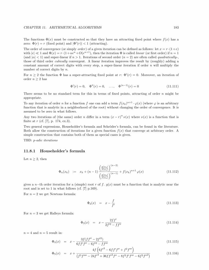
CHAPTER 11. ARITHMETICAL ALGORITHMS 183
The functions Φ(x) must be constructed so that they have an attracting fixed point where f(x) has azero: Φ(r) = r (fixed point) and |Φ′(r)| < 1 (attracting).
The order of convergence (or simply order) of a given iteration can be defined as follows: let x = r ·(1+e)with |e| ¿ 1 and Φ(x) = r ·(1+αen+O(en+1), then the iteration Φ is called linear (or first order) if n = 1(and |α| < 1) and super-linear if n > 1. Iterations of second order (n = 2) are often called quadratically-,those of third order cubically convergent. A linear iteration improves the result by (roughly) adding aconstant amount of correct digits with every step, a super-linear iteration if order n will multiply thenumber of correct digits by n.
For n ≥ 2 the function Φ has a super-attracting fixed point at r: Φ′(r) = 0. Moreover, an iteration oforder n ≥ 2 has
Φ′(r) = 0, Φ′′(r) = 0, . . . , Φ(n−1)(r) = 0 (11.111)
There seems to be no standard term for this in terms of fixed points, attracting of order n might beappropriate.
To any iteration of order n for a function f one can add a term f(xk)n+1 · ϕ(x) (where ϕ is an arbitraryfunction that is analytic in a neighborhood of the root) without changing the order of convergence. It isassumed to be zero in what follows.
Any two iterations of (the same) order n differ in a term (x− r)nν(x) where ν(x) is a function that is
finite at r (cf. [7], p. 174, ex.3).
Two general expressions, Householder’s formula and Schroder’s formula, can be found in the literature.Both allow the construction of iterations for a given function f(x) that converge at arbitrary order. Asimple construction that contains both of them as special cases is given.
TBD: p-adic iterations
11.8.1 Householder’s formula
Let n ≥ 2, then
Φn(xk) := xk + (n− 1)
(g(xk)f(xk)
)(n−2)
(g(xk)f(xk)
)(n−1)+ f(xk)n+1 ϕ(x) (11.112)
gives a n−th order iteration for a (simple) root r of f . g(x) must be a function that is analytic near theroot and is set to 1 in what follows (cf. [7] p.169).
For n = 2 we get Newtons formula:
Φ2(x) = x− f
f ′(11.113)
For n = 3 we get Halleys formula:
Φ3(x) = x− 2ff ′
2f ′2 − ff ′′(11.114)
n = 4 and n = 5 result in:
Φ4(x) = x− 3f(ff ′′ − 2f ′2)6ff ′f ′′ − 6f ′3 − ff ′′′
(11.115)
Φ5(x) = x +4f
(6f ′3 − 6ff ′f ′′ + f2f ′′′
)
(f3f ′′′′ − 24f ′4 + 36ff ′2f ′′ − 8f2f ′f ′′′ − 6f2f ′′2
) (11.116)
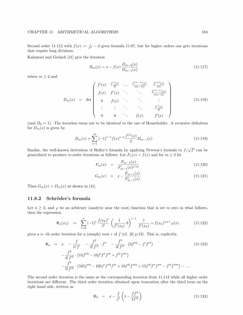
CHAPTER 11. ARITHMETICAL ALGORITHMS 184
Second order 11.112 with f(x) := 1xa − d gives formula 11.67, but for higher orders one gets iterations
that require long divisions.
Kalantari and Gerlach [41] give the iteration
Bm(x) = x− f(x)Dm−2(x)Dm−1(x)
(11.117)
where m ≥ 2 and
Dm(x) = det
f ′(x) f ′′(x)2! . . . f(m−1)(x)
(m−1)!f(m)(x)
m!
f(x) f ′(x). . . . . . f(m−1)(x)
(m−1)!
0 f(x). . . . . .
......
.... . . . . . f ′′(x)
2!
0 0. . . f(x) f ′(x)
(11.118)
(and D0 = 1). The iteration turns out to be identical to the one of Householder. A recursive definitionfor Dm(x) is given by
Dm(x) =m∑
i=1
(−1)i−1f(x)i−1 f (i)(x)
i!Dm−i(x) (11.119)
Similar, the well-known derivation of Halley’s formula by applying Newton’s formula to f/√
f ′ can begeneralized to produce m-order iterations as follows: Let F1(x) = f(x) and for m ≥ 2 let
Fm(x) =Fm−1(x)
F ′m−1(x)1/m(11.120)
Gm(x) = x− Fm−1(x)F ′m−1(x)
(11.121)
Then Gm(x) = Dm(x) as shown in [41].
11.8.2 Schroder’s formula
Let n ≥ 2, and ϕ be an arbitrary (analytic near the root) function that is set to zero in what follows,then the expression
Φn(xk) :=n∑
t=0
(−1)t f(xk)t
t!
(1
f ′(xk)∂
)t−1 1f ′(xk)
+ f(xk)n+1 ϕ(x) (11.122)
gives a n−th order iteration for a (simple) root r of f (cf. [6] p.13). This is, explicitly,
Φn = x − f
1! f ′− f2
2! f ′3· f ′′ − f3
3! f ′5· (3f ′′2 − f ′f ′′′
)(11.123)
− f4
4! f ′7· (15f ′′3 − 10f ′f ′′f ′′′ + f ′2f ′′′′
)
− f5
5! f ′9· (105f ′′4 − 105f ′f ′′2f ′′′ + 10f ′2f ′′′2 + 15f ′2f ′′f ′′′′ − f ′3f ′′′′′
)− . . .
The second order iteration is the same as the corresponding iteration from 11.112 while all higher orderiterations are different. The third order iteration obtained upon truncation after the third term on theright hand side, written as
Φ3 = x− f
f ′
(1− ff ′′
2f ′2
)(11.124)
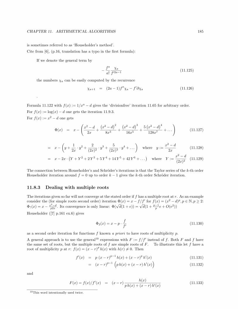
CHAPTER 11. ARITHMETICAL ALGORITHMS 185
is sometimes referred to as ‘Householder’s method’.
Cite from [6], (p.16, translation has a typo in the first formula):
If we denote the general term by
− fa
a!χa
f ′2a−1(11.125)
the numbers χa can be easily computed by the recurrence
χa+1 = (2a− 1)f ′′χa − f ′∂χa (11.126)
.
Formula 11.122 with f(x) := 1/xa − d gives the ‘divisionfree’ iteration 11.65 for arbitrary order.
For f(x) := log(x)− d one gets the iteration 11.9.3.
For f(x) := x2 − d one gets
Φ(x) = x−(
x2 − d
2x+
(x2 − d
)2
8x3+
(x2 − d
)3
16x5+
5(x2 − d
)4
128x7+ . . .
)(11.127)
= x−(
y +12x
· y2 +2
(2x)2· y3 +
5(2x)3
· y4 + . . .
)where y :=
x2 − d
2x(11.128)
= x− 2x · (Y + Y 2 + 2 Y 3 + 5 Y 4 + 14 Y 5 + 42 Y 6 + . . .)
where Y :=x2 − d
(2x)2(11.129)
The connection between Householder’s and Schroder’s iterations is that the Taylor series of the k-th orderHouseholder iteration around f = 0 up to order k − 1 gives the k-th order Schroder iteration.
11.8.3 Dealing with multiple roots
The iterations given so far will not converge at the stated order if f has a multiple root at r. As an exampleconsider the (for simple roots second order) iteration Φ(x) = x− f/f ′ for f(x) = (x2 − d)p, p ∈ N, p ≥ 2:Φ?(x) = x− x2−d
p2x . Its convergence is only linear: Φ(√
d(1 + e)) =√
d(1 + p−1p e + O(e2))
Householder ([7] p.161 ex.6) gives
Φ2(x) = x− p · f
f ′(11.130)
as a second order iteration for functions f known a priori to have roots of multiplicity p.
A general approach is to use the general10 expressions with F := f/f ′ instead of f . Both F and f havethe same set of roots, but the multiple roots of f are simple roots of F . To illustrate this let f have aroot of multiplicity p at r: f(x) = (x− r)p
h(x) with h(r) 6= 0. Then
f ′(x) = p (x− r)p−1h(x) + (x− r)p
h′(x) (11.131)
= (x− r)p−1(p h(x) + (x− r)h′(x)
)(11.132)
and
F (x) = f(x)/f ′(x) = (x− r)h(x)
p h(x) + (x− r) h′(x)(11.133)
10This word intentionally used twice.
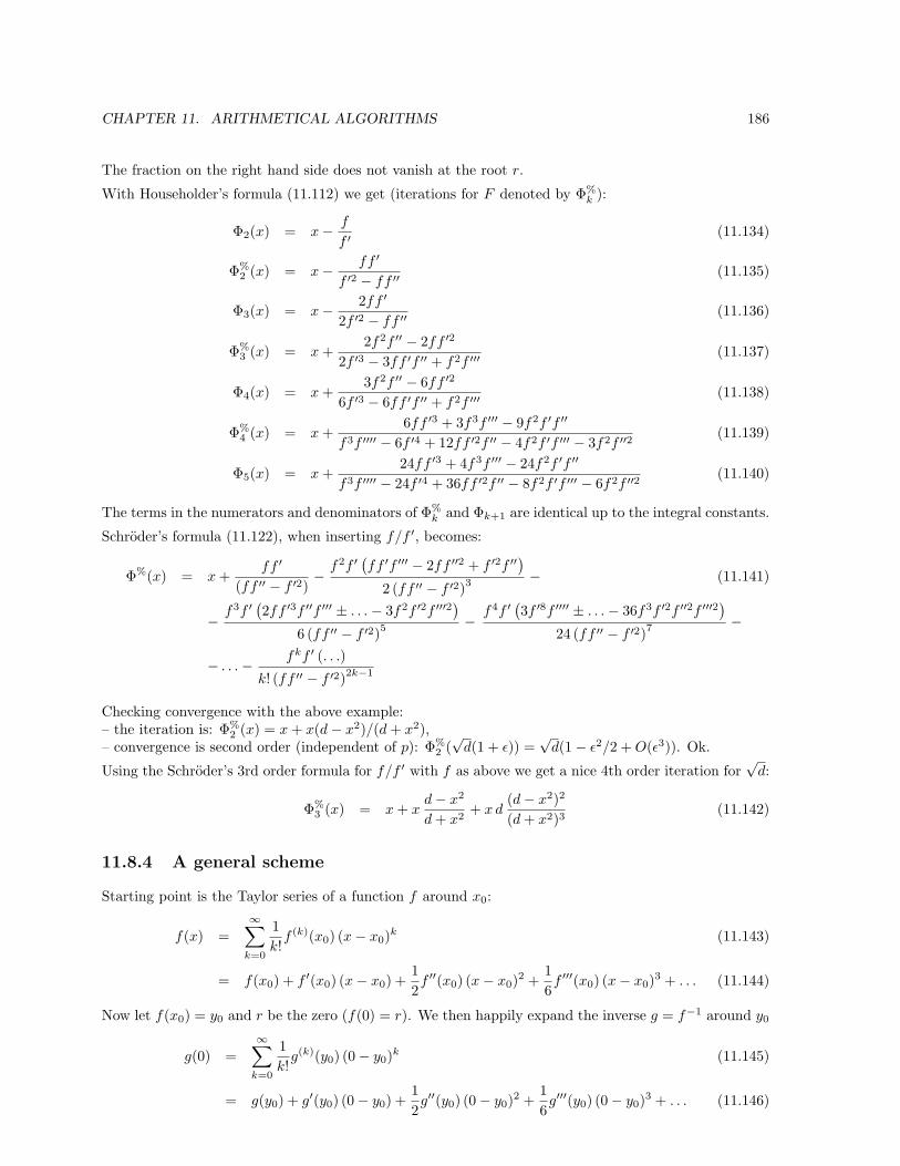
CHAPTER 11. ARITHMETICAL ALGORITHMS 186
The fraction on the right hand side does not vanish at the root r.
With Householder’s formula (11.112) we get (iterations for F denoted by Φ%k ):
Φ2(x) = x− f
f ′(11.134)
Φ%2 (x) = x− ff ′
f ′2 − ff ′′(11.135)
Φ3(x) = x− 2ff ′
2f ′2 − ff ′′(11.136)
Φ%3 (x) = x +
2f2f ′′ − 2ff ′2
2f ′3 − 3ff ′f ′′ + f2f ′′′(11.137)
Φ4(x) = x +3f2f ′′ − 6ff ′2
6f ′3 − 6ff ′f ′′ + f2f ′′′(11.138)
Φ%4 (x) = x +
6ff ′3 + 3f3f ′′′ − 9f2f ′f ′′
f3f ′′′′ − 6f ′4 + 12ff ′2f ′′ − 4f2f ′f ′′′ − 3f2f ′′2(11.139)
Φ5(x) = x +24ff ′3 + 4f3f ′′′ − 24f2f ′f ′′
f3f ′′′′ − 24f ′4 + 36ff ′2f ′′ − 8f2f ′f ′′′ − 6f2f ′′2(11.140)
The terms in the numerators and denominators of Φ%k and Φk+1 are identical up to the integral constants.
Schroder’s formula (11.122), when inserting f/f ′, becomes:
Φ%(x) = x +ff ′
(ff ′′ − f ′2)− f2f ′
(ff ′f ′′′ − 2ff ′′2 + f ′2f ′′
)
2 (ff ′′ − f ′2)3− (11.141)
− f3f ′(2ff ′3f ′′f ′′′ ± . . .− 3f2f ′2f ′′′2
)
6 (ff ′′ − f ′2)5− f4f ′
(3f ′8f ′′′′ ± . . .− 36f3f ′2f ′′2f ′′′2
)
24 (ff ′′ − f ′2)7−
− . . .− fkf ′ (. . .)
k! (ff ′′ − f ′2)2k−1
Checking convergence with the above example:– the iteration is: Φ%
2 (x) = x + x(d− x2)/(d + x2),– convergence is second order (independent of p): Φ%
2 (√
d(1 + ε)) =√
d(1− ε2/2 + O(ε3)). Ok.
Using the Schroder’s 3rd order formula for f/f ′ with f as above we get a nice 4th order iteration for√
d:
Φ%3 (x) = x + x
d− x2
d + x2+ x d
(d− x2)2
(d + x2)3(11.142)
11.8.4 A general scheme
Starting point is the Taylor series of a function f around x0:
f(x) =∞∑
k=0
1k!
f (k)(x0) (x− x0)k (11.143)
= f(x0) + f ′(x0) (x− x0) +12f ′′(x0) (x− x0)2 +
16f ′′′(x0) (x− x0)3 + . . . (11.144)
Now let f(x0) = y0 and r be the zero (f(0) = r). We then happily expand the inverse g = f−1 around y0
g(0) =∞∑
k=0
1k!
g(k)(y0) (0− y0)k (11.145)
= g(y0) + g′(y0) (0− y0) +12g′′(y0) (0− y0)2 +
16g′′′(y0) (0− y0)3 + . . . (11.146)
CHAPTER 11. ARITHMETICAL ALGORITHMS 187
Using x0 = g(y0) and r = g(0) we get
r = x0 − g′(y0) f(x0) +12g′′(y0) f(x0)2 − 1
6g′′′(y0) f(x0)3 + . . . (11.147)
Remains to express the derivatives of the inverse g in terms of (derivatives of) f . Not a difficult task,note that
f g = id that is: f(g(x)) = x (11.148)
and derive (chain rule) to get g′(f(x)) f ′(x) = 1, so g′(y) = 1f ′(x) . Derive f(g(x))− x multiple times and
set the expressions to zero (arguments y of g and x of f are omitted for readability):
1 = f ′g′ (11.149)
0 = g′f ′′ + f ′2g′′ (11.150)
0 = g′f ′′′ + 3f ′f ′′g′′ + f ′3g′′′ (11.151)
0 = g′f ′′′′ + 4f ′g′′f ′′′ + 3f ′′2g′′ + 6f ′2f ′′g′′′ + f ′4g′′′′ (11.152)
This system of linear equations in the derivatives of g is trivially solved because it is already triangular.We obtain:
g′ =1f ′
(11.153)
g′′ = − f ′′
f ′3(11.154)
g′′′ =1
f ′5(3f ′′2 − f ′f ′′′
)(11.155)
g′′′′ =1
f ′7(10f ′f ′′f ′′′ − 15f ′′3 − f ′2f ′′′′
)(11.156)
g′′′′′ =1
f ′9(105f ′′4 − f ′3f ′′′′′ − 105f ′f ′′2f ′′′ + 15f ′2f ′′f ′′′′ + 10f ′2f ′′′2
)(11.157)
Thereby equation 11.147 can be written as (omitting arguments x of f everywhere)
r = x− 1f ′
f +12
(− f ′′
f ′3
)f2 − 1
6
(1
f ′5(3f ′′2 − f ′f ′′′
))f3 + . . . (11.158)
= x− f
1! f ′− f2
2! f ′3· f ′′ − f3
3! f ′5· (3f ′′2 − f ′f ′′′
)− . . . (11.159)
which is Schroder’s iteration (equation 11.123).
Taking the [i, i]-th or [i + 1, i]-th Pade approximant (in f) gives the Householder iteration for even orodd orders, respectively.
More iterations can be found using other [i, j] pairs. Already for the second order (where the well knowngeneral formula, corresponding to [1, 0] is x− f
f ′ ) there is one alternative, namely [0, 1] which is
Φ2(x) = x− x f
f + x f ′= x− x f
(x f)′= x2 f ′
f + x f ′= x
(1 +
f
x f ′
)−1
(11.160)
For the third order there is also one ‘non-standard’ iteration: [0, 2]
Φ3(x) =2x3f ′3
2f2f ′ + 2fxf ′2 + f2xf ′′ + 2x2f ′3(11.161)
For order n there are n possible Pade approximants, two of which are the Householder and Schroderiteration (for n = 2 they coincide). Thereby n− 2 additional iteration schemes are found by the method
CHAPTER 11. ARITHMETICAL ALGORITHMS 188
described. The iterations of order n are fractions with numerator and denominator consisting only ofterms that are products of integral constants and x, f, f ′, f ′′, . . . , f (n−1). There are obviously other formsof iterations, e.g. the third order iteration
Φ3(x) = x− 1f ′′
(f ′ ±
√f ′2 − 2ff ′′
)= x− f ′
f ′′
(1±
√1− 2
f f ′′
f ′2
)(11.162)
that stems from directly solving the truncated Taylor expansion of f(r) = 0 =: Φ around x
f(r) = f(x) + f ′(x) (r − x) +12f ′′(x) (r − x)2 (11.163)
(For f(x) = ax2 + bx+ c it gives the two solutions of the quadratic equation f(x) = 0; for other functionsone gets an iterated square root expression for the roots.)
Alternative rational forms can also be obtained in a way that generalizes the the method used for multipleroots: if we emphasize the so far notationally omitted dedendency from the function f as Φ f. Theiteration Φ f has fixed points where f has a root r, so x−Φ f (x) again has a root at r. Hence we canbuild more iterations that will converge to those roots as Φ x− Φ f (x). For dealing with multipleroots we used Φ x− Φ f2k
= Φ f/f ′. An iteration Φ
x− Φ fj
k
can only be expected to havea kth order convergence.
Similarly, one can derive alternative iterations of given order by using functions that have roots where fhas them11. For example
g(x) := 1− 11− αf(x)
where α ∈ C, α 6= 0 (11.164)
leads to the second order iteration
Φ g2 = x− f(x)(1 + αf(x))f ′(x)
(11.165)
Using g := xf(x) leads to the alternative second order iteration.
Moreover, one could use a function g and its inverse g := g−1 and the corresponding iteration for f(g(x))and finally apply g to get the root: (Let r′ be the zero of f(g(x)): f(g(r′)) = 0 if g(r′) = r. r′ is whatwe get from Φ f g.) A simple example is g(x) = g(x) = 1/x, with f = xa − d and Schroder’s formulaone gets the divisionless iterations for the (inverse) a-th root of d. g subject to reasonable conditions: itmust be invertible near the root r of f .
11.8.5 Improvements by the delta squared process
Given a sequence of partial sums xk the so called delta squared process computes a new sequence x∗k ofextrapolated sums:
x∗k = xk+2 − (xk+2 − xk+1)2
xk+2 − 2 xk+1 + xk(11.166)
The method is due to Aitken. The name delta squared is due to the fact that the formula can be writtensymbolically as
x∗ = x− (∆x)2
(∆2x)(11.167)
where ∆ is the difference operator.11It does not do any harm if g has additional roots.
CHAPTER 11. ARITHMETICAL ALGORITHMS 189
Note that the mathematically equivalent form
x∗k =xk xk+2 − x2
k+1
xk+2 − 2 xk+1 + xk(11.168)
sometimes given should be avoided with numerical computations due to possible cancellation.
If xk =∑k
i=0 ai and the ratio of consecutive summands ai is approximately constant (that is, a is close toa geometric series) then x∗ converges significantly faster to x∞ than x. Let us partly rewrite the formulausing xk − xk−1 = ak:
x∗k = xk+2 − (ak+2)2
ak+2 − ak+1(11.169)
Then for a geometric series with ak+1/ak = q
x∗k = xk+2 − (ak+2)2
ak+2 − ak+1= xk+2 −
(a0 qk+2
)2
a0 (qk+2 − qk+1)(11.170)
= a01− qk+3
1− q+ a0 qk+2 · qk+2
qk+1 − qk+2=
a0
1− q
(1− qk+3 + qk+3
)(11.171)
=a0
1− q(11.172)
which is the exact sum.
Why do we meet the delta squared here? Consider the sequence
x0, x1 = Φ(x0), x2 = Φ(x1) = Φ(Φ(x0)), . . . (11.173)
of better and better approximations to some root r of a function f . Think of the xk as partial sums of aseries whose sum is the root r. Apply the idea to define an improved iteration Φ∗ from a given Φ:
Φ∗(x) = Φ(Φ(x))− (Φ(Φ(x))− Φ(x))2
Φ(Φ(x))− 2Φ(x) + x(11.174)
The good news is that Φ∗ will give quadratic convergence even if Φ only gives linear convergence. Asan example let us take f(x) = (x2 − d)2, forget that its root
√d is a double root, happily define Φ(x) =
x− f(x)/f ′(x) = x− (x2 − d)/(4x). Convergence is only linear:
Φ(√
d · (1 + e)) =√
d ·(
1 +e
2+
e2
4+ O(e3)
)(11.175)
Then try
Φ∗(x) =d (7x2 + d)
x (3 x2 + 5 d)(11.176)
and find that it offers quadratic convergence
Φ(√
d · (1 + e)) =√
d ·(
1− e2
4+
e3
16+ O(e4)
)(11.177)
In general, if Φ has convergence of order n then Φ∗ will be of order 2n− 1. (See [7]).
11.9 Trancendental functions & the AGM
11.9.1 The AGM
The AGM (arithmetic geometric mean) plays a central role in the high precision computation of logarithmsand π.
CHAPTER 11. ARITHMETICAL ALGORITHMS 190
The AGM(a, b) is defined as the limit of the iteration AGM iteration, cf.11.178 :
ak+1 =ak + bk
2(11.178)
bk+1 =√
ak bk (11.179)
starting with a0 = a and b0 = b. Both of the values converge quadratically to a common limit. Therelated quantity ck (used in many AGM based computations) is defined as
c2k = a2
k − b2k (11.180)
= (ak−1 − ak)2 (11.181)
One further defines (cf. [5] p.221)
R′(k) :=E(k)K(k)
=
[1−
∞∑n=0
2n−1c2n
]−1
(11.182)
where c2n := a2
n − b2n corresponding to AGM(1, k).
An alternative way for the computation for the AGM iteration is
ck+1 =ak − bk
2(11.183)
ak+1 =ak + bk
2(11.184)
bk+1 =√
a2k+1 − c2
k+1 (11.185)
Schonhage gives the most economic variant of the AGM, which, apart from the square root, only needsone squaring per step:
A0 = a20 (11.186)
B0 = b20 (11.187)
t0 = 1− (A0 −B0) (11.188)
Sk =Ak + Bk
4(11.189)
bk =√
Bk square root computation (11.190)
ak+1 =ak + bk
2(11.191)
Ak+1 = a2k+1 squaring (11.192)
=(√
Ak +√
Bk
2
)2
=Ak + Bk
4+√
Ak Bk
2(11.193)
Bk+1 = 2 (Ak+1 − SK) = b2k+1 (11.194)
c2k+1 = Ak+1 −Bk+1 (11.195)
tk+1 = tk − 2k+1 c2k+1 (11.196)
Starting with a0 = A0 = 1, B0 = 1/2 one has π ≈ (2 a2n)/tn.
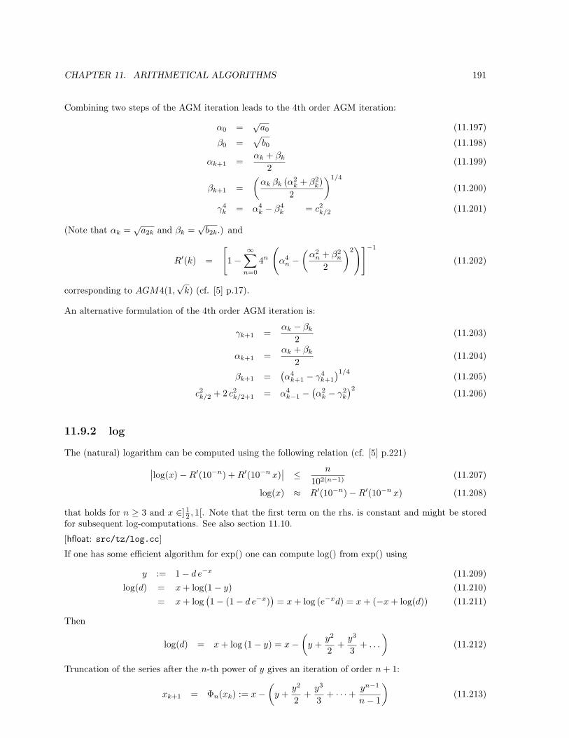
CHAPTER 11. ARITHMETICAL ALGORITHMS 191
Combining two steps of the AGM iteration leads to the 4th order AGM iteration:
α0 =√
a0 (11.197)
β0 =√
b0 (11.198)
αk+1 =αk + βk
2(11.199)
βk+1 =(
αk βk (α2k + β2
k)2
)1/4
(11.200)
γ4k = α4
k − β4k = c2
k/2 (11.201)
(Note that αk =√
a2k and βk =√
b2k.) and
R′(k) =
[1−
∞∑n=0
4n
(α4
n −(
α2n + β2
n
2
)2)]−1
(11.202)
corresponding to AGM4(1,√
k) (cf. [5] p.17).
An alternative formulation of the 4th order AGM iteration is:
γk+1 =αk − βk
2(11.203)
αk+1 =αk + βk
2(11.204)
βk+1 =(α4
k+1 − γ4k+1
)1/4(11.205)
c2k/2 + 2 c2
k/2+1 = α4k−1 −
(α2
k − γ2k
)2(11.206)
11.9.2 log
The (natural) logarithm can be computed using the following relation (cf. [5] p.221)∣∣log(x)−R′(10−n) + R′(10−n x)
∣∣ ≤ n
102(n−1)(11.207)
log(x) ≈ R′(10−n)−R′(10−n x) (11.208)
that holds for n ≥ 3 and x ∈] 12 , 1[. Note that the first term on the rhs. is constant and might be storedfor subsequent log-computations. See also section 11.10.
[hfloat: src/tz/log.cc]
If one has some efficient algorithm for exp() one can compute log() from exp() using
y := 1− d e−x (11.209)log(d) = x + log(1− y) (11.210)
= x + log(1− (1− d e−x)
)= x + log (e−xd) = x + (−x + log(d)) (11.211)
Then
log(d) = x + log (1− y) = x−(
y +y2
2+
y3
3+ . . .
)(11.212)
Truncation of the series after the n-th power of y gives an iteration of order n + 1:
xk+1 = Φn(xk) := x−(
y +y2
2+
y3
3+ · · ·+ yn−1
n− 1
)(11.213)

CHAPTER 11. ARITHMETICAL ALGORITHMS 192
Pade series P[i,j](z) of log (1− z) at z = 0 produce (order i + j + 2) iterations. For i = j we get
[i, j] 7→ x + P[i,j](z = 1− d e−x) (11.214)[0, 0] 7→ x− z (11.215)
[1, 1] 7→ x− z · 6− z
6− 4z(11.216)
[2, 2] 7→ x− z · 30− 21z + z2
30− 36z + 9z2(11.217)
[4, 4] 7→ x− z · 3780− 6510z + 3360z2 − 505z3 + 6z4
3780− 8400z + 6300z2 − 1800z3 + 150z4(11.218)
Compared to the power series based iteration one needs one additional long division but saves half of theexponentiations. This can be a substancial saving for high order iterations.
11.9.3 exp
The exponential function can be computed using the iteration that is obtained as follows:
exp(d) = x exp (d− log(x)) (11.219)= x exp(y) where y := d− log(x) (11.220)
= x
(1 + y +
y2
2+
y3
3!+ . . .
)(11.221)
The corresponding n-th oder iteration is
xk+1 = Φn(xk) := xk
(1 + y +
y2
2+
y3
3!+ . . .
yn−1
(n− 1)!
)(11.222)
As the computation of logarithms is expensive one should use a higher (e.g. 8th) order iteration.
[hfloat: src/tz/itexp.cc]
Pade series P[i,j](z) of exp (z) at z = 0 produce (order i + j + 1) iterations. For i = j we get
[i, j] 7→ x P[i,j](z = d− log x) (11.223)
[1, 1] 7→ x · z + 2z − 2
(11.224)
[2, 2] 7→ x · 12 + 6z + z2
12− 6z + z2(11.225)
[4, 4] 7→ x · 1680 + 840z + 180z2 + 20z3 + z4
1680− 840z + 180z2 − 20z3 + z4(11.226)
The [i, j]-th Pade approximant of exp(z) is
P[i,j](z) =
i∑
k=0
(ik
)(i+jk
) zk
k!
/
j∑
k=0
(jk
)(i+jk
) (−z)k
k!
(11.227)
The numerator for i = j (multiplied by (2i)!/i! in order to avoid rational coefficients) is
=(2i)!i!
·i∑
k=0
(ik
)(2 ik
) zk
k!(11.228)
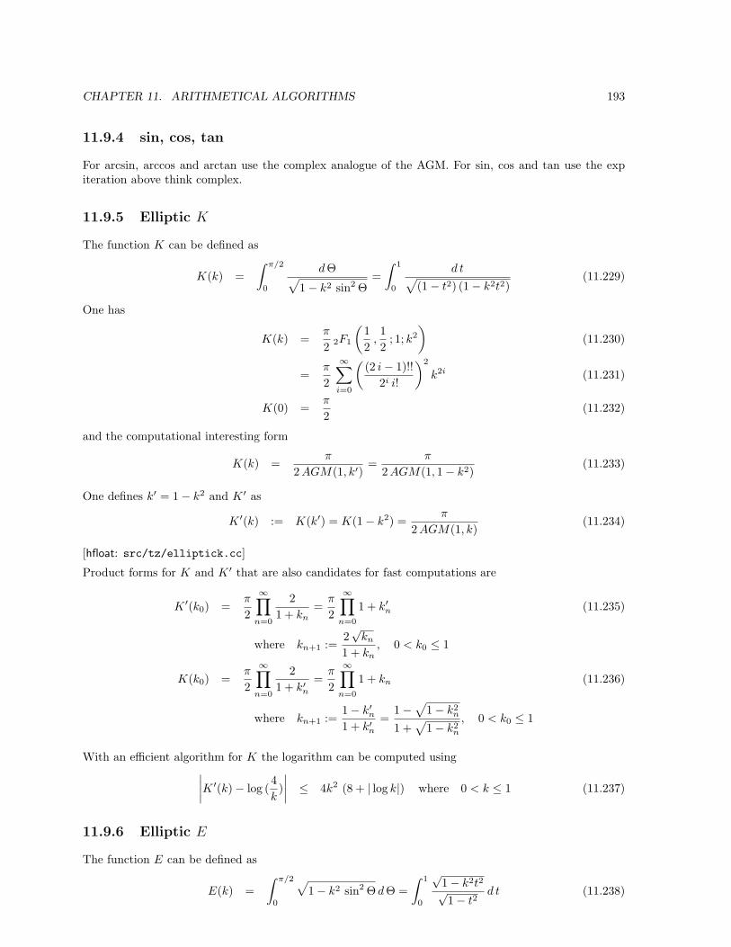
CHAPTER 11. ARITHMETICAL ALGORITHMS 193
11.9.4 sin, cos, tan
For arcsin, arccos and arctan use the complex analogue of the AGM. For sin, cos and tan use the expiteration above think complex.
11.9.5 Elliptic K
The function K can be defined as
K(k) =∫ π/2
0
dΘ√1− k2 sin2 Θ
=∫ 1
0
d t√(1− t2) (1− k2t2)
(11.229)
One has
K(k) =π
2 2F1
(12
,12
; 1; k2
)(11.230)
=π
2
∞∑
i=0
((2 i− 1)!!
2i i!
)2
k2i (11.231)
K(0) =π
2(11.232)
and the computational interesting form
K(k) =π
2 AGM(1, k′)=
π
2 AGM(1, 1− k2)(11.233)
One defines k′ = 1− k2 and K ′ as
K ′(k) := K(k′) = K(1− k2) =π
2 AGM(1, k)(11.234)
[hfloat: src/tz/elliptick.cc]
Product forms for K and K ′ that are also candidates for fast computations are
K ′(k0) =π
2
∞∏n=0
21 + kn
=π
2
∞∏n=0
1 + k′n (11.235)
where kn+1 :=2√
kn
1 + kn, 0 < k0 ≤ 1
K(k0) =π
2
∞∏n=0
21 + k′n
=π
2
∞∏n=0
1 + kn (11.236)
where kn+1 :=1− k′n1 + k′n
=1−
√1− k2
n
1 +√
1− k2n
, 0 < k0 ≤ 1
With an efficient algorithm for K the logarithm can be computed using∣∣∣∣K ′(k)− log (
4k
)∣∣∣∣ ≤ 4k2 (8 + | log k|) where 0 < k ≤ 1 (11.237)
11.9.6 Elliptic E
The function E can be defined as
E(k) =∫ π/2
0
√1− k2 sin2 Θ d Θ =
∫ 1
0
√1− k2t2√1− t2
d t (11.238)
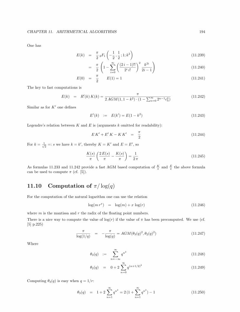
CHAPTER 11. ARITHMETICAL ALGORITHMS 194
One has
E(k) =π
2 2F1
(−1
2,12
; 1; k2
)(11.239)
=π
2
(1−
∞∑
i=0
((2 i− 1)!!
2i i!
)2k2i
2i− 1
)(11.240)
E(0) =π
2E(1) = 1 (11.241)
The key to fast computations is
E(k) = R′(k)K(k) =π
2 AGM(1, 1− k2) · (1−∑∞n=0 2n−1c2
n)(11.242)
Similar as for K ′ one defines
E′(k) := E(k′) = E(1− k2) (11.243)
Legendre’s relation between K and E is (arguments k omitted for readability):
E K ′ + E′K −K K ′ =π
2(11.244)
For k = 1√2
=: s we have k = k′, thereby K = K ′ and E = E′, so
K(s)π
(2 E(s)
π− K(s)
π
)=
12 π
(11.245)
As formulas 11.233 and 11.242 provide a fast AGM based computation of Kπ and E
π the above formulacan be used to compute π (cf. [5]).
11.10 Computation of π/ log(q)
For the computation of the natural logarithm one can use the relation
log(mrx) = log(m) + x log(r) (11.246)
where m is the mantissa and r the radix of the floating point numbers.
There is a nice way to compute the value of log(r) if the value of π has been precomputed. We use (cf.[5] p.225)
π
log(1/q)= − π
log(q)= AGM(θ3(q)2, θ2(q)2) (11.247)
Where
θ3(q) :=∞∑
n=−∞qn2
(11.248)
θ2(q) = 0 + 2∞∑
n=0
q(n+1/2)2 (11.249)
Computing θ3(q) is easy when q = 1/r:
θ3(q) = 1 + 2∞∑
n=1
qn2= 2 (1 +
∞∑n=1
qn2)− 1 (11.250)
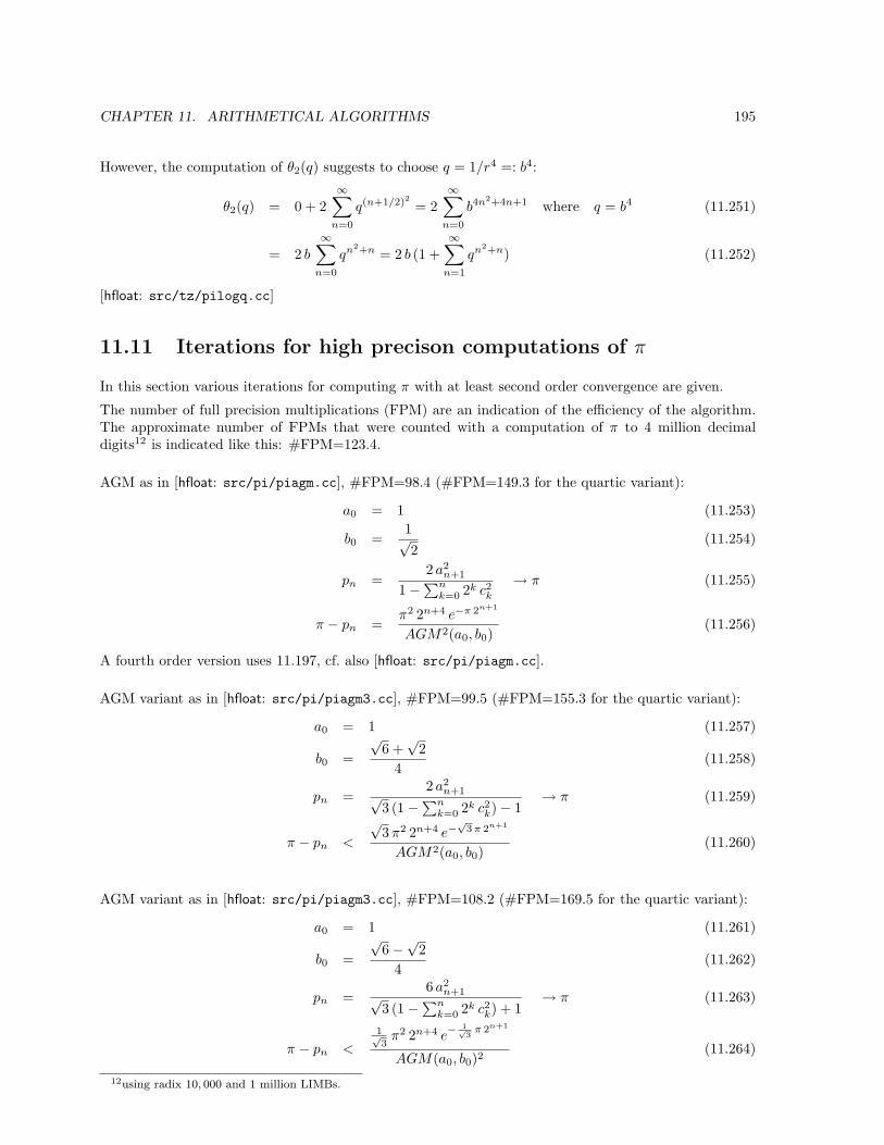
CHAPTER 11. ARITHMETICAL ALGORITHMS 195
However, the computation of θ2(q) suggests to choose q = 1/r4 =: b4:
θ2(q) = 0 + 2∞∑
n=0
q(n+1/2)2 = 2∞∑
n=0
b4n2+4n+1 where q = b4 (11.251)
= 2 b
∞∑n=0
qn2+n = 2 b (1 +∞∑
n=1
qn2+n) (11.252)
[hfloat: src/tz/pilogq.cc]
11.11 Iterations for high precison computations of π
In this section various iterations for computing π with at least second order convergence are given.
The number of full precision multiplications (FPM) are an indication of the efficiency of the algorithm.The approximate number of FPMs that were counted with a computation of π to 4 million decimaldigits12 is indicated like this: #FPM=123.4.
AGM as in [hfloat: src/pi/piagm.cc], #FPM=98.4 (#FPM=149.3 for the quartic variant):
a0 = 1 (11.253)
b0 =1√2
(11.254)
pn =2 a2
n+1
1−∑nk=0 2k c2
k
→ π (11.255)
π − pn =π2 2n+4 e−π 2n+1
AGM2(a0, b0)(11.256)
A fourth order version uses 11.197, cf. also [hfloat: src/pi/piagm.cc].
AGM variant as in [hfloat: src/pi/piagm3.cc], #FPM=99.5 (#FPM=155.3 for the quartic variant):
a0 = 1 (11.257)
b0 =√
6 +√
24
(11.258)
pn =2 a2
n+1√3 (1−∑n
k=0 2k c2k)− 1
→ π (11.259)
π − pn <
√3 π2 2n+4 e−
√3 π 2n+1
AGM2(a0, b0)(11.260)
AGM variant as in [hfloat: src/pi/piagm3.cc], #FPM=108.2 (#FPM=169.5 for the quartic variant):
a0 = 1 (11.261)
b0 =√
6−√24
(11.262)
pn =6 a2
n+1√3 (1−∑n
k=0 2k c2k) + 1
→ π (11.263)
π − pn <
1√3
π2 2n+4 e− 1√
3π 2n+1
AGM(a0, b0)2(11.264)
12using radix 10, 000 and 1 million LIMBs.

CHAPTER 11. ARITHMETICAL ALGORITHMS 196
Borwein’s quartic (fourth order) iteration, variant r = 4 as in [hfloat: src/pi/pi4th.cc], #FPM=170.5:
y0 =√
2− 1 (11.265)
a0 = 6− 4√
2 (11.266)
yk+1 =1− (1− y4
k)1/4
1 + (1− y4k)1/4
→ 0 + (11.267)
=(1− y4
k)−1/4 − 1(1− y4
k)−1/4 + 1(11.268)
ak+1 = ak (1 + yk+1)4 − 22k+3 yk+1 (1 + yk+1 + y2k+1) → 1
π(11.269)
= ak ((1 + yk+1)2)2 − 22k+3 yk+1 ((1 + yk+1)2 − yk+1) (11.270)0 < ak − π−1 ≤ 16 · 4n 2 e−4n 2 π (11.271)
Identities 11.268 and 11.270 show how to save operations.
Borwein’s quartic (fourth order) iteration, variant r = 16 as in [hfloat: src/pi/pi4th.cc], #FPM=164.4:
y0 =1− 2−1/4
1 + 2−1/4(11.272)
a0 =8/√
2− 2(2−1/4 + 1)4
(11.273)
yk+1 =(1− y4
k)−1/4 − 1(1− y4
k)−1/4 + 1→ 0 + (11.274)
ak+1 = ak (1 + yk+1)4 − 22k+4 yk+1 (1 + yk+1 + y2k+1) → 1
π(11.275)
0 < ak − π−1 ≤ 16 · 4n 4 e−4n 4 π (11.276)
Same operation count as before, but this variant gives approximately twice as much precision after thesame number of steps.
The general form of the quartic iterations (11.265 and 11.272) is
y0 =√
λ∗(r) (11.277)a0 = α(r) (11.278)
yk+1 =(1− y4
k)−1/4 − 1(1− y4
k)−1/4 + 1→ 0 + (11.279)
ak+1 = ak (1 + yk+1)4 − 22k+2√
r yk (1 + yk+1 + y2k+1) → 1
π(11.280)
0 < ak − π−1 ≤ 16 · 4n√
r e−4n √r π (11.281)
Cf. [5], p.170f.
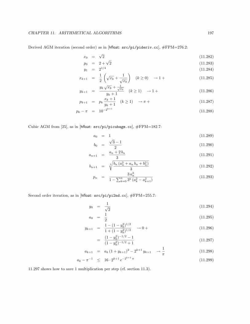
CHAPTER 11. ARITHMETICAL ALGORITHMS 197
Derived AGM iteration (second order) as in [hfloat: src/pi/pideriv.cc], #FPM=276.2:
x0 =√
2 (11.282)
p0 = 2 +√
2 (11.283)y1 = 21/4 (11.284)
xk+1 =12
(√xk +
1√xk
)(k ≥ 0) → 1 + (11.285)
yk+1 =yk√
xk + 1√xk
yk + 1(k ≥ 1) → 1 + (11.286)
pk+1 = pkxk + 1yk + 1
(k ≥ 1) → π + (11.287)
pk − π = 10−2k+1(11.288)
Cubic AGM from [25], as in [hfloat: src/pi/picubagm.cc], #FPM=182.7:
a0 = 1 (11.289)
b0 =√
3− 12
(11.290)
an+1 =an + 2 bn
3(11.291)
bn+1 = 3
√bn (a2
n + an bn + b2n)
3(11.292)
pn =3 a2
n
1−∑nk=0 3k (a2
k − a2k+1)
(11.293)
Second order iteration, as in [hfloat: src/pi/pi2nd.cc], #FPM=255.7:
y0 =1√2
(11.294)
a0 =12
(11.295)
yk+1 =1− (1− y2
k)1/2
1 + (1− y2k)1/2
→ 0 + (11.296)
=(1− y2
k)−1/2 − 1(1− y2
k)−1/2 + 1(11.297)
ak+1 = ak (1 + yk+1)2 − 2k+1 yk+1 → 1π
(11.298)
ak − π−1 ≤ 16 · 2k+1 e−2k+1 π (11.299)
11.297 shows how to save 1 multiplication per step (cf. section 11.3).
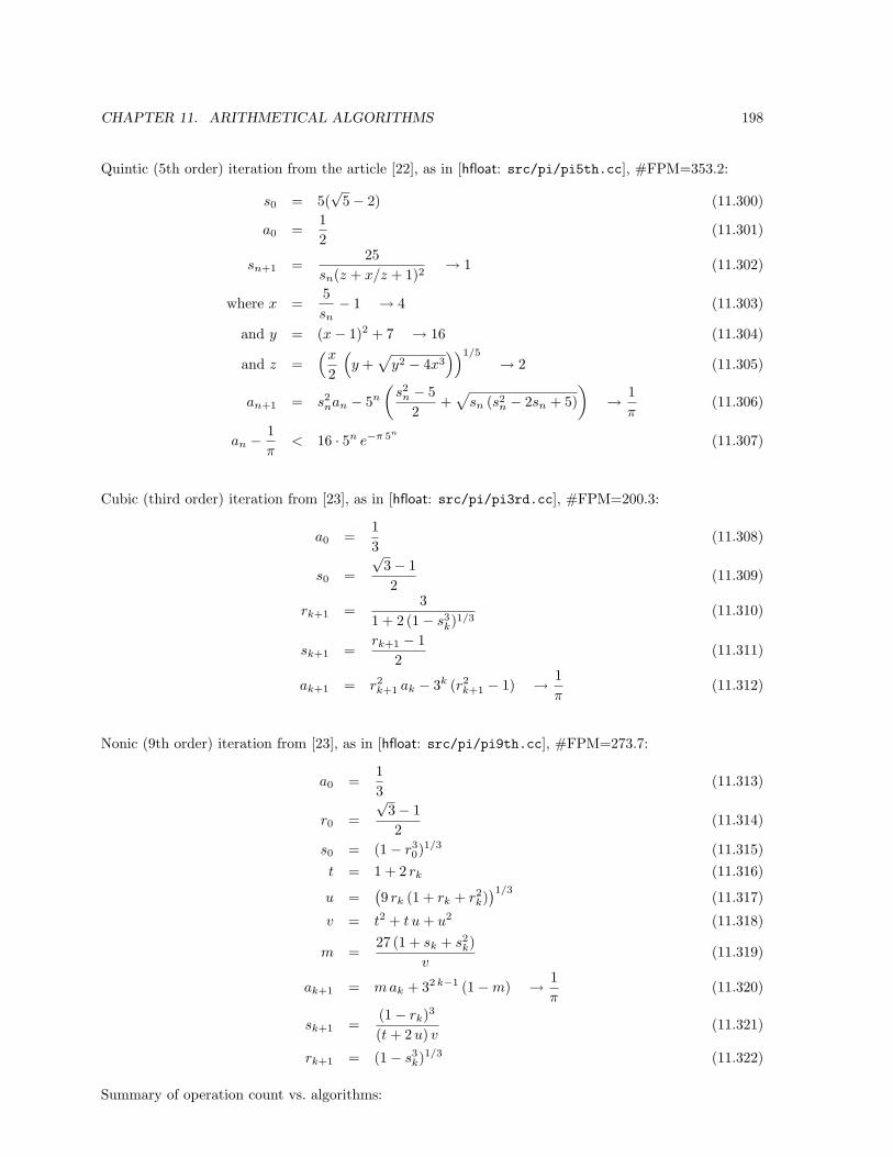
CHAPTER 11. ARITHMETICAL ALGORITHMS 198
Quintic (5th order) iteration from the article [22], as in [hfloat: src/pi/pi5th.cc], #FPM=353.2:
s0 = 5(√
5− 2) (11.300)
a0 =12
(11.301)
sn+1 =25
sn(z + x/z + 1)2→ 1 (11.302)
where x =5sn− 1 → 4 (11.303)
and y = (x− 1)2 + 7 → 16 (11.304)
and z =(x
2
(y +
√y2 − 4x3
))1/5
→ 2 (11.305)
an+1 = s2nan − 5n
(s2
n − 52
+√
sn (s2n − 2sn + 5)
)→ 1
π(11.306)
an − 1π
< 16 · 5n e−π 5n
(11.307)
Cubic (third order) iteration from [23], as in [hfloat: src/pi/pi3rd.cc], #FPM=200.3:
a0 =13
(11.308)
s0 =√
3− 12
(11.309)
rk+1 =3
1 + 2 (1− s3k)1/3
(11.310)
sk+1 =rk+1 − 1
2(11.311)
ak+1 = r2k+1 ak − 3k (r2
k+1 − 1) → 1π
(11.312)
Nonic (9th order) iteration from [23], as in [hfloat: src/pi/pi9th.cc], #FPM=273.7:
a0 =13
(11.313)
r0 =√
3− 12
(11.314)
s0 = (1− r30)
1/3 (11.315)t = 1 + 2 rk (11.316)
u =(9 rk (1 + rk + r2
k))1/3
(11.317)
v = t2 + t u + u2 (11.318)
m =27 (1 + sk + s2
k)v
(11.319)
ak+1 = mak + 32 k−1 (1−m) → 1π
(11.320)
sk+1 =(1− rk)3
(t + 2 u) v(11.321)
rk+1 = (1− s3k)1/3 (11.322)
Summary of operation count vs. algorithms:
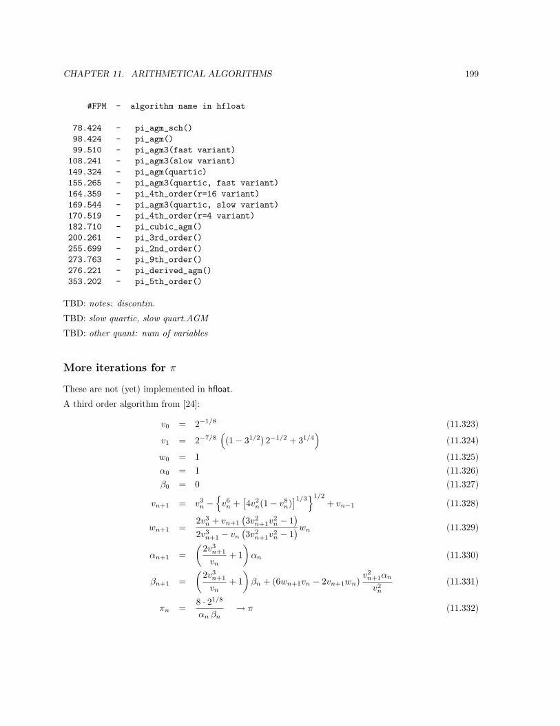
CHAPTER 11. ARITHMETICAL ALGORITHMS 199
#FPM - algorithm name in hfloat
78.424 - pi_agm_sch()98.424 - pi_agm()99.510 - pi_agm3(fast variant)
108.241 - pi_agm3(slow variant)149.324 - pi_agm(quartic)155.265 - pi_agm3(quartic, fast variant)164.359 - pi_4th_order(r=16 variant)169.544 - pi_agm3(quartic, slow variant)170.519 - pi_4th_order(r=4 variant)182.710 - pi_cubic_agm()200.261 - pi_3rd_order()255.699 - pi_2nd_order()273.763 - pi_9th_order()276.221 - pi_derived_agm()353.202 - pi_5th_order()
TBD: notes: discontin.
TBD: slow quartic, slow quart.AGM
TBD: other quant: num of variables
More iterations for π
These are not (yet) implemented in hfloat.
A third order algorithm from [24]:
v0 = 2−1/8 (11.323)
v1 = 2−7/8((1− 31/2) 2−1/2 + 31/4
)(11.324)
w0 = 1 (11.325)α0 = 1 (11.326)β0 = 0 (11.327)
vn+1 = v3n −
v6
n +[4v2
n(1− v8n)
]1/31/2
+ vn−1 (11.328)
wn+1 =2v3
n + vn+1
(3v2
n+1v2n − 1
)
2v3n+1 − vn
(3v2
n+1v2n − 1
)wn (11.329)
αn+1 =(
2v3n+1
vn+ 1
)αn (11.330)
βn+1 =(
2v3n+1
vn+ 1
)βn + (6wn+1vn − 2vn+1wn)
v2n+1αn
v2n
(11.331)
πn =8 · 21/8
αn βn→ π (11.332)
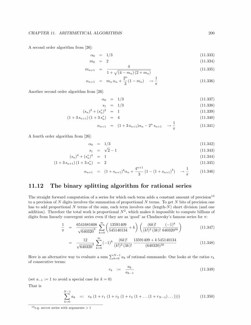
CHAPTER 11. ARITHMETICAL ALGORITHMS 200
A second order algorithm from [26]:
α0 = 1/3 (11.333)m0 = 2 (11.334)
mn+1 =4
1 +√
(4−mn) (2 + mn)(11.335)
αn+1 = mn αn +2n
3(1−mn) → 1
π(11.336)
Another second order algorithm from [26]:
α0 = 1/3 (11.337)s1 = 1/3 (11.338)
(sn)2 + (s∗n)2 = 1 (11.339)(1 + 3 sn+1) (1 + 3 s∗n) = 4 (11.340)
αn+1 = (1 + 3 sn+1)αn − 2n sn+1 → 1π
(11.341)
A fourth order algorithm from [26]:
α0 = 1/3 (11.342)
s1 =√
2− 1 (11.343)(sn)4 + (s∗n)4 = 1 (11.344)
(1 + 3 sn+1) (1 + 3 s∗n) = 2 (11.345)
αn+1 = (1 + sn+1)4αn +4n+1
3(1− (1 + sn+1)
4) → 1π
(11.346)
11.12 The binary splitting algorithm for rational series
The straight forward computation of a series for which each term adds a constant amount of precision13
to a precision of N digits involves the summation of proportional N terms. To get N bits of precision onehas to add proportional N terms of the sum, each term involves one (length-N) short division (and oneaddition). Therefore the total work is proportional N2, which makes it impossible to compute billions ofdigits from linearly convergent series even if they are as ‘good’ as Chudnovsky’s famous series for π:
1π
=6541681608√
6403203
∞∑
k=0
(13591409545140134
+ k
) ((6k)!
(k!)3 (3k)!(−1)k
6403203k
)(11.347)
=12
√640320
3
∞∑
k=0
(−1)k (6k)!(k!)3 (3k)!
13591409 + k 545140134(640320)3k
(11.348)
Here is an alternative way to evaluate a sum∑N−1
k=0 ak of rational summands: One looks at the ratios rk
of consecutive terms:
rk :=ak
ak−1(11.349)
(set a−1 := 1 to avoid a special case for k = 0)
That isN−1∑
k=0
ak =: r0 (1 + r1 (1 + r2 (1 + r3 (1 + . . . (1 + rN−1) . . . )))) (11.350)
13e.g. arccot series with arguments > 1
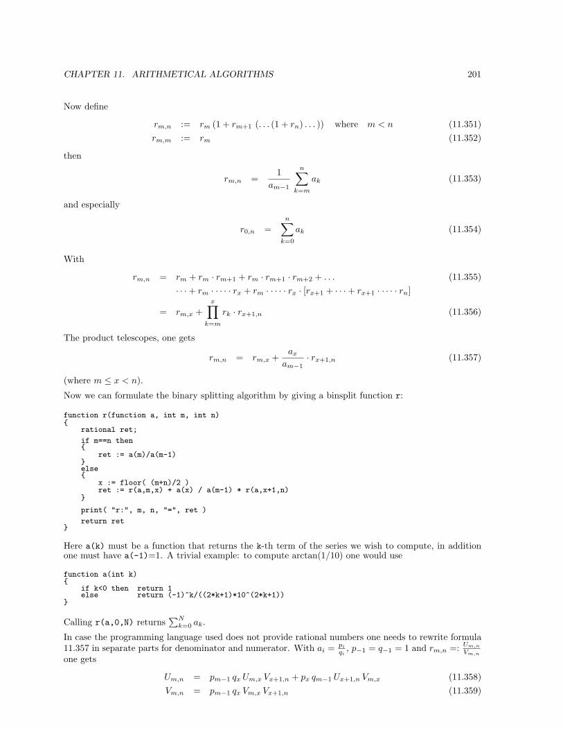
CHAPTER 11. ARITHMETICAL ALGORITHMS 201
Now define
rm,n := rm (1 + rm+1 (. . . (1 + rn) . . . )) where m < n (11.351)rm,m := rm (11.352)
then
rm,n =1
am−1
n∑
k=m
ak (11.353)
and especially
r0,n =n∑
k=0
ak (11.354)
With
rm,n = rm + rm · rm+1 + rm · rm+1 · rm+2 + . . . (11.355)· · ·+ rm · · · · · rx + rm · · · · · rx · [rx+1 + · · ·+ rx+1 · · · · · rn]
= rm,x +x∏
k=m
rk · rx+1,n (11.356)
The product telescopes, one gets
rm,n = rm,x +ax
am−1· rx+1,n (11.357)
(where m ≤ x < n).
Now we can formulate the binary splitting algorithm by giving a binsplit function r:
function r(function a, int m, int n)
rational ret;
if m==n then
ret := a(m)/a(m-1)else
x := floor( (m+n)/2 )ret := r(a,m,x) + a(x) / a(m-1) * r(a,x+1,n)
print( "r:", m, n, "=", ret )
return ret
Here a(k) must be a function that returns the k-th term of the series we wish to compute, in additionone must have a(-1)=1. A trivial example: to compute arctan(1/10) one would use
function a(int k)
if k<0 then return 1else return (-1)^k/((2*k+1)*10^(2*k+1))
Calling r(a,0,N) returns∑N
k=0 ak.
In case the programming language used does not provide rational numbers one needs to rewrite formula11.357 in separate parts for denominator and numerator. With ai = pi
qi, p−1 = q−1 = 1 and rm,n =: Um,n
Vm,n
one gets
Um,n = pm−1 qx Um,x Vx+1,n + px qm−1 Ux+1,n Vm,x (11.358)Vm,n = pm−1 qx Vm,x Vx+1,n (11.359)

CHAPTER 11. ARITHMETICAL ALGORITHMS 202
The reason why binary splitting is better than the straight forward way is that the involved work is onlyO((log N)2 M(N)), where M(N) is the complexity of one N -bit multiplication (see [21]). This meansthat sums of linear but sufficient convergence are again candidates for high precision computations.
In addition, the ratio r0,N−1 (i.e. the sum of the first N terms) can be reused if one wants to evaluatethe sum to a higher precision than before. To get twice the precision use
r0,2 N−1 = r0,N−1 + aN−1 · rN,2 N−1 (11.360)
(this is formula 11.357 with m = 0, x = N − 1, n = 2N − 1). With explicit rational arithmetic:
U0,2N−1 = qN−1 U0,N−1 VN,2N−1 + pN−1 UN,2N−1 V0,N−1 (11.361)V0,2N−1 = qN−1 V0,N−1 VN,2N−1 (11.362)
Thereby with the appearence of some new computer that can multiply two length 2·N numbers14 one onlyneeds to combine the two ratios r0,N−1 and rN,2N−1 that had been precomputed by the last generationof computers. This costs only a few fullsize multiplications on your new and expensive supercomputer(instead of several hundreds for the iterative schemes), which means that one can improve on priorcomputations at low cost.
If one wants to stare at zillions of decimal digits of the floating point expansion then one division is alsoneeded which costs not more than 4 multiplications (cf. section 11.3).
Note that this algorithm can trivially be extended (or rather simplified) to infinite products, e.g. matrixproducts as Bellard’s
∞∏
k=0
[2 (k− 1
2 ) (k+2)
27 (k+ 23 ) (k+ 4
3 )10
0 1
]=
[0 π + 60 1
](11.363)
Cf. [21] and [27].
11.13 The magic sumalt algorithm
The following algorithm is due to Cohen, Villegas and Zagier, see [29].
Pseudo code to compute an estimate of∑∞
k=0 xk using the first n summands. The xk summands areexpected in x[0,1, ...,n-1].
function sumalt(x[], n)
d := (3+sqrt(8))^nd := (d+1/d)/2
b := 1c := ds := 0for k:=0 to n-1
c := c - bs := s + c * x[k]b := b * (2*(n+k)*(n-k)) / ((2*k+1)*(k+1))
return s/d
With alternating sums the accuracy of the estimate will be (3 +√
8)−n ≈ 5.82−n.
As an example let us explicitely write down the estimate for the 4 · arctan(1) using the first 8 terms
π ≈ 4 ·(
11− 1
3+
15− 1
7+
19− 1
11+
113− 1
15
)= 3.017 . . . (11.364)
14assuming one could multiply length-N numbers before
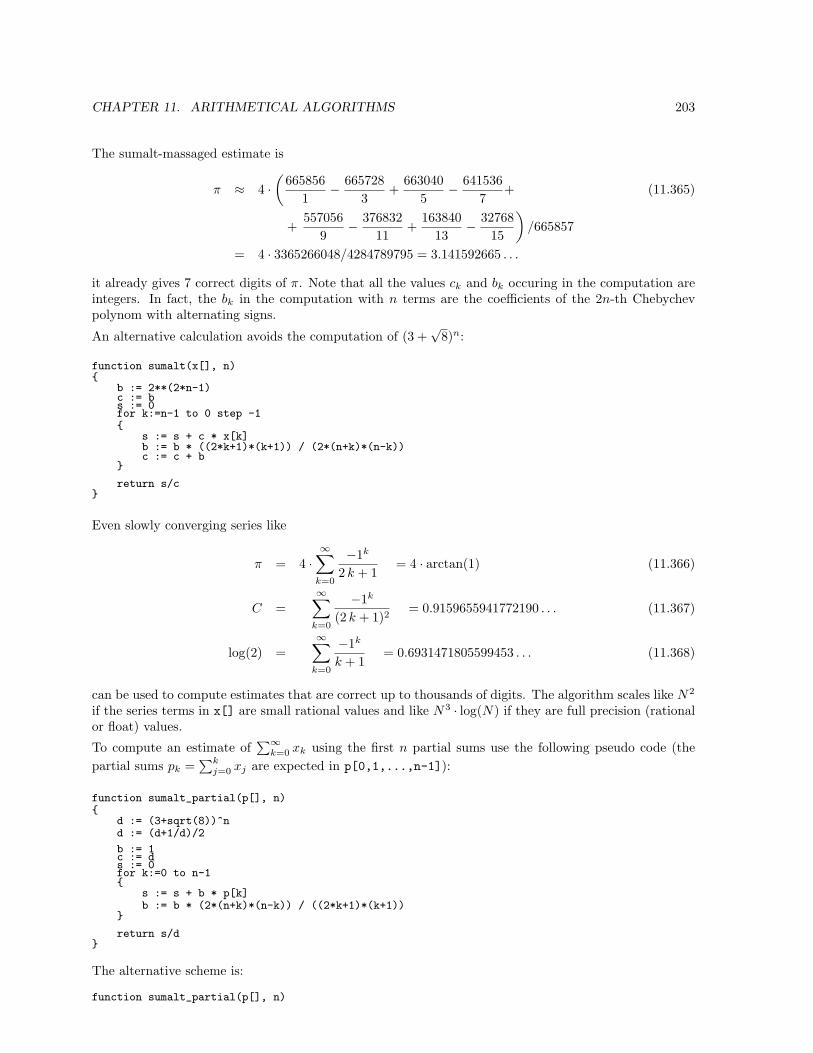
CHAPTER 11. ARITHMETICAL ALGORITHMS 203
The sumalt-massaged estimate is
π ≈ 4 ·(
6658561
− 6657283
+663040
5− 641536
7+ (11.365)
+557056
9− 376832
11+
16384013
− 3276815
)/665857
= 4 · 3365266048/4284789795 = 3.141592665 . . .
it already gives 7 correct digits of π. Note that all the values ck and bk occuring in the computation areintegers. In fact, the bk in the computation with n terms are the coefficients of the 2n-th Chebychevpolynom with alternating signs.
An alternative calculation avoids the computation of (3 +√
8)n:
function sumalt(x[], n)
b := 2**(2*n-1)c := bs := 0for k:=n-1 to 0 step -1
s := s + c * x[k]b := b * ((2*k+1)*(k+1)) / (2*(n+k)*(n-k))c := c + b
return s/c
Even slowly converging series like
π = 4 ·∞∑
k=0
−1k
2 k + 1= 4 · arctan(1) (11.366)
C =∞∑
k=0
−1k
(2 k + 1)2= 0.9159655941772190 . . . (11.367)
log(2) =∞∑
k=0
−1k
k + 1= 0.6931471805599453 . . . (11.368)
can be used to compute estimates that are correct up to thousands of digits. The algorithm scales like N2
if the series terms in x[] are small rational values and like N3 · log(N) if they are full precision (rationalor float) values.
To compute an estimate of∑∞
k=0 xk using the first n partial sums use the following pseudo code (thepartial sums pk =
∑kj=0 xj are expected in p[0,1,...,n-1]):
function sumalt_partial(p[], n)
d := (3+sqrt(8))^nd := (d+1/d)/2
b := 1c := ds := 0for k:=0 to n-1
s := s + b * p[k]b := b * (2*(n+k)*(n-k)) / ((2*k+1)*(k+1))
return s/d
The alternative scheme is:
function sumalt_partial(p[], n)
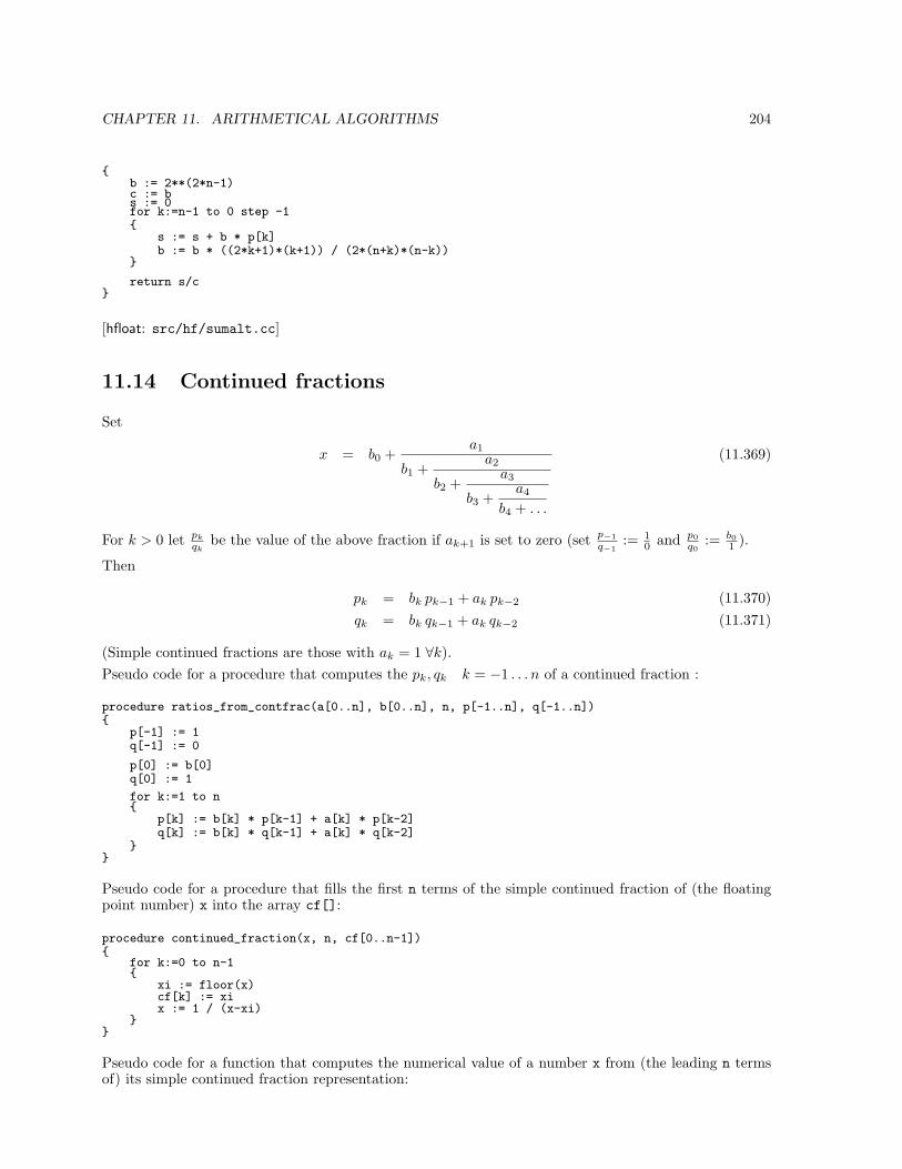
CHAPTER 11. ARITHMETICAL ALGORITHMS 204
b := 2**(2*n-1)c := bs := 0for k:=n-1 to 0 step -1
s := s + b * p[k]b := b * ((2*k+1)*(k+1)) / (2*(n+k)*(n-k))
return s/c
[hfloat: src/hf/sumalt.cc]
11.14 Continued fractions
Set
x = b0 +a1
b1 +a2
b2 +a3
b3 +a4
b4 + . . .
(11.369)
For k > 0 let pk
qkbe the value of the above fraction if ak+1 is set to zero (set p−1
q−1:= 1
0 and p0q0
:= b01 ).
Then
pk = bk pk−1 + ak pk−2 (11.370)qk = bk qk−1 + ak qk−2 (11.371)
(Simple continued fractions are those with ak = 1 ∀k).Pseudo code for a procedure that computes the pk, qk k = −1 . . . n of a continued fraction :
procedure ratios_from_contfrac(a[0..n], b[0..n], n, p[-1..n], q[-1..n])
p[-1] := 1q[-1] := 0
p[0] := b[0]q[0] := 1
for k:=1 to n
p[k] := b[k] * p[k-1] + a[k] * p[k-2]q[k] := b[k] * q[k-1] + a[k] * q[k-2]
Pseudo code for a procedure that fills the first n terms of the simple continued fraction of (the floatingpoint number) x into the array cf[]:
procedure continued_fraction(x, n, cf[0..n-1])
for k:=0 to n-1
xi := floor(x)cf[k] := xix := 1 / (x-xi)
Pseudo code for a function that computes the numerical value of a number x from (the leading n termsof) its simple continued fraction representation:
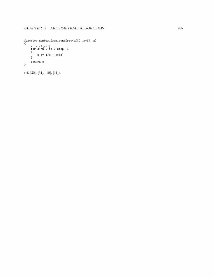
CHAPTER 11. ARITHMETICAL ALGORITHMS 205
function number_from_contfrac(cf[0..n-1], n)
x := cf[n-1]for k:=n-2 to 0 step -1
x := 1/x + cf[k]
return x
(cf. [30], [31], [10], [11]).
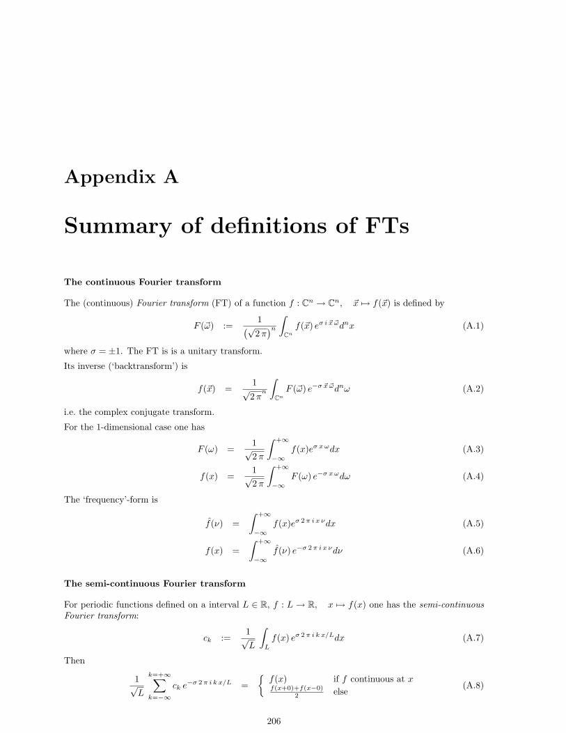
Appendix A
Summary of definitions of FTs
The continuous Fourier transform
The (continuous) Fourier transform (FT) of a function f : Cn → Cn, ~x 7→ f(~x) is defined by
F (~ω) :=1(√2 π
)n
∫
Cn
f(~x) eσ i ~x ~ωdnx (A.1)
where σ = ±1. The FT is is a unitary transform.
Its inverse (‘backtransform’) is
f(~x) =1√2 π
n
∫
Cn
F (~ω) e−σ ~x ~ωdnω (A.2)
i.e. the complex conjugate transform.
For the 1-dimensional case one has
F (ω) =1√2 π
∫ +∞
−∞f(x)eσ x ωdx (A.3)
f(x) =1√2 π
∫ +∞
−∞F (ω) e−σ x ωdω (A.4)
The ‘frequency’-form is
f(ν) =∫ +∞
−∞f(x)eσ 2 π i x νdx (A.5)
f(x) =∫ +∞
−∞f(ν) e−σ 2 π i x νdν (A.6)
The semi-continuous Fourier transform
For periodic functions defined on a interval L ∈ R, f : L → R, x 7→ f(x) one has the semi-continuousFourier transform:
ck :=1√L
∫
L
f(x) eσ 2 π i k x/Ldx (A.7)
Then
1√L
k=+∞∑
k=−∞ck e−σ 2 π i k x/L =
f(x) if f continuous at xf(x+0)+f(x−0)
2 else(A.8)
206
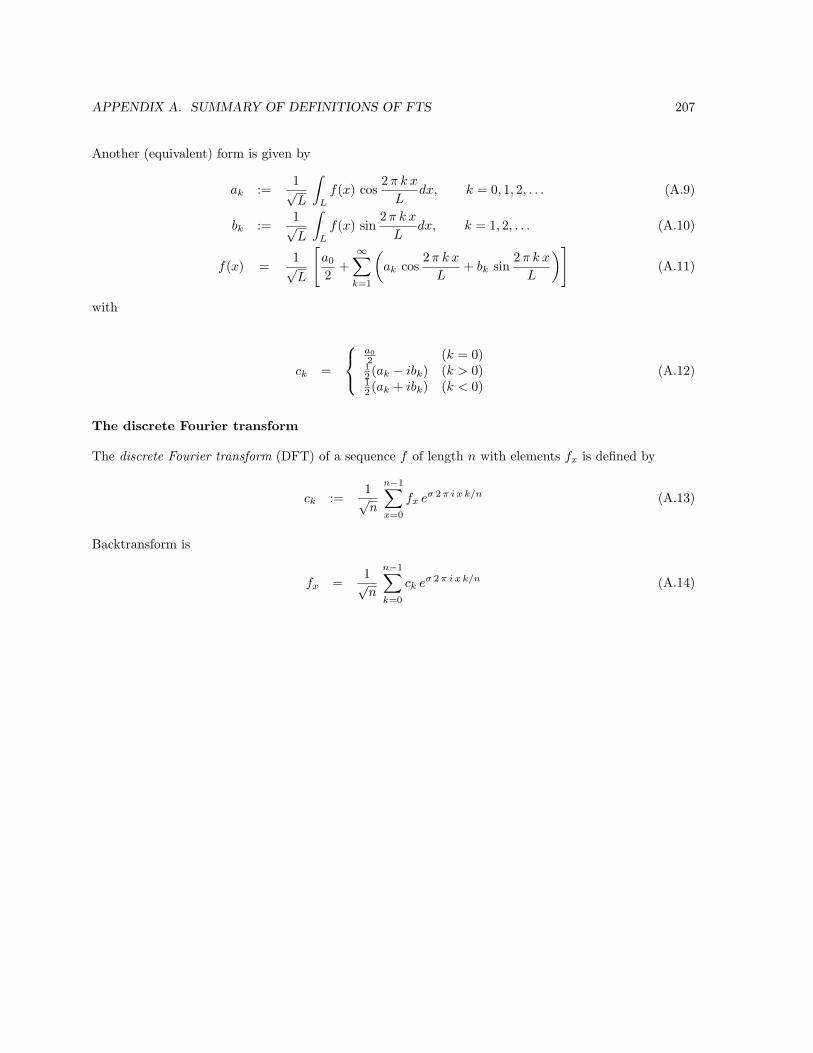
APPENDIX A. SUMMARY OF DEFINITIONS OF FTS 207
Another (equivalent) form is given by
ak :=1√L
∫
L
f(x) cos2 π k x
Ldx, k = 0, 1, 2, . . . (A.9)
bk :=1√L
∫
L
f(x) sin2 π k x
Ldx, k = 1, 2, . . . (A.10)
f(x) =1√L
[a0
2+
∞∑
k=1
(ak cos
2 π k x
L+ bk sin
2 π k x
L
)](A.11)
with
ck =
a02 (k = 0)12 (ak − ibk) (k > 0)12 (ak + ibk) (k < 0)
(A.12)
The discrete Fourier transform
The discrete Fourier transform (DFT) of a sequence f of length n with elements fx is defined by
ck :=1√n
n−1∑x=0
fx eσ 2 π i x k/n (A.13)
Backtransform is
fx =1√n
n−1∑
k=0
ck eσ 2 π i x k/n (A.14)

Appendix B
The pseudo language Sprache
Many algorithms in this book are given in a pseudo language called Sprache. Sprache is meant to beimmediately understandable for everyone who ever had contact with programming languages like C,FORTRAN, pascal or algol. Sprache is hopefully self explanatory. The intention of using Sprache insteadof e.g. mathematical formulas (cf. [4]) or description by words (cf. [8] or [14]) was to minimize the work ittakes to translate the given algorithm to one’s favorite programming language, it should be mere syntaxadaptation.
By the way ‘Sprache’ is the german word for language,
// a comment:// comments are useful.
// assignment:t := 2.71
// parallel assignment:s, t, u := 5, 6, 7// same as:s := 5t := 6u := 7
s, t := s+t, s-t// same as (avoid temporary):temp := s + tt := s - t;s := temp
// if conditional:if a==b then a:=3
// with blockif a>=3 then
// do something ...
// a function returns a value:function plus_three(x)
return x + 3;
// a procedure works on data:procedure increment_copy(f[],g[],n)// real f[0..n-1] input// real g[0..n-1] result
for k:=0 to n-1
g[k] := f[k] + 1
208
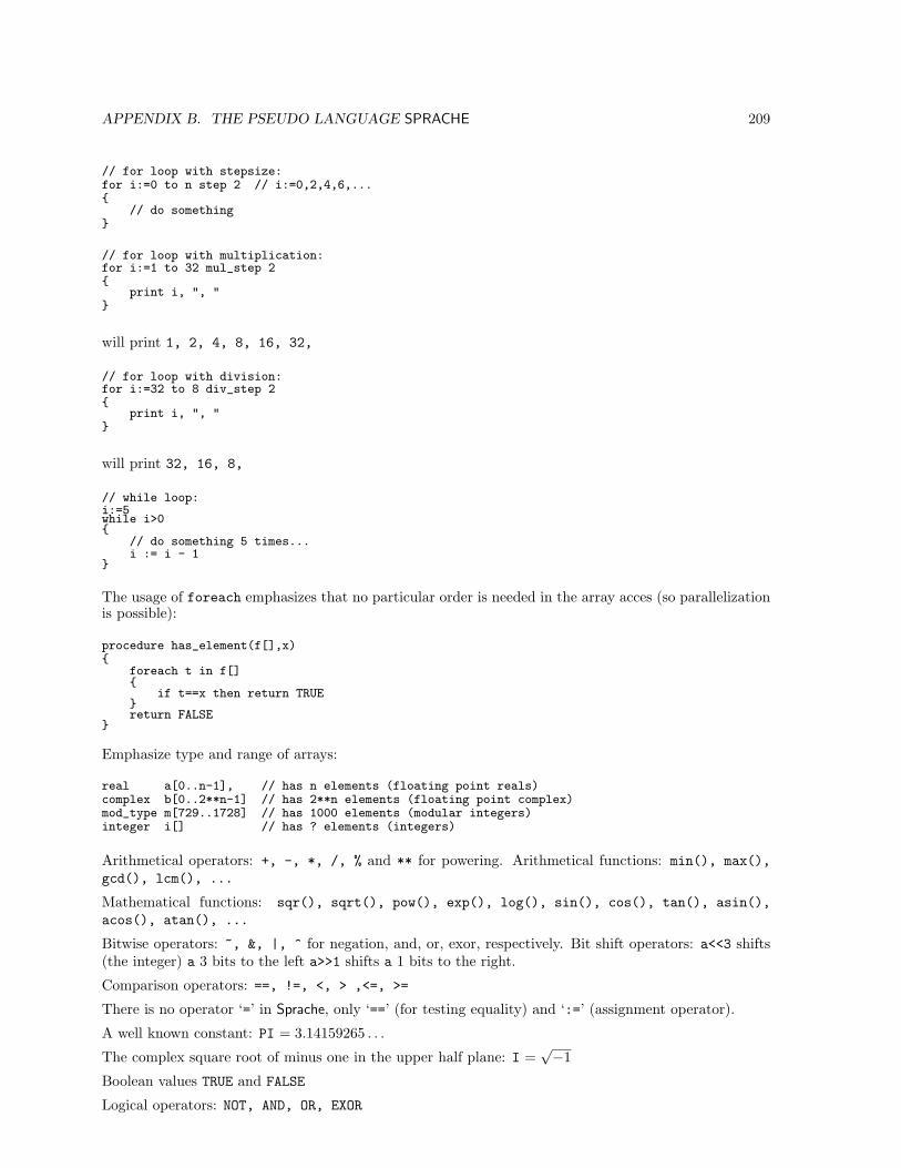
APPENDIX B. THE PSEUDO LANGUAGE SPRACHE 209
// for loop with stepsize:for i:=0 to n step 2 // i:=0,2,4,6,...
// do something
// for loop with multiplication:for i:=1 to 32 mul_step 2
print i, ", "
will print 1, 2, 4, 8, 16, 32,
// for loop with division:for i:=32 to 8 div_step 2
print i, ", "
will print 32, 16, 8,
// while loop:i:=5while i>0
// do something 5 times...i := i - 1
The usage of foreach emphasizes that no particular order is needed in the array acces (so parallelizationis possible):
procedure has_element(f[],x)
foreach t in f[]
if t==x then return TRUEreturn FALSE
Emphasize type and range of arrays:
real a[0..n-1], // has n elements (floating point reals)complex b[0..2**n-1] // has 2**n elements (floating point complex)mod_type m[729..1728] // has 1000 elements (modular integers)integer i[] // has ? elements (integers)
Arithmetical operators: +, -, *, /, % and ** for powering. Arithmetical functions: min(), max(),gcd(), lcm(), ...
Mathematical functions: sqr(), sqrt(), pow(), exp(), log(), sin(), cos(), tan(), asin(),acos(), atan(), ...
Bitwise operators: ~, &, |, ^ for negation, and, or, exor, respectively. Bit shift operators: a<<3 shifts(the integer) a 3 bits to the left a>>1 shifts a 1 bits to the right.
Comparison operators: ==, !=, <, > ,<=, >=
There is no operator ‘=’ in Sprache, only ‘==’ (for testing equality) and ‘:=’ (assignment operator).
A well known constant: PI = 3.14159265 . . .
The complex square root of minus one in the upper half plane: I =√−1
Boolean values TRUE and FALSE
Logical operators: NOT, AND, OR, EXOR

APPENDIX B. THE PSEUDO LANGUAGE SPRACHE 210
// copying arrays of same length:copy a[] to b[]
// more copying arrays:copy a[n..n+m] to b[0..m]
// skip copy array:copy a[0,2,4,...,n-1] to b[0,1,2,...,n/2-1]
Modular arithmetic: x := a * b mod m shall do what it says, i := a**(-1) mod m shall set i to themodular inverse of a.

Appendix C
Optimisation considerations for fasttransforms
• Reduce operations: use higher radix, at least radix 4 (with high radix algorithms note that the intelx86-architecture is severely register impaired)
• Mass storage FFTs: use MFA as described
• Trig recursion: loss of precision (not with mod FFTs), use stable versions, use table for initial valuesof recursion.
• Trig table: only for small lengths, else cache problem.
• Fused routines: combine first/last (few) step(s) in transforms with squar-ing/normalization/revbin/transposition etc. e.g. revbin-squaring in convol,
• Use explicit last/first step with radix as high a possible
• Write special versions for zero padded data (e.g. for convolutions), also write a special version ofrevbin permute for zero padded data
• Integer stuff (e.g. exact convolutions): consider NTTs but be prepared for work & disappointments
• Image processing & effects: also check Walsh transform etc.
• Direct mapped cache: Avoid stride-2n access (e.g. use gray-ffts, gray-walsh); try to achieve unitstride data access. Use the general prime factor algorithm. Improve memory locality (e.g. use thematrix Fourier algorithm (MFA))
• Vectorization: SIMD versions often boost performance
• For correlations/convolutions save two revbin permute (or transpose) operations by combining DIFand DIT algorithms.
• Real-valued transforms & convolution: use hartley transform (also for computation of spectrum).Even use complex FHT for forward step in real convolution.
• Reducing multiplications: Winograd FFT, mainly of theoretical interest (today the speed of multi-plication is almost that of addition, often mults go parallel to adds)
• Only general rule for big sizes: better algorithms win.
• Do NOT blindly believe that some code is fast without profiling. Statements that some code is”the fastest” are always bogus.
211
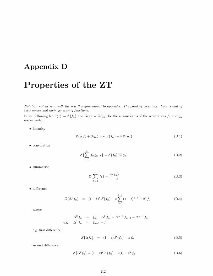
Appendix D
Properties of the ZT
Notation not in sync with the rest therefore moved to appendix. The point of view taken here is that ofrecurrences and their generating functions.
In the following let F (z) := Zfn and G(z) := Zgn be the z-transforms of the recurrences fn and gn
respectively.
• linearity
Zα fn + β gn = α Zfn+ β Zgn (D.1)
• convolution
Zn∑
k=0
fk gn−k = ZfnZgn (D.2)
• summation
Zn∑
k=0
fk =Zfn1− z
(D.3)
• difference
Z∆kfn = (1− z)k Zfn − z
k−1∑
i=0
(1− z)k−i−1 ∆i f0 (D.4)
where
∆0 fn := fn, ∆k fn := ∆k−1 fn+1 −∆k−1 fn
e.g. ∆1 fn = fn+1 − fn
e.g. first difference:
Z∆fn = (1− z)Zfn − z f0 (D.5)
second difference:
Z∆2fn = (1− z)2 Zfn − z f1 + z2 f0 (D.6)
212

APPENDIX D. PROPERTIES OF THE ZT 213
• index shifting
Zfn−k = zk Zfn (D.7)
Zfn+k = z−k
(Zfn −
k−1∑
i=0
fi zi
)= (D.8)
= z−k(F (z)− f0 − f1 z − f2 z2 − f3 z3 − · · · − fk−1 zk−1
)
• similarity
Zλn fn = F( z
λ
)λ ∈ C, λ 6= 0 (D.9)
• multiplication
Zn fn = zd
d zF (z) (D.10)
• division
Zfn
n =
∫ ∞
z
F (ξ)ξ
d ξ (D.11)
Z fn
n + 1 =
∫ z
0
F (ξ) d ξ (D.12)
• index transformation
for i fixed let gm0≤m<∞ := fn (m = n i), 0 (else)
then Zgn = F (zi) (D.13)
Appendix E
Eigenvectors of the Fouriertransform
For aS := a + a, the symmetric part of a sequence a:
F [F [aS ]] = aS (E.1)
Now let u+ := aS + F [aS ] and u− := aS −F [aS ] then
F [u+] = F [aS ] + aS = aS + F [aS ] = +1 · u+ (E.2)F [u−] = F [aS ]− aS = −(aS −F [aS ]) = −1 · u− (E.3)
u+ and u− are symmetric.
For aA := a− a, the antisymmetric part of a we have
F [F [aA]] = −aA (E.4)
Therefore with v+ := aA + iF [aA] and v− := aA − iF [aA]:
F [v+] = F [aA]− i aA = −i (aA + iF [aA]) = −i · v+ (E.5)F [v−] = F [aA] + i aA = +i (aA − iF [aA]) = +i · v− (E.6)
v+ and v− are antisymmetric.
u+, u−, v+ and v− are eigenvectors of the FT, with eigenvalues +1, −1, −i and +i respectively. Theeigenvectors are pairwise perpendicular.
Using
a =12
(u+ + u− + v+ + v−) (E.7)
we can, for a given sequence, find a transform that is the ‘square root’ of the FT: Simply compute u+,u−, v+, v−. Then for λ ∈ R one can define a transform Fλ [a] as
Fλ [a] =12
((+1)λ u+ + (−1)λ u− + (−i)λ v+ + (+i)λ v−
)(E.8)
F0 [a] is the identity, F1 [a] is the (usual) FT, F1/2 [a] (which is not unique) is a transform so thatF1/2
[F1/2 [a]]
= F [a], that is, a ‘quare root’ of the FT.
The eigenvectors of the Hartley Transform are u+ := a +H [a] (with eigenvalue +1) and u+ := a−H [a](with eigenvalue −1).
214
Bibliography
[1] H.S.Wilf: Algorithms and Complexity, internet edition, 1994,online at ftp://ftp.cis.upenn.edu/pub/wilf/AlgComp.ps.Z
[2] H.J.Nussbaumer: Fast Fourier Transform and Convolution Algorithms, 2.ed, Springer 1982
[3] J.D.Lipson: Elements of algebra and algebraic computing, Addison-Wesley 1981
[4] R.Tolimieri, M.An, C.Lu: Algorithms for Discrete Fourier Transform and Convolution, Springer1997 (second edition)
[5] J.M.Borwein, P.B.Borwein: Pi and the AGM, Wiley 1987
[6] E.Schroder: On Infinitely Many Algorithms for Solving Equations (translation by G.W.Stewart of:‘Ueber unendlich viele Algorithmen zur Auflosung der Gleichungen’, which appeared 1870 in the‘Mathematische Annalen’)online at ftp://thales.cs.umd.edu/pub/reports/
[7] Householder: The Numerical Treatment of a Single Nonlinear Equation, McGraw-Hill 1970
[8] D.E.Knuth: The Art of Computer Programming, 2.edition, Volume 2: Seminumerical Algorithms,Addison-Wesley 1981,online errata list at http://www-cs-staff.stanford.edu/~knuth/
[9] W.H.Press, S.A.Teukolsky, W.T.Vetterling, B.P.Flannery: Numerical Recipes in C, CambridgeUniversity Press, 1988, 2nd Edition 1992online at http://nr.harvard.edu/nr/
[10] R.L.Graham, D.E.Knuth, O.Patashnik: Concrete Mathematics, Addison-Wesley, New York 1988
[11] I.N.Bronstein, K.A.Semendjajew, G.Grosche, V.Ziegler, D.Ziegler, ed: E.Zeidler: Teubner-Taschenbuch der Mathematik, vol. 1+2, B.G.Teubner Stuttgart, Leipzig 1996, the new editionof Bronstein’s Handbook of Mathematics, (english edition in preparation)
[12] J.Stoer, R.Bulirsch: Introduction to Numerical Analysis, Springer-Verlag, New York, Heidelberg,Berlin 1980
[13] M.Waldschmidt, P.Moussa, J.-M. Luck, C.Itzykson (Eds.): From Number Theory to Physics,Springer Verlag 1992
[14] H.Cohen: A Course in Computational Algebraic Number Theory, Springer Verlag, Berlin Heidel-berg, 1993
[15] Thomas H.Corman, Charles E.Leiserson, Ronald L.Rivest: Introduction to Algorithms, MIT Press,1990 (twenty-first printing, 1998)
[16] H.Malvar: Fast computation of the discrete cosine transform through fast Hartley transform, Elec-tronics Letters 22 pp.352-353, 1986
215
BIBLIOGRAPHY 216
[17] H.Malvar: Fast Computation of the discrete cosine transform and the discrete Hartley transform,IEEE Trans. on Acoustics, Speech and Signal Processing, ASSP-35 pp.1484-1485, 1987
[18] R.Crandall, B.Fagin: Discrete Weighted Transforms and Large Integer Arithmetic, Math. Comp.(62) 1994 pp.305-324
[19] Zhong-De Wang: New algorithm for the slant transform, IEEE Trans. Pattern Anal. Mach. Intell.PAMI-4, No.5, pp.551-555, September 1982
[20] R.P.Brent: Fast multiple-precision evaluation of elementary functions, J. ACM (23) 1976 pp.242-251
[21] B.Haible, T.Papanikolaou: Fast multiprecision evaluation of series of rational numbersonline at http://???/
[22] J.M.Borwein, P.B.Borwein: Scientific American, March 1988
[23] D.H.Bailey, J.M.Borwein, P.B.Borwein and S.Plouffe: The Quest for Pi, 1996,online at http://www.cecm.sfu.ca/~pborwein/
[24] J.M.Borwein, P.B.Borwein: Cubic and higher order algorithms for π Canad.Math.Bull. Vol.27 (4),1984, pp.436-443
[25] J.M.Borwein, P.B.Borwein, F.G.Garvan: Some cubic modular identities of Ramanujan, Trans.A.M.S. 343, 1994, pp.35-47
[26] J.M.Borwein, F.G.Garvan: Approximations to π via the Dedekind eta function, ???, March 27,1996
[27] D.V.Chudnovsky, G.V.Chudnovsky: Classical constants and functions: computations and contin-ued fraction expansions, in Number Theory: New York seminar 1989-1990, Springer Verlag 1991
[28] A.Schonhage, V.Strassen: Schnelle Multiplikation grosser Zahlen, Computing (7) 1971 pp.281-292(in german)
[29] H.Cohen, F.R.Villegas, D.Zagier: Convergence acceleration of alternating series, 1997 preprint
[30] C.D.Olds: Continued Fractions, The Mathematical Association of America, 1963
[31] L.Lorentzen and H.Waadeland: Continued Fractions and Applications, North-Holland 1992 pp.561-562
[32] Robert Sedgewick: Algorithms in C, Addison-Wesley, 1990
[33] Mladen Victor Wickerhauser: Adapted Wavelet Analysis from Theory to Software, AK Peters,Ltd., Wellesley, Mass., 1994
[34] D.H.Bailey: FFTs in External or Hierarchical Memory, 1989online at http://citeseer.nj.nec.com/
[35] D.H.Bailey: The Fractional Fourier Transform and Applications, 1995online at http://citeseer.nj.nec.com/
[36] Mikko Tommila: apfloat, A High Performance Arbitrary Precision Arithmetic Package, 1996,online at http://www.jjj.de/mtommila/
[37] M.Beeler, R.W.Gosper, R.Schroeppel: HAKMEM. MIT AI Memo 239, Feb. 29, 1972, Retyped andconverted to html by Henry Baker, April 1995,online at ftp://ftp.netcom.com/pub/hb/hbaker/hakmem/hakmem.html/#contents
[38] Advanced Micro Devices (AMD) Inc.: AMD Athlon Processor, x86 code optimization guideonline at http://www.amd.com/
BIBLIOGRAPHY 217
[39] P.Soderquist, M.Leeser: An Area/Performance Comparison of Subtractive and Multiplicative Di-vide/Square Root Implementations, Cornell School of Electrical Engineeringonline at http://orac.ee.cornell.edu:80/unit1/pgs/#papers
[40] F.L.Bauer: An Infinite Product for Square-Rooting with Cubic Convergence, The MathematicalIntelligencer, 1998
[41] Bahman Kalantari, Jurgen Gerlach: Newton’s Method and Generation of a Determinantal Familyof Iteration Functions. ???, 1998

Index
acyclic convolution, 34AGM
4-th order variant, 187AGM (arithmetic geometric mean), 185algorithm
Karatsuba, 167Toom Cook, 167
arithmetic geometric mean (AGM), 185
C2RFT, via FHT, 53C2RFT, with wrap routines, 22cache, direct mapped, 28carry
in multiplication, 168complex to real FFT, via FHT, 53convolution
acyclic, 34and multiplication, 167cyclic, 32half cyclic, 40linear, 34mass storage, 37negacyclic, 39right-angle, 39skew circular, 39weighted, 39
convolution, and FHT, 56convolution, negacyclic, 58cos rot, 54cosine transform (DCT), 54cosine transform, inverse (IDCT), 55CRT for two moduli
code, 65cube root extraction, 172cyclic auto convolution, via FHT, 57cyclic convolution, 32cyclic convolution, via FFT, 33cyclic convolution, via FHT, 56
DCT via FHT, 54DFT
definition, 4direct mapped cache, 28discrete Fourier transform
definition, 4
division, 170using multiplication only, 170
DST via DCT, 55
expiteration for, 188
FFTis polynomial evaluation, 169
FFT, radix 2 DIF, 11FFT, radix 2 DIT, 8FFT, radix 2 DIT, localized, 8FFT, radix 4 DIF, 17FFT, radix 4 DIT, 16FFT, split radix DIF, 18FHT, and convolution, 56FHT, DIF step, 48FHT, DIF, recursive, 49FHT, DIT step, 45FHT, DIT, recursive, 46FHT, radix 2 DIF, 49FHT, radix 2 DIT, 46FHT, shift, 46Fourier shift, 8Fourier transform
definition, 4,Fp, prime modulus, 59FT
definition, 4
Haar transform, int to int, 82Haar transform, inverse, int to int, 82half cyclic convolution, 40Hartley shift, 46
IDCT via FHT, 55IDST via IDCT, 56inverse cosine transform (IDCT), 55inverse cube root
iteration for, 172inverse Haar transform, int to int, 82inverse root
iteration for, 175inverse root extraction, 174inverse sine transform (IDST), 56inverse square root
218
INDEX 219
iteration for, 171inversion
iteration for, 170
Karatsuba algorithm, 167Karatsuba multiplication, 167
linear convolution, 34log
iteration using exp, 187
mass storage convolution, 37mean
arithmetic geometric, 185multiplication
FFT, 167is convolution, 167Karatsuba, 167Toom Cook, 167
negacyclic convolution, 39, 58
R2CFT, via FHT, 53R2CFT, with wrap routines, 21real to complex FFT, via FHT, 53revbin permute, naive, 111right-angle convolution, 39root extraction, 174
sequency, 70shift, for FHT, 46shift, Fourier, 8sine transform (DST), 55sine transform, inverse (IDST), 56skew circular convolution, 39square root extraction, 171
Toom Cook algorithm, 167Toom Cook multiplication, 167transcendental functions
iterations for, 187
unzip rev, 55
Walsh transform, radix 2 DIF, 70Walsh transform, radix 2 DIT , 69Walsh transform, sequency ordered (wal), 70weighted convolution, 39
zip rev, 55,Z/mZ, composite modulus, 60,Z/pZ, prime modulus, 59