Optimal Policy for Expediting Orders in Transit

Chiwon Kim ∗ Diego Klabjan † David Simchi-Levi ‡

December 18, 2009

Abstract

Recent globalization adds complexity to supply chains and increases lead times as

goods travel through multiple locations around the globe. Under this changing envi-

ronment a supply chain must be agile to respond quickly to demand spikes. One way

to achieve this objective is by expediting outstanding orders from multiple locations in

the supply chain through premium delivery, overtime work, or extra capacity available

at a higher cost. We study the single-item periodic review stochastic inventory prob-

lem where outstanding orders may be expedited. For so-called sequential systems, in

which expediting costs are convex, it is proved that expedited orders do not cross reg-

ular orders in time under the optimal policy. For sequential systems, we show that the

optimal policy is the base stock type policy with respect to regular ordering and expe-

diting. If a system is not sequential, orders may cross in time, thus optimal policies are

hard to obtain. We propose a heuristic for such systems and discuss its performance

and limitations.

1 Introduction

One of the recent challenges of companies is increasing complexity of supply chains due to

globalization of production and as a result increased lead times. An excellent example is

∗Massachusetts Institute of Technology, chiwon@alum.mit.edu†Northwestern University, d-klabjan@northwestern.edu‡Massachusetts Institute of Technology, dslevi@mit.edu

1

provided by the retail industry in North America and its suppliers. Several domestic suppliers

in North America have already outsourced their production to offshore, e.g., Taiwan and

China, with ever increasing volume of outsourcing. At the same time, emerging international

suppliers either build production facilities near the North American market or outsource

production to manufacturing service companies located near North America to improve

market accessibility. In this changing environment, the retailers must cope with the challenge

of how to best exploit the changes in supply chains. One of the opportunities at hand for

retailers is to utilize more flexible sourcing through order expediting from multiple locations

along the supply chain. Rather than incurring excessive cost due to a sudden spike in

demand, expediting the delivery of partial or complete orders through either overtime work

or premium delivery such as by air is a viable option for many retailers. This paper studies

the retailer’s optimal order expediting policy as well as the regular ordering policy from a

global supplier with multiple stages in production and distribution.

Consider the following business case published in EMS NOW [8]. An LCD TV producer

in South Korea decided to outsource its small to medium sized LCD TV production for the

North American market to a manufacturing service company in Mexico, which assembles

final products with some of the key components such as LCD panels shipped directly from

South Korea. Since an LCD panel constitutes the bulk of an LCD TV, the two of them are

virtually indistinguishable from the inventory viewpoint. Consider a regional distribution

center of a consumer electronics retailer where a manager of the regional distribution center

decides how many LCD TVs to order and how many to expedite in case of an emergency.

Regular orders must be placed in South Korea where the supply chain’s one end is located

due to the LCD panel supply, but expediting can be done from multiple locations, i.e.,

Mexico and South Korea. On the one hand, expediting by overtime work and overnight

ground shipping from Mexico is cheaper, but it is constrained by the availability of LCD

panels and the reduction in lead time is marginal. On the other hand, expediting assembled

LCD TVs from South Korea directly by air is costlier but the reduction in lead time is higher.

This is possible because the LCD TV manufacturer is producing LCD TVs in South Korea

for other markets. We study the decision problem of the retailer on how much to order for

future use as regular orders and how much to expedite for immediate use (also from which

locations).

2

The model is as follows. The retailer faces a stochastic demand, periodically reviews

inventory on hand, and places regular orders at the supplier, i.e., the LCD TV maker,

with a nonnegative fixed ordering cost as well as a per item cost. Regular orders pass to

an intermediate installation, i.e., the manufacturing service company, and then they are

finally delivered to the retailer. The lead time between the supplier and the intermediate

installation, i.e., the shipping time for an LCD panel from South Korea to Mexico, is one

review period. Similarly, the lead time between the intermediate installation and the retailer,

i.e., LCD TV assembly time plus ground transportation, is also one review period. In

addition to regular ordering, expedited delivery is available with extra linear costs in units

for all or part of the outstanding orders in the pipeline, i.e., the supplier and the intermediate

installation. The retailer may expedite orders as demand realizes. When expedited, orders

instantaneously arrive at the retailer’s distribution center and they are ready to fulfill the

upcoming demand. Without expediting, it is well known that the optimal regular ordering

follows the base stock policy, or (s, S) if a fixed cost exists, with respect to the inventory

position.

In our setting, all decisions are made by a manager of the retailer’s distribution center (or

other location with the same function), and it is assumed that the manager cannot influence

the inventory flow between the supplier and the intermediate installation. As a consequence,

expediting is allowed only to the retailer’s distribution center, which is a practical consider-

ation in the LCD TV example. There are also business cases where expediting between the

supplier and the intermediate installation should be allowed. Such cases are addressed by

Lawson and Porteus [17] and Muharremoglu and Tsitsiklis [18]. We note that their models

do not reduce to ours, and a different analysis is required for our setting because we cannot

eliminate undesired behavior of the solution from their models, i.e., expediting between the

supplier and the intermediate installation. We discuss this in detail in the literature review

section.

Finding an optimal inventory control policy with respect to regular ordering and expedit-

ing depends critically on the system parameters such as the expediting costs. We introduce

the notion of sequential systems, where it is never optimal to expedite from the supplier

before expediting all outstanding orders in the intermediate installation. We show that in

sequential systems the regular ordering policy is the (s, S) policy with respect to the inven-

3

tory position, and the expediting policy is a variant of the base stock policy, which involves

multiple base stock levels with respect to the inventory on hand and inventory position. If

a system is not sequential, the structure of the optimal policies is complex, and analytical

results are hard to obtain. Instead, we propose a heuristic policy called the extended heuris-

tic, which is a natural extension of the identified optimal policy for sequential systems to

non-sequential systems. We test the extended heuristic by means of a numerical study. In

Kim et al. [16] (online appendix), we generalize the two stage supply chain system into a

general L stage supply chain system, and show that the same optimal policies of regular

ordering and expediting are applicable.

There are three major contributions of this paper. First, for sequential systems, we

establish that the (s, S) policy is optimal for regular orders and a variant of the base stock

policy with respect to various stock positions is optimal for expedited orders. We provide

simple recursive equations to compute the reorder point and the base stock levels. We

further reveal that the structure of the optimal expediting policy is to expedite everything

up to a certain point in the pipeline, and nothing beyond. Second, modeling and proof

techniques are novel. We propose a unique relationship among multiple cost-to-go functions

with various restrictions appropriate for sequential systems. The main results are derived

from these relationships. Standard inductive arguments coupled with separability of the

cost-to-go functions as often done in the literature cannot be carried out in our context.

Indeed, our proof technique is based on studying the difference in the cost-to-go functions

with different states as well as induction arguments. Finally, we propose a heuristic policy,

the extended heuristic, for non-sequential systems that do not allow simple optimal policies.

By means of a computational study, we argue that the extended heuristic achieves a local

optimum for a much wider class of systems, which include all sequential systems.

In Section 2 we formally state the model together with the general optimality equation.

We characterize sequential systems and derive the relationship of the cost-to-go functions

in Section 3. Section 4 presents the optimal policy for sequential systems. We numerically

investigate the performance of the proposed heuristic for non-sequential systems in Section

5. We provide a generalization to an L stage system in Kim et al. [16]. We conclude the

introduction by a literature review.

4

Literature Review

The problem studied has similarities with multi-supplier inventory problems. One supplier

with a much shorter lead time can be used as the expedited mode while the remaining

suppliers with possibly longer lead time as the regular mode. Barankin [2], Daniel [6],

Neuts [20], and Veinott [23] have considered the inventory system with two supply modes of

instantaneous and one period lead time. Their models are special cases of our model, and

thus they have the same optimal policy structure. Fukuda [10] extends this model to the

case where the lead times are k and k+ 1 periods. Whittemore and Saunders [25] generalize

the two supply mode problem to arbitrary lead times, however the optimal ordering policies

are no longer simple functions if the difference in the lead times is more than one period.

They also give conditions on optimality of using a single supplier. The stochastic lead time

model of zero or one period is considered by Anupindi and Akella [1]. While most of the

literature for multiple supply modes addresses the two supply mode case, some researchers,

including Fukuda [10], Zhang [26], and Feng et al. [9], consider the three supply mode case.

Their optimal policies are generally not base stock policies.

In the same spirit, models with emergency orders relate to our problem, since expediting

has a similar effect. The periodic review inventory model with emergency supply is considered

by Chiang and Gutierrez [3, 4], Tagaras and Vlachos [22], and Huggins and Olsen [13].

Chiang and Gutierrez [4] allow placing multiple emergency orders within a review period,

while the others allow placing a single emergency order per cycle. Huggins and Olsen [13]

consider a two-stage supply chain system where shortages are not allowed, so the shortage

must be fulfilled by some form of expediting such as overtime production. They found that

the optimal regular ordering policy is the (s, S) type policy, but the expediting policy is not

a base stock type policy. Related research in this area includes Groenevelt and Rudi [12],

where a manufacturing order can be split into fast and slow shipping modes, and Vlachos

and Tagaras [24], where there is a capacity cap on the size of an emergency order. Both

multi-supplier and emergency order models in the literature differ significantly from our

model since in our case the realized lead time can be any number between 0 and the regular

lead time, and it varies dynamically.

Our model can be generalized to include multiple consecutive intermediate installations

5

as presented in Kim et al. [16]. With regard to our generalized model, the serial multi-

echelon inventory system with expediting has been studied by Lawson and Porteus [17] who

extend the work by Clark and Scarf [5] by introducing expedited deliveries with zero lead

time between two consecutive installations. They prove optimality of the base stock policy

for expediting orders. Our model resembles the model in Lawson and Porteus [17] because a

unit can be also expedited through several consecutive installations in their model. However,

our model is substantially different from Lawson and Porteus [17] in that we do not allow

expediting between two consecutive installations due to practical reasons of businesses. In

our model expediting can only occur from the supplier or intermediate installations to the

retailer. The model in Lawson and Porteus [17] cannot capture the same situation as ours.

To see this more clearly, consider the Lawson and Porteus [17] model with a supplier, an

intermediate installation, and a retailer. Let us denote by c2 the expediting cost from the

supplier to the intermediate installation, and by c1 the expediting cost from the intermediate

installation to the retailer. In their model, the expediting cost d from the supplier to the

retailer is d = c2 + c1 since both of expediting should happen consecutively in the same time

period. In order to prevent expediting from the supplier to the intermediate installation,

c2 needs to have a high enough value. As a consequence, d should be high as well and

this prevents any expediting from the supplier to the retailer. To view this from a different

angle, if we predefine c1 and d, then c2 should be d − c1, which can be fairly small, and

the model fails to prevent any expediting from the supplier to the intermediate installation,

which is restricted in our model. As a result, their model addresses different situations with

different solution dynamics from those captured by our model. Muharremoglu and Tsitsiklis

[18] generalize Lawson and Porteus [17] further by allowing super modular expediting cost

instead of a linear one. Their model is different from our model by the same reason as

Lawson and Porteus [17].

Furthermore, Lawson and Porteus [17] and Muharremoglu and Tsitsiklis [18] assume a

linear cost structure. More specifically, the main method of Muharremoglu and Tsitsiklis [18]

is single-unit decomposition, which is applicable only to decomposable systems with linear

expediting and procurement costs and no interactions among different units are allowed.

Our model is more general in the sense that the holding and backlogging costs in our model

constitute a convex function in the number of units. In addition, while our model can

6

handle a fixed ordering cost, single-unit decomposition cannot capture it because it imposes

a further interaction among the units.

2 Model Statement

We consider a supply chain that consists of 3 installations1 labeled from 0 to 2, where instal-

lation 0 is the retailer, installation 1 is the intermediate installation such as a manufacturing

service company, and installation 2 is the supplier. In regular delivery, a unit of goods passes

through all the installations from the supplier to the retailer and stays for one period at each

installation. Expedited delivery of a fraction or all of the outstanding orders is available at

each installation, and the lead time of such a delivery is instantaneous. Therefore the actual

lead time for a unit is dynamic with the maximum of 2 time periods and the minimum of

0. The per unit expediting cost from installation i at time period k is di,k. The planning

horizon consists of T time periods. Figure 1 depicts the model.

McKinsey & Company 0

Work

ing

Dra

ft -L

ast M

od

ified 1

2/1

2/2

00

9 8

:08

:30

PM

Prin

ted

|

22 11 00

d2,k

d1,k

Supplier Intermediate

installation

Retailer

Regular flow

Expediting options

Figure 1: The underlying supply chain

Demand Dk for period k is a nonnegative continuous random variable. (It can also be a

discrete random variable with a finite support.) At the retailer, excess demand is backlogged

and incurs a backlogging cost, while excess inventory incurs a holding cost. We require that

the holding/backlogging cost function is convex in the amount of inventory. Let rk(·) be any

convex holding/backlogging cost function and for ease of notation let Lk(x) = E[rk(x−Dk)].

Clearly, Lk(·) is convex.

1We extend the model to a general length system in Kim et al. [16].

7

The sequence of events is as follows. At the beginning of time period k, the retailer first

places a new regular order with the supplier at cost ck per unit and fixed ordering cost K, and

next decides how much to expedite from each installation. The retailer may also expedite

from the supplier up to the amount of the regular order just placed. After the expedited

deliveries of the outstanding orders are received, demand realizes at the retailer. Holding

or backlogging cost is accounted for at the end of time period k. After cost accounting,

the outstanding orders at installations 1 and 2 move to the next downstream installation

instantaneously and then the next time period begins.

The problem is to determine an optimal regular ordering quantity and optimal expediting

quantities from each of the two installations 1 and 2 at the beginning of each time period.

Let us denote by vi the amount of inventory at installation i at the beginning of a time

period before expediting for i = 0, 1. Before receiving the regular order, the supplier has no

inventory assigned for the retailer at the beginning of the time period, therefore (v0, v1) is the

current state of the system. Let Jk(v0, v1) be the cost-to-go function at the beginning of time

period k under optimal regular ordering and expediting in time periods k, k+ 1, · · · , T . For

simplicity, we do not discount any future costs. After time period T , holding and backlogging

costs are assumed to be zero with no salvage value for remaining inventory, thus the terminal

cost JT+1 at time T + 1 is zero. The optimality equation reads

Jk(v0, v1) = minu,e1,e2u≥e2≥0v1≥e1≥0

{d1,ke1 + d2,ke2 + Lk(v0 + e1 + e2) + cku+Kδ(u)

+ E[Jk+1(v0 + v1 + e2 −D, u− e2)]},

(1)

where u is the regular ordering quantity, e1 and e2 are the expediting quantities from in-

stallation 1 and 2, respectively, and δ(u) = 1 if u > 0 and 0 otherwise. Note that after

expediting from installation 1, v1 − e1 units remain at installation 1 and u− e2 at installa-

tion 2. The remaining inventory at each installation moves to the next installation at the

end of the time period after demand D realizes, therefore the state of the next time period

is (v0 + v1 + e2 −D, u− e2).For ease of exposition, we consider only stationary demand distributions and cost coef-

ficients. All presented results hold also in the nonstationary case as discussed in Section 4.

Therefore, we drop time index k from the demand variables and the cost coefficients. We

also use L(·) for stationary systems instead of Lk(·).

8

3 Sequential Systems

Optimality equation (1) does not exhibit a simple policy. To obtain analytical results, we

have to confine our interest to a special class of systems. In this section, we explore systems

that are analytically manageable and derive structural results for such systems. First, we

formally define sequential systems using expediting costs.

Sequential systems: A system is sequential, if expediting cost coefficients di’s satisfy

d1 − d0 ≤ d2 − d1, where d0 = 0.2

For sequential systems, the expediting cost coefficient di as well as marginal expediting

cost di+1 − di are increasing in installation index i. Sequential systems are encountered in

international supply chains such as our LCD TV example. One of the primary reasons of

outsourcing to a manufacturing service company is to get closer to the market to save logistics

costs, which in turn implies that shipping or expediting from the intermediate installation

at cost d1 is much cheaper than from the supplier at cost d2.

The following is a key theorem to derive the optimal policies for regular ordering and

expediting.

Theorem 1. Sequential systems preserve the sequence of orders in time when operated op-

timally.

Proof. Consider expediting a unit from each installation. Expediting a unit from installation

1 has an effect of raising the inventory of the retailer by 1 unit for 1 time period at the cost

of d1. Similarly, expediting a unit from installation 1 has an effect to raise the inventory for

2 time periods at d2. If installation 1 is non empty, then expediting a unit from installation

2 is always replicable with respect to the inventory level of the retailer at equal or lower

cost by expediting a unit from installation 1 in the current time period, and another unit

from installation 1 in the next time period since d2 ≥ 2d1. To summarize, if installation

1 is non empty, it is always better to consider expediting from installation 1 first if any

2If the expediting costs are nonstationary, then the system is sequential if d1,k − d0,k+1 ≤ d2,k − d1,k+1,

for 1 ≤ k ≤ T , where d0,k+1 = 0 and d1,T+1 = 0.

9

expediting is necessary. Therefore, sequential systems preserve the sequence of orders even

with expediting.

Using this theorem, we now derive an important property of the cost-to-go function for

sequential systems. Let us denote for convenience x0 = v0 and x1 = v0 + v1. We interpret

the process of expediting multiple units as multiple decisions of expediting a unit until there

is no further need of expediting. Consider a general state (x0, v1) of a sequential system.

If we expedite a unit, then it is best to expedite it from installation 1 by the definition of

sequential systems. The resultant state after this expediting is (x0 + 1, v1 − 1) provided

that v1 ≥ 1. If we continue expediting units, installation 1 is eventually emptied and the

state becomes (x0 + v1, 0) in which expediting from installation 2 starts. Therefore, state

(x0 + v1, 0) requires a special treatment. In order to capture this, we introduce restricted

cost-to-go functions. Let J1k be the optimal cost-to-go that can be achieved by a restricted

control space in which expediting only from installation 1 is allowed. The control space for

J1k is restricted in time period k, but unrestricted after time period k. In the following, we

provide a relationship between the unrestricted cost-to-go Jk and the restricted cost-to-go

J1k . For i ≤ L− 1, the optimality equation for J1

k (x0, v1) is given by

J1k (x0, v1) = min

x0≤y1≤x1,z≥x1{d1(y1 − x0) + L(y1) + c(z − x1)

+Kδ(z − x1) + E[Jk+1(x1 −D, z − x1)]},

(2)

where y1 and z are decision variables: y1 − x0 corresponds to the expediting amount from

installation i, and z−x1 corresponds to the regular ordering amount. The optimality equation

at state (x1, 0) reads

Jk(x1, 0) = minz≥y2≥x1

{d2(y2 − x1) + L(y2) + c(z − x1)

+Kδ(z − x1) + E[Jk+1(y2 −D, z − y2)]}.(3)

where y2 − x1 is the expediting amount from installation 2, which is less than or equal to

the regular order amount, z − x1.We have the following obvious relationship between the unrestricted cost-to-go Jk and

the restricted cost-to-go J1k :

Jk(v0, v1) = min{J1k (x0, v1), d1v1 + Jk(x1, 0)}. (4)

10

By Theorem 1, in sequential systems it is optimal to first expedite from downstream. At

time period k, the first term corresponds to expediting partially or fully from installation

1 and no expediting beyond, and the second term captures expediting everything from

installation 1, expediting partially or fully from installation 2. From the minimum term in

(4), we can determine the optimal control of expediting, i.e., yi from installation i. Also,

the optimal regular ordering decision is to place a regular order of the amount z − x1 that

is determined in the same term.

4 Optimal Policies for Sequential Systems

In analyzing (4), we compare the difference of Jk(x0, v1) and Jk(x1, 0). The key finding is

the observation that Jk(x0, v1) − Jk(x1, 0) is only a function of k, x0, and x1. Furthermore,

this function has the form of S0k + S1

k(x0) + S2k(x1) for well defined functions S0

k , S1k and S2

k .

Another key finding is that the minimization with respect to yi in (2) can be isolated from

the minimization with respect to z, and it has the form of min fi,k(yi) for a function fi,k,

which is defined by using S0k , S

1k and S2

k for i = 1, 2. We provide the details of S0k , S

1k , S

2k ,

and fi,k after the following lemma from Lawson and Porteus [17], which originates in Karush

[15]. We use this lemma frequently throughout the paper.

Lemma 1. Let f be convex with a finite minimizer in R. Let y∗ = arg min f(x). Then,

minx1≤x≤x2

f(x) = a + g(x1) + h(x2), where a = f(y∗), and penalty functions g(x1) and h(x2)

are defined by

g(x1) =

0 x1 ≤ y∗

f(x1)− a x1 > y∗and h(x2) =

f(x2)− a x2 ≤ y∗

0 x2 > y∗.

For a nondecreasing convex f , we define a = 0, g(x) = f(x), and h(x) = 0. On the other

hand, for a nonincreasing convex f , we define a = 0, g(x) = 0, and h(x) = f(x).

In Lemma 1, g is nondecreasing convex, while h is nonincreasing convex. For k ≤ T , let

11

us recursively define

f1,k(x) = d1x+ L(x),

f2,k(x) = d2x+ L(x) + E[S1k+1(x−D)], (5)

S0k = a1,k,

S1k(x) = g1,k(x)− d1x, (6)

S2k(x) = h1,k(x)− L(x),

where S0T+1 = S1

T+1(·) = S2T+1(·) = 0 for all i. Here, a1,k, g1,k, and h1,k are defined according

to Lemma 1 with respect to f1,k. Functions fi,k and Sjk are well defined, and starting from

the last time period T , they can be obtained recursively. In particular, from (5) we can

compute f2,T , then from (6) we obtain S1T . Next we compute f2,T−1 from (5), and in turn,

S1T−1 from (6). We repeat this procedure to define all f2,k and S1

k . For others, we use a

similar procedure.

Optimal Expediting Policy

The optimal expediting policy of expediting from installation i for sequential systems is

established by the following theorem.

Theorem 2. For sequential systems, the optimal expediting policy for expediting orders from

installation i is the base stock policy with respect to stock position xi−1. The base stock level

is given by y∗i,k = arg min fi,k(x) for time period k.

The base stock levels y∗i,k for expediting from installation i at time period k have a

monotonic property as noted in the following theorem.

Theorem 3. For sequential systems, we have y∗1,k ≥ y∗2,k for all k.

This theorem can be proved independently and the proof is given in Appendix A. The

implication of Theorems 2 and 3 is the following. Because the base stock levels satisfy

y∗1,k ≥ y∗2,k and stock positions x1 ≥ x0, there are four cases. First, if x0 ≥ y∗1,k, then

x1 ≥ y∗2,k, and thus no expediting from anywhere is necessary. Second, if x1 ≥ y∗1,k ≥ x0,

then it is optimal to expedite y∗1,k − x0 from installation 1 but no expediting is required

12

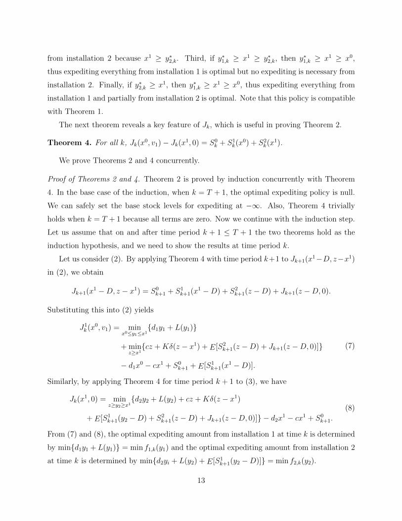
from installation 2 because x1 ≥ y∗2,k. Third, if y∗1,k ≥ x1 ≥ y∗2,k, then y∗1,k ≥ x1 ≥ x0,

thus expediting everything from installation 1 is optimal but no expediting is necessary from

installation 2. Finally, if y∗2,k ≥ x1, then y∗1,k ≥ x1 ≥ x0, thus expediting everything from

installation 1 and partially from installation 2 is optimal. Note that this policy is compatible

with Theorem 1.

The next theorem reveals a key feature of Jk, which is useful in proving Theorem 2.

Theorem 4. For all k, Jk(x0, v1)− Jk(x1, 0) = S0k + S1

k(x0) + S2k(x1).

We prove Theorems 2 and 4 concurrently.

Proof of Theorems 2 and 4. Theorem 2 is proved by induction concurrently with Theorem

4. In the base case of the induction, when k = T + 1, the optimal expediting policy is null.

We can safely set the base stock levels for expediting at −∞. Also, Theorem 4 trivially

holds when k = T + 1 because all terms are zero. Now we continue with the induction step.

Let us assume that on and after time period k + 1 ≤ T + 1 the two theorems hold as the

induction hypothesis, and we need to show the results at time period k.

Let us consider (2). By applying Theorem 4 with time period k+1 to Jk+1(x1−D, z−x1)

in (2), we obtain

Jk+1(x1 −D, z − x1) = S0

k+1 + S1k+1(x

1 −D) + S2k+1(z −D) + Jk+1(z −D, 0).

Substituting this into (2) yields

J1k (x0, v1) = min

x0≤y1≤x1{d1y1 + L(y1)}

+ minz≥x1{cz +Kδ(z − x1) + E[S2

k+1(z −D) + Jk+1(z −D, 0)]}

− d1x0 − cx1 + S0k+1 + E[S1

k+1(x1 −D)].

(7)

Similarly, by applying Theorem 4 for time period k + 1 to (3), we have

Jk(x1, 0) = minz≥y2≥x1

{d2y2 + L(y2) + cz +Kδ(z − x1)

+ E[S1k+1(y2 −D) + S2

k+1(z −D) + Jk+1(z −D, 0)]} − d2x1 − cx1 + S0k+1.

(8)

From (7) and (8), the optimal expediting amount from installation 1 at time k is determined

by min{d1y1 +L(y1)} = min f1,k(y1) and the optimal expediting amount from installation 2

at time k is determined by min{d2yi + L(y2) + E[S1k+1(y2 −D)]} = min f2,k(y2).

13

It is easy to show that fi,k(yi) is a convex function. Therefore, the optimal expediting

policy from installation i at time k is the base stock policy with the base stock level y∗i,k =

arg min fi,k(yi) with respect to xi−1. Note that the actual expediting amount is limited by

the availability of the inventory in installation 1 or the regular order amount at installation

2. This completes the proof of Theorem 2 for time period k.

Now let us prove Theorem 4 for time period k. Combined with Theorem 3, we know the

optimal expediting policy for Jk in time period k as part of the induction step. We compare

Jk(x0, v1) and Jk(x1, 0) for three possible cases. First, if y∗1,k ≤ x0, then no expediting is

necessary from installation 1 and beyond, therefore

Jk(x0, v1) = L(x0) + minz≥x1{c(z − x1) +Kδ(z − x1) + E[Jk+1(x

1 −D, z − x1)]},

where term L(x0) is present because we only have x0 on hand at the beginning of time

period k due to no expediting, c(z − x1) + Kδ(z − xL−1) due to regular ordering, and

E[Jk+1(x1 − D, z − x1)] as future cost. Also, since y∗i+1,k ≤ xi ≤ xi+1, no expediting is

necessary, thus similarly we have

Jk(x1, 0) = L(x1) + minz≥x1{c(z − x1) +Kδ(z − x1) + E[Jk+1(x

1 −D, z − x1)]}.

Therefore, Jk(x0, v1)− Jk(x1, 0) = L(x0)− L(x1).

Next, if x0 < y∗1,k ≤ x1, then expediting y∗1,k−x0 from installation 1 is necessary, but not

from installation 2. We have by similar reasoning as above

Jk(x0, v1) = d1(y∗1,k − x0) + L(y∗1,k) + min

z≥x1{c(z − x1) +Kδ(z − x1) + E[Jk+1(x

1 −D, z − x1)]},

and

Jk(x1, 0) = L(x1) + minz≥x1{c(z − x1) +Kδ(z − x1) + E[Jk+1(x

1 −D, z − x1)]}.

Therefore, Jk(x0, v1)− Jk(x1, 0) = d1y∗1,k + L(y∗1,k)− d1x0 − L(x1).

Finally, if y∗1,k > x1, then we expedite everything in installation 1. Thus the only cost

difference is d1v1 = d1x1 − d1x0, and we obtain Jk(x0, v1)− Jk(x1, 0) = d1x

1 − d1x0.Therefore, we have

Jk(x0, v1)− Jk(x1, 0) =

L(x0)− L(x1) y∗1,k ≤ x0

d1y∗1,k + L(y∗1,k)− d1x0 − L(x1) x0 < y∗1,k ≤ x1

d1x1 − d1x0 y∗1,k > x1.

14

Now, let us study the function a1,k + g1,k(x0) + h1,k(x1) for each of the three cases.

When y∗1,k ≤ x0, we have g1,k(x0) = f1,k(x0) − a1,k and h1,k(x1) = 0, and thus a1,k +

g1,k(x0) + h1,k(x1) = d1x0 + L(x0). When x0 < y∗1,k ≤ x1, we have g1,k(x0) = 0 and

h1,k(x1) = 0, and thus a1,k + g1,k(x0) + h1,k(x1) = a1,k = d1y∗1,k + L(y∗1,k). Finally, when

y∗1,k > x1, we have g1,k(x0) = 0 and h1,k(x1) = f1,k(x1)− a1,k = d1x1 +L(x1)− a1,k, and thus

a1,k+g1,k(x0)+h1,k(x1) = d1y∗1,k+L(y∗1,k). We can easily check that a1,k+g1,k(x0)+h1,k(x1) =

Jk(x0, v1)− Jk(x1, 0) + d1x0 + L(x1) in all of the cases. Thus, we have

Jk(x0, v1)− Jk(x1, 0) =a1,k + g1,k(x0) + h1,k(x1)− d1x0 − L(x1)

=S0k + S1

k(x0) + S2k(x1).

Therefore, Theorem 4 at time period k is proved. This completes the proofs of Theorems

2 and 4 by induction arguments.

Optimal Regular Ordering Policy

Now we derive the optimal regular ordering policy, which is affected by expediting decisions.

Let us denote cost-to-go Jk(x, 0) by Hk(x) for convenience. Also, let H̃k(z) = h2,k(z) + cz +

E[S2k+1(z −D) + Hk+1(z −D)]. Note that if S2

k(x1) + Hk(x1) is continuous and K-convex,

then H̃k(z) is also continuous and K-convex. The next theorem gives the optimal regular

ordering policy.

Theorem 5. For sequential systems, the optimal regular ordering policy is the (s, S) policy

with S = Z∗k = arg min H̃k(z), and s = z∗k defined by H̃k(z∗k) = K + H̃k(Z∗k). The base stock

level Z∗k is considered with respect to inventory position x1, thus if x1 ≤ z∗k, then it is optimal

to place the regular order in the amount of Z∗k − x1, and otherwise no order is placed.

Proof. We concurrently show both the theorem and that Hk(x) and S2k(x1) + Hk(x1) are

continuous and K-convex by induction. In the base case of k = T + 1, the optimal regular

ordering policy is null, and we can safely set z∗T+1 and Z∗T+1 to be −∞. Also, Hk(x) and

H̃k(z) are 0. Let us assume that on and after time k + 1 ≤ T + 1, the theorem, continuity,

and K-convexity hold.

15

Recalling the definition of f2,k, (8) becomes

Jk(x1, 0) = minz≥y2≥x1

{f2,k(y2) + cz +Kδ(z − x1) + E[S2k+1(z −D)

+ Jk+1(z −D, 0)]}+ S0k+1 − d2x1 − cx1.

(9)

By applying Lemma (6) in Appendix A to (9), we have

Jk(x1, 0) = minz≥x1{h2,k(z) + cz +Kδ(z − x1) + E[S2

k+1(z −D)

+ Jk+1(z −D, 0)]}+ S0k+1 − d2x1 − cx1 + g2,k(x1) + a2,k.

(10)

By adding S2k(x1) on both sides of (10), we obtain

S2k(x1) +Hk(x1) = min

z≥x1{h2,k(z) + cz +Kδ(z − x1) + E[S2

k+1(z −D)

+Hk+1(z −D)]}+ S0k+1 − d2x1 − cx1 + g2,k(x1) + a2,k + S2

k(x1).

Therefore, we have Hk(x) = minz≥x{Kδ(z−x) + H̃k(z)}+ a2 + g2(x)− d2x− cx. Also, because

g2,k(x1) + S2k(x1) is convex by Lemma 7 in Appendix A and S2

k+1(z −D) + Hk+1(z −D) is

K-convex by the induction hypothesis, we conclude that S2k(x1) +Hk(x1) is continuous and

K-convex.

The optimal regular ordering quantity is determined either from (7),

minz≥x1{cz +Kδ(z − x1) + E[S2

k+1(z −D) + Jk+1(z −D, 0)]}, (11)

or, from (8),

minz≥x1{h2,k(z) + cz +Kδ(z − x1) + E[S2

k+1(z −D) + Jk+1(z −D, 0)]}

= minz≥x1{Kδ(z − x1) + H̃k(z)}.

(12)

Let us first consider (12). Since S2k+1(z) + Hk+1(z) is K-convex, Kδ(z − x1) + H̃k(z) is

also K-convex, thus the (s, S) policy with respect to the inventory position is optimal with

parameters z∗k = s and Z∗k = S, where Z∗k = arg min H̃k(z) and H̃k(z∗k) = K + H̃k(Z∗k).

Now consider (11). By the same reason, the (s, S) policy is optimal, and let us similarly

define z̃∗k and Z̃∗k . We show that using (12) is optimal instead of (11). Because h2,k(z) is

nonincreasing convex and h2,k(z) = 0 for z ≥ y∗2,k, we have z̃∗k ≥ z∗k and Z̃∗k ≥ Z∗k by reasoning

16

similarly as in Lemmas 4 and 5. If z̃∗k ≥ y∗2,k, then (11) and (12) lead to the same parameters

z̃∗k = z∗k and Z̃∗k = Z∗k . On the other hand, if z̃∗k < y∗2,k, then we consider the following two

cases: x1 ≤ y∗2,k and x1 > y∗2,k. When x1 ≤ y∗2,k, we have x1 ≤ y∗i,k for all i by Theorem 3,

which results in expediting every outstanding order. In this case, (12) leads to the optimal

(s, S) policy. When x1 > y∗2,k, we have x1 > y∗2,k > z̃∗k ≥ z∗k. Therefore, both (11) and (12)

indicate that the optimal regular ordering quantity is zero, and thus they yield the same

consequence. As a result, we conclude that (12) determines the optimal regular ordering in

both cases.

Finally, we show that Hk(x) is continuous and K-convex. The continuity part is true

because Hk(x) = K + H̃k(Z∗) + S0k+1 − d2x − cx + g2,k(x) + a2,k − cx for x ≤ z∗ and

Hk(x) = H̃k(x) + S0k+1 − d2x − cx + g2,k(x) + a2,k − cx for x > z∗. The K-convexity part

follows from Proposition 8.3.3 in Simchi-Levi et al. [21]. The proof of Theorem 5 is thus

completed.

A Numerical Example - Base Stock Levels with Nonstationary De-

mand Distribution

Consider an example sequential supply chain consisting of a supplier, an intermediate in-

stallation, and a retailer, with stationary cost parameters facing a nonstationary stochastic

demand while K = 0. Figure 2 shows the base stock levels for expediting and regular

ordering.

In the figure, the solid line is the mean of the nonstationary demand distribution in each

time period, and the line with triangles corresponds to the base stock levels without the

expediting option. Also, the line with circles corresponds to the regular ordering base stock

levels with the expediting options, the line with pluses corresponds to the base stock levels

for expediting from stage 1, and the line with crosses corresponds to the expediting base

stock levels for expediting from stage 2. The planning horizon is 26 periods.

We observe several interesting points. Approaching the last time period, specifically in

time periods 25 and 26, the regular ordering base stock levels without the expediting options

become large negative numbers, which makes sense since new orders would never arrive at the

destination (the lead time is 2). However, with the expediting options, the regular ordering

17

5 10 15 20 250

50

100

150

200

250

300

350

400

450

Time period

Ba

se

Sto

ck L

eve

ls

y*

1y

*

2

z*

no expeditingmean demand

Figure 2: The base stock levels with nonstationary demand

base stock level at time period 25 is not a large negative number (indeed, it is positive in

this example). This also makes sense since we may expedite orders placed in time period 25.

Other than the time periods close to the end of the planning horizon, the regular ordering

base stock levels with expediting options are smaller than those without expediting. This

is due to the increased agility of the supply chain resulting from the expediting options,

hence decreased need for safety stock in the pipeline. Furthermore, the expediting options

effectively reduce lead times. Therefore, as the mean of the demand increases, the increment

of the regular ordering base stock levels with expediting options is not as pronounced as

that of the base stock levels without the expediting options. It implies that the decreased

realized lead times with the expediting options reduce the variability in the regular ordering

quantity. As for expediting base stock levels, they follow closely the mean demand curve.

Directional Sensitivity of Expediting Base Stock Levels for Station-

ary Sequential System

We now derive additional insight in the stationary case, i.e., the demand distribution and all

the cost coefficients are stationary. We provide the proof of the following lemma in Appendix

18

A.

Lemma 2. If the demand distribution and cost coefficients are stationary, then for 1 ≤ i ≤ 2

and k ≤ T − i+ 1, we have y∗i,k = y∗i,1.

Lemma 2 states that the expediting levels are independent of k for k ≤ T − 2. Note that

in practice T is much larger than 2. Therefore, for a stationary system the base stock levels

become constant in time for most of the time periods except a few periods at the end of the

planning horizon. This leads to a simple set of optimal parameters.

Another interesting observation can be made in a stationary system. Let z∗ and y∗i be

the base stock levels before time T − 2. If z∗ < y∗i , then we never use installations 1 to i

at least until time T − 2, because all units are always expedited on and before arriving at

installation i. As a special case, if z∗ < y∗2, then we always expedite the entire regular order

directly from the supplier, and never use the intermediate installation at least until time

T − 2.

We present the following lemma by assuming that holding and backlogging cost functions

have bounded derivatives, so integrals and derivatives are interchangeable by Lemma 3.2 in

Glasserman and Tayur [11].

Lemma 3. For sequential systems, we have for k ≤ T − 2

∂y∗1,k∂d1

< 0,∂y∗2,k∂d2

< 0,∂y∗2,k∂d1

≥ 0,y∗1,k∂d2

= 0.

Proof. Let us recall the following definitions:

f1,k(x) = d1x+ L(x),

f2,k(x) = d2x+ L(x) + E[S1k+1(x−D)],

S1k(x) = g1,k(x)− d1x.

As d1 increases, minimizer y∗1,k decreases because f1,k is convex, therefore∂y∗1,k∂d1

< 0. Similarly,∂y∗2,k∂d2

< 0 because S1k+1(x) is independent of d2. It is easy to see that

y∗1,k∂d2

= 0.

Now, let us prove that∂y∗2,k∂d1≥ 0 by studying S1

k+1(x). By definition g1,k+1(x) is f1,k+1(x)−a1,k+1 for x ≥ y∗1,k+1, and 0 otherwise. Therefore, S1

k+1(x) = L(x) for x ≥ y∗1,k+1, and −d1xotherwise. Since y∗2,k − D = y∗2,k+1 − D ≤ y∗1,k+1 by the previous theorem and lemma for

19

all D ≥ 0 and k ≤ T − 2, an increment of d1 is equivalent to adding a monotonically

decreasing function near the minimizer y∗2,k of a convex function f2,k. Therefore,∂y∗2,k∂d1≥ 0.

This completes the proof.

This lemma shows how expediting base stock levels move as expediting costs vary. That

is, as d1 increases, the corresponding base stock level y∗1,k decreases, which is expected due

to the increased cost. Same observation is made for d2, i.e., y∗2,k decreases as d2 goes up.

At the same time, d2 does not affect y∗1,k due to the sequential property of the system,

i.e., expediting from the supplier is only considered when expediting from the intermediate

installation is completed. On the other hand, d1 does affect y∗2,k in such a way that pushing

y∗2,k up as d1 increases, y∗1,k and y∗2,k become closer to each other. This is due to the fact that

as d1 increases, y∗1,k decreases, which results in less safety stock at the retailer, which again

calls for more expediting from the supplier.

Existence of Linear Holding Costs at the Intermediate Installation

We briefly discuss here the fact that we may apply the following simple transformation to

handle nonzero per unit holding or processing cost at the intermediate installation. Let the

linear holding or processing cost be h ≥ 0 at the intermediate installation, and let the actual

procurement cost be c′. Let also the actual expediting cost be d′1 for expediting a unit from

the intermediate installation, and d2 be expediting from the supplier. First, let c = c′ + h,

and let us use c as the hypothetical per unit procurement cost in our model. It means that

we pay all the holding costs in advance when we place an order. Second, let d1 = d′1 − h,

and let us use d1 and d2 as the expediting cost in our model. If di < 0, then it is always

better to expedite from the intermediate installation to the manufacturing facility than to

pay more expensive holding or processing costs at the intermediate installation. In this case,

we never use the intermediate installation, which leads to a shorter lead time. Note that

this transformation is possible because a unit stays exactly one period at each installation,

if it is not expedited.

20

5 Heuristics for Non-sequential Systems

So far we have studied sequential systems, and derived simple optimal policies. Recall that

for sequential systems we are able to use (4) instead of (1), which led us to derive the

analytical results. In general, we cannot eliminate the possibility of order crossing in time in

non-sequential systems under optimal control. Prior research on multiple lead time models,

or stochastic lead time models such as Kaplan [14], Nahmias [19], and Ehrhardt [7], assumes

that orders do not cross in time. If order crossing does occur, the resulting policy is complex

and it depends on the system state.

In this section, we discuss non-sequential systems through a three installation system

consisting of a supplier with zero fixed ordering cost, a retailer, and an intermediate instal-

lation between them. Though this three installation system is simple, it is nontrivial and

shares complexity with general length non-sequential systems, hence its analytical results

are hard to obtain.

Instead of trying to derive an optimal policy, which is a daunting task due to the com-

plexity and state dependency, we confine our interest to the set of all base stock policies. We

attempt to find the best base stock levels since base stock policies are practical due to their

simplicity. We next propose a heuristic policy that gives base stock levels for non-sequential

systems and evaluate its performance numerically using the three installation systems.

The Extended Heuristic The extended heuristic is to apply the base stock policies with

the base stock levels as described in Theorems 2 and 5 to non-sequential systems. Note that

the definitions of fi,k and Sji,k do not require systems to be sequential, hence the extended

heuristic is well defined. Also, if the system is sequential, the extended heuristic finds an

optimal control. Note that the extended heuristic is also applicable to general length systems.

In order to evaluate the performance of the extended heuristic, we use the following

derivative method introduced in Glasserman and Tayur [11].

The Derivative Method The derivative method is a numerical method to find the sen-

sitivity of the cost-to-go under the base stock policies as the base stock levels vary. The

method can be used to find locally optimal base stock levels within the set of all base stock

policies using simulation and optimization. Here we briefly explain the derivative method

21

customized to our three installation systems.

Step 1. Set the initial base stock levels: y1, y2, and z.

Step 2. Compute the derivatives of the dynamic programming optimality equation (1) with

respect to the base stock levels. We get recursive equations of the derivatives of the

cost-to-go with respect to each one of y1, y2, and z.

Step 3. Evaluate the cost to go at the beginning of the time horizon, i.e., time period 1,

using simulation with the given base stock levels. Evaluate also the derivatives of

the cost-to-go at time period 1 using the recursive equations from Step 2. The

derivatives give the steepest decent direction of the cost-to-go at time period 1.

Step 4. Search linearly along the steepest decent direction for the best step size, and then

set the new base stock levels using the result of the line search.

Step 5. Evaluate the derivatives of the cost-to-go with respect to the base stock levels from

Step 4 using simulation. If the norm of the derivatives is smaller than a given

threshold, then terminate. Otherwise, go to Step 3.

At the termination of the derivative method, we get the locally optimal base stock levels

and the corresponding cost-to-go at time period 1. Formally, the derivative method only

works when derivatives and integrals in expectations are interchangeable. All systems under

consideration in this paper have this interchangeability property. In what follows, we always

start the derivative method with the base stock levels from the extended heuristic, hence the

derivative method never produces an inferior solution. When the derivative method does

not improve the initial solution, we conclude that the extended heuristic achieves a local

optimum.

The following is the detailed data for the numerical study: the procurement cost c = 100,

the holding cost is 50 per unit, and the backlogging cost is 150 per unit. The demand

distribution is triangular with (mean, min, max) = (50, 0, 100). Expediting cost d2 varies

from 10 to 120, while d1 varies so that d1/d2 ranges from 0.4 to 2.4.

Figure 3 summarizes the numerical results. The horizontal axis is d1/d2, which measures

how close is a system to a sequential system. The vertical axis shows the percentage-wise

22

improvement of the cost-to-go using the base stock levels from the derivative method over

the cost-to-go of the extended heuristic. When the gap is zero, it means that the extended

heuristic produces a locally optimal solution. Different trend lines in the figure stand for

different values of d2, and within a trend line, d1 varies. The 95% confidence interval for any

data point in the figure is within 0.05% of its value.

0.4 0.6 0.8 1 1.2 1.4 1.6 1.8 2 2.2 2.40

0.5

1

1.5

2

2.5

3

3.5

4

4.5

Impro

vem

ent (%

)

d1/d

2

Figure 3: Improvements in cost-to-go of the derivative method with respect to the extended

heuristic (different trend lines stand for different values of d2, and within a trend line, d1

varies)

If d1/d2 ≤ 0.5, then the system is sequential, thus the extended heuristic is optimal, and

the gap is 0%. Interestingly, we observe that even though the system is non-sequential for

0.5 < d1/d2 ≤ 1, the extended heuristic achieves a local optimum (or it is very close to a

local optimum) among all the base stock policies. As d1/d2 increase above 1, we observe a

gradual departure from local optimality of the extended heuristic.

In the figure, we see some lines that are always close to zero regardless of the value of

d1/d2. These lines correspond to the case of d2 being too small or too large compared to

the other costs in the system. As a result, we always expedite everything or do not use

expediting at all. In these extreme cases, the extended heuristic performs well regardless of

23

d1/d2.

These numerical results show that the extended heuristic performs well for a larger set

of systems (systems with d1/d2 ≤ 1) than the set of sequential systems (systems with

d1/d2 ≤ 0.5). For systems with 1 ≤ d1/d2 ≤ 2.4, the gap is always less than 4.5%, which

is encouraging and acceptable. On the downside, the gap keeps increasing with increasing

d1/d2 and it seems that it can be arbitrarily large. Figure 4 provides a summary.

2

Local Optimal:Larger class of systems (d

2≥ d

1)

Optimal: sequential systems (d

2≥ 2d

1)

Gradual deviation from local optimum

Threshold for large

deviations

Figure 4: Local optimality and limitations of the extended heuristic

6 Conclusions

In this paper, we derive the optimal regular ordering and expediting policies for a single

item, periodic review inventory system with deterministic delivery lead time of at most two

periods when the system is sequential. Sequential systems do not allow orders crossing in

time under optimal control.

The optimal regular ordering policy for sequential systems is the (s, S) policy with respect

to inventory position x1, and the structure of the optimal expediting policy is to expedite

everything up to a certain installation, partially from the next installation according to the

corresponding base stock level, and nothing beyond. This optimal policy is simple and thus

easy to implement. The corresponding (s, S) levels and the base stock levels are defined

recursively and are easily computable. Our mathematical approach is novel, and it shows

24

separability of the optimal cost-to-go.

On the other hand, for non-sequential system, we argue that the optimal policy is com-

plex. The optimal regular ordering and expediting quantities are functions of the state. We

propose the extended heuristic. The numerical study of the three installation systems reveals

that this heuristic exhibits good performance for a much wider class of systems than the set

of sequential systems.

Appendix A

For a convex function f : R → R, let ∂f(x) be its subdifferential at x, which is a set. For

two sets S1 and S2, we denote S1 ≤ S2 if there exists s2 ∈ S2 such that s1 ≤ s2 for any

s1 ∈ S1, and there exists s1 ∈ S1 such that s1 ≤ s2 for any s2 ∈ S2. The following lemmas

can be proved by using elementary techniques.

Lemma 4. Let f1 and f2 be convex functions. If ∂f1(x) ≤ ∂f2(x) for all x ∈ R, then

arg minxf1(x) ≥ arg min

xf2(x).

Lemma 5. Let f1, f2, f̃1, and f̃2 be convex functions. If ∂f1(x) ≤ ∂f2(x) and ∂f̃1(x) ≤∂f̃2(x), then ∂{f1 + f̃1}(x) ≤ ∂{f2 + f̃2}(x).

Proof of Theorem 3. For any k,

f1,k(x) = d1x+ L(x)

f2,k(x) = (d2 − d1)x+ L(x) + E[g1,k+1(x−D)] + d1E[D]

Since d2 − d1 ≥ d1 for sequential systems and g1,k is nondecreasing convex function we

have ∂(d2−d1)x ≥ d1x and ∂E[g1,k+1(x−D)] ≥ 0. By Lemma 5, we have ∂f2,k(x) ≥ ∂f1,k(x),

and by Lemma 4, we have arg minx f1,k(x) ≥ arg minx f2,k(x), or y∗1,k ≥ y∗2,k. This completes

the proof.

Lemma 6. Let f1 be convex and b ∈ R. We have minb≤x≤y

{f1(x) + f2(y)} = a1 + g1(b) +

minb≤y{h1(y) + f2(y)}, where a1, h1, and g1 are defined as in Lemma 1 with respect to f1.

25

Proof. We first fix y and minimize over x as a function of y, then minimize over y. We

obtain

minb≤x≤y

{f1(x) + f2(y)} = minb≤y{{ min

b≤x≤yf1(x)}+ f2(y)}

= minb≤y{a1 + g1(b) + h1(y) + f2(y)} (13)

= a1 + g1(b) + minb≤y{h1(y) + f2(y)},

where, in (13), we use Lemma 1.

Lemma 7. For sequential systems, function g2,k(x) + S2k(x) is convex for all k.

Proof. Recall that y∗i,k ≤ y∗i−1,k by Theorem 3, and

g2,k(x) + S2k(x) = g2,k(x) + h1,k(x)− L(x).

Recall also that if x ≤ y∗i,k, then gi,k(x) = 0, and if x ≥ y∗i,k, then hi,k(x) = 0 from Lemma 1.

Now, if x ≤ y∗1,k, then h1,k(x) = f1,k(x)− a1,k, thus

h1,k(x)− L(x) = d1x− a1,k, (14)

which is clearly a convex function. On the other hand, if x ≥ y∗2,k, then g2,k(x) = f2,k(x)−a2,k.

Thus,

g2,k(x)− L(x) = d2x+ E[S1k+1(x−D)]− a2,k = d2x− a2,k + E[g1,k+1(x)− d1x] (15)

is convex.

To summarize, if x ≤ y∗1,k, then g2,k(x)+S2k(x) = g2,k(x)+{h1,k(x)−L(x)} is convex (see

(14)). On the other hand, if x ≥ y∗2,k, then g2,k(x) + S2k(x) = h1,k(x) + {gi,k(x) − L(x)} is

convex (see (15)). If y∗2,k < y∗1,k, then g2,k(x) +S21,k(x) is globally convex because it is convex

for two partially overlapping intervals, which are x ≤ y∗1,k and x ≥ y∗2,k.

It remains to prove convexity when y∗2,k = y∗1,k. In this case, again from (14) and (15),

we get

g2,k(x) + S2k(x) =

h1,k(x)− L(x) x ≤ y∗1,k = y∗2,k

g2,k(x)− L(x) x ≥ y∗1,k = y∗2,k.

26

We already know that g2,k(x) + S2k(x) is convex on [−∞, y∗1,k] and [y∗2,k,∞]. Since g2,k is

nondecreasing at y∗2,k, and h1,k is nonincreasing at y∗1,k = y∗2,k, it follows that ∂h1,k(y∗2,k) ≤∂g2,k(y∗2,k). In turn we get ∂{h1,k(·)−L(·)}(y∗2,k) ≤ ∂{gi,k(·)−L(·)}(y∗2,k), which means global

convexity. This completes the proof.

Proof of Lemma 2. Because y∗i,k = arg min fi,k(y), we instead prove that fi,k(y) and S1i,k(x)

are all equal for 1 ≤ i ≤ L and k ≤ T − i + 1. We use induction on i. For the base case

i = 1, f1,k(y) and S11,k(x) are independent of k by definition.

Now assume for a fixed i ≥ 1, that fi,k(y) and S1i,k(x) are independent of k for k ≤ T−i+1.

Therefore S1i,k+1(x) is independent of k for k + 1 ≤ T − i + 1. Then fi+1,k(y) = di+1y +

L(yi+1)+E[S1i,k+1(y−D)] is independent of k for k+1 ≤ T − i+1 = T − (i+1)+2. In other

words, fi+1,k(y) is independent of k for k ≤ T − (i+ 1) + 1. This completes the proof.

References

[1] R. Anupindi and R. Akella. Diversification under supply uncertainty. Management

Science, 39:944–963, 1993.

[2] E. W. Barankin. A delivery-lag inventory model with an emergency provision (the

single-period case). Naval Research Logistics Quarterly, 8:285–311, 1961.

[3] C. Chiang and G. J. Gutierrez. A periodic review inventory system with two supply

modes. European Journal of Operations Research, 94:527–547, 1996.

[4] C. Chiang and G. J. Gutierrez. Optimal control policies for a periodic review inventory

system with emergency orders. Naval Research Logistics, 45:187–204, 1998.

[5] A. J. Clark and H. Scarf. Optimal policies for a multi-echelon inventory problem.

Management Science, 6:475–490, 1960.

[6] K. H. Daniel. A delivery-lag inventory model with emergency. In Herbert Scarf, D. M.

Gilford, and M. W. Shelly, editors, Multistage Inventory Models and Techniques, chap-

ter 2, pages 32–46. Stanford University Press, 1963.

27

[7] R. Ehrhardt. (s, S) policies for a dynamic inventory model with stochastic lead times.

Operations Research, 32:121–132, 1984.

[8] EMS NOW. Flextronics selected by LG Electronics to manufacture assorted LCD TV

products. http://www.emsnow.com/npps/story.cfm?pg=story&id=40377, 2009.

[9] Q. Feng, G. Gallego, S. P. Sethi, H. Yan, and H. Zhang. Periodic-review inventory model

with three consecutive delivery modes and forecast updates. Journal of Optimization

Theory and Applications, 124:137–155, 2005.

[10] Y. Fukuda. Optimal policies for the inventory problem with negotiable leadtime. Man-

agement Science, 10:690–708, 1964.

[11] P. Glasserman and S. Tayur. Sensitivity analysis for base-stock levels in multi-echelon

production-inventory systems. Management Science, 41:263–281, 1995.

[12] H. Groenevelt and N. Rudi. A base stock inventory model with possibility of rushing

part of order. Working Paper, University of Rochester, Rochester, NY, 2003.

[13] E. L. Huggins and T. L. Olsen. Supply chain management with guaranteed delivery.

Management Science, 49:1154–1167, 2003.

[14] R. S. Kaplan. A dynamic inventory model with stochastic lead times. Management

Science, 16:491–507, 1970.

[15] W. Karush. A theorem in convex programming. Naval Research Logistics Quarterly, 6:

245–260, 1959.

[16] C. Kim, D. Klabjan, and D. Simchi-Levi. Online appendix -

generalization of optimal policy for expediting orders in transit.

http://www.klabjan.dynresmanagement.com/articles/Optimal Expediting OnlineAppendix.pdf,

2009.

[17] D. G. Lawson and E. L. Porteus. Multistage inventory management with expediting.

Operations Research, 48:878–893, 2000.

28

[18] A. Muharremoglu and J. N. Tsitsiklis. Dynamic leadtime management in supply chains.

Technical report, Massachusetts Institute of Technology, Cambridge, MA, 2003.

[19] S. Nahmias. Simple approximations for a variety of dynamic leadtime lost-sales inven-

tory models. Operations Research, 27:904–924, 1979.

[20] M. F. Neuts. An inventory model with an optional time lag. Journal of the Society for

Industrial and Applied Mathematics, 12:179–185, 1964.

[21] D. Simchi-Levi, X. Chen, and J. Bramel. The Logic of Logistics: Theory, Algorithms,

and Applications for Logistics and Supply Chain Management. Springer, 2 edition,

October 2004.

[22] G. Tagaras and D. Vlachos. A periodic review inventory system with emergency replen-

ishments. Management Science, 47:415–429, 2001.

[23] A. F. Veinott. The status of mathematical inventory theory. Management Science, 12:

745–777, 1966.

[24] D. Vlachos and G. Tagaras. An inventory system with two supply modes and capacity

constraints. International Journal of Production Economics, 72:41–58, 2001.

[25] A. S. Whittemore and S. C. Saunders. Optimal inventory under stochastic demand with

two supply options. Journal of the Society for Industrial and Applied Mathematics, 32:

293–305, 1977.

[26] V. L. Zhang. Ordering policies for an inventory system with three supply modes. Naval

Research Logistics, 43:691–708, 1996.

29