Optimal Expediting Policies for an Inventory System with Expiry

Dates

Chiwon Kim ∗ Diego Klabjan † David Simchi-Levi ‡

Abstract

We study serial stochastic lead time supply chains with a single supplier and a single manufac-

turing facility, where outstanding orders can be expedited to the manufacturing facility to avoid

high backlogging costs in addition to the regular delivery channel. Furthermore, goods in transit

are assumed to be perishable and have deterministic expiry dates, thus the outstanding orders

close to the expiry date have to be mandatorily expedited in order to avoid high scrapping or

spoilage costs. Under a particular expediting cost structure, we derive an optimal policy which

minimizes the holding and backlogging costs, and the costs of expediting and regular ordering.

The optimal expediting policy identifies a number of expediting base stock levels, which are

monotone at any point in time. Because of this dynamic monotonicity, the optimal expediting

policy is simple and well-structured. On the other hand, the optimal regular ordering policy is

base stock with a single base stock level with respect to the inventory position.

1 Introduction

Inventory management is to find an optimal tradeoff among various costs such as holding, backlog-

ging, spoilage, and delivery under various uncertainties including stochastic lead time and demand.

Uncertainties and costs are closely related and have to be considered altogether in controlling the

inventory. A frequent issue is high backlogging cost due to demand spikes and/or elongated lead

time, thus many firms employ an expedited delivery channel, e.g., by air, in addition to its regular

delivery channel, e.g., by ground. Though expediting of outstanding orders may incur additional

expediting cost, it can reduce unexpected high backlogging cost if used effectively, and thus reduce

the total costs. Furthermore, the utilization of expediting options adds agility to the supply chain

∗Massachusetts Institute of Technology, chiwon@alum.mit.edu†Northwestern University, d-klabjan@northwestern.edu‡Massachusetts Institute of Technology, dslevi@mit.edu

1

and results in less safety stock on average in the system, hence less holding cost. Another frequent

issue is managing time-bound goods or raw materials. Supply chain participants are now very

concerned about the “freshness” of goods to guarantee a certain quality level. Setting expiry dates

on orders in transit to manufacturers is becoming a common business practice. If such a time-

bound item is ordered and not delivered within the set expiry date due to the stochastic nature of

lead time, a high scrapping cost occurs. Again expediting can be used in order to avoid this high

unexpected scrapping cost. This paper studies the optimal use of expediting options in a single

supplier and manufacturing facility setting where there are multiple intermediate installations with

stochastic lead time and goods in transit have deterministic expiry dates.

In practice, outstanding orders often do not cross in time. We also impose this observation in our

problem by confining systems so that outstanding orders do not cross in time for both expediting

and regular ordering by imposing certain conditions on the expediting costs. We call such systems

sequential systems because they keep the sequence of orders in time within the optimal expediting

practice. For these systems we provide analytical results on optimal policies, which also provide a

valuable insight or a valid starting point in finding well-performing heuristics for general systems.

In our model, the manufacturer places an order to the supplier, and it takes stochastic time to

deliver it through multiple intermediate installations. The expiry date is imposed on outstanding

orders in transit. If an order is not delivered within the expiry date, we assume that the man-

ufacturer must expedite it just before its expiry date to avoid much higher scrapping costs, and

we call this process mandatory expediting. Since expediting is instantaneous relative to the scale

of a time period, it implies that orders always arrive at the manufacturer before the expiry date.

The manufacturer could also scrap the order instead of mandatory expediting, however this is not

considered here. Another important modeling assumption is that we do not impose any expiry

dates on delivered orders at the manufacturing facility. Once an order is delivered, we assume that

the order is immediately processed and transformed into a nonperishable product. For example,

canned products of meats, fish, or produce are possible applications of the model. After canning,

the expiry date becomes much longer than the expiry date of raw materials, usually ranging up

to several years. Similarly, any processed product with preservatives falls within this application

category.

For sequential systems, the optimal policy for expediting identifies base stock levels for every

age - time in the supply chain - and location of outstanding orders. In order for an optimal policy

to be simple and practical, it is usually required to have a certain relationship among these base

stock levels, for example monotonicity. We find two types of monotonicity: first, monotonicity

2

with respect to a location for a fixed age, and second, the monotonicity with respect to age for

a fixed location. Considering these two types of monotonicity together does not provide overall

monotonicity of all the base stock levels (monotonicity is essential to get a simple optimal policy).

Therefore, we introduce a concept of dynamic monotonicity for a subset of base stock levels, which

is determined dynamically according to the current state of the system. We find that for sequential

systems, dynamic monotonicity is always guaranteed and thus a simple optimal policy which is a

variant of the base stock policy is obtained. At the same time, we find that the optimal policy for

regular ordering is the base stock policy with respect to the inventory position.

We make several contributions. First, this is the seminal work considering expiry dates in a

stochastic lead time setting with expediting. Second, the optimal policy for sequential systems is

obtained. The optimal policy for expediting is a variant of the base stock policy with a number

of base stock levels for each time period. The optimal regular ordering policy is also the base

stock policy with a single base stock level for each time period. Third, the concept of dynamic

monotonicity is introduced revealing a simple optimal policy.

In Section 2, we describe the model. Sequential systems are defined in Section 3. Optimal

policies are derived and illustrated in Section 4. We conclude the introduction with the literature

review.

Literature Review

Multi-modal supply problems are studied by Barankin (1961), Neuts (1964), Daniel (1963), Fukuda

(1964), Veinott (1966), Lawson and Porteus (2000), Muharremoglu and Tsitsiklis (2003), Kim et al.

(2009), and Kim et al. (2012). All of these multi-modal supply models assume non-order-crossing,

and the optimal policy is usually the base stock type policy. The concept of sequential systems,

which prevents order-crossing in the optimal expediting practice is first introduced in Kim et al.

(2009) and extended in Kim et al. (2012). Kim et al. (2009) study the performance of systems with

deterministic lead times under order-crossing numerically by using heuristics based on the optimal

policy obtained for sequential systems.

Kim et al. (2012) consider a model with stochastic lead time, as apposed to deterministic

as is the case in Kim et al. (2009), through multiple intermediate installations but no expiry

date constraints. The added control constraints of expiry dates and mandatory expediting bring

additional complexity to the solution structure, and a careful treatment is required. For instance,

because of the expiry date, we have to keep track of the ages of all outstanding orders, which means

many more dimensions in the state space and thus increased complexity. To manage the increased

3

state space dimensionality, we have to carefully structure the state space. To optimally capture

control with the expiry dates, the control scheme is much more sophisticated.

There are two major directions in the literature that consider both the expiry dates and exact

optimal policies. One thread considers deterministic expiry dates while the other one considers

random expiry dates. Most of the random expiry models assume continuous review, and we refer

to Nahmias (1982) for a complete review. For models with deterministic expiry dates and periodic

review, there are only a few notable works. For convenience, let us denote the deterministic lead

time by l and the expiry date on shelf (shelf life) by m. The model with arbitrary deterministic shelf

life m ≥ 1 and lead time l = 0, where unmet demand is backlogged, is studied by Nahmias (1975)

and Fries (1975) independently. These works are analytical, and they found that the optimal policy

is a threshold policy, but the order-up-to level is a complex function of system states. Furthermore,

the optimal policy depends on the initial amount of stock in time period 1. Nahmias (1982) states

that the actual computation is impractical for m ≥ 3. On the other hand, the model with m = 2

and arbitrary deterministic lead time l ≥ 0, where unmet demand is lost, is studied by Williams and

Patuwo (1999). Their work is computational and also shows that the optimal policy is complex.

All other publications consider special cases either of Nahmias (1975), Fries (1975), or Williams

and Patuwo (1999). For a review of approximation models, we refer to Nahmias (1982). All these

differ with our work by not having stochastic lead time and not allowing expediting.

2 Model Statement

We consider a single supplier with a single-item manufacturing facility facing random demand Dt

which has a compact support with known distribution, and K̄ − 1 serial intermediate installations

between them. The supplier is denoted as installation K̄ and the manufacturing facility is denoted

as installation 0. The intermediate installations are numbered from 1 (next to the manufacturing

facility) to K̄ − 1 (next to the supplier). The manufacturer periodically reviews the inventory on

hand and places a regular order at the supplier by paying per unit procurement cost ct in time

period t. Unsatisfied demand is backlogged and excessive inventory at the manufacturing facility

is penalized. Let us denote by r(·) the convex holding and backlogging cost function with respect

to the on-hand inventory at the manufacturing facility, and Lt(x) = E[r(x − Dt)]. The amount

of inventory at installation i for 0 ≤ i ≤ K̄ is denoted by vi. The manufacturer may expedite

any of the outstanding orders with an expediting cost di for expediting a unit from installation i.

Every new order that the manufacturing facility places has an expiry date of R time periods. If an

4

order is not delivered within R time periods, the manufacturer must expedite it from its current

location just before it expires, and this is called mandatory expediting. Once the order arrives at

K̄ or less time periods, it is assumed that it is immediately processed and thus the expiry date no

longer applies. The planning horizon consists of T time periods. For simplicity, we assume that the

system is stationary with respect to demand distribution and procurement, holding, backlogging,

and expediting costs. These assumptions are without loss of generality.

A movement pattern w defines the destination installation of outstanding orders for each

installation in a time period. Multiple possible movement patterns may exist to describe the

stochastic behavior of a delivery. Let us denote by W the set of all movement patterns, i.e.,

W = {w1, w2, w3, · · · }. There is an exogenous random variable W with a known distribution that

selects a movement pattern in W. In each time period, W realizes, and according to the realized

movement pattern w, the outstanding orders at installation i, 1 ≤ i ≤ K̄, move to installation

j = M(i, w), 0 ≤ j ≤ i, where M is a function that takes the origin installation i and the re-

alized movement pattern w as arguments. Note that orders are not allowed to go backward to

the upstream installations based on this definition though they may stay at the current location

(installation). We define M(0, w) = 0, and before W is realized we denote the corresponding ran-

dom variable by M(i,W ). Let us denote by Mn(i,W ) the n-period random movement function

that represents the location after n regular movements of the outstanding orders at installation i.

Formally, M1(i,W ) = M(i,W ) and Mn(i,W ) = M(Mn−1(i,W ),W ). We denote the stochastic

lead time of an order at installation i by l(i,W ) = min{n : Mn(i,W ) = 0, n ≥ 1}. The lead time of

a regular order is stochastic and determined by multiple realized movement patterns until delivery.

This definition does not consider mandatory expediting, thus it is possible that it can be greater

than R.

We make the following assumptions. Assumption 1 states that orders do not cross in time in

movement patterns. This assumption is necessary for analytical tractability and is standard in

treatment of stochastic lead times.

Assumption 1 (Orders not crossing in time). M(i, w) ≥M(i− 1, w) for all i and w ∈W.

The next assumption states that all regular orders must be eventually delivered, which is a

natural assumption.

Assumption 2 (Eventual delivery of regular orders). Prob[∪∞n=1{w : Mn(i, w) = 0}] = 1 for every

installation i.

5

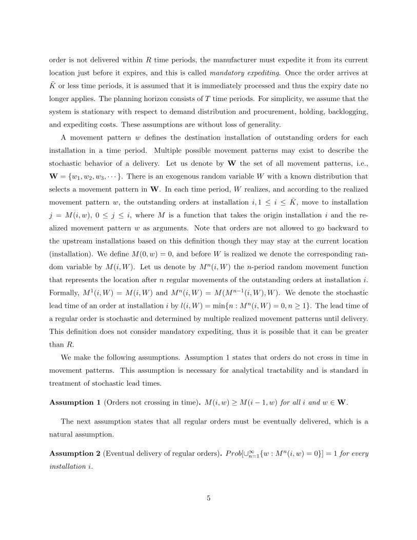
Age of an order is the number of time periods since it was placed. When it has just been placed

the age is 0, and there can be multiple outstanding orders with different ages in an installation.

In Figure 1, we show physical installations with age bins for orders with different ages. Note that

Manufacturing

facility

K 0...K-1 K-2 1

1 2 3 R-1 1 2 3 R-1... 1 2 3 R-10

R bins R-1 bins R-1 bins

... ... 1 2 3 R-1...

R-1 bins

Figure 1: Physical installations with age bins

the bin for age 0 is only in installation K̄ because fresh orders are always placed to installation K̄

(The figure for consistency actually shows all of them). Also, there are no bins for age R because

of mandatory expediting: if an order with age R− 1 is not expedited at time period t, then it will

move to a certain downstream installation according to the regular movement for time period t and

will be expedited mandatorily at the beginning of time period t+ 1. Therefore we do not need age

bins for age R. If an order about to expire is delivered to the manufacturing facility by a regular

movement, we do not have to mandatorily expedite it. For convenience the cost of mandatory

expediting at time period t + 1 is accounted in time period t. We note that a higher aged order is

closer to a lower aged order.

The sequence of events in a time period is as follows. At the beginning of the time period,

the state information is given. First, mandatory expediting from the current location happens

for goods that have been in age bin R − 1 in the previous time period. Then the manufacturer

places a regular order with the supplier (installation K̄). Next, the manufacturer makes decisions

on expediting for each installation, and the expedited orders arrive at the manufacturing facility

instantaneously. After that, demand D realizes in the current time period. Inventory holding or

backlogging cost is accounted for at the manufacturing facility after demand realization. Next, W

realizes and regular delivery occurs just before the end of the time period. Then the next time

period begins.

Let us denote the order that has j remaining time periods until mandatory expediting as a

stage j order: stage = R–age. Again, we say that on order is closer to the manufacturing facility

than a different order in the same physical location if its stage is lower. We express the state of

the system by the stage inventory level and location as

(v0, v1, · · · , vR−1, l1, l2, · · · , lR−1),

6

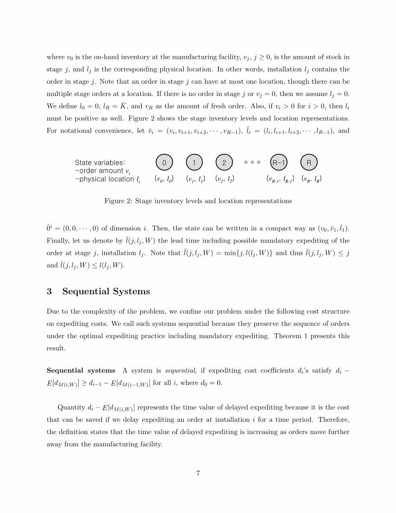
where v0 is the on-hand inventory at the manufacturing facility, vj , j ≥ 0, is the amount of stock in

stage j, and lj is the corresponding physical location. In other words, installation lj contains the

order in stage j. Note that an order in stage j can have at most one location, though there can be

multiple stage orders at a location. If there is no order in stage j or vj = 0, then we assume lj = 0.

We define l0 = 0, lR = K̄, and vR as the amount of fresh order. Also, if vi > 0 for i > 0, then li

must be positive as well. Figure 2 shows the stage inventory levels and location representations.

For notational convenience, let v̄i = (vi, vi+1, vi+2, · · · , vR−1), l̄i = (li, li+1, li+2, · · · , lR−1), and

0 1 2 R-1 RState variables:-order amount v

i

-physical location li

(v0, l

0) (v

1, l

1) (v

2, l

2) (v

R-1, l

R-1) (v

R, l

R)

Figure 2: Stage inventory levels and location representations

0̄i = (0, 0, · · · , 0) of dimension i. Then, the state can be written in a compact way as (v0, v̄1, l̄1).

Finally, let us denote by l̄(j, lj ,W ) the lead time including possible mandatory expediting of the

order at stage j, installation lj . Note that l̄(j, lj ,W ) = min{j, l(lj ,W )} and thus l̄(j, lj ,W ) ≤ j

and l̄(j, lj ,W ) ≤ l(lj ,W ).

3 Sequential Systems

Due to the complexity of the problem, we confine our problem under the following cost structure

on expediting costs. We call such systems sequential because they preserve the sequence of orders

under the optimal expediting practice including mandatory expediting. Theorem 1 presents this

result.

Sequential systems A system is sequential, if expediting cost coefficients di’s satisfy di −

E[dM(i,W )] ≥ di−1 − E[dM(i−1,W )] for all i, where d0 = 0.

Quantity di −E[dM(i,W )] represents the time value of delayed expediting because it is the cost

that can be saved if we delay expediting an order at installation i for a time period. Therefore,

the definition states that the time value of delayed expediting is increasing as orders move further

away from the manufacturing facility.

7

Theorem 1. Sequential systems preserve the sequence of orders in time when operated optimally.

Proof. Consider two nonempty stages i and j, i > j, which contain uniti and unitj , respectively.

We compare the following two strategies.

• Strategy 1: Expedite unitj from stage j, and then expedite uniti after (realized) l̄(j, lj , w)

time periods from the corresponding position. This strategy is feasible by keeping track of

the position of a fictitious unit in stage j, since it takes (realized) l̄(j, lj , w) time periods for

the fictitious unit to arrive at the manufacturing facility. The expected cost of strategy 1 is

dlj + E[dM l̄(j,lj ,W )(li,W )

].

• Strategy 2: Expedite uniti, and then do not do anything on unitj except mandatory expe-

diting. The expected cost of strategy 2 is dli + E[dM l̄(j,lj ,W )(lj ,W )

].

These two strategies are identical in the view point of the manufacturer because they yield the

same inventory level at the manufacturer. However, the cost implication is different.

Sequential systems satisfy di − E[dM(i,W )] ≥ di−1 − E[dM(i−1,W )] for all i, where d0 = 0. From

Lemma 2 in Appendix, we have di − dj ≥ E[dMn(i,W ) − dMn(j,W )], for any i and j, i ≥ j, and

n ≥ 1 because M is defined independently from the expiry date of R time periods. By considering

n = l̄(j, lj , w), we have

dli + E[dM l̄(j,lj ,W )(lj ,W )

] ≥ dlj + E[dM l̄(j,lj ,W )(li,W )

]. (1)

This implies that Strategy 1 is always better than or equal to Strategy 2 in terms of costs. In

other words, any policy that starts with Strategy 2 cannot be optimal. Therefore, if expediting is

necessary in sequential systems, it is optimal to expedite from the nonempty installation that is

closest to the manufacturing facility. Therefore, orders preserve sequence in time under an optimal

expediting policy for sequential systems. The proof is completed.

Theorem 1 provides an important fact of the optimal expediting policy for sequential systems:

it is best to expedite the closest order to the manufacturing facility if we need to expedite any

outstanding orders. We build the optimality equation based on this theorem. To do so, let us

define restricted cost-to-go functions: for 1 ≤ j ≤ R, let J jt (·) be the optimal cost-to-go from time

period t onwards that is achieved by a restricted control space, in which expediting from stages

j + 1, j + 2, · · · , R in time period t is not allowed. The control space for J jt is restricted in time

period t, but unrestricted after time period t. We mainly utilize J jt with respect to special states

Ai = (x, 0̄i−1, v̄i, 0̄i−1, l̄i) for 1 ≤ i ≤ R − 1. This state represents x units at the manufacturing

8

facility, no inventory from stage 1 up to stage i−1, vi units in stage i, vi+1 units in stage i+ 1, and

so on. The corresponding locations are zero up to stage i − 1 by definition, li for stage i, li+1 for

stage i + 1, and so on. Also, let us denote by NSi the next state in the next time period from the

current state Ai under the restriction that expediting only from stage i is allowed in the current

time period.

Let Jt be the optimal cost-to-go without any restrictions and let the echelon stock be xi =

v0 + v1 + · · ·+ vi. For a sequential system, we have the following optimality equation

Jt(v0, v̄1, l̄1) = min{J1t (x0, v̄1, l̄1),

dl1v1 + J2t (x1, 0, v̄2, 0, l̄2),

dl1v1 + dl2v2 + J3t (x2, 0̄2, v̄3, 0̄

2, l̄3),

· · · ,R−1∑i=1

dlivi + JRt (xR−1, 0̄R−1, 0̄R−1)},

where

J1t (x0, v̄1, l̄1) = min

x0≤y1≤x1

z≥xR−1

{dl1(y1 − x0) + c(z − xR−1) + L(y1)

+ E[dM(l1,W )](x1 − y1) + E[Jt+1(NS1)]},

(2)

and

J it (x

i−1, 0̄i−1, v̄i, 0̄i−1, l̄i) = min

xi−1≤yi≤xi

z≥xR−1

{dli(yi − xi−1) + c(z − xR−1) + L(yi)

+ E[Jt+1(NSi)]},

(3)

for i > 1, where yi and z are decision variables: yi − xi−1 corresponds to the expediting amount

from stage i, and z−xL−1 corresponds to the regular ordering amount. In (2), E[dM(l1,W )](x1−y1)

represents the mandatory expediting cost. To facilitate the analysis of the system dynamics, let us

define the following set of probabilities:

• p(li) = prob(M(li,W ) > 0), and

• p(li, li+1) = prob{M(li,W ) = 0 and M(li+1,W ) > 0} for all i.

Note that p’s are deterministic functions, and if li = li+1, then p(li, li+1) = 0. We first present the

following lemma with its proof in Appendix.

9

Lemma 1. We have p(li) + p(li, li+1) = p(li+1) for all i.

For ease of exposition, let M(l̄i,W ) = (M(li,W ),M(li+1,W ), · · · ,M(lR,W )). Then, the future

cost E[Jt+1(NSi)] is

E[Jt+1(NSi)] = p(li)E[Jt+1(yi −D, 0̄i−2, xi − yi, v̄i+1, u, 0̄i−2,M(l̄i,W ))|M(li,W ) > 0]

+ p(li, li+1)E[Jt+1(xi −D, 0̄i−1, v̄i+1, u, 0̄

i−1,M(l̄i+1,W ))|M(li+1,W ) > 0]

+ p(li+1, li+2)E[Jt+1(xi+1 −D, 0̄i, v̄i+2, u, 0̄

i,M(l̄i+2,W ))|M(li+2,W ) > 0]

...

+ p(lR−1, lR)E[Jt+1(xR−1 −D, 0̄R−2, u, 0̄R−2,M(lR,W ))|M(lR,W ) > 0]

+ (1− p(lR))E[Jt+1(z −D, 0̄R−1, 0̄R−1)],

(4)

where u is the amount of the regular order: i.e. u = z − xR−1. Note the conditional expectations

in (4) to distinguish different cases. We also assume that all terminal functions are 0.

4 Optimal Policies for Sequential Systems

In this section, we focus on identifying optimal policies for sequential systems with mandatory

expediting. We start with preliminary results.

4.1 Preliminaries

In analyzing the optimality equation, an important result is that

Jt(xi−1, 0̄i−1, v̄i, 0̄

i−1, l̄i)− Jk(xi, 0̄i, v̄i+1, 0̄i, l̄i+1) is only a function of i, t, li, x

i−1, and xi.

Furthermore, this function has the form of S0i,t(li) +S1

i,t(xi−1, li) +S2

i,t(xi, li) for recursively defined

functions S0i,t, S

1i,t and S2

i,t. Another important result is that the minimization with respect to yi

in (2) and (3) can be isolated from the minimization with respect to z, and it has the form of

min fi,t(yi, li) for a function fi,t defined by using S0i,t, S

1i,t and S2

i,t. These key functions greatly

simply the analysis of the optimal policy. The definition of these key functions is as follows.

f1,t(y1, l1) = dl1y1 + L(y1)− p(l1)E[dM(l1,W )(y1 −D)|M(l1,W ) > 0]

= dl1y1 + L(y1)− E[dM(l1,W )(y1 −D)]

fi,t(yi, li) = dliyi + L(yi) + p(li)E[S1i−1,t+1(yi −D,M(li,W ))|M(li,W ) > 0]

= dliyi + L(yi) + E[S1i−1,t+1(yi −D,M(li,W ))] for i > 1

10

S0i,t(li) = p(li)E[S0

i−1,t+1(M(li,W ))|M(li,W ) > 0] + ai,t(li)

= E[S0i−1,t+1(M(li,W ))] + ai,t(li)

S1i,t(x

i−1, li) = gi,t(xi−1, li)− dlix

i−1

S21,t(x

1, l1) = h1,t(x1, l1)− L(x1) + p(l1)E[dM(l1,W )|M(l1,W ) > 0]x1

= h1,t(x1, l1)− L(x1) + E[dM(l1,W )]x

1

S2i,t(x

i, li) = hi,t(xi, li)− L(xi) + p(li)E[S2

i−1,t+1(xi −D,M(li,W ))|M(li,W ) > 0]

= hi,t(xi, li)− L(xi) + E[S2

i−1,t+1(xi −D,M(li,W ))] for 1 < i ≤ R− 1

We also define S00,t(·) = S1

0,t(·) = S20,t(·) = 0 for all t and S0

i,T+1(·) = S1i,T+1(·) = S2

i,T+1(·) = 0

for all i. Here, ai,t, gi,t, and hi,t are defined according to Lemma 3 in Appendix with respect to

fi,t. This lemma is applied for any fixed li and thus ai,t, gi,t, and hi,t depend on li. Starting

from the last time period T , functions fi,t and Sji,t can be obtained recursively. It is easy to

check for all i and t that fi,t(yi, li) is convex in yi for a given li, if the system is sequential. Also,

S0i,t(li) + S1

i,t(x, li) + S2i,t(x, li) = 0 for every x and li.

Let us denote by y∗i,t(li) a minimizer of fi,t(yi, li): y∗i,t(li) ∈ arg minyi fi,t(yi, li). The following

theorem is an important property of fi,t(yi, li) for sequential systems, and the proof is given in

Appendix.

Theorem 2. For sequential systems, the following holds:

a. for any given j, y∗i,t(j) is nonincreasing in i, and

b. for any given i, y∗i,t(j) is nonincreasing in j.

4.2 Optimal Policies

For sequential systems we have the following theorem, which is the key result in this paper.

Theorem 3. a. The base stock policy with respect to the corresponding echelon stock xi−1 is optimal

for expediting from stage i. Also, the base stock policy with respect to the inventory position xR−1

is optimal for regular ordering.

b. Function p(lR)E[S2R−1,t(z−D,M(lR, w))|M(lR, w) > 0] +E[Jt(z−D, 0̄R−1, 0̄R−1)] is convex in

z.

c. For 1 ≤ i ≤ R − 1, we have Jt(xi−1, 0̄i−1, v̄i, 0̄

i−1, l̄i) − Jk(xi, 0̄i, v̄i+1, 0̄i, l̄i+1) = S0

i,t(li) +

S1i,t(x

i−1, li) + S2i,t(x

i, li).

11

Part a is the most important as it describes the optimal policies. Part b and c are needed in the

inductive proof. We postpone the proof of this theorem to later in the document and first provide

an illustrative example.

4.3 Illustration of the Optimal Policy

Part (a) of Theorem 3 states that the optimal regular ordering policy follows the base stock policy

with respect to the inventory position. Compared to the result in Kim et al. (2012), though the base

stock level is different, the optimal regular ordering policy remains the same regardless of mandatory

expediting. However, the optimal expediting policy is quite different with the introduction of

mandatory expediting. We explain the optimal expediting policy described in Theorems 2 and 3

through the following illustrative example.

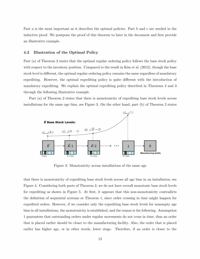
Part (a) of Theorem 2 states that there is monotonicity of expediting base stock levels across

installations for the same age bins, see Figure 3. On the other hand, part (b) of Theorem 2 states

K Base Stock Levels:

K 0...

1 2 3 R-1

K-1 K-2

0

R bins R-1 bins R-1 bins

...

1

2 Manufacturing facility

R-1 bins

1 2 3 R-1...2 1 2 3 R-1...2 1 2 3 R-1...2

Figure 3: Monotonicity across installations of the same age

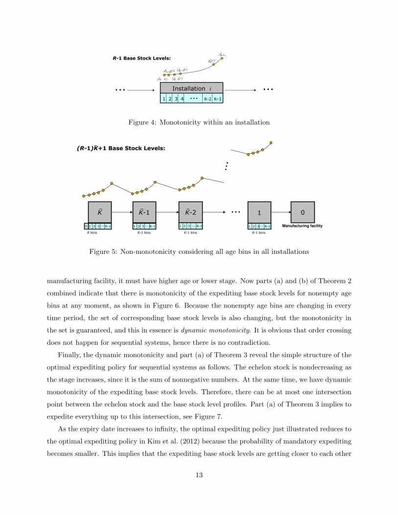
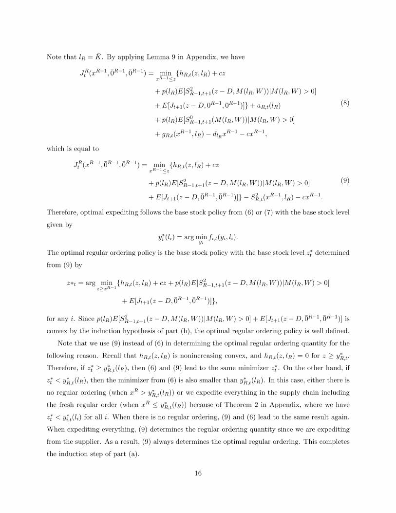
that there is monotonicity of expediting base stock levels across all age bins in an installation, see

Figure 4. Considering both parts of Theorem 2, we do not have overall monotonic base stock levels

for expediting as shown in Figure 5. At first, it appears that this non-monotonicity contradicts

the definition of sequential systems or Theorem 1, since order crossing in time might happen for

expedited orders. However, if we consider only the expediting base stock levels for nonempty age

bins in all installations, the monotonicity is established, and the reason is the following. Assumption

1 guarantees that outstanding orders under regular movements do not cross in time, thus an order

that is placed earlier should be closer to the manufacturing facility. Also, the order that is placed

earlier has higher age, or in other words, lower stage. Therefore, if an order is closer to the

12

Installation i .........

R-1 Base Stock Levels:

1 2 3 4 R-2 R-1

Figure 4: Monotonicity within an installation

K 0...K-1 K-2 1

...

(R-1)K+1 Base Stock Levels:

Manufacturing facility1 2 3 R-1 1 2 3 R-1... 1 2 3 R-10

R bins R-1 bins R-1 bins

... ... 1 2 3 R-1...

R-1 bins

Figure 5: Non-monotonicity considering all age bins in all installations

manufacturing facility, it must have higher age or lower stage. Now parts (a) and (b) of Theorem 2

combined indicate that there is monotonicity of the expediting base stock levels for nonempty age

bins at any moment, as shown in Figure 6. Because the nonempty age bins are changing in every

time period, the set of corresponding base stock levels is also changing, but the monotonicity in

the set is guaranteed, and this in essence is dynamic monotonicity. It is obvious that order crossing

does not happen for sequential systems, hence there is no contradiction.

Finally, the dynamic monotonicity and part (a) of Theorem 3 reveal the simple structure of the

optimal expediting policy for sequential systems as follows. The echelon stock is nondecreasing as

the stage increases, since it is the sum of nonnegative numbers. At the same time, we have dynamic

monotonicity of the expediting base stock levels. Therefore, there can be at most one intersection

point between the echelon stock and the base stock level profiles. Part (a) of Theorem 3 implies to

expedite everything up to this intersection, see Figure 7.

As the expiry date increases to infinity, the optimal expediting policy just illustrated reduces to

the optimal expediting policy in Kim et al. (2012) because the probability of mandatory expediting

becomes smaller. This implies that the expediting base stock levels are getting closer to each other

13

...

K 0...

1 2 3 R-1

K-1

1 2 3 R-1...

K-2

1 2 3 R-10

R bins R-1 bins R-1 bins

... ...

1

1 2 3 R...

At most R Base Stock Levels for nonempty bins:

0 1 2 3 R-1 Manufacturing facility

R-1 bins

Figure 6: Dynamic monotonicity of nonempty age bins in all installations

K 0...

1 2 3 R

K-1

1 2 3 R...

K-2

1 2 3 R0

R+1 bins R bins R bins

1 2 3 R...0

R+2 bins

R+1... ...

1

1 2 3 R...0 1 2 3 R

Echelon

Stock

Base Stock Level

Expediting Everything

Figure 7: The simple structure of the optimal expediting policy

as the expiry date increases, and we conjecture that they eventually converge to a single value for

each installation, and we have a unique expediting base stock level for each installation. Since they

are monotonic, we must have the optimal expediting policy as described in Kim et al. (2012).

4.4 Proof of Optimality

Proof of Theorem 3. We prove parts (a), (b), and (c) concurrently by induction on t. In the base

case t = T + 1, the optimal expediting and regular ordering policies are null. Also (b) and (c) hold

obviously when t = T + 1. Now we proceed to the induction step.

We prove that part (a) holds at time period t. First consider (4). By repeatedly applying part

14

(c) with time period t + 1, which holds by the induction hypothesis, we have

E[Jt+1(NSi)] = p(li)E[S0i−1,t+1(M(li,W )) + S1

i−1,t+1(yi −D,M(li,W ))

+ S2i−1,t+1(x

i −D,M(li,W ))|M(li,W ) > 0]

+ · · ·

+ p(lR)E[Jt+1(xR−1 −D, 0̄R−2, u, 0̄R−2,M(lR,W ))|M(lR,W ) > 0]

+ (1− p(lR))E[Jt+1(z −D, 0̄R−1, 0̄R−1)],

where Lemma 1 is used. This is again rearranged to the following by using part (c):

E[Jt+1(NSi)] = p(li)E[S0i−1,t+1(M(li,W )) + S1

i−1,t+1(yi −D,M(li,W ))

+ S2i−1,t+1(x

i −D,M(li,W ))|M(li,W ) > 0]

+ · · ·

+ p(lR)E[S0R−1,t+1(M(lR,W )) + S1

R−1,t+1(xR−1 −D,M(lR,W ))

+ S2R−1,t+1(z −D,M(lR,W ))|M(lR,W ) > 0] + E[Jt+1(z −D, 0̄R−1, 0̄R−1)].

Let us denote by OT the terms that contain only state variables. Then,

E[Jt+1(NSi)] = p(li)E[S1i−1,t+1(yi −D,M(li,W ))|M(li,W ) > 0]

+ p(lR)E[S2R−1,t+1(z −D,M(lR,W ))|M(lR,W ) > 0]

+ E[Jt+1(z −D, 0̄R−1, 0̄R−1)] + OT.

(5)

Plugging (5) into (2) and (3) yields

J it (x

i−1, 0̄i−1, v̄i, 0̄i−1, l̄i) = min

xi−1≤yi≤xifi,t(yi, li)

+ minz≥xR−1

{cz + p(lR)E[S2R−1,t+1(z −D,M(lR,W ))|M(lR,W ) > 0]

+ E[Jt+1(z −D, 0̄R−1, 0̄R−1)]}+ OT,

(6)

for i < R. For i = R, we have

JRt (xR−1, 0̄R−1, 0̄R−1) = min

xR−1≤yR≤z{fR,t(yR, lR) + cz

+ p(lR)E[S2R−1,t+1(z −D,M(lR,W ))|M(lR,W ) > 0]

+ E[Jt+1(z −D, 0̄R−1, 0̄R−1)]}

+ p(lR)E[S0R−1,t+1(M(lR,W ))|M(lR,W ) > 0]

− dlRxR−1 − cxR−1.

(7)

15

Note that lR = K̄. By applying Lemma 9 in Appendix, we have

JRt (xR−1, 0̄R−1, 0̄R−1) = min

xR−1≤z{hR,t(z, lR) + cz

+ p(lR)E[S2R−1,t+1(z −D,M(lR,W ))|M(lR,W ) > 0]

+ E[Jt+1(z −D, 0̄R−1, 0̄R−1)]}+ aR,t(lR)

+ p(lR)E[S0R−1,t+1(M(lR,W ))|M(lR,W ) > 0]

+ gR,t(xR−1, lR)− dlRx

R−1 − cxR−1,

(8)

which is equal to

JRt (xR−1, 0̄R−1, 0̄R−1) = min

xR−1≤z{hR,t(z, lR) + cz

+ p(lR)E[S2R−1,t+1(z −D,M(lR,W ))|M(lR,W ) > 0]

+ E[Jt+1(z −D, 0̄R−1, 0̄R−1)]} − S2R,t(x

R−1, lR)− cxR−1.

(9)

Therefore, optimal expediting follows the base stock policy from (6) or (7) with the base stock level

given by

y∗i (li) = arg minyi

fi,t(yi, li).

The optimal regular ordering policy is the base stock policy with the base stock level z∗t determined

from (9) by

z∗t = arg minz≥xR−1

{hR,t(z, lR) + cz + p(lR)E[S2R−1,t+1(z −D,M(lR,W ))|M(lR,W ) > 0]

+ E[Jt+1(z −D, 0̄R−1, 0̄R−1)]},

for any i. Since p(lR)E[S2R−1,t+1(z −D,M(lR,W ))|M(lR,W ) > 0] + E[Jt+1(z −D, 0̄R−1, 0̄R−1)] is

convex by the induction hypothesis of part (b), the optimal regular ordering policy is well defined.

Note that we use (9) instead of (6) in determining the optimal regular ordering quantity for the

following reason. Recall that hR,t(z, lR) is nonincreasing convex, and hR,t(z, lR) = 0 for z ≥ y∗R,t.

Therefore, if z∗t ≥ y∗R,t(lR), then (6) and (9) lead to the same minimizer z∗t . On the other hand, if

z∗t < y∗R,t(lR), then the minimizer from (6) is also smaller than y∗R,t(lR). In this case, either there is

no regular ordering (when xR > y∗R,t(lR)) or we expedite everything in the supply chain including

the fresh regular order (when xR ≤ y∗R,t(lR)) because of Theorem 2 in Appendix, where we have

z∗t < y∗i,t(li) for all i. When there is no regular ordering, (9) and (6) lead to the same result again.

When expediting everything, (9) determines the regular ordering quantity since we are expediting

from the supplier. As a result, (9) always determines the optimal regular ordering. This completes

the induction step of part (a).

16

Next, we prove that part (b) holds at time period t. Adding

p(lR)E[S2R−1,t(x

R−1,M(lR,W ))|M(lR,W )) > 0]

to both sides of (8), we have

p(lR)E[S2R−1,t(x

R−1,M(lR,W ))|M(lR,W )) > 0] + JRt (xR−1, 0̄R−1, 0̄R−1)

= minxR−1≤z

{hR,t(z, lR) + cz + p(lR)E[S2R−1,t+1(z −D,M(lR,W ))|M(lR,W ) > 0]

+ Jt+1(z −D, 0̄R−1, 0̄R−1)]}+ p(lR)E[S0R−1,t+1(M(lR,W ))|M(lR,W ) > 0]

+ gR,t(xR−1, lR) + p(lR)E[S2

R−1,t(xR−1,M(lR,W ))|M(lR,W )) > 0]

+ aR,t(lR)− dlRxR−1 − cxR−1.

By the induction hypothesis,

p(lR)E[S2R−1,t+1(z −D,M(lR, w))|M(lR, w) > 0] + E[Jt+1(z −D, 0̄R−1, 0̄R−1)]

is convex in z. Therefore,

minxR−1≤z

{hR,t(z, lR) + cz + p(lR)E[S2R−1,t+1(z −D,M(lR,W ))|M(lR,W ) > 0]

+ Jt+1(z −D, 0̄R−1, 0̄R−1)]}

is convex in xR−1. Also, gR,t(xR−1, lR) + p(lR)E[S2

R−1,t(xR−1,M(lR,W ))|M(lR,W )) > 0] is convex

in xR−1 by Lemma 8 in Appendix. All the other terms are either constant or linear in xR−1.

Therefore,

p(lR)E[S2R−1,t+1(x

R−1,M(lR,W ))|M(lR,W )) > 0] + JRt (xR−1, 0̄R−1, 0̄R−1)

is convex in xR−1, and the proof of part (b) is completed.

The proof of part (c) is provided in Appendix.

5 Concluding Remarks

This paper addresses operational issues resulting from both stochastic demand and lead time with

expiry dates by considering expediting. It presents the optimal policy of regular ordering and

expediting. The mandatory expediting brings complexity to the optimal policy but in a manageable

and well-structured fashion due to the dynamic monotonicity of expediting base stock levels. This

17

result certainly broadens our understanding and intuition when coping with demand and lead time

related emergencies in supply chains.

An important but unaddressed situation, though, is the expiry constraint within the manufac-

turing facility. There exists literature on the shelf life of various models that have deterministic

lead times. We deem that an important task in the future is to extend our results to include the

shelf life of the delivered orders in the manufacturing facility. Figure 8 summarized the previous

research, the position of this paper, and the future direction. We do not think that this extension

Expiry on Delivery

Stochastic Lead Time

Deterministic Lead Time

Nonzero

Our research

Nahmias(1975), Fries (1975)- Analytical

No previous literature

Shelf Life

At most 2time periods

Multiple time periods

Williams and Patuwo (1999)- Computational

Zero Not meaningful

Not meaningful

Not meaningful

No previous literature

No previous literature

Figure 8: Future research

will be immediate, since the previous literature on the shelf life suggests inherent complexity of

the optimal policy in simpler cases. However, we believe that there can be theoretical or practical

solutions for this extension with the advancement of our understanding in complex supply chain

systems.

Appendix

Lemma 2. In sequential systems, di − dj ≥ E[dMn(i,W ) − dMn(j,W )], for any i and j, i ≥ j, and

n ≥ 1.

Proof. The proof can be found in Kim et al. (2012).

Proof of Lemma 1. By assumption, regular orders do not cross in time. From p(li) = prob(M(li,W ) >

0) = prob{M(li,W ) > 0 and M(li+1,W ) > 0}, we have p(li) + p(li, li+1) = prob{M(li,W ) > 0 and

M(li+1,W ) > 0} + prob{M(li,W ) = 0, and M(li+1,W ) > 0} = prob(M(li+1,W ) > 0) = p(li+1)

for all i and any value of li.

18

Lemma 3. Let f be convex and have a finite minimizer on R. Let y∗ = arg min f(x). Then,

minx1≤x≤x2

f(x) = a + g(x1) + h(x2), where a = f(y∗), and penalty functions g(x1) and h(x2) are

g(x1) =

0 x1 ≤ y∗

f(x1)− a x1 > y∗and h(x2) =

f(x2)− a x2 ≤ y∗

0 x2 > y∗.

For a nondecreasing convex f , we define a = 0, g(x) = f(x), and h(x) = 0. On the other hand, for

a nonincreasing convex f , we define a = 0, g(x) = 0, and h(x) = f(x).

Proof. The proof can be found in Karush (1959).

For a convex function f : R → R, let ∂f(x) be its subdifferential at x, which is a set. For two

sets S1 and S2, we denote S1 ≤ S2 if there exists s2 ∈ S2 such that s1 ≤ s2 for any s1 ∈ S1, and

there exists s1 ∈ S1 such that s1 ≤ s2 for any s2 ∈ S2. The following lemmas are from Kim et al.

(2012).

Lemma 4. Let f1 and f2 be convex functions. If ∂f1(x) ≤ ∂f2(x) for all x ∈ R, then

arg minx

f1(x) ≥ arg minx

f2(x).

Lemma 5. Let f1 and f2 be convex functions, and let g1 and g2 be their penalty functions as in

Lemma 3. If ∂f1(x) ≤ ∂f2(x), then ∂g1(x) ≤ ∂g2(x).

Lemma 6. Let f1, f2, f̃1, and f̃2 be convex functions. If ∂f1(x) ≤ ∂f2(x) and ∂f̃1(x) ≤ ∂f̃2(x),

then ∂{f1 + f̃2}(x) ≤ ∂{f2 + f̃2}(x).

Lemma 7. Let f1 and f2 be convex functions, and let F1(x) = E[f1(x−D)] and F2(x) = E[f2(x−

D)]. If ∂f1(x) ≤ ∂f2(x), then ∂F1(x) ≤ ∂F2(x).

Proof of Theorem 2. In this proof, we use Lemmas 4, 5, 6, and 7. Let us first consider part (a).

We first rewrite

f1,t(y1, j) = djy1 + L(y1)− E[dM(j,W )]y1 + E[dM(j,W )D]

= (dj − E[dM(j,W )])y1 + L(y1) + E[dM(j,W )D],

and

fi,t(yi, j) = djyi + L(yi) + E[S1i−1,t+1(yi −D,M(j,W ))]

= djyi + L(yi) + E[gi−1,t+1(yi −D,M(j,W ))− dM(j,W )(yi −D)]

= (dj − E[dM(j,W )])yi + L(yi) + E[gi−1,t+1(yi −D,M(j,W ))]

+ E[dM(j,W )D],

19

for i > 1. Also,

fi+1,t(yi+1, j) = (dj − E[dM(j,W )])yi+1 + L(yi+1) + E[gi,t+1(yi+1 −D,M(j,W ))]

+ E[dM(j,W )D].

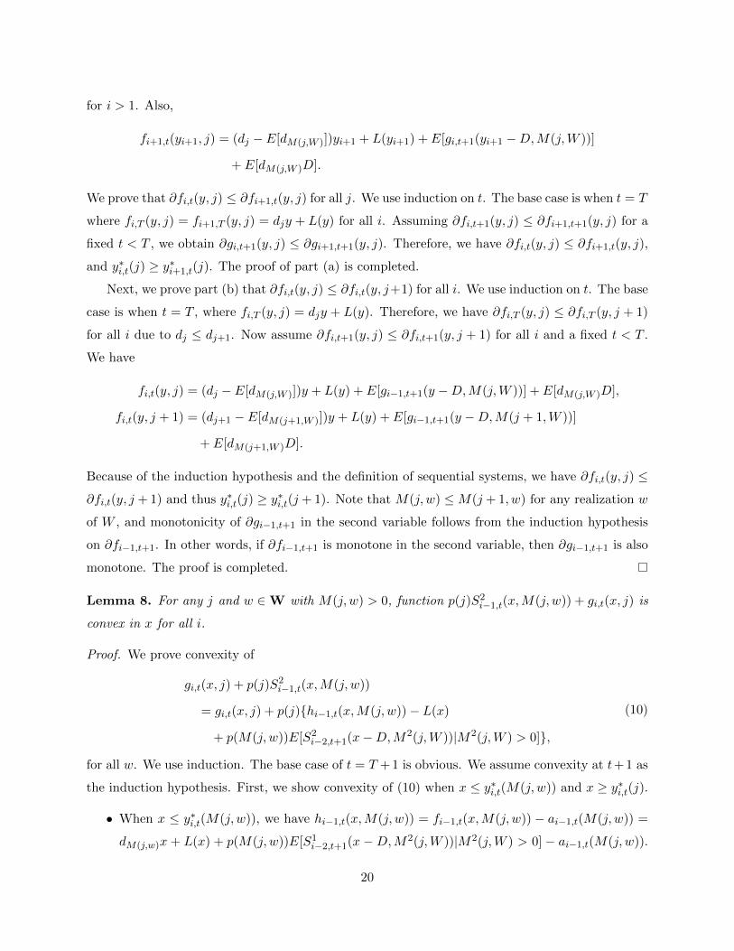
We prove that ∂fi,t(y, j) ≤ ∂fi+1,t(y, j) for all j. We use induction on t. The base case is when t = T

where fi,T (y, j) = fi+1,T (y, j) = djy + L(y) for all i. Assuming ∂fi,t+1(y, j) ≤ ∂fi+1,t+1(y, j) for a

fixed t < T , we obtain ∂gi,t+1(y, j) ≤ ∂gi+1,t+1(y, j). Therefore, we have ∂fi,t(y, j) ≤ ∂fi+1,t(y, j),

and y∗i,t(j) ≥ y∗i+1,t(j). The proof of part (a) is completed.

Next, we prove part (b) that ∂fi,t(y, j) ≤ ∂fi,t(y, j+1) for all i. We use induction on t. The base

case is when t = T , where fi,T (y, j) = djy + L(y). Therefore, we have ∂fi,T (y, j) ≤ ∂fi,T (y, j + 1)

for all i due to dj ≤ dj+1. Now assume ∂fi,t+1(y, j) ≤ ∂fi,t+1(y, j + 1) for all i and a fixed t < T .

We have

fi,t(y, j) = (dj − E[dM(j,W )])y + L(y) + E[gi−1,t+1(y −D,M(j,W ))] + E[dM(j,W )D],

fi,t(y, j + 1) = (dj+1 − E[dM(j+1,W )])y + L(y) + E[gi−1,t+1(y −D,M(j + 1,W ))]

+ E[dM(j+1,W )D].

Because of the induction hypothesis and the definition of sequential systems, we have ∂fi,t(y, j) ≤

∂fi,t(y, j + 1) and thus y∗i,t(j) ≥ y∗i,t(j + 1). Note that M(j, w) ≤M(j + 1, w) for any realization w

of W , and monotonicity of ∂gi−1,t+1 in the second variable follows from the induction hypothesis

on ∂fi−1,t+1. In other words, if ∂fi−1,t+1 is monotone in the second variable, then ∂gi−1,t+1 is also

monotone. The proof is completed.

Lemma 8. For any j and w ∈W with M(j, w) > 0, function p(j)S2i−1,t(x,M(j, w)) + gi,t(x, j) is

convex in x for all i.

Proof. We prove convexity of

gi,t(x, j) + p(j)S2i−1,t(x,M(j, w))

= gi,t(x, j) + p(j){hi−1,t(x,M(j, w))− L(x)

+ p(M(j, w))E[S2i−2,t+1(x−D,M2(j,W ))|M2(j,W ) > 0]},

(10)

for all w. We use induction. The base case of t = T + 1 is obvious. We assume convexity at t+ 1 as

the induction hypothesis. First, we show convexity of (10) when x ≤ y∗i,t(M(j, w)) and x ≥ y∗i,t(j).

• When x ≤ y∗i,t(M(j, w)), we have hi−1,t(x,M(j, w)) = fi−1,t(x,M(j, w)) − ai−1,t(M(j, w)) =

dM(j,w)x + L(x) + p(M(j, w))E[S1i−2,t+1(x −D,M2(j,W ))|M2(j,W ) > 0] − ai−1,t(M(j, w)).

20

By using the fact that S1(x, j) + S2(x, j) = −S0(j), it is easy to see that gi,t(x, j) +

p(j)S2i−1,t(x,M(j, w)) is convex in x for x ≤ y∗i,t(M(j, w)).

• When x ≥ y∗i,t(j), we have gi,t(x, j) = fi,t(x, j) − ai,t(j) = djx + L(x) + p(j)E[S1i−1,t+1(x −

D,M(j, w))]−ai,t(j). Since S1i−1,t+1(x−D,M(j, w)) = gi−1,t+1(x−D,M(j, w))−dM(j,w)(x−

D), and p(M(j, w))E[S2i−2,t+1(x−D,M2(j,W ))|M2(j,W ) > 0] + gi−1,t+1(x−D,M(j, w)) is

convex by induction hypothesis, it is also easy to see convexity for x ≥ y∗i,t(j).

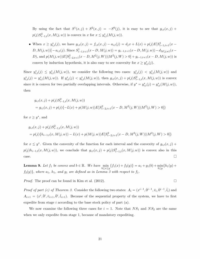
Since y∗i,t(j) ≤ y∗i,t(M(j, w)), we consider the following two cases: y∗i,t(j) < y∗i,t(M(j, w)) and

y∗i,t(j) = y∗i,t(M(j, w)). If y∗i,t(j) < y∗i,t(M(j, w)), then gi,t(x, j) + p(j)S2i−1,t(x,M(j, w)) is convex

since it is convex for two partially overlapping intervals. Otherwise, if y∗ = y∗i,t(j) = y∗i,t(M(j, w)),

then

gi,t(x, j) + p(j)S2i−1,t(x,M(j, w))

= gi,t(x, j) + p(j){−L(x) + p(M(j, w))E[S2i−2,t+1(x−D,M2(j,W ))|M2(j,W ) > 0]}

for x ≥ y∗, and

gi,t(x, j) + p(j)S2i−1,t(x,M(j, w))

= p(j){hi−1,t(x,M(j, w))− L(x) + p(M(j, w))E[S2i−2,t+1(x−D,M2(j,W ))|M2(j,W ) > 0]}

for x ≤ y∗. Given the convexity of the function for each interval and the convexity of gi,t(x, j) +

p(j)hi−1,t(x,M(j, w)), we conclude that gi,t(x, j) + p(j)S2i−1,t(x,M(j, w)) is convex also in this

case.

Lemma 9. Let f1 be convex and b ∈ R. We have minb≤x≤y

{f1(x) + f2(y)} = a1 + g1(b) + minb≤y{h1(y) +

f2(y)}, where a1, h1, and g1 are defined as in Lemma 3 with respect to f1.

Proof. The proof can be found in Kim et al. (2012).

Proof of part (c) of Theorem 3. Consider the following two states: Ai = (xi−1, 0̄i−1, v̄i, 0̄i−1, l̄i) and

Ai+1 = (xi, 0̄i, v̄i+1, 0̄i, l̄i+1). Because of the sequential property of the system, we have to first

expedite from stage i according to the base stock policy of part (a).

We now examine the following three cases for i = 1. Note that NS1 and NS2 are the same

when we only expedite from stage 1, because of mandatory expediting.

21

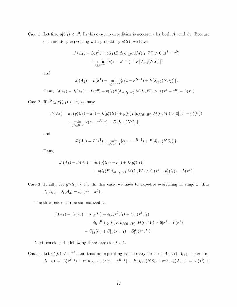
Case 1. Let first y∗1(l1) < x0. In this case, no expediting is necessary for both A1 and A2. Because

of mandatory expediting with probability p(l1), we have

Jt(A1) = L(x0) + p(l1)E[dM(l1,W )|M(l1,W ) > 0](x1 − x0)

+ minz≥xR−1

{c(z − xR−1) + E[Jt+1(NS1)]}

and

Jt(A2) = L(x1) + minz≥xR−1

{c(z − xR−1) + E[Jt+1(NS2)]}.

Thus, Jt(A1)− Jt(A2) = L(x0) + p(l1)E[dM(l1,W )|M(l1,W ) > 0](x1 − x0)− L(x1).

Case 2. If x0 ≤ y∗1(l1) < x1, we have

Jt(A1) = dl1(y∗1(l1)− x0) + L(y∗1(l1)) + p(l1)E[dM(l1,W )|M(l1,W ) > 0](x1 − y∗1(l1))

+ minz≥xR−1

{c(z − xR−1) + E[Jt+1(NS1)]}

and

Jt(A2) = L(x1) + minz≥xR−1

{c(z − xR−1) + E[Jt+1(NS2)]}.

Thus,

Jt(A1)− Jt(A2) = dl1(y∗1(l1)− x0) + L(y∗1(l1))

+ p(l1)E[dM(l1,W )|M(l1,W ) > 0](x1 − y∗1(l1))− L(x1).

Case 3. Finally, let y∗1(l1) ≥ x1. In this case, we have to expedite everything in stage 1, thus

Jt(A1)− Jt(A2) = dl1(x1 − x0).

The three cases can be summarized as

Jt(A1)− Jt(A2) = a1,t(l1) + g1,t(x0, l1) + h1,t(x

1, l1)

− dl1x0 + p(l1)E[dM(l1,W )|M(l1,W ) > 0]x1 − L(x1)

= S01,t(l1) + S1

1,t(x0, l1) + S2

1,t(x1, l1).

Next, consider the following three cases for i > 1.

Case 1. Let y∗i (li) < xi−1, and thus no expediting is necessary for both Ai and Ai+1. Therefore

Jt(Ai) = L(xi−1) + minz≥xR−1{c(z − xR−1) + E[Jt+1(NSi)]} and Jt(Ai+1) = L(xi) +

22

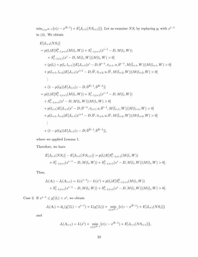
minz≥xR−1{c(z − xR−1) +E[Jt+1(NSi+1)]}. Let us examine NSi by replacing yi with xi−1

in (4). We obtain

E[Jt+1(NSi)]

= p(li)E[S0i−1,t+1(M(li,W )) + S1

i−1,t+1(xi−1 −D,M(li,W ))

+ S2i−1,t+1(x

i −D,M(li,W ))|M(li,W ) > 0]

+ (p(li) + p(li, li+1))E[Jt+1(xi −D, 0̄i−1, v̄i+1, u, 0̄

i−1,M(l̄i+1,W ))|M(li+1,W ) > 0]

+ p(li+1, li+2)E[Jt+1(xi+1 −D, 0̄i, v̄i+2, u, 0̄

i,M(l̄i+2,W ))|M(li+2,W ) > 0]

...

+ (1− p(lR))E[Jt+1(z −D, 0̄R−1, 0̄R−1)]

= p(li)E[S0i−1,t+1(M(li,W )) + S1

i−1,t+1(xi−1 −D,M(li,W ))

+ S2i−1,t+1(x

i −D,M(li,W ))|M(li,W ) > 0]

+ p(li+1)E[Jt+1(xi −D, 0̄i−1, v̄i+1, u, 0̄

i−1,M(l̄i+1,W ))|M(li+1,W ) > 0]

+ p(li+1, li+2)E[Jt+1(xi+1 −D, 0̄i, v̄i+2, u, 0̄

i,M(l̄i+2,W ))|M(li+2,W ) > 0]

...

+ (1− p(lR))E[Jt+1(z −D, 0̄R−1, 0̄R−1)],

where we applied Lemma 1.

Therefore, we have

E[Jt+1(NSi)]− E[Jt+1(NSi+1)] = p(li)E[S0i−1,t+1(M(li,W ))

+ S1i−1,t+1(x

i−1 −D,M(li,W )) + S2i−1,t+1(x

i −D,M(li,W ))|M(li,W ) > 0].

Thus,

Jt(Ai)− Jt(Ai+1) = L(xi−1)− L(xi) + p(li)E[S0i−1,t+1(M(li,W ))

+ S1i−1,t+1(x

i−1 −D,M(li,W )) + S2i−1,t+1(x

i −D,M(li,W ))|M(li,W ) > 0].

Case 2. If xi−1 ≤ y∗i (li) < xi, we obtain

Jt(Ai) = dli(y∗i (li)− xi−1) + L(y∗i (li)) + min

z≥xR−1{c(z − xR−1) + E[Jt+1(NSi)]}

and

Jt(Ai+1) = L(xi) + minz≥xR−1

{c(z − xR−1) + E[Jt+1(NSi+1)]}.

23

Similarly to the previous case, we have

E[Jt+1(NSi)]− E[Jt+1(NSi+1)] = p(li)E[S0i−1,t+1(M(li,W ))

+ S1i−1,t+1(yi(li)−D,M(li,W )) + S2

i−1,t+1(xi −D,M(li,W ))|M(li,W ) > 0].

Therefore,

Jt(A1)− Jt(A2) = dli(y∗i (li)− xi−1) + L(y∗i (li))− L(xi) + p(li)E[S0

i−1,t+1(M(li,W ))

+ S1i−1,t+1(yi(li)−D,M(li,W )) + S2

i−1,t+1(xi −D,M(li,W ))|M(li,W ) > 0].

Case 3. If y∗1(li) ≥ xi, then we simply have Jt(A1)− Jt(A2) = dli(xi − xi−1).

The three cases can be summarized as

Jt(Ai)− Jt(Ai+1) = ai,t(li) + gi,t(xi−1, li) + hi,t(x

i, li)− dlixi−1 − L(xi)

+ p(li)E[S0i−1,t+1(M(li,W ))

+ S2i−1,t+1(x

i −D,M(li,W ))|M(li,W ) > 0]

= S0i,t(li) + S1

i,t(xi−1, li) + S2

1,t(xi, li).

The proof of part (c) is thus completed.

References

Barankin, E. W. 1961. A delivery-lag inventory model with an emergency provision (the single-

period case). Naval Research Logistics Quarterly 8 285–311.

Daniel, K. H. 1963. A delivery-lag inventory model with emergency. Herbert Scarf, D. M. Gilford,

M. W. Shelly, eds., Multistage Inventory Models and Techniques, chap. 2. Stanford University

Press, 32–46.

Fries, B. E. 1975. Optimal ordering policy for a perishable commodity with fixed lifetime. Operations

Research 23 46–61.

Fukuda, Y. 1964. Optimal policies for the inventory problem with negotiable leadtime. Management

Science 10 690–708.

Karush, W. 1959. A theorem in convex programming. Naval Research Logistics Quarterly 6 245–

260.

24

Kim, C., D. Klabjan, D. Simchi-Levi. 2009. Optimal policies for expediting orders in transit.

Working Paper, Massachusetts Institute of Technology.

Kim, C., D. Klabjan, D. Simchi-Levi. 2012. Optimal expediting policies for a serial inventory system

with stochastic lead time with visibility of orders in transit. Working Paper, Massachusetts

Institute of Technology.

Lawson, D. G., E. L. Porteus. 2000. Multistage inventory management with expediting. Operations

Research 48 878–893.

Muharremoglu, A., J. N. Tsitsiklis. 2003. Dynamic leadtime management in supply chains. Tech.

rep., Massachusetts Institute of Technology, Cambridge, MA.

Nahmias, S. 1975. Optimal ordering policies for perishable inventory-II. Operations Research 23

735–749.

Nahmias, S. 1982. Perishable inventory theory: A review. Operations Research 30 680–708.

Neuts, M. F. 1964. An inventory model with an optional time lag. Journal of the Society for

Industrial and Applied Mathematics 12 179–185.

Veinott, A. F. 1966. The status of mathematical inventory theory. Management Science 12 745–777.

Williams, C. L., B. E. Patuwo. 1999. A perishable inventory model with positive order lead times.

European Journal of Operational Research 116 352–373.

25