
LONG-TERM OPTIMAL HYDROPOWER RESERVOIR ...
174
TECHNICAL UNIVERSITY OF MADRID ESCUELA DE INGENIEROS DE CAMINOS, CANALES Y PUERTOS LONG-TERM OPTIMAL HYDROPOWER RESERVOIR OPERATION WITH MINIMUM FLOWS AND MAXIMUM RAMPING RATES Thesis submitted for the degree of Doctor in Civil Engineering Systems by Ignacio Guisández González Ingeniero de Caminos, Canales y Puertos (UPM) Máster Universitario en Investigación en Ingeniería Eléctrica, Electrónica y Control Industrial (UNED) July 2016
-
Upload
khangminh22 -
Category
Documents
-
view
2 -
download
0
Transcript of LONG-TERM OPTIMAL HYDROPOWER RESERVOIR ...

TECHNICAL UNIVERSITY OF MADRID
ESCUELA DE INGENIEROS DE
CAMINOS, CANALES Y PUERTOS
LONG-TERM OPTIMAL HYDROPOWER RESERVOIR OPERATION WITH
MINIMUM FLOWS AND MAXIMUM RAMPING RATES
Thesis submitted for the degree of
Doctor in Civil Engineering Systems
by
Ignacio Guisández González
Ingeniero de Caminos, Canales y Puertos (UPM)
Máster Universitario en Investigación en
Ingeniería Eléctrica, Electrónica y Control Industrial (UNED)
July 2016

DEPARTMENT OF HYDRAULIC, ENERGY AND ENVIRONMENTAL ENGINEERING
ESCUELA DE INGENIEROS DE
CAMINOS, CANALES Y PUERTOS
LONG-TERM OPTIMAL HYDROPOWER RESERVOIR OPERATION WITH
MINIMUM FLOWS AND MAXIMUM RAMPING RATES
Author: Ignacio Guisández González
Ingeniero de Caminos, Canales y Puertos (UPM)
Máster Universitario en Investigación en Ingeniería
Eléctrica, Electrónica y Control Industrial (UNED)
Supervisors: Juan Ignacio Pérez Díaz
Doctor Ingeniero de Caminos, Canales y Puertos (UPM)
José Román Wilhelmi Ayza
Doctor Ingeniero de Caminos, Canales y Puertos (UPM)
July 2016

This thesis was awarded in 2018 by both the Technical University
of Madrid and the José Entrecanales Ibarra Foundation. The
research that it contains was funded by the Spanish Ministry of
Science and Innovation (CGL2009‐14258), the Department of
Hydraulic, Energy and Environmental Engineering of the Technical
University of Madrid (Carlos González Cruz Scholarship), and
SINTEF Energy Research (three‐month research stay at Trondheim).


a mis padres

Contents
Abstract 1
Resumen 3
Coautores 5
1. INTRODUCTION 71.1. Overview . . . . . . . . . . . . . . . . . . . . . . . . . . . . . . . . . . . . . . 71.2. Problem description . . . . . . . . . . . . . . . . . . . . . . . . . . . . . . . . 101.3. Scope and objectives . . . . . . . . . . . . . . . . . . . . . . . . . . . . . . . . 121.4. Structure of the thesis . . . . . . . . . . . . . . . . . . . . . . . . . . . . . . . 13
2. LITERATURE REVIEW 152.1. Decision support tools . . . . . . . . . . . . . . . . . . . . . . . . . . . . . . . 15
2.1.1. Decision-making approaches . . . . . . . . . . . . . . . . . . . . . . . . 152.1.2. Uncertainty treatments . . . . . . . . . . . . . . . . . . . . . . . . . . 162.1.3. Control approaches . . . . . . . . . . . . . . . . . . . . . . . . . . . . . 16
2.2. Optimisation techniques . . . . . . . . . . . . . . . . . . . . . . . . . . . . . . 172.2.1. Linear programming . . . . . . . . . . . . . . . . . . . . . . . . . . . . 172.2.2. Dynamic programming . . . . . . . . . . . . . . . . . . . . . . . . . . . 20
2.3. Input variables . . . . . . . . . . . . . . . . . . . . . . . . . . . . . . . . . . . 242.3.1. Markov chain theory . . . . . . . . . . . . . . . . . . . . . . . . . . . . 252.3.2. Water inflow . . . . . . . . . . . . . . . . . . . . . . . . . . . . . . . . 262.3.3. Energy price . . . . . . . . . . . . . . . . . . . . . . . . . . . . . . . . 272.3.4. Evaporation . . . . . . . . . . . . . . . . . . . . . . . . . . . . . . . . . 27
2.4. Generation characteristics . . . . . . . . . . . . . . . . . . . . . . . . . . . . . 282.4.1. Performance curves . . . . . . . . . . . . . . . . . . . . . . . . . . . . . 282.4.2. Instantaneous load dispatch . . . . . . . . . . . . . . . . . . . . . . . . 29
2.5. Hydro scheduling models with minimum flows and maximum ramping rates . 302.5.1. Linear programming models . . . . . . . . . . . . . . . . . . . . . . . . 302.5.2. Non-linear programming models . . . . . . . . . . . . . . . . . . . . . 352.5.3. Dynamic programming models . . . . . . . . . . . . . . . . . . . . . . 362.5.4. Other models . . . . . . . . . . . . . . . . . . . . . . . . . . . . . . . . 372.5.5. Common absences of the cited models relevant for this work . . . . . . 38
i

Contents Contents
3. ASSESING THE LONG-TERM EFFECTS OF MINIMUM FLOWS AND MAXI-MUM RAMPING RATES ON HYDROPEAKING 413.1. Assessment of the economic impact of environmental constraints on annual
hydropower plant operation . . . . . . . . . . . . . . . . . . . . . . . . . . . . 413.1.1. Methodology . . . . . . . . . . . . . . . . . . . . . . . . . . . . . . . . 413.1.2. Case study . . . . . . . . . . . . . . . . . . . . . . . . . . . . . . . . . 453.1.3. Main results and discussion . . . . . . . . . . . . . . . . . . . . . . . . 46
3.2. Effects of the maximum flow ramping rates on the long-term operation deci-sions of a hydropower plant . . . . . . . . . . . . . . . . . . . . . . . . . . . . 493.2.1. Methodology . . . . . . . . . . . . . . . . . . . . . . . . . . . . . . . . 493.2.2. Case study . . . . . . . . . . . . . . . . . . . . . . . . . . . . . . . . . 513.2.3. Main results and discussion . . . . . . . . . . . . . . . . . . . . . . . . 52
3.3. Approximate formulae for the assessment of the long-term economic impact ofenvironmental constraints on hydropeaking . . . . . . . . . . . . . . . . . . . 533.3.1. Methodology . . . . . . . . . . . . . . . . . . . . . . . . . . . . . . . . 533.3.2. Case studies . . . . . . . . . . . . . . . . . . . . . . . . . . . . . . . . . 563.3.3. Main results and discussion . . . . . . . . . . . . . . . . . . . . . . . . 57
4. LONG-TERM OPTIMISATIONMODELS FOR HYDRO SCHEDULING SUBJECTTO MINIMUM FLOWS AND MAXIMUM RAMPING RATES 634.1. Influence of the environmental constraints on the water and flow values . . . 63
4.1.1. Methodology . . . . . . . . . . . . . . . . . . . . . . . . . . . . . . . . 684.1.2. Case study . . . . . . . . . . . . . . . . . . . . . . . . . . . . . . . . . 714.1.3. Main results and discussion . . . . . . . . . . . . . . . . . . . . . . . . 72
4.2. Optimisation models for long-term hydro scheduling subject to environmentalconstraints (part I) . . . . . . . . . . . . . . . . . . . . . . . . . . . . . . . . . 804.2.1. Methodology . . . . . . . . . . . . . . . . . . . . . . . . . . . . . . . . 804.2.2. Case study . . . . . . . . . . . . . . . . . . . . . . . . . . . . . . . . . 814.2.3. Main results and discussion . . . . . . . . . . . . . . . . . . . . . . . . 82
4.3. Optimisation models for long-term hydro scheduling subject to environmentalconstraints (part II) . . . . . . . . . . . . . . . . . . . . . . . . . . . . . . . . 864.3.1. Methodology . . . . . . . . . . . . . . . . . . . . . . . . . . . . . . . . 864.3.2. Case study . . . . . . . . . . . . . . . . . . . . . . . . . . . . . . . . . 874.3.3. Main results and discussion . . . . . . . . . . . . . . . . . . . . . . . . 87
5. CONCLUSIONS 895.1. Main contributions . . . . . . . . . . . . . . . . . . . . . . . . . . . . . . . . . 895.2. Main conclusions . . . . . . . . . . . . . . . . . . . . . . . . . . . . . . . . . . 905.3. Future research directions . . . . . . . . . . . . . . . . . . . . . . . . . . . . . 91
ii

Contents
A. EQUATIONS OF THE OPTIMISATION MODELS 93A.1. Equations of the dynamic programming algorithms . . . . . . . . . . . . . . . 93
A.1.1. Recursive equations . . . . . . . . . . . . . . . . . . . . . . . . . . . . 93A.1.2. State transition equations . . . . . . . . . . . . . . . . . . . . . . . . . 94A.1.3. Revenue estimation equations . . . . . . . . . . . . . . . . . . . . . . . 94A.1.4. Convergence criteria . . . . . . . . . . . . . . . . . . . . . . . . . . . . 95
A.2. Equations of the linear programming algorithms . . . . . . . . . . . . . . . . 95A.2.1. Objective functions . . . . . . . . . . . . . . . . . . . . . . . . . . . . . 95A.2.2. Constraints . . . . . . . . . . . . . . . . . . . . . . . . . . . . . . . . . 97
B. MAIN DATA OF THE CASE STUDIES 107
References 129
Nomenclature 151
iii


List of Figures
2.1. Classification of reservoir decision support tools. . . . . . . . . . . . . . . . . 172.2. Types of linear programming. . . . . . . . . . . . . . . . . . . . . . . . . . . . 182.3. Types of dynamic programming. . . . . . . . . . . . . . . . . . . . . . . . . . 21
3.1. Flowchart of the solution strategy of the study 1 in each scenario. . . . . . . . 433.2. Coupling of the flows released by the plant between consecutive stages. . . . . 453.3. Annual losses according to φ and ρ of the plant I corresponding to the: (a)
Average of the water years; b) Very wet water year; c) Wet water year; d)Normal water year; e) Dry water year; f) Very dry water year scenario. . . . . 47
3.4. Average annual losses of the plant I according to: (a) φ; (b) ρ. . . . . . . . . . 483.5. Histogram of the initial and final F of the subproblems of the best policies
with ρ>0 obtained by mod2stu1. . . . . . . . . . . . . . . . . . . . . . . . . . 483.6. Flowchart of the solution strategy of the study 3 in each hydropower plant. . 543.7. Calculated and predicted long-term economic impact in terms of: (a) φ of the
plant A; (b) φ of the plant B; (c) ρ of the plant A; (d) ρ of the plant B. . . . 593.8. Long-term economic impact in terms of φ and ρ of the plant: (a) A calculated
by the models; (b) A predicted by formula (3.3); (c) B calculated by themodels; (d) B predicted by formula (3.3). . . . . . . . . . . . . . . . . . . . . 60
3.9. Power·Price-duration curves of the annual plants in terms of: (a) φ; (b) ρ. . 603.10. Energy generated by the annual plants in terms of price quartiles and: (a) φ;
(b) ρ. . . . . . . . . . . . . . . . . . . . . . . . . . . . . . . . . . . . . . . . . . 613.11. Variations relative to the problem without environmental constraints of the
averages of the efficiency, net head, operating hours, spillage volume and start-ups and shut-downs of the annual plants in terms of: (a) φ; (b) ρ. . . . . . . . 62
4.1. Examples of different ρ. . . . . . . . . . . . . . . . . . . . . . . . . . . . . . . 664.2. (a) Historical weekly profiles (grey lines) and their average (black line) of the
hourly energy prices of the first week of the water year; (b) Calculation of theweighting factors for disaggregation of the classes of the Markov chain of theenergy price of the first week of the water year; (c) Hourly disaggregations ofthe three classes of the Markov chain of the energy price of the first week ofthe water year. . . . . . . . . . . . . . . . . . . . . . . . . . . . . . . . . . . . 69
4.3. Average relative water values of the plant I in terms of: (a) φ; (b) ρ. . . . . . 73
v

List of Figures List of Figures
4.4. Average water values of the plant I in terms of: (a) φ; (b) ρ. . . . . . . . . . . 73
4.5. (a) Average relative water values of the plant I in terms of constant φ; (b)Average water values of the plant I in terms of constant φ; (c) Difference inaverage water values of the plant I in terms of constant φ. . . . . . . . . . . . 74
4.6. Average flow values of the plant I in terms of ρ. . . . . . . . . . . . . . . . . . 75
4.7. Water value level curves of the plant I of the scenario without environmentalconstraints. . . . . . . . . . . . . . . . . . . . . . . . . . . . . . . . . . . . . . 75
4.8. Water value level curves of the plant I with: (a) φ=2%; (b) ρ=24 h; (c) φ=4%;(d) ρ=48 h; (e) φ=8%; (f) ρ=72 h. . . . . . . . . . . . . . . . . . . . . . . . . 76
4.9. Average profiles of water value for five different, and constant through theyear, weekly water inflows (Very dry=lowest cluster; Dry=second lowest clus-ter; Normal=medium cluster; Wet=second highest cluster; Very wet=highestcluster). . . . . . . . . . . . . . . . . . . . . . . . . . . . . . . . . . . . . . . . 77
4.10. Flow value level curves of the plant I with: (a) ρ=24 h at V=570 hm3; (b)ρ=24 h at V=123 hm3; (c) ρ=48 h at V=570 hm3; (d) ρ=48 h at V=123 hm3;(e) ρ=72 h at V=570 hm3; (f) ρ=72 h at V=123 hm3. . . . . . . . . . . . . . 79
4.11. Revenue of the plant B in the study 5 relative to WV00 of: (a) WVφρ in termsof φ; (b) both WVφρ and W&FVφρ in terms of ρ. . . . . . . . . . . . . . . . . 83
4.12. Long-term economic impacts of the plant B deterministically calculated instudy 3, those determined in study 5 through simulation considering WV00,WVφρ and W&FVφρ, and those predicted by the formulae (3.1-3.2) in termsof: (a) φ; (b) ρ. . . . . . . . . . . . . . . . . . . . . . . . . . . . . . . . . . . . 84
4.13. Average power·price-duration curves across all simulations of the plant B interms of: (a) φ under WVφρ; (b) ρ f under WV00. . . . . . . . . . . . . . . . 85
4.14. Average variations across all simulations relative to the problem without envi-ronmental constraints of the generated energy, operating hours, spillage volumeand start-ups and shut-downs of the plant B in terms of: (a) φ under WVφρ;(b) ρ under WV00. . . . . . . . . . . . . . . . . . . . . . . . . . . . . . . . . . 86
4.15. Revenue of the plant B in the study 6 relative to WV00 of: (a) WVφρ in termsof φ; (b) both WVφρ and W&FVφρ in terms of ρ. . . . . . . . . . . . . . . . . 87
5.1. Long-term effects of minimum flows and maximum ramping rates on hydropeak-ing. . . . . . . . . . . . . . . . . . . . . . . . . . . . . . . . . . . . . . . . . . . 90
B.1. Location of the plants used in the thesis (image taken from Google EarthTM). 110
B.2. Water inflow scenarios of study 1: (a) Histogram and probability distribution;(b) Hourly values for each scenario. . . . . . . . . . . . . . . . . . . . . . . . . 110
B.3. Hourly and average weekly energy prices of studies 1 to 3. . . . . . . . . . . . 111
vi

List of Figures
B.4. Maximum available flows of the bottom outlets and spillways of the plant I:(a) Right spillway; (b) Left spillway; (c) Bottom outlets; (d) Aggregate realvalues vs. Linear approximations. . . . . . . . . . . . . . . . . . . . . . . . . . 111
B.5. Performance curves without hydraulic losses of the plant I: (a) Calculated val-ues; (b) Linear concave approximation; (c) Linear non-concave approximation;(d) Calculated values vs. Linear concave approximation; (e) Calculated valuesvs. Linear non-concave approximation. . . . . . . . . . . . . . . . . . . . . . . 112
B.6. Performance curves with hydraulic losses of the plant I: (a) Calculated values;(b) Linear concave approximation; (c) Calculated values vs. Linear concaveapproximation. . . . . . . . . . . . . . . . . . . . . . . . . . . . . . . . . . . . 113
B.7. Performance curves without hydraulic losses of the plant II: (a) Calculatedvalues; (b) Linear concave approximation; (c) Linear non-concave approxima-tion; (d) Calculated values vs. Linear concave approximation; (e) Calculatedvalues vs. Linear non-concave approximation. . . . . . . . . . . . . . . . . . . 114
B.8. Performance curves without hydraulic losses of the plant III: (a) Calculatedvalues; (b) Linear concave approximation; (c) Linear non-concave approxima-tion; (d) Calculated values vs. Linear concave approximation; (e) Calculatedvalues vs. Linear non-concave approximation. . . . . . . . . . . . . . . . . . . 115
B.9. Performance curves without hydraulic losses of the plant IV: (a) Calculatedvalues; (b) Linear concave approximation; (c) Linear non-concave approxima-tion; (d) Calculated values vs. Linear concave approximation; (e) Calculatedvalues vs. Linear non-concave approximation. . . . . . . . . . . . . . . . . . . 116
B.10.Performance curves without hydraulic losses of the plant V: (a) Calculatedvalues; (b) Linear concave approximation; (c) Linear non-concave approxima-tion; (d) Calculated values vs. Linear concave approximation; (e) Calculatedvalues vs. Linear non-concave approximation. . . . . . . . . . . . . . . . . . . 117
B.11.Performance curves without hydraulic losses of the plant VI: (a) Calculatedvalues; (b) Linear concave approximation; (c) Calculated values vs. Linearconcave approximation. . . . . . . . . . . . . . . . . . . . . . . . . . . . . . . 118
B.12.Performance curves without hydraulic losses of the plant VII: (a) Calculatedvalues; (b) Linear concave approximation; (c) Calculated values vs. Linearconcave approximation. . . . . . . . . . . . . . . . . . . . . . . . . . . . . . . 118
B.13.Performance curves without hydraulic losses of the plant VIII: (a) Calculatedvalues; (b) Linear concave approximation; (c) Calculated values vs. Linearconcave approximation. . . . . . . . . . . . . . . . . . . . . . . . . . . . . . . 119
B.14.Performance curves without hydraulic losses of the plant IX: (a) Calculatedvalues; (b) Linear concave approximation; (c) Linear non-concave approxima-tion; (d) Calculated values vs. Linear concave approximation; (e) Calculatedvalues vs. Linear non-concave approximation. . . . . . . . . . . . . . . . . . . 120
vii

List of Figures List of Figures
B.15.Performance curves without hydraulic losses of the plant X: (a) Calculatedvalues; (b) Linear concave approximation; (c) Linear non-concave approxima-tion; (d) Calculated values vs. Linear concave approximation; (e) Calculatedvalues vs. Linear non-concave approximation. . . . . . . . . . . . . . . . . . . 121
B.16.Performance curves without hydraulic losses of the plant A: (a) Calculatedvalues; (b) Linear concave approximation; (c) Calculated values vs. Linearconcave approximation. . . . . . . . . . . . . . . . . . . . . . . . . . . . . . . 122
B.17.Performance curves without hydraulic losses of the plant B: (a) Calculated val-ues; (b) Linear concave approximation; (c) Linear non-concave approximation;(d) Calculated values vs. Linear concave approximation; (e) Calculated valuesvs. Linear non-concave approximation. . . . . . . . . . . . . . . . . . . . . . . 123
B.18.Head-storage curves of the plants: (a) I; (b) II; (c) III; (d) IV; (e) V; (f) VI. 124B.19.Head-storage curves of the plants: (a) VII; (b) VIII; (c) IX; (d) X; (e) A; (f) B.125B.20.Mean water inflow volumes of the plants: (a) I; (b) II; (c) III; (d) IV; (e) V;
(f) VI. . . . . . . . . . . . . . . . . . . . . . . . . . . . . . . . . . . . . . . . . 126B.21.Mean water inflow volumes of the plants: (a) VII; (b) VIII; (c) IX; (d) X; (e)
A; (f) B. . . . . . . . . . . . . . . . . . . . . . . . . . . . . . . . . . . . . . . . 127
viii
List of Tables
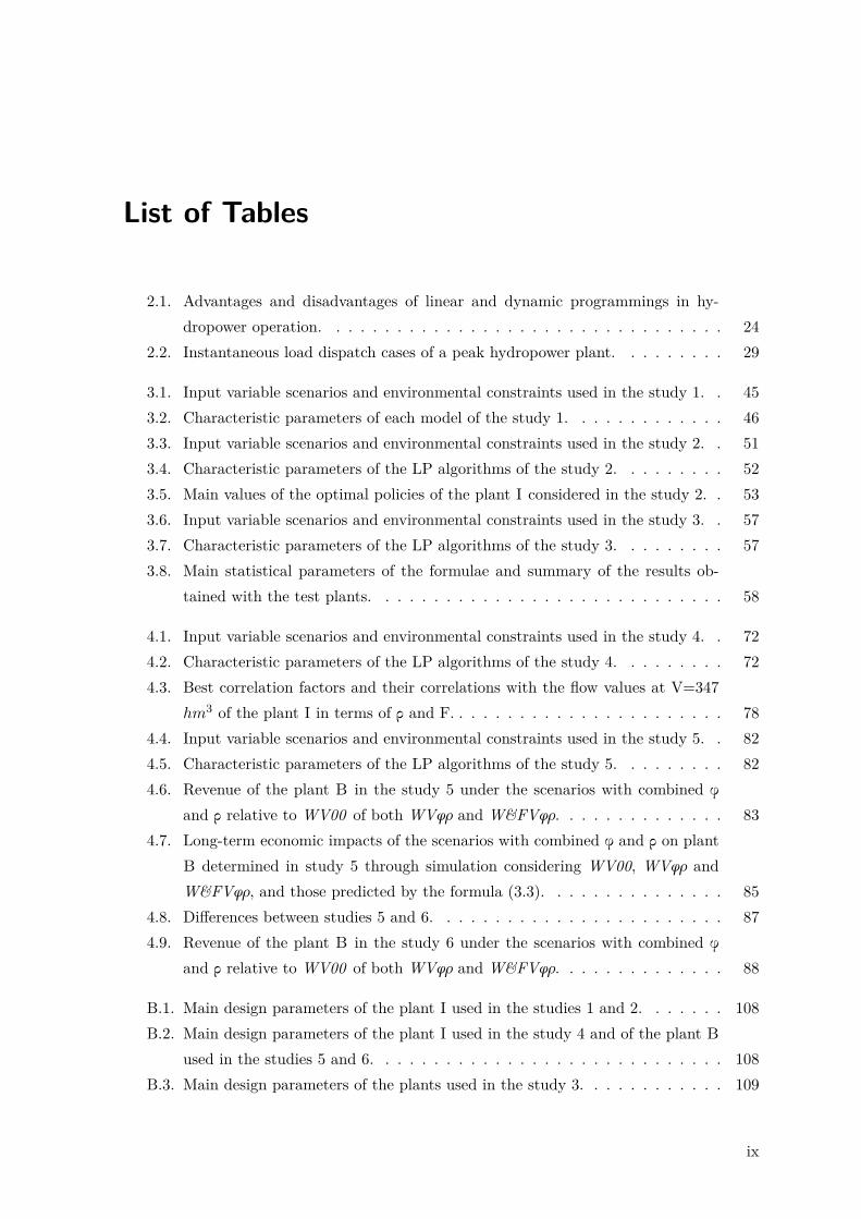
2.1. Advantages and disadvantages of linear and dynamic programmings in hy-dropower operation. . . . . . . . . . . . . . . . . . . . . . . . . . . . . . . . . 24
2.2. Instantaneous load dispatch cases of a peak hydropower plant. . . . . . . . . 29
3.1. Input variable scenarios and environmental constraints used in the study 1. . 453.2. Characteristic parameters of each model of the study 1. . . . . . . . . . . . . 463.3. Input variable scenarios and environmental constraints used in the study 2. . 513.4. Characteristic parameters of the LP algorithms of the study 2. . . . . . . . . 523.5. Main values of the optimal policies of the plant I considered in the study 2. . 533.6. Input variable scenarios and environmental constraints used in the study 3. . 573.7. Characteristic parameters of the LP algorithms of the study 3. . . . . . . . . 573.8. Main statistical parameters of the formulae and summary of the results ob-
tained with the test plants. . . . . . . . . . . . . . . . . . . . . . . . . . . . . 58
4.1. Input variable scenarios and environmental constraints used in the study 4. . 724.2. Characteristic parameters of the LP algorithms of the study 4. . . . . . . . . 724.3. Best correlation factors and their correlations with the flow values at V=347
hm3 of the plant I in terms of ρ and F. . . . . . . . . . . . . . . . . . . . . . . 784.4. Input variable scenarios and environmental constraints used in the study 5. . 824.5. Characteristic parameters of the LP algorithms of the study 5. . . . . . . . . 824.6. Revenue of the plant B in the study 5 under the scenarios with combined φ
and ρ relative to WV00 of both WVφρ and W&FVφρ. . . . . . . . . . . . . . 834.7. Long-term economic impacts of the scenarios with combined φ and ρ on plant
B determined in study 5 through simulation considering WV00, WVφρ andW&FVφρ, and those predicted by the formula (3.3). . . . . . . . . . . . . . . 85
4.8. Differences between studies 5 and 6. . . . . . . . . . . . . . . . . . . . . . . . 874.9. Revenue of the plant B in the study 6 under the scenarios with combined φ
and ρ relative to WV00 of both WVφρ and W&FVφρ. . . . . . . . . . . . . . 88
B.1. Main design parameters of the plant I used in the studies 1 and 2. . . . . . . 108B.2. Main design parameters of the plant I used in the study 4 and of the plant B
used in the studies 5 and 6. . . . . . . . . . . . . . . . . . . . . . . . . . . . . 108B.3. Main design parameters of the plants used in the study 3. . . . . . . . . . . . 109
ix


Abstract
This thesis studies the long-term operation of price-taker peak hydropower plants associatedto reservoirs and subject to minimum flows and maximum ramping rates that sell energy inday-ahead electricity markets. The thesis is organised in five chapters and two appendixes.The first chapter is an introduction of the above-mentioned issue. It aims to provide both
an overview as well as a mathematical description of the addressed problem and define thescope and objectives of the thesis.The second chapter shows a review of the literature related to the main topics tackled in
the thesis, such as the principal approaches of reservoir decision support tools, the optimisa-tion techniques most used in hydro scheduling, the main procedures for the characterisationof the involved random inputs and the methods most employed to estimate the generationcharacteristic of a peak hydropower plant. Furthermore, the chapter also presents a brief de-scription of the hydro scheduling models that have considered minimum flows and maximumramping rates jointly.The third and the fourth chapters are devoted to the achievement of the thesis objectives
and are divided in several studies. Among the main contributions cointaned in these studiescan be found different long-term optimisation models for hydropeaking subject to minimumflows and maximum ramping rates, several sensitivity analyses of the long-term effects ofthese constraints on certain economical and operational aspects of a peak hydropower plant,a set of formulae for the approximate assessment of the long-term economic impact causedby these constraints on this type of plants, and the introduction of a new concept in hydroscheduling: flow value.The fith chapter sets out the conclusions of the thesis which can be summarised as follows.
On the one hand, the presence of minimum flows in hydropeaking increases the spillagevolume and the water value, whereas decreases the generated energy, the number of start-upsand shut-downs of the hydro units, the plant capability for price tracking and the revenue.On the other hand, the presence of maximum ramping rates, in turn, increases the number ofplant operating hours, the spillage volume, and, in the driest weeks, the flow value, whereasdecreases the number of start-ups and shut-downs of the hydro units, the plant capability forprice tracking, the revenue, the water value, and, in the wettest weeks, the flow value.The appendix A contains the equations involved in the developed optimisation models and
the appendix B provides a summary of the main data of the case studies considered in thethird and fourth chapters. Finally, both the cited references and the applied nomenclaturecan be found at the end of the thesis.
1


Resumen
Esta tesis estudia la operación a largo plazo de plantas hidroeléctricas asociadas a embalsessujetas a caudales mínimos y rampas máximas que participan en mercados eléctricos diarioscomo tomadoras de precios. La tesis se compone de cinco capítulos y dos apéndices.El primer capítulo es una introducción de la cuestión mencionada. Proporciona una visión
panorámica, así como una descripción matemática del problema abordado y define el alcancey los objetivos de la tesis.El segundo capítulo muestra una revisión de la literatura relacionada con los principales
temas afrontados en la tesis, tales como los principales enfoques de herramientas de ayudaa la toma de decisión en embalses, las técnicas de optimización más utilizados en progra-mación hidroeléctrica, los principales procedimientos para la caracterización de las variablesaleatorias de entrada implicadas y los métodos más empleados para estimar la característicade generación de una central hidroeléctrica de puntas. Además, el capítulo también presentauna breve descripción de los modelos de programación hidroeléctricos que han consideradoconjuntamente caudales mínimos y rampas máximas.Los capítulos tercero y cuarto están dedicados a la consecución de los objetivos de la tesis y
se componen de varios estudios. Entre las principales aportaciones de estos estudios se puedenencontrar diferentes modelos de optimización a largo plazo para operación hidroeléctrica depuntas sujetos a caudales mínimos y rampas máximas, varios análisis de sensibilidad de losefectos a largo plazo de estas restricciones sobre ciertos aspectos económicos y operativos deuna planta hidroeléctrica de puntas, un conjunto de fórmulas para la evaluación aproximadadel impacto económico a largo plazo causado por dichas restricciones en este tipo de plantas,y la introducción de un nuevo concepto en programación hidroeléctrica: valor del caudal.El quinto capítulo expone las conclusiones de la tesis que se pueden resumir de la siguiente
manera. Por un lado, la presencia de caudales mínimos en la operación hidroeléctrica depuntas aumenta el volumen de vertido y el valor del agua, mientras que disminuye la energíagenerada, el número de arranques y paradas de los grupos hidroeléctricos, la capacidad dela planta para el seguimiento de los precios y los ingresos. Por otro lado, la presencia derampas máximas, a su vez, aumenta el número de horas de funcionamiento de la planta, elvolumen de vertido y, en las semanas más secas, el valor del caudal, mientras que disminuye elnúmero de arranques y paradas de los grupos hidroeléctricos, la capacidad de la planta parael seguimiento de los precios, los ingresos, el valor del agua, y, en las semanas más húmedas,el valor del caudal.El apéndice A contiene las ecuaciones que intervienen en los modelos de optimización desar-
3

rollados y el apéndice B ofrece un resumen de los principales datos de los casos consideradosen los estudios de los capítulos tercero y cuarto. Finalmente, tanto las referencias citadascomo la nomenclatura aplicada se pueden encontrar al final de la tesis.
4

Coautores
No recuerdo cuando fue la primera vez que me imaginé escribiendo estas líneas, pero de loque si me acuerdo es que, ya entonces, intuí que agradecer sería muy poco en comparacióncon la ayuda recibida. Y así ha sido. De ahí la elección del encabezamiento superior, puescon él trato no sólo de dar las gracias, sino de compartir las pequeñas luces que contiene estatesis.Me resulta ineludible comenzar por los principales coautores de este documento: sus direc-
tores. Los profesores J.I. Pérez y J.R. Wilhelmi han sido el genial, en todas sus acepciones,motor de este trabajo siendo yo tan sólo su combustible, en muchas ocasiones para desgraciade ellos, no refinado. Son literalmente maravillosos y no creo que nunca pueda agradecerlestodo lo que han hecho por mí.Afortunada y generosamente, otras muchas personas han colaborado a la realización de este
trabajo con su experiencia, consejo e incluso con sus preguntas. De entre todas ellas cabedestacar, por orden alfabético, a: A. Granados, A. Helseth, A. Rossi, D. García, D. Santillán,D. Valigi, E.E. Rodríguez, F.J. Guisández, G. Doorman, H.I. Skjelbred, J.A. Sánchez, J.I.Sarasúa, K.D.W. Nandalal, L. Garrote, L. Mediero, M. Chazarra, M.T. Guisández, R. Millán,S.P. Bianucci, S. Sañudo, y W. Dragoni.Concluyo aquí mi tesis, en la festividad de Santo Domingo de la Calzada, y a menos de dos
días de casarme con la mujer de mi vida, dando gracias a Dios por todo.
5


1. INTRODUCTION
This chapter aims to provide both an overview as well as a mathematical description of theaddressed problem and define the objectives and structure of the thesis.
1.1. Overview
Energy is essential to economic and social development, to improve quality of life and itmust be produced in a sustainable way [UN (1992)]. Electricity is the most versatile form ofenergy [Perrin (1971)], but nowadays cannot be economically stored [Uritskaya and Uritsky(2015)]. Thus, electricity must be produced at the moment of consumption and, for the sakeof sustainability, it is increasingly generated by new renewable energy sources [BP (2016)],which are usually characterised by being weather-driven and non-dispatchable [Kirkham et al.(1981)].In order to cope with the complexity of generating systems, maintaining high reliability
and low cost, electric systems in many countries all over the world have been moved froma regulated to a liberalised competitive environments [Nogales et al. (2002)]. The resultingelectricity markets operate, usually on a daily basis, assigning hourly energy prices whichare signals that mirror the variations of cost of the energy supplied to the electric system[Schweppe et al. (1980)]; these variations result in avoided costs, reduction in CO2 emissions,etc [Pérez-Díaz and Wilhelmi (2010)]. The operation of these markets is developed in severalstages of transaction [Smeers (2008)]: day-ahead, intra-day and real-time electricity markets.In this context, it is worth highlighting one of the main advantages of hydroelectricity, that
is, its ability to change the generated power quickly; additionally no significant losses are facedwhen at a standstill, except those caused by spillage, evaporation or seepage (depending onthe type of plant and location). This feature allows hydroelectricity to meet hours withthe highest energy consumption (peak hours) at minimum cost [Weedy (1972)] and, as aconsequence, to play a crucial role in the integration of new intermittent renewable energysources [World Water Council (2003)]. This activity is usually carried out by adapting itsproduction to the energy price profile (hydropeaking) [Pérez-Díaz and Wilhelmi (2010)].Hydroelectricy has the highest efficiency, flexibility and reliability of any source of electricity
[Egré and Milewski (2002)] and therefore has become the fourth source of primary energyin the world and the first one among renewable energies [BP (2016)]. However, despite itsrenewable nature, several investigations indicate that hydropower plants can yield undesirableeffects on the ecosystems where are located [Cushman (1985); Eckberg (1986); Pelc and
7

Chapter 1 INTRODUCTION
Fujita (2002); Trussart et al. (2002)]. This is the motive why many countries have developedspecific policies to reduce environmental impacts caused by this power generation technology[ESHA (2012)] and, as a result of these initiatives, the number of constraints to which hydroscheduling is subject has increased considerably [Kosnik (2010)].A hydropower plant is a facility whose purpose is to convert part of the energy of water
(kinetic, potential or pressure) into available electrical energy. There are many types ofhydropower plants [Raabe (1985)], differing greatly from each other in their characteristicsand modes of operation. This thesis is focused on the typology of peak hydropower plantsassociated to reservoirs since it has the greatest installed capacity in Europe [Lehner et al.(2005)].The power generated by a peak hydropower plant depends on the efficiency of the above
named conversion, on the mass of water flowing through each of its turbines per unit time andon the net head. The net head is the energy height at the turbine inlet referred to tailwaterlevel [Warnick (1984)]. The mathematical representation of the relationship among power,flow and net head in a plant is called, i.a., generation characteristic [Pereira (1985)].The operation of this type of plants is usually subject to technical, strategic and opera-
tional constraints [Pérez-Díaz and Wilhelmi (2010)]. Technical constraints habitually denotethose restrictions derived from certain inherent properties of the plant generation equipmentand hydraulic system as, e.g., the maximum and minimum flow through the turbines [Little(1955)]. Strategic constraints, in turn, consider commonly the tracking of longer term guide-lines such as, for instance, water value curves [Boshier et al. (1983)]. Operational constraintscan be due to several reasons such as, e.g., the existence of other priority uses in the reservoir[Kumar and Baliarsingh (2003)].Environmental constraints may be sorted within the group of operational constraints [Ed-
wards et al. (1999)]. There are various types of environmental constraints but the mostcommon, and therefore the only ones considered in this thesis, are minimum flows (φ), whichforce minimum values of water release (F) [EU (2007)], and maximum ramping rates (ρ),which impose maximum rates of change of F [Patten et al. (2001)].Unfortunately, these environmental constraints may cause several negative effects on the
operation of a peak hydropower plant. Perhaps the most important are, on the one hand,that φ limit the ability to store water in the reservoir for use in peak hours and, on the otherhand, that ρ limit its ability to change power output levels [Harpman (1999)]; that is, theseramps introduce some kind of inertia in the plant operation.The immediate consequences of these effects are the reduction in the above-mentioned
ability to follow the load variations as well as in the contribution of the plant to the systemoperation [Harpman (1999)]. This contribution (ancillary services [Eurelectric (2003)]) isoften provided by hydropower plants [Perekhodtsev and Lave (2005)].The subsequent consequences are economic losses [Harpman (1999)], whose quantification
is important to assess the implementation of new environmental regimes [Paredes-Arquiolaet al. (2011)] and in relicensing negotiations [Rheinheimer et al. (2013)], as well as more
8

1.1 Overview
operational difficulties for hydropower producers [Farhat and El-Hawary (2009)]. These lastconsequences are the main motivation of this thesis.
The aim of planning in any activity is to take into account the future consequences ofpresent actions in order to reach a favourable future [Martino (1993)]. From the hydropowerproducer’s point of view, as in any other company, this favourable future is usually that whichmaximises revenue. Accomplishing this goal is a difficult problem due, in addition to the saidissues, to the random nature of the variables involved in hydropower operation such as waterinflow, energy demand, wind generation, temperature and network contingencies [Forsund(2007)].
Water inflow affects the stored volume of water in the reservoir (V) which in turn influencesthe net head of the plant [Little (1955)]. Energy demand influences the energy price [Sauterand Lobashov (2011)]. Wind generation also affects the energy price, if the amount of installedwind power is significant, but it does in reverse direction, the higher the wind generation,the lower the energy price [Jensen and Skytte (2003)]. Temperature influences the energyprice too; this influence is usually direct with high temperature values [Knittel and Roberts(2005)] and inverse with low ones [Koreneff et al. (1998)]. Furthermore, high values of bothwind speed and temperature contribute to the increase in evaporation and, therefore, tothe decrease in V and the net head [Harbeck (1962)]. Network contingencies are relatedto any problem in the electrical system able to affect externally the hydro operation, e.g.:transformer outages, transmission lines outages caused by storms, etc. [Forsund (2007)].
The key question in hydropower operation is to decide when to produce energy, given Vand the available information about the future [Forsund (2007)]. Many decision supporttools have been proposed during past decades to help to answer this question in real-time[Koutsoyiannis et al. (2002)], although very few under environmental constraints [Smith et al.(2007)], especially ρ [Rheinheimer et al. (2013)] and more particularly in a long-term planningperiod (usually one year [Zhao et al. (2010)]).
Real-time in this context usually concerns the optimal operation of an existing reservoirsystem [Yeh (1985)] in which a complex [Guise and Flinn (1970)], and mostly specific [Howard(2006)], set of objectives has to be generally considered. This is due to the fact that eachplant has its own production process and these processes depending on each other within eachbasin [Keppo (2002)]. In addition, from the point of view of the power market, the decisionto produce is also conditioned by the installed capacity of each system: if its capacity islarge enough to influence energy price, the system is a price-maker, otherwise a price-taker[Kelman et al. (2001)].
In conclusion, the problem of hydropeaking operation is hard in itself and even more ifenvironmental criteria are considered. As a matter of fact, despite the large number ofhydroelectric decision support tools developed for this purpose, this aspect has been rarelyconsidered in great detail in the literature and even less in a long-term period.
9

Chapter 1 INTRODUCTION
1.2. Problem description
The problem considered consists of studying the long-term optimal operation of hydropowerreservoirs subject to φ and ρ acting as price-takers within liberalised electricity markets.Optimisation is the science of finding the best solutions to certain mathematical problems
[Fletcher (2000)]. Mathematically speaking, it deals with the minimisation or maximisation ofa function (objective function), which represents the desired objective, subject to constraintson its variables [Nocedal and Wright (2006)]. In the case of the operation of a hydropowersystem, the best solution generally consists in maximising the value of the energy generatedby the system over the time of study (planning period) plus the expected future revenue fromV (water value) at the end of that time (time horizon) [Grygier and Stedinger (1985)].Hydro scheduling is a multistage optimisation problem [Little (1955)]. In this type of
problems, the state of the system at any stage is represented by a set of quantities (statevariables). At each stage, a set of decisions (decision variables) has to be taken in order tolead the system to some feasible state at the beginning of the next stage. This transitionis given by an equation (state transition equation) that takes into account the state at thebeginning of the stage, the decisions made along the stage (time step) and the environment(input variables) that surround and affect the system during the stage [Bellman (1954)].The evolution of the input variables along the planning period can be considered under
two different approaches [Bellman (1954)]: known, whereby the initial state and the decisionsuniquely determine the final state (deterministic approach), or unknown, so the initial stateand the decisions determines a probability distribution of final states (stochastic approach).Both approaches have drawbacks relative to each other. On the one hand, the deterministic
approach provides in general worse results than the stochastic one [Wallace and Fleten (2003)],and on the other hand, the computational burden corresponding to the stochastic approach ismuch higher than that associated to the deterministic one [Zambelli et al. (2006)]. The choicebetween these approaches may be conditioned by any of these certainties: that of forecastsor that, which may be called, of system’s equivalence.The uncertainty of a forecast has sometimes been neglected when the planning period
is short [Bensalem et al. (2007); Nandalal and Bogardi (2007)], e.g., a day [Keckler andLarson (1968)] or a week [Eschenbach et al. (2001)]. Deterministic approach may also berecommended if the system is certainty equivalent [Simon (1956)]. This is ensured whensystem output is measured by a quadratic function, the system dynamic is linear, thereare no inequality constraints and input variables are independent and normally distributed[Philbrick and Kitanidis (1999)].Unfortunately, hydro scheduling is a type of problem that is characterised by being discrete,
non-concave and non-linear [Chang et al. (2001)]. Discreteness is due to the turbine generatorset (hydro unit) on/off status (operating state). Non-concavity arises in some parts of thegeneration characteristic below its best efficiency points. Non-linearity is caused by the natureof the generation characteristic of the hydro units.
10

1.2 Problem description
Despite these features, the deterministic approach can provide both insight into the op-timal behaviour of the hydropower plants [Soares and Carneiro (1991)] and very good re-sults in those hydro systems whose outcomes can be approximated by a quadratic functionsand, provided that, whose reservoir levels are kept at or near the optimum hydraulic heads,whose storage volume capacities cannot significantly restrict normal operations and whose in-puts correspond to normal conditions [Karamouz and Houck (1987); Philbrick and Kitanidis(1999); Zambelli et al. (2006); Ratnayake and Harboe (2007); Ventura and Martinez (2011)].The most common aspects to be defined in order to address hydro scheduling have been
found to be some or all of the following [Yakowitz (1982); Yeh (1985); Wallace and Fleten(2003); Labadie (2004); Nandalal and Bogardi (2007); Iliadis et al. (2008); Gjelsvik et al.(2010); Fayaed et al. (2013)]:
• State transition equation: mass balance equation which represents the conservation ofmass throughout the system.
• Planning period: from one day or one week (short-term) to a few months (mid-term)or one year or more (long-term).
• Time step: from one hour or one day (short-term) to a couple of weeks or one month(mid-term).
• Decision variables: released volume of each reservoir during each stage, or state to bereached at the beginning or the end of each stage.
• Input variables: water inflow into each reservoir, evaporation on each reservoir, energydemand or, lately, energy price.
• State variables: V in each reservoir at the beginning of each stage and also, understochastic approach, previous or current stage’s water inflow into each reservoir and itsforecast for the next stage (if and only if it has not been selected as input variable),previous or current stage’s energy demand or previous or, lately, current stage’s meanenergy price (if and only if neither of them have been selected as input variable).
In the perspective of real-time operation, a hydro scheduling problem should be solved byan optimisation algorithm on the basis of forecast information. As forecasts deteriorate withtime and decisions based on the best possible information are necessary, the problem is usuallyapproached by means of various models with several planning periods (short-, mid- and/orlong-term), and different levels of detail, in such a manner that the shorter the planningperiod, the higher the level of detail [Yeh (1985); Labadie (2004)].These models are hierarchically related as follows: outputs from one model are used as
inputs into the next lower level model of shorter planning period, iterating and updatingwhenever new forecasts become available [Yeh (1985)]. This structure allows to reduce thecomputational burden and therefore the time necessary to obtain a solution [Yeh (2010)].
11

Chapter 1 INTRODUCTION
The process begins with the long- or mid-term model in order to determine the water valueat the end of each stage along the planning period, which depends on future system devel-opment [Doorman (2009)]. Therefore, the stochasticity of the inputs should be considered insome manner but, due to these uncertainties and the associated computational cost, the gen-eration characteristic at each plant is not usually defined with high accuracy. Inputs shouldbe updated at each stage [Yeh (1985)] if there are new mid- or long-term forecasts but, ifthere are not, it is a good practice to run this model in an off-line phase considering thehistorical data of the inputs [Takeuchi and Moreau (1974); Braga Jr et al. (1991); Pritchardet al. (2005); Castelletti et al. (2008)].
Next, the process usually continues, until the end of the planning period, running in real-time the short-term model to provide hourly water releases of every plant [Howard (2006)].This model, which should also be updated at each stage, is more accurate, its uncertaintylevel and computational burden are lower [Yeh (1985)], and its benefit sensitivity is higherthan in the mid- or long-term models [Karamouz et al. (2005)].
According to the above, the water value plays an important role between the long- ormid- and the short-term models [Fosso and Belsnes (2004)] and, in this context, it can beunderstood as an opportunity benefit. Its magnitude is function of V and the time of the year[Stage and Larsson (1961)] (usually monotonically decreasing with V and with the amount ofwater inflow [Gebrekiros et al. (2013)] because of the increasing risk of spill [Perera (1969)])and its performance is not optimal for a randomly given limited water inflow series [Doorman(2009)].
1.3. Scope and objectives
The thesis is focused on long-term optimal operation of peak hydropower plants associatedto reservoirs, operating as price-takers within a liberalised day-ahead electricity market, andsubject to φ and ρ. In order to define more precisely the scope of the study, it should bementioned that the objectives addressed in this thesis are oriented to the operation of singleplants located at the heads of their basins.
The objectives of this thesis are the following:
1. To develop one or more long-term optimisation models for a real-time decision supporttool of a plant subject to φ and ρ.
2. To study the sensitivity of the water value of an existing plant to φ and ρ.
3. To obtain one or more analytical expressions providing a rough estimate of the economicimpact that φ and ρ would cause to the operation of a plant of given characteristics.
4. To contribute to the knowledge about the effects of φ and ρ on the operation of a plant.
12

1.4 Structure of the thesis
1.4. Structure of the thesis
Besides this introduction, the thesis is organised in four chapters and two appendixes asfollows: chapter 2 reviews the key aspects of the literature related to the thesis, chapter 3and chapter 4 deal with the achievement of the above-mentioned objectives, chapter 5 sum-marises the findings of the thesis and proposes future research avenues, appendix A containsthe equations involved in the developed optimisation models and appendix B presents themain data of the considered case studies. Finally, both the used references and the appliednomenclature can be found at the end of the thesis.
13


2. LITERATURE REVIEW
This chapter shows a review of the literature related to the main topics tackled in the thesis.It begins describing the principal approaches of reservoir decision support tools under whichpeak hydropower plants have also been managed. Next, the optimisation techniques mostused in hydro scheduling are commented. Then, the main procedures used for the charac-terisation of the involved random inputs are presented. After, the methods most employedto estimate the generation characteristic of a peak hydropower plant are displayed. Finally,the chapter concludes with a brief description of the hydro scheduling models that haveconsidered φ and ρ jointly.
2.1. Decision support tools
A decision support tool is any implement that is applied to a decision support process[Kapelan et al. (2005)], whose mission is to calculate and manage the attendant risks ofpotential decisions involved in the process [Buchanan and O‘Connell (2006)].There have been appeared a huge number of decision support tools in the field of reservoir
system management during the last decades [Koutsoyiannis et al. (2002)]. These are oftenclassified according to one or more of the following three aspects (Fig. 2.1), which here havebeen termed: decision-making approaches, uncertainty treatments and control approaches.
2.1.1. Decision-making approaches
The distinction of three main basic decision-making approaches of a decision support tool iswidespread in the literature. These are simulation, optimisation and combined optimisation-simulation decision-making approaches. In what follows, the more important aspects of theseapproaches will be briefly discussed [Yeh (1985); Wurbs (1993); Labadie (2004); Loucks andvan Beek (2005); Rani and Moreira (2010); Fayaed et al. (2013)].The simulation approach consists in modelling a system in an accurate way and then, for
each set of input data, obtaining a response. These input data include decision rules, thus asimulation model helps to answer what if questions concerning the performance of differentoperational policies and determine which is the best of all them.The optimisation approach (as discussed in sec. 1.2) provides the best policy from a usually
simpler model of the system in one or more scenarios. This policy is the set of decisions thatoptimise one or more objective functions subject to a set of constraints.
15

Chapter 2 LITERATURE REVIEW
Whereas simulation tools are restricted to foreseeing system performance for the evaluatedscenarios, optimisation tools automatically search for the best response of the simplifiedmodel. The time spent to achieve this response it can be considerably less than that requiredby simulation.
The combined optimisation-simulation approach takes sequentially the best of both tech-niques. First, a suboptimal policy is obtained by means of an optimisation model. And then,this policy is simulated in order to furnish more precise evaluations of the system performanceassociated with the obtained decisions.
2.1.2. Uncertainty treatments
Uncertainty can be treated in two ways within decision support tools: implicit or explicitstochastic treatments. Their main features are presented below [Labadie (2004); Rani andMoreira (2010); Fayaed et al. (2013)].
The implicit treatment is characterised by the use, as input data, of series of historical orsynthetically generated values of the random input variables, or equally likely sequences. Inthis option, the stochastic aspects of the problem are implicitly included and the resultingpolicy is obtained by means of regression analysis.
The explicit treatment works directly through the probability distributions of the randominput variables by taking these functions as input data. The resultant policy is determinedautomatically by this approach.
Both treatments have drawbacks. In the implicit case, regression analysis can prove inreduced values of the correlations that would invalidate the obtained operating rules, andattempting to infer policies from other methods can need extensive trial and error processeswith little general applicability. The explicit case, in turn, is more computationally challeng-ing.
2.1.3. Control approaches
In its role of control tool, decision support tools may be structured in two ways: open- orclosed-loop control approaches. Their short descriptions are as follows [Bras et al. (1983);Golnaraghi and Kuo (2003)].
In the open-loop approach the values of the decision variables throughout a planning periodare chosen at the beginning of that period, regardless of system evolution.
In the closed-loop approach the decision support tool includes feedback from the systemstate and, thus, every decision is made according to the current state of the system, even theupdated forecasts of the input variables.
The first approach is easier to implement and faster to execute but does not consider thesystem evolution. The second one is obviously more difficult to develop and slower to runbut it includes feedback and therefore the results are more realistic.
16

2.2 Optimisation techniques
Figure 2.1.: Classification of reservoir decision support tools.
2.2. Optimisation techniques
A wide range of optimisation techniques has been applied to determine the optimal oper-ation of power systems since the past century [El-Hawary and Christensen (1979)]. Linearprogramming (LP) and dynamic programming (DP) are the most popular techniques amongthem for reservoir systems [Nandalal and Bogardi (2007)]. The former has been normallyused for short-term studies [Catalão et al. (2010)] and the latter more frequently for long-term ones [Dias et al. (2010)]. In addition, hybrid optimisation models that combine and takeadvantage of the best of both techniques have been used with remarkable success [Becker andYeh (1974); Mariño and Mohammadi (1983); Grygier and Stedinger (1985); Warland et al.(2008); Cristóbal et al. (2009); Abgottspon and Andersson (2012); Philpott et al. (2013)].What follows is an explanation of the foundations of both techniques as well as a review oftheir most accurate variants from a hydropeaking point of view.
2.2.1. Linear programming
LP [Fourier (1826), cited in Grattan-Guinness (1970)] is a technique to solve optimisationproblems in which their objective functions and constraints are linear. According to the typeof variables involved in the problem, there are several types of LP [Kall and Mayer (2011)](Fig. 2.2). These can be all reals (real LP), all integers (integer LP) or some reals and someintegers (mixed LP). In addition, the input variables may be treated in two specific manners(as discussed in sec. 1.2): deterministic (deterministic real {or} integer {or} mixed LP) orstochastic approaches (stochastic real {or} integer {or} mixed LP).
17

Chapter 2 LITERATURE REVIEW
Figure 2.2.: Types of linear programming.
Among its advantages (Tab. 2.1) stand out efficiency to solve big problems and convergenceto global optimal solutions [Yeh (1985)]. Furthermore, during the process of resolution, thebest solution obtained at each moment is available [Carrión and Arroyo (2006)] being de-creasing its speed of approximation to the optimum over time [Carvalho and Pinto (2006)].Its widespread use is due also to its ease for formulating a broad range of problems with mod-erate endeavour. This is because a huge number of objective functions and constraints thatappear in the practice are linear [Luenberger (2003)]. Unfortunately, the hydro schedulingproblem is discrete, non-concave and non-linear (as discussed in sec. 1.2).The treatment of this last feature represents the main disadvantage of LP (Tab. 2.1) that is
the restriction of using linear objective functions and constraints [Rani and Moreira (2010)].Some techniques to deal with these difficulties are: to add integer variables (in the cases of thereal versions) [Dantzig (1954)], to use piecewise linear approximations [Markowitz and Manne(1957)] and to apply successive times this optimisation technique increasing accuracy aroundthe previously obtained solution (successive LP [Griffith and Stewart (1961)]). Unfortunately,the two former techniques increase the computational burden [Babayev and Mardanov (1994)]and the latter may not converge or cause infeasibility [Vargas et al. (1993)]. Prominentexamples of these techniques within the hydropower systems field are:
• Yeh et al. (1979): the hydro scheduling of a large system was solved by successive LP.
• Piekutowski et al. (1993): the generation characteristics of a system were modelled bymeans of several piecewise linear concave curves whose break points were located atnull generation, maximum efficiency generation and full gate flow of each plant.
• Conejo et al. (2002): the generation characteristic of a plant was represented throughthree piecewise linear non-concave curves and five groups of binary variables that al-lowed to take into account the head effect, non-concavity of the characteristic and thehydro unit on/off status.
18

2.2 Optimisation techniques
Since all constraints are linear in a LP problem, its feasible region is usually an enclosedregion limited by linear hyperplanes [Deb (1995)].There are several methods to find the global optimum of real linear problems but, from
the computational viewpoint, the most competitive are [Illés and Terlaky (2002)]: pivot andinterior-point methods.The idea of pivot method [Dantzig (1948)] is to proceed from one solution to another,
both at extreme points of the feasible region, in such a way as to continually improve thevalue of the objective function until the global optimum is reached. For its part, the interior-point method [Karmarkar (1984)] performs the search of this optimum from the inside of thefeasible region to its surface. This difference in strategies, in the case of very large problems,provides faster resolution to interior-point method [Illés and Terlaky (2002)].There are also various methods to solve mixed linear problems. The most relevant are
[Bixby (2012)]: branch-and-bound, cutting-plane and branch-and-cut methods.Branch-and-bound method [Land and Doig (1960)] is based on the following process. Be-
ginning from the global optimum of the real linear relaxation of the mixed linear problem,the feasible region is sequentially divided into smaller and smaller subregions, and both bestand worst bounds for the objective function are estimated and updated by any of the above-mentioned methods to solve real linear problems. The division continues until all subregionshave been explored or until the distance between the best feasible solution and the updatedbest bound is lower than a specified tolerance.Cutting-plane method [Gomory (1960)] starts also from the global optimum of the real
linear relaxation of the mixed linear problem; likewise calculated by any of the methods forreal LP. If it is infeasible within the original problem, then a cut is made, that is, a constraint,which does not exclude any feasible solution, is introduced into the relaxed linear problem.Next, the real linear problem is solved again. This process is repeated until the globaloptimal feasible solution is found or until the distance between the best feasible solution andthe solution of the last relaxed linear problem is lower than a specified tolerance.Branch-and-cut method [Grötschel et al. (1985)] consists in the combination of the two
previous methods. In this combination, after each division and having not been successfulin searching a feasible solution within the subregion, a cut is made and it is solved again. Ifagain no solution is found, it branches and the process is repeated until the feasible region isdepleted.Of these three methods the most efficient is the last one [Li and Shahidehpour (2005)].
Because of the feasible region is reduced as the process progresses, and only if the problemis very large, the first relaxation can be calculated using the interior-point method and thefollowing can be estimated using the pivot method [Mitchell (2002)].There are three factors that influence the speed of solving mixed LP problems [Lima and
Grossmann (2011)]: problem statement, solver configuration and computer employed.Regarding the problem statement, a good example of how to accelerate the resolution
process is the above-mentioned approach proposed in Piekutowski et al. (1993). In relation
19

Chapter 2 LITERATURE REVIEW
to the configuration of the solver, and for a given type of problems, trying different methodsand carrying out a sensitivity analysis of the optimisation parameters of the solver in thetest phases can save much time later [Carvalho and Pinto (2006)]; e.g., in the case of largescale problems, stopping the calculation when the difference between the best integer solutionfound so far and the best possible integer solution (relative optimality criterion) less than1% [Fu and Shahidehpour (2007)]. Finally, not only the processor speed of the computer isimportant, using of multiple threads in parallel may be very convenient if enough memory isavailable [Baslis and Bakirtzis (2011)].
2.2.2. Dynamic programming
DP [von Neumann and Morgenstern (1944)] is a technique to solve multistage problems basedon the optimality principle [Bellman (1954)] which states that a sequence of decisions (policy)is optimal if and only if every decision of it is optimal. Following this principle, a multistageproblem can be decomposed, according to its state transition equation, into a series of one-stage problems that are solved sequentially over each stage in an iterative process (sense ofadvance).Different classifications of DP are possible depending on the chosen characterisation of the
features of the multistage problem. The most usual of them are described below: state space,decision making, input variables and sense of advance (Fig. 2.3).The state space can be considered discrete (discrete DP) or not (continuous DP). This latter
choice requires that the system functions are differentiable with respect to state and control[Yakowitz (1982)]. In the case of hydropower operation, it involves not only a substantialsimplification of its equations, causing loss of accuracy in the results, but also the use of sometechniques embedded in this continuous DP, e.g., mixed LP. Hereinafter only the discreteversion will be considered.The decisions may be taken discreetly (discrete DP) or continuously (continuous DP)
[Bellman and Kalaba (1965)]. What follows only deals with the first version because thestages in multireservoir system operation are uniform time intervals [Labadie (2004)]. Asin the literature, the combination of the above-mentioned discrete versions receives also thedenomination of discrete DP; this nomenclature is used hereinafter.The input variables may be considered in two different ways (as discussed in sec. 1.2):
deterministic (deterministic DP) or stochastic approaches (stochastic DP). In the first case,a single policy is obtained for each state, but in the second one, a decision is obtained forevery feasible state and input combination at each stage (steady-state policy) [Loucks andvan Beek (2005)].Under deterministic assumptions, the single policy is directly obtained through one run
of DP. However, unless the considered planning period were long enough, under stochasticassumptions and invariant probability distributions between stages for the input variables,it would be necessary to apply several times DP to find the steady-state policy because, at
20

2.2 Optimisation techniques
Figure 2.3.: Types of dynamic programming.
each iteration, the results of the previous iteration have to be aggregated at the beginningof the current iteration until convergence is reached [Loucks and van Beek (2005); Nandalaland Bogardi (2007)]. In the case of hydropower plants, the planning period of each iterationshould be at least larger than the ratio between the volume capacity of the reservoir and theaverage annual water inflow (regulation capacity).There are two criteria of convergence [Nandalal and Bogardi (2007)]: stabilisation of the
policy and stabilisation of the expected revenue increment.The convergence by stabilisation of the policy [Chow et al. (1975)] is achieved when the
decision for any state at any stage remains unchanged in each iteration.The expected revenue increment is, in each iteration, the increase in value of the objective
function for any state over the period of study. The stabilisation of the expected revenueincrement [Loucks et al. (1981)] is reached when this increase becomes constant and indepen-dent of the state. This criterion of convergence is not always achieved in practice [Nandalaland Bogardi (2007)] (as discussed in sec. 2.3.1).
21
Chapter 2 LITERATURE REVIEW
Regarding the last feature of the problem, the sense of advance can be forwards (forwardDP) or backwards (backward DP). In a deterministic context, forward advance is more effi-cient than the backward one when the initial state is fixed and the terminal state is free andand vice versa [Larson (1967)]. However, in a stochastic context, only backward advance hassense since the expectation over the future states has to be considered [Yeh (1985)].DP is, jointly with LP, the most used technique within the field of multireservoir sys-
tem operation [Nandalal and Bogardi (2007)]. Among its advantages (Tab. 2.1), it is worthhighlighting that its computational burden increases linearly with the number of stages anddecreases with the presence of constraints. Moreover, it deals well with the above-mentionedfeatures of hydropower operation [Labadie (2004)] (as discussed in sec. 1.2).The main disadvantage (Tab. 2.1) of this technique is its ingeniously named curse of di-
mensionality [Bellman (1957)]. It is due to the fact that the number of transitions to beevaluated increases exponentially and potentially as the number of state variables and theirdiscretisations increase respectively.Several variants of the conventional procedure of discrete DP and some methods, specifically
designed to simplify multireservoir problems, have been proposed in order to mollify the saidcurse.Concerning the general variants, the most significant are [Labadie (2004)]: coarse grid and
interpolation technique, incremental DP and DP successive approximations.Coarse grid and interpolation technique [Bellman (1957)] reduces the number of transi-
tions that must be evaluated by using big discretisation intervals and then interpolates overthis coarse grid. This interpolation can be made by means of different methods, piecewisepolynomial cubic splines being one of the most efficient [Johnson et al. (1993)].Incremental DP [Bernholtz and Graham (1960)] consists in iteratively optimising in the
state space neighbourhood (corridor) of one or more given trial policies. At the beginning,a corridor, with an arbitrary width, is built around each trial policy. Then, a new policyis obtained by means of DP and, after that, two possible convergence criteria can be useddepending on whether the width of the corridors is kept fixed [Bernholtz and Graham (1960)]or progressively reduced [Turgeon (1982)].By the first criterion, if the new policy is touching any of the boundaries of the considered
corridor, the process is repeated but now around this latter policy and so on until the obtainedpolicy does not touch. By the second criterion, the process stops only when the relativedifference between the values associated with consecutive iterations is less than a chosentolerance. Under this latter criterion, if the chosen tolerance is not reached but the obtainedpolicy does not touch the borders of the considered corridor, the width of the followingcorridor is reduced and so on until the tolerance is achieved [Nandalal and Bogardi (2007)].Anyway, this variant has some inherent difficulties such as it is very sensitive to the initialtrial policies and the width of the corridor [Labadie (2004)].DP successive approximations [Bellman and Dreyfus (1962)] decomposes the multidimen-
sional problem into a series of one-dimensional problems by optimising over one state variable
22

2.2 Optimisation techniques
at a time, with the rest of state variables kept at given current values.Although the former is the worst of these variants to overcome the curse [Yakowitz (1982);
Yeh (1985); Labadie (2004)], the two latter ones share two important limitations. Both arehighly dependent on knowledge of the system state with certainty and accordingly they are notadequate for stochastic DP [Labadie (2004)] and their convergence to global optimums is notguaranteed for non-concave and non-convex problems [Yakowitz (1982)] such as hydropoweroperation ones.Relating to the methods to simplify multireservoir problems (aggregation-decomposition
methods [Ahmed et al. (1965)]), all consists generally in five steps. First, calculating thepotential energy of each plant in the system. Second, adding the stored water volume ofthe system. Third, building a generation function of the whole system that represents itsmain characteristics. Fourth, optimising the resulting problem. And finally, decomposing theresults.Under deterministic approach, aggregation-decomposition methods are calculated in a sin-
gle optimisation. However, under stochastic assumptions, the needed number of optimisationsdepends on how the system has been defined. Thus, these methods can be computed in asingle optimisation when the whole system is aggregated in one state variable [Terry et al.(1986)] or in as many as considered reservoirs when the rest of the system is aggregated inone [Turgeon (1980)] or two state variables [Archibald et al. (1997)]. All these approachesseverely simplify the system topology [Castelletti et al. (2007)].State variable discretisation can be realised by many different space filling ways [Crombecq
et al. (2011)] but perhaps the most interesting in DP are [Cervellera et al. (2006); Fan et al.(2013)]: uniform, orthogonal array and number theoretic methods.The discretisation on uniform grid is the most employed distribution and, as its name
implies, is homogeneous in the whole state space [Cervellera et al. (2006)]. It provides a goodperformance when the problem is not too large [Philbrick and Kitanidis (2001)].Orthogonal array [Kishen (1942)] consists in, from the intervals of a uniform discretisation,
selecting randomly states in such a way that, according to an arbitrary number (strength),for any subset of the involved state variables, all possible variable-state combinations appearwith the same frequency. In the case that the strength is one, the resulting orthogonal arrayis called Latin hypercube [Tang (1993)].Number theoretic methods are a combination of number theory and numerical analysis
[Fang et al. (1994)]. This class of methods generates uniformly spaced designs where thedomain of interest is normalised to the closed and bounded unit “cube” (with as manydimensions as state variables) for convenience by minimising a discrepancy measure. Stardiscrepancy is among the most used measures [Fan et al. (2013)] and it can be defined asthe maximum deviation between the uniform distribution and the generated by this classof methods [Niederreiter (1992)]. The generation of the states is based on low discrepancysequences such as, e.g., Hammersley [Hammersley (1960)], Halton [Halton (1960)] and Sobol[Sobol (1967), cited in Atanassov (2003)] sequences. Both this way and the previous one
23

Chapter 2 LITERATURE REVIEW
reduce the computational burden of high dimensional problems [Cervellera et al. (2006)].
Regardless of the way chosen, the discretisation of V, which is probably the most importantstate variable in reservoir operation [Goulter and Tai (1985)], has two important features. Onthe one hand, a coarse discretisation produces high skewness in the storage probability distri-bution functions and influences the optimal policy [Klemeš (1977); Goulter and Tai (1985)].On the other hand, the decreasing size of its intervals does not automatically guarantee betterresults and the improvement, if any, does not occur continuously [Bogardi et al. (1988)].
A specific criterion for selecting the discretisation of this variable is to set its interval shorterthan the volume equivalent to the smallest water inflow [Ratnayake and Harboe (2007)]. Inthis context, several studies have shown numerical results that suggest as a good discretisationthat in which the number of V states per reservoir is between 9 and 33 [Moran (1959); Doran(1975); Goulter and Tai (1985); Bogardi et al. (1988)].
Finally, since V in a system are related to each other [Durán et al. (1985)], some combina-tions of these are really unreasonable, e.g., one reservoir will not be empty while the othersare full. Thereupon it may be convenient to reduce the state space around a corridor ofreasonable volumes [Stedinger et al. (2013)].
Table 2.1.: Advantages and disadvantages of linear and dynamic programmings in hy-dropower operation.
Techniques Advantages Disadvantages
LP· Convergence to global optimal solutions. · Restriction of using linear· Ease of formulating. objective functions and· Efficiency to solve big problems. constraints.
DP
· Computational burden increases linearly · Computational burdenwith stages and decreases with increases exponentiallyconstraints. with state variables and
· Discreteness, non-concavity and potentially with statenon-linearity immunity. space discretisation.
2.3. Input variables
Any dynamics in nature is stochastic to some degree [Cvitanovic et al. (1999)] and hydropoweroperation is not an exception [Little (1955)]. Markov chains are the first, most importantand simplest mathematical models for random phenomena evolving in time [Norris (1998)]and they have been used extensively in reservoir operation models [Yakowitz (1982); Yeh(1985); Labadie (2004); Loucks and van Beek (2005); Nandalal and Bogardi (2007)]. Thereare many input variables that affect hydro scheduling [Forsund (2007)] but probably the mostsignificant are: water inflow [Belsnes and Fosso (2008)], energy price [Fosso et al. (1999)] andin some basins [Torcellini et al. (2004)], especially over the long-term [Yu et al. (1998)],evaporation [Teixeira and Mariño (2002)]. What follows deals with these input variables butbefore an explanation of Markov chain theory is given.
24

2.3 Input variables
2.3.1. Markov chain theory
Markov chains are frequently applied in optimisation of multireservoir systems and consideredconvenient for this function [Loucks and van Beek (2005)] despite showing low persistence andnot capturing the variance of some of their input variables [Stedinger et al. (2013)]. A Markovchain [Markov (1906), cited in Basharin et al. (2004)] consists in a set of states (classes) and aset of branded transitions between these classes. After a halt in a class, the Markov chain willmake a transition to another class. Such transitions are branded with either probabilities oftransition (discrete-time Markov chain) or rates of transition (continuous-time Markov chain)[Bolch et al. (2006)]. What follows only deals with the discrete type because the stages inmultireservoir system operation are uniform time units [Labadie (2004)].
In order to model a random variable during a period of time in which it has a repetitivepattern (time cycle) by means of a Markov chain, it is necessary to make two assumptions[Kemeny and Snell (1960)]: each transition probability of the variable depends only on itsrecent past (markovianity) and remains constant over the time cycle (stationarity).
Markovianity is the critical feature of a Markov model [Meyn and Tweedie (1993)] andmay manifest itself with different orders of dependence. The order (lag) of a Markov chainis the number of time units from the current time whose variable values are involved in thedefinition of the actual variable value [Lowry and Guthrie (1968)]. With the aim to operatewith ease, the transition probabilities of a random variable are usually collected in an array(transition probability array) of order equals to one plus its lag [Preda and Balcau (2008)].
Stationarity is the necessary condition to guarantee that the policy of a multistage problemwill become stable after a certain number of cycles [Nandalal and Bogardi (2007)]. Thisproperty is recognised within a Markov chain when its transition probability arrays do notchange over the cycle [Wallace and Bassuk (1991)].
There are several types of Markov chains [Kolmogoroff (1936), cited in Mazliak (2007)]but there is only one that ensures that the stable policy of a multistage problem, that hasbeen derived from it, will be the global optimum [Howard (1960)]: ergodic Markov chain.This type has the three following properties [Solow and Smith (2006)]: each of its classes caneventually be reached from every other class (irreducible), the expected return time to eachclass is finite (positive recurrent) and starting in each class, there exists no regular period atwhich the class cannot be reached (aperiodic).
The violation of the ergodicity can be caused by a large number of zero elements in the tran-sition probability arrays, and additionally can provoke the failure in the stabilisation of theexpected revenue increment (as discussed in sec. 2.2.2). Those zero elements are inaccuraciesbecause of lack of data [Nandalal and Bogardi (2007)].
This problem can be circumvented by two compatible methods [Nandalal and Bogardi(2007)]: smoothing and, which may be called, discretisation thickening.
The smoothing method [Bellman and Dreyfus (1962)] consist in replacing the zero elementsby small quantities which are subtracted from the non-zero elements. This replacement is
25

Chapter 2 LITERATURE REVIEW
done only when more than half the elements of a subarray of a discretisation class are zeroand must be done such that the sum of the transition probabilities of this subarray equalsone [Nandalal and Bogardi (2007)].
The discretisation thickening method [Nandalal and Bogardi (2007)] is based on the ideathat the number of zero elements depends on the ratio between the number of discretisationclasses of the considered variable and its total number of available historical observation data.It is convenient that the total number of data be greater than half the cubic of its classes.
Regarding the determination of the lag of a Markov chain, the most common tests are[Wilks (2006)]: Akaike [Akaike (1971)] and Bayesian [Schwarz (1978)] information criteria.Both criteria are based on the log likelihood functions for the transition probabilities of theMarkov chains. These log likelihoods depend on the transition counts and the estimatedtransition probabilities [Wilks (2006)]. The Akaike criterion tends to be less conservative,generally picking higher orders than the Bayesian one when the results of the two tests differ.The use of this last criterion can be preferable for sufficiently long time series (between 100and 1000 data) depending on the nature of the serial correlation [Katz (1981)].
Finally, regarding the variable discretisation, in addition to the considerations mentionedin the previous section, it is advisable to maintain its extreme values, both low and high, toimprove the performance of the system operation [Kim and Palmer (1997); Mo et al. (2001)].
2.3.2. Water inflow
Water inflow can be defined as the volume of water that arrives in a natural way (by rainfall,runoff and snowmelt) at a reservoir per stage. It is the most important input variable inhydropower operation [Belsnes and Fosso (2008)], especially when the storage levels are nearlyempty or nearly full [Fleten et al. (2009)], and its importance lies in its influence on V andthe net head [Little (1955)].
The use of Markov chains to model monthly water inflow [Stedinger et al. (1984)], aswell as daily [Jimoh and Webster (1996)] and weekly [Deni and Jemain (2012)] rainfall, iswidespread in the literature. Generally, in a multireservoir system, water inflows are spatiallyand temporally correlated and only for very long time steps, of perhaps one year or more,these correlations do not occur [Philbrick and Kitanidis (1999)]. With the aim of reducing thenumber of water inflow variables to be modelled in a this kind of systems, it has been appliedprincipal component analysis providing good results [Saad and Turgeon (1988); Archibaldet al. (2006)]. This is possibly the most broadly used multivariate statistical technique in theatmospheric sciences [Wilks (2006)].
Principal component analysis [Pearson (1901)] consists in transforming an original set ofinterrelated variables into another smaller one formed by new uncorrelated variables whichare linear combinations of the initial ones. This transformation has to be made with the goalof keeping as much as possible of the variability present in the original set.
26

2.3 Input variables
2.3.3. Energy price
Energy price, in this context, represents the price received by producers for selling energy. Inthe case of deregulated electricity markets, this price is generated from one day to anotherand would represent the marginal value of produced energy at each hour in the market [Fossoet al. (1999)]. Its behaviour is characterised by: non-constant mean and variance, multipleseasonality, calendar effect, and high frequency, volatility and percentage of unusual values[Nogales et al. (2002)]. Despite the difficulty of modelling these features, given the importanceto price-takers [Gjelsvik et al. (2010)], there is a large variety of techniques that try to do it[Bunn (2004)].In mid- and long-term hydro scheduling of a system composed only of price-takers, one of
these techniques consists in using the average of energy price during the considered stage bymeans of a Markov chain [Gjelsvik et al. (1999)]. This technique, on the one hand, is probablythe simplest and computationally less burdensome one, but, on the other hand, usuallyunderestimates revenues because it disregards hydropeaking [Olivares and Lund (2011)]. Analternative to model this input variable is based on the consideration of different scenariosof hourly values [Abgottspon and Andersson (2012)]. Of course, it is also possible to useboth [Helseth et al. (2013)]. Finally, if, after a statistical analysis, there is a significantcorrelation between this input variable and others (usually water inflow), this correlationmust be considered [Löhndorf et al. (2013)].
2.3.4. Evaporation
Evaporation is the gradual solution of water in air [Hamilton (1767)]. This process is in-fluenced by many factors, such as solar radiation, vapour pressure deficit, relative humidity,wind speed and air temperature [Xu and Singh (1998)]. Depending on the climate where itsmagnitude need to be determined, it can be estimated by many different equations which, inturn, may require very diverse data. This circumstance usually makes it difficult to decidewhich is the most proper one for a given location [Winter et al. (1995)].Among the principal factors that inevitably conditions the choice of a particular equation
is the available data [Warnaka and Pochop (1988)]. As air temperature is the easiest andcheapest data to measure among the above-mentioned [Ortuño et al. (2010)], the equationsthat require only this input (temperature-based equations) are frequently used [Zhang et al.(2012)]; sometimes even offering better results than more complex equations [Rosenberryet al. (2007)]. The main drawback of the temperature-based equations is that its accuracydepends on the correlation between air temperature and solar radiation of the place wherethey were developed [Juday et al. (2011)]. Therefore, if this correlation varies from a placeto another, then their parameters must be recalibrated [Xu and Singh (2001)].Regardless of the equation used to calculate the evaporation rate, reservoir evaporation
loss is commonly estimated as the product of this rate and the average water surface duringthe considered period [Loucks et al. (1981)]. Therefore this loss is related to V.
27

Chapter 2 LITERATURE REVIEW
2.4. Generation characteristics
The generation characteristic (also known as water rate curves, characteristic curves andproduction function [Pérez-Díaz et al. (2010)]), of both a single hydro unit and a whole peakhydropower plant, describes the relationship between its released flow, its available head,and its generated power [Conejo et al. (2002)]. Its graphical representation (power charac-teristic surface) is, therefore, three-dimensional and it can be modelled by a set of usuallypower-discharge curves (performance curves), each for a specified head [García-González andCastro (2001)]. It is the most crucial modelling aspect in daily hydro scheduling [Nilsson andSjelvgren (1997b)].In the case of a single hydro unit, its power characteristic surface is usually provided by its
manufacturer and so the hydraulic losses in the plant conduits are not included [Maruzewskiet al. (2012)]. Additional information that should be included in this case, if any, are theundesirable generation levels (forbidden zones) of the hydro unit [Finardi and da Silva (2005)].In the case of a whole plant with several hydro units, its generation characteristic can be
modelled individually per hydro unit [Chang et al. (2001)] or as the result of the allocationof water among the hydro units that maximises total plant power output for given flowdischarged and gross head (instantaneous load dispatch) [Allen and Bridgeman (1986)]. Akey aspect of this allocation is that the hydro unit start-up and shut-down costs [Nilsson andSjelvgren (1997a)] must be contemplated [Siu et al. (2001)].Given its importance in short-term and that LP (as discussed in sec. 2.2.1) is the most
used technique in this planning period, an explanation of the main types of models of theperformance curves used within LP based hydro scheduling models is included in what follows.After, a description of the cases of hydropower instantaneous load dispatch is provided.
2.4.1. Performance curves
There are several models to represent performance curves in LP based hydro scheduling mod-els. The most representative can be enumerated, in order of increasing accuracy [Borghettiet al. (2008); D’Ambrosio et al. (2010)], as follows:
1. A piecewise linear concave function with breakpoints at the points corresponding tominimum power, local best efficiencies and maximum total flow [Habibollahzadeh andBubenko (1986)].
2. Several piecewise linear non-concave functions [Conejo et al. (2002)].
3. A dotted non-concave mesh (one-dimensional method) [D’Ambrosio et al. (2010)].
4. A triangular non-concave mesh (rectangle method) [García-González and Castro (2001)].
The choice among these models depends on the trade-off between the quality of the repre-sentation and the computational time on its evaluation [D’Ambrosio et al. (2010)]. On theone hand, models with one linear function neglect the variation of the head [Conejo et al.
28

2.4 Generation characteristics
(2002)] which is only recommended for relatively large reservoirs and short-term planningperiods. On the other hand, numerical results have shown that one-dimensional method isconsiderably better than several other functions [Borghetti et al. (2008)] but, in comparisonwith rectangle method, it improves very little the solution at the expense of spending a lotof time [D’Ambrosio et al. (2010)].
2.4.2. Instantaneous load dispatch
Depending on the number of hydro units, whether or not the turbine models are equal,they are fed by the same penstock or have the same hydraulic losses, and their individualgeneration characteristics are concave, three different cases can be distinguished to determinethe instantaneous load dispatch of a peak hydropower plant (Tab. 2.2) whose descriptions areas follows:
Table 2.2.: Instantaneous load dispatch cases of a peak hydropower plant.
Hydro Turbine Hydraulic Power characteristicCases
units models losses surfaces
1 ∀ ∀ ∀ A
>1 == concave B
non-concave
C6= ∀
6= ∀ ∀
• Case A refers to a hydro plant with a single unit. The instantaneous load dispatch isobviously straightforward and the resulting generation characteristic consists simply inadding the hydraulic losses of the plant to the hydro unit power characteristic surface.
• Case B refers to a hydro plant with several identical hydro units with a concave powercharacteristic surface and equal hydraulic losses. From the Karush-Kuhn-Tucker con-ditions [Karush (1939)], it is possible to demonstrate that the solution is such that allunits in operation must have the same partial derivative of the flow with respect to thepower. Since for each flow and gross head, there may exist several feasible combina-tions of units in operation, it is necessary to evaluate and compare to each other themaximum power of each feasible combination in order to determine the best solution.
• Case C encompasses the rest of the situations. Many optimisation techniques have beenapplied to solve this case being DP (as discussed in sec. 2.2.2), due to its effectiveness[Yi et al. (2003)], one of the most common among them [Padhy (2004)].
29

Chapter 2 LITERATURE REVIEW
2.5. Hydro scheduling models with minimum flows and maximumramping rates
What follows is a revision of the most hydro scheduling models that have considered φ andρ jointly according to their optimisation techniques.
2.5.1. Linear programming models
LP (as discussed in sec. 2.2.1) has been the most applied technique in hydro scheduling modelswith φ and ρ. It may be highlighted the following:
• [Shafer and Labadie (1978); Colorado State University (2010)]
MODSIMTMis a river basin decision support tool, elaborated at the Colorado State University(USA), for developing regional strategies for different purposes, such as: short-term watermanagement, long-term operational planning, drought contingency planning, etc. It hasbeen applied to several existing power systems, especially at the United States, and it takesadvantage of the network nature of the basin (network flow programming [Kirchhoff (1845),cited in Ahuja et al. (1993)]), to obtain its output.MODSIMTM considers the influence of the head on the power generation, distinguishes
between on- and off-peak periods and is able to model both water inflows and consumptiveand instream flow demands as stochastic variables. The time step can be monthly, weekly ordaily and the planning period can reach many years.
• [Veselka et al. (1995)]
This technical report, developed at the University of Chicago (USA), was redacted to study,among other topics, hydropower operational constraints in combination with alternative con-tractual commitments at the Salt Lake City Area Integrated Projects (USA). A couple ofmodels, one based on simulation and one based on optimisation, were devoted to this specificpurpose.The mission of the simulation model was to project future monthly hydropower plant
capabilities in probabilistic terms. It had a planning period of 150 years and monthly timesteps. Combinations of 85 historical series of water inflows, 4 contractual commitments and 3operational scenarios were simulated considering evaporation and snow pack. Because of thelength of the time step and with the aim of introducing the effect of the hourly constraints onthe model, a geometric algorithm was applied in three real annual series of water inflows andinterpolated in the rest of them later. This algorithm, that distinguished between off-peakand on-peak periods, worked under the assumption that on-peak periods lasted four hours.The optimisation model, based on real LP, was used to minimise the system’s net operating
costs. From the total monthly energy generation of each plant estimated by the simulationmodel and the energy prices determined by another model, this optimisation model wasemployed with hourly time step for one week per month in combinations of three annual
30

2.5 Hydro scheduling models with minimum flows and maximum ramping rates
series, four contractual commitments and three operational scenarios. Monthly results wereestimated by scaling up aggregated weekly results.Among the results showed in this report, it is worthy to mention that the operational
scenarios affected monthly but not annual water release volumes.
• [Mo et al. (1997); Belsnes et al. (2013)]
SHOPTM is a program for short-term hydro operation planning developed by SINTEF EnergiAS and currently used at many existing systems. This tool, based on successive real or mixedLP, is deterministic and considers water inflows and energy prices. The time step and theplanning period are flexible and the endpoint reservoir level can be described by water valuesor specified endpoint volumes. The hydro units can be defined by any number of performancecurves, the start-up costs and the head losses in water tunnels being also modelled.
• [Chang et al. (2001)]
This paper described a model, based on mixed LP, for the short-term hydro scheduling ofmultireservoir systems in deregulated markets. The model was tested in the hydro resourcesof two systems: Southern Generation Group of the Electricity Corporation of New ZealandLimited and Swiss Rail.Half hourly step and daily planning period were used in the first system and hourly step
and planning periods ranging from one day to one week in the second one. The operatingstates of the hydro units were represented by binary variables and a generation character-istic for each unit based on one piecewise linear concave function with breakpoints at thepoints corresponding to minimum power, local best efficiencies and maximum total flow wereimplemented in the model. Both water inflows and energy prices were estimated by forecasts.
• [Eschenbach et al. (2001); Zagona et al. (2001); University of Colorado (2014)]
RiverWareTM is a reservoir management modelling framework for optimisation and simulationof multipurpose reservoirs developed at the University of Colorado (USA). Nowadays, itis applied to several existing power systems such as the Tennessee Valley reservoir system(USA). The operation of this particular system is the result of the combined action of twooptimisation models which are updated every day considering both water inflow and energyprice forecasts.The first model defines the input variables of the second one which are the daily F. It has a
six hourly time step, covers a two-weekly planning period and, besides the updated forecasts,needs as inputs the water values at the time horizon. The generation characteristics aremodelled through a single piecewise linear concave function for each plant.The second model, in turn, calculates the hourly power generation from each hydropower
plant. It uses an hourly time step and covers a planning period of two days. This model canrepresent hydro unit on/off status and forbidden zones as well as the generation characteristicof each hydropower plant by means of the rectangle method, but at the expense of a highcomputational cost.
31

Chapter 2 LITERATURE REVIEW
After each optimisation, based on real or mixed LP, a simulation is run to determine howmuch error was introduced into the optimisation model due to approximations.In order to reduce the computation time, RiverWareTM uses a heuristic procedure that
gradually imposes integer restrictions starting from the first time steps forward. After eachiteration, the optimal integer values for the time steps, in which integer restrictions wereimposed, are locked in. The process continues until all time steps are solved with integerrestrictions, holding fixed the time horizon.
• [Rauscher et al. (2002); Robitaille et al. (2005); Hatch Ltd. (2013)]
Vista DSSTMis a decision support tool for dispatch, planning and scheduling of power systemsdeveloped by Hatch Ltd. and used at many existing systems at the present time. This toolis composed, among other parts, of two models that are based on real and mixed LP and,respectively, focused on the long and short-term scheduling.The long-term model estimates the water values at the end of each stage of the short-
term one. Its planning period ranges between one or more years and its time step increasesprogressively along the planning period from one week to one month. It considers betweenfive and nine scenarios of water inflows and one scenario of costs or prices. The time stepcan be decomposed up to twenty off-peak and on-peak periods. This model is usually run atleast once every week with updated information about the system.The short-term model maximises the revenue or minimises the system generation costs
using the previous water values over a planning period of one or two weeks. By means ofsuccessive mixed LP, this model takes into account, usually on an hourly basis, the influenceof the head on the power generation as well as the operating states and forbidden zones ofthe hydro units. With the aim of ensuring the feasibility of each problem considered, slackvariables for constraints are included in the problem formulation.
• [Kotchen et al. (2006)]
This study, based on real LP, was proposed to conduct a benefit-cost analysis of a relicensingagreement for two peak hydropower plants in the Manistee River (USA). This agreementimplied a change in the operation, from hydropeaking to operate according to the naturalflow present at any time (run-of-river). The reduction in the annual benefit of the plants wascalculated as the annual cost of the necessary replacement power supplied by thermal powerplants. It used an annual time step covering a planning period of twelve years. A coupleof different energy marginal costs, peak and off-peak costs, were used and the characteristicgeneration considered only one head value.
• [Borghetti et al. (2008)]
This paper compared several mixed LP models for the short-term hydro scheduling of a singlepump-storage hydropower plant in a deregulated market. The distinguishing feature of themodels was the way to represent performance curves which were basically based on several
32

2.5 Hydro scheduling models with minimum flows and maximum ramping rates
piecewise linear non-concave functions or on the rectangle method (the main conclusionsof this comparison have been summarised in sec. 2.4.1). Regarding of other features of themodels, three different scenarios were studied in a deterministic manner, the operating statesof the hydro units were contemplated and the planning period used was one week dividedinto hourly steps.
• [Olivares (2008)]
This thesis developed two revenue-driven optimisation models to operate under environmentalconstraints. The first model, based on real LP, neglected the influence of the head on thepower generation as well as the hydro unit on/off status, whereas the second one did not.Both used hourly time steps but the first covered one day and the second one week. Bothconsidered, in a deterministic way, the water inflows; the first one treated also, in the sameway, the energy prices, while the other considered the frequency curve of these energy prices.The dissertation states that φ forces a plant to generate electricity during less valuable
hours and ρ causes more uniform hourly F. Among its results, it is worthy to mention thatthe daily revenue losses of the studied plant showed an almost linear and quadratic growthas φ and ρ became more restrictive, respectively.
• [Pérez-Díaz and Wilhelmi (2010)]
This paper proposed a model, based on mixed LP, to assess the economic impact of environ-mental constraints in the short-term operation of a peak hydropower plant. It was a dailyrevenue optimisation model with hourly time step. The generation characteristic was mod-elled by means of several piecewise linear non-concave functions and both the energy pricesand the water inflows were considered deterministic. Its application to a real plant locatedin the Northwest of Spain resulted in a similar behaviour of the daily revenue losses to thatdetected in Olivares (2008).
• [Alemu et al. (2011)]
StormTM was a decision support tool that was developed for a small system with two reservoirsand one peak hydropower plant, associated to one of the reservoirs, located in the SultanRiver (USA). It was composed of two models: one based on simulation and the other basedon optimisation.The simulation model, with daily time step, was created to provide guidance for long-term
system operation and was based upon historic reservoir operating policies. The optimisationmodel, based on real LP, was designed, among several objectives, to maximise the value ofthe energy produced over a shorter planning period and used forecasts of water inflows andenergy prices.
• [Pérez-Díaz et al. (2012)]
This paper studied the contribution of a re-regulation reservoir to fulfilling φ and ρ whilereducing the economic impact of said constraints. For that purpose, four revenue-driven
33

Chapter 2 LITERATURE REVIEW
models, based on mixed LP, were applied in a real hydropower plant located in the Northwestarea of Spain. The first one calculated the optimal operation of a hydropower plant withoutconsidering any environmental constraint; the second one calculated this operation whilefulfilling φ and ρ; the third one considered the existence of a re-regulation reservoir rightdownstream of the main reservoir; and the last one considered the addition of pumpingcapability between both reservoirs. All the models used an hourly time step covering aplanning period of one month and the generation characteristic was modelled by one piecewiselinear concave function because of the small range of variation of the operating heads incomparison to the total gross head of the considered hydropower plant.A sensitivity analysis of the economic impact of φ and ρ were carried out in a deterministic
way for three water inflow scenarios (dry, normal and wet) and one real energy price scenario.The results showed a similar evolution of those obtained in Olivares (2008) and Pérez-Díazand Wilhelmi (2010).
• [O’Neil et al. (2013); Steinschneider et al. (2014)]
These studies used a real linear optimisation model to examine trade-offs between the main-tenance of natural flows and common operational objectives of the main dams at the Con-necticut River basin (USA). The model minimised the value of penalties due to the deviationsfrom the natural flows minus the income of the hydropower plants. Its time step and planningperiod were daily and yearly respectively. Energy prices were aggregated and averaged foreach day of the year and many water inflow projections were considered in order to evaluatethe aforementioned trade-offs facing the climate change.
• [Rheinheimer et al. (2013)]
This study developed a model, based on real LP, to estimate the generation and revenuevariations caused by environmental constraints and climate warming in five plants in theYuba River (USA). It was a two-yearly model with weekly time step in which the net headand generation efficiency were assumed constant for each plant. The revenue losses obtainedin this research showed the same behaviour as in Olivares (2008), Pérez-Díaz and Wilhelmi(2010) and Pérez-Díaz et al. (2012).
• [Diniz and Souza (2014)]
This paper suggested a deterministic real LP model to minimise the costs of systems withhydro and thermal plants and it was tested with the Brazilian system composed of 141hydro plants and 96 thermal plants. The model was focused on river level and routingconstraints and the coordination between short- and mid-term planning. In order to improvethis coordination, the objective function took into account the water value provided by themoving water between reservoirs as if these volumes had already reached their respectivelydownstream dams. With two planning periods of one day and one week, both discretisedin hourly time steps, the model also considered the generation characteristic of each hydroplant by means of a piecewise linear function in which the tailrace elevations were included.
34
2.5 Hydro scheduling models with minimum flows and maximum ramping rates
A novel contribution of this paper was the way in which ρ was modeled. This way, basedin the river level variations (usual practice in USA law), was carried out approximating thefunction that relates F to the level variations (rating curve) through a linear regression.
• [Olivares et al. (2015)]
In this study, a hydrothermal model, based on mixed LP, was used to assess the economicand environmental efficiency of φ and ρ on the Central Interconnected System in Chile. Themodel minimised the sum of the operational costs of the thermal and renewable plants, thecost of unserved load at the buses of the grid and the water values of the hydropower plants(these water values were given without considering φ and ρ). Its planning period and timestep were weekly and hourly, respectively. The net head of each plant was updated at thebeginning of each week and its generation characteristic was modelled by one linear segment.A sensitivity analysis of φ and ρ were carried out in a deterministic way for three water
inflow scenarios (dry, normal and wet) and one energy price scenario. The authors statedthat while ρ did not cause significant economic impact because the global flexibility of thesystem, φ was more costly by reducing V in the reservoirs.
2.5.2. Non-linear programming models
Non-linear programming [Kuhn and Tucker (1950)] is a technique to solve optimisation prob-lems in which the objective functions and/or constraints are non-linear [Bertsekas (1999)].Although this technique is very convenient for modelling problems, its convergence to globaloptimal solutions is usually not guaranteed [Martin (1983)]. Some of the non-linear program-ming based hydro scheduling models that have considered φ and ρ are the following:
• [Harpman (1999)]
This monthly peak shaving model with hourly time step was developed to estimate theannual economic cost of environmental constraints at Glen Canyon dam in the Colorado River(USA). A non-linear function to consider the influence of the head on power generation anda representative annual water inflow scenario were used to calculate the optimal operation.Thereafter, a simulation, based on the mean daily on- and off-peak energy prices, was carriedout to obtain the results. These indicated that restrictions on maximum and φ, ρ and dailyflow changes may produce a significant fall in the annual economic value of hydropower.
• [Niu and Insley (2010)]
This model was created to study the economic impact of ρ in the short-term. With the aimof maximising the revenue, its features were: hourly time step, five-daily planning period,influence of the head and energy prices as in Harpman (1999), and a constant hourly waterinflow. It was applied on a medium sized plant in Ontario (Canada) and, as in Olivares (2008),Pérez-Díaz and Wilhelmi (2010), Pérez-Díaz et al. (2012) and Rheinheimer et al. (2013), therevenue losses of this plant showed a quadratic growth as ρ became more restrictive.
35

Chapter 2 LITERATURE REVIEW
• [Babel et al. (2012)]
This study analysed the impact of five alternative scenarios of operation on the energy pro-duction of two plants in cascade in the La Nga River basin (Vietnam) by means of a simulationmodel. In one of these scenarios, the decision rules of the upstream plant were previouslyobtained by optimisation considering the downstream one as a run-of-river plant. The usedoptimisation model, with two-yearly planning period and monthly time step, contemplatedthe influences of the head as well as the hydraulic losses on the power generation and alsothe effect of evaporation on V.
• [Pousinho et al. (2012)]
This paper suggested a model, based on mixed quadratic programming, for the short-termscheduling of a Portuguese hydro system with seven cascaded plants. It was a daily revenueoptimisation model with hourly time step. The generation characteristics were representedby non-linear functions but, although the on/off behaviour of the plants were modelled, thehydro unit on/off status were not considered. The water inflows were deemed deterministicand the energy prices were shaped by twenty scenarios. Different levels of risk assumed bythe producers were compared.
2.5.3. Dynamic programming models
In what follows, some of the models based on DP (as discussed in sec. 2.2.2) that have beenconsidered both φ and ρ are described:
• [Edwards et al. (1999)]
This paper applied a deterministic model and subsequently simulations to examine, underdifferent environmental constraints scenarios, the monthly hydro scheduling of Flaming Gorgeplant in the Green River (USA). The optimisation model, based on continuous DP, usedhalf-daily time steps, a linear function of V to represent the influence of the head on powergeneration, and the same two energy prices each day distinguishing between on- and off-peakperiods. The simulations, in turn, were carried out with the same data but hourly time step.The paper showed that ρ can increase the release volume during off-peak periods.
• [Petreski (1999)]
AllocateTM and WoproTM were proposed as hydropower decision support tools based onoptimisation for real-time multireservoir operation and planning. The purpose of AllocateTM
was the determination of the instantaneous load dispatch and the objective of WoproTM couldbe selected among different options, e.g., maximisation of energy, maximisation of benefitsor minimisation of costs in systems with hydro and thermal plants. Discrete DP was appliedin two steps: the first, with a coarse grid, to produce a near optimal solution and the second,around the previous operating policy, to refine the solution.
36
2.5 Hydro scheduling models with minimum flows and maximum ramping rates
WoproTM admitted time steps from 1 minute to 1 month supporting up to 600 time steps.It was able to solve problems for up to three reservoirs in series or parallel connection. Waterinflow forecasts could be generated within the program or imported from an external source.Hydraulic losses could be defined for common or separate conduit systems and the net headwas calculated in each time step.
• [Chen and Forsyth (2008)]
The objective of this weekly hydro scheduling model with hourly time step, based on con-tinuous DP, was to maximise the revenue in the short-term. The influence of the head onpower generation was represented by a non-linear function, the water inflow was consideredconstant and the nature of the energy prices was considered through an one-factor model.As in Olivares (2008), Niu and Insley (2010), Pérez-Díaz and Wilhelmi (2010), Pérez-Díazet al. (2012) and Rheinheimer et al. (2013), numerical results obtained in the application ofthis model from a single hydropower plant showed a quadratic growth of the revenue lossesas ρ became more restrictive.
• [Niu and Insley (2013)]
With the same objective, most assumptions and case study as in Niu and Insley (2010) butby means of an approach similar to which was used in Chen and Forsyth (2008), this modelapplied a fully implicit finite-difference scheme to solve the weekly scheduling problem inwhich the energy prices were modelled by a regime-switching model. In this work, a constantcost of hydropower generation was assumed for the hydro station. The results showed thatthe effect of ρ on revenue mostly depends on the level of the price relative to the cost ofgeneration.
2.5.4. Other models
Although rarely with φ and ρ, combinations of any of the aforementioned techniques or othershave also been used in hydro scheduling models, such as: genetic algorithms [Box (1957)] andprogressive optimisation algorithm [Howson and Sancho (1975)].Genetic algorithms combine the principle of natural selection [Wells (1818)], based on the
survival of the fittest, with genetic processes copied from nature [Holland (1975)], such ascrossover, inheritance, mutation and selection. On the one hand this technique is suitablefor non-concave and non-linear problems such us hydropower operation ones, but on theother hand, in addition to its large computational burden, its convergence to global optimalsolutions is not guaranteed [Labadie (2004)].Progressive optimisation algorithm is a technique, based on an a priori deduction from the
optimality principle (as discussed in sec. 2.2.2), to solve multistage problems by means ofdecomposing them into series of overlapping two-stage problems that are solved successively[Howson and Sancho (1975)]. Among its advantages are non-linearity inmunity and low
37

Chapter 2 LITERATURE REVIEW
computational burden, but its main drawback is that the convergence to global optimum isnot ensured [Cheng et al. (2012)].In what follows, some of these models are described:
• [Liu et al. (2011)]
The objective of this study was to derive optimal reservoir refill rules for a multipurposereservoir considering flood control and comprehensive utilisation benefits. With this aim, aniterative method composed of three models was proposed and applied to the Three Gorgesreservoir in the Yangtze River (China). These models were developed for simulation, optimi-sation and testing of the feasibility of the obtained solutions respectively. Both the simulationand optimisation models considered four objective functions: minimise flood risk, maximisehydropower generation, maximise refill probability, and minimise spillages.The iterative method worked as follows. At the beginning of each iteration, the first model
estimated the values of the above-mentioned functions by simulating the refill rule curvesexisting in the current iteration. Then, the second model produced new rule curves andchose the best ones by optimisation and comparison with the prior values. Finally, to endthe iteration, the third model tested the obtained rule curve in order to ensure the safety ofthe system.The optimisation model, based on genetic algorithms and progressive optimisation algo-
rithm, considered the influence of the head on power generation. It had a planning period of6,426 days, corresponding to all refill periods of the whole historical series of water inflows,divided into daily steps and it used the observed data.
• [Wang and Zhang (2012)]
This paper described a short-term model of a decision support tool developed for CentralChina Grid Company Limited and its application to the cascade system composed of theThree Gorges reservoir and its immediately downstream plant in the Yangtze River (China).The model, based on mixed LP and continuous (from the point of view of the state space)DP, had a planning period of one day divided into hourly steps and its objective was tomaximise the revenue of a system for supplying energy and spinning reserve. It took intoaccount the operating states and forbidden zones of the hydro units, which were grouped intoequivalent units in order to reduce the computational burden. The water values used werepredetermined by sensitivity analysis in a five-daily optimal system operation problem.
2.5.5. Common absences of the cited models relevant for this work
All the references about the models that have been discussed in this section have in commontwo absences which, because of its importance for this thesis, are highlighted below:
1. No estimation of the water values taking into account the effects of φ and ρ on thelong-term operation has been carried out and, therefore, no sensitivity analysis of thewater values to these constraints has been conducted.
38

2.5 Hydro scheduling models with minimum flows and maximum ramping rates
2. No analytical expression of the economic impact that φ and ρ would introduce on theoperation of a plant of given characteristics has been proposed.
39


3. ASSESING THE LONG-TERM EFFECTSOF MINIMUM FLOWS AND MAXIMUMRAMPING RATES ON HYDROPEAKING
This chapter is devoted to the achievement of the objectives 3 and 4 of the thesis (as discussedin sec. 1.3) and contains three studies. The first two studies [Guisández et al. (2013) andGuisández et al. (2014)] were mainly conducted for the development of a methodology suitableto assess the long-term economic impact of φ and ρ on the operation of a hydropower plant.The third study [Guisández et al. (2016a)] was fully focused on the achievement of theobjectives 3 and 4 of the thesis.The chapter is divided in three parts, one for each study. Each part starts with a description
of the methodology applied in every research. Then the case studies considered in the researchare presented. Finally, the main results obtained in the study together with their discussionare commented.
3.1. Assessment of the economic impact of environmentalconstraints on annual hydropower plant operation
The main objective of the study which gives name to this section is to propose a methodol-ogy for the assessment of the long-term economic impact of φ and ρ on the operation of ahydropower plant. The methodology might be of help in a hypothetical negotiation betweena hydropower producer and the corresponding river authority about the implementation of anew environmental regime.
3.1.1. Methodology
In order to facilitate the understanding of the results and make them applicable to othernegotiation processes, both the economic impact caused by the presence of φ and ρ andthe magnitude of these constraints are expressed in relative terms with respect to the plantunder study. Thus, the economic losses are encouraged to be expressed as percentage of thelong-term revenue corresponding to the scenario without φ and ρ, φ as the percentage of themaximum flow of the plant, and ρ as the number of hours necessary for the hydropower plantto “go” from standstill to maximum flow (or vice versa) at a rate equal to the average of theup and down ρ.
41

Chapter 3ASSESING THE LONG-TERM EFFECTS OF MINIMUM FLOWS AND MAXIMUM
RAMPING RATES ON HYDROPEAKING
The application of the methodology proposed in this study may involve the analysis of alarge number of combinations of φ and ρ, each defined in a long-term optimisation problem,which entails a considerable computational burden. This is the reason why this methodologyis deterministic (as discussed in sec. 1.2), follows a solution strategy that takes advantage ofthe likenesses between the considered problems and uses several models specifically designedfor this purpose.Water inflow and energy price must be considered as input variables. The former is sug-
gested to be modelled by using five annual scenarios (very dry, dry, normal, wet and verywet) with the same probability of occurrence (as in Stillwater Sciences et al. (2006)) and thelatter by using the average annual scenario of the historical series. The initial and final V ofall problems must be identical and equal to the most frequent value of the historical series inorder to make the calculations easier and more realistic.Relating to the solution strategy, it is based on the hypothesis that for a given scenario
of water inflows and energy prices and for given values of the φ, the more similar are the ρ,the closer to each other will be the optimal policies that should follow the hydropower plantthroughout the time of study. The hypothesis was empirically verified in this work.As regards the models, the proposed methodology is composed of three ones. Sequentially
applied by the solution strategy (Fig. 3.1), these models are mainly based on: backwarddeterministic discrete DP (mod1stu1 ), deterministic mixed LP (mod3stu1 ) and a hybridcombination of both optimisation techniques (mod2stu1 ). These techniques (as discussed insec. 2.2) have been chosen since DP allows decomposing large problems (in this study, an-nual problems) into smaller ones (in this study, weekly subproblems), thereby reducing thecomputational burden, whereas mixed LP offers the opportunity to represent the hydropoweroperation of a plant with enough accuracy. Finally, it is recommended that the methodologyfollows the combined optimisation-simulation approach (as discussed in sec. 2.1.1) by recal-culating the power outputs and the resulting revenue from the decisions obtained in all LPoptimisations with the real generation characteristic of the plant.
• Description of mod1stu1
The purpose of mod1stu1, Eqs. (A.1, A.5 and A.9-A.10), is to localise a corridor within thespace of feasible policies (policy space) close to the optimal policy. Based on backward deter-ministic discrete DP and limited to problems without ρ, mod1stu1 is aimed at maximising thehydropower plant revenue in the day-ahead electricity market throughout a planning periodof one year divided into weekly time steps.mod1stu1 uses V at the end of each week as decision variable, weekly water inflow and
weekly average energy price as input variables, and V at the beginning of each week as statevariable. This study recommends that the discretisation of the policy space should be selecteduniformly distributed in such a way that at least three possible V at the end of every weekcould be reached from each V at the beginning of the same week, trying to cover, wheneverpossible, the full range between the minimum and maximum allowed V.
42

3.1 Assessment of the economic impact of environmental constraints on annual hydropowerplant operation
Figure 3.1.: Flowchart of the solution strategy of the study 1 in each scenario.
The revenue corresponding to each feasible transition within the policy space is assumed bymod1stu1 to be proportional to the product of the weekly average energy price, the mean grosshead of the transition and the volume released through the hydro units during the transition,Eq. (A.9). This volume is in turn assumed to be equal to the maximum allowed one of theplant, when the average flow released by the reservoir is equal or above the maximum plantflow, or reduced proportionally in other case, Eq. (A.10).
• Description of mod2stu1
The purpose of mod2stu1, Eqs. (A.1, A.5, A.16, A.21, A.23-A.24, A.27, A.30-A.31, A.46,A.49, A.51-A.60, A.63-A.68 and A.72), is to determine the best policy within the corridorobtained by mod1stu1. It is a hybrid optimisation model consists of two modules, one based
43
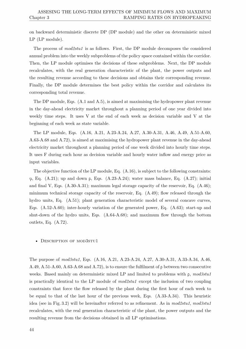
Chapter 3ASSESING THE LONG-TERM EFFECTS OF MINIMUM FLOWS AND MAXIMUM
RAMPING RATES ON HYDROPEAKING
on backward deterministic discrete DP (DP module) and the other on deterministic mixedLP (LP module).
The process of mod2stu1 is as follows. First, the DP module decomposes the consideredannual problem into the weekly subproblems of the policy space contained within the corridor.Then, the LP module optimises the decisions of these subproblems. Next, the DP modulerecalculates, with the real generation characteristic of the plant, the power outputs andthe resulting revenue according to these decisions and obtains their corresponding revenue.Finally, the DP module determines the best policy within the corridor and calculates itscorresponding total revenue.
The DP module, Eqs. (A.1 and A.5), is aimed at maximising the hydropower plant revenuein the day-ahead electricity market throughout a planning period of one year divided intoweekly time steps. It uses V at the end of each week as decision variable and V at thebeginning of each week as state variable.
The LP module, Eqs. (A.16, A.21, A.23-A.24, A.27, A.30-A.31, A.46, A.49, A.51-A.60,A.63-A.68 and A.72), is aimed at maximising the hydropower plant revenue in the day-aheadelectricity market throughout a planning period of one week divided into hourly time steps.It uses F during each hour as decision variable and hourly water inflow and energy price asinput variables.
The objective function of the LP module, Eq. (A.16), is subject to the following constraints:φ, Eq. (A.21); up and down ρ, Eqs. (A.23-A.24); water mass balance, Eq. (A.27); initialand final V, Eqs. (A.30-A.31); maximum legal storage capacity of the reservoir, Eq. (A.46);minimum technical storage capacity of the reservoir, Eq. (A.49); flow released through thehydro units, Eq. (A.51); plant generation characteristic model of several concave curves,Eqs. (A.52-A.60); inter-hourly variation of the generated power, Eq. (A.63); start-up andshut-down of the hydro units, Eqs. (A.64-A.68); and maximum flow through the bottomoutlets, Eq. (A.72).
• Description of mod3stu1
The purpose of mod3stu1, Eqs. (A.16, A.21, A.23-A.24, A.27, A.30-A.31, A.33-A.34, A.46,A.49, A.51-A.60, A.63-A.68 and A.72), is to ensure the fulfilment of ρ between two consecutiveweeks. Based mainly on deterministic mixed LP and limited to problems with ρ, mod3stu1is practically identical to the LP module of mod2stu1 except the inclusion of two couplingconstraints that force the flow released by the plant during the first hour of each week tobe equal to that of the last hour of the previous week, Eqs. (A.33-A.34). This heuristicidea (see in Fig. 3.2) will be hereinafter referred to as refinement. As in mod2stu1, mod3stu1recalculates, with the real generation characteristic of the plant, the power outputs and theresulting revenue from the decisions obtained in all LP optimisations.
44

3.1 Assessment of the economic impact of environmental constraints on annual hydropowerplant operation
Figure 3.2.: Coupling of the flows released by the plant between consecutive stages.
3.1.2. Case study
A Spanish peak hydropower plant (plant I), located in the northwest of Spain (Fig. B.1),was selected to test the above-described methodology. The technical data of the plant wereprovided by the company that owns and manages it. Tab.B.1 summarises the main designparameters of the plant. The performance curves of the plant, calculated without hydrauliclosses, and their linear concave approximations (used by the LP module of mod2stu1 andmod3stu1 ) are plotted in Fig. B.5(a-b-d). The head-storage curve of the plant is drawn inFig. B.18(a).
Regarding the considered input variables, on the one hand, the historical series of waterinflows were taken from the web page of the Centre for Public Works Studies and Experi-mentation [CEDEX (2013)]. A linear variation between the mid-days of each two consecutivedays was assumed in order to transform the available data (daily flows) into hourly water in-flows; the obtained histogram, probability distribution and scenarios can be seen in Fig. B.2.On the other hand, the historical series of hourly energy prices were taken from the web pageof the Iberian Electricity Market Operator [OMIE (2011)]; the hourly values and their weeklyaverages of the used energy prices are depicted in Fig. B.3. The analysed scenarios of theseinput variables as well as the magnitudes of φ and ρ considered in the study are included inTab. 3.1; the maximum values of φ and ρ were taken from the web page of the Miño-Sil RiverBasin District Authority [CHMS (2010)].
Table 3.1.: Input variable scenarios and environmental constraints used in the study 1.
Concept Scenarios Description
Water inflows Very dry; Dry; EquiprobableNormal; Wet; Very wet and hourly
Energy prices Average Hourly
φ0.0%; 0.6%; 1.2%; 1.8%; ϕOct.−Dec. = 0.75φ; ϕJan.−Mar. = 1.75φ;2.4%; 3.0%; 4.0%; 5.0% ϕApr.−Jun. = 1.20φ; ϕJul.−Sep. = 0.30φ
ρ0 h; 6 h; 12 h; ρup
1−kmax = 0.75ρ;24 h; 36 h; 48 h; 60 h ρdown
1−kmax = 1.50ρ
45

Chapter 3ASSESING THE LONG-TERM EFFECTS OF MINIMUM FLOWS AND MAXIMUM
RAMPING RATES ON HYDROPEAKING
Following the above-mentioned discretisation criterion (as discussed in sec. 3.1.1), the statediagram of the problem comprises 11 states per stage. It results in a total of 280 annual prob-lems to be assessed (5 water inflow scenarios · 1 energy price scenario · 56 combinations ofφ and ρ), i.e. a total of 275,765 weekly subproblems to be solved. As a result of mod1stu1(39,031 subproblems), only a third of the total had to be solved by mod2stu1 (91,360 sub-problems), of which less than 14% had to be recalculated by mod3stu1 (12,480 subproblems).Thus, 280 problems decomposed in a total of 142,871 subproblems were solved.
The proposed methodology (as discussed in sec. 3.1.1) was implemented in MATLAB®,each subproblem being solved using CPLEXTM under GAMSTM, on two threads in parallel[Baslis and Bakirtzis (2011)] of an Intel® CoreTM i5 at 2.4 GHz and 4 GB RAM running onMicrosoft Windows®. As recommended in Carvalho and Pinto (2006) (seen in sec. 2.2.1), asensitivity analysis of the performance of the above-described models to certain parameters(Tab. 3.2) was carried out. After this analysis, the most time consuming problem and itscounterpart without φ and ρ were calculated with practically no time limit (109 s) and avery demanding relative optimality criterion (0.1‰) in order to check the accuracy of thesolutions obtained with the chosen values of these parameters (Tab. 3.2). The error betweenthe economic impacts calculated by means of the two approaches was only 1.8‰.
Table 3.2.: Characteristic parameters of each model of the study 1.
Models Parameter Value
mod1stu1 Radius of the corridor (% useful volume) 40
mod2stu1
Maximum number of performance curves (cmax) ∞Gross head “covered” by each performance curve (H%) 20
Relative optimality criterion (%) 2Time limit for each subproblem (s) 1,800
mod3stu1
Maximum number of performance curves (cmax) ∞Gross head “covered” by each performance curve (H%) 10
Relative optimality criterion (%) 1Time limit for each subproblem (s) 1,800
3.1.3. Main results and discussion
Fig. 3.3(a) represents the level curves of the average annual losses for different values of φ andρ. This figure reveals, among other things, that the combination proposed by the river basinauthority for this plant, given by φ=5% and ρ=60 h, would reduce the plant revenues morethan 10%. Regarding the joint influence of φ and ρ, it is clearly appreciable that the higherthe one, the smaller the rise in the economic impact caused by the increase in the other.Fig. 3.3(b-c-d-e-f) represent in turn the same level curves of each water inflow scenario. As itcan be observed in these figures, the smaller the rainfall of the scenario, the greater were theannual revenue losses caused by a given combination of φ and ρ.
46

3.1 Assessment of the economic impact of environmental constraints on annual hydropowerplant operation
Figure 3.3.: Annual losses according to φ and ρ of the plant I corresponding to the: (a)Average of the water years; b) Very wet water year; c) Wet water year; d) Normal wateryear; e) Dry water year; f) Very dry water year scenario.
The evolution of the average annual losses as a function of φ and ρ are depicted in Fig. 3.4(a-b), respectively. As it can be seen, for a given φ, the annual revenue losses followed a quadratic
47

Chapter 3ASSESING THE LONG-TERM EFFECTS OF MINIMUM FLOWS AND MAXIMUM
RAMPING RATES ON HYDROPEAKING
behaviour as ρ varied; whereas for a given ρ, the annual losses followed an almost linearbehaviour as φ varied. Similar trends were obtained in Chen and Forsyth (2008), Olivares(2008), Niu and Insley (2010), Pérez-Díaz and Wilhelmi (2010), Pérez-Díaz et al. (2012) andRheinheimer et al. (2013) (as discussed in sec. 2.5).
Figure 3.4.: Average annual losses of the plant I according to: (a) φ; (b) ρ.
In Fig. 3.5, the histogram of the initial and final F of the subproblems of the best policieswith ρ>0 obtained by mod2stu1 is drawn. It can be appreciated that, despite its irregularity,the distribution covered practically the whole range of possible values. It is significant thatthree quarters of the values were grouped around φ and q2. It is also interesting to notehow certain flows standed out above the rest; these in order of frequency were: φ (46.0%),q2 (10.2%), Qmin (6.5%), Qmax (6.5%), q3 (4.2%), 66 m3/s that was the flow correspond-ing to the maximum efficiency for one hydro unit (3.5%), and 198 m3/s that was the onecorresponding to the maximum efficiency for the whole plant (2.0%).
Figure 3.5.: Histogram of the initial and final F of the subproblems of the best policies withρ>0 obtained by mod2stu1.
48

3.2 Effects of the maximum flow ramping rates on the long-term operation decisions of ahydropower plant
Finally, all the above-mentioned breaches of ρ between the last hour of each week andthe first hour of the following one were computed and it was observed that the averagelength of these breaches was above five hours with a deviation standard of more than tenhours. Therefore, the heuristic idea of the applied refinement (illustrated in Fig. 3.2) might beaccurate enough for the proposed methodology. Nevertheless, given the magnitude of thesebreaches, it would be convenient to develope new ways to couple the hydropower operationbetween consecutive stages; e.g., to add a new state variable in the DP that ensures thefulfilment of ρ along the whole planning period.
3.2. Effects of the maximum flow ramping rates on the long-termoperation decisions of a hydropower plant
The main objective of the study of the current section is to analyse the influence of ρ on theannual operation of a real peak hydropower plant. The secondary objective is to test whetherthe introduction of F as a second state variable into the DP-based long-term scheduling canimprove the performance of the model developed so far.
3.2.1. Methodology
Five annual models were used in the study 2. The models are mainly based on: backwarddeterministic discrete DP (mod1stu2 ), deterministic mixed LP (mod3Vstu2 andmod3VFstu2)and a hybrid combination of backward incremental DP and deterministic mixed LP (mod2Vstu2and mod2VFstu2 ). The reason why the methodology applied in this study moved from thesimplest discrete DP (used in the previous study) to the incremental variant of DP is dueto the computational burden increases exponentially with the number of state variables inDP (as discussed in sec. 2.2.2) and the selected deterministic approach allows this change(as discussed in sec. 1.2). On the other hand, this methodology still follows the combinedoptimisation-simulation approach (as discussed in sec. 2.1.1) by recalculating the power out-puts and the resulting revenue from the decisions obtained in all LP optimisations with thereal generation characteristic of the plant.As regards the used incremental DP, the chosen convergence criterion combined the two
criteria normally used with this technique (as discussed in sec. 2.2.2). If the obtained policy"touched" any border of the corridor, a new corridor was built around said policy with theprevious discretisation size; otherwise, the discretisation size of the corridor was reduced.The process stopped, defining the optimal policy, once that the difference in annual revenuebetween consecutive iterations was lower than the selected tolerance: in this study was 0.1‰[Nandalal and Bogardi (2007)].The developed models considered again (as in the study 1) water inflow and energy price
as input variables but both variables were modelled by using the average annual scenario oftheir respective historical series. The initial and final V of all problems were also specified
49
Chapter 3ASSESING THE LONG-TERM EFFECTS OF MINIMUM FLOWS AND MAXIMUM
RAMPING RATES ON HYDROPEAKING
with the same value, equal to the most frequent value of the historical series.Due to the test nature of the study and given that it was focused specifically on ρ, only
two environmental situations were analysed: without and with ρ. Thus, the used solutionstrategy, although simpler than the previous one, was still taking advantage of the likenessesbetween the three considered annual problems. These problems, listed in order of resolution,were: problem without ρ, problem with ρ considering V as state variable, and problem withρ considering V and F as state variables.
• Description of mod1stu2
The purpose of mod1stu2, Eqs. (A.1, A.5 and A.10-A.12), is the same as that of mod1stu1(as discussed in sec. 3.1.1). It is an improved version of that model and it is also based onbackward deterministic discrete DP. The main difference between them is how the revenuecorresponding to each feasible transition within the policy space is obtained. In mod1stu2, theweekly revenue is estimated as the product of the weekly average energy price, the generatedpower (determined from the average net head and the plant operating flow) and the operatingtime, Eq. (A.12). This time is assumed to be equal to 168 hours, when the average flowreleased by the reservoir is equal or above the operational minimum, or reduced proportionallyin other case, Eq. (A.11). Finally, given the few problems to solve, the discretisation of thepolicy space used by mod1stu2 was finer than in the previous study, reaching 1% of V.
• Description of mod2Vstu2
The purpose of mod2Vstu2, Eqs. (A.1, A.5, A.13, A.16, A.21, A.23-A.24, A.27, A.30-A.31,A.46, A.49, A.51-A.60, A.63-A.68 and A.72), is the same as that of mod2stu1 (as discussedin sec. 3.1.1). As that model, mod2Vstu2 is a hybrid optimisation model, but instead of onbackward deterministic discrete DP, is based on backward incremental DP. Therefore, it isan improved version of mod2stu1 whose only difference from that model is the need of verifya convergence criterion related to its incremental nature, Eq. (A.13).
• Description of mod2VFstu2
The purpose of mod2VFstu2, Eqs. (A.3, A.5, A.7, A.13, A.16, A.21, A.23-A.24, A.27,A.30-A.31, A.35-A.36, A.46, A.49, A.51-A.60, A.63-A.68 and A.72), is the same as thatof mod2Vstu2 and its structure is practically identical to that model. The main novelty ofmod2VFstu2 is the use of F as state variable.On the one hand, the DP module needs a new state transition equation, Eq. (A.7), that rep-
resents the operational inertia of the reservoir, and, therefore, to replace the one-dimensionalDP equation, Eq. (A.1), by its two-dimensional equivalent, Eq. (A.3). On the other hand,the LP module includes a pair of constraints that considers the initial and final F, Eqs.(A.35-A.36), defined by the DP module and involved in that new state transition equation,Eq. (A.7).
50
3.2 Effects of the maximum flow ramping rates on the long-term operation decisions of ahydropower plant
• Description of mod3Vstu2
The main purpose of mod3Vstu2, Eqs. (A.16, A.21, A.23-A.24, A.27, A.30-A.31, A.33-A.34,A.46, A.49, A.51-A.58, A.61-A.68 and A.72), is the same as that of mod3stu1 (as discussed insec. 3.1.1) and its secondary purpose is to improve the revenue. Based mainly on deterministicmixed LP, mod3Vstu2 refines as in the study 1, Eqs. (A.33-A.34), the policy obtained bymod2Vstu2 (illustrated in Fig. 3.2). Moreover, it is an improved version of mod3stu1 becausethe generation characteristic model is shaped non-concave, Eqs. (A.61-A.62).
• Description of mod3VFstu2
The purpose of mod3VFstu2, Eqs. (A.16, A.21, A.23-A.24, A.27, A.30-A.31, A.35-A.36, A.46,A.49, A.51-A.58, A.61-A.68 and A.72), is to recalculate the policy obtained by mod2VFstu2with a non-concave generation characteristic model, Eqs. (A.61-A.62), in order to obtain thesame accuracy as mod3Vstu2. Based mainly on deterministic mixed LP and very similar tothat model, mod3VFstu2 replaces the refinement constraints, Eqs. (A.33-A.34), by anotherpair, Eqs. (A.35-A.36), with the aim of considering the initial and final F of each subproblemdefined by mod2VFstu2.
3.2.2. Case study
Plant I (Tab.B.1), the same peak hydropower plant as in the study 1, located in the northwestof Spain (Fig. B.1), was the selected one for carrying out the current study. The performancecurves of the plant, calculated without hydraulic losses, and both their linear concave (usedby mod2Vstu2 and mod2VFstu2 ) and non-concave (used by mod3Vstu2 and mod3VFstu2 )approximations, are plotted in Fig. B.5. The head-storage curve of the plant is drawn inFig. B.18(a).Regarding the considered input variables, the same historical series applied in the study 1
were used [CEDEX (2013); OMIE (2011)]. Their scenarios as well as the magnitudes of φand ρ considered in this study are included in Tab. 3.3; the values of φ and ρ, expressed inrelative terms following the methodology of the study 1 (as discussed in sec. 3.1.1), were thoseplanned to be imposed by the water basin authority of the studied plant [CHMS (2010)].
Table 3.3.: Input variable scenarios and environmental constraints used in the study 2.
Concept Scenarios Description
Water inflows Average HourlyEnergy prices Average Hourly
φ 5.0% ϕOct.−Dec. = 0.75φ; ϕJan.−Mar. = 1.75φ;ϕApr.−Jun. = 1.20φ; ϕJul.−Sep. = 0.30φ
ρ 0 h; 60 h ρup1−kmax = 0.75ρ; ρdown
1−kmax = 1.50ρ
For the resolution procedure of the problem without ρ: 109,463 subproblems were calculatedby mod1stu2, 3,494 by mod2Vstu2 and 52 by mod3Vstu2. For the procedure of the problem
51

Chapter 3ASSESING THE LONG-TERM EFFECTS OF MINIMUM FLOWS AND MAXIMUM
RAMPING RATES ON HYDROPEAKING
with ρ considering V as state variable: 3,874 subproblems were calculated by mod2Vstu2and 52 by mod3Vstu2. And for the third resolution procedure: 8,656 subproblems werecalculated by mod2VFstu2 and 52 by mod3VFstu2. Therefore, 3 problems decomposed in atotal of 125,643 subproblems were solved in this study.
The above-described optimisation models (as discussed in sec. 3.2.1) were implementedin MATLAB®, each subproblem being solved using CPLEXTM under GAMSTM, on fourthreads in parallel [Baslis and Bakirtzis (2011)] of an Intel® CoreTM i5 at 2.4 GHz and 4GB RAM running on Microsoft Windows®. Again, following the suggestion in Carvalho andPinto (2006), a sensitivity analysis of the performance of the models involved in the lastpart of the resolution procedures to certain parameters (Tab. 3.4) was carried out. Half athousand randomly selected [MacCallum et al. (1999)] weekly subproblems were calculatedwith practically no time limit (109 s) and a very demanding relative optimality criterion(0.1‰) in order to check the accuracy of the solutions obtained with the chosen values ofthese parameters (Tab. 3.4). The error between the economic impacts calculated by meansof the two approaches was only 4.8%.
Table 3.4.: Characteristic parameters of the LP algorithms of the study 2.
Parameter Value
Maximum number of performance curves (cmax) ∞Gross head “covered” by each performance curve (H%) 10
Relative optimality criterion (%) 0.1a
Time limit for each subproblem (s) 10
aAs recommended in Fu and Shahidehpour (2007)
3.2.3. Main results and discussion
The main results of the optimal policies of the plant I considered in the study 2 are sum-marised in Tab. 3.5. As it can be observed, on the one hand, the economic impact of ρwas almost 6% even though the energy generation was more than 2% greater and the num-ber of hours in operation was almost 20% greater. Some of these effects were obtained inEdwards et al. (1999), Harpman (1999), Kotchen et al. (2006), Chen and Forsyth (2008),Olivares (2008), Niu and Insley (2010), Pérez-Díaz and Wilhelmi (2010), Babel et al. (2012),Pérez-Díaz et al. (2012), Niu and Insley (2013) and Rheinheimer et al. (2013) (as discussedin sec. 2.5). On the other hand, Tab. 3.5 shows that the average units’ efficiency was 1.1%higher than the one without ρ, and the efficiency standard deviation was 1.3% lower thanthe one obtained without ρ, what yielded a more efficient operation. Furthermore with ρ, thenumber of start-ups and shut-downs of the hydro units was about 90% lower and the totalvolume discharged by the bottom outlets was significantly lower, about one half. Finally,regarding the introduction of F as a second state variable into the incremental DP, it can alsobe noted that the improvement in the annual revenue was barely appreciable, only 0.2%.
52

3.3 Approximate formulae for the assessment of the long-term economic impact ofenvironmental constraints on hydropeaking
Table 3.5.: Main values of the optimal policies of the plant I considered in the study 2.
Optimal Annual Generated Operating Average Start-up Waterpolicy of revenue energy hours efficiency and spillages
the problem [M€] [GWh] [h] [%] shut-downs [hm3]
without ρ 45.28 910.5 6,175 90.3 ± 2.5 1,248 64.8with ρ by V 42.59 933.5 7,394 91.4 ± 1.2 110 33.9
with ρ by V&F 42.72 936.0 7,384 91.4 ± 1.2 96 33.3
3.3. Approximate formulae for the assessment of the long-termeconomic impact of environmental constraints onhydropeaking
The objectives of the present study correspond to the objectives 3 and 4 of the thesis (asdiscussed in sec. 1.3). The former is defined by the title of the current section and the latteris aimed to provide insight into the effects of φ and ρ on hydropeaking.
3.3.1. Methodology
Given the complexity of the studied phenomenon (as discussed in sec. 1.1) and, therefore, theinherent difficulty to deduce its exact analytical expression, several regression models weredeveloped to reach the desired formulae. In order to obtain these formulae, a sample, as largeand representative as possible, of results of long-term hydro scheduling problems subject todifferent magnitudes of φ and ρ corresponding to distinct hydropower plants was used. Thus,a very much larger computational burden than in the study 1 was faced and therefore, asbefore, similar measures were again taken.Once more, the approach was deterministic and it only used water inflow and energy price
as input variables. Therefore, the study should at least be considered useful for clarifying theeffects of the main terms involved in the obtained formulae [Rossi (2012)]. Only one scenarioper hydropower plant was calculated (the average historical values of the input variables) inorder to reduce even more the computational burden than in the study 1. With the aim ofgreater realism, as in the previous studies, the initial and final V of all problems were alsospecified with the same value, equal to the most frequent value of the historical series of eachconsidered reservoir.Once more also, the solution strategy was based on the same hypothesis made in the
study 1 (as discussed in sec. 3.1.1) but now, taking advantage of what has been learnedlater, the three sequentially used optimisation models (see in Fig. 3.6) are based on thesame techniques applied in the study 2: backward deterministic discrete DP (mod1stu2 ; asdiscussed in sec. 3.2.1 but in this study with a discretisation of the policy space of 33 values[Bogardi et al. (1988)]), deterministic mixed LP (mod3stu3 ) and a hybrid combination ofbackward incremental DP and deterministic mixed LP (mod2stu3 ). Because of different
53

Chapter 3ASSESING THE LONG-TERM EFFECTS OF MINIMUM FLOWS AND MAXIMUM
RAMPING RATES ON HYDROPEAKING
hydropower plants were evaluated, the planning period used for each one varied between oneor more years, as a function of the reservoir’s regulation capacity. As both previous studies,the methodology follows the combined optimisation-simulation approach (as discussed insec. 2.1.1) by recalculating the power outputs and the resulting revenue from the decisionsobtained in all LP optimisations with the real generation characteristic of the consideredplant.
Figure 3.6.: Flowchart of the solution strategy of the study 3 in each hydropower plant.
Regarding to the development of the regression models, the first efforts to get them werebased on correlation and factor analysis but, given the resulting low accuracy, this procedurewas abandoned in favour of the classical trial-and-error approach. The results of the factoranalysis helped to orient the trial-and-error based search. However, hundreds of attempts weremade to reach the final formulae showed in this study. Finally, three formulae are providedsince two of them are focused on problems in which only φ or ρ are present, and thereforeare univariate, and the third one, bivariate, is for the problems with both constraints.
54

3.3 Approximate formulae for the assessment of the long-term economic impact ofenvironmental constraints on hydropeaking
• Description of mod2stu3
The purpose of mod2stu3, Eqs. (A.3, A.5, A.7, A.13, A.16, A.21, A.23-A.24, A.27, A.30-A.31,A.37-A.39, A.46, A.49, A.51-A.60, A.63-A.68 and A.72), is the same as that of mod2VFstu2(as discussed in sec. 3.2.1) but its procedure is slightly different from that model.
Initially, because of the findings of the study 2 (as discussed in sec. 3.2.3), the current studywas going to use the refinement proposed in the study 1 (illustrated in Fig. 3.1.1). However,during the course of this study, the first results that were obtained demonstrated that thatapproach would be generally valid only for low values of ρ, that is, approximately below 24hours.
Given the necessity of using both state variables and taking advantage of the lower influenceof F on the revenue, mod2stu3 considers both variables but V is treated in an incrementalmanner (alike in an incremental DP), whereas F is coarsely discretised. In this way, theapplied corridors decrease only in one dimension, corresponding to V, as the solution searchadvances. Thus, V starts with 33 values [Bogardi et al. (1988)] and, in each iteration, isdoubled, while the dimension of F is maintained in four plus the number of hydro units ofthe considered plant. Based on the results of the study 2 (as discussed in sec. 3.2.3), theseflows correspond to φ, Qmin, their average, Qmax and as many flows as hydro units installedin the plant, these equidistributed between Qmin and Qmax.
Finally, the LP module of mod2stu3 shows a small modification of the initial and final Fconstraints of the hydro units, Eqs. (A.35-A.36), in order to improve the performance duringthe first hour of each subproblem and to fulfil ρ in every hour, Eqs. (A.37-A.39).
• Description of mod3stu3
The main purpose of mod3stu3, Eqs. (A.16-A.18, A.21, A.23-A.24, A.27, A.30-A.31, A.37-A.39, A.42-A.46, A.49, A.51-A.58, A.61-A.68 and A.72), is to reduce the errors caused by thediscretisation of the state variables in the policy obtained by mod2stu3. Moreover, mod3stu3has as secondary purpose the same of mod3VFstu2 (as discussed in sec. 3.2.1).
In order to achieve its main purpose, mod3stu3 undertakes successive relaxations of thestate boundary conditions at the end of each subproblem. Thus, from the policies obtainedby mod2VFstu3, a series of 2-weekly, or longer in the case of hydropower plants with multi-annual reservoirs, subproblems are solved with an overlap of one week between consecutivesubproblems. The final V and F constraints, Eqs. (A.31 and A.39), used in the previousmodels are relaxed, Eqs. (A.42-A.45), and a penalty term is included in the objective functionas a function of the final V and of this one and the final F, Eqs. (A.17 or A.18). Then, butnow week by week, without overlap and by reintroducing the final V and F constraints, Eqs.(A.31 and A.39), the resulting policy is calculated for the last time by mod3stu3 and itshourly results are saved.
55

Chapter 3ASSESING THE LONG-TERM EFFECTS OF MINIMUM FLOWS AND MAXIMUM
RAMPING RATES ON HYDROPEAKING
3.3.2. Case studies
A dozen of peak hydropower plants, located in several regions of Spain (Fig. B.1), wereselected to perform this study. There were two main criteria for choosing these hydropowerplants. First, every hydropower plant must be located at the head of its basin with the aimof ignoring the influence of the rest of the water basin regulation infrastructures, without asignificant loss of accuracy as well as of easing the characterisation of the water inflows toits reservoir. Second, every hydropower plant must also show, as far as possible, differentcharacteristics with respect to the other hydropower plants in order to increase the diversityand representativity of the sample.
Tab.B.3 includes the main design parameters of the selected hydropower plants. Theresults in terms of long-term economic impacts corresponding to the hydropower plants (I-X)in this table were used to derive the formulae whereas the results corresponding to the otherhydropower plants (A and B) were used to check their accuracy. The performance curvesof the plants, calculated without hydraulic losses, and both their linear concave (used bymod2stu3 ) and non-concave (used by mod3stu3 ) approximations, are plotted in Fig. B.5 toFig. B.17. The head-storage curves of the plants are drawn in Fig. B.18 and Fig. B.19.
Regarding the historical series of the considered input variables, the hourly energy prices(see in Fig. B.3) were taken from the web page of the Iberian Electricity Market Operator[OMIE (2011)] and the monthly water inflows (see in Fig. B.20 and Fig. B.21) from the webpages of the Centre for Public Works Studies and Experimentation [CEDEX (2013)] and ofthe Catalan Water Agency [ACA (2015)]. The analysed scenarios of these input variables aswell as the magnitudes of φ and ρ evaluated in the study, expressed in relative terms followingthe methodology of the study 1 (as discussed in sec. 3.1.1), are included in Tab. 3.6.
The above-described optimisation models (as discussed in sec. 3.3.1) were implementedin MATLAB®, each subproblem being solved using CPLEXTM under GAMSTM, on eightcomputers, totaling 52 threads (used each pair in parallel [Baslis and Bakirtzis (2011)] ateach computer): one Intel® Xeon® E5 at 1.8 GHz and 16 GB RAM, two Intel® CoreTM i3at 2.13 GHz and 4 GB RAM, two Intel® CoreTM i5 at 2.4 GHz and 4 GB RAM, two Intel®
CoreTM i7 at 2.4 GHz and 8 GB RAM, and one Intel® Xeon® E5 at 3.1 GHz and 64 GBRAM. Once more, following the suggestion in Carvalho and Pinto (2006), a small sensitivityanalysis of the performance of the mixed LP algorithms was undertaken, using as a basis theresults of that carried out in the study 2 (as discussed in sec. 3.2.2). The resulting selectedparameters are given in Tab. 3.7.
A total of 574 long-term problems were solved in this study; 476 to derive the formulaeand 98 to check their accuracy. These problems were decomposed into 14,072,632 short-termsubproblems: 712,552 were solved by mod1stu2, 12,892,379 by mod2stu3, and 467,701 bymod3stu3.
56

3.3 Approximate formulae for the assessment of the long-term economic impact ofenvironmental constraints on hydropeaking
Table 3.6.: Input variable scenarios and environmental constraints used in the study 3.
Concept Scenarios Description
Water inflows Average HourlyEnergy prices Average Hourly
φ0%; 1%; 2%; 3%; ϕOct.−Dec. = 0.75φ; ϕJan.−Mar. = 1.75φ;4%; 5%; 7%; 10% ϕApr.−Jun. = 1.20φ; ϕJul.−Sep. = 0.30φ
ρ0 h; 6 h; 12 h; ρup
1−kmax = 0.75ρ;18 h; 24 h; 48 h; 72 h ρdown
1−kmax = 1.50ρ
Table 3.7.: Characteristic parameters of the LP algorithms of the study 3.
ModelPlanning
Parameter ValuePeriod
Weekly
Maximum number of performance curves (cmax) ∞mod2stu3’s Gross head “covered” by each 10LP performance curve (H%)module Relative optimality criterion (%) 1.0
Time limit for each subproblem (s) 10
mod3stu3
N-weekly
Maximum number of performance curves (cmax) 1Gross head “covered” by each 100performance curve (H%)
Relative optimality criterion (%) 0.5Time limit for each subproblem (s) (N-1)·25·umax
Weekly
Maximum number of performance curves (cmax) ∞Gross head “covered” by each 10performance curve (H%)
Relative optimality criterion (%) 0.1a
Time limit for each subproblem (s) 100·umax
aAs recommended in Fu and Shahidehpour (2007)
3.3.3. Main results and discussion
Each of the formulae (3.1-3.3) gives a rough estimation of the long-term economic impact onthe operation of a peak hydropower plant, expressed as percentage of the revenue correspond-ing to the scenario without environmental constraints, caused by φ and/or ρ (ε) as a functionof two adimensional parameters of the plant: maximum plant flow divided by average riverflow (Qmax/W avg) and minimum plant flow divided by average river flow (Qmin/W avg).
ε (ϕ) ∼= 0.31·(Qmax
W avg
)[2.6−(Qmax
Wavg
)0.06]
·ϕ
1.05·(Qmin
Qmax
)[0.11·(Qmin
Wavg
)−1.1]
;
∀ϕ ∈ [0, 10] | Qmax·ϕ < W avg
(3.1)
57
Chapter 3ASSESING THE LONG-TERM EFFECTS OF MINIMUM FLOWS AND MAXIMUM
RAMPING RATES ON HYDROPEAKING
ε (ρ) ∼=
(Qmin
Wavg
)[2.21·(Qmin
Qmax
)0.16−0.13·
(Qmax
Wavg
)]·ρ
[(Qmin
Wavg
)−0.22]
1 + 0.23·(Qmin
Qmax
)·ρ
[(Qmin
Wavg
)−0.22] ;
∀ρ ∈ [0, 72]
(3.2)
ε (ϕ, ρ) ∼= 0.41·(Qmax
W avg
)1.33·ϕ
0.95·(Qmin
Qmax
)[0.48·(Qmin
Wavg
)−3.82]
+
(Qmin
Wavg
)[1.68−0.16·(Qmax
Wavg
)]·ρ
[(Qmin
Wavg
)−0.15]
1
ϕ
[(QmaxWavg )−0.88
] + 0.23·(Qmin
Qmax
)·ρ
[(Qmin
Wavg
)−0.15] ;
∀ϕ ∈ [1, 10] | Qmax·ϕ < W avg ∧ ∀ρ ∈ [6, 72]
(3.3)
Tab. 3.8 summarises the main statistical parameters of these formulae, as well as their per-formance for the problems considered with the test plants A and B.
Table 3.8.: Main statistical parameters of the formulae and summary of the results obtainedwith the test plants.
ConceptFormula
(3.1) (3.2) (3.3)
Sample size 68 70 348Average relative error of the sample (%) 8.2 7.5 8.1Standard deviation of the sample (%) 9.0 8.6 7.2
Maximum relative error at 95% confidence interval (%) 19.0 17.6 17.3Number of problems checked of the hydropower plant A 7 7 36Average relative error of the predicted values for A (%) 2.4 6.9 4.5Standard deviation of the predicted values for A (%) 2.4 4.3 4.7
Maximum relative error of the predicted values for A (%) 6.5 13.2 18.8Number of problems checked of the hydropower plant B 7 7 36Average relative error of the predicted values for B (%) 7.9 4.6 7.4Standard deviation of the predicted values for B (%) 10.4 2.1 4.8
Maximum relative error of the predicted values for B (%) 30.0 6.2 17.2
The long-term economic impact calculated (by the models) and predicted (by the formulae)in these test plants for different values of φ, ρ, and φ and ρ simultaneously are representedin Fig. 3.7(a-b), Fig. 3.7(c-d) and Fig. 3.8, respectively. As it can be observed, the differencesbetween them were not significant, thus verifying the adequacy of the proposed formulae.
58

3.3 Approximate formulae for the assessment of the long-term economic impact ofenvironmental constraints on hydropeaking
Figure 3.7.: Calculated and predicted long-term economic impact in terms of: (a) φ of theplant A; (b) φ of the plant B; (c) ρ of the plant A; (d) ρ of the plant B.
A ten of the selected hydropower plants have annual regulation capacity (hereinafter re-ferred to as annual plants). The power·price-duration curves of the set formed by theseannual plants (I-VIII, A and B) in terms of φ and ρ are depicted in Fig. 3.9, respectively.As it can be expected, the larger φ or ρ, the worse the price tracking, this effect being morepronounced in the cases subject to ρ. Furthermore, Fig. 3.10 shows the energy generated bythe annual plants distributed in quartiles of energy prices, in terms of φ and ρ, respectively(Q1 and Q4 correspond respectively to the higher and lower prices). It is worth noting that,while the amount of generated energy remained almost constant for the second and thirdquartiles of the energy prices (Q2 and Q3), a progressive transfer of the energy generated atfirst quartile prices (Q1) to the fourth one (Q4) took place when φ or ρ were increased.
59

Chapter 3ASSESING THE LONG-TERM EFFECTS OF MINIMUM FLOWS AND MAXIMUM
RAMPING RATES ON HYDROPEAKING
Figure 3.8.: Long-term economic impact in terms of φ and ρ of the plant: (a) A calculatedby the models; (b) A predicted by formula (3.3); (c) B calculated by the models; (d) Bpredicted by formula (3.3).
Figure 3.9.: Power·Price-duration curves of the annual plants in terms of: (a) φ; (b) ρ.
60

3.3 Approximate formulae for the assessment of the long-term economic impact ofenvironmental constraints on hydropeaking
Figure 3.10.: Energy generated by the annual plants in terms of price quartiles and: (a) φ;(b) ρ.
In Fig. 3.11 are drawn the variations relative to the problem without environmental con-straints, in terms of φ and ρ, of the average efficiency, net head, number of operating hours,spillage volumes and start-ups and shut-downs across the annual plants, corresponding to thecases in which only φ or ρ are present. As it can be seen both Fig. 3.10(a) and Fig. 3.11(a),as φ increased, the number of operating hours and the amount of spilled water grew, whilethe efficiency, the net head, the total generated energy and the number of start-ups andshut-downs of the hydro units decreased. In the same way in Fig. 3.11(b), as ρ increased, theoperating hours and the spillage volumes grew and the number of start-ups and shut-downsof the hydro units decreased. Some of these effects could be expected to a certain extent;both φ and ρ limit the capacity of the hydropower plant to concentrate the water releasedthrough the turbines in the peak hours at rated or design flow.
Among the just-mentioned behaviours, only the following were fulfilled in each hydropowerplant practically always: as φ increased, the spillage grew and the generated energy andthe number of start-ups and shut-downs decreased; as ρ increased, the operating hours andspillages grew, whereas the number of start-ups and shut-downs decreased. As it was dis-cussed in sec. 2.5, these effects of φ on the spillages and the generated energy as well as theone of ρ on the number of operating hours were obtained in Edwards et al. (1999), Harpman(1999), Kotchen et al. (2006), Chen and Forsyth (2008), Olivares (2008), Niu and Insley(2010), Pérez-Díaz and Wilhelmi (2010), Babel et al. (2012), Pérez-Díaz et al. (2012), Niuand Insley (2013) and Rheinheimer et al. (2013). Regarding the enhancer effect of ρ on thespillages, it seems to be contradictory to the findings of the study 2 (summarised in Tab. 3.5)but it must be remembered that in the two scenarios investigated by that study φ was stronglypresent. The same mitigating effect of ρ on the spillages when φ was significant was foundin the current study. Moreover, the decrease of the number of start-ups and shut-downs as aconsequence of ρ, was also detected in the study 2. Finally, the reduction in the number of
61
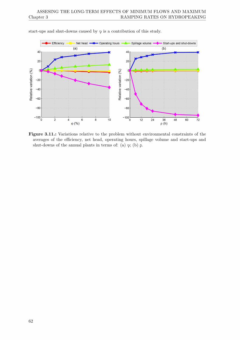
Chapter 3ASSESING THE LONG-TERM EFFECTS OF MINIMUM FLOWS AND MAXIMUM
RAMPING RATES ON HYDROPEAKING
start-ups and shut-downs caused by φ is a contribution of this study.
Figure 3.11.: Variations relative to the problem without environmental constraints of theaverages of the efficiency, net head, operating hours, spillage volume and start-ups andshut-downs of the annual plants in terms of: (a) φ; (b) ρ.
62

4. LONG-TERM OPTIMISATION MODELSFOR HYDRO SCHEDULING SUBJECTTO MINIMUM FLOWS AND MAXIMUMRAMPING RATES
This chapter is mainly devoted to the achievement of the objectives 1 and 2 of the thesis (asdiscussed in sec. 1.3) and is developed in three studies (hereinafter referred to as studies 4,5 and 6). The study 4 [Guisández et al. (2015, 2016b,c)] with the latter objective and thestudies 5 and 6 with the former one.The chapter is divided in three parts, one for each study, and each part is structured as in
the previous chapter: explanation of the applied methodology, description of the consideredcase study, and presentation of the main obtained results with their discussion.
4.1. Influence of the environmental constraints on the water andflow values
The objectives of the present study, which gives name to this section, correspond, on the onehand, to the objective 2 of the thesis (as discussed in sec. 1.3) and, on the other hand, to acongruent extension of that objective due to the emergence of a new concept: flow value. Thepresence of this new value arose as a consequence of the consideration of F in the calculationof the water value. If water value can be defined, from a revenue-based point of view, asthe marginal change in the hydropower producer’s expected revenue for a marginal changein its hydro (or potential) resources [Reneses et al. (2015)], then, in the same way, flow valueis coined in this thesis as the analogous change when varying its “discharge (or cinematic)resources”, i.e. its released flow.In order to obtain an a priori idea of how φ and ρ affect water and flow values and with
the aim of clarifying the concept of this latter value, a simplified hydro scheduling problem isformulated below in two different forms: one by considering only water value and the otherby water and flow values.
• Hydro scheduling problem considering only water value
min
[−∑t∈T
(pt·gvt,ftt
)− zvtmax
](4.1)
63

Chapter 4LONG-TERM OPTIMISATION MODELS FOR HYDRO SCHEDULING SUBJECT TO
MINIMUM FLOWS AND MAXIMUM RAMPING RATES
subject to:
vt − vt−1 +Kc1· (ft − wt) = 0;∀t ∈ T ∧ v0 = V0 (4.2)
vt − V max ≤ 0;∀t ∈ T (4.3)
V min − vt ≤ 0;∀t ∈ T (4.4)
ft − Fmax ≤ 0;∀t ∈ T (4.5)
ϕk − ft ≤ 0;∀t ∈ T (4.6)
ft − ft−1 − ρup ≤ 0;∀t ∈ T ∧ f0 = F0 (4.7)
−ft + ft−1 − ρdown ≤ 0;∀t ∈ T ∧ f0 = F0 (4.8)
Eq.(4.1) is the objective function in which pt represents the energy price during the hour t,gvt,ftt refers to the power generated by releasing ft at vt during the hour t, and zvtmax meansthe future expected revenue starting from the V vtmax at the end of the planning period tmax.Eq.(4.2) is the state transition equation of V, the so-called water mass balance equation,where Kc1 signifies a conversion factor for converting an hourly constant flow expressed inm3/s into a volume in hm3. Eqs.(4.3-4.4) are the limits of V and Eq.(4.5) is the upper oneof qt. Finally, Eqs.(4.6-4.8) are the environmental constraints.The resulting Lagrangian function of the above-described problem is:
L(vt, ft, λ
vt , µ
Vmax
t , µVmin
t , µFmax
t , µϕt , µρup
t , µρdown
t
)
=∑t∈T
−pt·gvt,ftt + λvt·[vt − vt−1 +Kc1· (ft − wt)
]+µVmaxt · (vt − V max) + µV
min
t ·(V min − vt
)+µFmaxt · (ft − Fmax) + µϕt · (ϕk − ft)
+µρup
t · (ft − ft−1 − ρup) + µρdown
t ·(−ft + ft−1 − ρdown
)
− zvtmax (4.9)
64
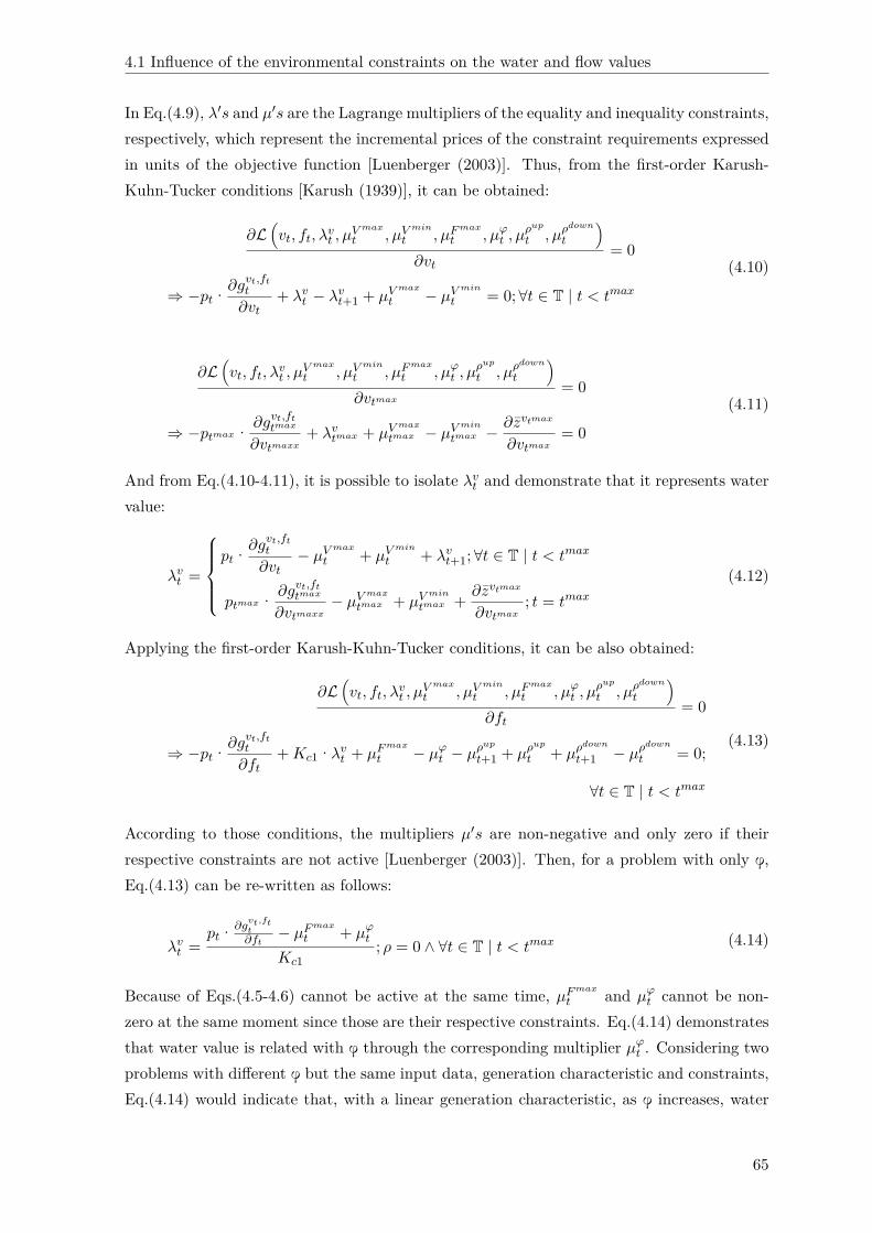
4.1 Influence of the environmental constraints on the water and flow values
In Eq.(4.9), λ′s and µ′s are the Lagrange multipliers of the equality and inequality constraints,respectively, which represent the incremental prices of the constraint requirements expressedin units of the objective function [Luenberger (2003)]. Thus, from the first-order Karush-Kuhn-Tucker conditions [Karush (1939)], it can be obtained:
∂L(vt, ft, λ
vt , µ
Vmaxt , µV
min
t , µFmax
t , µϕt , µρup
t , µρdown
t
)∂vt
= 0
⇒ −pt·∂gvt,ftt
∂vt+ λvt − λvt+1 + µV
max
t − µVmint = 0;∀t ∈ T | t < tmax
(4.10)
∂L(vt, ft, λ
vt , µ
Vmaxt , µV
min
t , µFmax
t , µϕt , µρup
t , µρdown
t
)∂vtmax
= 0
⇒ −ptmax· ∂gvt,fttmax
∂vtmaxx+ λvtmax + µV
max
tmax − µVmin
tmax −∂zvtmax
∂vtmax= 0
(4.11)
And from Eq.(4.10-4.11), it is possible to isolate λvt and demonstrate that it represents watervalue:
λvt =
pt·
∂gvt,ftt
∂vt− µVmaxt + µV
min
t + λvt+1;∀t ∈ T | t < tmax
ptmax· ∂gvt,fttmax
∂vtmaxx− µVmaxtmax + µV
min
tmax + ∂zvtmax
∂vtmax; t = tmax
(4.12)
Applying the first-order Karush-Kuhn-Tucker conditions, it can be also obtained:
∂L(vt, ft, λ
vt , µ
Vmaxt , µV
min
t , µFmax
t , µϕt , µρup
t , µρdown
t
)∂ft
= 0
⇒ −pt·∂gvt,ftt
∂ft+Kc1·λvt + µF
max
t − µϕt − µρup
t+1 + µρup
t + µρdown
t+1 − µρdown
t = 0;
∀t ∈ T | t < tmax
(4.13)
According to those conditions, the multipliers µ′s are non-negative and only zero if theirrespective constraints are not active [Luenberger (2003)]. Then, for a problem with only φ,Eq.(4.13) can be re-written as follows:
λvt =pt·∂g
vt,ftt∂ft
− µFmaxt + µϕt
Kc1; ρ = 0 ∧ ∀t ∈ T | t < tmax (4.14)
Because of Eqs.(4.5-4.6) cannot be active at the same time, µFmaxt and µϕt cannot be non-zero at the same moment since those are their respective constraints. Eq.(4.14) demonstratesthat water value is related with φ through the corresponding multiplier µϕt . Considering twoproblems with different φ but the same input data, generation characteristic and constraints,Eq.(4.14) would indicate that, with a linear generation characteristic, as φ increases, water
65

Chapter 4LONG-TERM OPTIMISATION MODELS FOR HYDRO SCHEDULING SUBJECT TO
MINIMUM FLOWS AND MAXIMUM RAMPING RATES
value would also increase, assuming that, in general, µϕt grows as φ increases. In a case witha non-linear generation characteristic, the influence of φ on water value depends also on thefirst derivative of the generation characteristic with respect to ft.For a problem with only ρ, and considering that ft is not at its limits, Eq.(4.13) can be
re-written as follows:
λvt =pt·∂g
vt,ftt∂ft
+(µρ
up
t+1 − µρup
t
)−(µρ
down
t+1 − µρdown
t
)Kc1
;
ϕ = 0 ∧ 0 < ft < Fmax ∧ ∀t ∈ T | t < tmax
(4.15)
Eq.(4.15) indicates that water value is related with ρup and ρdown through the correspondingmultipliers. Considering two problems with different ρ but the same input data, generationcharacteristic and constraints, Eq.(4.15) would indicate that, with a linear generation charac-teristic, water value would increase if
(µρ
up
t+1 − µρup
t
)increases or
(µρ
down
t+1 − µρdown
t
)decreases.
In order to anticipate the variation in(µρ
up
t+1 − µρup
t
)or(µρ
down
t+1 − µρdown
t
)between these
latter problems, it can be analysed Fig. 4.1, where the hypothetical resulting water releaseft of a set of problems with different ρ is depicted. From this figure, it can be deducedthat
(µρ
up
t+1 − µρup
t
)increases and
(µρ
down
t+1 − µρdown
t
)decreases as the severity of ρ decreases,
and therefore water value would grow. In a case with a non-linear generation characteris-tic, the influence of ρ on water value depends also on the first derivative of the generationcharacteristic with respect to ft.Despite the foregoing, the conclusions of this analysis should be confirmed with some nu-
merical results.
Figure 4.1.: Examples of different ρ.
• Hydro scheduling problem considering water and flow values
min
[−∑t∈T
(pt·gvt,ftt
)− zvtmax ,ftmax
](4.16)
66

4.1 Influence of the environmental constraints on the water and flow values
subject to: Eqs.(4.2-4.6) and
ft − ft−1 − dt = 0;∀t ∈ T | f0 = F0 (4.17)
dt − ρup ≤ 0;∀t ∈ T (4.18)
−dt − ρdown ≤ 0;∀t ∈ T (4.19)
Eq.(4.16) is the objective function in which zvtmax ,ftmax means the future expected revenuestarting from the V vtmax and the F ftmax (released through the hydro units, bottom outletsand spillways) at the end of the planning period tmax. Eq.(4.17) is the analogous equation ofEq.(4.2) for F, which may be named operational inertia equation until a better term can befound, where dt indicates the decision which corresponds to the hourly variation of F. Finally,Eqs.(4.18-4.19) are the ρ constraints.
The resulting Lagrangian function of the current problem is:
L(dt, vt, ft, λ
vt , λ
ft , µ
Vmax
t , µVmin
t , µFmax
t , µϕt , µρup
t , µρdown
t
)
=∑t∈T
−pt·gvt,ftt + λvt·[vt − vt−1 +Kc1· (ft − wt)
]+ λft · (ft − ft−1 − dt)
+µVmaxt · (vt − V max) + µVmin
t ·(V min − vt
)+µFmaxt · (ft − Fmax) + µϕt · (ϕk − ft)
+µρup
t · (dt − ρup) + µρdown
t ·(−dt − ρdown
)
−zvtmax ,ftmax
(4.20)
As before, λ′s and µ′s are the Lagrange multipliers of the equality and inequality constraintsin Eq.(4.20), respectively.
From the first-order Karush-Kuhn-Tucker conditions [Karush (1939)] it can be obtained:
∂L(dt, vt, ft, λ
vt , λ
ft , µ
Vmaxt , µV
min
t , µFmax
t , µϕt , µρup
t , µρdown
t
)∂ft
= 0
⇒ −pt·∂gvt,ftt
∂ft+Kc1·λvt + λft − λ
ft+1 + µF
max
t − µϕt = 0;
∀t ∈ T | t < tmax
(4.21)
67

Chapter 4LONG-TERM OPTIMISATION MODELS FOR HYDRO SCHEDULING SUBJECT TO
MINIMUM FLOWS AND MAXIMUM RAMPING RATES
∂L(dt, vt, ft, λ
vt , λ
ft , µ
Vmaxt , µV
min
t , µFmax
t , µϕt , µρup
t , µρdown
t
)∂ftmax
= 0
⇒ −ptmax·∂gvt,fttmax
∂ftmax+Kc1·λvtmax + λftmax + µF
max
tmax − µϕtmax −
∂zvtmax ,ftmax
∂ftmax= 0;
∀k ∈ K
(4.22)
And from Eq.(4.21-4.22), it is possible to isolate λft and demonstrate that it represents flowvalue:
λft =
pt·
∂gvt,ftt
∂ft−Kc1·λvt − µF
max
t + µϕt + λft+1; ∀t ∈ T | t < tmax
ptmax· ∂gvt,fttmax
∂vtmaxx−Kc1·λvtmax − µF
max
tmax + µϕtmax + ∂zvtmax ,ftmax
∂vtmax; t = tmax
(4.23)
Eq.(4.23) shows, logically, that flow value is function of F and, besides, reveals that flowand water values are related with each other, and that therefore, the former also varies as afunction of V and the time of the year (as discussed in sec. 1.2).
Finally, applying the first-order Karush-Kuhn-Tucker conditions, it can be also obtained:
∂L(dt, vt, ft, λ
vt , λ
ft , µ
Vmaxt , µV
min
t , µFmax
t , µϕt , µρup
t , µρdown
t
)∂dt
= 0
⇒ −λft + µρup
t − µρdown
t = 0;∀t ∈ T
(4.24)
As it can be seen, Eq.(4.24) indicates that flow value can be positive or negative, dependingon what ρ is activated.
4.1.1. Methodology
Two annual models (modVstu4 and modVFstu4 ), based on a hybrid combination of stochasticdiscrete DP and deterministic mixed LP, were developed in this study. The methodologyapplied in this study moved from the deterministic approach (used in the previous studies)to the stochastic one since the latter is more widely used to determine the water value and,in general, to make any long- or mid-term decision to be used in short-term hydro scheduling(as discussed in sec. 1.2). As in the previous studies, the combined optimisation-simulationapproach (as discussed in sec. 2.1.1) was also applied by recalculating, with the real generationcharacteristic of the plant, the power outputs and the resulting revenue from the decisionsobtained in all LP optimisations.
Water inflow and energy price were considered as state variables in the DP algorithms andas input variables in the LP ones. The stochasticity of these variables in the DP algorithmswas modelled by Markov chains whose orders were selected through the Akaike informa-tion criterion, whose numbers of classes were determined using the discretisation thickening
68
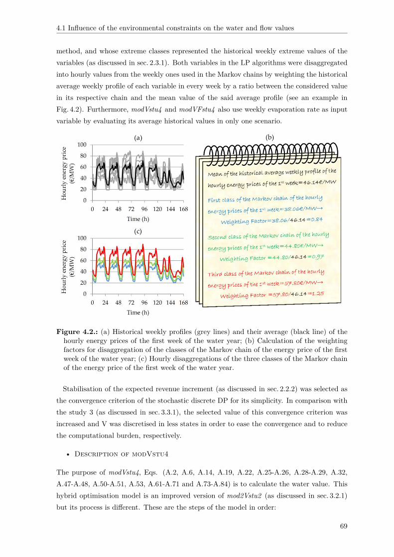
4.1 Influence of the environmental constraints on the water and flow values
method, and whose extreme classes represented the historical weekly extreme values of thevariables (as discussed in sec. 2.3.1). Both variables in the LP algorithms were disaggregatedinto hourly values from the weekly ones used in the Markov chains by weighting the historicalaverage weekly profile of each variable in every week by a ratio between the considered valuein its respective chain and the mean value of the said average profile (see an example inFig. 4.2). Furthermore, modVstu4 and modVFstu4 also use weekly evaporation rate as inputvariable by evaluating its average historical values in only one scenario.
Figure 4.2.: (a) Historical weekly profiles (grey lines) and their average (black line) of thehourly energy prices of the first week of the water year; (b) Calculation of the weightingfactors for disaggregation of the classes of the Markov chain of the energy price of the firstweek of the water year; (c) Hourly disaggregations of the three classes of the Markov chainof the energy price of the first week of the water year.
Stabilisation of the expected revenue increment (as discussed in sec. 2.2.2) was selected asthe convergence criterion of the stochastic discrete DP for its simplicity. In comparison withthe study 3 (as discussed in sec. 3.3.1), the selected value of this convergence criterion wasincreased and V was discretised in less states in order to ease the convergence and to reducethe computational burden, respectively.
• Description of modVstu4
The purpose of modVstu4, Eqs. (A.2, A.6, A.14, A.19, A.22, A.25-A.26, A.28-A.29, A.32,A.47-A.48, A.50-A.51, A.53, A.61-A.71 and A.73-A.84) is to calculate the water value. Thishybrid optimisation model is an improved version of mod2Vstu2 (as discussed in sec. 3.2.1)but its process is different. These are the steps of the model in order:
69

Chapter 4LONG-TERM OPTIMISATION MODELS FOR HYDRO SCHEDULING SUBJECT TO
MINIMUM FLOWS AND MAXIMUM RAMPING RATES
1. The DP module decomposes the considered annual problem into weekly subproblems.
2. Starting from the last week of the year, the LP module optimises the decisions of allsubproblems contained in the considered week.
3. The DP module recalculates, with the real generation characteristic of the plant, thepower outputs according to the decisions provided by the LP module of each subproblemand obtains the resulting revenue.
4. The DP module calculates the water value at the beginning of the considered week.
5. Second, third and fourth steps are repeated backwards until the beginning of the yearfor the rest of the weeks using the last-obtained water value.
6. The DP module checks if the relative interannual variations of the expected revenue atthe beginning of each week converge. If the answer is yes, the process stops; otherwisethe process is repeated from the second step but now considering the last-obtainedwater value at the end of the last week.
The DP module, Eqs. (A.2, A.6 and A.14), is aimed at maximising the hydropower plantrevenue in the day-ahead electricity market throughout a planning period of one year dividedinto weekly time steps. It uses the volume released from the reservoir throughout each weekas decision variable and, as state variables, V at the beginning of each week (discretised innine equidistant values from the dead volume to the maximum one; as discussed in sec. 2.2.2),the current weekly water inflow, and the current average weekly energy price.The LP module, Eqs. (A.19, A.22, A.25-A.26, A.28-A.29, A.32, A.47-A.48, A.50-A.51,
A.53, A.61-A.71 and A.73-A.84) is aimed at maximising the hydropower plant revenue in theday-ahead electricity market throughout a planning period of one week, divided into hourlytime steps, plus the future expected revenue, given by the water value. It uses F during eachhour as decision variable and hourly water inflow and energy price as input variables.The objective function of the LP module (Eq. A.19) is subject to the following constraints:φ (Eq. A.22); up and down ρ, Eqs. (A.25-A.26); water mass balance (Eq. A.28); evaporationlosses (Eq. A.29); initial V (Eq. A.32); maximum legal storage capacity of the reservoir (Eq.A.47); maximum technical storage capacity of the reservoir (Eq. A.48); dead storage capacity(Eq. A.50); flow released through the hydro units (Eq. A.51); plant generation characteristicmodel of one non-concave curve, Eqs. (A.53 and A.61-A.62); inter-hourly variation of thegenerated power (Eq. A.63); start-up and shut-down of the hydro units, Eqs. (A.64-A.68);maximum technical plant flow, Eqs. (A.69-A.71); maximum flow through the bottom outlets(Eq. A.73); maximum flow over the spillways, Eqs. (A.74-A.78); inter-hourly variation ofthe total flow released through the bottom outlets and/or over the spillways (Eq. A.79) andthe water value at the end of each subproblem, Eqs. (A.80-A.84).
70

4.1 Influence of the environmental constraints on the water and flow values
• Description of modVFstu4
The purpose of modVFstu4, Eqs. (A.4, A.6, A.8, A.15, A.20, A.22, A.25-A.26, A.28-A.29,A.32, A.40-A.41, A.47-A.48, A.50-A.51, A.53, A.61-A.71, A.73-A.79 and A.85-A.95) is tocalculate the water and flow values. The structure of modVFstu4 is practically identical tomodVstu4 and its main variations from that model are the use of F as state variable (Eq.A.8), with the same discretisation used in mod2stu3 (as discussed in sec. 3.3.1), and theconsideration of the water value together with the flow value at the end of each subproblem,Eqs. (A.20 and A.85-A.95), modelled through the one-dimensional method (as discussed insec. 2.4.1).
4.1.2. Case study
Plant I (Tab.B.2), the same peak hydropower plant as in the studies 1 and 2, located in thenorthwest of Spain (Fig. B.1), was the selected one for carrying out the current study. In thiscase, its modelling was improved by the introduction of the hydraulic losses in its performancecurves (see in Fig. B.6) as well as by the consideration of the maximum available flows of itsbottom outlets and spillways according to the current V (see in Fig. B.4). The head-storagecurve of the plant was also used (see in Fig. B.18(a)).
Once more, the daily water inflows and the hourly energy prices were taken from the webpage of the Centre for Public Works Studies and Experimentation [CEDEX (2013)] and fromthe web page of the Iberian Electricity Market Operator [OMIE (2011)], respectively. Theweekly evaporation rates were estimated by application of the empirical temperature-basedformula proposed in Dragoni and Valigi (1994) and of the average monthly temperaturestaken from the web page of Spanish Statistical Office [INE (1960)]. The analysed scenarios ofthe input variables as well as the evaluated magnitudes of φ and ρ, expressed in relative termsfollowing the methodology of the study 1 (as discussed in sec. 3.1.1), are noted in Tab. 4.1.
The above-described optimisation models (sec. 4.1.1) were implemented in MATLAB®, eachsubproblem being solved using CPLEXTM under GAMSTM, on three computers, totaling 32threads (used each pair in parallel [Baslis and Bakirtzis (2011)] at each computer): two Intel®
CoreTM i7 at 2.4 GHz and 8 GB RAM and one Intel® Xeon® E5 at 3.1 GHz and 64 GB RAM.Following again the suggestion in Carvalho and Pinto (2006), a small sensitivity analysis ofthe performance of the LP algorithms of the models was done, using as a basis the results ofthose carried out in the studies 2 and 3 (as discussed in sec. 3.2.2 and sec. 3.3.2). The selectedparameters are given in Tab. 4.2.
A total of 36 estimations of water and flow values were undertaken in this study; 28considering only V and 8 considering V and F. These estimations were decomposed into4,841,928 short-term subproblems: 1,107,288 were solved by modVstu4 and 3,734,640 bymodVFstu4.
71

Chapter 4LONG-TERM OPTIMISATION MODELS FOR HYDRO SCHEDULING SUBJECT TO
MINIMUM FLOWS AND MAXIMUM RAMPING RATES
Table 4.1.: Input variable scenarios and environmental constraints used in the study 4.
Concept Scenarios Description
Water inflows 5 Markov classes of lag 1 HourlyEnergy prices 3 Markov classes of lag 1 Hourly
Evaporation rates Average Weekly
(φ,ρ)
(0%,0 h); (0.5%,0 h); (1%,0 h); ϕOct.−Dec. = 0.75φ;(2%,0 h); (3%,0 h); (4%,0 h); ϕJan.−Mar. = 1.75φ;(5%,0 h); (8%,0 h); (0%,6 h); ϕApr.−Jun. = 1.20φ;
(0%,12 h); (0%,24 h); (0%,36 h); ϕJul.−Sep. = 0.30φ;(0%,48 h); (0%,60 h); (0%,72 h); ρup
1−kmax = 0.75ρ;(5%,60 h)a ρdown
1−kmax = 1.50ρ(0.5%,0 h); (1%,0 h); ϕOct.−Dec. = φ;(2%,0 h); (3%,0 h); ϕJan.−Mar. = φ;(4%,0 h); (5%,0 h); ϕApr.−Jun. = φ;
(8%,0 h) ϕJul.−Sep. = φ
aPlanned to be imposed by the water basin authority.
Table 4.2.: Characteristic parameters of the LP algorithms of the study 4.
Parameter Value
Relative optimality criterion (%) 1Time limit for each subproblem (s) 10
4.1.3. Main results and discussion
The averages across V and the seasons of the water value in relative terms with respect tothe scenario without environmental constraints are included in Fig. 4.3 for every consideredφ and ρ. This figure corroborates the conclusions of the discussion carried out in sec. 4.1,i.e. the water value increased (almost linearly) with φ and decreased (quadratically) with ρ.These opposing effects are also caused by the head-storage relationship. Suppose two separateproblems aimed at maximising the future revenue of a peak hydropower plant starting fromtwo different V. Regardless of the future values of the input variables, the policy followed bythe plant from the upper V would have a bigger average head than the one correspondingto the lower V, and therefore the impact of φ would be higher for the lower V than for theupper one since the detraction of water represents a larger reduction of head for the lower Vthan for the upper one. As regards ρ, its impact would be bigger for the upper V than forthe lower one because the average head is larger at the upper V than at the lower one. Inboth constraints, the greater their values, the greater their impacts on the water value.
72

4.1 Influence of the environmental constraints on the water and flow values
Figure 4.3.: Average relative water values of the plant I in terms of: (a) φ; (b) ρ.
Returning to Fig. 4.3, it can also be observed that the effect of φ was more significant inspring and winter, whereas ρ had more influence in spring and summer. It is must be notedthat Fig. 4.3 shows relative values but the water value in absolute terms was higher in springand summer than in autumn and winter as it can be seen in Fig. 4.4. On the other hand, itis important to bear in mind that φ had its largest value during spring and winter (see inTab. 4.1). Even though φ usually varies seasonally, Fig. 4.5(a)-(b) show, for the sake of clarity,the same results as Fig. 4.3(a) and Fig. 4.4(a) but considering φ constant along the year. Inaddition, Fig. 4.5(c) shows the impact of φ on the water value in k€/hm3. As regards ρ, itshigher impact on the water value in spring and summer is to a certain extent expected, sincethe lower the water inflow, the higher the economic value of the the operational flexibility.
Figure 4.4.: Average water values of the plant I in terms of: (a) φ; (b) ρ.
73

Chapter 4LONG-TERM OPTIMISATION MODELS FOR HYDRO SCHEDULING SUBJECT TO
MINIMUM FLOWS AND MAXIMUM RAMPING RATES
Figure 4.5.: (a) Average relative water values of the plant I in terms of constant φ; (b)Average water values of the plant I in terms of constant φ; (c) Difference in average watervalues of the plant I in terms of constant φ.
Regarding the flow values, their absolute averages across F and the seasons are showed inFig. 4.6 for every evaluated ρ. It is worth noting that unlike the water value, which can bebelow zero only under very specific conditions (such as considering negative energy prices ora spillage penalty), the flow value is able to reach negative magnitudes (see Eq.(4.24)) undernormal conditions in order to show the expected profitability of finishing the weekly operationat low F (this is the reason why they are not represented in relative terms with respect to anyscenario). Fig. 4.6 seems to suggest that the flow value tends to increase with ρ in the wettestseason and conversely in the driest one. This effect is coherent with the seasonal nature ofthe water value, which is usually decreasing with the amount of water inflow (as discussed insec. 1.2), since the more valuable is the water stored into the reservoir, the less economicallyinteresting is scheduling an aggressive profile at the beginning of the week and vice versa.
74
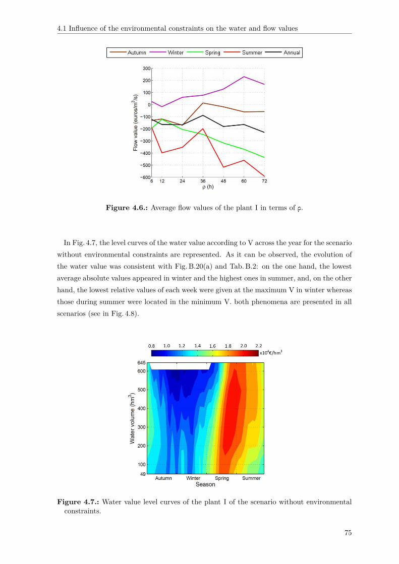
4.1 Influence of the environmental constraints on the water and flow values
Figure 4.6.: Average flow values of the plant I in terms of ρ.
In Fig. 4.7, the level curves of the water value according to V across the year for the scenariowithout environmental constraints are represented. As it can be observed, the evolution ofthe water value was consistent with Fig. B.20(a) and Tab.B.2: on the one hand, the lowestaverage absolute values appeared in winter and the highest ones in summer, and, on the otherhand, the lowest relative values of each week were given at the maximum V in winter whereasthose during summer were located in the minimum V. both phenomena are presented in allscenarios (see in Fig. 4.8).
Figure 4.7.: Water value level curves of the plant I of the scenario without environmentalconstraints.
75

Chapter 4LONG-TERM OPTIMISATION MODELS FOR HYDRO SCHEDULING SUBJECT TO
MINIMUM FLOWS AND MAXIMUM RAMPING RATES
Figure 4.8.: Water value level curves of the plant I with: (a) φ=2%; (b) ρ=24 h; (c) φ=4%;(d) ρ=48 h; (e) φ=8%; (f) ρ=72 h.
76
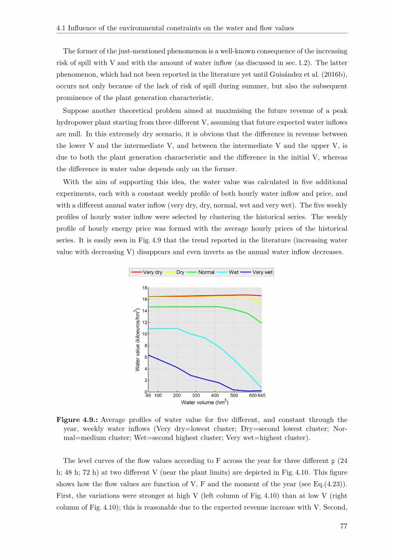
4.1 Influence of the environmental constraints on the water and flow values
The former of the just-mentioned phenomenon is a well-known consequence of the increasingrisk of spill with V and with the amount of water inflow (as discussed in sec. 1.2). The latterphenomenon, which had not been reported in the literature yet until Guisández et al. (2016b),occurs not only because of the lack of risk of spill during summer, but also the subsequentprominence of the plant generation characteristic.
Suppose another theoretical problem aimed at maximising the future revenue of a peakhydropower plant starting from three different V, assuming that future expected water inflowsare null. In this extremely dry scenario, it is obvious that the difference in revenue betweenthe lower V and the intermediate V, and between the intermediate V and the upper V, isdue to both the plant generation characteristic and the difference in the initial V, whereasthe difference in water value depends only on the former.
With the aim of supporting this idea, the water value was calculated in five additionalexperiments, each with a constant weekly profile of both hourly water inflow and price, andwith a different annual water inflow (very dry, dry, normal, wet and very wet). The five weeklyprofiles of hourly water inflow were selected by clustering the historical series. The weeklyprofile of hourly energy price was formed with the average hourly prices of the historicalseries. It is easily seen in Fig. 4.9 that the trend reported in the literature (increasing watervalue with decreasing V) disappears and even inverts as the annual water inflow decreases.
Figure 4.9.: Average profiles of water value for five different, and constant through theyear, weekly water inflows (Very dry=lowest cluster; Dry=second lowest cluster; Nor-mal=medium cluster; Wet=second highest cluster; Very wet=highest cluster).
The level curves of the flow values according to F across the year for three different ρ (24h; 48 h; 72 h) at two different V (near the plant limits) are depicted in Fig. 4.10. This figureshows how the flow values are function of V, F and the moment of the year (see Eq.(4.23)).First, the variations were stronger at high V (left column of Fig. 4.10) than at low V (rightcolumn of Fig. 4.10); this is reasonable due to the expected revenue increase with V. Second,
77

Chapter 4LONG-TERM OPTIMISATION MODELS FOR HYDRO SCHEDULING SUBJECT TO
MINIMUM FLOWS AND MAXIMUM RAMPING RATES
the highest values were located at low F; this is also expected since the highest slopes ofthe performance curves are located at low F (see in Fig. B.6) and, furthermore, becausethe beginning of the stage was selected at midnight when energy prices are usually lower.Third, and finally, the highest averages took place at the wettest moments of the year; asabove-discussed in Fig. 4.6.
Several correlation analyses of the obtained flow values with different factors were per-formed with the aim of identifying any factor able to explain the seasonality of these values.Unfortunately, poor correlations were found in these trials; the highest ones being thoseobtained with the factors in the following expression:
factorρ =∑ρ−1
t=1 |pt−pt+1|∑tmaxt=1 (fc1·wt)
These best found correlation factors with their correlations at V=347 hm3 (in the middleof the reservoir of plant I) in terms of the evaluated ρ and F are gathered in Tab. 4.3.
Table 4.3.: Best correlation factors and their correlations with the flow values at V=347hm3 of the plant I in terms of ρ and F.
Interval of Best factor and correlation for ρ ofthe plant flow 6 h 12 h 24 h 36 h 48 h 60 h 72 hFrom 0m3/s factor72 factor6 factor12 factor48 factor6 factor12 factor72
to 20m3/s -0.19 -0.20 0.08 0.24 0.06 -0.12 -0.32From 20m3/s factor6 factor24 factor6 factor6 factor12 factor24 factor6
to 40m3/s 0.18 -0.07 -0.11 -0.06 0.14 -0.06 -0.21From 40m3/s factor12 factor6 factor6 factor6 factor6 factor6 factor6
to 100m3/s -0.11 0.09 -0.08 -0.22 -0.63 -0.34 -0.59From 100m3/s factor6 factor72 factor6 factor24 factor72 factor12 factor12
to 160m3/s 0.03 0.09 -0.20 -0.49 -0.04 -0.02 -0.12From 160m3/s factor12 factor6 factor6 factor60 factor6 factor6 factor48
to 219m3/s 0.06 -0.43 -0.12 0.21 -0.03 -0.16 0.14From 219m3/s factor24 factor6 factor6 factor24 factor24 factor24 factor6
to 279m3/s 0.06 0.16 0.25 0.22 0.32 0.36 -0.03
78

4.1 Influence of the environmental constraints on the water and flow values
Figure 4.10.: Flow value level curves of the plant I with: (a) ρ=24 h at V=570 hm3; (b)ρ=24 h at V=123 hm3; (c) ρ=48 h at V=570 hm3; (d) ρ=48 h at V=123 hm3; (e) ρ=72 hat V=570 hm3; (f) ρ=72 h at V=123 hm3.
79

Chapter 4LONG-TERM OPTIMISATION MODELS FOR HYDRO SCHEDULING SUBJECT TO
MINIMUM FLOWS AND MAXIMUM RAMPING RATES
4.2. Optimisation models for long-term hydro scheduling subjectto environmental constraints (part I)
This study has three objectives. The main objective is the first one of the thesis (as discussedin sec. 1.3) that matches with the title of the current section. The secondary objectivesare to check again the validity of the formulae (3.1-3.3) as well as to corroborate some ofthe findings of the study 3 related to the generated energy, operating hours, price tracking,spillage volume, and start-ups and shut-downs (as discussed in sec. 3.3.3).
4.2.1. Methodology
In the previous study, the water and flow values of a peak hydropower plant were calculatedsubject to different magnitudes of φ and ρ. The usefulness of those calculations only can beevaluated by means of simulations [Doorman (2009)]. Therefore, three sets of simulationswere carried out in this study in order to select the best approach for a long-term hydroscheduling model.The first approach, what might be called the classical approach or WV00, consists in
neglecting the effects of φ and ρ on the long-term scheduling by using in all the simulationsthe water values obtained in the scenario without environmental constraints. The secondapproach, WVφρ, is based on the assumption that the long-term influence of φ and ρ canbe adequately modelled by the water value calculated in each considered scenario with themodel modVstu4 (as discussed in sec. 4.1.1). Finally, the third approach, W&FVφρ, uses thecorresponding water and flow values calculated in each considered scenario with the modelmodVFstu4 (as discussed in sec. 4.1.1).Two models were developed to perform the simulations in this study; both based on de-
terministic mixed LP and subsequent recalculations of the power outputs and the resultingrevenue from the obtained decisions with the real generation characteristic of the plant. Onemodel (simWV ) was used for WV00 and WVφρ, and the other (simW&FV ) for W&FVφρ.As in the study 4, water inflow, energy price and evaporation rate were considered as input
variables. In this study, three synthetic series (S1, S2 and S3) were built through the Markovchains of these input variables with a length of a decade.In order to make the calculations easier and given the length of the used stage (as discussed
in sec. 1.2), a weekly perfect forecast of all input variables was assumed, the same V was im-posed at the beginning of each simulation series, and the results obtained with the water valueof the problem without environmental constraints was used as a comparison standard. Giventhe coarse grid used to obtain the water and flow values, the applied mixed LP formulationsof these values were built from spline interpolations of their obtained values (21 states forboth V and F) with the aim of increasing the accuracy (as discussed in sec. 2.2.2).
80

4.2 Optimisation models for long-term hydro scheduling subject to environmentalconstraints (part I)
• Description of simWV
The purpose of simWV, Eqs. (A.19, A.22, A.25-A.26, A.28-A.29, A.32, A.47-A.48, A.50-A.58,A.61-A.71 and A.73-A.84), is to obtain the optimal hourly operation of a peak hydropowerplant through a weekly planning period, considering WV00 or WVφρ. It is an improvedversion of the LP module of modVstu4 (as discussed in sec. 4.1.1) whose only difference fromthat model is the use of up to two performance curves per subproblem instead of one, Eq.(A.52).
• Description of simW&FV
The purpose of simW&FV, Eqs. (A.20, A.22, A.25-A.26, A.28-A.32, A.40-A.41, A.47-A.48,A.50-A.58, A.61-A.71, A.73-A.79 and A.85-A.95), is the same as that of simWV but inthis case considering W&FVφρ. simW&FV is an improved version of the LP module ofmodVFstu4 (as discussed in sec. 4.1.1) and, again, its only difference from that model is theuse of up to two performance curves per subproblem instead of one, Eq. (A.52).
4.2.2. Case study
Plant B (Tab.B.2, Fig. B.17 and Fig. B.19(f)), located in the northwest of Spain (Fig. B.1),was the peak hydropower plant selected for carrying out the current study with the aim ofchecking the validity of the formulae (3.1-3.3) since this plant was the one with the worstresults among those tested in the study 3 (as discussed in sec. 3.3.3). Therefore, the water andflow values of this plant were calculated with the same models used in the study 4, modVstu4and modVFstu4 (as discussed in sec. 4.1.1), prior to the simulations.The daily water inflows and the hourly energy prices were again taken from the web page
of the Centre for Public Works Studies and Experimentation [CEDEX (2013)] and fromthe web page of the Iberian Electricity Market Operator [OMIE (2011)], respectively. Theweekly evaporation rates were again estimated by application of the empirical temperature-based formula proposed in Dragoni and Valigi (1994) to the average monthly temperaturestaken from the web page of Spanish Statistical Office [INE (1960)]. The analysed scenariosof the input variables as well as the evaluated magnitudes of φ and ρ, expressed in relativeterms following the methodology of the study 1 (as discussed in sec. 3.1.1), are included inTab. 4.4.The above-described models (sec. 4.2.1) were implemented in MATLAB®, each subproblem
being solved using CPLEXTM under GAMSTM, on 16 threads (used each pair in parallel[Baslis and Bakirtzis (2011)]) of an Intel® Xeon® E5 at 3.1 GHz and 64 GB RAM runningon Microsoft Windows®. Once more, following the suggestion in Carvalho and Pinto (2006),a small sensitivity analysis of the performance of the models was done using as a basis theresults of those carried out in the previous studies. The selected parameters are given inTab. 4.5.A total of 18 estimations of water and flow values were undertaken in this study; 11 consid-
ering only V and 7 considering V and F. These estimations were decomposed into 2,446,080
81

Chapter 4LONG-TERM OPTIMISATION MODELS FOR HYDRO SCHEDULING SUBJECT TO
MINIMUM FLOWS AND MAXIMUM RAMPING RATES
short-term subproblems: 687,960 were solved by modVstu4 and 1,755,120 by modVFstu4. Af-ter that, a total of 84 long-term simulations were carried out; 33 considering WV00, 30 underWVφρ and 21 under W&FVφρ. These simulations were decomposed into 43,680 short-termsubproblems: 32,760 were solved by simWV and 10,920 by simW&FV.
Table 4.4.: Input variable scenarios and environmental constraints used in the study 5.
Concept Scenarios Description
Water inflows 5 Markov classes of lag 1 HourlyEnergy prices 3 Markov classes of lag 1 Hourly
Evaporation rates Average Weekly
(φ,ρ)
(0%,0 h); (1%,0 h); ϕOct.−Dec. = 0.75φ;(5%,0 h); (9%,0 h); ϕJan.−Mar. = 1.75φ;(0%,24 h); (0%,48 h); ϕApr.−Jun. = 1.20φ;(0%,72 h); (1%,24 h); ϕJul.−Sep. = 0.30φ;(5%,48 h); (9%,72 h); ρup
1−kmax = 0.75ρ;(3.97%,133.58 h)a ρdown
1−kmax = 1.50ρ
aPlanned to be imposed by the water basin authority.
Table 4.5.: Characteristic parameters of the LP algorithms of the study 5.
Models Parameter Value
modVstu4 Relative optimality criterion (%) 0.1modVFstu4 Time limit for each subproblem (s) 20
Maximum number of performance curves (cmax) 2simWV Gross head “covered” by each performance curve (H%) 10
simW&FV Relative optimality criterion (%) 0.1a
Time limit for each subproblem (s) 200
aAs recommended in Fu and Shahidehpour (2007)
4.2.3. Main results and discussion
The variations relative to WV00 calculated by simWV, in terms of φ or ρ, of the aggregaterevenue calculated by simWV under WVφρ and by simW&FV under W&FVφρ plus thefuture expected revenue according to WV00 corresponding to the final volume obtained ineach simulation of each synthetic series (S1, S2 and S3) are drawn in Fig. 4.11. This figureseems to indicate that WVφρ was more convenient for scenarios with only φ, whereas WV00was more suitable for those with only ρ. Moreover, Fig. 4.11(b) shows a very bad performanceof W&FVφρ. As φ must be present in all natural flows of the river [Sanguedo Baptista andDe Aquino Galeano Massera Da Hora (2013)], it was imposed to be lower than or equal tothe current water inflow into the reservoir (Eq.(A.22)) and this is the reason why Fig. 4.11(a)shows results for φ=4.6% and φ=7.6% instead of φ=5% and φ=9%. This circumstance isrepeated in the following figures and tables.
82
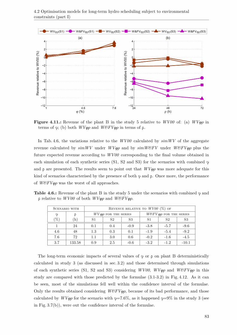
4.2 Optimisation models for long-term hydro scheduling subject to environmentalconstraints (part I)
Figure 4.11.: Revenue of the plant B in the study 5 relative to WV00 of: (a) WVφρ interms of φ; (b) both WVφρ and W&FVφρ in terms of ρ.
In Tab. 4.6, the variations relative to the WV00 calculated by simWV of the aggregaterevenue calculated by simWV under WVφρ and by simW&FV under W&FVφρ plus thefuture expected revenue according to WV00 corresponding to the final volume obtained ineach simulation of each synthetic series (S1, S2 and S3) for the scenarios with combined φand ρ are presented. The results seem to point out that WVφρ was more adequate for thiskind of scenarios characterised by the presence of both φ and ρ. Once more, the performanceof W&FVφρ was the worst of all approaches.
Table 4.6.: Revenue of the plant B in the study 5 under the scenarios with combined φ andρ relative to WV00 of both WVφρ and W&FVφρ.
Scenario with Revenue relative to WV00 (%) ofφ ρ WVφρ for the series W&FVφρ for the series
(%) (h) S1 S2 S3 S1 S2 S3
1 24 0.1 0.4 -0.9 -3.8 -5.7 -9.64.6 48 1.3 0.3 0.1 -1.9 -5.4 -9.27.6 72 1.1 3.0 0.6 -0.2 -1.6 -4.53.7 133.58 0.9 2.5 -0.6 -3.2 -1.2 -10.1
The long-term economic impacts of several values of φ or ρ on plant B deterministicallycalculated in study 3 (as discussed in sec. 3.2) and those determined through simulationsof each synthetic series (S1, S2 and S3) considering WV00, WVφρ and W&FVφρ in thisstudy are compared with those predicted by the formulae (3.1-3.2) in Fig. 4.12. As it canbe seen, most of the simulations fell well within the confidence interval of the formulae.Only the results obtained considering W&FVφρ, because of its bad performance, and thosecalculated by WVφρ for the scenario with φ=7.6%, as it happened φ=9% in the study 3 (seein Fig. 3.7(b)), were out the confidence interval of the formulae.
83
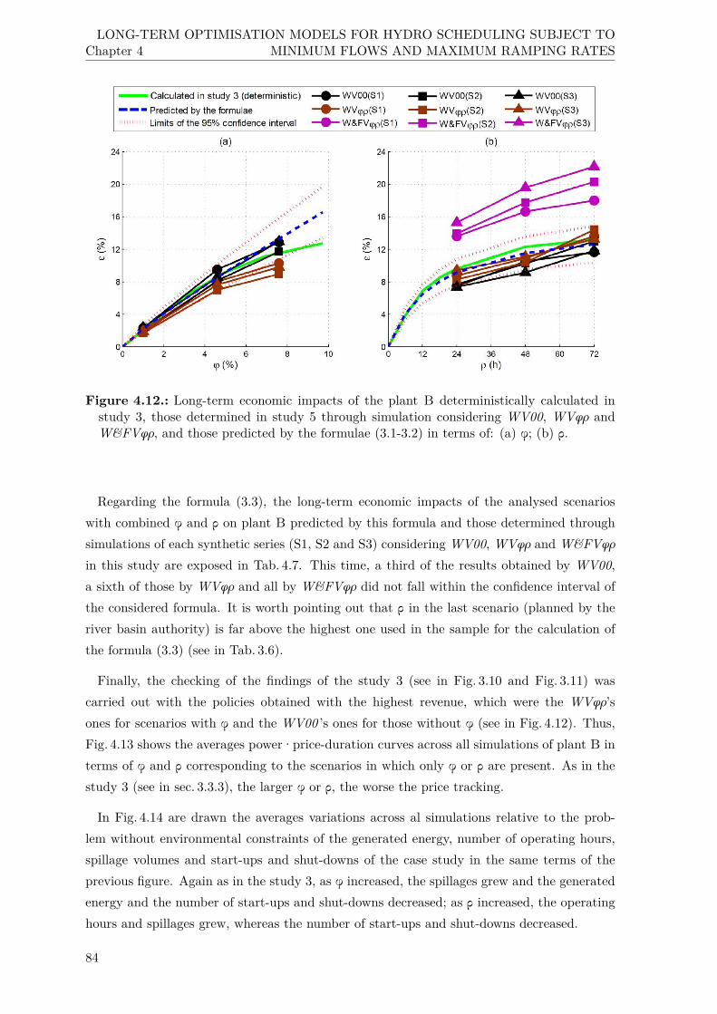
Chapter 4LONG-TERM OPTIMISATION MODELS FOR HYDRO SCHEDULING SUBJECT TO
MINIMUM FLOWS AND MAXIMUM RAMPING RATES
Figure 4.12.: Long-term economic impacts of the plant B deterministically calculated instudy 3, those determined in study 5 through simulation considering WV00, WVφρ andW&FVφρ, and those predicted by the formulae (3.1-3.2) in terms of: (a) φ; (b) ρ.
Regarding the formula (3.3), the long-term economic impacts of the analysed scenarioswith combined φ and ρ on plant B predicted by this formula and those determined throughsimulations of each synthetic series (S1, S2 and S3) considering WV00, WVφρ and W&FVφρin this study are exposed in Tab. 4.7. This time, a third of the results obtained by WV00,a sixth of those by WVφρ and all by W&FVφρ did not fall within the confidence interval ofthe considered formula. It is worth pointing out that ρ in the last scenario (planned by theriver basin authority) is far above the highest one used in the sample for the calculation ofthe formula (3.3) (see in Tab. 3.6).
Finally, the checking of the findings of the study 3 (see in Fig. 3.10 and Fig. 3.11) wascarried out with the policies obtained with the highest revenue, which were the WVφρ’sones for scenarios with φ and the WV00 ’s ones for those without φ (see in Fig. 4.12). Thus,Fig. 4.13 shows the averages power·price-duration curves across all simulations of plant B interms of φ and ρ corresponding to the scenarios in which only φ or ρ are present. As in thestudy 3 (see in sec. 3.3.3), the larger φ or ρ, the worse the price tracking.
In Fig. 4.14 are drawn the averages variations across al simulations relative to the prob-lem without environmental constraints of the generated energy, number of operating hours,spillage volumes and start-ups and shut-downs of the case study in the same terms of theprevious figure. Again as in the study 3, as φ increased, the spillages grew and the generatedenergy and the number of start-ups and shut-downs decreased; as ρ increased, the operatinghours and spillages grew, whereas the number of start-ups and shut-downs decreased.
84

4.2 Optimisation models for long-term hydro scheduling subject to environmentalconstraints (part I)
Table 4.7.: Long-term economic impacts of the scenarios with combined φ and ρ on plant Bdetermined in study 5 through simulation considering WV00, WVφρ and W&FVφρ, andthose predicted by the formula (3.3).
Scenario
Series
ε (%)with determined with the predicted by
φ ρ simulation approach the formula (3.3) within(%) (h) WV00 WVφρ W&FVφρ the confidence interval
S1 11.0 10.8 14.31 24 S2 9.8 9.4 14.9 11.5 [9.5;13.5]
S3 9.1 9.9 17.9S1 18.6 17.5 20.2
4.6 48 S2 17.4 17.2 21.8 16.9 [14.0;19.9]S3 16.7 16.6 24.4S1 22.0 21.2 22.2
7.6 72 S2 22.5 20.2 23.8 18.8 [15.5;22.0]S3 21.3 20.9 24.8S1 21.8 21.1 24.3
3.7 133.58 S2 24.8 22.8 25.7 18.2 [15.0;21.3]S3 19.7 20.1 27.7
*The values in red are out the confidence interval of the formula.
Figure 4.13.: Average power·price-duration curves across all simulations of the plant B interms of: (a) φ under WVφρ; (b) ρ f under WV00.
85

Chapter 4LONG-TERM OPTIMISATION MODELS FOR HYDRO SCHEDULING SUBJECT TO
MINIMUM FLOWS AND MAXIMUM RAMPING RATES
Figure 4.14.: Average variations across all simulations relative to the problem without en-vironmental constraints of the generated energy, operating hours, spillage volume andstart-ups and shut-downs of the plant B in terms of: (a) φ under WVφρ; (b) ρ underWV00.
4.3. Optimisation models for long-term hydro scheduling subjectto environmental constraints (part II)
This is the final study of the thesis and it was fully focused on the achievement of its firstobjective. It is a natural continuation of the previous study, providing insight into the per-formance of the best approaches found in that one. The idea of the current study was toconfirm the validity of the results obtained in the study 5 (as discussed in sec. 4.2.3) on theconvenience of considering φ and ρ for the determination of water value.The results obtained in the study 5 suggest that considering φ or ρ for the determination of
water value provides, respectively, better or worse results than the classical approach whichneglects φ and ρ for the said determination. Given that the average flow of the Markov chainused to model the water inflow in the study 5 (4.7 m3/s) differs, due to inherent limitations ofthe methodology used to build Markov chains (as discussed in sec. 2.3.1), from the historicalaverage water inflow (4.4 m3/s), which was also the average water inflow of the simulationseries used in that study, a longer water inflow series with the same average flow of the appliedMarkov chain was used in this study to confirm that the mismatch between the average waterinflows of the Markov chain and the simulation series did not lead to misleading results.
4.3.1. Methodology
The methodology used in this study is practically identical to the one applied in the study 5(see in sec. 4.2.1). The differences between both studies are related to the considered syntheticseries and are summarised in Tab. 4.8.
86

4.3 Optimisation models for long-term hydro scheduling subject to environmentalconstraints (part II)
Table 4.8.: Differences between studies 5 and 6.
Concept Study 5 Study 6
Average flow series Historical Average flow of the Markov chainNumber of series 3 1
Length of the series Decade Century
4.3.2. Case study
The same case study, input data, scenarios and characteristic parameters of the LP algorithmsapplied in the study 5 were reutilised in this one (as discussed in sec. 4.2.2).A total of 28 long-term simulations were carried out; 11 considering WV00, 10 under
WVφρ and 7 under W&FVφρ. These simulations were decomposed into 145,600 short-termsubproblems: 109,200 were solved by simWV and 36,400 by simW&FV.
4.3.3. Main results and discussion
The variations relative to WV00 calculated by simWV, in terms of φ or ρ, of the aggregaterevenue calculated by simWV under WVφρ and by simW&FV under W&FVφρ plus thefuture expected revenue according to WV00 corresponding to the final volume obtained ineach simulation are drawn in Fig. 4.15. This figure seems to corroborate the results obtainedin the previous study, that is, WVφρ was more convenient for scenarios with only φ, whereasWV00 was more suitable for those with only ρ.
Figure 4.15.: Revenue of the plant B in the study 6 relative to WV00 of: (a) WVφρ interms of φ; (b) both WVφρ and W&FVφρ in terms of ρ.
In Tab. 4.9, the variations relative to the WV00 calculated by simWV of the aggregaterevenue calculated by simWV under WVφρ and by simW&FV under W&FVφρ plus thefuture expected revenue according to WV00 corresponding to the final volume obtained in
87

Chapter 4LONG-TERM OPTIMISATION MODELS FOR HYDRO SCHEDULING SUBJECT TO
MINIMUM FLOWS AND MAXIMUM RAMPING RATES
each simulation for the scenarios with combined φ and ρ are presented. Unlike the study5, the results seem to point out that WV00 was more adequate for this kind of scenarioscharacterised by the presence of both φ and ρ. Once more, the performance of W&FVφρ wasthe worst of all approaches.
Table 4.9.: Revenue of the plant B in the study 6 under the scenarios with combined φ andρ relative to WV00 of both WVφρ and W&FVφρ.
Scenario with Revenue relativeφ ρ to WV00 (%) of
(%) (h) WVφρ W&FVφρ
1 24 -1.2 -6.44.5 48 -0.4 -5.57.6 72 0.5 -2.73.7 133.58 -1.2 -5.4
88

5. CONCLUSIONS
This chapter sets out the main contributions and conclusions of the thesis and proposes somefuture research directions.
5.1. Main contributions
The main contributions of the thesis are the following:
• Two different long-term optimisation models for hydro scheduling subject to minimumflows and maximum ramping rates (developed through chapter 4): a model with onestate variable (stored volume) and the other with two (stored volume and released flow).This contribution constitutes the first objective of the thesis.
• Several sensitivity analyses of the long-term effects of minimum flows and maximumramping rates on certain economical and operational aspects of a peak hydropowerplant, such as economic impact, generated energy, hydropower efficiency, net head,operating hours, price tracking, spillage volume, start-ups and shut-downs, and waterand flow values (developed through chapters 3 and 4). This contribution constitutesthe second and the fourth objectives of the thesis.
• A set of three formulae (3.1-3.3) for the approximate assessment of the long-term eco-nomic impact of minimum flows and maximum ramping rates on a peak hydropowerplant. This contribution constitutes the third objective of the thesis.
• A revision of the state of the art of the hydro scheduling models, including past andpresent commercial tools, capable of dealing jointly with minimum flows and maximumramping rates (developed through sec. 2.5). The absence, so far, of published contribu-tions concerning the achievements of the first three objectives of the thesis (as discussedin sec. 1.3) was confirmed in that revision.
• Four different methodologies for the assessment of the long-term economic impact ofminimum flows and maximum ramping rates on a peak hydropower plant: two ofthem are deterministic (developed through chapter 3) and the others are stochastic(developed through chapter 4). In each pair, a methodology considers one state variable(stored volume), while the other considers two (stored volume and released flow).
• The definition, determination and application of the flow value (developed throughchapter 4).
89

Chapter 5 CONCLUSIONS
5.2. Main conclusions
The main conclusions of the thesis are the following:
• The long-term revenue and the water and flow values of a peak hydropower plant arevery sensitive to the presence of minimum flows and maximum ramping rates, as wellas to their magnitudes.
• The smaller the annual rainfall, the larger the long-term economic impact (in relativeterms) caused by minimum flows and maximum ramping rates on hydropeaking.
• From the following two parameters, it is possible to assess the long-term economicimpact of minimum flows and maximum ramping rates on hydropeaking: maximumplant flow divided by average river flow and minimum plant flow divided by averageriver flow.
• The presence of minimum flows in hydropeaking increases the spillage volume and thewater value, whereas decreases the generated energy, the number of start-ups and shut-downs of the hydro units, the plant capability for price tracking and the revenue.
• The presence of maximum ramping rates in hydropeaking increases the number ofplant operating hours, the spillage volume, and, in the wettest weeks, the flow value,whereas decreases the number of start-ups and shut-downs of the hydro units, the plantcapability for price tracking, the revenue, the water value, and, in the driest weeks, theflow value.
Figure 5.1.: Long-term effects of minimum flows and maximum ramping rates onhydropeaking.
• The consideration of minimum flows for the determination of the water value of a testhydropower plant subject to this constraint provided better economical results thanthe classical approach, which neglects the influence of minimum flows in the long-termscheduling.
90

5.3 Future research directions
• The consideration of maximum ramping rates for the determination of the water valueof a test hydropower plant subject to this constraint provided worse economical resultsthan the classical approach, which neglects the influence of maximum ramping rates inthe long-term scheduling.
5.3. Future research directions
Given the logical limitations in the scope of a doctoral thesis and from the obtained results,a trio of main research directions emerge:
• To analyse the convenience of applying the developed methodology within anotherelectricity markets, such as balancing ones. This is an ongoing research line.
• To extend the same objectives pursued in this thesis to entire river basins or pumped-storage plants.
• To delve into the idea of the flow value and its applicability by testing different numericalrealisations of this concept on several peak hydropower plants.
91


A. EQUATIONS OF THE OPTIMISATIONMODELS
Fourteen optimisation models were developed along this thesis in order to accomplish itsobjectives (as discussed in sec. 1.3). These models are mainly based on LP (as discussedin sec. 2.2.1), DP (as discussed in sec. 2.2.2) or a hybrid combination of both optimisationtechniques.This appendix contains the equations used in the above-mentioned models.
A.1. Equations of the dynamic programming algorithms
A.1.1. Recursive equations
• One-dimensional backward deterministic discrete DP.
Zivk = max(ziv,fvk + Zfvk+1
);
∀ {iv, fv} ∈ Vk ∧ ∀k ∈ K(A.1)
• One-dimensional stochastic discrete DP.
Ziv,a,bk = max{ziv,a,b,V fin
kk +
∑x
[θa,xk ·
∑y
(θb,yk ·ZV
fink
,x,y
k+1
)]};
∀ {a, b, iv, x, y} ∈ VWPk ∧ ∀k ∈ K
(A.2)
• Two-dimensional backward deterministic discrete DP.
Ziv,ifk = max(ziv,if,fv,ffk + Zfv,ffk+1
);
∀ {iv, if, fv, ff} ∈ VFk ∧ ∀k ∈ K ∧ ρ > 0(A.3)
• Two-dimensional stochastic discrete DP.
Ziv,if,a,bk = max{ziv,if,a,b,V fin
k,F fink
k +∑x
[θa,xk ·
∑y
(θb,yk ·ZV
fink
,F fink
,x,y
k+1
)]};
∀ {a, b, iv, if, x, y} ∈ VFWPk ∧ ∀k ∈ K
(A.4)
93

Appendix A EQUATIONS OF THE OPTIMISATION MODELS
A.1.2. State transition equations
• Mass balance.
V fvk+1 = V iv
k +Kc1·∑t∈T
wt − V rel,iv,fvk ;
∀ {iv, fv} ∈ Vk ∧ ∀k ∈ K(A.5)
• Mass balance considering evaporation.
V fvk+1 = V iv
k +Kc1·∑t∈T
(wt − et)− V rel,iv,fvk ;
∀ {iv, fv} ∈ Vk ∧ ∀k ∈ K(A.6)
• Operational inertia considering the bottom outlets.
F ffk+1 = F ifk +∑t∈T
[(qt+1 + qbot+1
)−(qt + qbot
)];
∀ {if, ff} ∈ VFk ∧ ∀k ∈ K ∧ ρ > 0(A.7)
• Operational inertia considering the bottom outlets and the spillways.
F ffk+1 = F ifk +∑t∈T
[(qt+1 + qbot+1 + qspt+1
)−(qt + qbot + qspt
)];
∀ {if, ff} ∈ VFk ∧ ∀k ∈ K(A.8)
A.1.3. Revenue estimation equations
• Proportional estimation of the hydropower plant revenue corresponding to the decisionto go from V iv
k to V fvk+1.
ziv,fvk � Pk·H iv,fvk ·V tur,iv,fv
k ;
∀ {iv, fv} ∈ Vk ∧ ∀k ∈ K(A.9)
• Approximated estimation of the water volume released through the hydro units corre-sponding to the decision to go from V iv
k to V fvk+1.
V tur,iv,fvk =
Kc1·Qmax·tmax; V rel,iv,fvk ≥ Kc1·Qmax·tmax
V rel,iv,fvk ; Kc1·Qmin·tmax ≤ V rel,iv,fv
k < Kc1·Qmax·tmaxQmin·
(V rel,iv,fvk
−Kc1·ϕk·tmax)
Qmin−ϕk; ϕk < Qmin ∧ V rel,iv,fv
k < Kc1·Qmin·tmax
0; ϕk ≥ Qmin ∧ V rel,iv,fvk < Kc1·Qmin·tmax
;
∀ {iv, fv} ∈ Vk ∧ ∀k ∈ K(A.10)
94

A.2 Equations of the linear programming algorithms
• Approximated estimation of the number of operating hours corresponding to the deci-sion to go from V iv
k to V fvk+1.
T ope,iv,fvk =
tmax; V tur,iv,fv
k ≥ Kc1·Qmin·tmaxV rel,iv,fvk
−Kc1·ϕkKc1·(Qmin−ϕk) ; V tur,iv,fv
k < Kc1·Qmin·tmax ∧ ϕk < Qmin
V rel,iv,fvk
−Kc1Qmin
Kc1·(ϕk−Qmin) ; V tur,iv,fvk < Kc1·Qmin·tmax ∧ ϕk ≥ Qmin
;
∀ {iv, fv} ∈ Vk ∧ ∀k ∈ K
(A.11)
• Estimation of the hydropower plant revenue corresponding to the decision to go fromV ivk to V fv
k+1.
ziv,fvk∼= Pk·T ope,iv,fvk ·Giv,fvk ;
∀ {iv, fv} ∈ Vk ∧ ∀k ∈ K(A.12)
A.1.4. Convergence criteria
• For incremental DP [Nandalal and Bogardi (2007)].
Z)n − Z)n−1
Z)n−1 ≤ 0.1‰ (A.13)
• For one-dimensional stochastic discrete DP.∣∣∣Ziv,a,bk )n − Ziv,a,bk )n−1∣∣∣
Ziv,a,bk )n−1≤ 1%;
∀ {a, b, iv} ∈ VWPk ∧ ∀k ∈ K
(A.14)
• For two-dimensional stochastic discrete DP.∣∣∣Ziv,if,a,bk )n − Ziv,if,a,bk )n−1∣∣∣
Ziv,if,a,bk )n−1≤ 3%;
∀ {a, b, iv, if} ∈ VFWPk ∧ ∀k ∈ K
(A.15)
A.2. Equations of the linear programming algorithms
A.2.1. Objective functions
• Objective function considering the wear and tear costs and the start-up and shut-downcosts of the hydro units.
max
∑t∈T
(pt·gt)−tmax∑t=2
α·(gdect + ginct
)+ β·
∑u∈U
(sdut + suut )
;
tmax = 168 h
(A.16)
95

Appendix A EQUATIONS OF THE OPTIMISATION MODELS
• Objective function for the relaxed final V constraints (Eqs. A.42-A.43) considering thewear and tear costs and the start-up and shut-down costs of the hydro units.
max
∑t∈T
(pt·gt)−tmax∑t=2
α·(gdect + ginct
)+ β·
∑u∈U
(sdut + suut )
−109·
(vdectmax + vinctmax
) ;
tmax > 168 h ∧ ρ = 0 h
(A.17)
• Objective function for the relaxed final V and F constraints (Eqs. A.42-A.45) consid-ering the wear and tear costs and the start-up and shut-down costs of the hydro units.
max
∑t∈T
(pt·gt)−tmax∑t=2
α·(gdect + ginct
)+ β·
∑u∈U
(sdut + suut )
−109·
(vdectmax + vinctmax + fdectmax + f inctmax
) ;
tmax > 168 h ∧ ρ > 0 h
(A.18)
• Objective function considering the wear and tear costs and the start-up and shut-downcosts of the hydro units, an artificial cost of the use of the bottom outlets and thespillways, and the expected value of the water at the end of the subproblem.
max
∑t∈T
(pt·gt)−tmax∑t=2
α·(gdect + ginct
)+ β·
∑u∈U
(sdut + suut )
−γ·(qbosp
dec
t + qbospinc
t
)]+ Z
V fink
k+1
(a,b
;
∀ {a, b} ∈ VWPk ∧ ∀k ∈ K
(A.19)
• Objective function considering the wear and tear costs and the start-up and shut-downcosts of the hydro units, an artificial cost of the use of the bottom outlets and thespillways, and the expected value of the water and the flow at the end of the subproblem.
max
∑t∈T
(pt·gt)−tmax∑t=2
α·(gdect + ginct
)+ β·
∑u∈U
(sdut + suut )
−γ·(qbosp
dec
t + qbospinc
t
)]+ Z
V fink
,F fink
k+1
(a,b
;
∀ {a, b} ∈ VWPk ∧ ∀k ∈ K
(A.20)
Both α and β were determined from the information contained in EPRI (2001) and Nilssonand Sjelvgren (1997a), respectively. γ is a small and artificial cost (0.01 €/m3/s in the study4 and 10 €/m3/s in the studies 5 and 6; all of them in chapter 4) introduced with the aim
96

A.2 Equations of the linear programming algorithms
of obtaining a more realistic use of the bottom outlets and spillways. γ was neglected duringthe recalculations of the power outputs and the resulting revenue from the decisions obtainedin the LP optimisations with the real generation characteristic of the considered plant.
A.2.2. Constraints
• φ considering the hydro units and the bottom outlets.
As φ must be present in all natural flows of the river [Sanguedo Baptista and De AquinoGaleano Massera Da Hora (2013)], it was imposed to be lower than or equal to the currentwater inflow into the reservoir.
qt + qbot ≥ min (ϕk, wt) ;
∀t ∈ T ∧ ϕ > 0%(A.21)
• φ considering the hydro units, the bottom outlets and the spillways.
qt + qbot + qspt ≥ min (ϕk, wt) ;
∀t ∈ T ∧ ϕ > 0%(A.22)
• ρ considering the hydro units and the bottom outlets.
The effect of ρ was introduced as in Guan et al. (1999):
qt+1 + qbot+1 − qt − qbot ≤ ρupk ;
∀k ∈ K ∧ ∀t ∈ T | t < tmax ∧ ρ > 0 h(A.23)
qt+1 + qbot+1 − qt − qbot ≥ −ρdownk ;
∀k ∈ K ∧ ∀t ∈ T | t < tmax ∧ ρ > 0 h(A.24)
• ρ considering the hydro units, the bottom outlets and the spillways.
qt+1 + qbot+1 + qspt+1 − qt − qbot − q
spt ≤ ρ
upk ;
∀k ∈ K ∧ ∀t ∈ T | t < tmax ∧ ρ > 0 h(A.25)
qt+1 + qbot+1 + qspt+1 − qt − qbot − q
spt ≥ −ρdownk ;
∀k ∈ K ∧ ∀t ∈ T | t < tmax ∧ ρ > 0 h(A.26)
• Mass balance considering the bottom outlets.
vt = vt−1 +Kc1·(wt − qt − qbot
);
∀t ∈ T(A.27)
97

Appendix A EQUATIONS OF THE OPTIMISATION MODELS
• Mass balance considering the bottom outlets, the spillways and evaporation.
vt = vt−1 +Kc1·(wt − qt − qbot − q
spt − et
);
∀t ∈ T(A.28)
• Evaporation losses.
et = Kc2·Ek· (Ke1·vt +Ke2) ;
∀k ∈ K ∧ ∀t ∈ T(A.29)
• Initial and final V of the subproblems within deterministic DP.
v0 =
V#; k = 1
V ivk ; ∀iv ∈ Vk ∧ ∀k ∈ K | k > 1
(A.30)
vtmax =
V#; k = kmax
V fvk ; ∀fv ∈ Vk ∧ ∀k ∈ K | k < kmax ∧ tmax = 168 h
(A.31)
• Initial V of the subproblems within stochastic DP.
v0 = V ivk ;
∀iv ∈ Vk ∧ ∀k ∈ K(A.32)
• Initial and final F of the subproblems defined by refinement (illustrated in Fig. 3.2).
q1 =qostmax,k−1 + qos1,k
2 ;
∀k ∈ K | k > 1 ∧ ρ > 0 h(A.33)
qtmax =qostmax,k + qos1,k+1
2 ;
∀k ∈ K | k < kmax ∧ ρ > 0 h(A.34)
• Initial and final F of the subproblems considering the hydro units within deterministicDP with F as state variable.
q1 = F ifk ;
∀if ∈ VFk ∧ ∀k ∈ K | k > 1 ∧ ρ > 0 h(A.35)
98
A.2 Equations of the linear programming algorithms
qtmax = F ffk+1;
∀ff ∈ VFk ∧ ∀k ∈ K | k < kmax ∧ ρ > 0 h(A.36)
• Initial and final F of the subproblems considering the hydro units and the bottomoutlets within deterministic DP with F as state variable.
q0 + qbo0 ≤ Fifk + ρupk ;
∀if ∈ VFk ∧ ∀k ∈ K | k > 1 ∧ ρ > 0 h(A.37)
q0 + qbo0 ≥ Fifk − ρ
downk ;
∀if ∈ VFk ∧ ∀k ∈ K | k > 1 ∧ ρ > 0 h(A.38)
qtmax + qbotmax = F ffk+1;
∀ff ∈ VFk ∧ ∀k ∈ K | k < kmax ∧ tmax = 168 h ∧ ρ > 0 h(A.39)
• Initial F of the subproblems considering the hydro units, the bottom outlets and thespillways.
q0 + qbo0 + qsp0 ≤ Fifk + ρupk ;
∀if ∈ VFk ∧ ∀k ∈ K | k > 1(A.40)
q0 + qbo0 + qsp0 ≥ Fifk − ρ
downk ;
∀if ∈ VFk ∧ ∀k ∈ K | k > 1(A.41)
• Relaxation of the state boundary conditions at the end of the subproblems withindeterministic DP.
vdectmax ≥ Vfvk+1 − vtmax ;
∀fv ∈ Vk ∧ ∀k ∈ K ∧ tmax > 168 h(A.42)
vinctmax ≥ vtmax − Vfvk+1;
∀fv ∈ Vk ∧ ∀k ∈ K ∧ tmax > 168 h(A.43)
fdectmax ≥ Fffk+1 − qtmax − q
botmax ;
∀ff ∈ VFk ∧ ∀k ∈ K ∧ tmax > 168 h ∧ ρ > 0 h(A.44)
99

Appendix A EQUATIONS OF THE OPTIMISATION MODELS
f inctmax ≥ qtmax + qbotmax − Fffk+1;
∀ff ∈ VFk ∧ ∀k ∈ K ∧ tmax > 168 h ∧ ρ > 0 h(A.45)
• Maximum legal water content of the reservoir.
Although River Basin District Authorities usually demand the strict fulfilment of the maxi-mum legal water content of the reservoirs (considered in chapter 3):
vt ≤ V maxlegk ;
∀k ∈ K ∧ ∀t ∈ T(A.46)
its application was limited to the last hour of each week in chapter 4 because of numerousproblems of infeasibility caused by the considered stochasticity of the water inflows and itssubsequent floods:
vtmax ≤ V maxlegk ;
∀k ∈ K(A.47)
• Maximum technical water content of the reservoir.
vt ≤ V maxtec;
∀t ∈ T(A.48)
• Minimum technical water content of the reservoir below which it is not convenient orpossible to generate power.
vt ≥ V mintec;
∀t ∈ T(A.49)
• Minimum water content of the reservoir below which it is not possible to release water.
vt ≥ V dead;
∀t ∈ T(A.50)
• Flow released through the hydro units.
qt = ol1t·q1 +∑s∈S
qst ;
∀t ∈ T(A.51)
100

A.2 Equations of the linear programming algorithms
• Plant generation characteristic model of piecewise linear curves.
The plant generation characteristics used in the thesis were modelled by series of one or moreperformance piecewise linear curves, each curve corresponding to a different water content ofthe considered reservoir (as in Conejo et al. (2002)). This model was selected for its balancebetween accuracy and simplicity (as discussed in sec. 2.4.1).
The number of performance curves used in each subproblem was selected according to thedegree of accuracy pursued in each study and to the maximum range of head available duringthe subproblem:
cmax = min
{cmax,
⌊hmaxf,iv,fvk − hminf,iv,fvk
H%·(Hmaxk −Hmin
k
) ⌋+ 1}
;
∀ {iv, fv} ∈ Vk ∧ ∀k ∈ K(A.52)
hmaxf,iv,fvk (hminf,iv,fvk ) was calculated assuming that ϕk (Qmax) was released during the firstn hours of the subproblem and that Qmax (ϕk) was released during the last (tmax–n) hoursof the subproblem; n was obtained in a time-volume diagram as the intersection of two linesbeginning at the initial and final reservoir volumes of the stage. cmax and H% was selecteddepending on the pursued accuracy in each study.
Once cmax was determined, the generated power was defined by:
gt = ol1t·gmin +∑s∈S
(qst·rs) ;
∀t ∈ T ∧ cmax = 1(A.53)
gt ≤ ol1t · gmin,c +∑s∈S
(qst · rs,c) +
c− 1−c−1∑c=1
pcct +cmax−1∑c=c
pcct
· gmax;
∀t ∈ T ∧ ∀c ∈ Civ,fvk | c > 1 ∧ cmax > 1 ∧ ∀ {iv, fv} ∈ Vk ∧ ∀k ∈ K
(A.54)
gt ≥ ol1t · gmin,c +∑s∈S
(qst · rs,c)−
c− 1−c−1∑c=1
pcct +cmax−1∑c=c
pcct
· gmax;
∀t ∈ T ∧ ∀c ∈ Civ,fvk | c > 1 ∧ cmax > 1 ∧ ∀ {iv, fv} ∈ Vk ∧ ∀k ∈ K
(A.55)
pcct ≥ pcc+1t ;
∀t ∈ T ∧ ∀c ∈ Civ,fvk | c < cmax − 1 | cmax > 1 ∧ ∀ {iv, fv} ∈ Vk ∧ ∀k ∈ K(A.56)
101

Appendix A EQUATIONS OF THE OPTIMISATION MODELS
vt ≥cmax−2∑c=1
[(pcct − pcc+1
t
)·vc
]+ pcc
max−1t ·vcmax−1;
∀t ∈ T ∧ cmax > 1
(A.57)
vt ≤ pccmax−1t · vmaxf,iv,fvk +
(1− pc1
t
)· v1 +
cmax−2∑c=1
[(pcct − pcc+1
t
)· vc+1
];
∀t ∈ T ∧ cmax > 1 ∧ ∀ {iv, fv} ∈ Vk ∧ ∀k ∈ K
(A.58)
It must be noted that in the case of several performance curves, the segments that resultfrom joining the suggested break points may have different lengths in each performancecurve. In order for the algorithm to perform correctly, the length of each segment mustbe equal in all curves. For this reason, these lengths were calculated as the means of thelengths of the segments of all (every meter) performance curve comprised within the interval[hminf,iv,fvk ,hmaxf,iv,fvk ]; the used performance curves were consistently modified.
The shape of the performance curves were defined in two different ways according to thedegree of accuracy pursued in each study of the thesis: concave or non-concave. On the onehand, when the concave approach was used, each performance curve was forced to comprisesmax linear segments with break points at the points corresponding to minimum power, localbest efficiencies and maximum total flow (as in Habibollahzadeh and Bubenko (1986)) inorder to reduce the computational burden [Borghetti et al. (2008)]:
smax = umax + 1 (A.59)
qst ≤ ol1t·qmax,s;
∀s ∈ S ∧ ∀t ∈ T(A.60)
On the other hand, when the non-concave approach was selected, each performance curveshowed break points at the same locations as in the concave version plus those correspondingto the plant flows beyond which each hydro unit starts up and some additional ones used toguarantee that the lengths of all segments were lower or equal to the 10% of the maximumvariation of the plant flow:
qst ≤
olut ·qmax,s; ∀s ∈ S | su ≤ s ≤ su+1 ∧ u ∈ U | 1 ≤ u ≤ umax
olumax
t ·qmax,s; ∀s ∈ S | su ≥ sumax;∀t ∈ T (A.61)
qst ≥ olut ·qmax,s; ∀s ∈ S | su−1 ≤ s ≤ su ∧ u ∈ U | u > 1 ∧ ∀t ∈ T (A.62)
102

A.2 Equations of the linear programming algorithms
• Inter-hourly variation of the generated power.
ginct − gdect = gt+1 − gt;
∀t ∈ T | t < tmax(A.63)
• Start-up and shut-down of the hydro units.
The start-ups and shut-downs of the hydro units were introduced according to the formulationproposed in Arroyo and Conejo (2004):
qt ≥ ol1t·q1 + ol2t·(q2 − q1
)+umax∑u=3
[olut ·
(qu − qu−1
)];
∀t ∈ T
(A.64)
qt ≤ ol1t·q2 +umax−1∑u=2
[olut ·
(qu+1 − qu
)]+ olu
max
t ·(qmax − qumax
);
∀t ∈ T
(A.65)
suut+1 − sdut+1 = olut+1 − olut ;
∀u ∈ U ∧ ∀t ∈ T | t < tmax(A.66)
sdut + suut ≤ 1;
∀u ∈ U ∧ ∀t ∈ T(A.67)
olut ≥ olu+1t ;
∀u ∈ U ∧ ∀t ∈ T | t < tmax(A.68)
Maximum technical plant flow.
qt ≤∑d∈D
(Qmax,d·vqdt
);
∀t ∈ T(A.69)
vt ≥∑d∈D
(V Qd·vqdt
);
∀t ∈ T(A.70)
103

Appendix A EQUATIONS OF THE OPTIMISATION MODELS
ol1t ≤ vq1t ;
∀t ∈ T(A.71)
• Maximum flow through the bottom outlets.
For practical reasons, Taintor type gates were assumed to be installed in the bottom outletsof all studied plants, being therefore possible to modify the released flow in a continuous wayfrom 0 to the maximum available value (Morgan et al. (1957)). This latter was considered intwo different ways according to the degree of accuracy pursued in each study of the thesis.
In chapter 3, the maximum available flow through the bottom outlets was calculated ineach subproblem from the mean of its gross head and it was introduced constant into theformulation:
qbot ≤ Qmaxbo;
∀t ∈ T(A.72)
On the other hand, in chapter 4, this flow was hourly calculated by means of a linear approx-imation (e.g. illustrated in Fig. B.4) of the real values according to V:
qbot ≤ Kbo1·vt +Kbo2;
∀t ∈ T(A.73)
• Maximum flow over the spillways.
qspt ≤ Ksp·vabospt ;
∀t ∈ T(A.74)
vt = vabospt + vbelspt ;
∀t ∈ T(A.75)
vabospt ≤(V maxtec − V sp
)·spt;
∀t ∈ T(A.76)
spt ≤vbelspt
V sp;
∀t ∈ T(A.77)
104

A.2 Equations of the linear programming algorithms
vbelspt ≤ V sp;
∀t ∈ T(A.78)
• Inter-hourly variation of the total flow released through the bottom outlets and/or overthe spillways.
qbospinc
t − qbospdec
t = qbot+1 + qspt+1 − qbot − q
spt ;
∀t ∈ T | t < tmax(A.79)
• Future expected revenue at the end of the subproblem considering the water value.
ZV fink
k+1
(a,b=∑j∈J
(vwvj· WV j
k+1
(a,b);
∀ {a, b} ∈ VWPk ∧ ∀k ∈ K
(A.80)
vtmax = V dead +∑j∈J
vwvj (A.81)
vwvj ≤ VWV j·wvj ;
∀j ∈ J(A.82)
vwvj ≥ VWV j·wvj+1;
∀j ∈ J | j < jmax(A.83)
wvj ≥ wvj+1;
∀j ∈ J | j < jmax(A.84)
• Future expected revenue at the end of the subproblem considering the water and theflow value.
Despite its computational burden, the one-dimensional method (as discussed in sec. 2.4.1)was selected to model the new two-dimensional nature of the expected revenue since itsapplication is restricted to the last hour of each subproblem.
ZVfink
,F fink
(a,b≤
mfmax−1∑mf=1
cqmf·zmv,mf,a,b + (1− bvmv) ·zmvmax,mfmax,a,b;
∀ {a, b} ∈ VFWPk ∧ ∀k ∈ K ∧ ∀mv ∈MV | mv < mvmax
(A.85)
105

Appendix A EQUATIONS OF THE OPTIMISATION MODELS
ZVfink
,F fink
(a,b≥
mfmax−1∑mf=1
cqmf·zmv,mf,a,b − (1− bvmv) ·zmvmax,mfmax,a,b;
∀ {a, b} ∈ VFWPk ∧ ∀k ∈ K ∧ ∀mv ∈MV | mv < mvmax
(A.86)
cq1 ≤ bq1 (A.87)
cqmf ≤ bqmf−1 + bqmf ;
∀mf ∈MF | 1 < mf < mfmax(A.88)
cqmfmax ≤ bqmfmax−1 (A.89)
∑mf∈MF
cqmf = 1 (A.90)
mfmax−1∑mf=1
bqmf = 1 (A.91)
qtmax + qbotmax + qsptmax =∑
mf∈MF
(cqmf·fmf
)(A.92)
vtmax ≤mvmax−1∑mv=1
bvmv·vmv+1 (A.93)
vtmax ≥mvmax−1∑mv=1
bvmv·vmv (A.94)
mvmax−1∑mv=1
bvmv = 1 (A.95)
106

B. MAIN DATA OF THE CASE STUDIES
Twelve real peak hydropower plants located in several regions of Spain have studied alongthis thesis in order to accomplish its objectives (as discussed in sec. 1.3). In addition to theavailability of their data, two main criteria have been used to select each of these hydropowerplants. First, every hydropower plant must be located at the head of its basin with the aimof ignoring the influence of the rest of the water basin regulation infrastructures, without asignificant loss of accuracy as well as of easing the characterisation of the water inflows toits reservoir. Second, every hydropower plant must also show, as far as possible, differentcharacteristics with respect to the other hydropower plants in order to increase the diversityand representativity of the sample.
Most of the considered technical data of the hydropower plants used in the thesis havebeen provided either by the companies that own and manage them or by the river basinauthorities under whose jurisdiction the hydropower plants operate. The most problematicdata to gather have been the performance curves; whenever this information was not available,performance curves contained in USBR (1976) have been used, conveniently adjusted to therespective parameters of the hydropower plant. The second data most difficult to obtainhave been the head-storage curves of the reservoirs; again, whenever this information wasnot available, head-storage curves have been estimated by means of second-order polynomialfunctions [Bayón et al. (2008)], properly fixed at the respective parameters of the reservoir.
Three stochastic variables have been introduced in some or all the models of the thesis:water inflows, energy prices and evaporation rates. Regarding the daily and monthly waterinflows, their rainfall probability density functions have been obtained from Pérez Gonzálezand Sanz Donaire (2001) and their historical series have been taken from the web pagesof the Centre for Public Works Studies and Experimentation [CEDEX (2013)] and of theCatalan Water Agency [ACA (2015)]. Relating to the hourly energy prices, its historicalseries has been taken from the web page of the Iberian Electricity Market Operator [OMIE(2011)]. As regards the weekly evaporation rates, these values have been estimated thanks tothe application of the empirical temperature-based formula proposed in Dragoni and Valigi(1994) and of the average monthly temperatures took from the web page of the SpanishStatistical Office [INE (1960)].
This appendix provides a summary of the main data of the above-mentioned hydropowerplants by means of several self-explanatory figures and tables.
107

Appendix B MAIN DATA OF THE CASE STUDIES
Table B.1.: Main design parameters of the plant I used in the studies 1 and 2.
Parameter Value Unit
Maximum plant flow 279 m3/s
Minimum plant flow 40 m3/s
Maximum outlet flow 159 m3/s
Average river flow 91.2 m3/s
Maximum net head 132 m
Minimum net head 72 m
Maximum power 316.8 MW
Minimum power 22.2 MW
Hydro units 3 FrancisMaximum legal storage capacity (15th Oct.-15th Apr.) 607.6 hm3
Maximum legal storage capacity (16th Apr.-14th Oct.) 644.6 hm3
Maximum technical storage capacity 644.6 hm3
Minimum technical storage capacity 71.0 hm3
Table B.2.: Main design parameters of the plant I used in the study 4 and of the plant Bused in the studies 5 and 6.
ParameterDenomination of the plant
UnitI B
Maximum plant flow 279 16 m3/s
Minimum plant flow 40 4 m3/s
Maximum outlet flow 159 29 m3/s
Maximum spillway flow 2,425 360 m3/s
Average river flow 91.2 4.4 m3/s
Maximum net head 132 160 m
Minimum net head 72 142 m
Maximum power 312.5 21.6 MW
Minimum power 22.2 4.8 MW
Hydro units 3 2 FrancisMaximum legal storage capacity (15th Oct.-15th Apr.) 607.6 45.0 hm3
Maximum legal storage capacity (16th Apr.-14th Oct.) 644.6 hm3
Maximum technical storage capacity 654.1 46.0 hm3
Minimum technical storage capacity 71.0 18.8 hm3
Dead storage capacity 48.1 9.0 hm3
108

MAIN DATA OF THE CASE STUDIES
Table B.3.: Main design parameters of the plants used in the study 3.
Denomination of the plantParameters I II III IV V VI VII VIII IX X A B
Maximumplant flow(m3/s)
279 120 63 70 168 14 8 45 8 100 22 16
Minimumplant flow(m3/s)
40 25 8 19 16 3 4 19 2 15 10 4
Maximumoutlet flow(m3/s)
159 357 239 140 63 48 72 79 45 432 18 29
Averageriver flow(m3/s)
91.2 24.9 27.3 12.9 55.2 5.3 3.0 11.2 0.6 7.7 4.2 4.4
Maximumnet head
(m)132 81 72 84 112 42 120 155 20 91 259 160
Minimumnet head
(m)72 52 42 47 61 24 76 92 11 38 230 142
Maximumpower(MW )
316.8 81.7 38.1 52.4 158.6 5.2 8.4 58.6 1.4 76.4 48.0 21.6
Minimumpower(MW )
22.2 10.6 2.7 7.2 7.8 0.5 2.6 14.4 0.2 4.3 18.9 4.8
Rainfallprobabilitydensityfunction W
eibu
ll
Weibu
ll
Logn
ormal
Logn
ormal
Normal
Logn
ormal
Erlang
Normal
Logn
ormal
Gam
ma
Normal
Gam
ma
Number ofhydro units 3 2 3 2 4 1 1 1 2 2 1 2
Type ofhydro units Fr
ancis
Fran
cis
F ran
cis
F ran
cis
Fran
cis
Kap
lan
F ran
cis
Fran
cis
Kap
lan
Fran
cis
F ran
cis
F ran
cis
Usefulwatervolume(hm3)
574 231 78 141 224 157 62 89 26 885 86 26
109

Appendix B MAIN DATA OF THE CASE STUDIES
Figure B.1.: Location of the plants used in the thesis (image taken from Google EarthTM).
Figure B.2.: Water inflow scenarios of study 1: (a) Histogram and probability distribution;(b) Hourly values for each scenario.
110

MAIN DATA OF THE CASE STUDIES
*The origins in study 3 were selected acording to each plant (as discussed in sec. 3.3.1).
Figure B.3.: Hourly and average weekly energy prices of studies 1 to 3.
Figure B.4.: Maximum available flows of the bottom outlets and spillways of the plant I:(a) Right spillway; (b) Left spillway; (c) Bottom outlets; (d) Aggregate real values vs.Linear approximations.
111

Appendix B MAIN DATA OF THE CASE STUDIES
Figure B.5.: Performance curves without hydraulic losses of the plant I: (a) Calculatedvalues; (b) Linear concave approximation; (c) Linear non-concave approximation; (d) Cal-culated values vs. Linear concave approximation; (e) Calculated values vs. Linear non-concave approximation.
112

MAIN DATA OF THE CASE STUDIES
Figure B.6.: Performance curves with hydraulic losses of the plant I: (a) Calculated values;(b) Linear concave approximation; (c) Calculated values vs. Linear concave approximation.
113

Appendix B MAIN DATA OF THE CASE STUDIES
Figure B.7.: Performance curves without hydraulic losses of the plant II: (a) Calculatedvalues; (b) Linear concave approximation; (c) Linear non-concave approximation; (d) Cal-culated values vs. Linear concave approximation; (e) Calculated values vs. Linear non-concave approximation.
114

MAIN DATA OF THE CASE STUDIES
Figure B.8.: Performance curves without hydraulic losses of the plant III: (a) Calculatedvalues; (b) Linear concave approximation; (c) Linear non-concave approximation; (d) Cal-culated values vs. Linear concave approximation; (e) Calculated values vs. Linear non-concave approximation.
115

Appendix B MAIN DATA OF THE CASE STUDIES
Figure B.9.: Performance curves without hydraulic losses of the plant IV: (a) Calculatedvalues; (b) Linear concave approximation; (c) Linear non-concave approximation; (d) Cal-culated values vs. Linear concave approximation; (e) Calculated values vs. Linear non-concave approximation.
116

MAIN DATA OF THE CASE STUDIES
Figure B.10.: Performance curves without hydraulic losses of the plant V: (a) Calculatedvalues; (b) Linear concave approximation; (c) Linear non-concave approximation; (d) Cal-culated values vs. Linear concave approximation; (e) Calculated values vs. Linear non-concave approximation.
117

Appendix B MAIN DATA OF THE CASE STUDIES
Figure B.11.: Performance curves withouthydraulic losses of the plant VI: (a) Cal-culated values; (b) Linear concave approx-imation; (c) Calculated values vs. Linearconcave approximation.
Figure B.12.: Performance curves withouthydraulic losses of the plant VII: (a) Cal-culated values; (b) Linear concave approx-imation; (c) Calculated values vs. Linearconcave approximation.
118

MAIN DATA OF THE CASE STUDIES
Figure B.13.: Performance curves without hydraulic losses of the plant VIII: (a) Calcu-lated values; (b) Linear concave approximation; (c) Calculated values vs. Linear concaveapproximation.
119

Appendix B MAIN DATA OF THE CASE STUDIES
Figure B.14.: Performance curves without hydraulic losses of the plant IX: (a) Calculatedvalues; (b) Linear concave approximation; (c) Linear non-concave approximation; (d) Cal-culated values vs. Linear concave approximation; (e) Calculated values vs. Linear non-concave approximation.
120
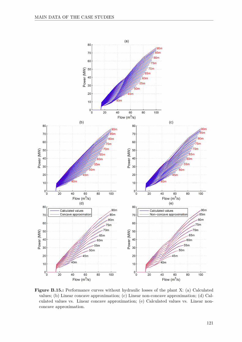
MAIN DATA OF THE CASE STUDIES
Figure B.15.: Performance curves without hydraulic losses of the plant X: (a) Calculatedvalues; (b) Linear concave approximation; (c) Linear non-concave approximation; (d) Cal-culated values vs. Linear concave approximation; (e) Calculated values vs. Linear non-concave approximation.
121
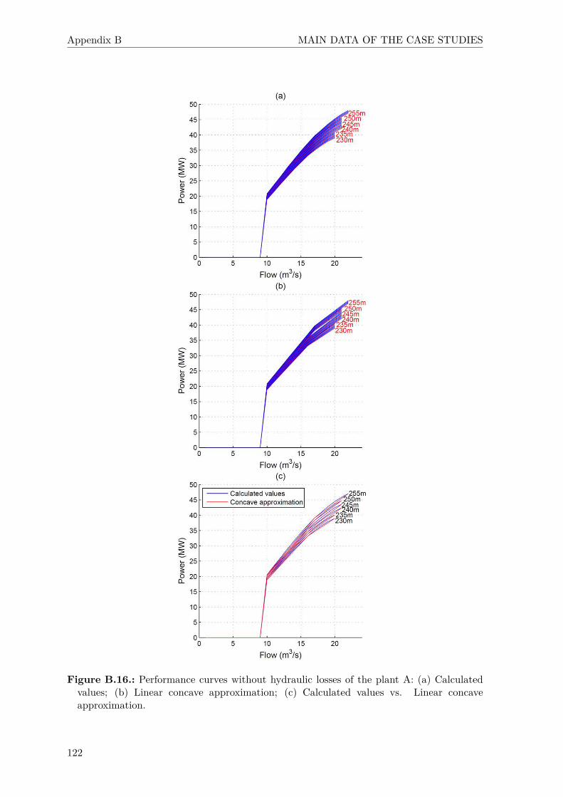
Appendix B MAIN DATA OF THE CASE STUDIES
Figure B.16.: Performance curves without hydraulic losses of the plant A: (a) Calculatedvalues; (b) Linear concave approximation; (c) Calculated values vs. Linear concaveapproximation.
122
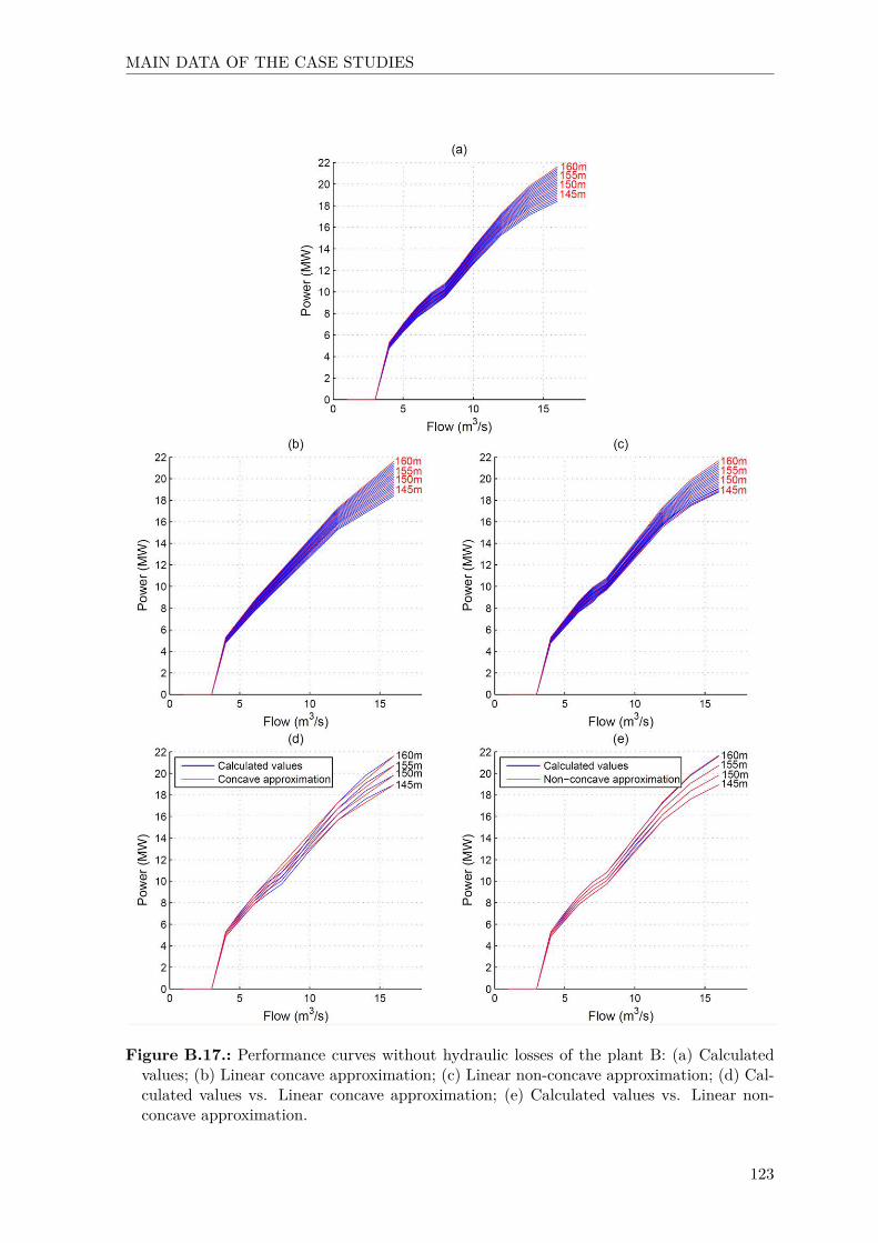
MAIN DATA OF THE CASE STUDIES
Figure B.17.: Performance curves without hydraulic losses of the plant B: (a) Calculatedvalues; (b) Linear concave approximation; (c) Linear non-concave approximation; (d) Cal-culated values vs. Linear concave approximation; (e) Calculated values vs. Linear non-concave approximation.
123
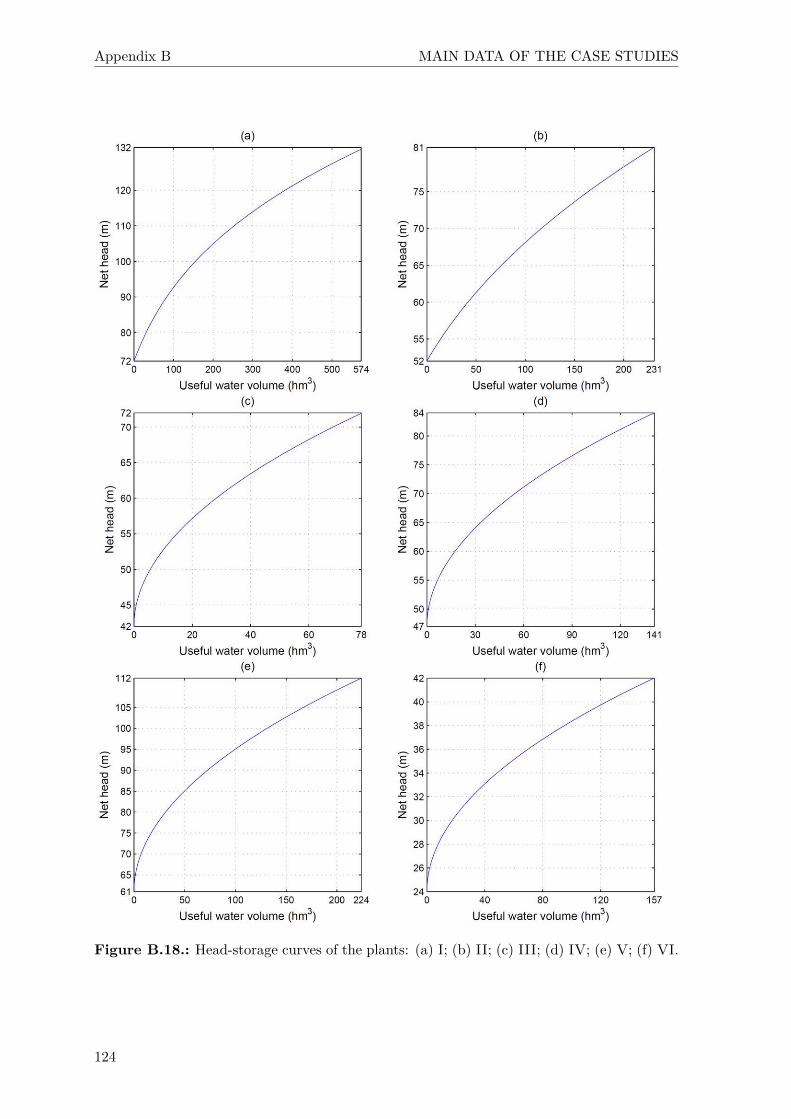
Appendix B MAIN DATA OF THE CASE STUDIES
Figure B.18.: Head-storage curves of the plants: (a) I; (b) II; (c) III; (d) IV; (e) V; (f) VI.
124
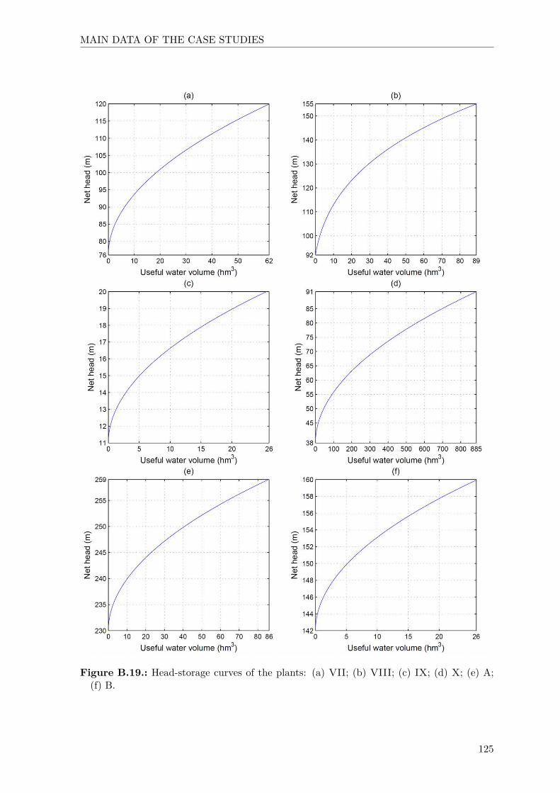
MAIN DATA OF THE CASE STUDIES
Figure B.19.: Head-storage curves of the plants: (a) VII; (b) VIII; (c) IX; (d) X; (e) A;(f) B.
125

Appendix B MAIN DATA OF THE CASE STUDIES
Figure B.20.: Mean water inflow volumes of the plants: (a) I; (b) II; (c) III; (d) IV; (e) V;(f) VI.
126

MAIN DATA OF THE CASE STUDIES
Figure B.21.: Mean water inflow volumes of the plants: (a) VII; (b) VIII; (c) IX; (d) X;(e) A; (f) B.
127


References
Abgottspon, H., Andersson, G., 20-23 May 2012. "Approach of integrating ancillary servicesinto a medium-term hydro optimization". In: 12th symposium of specialists in electricoperational and expansion planning. SEPOPE, Rio de Janeiro, Brazil.
ACA, 2015. Water inflows data (from the Catalan Water Agency).URL http://aca-web.gencat.cat/aca/appmanager/aca/aca?_nfpb=true&_
pageLabel=P1232354461208201788774
Ahmed, K. M., Petersen, E. H., Arvanitides, N. V., 1965. Optimal operation and controlof multi-dam hydroelectric power systems : an application of decision theory. StanfordUniversity, Stanford, USA.
Ahuja, R. K., Magnanti, T. L., Orlin, J. B., 1993. Network flows: theory, algorithms, andapplications. Prentice-Hall Incorporated, Upper Saddle River, USA.
Akaike, H., 2-8 September 1971. "Information theory and an extension of the maximumlikelihood principle". In: 2nd international symposium on information theory. AkademinaiKiado, Tsahkadsor, Armenia, USSR.
Alemu, E. T., Palmer, R. N., Polebitski, A., Meaker, B., 2011. "Decision support system foroptimizing reservoir operations using ensemble streamflow predictions". Journal of WaterResources Planning and Management 137 (1), 72–82.
Allen, R. B., Bridgeman, S. G., 1986. "Dynamic programming in hydropower scheduling".Journal of Water Resources Planning and Management 112 (3), 339–353.
Archibald, T. W., McKinnon, K. I. M., Thomas, L. C., 1997. "An aggregate stochasticdynamic programming model of multireservoir systems". Water Resources Research 33 (2),333–340.
Archibald, T. W., McKinnon, K. I. M., Thomas, L. C., 2006. "Modeling the operation ofmultireservoir systems using decomposition and stochastic dynamic programming". NavalResearch Logistics 53 (3), 217–225.
Arroyo, J. M., Conejo, A. J., 2004. "Modeling of start-up and shut-down power trajectoriesof thermal units". IEEE Transactions on Power Systems 19 (3), 1562–1568.
129
References
Atanassov, E. I., 2003. "A new efficient algorithm for generating the scrambledSobol’sequence". In: Numerical methods and applications. Springer, Berlin, Germany, pp.83–90.
Babayev, D. A., Mardanov, S. S., 1994. "Reducing the number of variables in integer andlinear programming problems". Computational Optimization and Applications 3 (2), 99–109.
Babel, M. S., Nguyen Dinh, C., Mullick, M. R. A., Nanduri, U. V., 2012. "Operation of ahydropower system considering environmental flow requirements: a case study in La NgaRiver basin, Vietnam". Journal of Hydro-environment Research 6 (1), 63–73.
Basharin, G. P., Langville, A. N., Naumov, V. A., 2004. "The life and work of A.A. Markov".Linear Algebra and its Applications 386, 3–26.
Baslis, C. G., Bakirtzis, A. G., 2011. "Mid-term stochastic scheduling of a price-maker hydroproducer with pumped storage". IEEE Transactions on Power Systems 26 (4), 1856–1865.
Bayón, L., Grau, J. M., Ruiz, M. M., Suárez, P. M., 18-22 September 2008. "Influence of theelevation-storage curve in the optimization of hydro-plants". In: 2nd international confer-ence on multidisciplinary design optimization and applications. ASMDO, Gijón, Spain.
Becker, L., Yeh, W. W.-G., 1974. "Optimization of real time operation of a multiple-reservoirsystem". Water Resources Research 10 (6), 1107–1112.
Bellman, R., 1954. "The theory of dynamic programming". Bulletin of the American Mathe-matical Society 60 (3), 503–515.
Bellman, R., 1957. Dynamic programming. Princeton University Press, Princeton, USA.
Bellman, R., Dreyfus, S. E., 1962. Applied dynamic programming. Princeton University Press,Princeton, USA.
Bellman, R., Kalaba, R. E., 1965. Dynamic programming and modern control theory. Aca-demic Press, New York, USA.
Belsnes, M. M., Fosso, O. B., 16-18 March 2008. "Competitive optimal hydropower schedulingfrom strategy to operation". In: 8th IASTED international conference. IASTED, Phuket,Thailand.
Belsnes, M. M., Fosso, O. B., Røynstrand, J., Honve, I., Steinsland, I., Lund, M. W., San-danger, M. I., Dorn, F., 2013. Building input for SHOP. SINTEF Energi AS, Trondheim,Norway.
Bensalem, A., Miloudi, A., Zouzou, S. E., Mahdad, B., Bouhentala, A., 2007. "Optimalshort term hydro scheduling of large power systems with discretized horizon". Journal ofElectrical Engineering 58 (4), 214.
130

References
Bernholtz, B., Graham, L., 1960. "Hydrothermal economic scheduling: part I - Solution byincremental dynamic programming". IEEE Transactions on Power Apparatus and Systems79 (3), 921–929.
Bertsekas, D. P., 1999. Nonlinear programming, 2nd Edition. Vol. 2 of Optimization andcomputation. Athena Scientific, Belmont, USA.
Bixby, R. E., 2012. "A brief history of linear and mixed-integer programming computation".Documenta Mathematica Extra volume: optimization stories, 107–121.
Bogardi, J. J., Budhakooncharoen, S., Shrestha, D. L., Nandalal, K. D. W., 20-22 July 1988."Effect of state space and inflow discretization on stochastic dynamic programming basedreservoir operation rules and system performance". In: 6th congress Asian and Pacificregional division. IAHR, Kyoto, Japan.
Bolch, G., Greiner, S., de Meer, H., Trivedi, K. S., 2006. Queueing networks and Markovchains: modeling and performance evaluation with computer science applications. JohnWiley & Sons, Inc., New York, USA.
Borghetti, A., D’Ambrosio, C., Lodi, A., Martello, S., 2008. "An MILP approach for short-term hydro scheduling and unit commitment with head-dependent reservoir". IEEE Trans-actions on Power Systems 23 (3), 1115–1124.
Boshier, J. F., Manning, G. B., Read, E. G., 1983. "Scheduling releases from New Zealand’shydro reservoirs". Transactions of the Institution of Professional Engineers New Zealand:Electrical/Mechanical/Chemical Engineering Section 10 (2), 33–41.
Box, G. E. P., 1957. "Evolutionary operation: a method for increasing industrial productiv-ity". Applied Statistics 6 (2), 81–101.
BP, 2016. "BP statistical review of world energy June 2016". Tech. rep., British Petroleum.URL http://www.bp.com/content/dam/bp/pdf/energy-economics/
statistical-review-2016/bp-statistical-review-of-world-energy-2016-full-report.
Braga Jr, B. P. F., Yen, W. W.-G., Becker, L., Barros, M. T. L., 1991. "Stochastic op-timization of multiple-reservoir-system operation". Journal of Water Resources Planningand Management 117 (4), 471–481.
Bras, R. L., Buchanan, R., Curry, K. C., 1983. "Real time adaptive closed loop control ofreservoirs with the High Aswan Dam as a case study". Water Resources Research 19 (1),33–52.
Buchanan, L., O‘Connell, A., 2006. "A brief history of decision making". Harvard BusinessReview 84 (1), 32–41.
131

References
Bunn, D. W., 2004. Modelling prices in competitive electricity markets. Wiley Finance. JohnWiley & Sons, Ltd, Chichester, England.
Carrión, M., Arroyo, J. M., 2006. "A computationally efficient mixed-integer linear formu-lation for the thermal unit commitment problem". IEEE Transactions on Power Systems21 (3), 1371–1378.
Carvalho, M. C. A., Pinto, J. M., 2006. "A bilevel decomposition technique for the optimalplanning of offshore platforms". Brazilian Journal of Chemical Engineering 23 (1), 67–82.
Castelletti, A., de Rigo, D., Rizzoli, A. E., Soncini-Sessa, R., Weber, E., 2007. "Neuro-dynamic programming for designing water reservoir network management policies". ControlEngineering Practice 15 (8), 1031–1038.
Castelletti, A., Pianosi, F., Soncini-Sessa, R., 2008. "Water reservoir control under economic,social and environmental constraints". Automatica 44 (6), 1595–1607.
Catalão, J. P. S., Mariano, S. J. P. S., Mendes, V. M., Ferreira, L. A. F., 2010. "Nonlin-ear optimization method for short-term hydro scheduling considering head-dependency".European Transactions on Electrical Power 20 (2), 172–183.
CEDEX, 2013. Water inflows data (from the Centre for Public Works Studies and Experi-mentation).URL http://ceh-flumen64.cedex.es/anuarioaforos/default.asp
Cervellera, C., Chen, V. C. P., Wen, A., 2006. "Optimization of a large-scale water reser-voir network by stochastic dynamic programming with efficient state space discretization".European Journal of Operational Research 171 (3), 1139–1151.
Chang, G. W., Aganagic, M., Waight, J. G., Medina, J., Burton, T., Reeves, S., Christo-foridis, M., 2001. "Experiences with mixed integer linear programming based approacheson short-term hydro scheduling". IEEE Transactions on Power Systems 16 (4), 743–749.
Chen, Z., Forsyth, P. A., 2008. Nonlinear models in mathematical finance: new researchtrends in option pricing. Vol. 1. Technical University of Berlin, Berlin, Germany, Ch. 9, pp.275–304.
Cheng, C., Shen, J., Wu, X., Chau, K.-w., 2012. "Short-term hydroscheduling with discrepantobjectives using multi-step progressive optimality algorithm". Journal of the American Wa-ter Resources Association 48 (3), 464–479.
CHMS, 2010. Maximum values of the environmental constraints (from the Miño-Sil RiverBasin District Authority).URL http://www.chminosil.es/es/chms/planificacionhidrologica
132

References
Chow, V. T., Maidment, D. R., Tauxe, G. W., 1975. "Computer time and memory require-ments for DP and DDDP in water resource systems analysis". Water Resources Research11 (5), 621–628.
Colorado State University, 2010. MODSIM 8.1: river basin management decision supportsystem. User manual and documentation. Colorado State University, Fort Collins, USA.
Conejo, A. J., Arroyo, J. M., Contreras, J., Villamor, F. A., 2002. "Self-scheduling of a hydroproducer in a pool-based electricity market". IEEE Transactions on Power Systems 17 (4),1265–1272.
Cristóbal, M. P., Escudero, L. F., Monge, J. F., 2009. "On stochastic dynamic programmingfor solving large-scale planning problems under uncertainty". Computers & Operations Re-search 36 (8), 2418–2428.
Crombecq, K., Laermans, E., Dhaene, T., 2011. "Efficient space-filling and non-collapsing se-quential design strategies for simulation-based modeling". European Journal of OperationalResearch 214 (3), 683–696.
Cushman, R. M., 1985. "Review of ecological effects of rapidly varying flows downstreamfrom hydroelectric facilities". North American Journal of Fisheries Management 5 (3A),330–339.
Cvitanovic, P., Dettmann, C. P., Mainieri, R., Vattay, G., 1999. "Trace formulae for stochasticevolution operators: smooth conjugation method". Nonlinearity 12 (4), 939.
D’Ambrosio, C., Lodi, A., Martello, S., 2010. "Piecewise linear approximation of functions oftwo variables in MILP models". Operations Research Letters 38 (1), 39–46.
Dantzig, G. B., July 1948. "Linear programming". In: Symposium on numerical methods.Previously invited paper. NBS, Los Angeles, USA.
Dantzig, G. B., 1954. "A comment on Edie’s: traffic delays at toll booths". Journal of theOperations Research Society of America 2 (3), 339–341.
Deb, K., 1995. Optimization for engineering design. Algorithms and examples. PHI LearningPvt. Ltd., New Delhi, India.
Deni, S. M., Jemain, A. A., 4-6 July 2012. "Comparison between mixed probability modelsand Markov chain models for weekly dry and wet spells in Peninsular Malaysia". In: Worldcongress on engineering. IAENG, London, England.
Dias, B. H., Marcato, A. L. M., Souza, R. C., Soares, M. P., Silva Junior, I. C., Oliveira,E. J. d., Brandi, R., Ramos, T. P., 2010. "Stochastic dynamic programming applied to hy-drothermal power systems operation planning based on the convex hull algorithm". Math-ematical Problems in Engineering 2010, 390940–390959.
133

References
Diniz, A. L., Souza, T. M., 2014. "Short-term hydrothermal dispatch with river-level androuting constraints". IEEE Transactions on Power Systems PP (99), 1–9.
Doorman, G. L., 2009. Hydro power scheduling. NTNU, Trondheim, Norway.
Doran, D. G., 1975. "An efficient transition definition for discrete state reservoir analysis: thedivided interval technique". Water Resources Research 11 (6), 867–873.
Dragoni, W., Valigi, D., 1994. "Contributo alla stima dell evaporazione dalle superfici liquidenell Italia Centrale". Geologica Romana 30, 151–158.
Durán, H., Puech, C., Díaz, J., Sánchez, G., 1985. "Optimal operation of multireservoirsystems using an aggregation-decomposition approach". IEEE Transactions on Power Ap-paratus and Systems 104 (8), 2086–2092.
Eckberg, D. K., 1986. "Cumulative impacts of hydropower development under NEPA". En-vironmental Law 16, 673–963.
Edwards, B. K., Flaim, S. J., Howitt, R. E., 1999. "Optimal provision of hydroelectric powerunder environmental and regulatory constraints". Land Economics 75 (2), 267–283.
Egré, D., Milewski, J. C., 2002. "The diversity of hydropower projects". Energy Policy 30 (14),1225–1230.
El-Hawary, M. E., Christensen, G. S., 1979. Optimal economic operation of electric powersystems. Vol. 26. Academic Press, New York, USA.
EPRI, 2001. "Hydropower Technology Roundup Report: accommodating wear and teareffects on hydroelectric facilities operating to provide ancillary services: TR-113584-V4".Tech. rep., Electric Power Research Institute.URL http://www.epri.com/abstracts/Pages/ProductAbstract.aspx?ProductId=
000000000001004047
Eschenbach, E. A., Magee, T., Zagona, E., Goranflo, M., Shane, R., 2001. "Goal programmingdecision support system for multiobjective operation of reservoir systems". Journal of WaterResources Planning and Management 127 (2), 108–120.
ESHA, 2012. "Small hydropower roadmap. Condensed research data for the EU-27". Tech.rep., European Small Hydropower Association.URL http://streammap.esha.be/fileadmin/documents/Press_Corner_
Publications/SHPRoadmap_FINAL_Public.pdf
EU, 2007. "Water Framework Directive & hydropower. Key conclusions". Tech. rep., EuropeanUnion.URL http://www.ecologic-events.de/hydropower/documents/key_conclusions.pdf
134

References
Eurelectric, 2003. "Ancillary services. Unbundling electricity products. An emerging market".Tech. rep., Union of the Electricity Industry.URL http://www.eurelectric.org/Download/Download.aspx?DocumentID=13934
Fan, H., Tarun, P. K., Chen, V. C. P., 2013. "Adaptive value function approximation forcontinuous-state stochastic dynamic programming". Computers & Operations Research40 (4), 1076–1084.
Fang, K.-T., Wang, Y., Bentler, P. M., 1994. "Some applications of number-theoretic methodsin statistics". Statistical Science 9 (3), 416–428.
Farhat, I. A., El-Hawary, M. E., 2009. "Optimization methods applied for solving the short-term hydrothermal coordination problem". Electric Power Systems Research 79 (9), 1308–1320.
Fayaed, S. S., El-Shafie, A., Jaafar, O., 2013. "Reservoir-system simulation and optimizationtechniques". Stochastic Environmental Research and Risk Assessment 27 (7), 1751–1772.
Finardi, E. C., da Silva, E. L., 2005. "Unit commitment of single hydroelectric plant". ElectricPower Systems Research 75 (2), 116–123.
Fletcher, R., 2000. Practical methods of optimization, 2nd Edition. John Wiley & Sons, Ltd,Chichester, England.
Fleten, S. E., Keppo, J., Lumba, H., Weiss, V., 19-22 August 2009. "Derivative price in-formation use in hydroelectric scheduling". In: EFA 36th annual meeting. EFA, Bergen,Norway.
Forsund, F. R., 2007. Hydropower economics. Vol. 112 of International series in operationsresearch and management science. Springer, New York, USA.
Fosso, O. B., Belsnes, M. M., 21-24 November 2004. "Short-term hydro scheduling in aliberalized power system". In: 4th intenational conference on power system technology.IEEE, Singapore, Singapore.
Fosso, O. B., Gjelsvik, A., Haugstad, A., Mo, B., Wangensteen, I., 1999. "Generation schedul-ing in a deregulated system. The Norwegian case". IEEE Transactions on Power Systems14 (1), 75–81.
Fourier, J. B. J., 1826. "Solution d une question particuliere du calcul des inégalités". NouveauBulletin des Sciences par la Société Philomatique de Paris 99, 100.
Fu, Y., Shahidehpour, M., 2007. "Fast SCUC for large-scale power systems". IEEE Transac-tions on Power Systems 22 (4), 2144–2151.
135
References
García-González, J., Castro, G. A., 10-13 September 2001. "Short-term hydro scheduling withcascaded and head-dependent reservoirs based on mixed-integer linear programming". In:Power tech conference. IEEE, Porto, Portugal.
Gebrekiros, Y., Doorman, G., Jaehnert, S., Farahmand, H., 6-9 October 2013. "Bidding in thefrequency restoration reserves (FRR) market for a hydropower unit". In: 4 th innovativesmart grid technologies Europe. IEEE, Copenhagen, Denmark.
Gjelsvik, A., Belsnes, M. M., Haugstad, A., 28 June - 2 July 1999. "An algorithm for stochas-tic medium-term hydrothermal scheduling under spot price uncertainty". In: 13th powersystems computation conference. PSCC, Trondheim, Norway.
Gjelsvik, A., Mo, B., Haugstad, A., 2010. "Long-and medium-term operations planning andstochastic modelling in hydro-dominated power systems based on stochastic dual dynamicprogramming". In: Handbook of power systems I. Springer, Berlin, Germany, pp. 33–55.
Golnaraghi, M. F., Kuo, B. C., 2003. Automatic control systems. Vol. 4. John Wiley & Sons,Inc., New York, USA.
Gomory, R. E., 1960. "Outline of an algorithm for integer solutions to linear programs".Bulletin of the American Mathematical Society 28 (1), 30–44.
Goulter, I. C., Tai, F.-K., 1985. "Practical implications in the use of stochastic dynamic pro-gramming for reservoir operation". Journal of the American Water Resources Association21 (1), 65–74.
Grattan-Guinness, I., 1970. "Joseph Fourier’s anticipation of linear programming". Opera-tional Research Quarterly 21 (3), 361–364.
Griffith, R. E., Stewart, R. A., 1961. "A nonlinear programming technique for the optimizationof continuous processing systems". Management Science 7 (4), 379–392.
Grötschel, M., Jünger, M., Reinelt, G., 1985. "On the acyclic subgraph polytope". Mathemat-ical Programming 33 (1), 28–42.
Grygier, J. C., Stedinger, J. R., 1985. "Algorithms for optimizing hydropower system opera-tion". Water Resources Research 21 (1), 1–10.
Guan, X., Svoboda, A., Li, C., 1999. "Scheduling hydro power systems with restricted op-erating zones and discharge ramping constraints". IEEE Transactions on Power Systems14 (1), 126–131.
Guisández, I., Pérez-Díaz, J. I., Wilhelmi, J. R., 2013. "Assessment of the economic impactof environmental constraints on annual hydropower plant operation". Energy Policy 61,1332–1343.
136

References
Guisández, I., Pérez-Díaz, J. I., Wilhelmi, J. R., 8-10 April 2014. "Effects of the maximumflow ramping rates on the long-term operation decisions of a hydropower plant". In: Inter-national conference on renewable energies and power quality. ICREPQ, Córdoba, Spain.
Guisández, I., Pérez-Díaz, J. I., Wilhelmi, J. R., 17-18 September 2015. "Influence of themaximum flow ramping rates on the water value". In: 5th international workshop on hydroscheduling in competitive electricity markets. IWHSCEM, Trondheim, Norway.
Guisández, I., Pérez-Díaz, J. I., Wilhelmi, J. R., 2016a. "Approximate formulae for the as-sessment of the long-term economic impact of environmental constraints on hydropeaking".Energy 112, 629–641.
Guisández, I., Pérez-Díaz, J. I., Wilhelmi, J. R., 2016b. "Influence of the maximum flowramping rates on the water value". Energy Procedia 87, 100–107.
Guisández, I., Pérez-Díaz, J. I., Wilhelmi, J. R., 2016c. "The influence of environmentalconstraints on the water value". Energies 9 (6).
Guise, J. W. B., Flinn, J. C., 1970. "The allocation and pricing of water in a river basin".American Journal of Agricultural Economics 52 (3), 411–421.
Habibollahzadeh, H., Bubenko, J. A., 1986. "Application of decomposition techniques toshort-term operation planning of hydrothermal power system". IEEE Transactions onPower Systems 1 (1), 41–47.
Halton, J. H., 1960. "On the efficiency of certain quasi-random sequences of points in evalu-ating multi-dimensional integrals". Numerische Mathematik 2 (1), 84–90.
Hamilton, H., 1767. Philosophical essays: on the following subjects: I. On the ascent ofvapours, the formation of clouds, rain and dew, and on several other phoenomena of airand water, II. Observations and conjectures on the nature of the aurora borealis, and thetails of comets, III. On the principles of mechanicks, 2nd Edition. John Nourse, London,England.
Hammersley, J. M., 1960. "Monte Carlo methods for solving multivariable problems". Annalsof the New York Academy of Sciences 86 (3), 844–874.
Harbeck, G. E., 1962. "A practical field technique for measuring reservoir evaporation utilizingmass-transfer theory". U.S. Geological Survey 272-E, 101–105.
Harpman, D. A., 1999. "Assessing the short-run economic cost of environmental constraintson hydropower operations at Glen Canyon Dam". Land Economics 75 (3), 390–401.
Hatch Ltd., 2013. Vista DSS. Statement of qualifications for power and water optimization(PWO). Hatch Ltd., Mississauga, Canada.
137

References
Helseth, A., Gjelsvik, A., Mo, B., Linnet, Ú., 2013. "A model for optimal scheduling of hydrothermal systems including pumped-storage and wind power". IET Generation, Transmis-sion & Distribution 7 (12), 1426–1434.
Holland, J. H., 1975. Adaptation in natural and artificial systems. University of MichiganPress, Ann Arbor, USA.
Howard, C. D. D., 24-27 October 2006. "Hydroelectric system operations optimization". In:Great Wall world renewable energy forum and exhibition. CWEA, Beijing, China.
Howard, R. A., 1960. Dynamic programming and Markov processes. The M.I.T. Press, Cam-bridge, USA.
Howson, H. R., Sancho, N. G. F., 1975. "A new algorithm for the solution of multi-statedynamic programming problems". Mathematical programming 8 (1), 104–116.
Iliadis, N. A., Tilmant, A., Chabar, R., Granville, S., Pereira, M., 17-23 September 2008. "Op-timal operation of hydro-dominated multireservoir systems in deregulated electricity mar-kets". In: International conference for reservoir operation and river management. ICROM,Guanghzou and Three Gorges, China.
Illés, T., Terlaky, T., 2002. "Pivot versus interior point methods: pros and cons". EuropeanJournal of Operational Research 140 (2), 170–190.
INE, 1960. Temperature data (from the Spanish Statistical Office).URL http://www.ine.es/inebaseweb/pdfDispacher.do;jsessionid=
09739D168C9F3EF056383E89BACE7A07.inebaseweb01?td=183760
Jensen, S. G., Skytte, K., 2003. "Simultaneous attainment of energy goals by means of greencertificates and emission permits". Energy Policy 31 (1), 63–71.
Jimoh, O. D., Webster, P., 1996. "The optimum order of a Markov chain model for dailyrainfall in Nigeria". Journal of Hydrology 185 (1), 45–69.
Johnson, S. A., Stedinger, J. R., Shoemaker, C. A., Li, Y., Tejada-Guibert, J. A., 1993."Numerical solution of continuous-state dynamic programs using linear and spline interpo-lation". Operations Research 41 (3), 484–500.
Juday, D. G., Brummer, J. E., Smith, D. H., 2011. "Use of alternative temperature expressionswith Blaney-Criddle". Journal of Irrigation and Drainage Engineering 137 (9), 573–584.
Kall, P., Mayer, J., 2011. Stochastic linear programming. Models, theory, and computation.Vol. 156 of International Series in Operations Research & Management Science. Springer,New York, USA.
Kapelan, Z., Savic, D. A., Walters, G. A., 2005. "Decision-support tools for sustainable urbandevelopment". Proceedings of the ICE-Engineering Sustainability 158 (3), 135–142.
138

References
Karamouz, M., Houck, M. H., 1987. "Comparison of stochastic and deterministic dynamicprogramming for reservoir operating rule generation". Journal of the American Water Re-sources Association 23 (1), 1–9.
Karamouz, M., Zahraie, B., Araghinejad, S., 2005. "Decision support system for monthly op-eration of hydropower reservoirs: a case study". Journal of Computing in Civil Engineering19 (2), 194–207.
Karmarkar, N., 30 April - 2 May 1984. "A new polynomial-time algorithm for linear pro-gramming". In: 16th annual symposium on theory of computing. ACM, Washington, USA.
Karush, W., 1939. Minima of functions of several variables with inequalities as side con-straints. Ph.D. thesis, The University of Chicago, Chicago, USA.
Katz, R. W., 1981. "On some criteria for estimating the order of a Markov chain". Techno-metrics 23 (3), 243–249.
Keckler, W. G., Larson, R. E., 1968. "Dynamic programming applications to water resourcesystem operation and planning". Journal of Mathematical Analysis and Applications 24 (1),80–109.
Kelman, R., Barroso, L. A. N., Pereira, M. V. F., 2001. "Market power assessment andmitigation in hydrothermal systems". IEEE Transactions on Power Systems 16 (3), 354–359.
Kemeny, J. G., Snell, J. L., 1960. Finite Markov chains. Van Nostrand Company, Princeton,USA.
Keppo, J., 2002. "Optimality with hydropower system". IEEE Transactions on Power Systems17 (3), 583–589.
Kim, Y. O., Palmer, R. N., 1997. "Value of seasonal flow forecasts in Bayesian stochasticprogramming". Journal of Water Resources Planning and Management 123 (6), 327–335.
Kirchhoff, G. R., 1845. "Ueber den Durchgang eines elektrischen Stromes durch eine Ebene,insbesondere durch eine kreisförmige". Annalen der Physik 140 (4), 497–514.
Kirkham, H., Nightingale, D., Koerner, T., 1981. "Energy management system design withdispersed storage and generation". IEEE Transactions on Power Apparatus and Systems100 (7), 3432–3441.
Kishen, K., 1942. "On Latin and hyper-Graeco-Latin cubes and hyper-cubes". Current Science11 (3), 98–99.
Klemeš, V., 1977. "Discrete representation of storage for stochastic reservoir optimization".Water Resources Research 13 (1), 149–158.
139

References
Knittel, C. R., Roberts, M. R., 2005. "An empirical examination of restructured electricityprices". Energy Economics 27 (5), 791–817.
Kolmogoroff, A., 1936. "Zur theorie der markoffschen ketten".Mathematische Annalen 112 (1),155–160.
Koreneff, G., Seppala, A., Lehtonen, M., Kekkonen, V., Laitinen, E., Hakli, J., Antila, E.,3-5 March 1998. "Electricity spot price forecasting as a part of energy management in de-regulated power market". In: International conference on energy management and powerdelivery. IEEE, Singapore.
Kosnik, L.-R. D., 2010. "Balancing environmental protection and energy production in theFederal hydropower licensing process". Land Economics 86 (3), 444–466.
Kotchen, M. J., Moore, M. R., Lupi, F., Rutherford, E. S., 2006. "Environmental constraintson hydropower: an ex post benefit-cost analysis of dam relicensing in Michigan". LandEconomics 82 (3), 384–403.
Koutsoyiannis, D., Efstratiadis, A., Karavokiros, G., 2002. "A decision support tool for themanagement of multi-reservoir systems". Journal of the American Water Resources Asso-ciation 38 (4), 945–958.
Kuhn, H. W., Tucker, A. W., 31 July - 12 August 1950. "Nonlinear programming". In: 2ndBerkeley symposium on mathematical statistics and probability. University of California,Berkeley, USA.
Kumar, N., Baliarsingh, F., 2003. "Folded dynamic programming for optimal operation ofmultireservoir system". Water Resources Management 17 (5), 337–353.
Labadie, J. W., 2004. "Optimal operation of multireservoir systems: state-of-the-art review".Journal of Water Resources Planning and Management 130 (2), 93–111.
Land, A. H., Doig, A. G., 1960. "An automatic method of solving discrete programmingproblems". Econometrica 28 (3), 497–520.
Larson, R., 1967. "A survey of dynamic programming computational procedures". IEEETransactions on Automatic Control 12 (6), 767–774.
Lehner, B., Czisch, G., Vassolo, S., 2005. "The impact of global change on the hydropowerpotential of Europe: a model-based analysis". Energy Policy 33 (7), 839–855.
Li, T., Shahidehpour, M., 2005. "Price-based unit commitment: a case of Lagrangian relax-ation versus mixed integer programming". IEEE Transactions on Power Systems 20 (4),2015–2025.
140

References
Lima, R. M., Grossmann, I. E., 2011. "Computational advances in solving mixed integerlinear programming problems". In: Chemical engineering greetings to prof. Sauro Pieruccion occasion of his 65th birthday. The Italian Association of Chemical Engineering, Milano,Italy, pp. 151–160.
Little, J. D. C., 1955. "The use of storage water in a hydroelectric system". OperationsResearch 3 (2), 187–197.
Liu, X., Guo, S., Liu, P., Chen, L., Li, X., 2011. "Deriving optimal refill rules for multi-purposereservoir operation". Water Resources Management 25 (2), 431–448.
Löhndorf, N., Wozabal, D., Minner, S., 2013. "Optimizing trading decisions for hydro storagesystems using approximate dual dynamic programming". Operations Research 61 (4), 810–823.
Loucks, D. P., Stedinger, J. R., Haith, D. A., 1981. Water resource systems planning andanalysis. Prentice-Hall Incorporated, Englewood Cliffs, USA.
Loucks, D. P., van Beek, E., 2005. Water resources systems planning and management. Anintroduction to methods, models and applications. UNESCO, Paris, France.
Lowry, W. P., Guthrie, D., 1968. "Markov chains of order greater than one". Monthly WeatherReview 96 (11), 798–801.
Luenberger, D. G., 2003. Linear and nonlinear programming. Springer, Boston, USA.
MacCallum, R. C., Widaman, K. F., Zhang, S., Hong, S., 1999. "Sample size in factoranalysis". Psychological Methods 4 (1), 84–99.
Mariño, M. A., Mohammadi, B., 1983. "Reservoir operation by linear and dynamic program-ming". Journal of Water Resources Planning and Management 109 (4), 303–319.
Markov, A. A., 1906. "Rasprostranenie zakona bol shih chisel na velichiny, zavisyaschie drugot druga". Izvestiya Fiziko-matematicheskogo obschestva pri Kazanskom universitete 15 (2),135–156.
Markowitz, H. M., Manne, A. S., 1957. "On the solution of discrete programming problems".Econometrica 25 (1), 84–110.
Martin, Q. W., 1983. "Optimal operation of multiple reservoir systems". Journal of WaterResources Planning and Management 109 (1), 58–74.
Martino, J. P., 1993. Technological forecasting for decision making, 3rd Edition. McGraw-Hill,Inc., New York, USA.
Maruzewski, P., Rogeaux, C., Laurier, P., 19-23 August 2012. "Unit-sizing of hydro powerplant". In: IOP conference series: earth and environmental science. IAHR, Beijing, China.
141
References
Mazliak, L., 2007. "On the exchanges between Wolfgang Doeblin and Bohuslav Hostinsky".Revue d’histoire des mathématiques 13 (1), 155–180.
Meyn, S. S. P., Tweedie, R. L., 1993. Markov chains and stochastic stability. Springer-Verlag,London, England.
Mitchell, J. E., 2002. Handbook of applied optimization. Vol. 1. Oxford University Press,Oxford, England, Ch. 3.3, pp. 65–77.
Mo, B., Gjelsvik, A., Grundt, A., Kåresen, K., 10-13 September 2001. "Optimisation ofhydropower operation in a liberalised market with focus on price modelling". In: Powertech conference. IEEE, Porto, Portugal.
Mo, B., Haugstad, A., Fosso, O. B., 30 June - 2 July 1997. "Integrating Long and Short-TermModes for Hydro Scheduling". In: 3rd international conference on hydropower. NTNU,Trondheim, Norway.
Moran, P. A. P., 1959. The theory of storage. Metheun Publications, London, England.
Morgan, H. D., Doran, W. E., Mair, J., Edginton, R. H., Addison, H., Thornton, J. H.,1957. "Discussion on hydraulics paper no. 16: control of flow by gates and valves". ICEProceedings 7 (3), 569–574.
Nandalal, K. D. W., Bogardi, J. J., 2007. Dynamic programming based operation of reservoirs.Applicability and limits. Cambridge University Press, Cambridge, England.
Niederreiter, H., 1992. Quasi-Monte Carlo methods. John Wiley & Sons, Inc., New York,USA.
Nilsson, O., Sjelvgren, D., 1997a. "Hydro unit start-up costs and their impact on the shortterm scheduling strategies of Swedish power producers". IEEE Transactions on Power Sys-tems 12 (1), 38–44.
Nilsson, O., Sjelvgren, D., 1997b. "Variable splitting applied to modelling of start-up costsin short term hydro generation scheduling". IEEE Transactions on Power Systems 12 (2),770–775.
Niu, S., Insley, M., 2010. "On the economics of ramping rate restrictions at hydro powerplants: balancing profitability and environmental costs". Working paper, University ofWaterloo.URL affinity.uwaterloo.ca/~minsley/ramping%20rate%20paper%20Jan%203%
202011.pdf
Niu, S., Insley, M., 2013. "An options pricing approach to ramping rate restrictions at hydropower plants". Working paper, University of Waterloo.URL economics.ualberta.ca/en/EventsandSeminars/EMEE2013/~/media/economics/
EventsAndS/EMEE-2013/AP-Niu-Insley.pdf
142

References
Nocedal, J., Wright, S. J., 2006. Numerical optimization, 2nd Edition. Operations Researchand Financial Engineering. Springer, New York, USA.
Nogales, F. J., Contreras, J., Conejo, A. J., Espínola, R., 2002. "Forecasting next-day elec-tricity prices by time series models". IEEE Transactions on Power Systems 17 (2), 342–348.
Norris, J. R., 1998. Markov chains. No. 2008. Cambridge University Press, Cambridge, Eng-land.
Olivares, M. A., 2008. Optimal hydropower reservoir operation with environmental require-ments. Ph.D. thesis, The University of California, Davis, USA.
Olivares, M. A., Haas, J., Palma-Behnke, R., Benavides, C., 2015. "A framework to identifyPareto-efficient subdaily environmental flow constraints on hydropower reservoirs using agrid-wide power dispatch model". Water Resources Research 51 (5), 3664–3680.
Olivares, M. A., Lund, J. R., 2011. "Representing energy price variability in long-and medium-term hydropower optimization". Journal of Water Resources Planning and Management138 (6), 606–613.
OMIE, 2011. Day-ahead market data (from the Iberian Electricity Market Operator).URL http://www.omel.es/files/flash/ResultadosMercado.swf
O’Neil, K., Bernstein, A., Steinschneider, S., Polebitski, A., Palmer, R., 20-22 May 2013."Modeling the impact of climate change on hydropower operations in the ConnecticutRiver basin". In: World environmental and water resources congress. ASCE, Cincinnati,USA.
Ortuño, M. F., Conejero, W., Moreno, F., Moriana, A., Intrigliolo, D. S., Biel, C., Mellisho,C. D., Pérez-Pastor, A., Domingo, R., Ruiz-Sánchez, M. C., Casadeus, J., Bonany, J.,Torrecillas, A., 2010. "Could trunk diameter sensors be used in woody crops for irrigationscheduling? A review of current knowledge and future perspectives". Agricultural WaterManagement 97 (1), 1–11.
Padhy, N. P., 2004. "Unit commitment-a bibliographical survey". IEEE Transactions onPower Systems 19 (2), 1196–1205.
Paredes-Arquiola, J., Martinez-Capel, F., Solera, A., Aguilella, V., 2011. "Implementingenvironmental flows in complex water resources systems–case study: the Duero River basin,Spain". River Research and Applications 29 (4), 451–468.
Patten, D. T., Harpman, D. A., Voita, M. I., Randle, T. J., 2001. "A managed flood on theColorado River: background, objectives, design, and implementation". Ecological Applica-tions 11 (3), 635–643.
143

References
Pearson, K., 1901. "On lines and planes of closest fit to systems of points in space". TheLondon, Edinburgh, and Dublin Philosophical Magazine and Journal of Science 2 (11),559–572.
Pelc, R., Fujita, R. M., 2002. "Renewable energy from the ocean". Marine Policy 26 (6),471–479.
Pereira, M., 22-25 July 1985. "Optimal scheduling of hydrothermal systems-an overview". In:Symposium on planning and operation of electric energy systems. IFAC, Rio de Janeiro,Brazil.
Perekhodtsev, D., Lave, L., 2005. "Efficient bidding for hydro power plants in markets forenergy and ancillary services". Working paper, Massachusetts Institute of Technology.URL http://scholar.google.es/scholar?start=10&q=%22ancillary+services%22+
hydropower&hl=es&as_sdt=1,5&as_vis=1
Perera, K. K. Y. W., 1969. A study of power system economic operation. Ph.D. thesis, TheUniversity of British Columbia, Vancouver, Canada.
Pérez-Díaz, J. I., Millán, R., García, D., Guisández, I., Wilhelmi, J. R., 2012. "Contribu-tion of re-regulation reservoirs considering pumping capability to environmentally friendlyhydropower operation". Energy 48 (1), 144–152.
Pérez-Díaz, J. I., Wilhelmi, J. R., 2010. "Assessment of the economic impact of environmentalconstraints on short-term hydropower plant operation". Energy Policy 38 (12), 7960–7970.
Pérez-Díaz, J. I., Wilhelmi, J. R., Arévalo, L. A., 2010. "Optimal short-term operation sched-ule of a hydropower plant in a competitive electricity market". Energy Conversion andManagement 51 (12), 2955–2966.
Pérez González, M., Sanz Donaire, J., 2001. "Aspectos geográficos de las distribuciones es-tadísticas ajustadas a las series temporales rellenadas de totales anuales de precipitaciónespañola". Nimbus 7-8, 135–159.
Perrin, F., 1971. "Recent advances in energy systems". Annals of the New York Academy ofSciences 184 (1), 242–251.
Petreski, Z., 6-9 July 1999. "Waterpower optimization software: WOPRO 4.0-ALLOCATE2.0". In: Waterpower conference 1999. ASCE, Las Vegas, USA.
Philbrick, C. R., Kitanidis, P. K., 1999. "Limitations of deterministic optimization appliedto reservoir operations". Journal of Water Resources Planning and Management 125 (3),135–142.
Philbrick, C. R., Kitanidis, P. K., 2001. "Improved dynamic programming methods for opti-mal control of lumped-parameter stochastic systems". Operations Research 49 (3), 398–412.
144

References
Philpott, A. B., Dallagi, A., Gallet, E., 2013. "On cutting plane algorithms and dynamicprogramming for hydroelectricity generation". In: Handbook of risk management in energyproduction and trading. Springer, Berlin, Germany, pp. 105–127.
Piekutowski, M. R., Litwinowicz, T., Frowd, R., 4-7 May 1993. "Optimal short-term schedul-ing for a large-scale cascaded hydro system". In: Power industry computer applicationconference. IEEE, Phoenix, USA.
Pousinho, H. M. I., Mendes, V. M. F., Catalão, J. P. S., 2012. "Scheduling of a hydro producerconsidering head-dependency, price scenarios and risk-aversion". Energy Conversion andManagement 56, 96–103.
Preda, V., Balcau, C., 2008. "Homogeneous stationary multiple Markov chains with maximumIosifescu-Theodorescu entropy". Revue Roumaine de Mathematiques Pures et Appliquees53 (1), 55–62.
Pritchard, G., Philpott, A. B., Neame, P. J., 2005. "Hydroelectric reservoir optimization ina pool market". Mathematical Programming 103 (3), 445–461.
Raabe, J., 1985. Hydro power: the design, use, and function of hydromechanical, hydraulic,and electrical equipment. VDI-Verlag, Dusserldorf, Germany.
Rani, D., Moreira, M. M., 2010. "Simulation–optimization modeling: a survey and potentialapplication in reservoir systems operation". Water Resources Management 24 (6), 1107–1138.
Ratnayake, U., Harboe, R., 2007. "Deterministic and stochastic optimization of a reservoirsystem". Water International 32 (1), 155–162.
Rauscher, B., Olason, T., Welt, F., Bridgeman, S. G., 29 July - 2 August 2002. "Environ-mental compliance and optimum hydroelectric system dispatch". In: HydroVision 2002conference. HCI Publications, Inc., Portland, USA.
Reneses, J., Barquín, J., García-González, J., Centeno, E., 2015. "Water value in electricitymarkets". International Transactions on Electrical Energy Systems.
Rheinheimer, D. E., Yarnell, S. M., Viers, J. H., 2013. "Hydropower costs of environmentalflows and climate warming in California’s Upper Yuba River watershed". River Researchand Applications 29 (10), 1291–1305.
Robitaille, A., Audette, L., Tinker, D., 17-20 October 2005. "Benefits in optimizing hydroplant operations while meeting sophisticated environmental requirements". In: Hydro 2005.Hydropower & Dams and NetWork Events Ltd, Villach, Austria.
Rosenberry, D. O., Winter, T. C., Buso, D. C., Likens, G. E., 2007. "Comparison of 15evaporation methods applied to a small mountain lake in the Northeastern USA". Journalof Hydrology 340 (3), 149–166.
145

References
Rossi, G. B., 2012. "Toward an interdisciplinary probabilistic theory of measurement". IEEETransactions on Instrumentation and Measurement 61 (8), 2095–2106.
Saad, M., Turgeon, A., 1988. "Application of principal component analysis to long-termreservoir management". Water Resources Research 24 (7), 907–912.
Sanguedo Baptista, R., De Aquino Galeano Massera Da Hora, M., 2013. "Estimated ecologicalflow of the Preto River by the wetted perimeter method". Global Journal of Researches inEngineering 13 (7).
Sauter, T., Lobashov, M., 2011. "End-to-end communication architecture for smart grids".IEEE Transactions on Industrial Electronics 58 (4), 1218–1228.
Schwarz, G., 1978. "Estimating the dimension of a model". The Annals of Statistics 6 (2),461–464.
Schweppe, F. C., Tabors, R. D., Kirtley, J. L., Outhred, H. R., Pickel, F. H., Cox, A. J.,1980. "Homeostatic utility control". IEEE Transactions on Power Apparatus and SystemsPAS-99 (3), 1151–1163.
Shafer, J. M., Labadie, J. W., 1978. "Synthesis and calibration of a river basin water man-agement model". Tech. rep., Office of Water Research and Technology.URL http://cwi.colostate.edu/publications/cr/89.pdf
Simon, H. A., 1956. "Dynamic programming under uncertainty with a quadratic criterionfunction". Econometrica 24 (1), 74–81.
Siu, T. K., Nash, G. A., Shawwash, Z. K., 2001. "A practical hydro, dynamic unit commitmentand loading model". IEEE Transactions on Power Systems 16 (2), 301–306.
Smeers, Y., 2008. "Study on the general design of electricity market mechanisms close to realtime". Tech. rep., Commission for Electricity and Gas Regulation.URL http://www.creg.info/pdf/Etudes/F810UK.pdf
Smith, B. T., Jager, H. I., March, P., 23-26 July 2007. "Prospects for combining energy andenvironmental objectives in hydropower optimization". In: Waterpower 15th conference andexhibition. HCI Publications, Inc., Chattanooga, USA.
Soares, S., Carneiro, A. A. F. M., 1991. "Optimal operation of reservoirs for electric genera-tion". IEEE Transactions on Power Delivery 6 (3), 1101–1107.
Sobol, I. M., 1967. "O raspredelenii tochek v kube i priblizhennom vychislenii integralov".ZH. vychisl. matem. i matem. fiz. 7 (4), 86–112.
Solow, A. R., Smith, W. K., 2006. "Using Markov chain successional models backwards".Journal of Applied Ecology 43 (1), 185–188.
146
References
Stage, S., Larsson, Y., 1961. "Incremental cost of water power". Power Apparatus and Systems,Part III. Transactions of the American Institute of Electrical Engineers 80 (3), 361–364.
Stedinger, J. R., Faber, B. A., Lamontagne, J. R., 19-23 May 2013. "Developments in stochas-tic dynamic programming for reservoir operation optimization". In: World environmentaland water resources congress 2013: showcasing the future. ASCE, Cincinnati, USA.
Stedinger, J. R., Sule, B. F., Loucks, D. P., 1984. "Stochastic dynamic programming modelsfor reservoir operation optimization". Water Resources Research 20 (11), 1499–1505.
Steinschneider, S., Bernstein, A., Palmer, R., Polebitski, A., 2014. "Reservoir managementoptimization for basin-wide ecological restoration in the Connecticut River". Journal ofWater Resources Planning and Management 140 (9).
Stillwater Sciences, Whittaker, D., Shelby, B., Toepel, K. A., Oetting, A. C., 2006. "ScientificApproaches for Evaluating Hydroelectric Project Effects". Tech. rep., Hydropower ReformCoalition.URL http://www.hydroreform.org/sites/default/files/HRC-%20Scientific%
20approaches%20for%20evaluating%20hydroelectric%20project%20effects%20-%
20Stillwater%20-%202006.pdf
Takeuchi, K., Moreau, D. H., 1974. "Optimal control of multiunit interbasin water resourcesystems". Water Resources Research 10 (3), 407–414.
Tang, B., 1993. "Orthogonal array-based Latin hypercubes". Journal of the American Statis-tical Association 88 (424), 1392–1397.
Teixeira, A. S., Mariño, M. A., 2002. "Coupled reservoir operation-irrigation scheduling bydynamic programming". Journal of Irrigation and Drainage Engineering 128 (2), 63–73.
Terry, L. A., Pereira, M. V. F., Neto, T. A. A., Silva, L. F. C. A., Sales, P. R. H., 1986. "Coor-dinating the energy generation of the Brazilian national hydrothermal electrical generatingsystem". Interfaces 16 (1), 16–38.
Torcellini, P. A., Long, N., Judkoff, R. D., 2004. "Consumptive water use for US powerproduction.". ASHRAE Transactions 110 (1), 96–100.
Trussart, S., Messier, D., Roquet, V., Aki, S., 2002. "Hydropower projects: a review of mosteffective mitigation measures". Energy Policy 30 (14), 1251–1259.
Turgeon, A., 1980. "Optimal operation of multireservoir power systems with stochastic in-flows". Water Resources Research 16 (2), 275–283.
Turgeon, A., 1982. "Incremental dynamic programing may yield nonoptimal solutions". WaterResources Research 18 (6), 1599–1604.
147

References
UN, 1992. "Agenda 21: programme of action for sustainable development". Tech. rep., UnitedNations.URL http://sustainabledevelopment.un.org/content/documents/Agenda21.pdf
University of Colorado, 2014. RiverWare. Technical documentation version 6.5. Optimization.University of Colorado, Boulder, USA.
Uritskaya, O. Y., Uritsky, V. M., 2015. "Predictability of price movements in deregulatedelectricity markets". Energy Economics 49, 72–81.
USBR, 1976. "Selecting hydraulic reaction turbines. A water resources technical publicationengineering monograph no. 20". Tech. rep., United States Department of the Interior, Bu-reau of Reclamation.URL http://www.usbr.gov/pmts/hydraulics_lab/pubs/EM/EM20.pdf
Vargas, L. S., Quintana, V. H., Vannelli, A., 1993. "A tutorial description of an interior pointmethod and its applications to security-constrained economic dispatch". IEEE Transactionson Power Systems 8 (3), 1315–1324.
Ventura, E. S., Martinez, L., 28 August - 2 September 2011. "A comparative study of closed-loop control policy for long term hydrothermal scheduling". In: World congress. IFAC,Milano, Italy.
Veselka, T. D., Portante, E. C., Koritarov, V., Hamilton, S., VanKuiken, J. C., McCoy, J. J.,Paprockas, K. R., North, M. J., Kavicky, J. A., Guziel, K. A., Moulton, R., Poch, L. A.,Folga, S. M., Tompkins, M. M., Sedlacek, J., Novickas, A. A., 1995. "Impacts of WesternArea Power Administration’s power marketing alternatives on electric utility systems".Tech. rep., Argonne National Laboratory, University of Chicago.URL http://inis.iaea.org/search/search.aspx?orig_q=RN:27052137
von Neumann, J., Morgenstern, O., 1944. Theory of games and economic behavior. PrincetonUniversity Press, Princeton, USA.
Wallace, R., Bassuk, E., 1991. "Housing famine and homelessness: how the low-income hous-ing crisis affects families with inadequate supports". Environment and Planning A 23 (4),485–498.
Wallace, S. W., Fleten, S.-E., 2003. Handbooks in operations research and management sci-ence. Vol. 10. Elsevier, Amsterdam, Holland, Ch. 10, pp. 637–677.
Wang, J., Zhang, Y., 2012. "Short-term optimal operation of hydropower reservoirs withunit commitment and navigation". Journal of Water Resources Planning and Management138 (1), 3–12.
148

References
Warland, G., Haugstad, A., Huse, E. S., 14-18 July 2008. "Including thermal unit start-upcosts in a long-term hydro-thermal scheduling model". In: 16th power systems computationconference. PSCC, Glasgow, Scotland.
Warnaka, K., Pochop, L., 1988. "Analyses of equations for free water evaporation estimates".Water Resources Research 24 (7), 979–984.
Warnick, C. C., 1984. Hydropower engineering. Prentice-Hall Incorporated, Englewood Cliffs,USA.
Weedy, B. M., 1972. Electric power systems. John Wiley & Sons Ltd, London, England.
Wells, W. C., 1818. Two essays: one upon single vision with two eyes; the other on dew. Aletter to the Right Hon. LLoyd, Lord Kenyon and an account of a female of the white raceof mankind, part of whose skin resembles that of a negro;... by the late William CharlesWells,... with a memoir of his life, written by himself. Archibald Constable and Company,London, England.
Wilks, D. S., 2006. Statistical methods in the atmospheric sciences, 2nd Edition. Vol. 91 ofInternational Geophysics Series. Elsevier, Burlington, USA.
Winter, T. C., Rosenberry, D. O., Sturrock, A. M., 1995. "Evaluation of 11 equations for de-termining evaporation for a small lake in the north central United States". Water ResourcesResearch 31 (4), 983–993.
World Water Council, 2003. "The 3rd World Water Forum final report". Tech. rep., Secre-tariat of the 3rd World Water Forum.URL http://www.worldwatercouncil.org/fileadmin/world_water_council/
documents/world_water_forum_3/3d_World_Water_Forum_FinalReport_BD.pdf
Wurbs, R. A., 1993. "Reservoir-system simulation and optimization models". Journal of WaterResources Planning and Management 119 (4), 455–472.
Xu, C. Y., Singh, V. P., 1998. "Dependence of evaporation on meteorological variables atdifferent time-scales and intercomparison of estimation methods". Hydrological Processes12 (3), 429–442.
Xu, C. Y., Singh, V. P., 2001. "Evaluation and generalization of temperature-based methodsfor calculating evaporation". Hydrological Processes 15 (2), 305–319.
Yakowitz, S., 1982. "Dynamic programming applications in water resources".Water ResourcesResearch 18 (4), 673–696.
Yeh, W. W.-G., 1985. "Reservoir management and operations models: a state-of-the-artreview". Water Resources Research 21 (12), 1797–1818.
149

References
Yeh, W. W.-G., 16-20 May 2010. "Optimization of hydrosystem operation - A 40-year ret-rospective". In: World environmental and water resources congress 2010: challenges ofchange. ASCE, Providence, USA.
Yeh, W. W.-G., Chu, W.-S., Becker, L., 1979. "Real-time hourly reservoir operation". Journalof the Water Resources Planning and Management Division 105 (2), 187–203.
Yi, J., Labadie, J. W., Stitt, S., 2003. "Dynamic optimal unit commitment and loadingin hydropower systems". Journal of Water Resources Planning and Management 129 (5),388–398.
Yu, Z., Sparrow, F. T., Bowen, B. H., 1998. "A new long-term hydro production schedulingmethod for maximizing the profit of hydroelectric systems". Power Systems, IEEE Trans-actions on 13 (1), 66–71.
Zagona, E. A., Fulp, T. J., Shane, R., Magee, T., Goranflo, H. M., 2001. "Riverware: ageneralized tool for complex reservoir system modelling". Journal of the American WaterResources Association 37 (4), 913–929.
Zambelli, M., Siqueira, T. G., Cicogna, M., Soares, S., 18-22 June 2006. "Deterministic versusstochastic models for long term hydrothermal scheduling". In: Power engineering societygeneral meeting. IEEE, Montreal, Canada.
Zhang, M., Wei, X., Sun, P., Liu, S., 2012. "The effect of forest harvesting and climaticvariability on runoff in a large watershed: the case study in the upper Minjiang River ofYangtze River basin". Journal of Hydrology 464 (1), 1–11.
Zhao, Y., Chen, X., Jia, Q.-S., Guan, X., Zhang, S., Jiang, Y., 2010. "Long-term schedulingfor cascaded hydro energy systems with annual water consumption and release constraints".IEEE Transactions on Automation Science and Engineering 7 (4), 969–976.
150

Nomenclature
Abbreviations
φ Minimum flows [%].
ρ Maximum ramping rates [h].
F Flow released by the reservoir.
V Water volume stored in the reservoir.
Acronyms
DP Dynamic programming.
LP Linear programming.
Constants
Kc1 Conversion factor [0.0036hm3/(m3/s)].
Kc2 Conversion factor [0.6048−1hm3/(m3/s)].
Indexes
a Water inflow of the subproblem.
b Average energy price of the subproblem.
c, ç Curve of the set of performance curves.
d Volume segment of the reservoir storage-maximum technical plant flow.
ff Final F of the subproblem.
fv Final V of the subproblem.
if Initial F of the subproblem.
iv Initial V of the subproblem.
j Volume segment of the reservoir storage-water value curve.
k Problem stage.
151
Nomenclature
mf Breakpoint of F for the calculation of the expected cumulative revenue fromthe end of the subproblem to the time horizon.
mv Breakpoint of V for the calculation of the expected cumulative revenue fromthe end of the subproblem to the time horizon.
n Iteration of the incremental or stochastic DP.
s Segment of the performance curve.
su First segment of the performance curve of the u-th hydro unit in ascendingorder of the flow discharged.
t Hour within the stage.
u Hydro unit of the plant.
x Next event of the water inflow of the subproblem.
y Next event of the average energy price of the subproblem.
Parameters
α Wear and tear costs of hydro units due to variations in the generated power[€/MW ].
β Shut-down and start-up costs for hydro units [€].
γ Virtual cost, neglected during the recalculations, of the bottom outlets andthe spillways due to variations in the released flow [€/(m3/s)].
ρmax Maximum value of ρ to evaluate [(m3/s)/h].
ρdownk Down ρ during the stage k [(m3/s)/h].
ρupk Up ρ during the stage k [(m3/s)/h].
ϕmax Maximum value of φ to evaluate [m3/s].
ϕk φ at the stage k [m3/s].
cmax Total number of performance curves of the subproblem.
cmax Maximum number of performance curves of the subproblem.
Ek Rate of hourly evaporated water volume per flooded area during the stage k[hm3/km2].
fmf F at the mf -th breakpoint for the calculation of the expected cumulativerevenue from the end of the subproblem to the time horizon [m3/s].
152

Nomenclature
F0 F at the beginning of the planning period [m3/s].
gmax Maximum hydropower plant power output of the subproblem [MW ].
gmin Minimum hydropower plant power output according to the performance curve[MW ].
gmin,ç Minimum hydropower plant power output according to the ç-th performancecurve [MW ].
H% Percentage of the range of operating gross head that must be “covered” byeach performance curve.
Hmaxk Maximum normal operating gross head during the stage k [m].
Hmink Minimum normal operating gross head during the stage k [m].
jmax Total number of segments of the reservoir storage-water value curve.
kmax Final stage of the problem.
Kbo1,Kbo2 Coefficients of the linear approximation of the reservoir storage-maximumbottom outlet flow curve [(m3/s)/hm3;m3/s].
Ke1,Ke2 Coefficients of the linear approximation of the reservoir storage-flooded areacurve [km2/hm3;hm3].
Ksp Coefficient of the linear approximation of the reservoir storage-maximumspillway flow curve [(m3/s)/hm3].
mfmax Total number of breakpoints of F for the calculation of the expected cumu-lative revenue from the end of the subproblem to the time horizon.
mvmax Total number of breakpoints of V for the calculation of the expected cumu-lative revenue from the end of the subproblem to the time horizon.
pt Energy price during the hour t [€/MW ].
Pk Mean of the energy prices during the stage k [€/MW ].
qmax Maximum plant flow during subproblem [m3/s].
qmax,s Maximum flow of the s-th segment of the performance curves [m3/s].
qu Plant flow above which the u-th hydro unit starts up [m3/s].
Qmax Maximum technical plant flow [m3/s].
Qmax,d Plant flow corresponding to the d-th volume segment of the reservoir storage-maximum technical plant flow [m3/s].
153

Nomenclature
Qmaxbo Maximum flow through the bottom outlets [m3/s].
Qmin Minimum technical plant flow [m3/s].
rs Slope of the s-th segment of the performance curve [MW/(m3/s)].
rs,ç Slope of the s-th segment of the ç-th performance curve [MW/(m3/s)].
smax Total number of segments of the performance curves.
tmax Total number of hours per stage.
umax Total number of hydro units of the plant.
vc V of the corresponding one to the c-th performance curve [hm3].
vmv V at the mv-th breakpoint for the calculation of the expected cumulativerevenue from the end of the subproblem to the time horizon [hm3].
V # V at the beginning and end of the planning period [hm3].
V0 V at the beginning of the planning period [hm3].
V dead V below the bottom outlets [hm3].
V maxlegk Maximum legal V during the stage k [hm3].
V maxtec Maximum technical V above which it is not convenient or possible to generatepower [hm3].
V mintec Minimum technical V below which it is not convenient or possible to generatepower [hm3].
V sp V above which the spillways can operate [hm3].
V Qd Minimum V of the d-th segment of the reservoir storage-maximum technicalplant flow [hm3].
VWV j V of the j-th segment of the reservoir storage-water value curve [hm3].
wt Water inflow to the reservoir during the hour t [m3/s].
W avg Average river flow during the year [m3/s].
WV jk+1(a,b Water value of the j-th segment of the reservoir storage-water value curve
at the beginning of the stage k + 1 weighted by the transition probabilitiescorresponding to (W a
k , Pbk) [€/MW ].
zmv,mf,a,b Expected cumulative revenue at (V mv, Fmf ,W ak , P
bk) from the stage k to the
time horizon [€].
154

Nomenclature
Sets
Civ,fvk Performance curves of the subproblem corresponding to the decision to gofrom V iv
k to V fvk+1.
D Volume segments of the reservoir storage-maximum technical plant flow.
J Segments of the reservoir storage-water value curve.
K Stages of the problem.
MF Breakpoints of F for the calculation of the expected cumulative revenue fromthe end of the subproblem to the time horizon.
MV Breakpoints of V for the calculation of the expected cumulative revenue fromthe end of the subproblem to the time horizon.
S Segments of the performance curves.
T Hours of the stage.
U Hydro units of the plant.
Vk Feasible states within the discretisation of V during the stage k.
VFk Feasible states within the discretisation of V and F during the stage k.
VFWPk Feasible states within the discretisation of V, F, water inflow and energy priceduring the stage k.
VWPk Feasible states within the discretisation of V, water inflow and energy priceduring the stage k.
Binary variables
bqmf = 1 if F at the hour tmax is within the interval [mf ,mf+1] for the calculationof the expected cumulative revenue from the end of the subproblem to thetime horizon.
bvmv = 1 if V at the hour tmax is within the interval [mv,mv+1] for the calculationof the expected cumulative revenue from the end of the subproblem to thetime horizon.
olut = 1 if the u-th hydro unit is on-line during the hour t.
pcct = 1 if V is above vc during the hour t.
sdut = 1 if the u-th hydro unit is shut-down during the hour t.
spt = 1 if V is above V sp during the hour t.
155

Nomenclature
suut = 1 if the u-th hydro unit is started-up during the hour t.
vqdt = 1 if V is above V Qd during the hour t.
wvj = 1 if V is above the minimum V of the j-th segment of the reservoir storage-water value curve.
Non-negative variables
ε Long-term economic impact caused by φ and/or ρ [%].
λt Lagrange multiplier of an equality constraint during the hour t [€].
µt Lagrange multiplier of an inequality constraint during the hour t [€].
θa,xk Probability that the water inflow at stage k + 1 is x given that at stage k itwas a.
θb,yk Probability that the average energy price at stage k + 1 is y given that atstage k it was b.
cqmf Variable whose maximum value is 1 corresponding to the mf -th breakpointof F for the calculation of the expected cumulative revenue from the end ofthe subproblem to the time horizon.
dt Decision which corresponds to the hourly variation of ft during the hour t[m3/s].
et Evaporation flow during the hour t [m3/s].
fdectmax Decrease in flow released by the reservoir respect to the value obtained in theestimation step during hour tmax [m3/s].
f inctmax Increase in flow released by the reservoir respect to the value obtained in theestimation step during hour tmax [m3/s].
F fink F at the end of the stage k [m3/s].
ft Flow released by the reservoir [m3/s].
F ifk F corresponding to the state if at the beginning of the stage k [m3/s].
F ffk+1 F corresponding to the state ff at the beginning of the stage k + 1 [m3/s].
gt Generated power during the hour t [MW ].
gdect Decrease in generated power between the hours t and t+ 1 [MW ].
ginct Increase in generated power between the hours t and t+ 1 [MW ].
gvt,ftt Power generated by releasing ft at vt during the hour t [MW ].
156

Nomenclature
Giv,fvk Generated power corresponding to the decision to go from V ivk to V fv
k+1 linearlyinterpolated in the generation characteristic from the weekly average valuesof both the net head and the plant operating flow [MW ].
Gmax,iv,vminf,iv,a,bk Average of the maximum generated powers corresponding to go from V iv
k
to vminf,iv,a,bk [MW ].
hmaxf,iv,fvk Maximum feasible gross head corresponding to the decision to go from V ivk
to V fvk+1 [m].
hminf,iv,fvk Minimum feasible gross head corresponding to the decision to go from V ivk
to V fvk+1 [m].
H iv,fvk Mean gross head of the reservoir corresponding to the decision to go from
V ivk to V fv
k+1 [m].
P bk Average energy price of the stage k corresponding to the state b [€/MW ].
qt Plant flow during the hour t [m3/s].
qbot Flow released through the bottom outlets during the hour t [m3/s].
qbospdec
t Decrease in the flow released through the bottom outlets and spillways duringthe hour t [m3/s].
qbospinc
t Increase in the flow released through the bottom outlets and spillways duringthe hour t [m3/s].
qos1,k Plant flow at the beginning of the stage k, according to the optimal solutionobtained by mod3V stu1 or by mod3V stu2 [m3/s].
qostmax,k Plant flow at the end of the stage k, according to the optimal solution ob-tained by mod3V stu1 or by mod3V stu2 [m3/s].
qst Plant flow corresponding to the s-th segment of the performance curves dur-ing the hour t [m3/s].
qspt Flow released through the spillways during the hour t [m3/s].
T ope,iv,fvk Number of operating hours corresponding to the decision to go from V ivk to
V fvk+1.
vt V at the end of the hour t [hm3].
vabospt V at the end of the hour t above the spillways [hm3].
vbelspt V at the end of the hour t below the spillways [hm3].
157

Nomenclature
vdectmax Decrease in V of the reservoir respect to the value obtained by mod2stu3during hour tmax [hm3].
vinctmax Increase in V of the reservoir respect to the value obtained by mod2stu3during hour tmax [hm3].
vmaxf,iv,a,bk Maximum feasible V from (V ivk ,W
ak , P
bk) at the end of the stage k [hm3].
vmaxf,iv,fvk Maximum feasible V corresponding to the decision to go from V ivk to V fv
k+1
[hm3].
vminf,iv,a,bk Minimum feasible V from (V ivk ,W
ak , P
bk) at the end of the stage k [hm3].
V fink V at the end of the stage k [hm3].
V fvk+1 V corresponding to the state fv at the beginning of stage k + 1 [hm3].
V ivk V corresponding to the state iv at the beginning of the stage k [hm3].
V rel,iv,fvk Total released water volume corresponding to the decision to go from V iv
k toV fvk+1 [hm3].
V tur,iv,fvk V discharged through the hydro units corresponding to the decision to go
from V ivk to V fv
k+1 [hm3].
vwvj V in the j-th segment of the reservoir storage-water value curve [hm3].
W ak Water inflow of the stage k corresponding to the state a [hm3].
ziv,fvk Revenue corresponding to the decision to go from V ivk to V fv
k+1 [€].
ziv,if,fv,ffk Revenue corresponding to the decision to go from (V ivk ,F ifk ) to (V fv
k+1,Fffk+1)
[€].
ziv,a,b,V fin
kk Revenue corresponding to the decision to go from (V iv
k ,Wak , P
bk) to V fin
k [€].
ziv,if,a,b,V fin
k,F fink
k Revenue corresponding to the decision to go from (V ivk , F
ifk ,W
ak , P
bk) to
(V fink , F fink ) [€].
zvtmax Future expected revenue starting from vmaxt at the end of the planning period[€].
zvtmax ,ftmax Future expected revenue starting from vmaxt and ftmax at the end of theplanning period [€].
Zivk Optimum cumulative revenue at V ivk from the stage k to the time horizon
[€].
Ziv,ifk Optimum cumulative revenue at (V ivk ,F ifk ) from the stage k to the time hori-
zon [€].
158

Nomenclature
Z)n Optimum cumulative revenue at the iteration n of the incremental DP [€].
Ziv,a,bk Optimum cumulative expected revenue at (V ivk ,W
ak , P
bk) from the stage k to
the time horizon [€].
Ziv,a,bk )n Optimum cumulative expected revenue at (V ivk ,W
ak , P
bk) from the stage k to
the time horizon of the iteration n of the stochastic DP [€].
Ziv,if,a,bk Optimum cumulative expected revenue at (V ivk , F
ifk ,W
ak , P
bk) from the stage
k to the time horizon [€].
Ziv,if,a,bk )n Optimum cumulative expected revenue at (V ivk , F
ifk ,W
ak , P
bk) from the stage
k to the time horizon of the iteration n of the stochastic DP [€].
ZV fink
,x,y
k+1 Optimum cumulative expected revenue at (V fink ,W x
k+1, Pyk+1) from the stage
k + 1 to the time horizon [€].
ZV fink
,F fink
,x,y
k+1 Optimum cumulative expected revenue at (V fink , F fink ,W x
k+1, Pyk+1) from the
stage k + 1 to the time horizon [€].
ZV fink
k+1 (a,b Optimum cumulative expected revenue at V fink from the stage k + 1 to
the time horizon weighted by the transition probabilities corresponding to(W a
k , Pbk) [€].
ZV fink
,F fink
k+1 (a,b Optimum cumulative expected revenue at (V fink , F fink ) from the stage k + 1
to the time horizon weighted by the transition probabilities corresponding to(W a
k , Pbk) [€].
159