Reservoir Optimal Operation Using DP-ANN

Reservoir Optimal Operation Using DP-ANN

FARID SHARIFI, OMID BOZORG HADDAD, MAHSOO NADERI Department of Civil Engineering

Iran University of Science & Technology Narmak, Tehran, IRAN

Abstract: -According to desirable usage of water resources and because of large amount of existence dam in the world especially in Iran, optimum operation of these reservoirs and suitable operation rules is unavoidable. To achieve this goal and because of efficiency of Artificial Neural Networks (ANNs) in forecasting, this model was used to derive operation rules of reservoirs. In this paper, the amount of release in each period was calculated according to the storage of reservoir and the amount of inflow in the same period. We implied this methodology to Dez dam in west-south of Iran. The results were compared with regression model. Results show the high accuracy in this field of water resource management.

Key-Words: -Artificial Neural Networks, Dynamic Programming, Reservoir Optimal Operation.

1 Introduction According to the deficiency and crisis of water in the world especially in Iran, necessity of optimum operation of water resources is unavoidable. And because of importance of problem, finding good and essential rules for operation of these reservoirs is vital. In this paper, we have tried to use a new way in every step of reservoir operating by assigning the water level and amount of demand at each period.

Achieving this aim, operation rule of reservoir for a specific duration was derived by dynamic programming. Output of this model was used as a set of train and test data for artificial neural networks model. Finally, with preparation of ANN model, the decision maker has the ability of deciding in each instance even with changing in inflow of reservoir, reservoir volume demands or a

component of them is possible.

2 Artificial Neural Networks Computational Intelligence (CI) is to extract algorithm from computational mathematics. An important characteristic of CI is being simple, accurate and flexible. Artificial Neural Networks, Fuzzy Logic and Genetic Algorithms are the components of CI. ANNs process data and try to learn the rule governing them.

The development of ANNs began in 1943 by Warren McCulloch and Walter Pitts. Then some effective researches on ANNs were carried out by different scientists such as Hebb, Rosenbellat, Widrow, Kohenon, Anderson, Grossberg and Carpenter. The fundamental revolution in this area, however, happened in 1980s by John Hopfield

Proceedings of the 6th WSEAS Int. Conf. on EVOLUTIONARY COMPUTING, Lisbon, Portugal, June 16-18, 2005 (pp332-338)

(1982) and then by David Rumelhart and James Mc Land who presented the Back Propagation Algorithm. Since then ANNs have found application in such different areas such as physics, neurophysiology, biomedical engineering, electrical engineering, robotics and others.

Since the early nineties, there has been a rapidly growing interest among water scientists to apply ANNs in diverse field of water engineering like rainfall-runoff modeling, stream flow and precipitation forecasting, water quality and ground water modeling, water management policy and so on. Some of applications of ANNs in stream flow and runoff forecasting are: application of ANN for reservoir inflow prediction and operation (Jain et al., 1999), river stage forecasting using artificial neural networks [4], back propagation in hydrological time series forecasting (Fuller and Lachtermacher,1994), performance of neural networks in daily stream flow forecasting [11], daily reservoir inflow forecasting using artificial neural networks with stopped training approach [3], multivariate reservoir inflow forecasting using temporal neural networks [2] and finally comparative analysis of event-based rainfall-runoff modeling techniques-deterministic, statistical, and artificial neural networks (Jain and Indurthy,2003).

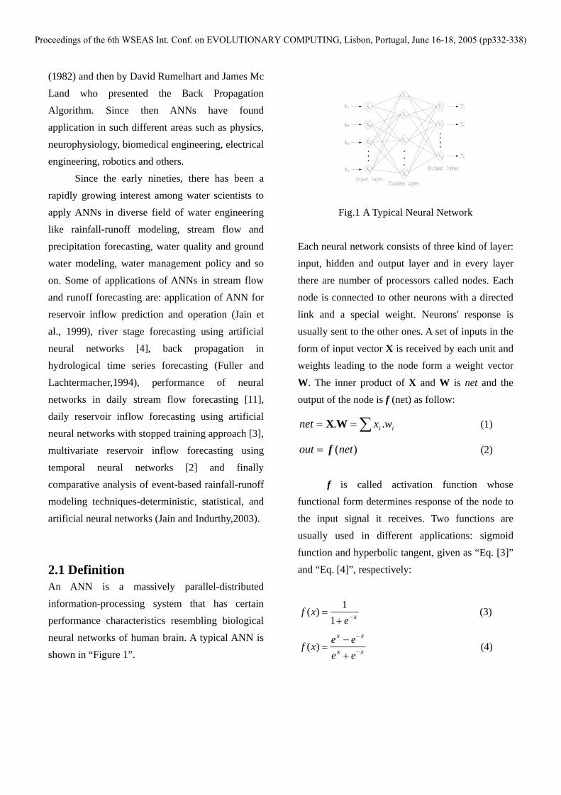
2.1 Definition An ANN is a massively parallel-distributed information-processing system that has certain performance characteristics resembling biological neural networks of human brain. A typical ANN is shown in “Figure 1”.

Fig.1 A Typical Neural Network

Each neural network consists of three kind of layer: input, hidden and output layer and in every layer there are number of processors called nodes. Each node is connected to other neurons with a directed link and a special weight. Neurons' response is usually sent to the other ones. A set of inputs in the

form of input vector X is received by each unit and weights leading to the node form a weight vector

W. The inner product of X and W is net and the output of the node is f (net) as follow:

∑== ii wxnet ..WX (1)

)(netout f= (2)

f is called activation function whose functional form determines response of the node to the input signal it receives. Two functions are usually used in different applications: sigmoid function and hyperbolic tangent, given as “Eq. [3]” and “Eq. [4]”, respectively:

xexf −+=

11

)( (3)

xx

xx

eeee

xf −

−

+=

−)( (4)


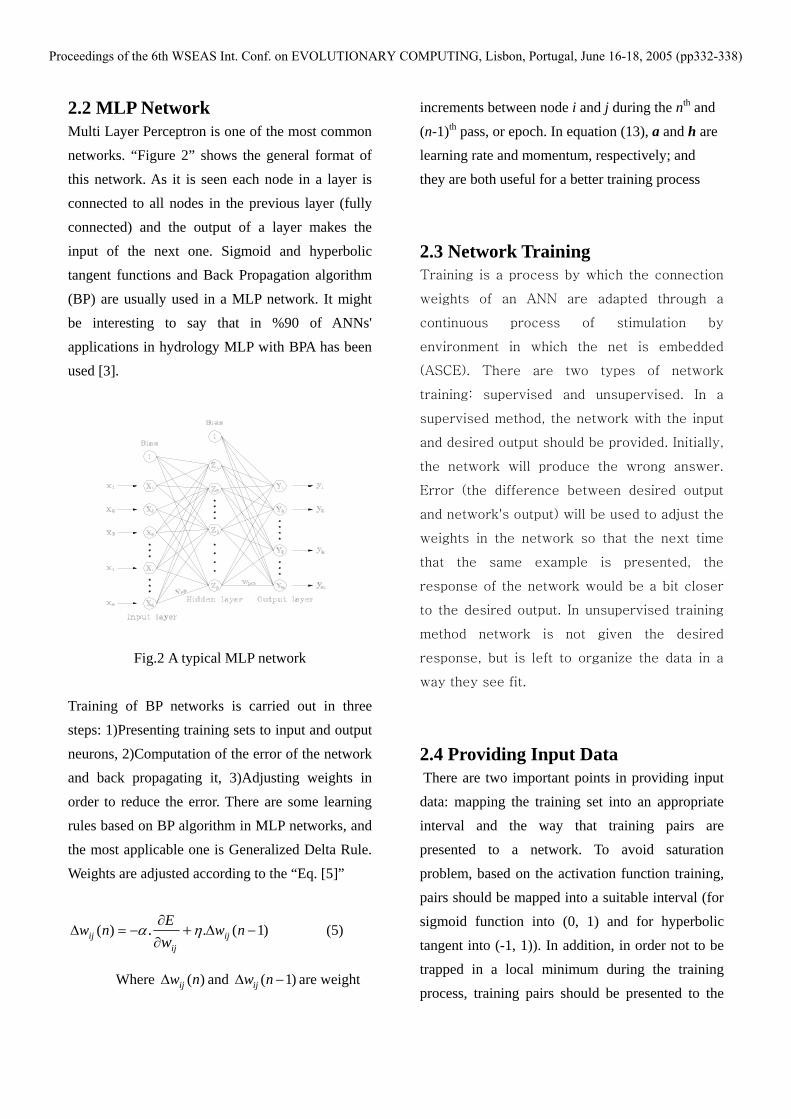
2.2 MLP Network Multi Layer Perceptron is one of the most common networks. “Figure 2” shows the general format of this network. As it is seen each node in a layer is connected to all nodes in the previous layer (fully connected) and the output of a layer makes the input of the next one. Sigmoid and hyperbolic tangent functions and Back Propagation algorithm (BP) are usually used in a MLP network. It might be interesting to say that in %90 of ANNs' applications in hydrology MLP with BPA has been used [3].

Fig.2 A typical MLP network

Training of BP networks is carried out in three steps: 1)Presenting training sets to input and output neurons, 2)Computation of the error of the network and back propagating it, 3)Adjusting weights in order to reduce the error. There are some learning rules based on BP algorithm in MLP networks, and the most applicable one is Generalized Delta Rule. Weights are adjusted according to the “Eq. [5]”

)1(.)( . −∆∂∂

−=∆ + nwE

nw ijij

ij wηα (5)

Where )(nwij∆ and )1( −∆ nwij are weight

increments between node i and j during the nth and

(n-1)th pass, or epoch. In equation (13), a and h are learning rate and momentum, respectively; and they are both useful for a better training process 2.3 Network Training Training is a process by which the connection

weights of an ANN are adapted through a

continuous process of stimulation by

environment in which the net is embedded

(ASCE). There are two types of network

training: supervised and unsupervised. In a

supervised method, the network with the input

and desired output should be provided. Initially,

the network will produce the wrong answer.

Error (the difference between desired output

and network's output) will be used to adjust the

weights in the network so that the next time

that the same example is presented, the

response of the network would be a bit closer

to the desired output. In unsupervised training

method network is not given the desired

response, but is left to organize the data in a

way they see fit.

2.4 Providing Input Data There are two important points in providing input data: mapping the training set into an appropriate interval and the way that training pairs are presented to a network. To avoid saturation problem, based on the activation function training, pairs should be mapped into a suitable interval (for sigmoid function into (0, 1) and for hyperbolic tangent into (-1, 1)). In addition, in order not to be trapped in a local minimum during the training process, training pairs should be presented to the


network randomly.

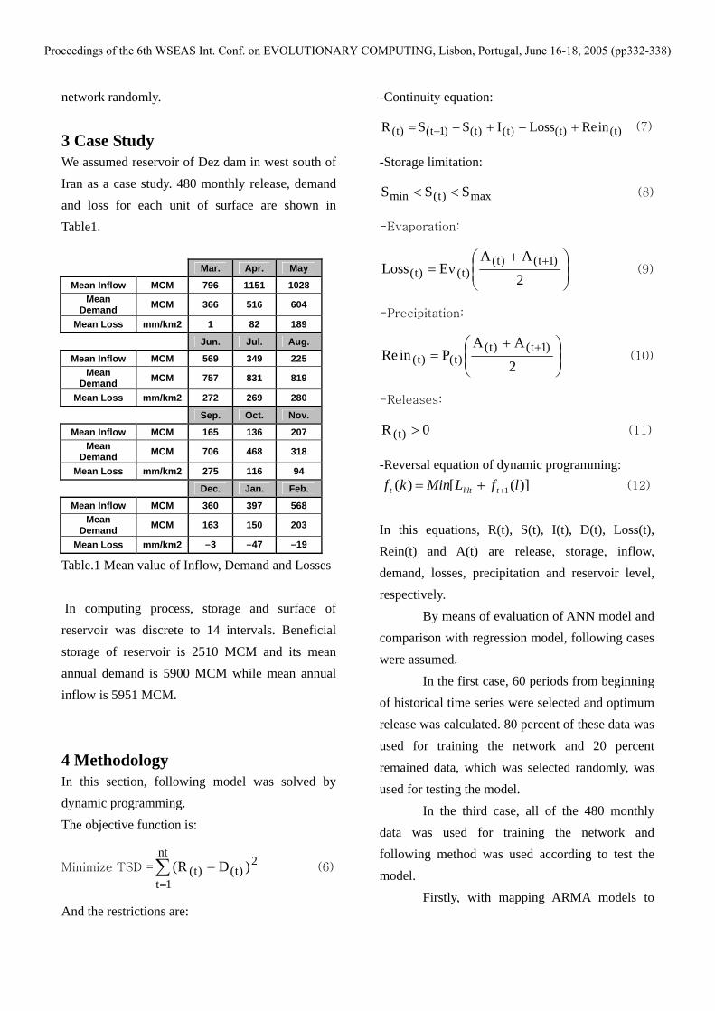
3 Case Study We assumed reservoir of Dez dam in west south of Iran as a case study. 480 monthly release, demand and loss for each unit of surface are shown in Table1.

Mar. Apr. May

Mean Inflow MCM 796 1151 1028 Mean

Demand MCM 366 516 604

Mean Loss mm/km2 1 82 189

Jun. Jul. Aug.




Sep. Oct. Nov.




Dec. Jan. Feb.



Mean Loss mm/km2 3- 47- 19-

Table.1 Mean value of Inflow, Demand and Losses In computing process, storage and surface of reservoir was discrete to 14 intervals. Beneficial storage of reservoir is 2510 MCM and its mean annual demand is 5900 MCM while mean annual inflow is 5951 MCM.

4 Methodology In this section, following model was solved by dynamic programming. The objective function is:

Minimize TSD =∑=

−nt

1t

2)t()t( )DR( (6)

And the restrictions are:

-Continuity equation:

)t()t()t()t()1t()t( inReLossISSR +−+−= + (7)

-Storage limitation:

max)t(min SSS << (8)

-Evaporation:

⎟⎟⎠

⎞⎜⎜⎝

⎛ +ν= +

2

AAELoss )1t()t(

)t()t( (9)

-Precipitation:

⎟⎟⎠

⎞⎜⎜⎝

⎛ += +

2

AAPinRe )1t()t(

)t()t( (10)

-Releases:

0R )t( > (11)

-Reversal equation of dynamic programming: )]([)( 1 lfLMinkf tkltt ++= (12)

In this equations, R(t), S(t), I(t), D(t), Loss(t), Rein(t) and A(t) are release, storage, inflow, demand, losses, precipitation and reservoir level, respectively.

By means of evaluation of ANN model and comparison with regression model, following cases were assumed.

In the first case, 60 periods from beginning of historical time series were selected and optimum release was calculated. 80 percent of these data was used for training the network and 20 percent remained data, which was selected randomly, was used for testing the model.

In the third case, all of the 480 monthly data was used for training the network and following method was used according to test the model.

Firstly, with mapping ARMA models to


historical series and selecting appropriated model (AR(1)), a monthly release data was used to solve DP model and results were used to test the ANN model.

In the forth case, the method was like third one with little difference. In this case 480 last release time series was used to solve DP model.

Reservoir storage at the first of each period and amount of demand in that period was used as input series of ANN model and outflow reservoir in that period was considered as output of ANN model.

All training process was done to reduce the amount of errors. In all cases, back propagation (MLP) was used as a solution. According to the best results for training the network, delta rule and sigmoid function were used as training rule and excitation, respectively. The number of hidden layers in each case is 1 or 2 and the number of neurons in each layer is between 1 and 4. in all cases, the number of hidden layers and neurons are selected corresponding to reduce RMS error.

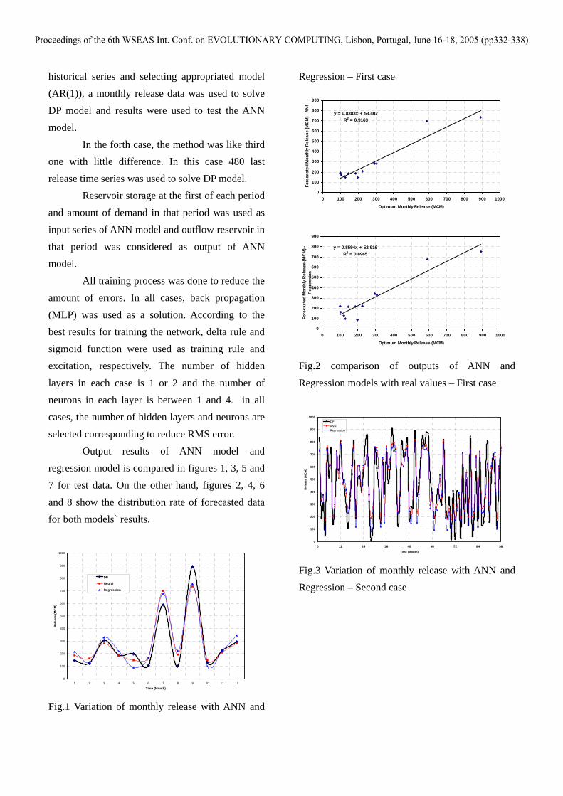
Output results of ANN model and regression model is compared in figures 1, 3, 5 and 7 for test data. On the other hand, figures 2, 4, 6 and 8 show the distribution rate of forecasted data for both models` results.

0

100

200

300

400

500

600

700

800

900

1000

1 2 3 4 5 6 7 8 9 10 11 12

Time (Month)

Rel

ease

(MC

M)

DP

Neural

Regression

Fig.1 Variation of monthly release with ANN and

Regression – First case

y = 0.8383x + 53.402R2 = 0.9163

0

100

200

300

400

500

600

700

800

900

0 100 200 300 400 500 600 700 800 900 1000

Optimum Monthly Release (MCM)

Fore

cast

ed M

onth

ly R

elea

se (M

CM

) - A

NN

y = 0.8594x + 52.916R2 = 0.8965

0

100

200

300

400

500

600

700

800

900

0 100 200 300 400 500 600 700 800 900 1000


Fore

cast

ed M

onth

ly R

elea

se (M

CM

) -

Reg

ress

ion

Fig.2 comparison of outputs of ANN and Regression models with real values – First case

0

100

200

300

400

500

600

700

800

900

1000

0 12 24 36 48 60 72 84 96Time (Month)

Rel

ease

(MC

M)

DPANNRegression

Fig.3 Variation of monthly release with ANN and Regression – Second case


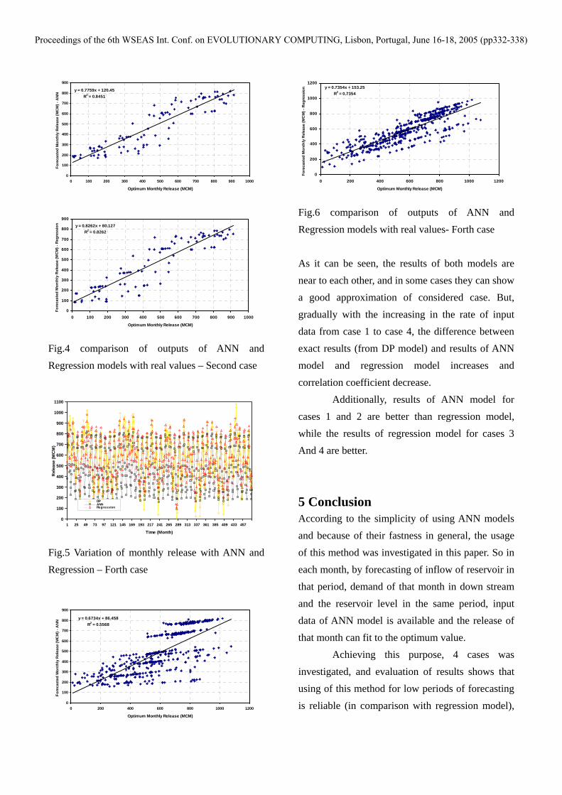
y = 0.7759x + 120.45R2 = 0.8451

0

100

200

300

400

500

600

700

800

900

0 100 200 300 400 500 600 700 800 900 1000


Fore

cast

ed M

onth

ly R

elea

se (M

CM

) - A

NN

y = 0.8262x + 80.127R2 = 0.8262

0

100

200

300

400

500

600

700

800

900

0 100 200 300 400 500 600 700 800 900 1000


Fore

cast

ed M

onth

ly R

elea

se (M

CM

) - R

egre

ssio

n

Fig.4 comparison of outputs of ANN and Regression models with real values – Second case

0

100

200

300

400

500

600

700

800

900

1000

1100

1 25 49 73 97 121 145 169 193 217 241 265 289 313 337 361 385 409 433 457

Time (Month)

Rel

ease

(MC

M)

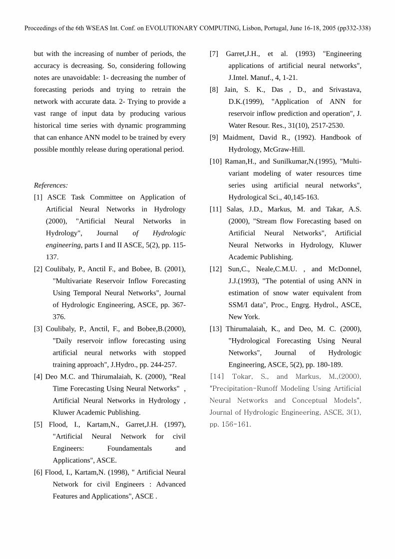
DPANNRegression

Fig.5 Variation of monthly release with ANN and Regression – Forth case

y = 0.6734x + 86.458R2 = 0.5568

0

100

200

300

400

500

600

700

800

900

0 200 400 600 800 1000 1200


Fore

cast

ed M

onth

ly R

elea

se (M

CM

) - A

NN

y = 0.7354x + 153.25R2 = 0.7354

0

200

400

600

800

1000

1200

0 200 400 600 800 1000 1200


Fore

cast

ed M

onth

ly R

elea

se (M

CM

) - R

egre

ssio

n

Fig.6 comparison of outputs of ANN and Regression models with real values- Forth case As it can be seen, the results of both models are near to each other, and in some cases they can show a good approximation of considered case. But, gradually with the increasing in the rate of input data from case 1 to case 4, the difference between exact results (from DP model) and results of ANN model and regression model increases and correlation coefficient decrease.

Additionally, results of ANN model for cases 1 and 2 are better than regression model, while the results of regression model for cases 3 And 4 are better.

5 Conclusion According to the simplicity of using ANN models and because of their fastness in general, the usage of this method was investigated in this paper. So in each month, by forecasting of inflow of reservoir in that period, demand of that month in down stream and the reservoir level in the same period, input data of ANN model is available and the release of that month can fit to the optimum value.

Achieving this purpose, 4 cases was investigated, and evaluation of results shows that using of this method for low periods of forecasting is reliable (in comparison with regression model),


but with the increasing of number of periods, the accuracy is decreasing. So, considering following notes are unavoidable: 1- decreasing the number of forecasting periods and trying to retrain the network with accurate data. 2- Trying to provide a vast range of input data by producing various historical time series with dynamic programming that can enhance ANN model to be trained by every possible monthly release during operational period.

References: [1] ASCE Task Committee on Application of

Artificial Neural Networks in Hydrology (2000), "Artificial Neural Networks in Hydrology", Journal of Hydrologic engineering, parts I and II ASCE, 5(2), pp. 115-137.

[2] Coulibaly, P., Anctil F., and Bobee, B. (2001), "Multivariate Reservoir Inflow Forecasting Using Temporal Neural Networks", Journal of Hydrologic Engineering, ASCE, pp. 367-376.

[3] Coulibaly, P., Anctil, F., and Bobee,B.(2000), "Daily reservoir inflow forecasting using artificial neural networks with stopped training approach", J.Hydro., pp. 244-257.

[4] Deo M.C. and Thirumalaiah, K. (2000), "Real Time Forecasting Using Neural Networks" , Artificial Neural Networks in Hydrology , Kluwer Academic Publishing.

[5] Flood, I., Kartam,N., Garret,J.H. (1997), "Artificial Neural Network for civil Engineers: Foundamentals and Applications", ASCE.

[6] Flood, I., Kartam,N. (1998), " Artificial Neural Network for civil Engineers : Advanced Features and Applications", ASCE .

[7] Garret,J.H., et al. (1993) "Engineering applications of artificial neural networks", J.Intel. Manuf., 4, 1-21.

[8] Jain, S. K., Das , D., and Srivastava, D.K.(1999), "Application of ANN for reservoir inflow prediction and operation", J. Water Resour. Res., 31(10), 2517-2530.

[9] Maidment, David R., (1992). Handbook of Hydrology, McGraw-Hill.

[10] Raman,H., and Sunilkumar,N.(1995), "Multi-variant modeling of water resources time series using artificial neural networks", Hydrological Sci., 40,145-163.

[11] Salas, J.D., Markus, M. and Takar, A.S. (2000), "Stream flow Forecasting based on Artificial Neural Networks", Artificial Neural Networks in Hydrology, Kluwer Academic Publishing.

[12] Sun,C., Neale,C.M.U. , and McDonnel, J.J.(1993), "The potential of using ANN in estimation of snow water equivalent from SSM/I data", Proc., Engrg. Hydrol., ASCE, New York.

[13] Thirumalaiah, K., and Deo, M. C. (2000), "Hydrological Forecasting Using Neural Networks", Journal of Hydrologic Engineering, ASCE, 5(2), pp. 180-189.

[14] Tokar, S., and Markus, M.,(2000),

"Precipitation-Runoff Modeling Using Artificial

Neural Networks and Conceptual Models",

Journal of Hydrologic Engineering, ASCE, 3(1),

pp. 156-161.


Reservoir Optimal Operation Using DP-ANN

Documents

Transcript of Reservoir Optimal Operation Using DP-ANN