Reservoir Stimulation v

◆

Reservoir StimulationContents

Preface: Hydraulic Fracturing, A Technology for All TimeAhmed S. Abou-Sayed . . . . . . . . . . . . . . . . . . . . . . . . . . . . . . . . . . . . . . . . . . . . . . . . . . . . . . . . . . . . . . . . . . . . . . . . P-1

Chapter 1 Reservoir Stimulation in Petroleum ProductionMichael J. Economides and Curtis Boney

1-1. Introduction . . . . . . . . . . . . . . . . . . . . . . . . . . . . . . . . . . . . . . . . . . . . . . . . . . . . . . . . . . . . . . . . . . . . . . . . . . 1-11-1.1. Petroleum production . . . . . . . . . . . . . . . . . . . . . . . . . . . . . . . . . . . . . . . . . . . . . . . . . . . . . . . . . . 1-11-1.2. Units . . . . . . . . . . . . . . . . . . . . . . . . . . . . . . . . . . . . . . . . . . . . . . . . . . . . . . . . . . . . . . . . . . . . . . . . . 1-3

1-2. Inflow performance . . . . . . . . . . . . . . . . . . . . . . . . . . . . . . . . . . . . . . . . . . . . . . . . . . . . . . . . . . . . . . . . . . . 1-31-2.1. IPR for steady state . . . . . . . . . . . . . . . . . . . . . . . . . . . . . . . . . . . . . . . . . . . . . . . . . . . . . . . . . . . 1-41-2.2. IPR for pseudosteady state. . . . . . . . . . . . . . . . . . . . . . . . . . . . . . . . . . . . . . . . . . . . . . . . . . . . . 1-51-2.3. IPR for transient (or infinite-acting) flow . . . . . . . . . . . . . . . . . . . . . . . . . . . . . . . . . . . . . . . 1-51-2.4. Horizontal well production . . . . . . . . . . . . . . . . . . . . . . . . . . . . . . . . . . . . . . . . . . . . . . . . . . . . 1-61-2.5. Permeability anisotropy . . . . . . . . . . . . . . . . . . . . . . . . . . . . . . . . . . . . . . . . . . . . . . . . . . . . . . . 1-10

1-3. Alterations in the near-wellbore zone . . . . . . . . . . . . . . . . . . . . . . . . . . . . . . . . . . . . . . . . . . . . . . . . . . . 1-111-3.1. Skin analysis . . . . . . . . . . . . . . . . . . . . . . . . . . . . . . . . . . . . . . . . . . . . . . . . . . . . . . . . . . . . . . . . . 1-111-3.2. Components of the skin effect . . . . . . . . . . . . . . . . . . . . . . . . . . . . . . . . . . . . . . . . . . . . . . . . . 1-121-3.3. Skin effect caused by partial completion and slant . . . . . . . . . . . . . . . . . . . . . . . . . . . . . . . 1-121-3.4. Perforation skin effect . . . . . . . . . . . . . . . . . . . . . . . . . . . . . . . . . . . . . . . . . . . . . . . . . . . . . . . . . 1-131-3.5. Hydraulic fracturing in production engineering. . . . . . . . . . . . . . . . . . . . . . . . . . . . . . . . . . 1-16

1-4. Tubing performance and NODAL* analysis . . . . . . . . . . . . . . . . . . . . . . . . . . . . . . . . . . . . . . . . . . . . . 1-181-5. Decision process for well stimulation . . . . . . . . . . . . . . . . . . . . . . . . . . . . . . . . . . . . . . . . . . . . . . . . . . . 1-20

1-5.1. Stimulation economics . . . . . . . . . . . . . . . . . . . . . . . . . . . . . . . . . . . . . . . . . . . . . . . . . . . . . . . . 1-211-5.2. Physical limits to stimulation treatments . . . . . . . . . . . . . . . . . . . . . . . . . . . . . . . . . . . . . . . . 1-22

1-6. Reservoir engineering considerations for optimal production enhancement strategies . . . . . . . 1-221-6.1. Geometry of the well drainage volume . . . . . . . . . . . . . . . . . . . . . . . . . . . . . . . . . . . . . . . . . 1-231-6.2. Well drainage volume characterizations and production optimization strategies . . . . 1-24

1-7. Stimulation execution . . . . . . . . . . . . . . . . . . . . . . . . . . . . . . . . . . . . . . . . . . . . . . . . . . . . . . . . . . . . . . . . . 1-281-7.1. Matrix stimulation . . . . . . . . . . . . . . . . . . . . . . . . . . . . . . . . . . . . . . . . . . . . . . . . . . . . . . . . . . . . 1-281-7.2. Hydraulic fracturing . . . . . . . . . . . . . . . . . . . . . . . . . . . . . . . . . . . . . . . . . . . . . . . . . . . . . . . . . . 1-18

Chapter 2 Formation Characterization: Well and Reservoir TestingChristine A. Ehlig-Economides and Michael J. Economides

2-1. Evolution of a technology . . . . . . . . . . . . . . . . . . . . . . . . . . . . . . . . . . . . . . . . . . . . . . . . . . . . . . . . . . . . . 2-12-1.1. Horner semilogarithmic analysis . . . . . . . . . . . . . . . . . . . . . . . . . . . . . . . . . . . . . . . . . . . . . . . 2-12-1.2. Log-log plot . . . . . . . . . . . . . . . . . . . . . . . . . . . . . . . . . . . . . . . . . . . . . . . . . . . . . . . . . . . . . . . . . . 2-2

2-2. Pressure derivative in well test diagnosis. . . . . . . . . . . . . . . . . . . . . . . . . . . . . . . . . . . . . . . . . . . . . . . . 2-32-3. Parameter estimation from pressure transient data . . . . . . . . . . . . . . . . . . . . . . . . . . . . . . . . . . . . . . . 2-7

2-3.1. Radial flow. . . . . . . . . . . . . . . . . . . . . . . . . . . . . . . . . . . . . . . . . . . . . . . . . . . . . . . . . . . . . . . . . . . 2-72-3.2. Linear flow. . . . . . . . . . . . . . . . . . . . . . . . . . . . . . . . . . . . . . . . . . . . . . . . . . . . . . . . . . . . . . . . . . . 2-9

vi Contents

2-3.3. Spherical flow . . . . . . . . . . . . . . . . . . . . . . . . . . . . . . . . . . . . . . . . . . . . . . . . . . . . . . . . . . . . . . . . 2-102-3.4. Dual porosity . . . . . . . . . . . . . . . . . . . . . . . . . . . . . . . . . . . . . . . . . . . . . . . . . . . . . . . . . . . . . . . . . 2-112-3.5. Wellbore storage and pseudosteady state. . . . . . . . . . . . . . . . . . . . . . . . . . . . . . . . . . . . . . . . 2-11

2-4. Test interpretation methodology . . . . . . . . . . . . . . . . . . . . . . . . . . . . . . . . . . . . . . . . . . . . . . . . . . . . . . . . 2-122-5. Analysis with measurement of layer rate . . . . . . . . . . . . . . . . . . . . . . . . . . . . . . . . . . . . . . . . . . . . . . . . 2-142-6. Layered reservoir testing . . . . . . . . . . . . . . . . . . . . . . . . . . . . . . . . . . . . . . . . . . . . . . . . . . . . . . . . . . . . . . 2-15

2-6.1. Selective inflow performance analysis . . . . . . . . . . . . . . . . . . . . . . . . . . . . . . . . . . . . . . . . . . 2-152-6.2. Analysis of multilayer transient test data. . . . . . . . . . . . . . . . . . . . . . . . . . . . . . . . . . . . . . . . 2-16

2-7. Testing multilateral and multibranch wells . . . . . . . . . . . . . . . . . . . . . . . . . . . . . . . . . . . . . . . . . . . . . . 2-162-8. Permeability determination from a fracture injection test . . . . . . . . . . . . . . . . . . . . . . . . . . . . . . . . . 2-17

2-8.1. Pressure decline analysis with the Carter leakoff model . . . . . . . . . . . . . . . . . . . . . . . . . . 2-172-8.2. Filter-cake plus reservoir pressure drop leakoff model

(according to Mayerhofer et al., 1993). . . . . . . . . . . . . . . . . . . . . . . . . . . . . . . . . . . . . . . . . . 2-21

Chapter 3 Formation Characterization: Rock MechanicsM. C. Thiercelin and J.-C. Roegiers

3-1. Introduction . . . . . . . . . . . . . . . . . . . . . . . . . . . . . . . . . . . . . . . . . . . . . . . . . . . . . . . . . . . . . . . . . . . . . . . . . . 3-1Sidebar 3A. Mechanics of hydraulic fracturing . . . . . . . . . . . . . . . . . . . . . . . . . . . . . . . . . . . . . . . . . 3-2

3-2. Basic concepts . . . . . . . . . . . . . . . . . . . . . . . . . . . . . . . . . . . . . . . . . . . . . . . . . . . . . . . . . . . . . . . . . . . . . . . . 3-43-2.1. Stresses . . . . . . . . . . . . . . . . . . . . . . . . . . . . . . . . . . . . . . . . . . . . . . . . . . . . . . . . . . . . . . . . . . . . . . 3-43-2.2. Strains . . . . . . . . . . . . . . . . . . . . . . . . . . . . . . . . . . . . . . . . . . . . . . . . . . . . . . . . . . . . . . . . . . . . . . . 3-5

Sidebar 3B. Mohr circle . . . . . . . . . . . . . . . . . . . . . . . . . . . . . . . . . . . . . . . . . . . . . . . . . . . . . . 3-53-3. Rock behavior . . . . . . . . . . . . . . . . . . . . . . . . . . . . . . . . . . . . . . . . . . . . . . . . . . . . . . . . . . . . . . . . . . . . . . . . 3-6

3-3.1. Linear elasticity . . . . . . . . . . . . . . . . . . . . . . . . . . . . . . . . . . . . . . . . . . . . . . . . . . . . . . . . . . . . . . 3-6Sidebar 3C. Elastic constants. . . . . . . . . . . . . . . . . . . . . . . . . . . . . . . . . . . . . . . . . . . . . . . . . . 3-8

3-3.2. Influence of pore pressure . . . . . . . . . . . . . . . . . . . . . . . . . . . . . . . . . . . . . . . . . . . . . . . . . . . . . 3-83-3.3. Fracture mechanics . . . . . . . . . . . . . . . . . . . . . . . . . . . . . . . . . . . . . . . . . . . . . . . . . . . . . . . . . . . 3-93-3.4. Nonelastic deformation. . . . . . . . . . . . . . . . . . . . . . . . . . . . . . . . . . . . . . . . . . . . . . . . . . . . . . . . 3-113-3.5. Failure . . . . . . . . . . . . . . . . . . . . . . . . . . . . . . . . . . . . . . . . . . . . . . . . . . . . . . . . . . . . . . . . . . . . . . . 3-11

3-4. Rock mechanical property measurement . . . . . . . . . . . . . . . . . . . . . . . . . . . . . . . . . . . . . . . . . . . . . . . . 3-123-4.1. Importance of rock properties in stimulation . . . . . . . . . . . . . . . . . . . . . . . . . . . . . . . . . . . . 3-123-4.2. Laboratory testing . . . . . . . . . . . . . . . . . . . . . . . . . . . . . . . . . . . . . . . . . . . . . . . . . . . . . . . . . . . . 3-133-4.3. Stress-strain curve . . . . . . . . . . . . . . . . . . . . . . . . . . . . . . . . . . . . . . . . . . . . . . . . . . . . . . . . . . . . 3-143-4.4. Elastic parameters . . . . . . . . . . . . . . . . . . . . . . . . . . . . . . . . . . . . . . . . . . . . . . . . . . . . . . . . . . . . 3-153-4.5. Rock strength, yield criterion and failure envelope . . . . . . . . . . . . . . . . . . . . . . . . . . . . . . 3-193-4.6. Fracture toughness . . . . . . . . . . . . . . . . . . . . . . . . . . . . . . . . . . . . . . . . . . . . . . . . . . . . . . . . . . . . 3-19

Sidebar 3D. Fracture toughness testing. . . . . . . . . . . . . . . . . . . . . . . . . . . . . . . . . . . . . . . . . 3-203-5. State of stress in the earth. . . . . . . . . . . . . . . . . . . . . . . . . . . . . . . . . . . . . . . . . . . . . . . . . . . . . . . . . . . . . . 3-21

3-5.1. Rock at rest . . . . . . . . . . . . . . . . . . . . . . . . . . . . . . . . . . . . . . . . . . . . . . . . . . . . . . . . . . . . . . . . . . 3-223-5.2. Tectonic strains . . . . . . . . . . . . . . . . . . . . . . . . . . . . . . . . . . . . . . . . . . . . . . . . . . . . . . . . . . . . . . . 3-233-5.3. Rock at failure. . . . . . . . . . . . . . . . . . . . . . . . . . . . . . . . . . . . . . . . . . . . . . . . . . . . . . . . . . . . . . . . 3-233-5.4. Influence of pore pressure . . . . . . . . . . . . . . . . . . . . . . . . . . . . . . . . . . . . . . . . . . . . . . . . . . . . . 3-253-5.5. Influence of temperature. . . . . . . . . . . . . . . . . . . . . . . . . . . . . . . . . . . . . . . . . . . . . . . . . . . . . . . 3-263-5.6. Principal stress direction . . . . . . . . . . . . . . . . . . . . . . . . . . . . . . . . . . . . . . . . . . . . . . . . . . . . . . 3-263-5.7. Stress around the wellbore. . . . . . . . . . . . . . . . . . . . . . . . . . . . . . . . . . . . . . . . . . . . . . . . . . . . . 3-263-5.8. Stress change from hydraulic fracturing . . . . . . . . . . . . . . . . . . . . . . . . . . . . . . . . . . . . . . . . 3-27

3-6. In-situ stress management . . . . . . . . . . . . . . . . . . . . . . . . . . . . . . . . . . . . . . . . . . . . . . . . . . . . . . . . . . . . . 3-283-6.1. Importance of stress measurement in stimulation . . . . . . . . . . . . . . . . . . . . . . . . . . . . . . . . 3-283-6.2. Micro-hydraulic fracturing techniques . . . . . . . . . . . . . . . . . . . . . . . . . . . . . . . . . . . . . . . . . . 3-28

Reservoir Stimulation vii

3-6.3. Fracture calibration techniques. . . . . . . . . . . . . . . . . . . . . . . . . . . . . . . . . . . . . . . . . . . . . . . . . 3-343-6.4. Laboratory techniques. . . . . . . . . . . . . . . . . . . . . . . . . . . . . . . . . . . . . . . . . . . . . . . . . . . . . . . . . 3-34

Chapter 4 Formation Characterization: Well LogsJean Desroches and Tom Bratton

4-1. Introduction . . . . . . . . . . . . . . . . . . . . . . . . . . . . . . . . . . . . . . . . . . . . . . . . . . . . . . . . . . . . . . . . . . . . . . . . . . 4-14-2. Depth . . . . . . . . . . . . . . . . . . . . . . . . . . . . . . . . . . . . . . . . . . . . . . . . . . . . . . . . . . . . . . . . . . . . . . . . . . . . . . . . 4-24-3. Temperature . . . . . . . . . . . . . . . . . . . . . . . . . . . . . . . . . . . . . . . . . . . . . . . . . . . . . . . . . . . . . . . . . . . . . . . . . . 4-24-4. Properties related to the diffusion of fluids . . . . . . . . . . . . . . . . . . . . . . . . . . . . . . . . . . . . . . . . . . . . . . 4-3

4-4.1. Porosity . . . . . . . . . . . . . . . . . . . . . . . . . . . . . . . . . . . . . . . . . . . . . . . . . . . . . . . . . . . . . . . . . . . . . . 4-34-4.2. Lithology and saturation. . . . . . . . . . . . . . . . . . . . . . . . . . . . . . . . . . . . . . . . . . . . . . . . . . . . . . . 4-54-4.3. Permeability. . . . . . . . . . . . . . . . . . . . . . . . . . . . . . . . . . . . . . . . . . . . . . . . . . . . . . . . . . . . . . . . . . 4-6

Sidebar 4A. Permeability-porosity correlations . . . . . . . . . . . . . . . . . . . . . . . . . . . . . . . . . 4-84-4.4. Pore pressure . . . . . . . . . . . . . . . . . . . . . . . . . . . . . . . . . . . . . . . . . . . . . . . . . . . . . . . . . . . . . . . . . 4-104-4.5. Skin effect and damage radius . . . . . . . . . . . . . . . . . . . . . . . . . . . . . . . . . . . . . . . . . . . . . . . . . 4-114-4.6. Composition of fluids . . . . . . . . . . . . . . . . . . . . . . . . . . . . . . . . . . . . . . . . . . . . . . . . . . . . . . . . . 4-12

4-5. Properties related to the deformation and fracturing of rock . . . . . . . . . . . . . . . . . . . . . . . . . . . . . . 4-134-5.1. Mechanical properties . . . . . . . . . . . . . . . . . . . . . . . . . . . . . . . . . . . . . . . . . . . . . . . . . . . . . . . . . 4-134-5.2. Stresses . . . . . . . . . . . . . . . . . . . . . . . . . . . . . . . . . . . . . . . . . . . . . . . . . . . . . . . . . . . . . . . . . . . . . . 4-15

4-6. Zoning . . . . . . . . . . . . . . . . . . . . . . . . . . . . . . . . . . . . . . . . . . . . . . . . . . . . . . . . . . . . . . . . . . . . . . . . . . . . . . . 4-24

Chapter 5 Basics of Hydraulic FracturingM. B. Smith and J. W. Shlyapobersky

5-1. Introduction . . . . . . . . . . . . . . . . . . . . . . . . . . . . . . . . . . . . . . . . . . . . . . . . . . . . . . . . . . . . . . . . . . . . . . . . . . 5-15-1.1. What is fracturing?. . . . . . . . . . . . . . . . . . . . . . . . . . . . . . . . . . . . . . . . . . . . . . . . . . . . . . . . . . . . 5-15-1.2. Why fracture? . . . . . . . . . . . . . . . . . . . . . . . . . . . . . . . . . . . . . . . . . . . . . . . . . . . . . . . . . . . . . . . . 5-45-1.3. Design considerations and primary variables . . . . . . . . . . . . . . . . . . . . . . . . . . . . . . . . . . . . 5-6

Sidebar 5A. Design goals and variables . . . . . . . . . . . . . . . . . . . . . . . . . . . . . . . . . . . . . . . . 5-75-1.4. Variable interaction . . . . . . . . . . . . . . . . . . . . . . . . . . . . . . . . . . . . . . . . . . . . . . . . . . . . . . . . . . . 5-9

5-2. In-situ stress . . . . . . . . . . . . . . . . . . . . . . . . . . . . . . . . . . . . . . . . . . . . . . . . . . . . . . . . . . . . . . . . . . . . . . . . . . 5-95-3. Reservoir engineering . . . . . . . . . . . . . . . . . . . . . . . . . . . . . . . . . . . . . . . . . . . . . . . . . . . . . . . . . . . . . . . . . 5-10

5-3.1. Design goals . . . . . . . . . . . . . . . . . . . . . . . . . . . . . . . . . . . . . . . . . . . . . . . . . . . . . . . . . . . . . . . . . 5-11Sidebar 5B. Highway analogy for dimensionless fracture conductivity . . . . . . . . . . . 5-11

5-3.2. Complicating factors . . . . . . . . . . . . . . . . . . . . . . . . . . . . . . . . . . . . . . . . . . . . . . . . . . . . . . . . . . 5-125-3.3. Reservoir effects on fluid loss. . . . . . . . . . . . . . . . . . . . . . . . . . . . . . . . . . . . . . . . . . . . . . . . . . 5-13

5-4. Rock and fluid mechanics. . . . . . . . . . . . . . . . . . . . . . . . . . . . . . . . . . . . . . . . . . . . . . . . . . . . . . . . . . . . . . 5-135-4.1. Material balance . . . . . . . . . . . . . . . . . . . . . . . . . . . . . . . . . . . . . . . . . . . . . . . . . . . . . . . . . . . . . . 5-135-4.2. Fracture height . . . . . . . . . . . . . . . . . . . . . . . . . . . . . . . . . . . . . . . . . . . . . . . . . . . . . . . . . . . . . . . 5-145-4.3. Fracture width . . . . . . . . . . . . . . . . . . . . . . . . . . . . . . . . . . . . . . . . . . . . . . . . . . . . . . . . . . . . . . . . 5-155-4.4. Fluid mechanics and fluid flow. . . . . . . . . . . . . . . . . . . . . . . . . . . . . . . . . . . . . . . . . . . . . . . . . 5-155-4.5. Fracture mechanics and fracture tip effects. . . . . . . . . . . . . . . . . . . . . . . . . . . . . . . . . . . . . . 5-165-4.6. Fluid loss . . . . . . . . . . . . . . . . . . . . . . . . . . . . . . . . . . . . . . . . . . . . . . . . . . . . . . . . . . . . . . . . . . . . 5-175-4.7. Variable sensitivities and interactions. . . . . . . . . . . . . . . . . . . . . . . . . . . . . . . . . . . . . . . . . . . 5-18

5-5. Treatment pump scheduling. . . . . . . . . . . . . . . . . . . . . . . . . . . . . . . . . . . . . . . . . . . . . . . . . . . . . . . . . . . . 5-205-5.1. Fluid and proppant selection . . . . . . . . . . . . . . . . . . . . . . . . . . . . . . . . . . . . . . . . . . . . . . . . . . . 5-215-5.2. Pad volume . . . . . . . . . . . . . . . . . . . . . . . . . . . . . . . . . . . . . . . . . . . . . . . . . . . . . . . . . . . . . . . . . . 5-215-5.3. Proppant transport . . . . . . . . . . . . . . . . . . . . . . . . . . . . . . . . . . . . . . . . . . . . . . . . . . . . . . . . . . . . 5-235-5.4. Proppant admittance . . . . . . . . . . . . . . . . . . . . . . . . . . . . . . . . . . . . . . . . . . . . . . . . . . . . . . . . . . 5-245-5.5. Fracture models . . . . . . . . . . . . . . . . . . . . . . . . . . . . . . . . . . . . . . . . . . . . . . . . . . . . . . . . . . . . . . 5-25

viii Contents

5-6. Economics and operational considerations . . . . . . . . . . . . . . . . . . . . . . . . . . . . . . . . . . . . . . . . . . . . . . 5-265-6.1. Economics . . . . . . . . . . . . . . . . . . . . . . . . . . . . . . . . . . . . . . . . . . . . . . . . . . . . . . . . . . . . . . . . . . . 5-265-6.2. Operations . . . . . . . . . . . . . . . . . . . . . . . . . . . . . . . . . . . . . . . . . . . . . . . . . . . . . . . . . . . . . . . . . . . 5-27

Appendix: Evolution of hydraulic fracturing design and evaluationK. G. Nolte . . . . . . . . . . . . . . . . . . . . . . . . . . . . . . . . . . . . . . . . . . . . . . . . . . . . . . . . . . . . . . . . . . . . . . . . . . . . . . . . . . A5-1

Chapter 6 Mechanics of Hydraulic FracturingMark G. Mack and Norman R. Warpinski

6-1. Introduction . . . . . . . . . . . . . . . . . . . . . . . . . . . . . . . . . . . . . . . . . . . . . . . . . . . . . . . . . . . . . . . . . . . . . . . . . . 6-16-2. History of early hydraulic fracture modeling . . . . . . . . . . . . . . . . . . . . . . . . . . . . . . . . . . . . . . . . . . . . 6-2

6-2.1. Basic fracture modeling . . . . . . . . . . . . . . . . . . . . . . . . . . . . . . . . . . . . . . . . . . . . . . . . . . . . . . . 6-26-2.2. Hydraulic fracture modeling . . . . . . . . . . . . . . . . . . . . . . . . . . . . . . . . . . . . . . . . . . . . . . . . . . . 6-3

Sidebar 6A. Approximation to the Carter equation for leakoff . . . . . . . . . . . . . . . . . . . 6-6Sidebar 6B. Approximations to Nordgren’s equations. . . . . . . . . . . . . . . . . . . . . . . . . . . 6-6Sidebar 6C. Radial fracture geometry models . . . . . . . . . . . . . . . . . . . . . . . . . . . . . . . . . . 6-8

6-3. Three-dimensional and pseudo-three-dimensional models . . . . . . . . . . . . . . . . . . . . . . . . . . . . . . . . 6-8Sidebar 6D. Field determination of fracture geometry . . . . . . . . . . . . . . . . . . . . . . . . . . . . . . . . . . . 6-106-3.1. Planar three-dimensional models . . . . . . . . . . . . . . . . . . . . . . . . . . . . . . . . . . . . . . . . . . . . . . . 6-11

Sidebar 6E. Lateral coupling in pseudo-three-dimensional models . . . . . . . . . . . . . . . 6-12Sidebar 6F. Momentum conservation equation for hydraulic fracturing . . . . . . . . . . 6-13Sidebar 6G. Momentum balance and constitutive equation for non-Newtonian fluids . . . . . . . . . . . . . . . . . . . . . . . . . . . . . . . . . . . . . . . . . . . . . . . . . . . . . . . . . 6-14

6-3.2. Cell-based pseudo-three-dimensional models . . . . . . . . . . . . . . . . . . . . . . . . . . . . . . . . . . . 6-16Sidebar 6H. Stretching coordinate system and stability analysis . . . . . . . . . . . . . . . . . 6-20

6-3.3. Lumped pseudo-three-dimensional models. . . . . . . . . . . . . . . . . . . . . . . . . . . . . . . . . . . . . . 6-236-4. Leakoff. . . . . . . . . . . . . . . . . . . . . . . . . . . . . . . . . . . . . . . . . . . . . . . . . . . . . . . . . . . . . . . . . . . . . . . . . . . . . . . 6-25

6-4.1. Filter cake. . . . . . . . . . . . . . . . . . . . . . . . . . . . . . . . . . . . . . . . . . . . . . . . . . . . . . . . . . . . . . . . . . . . 6-256-4.2. Filtrate zone . . . . . . . . . . . . . . . . . . . . . . . . . . . . . . . . . . . . . . . . . . . . . . . . . . . . . . . . . . . . . . . . . . 6-266-4.3. Reservoir zone. . . . . . . . . . . . . . . . . . . . . . . . . . . . . . . . . . . . . . . . . . . . . . . . . . . . . . . . . . . . . . . . 6-266-4.4. Combined mechanisms . . . . . . . . . . . . . . . . . . . . . . . . . . . . . . . . . . . . . . . . . . . . . . . . . . . . . . . . 6-266-4.5. General model of leakoff . . . . . . . . . . . . . . . . . . . . . . . . . . . . . . . . . . . . . . . . . . . . . . . . . . . . . . 6-276-4.6. Other effects. . . . . . . . . . . . . . . . . . . . . . . . . . . . . . . . . . . . . . . . . . . . . . . . . . . . . . . . . . . . . . . . . . 6-27

6-5. Proppant placement . . . . . . . . . . . . . . . . . . . . . . . . . . . . . . . . . . . . . . . . . . . . . . . . . . . . . . . . . . . . . . . . . . . 6-286-5.1. Effect of proppant on fracturing fluid rheology . . . . . . . . . . . . . . . . . . . . . . . . . . . . . . . . . . 6-286-5.2. Convection . . . . . . . . . . . . . . . . . . . . . . . . . . . . . . . . . . . . . . . . . . . . . . . . . . . . . . . . . . . . . . . . . . . 6-286-5.3. Proppant transport . . . . . . . . . . . . . . . . . . . . . . . . . . . . . . . . . . . . . . . . . . . . . . . . . . . . . . . . . . . . 6-29

6-6. Heat transfer models . . . . . . . . . . . . . . . . . . . . . . . . . . . . . . . . . . . . . . . . . . . . . . . . . . . . . . . . . . . . . . . . . . 6-296-6.1. Historical heat transfer models . . . . . . . . . . . . . . . . . . . . . . . . . . . . . . . . . . . . . . . . . . . . . . . . . 6-306-6.2. Improved heat transfer models . . . . . . . . . . . . . . . . . . . . . . . . . . . . . . . . . . . . . . . . . . . . . . . . . 6-30

6-7. Fracture tip effects . . . . . . . . . . . . . . . . . . . . . . . . . . . . . . . . . . . . . . . . . . . . . . . . . . . . . . . . . . . . . . . . . . . . 6-30Sidebar 6I. Efficient heat transfer algorithm . . . . . . . . . . . . . . . . . . . . . . . . . . . . . . . . . . . . . . . . . . . . 6-31Sidebar 6J. Verification of efficient thermal calculations . . . . . . . . . . . . . . . . . . . . . . . . . . . . . . . . . 6-326-7.1. Linear elastic fracture mechanics. . . . . . . . . . . . . . . . . . . . . . . . . . . . . . . . . . . . . . . . . . . . . . . 6-32

Sidebar 6K. Crack tip stresses and the Rice equation . . . . . . . . . . . . . . . . . . . . . . . . . . . 6-336-7.2. Extensions to LEFM . . . . . . . . . . . . . . . . . . . . . . . . . . . . . . . . . . . . . . . . . . . . . . . . . . . . . . . . . . 6-346-7.3. Field calibration . . . . . . . . . . . . . . . . . . . . . . . . . . . . . . . . . . . . . . . . . . . . . . . . . . . . . . . . . . . . . . 6-35

6-8. Tortuosity and other near-well effects . . . . . . . . . . . . . . . . . . . . . . . . . . . . . . . . . . . . . . . . . . . . . . . . . . . 6-366-8.1. Fracture geometry around a wellbore . . . . . . . . . . . . . . . . . . . . . . . . . . . . . . . . . . . . . . . . . . . 6-366-8.2. Perforation and deviation effects . . . . . . . . . . . . . . . . . . . . . . . . . . . . . . . . . . . . . . . . . . . . . . . 6-36

Reservoir Stimulation ix

6-8.3. Perforation friction. . . . . . . . . . . . . . . . . . . . . . . . . . . . . . . . . . . . . . . . . . . . . . . . . . . . . . . . . . . . 6-376-8.4. Tortuosity . . . . . . . . . . . . . . . . . . . . . . . . . . . . . . . . . . . . . . . . . . . . . . . . . . . . . . . . . . . . . . . . . . . . 6-376-8.5. Phasing misalignment . . . . . . . . . . . . . . . . . . . . . . . . . . . . . . . . . . . . . . . . . . . . . . . . . . . . . . . . . 6-38

6-9. Acid fracturing. . . . . . . . . . . . . . . . . . . . . . . . . . . . . . . . . . . . . . . . . . . . . . . . . . . . . . . . . . . . . . . . . . . . . . . . 6-406-9.1. Historical acid fracturing models . . . . . . . . . . . . . . . . . . . . . . . . . . . . . . . . . . . . . . . . . . . . . . . 6-406-9.2. Reaction stoichiometry . . . . . . . . . . . . . . . . . . . . . . . . . . . . . . . . . . . . . . . . . . . . . . . . . . . . . . . . 6-406-9.3. Acid fracture conductivity . . . . . . . . . . . . . . . . . . . . . . . . . . . . . . . . . . . . . . . . . . . . . . . . . . . . . 6-416-9.4. Energy balance during acid fracturing . . . . . . . . . . . . . . . . . . . . . . . . . . . . . . . . . . . . . . . . . . 6-426-9.5. Reaction kinetics . . . . . . . . . . . . . . . . . . . . . . . . . . . . . . . . . . . . . . . . . . . . . . . . . . . . . . . . . . . . . 6-426-9.6. Mass transfer . . . . . . . . . . . . . . . . . . . . . . . . . . . . . . . . . . . . . . . . . . . . . . . . . . . . . . . . . . . . . . . . . 6-426-9.7. Acid reaction model . . . . . . . . . . . . . . . . . . . . . . . . . . . . . . . . . . . . . . . . . . . . . . . . . . . . . . . . . . 6-436-9.8. Acid fracturing: fracture geometry model . . . . . . . . . . . . . . . . . . . . . . . . . . . . . . . . . . . . . . . 6-43

6-10. Multilayer fracturing . . . . . . . . . . . . . . . . . . . . . . . . . . . . . . . . . . . . . . . . . . . . . . . . . . . . . . . . . . . . . . . . . . 6-446-11. Pump schedule generation . . . . . . . . . . . . . . . . . . . . . . . . . . . . . . . . . . . . . . . . . . . . . . . . . . . . . . . . . . . . . 6-46

Sidebar 6L. Approximate proppant schedules . . . . . . . . . . . . . . . . . . . . . . . . . . . . . . . . . . . . . . . . . . . 6-476-12. Pressure history matching. . . . . . . . . . . . . . . . . . . . . . . . . . . . . . . . . . . . . . . . . . . . . . . . . . . . . . . . . . . . . . 6-48

Sidebar 6M. Theory and method of pressure inversion . . . . . . . . . . . . . . . . . . . . . . . . . . . . . . . . . . 6-48

Chapter 7 Fracturing Fluid Chemistry and ProppantsJanet Gulbis and Richard M. Hodge

7-1. Introduction . . . . . . . . . . . . . . . . . . . . . . . . . . . . . . . . . . . . . . . . . . . . . . . . . . . . . . . . . . . . . . . . . . . . . . . . . . 7-17-2. Water-base fluids. . . . . . . . . . . . . . . . . . . . . . . . . . . . . . . . . . . . . . . . . . . . . . . . . . . . . . . . . . . . . . . . . . . . . . 7-17-3. Oil-base fluids . . . . . . . . . . . . . . . . . . . . . . . . . . . . . . . . . . . . . . . . . . . . . . . . . . . . . . . . . . . . . . . . . . . . . . . . 7-67-4. Acid-based fluids . . . . . . . . . . . . . . . . . . . . . . . . . . . . . . . . . . . . . . . . . . . . . . . . . . . . . . . . . . . . . . . . . . . . . 7-7

7-4.1. Materials and techniques for acid fluid-loss control . . . . . . . . . . . . . . . . . . . . . . . . . . . . . . 7-77-4.2. Materials and techniques for acid reaction-rate control . . . . . . . . . . . . . . . . . . . . . . . . . . . 7-8

7-5. Multiphase fluids. . . . . . . . . . . . . . . . . . . . . . . . . . . . . . . . . . . . . . . . . . . . . . . . . . . . . . . . . . . . . . . . . . . . . . 7-87-5.1. Foams . . . . . . . . . . . . . . . . . . . . . . . . . . . . . . . . . . . . . . . . . . . . . . . . . . . . . . . . . . . . . . . . . . . . . . . 7-97-5.2. Emulsions . . . . . . . . . . . . . . . . . . . . . . . . . . . . . . . . . . . . . . . . . . . . . . . . . . . . . . . . . . . . . . . . . . . . 7-9

7-6. Additives . . . . . . . . . . . . . . . . . . . . . . . . . . . . . . . . . . . . . . . . . . . . . . . . . . . . . . . . . . . . . . . . . . . . . . . . . . . . . 7-107-6.1. Crosslinkers . . . . . . . . . . . . . . . . . . . . . . . . . . . . . . . . . . . . . . . . . . . . . . . . . . . . . . . . . . . . . . . . . . 7-10

Sidebar 7A. Ensuring optimum crosslinker performance . . . . . . . . . . . . . . . . . . . . . . . . 7-137-6.2. Breakers . . . . . . . . . . . . . . . . . . . . . . . . . . . . . . . . . . . . . . . . . . . . . . . . . . . . . . . . . . . . . . . . . . . . . 7-14

Sidebar 7B. Breaker selection . . . . . . . . . . . . . . . . . . . . . . . . . . . . . . . . . . . . . . . . . . . . . . . . . 7-167-6.3. Fluid-loss additives . . . . . . . . . . . . . . . . . . . . . . . . . . . . . . . . . . . . . . . . . . . . . . . . . . . . . . . . . . . 7-167-6.4. Bactericides . . . . . . . . . . . . . . . . . . . . . . . . . . . . . . . . . . . . . . . . . . . . . . . . . . . . . . . . . . . . . . . . . . 7-187-6.5. Stabilizers . . . . . . . . . . . . . . . . . . . . . . . . . . . . . . . . . . . . . . . . . . . . . . . . . . . . . . . . . . . . . . . . . . . . 7-187-6.6. Surfactants . . . . . . . . . . . . . . . . . . . . . . . . . . . . . . . . . . . . . . . . . . . . . . . . . . . . . . . . . . . . . . . . . . . 7-197-6.7. Clay stabilizers . . . . . . . . . . . . . . . . . . . . . . . . . . . . . . . . . . . . . . . . . . . . . . . . . . . . . . . . . . . . . . . 7-19

7-7. Proppants. . . . . . . . . . . . . . . . . . . . . . . . . . . . . . . . . . . . . . . . . . . . . . . . . . . . . . . . . . . . . . . . . . . . . . . . . . . . . 7-197-7.1. Physical properties of proppants . . . . . . . . . . . . . . . . . . . . . . . . . . . . . . . . . . . . . . . . . . . . . . . 7-197-7.2. Classes of proppants . . . . . . . . . . . . . . . . . . . . . . . . . . . . . . . . . . . . . . . . . . . . . . . . . . . . . . . . . . 7-21

Sidebar 7C. Minimizing the effects of resin-coated proppants. . . . . . . . . . . . . . . . . . . . 7-227-8. Execution . . . . . . . . . . . . . . . . . . . . . . . . . . . . . . . . . . . . . . . . . . . . . . . . . . . . . . . . . . . . . . . . . . . . . . . . . . . . 7-22

7-8.1. Mixing . . . . . . . . . . . . . . . . . . . . . . . . . . . . . . . . . . . . . . . . . . . . . . . . . . . . . . . . . . . . . . . . . . . . . . . 7-227-8.2. Quality assurance . . . . . . . . . . . . . . . . . . . . . . . . . . . . . . . . . . . . . . . . . . . . . . . . . . . . . . . . . . . . . 7-23

Acknowledgments . . . . . . . . . . . . . . . . . . . . . . . . . . . . . . . . . . . . . . . . . . . . . . . . . . . . . . . . . . . . . . . . . . . . . . . . . . . . 7-23

x Contents

Chapter 8 Performance of Fracturing MaterialsVernon G. Constien, George W. Hawkins, R. K. Prud’homme and Reinaldo Navarrete

8-1. Introduction . . . . . . . . . . . . . . . . . . . . . . . . . . . . . . . . . . . . . . . . . . . . . . . . . . . . . . . . . . . . . . . . . . . . . . . . . . 8-18-2. Fracturing fluid characterization . . . . . . . . . . . . . . . . . . . . . . . . . . . . . . . . . . . . . . . . . . . . . . . . . . . . . . . . 8-18-3. Characterization basics . . . . . . . . . . . . . . . . . . . . . . . . . . . . . . . . . . . . . . . . . . . . . . . . . . . . . . . . . . . . . . . . 8-28-4. Translation of field conditions to a laboratory environment . . . . . . . . . . . . . . . . . . . . . . . . . . . . . . . 8-28-5. Molecular characterization of gelling agents. . . . . . . . . . . . . . . . . . . . . . . . . . . . . . . . . . . . . . . . . . . . . 8-2

8-5.1. Correlations of molecular weight and viscosity. . . . . . . . . . . . . . . . . . . . . . . . . . . . . . . . . . 8-28-5.2. Concentration and chain overlap . . . . . . . . . . . . . . . . . . . . . . . . . . . . . . . . . . . . . . . . . . . . . . . 8-38-5.3. Molecular weight distribution. . . . . . . . . . . . . . . . . . . . . . . . . . . . . . . . . . . . . . . . . . . . . . . . . . 8-48-5.4. Characterization of insoluble components. . . . . . . . . . . . . . . . . . . . . . . . . . . . . . . . . . . . . . . 8-58-5.5. Reaction sites and kinetics of crosslinking . . . . . . . . . . . . . . . . . . . . . . . . . . . . . . . . . . . . . . 8-5

8-6. Rheology . . . . . . . . . . . . . . . . . . . . . . . . . . . . . . . . . . . . . . . . . . . . . . . . . . . . . . . . . . . . . . . . . . . . . . . . . . . . . 8-68-6.1. Basic flow relations . . . . . . . . . . . . . . . . . . . . . . . . . . . . . . . . . . . . . . . . . . . . . . . . . . . . . . . . . . . 8-78-6.2. Power law model . . . . . . . . . . . . . . . . . . . . . . . . . . . . . . . . . . . . . . . . . . . . . . . . . . . . . . . . . . . . . 8-78-6.3. Models that more fully describe fluid behavior . . . . . . . . . . . . . . . . . . . . . . . . . . . . . . . . . . 8-88-6.4. Determination of fracturing fluid rheology . . . . . . . . . . . . . . . . . . . . . . . . . . . . . . . . . . . . . . 8-108-6.5. Rheology of foam and emulsion fluids. . . . . . . . . . . . . . . . . . . . . . . . . . . . . . . . . . . . . . . . . . 8-128-6.6. Effect of viscometer geometry on fluid viscosity . . . . . . . . . . . . . . . . . . . . . . . . . . . . . . . . 8-158-6.7. Characterization of fluid microstructure using dynamic oscillatory measurements . . 8-168-6.8. Relaxation time and slip . . . . . . . . . . . . . . . . . . . . . . . . . . . . . . . . . . . . . . . . . . . . . . . . . . . . . . . 8-178-6.9. Slurry rheology . . . . . . . . . . . . . . . . . . . . . . . . . . . . . . . . . . . . . . . . . . . . . . . . . . . . . . . . . . . . . . . 8-17

8-7. Proppant effects. . . . . . . . . . . . . . . . . . . . . . . . . . . . . . . . . . . . . . . . . . . . . . . . . . . . . . . . . . . . . . . . . . . . . . . 8-198-7.1. Characterization of proppant transport properties . . . . . . . . . . . . . . . . . . . . . . . . . . . . . . . . 8-198-7.2. Particle migration and concentration . . . . . . . . . . . . . . . . . . . . . . . . . . . . . . . . . . . . . . . . . . . 8-21

8-8. Fluid loss. . . . . . . . . . . . . . . . . . . . . . . . . . . . . . . . . . . . . . . . . . . . . . . . . . . . . . . . . . . . . . . . . . . . . . . . . . . . . 8-228-8.1. Fluid loss under static conditions. . . . . . . . . . . . . . . . . . . . . . . . . . . . . . . . . . . . . . . . . . . . . . . 8-238-8.2. Fluid loss under dynamic conditions . . . . . . . . . . . . . . . . . . . . . . . . . . . . . . . . . . . . . . . . . . . 8-248-8.3. Shear rate in the fracture and its influence on fluid loss . . . . . . . . . . . . . . . . . . . . . . . . . . 8-258-8.4. Influence of permeability and core length . . . . . . . . . . . . . . . . . . . . . . . . . . . . . . . . . . . . . . . 8-268-8.5. Differential pressure effects. . . . . . . . . . . . . . . . . . . . . . . . . . . . . . . . . . . . . . . . . . . . . . . . . . . . 8-26

Chapter 9 Fracture Evaluation Using Pressure DiagnosticsSunil N. Gulrajani and K. G. Nolte

9-1. Introduction . . . . . . . . . . . . . . . . . . . . . . . . . . . . . . . . . . . . . . . . . . . . . . . . . . . . . . . . . . . . . . . . . . . . . . . . . . 9-19-2. Background . . . . . . . . . . . . . . . . . . . . . . . . . . . . . . . . . . . . . . . . . . . . . . . . . . . . . . . . . . . . . . . . . . . . . . . . . . 9-29-3. Fundamental principles of hydraulic fracturing . . . . . . . . . . . . . . . . . . . . . . . . . . . . . . . . . . . . . . . . . . 9-3

9-3.1. Fluid flow in the fracture . . . . . . . . . . . . . . . . . . . . . . . . . . . . . . . . . . . . . . . . . . . . . . . . . . . . . . 9-39-3.2. Material balance or conservation of mass . . . . . . . . . . . . . . . . . . . . . . . . . . . . . . . . . . . . . . . 9-49-3.3. Rock elastic deformation . . . . . . . . . . . . . . . . . . . . . . . . . . . . . . . . . . . . . . . . . . . . . . . . . . . . . . 9-4

Sidebar 9A. What is closure pressure? . . . . . . . . . . . . . . . . . . . . . . . . . . . . . . . . . . . . . . . . . 9-6Sidebar 9B. Pressure response of toughness-dominated fractures. . . . . . . . . . . . . . . . . 9-9

9-4. Pressure during pumping . . . . . . . . . . . . . . . . . . . . . . . . . . . . . . . . . . . . . . . . . . . . . . . . . . . . . . . . . . . . . . 9-109-4.1. Time variation for limiting fluid efficiencies . . . . . . . . . . . . . . . . . . . . . . . . . . . . . . . . . . . . 9-129-4.2. Inference of fracture geometry from pressure . . . . . . . . . . . . . . . . . . . . . . . . . . . . . . . . . . . 9-129-4.3. Diagnosis of periods of controlled fracture height growth . . . . . . . . . . . . . . . . . . . . . . . . 9-149-4.4. Examples of injection pressure analysis. . . . . . . . . . . . . . . . . . . . . . . . . . . . . . . . . . . . . . . . . 9-15

Sidebar 9C. Pressure derivative analysis for diagnosing pumping pressure . . . . . . . . 9-169-4.5. Diagnostics for nonideal fracture propagation . . . . . . . . . . . . . . . . . . . . . . . . . . . . . . . . . . . 9-18

Reservoir Stimulation xi

Sidebar 9D. Fluid leakoff in natural fissures . . . . . . . . . . . . . . . . . . . . . . . . . . . . . . . . . . . . 9-239-4.6. Formation pressure capacity . . . . . . . . . . . . . . . . . . . . . . . . . . . . . . . . . . . . . . . . . . . . . . . . . . . 9-249-4.7. Pressure response after a screenout . . . . . . . . . . . . . . . . . . . . . . . . . . . . . . . . . . . . . . . . . . . . . 9-279-4.8. Fracture diagnostics from log-log plot slopes . . . . . . . . . . . . . . . . . . . . . . . . . . . . . . . . . . . 9-289-4.9. Near-wellbore effects . . . . . . . . . . . . . . . . . . . . . . . . . . . . . . . . . . . . . . . . . . . . . . . . . . . . . . . . . 9-30

Sidebar 9E. Rate step-down test analysis—a diagnostic for fracture entry. . . . . . . . . 9-329-5. Analysis during fracture closure . . . . . . . . . . . . . . . . . . . . . . . . . . . . . . . . . . . . . . . . . . . . . . . . . . . . . . . . 9-34

9-5.1. Fluid efficiency . . . . . . . . . . . . . . . . . . . . . . . . . . . . . . . . . . . . . . . . . . . . . . . . . . . . . . . . . . . . . . . 9-349-5.2. Basic pressure decline analysis. . . . . . . . . . . . . . . . . . . . . . . . . . . . . . . . . . . . . . . . . . . . . . . . . 9-379-5.3. Decline analysis during nonideal conditions. . . . . . . . . . . . . . . . . . . . . . . . . . . . . . . . . . . . . 9-389-5.4. Generalized pressure decline analysis . . . . . . . . . . . . . . . . . . . . . . . . . . . . . . . . . . . . . . . . . . 9-42

Sidebar 9F. G-function derivative analysis . . . . . . . . . . . . . . . . . . . . . . . . . . . . . . . . . . . . . 9-439-6. Pressure interpretation after fracture closure. . . . . . . . . . . . . . . . . . . . . . . . . . . . . . . . . . . . . . . . . . . . . 9-45

9-6.1. Why linear and radial flow after fracture closure? . . . . . . . . . . . . . . . . . . . . . . . . . . . . . . . 9-469-6.2. Linear, transitional and radial flow pressure responses . . . . . . . . . . . . . . . . . . . . . . . . . . . 9-48

Sidebar 9G. Impulse testing . . . . . . . . . . . . . . . . . . . . . . . . . . . . . . . . . . . . . . . . . . . . . . . . . . . 9-499-6.3. Mini-falloff test. . . . . . . . . . . . . . . . . . . . . . . . . . . . . . . . . . . . . . . . . . . . . . . . . . . . . . . . . . . . . . . 9-509-6.4. Integration of after-closure and preclosure analyses. . . . . . . . . . . . . . . . . . . . . . . . . . . . . . 9-509-6.5. Physical and mathematical descriptions. . . . . . . . . . . . . . . . . . . . . . . . . . . . . . . . . . . . . . . . . 9-519-6.6. Influence of spurt loss . . . . . . . . . . . . . . . . . . . . . . . . . . . . . . . . . . . . . . . . . . . . . . . . . . . . . . . . . 9-539-6.7. Consistent after-closure diagnostic framework . . . . . . . . . . . . . . . . . . . . . . . . . . . . . . . . . . 9-549-6.8. Application of after-closure analysis. . . . . . . . . . . . . . . . . . . . . . . . . . . . . . . . . . . . . . . . . . . . 9-569-6.9. Field example . . . . . . . . . . . . . . . . . . . . . . . . . . . . . . . . . . . . . . . . . . . . . . . . . . . . . . . . . . . . . . . . 9-57

9-7. Numerical simulation of pressure: combined analysis of pumping and closing . . . . . . . . . . . . . 9-599-7.1. Pressure matching . . . . . . . . . . . . . . . . . . . . . . . . . . . . . . . . . . . . . . . . . . . . . . . . . . . . . . . . . . . . 9-609-7.2. Nonuniqueness . . . . . . . . . . . . . . . . . . . . . . . . . . . . . . . . . . . . . . . . . . . . . . . . . . . . . . . . . . . . . . . 9-60

9-8. Comprehensive calibration test sequence. . . . . . . . . . . . . . . . . . . . . . . . . . . . . . . . . . . . . . . . . . . . . . . . 9-61

Appendix: Background for hydraulic fracturing pressure analysis techniquesSunil N. Gulrajani and K. G. Nolte. . . . . . . . . . . . . . . . . . . . . . . . . . . . . . . . . . . . . . . . . . . . . . . . . . . . . . . . . . . . . A9-1

Chapter 10 Fracture Treatment DesignJack Elbel and Larry Britt

10-1. Introduction . . . . . . . . . . . . . . . . . . . . . . . . . . . . . . . . . . . . . . . . . . . . . . . . . . . . . . . . . . . . . . . . . . . . . . . . . . 10-1Sidebar 10A. NPV for fixed costs or designated proppant mass . . . . . . . . . . . . . . . . . . . . . . . . . . 10-2

10-2. Design considerations . . . . . . . . . . . . . . . . . . . . . . . . . . . . . . . . . . . . . . . . . . . . . . . . . . . . . . . . . . . . . . . . . 10-310-2.1. Economic optimization . . . . . . . . . . . . . . . . . . . . . . . . . . . . . . . . . . . . . . . . . . . . . . . . . . . . . . . . 10-310-2.2. Treatment optimization design procedure . . . . . . . . . . . . . . . . . . . . . . . . . . . . . . . . . . . . . . . 10-310-2.3. Fracture conductivity. . . . . . . . . . . . . . . . . . . . . . . . . . . . . . . . . . . . . . . . . . . . . . . . . . . . . . . . . . 10-410-2.4. Dimensionless fracture conductivity . . . . . . . . . . . . . . . . . . . . . . . . . . . . . . . . . . . . . . . . . . . . 10-610-2.5. Non-Darcy effects . . . . . . . . . . . . . . . . . . . . . . . . . . . . . . . . . . . . . . . . . . . . . . . . . . . . . . . . . . . . 10-810-2.6. Proppant selection . . . . . . . . . . . . . . . . . . . . . . . . . . . . . . . . . . . . . . . . . . . . . . . . . . . . . . . . . . . . 10-810-2.7. Treatment size . . . . . . . . . . . . . . . . . . . . . . . . . . . . . . . . . . . . . . . . . . . . . . . . . . . . . . . . . . . . . . . . 10-910-2.8. Fluid loss . . . . . . . . . . . . . . . . . . . . . . . . . . . . . . . . . . . . . . . . . . . . . . . . . . . . . . . . . . . . . . . . . . . . 10-1010-2.9. Viscosity effects . . . . . . . . . . . . . . . . . . . . . . . . . . . . . . . . . . . . . . . . . . . . . . . . . . . . . . . . . . . . . . 10-11

Sidebar 10B. Fluid exposure time. . . . . . . . . . . . . . . . . . . . . . . . . . . . . . . . . . . . . . . . . . . . . . 10-1210-2.10. Injection rate . . . . . . . . . . . . . . . . . . . . . . . . . . . . . . . . . . . . . . . . . . . . . . . . . . . . . . . . . . . . . . . . . 10-13

10-3. Geometry modeling . . . . . . . . . . . . . . . . . . . . . . . . . . . . . . . . . . . . . . . . . . . . . . . . . . . . . . . . . . . . . . . . . . . 10-14Sidebar 10C. Geometry models. . . . . . . . . . . . . . . . . . . . . . . . . . . . . . . . . . . . . . . . . . . . . . . . . . . . . . . . 10-1410-3.1. Model selection. . . . . . . . . . . . . . . . . . . . . . . . . . . . . . . . . . . . . . . . . . . . . . . . . . . . . . . . . . . . . . . 10-15

xii Contents

10-3.2. Sources of formation parameters . . . . . . . . . . . . . . . . . . . . . . . . . . . . . . . . . . . . . . . . . . . . . . . 10-16Sidebar 10D. In-situ stress correlation with lithology . . . . . . . . . . . . . . . . . . . . . . . . . . . . 10-16

10-4. Treatment schedule. . . . . . . . . . . . . . . . . . . . . . . . . . . . . . . . . . . . . . . . . . . . . . . . . . . . . . . . . . . . . . . . . . . . 10-17Sidebar 10E. Fracturing economics sensitivity to formation permeability and skin effect . . . 10-1710-4.1. Normal proppant scheduling . . . . . . . . . . . . . . . . . . . . . . . . . . . . . . . . . . . . . . . . . . . . . . . . . . . 10-1810-4.2. Tip screenout . . . . . . . . . . . . . . . . . . . . . . . . . . . . . . . . . . . . . . . . . . . . . . . . . . . . . . . . . . . . . . . . . 10-21

10-5. Multilayer fracturing . . . . . . . . . . . . . . . . . . . . . . . . . . . . . . . . . . . . . . . . . . . . . . . . . . . . . . . . . . . . . . . . . . 10-2410-5.1. Limited entry . . . . . . . . . . . . . . . . . . . . . . . . . . . . . . . . . . . . . . . . . . . . . . . . . . . . . . . . . . . . . . . . . 10-2410-5.2. Interval grouping . . . . . . . . . . . . . . . . . . . . . . . . . . . . . . . . . . . . . . . . . . . . . . . . . . . . . . . . . . . . . 10-2510-5.3. Single fracture across multilayers . . . . . . . . . . . . . . . . . . . . . . . . . . . . . . . . . . . . . . . . . . . . . . 10-2510-5.4. Two fractures in a multilayer reservoir . . . . . . . . . . . . . . . . . . . . . . . . . . . . . . . . . . . . . . . . . 10-2610-5.5. Field example . . . . . . . . . . . . . . . . . . . . . . . . . . . . . . . . . . . . . . . . . . . . . . . . . . . . . . . . . . . . . . . . 10-28

Sidebar 10F. Fracture evaluation in multilayer zones. . . . . . . . . . . . . . . . . . . . . . . . . . . . 10-2810-6. Acid fracturing. . . . . . . . . . . . . . . . . . . . . . . . . . . . . . . . . . . . . . . . . . . . . . . . . . . . . . . . . . . . . . . . . . . . . . . . 10-30

10-6.1. Acid-etched fracture conductivity . . . . . . . . . . . . . . . . . . . . . . . . . . . . . . . . . . . . . . . . . . . . . . 10-31Sidebar 10G. Acid-etched conductivity. . . . . . . . . . . . . . . . . . . . . . . . . . . . . . . . . . . . . . . . . 10-32

10-6.2. Acid fluid loss . . . . . . . . . . . . . . . . . . . . . . . . . . . . . . . . . . . . . . . . . . . . . . . . . . . . . . . . . . . . . . . . 10-33Sidebar 10H. Fluid-loss control in wormholes . . . . . . . . . . . . . . . . . . . . . . . . . . . . . . . . . . 10-34

10-6.3. Acid reaction rate . . . . . . . . . . . . . . . . . . . . . . . . . . . . . . . . . . . . . . . . . . . . . . . . . . . . . . . . . . . . . 10-3510-6.4. Acid fracturing models . . . . . . . . . . . . . . . . . . . . . . . . . . . . . . . . . . . . . . . . . . . . . . . . . . . . . . . . 10-3610-6.5. Parameter sensitivity . . . . . . . . . . . . . . . . . . . . . . . . . . . . . . . . . . . . . . . . . . . . . . . . . . . . . . . . . . 10-3610-6.6. Formation reactivity properties. . . . . . . . . . . . . . . . . . . . . . . . . . . . . . . . . . . . . . . . . . . . . . . . . 10-4110-6.7. Propped or acid fracture decision . . . . . . . . . . . . . . . . . . . . . . . . . . . . . . . . . . . . . . . . . . . . . . 10-41

10-7. Deviated wellbore fracturing . . . . . . . . . . . . . . . . . . . . . . . . . . . . . . . . . . . . . . . . . . . . . . . . . . . . . . . . . . . 10-4210-7.1. Reservoir considerations . . . . . . . . . . . . . . . . . . . . . . . . . . . . . . . . . . . . . . . . . . . . . . . . . . . . . . 10-4310-7.2. Fracture spacing . . . . . . . . . . . . . . . . . . . . . . . . . . . . . . . . . . . . . . . . . . . . . . . . . . . . . . . . . . . . . . 10-4510-7.3. Convergent flow . . . . . . . . . . . . . . . . . . . . . . . . . . . . . . . . . . . . . . . . . . . . . . . . . . . . . . . . . . . . . . 10-4510-7.4. Fracturing execution in deviated and horizontal wells. . . . . . . . . . . . . . . . . . . . . . . . . . . . 10-4710-7.5. Horizontal well example . . . . . . . . . . . . . . . . . . . . . . . . . . . . . . . . . . . . . . . . . . . . . . . . . . . . . . 10-49

Chapter 11 Fracturing OperationsJ. E. Brown, R. W. Thrasher and L. A. Behrmann

11-1. Introduction . . . . . . . . . . . . . . . . . . . . . . . . . . . . . . . . . . . . . . . . . . . . . . . . . . . . . . . . . . . . . . . . . . . . . . . . . . 11-111-2. Completions . . . . . . . . . . . . . . . . . . . . . . . . . . . . . . . . . . . . . . . . . . . . . . . . . . . . . . . . . . . . . . . . . . . . . . . . . . 11-1

11-2.1. Deviated and S-shaped completions . . . . . . . . . . . . . . . . . . . . . . . . . . . . . . . . . . . . . . . . . . . . 11-111-2.2. Horizontal and multilateral completions . . . . . . . . . . . . . . . . . . . . . . . . . . . . . . . . . . . . . . . . 11-211-2.3. Slimhole and monobore completions . . . . . . . . . . . . . . . . . . . . . . . . . . . . . . . . . . . . . . . . . . . 11-211-2.4. Zonal isolation. . . . . . . . . . . . . . . . . . . . . . . . . . . . . . . . . . . . . . . . . . . . . . . . . . . . . . . . . . . . . . . . 11-2

Sidebar 11A. Factors influencing cement bond integrity . . . . . . . . . . . . . . . . . . . . . . . . . 11-3Sidebar 11B. Coiled tubing–conveyed fracture treatments . . . . . . . . . . . . . . . . . . . . . . . 11-6

11-3. Perforating . . . . . . . . . . . . . . . . . . . . . . . . . . . . . . . . . . . . . . . . . . . . . . . . . . . . . . . . . . . . . . . . . . . . . . . . . . . 11-811-3.1. Background . . . . . . . . . . . . . . . . . . . . . . . . . . . . . . . . . . . . . . . . . . . . . . . . . . . . . . . . . . . . . . . . . . 11-8

Sidebar 11C. Estimating multizone injection profiles during hydraulic fracturing . . 11-9Sidebar 11D. Propagating a microannulus during formation breakdown. . . . . . . . . . . 11-11

11-3.2. Perforation phasing for hard-rock hydraulic fracturing . . . . . . . . . . . . . . . . . . . . . . . . . . . 11-1111-3.3. Other perforating considerations for fracturing . . . . . . . . . . . . . . . . . . . . . . . . . . . . . . . . . . 11-1411-3.4. Frac and packs and high-rate water packs. . . . . . . . . . . . . . . . . . . . . . . . . . . . . . . . . . . . . . . 11-1611-3.5. Fracturing for sand control without gravel-pack screens. . . . . . . . . . . . . . . . . . . . . . . . . . 11-16

Sidebar 11E. Calculation of minimum shot density for fracture stimulation . . . . . . . 11-1711-3.6. Extreme overbalance stimulation. . . . . . . . . . . . . . . . . . . . . . . . . . . . . . . . . . . . . . . . . . . . . . . 11-18

Reservoir Stimulation xiii

11-3.7. Well and fracture connectivity . . . . . . . . . . . . . . . . . . . . . . . . . . . . . . . . . . . . . . . . . . . . . . . . . 11-1811-4. Surface equipment for fracturing operations . . . . . . . . . . . . . . . . . . . . . . . . . . . . . . . . . . . . . . . . . . . . . 11-19

11-4.1. Wellhead isolation . . . . . . . . . . . . . . . . . . . . . . . . . . . . . . . . . . . . . . . . . . . . . . . . . . . . . . . . . . . . 11-1911-4.2. Treating iron . . . . . . . . . . . . . . . . . . . . . . . . . . . . . . . . . . . . . . . . . . . . . . . . . . . . . . . . . . . . . . . . . 11-1911-4.3. High-pressure pumps. . . . . . . . . . . . . . . . . . . . . . . . . . . . . . . . . . . . . . . . . . . . . . . . . . . . . . . . . . 11-2211-4.4. Blending equipment. . . . . . . . . . . . . . . . . . . . . . . . . . . . . . . . . . . . . . . . . . . . . . . . . . . . . . . . . . . 11-2311-4.5. Proppant storage and delivery. . . . . . . . . . . . . . . . . . . . . . . . . . . . . . . . . . . . . . . . . . . . . . . . . . 11-2311-4.6. Vital signs from sensors . . . . . . . . . . . . . . . . . . . . . . . . . . . . . . . . . . . . . . . . . . . . . . . . . . . . . . . 11-2411-4.7. Equipment placement . . . . . . . . . . . . . . . . . . . . . . . . . . . . . . . . . . . . . . . . . . . . . . . . . . . . . . . . . 11-26

11-5. Bottomhole pressure measurement and analysis . . . . . . . . . . . . . . . . . . . . . . . . . . . . . . . . . . . . . . . . . 11-2611-6. Proppant flowback control . . . . . . . . . . . . . . . . . . . . . . . . . . . . . . . . . . . . . . . . . . . . . . . . . . . . . . . . . . . . . 11-29

11-6.1. Forced closure . . . . . . . . . . . . . . . . . . . . . . . . . . . . . . . . . . . . . . . . . . . . . . . . . . . . . . . . . . . . . . . . 11-3011-6.2. Resin flush . . . . . . . . . . . . . . . . . . . . . . . . . . . . . . . . . . . . . . . . . . . . . . . . . . . . . . . . . . . . . . . . . . . 11-3011-6.3. Resin-coated proppants. . . . . . . . . . . . . . . . . . . . . . . . . . . . . . . . . . . . . . . . . . . . . . . . . . . . . . . . 11-3011-6.4. Fiber technology. . . . . . . . . . . . . . . . . . . . . . . . . . . . . . . . . . . . . . . . . . . . . . . . . . . . . . . . . . . . . . 11-30

11-7. Flowback strategies . . . . . . . . . . . . . . . . . . . . . . . . . . . . . . . . . . . . . . . . . . . . . . . . . . . . . . . . . . . . . . . . . . . 11-30Sidebar 11F. Fiber technology . . . . . . . . . . . . . . . . . . . . . . . . . . . . . . . . . . . . . . . . . . . . . . . . . . . . . . . . . 11-31

11-8. Quality assurance and quality control . . . . . . . . . . . . . . . . . . . . . . . . . . . . . . . . . . . . . . . . . . . . . . . . . . . 11-3211-9. Health, safety and environment . . . . . . . . . . . . . . . . . . . . . . . . . . . . . . . . . . . . . . . . . . . . . . . . . . . . . . . . 11-32

11-9.1. Safety considerations. . . . . . . . . . . . . . . . . . . . . . . . . . . . . . . . . . . . . . . . . . . . . . . . . . . . . . . . . . 11-3211-9.2. Environmental considerations. . . . . . . . . . . . . . . . . . . . . . . . . . . . . . . . . . . . . . . . . . . . . . . . . . 11-33

Appendix: Understanding perforator penetration and flow performancePhillip M. Halleck . . . . . . . . . . . . . . . . . . . . . . . . . . . . . . . . . . . . . . . . . . . . . . . . . . . . . . . . . . . . . . . . . . . . . . . . . . . . A11-1

Chapter 12 Post-Treatment Evaluation and Fractured Well PerformanceB. D. Poe, Jr., and Michael J. Economides

12-1. Introduction . . . . . . . . . . . . . . . . . . . . . . . . . . . . . . . . . . . . . . . . . . . . . . . . . . . . . . . . . . . . . . . . . . . . . . . . . . 12-112-1.1. Fracture mapping techniques . . . . . . . . . . . . . . . . . . . . . . . . . . . . . . . . . . . . . . . . . . . . . . . . . . 12-112-1.2. Pressure transient analysis . . . . . . . . . . . . . . . . . . . . . . . . . . . . . . . . . . . . . . . . . . . . . . . . . . . . . 12-6

12-2. Post-treatment fracture evaluation . . . . . . . . . . . . . . . . . . . . . . . . . . . . . . . . . . . . . . . . . . . . . . . . . . . . . . 12-1012-2.1. Wellbore storage dominated flow regime . . . . . . . . . . . . . . . . . . . . . . . . . . . . . . . . . . . . . . . 12-1112-2.2. Fracture storage linear flow regime. . . . . . . . . . . . . . . . . . . . . . . . . . . . . . . . . . . . . . . . . . . . . 12-1112-2.3. Bilinear flow regime . . . . . . . . . . . . . . . . . . . . . . . . . . . . . . . . . . . . . . . . . . . . . . . . . . . . . . . . . . 12-1112-2.4. Formation linear flow regime . . . . . . . . . . . . . . . . . . . . . . . . . . . . . . . . . . . . . . . . . . . . . . . . . . 12-1312-2.5. Pseudoradial flow regime. . . . . . . . . . . . . . . . . . . . . . . . . . . . . . . . . . . . . . . . . . . . . . . . . . . . . . 12-1412-2.6. Pseudosteady-state flow regime . . . . . . . . . . . . . . . . . . . . . . . . . . . . . . . . . . . . . . . . . . . . . . . . 12-15

12-3. Factors affecting fractured well performance . . . . . . . . . . . . . . . . . . . . . . . . . . . . . . . . . . . . . . . . . . . . 12-1612-3.1. Non-Darcy flow behavior. . . . . . . . . . . . . . . . . . . . . . . . . . . . . . . . . . . . . . . . . . . . . . . . . . . . . . 12-1612-3.2. Nonlinear fluid properties . . . . . . . . . . . . . . . . . . . . . . . . . . . . . . . . . . . . . . . . . . . . . . . . . . . . . 12-2012-3.3. Fracture damage and spatially varying fracture properties . . . . . . . . . . . . . . . . . . . . . . . . 12-2112-3.4. Damage in high-permeability fracturing . . . . . . . . . . . . . . . . . . . . . . . . . . . . . . . . . . . . . . . . 12-2512-3.5. Heterogeneous systems. . . . . . . . . . . . . . . . . . . . . . . . . . . . . . . . . . . . . . . . . . . . . . . . . . . . . . . . 12-26

12-4. Well test analysis of vertically fractured wells . . . . . . . . . . . . . . . . . . . . . . . . . . . . . . . . . . . . . . . . . . . 12-2712-4.1. Wellbore storage dominated flow analysis . . . . . . . . . . . . . . . . . . . . . . . . . . . . . . . . . . . . . . 12-2812-4.2. Fracture storage linear flow analysis. . . . . . . . . . . . . . . . . . . . . . . . . . . . . . . . . . . . . . . . . . . . 12-2812-4.3. Bilinear flow analysis . . . . . . . . . . . . . . . . . . . . . . . . . . . . . . . . . . . . . . . . . . . . . . . . . . . . . . . . . 12-2912-4.4. Formation linear flow analysis . . . . . . . . . . . . . . . . . . . . . . . . . . . . . . . . . . . . . . . . . . . . . . . . . 12-2912-4.5. Pseudoradial flow analysis. . . . . . . . . . . . . . . . . . . . . . . . . . . . . . . . . . . . . . . . . . . . . . . . . . . . . 12-2912-4.6. Well test design considerations. . . . . . . . . . . . . . . . . . . . . . . . . . . . . . . . . . . . . . . . . . . . . . . . . 12-30

xiv Contents

12-4.7. Example well test analyses . . . . . . . . . . . . . . . . . . . . . . . . . . . . . . . . . . . . . . . . . . . . . . . . . . . . 12-3112-5. Prediction of fractured well performance. . . . . . . . . . . . . . . . . . . . . . . . . . . . . . . . . . . . . . . . . . . . . . . . 12-39

Chapter 13 Introduction to Matrix TreatmentsR. L. Thomas and L. N. Morgenthaler

13-1. Introduction . . . . . . . . . . . . . . . . . . . . . . . . . . . . . . . . . . . . . . . . . . . . . . . . . . . . . . . . . . . . . . . . . . . . . . . . . . 13-113-1.1. Candidate selection . . . . . . . . . . . . . . . . . . . . . . . . . . . . . . . . . . . . . . . . . . . . . . . . . . . . . . . . . . . 13-1

Sidebar 13A. The history of matrix stimulation . . . . . . . . . . . . . . . . . . . . . . . . . . . . . . . . . 13-213-1.2. Formation damage characterization. . . . . . . . . . . . . . . . . . . . . . . . . . . . . . . . . . . . . . . . . . . . . 13-313-1.3. Stimulation technique determination . . . . . . . . . . . . . . . . . . . . . . . . . . . . . . . . . . . . . . . . . . . 13-313-1.4. Fluid and additive selection. . . . . . . . . . . . . . . . . . . . . . . . . . . . . . . . . . . . . . . . . . . . . . . . . . . . 13-313-1.5. Pumping schedule generation and simulation . . . . . . . . . . . . . . . . . . . . . . . . . . . . . . . . . . . 13-313-1.6. Economic evaluation . . . . . . . . . . . . . . . . . . . . . . . . . . . . . . . . . . . . . . . . . . . . . . . . . . . . . . . . . . 13-413-1.7. Execution . . . . . . . . . . . . . . . . . . . . . . . . . . . . . . . . . . . . . . . . . . . . . . . . . . . . . . . . . . . . . . . . . . . . 13-413-1.8. Evaluation. . . . . . . . . . . . . . . . . . . . . . . . . . . . . . . . . . . . . . . . . . . . . . . . . . . . . . . . . . . . . . . . . . . . 13-4

13-2. Candidate selection . . . . . . . . . . . . . . . . . . . . . . . . . . . . . . . . . . . . . . . . . . . . . . . . . . . . . . . . . . . . . . . . . . . 13-413-2.1. Identifying low-productivity wells and stimulation candidates . . . . . . . . . . . . . . . . . . . . 13-4

Sidebar 13B. Candidate selection field case history . . . . . . . . . . . . . . . . . . . . . . . . . . . . . 13-613-2.2. Impact of formation damage on productivity . . . . . . . . . . . . . . . . . . . . . . . . . . . . . . . . . . . . 13-613-2.3. Preliminary economic evaluation. . . . . . . . . . . . . . . . . . . . . . . . . . . . . . . . . . . . . . . . . . . . . . . 13-7

13-3. Formation damage characterization . . . . . . . . . . . . . . . . . . . . . . . . . . . . . . . . . . . . . . . . . . . . . . . . . . . . . 13-8Sidebar 13C. Formation damage characterization field case history . . . . . . . . . . . . . . . . . . . . . . . 13-9Sidebar 13D. Fluid and additive selection field case history . . . . . . . . . . . . . . . . . . . . . . . . . . . . . . 13-10

13-4. Stimulation technique determination. . . . . . . . . . . . . . . . . . . . . . . . . . . . . . . . . . . . . . . . . . . . . . . . . . . . 13-1013-5. Treatment design. . . . . . . . . . . . . . . . . . . . . . . . . . . . . . . . . . . . . . . . . . . . . . . . . . . . . . . . . . . . . . . . . . . . . . 13-11

13-5.1. Matrix stimulation techniques. . . . . . . . . . . . . . . . . . . . . . . . . . . . . . . . . . . . . . . . . . . . . . . . . . 13-1113-5.2. Treatment fluid selection . . . . . . . . . . . . . . . . . . . . . . . . . . . . . . . . . . . . . . . . . . . . . . . . . . . . . . 13-1213-5.3. Pumping schedule generation and simulation . . . . . . . . . . . . . . . . . . . . . . . . . . . . . . . . . . . 13-19

Sidebar 13E. Placement study case histories. . . . . . . . . . . . . . . . . . . . . . . . . . . . . . . . . . . . 13-2913-6. Final economic evaluation . . . . . . . . . . . . . . . . . . . . . . . . . . . . . . . . . . . . . . . . . . . . . . . . . . . . . . . . . . . . . 13-3213-7. Execution . . . . . . . . . . . . . . . . . . . . . . . . . . . . . . . . . . . . . . . . . . . . . . . . . . . . . . . . . . . . . . . . . . . . . . . . . . . . 13-32

13-7.1. Quality control . . . . . . . . . . . . . . . . . . . . . . . . . . . . . . . . . . . . . . . . . . . . . . . . . . . . . . . . . . . . . . . 13-3213-7.2. Data collection . . . . . . . . . . . . . . . . . . . . . . . . . . . . . . . . . . . . . . . . . . . . . . . . . . . . . . . . . . . . . . . 13-34

13-8. Treatment evaluation . . . . . . . . . . . . . . . . . . . . . . . . . . . . . . . . . . . . . . . . . . . . . . . . . . . . . . . . . . . . . . . . . . 13-3513-8.1. Pretreatment evaluation . . . . . . . . . . . . . . . . . . . . . . . . . . . . . . . . . . . . . . . . . . . . . . . . . . . . . . . 13-3513-8.2. Real-time evaluation . . . . . . . . . . . . . . . . . . . . . . . . . . . . . . . . . . . . . . . . . . . . . . . . . . . . . . . . . . 13-3513-8.3. Post-treatment evaluation. . . . . . . . . . . . . . . . . . . . . . . . . . . . . . . . . . . . . . . . . . . . . . . . . . . . . . 13-37

Chapter 14 Formation Damage: Origin, Diagnosis and Treatment StrategyDonald G. Hill, Olivier M. Liétard, Bernard M. Piot and George E. King

14-1. Introduction . . . . . . . . . . . . . . . . . . . . . . . . . . . . . . . . . . . . . . . . . . . . . . . . . . . . . . . . . . . . . . . . . . . . . . . . . . 14-114-2. Damage characterization. . . . . . . . . . . . . . . . . . . . . . . . . . . . . . . . . . . . . . . . . . . . . . . . . . . . . . . . . . . . . . . 14-1

14-2.1. Pseudodamage. . . . . . . . . . . . . . . . . . . . . . . . . . . . . . . . . . . . . . . . . . . . . . . . . . . . . . . . . . . . . . . . 14-214-2.2. Pseudoskin effects and well completion and configuration . . . . . . . . . . . . . . . . . . . . . . . 14-3

14-3. Formation damage descriptions . . . . . . . . . . . . . . . . . . . . . . . . . . . . . . . . . . . . . . . . . . . . . . . . . . . . . . . . 14-414-3.1. Fines migration . . . . . . . . . . . . . . . . . . . . . . . . . . . . . . . . . . . . . . . . . . . . . . . . . . . . . . . . . . . . . . . 14-414-3.2. Swelling clays . . . . . . . . . . . . . . . . . . . . . . . . . . . . . . . . . . . . . . . . . . . . . . . . . . . . . . . . . . . . . . . . 14-614-3.3. Scales. . . . . . . . . . . . . . . . . . . . . . . . . . . . . . . . . . . . . . . . . . . . . . . . . . . . . . . . . . . . . . . . . . . . . . . . 14-614-3.4. Organic deposits . . . . . . . . . . . . . . . . . . . . . . . . . . . . . . . . . . . . . . . . . . . . . . . . . . . . . . . . . . . . . . 14-714-3.5. Mixed deposits . . . . . . . . . . . . . . . . . . . . . . . . . . . . . . . . . . . . . . . . . . . . . . . . . . . . . . . . . . . . . . . 14-8

Reservoir Stimulation xv

14-3.6. Emulsions . . . . . . . . . . . . . . . . . . . . . . . . . . . . . . . . . . . . . . . . . . . . . . . . . . . . . . . . . . . . . . . . . . . . 14-914-3.7. Induced particle plugging. . . . . . . . . . . . . . . . . . . . . . . . . . . . . . . . . . . . . . . . . . . . . . . . . . . . . . 14-914-3.8. Wettability alteration . . . . . . . . . . . . . . . . . . . . . . . . . . . . . . . . . . . . . . . . . . . . . . . . . . . . . . . . . . 14-1014-3.9. Acid reactions and acid reaction by-products. . . . . . . . . . . . . . . . . . . . . . . . . . . . . . . . . . . . 14-1114-3.10. Bacteria . . . . . . . . . . . . . . . . . . . . . . . . . . . . . . . . . . . . . . . . . . . . . . . . . . . . . . . . . . . . . . . . . . . . . . 14-1114-3.11. Water blocks . . . . . . . . . . . . . . . . . . . . . . . . . . . . . . . . . . . . . . . . . . . . . . . . . . . . . . . . . . . . . . . . . 14-1214-3.12. Oil-base drilling fluids . . . . . . . . . . . . . . . . . . . . . . . . . . . . . . . . . . . . . . . . . . . . . . . . . . . . . . . . 14-13

14-4. Origins of formation damage. . . . . . . . . . . . . . . . . . . . . . . . . . . . . . . . . . . . . . . . . . . . . . . . . . . . . . . . . . . 14-1314-4.1. Drilling . . . . . . . . . . . . . . . . . . . . . . . . . . . . . . . . . . . . . . . . . . . . . . . . . . . . . . . . . . . . . . . . . . . . . . 14-1314-4.2. Cementing . . . . . . . . . . . . . . . . . . . . . . . . . . . . . . . . . . . . . . . . . . . . . . . . . . . . . . . . . . . . . . . . . . . 14-2114-4.3. Perforating . . . . . . . . . . . . . . . . . . . . . . . . . . . . . . . . . . . . . . . . . . . . . . . . . . . . . . . . . . . . . . . . . . . 14-2114-4.4. Gravel packing . . . . . . . . . . . . . . . . . . . . . . . . . . . . . . . . . . . . . . . . . . . . . . . . . . . . . . . . . . . . . . . 14-2214-4.5. Workovers . . . . . . . . . . . . . . . . . . . . . . . . . . . . . . . . . . . . . . . . . . . . . . . . . . . . . . . . . . . . . . . . . . . 14-2214-4.6. Stimulation and remedial treatments. . . . . . . . . . . . . . . . . . . . . . . . . . . . . . . . . . . . . . . . . . . . 14-2314-4.7. Normal production or injection operations . . . . . . . . . . . . . . . . . . . . . . . . . . . . . . . . . . . . . . 14-24

14-5. Laboratory identification and treatment selection . . . . . . . . . . . . . . . . . . . . . . . . . . . . . . . . . . . . . . . . 14-2614-5.1. Damage identification . . . . . . . . . . . . . . . . . . . . . . . . . . . . . . . . . . . . . . . . . . . . . . . . . . . . . . . . . 14-2614-5.2. Treatment selection . . . . . . . . . . . . . . . . . . . . . . . . . . . . . . . . . . . . . . . . . . . . . . . . . . . . . . . . . . . 14-28

14-6. Treatment strategies and concerns . . . . . . . . . . . . . . . . . . . . . . . . . . . . . . . . . . . . . . . . . . . . . . . . . . . . . . 14-3114-6.1. Fines and clays . . . . . . . . . . . . . . . . . . . . . . . . . . . . . . . . . . . . . . . . . . . . . . . . . . . . . . . . . . . . . . . 14-3314-6.2. Scales. . . . . . . . . . . . . . . . . . . . . . . . . . . . . . . . . . . . . . . . . . . . . . . . . . . . . . . . . . . . . . . . . . . . . . . . 14-3414-6.3. Organic deposits . . . . . . . . . . . . . . . . . . . . . . . . . . . . . . . . . . . . . . . . . . . . . . . . . . . . . . . . . . . . . . 14-3514-6.4. Mixed deposits . . . . . . . . . . . . . . . . . . . . . . . . . . . . . . . . . . . . . . . . . . . . . . . . . . . . . . . . . . . . . . . 14-3514-6.5. Emulsions . . . . . . . . . . . . . . . . . . . . . . . . . . . . . . . . . . . . . . . . . . . . . . . . . . . . . . . . . . . . . . . . . . . . 14-3614-6.6. Bacteria . . . . . . . . . . . . . . . . . . . . . . . . . . . . . . . . . . . . . . . . . . . . . . . . . . . . . . . . . . . . . . . . . . . . . . 14-3614-6.7. Induced particle plugging. . . . . . . . . . . . . . . . . . . . . . . . . . . . . . . . . . . . . . . . . . . . . . . . . . . . . . 14-3614-6.8. Oil-base drilling fluids . . . . . . . . . . . . . . . . . . . . . . . . . . . . . . . . . . . . . . . . . . . . . . . . . . . . . . . . 14-3714-6.9. Water blocks . . . . . . . . . . . . . . . . . . . . . . . . . . . . . . . . . . . . . . . . . . . . . . . . . . . . . . . . . . . . . . . . . 14-3714-6.10. Wettability alteration . . . . . . . . . . . . . . . . . . . . . . . . . . . . . . . . . . . . . . . . . . . . . . . . . . . . . . . . . . 14-3814-6.11. Wellbore damage . . . . . . . . . . . . . . . . . . . . . . . . . . . . . . . . . . . . . . . . . . . . . . . . . . . . . . . . . . . . . 14-38

14-7. Conclusions . . . . . . . . . . . . . . . . . . . . . . . . . . . . . . . . . . . . . . . . . . . . . . . . . . . . . . . . . . . . . . . . . . . . . . . . . . 14-39

Chapter 15 Additives in Acidizing FluidsSyed A. Ali and Jerald J. Hinkel

15-1. Introduction . . . . . . . . . . . . . . . . . . . . . . . . . . . . . . . . . . . . . . . . . . . . . . . . . . . . . . . . . . . . . . . . . . . . . . . . . . 15-115-2. Corrosion inhibitors . . . . . . . . . . . . . . . . . . . . . . . . . . . . . . . . . . . . . . . . . . . . . . . . . . . . . . . . . . . . . . . . . . . 15-2

15-2.1. Corrosion of metals . . . . . . . . . . . . . . . . . . . . . . . . . . . . . . . . . . . . . . . . . . . . . . . . . . . . . . . . . . . 15-215-2.2. Acid corrosion on steel . . . . . . . . . . . . . . . . . . . . . . . . . . . . . . . . . . . . . . . . . . . . . . . . . . . . . . . . 15-215-2.3. Pitting types of acid corrosion . . . . . . . . . . . . . . . . . . . . . . . . . . . . . . . . . . . . . . . . . . . . . . . . . 15-315-2.4. Hydrogen embrittlement. . . . . . . . . . . . . . . . . . . . . . . . . . . . . . . . . . . . . . . . . . . . . . . . . . . . . . . 15-315-2.5. Corrosion by different acid types. . . . . . . . . . . . . . . . . . . . . . . . . . . . . . . . . . . . . . . . . . . . . . . 15-315-2.6. Inhibitor types . . . . . . . . . . . . . . . . . . . . . . . . . . . . . . . . . . . . . . . . . . . . . . . . . . . . . . . . . . . . . . . . 15-415-2.7. Compatibility with other additives . . . . . . . . . . . . . . . . . . . . . . . . . . . . . . . . . . . . . . . . . . . . . 15-415-2.8. Laboratory evaluation of inhibitors . . . . . . . . . . . . . . . . . . . . . . . . . . . . . . . . . . . . . . . . . . . . . 15-515-2.9. Suggestions for inhibitor selection . . . . . . . . . . . . . . . . . . . . . . . . . . . . . . . . . . . . . . . . . . . . . 15-5

15-3. Surfactants . . . . . . . . . . . . . . . . . . . . . . . . . . . . . . . . . . . . . . . . . . . . . . . . . . . . . . . . . . . . . . . . . . . . . . . . . . . 15-515-3.1. Anionic surfactants . . . . . . . . . . . . . . . . . . . . . . . . . . . . . . . . . . . . . . . . . . . . . . . . . . . . . . . . . . . 15-615-3.2. Cationic surfactants . . . . . . . . . . . . . . . . . . . . . . . . . . . . . . . . . . . . . . . . . . . . . . . . . . . . . . . . . . . 15-615-3.3. Nonionic surfactants . . . . . . . . . . . . . . . . . . . . . . . . . . . . . . . . . . . . . . . . . . . . . . . . . . . . . . . . . . 15-615-3.4. Amphoteric surfactants . . . . . . . . . . . . . . . . . . . . . . . . . . . . . . . . . . . . . . . . . . . . . . . . . . . . . . . . 15-7

xvi Contents

15-3.5. Fluorocarbon surfactants . . . . . . . . . . . . . . . . . . . . . . . . . . . . . . . . . . . . . . . . . . . . . . . . . . . . . . 15-715-3.6. Properties affected by surfactants . . . . . . . . . . . . . . . . . . . . . . . . . . . . . . . . . . . . . . . . . . . . . . 15-715-3.7. Applications and types of surfactants . . . . . . . . . . . . . . . . . . . . . . . . . . . . . . . . . . . . . . . . . . . 15-9

15-4. Clay stabilizers . . . . . . . . . . . . . . . . . . . . . . . . . . . . . . . . . . . . . . . . . . . . . . . . . . . . . . . . . . . . . . . . . . . . . . . 15-1115-4.1. Highly charged cations . . . . . . . . . . . . . . . . . . . . . . . . . . . . . . . . . . . . . . . . . . . . . . . . . . . . . . . . 15-1115-4.2. Quaternary surfactants . . . . . . . . . . . . . . . . . . . . . . . . . . . . . . . . . . . . . . . . . . . . . . . . . . . . . . . . 15-1215-4.3. Polyamines . . . . . . . . . . . . . . . . . . . . . . . . . . . . . . . . . . . . . . . . . . . . . . . . . . . . . . . . . . . . . . . . . . . 15-1215-4.4. Polyquaternary amines . . . . . . . . . . . . . . . . . . . . . . . . . . . . . . . . . . . . . . . . . . . . . . . . . . . . . . . . 15-1215-4.5. Organosilane . . . . . . . . . . . . . . . . . . . . . . . . . . . . . . . . . . . . . . . . . . . . . . . . . . . . . . . . . . . . . . . . . 15-13

15-5. Mutual solvents . . . . . . . . . . . . . . . . . . . . . . . . . . . . . . . . . . . . . . . . . . . . . . . . . . . . . . . . . . . . . . . . . . . . . . . 15-1315-5.1. Adsorption of mutual solvents . . . . . . . . . . . . . . . . . . . . . . . . . . . . . . . . . . . . . . . . . . . . . . . . . 15-1415-5.2. Chlorination of mutual solvents . . . . . . . . . . . . . . . . . . . . . . . . . . . . . . . . . . . . . . . . . . . . . . . . 15-14

15-6. Iron control additives. . . . . . . . . . . . . . . . . . . . . . . . . . . . . . . . . . . . . . . . . . . . . . . . . . . . . . . . . . . . . . . . . . 15-1415-6.1. Sources of iron . . . . . . . . . . . . . . . . . . . . . . . . . . . . . . . . . . . . . . . . . . . . . . . . . . . . . . . . . . . . . . . 15-1415-6.2. Methods of iron control . . . . . . . . . . . . . . . . . . . . . . . . . . . . . . . . . . . . . . . . . . . . . . . . . . . . . . . 15-15

15-7. Alcohols . . . . . . . . . . . . . . . . . . . . . . . . . . . . . . . . . . . . . . . . . . . . . . . . . . . . . . . . . . . . . . . . . . . . . . . . . . . . . 15-1615-8. Acetic acid . . . . . . . . . . . . . . . . . . . . . . . . . . . . . . . . . . . . . . . . . . . . . . . . . . . . . . . . . . . . . . . . . . . . . . . . . . . 15-1815-9. Organic dispersants . . . . . . . . . . . . . . . . . . . . . . . . . . . . . . . . . . . . . . . . . . . . . . . . . . . . . . . . . . . . . . . . . . . 15-1815-10. Organic solvents . . . . . . . . . . . . . . . . . . . . . . . . . . . . . . . . . . . . . . . . . . . . . . . . . . . . . . . . . . . . . . . . . . . . . . 15-1815-11. Diversion. . . . . . . . . . . . . . . . . . . . . . . . . . . . . . . . . . . . . . . . . . . . . . . . . . . . . . . . . . . . . . . . . . . . . . . . . . . . . 15-1815-12. Additive compatibility. . . . . . . . . . . . . . . . . . . . . . . . . . . . . . . . . . . . . . . . . . . . . . . . . . . . . . . . . . . . . . . . . 15-1915-13. Facility upsets following acid stimulation . . . . . . . . . . . . . . . . . . . . . . . . . . . . . . . . . . . . . . . . . . . . . . . 15-19

15-13.1. Discharge requirements . . . . . . . . . . . . . . . . . . . . . . . . . . . . . . . . . . . . . . . . . . . . . . . . . . . . . . . 15-1915-13.2. Prevention of facility upsets . . . . . . . . . . . . . . . . . . . . . . . . . . . . . . . . . . . . . . . . . . . . . . . . . . . 15-20

Chapter 16 Fundamentals of Acid StimulationA. Daniel Hill and Robert S. Schechter

16-1. Introduction . . . . . . . . . . . . . . . . . . . . . . . . . . . . . . . . . . . . . . . . . . . . . . . . . . . . . . . . . . . . . . . . . . . . . . . . . . 16-116-2. Acid-mineral interactions . . . . . . . . . . . . . . . . . . . . . . . . . . . . . . . . . . . . . . . . . . . . . . . . . . . . . . . . . . . . . . 16-2

16-2.1. Acid-mineral reaction stoichiometry. . . . . . . . . . . . . . . . . . . . . . . . . . . . . . . . . . . . . . . . . . . . 16-216-2.2. Acid-mineral reaction kinetics . . . . . . . . . . . . . . . . . . . . . . . . . . . . . . . . . . . . . . . . . . . . . . . . . 16-4

Sidebar 16A. Calculating minimum acid volume using dissolving power . . . . . . . . . 16-5Sidebar 16B. Relative reaction rates of sandstone minerals . . . . . . . . . . . . . . . . . . . . . . 16-8

16-2.3. Precipitation of reaction products . . . . . . . . . . . . . . . . . . . . . . . . . . . . . . . . . . . . . . . . . . . . . . 16-10Sidebar 16C. Geochemical model predictions. . . . . . . . . . . . . . . . . . . . . . . . . . . . . . . . . . . 16-11

16-3. Sandstone acidizing . . . . . . . . . . . . . . . . . . . . . . . . . . . . . . . . . . . . . . . . . . . . . . . . . . . . . . . . . . . . . . . . . . . 16-1316-3.1. Introduction . . . . . . . . . . . . . . . . . . . . . . . . . . . . . . . . . . . . . . . . . . . . . . . . . . . . . . . . . . . . . . . . . . 16-1316-3.2. Acid selection . . . . . . . . . . . . . . . . . . . . . . . . . . . . . . . . . . . . . . . . . . . . . . . . . . . . . . . . . . . . . . . . 16-1316-3.3. Sandstone acidizing models . . . . . . . . . . . . . . . . . . . . . . . . . . . . . . . . . . . . . . . . . . . . . . . . . . . 16-13

Sidebar 16D. Comparison of acid volumes for radial and perforation flow . . . . . . . . 16-1616-3.4. Permeability response . . . . . . . . . . . . . . . . . . . . . . . . . . . . . . . . . . . . . . . . . . . . . . . . . . . . . . . . . 16-19

16-4. Carbonate acidizing . . . . . . . . . . . . . . . . . . . . . . . . . . . . . . . . . . . . . . . . . . . . . . . . . . . . . . . . . . . . . . . . . . . 16-1916-4.1. Distinctive features . . . . . . . . . . . . . . . . . . . . . . . . . . . . . . . . . . . . . . . . . . . . . . . . . . . . . . . . . . . 16-1916-4.2. Wormholes . . . . . . . . . . . . . . . . . . . . . . . . . . . . . . . . . . . . . . . . . . . . . . . . . . . . . . . . . . . . . . . . . . . 16-2016-4.3. Initiation of wormholes . . . . . . . . . . . . . . . . . . . . . . . . . . . . . . . . . . . . . . . . . . . . . . . . . . . . . . . 16-2116-4.4. Acidizing experiments . . . . . . . . . . . . . . . . . . . . . . . . . . . . . . . . . . . . . . . . . . . . . . . . . . . . . . . . 16-23

Sidebar 16E. Optimum injection rate for initiating carbonate treatment . . . . . . . . . . . 16-2616-4.5. Propagation of wormholes . . . . . . . . . . . . . . . . . . . . . . . . . . . . . . . . . . . . . . . . . . . . . . . . . . . . . 16-27

Reservoir Stimulation xvii

Appendix: Advances in understanding and predicting wormhole formationChristopher N. Fredd. . . . . . . . . . . . . . . . . . . . . . . . . . . . . . . . . . . . . . . . . . . . . . . . . . . . . . . . . . . . . . . . . . . . . . . . . . A16-1

Chapter 17 Carbonate Acidizing DesignJ. A. Robert and C. W. Crowe

17-1. Introduction . . . . . . . . . . . . . . . . . . . . . . . . . . . . . . . . . . . . . . . . . . . . . . . . . . . . . . . . . . . . . . . . . . . . . . . . . . 17-117-2. Rock and damage characteristics in carbonate formations . . . . . . . . . . . . . . . . . . . . . . . . . . . . . . . . 17-1

17-2.1. Rock characteristics . . . . . . . . . . . . . . . . . . . . . . . . . . . . . . . . . . . . . . . . . . . . . . . . . . . . . . . . . . . 17-117-2.2. Damage characteristics . . . . . . . . . . . . . . . . . . . . . . . . . . . . . . . . . . . . . . . . . . . . . . . . . . . . . . . . 17-2

17-3. Carbonate acidizing with hydrochloric acid . . . . . . . . . . . . . . . . . . . . . . . . . . . . . . . . . . . . . . . . . . . . . 17-217-3.1. Introduction . . . . . . . . . . . . . . . . . . . . . . . . . . . . . . . . . . . . . . . . . . . . . . . . . . . . . . . . . . . . . . . . . . 17-217-3.2. Historical background . . . . . . . . . . . . . . . . . . . . . . . . . . . . . . . . . . . . . . . . . . . . . . . . . . . . . . . . . 17-217-3.3. Reactivity of carbonate minerals with hydrochloric acid . . . . . . . . . . . . . . . . . . . . . . . . . 17-317-3.4. Acidizing physics . . . . . . . . . . . . . . . . . . . . . . . . . . . . . . . . . . . . . . . . . . . . . . . . . . . . . . . . . . . . . 17-4

Sidebar 17A. Wormhole initiation and propagation. . . . . . . . . . . . . . . . . . . . . . . . . . . . . . 17-617-3.5. Application to field design. . . . . . . . . . . . . . . . . . . . . . . . . . . . . . . . . . . . . . . . . . . . . . . . . . . . . 17-7

Sidebar 17B. Acidizing case study . . . . . . . . . . . . . . . . . . . . . . . . . . . . . . . . . . . . . . . . . . . . . 17-817-4. Other formulations . . . . . . . . . . . . . . . . . . . . . . . . . . . . . . . . . . . . . . . . . . . . . . . . . . . . . . . . . . . . . . . . . . . . 17-9

17-4.1. Organic acids . . . . . . . . . . . . . . . . . . . . . . . . . . . . . . . . . . . . . . . . . . . . . . . . . . . . . . . . . . . . . . . . . 17-917-4.2. Gelled acids . . . . . . . . . . . . . . . . . . . . . . . . . . . . . . . . . . . . . . . . . . . . . . . . . . . . . . . . . . . . . . . . . . 17-1017-4.3. Emulsions . . . . . . . . . . . . . . . . . . . . . . . . . . . . . . . . . . . . . . . . . . . . . . . . . . . . . . . . . . . . . . . . . . . . 17-1117-4.4. Microemulsions . . . . . . . . . . . . . . . . . . . . . . . . . . . . . . . . . . . . . . . . . . . . . . . . . . . . . . . . . . . . . . 17-1117-4.5. Special treatments . . . . . . . . . . . . . . . . . . . . . . . . . . . . . . . . . . . . . . . . . . . . . . . . . . . . . . . . . . . . 17-1217-4.6. Self-diverting acid . . . . . . . . . . . . . . . . . . . . . . . . . . . . . . . . . . . . . . . . . . . . . . . . . . . . . . . . . . . . 17-12

Sidebar 17C. Examples of special treatments . . . . . . . . . . . . . . . . . . . . . . . . . . . . . . . . . . . 17-13Sidebar 17D. Placement using self-diverting acid . . . . . . . . . . . . . . . . . . . . . . . . . . . . . . . 17-13

17-5. Treatment design. . . . . . . . . . . . . . . . . . . . . . . . . . . . . . . . . . . . . . . . . . . . . . . . . . . . . . . . . . . . . . . . . . . . . . 17-1417-5.1. Candidate selection . . . . . . . . . . . . . . . . . . . . . . . . . . . . . . . . . . . . . . . . . . . . . . . . . . . . . . . . . . . 17-1417-5.2. Pumping schedule . . . . . . . . . . . . . . . . . . . . . . . . . . . . . . . . . . . . . . . . . . . . . . . . . . . . . . . . . . . . 17-1417-5.3. Additives. . . . . . . . . . . . . . . . . . . . . . . . . . . . . . . . . . . . . . . . . . . . . . . . . . . . . . . . . . . . . . . . . . . . . 17-1417-5.4. Placement . . . . . . . . . . . . . . . . . . . . . . . . . . . . . . . . . . . . . . . . . . . . . . . . . . . . . . . . . . . . . . . . . . . . 17-14

17-6. Conclusions . . . . . . . . . . . . . . . . . . . . . . . . . . . . . . . . . . . . . . . . . . . . . . . . . . . . . . . . . . . . . . . . . . . . . . . . . . 17-14Acknowledgments . . . . . . . . . . . . . . . . . . . . . . . . . . . . . . . . . . . . . . . . . . . . . . . . . . . . . . . . . . . . . . . . . . . . . . . . . . . . 17-15

Chapter 18 Sandstone AcidizingHarry O. McLeod and William David Norman

18-1. Introduction . . . . . . . . . . . . . . . . . . . . . . . . . . . . . . . . . . . . . . . . . . . . . . . . . . . . . . . . . . . . . . . . . . . . . . . . . . 18-118-2. Treating fluids . . . . . . . . . . . . . . . . . . . . . . . . . . . . . . . . . . . . . . . . . . . . . . . . . . . . . . . . . . . . . . . . . . . . . . . . 18-1

18-2.1. Hydrochloric acid chemistry . . . . . . . . . . . . . . . . . . . . . . . . . . . . . . . . . . . . . . . . . . . . . . . . . . . 18-218-2.2. Chemistry of hydrofluoric acid systems. . . . . . . . . . . . . . . . . . . . . . . . . . . . . . . . . . . . . . . . . 18-2

18-3. Solubility of by-products . . . . . . . . . . . . . . . . . . . . . . . . . . . . . . . . . . . . . . . . . . . . . . . . . . . . . . . . . . . . . . 18-418-3.1. Calcium fluoride . . . . . . . . . . . . . . . . . . . . . . . . . . . . . . . . . . . . . . . . . . . . . . . . . . . . . . . . . . . . . . 18-518-3.2. Alkali fluosilicates and fluoaluminates. . . . . . . . . . . . . . . . . . . . . . . . . . . . . . . . . . . . . . . . . . 18-518-3.3. Aluminum fluoride and hydroxide. . . . . . . . . . . . . . . . . . . . . . . . . . . . . . . . . . . . . . . . . . . . . . 18-518-3.4. Ferric complexes . . . . . . . . . . . . . . . . . . . . . . . . . . . . . . . . . . . . . . . . . . . . . . . . . . . . . . . . . . . . . 18-5

18-4. Kinetics: factors affecting reaction rates . . . . . . . . . . . . . . . . . . . . . . . . . . . . . . . . . . . . . . . . . . . . . . . . 18-618-4.1. Hydrofluoric acid concentration . . . . . . . . . . . . . . . . . . . . . . . . . . . . . . . . . . . . . . . . . . . . . . . . 18-618-4.2. Hydrochloric acid concentration . . . . . . . . . . . . . . . . . . . . . . . . . . . . . . . . . . . . . . . . . . . . . . . 18-618-4.3. Temperature . . . . . . . . . . . . . . . . . . . . . . . . . . . . . . . . . . . . . . . . . . . . . . . . . . . . . . . . . . . . . . . . . . 18-7

xviii Contents

18-4.4. Mineralogical composition and accessible surface area . . . . . . . . . . . . . . . . . . . . . . . . . . 18-718-4.5. Pressure. . . . . . . . . . . . . . . . . . . . . . . . . . . . . . . . . . . . . . . . . . . . . . . . . . . . . . . . . . . . . . . . . . . . . . 18-7

18-5. Hydrofluoric acid reaction modeling. . . . . . . . . . . . . . . . . . . . . . . . . . . . . . . . . . . . . . . . . . . . . . . . . . . . 18-718-6. Other acidizing formulations . . . . . . . . . . . . . . . . . . . . . . . . . . . . . . . . . . . . . . . . . . . . . . . . . . . . . . . . . . . 18-8

18-6.1. Fluoboric acid . . . . . . . . . . . . . . . . . . . . . . . . . . . . . . . . . . . . . . . . . . . . . . . . . . . . . . . . . . . . . . . . 18-818-6.2. Sequential mud acid . . . . . . . . . . . . . . . . . . . . . . . . . . . . . . . . . . . . . . . . . . . . . . . . . . . . . . . . . . 18-1018-6.3. Alcoholic mud acid . . . . . . . . . . . . . . . . . . . . . . . . . . . . . . . . . . . . . . . . . . . . . . . . . . . . . . . . . . . 18-1118-6.4. Mud acid plus aluminum chloride for retardation. . . . . . . . . . . . . . . . . . . . . . . . . . . . . . . . 18-1118-6.5. Organic mud acid . . . . . . . . . . . . . . . . . . . . . . . . . . . . . . . . . . . . . . . . . . . . . . . . . . . . . . . . . . . . . 18-1118-6.6. Self-generating mud acid systems . . . . . . . . . . . . . . . . . . . . . . . . . . . . . . . . . . . . . . . . . . . . . . 18-1218-6.7. Buffer-regulated hydrofluoric acid systems. . . . . . . . . . . . . . . . . . . . . . . . . . . . . . . . . . . . . . 18-12

18-7. Damage removal mechanisms. . . . . . . . . . . . . . . . . . . . . . . . . . . . . . . . . . . . . . . . . . . . . . . . . . . . . . . . . . 18-1218-7.1. Formation response to acid . . . . . . . . . . . . . . . . . . . . . . . . . . . . . . . . . . . . . . . . . . . . . . . . . . . . 18-1318-7.2. Formation properties . . . . . . . . . . . . . . . . . . . . . . . . . . . . . . . . . . . . . . . . . . . . . . . . . . . . . . . . . . 18-1318-7.3. Formation brine compatibility . . . . . . . . . . . . . . . . . . . . . . . . . . . . . . . . . . . . . . . . . . . . . . . . . 18-1318-7.4. Crude oil compatibility . . . . . . . . . . . . . . . . . . . . . . . . . . . . . . . . . . . . . . . . . . . . . . . . . . . . . . . . 18-1418-7.5. Formation mineral compatibility with fluid systems . . . . . . . . . . . . . . . . . . . . . . . . . . . . . 18-1418-7.6. Acid type and concentration . . . . . . . . . . . . . . . . . . . . . . . . . . . . . . . . . . . . . . . . . . . . . . . . . . . 18-16

18-8. Methods of controlling precipitates . . . . . . . . . . . . . . . . . . . . . . . . . . . . . . . . . . . . . . . . . . . . . . . . . . . . . 18-1818-8.1. Preflush . . . . . . . . . . . . . . . . . . . . . . . . . . . . . . . . . . . . . . . . . . . . . . . . . . . . . . . . . . . . . . . . . . . . . . 18-1818-8.2. Mud acid volume and concentration . . . . . . . . . . . . . . . . . . . . . . . . . . . . . . . . . . . . . . . . . . . . 18-1818-8.3. Postflush or overflush . . . . . . . . . . . . . . . . . . . . . . . . . . . . . . . . . . . . . . . . . . . . . . . . . . . . . . . . . 18-18

18-9. Acid treatment design considerations . . . . . . . . . . . . . . . . . . . . . . . . . . . . . . . . . . . . . . . . . . . . . . . . . . . 18-1918-9.1. Selection of fluid sequence stages . . . . . . . . . . . . . . . . . . . . . . . . . . . . . . . . . . . . . . . . . . . . . . 18-2018-9.2. Typical sandstone acid job stages . . . . . . . . . . . . . . . . . . . . . . . . . . . . . . . . . . . . . . . . . . . . . . 18-2018-9.3. Tubing pickle. . . . . . . . . . . . . . . . . . . . . . . . . . . . . . . . . . . . . . . . . . . . . . . . . . . . . . . . . . . . . . . . . 18-2018-9.4. Preflushes . . . . . . . . . . . . . . . . . . . . . . . . . . . . . . . . . . . . . . . . . . . . . . . . . . . . . . . . . . . . . . . . . . . . 18-2018-9.5. Main fluid stage . . . . . . . . . . . . . . . . . . . . . . . . . . . . . . . . . . . . . . . . . . . . . . . . . . . . . . . . . . . . . . 18-2118-9.6. Overflush stage . . . . . . . . . . . . . . . . . . . . . . . . . . . . . . . . . . . . . . . . . . . . . . . . . . . . . . . . . . . . . . . 18-2118-9.7. Diversion techniques . . . . . . . . . . . . . . . . . . . . . . . . . . . . . . . . . . . . . . . . . . . . . . . . . . . . . . . . . . 18-2218-9.8. Typical sandstone acid job stages . . . . . . . . . . . . . . . . . . . . . . . . . . . . . . . . . . . . . . . . . . . . . . 18-22

18-10. Matrix acidizing design guidelines . . . . . . . . . . . . . . . . . . . . . . . . . . . . . . . . . . . . . . . . . . . . . . . . . . . . . 18-2318-10.1. Calculations . . . . . . . . . . . . . . . . . . . . . . . . . . . . . . . . . . . . . . . . . . . . . . . . . . . . . . . . . . . . . . . . . . 18-2418-10.2. Flowback and cleanup techniques . . . . . . . . . . . . . . . . . . . . . . . . . . . . . . . . . . . . . . . . . . . . . . 18-25

18-11. Acid treatment evaluation. . . . . . . . . . . . . . . . . . . . . . . . . . . . . . . . . . . . . . . . . . . . . . . . . . . . . . . . . . . . . . 18-2618-12. Conclusions . . . . . . . . . . . . . . . . . . . . . . . . . . . . . . . . . . . . . . . . . . . . . . . . . . . . . . . . . . . . . . . . . . . . . . . . . . 18-27

Chapter 19 Fluid Placement and Pumping StrategyJ. A. Robert and W. R. Rossen

19-1. Introduction . . . . . . . . . . . . . . . . . . . . . . . . . . . . . . . . . . . . . . . . . . . . . . . . . . . . . . . . . . . . . . . . . . . . . . . . . . 19-119-2. Choice of pumping strategy . . . . . . . . . . . . . . . . . . . . . . . . . . . . . . . . . . . . . . . . . . . . . . . . . . . . . . . . . . . . 19-1

19-2.1. Importance of proper placement . . . . . . . . . . . . . . . . . . . . . . . . . . . . . . . . . . . . . . . . . . . . . . . 19-119-2.2. Comparison of diversion methods . . . . . . . . . . . . . . . . . . . . . . . . . . . . . . . . . . . . . . . . . . . . . . 19-219-2.3. Fluid placement versus injection rate . . . . . . . . . . . . . . . . . . . . . . . . . . . . . . . . . . . . . . . . . . . 19-319-2.4. MAPDIR method . . . . . . . . . . . . . . . . . . . . . . . . . . . . . . . . . . . . . . . . . . . . . . . . . . . . . . . . . . . . . 19-3

19-3. Chemical diverter techniques . . . . . . . . . . . . . . . . . . . . . . . . . . . . . . . . . . . . . . . . . . . . . . . . . . . . . . . . . . 19-419-3.1. Historical background . . . . . . . . . . . . . . . . . . . . . . . . . . . . . . . . . . . . . . . . . . . . . . . . . . . . . . . . . 19-419-3.2. Diverting agent properties . . . . . . . . . . . . . . . . . . . . . . . . . . . . . . . . . . . . . . . . . . . . . . . . . . . . . 19-419-3.3. Classification of diverting agents . . . . . . . . . . . . . . . . . . . . . . . . . . . . . . . . . . . . . . . . . . . . . . . 19-419-3.4. Potential problems during diversion treatment. . . . . . . . . . . . . . . . . . . . . . . . . . . . . . . . . . . 19-5

Reservoir Stimulation xix

19-3.5. Laboratory characterization . . . . . . . . . . . . . . . . . . . . . . . . . . . . . . . . . . . . . . . . . . . . . . . . . . . . 19-619-3.6. Modeling diverter effects . . . . . . . . . . . . . . . . . . . . . . . . . . . . . . . . . . . . . . . . . . . . . . . . . . . . . . 19-719-3.7. Field design . . . . . . . . . . . . . . . . . . . . . . . . . . . . . . . . . . . . . . . . . . . . . . . . . . . . . . . . . . . . . . . . . . 19-9

19-4. Foam diversion . . . . . . . . . . . . . . . . . . . . . . . . . . . . . . . . . . . . . . . . . . . . . . . . . . . . . . . . . . . . . . . . . . . . . . . 19-1019-4.1. Historical background . . . . . . . . . . . . . . . . . . . . . . . . . . . . . . . . . . . . . . . . . . . . . . . . . . . . . . . . . 19-1019-4.2. Foam mechanisms . . . . . . . . . . . . . . . . . . . . . . . . . . . . . . . . . . . . . . . . . . . . . . . . . . . . . . . . . . . . 19-1019-4.3. Foam behavior in porous media . . . . . . . . . . . . . . . . . . . . . . . . . . . . . . . . . . . . . . . . . . . . . . . . 19-1219-4.4. Foam diversion experiments . . . . . . . . . . . . . . . . . . . . . . . . . . . . . . . . . . . . . . . . . . . . . . . . . . . 19-1419-4.5. Modeling and predicting foam diversion . . . . . . . . . . . . . . . . . . . . . . . . . . . . . . . . . . . . . . . . 19-1519-4.6. Application to field design. . . . . . . . . . . . . . . . . . . . . . . . . . . . . . . . . . . . . . . . . . . . . . . . . . . . . 19-16

19-5. Ball sealers . . . . . . . . . . . . . . . . . . . . . . . . . . . . . . . . . . . . . . . . . . . . . . . . . . . . . . . . . . . . . . . . . . . . . . . . . . . 19-1819-6. Mechanical tools . . . . . . . . . . . . . . . . . . . . . . . . . . . . . . . . . . . . . . . . . . . . . . . . . . . . . . . . . . . . . . . . . . . . . . 19-1919-7. Horizontal wells . . . . . . . . . . . . . . . . . . . . . . . . . . . . . . . . . . . . . . . . . . . . . . . . . . . . . . . . . . . . . . . . . . . . . . 19-20

19-7.1. Optimal treatment. . . . . . . . . . . . . . . . . . . . . . . . . . . . . . . . . . . . . . . . . . . . . . . . . . . . . . . . . . . . . 19-2019-7.2. Placement techniques . . . . . . . . . . . . . . . . . . . . . . . . . . . . . . . . . . . . . . . . . . . . . . . . . . . . . . . . . 19-22

19-8. Conclusions . . . . . . . . . . . . . . . . . . . . . . . . . . . . . . . . . . . . . . . . . . . . . . . . . . . . . . . . . . . . . . . . . . . . . . . . . . 19-23Acknowledgments . . . . . . . . . . . . . . . . . . . . . . . . . . . . . . . . . . . . . . . . . . . . . . . . . . . . . . . . . . . . . . . . . . . . . . . . . . . . 19-24

Chapter 20 Matrix Stimulation Treatment EvaluationCarl T. Montgomery and Michael J. Economides

20-1. Introduction . . . . . . . . . . . . . . . . . . . . . . . . . . . . . . . . . . . . . . . . . . . . . . . . . . . . . . . . . . . . . . . . . . . . . . . . . . 20-120-2. Derivation of bottomhole parameters from wellhead measurements . . . . . . . . . . . . . . . . . . . . . . . 20-120-3. Monitoring skin effect evolution during treatment . . . . . . . . . . . . . . . . . . . . . . . . . . . . . . . . . . . . . . . 20-1

20-3.1. McLeod and Coulter technique . . . . . . . . . . . . . . . . . . . . . . . . . . . . . . . . . . . . . . . . . . . . . . . . 20-120-3.2. Paccaloni technique . . . . . . . . . . . . . . . . . . . . . . . . . . . . . . . . . . . . . . . . . . . . . . . . . . . . . . . . . . . 20-2

20-4. Prouvost and Economides method . . . . . . . . . . . . . . . . . . . . . . . . . . . . . . . . . . . . . . . . . . . . . . . . . . . . . . 20-420-4.1. Deriving skin effect during treatment . . . . . . . . . . . . . . . . . . . . . . . . . . . . . . . . . . . . . . . . . . . 20-420-4.2. Determining reservoir characteristics before treatment . . . . . . . . . . . . . . . . . . . . . . . . . . . 20-4

20-5. Behenna method . . . . . . . . . . . . . . . . . . . . . . . . . . . . . . . . . . . . . . . . . . . . . . . . . . . . . . . . . . . . . . . . . . . . . . 20-520-6. Inverse injectivity diagnostic plot . . . . . . . . . . . . . . . . . . . . . . . . . . . . . . . . . . . . . . . . . . . . . . . . . . . . . . 20-520-7. Limitations of matrix treatment evaluation techniques . . . . . . . . . . . . . . . . . . . . . . . . . . . . . . . . . . . 20-5

Sidebar 20A. Example calculation of the Prouvost and Economides method . . . . . . . . . . . . . . 20-6Sidebar 20B. Example application of the Hill and Zhu method . . . . . . . . . . . . . . . . . . . . . . . . . . . 20-7

20-8. Treatment response diagnosis . . . . . . . . . . . . . . . . . . . . . . . . . . . . . . . . . . . . . . . . . . . . . . . . . . . . . . . . . . 20-8Sidebar 20C. Production indications for matrix stimulation requirements . . . . . . . . . . . . . . . . . 20-10

20-9. Post-treatment evaluation . . . . . . . . . . . . . . . . . . . . . . . . . . . . . . . . . . . . . . . . . . . . . . . . . . . . . . . . . . . . . . 20-1120-9.1. Return fluid analysis . . . . . . . . . . . . . . . . . . . . . . . . . . . . . . . . . . . . . . . . . . . . . . . . . . . . . . . . . . 20-1120-9.2. Tracer surveys . . . . . . . . . . . . . . . . . . . . . . . . . . . . . . . . . . . . . . . . . . . . . . . . . . . . . . . . . . . . . . . . 20-11

20-10. Conclusions . . . . . . . . . . . . . . . . . . . . . . . . . . . . . . . . . . . . . . . . . . . . . . . . . . . . . . . . . . . . . . . . . . . . . . . . . . 20-12

ReferencesChapters 1–12 . . . . . . . . . . . . . . . . . . . . . . . . . . . . . . . . . . . . . . . . . . . . . . . . . . . . . . . . . . . . . . . . . . . . . . . . . . . . . . . . R-1Chapters 13–20. . . . . . . . . . . . . . . . . . . . . . . . . . . . . . . . . . . . . . . . . . . . . . . . . . . . . . . . . . . . . . . . . . . . . . . . . . . . . . . R-45

Nomenclature . . . . . . . . . . . . . . . . . . . . . . . . . . . . . . . . . . . . . . . . . . . . . . . . . . . . . . . . . . . . . . . . . . . . . . . . . . . . . . . N-1

I was quite pleased when my friend Joseph Ayoub at Schlumberger Dowell approached me to write the preface for the third edition of ReservoirStimulation. It is indeed a pleasure and a complimentto be associated with the distinguished list of indi-viduals contributing to this volume. As an activemember of this close-knit community for the past 25 years, I have enjoyed working with most of the47 contributing authors. These outstanding scientistsand engineers have carried the technology ofhydraulic fracturing forward to its current high state.

This third edition is an updated classic referencefor well stimulation—or in today’s lingo, well per-formance enhancement technology—that includesnot only hydraulic fracturing but also an expandedtreatment of well acidizing and chemical treatmentas well as formation damage migration. ReservoirStimulation covers the topics necessary for under-standing the basis and practical aspects of treatmentdesign and execution. It addresses the scientific fun-damentals, engineering considerations and opera-tional procedures of a job. Pre- and post-treatmentanalyses, job monitoring and economic elements ofthe various injectivity and productivity enhancementprocesses are well presented.

Before I get into a technical discussion of the vol-ume’s contents, let me share with the reader a bit ofhistory and my personal point of view of the future. I am not trying to preempt the excellent contentscompiled by the volume’s editors, Michael Econo-mides and Ken Nolte. The two editors have suc-ceeded in bringing to the reader an integratedaccount of the objectives, mechanics and implemen-tation of the well and reservoir aspects of productiv-ity enhancement. Other significant contributions thathelped bring Reservoir Stimulation to the readercame from Joseph Ayoub and Eric Nelson, who pro-vided continual technical advice and reviewed thecontents for technical accuracy, and Bob Thrasher,who with utter competence and, I must say, sheerpatience and persistence pulled this treatise together

by managing the various chapters from the vast arrayof contributors.

A leading contributor, however, to this publica-tion’s success is Michael Economides, who, over thelast two decades, has contributed substantially to theintegration of reservoir performance into well stimu-lation technology and design. He has proficientlyfilled this gap in practice with his thorough workrelated to performance prediction and evaluation.Michael provides the continuous thread that givesthe volume its integrated form.

The other leading contributor is Ken Nolte, whopresents a compelling story that puts forward thehistory of hydraulic fracturing technology in theAppendix to Chapter 5. He describes its evolutionfrom the late 1940s from his vista, easily scoring atrue bull’s-eye. His towering work since the mid-1970s affords him a unique view of the technologicalprogress that he helped shape.

What further insight can I add to the views ofthese two? I guess you can call it the maverick’sview. I will be informal and hope my anecdotal stylewill not offend any serious student of the subject.What follows is my view of this fascinating technol-ogy, which has renewed itself many times since itsinception and has contributed substantial financialbenefits to the oil and gas industry.

During the late 1970s, considered the banner yearsof fracturing technology advances, there was a say-ing often used in jest by most of us working on frac-turing:

“When everything else fails, frac it.”

How true this has been; a lot of “fraccing” wasdone for well stimulation in those days and since. Wenow speak more appropriately about improved wellperformance, downhole flow integrity and enhancedproductivity or injectivity. How did we get here?

During the late 1940s, fracturing was a timid tech-nique. In the 1950s, its proliferation took place. In the1960s, we aimed at understanding what we were

Reservoir Stimulation P-1

◆

Preface: Hydraulic Fracturing,A Technology For All Time

Ahmed S. Abou-Sayed, ADVANTEK International

doing. The 1970s was a time to expand, quantify andoptimize our procedures. In the 1980s, we worked toinfluence the outcome through monitoring and real-time engineering. Now in the 1990s, it has been thetime for new frontiers. And in the middle of all that,we have managed environmental cleanup via injection.

Since its inception in 1946, hydraulic fracturingtechnology has been tapped by the oil and gas indus-try to solve a variety of problems and provide answersto a multitude of difficult issues. These issues coverthe areas of enhanced well productivity (by far themost significant utilization), improved well injectivity,storage and environmental remediation.

Three watershed phases have contributed to thewidespread technological advances. The first phasecoincided with the quick development of well stimu-lation techniques in the late 1940s and early 1950s bythe pioneering operating and service companies. Thesecond phase of prolific advances occurred in the mid-1970s, when the national energy policy makersdirected their attention and crucial U.S. governmentfunding to developing tight gas sands and unconven-tional energy resources. In the early to mid-1980s, themost significant advances better adapted the technol-ogy for use in stimulating medium- to high-permeabil-ity (i.e., prolific) reservoirs. The economic payout tothe industry has increased rapidly at each phase ofdevelopment and with every successful treatment.Ken Nolte provides the details in the Appendix toChapter 5.

In each phase, the producers and service companieshave collaborated to provide innovative and cost-effective approaches to problems. During the infancyof development, slow but consistent progress im-proved low-rate well productivity by pumping bettermaterials and using progressively more reliableequipment.

During the 1960s, the emphasis shifted to under-standing the fracturing process and increasing itseffectiveness by enhancing the quality of the pumpedmaterials (i.e., fluids and proppants) as well as bydeveloping chemical additives, including acidfracturing.

In the mid-1970s, massive hydraulic fracturingreplaced an ill-fated attempt to use a nuclear deviceto fracture a tight gas reservoir (the Gas Buggyexperiment, part of Project Plowshare, which wasdesigned to develop peaceful uses of nuclear explo-sive technology). The need for creating the massivehydraulic fractures required to unlock the vast

amount of gas trapped in tight sands and unconven-tional reservoirs gave impetus to the development ofsophisticated fluids (e.g., crosslinked gels), tougherproppants (e.g., bauxite and lower density ceramics)and large-volume pumping equipment and proppanthandling capacity. More in-depth analysis of fractur-ing processes and vastly improved monitoring andanalysis techniques were necessary during this periodfor optimizing treatments.

During the last decade of the twentieth century, thetechnology has pushed forward in more unchartedwaters. Examples of the new directions are horizontaland complex well fracturing for reservoir manage-ment (part of what Ken Nolte refers to as reservoirplumbing). Others applications include refracturing,frac and pack treatments for sand control and, finally,a class of operations termed environmental fracturing,which includes produced water disposal, drilling cut-tings injection and soil reclamation by crush andinject technology.

The new generation of hydraulic fracturing applica-tions is associated with additional operational costs,in contrast to revenue-enhancing well stimulationwork. However, in the final analysis these new appli-cations are extremely beneficial and essential toachieving industry’s goals of protecting the environ-ment and moving toward zero emission of explo-ration and production waste. They have been easyextensions of the know-how. That the underlyingunderstanding of conventional hydraulic fracturingoperations, and the tools and techniques developed,has been instantly applicable to these areas is a trib-ute to the innovation and robustness of the hydraulicfracturing technologists. They saw the opportunitiesas ways to expand their horizons and, let us not for-get, sometimes preserve their jobs.

Now, what about the present volume? ReservoirStimulation consists of 20 chapters with numeroussidebars and appendixes prepared by authors of indis-putably high reputation and respected as experts intheir fields. The list contains operating companyresearchers, practitioners, scientists from academicand national laboratory institutions as well as fieldoperations staff. The latter group offers unique insighton how the technologies are operationally imple-mented in the real world. As such, the contents of thisvolume provide a balanced view and offer somethingfor everyone. This integrated knowledge approachmakes Reservoir Stimulation a must read for engi-neers and geoscientists working with well stimulation

P-2 Preface

technology, from mechanical stimulation (fracturing)through chemical treatments (acidizing).

The reader must view this volume as a confirma-tion and accurate account of the larger context of theexciting progress that has been made in the field ofhydraulic fracturing and well stimulation. Recentemphasis has focused on fluid and proppant develop-ment, field equipment for mixing and pumping mate-rials, highly sophisticated (but simple to use) inter-pretation techniques or monitoring treatmentparameters, and computers that monitor, providefeedback and control the fracture. The available hard-ware enables real-time redesign during pumping.

Efforts also have been made, prior to job designand execution, to thoroughly characterize reservoirqualities and properties for the optimization of stimu-lation treatment design and better economic results.Logging tools are used for lithology, permeability,stress and natural fracture detection. Detection of thecreated fracture azimuth and length received attentionwith the development of techniques such as passiveborehole seismic methods, crosswell tomography, tilt-meters and hydraulic impedance tests.

The myriad techniques available for in-situ stressmagnitude and azimuth determination include corerelaxation, differential strain curve analysis, micro-fracturing and wellbore breakouts. Results of welltests and mini-fracture treatments are used readily in fracture treatment designs.

The development of accurate downhole pressuregauges with digital memory provides a detailedaccount of fluid pressure at the fracture inlet andassists on-site redesign and post-treatment analysis.Recent efforts are directed at the development ofdownhole gauges that transmit pressure, flow rate andfluid rheology data in real time. Such gauges are nowin service in well monitoring and testing applications.

Simpler techniques, such as using the annulus or atubing-based manometer, have been highly success-ful. These applications are limited operationally towells with large-diameter casing and tubing and byrig cost. Coiled tubing operations may reduce thislimitation and expand the application of real-timedownhole pressure monitoring.

Fluids now are available with excellent shear sensi-tivity and high-proppant carrying capacities for use athigh temperatures and flow rates. Additives such asborates make it possible to design fluids that have lowfrictional or viscosity properties while traveling down

the well tubulars, only to become viscous after turningthe corner of well perforations into the formation.

What comes next in this ever-changing world ofwell stimulation and performance enhancement?Current emphasis by the service industry in fluiddevelopment is on providing cleaner fluids to the usercommunity. Such fluids maintain the designed frac-ture conductivity, improve the treatment economicsand extend fracturing applications to higher perme-ability reservoirs.

Intermediate-density ceramic proppants are strongerand lighter, so they can be carried farther into the frac-ture at greater depths. Extensive efforts are directed atobtaining a more thorough understanding of proppanttransport mechanisms. Monitoring techniques andproppant placement and distribution are conductedusing multiple-isotope radioactive tagging.

More sophisticated logging tools and interpretationalgorithms are adding the ability to track the locationof several pumped stages. This development hasimproved the understanding of how to design moreeffective fracture treatments and has prompted anemphasis on fracture containment.

Pumping and surface handling equipment haveprogressed substantially ahead of the other technolo-gies, and more advances are under way. The avail-ability of new-generation blenders, offshore gellingand crosslinking of fluids on the fly, and high-pres-sure–high-flow-rate pumps and intensifiers providesthe industry with the capacity to execute and controlthe most complicated fracture. Emphasis must also bedirected toward zone isolation techniques and thehardware to conduct large stimulation jobs in long,complex wells.

As the hardware side of the technology (materialsand equipment) developed at a rapid pace over thelast two decades, the software side (modeling, moni-toring and interpretation) also moved forward. TheU.S. government, Gas Research Institute (GRI) andacademic communities with consulting company sup-port are delivering design codes with varying degreesof sophistication to the industry. Some of the codesare field based and used extensively for the optimiza-tion and redesign of fracture treatments. Computerhardware advances and experience-based intelligencesoftware must provide a window of opportunity forbroader and more effective use of modeling develop-ments.

Reservoir Stimulation P-3

The results of the current software and hardwareadvances are manifested in a growing area of applica-tion, refracturing and simultaneous multiple-job exe-cution. In an economically successful effort, thePrudhoe Bay Unit Operating Partners took advantageof these advances in technology to refracture manywells in Alaska North Slope fields such as Kuparuk.Previous jobs, performed in the mid-1980s, werebased on the standard approaches and supplies of thattime. The refracturing process systematically andconsistently used the latest technology and materials,including progressively bigger proppants, moreaggressive designs and a better knowledge base ofthe reservoir characteristics. The success of refractur-ing treatments between 1988 and 1995 was most sig-nificant in wells where the original design parame-ters, materials or execution was below the currentstandard. The result has been an additional 50 millionbarrels of reserves and a much needed 50,000 B/D ofoil production from the North Slope. The industrywill see more refracturing efforts emerge worldwide.

Fracturing technology has also been applied to hor-izontal and highly deviated wells. The advent of thistype of fracturing posed challenges to operators.Well-to-fracture conductivity affects treatment pres-sure, premature screenouts, proppant flowback andwell productivity. The pumping of sand slugs, high-overpressure perforating, dynamic formation break-down and fracture initiation are among the most suc-cessful methods for improving well connection andreducing fracture cornering and tortuosity in the near-wellbore region.

In economically sensitive fields, the use of S-shapedwells instead of highly deviated wells is gainingincreased acceptance when fracture stimulations areplanned. This approach, used successfully by BPAmoco in the North Sea Ravenspurn field, avoidsmany of the difficulties of fracturing and producingdeviated wells. It also minimizes the effect of anynear-wellbore tortuosity on treatment pressure, prop-pant flowback and production efficiency.

More complex issues face the horizontal well stim-ulation industry. Multiple fracturing perpendicular tothe borehole provides the most attractive hydrocarbonsweep and reserve recovery. However, fracturingalong the borehole is operationally easier but mayhave to be executed using multiple treatmentsthrough perforated intervals in long horizontal wells.The industry must sort through these competing

issues and arrive at satisfactory design and optimiza-tion criteria.

Criteria for the completion, perforation, zonal iso-lation and design of job stages for extended reach,horizontal, multilateral, openhole and high-rate wellsare needed to help produce a material difference inthe productivity of fractured or acidized horizontalwells. Innovative techniques are required for execut-ing multiple jobs within a horizontal well withoutexcessive cost while minimizing interference of thecreated fractures. Monitoring techniques for proppantplacement, production logging and downhole pres-sure profiling also are desirable, if not necessary, forjob optimization.

A new chapter was opened with the application of hydraulic fracturing technology for sand control in producing soft and unconsolidated formations.This technology involves sequential, uninterruptedfracturing and gravel-pack operations through down-hole gravel-pack hardware. The first application ofthe frac and pack technique was implemented in 1985for well stimulation at west Sak, a heavy-oil reservoiron the North Slope. The treatment was successful,but the heavy-oil development was halted owing tothe price collapse and drop in global oil economics.

Finally, operators recently began development ofdeepwater reservoirs using frac and pack technologyin the Gulf of Mexico. The technique has almosteliminated the chronic high positive skin factor(20–30) normally associated with gravel-pack opera-tions. Well productivity has increased 2 to 3 timesand skin factors are reduced to almost zero or below,while complete sand control is maintained. Thesetreatments will grow in number and magnitude asdeeper water is conquered and higher well produc-tivity is a must.

In this context, let us review the contents of thisvolume.

The third edition begins with an introductory chap-ter by Michael Economides and Curtis Boney. Theydiscuss the inflow performance of regular, horizontaland complex wells in combination with various reser-voirs. This chapter lays the groundwork for assessingthe need for well stimulation, its applicability andexpected rewards. Finally, the authors address reser-voir engineering considerations for optimal produc-tion enhancement strategies.

In Chapter 2, the other Dr. Economides joinsMichael. Christine Ehlig-Economides and Michael

P-4 Preface

Economides present the well testing methodologyand pressure transient analysis used to characterizeformations and describe the status of well damage.

The well-recognized rock mechanics engineersMark Thiercelin and Jean-Claude Roegiers (knownas “JC”) authored Chapter 3. They present a well-thought-out treatment of rock mechanics—the char-acterization of the box containing recoverablehydrocarbons. Their work details the theoretical com-ponents describing rock behavior and reactions underthe loads and stresses generated by E&P operations.The presentation is thorough and on a high funda-mental level, while providing insight into the practi-cal application of this specialty in a useful andtractable fashion.

Jean Desroches and Tom Bratton describe inChapter 4 how to use well logs and other geophysicalinformation to obtain pertinent properties of the rockformation for effective treatment design. In additionto the conventional, routine properties such as poros-ity, permeability and saturation, they cover the esti-mation of pore pressure, formation tests, skin effectand damage extent, in-situ stress and other mechani-cal properties. An interesting treatment of predictingin-situ rock stress and strength from logs is presented.

In Chapter 5, Mike Smith (the pipe-smoking half ofthe well-known Nolte-Smith duo) and my dear latefriend Jacob Shlyapobersky collaborated to lay downfor the reader the basics of hydraulic fracturing. Thisis a pragmatic chapter that serves well as a primer fornew engineers searching for a quick appreciation ofthe factors with an impact on fracture design. Its valueis further enhanced by the historical perspective writ-ten as the aforementioned Appendix by Ken Nolte.

Mark Mack joins Norm Warpinski of SandiaNational Laboratories in Chapter 6 to provide a com-prehensive treatment of the mechanics of hydraulicfracturing and discuss the science behind the technol-ogy. The chapter reflects their massive contributionsto the understanding, through extensive field observa-tion efforts, of the phenomena and processes involvedin hydraulic fracturing. The theoretical and practicalknowledge collected throughout their illustrativecareers is well represented.

Chapter 7 exposes the reader to the materialspumped in the well during stimulation treatments.Janet Gulbis and Richard Hodge have written a rigor-ous, but easily read, discussion of the chemical andrheological aspects of stimulation fluids and prop-pants. They cover fluid additives, including fluid-loss

control materials, crosslinking agents, breakers, sur-factants, clay stabilizers and bactericides, anddescribe their appropriate uses.

The performance of fracturing materials, a subjectthat has seen tremendous advances in the last 20years, is presented in Chapter 8 by Vern Constien,George Hawkins, Bob Prud’homme and ReinaldoNavarrete. The chapter outlines techniques for mea-suring and designing the necessary rheology for frac-turing fluids and treatment chemicals. The authorsalso discuss the important topic of propped fractureconductivity and proppant flowback and the impactof fluid rheology on both. Damage resulting frompolymer loading is also covered in this chapter.

Sunil Gulrajani and Ken Nolte discuss the latter’sfavorite topic of fracture evaluation using pressurediagnostics in Chapter 9. These techniques, when firstintroduced in 1978, provided quantitative tools forassessing the nature, extent and containment of thehydraulic fracture. They subsequently established thebasis for efforts toward real-time diagnostics and con-trol of the well treatment progress. The authors exam-ine the mathematical foundation of the diagnostictechnique, including an accompanying Appendix,provide field verification examples and present meansof integrating this approach with other evaluationtools, well measurements and field observations.

Jack Elbel and Larry Britt collaborated in Chapter10 to present the art and science of fracture treatmentdesign. The inclusion of economic analysis as the firststep in the design optimization process, along with theauthors’ vast experience with treatment design andfield implementation, offers a unique glimpse of thisessential process. Staff from the operating divisions(or asset teams, in today’s lingo) will find this materialreadily applicable for both hydraulic fracturing andacidizing treatments. The subject matter is well orga-nized with simple recommendations that can be fol-lowed without great effort.

Ernie Brown, Bob Thrasher and Larry Behrmannuse Chapter 11 to introduce the reader to the opera-tional procedures and completion considerations nec-essary for successful field execution of well stimula-tion treatments. Their discussion includes vertical,deviated and S-shaped wells, in addition to wellswith more complex geometries. Factors that have animpact on quality assurance, technologies for treat-ment monitoring and operational integrity during jobexecution are all addressed in detail. Field instrumen-tation, real-time analysis and recommended remedi-

Reservoir Stimulation P-5

P-6 Preface

ation actions during execution are presented in a logi-cal sequence. The Appendix by Phillip Halleck thor-oughly reviews perforator penetration and its relationto permeability damage.

In Chapter 12, Bob Poe and Michael Economidesdiscuss post-treatment evaluation and well perfor-mance prediction. The authors also present applica-tions of fracture-mapping techniques, production log-ging and pressure transient analysis. The chapterconcludes this half of the volume on the salientaspects of hydraulic fracturing technology for wellstimulation.

The second set of chapters is dedicated to the tech-nology of chemical stimulation and formation damagemitigation using chemical treatments. It begins withthe introduction of matrix treatment (acidizing) bychemical means by Ron Thomas and Lee Morgen-haler. Both authors are highly experienced in theirtopic, as reflected by the thoroughness of the informa-tion in Chapter 13. The initial overview of using acandidate selection advisor walks the reader throughthe process in a simple and able manner. They alsoprovide an interesting historical progression of thetechnology. In addition to candidate selection, theauthors cover fluid selection, treatment placement andoperational processes as well as treatment economics.The discussion is well supported by the introductionof case histories and process flow charts, and thetheme of advice is clear throughout the chapter.

Don Hill, George King, Olivier Liétard and BernardPiot discuss formation damage in Chapter 14. Coveredthoroughly are the origin and diagnosis of formationdamage along with suitable treatment strategies for itsmitigation and elimination. Various mechanisms andstages of the formation damage process are presentedin a logical sequence. Damage causes are identified fordrilling, completion (i.e., casing, cementing, perforat-ing and gravel packing), stimulation, and productionand injection operations.

Chapter 15 covers damage removal materials andtheir impact on well performance and integrity. SyedAli and Jerry Hinkel explain the association of treat-ment materials and damage types for recommendedstimulation processes. The discussion is both compre-hensive and concise, providing the practicing engineerwith a useful guide for assessing the impact of chemi-cal treatment additives and production chemistry onformation deliverability and well productivity.

Professors Dan Hill and Bob Schechter explain thefundamentals of acid stimulation in Chapter 16. This

scientifically rigorous treatment of the subject sum-marizes extensive research results with great clarity.The implications of pumping procedures and fluidchemistry on well stimulation results are thoroughlypresented for the reader. Acidizing of both sandstoneand carbonate rock is covered. The subjects of worm-hole formation and permeability enhancement in theacid injection path are discussed, with an additionaltreatment of wormhole formation in the Appendix byChris Fredd.

The subject of carbonate acidizing is well served in Chapter 17 by Joel Robert and Curtis Crowe. Thechapter includes a detailed discussion of the reactionof hydrochloric acid with carbonate rocks. Placementand diversion techniques are highlighted along withcase studies and field illustrations.

Harry McLeod and W. David Norman present anauthoritative treatment of sandstone acidizing inChapter 18. The authors share their thorough knowl-edge of the theoretical and practical aspects of thissubject. Treatment fluids, reaction kinetics and mod-eling, and damage removal mechanisms are covered.The effective discussion of acid staging, divertingand operational procedures will guide the practicingengineer in successfully planning job execution.

Joel Robert and Bill Rossen continue the opera-tional theme in Chapter 19. They discuss pumpingstrategies, diversion techniques, foam treatments, ballsealers and mechanical tools. Horizontal well acidiz-ing is specifically addressed.

In the final chapter, Carl Montgomery and MichaelEconomides address matrix stimulation treatmentevaluation. Several analysis methods are presentedand critiqued. The authors also provide sharp insightsinto the comparative analytical tools used for treat-ment monitoring and diagnostics. Chapter 20 endswith a process diagram of job treatment evaluationand an assessment of production logging and tracermethods as evaluation tools.

So here you have it, a technology for all time andall places, a money-making endeavor and a challeng-ing engineering effort that is made easier with refer-ences such as this volume.

The third edition of Reservoir Stimulation will be,like its two predecessors, on the desk of every prac-ticing engineer and technologist working on wellstimulation, whether the concern is hydraulic fractur-ing, acidizing or chemical treatment. The traditionestablished by the previous editions is continued andfurther expanded in the present version. The pleasure

I had in reading through the vast amount of knowl-edge imbedded in the 20 chapters more than makesup for the strange hour at which I am working onthese final thoughts. I hope the reader will find thisvolume as stimulating (no pun intended), educationaland useful as I believe it to be and will recognize andutilize the contributions and know-how of its authorsto achieve his or her goals.

Good reading.

Reservoir Stimulation P-7

1-1. IntroductionReservoir stimulation and artificial lift are the twomain activities of the production engineer in thepetroleum and related industries. The main purposeof stimulation is to enhance the property value bythe faster delivery of the petroleum fluid and/or toincrease ultimate economic recovery.

Matrix stimulation and hydraulic fracturing areintended to remedy, or even improve, the naturalconnection of the wellbore with the reservoir, whichcould delay the need for artificial lift. This chapteroutlines stimulation techniques as tools to help man-age and optimize reservoir development.

Understanding stimulation requires understandingthe fundamental issues of petroleum production andthe position and applicability of the process.

1-1.1. Petroleum productionPetroleum reservoirs are found in geologic forma-tions containing porous rock. Porosity φ is the frac-tion of the rock volume describing the maximumpossible fluid volume that can be stored.

Petroleum, often referred to in the vernacular as oil or gas depending on the in-situ conditions ofpressure and temperature, is a mixture of hydrocar-bons ranging from the simplest, methane, to long-chain hydrocarbons or complex aromatics of consid-erable molecular weights. Crude oils are frequentlyreferred to as paraffinic or asphaltenic, depending onthe dominant presence of compounds within thosehydrocarbon families.

The phase behavior of petroleum hydrocarbons isusually greatly simplified, separating compounds inthe gaseous phase from those in the liquid phase intotwo pseudocompounds (oil and gas). The bubble-point pressure pb of the mixture becomes important.If the reservoir pressure is greater than this value,the fluid is referred to as undersaturated. If the reser-voir pressure is below pb, free gas will form, and the

reservoir is known as saturated or two phase. Gasreservoirs exist below the dewpoint pressure.

Petroleum reservoirs also always contain water.The water appears in two forms: within the hydro-carbon zone, comprising the interstitial or connatewater saturation Swc, and in underlying water zones,which have different magnitudes in different reser-voirs. The connate water saturation is always pre-sent because of surface tension and other adhesionaffinities between water and rock and cannot bereduced.

The underlying water, segregated from hydrocar-bons by gravity, forms a gas-water or oil-watercontact that is not sharp and may traverse severalfeet of formation because of capillary pressureeffects. The water may intrude into the hydrocarbonzone as a result of perturbations made during petro-leum production.

The ideas of porosity and connate water satura-tion are coupled with the areal extent of a reservoirA and the reservoir net thickness h to provide thehydrocarbon volume, referred to as initial-oil-in-place or initial-gas-in-place:

VHC = Ahφ(1 – Swc). (1-1)

Because oil and gas production rates in the petro-leum industry are accounted in standard-conditionvolumes (e.g., standard pressure psc = 14.7 psi or 1 atm [1 × 105 Pa] and standard temperature Tsc =60°F [15.6°C]), the right-hand side of Eq. 1-1 isdivided by the formation volume factor for oil Bo

or for gas Bg.Wells drilled to access petroleum formations

cause a pressure gradient between the reservoirpressure and that at the bottom of the well. Duringproduction or injection the pressure gradient forcesfluids to flow through the porous medium. Centralto this flow is the permeability k, a concept firstintroduced by Darcy (1856) that led to the well-known Darcy’s law. This law suggests that the flowrate q is proportional to the pressure gradient ∆p:

Reservoir Stimulation 1-1

◆

Reservoir Stimulationin Petroleum Production

Michael J. Economides, University of HoustonCurtis Boney, Schlumberger Dowell

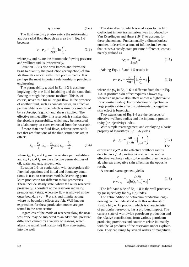
q ∝ k∆p. (1-2)

The fluid viscosity µ also enters the relationship,and for radial flow through an area 2πrh, Eq. 1-2becomes

(1-3)

where pwf and rw are the bottomhole flowing pressureand wellbore radius, respectively.

Equation 1-3 is also well known and forms thebasis to quantify the production (or injection) of flu-ids through vertical wells from porous media. It isperhaps the most important relationship in petroleumengineering.

The permeability k used in Eq. 1-3 is absolute,implying only one fluid inhabiting and the same fluidflowing through the porous medium. This is, ofcourse, never true for oil or gas flow. In the presenceof another fluid, such as connate water, an effectivepermeability is in force, which is usually symbolizedby a subscript (e.g., ko) and always implied. Theeffective permeability in a reservoir is smaller thanthe absolute permeability, which may be measured in a laboratory on cores extracted from the reservoir.

If more than one fluid flows, relative permeabili-ties that are functions of the fluid saturations are ineffect:

(1-4)

where kro, krw and krg are the relative permeabilitiesand ko, kw and kg are the effective permeabilities ofoil, water and gas, respectively.

Equation 1-3, in conjunction with appropriate dif-ferential equations and initial and boundary condi-tions, is used to construct models describing petro-leum production for different radial geometries.These include steady state, where the outer reservoirpressure pe is constant at the reservoir radius re;pseudosteady state, where no flow is allowed at theouter boundary (q = 0 at re); and infinite acting,where no boundary effects are felt. Well-knownexpressions for these production modes are pre-sented in the next section.

Regardless of the mode of reservoir flow, the near-well zone may be subjected to an additional pressuredifference caused by a variety of reasons, whichalters the radial (and horizontal) flow converginginto the well.

The skin effect s, which is analogous to the filmcoefficient in heat transmission, was introduced byVan Everdingen and Hurst (1949) to account forthese phenomena. Fundamentally a dimensionlessnumber, it describes a zone of infinitesimal extentthat causes a steady-state pressure difference, conve-niently defined as

(1-5)

Adding Eqs. 1-3 and 1-5 results in

(1-6)

where the pwf in Eq. 1-6 is different from that in Eq.1-3. A positive skin effect requires a lower pwf,whereas a negative skin effect allows a higher valuefor a constant rate q. For production or injection, alarge positive skin effect is detrimental; a negativeskin effect is beneficial.

Two extensions of Eq. 1-6 are the concepts ofeffective wellbore radius and the important produc-tivity (or injectivity) index.

With simple rearrangement and employing a basicproperty of logarithms, Eq. 1-6 yields

(1-7)

Theexpression rwe–s is the effective wellbore radius,denoted as rw´. A positive skin effect causes theeffective wellbore radius to be smaller than the actu-al, whereas a negative skin effect has the oppositeresult.

A second rearrangement yields

(1-8)

The left-hand side of Eq. 1-8 is the well productiv-ity (or injectivity for pwf > p) index.

The entire edifice of petroleum production engi-neering can be understood with this relationship.First, a higher kh product, which is characteristic of particular reservoirs, has a profound impact. Thecurrent state of worldwide petroleum production and the relative contributions from various petroleum-producing provinces and countries relate intimatelywith the kh products of the reservoirs under exploita-tion. They can range by several orders of magnitude.

1-2 Reservoir Stimulation in Petroleum Production

p pq

kh

r

rwf

w

– ln ,= µπ2

kk

kk

k

kk

k

kroo

rww

rgg= = =, ,and

∆pq

khss = µ

π2.

p pq

kh

r

r ewf

ws

– ln .–

=

µπ2

q

p p

kh

r r swf e w– ln /.= ( ) +[ ]

2πµ

p pq

kh

r

rswf

w

– ln ,= +

µπ2

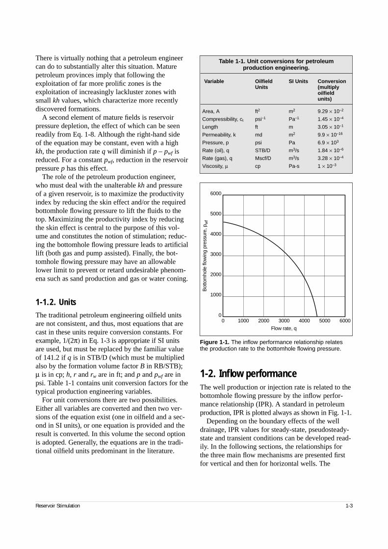
There is virtually nothing that a petroleum engineercan do to substantially alter this situation. Maturepetroleum provinces imply that following theexploitation of far more prolific zones is theexploitation of increasingly lackluster zones withsmall kh values, which characterize more recentlydiscovered formations.

A second element of mature fields is reservoirpressure depletion, the effect of which can be seenreadily from Eq. 1-8. Although the right-hand side of the equation may be constant, even with a highkh, the production rate q will diminish if p – pwf isreduced. For a constant pwf, reduction in the reservoirpressure p has this effect.

The role of the petroleum production engineer,who must deal with the unalterable kh and pressureof a given reservoir, is to maximize the productivityindex by reducing the skin effect and/or the requiredbottomhole flowing pressure to lift the fluids to thetop. Maximizing the productivity index by reducingthe skin effect is central to the purpose of this vol-ume and constitutes the notion of stimulation; reduc-ing the bottomhole flowing pressure leads to artificiallift (both gas and pump assisted). Finally, the bot-tomhole flowing pressure may have an allowablelower limit to prevent or retard undesirable phenom-ena such as sand production and gas or water coning.

1-1.2. UnitsThe traditional petroleum engineering oilfield unitsare not consistent, and thus, most equations that arecast in these units require conversion constants. Forexample, 1/(2π) in Eq. 1-3 is appropriate if SI unitsare used, but must be replaced by the familiar valueof 141.2 if q is in STB/D (which must be multipliedalso by the formation volume factor B in RB/STB);µ is in cp; h, r and rw are in ft; and p and pwf are inpsi. Table 1-1 contains unit conversion factors for thetypical production engineering variables.

For unit conversions there are two possibilities.Either all variables are converted and then two ver-sions of the equation exist (one in oilfield and a sec-ond in SI units), or one equation is provided and theresult is converted. In this volume the second optionis adopted. Generally, the equations are in the tradi-tional oilfield units predominant in the literature.

1-2. Inflow performanceThe well production or injection rate is related to thebottomhole flowing pressure by the inflow perfor-mance relationship (IPR). A standard in petroleumproduction, IPR is plotted always as shown in Fig. 1-1.

Depending on the boundary effects of the welldrainage, IPR values for steady-state, pseudosteady-state and transient conditions can be developed read-ily. In the following sections, the relationships forthe three main flow mechanisms are presented firstfor vertical and then for horizontal wells. The

Reservoir Stimulation 1-3

Figure 1-1. The inflow performance relationship relates the production rate to the bottomhole flowing pressure.

Flow rate, q

Bot

tom

hole

flow

ing

pres

sure

, pw

f

6000

5000

4000

3000

2000

1000

01000 2000 3000 4000 5000 60000

Table 1-1. Unit conversions for petroleumproduction engineering.

Variable Oilfield SI Units ConversionUnits (multiply

oilfieldunits)

Area, A ft2 m2 9.29 × 10–2

Compressibility, ct psi–1 Pa–1 1.45 × 10–4

Length ft m 3.05 × 10–1

Permeability, k md m2 9.9 × 10–16

Pressure, p psi Pa 6.9 × 103

Rate (oil), q STB/D m3/s 1.84 × 10–6

Rate (gas), q Mscf/D m3/s 3.28 × 10–4

Viscosity, µ cp Pa-s 1 × 10–3

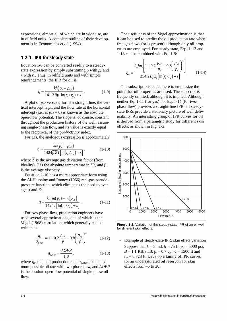
expressions, almost all of which are in wide use, arein oilfield units. A complete outline of their develop-ment is in Economides et al. (1994).

1-2.1. IPR for steady stateEquation 1-6 can be converted readily to a steady-state expression by simply substituting p with pe andr with re. Thus, in oilfield units and with simplerearrangements, the IPR for oil is

(1-9)

A plot of pwf versus q forms a straight line, the ver-tical intercept is pe, and the flow rate at the horizontalintercept (i.e., at pwf = 0) is known as the absoluteopen-flow potential. The slope is, of course, constantthroughout the production history of the well, assum-ing single-phase flow, and its value is exactly equalto the reciprocal of the productivity index.

For gas, the analogous expression is approximately

(1-10)

where Z—

is the average gas deviation factor (fromideality), T is the absolute temperature in °R, and µ–

is the average viscosity.Equation 1-10 has a more appropriate form using

the Al-Hussainy and Ramey (1966) real-gas pseudo-pressure function, which eliminates the need to aver-age µ and Z:

(1-11)

For two-phase flow, production engineers haveused several approximations, one of which is theVogel (1968) correlation, which generally can bewritten as

(1-12)

(1-13)

where qo is the oil production rate, qo,max is the maxi-mum possible oil rate with two-phase flow, and AOFPis the absolute open-flow potential of single-phase oilflow.

The usefulness of the Vogel approximation is thatit can be used to predict the oil production rate whenfree gas flows (or is present) although only oil prop-erties are employed. For steady state, Eqs. 1-12 and1-13 can be combined with Eq. 1-9:

(1-14)

The subscript o is added here to emphasize thepoint that oil properties are used. The subscript isfrequently omitted, although it is implied. Althoughneither Eq. 1-11 (for gas) nor Eq. 1-14 (for two-phase flow) provides a straight-line IPR, all steady-state IPRs provide a stationary picture of well deliv-erability. An interesting group of IPR curves for oilis derived from a parametric study for different skineffects, as shown in Fig. 1-2.

• Example of steady-state IPR: skin effect variation

Suppose that k = 5 md, h = 75 ft, pe = 5000 psi,B = 1.1 RB/STB, µ = 0.7 cp, re = 1500 ft and rw = 0.328 ft. Develop a family of IPR curvesfor an undersaturated oil reservoir for skineffects from –5 to 20.

1-4 Reservoir Stimulation in Petroleum Production

Figure 1-2. Variation of the steady-state IPR of an oil wellfor different skin effects.

qkh p p

B r r s

e wf

e w

=( )

( ) +[ ]–

. ln /.

141 2 µ

qkh p p

ZT r r s

e wf

e w

=( )

( ) +[ ]2 2

1424

–

ln /,

µ

qkh m p m p

T r r s

e wf

e w

=( ) ( )[ ]

( ) +[ ]–

ln /.

1424

q

q

p

p

p

po

o,max

wf wf= − −

1 0 2 0 82

. .

qAOFP

o,max =1 8.

,

q

k hpp

p

p

p

B r r so

o ewf

e

wf

e

o o e w

=

− −

( ) +[ ]1 0 2 0 8

254 2

2

. .

. ln.

µ

Flow rate, q

Bot

tom

hole

flow

ing

pres

sure

, pw

f

6000

5000

4000

3000

2000

1000

01000 2000 3000 4000 5000 60000

s = 20 s = 10 s = 0

s = –5

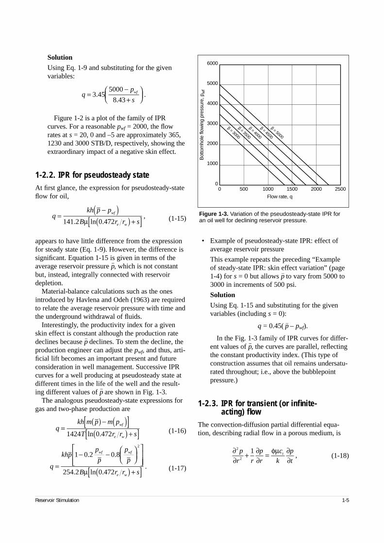
Solution

Using Eq. 1-9 and substituting for the givenvariables:

Figure 1-2 is a plot of the family of IPRcurves. For a reasonable pwf = 2000, the flowrates at s = 20, 0 and –5 are approximately 365,1230 and 3000 STB/D, respectively, showing theextraordinary impact of a negative skin effect.

1-2.2. IPR for pseudosteady stateAt first glance, the expression for pseudosteady-stateflow for oil,

(1-15)

appears to have little difference from the expressionfor steady state (Eq. 1-9). However, the difference issignificant. Equation 1-15 is given in terms of theaverage reservoir pressure p–, which is not constantbut, instead, integrally connected with reservoirdepletion.

Material-balance calculations such as the onesintroduced by Havlena and Odeh (1963) are requiredto relate the average reservoir pressure with time andthe underground withdrawal of fluids.

Interestingly, the productivity index for a givenskin effect is constant although the production ratedeclines because p– declines. To stem the decline, theproduction engineer can adjust the pwf, and thus, arti-ficial lift becomes an important present and futureconsideration in well management. Successive IPRcurves for a well producing at pseudosteady state atdifferent times in the life of the well and the result-ing different values of p– are shown in Fig. 1-3.

The analogous pseudosteady-state expressions forgas and two-phase production are

(1-16)

(1-17)

• Example of pseudosteady-state IPR: effect ofaverage reservoir pressure

This example repeats the preceding “Example of steady-state IPR: skin effect variation” (page1-4) for s = 0 but allows p– to vary from 5000 to3000 in increments of 500 psi.

Solution

Using Eq. 1-15 and substituting for the givenvariables (including s = 0):

q = 0.45( p– – pwf).

In the Fig. 1-3 family of IPR curves for differ-ent values of p–, the curves are parallel, reflectingthe constant productivity index. (This type ofconstruction assumes that oil remains undersatu-rated throughout; i.e., above the bubblepointpressure.)

1-2.3. IPR for transient (or infinite-acting) flow

The convection-diffusion partial differential equa-tion, describing radial flow in a porous medium, is

(1-18)

Reservoir Stimulation 1-5

qp

swf=

−+

3 455000

8 43.

..

qkh p p

B r r s

wf

e w

=−( )

( ) +[ ]141 2 0 472. ln .,

µ

∂∂

∂∂

φµ ∂∂

2

2

1p

r r

p

r

c

k

p

tt+ = ,

qkh m p m p

T r r s

wf

e w

=( ) − ( )[ ]( ) +[ ]1424 0 472ln .

q

khpp

p

p

p

B r r s

wf wf

e w

=

− −

( ) +[ ]1 0 2 0 8

254 2 0 472

2

. .

. ln ..

µ

Figure 1-3. Variation of the pseudosteady-state IPR for an oil well for declining reservoir pressure.

Flow rate, qB

otto

mho

le fl

owin

g pr

essu

re, p

wf

6000

5000

4000

3000

2000

1000

0500 1000 1500 2000 25000

p = 5000

p = 4500

p = 4000

p = 3500

p = 3000

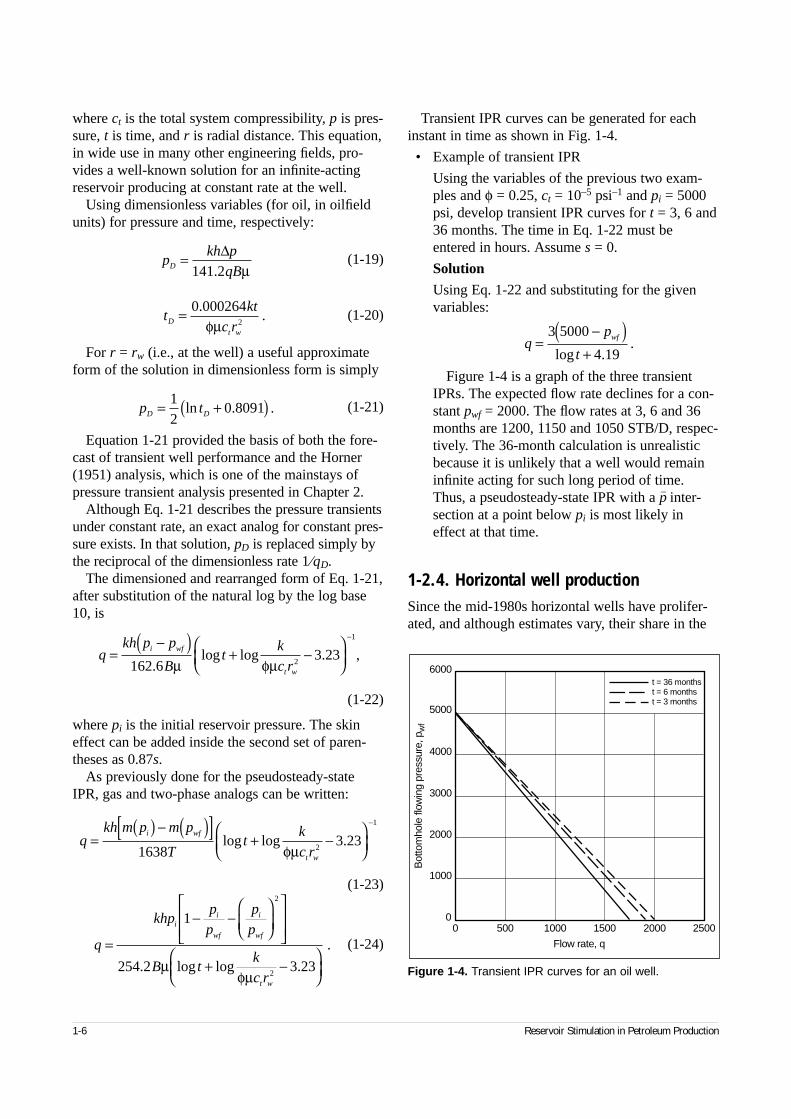
where ct is the total system compressibility, p is pres-sure, t is time, and r is radial distance. This equation,in wide use in many other engineering fields, pro-vides a well-known solution for an infinite-actingreservoir producing at constant rate at the well.

Using dimensionless variables (for oil, in oilfieldunits) for pressure and time, respectively:

(1-19)

(1-20)

For r = rw (i.e., at the well) a useful approximateform of the solution in dimensionless form is simply

(1-21)

Equation 1-21 provided the basis of both the fore-cast of transient well performance and the Horner(1951) analysis, which is one of the mainstays ofpressure transient analysis presented in Chapter 2.

Although Eq. 1-21 describes the pressure transientsunder constant rate, an exact analog for constant pres-sure exists. In that solution, pD is replaced simply bythe reciprocal of the dimensionless rate 1⁄qD.

The dimensioned and rearranged form of Eq. 1-21,after substitution of the natural log by the log base10, is

(1-22)

where pi is the initial reservoir pressure. The skineffect can be added inside the second set of paren-theses as 0.87s.

As previously done for the pseudosteady-stateIPR, gas and two-phase analogs can be written:

(1-23)

(1-24)

Transient IPR curves can be generated for eachinstant in time as shown in Fig. 1-4.

• Example of transient IPR

Using the variables of the previous two exam-ples and φ = 0.25, ct = 10–5 psi–1 and pi = 5000psi, develop transient IPR curves for t = 3, 6 and36 months. The time in Eq. 1-22 must beentered in hours. Assume s = 0.

Solution

Using Eq. 1-22 and substituting for the givenvariables:

Figure 1-4 is a graph of the three transientIPRs. The expected flow rate declines for a con-stant pwf = 2000. The flow rates at 3, 6 and 36months are 1200, 1150 and 1050 STB/D, respec-tively. The 36-month calculation is unrealisticbecause it is unlikely that a well would remaininfinite acting for such long period of time.Thus, a pseudosteady-state IPR with a p– inter-section at a point below pi is most likely ineffect at that time.

1-2.4. Horizontal well productionSince the mid-1980s horizontal wells have prolifer-ated, and although estimates vary, their share in the

1-6 Reservoir Stimulation in Petroleum Production

qkh p p

Bt

k

c ri wf

t w

=−( )

+ −

−

162 63 23

2

1

.log log . ,

µ φµ

qkh m p m p

Tt

k

c r

i wf

t w

=( ) − ( )[ ]

+ −

−

16383 23

2

1

log log .φµ

qp

twf=

−( )+

3 5000

4 19log ..

Figure 1-4. Transient IPR curves for an oil well.

Flow rate, q

Bot

tom

hole

flow

ing

pres

sure

, pw

f

6000

5000

4000

3000

2000

1000

0500 1000 1500 2000 25000

t = 36 monthst = 6 monthst = 3 months

pkh p

qBD = ∆141 2. µ

tkt

c rD

t w

= 0 0002642

..

φµ

p tD D= +( )12

0 8091ln . .

q

khpp

p

p

p

B tk

c r

ii

wf

i

wf

t w

=

− −

+ −

1

254 2 3 23

2

2. log log .

.

µφµ

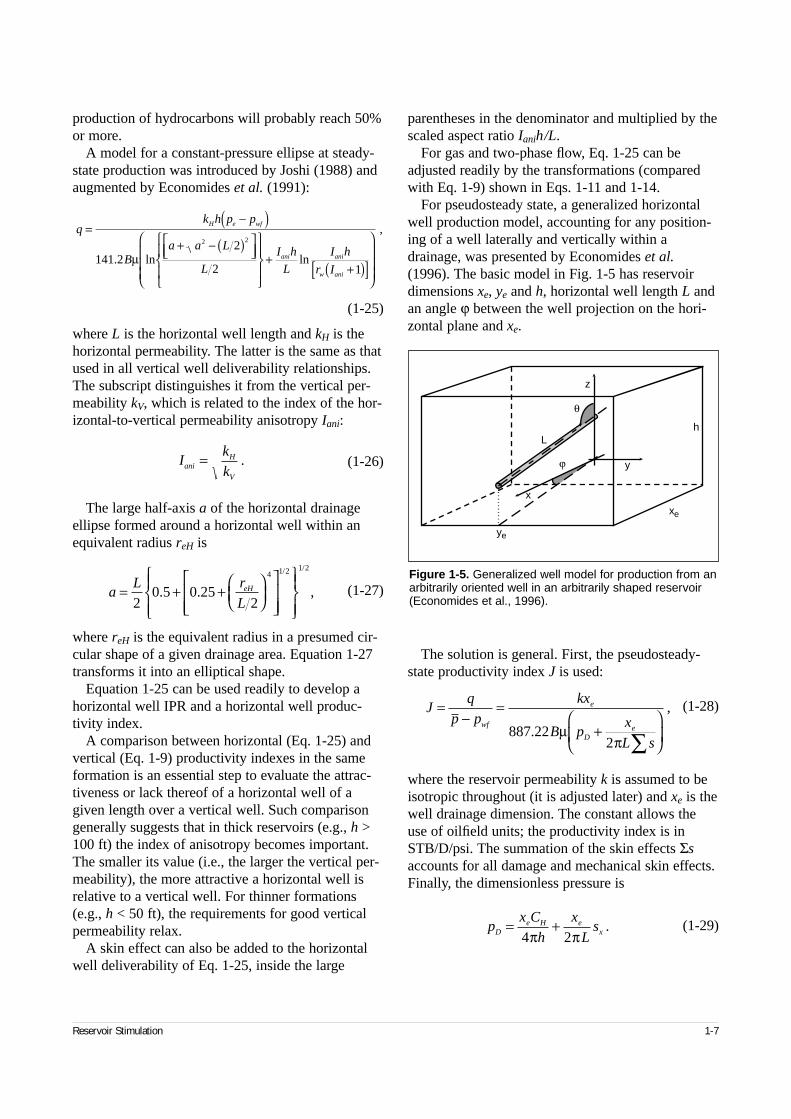
production of hydrocarbons will probably reach 50%or more.

A model for a constant-pressure ellipse at steady-state production was introduced by Joshi (1988) andaugmented by Economides et al. (1991):

(1-25)

where L is the horizontal well length and kH is thehorizontal permeability. The latter is the same as thatused in all vertical well deliverability relationships.The subscript distinguishes it from the vertical per-meability kV, which is related to the index of the hor-izontal-to-vertical permeability anisotropy Iani:

(1-26)

The large half-axis a of the horizontal drainageellipse formed around a horizontal well within anequivalent radius reH is

(1-27)

where reH is the equivalent radius in a presumed cir-cular shape of a given drainage area. Equation 1-27transforms it into an elliptical shape.

Equation 1-25 can be used readily to develop ahorizontal well IPR and a horizontal well produc-tivity index.

A comparison between horizontal (Eq. 1-25) andvertical (Eq. 1-9) productivity indexes in the sameformation is an essential step to evaluate the attrac-tiveness or lack thereof of a horizontal well of agiven length over a vertical well. Such comparisongenerally suggests that in thick reservoirs (e.g., h >100 ft) the index of anisotropy becomes important.The smaller its value (i.e., the larger the vertical per-meability), the more attractive a horizontal well isrelative to a vertical well. For thinner formations(e.g., h < 50 ft), the requirements for good verticalpermeability relax.

A skin effect can also be added to the horizontalwell deliverability of Eq. 1-25, inside the large

parentheses in the denominator and multiplied by thescaled aspect ratio Ianih/L.

For gas and two-phase flow, Eq. 1-25 can beadjusted readily by the transformations (compared with Eq. 1-9) shown in Eqs. 1-11 and 1-14.

For pseudosteady state, a generalized horizontalwell production model, accounting for any position-ing of a well laterally and vertically within adrainage, was presented by Economides et al.(1996). The basic model in Fig. 1-5 has reservoirdimensions xe, ye and h, horizontal well length L andan angle ϕ between the well projection on the hori-zontal plane and xe.

The solution is general. First, the pseudosteady-state productivity index J is used:

(1-28)

where the reservoir permeability k is assumed to beisotropic throughout (it is adjusted later) and xe is thewell drainage dimension. The constant allows theuse of oilfield units; the productivity index is inSTB/D/psi. The summation of the skin effects Σsaccounts for all damage and mechanical skin effects.Finally, the dimensionless pressure is

(1-29)

Reservoir Stimulation 1-7

qk h p p

Ba a L

L

I h

L

I h

r I

H e wf

ani ani

w ani

=−( )

+ − ( )

++( )[ ]

141 22

2 1

2 2

. ln ln

,

µ

Ik

kaniH

V

= .

aL r

LeH= + +

2

0 5 0 252

4 1 2 1 2

. . ,

/ /Figure 1-5. Generalized well model for production from anarbitrarily oriented well in an arbitrarily shaped reservoir(Economides et al., 1996).

ye

xe

L

x

y

z

θ

ϕ

h

Jq

p p

kx

B px

L s

wf

e

De

=−

=

+

∑

887 222

.

,

µπ

px C

h

x

LsD

e H ex= +

4 2π π.

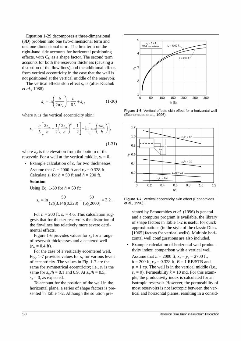
Equation 1-29 decomposes a three-dimensional(3D) problem into one two-dimensional term andone one-dimensional term. The first term on theright-hand side accounts for horizontal positioningeffects, with CH as a shape factor. The second termaccounts for both the reservoir thickness (causing adistortion of the flow lines) and the additional effectsfrom vertical eccentricity in the case that the well isnot positioned at the vertical middle of the reservoir.

The vertical effects skin effect sx is (after Kuchuket al., 1988)

(1-30)

where se is the vertical eccentricity skin:

(1-31)

where zw is the elevation from the bottom of thereservoir. For a well at the vertical middle, se = 0.

• Example calculation of sx for two thicknesses

Assume that L = 2000 ft and rw = 0.328 ft.Calculate sx for h = 50 ft and h = 200 ft.

Solution

Using Eq. 1-30 for h = 50 ft:

For h = 200 ft, sx = 4.6. This calculation sug-gests that for thicker reservoirs the distortion ofthe flowlines has relatively more severe detri-mental effects.

Figure 1-6 provides values for sx for a rangeof reservoir thicknesses and a centered well (rw = 0.4 ft).

For the case of a vertically eccentered well,Fig. 1-7 provides values for se for various levelsof eccentricity. The values in Fig. 1-7 are thesame for symmetrical eccentricity; i.e., se is thesame for zw/h = 0.1 and 0.9. At zw/h = 0.5, se = 0, as expected.

To account for the position of the well in thehorizontal plane, a series of shape factors is pre-sented in Table 1-2. Although the solution pre-

sented by Economides et al. (1996) is generaland a computer program is available, the libraryof shape factors in Table 1-2 is useful for quickapproximations (in the style of the classic Dietz[1965] factors for vertical wells). Multiple hori-zontal well configurations are also included.

• Example calculation of horizontal well produc-tivity index: comparison with a vertical well

Assume that L = 2000 ft, xe = ye = 2700 ft, h = 200 ft, rw = 0.328 ft, B = 1 RB/STB and µ = 1 cp. The well is in the vertical middle (i.e.,se = 0). Permeability k = 10 md. For this exam-ple, the productivity index is calculated for anisotropic reservoir. However, the permeability ofmost reservoirs is not isotropic between the ver-tical and horizontal planes, resulting in a consid-

1-8 Reservoir Stimulation in Petroleum Production

sh

r

h

Lsx

w

e=

+ln – ,2 6π

sh

L

z

h

z

h

z

hew w w= −

−

−

2 12

2 12

2

ln sin ,π

sx = − =ln( )( . )( . ) ( )( )

. .50

2 3 14 0 32850

6 20003 2

Figure 1-6. Vertical effects skin effect for a horizontal well(Economides et al., 1996).

h (ft)

s x

50 100 150 200 250 3000

2

3

4

5

1

rw = 0.4 ftWell is centered L = 4000 ft

L = 200 ft

Figure 1-7. Vertical eccentricity skin effect (Economides et al., 1996).

h/L

se

1.2

1.0

0.8

0.6

0.4

0.2

00.2 0.4 0.6 0.8 1.0 1.20

zw/h = 0.1

zw/h = 0.2

zw/h = 0.3

zw/h = 0.4

hzw

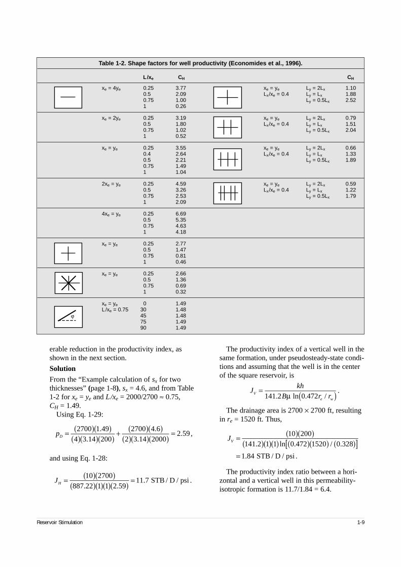
erable reduction in the productivity index, asshown in the next section.

Solution

From the “Example calculation of sx for twothicknesses” (page 1-8), sx = 4.6, and from Table1-2 for xe = ye and L/xe = 2000/2700 ≈ 0.75,CH = 1.49.

Using Eq. 1-29:

and using Eq. 1-28:

The productivity index of a vertical well in thesame formation, under pseudosteady-state condi-tions and assuming that the well is in the centerof the square reservoir, is

The drainage area is 2700 × 2700 ft, resultingin re = 1520 ft. Thus,

The productivity index ratio between a hori-zontal and a vertical well in this permeability-isotropic formation is 11.7/1.84 = 6.4.

Reservoir Stimulation 1-9

pD = ( )( )( )( )( )

+ ( )( )( )( )( )

=2700 1 494 3 14 200

2700 4 62 3 14 2000

2 59.

..

.. ,

JH = ( )( )( )( )( )( )

=10 2700887 22 1 1 2 59

11 7. .

. STB / D / psi .

Jkh

B r rV

e w

= ( )141 2 0 472. ln . /.

µ

JV = ( )( )( )( )( ) ( )( ) ( )[ ]

=

10 200141 2 1 1 1520 0 328

1 84

. / .

.

ln 0.472

STB / D / psi .

Table 1-2. Shape factors for well productivity (Economides et al., 1996).

L /xe CH CH

xe = 4ye 0.25 3.77 xe = ye Ly = 2Lx 1.100.5 2.09 Lx/xe = 0.4 Ly = Lx 1.880.75 1.00 Ly = 0.5Lx 2.521 0.26

xe = 2ye 0.25 3.19 xe = ye Ly = 2Lx 0.790.5 1.80 Lx/xe = 0.4 Ly = Lx 1.510.75 1.02 Ly = 0.5Lx 2.041 0.52

xe = ye 0.25 3.55 xe = ye Ly = 2Lx 0.660.4 2.64 Lx/xe = 0.4 Ly = Lx 1.330.5 2.21 Ly = 0.5Lx 1.890.75 1.491 1.04

2xe = ye 0.25 4.59 xe = ye Ly = 2Lx 0.590.5 3.26 Lx/xe = 0.4 Ly = Lx 1.220.75 2.53 Ly = 0.5Lx 1.791 2.09

4xe = ye 0.25 6.690.5 5.350.75 4.631 4.18

xe = ye 0.25 2.770.5 1.470.75 0.811 0.46

xe = ye 0.25 2.660.5 1.360.75 0.691 0.32

xe = ye 0 1.49L /xe = 0.75 30 1.48

45 1.4875 1.4990 1.49

ϕ

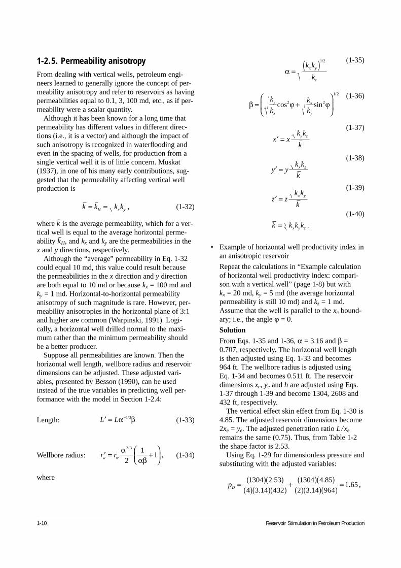
1-2.5. Permeability anisotropyFrom dealing with vertical wells, petroleum engi-neers learned to generally ignore the concept of per-meability anisotropy and refer to reservoirs as havingpermeabilities equal to 0.1, 3, 100 md, etc., as if per-meability were a scalar quantity.

Although it has been known for a long time thatpermeability has different values in different direc-tions (i.e., it is a vector) and although the impact ofsuch anisotropy is recognized in waterflooding andeven in the spacing of wells, for production from asingle vertical well it is of little concern. Muskat(1937), in one of his many early contributions, sug-gested that the permeability affecting vertical wellproduction is

(1-32)

where k–

is the average permeability, which for a ver-tical well is equal to the average horizontal perme-ability k

–H, and kx and ky are the permeabilities in the

x and y directions, respectively.Although the “average” permeability in Eq. 1-32

could equal 10 md, this value could result becausethe permeabilities in the x direction and y directionare both equal to 10 md or because kx = 100 md andky = 1 md. Horizontal-to-horizontal permeabilityanisotropy of such magnitude is rare. However, per-meability anisotropies in the horizontal plane of 3:1and higher are common (Warpinski, 1991). Logi-cally, a horizontal well drilled normal to the maxi-mum rather than the minimum permeability shouldbe a better producer.

Suppose all permeabilities are known. Then thehorizontal well length, wellbore radius and reservoirdimensions can be adjusted. These adjusted vari-ables, presented by Besson (1990), can be usedinstead of the true variables in predicting well per-formance with the model in Section 1-2.4:

Length: (1-33)

Wellbore radius: (1-34)

where

(1-35)

(1-36)

(1-37)

(1-38)

(1-39)

(1-40)

• Example of horizontal well productivity index inan anisotropic reservoir

Repeat the calculations in “Example calculationof horizontal well productivity index: compari-son with a vertical well” (page 1-8) but with kx = 20 md, ky = 5 md (the average horizontalpermeability is still 10 md) and kz = 1 md.Assume that the well is parallel to the xe bound-ary; i.e., the angle ϕ = 0.

Solution

From Eqs. 1-35 and 1-36, α = 3.16 and β =0.707, respectively. The horizontal well length is then adjusted using Eq. 1-33 and becomes 964 ft. The wellbore radius is adjusted using Eq. 1-34 and becomes 0.511 ft. The reservoirdimensions xe, ye and h are adjusted using Eqs.1-37 through 1-39 and become 1304, 2608 and432 ft, respectively.

The vertical effect skin effect from Eq. 1-30 is4.85. The adjusted reservoir dimensions become2xe = ye. The adjusted penetration ratio L/xe

remains the same (0.75). Thus, from Table 1-2the shape factor is 2.53.

Using Eq. 1-29 for dimensionless pressure andsubstituting with the adjusted variables:

1-10 Reservoir Stimulation in Petroleum Production

k k k kH x y= = ,

pD = ( )( )( )( )( )

+ ( )( )( )( )( )

=1304 2 534 3 14 432

1304 4 852 3 14 964

1 65.

..

.. ,

′ = +

r rw w

ααβ

2 3

21

1/

,

β ϕ ϕ= +

k

k

k

ky

x

x

y

cos sin2 2

1 2/

′ =x xk k

ky z

′ =y yk k

kx z

′ =z zk k

kx y

k k k kx y z= 3 .

α =( )k k

kx y

z

1 2/

′ =L Lα β– /1 3

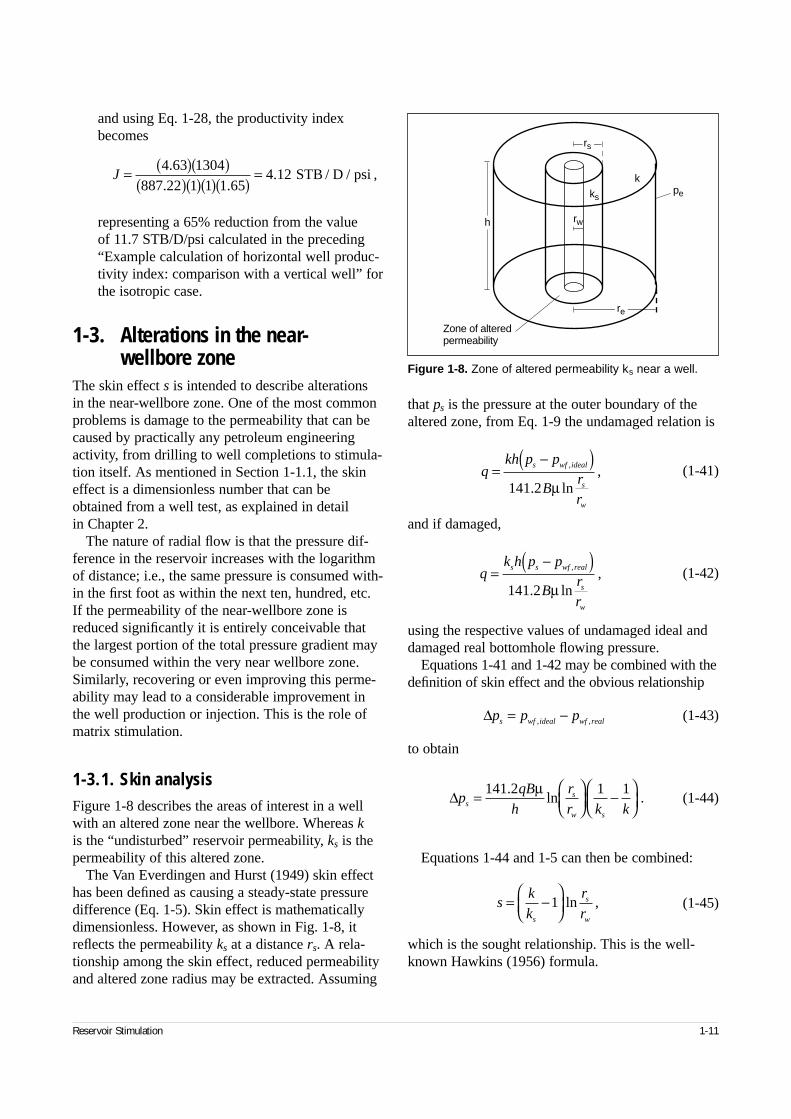
and using Eq. 1-28, the productivity indexbecomes

representing a 65% reduction from the value of 11.7 STB/D/psi calculated in the preceding“Example calculation of horizontal well produc-tivity index: comparison with a vertical well” forthe isotropic case.

1-3. Alterations in the near-wellbore zone

The skin effect s is intended to describe alterations in the near-wellbore zone. One of the most commonproblems is damage to the permeability that can becaused by practically any petroleum engineeringactivity, from drilling to well completions to stimula-tion itself. As mentioned in Section 1-1.1, the skineffect is a dimensionless number that can beobtained from a well test, as explained in detail in Chapter 2.

The nature of radial flow is that the pressure dif-ference in the reservoir increases with the logarithmof distance; i.e., the same pressure is consumed with-in the first foot as within the next ten, hundred, etc.If the permeability of the near-wellbore zone isreduced significantly it is entirely conceivable thatthe largest portion of the total pressure gradient maybe consumed within the very near wellbore zone.Similarly, recovering or even improving this perme-ability may lead to a considerable improvement inthe well production or injection. This is the role ofmatrix stimulation.

1-3.1. Skin analysisFigure 1-8 describes the areas of interest in a wellwith an altered zone near the wellbore. Whereas kis the “undisturbed” reservoir permeability, ks is thepermeability of this altered zone.

The Van Everdingen and Hurst (1949) skin effecthas been defined as causing a steady-state pressuredifference (Eq. 1-5). Skin effect is mathematicallydimensionless. However, as shown in Fig. 1-8, itreflects the permeability ks at a distance rs. A rela-tionship among the skin effect, reduced permeabilityand altered zone radius may be extracted. Assuming

that ps is the pressure at the outer boundary of thealtered zone, from Eq. 1-9 the undamaged relation is

(1-41)

and if damaged,

(1-42)

using the respective values of undamaged ideal anddamaged real bottomhole flowing pressure.

Equations 1-41 and 1-42 may be combined with thedefinition of skin effect and the obvious relationship

(1-43)

to obtain

(1-44)

Equations 1-44 and 1-5 can then be combined:

(1-45)

which is the sought relationship. This is the well-known Hawkins (1956) formula.

Reservoir Stimulation 1-11

Figure 1-8. Zone of altered permeability ks near a well.

k

kspe

Zone of altered permeability

h

re

rs

rw

J = ( )( )( )( )( )( )

=4 63 1304887 22 1 1 1 65

4 12.

. .. STB / D / psi ,

qkh p p

Brr

s wf ideal

s

w

=−( ),

. ln,

141 2 µ

qk h p p

Brr

s s wf real

s

w

=−( ),

. ln,

141 2 µ

∆p p ps wf ideal wf real= −, ,

∆pqB

h

r

r k kss

w s

=

−

141 2 1 1.ln .

µ

sk

k

r

rs

s

w

= −

1 ln ,

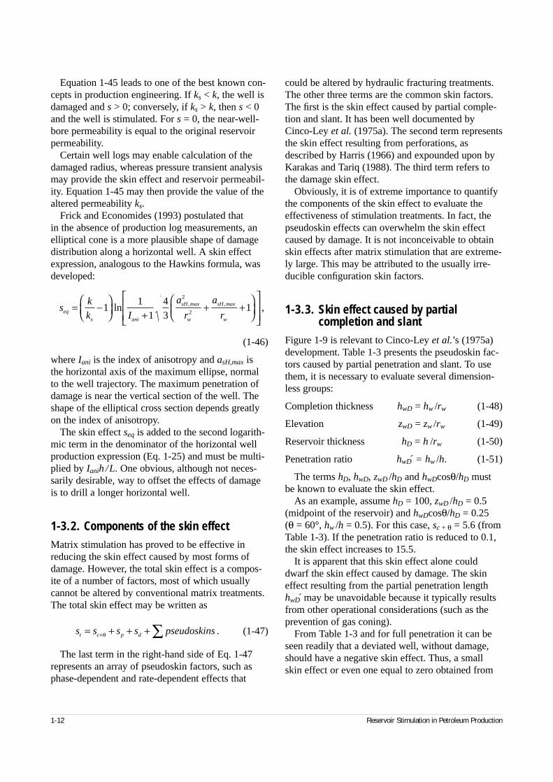
Equation 1-45 leads to one of the best known con-cepts in production engineering. If ks < k, the well isdamaged and s > 0; conversely, if ks > k, then s < 0and the well is stimulated. For s = 0, the near-well-bore permeability is equal to the original reservoirpermeability.

Certain well logs may enable calculation of thedamaged radius, whereas pressure transient analysismay provide the skin effect and reservoir permeabil-ity. Equation 1-45 may then provide the value of thealtered permeability ks.

Frick and Economides (1993) postulated that in the absence of production log measurements, anelliptical cone is a more plausible shape of damagedistribution along a horizontal well. A skin effectexpression, analogous to the Hawkins formula, wasdeveloped:

(1-46)

where Iani is the index of anisotropy and asH,max isthe horizontal axis of the maximum ellipse, normalto the well trajectory. The maximum penetration ofdamage is near the vertical section of the well. Theshape of the elliptical cross section depends greatlyon the index of anisotropy.

The skin effect seq is added to the second logarith-mic term in the denominator of the horizontal wellproduction expression (Eq. 1-25) and must be multi-plied by Ianih /L. One obvious, although not neces-sarily desirable, way to offset the effects of damageis to drill a longer horizontal well.

1-3.2. Components of the skin effectMatrix stimulation has proved to be effective inreducing the skin effect caused by most forms ofdamage. However, the total skin effect is a compos-ite of a number of factors, most of which usuallycannot be altered by conventional matrix treatments.The total skin effect may be written as

(1-47)

The last term in the right-hand side of Eq. 1-47represents an array of pseudoskin factors, such asphase-dependent and rate-dependent effects that

could be altered by hydraulic fracturing treatments.The other three terms are the common skin factors.The first is the skin effect caused by partial comple-tion and slant. It has been well documented byCinco-Ley et al. (1975a). The second term representsthe skin effect resulting from perforations, asdescribed by Harris (1966) and expounded upon byKarakas and Tariq (1988). The third term refers tothe damage skin effect.

Obviously, it is of extreme importance to quantifythe components of the skin effect to evaluate theeffectiveness of stimulation treatments. In fact, thepseudoskin effects can overwhelm the skin effectcaused by damage. It is not inconceivable to obtainskin effects after matrix stimulation that are extreme-ly large. This may be attributed to the usually irre-ducible configuration skin factors.

1-3.3. Skin effect caused by partial completion and slant

Figure 1-9 is relevant to Cinco-Ley et al.’s (1975a)development. Table 1-3 presents the pseudoskin fac-tors caused by partial penetration and slant. To usethem, it is necessary to evaluate several dimension-less groups:

Completion thickness hwD = hw /rw (1-48)

Elevation zwD = zw /rw (1-49)

Reservoir thickness hD = h /rw (1-50)

Penetration ratio hwD́ = hw /h. (1-51)

The terms hD, hwD, zwD /hD and hwDcosθ/hD mustbe known to evaluate the skin effect.

As an example, assume hD = 100, zwD /hD = 0.5(midpoint of the reservoir) and hwDcosθ/hD = 0.25 (θ = 60°, hw /h = 0.5). For this case, sc + θ = 5.6 (fromTable 1-3). If the penetration ratio is reduced to 0.1,the skin effect increases to 15.5.

It is apparent that this skin effect alone coulddwarf the skin effect caused by damage. The skineffect resulting from the partial penetration lengthhwD́ may be unavoidable because it typically resultsfrom other operational considerations (such as theprevention of gas coning).

From Table 1-3 and for full penetration it can beseen readily that a deviated well, without damage,should have a negative skin effect. Thus, a smallskin effect or even one equal to zero obtained from

1-12 Reservoir Stimulation in Petroleum Production

sk

k I

a

r

a

req

s ani

sH

w

sH

w

= −

+

+ +

11

143

12

2ln ,, ,max max

s s s s pseudoskinst c p d= + + ++ ∑θ .

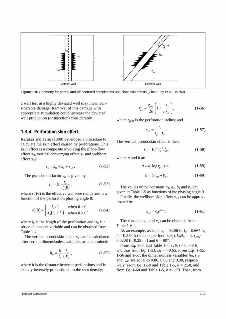
a well test in a highly deviated well may mean con-siderable damage. Removal of this damage withappropriate stimulation could increase the deviatedwell production (or injection) considerably.

1-3.4. Perforation skin effectKarakas and Tariq (1988) developed a procedure tocalculate the skin effect caused by perforations. Thisskin effect is a composite involving the plane-floweffect sH, vertical converging effect sV and wellboreeffect swb:

(1-52)

The pseudoskin factor sH is given by

(1-53)

where rẃ (θ) is the effective wellbore radius and is afunction of the perforation phasing angle θ:

(1-54)

where lp is the length of the perforation and αθ is aphase-dependent variable and can be obtained fromTable 1-4.

The vertical pseudoskin factor sV can be calculatedafter certain dimensionless variables are determined:

(1-55)

where h is the distance between perforations and isexactly inversely proportional to the shot density;

(1-56)

where rperf is the perforation radius; and

(1-57)

The vertical pseudoskin effect is then

(1-58)

where a and b are

(1-59)

(1-60)

The values of the constants a1, a2, b1 and b2 aregiven in Table 1-5 as functions of the phasing angle θ.

Finally, the wellbore skin effect swb can be approx-imated by

(1-61)

The constants c1 and c2 can be obtained fromTable 1-6.

As an example, assume rw = 0.406 ft, lp = 0.667 ft,h = 0.333 ft (3 shots per foot [spf]), kH/kv = 3, rperf =0.0208 ft [0.25 in.] and θ = 90°.

From Eq. 1-54 and Table 1-4, rẃ (θ) = 0.779 ft,and thus from Eq. 1-53, sH = –0.65. From Eqs. 1-55,1-56 and 1-57, the dimensionless variables hD, rpD

and rwD are equal to 0.86, 0.05 and 0.38, respect-ively. From Eq. 1-59 and Table 1-5, a = 2.58, andfrom Eq. 1-60 and Table 1-5, b = 1.73. Then, from

Reservoir Stimulation 1-13

Figure 1-9. Geometry for partial and off-centered completions and slant skin effects (Cinco-Ley et al., 1975a).

Vertical well Slanted well

hwhw

zw zw

θ

h

rw

rw

h

s s s sp H V wb= + + .

sr

rHw

w

=′( )

lnθ

,

′( ) = +( ) ≠

rl

r lw

p

w p

θ αθθθ

4 0

0

when

when

=,

hh

l

k

kD

p

H

V

= ,

rr

h

k

kpDperf V

H

= +

21 ,

rr

l rwDw

p w

=+

.

s h rVa

Db

pDb= −10 1 ,

a a r apD= +1 2log

b b r bpD= +1 2 .

s c ewbc rwD= 1

2 .

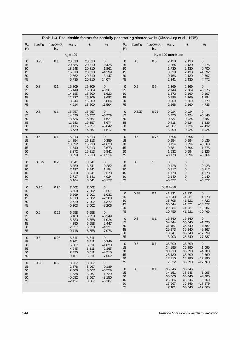
1-14 Reservoir Stimulation in Petroleum Production

Table 1-3. Pseudoskin factors for partially penetrating slanted wells (Cinco-Ley et al., 1975).

θw zwD /hD hwD cosθw s θ + c sc s θ

(°) hD

hD = 100

0 0.95 0.1 20.810 20.810 015 20.385 20.810 –0.42530 18.948 20.810 –1.86145 16.510 20.810 –4.29960 12.662 20.810 –8.14775 6.735 20.810 –14.074

0 0.8 0.1 15.809 15.809 015 15.449 15.809 –0.3630 14.185 15.809 –1.62345 12.127 15.809 –3.68260 8.944 15.809 –6.86475 4.214 15.809 –11.594

0 0.6 0.1 15.257 15.257 015 14.898 15.257 –0.35930 13.636 15.257 –1.62145 11.583 15.257 –3.67460 8.415 15.257 –6.84275 3.739 15.257 –11.517

0 0.5 0.1 15.213 15.213 015 14.854 15.213 –0.35930 13.592 15.213 –1.62045 11.540 15.213 –3.67360 8.372 15.213 –6.84175 3.699 15.213 –11.514

0 0.875 0.25 8.641 8.641 015 8.359 8.641 –0.28230 7.487 8.641 –1.15445 5.968 8.641 –2.67360 3.717 8.641 –4.92475 0.464 8.641 –8.177

0 0.75 0.25 7.002 7.002 015 6.750 7.002 –0.25130 5.969 7.002 –1.03245 4.613 7.002 –2.38860 2.629 7.002 –4.37275 –0.203 7.002 –7.206

0 0.6 0.25 6.658 6.658 015 6.403 6.658 –0.24930 5.633 6.658 –1.02445 4.290 6.658 –2.44760 2.337 6.658 –4.3275 –0.418 6.658 –7.076

0 0.5 0.25 6.611 6.611 015 6.361 6.611 –0.24930 5.587 6.611 –1.02345 4.245 6.611 –2.36560 2.295 6.611 –4.31575 –0.451 6.611 –7.062

0 0.75 0.5 3.067 3.067 015 2.878 3.067 –0.18930 2.308 3.067 –0.75945 1.338 3.067 –1.72960 –0.082 3.067 –3.15075 –2.119 3.067 –5.187

θw zwD /hD hwD cosθw s θ + c sc s θ

(°) hD

hD = 100 continued

0 0.6 0.5 2.430 2.430 015 2.254 2.430 –0.17630 1.730 2.430 –0.70045 0.838 2.430 –1.59260 –0.466 2.430 –2.89775 –2.341 2.430 –4.772

0 0.5 0.5 2.369 2.369 015 2.149 2.369 –0.17530 1.672 2.369 –0.69745 0.785 2.369 –1.58460 –0.509 2.369 –2.87975 –2.368 2.369 –4.738

0 0.625 0.75 0.924 0.924 015 0.778 0.924 –0.14530 0.337 0.924 –0.58745 –0.411 0.924 –1.33660 –1.507 0.924 –2.43275 –3.099 0.924 –4.024

0 0.5 0.75 0.694 0.694 015 0.554 0.694 –0.13930 0.134 0.694 –0.56045 –0.581 0.694 –1.27560 –1.632 0.694 –2.32675 –3.170 0.694 –3.864

0 0.5 1 0 0 015 –0.128 0 –0.12830 –0.517 0 –0.51745 –1.178 0 –1.17860 –2.149 0 –2.14975 –3.577 0 –3.577

hD = 1000

0 0.95 0.1 41.521 41.521 015 40.343 41.521 –1.17830 36.798 41.521 –4.72245 30.844 41.521 –10.67760 22.334 41.521 –19.18775 10.755 41.521 –30.766

0 0.8 0.1 35.840 35.840 015 34.744 35.840 –1.09530 31.457 35.840 –4.38245 25.973 35.840 –9.86760 18.241 35.840 –17.59975 8.003 35.840 –27.837

0 0.6 0.1 35.290 35.290 015 34.195 35.290 –1.09530 30.910 35.290 –4.38045 25.430 35.290 –9.86060 17.710 35.290 –17.58075 7.522 35.290 –27.768

0 0.5 0.1 35.246 35.246 015 34.151 35.246 –1.09530 30.866 35.246 –4.38045 25.386 35.246 –9.86060 17.667 35.246 –17.57975 7.481 35.246 –27.765

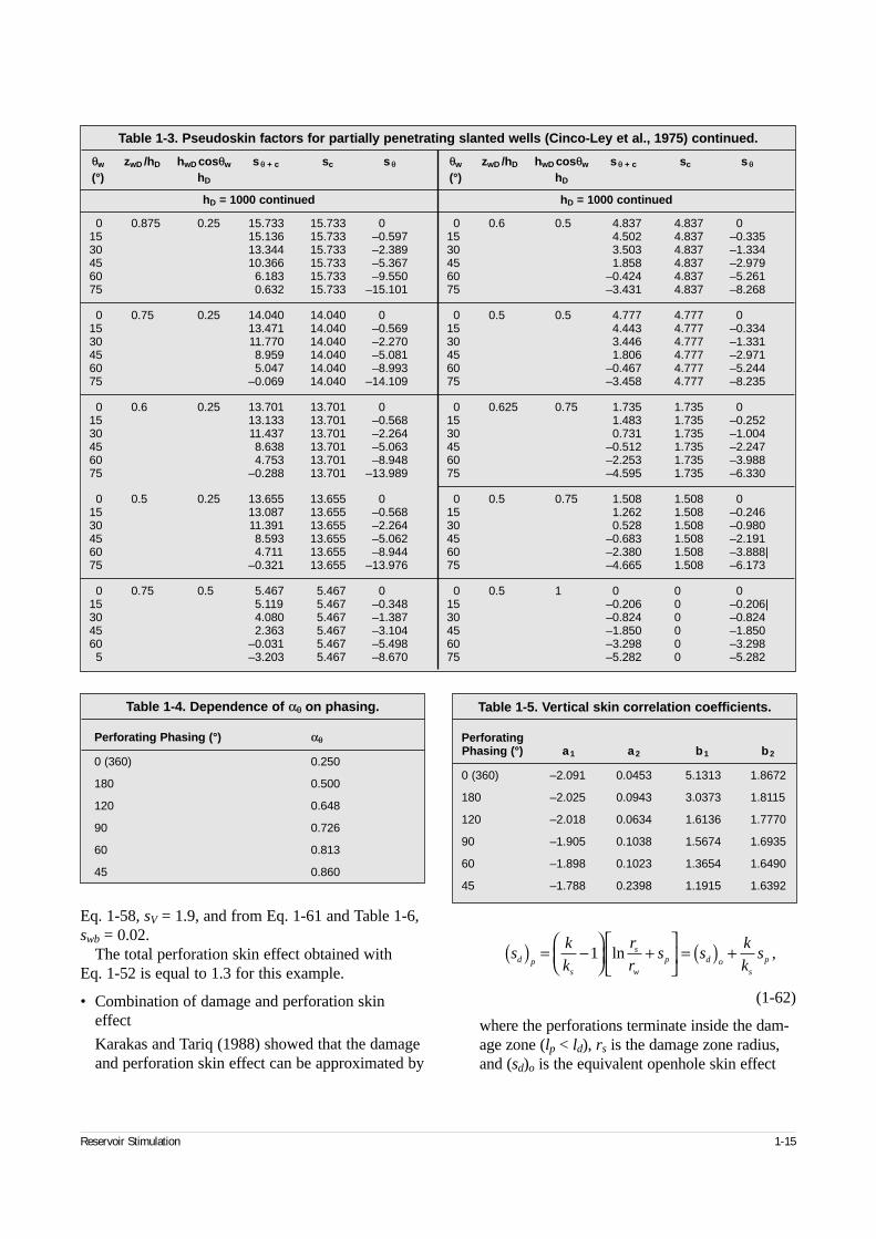
Eq. 1-58, sV = 1.9, and from Eq. 1-61 and Table 1-6,swb = 0.02.

The total perforation skin effect obtained with Eq. 1-52 is equal to 1.3 for this example.

• Combination of damage and perforation skineffect

Karakas and Tariq (1988) showed that the damageand perforation skin effect can be approximated by

(1-62)

where the perforations terminate inside the dam-age zone (lp < ld), rs is the damage zone radius,and (sd)o is the equivalent openhole skin effect

Reservoir Stimulation 1-15

Table 1-3. Pseudoskin factors for partially penetrating slanted wells (Cinco-Ley et al., 1975) continued.

θw zwD /hD hwD cosθw s θ + c sc s θ

(°) hD

hD = 1000 continued

0 0.875 0.25 15.733 15.733 015 15.136 15.733 –0.59730 13.344 15.733 –2.38945 10.366 15.733 –5.36760 6.183 15.733 –9.55075 0.632 15.733 –15.101

0 0.75 0.25 14.040 14.040 015 13.471 14.040 –0.56930 11.770 14.040 –2.27045 8.959 14.040 –5.08160 5.047 14.040 –8.99375 –0.069 14.040 –14.109

0 0.6 0.25 13.701 13.701 015 13.133 13.701 –0.56830 11.437 13.701 –2.26445 8.638 13.701 –5.06360 4.753 13.701 –8.94875 –0.288 13.701 –13.989

0 0.5 0.25 13.655 13.655 015 13.087 13.655 –0.56830 11.391 13.655 –2.26445 8.593 13.655 –5.06260 4.711 13.655 –8.94475 –0.321 13.655 –13.976

0 0.75 0.5 5.467 5.467 015 5.119 5.467 –0.34830 4.080 5.467 –1.38745 2.363 5.467 –3.10460 –0.031 5.467 –5.4985 –3.203 5.467 –8.670

θw zwD /hD hwD cosθw s θ + c sc s θ

(°) hD

hD = 1000 continued

0 0.6 0.5 4.837 4.837 015 4.502 4.837 –0.33530 3.503 4.837 –1.33445 1.858 4.837 –2.97960 –0.424 4.837 –5.26175 –3.431 4.837 –8.268

0 0.5 0.5 4.777 4.777 015 4.443 4.777 –0.33430 3.446 4.777 –1.33145 1.806 4.777 –2.97160 –0.467 4.777 –5.24475 –3.458 4.777 –8.235

0 0.625 0.75 1.735 1.735 015 1.483 1.735 –0.25230 0.731 1.735 –1.00445 –0.512 1.735 –2.24760 –2.253 1.735 –3.98875 –4.595 1.735 –6.330

0 0.5 0.75 1.508 1.508 015 1.262 1.508 –0.24630 0.528 1.508 –0.98045 –0.683 1.508 –2.19160 –2.380 1.508 –3.888|75 –4.665 1.508 –6.173

0 0.5 1 0 0 015 –0.206 0 –0.206|30 –0.824 0 –0.82445 –1.850 0 –1.85060 –3.298 0 –3.29875 –5.282 0 –5.282

Table 1-5. Vertical skin correlation coefficients.

PerforatingPhasing (°) a1 a2 b1 b2

0 (360) –2.091 0.0453 5.1313 1.8672

180 –2.025 0.0943 3.0373 1.8115

120 –2.018 0.0634 1.6136 1.7770

90 –1.905 0.1038 1.5674 1.6935

60 –1.898 0.1023 1.3654 1.6490

45 –1.788 0.2398 1.1915 1.6392

Table 1-4. Dependence of αθ on phasing.

Perforating Phasing (°) αθ

0 (360) 0.250

180 0.500

120 0.648

90 0.726

60 0.813

45 0.860

sk

k

r

rs s

k

ksd p

s

s

w

p d os

p( ) = −

+

= ( ) +1 ln ,

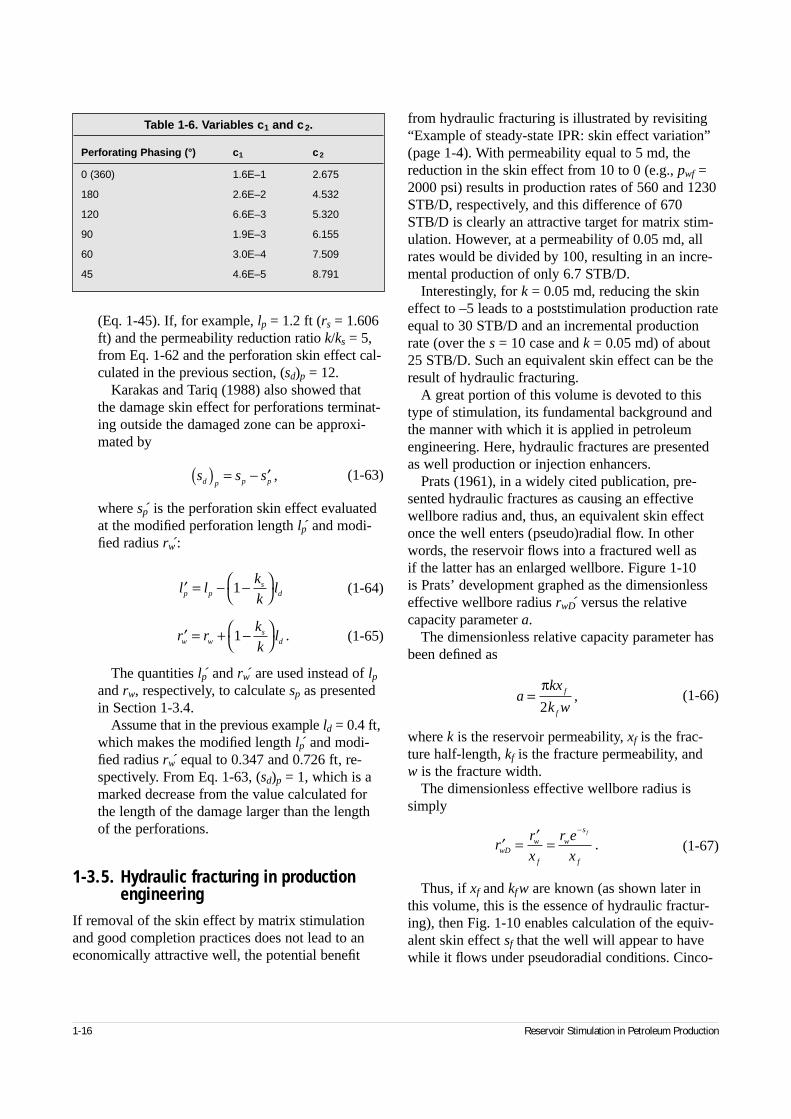
1-16 Reservoir Stimulation in Petroleum Production

(Eq. 1-45). If, for example, lp = 1.2 ft (rs = 1.606ft) and the permeability reduction ratio k/ks = 5,from Eq. 1-62 and the perforation skin effect cal-culated in the previous section, (sd)p = 12.

Karakas and Tariq (1988) also showed that the damage skin effect for perforations terminat-ing outside the damaged zone can be approxi-mated by

(1-63)

where sṕ is the perforation skin effect evaluatedat the modified perforation length lṕ and modi-fied radius rẃ :

(1-64)

(1-65)

The quantities lṕ and rẃ are used instead of lpand rw, respectively, to calculate sp as presentedin Section 1-3.4.

Assume that in the previous example ld = 0.4 ft,which makes the modified length lṕ and modi-fied radius rẃ equal to 0.347 and 0.726 ft, re-spectively. From Eq. 1-63, (sd)p = 1, which is amarked decrease from the value calculated forthe length of the damage larger than the lengthof the perforations.

1-3.5. Hydraulic fracturing in production engineering

If removal of the skin effect by matrix stimulationand good completion practices does not lead to aneconomically attractive well, the potential benefit

from hydraulic fracturing is illustrated by revisiting“Example of steady-state IPR: skin effect variation”(page 1-4). With permeability equal to 5 md, thereduction in the skin effect from 10 to 0 (e.g., pwf =2000 psi) results in production rates of 560 and 1230STB/D, respectively, and this difference of 670STB/D is clearly an attractive target for matrix stim-ulation. However, at a permeability of 0.05 md, allrates would be divided by 100, resulting in an incre-mental production of only 6.7 STB/D.

Interestingly, for k = 0.05 md, reducing the skineffect to –5 leads to a poststimulation production rateequal to 30 STB/D and an incremental productionrate (over the s = 10 case and k = 0.05 md) of about25 STB/D. Such an equivalent skin effect can be theresult of hydraulic fracturing.

A great portion of this volume is devoted to thistype of stimulation, its fundamental background andthe manner with which it is applied in petroleumengineering. Here, hydraulic fractures are presentedas well production or injection enhancers.

Prats (1961), in a widely cited publication, pre-sented hydraulic fractures as causing an effectivewellbore radius and, thus, an equivalent skin effectonce the well enters (pseudo)radial flow. In otherwords, the reservoir flows into a fractured well as if the latter has an enlarged wellbore. Figure 1-10 is Prats’ development graphed as the dimensionlesseffective wellbore radius rwD́ versus the relativecapacity parameter a.

The dimensionless relative capacity parameter hasbeen defined as

(1-66)

where k is the reservoir permeability, xf is the frac-ture half-length, kf is the fracture permeability, and w is the fracture width.

The dimensionless effective wellbore radius issimply

(1-67)

Thus, if xf and kfw are known (as shown later inthis volume, this is the essence of hydraulic fractur-ing), then Fig. 1-10 enables calculation of the equiv-alent skin effect sf that the well will appear to havewhile it flows under pseudoradial conditions. Cinco-

s s sd p p p( ) = − ′ ,

′ = − −

l l

k

klp p

sd1

′ = + −

r r

k

klw w

sd1 .

akx

k wf

f

=π2

,

′ = ′ =−

rr

x

r e

xwDw

f

w

s

f

f

.

Table 1-6. Variables c1 and c2.

Perforating Phasing (°) c1 c2

0 (360) 1.6E–1 2.675

180 2.6E–2 4.532

120 6.6E–3 5.320

90 1.9E–3 6.155

60 3.0E–4 7.509

45 4.6E–5 8.791

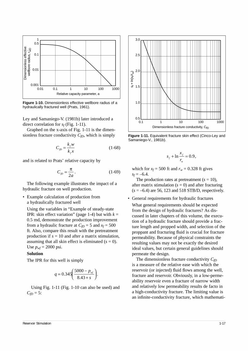
Reservoir Stimulation 1-17

Ley and Samaniego-V. (1981b) later introduced adirect correlation for sf (Fig. 1-11).

Graphed on the x-axis of Fig. 1-11 is the dimen-sionless fracture conductivity CfD, which is simply

(1-68)

and is related to Prats’ relative capacity by

(1-69)

The following example illustrates the impact of ahydraulic fracture on well production.

• Example calculation of production from a hydraulically fractured well

Using the variables in “Example of steady-stateIPR: skin effect variation” (page 1-4) but with k =0.5 md, demonstrate the production improvementfrom a hydraulic fracture at CfD = 5 and xf = 500ft. Also, compare this result with the pretreatmentproduction if s = 10 and after a matrix stimulation,assuming that all skin effect is eliminated (s = 0).Use pwf = 2000 psi.

Solution

The IPR for this well is simply

Using Fig. 1-11 (Fig. 1-10 can also be used) andCfD = 5:

which for xf = 500 ft and rw = 0.328 ft gives sf = –6.4.

The production rates at pretreatment (s = 10),after matrix stimulation (s = 0) and after fracturing(s = –6.4) are 56, 123 and 518 STB/D, respectively.

• General requirements for hydraulic fractures

What general requirements should be expectedfrom the design of hydraulic fractures? As dis-cussed in later chapters of this volume, the execu-tion of a hydraulic fracture should provide a frac-ture length and propped width, and selection of theproppant and fracturing fluid is crucial for fracturepermeability. Because of physical constraints theresulting values may not be exactly the desiredideal values, but certain general guidelines shouldpermeate the design.

The dimensionless fracture conductivity CfD

is a measure of the relative ease with which thereservoir (or injected) fluid flows among the well,fracture and reservoir. Obviously, in a low-perme-ability reservoir even a fracture of narrow widthand relatively low permeability results de facto ina high-conductivity fracture. The limiting value isan infinite-conductivity fracture, which mathemati-

Ck w

k xfDf

f

=

Ck w

k xfDf

f

=

sx

rff

w

+ =ln . ,0 9

CafD = π

2.

qp

swf=

−+

0 3455000

8 43.

..

Figure 1-10. Dimensionless effective wellbore radius of ahydraulically fractured well (Prats, 1961).

Relative capacity parameter, a

10.5

0.1

0.01

0.0010.1 1 10 100 10000.01

Dim

ensi

onle

ss e

ffect

ive

wel

lbor

e ra

dius

, r ' w

D

Figure 1-11. Equivalent fracture skin effect (Cinco-Ley andSamaniego-V., 1981b).

Dimensionless fracture conductivity, CfD s

f+ ln

(xf/r

w)

1 10 100 10000.1

3.0

2.5

2.0

1.5

1.0

0.5

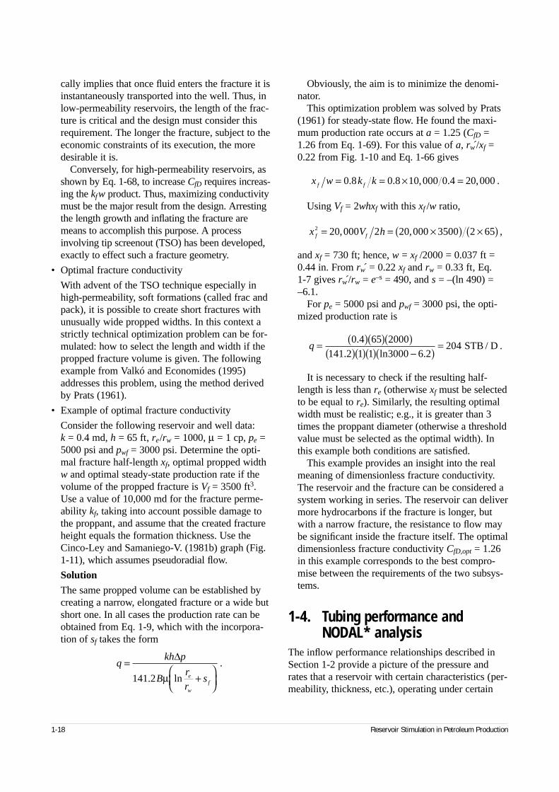
1-18 Reservoir Stimulation in Petroleum Production

cally implies that once fluid enters the fracture it isinstantaneously transported into the well. Thus, inlow-permeability reservoirs, the length of the frac-ture is critical and the design must consider thisrequirement. The longer the fracture, subject to theeconomic constraints of its execution, the moredesirable it is.

Conversely, for high-permeability reservoirs, asshown by Eq. 1-68, to increase CfD requires increas-ing the kfw product. Thus, maximizing conductivitymust be the major result from the design. Arrestingthe length growth and inflating the fracture aremeans to accomplish this purpose. A processinvolving tip screenout (TSO) has been developed,exactly to effect such a fracture geometry.

• Optimal fracture conductivity

With advent of the TSO technique especially inhigh-permeability, soft formations (called frac andpack), it is possible to create short fractures withunusually wide propped widths. In this context astrictly technical optimization problem can be for-mulated: how to select the length and width if thepropped fracture volume is given. The followingexample from Valkó and Economides (1995)addresses this problem, using the method derivedby Prats (1961).

• Example of optimal fracture conductivity

Consider the following reservoir and well data: k = 0.4 md, h = 65 ft, re/rw = 1000, µ = 1 cp, pe =5000 psi and pwf = 3000 psi. Determine the opti-mal fracture half-length xf, optimal propped widthw and optimal steady-state production rate if thevolume of the propped fracture is Vf = 3500 ft3.Use a value of 10,000 md for the fracture perme-ability kf, taking into account possible damage tothe proppant, and assume that the created fractureheight equals the formation thickness. Use theCinco-Ley and Samaniego-V. (1981b) graph (Fig.1-11), which assumes pseudoradial flow.

Solution

The same propped volume can be established bycreating a narrow, elongated fracture or a wide butshort one. In all cases the production rate can beobtained from Eq. 1-9, which with the incorpora-tion of sf takes the form

Obviously, the aim is to minimize the denomi-nator.

This optimization problem was solved by Prats(1961) for steady-state flow. He found the maxi-mum production rate occurs at a = 1.25 (CfD =1.26 from Eq. 1-69). For this value of a, rẃ /xf =0.22 from Fig. 1-10 and Eq. 1-66 gives

Using Vf = 2whxf with this xf /w ratio,

and xf = 730 ft; hence, w = xf /2000 = 0.037 ft =0.44 in. From rẃ = 0.22 xf and rw = 0.33 ft, Eq. 1-7 gives rẃ /rw = e–s = 490, and s = –(ln 490) =–6.1.

For pe = 5000 psi and pwf = 3000 psi, the opti-mized production rate is

It is necessary to check if the resulting half-length is less than re (otherwise xf must be selectedto be equal to re). Similarly, the resulting optimalwidth must be realistic; e.g., it is greater than 3times the proppant diameter (otherwise a thresholdvalue must be selected as the optimal width). Inthis example both conditions are satisfied.

This example provides an insight into the realmeaning of dimensionless fracture conductivity.The reservoir and the fracture can be considered asystem working in series. The reservoir can delivermore hydrocarbons if the fracture is longer, butwith a narrow fracture, the resistance to flow maybe significant inside the fracture itself. The optimaldimensionless fracture conductivity CfD,opt = 1.26in this example corresponds to the best compro-mise between the requirements of the two subsys-tems.

1-4. Tubing performance and NODAL* analysis

The inflow performance relationships described inSection 1-2 provide a picture of the pressure andrates that a reservoir with certain characteristics (per-meability, thickness, etc.), operating under certain

qkh p

Br

rse

w

f

=+

∆

141 2. ln

.

µ

x w k kf f= = × =0 8 0 8 10 000 0 4 20 000. . , . , .

x V hf f2 20 000 2 20 000 3500 2 65= = ×( ) ×( ), , ,

q = ( )( )( )( )( )( ) −( )

=0 4 65 2000141 2 1 1 3000 6 2

204.

. .ln STB / D .

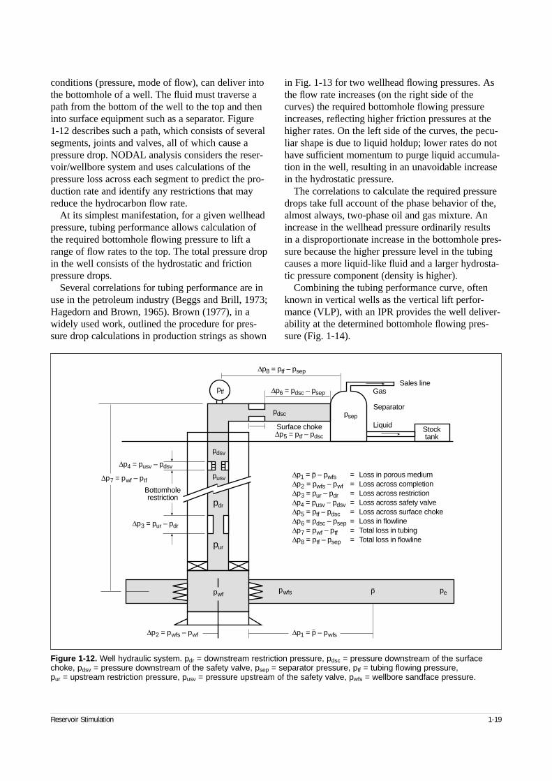
Reservoir Stimulation 1-19

conditions (pressure, mode of flow), can deliver intothe bottomhole of a well. The fluid must traverse apath from the bottom of the well to the top and theninto surface equipment such as a separator. Figure 1-12 describes such a path, which consists of severalsegments, joints and valves, all of which cause apressure drop. NODAL analysis considers the reser-voir/wellbore system and uses calculations of thepressure loss across each segment to predict the pro-duction rate and identify any restrictions that mayreduce the hydrocarbon flow rate.

At its simplest manifestation, for a given wellheadpressure, tubing performance allows calculation ofthe required bottomhole flowing pressure to lift arange of flow rates to the top. The total pressure dropin the well consists of the hydrostatic and frictionpressure drops.

Several correlations for tubing performance are inuse in the petroleum industry (Beggs and Brill, 1973;Hagedorn and Brown, 1965). Brown (1977), in awidely used work, outlined the procedure for pres-sure drop calculations in production strings as shown

in Fig. 1-13 for two wellhead flowing pressures. Asthe flow rate increases (on the right side of thecurves) the required bottomhole flowing pressureincreases, reflecting higher friction pressures at thehigher rates. On the left side of the curves, the pecu-liar shape is due to liquid holdup; lower rates do nothave sufficient momentum to purge liquid accumula-tion in the well, resulting in an unavoidable increasein the hydrostatic pressure.

The correlations to calculate the required pressuredrops take full account of the phase behavior of the,almost always, two-phase oil and gas mixture. Anincrease in the wellhead pressure ordinarily results in a disproportionate increase in the bottomhole pres-sure because the higher pressure level in the tubingcauses a more liquid-like fluid and a larger hydrosta-tic pressure component (density is higher).

Combining the tubing performance curve, oftenknown in vertical wells as the vertical lift perfor-mance (VLP), with an IPR provides the well deliver-ability at the determined bottomhole flowing pres-sure (Fig. 1-14).

Figure 1-12. Well hydraulic system. pdr = downstream restriction pressure, pdsc = pressure downstream of the surfacechoke, pdsv = pressure downstream of the safety valve, psep = separator pressure, ptf = tubing flowing pressure, pur = upstream restriction pressure, pusv = pressure upstream of the safety valve, pwfs = wellbore sandface pressure.

∆p1 = p – pwfs = Loss in porous medium∆p2 = pwfs – pwf = Loss across completion∆p3 = pur – pdr = Loss across restriction∆p4 = pusv – pdsv = Loss across safety valve∆p5 = ptf – pdsc = Loss across surface choke∆p6 = pdsc – psep = Loss in flowline∆p7 = pwf – ptf = Total loss in tubing∆p8 = ptf – psep = Total loss in flowline

∆p1 = p – pwfs∆p2 = pwfs – pwf

pwf

pdr

pur

pusv

psep

pdsv

pdsc

ptf

pepwfs p

∆p3 = pur – pdr

∆p7 = pwf – ptf

Bottomholerestriction

∆p4 = pusv – pdsv

Surface choke Liquid

Separator

GasSales line

Stocktank∆p5 = ptf – pdsc

∆p6 = pdsc – psep

∆p8 = ptf – psep

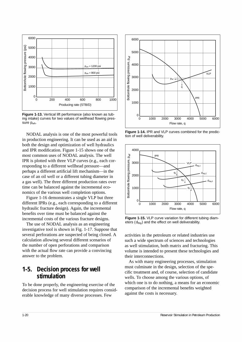
1-20 Reservoir Stimulation in Petroleum Production

NODAL analysis is one of the most powerful toolsin production engineering. It can be used as an aid inboth the design and optimization of well hydraulicsand IPR modification. Figure 1-15 shows one of themost common uses of NODAL analysis. The wellIPR is plotted with three VLP curves (e.g., each cor-responding to a different wellhead pressure—andperhaps a different artificial lift mechanism—in thecase of an oil well or a different tubing diameter in a gas well). The three different production rates overtime can be balanced against the incremental eco-nomics of the various well completion options.

Figure 1-16 demonstrates a single VLP but threedifferent IPRs (e.g., each corresponding to a differenthydraulic fracture design). Again, the incrementalbenefits over time must be balanced against theincremental costs of the various fracture designs.

The use of NODAL analysis as an engineeringinvestigative tool is shown in Fig. 1-17. Suppose thatseveral perforations are suspected of being closed. Acalculation allowing several different scenarios ofthe number of open perforations and comparisonwith the actual flow rate can provide a convincinganswer to the problem.

1-5. Decision process for wellstimulation

To be done properly, the engineering exercise of thedecision process for well stimulation requires consid-erable knowledge of many diverse processes. Few

activities in the petroleum or related industries usesuch a wide spectrum of sciences and technologiesas well stimulation, both matrix and fracturing. Thisvolume is intended to present these technologies andtheir interconnections.

As with many engineering processes, stimulationmust culminate in the design, selection of the spe-cific treatment and, of course, selection of candidatewells. To choose among the various options, ofwhich one is to do nothing, a means for an economiccomparison of the incremental benefits weightedagainst the costs is necessary.

Figure 1-13. Vertical lift performance (also known as tub-ing intake) curves for two values of wellhead flowing pres-sure pwh.

Producing rate (STB/D)

Bot

tom

hole

flow

ing

pres

sure

(psi

)

6000

5000

4000

3000

2000

1000

0200 400 600 800 10000

pwh = 1200 psi

pwh = 800 psi

Figure 1-14. IPR and VLP curves combined for the predic-tion of well deliverability.

Flow rate, qB

otto

mho

le fl

owin

g pr

essu

re, p

wf

6000

5000

4000

3000

2000

1000

01000 2000 3000 4000 5000 60000

q

VLP

IPR

pwf

Figure 1-15. VLP curve variation for different tubing diam-eters (dtbg) and the effect on well deliverability.

Flow rate, q

Bot

tom

hole

flow

ing

pres

sure

, pw

f

4000

3000

2000

1000

01000 2000 3000 4000 5000 60000

IPR

VLP

q1

q2

q3

dtbg,1

dtbg,2

dtbg,3

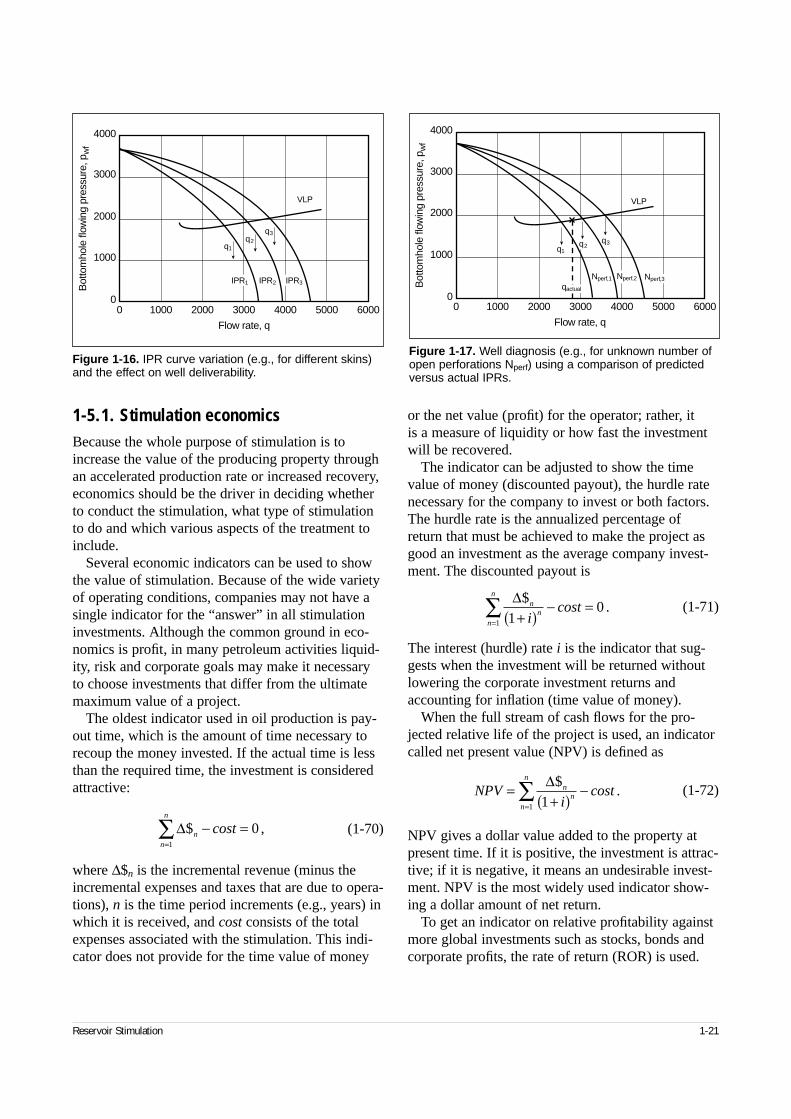
Reservoir Stimulation 1-21

1-5.1. Stimulation economicsBecause the whole purpose of stimulation is toincrease the value of the producing property throughan accelerated production rate or increased recovery,economics should be the driver in deciding whetherto conduct the stimulation, what type of stimulationto do and which various aspects of the treatment toinclude.

Several economic indicators can be used to showthe value of stimulation. Because of the wide varietyof operating conditions, companies may not have asingle indicator for the “answer” in all stimulationinvestments. Although the common ground in eco-nomics is profit, in many petroleum activities liquid-ity, risk and corporate goals may make it necessaryto choose investments that differ from the ultimatemaximum value of a project.

The oldest indicator used in oil production is pay-out time, which is the amount of time necessary torecoup the money invested. If the actual time is lessthan the required time, the investment is consideredattractive:

(1-70)

where ∆$n is the incremental revenue (minus theincremental expenses and taxes that are due to opera-tions), n is the time period increments (e.g., years) inwhich it is received, and cost consists of the totalexpenses associated with the stimulation. This indi-cator does not provide for the time value of money

or the net value (profit) for the operator; rather, it is a measure of liquidity or how fast the investmentwill be recovered.

The indicator can be adjusted to show the timevalue of money (discounted payout), the hurdle ratenecessary for the company to invest or both factors.The hurdle rate is the annualized percentage ofreturn that must be achieved to make the project asgood an investment as the average company invest-ment. The discounted payout is

(1-71)

The interest (hurdle) rate i is the indicator that sug-gests when the investment will be returned withoutlowering the corporate investment returns andaccounting for inflation (time value of money).

When the full stream of cash flows for the pro-jected relative life of the project is used, an indicatorcalled net present value (NPV) is defined as

(1-72)

NPV gives a dollar value added to the property atpresent time. If it is positive, the investment is attrac-tive; if it is negative, it means an undesirable invest-ment. NPV is the most widely used indicator show-ing a dollar amount of net return.

To get an indicator on relative profitability againstmore global investments such as stocks, bonds andcorporate profits, the rate of return (ROR) is used.

Figure 1-16. IPR curve variation (e.g., for different skins)and the effect on well deliverability.

Flow rate, q

Bot

tom

hole

flow

ing

pres

sure

, pw

f

4000

3000

2000

1000

01000 2000 3000 4000 5000 60000

q1

q2

q3

IPR1 IPR2 IPR3

VLP

Figure 1-17. Well diagnosis (e.g., for unknown number ofopen perforations Nperf) using a comparison of predictedversus actual IPRs.

Flow rate, q

Bot

tom

hole

flow

ing

pres

sure

, pw

f

4000

3000

2000

1000

01000 2000 3000 4000 5000 60000

Nperf,1 Nperf,2 Nperf,3

q1

VLP

q2q3

qactual

∆$ ,nn

n

− ==

∑ cost 01

∆$.n

nn

n

i10

1 +( )− =

=∑ cost

NPVin

nn

n

=+( )

−=

∑ ∆$11

cost .

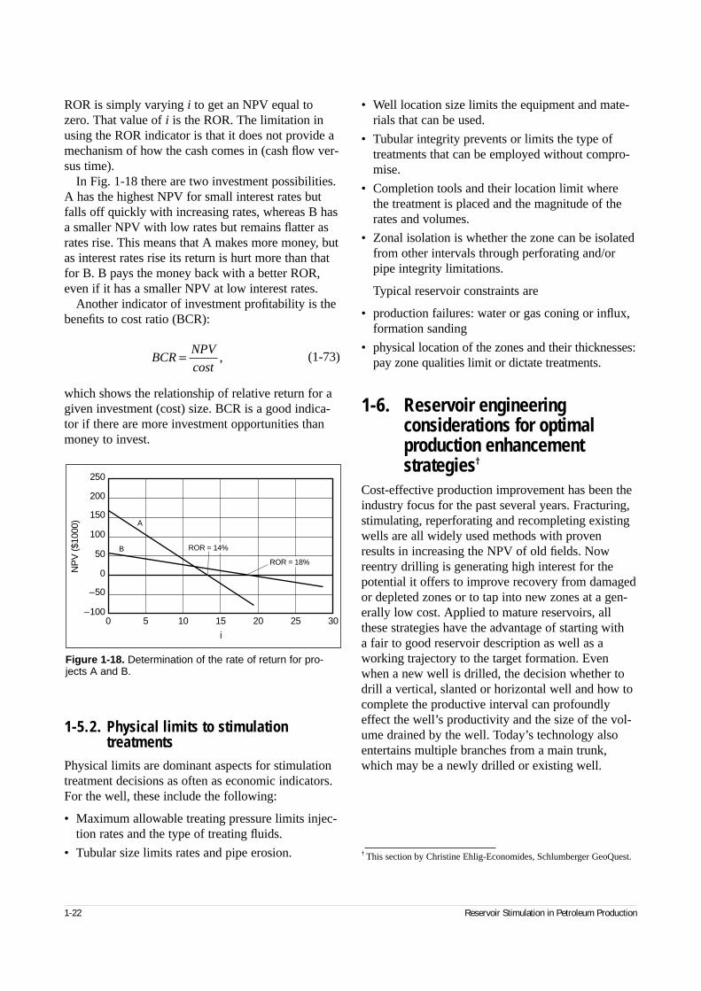
1-22 Reservoir Stimulation in Petroleum Production

ROR is simply varying i to get an NPV equal tozero. That value of i is the ROR. The limitation inusing the ROR indicator is that it does not provide amechanism of how the cash comes in (cash flow ver-sus time).

In Fig. 1-18 there are two investment possibilities.A has the highest NPV for small interest rates butfalls off quickly with increasing rates, whereas B hasa smaller NPV with low rates but remains flatter asrates rise. This means that A makes more money, butas interest rates rise its return is hurt more than thatfor B. B pays the money back with a better ROR,even if it has a smaller NPV at low interest rates.

Another indicator of investment profitability is thebenefits to cost ratio (BCR):

(1-73)

which shows the relationship of relative return for agiven investment (cost) size. BCR is a good indica-tor if there are more investment opportunities thanmoney to invest.

1-5.2. Physical limits to stimulation treatments

Physical limits are dominant aspects for stimulationtreatment decisions as often as economic indicators.For the well, these include the following:

• Maximum allowable treating pressure limits injec-tion rates and the type of treating fluids.

• Tubular size limits rates and pipe erosion.

• Well location size limits the equipment and mate-rials that can be used.

• Tubular integrity prevents or limits the type oftreatments that can be employed without compro-mise.

• Completion tools and their location limit wherethe treatment is placed and the magnitude of therates and volumes.

• Zonal isolation is whether the zone can be isolatedfrom other intervals through perforating and/orpipe integrity limitations.

Typical reservoir constraints are

• production failures: water or gas coning or influx,formation sanding

• physical location of the zones and their thicknesses:pay zone qualities limit or dictate treatments.

1-6. Reservoir engineering considerations for optimal production enhancement strategies†

Cost-effective production improvement has been theindustry focus for the past several years. Fracturing,stimulating, reperforating and recompleting existingwells are all widely used methods with provenresults in increasing the NPV of old fields. Nowreentry drilling is generating high interest for thepotential it offers to improve recovery from damagedor depleted zones or to tap into new zones at a gen-erally low cost. Applied to mature reservoirs, allthese strategies have the advantage of starting with a fair to good reservoir description as well as aworking trajectory to the target formation. Evenwhen a new well is drilled, the decision whether todrill a vertical, slanted or horizontal well and how tocomplete the productive interval can profoundlyeffect the well’s productivity and the size of the vol-ume drained by the well. Today’s technology alsoentertains multiple branches from a main trunk,which may be a newly drilled or existing well.

† This section by Christine Ehlig-Economides, Schlumberger GeoQuest.

BCRNPV=cost

,

Figure 1-18. Determination of the rate of return for pro-jects A and B.

NP

V ($

1000

)

0

50

100

150

200

250

–50

–1005 10 15 20 25 300

A

B ROR = 14%

ROR = 18%

i

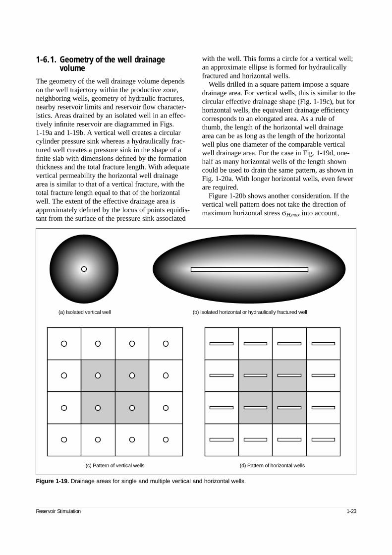
Reservoir Stimulation 1-23

1-6.1. Geometry of the well drainage volume

The geometry of the well drainage volume dependson the well trajectory within the productive zone,neighboring wells, geometry of hydraulic fractures,nearby reservoir limits and reservoir flow character-istics. Areas drained by an isolated well in an effec-tively infinite reservoir are diagrammed in Figs. 1-19a and 1-19b. A vertical well creates a circular cylinder pressure sink whereas a hydraulically frac-tured well creates a pressure sink in the shape of afinite slab with dimensions defined by the formationthickness and the total fracture length. With adequatevertical permeability the horizontal well drainagearea is similar to that of a vertical fracture, with thetotal fracture length equal to that of the horizontalwell. The extent of the effective drainage area isapproximately defined by the locus of points equidis-tant from the surface of the pressure sink associated

with the well. This forms a circle for a vertical well;an approximate ellipse is formed for hydraulicallyfractured and horizontal wells.

Wells drilled in a square pattern impose a squaredrainage area. For vertical wells, this is similar to thecircular effective drainage shape (Fig. 1-19c), but forhorizontal wells, the equivalent drainage efficiencycorresponds to an elongated area. As a rule ofthumb, the length of the horizontal well drainagearea can be as long as the length of the horizontalwell plus one diameter of the comparable verticalwell drainage area. For the case in Fig. 1-19d, one-half as many horizontal wells of the length showncould be used to drain the same pattern, as shown inFig. 1-20a. With longer horizontal wells, even fewerare required.

Figure 1-20b shows another consideration. If thevertical well pattern does not take the direction ofmaximum horizontal stress σΗ,max into account,

Figure 1-19. Drainage areas for single and multiple vertical and horizontal wells.

(a) Isolated vertical well (b) Isolated horizontal or hydraulically fractured well

(c) Pattern of vertical wells (d) Pattern of horizontal wells

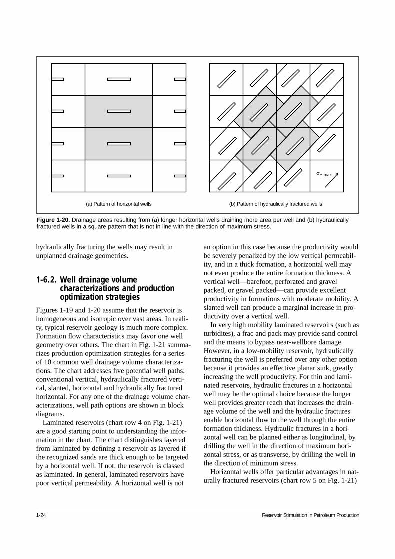
1-24 Reservoir Stimulation in Petroleum Production

hydraulically fracturing the wells may result inunplanned drainage geometries.

1-6.2. Well drainage volume characterizations and production optimization strategies

Figures 1-19 and 1-20 assume that the reservoir ishomogeneous and isotropic over vast areas. In reali-ty, typical reservoir geology is much more complex.Formation flow characteristics may favor one wellgeometry over others. The chart in Fig. 1-21 summa-rizes production optimization strategies for a seriesof 10 common well drainage volume characteriza-tions. The chart addresses five potential well paths:conventional vertical, hydraulically fractured verti-cal, slanted, horizontal and hydraulically fracturedhorizontal. For any one of the drainage volume char-acterizations, well path options are shown in blockdiagrams.

Laminated reservoirs (chart row 4 on Fig. 1-21)are a good starting point to understanding the infor-mation in the chart. The chart distinguishes layeredfrom laminated by defining a reservoir as layered ifthe recognized sands are thick enough to be targetedby a horizontal well. If not, the reservoir is classedas laminated. In general, laminated reservoirs havepoor vertical permeability. A horizontal well is not

an option in this case because the productivity wouldbe severely penalized by the low vertical permeabil-ity, and in a thick formation, a horizontal well maynot even produce the entire formation thickness. Avertical well—barefoot, perforated and gravelpacked, or gravel packed—can provide excellentproductivity in formations with moderate mobility. Aslanted well can produce a marginal increase in pro-ductivity over a vertical well.

In very high mobility laminated reservoirs (such asturbidites), a frac and pack may provide sand controland the means to bypass near-wellbore damage.However, in a low-mobility reservoir, hydraulicallyfracturing the well is preferred over any other optionbecause it provides an effective planar sink, greatlyincreasing the well productivity. For thin and lami-nated reservoirs, hydraulic fractures in a horizontalwell may be the optimal choice because the longerwell provides greater reach that increases the drain-age volume of the well and the hydraulic fracturesenable horizontal flow to the well through the entireformation thickness. Hydraulic fractures in a hori-zontal well can be planned either as longitudinal, bydrilling the well in the direction of maximum hori-zontal stress, or as transverse, by drilling the well inthe direction of minimum stress.

Horizontal wells offer particular advantages in nat-urally fractured reservoirs (chart row 5 on Fig. 1-21)

Figure 1-20. Drainage areas resulting from (a) longer horizontal wells draining more area per well and (b) hydraulicallyfractured wells in a square pattern that is not in line with the direction of maximum stress.

(b) Pattern of hydraulically fractured wells(a) Pattern of horizontal wells

σH,max

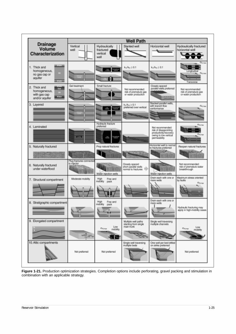
Reservoir Stimulation 1-25

Figure 1-21. Production optimization strategies. Completion options include perforating, gravel packing and stimulation incombination with an applicable strategy.

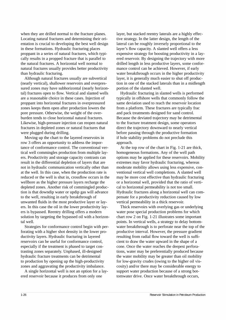
when they are drilled normal to the fracture planes.Locating natural fractures and determining their ori-entation is crucial to developing the best well designin these formations. Hydraulic fracturing placesproppant in a series of natural fractures, which typi-cally results in a propped fracture that is parallel tothe natural fractures. A horizontal well normal tonatural fractures usually provides better productivitythan hydraulic fracturing.

Although natural fractures usually are subvertical(nearly vertical), shallower reservoirs and overpres-sured zones may have subhorizontal (nearly horizon-tal) fractures open to flow. Vertical and slanted wellsare a reasonable choice in these cases. Injection ofproppant into horizontal fractures in overpressuredzones keeps them open after production lowers thepore pressure. Otherwise, the weight of the over-burden tends to close horizontal natural fractures.Likewise, high-pressure injection can reopen naturalfractures in depleted zones or natural fractures thatwere plugged during drilling.

Moving up the chart to the layered reservoirs inrow 3 offers an opportunity to address the impor-tance of conformance control. The conventional ver-tical well commingles production from multiple lay-ers. Productivity and storage capacity contrasts canresult in the differential depletion of layers that arenot in hydraulic communication vertically other thanat the well. In this case, when the production rate isreduced or the well is shut in, crossflow occurs in thewellbore as the higher pressure layers recharge thedepleted zones. Another risk of commingled produc-tion is that downdip water or updip gas will advanceto the well, resulting in early breakthrough ofunwanted fluids in the most productive layer or lay-ers. In this case the oil in the lower productivity lay-ers is bypassed. Reentry drilling offers a modernsolution by targeting the bypassed oil with a horizon-tal well.

Strategies for conformance control begin with per-forating with a higher shot density in the lower pro-ductivity layers. Hydraulic fracturing in layeredreservoirs can be useful for conformance control,especially if the treatment is phased to target con-trasting zones separately. Unphased, ill-designedhydraulic fracture treatments can be detrimental to production by opening up the high-productivityzones and aggravating the productivity imbalance.

A single horizontal well is not an option for a lay-ered reservoir because it produces from only one

layer, but stacked reentry laterals are a highly effec-tive strategy. In the latter design, the length of thelateral can be roughly inversely proportional to thelayer’s flow capacity. A slanted well offers a lessexpensive strategy for boosting productivity in a lay-ered reservoir. By designing the trajectory with moredrilled length in less productive layers, some confor-mance control can be achieved. However, if earlywater breakthrough occurs in the higher productivitylayer, it is generally much easier to shut off produc-tion in one of the stacked laterals than in a midlengthportion of the slanted well.

Hydraulic fracturing in slanted wells is performedtypically in offshore wells that commonly follow thesame deviation used to reach the reservoir locationfrom a platform. These fractures are typically fracand pack treatments designed for sand control.Because the deviated trajectory may be detrimentalto the fracture treatment design, some operatorsdirect the trajectory downward to nearly verticalbefore passing through the productive formation if hole stability problems do not preclude thisapproach.

At the top row of the chart in Fig. 1-21 are thick,homogeneous formations. Any of the well pathoptions may be applied for these reservoirs. Mobilityextremes may favor hydraulic fracturing, whereasmoderate mobility allows using less expensive, con-ventional vertical well completions. A slanted wellmay be more cost effective than hydraulic fracturingor a horizontal well, provided that the ratio of verti-cal to horizontal permeability is not too small.Hydraulic fractures along a horizontal well can com-pensate for a productivity reduction caused by lowvertical permeability in a thick reservoir.

Thick reservoirs with overlying gas or underlyingwater pose special production problems for whichchart row 2 on Fig. 1-21 illustrates some importantpoints. In vertical wells, a strategy to delay bottom-water breakthrough is to perforate near the top of theproductive interval. However, the pressure gradientresulting from radial flow toward the well is suffi-cient to draw the water upward in the shape of acone. Once the water reaches the deepest perfora-tions, water may be preferentially produced becausethe water mobility may be greater than oil mobilityfor low-gravity crudes (owing to the higher oil vis-cosity) and/or there may be considerable energy tosupport water production because of a strong bot-tomwater drive. Once water breakthrough occurs,

1-26 Reservoir Stimulation in Petroleum Production

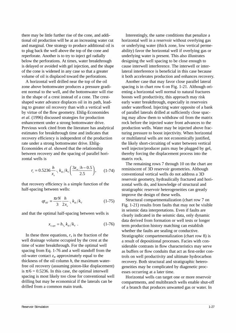
there may be little further rise of the cone, and addi-tional oil production will be at an increasing water cutand marginal. One strategy to produce additional oil isto plug back the well above the top of the cone andreperforate. Another is to try to inject gel radiallybelow the perforations. At times, water breakthroughis delayed or avoided with gel injection, and the shapeof the cone is widened in any case so that a greatervolume of oil is displaced toward the perforations.

A horizontal well drilled near the top of the oilzone above bottomwater produces a pressure gradi-ent normal to the well, and the bottomwater will risein the shape of a crest instead of a cone. The crest-shaped water advance displaces oil in its path, lead-ing to greater oil recovery than with a vertical wellby virtue of the flow geometry. Ehlig-Economides et al. (1996) discussed strategies for productionenhancement under a strong bottomwater drive.Previous work cited from the literature has analyticalestimates for breakthrough time and indicates thatrecovery efficiency is independent of the productionrate under a strong bottomwater drive. Ehlig-Economides et al. showed that the relationshipbetween recovery and the spacing of parallel hori-zontal wells is

(1-74)

that recovery efficiency is a simple function of thehalf-spacing between wells:

(1-75)

and that the optimal half-spacing between wells is

(1-76)

In these three equations, rv is the fraction of thewell drainage volume occupied by the crest at thetime of water breakthrough. For the optimal wellspacing from Eq. 1-76 and a well standoff from theoil-water contact zw approximately equal to thethickness of the oil column h, the maximum water-free oil recovery (assuming piston-like displacement)is π/6 = 0.5236. In this case, the optimal interwellspacing is most likely too close for conventional welldrilling but may be economical if the laterals can bedrilled from a common main trunk.

Interestingly, the same conditions that penalize ahorizontal well in a reservoir without overlying gasor underlying water (thick zone, low vertical perme-ability) favor the horizontal well if overlying gas orunderlying water is present. This also illustratesdesigning the well spacing to be close enough tocause interwell interference. The interwell or inter-lateral interference is beneficial in this case becauseit both accelerates production and enhances recovery.

Another case that may favor close parallel lateralspacing is in chart row 6 on Fig. 1-21. Although ori-enting a horizontal well normal to natural fracturesboosts well productivity, this approach may riskearly water breakthrough, especially in reservoirsunder waterflood. Injecting water opposite of a bankof parallel laterals drilled at sufficiently close spac-ing may allow them to withdraw oil from the matrixrock before the injected water front advances to theproduction wells. Water may be injected above frac-turing pressure to boost injectivity. When horizontalor multilateral wells are not economically justified,the likely short-circuiting of water between verticalwell injector/producer pairs may be plugged by gel,thereby forcing the displacement process into thematrix rock.

The remaining rows 7 through 10 on the chart arereminiscent of 3D reservoir geometries. Althoughconventional vertical wells do not address a 3Dreservoir geometry, hydraulically fractured and hori-zontal wells do, and knowledge of structural andstratigraphic reservoir heterogeneities can greatlyimprove the design of these wells.

Structural compartmentalization (chart row 7 onFig. 1-21) results from faults that may not be visiblein seismic data interpretations. Even if faults areclearly indicated in the seismic data, only dynamicdata derived from formation or well tests or longerterm production history matching can establishwhether the faults are sealing or conductive.Stratigraphic compartmentalization (chart row 8) is a result of depositional processes. Facies with con-siderable contrasts in flow characteristics may serveas buffers or flow conduits that act as first-order con-trols on well productivity and ultimate hydrocarbonrecovery. Both structural and stratigraphic hetero-geneities may be complicated by diagenetic proc-esses occurring at a later time.

Horizontal wells can target one or more reservoircompartments, and multibranch wells enable shut-offof a branch that produces unwanted gas or water. In

Reservoir Stimulation 1-27

rh

xk k

z hv

e

H Vw= −

0 5236

3 0 52 5

..

.,

qtrN h

xk kBT

e

H V= π3 2

x h k ke opt H V, .=

tight reservoirs with considerable faulting, the faultsmay be associated with natural fractures that can betargeted with horizontal wells, or they may providereliable information on the maximum stress directionthat is essential for planning hydraulic fractures invertical or horizontal wells.

Stratigraphic limits (chart row 8 on Fig. 1-21) mayaccount for additional reservoir compartmentaliza-tion, both vertically and areally. In some cases thereservoir sands may be too thin to be individuallyidentified in a seismic data cross section, but theymay have sufficient areal extent to be visible in seis-mic attribute maps for a structural horizon. In thatcase, horizontal wells may be an ideal strategy forproducing thin formations and for reaching multiplesands.

Chart row 9 on Fig. 1-21 refers to elongated com-partmentalization. Although these diagrams depictfluvial reservoir geology, elongated reservoirs canalso occur in heavily faulted formations. In eithercase, the apparent drilling strategies depend on theobjective for the well. For example, the well direc-tion can be planned to stay in an elongated reservoirbody or to intersect as many reservoir bodies as pos-sible. The latter case implies drilling in the directionnormal to the elongation, which for a fluvial reser-voir means drilling normal to the downslope direc-tion at the time of deposition. Another approach maybe a multibranch well designed to target channelsidentified with borehole seismic measurements in thehorizontal trunk well.

Hydraulic fracturing offers different challengesand possibilities. First, unlike a well trajectory plan,the direction of the hydraulic fracture is not a designchoice. Rather, the fracture propagates normal to thedirection of minimum stress. A hydraulic fracturemay propagate into isolated sand bodies not con-tacted by the drilled well trajectory, but in othercases the fracture propagation may be inhibited byfacies changes or structural discontinuities, and ascreenout may occur. In general, drilling solutionsmay be more flexible in elongated reservoir systems.

The last chart row on Fig. 1-21 is for the specialgeometry of the attic compartment. In this case,steeply dipping beds may be in contact with an updipgas cap, downdip aquifer or both. One strategy is todrill a horizontal well that passes through several ofthe beds and stays sufficiently below the updip gasand above the downdip water. Although this seemsto be an efficient approach, it suffers from a signifi-

cant disadvantage in that flow is commingled amongthe layers, and when gas or water breakthrough occursit interferes with production from other layers. Thebetter strategy may be to drill multiple horizontalwells, each on strike and staying in a specific bed. The advantage to this strategy is that each of the wellsis optimal in its standoff from the gas-oil or oil-watercontact, thus delaying multiphase production as longas possible, and in its productive length within the for-mation, thus maximizing productivity.

1-7. Stimulation executionA good understanding of job execution is necessaryfor making decisions on the applicability and risk ofvarious treatments. As with any well work, basicsafety procedures must be developed and followed to prevent catastrophic failure of the treatment,which could result in damage to or loss of the well,personnel and equipment. Specific standards andoperating procedures have been developed for stimu-lation treatments, which if followed can lead to asafe, smooth and predictable operation. Chapters 11and 19 fully detail execution concerns.

1-7.1. Matrix stimulationMatrix stimulation, mainly acidizing, is the originaland simplest stimulation treatment. More than40,000 acid treatments are pumped each year in oiland gas wells. These treatments (Fig. 1-22) typicallyinvolve small crews and minimal equipment. Theequipment usually consists of one low-horsepower,single-action reciprocating pump, a supply centrifu-gal and storage tanks for the acid and flush fluids.Blending equipment is used when solids are added to the treatment.

The most common process is for the fluids to bepreblended at the service company facility and thentransported to the location. This allows blendingsmall volumes accurately, controlling environmentalhazards. The fluids are then pumped with little effortor quality risk.

1-7.2. Hydraulic fracturingUnlike matrix stimulation, fracturing can be one ofthe more complex procedures performed on a well(Fig. 1-23). This is due in part to the high rates and

1-28 Reservoir Stimulation in Petroleum Production

pressures, large volume of materials injected, contin-uous blending of materials and large amount ofunknown variables for sound engineering design.

The fracturing pressure is generated by single-action reciprocating pumping units that havebetween 700 and 2000 hydraulic horsepower (Fig. 1-24). These units are powered by diesel, turbine orelectric engines. The pumps are purpose-built andhave not only horsepower limits but job specificationlimits. These limits are normally known (e.g., smallerplungers provide a higher working pressure andlower rates). Because of the erosive nature of thematerials (i.e., proppant) high pump efficiency mustbe maintained or pump failure may occur. The limitsare typically met when using high fluid velocitiesand high proppant concentrations (+18 ppg). Theremay be numerous pumps on a job, depending on thedesign.

Mixing equipment blends the fracturing fluid sys-tem, adds the proppant and supplies this mixture tothe high-pressure pumps. The slurry can be continu-ously mixed by the equipment (Fig. 1-25) or batchmixed in the fluid storage tanks. The batch-mixedfluid is then blended with proppant in a continuousstream and fed to the pumps.

Reservoir Stimulation 1-29

Figure 1-22. Matrix stimulation treatment using a coiled tubing unit, pump truck and fluid transport.

Figure 1-23. This large fracturing treatment used 25,000hydraulic horsepower and 1.54 million gal of fracturing fluidto place 6.3 million lbm of propping agent. The job lasted11 hours.

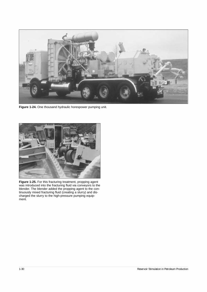
1-30 Reservoir Stimulation in Petroleum Production

Figure 1-25. For this fracturing treatment, propping agentwas introduced into the fracturing fluid via conveyors to theblender. The blender added the propping agent to the con-tinuously mixed fracturing fluid (creating a slurry) and dis-charged the slurry to the high-pressure pumping equip-ment.

Figure 1-24. One thousand hydraulic horespower pumping unit.

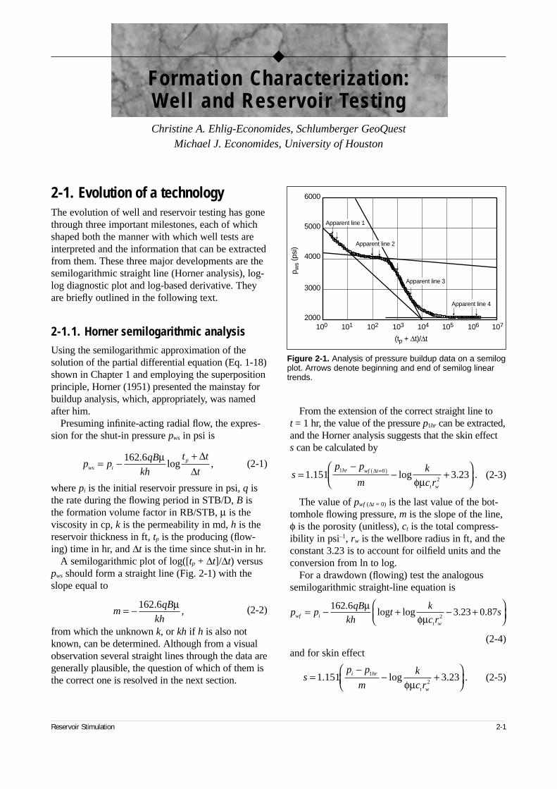
2-1. Evolution of a technologyThe evolution of well and reservoir testing has gonethrough three important milestones, each of whichshaped both the manner with which well tests areinterpreted and the information that can be extractedfrom them. These three major developments are thesemilogarithmic straight line (Horner analysis), log-log diagnostic plot and log-based derivative. Theyare briefly outlined in the following text.

2-1.1. Horner semilogarithmic analysisUsing the semilogarithmic approximation of thesolution of the partial differential equation (Eq. 1-18)shown in Chapter 1 and employing the superpositionprinciple, Horner (1951) presented the mainstay forbuildup analysis, which, appropriately, was namedafter him.

Presuming infinite-acting radial flow, the expres-sion for the shut-in pressure pws in psi is

(2-1)

where pi is the initial reservoir pressure in psi, q isthe rate during the flowing period in STB/D, B isthe formation volume factor in RB/STB, µ is theviscosity in cp, k is the permeability in md, h is thereservoir thickness in ft, tp is the producing (flow-ing) time in hr, and ∆t is the time since shut-in in hr.

A semilogarithmic plot of log([tp + ∆t]/∆t) versuspws should form a straight line (Fig. 2-1) with theslope equal to

(2-2)

from which the unknown k, or kh if h is also notknown, can be determined. Although from a visualobservation several straight lines through the data aregenerally plausible, the question of which of them isthe correct one is resolved in the next section.

From the extension of the correct straight line to t = 1 hr, the value of the pressure p1hr can be extracted,and the Horner analysis suggests that the skin effect s can be calculated by

(2-3)

The value of pwf (∆t = 0) is the last value of the bot-tomhole flowing pressure, m is the slope of the line,φ is the porosity (unitless), ct is the total compress-ibility in psi–1, rw is the wellbore radius in ft, and theconstant 3.23 is to account for oilfield units and theconversion from ln to log.

For a drawdown (flowing) test the analogoussemilogarithmic straight-line equation is

(2-4)and for skin effect

(2-5)

Reservoir Stimulation 2-1

◆

Formation Characterization: Well and Reservoir TestingChristine A. Ehlig-Economides, Schlumberger GeoQuest

Michael J. Economides, University of Houston

p pqB

kh

t t

tws ip= −

+162 6.,

µlog

∆∆

mqB

kh= − 162 6.

,µ

p pqB

kht

k

c rswf i

t w

= − + − +

162 63 23 0 87

2

.. .

µφµ

log log

sp p

m

k

c ri hr

t w

=−

− +

1 151 3 231

2. . .log

φµ

Figure 2-1. Analysis of pressure buildup data on a semilogplot. Arrows denote beginning and end of semilog lineartrends.

(tp + ∆t)/∆t

2000

3000

4000

5000

6000

pw

s (p

si)

Apparent line 1

Apparent line 4

Apparent line 3

Apparent line 2

100 101 102 103 104 105 106 107

sp p

m

k

c rhr wf t

t w

=−

− +

=( )1 151 3 231 0

2. . .∆ log

φµ

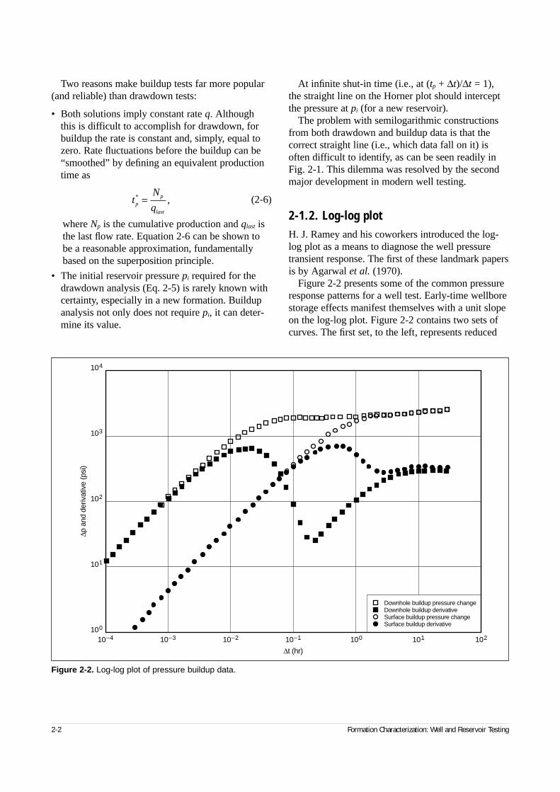
Two reasons make buildup tests far more popular(and reliable) than drawdown tests:

• Both solutions imply constant rate q. Althoughthis is difficult to accomplish for drawdown, forbuildup the rate is constant and, simply, equal tozero. Rate fluctuations before the buildup can be“smoothed” by defining an equivalent productiontime as

(2-6)

where Np is the cumulative production and qlast isthe last flow rate. Equation 2-6 can be shown tobe a reasonable approximation, fundamentallybased on the superposition principle.

• The initial reservoir pressure pi required for thedrawdown analysis (Eq. 2-5) is rarely known withcertainty, especially in a new formation. Buildupanalysis not only does not require pi, it can deter-mine its value.

At infinite shut-in time (i.e., at (tp + ∆t)/∆t = 1),the straight line on the Horner plot should interceptthe pressure at pi (for a new reservoir).

The problem with semilogarithmic constructionsfrom both drawdown and buildup data is that thecorrect straight line (i.e., which data fall on it) isoften difficult to identify, as can be seen readily inFig. 2-1. This dilemma was resolved by the secondmajor development in modern well testing.

2-1.2. Log-log plotH. J. Ramey and his coworkers introduced the log-log plot as a means to diagnose the well pressuretransient response. The first of these landmark papersis by Agarwal et al. (1970).

Figure 2-2 presents some of the common pressureresponse patterns for a well test. Early-time wellborestorage effects manifest themselves with a unit slopeon the log-log plot. Figure 2-2 contains two sets ofcurves. The first set, to the left, represents reduced

2-2 Formation Characterization: Well and Reservoir Testing

Figure 2-2. Log-log plot of pressure buildup data.

∆t (hr)

10–4100

10–3 10–2 10–1 100 101 102

101

102

103

104

∆p a

nd d

eriv

ativ

e (p

si)

Downhole buildup pressure changeDownhole buildup derivativeSurface buildup pressure changeSurface buildup derivative

tN

qpp

last

* ,=

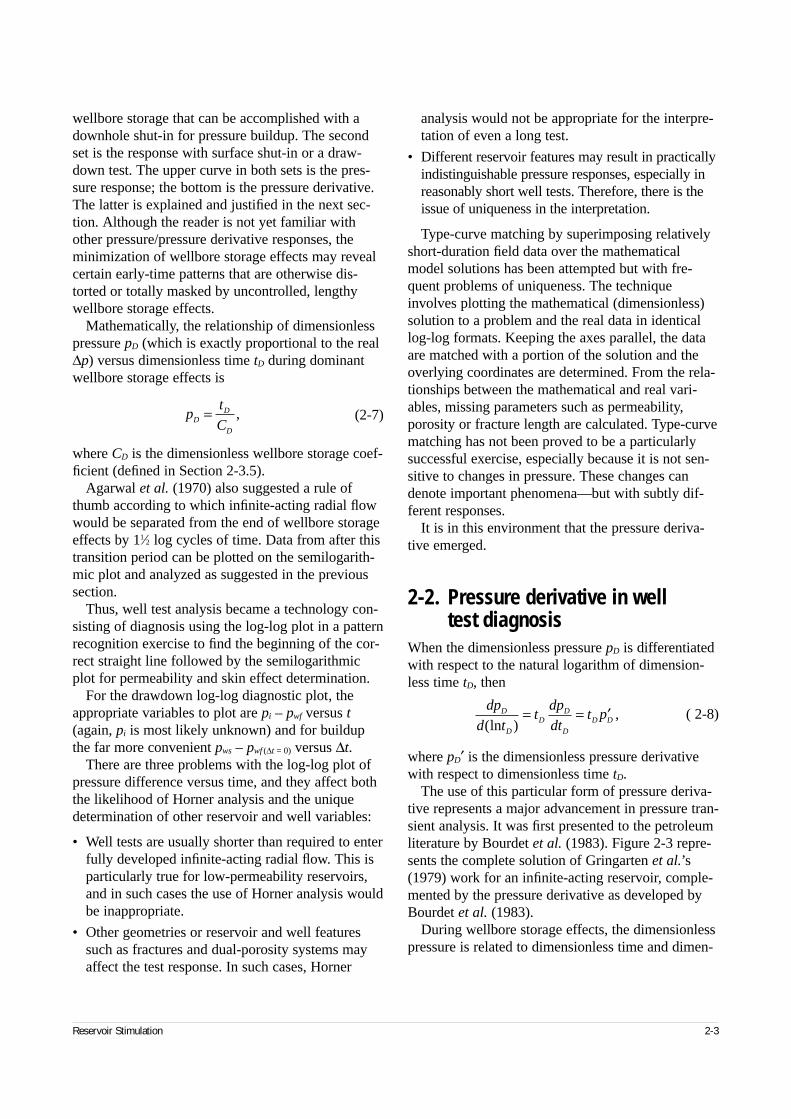
wellbore storage that can be accomplished with adownhole shut-in for pressure buildup. The secondset is the response with surface shut-in or a draw-down test. The upper curve in both sets is the pres-sure response; the bottom is the pressure derivative.The latter is explained and justified in the next sec-tion. Although the reader is not yet familiar withother pressure/pressure derivative responses, theminimization of wellbore storage effects may revealcertain early-time patterns that are otherwise dis-torted or totally masked by uncontrolled, lengthywellbore storage effects.

Mathematically, the relationship of dimensionlesspressure pD (which is exactly proportional to the real∆p) versus dimensionless time tD during dominantwellbore storage effects is

(2-7)

where CD is the dimensionless wellbore storage coef-ficient (defined in Section 2-3.5).

Agarwal et al. (1970) also suggested a rule ofthumb according to which infinite-acting radial flowwould be separated from the end of wellbore storageeffects by 11⁄2 log cycles of time. Data from after thistransition period can be plotted on the semilogarith-mic plot and analyzed as suggested in the previoussection.

Thus, well test analysis became a technology con-sisting of diagnosis using the log-log plot in a patternrecognition exercise to find the beginning of the cor-rect straight line followed by the semilogarithmicplot for permeability and skin effect determination.

For the drawdown log-log diagnostic plot, theappropriate variables to plot are pi – pwf versus t(again, pi is most likely unknown) and for buildupthe far more convenient pws – pwf (∆t = 0) versus ∆t.

There are three problems with the log-log plot ofpressure difference versus time, and they affect boththe likelihood of Horner analysis and the uniquedetermination of other reservoir and well variables:

• Well tests are usually shorter than required to enterfully developed infinite-acting radial flow. This isparticularly true for low-permeability reservoirs,and in such cases the use of Horner analysis wouldbe inappropriate.

• Other geometries or reservoir and well featuressuch as fractures and dual-porosity systems mayaffect the test response. In such cases, Horner

analysis would not be appropriate for the interpre-tation of even a long test.

• Different reservoir features may result in practicallyindistinguishable pressure responses, especially inreasonably short well tests. Therefore, there is theissue of uniqueness in the interpretation.

Type-curve matching by superimposing relativelyshort-duration field data over the mathematicalmodel solutions has been attempted but with fre-quent problems of uniqueness. The techniqueinvolves plotting the mathematical (dimensionless)solution to a problem and the real data in identicallog-log formats. Keeping the axes parallel, the dataare matched with a portion of the solution and theoverlying coordinates are determined. From the rela-tionships between the mathematical and real vari-ables, missing parameters such as permeability,porosity or fracture length are calculated. Type-curvematching has not been proved to be a particularlysuccessful exercise, especially because it is not sen-sitive to changes in pressure. These changes candenote important phenomena—but with subtly dif-ferent responses.

It is in this environment that the pressure deriva-tive emerged.

2-2. Pressure derivative in well test diagnosis

When the dimensionless pressure pD is differentiatedwith respect to the natural logarithm of dimension-less time tD, then

( 2-8)

where pD′ is the dimensionless pressure derivativewith respect to dimensionless time tD.

The use of this particular form of pressure deriva-tive represents a major advancement in pressure tran-sient analysis. It was first presented to the petroleumliterature by Bourdet et al. (1983). Figure 2-3 repre-sents the complete solution of Gringarten et al.’s(1979) work for an infinite-acting reservoir, comple-mented by the pressure derivative as developed byBourdet et al. (1983).

During wellbore storage effects, the dimensionlesspressure is related to dimensionless time and dimen-

Reservoir Stimulation 2-3

pt

CDD

D

= ,

dp

d tt

dp

dtt pD

D

DD

D

D D( ),

ln= = ′

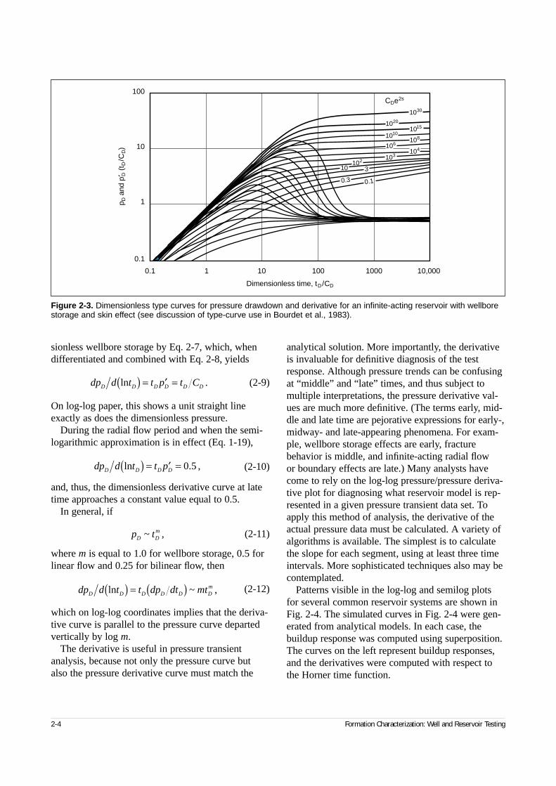
sionless wellbore storage by Eq. 2-7, which, whendifferentiated and combined with Eq. 2-8, yields

(2-9)

On log-log paper, this shows a unit straight lineexactly as does the dimensionless pressure.

During the radial flow period and when the semi-logarithmic approximation is in effect (Eq. 1-19),

(2-10)

and, thus, the dimensionless derivative curve at latetime approaches a constant value equal to 0.5.

In general, if

(2-11)

where m is equal to 1.0 for wellbore storage, 0.5 forlinear flow and 0.25 for bilinear flow, then

(2-12)

which on log-log coordinates implies that the deriva-tive curve is parallel to the pressure curve departedvertically by log m.

The derivative is useful in pressure transientanalysis, because not only the pressure curve butalso the pressure derivative curve must match the

analytical solution. More importantly, the derivativeis invaluable for definitive diagnosis of the testresponse. Although pressure trends can be confusingat “middle” and “late” times, and thus subject tomultiple interpretations, the pressure derivative val-ues are much more definitive. (The terms early, mid-dle and late time are pejorative expressions for early-,midway- and late-appearing phenomena. For exam-ple, wellbore storage effects are early, fracturebehavior is middle, and infinite-acting radial flow or boundary effects are late.) Many analysts havecome to rely on the log-log pressure/pressure deriva-tive plot for diagnosing what reservoir model is rep-resented in a given pressure transient data set. Toapply this method of analysis, the derivative of theactual pressure data must be calculated. A variety ofalgorithms is available. The simplest is to calculatethe slope for each segment, using at least three timeintervals. More sophisticated techniques also may becontemplated.

Patterns visible in the log-log and semilog plotsfor several common reservoir systems are shown inFig. 2-4. The simulated curves in Fig. 2-4 were gen-erated from analytical models. In each case, thebuildup response was computed using superposition.The curves on the left represent buildup responses,and the derivatives were computed with respect tothe Horner time function.

2-4 Formation Characterization: Well and Reservoir Testing

dp d t t p t CD D D D D Dln( ) = ′ = .

dp d t t pD D D Dln( ) = ′ = 0 5. ,

p tD Dm~ ,

dp d t t dp dt mtD D D D D Dmln( ) = ( ) ~ ,

Figure 2-3. Dimensionless type curves for pressure drawdown and derivative for an infinite-acting reservoir with wellborestorage and skin effect (see discussion of type-curve use in Bourdet et al., 1983).

Dimensionless time, tD/CD

p D a

nd p

′ D (t

D/C

D)

0.1 1 10 100 1000 10,000

100

10

1

0.1

CDe2s

103

1030

1020

1015

10 3102

108

104

1010

106

0.3 0.1

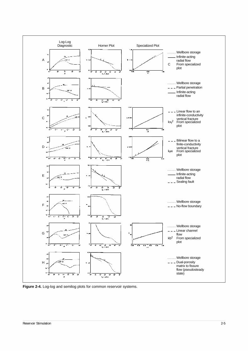
Reservoir Stimulation 2-5

Figure 2-4. Log-log and semilog plots for common reservoir systems.

Log-LogDiagnostic Horner Plot Specialized Plot

A

B

C

D

E

F

G

H

C

Wellbore storageInfinite-actingradial flowFrom specializedplot

kb2

Wellbore storageLinear channelflowFrom specializedplot

Wellbore storagePartial penetrationInfinite-actingradial flow

Wellbore storage

Sealing fault

Infinite-actingradial flow

Wellbore storageNo-flow boundary

Wellbore storageDual-porositymatrix to fissureflow (pseudosteadystate)

Linear flow to aninfinite-conductivityvertical fractureFrom specializedplot

kxf2

Bilinear flow to afinite-conductivityvertical fractureFrom specializedplot

kfw

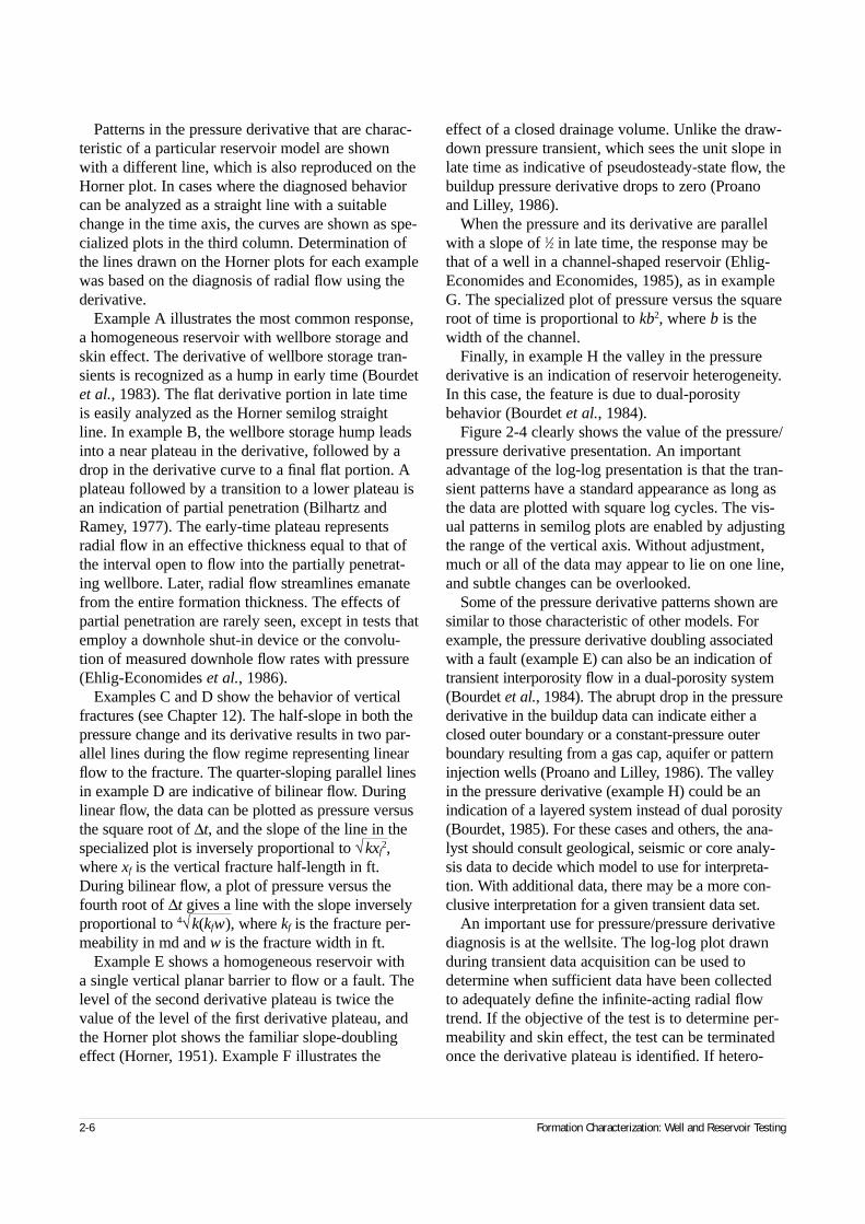
Patterns in the pressure derivative that are charac-teristic of a particular reservoir model are shownwith a different line, which is also reproduced on theHorner plot. In cases where the diagnosed behaviorcan be analyzed as a straight line with a suitablechange in the time axis, the curves are shown as spe-cialized plots in the third column. Determination ofthe lines drawn on the Horner plots for each examplewas based on the diagnosis of radial flow using thederivative.

Example A illustrates the most common response,a homogeneous reservoir with wellbore storage andskin effect. The derivative of wellbore storage tran-sients is recognized as a hump in early time (Bourdetet al., 1983). The flat derivative portion in late timeis easily analyzed as the Horner semilog straightline. In example B, the wellbore storage hump leadsinto a near plateau in the derivative, followed by adrop in the derivative curve to a final flat portion. Aplateau followed by a transition to a lower plateau isan indication of partial penetration (Bilhartz andRamey, 1977). The early-time plateau representsradial flow in an effective thickness equal to that ofthe interval open to flow into the partially penetrat-ing wellbore. Later, radial flow streamlines emanatefrom the entire formation thickness. The effects ofpartial penetration are rarely seen, except in tests thatemploy a downhole shut-in device or the convolu-tion of measured downhole flow rates with pressure(Ehlig-Economides et al., 1986).

Examples C and D show the behavior of verticalfractures (see Chapter 12). The half-slope in both thepressure change and its derivative results in two par-allel lines during the flow regime representing linearflow to the fracture. The quarter-sloping parallel linesin example D are indicative of bilinear flow. Duringlinear flow, the data can be plotted as pressure versusthe square root of ∆t, and the slope of the line in thespecialized plot is inversely proportional to √kxf

2,where xf is the vertical fracture half-length in ft.During bilinear flow, a plot of pressure versus thefourth root of ∆t gives a line with the slope inverselyproportional to 4√k(kfw), where kf is the fracture per-meability in md and w is the fracture width in ft.

Example E shows a homogeneous reservoir with a single vertical planar barrier to flow or a fault. Thelevel of the second derivative plateau is twice thevalue of the level of the first derivative plateau, andthe Horner plot shows the familiar slope-doublingeffect (Horner, 1951). Example F illustrates the

effect of a closed drainage volume. Unlike the draw-down pressure transient, which sees the unit slope inlate time as indicative of pseudosteady-state flow, thebuildup pressure derivative drops to zero (Proanoand Lilley, 1986).

When the pressure and its derivative are parallelwith a slope of 1⁄2 in late time, the response may bethat of a well in a channel-shaped reservoir (Ehlig-Economides and Economides, 1985), as in exampleG. The specialized plot of pressure versus the squareroot of time is proportional to kb2, where b is thewidth of the channel.

Finally, in example H the valley in the pressurederivative is an indication of reservoir heterogeneity.In this case, the feature is due to dual-porositybehavior (Bourdet et al., 1984).

Figure 2-4 clearly shows the value of the pressure/pressure derivative presentation. An important advantage of the log-log presentation is that the tran-sient patterns have a standard appearance as long asthe data are plotted with square log cycles. The vis-ual patterns in semilog plots are enabled by adjustingthe range of the vertical axis. Without adjustment,much or all of the data may appear to lie on one line,and subtle changes can be overlooked.

Some of the pressure derivative patterns shown aresimilar to those characteristic of other models. Forexample, the pressure derivative doubling associatedwith a fault (example E) can also be an indication oftransient interporosity flow in a dual-porosity system(Bourdet et al., 1984). The abrupt drop in the pressurederivative in the buildup data can indicate either aclosed outer boundary or a constant-pressure outerboundary resulting from a gas cap, aquifer or patterninjection wells (Proano and Lilley, 1986). The valleyin the pressure derivative (example H) could be anindication of a layered system instead of dual porosity(Bourdet, 1985). For these cases and others, the ana-lyst should consult geological, seismic or core analy-sis data to decide which model to use for interpreta-tion. With additional data, there may be a more con-clusive interpretation for a given transient data set.

An important use for pressure/pressure derivativediagnosis is at the wellsite. The log-log plot drawnduring transient data acquisition can be used todetermine when sufficient data have been collectedto adequately define the infinite-acting radial flowtrend. If the objective of the test is to determine per-meability and skin effect, the test can be terminatedonce the derivative plateau is identified. If hetero-

2-6 Formation Characterization: Well and Reservoir Testing

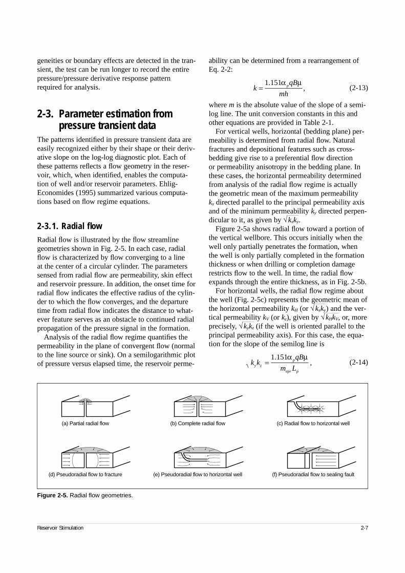
geneities or boundary effects are detected in the tran-sient, the test can be run longer to record the entirepressure/pressure derivative response patternrequired for analysis.

2-3. Parameter estimation from pressure transient data

The patterns identified in pressure transient data areeasily recognized either by their shape or their deriv-ative slope on the log-log diagnostic plot. Each ofthese patterns reflects a flow geometry in the reser-voir, which, when identified, enables the computa-tion of well and/or reservoir parameters. Ehlig-Economides (1995) summarized various computa-tions based on flow regime equations.

2-3.1. Radial flowRadial flow is illustrated by the flow streamlinegeometries shown in Fig. 2-5. In each case, radialflow is characterized by flow converging to a line at the center of a circular cylinder. The parameterssensed from radial flow are permeability, skin effectand reservoir pressure. In addition, the onset time forradial flow indicates the effective radius of the cylin-der to which the flow converges, and the departuretime from radial flow indicates the distance to what-ever feature serves as an obstacle to continued radialpropagation of the pressure signal in the formation.

Analysis of the radial flow regime quantifies thepermeability in the plane of convergent flow (normalto the line source or sink). On a semilogarithmic plotof pressure versus elapsed time, the reservoir perme-

ability can be determined from a rearrangement ofEq. 2-2:

(2-13)

where m is the absolute value of the slope of a semi-log line. The unit conversion constants in this andother equations are provided in Table 2-1.

For vertical wells, horizontal (bedding plane) per-meability is determined from radial flow. Naturalfractures and depositional features such as cross-bedding give rise to a preferential flow direction or permeability anisotropy in the bedding plane. Inthese cases, the horizontal permeability determinedfrom analysis of the radial flow regime is actuallythe geometric mean of the maximum permeability kx directed parallel to the principal permeability axisand of the minimum permeability ky directed perpen-dicular to it, as given by √kxky.

Figure 2-5a shows radial flow toward a portion ofthe vertical wellbore. This occurs initially when thewell only partially penetrates the formation, whenthe well is only partially completed in the formationthickness or when drilling or completion damagerestricts flow to the well. In time, the radial flowexpands through the entire thickness, as in Fig. 2-5b.

For horizontal wells, the radial flow regime aboutthe well (Fig. 2-5c) represents the geometric mean ofthe horizontal permeability kH (or √kxky) and the ver-tical permeability kV (or kz), given by √kHkV, or, moreprecisely, √kykz (if the well is oriented parallel to theprincipal permeability axis). For this case, the equa-tion for the slope of the semilog line is

(2-14)

Reservoir Stimulation 2-7

Figure 2-5. Radial flow geometries.

(a) Partial radial flow

(d) Pseudoradial flow to fracture (e) Pseudoradial flow to horizontal well (f) Pseudoradial flow to sealing fault

(b) Complete radial flow (c) Radial flow to horizontal well

kqB

mhp=

1 151.,

α µ

k kqB

m Ly zp

epr p

=1 151.

,α µ

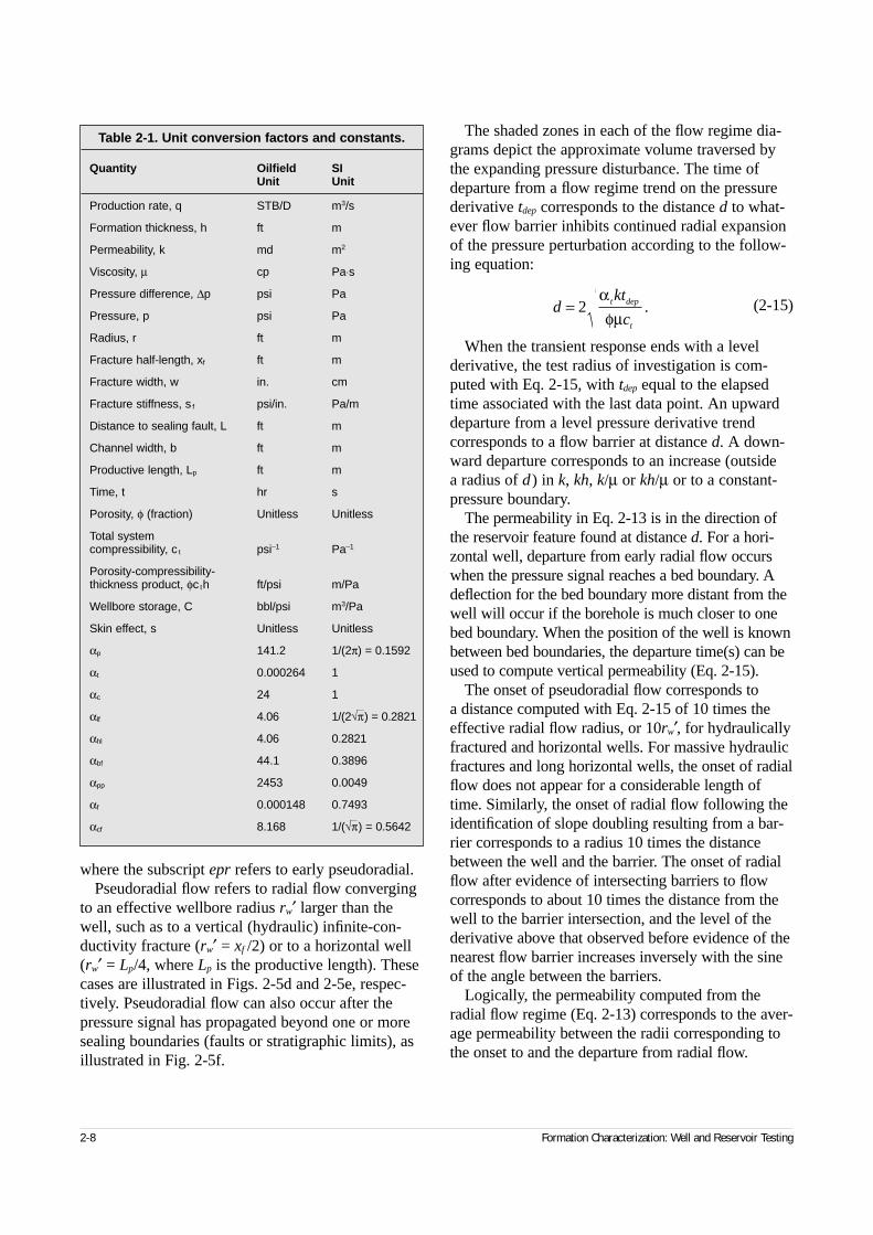
where the subscript epr refers to early pseudoradial.Pseudoradial flow refers to radial flow converging

to an effective wellbore radius rw′ larger than thewell, such as to a vertical (hydraulic) infinite-con-ductivity fracture (rw′ = xf /2) or to a horizontal well(rw′ = Lp/4, where Lp is the productive length). Thesecases are illustrated in Figs. 2-5d and 2-5e, respec-tively. Pseudoradial flow can also occur after thepressure signal has propagated beyond one or moresealing boundaries (faults or stratigraphic limits), asillustrated in Fig. 2-5f.

The shaded zones in each of the flow regime dia-grams depict the approximate volume traversed bythe expanding pressure disturbance. The time ofdeparture from a flow regime trend on the pressurederivative tdep corresponds to the distance d to what-ever flow barrier inhibits continued radial expansionof the pressure perturbation according to the follow-ing equation:

(2-15)

When the transient response ends with a levelderivative, the test radius of investigation is com-puted with Eq. 2-15, with tdep equal to the elapsedtime associated with the last data point. An upwarddeparture from a level pressure derivative trendcorresponds to a flow barrier at distance d. A down-ward departure corresponds to an increase (outside a radius of d) in k, kh, k/µ or kh/µ or to a constant-pressure boundary.

The permeability in Eq. 2-13 is in the direction ofthe reservoir feature found at distance d. For a hori-zontal well, departure from early radial flow occurswhen the pressure signal reaches a bed boundary. Adeflection for the bed boundary more distant from thewell will occur if the borehole is much closer to onebed boundary. When the position of the well is knownbetween bed boundaries, the departure time(s) can beused to compute vertical permeability (Eq. 2-15).

The onset of pseudoradial flow corresponds to a distance computed with Eq. 2-15 of 10 times theeffective radial flow radius, or 10rw′, for hydraulicallyfractured and horizontal wells. For massive hydraulicfractures and long horizontal wells, the onset of radialflow does not appear for a considerable length oftime. Similarly, the onset of radial flow following theidentification of slope doubling resulting from a bar-rier corresponds to a radius 10 times the distancebetween the well and the barrier. The onset of radialflow after evidence of intersecting barriers to flowcorresponds to about 10 times the distance from thewell to the barrier intersection, and the level of thederivative above that observed before evidence of thenearest flow barrier increases inversely with the sineof the angle between the barriers.

Logically, the permeability computed from theradial flow regime (Eq. 2-13) corresponds to the aver-age permeability between the radii corresponding tothe onset to and the departure from radial flow.

2-8 Formation Characterization: Well and Reservoir Testing

Table 2-1. Unit conversion factors and constants.

Quantity Oilfield SIUnit Unit

Production rate, q STB/D m3/s

Formation thickness, h ft m

Permeability, k md m2

Viscosity, µ cp Pa⋅s

Pressure difference, ∆p psi Pa

Pressure, p psi Pa

Radius, r ft m

Fracture half-length, xf ft m

Fracture width, w in. cm

Fracture stiffness, s f psi/in. Pa/m

Distance to sealing fault, L ft m

Channel width, b ft m

Productive length, Lp ft m

Time, t hr s

Porosity, φ (fraction) Unitless Unitless

Total system compressibility, c t psi–1 Pa–1

Porosity-compressibility-thickness product, φc th ft/psi m/Pa

Wellbore storage, C bbl/psi m3/Pa

Skin effect, s Unitless Unitless

αp 141.2 1/(2π) = 0.1592

αt 0.000264 1

αc 24 1

αlf 4.06 1/(2√π) = 0.2821

αhl 4.06 0.2821

αbf 44.1 0.3896

αpp 2453 0.0049

αf 0.000148 0.7493

αcf 8.168 1/(√π) = 0.5642

dkt

ct dep

t

= 2αφµ

.

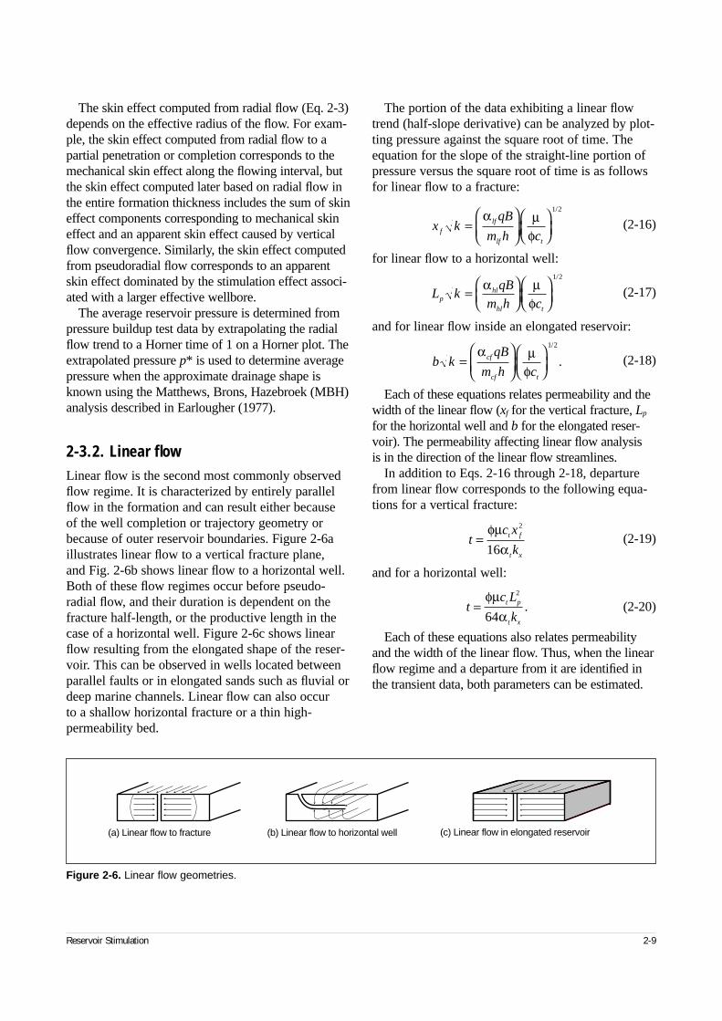
The skin effect computed from radial flow (Eq. 2-3)depends on the effective radius of the flow. For exam-ple, the skin effect computed from radial flow to apartial penetration or completion corresponds to themechanical skin effect along the flowing interval, butthe skin effect computed later based on radial flow inthe entire formation thickness includes the sum of skineffect components corresponding to mechanical skineffect and an apparent skin effect caused by verticalflow convergence. Similarly, the skin effect computedfrom pseudoradial flow corresponds to an apparentskin effect dominated by the stimulation effect associ-ated with a larger effective wellbore.

The average reservoir pressure is determined frompressure buildup test data by extrapolating the radialflow trend to a Horner time of 1 on a Horner plot. Theextrapolated pressure p* is used to determine averagepressure when the approximate drainage shape isknown using the Matthews, Brons, Hazebroek (MBH)analysis described in Earlougher (1977).

2-3.2. Linear flowLinear flow is the second most commonly observedflow regime. It is characterized by entirely parallelflow in the formation and can result either because of the well completion or trajectory geometry orbecause of outer reservoir boundaries. Figure 2-6aillustrates linear flow to a vertical fracture plane, and Fig. 2-6b shows linear flow to a horizontal well.Both of these flow regimes occur before pseudo-radial flow, and their duration is dependent on thefracture half-length, or the productive length in thecase of a horizontal well. Figure 2-6c shows linearflow resulting from the elongated shape of the reser-voir. This can be observed in wells located betweenparallel faults or in elongated sands such as fluvial ordeep marine channels. Linear flow can also occur to a shallow horizontal fracture or a thin high-permeability bed.

The portion of the data exhibiting a linear flowtrend (half-slope derivative) can be analyzed by plot-ting pressure against the square root of time. Theequation for the slope of the straight-line portion ofpressure versus the square root of time is as followsfor linear flow to a fracture:

(2-16)

for linear flow to a horizontal well:

(2-17)

and for linear flow inside an elongated reservoir:

(2-18)

Each of these equations relates permeability and thewidth of the linear flow (xf for the vertical fracture, Lp

for the horizontal well and b for the elongated reser-voir). The permeability affecting linear flow analysis is in the direction of the linear flow streamlines.

In addition to Eqs. 2-16 through 2-18, departurefrom linear flow corresponds to the following equa-tions for a vertical fracture:

(2-19)

and for a horizontal well:

(2-20)

Each of these equations also relates permeabilityand the width of the linear flow. Thus, when the linearflow regime and a departure from it are identified inthe transient data, both parameters can be estimated.

Reservoir Stimulation 2-9

Figure 2-6. Linear flow geometries.

(a) Linear flow to fracture (c) Linear flow in elongated reservoir(b) Linear flow to horizontal well

x kqB

m h cflf

lf t

=

α µφ

1 2/

L kqB

m h cphl

hl t

=

α µφ

1 2/

b kqB

m h ccf

cf t

=

α µφ

1 2/

.

tc x

kt f

t x

=φµ

α

2

16

tc L

kt p

t x

=φµ

α

2

64.

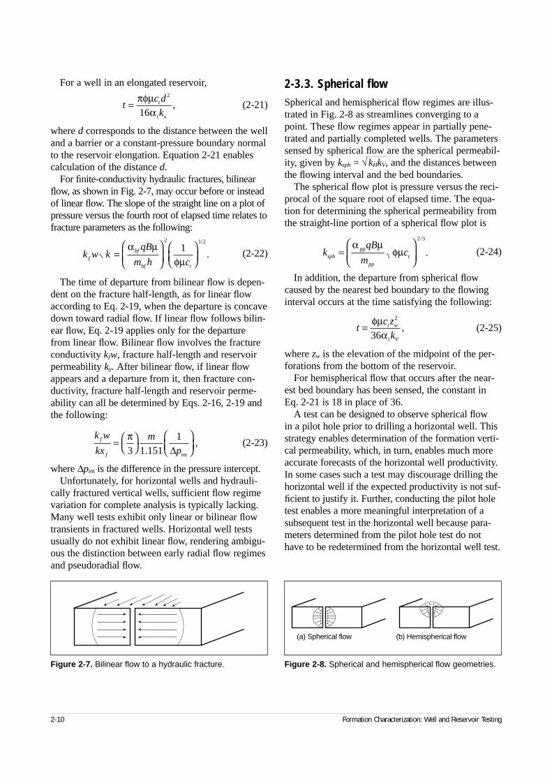
For a well in an elongated reservoir,

(2-21)

where d corresponds to the distance between the welland a barrier or a constant-pressure boundary normalto the reservoir elongation. Equation 2-21 enablescalculation of the distance d.

For finite-conductivity hydraulic fractures, bilinearflow, as shown in Fig. 2-7, may occur before or insteadof linear flow. The slope of the straight line on a plot ofpressure versus the fourth root of elapsed time relates tofracture parameters as the following:

(2-22)

The time of departure from bilinear flow is depen-dent on the fracture half-length, as for linear flowaccording to Eq. 2-19, when the departure is concavedown toward radial flow. If linear flow follows bilin-ear flow, Eq. 2-19 applies only for the departurefrom linear flow. Bilinear flow involves the fractureconductivity kfw, fracture half-length and reservoirpermeability ky. After bilinear flow, if linear flowappears and a departure from it, then fracture con-ductivity, fracture half-length and reservoir perme-ability can all be determined by Eqs. 2-16, 2-19 andthe following:

(2-23)

where ∆pint is the difference in the pressure intercept.Unfortunately, for horizontal wells and hydrauli-

cally fractured vertical wells, sufficient flow regimevariation for complete analysis is typically lacking.Many well tests exhibit only linear or bilinear flowtransients in fractured wells. Horizontal well testsusually do not exhibit linear flow, rendering ambigu-ous the distinction between early radial flow regimesand pseudoradial flow.

2-3.3. Spherical flowSpherical and hemispherical flow regimes are illus-trated in Fig. 2-8 as streamlines converging to apoint. These flow regimes appear in partially pene-trated and partially completed wells. The parameterssensed by spherical flow are the spherical permeabil-ity, given by ksph = √kHkV, and the distances betweenthe flowing interval and the bed boundaries.

The spherical flow plot is pressure versus the reci-procal of the square root of elapsed time. The equa-tion for determining the spherical permeability fromthe straight-line portion of a spherical flow plot is

(2-24)

In addition, the departure from spherical flowcaused by the nearest bed boundary to the flowinginterval occurs at the time satisfying the following:

(2-25)

where zw is the elevation of the midpoint of the per-forations from the bottom of the reservoir.

For hemispherical flow that occurs after the near-est bed boundary has been sensed, the constant inEq. 2-21 is 18 in place of 36.

A test can be designed to observe spherical flow in a pilot hole prior to drilling a horizontal well. Thisstrategy enables determination of the formation verti-cal permeability, which, in turn, enables much moreaccurate forecasts of the horizontal well productivity.In some cases such a test may discourage drilling thehorizontal well if the expected productivity is not suf-ficient to justify it. Further, conducting the pilot holetest enables a more meaningful interpretation of asubsequent test in the horizontal well because para-meters determined from the pilot hole test do nothave to be redetermined from the horizontal well test.

2-10 Formation Characterization: Well and Reservoir Testing

tc d

kt

t x

= πφµα

2

16,

k w kqB

m h cfbf

bf t

=

α µφµ

2 1 21

/

.

k w

kx

m

pf

f int

=

π3 1 151

1.

,∆

Figure 2-7. Bilinear flow to a hydraulic fracture.

kqB

mcsph

pp

pp

t=

α µ

φµ2 3/

.

tc z

kt w

t V

= φµα

2

36,

Figure 2-8. Spherical and hemispherical flow geometries.

(a) Spherical flow (b) Hemispherical flow

2-3.4. Dual porosityDual-porosity flow behavior results when reservoirrocks contain distributed internal heterogeneities thathave highly contrasting flow characteristics such thatflow occurs mainly in a high-permeability formationfeature that accounts for a small fraction of the for-mation storativity. Examples are naturally fracturedreservoirs and laminated systems with thin high-per-meability layers.

The two commonly observed dual-porosity tran-sient trends are shown in examples E and H in Fig.2-4. Example E illustrates transient dual-porositybehavior typical of highly laminated systems, whichis virtually impossible to distinguish from a sealingfault without additional information. In example H,which shows pseudosteady-state dual-porositybehavior typical of naturally fractured formations, avalley-shaped drop in the pressure derivative signalsrecharge from matrix rock into the natural fractures.Dual-porosity behavior can appear during any of theflow regimes and complicates transient analysis.

Recognizing and characterizing dual-porosity flowbehavior is extremely important to reserves estima-tion, trajectory planning for deviated and horizontalwells, and stimulation design and post-treatmentevaluation.

The two parameters that characterize dual-porositysystems are the storativity ratio ω and the interporos-ity flow parameter λ. For pseudosteady-state dualporosity, the time of the onset of dual-porositybehavior ton is a function of both parameters:

(2-26)

Similarly, the time of the end of dual-porositybehavior tend is

(2-27)

and the time of the valley minimum tmin is given byBourdet et al. (1983) as

(2-28)

When two of these three times can be identified in the pressure derivative response, ω and λ can beestimated.

Dual-porosity reservoirs are likely to exhibithighly anisotropic flow behavior. Highly laminatedsystems usually have considerable contrast in hori-zontal and vertical permeability, whereas naturallyfractured systems usually have a preferential flowdirection oriented parallel to the natural fractures.Laminated formations favor vertical wells; horizontalwells are particularly attractive in naturally fracturedreservoirs. Because natural fractures are usually sub-vertical and oriented with the stress field, the maxi-mum permeability and maximum stress directionsare usually closely aligned, resulting in enormousimplications for hydraulic fracture design and trajec-tory planning in deviated wells.

Observance of dual-porosity transients should trig-ger additional measurements or analysis to establishthe direction and magnitude of the implicit perme-ability anisotropies.

2-3.5. Wellbore storage and pseudosteady state

Wellbore storage and pseudosteady state both resultfrom fluid compression or expansion in a limitedvolume. For wellbore storage the control volume isthe wellbore; for pseudosteady state it is the reser-voir drainage volume. Both these cases are sensitivemainly to two parameters, fluid compressibility andthe control volume, but other factors determine theironset and duration. Both are recognized by a unit-slope trend in the pressure derivative.

For wellbore storage, the pressure change and thederivative coincide with a unit-slope trend on thelog-log diagnostic plot in early time. The derivativetypically departs below the pressure change andappears as a hump during the transition to reservoir-dominated flow regimes. This is typically the firstflow regime observed in any test, and it usually dom-inates the transient response. The wellbore storagecoefficient can be computed from the straight-lineportion of the plot of pressure change versus elapsedtime using the following equation (the line must passthrough the origin on the plot):

(2-29)

The duration of wellbore storage can be reduced bydesigning buildup tests with downhole shut-in. Otherfactors affecting wellbore storage duration are perme-

Reservoir Stimulation 2-11

tc r

kont w

t

=−( )

φµα

ωλ ω ω

2 2 271

1ln .

tc r

kendt w

t

= −( )φµα

ωλ

2 17

,

tc

kmint

t

=

+ −

− −12

11

1 1φηα

ω ωωω

ω

. CqB

mc c

=α

.

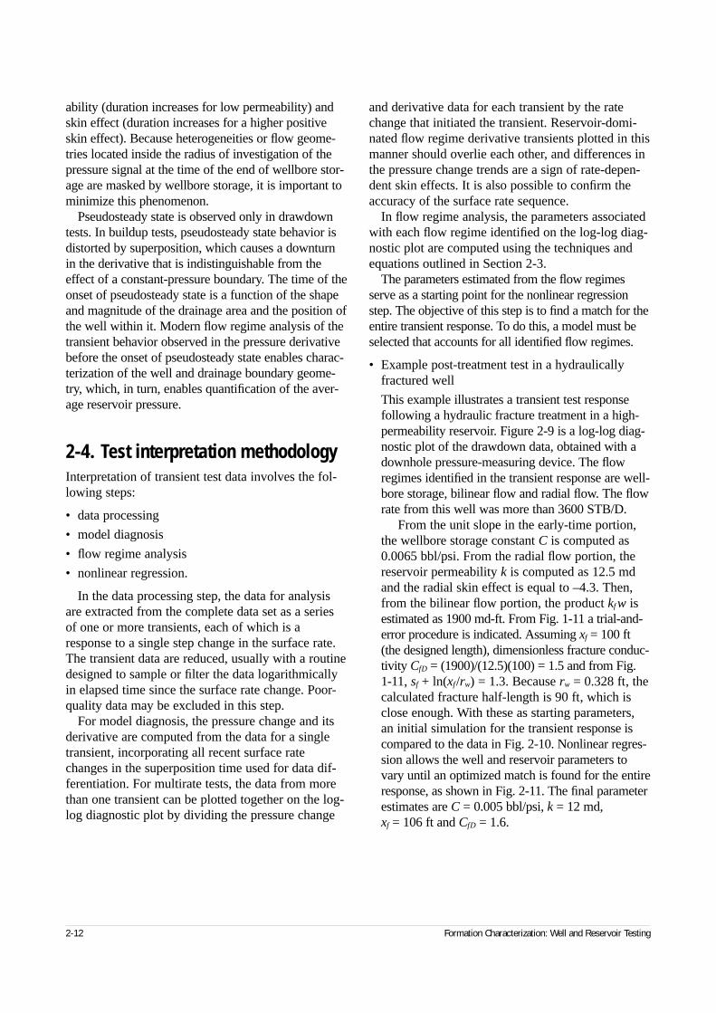
ability (duration increases for low permeability) andskin effect (duration increases for a higher positiveskin effect). Because heterogeneities or flow geome-tries located inside the radius of investigation of thepressure signal at the time of the end of wellbore stor-age are masked by wellbore storage, it is important tominimize this phenomenon.

Pseudosteady state is observed only in drawdowntests. In buildup tests, pseudosteady state behavior isdistorted by superposition, which causes a downturnin the derivative that is indistinguishable from the effect of a constant-pressure boundary. The time of theonset of pseudosteady state is a function of the shapeand magnitude of the drainage area and the position ofthe well within it. Modern flow regime analysis of thetransient behavior observed in the pressure derivativebefore the onset of pseudosteady state enables charac-terization of the well and drainage boundary geome-try, which, in turn, enables quantification of the aver-age reservoir pressure.

2-4. Test interpretation methodologyInterpretation of transient test data involves the fol-lowing steps:

• data processing

• model diagnosis

• flow regime analysis

• nonlinear regression.

In the data processing step, the data for analysisare extracted from the complete data set as a seriesof one or more transients, each of which is aresponse to a single step change in the surface rate.The transient data are reduced, usually with a routinedesigned to sample or filter the data logarithmicallyin elapsed time since the surface rate change. Poor-quality data may be excluded in this step.

For model diagnosis, the pressure change and itsderivative are computed from the data for a singletransient, incorporating all recent surface ratechanges in the superposition time used for data dif-ferentiation. For multirate tests, the data from morethan one transient can be plotted together on the log-log diagnostic plot by dividing the pressure change

and derivative data for each transient by the ratechange that initiated the transient. Reservoir-domi-nated flow regime derivative transients plotted in thismanner should overlie each other, and differences inthe pressure change trends are a sign of rate-depen-dent skin effects. It is also possible to confirm theaccuracy of the surface rate sequence.

In flow regime analysis, the parameters associatedwith each flow regime identified on the log-log diag-nostic plot are computed using the techniques andequations outlined in Section 2-3.

The parameters estimated from the flow regimesserve as a starting point for the nonlinear regressionstep. The objective of this step is to find a match for theentire transient response. To do this, a model must beselected that accounts for all identified flow regimes.

• Example post-treatment test in a hydraulicallyfractured well

This example illustrates a transient test responsefollowing a hydraulic fracture treatment in a high-permeability reservoir. Figure 2-9 is a log-log diag-nostic plot of the drawdown data, obtained with adownhole pressure-measuring device. The flowregimes identified in the transient response are well-bore storage, bilinear flow and radial flow. The flowrate from this well was more than 3600 STB/D.

From the unit slope in the early-time portion,the wellbore storage constant C is computed as0.0065 bbl/psi. From the radial flow portion, thereservoir permeability k is computed as 12.5 mdand the radial skin effect is equal to –4.3. Then,from the bilinear flow portion, the product kf w isestimated as 1900 md-ft. From Fig. 1-11 a trial-and-error procedure is indicated. Assuming xf = 100 ft(the designed length), dimensionless fracture conduc-tivity CfD = (1900)/(12.5)(100) = 1.5 and from Fig. 1-11, sf + ln(xf/rw) = 1.3. Because rw = 0.328 ft, thecalculated fracture half-length is 90 ft, which isclose enough. With these as starting parameters, an initial simulation for the transient response iscompared to the data in Fig. 2-10. Nonlinear regres-sion allows the well and reservoir parameters tovary until an optimized match is found for the entireresponse, as shown in Fig. 2-11. The final parameterestimates are C = 0.005 bbl/psi, k = 12 md, xf = 106 ft and CfD = 1.6.

2-12 Formation Characterization: Well and Reservoir Testing

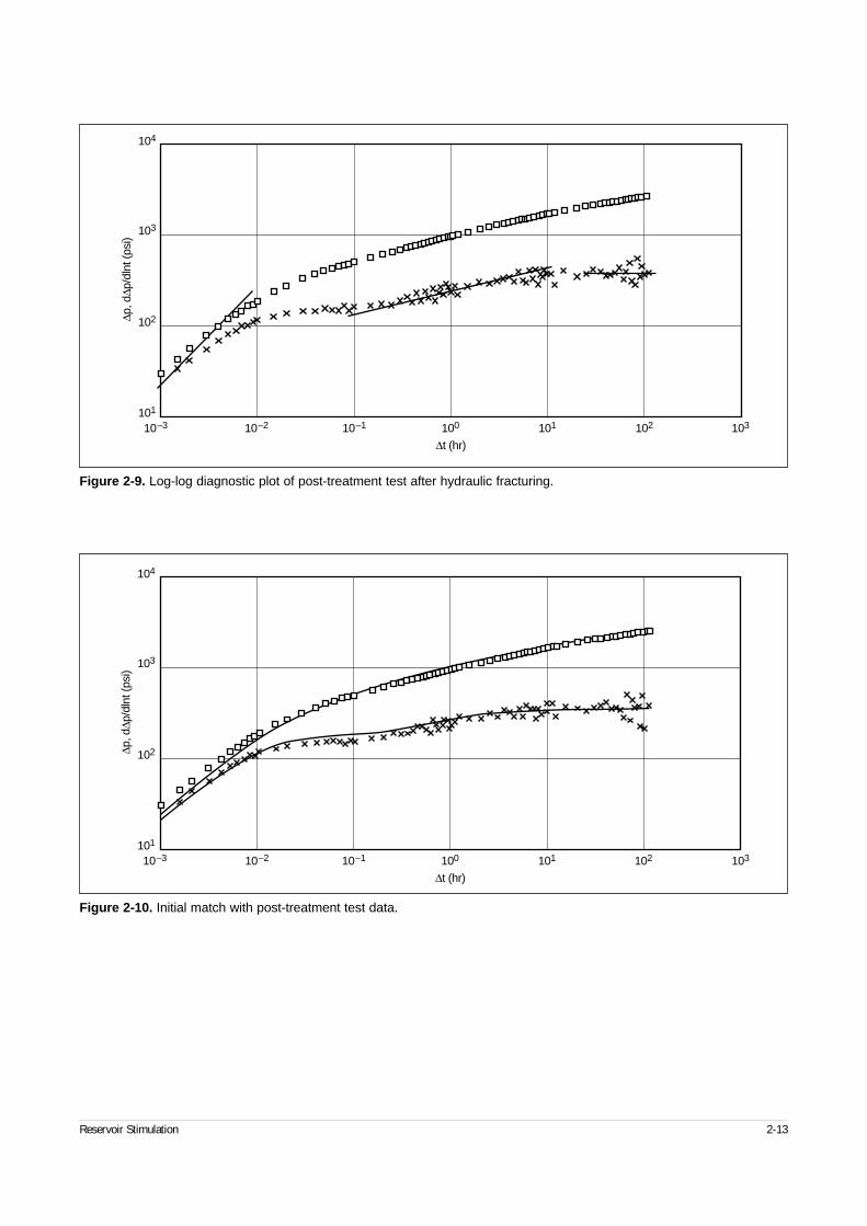
Reservoir Stimulation 2-13

Figure 2-9. Log-log diagnostic plot of post-treatment test after hydraulic fracturing.

∆t (hr)

∆p, d

∆p/d

lnt (

psi)

10–3 10–2

103

104

10–1 100 101 102 103

102

101

Figure 2-10. Initial match with post-treatment test data.

∆t (hr)

∆p, d

∆p/d

lnt (

psi)

10–3 10–2

103

104

10–1 100 101 102 103

102

101

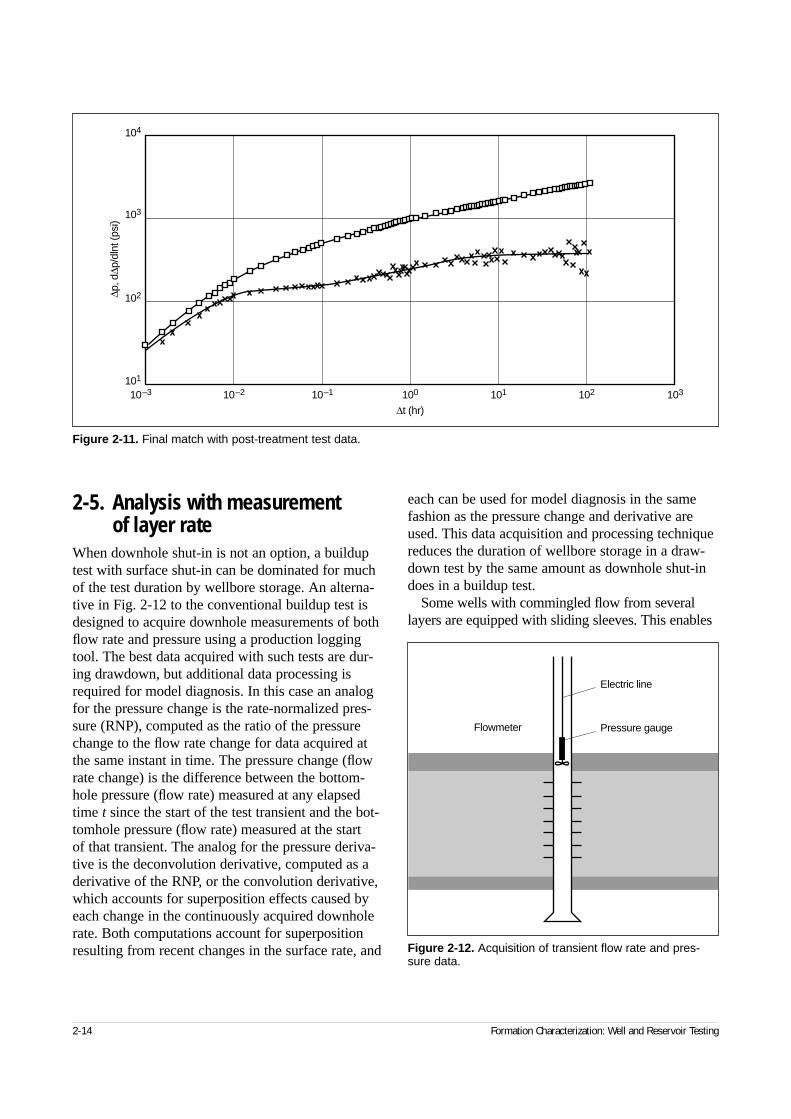
2-5. Analysis with measurement of layer rate

When downhole shut-in is not an option, a builduptest with surface shut-in can be dominated for muchof the test duration by wellbore storage. An alterna-tive in Fig. 2-12 to the conventional buildup test isdesigned to acquire downhole measurements of bothflow rate and pressure using a production loggingtool. The best data acquired with such tests are dur-ing drawdown, but additional data processing isrequired for model diagnosis. In this case an analogfor the pressure change is the rate-normalized pres-sure (RNP), computed as the ratio of the pressurechange to the flow rate change for data acquired atthe same instant in time. The pressure change (flowrate change) is the difference between the bottom-hole pressure (flow rate) measured at any elapsedtime t since the start of the test transient and the bot-tomhole pressure (flow rate) measured at the start of that transient. The analog for the pressure deriva-tive is the deconvolution derivative, computed as aderivative of the RNP, or the convolution derivative,which accounts for superposition effects caused byeach change in the continuously acquired downholerate. Both computations account for superpositionresulting from recent changes in the surface rate, and

each can be used for model diagnosis in the samefashion as the pressure change and derivative areused. This data acquisition and processing techniquereduces the duration of wellbore storage in a draw-down test by the same amount as downhole shut-indoes in a buildup test.

Some wells with commingled flow from severallayers are equipped with sliding sleeves. This enables

2-14 Formation Characterization: Well and Reservoir Testing

Figure 2-11. Final match with post-treatment test data.

∆t (hr)

∆p, d

∆p/d

lnt (

psi)

10–3 10–2

103

104

10–1 100 101 102 103

102

101

Figure 2-12. Acquisition of transient flow rate and pres-sure data.

Electric line

Pressure gaugeFlowmeter

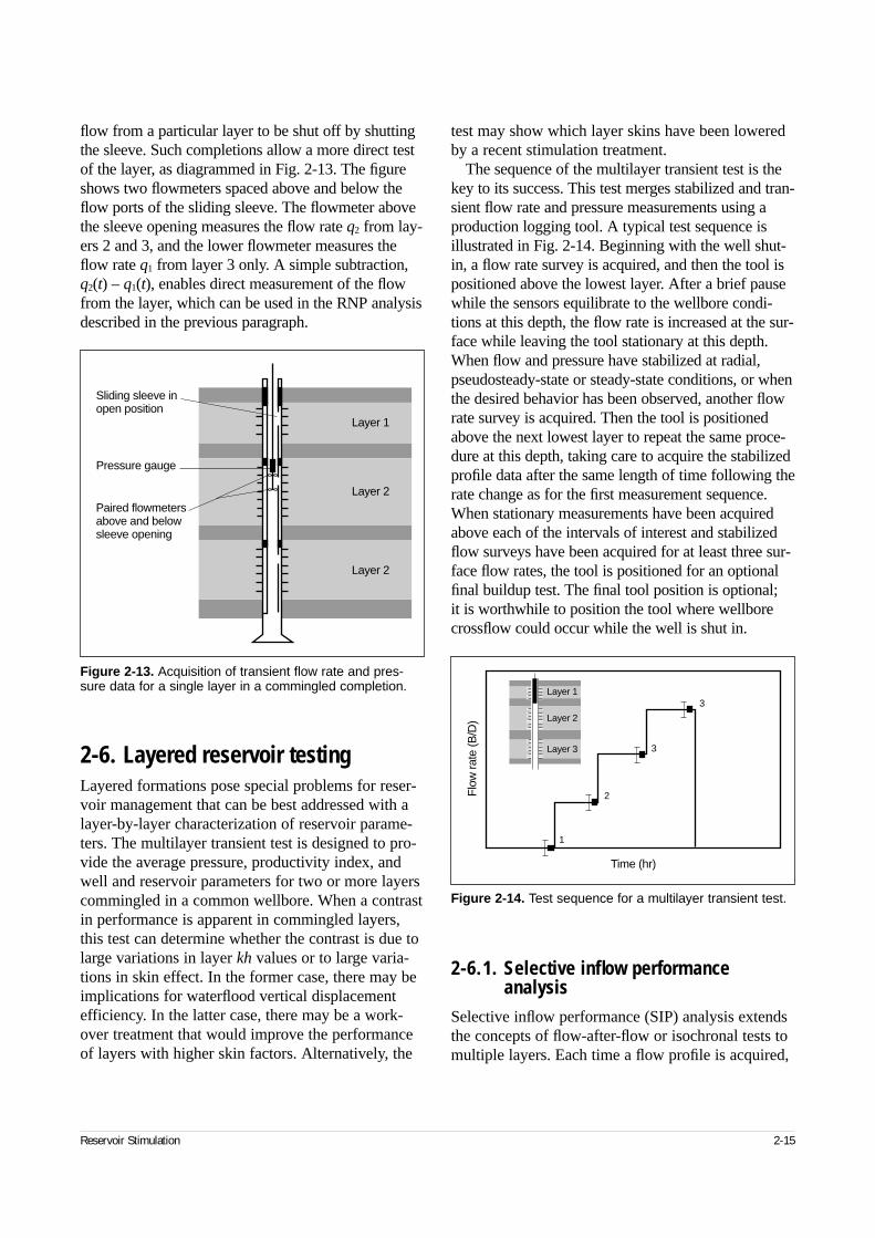
flow from a particular layer to be shut off by shuttingthe sleeve. Such completions allow a more direct testof the layer, as diagrammed in Fig. 2-13. The figureshows two flowmeters spaced above and below theflow ports of the sliding sleeve. The flowmeter abovethe sleeve opening measures the flow rate q2 from lay-ers 2 and 3, and the lower flowmeter measures theflow rate q1 from layer 3 only. A simple subtraction,q2(t) – q1(t), enables direct measurement of the flowfrom the layer, which can be used in the RNP analysisdescribed in the previous paragraph.

2-6. Layered reservoir testingLayered formations pose special problems for reser-voir management that can be best addressed with alayer-by-layer characterization of reservoir parame-ters. The multilayer transient test is designed to pro-vide the average pressure, productivity index, andwell and reservoir parameters for two or more layerscommingled in a common wellbore. When a contrastin performance is apparent in commingled layers,this test can determine whether the contrast is due tolarge variations in layer kh values or to large varia-tions in skin effect. In the former case, there may beimplications for waterflood vertical displacementefficiency. In the latter case, there may be a work-over treatment that would improve the performanceof layers with higher skin factors. Alternatively, the

test may show which layer skins have been loweredby a recent stimulation treatment.

The sequence of the multilayer transient test is thekey to its success. This test merges stabilized and tran-sient flow rate and pressure measurements using aproduction logging tool. A typical test sequence isillustrated in Fig. 2-14. Beginning with the well shut-in, a flow rate survey is acquired, and then the tool ispositioned above the lowest layer. After a brief pausewhile the sensors equilibrate to the wellbore condi-tions at this depth, the flow rate is increased at the sur-face while leaving the tool stationary at this depth.When flow and pressure have stabilized at radial,pseudosteady-state or steady-state conditions, or whenthe desired behavior has been observed, another flowrate survey is acquired. Then the tool is positionedabove the next lowest layer to repeat the same proce-dure at this depth, taking care to acquire the stabilizedprofile data after the same length of time following therate change as for the first measurement sequence.When stationary measurements have been acquiredabove each of the intervals of interest and stabilizedflow surveys have been acquired for at least three sur-face flow rates, the tool is positioned for an optionalfinal buildup test. The final tool position is optional; it is worthwhile to position the tool where wellborecrossflow could occur while the well is shut in.

2-6.1. Selective inflow performanceanalysis

Selective inflow performance (SIP) analysis extendsthe concepts of flow-after-flow or isochronal tests tomultiple layers. Each time a flow profile is acquired,

Reservoir Stimulation 2-15

Figure 2-13. Acquisition of transient flow rate and pres-sure data for a single layer in a commingled completion.

Layer 1

Layer 2

Layer 2

Sliding sleeve inopen position

Pressure gauge

Paired flowmetersabove and belowsleeve opening

Figure 2-14. Test sequence for a multilayer transient test.

3

3

2

1

Layer 1

Layer 2

Layer 3

Time (hr)

Flo

w ra

te (B

/D)

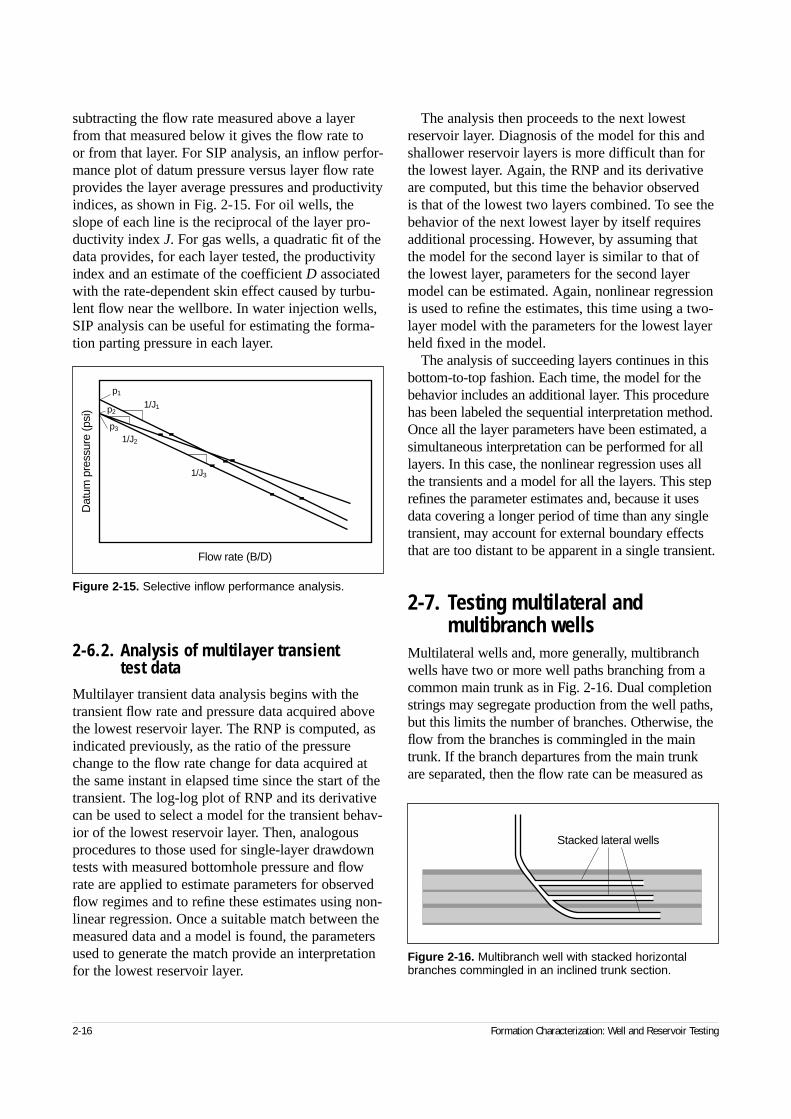
subtracting the flow rate measured above a layerfrom that measured below it gives the flow rate to or from that layer. For SIP analysis, an inflow perfor-mance plot of datum pressure versus layer flow rateprovides the layer average pressures and productivityindices, as shown in Fig. 2-15. For oil wells, theslope of each line is the reciprocal of the layer pro-ductivity index J. For gas wells, a quadratic fit of thedata provides, for each layer tested, the productivityindex and an estimate of the coefficient D associatedwith the rate-dependent skin effect caused by turbu-lent flow near the wellbore. In water injection wells,SIP analysis can be useful for estimating the forma-tion parting pressure in each layer.

2-6.2. Analysis of multilayer transient test data

Multilayer transient data analysis begins with thetransient flow rate and pressure data acquired abovethe lowest reservoir layer. The RNP is computed, asindicated previously, as the ratio of the pressurechange to the flow rate change for data acquired atthe same instant in elapsed time since the start of thetransient. The log-log plot of RNP and its derivativecan be used to select a model for the transient behav-ior of the lowest reservoir layer. Then, analogousprocedures to those used for single-layer drawdowntests with measured bottomhole pressure and flowrate are applied to estimate parameters for observedflow regimes and to refine these estimates using non-linear regression. Once a suitable match between themeasured data and a model is found, the parametersused to generate the match provide an interpretationfor the lowest reservoir layer.

The analysis then proceeds to the next lowestreservoir layer. Diagnosis of the model for this andshallower reservoir layers is more difficult than forthe lowest layer. Again, the RNP and its derivativeare computed, but this time the behavior observed is that of the lowest two layers combined. To see thebehavior of the next lowest layer by itself requiresadditional processing. However, by assuming thatthe model for the second layer is similar to that ofthe lowest layer, parameters for the second layermodel can be estimated. Again, nonlinear regressionis used to refine the estimates, this time using a two-layer model with the parameters for the lowest layerheld fixed in the model.

The analysis of succeeding layers continues in thisbottom-to-top fashion. Each time, the model for thebehavior includes an additional layer. This procedurehas been labeled the sequential interpretation method.Once all the layer parameters have been estimated, asimultaneous interpretation can be performed for alllayers. In this case, the nonlinear regression uses allthe transients and a model for all the layers. This steprefines the parameter estimates and, because it usesdata covering a longer period of time than any singletransient, may account for external boundary effectsthat are too distant to be apparent in a single transient.

2-7. Testing multilateral and multibranch wells

Multilateral wells and, more generally, multibranchwells have two or more well paths branching from acommon main trunk as in Fig. 2-16. Dual completionstrings may segregate production from the well paths,but this limits the number of branches. Otherwise, theflow from the branches is commingled in the maintrunk. If the branch departures from the main trunkare separated, then the flow rate can be measured as

2-16 Formation Characterization: Well and Reservoir Testing

Figure 2-15. Selective inflow performance analysis.

p1

p2

p3

1/J1

1/J2

1/J3

Flow rate (B/D)

Dat

um p

ress

ure

(psi

)

Figure 2-16. Multibranch well with stacked horizontalbranches commingled in an inclined trunk section.

Stacked lateral wells

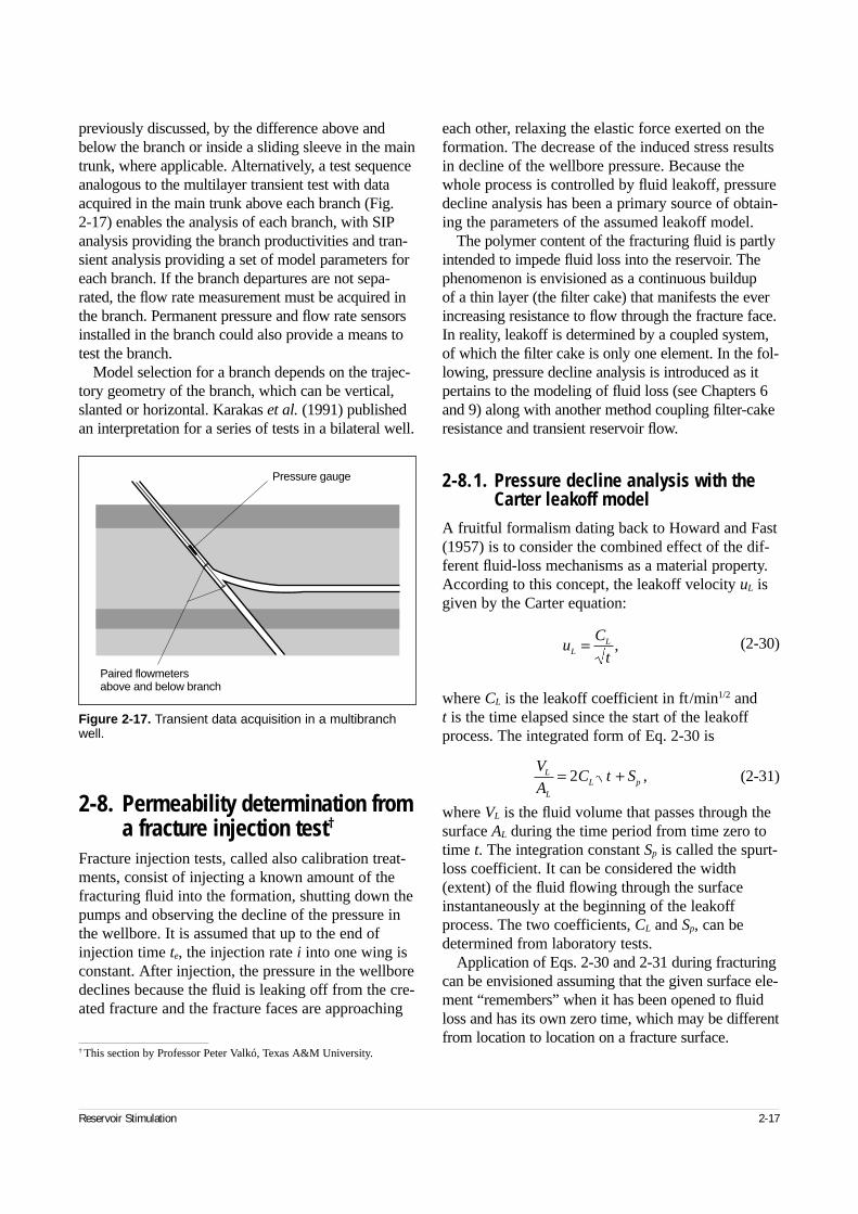
previously discussed, by the difference above andbelow the branch or inside a sliding sleeve in the maintrunk, where applicable. Alternatively, a test sequenceanalogous to the multilayer transient test with dataacquired in the main trunk above each branch (Fig. 2-17) enables the analysis of each branch, with SIPanalysis providing the branch productivities and tran-sient analysis providing a set of model parameters foreach branch. If the branch departures are not sepa-rated, the flow rate measurement must be acquired in the branch. Permanent pressure and flow rate sensorsinstalled in the branch could also provide a means totest the branch.

Model selection for a branch depends on the trajec-tory geometry of the branch, which can be vertical,slanted or horizontal. Karakas et al. (1991) publishedan interpretation for a series of tests in a bilateral well.

2-8. Permeability determination froma fracture injection test†

Fracture injection tests, called also calibration treat-ments, consist of injecting a known amount of thefracturing fluid into the formation, shutting down thepumps and observing the decline of the pressure inthe wellbore. It is assumed that up to the end ofinjection time te, the injection rate i into one wing isconstant. After injection, the pressure in the wellboredeclines because the fluid is leaking off from the cre-ated fracture and the fracture faces are approaching

† This section by Professor Peter Valkó, Texas A&M University.

each other, relaxing the elastic force exerted on theformation. The decrease of the induced stress resultsin decline of the wellbore pressure. Because thewhole process is controlled by fluid leakoff, pressuredecline analysis has been a primary source of obtain-ing the parameters of the assumed leakoff model.

The polymer content of the fracturing fluid is partlyintended to impede fluid loss into the reservoir. Thephenomenon is envisioned as a continuous buildup of a thin layer (the filter cake) that manifests the everincreasing resistance to flow through the fracture face.In reality, leakoff is determined by a coupled system,of which the filter cake is only one element. In the fol-lowing, pressure decline analysis is introduced as itpertains to the modeling of fluid loss (see Chapters 6and 9) along with another method coupling filter-cakeresistance and transient reservoir flow.

2-8.1. Pressure decline analysis with the Carter leakoff model

A fruitful formalism dating back to Howard and Fast(1957) is to consider the combined effect of the dif-ferent fluid-loss mechanisms as a material property.According to this concept, the leakoff velocity uL isgiven by the Carter equation:

(2-30)

where CL is the leakoff coefficient in ft/min1/2 andt is the time elapsed since the start of the leakoffprocess. The integrated form of Eq. 2-30 is

(2-31)

where VL is the fluid volume that passes through thesurface AL during the time period from time zero totime t. The integration constant Sp is called the spurt-loss coefficient. It can be considered the width(extent) of the fluid flowing through the surfaceinstantaneously at the beginning of the leakoffprocess. The two coefficients, CL and Sp, can bedetermined from laboratory tests.

Application of Eqs. 2-30 and 2-31 during fracturingcan be envisioned assuming that the given surface ele-ment “remembers” when it has been opened to fluidloss and has its own zero time, which may be differentfrom location to location on a fracture surface.

Reservoir Stimulation 2-17

Figure 2-17. Transient data acquisition in a multibranchwell.

Paired flowmetersabove and below branch

Pressure gauge

uC

tLL= ,

V

AC t SL

L

L p= +2 ,

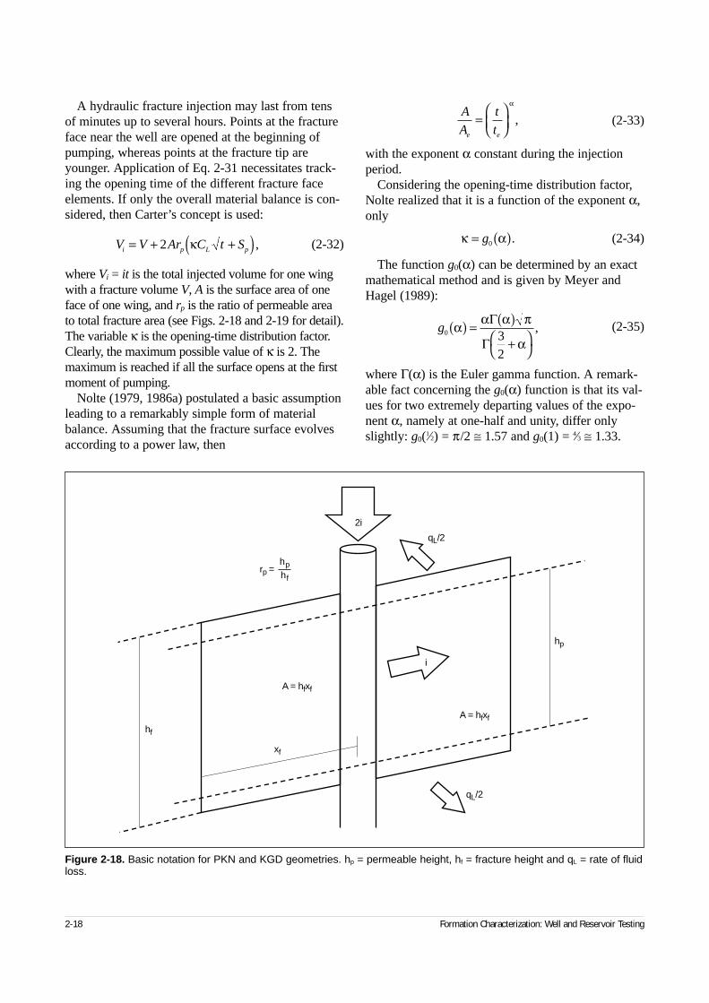
A hydraulic fracture injection may last from tensof minutes up to several hours. Points at the fractureface near the well are opened at the beginning ofpumping, whereas points at the fracture tip areyounger. Application of Eq. 2-31 necessitates track-ing the opening time of the different fracture faceelements. If only the overall material balance is con-sidered, then Carter’s concept is used:

(2-32)

where Vi = it is the total injected volume for one wingwith a fracture volume V, A is the surface area of oneface of one wing, and rp is the ratio of permeable areato total fracture area (see Figs. 2-18 and 2-19 for detail).The variable κ is the opening-time distribution factor.Clearly, the maximum possible value of κ is 2. Themaximum is reached if all the surface opens at the firstmoment of pumping.

Nolte (1979, 1986a) postulated a basic assumptionleading to a remarkably simple form of materialbalance. Assuming that the fracture surface evolvesaccording to a power law, then

(2-33)

with the exponent α constant during the injectionperiod.

Considering the opening-time distribution factor,Nolte realized that it is a function of the exponent α,only

(2-34)

The function g0(α) can be determined by an exactmathematical method and is given by Meyer andHagel (1989):

(2-35)

where Γ(α) is the Euler gamma function. A remark-able fact concerning the g0(α) function is that its val-ues for two extremely departing values of the expo-nent α, namely at one-half and unity, differ onlyslightly: g0(1⁄2) = π/2 ≅ 1.57 and g0(1) = 4⁄3 ≅ 1.33.

2-18 Formation Characterization: Well and Reservoir Testing

V V Ar C t Si p L p= + +( )2 κ ,

A

A

t

te e

=

α

,

κ α= ( )g0 .

g0 32

α α α π

α( ) = ( )

+

Γ

Γ,

Figure 2-18. Basic notation for PKN and KGD geometries. hp = permeable height, hf = fracture height and qL = rate of fluidloss.

2i

qL/2

qL/2

i

hp

hf

xf

A = hfxf

A = hfxf

rp =hphf

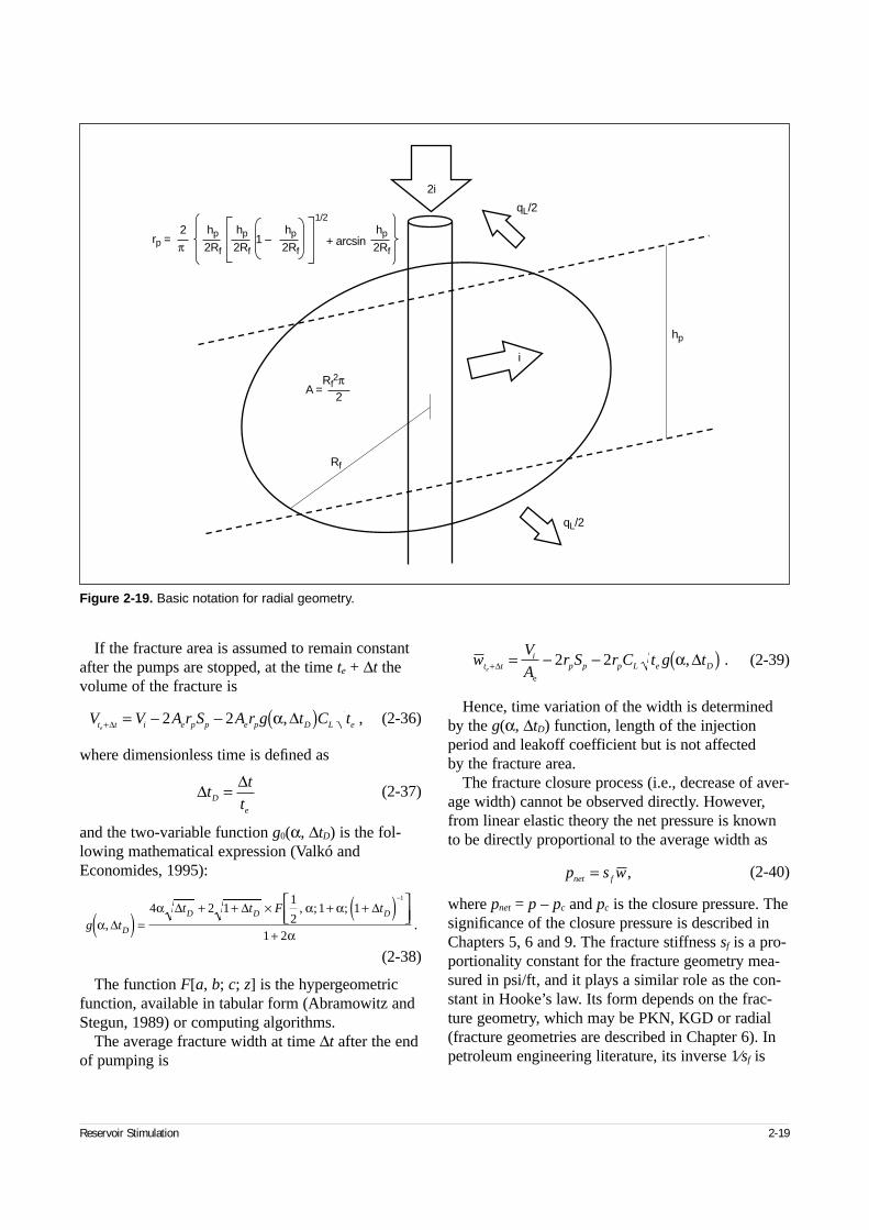
If the fracture area is assumed to remain constantafter the pumps are stopped, at the time te + ∆t thevolume of the fracture is

(2-36)

where dimensionless time is defined as

(2-37)

and the two-variable function g0(α, ∆tD) is the fol-lowing mathematical expression (Valkó andEconomides, 1995):

(2-38)

The function F[a, b; c; z] is the hypergeometricfunction, available in tabular form (Abramowitz andStegun, 1989) or computing algorithms.

The average fracture width at time ∆t after the endof pumping is

(2-39)

Hence, time variation of the width is determinedby the g(α, ∆tD) function, length of the injectionperiod and leakoff coefficient but is not affected by the fracture area.

The fracture closure process (i.e., decrease of aver-age width) cannot be observed directly. However,from linear elastic theory the net pressure is knownto be directly proportional to the average width as

(2-40)

where pnet = p – pc and pc is the closure pressure. Thesignificance of the closure pressure is described inChapters 5, 6 and 9. The fracture stiffness sf is a pro-portionality constant for the fracture geometry mea-sured in psi/ft, and it plays a similar role as the con-stant in Hooke’s law. Its form depends on the frac-ture geometry, which may be PKN, KGD or radial(fracture geometries are described in Chapter 6). Inpetroleum engineering literature, its inverse 1⁄sf is

Reservoir Stimulation 2-19

Figure 2-19. Basic notation for radial geometry.

2i

qL/2

qL/2

i

hp

Rf

1 –hp

2Rf

hp

2Rf

hp

2Rf

2

πhp

2Rf

A =Rf

2π2

+ arcsinrp =

1/2

V V A r S A r g t C tt t i e p p e p D L ee + = − − ( )∆ ∆2 2 α, ,

.e

wV

Ar S r C t g tt t

ip p p L e De + = − − ( )∆ ∆2 2 α,

p s wnet f= ,

∆ ∆t

t

tD

e

=

g tt t F t

D

D D D

αα α α

α,

, ; ;.∆

∆ ∆ ∆( ) ( )

=

+ + × + +

+

−

4 2 11

21 1

1 2

1

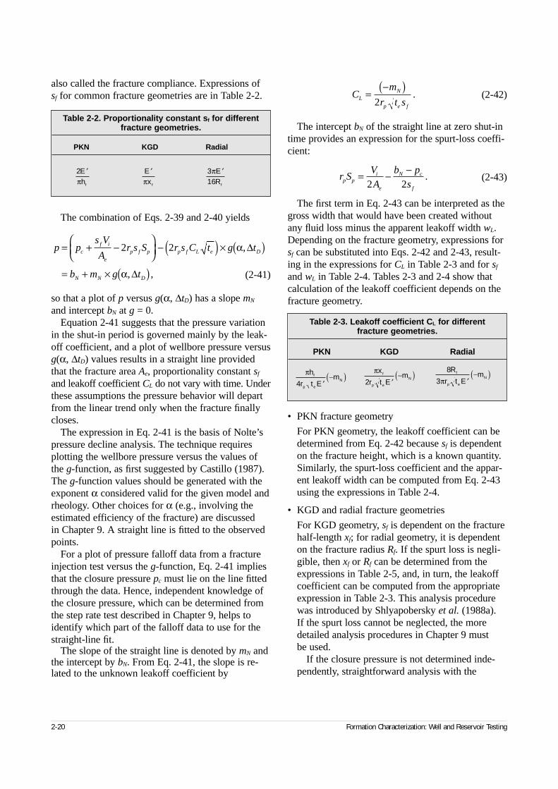
also called the fracture compliance. Expressions of sf for common fracture geometries are in Table 2-2.

The combination of Eqs. 2-39 and 2-40 yields

(2-41)

so that a plot of p versus g(α, ∆tD) has a slope mN

and intercept bN at g = 0.Equation 2-41 suggests that the pressure variation

in the shut-in period is governed mainly by the leak-off coefficient, and a plot of wellbore pressure versusg(α, ∆tD) values results in a straight line providedthat the fracture area Ae, proportionality constant sf

and leakoff coefficient CL do not vary with time. Underthese assumptions the pressure behavior will departfrom the linear trend only when the fracture finallycloses.

The expression in Eq. 2-41 is the basis of Nolte’spressure decline analysis. The technique requiresplotting the wellbore pressure versus the values ofthe g-function, as first suggested by Castillo (1987).The g-function values should be generated with theexponent α considered valid for the given model andrheology. Other choices for α (e.g., involving theestimated efficiency of the fracture) are discussed in Chapter 9. A straight line is fitted to the observedpoints.

For a plot of pressure falloff data from a fractureinjection test versus the g-function, Eq. 2-41 impliesthat the closure pressure pc must lie on the line fittedthrough the data. Hence, independent knowledge ofthe closure pressure, which can be determined fromthe step rate test described in Chapter 9, helps toidentify which part of the falloff data to use for thestraight-line fit.

The slope of the straight line is denoted by mN andthe intercept by bN. From Eq. 2-41, the slope is re-lated to the unknown leakoff coefficient by

(2-42)

The intercept bN of the straight line at zero shut-intime provides an expression for the spurt-loss coeffi-cient:

(2-43)

The first term in Eq. 2-43 can be interpreted as thegross width that would have been created withoutany fluid loss minus the apparent leakoff width wL.Depending on the fracture geometry, expressions forsf can be substituted into Eqs. 2-42 and 2-43, result-ing in the expressions for CL in Table 2-3 and for sf

and wL in Table 2-4. Tables 2-3 and 2-4 show thatcalculation of the leakoff coefficient depends on thefracture geometry.

• PKN fracture geometry

For PKN geometry, the leakoff coefficient can bedetermined from Eq. 2-42 because sf is dependenton the fracture height, which is a known quantity.Similarly, the spurt-loss coefficient and the appar-ent leakoff width can be computed from Eq. 2-43using the expressions in Table 2-4.

• KGD and radial fracture geometries

For KGD geometry, sf is dependent on the fracturehalf-length xf; for radial geometry, it is dependenton the fracture radius Rf. If the spurt loss is negli-gible, then xf or Rf can be determined from theexpressions in Table 2-5, and, in turn, the leakoffcoefficient can be computed from the appropriateexpression in Table 2-3. This analysis procedurewas introduced by Shlyapobersky et al. (1988a).If the spurt loss cannot be neglected, the moredetailed analysis procedures in Chapter 9 must be used.

If the closure pressure is not determined inde-pendently, straightforward analysis with the

2-20 Formation Characterization: Well and Reservoir Testing

Table 2-2. Proportionality constant sf for differentfracture geometries.

PKN KGD Radial

2 ′Ehfπ

′Exfπ

316

′ERf

π

p ps V

Ar s S r s C t g t

b m g t

cf i

e

p f p p f L e D

N N D

= + −

− ( ) × ( )

= + × ( )

2 2 α

α

,

, ,

∆

∆

Cm

r t sLN

p e f

=−( )

2.

r SV

A

b p

sp pi

e

N c

f

= − −2 2

.

Table 2-3. Leakoff coefficient CL for different fracture geometries.

PKN KGD Radial

πh

r t Emf

p e

N4 ′

−( )πx

r t Emf

p e

N2 ′

−( )π

R

r t Emf

p e

N

8

3 ′−( )

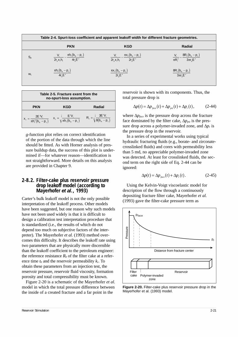
g-function plot relies on correct identification of the portion of the data through which the lineshould be fitted. As with Horner analysis of pres-sure buildup data, the success of this plot is under-mined if—for whatever reason—identification isnot straightforward. More details on this analysisare provided in Chapter 9.

2-8.2. Filter-cake plus reservoir pressure drop leakoff model (according to Mayerhofer et al., 1993)

Carter’s bulk leakoff model is not the only possibleinterpretation of the leakoff process. Other modelshave been suggested, but one reason why such modelshave not been used widely is that it is difficult todesign a calibration test interpretation procedure thatis standardized (i.e., the results of which do notdepend too much on subjective factors of the inter-preter). The Mayerhofer et al. (1993) method over-comes this difficulty. It describes the leakoff rate usingtwo parameters that are physically more discerniblethan the leakoff coefficient to the petroleum engineer:the reference resistance R0 of the filter cake at a refer-ence time t0 and the reservoir permeability kr. Toobtain these parameters from an injection test, thereservoir pressure, reservoir fluid viscosity, formationporosity and total compressibility must be known.

Figure 2-20 is a schematic of the Mayerhofer et al.model in which the total pressure difference betweenthe inside of a created fracture and a far point in the

reservoir is shown with its components. Thus, thetotal pressure drop is

(2-44)

where ∆pface is the pressure drop across the fractureface dominated by the filter cake, ∆ppiz is the pres-sure drop across a polymer-invaded zone, and ∆pr isthe pressure drop in the reservoir.

In a series of experimental works using typicalhydraulic fracturing fluids (e.g., borate- and zirconate-crosslinked fluids) and cores with permeability lessthan 5 md, no appreciable polymer-invaded zonewas detected. At least for crosslinked fluids, the sec-ond term on the right side of Eq. 2-44 can beignored:

(2-45)

Using the Kelvin-Voigt viscoelastic model fordescription of the flow through a continuouslydepositing fracture filter cake, Mayerhofer et al.(1993) gave the filter-cake pressure term as

Reservoir Stimulation 2-21

Table 2-4. Spurt-loss coefficient and apparent leakoff width for different fracture geometries.

PKN KGD Radial

Vr x h

h b p

r E

h b p

r E

i

p f f

f N c

p

f N c

p

2 4

4

−−( )′

−( )′

π

π

Vr x h

x b p

r E

x b p

r E

i

p f f

f N c

p

f N c

p

2 2

2

−−( )′

−( )′

π

π

VR

R b p

r E

R b p

r E

i

f

f N c

p

f N c

p

π π

π

2

8

3

8

3

−−( )

′

−( )′

Sp

wL

Table 2-5. Fracture exent from theno-spurt-loss assumption.

PKN KGD Radial

xE V

h b pfi

f N c

=′−( )

22π

xE V

h b pfi

f N c

=′

−( )πR

E V

b pfi

N c

=′−( )

3

83

Figure 2-20. Filter-cake plus reservoir pressure drop in theMayerhofer et al. (1993) model.

Pre

ssur

e

Distance from fracture center

Filtercake Polymer-invaded

zone

Reservoir

pface

pr

∆ ∆ ∆ ∆p t p t p t p tface piz r( ) = ( ) + ( ) + ( ) ,

∆ ∆ ∆p t p t p tface r( ) = ( ) + ( ) .

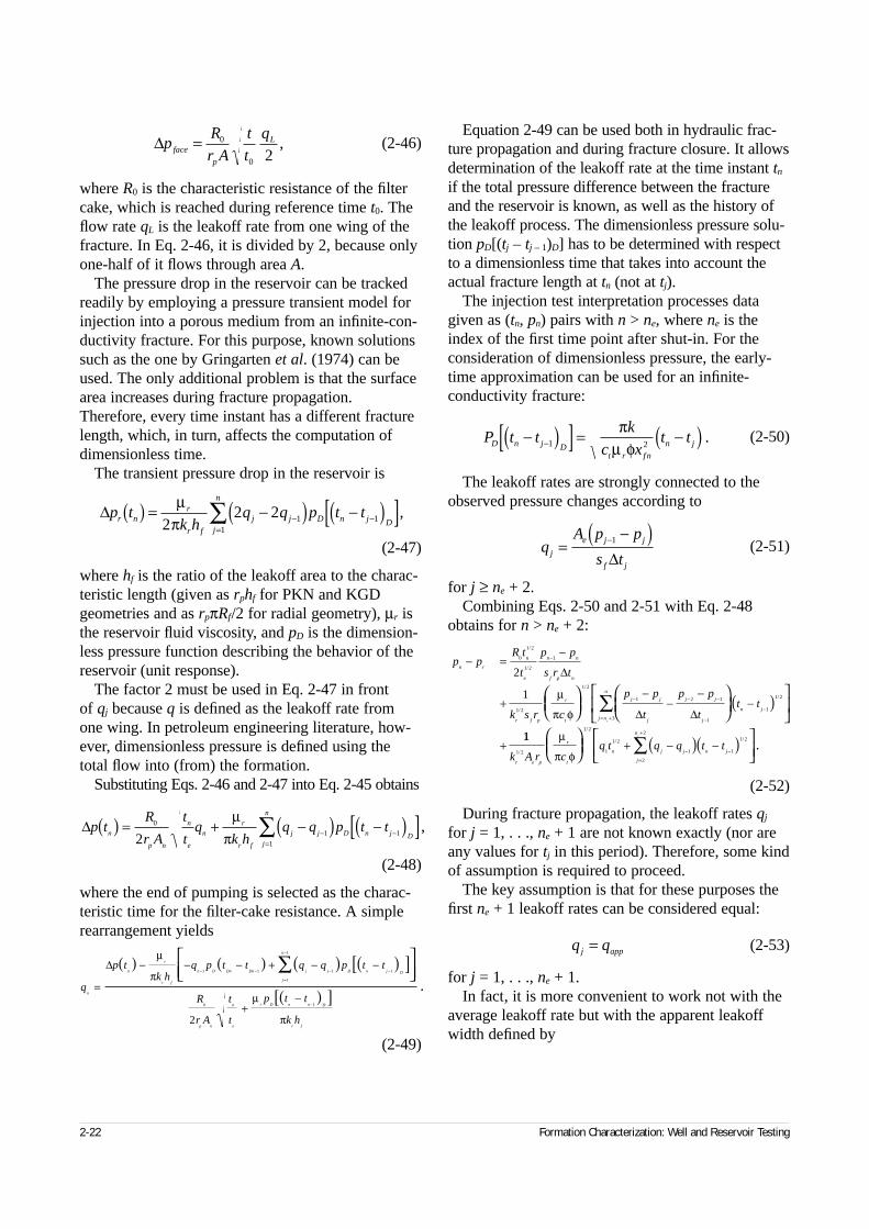
(2-46)

where R0 is the characteristic resistance of the filtercake, which is reached during reference time t0. Theflow rate qL is the leakoff rate from one wing of thefracture. In Eq. 2-46, it is divided by 2, because onlyone-half of it flows through area A.

The pressure drop in the reservoir can be trackedreadily by employing a pressure transient model forinjection into a porous medium from an infinite-con-ductivity fracture. For this purpose, known solutionssuch as the one by Gringarten et al. (1974) can beused. The only additional problem is that the surfacearea increases during fracture propagation.Therefore, every time instant has a different fracturelength, which, in turn, affects the computation ofdimensionless time.

The transient pressure drop in the reservoir is

(2-47)

where hf is the ratio of the leakoff area to the charac-teristic length (given as rphf for PKN and KGDgeometries and as rpπRf/2 for radial geometry), µr isthe reservoir fluid viscosity, and pD is the dimension-less pressure function describing the behavior of thereservoir (unit response).

The factor 2 must be used in Eq. 2-47 in front of qj because q is defined as the leakoff rate fromone wing. In petroleum engineering literature, how-ever, dimensionless pressure is defined using thetotal flow into (from) the formation.

Substituting Eqs. 2-46 and 2-47 into Eq. 2-45 obtains

(2-48)

where the end of pumping is selected as the charac-teristic time for the filter-cake resistance. A simplerearrangement yields

(2-49)

Equation 2-49 can be used both in hydraulic frac-ture propagation and during fracture closure. It allowsdetermination of the leakoff rate at the time instant tn

if the total pressure difference between the fractureand the reservoir is known, as well as the history ofthe leakoff process. The dimensionless pressure solu-tion pD[(tj – tj – 1)D] has to be determined with respectto a dimensionless time that takes into account theactual fracture length at tn (not at tj).

The injection test interpretation processes datagiven as (tn, pn) pairs with n > ne, where ne is theindex of the first time point after shut-in. For theconsideration of dimensionless pressure, the early-time approximation can be used for an infinite-conductivity fracture:

(2-50)

The leakoff rates are strongly connected to theobserved pressure changes according to

(2-51)

for j ≥ ne + 2.Combining Eqs. 2-50 and 2-51 with Eq. 2-48

obtains for n > ne + 2:

(2-52)

During fracture propagation, the leakoff rates qj

for j = 1, . . ., ne + 1 are not known exactly (nor areany values for tj in this period). Therefore, some kindof assumption is required to proceed.

The key assumption is that for these purposes thefirst ne + 1 leakoff rates can be considered equal:

(2-53)

for j = 1, . . ., ne + 1.In fact, it is more convenient to work not with the

average leakoff rate but with the apparent leakoffwidth defined by

2-22 Formation Characterization: Well and Reservoir Testing

∆pR

r A

t

t

qface

p

L= 0

0 2,

P t tk

c xt tD n j D

t r fn

n j−( )[ ] = −( )−1 2

πµ φ

.

qA p p

s tj

e j j

f j

=−( )−1

∆

q qj app=

p pR t

t

p p

s r t

k s r c

p p

t

p p

tt t

n r

n

e

n n

f p n

r f p

r

t

j j

j

j j

jj n

n

n j

e

− =−

+−

−−

−

+

−

− − −

−= +

−

( )

∑

0

1 2

1 2

1

1 2

1 2

1 2 1

13

1

1 2

2

1

/

/

/

/

/

∆

∆ ∆

µ

π φ

111 2

1 2

1

1 2

1

2

2

1

1 2

k A r cq t q q t t

r e p

r

t

n j j

j

n

n j

e

/

/

/ /

.µ

π φ

( )( )

+ − −−

=

+

−∑

∆p tk h

q q p t tr nr

r f

j j D n j Dj

n

( ) = −( ) −( )[ ]− −=

∑µπ2

2 2 1 11

,

∆p tR

r A

t

tq

k hq q p t tn

p n

n

e

n

r

r f

j j D n j Dj

n

( ) ( ) ( )[ ]= + − −− −=

∑01 1

12

µπ

,

q

p tk h

q p t t q q p t t

R

r A

t

t

p t t

k h

n

n

r

r f

n D Dn Dn j j D n j D

j

n

p n

n

e

r D n n D

r f

=

− − − + − −

+−

( ) ( ) ( ) ( )[ ]

( )[ ]− − − −

=

−

−

∑∆µ

π

µ

π

1 1 1 1

1

1

0 1

2

.

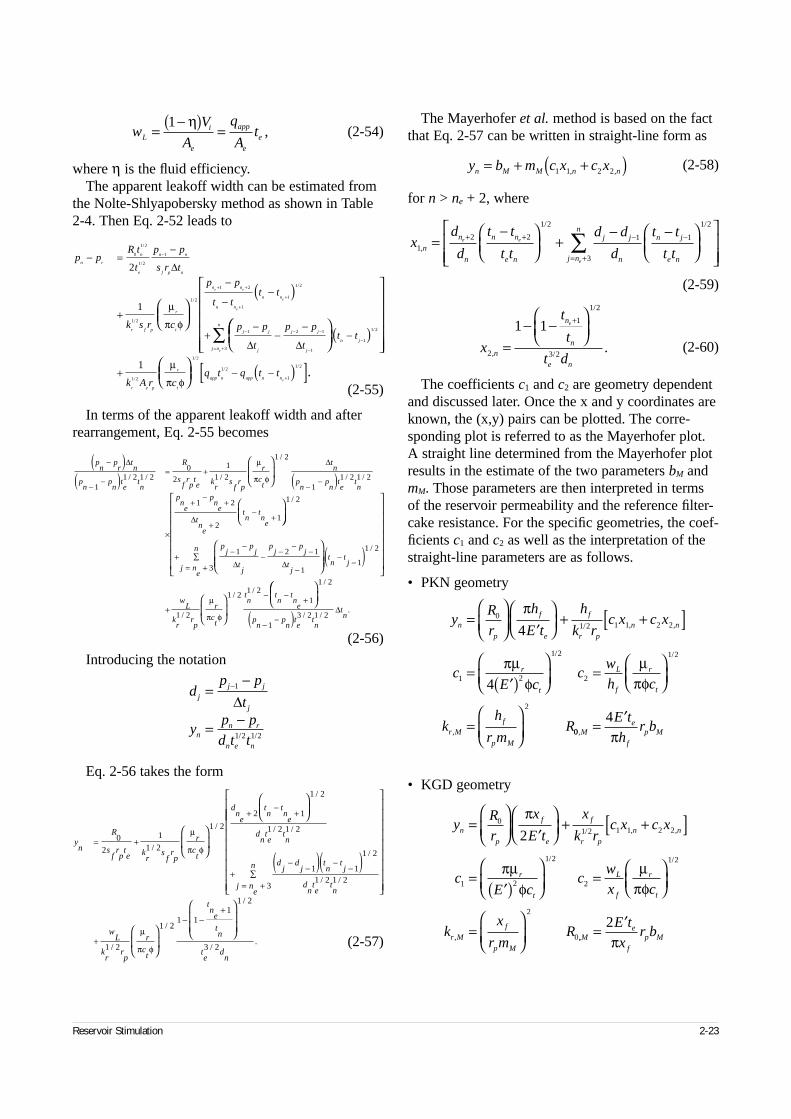
(2-54)

where η is the fluid efficiency.The apparent leakoff width can be estimated from

the Nolte-Shlyapobersky method as shown in Table2-4. Then Eq. 2-52 leads to

(2-55)

In terms of the apparent leakoff width and afterrearrangement, Eq. 2-55 becomes

(2-56)

Introducing the notation

Eq. 2-56 takes the form

(2-57)

The Mayerhofer et al. method is based on the factthat Eq. 2-57 can be written in straight-line form as

(2-58)

for n > ne + 2, where

(2-59)

(2-60)

The coefficients c1 and c2 are geometry dependentand discussed later. Once the x and y coordinates areknown, the (x,y) pairs can be plotted. The corre-sponding plot is referred to as the Mayerhofer plot.A straight line determined from the Mayerhofer plotresults in the estimate of the two parameters bM andmM. Those parameters are then interpreted in termsof the reservoir permeability and the reference filter-cake resistance. For the specific geometries, the coef-ficients c1 and c2 as well as the interpretation of thestraight-line parameters are as follows.

• PKN geometry

• KGD geometry

Reservoir Stimulation 2-23

wV

A

q

AtL

i

e

app

e

e=−( ) =

1 η,

yR

r

h

E t

h

k rc x c x

cE c

cw

h c

kh

r mR

n

p

f

e

f

r p

n n

r

t

L

f

r

t

r Mf

p M

=

′

+ +[ ]

=′( )

=

=

01 2 1 1 2 2

1 2

1 2

2

1 2

2

4

4

π

πµφ

µπφ

/ , ,

/ /

, 00

4,M

e

f

p M

E t

hr b= ′

π

yR

r

x

E t

x

k rc x c x

cE c

cw

x c

kx

r mR

n

p

f

e

f

r p

n n

r

t

L

f

r

t

r Mf

p M

=

′

+ +[ ]

=′( )

=

=

01 2 1 1 2 2

1 2

1 2

2

1 2

2

0

2

π

πµφ

µπφ

/ , ,

/ /

, ,,Me

f

p M

E t

xr b= ′2

π

dp p

t

yp p

d t t

jj j

j

nn r

n e n

=−

= −

−1

1 2 1 2

∆

/ /

yn

R

sf

rp

te k

rs

frp

r

ct

dne

tn

tne

dn

te

tn

dj

dj

tn

tj

dn

te

tn

j ne

n

= +

+−

+

+−

−−

−

= +∑

( )( )

0

2

1

1 2

1 2

2 1

1 2

1 2 1 2

1 1

1 2

1 2 1 23

/

/

/

/ /

/

/ /

µ

π φ

+

− −+

wL

kr

rp

r

ct

tne

tn

te

dn

1 2

1 21 1

11 2

3 2/

/

/

/.

µ

π φ

y b m c x c xn M M n n= + +( )1 1 2 2, ,

xd

d

t t

t t

d d

d

t t

t tn

n

n

n n

e n

j j

n

n j

e nj n

ne e

e

1

2 2

1 2

1 1

1 2

3,

/ /

=−

+− −

+ + − −

= +∑

x

t

t

t dn

n

n

e n

e

2

1

1 2

3 2

1 1

,

/

/.=

− −

+

p pR t

t

p p

s r t

k s r c

p p

t tt t

p p

t

p p

t

n r

n

e

n n

f p n

r f p

r

t

n n

n n

n n

j j

j

j j

j

e e

e

e

− =−

+

−

−−

+−

−−

−

+ +

+

+

− − −

−

( )

0

1 2

1 2

1

1 2

1 2

1 2

1

1

1 2

1 2 1

1

2

1

/

/

/

/

/

∆

∆ ∆

µ

π φ

( )

( )[ ]

= +

−

+

∑ −

+ − −

j n

n

n j

r e p

r

t

app n app n n

e

e

t t

k A r cq t q t t

3

1

1 2

1 2

1 2

1 2

1

1 21

/

/

/

//

.µ

π φ

pn

pr

tn

pn

pn

te

tn

R

sf

rp

te k

rs

frp

r

ct

tn

pn

pn

te

tn

pne

pne

tne

tn

tne

−

−−

= +

−−

×

+−

+

+−

+

( )( )

( )

∆ ∆

∆

11 2 1 2

0

2

1

1 2

1 2

11 2 1 2

1 2

21

/ / /

/

/ /

µ

π φ

( )

+−

−−

−−

−

−= +∑ −

−

+

− −+

1 2

1 2 1

131

1 2

1 2

1 21 2

1

/

/

/

//

pj

pj

tj

pj

pj

tjj n

e

ntn

tj

wL

kr

rp

r

ct

tn

tn

tne

∆ ∆

µ

π φ

( )−−

1 2

13 2 1 2

/

/ /.

pn

pn

te

tn

tn

∆

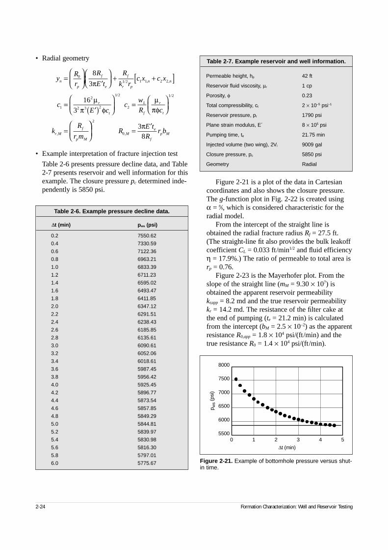
• Radial geometry

• Example interpretation of fracture injection test

Table 2-6 presents pressure decline data, and Table2-7 presents reservoir and well information for thisexample. The closure pressure pc determined inde-pendently is 5850 psi.

Figure 2-21 is a plot of the data in Cartesiancoordinates and also shows the closure pressure.The g-function plot in Fig. 2-22 is created using α = 8⁄9, which is considered characteristic for theradial model.

From the intercept of the straight line isobtained the radial fracture radius Rf = 27.5 ft.(The straight-line fit also provides the bulk leakoffcoefficient CL = 0.033 ft/min1/2 and fluid efficiencyη = 17.9%.) The ratio of permeable to total area isrp = 0.76.

Figure 2-23 is the Mayerhofer plot. From theslope of the straight line (mM = 9.30 × 107) isobtained the apparent reservoir permeability kr,app = 8.2 md and the true reservoir permeabilitykr = 14.2 md. The resistance of the filter cake atthe end of pumping (te = 21.2 min) is calculatedfrom the intercept (bM = 2.5 × 10–2) as the apparentresistance R0,app = 1.8 × 104 psi/(ft/min) and thetrue resistance R0 = 1.4 × 104 psi/(ft/min).

2-24 Formation Characterization: Well and Reservoir Testing

Table 2-6. Example pressure decline data.

∆t (min) pws (psi)

0.2 7550.62

0.4 7330.59

0.6 7122.36

0.8 6963.21

1.0 6833.39

1.2 6711.23

1.4 6595.02

1.6 6493.47

1.8 6411.85

2.0 6347.12

2.2 6291.51

2.4 6238.43

2.6 6185.85

2.8 6135.61

3.0 6090.61

3.2 6052.06

3.4 6018.61

3.6 5987.45

3.8 5956.42

4.0 5925.45

4.2 5896.77

4.4 5873.54

4.6 5857.85

4.8 5849.29

5.0 5844.81

5.2 5839.97

5.4 5830.98

5.6 5816.30

5.8 5797.01

6.0 5775.67

Table 2-7. Example reservoir and well information.

Permeable height, hp 42 ft

Reservoir fluid viscosity, µr 1 cp

Porosity, φ 0.23

Total compressibility, ct 2 × 10–5 psi–1

Reservoir pressure, pr 1790 psi

Plane strain modulus, E´ 8 × 105 psi

Pumping time, te 21.75 min

Injected volume (two wing), 2Vi 9009 gal

Closure pressure, pc 5850 psi

Geometry Radial

Figure 2-21. Example of bottomhole pressure versus shut-in time.

p ws

(psi

)

8000

7500

7000

6500

6000

55000 1 2 3 4 5

∆t (min)

yR

r

R

E t

R

k rc x c x

cE c

cw

R c

kR

r m

n

p

f

e

f

r p

n n

r

t

L

f

r

t

r Mf

p M

=

′

+ +[ ]

=′( )

=

=

01 2 1 1 2 2

1

2

2 3 2

1 2

2

1 2

8

3

16

3

π

µπ φ

µπφ

/ , ,

/ /

,

= ′

2

0

38

RE t

Rr bM

e

f

p M,

π

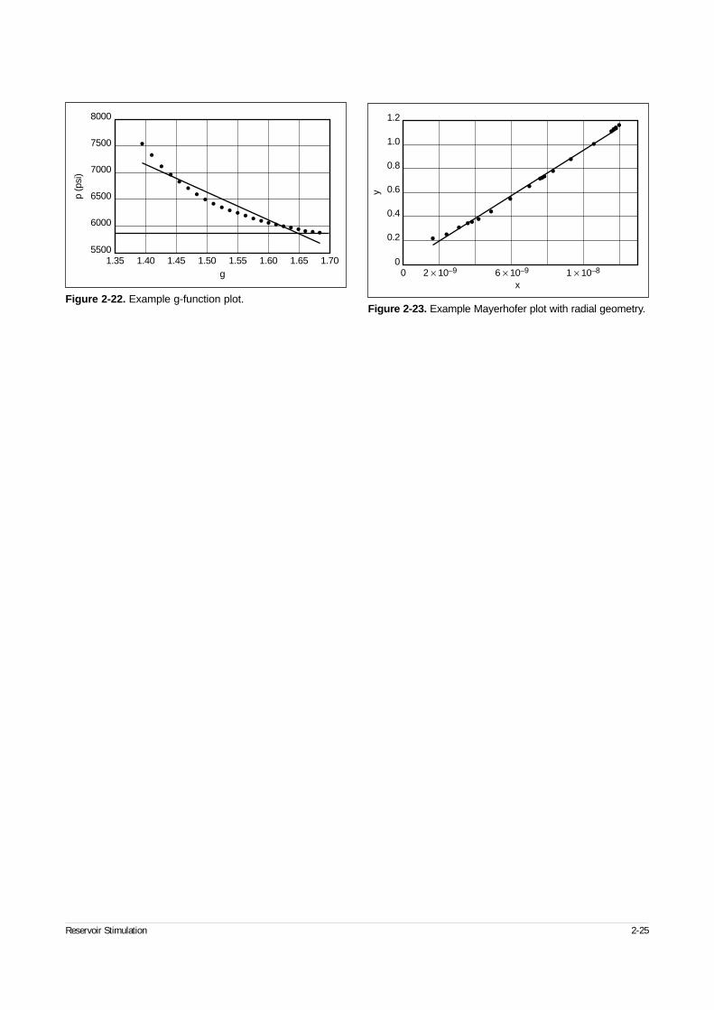
Reservoir Stimulation 2-25

Figure 2-22. Example g-function plot.

p (p

si)

6500

8000

7500

7000

6000

55001.35 1.40 1.45 1.50 1.55 1.60 1.65 1.70

g

Figure 2-23. Example Mayerhofer plot with radial geometry.

y

1.2

1.0

0.8

0.6

0.4

0.2

00 2 × 10–9 6 × 10–9 1 × 10–8

x

3-1. IntroductionThe National Academy of Sciences defines rockmechanics as “the theoretical and applied science of the mechanical behavior of rock; it is that branchof mechanics concerned with the response of the rockto the force fields of its physical environment.” Fromthis definition, the importance of rock mechanics inseveral aspects of the oil and gas industry can easilybe understood. The fragmentation of rock governs itsdrillability, whereas its mechanical behavior influencesall aspects of completion, stimulation and production.However, not until recently has this particular aspectof earth sciences started to play a predominant role inenergy extraction. The impetus was to explain, quali-tatively and quantitatively, the orientation of fractures(Hubbert and Willis, 1957), some unexpected reser-voir responses or catastrophic failures (e.g., less pro-duction after stimulation and pressure decline in wellssurrounding an injection well; Murphy, 1982), casingshear failure (Nester et al., 1956; Cheatham andMcEver, 1964), sand production (Bratli and Risnes,1981; Perkins and Weingarten, 1988; Morita et al.,1987; Veeken et al., 1991; Kooijman et al., 1992;Cook et al., 1994; Moricca et al., 1994; Geilikman et al., 1994; Ramos et al., 1994), rock matrix collapseduring production (Risnes et al., 1982; Pattillo andSmith, 1985; Smits et al., 1988; Abdulraheem et al.,1992) and borehole stability problems (Gnirk, 1972;Bradley, 1979; Guenot, 1989; Santarelli et al., 1992;Ong and Roegiers, 1993; Maury, 1994; Last et al., 1995).

The significant contribution as far as the orientationof fractures is concerned was provided by the workof Hubbert and Willis (1957; see Sidebar 3A), whichindicates ever-increasing differences between verticaland horizontal stresses within the earth’s crust. Untilthen, all design considerations were based on theassumption that an isostatic state of stress prevailedeverywhere.

As deeper completions were attempted, boreholecollapses and instabilities became more common andoften led to expensive remedial measures. The pri-mary cause of these problems is instabilities causedby large tectonic forces. The concepts developed bymining engineers that rocks are far from being inertwere found applicable (Cook, 1967; Hodgson andJoughin, 1967). Rocks are quite receptive to distur-bances, provided that some energy limits are notexceeded. If critical energies are exceeded, dynamicfailure is likely to occur, such as rock burst or casingcollapse. In addition, the importance of inherentdiscontinuities (e.g., faults, fissures) was realized(Goodman, 1976), especially as highly conductiveconduits. From this broader understanding of the roleof rock deformation, research focused on definition of the pertinent parameters required to properly char-acterize the targeted formations. Cores were taken notonly for the determination of permeability, porosityand lithology, but also to run mechanical tests undersimulated downhole conditions. Downhole tools weredeveloped to better characterize the formation in situ.

There will always remain some uncertainties on therelevance of laboratory-determined parameters to thefield situation, either because of the disturbance a coresample suffers during the coring and handling processor because of scale effects. There are also limitationson the use of simple constitutive laws to predict rockbehavior for heterogeneous, discontinuous, time-dependent and/or weak formations. Studies are cur-rently being conducted on these issues, and our under-standing and predictive capability of downhole rockbehavior can be expected to continue to progress.

This chapter briefly summarizes some of the mostimportant aspects of rock mechanics to characterizethe mechanical behavior of reservoirs and adjacentlayers, as applied to the stimulation process.

Reservoir Stimulation 3-1

◆

Formation Characterization:Rock Mechanics

M. C. Thiercelin, Schlumberger DowellJ.-C. Roegiers, University of Oklahoma

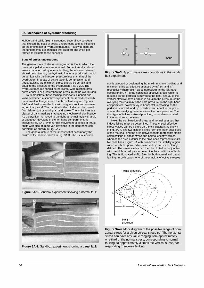
3-2 Formation Characterization: Rock Mechanics

3A. Mechanics of hydraulic fracturing

Hubbert and Willis (1957) introduced several key conceptsthat explain the state of stress underground and its influenceon the orientation of hydraulic fractures. Reviewed here arethe fundamental experiments that Hubbert and Willis per-formed to validate these concepts.

State of stress underground

The general state of stress underground is that in which thethree principal stresses are unequal. For tectonically relaxedareas characterized by normal faulting, the minimum stressshould be horizontal; the hydraulic fractures produced shouldbe vertical with the injection pressure less than that of theoverburden. In areas of active tectonic compression andthrust faulting, the minimum stress should be vertical andequal to the pressure of the overburden (Fig. 3-20). Thehydraulic fractures should be horizontal with injection pres-sures equal to or greater than the pressure of the overburden.

To demonstrate these faulting conditions, Hubbert andWillis performed a sandbox experiment that reproduces boththe normal fault regime and the thrust fault regime. Figures3A-1 and 3A-2 show the box with its glass front and contain-ing ordinary sand. The partition in the middle can be movedfrom left to right by turning a hand screw. The white lines areplaster of paris markers that have no mechanical significance.As the partition is moved to the right, a normal fault with a dipof about 60° develops in the left-hand compartment, asshown in Fig. 3A-1. With further movement, a series of thrustfaults with dips of about 30° develops in the right-hand com-partment, as shown in Fig. 3A-2.

The general nature of the stresses that accompany thefailure of the sand is shown in Fig. 3A-3. The usual conven-

tion is adopted of designating the maximum, intermediate andminimum principal effective stresses by σ1́ , σ2́ and σ3́ ,respectively (here taken as compressive). In the left-handcompartment, σ3́ is the horizontal effective stress, which isreduced as the partition is moved to the right, and σ1́ is thevertical effective stress, which is equal to the pressure of theoverlying material minus the pore pressure. In the right-handcompartment, however, σ1́ is horizontal, increasing as thepartition is moved, and σ3́ is vertical and equal to the pres-sure of the overlying material minus the pore pressure. Thethird type of failure, strike-slip faulting, is not demonstrated in the sandbox experiment.

Next, the combination of shear and normal stresses thatinduce failure must be determined. These critical effectivestress values can be plotted on a Mohr diagram, as shown in Fig. 3A-4. The two diagonal lines form the Mohr envelopesof the material, and the area between them represents stablecombinations of shear stress and normal effective stress,whereas the area exterior to the envelopes represents unsta-ble conditions. Figure 3A-4 thus indicates the stability regionwithin which the permissible values of σn´ and τ are clearlydefined. The stress circles can then be plotted in conjunctionwith the Mohr envelopes to determine the conditions of fault-ing. This is illustrated in Fig. 3A-4 for both normal and thrustfaulting. In both cases, one of the principal effective stresses

Figure 3A-1. Sandbox experiment showing a normal fault.

Figure 3A-2. Sandbox experiment showing a thrust fault.

Figure 3A-3. Approximate stress conditions in the sand-box experiment.

σ1 σ3

σ3 σ1

Sand

Figure 3A-4. Mohr diagram of the possible range of hori-zontal stress for a given vertical stress σv .́ The horizontalstress can have any value ranging from approximatelyone-third of the normal stress, corresponding to normalfaulting, to approximately 3 times the vertical stress, cor-responding to reverse faulting.

σ1́

σ3́

σv́

Mohrenvelope

0

τ

φφ

2a 2a

σ

Points of fracture

φφ

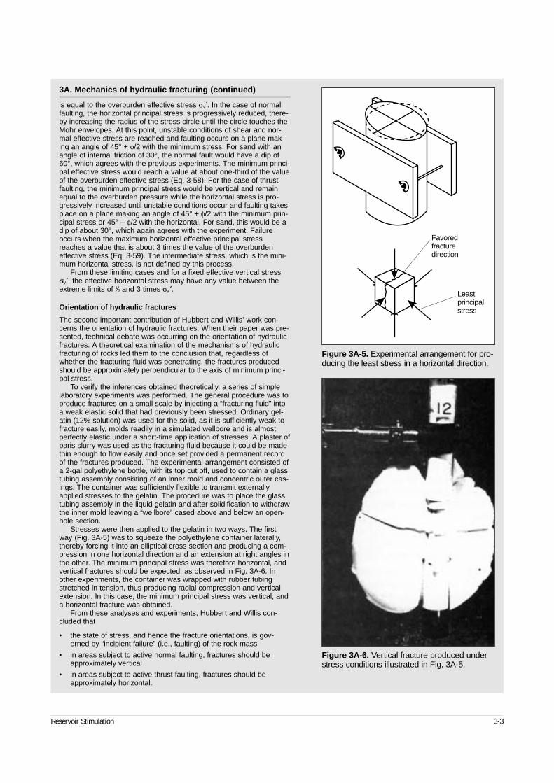
Reservoir Stimulation 3-3

3A. Mechanics of hydraulic fracturing (continued)

is equal to the overburden effective stress σv .́ In the case of normalfaulting, the horizontal principal stress is progressively reduced, there-by increasing the radius of the stress circle until the circle touches theMohr envelopes. At this point, unstable conditions of shear and nor-mal effective stress are reached and faulting occurs on a plane mak-ing an angle of 45° + φ/2 with the minimum stress. For sand with anangle of internal friction of 30°, the normal fault would have a dip of60°, which agrees with the previous experiments. The minimum princi-pal effective stress would reach a value at about one-third of the valueof the overburden effective stress (Eq. 3-58). For the case of thrustfaulting, the minimum principal stress would be vertical and remainequal to the overburden pressure while the horizontal stress is pro-gressively increased until unstable conditions occur and faulting takesplace on a plane making an angle of 45° + φ/2 with the minimum prin-cipal stress or 45° – φ/2 with the horizontal. For sand, this would be adip of about 30°, which again agrees with the experiment. Failureoccurs when the maximum horizontal effective principal stressreaches a value that is about 3 times the value of the overburdeneffective stress (Eq. 3-59). The intermediate stress, which is the mini-mum horizontal stress, is not defined by this process.

From these limiting cases and for a fixed effective vertical stressσv′, the effective horizontal stress may have any value between theextreme limits of 1⁄3 and 3 times σv′.

Orientation of hydraulic fractures

The second important contribution of Hubbert and Willis’ work con-cerns the orientation of hydraulic fractures. When their paper was pre-sented, technical debate was occurring on the orientation of hydraulicfractures. A theoretical examination of the mechanisms of hydraulicfracturing of rocks led them to the conclusion that, regardless ofwhether the fracturing fluid was penetrating, the fractures producedshould be approximately perpendicular to the axis of minimum princi-pal stress.

To verify the inferences obtained theoretically, a series of simplelaboratory experiments was performed. The general procedure was toproduce fractures on a small scale by injecting a “fracturing fluid” intoa weak elastic solid that had previously been stressed. Ordinary gel-atin (12% solution) was used for the solid, as it is sufficiently weak tofracture easily, molds readily in a simulated wellbore and is almostperfectly elastic under a short-time application of stresses. A plaster ofparis slurry was used as the fracturing fluid because it could be madethin enough to flow easily and once set provided a permanent recordof the fractures produced. The experimental arrangement consisted ofa 2-gal polyethylene bottle, with its top cut off, used to contain a glasstubing assembly consisting of an inner mold and concentric outer cas-ings. The container was sufficiently flexible to transmit externallyapplied stresses to the gelatin. The procedure was to place the glasstubing assembly in the liquid gelatin and after solidification to withdrawthe inner mold leaving a “wellbore” cased above and below an open-hole section.

Stresses were then applied to the gelatin in two ways. The firstway (Fig. 3A-5) was to squeeze the polyethylene container laterally,thereby forcing it into an elliptical cross section and producing a com-pression in one horizontal direction and an extension at right angles inthe other. The minimum principal stress was therefore horizontal, andvertical fractures should be expected, as observed in Fig. 3A-6. Inother experiments, the container was wrapped with rubber tubingstretched in tension, thus producing radial compression and verticalextension. In this case, the minimum principal stress was vertical, anda horizontal fracture was obtained.

From these analyses and experiments, Hubbert and Willis con-cluded that

• the state of stress, and hence the fracture orientations, is gov-erned by “incipient failure” (i.e., faulting) of the rock mass

• in areas subject to active normal faulting, fractures should beapproximately vertical

• in areas subject to active thrust faulting, fractures should beapproximately horizontal.

Figure 3A-5. Experimental arrangement for pro-ducing the least stress in a horizontal direction.

Favoredfracturedirection

Leastprincipalstress

Figure 3A-6. Vertical fracture produced understress conditions illustrated in Fig. 3A-5.

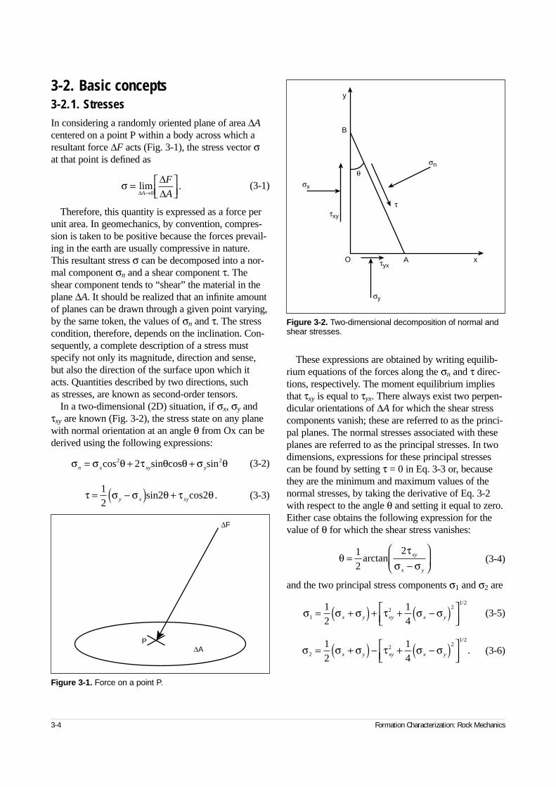
3-2. Basic concepts3-2.1. StressesIn considering a randomly oriented plane of area ∆Acentered on a point P within a body across which aresultant force ∆F acts (Fig. 3-1), the stress vector σat that point is defined as

(3-1)

Therefore, this quantity is expressed as a force perunit area. In geomechanics, by convention, compres-sion is taken to be positive because the forces prevail-ing in the earth are usually compressive in nature.This resultant stress σ can be decomposed into a nor-mal component σn and a shear component τ. Theshear component tends to “shear” the material in theplane ∆A. It should be realized that an infinite amountof planes can be drawn through a given point varying,by the same token, the values of σn and τ. The stresscondition, therefore, depends on the inclination. Con-sequently, a complete description of a stress mustspecify not only its magnitude, direction and sense,but also the direction of the surface upon which itacts. Quantities described by two directions, such as stresses, are known as second-order tensors.

In a two-dimensional (2D) situation, if σx, σy andτxy are known (Fig. 3-2), the stress state on any planewith normal orientation at an angle θ from Ox can bederived using the following expressions:

(3-2)

(3-3)

These expressions are obtained by writing equilib-rium equations of the forces along the σn and τ direc-tions, respectively. The moment equilibrium impliesthat τxy is equal to τyx. There always exist two perpen-dicular orientations of ∆A for which the shear stresscomponents vanish; these are referred to as the princi-pal planes. The normal stresses associated with theseplanes are referred to as the principal stresses. In twodimensions, expressions for these principal stressescan be found by setting τ = 0 in Eq. 3-3 or, becausethey are the minimum and maximum values of thenormal stresses, by taking the derivative of Eq. 3-2with respect to the angle θ and setting it equal to zero.Either case obtains the following expression for thevalue of θ for which the shear stress vanishes:

(3-4)

and the two principal stress components σ1 and σ2 are

(3-5)

(3-6)

3-4 Formation Characterization: Rock Mechanics

σ =

→

lim∆

∆∆A

F

A0.

σ σ θ τ θ θ σ θn x xy y= + +cos sin cos sin2 22

θτ

σ σ=

−

12

2arctan xy

x y

σ σ σ τ σ σ12 2

1 212

14

= +( ) + + −( )

x y xy x y

/

σ σ σ τ σ σ22 2

1 212

14

= +( ) − + −( )

x y xy x y

/

.

τ σ σ θ τ θ= −( ) +12

2y x xysin2 cos .

Figure 3-1. Force on a point P.

P∆A

∆F

Figure 3-2. Two-dimensional decomposition of normal andshear stresses.

y

B

θσn

σy

τ

σx

τxy

τyxA xO

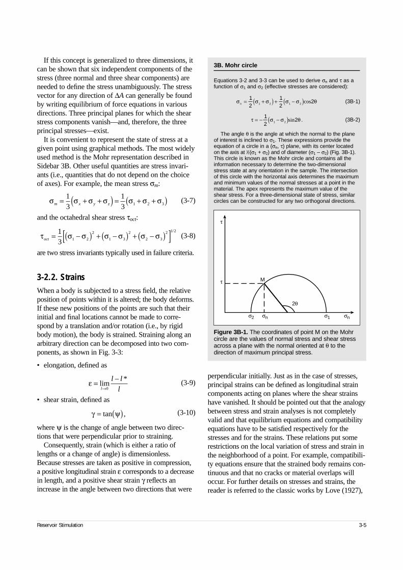
If this concept is generalized to three dimensions, itcan be shown that six independent components of thestress (three normal and three shear components) areneeded to define the stress unambiguously. The stressvector for any direction of ∆A can generally be foundby writing equilibrium of force equations in variousdirections. Three principal planes for which the shearstress components vanish—and, therefore, the threeprincipal stresses—exist.

It is convenient to represent the state of stress at agiven point using graphical methods. The most widelyused method is the Mohr representation described inSidebar 3B. Other useful quantities are stress invari-ants (i.e., quantities that do not depend on the choiceof axes). For example, the mean stress σm:

(3-7)

and the octahedral shear stress τoct:

(3-8)

are two stress invariants typically used in failure criteria.

3-2.2. StrainsWhen a body is subjected to a stress field, the relativeposition of points within it is altered; the body deforms.If these new positions of the points are such that theirinitial and final locations cannot be made to corre-spond by a translation and/or rotation (i.e., by rigidbody motion), the body is strained. Straining along anarbitrary direction can be decomposed into two com-ponents, as shown in Fig. 3-3:

• elongation, defined as

(3-9)

• shear strain, defined as

(3-10)

where ψ is the change of angle between two direc-tions that were perpendicular prior to straining.

Consequently, strain (which is either a ratio oflengths or a change of angle) is dimensionless.Because stresses are taken as positive in compression,a positive longitudinal strain ε corresponds to a decreasein length, and a positive shear strain γ reflects an increase in the angle between two directions that were

perpendicular initially. Just as in the case of stresses,principal strains can be defined as longitudinal straincomponents acting on planes where the shear strainshave vanished. It should be pointed out that the analogybetween stress and strain analyses is not completelyvalid and that equilibrium equations and compatibilityequations have to be satisfied respectively for thestresses and for the strains. These relations put somerestrictions on the local variation of stress and strain inthe neighborhood of a point. For example, compatibili-ty equations ensure that the strained body remains con-tinuous and that no cracks or material overlaps willoccur. For further details on stresses and strains, thereader is referred to the classic works by Love (1927),

Reservoir Stimulation 3-5

σ σ σ σ σ σ σm x y z= + +( ) = + +( )13

13 1 2 3

τ σ σ σ σ σ σoct = −( ) + −( ) + −( )[ ]13 1 2

2

1 3

2

2 3

2 1 2/

ε = −→

liml

l l

l0

*

γ ψ= ( )tan ,

3B. Mohr circle

Equations 3-2 and 3-3 can be used to derive σn and τ as afunction of σ1 and σ2 (effective stresses are considered):

(3B-1)

(3B-2)

The angle θ is the angle at which the normal to the planeof interest is inclined to σ1. These expressions provide theequation of a circle in a (σn, τ) plane, with its center locatedon the axis at 1⁄2(σ1 + σ2) and of diameter (σ1 – σ2) (Fig. 3B-1).This circle is known as the Mohr circle and contains all theinformation necessary to determine the two-dimensionalstress state at any orientation in the sample. The intersectionof this circle with the horizontal axis determines the maximumand minimum values of the normal stresses at a point in thematerial. The apex represents the maximum value of theshear stress. For a three-dimensional state of stress, similarcircles can be constructed for any two orthogonal directions.

σ σ σ σ σ θn = +( ) + −( )12

12

21 2 1 2 cos

τ σ σ θ= − −( )12

21 2 sin .

Figure 3B-1. The coordinates of point M on the Mohrcircle are the values of normal stress and shear stressacross a plane with the normal oriented at θ to thedirection of maximum principal stress.

τ

τ

σ2 σn σnσ1

2θ

M

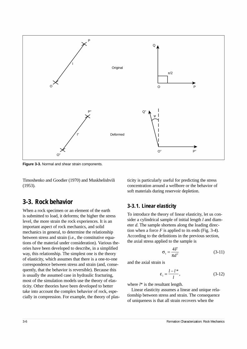
Timoshenko and Goodier (1970) and Muskhelishvili(1953).

3-3. Rock behaviorWhen a rock specimen or an element of the earth is submitted to load, it deforms; the higher the stresslevel, the more strain the rock experiences. It is animportant aspect of rock mechanics, and solidmechanics in general, to determine the relationshipbetween stress and strain (i.e., the constitutive equa-tions of the material under consideration). Various the-ories have been developed to describe, in a simplifiedway, this relationship. The simplest one is the theoryof elasticity, which assumes that there is a one-to-onecorrespondence between stress and strain (and, conse-quently, that the behavior is reversible). Because thisis usually the assumed case in hydraulic fracturing,most of the simulation models use the theory of elas-ticity. Other theories have been developed to bettertake into account the complex behavior of rock, espe-cially in compression. For example, the theory of plas-

ticity is particularly useful for predicting the stressconcentration around a wellbore or the behavior ofsoft materials during reservoir depletion.

3-3.1. Linear elasticityTo introduce the theory of linear elasticity, let us con-sider a cylindrical sample of initial length l and diam-eter d. The sample shortens along the loading direc-tion when a force F is applied to its ends (Fig. 3-4).According to the definitions in the previous section,the axial stress applied to the sample is

(3-11)

and the axial strain is

(3-12)

where l* is the resultant length.Linear elasticity assumes a linear and unique rela-

tionship between stress and strain. The consequenceof uniqueness is that all strain recovers when the

3-6 Formation Characterization: Rock Mechanics

Figure 3-3. Normal and shear strain components.

Original

Deformed

P

O

l

P∗ Q∗

ψ

π/2

l∗

O∗

Q

O P

O∗ P∗

σπ1 2

4= F

d

ε1 = −l l

l

*,

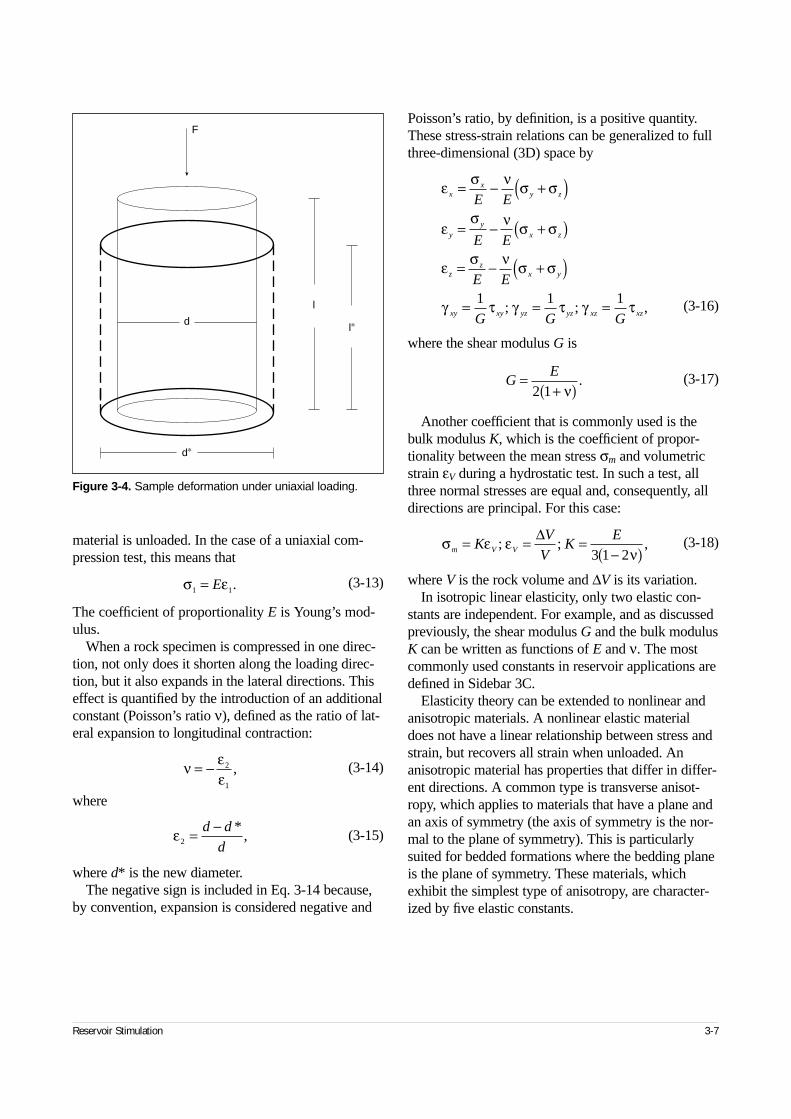
material is unloaded. In the case of a uniaxial com-pression test, this means that

(3-13)

The coefficient of proportionality E is Young’s mod-ulus.

When a rock specimen is compressed in one direc-tion, not only does it shorten along the loading direc-tion, but it also expands in the lateral directions. Thiseffect is quantified by the introduction of an additionalconstant (Poisson’s ratio ν), defined as the ratio of lat-eral expansion to longitudinal contraction:

(3-14)

where

(3-15)

where d* is the new diameter.The negative sign is included in Eq. 3-14 because,

by convention, expansion is considered negative and

Poisson’s ratio, by definition, is a positive quantity.These stress-strain relations can be generalized to fullthree-dimensional (3D) space by

(3-16)

where the shear modulus G is

(3-17)

Another coefficient that is commonly used is thebulk modulus K, which is the coefficient of propor-tionality between the mean stress σm and volumetricstrain εV during a hydrostatic test. In such a test, allthree normal stresses are equal and, consequently, alldirections are principal. For this case:

(3-18)

where V is the rock volume and ∆V is its variation.In isotropic linear elasticity, only two elastic con-

stants are independent. For example, and as discussedpreviously, the shear modulus G and the bulk modulusK can be written as functions of E and ν. The mostcommonly used constants in reservoir applications aredefined in Sidebar 3C.

Elasticity theory can be extended to nonlinear andanisotropic materials. A nonlinear elastic materialdoes not have a linear relationship between stress andstrain, but recovers all strain when unloaded. Ananisotropic material has properties that differ in differ-ent directions. A common type is transverse anisot-ropy, which applies to materials that have a plane andan axis of symmetry (the axis of symmetry is the nor-mal to the plane of symmetry). This is particularlysuited for bedded formations where the bedding planeis the plane of symmetry. These materials, whichexhibit the simplest type of anisotropy, are character-ized by five elastic constants.

Reservoir Stimulation 3-7

Figure 3-4. Sample deformation under uniaxial loading.

d

d∗

l∗

l

F

σ ε1 1= E .

ν εε

= − 2

1

,

ε2 = −d d

d

*,

ε σ ν σ σ

εσ ν σ σ

ε σ ν σ σ

γ τ γ τ γ τ

xx

y z

yy

x z

zz

x y

xy xy yz yz xz xz

E E

E E

E E

G G G

= − +( )= − +( )

= − +( )= = =1 1 1

; ; ,

GE=+( )2 1 ν

.

σ ε ενm V VK

V

VK

E= = =−( )

; ; ,∆

3 1 2

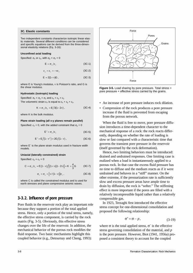
3-3.2. Influence of pore pressurePore fluids in the reservoir rock play an important rolebecause they support a portion of the total appliedstress. Hence, only a portion of the total stress, namely,the effective stress component, is carried by the rockmatrix (Fig. 3-5). Obviously, this effective stresschanges over the life of the reservoir. In addition, themechanical behavior of the porous rock modifies thefluid response. Two basic mechanisms highlight thiscoupled behavior (e.g., Detournay and Cheng, 1993):

• An increase of pore pressure induces rock dilation.

• Compression of the rock produces a pore pressureincrease if the fluid is prevented from escapingfrom the porous network.

When the fluid is free to move, pore pressure diffu-sion introduces a time-dependent character to themechanical response of a rock: the rock reacts differ-ently, depending on whether the rate of loading isslow or fast compared with a characteristic time thatgoverns the transient pore pressure in the reservoir(itself governed by the rock deformation).

Hence, two limiting behaviors must be introduced:drained and undrained responses. One limiting case isrealized when a load is instantaneously applied to aporous rock. In that case the excess fluid pressure hasno time to diffuse and the medium reacts as if it wereundrained and behaves in a “stiff” manner. On theother extreme, if the pressurization rate is sufficientlyslow and excess pressure areas have ample time todrain by diffusion, the rock is “softer.” The stiffeningeffect is more important if the pores are filled with arelatively incompressible liquid rather than a relativelycompressible gas.

In 1923, Terzaghi first introduced the effectivestress concept for one-dimensional consolidation andproposed the following relationship:

(3-19)

where σ is the total applied stress, σ´ is the effectivestress governing consolidation of the material, and pis the pore pressure. However, Biot (1941, 1956a) pro-posed a consistent theory to account for the coupled

3-8 Formation Characterization: Rock Mechanics

3C. Elastic constants

Two independent constants characterize isotropic linear elas-tic materials. Several different conditions can be consideredand specific equations can be derived from the three-dimen-sional elasticity relations (Eq. 3-16):

Unconfined axial loading

Specified: σx or εx, with σy = σz = 0

(3C-1)

(3C-2)

(3C-3)

where E is Young’s modulus, ν is Poisson’s ratio, and G isthe shear modulus.

Hydrostatic (isotropic) loading

Specified: σx = σy = σz and εx = εy = εz

The volumetric strain εV is equal to εx + εy + εz.

(3C-4)

where K is the bulk modulus.

Plane strain loading (all x-y planes remain parallel)

Specified: εz = 0, with the added constraint that σy = 0

(3C-5)

(3C-6)

where E´ is the plane strain modulus used in fracture widthmodels.

Uniaxial (laterally constrained) strain

Specified: εy = εz = 0

(3C-7)

(3C-8)

where C is called the constrained modulus and is used forearth stresses and plane compressive seismic waves.

E x x= σ ε

ε ε νεy z x= = −

E G= +2 1( ) ,ν

K Ex V= = −( )σ ε ν3 1 2 ,

′ =E x xσ ε

′ = −( ) = −( )E E G1 2 12ν ν ,

C E K Gx x= = −( ) +( ) −( )[ ] = +σ ε ν ν ν1 1 1 243

σ σ ν ν σz y x= = −( )[ ]/ ,1

Figure 3-5. Load sharing by pore pressure. Total stress =pore pressure + effective stress carried by the grains.

Force

Force

Pores

Grains

′ = −σ σ p ,

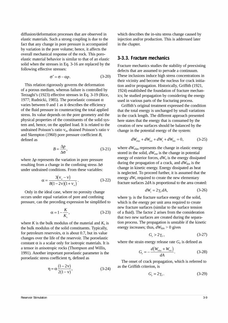
diffusion/deformation processes that are observed inelastic materials. Such a strong coupling is due to thefact that any change in pore pressure is accompaniedby variation in the pore volume; hence, it affects theoverall mechanical response of the rock. This poro-elastic material behavior is similar to that of an elasticsolid when the stresses in Eq. 3-16 are replaced by thefollowing effective stresses:

(3-20)

This relation rigorously governs the deformation of a porous medium, whereas failure is controlled byTerzaghi’s (1923) effective stresses in Eq. 3-19 (Rice,1977; Rudnicki, 1985). The poroelastic constant αvaries between 0 and 1 as it describes the efficiency of the fluid pressure in counteracting the total appliedstress. Its value depends on the pore geometry and thephysical properties of the constituents of the solid sys-tem and, hence, on the applied load. It is related to theundrained Poisson’s ratio νu, drained Poisson’s ratio νand Skempton (1960) pore pressure coefficient B,defined as

(3-21)

where ∆p represents the variation in pore pressureresulting from a change in the confining stress ∆σunder undrained conditions. From these variables:

(3-22)

Only in the ideal case, where no porosity changeoccurs under equal variation of pore and confiningpressure, can the preceding expression be simplified to

(3-23)

where K is the bulk modulus of the material and Ks isthe bulk modulus of the solid constituents. Typically,for petroleum reservoirs, α is about 0.7, but its valuechanges over the life of the reservoir. The poroelasticconstant α is a scalar only for isotropic materials. It isa tensor in anisotropic rocks (Thompson and Willis,1991). Another important poroelastic parameter is theporoelastic stress coefficient η, defined as

(3-24)

which describes the in-situ stress change caused byinjection and/or production. This is addressed later in the chapter.

3-3.3. Fracture mechanicsFracture mechanics studies the stability of preexistingdefects that are assumed to pervade a continuum.These inclusions induce high stress concentrations intheir vicinity and become the nucleus for crack initia-tion and/or propagation. Historically, Griffith (1921,1924) established the foundation of fracture mechan-ics; he studied propagation by considering the energyused in various parts of the fracturing process.

Griffith’s original treatment expressed the conditionthat the total energy is unchanged by small variationsin the crack length. The different approach presentedhere states that the energy that is consumed by thecreation of new surfaces should be balanced by thechange in the potential energy of the system:

(3-25)

where dWelas represents the change in elastic energystored in the solid, dWext is the change in potentialenergy of exterior forces, dWs is the energy dissipatedduring the propagation of a crack, and dWkin is thechange in kinetic energy. Energy dissipated as heat is neglected. To proceed further, it is assumed that theenergy dWs required to create the new elementaryfracture surfaces 2dA is proportional to the area created:

(3-26)

where γF is the fracture surface energy of the solid,which is the energy per unit area required to createnew fracture surfaces (similar to the surface tension of a fluid). The factor 2 arises from the considerationthat two new surfaces are created during the separa-tion process. The propagation is unstable if the kineticenergy increases; thus, dWkin > 0 gives

(3-27)

where the strain energy release rate Ge is defined as

(3-28)

The onset of crack propagation, which is referred toas the Griffith criterion, is

(3-29)

Reservoir Stimulation 3-9

′ = −σ σ αp.

Bp= ∆

∆σ,

dW dW dW dWelas ext s kin+ + + = 0,

dW dAs F= 2γ ,

Ge F> 2γ ,

Gd W W

dAeelas ext= −

+( ).

Ge F= 2γ .

αν νν ν

=−( )

−( ) +( )3

1 2 1u

uB.

α = −1K

Ks

,

η α νν

= −( )−( )

1 22 1

,

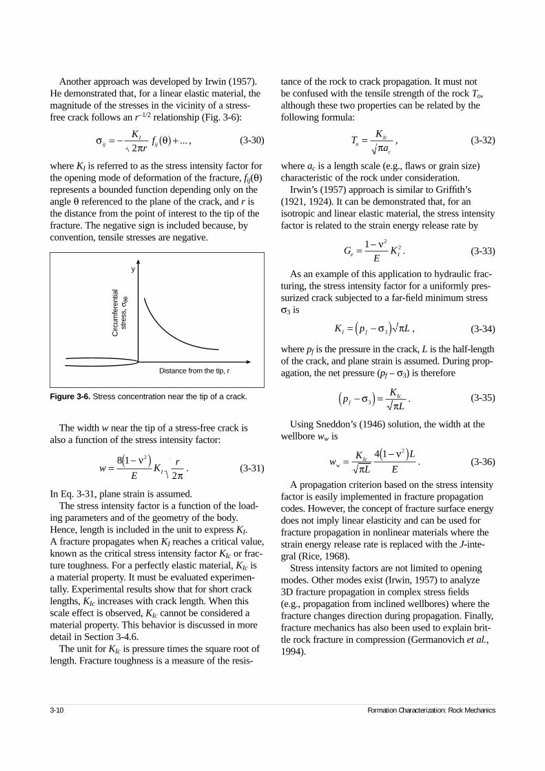
Another approach was developed by Irwin (1957).He demonstrated that, for a linear elastic material, themagnitude of the stresses in the vicinity of a stress-free crack follows an r–1/2 relationship (Fig. 3-6):

(3-30)

where KI is referred to as the stress intensity factor forthe opening mode of deformation of the fracture, fij(θ)represents a bounded function depending only on theangle θ referenced to the plane of the crack, and r isthe distance from the point of interest to the tip of thefracture. The negative sign is included because, byconvention, tensile stresses are negative.

The width w near the tip of a stress-free crack isalso a function of the stress intensity factor:

(3-31)

In Eq. 3-31, plane strain is assumed.The stress intensity factor is a function of the load-

ing parameters and of the geometry of the body.Hence, length is included in the unit to express KI.A fracture propagates when KI reaches a critical value,known as the critical stress intensity factor KIc or frac-ture toughness. For a perfectly elastic material, KIc isa material property. It must be evaluated experimen-tally. Experimental results show that for short cracklengths, KIc increases with crack length. When thisscale effect is observed, KIc cannot be considered amaterial property. This behavior is discussed in moredetail in Section 3-4.6.

The unit for KIc is pressure times the square root oflength. Fracture toughness is a measure of the resis-

tance of the rock to crack propagation. It must not be confused with the tensile strength of the rock To,although these two properties can be related by thefollowing formula:

(3-32)

where ac is a length scale (e.g., flaws or grain size)characteristic of the rock under consideration.

Irwin’s (1957) approach is similar to Griffith’s(1921, 1924). It can be demonstrated that, for anisotropic and linear elastic material, the stress intensityfactor is related to the strain energy release rate by

(3-33)

As an example of this application to hydraulic frac-turing, the stress intensity factor for a uniformly pres-surized crack subjected to a far-field minimum stressσ3 is

(3-34)

where pf is the pressure in the crack, L is the half-lengthof the crack, and plane strain is assumed. During prop-agation, the net pressure (pf – σ3) is therefore

(3-35)

Using Sneddon’s (1946) solution, the width at thewellbore ww is

(3-36)

A propagation criterion based on the stress intensityfactor is easily implemented in fracture propagationcodes. However, the concept of fracture surface energydoes not imply linear elasticity and can be used forfracture propagation in nonlinear materials where thestrain energy release rate is replaced with the J-inte-gral (Rice, 1968).

Stress intensity factors are not limited to openingmodes. Other modes exist (Irwin, 1957) to analyze 3D fracture propagation in complex stress fields (e.g., propagation from inclined wellbores) where thefracture changes direction during propagation. Finally,fracture mechanics has also been used to explain brit-tle rock fracture in compression (Germanovich et al.,1994).

3-10 Formation Characterization: Rock Mechanics

σπ

θijI

ij

K

rf= − ( ) +

2... , T

K

aoIc

c

=π

,

GE

Ke I= −1 22ν.

K p LI f= −( )σ π3 ,

pK

LfIc−( ) =σ

π3 .

wK

L

L

EwIc=

−( )π

ν4 1 2

.w

EK

rI=

−( )8 1

2

2νπ

.

Figure 3-6. Stress concentration near the tip of a crack.

y

Circ

umfe

rent

ial

stre

ss,σ

θθ

Distance from the tip, r

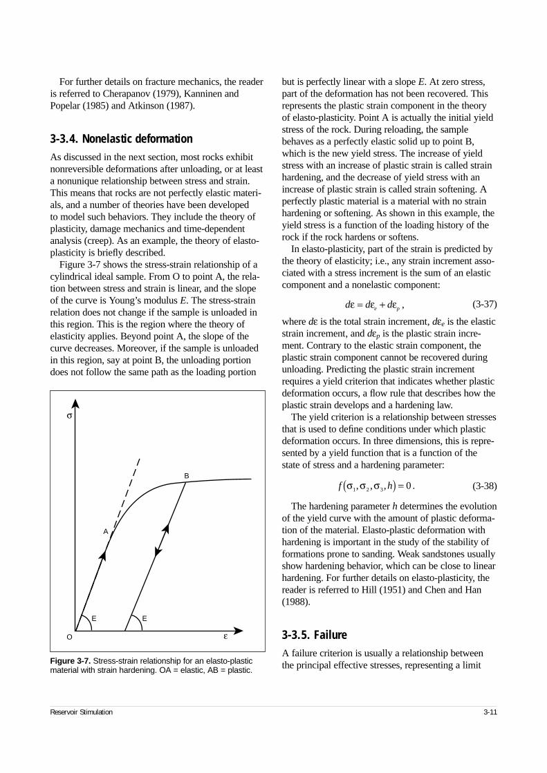
For further details on fracture mechanics, the readeris referred to Cherapanov (1979), Kanninen andPopelar (1985) and Atkinson (1987).

3-3.4. Nonelastic deformationAs discussed in the next section, most rocks exhibitnonreversible deformations after unloading, or at leasta nonunique relationship between stress and strain.This means that rocks are not perfectly elastic materi-als, and a number of theories have been developed to model such behaviors. They include the theory ofplasticity, damage mechanics and time-dependentanalysis (creep). As an example, the theory of elasto-plasticity is briefly described.

Figure 3-7 shows the stress-strain relationship of acylindrical ideal sample. From O to point A, the rela-tion between stress and strain is linear, and the slopeof the curve is Young’s modulus E. The stress-strainrelation does not change if the sample is unloaded inthis region. This is the region where the theory ofelasticity applies. Beyond point A, the slope of thecurve decreases. Moreover, if the sample is unloadedin this region, say at point B, the unloading portiondoes not follow the same path as the loading portion

but is perfectly linear with a slope E. At zero stress,part of the deformation has not been recovered. Thisrepresents the plastic strain component in the theoryof elasto-plasticity. Point A is actually the initial yieldstress of the rock. During reloading, the samplebehaves as a perfectly elastic solid up to point B,which is the new yield stress. The increase of yieldstress with an increase of plastic strain is called strainhardening, and the decrease of yield stress with anincrease of plastic strain is called strain softening. Aperfectly plastic material is a material with no strainhardening or softening. As shown in this example, theyield stress is a function of the loading history of therock if the rock hardens or softens.

In elasto-plasticity, part of the strain is predicted bythe theory of elasticity; i.e., any strain increment asso-ciated with a stress increment is the sum of an elasticcomponent and a nonelastic component:

(3-37)

where dε is the total strain increment, dεe is the elasticstrain increment, and dεp is the plastic strain incre-ment. Contrary to the elastic strain component, theplastic strain component cannot be recovered duringunloading. Predicting the plastic strain incrementrequires a yield criterion that indicates whether plasticdeformation occurs, a flow rule that describes how theplastic strain develops and a hardening law.

The yield criterion is a relationship between stressesthat is used to define conditions under which plasticdeformation occurs. In three dimensions, this is repre-sented by a yield function that is a function of thestate of stress and a hardening parameter:

(3-38)

The hardening parameter h determines the evolutionof the yield curve with the amount of plastic deforma-tion of the material. Elasto-plastic deformation withhardening is important in the study of the stability offormations prone to sanding. Weak sandstones usuallyshow hardening behavior, which can be close to linearhardening. For further details on elasto-plasticity, thereader is referred to Hill (1951) and Chen and Han(1988).

3-3.5. FailureA failure criterion is usually a relationship betweenthe principal effective stresses, representing a limit

Reservoir Stimulation 3-11

Figure 3-7. Stress-strain relationship for an elasto-plasticmaterial with strain hardening. OA = elastic, AB = plastic.

σ

A

O

B

ε

E E

d d de pε ε ε= + ,

f hσ σ σ1 2 3 0, , , .( ) =

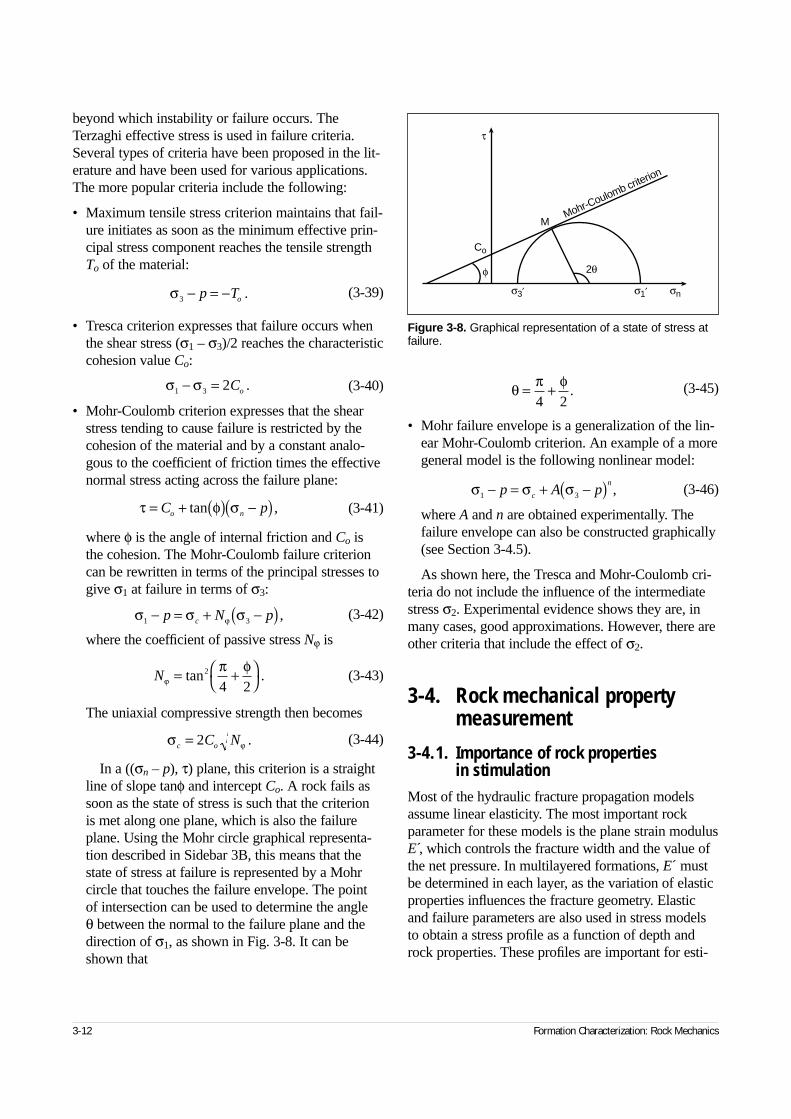
beyond which instability or failure occurs. TheTerzaghi effective stress is used in failure criteria.Several types of criteria have been proposed in the lit-erature and have been used for various applications.The more popular criteria include the following:

• Maximum tensile stress criterion maintains that fail-ure initiates as soon as the minimum effective prin-cipal stress component reaches the tensile strengthTo of the material:

(3-39)

• Tresca criterion expresses that failure occurs whenthe shear stress (σ1 – σ3)/2 reaches the characteristiccohesion value Co:

(3-40)

• Mohr-Coulomb criterion expresses that the shearstress tending to cause failure is restricted by thecohesion of the material and by a constant analo-gous to the coefficient of friction times the effectivenormal stress acting across the failure plane:

(3-41)

where φ is the angle of internal friction and Co isthe cohesion. The Mohr-Coulomb failure criterioncan be rewritten in terms of the principal stresses togive σ1 at failure in terms of σ3:

(3-42)

where the coefficient of passive stress Nϕ is

(3-43)

The uniaxial compressive strength then becomes

(3-44)

In a ((σn – p), τ) plane, this criterion is a straightline of slope tanφ and intercept Co. A rock fails assoon as the state of stress is such that the criterion is met along one plane, which is also the failureplane. Using the Mohr circle graphical representa-tion described in Sidebar 3B, this means that thestate of stress at failure is represented by a Mohrcircle that touches the failure envelope. The point of intersection can be used to determine the angle θ between the normal to the failure plane and thedirection of σ1, as shown in Fig. 3-8. It can beshown that

(3-45)

• Mohr failure envelope is a generalization of the lin-ear Mohr-Coulomb criterion. An example of a moregeneral model is the following nonlinear model:

(3-46)

where A and n are obtained experimentally. Thefailure envelope can also be constructed graphically(see Section 3-4.5).

As shown here, the Tresca and Mohr-Coulomb cri-teria do not include the influence of the intermediatestress σ2. Experimental evidence shows they are, inmany cases, good approximations. However, there areother criteria that include the effect of σ2.

3-4. Rock mechanical property measurement

3-4.1. Importance of rock properties in stimulation

Most of the hydraulic fracture propagation modelsassume linear elasticity. The most important rockparameter for these models is the plane strain modulusE ,́ which controls the fracture width and the value ofthe net pressure. In multilayered formations, E´ mustbe determined in each layer, as the variation of elasticproperties influences the fracture geometry. Elasticand failure parameters are also used in stress modelsto obtain a stress profile as a function of depth androck properties. These profiles are important for esti-

3-12 Formation Characterization: Rock Mechanics

σ3 − = −p To .

σ σ1 3 2− = Co . θ π φ= +4 2

.

σ σ σ1 3− = + −( )p A pc

n,

τ φ σ= + ( ) −( )C po ntan ,

σ σ σϕ1 3− = + −( )p N pc ,

Nϕπ φ= +

tan2

4 2.

σ ϕc oC N= 2 .

Figure 3-8. Graphical representation of a state of stress atfailure.

τ

φ

M

Co

σ3′ σ1′ σn

2θ

Mohr-Coulomb criterion

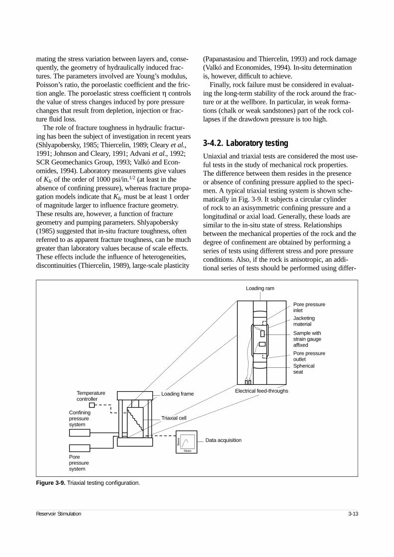
mating the stress variation between layers and, conse-quently, the geometry of hydraulically induced frac-tures. The parameters involved are Young’s modulus,Poisson’s ratio, the poroelastic coefficient and the fric-tion angle. The poroelastic stress coefficient η controlsthe value of stress changes induced by pore pressurechanges that result from depletion, injection or frac-ture fluid loss.

The role of fracture toughness in hydraulic fractur-ing has been the subject of investigation in recent years(Shlyapobersky, 1985; Thiercelin, 1989; Cleary et al.,1991; Johnson and Cleary, 1991; Advani et al., 1992;SCR Geomechanics Group, 1993; Valkó and Econ-omides, 1994). Laboratory measurements give valuesof KIc of the order of 1000 psi/in.1/2 (at least in theabsence of confining pressure), whereas fracture propa-gation models indicate that KIc must be at least 1 orderof magnitude larger to influence fracture geometry.These results are, however, a function of fracturegeometry and pumping parameters. Shlyapobersky(1985) suggested that in-situ fracture toughness, oftenreferred to as apparent fracture toughness, can be muchgreater than laboratory values because of scale effects.These effects include the influence of heterogeneities,discontinuities (Thiercelin, 1989), large-scale plasticity

(Papanastasiou and Thiercelin, 1993) and rock damage(Valkó and Economides, 1994). In-situ determinationis, however, difficult to achieve.

Finally, rock failure must be considered in evaluat-ing the long-term stability of the rock around the frac-ture or at the wellbore. In particular, in weak forma-tions (chalk or weak sandstones) part of the rock col-lapses if the drawdown pressure is too high.

3-4.2. Laboratory testingUniaxial and triaxial tests are considered the most use-ful tests in the study of mechanical rock properties.The difference between them resides in the presenceor absence of confining pressure applied to the speci-men. A typical triaxial testing system is shown sche-matically in Fig. 3-9. It subjects a circular cylinder of rock to an axisymmetric confining pressure and alongitudinal or axial load. Generally, these loads aresimilar to the in-situ state of stress. Relationshipsbetween the mechanical properties of the rock and thedegree of confinement are obtained by performing aseries of tests using different stress and pore pressureconditions. Also, if the rock is anisotropic, an addi-tional series of tests should be performed using differ-

Reservoir Stimulation 3-13

Figure 3-9. Triaxial testing configuration.

Loading ram

Pore pressureinlet

Jacketingmaterial

Sample withstrain gaugeaffixed

Pore pressureoutletSphericalseat

Electrical feed-throughs

Data acquisition

Triaxial cell

Strain

Stre

ss

Loading frameTemperaturecontroller

Confiningpressuresystem

Porepressuresystem

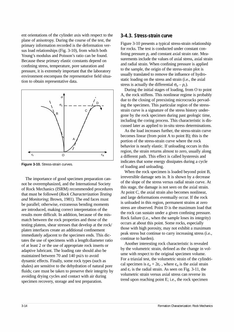
ent orientations of the cylinder axis with respect to theplane of anisotropy. During the course of the test, theprimary information recorded is the deformation ver-sus load relationships (Fig. 3-10), from which bothYoung’s modulus and Poisson’s ratio can be found.Because these primary elastic constants depend onconfining stress, temperature, pore saturation andpressure, it is extremely important that the laboratoryenvironment encompass the representative field situa-tion to obtain representative data.

The importance of good specimen preparation can-not be overemphasized, and the International Societyof Rock Mechanics (ISRM) recommended proceduresthat must be followed (Rock Characterization Testingand Monitoring; Brown, 1981). The end faces mustbe parallel; otherwise, extraneous bending momentsare introduced, making correct interpretation of theresults more difficult. In addition, because of the mis-match between the rock properties and those of thetesting platens, shear stresses that develop at the rock/platen interfaces create an additional confinementimmediately adjacent to the specimen ends. This dic-tates the use of specimens with a length:diameter ratioof at least 2 or the use of appropriate rock inserts oradaptive lubricant. The loading rate should also bemaintained between 70 and 140 psi/s to avoiddynamic effects. Finally, some rock types (such asshales) are sensitive to the dehydration of natural porefluids; care must be taken to preserve their integrity byavoiding drying cycles and contact with air duringspecimen recovery, storage and test preparation.

3-4.3. Stress-strain curveFigure 3-10 presents a typical stress-strain relationshipfor rocks. The test is conducted under constant con-fining pressure pc and constant axial strain rate. Mea-surements include the values of axial stress, axial strainand radial strain. When confining pressure is applied to the sample, the origin of the stress-strain plot isusually translated to remove the influence of hydro-static loading on the stress and strain (i.e., the axialstress is actually the differential σa – pc).

During the initial stages of loading, from O to pointA, the rock stiffens. This nonlinear regime is probablydue to the closing of preexisting microcracks pervad-ing the specimen. This particular region of the stress-strain curve is a signature of the stress history under-gone by the rock specimen during past geologic time,including the coring process. This characteristic is dis-cussed later as applied to in-situ stress determinations.

As the load increases further, the stress-strain curvebecomes linear (from point A to point B); this is theportion of the stress-strain curve where the rockbehavior is nearly elastic. If unloading occurs in thisregion, the strain returns almost to zero, usually alonga different path. This effect is called hysteresis andindicates that some energy dissipates during a cycle of loading and unloading.

When the rock specimen is loaded beyond point B,irreversible damage sets in. It is shown by a decreaseof the slope of the stress versus radial strain curve. Atthis stage, the damage is not seen on the axial strain.At point C, the axial strain also becomes nonlinear,and large deformations eventually occur. If the rock is unloaded in this region, permanent strains at zerostress are observed. Point D is the maximum load thatthe rock can sustain under a given confining pressure.Rock failure (i.e., when the sample loses its integrity)occurs at about this point. Some rocks, especiallythose with high porosity, may not exhibit a maximumpeak stress but continue to carry increasing stress (i.e.,continue to harden).

Another interesting rock characteristic is revealedby the volumetric strain, defined as the change in vol-ume with respect to the original specimen volume.For a triaxial test, the volumetric strain of the cylindri-cal specimen is εa + 2εr , where εa is the axial strainand εr is the radial strain. As seen on Fig. 3-11, thevolumetric strain versus axial stress can reverse itstrend upon reaching point E; i.e., the rock specimen

3-14 Formation Characterization: Rock Mechanics

Figure 3-10. Stress-strain curves.

B

A

C

D

O

σ

σc

εr εa

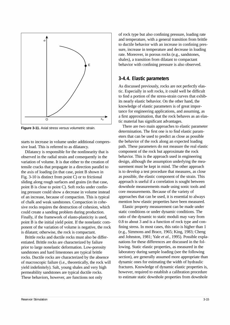
starts to increase in volume under additional compres-sive load. This is referred to as dilatancy.

Dilatancy is responsible for the nonlinearity that isobserved in the radial strain and consequently in thevariation of volume. It is due either to the creation oftensile cracks that propagate in a direction parallel tothe axis of loading (in that case, point B shown in Fig. 3-10 is distinct from point C) or to frictionalsliding along rough surfaces and grains (in that case,point B is close to point C). Soft rocks under confin-ing pressure could show a decrease in volume insteadof an increase, because of compaction. This is typicalof chalk and weak sandstones. Compaction in cohe-sive rocks requires the destruction of cohesion, whichcould create a sanding problem during production.Finally, if the framework of elasto-plasticity is used,point B is the initial yield point. If the nonelastic com-ponent of the variation of volume is negative, the rockis dilatant; otherwise, the rock is compactant.

Brittle rocks and ductile rocks must also be differ-entiated. Brittle rocks are characterized by failureprior to large nonelastic deformation. Low-porositysandstones and hard limestones are typical brittlerocks. Ductile rocks are characterized by the absenceof macroscopic failure (i.e., theoretically, the rock willyield indefinitely). Salt, young shales and very highpermeability sandstones are typical ductile rocks.These behaviors, however, are functions not only

of rock type but also confining pressure, loading rateand temperature, with a general transition from brittleto ductile behavior with an increase in confining pres-sure, increase in temperature and decrease in loadingrate. Moreover, in porous rocks (e.g., sandstones,shales), a transition from dilatant to compactantbehavior with confining pressure is also observed.

3-4.4. Elastic parametersAs discussed previously, rocks are not perfectly elas-tic. Especially in soft rocks, it could well be difficultto find a portion of the stress-strain curves that exhib-its nearly elastic behavior. On the other hand, theknowledge of elastic parameters is of great impor-tance for engineering applications, and assuming, as a first approximation, that the rock behaves as an elas-tic material has significant advantages.

There are two main approaches to elastic parameterdetermination. The first one is to find elastic param-eters that can be used to predict as close as possiblethe behavior of the rock along an expected loadingpath. These parameters do not measure the real elasticcomponent of the rock but approximate the rockbehavior. This is the approach used in engineeringdesign, although the assumption underlying the mea-surement must be kept in mind. The other approach is to develop a test procedure that measures, as closeas possible, the elastic component of the strain. Thisapproach is useful if a correlation is sought betweendownhole measurements made using sonic tools andcore measurements. Because of the variety ofapproaches that can be used, it is essential to alwaysmention how elastic properties have been measured.

Elastic property measurement can be made understatic conditions or under dynamic conditions. Theratio of the dynamic to static moduli may vary from0.8 to about 3 and is a function of rock type and con-fining stress. In most cases, this ratio is higher than 1(e.g., Simmons and Brace, 1965; King, 1983; Chengand Johnston, 1981; Yale et al., 1995). Possible expla-nations for these differences are discussed in the fol-lowing. Static elastic properties, as measured in thelaboratory during sample loading (see the followingsection), are generally assumed more appropriate thandynamic ones for estimating the width of hydraulicfractures. Knowledge of dynamic elastic properties is,however, required to establish a calibration procedureto estimate static downhole properties from downhole

Reservoir Stimulation 3-15

Figure 3-11. Axial stress versus volumetric strain.

E

σ

O εv

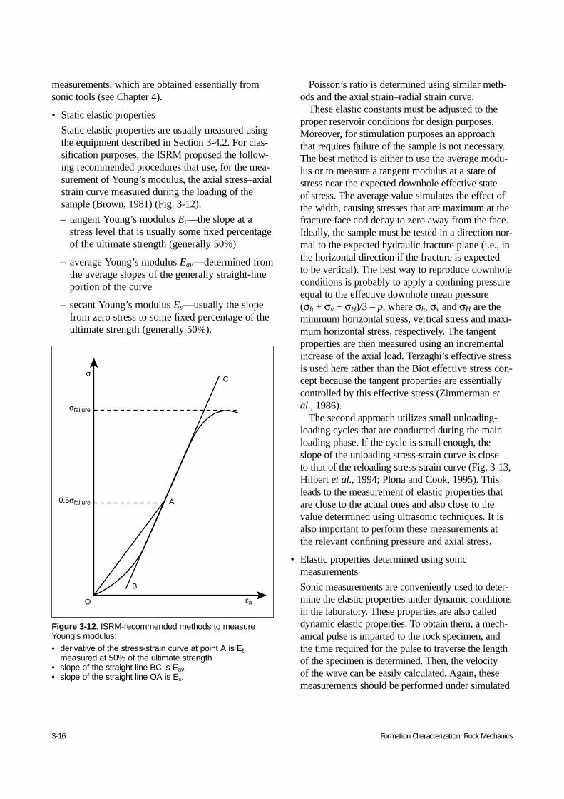
measurements, which are obtained essentially fromsonic tools (see Chapter 4).

• Static elastic properties

Static elastic properties are usually measured usingthe equipment described in Section 3-4.2. For clas-sification purposes, the ISRM proposed the follow-ing recommended procedures that use, for the mea-surement of Young’s modulus, the axial stress–axialstrain curve measured during the loading of thesample (Brown, 1981) (Fig. 3-12):

– tangent Young’s modulus Et—the slope at astress level that is usually some fixed percentageof the ultimate strength (generally 50%)

– average Young’s modulus Eav—determined fromthe average slopes of the generally straight-lineportion of the curve

– secant Young’s modulus Es—usually the slopefrom zero stress to some fixed percentage of theultimate strength (generally 50%).

Poisson’s ratio is determined using similar meth-ods and the axial strain–radial strain curve.

These elastic constants must be adjusted to theproper reservoir conditions for design purposes.Moreover, for stimulation purposes an approachthat requires failure of the sample is not necessary.The best method is either to use the average modu-lus or to measure a tangent modulus at a state ofstress near the expected downhole effective state of stress. The average value simulates the effect ofthe width, causing stresses that are maximum at thefracture face and decay to zero away from the face.Ideally, the sample must be tested in a direction nor-mal to the expected hydraulic fracture plane (i.e., inthe horizontal direction if the fracture is expected to be vertical). The best way to reproduce downholeconditions is probably to apply a confining pressureequal to the effective downhole mean pressure (σh + σv + σH)/3 – p, where σh, σv and σH are theminimum horizontal stress, vertical stress and maxi-mum horizontal stress, respectively. The tangentproperties are then measured using an incrementalincrease of the axial load. Terzaghi’s effective stressis used here rather than the Biot effective stress con-cept because the tangent properties are essentiallycontrolled by this effective stress (Zimmerman etal., 1986).

The second approach utilizes small unloading-loading cycles that are conducted during the mainloading phase. If the cycle is small enough, theslope of the unloading stress-strain curve is close to that of the reloading stress-strain curve (Fig. 3-13,Hilbert et al., 1994; Plona and Cook, 1995). Thisleads to the measurement of elastic properties thatare close to the actual ones and also close to thevalue determined using ultrasonic techniques. It isalso important to perform these measurements atthe relevant confining pressure and axial stress.

• Elastic properties determined using sonicmeasurements

Sonic measurements are conveniently used to deter-mine the elastic properties under dynamic conditionsin the laboratory. These properties are also calleddynamic elastic properties. To obtain them, a mech-anical pulse is imparted to the rock specimen, andthe time required for the pulse to traverse the lengthof the specimen is determined. Then, the velocity of the wave can be easily calculated. Again, thesemeasurements should be performed under simulated

3-16 Formation Characterization: Rock Mechanics

Figure 3-12. ISRM-recommended methods to measureYoung’s modulus:• derivative of the stress-strain curve at point A is Et,

measured at 50% of the ultimate strength• slope of the straight line BC is Eav• slope of the straight line OA is Es.

A

B

C

O

σ

σfailure

εa

0.5σfailure

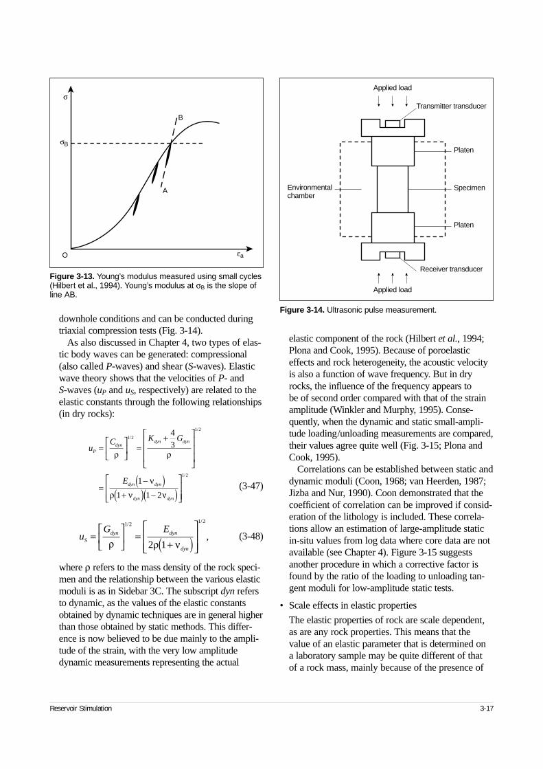
downhole conditions and can be conducted duringtriaxial compression tests (Fig. 3-14).

As also discussed in Chapter 4, two types of elas-tic body waves can be generated: compressional(also called P-waves) and shear (S-waves). Elasticwave theory shows that the velocities of P- and S-waves (uP and uS, respectively) are related to theelastic constants through the following relationships(in dry rocks):

(3-47)

(3-48)

where ρ refers to the mass density of the rock speci-men and the relationship between the various elasticmoduli is as in Sidebar 3C. The subscript dyn refersto dynamic, as the values of the elastic constantsobtained by dynamic techniques are in general higherthan those obtained by static methods. This differ-ence is now believed to be due mainly to the ampli-tude of the strain, with the very low amplitudedynamic measurements representing the actual

elastic component of the rock (Hilbert et al., 1994;Plona and Cook, 1995). Because of poroelasticeffects and rock heterogeneity, the acoustic velocityis also a function of wave frequency. But in dryrocks, the influence of the frequency appears to be of second order compared with that of the strainamplitude (Winkler and Murphy, 1995). Conse-quently, when the dynamic and static small-ampli-tude loading/unloading measurements are compared,their values agree quite well (Fig. 3-15; Plona andCook, 1995).

Correlations can be established between static anddynamic moduli (Coon, 1968; van Heerden, 1987;Jizba and Nur, 1990). Coon demonstrated that thecoefficient of correlation can be improved if consid-eration of the lithology is included. These correla-tions allow an estimation of large-amplitude staticin-situ values from log data where core data are notavailable (see Chapter 4). Figure 3-15 suggestsanother procedure in which a corrective factor isfound by the ratio of the loading to unloading tan-gent moduli for low-amplitude static tests.

• Scale effects in elastic properties

The elastic properties of rock are scale dependent,as are any rock properties. This means that thevalue of an elastic parameter that is determined on a laboratory sample may be quite different of that of a rock mass, mainly because of the presence of

Reservoir Stimulation 3-17

Figure 3-13. Young’s modulus measured using small cycles(Hilbert et al., 1994). Young’s modulus at σB is the slope ofline AB.

A

B

O

σB

εa

σ

Figure 3-14. Ultrasonic pulse measurement.

Applied load

Applied load

Receiver transducer

Transmitter transducer

Environmentalchamber

Specimen

Platen

Platen

uC K G

E

Pdyn

dyn dyn

dyn dyn

dyn dyn

=

=

+

=−( )

+( ) −( )

ρ ρ

ν

ρ ν ν

1 2

1 2

1 2

43

1

1 1 2

/

/

/

uG E

Sdyn dyn

dyn

=

=

+( )

ρ ρ ν

1 2 1 2

2 1

/ /

,

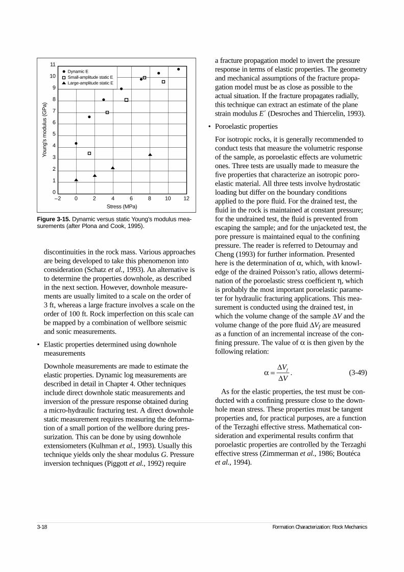
discontinuities in the rock mass. Various approachesare being developed to take this phenomenon intoconsideration (Schatz et al., 1993). An alternative isto determine the properties downhole, as describedin the next section. However, downhole measure-ments are usually limited to a scale on the order of3 ft, whereas a large fracture involves a scale on theorder of 100 ft. Rock imperfection on this scale canbe mapped by a combination of wellbore seismicand sonic measurements.

• Elastic properties determined using downholemeasurements

Downhole measurements are made to estimate theelastic properties. Dynamic log measurements aredescribed in detail in Chapter 4. Other techniquesinclude direct downhole static measurements andinversion of the pressure response obtained during a micro-hydraulic fracturing test. A direct downholestatic measurement requires measuring the deforma-tion of a small portion of the wellbore during pres-surization. This can be done by using downholeextensiometers (Kulhman et al., 1993). Usually thistechnique yields only the shear modulus G. Pressureinversion techniques (Piggott et al., 1992) require

a fracture propagation model to invert the pressureresponse in terms of elastic properties. The geometryand mechanical assumptions of the fracture propa-gation model must be as close as possible to theactual situation. If the fracture propagates radially,this technique can extract an estimate of the planestrain modulus E´ (Desroches and Thiercelin, 1993).

• Poroelastic properties

For isotropic rocks, it is generally recommended toconduct tests that measure the volumetric responseof the sample, as poroelastic effects are volumetricones. Three tests are usually made to measure thefive properties that characterize an isotropic poro-elastic material. All three tests involve hydrostaticloading but differ on the boundary conditionsapplied to the pore fluid. For the drained test, thefluid in the rock is maintained at constant pressure;for the undrained test, the fluid is prevented fromescaping the sample; and for the unjacketed test, thepore pressure is maintained equal to the confiningpressure. The reader is referred to Detournay andCheng (1993) for further information. Presentedhere is the determination of α, which, with knowl-edge of the drained Poisson’s ratio, allows determi-nation of the poroelastic stress coefficient η, whichis probably the most important poroelastic parame-ter for hydraulic fracturing applications. This mea-surement is conducted using the drained test, inwhich the volume change of the sample ∆V and thevolume change of the pore fluid ∆Vf are measuredas a function of an incremental increase of the con-fining pressure. The value of α is then given by thefollowing relation:

(3-49)

As for the elastic properties, the test must be con-ducted with a confining pressure close to the down-hole mean stress. These properties must be tangentproperties and, for practical purposes, are a functionof the Terzaghi effective stress. Mathematical con-sideration and experimental results confirm thatporoelastic properties are controlled by the Terzaghieffective stress (Zimmerman et al., 1986; Boutécaet al., 1994).

3-18 Formation Characterization: Rock Mechanics

Figure 3-15. Dynamic versus static Young’s modulus mea-surements (after Plona and Cook, 1995).

Dynamic ESmall-amplitude static ELarge-amplitude static E

–20

0 2 4 6 8 10 12

1

2

3

4

5

6

7

8

9

10

11

Stress (MPa)

Youn

g's

mod

ulus

(GP

a)

α =∆∆V

Vf .

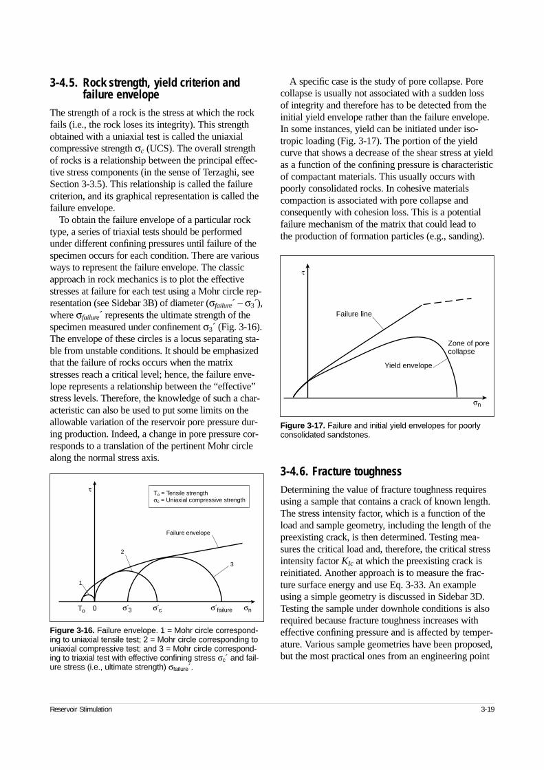
3-4.5. Rock strength, yield criterion and failure envelope

The strength of a rock is the stress at which the rockfails (i.e., the rock loses its integrity). This strengthobtained with a uniaxial test is called the uniaxialcompressive strength σc (UCS). The overall strengthof rocks is a relationship between the principal effec-tive stress components (in the sense of Terzaghi, seeSection 3-3.5). This relationship is called the failurecriterion, and its graphical representation is called thefailure envelope.

To obtain the failure envelope of a particular rocktype, a series of triaxial tests should be performedunder different confining pressures until failure of thespecimen occurs for each condition. There are variousways to represent the failure envelope. The classicapproach in rock mechanics is to plot the effectivestresses at failure for each test using a Mohr circle rep-resentation (see Sidebar 3B) of diameter (σfailure´ – σ3´),where σfailure´ represents the ultimate strength of thespecimen measured under confinement σ3´ (Fig. 3-16).The envelope of these circles is a locus separating sta-ble from unstable conditions. It should be emphasizedthat the failure of rocks occurs when the matrixstresses reach a critical level; hence, the failure enve-lope represents a relationship between the “effective”stress levels. Therefore, the knowledge of such a char-acteristic can also be used to put some limits on theallowable variation of the reservoir pore pressure dur-ing production. Indeed, a change in pore pressure cor-responds to a translation of the pertinent Mohr circlealong the normal stress axis.

A specific case is the study of pore collapse. Porecollapse is usually not associated with a sudden lossof integrity and therefore has to be detected from theinitial yield envelope rather than the failure envelope.In some instances, yield can be initiated under iso-tropic loading (Fig. 3-17). The portion of the yieldcurve that shows a decrease of the shear stress at yieldas a function of the confining pressure is characteristicof compactant materials. This usually occurs withpoorly consolidated rocks. In cohesive materialscompaction is associated with pore collapse andconsequently with cohesion loss. This is a potentialfailure mechanism of the matrix that could lead to the production of formation particles (e.g., sanding).

3-4.6. Fracture toughnessDetermining the value of fracture toughness requiresusing a sample that contains a crack of known length.The stress intensity factor, which is a function of theload and sample geometry, including the length of thepreexisting crack, is then determined. Testing mea-sures the critical load and, therefore, the critical stressintensity factor KIc at which the preexisting crack isreinitiated. Another approach is to measure the frac-ture surface energy and use Eq. 3-33. An exampleusing a simple geometry is discussed in Sidebar 3D.Testing the sample under downhole conditions is alsorequired because fracture toughness increases witheffective confining pressure and is affected by temper-ature. Various sample geometries have been proposed,but the most practical ones from an engineering point

Reservoir Stimulation 3-19

Figure 3-16. Failure envelope. 1 = Mohr circle correspond-ing to uniaxial tensile test; 2 = Mohr circle corresponding touniaxial compressive test; and 3 = Mohr circle correspond-ing to triaxial test with effective confining stress σc´ and fail-ure stress (i.e., ultimate strength) σfailure´.

1

2

3

Failure envelope

τ

To

To = Tensile strengthσc = Uniaxial compressive strength

0 σnσ 3́ σ ć σ f́ailure

Figure 3-17. Failure and initial yield envelopes for poorlyconsolidated sandstones.

τ

σn

Failure line

Yield envelope

Zone of pore collapse

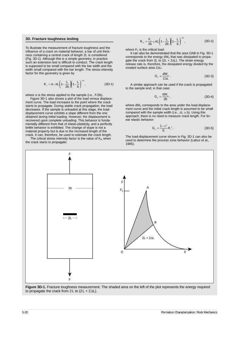
3-20 Formation Characterization: Rock Mechanics

3D. Fracture toughness testing

To illustrate the measurement of fracture toughness and theinfluence of a crack on material behavior, a bar of unit thick-ness containing a central crack of length 2L is considered(Fig. 3D-1). Although this is a simple geometry, in practicesuch an extension test is difficult to conduct. The crack lengthis supposed to be small compared with the bar width and thewidth small compared with the bar length. The stress intensityfactor for this geometry is given by

(3D-1)

where σ is the stress applied to the sample (i.e., F/2b).Figure 3D-1 also shows a plot of the load versus displace-

ment curve. The load increases to the point where the crackstarts to propagate. During stable crack propagation, the loaddecreases. If the sample is unloaded at this stage, the load-displacement curve exhibits a slope different from the oneobtained during initial loading. However, the displacement isrecovered upon complete unloading. This behavior is funda-mentally different from that of elasto-plasticity, and a perfectlybrittle behavior is exhibited. The change of slope is not amaterial property but is due to the increased length of thecrack. It can, therefore, be used to estimate the crack length.

The critical stress intensity factor is the value of KIc whenthe crack starts to propagate:

(3D-2)

where Fc is the critical load.It can also be demonstrated that the area OAB in Fig. 3D-1

corresponds to the energy dWs that was dissipated to propa-gate the crack from 2L to (2L + 2∆L). The strain energyrelease rate is, therefore, the dissipated energy divided by thecreated surface area 2∆L:

(3D-3)

A similar approach can be used if the crack is propagatedto the sample end; in that case:

(3D-4)

where dWs corresponds to the area under the load-displace-ment curve and the initial crack length is assumed to be smallcompared with the sample width (i.e., ∆L ≅ b). Using thisapproach, there is no need to measure crack length. For lin-ear elastic behavior:

(3D-5)

The load-displacement curve shown in Fig. 3D-1 can also beused to determine the process zone behavior (Labuz et al.,1985).

K LLb

LbI ≈ −

−

−

σ π 12

11 2/

,

KFb

LLb

LbIc

c≈ −

−

−

21

21

1 2

π/

,

GdW

Les=

2∆.

GdW

bes=

2,

GE

Ke I= −1 22ν.

Figure 3D-1. Fracture toughness measurement. The shaded area on the left of the plot represents the energy requiredto propagate the crack from 2L to (2L + 2∆L).

2b

2L

O

F

F

F

Fc

2L + 2∆L

B

A

δ

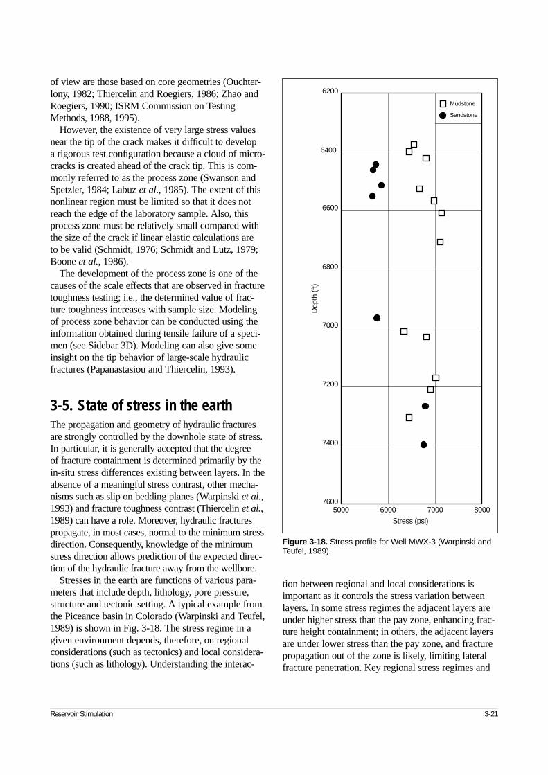
of view are those based on core geometries (Ouchter-lony, 1982; Thiercelin and Roegiers, 1986; Zhao andRoegiers, 1990; ISRM Commission on TestingMethods, 1988, 1995).

However, the existence of very large stress valuesnear the tip of the crack makes it difficult to develop a rigorous test configuration because a cloud of micro-cracks is created ahead of the crack tip. This is com-monly referred to as the process zone (Swanson andSpetzler, 1984; Labuz et al., 1985). The extent of thisnonlinear region must be limited so that it does notreach the edge of the laboratory sample. Also, thisprocess zone must be relatively small compared withthe size of the crack if linear elastic calculations are to be valid (Schmidt, 1976; Schmidt and Lutz, 1979;Boone et al., 1986).

The development of the process zone is one of thecauses of the scale effects that are observed in fracturetoughness testing; i.e., the determined value of frac-ture toughness increases with sample size. Modelingof process zone behavior can be conducted using theinformation obtained during tensile failure of a speci-men (see Sidebar 3D). Modeling can also give someinsight on the tip behavior of large-scale hydraulicfractures (Papanastasiou and Thiercelin, 1993).

3-5. State of stress in the earthThe propagation and geometry of hydraulic fracturesare strongly controlled by the downhole state of stress.In particular, it is generally accepted that the degree of fracture containment is determined primarily by thein-situ stress differences existing between layers. In theabsence of a meaningful stress contrast, other mecha-nisms such as slip on bedding planes (Warpinski et al.,1993) and fracture toughness contrast (Thiercelin et al.,1989) can have a role. Moreover, hydraulic fracturespropagate, in most cases, normal to the minimum stressdirection. Consequently, knowledge of the minimumstress direction allows prediction of the expected direc-tion of the hydraulic fracture away from the wellbore.

Stresses in the earth are functions of various para-meters that include depth, lithology, pore pressure,structure and tectonic setting. A typical example fromthe Piceance basin in Colorado (Warpinski and Teufel,1989) is shown in Fig. 3-18. The stress regime in agiven environment depends, therefore, on regionalconsiderations (such as tectonics) and local considera-tions (such as lithology). Understanding the interac-

tion between regional and local considerations isimportant as it controls the stress variation betweenlayers. In some stress regimes the adjacent layers areunder higher stress than the pay zone, enhancing frac-ture height containment; in others, the adjacent layersare under lower stress than the pay zone, and fracturepropagation out of the zone is likely, limiting lateralfracture penetration. Key regional stress regimes and

Reservoir Stimulation 3-21

Figure 3-18. Stress profile for Well MWX-3 (Warpinski andTeufel, 1989).

50007600

6000 7000 8000

7400

7200

7000

6800

6600

6400

6200

Stress (psi)

Dep

th (f

t)

Mudstone

Sandstone

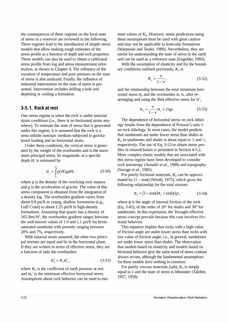
the consequences of these regimes on the local state of stress in a reservoir are reviewed in the following.These regimes lead to the introduction of simple stressmodels that allow making rough estimates of thestress profile as a function of depth and rock properties.These models can also be used to obtain a calibratedstress profile from log and stress measurement infor-mation, as shown in Chapter 4. The influence of thevariation of temperature and pore pressure on the stateof stress is also analyzed. Finally, the influence ofindustrial intervention on the state of stress is pre-sented. Intervention includes drilling a hole anddepleting or cooling a formation.

3-5.1. Rock at restOne stress regime is when the rock is under uniaxialstrain conditions (i.e., there is no horizontal strain any-where). To estimate the state of stress that is generatedunder this regime, it is assumed that the rock is asemi-infinite isotropic medium subjected to gravita-tional loading and no horizontal strain.

Under these conditions, the vertical stress is gener-ated by the weight of the overburden and is the maxi-mum principal stress. Its magnitude, at a specificdepth H, is estimated by

(3-50)

where ρ is the density of the overlying rock massesand g is the acceleration of gravity. The value of thisstress component is obtained from the integration of a density log. The overburden gradient varies fromabout 0.8 psi/ft in young, shallow formations (e.g.,Gulf Coast) to about 1.25 psi/ft in high-density formations. Assuming that quartz has a density of165 lbm/ft3, the overburden gradient ranges betweenthe well-known values of 1.0 and 1.1 psi/ft for brine-saturated sandstone with porosity ranging between20% and 7%, respectively.

With uniaxial strain assumed, the other two princi-pal stresses are equal and lie in the horizontal plane. If they are written in terms of effective stress, they area function of only the overburden:

(3-51)

where Ko is the coefficient of earth pressure at rest and σh´ is the minimum effective horizontal stress.Assumptions about rock behavior can be used to esti-

mate values of Ko. However, stress predictions usingthese assumptions must be used with great cautionand may not be applicable in lenticular formations(Warpinski and Teufel, 1989). Nevertheless, they areuseful for understanding the state of stress in the earthand can be used as a reference state (Engelder, 1993).

With the assumption of elasticity and for the bound-ary conditions outlined previously, Ko is

(3-52)

and the relationship between the total minimum hori-zontal stress σh and the overburden σv is, after re-arranging and using the Biot effective stress for σ´,

(3-53)

The dependence of horizontal stress on rock lithol-ogy results from the dependence of Poisson’s ratio νon rock lithology. In most cases, the model predictsthat sandstones are under lower stress than shales asKo in sandstones and shales is about equal to 1⁄3 and 1⁄2,respectively. The use of Eq. 3-53 to obtain stress pro-files in relaxed basins is presented in Section 4-5.2.More complex elastic models that are associated withthis stress regime have been developed to considerrock anisotropy (Amadéi et al., 1988) and topography(Savage et al., 1985).

For purely frictional materials, Ko can be approxi-mated by (1 – sinφ) (Wroth, 1975), which gives thefollowing relationship for the total stresses:

(3-54)

where φ is the angle of internal friction of the rock(Eq. 3-41), of the order of 20° for shales and 30° forsandstones. In this expression, the Terzaghi effectivestress concept prevails because this case involves fric-tional behavior.

This equation implies that rocks with a high valueof friction angle are under lower stress than rocks withlow value of friction angle; i.e., in general, sandstonesare under lower stress than shales. The observationthat models based on elasticity and models based onfrictional behavior give the same trend of stress contrastalways occurs, although the fundamental assumptionsfor these models have nothing in common.

For purely viscous materials (salt), Ko is simplyequal to 1 and the state of stress is lithostatic (Talobre,1957, 1958):

3-22 Formation Characterization: Rock Mechanics

σ ρv

H

H gdH= ( )∫0

,

Ko =−ν

ν1,

σ νν

σ ηh v p=−

+1

2 .

σ φ σ φh v p≈ −( ) + ( )1 sin sin ,

′ = ′σ σh o vK ,

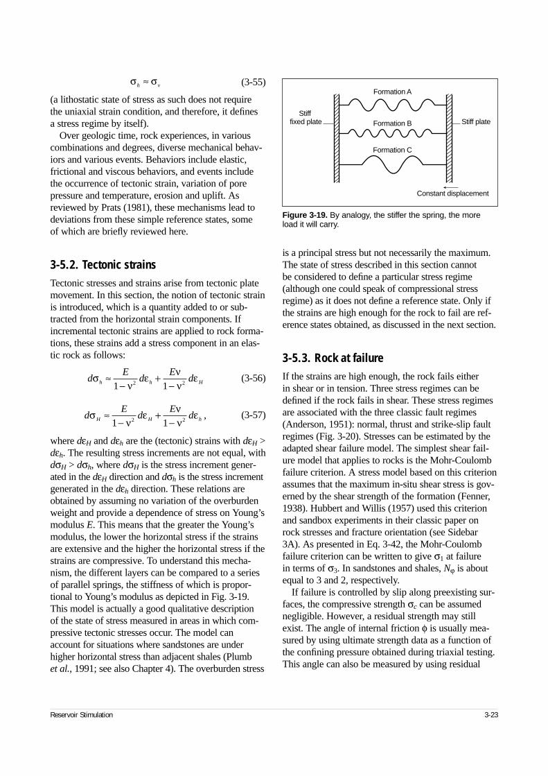
(3-55)

(a lithostatic state of stress as such does not requirethe uniaxial strain condition, and therefore, it defines a stress regime by itself).

Over geologic time, rock experiences, in variouscombinations and degrees, diverse mechanical behav-iors and various events. Behaviors include elastic,frictional and viscous behaviors, and events includethe occurrence of tectonic strain, variation of porepressure and temperature, erosion and uplift. Asreviewed by Prats (1981), these mechanisms lead todeviations from these simple reference states, some of which are briefly reviewed here.

3-5.2. Tectonic strainsTectonic stresses and strains arise from tectonic platemovement. In this section, the notion of tectonic strainis introduced, which is a quantity added to or sub-tracted from the horizontal strain components. Ifincremental tectonic strains are applied to rock forma-tions, these strains add a stress component in an elas-tic rock as follows:

(3-56)

(3-57)

where dεH and dεh are the (tectonic) strains with dεH >dεh. The resulting stress increments are not equal, withdσH > dσh, where dσH is the stress increment gener-ated in the dεH direction and dσh is the stress incrementgenerated in the dεh direction. These relations areobtained by assuming no variation of the overburdenweight and provide a dependence of stress on Young’smodulus E. This means that the greater the Young’smodulus, the lower the horizontal stress if the strainsare extensive and the higher the horizontal stress if thestrains are compressive. To understand this mecha-nism, the different layers can be compared to a seriesof parallel springs, the stiffness of which is propor-tional to Young’s modulus as depicted in Fig. 3-19.This model is actually a good qualitative description of the state of stress measured in areas in which com-pressive tectonic stresses occur. The model canaccount for situations where sandstones are underhigher horizontal stress than adjacent shales (Plumb et al., 1991; see also Chapter 4). The overburden stress

is a principal stress but not necessarily the maximum.The state of stress described in this section cannot be considered to define a particular stress regime(although one could speak of compressional stressregime) as it does not define a reference state. Only ifthe strains are high enough for the rock to fail are ref-erence states obtained, as discussed in the next section.

3-5.3. Rock at failureIf the strains are high enough, the rock fails either in shear or in tension. Three stress regimes can bedefined if the rock fails in shear. These stress regimesare associated with the three classic fault regimes(Anderson, 1951): normal, thrust and strike-slip faultregimes (Fig. 3-20). Stresses can be estimated by theadapted shear failure model. The simplest shear fail-ure model that applies to rocks is the Mohr-Coulombfailure criterion. A stress model based on this criterionassumes that the maximum in-situ shear stress is gov-erned by the shear strength of the formation (Fenner,1938). Hubbert and Willis (1957) used this criterionand sandbox experiments in their classic paper onrock stresses and fracture orientation (see Sidebar3A). As presented in Eq. 3-42, the Mohr-Coulombfailure criterion can be written to give σ1 at failure in terms of σ3. In sandstones and shales, Nϕ is aboutequal to 3 and 2, respectively.

If failure is controlled by slip along preexisting sur-faces, the compressive strength σc can be assumednegligible. However, a residual strength may stillexist. The angle of internal friction φ is usually mea-sured by using ultimate strength data as a function ofthe confining pressure obtained during triaxial testing.This angle can also be measured by using residual

Reservoir Stimulation 3-23

σ σh v≈

dE

dE

dh h Hσν

ε νν

ε≈−

+−1 12 2

dE

dE

dH H hσν

ε νν

ε≈−

+−1 12 2

,

Figure 3-19. By analogy, the stiffer the spring, the moreload it will carry.

Formation A

Formation B

Formation C

Stiff plateStiff

fixed plate

Constant displacement

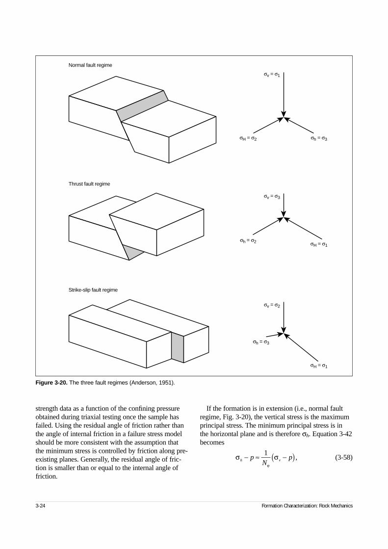
strength data as a function of the confining pressureobtained during triaxial testing once the sample hasfailed. Using the residual angle of friction rather thanthe angle of internal friction in a failure stress modelshould be more consistent with the assumption thatthe minimum stress is controlled by friction along pre-existing planes. Generally, the residual angle of fric-tion is smaller than or equal to the internal angle offriction.

If the formation is in extension (i.e., normal faultregime, Fig. 3-20), the vertical stress is the maximumprincipal stress. The minimum principal stress is inthe horizontal plane and is therefore σh. Equation 3-42becomes

(3-58)

3-24 Formation Characterization: Rock Mechanics

Figure 3-20. The three fault regimes (Anderson, 1951).

Normal fault regime

Thrust fault regime

Strike-slip fault regime

σv = σ1

σv = σ3

σv = σ2

σH = σ2 σh = σ3

σh = σ2

σh = σ3

σH = σ1

σH = σ1

σ σϕ

h vpN

p− ≈ −( )1,

in which the effect of strength is neglected. An equa-tion similar to Eq. 3-51 can be retrieved. However, ifthe rock is at failure, the coefficient of proportionalitycannot be considered as a coefficient of earth stress atrest. The most surprising and confusing result is that,in practice, Eqs. 3-53 and 3-58 give similar predic-tions, especially if, in the elastic model, α is assumedequal to 1. The coefficient of proportionality in sand-stones and shales is, whether elasticity or failure isassumed, about equal to 1⁄3 and 1⁄2, respectively. Thissimilarity has been demonstrated in more detail forone area of East Texas by Thiercelin and Plumb(1994b).

If the formation fails under compressive tectonicstrain, the maximum principal stress is in the horizon-tal plane and is therefore σH. In the thrust faultregime, the minimum principal stress is the verticalstress (Fig. 3-20):

(3-59)

In this case, σh is the intermediate principal stressand is equal to or greater than the vertical stress.Horizontal hydraulic fractures could be achieved.

Thus, the principal stresses can be estimated andordered by looking at the fault regime. In practice,these considerations must be checked with downholemeasurements, as the state of stress may deviate fromthe expected ordering of stresses because of stress his-tory. These models assume that the fault plane wascreated under the current tectonic setting; i.e., the nor-mal to the fault plane makes an angle (π/4 + φ/2) withthe direction of the maximum principal stress. Pre-existing faults can be reactivated under a state of stressthat differs from the one that created them. A Mohr-Coulomb stability criterion can still be applied, but Eq. 3-42 must be modified to take into considerationthat the fault plane orientation was not induced by thecurrent state of stress.

Another stress regime is associated with tensile fail-ure. Tensile failure is sometimes observed downhole,although it appears to contradict the general compres-sional regime of the earth. This mode of failure sim-ply states that σ3 – p = 0 (by neglecting the tensilestrength of the rock) and may be suspected if it isobserved from downhole images that the normal tothe plane of the preexisting fractures is the directionof minimum stress. This condition can occur in exten-sional regions with overpressured zones (where thepore pressure tends to be the value of the minimum

stress component) or when the in-situ stress ratio istoo large. As the rock is close to a uniaxial state ofstress, this regime can occur only in rocks with a com-pressive strength high enough to avoid normal fault-ing (as a rule of thumb, the uniaxial compressivestress must be equal to or greater than the effectiveoverburden stress). This condition is achieved for tightgas sandstones in some areas of the Western UnitedStates and East Texas.

Failure models also have an important role in provid-ing bounds for the in-situ stress. They represent a limitstate above which the rock is unstable in the long term.In the extension regime in particular, it is unlikely that a minimum stress value below the value predicted bythe failure model can be obtained.

3-5.4. Influence of pore pressureIt is of interest to understand what happens whendepleting or injecting into a reservoir. Elastic modelswith uniaxial strain conditions can be applied withsome confidence, as the variation of stresses occursover a short period of geologic time, although it isalways necessary to double check the assumptionsbecause failure models could well be the real physicalmechanism, as shown in the following.

If the material behaves elastically, and assuminguniaxial strain conditions, Eq. 3-53 gives

(3-60)

The range of 2η is approximately between 0.5 and0.7. Geertsma (1985) demonstrated the applicabilityof this model to stress decrease during depletion.

A failure model can also be applied. For example,Eq. 3-58 gives

(3-61)

If the coefficient of friction is 30°, the coefficient of proportionality is 0.67. As previously, a strong sim-ilarity exists between the predictions from the elasticand failure models. To use a failure model, however,requires checking that the effective state of stress sat-isfies the failure criterion prior to and during the varia-tion of pore pressure. The effective stresses increaseduring depletion, although the total minimum stressσh decreases.

Field data generally support the predictions of thesemodels and show that variation in the minimum stress

Reservoir Stimulation 3-25

σ σϕH vp N p− ≈ −( ) .

d dphσ η= 2 .

dN

Ndphσ ϕ

ϕ

=−1

.

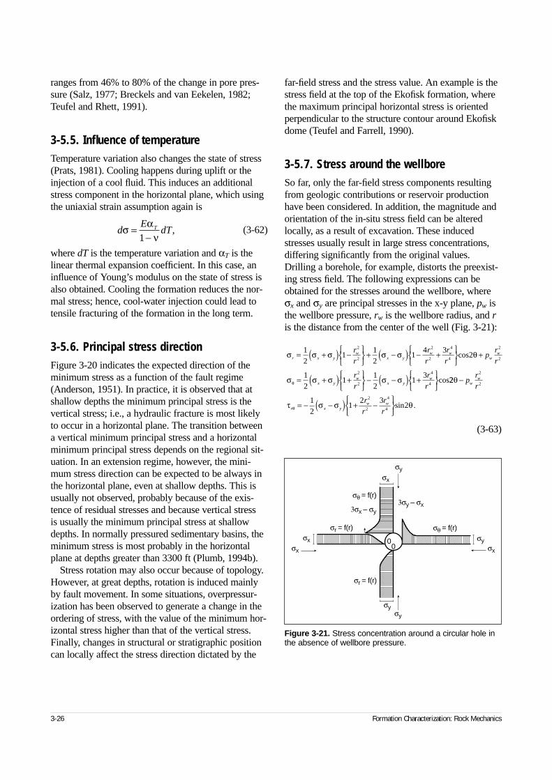
ranges from 46% to 80% of the change in pore pres-sure (Salz, 1977; Breckels and van Eekelen, 1982;Teufel and Rhett, 1991).

3-5.5. Influence of temperatureTemperature variation also changes the state of stress(Prats, 1981). Cooling happens during uplift or theinjection of a cool fluid. This induces an additionalstress component in the horizontal plane, which usingthe uniaxial strain assumption again is

(3-62)

where dT is the temperature variation and αT is thelinear thermal expansion coefficient. In this case, aninfluence of Young’s modulus on the state of stress isalso obtained. Cooling the formation reduces the nor-mal stress; hence, cool-water injection could lead totensile fracturing of the formation in the long term.

3-5.6. Principal stress directionFigure 3-20 indicates the expected direction of theminimum stress as a function of the fault regime(Anderson, 1951). In practice, it is observed that atshallow depths the minimum principal stress is thevertical stress; i.e., a hydraulic fracture is most likelyto occur in a horizontal plane. The transition betweena vertical minimum principal stress and a horizontalminimum principal stress depends on the regional sit-uation. In an extension regime, however, the mini-mum stress direction can be expected to be always inthe horizontal plane, even at shallow depths. This isusually not observed, probably because of the exis-tence of residual stresses and because vertical stress is usually the minimum principal stress at shallowdepths. In normally pressured sedimentary basins, theminimum stress is most probably in the horizontalplane at depths greater than 3300 ft (Plumb, 1994b).

Stress rotation may also occur because of topology.However, at great depths, rotation is induced mainlyby fault movement. In some situations, overpressur-ization has been observed to generate a change in theordering of stress, with the value of the minimum hor-izontal stress higher than that of the vertical stress.Finally, changes in structural or stratigraphic positioncan locally affect the stress direction dictated by the

far-field stress and the stress value. An example is thestress field at the top of the Ekofisk formation, wherethe maximum principal horizontal stress is orientedperpendicular to the structure contour around Ekofiskdome (Teufel and Farrell, 1990).

3-5.7. Stress around the wellboreSo far, only the far-field stress components resultingfrom geologic contributions or reservoir productionhave been considered. In addition, the magnitude andorientation of the in-situ stress field can be alteredlocally, as a result of excavation. These inducedstresses usually result in large stress concentrations,differing significantly from the original values.Drilling a borehole, for example, distorts the preexist-ing stress field. The following expressions can beobtained for the stresses around the wellbore, whereσx and σy are principal stresses in the x-y plane, pw isthe wellbore pressure, rw is the wellbore radius, and ris the distance from the center of the well (Fig. 3-21):

(3-63)

3-26 Formation Characterization: Rock Mechanics

dE

dTTσ αν

=−1

,

σ σ σ σ σ θ

σ σ σ σ σθ

r x yw

x yw w

ww

x yw

x yw

r

r

r

r

r

rp

r

r

r

r

r

r

= +( ) −

+ −( ) − +

+

= +( ) +

− −( ) +

12

11

21

4 32

1

21

12

13

2

2

2

2

4

4

2

2

2

2

4

4

cos

cos22

12

12 3

2

2

2

2

2

4

4

θ

τ σ σ θθ

−

= − −( ) + −

pr

r

r

r

r

r

ww

r x yw w sin .

Figure 3-21. Stress concentration around a circular hole inthe absence of wellbore pressure.

σy

σr = f(r)

σr = f(r) σθ = f(r)

σθ = f(r)

3σx – σy

3σy – σx

σy

σx

σy

σxσx

σyσx

00

To derive these expressions, it is assumed that therock remains linear elastic, the borehole is drilled par-allel to one of the principal stress directions, and thewellbore fluid pressure pw does not penetrate the rock(e.g., because of the presence of mudcake). At theborehole wall (i.e., r = rw), the following expressionsare obtained:

(3-64)

Considering only the directions parallel and per-pendicular to the minimum stress direction (i.e., θ = 0 and θ = π/2, respectively), these expressionsfurther simplify:

(3-65)

(3-66)

As an example, consider the case of 3000-psi well-bore pressure in equilibrium with the pore pressure ofthe reservoir and values of 3500 psi for σx and 5000 psifor σy. The equations lead to maximum values for theeffective tangential stress (σθ – p) of 5500 psi in com-pression (θ = 0°) and 500 psi in tension (θ = 90°). Thelatter result indicates the possibility for the occurrenceof tensile failure in a direction perpendicular to the min-imum stress, solely as a result of drilling the borehole.

A hydraulic fracture is induced by increasing thewellbore pressure pw up to the point where the effec-tive tangential stress (σθ – p) becomes equal to –To.If σx = σh, this happens at θ = 90° (where the stressconcentration induced by the far-field state of stress is minimum), which means that fracture initiates in a direction perpendicular to the minimum horizontalstress direction. Fracture initiation at the breakdownpressure pif is, therefore, obtained when (Hubbert andWillis, 1957)

(3-67)

These induced stresses diminish rapidly to zeroaway from the wellbore. Consequently, they affect thepressure to induce a fracture, but not the propagationof the fracture away from the wellbore wall.

If the wellbore fluid penetrates the formation, poro-elastic effects must be taken into account to calculatethe stress concentration around the wellbore. In partic-

ular, σθ at the wellbore becomes a function of time ifσx is not equal to σy (Detournay and Cheng, 1988).The long-time solutions are

(3-68)

(3-69)

If the wellbore fluid pressure is higher than the far-field pore pressure, poroelastic effects increase thestress concentration at the wellbore. The initiationpressure (Haimson and Fairhust, 1969) is obtainedfrom Eq. 3-69, with (σθ – pw) = –To:

(3-70)

A typical value of η is 0.25.These equations are used in Section 3-6.2. Finally,

plasticity effects reduce the stress concentration at thewellbore. Particularly in highly plastic rocks, the tan-gential stress at the wellbore never becomes tensile. Inthis case, fracture could initiate in shear(Papanastasiou et al., 1995).

3-5.8. Stress change from hydraulic fracturing

Two effects are considered in this section. The firstone addresses the increase of minimum stress becauseof the poroelastic effect. During the fracturing pro-cess, fracturing fluid leaks into the formation. Thisleakage induces a pore pressure increase around thefracture that results in dilation of the formation and,therefore, an increase of the minimum stress in thisregion. For a 2D crack in an infinite sheet, theincrease of minimum stress as a function of time is (Detournay and Cheng, 1991)

(3-71)

where pf is the fracturing fluid pressure and τc is acharacteristic time given by

(3-72)

where G is the shear modulus, k is the permeability, tis the time, µ is the viscosity, and L is the fracturehalf-length.

Reservoir Stimulation 3-27

στ

σ σ σ σ σ θθ

θ

r w

r

x y x y w

p

p

==

= +( ) − −( ) −

0

2 2cos .

σ σ σ ηθ θ( ) = − − + −( )=03 2y x w wp p p

σ σ σ ηθ θ π( ) = − − + −( )=2

3 2x y w wp p p .

pT p

ifh H o= − + −

−( )3 2

2 1σ σ η

η.

∆σ η τ3 = −( ) ( )p p ff c ,

τν ν ν

α µ ν νcu

u

tkG

L=

−( ) −( )−( ) −( )

2 1

1 2 12 2 2,

σ σ σθ θ( ) = − −=0

3 y x wp

σ σ σθ θ π( ) = − −=

2

3 x y wp .

p T pif h H o= − + −3σ σ .

The function f varies between 0 and 1 as τc increas-es from 0 to infinity. The value of the characteristictime at which poroelastic effects can start to influencethe state of stress around the fracture is about 10–3. Inreservoir rocks where η is equal to about 0.25, poro-elastic effects are important when the net pressure andcharacteristic time are high. This effect decreases if ahigh-pressure drop occurs at the fracture face. High-pressure drops happen, for example, when a goodfluid-loss control agent is used. Poroelastic effectseventually disappear when injection is stopped and theexcess pore pressure dissipates into the formation.

The second effect is the stress increase caused byopening of the fracture. This effect remains if the frac-ture is held open by proppant (Warpinski andBranagan, 1988; Palmer, 1993). An upper bound forthe stress increase once injection has been stopped isthe value of the net pressure at shut-in, but in practice,because the in-situ proppant concentration at shut-in isabout one-half of its compacted concentration, it couldbe about 50% of this value. This effect can be signifi-cant for short and wide fractures, where crack-tipscreenout induces a large net pressure (of the order of1000 psi) at the end of the job. It has been proposedthat this mechanism strengthens weak formations and,therefore, decreases the risk of sanding.

3-6. In-situ stress measurement

3-6.1. Importance of stress measurement in stimulation

The value of the minimum stress is one of the mostimportant parameters in hydraulic fracturing. At typi-cal reservoir depths, the fracturing pressure is a strongfunction of the minimum stress (or closure pressure).With some pumping regimes, the value of the netpressure, which is the fracturing pressure minus theclosure pressure, could be quite small compared withthe closure pressure. The net pressure is the mostrobust and usually the only parameter that is availablefor obtaining information on fracture geometry. Anerror in closure stress measurement can lead to a sig-nificant error in the estimation of the net pressure and,consequently, the fracture geometry. Because of thesmall value of the net pressure compared with theminimum stress, knowledge of the in-situ state ofstress at depth also gives insight into the expectedtreatment pressures.

It is also generally accepted that the degree of frac-ture containment is determined mainly by the in-situstress differences between layers, although, as men-tioned in the previous section, other mechanisms canplay a role in the absence of a meaningful stress con-trast. Knowledge of the stress variation between thepay zone and the adjacent layers is therefore essentialfor predicting the extent that the fracture grows out ofthe zone.

Fracturing from inclined or horizontal wellbores hasalso brought new requirements for determination ofthe far-field in-situ stress because it controls the com-plex stress field that is generated near the wellbore.The efficiency of a fracturing treatment is a functionof wellbore inclination with respect to the principalstress direction and magnitude (Martins et al., 1992a;Pearson et al., 1992).

Finally, the amount of stress confinement influencesthe rock properties (elasticity, strength and permeability).

Several methods are regularly used in the petroleumindustry to estimate the magnitude and orientation ofin-situ stress at depth. Some of them rely on field datainterpretations, whereas others rely on core measure-ments. Techniques based on wellbore images andsonic logs are presented in Chapter 4.

3-6.2. Micro-hydraulic fracturing techniquesFracturing techniques are commonly used to measurethe minimum stress. The micro-hydraulic fracturingtechnique is certainly the most reliable technique ifconducted properly, although it could be used in con-junction with other methods for added completeness.This technique uses the pressure response obtainedduring initiation, propagation and closure of ahydraulically induced fracture to accurately determinethe state of stress. Because stresses are functions ofrock properties, it is quite important to ensure that thetest provides a measure that is representative of agiven lithology. Small-scale hydraulic fractures areusually required, especially if the measurements willbe correlated with log or core information. However,the fracture must be large compared with the wellboreradius to measure the far-field minimum stress com-ponent, and a fracture with a size of 5–15 ft is a goodcompromise. At this scale, a tool that includes agamma ray sonde is recommended for accurate place-ment with regard to lithology. Analysis of the sonicand gamma ray logs should be made prior to testing

3-28 Formation Characterization: Rock Mechanics

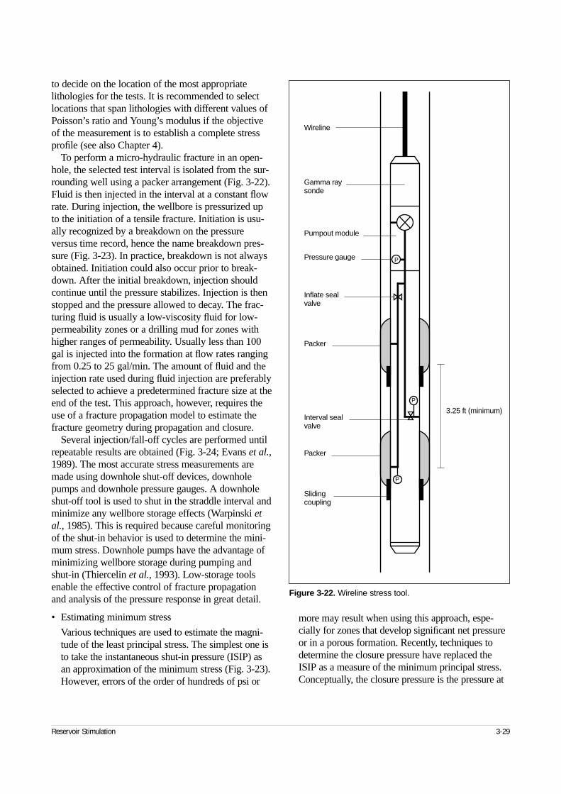
to decide on the location of the most appropriatelithologies for the tests. It is recommended to selectlocations that span lithologies with different values ofPoisson’s ratio and Young’s modulus if the objectiveof the measurement is to establish a complete stressprofile (see also Chapter 4).

To perform a micro-hydraulic fracture in an open-hole, the selected test interval is isolated from the sur-rounding well using a packer arrangement (Fig. 3-22).Fluid is then injected in the interval at a constant flowrate. During injection, the wellbore is pressurized upto the initiation of a tensile fracture. Initiation is usu-ally recognized by a breakdown on the pressureversus time record, hence the name breakdown pres-sure (Fig. 3-23). In practice, breakdown is not alwaysobtained. Initiation could also occur prior to break-down. After the initial breakdown, injection shouldcontinue until the pressure stabilizes. Injection is thenstopped and the pressure allowed to decay. The frac-turing fluid is usually a low-viscosity fluid for low-permeability zones or a drilling mud for zones withhigher ranges of permeability. Usually less than 100gal is injected into the formation at flow rates rangingfrom 0.25 to 25 gal/min. The amount of fluid and theinjection rate used during fluid injection are preferablyselected to achieve a predetermined fracture size at theend of the test. This approach, however, requires theuse of a fracture propagation model to estimate thefracture geometry during propagation and closure.

Several injection/fall-off cycles are performed untilrepeatable results are obtained (Fig. 3-24; Evans et al.,1989). The most accurate stress measurements aremade using downhole shut-off devices, downholepumps and downhole pressure gauges. A downholeshut-off tool is used to shut in the straddle interval andminimize any wellbore storage effects (Warpinski etal., 1985). This is required because careful monitoringof the shut-in behavior is used to determine the mini-mum stress. Downhole pumps have the advantage ofminimizing wellbore storage during pumping andshut-in (Thiercelin et al., 1993). Low-storage toolsenable the effective control of fracture propagationand analysis of the pressure response in great detail.

• Estimating minimum stress

Various techniques are used to estimate the magni-tude of the least principal stress. The simplest one isto take the instantaneous shut-in pressure (ISIP) asan approximation of the minimum stress (Fig. 3-23).However, errors of the order of hundreds of psi or

more may result when using this approach, espe-cially for zones that develop significant net pressureor in a porous formation. Recently, techniques todetermine the closure pressure have replaced theISIP as a measure of the minimum principal stress.Conceptually, the closure pressure is the pressure at

Reservoir Stimulation 3-29

Figure 3-22. Wireline stress tool.

P

P

P

Wireline

Gamma raysonde

Pumpout module

Pressure gauge

Inflate seal valve

Packer

Interval sealvalve

Packer

Slidingcoupling

3.25 ft (minimum)

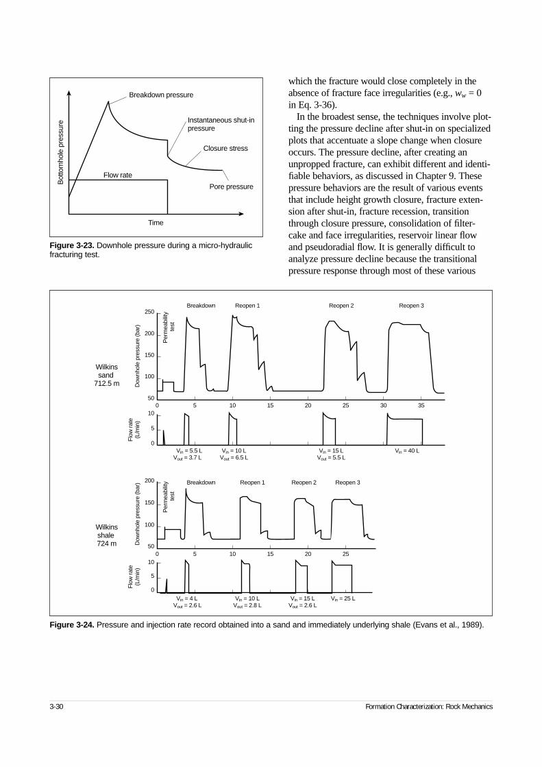
which the fracture would close completely in theabsence of fracture face irregularities (e.g., ww = 0 in Eq. 3-36).

In the broadest sense, the techniques involve plot-ting the pressure decline after shut-in on specializedplots that accentuate a slope change when closureoccurs. The pressure decline, after creating anunpropped fracture, can exhibit different and identi-fiable behaviors, as discussed in Chapter 9. Thesepressure behaviors are the result of various eventsthat include height growth closure, fracture exten-sion after shut-in, fracture recession, transitionthrough closure pressure, consolidation of filter-cake and face irregularities, reservoir linear flowand pseudoradial flow. It is generally difficult toanalyze pressure decline because the transitionalpressure response through most of these various

3-30 Formation Characterization: Rock Mechanics

Figure 3-23. Downhole pressure during a micro-hydraulicfracturing test.

Time

Bot

tom

hole

pre

ssur

e

Flow rate

Breakdown pressure

Instantaneous shut-in pressure

Closure stress

Pore pressure

Figure 3-24. Pressure and injection rate record obtained into a sand and immediately underlying shale (Evans et al., 1989).

Breakdown Reopen 1 Reopen 2 Reopen 3

Breakdown Reopen 1 Reopen 2 Reopen 3

Per

mea

bilit

yte

stP

erm

eabi

lity

test

050

0

5

10

0

5

10

5 10 15 20 25

0 5 10 15 20 25

30 35

100

150

200

50

100

150

200

250

Vin = 5.5 LVout = 3.7 L

Vin = 10 LVout = 6.5 L

Vin = 15 LVout = 5.5 L

Vin = 40 L

Vin = 4 LVout = 2.6 L

Vin = 10 LVout = 2.8 L

Vin = 15 LVout = 2.6 L

Vin = 25 L

Flo

w ra

te(L

/min

)F

low

rate

(L/m

in)

Dow

nhol

e pr

essu

re (b

ar)

Dow

nhol

e pr

essu

re (b

ar)

Wilkinssand

712.5 m

Wilkinsshale724 m

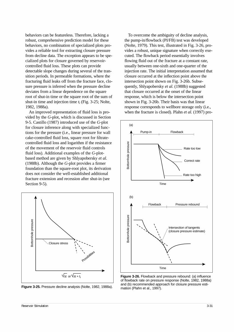
behaviors can be featureless. Therefore, lacking arobust, comprehensive prediction model for thesebehaviors, no combination of specialized plots pro-vides a reliable tool for extracting closure pressurefrom decline data. The exception appears to be spe-cialized plots for closure governed by reservoir-controlled fluid loss. These plots can providedetectable slope changes during several of the tran-sition periods. In permeable formations, where thefracturing fluid leaks off from the fracture face, clo-sure pressure is inferred when the pressure declinedeviates from a linear dependence on the squareroot of shut-in time or the square root of the sum ofshut-in time and injection time ti (Fig. 3-25; Nolte,1982, 1988a).

An improved representation of fluid loss is pro-vided by the G-plot, which is discussed in Section9-5. Castillo (1987) introduced use of the G-plotfor closure inference along with specialized func-tions for the pressure (i.e., linear pressure for wallcake-controlled fluid loss, square root for filtrate-controlled fluid loss and logarithm if the resistanceof the movement of the reservoir fluid controlsfluid loss). Additional examples of the G-plot-based method are given by Shlyapobersky et al.(1988b). Although the G-plot provides a firmerfoundation than the square-root plot, its derivationdoes not consider the well-established additionalfracture extension and recession after shut-in (seeSection 9-5).

To overcome the ambiguity of decline analysis,the pump-in/flowback (PI/FB) test was developed(Nolte, 1979). This test, illustrated in Fig. 3-26, pro-vides a robust, unique signature when correctly exe-cuted. The flowback period essentially involvesflowing fluid out of the fracture at a constant rate,usually between one-sixth and one-quarter of theinjection rate. The initial interpretation assumed thatclosure occurred at the inflection point above theintersection point shown on Fig. 3-26b. Subse-quently, Shlyapobersky et al. (1988b) suggestedthat closure occurred at the onset of the linearresponse, which is below the intersection pointshown in Fig. 3-26b. Their basis was that linearresponse corresponds to wellbore storage only (i.e.,when the fracture is closed). Plahn et al. (1997) pro-

Reservoir Stimulation 3-31

Figure 3-25. Pressure decline analysis (Nolte, 1982, 1988a).

∆t or ∆t + ti

Bot

tom

hole

pre

ssur

e

Possibiliti

es

Closure stress

Figure 3-26. Flowback and pressure rebound: (a) influenceof flowback rate on pressure response (Nolte, 1982, 1988a)and (b) recommended approach for closure pressure esti-mation (Plahn et al., 1997).

Time

Time

Bot

tom

hole

pre

ssur

eB

otto

mho

le p

ress

ure

Pump-in Flowback

Flowback Pressure rebound

Rate too low

Correct rate

Rate too high

Intersection of tangents(closure pressure estimate)

(a)

(b)

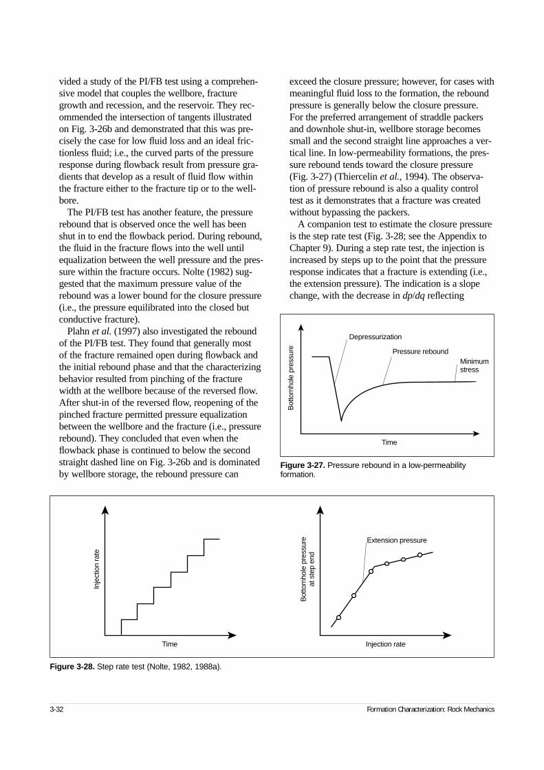
vided a study of the PI/FB test using a comprehen-sive model that couples the wellbore, fracturegrowth and recession, and the reservoir. They rec-ommended the intersection of tangents illustratedon Fig. 3-26b and demonstrated that this was pre-cisely the case for low fluid loss and an ideal fric-tionless fluid; i.e., the curved parts of the pressureresponse during flowback result from pressure gra-dients that develop as a result of fluid flow withinthe fracture either to the fracture tip or to the well-bore.

The PI/FB test has another feature, the pressurerebound that is observed once the well has beenshut in to end the flowback period. During rebound,the fluid in the fracture flows into the well untilequalization between the well pressure and the pres-sure within the fracture occurs. Nolte (1982) sug-gested that the maximum pressure value of therebound was a lower bound for the closure pressure(i.e., the pressure equilibrated into the closed butconductive fracture).

Plahn et al. (1997) also investigated the reboundof the PI/FB test. They found that generally most of the fracture remained open during flowback andthe initial rebound phase and that the characterizingbehavior resulted from pinching of the fracturewidth at the wellbore because of the reversed flow.After shut-in of the reversed flow, reopening of thepinched fracture permitted pressure equalizationbetween the wellbore and the fracture (i.e., pressurerebound). They concluded that even when theflowback phase is continued to below the secondstraight dashed line on Fig. 3-26b and is dominatedby wellbore storage, the rebound pressure can

exceed the closure pressure; however, for cases withmeaningful fluid loss to the formation, the reboundpressure is generally below the closure pressure.For the preferred arrangement of straddle packersand downhole shut-in, wellbore storage becomessmall and the second straight line approaches a ver-tical line. In low-permeability formations, the pres-sure rebound tends toward the closure pressure (Fig. 3-27) (Thiercelin et al., 1994). The observa-tion of pressure rebound is also a quality controltest as it demonstrates that a fracture was createdwithout bypassing the packers.

A companion test to estimate the closure pressureis the step rate test (Fig. 3-28; see the Appendix toChapter 9). During a step rate test, the injection isincreased by steps up to the point that the pressureresponse indicates that a fracture is extending (i.e.,the extension pressure). The indication is a slopechange, with the decrease in dp/dq reflecting

3-32 Formation Characterization: Rock Mechanics

Figure 3-27. Pressure rebound in a low-permeability formation.

Time

Bot

tom

hole

pre

ssur

e

Depressurization

Pressure reboundMinimumstress

Figure 3-28. Step rate test (Nolte, 1982, 1988a).

Time Injection rate

Inje

ctio

n ra

te

Bot

tom

hole

pre

ssur

eat

ste

p en

d

Extension pressure

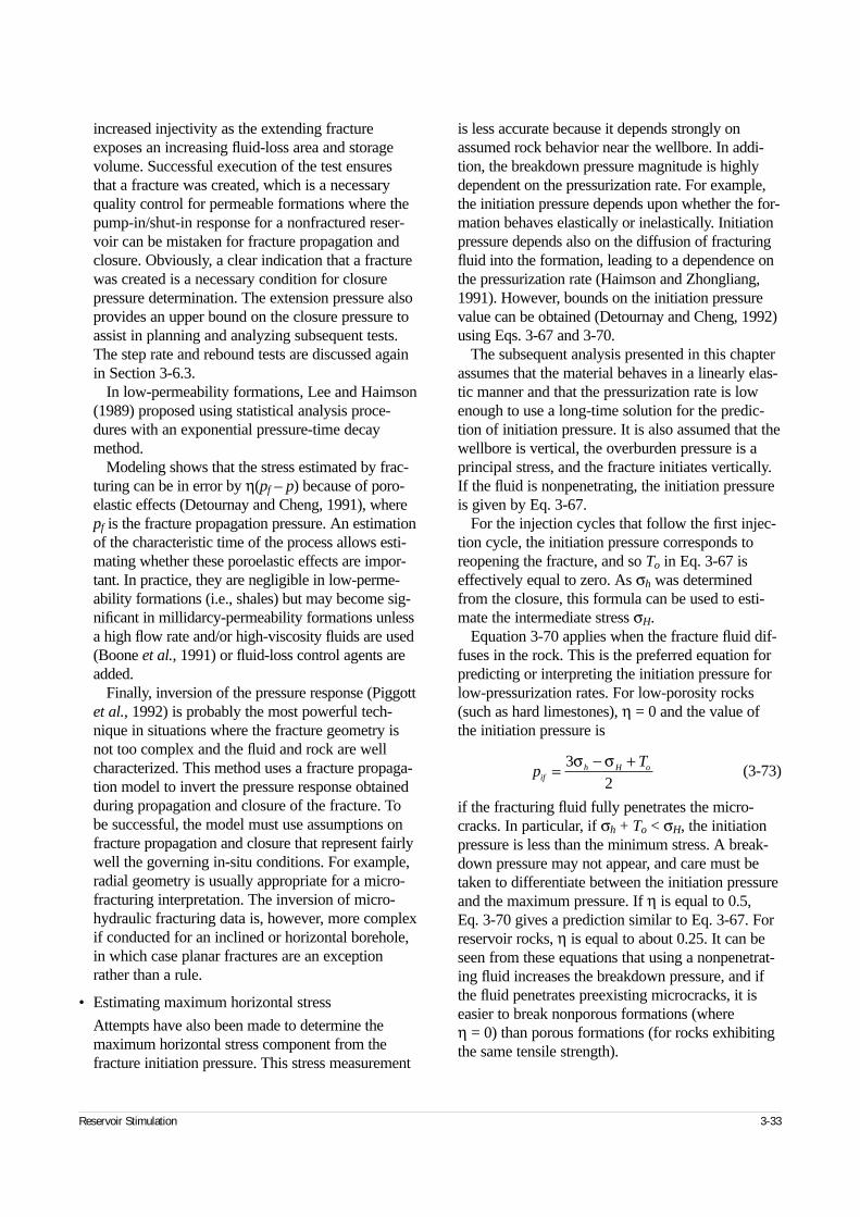
increased injectivity as the extending fractureexposes an increasing fluid-loss area and storagevolume. Successful execution of the test ensuresthat a fracture was created, which is a necessaryquality control for permeable formations where thepump-in/shut-in response for a nonfractured reser-voir can be mistaken for fracture propagation andclosure. Obviously, a clear indication that a fracturewas created is a necessary condition for closurepressure determination. The extension pressure alsoprovides an upper bound on the closure pressure toassist in planning and analyzing subsequent tests.The step rate and rebound tests are discussed againin Section 3-6.3.

In low-permeability formations, Lee and Haimson(1989) proposed using statistical analysis proce-dures with an exponential pressure-time decaymethod.

Modeling shows that the stress estimated by frac-turing can be in error by η(pf – p) because of poro-elastic effects (Detournay and Cheng, 1991), wherepf is the fracture propagation pressure. An estimationof the characteristic time of the process allows esti-mating whether these poroelastic effects are impor-tant. In practice, they are negligible in low-perme-ability formations (i.e., shales) but may become sig-nificant in millidarcy-permeability formations unlessa high flow rate and/or high-viscosity fluids are used(Boone et al., 1991) or fluid-loss control agents areadded.

Finally, inversion of the pressure response (Piggottet al., 1992) is probably the most powerful tech-nique in situations where the fracture geometry isnot too complex and the fluid and rock are wellcharacterized. This method uses a fracture propaga-tion model to invert the pressure response obtainedduring propagation and closure of the fracture. Tobe successful, the model must use assumptions onfracture propagation and closure that represent fairlywell the governing in-situ conditions. For example,radial geometry is usually appropriate for a micro-fracturing interpretation. The inversion of micro-hydraulic fracturing data is, however, more complexif conducted for an inclined or horizontal borehole,in which case planar fractures are an exceptionrather than a rule.

• Estimating maximum horizontal stress

Attempts have also been made to determine themaximum horizontal stress component from thefracture initiation pressure. This stress measurement

is less accurate because it depends strongly onassumed rock behavior near the wellbore. In addi-tion, the breakdown pressure magnitude is highlydependent on the pressurization rate. For example,the initiation pressure depends upon whether the for-mation behaves elastically or inelastically. Initiationpressure depends also on the diffusion of fracturingfluid into the formation, leading to a dependence onthe pressurization rate (Haimson and Zhongliang,1991). However, bounds on the initiation pressurevalue can be obtained (Detournay and Cheng, 1992)using Eqs. 3-67 and 3-70.

The subsequent analysis presented in this chapterassumes that the material behaves in a linearly elas-tic manner and that the pressurization rate is lowenough to use a long-time solution for the predic-tion of initiation pressure. It is also assumed that thewellbore is vertical, the overburden pressure is aprincipal stress, and the fracture initiates vertically.If the fluid is nonpenetrating, the initiation pressureis given by Eq. 3-67.

For the injection cycles that follow the first injec-tion cycle, the initiation pressure corresponds toreopening the fracture, and so To in Eq. 3-67 iseffectively equal to zero. As σh was determinedfrom the closure, this formula can be used to esti-mate the intermediate stress σH.

Equation 3-70 applies when the fracture fluid dif-fuses in the rock. This is the preferred equation forpredicting or interpreting the initiation pressure forlow-pressurization rates. For low-porosity rocks(such as hard limestones), η = 0 and the value ofthe initiation pressure is

(3-73)

if the fracturing fluid fully penetrates the micro-cracks. In particular, if σh + To < σH, the initiationpressure is less than the minimum stress. A break-down pressure may not appear, and care must betaken to differentiate between the initiation pressureand the maximum pressure. If η is equal to 0.5, Eq. 3-70 gives a prediction similar to Eq. 3-67. Forreservoir rocks, η is equal to about 0.25. It can beseen from these equations that using a nonpenetrat-ing fluid increases the breakdown pressure, and ifthe fluid penetrates preexisting microcracks, it iseasier to break nonporous formations (where η = 0) than porous formations (for rocks exhibitingthe same tensile strength).

Reservoir Stimulation 3-33

pT

ifh H o= − +3

2σ σ

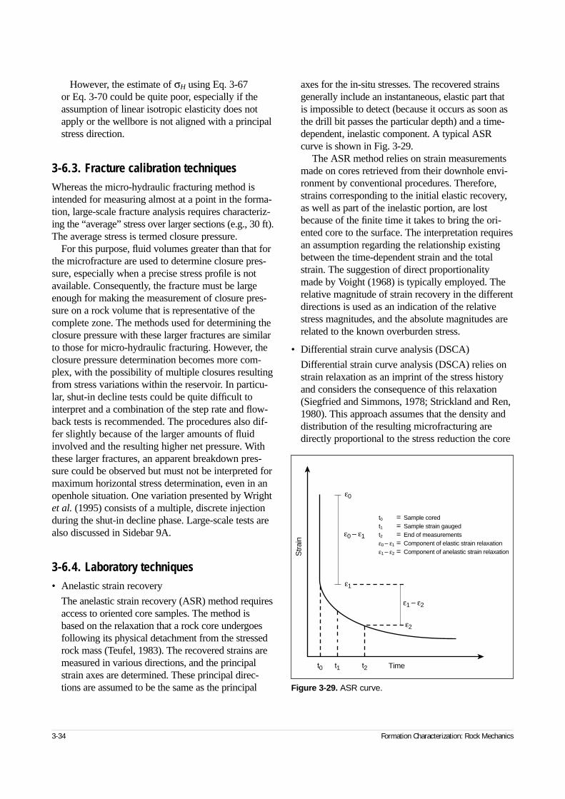
However, the estimate of σH using Eq. 3-67 or Eq. 3-70 could be quite poor, especially if theassumption of linear isotropic elasticity does notapply or the wellbore is not aligned with a principalstress direction.

3-6.3. Fracture calibration techniquesWhereas the micro-hydraulic fracturing method isintended for measuring almost at a point in the forma-tion, large-scale fracture analysis requires characteriz-ing the “average” stress over larger sections (e.g., 30 ft).The average stress is termed closure pressure.

For this purpose, fluid volumes greater than that forthe microfracture are used to determine closure pres-sure, especially when a precise stress profile is notavailable. Consequently, the fracture must be largeenough for making the measurement of closure pres-sure on a rock volume that is representative of thecomplete zone. The methods used for determining theclosure pressure with these larger fractures are similarto those for micro-hydraulic fracturing. However, theclosure pressure determination becomes more com-plex, with the possibility of multiple closures resultingfrom stress variations within the reservoir. In particu-lar, shut-in decline tests could be quite difficult tointerpret and a combination of the step rate and flow-back tests is recommended. The procedures also dif-fer slightly because of the larger amounts of fluidinvolved and the resulting higher net pressure. Withthese larger fractures, an apparent breakdown pres-sure could be observed but must not be interpreted formaximum horizontal stress determination, even in anopenhole situation. One variation presented by Wrightet al. (1995) consists of a multiple, discrete injectionduring the shut-in decline phase. Large-scale tests arealso discussed in Sidebar 9A.

3-6.4. Laboratory techniques• Anelastic strain recovery

The anelastic strain recovery (ASR) method requiresaccess to oriented core samples. The method isbased on the relaxation that a rock core undergoesfollowing its physical detachment from the stressedrock mass (Teufel, 1983). The recovered strains aremeasured in various directions, and the principalstrain axes are determined. These principal direc-tions are assumed to be the same as the principal

axes for the in-situ stresses. The recovered strainsgenerally include an instantaneous, elastic part thatis impossible to detect (because it occurs as soon asthe drill bit passes the particular depth) and a time-dependent, inelastic component. A typical ASRcurve is shown in Fig. 3-29.

The ASR method relies on strain measurementsmade on cores retrieved from their downhole envi-ronment by conventional procedures. Therefore,strains corresponding to the initial elastic recovery,as well as part of the inelastic portion, are lostbecause of the finite time it takes to bring the ori-ented core to the surface. The interpretation requiresan assumption regarding the relationship existingbetween the time-dependent strain and the totalstrain. The suggestion of direct proportionalitymade by Voight (1968) is typically employed. Therelative magnitude of strain recovery in the differentdirections is used as an indication of the relativestress magnitudes, and the absolute magnitudes arerelated to the known overburden stress.

• Differential strain curve analysis (DSCA)

Differential strain curve analysis (DSCA) relies onstrain relaxation as an imprint of the stress historyand considers the consequence of this relaxation(Siegfried and Simmons, 1978; Strickland and Ren,1980). This approach assumes that the density anddistribution of the resulting microfracturing aredirectly proportional to the stress reduction the core

3-34 Formation Characterization: Rock Mechanics

Figure 3-29. ASR curve.

Time

Stra

in

t0

t0 = Sample coredt1 = Sample strain gaugedt2 = End of measurementsε0 – ε1 = Component of elastic strain relaxationε1 – ε2 = Component of anelastic strain relaxation

t1 t2

ε0

ε0 – ε1

ε1 – ε2

ε1

ε2

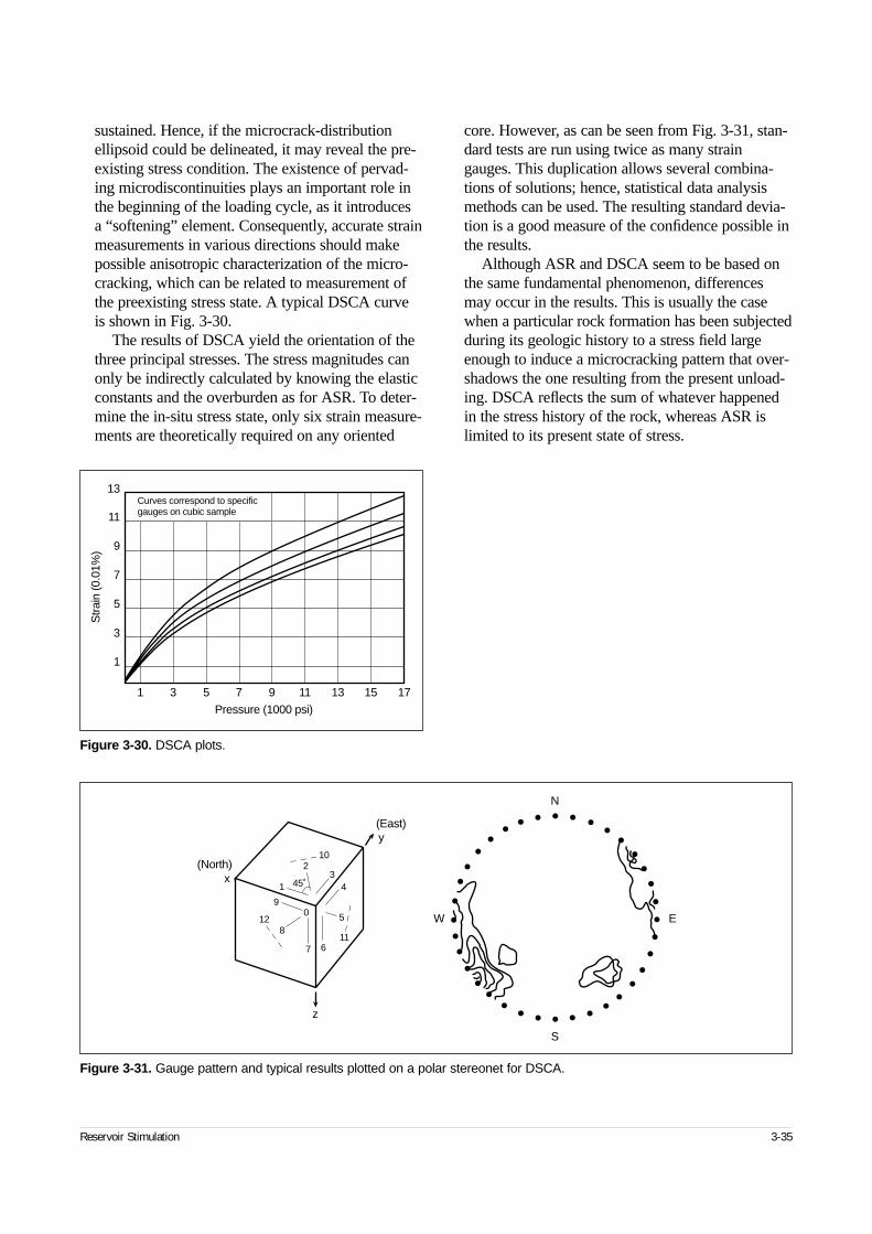
sustained. Hence, if the microcrack-distributionellipsoid could be delineated, it may reveal the pre-existing stress condition. The existence of pervad-ing microdiscontinuities plays an important role inthe beginning of the loading cycle, as it introduces a “softening” element. Consequently, accurate strainmeasurements in various directions should makepossible anisotropic characterization of the micro-cracking, which can be related to measurement ofthe preexisting stress state. A typical DSCA curveis shown in Fig. 3-30.

The results of DSCA yield the orientation of thethree principal stresses. The stress magnitudes canonly be indirectly calculated by knowing the elasticconstants and the overburden as for ASR. To deter-mine the in-situ stress state, only six strain measure-ments are theoretically required on any oriented

core. However, as can be seen from Fig. 3-31, stan-dard tests are run using twice as many straingauges. This duplication allows several combina-tions of solutions; hence, statistical data analysismethods can be used. The resulting standard devia-tion is a good measure of the confidence possible inthe results.

Although ASR and DSCA seem to be based onthe same fundamental phenomenon, differencesmay occur in the results. This is usually the casewhen a particular rock formation has been subjectedduring its geologic history to a stress field largeenough to induce a microcracking pattern that over-shadows the one resulting from the present unload-ing. DSCA reflects the sum of whatever happenedin the stress history of the rock, whereas ASR islimited to its present state of stress.

Reservoir Stimulation 3-35

Figure 3-30. DSCA plots.

1 3 5 7 9 11 13 15 17

1

Pressure (1000 psi)

3

5

7

9

11

13

Stra

in (0

.01%

)

Curves correspond to specificgauges on cubic sample

Figure 3-31. Gauge pattern and typical results plotted on a polar stereonet for DSCA.

0

7 6

5

43

2

1

10

118

9

12

45˚x

z

y

(North)

(East)

N

S

EW

4-1. IntroductionThe purpose of this chapter is to describe, strictly inthe context of reservoir stimulation, the use of geo-physical information (commonly referred to as logs)to obtain a description of the formation affected by a stimulation treatment. The entire process of classicformation evaluation for the determination of hydro-carbon reserves is out of the scope of this volume. A fundamental difference between these two pro-cesses is that all properties are required not only forthe hydrocarbon-bearing formations (pay zones) butalso for the adjacent formations (bounding layers).

The output of the process described in this chapteris a model of the formation to be stimulated. Themodel consists of a series of planar, parallel layers or beds, with known properties for each layer. Eachproperty in a layer is either a constant, averagedproperty or a linear function of depth (e.g., porepressure) (Fig. 4-1).

To construct the model, estimates first must beobtained of the relevant properties in each layer.These properties are in two broad classes: propertiesrelevant to the diffusion of fluid in the formation andproperties relevant to the deformation of the forma-

tion. Sections 4-4 and 4-5, respectively, discuss thevarious means of determining these properties.

All that is then necessary is to transform the datagathered into a consistent model. The first step forthis process is to fill any data gaps by relying ongeologic information. Each depositional basin has itsown “style,” characterized by unique properties.Moreover, the succession of layers is not arbitrary,but obeys worldwide a logic that is captured by thenotion of sequence (e.g., sand/shale sequence, lime-stone/marl sequence) (Wagoner et al., 1930; Fried-man and Sanders, 1978). Combining informationcharacterizing the basin with information from therelevant sequence makes it possible to estimate miss-ing data or interpolate between data points with aneducated guess or correlation. This process is partic-ularly crucial for the determination of lithology, porepressure and stress profiles. The need for a modelbased on a basin and field perspective is emphasizedthroughout this chapter. This approach also clearlyindicates the need for bringing geological expertiseinto the picture.

Once a complete description versus depth isachieved, the boundaries of the layers to be consid-ered are defined (i.e., zoning), which is also guidedby geologic information. Section 4-6 discusses thezoning process.

An important aspect stressed throughout this chap-ter is the calibration of geophysical data. Apart fromthe most basic properties, such as porosity and watersaturation, geophysical information requires calibra-tion with laboratory data. Again, the notion of basinand sequence is useful: the calibration procedure isusually portable within the same sequence in thesame basin. In other words, if no core samples havebeen tested for a particular well, results from othercores taken in the same formation and basin may beused, albeit with some caution.

In this chapter, it is assumed that the geophysicalinformation comes from the well to be stimulated.The porting of geophysical information from onewell to another is not addressed.

Reservoir Stimulation 4-1

◆

Formation Characterization:Well Logs

Jean Desroches, Schlumberger DowellTom Bratton, Schlumberger Sugar Land Product Center

Figure 4-1. Model of the earth in the vicinity of the forma-tion to be stimulated.

Layer 1

Layer 3

Layer 4

Layer 5

Layer 6

Layer 2

True

ver

tical

dep

th, z

TV

D

Profile of aproperty with

a constantvalue withineach layer

(e.g., porosity)

Profile ofhorizontal

stress—linearlyvarying within

each layer

Profile of pore pressure—

linearly varyingwithin each

layer

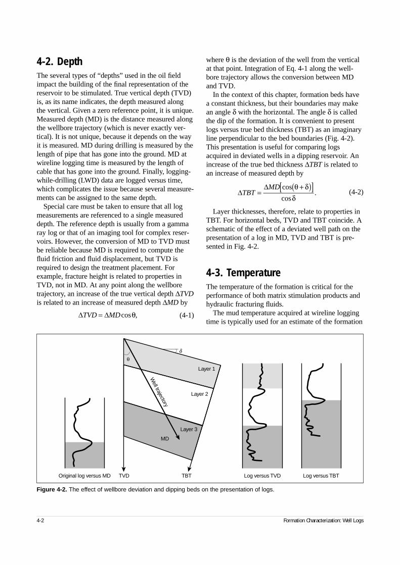
4-2. DepthThe several types of “depths” used in the oil fieldimpact the building of the final representation of thereservoir to be stimulated. True vertical depth (TVD)is, as its name indicates, the depth measured alongthe vertical. Given a zero reference point, it is unique.Measured depth (MD) is the distance measured alongthe wellbore trajectory (which is never exactly ver-tical). It is not unique, because it depends on the wayit is measured. MD during drilling is measured by thelength of pipe that has gone into the ground. MD atwireline logging time is measured by the length ofcable that has gone into the ground. Finally, logging-while-drilling (LWD) data are logged versus time,which complicates the issue because several measure-ments can be assigned to the same depth.

Special care must be taken to ensure that all logmeasurements are referenced to a single measureddepth. The reference depth is usually from a gammaray log or that of an imaging tool for complex reser-voirs. However, the conversion of MD to TVD mustbe reliable because MD is required to compute thefluid friction and fluid displacement, but TVD isrequired to design the treatment placement. Forexample, fracture height is related to properties inTVD, not in MD. At any point along the wellboretrajectory, an increase of the true vertical depth ∆TVDis related to an increase of measured depth ∆MD by

(4-1)

where θ is the deviation of the well from the verticalat that point. Integration of Eq. 4-1 along the well-bore trajectory allows the conversion between MDand TVD.

In the context of this chapter, formation beds havea constant thickness, but their boundaries may makean angle δ with the horizontal. The angle δ is calledthe dip of the formation. It is convenient to presentlogs versus true bed thickness (TBT) as an imaginaryline perpendicular to the bed boundaries (Fig. 4-2).This presentation is useful for comparing logsacquired in deviated wells in a dipping reservoir. Anincrease of the true bed thickness ∆TBT is related toan increase of measured depth by

(4-2)

Layer thicknesses, therefore, relate to properties inTBT. For horizontal beds, TVD and TBT coincide. Aschematic of the effect of a deviated well path on thepresentation of a log in MD, TVD and TBT is pre-sented in Fig. 4-2.

4-3. TemperatureThe temperature of the formation is critical for theperformance of both matrix stimulation products andhydraulic fracturing fluids.

The mud temperature acquired at wireline loggingtime is typically used for an estimate of the formation

Figure 4-2. The effect of wellbore deviation and dipping beds on the presentation of logs.

Layer 1

Layer 2

Layer 3

MD

Well trajectory

θδ

TVDOriginal log versus MD Log versus TVD Log versus TBTTBT

4-2 Formation Characterization: Well Logs

∆ ∆TVD MD= cos ,θ

∆∆

TBTMD

=+( )[ ]cos

cos.

θ δδ

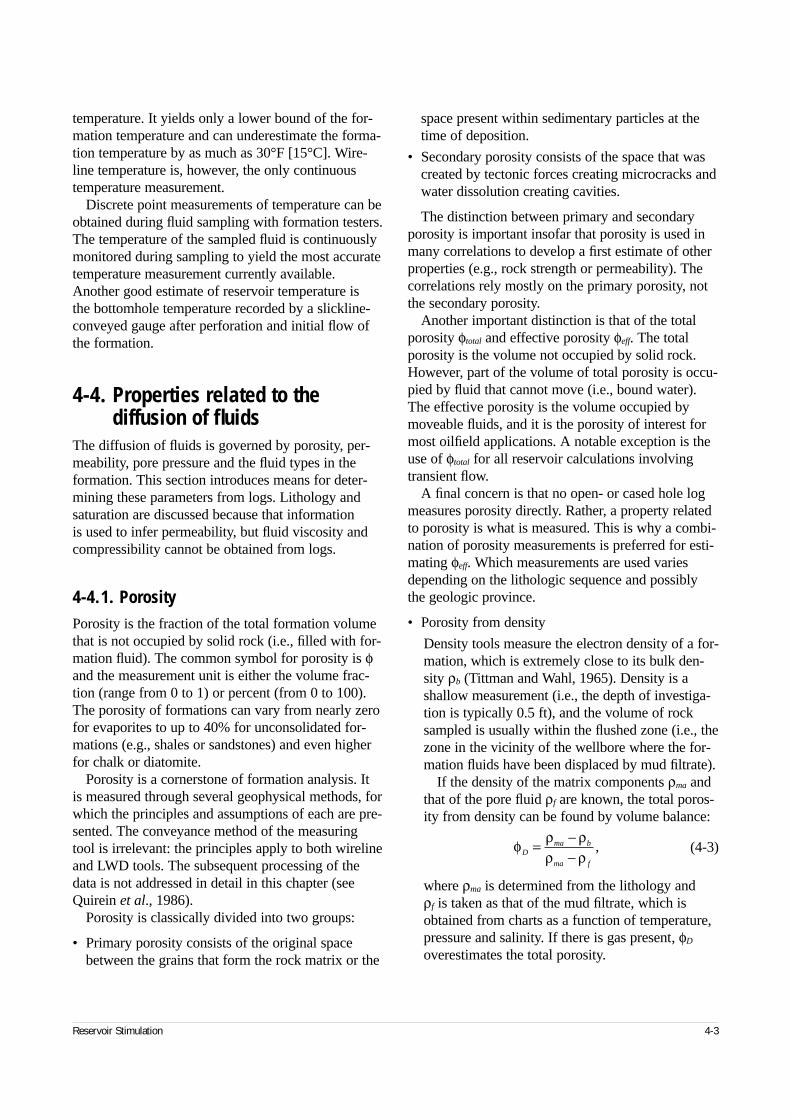
temperature. It yields only a lower bound of the for-mation temperature and can underestimate the forma-tion temperature by as much as 30°F [15°C]. Wire-line temperature is, however, the only continuoustemperature measurement.

Discrete point measurements of temperature can beobtained during fluid sampling with formation testers.The temperature of the sampled fluid is continuouslymonitored during sampling to yield the most accuratetemperature measurement currently available.Another good estimate of reservoir temperature is the bottomhole temperature recorded by a slickline-conveyed gauge after perforation and initial flow ofthe formation.

4-4. Properties related to the diffusion of fluids

The diffusion of fluids is governed by porosity, per-meability, pore pressure and the fluid types in theformation. This section introduces means for deter-mining these parameters from logs. Lithology andsaturation are discussed because that information is used to infer permeability, but fluid viscosity andcompressibility cannot be obtained from logs.

4-4.1. PorosityPorosity is the fraction of the total formation volumethat is not occupied by solid rock (i.e., filled with for-mation fluid). The common symbol for porosity is φand the measurement unit is either the volume frac-tion (range from 0 to 1) or percent (from 0 to 100).The porosity of formations can vary from nearly zerofor evaporites to up to 40% for unconsolidated for-mations (e.g., shales or sandstones) and even higherfor chalk or diatomite.

Porosity is a cornerstone of formation analysis. It is measured through several geophysical methods, forwhich the principles and assumptions of each are pre-sented. The conveyance method of the measuringtool is irrelevant: the principles apply to both wirelineand LWD tools. The subsequent processing of thedata is not addressed in detail in this chapter (seeQuirein et al., 1986).

Porosity is classically divided into two groups:

• Primary porosity consists of the original spacebetween the grains that form the rock matrix or the

space present within sedimentary particles at thetime of deposition.

• Secondary porosity consists of the space that wascreated by tectonic forces creating microcracks andwater dissolution creating cavities.

The distinction between primary and secondaryporosity is important insofar that porosity is used inmany correlations to develop a first estimate of otherproperties (e.g., rock strength or permeability). Thecorrelations rely mostly on the primary porosity, notthe secondary porosity.

Another important distinction is that of the totalporosity φtotal and effective porosity φeff. The totalporosity is the volume not occupied by solid rock.However, part of the volume of total porosity is occu-pied by fluid that cannot move (i.e., bound water).The effective porosity is the volume occupied bymoveable fluids, and it is the porosity of interest formost oilfield applications. A notable exception is theuse of φtotal for all reservoir calculations involvingtransient flow.

A final concern is that no open- or cased hole logmeasures porosity directly. Rather, a property relatedto porosity is what is measured. This is why a combi-nation of porosity measurements is preferred for esti-mating φeff. Which measurements are used variesdepending on the lithologic sequence and possiblythe geologic province.

• Porosity from density

Density tools measure the electron density of a for-mation, which is extremely close to its bulk den-sity ρb (Tittman and Wahl, 1965). Density is ashallow measurement (i.e., the depth of investiga-tion is typically 0.5 ft), and the volume of rocksampled is usually within the flushed zone (i.e., thezone in the vicinity of the wellbore where the for-mation fluids have been displaced by mud filtrate).

If the density of the matrix components ρma andthat of the pore fluid ρf are known, the total poros-ity from density can be found by volume balance:

(4-3)

where ρma is determined from the lithology and ρf is taken as that of the mud filtrate, which isobtained from charts as a function of temperature,pressure and salinity. If there is gas present, φD

overestimates the total porosity.

Reservoir Stimulation 4-3

φ ρ ρρ ρD

ma b

ma f

= −−

,

• Porosity from neutron

Neutron tools measure an index of how muchhydrogen is present in the formation (Allen etal., 1967). It is also a shallow measurement (i.e.,the depth of investigation is typically 1 ft). If nohydrogen is in the rock matrix and the hydrogenindex of the fluid is known, the neutron porosityφN obtains a measure of the total porosity.

Water and liquid hydrocarbons have similarhydrogen indices; therefore, φN is insensitive to thepresence of oil in the sampled volume. However, ifgas is present, φN underestimates the total porosity.

The deviation of φN and that of φD from the totalporosity tend to be in opposite directions. Oneexample, mentioned previously, is their oppositebehavior in the presence of gas. A simple averageof φN and φD yields a good estimate of the effectiveporosity:

(4-4)

• Porosity from sonic

The presence of pore fluid increases the rigidity of the rock over the case where porosity is trulyempty (i.e., “moon dry samples”). Moreover, mostof the attenuation of the sonic waves in a porousformation comes from the fluid (Biot, 1956b,1956c). If the elastic properties of the solid and thefluid are known, and therefore the traveltimes inthese media, an estimate of the total porosity canbe computed:

(4-5)

where A is a constant and ∆t denotes the measuredtransit time of a sonic wave in the formation. Thetransit time in the matrix ∆tma is known from thelithology. Because sonic is a shallow measurement(i.e., the depth of investigation is typically 1 ft),the fluid in the pore space is usually approximatedby the mud filtrate, the properties of which areknown functions of the temperature, pressure andsalinity. However, the sonic porosity φS is a strongfunction of the properties of the fluid in the porespace. Therefore, if the fluid in the sampled porespace contains hydrocarbons, φS can deviate signif-icantly from the total porosity.

The value of φS is of particular interest becauseit is sensitive primarily to the primary porosity, notto the secondary porosity.

• Porosity from nuclear magnetic resonance

Nuclear magnetic resonance (NMR) tools measurethe relaxation time of protons. The porosity mea-sured by NMR tools is similar to φN but is influ-enced primarily by moveable fluids.

Extracting porosity from NMR measurementsrequires complex processing. However, NMR-measured porosity has two major advantages.First, because it is influenced primarily by move-able fluids, it is extremely close to φeff, and second,it yields excellent estimates of porosity in shaly(i.e., clay-bearing) formations, which are typicallychallenging for estimating porosity (Minh et al.,1998).

• Porosity from resistivity

Porosity can also be estimated from resistivitymeasurements. If the resistivity of the rock matrixis assumed to be infinite compared with that of thefluid, the conductivity of the formation is propor-tional to the porosity.

The formation factor F is introduced as a ratio:

(4-6)

where Ro is the resistivity of the formation 100%saturated with brine of resistivity Rw.

Archie (1942) postulated that the formation fac-tor is related to the total porosity by the relation

(4-7)

where a and m are constants depending on the typeof formation. For example, a = 0.62 and m = 2.15for clean sandstones.

Therefore, if Rw is known (e.g., from water “cat-alogs,” samples or spontaneous potential [SP]measurements), an estimate of the total porosity ofthe formation can be obtained by equating Eqs. 4-6and 4-7:

(4-8)

This technique is not recommended, because it isgreatly affected by the fluid saturation and conduc-tive minerals in the matrix.

• Final estimate of porosity

As mentioned previously, the best estimate ofporosity is obtained from a combination of logs,using synergistic processing that accounts for the

4-4 Formation Characterization: Well Logs

φ φ φeff N D≅ +( )12

.

φSma

f ma

At t

t t= −

−∆ ∆∆ ∆

,

FR

Ro

w

= ,

Fa

m=

φ,

φ =

aR

Rw

o

m1

.

response of each tool and is tailored to the geo-logic environment. If such a processed porosityestimate is not available, the simple average of φD and φN in Eq. 4-4 is a good first-order estimateof φeff in noncomplex environments, and the poros-ity from NMR yields a good estimate in morecomplex environments.

4-4.2. Lithology and saturationLithology and saturation are primary inputs fordesigning matrix acidizing treatments. Lithology isalso part of the more general information that must beconsidered to build a stress model (see Section 4-5.2).For hydraulic fracturing, saturation is used to esti-mate the compressibility of the formation fluid forcomputing the compressibility-controlled leakoff.

• Saturation

Water saturation Sw is the fraction of the pore vol-ume occupied by water. By definition, 1 – Sw is thefraction of the pore volume occupied by hydrocar-bons. Also of interest is the irreducible water satu-ration Swi, which is the fraction of the pore volumeoccupied by water bound to the formation.

Special attention is devoted in formation evalua-tion to both porosity and saturation because theirproduct defines the volume of hydrocarbons in thereservoir. Similarly for reservoir stimulation, theseare important quantities because they indirectlygovern the flow of water-base fluids in a porousmedium filled with both water and hydrocarbons.The relative permeability to water is linked to thesaturation (see Section 4-4.3). The total compress-ibility of the formation fluids, which is used for thedetermination of leakoff during hydraulic fracturingtreatments, is also computed using the saturation.

The value of Sw is obtained mainly throughresistivity measurements. In a clean formation (i.e., a formation without shales or other conduc-tive minerals), all the conductivity of the formationis associated with the brine in the pore space. Con-ductivity is the reciprocal of resistivity.

For the true resistivity of the formation Rt,which is beyond the disturbances associated withthe wellbore, Archie (1942) derived experimen-tally that

(4-9)

where A, m and n are constants that are functionsof the formation.

Because resistivity is usually measured at differ-ent depths of investigation, it is possible to mea-sure both the resistivity of the flushed zone Rxo,where all movable fluid has been displaced fromthe formation by mud filtrate, and the resistivity ofthe virgin formation Rt, far from the wellbore. Thefollowing expression is thus useful because it isindependent of the porosity:

(4-10)

where Rmf is the known resistivity of the mud fil-trate and α is typically assigned a value of 5⁄8. Rw

can be determined from water catalogs, samples or SP measurements.

If conductive minerals (e.g., clay minerals) arein the formation, their effect can be accounted forby several weighted-average techniques, especiallyfor shaly formations (Poupon et al., 1970). Forcomplex cases, the best estimate of Sw is deter-mined by lithological analysis, as discussed in thefollowing.

• Lithology

The goal of a lithological analysis is to obtain avolumetric distribution of the minerals and fluids in the formation as a function of depth. The conceptis first explained in this section with the exampleanalysis of a sand/shale sequence. The concept is then generalized to any kind of formation.

Historically, much work was devoted to sand/shale sequences (e.g., 40 papers in Shaly Sands,1982). The simplest form of lithological analysisin such formations is a shaliness indicator—i.e., anindicator of the volumetric ratio of clay minerals toclean sand.

The crudest shaliness indicator is based ongamma ray measurement. If all natural radio-activity in a sand/shale sequence is assumed tocome from clay minerals, high gamma ray values(>90 API units) indicate a shale (i.e., almost exclu-sively clay minerals), low gamma ray values (<20 API units) indicate a clean sandstone, andvalues in between indicate a mixture of clay andsand.

This scale can be further refined by introducinga simple response equation of a gamma ray tool.For example,

Reservoir Stimulation 4-5

RR A

Stwm

wn

=φ

,

SR R

R Rwxo t

mf w

=

α

,

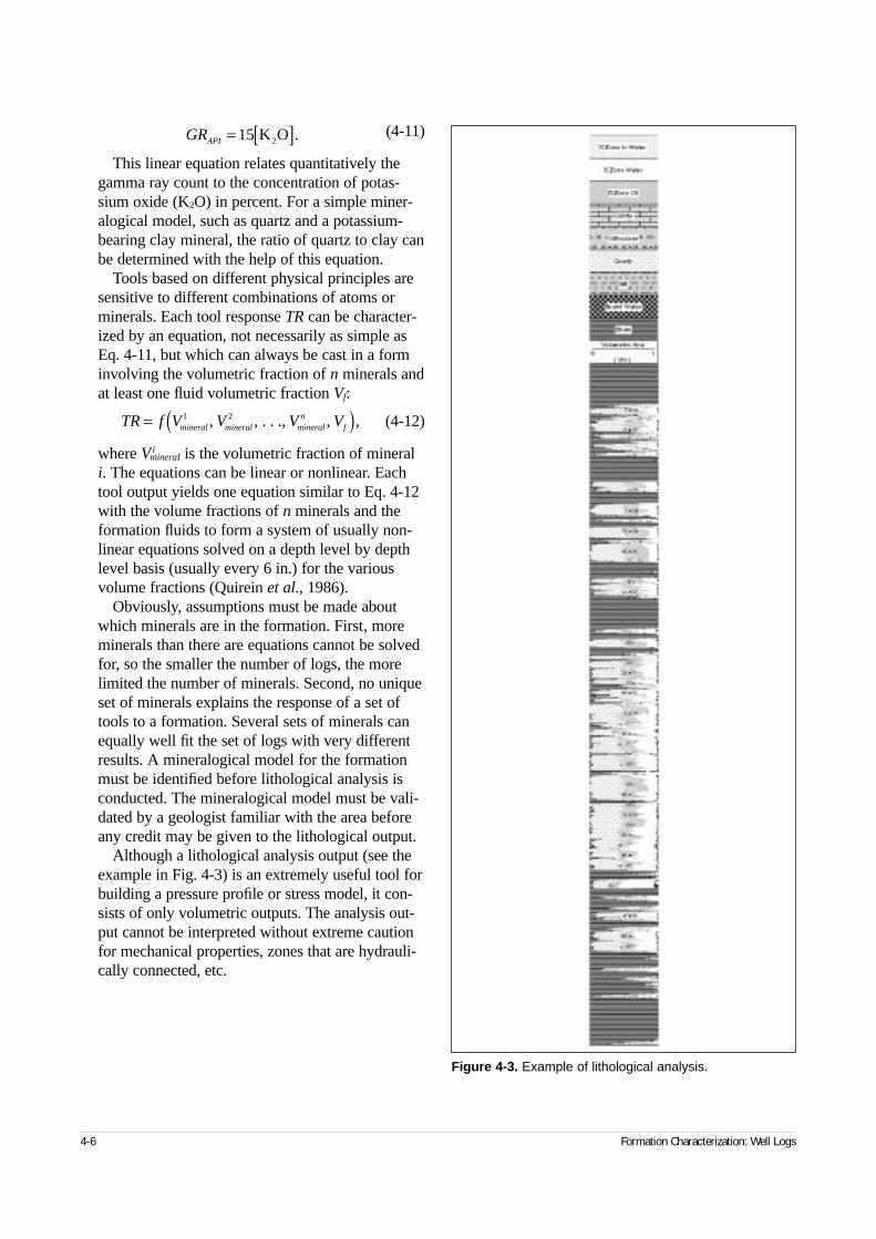
4-6 Formation Characterization: Well Logs

(4-11)

This linear equation relates quantitatively thegamma ray count to the concentration of potas-sium oxide (K2O) in percent. For a simple miner-alogical model, such as quartz and a potassium-bearing clay mineral, the ratio of quartz to clay canbe determined with the help of this equation.

Tools based on different physical principles aresensitive to different combinations of atoms orminerals. Each tool response TR can be character-ized by an equation, not necessarily as simple asEq. 4-11, but which can always be cast in a forminvolving the volumetric fraction of n minerals andat least one fluid volumetric fraction Vf:

(4-12)

where VimineraI is the volumetric fraction of mineral

i. The equations can be linear or nonlinear. Eachtool output yields one equation similar to Eq. 4-12with the volume fractions of n minerals and theformation fluids to form a system of usually non-linear equations solved on a depth level by depthlevel basis (usually every 6 in.) for the variousvolume fractions (Quirein et al., 1986).

Obviously, assumptions must be made aboutwhich minerals are in the formation. First, moreminerals than there are equations cannot be solvedfor, so the smaller the number of logs, the morelimited the number of minerals. Second, no uniqueset of minerals explains the response of a set oftools to a formation. Several sets of minerals canequally well fit the set of logs with very differentresults. A mineralogical model for the formationmust be identified before lithological analysis isconducted. The mineralogical model must be vali-dated by a geologist familiar with the area beforeany credit may be given to the lithological output.

Although a lithological analysis output (see theexample in Fig. 4-3) is an extremely useful tool forbuilding a pressure profile or stress model, it con-sists of only volumetric outputs. The analysis out-put cannot be interpreted without extreme cautionfor mechanical properties, zones that are hydrauli-cally connected, etc.

TR f V V V Vmineral mineral mineraln

f= ( )1 2, , . . ., , ,

Figure 4-3. Example of lithological analysis.

GRAPI = [ ]15 K O2 .

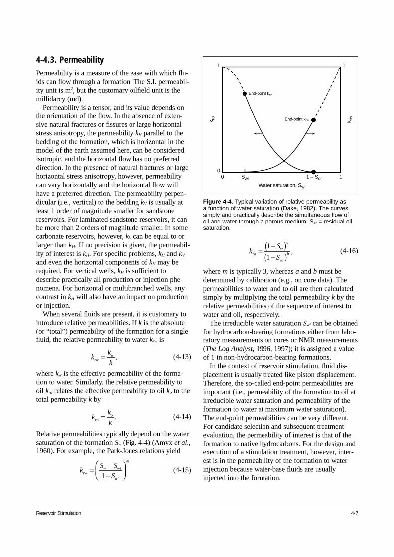
4-4.3. PermeabilityPermeability is a measure of the ease with which flu-ids can flow through a formation. The S.I. permeabil-ity unit is m2, but the customary oilfield unit is themillidarcy (md).

Permeability is a tensor, and its value depends onthe orientation of the flow. In the absence of exten-sive natural fractures or fissures or large horizontalstress anisotropy, the permeability kH parallel to thebedding of the formation, which is horizontal in themodel of the earth assumed here, can be consideredisotropic, and the horizontal flow has no preferreddirection. In the presence of natural fractures or largehorizontal stress anisotropy, however, permeabilitycan vary horizontally and the horizontal flow willhave a preferred direction. The permeability perpen-dicular (i.e., vertical) to the bedding kV is usually atleast 1 order of magnitude smaller for sandstonereservoirs. For laminated sandstone reservoirs, it canbe more than 2 orders of magnitude smaller. In somecarbonate reservoirs, however, kV can be equal to orlarger than kH. If no precision is given, the permeabil-ity of interest is kH. For specific problems, kH and kV

and even the horizontal components of kH may berequired. For vertical wells, kH is sufficient todescribe practically all production or injection phe-nomena. For horizontal or multibranched wells, anycontrast in kH will also have an impact on productionor injection.

When several fluids are present, it is customary tointroduce relative permeabilities. If k is the absolute(or “total”) permeability of the formation for a singlefluid, the relative permeability to water krw is

(4-13)

where kw is the effective permeability of the forma-tion to water. Similarly, the relative permeability tooil kro relates the effective permeability to oil ko to thetotal permeability k by

(4-14)

Relative permeabilities typically depend on the watersaturation of the formation Sw (Fig. 4-4) (Amyx et al.,1960). For example, the Park-Jones relations yield

(4-15)

(4-16)

where m is typically 3, whereas a and b must bedetermined by calibration (e.g., on core data). Thepermeabilities to water and to oil are then calculatedsimply by multiplying the total permeability k by therelative permeabilities of the sequence of interest towater and oil, respectively.

The irreducible water saturation Swi can be obtainedfor hydrocarbon-bearing formations either from labo-ratory measurements on cores or NMR measurements(The Log Analyst, 1996, 1997); it is assigned a valueof 1 in non-hydrocarbon-bearing formations.

In the context of reservoir stimulation, fluid dis-placement is usually treated like piston displacement.Therefore, the so-called end-point permeabilities areimportant (i.e., permeability of the formation to oil atirreducible water saturation and permeability of theformation to water at maximum water saturation).The end-point permeabilities can be very different.For candidate selection and subsequent treatmentevaluation, the permeability of interest is that of theformation to native hydrocarbons. For the design andexecution of a stimulation treatment, however, inter-est is in the permeability of the formation to waterinjection because water-base fluids are usuallyinjected into the formation.

Reservoir Stimulation 4-7

kk

krww= ,

kk

kroo= .

kS S

Srww wi

wi

m

= −−

1

kS

Sro

w

a

wi

b=−( )−( )

1

1,

Figure 4-4. Typical variation of relative permeability as a function of water saturation (Dake, 1982). The curvessimply and practically describe the simultaneous flow of oil and water through a porous medium. Sor = residual oilsaturation.

0

1 1

0 Swi

k ro

k rw

1 – Sor 1

Water saturation, Sw

End-point kro

End-point krw

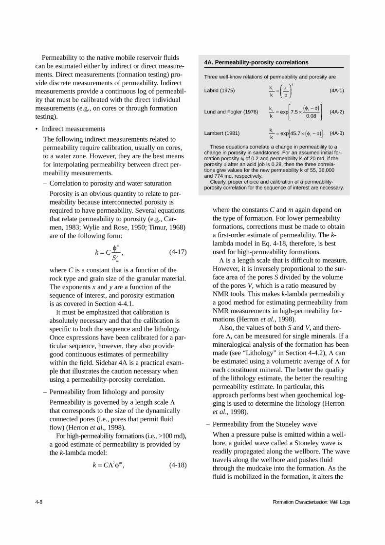
4-8 Formation Characterization: Well Logs

Permeability to the native mobile reservoir fluidscan be estimated either by indirect or direct measure-ments. Direct measurements (formation testing) pro-vide discrete measurements of permeability. Indirectmeasurements provide a continuous log of permeabil-ity that must be calibrated with the direct individualmeasurements (e.g., on cores or through formationtesting).

• Indirect measurements

The following indirect measurements related topermeability require calibration, usually on cores,to a water zone. However, they are the best meansfor interpolating permeability between direct per-meability measurements.

– Correlation to porosity and water saturation

Porosity is an obvious quantity to relate to per-meability because interconnected porosity isrequired to have permeability. Several equationsthat relate permeability to porosity (e.g., Car-men, 1983; Wylie and Rose, 1950; Timur, 1968)are of the following form:

(4-17)

where C is a constant that is a function of therock type and grain size of the granular material.The exponents x and y are a function of thesequence of interest, and porosity estimation is as covered in Section 4-4.1.

It must be emphasized that calibration isabsolutely necessary and that the calibration isspecific to both the sequence and the lithology.Once expressions have been calibrated for a par-ticular sequence, however, they also providegood continuous estimates of permeabilitywithin the field. Sidebar 4A is a practical exam-ple that illustrates the caution necessary whenusing a permeability-porosity correlation.

– Permeability from lithology and porosity

Permeability is governed by a length scale Λthat corresponds to the size of the dynamicallyconnected pores (i.e., pores that permit fluidflow) (Herron et al., 1998).

For high-permeability formations (i.e., >100 md),a good estimate of permeability is provided bythe k-lambda model:

(4-18)

where the constants C and m again depend onthe type of formation. For lower permeabilityformations, corrections must be made to obtain a first-order estimate of permeability. The k-lambda model in Eq. 4-18, therefore, is bestused for high-permeability formations.

Λ is a length scale that is difficult to measure.However, it is inversely proportional to the sur-face area of the pores S divided by the volumeof the pores V, which is a ratio measured byNMR tools. This makes k-lambda permeability a good method for estimating permeability fromNMR measurements in high-permeability for-mations (Herron et al., 1998).

Also, the values of both S and V, and there-fore Λ, can be measured for single minerals. If amineralogical analysis of the formation has beenmade (see “Lithology” in Section 4-4.2), Λ canbe estimated using a volumetric average of Λ foreach constituent mineral. The better the qualityof the lithology estimate, the better the resultingpermeability estimate. In particular, thisapproach performs best when geochemical log-ging is used to determine the lithology (Herronet al., 1998).

– Permeability from the Stoneley wave

When a pressure pulse is emitted within a well-bore, a guided wave called a Stoneley wave isreadily propagated along the wellbore. The wavetravels along the wellbore and pushes fluidthrough the mudcake into the formation. As thefluid is mobilized in the formation, it alters the

k CS

x

wiy

= φ,

4A. Permeability-porosity correlations

Three well-know relations of permeability and porosity are

Labrid (1975) (4A-1)

Lund and Fogler (1976) (4A-2)

Lambert (1981) (4A-3)

These equations correlate a change in permeability to achange in porosity in sandstones. For an assumed initial for-mation porosity φi of 0.2 and permeability ki of 20 md, if theporosity φ after an acid job is 0.28, then the three correla-tions give values for the new permeability k of 55, 36,000and 774 md, respectively.

Clearly, proper choice and calibration of a permeability-porosity correlation for the sequence of interest are necessary.

kk

i i=

φφ

3

kk

i i= ×−( )

exp ..

7 50 08

φ φ

kk

ii= × −( )[ ]exp . .45 7 φ φ

k C m= Λ2φ ,

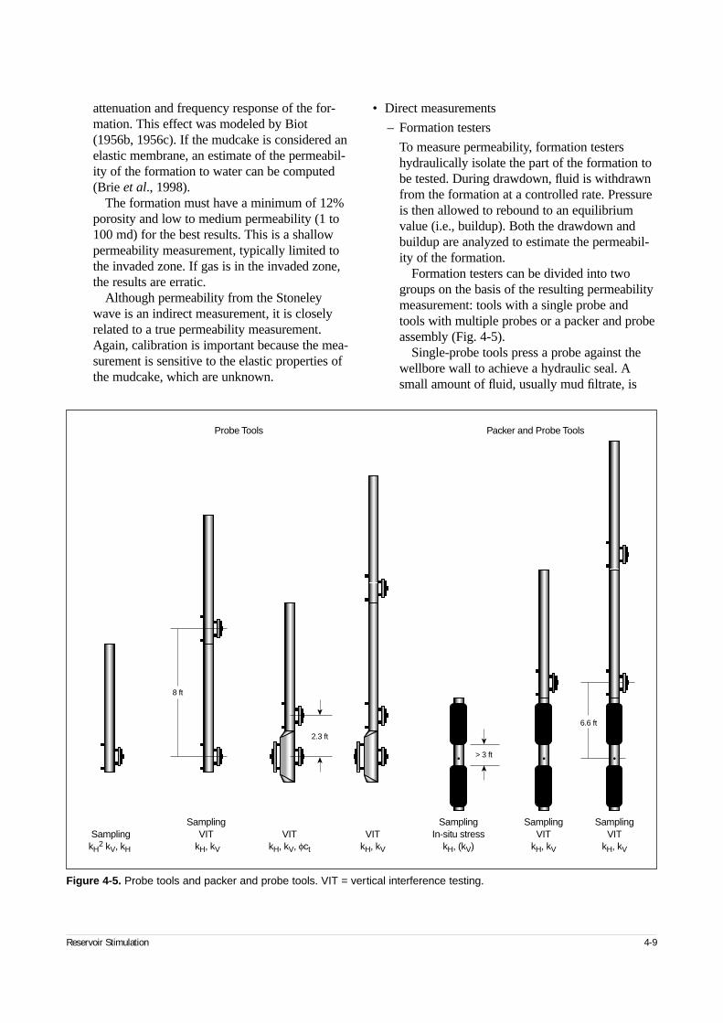
Reservoir Stimulation 4-9

attenuation and frequency response of the for-mation. This effect was modeled by Biot(1956b, 1956c). If the mudcake is considered anelastic membrane, an estimate of the permeabil-ity of the formation to water can be computed(Brie et al., 1998).

The formation must have a minimum of 12%porosity and low to medium permeability (1 to100 md) for the best results. This is a shallowpermeability measurement, typically limited tothe invaded zone. If gas is in the invaded zone,the results are erratic.

Although permeability from the Stoneleywave is an indirect measurement, it is closelyrelated to a true permeability measurement.Again, calibration is important because the mea-surement is sensitive to the elastic properties ofthe mudcake, which are unknown.

• Direct measurements

– Formation testers

To measure permeability, formation testershydraulically isolate the part of the formation tobe tested. During drawdown, fluid is withdrawnfrom the formation at a controlled rate. Pressureis then allowed to rebound to an equilibriumvalue (i.e., buildup). Both the drawdown andbuildup are analyzed to estimate the permeabil-ity of the formation.

Formation testers can be divided into twogroups on the basis of the resulting permeabilitymeasurement: tools with a single probe andtools with multiple probes or a packer and probeassembly (Fig. 4-5).

Single-probe tools press a probe against thewellbore wall to achieve a hydraulic seal. Asmall amount of fluid, usually mud filtrate, is

Figure 4-5. Probe tools and packer and probe tools. VIT = vertical interference testing.

SamplingkH

2 kV, kH

SamplingVIT

kH, kV

VITkH, kV, φct

VITkH, kV

SamplingIn-situ stress

kH, (kV)

SamplingVIT

kH, kV

SamplingVIT

kH, kV

6.6 ft

> 3 ft

8 ft

2.3 ft

Probe Tools Packer and Probe Tools

4-10 Formation Characterization: Well Logs

withdrawn during drawdown. The steady-statepressure drop at the sink probe ∆p is given by

(4-19)

(4-20)

(4-21)

where C is a shape factor accounting for the cur-vature of the wellbore, µ is the fluid viscosity(usually that of the mud filtrate), q is the rate of fluid withdrawal, rp is the radius of the probe,and K(η) is the complete elliptical integral of thefirst kind of modulus η (Wilkinson and Ham-mond, 1990). K(η) can be approximated byπ/2(1 + 1/4η2 + η4). The expression for theisotropic case kH = kV is typically used tocompute an estimate of kH.

Once drawdown is stopped, the pressurebounces back to the formation pressure (seeSection 4-4.2). In addition to µ, the expressiongoverning the pressure behavior now alsoincludes the formation porosity φ and the totalcompressibility ct of the fluid in the formation.

Drawdown and buildup permeability esti-mates are usually different. For small drawdownvolumes (i.e., of the order of 20 cm3), use of thedrawdown portion of the test is preferred forestimating the permeability of the formation.Then, a measure of the horizontal permeabilitykH to water can be obtained.

Permeability tests conducted with single-probe tools are commonly performed becausethey are simple, quick and reliable. Moreover,these tests provide a good relative indicator offormation permeability. The volume of investi-gation is of the order of a few feet.

In the multiple-probe configuration of a for-mation tester tool, several probes are used, sepa-rated by several meters. A pressure pulse is sentthrough one probe, and the response of the for-mation is monitored at the location of the otherprobes. This method enables the determination

of both kH and kV (Zimmerman et al., 1990; Popet al., 1993).

In the packer and probe configuration, a strad-dle packer is used to isolate part of the forma-tion to withdraw what can be large volumes offluids. The response of the formation is moni-tored by a probe several feet above the packer.This configuration also enables the determina-tion of both kH and kV, especially in high-perme-ability formations that require a large-volumewithdrawal to create a pressure response mea-surable at the probe.

The obvious advantage of the multiple-probetools and packer and probe tools is that they pro-duce kH and kV estimates. However, the radius ofinvestigation into the formation is also muchlarger than with a single-probe tool (i.e., at least3 times the spacing between the probes), whichdeparts from a discrete point measurement. Inparticular, the viscosity and compressibilityterms in the equations governing the flow corre-spond to those of the formation fluid. Theseextra parameters must be determined to estimatethe permeability. Thus, the design of formationtests using multiple-probe and packer and probetools is critical for obtaining representative data(Goode et al., 1991).

– Well tests

The same procedure as that used for formationtesting is used during well testing. The well isflowed at a constant rate during drawdownbefore it is shut in and pressure buildupobserved (see Chapter 2).

Well testing has a much larger volume ofinvestigation and produces an estimate of a com-posite kH. This composite value is crucial for theeconomic evaluation of stimulation treatments.However, for matrix stimulation, especially fluidplacement and diversion, knowledge of the per-meability within each layer is essential, hencethe need for continuous measurements of perme-ability by the methods outlined here.

4-4.4. Pore pressurePore pressure is the pressure of the fluid in the forma-tion. After production, its value can differ signifi-cantly from one layer to the next within a sequence.

∆pq

k

C

rk k

H p

V H= × =µ4

for

∆pq

k k

C

rK

k

kk k

V H p

H

V

V H= × −

>µ

π21 for ,

∆pq

k

C

rK

k

kk k

H p

V

H

V H= ×

<µ

π21– for

Reservoir Stimulation 4-11

It is a necessary input for designing matrix stimula-tion treatments of multiple layers, if only to accountfor and potentially take measures to control crossflowbetween zones. The pore pressure also strongly influ-ences the state of stress in a formation (by as much as50%) and is therefore a critical piece of informationfor designing hydraulic fracturing treatments.

• Pore pressure measurement

In addition to being measured by well tests, porepressure is measured by formation testers. Once a seal has been achieved between the formationtester and the formation, fluid is withdrawn fromthe formation to lower the pressure in the tester tobelow the far-field pore pressure. Flow is thenstopped, and if the formation has sufficient perme-ability, the formation will flow to equilibrate thetester with the bulk of the formation. The pressurein the tester will rise until a plateau is reached. Thepressure corresponding to the plateau is taken asan estimate of the pore pressure.

In low-permeability formations (<1 md), twoeffects can have an impact on the pressure mea-surement. First, the formation may not supplyenough fluid in a short enough time to equilibratewith the tester. In this case, the measurement maybe aborted before a meaningful plateau is reached.Second, even if a plateau is reached, it may indi-cate equilibrium with the higher local pore pres-sure induced by overbalance drilling (Fig. 4-6).This effect is commonly referred to as supercharg-ing (Phelps et al., 1984; Lane, 1993). It is there-fore a reasonable practice to question pore pressuremeasurements associated with a mobility that isless than 1 md/cp.

• Pressure profiles

Because pore pressure is a point measurement,there are gaps between the measurements. Thegaps can be filled by building pressure profiles.

If there are several fluids in the formation (e.g.,a mixture of water, oil and gas), only one of themis mobile and continuous across the pore space.This fluid is called the continuous fluid. Understatic conditions (i.e., no flow), pressure changesas a function of depth result from gravity only. Inother words, the pressure changes are a function ofthe density of the continuous fluid in the formation:

(4-22)

where p is the pore pressure, zTVD is the true verti-cal depth, ρf is the density of the continuous fluid,and g is the acceleration of gravity.

A normally pressured reservoir consists of for-mations where p is close to a reference pressuregiven by a continuous column of brine up to thesurface, which corresponds to a pressure gradientbetween 0.43 and 0.45 psi/ft in oilfield units:

(4-23)

where ρbrine is the density of the brine. An over-pressured reservoir consists of formations where pis much larger than the reference pressure, and anunderpressured reservoir exhibits values of p thatare much smaller than the reference pressure.

In simple virgin (i.e., unproduced) reservoirs, allthe permeable zones are equilibrated with eachother, and the pore pressure measurements plottedversus TVD should form a straight line with aslope given by the density of the continuous fluidin the formation. The straight line can be used tointerpolate the pore pressure values between thepoint measurements. The slope will changedepending on the fluid, which enables the determi-nation of fluid contacts (Fig. 4-7) (Stewart et al.,1982; Desbrandes and Gualdron, 1988).

In developed reservoirs or those with complexstructures, building pressure profiles requires manypore pressure measurements. The identification ofgradients is a powerful tool for detecting disconti-nuities in pore pressure that most likely correspondto discontinuities in permeability and discontinu-ities in stress magnitudes.

Figure 4-6. In high-permeability formations, the fluid leak-ing through the mudcake dissipates easily with no signifi-cant increase in formation pressure. In low-permeabilityzones, the fluid leaking through the mudcake cannot dissi-pate easily. In this latter case, the pressure measuredimmediately behind the mudcake is higher than the trueformation pressure. pbh = borehole pressure, pf = far-fieldpore pressure.

pbh

pf

pbh

pf

High-permeability formation Low-permeability formation

dp

dzg

TVD

f= ρ ,

p z dzTVD brine

zTVD

( ) ≈ ∫ ρ0

,

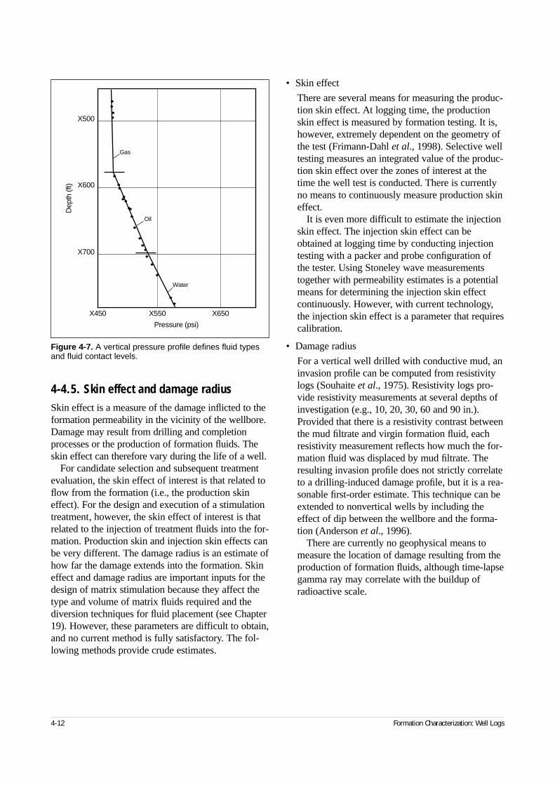
4-12 Formation Characterization: Well Logs

4-4.5. Skin effect and damage radiusSkin effect is a measure of the damage inflicted to theformation permeability in the vicinity of the wellbore.Damage may result from drilling and completionprocesses or the production of formation fluids. Theskin effect can therefore vary during the life of a well.

For candidate selection and subsequent treatmentevaluation, the skin effect of interest is that related toflow from the formation (i.e., the production skineffect). For the design and execution of a stimulationtreatment, however, the skin effect of interest is thatrelated to the injection of treatment fluids into the for-mation. Production skin and injection skin effects canbe very different. The damage radius is an estimate ofhow far the damage extends into the formation. Skineffect and damage radius are important inputs for thedesign of matrix stimulation because they affect thetype and volume of matrix fluids required and thediversion techniques for fluid placement (see Chapter19). However, these parameters are difficult to obtain,and no current method is fully satisfactory. The fol-lowing methods provide crude estimates.

• Skin effect

There are several means for measuring the produc-tion skin effect. At logging time, the productionskin effect is measured by formation testing. It is,however, extremely dependent on the geometry ofthe test (Frimann-Dahl et al., 1998). Selective welltesting measures an integrated value of the produc-tion skin effect over the zones of interest at thetime the well test is conducted. There is currentlyno means to continuously measure production skineffect.

It is even more difficult to estimate the injectionskin effect. The injection skin effect can beobtained at logging time by conducting injectiontesting with a packer and probe configuration ofthe tester. Using Stoneley wave measurementstogether with permeability estimates is a potentialmeans for determining the injection skin effectcontinuously. However, with current technology,the injection skin effect is a parameter that requirescalibration.

• Damage radius

For a vertical well drilled with conductive mud, aninvasion profile can be computed from resistivitylogs (Souhaite et al., 1975). Resistivity logs pro-vide resistivity measurements at several depths ofinvestigation (e.g., 10, 20, 30, 60 and 90 in.).Provided that there is a resistivity contrast betweenthe mud filtrate and virgin formation fluid, eachresistivity measurement reflects how much the for-mation fluid was displaced by mud filtrate. Theresulting invasion profile does not strictly correlateto a drilling-induced damage profile, but it is a rea-sonable first-order estimate. This technique can beextended to nonvertical wells by including theeffect of dip between the wellbore and the forma-tion (Anderson et al., 1996).

There are currently no geophysical means tomeasure the location of damage resulting from theproduction of formation fluids, although time-lapsegamma ray may correlate with the buildup ofradioactive scale.

Figure 4-7. A vertical pressure profile defines fluid typesand fluid contact levels.

X700

X600

X500

X450 X550 X650

Pressure (psi)

Dep

th (f

t)

Gas

Oil

Water

Reservoir Stimulation 4-13

4-4.6. Composition of fluidsAlthough there are indirect logging means for deter-mining the composition of formation fluids, they arelimited basically to distinguishing among water(brine), gas and oil (e.g., Schiuma et al., 1997). Someconclusions can be made about the type of oil bymeasuring its specific density through pressure profil-ing (see Section 4-4.4).

The only reliable method for determining thecomposition of fluids downhole is to collect unconta-minated fluid samples for laboratory analysis.Sampling is best achieved with formation testers (see“Formation testers” in Section 4-4.3). For example,the MDT* Modular Formation Dynamics Tester canmeasure both the resistivity and optical properties ofthe flowing fluid to distinguish between uncontami-nated formation fluid and the invading water- or oil-base drilling mud or mud filtrate. For more informa-tion on fluid sampling, see Hashem et al. (1997) andAkram et al. (1998).

4-5. Properties related to the deformation and fracturing of rock

As presented in Chapters 3 and 5, the geometry of a hydraulic fracture depends strongly on both themechanical properties of the rock formation, whichdescribe how the formation will deform under achange in stresses, and the stresses acting on the for-mation. The mechanical properties of the formationand the in-situ stresses are not independent. A differ-ence in mechanical properties between two adjacentformations usually leads to a difference in the in-situstresses. Except for the simplest situations, at least aqualitative model must be used to explain the rela-tionship between the formation mechanical propertiesand stresses.

4-5.1. Mechanical properties• Elastic properties

The only tool that responds to the elastic propertiesof the formation is the sonic. When a pressurepulse is created in a wellbore filled with fluid, thecomplex phenomena that occur at the boundarybetween the wellbore and the formation result inthe propagation of several types of waves into the

formation (Paillet and Chang, 1991). The twotypes of waves of interest for estimating the elasticconstants of a medium are compressional waves(P-waves) and shear waves (S-waves). The sonictool measures the characteristic propagation speedof the P- and S-waves.

In an isotropic medium, only the two elasticconstants of the shear modulus G and Poisson’sratio ν are independent. They are related to thevelocity of propagation of a P-wave uP and that of an S-wave uS by

(4-24)

(4-25)

The propagation velocity can be replaced withthe time ∆t it takes a wave to travel a fixed dis-tance d (e.g., between a source and a receiver):

(4-26)

(4-27)

where ∆tS and ∆tC are the S-wave and P-wavetraveltimes, respectively.

Young’s modulus E is related to the two con-stants by

(4-28)

These equations deserve a few comments. First,a measurement of ρb is required. Second, good-quality compressional and shear wave velocitymeasurements are crucial for the determination ofE and ν. In particular, both the compressional andshear waves must travel in the undisturbed forma-tion to yield a realistic estimate of ν—in otherwords, “deep” measurements of uP and uS areessential. A combination of sonic logs recordedwith different sources (e.g., monopole and dipole)may therefore be necessary to ensure the quality ofthe compressional and shear wave velocity esti-mates. For zones where the shear velocity is notknown, synthetic traveltimes can be generatedfrom lithological analysis, but these values must be used with caution. Third, because G is obtained

G ub S= ρ 2

ν = −−( )

2

2

2 2

2 2

u u

u uS P

S P

.

Gd

tb

S

= ρ2

2∆

ν =

−

−

12

1

1

2

2

∆∆

∆∆

t

t

t

t

S

C

S

C

,

E G= +( )2 1 ν .

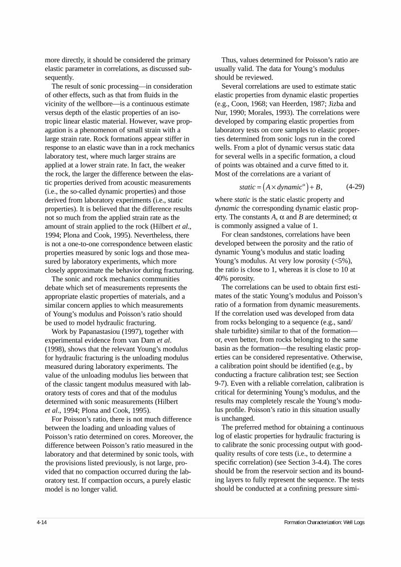
4-14 Formation Characterization: Well Logs

more directly, it should be considered the primaryelastic parameter in correlations, as discussed sub-sequently.

The result of sonic processing—in considerationof other effects, such as that from fluids in thevicinity of the wellbore—is a continuous estimateversus depth of the elastic properties of an iso-tropic linear elastic material. However, wave prop-agation is a phenomenon of small strain with alarge strain rate. Rock formations appear stiffer inresponse to an elastic wave than in a rock mechanicslaboratory test, where much larger strains areapplied at a lower strain rate. In fact, the weakerthe rock, the larger the difference between the elas-tic properties derived from acoustic measurements(i.e., the so-called dynamic properties) and thosederived from laboratory experiments (i.e., staticproperties). It is believed that the difference resultsnot so much from the applied strain rate as theamount of strain applied to the rock (Hilbert et al.,1994; Plona and Cook, 1995). Nevertheless, thereis not a one-to-one correspondence between elasticproperties measured by sonic logs and those mea-sured by laboratory experiments, which moreclosely approximate the behavior during fracturing.

The sonic and rock mechanics communitiesdebate which set of measurements represents theappropriate elastic properties of materials, and asimilar concern applies to which measurements of Young’s modulus and Poisson’s ratio should be used to model hydraulic fracturing.

Work by Papanastasiou (1997), together withexperimental evidence from van Dam et al.(1998), shows that the relevant Young’s modulusfor hydraulic fracturing is the unloading modulusmeasured during laboratory experiments. Thevalue of the unloading modulus lies between thatof the classic tangent modulus measured with lab-oratory tests of cores and that of the modulusdetermined with sonic measurements (Hilbert et al., 1994; Plona and Cook, 1995).

For Poisson’s ratio, there is not much differencebetween the loading and unloading values ofPoisson’s ratio determined on cores. Moreover, thedifference between Poisson’s ratio measured in thelaboratory and that determined by sonic tools, withthe provisions listed previously, is not large, pro-vided that no compaction occurred during the lab-oratory test. If compaction occurs, a purely elasticmodel is no longer valid.

Thus, values determined for Poisson’s ratio areusually valid. The data for Young’s modulusshould be reviewed.

Several correlations are used to estimate staticelastic properties from dynamic elastic properties(e.g., Coon, 1968; van Heerden, 1987; Jizba andNur, 1990; Morales, 1993). The correlations weredeveloped by comparing elastic properties fromlaboratory tests on core samples to elastic proper-ties determined from sonic logs run in the coredwells. From a plot of dynamic versus static datafor several wells in a specific formation, a cloud of points was obtained and a curve fitted to it.Most of the correlations are a variant of

(4-29)

where static is the static elastic property anddynamic the corresponding dynamic elastic prop-erty. The constants A, α and B are determined; αis commonly assigned a value of 1.

For clean sandstones, correlations have beendeveloped between the porosity and the ratio ofdynamic Young’s modulus and static loadingYoung’s modulus. At very low porosity (<5%), the ratio is close to 1, whereas it is close to 10 at40% porosity.

The correlations can be used to obtain first esti-mates of the static Young’s modulus and Poisson’sratio of a formation from dynamic measurements.If the correlation used was developed from datafrom rocks belonging to a sequence (e.g., sand/shale turbidite) similar to that of the formation—or, even better, from rocks belonging to the samebasin as the formation—the resulting elastic prop-erties can be considered representative. Otherwise,a calibration point should be identified (e.g., byconducting a fracture calibration test; see Section9-7). Even with a reliable correlation, calibration iscritical for determining Young’s modulus, and theresults may completely rescale the Young’s modu-lus profile. Poisson’s ratio in this situation usuallyis unchanged.

The preferred method for obtaining a continuouslog of elastic properties for hydraulic fracturing isto calibrate the sonic processing output with good-quality results of core tests (i.e., to determine aspecific correlation) (see Section 3-4.4). The coresshould be from the reservoir section and its bound-ing layers to fully represent the sequence. The testsshould be conducted at a confining pressure simi-

static A dynamic B= ×( ) +α ,

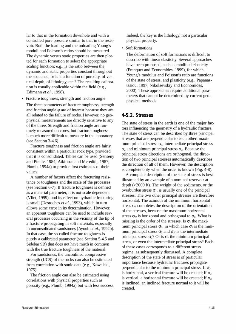
Reservoir Stimulation 4-15

lar to that in the formation downhole and with acontrolled pore pressure similar to that in the reser-voir. Both the loading and the unloading Young’smoduli and Poisson’s ratios should be measured.The dynamic versus static properties are then plot-ted for each formation to select the appropriatescaling function; e.g., is the ratio between thedynamic and static properties constant throughoutthe sequence, or is it a function of porosity, of ver-tical depth, of lithology, etc.? The resulting calibra-tion is usually applicable within the field (e.g.,Edimann et al., 1998).

• Fracture toughness, strength and friction angle

The three parameters of fracture toughness, strengthand friction angle ϕ are of interest because they areall related to the failure of rocks. However, no geo-physical measurements are directly sensitive to anyof the three. Strength and friction angle are rou-tinely measured on cores, but fracture toughness is much more difficult to measure in the laboratory(see Section 3-4.6).

Fracture toughness and friction angle are fairlyconsistent within a particular rock type, providedthat it is consolidated. Tables can be used (Sensenyand Pfiefle, 1984; Atkinson and Meredith, 1987;Plumb, 1994a) to provide first estimates of theirvalues.

A number of factors affect the fracturing resis-tance or toughness and the scale of the processes(see Section 6-7). If fracture toughness is definedas a material parameter, it is not scale dependent(Vliet, 1999), and its effect on hydraulic fracturingis small (Desroches et al., 1993), which in turnallows some error in its determination. However,an apparent toughness can be used to include sev-eral processes occurring in the vicinity of the tip ofa fracture propagating in soft materials, especiallyin unconsolidated sandstones (Ayoub et al., 1992b).In that case, the so-called fracture toughness ispurely a calibrated parameter (see Section 5-4.5 andSidebar 9B) that does not have much in commonwith the true fracture toughness of the material.

For sandstones, the unconfined compressivestrength (UCS) of the rocks can also be estimatedfrom correlation with sonic data (e.g., Kowalski,1975).

The friction angle can also be estimated usingcorrelations with physical properties such asporosity (e.g., Plumb, 1994a) but with less success.

Indeed, the key is the lithology, not a particularphysical property.

• Soft formations

The deformation of soft formations is difficult todescribe with linear elasticity. Several approacheshave been proposed, such as modified elasticity(Franquet and Economides, 1999), for whichYoung’s modulus and Poisson’s ratio are functionsof the state of stress, and plasticity (e.g., Papanas-tasiou, 1997; Nikolaevskiy and Economides,2000). These approaches require additional para-meters that cannot be determined by current geo-physical methods.

4-5.2. StressesThe state of stress in the earth is one of the major fac-tors influencing the geometry of a hydraulic fracture.The state of stress can be described by three principalstresses that are perpendicular to each other: maxi-mum principal stress σ1, intermediate principal stressσ2 and minimum principal stress σ3. Because theprincipal stress directions are orthogonal, the direc-tion of two principal stresses automatically describesthe direction of all of them. However, the descriptionis complete only when the order is known (Fig. 4-8).

A complete description of the state of stress is bestillustrated by an example of a nominal reservoir atdepth (>2000 ft). The weight of the sediments, or theoverburden stress σv, is usually one of the principalstresses. The two other principal stresses are thereforehorizontal. The azimuth of the minimum horizontalstress σh completes the description of the orientationof the stresses, because the maximum horizontalstress σH is horizontal and orthogonal to σh. What ismissing is the order of the stresses. Is σv the maxi-mum principal stress σ1, in which case σh is the mini-mum principal stress σ3 and σH is the intermediateprincipal stress σ2? Or is σv the minimum principalstress, or even the intermediate principal stress? Eachof these cases corresponds to a different stressregime, as subsequently discussed. A completedescription of the state of stress is of particularimportance because hydraulic fractures propagateperpendicular to the minimum principal stress. If σ3

is horizontal, a vertical fracture will be created; if σ3

is vertical, a horizontal fracture will be created; if σ3

is inclined, an inclined fracture normal to it will becreated.

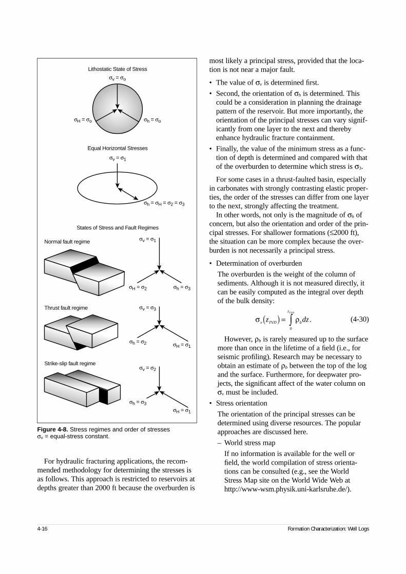
4-16 Formation Characterization: Well Logs

For hydraulic fracturing applications, the recom-mended methodology for determining the stresses isas follows. This approach is restricted to reservoirs atdepths greater than 2000 ft because the overburden is

most likely a principal stress, provided that the loca-tion is not near a major fault.

• The value of σv is determined first.

• Second, the orientation of σh is determined. Thiscould be a consideration in planning the drainagepattern of the reservoir. But more importantly, theorientation of the principal stresses can vary signif-icantly from one layer to the next and therebyenhance hydraulic fracture containment.

• Finally, the value of the minimum stress as a func-tion of depth is determined and compared with thatof the overburden to determine which stress is σ3.

For some cases in a thrust-faulted basin, especiallyin carbonates with strongly contrasting elastic proper-ties, the order of the stresses can differ from one layerto the next, strongly affecting the treatment.

In other words, not only is the magnitude of σh ofconcern, but also the orientation and order of the prin-cipal stresses. For shallower formations (≤2000 ft),the situation can be more complex because the over-burden is not necessarily a principal stress.

• Determination of overburden

The overburden is the weight of the column ofsediments. Although it is not measured directly, itcan be easily computed as the integral over depthof the bulk density:

(4-30)

However, ρb is rarely measured up to the surfacemore than once in the lifetime of a field (i.e., forseismic profiling). Research may be necessary toobtain an estimate of ρb between the top of the logand the surface. Furthermore, for deepwater pro-jects, the significant affect of the water column onσv must be included.

• Stress orientation

The orientation of the principal stresses can bedetermined using diverse resources. The popularapproaches are discussed here.

– World stress map

If no information is available for the well orfield, the world compilation of stress orienta-tions can be consulted (e.g., see the World Stress Map site on the World Wide Web athttp://www-wsm.physik.uni-karlsruhe.de/).

σ ρv TVD b

z

z dzTVD

( ) = ∫0

.

Figure 4-8. Stress regimes and order of stresses σo = equal-stress constant.

σv = σ1

σv = σ1

σH = σ2 σh = σ3

σh = σH = σ2 = σ3

σv = σ3

σh = σ2 σH = σ1

σv = σ2

σh = σ3

σH = σ1

Normal fault regime

States of Stress and Fault Regimes

Equal Horizontal Stresses

Thrust fault regime

Strike-slip fault regime

σv = σo

σh = σoσH = σo

Lithostatic State of Stress

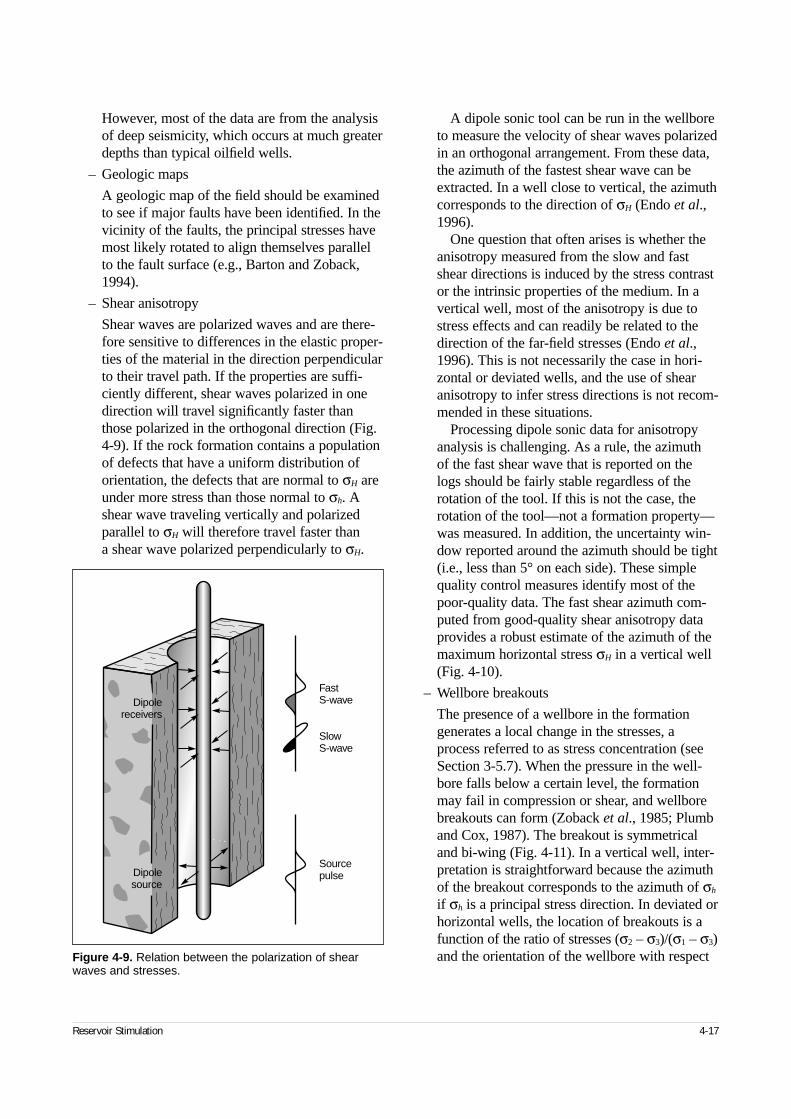
Reservoir Stimulation 4-17

However, most of the data are from the analysisof deep seismicity, which occurs at much greaterdepths than typical oilfield wells.

– Geologic maps

A geologic map of the field should be examinedto see if major faults have been identified. In thevicinity of the faults, the principal stresses havemost likely rotated to align themselves parallelto the fault surface (e.g., Barton and Zoback,1994).

– Shear anisotropy

Shear waves are polarized waves and are there-fore sensitive to differences in the elastic proper-ties of the material in the direction perpendicularto their travel path. If the properties are suffi-ciently different, shear waves polarized in onedirection will travel significantly faster thanthose polarized in the orthogonal direction (Fig.4-9). If the rock formation contains a populationof defects that have a uniform distribution oforientation, the defects that are normal to σH areunder more stress than those normal to σh. Ashear wave traveling vertically and polarizedparallel to σH will therefore travel faster than a shear wave polarized perpendicularly to σH.

A dipole sonic tool can be run in the wellboreto measure the velocity of shear waves polarizedin an orthogonal arrangement. From these data,the azimuth of the fastest shear wave can beextracted. In a well close to vertical, the azimuthcorresponds to the direction of σH (Endo et al.,1996).

One question that often arises is whether theanisotropy measured from the slow and fastshear directions is induced by the stress contrastor the intrinsic properties of the medium. In avertical well, most of the anisotropy is due tostress effects and can readily be related to thedirection of the far-field stresses (Endo et al.,1996). This is not necessarily the case in hori-zontal or deviated wells, and the use of shearanisotropy to infer stress directions is not recom-mended in these situations.

Processing dipole sonic data for anisotropyanalysis is challenging. As a rule, the azimuth of the fast shear wave that is reported on thelogs should be fairly stable regardless of therotation of the tool. If this is not the case, therotation of the tool—not a formation property—was measured. In addition, the uncertainty win-dow reported around the azimuth should be tight (i.e., less than 5° on each side). These simplequality control measures identify most of thepoor-quality data. The fast shear azimuth com-puted from good-quality shear anisotropy dataprovides a robust estimate of the azimuth of themaximum horizontal stress σH in a vertical well(Fig. 4-10).

– Wellbore breakouts

The presence of a wellbore in the formationgenerates a local change in the stresses, aprocess referred to as stress concentration (seeSection 3-5.7). When the pressure in the well-bore falls below a certain level, the formationmay fail in compression or shear, and wellborebreakouts can form (Zoback et al., 1985; Plumband Cox, 1987). The breakout is symmetricaland bi-wing (Fig. 4-11). In a vertical well, inter-pretation is straightforward because the azimuthof the breakout corresponds to the azimuth of σh

if σh is a principal stress direction. In deviated orhorizontal wells, the location of breakouts is afunction of the ratio of stresses (σ2 – σ3)/(σ1 – σ3)and the orientation of the wellbore with respectFigure 4-9. Relation between the polarization of shear

waves and stresses.

Dipolereceivers

Dipolesource

FastS-wave

SlowS-wave

Sourcepulse

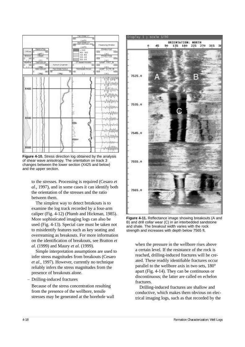
4-18 Formation Characterization: Well Logs

to the stresses. Processing is required (Cesaro etal., 1997), and in some cases it can identify boththe orientation of the stresses and the ratiobetween them.

The simplest way to detect breakouts is toexamine the log track recorded by a four-armcaliper (Fig. 4-12) (Plumb and Hickman, 1985).More sophisticated imaging logs can also beused (Fig. 4-13). Special care must be taken notto misidentify features such as key seating andoverreaming as breakouts. For more informationon the identification of breakouts, see Bratton etal. (1999) and Maury et al. (1999).

Simple interpretation assumptions are used toinfer stress magnitudes from breakouts (Cesaroet al., 1997). However, currently no techniquereliably infers the stress magnitudes from thepresence of breakouts alone.

– Drilling-induced fractures

Because of the stress concentration resultingfrom the presence of the wellbore, tensilestresses may be generated at the borehole wall

when the pressure in the wellbore rises above a certain level. If the resistance of the rock isreached, drilling-induced fractures will be cre-ated. These readily identifiable fractures occurparallel to the wellbore axis in two sets, 180°apart (Fig. 4-14). They can be continuous ordiscontinuous; the latter are called en echelonfractures.

Drilling-induced fractures are shallow andconductive, which makes them obvious on elec-trical imaging logs, such as that recorded by the

Figure 4-11. Reflectance image showing breakouts (A andB) and drill collar wear (C) in an interbedded sandstoneand shale. The breakout width varies with the rockstrength and increases with depth below 7565 ft.

Figure 4-10. Stress direction log obtained by the analysisof shear wave anisotropy. The orientation on track 3changes between the lower section (X425 and below) and the upper section.

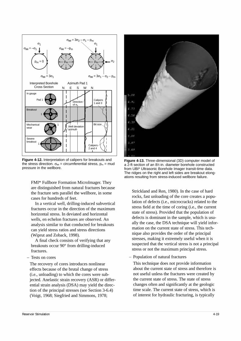
Reservoir Stimulation 4-19

FMI* Fullbore Formation MicroImager. Theyare distinguished from natural fractures becausethe fracture sets parallel the wellbore, in somecases for hundreds of feet.

In a vertical well, drilling-induced subverticalfractures occur in the direction of the maximumhorizontal stress. In deviated and horizontalwells, en echelon fractures are observed. Ananalysis similar to that conducted for breakoutscan yield stress ratios and stress directions(Wiprut and Zoback, 1998).

A final check consists of verifying that anybreakouts occur 90° from drilling-inducedfractures.

– Tests on cores

The recovery of cores introduces nonlineareffects because of the brutal change of stress(i.e., unloading) to which the cores were sub-jected. Anelastic strain recovery (ASR) or differ-ential strain analysis (DSA) may yield the direc-tion of the principal stresses (see Section 3-6.4)(Voigt, 1968; Siegfried and Simmons, 1978;

Strickland and Ren, 1980). In the case of hardrocks, fast unloading of the core creates a popu-lation of defects (i.e., microcracks) related to thestress field at the time of coring (i.e., the currentstate of stress). Provided that the population ofdefects is dominant in the sample, which is usu-ally the case, the DSA technique will yield infor-mation on the current state of stress. This tech-nique also provides the order of the principalstresses, making it extremely useful when it issuspected that the vertical stress is not a principalstress or not the maximum principal stress.

– Population of natural fractures

This technique does not provide informationabout the current state of stress and therefore isnot useful unless the fractures were created bythe current state of stress. The state of stresschanges often and significantly at the geologictime scale. The current state of stress, which isof interest for hydraulic fracturing, is typically

Figure 4-12. Interpretation of calipers for breakouts andthe stress direction. σθθ = circumferential stress, pm = mudpressure in the wellbore.

N E S W NAzimuth Pad 1Interpreted Borehole

Cross Section

Calipers1 and 3

1

1

1

Pad 1Directionof σh

Well deviationazimuth

Bit size

Calipers2 and 4

pm = 0 pm

σθθ = –pm

σθθ = 3σ2 – σ1 – pm

σθθ = 3σ1 – σ2 – pmσθθ = 3σ1

σθθ = –σ1

σ1 σ1

σ2pm

In gauge

Breakout

Mechanicalwear

Severebreakout

Figure 4-13. Three-dimensional (3D) computer model of a 2-ft section of an 81⁄2-in. diameter borehole constructedfrom UBI* Ultrasonic Borehole Imager transit-time data.The ridges on the right and left sides are breakout elong-ations resulting from stress-induced wellbore failure.

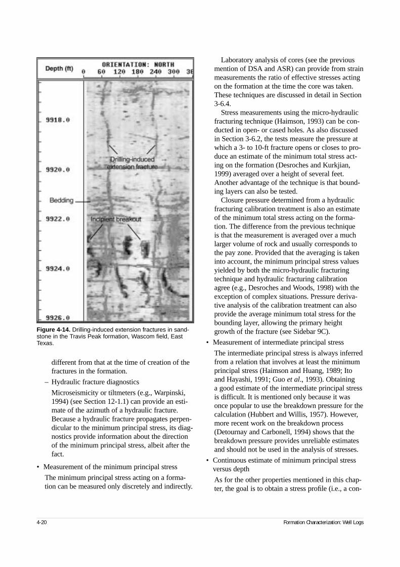
4-20 Formation Characterization: Well Logs

different from that at the time of creation of thefractures in the formation.

– Hydraulic fracture diagnostics

Microseismicity or tiltmeters (e.g., Warpinski,1994) (see Section 12-1.1) can provide an esti-mate of the azimuth of a hydraulic fracture.Because a hydraulic fracture propagates perpen-dicular to the minimum principal stress, its diag-nostics provide information about the directionof the minimum principal stress, albeit after thefact.

• Measurement of the minimum principal stress

The minimum principal stress acting on a forma-tion can be measured only discretely and indirectly.

Laboratory analysis of cores (see the previousmention of DSA and ASR) can provide from strainmeasurements the ratio of effective stresses actingon the formation at the time the core was taken.These techniques are discussed in detail in Section3-6.4.

Stress measurements using the micro-hydraulicfracturing technique (Haimson, 1993) can be con-ducted in open- or cased holes. As also discussedin Section 3-6.2, the tests measure the pressure atwhich a 3- to 10-ft fracture opens or closes to pro-duce an estimate of the minimum total stress act-ing on the formation (Desroches and Kurkjian,1999) averaged over a height of several feet.Another advantage of the technique is that bound-ing layers can also be tested.

Closure pressure determined from a hydraulicfracturing calibration treatment is also an estimateof the minimum total stress acting on the forma-tion. The difference from the previous technique is that the measurement is averaged over a muchlarger volume of rock and usually corresponds tothe pay zone. Provided that the averaging is takeninto account, the minimum principal stress valuesyielded by both the micro-hydraulic fracturingtechnique and hydraulic fracturing calibrationagree (e.g., Desroches and Woods, 1998) with theexception of complex situations. Pressure deriva-tive analysis of the calibration treatment can alsoprovide the average minimum total stress for thebounding layer, allowing the primary heightgrowth of the fracture (see Sidebar 9C).

• Measurement of intermediate principal stress

The intermediate principal stress is always inferredfrom a relation that involves at least the minimumprincipal stress (Haimson and Huang, 1989; Itoand Hayashi, 1991; Guo et al., 1993). Obtaining a good estimate of the intermediate principal stressis difficult. It is mentioned only because it wasonce popular to use the breakdown pressure for thecalculation (Hubbert and Willis, 1957). However,more recent work on the breakdown process(Detournay and Carbonell, 1994) shows that thebreakdown pressure provides unreliable estimatesand should not be used in the analysis of stresses.

• Continuous estimate of minimum principal stressversus depth

As for the other properties mentioned in this chap-ter, the goal is to obtain a stress profile (i.e., a con-

Figure 4-14. Drilling-induced extension fractures in sand-stone in the Travis Peak formation, Wascom field, EastTexas.

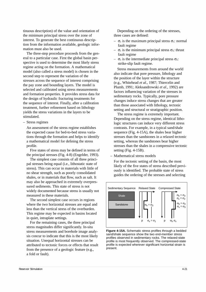
Reservoir Stimulation 4-21

tinuous description) of the value and orientation ofthe minimum principal stress over the zone ofinterest. To generate the best continuous descrip-tion from the information available, geologic infor-mation must also be used.

The three-step procedure proceeds from the gen-eral to a particular case. First the global basin per-spective is used to determine the most likely stressregime acting on the formation. A mathematicalmodel (also called a stress model) is chosen in thesecond step to represent the variation of thestresses across the sequence of interest comprisingthe pay zone and bounding layers. The model isselected and calibrated using stress measurementsand formation properties. It provides stress data forthe design of hydraulic fracturing treatments forthe sequence of interest. Finally, after a calibrationtreatment, further refinement based on lithologyyields the stress variations in the layers to bestimulated.

– Stress regimes

An assessment of the stress regime establishesthe expected cause for bed-to-bed stress varia-tions through the formation and helps to identifya mathematical model for defining the stressprofile.

Five states of stress may be defined in terms ofthe principal stresses (Fig. 4-8) (Engelder, 1993).

The simplest case consists of all three princi-pal stresses being equal (i.e., lithostatic state ofstress). This can occur in materials with little ofno shear strength, such as poorly consolidatedshales, or in materials that flow, such as salt. Itmay also be approached in extremely overpres-sured sediments. This state of stress is notwidely documented because stress is usually notmeasured in these materials.

The second simplest case occurs in regionswhere the two horizontal stresses are equal andless than the vertical stress of the overburden.This regime may be expected in basins locatedin quiet, intraplate settings.

For the remaining cases, the three principalstress magnitudes differ significantly. In-situstress measurements and borehole image analy-sis concur to indicate that this is the most likelysituation. Unequal horizontal stresses can beattributed to tectonic forces or effects that resultfrom the presence of a geologic feature (e.g., a fold or fault).

Depending on the ordering of the stresses,three cases are defined:

– σv is the maximum principal stress σ1: normalfault regime

– σv is the minimum principal stress σ3: thrustfault regime

– σv is the intermediate principal stress σ2:strike-slip fault regime.

Stress measurements from around the worldalso indicate that pore pressure, lithology andthe position of the layer within the structure(e.g., Whitehead et al., 1987; Thiercelin andPlumb, 1991; Aleksandrowski et al., 1992) arefactors influencing variation of the stresses insedimentary rocks. Typically, pore pressurechanges induce stress changes that are greaterthan those associated with lithology, tectonicsetting and structural or stratigraphic position.

The stress regime is extremely important.Depending on the stress regime, identical litho-logic structures can induce very different stresscontrasts. For example, in a typical sand/shalesequence (Fig. 4-15A), the shales bear higherstresses than the sandstones in a relaxed tectonicsetting, whereas the sandstones bear higherstresses than the shales in a compressive tectonicsetting (Fig. 4-15B).

– Mathematical stress models

For the tectonic setting of the basin, the mostlikely of the five states of stress described previ-ously is identified. The probable state of stressguides the ordering of the stresses and selecting

Figure 4-15A. Schematic stress profiles through a beddedsand/shale sequence show the two end-member stressprofiles observed in sedimentary rocks. The relaxed-stateprofile is most frequently observed. The compressed-stateprofile is expected wherever significant horizontal strain ispresent.

Shale

Sedimentary Sequence Relaxed State Compressed State

Sandstone σh = σ3

σh = σ3σv = σ2

σh = σ2σv = σ3

σv = σ1p σh σvp

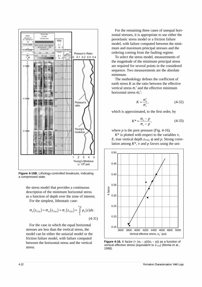
4-22 Formation Characterization: Well Logs

the stress model that provides a continuousdescription of the minimum horizontal stress as a function of depth over the zone of interest.

For the simplest, lithostatic case:

(4-31)

For the case in which the equal horizontalstresses are less than the vertical stress, themodel can be either the uniaxial model or thefriction failure model, with failure computedbetween the horizontal stress and the verticalstress.

For the remaining three cases of unequal hori-zontal stresses, it is appropriate to use either theporoelastic stress model or a friction failuremodel, with failure computed between the mini-mum and maximum principal stresses and theordering coming from the faulting regime.

To select the stress model, measurements ofthe magnitude of the minimum principal stressare required for several points in the consideredsequence. Two measurements are the absoluteminimum.

The methodology defines the coefficient ofearth stress K as the ratio between the effectivevertical stress σv′ and the effective minimumhorizontal stress σh′:

(4-32)

which is approximated, to the first order, by

(4-33)

where p is the pore pressure (Fig. 4-16).K* is plotted with respect to the variables ν,

E, true vertical depth zTVD, ϕ and p. Strong corre-lation among K*, ν and p favors using the uni-

Figure 4-15B. Lithology-controlled breakouts, indicating a compressed state.

Figure 4-16. K factor (= (σh – p)/(σv – p)) as a function ofvertical effective stress (equivalent to zTVD) (Morita et al.,1998).

3600 3800 4000 4200 4400 4600 4800 5000Vertical effective stress, σv´ (psi)

0.50

0.45

0.40

0.35

0.30

0.25

0.20

0.15

K fa

ctor

K h

v

= ′′

σσ

,

Kp

ph

v

* ,= −−

σσ

σ σ σ ρh TVD H TVD v TVD b

z

z z z z dzTVD

( ) = ( ) = ( ) = ( )∫0

.

Reservoir Stimulation 4-23

axial model. A continuous profile of σh isobtained by using the following equation withthe Biot constant α as an ad hoc potentiallylithology-dependent calibration parameter:

(4-34)

Use of this model is reasonable for low-porosity,low-permeability sandstones, shales and carbonates.

Strong correlation among K*, ν, E and pfavors using the poroelastic model. Indeed, asignificant effect of Young’s modulus suggeststectonic activity. A continuous profile of σh isobtained by using the following equation:

(4-35)

where the minimum tectonic strain εh and maxi-mum tectonic strain εH are the primary calibra-tion factors (i.e., adjusted first with α = 1) andα is the secondary calibration parameter adjustedonce the tectonic strains are adjusted. Theamount and sign of the tectonic strains must becompatible with the geologic setting. For exam-ple, negative strains are not possible in a com-pressive environment. This model applies inlithologies similar to those applicable to Eq. 4-34.

Strong correlation among K*, the frictionangle ϕ and p (but not ε or ν) favors use of theincipient failure model:

(4-36)

(4-37)

where Nϕ is the coefficient of passive stress.This model is appropriate for medium- to high-porosity sandstones (15% and greater) and clay-supported rocks, particularly in regions of nor-mal (or growth) faulting. The friction angle ofthese rocks does not vary greatly, so this settingyields only small variations of the stresses as afunction of lithology.

Correlation among K*, ϕ and p with depar-ture from Eq. 4-37 suggests use of the purelyfrictional model:

(4-38)

This model is appropriate in high-porosity, high-permeability sandstones, chalks and shales. Itcorresponds to rock at rest if the rock compacts.There are no calibration parameters in the mod-els governed by friction except for the frictionangle. Calibration is conducted by modifying thefriction angle.

The effect of pore pressure variations (througheither depletion or water flooding; see Section 3-5.7) and temperature variations can also beadded to the selected model (e.g., Perkins andGonzales, 1984). Another effect that can be con-sidered is stress relaxation; it reduces the differ-ence between the minimum and maximumstresses (e.g., Prats, 1981), especially in shales.Once the stress model is built, it usually isportable within the same sequence in the samebasin, provided that significance differences inpore pressure and possibly in temperature aretaken into account.

The methodology advocated in this chapterrelies on physical processes underlying themathematical form of the model selected tobuild a stress profile. Other mathematical formscan be selected, but without geologic confirma-tion, the portability of the stress profile toanother well is not likely.

– Stress profile adjustment after a calibrationtreatment

As mentioned previously, the analysis of a cali-bration treatment yields an average of the mini-mum stress acting on the pay zone (called theclosure pressure) and possibly a value of theaverage stress contrast between the pay zoneand the bounding layer in which the fracturemay have grown.

If only the stress acting on the pay σPZ isavailable, the model-based stress profile can bescaled or shifted to honor its value at depth. Ifthe stress acting on a bounding layer σBL is alsoavailable, further calibration can be performed.It is preferable to modify the parameters of themathematical model to honor these stress values,but the parameters may not be available at thetime of the calibration treatment. If this is thecase, a lithology-based stress interpolation canbe used as follows.

σ νν

σ α αh v p p=−

−( ) +1

.

σ σϕ

h vNp p= −( ) +1

Nϕπ ϕ= +

tan ,2

2 4

σ ϕ σ ϕh v p= −( ) + ( )1 sin sin .

σ νν

σ α αν

ε νν

εh v h Hp pE E=

−−( ) + +

−+

−1 1 12 2,

4-24 Formation Characterization: Well Logs

One of the formation properties can usually be identified as representative of the differencein stresses (e.g., the percentage of dolomite in a carbonate sequence or the volume of clay in a sand/shale sequence). For this property A, APZ

and ABL are its values in the pay zone and thebounding layers, respectively, and the stresses inthe vicinity of the pay zone may be estimated asa linear function of A:

(4-39)

where the linear regression constants are

(4-40)

(4-41)

This approach has been successfully appliedfor both sand/shale (Miller and Smith, 1989;Smith et al., 1989) and carbonate sequences.

4-6. ZoningMost of the models used in reservoir stimulationrequire defining zones with constant, or possibly lin-early varying, properties within each zone. Once allthe required properties have been collected, the logsmust be zoned into distinct zones that will be the finalinput to the stimulation process. If parallel, horizontalbeds are assumed, the zones must ultimately bedefined in TVD. If the beds are not parallel or nothorizontal, more complicated and ad hoc transforma-tions must be made, but these adjustments are outsidethe scope of this chapter.

Zoning can be done subjectively by hand or objec-tively in a manner called log squaring, which wasdeveloped for formation evaluation (Trouiller et al.,1989; Serra and Andreani, 1991). Log squaring usesthe response functions of the tools introduced in“Lithology” in Section 4-4.2. However, it is notdirectly applicable to reservoir stimulation because itconsiders only the classic measurements used in for-mation evaluation (e.g., porosity, density, resistivity).It ignores pore pressure, permeability, mechanicalproperties and stresses, which are integral to the zon-ing process considered here. Furthermore, because noresponse equation exists yet for these latter proper-ties, the zones output by log squaring must be manu-ally refined.

A simple solution is to consider as many zones asthere are significant changes. But this is not practicalbecause more than 100 zones could be defined andonly a limited number of zones can be considered.Therefore, broader zones must first be defined. Thefirst step is to decide which property, or set of proper-ties, should guide the definition of zones. In sand/shale sequences, for example, the volume of clay is a primary guide, whereas in carbonate sequences, thepercentage of dolomite is a good primary guide.However, permeability barriers (usually associatedwith pore pressure and hence stress changes), changesin elastic properties and changes in the stresses shouldalso be considered. The set of properties selected toguide the zoning process must also reflect the geo-logic understanding that guided choosing the modelfor the stresses. Determination of the leakoff height is also part of the zoning process. The zones must bedefined in a consistent manner so that the leakoffcoefficient determined from a calibration treatment is meaningful for the remainder of the sequence.

A zoning example is presented in Fig. 4-17. Thissand/shale sequence reservoir has strong variations in permeability and pore pressure because of waterflooding. The main properties selected to define zoneswere the separation between sands and shales and theprofile of pore pressure. More zones were added toconsider sharp changes in Young’s modulus, whichresulted in the definition of 25 zones. Zoning for for-mation evaluation would have been significantly dif-ferent, reflecting the analyst’s different point of view.

Once the zones have been defined, they must bepopulated with a constant value (or possibly linearlyvarying, for pore pressure and stresses). For thin bedswith significant contrast, taking the peak value is pre-ferred, whereas for thick beds, taking an averageaway from the bed boundaries is preferred.

Finally, most log measurements sample the forma-tion to only a few feet from the wellbore. The zoningprocess described here, however, populates zoneswith a constant value along the bed extension, ignor-ing any heterogeneity along the bed. The constancymay be arbitrary, especially for geologic environ-ments known to typically have lateral variations ofproperties (e.g., channels, bar sands). Crosswelltomography (Warpinski et al., 1998b) shows that for-mation properties can vary significantly along a bedin less than 50 ft of horizontal displacement. Yetknowledge of the geologic environment is the onlyqualifier of the information developed from the zoning process.

σ z m A z bTVD TVD( ) = × ( ) + ,

mA A

BL PZ

BL PZ

= −−

σ σ

b m APZ PZ= − ×σ .

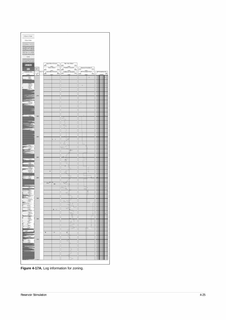
Reservoir Stimulation 4-25

Figure 4-17A. Log information for zoning.

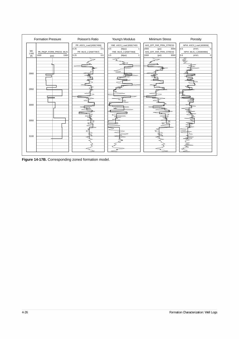
4-26 Formation Characterization: Well Logs

Figure 14-17B. Corresponding zoned formation model.

2950

2900

MD1:500

(ft) 1000 1500

PA_PAQP_FORM_PRESS .MLIS

(psi) 0.5 1

YME .MLIS_3 [A5877064]

(Mpsi)

0.5 1

YME .ASCII_Load [A5817403

(Mpsi)

2000 3000

AVG_EFF_FAR_PRIN_STRESS

(psi)

2000 3000

AVG_EFF_FAR_PRIN_STRESS

(psi)

0.6 0

NPHI .MLIS_1 [A5900984]

(ft3/ft3)

0.6 0

NPHI .ASCII_Load [A59006]

(ft3/ft3)

0.25 0.5

PR .MLIS_2 [A5877057]

0.25 0.5

PR .ASCII_Load [A5817406]

3100

3050

3000

Formation Pressure Poisson’s Ratio Minimum StressYoung’s Modulus Porosity

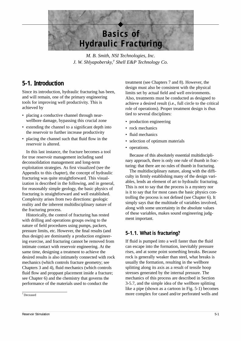
5-1. IntroductionSince its introduction, hydraulic fracturing has been,and will remain, one of the primary engineeringtools for improving well productivity. This isachieved by

• placing a conductive channel through near-wellbore damage, bypassing this crucial zone

• extending the channel to a significant depth intothe reservoir to further increase productivity

• placing the channel such that fluid flow in thereservoir is altered.

In this last instance, the fracture becomes a toolfor true reservoir management including sanddeconsolidation management and long-termexploitation strategies. As first visualized (see theAppendix to this chapter), the concept of hydraulicfracturing was quite straightforward. This visual-ization is described in the following, and in general,for reasonably simple geology, the basic physics offracturing is straightforward and well established.Complexity arises from two directions: geologicreality and the inherent multidisciplinary nature ofthe fracturing process.

Historically, the control of fracturing has restedwith drilling and operations groups owing to thenature of field procedures using pumps, packers,pressure limits, etc. However, the final results (andthus design) are dominantly a production engineer-ing exercise, and fracturing cannot be removed fromintimate contact with reservoir engineering. At thesame time, designing a treatment to achieve thedesired results is also intimately connected with rockmechanics (which controls fracture geometry; seeChapters 3 and 4), fluid mechanics (which controlsfluid flow and proppant placement inside a fracture;see Chapter 6) and the chemistry that governs theperformance of the materials used to conduct the

† Deceased

treatment (see Chapters 7 and 8). However, thedesign must also be consistent with the physicallimits set by actual field and well environments.Also, treatments must be conducted as designed toachieve a desired result (i.e., full circle to the criticalrole of operations). Proper treatment design is thustied to several disciplines:

• production engineering

• rock mechanics

• fluid mechanics

• selection of optimum materials

• operations.

Because of this absolutely essential multidiscipli-nary approach, there is only one rule of thumb in frac-turing: that there are no rules of thumb in fracturing.

The multidisciplinary nature, along with the diffi-culty in firmly establishing many of the design vari-ables, lends an element of art to hydraulic fracturing.This is not to say that the process is a mystery nor is it to say that for most cases the basic physics con-trolling the process is not defined (see Chapter 6). Itsimply says that the multitude of variables involved,along with some uncertainty in the absolute valuesof these variables, makes sound engineering judg-ment important.

5-1.1. What is fracturing?If fluid is pumped into a well faster than the fluidcan escape into the formation, inevitably pressurerises, and at some point something breaks. Becauserock is generally weaker than steel, what breaks isusually the formation, resulting in the wellboresplitting along its axis as a result of tensile hoopstresses generated by the internal pressure. Themechanics of this process are described in Section3-5.7, and the simple idea of the wellbore splittinglike a pipe (shown as a cartoon in Fig. 5-1) becomesmore complex for cased and/or perforated wells and

Reservoir Stimulation 5-1

◆

Basics ofHydraulic Fracturing

M. B. Smith, NSI Technologies, Inc.J. W. Shlyapobersky,† Shell E&P Technology Co.

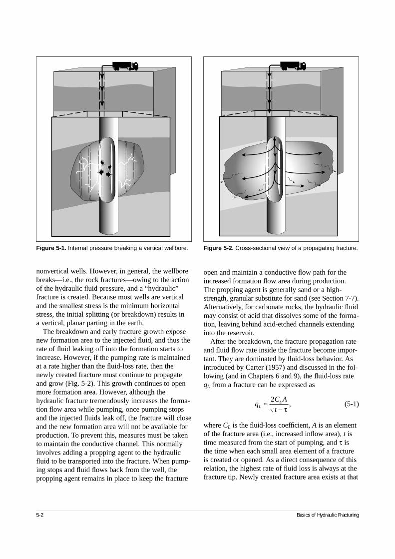
nonvertical wells. However, in general, the wellborebreaks—i.e., the rock fractures—owing to the actionof the hydraulic fluid pressure, and a “hydraulic”fracture is created. Because most wells are verticaland the smallest stress is the minimum horizontalstress, the initial splitting (or breakdown) results in a vertical, planar parting in the earth.

The breakdown and early fracture growth exposenew formation area to the injected fluid, and thus therate of fluid leaking off into the formation starts toincrease. However, if the pumping rate is maintainedat a rate higher than the fluid-loss rate, then thenewly created fracture must continue to propagateand grow (Fig. 5-2). This growth continues to openmore formation area. However, although thehydraulic fracture tremendously increases the forma-tion flow area while pumping, once pumping stopsand the injected fluids leak off, the fracture will closeand the new formation area will not be available forproduction. To prevent this, measures must be takento maintain the conductive channel. This normallyinvolves adding a propping agent to the hydraulicfluid to be transported into the fracture. When pump-ing stops and fluid flows back from the well, thepropping agent remains in place to keep the fracture

open and maintain a conductive flow path for theincreased formation flow area during production.The propping agent is generally sand or a high-strength, granular substitute for sand (see Section 7-7).Alternatively, for carbonate rocks, the hydraulic fluidmay consist of acid that dissolves some of the forma-tion, leaving behind acid-etched channels extendinginto the reservoir.

After the breakdown, the fracture propagation rateand fluid flow rate inside the fracture become impor-tant. They are dominated by fluid-loss behavior. Asintroduced by Carter (1957) and discussed in the fol-lowing (and in Chapters 6 and 9), the fluid-loss rateqL from a fracture can be expressed as

(5-1)

where CL is the fluid-loss coefficient, A is an elementof the fracture area (i.e., increased inflow area), t istime measured from the start of pumping, and τ isthe time when each small area element of a fractureis created or opened. As a direct consequence of thisrelation, the highest rate of fluid loss is always at thefracture tip. Newly created fracture area exists at that

5-2 Basics of Hydraulic Fracturing

Figure 5-2. Cross-sectional view of a propagating fracture.Figure 5-1. Internal pressure breaking a vertical wellbore.

qC A

tLL≈−

2τ

,

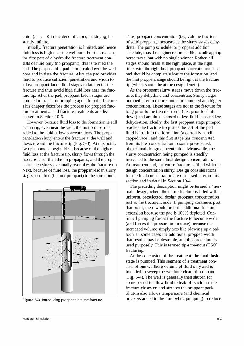
point (t – τ = 0 in the denominator), making qL in-stantly infinite.

Initially, fracture penetration is limited, and hencefluid loss is high near the wellbore. For that reason,the first part of a hydraulic fracture treatment con-sists of fluid only (no proppant); this is termed thepad. The purpose of a pad is to break down the well-bore and initiate the fracture. Also, the pad providesfluid to produce sufficient penetration and width toallow proppant-laden fluid stages to later enter thefracture and thus avoid high fluid loss near the frac-ture tip. After the pad, proppant-laden stages arepumped to transport propping agent into the fracture.This chapter describes the process for propped frac-ture treatments; acid fracture treatments are dis-cussed in Section 10-6.

However, because fluid loss to the formation is stilloccurring, even near the well, the first proppant isadded to the fluid at low concentrations. The prop-pant-laden slurry enters the fracture at the well andflows toward the fracture tip (Fig. 5-3). At this point,two phenomena begin. First, because of the higherfluid loss at the fracture tip, slurry flows through thefracture faster than the tip propagates, and the prop-pant-laden slurry eventually overtakes the fracture tip.Next, because of fluid loss, the proppant-laden slurrystages lose fluid (but not proppant) to the formation.

Thus, proppant concentration (i.e., volume fraction of solid proppant) increases as the slurry stages dehy-drate. The pump schedule, or proppant additionschedule, must be engineered much like handicappinghorse races, but with no single winner. Rather, allstages should finish at the right place, at the righttime, with the right final proppant concentration. Thepad should be completely lost to the formation, andthe first proppant stage should be right at the fracturetip (which should be at the design length).

As the proppant slurry stages move down the frac-ture, they dehydrate and concentrate. Slurry stagespumped later in the treatment are pumped at a higherconcentration. These stages are not in the fracture forlong prior to the treatment end (i.e., prior to shut-down) and are thus exposed to less fluid loss and lessdehydration. Ideally, the first proppant stage pumpedreaches the fracture tip just as the last of the padfluid is lost into the formation (a correctly handi-capped race), and this first stage has concentratedfrom its low concentration to some preselected,higher final design concentration. Meanwhile, theslurry concentration being pumped is steadilyincreased to the same final design concentration. At treatment end, the entire fracture is filled with thedesign concentration slurry. Design considerationsfor the final concentration are discussed later in thissection and in detail in Section 10-4.

The preceding description might be termed a “nor-mal” design, where the entire fracture is filled with auniform, preselected, design proppant concentrationjust as the treatment ends. If pumping continues pastthat point, there would be little additional fractureextension because the pad is 100% depleted. Con-tinued pumping forces the fracture to become wider(and forces the pressure to increase) because theincreased volume simply acts like blowing up a bal-loon. In some cases the additional propped widththat results may be desirable, and this procedure isused purposely. This is termed tip-screenout (TSO)fracturing.

At the conclusion of the treatment, the final flushstage is pumped. This segment of a treatment con-sists of one wellbore volume of fluid only and isintended to sweep the wellbore clean of proppant(Fig. 5-4). The well is generally then shut-in forsome period to allow fluid to leak off such that thefracture closes on and stresses the proppant pack.Shut-in also allows temperature (and chemicalbreakers added to the fluid while pumping) to reduce

Reservoir Stimulation 5-3

Figure 5-3. Introducing proppant into the fracture.

�����������������������������������������������

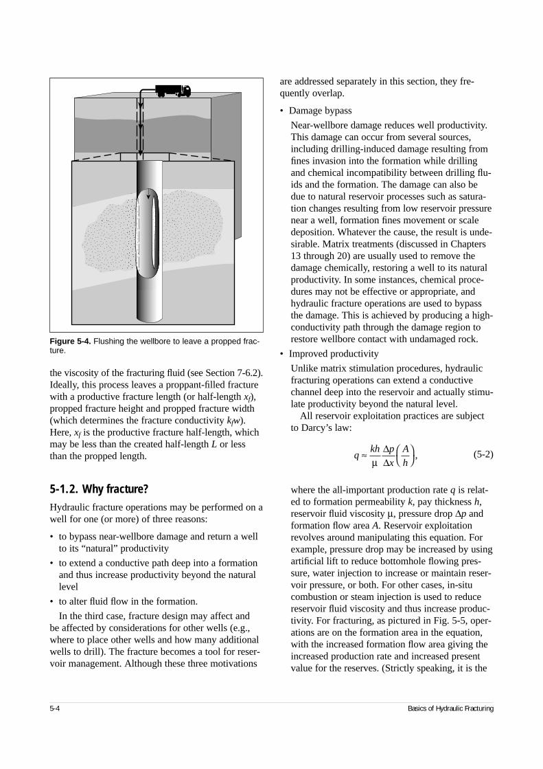
the viscosity of the fracturing fluid (see Section 7-6.2).Ideally, this process leaves a proppant-filled fracturewith a productive fracture length (or half-length xf),propped fracture height and propped fracture width(which determines the fracture conductivity kfw).Here, xf is the productive fracture half-length, whichmay be less than the created half-length L or lessthan the propped length.

5-1.2. Why fracture?Hydraulic fracture operations may be performed on awell for one (or more) of three reasons:

• to bypass near-wellbore damage and return a wellto its “natural” productivity

• to extend a conductive path deep into a formationand thus increase productivity beyond the naturallevel

• to alter fluid flow in the formation.

In the third case, fracture design may affect and be affected by considerations for other wells (e.g.,where to place other wells and how many additionalwells to drill). The fracture becomes a tool for reser-voir management. Although these three motivations

are addressed separately in this section, they fre-quently overlap.

• Damage bypass

Near-wellbore damage reduces well productivity.This damage can occur from several sources,including drilling-induced damage resulting fromfines invasion into the formation while drillingand chemical incompatibility between drilling flu-ids and the formation. The damage can also bedue to natural reservoir processes such as satura-tion changes resulting from low reservoir pressurenear a well, formation fines movement or scaledeposition. Whatever the cause, the result is unde-sirable. Matrix treatments (discussed in Chapters13 through 20) are usually used to remove thedamage chemically, restoring a well to its naturalproductivity. In some instances, chemical proce-dures may not be effective or appropriate, andhydraulic fracture operations are used to bypassthe damage. This is achieved by producing a high-conductivity path through the damage region torestore wellbore contact with undamaged rock.

• Improved productivity

Unlike matrix stimulation procedures, hydraulicfracturing operations can extend a conductivechannel deep into the reservoir and actually stimu-late productivity beyond the natural level.

All reservoir exploitation practices are subjectto Darcy’s law:

(5-2)

where the all-important production rate q is relat-ed to formation permeability k, pay thickness h,reservoir fluid viscosity µ, pressure drop ∆p andformation flow area A. Reservoir exploitationrevolves around manipulating this equation. Forexample, pressure drop may be increased by usingartificial lift to reduce bottomhole flowing pres-sure, water injection to increase or maintain reser-voir pressure, or both. For other cases, in-situcombustion or steam injection is used to reducereservoir fluid viscosity and thus increase produc-tivity. For fracturing, as pictured in Fig. 5-5, oper-ations are on the formation area in the equation,with the increased formation flow area giving theincreased production rate and increased presentvalue for the reserves. (Strictly speaking, it is the

5-4 Basics of Hydraulic Fracturing

Figure 5-4. Flushing the wellbore to leave a propped frac-ture.

����������������

qkh p

x

A

h≈

µ

∆∆

,

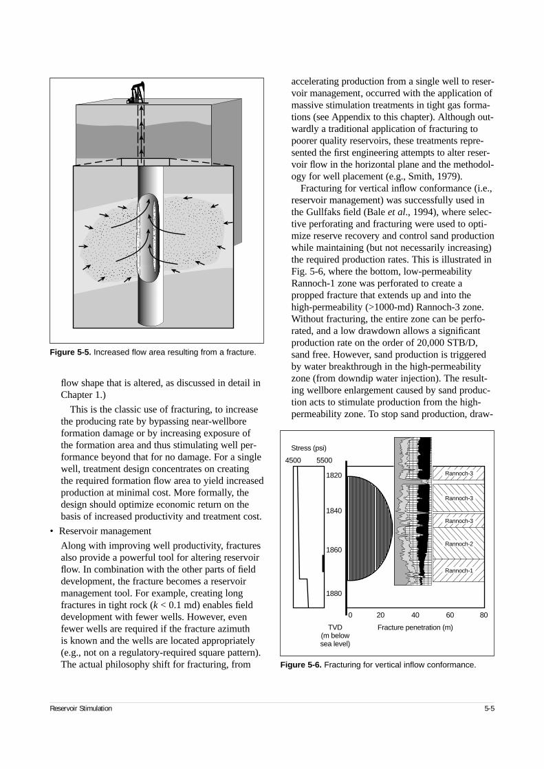
flow shape that is altered, as discussed in detail inChapter 1.)

This is the classic use of fracturing, to increasethe producing rate by bypassing near-wellboreformation damage or by increasing exposure ofthe formation area and thus stimulating well per-formance beyond that for no damage. For a singlewell, treatment design concentrates on creatingthe required formation flow area to yield increasedproduction at minimal cost. More formally, thedesign should optimize economic return on thebasis of increased productivity and treatment cost.

• Reservoir management

Along with improving well productivity, fracturesalso provide a powerful tool for altering reservoirflow. In combination with the other parts of fielddevelopment, the fracture becomes a reservoirmanagement tool. For example, creating longfractures in tight rock (k < 0.1 md) enables fielddevelopment with fewer wells. However, evenfewer wells are required if the fracture azimuth is known and the wells are located appropriately(e.g., not on a regulatory-required square pattern).The actual philosophy shift for fracturing, from

accelerating production from a single well to reser-voir management, occurred with the application ofmassive stimulation treatments in tight gas forma-tions (see Appendix to this chapter). Although out-wardly a traditional application of fracturing topoorer quality reservoirs, these treatments repre-sented the first engineering attempts to alter reser-voir flow in the horizontal plane and the methodol-ogy for well placement (e.g., Smith, 1979).

Fracturing for vertical inflow conformance (i.e.,reservoir management) was successfully used inthe Gullfaks field (Bale et al., 1994), where selec-tive perforating and fracturing were used to opti-mize reserve recovery and control sand productionwhile maintaining (but not necessarily increasing)the required production rates. This is illustrated inFig. 5-6, where the bottom, low-permeabilityRannoch-1 zone was perforated to create apropped fracture that extends up and into thehigh-permeability (>1000-md) Rannoch-3 zone.Without fracturing, the entire zone can be perfo-rated, and a low drawdown allows a significantproduction rate on the order of 20,000 STB/D,sand free. However, sand production is triggeredby water breakthrough in the high-permeabilityzone (from downdip water injection). The result-ing wellbore enlargement caused by sand produc-tion acts to stimulate production from the high-permeability zone. To stop sand production, draw-

Reservoir Stimulation 5-5

Figure 5-5. Increased flow area resulting from a fracture.

��������������������������������������������������������������������������

Figure 5-6. Fracturing for vertical inflow conformance.

200 40 60 80

Fracture penetration (m)

Rannoch-3

Rannoch-3

Rannoch-3

Rannoch-2

Rannoch-1

1820

1860

1880

1840

55004500

Stress (psi)

TVD(m belowsea level)

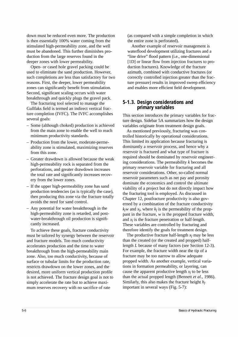
down must be reduced even more. The productionis then essentially 100% water coming from thestimulated high-permeability zone, and the wellmust be abandoned. This further diminishes pro-duction from the large reserves found in thedeeper zones with lower permeability.

Open- or cased hole gravel packing could beused to eliminate the sand production. However,such completions are less than satisfactory for tworeasons. First, the deeper, lower permeabilityzones can significantly benefit from stimulation.Second, significant scaling occurs with waterbreakthrough and quickly plugs the gravel pack.

The fracturing tool selected to manage theGullfaks field is termed an indirect vertical frac-ture completion (IVFC). The IVFC accomplishesseveral goals:

– Some (although choked) production is achievedfrom the main zone to enable the well to reachminimum productivity standards.

– Production from the lower, moderate-perme-ability zone is stimulated, maximizing reservesfrom this zone.

– Greater drawdown is allowed because the weakhigh-permeability rock is separated from theperforations, and greater drawdown increasesthe total rate and significantly increases recov-ery from the lower zones.

– If the upper high-permeability zone has sandproduction tendencies (as is typically the case),then producing this zone via the fracture totallyavoids the need for sand control.

– Any potential for water breakthrough in thehigh-permeability zone is retarded, and post-water-breakthrough oil production is signifi-cantly increased.

To achieve these goals, fracture conductivitymust be tailored by synergy between the reservoirand fracture models. Too much conductivityaccelerates production and the time to waterbreakthrough from the high-permeability mainzone. Also, too much conductivity, because ofsurface or tubular limits for the production rate,restricts drawdown on the lower zones, and thedesired, more uniform vertical production profileis not achieved. The fracture design goal is not tosimply accelerate the rate but to achieve maxi-mum reserves recovery with no sacrifice of rate

(as compared with a simple completion in whichthe entire zone is perforated).

Another example of reservoir management iswaterflood development utilizing fractures and a“line drive” flood pattern (i.e., one-dimensional[1D] or linear flow from injection fractures to pro-duction fractures). Knowledge of the fractureazimuth, combined with conductive fractures (orcorrectly controlled injection greater than the frac-ture pressure) results in improved sweep efficiencyand enables more efficient field development.

5-1.3. Design considerations and primary variables

This section introduces the primary variables for frac-ture design. Sidebar 5A summarizes how the designvariables originate from treatment design goals.

As mentioned previously, fracturing was con-trolled historically by operational considerations.This limited its application because fracturing isdominantly a reservoir process, and hence why areservoir is fractured and what type of fracture isrequired should be dominated by reservoir engineer-ing considerations. The permeability k becomes theprimary reservoir variable for fracturing and allreservoir considerations. Other, so-called normalreservoir parameters such as net pay and porositydominate the economics and control the ultimateviability of a project but do not directly impact howthe fracturing tool is employed. As discussed inChapter 12, postfracture productivity is also gov-erned by a combination of the fracture conductivitykfw and xf, where kf is the permeability of the prop-pant in the fracture, w is the propped fracture width,and xf is the fracture penetration or half-length.These variables are controlled by fracturing andtherefore identify the goals for treatment design.

The productive fracture half-length xf may be lessthan the created (or the created and propped) half-length L because of many factors (see Section 12-3).For example, the fracture width near the tip of afracture may be too narrow to allow adequatepropped width. As another example, vertical varia-tions in formation permeability, or layering, cancause the apparent productive length xf to be lessthan the actual propped length (Bennett et al., 1986).Similarly, this also makes the fracture height hf

important in several ways (Fig. 5-7):

5-6 Basics of Hydraulic Fracturing

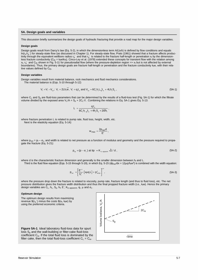
Reservoir Stimulation 5-7

5A. Design goals and variables

This discussion briefly summarizes the design goals of hydraulic fracturing that provide a road map for the major design variables.

Design goals

Design goals result from Darcy’s law (Eq. 5-2), in which the dimensionless term A/(∆xh) is defined by flow conditions and equalsln(re /rẃ ) for steady-state flow (as discussed in Chapter 1). For steady-state flow, Prats (1961) showed that a fracture affects produc-tivity through the equivalent wellbore radius rẃ and that rẃ is related to the fracture half-length or penetration xf by the dimension-less fracture conductivity (CfD = kfw/kxf). Cinco-Ley et al. (1978) extended these concepts for transient flow with the relation amongxf, rẃ and CfD shown in Fig. 5-11 for pseudoradial flow (where the pressure-depletion region >> xf but is not affected by externalboundaries). Thus, the primary design goals are fracture half-length or penetration and the fracture conductivity kfw, with their rela-tive values defined by CfD.

Design variables

Design variables result from material balance, rock mechanics and fluid mechanics considerations.The material balance is (Eqs. 5-10 through 5-12)

(5A-1)

where CL and Sp are fluid-loss parameters that can be determined by the results of a fluid-loss test (Fig. 5A-1) for which the filtratevolume divided by the exposed area VL/A = Sp + 2CL√t . Combining the relations in Eq. 5A-1 gives Eq. 5-13:

where fracture penetration L is related to pump rate, fluid loss, height, width, etc.Next is the elasticity equation (Eq. 5-14):

where pnet = pf – σc, and width is related to net pressure as a function of modulus and geometry and the pressure required to propa-gate the fracture (Eq. 5-21):

(5A-2)

where d is the characteristic fracture dimension and generally is the smaller dimension between hf and L.Third is the fluid flow equation (Eqs. 5-15 through 5-19), in which Eq. 5-15 (dpnet/dx = 12µq/hfw3) is combined with the width equation:

(5A-3)

where the pressure drop down the fracture is related to viscosity, pump rate, fracture length (and thus to fluid loss), etc. The netpressure distribution gives the fracture width distribution and thus the final propped fracture width (i.e., kfw). Hence the primarydesign variables are CL, hL, Sp, hf, E ,́ KIc-apparent, qi, µ and σc .

Optimum design

The optimum design results from maximizing revenue $(rw´) minus the costs $(xf, kfw) by using the preferred economic criteria.

2Cw

Sp

Vol

ume

lost

/are

a, V

L/A

√time

Lq t

6C h t 4h S 2whi p

L L p L p f

≈+ +

,

w2p d

E'maxnet= ,

p (p ) at tip K 1 / dtip c Ic apparent= − ∝ −σ ,

pE'h

q L pnet

3

f4 i net tip

4

1/ 4

≈ { } +

κµ ,

V V V ; V 2Lh w, V q t and V 6C h L t 4Lh Sf i Lp f f i i p Lp L L p L p= − = = ≈ + ,

Figure 5A-1. Ideal laboratory fluid-loss data for spurtloss Sp and the wall-building or filter-cake fluid-losscoefficient Cw. If the total fluid loss is dominated by thefilter cake, then the total fluid-loss coefficient CL = Cw.

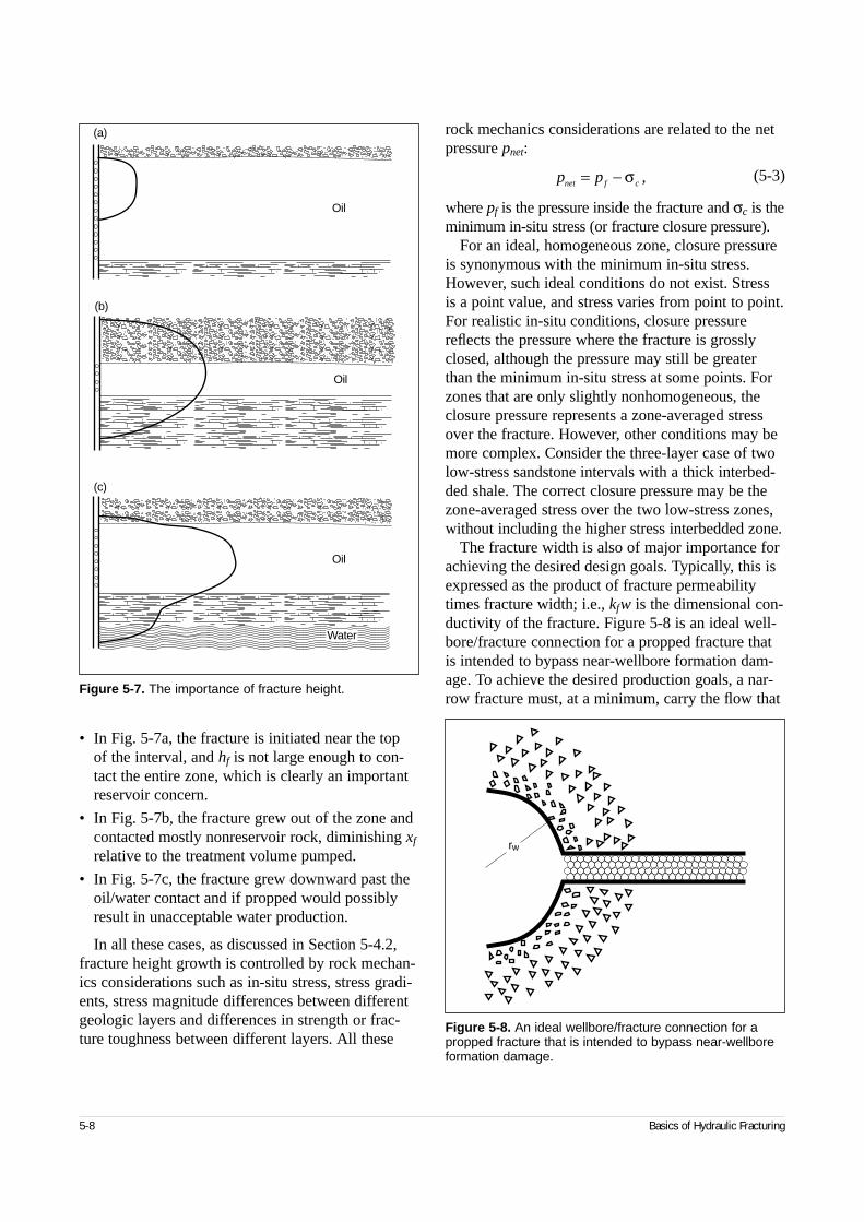
5-8 Basics of Hydraulic Fracturing

• In Fig. 5-7a, the fracture is initiated near the top of the interval, and hf is not large enough to con-tact the entire zone, which is clearly an importantreservoir concern.

• In Fig. 5-7b, the fracture grew out of the zone andcontacted mostly nonreservoir rock, diminishing xf

relative to the treatment volume pumped.

• In Fig. 5-7c, the fracture grew downward past theoil/water contact and if propped would possiblyresult in unacceptable water production.

In all these cases, as discussed in Section 5-4.2,fracture height growth is controlled by rock mechan-ics considerations such as in-situ stress, stress gradi-ents, stress magnitude differences between differentgeologic layers and differences in strength or frac-ture toughness between different layers. All these

rock mechanics considerations are related to the netpressure pnet:

(5-3)

where pf is the pressure inside the fracture and σc is theminimum in-situ stress (or fracture closure pressure).

For an ideal, homogeneous zone, closure pressureis synonymous with the minimum in-situ stress.However, such ideal conditions do not exist. Stress is a point value, and stress varies from point to point.For realistic in-situ conditions, closure pressurereflects the pressure where the fracture is grosslyclosed, although the pressure may still be greaterthan the minimum in-situ stress at some points. Forzones that are only slightly nonhomogeneous, theclosure pressure represents a zone-averaged stressover the fracture. However, other conditions may bemore complex. Consider the three-layer case of twolow-stress sandstone intervals with a thick interbed-ded shale. The correct closure pressure may be thezone-averaged stress over the two low-stress zones,without including the higher stress interbedded zone.

The fracture width is also of major importance forachieving the desired design goals. Typically, this isexpressed as the product of fracture permeabilitytimes fracture width; i.e., kfw is the dimensional con-ductivity of the fracture. Figure 5-8 is an ideal well-bore/fracture connection for a propped fracture thatis intended to bypass near-wellbore formation dam-age. To achieve the desired production goals, a nar-row fracture must, at a minimum, carry the flow that

p pnet f c= − σ ,

Figure 5-7. The importance of fracture height.

Oil

(a)

Oil

Water

(c)

Oil

(b)

Figure 5-8. An ideal wellbore/fracture connection for apropped fracture that is intended to bypass near-wellboreformation damage.

rw

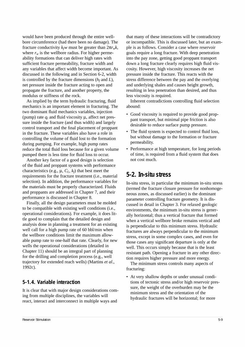
Reservoir Stimulation 5-9

would have been produced through the entire well-bore circumference (had there been no damage). Thefracture conductivity kfw must be greater than 2πrwk,where rw is the wellbore radius. For higher perme-ability formations that can deliver high rates withsufficient fracture permeability, fracture width andany variables that affect width become important. Asdiscussed in the following and in Section 6-2, widthis controlled by the fracture dimensions (hf and L),net pressure inside the fracture acting to open andpropagate the fracture, and another property, themodulus or stiffness of the rock.

As implied by the term hydraulic fracturing, fluidmechanics is an important element in fracturing. Thetwo dominant fluid mechanics variables, injection(pump) rate qi and fluid viscosity µ, affect net pres-sure inside the fracture (and thus width) and largelycontrol transport and the final placement of proppantin the fracture. These variables also have a role incontrolling the volume of fluid lost to the formationduring pumping. For example, high pump ratesreduce the total fluid loss because for a given volumepumped there is less time for fluid loss to occur.

Another key factor of a good design is selection of the fluid and proppant systems with performancecharacteristics (e.g., µ, CL, kf) that best meet therequirements for the fracture treatment (i.e., materialselection). In addition, the performance variables forthe materials must be properly characterized. Fluidsand proppants are addressed in Chapter 7, and theirperformance is discussed in Chapter 8.

Finally, all the design parameters must be moldedto be compatible with existing well conditions (i.e.,operational considerations). For example, it does lit-tle good to complain that the detailed design andanalysis done in planning a treatment for an existingwell call for a high pump rate of 60 bbl/min whenthe wellbore conditions limit the maximum allow-able pump rate to one-half that rate. Clearly, for newwells the operational considerations (detailed inChapter 11) should be an integral part of planningfor the drilling and completion process (e.g., welltrajectory for extended reach wells) (Martins et al.,1992c).

5-1.4. Variable interactionIt is clear that with major design considerations com-ing from multiple disciplines, the variables willreact, interact and interconnect in multiple ways and

that many of these interactions will be contradictoryor incompatible. This is discussed later, but an exam-ple is as follows. Consider a case where reservoirgoals require a long fracture. With deep penetrationinto the pay zone, getting good proppant transportdown a long fracture clearly requires high fluid vis-cosity. However, high viscosity increases the netpressure inside the fracture. This reacts with thestress difference between the pay and the overlyingand underlying shales and causes height growth,resulting in less penetration than desired, and thusless viscosity is required.

Inherent contradictions controlling fluid selectionabound:

• Good viscosity is required to provide good prop-pant transport, but minimal pipe friction is alsodesirable to reduce surface pump pressure.

• The fluid system is expected to control fluid loss,but without damage to the formation or fracturepermeability.

• Performance at high temperature, for long periodsof time, is required from a fluid system that doesnot cost much.

5-2. In-situ stressIn-situ stress, in particular the minimum in-situ stress(termed the fracture closure pressure for nonhomoge-neous zones, as discussed earlier) is the dominantparameter controlling fracture geometry. It is dis-cussed in detail in Chapter 3. For relaxed geologicenvironments, the minimum in-situ stress is gener-ally horizontal; thus a vertical fracture that formedwhen a vertical wellbore broke remains vertical andis perpendicular to this minimum stress. Hydraulicfractures are always perpendicular to the minimumstress, except in some complex cases, and even forthose cases any significant departure is only at thewell. This occurs simply because that is the leastresistant path. Opening a fracture in any other direc-tion requires higher pressure and more energy.

The minimum stress controls many aspects offracturing:

• At very shallow depths or under unusual condi-tions of tectonic stress and/or high reservoir pres-sure, the weight of the overburden may be theminimum stress and the orientation of thehydraulic fractures will be horizontal; for more

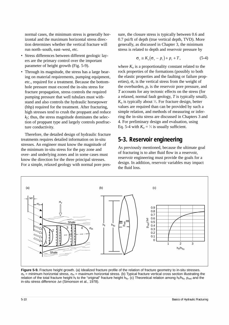
5-10 Basics of Hydraulic Fracturing

normal cases, the minimum stress is generally hor-izontal and the maximum horizontal stress direc-tion determines whether the vertical fracture willrun north–south, east–west, etc.

• Stress differences between different geologic lay-ers are the primary control over the importantparameter of height growth (Fig. 5-9).

• Through its magnitude, the stress has a large bear-ing on material requirements, pumping equipment,etc., required for a treatment. Because the bottom-hole pressure must exceed the in-situ stress forfracture propagation, stress controls the requiredpumping pressure that well tubulars must with-stand and also controls the hydraulic horsepower(hhp) required for the treatment. After fracturing,high stresses tend to crush the proppant and reducekf ; thus, the stress magnitude dominates the selec-tion of proppant type and largely controls postfrac-ture conductivity.

Therefore, the detailed design of hydraulic fracturetreatments requires detailed information on in-situstresses. An engineer must know the magnitude ofthe minimum in-situ stress for the pay zone andover- and underlying zones and in some cases mustknow the direction for the three principal stresses.For a simple, relaxed geology with normal pore pres-

sure, the closure stress is typically between 0.6 and0.7 psi/ft of depth (true vertical depth, TVD). Moregenerally, as discussed in Chapter 3, the minimumstress is related to depth and reservoir pressure by

(5-4)

where Ko is a proportionality constant related to therock properties of the formations (possibly to boththe elastic properties and the faulting or failure prop-erties), σv is the vertical stress from the weight of the overburden, pr is the reservoir pore pressure, andT accounts for any tectonic effects on the stress (fora relaxed, normal fault geology, T is typically small).Ko is typically about 1⁄3. For fracture design, bettervalues are required than can be provided by such asimple relation, and methods of measuring or infer-ring the in-situ stress are discussed in Chapters 3 and4. For preliminary design and evaluation, using Eq. 5-4 with Ko = 1⁄3 is usually sufficient.

5-3. Reservoir engineeringAs previously mentioned, because the ultimate goalof fracturing is to alter fluid flow in a reservoir,reservoir engineering must provide the goals for adesign. In addition, reservoir variables may impactthe fluid loss.

Figure 5-9. Fracture height growth. (a) Idealized fracture profile of the relation of fracture geometry to in-situ stresses. σh = minimum horizontal stress, σH = maximum horizontal stress. (b) Typical fracture vertical cross section illustrating therelation of the total fracture height hf to the “original” fracture height hfo. (c) Theoretical relation among hf/hfo, pnet and thein-situ stress difference ∆σ (Simonson et al., 1978).

1

23 4

Shale

σH

σvσh

∆σ

Shale

(a) (b) (c)

hf hfo p net

0.10.20.30.40.50.60.70.80.9

1 2 3

p net

/∆σ

hf/hfo

0

σ σc o v r rK p p T≅ −( ) + + ,

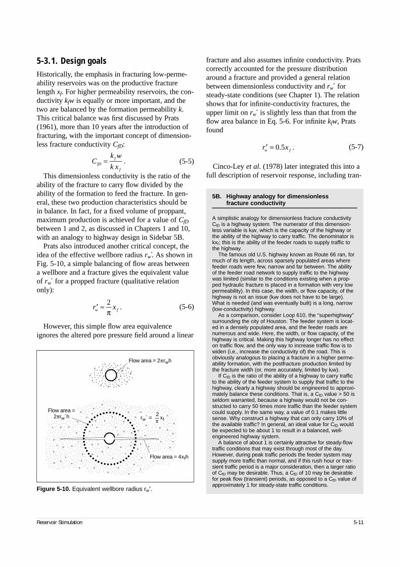
5-3.1. Design goalsHistorically, the emphasis in fracturing low-perme-ability reservoirs was on the productive fracturelength xf. For higher permeability reservoirs, the con-ductivity kfw is equally or more important, and thetwo are balanced by the formation permeability k.This critical balance was first discussed by Prats(1961), more than 10 years after the introduction offracturing, with the important concept of dimension-less fracture conductivity CfD:

(5-5)

This dimensionless conductivity is the ratio of theability of the fracture to carry flow divided by theability of the formation to feed the fracture. In gen-eral, these two production characteristics should bein balance. In fact, for a fixed volume of proppant,maximum production is achieved for a value of CfD

between 1 and 2, as discussed in Chapters 1 and 10,with an analogy to highway design in Sidebar 5B.

Prats also introduced another critical concept, theidea of the effective wellbore radius rẃ . As shown inFig. 5-10, a simple balancing of flow areas betweena wellbore and a fracture gives the equivalent valueof rẃ for a propped fracture (qualitative relationonly):

(5-6)

However, this simple flow area equivalenceignores the altered pore pressure field around a linear

fracture and also assumes infinite conductivity. Pratscorrectly accounted for the pressure distributionaround a fracture and provided a general relationbetween dimensionless conductivity and rẃ forsteady-state conditions (see Chapter 1). The relationshows that for infinite-conductivity fractures, theupper limit on rẃ is slightly less than that from theflow area balance in Eq. 5-6. For infinite kfw, Pratsfound

(5-7)

Cinco-Ley et al. (1978) later integrated this into afull description of reservoir response, including tran-

Reservoir Stimulation 5-11

′ ≈r xw f

2π

.

′ =r xw f0 5. .

Ck w

k xfDf

f

= .

5B. Highway analogy for dimensionless fracture conductivity

A simplistic analogy for dimensionless fracture conductivityCfD is a highway system. The numerator of this dimension-less variable is kfw, which is the capacity of the highway orthe ability of the highway to carry traffic. The denominator iskxf; this is the ability of the feeder roads to supply traffic tothe highway.

The famous old U.S. highway known as Route 66 ran, formuch of its length, across sparsely populated areas wherefeeder roads were few, narrow and far between. The abilityof the feeder road network to supply traffic to the highwaywas limited (similar to the conditions existing when a prop-ped hydraulic fracture is placed in a formation with very lowpermeability). In this case, the width, or flow capacity, of thehighway is not an issue (kfw does not have to be large).What is needed (and was eventually built) is a long, narrow(low-conductivity) highway.

As a comparison, consider Loop 610, the “superhighway”surrounding the city of Houston. The feeder system is locat-ed in a densely populated area, and the feeder roads arenumerous and wide. Here, the width, or flow capacity, of thehighway is critical. Making this highway longer has no effecton traffic flow, and the only way to increase traffic flow is towiden (i.e., increase the conductivity of) the road. This isobviously analogous to placing a fracture in a higher perme-ability formation, with the postfracture production limited bythe fracture width (or, more accurately, limited by kfw).

If CfD is the ratio of the ability of a highway to carry trafficto the ability of the feeder system to supply that traffic to thehighway, clearly a highway should be engineered to approxi-mately balance these conditions. That is, a CfD value > 50 isseldom warranted, because a highway would not be con-structed to carry 50 times more traffic than the feeder systemcould supply. In the same way, a value of 0.1 makes littlesense. Why construct a highway that can only carry 10% ofthe available traffic? In general, an ideal value for CfD wouldbe expected to be about 1 to result in a balanced, well-engineered highway system.

A balance of about 1 is certainly attractive for steady-flowtraffic conditions that may exist through most of the day.However, during peak traffic periods the feeder system maysupply more traffic than normal, and if this rush hour or tran-sient traffic period is a major consideration, then a larger ratioof CfD may be desirable. Thus, a CfD of 10 may be desirablefor peak flow (transient) periods, as opposed to a CfD value ofapproximately 1 for steady-state traffic conditions.

Figure 5-10. Equivalent wellbore radius rw′.������

..

. ... . . .

... ..

. ... . .

. .... ... .

.. ..

. . . ..

..... . . ....

.... .. .. .

..

.. .

..

..

. . .... .

..

.

.

.... .

Flow area = 2πrwh

Flow area = 4xfh

2rw´ = xfπ

Flow area =2πrw´h

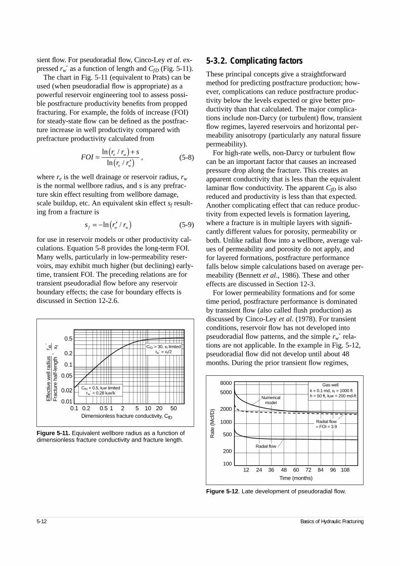
5-12 Basics of Hydraulic Fracturing

sient flow. For pseudoradial flow, Cinco-Ley et al. ex-pressed rẃ as a function of length and CfD (Fig. 5-11).

The chart in Fig. 5-11 (equivalent to Prats) can beused (when pseudoradial flow is appropriate) as apowerful reservoir engineering tool to assess possi-ble postfracture productivity benefits from proppedfracturing. For example, the folds of increase (FOI)for steady-state flow can be defined as the postfrac-ture increase in well productivity compared withprefracture productivity calculated from

(5-8)

where re is the well drainage or reservoir radius, rw

is the normal wellbore radius, and s is any prefrac-ture skin effect resulting from wellbore damage,scale buildup, etc. An equivalent skin effect sf result-ing from a fracture is

(5-9)

for use in reservoir models or other productivity cal-culations. Equation 5-8 provides the long-term FOI.Many wells, particularly in low-permeability reser-voirs, may exhibit much higher (but declining) early-time, transient FOI. The preceding relations are fortransient pseudoradial flow before any reservoirboundary effects; the case for boundary effects isdiscussed in Section 12-2.6.

5-3.2. Complicating factorsThese principal concepts give a straightforwardmethod for predicting postfracture production; how-ever, complications can reduce postfracture produc-tivity below the levels expected or give better pro-ductivity than that calculated. The major complica-tions include non-Darcy (or turbulent) flow, transientflow regimes, layered reservoirs and horizontal per-meability anisotropy (particularly any natural fissurepermeability).

For high-rate wells, non-Darcy or turbulent flowcan be an important factor that causes an increasedpressure drop along the fracture. This creates anapparent conductivity that is less than the equivalentlaminar flow conductivity. The apparent CfD is alsoreduced and productivity is less than that expected.Another complicating effect that can reduce produc-tivity from expected levels is formation layering,where a fracture is in multiple layers with signifi-cantly different values for porosity, permeability orboth. Unlike radial flow into a wellbore, average val-ues of permeability and porosity do not apply, andfor layered formations, postfracture performancefalls below simple calculations based on average per-meability (Bennett et al., 1986). These and othereffects are discussed in Section 12-3.

For lower permeability formations and for sometime period, postfracture performance is dominatedby transient flow (also called flush production) asdiscussed by Cinco-Ley et al. (1978). For transientconditions, reservoir flow has not developed intopseudoradial flow patterns, and the simple rw´ rela-tions are not applicable. In the example in Fig. 5-12,pseudoradial flow did not develop until about 48months. During the prior transient flow regimes,

Figure 5-12. Late development of pseudoradial flow.

Rat

e (M

cf/D

)

5000

2000

8000

1000

500

200

10012 24 36 48 60 72 84 96 108

Numericalmodel

Radial flow

Time (months)

Radial flow× FOI = 3.9

Gas wellk = 0.1 md, xf = 1000 fth = 50 ft, kfw = 200 md-ft

Figure 5-11. Equivalent wellbore radius as a function ofdimensionless fracture conductivity and fracture length.

Effe

ctiv

e w

ell r

adiu

sF

ract

ure

half-

leng

th

r w´

x f,

0.1 0.2 0.5 1 2 5 10 20 500.01

0.05

0.1

0.2

0.5

Dimensionless fracture conductivity, CfD

CfD > 30, xf limitedrw´ = xf/2

CfD < 0.5, kfw limitedrw´ = 0.28 kfw/k0.02

s r rf w w= − ′( )ln /

FOIr r s

r re w

e w

= ( ) +′( )

ln

ln

/

/,

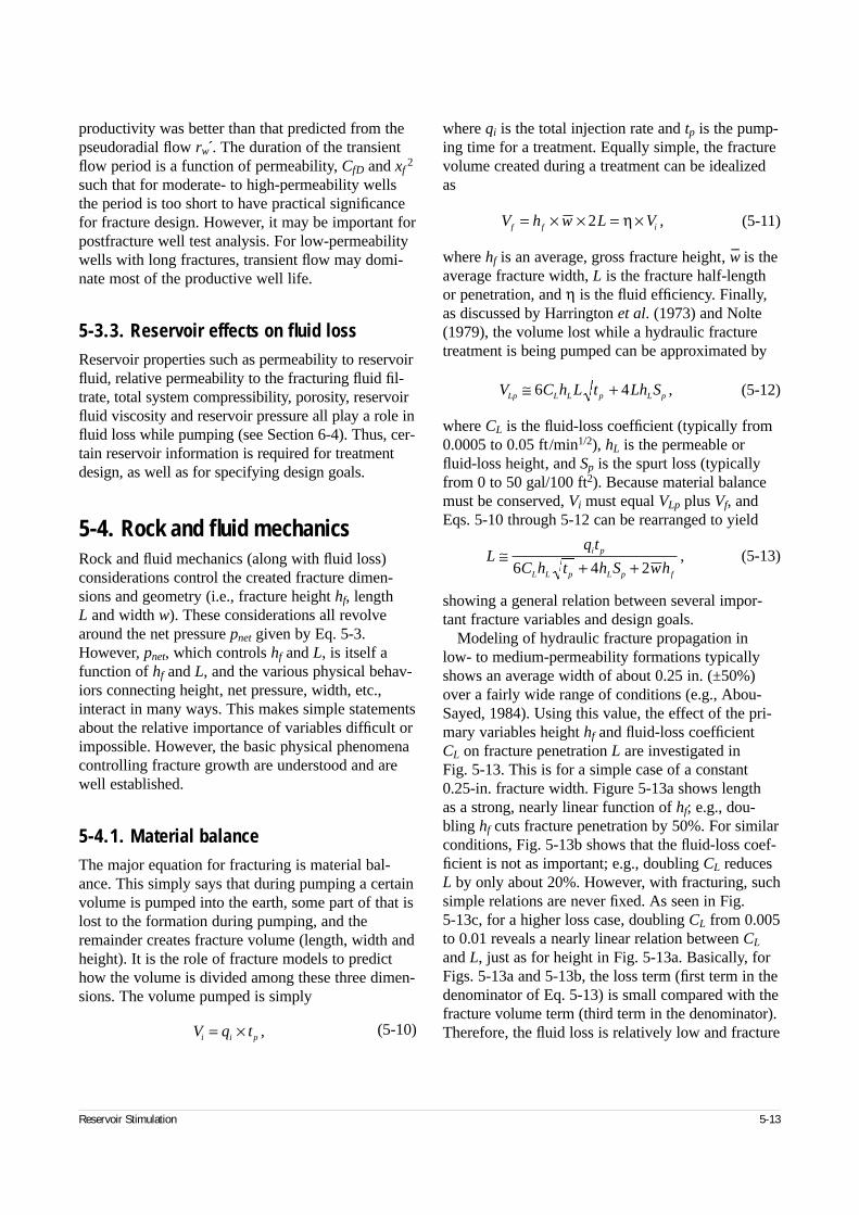
Reservoir Stimulation 5-13

productivity was better than that predicted from thepseudoradial flow rẃ . The duration of the transientflow period is a function of permeability, CfD and xf

2

such that for moderate- to high-permeability wellsthe period is too short to have practical significancefor fracture design. However, it may be important forpostfracture well test analysis. For low-permeabilitywells with long fractures, transient flow may domi-nate most of the productive well life.

5-3.3. Reservoir effects on fluid lossReservoir properties such as permeability to reservoirfluid, relative permeability to the fracturing fluid fil-trate, total system compressibility, porosity, reservoirfluid viscosity and reservoir pressure all play a role influid loss while pumping (see Section 6-4). Thus, cer-tain reservoir information is required for treatmentdesign, as well as for specifying design goals.

5-4. Rock and fluid mechanicsRock and fluid mechanics (along with fluid loss)considerations control the created fracture dimen-sions and geometry (i.e., fracture height hf, length L and width w). These considerations all revolvearound the net pressure pnet given by Eq. 5-3.However, pnet, which controls hf and L, is itself afunction of hf and L, and the various physical behav-iors connecting height, net pressure, width, etc.,interact in many ways. This makes simple statementsabout the relative importance of variables difficult orimpossible. However, the basic physical phenomenacontrolling fracture growth are understood and arewell established.

5-4.1. Material balanceThe major equation for fracturing is material bal-ance. This simply says that during pumping a certainvolume is pumped into the earth, some part of that islost to the formation during pumping, and theremainder creates fracture volume (length, width andheight). It is the role of fracture models to predicthow the volume is divided among these three dimen-sions. The volume pumped is simply

(5-10)

where qi is the total injection rate and tp is the pump-ing time for a treatment. Equally simple, the fracturevolume created during a treatment can be idealizedas

(5-11)

where hf is an average, gross fracture height, w– is theaverage fracture width, L is the fracture half-lengthor penetration, and η is the fluid efficiency. Finally,as discussed by Harrington et al. (1973) and Nolte(1979), the volume lost while a hydraulic fracturetreatment is being pumped can be approximated by

(5-12)

where CL is the fluid-loss coefficient (typically from0.0005 to 0.05 ft/min1/2), hL is the permeable orfluid-loss height, and Sp is the spurt loss (typicallyfrom 0 to 50 gal/100 ft2). Because material balancemust be conserved, Vi must equal VLp plus Vf, andEqs. 5-10 through 5-12 can be rearranged to yield

(5-13)

showing a general relation between several impor-tant fracture variables and design goals.

Modeling of hydraulic fracture propagation inlow- to medium-permeability formations typicallyshows an average width of about 0.25 in. (±50%)over a fairly wide range of conditions (e.g., Abou-Sayed, 1984). Using this value, the effect of the pri-mary variables height hf and fluid-loss coefficient CL on fracture penetration L are investigated in Fig. 5-13. This is for a simple case of a constant0.25-in. fracture width. Figure 5-13a shows length as a strong, nearly linear function of hf; e.g., dou-bling hf cuts fracture penetration by 50%. For similarconditions, Fig. 5-13b shows that the fluid-loss coef-ficient is not as important; e.g., doubling CL reducesL by only about 20%. However, with fracturing, suchsimple relations are never fixed. As seen in Fig. 5-13c, for a higher loss case, doubling CL from 0.005to 0.01 reveals a nearly linear relation between CL

and L, just as for height in Fig. 5-13a. Basically, forFigs. 5-13a and 5-13b, the loss term (first term in thedenominator of Eq. 5-13) is small compared with thefracture volume term (third term in the denominator).Therefore, the fluid loss is relatively low and fractureV q ti i p= × ,

V h w L Vf f i= × × = ×2 η ,

V C h L t Lh SLp L L p L p≅ +6 4 ,

Lq t

C h t h S whi p

L L p L p f

≅+ +6 4 2

,

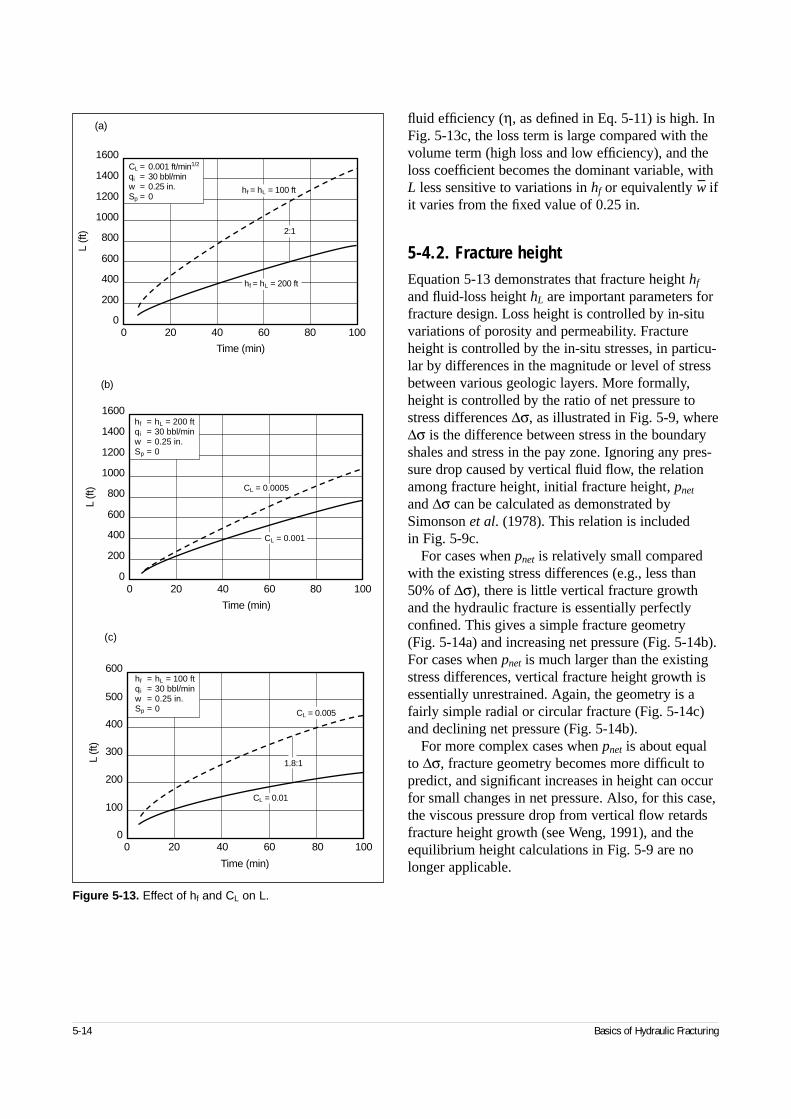
5-14 Basics of Hydraulic Fracturing

fluid efficiency (η, as defined in Eq. 5-11) is high. InFig. 5-13c, the loss term is large compared with thevolume term (high loss and low efficiency), and theloss coefficient becomes the dominant variable, withL less sensitive to variations in hf or equivalently w– ifit varies from the fixed value of 0.25 in.

5-4.2. Fracture heightEquation 5-13 demonstrates that fracture height hf

and fluid-loss height hL are important parameters forfracture design. Loss height is controlled by in-situvariations of porosity and permeability. Fractureheight is controlled by the in-situ stresses, in particu-lar by differences in the magnitude or level of stressbetween various geologic layers. More formally,height is controlled by the ratio of net pressure tostress differences ∆σ, as illustrated in Fig. 5-9, where∆σ is the difference between stress in the boundaryshales and stress in the pay zone. Ignoring any pres-sure drop caused by vertical fluid flow, the relationamong fracture height, initial fracture height, pnet

and ∆σ can be calculated as demonstrated bySimonson et al. (1978). This relation is included in Fig. 5-9c.

For cases when pnet is relatively small comparedwith the existing stress differences (e.g., less than50% of ∆σ), there is little vertical fracture growthand the hydraulic fracture is essentially perfectlyconfined. This gives a simple fracture geometry (Fig. 5-14a) and increasing net pressure (Fig. 5-14b).For cases when pnet is much larger than the existingstress differences, vertical fracture height growth isessentially unrestrained. Again, the geometry is afairly simple radial or circular fracture (Fig. 5-14c)and declining net pressure (Fig. 5-14b).

For more complex cases when pnet is about equalto ∆σ, fracture geometry becomes more difficult topredict, and significant increases in height can occurfor small changes in net pressure. Also, for this case,the viscous pressure drop from vertical flow retardsfracture height growth (see Weng, 1991), and theequilibrium height calculations in Fig. 5-9 are nolonger applicable.

Figure 5-13. Effect of hf and CL on L.

L(ft

)

1400

1600

1200

1000

800

600

400

200

0200 40 60 80 100

hf = hL = 100 ft

hf = hL = 200 ft

2:1

Time (min)

(a)

CL = 0.001 ft/min1/2

qi = 30 bbl/minw = 0.25 in.Sp = 0

L (ft

)

1400

1600

1200

1000

800

600

400

200

0200 40 60 80 100

Time (min)

CL = 0.0005

CL = 0.001

(b)

hf = hL = 200 ftqi = 30 bbl/minw = 0.25 in.Sp = 0

L (ft

)

500

600

400

300

200

100

0200 40 60 80 100

CL = 0.005

CL = 0.01

1.8:1

Time (min)

hf = hL = 100 ftqi = 30 bbl/minw = 0.25 in.Sp = 0

(c)

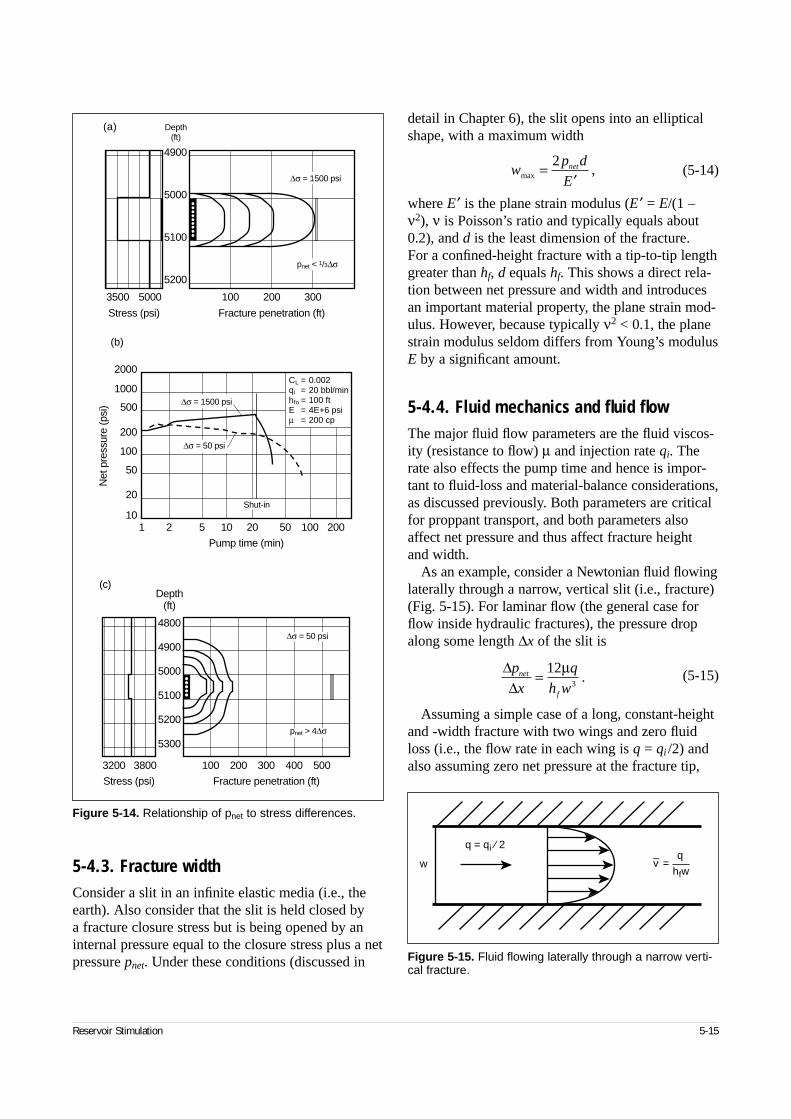
Reservoir Stimulation 5-15

5-4.3. Fracture widthConsider a slit in an infinite elastic media (i.e., theearth). Also consider that the slit is held closed by a fracture closure stress but is being opened by aninternal pressure equal to the closure stress plus a netpressure pnet. Under these conditions (discussed in

detail in Chapter 6), the slit opens into an ellipticalshape, with a maximum width

(5-14)

where E′ is the plane strain modulus (E′ = E/(1 –ν2), ν is Poisson’s ratio and typically equals about0.2), and d is the least dimension of the fracture. For a confined-height fracture with a tip-to-tip lengthgreater than hf, d equals hf. This shows a direct rela-tion between net pressure and width and introducesan important material property, the plane strain mod-ulus. However, because typically ν2 < 0.1, the planestrain modulus seldom differs from Young’s modulusE by a significant amount.

5-4.4. Fluid mechanics and fluid flowThe major fluid flow parameters are the fluid viscos-ity (resistance to flow) µ and injection rate qi. Therate also effects the pump time and hence is impor-tant to fluid-loss and material-balance considerations,as discussed previously. Both parameters are criticalfor proppant transport, and both parameters alsoaffect net pressure and thus affect fracture height and width.

As an example, consider a Newtonian fluid flowinglaterally through a narrow, vertical slit (i.e., fracture) (Fig. 5-15). For laminar flow (the general case forflow inside hydraulic fractures), the pressure dropalong some length ∆x of the slit is

(5-15)

Assuming a simple case of a long, constant-heightand -width fracture with two wings and zero fluidloss (i.e., the flow rate in each wing is q = qi /2) andalso assuming zero net pressure at the fracture tip,

Figure 5-14. Relationship of pnet to stress differences.

3500 5000 100 200 300

5200

5100

5000

4900

Stress (psi) Fracture penetration (ft)

∆σ = 1500 psi

pnet < 1/3∆σ

(a) Depth(ft)

Net

pre

ssur

e (p

si)

2000

1000

500

200

100

50

20

101 2 5 10 20 50 100 200

Pump time (min)

Shut-in

∆σ = 1500 psi

∆σ = 50 psi

(b)

CL = 0.002qi = 20 bbl/minhfo = 100 ftE = 4E+6 psiµ = 200 cp

3200 3800 100 300 400 500200

4800

4900

5000

5100

5200

5300

Stress (psi) Fracture penetration (ft)

∆σ = 50 psi

pnet > 4∆σ

(c)Depth

(ft)

∆∆p

x

q

h wnet

f

= 123

µ.

Figure 5-15. Fluid flowing laterally through a narrow verti-cal fracture.

w

q = qi ⁄ 2q

v– = hfw

wp d

Enet

max ,=′

2

5-16 Basics of Hydraulic Fracturing

Eq. 5-15 is integrated from the fracture tip back tothe wellbore to give

(5-16)

For this long, confined-height fracture, hf is theminimum fracture dimension for Eq. 5-14, and thefracture width and net pressure are related by

(5-17)

Combining the two equations gives the proportionality

(5-18)

The exponent of 1⁄4 for this simple fracture geome-try and for Newtonian fluids implies that the fracturewidth is virtually constant; e.g., doubling the pumprate from 20 to 40 bbl/min increases the width onlyby about 20%. The same effect is found for all thevariables in Eq. 5-18. Generally, for non-Newtonianfluids, the exponent is approximately 1⁄3.

This relationship for fracture width can also beused with Eq. 5-17 to give net pressure expressed as

(5-19)

where κ is a constant (see Eq. 6-11) to provide anequality for this expression.

Thus, as a result of viscous forces alone, net pres-sure inside the fracture develops as a function of themodulus, height and (qµ)1/4. From the nature of thisrelation, however, it is clear that modulus and heightare much more important in controlling net pressurethan are pump rate and viscosity, the effect of whichis muted by the small exponent for the relation.

5-4.5. Fracture mechanics and fracture tip effects

The fluid mechanics relations show pnet relatedto modulus, height, fluid viscosity and pump rate.However, in some cases, field observations haveshown net pressure (and presumably fracture width)to be greater than predicted by Eq. 5-19 (Palmer andVeatch, 1987). In such cases the fluid viscosity has asmaller effect on fracture width than predicted byEq. 5-19. This is probably because the simple rela-

tion in Eq. 5-16 assumes no net pressure at the frac-ture tip; i.e., fracture tip effects or fracture propaga-tion effects are ignored. When tip effects are takeninto account, the fracture width is affected by bothfluid viscosity and tip effects (Shlyapobersky et al.,1988a, 1988b). As shown by Nolte (1991), tipeffects can be approximated by considering the netpressure within the tip region to equal ptip (asopposed to zero) in Eq. 5-16. For a positive tip pres-sure, the net pressure equation becomes

(5-20)

where ptip is the pressure required at the fracture tipto open new fracture area and keep the fracture prop-agating forward. This simple relationship serves toillustrate that there are always two components to netpressure: a viscous component and a fracture tip-effects component. The relative magnitude of thetwo effects varies from case to case, and because ofthe small exponent, the combined effects are muchless than the direct sum of the individual effects. Forexample, when the viscous component and the tipcomponent are equal, the net pressure is increased byonly 20% over that predicted when one of the com-ponents is ignored.

• Fracture toughness and elastic fracture mechanics

The fracture tip propagation pressure, or fracturetip effect, is generally assumed to follow thephysics of elastic fracture mechanics. In that case,the magnitude of the tip extension pressure ptip iscontrolled by the critical stress intensity factor KIc

(also called the fracture toughness). Fracturetoughness is a material parameter, and it may bedefined as the strength of a material in the pres-ence of a preexisting flaw. For example, glass hasa high tensile strength, but the presence of a tinyscratch or fracture greatly reduces the strength(i.e., high tensile strength but low fracture tough-ness). On the other hand, modeling clay has lowstrength, but the presence of a flaw or fracturedoes not significantly reduce the strength. Lab-oratory-measured values for the material propertyKIc show toughness ranging from about 1000 toabout 3500 psi/in.1/2, with a typical value of about2000 psi/in.1/2. These tests (after Schmidt andHuddle, 1977; Thiercelin, 1987) include a rangeof rock types from mudstones and sandstones to

pE

hq Lnet

f

i= ′ { }3 4

1 4/

/,κµ

pE

hq L pnet

f

i tip≈ ′ { } +

3

4

4

1 4

κµ/

,

pE w

hnet

f

= ′2

.

pq L

h wneti

f

= 63

µ.

wq L

Ei∝′

µ 1 4/

.

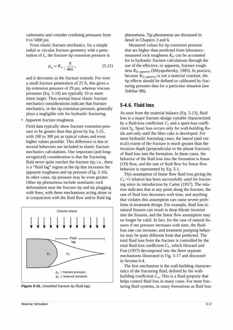
Reservoir Stimulation 5-17

carbonates and consider confining pressures from0 to 5000 psi.

From elastic fracture mechanics, for a simpleradial or circular fracture geometry with a pene-tration of L, the fracture tip extension pressure is

(5-21)

and it decreases as the fracture extends. For evena small fracture penetration of 25 ft, this gives atip extension pressure of 29 psi, whereas viscouspressures (Eq. 5-19) are typically 10 or moretimes larger. Thus normal linear elastic fracturemechanics considerations indicate that fracturemechanics, or the tip extension pressure, generallyplays a negligible role for hydraulic fracturing.

• Apparent fracture toughness

Field data typically show fracture extension pres-sure to be greater than that given by Eq. 5-21,with 100 to 300 psi as typical values and evenhigher values possible. This difference is due toseveral behaviors not included in elastic fracturemechanics calculations. One important (and long-recognized) consideration is that the fracturingfluid never quite reaches the fracture tip; i.e., thereis a “fluid lag” region at the tip that increases theapparent toughness and tip pressure (Fig. 5-16). In other cases, tip pressure may be even greater.Other tip phenomena include nonelastic rockdeformation near the fracture tip and tip pluggingwith fines, with these mechanisms acting alone orin conjunction with the fluid flow and/or fluid lag

phenomena. Tip phenomena are discussed indetail in Chapters 3 and 6.

Measured values for tip extension pressure that are higher than predicted from laboratory-measured rock toughness KIc can be accounted for in hydraulic fracture calculations through theuse of the effective, or apparent, fracture tough-ness KIc-apparent (Shlyapobersky, 1985). In practice,because KIc-apparent is not a material constant, thetip effects should be defined or calibrated by frac-turing pressure data for a particular situation (seeSidebar 9B).

5-4.6. Fluid lossAs seen from the material balance (Eq. 5-13), fluidloss is a major fracture design variable characterizedby a fluid-loss coefficient CL and a spurt-loss coeffi-cient Sp. Spurt loss occurs only for wall-building flu-ids and only until the filter cake is developed. Formost hydraulic fracturing cases, the lateral (and ver-tical) extent of the fracture is much greater than theinvasion depth (perpendicular to the planar fracture)of fluid loss into the formation. In these cases, thebehavior of the fluid loss into the formation is linear(1D) flow, and the rate of fluid flow for linear flowbehavior is represented by Eq. 5-1.

This assumption of linear flow fluid loss giving theCL ⁄√ t relation has been successfully used for fractur-ing since its introduction by Carter (1957). The rela-tion indicates that at any point along the fracture, therate of fluid loss decreases with time, and anythingthat violates this assumption can cause severe prob-lems in treatment design. For example, fluid loss tonatural fissures can result in deep filtrate invasioninto the fissures, and the linear flow assumption mayno longer be valid. In fact, for the case of natural fis-sures if net pressure increases with time, the fluid-loss rate can increase, and treatment pumping behav-ior may be quite different from that predicted. Thetotal fluid loss from the fracture is controlled by thetotal fluid-loss coefficient CL, which Howard andFast (1957) decomposed into the three separatemechanisms illustrated in Fig. 5-17 and discussed in Section 6-4.

The first mechanism is the wall-building character-istics of the fracturing fluid, defined by the wall-building coefficient Cw. This is a fluid property thathelps control fluid loss in many cases. For most frac-turing fluid systems, in many formations as fluid loss

p KLtip Ic= π

48,

Figure 5-16. Unwetted fracture tip (fluid lag).

p1 = fracture pressurep2 ≤ reservoir pressure

Fluidlag

Closure stress

p1 p2

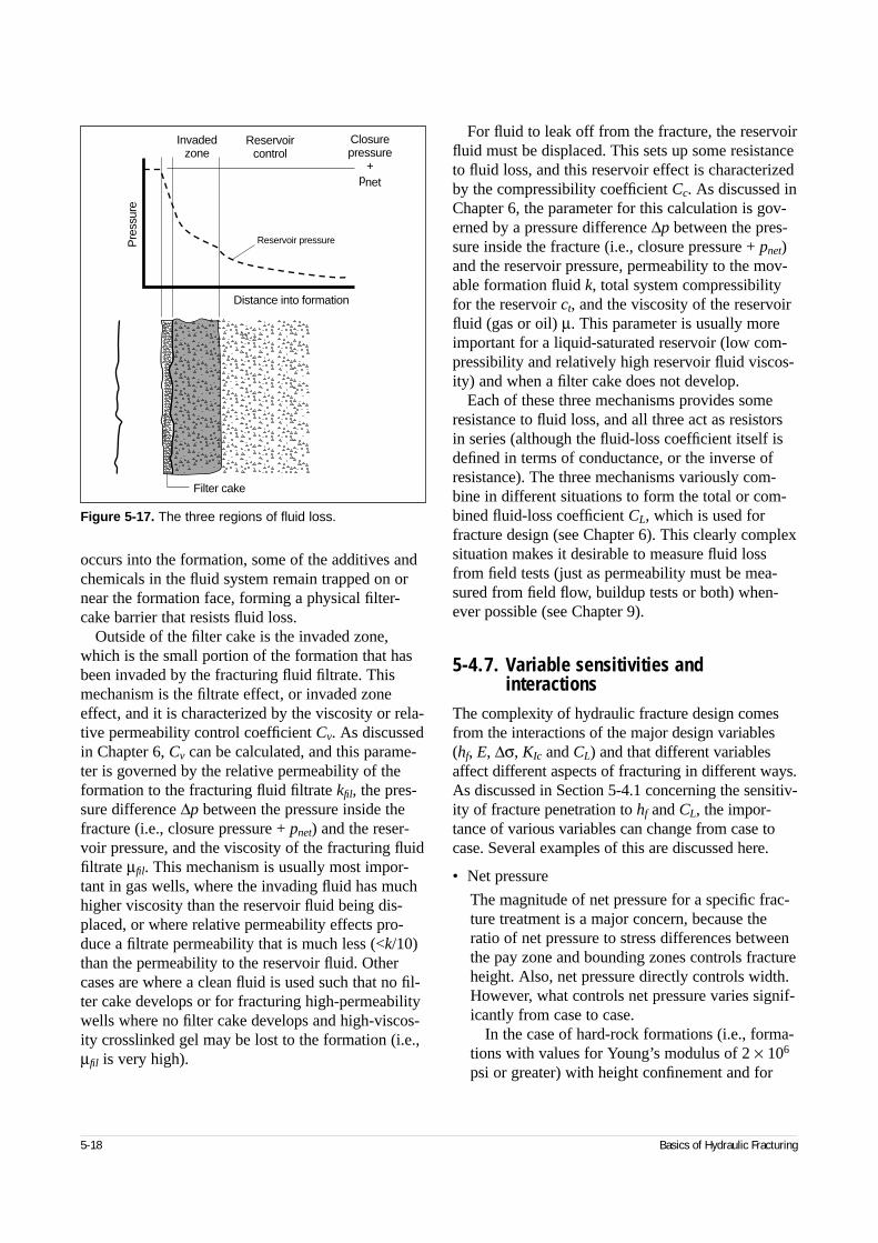
5-18 Basics of Hydraulic Fracturing

occurs into the formation, some of the additives andchemicals in the fluid system remain trapped on ornear the formation face, forming a physical filter-cake barrier that resists fluid loss.

Outside of the filter cake is the invaded zone,which is the small portion of the formation that hasbeen invaded by the fracturing fluid filtrate. Thismechanism is the filtrate effect, or invaded zoneeffect, and it is characterized by the viscosity or rela-tive permeability control coefficient Cv. As discussedin Chapter 6, Cv can be calculated, and this parame-ter is governed by the relative permeability of theformation to the fracturing fluid filtrate kfil, the pres-sure difference ∆p between the pressure inside thefracture (i.e., closure pressure + pnet) and the reser-voir pressure, and the viscosity of the fracturing fluidfiltrate µfil. This mechanism is usually most impor-tant in gas wells, where the invading fluid has muchhigher viscosity than the reservoir fluid being dis-placed, or where relative permeability effects pro-duce a filtrate permeability that is much less (<k/10)than the permeability to the reservoir fluid. Othercases are where a clean fluid is used such that no fil-ter cake develops or for fracturing high-permeabilitywells where no filter cake develops and high-viscos-ity crosslinked gel may be lost to the formation (i.e.,µfil is very high).

For fluid to leak off from the fracture, the reservoirfluid must be displaced. This sets up some resistanceto fluid loss, and this reservoir effect is characterizedby the compressibility coefficient Cc. As discussed inChapter 6, the parameter for this calculation is gov-erned by a pressure difference ∆p between the pres-sure inside the fracture (i.e., closure pressure + pnet)and the reservoir pressure, permeability to the mov-able formation fluid k, total system compressibilityfor the reservoir ct, and the viscosity of the reservoirfluid (gas or oil) µ. This parameter is usually moreimportant for a liquid-saturated reservoir (low com-pressibility and relatively high reservoir fluid viscos-ity) and when a filter cake does not develop.

Each of these three mechanisms provides someresistance to fluid loss, and all three act as resistorsin series (although the fluid-loss coefficient itself isdefined in terms of conductance, or the inverse ofresistance). The three mechanisms variously com-bine in different situations to form the total or com-bined fluid-loss coefficient CL, which is used forfracture design (see Chapter 6). This clearly complexsituation makes it desirable to measure fluid lossfrom field tests (just as permeability must be mea-sured from field flow, buildup tests or both) when-ever possible (see Chapter 9).

5-4.7. Variable sensitivities and interactions

The complexity of hydraulic fracture design comesfrom the interactions of the major design variables(hf, E, ∆σ, KIc and CL) and that different variablesaffect different aspects of fracturing in different ways.As discussed in Section 5-4.1 concerning the sensitiv-ity of fracture penetration to hf and CL, the impor-tance of various variables can change from case tocase. Several examples of this are discussed here.

• Net pressure

The magnitude of net pressure for a specific frac-ture treatment is a major concern, because theratio of net pressure to stress differences betweenthe pay zone and bounding zones controls fractureheight. Also, net pressure directly controls width.However, what controls net pressure varies signif-icantly from case to case.

In the case of hard-rock formations (i.e., forma-tions with values for Young’s modulus of 2 × 106

psi or greater) with height confinement and for

Figure 5-17. The three regions of fluid loss.

Pre

ssur

eInvaded

zoneReservoir

controlClosurepressure

+pnet

Distance into formation

Reservoir pressure

Filter cake

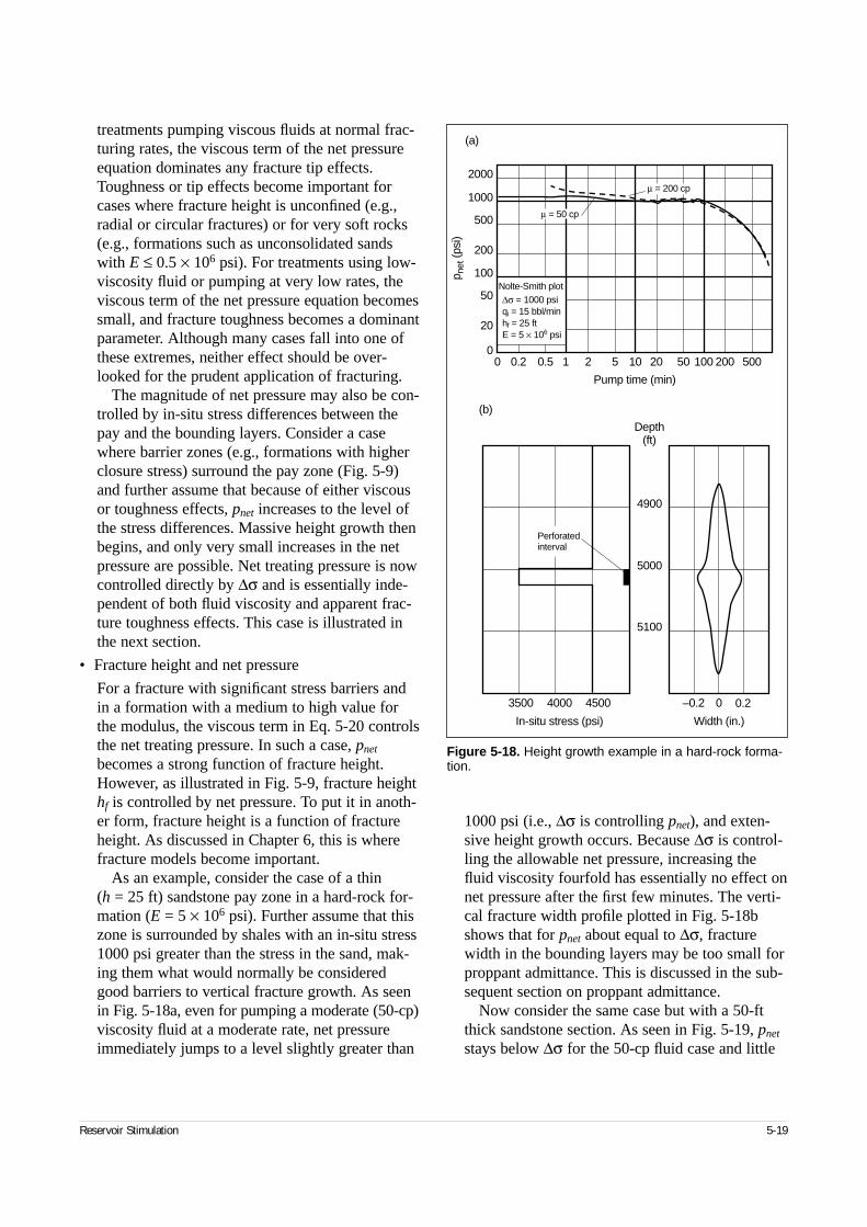
Reservoir Stimulation 5-19

treatments pumping viscous fluids at normal frac-turing rates, the viscous term of the net pressureequation dominates any fracture tip effects.Toughness or tip effects become important forcases where fracture height is unconfined (e.g.,radial or circular fractures) or for very soft rocks(e.g., formations such as unconsolidated sandswith E ≤ 0.5 × 106 psi). For treatments using low-viscosity fluid or pumping at very low rates, theviscous term of the net pressure equation becomessmall, and fracture toughness becomes a dominantparameter. Although many cases fall into one ofthese extremes, neither effect should be over-looked for the prudent application of fracturing.

The magnitude of net pressure may also be con-trolled by in-situ stress differences between thepay and the bounding layers. Consider a casewhere barrier zones (e.g., formations with higherclosure stress) surround the pay zone (Fig. 5-9)and further assume that because of either viscousor toughness effects, pnet increases to the level ofthe stress differences. Massive height growth thenbegins, and only very small increases in the netpressure are possible. Net treating pressure is nowcontrolled directly by ∆σ and is essentially inde-pendent of both fluid viscosity and apparent frac-ture toughness effects. This case is illustrated inthe next section.

• Fracture height and net pressure

For a fracture with significant stress barriers andin a formation with a medium to high value forthe modulus, the viscous term in Eq. 5-20 controlsthe net treating pressure. In such a case, pnet

becomes a strong function of fracture height.However, as illustrated in Fig. 5-9, fracture heighthf is controlled by net pressure. To put it in anoth-er form, fracture height is a function of fractureheight. As discussed in Chapter 6, this is wherefracture models become important.

As an example, consider the case of a thin (h = 25 ft) sandstone pay zone in a hard-rock for-mation (E = 5 × 106 psi). Further assume that thiszone is surrounded by shales with an in-situ stress1000 psi greater than the stress in the sand, mak-ing them what would normally be consideredgood barriers to vertical fracture growth. As seenin Fig. 5-18a, even for pumping a moderate (50-cp)viscosity fluid at a moderate rate, net pressureimmediately jumps to a level slightly greater than

1000 psi (i.e., ∆σ is controlling pnet), and exten-sive height growth occurs. Because ∆σ is control-ling the allowable net pressure, increasing thefluid viscosity fourfold has essentially no effect onnet pressure after the first few minutes. The verti-cal fracture width profile plotted in Fig. 5-18bshows that for pnet about equal to ∆σ, fracturewidth in the bounding layers may be too small forproppant admittance. This is discussed in the sub-sequent section on proppant admittance.

Now consider the same case but with a 50-ftthick sandstone section. As seen in Fig. 5-19, pnet

stays below ∆σ for the 50-cp fluid case and little

Figure 5-18. Height growth example in a hard-rock forma-tion.

p net

(psi

)

2000

1000

500

200

100

50

20

00.20 0.5 1 2 5 10 20 50 100 200 500

Pump time (min)

µ = 200 cp

µ = 50 cp

∆σ = 1000 psiqi = 15 bbl/minhf = 25 ftE = 5 × 106 psi

Nolte-Smith plot

(a)

5100

5000

4900

3500 4000 4500 –0.2 0 0.2

In-situ stress (psi) Width (in.)

Depth(ft)

Perforatedinterval

(b)

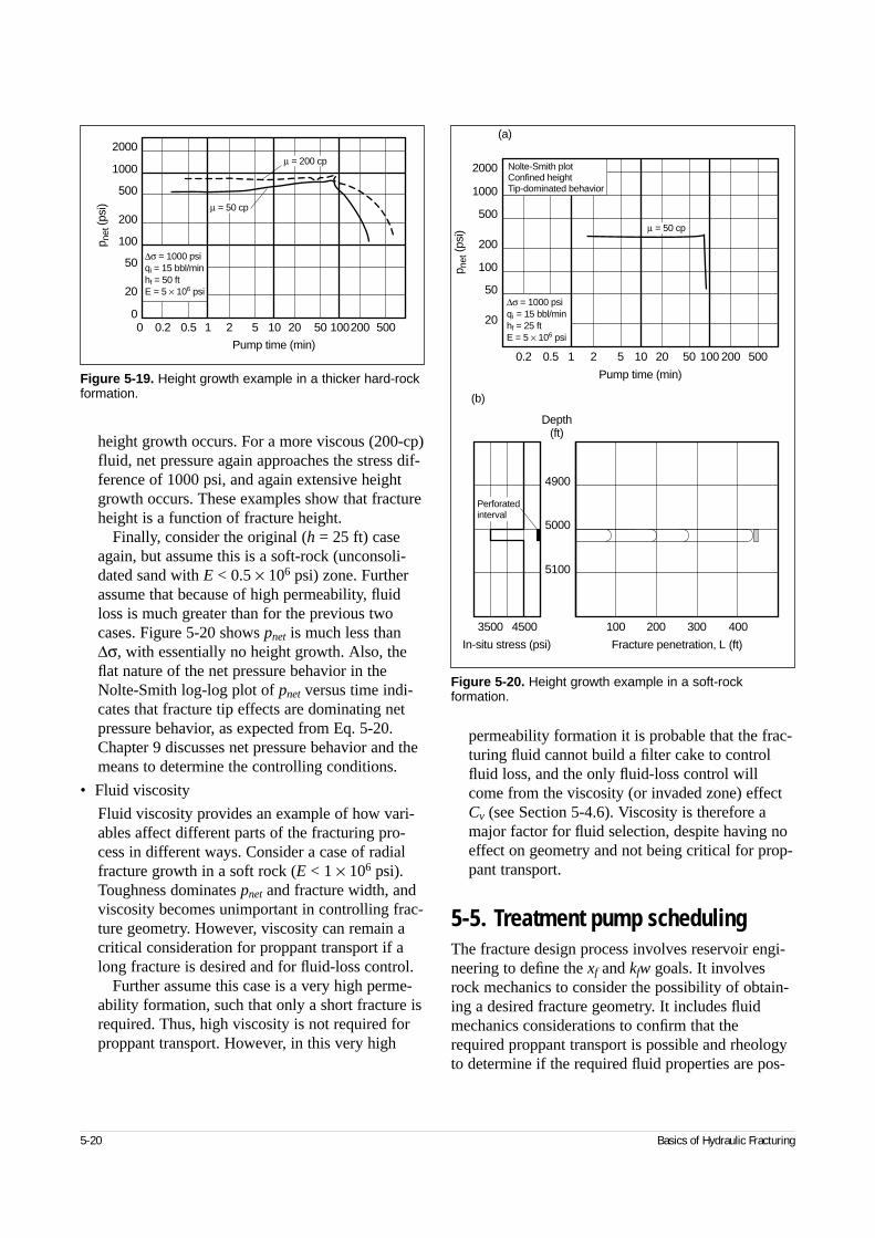
5-20 Basics of Hydraulic Fracturing

height growth occurs. For a more viscous (200-cp)fluid, net pressure again approaches the stress dif-ference of 1000 psi, and again extensive heightgrowth occurs. These examples show that fractureheight is a function of fracture height.

Finally, consider the original (h = 25 ft) caseagain, but assume this is a soft-rock (unconsoli-dated sand with E < 0.5 × 106 psi) zone. Furtherassume that because of high permeability, fluidloss is much greater than for the previous twocases. Figure 5-20 shows pnet is much less than∆σ, with essentially no height growth. Also, theflat nature of the net pressure behavior in theNolte-Smith log-log plot of pnet versus time indi-cates that fracture tip effects are dominating netpressure behavior, as expected from Eq. 5-20.Chapter 9 discusses net pressure behavior and themeans to determine the controlling conditions.

• Fluid viscosity

Fluid viscosity provides an example of how vari-ables affect different parts of the fracturing pro-cess in different ways. Consider a case of radialfracture growth in a soft rock (E < 1 × 106 psi).Toughness dominates pnet and fracture width, andviscosity becomes unimportant in controlling frac-ture geometry. However, viscosity can remain acritical consideration for proppant transport if along fracture is desired and for fluid-loss control.

Further assume this case is a very high perme-ability formation, such that only a short fracture isrequired. Thus, high viscosity is not required forproppant transport. However, in this very high

permeability formation it is probable that the frac-turing fluid cannot build a filter cake to controlfluid loss, and the only fluid-loss control willcome from the viscosity (or invaded zone) effectCv (see Section 5-4.6). Viscosity is therefore amajor factor for fluid selection, despite having noeffect on geometry and not being critical for prop-pant transport.

5-5. Treatment pump schedulingThe fracture design process involves reservoir engi-neering to define the xf and kfw goals. It involvesrock mechanics to consider the possibility of obtain-ing a desired fracture geometry. It includes fluidmechanics considerations to confirm that therequired proppant transport is possible and rheologyto determine if the required fluid properties are pos-

Figure 5-19. Height growth example in a thicker hard-rockformation.

p net

(psi

)

2000

1000

500

200

100

50

20

00.20 0.5 1 2 5 10 20 50 100200 500

Pump time (min)

µ = 200 cp

µ = 50 cp

∆σ = 1000 psi qi = 15 bbl/minhf = 50 ftE = 5 × 106 psi

Figure 5-20. Height growth example in a soft-rock formation.

∆σ = 1000 psiqi = 15 bbl/minhf = 25 ftE = 5 × 106 psi

µ = 50 cp

Nolte-Smith plot Confined heightTip-dominated behavior

p net

(psi

)

2000

1000

500

200

100

50

20

0.2 0.5 1 2 5 10 20 50 100 200 500

Pump time (min)

(a)

5100

5000

4900

3500 4500 100 200 300 400

In-situ stress (psi) Fracture penetration, L (ft)

Perforatedinterval

Depth(ft)

(b)

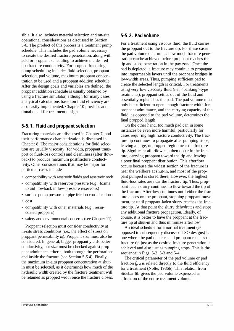
Reservoir Stimulation 5-21

sible. It also includes material selection and on-siteoperational considerations as discussed in Section 5-6. The product of this process is a treatment pumpschedule. This includes the pad volume necessary to create the desired fracture penetration, along withacid or proppant scheduling to achieve the desiredpostfracture conductivity. For propped fracturing,pump scheduling includes fluid selection, proppantselection, pad volume, maximum proppant concen-tration to be used and a proppant addition schedule.After the design goals and variables are defined, theproppant addition schedule is usually obtained byusing a fracture simulator, although for many casesanalytical calculations based on fluid efficiency arealso easily implemented. Chapter 10 provides addi-tional detail for treatment design.

5-5.1. Fluid and proppant selectionFracturing materials are discussed in Chapter 7, andtheir performance characterization is discussed inChapter 8. The major considerations for fluid selec-tion are usually viscosity (for width, proppant trans-port or fluid-loss control) and cleanliness (after flow-back) to produce maximum postfracture conduct-ivity. Other considerations that may be major forparticular cases include

• compatibility with reservoir fluids and reservoir rock

• compatibility with reservoir pressure (e.g., foamsto aid flowback in low-pressure reservoirs)

• surface pump pressure or pipe friction considerations

• cost

• compatibility with other materials (e.g., resin-coated proppant)

• safety and environmental concerns (see Chapter 11).

Proppant selection must consider conductivity atin-situ stress conditions (i.e., the effect of stress onproppant permeability kf). Proppant size must also beconsidered. In general, bigger proppant yields betterconductivity, but size must be checked against prop-pant admittance criteria, both through the perforationsand inside the fracture (see Section 5-5.4). Finally,the maximum in-situ proppant concentration at shut-in must be selected, as it determines how much of thehydraulic width created by the fracture treatment willbe retained as propped width once the fracture closes.

5-5.2. Pad volumeFor a treatment using viscous fluid, the fluid carriesthe proppant out to the fracture tip. For these casesthe pad volume determines how much fracture pene-tration can be achieved before proppant reaches thetip and stops penetration in the pay zone. Once thepad is depleted, a fracture may continue to propagateinto impermeable layers until the proppant bridges inlow-width areas. Thus, pumping sufficient pad tocreate the selected length is critical. For treatmentsusing very low viscosity fluid (i.e., “banking”-typetreatments), proppant settles out of the fluid andessentially replenishes the pad. The pad volume mustonly be sufficient to open enough fracture width forproppant admittance, and the carrying capacity of thefluid, as opposed to the pad volume, determines thefinal propped length.

On the other hand, too much pad can in someinstances be even more harmful, particularly forcases requiring high fracture conductivity. The frac-ture tip continues to propagate after pumping stops,leaving a large, unpropped region near the fracturetip. Significant afterflow can then occur in the frac-ture, carrying proppant toward the tip and leaving a poor final proppant distribution. This afterflowoccurs because the widest section of the fracture isnear the wellbore at shut-in, and most of the prop-pant pumped is stored there. However, the highestfluid-loss rates are near the fracture tip. Thus, prop-pant-laden slurry continues to flow toward the tip ofthe fracture. Afterflow continues until either the frac-ture closes on the proppant, stopping proppant move-ment, or until proppant-laden slurry reaches the frac-ture tip. At that point the slurry dehydrates and stopsany additional fracture propagation. Ideally, ofcourse, it is better to have the proppant at the frac-ture tip at shut-in and thus minimize afterflow.

An ideal schedule for a normal treatment (asopposed to subsequently discussed TSO designs) isone where the pad depletes and proppant reaches thefracture tip just as the desired fracture penetration isachieved and also just as pumping stops. This is thesequence in Figs. 5-2, 5-3 and 5-4.

The critical parameter of the pad volume or padfraction fpad is related directly to the fluid efficiencyfor a treatment (Nolte, 1986b). This relation fromSidebar 6L gives the pad volume expressed as a fraction of the entire treatment volume:

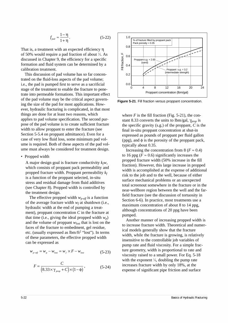
5-22 Basics of Hydraulic Fracturing

(5-22)

That is, a treatment with an expected efficiency ηof 50% would require a pad fraction of about 1⁄3. Asdiscussed in Chapter 9, the efficiency for a specificformation and fluid system can be determined by acalibration treatment.

This discussion of pad volume has so far concen-trated on the fluid-loss aspects of the pad volume;i.e., the pad is pumped first to serve as a sacrificialstage of the treatment to enable the fracture to pene-trate into permeable formations. This important effectof the pad volume may be the critical aspect govern-ing the size of the pad for most applications. How-ever, hydraulic fracturing is complicated, in that mostthings are done for at least two reasons, whichapplies to pad volume specification. The second pur-pose of the pad volume is to create sufficient fracturewidth to allow proppant to enter the fracture (seeSection 5-5.4 on proppant admittance). Even for acase of very low fluid loss, some minimum pad vol-ume is required. Both of these aspects of the pad vol-ume must always be considered for treatment design.

• Propped width

A major design goal is fracture conductivity kfw,which consists of proppant pack permeability andpropped fracture width. Proppant permeability kf

is a function of the proppant selected, in-situstress and residual damage from fluid additives(see Chapter 8). Propped width is controlled bythe treatment design.

The effective propped width wp-eff is a functionof the average fracture width wf at shutdown (i.e.,hydraulic width at the end of pumping a treat-ment), proppant concentration C in the fracture atthat time (i.e., giving the ideal propped width wp)and the volume of proppant wlost that is lost on thefaces of the fracture to embedment, gel residue,etc. (usually expressed as lbm/ft2 “lost”). In termsof these parameters, the effective propped widthcan be expressed as

(5-23)

(5-24)

where F is the fill fraction (Fig. 5-21), the con-stant 8.33 converts the units to lbm/gal, γprop isthe specific gravity (s.g.) of the proppant, C is thefinal in-situ proppant concentration at shut-inexpressed as pounds of proppant per fluid gallon(ppg), and φ is the porosity of the proppant pack,typically about 0.35.

Increasing the concentration from 8 (F ≈ 0.4)to 16 ppg (F ≈ 0.6) significantly increases thepropped fracture width (50% increase in the fillfraction). However, this large increase in proppedwidth is accomplished at the expense of additionalrisk to the job and to the well, because of eithersurface mechanical problems or an unexpectedtotal screenout somewhere in the fracture or in thenear-wellbore region between the well and the far-field fracture (see the discussion of tortuosity inSection 6-6). In practice, most treatments use amaximum concentration of about 8 to 14 ppg,although concentrations of 20 ppg have beenpumped.

Another manner of increasing propped width isto increase fracture width. Theoretical and numer-ical models generally show that the fracturewidth, while the fracture is growing, is relativelyinsensitive to the controllable job variables ofpump rate and fluid viscosity. For a simple frac-ture geometry, width is proportional to rate andviscosity raised to a small power. For Eq. 5-18with the exponent 1⁄4, doubling the pump rateincreases fracture width by only 18%, at theexpense of significant pipe friction and surface

w w w w F wp eff p lost f lost− = − = × −

FC

Cprop

=× +( ) × −( )8 33 1.

,γ φ

Figure 5-21. Fill fraction versus proppant concentration.

Fill

frac

tion,

F

0.8

1.0

0.6

0.4

0.2

0.040 8 12 16 20 24

Proppant concentration (lbm/gal)

% of fracture filled by proppant pack Pack porosity = 0.35

Proppant s.g. = 2.65(sand)

Proppant s.g. = 3.2(intermediate strength)

fpad ≈ −+

11

ηη

.

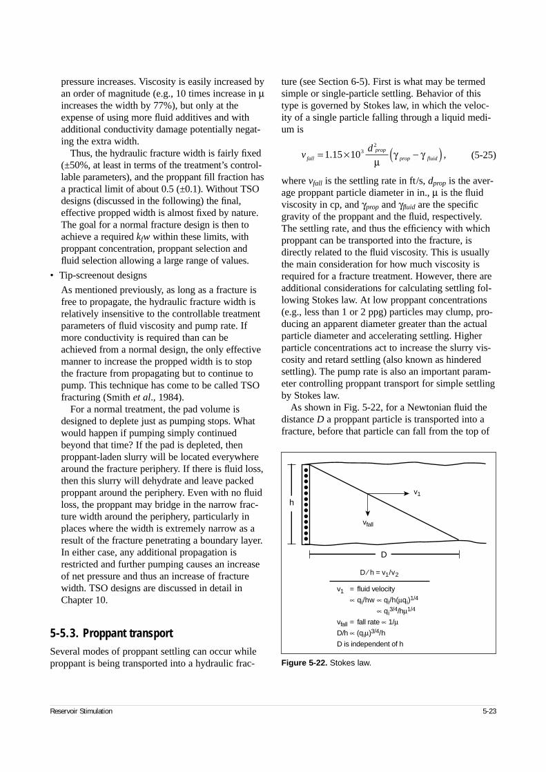
Reservoir Stimulation 5-23

pressure increases. Viscosity is easily increased byan order of magnitude (e.g., 10 times increase in µincreases the width by 77%), but only at theexpense of using more fluid additives and withadditional conductivity damage potentially negat-ing the extra width.

Thus, the hydraulic fracture width is fairly fixed(±50%, at least in terms of the treatment’s control-lable parameters), and the proppant fill fraction hasa practical limit of about 0.5 (±0.1). Without TSOdesigns (discussed in the following) the final,effective propped width is almost fixed by nature.The goal for a normal fracture design is then toachieve a required kfw within these limits, withproppant concentration, proppant selection andfluid selection allowing a large range of values.

• Tip-screenout designs

As mentioned previously, as long as a fracture isfree to propagate, the hydraulic fracture width isrelatively insensitive to the controllable treatmentparameters of fluid viscosity and pump rate. Ifmore conductivity is required than can beachieved from a normal design, the only effectivemanner to increase the propped width is to stopthe fracture from propagating but to continue topump. This technique has come to be called TSOfracturing (Smith et al., 1984).

For a normal treatment, the pad volume isdesigned to deplete just as pumping stops. Whatwould happen if pumping simply continuedbeyond that time? If the pad is depleted, thenproppant-laden slurry will be located everywherearound the fracture periphery. If there is fluid loss,then this slurry will dehydrate and leave packedproppant around the periphery. Even with no fluidloss, the proppant may bridge in the narrow frac-ture width around the periphery, particularly inplaces where the width is extremely narrow as aresult of the fracture penetrating a boundary layer.In either case, any additional propagation isrestricted and further pumping causes an increaseof net pressure and thus an increase of fracturewidth. TSO designs are discussed in detail inChapter 10.

5-5.3. Proppant transportSeveral modes of proppant settling can occur whileproppant is being transported into a hydraulic frac-

ture (see Section 6-5). First is what may be termedsimple or single-particle settling. Behavior of thistype is governed by Stokes law, in which the veloc-ity of a single particle falling through a liquid medi-um is

(5-25)

where vfall is the settling rate in ft/s, dprop is the aver-age proppant particle diameter in in., µ is the fluidviscosity in cp, and γprop and γfluid are the specificgravity of the proppant and the fluid, respectively.The settling rate, and thus the efficiency with whichproppant can be transported into the fracture, isdirectly related to the fluid viscosity. This is usuallythe main consideration for how much viscosity isrequired for a fracture treatment. However, there areadditional considerations for calculating settling fol-lowing Stokes law. At low proppant concentrations(e.g., less than 1 or 2 ppg) particles may clump, pro-ducing an apparent diameter greater than the actualparticle diameter and accelerating settling. Higherparticle concentrations act to increase the slurry vis-cosity and retard settling (also known as hinderedsettling). The pump rate is also an important param-eter controlling proppant transport for simple settlingby Stokes law.

As shown in Fig. 5-22, for a Newtonian fluid thedistance D a proppant particle is transported into afracture, before that particle can fall from the top of

vd

fall

prop

prop fluid= × −( )1 15 1032

. ,µ

γ γ

Figure 5-22. Stokes law.

h

D

vfall

v1

D ⁄ h = v1/v2

v1 = fluid velocity

∝ qi/hw ∝ qi/h(µqi)1/4

∝ qi3/4/hµ1/4

vfall = fall rate ∝ 1/µD/h ∝ (qiµ)3/4/h

D is independent of h

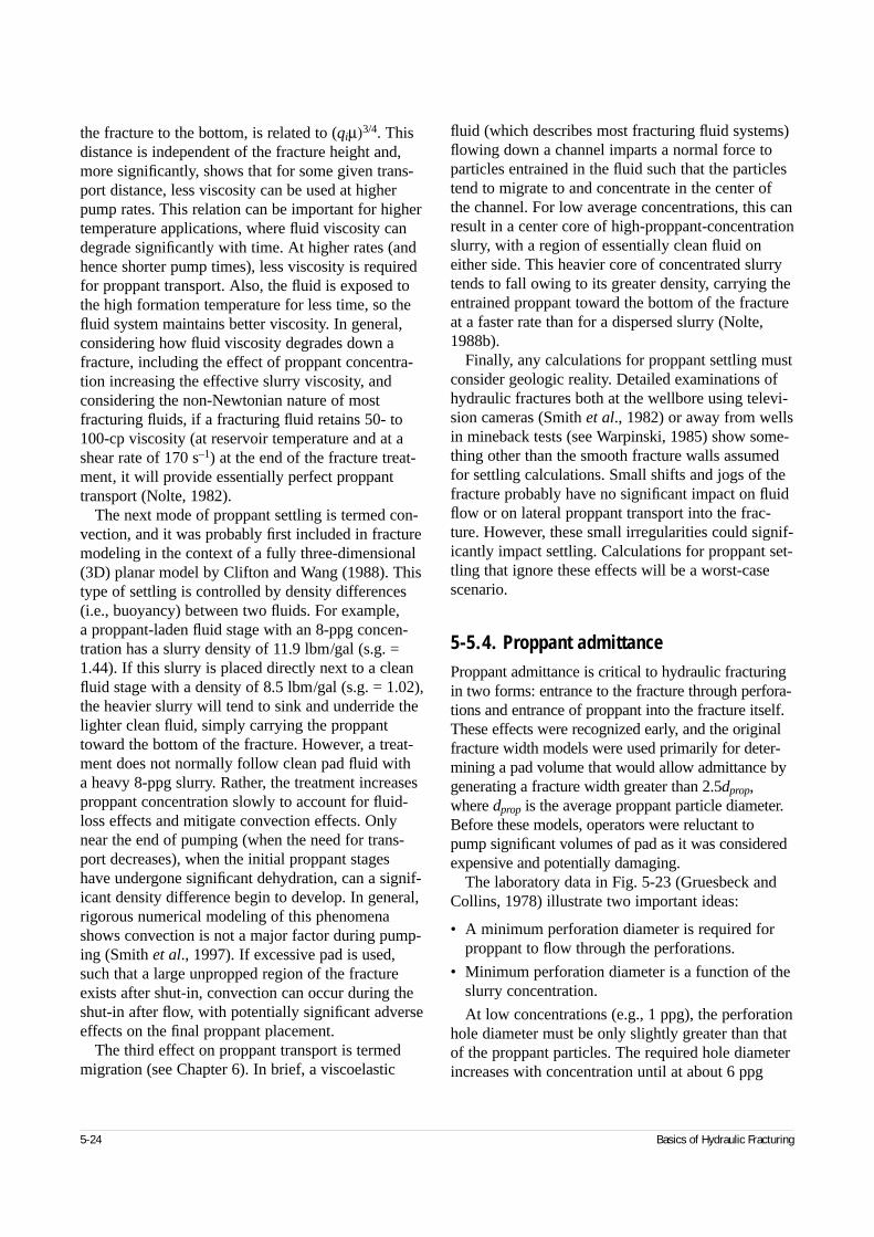
5-24 Basics of Hydraulic Fracturing

the fracture to the bottom, is related to (qiµ)3/4. Thisdistance is independent of the fracture height and,more significantly, shows that for some given trans-port distance, less viscosity can be used at higherpump rates. This relation can be important for highertemperature applications, where fluid viscosity candegrade significantly with time. At higher rates (andhence shorter pump times), less viscosity is requiredfor proppant transport. Also, the fluid is exposed tothe high formation temperature for less time, so thefluid system maintains better viscosity. In general,considering how fluid viscosity degrades down afracture, including the effect of proppant concentra-tion increasing the effective slurry viscosity, andconsidering the non-Newtonian nature of mostfracturing fluids, if a fracturing fluid retains 50- to100-cp viscosity (at reservoir temperature and at ashear rate of 170 s–1) at the end of the fracture treat-ment, it will provide essentially perfect proppanttransport (Nolte, 1982).

The next mode of proppant settling is termed con-vection, and it was probably first included in fracturemodeling in the context of a fully three-dimensional(3D) planar model by Clifton and Wang (1988). Thistype of settling is controlled by density differences(i.e., buoyancy) between two fluids. For example, a proppant-laden fluid stage with an 8-ppg concen-tration has a slurry density of 11.9 lbm/gal (s.g. =1.44). If this slurry is placed directly next to a cleanfluid stage with a density of 8.5 lbm/gal (s.g. = 1.02),the heavier slurry will tend to sink and underride thelighter clean fluid, simply carrying the proppanttoward the bottom of the fracture. However, a treat-ment does not normally follow clean pad fluid with a heavy 8-ppg slurry. Rather, the treatment increasesproppant concentration slowly to account for fluid-loss effects and mitigate convection effects. Onlynear the end of pumping (when the need for trans-port decreases), when the initial proppant stageshave undergone significant dehydration, can a signif-icant density difference begin to develop. In general,rigorous numerical modeling of this phenomenashows convection is not a major factor during pump-ing (Smith et al., 1997). If excessive pad is used,such that a large unpropped region of the fractureexists after shut-in, convection can occur during theshut-in after flow, with potentially significant adverseeffects on the final proppant placement.

The third effect on proppant transport is termedmigration (see Chapter 6). In brief, a viscoelastic

fluid (which describes most fracturing fluid systems)flowing down a channel imparts a normal force toparticles entrained in the fluid such that the particlestend to migrate to and concentrate in the center ofthe channel. For low average concentrations, this canresult in a center core of high-proppant-concentrationslurry, with a region of essentially clean fluid oneither side. This heavier core of concentrated slurrytends to fall owing to its greater density, carrying theentrained proppant toward the bottom of the fractureat a faster rate than for a dispersed slurry (Nolte,1988b).

Finally, any calculations for proppant settling mustconsider geologic reality. Detailed examinations ofhydraulic fractures both at the wellbore using televi-sion cameras (Smith et al., 1982) or away from wellsin mineback tests (see Warpinski, 1985) show some-thing other than the smooth fracture walls assumedfor settling calculations. Small shifts and jogs of thefracture probably have no significant impact on fluidflow or on lateral proppant transport into the frac-ture. However, these small irregularities could signif-icantly impact settling. Calculations for proppant set-tling that ignore these effects will be a worst-casescenario.

5-5.4. Proppant admittanceProppant admittance is critical to hydraulic fracturingin two forms: entrance to the fracture through perfora-tions and entrance of proppant into the fracture itself.These effects were recognized early, and the originalfracture width models were used primarily for deter-mining a pad volume that would allow admittance bygenerating a fracture width greater than 2.5dprop,where dprop is the average proppant particle diameter.Before these models, operators were reluctant topump significant volumes of pad as it was consideredexpensive and potentially damaging.

The laboratory data in Fig. 5-23 (Gruesbeck andCollins, 1978) illustrate two important ideas:

• A minimum perforation diameter is required forproppant to flow through the perforations.

• Minimum perforation diameter is a function of theslurry concentration.

At low concentrations (e.g., 1 ppg), the perforationhole diameter must be only slightly greater than thatof the proppant particles. The required hole diameterincreases with concentration until at about 6 ppg

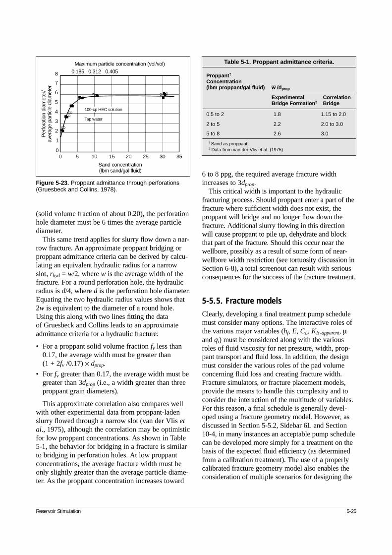
Reservoir Stimulation 5-25

(solid volume fraction of about 0.20), the perforationhole diameter must be 6 times the average particlediameter.

This same trend applies for slurry flow down a nar-row fracture. An approximate proppant bridging orproppant admittance criteria can be derived by calcu-lating an equivalent hydraulic radius for a narrowslot, rhyd = w/2, where w is the average width of thefracture. For a round perforation hole, the hydraulicradius is d/4, where d is the perforation hole diameter.Equating the two hydraulic radius values shows that2w is equivalent to the diameter of a round hole.Using this along with two lines fitting the data of Gruesbeck and Collins leads to an approximateadmittance criteria for a hydraulic fracture:

• For a proppant solid volume fraction fv less than0.17, the average width must be greater than (1 + 2fv /0.17) × dprop.

• For fv greater than 0.17, the average width must begreater than 3dprop (i.e., a width greater than threeproppant grain diameters).

This approximate correlation also compares wellwith other experimental data from proppant-ladenslurry flowed through a narrow slot (van der Vlis etal., 1975), although the correlation may be optimisticfor low proppant concentrations. As shown in Table5-1, the behavior for bridging in a fracture is similarto bridging in perforation holes. At low proppantconcentrations, the average fracture width must beonly slightly greater than the average particle diame-ter. As the proppant concentration increases toward

6 to 8 ppg, the required average fracture widthincreases to 3dprop.

This critical width is important to the hydraulicfracturing process. Should proppant enter a part of thefracture where sufficient width does not exist, theproppant will bridge and no longer flow down thefracture. Additional slurry flowing in this directionwill cause proppant to pile up, dehydrate and blockthat part of the fracture. Should this occur near thewellbore, possibly as a result of some form of near-wellbore width restriction (see tortuosity discussion inSection 6-8), a total screenout can result with seriousconsequences for the success of the fracture treatment.

5-5.5. Fracture modelsClearly, developing a final treatment pump schedulemust consider many options. The interactive roles ofthe various major variables (hf, E, CL, KIc-apparent, µand qi) must be considered along with the variousroles of fluid viscosity for net pressure, width, prop-pant transport and fluid loss. In addition, the designmust consider the various roles of the pad volumeconcerning fluid loss and creating fracture width.Fracture simulators, or fracture placement models,provide the means to handle this complexity and toconsider the interaction of the multitude of variables.For this reason, a final schedule is generally devel-oped using a fracture geometry model. However, asdiscussed in Section 5-5.2, Sidebar 6L and Section10-4, in many instances an acceptable pump schedulecan be developed more simply for a treatment on thebasis of the expected fluid efficiency (as determinedfrom a calibration treatment). The use of a properlycalibrated fracture geometry model also enables theconsideration of multiple scenarios for designing the

Table 5-1. Proppant admittance criteria.

Proppant†

Concentration(lbm proppant/gal fluid) w— /dprop

Experimental CorrelationBridge Formation‡ Bridge

0.5 to 2 1.8 1.15 to 2.0

2 to 5 2.2 2.0 to 3.0

5 to 8 2.6 3.0

† Sand as proppant‡ Data from van der Vlis et al. (1975)

Figure 5-23. Proppant admittance through perforations(Gruesbeck and Collins, 1978).

Per

fora

tion

diam

eter

/av

erag

e pa

rticl

e di

amet

er

7

8

6

5

4

3

2

1

050 10 15 20 25 30 35

Sand concentration(lbm sand/gal fluid)

0.185 0.312 0.405Maximum particle concentration (vol/vol)

100-cp HEC solution

Tap water

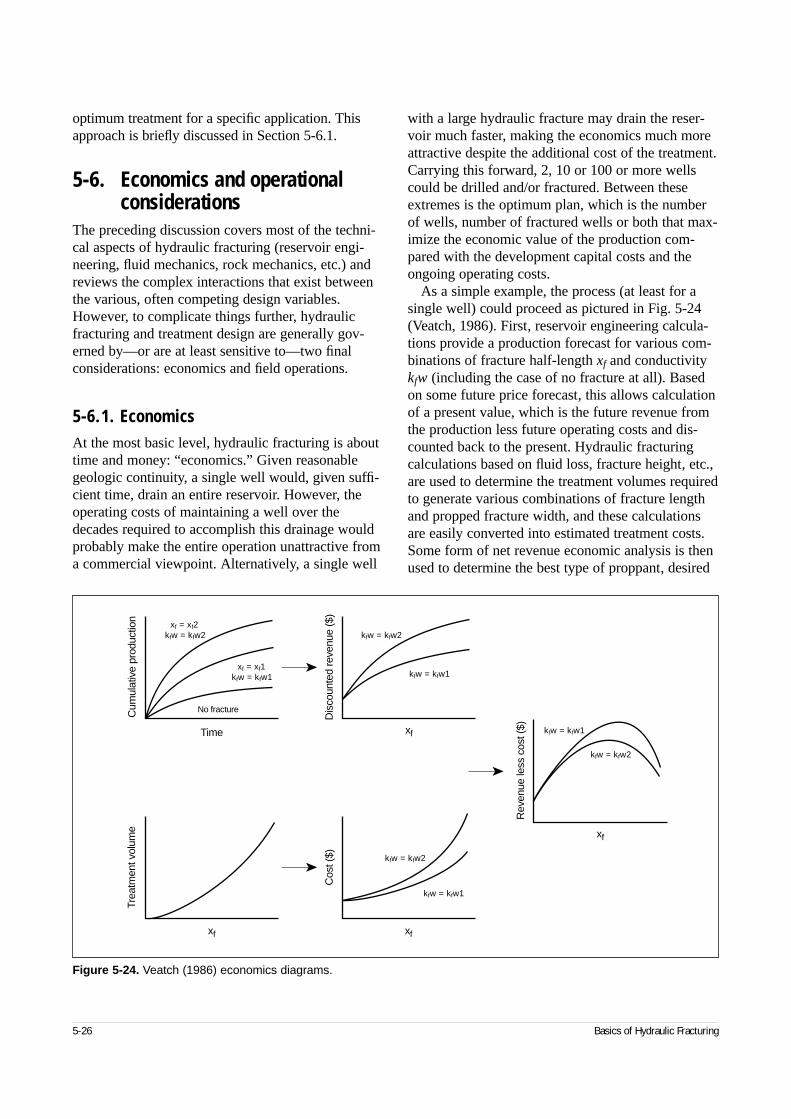
5-26 Basics of Hydraulic Fracturing

optimum treatment for a specific application. Thisapproach is briefly discussed in Section 5-6.1.

5-6. Economics and operational considerations

The preceding discussion covers most of the techni-cal aspects of hydraulic fracturing (reservoir engi-neering, fluid mechanics, rock mechanics, etc.) andreviews the complex interactions that exist betweenthe various, often competing design variables.However, to complicate things further, hydraulicfracturing and treatment design are generally gov-erned by—or are at least sensitive to—two finalconsiderations: economics and field operations.

5-6.1. EconomicsAt the most basic level, hydraulic fracturing is abouttime and money: “economics.” Given reasonablegeologic continuity, a single well would, given suffi-cient time, drain an entire reservoir. However, theoperating costs of maintaining a well over thedecades required to accomplish this drainage wouldprobably make the entire operation unattractive froma commercial viewpoint. Alternatively, a single well

with a large hydraulic fracture may drain the reser-voir much faster, making the economics much moreattractive despite the additional cost of the treatment.Carrying this forward, 2, 10 or 100 or more wellscould be drilled and/or fractured. Between theseextremes is the optimum plan, which is the numberof wells, number of fractured wells or both that max-imize the economic value of the production com-pared with the development capital costs and theongoing operating costs.

As a simple example, the process (at least for asingle well) could proceed as pictured in Fig. 5-24(Veatch, 1986). First, reservoir engineering calcula-tions provide a production forecast for various com-binations of fracture half-length xf and conductivitykfw (including the case of no fracture at all). Basedon some future price forecast, this allows calculationof a present value, which is the future revenue fromthe production less future operating costs and dis-counted back to the present. Hydraulic fracturingcalculations based on fluid loss, fracture height, etc.,are used to determine the treatment volumes requiredto generate various combinations of fracture lengthand propped fracture width, and these calculationsare easily converted into estimated treatment costs.Some form of net revenue economic analysis is thenused to determine the best type of proppant, desired

Figure 5-24. Veatch (1986) economics diagrams.

xf = xf2kfw = kfw2 kfw = kfw2

kfw = kfw2

kfw = kfw2

kfw = kfw1xf = xf1

kfw = kfw1

kfw = kfw1

kfw = kfw1

No fracture

Trea

tmen

t vol

ume

Cum

ulat

ive

prod

uctio

n

Dis

coun

ted

reve

nue

($)

Cos

t ($)

Rev

enue

less

cos

t ($)Time xf

xf

xfxf

Reservoir Stimulation 5-27

fracture length and other requirements for the opti-mum treatment.

There are, of course, many variations of this basicprocess. For example, full-cycle economics includesdrilling and other completion costs, along with frac-ture treatment costs, in determining the optimumfracture design. This type of analysis is usuallyappropriate in any case involving multiple wells(e.g., should a resource be developed using 10 wellswith huge fractures or 20 wells with smaller or nofracture treatments?). Point-forward analysis, on theother hand, considers only the fracture treatmentcosts (because drilling and other completion costsare already expended) and is most appropriate forworking over existing wells.

5-6.2. OperationsAs discussed in the preceding section, economicsprovides the final design consideration for hydraulicfracturing, whereas field conditions provide the prac-tical limits within which the design must fit. Evenbeyond defining these limiting conditions, however,any design is only as good as its execution; thus thetreatment must be pumped as designed. Field opera-tions and operational considerations impacthydraulic fracturing in two ways:

• prefracture condition of the wellbore, quality ofthe cement job, perforations, pressure limits, etc.,with these considerations defining practical limitsthat the design must meet

• quality assurance and quality control (QA/QC)before and during the actual treatment.

These operational considerations are discussed inChapters 7 and 11, with some of the major itemshighlighted in the following.

• Wellbore considerations

Some of the major wellbore considerations forhydraulic fracturing include

– size and condition of wellbore tubulars

– quality of the cement job for zonal isolation

– perforations

– wellbore deviation.

During a hydraulic fracture treatment, the pre-dicted surface pressure psurf and the hydraulichorsepower required for a treatment are related

to the hydrostatic head of the fluid in the wellborephead and the pipe friction ppipe friction:

(5-26)

(5-27)

Pipe friction is a major term, and thus the sizeof the well tubulars has a strong influence onallowable pump rates (because pipe friction is typ-ically related to ve, where v = qi/A is the flowvelocity down the tubing, and e is typically about1.1 to 1.7). Also, the strength and condition of thetubulars (along with the associated wellheadequipment) set an allowable surface pressure andthus indirectly set an allowable injection rate. Inaddition, the size, type and condition of the well-bore tubulars may limit (or prohibit) future work-over and recompletion opportunities.

A critical aspect of wellbore considerations is agood cement job around the casing or liner to pro-vide zonal isolation. In general, a fracture growswhere nature dictates, and the engineer has littlecontrol over fracture height growth. The only con-trol possible is the ability to specify where theperforations are placed and the fracture initiates. If that ability is compromised by a poor cementsheath around the casing that allows the perfora-tions to communicate directly with an undesiredinterval, then even this minimal level of control islost, and the hydraulic fracture treatment may beseriously compromised.

Another important consideration is the perfora-tions that allow the fluid to leave the wellbore andcreate the fracture. The number and size of theperforation holes are important for proppantadmittance, as discussed briefly in Section 5-5.4and in detail in Section 11-3.

• Quality assurance and quality control

Quality issues are critical for hydraulic fracturing.After proppant pumping starts, a treatment cannotbe stopped because of problems without signifi-cantly compromising the design goals. For thistime period, everything must work, including the wellbore equipment, pumping and blendingequipment and chemicals (i.e., the fluid system).To cite a simple example, if a treatment uses 10 tanks of batch-mixed fluid, and one of the

p p p psurf c net pipe friction head= + + −σ

hhp q pi surf∝ × .

5-28 Basics of Hydraulic Fracturing

tanks is bad, then the QA score is a relatively high90%. However, if the bad fluid is pumped justafter proppant addition starts, it may easily causetotal failure of the treatment, and if successfultreatment is critical to economic success of thewell, this causes total economic failure. Typically,this type of failure cannot be overcome withoutcompletely redrilling the well (refracturing opera-tions are usually a risky procedure), and thus 90%can be a failing grade for QA.

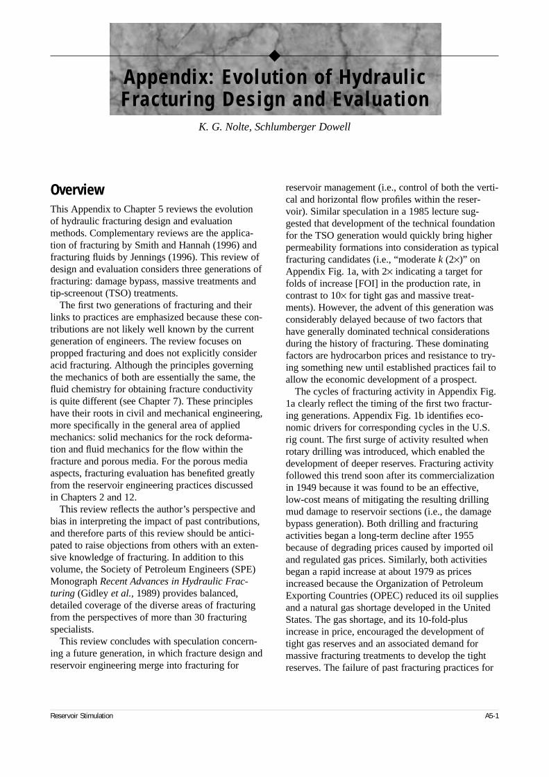
OverviewThis Appendix to Chapter 5 reviews the evolutionof hydraulic fracturing design and evaluationmethods. Complementary reviews are the applica-tion of fracturing by Smith and Hannah (1996) andfracturing fluids by Jennings (1996). This review ofdesign and evaluation considers three generations offracturing: damage bypass, massive treatments andtip-screenout (TSO) treatments.

The first two generations of fracturing and theirlinks to practices are emphasized because these con-tributions are not likely well known by the currentgeneration of engineers. The review focuses onpropped fracturing and does not explicitly consideracid fracturing. Although the principles governingthe mechanics of both are essentially the same, thefluid chemistry for obtaining fracture conductivity is quite different (see Chapter 7). These principleshave their roots in civil and mechanical engineering,more specifically in the general area of appliedmechanics: solid mechanics for the rock deforma-tion and fluid mechanics for the flow within thefracture and porous media. For the porous mediaaspects, fracturing evaluation has benefited greatlyfrom the reservoir engineering practices discussed in Chapters 2 and 12.

This review reflects the author’s perspective andbias in interpreting the impact of past contributions,and therefore parts of this review should be antici-pated to raise objections from others with an exten-sive knowledge of fracturing. In addition to thisvolume, the Society of Petroleum Engineers (SPE)Monograph Recent Advances in Hydraulic Frac-turing (Gidley et al., 1989) provides balanced,detailed coverage of the diverse areas of fracturingfrom the perspectives of more than 30 fracturingspecialists.

This review concludes with speculation concern-ing a future generation, in which fracture design andreservoir engineering merge into fracturing for

reservoir management (i.e., control of both the verti-cal and horizontal flow profiles within the reser-voir). Similar speculation in a 1985 lecture sug-gested that development of the technical foundationfor the TSO generation would quickly bring higherpermeability formations into consideration as typicalfracturing candidates (i.e., “moderate k (2×)” onAppendix Fig. 1a, with 2× indicating a target forfolds of increase [FOI] in the production rate, incontrast to 10× for tight gas and massive treat-ments). However, the advent of this generation wasconsiderably delayed because of two factors thathave generally dominated technical considerationsduring the history of fracturing. These dominatingfactors are hydrocarbon prices and resistance to try-ing something new until established practices fail toallow the economic development of a prospect.

The cycles of fracturing activity in Appendix Fig.1a clearly reflect the timing of the first two fractur-ing generations. Appendix Fig. 1b identifies eco-nomic drivers for corresponding cycles in the U.S.rig count. The first surge of activity resulted whenrotary drilling was introduced, which enabled thedevelopment of deeper reserves. Fracturing activityfollowed this trend soon after its commercializationin 1949 because it was found to be an effective,low-cost means of mitigating the resulting drillingmud damage to reservoir sections (i.e., the damagebypass generation). Both drilling and fracturingactivities began a long-term decline after 1955because of degrading prices caused by imported oiland regulated gas prices. Similarly, both activitiesbegan a rapid increase at about 1979 as pricesincreased because the Organization of PetroleumExporting Countries (OPEC) reduced its oil suppliesand a natural gas shortage developed in the UnitedStates. The gas shortage, and its 10-fold-plusincrease in price, encouraged the development oftight gas reserves and an associated demand formassive fracturing treatments to develop the tightreserves. The failure of past fracturing practices for

Reservoir Stimulation A5-1

◆

Appendix: Evolution of Hydraulic Fracturing Design and Evaluation

K. G. Nolte, Schlumberger Dowell

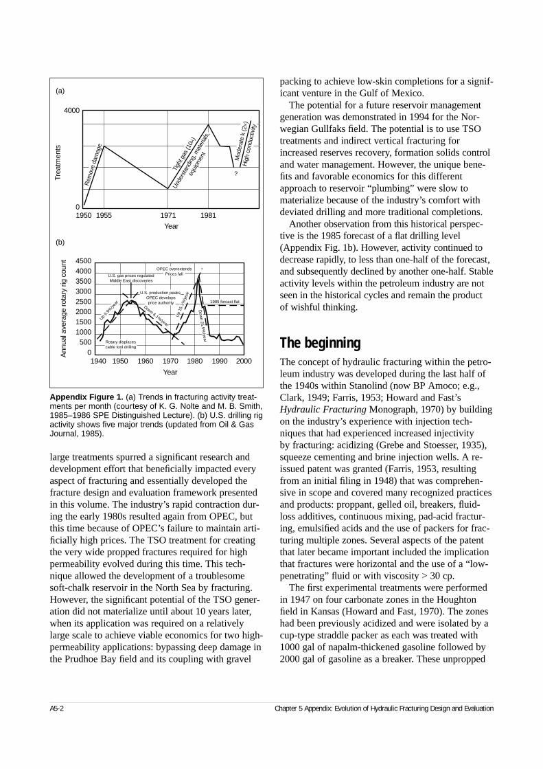
large treatments spurred a significant research anddevelopment effort that beneficially impacted everyaspect of fracturing and essentially developed thefracture design and evaluation framework presentedin this volume. The industry’s rapid contraction dur-ing the early 1980s resulted again from OPEC, butthis time because of OPEC’s failure to maintain arti-ficially high prices. The TSO treatment for creatingthe very wide propped fractures required for highpermeability evolved during this time. This tech-nique allowed the development of a troublesomesoft-chalk reservoir in the North Sea by fracturing.However, the significant potential of the TSO gener-ation did not materialize until about 10 years later,when its application was required on a relativelylarge scale to achieve viable economics for two high-permeability applications: bypassing deep damage inthe Prudhoe Bay field and its coupling with gravel

packing to achieve low-skin completions for a signif-icant venture in the Gulf of Mexico.

The potential for a future reservoir managementgeneration was demonstrated in 1994 for the Nor-wegian Gullfaks field. The potential is to use TSOtreatments and indirect vertical fracturing forincreased reserves recovery, formation solids controland water management. However, the unique bene-fits and favorable economics for this differentapproach to reservoir “plumbing” were slow tomaterialize because of the industry’s comfort withdeviated drilling and more traditional completions.

Another observation from this historical perspec-tive is the 1985 forecast of a flat drilling level(Appendix Fig. 1b). However, activity continued todecrease rapidly, to less than one-half of the forecast,and subsequently declined by another one-half. Stableactivity levels within the petroleum industry are notseen in the historical cycles and remain the product of wishful thinking.

The beginningThe concept of hydraulic fracturing within the petro-leum industry was developed during the last half ofthe 1940s within Stanolind (now BP Amoco; e.g.,Clark, 1949; Farris, 1953; Howard and Fast’sHydraulic Fracturing Monograph, 1970) by buildingon the industry’s experience with injection tech-niques that had experienced increased injectivity by fracturing: acidizing (Grebe and Stoesser, 1935),squeeze cementing and brine injection wells. A re-issued patent was granted (Farris, 1953, resultingfrom an initial filing in 1948) that was comprehen-sive in scope and covered many recognized practicesand products: proppant, gelled oil, breakers, fluid-loss additives, continuous mixing, pad-acid fractur-ing, emulsified acids and the use of packers for frac-turing multiple zones. Several aspects of the patentthat later became important included the implicationthat fractures were horizontal and the use of a “low-penetrating” fluid or with viscosity > 30 cp.

The first experimental treatments were performedin 1947 on four carbonate zones in the Houghtonfield in Kansas (Howard and Fast, 1970). The zoneshad been previously acidized and were isolated by acup-type straddle packer as each was treated with1000 gal of napalm-thickened gasoline followed by2000 gal of gasoline as a breaker. These unpropped

A5-2 Chapter 5 Appendix: Evolution of Hydraulic Fracturing Design and Evaluation

Appendix Figure 1. (a) Trends in fracturing activity treat-ments per month (courtesy of K. G. Nolte and M. B. Smith,1985–1986 SPE Distinguished Lecture). (b) U.S. drilling rigactivity shows five major trends (updated from Oil & GasJournal, 1985).

1950 1955 1971 1981

Year

4000

0

Trea

tmen

ts

Rem

ove

dam

age

Tigh

t gas

(10×

)

Mod

erat

e k

(2×)

Hig

h co

nduc

tivity

Und

erst

andi

ng, m

ater

ials

,

equi

pmen

t

?

45004000350030002500200015001000500

01940 1950 1960 1970 1980 1990 2000

Year

Ann

ual a

vera

ge ro

tary

rig

coun

t

1985 forcast flat

OPEC overextendsPrices fallU.S. gas prices regulated

Middle East discoveries

U.S. production peaks OPEC developsprice authority

Rotary displacescable tool drilling

Up 9.

9%/ye

ar

Up

15.1

%/y

ear

Down 6.1%/year

Dow

n 25.5%/year

(a)

(b)

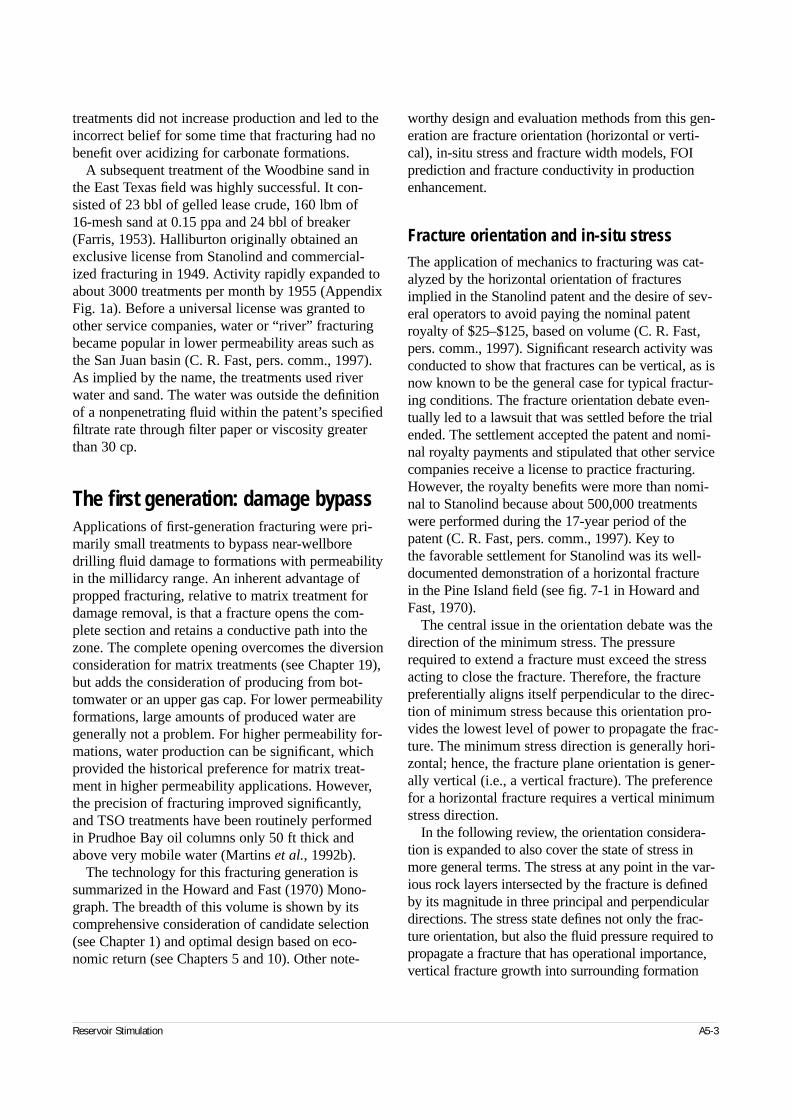
treatments did not increase production and led to theincorrect belief for some time that fracturing had nobenefit over acidizing for carbonate formations.

A subsequent treatment of the Woodbine sand inthe East Texas field was highly successful. It con-sisted of 23 bbl of gelled lease crude, 160 lbm of 16-mesh sand at 0.15 ppa and 24 bbl of breaker(Farris, 1953). Halliburton originally obtained anexclusive license from Stanolind and commercial-ized fracturing in 1949. Activity rapidly expanded toabout 3000 treatments per month by 1955 (AppendixFig. 1a). Before a universal license was granted toother service companies, water or “river” fracturingbecame popular in lower permeability areas such asthe San Juan basin (C. R. Fast, pers. comm., 1997).As implied by the name, the treatments used riverwater and sand. The water was outside the definitionof a nonpenetrating fluid within the patent’s specifiedfiltrate rate through filter paper or viscosity greaterthan 30 cp.

The first generation: damage bypassApplications of first-generation fracturing were pri-marily small treatments to bypass near-wellboredrilling fluid damage to formations with permeabilityin the millidarcy range. An inherent advantage ofpropped fracturing, relative to matrix treatment fordamage removal, is that a fracture opens the com-plete section and retains a conductive path into thezone. The complete opening overcomes the diversionconsideration for matrix treatments (see Chapter 19),but adds the consideration of producing from bot-tomwater or an upper gas cap. For lower permeabilityformations, large amounts of produced water aregenerally not a problem. For higher permeability for-mations, water production can be significant, whichprovided the historical preference for matrix treat-ment in higher permeability applications. However,the precision of fracturing improved significantly,and TSO treatments have been routinely performedin Prudhoe Bay oil columns only 50 ft thick andabove very mobile water (Martins et al., 1992b).

The technology for this fracturing generation issummarized in the Howard and Fast (1970) Mono-graph. The breadth of this volume is shown by itscomprehensive consideration of candidate selection(see Chapter 1) and optimal design based on eco-nomic return (see Chapters 5 and 10). Other note-

worthy design and evaluation methods from this gen-eration are fracture orientation (horizontal or verti-cal), in-situ stress and fracture width models, FOIprediction and fracture conductivity in productionenhancement.

Fracture orientation and in-situ stressThe application of mechanics to fracturing was cat-alyzed by the horizontal orientation of fracturesimplied in the Stanolind patent and the desire of sev-eral operators to avoid paying the nominal patentroyalty of $25–$125, based on volume (C. R. Fast,pers. comm., 1997). Significant research activity wasconducted to show that fractures can be vertical, as isnow known to be the general case for typical fractur-ing conditions. The fracture orientation debate even-tually led to a lawsuit that was settled before the trialended. The settlement accepted the patent and nomi-nal royalty payments and stipulated that other servicecompanies receive a license to practice fracturing.However, the royalty benefits were more than nomi-nal to Stanolind because about 500,000 treatmentswere performed during the 17-year period of thepatent (C. R. Fast, pers. comm., 1997). Key to the favorable settlement for Stanolind was its well-documented demonstration of a horizontal fracture in the Pine Island field (see fig. 7-1 in Howard andFast, 1970).

The central issue in the orientation debate was thedirection of the minimum stress. The pressurerequired to extend a fracture must exceed the stressacting to close the fracture. Therefore, the fracturepreferentially aligns itself perpendicular to the direc-tion of minimum stress because this orientation pro-vides the lowest level of power to propagate the frac-ture. The minimum stress direction is generally hori-zontal; hence, the fracture plane orientation is gener-ally vertical (i.e., a vertical fracture). The preferencefor a horizontal fracture requires a vertical minimumstress direction.

In the following review, the orientation considera-tion is expanded to also cover the state of stress inmore general terms. The stress at any point in the var-ious rock layers intersected by the fracture is definedby its magnitude in three principal and perpendiculardirections. The stress state defines not only the frac-ture orientation, but also the fluid pressure required topropagate a fracture that has operational importance,vertical fracture growth into surrounding formation

Reservoir Stimulation A5-3

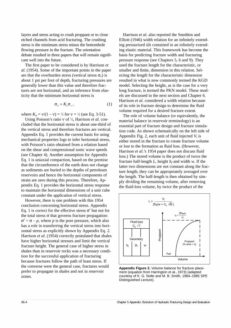
layers and stress acting to crush proppant or to closeetched channels from acid fracturing. The crushingstress is the minimum stress minus the bottomholeflowing pressure in the fracture. The orientationdebate resulted in three papers that will remain signifi-cant well into the future.

The first paper to be considered is by Harrison etal. (1954). Some of the important points in the paperare that the overburden stress (vertical stress σv) isabout 1 psi per foot of depth, fracturing pressures aregenerally lower than this value and therefore frac-tures are not horizontal, and an inference from elas-ticity that the minimum horizontal stress is

(1)

where Ko = ν/(1 – ν) = 1⁄3 for ν = 1⁄4 (see Eq. 3-51).Using Poisson’s ratio ν of 1⁄4, Harrison et al. con-

cluded that the horizontal stress is about one-third ofthe vertical stress and therefore fractures are vertical.Appendix Eq. 1 provides the current basis for usingmechanical properties logs to infer horizontal stress,with Poisson’s ratio obtained from a relation basedon the shear and compressional sonic wave speeds(see Chapter 4). Another assumption for AppendixEq. 1 is uniaxial compaction, based on the premisethat the circumference of the earth does not changeas sediments are buried to the depths of petroleumreservoirs and hence the horizontal components ofstrain are zero during this process. Therefore, Ap-pendix Eq. 1 provides the horizontal stress responseto maintain the horizontal dimensions of a unit cubeconstant under the application of vertical stress.

However, there is one problem with this 1954 conclusion concerning horizontal stress. AppendixEq. 1 is correct for the effective stress σ′ but not forthe total stress σ that governs fracture propagation:σ′ = σ – p, where p is the pore pressure, which alsohas a role in transferring the vertical stress into hori-zontal stress as explicitly shown by Appendix Eq. 2.Harrison et al. (1954) correctly postulated that shaleshave higher horizontal stresses and limit the verticalfracture height. The general case of higher stress inshales than in reservoir rocks was a necessary condi-tion for the successful application of fracturingbecause fractures follow the path of least stress. Ifthe converse were the general case, fractures wouldprefer to propagate in shales and not in reservoirzones.

Harrison et al. also reported the Sneddon andElliott (1946) width relation for an infinitely extend-ing pressurized slit contained in an infinitely extend-ing elastic material. This framework has become thebasis for predicting fracture width and fracturingpressure response (see Chapters 5, 6 and 9). Theyused the fracture length for the characteristic, orsmaller and finite, dimension in this relation. Sel-ecting the length for the characteristic dimensionresulted in what is now commonly termed the KGDmodel. Selecting the height, as is the case for a verylong fracture, is termed the PKN model. These mod-els are discussed in the next section and Chapter 6.Harrison et al. considered a width relation becauseof its role in fracture design to determine the fluidvolume required for a desired fracture extent.

The role of volume balance (or equivalently, thematerial balance in reservoir terminology) is anessential part of fracture design and fracture simula-tion code. As shown schematically on the left side ofAppendix Fig. 2, each unit of fluid injected Vi iseither stored in the fracture to create fracture volumeor lost to the formation as fluid loss. (However,Harrison et al.’s 1954 paper does not discuss fluidloss.) The stored volume is the product of twice thefracture half-length L, height hf and width w. If thelatter two dimensions are not constant along the frac-ture length, they can be appropriately averaged overthe length. The half-length is then obtained by sim-ply dividing the remaining volume, after removingthe fluid-loss volume, by twice the product of the

A5-4 Chapter 5 Appendix: Evolution of Hydraulic Fracturing Design and Evaluation

σ σh o vK= ,

Appendix Figure 2. Volume balance for fracture place-ment (equation from Harrington et al., 1973) (adaptedcourtesy of K. G. Nolte and M. B. Smith, 1984–1985 SPEDistinguished Lecture).

Geometry

hf 2L w

Fluid lossCL √ t

Volume

Pro

ppan

t

Pad

Proppant(% area = η)

η =2hfwL

Vi

L =Vi

2hf(w + CL √8t )

average height and the average width. The fluid-lossvolume depends on the fluid-loss surface area, or aheight-length product. Furthermore, as shown on theright side of Appendix Fig. 2, the ratio of stored tototal volume is termed the fluid efficiency η and dir-ectly affects the proppant additional schedule (Har-rington et al., 1973; Nolte, 1986b) (see Sidebar 6L).

The second paper to be discussed from the orienta-tion era is by Hubbert and Willis (1957). The lessonsfrom this paper extend beyond fracturing and intothe area of structural geology. This work providessimple and insightful experiments to define the stateof in-situ stress and demonstrate a fracture’s prefer-ence to propagate in the plane with minimum stressresistance. For the latter experiments, the “forma-tion” was gelatin within a plastic bottle preferentiallystressed to create various planes of minimal stress.

They also used simple sandbox experiments todemonstrate normal and thrust faulting and to definethe state of stress for these conditions (see Sidebar3A). They showed that Ko, or equivalently the hori-zontal stress, within Appendix Eq. 1 is defined bythe internal friction angle (ϕ = 30° for sand) and is 1⁄3 for the minimum stress during normal faulting and3 for the maximum stress during thrust faulting. Forthe normal faulting case and correctly including porepressure in Appendix Eq. 1, the total minimum hori-zontal stress becomes

(2)

where Ko = 1⁄3 with ϕ = 30°. For this case the horizon-tal stress is much less than the vertical stress exceptin the extreme geopressure case of pore pressureapproaching overburden, which causes all stressesand pore pressure to converge to the overburdenstress. For the thrust faulting case, the larger horizon-tal stress (i.e., for the two horizontal directions) isgreater than the overburden and the smaller horizon-tal stress is equal to or greater than the overburden.Both the extreme geopressure case and an activethrust faulting regime can lead to either vertical orhorizontal fractures. The author has found AppendixEq. 2 to accurately predict the horizontal stress in tec-tonically relaxed sandstone formations ranging frommicrodarcy to darcy permeability. The accuracy at the high range is not surprising, as the formationsapproach the unconsolidated sand in the sandboxexperiments. The accuracy obtained for microdarcy-permeability sands is subsequently explained.

Hubbert and Willis also provided an important setof postulates: the rock stresses within the earth aredefined by rock failure from tectonic action and theearth is in a continuous state of incipient faulting.From this perspective, the stress is not governed by the behavior of the intact rock matrix, but by anactive state of failure along discrete boundaries (e.g.,by sand grains within fault boundaries, whichexplains the application of Appendix Eq. 2 to micro-darcy-permeability sandstones). This insightful con-clusion about the role of failure is at the otherextreme of the behavior spectrum from the elasticassumptions that Poisson’s ratio (Appendix Eq. 1)governs the horizontal stress and that failure has noeffect on the stress. This extreme difference in theassumptions for Appendix Eqs. 1 and 2 is oftenoverlooked because of the similar value of Ko = ~1⁄3obtained in the case of a tectonically relaxed regionand Poisson’s ratio near 1⁄4. However, the role of elas-ticity becomes important in thrusting areas (seeSection 3-5.2) because of the difference in horizontalstress resulting for layers with different values ofYoung’s modulus (stiffness). More of the tectonicaction and higher levels of stress are supported by thestiffer layers.

Additional considerations for horizontal stress out-lined by Prats (1981) include the role of long-termcreep. Creep deformation allows relaxation of thestress difference between the overburden and hori-zontal stresses, thereby enabling the horizontal stressto increase toward the larger vertical stress governedby the weight of the overburden. This effect is wellknown for salt layers that readily creep and can col-lapse casing by transferring most of the larger over-burden stress into horizontal stress. The role of stressrelaxation is an important mechanism for providingfavorable stress differences between relatively cleansands governed by friction (i.e., Appendix Eq. 2) withminimal creep and sediments with higher clay con-tent. In the latter case, the clay supports some of theintergranular stresses. The clay structure is prone tocreep that relaxes the in-situ stress differences andincreases the horizontal stress for a clay-rich formation.

Hence, both clay content and Poisson’s ratio pro-duce the same effect on horizontal stress. Becauseclay content also increases Poisson’s ratio, there is a positive correlation of clay content (creep-inducedstress) to larger Poisson’s ratios (and elastic stress,from Appendix Eq. 1) inferred from sonic velocities.The implication of the correlation is that clay-rich

Reservoir Stimulation A5-5

σ σh v p= +( ) ,2 3

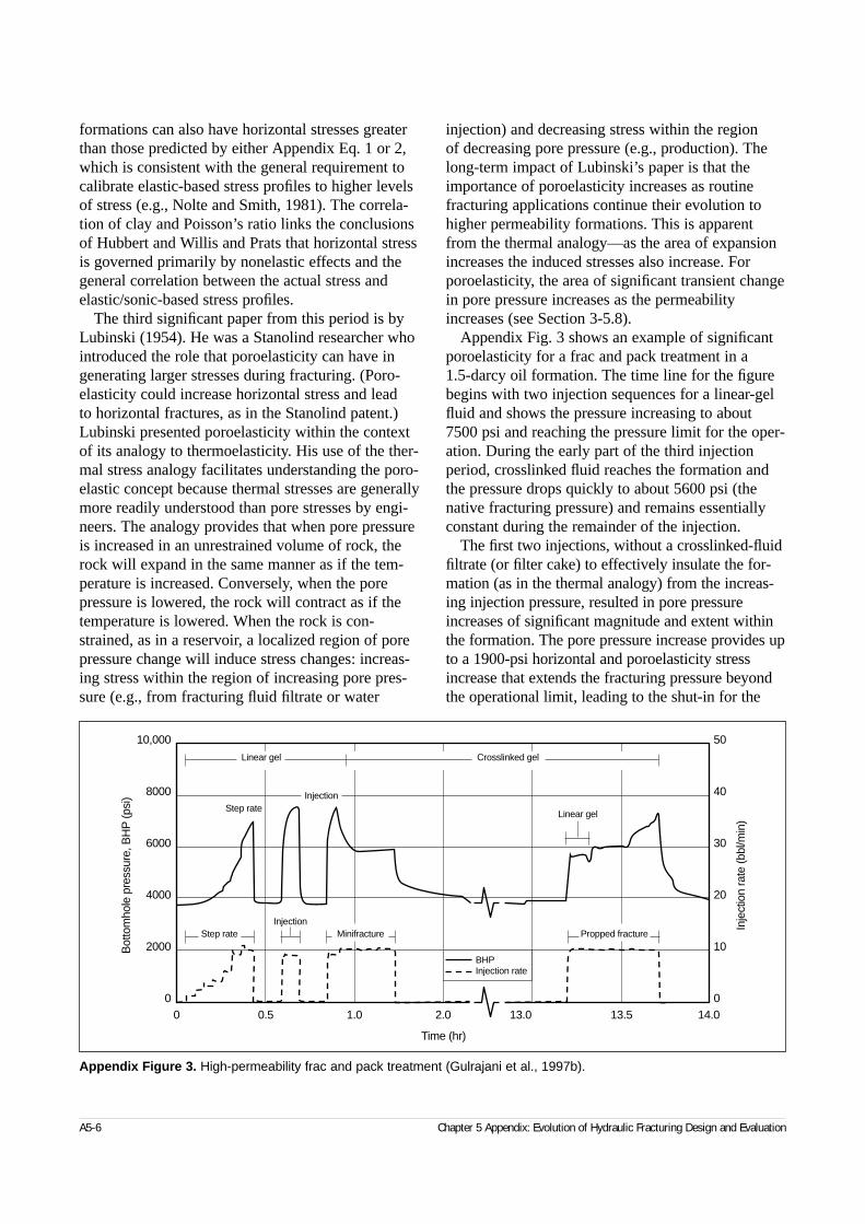
formations can also have horizontal stresses greaterthan those predicted by either Appendix Eq. 1 or 2,which is consistent with the general requirement tocalibrate elastic-based stress profiles to higher levelsof stress (e.g., Nolte and Smith, 1981). The correla-tion of clay and Poisson’s ratio links the conclusionsof Hubbert and Willis and Prats that horizontal stressis governed primarily by nonelastic effects and thegeneral correlation between the actual stress andelastic/sonic-based stress profiles.

The third significant paper from this period is byLubinski (1954). He was a Stanolind researcher whointroduced the role that poroelasticity can have ingenerating larger stresses during fracturing. (Poro-elasticity could increase horizontal stress and lead to horizontal fractures, as in the Stanolind patent.)Lubinski presented poroelasticity within the contextof its analogy to thermoelasticity. His use of the ther-mal stress analogy facilitates understanding the poro-elastic concept because thermal stresses are generallymore readily understood than pore stresses by engi-neers. The analogy provides that when pore pressureis increased in an unrestrained volume of rock, therock will expand in the same manner as if the tem-perature is increased. Conversely, when the porepressure is lowered, the rock will contract as if thetemperature is lowered. When the rock is con-strained, as in a reservoir, a localized region of porepressure change will induce stress changes: increas-ing stress within the region of increasing pore pres-sure (e.g., from fracturing fluid filtrate or water

injection) and decreasing stress within the region of decreasing pore pressure (e.g., production). Thelong-term impact of Lubinski’s paper is that theimportance of poroelasticity increases as routinefracturing applications continue their evolution tohigher permeability formations. This is apparentfrom the thermal analogy—as the area of expansionincreases the induced stresses also increase. Forporoelasticity, the area of significant transient changein pore pressure increases as the permeabilityincreases (see Section 3-5.8).

Appendix Fig. 3 shows an example of significantporoelasticity for a frac and pack treatment in a 1.5-darcy oil formation. The time line for the figurebegins with two injection sequences for a linear-gelfluid and shows the pressure increasing to about7500 psi and reaching the pressure limit for the oper-ation. During the early part of the third injectionperiod, crosslinked fluid reaches the formation andthe pressure drops quickly to about 5600 psi (thenative fracturing pressure) and remains essentiallyconstant during the remainder of the injection.

The first two injections, without a crosslinked-fluidfiltrate (or filter cake) to effectively insulate the for-mation (as in the thermal analogy) from the increas-ing injection pressure, resulted in pore pressureincreases of significant magnitude and extent withinthe formation. The pore pressure increase provides upto a 1900-psi horizontal and poroelasticity stressincrease that extends the fracturing pressure beyondthe operational limit, leading to the shut-in for the

A5-6 Chapter 5 Appendix: Evolution of Hydraulic Fracturing Design and Evaluation

Appendix Figure 3. High-permeability frac and pack treatment (Gulrajani et al., 1997b).

10,000

8000

6000

4000

2000

0

Bot

tom

hole

pre

ssur

e, B

HP

(psi

)

50

40

30

20

10

0

Inje

ctio

n ra

te (b

bl/m

in)

0 0.5 1.0 2.0 13.0 13.5 14.0

Time (hr)

Linear gel

Linear gel Crosslinked gel

Step rateInjection

BHPInjection rate

Step rate Minifracture Propped fractureInjection

second injection. This increase is about one-third ofthe native stress. However, during the two subsequentinjections the insulating effect of the crosslinkedfluid’s internal cake and filtrate allows fracture exten-sion within essentially the native stress state. Thepressure drop supported by the cake and filtrate isabout 1300 psi, as reflected by the rapid pressuredecrease after the third injection. This decreaseoccurs because of the rapid closure and cessation offluid loss (that activated the pressure drop), which isthe same reason that surface pressure decreases at thecessation of injection and loss of pipe friction. Thelast injection for the proppant treatment is also ofinterest because of the absence of a poroelastic effectduring the initial linear-gel injection. This observationindicates that the insulating effect remained effectivefrom the prior injection of crosslinked fluid.

For a normally pressured and tectonically relaxedarea, the maximum increase in horizontal stressbefore substantial fracture extension is about one-third of the native horizontal stress (Nolte, 1997), as was found for the case shown in Appendix Fig. 3. Also, for any pore pressure condition in a relaxedarea, the stress increase will not cause the horizontalstress to exceed the overburden (i.e., cause horizontalfracturing). However, as the example shows, withoutfluid-loss control, poroelasticity can significantlyincrease the fracturing pressure and extend it beyondoperational limits for high-permeability reservoirs.

Width modelsThe first rigorous coupling of fluid flow and the elas-tic response of the formation was reported byKhristianovich and Zheltov (1955). They used a two-dimensional (2D) formulation based on a complexvariable analysis. Their formulation was equivalentto the length becoming the characteristic, or smaller,dimension and provides the initial “K” for the KGDwidth model discussed later and in Chapter 6. Inaddition to being the first paper to provide the cou-pling of fluid flow and rock interaction that is theembodiment of the hydraulic fracturing process, thepaper also identified the role for a fluid lag region atthe fracture tip. This low-pressure region, beyond thereach of fracturing fluid and filling with pore fluid,has a large, negative net pressure and acts as a clampat the fracture tip. The fluid lag’s clamping effectprovides the natural means to lower the potentially

large tip-region stresses to a level that can be accom-modated by the in-situ condition. The presence ofthe lag region has been demonstrated by field experi-ments at a depth of 1400 ft at the U.S. Department ofEnergy (DOE) Nevada Test Site (Warpinski, 1985).

Appendix Fig. 4 compares the Khristianovich andZheltov analytical results for width and pressure tothe corresponding parameters from the Warpinskifield results. For the analytical results, decreasingvalues of the complex variable angle ϑ0 toward theright side of the figure correspond to relativelysmaller lag regions and larger differences betweenthe minimum stress and pressure in the lag region(i.e., generally deeper formations). The width pro-files clearly show the clamping action at the tip, andthe field data appear to be represented by a ϑ0 valveof about π/8 for the analytical cases. Also notewor-thy of the experimental results is that tests 4 through7 with water and test 9 with gel show similar behav-ior when test 4, which had a relatively low injectionrate, is ignored. Tests 10 and 11 were with a gelledfluid and clearly show progressively different behav-ior from the preceding tests because of the altered tipbehavior resulting from prior gel injections and theresidual gel filter cakes that fill the fracture apertureafter closure. The cakes have the consistency of sili-con rubber and functionally provide an analogoussealing affect for subsequent tests.

The practical importance of the lag region cannotbe overemphasized. The extent of the region, whichis extremely small in comparison with commercial-scale fractures, adjusts to the degree required toessentially eliminate the role of the rock’s fractureresistance or toughness (e.g., see SCR GeomechanicsGroup, 1993) and to isolate the fluid path from allbut the primary opening within the multitude ofcracks (process zone) forming ahead of the fracture(see Chapters 3 and 6). The field data show thewidth at the fluid front is well established (i.e., gen-erally greater than 5% of the maximum width at thewellbore) and that fluid enters only a well-establishedchannel behind the complexity of the process zone.These aspects of the lag region provide great simpli-fication and increased predictablility for applyingcommercial-scale hydraulic fracturing processes.

A paper by Howard and Fast (1957), and particu-larly the accompanying appendix by R. D. Carter,provides the current framework for fluid loss. Thepaper identifies the three factors controlling fluidloss: filter-cake accumulation, filtrate resistance into

Reservoir Stimulation A5-7

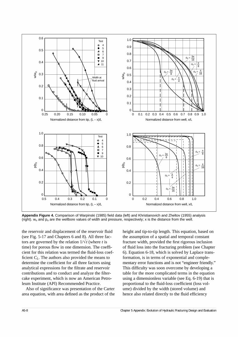
the reservoir and displacement of the reservoir fluid(see Fig. 5-17 and Chapters 6 and 8). All three fac-tors are governed by the relation 1/√ t (where t istime) for porous flow in one dimension. The coeffi-cient for this relation was termed the fluid-loss coef-ficient CL. The authors also provided the means todetermine the coefficient for all three factors usinganalytical expressions for the filtrate and reservoircontributions and to conduct and analyze the filter-cake experiment, which is now an American Petro-leum Institute (API) Recommended Practice.

Also of significance was presentation of the Carterarea equation, with area defined as the product of the

height and tip-to-tip length. This equation, based onthe assumption of a spatial and temporal constantfracture width, provided the first rigorous inclusionof fluid loss into the fracturing problem (see Chapter6). Equation 6-18, which is solved by Laplace trans-formation, is in terms of exponential and comple-mentary error functions and is not “engineer friendly.”This difficulty was soon overcome by developing atable for the more complicated terms in the equationusing a dimensionless variable (see Eq. 6-19) that isproportional to the fluid-loss coefficient (loss vol-ume) divided by the width (stored volume) andhence also related directly to the fluid efficiency

A5-8 Chapter 5 Appendix: Evolution of Hydraulic Fracturing Design and Evaluation

Appendix Figure 4. Comparison of Warpinski (1985) field data (left) and Khristianovich and Zheltov (1955) analysis(right). wo and po are the wellbore values of width and pressure, respectively; x is the distance from the well.

1.0

0.9

0.8

0.7

0.6

0.5

0.4

0.3

0.2

0.1

0

w/w

o

0.6

0.5

0.4

0.3

0.2

0.1

0

w/w

o

1.0

0.8

0.6

0.4

0.2

0

p/p o

1.0

0.8

0.6

0.4

0.2

0

p/p o

45679

1011

Test

45679

10

Test

Width atfluid arrival

0.25 0.20 0.15 0.10 0.05 0

Normalized distance from tip, (L – x)/L

0 0.1 0.2 0.3 0.4 0.5 0.6 0.7 0.8 0.9 1.0

Normalized distance from well, x/L

0.5 0.4 0.3 0.2 0.1 0

Normalized distance from tip, (L – x)/L

0 0.2 0.4 0.6 0.8 1.0

Normalized distance from well, x/L

ϑ0 = π4

ϑ0 = π8

ϑ0 = π16

ϑ0 = 3π16

ϑ0 = 3π8

ϑ0 = π4

ϑ0 = π8

ϑ0 = π16

ϑ0 = 3π16

ϑ0 = 3π8

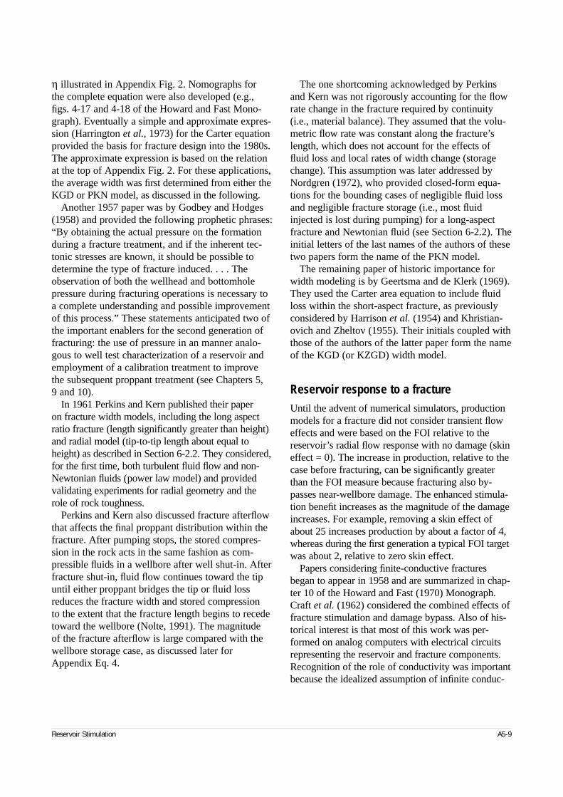
η illustrated in Appendix Fig. 2. Nomographs for the complete equation were also developed (e.g., figs. 4-17 and 4-18 of the Howard and Fast Mono-graph). Eventually a simple and approximate expres-sion (Harrington et al., 1973) for the Carter equationprovided the basis for fracture design into the 1980s.The approximate expression is based on the relationat the top of Appendix Fig. 2. For these applications,the average width was first determined from either theKGD or PKN model, as discussed in the following.

Another 1957 paper was by Godbey and Hodges(1958) and provided the following prophetic phrases:“By obtaining the actual pressure on the formationduring a fracture treatment, and if the inherent tec-tonic stresses are known, it should be possible todetermine the type of fracture induced. . . . Theobservation of both the wellhead and bottomholepressure during fracturing operations is necessary toa complete understanding and possible improvementof this process.” These statements anticipated two ofthe important enablers for the second generation offracturing: the use of pressure in an manner analo-gous to well test characterization of a reservoir andemployment of a calibration treatment to improvethe subsequent proppant treatment (see Chapters 5, 9 and 10).

In 1961 Perkins and Kern published their paper on fracture width models, including the long aspectratio fracture (length significantly greater than height)and radial model (tip-to-tip length about equal toheight) as described in Section 6-2.2. They considered,for the first time, both turbulent fluid flow and non-Newtonian fluids (power law model) and providedvalidating experiments for radial geometry and therole of rock toughness.

Perkins and Kern also discussed fracture afterflowthat affects the final proppant distribution within thefracture. After pumping stops, the stored compres-sion in the rock acts in the same fashion as com-pressible fluids in a wellbore after well shut-in. Afterfracture shut-in, fluid flow continues toward the tipuntil either proppant bridges the tip or fluid lossreduces the fracture width and stored compression to the extent that the fracture length begins to recedetoward the wellbore (Nolte, 1991). The magnitude of the fracture afterflow is large compared with thewellbore storage case, as discussed later forAppendix Eq. 4.

The one shortcoming acknowledged by Perkinsand Kern was not rigorously accounting for the flowrate change in the fracture required by continuity(i.e., material balance). They assumed that the volu-metric flow rate was constant along the fracture’slength, which does not account for the effects offluid loss and local rates of width change (storagechange). This assumption was later addressed byNordgren (1972), who provided closed-form equa-tions for the bounding cases of negligible fluid lossand negligible fracture storage (i.e., most fluidinjected is lost during pumping) for a long-aspectfracture and Newtonian fluid (see Section 6-2.2). Theinitial letters of the last names of the authors of thesetwo papers form the name of the PKN model.

The remaining paper of historic importance forwidth modeling is by Geertsma and de Klerk (1969).They used the Carter area equation to include fluidloss within the short-aspect fracture, as previouslyconsidered by Harrison et al. (1954) and Khristian-ovich and Zheltov (1955). Their initials coupled withthose of the authors of the latter paper form the nameof the KGD (or KZGD) width model.

Reservoir response to a fractureUntil the advent of numerical simulators, productionmodels for a fracture did not consider transient floweffects and were based on the FOI relative to thereservoir’s radial flow response with no damage (skineffect = 0). The increase in production, relative to thecase before fracturing, can be significantly greaterthan the FOI measure because fracturing also by-passes near-wellbore damage. The enhanced stimula-tion benefit increases as the magnitude of the damageincreases. For example, removing a skin effect ofabout 25 increases production by about a factor of 4,whereas during the first generation a typical FOI targetwas about 2, relative to zero skin effect.

Papers considering finite-conductive fracturesbegan to appear in 1958 and are summarized in chap-ter 10 of the Howard and Fast (1970) Monograph.Craft et al. (1962) considered the combined effects offracture stimulation and damage bypass. Also of his-torical interest is that most of this work was per-formed on analog computers with electrical circuitsrepresenting the reservoir and fracture components.Recognition of the role of conductivity was importantbecause the idealized assumption of infinite conduc-

Reservoir Stimulation A5-9

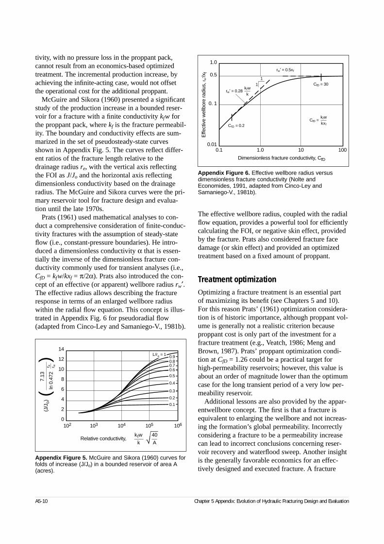
tivity, with no pressure loss in the proppant pack,cannot result from an economics-based optimizedtreatment. The incremental production increase, byachieving the infinite-acting case, would not offsetthe operational cost for the additional proppant.

McGuire and Sikora (1960) presented a significantstudy of the production increase in a bounded reser-voir for a fracture with a finite conductivity kfw forthe proppant pack, where kf is the fracture permeabil-ity. The boundary and conductivity effects are sum-marized in the set of pseudosteady-state curvesshown in Appendix Fig. 5. The curves reflect differ-ent ratios of the fracture length relative to thedrainage radius re, with the vertical axis reflectingthe FOI as J/Jo and the horizontal axis reflectingdimensionless conductivity based on the drainageradius. The McGuire and Sikora curves were the pri-mary reservoir tool for fracture design and evalua-tion until the late 1970s.

Prats (1961) used mathematical analyses to con-duct a comprehensive consideration of finite-conduc-tivity fractures with the assumption of steady-stateflow (i.e., constant-pressure boundaries). He intro-duced a dimensionless conductivity α that is essen-tially the inverse of the dimensionless fracture con-ductivity commonly used for transient analyses (i.e.,CfD = kfw/kxf = π/2α). Prats also introduced the con-cept of an effective (or apparent) wellbore radius rw′.The effective radius allows describing the fractureresponse in terms of an enlarged wellbore radiuswithin the radial flow equation. This concept is illus-trated in Appendix Fig. 6 for pseudoradial flow(adapted from Cinco-Ley and Samaniego-V., 1981b).

The effective wellbore radius, coupled with the radialflow equation, provides a powerful tool for efficientlycalculating the FOI, or negative skin effect, providedby the fracture. Prats also considered fracture facedamage (or skin effect) and provided an optimizedtreatment based on a fixed amount of proppant.

Treatment optimizationOptimizing a fracture treatment is an essential part of maximizing its benefit (see Chapters 5 and 10).For this reason Prats’ (1961) optimization considera-tion is of historic importance, although proppant vol-ume is generally not a realistic criterion becauseproppant cost is only part of the investment for afracture treatment (e.g., Veatch, 1986; Meng andBrown, 1987). Prats’ proppant optimization condi-tion at CfD = 1.26 could be a practical target forhigh-permeability reservoirs; however, this value isabout an order of magnitude lower than the optimumcase for the long transient period of a very low per-meability reservoir.

Additional lessons are also provided by the appar-entwellbore concept. The first is that a fracture isequivalent to enlarging the wellbore and not increas-ing the formation’s global permeability. Incorrectlyconsidering a fracture to be a permeability increasecan lead to incorrect conclusions concerning reser-voir recovery and waterflood sweep. Another insightis the generally favorable economics for an effec-tively designed and executed fracture. A fracture

A5-10 Chapter 5 Appendix: Evolution of Hydraulic Fracturing Design and Evaluation

Appendix Figure 5. McGuire and Sikora (1960) curves forfolds of increase (J/Jo) in a bounded reservoir of area A(acres).

14

12

10

8

6

4

2

0102 103 104 105 106

Relative conductivity,kfw 40

k A√

(

)(J

/Jo)

7.13

ln 0

.472

r e r w

0.90.80.70.60.5

0.4

0.3

0.2

0.1

L/re = 1

Appendix Figure 6. Effective wellbore radius versusdimensionless fracture conductivity (Nolte andEconomides, 1991, adapted from Cinco-Ley andSamaniego-V., 1981b).

1.0

0.5

0. 1

0.010.1 1.0 10 100

Dimensionless fracture conductivity, CfD

Effe

ctiv

e w

ellb

ore

radi

us, r

w′/x

f

CfD = 30

CfD = 0.2CfD =

kfw

kxf

rw′ = 0.28 kfw

k

rw′ = 0.5xf

11

treatment is equivalent to excavating a very largediameter borehole (e.g., hundreds of feet in mostcases) and therefore is an extremely cost-effectiveway to provide an equivalent excavation.

The most important optimization lesson is foundin Appendix Fig. 6 for the roles of conductivity kfw(achieved by proppant cost) and fracture penetration(achieved by fluid and other additive costs; seeChapter 7). The figure indicates that as CfD increasesbeyond 10, the effective wellbore radius approachesone-half of the fracture length and there are dimin-ishing returns for additional increases in conductivity(i.e., incurring proppant costs without an effectiveincrease in production rate). For this part of Appen-dix Fig. 6, the effective radius is constrained only by length and is termed the length-limited case.However, increasing both fracture length and con-ductivity to maintain a constant CfD achieves themost efficient conversion of length into an effectivewellbore radius. This conversion is the basis foreffectively fracturing low-permeability formations.

The practical limits for the length-limited case arereaching the drainage radius, increasing conductivitywithin the limits of achievable fracture width andefficiently extending a fracture when the pressurereaches the formation capacity, as discussed later. Aspermeability increases, and proportionally decreasesCfD, the ability to increase conductivity becomes the constraint. As CfD progressively decreases, theconductivity-limited case is reached. The figure indi-cates that as CfD decreases below 1, a log-log unitslope is approached that relates rw′ to kfw/k, with theobvious absence of an effect from length. When theunit slope is reached, near a value of 0.2, the well-bore drawdown completely dissipates within thefracture before reaching the tip, and the extremitiesof the fracture cannot provide a production benefit.For the conductivity-limited condition, the produc-tion rate can be increased economically only by pro-viding more conductivity kfw, with an obvious con-straint from the available fracture width developedduring the treatment. This constraint was significantlyextended by the third fracturing generation of TSOtreatments, which is discussed toward the end of thisAppendix.

Transition between the first and second generationsBy 1961, the design and evaluation tools for most of the next two decades had been established by thecontributions discussed. Incremental development ofthese tools slowed because fracturing was considereda mature technology. Also affecting technical devel-opment was the degrading economics for lower qual-ity reserves as oil import-export increased and frac-turing activity decreased (Appendix Fig. 1). Thiscondition did not change until the mid-1970sbrought natural gas shortages and higher gas pricesto the United States. Higher prices produced theincentive to develop extensive regions of tight gasreserves with fractures targeting the FOI = 10 rangeof the McGuire and Sikora curves (Appendix Fig. 5).Before this period, typical fracturing targets were oilreservoirs with an FOI of about 2, with FOI relativeto an undamaged wellbore. However the FOI = 10target required about an order-of-magnitude increasein the volume and cost for a typical treatment andwas hence termed massive hydraulic fracturing.

This new target introduced higher temperaturereservoirs, typically of tight gas, that generallyexceeded the performance limits for fracturing fluidsystems. These conditions stretched the so-calledmature technology in almost every conceivable wayand resulted in a bumpy journey because of the pro-portionally large economic penalty when a treatmentfailed to meet expectations. However, reports of suc-cessful field development (e.g., Fast et al., 1977)encouraged continued interest in tight gas develop-ment.

Realistic estimate of conductivityCooke (1975) reported realistic experiments for char-acterizing the conductivity of proppant packs. Hisprocedure formed proppant packs from a slurry com-posed of polymer-based fluids by using a cell withrock faces that allowed fluid loss and the subsequentapplication of closure stress. The Cooke cell is nowa standard apparatus for a fracturing fluid laboratory

Reservoir Stimulation A5-11

(see Chapter 8). The experiments showed that theretained pack permeability could be very small.These results were unexpected because prior testingprocedures did not use fracturing fluids or stress lev-els for deeper gas reserves. The primary differenceresulted because the rock acts as a polymer screen at moderate and smaller permeability levels, whichsignificantly increases the polymer concentrationremaining within the proppant pack porosity afterfracture closure.

Cooke also provided a simple mass-balance rela-tion for this important consideration. The concen-tration factor for the polymer and other additivesremaining in the fracture relative to the originalconcentration can be expressed as

(3)

for a typical proppant pack porosity of 0.33 andproppant specific gravity (s.g.) of 2.65. The relationdepends on the average concentration <ppa> definedas the total pounds of proppant divided by the totalgallons of polymer-based fluid. This relation indicatesa polymer concentration increase of 20 or greater fortypical treatments at that time (e.g., <ppa> of 1 to 2 lbm). This unexpected discovery of a significantreduction in retained permeability, coupled with theprior discussion on conductivity and effective well-bore radius, partly explains the difficult transition tomassive treatments.

Cooke’s pioneering work had obvious effects onproppant schedules for treatments and laboratorytesting procedures. Equally important, the work initi-ated substantial product development activities, asdiscussed in Chapter 7. These include improvedproppants, beginning with Cooke’s work on bauxitefor high crushing stress, improved breaker chemistryand breaker encapsulation, large reductions of poly-mer concentration for crosslinked fluids, foams andemulsions, and residue-free viscoelastic surfactantsystems. The evolution of fracturing fluid chemistrywas reviewed by Jennings (1996).

Height growth and proppant transportSimonson et al. (1978) presented the mechanics gov-erning fracture growth into a layer with higher stress,complementing the postulate by Harrison et al. (1954)concerning the role of stress for height confinement.The analysis considered a three-layer case for twosymmetric barriers (i.e., two barriers extending

infinitely above and below the pay section with eachbarrier having the same magnitude of stress). Thethree-layer case provided insight into how to adaptmore general relations to any number of layers (e.g.,Nolte and Smith, 1981; chapter 3 of Gidley et al.,1989). These relations led to the calculations employedin pseudo-three-dimensional (P3D) fracture simulators(see Section 6-3.2).

Novotny (1977) outlined a comprehensive basis forproppant transport calculations and in particular identi-fied the important roles of channel shear rate and frac-ture closure in determining the ultimate placement ofproppant (see Section 6-5.3. Both effects produce moreproppant fall. For non-Newtonian fluids, the effectiveviscosity for sedimentation is determined from the vec-toral sum of the shear rate in the channel and thatcaused by proppant fall (as for stagnant fluid). Thissum is generally dominated by the channel flow and is much greater than that for a particle in stagnant fluid(i.e., higher shear rate and lower viscosity). In addition,the closure period prolongs the time for proppant falland maintains the channel flow to reduce the effectiveviscosity. Novotny also provided a brief analysis of thevolume balance during closure, which is the essentialingredient for the fracturing pressure decline analysis(e.g., Nolte, 1979) that is used for calibration treat-ments (see Section 9-5).

Transient reservoir responseThe FOI consideration for fracture production wasfound to be completely inadequate for the substantialperiod of transient flow that occurs in tight formations(see Section 12-2). The first tool for finite-conductivitytransient flow was type curves provided by Agarwal et al. (1979). Although these curves were developedfrom numerical simulators, access to computers wasgenerally outside the reach of most engineers. Theseand similar type curves became the standard evalua-tion tool to assess production from a fracture treat-ment. Type curves were also used for optimizing treat-ment design. By the mid-1980s, as general access tocomputers increased, the use of type curves began todecrease accordingly.

Cinco-Ley and Samaniego-V. (1981b) providedseveral advancements for understanding and quanti-fying the transient behavior of a reservoir fracturesystem. In addition to advancing the effective well-bore concept (e.g., Appendix Fig. 6) and type curves,they identified and provided comprehensive descrip-

A5-12 Chapter 5 Appendix: Evolution of Hydraulic Fracturing Design and Evaluation

CF ppa= 44 / ,

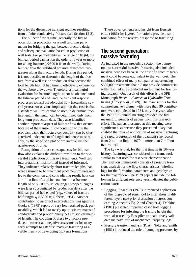
tions for the distinctive transient regimes resultingfrom a finite-conductivity fracture (see Section 12-2).

The bilinear flow regime, generally the first tooccur during production or a well test, was para-mount for bridging the gap between fracture designand subsequent evaluation based on production orwell tests. For permeability in the range of 10 µd, thebilinear period can last on the order of a year or morefor a long fracture (>2500 ft from the well). Duringbilinear flow the stabilized pressure drawdown pro-gresses along the fracture length. During this period,it is not possible to determine the length of the frac-ture from a well test or production data because thetotal length has not had time to effectively experiencethe wellbore drawdown. Therefore, a meaningfulevaluation for fracture length cannot be obtained untilthe bilinear period ends and the transient responseprogresses toward pseudoradial flow (potentially sev-eral years). An obvious implication in this case is thata standard well test cannot be used to determine frac-ture length; the length can be determined only fromlong-term production data. They also identifiedanother important aspect of bilinear flow that occursbecause of the transient flow condition within theproppant pack: the fracture conductivity can be char-acterized, independent of length and hence most reli-ably, by the slope of a plot of pressure versus thequarter-root of time.

Recognition of these consequences for bilinearflow also explains the difficult transition to the suc-cessful application of massive treatments. Well testinterpretations misinformed instead of informed.They indicated relatively short fracture lengths thatwere assumed to be treatment placement failures andled to the common and contradicting result: how can1 million lbm of sand be contained in a fracturelength of only 100 ft? Much longer propped lengthswere later substantiated by production data after thebilinear period had ended (e.g., values of fracturehalf-length xf > 5000 ft; Roberts, 1981). Anothercontribution to incorrect interpretations was ignoringCooke’s (1975) report of very low retained-pack per-meability, which led to overly optimistic estimates ofconductivity and proportionally pessimistic estimatesof length. The coupling of these two factors pro-duced incorrect and negative assessments for manyearly attempts to establish massive fracturing as aviable means of developing tight gas formations.

These advancements and insight from Bennett et al. (1986) for layered formations provide a solidfoundation for the reservoir response to fracturing.

The second generation: massive fracturingAs indicated in the preceding section, the bumpyroad to successful massive fracturing also includedmassive penalties because the cost of a fracture treat-ment could become equivalent to the well cost. Thecombined effect of many companies experiencing$500,000 treatments that did not provide commercialwells resulted in a significant investment for fractur-ing research. One result of this effort is the SPEMonograph Recent Advances in Hydraulic Frac-turing (Gidley et al., 1989). The manuscripts for thiscomprehensive volume, with more than 30 contribu-tors, were completed in 1984, only five years afterthe 1979 SPE annual meeting provided the firstmeaningful number of papers from this researcheffort. The papers presented at this meeting weresignificant also because they presented a key thatenabled the reliable application of massive fracturingand rapid progression of the treatment size recordfrom 2 million lbm in 1979 to more than 7 millionlbm by 1986.

The key was that, for the first time in its 30-yearhistory, fracturing was considered in a frameworksimilar to that used for reservoir characterization.The reservoir framework consists of pressure tran-sient analysis for the flow characteristics, wirelinelogs for the formation parameters and geophysics for the macroview. The 1979 papers include the fol-lowing (a different reference year indicates the publi-cation date):

• Logging: Rosepiler (1979) introduced applicationof the long-spaced sonic tool to infer stress in dif-ferent layers (see prior discussion of stress con-cerning Appendix Eq. 2 and Chapter 4). Dobkins(1981) presented improved cased hole loggingprocedures for inferring the fracture height thatwere also used by Rosepiler to qualitatively vali-date his novel use of mechanical property logs.

• Pressure transient analysis (PTA): Nolte and Smith(1981) introduced the role of pumping pressures by

Reservoir Stimulation A5-13

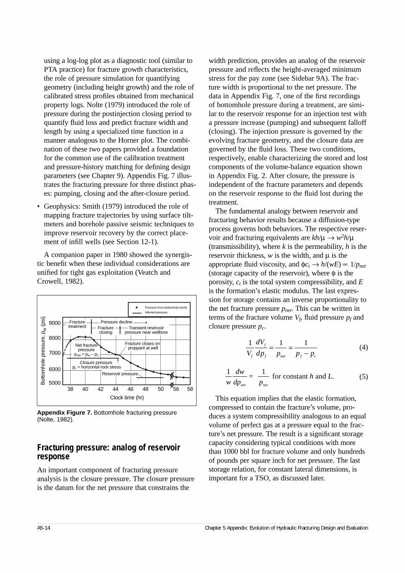
using a log-log plot as a diagnostic tool (similar toPTA practice) for fracture growth characteristics,the role of pressure simulation for quantifyinggeometry (including height growth) and the role ofcalibrated stress profiles obtained from mechanicalproperty logs. Nolte (1979) introduced the role ofpressure during the postinjection closing period toquantify fluid loss and predict fracture width andlength by using a specialized time function in amanner analogous to the Horner plot. The combi-nation of these two papers provided a foundationfor the common use of the calibration treatmentand pressure-history matching for defining designparameters (see Chapter 9). Appendix Fig. 7 illus-trates the fracturing pressure for three distinct phas-es: pumping, closing and the after-closure period.

• Geophysics: Smith (1979) introduced the role ofmapping fracture trajectories by using surface tilt-meters and borehole passive seismic techniques toimprove reservoir recovery by the correct place-ment of infill wells (see Section 12-1).

A companion paper in 1980 showed the synergis-tic benefit when these individual considerations areunified for tight gas exploitation (Veatch andCrowell, 1982).

Fracturing pressure: analog of reservoirresponseAn important component of fracturing pressureanalysis is the closure pressure. The closure pressureis the datum for the net pressure that constrains the

width prediction, provides an analog of the reservoirpressure and reflects the height-averaged minimumstress for the pay zone (see Sidebar 9A). The frac-ture width is proportional to the net pressure. Thedata in Appendix Fig. 7, one of the first recordingsof bottomhole pressure during a treatment, are simi-lar to the reservoir response for an injection test witha pressure increase (pumping) and subsequent falloff(closing). The injection pressure is governed by theevolving fracture geometry, and the closure data aregoverned by the fluid loss. These two conditions,respectively, enable characterizing the stored and lostcomponents of the volume-balance equation shownin Appendix Fig. 2. After closure, the pressure isindependent of the fracture parameters and dependson the reservoir response to the fluid lost during thetreatment.

The fundamental analogy between reservoir andfracturing behavior results because a diffusion-typeprocess governs both behaviors. The respective reser-voir and fracturing equivalents are kh/µ → w2h/µ(transmissibility), where k is the permeability, h is thereservoir thickness, w is the width, and µ is theappropriate fluid viscosity, and φct → h/(wE) ∝ 1/pnet

(storage capacity of the reservoir), where φ is theporosity, ct is the total system compressibility, and Eis the formation’s elastic modulus. The last expres-sion for storage contains an inverse proportionality tothe net fracture pressure pnet. This can be written interms of the fracture volume Vf, fluid pressure pf andclosure pressure pc.

(4)

(5)

This equation implies that the elastic formation,compressed to contain the fracture’s volume, pro-duces a system compressibility analogous to an equalvolume of perfect gas at a pressure equal to the frac-ture’s net pressure. The result is a significant storagecapacity considering typical conditions with morethan 1000 bbl for fracture volume and only hundredsof pounds per square inch for net pressure. The laststorage relation, for constant lateral dimensions, isimportant for a TSO, as discussed later.

A5-14 Chapter 5 Appendix: Evolution of Hydraulic Fracturing Design and Evaluation

Appendix Figure 7. Bottomhole fracturing pressure(Nolte, 1982).

38 40 42 44 46 48 50 56 58

9000

8000

7000

6000

5000Bot

tom

hole

pre

ssur

e, p

w (p

si)

Clock time (hr)

Fracturetreatment Fracture

closingTransient reservoir

pressure near wellbore

Pressure decline

Net fracturepressure

pnet = pw – pc

Fracture closes on proppant at well

Closure pressure pc = horizontal rock stress

Pressure from bottomhole bomb

Inferred pressure

Reservoir pressure

1 1 1V

dV

dp p p pf

f

f net f c

= =−

1w

dw

dp ph L

net net

=1

for constant and .

Fracture simulatorsDescribing a hydraulic fracture produces a signifi-cantly more complex role for the diffusive processthan the reservoir case because the basic parametergroups change continuously with time, with a nonlin-earity for the equivalent permeability, and the far-field elastic coupling between width and pressureproduces local parameters that have a general depen-dence on the pressure everywhere within the frac-ture’s unknown boundaries. For these reasons, frac-ture simulators that rigorously and robustly couplethese parameters in a general manner (see Section 6-3) have not progressed at the same rate as reservoirsimulators.

The modeling difficulties led to widespread use ofsimulators based on P3D assumptions that partiallycircumvent the far-field elastic-coupling condition.The two most common means were relaxing the lat-eral coupling in the long direction of the fracture (asfor the PKN model) to allow a cellular representationand vertical height growth of the cells (e.g., Nolte,1982) or prescribing the boundary and width profilesby elliptical segments and a lumped dependence onthe governing parameters (e.g., Settari and Cleary,1986). P3D models, or more precisely P2D models,evolved to include automated proppant schedulingand the temperature-exposure history for polymer andadditive scheduling (e.g., Nolte, 1982), acid fractur-ing (e.g., Mack and Elbel, 1994), economic optimiza-tion for treatment design (e.g., Veatch 1986; Mengand Brown, 1987), automated pressure-history match-ing (e.g., Gulrajani and Romero, 1996; Gulrajani etal., 1997b) and rigorous 2D slurry flow (e.g., Smithand Klein, 1995).

Originally restricted to in-office use, these modelsmerged with on-site fracture monitoring systems toprovide treatment evaluation and simulation in real-time mode. An equally important advance was theparallel evolution of process-controlled mixing andblending equipment for reliable execution of moredemanding treatment schedules and progressivelymore complex chemistry that requires precise pro-portioning (see Chapters 7 and 11).

Fracture mapping and model validationAn important achievement was the definition of frac-ture length, height and width by employing passiveseismic measurements and tiltmeters in observation

wells (Warpinski et al., 1996; see Section 12-1). Theimportance of these measurements for fracture designand evaluation cannot be overemphasized. Indepen-dent measurements for each component of the frac-ture volume (Appendix Fig. 2) provide a long-awaitedbenchmark for validating fracture models.

Like the first generation’s failure to find a consen-sus for width models (e.g., Perkins, 1973), pressure-history matching could not resolve the second gener-ation’s conflicting adaptations of the P3D framework(see Chapter 6). The convergence of modelingassumptions failed for several reasons. The first wasfundamental to the pressure-matching process andresults because of the multitude of opportunities fornonuniqueness. Another reason was the failure toachieve a dominant industry opinion on either thetechnique or procedures for a specific technique todefine closure pressure (e.g., Plahn et al., 1997). Thisstate of affairs allowed selecting a closure pressureprocedure to validate particular modeling assump-tions and therefore justify relatively arbitrary and adhoc modeling assumptions. Techniques to determinethe closure pressure are discussed in Section 3-6 andthe Appendix to Chapter 9.

Because of nonuniqueness in the reservoir responseand the basing of reservoir models on overly idealizedmodeling assumptions for a fracture, the reservoirresponse cannot generally provide an effectiveconstraint on the achieved fracture length (Elbel andAyoub, 1991; Nolte and Economides, 1991). Mappingconstraints on all three fracture dimensions provide aunique, objective test of the geometry model assump-tions (e.g., Gulrajani et al., 1997a) and a basis forrationally judging and selecting the model complexityappropriate for the specific application, available dataand simulation resources.

Treatment design and evaluationThe primary fracture evaluation advance from themassive treatment generation is the calibration treat-ment performed before the proppant treatment todefine placement parameters. Combining the calibra-tion treatment and the purpose-designed TSO treat-ment produced the primary treatment innovation ofthe second generation. The calibrated TSO treat-ment, developed by Smith et al. (1984), became thekey to the third fracturing generation (discussedlater) and essentially removed width as a constraintfor the conductivity required to successfully fracture

Reservoir Stimulation A5-15

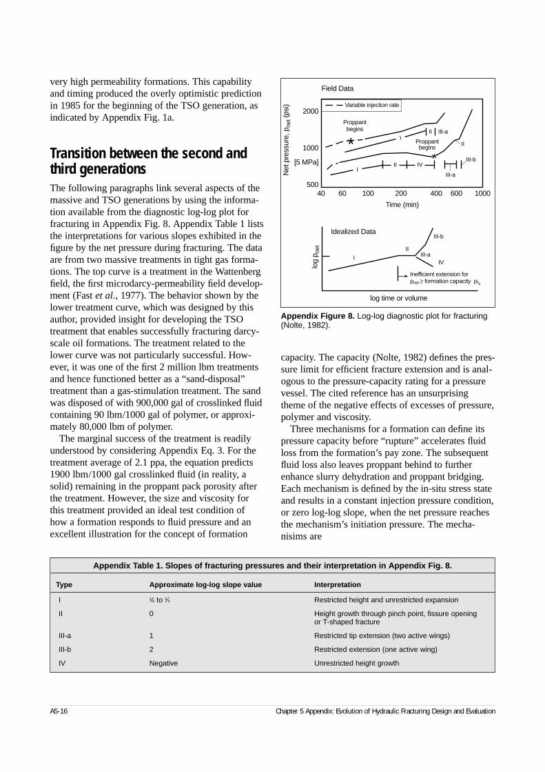
very high permeability formations. This capabilityand timing produced the overly optimistic predictionin 1985 for the beginning of the TSO generation, asindicated by Appendix Fig. 1a.

Transition between the second andthird generationsThe following paragraphs link several aspects of themassive and TSO generations by using the informa-tion available from the diagnostic log-log plot forfracturing in Appendix Fig. 8. Appendix Table 1 liststhe interpretations for various slopes exhibited in thefigure by the net pressure during fracturing. The dataare from two massive treatments in tight gas forma-tions. The top curve is a treatment in the Wattenbergfield, the first microdarcy-permeability field develop-ment (Fast et al., 1977). The behavior shown by thelower treatment curve, which was designed by thisauthor, provided insight for developing the TSOtreatment that enables successfully fracturing darcy-scale oil formations. The treatment related to thelower curve was not particularly successful. How-ever, it was one of the first 2 million lbm treatmentsand hence functioned better as a “sand-disposal”treatment than a gas-stimulation treatment. The sandwas disposed of with 900,000 gal of crosslinked fluidcontaining 90 lbm/1000 gal of polymer, or approxi-mately 80,000 lbm of polymer.

The marginal success of the treatment is readilyunderstood by considering Appendix Eq. 3. For thetreatment average of 2.1 ppa, the equation predicts1900 lbm/1000 gal crosslinked fluid (in reality, asolid) remaining in the proppant pack porosity afterthe treatment. However, the size and viscosity forthis treatment provided an ideal test condition ofhow a formation responds to fluid pressure and anexcellent illustration for the concept of formation

capacity. The capacity (Nolte, 1982) defines the pres-sure limit for efficient fracture extension and is anal-ogous to the pressure-capacity rating for a pressurevessel. The cited reference has an unsurprisingtheme of the negative effects of excesses of pressure,polymer and viscosity.

Three mechanisms for a formation can define itspressure capacity before “rupture” accelerates fluidloss from the formation’s pay zone. The subsequentfluid loss also leaves proppant behind to furtherenhance slurry dehydration and proppant bridging.Each mechanism is defined by the in-situ stress stateand results in a constant injection pressure condition,or zero log-log slope, when the net pressure reachesthe mechanism’s initiation pressure. The mecha-nisims are

A5-16 Chapter 5 Appendix: Evolution of Hydraulic Fracturing Design and Evaluation

Appendix Figure 8. Log-log diagnostic plot for fracturing(Nolte, 1982).

*x

2000

1000

500

[5 MPa]

Net

pre

ssur

e, p

net (

psi)

log

p net

40 60 100 200 400 600 1000

Time (min)

log time or volume

Idealized Data

Field Data

I

II

II

II

III-a

III-a

III-b

IV

Inefficient extension for pnet ≥ formation capacity pfc

I

Proppantbegins

Proppantbegins

Variable injection rate

III-a

III-bII

IIV

Appendix Table 1. Slopes of fracturing pressures and their interpretation in Appendix Fig. 8.

Type Approximate log-log slope value Interpretation

I 1⁄8 to 1⁄4 Restricted height and unrestricted expansion

II 0 Height growth through pinch point, fissure openingor T-shaped fracture

III-a 1 Restricted tip extension (two active wings)

III-b 2 Restricted extension (one active wing)

IV Negative Unrestricted height growth

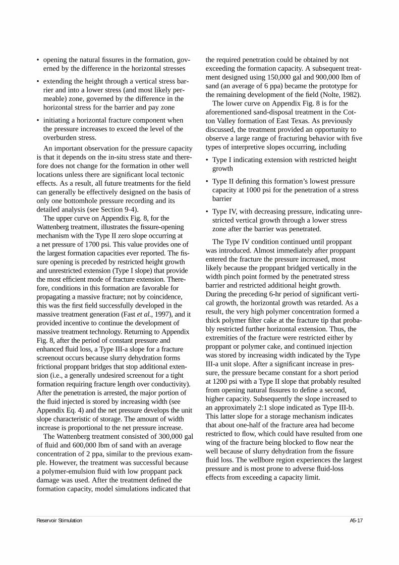
• opening the natural fissures in the formation, gov-erned by the difference in the horizontal stresses

• extending the height through a vertical stress bar-rier and into a lower stress (and most likely per-meable) zone, governed by the difference in thehorizontal stress for the barrier and pay zone

• initiating a horizontal fracture component whenthe pressure increases to exceed the level of theoverburden stress.

An important observation for the pressure capacityis that it depends on the in-situ stress state and there-fore does not change for the formation in other welllocations unless there are significant local tectoniceffects. As a result, all future treatments for the fieldcan generally be effectively designed on the basis ofonly one bottomhole pressure recording and itsdetailed analysis (see Section 9-4).

The upper curve on Appendix Fig. 8, for theWattenberg treatment, illustrates the fissure-openingmechanism with the Type II zero slope occurring at a net pressure of 1700 psi. This value provides one ofthe largest formation capacities ever reported. The fis-sure opening is preceded by restricted height growthand unrestricted extension (Type I slope) that providethe most efficient mode of fracture extension. There-fore, conditions in this formation are favorable forpropagating a massive fracture; not by coincidence,this was the first field successfully developed in themassive treatment generation (Fast et al., 1997), and itprovided incentive to continue the development ofmassive treatment technology. Returning to AppendixFig. 8, after the period of constant pressure andenhanced fluid loss, a Type III-a slope for a fracturescreenout occurs because slurry dehydration formsfrictional proppant bridges that stop additional exten-sion (i.e., a generally undesired screenout for a tightformation requiring fracture length over conductivity).After the penetration is arrested, the major portion ofthe fluid injected is stored by increasing width (seeAppendix Eq. 4) and the net pressure develops the unitslope characteristic of storage. The amount of widthincrease is proportional to the net pressure increase.

The Wattenberg treatment consisted of 300,000 galof fluid and 600,000 lbm of sand with an averageconcentration of 2 ppa, similar to the previous exam-ple. However, the treatment was successful becausea polymer-emulsion fluid with low proppant packdamage was used. After the treatment defined theformation capacity, model simulations indicated that

the required penetration could be obtained by notexceeding the formation capacity. A subsequent treat-ment designed using 150,000 gal and 900,000 lbm ofsand (an average of 6 ppa) became the prototype forthe remaining development of the field (Nolte, 1982).

The lower curve on Appendix Fig. 8 is for theaforementioned sand-disposal treatment in the Cot-ton Valley formation of East Texas. As previouslydiscussed, the treatment provided an opportunity toobserve a large range of fracturing behavior with fivetypes of interpretive slopes occurring, including

• Type I indicating extension with restricted heightgrowth

• Type II defining this formation’s lowest pressurecapacity at 1000 psi for the penetration of a stressbarrier

• Type IV, with decreasing pressure, indicating unre-stricted vertical growth through a lower stresszone after the barrier was penetrated.

The Type IV condition continued until proppantwas introduced. Almost immediately after proppantentered the fracture the pressure increased, mostlikely because the proppant bridged vertically in thewidth pinch point formed by the penetrated stressbarrier and restricted additional height growth.During the preceding 6-hr period of significant verti-cal growth, the horizontal growth was retarded. As aresult, the very high polymer concentration formed athick polymer filter cake at the fracture tip that proba-bly restricted further horizontal extension. Thus, theextremities of the fracture were restricted either byproppant or polymer cake, and continued injectionwas stored by increasing width indicated by the TypeIII-a unit slope. After a significant increase in pres-sure, the pressure became constant for a short periodat 1200 psi with a Type II slope that probably resultedfrom opening natural fissures to define a second,higher capacity. Subsequently the slope increased toan approximately 2:1 slope indicated as Type III-b.This latter slope for a storage mechanism indicatesthat about one-half of the fracture area had becomerestricted to flow, which could have resulted from onewing of the fracture being blocked to flow near thewell because of slurry dehydration from the fissurefluid loss. The wellbore region experiences the largestpressure and is most prone to adverse fluid-losseffects from exceeding a capacity limit.

Reservoir Stimulation A5-17

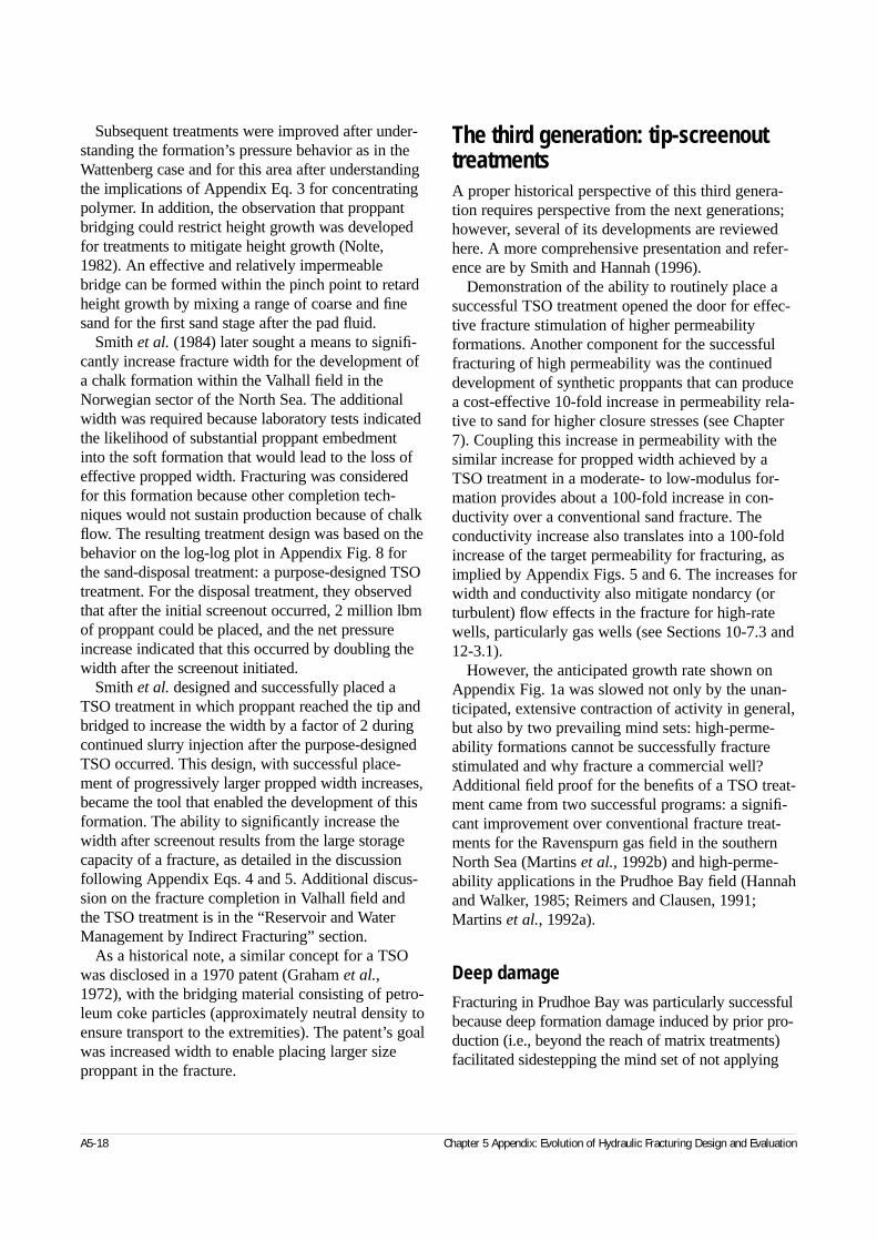
Subsequent treatments were improved after under-standing the formation’s pressure behavior as in theWattenberg case and for this area after understandingthe implications of Appendix Eq. 3 for concentratingpolymer. In addition, the observation that proppantbridging could restrict height growth was developedfor treatments to mitigate height growth (Nolte,1982). An effective and relatively impermeablebridge can be formed within the pinch point to retardheight growth by mixing a range of coarse and finesand for the first sand stage after the pad fluid.

Smith et al. (1984) later sought a means to signifi-cantly increase fracture width for the development ofa chalk formation within the Valhall field in theNorwegian sector of the North Sea. The additionalwidth was required because laboratory tests indicatedthe likelihood of substantial proppant embedmentinto the soft formation that would lead to the loss ofeffective propped width. Fracturing was consideredfor this formation because other completion tech-niques would not sustain production because of chalkflow. The resulting treatment design was based on thebehavior on the log-log plot in Appendix Fig. 8 forthe sand-disposal treatment: a purpose-designed TSOtreatment. For the disposal treatment, they observedthat after the initial screenout occurred, 2 million lbmof proppant could be placed, and the net pressureincrease indicated that this occurred by doubling thewidth after the screenout initiated.

Smith et al. designed and successfully placed aTSO treatment in which proppant reached the tip andbridged to increase the width by a factor of 2 duringcontinued slurry injection after the purpose-designedTSO occurred. This design, with successful place-ment of progressively larger propped width increases,became the tool that enabled the development of thisformation. The ability to significantly increase thewidth after screenout results from the large storagecapacity of a fracture, as detailed in the discussionfollowing Appendix Eqs. 4 and 5. Additional discus-sion on the fracture completion in Valhall field andthe TSO treatment is in the “Reservoir and WaterManagement by Indirect Fracturing” section.

As a historical note, a similar concept for a TSOwas disclosed in a 1970 patent (Graham et al.,1972), with the bridging material consisting of petro-leum coke particles (approximately neutral density toensure transport to the extremities). The patent’s goalwas increased width to enable placing larger sizeproppant in the fracture.

The third generation: tip-screenouttreatmentsA proper historical perspective of this third genera-tion requires perspective from the next generations;however, several of its developments are reviewedhere. A more comprehensive presentation and refer-ence are by Smith and Hannah (1996).

Demonstration of the ability to routinely place asuccessful TSO treatment opened the door for effec-tive fracture stimulation of higher permeabilityformations. Another component for the successfulfracturing of high permeability was the continueddevelopment of synthetic proppants that can producea cost-effective 10-fold increase in permeability rela-tive to sand for higher closure stresses (see Chapter7). Coupling this increase in permeability with thesimilar increase for propped width achieved by aTSO treatment in a moderate- to low-modulus for-mation provides about a 100-fold increase in con-ductivity over a conventional sand fracture. Theconductivity increase also translates into a 100-foldincrease of the target permeability for fracturing, asimplied by Appendix Figs. 5 and 6. The increases forwidth and conductivity also mitigate nondarcy (orturbulent) flow effects in the fracture for high-ratewells, particularly gas wells (see Sections 10-7.3 and12-3.1).

However, the anticipated growth rate shown onAppendix Fig. 1a was slowed not only by the unan-ticipated, extensive contraction of activity in general,but also by two prevailing mind sets: high-perme-ability formations cannot be successfully fracturestimulated and why fracture a commercial well?Additional field proof for the benefits of a TSO treat-ment came from two successful programs: a signifi-cant improvement over conventional fracture treat-ments for the Ravenspurn gas field in the southernNorth Sea (Martins et al., 1992b) and high-perme-ability applications in the Prudhoe Bay field (Hannahand Walker, 1985; Reimers and Clausen, 1991;Martins et al., 1992a).

Deep damageFracturing in Prudhoe Bay was particularly successfulbecause deep formation damage induced by prior pro-duction (i.e., beyond the reach of matrix treatments)facilitated sidestepping the mind set of not applying

A5-18 Chapter 5 Appendix: Evolution of Hydraulic Fracturing Design and Evaluation

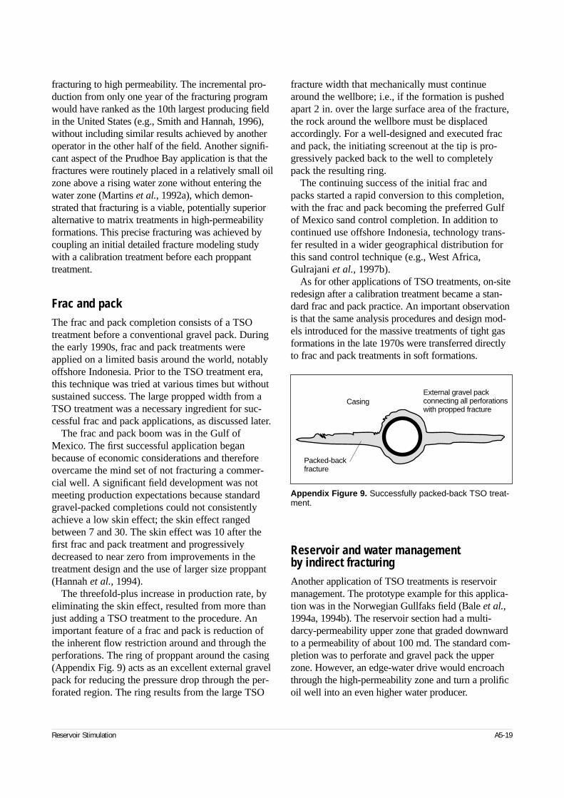
fracturing to high permeability. The incremental pro-duction from only one year of the fracturing programwould have ranked as the 10th largest producing fieldin the United States (e.g., Smith and Hannah, 1996),without including similar results achieved by anotheroperator in the other half of the field. Another signifi-cant aspect of the Prudhoe Bay application is that thefractures were routinely placed in a relatively small oilzone above a rising water zone without entering thewater zone (Martins et al., 1992a), which demon-strated that fracturing is a viable, potentially superioralternative to matrix treatments in high-permeabilityformations. This precise fracturing was achieved bycoupling an initial detailed fracture modeling studywith a calibration treatment before each proppanttreatment.

Frac and packThe frac and pack completion consists of a TSOtreatment before a conventional gravel pack. Duringthe early 1990s, frac and pack treatments wereapplied on a limited basis around the world, notablyoffshore Indonesia. Prior to the TSO treatment era,this technique was tried at various times but withoutsustained success. The large propped width from aTSO treatment was a necessary ingredient for suc-cessful frac and pack applications, as discussed later.

The frac and pack boom was in the Gulf ofMexico. The first successful application beganbecause of economic considerations and thereforeovercame the mind set of not fracturing a commer-cial well. A significant field development was notmeeting production expectations because standardgravel-packed completions could not consistentlyachieve a low skin effect; the skin effect rangedbetween 7 and 30. The skin effect was 10 after thefirst frac and pack treatment and progressivelydecreased to near zero from improvements in thetreatment design and the use of larger size proppant(Hannah et al., 1994).

The threefold-plus increase in production rate, byeliminating the skin effect, resulted from more thanjust adding a TSO treatment to the procedure. Animportant feature of a frac and pack is reduction ofthe inherent flow restriction around and through theperforations. The ring of proppant around the casing(Appendix Fig. 9) acts as an excellent external gravelpack for reducing the pressure drop through the per-forated region. The ring results from the large TSO

fracture width that mechanically must continuearound the wellbore; i.e., if the formation is pushedapart 2 in. over the large surface area of the fracture,the rock around the wellbore must be displacedaccordingly. For a well-designed and executed fracand pack, the initiating screenout at the tip is pro-gressively packed back to the well to completelypack the resulting ring.

The continuing success of the initial frac andpacks started a rapid conversion to this completion,with the frac and pack becoming the preferred Gulfof Mexico sand control completion. In addition tocontinued use offshore Indonesia, technology trans-fer resulted in a wider geographical distribution forthis sand control technique (e.g., West Africa,Gulrajani et al., 1997b).

As for other applications of TSO treatments, on-siteredesign after a calibration treatment became a stan-dard frac and pack practice. An important observationis that the same analysis procedures and design mod-els introduced for the massive treatments of tight gasformations in the late 1970s were transferred directlyto frac and pack treatments in soft formations.

Reservoir and water managementby indirect fracturingAnother application of TSO treatments is reservoirmanagement. The prototype example for this applica-tion was in the Norwegian Gullfaks field (Bale et al.,1994a, 1994b). The reservoir section had a multi-darcy-permeability upper zone that graded downwardto a permeability of about 100 md. The standard com-pletion was to perforate and gravel pack the upperzone. However, an edge-water drive would encroachthrough the high-permeability zone and turn a prolificoil well into an even higher water producer.

Reservoir Stimulation A5-19

Appendix Figure 9. Successfully packed-back TSO treat-ment.

Casing

Packed-backfracture

External gravel packconnecting all perforationswith propped fracture

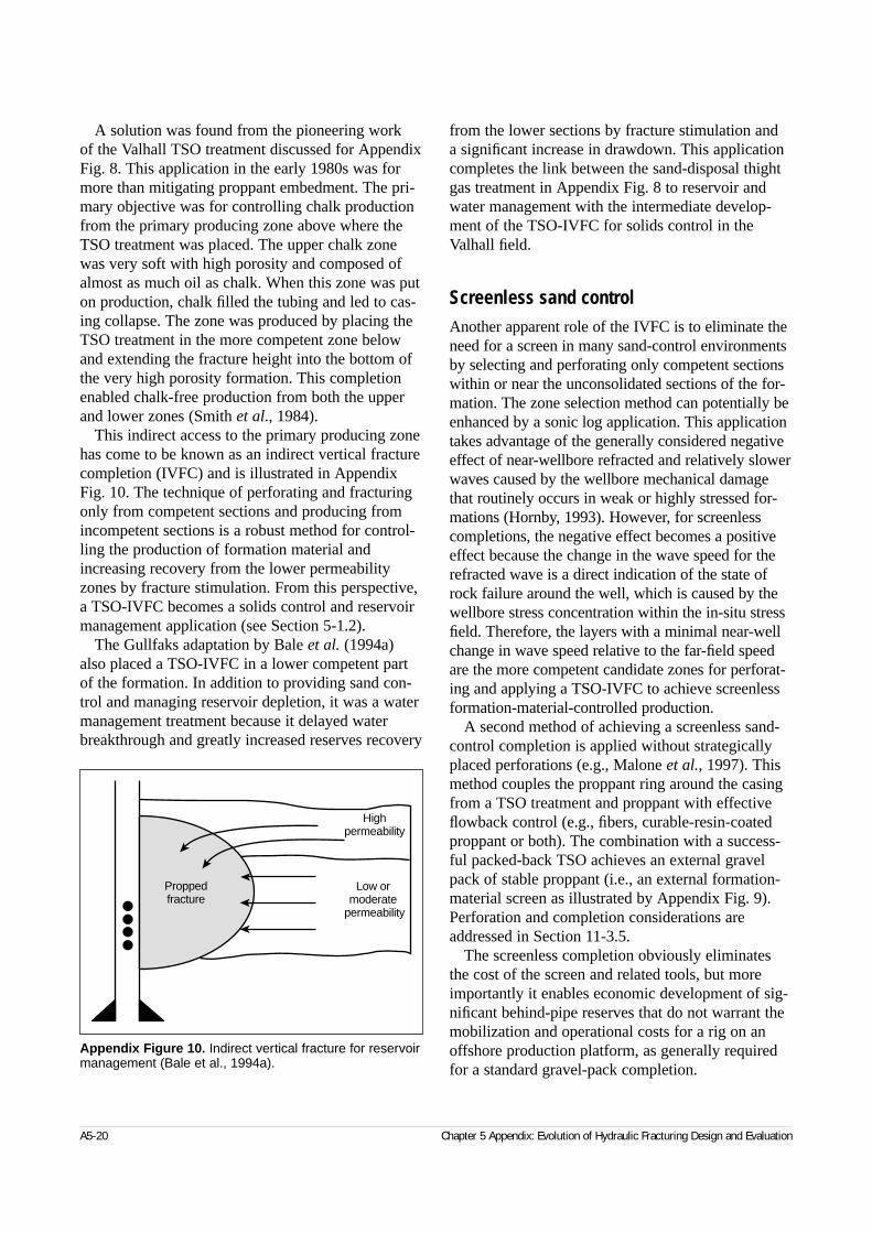
A solution was found from the pioneering work of the Valhall TSO treatment discussed for AppendixFig. 8. This application in the early 1980s was formore than mitigating proppant embedment. The pri-mary objective was for controlling chalk productionfrom the primary producing zone above where theTSO treatment was placed. The upper chalk zonewas very soft with high porosity and composed ofalmost as much oil as chalk. When this zone was puton production, chalk filled the tubing and led to cas-ing collapse. The zone was produced by placing theTSO treatment in the more competent zone belowand extending the fracture height into the bottom ofthe very high porosity formation. This completionenabled chalk-free production from both the upperand lower zones (Smith et al., 1984).

This indirect access to the primary producing zonehas come to be known as an indirect vertical fracturecompletion (IVFC) and is illustrated in AppendixFig. 10. The technique of perforating and fracturingonly from competent sections and producing fromincompetent sections is a robust method for control-ling the production of formation material andincreasing recovery from the lower permeabilityzones by fracture stimulation. From this perspective,a TSO-IVFC becomes a solids control and reservoirmanagement application (see Section 5-1.2).

The Gullfaks adaptation by Bale et al. (1994a)also placed a TSO-IVFC in a lower competent partof the formation. In addition to providing sand con-trol and managing reservoir depletion, it was a watermanagement treatment because it delayed waterbreakthrough and greatly increased reserves recovery

from the lower sections by fracture stimulation and a significant increase in drawdown. This applicationcompletes the link between the sand-disposal thightgas treatment in Appendix Fig. 8 to reservoir andwater management with the intermediate develop-ment of the TSO-IVFC for solids control in theValhall field.

Screenless sand controlAnother apparent role of the IVFC is to eliminate theneed for a screen in many sand-control environmentsby selecting and perforating only competent sectionswithin or near the unconsolidated sections of the for-mation. The zone selection method can potentially beenhanced by a sonic log application. This applicationtakes advantage of the generally considered negativeeffect of near-wellbore refracted and relatively slowerwaves caused by the wellbore mechanical damagethat routinely occurs in weak or highly stressed for-mations (Hornby, 1993). However, for screenlesscompletions, the negative effect becomes a positiveeffect because the change in the wave speed for therefracted wave is a direct indication of the state ofrock failure around the well, which is caused by thewellbore stress concentration within the in-situ stressfield. Therefore, the layers with a minimal near-wellchange in wave speed relative to the far-field speedare the more competent candidate zones for perforat-ing and applying a TSO-IVFC to achieve screenlessformation-material-controlled production.

A second method of achieving a screenless sand-control completion is applied without strategicallyplaced perforations (e.g., Malone et al., 1997). Thismethod couples the proppant ring around the casingfrom a TSO treatment and proppant with effectiveflowback control (e.g., fibers, curable-resin-coatedproppant or both). The combination with a success-ful packed-back TSO achieves an external gravelpack of stable proppant (i.e., an external formation-material screen as illustrated by Appendix Fig. 9).Perforation and completion considerations areaddressed in Section 11-3.5.

The screenless completion obviously eliminatesthe cost of the screen and related tools, but moreimportantly it enables economic development of sig-nificant behind-pipe reserves that do not warrant themobilization and operational costs for a rig on anoffshore production platform, as generally requiredfor a standard gravel-pack completion.

A5-20 Chapter 5 Appendix: Evolution of Hydraulic Fracturing Design and Evaluation

Appendix Figure 10. Indirect vertical fracture for reservoirmanagement (Bale et al., 1994a).

Proppedfracture

Highpermeability

Low or moderate

permeability

A future generation: fracturing andreservoir engineering merger?The previous discussion of the TSO generation clearlyshows the blurring of what can be controlled on theinside and outside of the casing and of what havebeen the traditional roles of a fracture design engineerand a reservoir engineer. This blurring of past distinc-tions provides prospects for additional innovationsand the advent of a fourth fracturing generation.

Optimal reservoir plumbingFrom a broader viewpoint, the IVFC and strategicallyplaced perforations provide the means to extend opti-mized plumbing into the reservoir. Optimized plumb-ing, through a NODAL analysis, is generally practicedonly for the surface facilities and within the wellbore.Extended optimization requires additional considera-tions for designing the plumbing system provided bythe fracture in the reservoir and also within the frac-ture itself.

The outline for these considerations was defined byBale et al. (1994b) for the Gullfaks application. Theyconsidered the role of the permeable fracture plane onthe reservoir’s 3D flow pattern and how tailoring thedistribution of conductivity can advantageously affectthis flow pattern (e.g., reducing the conductivity as thefracture approaches the high-permeability upper zoneto delay water production while increasing the con-ductivity in the lower permeability zone and applyinga large drawdown to accelerate production from thiszone; see Section 5-1.2). Therefore, the analysis anddesign tools have evolved for considering the role offractures in NODAL analysis for reservoir, formationmaterial and water management.

Achieving full potential for horizontal wells and laterals The preceding discussion of the IVFC is in the con-text of single, essentially vertical wells. The potentialfor innovative strategies to drain a reservoir increasesseveral fold by adding consideration of horizontal andlateral wells. These highly deviated wellbores are typ-ically placed without cemented casing because of eco-nomic considerations and therefore do not generallyreach their full potential because they lack an effectivetechnique to remove wellbore damage. The solution

of using cemented casing for effective treatmentdiversion tends to be overlooked because of an appar-ent failure to appreciate lifecycle economics or theeffectiveness of good cementing techniques (seeChapter 11). Staged fracturing, from correctly placedperforated sections, enables highly effective damagebypass, as demonstrated by the first fracturing genera-tion’s rate of 100 treatments per day in 1955.

The general benefit for a horizontal well, particularlywith vertical variations of permeability, is magnifiedby the fracture adding a large vertical permeabilitycomponent (see Chapters 11 and 12). Simply stated, an extended reach well cannot drain what it is not con-nected to nor can it efficiently drain what it is isolatedfrom by wellbore damage. The addition of a verticalfracture allows efficient drainage of all isolated sec-tions that the propped fracture reaches. The location of the fracture, or plumbing source, can be specified bycorrectly placed perforations within a cemented casingand an effective fracture design and execution. Casedhole logging and logging while drilling can be used to identify IVFC target locations for connection to by-passed reserves and management for their exploitation.

Fracturing for well testingThe after-closure portion of Appendix Fig. 7, labeled“transient reservoir pressure near wellbore,” shows thereturn of the fracturing pressure to the reservoir pres-sure and demonstrates the well testing potential forany injection above fracturing pressure. This potentialfor a fracture is ensured by the well-known result thatthe long-term reservoir response is pseudoradial flow(e.g., Cinco-Ley and Samaniego-V., 1981b) and is thesame flow regime used for standard well testing. Anattractive aspect of the use of fracturing for testing isthat the fracture enhances the likelihood that all thezones are open and captured by the test. This is animportant consideration for layered formations andparticularly thinly layered zones that can be missed by open perforations. Another attraction of fracturingor injection testing is that the wellbore is generallyfilled with water that provides minimal wellbore stor-age and formation volume factor effects.

The long-term radial response following fractureclosure was developed and presented in a pair ofpapers: Gu et al. (1993) from the application perspec-tive and Abousleiman et al. (1994) from the theoreti-cal perspective. They recognized that the radial

Reservoir Stimulation A5-21

response from fracture injection met the assumptionsfor a slug (or equivalently an impulse) test and thatthey could directly apply this developed area of reser-voir technology.

Another well-known flow regime for a fracture ispseudolinear flow. Incorporating the analysis of thisafter-closure flow regime was the last link of the frac-turing–pressure analysis chain between the beginningof injection and returning to reservoir pressure.Consideration of this regime by Nolte et al. (1997)indicated that the reservoir “memory” of the fractur-ing event can validate several aspects for analysis ofa calibration treatment (e.g., closure time and hencethe critical closure pressure, fracture length and hencethe fluid-loss coefficient, and the division of fluid lossbetween normal wall diffusion and tip spurt). Quan-

tifying spurt loss is particularly important for high-permeability formations and is not practically attain-able by any other means than after-closure analysis.The after-closure analyses are presented in Section 9-6, and a method to quantify reservoir parametersduring the closure period is presented in Section 2-8.

These applications from the reservoir behavior offracturing complement the 1979 adoption of reservoirmethodologies and achieve a direct merging of frac-turing into the classic realm of reservoir testing andcharacterization (see Chapters 2 and 12). Reservoircharacterization from a calibration testing sequence to define fracturing parameters provides the ingredi-ents essential for on-site, economics-based treatmentoptimization.

A5-22 Chapter 5 Appendix: Evolution of Hydraulic Fracturing Design and Evaluation

6-1. IntroductionThe mechanics of hydraulic fracturing is a convenientdescription of the processes and mechanisms that areimportant to fracturing technology. Mechanics gener-ally refers to an engineering discipline that is con-cerned with the mechanical properties of the materialunder consideration and the response of that materialto the physical forces of its environment. Hydraulicfracturing is complicated because it involves four dif-ferent types of mechanics: fluid, solid, fracture andthermal. In fracturing, fluid mechanics describes theflow of one, two or three phases within the fracture;solid mechanics describes the deformation or openingof the rock because of the fluid pressure; fracturemechanics describes all aspects of the failure andparting that occur near the tip of the hydraulic frac-ture; and thermal mechanics describes the exchangeof heat between the fracturing fluid and the forma-tion. Furthermore, the responses are coupled anddepend on each other. To develop tools for the designand analysis of a process as complicated as hydraulicfracturing, it is necessary to build models thatdescribe each of the responses sufficiently. This chap-ter describes the history and technology associatedwith these models.

A model of a process is a representation that cap-tures the essential features of the process in a mannerthat provides an understanding of the process (Star-field et al., 1990). The construction of the modeldepends on the type of question it is required toanswer. The three main types of models are physical,empirical and mechanistic (or analytic). Each hasadvantages and disadvantages, which are outlined in the following.

• Physical models are scale models of actualprocesses. The primary advantage of such modelsis that, by definition, they incorporate the correctassumptions of material behavior. For example, if a fracturing fluid is pumped between a pair of par-

allel rock faces with roughness comparable to frac-tured rock, no assumptions need to be made abouthow the fluid behaves rheologically. Instead, how it behaves is simply observed. Unfortunately, phys-ical models are usually expensive to build and use.

In addition, there are major issues of scale-up ifthe model is significantly smaller than the actualstructure. For example, in a model of a bridge, theweight is proportional to the scale factor cubed,but the length of any element is proportional onlyto the scale factor. Thus, even elements that do not fail in the model may fail in practice. Never-theless, scale models are useful provided an appro-priate dimensional analysis is performed and if thescale factor is not too great (de Pater et al., 1993).

• Empirical models are developed by observation.Typically, laboratory or field data are gathered andcombined to create design charts or empiricalequations, which can then be used to predict ordesign future cases. For example, if 100 wells in an area have been fractured with different-sizetreatments, 6 months of cumulative productioncould be plotted against treatment size. Providedthe scatter is not too great, the production responsefrom a new treatment can be predicted from thehistorical data.

The advantages of empirical models are that noassumptions need to be made about any behaviorand there is no scale effect. The primary disadvan-tage is low confidence in extrapolation outside therange of the data. The 100-well data set may beuseful in the same field, even for treatments slightlylarger than any in the data set, but is most likelyirrelevant in another area. For an empirical modelto be useful, the data must be arranged in terms of suitable dimensionless variables, so that it is as general as possible. For example, the 100-welldata set may be useful in a different area providedthe results are normalized with respect to perme-ability and pay thickness. To obtain the right

Reservoir Stimulation 6-1

◆

Mechanics of Hydraulic Fracturing

Mark G. Mack, Schlumberger DowellNorman R. Warpinski, Sandia National Laboratories

dimensionless quantities, however, it is generallynecessary to have at least some understanding ofthe mechanics of the physical process being modeled.

• Analytical models are mathematical representationsof a physical reality in which the governing mech-anics are stated in the form of equations. The equa-tions typically define both physical laws, such asconservation of mass, and constitutive laws, such as elasticity. The former are inviolable laws ofnature, whereas the latter are hypotheses of physicalbehavior that require laboratory work to confirmthat they are applicable and to determine the con-stants in the model.

The major advantages of analytical models arethat they may be extrapolated outside the range inwhich they were developed, provided the variouscomponent laws still hold. Thus, if the elastic con-stant of a spring has been measured, the forcerequired for a given displacement of the spring canbe predicted, even for displacements that have notbeen tested. If the spring is cut in half, the behaviorof each half can be predicted. Perhaps the greatestlimitation of analytical models, however, is theassumptions that are made in developing the model.For example, it is typically assumed that rock ishomogeneous, yet there are many cases where it isfractured or otherwise variable from point to point,and this may not be accounted for in the model.

A simulator is a computational implementation of a model. Many analytical models are tractable only ifthey are solved numerically, unless a large number ofapproximations or simplifying assumptions are made.With the widespread availability of computers, it isnow generally accepted that better answers may beobtained by numerically solving a more general modelrather than by solving a simplified model exactly.Nevertheless, it must be emphasized that useful rulesof thumb and relations between quantities can oftenbe developed much more easily using analytic solu-tions, which provide insight into the relations betweenparameters affecting the results for more complexconditions. Some of the simplest rules would probablynot be “discovered” from a numerical solution withouta great deal of effort, if at all. An extensive presenta-tion of analytic-based solutions and approximationsfor the mechanics of hydraulic fracturing was providedby Valkó and Economides (1996).

Four important reasons for developing and usingmodels of hydraulic fracture treatments are to

• perform economic optimization (i.e., determinewhat size treatment provides the highest rate ofreturn on investment)

• design a pump schedule

• simulate the fracture geometry and proppant place-ment achieved by a specified pump schedule

• evaluate a treatment (by comparing the predictionsof a model with actual behavior).

In each of these cases, the objective is a quantitativeestimate of either the volume of fluid and proppantrequired to create a fracture with a desired conduc-tivity and geometry or the geometry produced by aspecified pump schedule.

6-2. History of early hydraulic fracture modeling

6-2.1. Basic fracture modelingSneddon (1946) and Sneddon and Elliot (1946) devel-oped the solutions for the stress field and pressureassociated with static pressurized cracks. Theyshowed that the width of a static penny-shaped (i.e.,circular) crack of radius R under constant pressure isgiven by the expression

(6-1)

which describes an ellipsoid, and the volume of thecrack V by

(6-2)

where the net pressure pnet is defined as the pressure inthe crack minus the stress against which it opens, ν isPoisson’s ratio, and E is Young’s modulus. Sack(1946) showed that the pressure required to extend acrack of radius R under constant pressure is given by

(6-3)

where γF is the specific fracture surface energy.Equations 6-1 and 6-2 are derived using the theory of linear elasticity, and Eq. 6-3 is derived using linearelastic fracture mechanics. The basis of Eq. 6-3 is thatthe energy required to create the surface area when acrack is propagated must equal the work done by the

6-2 Mechanics of Hydraulic Fracturing

w rp R

Er Rnet( ) =

−( )− ( )8 1

12

2νπ

( ,

VR

Epnet=

−( )16 1

3

2 3ν,

pE

RnetF=

−( )πγ

ν2 1 2,

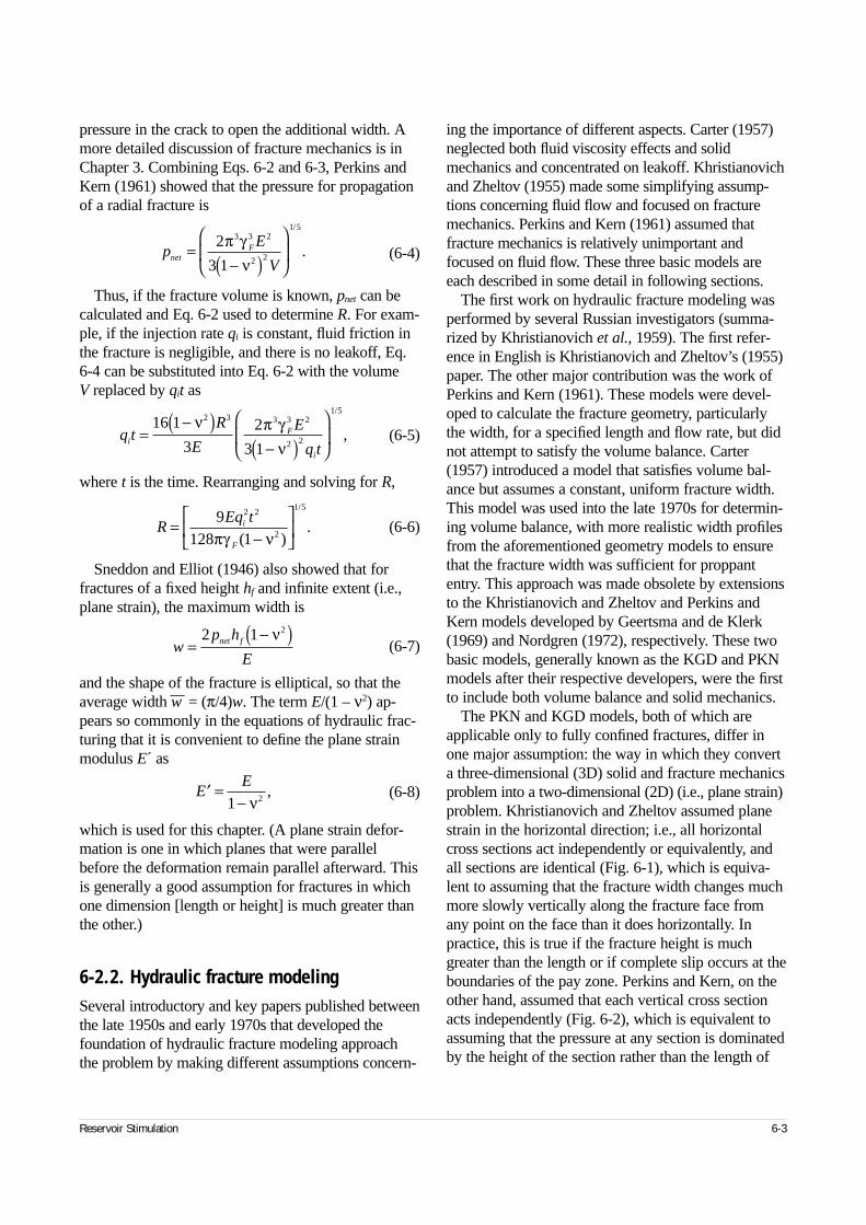
pressure in the crack to open the additional width. Amore detailed discussion of fracture mechanics is inChapter 3. Combining Eqs. 6-2 and 6-3, Perkins andKern (1961) showed that the pressure for propagationof a radial fracture is

(6-4)

Thus, if the fracture volume is known, pnet can becalculated and Eq. 6-2 used to determine R. For exam-ple, if the injection rate qi is constant, fluid friction inthe fracture is negligible, and there is no leakoff, Eq.6-4 can be substituted into Eq. 6-2 with the volume V replaced by qit as

(6-5)

where t is the time. Rearranging and solving for R,

(6-6)

Sneddon and Elliot (1946) also showed that forfractures of a fixed height hf and infinite extent (i.e.,plane strain), the maximum width is

(6-7)

and the shape of the fracture is elliptical, so that theaverage width w— = (π/4)w. The term E/(1 – ν2) ap-pears so commonly in the equations of hydraulic frac-turing that it is convenient to define the plane strainmodulus E´ as

(6-8)

which is used for this chapter. (A plane strain defor-mation is one in which planes that were parallelbefore the deformation remain parallel afterward. Thisis generally a good assumption for fractures in whichone dimension [length or height] is much greater thanthe other.)

6-2.2. Hydraulic fracture modelingSeveral introductory and key papers published betweenthe late 1950s and early 1970s that developed thefoundation of hydraulic fracture modeling approachthe problem by making different assumptions concern-

ing the importance of different aspects. Carter (1957)neglected both fluid viscosity effects and solidmechanics and concentrated on leakoff. Khristianovichand Zheltov (1955) made some simplifying assump-tions concerning fluid flow and focused on fracturemechanics. Perkins and Kern (1961) assumed thatfracture mechanics is relatively unimportant andfocused on fluid flow. These three basic models areeach described in some detail in following sections.

The first work on hydraulic fracture modeling wasperformed by several Russian investigators (summa-rized by Khristianovich et al., 1959). The first refer-ence in English is Khristianovich and Zheltov’s (1955)paper. The other major contribution was the work ofPerkins and Kern (1961). These models were devel-oped to calculate the fracture geometry, particularlythe width, for a specified length and flow rate, but didnot attempt to satisfy the volume balance. Carter(1957) introduced a model that satisfies volume bal-ance but assumes a constant, uniform fracture width.This model was used into the late 1970s for determin-ing volume balance, with more realistic width profilesfrom the aforementioned geometry models to ensurethat the fracture width was sufficient for proppantentry. This approach was made obsolete by extensionsto the Khristianovich and Zheltov and Perkins andKern models developed by Geertsma and de Klerk(1969) and Nordgren (1972), respectively. These twobasic models, generally known as the KGD and PKNmodels after their respective developers, were the firstto include both volume balance and solid mechanics.

The PKN and KGD models, both of which areapplicable only to fully confined fractures, differ inone major assumption: the way in which they converta three-dimensional (3D) solid and fracture mechanicsproblem into a two-dimensional (2D) (i.e., plane strain)problem. Khristianovich and Zheltov assumed planestrain in the horizontal direction; i.e., all horizontalcross sections act independently or equivalently, andall sections are identical (Fig. 6-1), which is equiva-lent to assuming that the fracture width changes muchmore slowly vertically along the fracture face fromany point on the face than it does horizontally. Inpractice, this is true if the fracture height is muchgreater than the length or if complete slip occurs at theboundaries of the pay zone. Perkins and Kern, on theother hand, assumed that each vertical cross sectionacts independently (Fig. 6-2), which is equivalent toassuming that the pressure at any section is dominatedby the height of the section rather than the length of

Reservoir Stimulation 6-3

pE

Vnet

F=−( )

2

3 1

3 3 2

2 2

1 5

π γν

/

.

q tR

E

E

q ti

F

i

=−( )

−( )

16 1

32

3 1

2 3 3 3 2

2 2

1 5

ν π γν

/

,

REq ti

F

=−

9128 1

2 2

2

1 5

πγ ν( ).

/

wp h

Enet f=

−( )2 1 2ν

′ =−

EE

1 2ν,

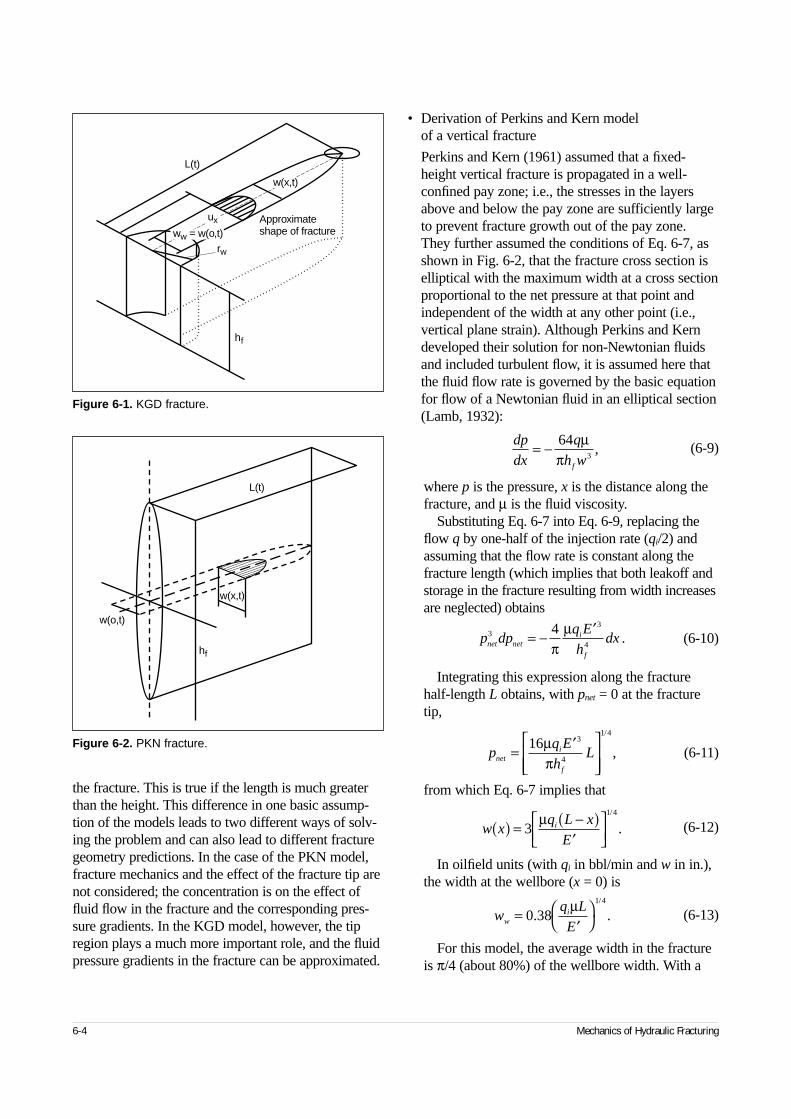
6-4 Mechanics of Hydraulic Fracturing

the fracture. This is true if the length is much greaterthan the height. This difference in one basic assump-tion of the models leads to two different ways of solv-ing the problem and can also lead to different fracturegeometry predictions. In the case of the PKN model,fracture mechanics and the effect of the fracture tip arenot considered; the concentration is on the effect offluid flow in the fracture and the corresponding pres-sure gradients. In the KGD model, however, the tipregion plays a much more important role, and the fluidpressure gradients in the fracture can be approximated.

• Derivation of Perkins and Kern model of a vertical fracture

Perkins and Kern (1961) assumed that a fixed-height vertical fracture is propagated in a well-confined pay zone; i.e., the stresses in the layersabove and below the pay zone are sufficiently largeto prevent fracture growth out of the pay zone.They further assumed the conditions of Eq. 6-7, asshown in Fig. 6-2, that the fracture cross section iselliptical with the maximum width at a cross sectionproportional to the net pressure at that point andindependent of the width at any other point (i.e.,vertical plane strain). Although Perkins and Kerndeveloped their solution for non-Newtonian fluidsand included turbulent flow, it is assumed here thatthe fluid flow rate is governed by the basic equationfor flow of a Newtonian fluid in an elliptical section(Lamb, 1932):

(6-9)

where p is the pressure, x is the distance along thefracture, and µ is the fluid viscosity.

Substituting Eq. 6-7 into Eq. 6-9, replacing theflow q by one-half of the injection rate (qi/2) andassuming that the flow rate is constant along thefracture length (which implies that both leakoff andstorage in the fracture resulting from width increasesare neglected) obtains

(6-10)

Integrating this expression along the fracturehalf-length L obtains, with pnet = 0 at the fracturetip,

(6-11)

from which Eq. 6-7 implies that

(6-12)

In oilfield units (with qi in bbl/min and w in in.),the width at the wellbore (x = 0) is

(6-13)

For this model, the average width in the fractureis π/4 (about 80%) of the wellbore width. With a

Figure 6-1. KGD fracture.

L(t)

hf

rw

w(x,t)

ux

ww = w(o,t)Approximateshape of fracture

Figure 6-2. PKN fracture.

L(t)

hf

w(o,t)

w(x,t)

dp

dx

q

h wf

= − 643

µπ

,

p dpq E

hdxnet net

i

f

33

4

4= − ′π

µ.

pq E

hLnet

i

f

= ′

16 3

4

1 4

µπ

/

,

w xq L x

Ei( ) = −( )

′

31 4µ /

.

wq L

Ewi=

′

0 38

1 4

. ./µ

Newtonian fluid, the model width is independent ofthe fracture height.

Perkins and Kern (1961) noted that the averagenet pressure in the fracture would greatly exceedthe minimum pressure for propagation, calculatedby an equation similar to Eq. 6-4, unless the fluidflow rate was extremely small or the fluid had anunrealistically low viscosity. Thus, under typicalhydraulic fracturing conditions, the pressure result-ing from fluid flow is far larger than the minimumpressure required to extend a stationary fracture.This justifies neglecting fracture mechanics effectsin this model. Furthermore, they pointed out thatthe fracture would continue to extend after pump-ing stopped, until either leakoff limited furtherextension or the minimum pressure for fracturepropagation was reached.

Several important observations concern thissolution:

– assumption of plane strain behavior in the verti-cal direction

– demonstration that fracture toughness could beneglected, because the energy required to propa-gate the fracture was significantly less than thatrequired to allow fluid flow along the fracturelength

– assumption that leakoff and storage or volumechange in the fracture could be neglected

– assumption of fixed height

– no direct provision of fracture length as part ofthe solution.

• Inclusion of leakoff

Although Perkins and Kern (1961) suggested thattheir paper could be used in practical applications,they neglected both leakoff and storage of fluid inthe fracture. They assumed that some other methodwould be used to calculate the fracture length, suchas that proposed by Carter (1957).

Carter introduced the basic equation for leakoff,which is discussed in detail in Section 6-4. Theleakoff velocity uL at a point on the fracture wall is

(6-14)

where CL is the leakoff coefficient, t is the currenttime, and texp is the time at which point uL wasexposed. Carter introduced a simple mass balance:

(6-15)

where qL is the leakoff rate over the whole fractureand qf is the volume rate of storage in the fracture.If the fracture width w– is assumed to be constant inboth space and time, Eq. 6-15 can be written as

(6-16)

where Af is the fracture face area. Carter showedthat Eq. 6-16 can be rewritten as

(6-17)

Substituting Eq. 6-14 into Eq. 6-17 and usingLaplace transformations, he showed that this couldbe solved to obtain

(6-18)

where

(6-19)

The fracture wing length L as a function of timeis then obtained by dividing the area by twice thefracture height. Harrington and Hannah (1975)showed (see Sidebar 6A) that Eq. 6-18 could besimplified with little loss of accuracy to

(6-20)

which is much easier to work with for simple cal-culations.

Designs were performed by iterating between theCarter technique to obtain the fracture length as afunction of time (Eq. 6-19) and the Perkins andKern model to determine the width (Eq. 6-13) untila consistent solution was found, and then Eq. 6-11was used to determine the pressure.

Nordgren (1972) added leakoff and storage with-in the fracture (resulting from increasing width) tothe Perkins and Kern model, deriving what is nowknown as the PKN model. To add storage andleakoff, the equation of continuity (i.e., conserva-tion of mass) is added to the set of equations (6-7and 6-9) used by Perkins and Kern:

(6-21)

Reservoir Stimulation 6-5

uC

t tLL

exp

=−

,

q q qi L f= + ,

q u dA wA

ti L

A t

ff

f

= +∫20

( )

,∂∂

q u tA

d wA

ti L

tf f= − +∫2

0

( ) .λ∂∂λ

λ∂∂

Aq w

Ce S Sf

i

L

s= ( ) + −

4

21

2

2

π πerfc ,

SC t

wL= 2 π

.

Aq t

w C tfi

L

=+ 2 2

,

∂∂

∂∂

q

xq

A

tL+ + = 0,

where q is the volume flow rate through a crosssection, A is the cross-sectional area of the fracture(πwhf /4 for the PKN model), and qL is the volumerate of leakoff per unit length:

(6-22)

where uL is from Eq. 6-14. The cross-sectional areaA is not Af, the area of the fracture face. Substi-tuting for pressure in terms of width, similar to themethod of Perkins and Kern, Eq. 6-21 can be writ-ten as

(6-23)

Nordgren solved this equation numerically in adimensionless form to obtain the width and lengthas a function of time. The dimensionless time tD

used in the solution is defined by

(6-24)

Dimensionless time tD is a stronger function ofthe leakoff coefficient (CL

10/3) than time t1.Because Nordgren’s solution was ultimately

obtained numerically, it is not possible to express it analytically. However, some useful approxima-tions to the fracture geometry for the limiting casesof high and low efficiency can be obtained (seeSidebar 6B). These expressions provide usefulphysical insight into the behavior of fractures. Forexample, the equation for length when leakoff ishigh (i.e., low efficiency) indicates that the lengthis determined simply by a mass balance betweenleakoff and flow into the fracture; i.e., the lengthincreases just fast enough for the leakoff rate tobalance the inflow. Analytical extensions to thePKN model that include power law fluids andexplicit consideration of the efficiency between thebounding values of 0 and 1 can be obtained.

It is important to reemphasize that even for con-tained fractures, the PKN solution is valid onlywhen the fracture length is much greater than theheight. Typically, if the height is less than aboutone-third of the total (tip to tip) fracture length, theerror resulting from the plane strain assumption isnegligible.

6-6 Mechanics of Hydraulic Fracturing

6A. Approximation to the Carter equation for leakoff

Equation 6-20 was derived by assuming that the exposuretime texp in Eq. 6-14 is equal to t/2, for which integration givesthe volume lost per unit area of the fracture face as

(6A-1)

Harrington and Hannah (1975) introduced efficiency as:

(6A-2)

where Vf is the fracture volume, Vi is the volume of fluidinjected, and VL is the leaked-off volume, which in terms of Eq. 6-20 becomes

(6A-3)

or

(6A-4)

This approximation allows the efficiency η and S in Eq. 6-19to be related by

(6A-5)

or

(6A-6)

which also shows that S tends to 0 as the efficiency tends to 1 (negligible fluid loss) and that S tends to infinity for zeroefficiency (i.e., negligible fracture volume relative to the fluid-loss volume). An improved approximation for √2t is inChapter 9 (i.e., g0√t, where g0 is within 5% of 1.5 and varieswith efficiency).

u C t C tL L L= =2 2 2 .

η = =+

VV

VV V

f

i

f

f L

,

η =+

w

w C tL2 2

η =+

1

1 2 2C t wL

.

η =+

11 0 8. S

S = −1 25

1. ,

ηη

6B. Approximations to Nordgren’s equations

Nordgren (1972) derived two limiting approximations, forstorage-dominated, or high-efficiency (tD < 0.01), cases andfor leakoff-dominated, or low-efficiency (tD > 1.0), cases, withtD defined by Eq. 6-24. They are useful for quick estimates offracture geometry and pressure within the limits of theapproximations. Both limiting solutions overestimate both thefracture length and width (one neglects fluid loss and theother neglects storage in the fracture), although within thestated limits on tD, the error is less than 10%.

The storage-dominated (η → 1) approximation is

(6B-1)

(6B-2)

and the high-leakoff (η → 0) approximation is

(6B-3)

(6B-4)

Equation 6B-3 could also be obtained from the approxima-tion in Sidebar 6A, with the fracture width set to zero and2√2t replaced by π√t, which is more correct. Once the widthis determined from Eq. 6B-2 or 6B-4, the pressure can befound from Eq. 6-7.

L tE q

hti

f

( ) =′

0 39

3

4

1 5

4 5./

/

µ

wq

E htw

i

f

=′

2 18

21 5

1 5. ,/

/µ

L tq t

C hi

L f

( ) =1 2

2

/

π

wq

E C htw

i

L f

=′

4

2

3

1 4

1 8µπ

/

/ .

q h uL f L= 2 ,

′ =− ( )

+E

h

w

x

C

t t x

w

tf

L

exp128

82 4

2µ∂∂ π

∂∂

.

tC E h

qtD

L f

i

=′

64 5

3 2

2 3

π µ

/

.

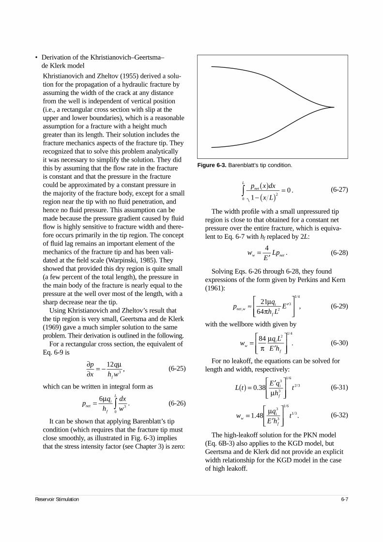
• Derivation of the Khristianovich–Geertsma–de Klerk model

Khristianovich and Zheltov (1955) derived a solu-tion for the propagation of a hydraulic fracture byassuming the width of the crack at any distancefrom the well is independent of vertical position(i.e., a rectangular cross section with slip at theupper and lower boundaries), which is a reasonableassumption for a fracture with a height muchgreater than its length. Their solution includes thefracture mechanics aspects of the fracture tip. Theyrecognized that to solve this problem analyticallyit was necessary to simplify the solution. They didthis by assuming that the flow rate in the fracture is constant and that the pressure in the fracturecould be approximated by a constant pressure inthe majority of the fracture body, except for a smallregion near the tip with no fluid penetration, andhence no fluid pressure. This assumption can bemade because the pressure gradient caused by fluidflow is highly sensitive to fracture width and there-fore occurs primarily in the tip region. The conceptof fluid lag remains an important element of themechanics of the fracture tip and has been vali-dated at the field scale (Warpinski, 1985). Theyshowed that provided this dry region is quite small(a few percent of the total length), the pressure inthe main body of the fracture is nearly equal to thepressure at the well over most of the length, with asharp decrease near the tip.

Using Khristianovich and Zheltov’s result thatthe tip region is very small, Geertsma and de Klerk(1969) gave a much simpler solution to the sameproblem. Their derivation is outlined in the following.

For a rectangular cross section, the equivalent ofEq. 6-9 is

(6-25)

which can be written in integral form as

(6-26)

It can be shown that applying Barenblatt’s tipcondition (which requires that the fracture tip mustclose smoothly, as illustrated in Fig. 6-3) impliesthat the stress intensity factor (see Chapter 3) is zero:

(6-27)

The width profile with a small unpressured tipregion is close to that obtained for a constant netpressure over the entire fracture, which is equiva-lent to Eq. 6-7 with hf replaced by 2L:

(6-28)

Solving Eqs. 6-26 through 6-28, they foundexpressions of the form given by Perkins and Kern(1961):

(6-29)

with the wellbore width given by

(6-30)

For no leakoff, the equations can be solved forlength and width, respectively:

(6-31)

(6-32)

The high-leakoff solution for the PKN model(Eq. 6B-3) also applies to the KGD model, butGeertsma and de Klerk did not provide an explicitwidth relationship for the KGD model in the caseof high leakoff.

Reservoir Stimulation 6-7

∂∂

µp

x

q

h wf

= − 123

,

pq

h

dx

wneti

f

L

= ∫63

0

µ.

Figure 6-3. Barenblatt’s tip condition.

p x dx

x L

net

L ( )− ( )

=∫1

02

0

.

wE

Lpw net=′

4.

pq

h LEnet w

i

f

,

/

,≈ ′

2164 2

3

1 4

µπ

wq L

E hwi

f

=′

84 21 4

πµ

/

.

L tE q

hti

f

( ) = ′

0 383

3

1 6

2 3.

/

/

µ

wq

E htw

i

f

=′

1 483

3

1 6

1 3. .

/

/µ

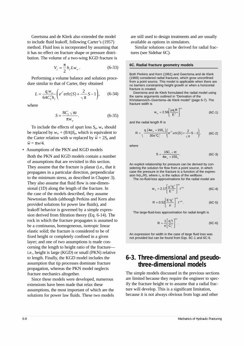
Geertsma and de Klerk also extended the modelto include fluid leakoff, following Carter’s (1957)method. Fluid loss is incorporated by assuming thatit has no effect on fracture shape or pressure distri-bution. The volume of a two-wing KGD fracture is

(6-33)

Performing a volume balance and solution proce-dure similar to that of Carter, they obtained

(6-34)

where

(6-35)

To include the effects of spurt loss Sp, ww shouldbe replaced by ww + (8/π)Sp, which is equivalent tothe Carter relation with w replaced by w– + 2Sp andw– = πw/4.

• Assumptions of the PKN and KGD models

Both the PKN and KGD models contain a numberof assumptions that are revisited in this section.They assume that the fracture is planar (i.e., that itpropagates in a particular direction, perpendicularto the minimum stress, as described in Chapter 3).They also assume that fluid flow is one-dimen-sional (1D) along the length of the fracture. In the case of the models described, they assumeNewtonian fluids (although Perkins and Kern alsoprovided solutions for power law fluids), andleakoff behavior is governed by a simple expres-sion derived from filtration theory (Eq. 6-14). Therock in which the fracture propagates is assumed tobe a continuous, homogeneous, isotropic linearelastic solid; the fracture is considered to be offixed height or completely confined in a givenlayer; and one of two assumptions is made con-cerning the length to height ratio of the fracture—i.e., height is large (KGD) or small (PKN) relativeto length. Finally, the KGD model includes theassumption that tip processes dominate fracturepropagation, whereas the PKN model neglectsfracture mechanics altogether.

Since these models were developed, numerousextensions have been made that relax theseassumptions, the most important of which are thesolutions for power law fluids. These two models

are still used to design treatments and are usuallyavailable as options in simulators.

Similar solutions can be derived for radial frac-tures (see Sidebar 6C).

6-3. Three-dimensional and pseudo-three-dimensional models

The simple models discussed in the previous sectionsare limited because they require the engineer to spec-ify the fracture height or to assume that a radial frac-ture will develop. This is a significant limitation,because it is not always obvious from logs and other

6-8 Mechanics of Hydraulic Fracturing

V h Lwf f w= π2

.

Lq w

C he S Si w

L f

s= ( ) + −

64

21

2

2

erfcπ

,

SC t

wL

w

= 8 ππ

.

6C. Radial fracture geometry models

Both Perkins and Kern (1961) and Geertsma and de Klerk(1969) considered radial fractures, which grow unconfinedfrom a point source. This model is applicable when there areno barriers constraining height growth or when a horizontalfracture is created.

Geertsma and de Klerk formulated the radial model usingthe same arguments outlined in “Derivation of theKhristianovich–Geertsma–de Klerk model” (page 6-7). Thefracture width is

(6C-1)

and the radial length R is

(6C-2)

where

(6C-3)

An explicit relationship for pressure can be derived by con-sidering the solution for flow from a point source, in whichcase the pressure in the fracture is a function of the expres-sion ln(rw/R), where rw is the radius of the wellbore.

The no-fluid-loss approximations for the radial model are

(6C-4)

(6C-5)

The large-fluid-loss approximation for radial length is

(6C-6)

An expression for width in the case of large fluid loss wasnot provided but can be found from Eqs. 6C-1 and 6C-6.

wq REw

i=′

2 561 4

./µ

Rq w S

Ce S S

i w p

L

s=+( ) ( ) + −

4 15

302

12 2

2

π πerfc ,

SC t

w SL

w p

=+

154 15

π.

wq

Etw

i=′

2 17

2 3

2

1 9

1 9./

/µ

RE q

ti=′

0 52

31 9

4 9. ./

/

µ

Rq tC

i

L

=

1 2

2

1 4

π

/

.

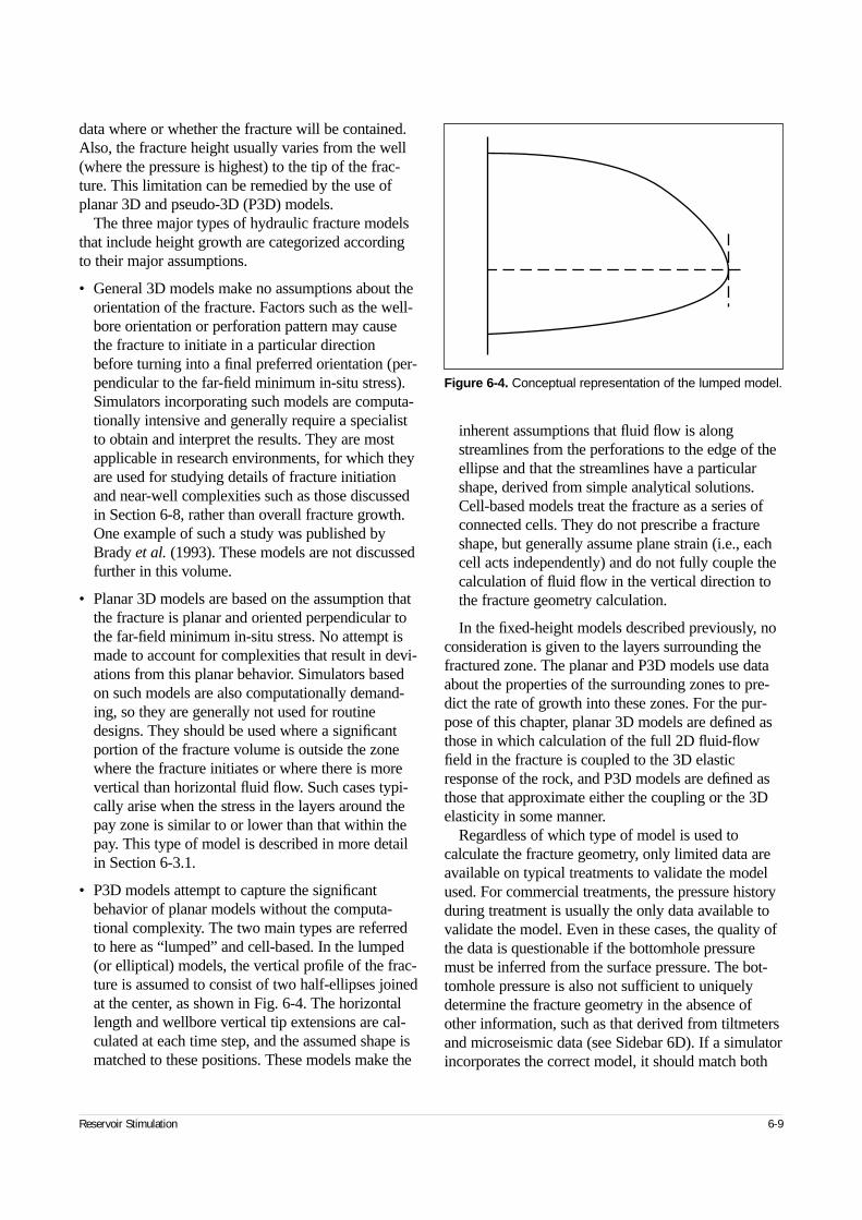
data where or whether the fracture will be contained.Also, the fracture height usually varies from the well(where the pressure is highest) to the tip of the frac-ture. This limitation can be remedied by the use ofplanar 3D and pseudo-3D (P3D) models.

The three major types of hydraulic fracture modelsthat include height growth are categorized accordingto their major assumptions.

• General 3D models make no assumptions about theorientation of the fracture. Factors such as the well-bore orientation or perforation pattern may causethe fracture to initiate in a particular directionbefore turning into a final preferred orientation (per-pendicular to the far-field minimum in-situ stress).Simulators incorporating such models are computa-tionally intensive and generally require a specialistto obtain and interpret the results. They are mostapplicable in research environments, for which theyare used for studying details of fracture initiationand near-well complexities such as those discussedin Section 6-8, rather than overall fracture growth.One example of such a study was published byBrady et al. (1993). These models are not discussedfurther in this volume.

• Planar 3D models are based on the assumption thatthe fracture is planar and oriented perpendicular tothe far-field minimum in-situ stress. No attempt ismade to account for complexities that result in devi-ations from this planar behavior. Simulators basedon such models are also computationally demand-ing, so they are generally not used for routinedesigns. They should be used where a significantportion of the fracture volume is outside the zonewhere the fracture initiates or where there is morevertical than horizontal fluid flow. Such cases typi-cally arise when the stress in the layers around thepay zone is similar to or lower than that within thepay. This type of model is described in more detailin Section 6-3.1.

• P3D models attempt to capture the significantbehavior of planar models without the computa-tional complexity. The two main types are referredto here as “lumped” and cell-based. In the lumped(or elliptical) models, the vertical profile of the frac-ture is assumed to consist of two half-ellipses joinedat the center, as shown in Fig. 6-4. The horizontallength and wellbore vertical tip extensions are cal-culated at each time step, and the assumed shape ismatched to these positions. These models make the

inherent assumptions that fluid flow is alongstreamlines from the perforations to the edge of theellipse and that the streamlines have a particularshape, derived from simple analytical solutions.Cell-based models treat the fracture as a series ofconnected cells. They do not prescribe a fractureshape, but generally assume plane strain (i.e., eachcell acts independently) and do not fully couple thecalculation of fluid flow in the vertical direction tothe fracture geometry calculation.

In the fixed-height models described previously, noconsideration is given to the layers surrounding thefractured zone. The planar and P3D models use dataabout the properties of the surrounding zones to pre-dict the rate of growth into these zones. For the pur-pose of this chapter, planar 3D models are defined asthose in which calculation of the full 2D fluid-flowfield in the fracture is coupled to the 3D elasticresponse of the rock, and P3D models are defined asthose that approximate either the coupling or the 3Delasticity in some manner.

Regardless of which type of model is used tocalculate the fracture geometry, only limited data areavailable on typical treatments to validate the modelused. For commercial treatments, the pressure historyduring treatment is usually the only data available tovalidate the model. Even in these cases, the quality ofthe data is questionable if the bottomhole pressuremust be inferred from the surface pressure. The bot-tomhole pressure is also not sufficient to uniquelydetermine the fracture geometry in the absence ofother information, such as that derived from tiltmetersand microseismic data (see Sidebar 6D). If a simulatorincorporates the correct model, it should match both

Reservoir Stimulation 6-9

Figure 6-4. Conceptual representation of the lumped model.

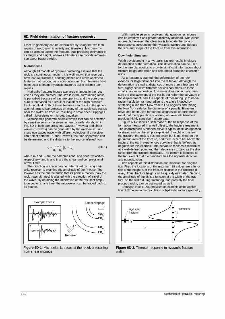
6-10 Mechanics of Hydraulic Fracturing

6D. Field determination of fracture geometry

Fracture geometry can be determined by using the two tech-niques of microseismic activity and tiltmeters. Microseismscan be used to locate the fracture, thus providing estimates ofits length and height, whereas tiltmeters can provide informa-tion about fracture width.

Microseisms

Although all models of hydraulic fracturing assume that therock is a continuous medium, it is well known that reservoirshave natural fractures, bedding planes and other weaknessfeatures that respond as a noncontinuum. Such features havebeen used to image hydraulic fractures using seismic tech-niques.

Hydraulic fractures induce two large changes in the reser-voir as they are created. The stress in the surrounding rocksis perturbed because of fracture opening, and the pore pres-sure is increased as a result of leakoff of the high-pressurefracturing fluid. Both of these features can result in the gener-ation of large shear stresses on many of the weakness planesnear the hydraulic fracture, resulting in small shear slippagescalled microseisms or microearthquakes.

Microseisms generate seismic waves that can be detectedby sensitive seismic receivers in nearby wells. As shown inFig. 6D-1, both compressional waves (P-waves) and shearwaves (S-waves) can be generated by the microseism, andthese two waves travel with different velocities. If a receivercan detect both the P- and S-waves, the time separation canbe determined and the distance to the source inferred from

(6D-1)

where uP and uS are the compressional and shear velocities,respectively, and tS and tP are the shear and compressionalarrival times.

The direction in space can be determined by using a tri-axial receiver to examine the amplitude of the P-wave. The P-wave has the characteristic that its particle motion (how therock mass vibrates) is aligned with the direction of travel ofthe wave. By obtaining the orientation of the resultant ampli-tude vector at any time, the microseism can be traced back toits source.

With multiple seismic receivers, triangulation techniquescan be employed and greater accuracy obtained. With eitherapproach, however, the objective is to locate the zone ofmicroseisms surrounding the hydraulic fracture and deducethe size and shape of the fracture from this information.

Downhole tiltmeters

Width development in a hydraulic fracture results in elasticdeformation of the formation. This deformation can be usedfor fracture diagnostics to provide significant information aboutfracture height and width and also about formation character-istics.

As a fracture is opened, the deformation of the rockextends for large distances into the reservoir. Although thedeformation is small at distances of more than a few tens offeet, highly sensitive tiltmeter devices can measure thesesmall changes in position. A tiltmeter does not actually mea-sure the displacement of the earth, but rather the curvature ofthe displacement, and it is capable of measuring up to nano-radian resolution (a nanoradian is the angle induced bystretching a line from New York to Los Angeles and raisingthe New York side by the diameter of a pencil). Tiltmetershave long been used for surface diagnostics of earth move-ment, but the application of a string of downhole tiltmetersprovides highly sensitive fracture data.

Figure 6D-2 shows a schematic of the tilt response of theformation measured in a well offset to the fracture treatment.The characteristic S-shaped curve is typical of tilt, as opposedto strain, and can be simply explained. Straight across fromthe fracture, the rock is pushed away, but is not tilted on thegeometric axis of the fracture, and there is zero tilt. Above thefracture, the earth experiences curvature that is defined asnegative for this example. The curvature reaches a maximumat a well-defined point and then decreases to zero as the dis-tance from the fracture increases. The bottom is identical tothe top, except that the curvature has the opposite directionand opposite sign.

Two aspects of this distribution are important for diagnos-tics. First, the locations of the maximum tilt values are a func-tion of the height hf of the fracture relative to the distance daway. Thus, fracture height can be quickly estimated. Second,the amplitude of the tilt is a function of the width of the frac-ture, so the width during fracturing, and possibly the finalpropped width, can be estimated as well.

Branagan et al. (1996) provided an example of the applica-tion of tiltmeters to the calculation of hydraulic fracture geometry.

du u

u ut tP S

P S

S P=−

−[ ] ,

Figure 6D-1. Microseismic traces at the receiver resultingfrom shear slippage.

Example traces

Receiver

Shear slippagex

y

S

S(t1)P(t1)

S(t2)

P(t2)

y x

P

Figure 6D-2. Tiltmeter response to hydraulic fracturewidth.

Hydraulicfracture

Tiltmeters

d

hf

treating pressure and fracture geometry. These issuesare addressed in Section 6-12 and Chapter 9.

6-3.1. Planar three-dimensional modelsA planar fracture is a narrow channel of variablewidth through which fluid flows. The fracture geome-try is defined by its width and the shape of its periph-ery (i.e., height at any distance from the well andlength). Both the width at any point and the overallshape vary with time. They depend on the pressuredistribution, which itself is determined by the pressuregradients caused by the fluid flow within the fracture.Because the relation between pressure gradient andflow rate is highly sensitive to the fracture width (Eq. 6-9), the geometry and fluid flow are tightly cou-pled. Although the mechanics of these processes aredescribed separately in this section, the complexity ofsolving any fracture model lies in the close couplingbetween the different processes. Three separate prob-lems are considered:

• width profile in a fracture of known shape and pres-sure distribution

• shape of the fracture

• flow of fluid in a fracture of known shape and width(i.e., known geometry).

Hirth and Lothe (1968) and Bui (1977) showedhow the pressure and width in a fracture may berelated. Basically, the width at any point (x,y) isdetermined by an integral of the net pressure over the entire fracture, expressed as

(6-36)

where σ is the stress.The details of the elastic influence function f in

Eq. 6-36 are beyond the scope of this volume. Use-able forms of Eq. 6-36 can be derived generally onlyfor homogeneous linear elastic materials (see Side-bar 6E). In fracturing applications, the rock is usuallyalso assumed to be isotropic.

The shape of the fracture evolves with time. Inessence, the boundary (i.e., the vertical and horizontaltips) moves outward as the fluid provides sufficientenergy to fracture the rock at the boundary. More com-plex tip behavior is discussed subsequently, but in this

section it is assumed that this process is described bylinear elastic fracture mechanics (LEFM). If the LEFMfailure criterion is exceeded at any point on the fractureperiphery, the fracture will extend until the criterion is again met. For simple shapes and pressure distribu-tions, such as ellipses under constant pressure, the cri-terion can be specified analytically, similar to Eq. 6-3.For more complex shapes and pressure distributions,analytical solutions are not available. In these cases,it can be shown that a relatively simple criterion can bewritten in terms of the width near the tip and the criti-cal stress intensity factor or fracture toughness KIc,which is introduced in Chapter 3:

(6-37)

where x is the distance measured from the tip. Rela-tions between fracture mechanics parameters such asthe specific surface energy (used in Eq. 6-3) and thefracture toughness are provided in Chapter 3.

The fluid flow is described by equations for conser-vation of mass (a general form of Eq. 6-21, includingthe density ρ and expressed in terms of velocity u):

(6-38)

which can be written as a vector equation:

(6-39)

and the conservation of momentum (a general form ofEq. 6-9) is

(6-40)

where τ is the shear stress and g– is the acceleration ofgravity.

The first two terms in Eq. 6-38 relate to the spatialchange of the mass-flow vector, and the second twoterms represent the storage resulting from widthincreases and leakoff, respectively. Equation 6-40 is a vector equation. The term on the left-hand side is therate of change of momentum, and the terms on theright-hand side are the pressure, viscous and gravita-tional forces, respectively. It simply states that a smallelement of fluid accelerates because of the forces act-ing on it. This equation can be expanded and then sim-plified for the geometries of interest in hydraulic frac-

Reservoir Stimulation 6-11

w x y f x x y y p x y x y dx dyS

( , ) ( , )( ( , ) ( , )) ,= − ′ − ′ ′ ′ − ′ ′ ′ ′∫∫ σ

w xK

ExIc( ) =

′4 2

π,

∂ ρ∂

∂ ρ∂

∂∂

ρ ρwu

x

wu

y tw ux y

L

( ) +( )

+ ( ) + =2 0,

∇ ⋅( ) + ( ) + =ρ ∂∂

ρ ρwut

w uL2 0,

ρ τ ρDu

Dtp g= −∇ − ∇ ⋅[ ] + ,

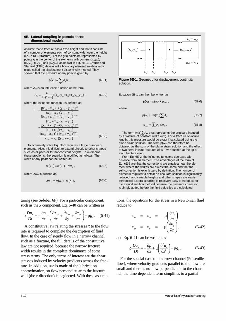
turing (see Sidebar 6F). For a particular component,such as the x component, Eq. 6-40 can be written as

(6-41)

A constitutive law relating the stresses τ to the flowrate is required to complete the description of fluidflow. In the case of steady flow in a narrow channelsuch as a fracture, the full details of the constitutivelaw are not required, because the narrow fracturewidth results in the complete dominance of somestress terms. The only terms of interest are the shearstresses induced by velocity gradients across the frac-ture. In addition, use is made of the lubricationapproximation, so flow perpendicular to the fracturewall (the z direction) is neglected. With these assump-

tions, the equations for the stress in a Newtonian fluidreduce to

(6-42)

and Eq. 6-41 can be written as

(6-43)

For the special case of a narrow channel (Poiseuilleflow), where velocity gradients parallel to the flow aresmall and there is no flow perpendicular to the chan-nel, the time-dependent term simplifies to a partial

6-12 Mechanics of Hydraulic Fracturing

6E. Lateral coupling in pseudo-three-dimensional models

Assume that a fracture has a fixed height and that it consists of a number of elements each of constant width over the height(i.e., a KGD fracture). Let the grid points be represented bypoints xi in the center of the elements with corners (xl,i,yb,i),(xl,i,yt,i), (xr,i,yt,i) and (xr,i,yb,i), as shown in Fig. 6E-1. Crouch andStarfield (1983) developed a boundary element solution tech-nique called the displacement discontinuity method. Theyshowed that the pressure at any point is given by

(6E-1)

where Aik is an influence function of the form

(6E-2)

where the influence function I is defined as

(6E-3)

To accurately solve Eq. 6E-1 requires a large number ofelements. Also, it is difficult to extend directly to other shapessuch as ellipses or for nonconstant heights. To overcomethese problems, the equation is modified as follows. Thewidth at any point can be written as

(6E-4)

where ∆wki is defined as

(6E-5)

Equation 6E-1 can then be written as

p(xi) = p(wi) + pcorr , (6E-6)

where

(6E-7)

(6E-8)

The term w(xi)ΣAik thus represents the pressure inducedby a fracture of constant width w(xi). For a fracture of infinitelength, this pressure would be exact if calculated using theplane strain solution. The term p(wi) can therefore beobtained as the sum of the plane strain solution and the effectof two semi-infinite fractures of w – wi attached at the tip ofeach fracture wing.

From Eq. 6E-2, the influence functions decrease withdistance from an element. The advantages of the form of Eq. 6E-8 are that the corrections are smallest near the ele-ment where the widths are almost the same and that the self-correction is exactly zero by definition. The number ofelements required to obtain an accurate solution is significantlyreduced, and variable heights and other shapes are easilyintroduced. Lateral coupling is relatively easy to introduce tothe explicit solution method because the pressure correction is simply added before the fluid velocities are calculated.

p x A wi ik k

k

( ) = ∑ ,

AG

I x y x x y yik c i c i l k r k b k t k=−( )4 1π ν

( , ; ; ) ,, , , , , ,

Ix x y y

x x y yx x y y

x x y yx x

c i r k c i t k

c i r k c i t k

c i l k c i t k

c i l k c i t k

c i l k

=− + −

− −

−+ + −

+ −

++ +

[( ) ( ) ]

( )( )[( ) ( ) ]

( )( )[( )

, , , ,/

, , , ,

, , , ,/

, , , ,

, ,

2 2 1 2

2 2 1 2

2 (( ) ]

( )( )[( ) ( ) ]

( )( ).

, ,/

, , , ,

, , , ,/

, , , ,

y y

x x y yx x y y

x x y y

c i b k

c i l k c i b k

c i r k c i b k

c i r k c i b k

++ +

−− + +

− +

2 1 2

2 2 1 2

w x w x wk i ki( ) = ( ) + ∆ ,

∆w w x w xki k i= ( ) − ( ) .

p w w x Ai i ik( ) = ( )∑p A wcorr ik ki= ∑ ∆ .

Figure 6E-1. Geometry for displacement continuitysolution.

yt,i = yt,k

yb,i = yb,k

xl,i xr,i xl,k xr,k

(xc,k,yc,k)(xc,i,yc,i)

ρ ∂∂

∂τ∂

∂τ∂

∂τ∂

ρDu

Dt

p

x x y zgx xx yx zx

x= − − + +

+ . τ τ µ ∂∂

τ τ µ∂∂

xz zxx

yz zyy

u

zu

z

= = −

= = −

,

ρ µ ρDu

Dt

p

x

u

zgx x

x= − ∂∂

+ ∂∂

+2

2.

Reservoir Stimulation 6-13

6F. Momentum conservation equation for hydraulic fracturing

Equation 6-40 is a vector equation, for which a componentcan be written as

(6F-1)

where u is the velocity, g is the gravitational acceleration, andi is x, y or z. The term on the left side of Eq. 6F-1 is termedthe substantial derivative, which is the rate of change seen byan observer moving with the fluid motion. It can be related tothe usual partial derivative (i.e., the rate of change seen by astationary observer) as

(6F-2)

Thus, Eq. 6F-2 can be expanded to

(6F-3)

This completely general equation can be simplified for anarrow channel in an impermeable medium. Leakoff does notoccur in this case, so components in the z direction can beneglected. In addition, the flow is assumed to be steady state,so time derivatives can be ignored. In this case, Eq. 6F-3 sim-plifies to

(6F-4)

for i = 1 or 2. Even for a permeable medium, Eq. 6F-4 isused. In this case, leakoff is treated as a sink term and included in the mass balance, but it is assumed not to affectthe equations relating pressure, stress and fluid velocity.

Newtonian fluids

To make Eq. 6F-4 useful, the stress components must bedetermined, which is done by assuming a model of fluidbehavior. For example, a Newtonian fluid is a model with oneparameter, the viscosity µ. The stress components are

(6F-5)

The first three components of Eq. 6F-5 are the normal stresses, and the last three are the shear stresses. The lastterm of the normal components is zero for incompressiblefluids. In the case of 1D flow between parallel plates, withoutleakoff, two of the velocity components are identically zero. In addition, conservation of mass implies that the third com-ponent cannot vary with position. Hence, all three normalcomponents are identically zero. The equations thus reduceto those for shear flow. Although these assumptions are notstrictly true in general, they are used for the flow calculationsin hydraulic fracture modeling. It can also be shown that for a narrow channel, the velocity gradients perpendicular to thewalls (the z direction) are much greater than those in the par-allel directions. Finally, therefore, the stress components for a Newtonian fluid in a hydraulic fracture can be written as

(6F-6)

Substituting Eq. 6F-6 into Eq. 6F-4 obtains

(6F-7)

For 1D flow along the fracture length, as typically assumed inP3D models, Eq. 6F-7 can be simplified to

(6F-8)

Assuming zero slip (i.e., zero velocity at the fracture wall), thesolution to Eq. 6F-8 is

(6F-9)

Integrating to obtain the average velocity across the channel,

(6F-10)

The flow rate per unit height is obtained by multiplying theaverage velocity by the width w.

In the case of 2D flow, the left-hand sides of Eq. 6F-7 arezero if inertia may be neglected. In this case for the y direc-tion, an equation can be formed similar to Eq. 6F-10, exceptthat it includes a gravitational term.

ρ ∂∂

∂τ∂

∂τ∂

∂τ∂

ρDuDt

px x y z

gi

i

xi yi zii= − − + +

+ ,

DDt t

ux

uy

uzx y z= ∂

∂+ ∂

∂+ ∂

∂+ ∂

∂.

ρ∂∂

∂∂

∂∂

∂∂

∂∂

∂τ∂

∂τ∂

∂τ∂

ρ

ut

uux

uuy

uuz

px x y z

g

ix

iy

iz

i

i

xi yi zii

+ + +

= − − + +

+ .

ρ∂∂

∂∂

∂∂

∂τ∂

∂τ∂

∂τ∂

ρ

uux

uuy

px x y z

g

xi

yi

i

xi yi zii

+

= − − + +

+ ,

τ µ µ

τ µ µ

τ µ µ

τ τ µ

τ τ µ

τ τ µ

xxx

yy

y

zzz

xy yxx y

yz zy

y z

zx xzz

ux

u

u

yu

uz

u

uy

u

x

u

zuy

u

= ∂∂

+ ∇ ⋅( )

=∂∂

+ ∇ ⋅( )

= ∂∂

+ ∇ ⋅( )

= = − ∂∂

+∂∂

= = −∂∂

+ ∂∂

= = − ∂

23

223

223

∂∂+ ∂

∂

x

uz

x .

ρ∂∂

∂∂

∂∂

µ∂∂

ρ∂∂

∂∂

∂∂

µ∂∂

ρ

uux

uuy

px

uz

uu

xu

u

ypy

u

zg

xx

yx x

x

y

y

y y

+

= − +

+

= − + +

2

2

2

2.

τ µ ∂∂

τ µ∂∂

zxx

zy

y

uz

u

z

= −

= −

.

∂∂ µ

∂∂

2

2

1uz

px

x = .

upx

z wx = − ( )( )12

22 2

µ∂∂

.

uw p

xx = − 2

12µ∂∂

.

derivative of velocity with respect to time. It is usuallyassumed that the flow is steady state, which finallyobtains

(6-44)

and a similar equation for the y component.Equations 6-36 through 6-44 summarize the planar

3D model for Newtonian fluids. Similar results can beobtained for non-Newtonian fluids (see Sidebar 6G).These equations are generally not amenable to ana-lytic solutions, but require a numerical simulation. In addition, although it is relatively straightforward to write the conceptual equations, efficient and robustnumerical solutions are difficult to obtain. The pri-mary reasons for this difficulty are the extremely close coupling of the different parts of the solution(e.g., fluid flow and solid deformation), the nonlinearrelation between width and pressure, and the com-plexity of a moving-boundary problem.

The first numerical implementation of a planarmodel was reported by Clifton and Abou-Sayed(1979). In essence, their approach was to define

a small fracture, initiated at the perforations, divide itinto a number of equal elements (typically 16 squares)and then begin solution of the equations. As theboundary extends, the elements distort to fit the newshape. One difficulty with such a solution is that theelements can develop large aspect ratios and verysmall angles, as shown in Fig. 6-5. The numericalschemes typically used to solve the equations do notusually perform well with such shapes.

A different formulation was described by Barree(1983), and numerous field applications have beenreported (e.g., Barree, 1991). It neatly avoids the prob-lem of grid distortion by dividing the layered reservoirinto a grid of equal-size rectangular elements, whichare defined over the entire region that the fracture maycover. In this case, the grid does not move. Instead, asthe failure criterion is exceeded, the elements ahead ofthe failed tip are opened to flow and become part ofthe fracture, as shown in Fig. 6-6. Two limitations ofthis approach are that

• the number of elements in the simulation increasesas the simulation proceeds, so that the initial num-ber may be small, resulting in inaccuracy

6-14 Mechanics of Hydraulic Fracturing

6G. Momentum balance and constitutive equation for non-Newtonian fluids

The definition of a Newtonian fluid is the one-parameter rela-tion between stress and velocity (Eq. 6G-5). In tensor notation,this can be written as

(6G-1)

where ∆ is the rate of deformation tensor, with components

(6G-2)

The viscosity may be a function of pressure and tempera-ture or other variables, including the history of the fluid, but notof ∆. For non-Newtonian fluids, an equation similar to Eq. 6G-1may be written:

(6G-3)

where µa is a function of ∆. For flows of the type of interest in fracturing, it can be shown that µa may depend only on ∆through a relation of the form

(6G-4)

where I2 is the second tensor invariant:

(6G-5)

For example, for a power law fluid, the function µa is

(6G-6)

and for a Bingham plastic

(6G-7)

The commonly used consistency index K´ is dependent onthe flow geometry and is related to a basic fluid property, thegeneralized consistency index K (Eq. 6G-6). For parallelplates (i.e., in a slot), which can represent a fracture, the rela-tionship is

(6G-8)

For a pipe it is

(6G-9)

The maximum difference between the two expressions is lessthan 4% for all values of n. For 1D flow of a power law fluidbetween parallel plates, the average fluid velocity is given by

(6G-10)

For the special case of the power law exponent n = 1, thisreverts to the equation for a Newtonian fluid, with K´ replacedby the viscosity. Table 6G-1 summarizes useful information forthe laminar flow of both Newtonian and power law fluidsunder different geometries. However, the expressions forpressure drop are not generally applicable for drag-reducingfluids such as those used in hydraulic fracturing.

∂∂

µ ∂∂

ρp

x

u

zgx

x=

+2

2

τ µij ij= − ∆ ,

′ = +

K Kn

n

n2 1

3.

′ = +

K Kn

n

n3 1

4.

uK

px

nn

wx

n nn

n

=

+

+

11 2 2

1 11

/ /

.∂∂

∆ iji

j

j

i

ux

u

x= +

∂∂

∂∂

.

τ µij a ij= − ∆ ,

µ µa a I= ( )2 ,

I ij ji

ji

2 = ∑∑ ∆ ∆ .

µ a

n

KI

=−

2

1

2

µ µτ

a

I= +0

0

2

2

.

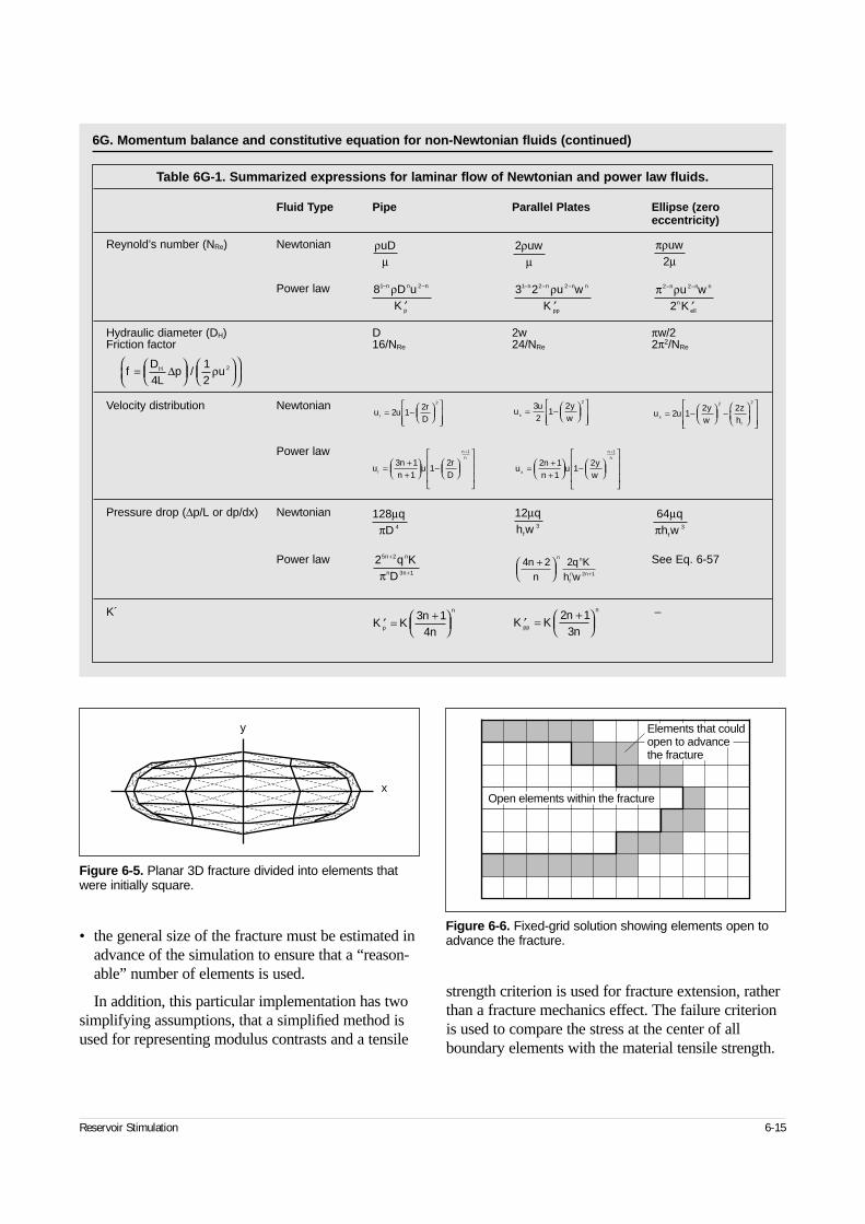
• the general size of the fracture must be estimated inadvance of the simulation to ensure that a “reason-able” number of elements is used.

In addition, this particular implementation has twosimplifying assumptions, that a simplified method isused for representing modulus contrasts and a tensile

strength criterion is used for fracture extension, ratherthan a fracture mechanics effect. The failure criterionis used to compare the stress at the center of allboundary elements with the material tensile strength.

Reservoir Stimulation 6-15

6G. Momentum balance and constitutive equation for non-Newtonian fluids (continued)

Table 6G-1. Summarized expressions for laminar flow of Newtonian and power law fluids.

Fluid Type Pipe Parallel Plates Ellipse (zero eccentricity)

Reynold’s number (NRe) Newtonian

Power law

Hydraulic diameter (DH) D 2w πw/2Friction factor 16/NRe 24/NRe 2π2/NRe

Velocity distribution Newtonian

Power law

Pressure drop (∆p/L or dp/dx) Newtonian

Power law See Eq. 6-57

K´ –

ρµuD

81 2− −

′

n n n

p

D uK

ρ

fD

Lp uH=

4

12

2∆ / ρ

2ρµuw

3 21 2 2− − −

′

n n n n

pp

u wK

ρ

πρµuw

2

π ρ2 2

2

− −

′

n n n

nell

u wK

u ur

Dr = −

2 12

2

unn

ur

Dr

nn

= ++

−

+

3 11

12

1

1284

µπ

qD

25 2

3 1

n n

n n

q KD

+

+π

′ = +

K Kn

np

n3 1

4′ = +

K Kn

npp

n2 1

3

4 2 22 1

nn

q Kh w

n n

fn n

+

+

uu y

wx = −

32

12

2

unn

uy

wx

nn

= ++

−

+

2 11

12

1

u uy

wz

hx

f

= −

−

2 12 2

2 2

123

µqh wf

643

µπ

qh wf

Figure 6-5. Planar 3D fracture divided into elements thatwere initially square.

y

x

Figure 6-6. Fixed-grid solution showing elements open toadvance the fracture.

Open elements within the fracture

Elements that could open to advance the fracture

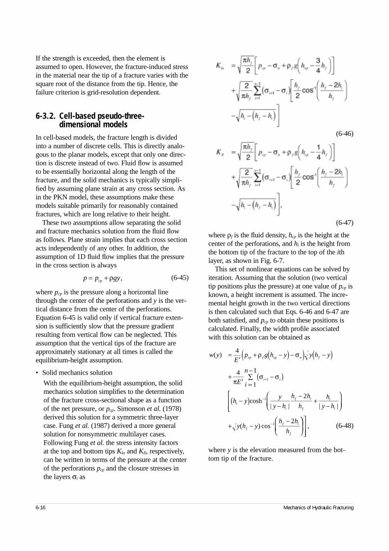
If the strength is exceeded, then the element isassumed to open. However, the fracture-induced stressin the material near the tip of a fracture varies with thesquare root of the distance from the tip. Hence, thefailure criterion is grid-resolution dependent.

6-3.2. Cell-based pseudo-three-dimensional models

In cell-based models, the fracture length is dividedinto a number of discrete cells. This is directly analo-gous to the planar models, except that only one direc-tion is discrete instead of two. Fluid flow is assumedto be essentially horizontal along the length of thefracture, and the solid mechanics is typically simpli-fied by assuming plane strain at any cross section. Asin the PKN model, these assumptions make thesemodels suitable primarily for reasonably containedfractures, which are long relative to their height.

These two assumptions allow separating the solidand fracture mechanics solution from the fluid flow as follows. Plane strain implies that each cross sectionacts independently of any other. In addition, theassumption of 1D fluid flow implies that the pressurein the cross section is always

(6-45)

where pcp is the pressure along a horizontal linethrough the center of the perforations and y is the ver-tical distance from the center of the perforations.Equation 6-45 is valid only if vertical fracture exten-sion is sufficiently slow that the pressure gradientresulting from vertical flow can be neglected. Thisassumption that the vertical tips of the fracture areapproximately stationary at all times is called theequilibrium-height assumption.

• Solid mechanics solution

With the equilibrium-height assumption, the solidmechanics solution simplifies to the determinationof the fracture cross-sectional shape as a functionof the net pressure, or pcp. Simonson et al. (1978)derived this solution for a symmetric three-layercase. Fung et al. (1987) derived a more generalsolution for nonsymmetric multilayer cases.Following Fung et al. the stress intensity factors at the top and bottom tips KIu and KIl, respectively,can be written in terms of the pressure at the centerof the perforations pcp and the closure stresses inthe layers σi as

(6-46)

(6-47)

where ρf is the fluid density, hcp is the height at thecenter of the perforations, and hi is the height fromthe bottom tip of the fracture to the top of the ithlayer, as shown in Fig. 6-7.

This set of nonlinear equations can be solved byiteration. Assuming that the solution (two verticaltip positions plus the pressure) at one value of pcp isknown, a height increment is assumed. The incre-mental height growth in the two vertical directionsis then calculated such that Eqs. 6-46 and 6-47 areboth satisfied, and pcp to obtain these positions iscalculated. Finally, the width profile associatedwith this solution can be obtained as

(6-48)

where y is the elevation measured from the bot-tom tip of the fracture.

6-16 Mechanics of Hydraulic Fracturing

p p gycp= + ρ ,

w yE

p g h y y h y

E i

n

h yy

y h

h h

h

h

y h

y h yh h

h

cp f cp n f

i i

i

i

f i

f

i

i

ff i

f

( )

| | | |

( ) cos

=′

+ −( ) −( ) −( )

+′

−( )=

−∑

−( )−

−+

−

+ −−

+

−

4

4

1

1

2

2

1

1

ρ σ

πσ σ

cosh–1

,

Consider, for example, the symmetric three-layercase shown in Fig. 6-8. If the gravitational compo-nent is neglected, so that the problem is symmetric,then the penetrations into the two barriers areequal. In this case, Eq. 6-46 can be simplified sig-nificantly and written as (Simonson et al., 1978)

(6-49)

where ∆σ is the difference in stress between thecentral layer (pay zone) and the surrounding layers,and hpay and σpay are the thickness and stress of thepay zone, respectively. Figure 6-9 shows fractureheight as a function of net pressure, as calculatedby Eq. 6-49.

Although Eq. 6-49 is for a special case, it showstwo interesting practical results. First, penetrationinto the barrier layers occurs at a critical net pressure:

(6-50)

For example, if KIc is 2000 psi/in.1/2 and hf is 20 ft[240 in.], the critical net pressure for breakthrough

Reservoir Stimulation 6-17

K Kh

ph

hIu Ilf

cp paypay

f

= = − −

−πσ σ

π22 1∆

cos ,

pK

hnet critIc

f

, .= 2 2

πFigure 6-7. Definition of variables for the fracture contain-ment problem.

Layer 1

2

i

n – 1

n

h

hi

y

Figure 6-8. Simple three-layer height growth problem.

∆σ

hf

σpay

hpay

Figure 6-9. Fracture height versus net pressure for sym-metric barriers. hs = penetration into the boundary layer.

hsh

0.5

1.0

1.5

00 0.2 0.4 0.6 0.8 1.0

σ2 – pσ2 – σ1

σ2 – σ1 = 1000 psi

KIc = 0, all σ2 – σ1

σ2 – σ1 = 500 psiσ2 – σ1 = 250 psi

h

σ2

σ1

σ2

hs

KIc = 1000 psi/in.1/2

Symmetric case

p

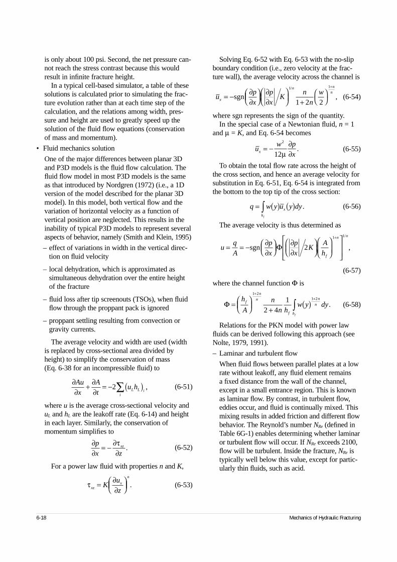
is only about 100 psi. Second, the net pressure can-not reach the stress contrast because this wouldresult in infinite fracture height.

In a typical cell-based simulator, a table of thesesolutions is calculated prior to simulating the frac-ture evolution rather than at each time step of thecalculation, and the relations among width, pres-sure and height are used to greatly speed up thesolution of the fluid flow equations (conservation of mass and momentum).

• Fluid mechanics solution

One of the major differences between planar 3Dand P3D models is the fluid flow calculation. Thefluid flow model in most P3D models is the sameas that introduced by Nordgren (1972) (i.e., a 1Dversion of the model described for the planar 3Dmodel). In this model, both vertical flow and thevariation of horizontal velocity as a function ofvertical position are neglected. This results in theinability of typical P3D models to represent severalaspects of behavior, namely (Smith and Klein, 1995)

– effect of variations in width in the vertical direc-tion on fluid velocity

– local dehydration, which is approximated assimultaneous dehydration over the entire heightof the fracture

– fluid loss after tip screenouts (TSOs), when fluidflow through the proppant pack is ignored

– proppant settling resulting from convection orgravity currents.

The average velocity and width are used (widthis replaced by cross-sectional area divided byheight) to simplify the conservation of mass (Eq. 6-38 for an incompressible fluid) to

(6-51)

where u is the average cross-sectional velocity anduL and hL are the leakoff rate (Eq. 6-14) and heightin each layer. Similarly, the conservation ofmomentum simplifies to

(6-52)

For a power law fluid with properties n and K,

(6-53)

Solving Eq. 6-52 with Eq. 6-53 with the no-slipboundary condition (i.e., zero velocity at the frac-ture wall), the average velocity across the channel is

(6-54)

where sgn represents the sign of the quantity.In the special case of a Newtonian fluid, n = 1

and µ = K, and Eq. 6-54 becomes

(6-55)

To obtain the total flow rate across the height ofthe cross section, and hence an average velocity forsubstitution in Eq. 6-51, Eq. 6-54 is integrated fromthe bottom to the top tip of the cross section:

(6-56)

The average velocity is thus determined as

(6-57)

where the channel function Φ is

(6-58)

Relations for the PKN model with power lawfluids can be derived following this approach (seeNolte, 1979, 1991).

– Laminar and turbulent flow

When fluid flows between parallel plates at a lowrate without leakoff, any fluid element remains a fixed distance from the wall of the channel,except in a small entrance region. This is knownas laminar flow. By contrast, in turbulent flow,eddies occur, and fluid is continually mixed. Thismixing results in added friction and different flowbehavior. The Reynold’s number NRe (defined inTable 6G-1) enables determining whether laminaror turbulent flow will occur. If NRe exceeds 2100,flow will be turbulent. Inside the fracture, NRe istypically well below this value, except for partic-ularly thin fluids, such as acid.

6-18 Mechanics of Hydraulic Fracturing

∂∂

∂∂

Au

x

A

tu hL L i

i

+ = − ( )∑2 ,

∂∂

∂τ∂

p

x zxz= − .

τ ∂∂xz

x

n

Ku

z=

.

up

x

px

Kn

n

wx

n n

n= − ∂

∂

∂∂

+

+

sgn1 1

1 2 2

/

,

uw p

xx = −2

12µ∂∂

.

q w y u y dyx

hf

= ( ) ( )∫ .

uq

A

p

x

px

KA

hf

n n

= = − ∂∂

+

sgn Φ ∂∂

2

1 1/

,

Φ =

+

( )+

+

∫h

A

n

n hw y dyf

n

n

f

n

n

hf

1 21 2

2 41

.

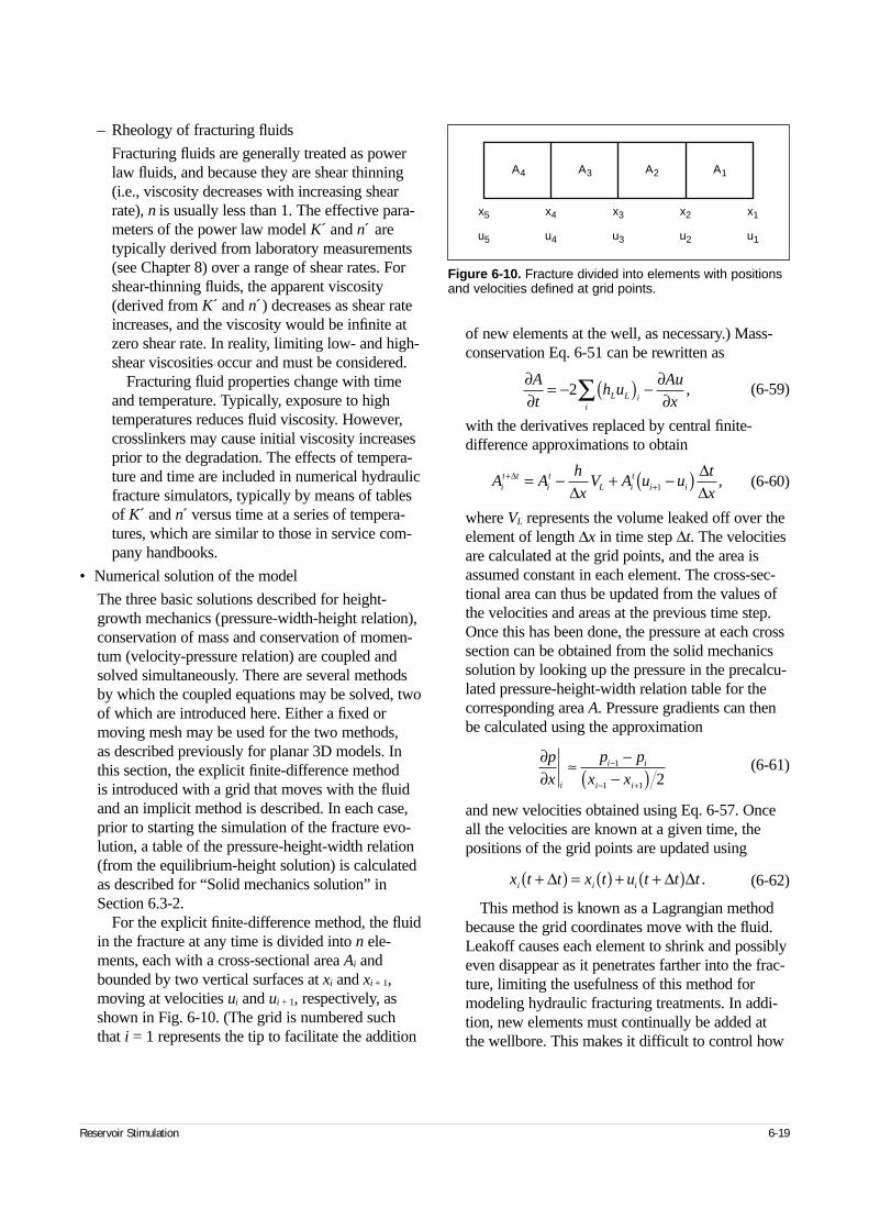
– Rheology of fracturing fluids

Fracturing fluids are generally treated as powerlaw fluids, and because they are shear thinning(i.e., viscosity decreases with increasing shearrate), n is usually less than 1. The effective para-meters of the power law model K´ and n´ aretypically derived from laboratory measurements(see Chapter 8) over a range of shear rates. Forshear-thinning fluids, the apparent viscosity(derived from K´ and n´) decreases as shear rateincreases, and the viscosity would be infinite atzero shear rate. In reality, limiting low- and high-shear viscosities occur and must be considered.

Fracturing fluid properties change with timeand temperature. Typically, exposure to hightemperatures reduces fluid viscosity. However,crosslinkers may cause initial viscosity increasesprior to the degradation. The effects of tempera-ture and time are included in numerical hydraulicfracture simulators, typically by means of tablesof K´ and n´ versus time at a series of tempera-tures, which are similar to those in service com-pany handbooks.

• Numerical solution of the model

The three basic solutions described for height-growth mechanics (pressure-width-height relation),conservation of mass and conservation of momen-tum (velocity-pressure relation) are coupled andsolved simultaneously. There are several methodsby which the coupled equations may be solved, twoof which are introduced here. Either a fixed ormoving mesh may be used for the two methods, as described previously for planar 3D models. Inthis section, the explicit finite-difference method is introduced with a grid that moves with the fluidand an implicit method is described. In each case,prior to starting the simulation of the fracture evo-lution, a table of the pressure-height-width relation(from the equilibrium-height solution) is calculatedas described for “Solid mechanics solution” inSection 6.3-2.

For the explicit finite-difference method, the fluidin the fracture at any time is divided into n ele-ments, each with a cross-sectional area Ai andbounded by two vertical surfaces at xi and xi + 1,moving at velocities ui and ui + 1, respectively, asshown in Fig. 6-10. (The grid is numbered suchthat i = 1 represents the tip to facilitate the addition

of new elements at the well, as necessary.) Mass-conservation Eq. 6-51 can be rewritten as

(6-59)

with the derivatives replaced by central finite-difference approximations to obtain

(6-60)

where VL represents the volume leaked off over theelement of length ∆x in time step ∆t. The velocitiesare calculated at the grid points, and the area isassumed constant in each element. The cross-sec-tional area can thus be updated from the values ofthe velocities and areas at the previous time step.Once this has been done, the pressure at each crosssection can be obtained from the solid mechanicssolution by looking up the pressure in the precalcu-lated pressure-height-width relation table for thecorresponding area A. Pressure gradients can thenbe calculated using the approximation

(6-61)

and new velocities obtained using Eq. 6-57. Onceall the velocities are known at a given time, thepositions of the grid points are updated using

(6-62)

This method is known as a Lagrangian methodbecause the grid coordinates move with the fluid.Leakoff causes each element to shrink and possiblyeven disappear as it penetrates farther into the frac-ture, limiting the usefulness of this method formodeling hydraulic fracturing treatments. In addi-tion, new elements must continually be added atthe wellbore. This makes it difficult to control how

Reservoir Stimulation 6-19

∂∂

∂∂

A

th u

Au

xL L ii

= − ( ) −∑2 ,

∂∂p

x

p p

x xi

i i

i i

≈ −−( )−

− +

1

1 1 2

x t t x t u t t ti i i+( ) = ( ) + +( )∆ ∆ ∆ .

A Ah

xV A u u

t

xit t

it

L it

i i+

+= − + −( )∆

∆∆∆1 ,

Figure 6-10. Fracture divided into elements with positionsand velocities defined at grid points.

A4 A3 A2 A1

x5

u5

x4

u4

x3

u3

x2

u2

x1

u1

many elements are present at any time or the sizesof the elements. Another approach is to introduce afixed grid, as discussed for planar 3D models. Thishas the advantage that the number of elements inthe simulation is relatively small near the beginningof the simulation when less accuracy is requiredand increases as the simulation progresses. Yetanother approach is to introduce a moving mesh in which the grid points move at some reasonablevelocity, for example, such that the fracture isalways divided into a fixed number of equal-sizeelements (i.e., using a stretching coordinate system;see Sidebar 6H).

One of the primary limitations of explicit finite-difference methods, such as those introduced in the

preceding text, is that the time step used in the cal-culation may not exceed a critical value to ensurestability. Because only quantities from the previousstep are used in moving forward, numerical errorscan grow larger from step to step if the time step istoo large. In the development of a general hydraulicfracturing simulator using such differencingschemes, the time step must be chosen carefully toavoid stability problems and yet minimize the com-putation time. A simple stability analysis is inSidebar 6H.

It has been found that in cases of high leakoff or large widths (such as TSO designs), the criticaltime step for stability may be too small for efficientsolution of the system, limiting the utility of the

6-20 Mechanics of Hydraulic Fracturing

6H. Stretching coordinate system and stability analysis

Stretching coordinate system

One way to simplify grid point bookkeeping is to use astretching coordinate system. If

(6H-1)

then X will always remain bounded between 0 and 1 while xvaries between 0 and L(t). Placing a grid on X will fully coverthe fracture regardless of the growth characteristics. However,although the gridding is simplified, the complexity of the differ-ential equation is increased. The derivatives are found as

(6H-2)

(6H-3)

Equation 6-59 becomes

(6H-4)

and the other equations of the system are similarly trans-formed.

Stability analysis

A full stability analysis for a nonlinear system is difficult, butan approximate time-step limitation can be found as follows.

Assume that the pressure gradient can be written as

(6H-5)

In the case of the PKN model, where the fracture height hf isfixed, Cp = βhf, where β is defined by

(6H-6)

Substituting Eq. 6H-5 into Eq. 6-59 and applying the chain rule,

(6H-7)

where absolute values must be assumed for all quantities,because an error analysis is being performed, and D isdefined as

(6H-8)

The highest order term in Eq. 6H-7 is

(6H-9)

If the derivative is expanded using a central differenceapproximation, the term in Ai becomes

(6H-10)

To investigate the effect of an error introduced into A, A isreplaced by A(1 + ε), which can be approximated (for small ε) as

(6H-11)

If a time step is taken (discretizing Eq. 6H-7 similar to Eq. 6-59),then the error ε grows to

(6H-12)

For this error to reduce in magnitude, it must be smaller thanAε, which can occur only if

(6H-13)

where the viscosity leakoff control coefficient Cv is

(6H-14)

Xx

L t= ( ) ,

∂∂

∂∂

∂∂

∂∂

At

Dn

A AAx

AA

xn A

Ax

n

n

n n=

+ +( )

+

−

+1

1 1

12

2

2

1/

,

DC

Kh

pn

fn n=

( )+

Φ 1

1 12

/

/ .

Dn

A AAx

AA

xn

n

n1

1 1

12

2

+

−

+

∂∂

∂∂

/

.

−( )

−

+22

1 1

3 1D

n x

Ax

An

n

∆∂∂

/

/ .

−( )

+ +

−

+21 3

12

1 1

3 1D

n x

Ax

An

n

n

∆∂∂

ε/

/ .

E tD

n x

Ax

An

n

n= −( )

+ +

−

+∆∆2

1 31

2

1 1

3 1∂∂

ε/

/ .

∆∆

tx

AC Cp v

<( )2

2,

Cn vpx

nv = −

+( )3 1

2∂∂

.

∂∂

∂∂x L X

= 1

∂∂

∂∂

∂∂t t

XL

dLdt X

= − .

∂∂

∂∂

∂∂

At

XL

dLdt

AX L

qX

qL− = − −1,

∂∂

∂∂

px

CAxp= .

p w= β .

explicit scheme. An implicit finite-differencescheme, with no time-step limitation, may elimi-nate this limitation. In essence, implicit and explicitmethods can be distinguished by the fact thatexplicit methods solve for quantities at one timestep on the basis of only values at the previous timesteps, whereas implicit methods include the use ofquantities at the current time. This implies that a setof equations is set up and solved, because the quan-tities at the current time step must all be foundsimultaneously. For linear problems, a set of linearequations results, and these are easily solved bystandard methods such as gaussian elimination. Forthe 1D flow problem, the implicit finite-differenceformulation yields a tridiagonal system of equa-tions (i.e., a sparse matrix with only three diagonalsfilled with nonzeros). Highly efficient solutiontechniques are available to solve such systems (e.g., Carnahan et al., 1969). For nonlinear prob-lems, however, such methods can be complex andare not always much more efficient than explicitmethods. Iteration is frequently required, because a nonlinear system is linearized. If the linearizationapproximation is inaccurate, it must be correctedand resolved.

Another method without the time-step limitation,and which avoids forming a system of equations, is a method using integrated or analytical elements.A similar method to that described in the followingwas the basis of the commercial time-sharingmethod made available by Amoco between 1981and 1983 (Nolte, 1982, 1988a). Consider onceagain the basic equations of the PKN model withx = φ at the tip:

(6-63)

(6-64)

Substituting Eq. 6-64 for p into Eq. 6-63 obtains

(6-65)

Detailed numerical simulations have shown thatthe velocity varies much more slowly than the flowrate q because the reduction in width toward the tippartially compensates for fluid leakoff and storagein the fracture. Instead of the Perkins and Kern

(1961) assumption that q is constant (Eq. 6-10),replacing q by πuhfw/4 allows writing Eq. 6-65 as

(6-66)

or

(6-67)

Integrating over a distance ∆x obtains

(6-68)

If the terms under the integral can be assumed tobe constant, this simplifies further to

(6-69)

If the height is not constant and the fluid is non-Newtonian, a similar equation can be written forthe cross-sectional area of the fracture by using thepower law rheological parameters:

(6-70)

where

(6-71)

For an analytical solution, ∆x would be the entirefracture length (Nolte, 1991), and this would becombined with a tip criterion and a volume-balanceequation. The numerical solution proceeds simi-larly, except that ∆x is chosen sufficiently small toobtain an accurate solution. Fluid loss is integratedover the time step, which allows obtaining accept-able accuracy, even with large time steps. The solu-tion method at each time step is as follows:

1. Estimate a tip velocity.

2. For each element, working in from the tip to thewell,

a. calculate an average fluid velocity based onthe velocity at the outer side of the elementand the estimated velocity at the inner side (At the first iteration, assume the inner fluidvelocity is equal to the outer fluid velocity.)

Reservoir Stimulation 6-21

wp h

Enet f=′

2

dp

dx

q

h wf

= 643

µπ

.

′ =E

h

dw

dx

q

h wf f264

3

µπ

.

dw

dx

h

E wuf=

′32

2

µ

w dwh

Eudxf2 32

=′

µ.

w x x w xh

Eudxf

x

x x

+( ) = ( ) +′

+

∫∆∆

3

1 396µ

/

.

w x x w xh

Eu xf+( ) = ( ) +

′

∆ ∆3

1 396µ /

.

A An Kh

Eu xi

tit n f

n

n

n

n

+

++ +

= ( ) ++( )

′

1

23 1 2

2 πΦ

∆/( )

,

Φ =+( )

+

∫n

h n

w y

wdy

f

n

n

hf2 4

1 2

( ).

b. determine the cross-sectional area at the innerside of the element for the estimated velocityby using Eq. 6-70

c. determine the velocity at the inner side suchthat the leakoff and element volume changeduring the time step result in a mass balance

d. repeat the iteration using the new velocity.

3. Compare the actual flow into the fracture withthe wellbore velocity calculated by the iterativescheme in the preceding step.

4. Refine the estimate of the tip velocity using aNewton-Raphson method until volume balance is achieved, which typically takes two to fouriterations.

This method of solving the equations is efficientbecause the velocity does not vary significantlyalong the fracture for typical cases. For typicalPKN cases with a single fluid, the fracture can be divided into about 10 elements. For non-PKNcases, the grid must be chosen sufficiently finethat the integrand in Eq. 6-68 (which includeseffects of fluid rheology and fracture height) isapproximately constant in each element (becausethe solution scheme is derived with the assump-tion that it is constant).

Regardless of whether a moving- or fixed-gridmethod is used, usually only a small number ofelements (about 10) is necessary to obtain areasonably accurate solution to the equationsdescribed so far. However, other information maybe required at a much finer resolution. To achievethis, the schedule is typically divided into a largenumber of substages (about 100). Quantities suchas proppant concentration, fluid temperature andacid concentration can then be tracked on thisfiner grid. In addition, particularly in acid frac-turing, it is desirable to track leakoff and etching on a finer grid. To do this for methods using a moving grid, a second grid that does not moveis established. Quantities such as reservoir tem-perature, proppant bank height and leakoff vol-ume in the reservoir are tracked on this solid-based grid.

• Nonequilibrium-height solution

It was noted in “Solid mechanics solution” inSection 6.3-2 that the assumption of slow heightgrowth allows creating a pressure-height-widthtable prior to solving the equations of fracture evo-lution. This so-called equilibrium-height assump-

tion is quite accurate, provided that the fluid ismoving relatively slowly in the vertical direction sothat the pressure drop resulting from vertical fluidflow is negligible. This assumption is violated ifhigh-permeability zones are exposed, because fluidmust then move rapidly because of the increasedleakoff in such layers. Also, if the stress in the sur-rounding zones is insufficient to confine the frac-ture and the vertical tips extend quickly, then thefluid must move quickly to fill the resulting frac-ture. In either of these cases, the pressure gradientresulting from vertical fluid flow may becomelarge, and the equilibrium-height assumptionbecomes invalid at these locations in the fracture.

To remove this assumption and obtain validresults from a simulator, some restriction must be placed on height growth. For nonequilibrium-height growth, the pressure gradient because offluid flow in the vertical direction must be approxi-mated, based on the rate of height growth. It iscommon to base this approximation on the KGDmodel (e.g., Settari and Cleary, 1982). In Section 6-7 on tip effects, an analytical near-tip solutiondeveloped by Lenoach (1994) is discussed that pro-vides an expression for the net pressure of the form

(6-72)

where utip is the tip velocity and β is 2/(2 + n). Aspreviously noted, for a fracture under constant pres-sure, the stress intensity factor is related to the netpressure by

(6-73)

The Lenoach tip solution can be used to obtainan apparent fracture toughness caused by the non-zero tip velocity by combining Eqs. 6-72 and 6-73.This effect can be added to the actual rock tough-ness, and the sum is used in Eqs. 6-46 and 6-47instead of the actual rock toughness to determinethe fracture height growth. The basic algorithmused to move from one pair of vertical tip positionsto another during a time step is as follows:

6-22 Mechanics of Hydraulic Fracturing

pK

hnetIc

f

=π 2

.

1. Estimate the top and bottom tip velocities forthe cell.

2. Calculate the new fracture tip positions at theend of the time step, using these velocities.

3. Calculate the stress intensity factors from Eqs.6-46 and 6-47.

4. Determine the excess stress intensity factors(i.e., the calculated value minus the rock toughness).

5. Calculate the velocities required to generatethese excess stress intensity factors, using Eqs.6-72 and 6-73.

6. Compare the velocities with the guessed valuesand iterate until the correct velocities are found.

One of the advantages of the equilibrium-heightmodels is the speed gained by precalculating atable of the fracture height-pressure relation. Notonly is this not possible for the nonequilibriummodel, but the iterative process to determine the tippositions can be time consuming. The nonequilib-rium-height algorithm should therefore be usedonly when necessary because of the apparent rapidheight growth indicated by the equilibrium-heightcalculation.

• Lateral coupling

In the description of the solid mechanics solutionprovided previously, the basic assumption is thatindividual cross sections act independently (i.e.,plane strain in the horizontal direction, or laterallydecoupled). This is implicit in the assumption thatthe pressure and width at any point are uniquelyrelated. In reality, the pressure at any point is depen-dent not only on the local width, but also on thewidth distribution over the entire fracture, as dis-cussed in Section 6-3.1 on planar 3D models. Thislateral coupling is generally not important, unlessthe fracture wing length is less than the height. Eventhen, the fracture geometry will not be significantlydifferent if lateral coupling is neglected, althoughthe pressure response may be underestimated. Lat-eral coupling can be included in the solutionsdescribed previously (see Sidebar 6E).

The effect of lateral coupling during pumping isto increase the pressure at and near the well and todecrease it near the tip. Figure 6-11 shows the evo-lution of pressure during a treatment for a confinedfracture simulated using the KGD, PKN and later-

ally coupled PKN models. The pressure predictedby the laterally coupled model is always higherthan either the KGD or PKN solution would pre-dict. It can also be shown that the width at the wellis always smaller than that predicted by either ofthe simple models. The point in Fig. 6-11 wherethe pressure from the laterally coupled model islowest (and where the pressures from the KGD andPKN models are equal) corresponds to a square,where the fracture wing length is one-half of theheight. The pressure calculated by the laterally cou-pled model exceeds that predicted by the KGD orPKN model at this time by approximately 40%,which is comparable to the pressure in a radialfracture of similar dimensions.

6-3.3. Lumped pseudo-three-dimensional models

Lumped models are an alternative to cell-based mod-els and were first introduced by Cleary (1980b).Although more details are presented in subsequentparagraphs, it is worthwhile at this point to quote twosentences from the conclusions of his paper: “the heartof the formulae can be extracted very simply by anondimensionalization of the governing equations; theremainder just involves a good physico-mathematicalchoice of the undetermined coefficients” and “resultscould be presented in the usual format of designcharts, based on dimensionless groups extracted, . . .[a] more appealing procedure may be to program thesolutions for a suitable pocket calculator, with the sep-arately determinable γ or Γ coefficients and job para-meters as input.” Although numerous papers have

Reservoir Stimulation 6-23

Figure 6-11. Pressure record with and without lateral coupling.

Pre

ssur

e (p

si)

1400

1300

1200

1100

10000 5 10 15 20 25

Time (min)

Lateral couplingKGDPKN

been presented on the use of this model (e.g., Clearyet al., 1994), which is now on laptop computers ratherthan pocket calculators, these sentences capture theessence of lumped models in that they are extremelysimple models and the key to their successful use is the selection of appropriate coefficients for theproblem analyzed.

Like all the models presented previously, the start-ing point of the lumped model is the set of basic equa-tions defining the hydraulic fracturing process, whichare mass conservation (Eq. 6-39), the relation betweenthe distribution of crack opening over the length of the fracture 2L, net pressure distribution (similar toEq. 6-36) expressed as

(6-74)

and conservation of momentum (Eq. 6-40) expressed as

(6-75)

where γ4 is the channel factor (1⁄12 for a Newtonianfluid), and various combinations of the power law fac-tors m for turbulence and n enable consideration ofboth non-Newtonian fluids and turbulent flow.

In the lumped models, these equations are simpli-fied by assuming a fracture shape and adopting a spa-tial averaging approach to reduce them to ordinarydifferential equations in time. This approach implicitlyrequires the assumption of a self-similar fractureshape (i.e., one that is the same as time evolves,except for a length scale). The shape is generallyassumed to consist of two half-ellipses of equal lateralextent, but with different vertical extent.

It is instructive to consider some of the lumpedequations for the KGD model (Cleary, 1980b). Themass balance is obtained by averaging over the frac-ture length:

(6-76)

where

(6-77)

(6-78)

where

(6-79)

which is the 1D form of Eq. 6-75. Equation 6-76 issimilar to Eq. 6-15 (based on Carter, 1957) with the

addition of γ3, and Eq. 6-77 is identical to that ofGeertsma and de Klerk (1969) with γ3 replacing4(1 – ν2). Superficially, these equations are extremelysimple, but the values of the γ coefficients are notalways obvious and may not be constant. As noted by Crockett et al. (1989), these models are extremelygeneral, with the degree of accuracy limited ultimatelyonly by the effort invested in determination of the γcoefficients by detailed simulations, laboratory experi-ments or field studies.

For more general fracture shapes (i.e., with heightgrowth), it is typically assumed that height growth isgoverned by a KGD-type solution and length growthby a PKN-type solution (Cleary et al., 1983), althoughthis is not a theoretical limitation of lumped models.

One area in which lumped models have beenexploited extensively is in the development of com-puter software systems to apply and use pressure dataduring a treatment. Some of the key characteristicsand requirements for such a software system are that(Crockett et al., 1989)

• the physics is realistic and general

• execution time is much faster than treatment time to allow repetitive execution for pressure historymatching

• the software can use improved estimates of parame-ters obtained in real time (i.e., during the treatment).

Although these real-time software systems are gen-erally referred to as real-time hydraulic fracture mod-els (e.g., Crockett et al., 1989), the model itself is onlya small part of the software and should address thefirst requirement listed (i.e., realistic and generalphysics). The second and third requirements are com-puter hardware and software design constraints.Because lumped models were developed for pocketcalculators in 1980, they impose a minimal impact oncomputer hardware and systems. As computing powercontinues to improve, it will become possible to runincreasingly sophisticated models during treatmentexecution either at the wellsite or remotely. There areother software design issues, such as robust executionwith a wide variety of parameter values, easy importand superposition of actual data on model output, andgraphical display, that are required for a useful soft-ware system for real-time applications. Discussion ofthese issues is beyond the scope of this volume.

6-24 Mechanics of Hydraulic Fracturing

p x I x x w x dxnet

L

L

( ) = ′( ) ′( ) ′−∫ , ,

˜ ˜ ,qq w pm n m− − += − ∇14

2 1γ µ

ρ γ ρqw Lq d wL dtL−( ) = ( )3 ,

w p E Lnet≈ ( )γ 1

q w w Lm m m n≈ ( ) +γ 5

2 2 2 ,

γ γ γ γ µ5 2 4 1m E≡ ( ),

6-4. LeakoffOne of the key issues in designing a fracture treatmentis accurate knowledge of how rapidly fluid will leakout of the fracture into the reservoir. Without thisinformation, it would be impossible to design a treat-ment that provides a specified fracture geometry.Mini-fracture treatments are performed to estimate theleakoff coefficient (see Chapter 9). Equation 6-14introduced in “Inclusion of leakoff” in Section 6-2.2 is the basic equation of filtration and was first used forfracturing by Carter (1957). He showed that it wasapplicable for three separate leakoff processes:

• displacement and compressibility of reservoir fluid

• invasion of the formation by filtrate or fracturing fluid

• buildup of an external filter cake.

Williams (1970) divided the leakoff into three timeperiods, rather than considering the three processes.During the initial period, leakoff is quick, followed by a decreasing leakoff rate and finally a steady-stateleakoff rate. In the initial period, filter cake has notformed, so the leakoff rate is controlled by the resis-tance of the formation to flow of the fracturing fluid.The external filter cake builds during the secondperiod. Finally, the cake stops building, because thehigh-velocity fluid in the fracture prevents furtherpolymer deposition. This last stage is referred to asdynamic leakoff. Williams lumped all leakoff prior to dynamic leakoff into a quantity he called spurtvolume, although spurt loss has since been generallyaccepted to refer only to the initial high-leakoff periodbefore the cake starts building.

Settari (1985) presented an excellent review of theclassic leakoff model, as well as an even more generalmodel of leakoff that represents an excellent frame-work for leakoff modeling. In the following sections,each of the three processes (displacement and com-pressibility of reservoir fluid, invasion of the forma-tion by filtrate or fracturing fluid and buildup of filtercakes, either externally on low-permeability rocks orinternally on high-permeability rocks) is considered as if it is the only one acting and then in combination.Finally, Settari’s general model is summarized.

The fluid-loss derivations in Eqs. 6-82 through 6-91are for the pressure drop for individual loss mecha-nisms. For general application, they are in terms of thetotal pressure drop between the fracture and initialreservoir pressures in Eqs. 6-94 through 6-96 and inoilfield units in Eqs. 8-26 and 8-27.

6-4.1. Filter cakeIn laboratory filtration experiments performed at con-stant pressure, the rate of filtration is proportional tothe square root of time (see Chapter 8). A model forthis process can be derived by assuming that

• the amount of cake deposited is proportional to thevolume of fluid VL passed through a unit surfacearea

• cake permeability kcake is independent of its thickness

• flow through the cake obeys Darcy’s law

• pressure drop across the cake ∆pcake is constant

to write

(6-80)

where µfil is the viscosity of the filtrate and it is assumedthat the cake thickness Lcake is proportional to the fluidvolume lost; i.e., VL = αLcake. By integrating for VL, itcan be shown that

(6-81)

where the fluid-loss coefficient through the wall filtercake is

(6-82)

Carter (1957) proposed that the volume leaked offcan then be determined as

(6-83)

where Sp is the volume that leaks off without forminga filter cake and can be interpreted as an integrationconstant. A more appropriate physical model is toassume that the initial volume that leaks off, withoutbuilding a cake, is the spurt volume and that Eq. 6-80applies after the cake is established. This interpreta-tion results in

(6-84)

where tsp is the spurt time.Another approach to account for leakoff by using

standard petroleum engineering concepts of reservoirpermeability and treating the filter cake as a pressure-dependent resistance is outlined in Chapter 2 alongwith high-permeability conditions (Valkó and Econ-omides, 1997). The following approach to the leakoffcoefficient is as presented by Settari (1985).

Reservoir Stimulation 6-25

udV

dt

k p

VLL cake

fil

cake

L

= =µ

α∆,

u C tL w= ,

Ck p

wcake cake

fil

= αµ∆

2.

V C t SL w p= +2 ,

V C t t SL w sp p= − +2 ,

6-4.2. Filtrate zoneThe first zone inside the reservoir is called the filtratezone or invaded zone. It is assumed that

• pressure drop ∆pv across the zone is constant

• filtrate fully displaces the mobile phase(s) withinthe formation, resulting in piston-like displacementand 100% filtrate saturation

• the fluid and rock are incompressible

to write

(6-85)

where kfil is the permeability related to the filtrate andLv is the length of the invaded zone. Integrating thisequation, with the assumption that

(6-86)

where φ is the porosity, obtains

(6-87)

where the viscosity control leakoff coefficient Cv is

(6-88)

and the leakoff volume at any time is

(6-89)

The permeability to the filtrate kfil reflects the rela-tive permeability of the formation to flow of the fil-trate. This effect may be significant when a waterfiltrate enters a hydrocarbon zone at nearly irreduciblewater saturation.

6-4.3. Reservoir zoneAlthough the uninvaded reservoir does not containfracturing fluid, pressure is required to displace thereservoir fluid away from the fracture face. Assuming

• constant pressure drop ∆pc between thefiltrate/reservoir interface and the far-field reservoir

• compressible flow with constant total compres-sibility ct

• relatively slow movement of the front of the invading fluid

• an infinite reservoir,

the front can be treated as the face of an infiniteporous medium, and an analytical solution (Collins,1961) is used to obtain

(6-90)

where the compressibility control leakoff coefficientCc is

(6-91)

where kr is the permeability of the reservoir rock andµr is the reservoir fluid viscosity.

6-4.4. Combined mechanismsIn practice, all three processes occur simultaneously.The leakoff velocities in Eqs. 6-80, 6-85 and 6-90must be equal, and the sum of the pressure drops mustequal the total pressure difference between the reser-voir pressure and the fracturing pressure:

(6-92)

(6-93)

where Ct is the total leakoff coefficient and ∆ptotal isthe difference between the pressure in the fracture andthe far-field reservoir pressure pr. If the spurt volumeand time can be neglected, these equations can becombined (Williams et al., 1979) to yield the totalleakoff coefficient:

(6-94)

with the coefficients Cw, Cc and Cv calculated usingthe overall pressure difference.

Equation 6-94 is valid only if the cake permeabilityis independent of pressure. If the cake is highly com-pressible and the cake permeability is approximatelyproportional to 1/∆p, Nolte (1988a) has shown that thefluid loss is limited either by the cake or the reservoir.In that case, the fluid-loss rate is the minimum of Eq. 6-81, with the pressure drop equal to the totalpressure drop, or

(6-95)

6-26 Mechanics of Hydraulic Fracturing

L V u dtv L L= = ∫φφ1

,

uC

tLv= ,

Ck p

vfil v

fil

=φµ∆

2

V C tL v= 2 .

uC

tLc= ,

Ck c

pcr t

r

c= φπµ

∆ ,

C

t

k p

t t

k p

t

k c

tpt cake cake

fil sp

fil v

fil

r t

r

c=−

=αµ

φµ

φπµ

∆ ∆∆

2 2( ) =

∆ ∆ ∆ ∆p p p pcake v c total+ + = ,

uC

tLcv= ,

C CC C C

C C C C C C Ct wcv

c v w

v w w v c v w

= =+ + +( )

2

42 2 2 2 2

udV

dt

k p

LLL fil

fil

v

v

= =µ

∆,

where the combined leakoff coefficient is

(6-96)

with the coefficients Cc and Cv again calculated usingthe total pressure difference.

6-4.5. General model of leakoffA great deal of complexity can be added to the leakoffmodel in an attempt to account for detailed behaviorsuch as the compressibility of the invading fluid andthe moving boundary of the reservoir fluid. Given the accuracy with which the other parameters in ahydraulic fracture treatment are known, the inclusion of such effects is generally unnecessary. This sectiondescribes modification of the models to incorporatethe two effects of the variable pressure difference andchanging fluid properties.

The model described in previous sections can begeneralized to account for multiple fluids. Settari(1985) showed that the fluid loss in the invaded zonecan be described by replacing the term Cv with anequivalent term:

(6-97)

where Cv is calculated using the average viscosity andrelative permeability of all the filtrate leaked off to the current time, and VL is the fluid volume that previ-ously leaked off into the reservoir. Settari also showedthat replacing the wall-building coefficient for thefluid under consideration with an equivalent valuewould account for variations in leakoff behaviorbetween fluids in a treatment. The equivalent value in this case is

(6-98)

where the previously leaked-off fluid volume VL hasalso contributed to wall building.

The critical fluid component affecting wall buildingis the gel and/or fluid-loss additive concentration. Anextension to Settari’s model can be derived by consid-ering Eq. 6-80, in which the thickness of the cake isassumed to be proportional not to the volume flowedthrough the wall but to the volume of gel deposited.Thus, the thickness is proportional not to the time-integrated velocity but to the integral over time of the

product of gel concentration and fluid velocity. In thiscase, Eq. 6-98 is replaced by

(6-99)

where Cgel is the gel mass concentration in the fluidand Mgel is its specific density. There is an implicitassumption that the term CgelCw

2 is constant. Thisassumption is consistent with laboratory work reportedby Mayerhofer et al. (1991). The viscosity of waterdecreases with increasing temperature, and this effecton the leakoff coefficient should be included in thefracture model.

6-4.6. Other effects• Pressure evolution during treatment

If an estimate of the leakoff coefficient has beenobtained from a mini-fracture decline analysis, thenthe most likely way to use the simulator would be to enter the total leakoff coefficient derived from theanalysis. It is thus assumed that the leakoff behaviorduring the minifracture is the best representation of what will occur during the main treatment. How-ever, if the leakoff behavior is unknown and is to be determined from fluid and reservoir properties,the best approach is to enter a laboratory-determinedwall-building coefficient for each fluid and use thesimulator to determine the total leakoff coefficientat each position in the fracture as a function of timeand on the basis of the continually evolving pressuredifference between the fracture and the reservoir.Except in overpressured reservoirs, the assumptionof a constant total pressure difference is generallyreasonable. The ratio of leakoff coefficients betweenthe lowest pressure difference during the treatment(when the net pressure is zero and the pressuredifference between the closure stress and the reser-voir pressure is just ∆p = σc – pr) and at the end ofpumping (when it is ∆p = pnet + σc – pr) is given forreservoir-controlled leakoff by

(6-100)

and for the wall-building or viscosity-controlledcases by

(6-101)

Reservoir Stimulation 6-27

CC C

C C Ccv

c v

v v c

=+ +

2

42 2

CC t

Vv

v

L

= 2 2

,

CC t

Vw

w

L

= 2 2

,

CC C t

Mwgel w

gel

=2 2

,

C p

C p p

p

p pc net

c net net max

c r

net max c r

=( )=( ) = −

+ −0

, ,

σσ

C p

C p p

p

p pL net

L net net max

c r

net max c r

=( )=( ) = −

+ −0

, ,

.σ

σ

If the ratio is close to 1, a constant leakoff modelcan be used, in which the leakoff coefficients (Cc,Cv and Cw) for each fluid in the treatment can beprecalculated on the basis of an assumed typical net pressure (e.g., 250 psi). If the effect of pressurechanges is large, a variable leakoff model can beused, in which the pressure changes in the fractureare accounted for as the simulation proceeds. In thiscase, the reservoir component of leakoff Cc shouldbe determined using a convolution of the pressurehistory during the treatment.

• Pressure-sensitive leakoff

One of the major assumptions of the analysis in theprevious sections is that the permeability remainsconstant. In fact, many reservoirs may have fissuresor other features that may open under the influenceof the fracture treatment. The effect of this openingis to increase the leakoff rate (Warpinski, 1991).Pressure-sensitive leakoff is addressed more fullyin Chapter 9.

• Poroelasticity and backstress

Chapter 3 discusses the influence of pore pressureon rock mass behavior. Poroelastic effects arechanges in stress that occur as a result of changes in pore pressure in the reservoir. As fluid leaks outof the fracture into the reservoir, the affected part of the reservoir dilates, and a “backstress” develops,which increases the effective closure pressure. Thiseffect is generally small, but it may be important in some cases, as discussed by Nolte et al. (1993).Chapter 3 provides the solution for a fracture in aninfinite, homogeneous medium. Although the addi-tional pressure results in an increased net pressure in the fracture, it generally has little effect on frac-ture geometry.

6-5. Proppant placementThe objective of hydraulic fracturing is to place prop-pant to provide a conductive path for production. Thepresence of proppant introduces three important issuesin the behavior of fluids in hydraulic fractures:

• effect of proppant on fluid rheology

• convection or gravity currents

• proppant transport.

6-5.1. Effect of proppant on fracturing fluid rheology

Generally the viscosity of a proppant-laden slurry µslurry

is higher than that of the carrying fluid µbase alone.Experimental relations are well established for New-tonian fluids, but much less so for power law fluids.Nolte (1988b) showed that relations for power lawfluids could be obtained by using the relations for New-tonian fluids and raising them to the power of n. Forexample, the viscosity ratio µr could be obtained as

(6-102)

where fv is the proppant volume fraction, and fvM is themaximum fraction for a mobile slurry.

6-5.2. ConvectionDensity differences between fluids may result in thedenser fluid flowing under the lighter fluid or thelighter fluid overriding the denser fluid. This phenom-enon, known as convection or gravitational flow, isimportant in many fields, such as saltwater intrusionunder fresh water (Badon Ghyben, 1888; Herzberg,1901). In fracturing, it may be relevant if a high-density slurry stage flows under a previously pumpedstage or pad, as well as for other 2D aspects of fluidflow, such as those considered by Clifton and Wang(1988).

The fluid flow equations for a Newtonian fluid canbe written as

(6-103)

and (Eq. 6-38 for incompressible fluids)

(6-104)

Substituting Eq. 6-103 into Eq. 6-104 obtains

(6-105)

6-28 Mechanics of Hydraulic Fracturing

µµµr

slurry

base v vM

nf f

= =−( )

1

12 5. ,

uw p

x

uw p

yg

x

y

= −

= − +

2

2

12

12

µ∂∂

µ∂∂

ρ

∂∂

∂∂

∂∂

wu

x

wu

y

w

tux y

L

( ) +( )

+ + =2 0.

112

21

12

2 3

2

2 3

2

3

µ∂

∂∂

∂∂∂ µ

∂ ρ∂

w p

x

w p

y

w

tu

w g

yL+

= + − .

The last (gravitational) term on the right-hand sideof Eq. 6-105 is the convective term. This can be treatedas a source term, just as the other two terms are storageor sink terms, resulting from width change and leakoff.Baree and Conway (1994), Unwin and Hammond(1995) and Smith and Klein (1995) showed that this is generally not significant for most properly designedfracturing treatments. Smith and Klein showed that ifexcess pad was pumped, the fluid flow after pumpingstops (i.e., afterflow) could lead to convection until thepad leaked off. Also, Eq. 6-105 shows the extremesensitivity of convection to fracture width. If the widthis large (e.g., in a low-modulus rock), convection maybe more critical. Fortunately, such low moduli are usu-ally associated with high permeabilities, in which caseTSO designs and rapid leakoff after shut-in effectivelyprevent convection. Cleary and Fonseca (1992) pre-sented a dimensionless number that reflects the ratio of buoyant and viscous forces. This ratio can be usedto estimate the effect of different conditions on theseverity of convection.

Finally, Clark and Courington’s (1994) and Clark andZhu’s (1994) experiments on convection largely verifythe theoretical and numerical results described here.

6-5.3. Proppant transportHydraulic fracturing produces a conductive channelby placing proppant in a crack created in a pay zone.Hence, an essential consideration in fracturing fluiddesign is to accomplish proppant transport. The effectof convection on proppant transport was previouslydiscussed. There are two other factors that may impactproppant placement. The first, and most commonlyunderstood, is settling. If a bottle containing a mixtureof sand and water is shaken up and then left on atable, the sand will settle out of the water. It can beshown theoretically that the terminal velocity of a sin-gle particle far from any walls in a stagnant Newton-ian fluid is given by Stokes law:

(6-106)

where ρsol is the solid particle density, ρf is the fluiddensity, and dsol is the solid particle diameter.

The assumptions of this equation are of limitedapplicability in hydraulic fracturing because the fluidsare non-Newtonian and the particles are highly con-

centrated and may be close to the channel walls, whichcauses two effects: hindered settling, which impliesthat particles get in the way of each other, and clus-tered settling, in which particles join together, effec-tively increasing the diameter in Eq. 6-106. Novotny(1977) presented a correlation for the particle velocityusol in hindered settling in terms of the volume fractionof solids fv:

(6-107)

where

(6-108)

and the exponent β ranges from 5.5 at low values ofNRe to 2 at high values of NRe. For power law fluids, a generalized form of Stokes law (Eq. 6-106) is used:

(6-109)

Equation 6-108 can still be used to account for hin-dered settling. Other correlations have been developed,but a definitive correlation has not appeared in the lit-erature. Many fracturing fluids are designed for almostperfect transport, so the settling rate is usually notimportant unless the fracture remains open for a longtime after pumping stops.

Another effect on proppant placement is fluid migration (Nolte, 1988b) or encapsulation (Cleary and Fonseca, 1992). Fracturing fluids are generallyviscoelastic. Although it is beyond the scope of thissection to discuss this phenomenon in detail, one of its important effects is to drive proppant to the centerof the flow channel. This migration could result in adense sheet near the center of the channel, surroundedby clear fluid. This has the effect of accelerating parti-cle settling, especially for low proppant concentrations.Unwin and Hammond (1995) presented simulationsshowing the effect of this migration on proppant placement.

6-6. Heat transfer modelsThe properties of many fracturing fluids show somedependence on temperature. In addition, the rates of the reactions that occur in acid fracturing aredependent on temperature. In a typical fracturingtreatment, the fluid is pumped at a temperature signifi-

Reservoir Stimulation 6-29

ug dsol f sol

∞ =−( )ρ ρ

µ

2

18,

u u F fsol v= ( )∞ ,

F f fv v( ) = −( )1β

ugd

Ksol f sol

n

n

n

∞

+

−=−( )

′

ρ ρ 1

1

1

3 18

/

.

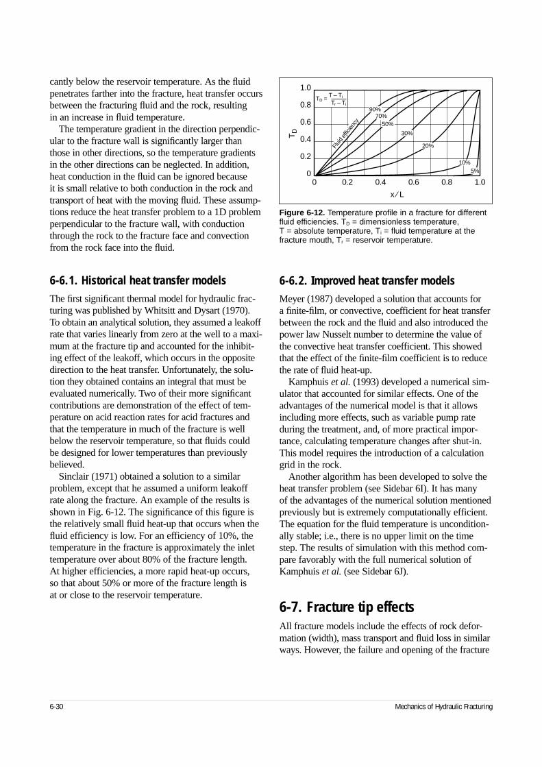
cantly below the reservoir temperature. As the fluidpenetrates farther into the fracture, heat transfer occursbetween the fracturing fluid and the rock, resulting in an increase in fluid temperature.

The temperature gradient in the direction perpendic-ular to the fracture wall is significantly larger thanthose in other directions, so the temperature gradientsin the other directions can be neglected. In addition,heat conduction in the fluid can be ignored because it is small relative to both conduction in the rock andtransport of heat with the moving fluid. These assump-tions reduce the heat transfer problem to a 1D problemperpendicular to the fracture wall, with conductionthrough the rock to the fracture face and convectionfrom the rock face into the fluid.

6-6.1. Historical heat transfer modelsThe first significant thermal model for hydraulic frac-turing was published by Whitsitt and Dysart (1970). To obtain an analytical solution, they assumed a leakoffrate that varies linearly from zero at the well to a maxi-mum at the fracture tip and accounted for the inhibit-ing effect of the leakoff, which occurs in the oppositedirection to the heat transfer. Unfortunately, the solu-tion they obtained contains an integral that must beevaluated numerically. Two of their more significantcontributions are demonstration of the effect of tem-perature on acid reaction rates for acid fractures andthat the temperature in much of the fracture is wellbelow the reservoir temperature, so that fluids could be designed for lower temperatures than previouslybelieved.

Sinclair (1971) obtained a solution to a similarproblem, except that he assumed a uniform leakoffrate along the fracture. An example of the results isshown in Fig. 6-12. The significance of this figure isthe relatively small fluid heat-up that occurs when thefluid efficiency is low. For an efficiency of 10%, thetemperature in the fracture is approximately the inlettemperature over about 80% of the fracture length. At higher efficiencies, a more rapid heat-up occurs, so that about 50% or more of the fracture length is at or close to the reservoir temperature.

6-6.2. Improved heat transfer modelsMeyer (1987) developed a solution that accounts for a finite-film, or convective, coefficient for heat transferbetween the rock and the fluid and also introduced thepower law Nusselt number to determine the value ofthe convective heat transfer coefficient. This showedthat the effect of the finite-film coefficient is to reducethe rate of fluid heat-up.

Kamphuis et al. (1993) developed a numerical sim-ulator that accounted for similar effects. One of theadvantages of the numerical model is that it allowsincluding more effects, such as variable pump rateduring the treatment, and, of more practical impor-tance, calculating temperature changes after shut-in.This model requires the introduction of a calculationgrid in the rock.

Another algorithm has been developed to solve theheat transfer problem (see Sidebar 6I). It has many of the advantages of the numerical solution mentionedpreviously but is extremely computationally efficient.The equation for the fluid temperature is uncondition-ally stable; i.e., there is no upper limit on the timestep. The results of simulation with this method com-pare favorably with the full numerical solution ofKamphuis et al. (see Sidebar 6J).

6-7. Fracture tip effectsAll fracture models include the effects of rock defor-mation (width), mass transport and fluid loss in similarways. However, the failure and opening of the fracture

6-30 Mechanics of Hydraulic Fracturing

Figure 6-12. Temperature profile in a fracture for differentfluid efficiencies. TD = dimensionless temperature, T = absolute temperature, Ti = fluid temperature at thefracture mouth, Tr = reservoir temperature.

TD

1.0

0.8

0.6

0.4

0.2

00 0.2 0.4 0.6 0.8 1.0

x ⁄ L

TD = T – Ti

Tr – Ti90%

70%50%

30%

20%

10%5%

Fluid

effic

iency

at its tip boundary are addressed in numerous ways.Nevertheless, certain general principles can bedescribed that apply to this region, and different imple-mentations can be considered as modifications of thegeneral principles. If the fracture tip is envisioned asthe zone between the fracturing fluid and the undis-turbed rock ahead of the fracture, then there are fourpossible features of this region that must be addressed:

• failure or opening process (normal LEFM)

• disturbed zone in the rock ahead of the fracture tip(damage not incorporated in the LEFM model)

• unwetted zone (fluid lag region)

• disturbed zone along the fracture face (e.g., dila-tancy or compaction).

Reservoir Stimulation 6-31

6I. Efficient heat transfer algorithm

Mack and Elbel (1994) presented an efficient algorithm for thecalculation of temperature changes in hydraulic fractures.

Consider a semi-infinite rock mass with constant surfaceflux F0 starting at time zero. The temperature change of therock surface ∆Tsurf as a function of time t is (Carslaw andJaeger, 1959)

(6I-1)

where

(6I-2)

where kh is the thermal conductivity of a solid and κ is thethermal diffusivity of a solid.

For a piecewise constant-flux history, Eq. 6I-1 can be gen-eralized to

(6I-3)

where ti and Fi represent the time and the surface flux,respectively, at the end of the ith time step. Thus,

(6I-4)

where Tr0 is the initial reservoir temperature, ∆tn = tn – tn – 1,

and En represents the effect of all previous time steps, whichcan be written as

(6I-5)

Now consider an element of fluid of height ∂y, length ∂xand width w/2 that experiences a change in temperature fromTfl

n – 1 at the beginning of a time step to Tfln at the end of the

step. The quantity of heat required to cause this temperaturechange is ρfCpflw∂x∂y (Tfl

n – Tfln – 1)/2. Assuming a constant

flux over time step ∆tn, this implies that the flux and tempera-tures over the area ∂x∂y are related by

(6I-6)

where

(6I-7)

Finally, consider the effect of heat transfer by convectionfrom a rock surface at temperature Tsurf

n to fluid at a tempera-ture Tfl

n. If the heat transfer coefficient is h, the flux is

(6I-8)

Equations 6I-3, 6I-6 and 6I-8 can be solved for Tfln, Fn and

Tsurfn to yield

(6I-9)

(6I-10)

(6I-11)

(6I-12)

Defining D0 as 1/C0,

(6I-13)

It has been shown (Kamphuis et al., 1993) that the effect ofleakoff on the heat flux is equivalent to reducing the conduc-tivity by the factor

(6I-14)

where P = CL/√kh.Meyer (1987) showed that the Nusselt number

(6I-15)

where kfl is the thermal conductivity of the fluid, for non-Newtonian fluids ranges from 6 for n´ = 0 to 4.11 for n´ = 1. A Nusselt number of 4.3 is most representative of typical frac-turing fluids.

If a fracture treatment is simulated with an explicit finite dif-ference scheme, it is not practical to retain the flux history ofeach solid grid point because many thousands of time stepsmay be required to simulate the entire treatment. It has beenfound that using 5 to 10 steps to represent the flux history issufficient, provided the time steps are merged in such a waythat the overall heat loss from the formation is conserved.This results in an accurate representation of the most recenttemperature changes in the simulation, yet retains computa-tional and storage efficiency.

∆T C F tsurf = − 0 0 ,

Ckh

0

1 22=

κπ

/

,

∆T C F F t tsurfn

i ii

n

n i= −( )∑ −−=

−0 11

1 ,

∆ ∆T T E C F tsurfn

r n n n= − −00 ,

E C F F t t C F tn i ii

n

n i n n= −( )∑ − −−=

−

− −0 11

1

1 0 1 ∆ .

T TFD

tfln

fln n

n– ,–1

1

( ) = ∆

DC wf pfl

1 2=

ρ.

TT E C T

Cfln r n fl

n

=− +

+

−02

1

21

FD T T

tn

fln

fln

n

=−( )−

11

∆

T TFhsurf

nfln n= +

C C t hDtn

n

2 011= +( )∆

∆.

ThD t T E D h t D T

hD t D h t Dfln

n r n n fln

n n

=−( ) + +( )

+ +( )−

0 1 01

0 1 0

∆ ∆

∆ ∆.

exp −( )+ ( )

P

P

2

1 erf,

hwkfl

,

F h T Tn surfn

fln= −( ) .

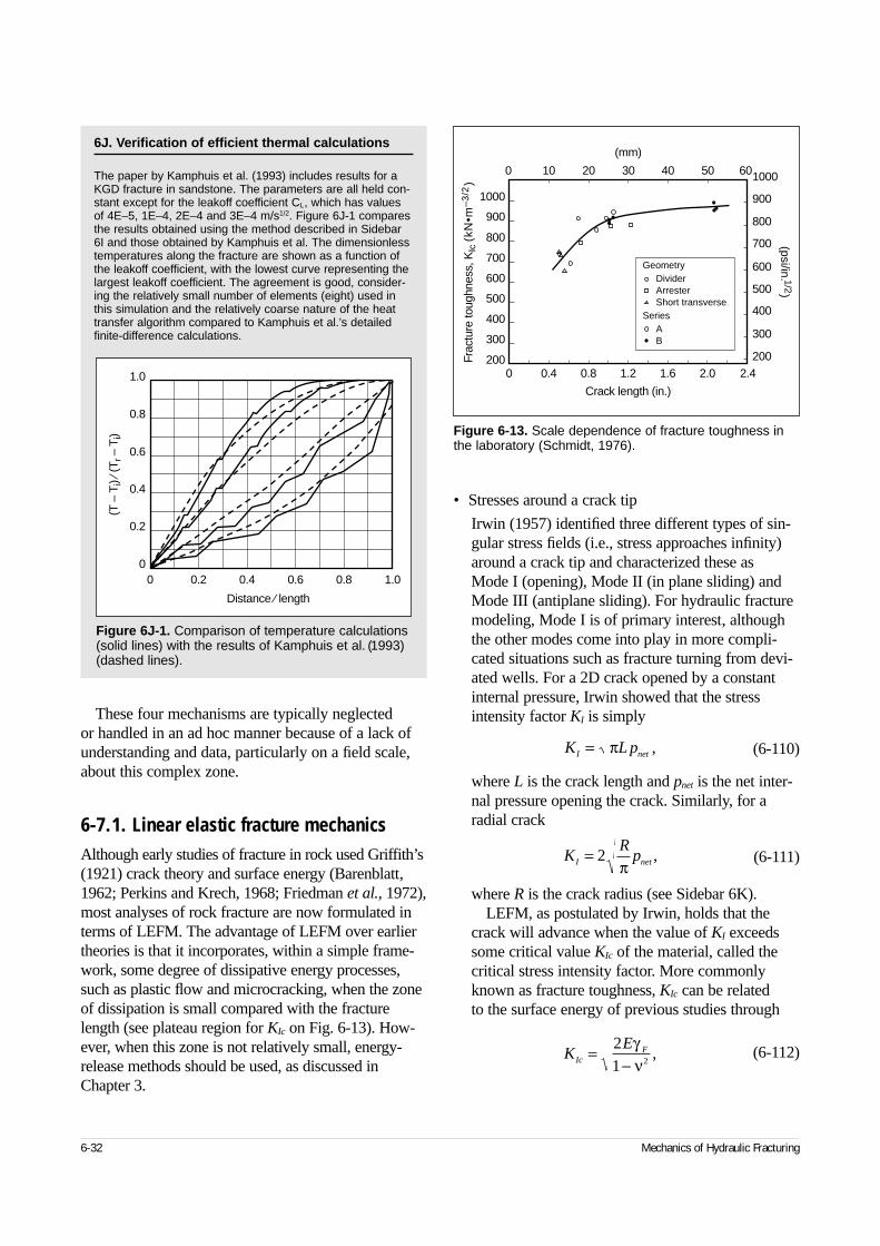
These four mechanisms are typically neglected or handled in an ad hoc manner because of a lack ofunderstanding and data, particularly on a field scale,about this complex zone.

6-7.1. Linear elastic fracture mechanicsAlthough early studies of fracture in rock used Griffith’s(1921) crack theory and surface energy (Barenblatt,1962; Perkins and Krech, 1968; Friedman et al., 1972),most analyses of rock fracture are now formulated interms of LEFM. The advantage of LEFM over earliertheories is that it incorporates, within a simple frame-work, some degree of dissipative energy processes,such as plastic flow and microcracking, when the zoneof dissipation is small compared with the fracturelength (see plateau region for KIc on Fig. 6-13). How-ever, when this zone is not relatively small, energy-release methods should be used, as discussed inChapter 3.

• Stresses around a crack tip

Irwin (1957) identified three different types of sin-gular stress fields (i.e., stress approaches infinity)around a crack tip and characterized these as Mode I (opening), Mode II (in plane sliding) andMode III (antiplane sliding). For hydraulic fracturemodeling, Mode I is of primary interest, althoughthe other modes come into play in more compli-cated situations such as fracture turning from devi-ated wells. For a 2D crack opened by a constantinternal pressure, Irwin showed that the stressintensity factor KI is simply

(6-110)

where L is the crack length and pnet is the net inter-nal pressure opening the crack. Similarly, for aradial crack

(6-111)

where R is the crack radius (see Sidebar 6K).LEFM, as postulated by Irwin, holds that the

crack will advance when the value of KI exceedssome critical value KIc of the material, called thecritical stress intensity factor. More commonlyknown as fracture toughness, KIc can be related to the surface energy of previous studies through

(6-112)

6-32 Mechanics of Hydraulic Fracturing

6J. Verification of efficient thermal calculations

The paper by Kamphuis et al. (1993) includes results for aKGD fracture in sandstone. The parameters are all held con-stant except for the leakoff coefficient CL, which has valuesof 4E–5, 1E–4, 2E–4 and 3E–4 m/s1/2. Figure 6J-1 comparesthe results obtained using the method described in Sidebar6I and those obtained by Kamphuis et al. The dimensionlesstemperatures along the fracture are shown as a function ofthe leakoff coefficient, with the lowest curve representing thelargest leakoff coefficient. The agreement is good, consider-ing the relatively small number of elements (eight) used inthis simulation and the relatively coarse nature of the heattransfer algorithm compared to Kamphuis et al.’s detailedfinite-difference calculations.

Figure 6J-1. Comparison of temperature calculations(solid lines) with the results of Kamphuis et al. (1993)(dashed lines).

(T –

Ti)

⁄ (T

r–

Ti)

1.0

0.8

0.6

0.4

0.2

00 0.2 0.4 0.6 0.8 1.0

Distance ⁄ length

Figure 6-13. Scale dependence of fracture toughness inthe laboratory (Schmidt, 1976).

Frac

ture

toug

hnes

s, K

Ic (

kN•m

–3

/2)

1000

900

800

700

600

500

400

300

200

(psi/in. 1/2)

1000

900

800

700

600

500

400

300

2000 0.4 0.8 1.2 1.6 2.0 2.4

6050403020100

Crack length (in.)

(mm)

GeometryDividerArresterShort transverse

SeriesAB

K L pI net= π ,

KR

pI net= 2π

,

KE

IcF=

−21 2

γν

,

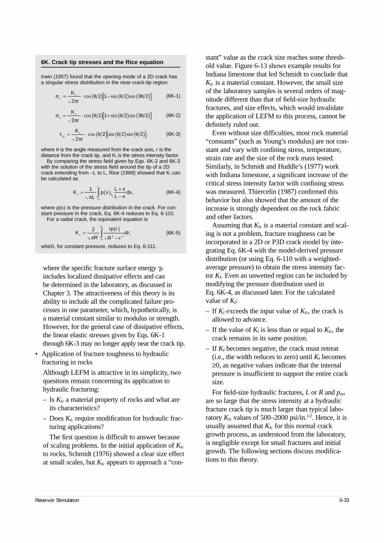
where the specific fracture surface energy γF

includes localized dissipative effects and can be determined in the laboratory, as discussed inChapter 3. The attractiveness of this theory is itsability to include all the complicated failure pro-cesses in one parameter, which, hypothetically, is a material constant similar to modulus or strength.However, for the general case of dissipative effects,the linear elastic stresses given by Eqs. 6K-1through 6K-3 may no longer apply near the crack tip.

• Application of fracture toughness to hydraulicfracturing in rocks

Although LEFM is attractive in its simplicity, twoquestions remain concerning its application tohydraulic fracturing:

– Is KIc a material property of rocks and what areits characteristics?

– Does KIc require modification for hydraulic frac-turing applications?

The first question is difficult to answer becauseof scaling problems. In the initial application of KIc

to rocks, Schmidt (1976) showed a clear size effectat small scales, but KIc appears to approach a “con-

stant” value as the crack size reaches some thresh-old value. Figure 6-13 shows example results forIndiana limestone that led Schmidt to conclude thatKIc is a material constant. However, the small sizeof the laboratory samples is several orders of mag-nitude different than that of field-size hydraulicfractures, and size effects, which would invalidatethe application of LEFM to this process, cannot bedefinitely ruled out.

Even without size difficulties, most rock material“constants” (such as Young’s modulus) are not con-stant and vary with confining stress, temperature,strain rate and the size of the rock mass tested.Similarly, in Schmidt and Huddle’s (1977) workwith Indiana limestone, a significant increase of thecritical stress intensity factor with confining stresswas measured. Thiercelin (1987) confirmed thisbehavior but also showed that the amount of theincrease is strongly dependent on the rock fabricand other factors.

Assuming that KIc is a material constant and scal-ing is not a problem, fracture toughness can beincorporated in a 2D or P3D crack model by inte-grating Eq. 6K-4 with the model-derived pressuredistribution (or using Eq. 6-110 with a weighted-average pressure) to obtain the stress intensity fac-tor KI. Even an unwetted region can be included bymodifying the pressure distribution used in Eq. 6K-4, as discussed later. For the calculatedvalue of KI:

– If KI exceeds the input value of KIc, the crack isallowed to advance.

– If the value of KI is less than or equal to KIc, thecrack remains in its same position.

– If KI becomes negative, the crack must retreat(i.e., the width reduces to zero) until KI becomes≥0, as negative values indicate that the internalpressure is insufficient to support the entire cracksize.

For field-size hydraulic fractures, L or R and pnet

are so large that the stress intensity at a hydraulicfracture crack tip is much larger than typical labo-ratory KIc values of 500–2000 psi/in.1/2. Hence, it isusually assumed that KIc for this normal crackgrowth process, as understood from the laboratory,is negligible except for small fractures and initialgrowth. The following sections discuss modifica-tions to this theory.

Reservoir Stimulation 6-33

6K. Crack tip stresses and the Rice equation

Irwin (1957) found that the opening mode of a 2D crack hasa singular stress distribution in the near-crack-tip region:

(6K-1)

(6K-2)

(6K-3)

where θ is the angle measured from the crack axis, r is thedistance from the crack tip, and KI is the stress intensity factor.

By comparing the stress field given by Eqs. 6K-2 and 6K-3with the solution of the stress field around the tip of a 2Dcrack extending from –L to L, Rice (1968) showed that KI canbe calculated as

(6K-4)

where p(x) is the pressure distribution in the crack. For con-stant pressure in the crack, Eq. 6K-4 reduces to Eq. 6-110.

For a radial crack, the equivalent equation is

(6K-5)

which, for constant pressure, reduces to Eq. 6-111.

σπ

θ θ θxIK

r= ( ) − ( ) ( )[ ]

22 1 2 3 2cos sin sin

σπ

θ θ θyIK

r= ( ) + ( ) ( )[ ]

22 1 2 3 2cos sin sin

τπ

θ θ θxyIK

r= ( ) ( ) ( )[ ]

22 2 2 ,cos sin sin

KL

p xL xL x

dxI

L

L

= ( ) +−

−∫1

π,

KR

rp r

R rdrI

R

=( )−∫2

2 20π

,

6-7.2. Extensions to LEFMIn the practical application of hydraulic fracturing, themeasured net pressures are usually larger than thosepredicted by models (Shlyapobersky, 1985, 1988a,1988b; Cleary et al., 1991). Although these high netpressures could be due to better than expected con-tainment, poor measurement of the closure stress,near-wellbore effects, complex fracturing, poor under-standing of rheology and many other factors, the gen-eral tendency has been to focus on the tip region asthe source of these anomalous results. Considerablework on fracture tip effects began after Shlyapobersky(1985) suggested that hydraulic fracture data could be interpreted to show a scale effect on KIc for field-size fractures. Since then, three additional majormechanisms have been proposed to account for thehigh net pressures at the crack tip: fluid lag effects(Jeffrey, 1989; Gardner, 1992; Advani et al., 1993),dilatancy (Cleary et al., 1991) and damage (Yew andLiu, 1993; Valkó and Economides, 1993a).

• Fluid lag region

As applied to hydraulic fracturing, the unwettedzone near the crack tip has pressure less than theclosure pressure and hence acts to clamp the frac-ture tip closed and reduce the stress intensity in therock. This zone was first introduced by Khristian-ovich and Zheltov (1955) and successfully used by Geertsma and de Klerk (1969) in modeling 2Dfractures. From their initial formulations, it is clearthat this unwetted region could have an impact onfracture parameters if it were sufficiently large. In a simple 2D geometry, the application is straight-forward, but the size of the unwetted zone and theexact pressure in the zone must be assumed. Thepressure within the unwetted region is most likelythe reservoir pressure for permeable rocks andcould be as low as the vapor pressure of the fluidfor impermeable rocks, so limits can be placed onits value. The size of the unwetted region is a moredifficult problem and has been the subject of con-siderable investigation.

Fluid lag can be incorporated into the standardKIc form by defining an effective fracture toughness(Jeffrey, 1989):

(6-113)

where

(6-114)

for a 2D (KGD) crack, where ptip is the net pressure(pressure near the tip minus the closure pressure) inthe nonwetted region and d is the fluid lag distance.Typically, ptip values are between –σc + pr and –σc +pvapor, where σc is the closure stress, pr is the reser-voir pressure, and pvapor is the vapor pressure of the fluid. The fracture propagation criterion nowbecomes

(6-115)

Similar equations can be written for radial cracks(Jeffrey, 1989).

Detailed study of the crack tip has led to the dis-covery of concepts unique to hydraulic fracturing.Modeling of the crack tip region by the SCR Geo-mechanics Group (1993; Lenoach, 1995) showsthat even when effects of fracture toughness KIc

are ignored, the consequences of coupled fluid flowand leakoff still result in a singularity at the cracktip. For an impermeable rock, the power of thehydraulic fracture singularity is not 1⁄2 as for therock behavior in LEFM, but rather n/(2 + n), wheren is the power law index of the fluid. For perme-able rocks, the power of the singularity is 3n/(4 + 4n),which is stronger than the impermeable singularity.Thus, an important singularity in stress may exist at the tip even under conditions in which the frac-ture toughness plays no role. They also madenumerical simulations that show that the size of the fluid lag region adjusts to meet the fracturepropagation criterion.

Models that determine the size of the unwettedregion (Jeffrey, 1989; Gardner, 1992; Yew and Liu,1993; SCR Geomechanics Group, 1993) generallyproduce small unwetted lengths, except at smallconfining stresses. However, only a small region isrequired near the tip to overshadow the effect fromthe fracture body. One shallow field experiment(relatively low confining stress) had sizable fluidlag zones (Warpinski, 1985), but no careful fieldstudy of fluid lag distances at higher confiningstresses has been made. Fracture models where thelag distance is calculated generally show only a

6-34 Mechanics of Hydraulic Fracturing

K K KIceff

Ic Iclag= + ,

KL p

L xdx

pL L d

L

Iclag tip

L d

L

tip

=−

= − −

−∫2

22

2 2π

ππ

arcsin

22 2

0

L p t

L xdx K K

L d

Ic Iclag

π( )−

= +−

∫ .

small influence on global fracture parameters; agood example is calculation of the 3D aspects ofthe lag effect by Advani et al. (1993). Earlier inthis chapter, it was shown that the dimension thatcontrols fracture width is the smaller one. Hence,the KGD model is most applicable for short frac-tures and the PKN model for long fractures.Advani et al.’s study shows that a similar effectoccurs for the fracture mechanics; i.e., the length L in Eq. 6-114 must be replaced by the fractureheight if the fracture length exceeds the height.

• Dilatancy

Although the LEFM concept can include small-scale damage and plasticity within its framework,the possibility exists that the damage zone around a field-size hydraulic fracture could be sufficientlylarge that the near-tip stress distribution becomesinvalid, or other effects could alter the stress distri-bution. For example, Cleary et al. (1991) suggestedthat the mechanism responsible for elevating cracktip pressures is dilatancy just behind the fracturetip. They postulated that if this dilatancy occursduring the rock failure process, then the fracturewidth just behind the tip may be pinched slightlyby the expanded fracture. Dilatation of material,which is essentially a volumetric expansion causedby failure, cannot be accommodated by the sur-rounding elastic material, so the rock stress in thenear-tip region must increase. Yew and Liu (1993)developed a modified fracture toughness to includedilatation of the material ahead of the crack tip for thecase where a plastic zone is created around the tip.An approximate equation for this behavior, in termsof an effective fracture toughness, was given as

(6-116)

where α is found by solving

(6-117)

where ϕ is the friction angle and Et is the Young’smodulus of the plastic material.

Throughout the body of a fracture such dilatancyis negligible, but it could play an important role inthe near-tip region, where the width is small. How-ever, numerical simulations of crack growth, assum-

ing the rock experiences dilatant-plastic yielding,(Papanastasiou and Thiercelin, 1993) show no over-all increase in the width at the fracture tip becauseplastic deformation dominates the dilation effect. De Pater et al. (1993) tried to identify dilatancy inlaboratory tests and through detailed modeling ofthe fracture tip, but no clear evidence of suchbehavior was obtained.

• Other behavior: damage- and fluid-induced effects

Another approach to modeling near-tip rock behav-ior is to use a cumulative damage approach, inwhich the microcrack damage ahead of the crackforces the undamaged material to accept more ofthe load. Valkó and Economides (1993a) formulateda fracture model using this approach. Their modelscales the damage with the fracture length, which is consistent with the KGD model and applies onlyto relatively short fractures. This analysis would be applicable for longer fractures if applied to a tipelement or with a scaling criterion.

Because most of the modeling efforts associatedwith hydraulic fracturing deal with either fluidmechanics or rock mechanics, the strong chemicalinteractions that can affect rock behavior are oftenforgotten. An extreme example of this effect is thelarge reduction in strength that can occur as a resultof stress corrosion cracking. Similarly, there hasbeen some evidence that the chemistry, rheology or molecular structure may influence tip behavior.Holder et al. (1993) conducted laboratory tests inwhich the inferred fracture toughness values usingcrosslinked gels were substantially greater thanthose with linear gels or Newtonian fluids. Dunning(1980) found that surfactants can have a majoreffect on the crack propagation stress (or, alterna-tively, the fracture toughness). The effects of pH,total ions, and breakers and other fluid additivescan cause additional chemical effects. However,these effects can influence tip failure only in theabsence of a fluid lag region or where the fluid pen-etrates a damaged area ahead of the fracture tip.

6-7.3. Field calibrationObtaining a definitive description of the fracture tipbehavior is complex and difficult. From a practicalstandpoint, because the tip pressure must be consistentwith field observations, its magnitude and impact canbe estimated using observed pressure data, as dis-

Reservoir Stimulation 6-35

K KE E

EEKIc

effIc

t

t

I= ++( )

−+

−

144

3 1 3

11

2

2

απ α

νν

,

tan ,ϕ αα

=−3

1 12 2

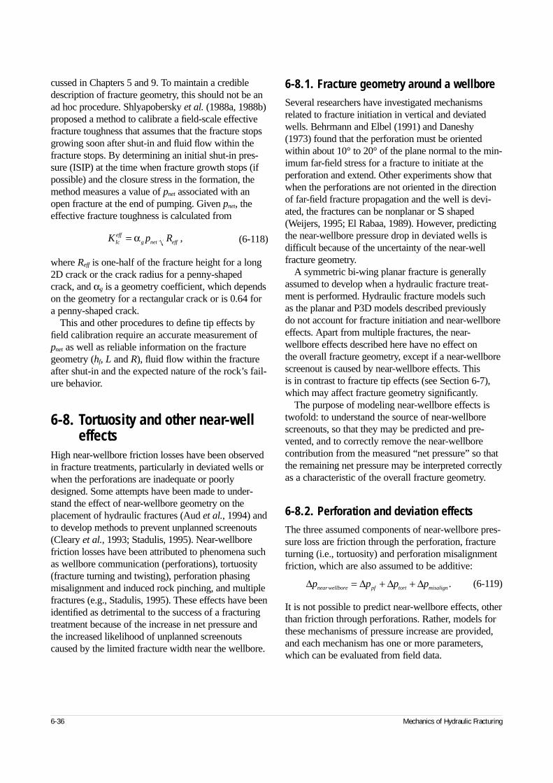
cussed in Chapters 5 and 9. To maintain a credibledescription of fracture geometry, this should not be anad hoc procedure. Shlyapobersky et al. (1988a, 1988b)proposed a method to calibrate a field-scale effectivefracture toughness that assumes that the fracture stopsgrowing soon after shut-in and fluid flow within thefracture stops. By determining an initial shut-in pres-sure (ISIP) at the time when fracture growth stops (ifpossible) and the closure stress in the formation, themethod measures a value of pnet associated with anopen fracture at the end of pumping. Given pnet, theeffective fracture toughness is calculated from

(6-118)

where Reff is one-half of the fracture height for a long2D crack or the crack radius for a penny-shapedcrack, and αg is a geometry coefficient, which dependson the geometry for a rectangular crack or is 0.64 fora penny-shaped crack.

This and other procedures to define tip effects byfield calibration require an accurate measurement ofpnet as well as reliable information on the fracturegeometry (hf, L and R), fluid flow within the fractureafter shut-in and the expected nature of the rock’s fail-ure behavior.

6-8. Tortuosity and other near-well effects

High near-wellbore friction losses have been observedin fracture treatments, particularly in deviated wells orwhen the perforations are inadequate or poorlydesigned. Some attempts have been made to under-stand the effect of near-wellbore geometry on theplacement of hydraulic fractures (Aud et al., 1994) andto develop methods to prevent unplanned screenouts(Cleary et al., 1993; Stadulis, 1995). Near-wellborefriction losses have been attributed to phenomena suchas wellbore communication (perforations), tortuosity(fracture turning and twisting), perforation phasingmisalignment and induced rock pinching, and multiplefractures (e.g., Stadulis, 1995). These effects have beenidentified as detrimental to the success of a fracturingtreatment because of the increase in net pressure andthe increased likelihood of unplanned screenoutscaused by the limited fracture width near the wellbore.

6-8.1. Fracture geometry around a wellboreSeveral researchers have investigated mechanismsrelated to fracture initiation in vertical and deviatedwells. Behrmann and Elbel (1991) and Daneshy(1973) found that the perforation must be orientedwithin about 10° to 20° of the plane normal to the min-imum far-field stress for a fracture to initiate at theperforation and extend. Other experiments show thatwhen the perforations are not oriented in the directionof far-field fracture propagation and the well is devi-ated, the fractures can be nonplanar or S shaped(Weijers, 1995; El Rabaa, 1989). However, predictingthe near-wellbore pressure drop in deviated wells isdifficult because of the uncertainty of the near-wellfracture geometry.

A symmetric bi-wing planar fracture is generallyassumed to develop when a hydraulic fracture treat-ment is performed. Hydraulic fracture models such as the planar and P3D models described previously do not account for fracture initiation and near-wellboreeffects. Apart from multiple fractures, the near-wellbore effects described here have no effect on the overall fracture geometry, except if a near-wellborescreenout is caused by near-wellbore effects. This is in contrast to fracture tip effects (see Section 6-7),which may affect fracture geometry significantly.

The purpose of modeling near-wellbore effects istwofold: to understand the source of near-wellborescreenouts, so that they may be predicted and pre-vented, and to correctly remove the near-wellborecontribution from the measured “net pressure” so thatthe remaining net pressure may be interpreted correctlyas a characteristic of the overall fracture geometry.

6-8.2. Perforation and deviation effectsThe three assumed components of near-wellbore pres-sure loss are friction through the perforation, fractureturning (i.e., tortuosity) and perforation misalignmentfriction, which are also assumed to be additive:

(6-119)

It is not possible to predict near-wellbore effects, otherthan friction through perforations. Rather, models forthese mechanisms of pressure increase are provided,and each mechanism has one or more parameters,which can be evaluated from field data.

6-36 Mechanics of Hydraulic Fracturing

K p RIceff

g net eff= α ,

∆ ∆ ∆ ∆p p p pnear wellbore pf tort misalign= + + .

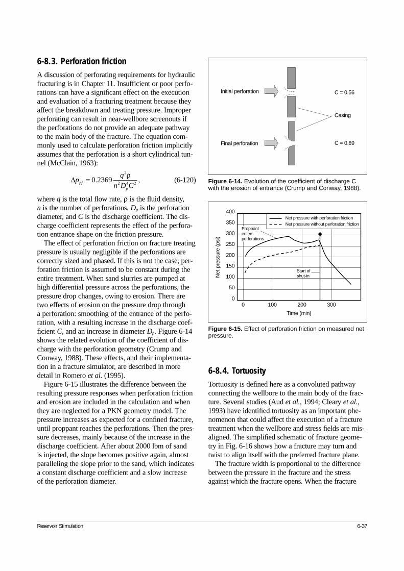
6-8.3. Perforation frictionA discussion of perforating requirements for hydraulicfracturing is in Chapter 11. Insufficient or poor perfo-rations can have a significant effect on the executionand evaluation of a fracturing treatment because theyaffect the breakdown and treating pressure. Improperperforating can result in near-wellbore screenouts ifthe perforations do not provide an adequate pathwayto the main body of the fracture. The equation com-monly used to calculate perforation friction implicitlyassumes that the perforation is a short cylindrical tun-nel (McClain, 1963):

(6-120)

where q is the total flow rate, ρ is the fluid density, n is the number of perforations, Dp is the perforationdiameter, and C is the discharge coefficient. The dis-charge coefficient represents the effect of the perfora-tion entrance shape on the friction pressure.

The effect of perforation friction on fracture treatingpressure is usually negligible if the perforations arecorrectly sized and phased. If this is not the case, per-foration friction is assumed to be constant during theentire treatment. When sand slurries are pumped athigh differential pressure across the perforations, thepressure drop changes, owing to erosion. There aretwo effects of erosion on the pressure drop through a perforation: smoothing of the entrance of the perfo-ration, with a resulting increase in the discharge coef-ficient C, and an increase in diameter Dp. Figure 6-14shows the related evolution of the coefficient of dis-charge with the perforation geometry (Crump andConway, 1988). These effects, and their implementa-tion in a fracture simulator, are described in moredetail in Romero et al. (1995).

Figure 6-15 illustrates the difference between theresulting pressure responses when perforation frictionand erosion are included in the calculation and whenthey are neglected for a PKN geometry model. Thepressure increases as expected for a confined fracture,until proppant reaches the perforations. Then the pres-sure decreases, mainly because of the increase in thedischarge coefficient. After about 2000 lbm of sand is injected, the slope becomes positive again, almostparalleling the slope prior to the sand, which indicatesa constant discharge coefficient and a slow increase of the perforation diameter.

6-8.4. TortuosityTortuosity is defined here as a convoluted pathwayconnecting the wellbore to the main body of the frac-ture. Several studies (Aud et al., 1994; Cleary et al.,1993) have identified tortuosity as an important phe-nomenon that could affect the execution of a fracturetreatment when the wellbore and stress fields are mis-aligned. The simplified schematic of fracture geome-try in Fig. 6-16 shows how a fracture may turn andtwist to align itself with the preferred fracture plane.

The fracture width is proportional to the differencebetween the pressure in the fracture and the stressagainst which the fracture opens. When the fracture

Reservoir Stimulation 6-37

∆pq

n D Cpf

p

= 0 23692

2 4 2. ,

ρFigure 6-14. Evolution of the coefficient of discharge Cwith the erosion of entrance (Crump and Conway, 1988).

Casing

C = 0.56Initial perforation

Final perforation C = 0.89

Figure 6-15. Effect of perforation friction on measured netpressure.

Net

pre

ssur

e (p

si)

400

350

300

250

200

150

100

50

00 100 200 300

Time (min)

Net pressure with perforation frictionNet pressure without perforation friction

Proppantentersperforations

Start of shut-in

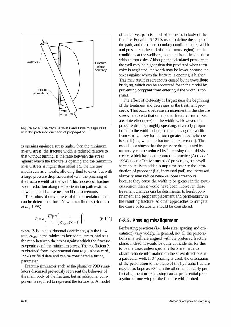
is opening against a stress higher than the minimumin-situ stress, the fracture width is reduced relative tothat without turning. If the ratio between the stressagainst which the fracture is opening and the minimumin-situ stress is higher than about 1.5, the fracturemouth acts as a nozzle, allowing fluid to enter, but witha large pressure drop associated with the pinching ofthe fracture width at the well. This process of fracturewidth reduction along the reorientation path restrictsflow and could cause near-wellbore screenouts.

The radius of curvature R of the reorientation pathcan be determined for a Newtonian fluid as (Romeroet al., 1995)

(6-121)

where λ is an experimental coefficient, q is the flowrate, σh,min is the minimum horizontal stress, and κ isthe ratio between the stress against which the fractureis opening and the minimum stress. The coefficient λis obtained from experimental data (e.g., Abass et al.,1994) or field data and can be considered a fittingparameter.

Fracture simulators such as the planar or P3D simu-lators discussed previously represent the behavior ofthe main body of the fracture, but an additional com-ponent is required to represent the tortuosity. A model

of the curved path is attached to the main body of thefracture. Equation 6-121 is used to define the shape ofthe path, and the outer boundary conditions (i.e., widthand pressure at the end of the tortuous region) are theconditions at the wellbore, obtained from the simulatorwithout tortuosity. Although the calculated pressure atthe well may be higher than that predicted when tortu-osity is neglected, the width may be lower because thestress against which the fracture is opening is higher.This may result in screenouts caused by near-wellborebridging, which can be accounted for in the model bypreventing proppant from entering if the width is toosmall.

The effect of tortuosity is largest near the beginningof the treatment and decreases as the treatment pro-ceeds. This occurs because an increment in the closurestress, relative to that on a planar fracture, has a fixedabsolute effect (∆w) on the width w. However, thepressure drop is, roughly speaking, inversely propor-tional to the width cubed, so that a change in widthfrom w to w – ∆w has a much greater effect when wis small (i.e., when the fracture is first created). Themodel also shows that the pressure drop caused bytortuosity can be reduced by increasing the fluid vis-cosity, which has been reported in practice (Aud et al.,1994) as an effective means of preventing near-wellscreenouts. Both added pump time prior to the intro-duction of proppant (i.e., increased pad) and increasedviscosity may reduce near-wellbore screenoutsbecause they cause the width to be greater in the tortu-ous region than it would have been. However, thesetreatment changes can be detrimental to height con-finement and proppant placement and permeability inthe resulting fracture, so other approaches to mitigatethe cause of tortuosity should be considered.

6-8.5. Phasing misalignmentPerforating practices (i.e., hole size, spacing and ori-entation) vary widely. In general, not all the perfora-tions in a well are aligned with the preferred fractureplane. Indeed, it would be quite coincidental for thisto be the case, unless special efforts are made toobtain reliable information on the stress directions at a particular well. If 0° phasing is used, the orientationof the perforation to the plane of the hydraulic fracturemay be as large as 90°. On the other hand, nearly per-fect alignment or 0° phasing causes preferential prop-agation of one wing of the fracture with limited

6-38 Mechanics of Hydraulic Fracturing

Figure 6-16. The fracture twists and turns to align itselfwith the preferred direction of propagation.

Fracturereorientation

Wellbore Fractureplane

at infinity

θ

RE q

hf h min

=−( )

λ µ

σ κ

32

11,

,

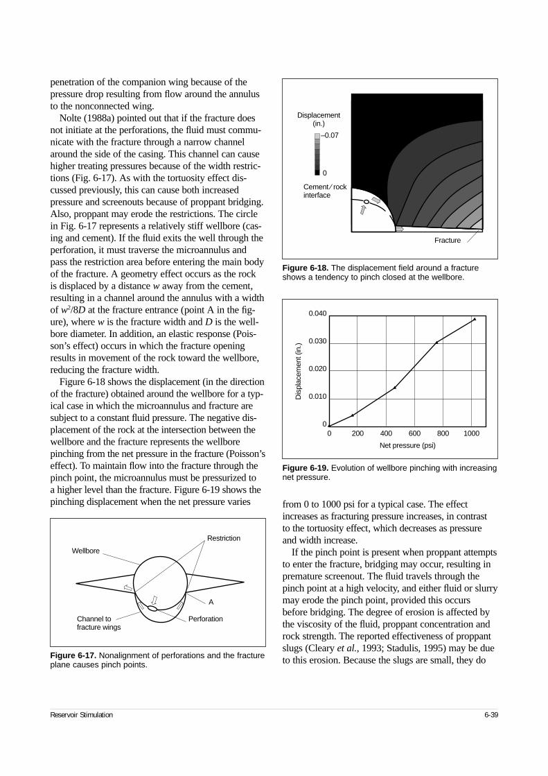
penetration of the companion wing because of thepressure drop resulting from flow around the annulusto the nonconnected wing.

Nolte (1988a) pointed out that if the fracture doesnot initiate at the perforations, the fluid must commu-nicate with the fracture through a narrow channelaround the side of the casing. This channel can causehigher treating pressures because of the width restric-tions (Fig. 6-17). As with the tortuosity effect dis-cussed previously, this can cause both increasedpressure and screenouts because of proppant bridging.Also, proppant may erode the restrictions. The circlein Fig. 6-17 represents a relatively stiff wellbore (cas-ing and cement). If the fluid exits the well through theperforation, it must traverse the microannulus andpass the restriction area before entering the main bodyof the fracture. A geometry effect occurs as the rock is displaced by a distance w away from the cement,resulting in a channel around the annulus with a widthof w2/8D at the fracture entrance (point A in the fig-ure), where w is the fracture width and D is the well-bore diameter. In addition, an elastic response (Pois-son’s effect) occurs in which the fracture openingresults in movement of the rock toward the wellbore,reducing the fracture width.

Figure 6-18 shows the displacement (in the directionof the fracture) obtained around the wellbore for a typ-ical case in which the microannulus and fracture aresubject to a constant fluid pressure. The negative dis-placement of the rock at the intersection between thewellbore and the fracture represents the wellborepinching from the net pressure in the fracture (Poisson’seffect). To maintain flow into the fracture through thepinch point, the microannulus must be pressurized to a higher level than the fracture. Figure 6-19 shows thepinching displacement when the net pressure varies from 0 to 1000 psi for a typical case. The effect

increases as fracturing pressure increases, in contrast to the tortuosity effect, which decreases as pressureand width increase.

If the pinch point is present when proppant attemptsto enter the fracture, bridging may occur, resulting inpremature screenout. The fluid travels through thepinch point at a high velocity, and either fluid or slurrymay erode the pinch point, provided this occursbefore bridging. The degree of erosion is affected bythe viscosity of the fluid, proppant concentration androck strength. The reported effectiveness of proppantslugs (Cleary et al., 1993; Stadulis, 1995) may be dueto this erosion. Because the slugs are small, they do

Reservoir Stimulation 6-39

Figure 6-17. Nonalignment of perforations and the fractureplane causes pinch points.

Wellbore

Restriction

Perforation

A

Channel to fracture wings

Figure 6-18. The displacement field around a fractureshows a tendency to pinch closed at the wellbore.

Displacement(in.)

Fracture

Cement ⁄ rockinterface

–0.07

0

Figure 6-19. Evolution of wellbore pinching with increasingnet pressure.

Dis

plac

emen

t (in

.)

0 200 400 600 800 1000

Net pressure (psi)

0.040

0.030

0.020

0.010

0

not bridge everywhere, so fluid entry at higher veloc-ity continues and erodes some channels. Even prior to the use of slugs, it was common to inject proppantat low concentration to erode restrictions when highpressures occurred during the fracture initiation stage.In contrast to tortuosity, pinching is increased by largepads and higher net pressures. This may explain why,in some cases, prepad slugs can be injected at low netpressures when the pinching is smaller, but in themain treatment a near-well screenout occurs.

6-9. Acid fracturingHydraulic fracturing with acid (usually hydrochloricacid [HCl]) is an alternative to propped fractures inacid-soluble formations such as dolomites and lime-stones. The major difference between acid and proppedfractures is that conductivity is obtained by etching thefracture faces instead of by using a proppant to preventthe fracture from closing. Acid fracturing may be pre-ferred operationally because the potential for unin-tended proppant bridging and proppant flowback isavoided. However, designing and controlling the depthof penetration of the live acid into the formation andthe etched conductivity are more difficult than control-ling proppant placement. Acid penetration is governedby the chemical reaction between the rock and thefracturing fluid (as opposed to a simple mass balancein propped fractures), and conductivity is determinedby the etching patterns formed by the reacting acid (asopposed to being a property of the proppant under agiven stress). In both cases, acid fracturing introduces a dependence on rock properties that is not present inpropped fracturing. In addition, the properties that acidfracturing design and control depend on are usually moredifficult to determine than other formation properties.

The geometry of acid fractures can be determinedby the same models used for propped fractures, withthe exception of the impact of etched width on thewidth-pressure relation. However, several additionalaspects of acid fracturing must be considered:

• acid transport to and reaction at the rock surface

• heat transfer, because the reaction releases heat, andthe reaction rate is temperature sensitive

• leakoff, because acid leakoff behavior is signifi-cantly different from that of nonreactive fluids.

6-9.1. Historical acid fracturing modelsWilliams et al. (1979) provided a detailed discussionof acid fracturing models prior to 1980, and Li et al.(1993) reviewed some of the more recent work. Oneof the main drawbacks of most of the early modelswas that the fracture geometry calculation was sepa-rated from the acid reaction calculation to developanalytically tractable solutions. Since then, computer-based models have overcome these limitations, andthe preceding models are no longer used. For exam-ple, Settari (1993) presented a detailed description of a comprehensive model with the fracture geometryand acid reaction calculations coupled, including acomprehensive leakoff model, coupled heat transferand the capability to include multiple fluids with vary-ing rheology.

Much of what follows is based on the workdescribed by Settari. Roodhart et al. (1993) presenteda model in which they developed the heat transfercalculations extensively, using the work of Kamphuiset al. (1993). The other factor they included was theeffect of the boundary layer thickness for acid reactiondeveloping as the fluid enters the fracture, resulting in a thinner layer near the well and causing a higheretching rate. The aforementioned publications containextensive lists of references.

6-9.2. Reaction stoichiometryThe main chemical reactions of interest in acid frac-turing are those between HCl and calcium carbonate(limestone) or calcium-magnesium carbonate (dolo-mite). The chemical reaction for limestone is written as

2HCl + CaCO3 H2O + CO2 + CaCl2

and for dolomite as

4HCl + CaMg(CO3)2 2H2O + 2CO2 + CaCl2

+ MgCl2

The first reaction equation indicates that two mole-cules of HCl react with one molecule of calcium car-bonate to form one molecule each of water, carbondioxide and calcium chloride. The second equationshows that four molecules of HCl react with one mole-cule of calcium-magnesium carbonate to form twomolecules each of water and carbon dioxide and oneeach of calcium chloride and magnesium chloride.

6-40 Mechanics of Hydraulic Fracturing

These so-called stoichiometric equations allow com-puting the volume of rock dissolved by a given volumeof acid. These equations can be used to determine thedissolving power XC of the acid, which is the volumeof rock dissolved per unit volume of acid reacted. Themass dissolving power (i.e., the mass of rock dissolvedper unit mass of acid reacted) is first defined as

(6-122)

For the limestone reaction,

(6-123)

so that each gram of 100% pure HCl dissolves 1.372 g of rock. To obtain the dissolving power, the masses must be converted to volumes:

(6-124)

where ρC and ρCaCO3 are the densities of the acid solu-tion and calcium carbonate, respectively, and C is theweight-fraction concentration (e.g., 0.28 for 28%acid). For example, the specific gravity of 28% acid is 1.14, whereas that for 15% acid is 1.07. A completetable of densities is in Williams et al. (1979). Applyingthis calculation for the limestone-HCl reaction, X15 is0.082, and X28 is 0.161. Similarly, for dolomite thevalues are 0.071 and 0.141, respectively.

The stoichiometric equations for acid reactions pro-vide a relation for the coupling between fracturegeometry and acid spending. Because there are manyunknowns in acid fracturing, the modeling can besimplified by neglecting the variation in density of theacid and using that of 10% acid, which is a suitableaverage for most acid fracture treatments. In this case,X100 can be approximated as 10X10 and XC as CX100.Now, consider the volume of a fracture element ofcross-sectional area (width times height) A and lengthδx in which the acid concentration changes by anamount ∆C. The volume of acid spent is A ⋅ δx ⋅ ∆C,and the volume ∆A ⋅ δx of rock dissolved is

(6-125)

where Aetch is the etched area and C–

is the average acidconcentration in the cross section.

6-9.3. Acid fracture conductivityAcid fracture conductivity is much more poorlyunderstood than propped fracture conductivity. Theflow rate through an open channel of width w is pro-portional to w3. If the etched channel were under nostress, this proportional relation would be used todetermine the conductivity of an acid fracture. How-ever, the stress in the reservoir acts to close the channel.If the etching were completely uniform, this closingcould be calculated in a manner similar to that used to calculate the width of an elliptical fracture, exceptthat the net pressure is negative. As an approximation,for a uniform etched width, the shape of the resultingclosed fracture would be

(6-126)

where wetch is the etched width, and the width is set to zero wherever Eq. 6-126 predicts a negative width. It is apparent from this equation that the width in mostof the channel would be much lower than that of anopen channel, as most of the channel would haveclosed completely. This would clearly reduce fractureconductivity significantly.

Fortunately, acid etches the rock surface in a non-uniform manner, because of rock heterogeneity andfingering of the acid through the wider previouslyetched channels. This results in numerous horizontal“pillars” supporting the channels between them, forwhich Eq. 6-126 could be used with the fixed fractureheight hf replaced by the distance between the pillars.It is not practical to model this in detail, because thepattern is not generally known. Because conductivityis higher in formations where numerous small chan-nels occur supported by numerous pillars, uniformetching is not desirable. If, however, the pillars lackthe strength to support the additional load required tokeep the channels open, some of the pillars will col-lapse, reducing the conductivity. Fracture conductivityis thus dependent not only on the etching pattern, butalso on the rock strength and closure stress. Nierodeand Kruk (1973) developed an empirical equation forconductivity:

(6-127)

where

(6-128)

Reservoir Stimulation 6-41

β = ( ) × ( )( ) × ( )molecular weight of rock rock stoichiometric coefficient

molecular weight of acid acid stoichiometric coefficient

.

β = ××

=100 09 136 47 2

1 372.

..

XC

CC

CaCO

= ρ βρ

3

,

∆ ∆A X A Cetch = 100 ,

w z wE

h zetchc

f( ) = −′

−4 2 2σ,

wk C Ceff( ) = −( )1 2exp σ ,

C wkfi10 8220 265= . .

(6-129)

(6-130)

where σ is the effective stress in psi, SRE is the rockembedment strength in psi, and wkfi is the conductivityin md-in. A typographical error in the original paper iscorrected in Eq. 6-129.

6-9.4. Energy balance during acid fracturingThe total heat generated (per unit volume) by achange in acid concentration ∆C

–is ∆C

–∆H, where ∆His the heat of reaction. Coupling of the acid and heattransfer models is provided by assuming that all theheat initially increases the fluid temperature, resultingin a fluid temperature change of

(6-131)

where ρf is the fluid density and Cpfl is the fluid heatcapacity. Section 6-6 describes how heat is transferredbetween the fluid and the formation. The magnitudeof the temperature change resulting from acid reactionmay be sufficient to cause the temperature of somefluids to exceed the reservoir temperature. It is thusparticularly important to use a numerical temperaturecalculation when simulating acid fracturing.

6-9.5. Reaction kineticsSurface reactions such as the acid-rock reactions dis-cussed here are complex, even under laboratory condi-tions. In general, the liquid-phase reaction betweenspecies A and B to form products C and D is gov-erned by an expression of the form

(6-132)

where ξ f is the forward rate constant, ξr is the reverserate constant, and aX represents the chemical activityof species X. In the reactions of interest in acid frac-turing, reverse reactions are usually much slower thanforward reactions and can be neglected. In very dilutesystems, the chemical activity is equal to the concen-tration. It is also usually observed that the reaction

rate constants are functions of temperature, followingthe Arrhenius equation:

(6-133)

The acid reaction rate at a surface is thus a complexfunction of the activities of all species involved in thereaction. Detailed modeling of the reaction in terms ofthese activities is not required for a hydraulic fracturesimulator, because of the large amount of uncertaintyin the other parameters. Instead, the reaction rate canbe assumed to be governed by the simple equation forthe rate of acid consumption r (Settari, 1993):

(6-134)

where the temperature-dependent reaction rateconstant is

(6-135)

where Macid is the moles of acid per unit rock facearea, t is the time, Cwall is the surface acid concentra-tion, Ceqm is the equilibrium concentration, m is theorder of reaction, k0 is the reaction rate constant at thereference temperature Tref (298K [25°C]), ∆E is theactivation energy, R is the universal gas constant, andT is the absolute temperature.

Ceqm is generally zero for the reactions of interest.

6-9.6. Mass transferBefore the reaction can occur at the fracture wall, theacid molecules must be transported to the wall. In astagnant fluid, diffusion in an ideal case can bedescribed by Fick’s law:

(6-136)

where vA,x is the velocity of species A, DA is the mole-cular diffusion coefficient, CA is the acid concentra-tion, and the derivative represents the concentrationgradient. Williams et al. (1979) proposed accountingfor leakoff by adding a term to the right-hand side ofEq. 6-136, resulting in

(6-137)

6-42 Mechanics of Hydraulic Fracturing

CS S

S SRE RE

RE RE2

3

3

13 9 1 3 10 0 20 000

3 8 0 28 10 20 000 500 000=

−( ) × < <−( ) × < <

−

−

. . ,

. . , ,

ln psi psi

ln psi psi

wkw

fietch= ×

9 36 10

1213

3

. ,

∆ ∆ ∆T

C H

Cfl

f pfl

=ρ

,

r a a a af An

Bn

r Cn

DnA B C D= −ξ ξ 1 ,

ζ ζfT

f

T

ref

refE

R T T= − −

exp

∆ 1 1.

rM

tK C Cacid

r wall eqm

m= = − −( )∂

∂,

K kE

R T Tr

ref

= − −

0

1 1exp ,

∆

v DC

xA x AA

, ,= − ∂∂

v DC

xC uA x A

AA L, .= − +∂

∂

In flowing fluids, this equation is no longer valid,because acid transport is by convection rather thandiffusion. For acid fracture modeling, Eq. 6-136 issimply replaced by

(6-138)

where the mass-transfer coefficient is

(6-139)

where Deff is the effective acid diffusion coefficient.The Sherwood number NSh is determined from thecorrelation (Lee and Roberts, 1980)

(6-140)

where the Reynold’s and Schmidt numbers aredefined respectively by

(6-141)

(6-142)

6-9.7. Acid reaction modelIf reaction occurs, the acid concentration varies acrossthe fracture width, and the surface concentration is lessthan the bulk acid concentration. The surface concen-tration is such that the amount consumed at the surfaceis balanced by transport to the surface by diffusion.

The wall concentration for a given bulk concentra-tion is obtained by equating the right-hand sides ofEqs. 6-134 and 6-138 to obtain

(6-143)

This equation, which is a general model of acidreaction, can easily be solved if m = 1 but is solvediteratively otherwise. If Kr is very large comparedwith Kg + uL, then Eq. 6-143 is satisfied when Cwall

is approximately equal to Ceqm. In this case, Ceqm canreplace Cwall on the right-hand side of Eq. 6-143, andEq. 6-138 can be written as

(6-144)

In this case, the reaction rate is termed mass-trans-fer limited, because the rate at which it occurs is con-trolled by the rate at which live acid can be brought tothe rock surface. Similarly, if Kg + uL is very largecompared with Kr, then Eq. 6-143 is satisfied whenCwall is approximately equal to C

–. In this case, C

–can

replace Cwall on the left-hand side of Eq. 6-143, andEq. 6-134 can be written as

(6-145)

Equation 6-145 represents the reaction-rate- orkinetics-limited case in which the rate of acid con-sumption is limited by the rate at the wall.

6-9.8. Acid fracturing: fracture geometry model

The movement of acid perpendicular to the fracturewall is considered in this section. The preceding sec-tions discuss the fluid flow equations typically solvedin fracture models. Acid movement within the fracturecan be modeled similarly to the movement of prop-pant. For a fracture simulator to simulate acid fractur-ing treatments accurately, several specific require-ments must be met relating to

• fluid tracking in the fracture and reservoir

• recession of the active fracture length

• effect of etching on the relation between pressureand width.

Although typical fluid flow calculation schemes usea coarse grid (about 10 elements), accurate fluid fronttracking can be obtained only by following up to 50fluid stages. Typical treatments include only about 10different stages, but stages can be subdivided for bet-ter tracking of the large gradients that may occur inacid concentration within a single stage. Also, a finergrid is required to track leakoff volumes into the for-mation and formation exposure to fluid stages foraccurate modeling of the extreme differences in leak-off characteristics and viscosity between acid andnonacid stages.

Acid fracturing treatments are typically designedwith sudden changes in flow rate because the differentfluids in the treatment have significantly different fric-tional properties. These sudden changes, as well as thehigh leakoff that may occur during pumping of the

Reservoir Stimulation 6-43

K C C K u C Cr wall eqm

m

g L wall−( ) = +( ) −( ) .

rM

tK C Cacid

r wall eqm

m= = − −( )∂

∂.

v K C C C C uA x g A wall A wall L, ,= −( ) + −( )

K D N wg eff Sh= ,

Nwv

Ref=

2 ρµ

NDSc

eff f

= µρ

.

N

N N

N N N

N N NSh

Sc Re

Re Sc Re

Re Sc Re

=<< <

>

6 26 1800

0 001104 1800 7000

0 026 7000

1 3

1 153 1 3

4 5 1 3

.

. ,

.

/

. /

/ /

rM

tK u C Cacid

g L eqm= = − +( ) −( )∂∂

.

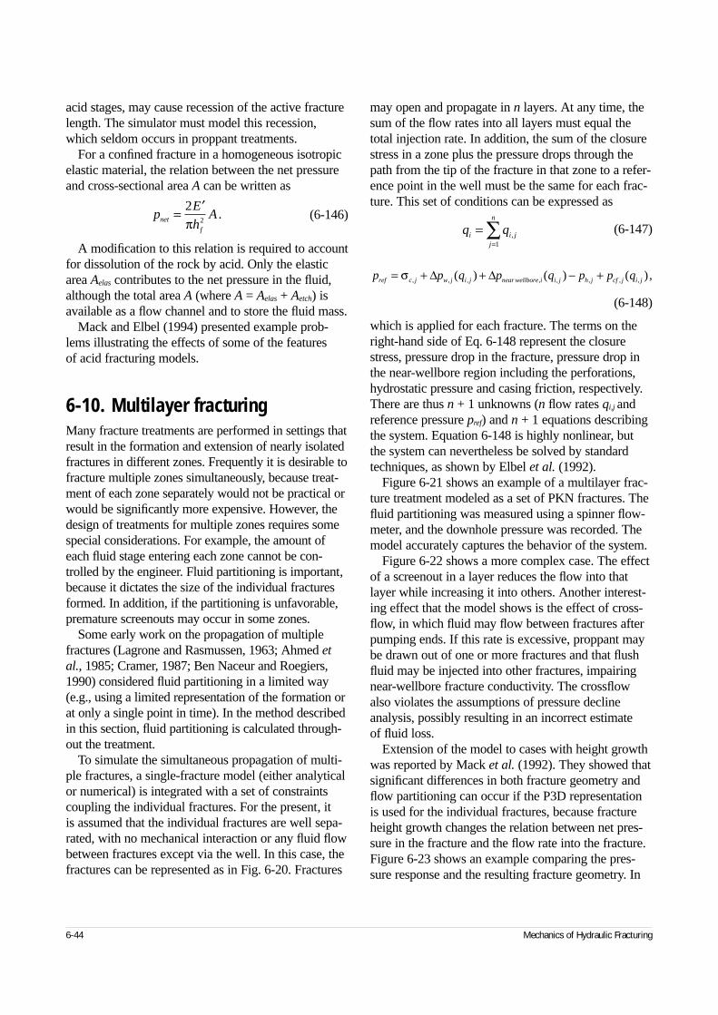
acid stages, may cause recession of the active fracturelength. The simulator must model this recession,which seldom occurs in proppant treatments.

For a confined fracture in a homogeneous isotropicelastic material, the relation between the net pressureand cross-sectional area A can be written as

(6-146)

A modification to this relation is required to accountfor dissolution of the rock by acid. Only the elasticarea Aelas contributes to the net pressure in the fluid,although the total area A (where A = Aelas + Aetch) isavailable as a flow channel and to store the fluid mass.

Mack and Elbel (1994) presented example prob-lems illustrating the effects of some of the features of acid fracturing models.

6-10. Multilayer fracturingMany fracture treatments are performed in settings thatresult in the formation and extension of nearly isolatedfractures in different zones. Frequently it is desirable tofracture multiple zones simultaneously, because treat-ment of each zone separately would not be practical orwould be significantly more expensive. However, thedesign of treatments for multiple zones requires somespecial considerations. For example, the amount ofeach fluid stage entering each zone cannot be con-trolled by the engineer. Fluid partitioning is important,because it dictates the size of the individual fracturesformed. In addition, if the partitioning is unfavorable,premature screenouts may occur in some zones.

Some early work on the propagation of multiplefractures (Lagrone and Rasmussen, 1963; Ahmed etal., 1985; Cramer, 1987; Ben Naceur and Roegiers,1990) considered fluid partitioning in a limited way(e.g., using a limited representation of the formation orat only a single point in time). In the method describedin this section, fluid partitioning is calculated through-out the treatment.

To simulate the simultaneous propagation of multi-ple fractures, a single-fracture model (either analyticalor numerical) is integrated with a set of constraintscoupling the individual fractures. For the present, it is assumed that the individual fractures are well sepa-rated, with no mechanical interaction or any fluid flowbetween fractures except via the well. In this case, thefractures can be represented as in Fig. 6-20. Fractures

may open and propagate in n layers. At any time, thesum of the flow rates into all layers must equal thetotal injection rate. In addition, the sum of the closurestress in a zone plus the pressure drops through thepath from the tip of the fracture in that zone to a refer-ence point in the well must be the same for each frac-ture. This set of conditions can be expressed as

(6-147)

(6-148)

which is applied for each fracture. The terms on theright-hand side of Eq. 6-148 represent the closurestress, pressure drop in the fracture, pressure drop inthe near-wellbore region including the perforations,hydrostatic pressure and casing friction, respectively.There are thus n + 1 unknowns (n flow rates qi,j andreference pressure pref) and n + 1 equations describingthe system. Equation 6-148 is highly nonlinear, butthe system can nevertheless be solved by standardtechniques, as shown by Elbel et al. (1992).

Figure 6-21 shows an example of a multilayer frac-ture treatment modeled as a set of PKN fractures. Thefluid partitioning was measured using a spinner flow-meter, and the downhole pressure was recorded. Themodel accurately captures the behavior of the system.

Figure 6-22 shows a more complex case. The effectof a screenout in a layer reduces the flow into thatlayer while increasing it into others. Another interest-ing effect that the model shows is the effect of cross-flow, in which fluid may flow between fractures afterpumping ends. If this rate is excessive, proppant maybe drawn out of one or more fractures and that flushfluid may be injected into other fractures, impairingnear-wellbore fracture conductivity. The crossflowalso violates the assumptions of pressure declineanalysis, possibly resulting in an incorrect estimate of fluid loss.

Extension of the model to cases with height growthwas reported by Mack et al. (1992). They showed thatsignificant differences in both fracture geometry andflow partitioning can occur if the P3D representationis used for the individual fractures, because fractureheight growth changes the relation between net pres-sure in the fracture and the flow rate into the fracture.Figure 6-23 shows an example comparing the pres-sure response and the resulting fracture geometry. In

6-44 Mechanics of Hydraulic Fracturing

pE

hAnet

f

= ′22π

.q qi i j

j

n

==

∑ ,1

p p q p q p p qref c j w j i j near wellbore i i j h j cf j i j= + + − +σ , , , , , , , ,( ) ( ) ( ) ,∆ ∆

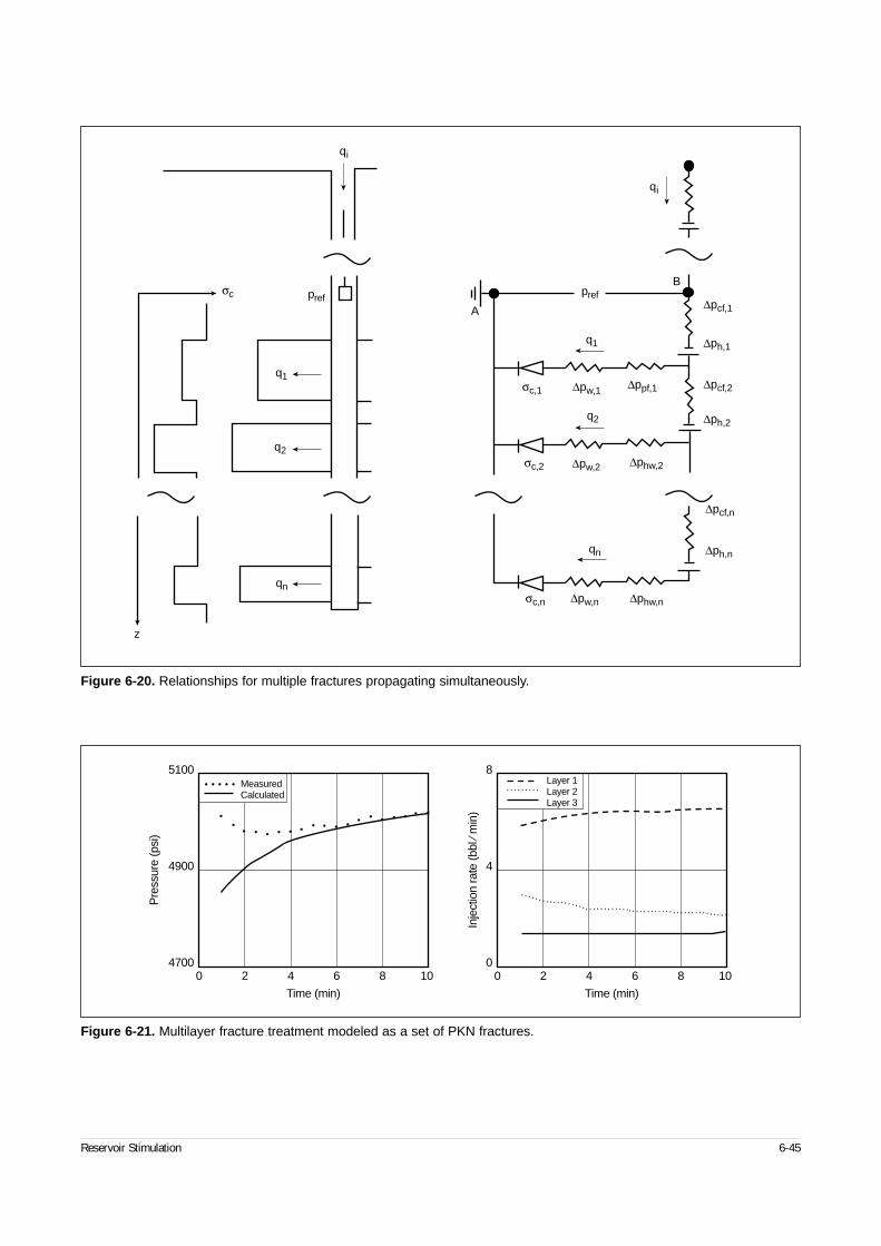
Reservoir Stimulation 6-45

Figure 6-20. Relationships for multiple fractures propagating simultaneously.

z

qi

qi

pref

σc,1

σc,2

prefσc

q1

q1

q2

q2

qn

qn

σc,n ∆pw,n

∆ph,n

∆pcf,n

∆pcf,2

∆pcf,1

∆ph,2

∆ph,1

∆ppf,1

∆phw,2

∆pw,1

∆pw,2

∆phw,n

A

B

Figure 6-21. Multilayer fracture treatment modeled as a set of PKN fractures.

5100

4900

4700

Pre

ssur

e (p

si)

0 2 4 6 8 10

Time (min)

MeasuredCalculated

8

4

0

Inje

ctio

n ra

te (b

bl ⁄

min

)

0 2 4 6 8 10

Time (min)

Layer 1Layer 2Layer 3

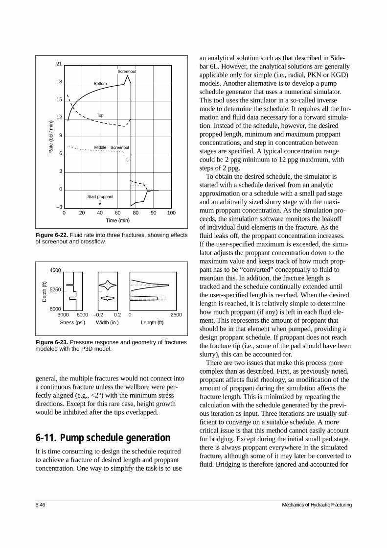
general, the multiple fractures would not connect intoa continuous fracture unless the wellbore were per-fectly aligned (e.g., <2°) with the minimum stressdirections. Except for this rare case, height growthwould be inhibited after the tips overlapped.

6-11. Pump schedule generationIt is time consuming to design the schedule requiredto achieve a fracture of desired length and proppantconcentration. One way to simplify the task is to use

an analytical solution such as that described in Side-bar 6L. However, the analytical solutions are generallyapplicable only for simple (i.e., radial, PKN or KGD)models. Another alternative is to develop a pumpschedule generator that uses a numerical simulator.This tool uses the simulator in a so-called inversemode to determine the schedule. It requires all the for-mation and fluid data necessary for a forward simula-tion. Instead of the schedule, however, the desiredpropped length, minimum and maximum proppantconcentrations, and step in concentration betweenstages are specified. A typical concentration rangecould be 2 ppg minimum to 12 ppg maximum, withsteps of 2 ppg.

To obtain the desired schedule, the simulator isstarted with a schedule derived from an analyticapproximation or a schedule with a small pad stageand an arbitrarily sized slurry stage with the maxi-mum proppant concentration. As the simulation pro-ceeds, the simulation software monitors the leakoff of individual fluid elements in the fracture. As thefluid leaks off, the proppant concentration increases. If the user-specified maximum is exceeded, the simu-lator adjusts the proppant concentration down to themaximum value and keeps track of how much prop-pant has to be “converted” conceptually to fluid tomaintain this. In addition, the fracture length istracked and the schedule continually extended untilthe user-specified length is reached. When the desiredlength is reached, it is relatively simple to determinehow much proppant (if any) is left in each fluid ele-ment. This represents the amount of proppant thatshould be in that element when pumped, providing adesign proppant schedule. If proppant does not reachthe fracture tip (i.e., some of the pad should have beenslurry), this can be accounted for.

There are two issues that make this process morecomplex than as described. First, as previously noted,proppant affects fluid rheology, so modification of theamount of proppant during the simulation affects thefracture length. This is minimized by repeating thecalculation with the schedule generated by the previ-ous iteration as input. Three iterations are usually suf-ficient to converge on a suitable schedule. A morecritical issue is that this method cannot easily accountfor bridging. Except during the initial small pad stage,there is always proppant everywhere in the simulatedfracture, although some of it may later be converted tofluid. Bridging is therefore ignored and accounted for

6-46 Mechanics of Hydraulic Fracturing

Figure 6-22. Fluid rate into three fractures, showing effectsof screenout and crossflow.

Rat

e (b

bl ⁄

min

)

21

18

15

12

9

6

3

0

–30 20 40 60 80 90 100

Time (min)

Screenout

Bottom

Top

Middle

Start proppant

Screenout

Figure 6-23. Pressure response and geometry of fracturesmodeled with the P3D model.

Dep

th (f

t)

4500

5250

60003000 6000 –0.2 0.2 0 2500

Stress (psi) Width (in.) Length (ft)

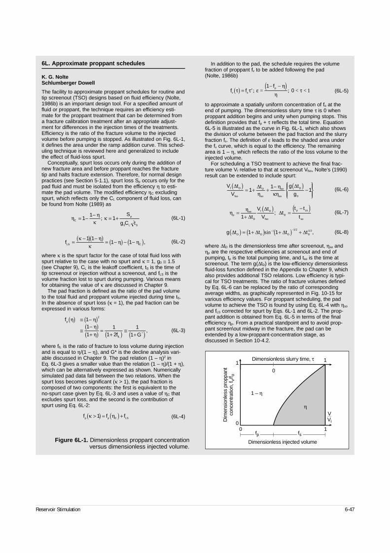
Reservoir Stimulation 6-47

6L. Approximate proppant schedules

K. G. NolteSchlumberger Dowell

The facility to approximate proppant schedules for routine andtip screenout (TSO) designs based on fluid efficiency (Nolte,1986b) is an important design tool. For a specified amount offluid or proppant, the technique requires an efficiency esti-mate for the proppant treatment that can be determined froma fracture calibration treatment after an appropriate adjust-ment for differences in the injection times of the treatments.Efficiency is the ratio of the fracture volume to the injectedvolume before pumping is stopped. As illustrated on Fig. 6L-1,it defines the area under the ramp addition curve. This sched-uling technique is reviewed here and generalized to includethe effect of fluid-loss spurt.

Conceptually, spurt loss occurs only during the addition ofnew fracture area and before proppant reaches the fracturetip and halts fracture extension. Therefore, for normal designpractices (see Section 5-1.1), spurt loss Sp occurs only for thepad fluid and must be isolated from the efficiency η to esti-mate the pad volume. The modified efficiency ηC excludingspurt, which reflects only the CL component of fluid loss, canbe found from Nolte (1989) as

(6L-1)

(6L-2)

where κ is the spurt factor for the case of total fluid loss withspurt relative to the case with no spurt and κ = 1, g0 ≅ 1.5(see Chapter 9), CL is the leakoff coefficient, tS is the time oftip screenout or injection without a screenout, and fLS is thevolume fraction lost to spurt during pumping. Various meansfor obtaining the value of κ are discussed in Chapter 9.

The pad fraction is defined as the ratio of the pad volumeto the total fluid and proppant volume injected during time tS.In the absence of spurt loss (κ = 1), the pad fraction can beexpressed in various forms:

(6L-3)

where ffL is the ratio of fracture to loss volume during injectionand is equal to η/(1 – η), and G* is the decline analysis vari-able discussed in Chapter 9. The pad relation (1 – η)2 inEq. 6L-3 gives a smaller value than the relation (1 – η)/(1 + η),which can be alternatively expressed as shown. Numericallysimulated pad data fall between the two relations. When thespurt loss becomes significant (κ > 1), the pad fraction iscomposed of two components: the first is equivalent to theno-spurt case given by Eq. 6L-3 and uses a value of ηC thatexcludes spurt loss, and the second is the contribution ofspurt using Eq. 6L-2:

(6L-4)

In addition to the pad, the schedule requires the volumefraction of proppant fv to be added following the pad (Nolte, 1986b)

(6L-5)

to approximate a spatially uniform concentration of fo at theend of pumping. The dimensionless slurry time τ is 0 whenproppant addition begins and unity when pumping stops. Thisdefinition provides that fp + τ reflects the total time. Equation6L-5 is illustrated as the curve in Fig. 6L-1, which also showsthe division of volume between the pad fraction and the slurryfraction fs. The definition of ε leads to the shaded area underthe fv curve, which is equal to the efficiency. The remainingarea is 1 – η, which reflects the ratio of the loss volume to theinjected volume.

For scheduling a TSO treatment to achieve the final frac-ture volume Vf relative to that at screenout Vfso, Nolte’s (1990)result can be extended to include spurt:

(6L-6)

(6L-7)

(6L-8)

where ∆tD is the dimensionless time after screenout, ηso andηp are the respective efficiencies at screenout and end ofpumping, tp is the total pumping time, and tso is the time atscreenout. The term g(∆tD) is the low-efficiency dimensionlessfluid-loss function defined in the Appendix to Chapter 9, whichalso provides additional TSO relations. Low efficiency is typi-cal for TSO treatments. The ratio of fracture volumes definedby Eq. 6L-6 can be replaced by the ratio of correspondingaverage widths, as graphically represented in Fig. 10-15 forvarious efficiency values. For proppant scheduling, the padvolume to achieve the TSO is found by using Eq. 6L-4 with ηso

and fLS corrected for spurt by Eqs. 6L-1 and 6L-2. The prop-pant addition is obtained from Eq. 6L-5 in terms of the finalefficiency ηp. From a practical standpoint and to avoid prop-pant screen\out midway in the fracture, the pad can beextended by a low-proppant-concentration stage, asdiscussed in Section 10-4.2.

η ηκ

κC

p

L S

S

g C t= − − = +1

11

0

;

fLS C=−( ) −( ) = −( ) − −( )κ η

κη η

1 11 1 ,

f

f G

p

fL

η ηηη

( ) ≅ −( )≅

−( )+( ) =

+( ) ≅+( )

11

11

1 21

1

2

*,

f f fp p C LSκ η>( ) = ( ) +1

f ff

v o

pτ τ εη

ητε( ) =

− −( ); = ; < < 1

10

V t

Vt g t

gf D

fso

D

so

so

so

D∆ ∆ ∆( )= + + − ( )

−

1

11

0ηη

κη

η ηp

so

D

f D

fso

D

p so

sot

V t

Vt

t t

t=

+( )

=−( )

1 ∆∆

∆;

g t t t tD D D D∆ ∆ ∆ ∆( ) = +( ) +( ) +− −1 1

1 2 1 2sin 1 / / ,

Figure 6L-1. Dimensionless proppant concentration versus dimensionless injected volume.

0 1

1

0

1

0

fp fs

Dimensionless injected volume

Dimensionless slurry time, τ

Dim

ensi

onle

ss p

ropp

ant

conc

entra

tion,

f v/f o

1 – η

ηVVi

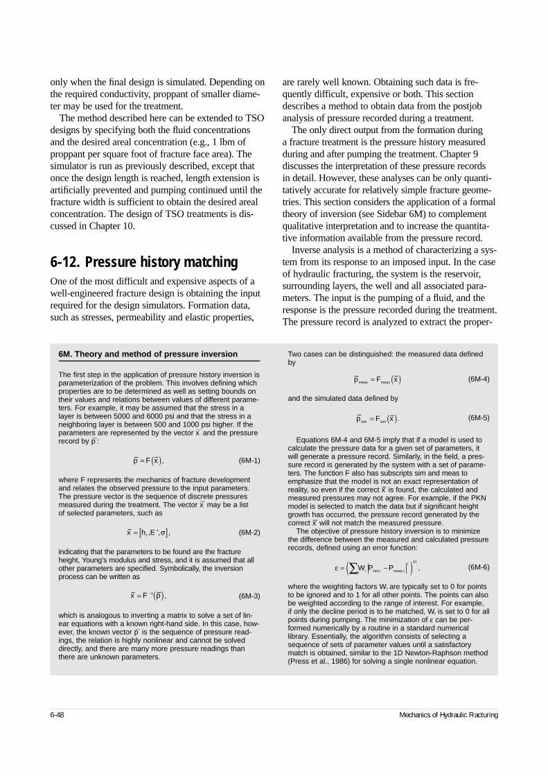
only when the final design is simulated. Depending onthe required conductivity, proppant of smaller diame-ter may be used for the treatment.

The method described here can be extended to TSOdesigns by specifying both the fluid concentrationsand the desired areal concentration (e.g., 1 lbm ofproppant per square foot of fracture face area). Thesimulator is run as previously described, except thatonce the design length is reached, length extension isartificially prevented and pumping continued until thefracture width is sufficient to obtain the desired arealconcentration. The design of TSO treatments is dis-cussed in Chapter 10.

6-12. Pressure history matchingOne of the most difficult and expensive aspects of awell-engineered fracture design is obtaining the inputrequired for the design simulators. Formation data,such as stresses, permeability and elastic properties,

are rarely well known. Obtaining such data is fre-quently difficult, expensive or both. This sectiondescribes a method to obtain data from the postjobanalysis of pressure recorded during a treatment.

The only direct output from the formation during a fracture treatment is the pressure history measuredduring and after pumping the treatment. Chapter 9 discusses the interpretation of these pressure records in detail. However, these analyses can be only quanti-tatively accurate for relatively simple fracture geome-tries. This section considers the application of a formaltheory of inversion (see Sidebar 6M) to complementqualitative interpretation and to increase the quantita-tive information available from the pressure record.

Inverse analysis is a method of characterizing a sys-tem from its response to an imposed input. In the caseof hydraulic fracturing, the system is the reservoir,surrounding layers, the well and all associated para-meters. The input is the pumping of a fluid, and theresponse is the pressure recorded during the treatment.The pressure record is analyzed to extract the proper-

6-48 Mechanics of Hydraulic Fracturing

6M. Theory and method of pressure inversion

The first step in the application of pressure history inversion isparameterization of the problem. This involves defining whichproperties are to be determined as well as setting bounds ontheir values and relations between values of different parame-ters. For example, it may be assumed that the stress in alayer is between 5000 and 6000 psi and that the stress in aneighboring layer is between 500 and 1000 psi higher. If theparameters are represented by the vector x— and the pressurerecord by p—:

(6M-1)

where F represents the mechanics of fracture developmentand relates the observed pressure to the input parameters.The pressure vector is the sequence of discrete pressuresmeasured during the treatment. The vector x— may be a list of selected parameters, such as

(6M-2)

indicating that the parameters to be found are the fractureheight, Young’s modulus and stress, and it is assumed that allother parameters are specified. Symbolically, the inversionprocess can be written as

(6M-3)

which is analogous to inverting a matrix to solve a set of lin-ear equations with a known right-hand side. In this case, how-ever, the known vector p— is the sequence of pressure read-ings, the relation is highly nonlinear and cannot be solveddirectly, and there are many more pressure readings thanthere are unknown parameters.

Two cases can be distinguished: the measured data definedby

(6M-4)

and the simulated data defined by

(6M-5)

Equations 6M-4 and 6M-5 imply that if a model is used tocalculate the pressure data for a given set of parameters, itwill generate a pressure record. Similarly, in the field, a pres-sure record is generated by the system with a set of parame-ters. The function F also has subscripts sim and meas toemphasize that the model is not an exact representation ofreality, so even if the correct x– is found, the calculated andmeasured pressures may not agree. For example, if the PKNmodel is selected to match the data but if significant heightgrowth has occurred, the pressure record generated by thecorrect x– will not match the measured pressure.

The objective of pressure history inversion is to minimizethe difference between the measured and calculated pressurerecords, defined using an error function:

(6M-6)

where the weighting factors Wi are typically set to 0 for pointsto be ignored and to 1 for all other points. The points can alsobe weighted according to the range of interest. For example,if only the decline period is to be matched, Wi is set to 0 for allpoints during pumping. The minimization of ε can be per-formed numerically by a routine in a standard numericallibrary. Essentially, the algorithm consists of selecting asequence of sets of parameter values until a satisfactorymatch is obtained, similar to the 1D Newton-Raphson method(Press et al., 1986) for solving a single nonlinear equation.

p F x= ( ),

p F xmeas meas= ( )

p F xsim sim= ( ).

ε = −( )∑W P Pii sim i meas i

r r

, ,

/

,1

x h Ef= ′[ ], , ,σ

x F p= ( )−1 ,

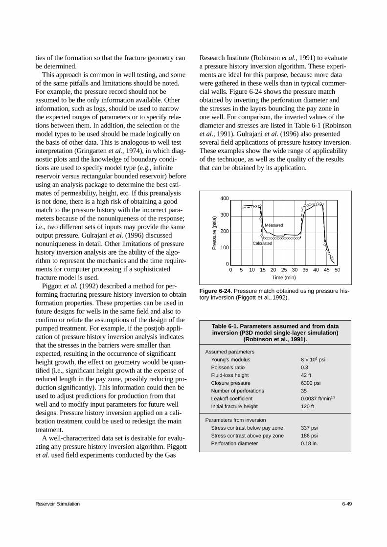
ties of the formation so that the fracture geometry canbe determined.

This approach is common in well testing, and someof the same pitfalls and limitations should be noted.For example, the pressure record should not beassumed to be the only information available. Otherinformation, such as logs, should be used to narrowthe expected ranges of parameters or to specify rela-tions between them. In addition, the selection of themodel types to be used should be made logically onthe basis of other data. This is analogous to well testinterpretation (Gringarten et al., 1974), in which diag-nostic plots and the knowledge of boundary condi-tions are used to specify model type (e.g., infinitereservoir versus rectangular bounded reservoir) beforeusing an analysis package to determine the best esti-mates of permeability, height, etc. If this preanalysis is not done, there is a high risk of obtaining a goodmatch to the pressure history with the incorrect para-meters because of the nonuniqueness of the response;i.e., two different sets of inputs may provide the sameoutput pressure. Gulrajani et al. (1996) discussednonuniqueness in detail. Other limitations of pressurehistory inversion analysis are the ability of the algo-rithm to represent the mechanics and the time require-ments for computer processing if a sophisticatedfracture model is used.

Piggott et al. (1992) described a method for per-forming fracturing pressure history inversion to obtainformation properties. These properties can be used infuture designs for wells in the same field and also toconfirm or refute the assumptions of the design of thepumped treatment. For example, if the postjob appli-cation of pressure history inversion analysis indicatesthat the stresses in the barriers were smaller thanexpected, resulting in the occurrence of significantheight growth, the effect on geometry would be quan-tified (i.e., significant height growth at the expense ofreduced length in the pay zone, possibly reducing pro-duction significantly). This information could then beused to adjust predictions for production from thatwell and to modify input parameters for future welldesigns. Pressure history inversion applied on a cali-bration treatment could be used to redesign the maintreatment.

A well-characterized data set is desirable for evalu-ating any pressure history inversion algorithm. Piggottet al. used field experiments conducted by the Gas

Research Institute (Robinson et al., 1991) to evaluatea pressure history inversion algorithm. These experi-ments are ideal for this purpose, because more datawere gathered in these wells than in typical commer-cial wells. Figure 6-24 shows the pressure matchobtained by inverting the perforation diameter and the stresses in the layers bounding the pay zone in one well. For comparison, the inverted values of thediameter and stresses are listed in Table 6-1 (Robinsonet al., 1991). Gulrajani et al. (1996) also presentedseveral field applications of pressure history inversion.These examples show the wide range of applicabilityof the technique, as well as the quality of the resultsthat can be obtained by its application.

Reservoir Stimulation 6-49

Figure 6-24. Pressure match obtained using pressure his-tory inversion (Piggott et al., 1992).

Pre

ssur

e (p

sia)

400

300

200

100

00 5 10 15 20 25 30 35 40 45 50

Time (min)

Measured

Calculated

Table 6-1. Parameters assumed and from datainversion (P3D model single-layer simulation)

(Robinson et al., 1991).

Assumed parameters

Young’s modulus 8 × 106 psi

Poisson’s ratio 0.3

Fluid-loss height 42 ft

Closure pressure 6300 psi

Number of perforations 35

Leakoff coefficient 0.0037 ft/min1/2

Initial fracture height 120 ft

Parameters from inversion

Stress contrast below pay zone 337 psi

Stress contrast above pay zone 186 psi

Perforation diameter 0.18 in.

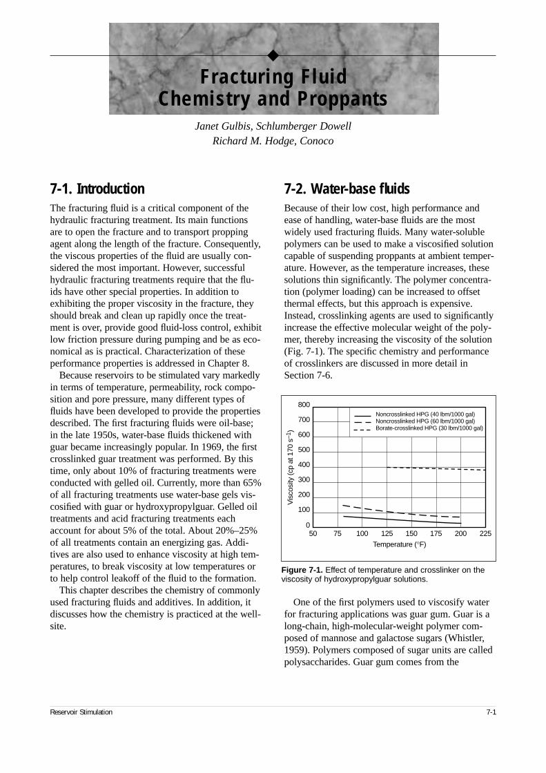
7-1. IntroductionThe fracturing fluid is a critical component of thehydraulic fracturing treatment. Its main functionsare to open the fracture and to transport proppingagent along the length of the fracture. Consequently,the viscous properties of the fluid are usually con-sidered the most important. However, successfulhydraulic fracturing treatments require that the flu-ids have other special properties. In addition toexhibiting the proper viscosity in the fracture, theyshould break and clean up rapidly once the treat-ment is over, provide good fluid-loss control, exhibitlow friction pressure during pumping and be as eco-nomical as is practical. Characterization of theseperformance properties is addressed in Chapter 8.

Because reservoirs to be stimulated vary markedlyin terms of temperature, permeability, rock compo-sition and pore pressure, many different types offluids have been developed to provide the propertiesdescribed. The first fracturing fluids were oil-base;in the late 1950s, water-base fluids thickened withguar became increasingly popular. In 1969, the firstcrosslinked guar treatment was performed. By thistime, only about 10% of fracturing treatments wereconducted with gelled oil. Currently, more than 65%of all fracturing treatments use water-base gels vis-cosified with guar or hydroxypropylguar. Gelled oiltreatments and acid fracturing treatments eachaccount for about 5% of the total. About 20%–25%of all treatments contain an energizing gas. Addi-tives are also used to enhance viscosity at high tem-peratures, to break viscosity at low temperatures orto help control leakoff of the fluid to the formation.

This chapter describes the chemistry of commonlyused fracturing fluids and additives. In addition, itdiscusses how the chemistry is practiced at the well-site.

7-2. Water-base fluidsBecause of their low cost, high performance andease of handling, water-base fluids are the mostwidely used fracturing fluids. Many water-solublepolymers can be used to make a viscosified solutioncapable of suspending proppants at ambient temper-ature. However, as the temperature increases, thesesolutions thin significantly. The polymer concentra-tion (polymer loading) can be increased to offsetthermal effects, but this approach is expensive.Instead, crosslinking agents are used to significantlyincrease the effective molecular weight of the poly-mer, thereby increasing the viscosity of the solution(Fig. 7-1). The specific chemistry and performanceof crosslinkers are discussed in more detail inSection 7-6.

One of the first polymers used to viscosify waterfor fracturing applications was guar gum. Guar is along-chain, high-molecular-weight polymer com-posed of mannose and galactose sugars (Whistler,1959). Polymers composed of sugar units are calledpolysaccharides. Guar gum comes from the

Reservoir Stimulation 7-1

Figure 7-1. Effect of temperature and crosslinker on theviscosity of hydroxypropylguar solutions.

Noncrosslinked HPG (40 lbm/1000 gal)Noncrosslinked HPG (60 lbm/1000 gal)Borate-crosslinked HPG (30 lbm/1000 gal)

0

100

50 75 100 125 150 175 200 225

Temperature (°F)

200

300

400

500

600

700

800

Vis

cosi

ty (c

p at

170

s–1

)

◆

Fracturing FluidChemistry and Proppants

Janet Gulbis, Schlumberger DowellRichard M. Hodge, Conoco

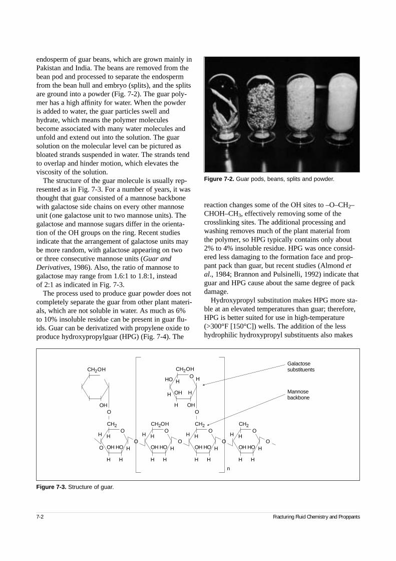
endosperm of guar beans, which are grown mainly inPakistan and India. The beans are removed from thebean pod and processed to separate the endospermfrom the bean hull and embryo (splits), and the splitsare ground into a powder (Fig. 7-2). The guar poly-mer has a high affinity for water. When the powderis added to water, the guar particles swell andhydrate, which means the polymer moleculesbecome associated with many water molecules andunfold and extend out into the solution. The guarsolution on the molecular level can be pictured asbloated strands suspended in water. The strands tendto overlap and hinder motion, which elevates theviscosity of the solution.

The structure of the guar molecule is usually rep-resented as in Fig. 7-3. For a number of years, it wasthought that guar consisted of a mannose backbonewith galactose side chains on every other mannoseunit (one galactose unit to two mannose units). Thegalactose and mannose sugars differ in the orienta-tion of the OH groups on the ring. Recent studiesindicate that the arrangement of galactose units maybe more random, with galactose appearing on two or three consecutive mannose units (Guar andDerivatives, 1986). Also, the ratio of mannose togalactose may range from 1.6:1 to 1.8:1, instead of 2:1 as indicated in Fig. 7-3.

The process used to produce guar powder does notcompletely separate the guar from other plant materi-als, which are not soluble in water. As much as 6%to 10% insoluble residue can be present in guar flu-ids. Guar can be derivatized with propylene oxide toproduce hydroxypropylguar (HPG) (Fig. 7-4). The

reaction changes some of the OH sites to –O–CH2–CHOH–CH3, effectively removing some of thecrosslinking sites. The additional processing andwashing removes much of the plant material fromthe polymer, so HPG typically contains only about2% to 4% insoluble residue. HPG was once consid-ered less damaging to the formation face and prop-pant pack than guar, but recent studies (Almond etal., 1984; Brannon and Pulsinelli, 1992) indicate thatguar and HPG cause about the same degree of packdamage.

Hydroxypropyl substitution makes HPG more sta-ble at an elevated temperatures than guar; therefore,HPG is better suited for use in high-temperature(>300°F [150°C]) wells. The addition of the lesshydrophilic hydroxypropyl substituents also makes

7-2 Fracturing Fluid Chemistry and Proppants

Figure 7-2. Guar pods, beans, splits and powder.

Figure 7-3. Structure of guar.

H H

H

H

H

HOOH

O

O

CH2

OOH

O

H H

H

H

H

HOOH

OCH2OH

O

H H

H

H

H

HOOH

OCH2

O

H H

H

H

H

HOOH

OCH2

O

CH2OH

H

H

H OH H

OH

OHO H

CH2OH

O

n

Galactosesubstituents

Mannosebackbone

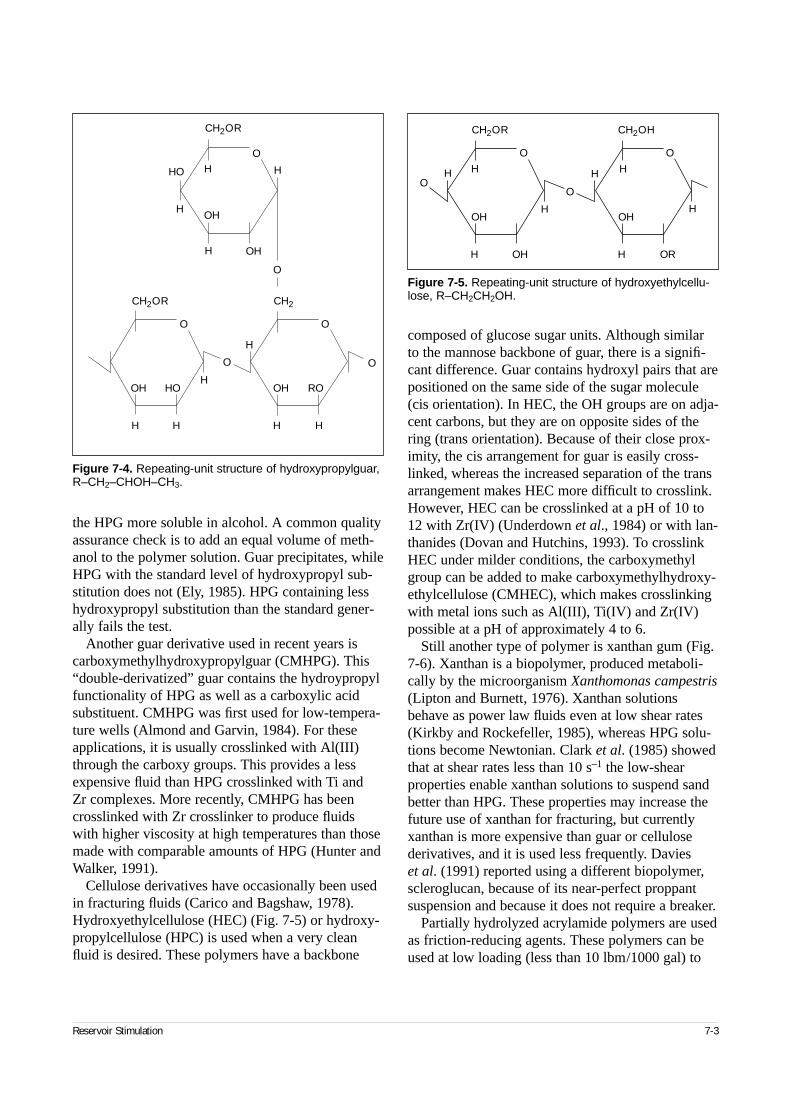
the HPG more soluble in alcohol. A common qualityassurance check is to add an equal volume of meth-anol to the polymer solution. Guar precipitates, whileHPG with the standard level of hydroxypropyl sub-stitution does not (Ely, 1985). HPG containing lesshydroxypropyl substitution than the standard gener-ally fails the test.

Another guar derivative used in recent years iscarboxymethylhydroxypropylguar (CMHPG). This“double-derivatized” guar contains the hydroypropylfunctionality of HPG as well as a carboxylic acidsubstituent. CMHPG was first used for low-tempera-ture wells (Almond and Garvin, 1984). For these applications, it is usually crosslinked with Al(III)through the carboxy groups. This provides a less expensive fluid than HPG crosslinked with Ti and Zr complexes. More recently, CMHPG has beencrosslinked with Zr crosslinker to produce fluidswith higher viscosity at high temperatures than thosemade with comparable amounts of HPG (Hunter andWalker, 1991).

Cellulose derivatives have occasionally been usedin fracturing fluids (Carico and Bagshaw, 1978).Hydroxyethylcellulose (HEC) (Fig. 7-5) or hydroxy-propylcellulose (HPC) is used when a very cleanfluid is desired. These polymers have a backbone

composed of glucose sugar units. Although similarto the mannose backbone of guar, there is a signifi-cant difference. Guar contains hydroxyl pairs that arepositioned on the same side of the sugar molecule(cis orientation). In HEC, the OH groups are on adja-cent carbons, but they are on opposite sides of thering (trans orientation). Because of their close prox-imity, the cis arrangement for guar is easily cross-linked, whereas the increased separation of the transarrangement makes HEC more difficult to crosslink.However, HEC can be crosslinked at a pH of 10 to12 with Zr(IV) (Underdown et al., 1984) or with lan-thanides (Dovan and Hutchins, 1993). To crosslinkHEC under milder conditions, the carboxymethylgroup can be added to make carboxymethylhydroxy-ethylcellulose (CMHEC), which makes crosslinkingwith metal ions such as Al(III), Ti(IV) and Zr(IV)possible at a pH of approximately 4 to 6.

Still another type of polymer is xanthan gum (Fig.7-6). Xanthan is a biopolymer, produced metaboli-cally by the microorganism Xanthomonas campestris(Lipton and Burnett, 1976). Xanthan solutionsbehave as power law fluids even at low shear rates(Kirkby and Rockefeller, 1985), whereas HPG solu-tions become Newtonian. Clark et al. (1985) showedthat at shear rates less than 10 s–1 the low-shearproperties enable xanthan solutions to suspend sandbetter than HPG. These properties may increase thefuture use of xanthan for fracturing, but currentlyxanthan is more expensive than guar or cellulosederivatives, and it is used less frequently. Davies et al. (1991) reported using a different biopolymer,scleroglucan, because of its near-perfect proppantsuspension and because it does not require a breaker.

Partially hydrolyzed acrylamide polymers are usedas friction-reducing agents. These polymers can beused at low loading (less than 10 lbm/1000 gal) to

Reservoir Stimulation 7-3

Figure 7-4. Repeating-unit structure of hydroxypropylguar,R–CH2–CHOH–CH3.

CH2OR

CH2OR

HO

H

H H

H

H

H H

OH

OH

OH HO OH RO

H

H H

O

O

O

O

O

O

CH2

Figure 7-5. Repeating-unit structure of hydroxyethylcellu-lose, R–CH2CH2OH.

CH2OR CH2OH

H

H H

H

OH

H

H H

H OR

OH OH

O

OO

O

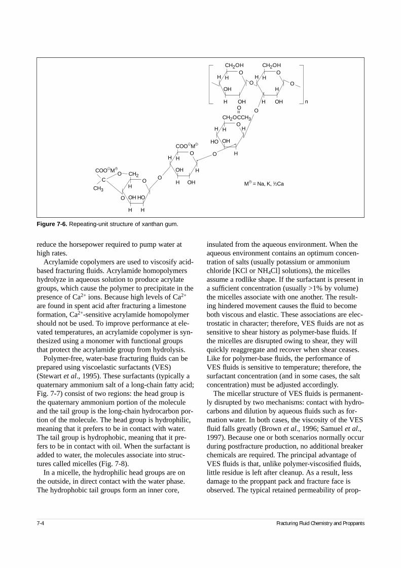
reduce the horsepower required to pump water athigh rates.

Acrylamide copolymers are used to viscosify acid-based fracturing fluids. Acrylamide homopolymershydrolyze in aqueous solution to produce acrylategroups, which cause the polymer to precipitate in thepresence of Ca2+ ions. Because high levels of Ca2+

are found in spent acid after fracturing a limestoneformation, Ca2+-sensitive acrylamide homopolymershould not be used. To improve performance at ele-vated temperatures, an acrylamide copolymer is syn-thesized using a monomer with functional groupsthat protect the acrylamide group from hydrolysis.

Polymer-free, water-base fracturing fluids can beprepared using viscoelastic surfactants (VES)(Stewart et al., 1995). These surfactants (typically aquaternary ammonium salt of a long-chain fatty acid;Fig. 7-7) consist of two regions: the head group isthe quaternary ammonium portion of the moleculeand the tail group is the long-chain hydrocarbon por-tion of the molecule. The head group is hydrophilic,meaning that it prefers to be in contact with water.The tail group is hydrophobic, meaning that it pre-fers to be in contact with oil. When the surfactant isadded to water, the molecules associate into struc-tures called micelles (Fig. 7-8).

In a micelle, the hydrophilic head groups are onthe outside, in direct contact with the water phase.The hydrophobic tail groups form an inner core,

insulated from the aqueous environment. When theaqueous environment contains an optimum concen-tration of salts (usually potassium or ammoniumchloride [KCl or NH4Cl] solutions), the micellesassume a rodlike shape. If the surfactant is present ina sufficient concentration (usually >1% by volume)the micelles associate with one another. The result-ing hindered movement causes the fluid to becomeboth viscous and elastic. These associations are elec-trostatic in character; therefore, VES fluids are not assensitive to shear history as polymer-base fluids. Ifthe micelles are disrupted owing to shear, they willquickly reaggregate and recover when shear ceases.Like for polymer-base fluids, the performance ofVES fluids is sensitive to temperature; therefore, thesurfactant concentration (and in some cases, the saltconcentration) must be adjusted accordingly.

The micellar structure of VES fluids is permanent-ly disrupted by two mechanisms: contact with hydro-carbons and dilution by aqueous fluids such as for-mation water. In both cases, the viscosity of the VESfluid falls greatly (Brown et al., 1996; Samuel et al.,1997). Because one or both scenarios normally occurduring postfracture production, no additional breakerchemicals are required. The principal advantage ofVES fluids is that, unlike polymer-viscosified fluids,little residue is left after cleanup. As a result, lessdamage to the proppant pack and fracture face isobserved. The typical retained permeability of prop-

7-4 Fracturing Fluid Chemistry and Proppants

Figure 7-6. Repeating-unit structure of xanthan gum.

H H

H

HOOH

OO

O

CH2

H OH

OH

O

OC

CH3

COO – +M

COO – +M

H

H

HH

OH

O

O

CH2OCCH3

H H H

HO

H

H

OH

O

OH H

O

CH2OH

H

OH

OH

O

O

OH H

CH2OH

=

n

+M = Na, K, 1⁄2Ca

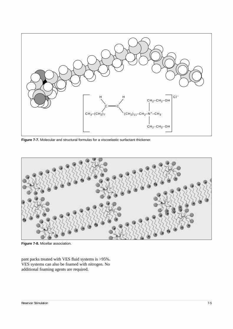
pant packs treated with VES fluid systems is >95%.VES systems can also be foamed with nitrogen. Noadditional foaming agents are required.

Reservoir Stimulation 7-5

Figure 7-7. Molecular and structural formulas for a viscoelastic surfactant thickener.

CH3–(CH2)7 (CH2)11–CH2–N+–CH3

CH2–CH2–OH

CH2–CH2–OH

H

C

H

C

C l –

Figure 7-8. Micellar association.

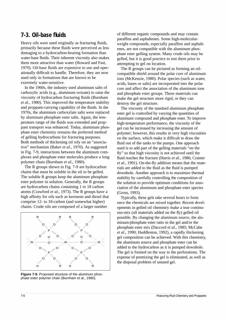
7-3. Oil-base fluidsHeavy oils were used originally as fracturing fluids,primarily because these fluids were perceived as lessdamaging to a hydrocarbon-bearing formation thanwater-base fluids. Their inherent viscosity also makesthem more attractive than water (Howard and Fast,1970). Oil-base fluids are expensive to use and oper-ationally difficult to handle. Therefore, they are nowused only in formations that are known to beextremely water-sensitive.

In the 1960s, the industry used aluminum salts ofcarboxylic acids (e.g., aluminum octoate) to raise theviscosity of hydrocarbon fracturing fluids (Burnhamet al., 1980). This improved the temperature stabilityand proppant-carrying capability of the fluids. In the1970s, the aluminum carboxylate salts were replacedby aluminum phosphate ester salts. Again, the tem-perature range of the fluids was extended and prop-pant transport was enhanced. Today, aluminum phos-phate ester chemistry remains the preferred methodof gelling hydrocarbons for fracturing purposes.Both methods of thickening oil rely on an “associa-tive” mechanism (Baker et al., 1970). As suggestedin Fig. 7-9, interactions between the aluminum com-plexes and phosphate ester molecules produce a longpolymer chain (Burnham et al., 1980).

The R groups shown in Fig. 7-9 are hydrocarbonchains that must be soluble in the oil to be gelled.The soluble R groups keep the aluminum phosphateester polymer in solution. Generally, the R groupsare hydrocarbon chains containing 1 to 18 carbonatoms (Crawford et al., 1973). The R groups have ahigh affinity for oils such as kerosene and diesel thatcomprise 12- to 18-carbon (and somewhat higher)chains. Crude oils are composed of a larger number

of different organic compounds and may containparaffins and asphaltenes. Some high-molecular-weight compounds, especially paraffins and asphalt-enes, are not compatible with the aluminum phos-phate ester gelling system. Many crude oils may begelled, but it is good practice to test them prior toattempting to gel on location.

The R groups can be pictured as forming an oil-compatible shield around the polar core of aluminumions (McKenzie, 1980). Polar species (such as water,acids, bases or salts) are incorporated into the polarcore and affect the association of the aluminum ionsand phosphate ester groups. These materials canmake the gel structure more rigid, or they candestroy the gel structure.

The viscosity of the standard aluminum phosphateester gel is controlled by varying the quantities ofaluminum compound and phosphate ester. To improvehigh-temperature performance, the viscosity of thegel can be increased by increasing the amount ofpolymer; however, this results in very high viscositieson the surface, which make it difficult to draw thefluid out of the tanks to the pumps. One approachused is to add part of the gelling materials “on thefly” so that high viscosity is not achieved until thefluid reaches the fracture (Harris et al., 1986; Crameret al., 1991). On-the-fly addition means that the mate-rials are added to the fluid as the fluid is pumpeddownhole. Another approach is to maximize thermalstability by carefully controlling the composition ofthe solution to provide optimum conditions for asso-ciation of the aluminum and phosphate ester species(Gross, 1993).

Typically, these gels take several hours to formonce the chemicals are mixed together. Recent devel-opments in gelled oil chemistry make a true continu-ous-mix (all materials added on the fly) gelled oilpossible. By changing the aluminum source, the alu-minum/phosphate ester ratio in the gel and/or thephosphate ester mix (Daccord et al., 1985; McCabe et al., 1990; Huddleston, 1992), a rapidly thickeninggel composition can be achieved. With this chemistry,the aluminum source and phosphate ester can beadded to the hydrocarbon as it is pumped downhole.The gel is formed on the way to the perforations. Theexpense of premixing the gel is eliminated, as well asthe disposal problem of unused gel.

7-6 Fracturing Fluid Chemistry and Proppants

Figure 7-9. Proposed structure of the aluminum phos-phate ester polymer chain (Burnham et al., 1980).

R

RH

R

O

O

O

O

O

O O

O

O

P

H

P

R

RH

R

O

O

O

O

O

O O

O

O

P

H

P

Al AlAl

7-4. Acid-based fluidsAcid fracturing is a well stimulation process inwhich acid, usually hydrochloric acid (HCl), isinjected into a carbonate formation at a pressure suf-ficient to fracture the formation or to open existingnatural fractures. As the acid flows along the frac-ture, portions of the fracture face are dissolved.Because flowing acid tends to etch in a nonuniformmanner, conductive channels are created that usuallyremain when the fracture closes. The effective lengthof the fracture is determined by the etched length,which depends on the volume of acid used, its reac-tion rate and the acid fluid loss from the fracture intothe formation. The effectiveness of the acid fractur-ing treatment is determined largely by the length ofthe etched fracture.

In some cases, especially in carbonates, a choiceexists between acid and propped fracturing treat-ments. Operationally, acid fracturing is less compli-cated because no propping agent is employed. Also,the danger of proppant screenout and the problems ofproppant flowback and cleanout from the wellboreafter the treatment are eliminated. However, acid ismore expensive than most nonreactive treating fluids.

The major barrier to effective fracture penetrationby acid appears to be excessive fluid loss (Nierodeand Kruk, 1973). Fluid loss is a greater problemwhen using acid than when using a nonreactive fluid.The constant erosion of fracture faces during treat-ment makes it difficult to deposit an effective filter-cake barrier. In addition, acid leakoff is extremelynonuniform and results in wormholes and theenlargement of natural fractures. This greatlyincreases the effective area from which leakoffoccurs and makes fluid-loss control difficult.

7-4.1. Materials and techniques for acid fluid-loss control

Various additives and treating techniques have beendeveloped to control acid fluid loss. Among these areparticulates (oil-soluble resins and 100-mesh sand)and gelling agents. In general, acid fluid-loss addi-tives have not been used extensively because of per-formance and cost limitations. As a result, alternatemethods of fluid-loss control usually are employed.The most common technique involves the use of aviscous pad preceding the acid. The pad is used to

initiate the fracture and to deposit a filter cake thatacts as a barrier to acid leakoff. The ability of a sin-gle viscous pad fluid to control fluid loss is question-able. Studies by Nierode and Kruk (1973), Coulter etal. (1976) and Crowe et al. (1989) show that the fil-ter cake deposited by the pad is quickly penetratedby wormholes resulting from acid leakoff. Once thisoccurs, the acid fluid loss is identical to that occur-ring if no pad were used. In recent years, multiplestages of viscous pad have been used to control acidfluid loss (Coulter et al., 1976). In this widely usedtechnique, the fracture is initially created by a gelledpad, after which alternating stages of acid and addi-tional polymer pad are pumped. These additional padstages are designed to enter and seal wormholes cre-ated by the preceding acid. Each alternating padstage in this treatment is usually equal to or largerthan the acid stage that preceded it.

In addition to fluid-loss additives, two-phase fluids(foams and emulsions) have been shown to effect-ively control fluid loss during acid fracturing treat-ments. Nierode and Kruk (1973) presented datashowing that an acid external emulsion, consisting of an oil inner phase with gelled acid as the outerphase, provides good fluid-loss control. The use ofthese acid external emulsions in well stimulation hasbeen rather limited. The use of foamed acid is one ofthe most effective methods for controlling acid fluidloss. Scherubel and Crowe (1978) and Ford (1981)showed that foamed acids provide excellent fluid-losscontrol. Fluid-loss control is further enhanced by theuse of a viscous pad preceding the foamed acid.However, foaming the acid reduces the effectiveamount of acid available for etching because there is less acid present per unit volume injected. As aresult, a high acid concentration (e.g., 28% HCl)should be used in preparing foamed acid to maximizethe amount of acid available for fracture etching.

Acid fluid loss can also be reduced by gelling the acid. This method of control has become widelyused since the development of more acid-stablethickening agents. Commonly, thickeners includexanthan biopolymers, various acrylamide copoly-mers and certain surfactants that thicken acid bymicellar association.

A gelling agent must be sufficiently stable to allowthe gelled acid to retain its viscosity at the treatingtemperature. However, slow cleanup or actual plug-ging of the well may result if the viscosity of the

Reservoir Stimulation 7-7

spent acid is too high or if the polymer degrades to form insoluble reaction products. Procedures forevaluating acid gelling agents and the advantagesand limitations of various materials were describedby Crowe et al. (1981). Guar and cellulose basethickeners lack sufficient stability for use in acid attemperatures above 125°F [50°C]. Xanthan biopoly-mers can be used at temperatures up to 200°F[90°C]; at higher temperatures acrylamide copoly-mers are generally employed. Certain acrylamidecopolymers are stable at high temperatures and donot produce insoluble reaction products. However,acrylamide homopolymers should not be used asacid thickeners. They are rapidly hydrolyzed andcombine with calcium to form insoluble precipitatesupon spending of the acid.

A number of crosslinked gelled acids have beendeveloped. These systems employ various acidgelling agents and use either polyvalent metal ions oraldehydes as crosslinkers. In general, the crosslinkedacids tend to be shear sensitive and are usuallyunstable at elevated temperatures. Breaking of thecrosslinked gel in spent acid also is a problem. Itmay be claimed that the gel will be broken by aciddegradation, and data are usually presented showinga loss of viscosity with time in live acid. However, inactual practice, the acid spends rapidly with no liveacid available to degrade the polymer. As a result oftheir high viscosity, the crosslinked systems presenta greater risk of formation damage and have notbeen widely used.

Certain surfactants can also be used as thickenersfor gelling acid (Norman, 1978). These gellingagents thicken acid by forming micelles that associ-ate in chainlike structures and therefore behave muchlike polymers. Gelled acids of this type are quiteshear-stable, because micellar chains reform quicklyfollowing shearing. Another advantage of the surfac-tant thickeners is the low viscosity of the spent acid.These acid thickeners are usually designed to pro-vide considerable viscosity in live acid but to thinduring spending. This occurs as the result of thedisruption of micellar association brought about by changes in the ionic environment caused byincreased concentrations of reaction products formedduring spending of the acid. The lowered spent-acidviscosity aids the recovery of treating fluids follow-ing the treatment. However, this can also be a disad-vantage. Acid fluid loss is dependent largely uponthe leakoff viscosity of the spent acid. As a result,

the fluid loss of acid gelled with surfactant-typethickeners, which break during spending, is not sig-nificantly different from that of ungelled acid. Onlythose gelled acids that retain their viscosity duringleakoff are capable of providing effective fluid-losscontrol. Another disadvantage of this gelling agent is the limited temperature range over which it can be used. Although the surfactant itself is stable inacid, it provides little increase in viscosity above150°F [65°C]. High temperatures disrupt the micellarassociation responsible for acid viscosity.

7-4.2. Materials and techniques for acid reaction-rate control

Reducing the reaction rate of acid to achieveincreased etched fracture penetration is an importantconsideration. In low- to moderate-temperature wells,retardation is not critical. However, in applicationsgreater than about 250°F [120°C] retardation can becritical to the success of the treatment (Nierode andKruk, 1973). One of the most common methods ofextending live acid penetration involves the injectionof a viscous nonreactive pad preceding the acid. Thepad reduces the acid reaction rate by increasing thefracture width and by cooling the fracture surfaces.Weak organic acids (acetic or formic acid) are usedas retarded acids. These weakly ionized acids react ata much slower rate than HCl, even at very high tem-peratures. Additives, such as retarders, reduce thereaction rate by forming a protective hydrophobicfilm on carbonate surfaces that acts as a barrier toslow acid attack or by blanketing carbonate surfaceswith a thin layer of carbon dioxide foam. Oil-outsideemulsions are the most effective retarders becausethe external oil phase physically separates the acidfrom the reactive carbonate surface.

Gelled acids are usually considered retarded. However, the amount of retardation provided by theincreased acid viscosity is generally small and canactually accelerate the acid reaction rate under flow-ing conditions, as shown by examining the data pre-sented by Gdanski and Norman (1986) and Crowe et al. (1990).

7-5. Multiphase fluidsThere are situations in which the properties of stan-dard water-base, oil-base or acid-based fluids can be

7-8 Fracturing Fluid Chemistry and Proppants

enhanced by incorporating a second phase into thefluid. Foams are created by adding gas to the fluid.Emulsions are created by mixing oil and watertogether. The different systems are described in thissection.

7-5.1. FoamsA foam is a stable mixture of liquid and gas. Tomake the mixture stable, a surface-active agent (sur-factant) is used. The surfactant concentrates at thegas/liquid interface and lowers the interfacial ten-sion. The surfactant stabilizes thin liquid films andprevents the cells from coalescing.

Pressurized gas (nitrogen or carbon dioxide) in a foam expands when the well is flowed back andforces liquid out of the fracture. Foams acceleratethe recovery of liquid from a propped fracture andthus are excellent fluids to use in low-pressure reser-voirs. Also, the liquid phase is minimal becausefoams contain up to 95% by volume gas. In the caseof a water-base fluid, foaming the fluid significantlydecreases the amount of liquid in contact with theformation. Therefore, foams perform well in water-sensitive formations (Ward, 1984; Ainley, 1983).Foams yield pseudoplastic fluids with good transportproperties (King, 1982; Reidenbach et al., 1986).They provide good fluid-loss control in low-perme-ability formations where the gas bubbles are approxi-mately the size of the rock pore openings (Harris,1985).

Foams are described by their quality:

(7-1)

Originally, foam quality was considered to rangefrom 52% to 95%. Above 95%, the foam usuallychanges to a mist, with gas as the continuous phase.Below 52%, a stable foam does not exist becausethere are no bubble/bubble interactions to provideresistance to flow or to gravity separation (Mitchell,1969). Above 52% gas, the gas concentration is highenough that the bubble surfaces touch.

Stable dispersions of gas in liquid can be preparedwith qualities less than 52% (Watkins et al., 1983). Itmay not be appropriate to call them foams, but theycan be used effectively as energized fluids. Viscos-ifying the liquid phase with a polymer is an effectivemethod for increasing the stability of foams (Wen-

dorff and Ainley, 1981). The thicker the continuousphase, the more difficult it is for the gas bubbles tomove together and coalesce. Guar, HPG and xanthangum have been used as stabilizers. Still, a relativelyhigh quality, although not as high as 52%, is requiredto maintain dispersion of the gas phase.

A further improvement in foam stability can beachieved by crosslinking the polymer in the aqueousphase (Watkins et al., 1983). The liquid phase thenbecomes viscous enough to maintain dispersion ofthe gas bubbles, even at foam quality less than 40%.Thickening the liquid phase also improves foam rhe-ology and fluid-loss control. Proppant concentrationsin the foamed fluid are generally lower than the con-centration achieved with single-phase, liquid treat-ments. Therefore, a larger volume of foam may berequired to place the desired amount of proppant.

Nitrogen and carbon dioxide are used as energizinggases. N2 is less dense than CO2. CO2 creates adenser foam and, consequently, lower surface treatingpressures because of the increased hydrostatic head inthe wellbore. Lower treating pressures reduce pump-ing costs. On the other hand, because CO2 is muchmore soluble in oil and water than N2, it takes moreCO2 to saturate the liquid and to create the foam.Reductions in pumping costs may be offset byincreases in material costs.

7-5.2. EmulsionsAn emulsion is a dispersion of two immisciblephases such as oil in water or water in oil stabilizedwith a surfactant. Emulsion-based fracturing fluidsare highly viscous solutions with good transportproperties. The higher the percentage of the internalphase, the more resistance there is to droplet move-ment, resulting in a higher viscosity.

Emulsion-based fracturing fluids have been usedfor a number of years (Kiel, 1971). The most com-mon fluid, termed polyemulsion, is composed of67% hydrocarbon internal phase, 33% viscosifiedbrine external phase and an emulsifying surfactant.Viscosifying the aqueous phase improves the emul-sion stability and significantly reduces friction pres-sure during pumping because the polymer acts as afriction reducer. The polymer concentration used isgenerally 20 to 40 lbm/1000 gal, so the fluid con-tains only one-sixth to one-third as much polymer asa standard water-base fracturing fluid. The emulsion

Reservoir Stimulation 7-9

foam quality =gas volume

foam volume×100 .

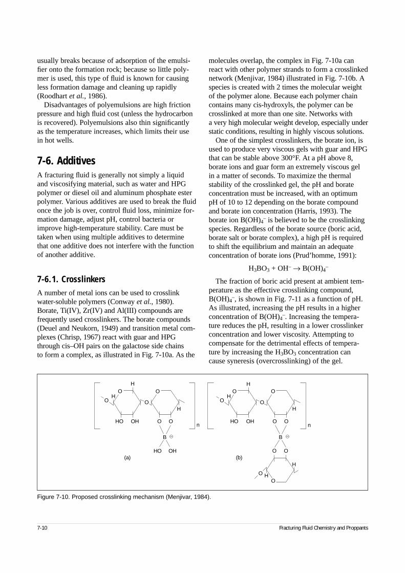
usually breaks because of adsorption of the emulsi-fier onto the formation rock; because so little poly-mer is used, this type of fluid is known for causingless formation damage and cleaning up rapidly(Roodhart et al., 1986).

Disadvantages of polyemulsions are high frictionpressure and high fluid cost (unless the hydrocarbonis recovered). Polyemulsions also thin significantlyas the temperature increases, which limits their usein hot wells.

7-6. AdditivesA fracturing fluid is generally not simply a liquidand viscosifying material, such as water and HPGpolymer or diesel oil and aluminum phosphate esterpolymer. Various additives are used to break the fluidonce the job is over, control fluid loss, minimize for-mation damage, adjust pH, control bacteria orimprove high-temperature stability. Care must betaken when using multiple additives to determinethat one additive does not interfere with the functionof another additive.

7-6.1. CrosslinkersA number of metal ions can be used to crosslinkwater-soluble polymers (Conway et al., 1980).Borate, Ti(IV), Zr(IV) and Al(III) compounds arefrequently used crosslinkers. The borate compounds(Deuel and Neukorn, 1949) and transition metal com-plexes (Chrisp, 1967) react with guar and HPGthrough cis–OH pairs on the galactose side chains to form a complex, as illustrated in Fig. 7-10a. As the

molecules overlap, the complex in Fig. 7-10a canreact with other polymer strands to form a crosslinkednetwork (Menjivar, 1984) illustrated in Fig. 7-10b. Aspecies is created with 2 times the molecular weightof the polymer alone. Because each polymer chaincontains many cis-hydroxyls, the polymer can becrosslinked at more than one site. Networks with a very high molecular weight develop, especially understatic conditions, resulting in highly viscous solutions.

One of the simplest crosslinkers, the borate ion, isused to produce very viscous gels with guar and HPGthat can be stable above 300°F. At a pH above 8,borate ions and guar form an extremely viscous gel in a matter of seconds. To maximize the thermalstability of the crosslinked gel, the pH and borateconcentration must be increased, with an optimumpH of 10 to 12 depending on the borate compoundand borate ion concentration (Harris, 1993). Theborate ion B(OH)4

– is believed to be the crosslinkingspecies. Regardless of the borate source (boric acid,borate salt or borate complex), a high pH is requiredto shift the equilibrium and maintain an adequateconcentration of borate ions (Prud’homme, 1991):

H3BO3 + OH– → B(OH)4–

The fraction of boric acid present at ambient tem-perature as the effective crosslinking compound,B(OH)4

–, is shown in Fig. 7-11 as a function of pH.As illustrated, increasing the pH results in a higherconcentration of B(OH)4

–. Increasing the tempera-ture reduces the pH, resulting in a lower crosslinkerconcentration and lower viscosity. Attempting tocompensate for the detrimental effects of tempera-ture by increasing the H3BO3 concentration cancause syneresis (overcrosslinking) of the gel.

7-10 Fracturing Fluid Chemistry and Proppants

Figure 7-10. Proposed crosslinking mechanism (Menjivar, 1984).

HO OH

HO OH

H

HO

O

O O

H

O

O

B

HO OH

O O

H

HO

O

O O

H

O

O

H

H

OO

B

n n

(a) (b)

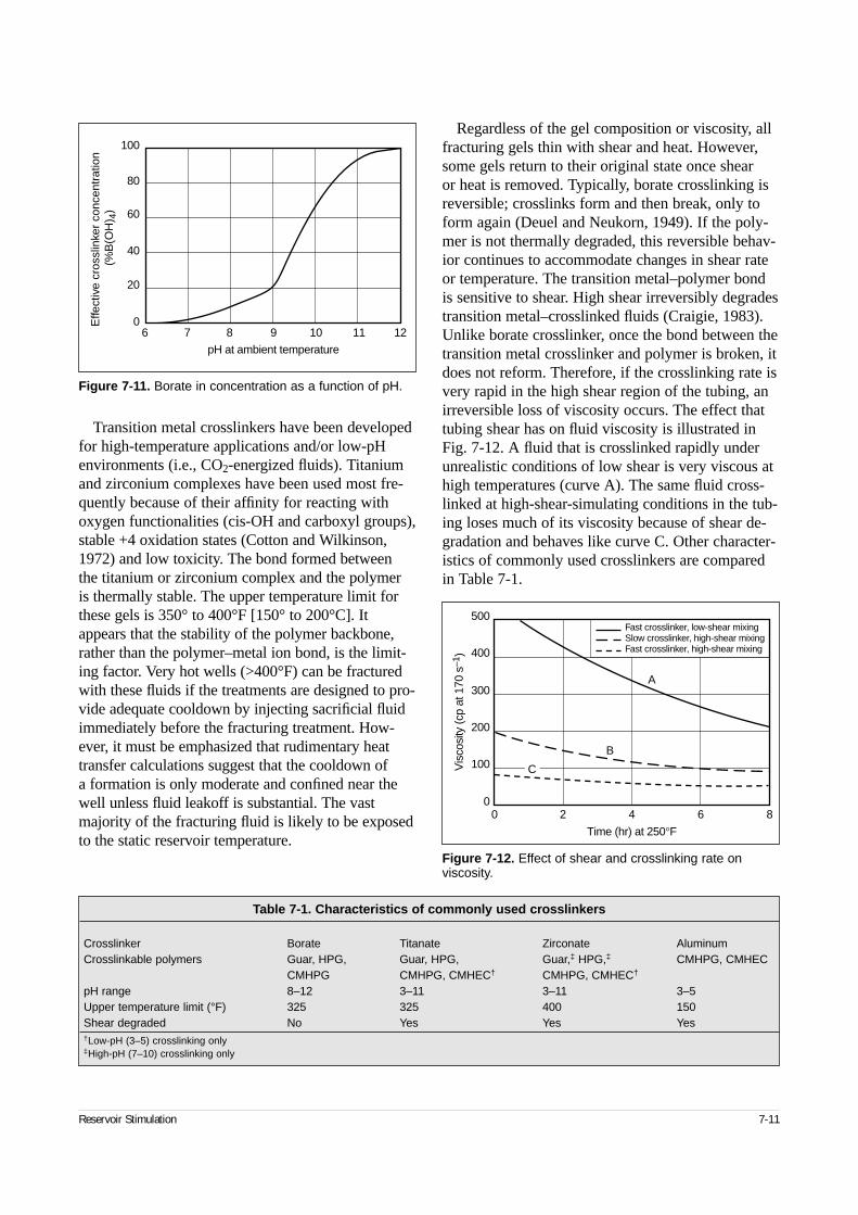
Transition metal crosslinkers have been developedfor high-temperature applications and/or low-pHenvironments (i.e., CO2-energized fluids). Titaniumand zirconium complexes have been used most fre-quently because of their affinity for reacting withoxygen functionalities (cis-OH and carboxyl groups),stable +4 oxidation states (Cotton and Wilkinson,1972) and low toxicity. The bond formed between the titanium or zirconium complex and the polymer is thermally stable. The upper temperature limit forthese gels is 350° to 400°F [150° to 200°C]. Itappears that the stability of the polymer backbone,rather than the polymer–metal ion bond, is the limit-ing factor. Very hot wells (>400°F) can be fracturedwith these fluids if the treatments are designed to pro-vide adequate cooldown by injecting sacrificial fluidimmediately before the fracturing treatment. How-ever, it must be emphasized that rudimentary heattransfer calculations suggest that the cooldown of a formation is only moderate and confined near thewell unless fluid leakoff is substantial. The vastmajority of the fracturing fluid is likely to be exposedto the static reservoir temperature.

Regardless of the gel composition or viscosity, allfracturing gels thin with shear and heat. However,some gels return to their original state once shear or heat is removed. Typically, borate crosslinking isreversible; crosslinks form and then break, only toform again (Deuel and Neukorn, 1949). If the poly-mer is not thermally degraded, this reversible behav-ior continues to accommodate changes in shear rateor temperature. The transition metal–polymer bondis sensitive to shear. High shear irreversibly degradestransition metal–crosslinked fluids (Craigie, 1983).Unlike borate crosslinker, once the bond between thetransition metal crosslinker and polymer is broken, itdoes not reform. Therefore, if the crosslinking rate isvery rapid in the high shear region of the tubing, anirreversible loss of viscosity occurs. The effect thattubing shear has on fluid viscosity is illustrated inFig. 7-12. A fluid that is crosslinked rapidly underunrealistic conditions of low shear is very viscous athigh temperatures (curve A). The same fluid cross-linked at high-shear-simulating conditions in the tub-ing loses much of its viscosity because of shear de-gradation and behaves like curve C. Other character-istics of commonly used crosslinkers are comparedin Table 7-1.

Reservoir Stimulation 7-11

Figure 7-11. Borate in concentration as a function of pH.

6 7 8 9 10 11 12

Effe

ctiv

e cr

ossl

inke

r co

ncen

trat

ion

(%B

(OH

) 4)

20

0

40

60

80

100

pH at ambient temperature

Figure 7-12. Effect of shear and crosslinking rate onviscosity.

0 20

100

200

300

400

500

4 6 8

Time (hr) at 250°F

Vis

cosi

ty (c

p at

170

s–1

)

Fast crosslinker, low-shear mixingSlow crosslinker, high-shear mixingFast crosslinker, high-shear mixing

A

B

C

Table 7-1. Characteristics of commonly used crosslinkers

Crosslinker Borate Titanate Zirconate AluminumCrosslinkable polymers Guar, HPG, Guar, HPG, Guar,‡ HPG,‡ CMHPG, CMHEC

CMHPG CMHPG, CMHEC† CMHPG, CMHEC†

pH range 8–12 3–11 3–11 3–5Upper temperature limit (°F) 325 325 400 150Shear degraded No Yes Yes Yes†Low-pH (3–5) crosslinking only‡High-pH (7–10) crosslinking only

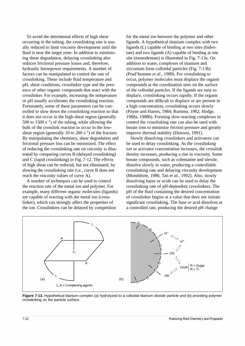
To avoid the detrimental effects of high shearoccurring in the tubing, the crosslinking rate is usu-ally reduced to limit viscosity development until thefluid is near the target zone. In addition to minimiz-ing shear degradation, delaying crosslinking alsoreduces frictional pressure losses and, therefore,hydraulic horsepower requirements. A number offactors can be manipulated to control the rate ofcrosslinking. These include fluid temperature andpH, shear conditions, crosslinker type and the pres-ence of other organic compounds that react with thecrosslinker. For example, increasing the temperatureor pH usually accelerates the crosslinking reaction.Fortunately, some of these parameters can be con-trolled to slow down the crosslinking reaction so thatit does not occur in the high-shear region (generally500 to 1500 s–1) of the tubing, while allowing thebulk of the crosslink reaction to occur in the low-shear region (generally 10 to 200 s–1) of the fracture.By manipulating the chemistry, shear degradation andfrictional pressure loss can be minimized. The effectof reducing the crosslinking rate on viscosity is illus-trated by comparing curves B (delayed crosslinking)and C (rapid crosslinking) in Fig. 7-12. The effects of high shear can be reduced, but not eliminated, byslowing the crosslinking rate (i.e., curve B does notreach the viscosity values of curve A).

A number of techniques can be used to control the reaction rate of the metal ion and polymer. Forexample, many different organic molecules (ligands)are capable of reacting with the metal ion (cross-linker), which can strongly affect the properties ofthe ion. Crosslinkers can be delayed by competition

for the metal ion between the polymer and otherligands. A hypothetical titanium complex with twoligands (L) capable of binding at two sites (biden-tate) and two ligands (A) capable of binding at onesite (monodentate) is illustrated in Fig. 7-13a. Onaddition to water, complexes of titanium andzirconium form colloidal particles (Fig. 7-13b)(Prud’homme et al., 1989). For crosslinking tooccur, polymer molecules must displace the organiccompounds at the coordination sites on the surface of the colloidal particles. If the ligands are easy todisplace, crosslinking occurs rapidly. If the organiccompounds are difficult to displace or are present ina high concentration, crosslinking occurs slowly(Payne and Harms, 1984; Rummo, 1982; Hodge,1988a, 1988b). Forming slow-reacting complexes tocontrol the crosslinking rate can also be used withborate ions to minimize friction pressure and greatlyimprove thermal stability (Dawson, 1991).

Slowly dissolving crosslinkers and activators canbe used to delay crosslinking. As the crosslinkingion or activator concentration increases, the crosslinkdensity increases, producing a rise in viscosity. Someborate compounds, such as colemanite and ulexite,dissolve slowly in water, producing a controllablecrosslinking rate and delaying viscosity development(Mondshine, 1986; Tan et al., 1992). Also, slowlydissolving bases or acids can be used to delay thecrosslinking rate of pH-dependent crosslinkers. ThepH of the fluid containing the desired concentrationof crosslinker begins at a value that does not initiatesignificant crosslinking. The base or acid dissolves ata controlled rate, producing the desired pH change

7-12 Fracturing Fluid Chemistry and Proppants

Figure 7-13. Hypothetical titanium complex (a) hydrolyzed to a colloidal titanium dioxide particle and (b) providing polymercrosslinking on the particle surface.

A

A

L

L

Ti

L, A = Complexing agents

Ti

Ti

Ti

Ti

Ti

O

O

O

O

OH

OR

O–

H+

HOR R = SugarR = Ti

(a) (b)

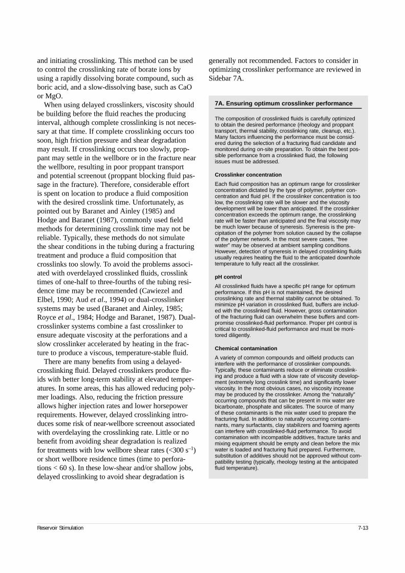
and initiating crosslinking. This method can be usedto control the crosslinking rate of borate ions byusing a rapidly dissolving borate compound, such asboric acid, and a slow-dissolving base, such as CaOor MgO.

When using delayed crosslinkers, viscosity shouldbe building before the fluid reaches the producinginterval, although complete crosslinking is not neces-sary at that time. If complete crosslinking occurs toosoon, high friction pressure and shear degradationmay result. If crosslinking occurs too slowly, prop-pant may settle in the wellbore or in the fracture nearthe wellbore, resulting in poor proppant transportand potential screenout (proppant blocking fluid pas-sage in the fracture). Therefore, considerable effort is spent on location to produce a fluid compositionwith the desired crosslink time. Unfortunately, aspointed out by Baranet and Ainley (1985) andHodge and Baranet (1987), commonly used fieldmethods for determining crosslink time may not bereliable. Typically, these methods do not simulate the shear conditions in the tubing during a fracturingtreatment and produce a fluid composition thatcrosslinks too slowly. To avoid the problems associ-ated with overdelayed crosslinked fluids, crosslinktimes of one-half to three-fourths of the tubing resi-dence time may be recommended (Cawiezel andElbel, 1990; Aud et al., 1994) or dual-crosslinkersystems may be used (Baranet and Ainley, 1985;Royce et al., 1984; Hodge and Baranet, 1987). Dual-crosslinker systems combine a fast crosslinker toensure adequate viscosity at the perforations and aslow crosslinker accelerated by heating in the frac-ture to produce a viscous, temperature-stable fluid.

There are many benefits from using a delayed-crosslinking fluid. Delayed crosslinkers produce flu-ids with better long-term stability at elevated temper-atures. In some areas, this has allowed reducing poly-mer loadings. Also, reducing the friction pressureallows higher injection rates and lower horsepowerrequirements. However, delayed crosslinking intro-duces some risk of near-wellbore screenout associatedwith overdelaying the crosslinking rate. Little or nobenefit from avoiding shear degradation is realizedfor treatments with low wellbore shear rates (<300 s–1)or short wellbore residence times (time to perfora-tions < 60 s). In these low-shear and/or shallow jobs,delayed crosslinking to avoid shear degradation is

generally not recommended. Factors to consider inoptimizing crosslinker performance are reviewed inSidebar 7A.

Reservoir Stimulation 7-13

7A. Ensuring optimum crosslinker performance

The composition of crosslinked fluids is carefully optimized to obtain the desired performance (rheology and proppanttransport, thermal stability, crosslinking rate, cleanup, etc.).Many factors influencing the performance must be consid-ered during the selection of a fracturing fluid candidate andmonitored during on-site preparation. To obtain the best pos-sible performance from a crosslinked fluid, the followingissues must be addressed.

Crosslinker concentration

Each fluid composition has an optimum range for crosslinkerconcentration dictated by the type of polymer, polymer con-centration and fluid pH. If the crosslinker concentration is toolow, the crosslinking rate will be slower and the viscositydevelopment will be lower than anticipated. If the crosslinkerconcentration exceeds the optimum range, the crosslinkingrate will be faster than anticipated and the final viscosity maybe much lower because of syneresis. Syneresis is the pre-cipitation of the polymer from solution caused by the collapseof the polymer network. In the most severe cases, “freewater” may be observed at ambient sampling conditions.However, detection of syneresis in delayed crosslinking fluidsusually requires heating the fluid to the anticipated downholetemperature to fully react all the crosslinker.

pH control

All crosslinked fluids have a specific pH range for optimumperformance. If this pH is not maintained, the desiredcrosslinking rate and thermal stability cannot be obtained. Tominimize pH variation in crosslinked fluid, buffers are includ-ed with the crosslinked fluid. However, gross contaminationof the fracturing fluid can overwhelm these buffers and com-promise crosslinked-fluid performance. Proper pH control iscritical to crosslinked-fluid performance and must be moni-tored diligently.

Chemical contamination

A variety of common compounds and oilfield products caninterfere with the performance of crosslinker compounds.Typically, these contaminants reduce or eliminate crosslink-ing and produce a fluid with a slow rate of viscosity develop-ment (extremely long crosslink time) and significantly lowerviscosity. In the most obvious cases, no viscosity increasemay be produced by the crosslinker. Among the “naturally”occurring compounds that can be present in mix water arebicarbonate, phosphate and silicates. The source of many of these contaminants is the mix water used to prepare thefracturing fluid. In addition to naturally occurring contami-nants, many surfactants, clay stabilizers and foaming agentscan interfere with crosslinked-fluid performance. To avoidcontamination with incompatible additives, fracture tanks andmixing equipment should be empty and clean before the mixwater is loaded and fracturing fluid prepared. Furthermore,substitution of additives should not be approved without com-patibility testing (typically, rheology testing at the anticipatedfluid temperature).

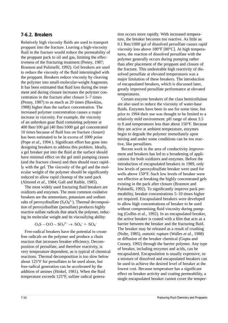
7-6.2. BreakersRelatively high viscosity fluids are used to transportproppant into the fracture. Leaving a high-viscosityfluid in the fracture would reduce the permeability ofthe proppant pack to oil and gas, limiting the effec-tiveness of the fracturing treatment (Penny, 1987;Brannon and Pulsinelli, 1992). Gel breakers are usedto reduce the viscosity of the fluid intermingled withthe proppant. Breakers reduce viscosity by cleavingthe polymer into small-molecular-weight fragments.It has been estimated that fluid loss during the treat-ment and during closure increases the polymer con-centration in the fracture after closure 5–7 times(Penny, 1987) to as much as 20 times (Hawkins,1988) higher than the surface concentration. Theincreased polymer concentration causes a majorincrease in viscosity. For example, the viscosity of an unbroken guar fluid containing polymer at 400 lbm/100 gal (40 lbm/1000 gal gel concentrated10 times because of fluid loss on fracture closure)has been estimated to be in excess of 1000 poise(Pope et al., 1994 ). Significant effort has gone intodesigning breakers to address this problem. Ideally, a gel breaker put into the fluid at the surface shouldhave minimal effect on the gel until pumping ceases(and the fracture closes) and then should react rapid-ly with the gel. The viscosity of the gel and the mol-ecular weight of the polymer should be significantlyreduced to allow rapid cleanup of the sand pack(Almond et al., 1984; Gall and Raible, 1985).

The most widely used fracturing fluid breakers areoxidizers and enzymes. The most common oxidativebreakers are the ammonium, potassium and sodiumsalts of peroxydisulfate (S2O8

2–). Thermal decomposi-tion of peroxydisulfate (persulfate) produces highlyreactive sulfate radicals that attack the polymer, reduc-ing its molecular weight and its viscosifying ability:

O3S – O:O – SO32– → ·SO4

– + ·SO4–

Free-radical breakers have the potential to createfree radicals on the polymer and produce a chainreaction that increases breaker efficiency. Decom-position of persulfate, and therefore reactivity, isvery temperature dependent, as is typical of chemicalreactions. Thermal decomposition is too slow belowabout 125°F for persulfates to be used alone, butfree-radical generation can be accelerated by theaddition of amines (Hinkel, 1981). When the fluidtemperature exceeds 125°F, sulfate radical genera-

tion occurs more rapidly. With increased tempera-ture, the breaker becomes too reactive. As little as0.1 lbm/1000 gal of dissolved persulfate causes rapidviscosity loss above 180°F [80°C]. At high tempera-tures, the reaction of dissolved persulfate with thepolymer generally occurs during pumping ratherthan after placement of the proppant and closure ofthe fracture. This undesirable high reactivity of dis-solved persulfate at elevated temperatures was amajor limitation of these breakers. The introductionof encapsulated breakers, which is discussed later,greatly improved persulfate performance at elevatedtemperatures.

Certain enzyme breakers of the class hemicellulaseare also used to reduce the viscosity of water-basefluids. Enzymes have been in use for some time, butprior to 1994 their use was thought to be limited to arelatively mild environment: pH range of about 3.5to 8 and temperatures less than about 150°F. Becausethey are active at ambient temperature, enzymesbegin to degrade the polymer immediately uponmixing and under some conditions can be too reac-tive, like persulfates.

Recent work in the area of conductivity improve-ment and breakers has led to a broadening of appli-cations for both oxidizers and enzymes. Before theintroduction of encapsulated breakers in 1989, onlylow levels of peroxydisulfate breaker were used forwells above 150°F. Such low levels of breaker werenot effective at breaking the highly concentrated gelsexisting in the pack after closure (Brannon andPulsinelli, 1992). To significantly improve pack per-meability, breaker concentrations 5–10 times higherare required. Encapsulated breakers were developedto allow high concentrations of breaker to be usedwithout compromising fluid viscosity during pump-ing (Gulbis et al., 1992). In an encapsulated breaker,the active breaker is coated with a film that acts as abarrier between the breaker and the fracturing fluid.The breaker may be released as a result of crushing(Nolte, 1985), osmotic rupture (Walles et al., 1988)or diffusion of the breaker chemical (Gupta andCooney, 1992) through the barrier polymer. Any typeof breaker, including enzymes and acids, can beencapsulated. Encapsulation is usually expensive, soa mixture of dissolved and encapsulated breakers canbe used to achieve the desired level of breaker at thelowest cost. Because temperature has a significanteffect on breaker activity and coating permeability, asingle encapsulated breaker cannot cover the temper-

7-14 Fracturing Fluid Chemistry and Proppants

ature range of 70° to 300°F [20° to 150°C]. A highertemperature usually requires that the breaker have aless permeable coating, which is achieved byincreasing the coating thickness or by using a differ-ent barrier polymer. The breaker chemical itself mayhave to be changed for high-temperature applica-tions. For example, the half-life of persulfate at160°F [70°C] is about 6.8 hr, but at 200°F it is onlyabout 15 min. Thus, even encapsulated persulfatebreakers have limited utility above 200°–225°F[90°–110°C].

Consideration of the theoretical advantages ofenzyme breakers has led to a renewed interest inthese materials. Enzymes are biocatalysts, meaningthey are not used up when they react with guar.Theoretically, a single enzyme molecule can reactwith many different guar molecules (i.e., turnoverrate) so polymer degradation might go on for alonger time and be more complete than with an oxi-dizer. These enzymes are globular proteins withthree-dimensional (3D) structures. They promotereactions with molecules that are able to becomeproperly oriented at the enzyme’s 3D active site.Therefore, enzymes are fairly specific in terms oftheir reactions. In the case of oilfield polymers, anenzyme that catalyzes the hydrolysis of the inter-ringlinkages is required. It has been suggested that themost effective enzyme breaker for guar would con-tain a beta-mannanase for attacking the polymerbackbone and an alpha-galactosidase for removingthe side chains (Brannon and Tjon-Joe-Pin, 1994).Commercial oilfield enzyme mixtures used in frac-turing fluids contain these enzymes. The ratio ofmannanase to galactosidase varies.

Recently, enzymes have been identified that areeffective up to a pH of about 10, making it possibleto use them in high-pH fluids such as borates. Also,it has been found that commercial enzymes retainsome level of activity, for at least a short period oftime, above 150°F. They can be used at elevatedtemperatures if the concentration is increased signifi-cantly. This is particularly true above 200°F, wherehigher concentrations are required because of dena-turing (permanent loss of the 3D structure) of theenzyme. A mitigating factor is pressure. Enzymescan have increased lifetimes at high pressure(Michels and Clark, 1992), which can reduce theconcentration necessary at temperatures of150°–200°F. As with oxidizers, enzymes can beextremely reactive when first introduced into the

fluid, before it heats up in the reservoir, and prema-ture viscosity loss may result.

Since 1994, enzymes have been used in conditionspreviously thought impossible. Oxidizers andenzymes are also being used together, which mayprovide the best performance. Breaker selection cri-teria are listed in Sidebar 7B. It remains to be seenwhether they will evolve to displace the workhorseoxidizers.

Other materials have been considered for use asbreakers. Oxidizers that are not as active as persul-fates may be used (Misak, 1975). Under controlledconditions, many organic peroxides do not begin toproduce free radicals unless the temperatureapproaches 200°F (Norman, 1968). Unfortunately,these materials are usually hazardous and difficult tohandle. Inorganic peroxides, such as CaO2, can alsobe used (Mondshine, 1993). Inorganic peroxides arecontrolled-release breakers because of the limitedsolubility of the inorganic peroxides at high pH. Therelease of the peroxide ion, and therefore the rate ofreaction with the polymer, is pH dependent. Con-taminants such as metal ions can rapidly acceleratethe decomposition of both organic and inorganic per-oxides (Sheppard and Kamath, 1978), which canmake their performance unpredictable.

Another category of breaker acts by eliminatingcrosslinking. A solution of fluoride ions at low pHhas been used as an overflush to dissolve filter cakeformed from a titanate- or zirconate-crosslinked fluid(Norman et al., 1989).

Acids degrade guar polymers. The release must becontrolled, because fracturing fluids for high-temper-ature formations generally are high pH to achieve thedesired stability. A combination breaker/fluid-lossadditive was developed using an acid condensationproduct (Cantu and Boyd, 1988). The material has aparticle-size distribution appropriate for a fluid-lossadditive and hydrolyzes to slowly release an organicacid. High concentrations of acid are typicallyrequired to reduce the pH of the fracturing fluid suf-ficiently for conductivity improvement, so this typeof breaker has not been widely used.

Guar polymers decompose at elevated tempera-tures because of hydrolysis or reaction with dis-solved oxygen, so it would seem that at some tem-perature breakers would not be necessary. However,the benefits of a high-temperature breaker have beenobserved even in 300°F wells (McConnell, 1994).The reason breakers are beneficial even at very high

Reservoir Stimulation 7-15

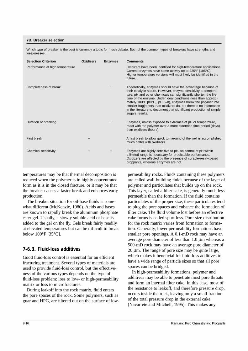
temperatures may be that thermal decomposition isreduced when the polymer is in highly concentratedform as it is in the closed fracture, or it may be thatthe breaker causes a faster break and enhances earlyproduction.

The breaker situation for oil-base fluids is some-what different (McKenzie, 1980). Acids and basesare known to rapidly break the aluminum phosphateester gel. Usually, a slowly soluble acid or base isadded to the gel on the fly. Gels break fairly readilyat elevated temperatures but can be difficult to breakbelow 100°F [35°C].

7-6.3. Fluid-loss additivesGood fluid-loss control is essential for an efficientfracturing treatment. Several types of materials areused to provide fluid-loss control, but the effective-ness of the various types depends on the type offluid-loss problem: loss to low- or high-permeabilitymatrix or loss to microfractures.

During leakoff into the rock matrix, fluid entersthe pore spaces of the rock. Some polymers, such asguar and HPG, are filtered out on the surface of low-

permeability rocks. Fluids containing these polymersare called wall-building fluids because of the layer ofpolymer and particulates that builds up on the rock.This layer, called a filter cake, is generally much lesspermeable than the formation. If the fluid containsparticulates of the proper size, these particulates tendto plug the pore spaces and enhance the formation offilter cake. The fluid volume lost before an effectivecake forms is called spurt loss. Pore-size distributionfor the rock matrix varies from formation to forma-tion. Generally, lower permeability formations havesmaller pore openings. A 0.1-mD rock may have anaverage pore diameter of less than 1.0 µm whereas a500-mD rock may have an average pore diameter of20 µm. The range of pore size may be quite large,which makes it beneficial for fluid-loss additives tohave a wide range of particle sizes so that all porespaces can be bridged.

In high-permeability formations, polymer andadditives may be able to penetrate most pore throatsand form an internal filter cake. In this case, most ofthe resistance to leakoff, and therefore pressure drop,occurs inside the rock, leaving only a small fractionof the total pressure drop in the external cake(Navarrete and Mitchell, 1995). This makes any

7-16 Fracturing Fluid Chemistry and Proppants

7B. Breaker selection

Which type of breaker is the best is currently a topic for much debate. Both of the common types of breakers have strengths andweaknesses.

Selection Criterion Oxidizers Enzymes Comments

Performance at high temperature + Oxidizers have been identified for high-temperature applications. Current enzymes have some activity up to 225°F [105°C].Higher temperature versions will most likely be identified in the future.

Completeness of break + Theoretically, enzymes should have the advantage because of their catalytic nature. However, enzyme sensitivity to tempera-ture, pH and other chemicals can significantly shorten the life-time of the enzyme. Under ideal conditions (less than approxi-mately 180°F [80°C], pH 5–8), enzymes break the polymer into smaller frag|ments than oxidizers do, but there is no information in the literature to document that significant production of simple sugars results.

Duration of breaking + Enzymes, unless exposed to extremes of pH or temperature, react with the polymer over a more extended time period (days) than oxidizers (hours).

Fast break + A fast break to allow quick turnaround of the well is accomplishedmuch better with oxidizers.

Chemical sensitivity + + Enzymes are highly sensitive to pH, so control of pH within a limited range is necessary for predictable performance. Oxidizers are affected by the presence of curable-resin-coated proppants, whereas enzymes are not.

external filter cake vulnerable to shear degradationby the fluid. During a fracturing treatment, fluid lossoccurs under dynamic conditions (i.e., fluid flowsalong the face of the formation). Prud’homme andWang (1993) proposed that the extent to which thethickness of the filter cake grows is controlled by theshear stress τ exerted by the fluid at the wall of thecake and the yield stress of the cake. The cake stopsgrowing when the fluid stress becomes equal to theyield stress of the cake, and it starts to erode whenthe fluid stress is larger than the yield stress of thecake. The yield stress of a polymer cake depends onthe polymer concentration and pressure gradient inthe cake, whereas the shear stress of the fluid isdetermined by the rheological properties of the fluidand the shear rate γ at the formation face.

Silica flour has been shown to be an effectivefluid-loss additive for helping establish a filter cake.Penny et al. (1985) reported a 10-fold reduction inspurt loss for 5- to 100-mD rock when silica flourwas used. Navarrete et al. (1994) determined that theeffectiveness of a particulate fluid-loss additive, suchas silica flour, depends on whether it can reach thewall of the rock and avoid being sheared off the sur-face. This depends on the relative ratio of the forcedriving the particle toward the wall Fy and the shearforce driving the particle tangentially to the wall Fx.The chance that a particle will reach the wall andstay there increases as Fy/Fx increases:

(7-2)

The ratio Fy /Fx increases with

• larger leakoff flux toward the wall (qL)

• smaller particle size (d)

• smaller shear stress (τw) of the fluid along the wall.

The shape of a particle plays an important role inits effectiveness to approaching and staying at thewall. Gauthier et al. (1971) showed experimentallythat axisymmetric particles (rods, platelets, etc.) in a shear flow tend to align their major axis with theflow. Under dynamic conditions, an axisymmetricparticle approaches the fracture surface with itsmajor axis parallel to the surface. Once the particle is on the surface, there is little torque exerted on theparticle for removal. Therefore, larger aspect ratioaxisymmetric particles are better fluid-loss additivesthan low-aspect-ratio particles.

Deformable particles such as starches are alsogood fluid-loss additives. Starches are polysaccha-rides of long chains of glucose molecules, compris-ing 20%–30% linear amylose molecules and80%–70% branched amylopectin molecules. Theyare extracted in granular form from the cells of cer-tain plants, such as potato, maize, wheat and tapioca,which determine their shape and size. Starches canbe viewed as soft particles that can deform underpressure or stress. This makes them well suited toproduce low-permeability filter cakes, because theycan deform and block pore throats or fill in emptyspaces, thus reducing the porosity of the cake. Onthe other hand, the deformability of a starch can playan adverse role when pore throats are too big. In thatcase, starch penetrates into the formation withoutreducing spurt loss. Combining starch with particu-lates can provide an overall fluid-loss additive thatreduces spurt and forms a low-permeability filtercake. Starches are considered less damaging thaninorganic particles because they degrade naturally or by the addition of amylase enzymes and oxidizers(Williamson and Allenson, 1989).

Oil-soluble resins also can be used to control fluidloss. These materials, when sized properly with anadequate thermal-softening point, can bridge andseal the pore spaces to reduce fluid loss. An advan-tage that these materials have over silica flour orstarches is that they are oil-soluble and dissolve inproduced liquid hydrocarbons. On dissolving, forma-tion or proppant-pack damage is minimized. How-ever, oil-soluble resins are considerably more expen-sive than other types of fluid-loss additives.

Another method for controlling fluid loss is to usedispersed fluids. These fluids are oil-in-water disper-sions that contain a fairly small oil concentration andexhibit good fluid-loss control. For low permeability,the dispersed droplets are effective as deformableparticles to block pore throats. The dispersion alsoproduces two-phase flow through the filter cake,which significantly reduces its permeability to water.The effectiveness of 5% diesel as a fluid-loss addi-tive has been demonstrated in dynamic tests (Gulbis,1983; Penny et al., 1985). However, Gulbis pointedout that diesel is not nearly as effective in a dynamictest as in a static test. In a static test, 5% dieselreduced the fluid-loss rate by a factor of 5. In adynamic test, the reduction was only by a factor of1.5. A possible explanation for the difference is thatdynamic filter cake containing oil is very thin com-

Reservoir Stimulation 7-17

F

F ~ q /dy

x

L wτ( ) .

pared with one without oil, indicating that oil has adetrimental effect on cake durability and thickness.Penny et al. (1985) and Nolte (1982) also empha-sized the fragile nature of filter cakes that contain oil.

Controlling fluid loss to natural fractures thatintersect the main fracture is more difficult than con-trolling fluid loss to the matrix because the openingsto be blocked can be larger and can expand from thepressurized filtrate. Solid materials (such as silicaflour) can bridge a fracture and plug it off (Hall andHouk, 1983; Wood and Cramer, 1984), but theireffectiveness depends on the size of the intersectingfracture. Silica flour smaller than 200 mesh is veryuseful against microfractures (<50 µm wide), butlarger particles (such as 100-mesh sand) are neces-sary after the macrofracture aperture expands (>50 µm wide). These large particulates also areavailable as oil-soluble resins.

As stated earlier, the primary purpose of a fractur-ing treatment is to generate a highly conductive flowchannel through the producing formation to the well-bore. Ideally, fluid-loss additives should not damagethe permeability of the formation, fracture face orproppant pack. In reality, many of the fluids andadditives form long-lasting filter cakes that are notreadily removed from the fracture. As demonstratedby Holditch (1979b), a 90% reduction in permea-bility of the fracture face can be tolerated, because of the linear flow regime caused by the fracture. Thisis true for relatively low-permeability reservoirs(e.g., k < 5 mD) where the fracture conductivity is moderate to large and the fracture length is large(invariably longer than 200 ft). Fracture face dam-age, caused by fluid leakoff, is important in high-permeability fracturing where the fracture lengthmay be as short as 15 ft. This damage is one of thedominant reasons for post-treatment positive skineffects (Mathur et al., 1995). For moderate-perme-ability reservoirs, the conductivity of the proppedfracture, rather than formation permeability, tends to be the limiting factor in long-term productivity.Therefore, formation face damage caused by fluid-loss additives is usually a secondary concern.

7-6.4. BactericidesBactericides are added to polymer-containing aque-ous fracturing fluids to prevent viscosity loss causedby bacterial degradation of the polymer. The poly-

saccharides (sugar polymers) used to thicken waterare an excellent food source for bacteria. Bacterianot only ruin gel by reducing the molecular weightof the polymer, but some can turn the reservoir fluidssour. Once introduced into the reservoir, some bacte-ria can survive and reduce sulfate ions to hydrogensulfide (H2S), an extremely dangerous gas with acharacteristic rotten-egg odor (i.e., sour).

Materials such as glutaraldehyde, chlorophenates,quaternary amines and isothiazoline are used to con-trol bacteria (Ruseska et al., 1982). Usually thematerials kill the bacteria, but they do not alwaysinactivate the enzymes they have produced that areresponsible for breaking down the polysaccharides.For this reason, it is common practice to add bacteri-cide to fracture tanks before the water is added toensure that the bacterial enzyme level is kept low.Improvements and changes in bactericides are made sothat if a strain develops that is resistant to one type ofbactericide, another can be used. Bactericides are notnecessary in acid-based or oil-base fracturing fluids.

7-6.5. StabilizersStabilizers are used to prevent degradation of poly-saccharide gels at temperatures above 200°F(Thomas and Elbel, 1979). The common stabilizersare methanol and sodium thiosulfate (Na2S2O3).Methanol is more hazardous to handle and is used as5% to 10% of the fluid volume. Sodium thiosulfateis generally used at 10 to 20 lbm/1000 gal. Sodiumthiosulfate is the more effective of the two, increas-ing the viscosity at elevated temperatures by a factorof 2 to 10, depending on the temperature and time ofexposure to temperature (Thomas and Elbel, 1979).

The mechanism for these stabilizers is not fullyunderstood. It is believed that they act as oxygenscavengers and prevent the rapid gel degradationcaused by dissolved oxygen. Walker et al. (1995)studied several oxygen scavengers and found sodiumthiosulfate to be the most effective at maintaining gelstability. Sodium thiosulfate must be used in greatexcess because its reaction with oxygen is not favor-able. Other materials that are better oxygen scav-engers, such as sodium sulfite and sodium erythor-bate, are not good gel stabilizers, apparently becausethe reaction products also cause gel degradation.

Fluid pH also should be considered in maximizingfluid stability. Guar and its derivatives are hydrolyzed

7-18 Fracturing Fluid Chemistry and Proppants

at low pH, especially at elevated temperatures(>200°F). Therefore, if long-term fluid stability isdesired, a high-pH (e.g., 9–11) fluid should be used.

7-6.6. SurfactantsA surface-active agent, or surfactant, is a materialthat at low concentration adsorbs at the interfacebetween two immiscible substances. The immisciblesubstances may be two liquids, such as oil and water,a liquid and a gas, or a liquid and a solid. The sur-factant becomes involved in the interface and lowersthe amount of energy required to expand the inter-face (Rosen, 1972). More detailed information aboutsurfactant structure and function is in Chapter 15.

Some applications for surfactants in fracturingfluids have already been discussed. They are neces-sary ingredients in foams to promote the formationof stable bubbles. They are used in polyemulsion flu-ids to stabilize the oil-in-water emulsion. In addition,they are used as surface-tension-reducing agents andformation-conditioning agents (Penny et al., 1983) topromote cleanup of the fracturing fluid from the frac-ture. Some bactericides and clay-control agents aresurfactants.

7-6.7. Clay stabilizersClays are layered particles of silicon and aluminumoxide averaging 2 µm in size (Moore, 1960). Nega-tively charged particles result when the charge bal-ance between positive (aluminum) and negative(oxygen) is disrupted through displacement ofcations or breaking of the particles. Cations, fromsolution, surround the clay particle and create a posi-tively charged cloud. Such particles repel each otherand are prone to migration (Crowe, 1979). Once clayparticles are dispersed, the particles can block porespaces in the rock and reduce permeability.

Solutions containing 1% to 3% KCl are commonlyused as the base liquid in fracturing fluids to stabilizeclays and prevent swelling. In addition to KCl, theorganic cation tetramethyl ammonium chloride is aneffective stabilizer (Himes and Vinson, 1991). Allthese salts help maintain the chemical environment ofthe clay particles, but they do not provide permanentprotection. More permanent methods for controllingclay migration involve the use of quaternary aminesor inorganic polynuclear cations. The latter materials,

such as zirconium oxychloride (Veley, 1969) andhydroxyaluminum (Haskin, 1976), are used primarilyin matrix-acidizing treatments to neutralize the sur-face charge on clays (Thomas et al., 1976). Unfor-tunately, they have limited compatibility with higherpH fracturing fluids.

Quaternary amines possess a positively chargedgroup that is attracted to the negatively charged clayparticle. Once the quaternary amine is attached to theclay particle, the hydrocarbon chain portion extendsfrom the particle, forming an organic barrier andminimizing the cationic cloud. This type of claystabilizer is used in water-base fracturing treatments.

7-7. ProppantsProppants are used to hold the walls of the fractureapart to create a conductive path to the wellbore afterpumping has stopped and the fracturing fluid hasleaked off. Placing the appropriate concentration andtype of proppant in the fracture is critical to the suc-cess of a hydraulic fracturing treatment. Factorsaffecting the fracture conductivity (a measurement of how a propped fracture is able to convey the pro-duced fluids over the producing life of the well) are

• proppant composition

• physical properties of the proppant

• proppant-pack permeability

• effects of postclosure polymer concentration in thefracture

• movement of formation fines in the fracture

• long-term degradation of the proppant.

7-7.1. Physical properties of proppantsThe physical properties of proppants that have animpact on fracture conductivity are

• proppant strength

• grain size and grain-size distribution

• quantities of fines and impurities

• roundness and sphericity

• proppant density.

To open and propagate a hydraulic fracture, the in-situ stresses must be overcome. After the well is puton production, stress acts to close the fracture and

Reservoir Stimulation 7-19

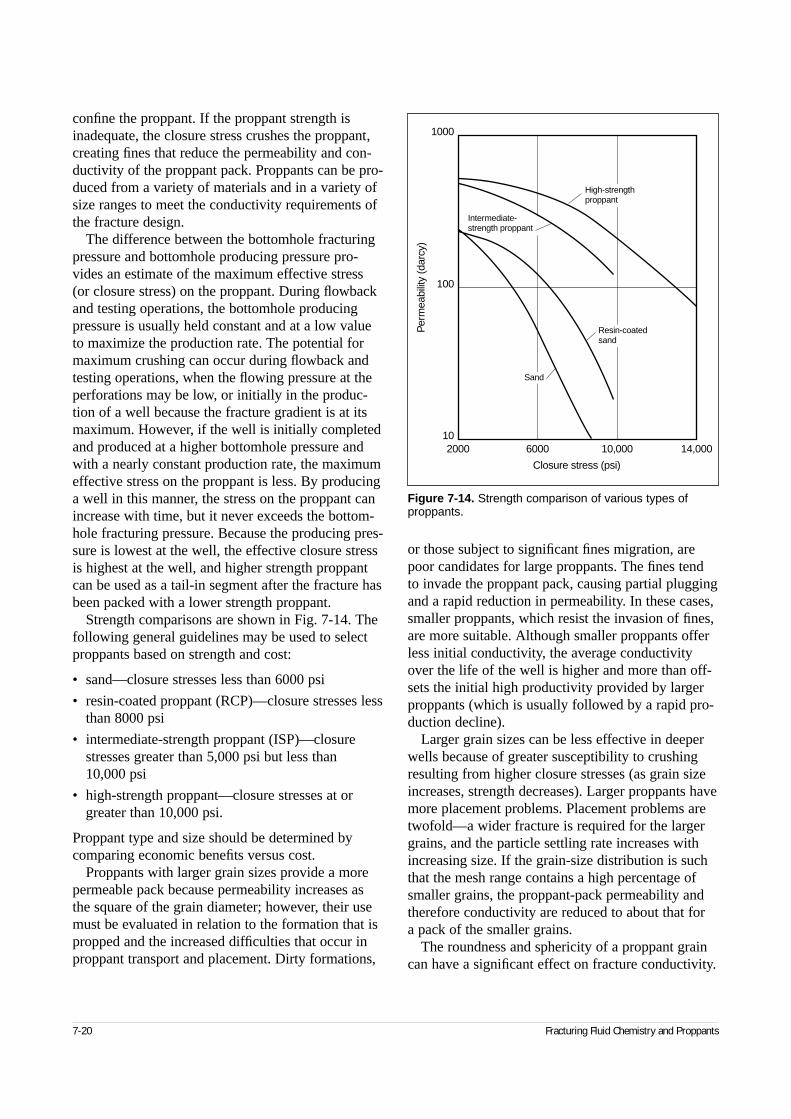
confine the proppant. If the proppant strength isinadequate, the closure stress crushes the proppant,creating fines that reduce the permeability and con-ductivity of the proppant pack. Proppants can be pro-duced from a variety of materials and in a variety ofsize ranges to meet the conductivity requirements ofthe fracture design.

The difference between the bottomhole fracturingpressure and bottomhole producing pressure pro-vides an estimate of the maximum effective stress(or closure stress) on the proppant. During flowbackand testing operations, the bottomhole producingpressure is usually held constant and at a low valueto maximize the production rate. The potential formaximum crushing can occur during flowback andtesting operations, when the flowing pressure at theperforations may be low, or initially in the produc-tion of a well because the fracture gradient is at itsmaximum. However, if the well is initially completedand produced at a higher bottomhole pressure andwith a nearly constant production rate, the maximumeffective stress on the proppant is less. By producinga well in this manner, the stress on the proppant canincrease with time, but it never exceeds the bottom-hole fracturing pressure. Because the producing pres-sure is lowest at the well, the effective closure stressis highest at the well, and higher strength proppantcan be used as a tail-in segment after the fracture hasbeen packed with a lower strength proppant.

Strength comparisons are shown in Fig. 7-14. Thefollowing general guidelines may be used to selectproppants based on strength and cost:

• sand—closure stresses less than 6000 psi

• resin-coated proppant (RCP)—closure stresses lessthan 8000 psi

• intermediate-strength proppant (ISP)—closurestresses greater than 5,000 psi but less than 10,000 psi

• high-strength proppant—closure stresses at orgreater than 10,000 psi.

Proppant type and size should be determined bycomparing economic benefits versus cost.

Proppants with larger grain sizes provide a morepermeable pack because permeability increases asthe square of the grain diameter; however, their usemust be evaluated in relation to the formation that ispropped and the increased difficulties that occur inproppant transport and placement. Dirty formations,

or those subject to significant fines migration, arepoor candidates for large proppants. The fines tendto invade the proppant pack, causing partial pluggingand a rapid reduction in permeability. In these cases,smaller proppants, which resist the invasion of fines,are more suitable. Although smaller proppants offerless initial conductivity, the average conductivityover the life of the well is higher and more than off-sets the initial high productivity provided by largerproppants (which is usually followed by a rapid pro-duction decline).

Larger grain sizes can be less effective in deeperwells because of greater susceptibility to crushingresulting from higher closure stresses (as grain sizeincreases, strength decreases). Larger proppants havemore placement problems. Placement problems aretwofold—a wider fracture is required for the largergrains, and the particle settling rate increases withincreasing size. If the grain-size distribution is suchthat the mesh range contains a high percentage ofsmaller grains, the proppant-pack permeability andtherefore conductivity are reduced to about that for a pack of the smaller grains.

The roundness and sphericity of a proppant graincan have a significant effect on fracture conductivity.

7-20 Fracturing Fluid Chemistry and Proppants

Figure 7-14. Strength comparison of various types ofproppants.

2000 6000 10,000 14,00010

100

1000

Closure stress (psi)

Per

mea

bilit

y (d

arcy

)

Sand

Resin-coatedsand

High-strengthproppant

Intermediate-strength proppant

Proppant grain roundness is a measure of the relativesharpness of the grain corners, or grain curvature.Particle sphericity is a measure of how close theproppant particle or grain approaches the shape of a sphere. If the grains are round and about the samesize, stresses on the proppant are more evenly dis-tributed, resulting in higher loads before grain failureoccurs. Angular grains fail at lower closure stresses,producing fines that reduce fracture conductivity.

Proppant density has an influence on proppanttransport because the settling rate increases linearlywith density. Therefore, high-density proppants aremore difficult to suspend in the fracturing fluid andto transport to the top of the fracture. Placement canbe improved in two ways: using high-viscosity fluidsto reduce settling or increasing the injection rate toreduce treatment time and the required suspensiontime. Also, high-density proppants require moremass of material to fill a given fracture volume.

7-7.2. Classes of proppantsSand is the most commonly used proppant. It is themost economical, is readily available and generallyprovides sufficient fracture conductivity for closurestresses less than 6000 psi. Its specific gravity is about2.65. Depending on the overall balance of physicalproperties, sand can be subdivided into groups:

• northern white sand

• Texas brown sand

• Colorado silica sand

• Arizona silica sand.

American Petroleum Institute (API) standards can be used to similarly qualify and group any sand source.

Resin coatings are applied to sand (usually north-ern white sand) to improve proppant strength and to reduce flowback during production. Resin-coatedsand is stronger than conventional sand and may beused at closure stresses less than 8000 psi, dependingon the type of resin-coated sand. At closure stressesgreater than 4000 psi and without adverse fluideffects on the resin, resin-coated sand has a higherconductivity than conventional sand. The resin helpsspread the stress over a larger area of the sand grainand reduces the point loading. When grains crush,the resin coating helps encapsulate the crushed por-tions of the grains and prevents them from migratingand plugging the flow channel. In some cases, resin-

coated proppant may be used as an alternative to ISP,which is discussed next. Resin-coated sands have aspecific gravity of about 2.55.

The resin coating on some RCPs is cured (at leastpartially) during the manufacturing process to form a nonmelting, inert film. Proppants processed in thisfashion are called precured-resin-coated proppants.The major application for precured-resin-coatedproppants is to enhance the performance of sand at high stress levels.

A curable resin coating may also be applied tosand or other types of proppants. The major applica-tion of curable-resin-coated proppants is to preventthe flowback of proppants near the wellbore. Thecurable-resin-coated proppants are mixed andpumped in the later stages of the treatment, and thewell is shut in for a period of time to allow the resinto bind the proppant particles together. Theoretically,the RCP cures into a consolidated, but permeable,filter near the wellbore.

Although they provide versatile and reliable per-formance, RCPs contain components that can inter-fere with common fracturing fluid additives, such asorganometallic crosslinkers, buffers and oxidativebreakers. These undesirable interactions have beenreported to interfere with the crosslinking of organ-ometallic crosslinkers, suppress fracturing fluidcleanup by consuming oxidative breakers and com-promise proppant-pack bonding, leading to reducedpermeability, proppant flowback and increased prop-pant crushing (Dewprashad et al., 1993; Nimerick et al., 1990; Stiles, 1991; Smith et al., 1994). Fibertechnology, as discussed in Section 11-6.4, is analternative technique for proppant flowback prob-lems that introduces no chemical compatibilityissues or special curing requirements for time andtemperature. Guidelines for minimizing the undesir-able effects of RCPs are listed in Sidebar 7C.

ISP is fused-ceramic (low-density) proppant orsintered-bauxite (medium-density) proppant. Thesintered-bauxite ISP is processed from bauxite orecontaining large amounts of mullite. This is in con-trast to a high-strength proppant, which is processedfrom bauxite ore high in corundum. ISP is generallyused at closure stresses greater than 5,000 psi, butless than 10,000 psi. The specific gravity of ISPranges from 2.7 to 3.3.

High-strength proppant is sintered bauxite contain-ing large amounts of corundum, and it is used at clo-sure stresses greater than 10,000 psi. High-strength

Reservoir Stimulation 7-21

proppant is the most costly proppant. Its specificgravity is 3.4 or greater.

7-8. ExecutionDuring the fracturing treatment, fluid chemistrycomes together with proppant handling, mixing andpumping equipment to create the desired proppedfracture. The field environment is often quite differ-ent from the ideal laboratory conditions in which thefracturing fluid or additive was developed. The fol-lowing sections address the field environment.

7-8.1. MixingFluids may be batch mixed or continuously mixed.Batch mixing has slightly different meanings,depending on the fluid prepared. For oil-base fluids,

it means that all ingredients (except fluid-loss addi-tive, breaker and proppant) are blended together inthe fracture tanks (typically, 500-bbl capacity) beforepumping begins. The tanks are usually mixed theday before pumping because the gel takes severalhours to form. A fluid-loss additive and a breaker areadded on the fly as the gel is pumped. These materi-als are added on the fly to prevent the fluid-loss addi-tive from settling out in the fracture tanks or thebreaker from prematurely reducing the gel viscosityprior to pumping.

For batch-mixed, water-base fluids, the bacteri-cide, polymer, salt, clay stabilizer, etc., are mixedtogether before pumping. The polymer is given suffi-cient time to hydrate in the tanks before the jobbegins. The pH of the gel is adjusted for optimumcrosslinking. Crosslinker is added on the fly in thecase of transition metal (Ti and Zr) crosslinkers.Because borate crosslinking occurs only at a highpH, boric acid can be added to the polymer in thetanks, and a base such as NaOH can then be addedon the fly to raise the pH and to initiate crosslinking.

As discussed later, batch mixing affords the bestopportunity for quality assurance. Unfortunately, italso results in wasted materials. There are alwaystank bottoms, the fluid that cannot be drawn out ofthe fracture tanks. Typically, tank bottoms representat least 7% of the total volume of fluid in the tanks,resulting in the waste of 7% of the batch-mixedchemicals and requiring costly disposal. Also, thisfluid must be broken and the fracture tanks should becleaned. If the job is postponed and the gel degradesbecause of bacterial action, the entire batch of gelmay have to be discarded. From a cost standpoint,continuously mixed fluid is more desirable. In thismode, all materials are added on the fly, so there isno wasted fluid and no unnecessary expense. Poly-mer slurries (concentrated suspensions of guar orHPG in diesel) were developed so that polymercould be accurately metered and so that it would dis-perse and hydrate rapidly enough for continuousmixing (Constien et al., 1988; Yeager and Bailey,1988). This type of operation requires accuratemetering of all materials and makes quality assur-ance more difficult. Techniques for on-site rheologymeasurement have been developed so that the linear(precrosslinked) gel viscosity can be closely moni-tored. Because of environmental considerations anddisposal costs, most aqueous-based fluids are nowcontinuously mixed.

7-22 Fracturing Fluid Chemistry and Proppants

7C. Minimizing the effects of resin-coated proppants

To minimize the effects of curable-resin-coated proppant andfluid interactions, the following guidelines are recommended.

• Use fiber reinforcement.

• Minimize the amount of RCP. If proppant flowback controlis required, consider alternate materials for addressingthe problem. Card et al. (1994) described the incorpora-tion of fibers in the proppant pack as a means to preventflowback.

• Use precured-resin-coated proppants. These materialsare cured (at least partially) and are typically less reactivewith fracturing fluid additives than fully curable-resin-coated proppants.

• Avoid using curable-resin-coated proppants in conjunctionwith high concentrations of oxidative breakers. RCPsdecrease breaker effectiveness. Conversely, oxidativebreakers can compromise the strength development of an RCP. The reactivity of RCPs with oxidative breakersvaries, and some RCPs have little effect on breaker activ-ity. Additional breaker may be required when using RCPsto ensure adequate cleanup.

• Always determine the compatibility of the fracturing fluidand the RCP before the treatment. Typically, 30%–60%of the curable-resin coating can be lost to the fluid. Resinloss does not behave in a straightforward manner withchanges in temperature or time at temperature. Resinloss increases as exposure to shear increases.

• Never batch mix RCPs in fracturing fluids. Minimize han-dling of RCPs to keep dust levels low. Solid resin is agood emulsion stabilizer and can create an emulsion withthe fracturing fluid that is not miscible in water.

7-8.2. Quality assuranceTesting the components of the fracturing fluid priorto the treatment is the only way to ensure that thefluid used will have the properties expected of it. In the case of a water-base fluid, the mix water mustmeet certain specifications. It should be relativelyfree of iron (<25-ppm Fe2+) and other reducingagents that promote gel degradation or catalyze thereaction of peroxydisulfate (persulfate) breakers(Ely, 1985). The pH of the water affects the polymerhydration rate. If the water pH is low, hydration maybe rapid and lumping of the gel results. If the waterpH is too high, the gel hydrates too slowly. Watertemperature also affects hydration rate. Increasingthe water temperature causes faster polymer hydra-tion (viscosity development). A sample of polymerfrom location should be used to prepare a linear(precrosslink) gel with the water from the fracturetanks. Testing should ensure that proper dispersion(no lumps) and hydration (viscosity development)will be obtained on location.

If the proper viscosity can be achieved, crosslinkerperformance can be evaluated. A fracturing fluidsample containing the appropriate concentration ofcrosslinker can be heated to accelerate crosslinkingand produce a thick gel. In addition to gross cross-linker performance, a measure of how long it willtake for the gel to crosslink should be performed(crosslink time). Common on-site tests for measuringcrosslink time are the vortex closure test, static stiff-ness test (Hodge and Baranet, 1987) and falling-ballviscometer method (Cawiezel and Elbel, 1990). Inthe vortex closure test, polymer solution is stirred in a blender to create a vortex. The crosslinker isadded, and the time required for the vortex to close,forming a smooth surface, is termed the vortex clo-sure time. The static stiffness test involves mixingthe fluid components together and then pouring the

fluid back and forth between two containers. Thetime at which the fluid appears very thick (stringy orpours as one mass from container to container) is thecrosslink time. The falling-ball viscometer measuresthe time required for the crosslinked fluid to developsuspending properties. Hodge and Baranet (1987)point out that the vortex closure and static stiffnesstests are misleading because the procedures do notsimulate the shear the fluids experience in the tubingor the heat-up that occurs in the wellbore. Both fac-tors greatly impact the crosslinking rate and viscositydevelopment. As discussed in Section 7-6.1, the useof dual-crosslinker systems can eliminate the neces-sity of accurate control of the crosslink time.

Not all potential mix water sources or fracturingfluid additives are compatible. When preparing thetest sample with materials from location, all compo-nents should be included. Any severe compatibilityproblems should show up in this test, preferably wellbefore the treatment and in a laboratory setting. Todetermine how well the fluid will perform at elevatedtemperatures, a Fann 50 rheology test (see Chapter8) is usually performed. This preliminary test shouldreveal problems with the chemicals or problems withthe mix water or oil source.

Once the job is in progress, the viscosity of anycontinuously mixed linear gel should be monitoredto quickly identify problems that could develop.Also, a sample of the crosslinked fluid should beinspected periodically. A detailed discussion of qual-ity assurance procedures is provided by Ely (1985).

AcknowledgmentsCurtis Crowe contributed the acid fracturing section.Reinaldo Navarrete updated the fluid-loss section.The proppant section was written originally by BrianAinley and edited by Bob Thrasher.

Reservoir Stimulation 7-23

8-1. IntroductionHydraulic fracturing employs special fluids that areintended primarily to create an appropriate fracturegeometry while transporting proppants. Key to theentire exercise is the fluid rheology, which affects thefluid viscosity, its proppant-carrying capability and itspropensity for leaking off into the porous medium.

This chapter begins with fracturing fluid character-ization, followed by the translation of laboratory-obtained information to field conditions. There is aclear link between the chemistry of fracturing fluids,most of which are polymer solutions with their prop-erties augmented by several additives, and the physi-cal properties expected from these fluids. Rheologyand its modeling and control take center stage in thechapter. This includes not only traditional water-basepolymer solutions but also complex fluids such asfoams. Proppant-transporting slurries are also exam-ined in relative detail with regard to both their rheol-ogy and potentially problematic proppant settling.The general discussion of fracturing fluid loss con-tains some of the classic thinking, especially withregard to laboratory-derived data. This discussionshould be read in conjunction with Chapters 9 and 2, which address leakoff modeling and the interpre-tation of fracturing pressure behavior, which are inti-mately related phenomena. Finally, damage fromfracturing fluids to the formation face and the result-ing proppant pack, the first from fracturing fluidleakoff and the second because of unbroken polymerfollowing the treatment, are outlined. These prob-lems are tackled in detail in Chapter 12.

8-2. Fracturing fluid characterizationFracturing fluid additives and fluid systems are char-acterized for the following purposes:

• additive and system development

• obtaining input data for use in fracture designsimulators

• quality control before or during the treatment.

Characterization during the development processfor an additive or fluid system is typically used todetermine if a new composition is an improvementover an existing system or if it can provide similarperformance at a lower cost.

Characterization of fluid systems that obtains rep-resentative performance data in critical areas such asrheology, pipe friction pressure, fluid-loss rates, frac-ture conductivity and formation damage is conductedto obtain data that can be used in fracture design andproduction simulators.

Characterization of fluid systems at the point of usefor quality assurance purposes usually involves meth-ods that can be applied at less than ideal conditions toindicate how the systems are performing. Examplesof these tests are provided in Davidson et al. (1994),Ely (1985) and Section 7-8 of this volume.

The American Petroleum Institute (API) hasdeveloped recommended practices for several of thelaboratory characterization methods described in thischapter. An excellent review of laboratory methodsis also in the Society of Petroleum Engineers (SPE)Monograph 12, Recent Advances in HydraulicFracturing (Gidley et al., 1989).

This chapter addresses the characterization meth-ods used for additive and system development andfor obtaining input data for use in fracture designsimulators. The focus is on the most commonly usedfluids: water-base systems utilizing guar or deriva-tized guar as the polymer viscosifier (see Chapter 7).In general, methods used for water-base fluids can beapplied—with appropriate modification—to otherfluids such as gelled oils, emulsions and foams.

Whatever the fluid system, a set of data describingthe fluid rheology, fluid loss, pipe friction, fractureconductivity and possible formation damage shouldbe determined before the fluid system is used in fieldoperations.

Reservoir Stimulation 8-1

◆

Performance ofFracturing Materials

Vernon G. Constien, Constien and AssociatesGeorge W. Hawkins, Schlumberger DowellR. K. Prud’homme, Princeton UniversityReinaldo Navarrete, Kelco Oilfield Group

8-3. Characterization basicsBefore any significant laboratory work to determinefluid system properties is begun, representative mater-ial samples of all components must be obtained.These include samples of the water, hydrocarbon andacid. In some instances sampling may require obtain-ing multiple lots of materials to prepare a compositeblend. At a minimum, all materials must be identifiedby the manufacturer and lot number so that they canbe traced back to the point of origin. In the case ofproppants, special care must be taken because it isgenerally difficult to obtain representative samplesfrom any size lot (Recommended Practices for TestingSand Used in Hydraulic Fracturing Operations[RP 56], 1983). This difficulty arises because of sizesegregation during transport and transfer.

In addition to obtaining representative materialsamples, calibrating and maintaining the laboratoryinstruments before and during testing is required.Adherence to the prescribed testing methods is cru-cial for comparing different systems and avoiding fre-quent rerunning of the data to obtain an exact matchto the testing conditions. Complete records containingmaterial sample and calibration data information areessential for product or system comparisons becausethe usable lifetime of the data can span several years.

8-4. Translation of field conditionsto a laboratory environment

The range of conditions that fracturing fluids experi-ence during their use is so diverse and the physicalscale so large that the characterization process is usu-ally divided into a series of small-scale tests that sim-ulate key portions of the large, complex physicalenvironment. The scope of the characterization canpotentially range from the molecular level to testingfluids in large-scale equipment, which may approachactual mixing, wellbore and fracture dimensions.

The exact details of the characterization methodmay change depending on the composition of thefluid. For example, oil-base fluids, emulsions andfoams may have compressibility or bubble- or drop-size effects that require the determination of proper-ties over a range of pressures.

8-5. Molecular characterization of gelling agents

An important set of techniques for the understandingand prediction of fracturing fluid performanceinvolves characterization at the molecular level. Asdiscussed in Chapter 7, water-base fracturing fluidsare formulated primarily from guar or derivatized guarpolymers. Methods such as intrinsic viscosity mea-surements, dynamic light scattering, nuclear magneticresonance (NMR), size-exclusion chromatography(SEC) and freeze-fracture electron microscopy pro-vide information on guar molecular size, crosslinking,degradation mechanisms and gel structure.

Before extensive investigations are made of theproperties of fully formulated guar-based fracturingfluid systems, it is worthwhile to consider the proper-ties of the guar itself. Guar is a natural product and,as such, is subject to variation of its properties.Suppliers of oilfield-grade guar blend batches toobtain consistent performance from the materials.However, before an investment is made in the devel-opment of a new fluid system, the basic properties ofblended representative batches of the base polymershould be determined.

8-5.1. Correlations of molecular weight and viscosity

Guar and its derivatives are the polymers most com-monly used in fracturing fluids. Like many polysac-charides, guar is conformationally mobile and adoptsa disordered or “random-coil” geometry in dilutesolutions.

Viscosity–molecular weight relations for severalguar samples were determined by Robinson et al.(1982) using dilute solution viscometry and light-scattering measurements. They concluded that guaracts as a random-coil polymer and that the methodscommonly used to study synthetic polymers could beused to determine information such as intrinsic chainflexibility.

Intrinsic viscosity µi is a convenient index of thesize or hydrodynamic volume of isolated polymercoils in solution. For random-coil polymer solutions,µi can be expressed as a function of the end-to-end

8-2 Performance of Fracturing Materials

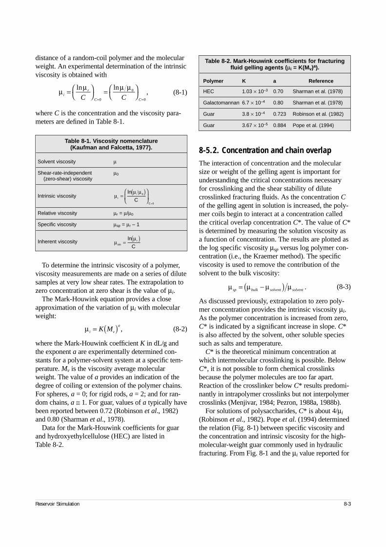
distance of a random-coil polymer and the molecularweight. An experimental determination of the intrinsicviscosity is obtained with

(8-1)

where C is the concentration and the viscosity para-meters are defined in Table 8-1.

To determine the intrinsic viscosity of a polymer,viscosity measurements are made on a series of dilutesamples at very low shear rates. The extrapolation tozero concentration at zero shear is the value of µi.

The Mark-Houwink equation provides a closeapproximation of the variation of µi with molecularweight:

(8-2)

where the Mark-Houwink coefficient K in dL/g andthe exponent a are experimentally determined con-stants for a polymer-solvent system at a specific tem-perature. Mv is the viscosity average molecularweight. The value of a provides an indication of thedegree of coiling or extension of the polymer chains.For spheres, a = 0; for rigid rods, a = 2; and for ran-dom chains, a ≅ 1. For guar, values of a typically havebeen reported between 0.72 (Robinson et al., 1982)and 0.80 (Sharman et al., 1978).

Data for the Mark-Houwink coefficients for guarand hydroxyethylcellulose (HEC) are listed in Table 8-2.

8-5.2. Concentration and chain overlapThe interaction of concentration and the molecularsize or weight of the gelling agent is important forunderstanding the critical concentrations necessaryfor crosslinking and the shear stability of dilutecrosslinked fracturing fluids. As the concentration Cof the gelling agent in solution is increased, the poly-mer coils begin to interact at a concentration calledthe critical overlap concentration C*. The value of C*is determined by measuring the solution viscosity asa function of concentration. The results are plotted asthe log specific viscosity µsp versus log polymer con-centration (i.e., the Kraemer method). The specificviscosity is used to remove the contribution of thesolvent to the bulk viscosity:

(8-3)

As discussed previously, extrapolation to zero poly-mer concentration provides the intrinsic viscosity µi.As the polymer concentration is increased from zero,C* is indicated by a significant increase in slope. C*is also affected by the solvent, other soluble speciessuch as salts and temperature.

C* is the theoretical minimum concentration atwhich intermolecular crosslinking is possible. BelowC*, it is not possible to form chemical crosslinksbecause the polymer molecules are too far apart.Reaction of the crosslinker below C* results predomi-nantly in intrapolymer crosslinks but not interpolymercrosslinks (Menjivar, 1984; Pezron, 1988a, 1988b).

For solutions of polysaccharides, C* is about 4/µi

(Robinson et al., 1982). Pope et al. (1994) determinedthe relation (Fig. 8-1) between specific viscosity andthe concentration and intrinsic viscosity for the high-molecular-weight guar commonly used in hydraulicfracturing. From Fig. 8-1 and the µi value reported for

Reservoir Stimulation 8-3

µ µ µ µi

r

C CC C=

=

= =

ln ln,

0

0

0

µ i v

aK M= ( ) ,

µ µ µ µsp bulk solvent solvent= −( ) .

Table 8-1. Viscosity nomenclature (Kaufman and Falcetta, 1977).

Solvent viscosity µ

Shear-rate-independent µ0(zero-shear) viscosity

Intrinsic viscosity

Relative viscosity µr = µ/µ0

Specific viscosity µsp = µr – 1

Inherent viscosity

µµ µ

i

CC

=( )

=

ln 0

0

µµ

inh

r

C=

( )ln

Table 8-2. Mark-Houwink coefficients for fracturingfluid gelling agents (µi = K(Mv)a).

Polymer K a Reference

HEC 1.03 × 10–3 0.70 Sharman et al. (1978)

Galactomannan 6.7 × 10–4 0.80 Sharman et al. (1978)

Guar 3.8 × 10–4 0.723 Robinson et al. (1982)

Guar 3.67 × 10–5 0.884 Pope et al. (1994)

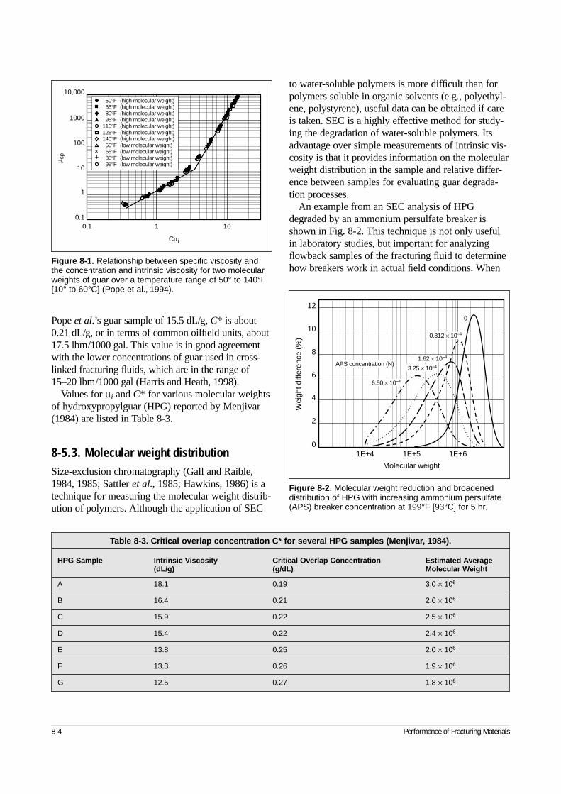
Pope et al.’s guar sample of 15.5 dL/g, C* is about0.21 dL/g, or in terms of common oilfield units, about17.5 lbm/1000 gal. This value is in good agreementwith the lower concentrations of guar used in cross-linked fracturing fluids, which are in the range of15–20 lbm/1000 gal (Harris and Heath, 1998).

Values for µi and C* for various molecular weightsof hydroxypropylguar (HPG) reported by Menjivar(1984) are listed in Table 8-3.

8-5.3. Molecular weight distributionSize-exclusion chromatography (Gall and Raible,1984, 1985; Sattler et al., 1985; Hawkins, 1986) is atechnique for measuring the molecular weight distrib-ution of polymers. Although the application of SEC

to water-soluble polymers is more difficult than forpolymers soluble in organic solvents (e.g., polyethyl-ene, polystyrene), useful data can be obtained if careis taken. SEC is a highly effective method for study-ing the degradation of water-soluble polymers. Itsadvantage over simple measurements of intrinsic vis-cosity is that it provides information on the molecularweight distribution in the sample and relative differ-ence between samples for evaluating guar degrada-tion processes.

An example from an SEC analysis of HPGdegraded by an ammonium persulfate breaker isshown in Fig. 8-2. This technique is not only usefulin laboratory studies, but important for analyzingflowback samples of the fracturing fluid to determinehow breakers work in actual field conditions. When

8-4 Performance of Fracturing Materials

Figure 8-1. Relationship between specific viscosity andthe concentration and intrinsic viscosity for two molecularweights of guar over a temperature range of 50° to 140°F[10° to 60°C] (Pope et al., 1994).

0.1 1 10

µ sp

Cµi

10,000

1000

100

10

1

0.1

+

+

+

+

+

+

+

+

+

++

++

+

50°F (high molecular weight)65°F (high molecular weight)80°F (high molecular weight)95°F (high molecular weight)

110°F (high molecular weight)125°F (high molecular weight)140°F (high molecular weight)50°F (low molecular weight)65°F (low molecular weight)80°F (low molecular weight)95°F (low molecular weight)

++

Figure 8-2. Molecular weight reduction and broadeneddistribution of HPG with increasing ammonium persulfate(APS) breaker concentration at 199°F [93°C] for 5 hr.

1E+4 1E+5 1E+6

Wei

ght d

iffer

ence

(%

)

Molecular weight

12

10

8

6

4

2

0

6.50 × 10–4

3.25 × 10–4

1.62 × 10–4

0.812 × 10–4

0

APS concentration (N)

Table 8-3. Critical overlap concentration C* for several HPG samples (Menjivar, 1984).

HPG Sample Intrinsic Viscosity Critical Overlap Concentration Estimated Average(dL/g) (g/dL) Molecular Weight

A 18.1 0.19 3.0 × 106

B 16.4 0.21 2.6 × 106

C 15.9 0.22 2.5 × 106

D 15.4 0.22 2.4 × 106

E 13.8 0.25 2.0 × 106

F 13.3 0.26 1.9 × 106

G 12.5 0.27 1.8 × 106

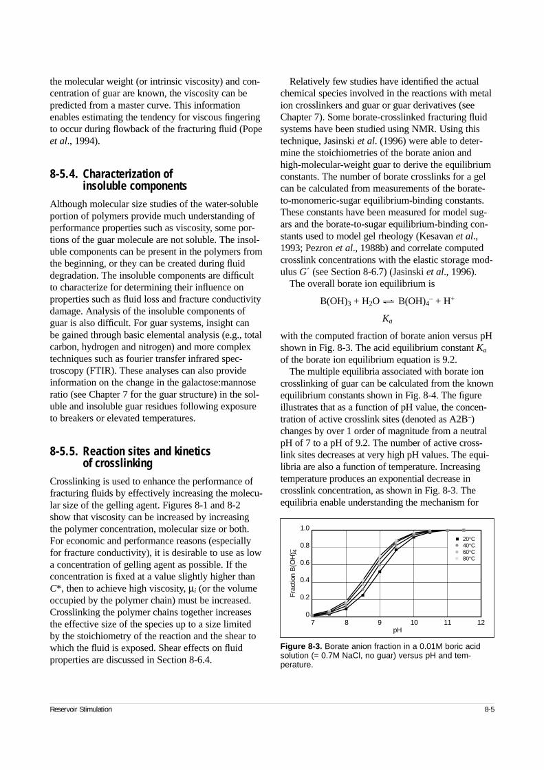
the molecular weight (or intrinsic viscosity) and con-centration of guar are known, the viscosity can bepredicted from a master curve. This informationenables estimating the tendency for viscous fingeringto occur during flowback of the fracturing fluid (Popeet al., 1994).

8-5.4. Characterization of insoluble components

Although molecular size studies of the water-solubleportion of polymers provide much understanding ofperformance properties such as viscosity, some por-tions of the guar molecule are not soluble. The insol-uble components can be present in the polymers fromthe beginning, or they can be created during fluiddegradation. The insoluble components are difficultto characterize for determining their influence onproperties such as fluid loss and fracture conductivitydamage. Analysis of the insoluble components ofguar is also difficult. For guar systems, insight can be gained through basic elemental analysis (e.g., totalcarbon, hydrogen and nitrogen) and more complextechniques such as fourier transfer infrared spec-troscopy (FTIR). These analyses can also provideinformation on the change in the galactose:mannoseratio (see Chapter 7 for the guar structure) in the sol-uble and insoluble guar residues following exposureto breakers or elevated temperatures.

8-5.5. Reaction sites and kinetics of crosslinking

Crosslinking is used to enhance the performance offracturing fluids by effectively increasing the molecu-lar size of the gelling agent. Figures 8-1 and 8-2show that viscosity can be increased by increasingthe polymer concentration, molecular size or both.For economic and performance reasons (especiallyfor fracture conductivity), it is desirable to use as lowa concentration of gelling agent as possible. If theconcentration is fixed at a value slightly higher thanC*, then to achieve high viscosity, µi (or the volumeoccupied by the polymer chain) must be increased.Crosslinking the polymer chains together increasesthe effective size of the species up to a size limited by the stoichiometry of the reaction and the shear towhich the fluid is exposed. Shear effects on fluidproperties are discussed in Section 8-6.4.

Relatively few studies have identified the actualchemical species involved in the reactions with metalion crosslinkers and guar or guar derivatives (seeChapter 7). Some borate-crosslinked fracturing fluidsystems have been studied using NMR. Using thistechnique, Jasinski et al. (1996) were able to deter-mine the stoichiometries of the borate anion andhigh-molecular-weight guar to derive the equilibriumconstants. The number of borate crosslinks for a gelcan be calculated from measurements of the borate-to-monomeric-sugar equilibrium-binding constants.These constants have been measured for model sug-ars and the borate-to-sugar equilibrium-binding con-stants used to model gel rheology (Kesavan et al.,1993; Pezron et al., 1988b) and correlate computedcrosslink concentrations with the elastic storage mod-ulus G´ (see Section 8-6.7) (Jasinski et al., 1996).

The overall borate ion equilibrium is

B(OH)3 + H2O B(OH)4– + H+

Ka

with the computed fraction of borate anion versus pHshown in Fig. 8-3. The acid equilibrium constant Ka

of the borate ion equilibrium equation is 9.2.The multiple equilibria associated with borate ion

crosslinking of guar can be calculated from the knownequilibrium constants shown in Fig. 8-4. The figureillustrates that as a function of pH value, the concen-tration of active crosslink sites (denoted as A2B–)changes by over 1 order of magnitude from a neutralpH of 7 to a pH of 9.2. The number of active cross-link sites decreases at very high pH values. The equi-libria are also a function of temperature. Increasingtemperature produces an exponential decrease incrosslink concentration, as shown in Fig. 8-3. Theequilibria enable understanding the mechanism for

Reservoir Stimulation 8-5

Figure 8-3. Borate anion fraction in a 0.01M boric acidsolution (= 0.7M NaCl, no guar) versus pH and tem-perature.

1.0

0.8

0.6

0.4

0.2

0

Fra

ctio

n B

(OH

)– 4

pH7 8 9 10 11 12

20°C40°C60°C80°C

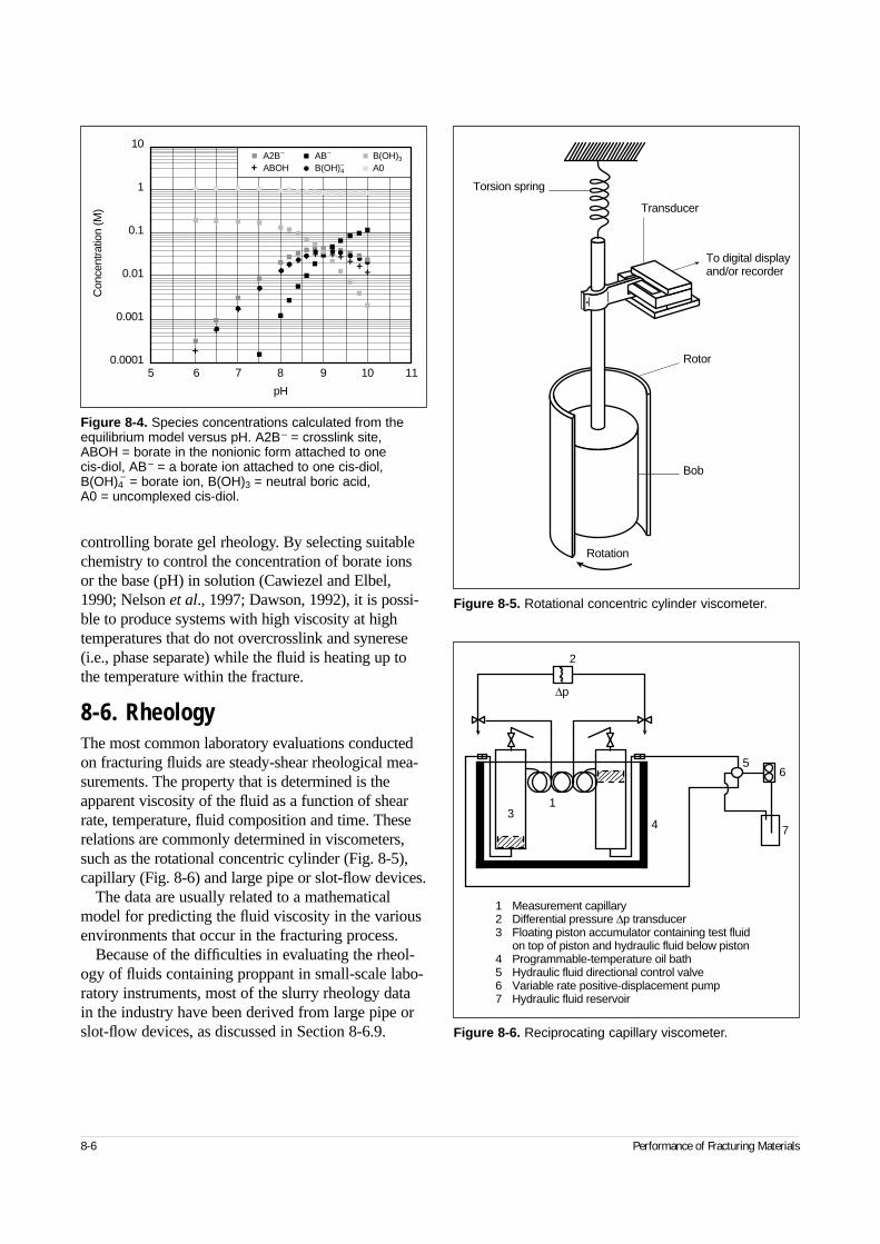
controlling borate gel rheology. By selecting suitablechemistry to control the concentration of borate ionsor the base (pH) in solution (Cawiezel and Elbel,1990; Nelson et al., 1997; Dawson, 1992), it is possi-ble to produce systems with high viscosity at hightemperatures that do not overcrosslink and synerese(i.e., phase separate) while the fluid is heating up tothe temperature within the fracture.

8-6. RheologyThe most common laboratory evaluations conductedon fracturing fluids are steady-shear rheological mea-surements. The property that is determined is theapparent viscosity of the fluid as a function of shearrate, temperature, fluid composition and time. Theserelations are commonly determined in viscometers,such as the rotational concentric cylinder (Fig. 8-5),capillary (Fig. 8-6) and large pipe or slot-flow devices.

The data are usually related to a mathematicalmodel for predicting the fluid viscosity in the variousenvironments that occur in the fracturing process.

Because of the difficulties in evaluating the rheol-ogy of fluids containing proppant in small-scale labo-ratory instruments, most of the slurry rheology datain the industry have been derived from large pipe orslot-flow devices, as discussed in Section 8-6.9.

8-6 Performance of Fracturing Materials

Figure 8-4. Species concentrations calculated from theequilibrium model versus pH. A2B– = crosslink site, ABOH = borate in the nonionic form attached to one cis-diol, AB– = a borate ion attached to one cis-diol,B(OH)4

– = borate ion, B(OH)3 = neutral boric acid, A0 = uncomplexed cis-diol.

+

+

+

+

+ + + ++ + + + + +

10

1

0.1

0.01

0.001

0.0001

Con

cent

ratio

n (M

)

pH

5 6 7 8 9 10 11

A2B– AB– B(OH)3

ABOH B(OH)–4 A0+

Figure 8-5. Rotational concentric cylinder viscometer.

Torsion spring

Transducer

To digital displayand/or recorder

Rotor

Bob

Rotation

Figure 8-6. Reciprocating capillary viscometer.

1

2

∆p

34

56

7

1 Measurement capillary2 Differential pressure ∆p transducer3 Floating piston accumulator containing test fluid

on top of piston and hydraulic fluid below piston4 Programmable-temperature oil bath5 Hydraulic fluid directional control valve6 Variable rate positive-displacement pump7 Hydraulic fluid reservoir

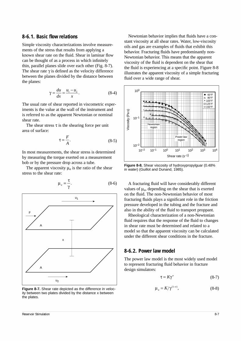
8-6.1. Basic flow relationsSimple viscosity characterizations involve measure-ments of the stress that results from applying aknown shear rate on the fluid. Shear in laminar flowcan be thought of as a process in which infinitelythin, parallel planes slide over each other (Fig. 8-7).The shear rate γ is defined as the velocity differencebetween the planes divided by the distance betweenthe planes:

(8-4)

The usual rate of shear reported in viscometric exper-iments is the value at the wall of the instrument andis referred to as the apparent Newtonian or nominalshear rate.

The shear stress τ is the shearing force per unitarea of surface:

(8-5)

In most measurements, the shear stress is determinedby measuring the torque exerted on a measurementbob or by the pressure drop across a tube.

The apparent viscosity µa is the ratio of the shearstress to the shear rate:

(8-6)

Newtonian behavior implies that fluids have a con-stant viscosity at all shear rates. Water, low-viscosityoils and gas are examples of fluids that exhibit thisbehavior. Fracturing fluids have predominantly non-Newtonian behavior. This means that the apparentviscosity of the fluid is dependent on the shear thatthe fluid is experiencing at a specific point. Figure 8-8illustrates the apparent viscosity of a simple fracturingfluid over a wide range of shear.

A fracturing fluid will have considerably differentvalues of µa, depending on the shear that is exertedon the fluid. The non-Newtonian behavior of mostfracturing fluids plays a significant role in the frictionpressure developed in the tubing and the fracture andalso in the ability of the fluid to transport proppant.

Rheological characterization of a non-Newtonianfluid requires that the response of the fluid to changesin shear rate must be determined and related to amodel so that the apparent viscosity can be calculatedunder the different shear conditions in the fracture.

8-6.2. Power law modelThe power law model is the most widely used modelto represent fracturing fluid behavior in fracturedesign simulators:

(8-7)

(8-8)

Reservoir Stimulation 8-7

Figure 8-7. Shear rate depicted as the difference in veloc-ity between two plates divided by the distance x betweenthe plates.

A

x

F

A

u1

u2

Figure 8-8. Shear viscosity of hydroxypropylguar (0.48%in water) (Guillot and Dunand, 1985).

100

10–1

10–2

10–2 10–1 100 101 102 103 104

Shear rate (s–1)

Vis

cosi

ty (P

a·s)

60°F80°F

100°F125°F150°F

Newtonianregion

Power lawregion

+

+

+

+

+

+

++

+

+ + + + + + + + + +++ +

γ = = −du

dx

u u

x1 2 .

τ = F

A.

µ τγa = .

τ γ= K n

µ γanK= −( )1 ,

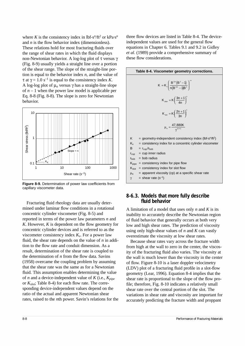
8-8 Performance of Fracturing Materials

where K is the consistency index in lbf-sn/ft2 or kPa·sn

and n is the flow behavior index (dimensionless).These relations hold for most fracturing fluids overthe range of shear rates in which the fluid displaysnon-Newtonian behavior. A log-log plot of τ versus γ(Fig. 8-9) usually yields a straight line over a portionof the shear range. The slope of the straight-line por-tion is equal to the behavior index n, and the value ofτ at γ = 1.0 s–1 is equal to the consistency index K.A log-log plot of µa versus γ has a straight-line slopeof n – 1 when the power law model is applicable perEq. 8-8 (Fig. 8-8). The slope is zero for Newtonianbehavior.

Fracturing fluid rheology data are usually deter-mined under laminar flow conditions in a rotationalconcentric cylinder viscometer (Fig. 8-5) andreported in terms of the power law parameters n andK. However, K is dependent on the flow geometry forconcentric cylinder devices and is referred to as theviscometer consistency index Kv. For a power lawfluid, the shear rate depends on the value of n in addi-tion to the flow rate and conduit dimension. As aresult, determination of the shear rate is coupled tothe determination of n from the flow data. Savins(1958) overcame the coupling problem by assumingthat the shear rate was the same as for a Newtonianfluid. This assumption enables determining the valueof n and a device-independent value of K (i.e., Kpipe

or Kslot; Table 8-4) for each flow rate. The corre-sponding device-independent values depend on theratio of the actual and apparent Newtonian shearrates, raised to the nth power. Savin’s relations for the

three flow devices are listed in Table 8-4. The device-independent values are used for the general flowequations in Chapter 6. Tables 9.1 and 9.2 in Gidleyet al. (1989) provide a comprehensive summary ofthese flow considerations.

8-6.3. Models that more fully describe fluid behavior

A limitation of a model that uses only n and K is itsinability to accurately describe the Newtonian regionof fluid behavior that generally occurs at both verylow and high shear rates. The prediction of viscosityusing only high-shear values of n and K can vastlyoverestimate the viscosity at low shear rates.

Because shear rates vary across the fracture widthfrom high at the wall to zero in the center, the viscos-ity of the fracturing fluid also varies. The viscosity atthe wall is much lower than the viscosity in the centerof flow. Figure 8-10 is a laser doppler velocimetry(LDV) plot of a fracturing fluid profile in a slot-flowgeometry (Lear, 1996). Equation 8-4 implies that theshear rate is proportional to the slope of the flow pro-file; therefore, Fig. 8-10 indicates a relatively smallshear rate over the central portion of the slot. Thevariations in shear rate and viscosity are important foraccurately predicting the fracture width and proppant

Figure 8-9. Determination of power law coefficients fromcapillary viscometer data.

Slope = n

Kv

1 10 100 1000

She

ar s

tress

(lbf

/ft2 )

Shear rate (s–1)

10

1

0.1

Table 8-4. Viscometer geometry corrections.

K = geometry-independent consistency index (lbf-sn/ft2)

Kv = consistency index for a concentric cylinder viscometer

B = rcup /rbob

rcup = cup inner radius

rbob = bob radius

Kpipe = consistency index for pipe flow

Kslot = consistency index for slot flow

µa = apparent viscosity (cp) at a specific shear rate

γ = shear rate (s–1)

K Kn

npipe

n

= +

3 14

K Kn

nslot

n

= +

2 13

µγa n

K= −( )47 880

1

,

K KB B

n B Bv

n

n

n

=−( )

−( )

−2 2

2 2

1

1

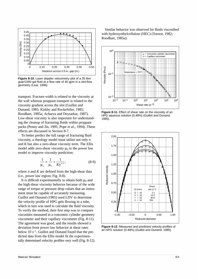
Reservoir Stimulation 8-9

transport. Fracture width is related to the viscosity atthe wall whereas proppant transport is related to theviscosity gradient across the slot (Guillot andDunand, 1985; Kirkby and Rockefeller, 1985;Roodhart, 1985a; Acharya and Deysarkar, 1987).Low-shear viscosity is also important for understand-ing the cleanup of fracturing fluids within proppantpacks (Penny and Jin, 1995; Pope et al., 1994). Theseeffects are discussed in Section 8-7.

To better predict the full range of fracturing fluidviscosity, a rheology model must utilize not only nand K but also a zero-shear viscosity term. The Ellismodel adds zero-shear viscosity µ0 to the power lawmodel to improve viscosity prediction:

(8-9)

where n and K are defined from the high-shear data(i.e., power law region; Fig. 8-8).

It is difficult experimentally to obtain both µ0 andthe high-shear viscosity behavior because of the widerange of torque or pressure drop values that an instru-ment must be capable of accurately measuring.Guillot and Dunand (1985) used LDV to determinethe velocity profile of HPG gels flowing in a tube,which in turn was used to calculate the fluid viscosity.To verify the method, their first step was to compareviscosities measured in a concentric cylinder geometryviscometer and their capillary viscometer (Fig. 8-11).The agreement was good, and the results showed adeviation from power law behavior at shear ratesbelow 10 s–1. Guillot and Dunand found that the pre-dicted data from the Ellis model fit the experimen-tally determined velocity profiles very well (Fig. 8-12).

Similar behavior was observed for fluids viscosifiedwith hydroxyethylcellulose (HEC) (Torrest, 1982;Roodhart, 1985a).

Figure 8-10. Laser doppler velocimetry plot of a 35 lbmguar/1000 gal fluid at a flow rate of 40 gpm in a slot-flowgeometry (Lear, 1996).

0 0.10 0.20 0.30 0.40 0.50

Vel

ocity

(ft/

s)

Distance across 0.5-in. gap (in.)

0.45

0.35

0.25

0.15

0.050.10

0.20

0.30

0.40

0

Figure 8-11. Effect of shear rate on the viscosity of anHPG aqueous solution (0.48%) (Guillot and Dunand,1985).

100

10–1

10–2

10–2 10–1 100 101 102 103 104

Shear rate (s–1)V

isco

sity

(Pa·

s)

= Concentric cylinder viscometer= Capillary viscometer

Temperature = 70°F

Figure 8-12. Measured and predicted velocity profiles ofan HPG solution (0.48%) (Guillot and Dunand, 1985).

+

+

+

+

++

+

+

+

+

+

++++++

+

+

+

+

++

+

+

+

+

2.00

1.75

1.50

1.25

1.00

0.75

0.50

0.25

0–1.00 –0.50 0 0.50 1.00

Reduced diameter

Red

uced

vel

ocity

ShearID (mm) rate (s–1)

+

= 10 2.1= 10 13.3= 10 80.6= 10 353

1 1 1

01µ µ γa

nK= + − ,

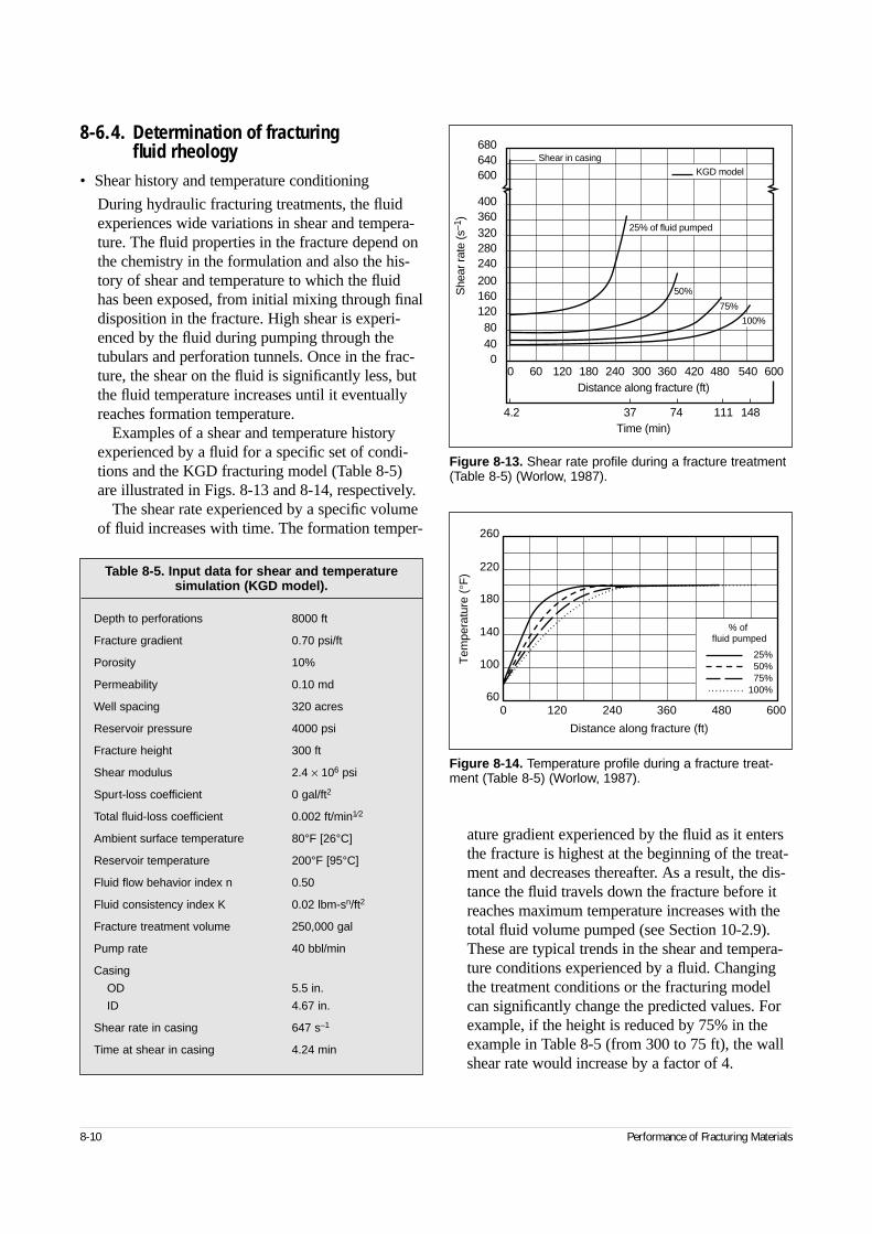
8-10 Performance of Fracturing Materials

8-6.4. Determination of fracturing fluid rheology

• Shear history and temperature conditioning

During hydraulic fracturing treatments, the fluidexperiences wide variations in shear and tempera-ture. The fluid properties in the fracture depend onthe chemistry in the formulation and also the his-tory of shear and temperature to which the fluidhas been exposed, from initial mixing through finaldisposition in the fracture. High shear is experi-enced by the fluid during pumping through thetubulars and perforation tunnels. Once in the frac-ture, the shear on the fluid is significantly less, butthe fluid temperature increases until it eventuallyreaches formation temperature.

Examples of a shear and temperature historyexperienced by a fluid for a specific set of condi-tions and the KGD fracturing model (Table 8-5)are illustrated in Figs. 8-13 and 8-14, respectively.

The shear rate experienced by a specific volumeof fluid increases with time. The formation temper-

ature gradient experienced by the fluid as it entersthe fracture is highest at the beginning of the treat-ment and decreases thereafter. As a result, the dis-tance the fluid travels down the fracture before itreaches maximum temperature increases with thetotal fluid volume pumped (see Section 10-2.9).These are typical trends in the shear and tempera-ture conditions experienced by a fluid. Changingthe treatment conditions or the fracturing modelcan significantly change the predicted values. Forexample, if the height is reduced by 75% in theexample in Table 8-5 (from 300 to 75 ft), the wallshear rate would increase by a factor of 4.

Table 8-5. Input data for shear and temperature simulation (KGD model).

Depth to perforations 8000 ft

Fracture gradient 0.70 psi/ft

Porosity 10%

Permeability 0.10 md

Well spacing 320 acres

Reservoir pressure 4000 psi

Fracture height 300 ft

Shear modulus 2.4 × 106 psi

Spurt-loss coefficient 0 gal/ft2

Total fluid-loss coefficient 0.002 ft/min1⁄2

Ambient surface temperature 80°F [26°C]

Reservoir temperature 200°F [95°C]

Fluid flow behavior index n 0.50

Fluid consistency index K 0.02 lbm-sn/ft2

Fracture treatment volume 250,000 gal

Pump rate 40 bbl/min

Casing

OD 5.5 in.

ID 4.67 in.

Shear rate in casing 647 s–1

Time at shear in casing 4.24 min

Figure 8-13. Shear rate profile during a fracture treatment(Table 8-5) (Worlow, 1987).

680640600

400360320280240

20016012080400

She

ar ra

te (s

–1)

0 60 120 180 240 300 360 420 480 540 600

4.2 37 74 111 148

Distance along fracture (ft)

Time (min)

100%

75%

50%

25% of fluid pumped

Shear in casing

KGD model

Figure 8-14. Temperature profile during a fracture treat-ment (Table 8-5) (Worlow, 1987).

0 120 240 360 480 600

Tem

pera

ture

(°F

)

Distance along fracture (ft)

260

100

140

180

220

60

25%50%75%

100%

% of fluid pumped

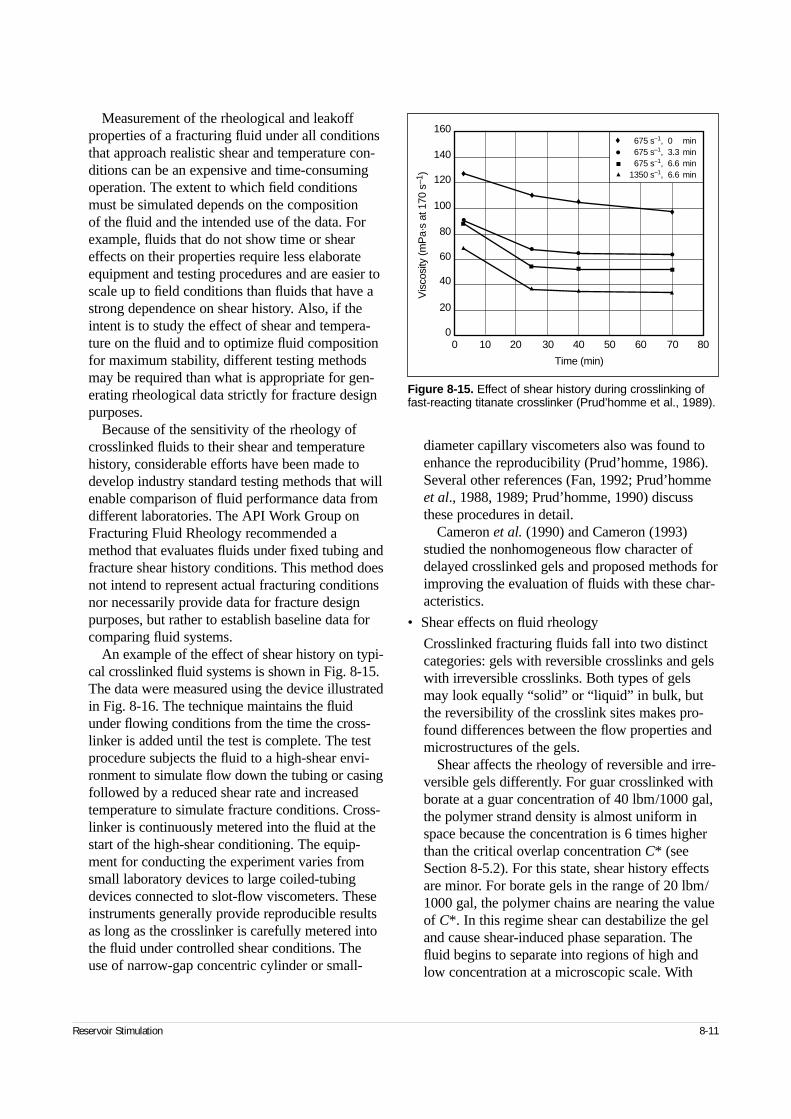
Measurement of the rheological and leakoffproperties of a fracturing fluid under all conditionsthat approach realistic shear and temperature con-ditions can be an expensive and time-consumingoperation. The extent to which field conditionsmust be simulated depends on the composition of the fluid and the intended use of the data. Forexample, fluids that do not show time or sheareffects on their properties require less elaborateequipment and testing procedures and are easier toscale up to field conditions than fluids that have astrong dependence on shear history. Also, if theintent is to study the effect of shear and tempera-ture on the fluid and to optimize fluid compositionfor maximum stability, different testing methodsmay be required than what is appropriate for gen-erating rheological data strictly for fracture designpurposes.

Because of the sensitivity of the rheology ofcrosslinked fluids to their shear and temperaturehistory, considerable efforts have been made todevelop industry standard testing methods that willenable comparison of fluid performance data fromdifferent laboratories. The API Work Group onFracturing Fluid Rheology recommended amethod that evaluates fluids under fixed tubing andfracture shear history conditions. This method doesnot intend to represent actual fracturing conditionsnor necessarily provide data for fracture designpurposes, but rather to establish baseline data forcomparing fluid systems.

An example of the effect of shear history on typi-cal crosslinked fluid systems is shown in Fig. 8-15.The data were measured using the device illustratedin Fig. 8-16. The technique maintains the fluidunder flowing conditions from the time the cross-linker is added until the test is complete. The testprocedure subjects the fluid to a high-shear envi-ronment to simulate flow down the tubing or casingfollowed by a reduced shear rate and increasedtemperature to simulate fracture conditions. Cross-linker is continuously metered into the fluid at thestart of the high-shear conditioning. The equip-ment for conducting the experiment varies fromsmall laboratory devices to large coiled-tubingdevices connected to slot-flow viscometers. Theseinstruments generally provide reproducible resultsas long as the crosslinker is carefully metered intothe fluid under controlled shear conditions. Theuse of narrow-gap concentric cylinder or small-

diameter capillary viscometers also was found toenhance the reproducibility (Prud’homme, 1986).Several other references (Fan, 1992; Prud’hommeet al., 1988, 1989; Prud’homme, 1990) discussthese procedures in detail.

Cameron et al. (1990) and Cameron (1993)studied the nonhomogeneous flow character ofdelayed crosslinked gels and proposed methods forimproving the evaluation of fluids with these char-acteristics.

• Shear effects on fluid rheology

Crosslinked fracturing fluids fall into two distinctcategories: gels with reversible crosslinks and gelswith irreversible crosslinks. Both types of gelsmay look equally “solid” or “liquid” in bulk, butthe reversibility of the crosslink sites makes pro-found differences between the flow properties andmicrostructures of the gels.

Shear affects the rheology of reversible and irre-versible gels differently. For guar crosslinked withborate at a guar concentration of 40 lbm/1000 gal,the polymer strand density is almost uniform inspace because the concentration is 6 times higherthan the critical overlap concentration C* (seeSection 8-5.2). For this state, shear history effectsare minor. For borate gels in the range of 20 lbm/1000 gal, the polymer chains are nearing the valueof C*. In this regime shear can destabilize the geland cause shear-induced phase separation. Thefluid begins to separate into regions of high andlow concentration at a microscopic scale. With

Reservoir Stimulation 8-11

Figure 8-15. Effect of shear history during crosslinking offast-reacting titanate crosslinker (Prud’homme et al., 1989).

0 10 20 30 40 50 60 70 80

Vis

cosi

ty (m

Pa·

s at

170

s–1

)

Time (min)

160

80

100

120

140

0

20

40

60

675 s–1, 0 min675 s–1, 3.3 min675 s–1, 6.6 min

1350 s–1, 6.6 min

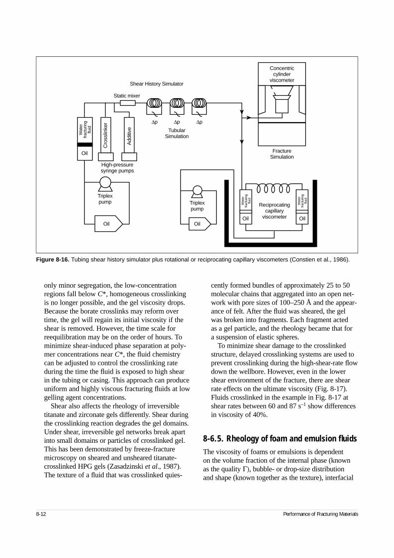
8-12 Performance of Fracturing Materials

only minor segregation, the low-concentrationregions fall below C*, homogeneous crosslinkingis no longer possible, and the gel viscosity drops.Because the borate crosslinks may reform overtime, the gel will regain its initial viscosity if theshear is removed. However, the time scale forreequilibration may be on the order of hours. Tominimize shear-induced phase separation at poly-mer concentrations near C*, the fluid chemistrycan be adjusted to control the crosslinking rateduring the time the fluid is exposed to high shearin the tubing or casing. This approach can produceuniform and highly viscous fracturing fluids at lowgelling agent concentrations.

Shear also affects the rheology of irreversibletitanate and zirconate gels differently. Shear duringthe crosslinking reaction degrades the gel domains.Under shear, irreversible gel networks break apartinto small domains or particles of crosslinked gel.This has been demonstrated by freeze-fracturemicroscopy on sheared and unsheared titanate-crosslinked HPG gels (Zasadzinski et al., 1987).The texture of a fluid that was crosslinked quies-

cently formed bundles of approximately 25 to 50molecular chains that aggregated into an open net-work with pore sizes of 100–250 Å and the appear-ance of felt. After the fluid was sheared, the gelwas broken into fragments. Each fragment acted as a gel particle, and the rheology became that for a suspension of elastic spheres.

To minimize shear damage to the crosslinkedstructure, delayed crosslinking systems are used toprevent crosslinking during the high-shear-rate flowdown the wellbore. However, even in the lowershear environment of the fracture, there are shearrate effects on the ultimate viscosity (Fig. 8-17).Fluids crosslinked in the example in Fig. 8-17 atshear rates between 60 and 87 s–1 show differencesin viscosity of 40%.

8-6.5. Rheology of foam and emulsion fluidsThe viscosity of foams or emulsions is dependent on the volume fraction of the internal phase (knownas the quality Γ), bubble- or drop-size distribution and shape (known together as the texture), interfacial

Figure 8-16. Tubing shear history simulator plus rotational or reciprocating capillary viscometers (Constien et al., 1986).

Triplexpump

Oil

Triplexpump

High-pressuresyringe pumps

Cro

sslin

ker

Add

itive

OilOil

Reciprocatingcapillary

viscometer

FractureSimulation

TubularSimulation

Shear History Simulator

Static mixer

∆p∆p ∆p

Concentriccylinder

viscometer

Oil

Wat

erfra

ctur

ing

fluid

Oil

Wat

erfra

ctur

ing

fluid

Wat

erfra

ctur

ing

fluid

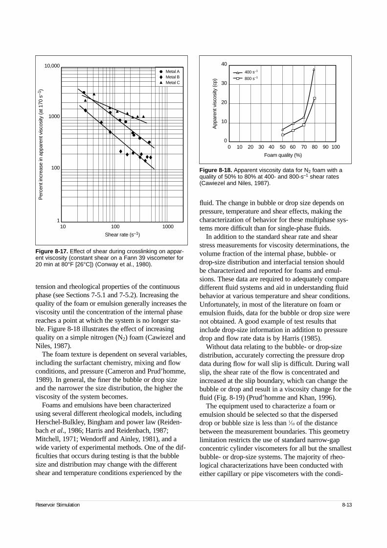
Reservoir Stimulation 8-13

tension and rheological properties of the continuousphase (see Sections 7-5.1 and 7-5.2). Increasing thequality of the foam or emulsion generally increases theviscosity until the concentration of the internal phasereaches a point at which the system is no longer sta-ble. Figure 8-18 illustrates the effect of increasingquality on a simple nitrogen (N2) foam (Cawiezel andNiles, 1987).

The foam texture is dependent on several variables,including the surfactant chemistry, mixing and flowconditions, and pressure (Cameron and Prud’homme,1989). In general, the finer the bubble or drop sizeand the narrower the size distribution, the higher theviscosity of the system becomes.

Foams and emulsions have been characterizedusing several different rheological models, includingHerschel-Bulkley, Bingham and power law (Reiden-bach et al., 1986; Harris and Reidenbach, 1987;Mitchell, 1971; Wendorff and Ainley, 1981), and awide variety of experimental methods. One of the dif-ficulties that occurs during testing is that the bubblesize and distribution may change with the differentshear and temperature conditions experienced by the

fluid. The change in bubble or drop size depends onpressure, temperature and shear effects, making thecharacterization of behavior for these multiphase sys-tems more difficult than for single-phase fluids.

In addition to the standard shear rate and shearstress measurements for viscosity determinations, thevolume fraction of the internal phase, bubble- ordrop-size distribution and interfacial tension shouldbe characterized and reported for foams and emul-sions. These data are required to adequately comparedifferent fluid systems and aid in understanding fluidbehavior at various temperature and shear conditions.Unfortunately, in most of the literature on foam oremulsion fluids, data for the bubble or drop size werenot obtained. A good example of test results thatinclude drop-size information in addition to pressuredrop and flow rate data is by Harris (1985).

Without data relating to the bubble- or drop-sizedistribution, accurately correcting the pressure dropdata during flow for wall slip is difficult. During wallslip, the shear rate of the flow is concentrated andincreased at the slip boundary, which can change thebubble or drop and result in a viscosity change for thefluid (Fig. 8-19) (Prud’homme and Khan, 1996).

The equipment used to characterize a foam oremulsion should be selected so that the disperseddrop or bubble size is less than 1⁄10 of the distancebetween the measurement boundaries. This geometrylimitation restricts the use of standard narrow-gapconcentric cylinder viscometers for all but the smallestbubble- or drop-size systems. The majority of rheo-logical characterizations have been conducted witheither capillary or pipe viscometers with the condi-

Figure 8-17. Effect of shear during crosslinking on appar-ent viscosity (constant shear on a Fann 39 viscometer for20 min at 80°F [26°C]) (Conway et al., 1980).

10 100 1000

Per

cent

incr

ease

in a

ppar

ent v

isco

sity

(at 1

70 s

–1)

Shear rate (s–1)

10,000

1000

100

1

Metal AMetal BMetal C

Figure 8-18. Apparent viscosity data for N2 foam with aquality of 50% to 80% at 400- and 800-s–1 shear rates(Cawiezel and Niles, 1987).

40

30

20

10

00 10 20 30 40 50 60 70 80 90 100

Foam quality (%)

App

aren

t vis

cosi

ty (c

p)

400 s–1

800 s–1

8-14 Performance of Fracturing Materials

tions made to match the actual fracturing treatmentconditions of shear, temperature and pressure asclosely as possible. The viscometers are high-pres-sure circulating systems (Reidenbach et al., 1986;Harris and Heath, 1996) or single-pass pipe viscome-ters (Harris, 1985; Cawiezel and Niles, 1987; Harriset al., 1995).

One of the more extensive studies of N2 andcarbon dioxide (CO2) foams was conducted byReidenbach et al. (1986). A model for calculatingrheological properties based on the foam quality Γ,yield point τyp, and n and K for the liquid phase wasproposed. The basic equation is

(8-10)

where τyp is related to the foam quality and gas com-position, Dp and L are the pipe diameter and length,respectively, and ∆p is the pressure drop. The consis-tency coefficient Kfoam was found to be dependent onthe liquid-phase consistency coefficient K and quality:

(8-11)

where the constant C1 varies with the external phase.Typical values for τyp, C1 and K are listed for N2 andCO2 foams in Tables 8-6 and 8-7, respectively.

One of the difficulties that typically occurs in relat-ing laboratory-generated data on foams to field-scaletubing is the effect of the pipe diameter on the result-ing stress, which may result from texture differencesnear the pipe wall. Winkler et al. (1994) proposedusing a volume-equalized power law (VEPL) modelas a constitutive flow behavior equation to provide a

geometry-independent approach for the prediction offoam properties in pipes at different conditions:

(8-12)

where the specific volume expansion ratio εS isdefined as the ratio of the specific volume of thefoam v̂ to the specific volume of the base liquid v̂l andis also equal to the ratio of the liquid density ρl to thefoam density ρ. In terms of the VEPL model, theeffective viscosity is (Enzendorfer et al., 1995)

(8-13)

Foams with qualities from 30% to 75% were gen-erated in a 40-ppg HPG solution and the pressure wasmeasured in a series of pipe diameters. Figure 8-20illustrates the shear stress versus volume-equalizedshear rate for these foams pumped through four dif-ferent pipe diameters.

Figure 8-19. Flow of foam in a tube. The foam slips at thewall and is in plug flow at the center of the tube, where the shear stress is below the yield stress of the foam τo.r = tube radius.

r

τo

∆pD

LK

v

Dp

yp foam

p

n

48= +

τ ,

K Kefoam

C= +( )120 75Γ Γ.

,

ε ρρS

l

lv

v= =

ˆˆ

,

µ εeff Sn n n

n

K u Dn

n= +

− − −1 1 1 18

6 2.

Table 8-6. Parameters for N2 foams(Reidenbach et al., 1986).

Foam Quality (%) True Yield Point (lbf/ft2)

Γ ≤ 0.6 0.07Γ

Γ > 0.6 0.0002e9Γ

True Foam Consistency Index (lbf-sn/ft2)

External Phase K C1 n

Water 0.00002 3.6 1.0

10 lbm HPG/1000 gal 0.00053 2.1 0.75

20 lbm HPG/1000 gal 0.00256 1.7 0.607

40 lbm HPG/1000 gal 0.0152 1.2 0.45

Table 8-7. Parameters for CO2 foams(Reidenbach et al., 1986).

Foam Quality (%) True Yield Point (lbf/ft2)

Γ ≤ 0.6 0.042Γ

Γ > 0.6 0.00012e8.9Γ

True Foam Consistency Index (lbf-sn/ft2)

External Phase K C1 n

Water 0.00002 4.0 1.0

10 lbm HPG/1000 gal 0.00053 2.6 0.75

20 lbm HPG/1000 gal 0.00256 2.2 0.607

40 lbm HPG/1000 gal 0.0152 1.0 0.45

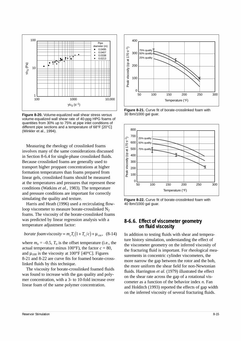
Reservoir Stimulation 8-15

Measuring the rheology of crosslinked foamsinvolves many of the same considerations discussedin Section 8-6.4 for single-phase crosslinked fluids.Because crosslinked foams are generally used totransport higher proppant concentrations at higherformation temperatures than foams prepared fromlinear gels, crosslinked foams should be measured at the temperatures and pressures that represent theseconditions (Watkins et al., 1983). The temperatureand pressure conditions are important for correctlysimulating the quality and texture.

Harris and Heath (1996) used a recirculating flow-loop viscometer to measure borate-crosslinked N2

foams. The viscosity of the borate-crosslinked foamswas predicted by linear regression analysis with atemperature adjustment factor:

(8-14)

where mo = –0.5, To is the offset temperature (i.e., theactual temperature minus 100°F), the factor c = 80,and µ100 is the viscosity at 100°F [40°C]. Figures 8-21 and 8-22 are curve fits for foamed borate-cross-linked fluids by this technique.

The viscosity for borate-crosslinked foamed fluidswas found to increase with the gas quality and poly-mer concentration, with a 3- to 10-fold increase overlinear foam of the same polymer concentration.

8-6.6. Effect of viscometer geometry on fluid viscosity

In addition to testing fluids with shear and tempera-ture history simulation, understanding the effect ofthe viscometer geometry on the inferred viscosity ofthe fracturing fluid is important. For rheological mea-surements in concentric cylinder viscometers, themore narrow the gap between the rotor and the bob,the more uniform the shear field for non-Newtonianfluids. Harrington et al. (1979) illustrated the effecton the shear rate across the gap of a rotational vis-cometer as a function of the behavior index n. Fanand Holditch (1993) reported the effects of gap widthon the inferred viscosity of several fracturing fluids.

Figure 8-20. Volume-equalized wall shear stress versusvolume-equalized wall shear rate of 40-ppg HPG foams ofquantities from 30% up to 75% at pipe inlet conditions ofdifferent pipe sections and a temperature of 68°F [20°C](Winkler et al., 1994).

100 1000 10,000

τ/ε S

(Pa)

γ/εS (s–1)

100

10

1

0.04950.04070.03380.0213

Pipediameter (m)

Figure 8-21. Curve fit of borate-crosslinked foam with 30 lbm/1000 gal guar.

400

300

200

100

050 100 150 200 250 300

Temperature (°F)

Pea

k vi

scos

ity (c

p at

170

s–1

)

75% quality50% quality

25% quality

Figure 8-22. Curve fit of borate-crosslinked foam with 40 lbm/1000 gal guar.

800

700

600

500

400

300

200

100

050 100 150 200 250 300

Temperature (°F)

Pea

k vi

scos

ity (c

p at

170

s–1

) 25% quality

50% quality

75% quality

borate foam viscosity m T T co o o= +( ) +1 100µ ,

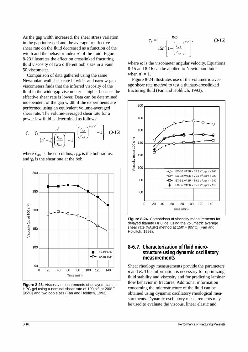
8-16 Performance of Fracturing Materials

As the gap width increased, the shear stress variationin the gap increased and the average or effectiveshear rate on the fluid decreased as a function of thewidth and the behavior index n´ of the fluid. Figure8-23 illustrates the effect on crosslinked fracturingfluid viscosity of two different bob sizes in a Fann 50 viscometer.

Comparison of data gathered using the sameNewtonian wall shear rate in wide- and narrow-gapviscometers finds that the inferred viscosity of thefluid in the wide-gap viscometer is higher because theeffective shear rate is lower. Data can be determinedindependent of the gap width if the experiments areperformed using an equivalent volume-averagedshear rate. The volume-averaged shear rate for apower law fluid is determined as follows:

(8-15)

where rcup is the cup radius, rbob is the bob radius,and γb is the shear rate at the bob:

(8-16)

where ω is the viscometer angular velocity. Equations8-15 and 8-16 can be applied to Newtonian fluidswhen n´ = 1.

Figure 8-24 illustrates use of the volumetric aver-age shear rate method to test a titanate-crosslinkedfracturing fluid (Fan and Holditch, 1993).

8-6.7. Characterization of fluid micro-structure using dynamic oscillatory measurements

Shear rheology measurements provide the parametersn and K. This information is necessary for optimizingfluid stability and viscosity and for predicting laminarflow behavior in fractures. Additional informationconcerning the microstructure of the fluid can beobtained using dynamic oscillatory rheological mea-surements. Dynamic oscillatory measurements maybe used to evaluate the viscous, linear elastic and

γ γv b

cup

bob

cup

bob

n

n

nr

r

r

r= ′

′ −( )

−

−

− ′

1 1

12

2 2

,

γ πωb

bob

cup

n

nrr

=

′ −

′

15 1

2,

Figure 8-23. Viscosity measurements of delayed titanateHPG gel using a nominal shear rate of 100 s–1 at 200°F[95°C] and two bob sizes (Fan and Holditch, 1993).

300

250

200

150

100

500 20 40 60 80 100 120 140

Time (min)

Vis

cosi

ty (c

p at

100

s–1

)

EX-B2 bob

EX-B5 bob

Figure 8-24. Comparison of viscosity measurements fordelayed titanate HPG gel using the volumetric averageshear rate (VASR) method at 150°F [65°C] (Fan andHolditch, 1993).

200

180

160

140

120

100

80

60

0 20 40 60 80 100 120 140

Time (min)

Vis

cosi

ty (c

p at

100

s–1

)

EX-B2: VASR = 59.3 s–1, rpm = 265

EX-B2: VASR = 71.6 s–1, rpm = 323

EX-B2: VASR = 85.1 s–1, rpm = 380

EX-B5: VASR = 85.6 s–1, rpm = 118

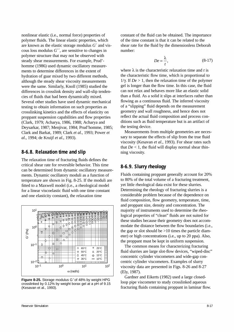
Reservoir Stimulation 8-17

nonlinear elastic (i.e., normal force) properties ofpolymer fluids. The linear elastic properties, whichare known as the elastic storage modulus G´ and vis-cous loss modulus G´´, are sensitive to changes inpolymer structure that may not be observed withsteady shear measurements. For example, Prud’-homme (1986) used dynamic oscillatory measure-ments to determine differences in the extent ofhydration of guar mixed by two different methods,although the steady shear viscosity measurementswere the same. Similarly, Knoll (1985) studied thedifferences in crosslink density and wall-slip tenden-cies of fluids that had been dynamically mixed.Several other studies have used dynamic mechanicaltesting to obtain information on such properties ascrosslinking kinetics and the effects of elasticity onproppant suspension capabilities and flow properties(Clark, 1979; Acharya, 1986, 1988; Acharya andDeysarkar, 1987; Menjivar, 1984; Prud’homme, 1985;Clark and Barkat, 1989; Clark et al., 1993; Power etal., 1994; de Kruijf et al., 1993).

8-6.8. Relaxation time and slipThe relaxation time of fracturing fluids defines thecritical shear rate for reversible behavior. This timecan be determined from dynamic oscillatory measure-ments. Dynamic oscillatory moduli as a function oftemperature are shown in Fig. 8-25. If the moduli arefitted to a Maxwell model (i.e., a rheological modelfor a linear viscoelastic fluid with one time constantand one elasticity constant), the relaxation time

constant of the fluid can be obtained. The importanceof the time constant is that it can be related to theshear rate for the fluid by the dimensionless Deborahnumber:

(8-17)

where λ is the characteristic relaxation time and t isthe characteristic flow time, which is proportional to1/γ. If De > 1, then the relaxation time of the polymergel is longer than the flow time. In this case, the fluidcan not relax and behaves more like an elastic solidthan a fluid. As a solid it slips at interfaces rather thanflowing as a continuous fluid. The inferred viscosityof a “slipping” fluid depends on the measurementgeometry and wall roughness, and hence does notreflect the actual fluid composition and process con-ditions such as fluid temperature but is an artifact ofthe testing device.

Measurements from multiple geometries are neces-sary to separate the effects of slip from the true fluidviscosity (Kesavan et al., 1993). For shear rates suchthat De < 1, the fluid will display normal shear thin-ning viscosity.

8-6.9. Slurry rheologyFluids containing proppant generally account for 20%to 80% of the total volume of a fracturing treatment,yet little rheological data exist for these slurries.Determining the rheology of fracturing slurries is aconsiderable problem because of the dependence onfluid composition, flow geometry, temperature, time,and proppant size, density and concentration. Themajority of instruments used to determine the rheo-logical properties of “clean” fluids are not suited forthese studies because their geometry does not accom-modate the distance between the flow boundaries (i.e.,the gap or slot should be >10 times the particle diam-eter) or high concentrations (i.e., up to 20 ppa). Also,the proppant must be kept in uniform suspension.

The common means for characterizing fracturingfluid slurries are large slot-flow devices, “wiped-disc”concentric cylinder viscometers and wide-gap con-centric cylinder viscometers. Examples of slurryviscosity data are presented in Figs. 8-26 and 8-27(Ely, 1987).

Gardner and Eikerts (1982) used a large closed-loop pipe viscometer to study crosslinked aqueousfracturing fluids containing proppant in laminar flow.

Det

= λ,

Figure 8-25. Storage modulus G′ of 48% by weight HPGcrosslinked by 0.12% by weight borax gel at a pH of 9.15(Kesavan et al., 1993).

101

100

10–1

10–2

10–1 100 101 102

ω (rad/s)

G′ (

Pa)

++++ + + + + + + + + + + + + + + + + + + +

65°C 25°C55°C 20°C45°C 15°C35°C 10°C

+

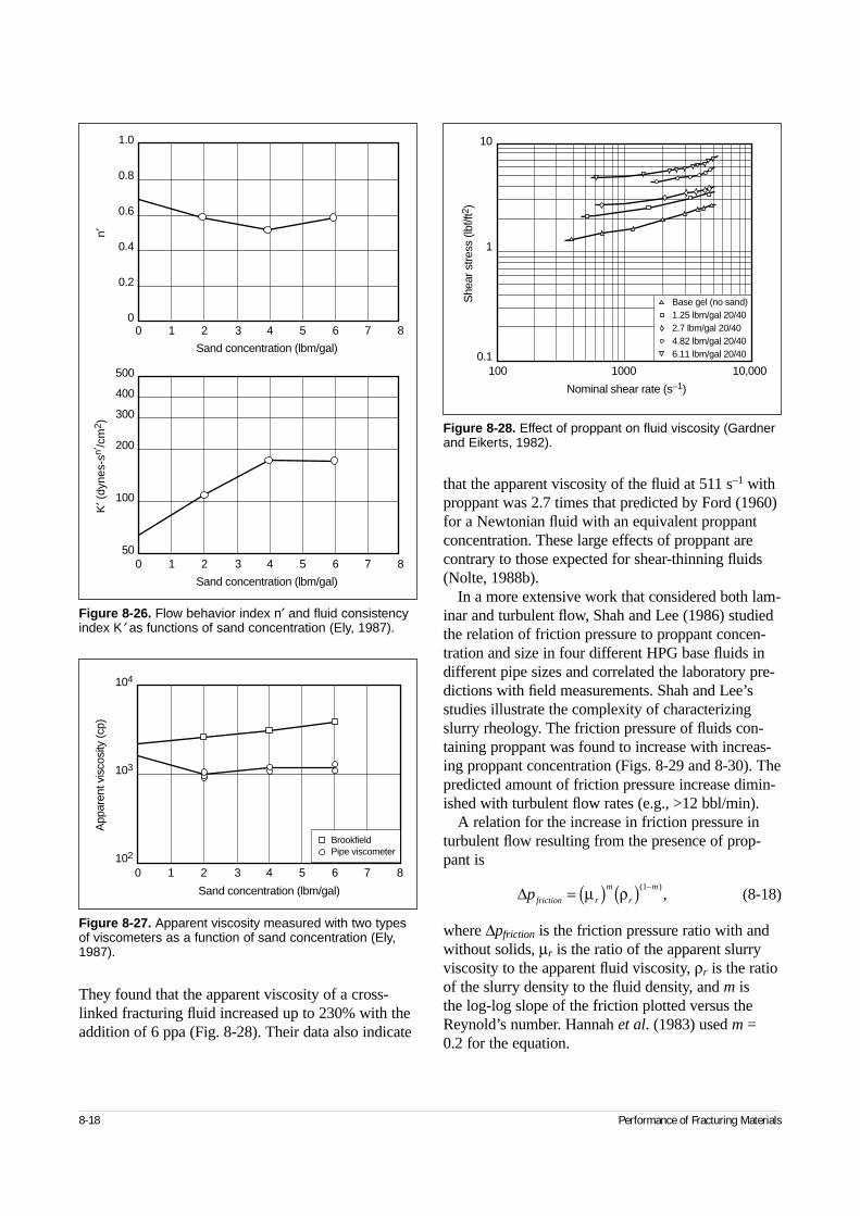
8-18 Performance of Fracturing Materials

They found that the apparent viscosity of a cross-linked fracturing fluid increased up to 230% with theaddition of 6 ppa (Fig. 8-28). Their data also indicate

that the apparent viscosity of the fluid at 511 s–1 withproppant was 2.7 times that predicted by Ford (1960)for a Newtonian fluid with an equivalent proppantconcentration. These large effects of proppant arecontrary to those expected for shear-thinning fluids(Nolte, 1988b).

In a more extensive work that considered both lam-inar and turbulent flow, Shah and Lee (1986) studiedthe relation of friction pressure to proppant concen-tration and size in four different HPG base fluids indifferent pipe sizes and correlated the laboratory pre-dictions with field measurements. Shah and Lee’sstudies illustrate the complexity of characterizingslurry rheology. The friction pressure of fluids con-taining proppant was found to increase with increas-ing proppant concentration (Figs. 8-29 and 8-30). Thepredicted amount of friction pressure increase dimin-ished with turbulent flow rates (e.g., >12 bbl/min).

A relation for the increase in friction pressure inturbulent flow resulting from the presence of prop-pant is

(8-18)

where ∆pfriction is the friction pressure ratio with andwithout solids, µr is the ratio of the apparent slurryviscosity to the apparent fluid viscosity, ρr is the ratioof the slurry density to the fluid density, and m isthe log-log slope of the friction plotted versus theReynold’s number. Hannah et al. (1983) used m =0.2 for the equation.

Figure 8-26. Flow behavior index n′ and fluid consistencyindex K′ as functions of sand concentration (Ely, 1987).

1.0

0.8

0.6

0.4

0.2

00 1 2 3 4 5 6 7 8

Sand concentration (lbm/gal)

n′

500

400

300

200

100

500 1 2 3 4 5 6 7 8

Sand concentration (lbm/gal)

K′ (

dyne

s-sn

′ /cm

2 ) Figure 8-28. Effect of proppant on fluid viscosity (Gardnerand Eikerts, 1982).

10

1

0.1100 1000 10,000

Nominal shear rate (s–1)

She

ar s

tress

(lbf

/ft2 )

Base gel (no sand)1.25 lbm/gal 20/402.7 lbm/gal 20/404.82 lbm/gal 20/406.11 lbm/gal 20/40

Figure 8-27. Apparent viscosity measured with two typesof viscometers as a function of sand concentration (Ely,1987).

104

103

102

0 1 2 3 4 5 6 7 8

Sand concentration (lbm/gal)

App

aren

t vis

cosi

ty (c

p)

BrookfieldPipe viscometer

∆pfriction r

m

r

m= ( ) ( )µ ρ ( – ),

1

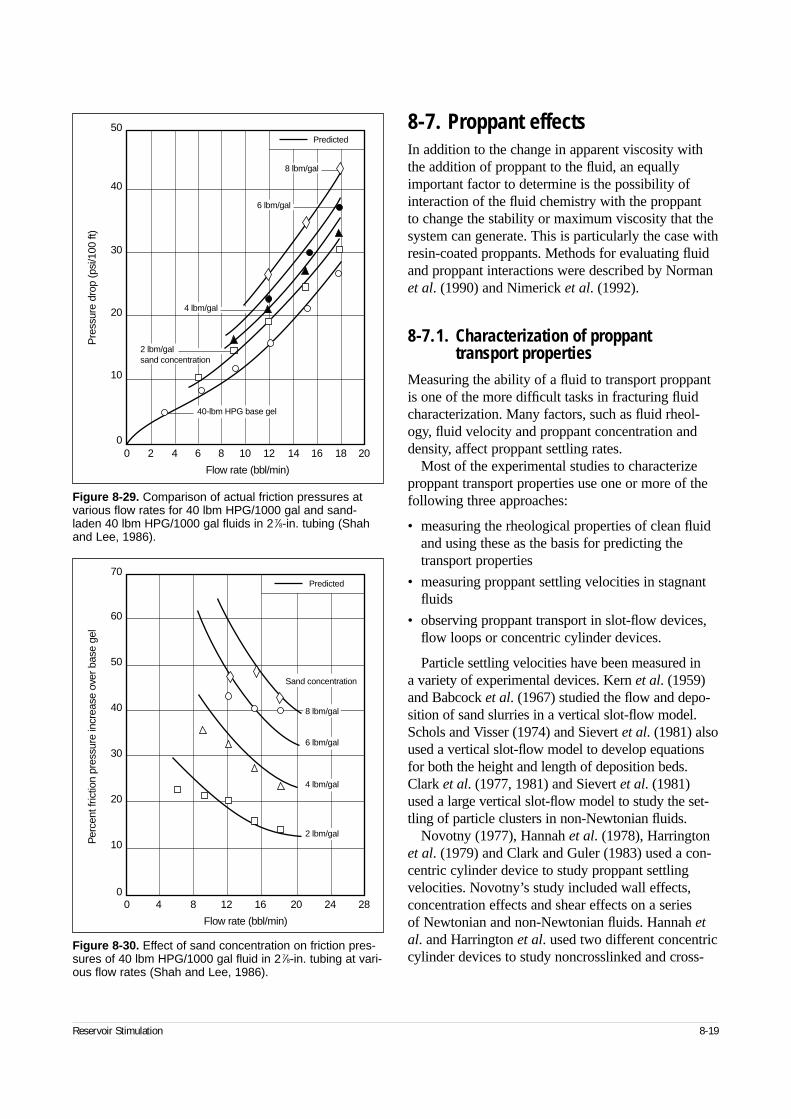
Reservoir Stimulation 8-19

8-7. Proppant effectsIn addition to the change in apparent viscosity withthe addition of proppant to the fluid, an equallyimportant factor to determine is the possibility ofinteraction of the fluid chemistry with the proppant to change the stability or maximum viscosity that thesystem can generate. This is particularly the case withresin-coated proppants. Methods for evaluating fluidand proppant interactions were described by Normanet al. (1990) and Nimerick et al. (1992).

8-7.1. Characterization of proppant transport properties

Measuring the ability of a fluid to transport proppantis one of the more difficult tasks in fracturing fluidcharacterization. Many factors, such as fluid rheol-ogy, fluid velocity and proppant concentration anddensity, affect proppant settling rates.

Most of the experimental studies to characterizeproppant transport properties use one or more of thefollowing three approaches:

• measuring the rheological properties of clean fluidand using these as the basis for predicting thetransport properties

• measuring proppant settling velocities in stagnantfluids

• observing proppant transport in slot-flow devices,flow loops or concentric cylinder devices.

Particle settling velocities have been measured in a variety of experimental devices. Kern et al. (1959)and Babcock et al. (1967) studied the flow and depo-sition of sand slurries in a vertical slot-flow model.Schols and Visser (1974) and Sievert et al. (1981) alsoused a vertical slot-flow model to develop equationsfor both the height and length of deposition beds.Clark et al. (1977, 1981) and Sievert et al. (1981)used a large vertical slot-flow model to study the set-tling of particle clusters in non-Newtonian fluids.

Novotny (1977), Hannah et al. (1978), Harringtonet al. (1979) and Clark and Guler (1983) used a con-centric cylinder device to study proppant settlingvelocities. Novotny’s study included wall effects,concentration effects and shear effects on a series of Newtonian and non-Newtonian fluids. Hannah etal. and Harrington et al. used two different concentriccylinder devices to study noncrosslinked and cross-

Figure 8-29. Comparison of actual friction pressures atvarious flow rates for 40 lbm HPG/1000 gal and sand-laden 40 lbm HPG/1000 gal fluids in 2 7⁄8-in. tubing (Shahand Lee, 1986).

50

40

30

20

10

00 2 4 6 8 10 12 14 16 18 20

Flow rate (bbl/min)

Pre

ssur

e dr

op (p

si/1

00 ft

)

Predicted

8 lbm/gal

6 lbm/gal

4 lbm/gal

2 lbm/galsand concentration

40-lbm HPG base gel

Figure 8-30. Effect of sand concentration on friction pres-sures of 40 lbm HPG/1000 gal fluid in 2 7⁄8-in. tubing at vari-ous flow rates (Shah and Lee, 1986).

70

60

50

40

30

20

10

00 4 8 12 16 20 24 28

Flow rate (bbl/min)

Per

cent

fric

tion

pres

sure

incr

ease

ove

r bas

e ge

l

Predicted

2 lbm/gal

4 lbm/gal

6 lbm/gal

8 lbm/gal

Sand concentration

8-20 Performance of Fracturing Materials

linked fluids. The results of both studies indicate thatthe settling of particles in the fluids deviated fromStokes law settling velocities. Clark et al. (1981) andQuadir (1981) reported results from a study usingboth a parallel-plate device and a concentric cylinderdevice. They also reported significant deviations fromStokes law settling velocities.

Flow loops with particles suspended in a verticalsection were used by Shah (1986).

More recently, proppant transport has been evalu-ated in large slot-flow devices at commercial testinglaboratories (Barree and Conway, 1994; Zhao et al.,1995) and universities (Clark and Zhu, 1995a; Shahand Subramanian, 1997; Goel et al., 1997; Hejjo etal., 1997; Shah et al., 1998; Shah and Asadi, 1998).The transport efficiency in these tests is usually deter-mined by visual observation of proppant fall, andcomparisons are made to the performance of otherfracturing fluids under similar test conditions.

When the results of the experimental measure-ments are translated to predictive models, Stokes set-tling law for a Newtonian fluid (see Eq. 6-106) ismost frequently used as an initial frame of reference.

Most fracturing fluids are non-Newtonian, withfluid viscosity decreasing as shear increases. Novotny(1977) determined that the most important variablesaffecting proppant settling are the non-Newtoniancharacteristics of the fluid, wall effects and proppantconcentration. For a non-Newtonian transportingfluid, Novotny found that the shear rate within a fluidhad a significant effect caused by its reduction in theapparent viscosity affecting particle settling.

A modified version of Stokes law for the terminalsettling velocity ut of a single particle in a quiescentpower law fluid is

(8-19)

where ρp and ρf are the densities of the particle andthe fluid, respectively, g is the gravitational accelera-tion, and dprop is the particle diameter. This equationand other forms of Stokes equations in this sectionassume that the particle Reynold’s numbers are lessthan 2.

With Eq. 8-19, the particle settling velocity becomesa function of the fluid parameters n and K. The set-tling velocity in power law fluids is proportional to

(8-20)

For Newtonian fluids, the relation is

(8-21)

Equation 8-19 can be used to determine only single-particle fall rates over shear ranges in which the fluidfollows power law behavior. As shear rates approachvery low or very high values, limiting values of theapparent viscosity are reached. In actual treatments,values of high-shear-limiting viscosity µ∞ are notapproached in the fracture. However, at the center ofthe fracture channel the shear rate is zero and thefluid viscosity approaches the value for zero-shearviscosity µ0 (Fig. 8-10). Roodhart (1985b) and otherinvestigators determined that low-shear viscosityplays a considerable role in proppant transport duringflow conditions (Kirkby and Rockefeller, 1985). Tocorrect the limitation of the power law model todescribe flow fields where the shear rates approachzero, Slattery and Bird (1961), Turian (1967),Dunand et al. (1984) and Roodhart (1985b) studiedthe Ellis fluid model, which incorporates a µ0 term(Eq. 8-9).

Combining Eq. 8-9 with Stokes law leads to a set-tling velocity equation of the form

(8-22)

where ∆ρ = ρp – ρf and the shear rate induced by par-ticle settling is assumed to be (Novotny, 1977)

(8-23)

(versus 3 times this value in Eq. 8-19).Roodhart (1985b) tested the validity of Eqs. 8-9 and

8-22 under static and flowing conditions. He foundexcellent correlation with experimental data for theapparent viscosity versus shear rate (Fig. 8-31) andstatic settling velocities for glass and steel particles(Fig. 8-32). Roodhart also found that the shear fromthe horizontal fluid flow could be ignored for fractureshear conditions from 0 to approximately 25 s–1 andthat an extended power law model that includes aterm for zero-shear viscosity was applicable for deter-mining proppant settling rates within the fracture forpump rates for these wall shear conditions.

u Kgd

Kt

p f propn

n

n

=−( )

( )

+( )

−( )

ρ ρ 1

1

1

18 3,

u dt propn n∝ +( )1 .

u dt prop∝ 2 .

ug d g d

K

u

dtprop prop t

prop

n

= +′

− ′∆ ∆ρ

µρ2

0

21

18 18,

γ = u

dt

prop

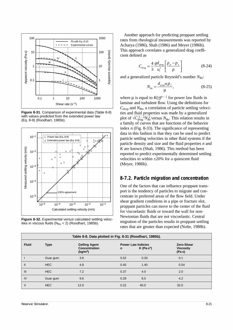
Reservoir Stimulation 8-21

Another approach for predicting proppant settlingrates from rheological measurements was reported byAcharya (1986), Shah (1986) and Meyer (1986b).This approach correlates a generalized drag coeffi-cient defined as

(8-24)

and a generalized particle Reynold’s number NRe:

(8-25)

where µ is equal to K(γ)n – 1 for power law fluids inlaminar and turbulent flow. Using the definitions forCdrag and NRe, a correlation of particle settling veloci-ties and fluid properties was made by a generalizedplot of √Cdrag

2 – nNRe2 versus NRe. This relation results in

a family of curves that are functions of the behaviorindex n (Fig. 8-33). The significance of representingdata in this fashion is that they can be used to predictparticle settling velocities in other fluid systems if theparticle density and size and the fluid properties n andK are known (Shah, 1986). This method has beenreported to predict experimentally determined settlingvelocities to within ±20% for a quiescent fluid(Meyer, 1986b).

8-7.2. Particle migration and concentrationOne of the factors that can influence proppant trans-port is the tendency of particles to migrate and con-centrate in preferred areas of the flow field. Undershear gradient conditions in a pipe or fracture slot,proppant particles can move to the center of the fluidfor viscoelastic fluids or toward the wall for non-Newtonian fluids that are not viscoelastic. Centralmigration of the particles results in proppant settlingrates that are greater than expected (Nolte, 1988b).

Figure 8-31. Comparison of experimental data (Table 8-8)with values predicted from the extended power law (Eq. 8-9) (Roodhart, 1985b).

1000

100

10

1

100

10

1

0.1

App

aren

t vis

cosi

ty (P

a·s)

App

aren

t vis

cosi

ty (p

oise

)

0.1 1 10 100 1000

Shear rate (s–1)

I

II

III

IV V

Fit with Eq. 8-23Experimental curves

Figure 8-32. Experimental versus calculated settling veloc-ities in viscous fluids (NRe < 2) (Roodhart, 1985b).

x

x xxx

x

x

x

xx

xxx

x

xxxxxx

xxx

x

x

x

xx

10–5 10–4 10–3 10–2 10–1

10–1

10–2

10–3

10–4

10–5

Calculated settling velocity (m/s)

Mea

sure

d se

ttlin

g ve

loci

ty (m

/s)

100% agreement

Power law (Eq. 8-8)Extended power law (Eq. 8-9)

x

Table 8-8. Data plotted in Fig. 8-31 (Roodhart, 1985b).

Fluid Type Gelling Agent Power Law Indicies Zero-ShearConcentration n K (Pa⋅sn) Viscosity(kg/m3) (Pa⋅s)

I Guar gum 3.6 0.52 0.33 0.1

II HEC 4.8 0.45 1.40 0.54

III HEC 7.2 0.37 4.0 2.0

IV Guar gum 9.6 0.29 8.5 4.2

V HEC 12.0 0.22 40.0 32.0

Cgd

udragprop

t

p f=−

43 2

ρ ρρ

Nd u

Reprop t f=

ρµ

,

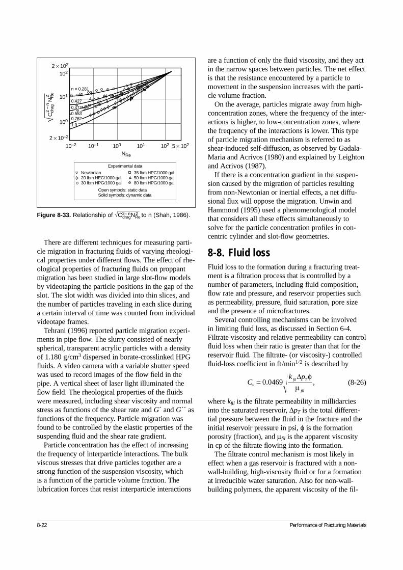
There are different techniques for measuring parti-cle migration in fracturing fluids of varying rheologi-cal properties under different flows. The effect of rhe-ological properties of fracturing fluids on proppantmigration has been studied in large slot-flow modelsby videotaping the particle positions in the gap of theslot. The slot width was divided into thin slices, andthe number of particles traveling in each slice duringa certain interval of time was counted from individualvideotape frames.

Tehrani (1996) reported particle migration experi-ments in pipe flow. The slurry consisted of nearlyspherical, transparent acrylic particles with a densityof 1.180 g/cm3 dispersed in borate-crosslinked HPGfluids. A video camera with a variable shutter speedwas used to record images of the flow field in thepipe. A vertical sheet of laser light illuminated theflow field. The rheological properties of the fluidswere measured, including shear viscosity and normalstress as functions of the shear rate and G´ and G´´ asfunctions of the frequency. Particle migration wasfound to be controlled by the elastic properties of thesuspending fluid and the shear rate gradient.

Particle concentration has the effect of increasingthe frequency of interparticle interactions. The bulkviscous stresses that drive particles together are astrong function of the suspension viscosity, which is a function of the particle volume fraction. Thelubrication forces that resist interparticle interactions

are a function of only the fluid viscosity, and they actin the narrow spaces between particles. The net effectis that the resistance encountered by a particle tomovement in the suspension increases with the parti-cle volume fraction.

On the average, particles migrate away from high-concentration zones, where the frequency of the inter-actions is higher, to low-concentration zones, wherethe frequency of the interactions is lower. This typeof particle migration mechanism is referred to asshear-induced self-diffusion, as observed by Gadala-Maria and Acrivos (1980) and explained by Leightonand Acrivos (1987).

If there is a concentration gradient in the suspen-sion caused by the migration of particles resultingfrom non-Newtonian or inertial effects, a net diffu-sional flux will oppose the migration. Unwin andHammond (1995) used a phenomenological modelthat considers all these effects simultaneously tosolve for the particle concentration profiles in con-centric cylinder and slot-flow geometries.

8-8. Fluid lossFluid loss to the formation during a fracturing treat-ment is a filtration process that is controlled by anumber of parameters, including fluid composition,flow rate and pressure, and reservoir properties suchas permeability, pressure, fluid saturation, pore sizeand the presence of microfractures.

Several controlling mechanisms can be involved in limiting fluid loss, as discussed in Section 6-4.Filtrate viscosity and relative permeability can controlfluid loss when their ratio is greater than that for thereservoir fluid. The filtrate- (or viscosity-) controlledfluid-loss coefficient in ft/min1⁄ 2 is described by

(8-26)

where kfil is the filtrate permeability in millidarciesinto the saturated reservoir, ∆pT is the total differen-tial pressure between the fluid in the fracture and theinitial reservoir pressure in psi, φ is the formationporosity (fraction), and µfil is the apparent viscosity in cp of the filtrate flowing into the formation.

The filtrate control mechanism is most likely ineffect when a gas reservoir is fractured with a non-wall-building, high-viscosity fluid or for a formationat irreducible water saturation. Also for non-wall-building polymers, the apparent viscosity of the fil-

8-22 Performance of Fracturing Materials

Figure 8-33. Relationship of √C2– ndragNRe

2 to n (Shah, 1986).

2 × 102

102

101

100

2 × 10–2

10–2 10–1 100 101 102 5 × 102

NRe

Cdr

ag N

Re

2–

n

2√

35 lbm HPC/1000 gal50 lbm HPG/1000 gal80 lbm HPG/1000 gal

Newtonian20 lbm HEC/1000 gal30 lbm HPG/1000 gal

Open symbols: static dataSolid symbols: dynamic data

Experimental data

n = 0.281

0.427

0.7621.0

0.470.553

Ck p

vfil T

fil

= 0 0469. ,∆ φµ

Reservoir Stimulation 8-23

trate is lower than that in the fracture because ofhigher shear rates for the filtrate. The viscosity of thefiltrate from a wall-building fluid is generally muchlower than the viscosity of the fracturing fluid.

The viscosity and compressibility of the reservoirfluid also help to control leakoff into the formation.This control mechanism is most effective when thereservoir fluids have high viscosities and are notgreatly compressible (e.g., heavy oil). The reservoir-(or compressibility-) controlled fluid-loss coefficientis calculated as follows:

(8-27)

where kr is the reservoir permeability, ct is the com-pressibility of the reservoir in psi–1, and µr is the vis-cosity of the reservoir fluid in cp. These equations forCv and Cc differ from Eqs. 6-88 and 6-99, respec-tively, because they are expressed in common refer-ence to the total differential pressure.

Because it is possible for both filtrate and reservoireffects to be factors in controlling fluid loss, it iscommon practice to combine the two coefficients (seeEq. 6-96):

(8-28)

A third fluid-loss control mechanism is in opera-tion with wall-building fluids. When a wall-buildingfluid is forced onto a rock, a thin film of material(i.e., polymer, fluid-loss additives or both) is filteredout and deposited on, or within the surface region of,the formation face surface. This thin film of material,known as the filter cake, is less permeable than therock. Fluid loss can then become controlled by thefilter cake rather than by the rock (i.e., Cv or Cc).

Depending on the pore size of the formation, poly-mers and fluid-loss additives in the fracturing fluidmay be filtered out on the formation surface or mayinvade into the matrix and deposit by bridging andadsorption mechanisms in the pore space. The depthof invasion of the polymers and fluid-loss additives isa function of their size, degree of entanglement andionic character. High deformation gradients resultingfrom pressure differentials can cause polymer mole-cules to transform from coiled conformations to astretched state, which enables them to flow into poresizes smaller than their largest dimension. If adsorp-tion or plugging occurs in the pore throats, the poly-mer chains form bridges in the pore throats (Pacelli

Zitha, 1995), resulting in lower leakoff rates. Thismechanism is called internal filter-cake formation.

The rate of filtrate leakoff is specific to the particu-lar fluid composition and formation properties andmust be determined experimentally, either in the lab-oratory or by in-situ calibration treatments, as dis-cussed in Section 9-5. The following provides anintroduction to the laboratory tests.

8-8.1. Fluid loss under static conditionsStatic fluid-loss tests for fracturing fluids have beenused for many years (Howard and Fast, 1970; Rec-ommended Practice for Standard Procedures forEvaluation of Hydraulic Fracturing Fluids [RP 39],1983). A simple schematic of a static fluid-loss test is shown in Fig. 8-34.

In static fluid-loss tests, fluid is heated to the testtemperature, a differential pressure is applied across

C pk c

c Tr t

r

= 0 00118. ,∆ φµ

CC C

C C Ccv

v c

v v c

=+ +( )

2

42 2 1 2/ .

Figure 8-34. Schematic of a static fluid-loss cell.

Core holder

Core

Fuid

N2

Seal

Filtrate

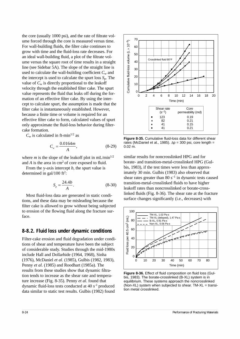
8-24 Performance of Fracturing Materials

the core (usually 1000 psi), and the rate of filtrate vol-ume forced through the core is measured versus time.For wall-building fluids, the filter cake continues togrow with time and the fluid-loss rate decreases. Foran ideal wall-building fluid, a plot of the filtrate vol-ume versus the square root of time results in a straightline (see Sidebar 5A). The slope of the straight line isused to calculate the wall-building coefficient Cw andthe intercept is used to calculate the spurt loss Sp. Thevalue of Cw is directly proportional to the leakoffvelocity through the established filter cake. The spurtvalue represents the fluid that leaks off during the for-mation of an effective filter cake. By using the inter-cept to calculate spurt, the assumption is made that thefilter cake is instantaneously established. However,because a finite time or volume is required for aneffective filter cake to form, calculated values of spurtonly approximate the fluid-loss behavior during filter-cake formation.

Cw is calculated in ft-min1/2 as

(8-29)

where m is the slope of the leakoff plot in mL/min1/2

and A is the area in cm2 of core exposed to fluid.From the y-axis intercept b, the spurt value is

determined in gal/100 ft2:

(8-30)

Most fluid-loss data are generated in static condi-tions, and these data may be misleading because thefilter cake is allowed to grow without being subjectedto erosion of the flowing fluid along the fracture sur-face.

8-8.2. Fluid loss under dynamic conditionsFilter-cake erosion and fluid degradation under condi-tions of shear and temperature have been the subjectof considerable study. Studies through the mid-1980sinclude Hall and Dollarhide (1964, 1968), Sinha(1976), McDaniel et al. (1985), Gulbis (1982, 1983),Penny et al. (1985) and Roodhart (1985a). Theresults from these studies show that dynamic filtra-tion tends to increase as the shear rate and tempera-ture increase (Fig. 8-35). Penny et al. found thatdynamic fluid-loss tests conducted at 40 s–l produceddata similar to static test results. Gulbis (1982) found

similar results for noncrosslinked HPG and forborate- and transition-metal-crosslinked HPG (Gul-bis, 1983), if the test times were less than approx-imately 30 min. Gulbis (1983) also observed thatshear rates greater than 80 s–1 in dynamic tests causedtransition-metal-crosslinked fluids to have higherleakoff rates than noncrosslinked or borate-cross-linked fluids (Fig. 8-36). The shear rate at the fracturesurface changes significantly (i.e., decreases) with

Cm

Aw = 0 0164.,

Sb

Ap = 24 4..

Figure 8-35. Cumulative fluid-loss data for different shearrates (McDaniel et al., 1985). ∆p = 300 psi, core length =0.02 m.

70

60

50

40

30

20

10

00 2 4 6 8 10 12 14 16 18 20

Time (min)

Cum

ulat

ive

fluid

-loss

vol

ume

(L ×

10–

3 )

Crosslinked fluid 80°F

Shear rate Core (s–1) permeability (md)

123 0.19 82 0.2141 0.1541 0.21

Figure 8-36. Effect of fluid composition on fluid loss (Gul-bis, 1983). The borate-crosslinked (B-XL) system is inequilibrium. These systems approach the noncrosslinked(Non-XL) system when subjected to shear. TM-XL = transi-tion metal crosslinked.

TM-XL, 1.02 Pa·sTM-XL (delayed), 1.47 Pa·sB-XL, 0.91 Pa·sNon-XL, 0.06 Pa·s

0 10 20 30 40 50 60 70 80

Time (min)

100

80

60

40

20

0

Flu

id lo

ss p

er 4

0.5

cm2

(mL)

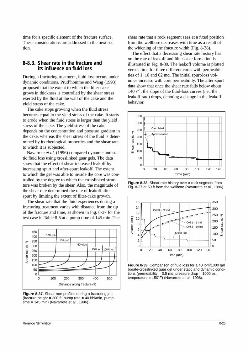
Reservoir Stimulation 8-25

time for a specific element of the fracture surface.These considerations are addressed in the next sec-tion.

8-8.3. Shear rate in the fracture and its influence on fluid loss

During a fracturing treatment, fluid loss occurs underdynamic conditions. Prud’homme and Wang (1993)proposed that the extent to which the filter cakegrows in thickness is controlled by the shear stressexerted by the fluid at the wall of the cake and theyield stress of the cake.

The cake stops growing when the fluid stressbecomes equal to the yield stress of the cake. It startsto erode when the fluid stress is larger than the yieldstress of the cake. The yield stress of the cakedepends on the concentration and pressure gradient inthe cake, whereas the shear stress of the fluid is deter-mined by its rheological properties and the shear rateto which it is subjected.

Navarrete et al. (1996) compared dynamic and sta-tic fluid loss using crosslinked guar gels. The datashow that the effect of shear increased leakoff byincreasing spurt and after-spurt leakoff. The extent to which the gel was able to invade the core was con-trolled by the degree to which the crosslinked struc-ture was broken by the shear. Also, the magnitude ofthe shear rate determined the rate of leakoff afterspurt by limiting the extent of filter-cake growth.

The shear rate that the fluid experiences during afracturing treatment varies with distance from the tipof the fracture and time, as shown in Fig. 8-37 for thetest case in Table 8-5 at a pump time of 145 min. The

shear rate that a rock segment sees at a fixed positionfrom the wellbore decreases with time as a result ofthe widening of the fracture width (Fig. 8-38).

The effect that a decreasing shear rate history hason the rate of leakoff and filter-cake formation isillustrated in Fig. 8-39. The leakoff volume is plottedversus time for three different cores with permeabili-ties of 1, 10 and 62 md. The initial spurt-loss vol-umes increase with core permeability. The after-spurtdata show that once the shear rate falls below about140 s–1, the slope of the fluid-loss curves (i.e., theleakoff rate) drops, denoting a change in the leakoffbehavior.

Figure 8-37. Shear rate profiles during a fracturing job(fracture height = 300 ft, pump rate = 40 bbl/min, pumptime = 145 min) (Navarrete et al., 1996).

0 100 200 300 400 500

Distance along fracture (ft)

450400350300250200150100500

She

ar ra

te (s

–1)

10% job

25% job

50% job

75% job 100% job

Figure 8-38. Shear rate history over a rock segment fromFig. 8-37 at 50 ft from the wellbore (Navarrete et al., 1996).

0 20 40 60 80 100 120 140

Time (min)

350

300

250

200

150

100

50

0

She

ar ra

te (s

–1)

Approximation

Calculated

Figure 8-39. Comparison of fluid loss for a 40 lbm/1000 galborate-crosslinked guar gel under static and dynamic condi-tions (permeability = 0.5 md, pressure drop = 1000 psi,temperature = 150°F) (Navarrete et al., 1996).

0 20 40 60 80 100 120 140

Vol

ume

(mL)

She

ar ra

te (s

–1)

Time (min)

16

14

12

10

8

6

4

2

0

350

300

250

200

150

100

50

0

Cell 3 – 62 md

Cell 1 – 1 md

Cell 2 – 10 md

Shear rate

8-26 Performance of Fracturing Materials

8-8.4. Influence of permeability and core length

Permeability and core length are important variablesin fluid-loss tests on high-permeability cores, wherethe polymer and fluid-loss additives can invade therock and plug pore throats deeper into the formation.

The length of high-permeability cores used in fluid-loss tests must be longer than the invasion zonelength of the polymer. Otherwise, polymer may pene-trate the entire core length, and the measured spurtvalues will be unrealistically high. Parlar et al. (1995)used 1000-md cores under static conditions to deter-mine that spurt loss became insensitive at corelengths of 5 in. and larger. For 500-md cores underdynamic conditions, Navarrete and Mitchell (1995)determined that most of the polymer accumulationoccurred in less than about 1 in.

8-8.5. Differential pressure effectsThe effect of the pressure drop is significant on spurtin high-permeability cores. Parlar et al. (1995)reported a linear dependency of spurt with the pres-sure drop under static conditions in 1000-md, 5-in.long cores at pressure drops of 500 to 1500 psi. Theeffect of the pressure drop on Cw in high-permeabilitycores was found to scale with ∆p0.5 or follow thepressure dependency of an incompressible filter cake(see Eq. 6-82). This implies that the internal filtercake, which dominates the resistance to fluid loss in high-permeability cores, behaves incompressibly.

The effect of the pressure drop on Cw under staticconditions in low-permeability cores (i.e., where thefilter cake is external) was found to scale with ∆p0.6

for borate-crosslinked fluids and ∆p0.56 for zirconium-crosslinked fluids at low pressure drops (100 psi < ∆p< 500 psi). At higher pressure drops (600 psi < ∆p <1400 psi), Cw ~ ∆p0.1 (Mayerhofer et al., 1991). If theclassic models for filter cake are considered in theinterpretation of these results, the resulting conclu-sions are that as the pressure drop increases, the filtercake becomes less permeable and Cw becomes insen-sitive to the pressure drop. This indicates that the fil-ter cake is compressible at those differential pres-sures. Similar results were found by Nolte (1982,1998a) and Penny et al. (1985).

9-1. IntroductionThe hydraulic fracture design process requires sub-stantial information about the reservoir and the frac-turing fluid. The effectiveness of a design is alsodependent on the quality of the required data. Thefracture design parameters can be inferred from wire-line logs and through laboratory fluid and core testingprocedures. The reliability of the data inferred fromthese methods is reduced by factors such as the scaleof measurement, variability in the geologic environ-ment, assumption of an overly simplified fractureresponse and significant deviations of the test envi-ronment from in-situ reservoir conditions. Fractureparameter uncertainties can result in a suboptimalfracture, at best, or in a complete failure of the stimu-lation procedure under the worst-case scenario.

An on-site procedure for predicting fracturedimensions is desirable but extremely difficult toobtain. Numerous fracture-mapping techniques, suchas radioactive tracers, surface and bottomhole tilt-meters and various electromagnetic measurements,have been applied to infer fracture dimensions (seeSection 12-1.1). The techniques, however, provideonly a limited amount of information (e.g., fractureazimuth or wellbore height) that is available gener-ally only after completion of the fracture treatment.Although sophisticated microseismic measurementshave been developed to infer the created fracturedimensions, their restricted spatial range of observa-tion and expensive instrumentation currently limitwidespread application.

In contrast, pressure analysis during and after afracture treatment is recognized as a powerful tech-nique for developing a comprehensive understandingof the fracturing process. A recording of the well-bore pressures provides an inexpensive measurementfor fracture diagnostics. The specialized analysis ofpressure provides a qualitative indicator of the frac-ture growth, as well as estimates of the primary frac-ture parameters. An analysis of the reservoir

response after fracturing characterizes its hydrocar-bon production potential. Finally, the versatility andease of use of these techniques lend their applicationto most field situations, enabling an assessment ofthe fracturing process, either on site and in real timeor after completion of the treatment for the improve-ment of future designs.

Figure 9-1 shows a recording of the bottomholepressure measured during a fracture stimulation.Fluid and proppant were injected for approximately3 hr, followed by an extended period of shut-in thatlasted for more than 18 hr. The pressure responsewas recorded for all facets of the fracture and reser-voir response—the pumping period, pressure declineas the fracture closes, time at which the fracturecloses on the proppant and finally the asymptoticapproach to the reservoir pressure. Of particularinterest to the fracture design process is the analysisof pressure measured during a calibration treatment.A calibration treatment, or a mini-fracture treatment,precedes the main fracture treatment and is per-formed without the addition of proppant under con-ditions that mimic the main treatment. The pressureresponse for this test follows the sequence in Fig. 9-1.Fracturing pressures during each stage of fractureevolution (i.e., growth, closing phase and after-closure period) provide complementary informationpertinent to the fracture design process. The frame-

Reservoir Stimulation 9-1

◆

Fracture Evaluation UsingPressure Diagnostics

Sunil N. Gulrajani and K. G. Nolte, Schlumberger Dowell

Figure 9-1. Bottomhole fracture pressure history (Nolte,1982, 1988c).

38 40 42 44 46 48 50 56 58

9000

8000

7000

6000

5000Bot

tom

hole

pre

ssur

e, p

w (p

si)

Time (hr)

InjectionFractureclosing

Transient reservoirpressure near the wellbore

Shut-in

Net fracturepressurepw – pc

Fracture closes on proppant at well

Closure pressure pc = horizontal rock stress

Reservoir pressure

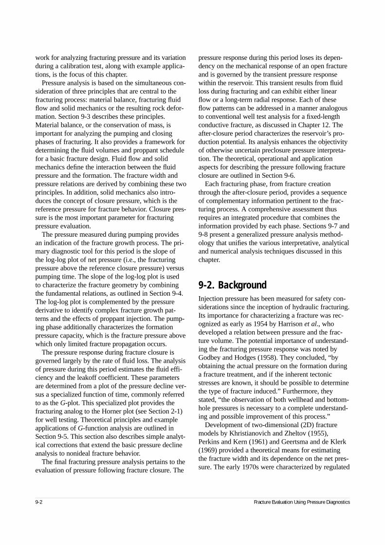
work for analyzing fracturing pressure and its variationduring a calibration test, along with example applica-tions, is the focus of this chapter.

Pressure analysis is based on the simultaneous con-sideration of three principles that are central to thefracturing process: material balance, fracturing fluidflow and solid mechanics or the resulting rock defor-mation. Section 9-3 describes these principles.Material balance, or the conservation of mass, isimportant for analyzing the pumping and closingphases of fracturing. It also provides a framework fordetermining the fluid volumes and proppant schedulefor a basic fracture design. Fluid flow and solidmechanics define the interaction between the fluidpressure and the formation. The fracture width andpressure relations are derived by combining these twoprinciples. In addition, solid mechanics also intro-duces the concept of closure pressure, which is thereference pressure for fracture behavior. Closure pres-sure is the most important parameter for fracturingpressure evaluation.

The pressure measured during pumping providesan indication of the fracture growth process. The pri-mary diagnostic tool for this period is the slope of the log-log plot of net pressure (i.e., the fracturingpressure above the reference closure pressure) versuspumping time. The slope of the log-log plot is used to characterize the fracture geometry by combiningthe fundamental relations, as outlined in Section 9-4.The log-log plot is complemented by the pressurederivative to identify complex fracture growth pat-terns and the effects of proppant injection. The pump-ing phase additionally characterizes the formationpressure capacity, which is the fracture pressure abovewhich only limited fracture propagation occurs.

The pressure response during fracture closure isgoverned largely by the rate of fluid loss. The analysisof pressure during this period estimates the fluid effi-ciency and the leakoff coefficient. These parametersare determined from a plot of the pressure decline ver-sus a specialized function of time, commonly referredto as the G-plot. This specialized plot provides thefracturing analog to the Horner plot (see Section 2-1)for well testing. Theoretical principles and exampleapplications of G-function analysis are outlined inSection 9-5. This section also describes simple analyt-ical corrections that extend the basic pressure declineanalysis to nonideal fracture behavior.

The final fracturing pressure analysis pertains to theevaluation of pressure following fracture closure. The

pressure response during this period loses its depen-dency on the mechanical response of an open fractureand is governed by the transient pressure responsewithin the reservoir. This transient results from fluidloss during fracturing and can exhibit either linearflow or a long-term radial response. Each of theseflow patterns can be addressed in a manner analogousto conventional well test analysis for a fixed-lengthconductive fracture, as discussed in Chapter 12. Theafter-closure period characterizes the reservoir’s pro-duction potential. Its analysis enhances the objectivityof otherwise uncertain preclosure pressure interpreta-tion. The theoretical, operational and applicationaspects for describing the pressure following fractureclosure are outlined in Section 9-6.

Each fracturing phase, from fracture creationthrough the after-closure period, provides a sequenceof complementary information pertinent to the frac-turing process. A comprehensive assessment thusrequires an integrated procedure that combines theinformation provided by each phase. Sections 9-7 and9-8 present a generalized pressure analysis method-ology that unifies the various interpretative, analyticaland numerical analysis techniques discussed in thischapter.

9-2. BackgroundInjection pressure has been measured for safety con-siderations since the inception of hydraulic fracturing.Its importance for characterizing a fracture was rec-ognized as early as 1954 by Harrison et al., whodeveloped a relation between pressure and the frac-ture volume. The potential importance of understand-ing the fracturing pressure response was noted byGodbey and Hodges (1958). They concluded, “byobtaining the actual pressure on the formation duringa fracture treatment, and if the inherent tectonicstresses are known, it should be possible to determinethe type of fracture induced.” Furthermore, theystated, “the observation of both wellhead and bottom-hole pressures is necessary to a complete understand-ing and possible improvement of this process.”

Development of two-dimensional (2D) fracturemodels by Khristianovich and Zheltov (1955),Perkins and Kern (1961) and Geertsma and de Klerk(1969) provided a theoretical means for estimatingthe fracture width and its dependence on the net pres-sure. The early 1970s were characterized by regulated

9-2 Fracture Evaluation Using Pressure Diagnostics

gas prices in the United States and significant oil dis-coveries in the Middle East, which caused a lull infracturing activity and hence a reduced interest infracturing research. Renewed activity was fosteredduring the mid-1970s when massive hydraulic frac-turing led to an emphasis on improved fracturing eco-nomics. The fluid and proppant volumes utilized forthese fracturing operations significantly increased,which increased execution costs. Successful fractureexecution was recognized as critical for economicfield development. These developments spurred arenewed interest in understanding fracture pressurebehavior for the effective design and analysis of frac-ture treatments. The Appendix to Chapter 5 providesa detailed discussion of these activities.

A numerical simulation describing the pressuredecline response during fracture closure was pre-sented by Novotny (1977). Nolte (1979) presented afundamental analysis to estimate the fluid-loss para-meters and the fracture length for the PKN fracturegeometry. This analysis was subsequently extended to the other 2D fracture geometry models (Nolte,1986a). Simonson et al. (1978) characterized heightgrowth into stress barriers. Nolte and Smith (1981)related trends on the log-log net pressure plot to theevolution of the fracture geometry, and Clifton andAbou-Sayed (1981) generalized fracture modelingand the related pressure response to three-dimensional(3D) hydraulic fracture models.

Later developments attempted to address the non-ideal conditions that commonly occur during fieldpractice but had been excluded in these early studies.Soliman (1986a) developed an analysis to considerthe effects caused by fluid compressibility and tem-perature change during shut-in. A correction to incor-porate pressure-dependent fluid-loss behavior wasproposed by Castillo (1987). Nolte (1991) addressedseveral nonideal conditions during injection as wellas shut-in and provided techniques to diagnose therelated pressure responses. A semianalytical approachto account for variation of the fluid-leakoff coefficientfollowing the end of treatment as well as the effectsresulting from fluid flowback was developed byMeyer (1986a). A decline analysis methodology thataddresses a comprehensive list of nonideal factorsduring fracture closure was proposed by Nolte et al.(1993).

Pressure analysis has been applied since the early1980s to improve fracture performance in a variety of applications, including routine fracture design (e.g.,

Schlottman et al., 1981; Elbel et al., 1984; Morris andSinclair, 1984; Cleary et al., 1993) and fracturing forspecialized applications (e.g., Smith, 1985; Bale et al.,1992). It is most effective when used to characterizefracture growth behavior during the early stages offield development. Variations of the traditional cali-bration test have also been proposed for specializedpurposes, such as the step rate/flowback test to deter-mine closure pressure (e.g., Felsenthal, 1974; Nolte,1982; Singh et al., 1985; Plahn et al., 1997), step-down test to identify near-wellbore effects (e.g.,Cleary et al., 1993) and short impulse injection test to obtain reservoir permeability (e.g., Gu et al., 1993;Abousleiman et al., 1994). Additional studies(Mayerhofer et al., 1993; Nolte et al., 1997) extendfracture pressure analysis to the realm of well testing,wherein reservoir information typically obtained fromconventional well tests can be inferred from calibra-tion treatments.

9-3. Fundamental principles of hydraulic fracturing

Three basic relations govern the hydraulic fracturingprocess: fluid flow in the fracture, material balance orconservation of mass, and rock elastic deformation.These relations are reviewed in Chapter 5, presentedin the context of fracture modeling in Chapter 6 andreformulated in this section to facilitate the develop-ment of pressure analysis techniques.

9-3.1. Fluid flow in the fractureThe fracture essentially is a channel of varying widthover its length and height. The local pressure gradientwithin the fracture is determined by the fracturingfluid rheology, fluid velocity and fracture width.Equations governing fluid flow within the fracturecan be derived using the principle of conservation ofmomentum and lubrication theory applied to a fluidtraveling in a narrow conduit. The rheology of frac-turing fluids is generally represented by a power lawmodel (see Chapter 8) that incorporates the parame-ters K and n. In recognition that fluid flow within afracture is laminar for most fracturing applications(Perkins and Kern, 1961), the global pressure gradi-ent along the length of a fracture can be expressed as

(9-1)

Reservoir Stimulation 9-3

dp

dx

Kv

wxn

n∝ +1

,

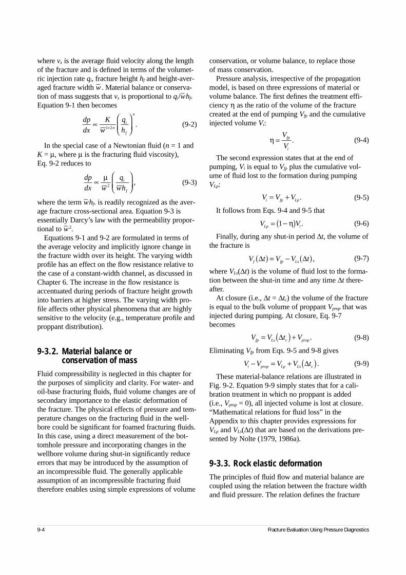
where vx is the average fluid velocity along the lengthof the fracture and is defined in terms of the volumet-ric injection rate qi, fracture height hf and height-aver-aged fracture width w– . Material balance or conserva-tion of mass suggests that vx is proportional to qi/w– hf.Equation 9-1 then becomes

(9-2)

In the special case of a Newtonian fluid (n = 1 andK = µ, where µ is the fracturing fluid viscosity), Eq. 9-2 reduces to

(9-3)

where the term w– hf. is readily recognized as the aver-age fracture cross-sectional area. Equation 9-3 isessentially Darcy’s law with the permeability propor-tional to w– 2.

Equations 9-1 and 9-2 are formulated in terms ofthe average velocity and implicitly ignore change inthe fracture width over its height. The varying widthprofile has an effect on the flow resistance relative tothe case of a constant-width channel, as discussed inChapter 6. The increase in the flow resistance isaccentuated during periods of fracture height growthinto barriers at higher stress. The varying width pro-file affects other physical phenomena that are highlysensitive to the velocity (e.g., temperature profile andproppant distribution).

9-3.2. Material balance or conservation of mass

Fluid compressibility is neglected in this chapter forthe purposes of simplicity and clarity. For water- andoil-base fracturing fluids, fluid volume changes are ofsecondary importance to the elastic deformation ofthe fracture. The physical effects of pressure and tem-perature changes on the fracturing fluid in the well-bore could be significant for foamed fracturing fluids.In this case, using a direct measurement of the bot-tomhole pressure and incorporating changes in thewellbore volume during shut-in significantly reduceerrors that may be introduced by the assumption ofan incompressible fluid. The generally applicableassumption of an incompressible fracturing fluidtherefore enables using simple expressions of volume

conservation, or volume balance, to replace those of mass conservation.

Pressure analysis, irrespective of the propagationmodel, is based on three expressions of material orvolume balance. The first defines the treatment effi-ciency η as the ratio of the volume of the fracturecreated at the end of pumping Vfp and the cumulativeinjected volume Vi:

(9-4)

The second expression states that at the end ofpumping, Vi is equal to Vfp plus the cumulative vol-ume of fluid lost to the formation during pumpingVLp:

(9-5)

It follows from Eqs. 9-4 and 9-5 that

(9-6)

Finally, during any shut-in period ∆t, the volume ofthe fracture is

(9-7)

where VLs(∆t) is the volume of fluid lost to the forma-tion between the shut-in time and any time ∆t there-after.

At closure (i.e., ∆t = ∆tc) the volume of the fractureis equal to the bulk volume of proppant Vprop that wasinjected during pumping. At closure, Eq. 9-7becomes

(9-8)

Eliminating Vfp from Eqs. 9-5 and 9-8 gives

(9-9)

These material-balance relations are illustrated inFig. 9-2. Equation 9-9 simply states that for a cali-bration treatment in which no proppant is added (i.e., Vprop = 0), all injected volume is lost at closure.“Mathematical relations for fluid loss” in theAppendix to this chapter provides expressions for VLp and VLs(∆t) that are based on the derivations pre-sented by Nolte (1979, 1986a).

9-3.3. Rock elastic deformationThe principles of fluid flow and material balance arecoupled using the relation between the fracture widthand fluid pressure. The relation defines the fracture

9-4 Fracture Evaluation Using Pressure Diagnostics

dp

dx

K

w

q

hni

f

n

∝

+1 2.

η =V

Vfp

i

.

V V Vi fp Lp= + .

V VLp i= −( )1 η .

V t V V tf fp Ls∆ ∆( ) = − ( ) ,

V V t Vfp Ls c prop= ( ) +∆ .

V V V V ti prop Lp Ls c− = + ( )∆ .

dp

dx w

q

whi

f

∝

µ

2,

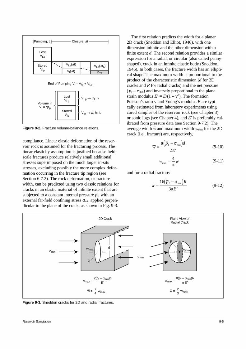
compliance. Linear elastic deformation of the reser-voir rock is assumed for the fracturing process. Thelinear elasticity assumption is justified because field-scale fractures produce relatively small additionalstresses superimposed on the much larger in-situstresses, excluding possibly the more complex defor-mation occurring in the fracture tip region (seeSection 6-7.2). The rock deformation, or fracturewidth, can be predicted using two classic relations forcracks in an elastic material of infinite extent that aresubjected to a constant internal pressure p–f, with anexternal far-field confining stress σmin applied perpen-dicular to the plane of the crack, as shown in Fig. 9-3.

The first relation predicts the width for a planar 2D crack (Sneddon and Elliot, 1946), with onedimension infinite and the other dimension with afinite extent d. The second relation provides a similarexpression for a radial, or circular (also called penny-shaped), crack in an infinite elastic body (Sneddon,1946). In both cases, the fracture width has an ellipti-cal shape. The maximum width is proportional to theproduct of the characteristic dimension (d for 2Dcracks and R for radial cracks) and the net pressure( p–f – σmin) and inversely proportional to the planestrain modulus E′ = E/(1 – ν2). The formationPoisson’s ratio ν and Young’s modulus E are typi-cally estimated from laboratory experiments usingcored samples of the reservoir rock (see Chapter 3) or sonic logs (see Chapter 4), and E′ is preferably cal-ibrated from pressure data (see Section 9-7.2). Theaverage width w– and maximum width wmax for the 2Dcrack (i.e., fracture) are, respectively,

(9-10)

(9-11)

and for a radial fracture:

(9-12)

Reservoir Stimulation 9-5

Figure 9-2. Fracture volume-balance relations.

LostVLp

Pumping, tp Closure, ∆t

StoredVfp

LostVLp

StoredVfp

End of Pumping Vi = Vfp + VLp

Volume inVi = qitp

VLp → CL, κ

Vfp → w, hf, L

VLs(∆t) VLs(∆tc)

Vf(∆t) Vprop

Figure 9-3. Sneddon cracks for 2D and radial fractures.

2D Crack

σminpf

wmax

wmax =

d wmax

R

σmin

Plane View ofRadial Crack

2(pf – σmin)dE´

w = wmaxπ4

wmax =8(pf – σmin)R

π E´

w = wmax23

wp d

Ef min=

−( )′

π σ2

w wmax = 4π

wp R

Ef min=

−( )′

16

3

σπ

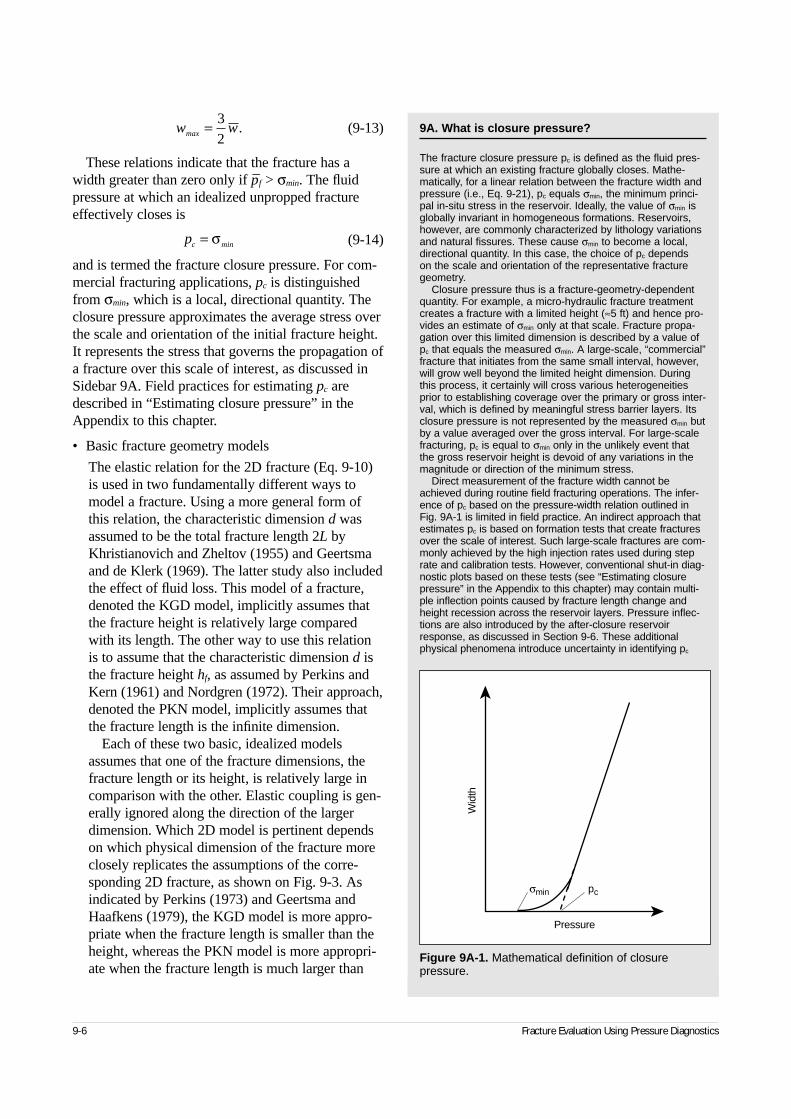
9-6 Fracture Evaluation Using Pressure Diagnostics

(9-13)

These relations indicate that the fracture has awidth greater than zero only if p–f > σmin. The fluidpressure at which an idealized unpropped fractureeffectively closes is

(9-14)

and is termed the fracture closure pressure. For com-mercial fracturing applications, pc is distinguishedfrom σmin, which is a local, directional quantity. Theclosure pressure approximates the average stress overthe scale and orientation of the initial fracture height.It represents the stress that governs the propagation ofa fracture over this scale of interest, as discussed inSidebar 9A. Field practices for estimating pc aredescribed in “Estimating closure pressure” in theAppendix to this chapter.

• Basic fracture geometry models

The elastic relation for the 2D fracture (Eq. 9-10)is used in two fundamentally different ways tomodel a fracture. Using a more general form ofthis relation, the characteristic dimension d wasassumed to be the total fracture length 2L byKhristianovich and Zheltov (1955) and Geertsmaand de Klerk (1969). The latter study also includedthe effect of fluid loss. This model of a fracture,denoted the KGD model, implicitly assumes thatthe fracture height is relatively large comparedwith its length. The other way to use this relationis to assume that the characteristic dimension d isthe fracture height hf, as assumed by Perkins andKern (1961) and Nordgren (1972). Their approach,denoted the PKN model, implicitly assumes thatthe fracture length is the infinite dimension.

Each of these two basic, idealized modelsassumes that one of the fracture dimensions, thefracture length or its height, is relatively large incomparison with the other. Elastic coupling is gen-erally ignored along the direction of the largerdimension. Which 2D model is pertinent dependson which physical dimension of the fracture moreclosely replicates the assumptions of the corre-sponding 2D fracture, as shown on Fig. 9-3. Asindicated by Perkins (1973) and Geertsma andHaafkens (1979), the KGD model is more appro-priate when the fracture length is smaller than theheight, whereas the PKN model is more appropri-ate when the fracture length is much larger than

w wmax = 32

.

pc min= σ

9A. What is closure pressure?

The fracture closure pressure pc is defined as the fluid pres-sure at which an existing fracture globally closes. Mathe-matically, for a linear relation between the fracture width andpressure (i.e., Eq. 9-21), pc equals σmin, the minimum princi-pal in-situ stress in the reservoir. Ideally, the value of σmin isglobally invariant in homogeneous formations. Reservoirs,however, are commonly characterized by lithology variationsand natural fissures. These cause σmin to become a local,directional quantity. In this case, the choice of pc dependson the scale and orientation of the representative fracturegeometry.

Closure pressure thus is a fracture-geometry-dependentquantity. For example, a micro-hydraulic fracture treatmentcreates a fracture with a limited height (≈5 ft) and hence pro-vides an estimate of σmin only at that scale. Fracture propa-gation over this limited dimension is described by a value ofpc that equals the measured σmin. A large-scale, “commercial”fracture that initiates from the same small interval, however,will grow well beyond the limited height dimension. Duringthis process, it certainly will cross various heterogeneitiesprior to establishing coverage over the primary or gross inter-val, which is defined by meaningful stress barrier layers. Itsclosure pressure is not represented by the measured σmin butby a value averaged over the gross interval. For large-scalefracturing, pc is equal to σmin only in the unlikely event thatthe gross reservoir height is devoid of any variations in themagnitude or direction of the minimum stress.

Direct measurement of the fracture width cannot beachieved during routine field fracturing operations. The infer-ence of pc based on the pressure-width relation outlined inFig. 9A-1 is limited in field practice. An indirect approach thatestimates pc is based on formation tests that create fracturesover the scale of interest. Such large-scale fractures are com-monly achieved by the high injection rates used during steprate and calibration tests. However, conventional shut-in diag-nostic plots based on these tests (see “Estimating closurepressure” in the Appendix to this chapter) may contain multi-ple inflection points caused by fracture length change andheight recession across the reservoir layers. Pressure inflec-tions are also introduced by the after-closure reservoirresponse, as discussed in Section 9-6. These additionalphysical phenomena introduce uncertainty in identifying pc

Figure 9A-1. Mathematical definition of closure pressure.

Pressure

Wid

th

σmin pc

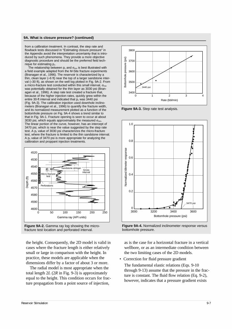
the height. Consequently, the 2D model is valid incases where the fracture length is either relativelysmall or large in comparison with the height. Inpractice, these models are applicable when thedimensions differ by a factor of about 3 or more.

The radial model is most appropriate when thetotal length 2L (2R in Fig. 9-3) is approximatelyequal to the height. This condition occurs for frac-ture propagation from a point source of injection,

as is the case for a horizontal fracture in a verticalwellbore, or as an intermediate condition betweenthe two limiting cases of the 2D models.

• Correction for fluid pressure gradient

The fundamental elastic relations (Eqs. 9-10through 9-13) assume that the pressure in the frac-ture is constant. The fluid flow relation (Eq. 9-2),however, indicates that a pressure gradient exists

from a calibration treatment. In contrast, the step rate andflowback tests discussed in “Estimating closure pressure” inthe Appendix avoid the interpretation uncertainty that is intro-duced by such phenomena. They provide a more objectivediagnostic procedure and should be the preferred field tech-nique for estimating pc.

The relationship between pc and σmin is best illustrated with a field example adapted from the M-Site fracture experiments(Branagan et al., 1996). The reservoir is characterized by a thin, clean layer (≈6 ft) near the top of a larger sandstone inter-val (≈30 ft), as shown on the well log plotted in Fig. 9A-2. Froma micro-fracture test conducted within this small interval, σmin

was potentially obtained for the thin layer as 3030 psi (Bran-agan et al., 1996). A step rate test created a fracture that,because of the higher injection rates, quickly grew within theentire 30-ft interval and indicated that pc was 3440 psi (Fig. 9A-3). The calibration injection used downhole inclino-meters (Branagan et al., 1996) to quantify the fracture width,and its normalized measurement plotted as a function of thebottomhole pressure on Fig. 9A-4 shows a trend similar to that in Fig. 9A-1. Fracture opening is seen to occur at about3030 psi, which equals approximately the measured σmin.The linear portion of the curve, however, has an intercept of 3470 psi, which is near the value suggested by the step ratetest. A pc value of 3030 psi characterizes the micro-fracturetest, where the fracture is limited to the thin sandstone interval.A pc value of 3470 psi is more appropriate for analyzing thecalibration and proppant injection treatments.

Reservoir Stimulation 9-7

Figure 9A-2. Gamma ray log showing the micro-fracture test location and perforated interval.

Figure 9A-3. Step rate test analysis.

3800

3700

3600

3500

3400

Bot

tom

hole

pre

ssur

e (p

si)

0 1 2 3 4

Rate (bbl/min)

3440 psi

4520

4530

4540

4550

4560

4570

4580

4590

4600

Dep

th (f

t)

0 50 100 150 200 250

Gamma ray (API units)

Grossinterval

Sandstone stringer+

Perforations

Micro-fracturetest

Figure 9A-4. Normalized inclinometer response versusbottomhole pressure.

1.0

0.8

0.6

0.4

0.2

0

Nor

mal

ized

tiltm

eter

resp

onse

3000 3200 3400 3600

Bottomhole pressure (psi)

3470 psi

9A. What is closure pressure? (continued)

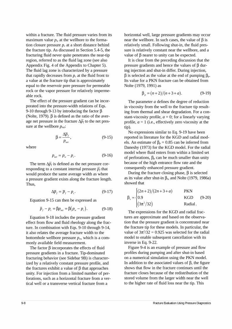
9-8 Fracture Evaluation Using Pressure Diagnostics

within a fracture. The fluid pressure varies from itsmaximum value pw at the wellbore to the forma-tion closure pressure pc at a short distance behindthe fracture tip. As discussed in Section 5.4-5, thefracturing fluid never quite penetrates the near-tipregion, referred to as the fluid lag zone (see alsoAppendix Fig. 4 of the Appendix to Chapter 5).The fluid lag zone is characterized by a pressurethat rapidly decreases from pc at the fluid front to a value at the fracture tip that is approximatelyequal to the reservoir pore pressure for permeablerock or the vapor pressure for relatively imperme-able rock.

The effect of the pressure gradient can be incor-porated into the pressure-width relations of Eqs. 9-10 through 9-13 by introducing the factor β(Nolte, 1979). β is defined as the ratio of the aver-age net pressure in the fracture ∆p–f to the net pres-sure at the wellbore pnet:

(9-15)

where

(9-16)

The term ∆p–f is defined as the net pressure cor-responding to a constant internal pressure p–f thatwould produce the same average width as where a pressure gradient exists along the fracture length.Thus,

(9-17)

Equation 9-15 can then be expressed as

(9-18)

Equation 9-18 includes the pressure gradienteffect from flow and fluid rheology along the frac-ture. In combination with Eqs. 9-10 through 9-14,it also relates the average fracture width to thebottomhole wellbore pressure pw, which is a com-monly available field measurement.

The factor β incorporates the effects of fluidpressure gradients in a fracture. Tip-dominatedfracturing behavior (see Sidebar 9B) is character-ized by a relatively constant pressure profile, andthe fractures exhibit a value of β that approachesunity. For injection from a limited number of per-forations, such as a horizontal fracture from a ver-tical well or a transverse vertical fracture from a

horizontal well, large pressure gradients may occurnear the wellbore. In such cases, the value of β isrelatively small. Following shut-in, the fluid pres-sure is relatively constant near the wellbore, and avalue of β nearer to unity can be expected.

It is clear from the preceding discussion that thepressure gradients and hence the values of β dur-ing injection and shut-in differ. During injection, β is selected as the value at the end of pumping βp.Its value for a PKN fracture can be obtained fromNolte (1979, 1991) as

(9-19)

The parameter a defines the degree of reductionin viscosity from the well to the fracture tip result-ing from thermal and shear degradation. For a con-stant-viscosity profile, a = 0; for a linearly varyingprofile, a = 1 (i.e., effectively zero viscosity at thetip).

No expressions similar to Eq. 9-19 have beenreported in literature for the KGD and radial mod-els. An estimate of βp = 0.85 can be inferred fromDaneshy (1973) for the KGD model. For the radialmodel where fluid enters from within a limited setof perforations, βp can be much smaller than unitybecause of the high entrance flow rate and theconsequently enhanced pressure gradient.

During the fracture closing phase, β is selectedas its value after shut-in βs, and Nolte (1979, 1986a)showed that

(9-20)

The expressions for the KGD and radial frac-tures are approximate and based on the observa-tion that the pressure gradient is concentrated nearthe fracture tip for these models. In particular, thevalue of 3π2/32 = 0.925 was selected for the radialmodel to enable subsequent cancellation with itsinverse in Eq. 9-22.

Figure 9-4 is an example of pressure and flowprofiles during pumping and after shut-in based on a numerical simulation using the PKN model.In addition to the associated values of β, the figureshows that flow in the fracture continues until thefracture closes because of the redistribution of thestored volume from the larger width near the wellto the higher rate of fluid loss near the tip. This

β =∆p

pf

net

,

β p n n a= +( ) + +( )2 3 .

βπ

s

n n a

≈+( ) + +( )

( )

2 2 2 3

0 9

3 322

PKN

KGD

Radial .

.

p p pnet w c= − .

∆p p pf f c= − .

p p p p pf c net w c− = = −( )β β .

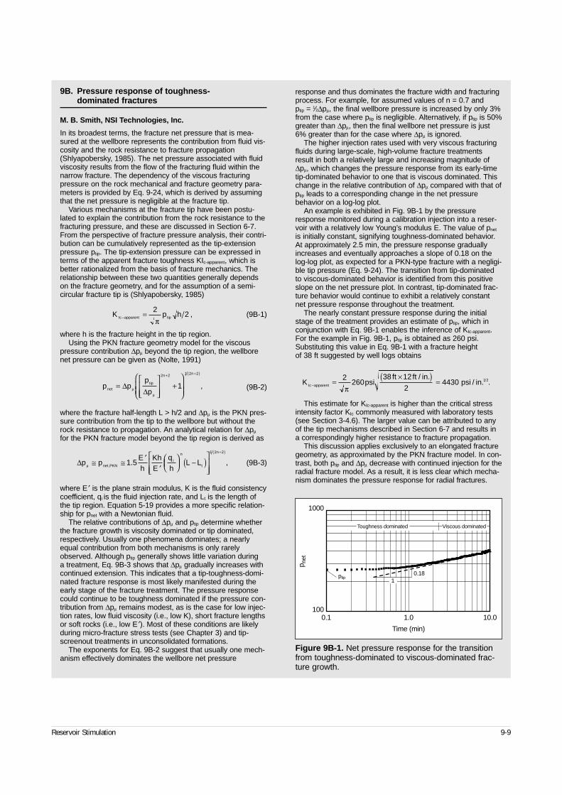
Reservoir Stimulation 9-9

9B. Pressure response of toughness-dominated fractures

M. B. Smith, NSI Technologies, Inc.

In its broadest terms, the fracture net pressure that is mea-sured at the wellbore represents the contribution from fluid vis-cosity and the rock resistance to fracture propagation(Shlyapobersky, 1985). The net pressure associated with fluidviscosity results from the flow of the fracturing fluid within thenarrow fracture. The dependency of the viscous fracturingpressure on the rock mechanical and fracture geometry para-meters is provided by Eq. 9-24, which is derived by assumingthat the net pressure is negligible at the fracture tip.

Various mechanisms at the fracture tip have been postu-lated to explain the contribution from the rock resistance to thefracturing pressure, and these are discussed in Section 6-7.From the perspective of fracture pressure analysis, their contri-bution can be cumulatively represented as the tip-extensionpressure ptip. The tip-extension pressure can be expressed interms of the apparent fracture toughness KIc-apparent, which isbetter rationalized from the basis of fracture mechanics. Therelationship between these two quantities generally dependson the fracture geometry, and for the assumption of a semi-circular fracture tip is (Shlyapobersky, 1985)

(9B-1)

where h is the fracture height in the tip region.Using the PKN fracture geometry model for the viscous

pressure contribution ∆pµ beyond the tip region, the wellborenet pressure can be given as (Nolte, 1991)

(9B-2)

where the fracture half-length L > h/2 and ∆pµ is the PKN pres-sure contribution from the tip to the wellbore but without therock resistance to propagation. An analytical relation for ∆pµ

for the PKN fracture model beyond the tip region is derived as

(9B-3)

where E ′ is the plane strain modulus, K is the fluid consistencycoefficient, qi is the fluid injection rate, and Lt is the length ofthe tip region. Equation 5-19 provides a more specific relation-ship for pnet with a Newtonian fluid.

The relative contributions of ∆pµ and ptip determine whetherthe fracture growth is viscosity dominated or tip dominated,respectively. Usually one phenomena dominates; a nearlyequal contribution from both mechanisms is only rarelyobserved. Although ptip generally shows little variation during a treatment, Eq. 9B-3 shows that ∆pµ gradually increases withcontinued extension. This indicates that a tip-toughness-domi-nated fracture response is most likely manifested during theearly stage of the fracture treatment. The pressure responsecould continue to be toughness dominated if the pressure con-tribution from ∆pµ remains modest, as is the case for low injec-tion rates, low fluid viscosity (i.e., low K), short fracture lengthsor soft rocks (i.e., low E ′). Most of these conditions are likelyduring micro-fracture stress tests (see Chapter 3) and tip-screenout treatments in unconsolidated formations.

The exponents for Eq. 9B-2 suggest that usually one mech-anism effectively dominates the wellbore net pressure

response and thus dominates the fracture width and fracturingprocess. For example, for assumed values of n = 0.7 and ptip = 1⁄2∆pµ, the final wellbore pressure is increased by only 3%from the case where ptip is negligible. Alternatively, if ptip is 50%greater than ∆pµ, then the final wellbore net pressure is just6% greater than for the case where ∆pµ is ignored.

The higher injection rates used with very viscous fracturingfluids during large-scale, high-volume fracture treatmentsresult in both a relatively large and increasing magnitude of∆pµ, which changes the pressure response from its early-timetip-dominated behavior to one that is viscous dominated. Thischange in the relative contribution of ∆pµ compared with that ofptip leads to a corresponding change in the net pressurebehavior on a log-log plot.

An example is exhibited in Fig. 9B-1 by the pressureresponse monitored during a calibration injection into a reser-voir with a relatively low Young’s modulus E. The value of pnet

is initially constant, signifying toughness-dominated behavior.At approximately 2.5 min, the pressure response graduallyincreases and eventually approaches a slope of 0.18 on thelog-log plot, as expected for a PKN-type fracture with a negligi-ble tip pressure (Eq. 9-24). The transition from tip-dominatedto viscous-dominated behavior is identified from this positiveslope on the net pressure plot. In contrast, tip-dominated frac-ture behavior would continue to exhibit a relatively constantnet pressure response throughout the treatment.

The nearly constant pressure response during the initialstage of the treatment provides an estimate of ptip, which inconjunction with Eq. 9B-1 enables the inference of KIc-apparent.For the example in Fig. 9B-1, ptip is obtained as 260 psi.Substituting this value in Eq. 9B-1 with a fracture height of 38 ft suggested by well logs obtains

This estimate for KIc-apparent is higher than the critical stressintensity factor KIc commonly measured with laboratory tests(see Section 3-4.6). The larger value can be attributed to anyof the tip mechanisms described in Section 6-7 and results ina correspondingly higher resistance to fracture propagation.

This discussion applies exclusively to an elongated fracturegeometry, as approximated by the PKN fracture model. In con-trast, both ptip and ∆pµ decrease with continued injection for theradial fracture model. As a result, it is less clear which mecha-nism dominates the pressure response for radial fractures.

K p hIc apparent tip− = 22

π,

p pp

pnet

tip

n n

=

+

+ +( )

∆∆µ

µ

2 2 1 2 2

1 ,

∆p pEh

KhE

qh

L Lnet PKNi

n

t

n

µ ≅ ≅ ′′

−( )

+( )

, . ,1 5

1 2 2

K Ic apparent− =×( ) =2

26038 12

24430 1 2

πpsi

ft ft / in. psi / in. .

Figure 9B-1. Net pressure response for the transitionfrom toughness-dominated to viscous-dominated frac-ture growth.

1000

100

p net

0.1 1.0 10.0

Time (min)

0.181

Toughness dominated Viscous dominated

ptip

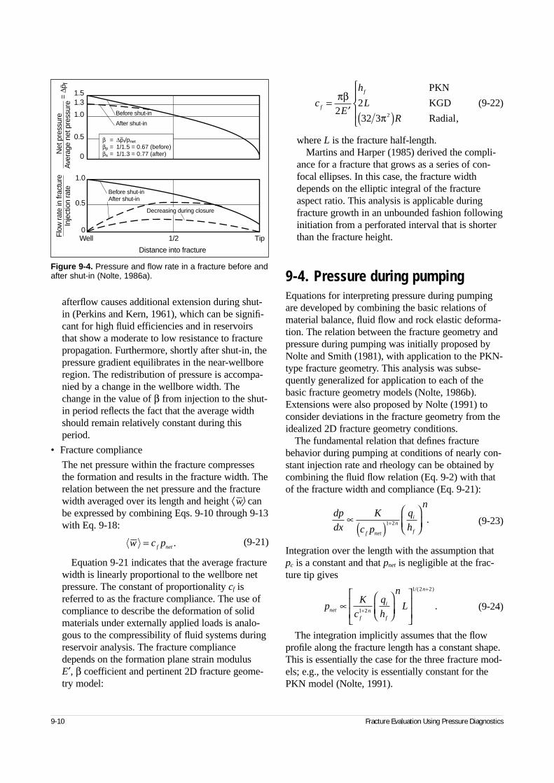
9-10 Fracture Evaluation Using Pressure Diagnostics

afterflow causes additional extension during shut-in (Perkins and Kern, 1961), which can be signifi-cant for high fluid efficiencies and in reservoirsthat show a moderate to low resistance to fracturepropagation. Furthermore, shortly after shut-in, thepressure gradient equilibrates in the near-wellboreregion. The redistribution of pressure is accompa-nied by a change in the wellbore width. Thechange in the value of β from injection to the shut-in period reflects the fact that the average widthshould remain relatively constant during thisperiod.

• Fracture compliance

The net pressure within the fracture compressesthe formation and results in the fracture width. Therelation between the net pressure and the fracturewidth averaged over its length and height ⟨w–⟩ canbe expressed by combining Eqs. 9-10 through 9-13with Eq. 9-18:

(9-21)

Equation 9-21 indicates that the average fracturewidth is linearly proportional to the wellbore netpressure. The constant of proportionality cf isreferred to as the fracture compliance. The use ofcompliance to describe the deformation of solidmaterials under externally applied loads is analo-gous to the compressibility of fluid systems duringreservoir analysis. The fracture compliancedepends on the formation plane strain modulus E′, β coefficient and pertinent 2D fracture geome-try model:

(9-22)

where L is the fracture half-length.Martins and Harper (1985) derived the compli-

ance for a fracture that grows as a series of con-focal ellipses. In this case, the fracture widthdepends on the elliptic integral of the fractureaspect ratio. This analysis is applicable duringfracture growth in an unbounded fashion followinginitiation from a perforated interval that is shorterthan the fracture height.

9-4. Pressure during pumpingEquations for interpreting pressure during pumpingare developed by combining the basic relations ofmaterial balance, fluid flow and rock elastic deforma-tion. The relation between the fracture geometry andpressure during pumping was initially proposed byNolte and Smith (1981), with application to the PKN-type fracture geometry. This analysis was subse-quently generalized for application to each of thebasic fracture geometry models (Nolte, 1986b).Extensions were also proposed by Nolte (1991) toconsider deviations in the fracture geometry from theidealized 2D fracture geometry conditions.

The fundamental relation that defines fracturebehavior during pumping at conditions of nearly con-stant injection rate and rheology can be obtained bycombining the fluid flow relation (Eq. 9-2) with thatof the fracture width and compliance (Eq. 9-21):

(9-23)

Integration over the length with the assumption thatpc is a constant and that pnet is negligible at the frac-ture tip gives

(9-24)

The integration implicitly assumes that the flowprofile along the fracture length has a constant shape.This is essentially the case for the three fracture mod-els; e.g., the velocity is essentially constant for thePKN model (Nolte, 1991).

Figure 9-4. Pressure and flow rate in a fracture before andafter shut-in (Nolte, 1986a).

Distance into fracture

Well 1/2 Tip

Before shut-in

After shut-in

Before shut-inAfter shut-in

1.51.3

1.0

0.5

0

1.0

0.5

0

Decreasing during closure

Flo

w ra

te in

frac

ture

Inje

ctio

n ra

teN

et p

ress

ure

Ave

rage

net

pre

ssur

e

β = ∆pf/pnetβp = 1/1.5 = 0.67 (before)βs = 1/1.3 = 0.77 (after)

=∆p

f

w c pf net= .

cE

h

L

Rf

f

=′ ( )

πβ

π2

2

32 3 2

PKN

KGD

Radial,

dp

dx

K

c p

q

h

n

f net

ni

f

∝( )

+1 2 .

pK

c

q

h

n

Lnet

fn

i

f

n

∝

+

+

1 2

1 2 2/( )

.

Reservoir Stimulation 9-11

Equation 9-24 and the following equations assumethat pnet is dominated by the frictional effects fromflow of a viscous fluid within the fracture. Thisassumption may not be valid under specific condi-tions, as discussed in Section 5-4.5. Sidebar 9B out-lines a diagnostic procedure for comparing the netpressure contribution from the fracture tip to the netpressure from fluid flow (or the viscous net pressure)predicted by Eq. 9-24.

Introducing the appropriate compliance relation inEq. 9-24 for the three models and using L = hf /2 = Rfor the radial model:

(9-25)

where the exponent e represents

(9-26)

On the basis of Eq. 9-21, the fracture width wat the wellbore is proportional to cfpnet for the threefracture geometry models. Multiplying each sideof Eq. 9-25 by the appropriate definition of cf fromEq. 9-22 results in

(9-27)

These fracturing pressure and width relations indicatethat their dependence on the fluid rheology parame-ters K and n, wellbore injection rate qi and planestrain modulus E′ is the same for all the models.Their dependence on the fracture extension L or Rand height hf differs. In addition, Eqs. 9-25 and 9-27also show that pnet and w, respectively, have a weakdependence on qi and that for increasing penetrationL or R, pnet increases for the PKN model butdecreases for the KGD and radial models.

The time dependence of the fracture width andpressure is developed using the definition of η fromEq. 9-4 at a constant injection rate qi (i.e., Vi = qit):

(9-28)

where t* is referred to as the reduced time (Nolte,1991). The fracture surface area Af for the basic frac-ture geometry models is

(9-29)

Combining Eqs. 9-27 through 9-29, an expressionfor the fracture width as a function of reduced timefor the three basic models can be obtained:

(9-30)

Substituting the relation between width and netpressure in Eq. 9-21 into Eq. 9-30 gives the followingexpressions for pnet in terms of the reduced time:

(9-31)

Equation 9-31 indicates that for typical fracturing flu-ids (i.e., n ≈ 0.4–1.0), the fracture pressure duringinjection is only nominally sensitive to the reducedtime t* or fluid efficiency η. Consequently, the effi-ciency, or alternatively the fluid-leakoff coefficient,cannot be determined by analyzing pressure duringfluid injection exclusively.

Equations 9-30 and 9-31 also show that the netpressure and fracture width for any efficiency η canbe approximated by their values for the case of nofluid loss, if the time is scaled by ηt. This time scal-ing is illustrated for the PKN fracture model in Fig. 9-5, which shows the net pressure correspondingto no fluid loss (i.e., η = 1) and to an efficiency η =0.2 at a time of 50 min. The latter case corresponds to a reduced time of t* = ηt = 50 × 0.2 = 10 min.Figure 9-5 illustrates that the net pressure at a time of50 min for the fluid-loss case is equal to the net pres-

PKN

KGD

Radial

p E KqL

h

p E Kqh L

p E KqR

netn

in e

fn

e

netn

in e

fn n

e

netn

in e

n

e

∝ ′( )

∝ ′( )

∝ ′( )

++

+

+

2 1

3 1

2 1

2

2 1

3

1

1,

e n= +( )1 2 2 .

Aq t

w

q t

wfi i= =η *

,

A

Lh

Lh

Rf =

2

22

PKN

KGD

Radial.π

PKN

KGD

Radial

wKq

E ht

wKq

E ht

wK q

Et

in

fn

n

n

in

fn

n

n

in n

n n

∝′

( )

∝′

( )

∝′

( )

++( )

+( )

+

+

+( )+( )

+ +( )−( ) +( )

11 2 3

1 2 3

2

2

1 2 4

1 2

2 2

2

1 3 6

2 3 6

*

*

* .

PKN

KGD

Radial

pKE q

ht

p KE t

p KE t

net

nin

fn

n

n

netn n n n

netn n n n

∝ ′

( )

∝ ′( ) ( )∝ ′( ) ( )

+ +

+

+( )+( )

+ +( ) − +( )

+ +( ) − +( )

3 1 1

3 3

1 2 3

1 2 3

1 1 2 2

1 1 2 2

/

/

/ /

/ /

*

*

* .PKN

KGD

Radial

wKq

Eh L

wKq

E

L

h

wKq

ER

in e

fn e

in e

fn

e

in e

n e

∝′

[ ]

∝′

∝′

[ ]

−

−

1

2

2 .

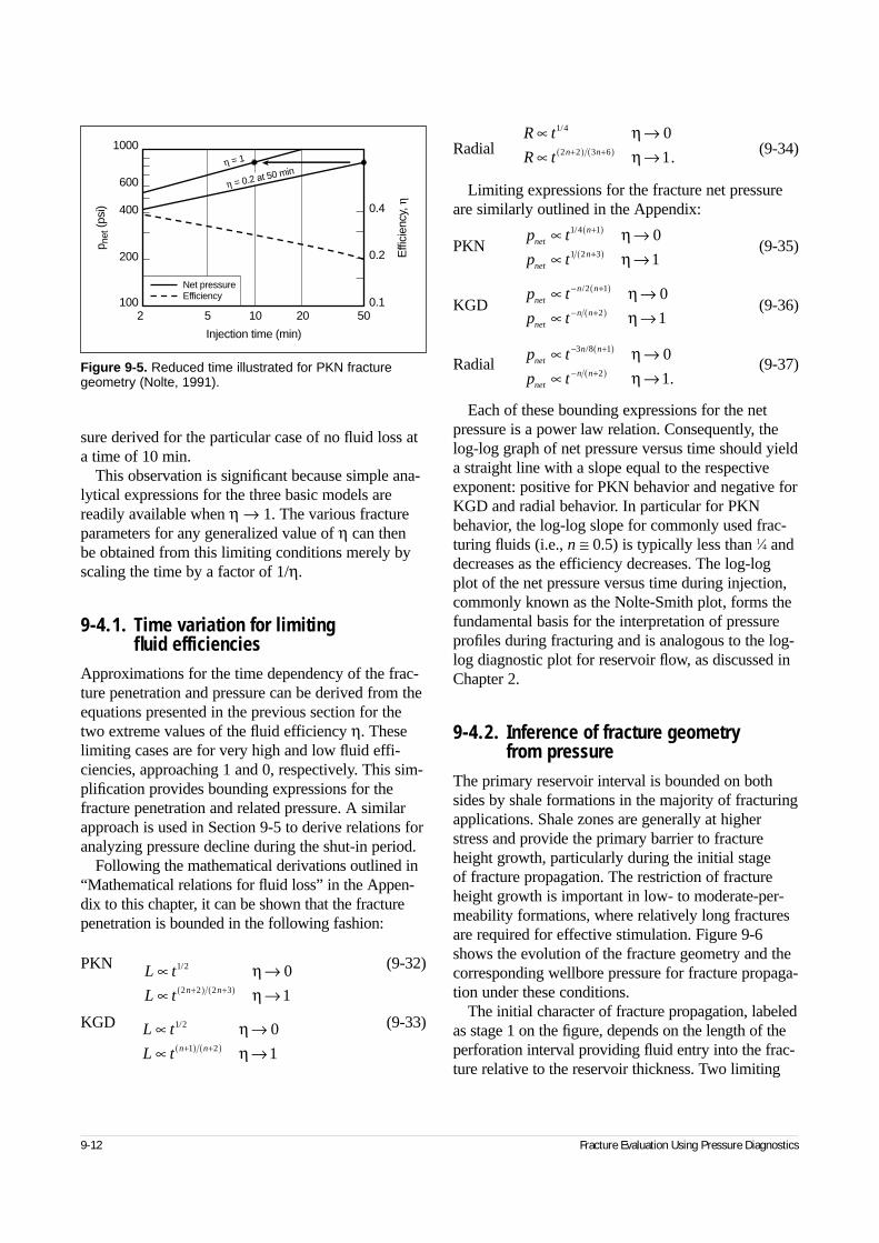
9-12 Fracture Evaluation Using Pressure Diagnostics

sure derived for the particular case of no fluid loss ata time of 10 min.

This observation is significant because simple ana-lytical expressions for the three basic models arereadily available when η → 1. The various fractureparameters for any generalized value of η can then be obtained from this limiting conditions merely byscaling the time by a factor of 1/η.

9-4.1. Time variation for limiting fluid efficiencies

Approximations for the time dependency of the frac-ture penetration and pressure can be derived from theequations presented in the previous section for thetwo extreme values of the fluid efficiency η. Theselimiting cases are for very high and low fluid effi-ciencies, approaching 1 and 0, respectively. This sim-plification provides bounding expressions for thefracture penetration and related pressure. A similarapproach is used in Section 9-5 to derive relations foranalyzing pressure decline during the shut-in period.

Following the mathematical derivations outlined in“Mathematical relations for fluid loss” in the Appen-dix to this chapter, it can be shown that the fracturepenetration is bounded in the following fashion:

PKN (9-32)

KGD (9-33)

Radial (9-34)

Limiting expressions for the fracture net pressureare similarly outlined in the Appendix:

PKN (9-35)

KGD (9-36)

Radial (9-37)

Each of these bounding expressions for the netpressure is a power law relation. Consequently, thelog-log graph of net pressure versus time should yielda straight line with a slope equal to the respectiveexponent: positive for PKN behavior and negative forKGD and radial behavior. In particular for PKNbehavior, the log-log slope for commonly used frac-turing fluids (i.e., n ≅ 0.5) is typically less than 1⁄4 anddecreases as the efficiency decreases. The log-logplot of the net pressure versus time during injection,commonly known as the Nolte-Smith plot, forms thefundamental basis for the interpretation of pressureprofiles during fracturing and is analogous to the log-log diagnostic plot for reservoir flow, as discussed inChapter 2.

9-4.2. Inference of fracture geometry from pressure

The primary reservoir interval is bounded on bothsides by shale formations in the majority of fracturingapplications. Shale zones are generally at higherstress and provide the primary barrier to fractureheight growth, particularly during the initial stage of fracture propagation. The restriction of fractureheight growth is important in low- to moderate-per-meability formations, where relatively long fracturesare required for effective stimulation. Figure 9-6shows the evolution of the fracture geometry and thecorresponding wellbore pressure for fracture propaga-tion under these conditions.

The initial character of fracture propagation, labeledas stage 1 on the figure, depends on the length of theperforation interval providing fluid entry into the frac-ture relative to the reservoir thickness. Two limiting

Figure 9-5. Reduced time illustrated for PKN fracturegeometry (Nolte, 1991).

1000

600

400

200

100

p net

(psi

) 0.4

0.2

0.1

Effi

cien

cy, η

2 5 10 20 50

Injection time (min)

η = 1

η = 0.2 at 50 min

Net pressureEfficiency

L t

L t n n

∝ →∝ →+( ) +( )

1 2

2 2 2 3

0

1

/ ηη

L t

L t n n

∝ →∝ →+( ) +( )

1 2

1 2

0

1

/ ηη

R t

R t n n

∝ →∝ →+( ) +( )

1 4

2 2 3 6

0

1

/

.

ηη

p t

p tnet

n

netn

∝ →∝ →

+( )

+( )

1 4 1

1 2 3

0

1

/ ηη

p t

p tnet

n n

netn n

∝ →∝ →

− +( )

− +( )

/2 1

2

0

1

ηη

p t

p tnet

n n

netn n

∝ →∝ →

− +( )

− +( )

3 8 1

2

0

1

/

.

ηη

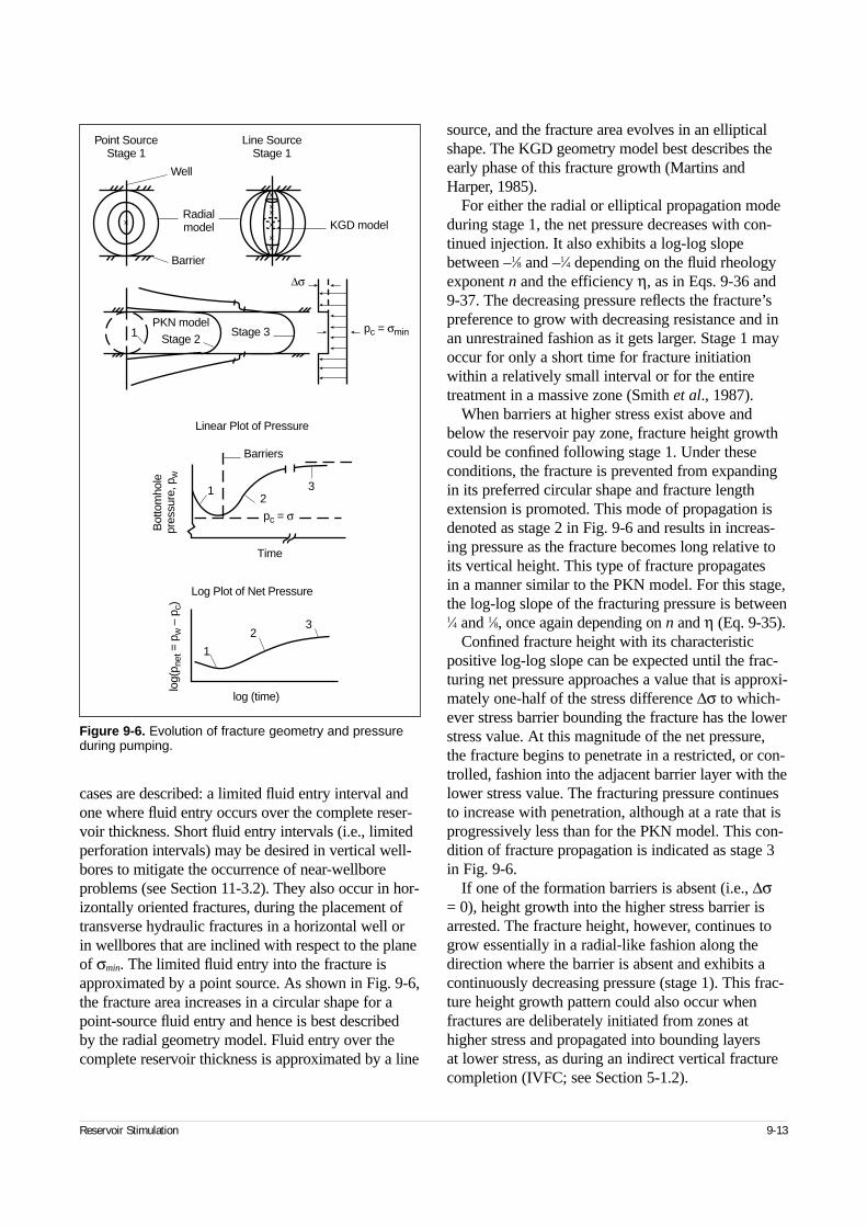
Reservoir Stimulation 9-13

cases are described: a limited fluid entry interval andone where fluid entry occurs over the complete reser-voir thickness. Short fluid entry intervals (i.e., limitedperforation intervals) may be desired in vertical well-bores to mitigate the occurrence of near-wellboreproblems (see Section 11-3.2). They also occur in hor-izontally oriented fractures, during the placement oftransverse hydraulic fractures in a horizontal well orin wellbores that are inclined with respect to the planeof σmin. The limited fluid entry into the fracture isapproximated by a point source. As shown in Fig. 9-6,the fracture area increases in a circular shape for apoint-source fluid entry and hence is best described by the radial geometry model. Fluid entry over thecomplete reservoir thickness is approximated by a line

source, and the fracture area evolves in an ellipticalshape. The KGD geometry model best describes theearly phase of this fracture growth (Martins andHarper, 1985).

For either the radial or elliptical propagation modeduring stage 1, the net pressure decreases with con-tinued injection. It also exhibits a log-log slopebetween –1⁄8 and –1⁄4 depending on the fluid rheologyexponent n and the efficiency η, as in Eqs. 9-36 and9-37. The decreasing pressure reflects the fracture’spreference to grow with decreasing resistance and inan unrestrained fashion as it gets larger. Stage 1 mayoccur for only a short time for fracture initiationwithin a relatively small interval or for the entiretreatment in a massive zone (Smith et al., 1987).

When barriers at higher stress exist above andbelow the reservoir pay zone, fracture height growthcould be confined following stage 1. Under theseconditions, the fracture is prevented from expandingin its preferred circular shape and fracture lengthextension is promoted. This mode of propagation isdenoted as stage 2 in Fig. 9-6 and results in increas-ing pressure as the fracture becomes long relative toits vertical height. This type of fracture propagates in a manner similar to the PKN model. For this stage,the log-log slope of the fracturing pressure is between1⁄4 and 1⁄8, once again depending on n and η (Eq. 9-35).

Confined fracture height with its characteristicpositive log-log slope can be expected until the frac-turing net pressure approaches a value that is approxi-mately one-half of the stress difference ∆σ to which-ever stress barrier bounding the fracture has the lowerstress value. At this magnitude of the net pressure,the fracture begins to penetrate in a restricted, or con-trolled, fashion into the adjacent barrier layer with thelower stress value. The fracturing pressure continuesto increase with penetration, although at a rate that isprogressively less than for the PKN model. This con-dition of fracture propagation is indicated as stage 3in Fig. 9-6.

If one of the formation barriers is absent (i.e., ∆σ= 0), height growth into the higher stress barrier isarrested. The fracture height, however, continues togrow essentially in a radial-like fashion along thedirection where the barrier is absent and exhibits acontinuously decreasing pressure (stage 1). This frac-ture height growth pattern could also occur whenfractures are deliberately initiated from zones athigher stress and propagated into bounding layers at lower stress, as during an indirect vertical fracturecompletion (IVFC; see Section 5-1.2).

Figure 9-6. Evolution of fracture geometry and pressureduring pumping.

+++++

+

+

Point SourceStage 1

Line SourceStage 1

Well

Barrier

PKN model

Radialmodel KGD model

1 Stage 3 pc = σmin

∆σ

32

1

Stage 2

Linear Plot of Pressure

Log Plot of Net Pressure

Barriers

1

23

Time

log (time)

Bot

tom

hole

pres

sure

, pw

log(

p net

= p

w–

p c)

pc = σ

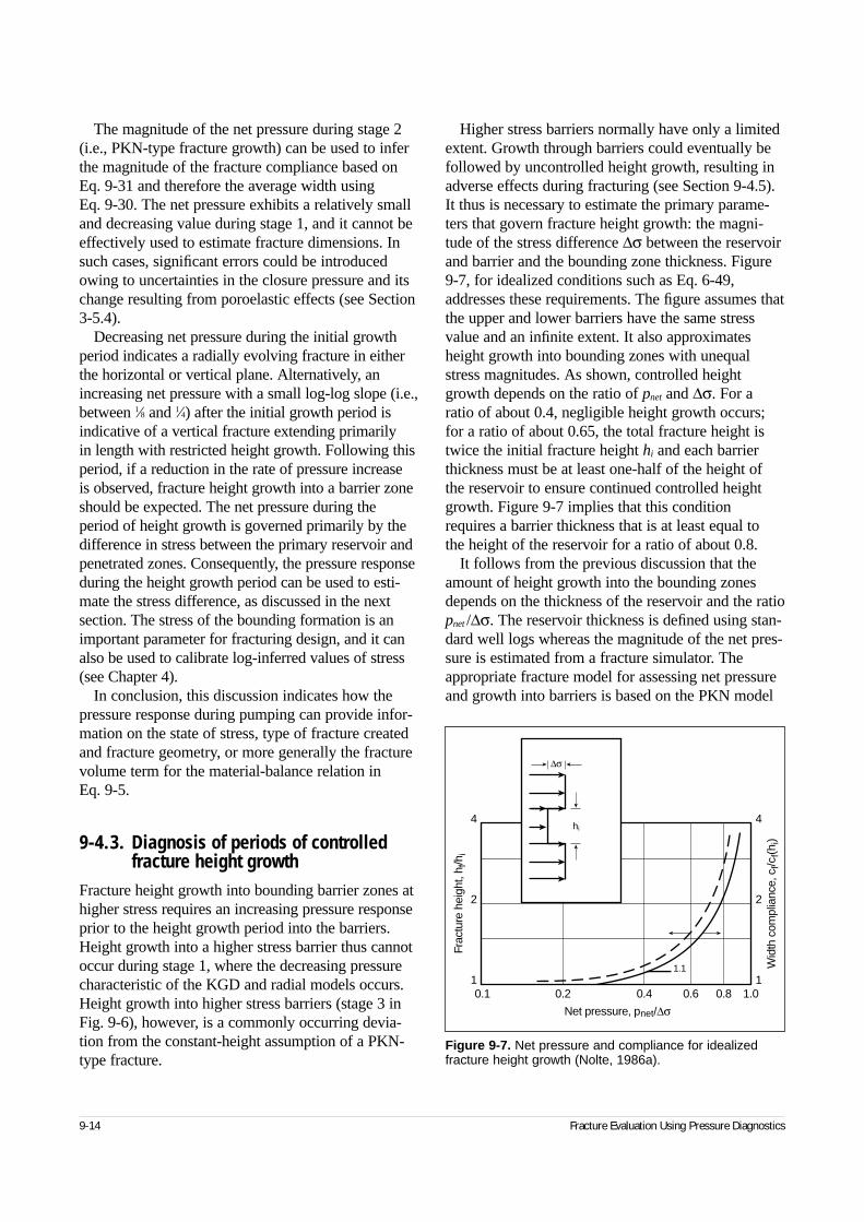
9-14 Fracture Evaluation Using Pressure Diagnostics

The magnitude of the net pressure during stage 2(i.e., PKN-type fracture growth) can be used to inferthe magnitude of the fracture compliance based onEq. 9-31 and therefore the average width using Eq. 9-30. The net pressure exhibits a relatively smalland decreasing value during stage 1, and it cannot beeffectively used to estimate fracture dimensions. Insuch cases, significant errors could be introducedowing to uncertainties in the closure pressure and itschange resulting from poroelastic effects (see Section3-5.4).

Decreasing net pressure during the initial growthperiod indicates a radially evolving fracture in eitherthe horizontal or vertical plane. Alternatively, anincreasing net pressure with a small log-log slope (i.e.,between 1⁄8 and 1⁄4) after the initial growth period isindicative of a vertical fracture extending primarily in length with restricted height growth. Following thisperiod, if a reduction in the rate of pressure increase is observed, fracture height growth into a barrier zoneshould be expected. The net pressure during theperiod of height growth is governed primarily by thedifference in stress between the primary reservoir andpenetrated zones. Consequently, the pressure responseduring the height growth period can be used to esti-mate the stress difference, as discussed in the nextsection. The stress of the bounding formation is animportant parameter for fracturing design, and it canalso be used to calibrate log-inferred values of stress(see Chapter 4).

In conclusion, this discussion indicates how thepressure response during pumping can provide infor-mation on the state of stress, type of fracture createdand fracture geometry, or more generally the fracturevolume term for the material-balance relation in Eq. 9-5.

9-4.3. Diagnosis of periods of controlled fracture height growth

Fracture height growth into bounding barrier zones athigher stress requires an increasing pressure responseprior to the height growth period into the barriers.Height growth into a higher stress barrier thus cannotoccur during stage 1, where the decreasing pressurecharacteristic of the KGD and radial models occurs.Height growth into higher stress barriers (stage 3 inFig. 9-6), however, is a commonly occurring devia-tion from the constant-height assumption of a PKN-type fracture.

Higher stress barriers normally have only a limitedextent. Growth through barriers could eventually befollowed by uncontrolled height growth, resulting inadverse effects during fracturing (see Section 9-4.5).It thus is necessary to estimate the primary parame-ters that govern fracture height growth: the magni-tude of the stress difference ∆σ between the reservoirand barrier and the bounding zone thickness. Figure9-7, for idealized conditions such as Eq. 6-49,addresses these requirements. The figure assumes thatthe upper and lower barriers have the same stressvalue and an infinite extent. It also approximatesheight growth into bounding zones with unequalstress magnitudes. As shown, controlled heightgrowth depends on the ratio of pnet and ∆σ. For aratio of about 0.4, negligible height growth occurs;for a ratio of about 0.65, the total fracture height istwice the initial fracture height hi and each barrierthickness must be at least one-half of the height ofthe reservoir to ensure continued controlled heightgrowth. Figure 9-7 implies that this conditionrequires a barrier thickness that is at least equal to the height of the reservoir for a ratio of about 0.8.

It follows from the previous discussion that theamount of height growth into the bounding zonesdepends on the thickness of the reservoir and the ratiopnet /∆σ. The reservoir thickness is defined using stan-dard well logs whereas the magnitude of the net pres-sure is estimated from a fracture simulator. Theappropriate fracture model for assessing net pressureand growth into barriers is based on the PKN model

Figure 9-7. Net pressure and compliance for idealizedfracture height growth (Nolte, 1986a).

1.1

4

2

1

4

2

1

Frac

ture

hei

ght,

h f/h

i

Wid

th c

ompl

ianc

e, c

f/cf(h

i)

Net pressure, pnet/∆σ0.1 0.2 0.4 0.6 0.8 1.0

∆σ

hi

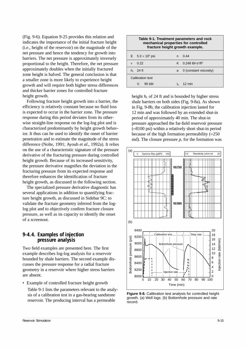
Reservoir Stimulation 9-15

(Fig. 9-6). Equation 9-25 provides this relation andindicates the importance of the initial fracture height(i.e., height of the reservoir) on the magnitude of thenet pressure and hence the tendency for growth intobarriers. The net pressure is approximately inverselyproportional to the height. Therefore, the net pressureapproximately doubles when the initially fracturedzone height is halved. The general conclusion is thata smaller zone is more likely to experience heightgrowth and will require both higher stress differencesand thicker barrier zones for controlled fractureheight growth.

Following fracture height growth into a barrier, theefficiency is relatively constant because no fluid lossis expected to occur in the barrier zone. The pressureresponse during this period deviates from its other-wise straight-line response on the log-log plot and ischaracterized predominantly by height growth behav-ior. It thus can be used to identify the onset of barrierpenetration and to estimate the magnitude of the stressdifference (Nolte, 1991; Ayoub et al., 1992a). It relieson the use of a characteristic signature of the pressurederivative of the fracturing pressure during controlledheight growth. Because of its increased sensitivity,the pressure derivative magnifies the deviation in thefracturing pressure from its expected response andtherefore enhances the identification of fractureheight growth, as discussed in the following section.

The specialized pressure derivative diagnostic hasseveral applications in addition to quantifying frac-ture height growth, as discussed in Sidebar 9C: tovalidate the fracture geometry inferred from the log-log plot and to objectively confirm fracture closurepressure, as well as its capacity to identify the onsetof a screenout.

9-4.4. Examples of injection pressure analysis

Two field examples are presented here. The firstexample describes log-log analysis for a reservoirbounded by shale barriers. The second example dis-cusses the pressure response for a radial fracturegeometry in a reservoir where higher stress barriersare absent.

• Example of controlled fracture height growth

Table 9-1 lists the parameters relevant to the analy-sis of a calibration test in a gas-bearing sandstonereservoir. The producing interval has a permeable

height hL of 24 ft and is bounded by higher stressshale barriers on both sides (Fig. 9-8a). As shownin Fig. 9-8b, the calibration injection lasted for 12 min and was followed by an extended shut-inperiod of approximately 40 min. The shut-inpressure approached the far-field reservoir pressure(≈8100 psi) within a relatively short shut-in periodbecause of the high formation permeability (≈250md). The closure pressure pc for the formation was

Table 9-1. Treatment parameters and rock mechanical properties for controlled

fracture height growth example.

E 5.3 × 105 psi n 0.44

ν 0.22 K 0.248 lbf-sn/ft2

hL 24 ft a 0 (constant viscosity)

Calibration test

Vi 95 bbl tp 12 min

Figure 9-8. Calibration test analysis for controlled heightgrowth. (a) Well logs. (b) Bottomhole pressure and raterecord.

(a)

(b)

Calibration test Step rate

9400

9200

9000

8800

8600

8400

8200

80000 10 20 30 40 50 60 70 80 90 100

181614121086420

20

Bot

tom

hole

pre

ssur

e (p

si)

Inje

ctio

n ra

te (

bbl/m

in)

Time (min)

Injection rate

Bottomhole pressure

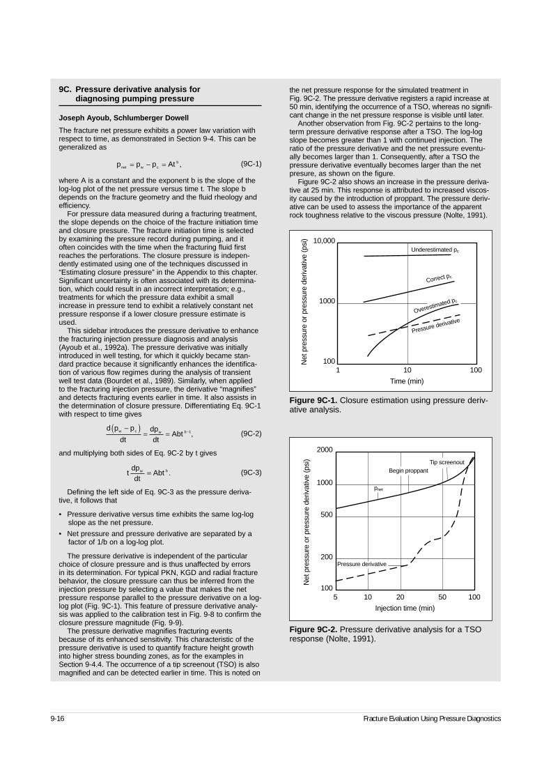
9-16 Fracture Evaluation Using Pressure Diagnostics

9C. Pressure derivative analysis for diagnosing pumping pressure

Joseph Ayoub, Schlumberger Dowell

The fracture net pressure exhibits a power law variation withrespect to time, as demonstrated in Section 9-4. This can begeneralized as

(9C-1)

where A is a constant and the exponent b is the slope of thelog-log plot of the net pressure versus time t. The slope bdepends on the fracture geometry and the fluid rheology andefficiency.

For pressure data measured during a fracturing treatment,the slope depends on the choice of the fracture initiation timeand closure pressure. The fracture initiation time is selectedby examining the pressure record during pumping, and itoften coincides with the time when the fracturing fluid firstreaches the perforations. The closure pressure is indepen-dently estimated using one of the techniques discussed in“Estimating closure pressure” in the Appendix to this chapter.Significant uncertainty is often associated with its determina-tion, which could result in an incorrect interpretation; e.g.,treatments for which the pressure data exhibit a smallincrease in pressure tend to exhibit a relatively constant netpressure response if a lower closure pressure estimate isused.

This sidebar introduces the pressure derivative to enhancethe fracturing injection pressure diagnosis and analysis(Ayoub et al., 1992a). The pressure derivative was initiallyintroduced in well testing, for which it quickly became stan-dard practice because it significantly enhances the identifica-tion of various flow regimes during the analysis of transientwell test data (Bourdet et al., 1989). Similarly, when applied to the fracturing injection pressure, the derivative “magnifies”and detects fracturing events earlier in time. It also assists inthe determination of closure pressure. Differentiating Eq. 9C-1with respect to time gives

(9C-2)

and multiplying both sides of Eq. 9C-2 by t gives

(9C-3)

Defining the left side of Eq. 9C-3 as the pressure deriva-tive, it follows that

• Pressure derivative versus time exhibits the same log-logslope as the net pressure.

• Net pressure and pressure derivative are separated by afactor of 1/b on a log-log plot.

The pressure derivative is independent of the particularchoice of closure pressure and is thus unaffected by errors in its determination. For typical PKN, KGD and radial fracturebehavior, the closure pressure can thus be inferred from theinjection pressure by selecting a value that makes the netpressure response parallel to the pressure derivative on a log-log plot (Fig. 9C-1). This feature of pressure derivative analy-sis was applied to the calibration test in Fig. 9-8 to confirm theclosure pressure magnitude (Fig. 9-9).

The pressure derivative magnifies fracturing eventsbecause of its enhanced sensitivity. This characteristic of thepressure derivative is used to quantify fracture height growthinto higher stress bounding zones, as for the examples inSection 9-4.4. The occurrence of a tip screenout (TSO) is alsomagnified and can be detected earlier in time. This is noted on

the net pressure response for the simulated treatment in Fig. 9C-2. The pressure derivative registers a rapid increase at50 min, identifying the occurrence of a TSO, whereas no signifi-cant change in the net pressure response is visible until later.

Another observation from Fig. 9C-2 pertains to the long-term pressure derivative response after a TSO. The log-logslope becomes greater than 1 with continued injection. Theratio of the pressure derivative and the net pressure eventu-ally becomes larger than 1. Consequently, after a TSO thepressure derivative eventually becomes larger than the netpresure, as shown on the figure.

Figure 9C-2 also shows an increase in the pressure deriva-tive at 25 min. This response is attributed to increased viscos-ity caused by the introduction of proppant. The pressure deriv-ative can be used to assess the importance of the apparentrock toughness relative to the viscous pressure (Nolte, 1991).

p p p Atnet w cb= − = ,

d p p

dtdpdt

Abtw c w b−( )

= = −1,

tdpdt

Abtw b= .

Figure 9C-1. Closure estimation using pressure deriv-ative analysis.

10,000

1000

100Net

pre

ssur

e or

pre

ssur

e de

rivat

ive

(psi

)

1 10 100

Time (min)

Underestimated pc

Correct pc

Overestimated pc

Pressure derivative

Figure 9C-2. Pressure derivative analysis for a TSOresponse (Nolte, 1991).

2000

1000

500

200

100

Net

pre

ssur

e or

pre

ssur

e de

rivat

ive

(psi

)

5 10 20 50 100

Injection time (min)

Tip screenoutBegin proppant

pnet

Pressure derivative

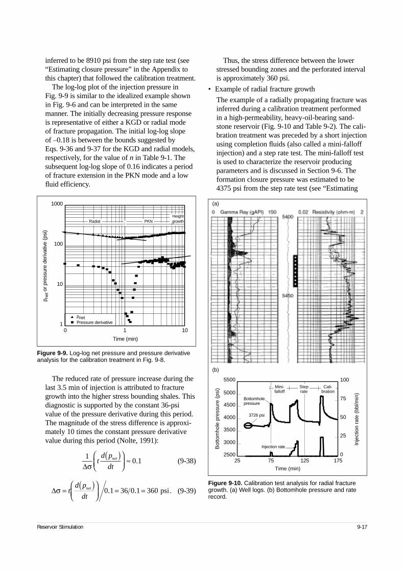
Reservoir Stimulation 9-17

inferred to be 8910 psi from the step rate test (see“Estimating closure pressure” in the Appendix tothis chapter) that followed the calibration treatment.

The log-log plot of the injection pressure in Fig. 9-9 is similar to the idealized example shownin Fig. 9-6 and can be interpreted in the samemanner. The initially decreasing pressure responseis representative of either a KGD or radial mode of fracture propagation. The initial log-log slope of –0.18 is between the bounds suggested by Eqs. 9-36 and 9-37 for the KGD and radial models,respectively, for the value of n in Table 9-1. Thesubsequent log-log slope of 0.16 indicates a periodof fracture extension in the PKN mode and a lowfluid efficiency.

The reduced rate of pressure increase during thelast 3.5 min of injection is attributed to fracturegrowth into the higher stress bounding shales. Thisdiagnostic is supported by the constant 36-psivalue of the pressure derivative during this period.The magnitude of the stress difference is approxi-mately 10 times the constant pressure derivativevalue during this period (Nolte, 1991):

(9-38)

(9-39)

Thus, the stress difference between the lowerstressed bounding zones and the perforated intervalis approximately 360 psi.

• Example of radial fracture growth

The example of a radially propagating fracture wasinferred during a calibration treatment performedin a high-permeability, heavy-oil-bearing sand-stone reservoir (Fig. 9-10 and Table 9-2). The cali-bration treatment was preceded by a short injectionusing completion fluids (also called a mini-falloffinjection) and a step rate test. The mini-falloff testis used to characterize the reservoir producingparameters and is discussed in Section 9-6. Theformation closure pressure was estimated to be4375 psi from the step rate test (see “Estimating

10 1

∆σt

d p

dtnet( )

≈ .

∆σ = ( )

= =td p

dtnet 0 1 36 0 1 360. . psi.

Figure 9-9. Log-log net pressure and pressure derivativeanalysis for the calibration treatment in Fig. 9-8.

1000

100

10

1

p net

or p

ress

ure

deriv

ativ

e (p

si)

0 1 10

Time (min)

pnetPressure derivative

PKNHeightgrowthRadial

Figure 9-10. Calibration test analysis for radial fracturegrowth. (a) Well logs. (b) Bottomhole pressure and raterecord.

Cali-bration

Mini-falloff

Steprate

5500

5000

4500

4000

3500

3000

250025 75 125 175

100

75

50

25

0

Bot

tom

hole

pre

ssur

e (p

si)

Inje

ctio

n ra

te (

bbl/m

in)

Time (min)

Injection rate

3726 psi

Bottomholepressure

(a)

(b)

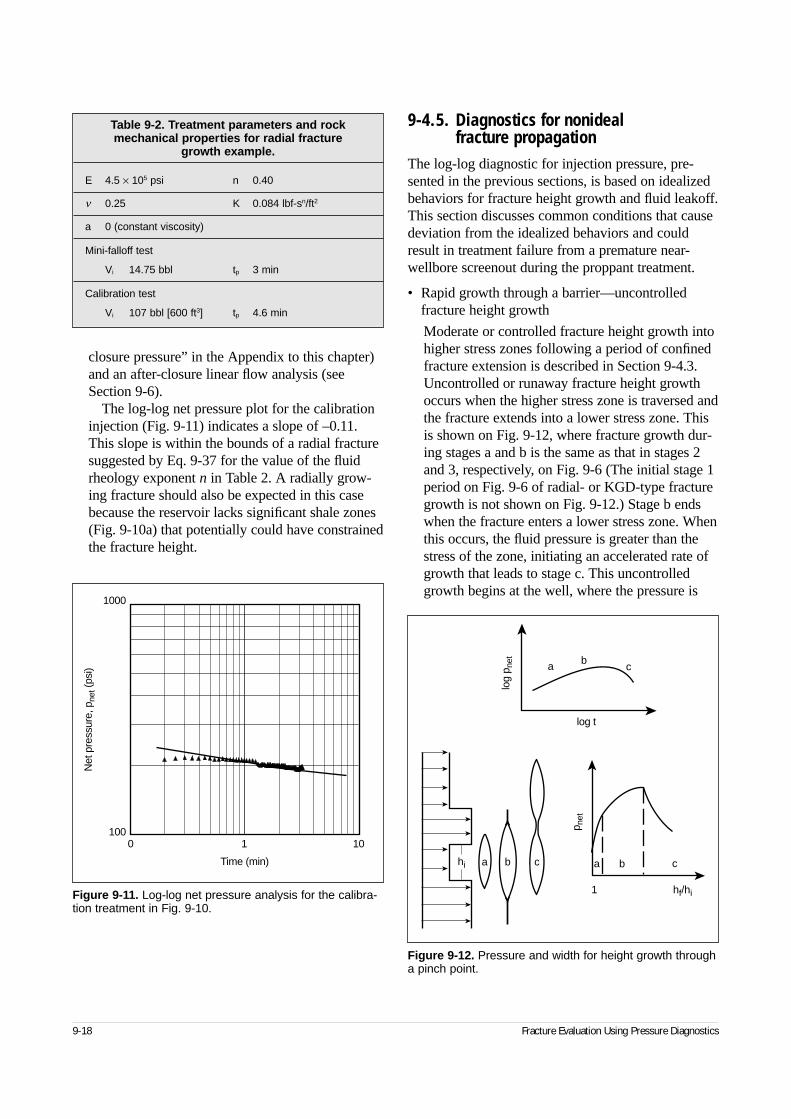
9-18 Fracture Evaluation Using Pressure Diagnostics

closure pressure” in the Appendix to this chapter)and an after-closure linear flow analysis (seeSection 9-6).

The log-log net pressure plot for the calibrationinjection (Fig. 9-11) indicates a slope of –0.11.This slope is within the bounds of a radial fracturesuggested by Eq. 9-37 for the value of the fluidrheology exponent n in Table 2. A radially grow-ing fracture should also be expected in this casebecause the reservoir lacks significant shale zones(Fig. 9-10a) that potentially could have constrainedthe fracture height.

9-4.5. Diagnostics for nonideal fracture propagation

The log-log diagnostic for injection pressure, pre-sented in the previous sections, is based on idealizedbehaviors for fracture height growth and fluid leakoff.This section discusses common conditions that causedeviation from the idealized behaviors and couldresult in treatment failure from a premature near-wellbore screenout during the proppant treatment.

• Rapid growth through a barrier—uncontrolledfracture height growth

Moderate or controlled fracture height growth intohigher stress zones following a period of confinedfracture extension is described in Section 9-4.3.Uncontrolled or runaway fracture height growthoccurs when the higher stress zone is traversed andthe fracture extends into a lower stress zone. Thisis shown on Fig. 9-12, where fracture growth dur-ing stages a and b is the same as that in stages 2and 3, respectively, on Fig. 9-6 (The initial stage 1period on Fig. 9-6 of radial- or KGD-type fracturegrowth is not shown on Fig. 9-12.) Stage b endswhen the fracture enters a lower stress zone. Whenthis occurs, the fluid pressure is greater than thestress of the zone, initiating an accelerated rate ofgrowth that leads to stage c. This uncontrolledgrowth begins at the well, where the pressure is

Table 9-2. Treatment parameters and rock mechanical properties for radial fracture

growth example.

E 4.5 × 105 psi n 0.40

ν 0.25 K 0.084 lbf-sn/ft2

a 0 (constant viscosity)

Mini-falloff test

Vi 14.75 bbl tp 3 min

Calibration test

Vi 107 bbl [600 ft3] tp 4.6 min

Figure 9-11. Log-log net pressure analysis for the calibra-tion treatment in Fig. 9-10.

1000

100

Net

pre

ssur

e, p

net (

psi)

0 1 10

Time (min)

Figure 9-12. Pressure and width for height growth througha pinch point.

log t

log

p net

a bc

hf/hi

hi

1

p net

aa b c b c

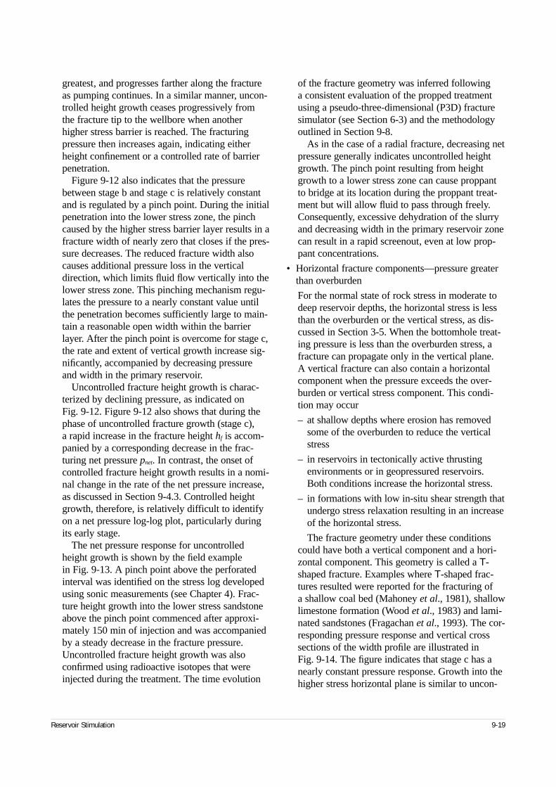
Reservoir Stimulation 9-19

greatest, and progresses farther along the fractureas pumping continues. In a similar manner, uncon-trolled height growth ceases progressively fromthe fracture tip to the wellbore when anotherhigher stress barrier is reached. The fracturingpressure then increases again, indicating eitherheight confinement or a controlled rate of barrierpenetration.

Figure 9-12 also indicates that the pressurebetween stage b and stage c is relatively constantand is regulated by a pinch point. During the initialpenetration into the lower stress zone, the pinchcaused by the higher stress barrier layer results in afracture width of nearly zero that closes if the pres-sure decreases. The reduced fracture width alsocauses additional pressure loss in the verticaldirection, which limits fluid flow vertically into thelower stress zone. This pinching mechanism regu-lates the pressure to a nearly constant value untilthe penetration becomes sufficiently large to main-tain a reasonable open width within the barrierlayer. After the pinch point is overcome for stage c,the rate and extent of vertical growth increase sig-nificantly, accompanied by decreasing pressureand width in the primary reservoir.

Uncontrolled fracture height growth is charac-terized by declining pressure, as indicated on Fig. 9-12. Figure 9-12 also shows that during thephase of uncontrolled fracture growth (stage c), a rapid increase in the fracture height hf is accom-panied by a corresponding decrease in the frac-turing net pressure pnet. In contrast, the onset ofcontrolled fracture height growth results in a nomi-nal change in the rate of the net pressure increase,as discussed in Section 9-4.3. Controlled heightgrowth, therefore, is relatively difficult to identifyon a net pressure log-log plot, particularly duringits early stage.

The net pressure response for uncontrolledheight growth is shown by the field example in Fig. 9-13. A pinch point above the perforatedinterval was identified on the stress log developedusing sonic measurements (see Chapter 4). Frac-ture height growth into the lower stress sandstoneabove the pinch point commenced after approxi-mately 150 min of injection and was accompaniedby a steady decrease in the fracture pressure.Uncontrolled fracture height growth was alsoconfirmed using radioactive isotopes that wereinjected during the treatment. The time evolution

of the fracture geometry was inferred following a consistent evaluation of the propped treatmentusing a pseudo-three-dimensional (P3D) fracturesimulator (see Section 6-3) and the methodologyoutlined in Section 9-8.

As in the case of a radial fracture, decreasing netpressure generally indicates uncontrolled heightgrowth. The pinch point resulting from heightgrowth to a lower stress zone can cause proppantto bridge at its location during the proppant treat-ment but will allow fluid to pass through freely.Consequently, excessive dehydration of the slurryand decreasing width in the primary reservoir zonecan result in a rapid screenout, even at low prop-pant concentrations.

• Horizontal fracture components—pressure greaterthan overburden

For the normal state of rock stress in moderate todeep reservoir depths, the horizontal stress is lessthan the overburden or the vertical stress, as dis-cussed in Section 3-5. When the bottomhole treat-ing pressure is less than the overburden stress, afracture can propagate only in the vertical plane. A vertical fracture can also contain a horizontalcomponent when the pressure exceeds the over-burden or vertical stress component. This condi-tion may occur

– at shallow depths where erosion has removedsome of the overburden to reduce the verticalstress

– in reservoirs in tectonically active thrustingenvironments or in geopressured reservoirs.Both conditions increase the horizontal stress.

– in formations with low in-situ shear strength thatundergo stress relaxation resulting in an increaseof the horizontal stress.

The fracture geometry under these conditionscould have both a vertical component and a hori-zontal component. This geometry is called a T-shaped fracture. Examples where T-shaped frac-tures resulted were reported for the fracturing of a shallow coal bed (Mahoney et al., 1981), shallowlimestone formation (Wood et al., 1983) and lami-nated sandstones (Fragachan et al., 1993). The cor-responding pressure response and vertical crosssections of the width profile are illustrated in Fig. 9-14. The figure indicates that stage c has anearly constant pressure response. Growth into thehigher stress horizontal plane is similar to uncon-

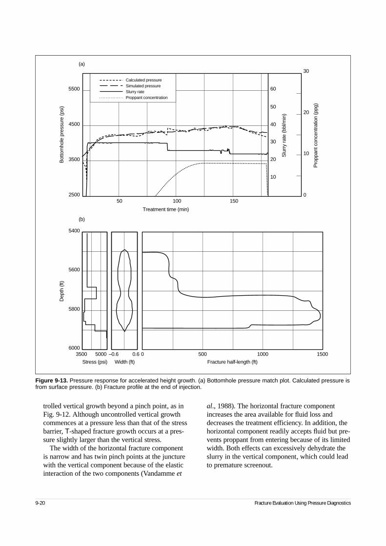
9-20 Fracture Evaluation Using Pressure Diagnostics

trolled vertical growth beyond a pinch point, as inFig. 9-12. Although uncontrolled vertical growthcommences at a pressure less than that of the stressbarrier, T-shaped fracture growth occurs at a pres-sure slightly larger than the vertical stress.

The width of the horizontal fracture componentis narrow and has twin pinch points at the juncturewith the vertical component because of the elasticinteraction of the two components (Vandamme et

al., 1988). The horizontal fracture componentincreases the area available for fluid loss anddecreases the treatment efficiency. In addition, thehorizontal component readily accepts fluid but pre-vents proppant from entering because of its limitedwidth. Both effects can excessively dehydrate theslurry in the vertical component, which could leadto premature screenout.

Figure 9-13. Pressure response for accelerated height growth. (a) Bottomhole pressure match plot. Calculated pressure isfrom surface pressure. (b) Fracture profile at the end of injection.

3500 5000 –0.6 0.6 0 500

Fracture half-length (ft)Width (ft)Stress (psi)

1000 1500

50 100 150

Treatment time (min)

2500

5400

5600

5800

6000

3500

4500

5500

10

20

30

40

50

60

10

0

20

30

Slu

rry

rate

(bbl

/min

)

Pro

ppan

t con

cent

ratio

n (p

pg)

Calculated pressureSimulated pressureSlurry rateProppant concentration

Bot

tom

hole

pre

ssur

e (p

si)

Dep

th (f

t)(a)

(b)

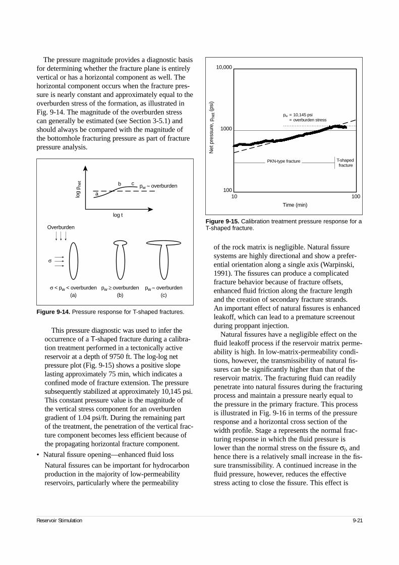
Reservoir Stimulation 9-21

The pressure magnitude provides a diagnostic basisfor determining whether the fracture plane is entirelyvertical or has a horizontal component as well. Thehorizontal component occurs when the fracture pres-sure is nearly constant and approximately equal to theoverburden stress of the formation, as illustrated inFig. 9-14. The magnitude of the overburden stresscan generally be estimated (see Section 3-5.1) andshould always be compared with the magnitude ofthe bottomhole fracturing pressure as part of fracturepressure analysis.

This pressure diagnostic was used to infer theoccurrence of a T-shaped fracture during a calibra-tion treatment performed in a tectonically activereservoir at a depth of 9750 ft. The log-log netpressure plot (Fig. 9-15) shows a positive slopelasting approximately 75 min, which indicates aconfined mode of fracture extension. The pressuresubsequently stabilized at approximately 10,145 psi.This constant pressure value is the magnitude ofthe vertical stress component for an overburdengradient of 1.04 psi/ft. During the remaining part of the treatment, the penetration of the vertical frac-ture component becomes less efficient because ofthe propagating horizontal fracture component.

• Natural fissure opening—enhanced fluid loss

Natural fissures can be important for hydrocarbonproduction in the majority of low-permeabilityreservoirs, particularly where the permeability

of the rock matrix is negligible. Natural fissuresystems are highly directional and show a prefer-ential orientation along a single axis (Warpinski,1991). The fissures can produce a complicatedfracture behavior because of fracture offsets,enhanced fluid friction along the fracture lengthand the creation of secondary fracture strands. An important effect of natural fissures is enhancedleakoff, which can lead to a premature screenoutduring proppant injection.

Natural fissures have a negligible effect on thefluid leakoff process if the reservoir matrix perme-ability is high. In low-matrix-permeability condi-tions, however, the transmissibility of natural fis-sures can be significantly higher than that of thereservoir matrix. The fracturing fluid can readilypenetrate into natural fissures during the fracturingprocess and maintain a pressure nearly equal tothe pressure in the primary fracture. This processis illustrated in Fig. 9-16 in terms of the pressureresponse and a horizontal cross section of thewidth profile. Stage a represents the normal frac-turing response in which the fluid pressure islower than the normal stress on the fissure σf, andhence there is a relatively small increase in the fis-sure transmissibility. A continued increase in thefluid pressure, however, reduces the effectivestress acting to close the fissure. This effect is

Figure 9-14. Pressure response for T-shaped fractures.

σ < pw < overburden(a)

pw ≥ overburden(b)

pw ≈ overburden(c)

pw ≈ overburden

log t

log

p net

a

b c

Overburden

σ

Figure 9-15. Calibration treatment pressure response for aT-shaped fracture.

10,000

1000

100

Net

pre

ssur

e, p

net (

psi)

pw = 10,145 psi= overburden stress

10 100

Time (min)

PKN-type fracture T-shaped fracture

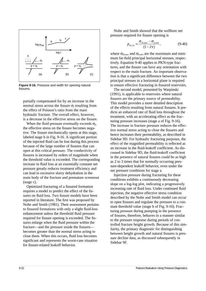
9-22 Fracture Evaluation Using Pressure Diagnostics

partially compensated for by an increase in thenormal stress across the fissure σf resulting fromthe effect of Poisson’s ratio from the mainhydraulic fracture. The overall effect, however, is a decrease in the effective stress on the fissure.

When the fluid pressure eventually exceeds σf,the effective stress on the fissure becomes nega-tive. The fissure mechanically opens at this stage,labeled stage b in Fig. 9-16. A significant portionof the injected fluid can be lost during this processbecause of the large number of fissures that canopen at this critical pressure. The conductivity offissures is increased by orders of magnitude whenthe threshold value is exceeded. The correspondingincrease in fluid loss at an essentially constant netpressure greatly reduces treatment efficiency andcan lead to excessive slurry dehydration in themain body of the fracture and premature screenout(stage c).

Optimized fracturing of a fissured formationrequires a model to predict the effect of the fis-sures on fluid loss. Two fissure models have beenreported in literature. The first was proposed byNolte and Smith (1981). Their assessment pertainsto fissured formations with only a slight fluid-lossenhancement unless the threshold fluid pressurerequired for fissure opening is exceeded. The fis-sures enlarge when the fluid pressure within thefracture—and the pressure inside the fissures—becomes greater than the normal stress acting toclose them. When this occurs, fluid loss becomessignificant and represents the worst-case situationfor fissure-related leakoff behavior.

Nolte and Smith showed that the wellbore netpressure required for fissure opening is

(9-40)

where σH,max and σh,min are the maximum and mini-mum far-field principal horizontal stresses, respec-tively. Equation 9-40 applies to PKN-type frac-tures, and the fissure can have any orientation withrespect to the main fracture. An important observa-tion is that a significant difference between the twoprincipal stresses in a horizontal plane is requiredto ensure effective fracturing in fissured reservoirs.

The second model, presented by Warpinski(1991), is applicable to reservoirs where naturalfissures are the primary source of permeability.This model provides a more detailed description of the effects resulting from natural fissures. It pre-dicts an enhanced rate of fluid loss throughout thetreatment, with an accelerating effect as the frac-turing pressure increases (stage a of Fig. 9-16).The increase in fracture pressure reduces the effec-tive normal stress acting to close the fissures andhence increases their permeability, as described inSidebar 9D. For hydraulic fracturing purposes, theeffect of the magnified permeability is reflected asan increase in the fluid-leakoff coefficient. As dis-cussed in Sidebar 9D, the fluid-leakoff coefficientin the presence of natural fissures could be as highas 2 to 3 times that for normally occurring pres-sure-dependent leakoff behavior, even under thenet pressure conditions for stage a.

Injection pressure during fracturing for theseconditions exhibits a continuously decreasingslope on a log-log plot, indicating a progressivelyincreasing rate of fluid loss. Under continued fluidinjection, the negative effective stress conditiondescribed by the Nolte and Smith model can occurto open fissures and regulate the pressure to a con-stant threshold value (stage b of Fig. 9-16). Frac-turing pressure during pumping in the presence of fissures, therefore, behaves in a manner similarto the pressure response during periods of con-trolled fracture height growth. Because of this sim-ilarity, the primary diagnostic for distinguishingbetween height growth and natural fissures is pres-sure decline data, as discussed subsequently inSidebar 9F.

Figure 9-16. Pressure and width for opening natural fissures.

a

(a) (b) (c)

b

log t

log pnet

σf

σ

p < σf p ≈ σf p > σf

c

σf

pnet foH max h min

,, , ,=

−−( )

σ σν1 2

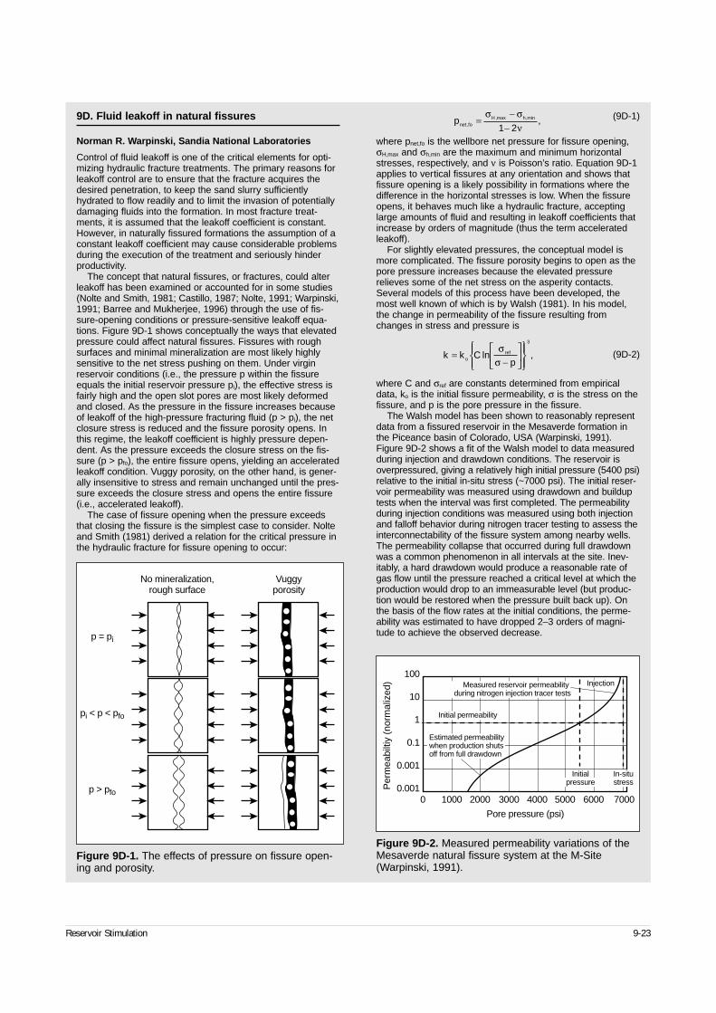
Reservoir Stimulation 9-23

9D. Fluid leakoff in natural fissures

Norman R. Warpinski, Sandia National Laboratories

Control of fluid leakoff is one of the critical elements for opti-mizing hydraulic fracture treatments. The primary reasons forleakoff control are to ensure that the fracture acquires thedesired penetration, to keep the sand slurry sufficientlyhydrated to flow readily and to limit the invasion of potentiallydamaging fluids into the formation. In most fracture treat-ments, it is assumed that the leakoff coefficient is constant.However, in naturally fissured formations the assumption of aconstant leakoff coefficient may cause considerable problemsduring the execution of the treatment and seriously hinderproductivity.

The concept that natural fissures, or fractures, could alterleakoff has been examined or accounted for in some studies(Nolte and Smith, 1981; Castillo, 1987; Nolte, 1991; Warpinski,1991; Barree and Mukherjee, 1996) through the use of fis-sure-opening conditions or pressure-sensitive leakoff equa-tions. Figure 9D-1 shows conceptually the ways that elevatedpressure could affect natural fissures. Fissures with roughsurfaces and minimal mineralization are most likely highlysensitive to the net stress pushing on them. Under virginreservoir conditions (i.e., the pressure p within the fissureequals the initial reservoir pressure pi), the effective stress isfairly high and the open slot pores are most likely deformedand closed. As the pressure in the fissure increases becauseof leakoff of the high-pressure fracturing fluid (p > pi), the netclosure stress is reduced and the fissure porosity opens. Inthis regime, the leakoff coefficient is highly pressure depen-dent. As the pressure exceeds the closure stress on the fis-sure (p > pfo), the entire fissure opens, yielding an acceleratedleakoff condition. Vuggy porosity, on the other hand, is gener-ally insensitive to stress and remain unchanged until the pres-sure exceeds the closure stress and opens the entire fissure(i.e., accelerated leakoff).

The case of fissure opening when the pressure exceedsthat closing the fissure is the simplest case to consider. Nolteand Smith (1981) derived a relation for the critical pressure inthe hydraulic fracture for fissure opening to occur:

(9D-1)

where pnet,fo is the wellbore net pressure for fissure opening,σH,max and σh,min are the maximum and minimum horizontalstresses, respectively, and ν is Poisson’s ratio. Equation 9D-1applies to vertical fissures at any orientation and shows thatfissure opening is a likely possibility in formations where thedifference in the horizontal stresses is low. When the fissureopens, it behaves much like a hydraulic fracture, acceptinglarge amounts of fluid and resulting in leakoff coefficients thatincrease by orders of magnitude (thus the term acceleratedleakoff).

For slightly elevated pressures, the conceptual model ismore complicated. The fissure porosity begins to open as thepore pressure increases because the elevated pressurerelieves some of the net stress on the asperity contacts.Several models of this process have been developed, themost well known of which is by Walsh (1981). In his model,the change in permeability of the fissure resulting fromchanges in stress and pressure is

(9D-2)

where C and σref are constants determined from empiricaldata, ko is the initial fissure permeability, σ is the stress on thefissure, and p is the pore pressure in the fissure.

The Walsh model has been shown to reasonably representdata from a fissured reservoir in the Mesaverde formation inthe Piceance basin of Colorado, USA (Warpinski, 1991). Figure 9D-2 shows a fit of the Walsh model to data measuredduring injection and drawdown conditions. The reservoir isoverpressured, giving a relatively high initial pressure (5400 psi)relative to the initial in-situ stress (~7000 psi). The initial reser-voir permeability was measured using drawdown and builduptests when the interval was first completed. The permeabilityduring injection conditions was measured using both injectionand falloff behavior during nitrogen tracer testing to assess theinterconnectability of the fissure system among nearby wells.The permeability collapse that occurred during full drawdownwas a common phenomenon in all intervals at the site. Inev-itably, a hard drawdown would produce a reasonable rate ofgas flow until the pressure reached a critical level at which theproduction would drop to an immeasurable level (but produc-tion would be restored when the pressure built back up). Onthe basis of the flow rates at the initial conditions, the perme-ability was estimated to have dropped 2–3 orders of magni-tude to achieve the observed decrease.

pnet foH max h min

,, , ,=

−−

σ σν1 2

k k Cpo

ref=−

ln ,

σσ

3

Figure 9D-2. Measured permeability variations of theMesaverde natural fissure system at the M-Site(Warpinski, 1991).

Figure 9D-1. The effects of pressure on fissure open-ing and porosity.

100

10

1

0.1

0.001

0.001Per

mea

bilti

y (n

orm

aliz

ed)

0 1000 2000 3000 4000 5000 6000 7000

Pore pressure (psi)

In-situstress

Initialpressure

Initial permeability

Measured reservoir permeability during nitrogen injection tracer tests

Estimated permeabilitywhen production shutsoff from full drawdown

Injection

No mineralization,rough surface

Vuggyporosity

p = pi

pi < p < pfo

p > pfo

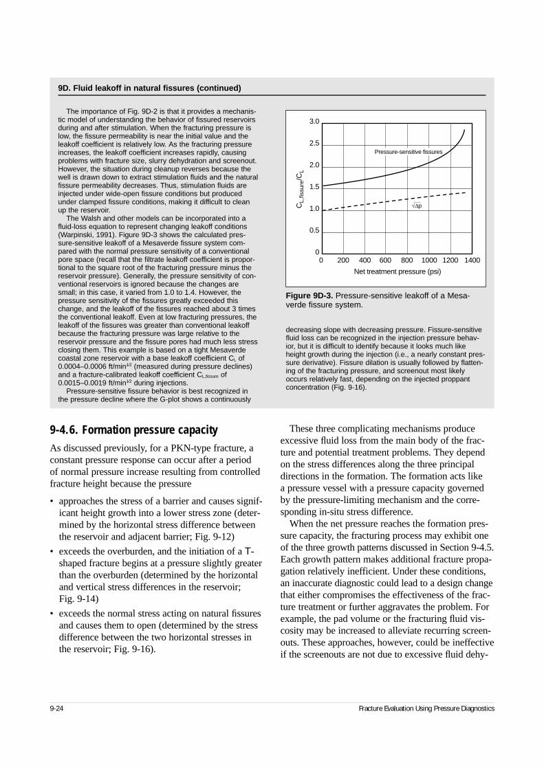
9-24 Fracture Evaluation Using Pressure Diagnostics

9-4.6. Formation pressure capacityAs discussed previously, for a PKN-type fracture, aconstant pressure response can occur after a period of normal pressure increase resulting from controlledfracture height because the pressure

• approaches the stress of a barrier and causes signif-icant height growth into a lower stress zone (deter-mined by the horizontal stress difference betweenthe reservoir and adjacent barrier; Fig. 9-12)

• exceeds the overburden, and the initiation of a T-shaped fracture begins at a pressure slightly greaterthan the overburden (determined by the horizontaland vertical stress differences in the reservoir; Fig. 9-14)

• exceeds the normal stress acting on natural fissuresand causes them to open (determined by the stressdifference between the two horizontal stresses inthe reservoir; Fig. 9-16).

These three complicating mechanisms produceexcessive fluid loss from the main body of the frac-ture and potential treatment problems. They dependon the stress differences along the three principaldirections in the formation. The formation acts like a pressure vessel with a pressure capacity governedby the pressure-limiting mechanism and the corre-sponding in-situ stress difference.

When the net pressure reaches the formation pres-sure capacity, the fracturing process may exhibit oneof the three growth patterns discussed in Section 9-4.5.Each growth pattern makes additional fracture propa-gation relatively inefficient. Under these conditions,an inaccurate diagnostic could lead to a design changethat either compromises the effectiveness of the frac-ture treatment or further aggravates the problem. Forexample, the pad volume or the fracturing fluid vis-cosity may be increased to alleviate recurring screen-outs. These approaches, however, could be ineffectiveif the screenouts are not due to excessive fluid dehy-

The importance of Fig. 9D-2 is that it provides a mechanis-tic model of understanding the behavior of fissured reservoirsduring and after stimulation. When the fracturing pressure islow, the fissure permeability is near the initial value and theleakoff coefficient is relatively low. As the fracturing pressureincreases, the leakoff coefficient increases rapidly, causingproblems with fracture size, slurry dehydration and screenout.However, the situation during cleanup reverses because thewell is drawn down to extract stimulation fluids and the naturalfissure permeability decreases. Thus, stimulation fluids areinjected under wide-open fissure conditions but producedunder clamped fissure conditions, making it difficult to cleanup the reservoir.

The Walsh and other models can be incorporated into afluid-loss equation to represent changing leakoff conditions(Warpinski, 1991). Figure 9D-3 shows the calculated pres-sure-sensitive leakoff of a Mesaverde fissure system com-pared with the normal pressure sensitivity of a conventionalpore space (recall that the filtrate leakoff coefficient is propor-tional to the square root of the fracturing pressure minus thereservoir pressure). Generally, the pressure sensitivity of con-ventional reservoirs is ignored because the changes aresmall; in this case, it varied from 1.0 to 1.4. However, thepressure sensitivity of the fissures greatly exceeded thischange, and the leakoff of the fissures reached about 3 timesthe conventional leakoff. Even at low fracturing pressures, theleakoff of the fissures was greater than conventional leakoffbecause the fracturing pressure was large relative to thereservoir pressure and the fissure pores had much less stressclosing them. This example is based on a tight Mesaverdecoastal zone reservoir with a base leakoff coefficient CL of0.0004–0.0006 ft/min1⁄2 (measured during pressure declines)and a fracture-calibrated leakoff coefficient CL,fissure of0.0015–0.0019 ft/min1⁄2 during injections.

Pressure-sensitive fissure behavior is best recognized inthe pressure decline where the G-plot shows a continuously

decreasing slope with decreasing pressure. Fissure-sensitivefluid loss can be recognized in the injection pressure behav-ior, but it is difficult to identify because it looks much likeheight growth during the injection (i.e., a nearly constant pres-sure derivative). Fissure dilation is usually followed by flatten-ing of the fracturing pressure, and screenout most likelyoccurs relatively fast, depending on the injected proppantconcentration (Fig. 9-16).

Figure 9D-3. Pressure-sensitive leakoff of a Mesa-verde fissure system.

3.0

2.5

2.0

1.5

1.0

0.5

0

CL,

fissu

re/C

L

0 200 400 600 800 1000 1200 1400

Net treatment pressure (psi)

√∆p

Pressure-sensitive fissures

9D. Fluid leakoff in natural fissures (continued)

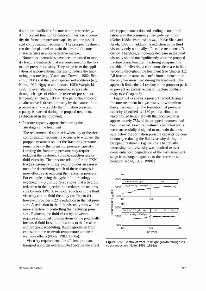
Reservoir Stimulation 9-25

dration or insufficient fracture width, respectively. An important function of calibration tests is to iden-tify the formation pressure capacity and the associ-ated complicating mechanism. The propped treatmentcan then be planned to attain the desired fracturecharacteristics in a cost-effective manner.

Numerous alternatives have been proposed to mod-ify fracture treatments that are constrained by the for-mation pressure capacity. They range from the appli-cation of unconventional designs to reduce the frac-turing pressure (e.g., Veatch and Crowell, 1982; Brittet al., 1994) and the use of specialized additives (e.g.,Nolte, 1982; Nguyen and Larson, 1983; Warpinski,1990) to even altering the reservoir stress statethrough changes of either the reservoir pressure ortemperature (Cleary, 1980a). The particular choice ofan alternative is driven primarily by the nature of theproblem and how quickly the formation pressurecapacity is reached during the propped treatment, as discussed in the following.

• Pressure capacity approached during the late stage of the treatment

The recommended approach when any of the threecomplicating mechanisms occurs is to engineer thepropped treatment so that the fracturing pressureremains below the formation pressure capacity.Limiting the fracturing pressure may requirereducing the treatment volume, injection rate orfluid viscosity. The pressure relation for the PKNfracture geometry in Eq. 9-25 provides an assess-ment for determining which of these changes ismost effective at reducing the fracturing pressure.For example, using the typical fluid rheologyexponent n = 0.5 in Eq. 9-25 shows that a twofoldreduction in the injection rate reduces the net pres-sure by only 11%. A twofold reduction in the fluidviscosity (or the fluid rheology coefficient K),however, provides a 22% reduction in the net pres-sure. A reduction in the fluid viscosity thus will bemore effective in controlling the fracturing pres-sure. Reducing the fluid viscosity, however,requires additional considerations of the potentiallyincreased fluid loss, modifications to the breakerand proppant scheduling, fluid degradation fromexposure to the reservoir temperature and near-wellbore effects (Nolte, 1982, 1988a).

Viscosity requirements for efficient proppanttransport are often overestimated because the effect

of proppant convection and settling is not a limi-tation with the commonly used polymer fluids(Nolte, 1988a; Warpinski et al., 1998a; Shah andAsadi, 1998). In addition, a reduction in the fluidviscosity only nominally affects the treatment effi-ciency. Therefore, a moderate decrease in the fluidviscosity should not significantly alter the proppedfracture characteristics. Fracturing equipment iscapable of delivering a continuous decrease in fluidviscosity throughout the treatment (see Chapter 11).All fracture treatments benefit from a reduction inthe polymer mass used during the treatment. Thisapproach limits the gel residue in the proppant packto prevent an excessive loss of fracture conduc-tivity (see Chapter 8).

Figure 9-17a shows a pressure record during afracture treatment in a gas reservoir with micro-darcy permeability. The formation net pressurecapacity identified as 1180 psi is attributed touncontrolled height growth that occurred afterapproximately 75% of the propped treatment hadbeen injected. Fracture treatments on offset wellswere successfully designed to maintain the pres-sure below the formation pressure capacity by con-tinuously reducing the fluid viscosity during theproppant treatment (Fig. 9-17b). The initiallyincreasing fluid viscosity was required to over-come enhanced degradation of the early treatmentstage from longer exposure to the reservoir tem-perature (Nolte, 1982, 1988a).

Figure 9-17. Control of fracture height growth through vis-cosity reduction (Nolte, 1982, 1988a).

Time (min)

10 100 1000

2000

1000

500

Gel (lbm/1000 gal) 60 50 40 30

10 100 1000

2000

1000

500

(a)

(b)

Gel (lbm/1000 gal) 60

pnet capacity = 1180 psi

Net

pre

ssur

e, p

net (

psi)

pnet capacity = 1180 psi

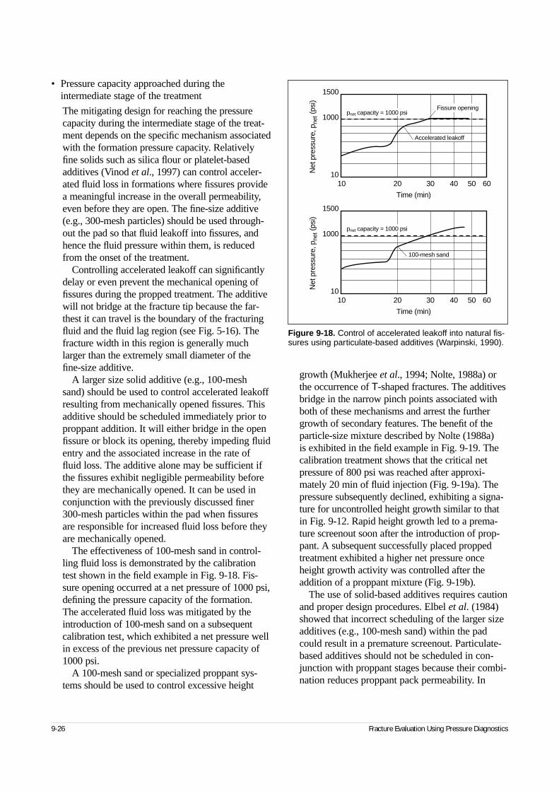
9-26 Fracture Evaluation Using Pressure Diagnostics

• Pressure capacity approached during theintermediate stage of the treatment

The mitigating design for reaching the pressurecapacity during the intermediate stage of the treat-ment depends on the specific mechanism associatedwith the formation pressure capacity. Relativelyfine solids such as silica flour or platelet-basedadditives (Vinod et al., 1997) can control acceler-ated fluid loss in formations where fissures providea meaningful increase in the overall permeability,even before they are open. The fine-size additive(e.g., 300-mesh particles) should be used through-out the pad so that fluid leakoff into fissures, andhence the fluid pressure within them, is reducedfrom the onset of the treatment.

Controlling accelerated leakoff can significantlydelay or even prevent the mechanical opening offissures during the propped treatment. The additivewill not bridge at the fracture tip because the far-thest it can travel is the boundary of the fracturingfluid and the fluid lag region (see Fig. 5-16). Thefracture width in this region is generally muchlarger than the extremely small diameter of thefine-size additive.

A larger size solid additive (e.g., 100-meshsand) should be used to control accelerated leakoffresulting from mechanically opened fissures. Thisadditive should be scheduled immediately prior toproppant addition. It will either bridge in the openfissure or block its opening, thereby impeding fluidentry and the associated increase in the rate offluid loss. The additive alone may be sufficient ifthe fissures exhibit negligible permeability beforethey are mechanically opened. It can be used inconjunction with the previously discussed finer300-mesh particles within the pad when fissuresare responsible for increased fluid loss before theyare mechanically opened.

The effectiveness of 100-mesh sand in control-ling fluid loss is demonstrated by the calibrationtest shown in the field example in Fig. 9-18. Fis-sure opening occurred at a net pressure of 1000 psi,defining the pressure capacity of the formation. The accelerated fluid loss was mitigated by theintroduction of 100-mesh sand on a subsequentcalibration test, which exhibited a net pressure wellin excess of the previous net pressure capacity of1000 psi.

A 100-mesh sand or specialized proppant sys-tems should be used to control excessive height

growth (Mukherjee et al., 1994; Nolte, 1988a) orthe occurrence of T-shaped fractures. The additivesbridge in the narrow pinch points associated withboth of these mechanisms and arrest the furthergrowth of secondary features. The benefit of theparticle-size mixture described by Nolte (1988a) is exhibited in the field example in Fig. 9-19. Thecalibration treatment shows that the critical netpressure of 800 psi was reached after approxi-mately 20 min of fluid injection (Fig. 9-19a). Thepressure subsequently declined, exhibiting a signa-ture for uncontrolled height growth similar to thatin Fig. 9-12. Rapid height growth led to a prema-ture screenout soon after the introduction of prop-pant. A subsequent successfully placed proppedtreatment exhibited a higher net pressure onceheight growth activity was controlled after theaddition of a proppant mixture (Fig. 9-19b).

The use of solid-based additives requires cautionand proper design procedures. Elbel et al. (1984)showed that incorrect scheduling of the larger sizeadditives (e.g., 100-mesh sand) within the padcould result in a premature screenout. Particulate-based additives should not be scheduled in con-junction with proppant stages because their combi-nation reduces proppant pack permeability. In

Figure 9-18. Control of accelerated leakoff into natural fis-sures using particulate-based additives (Warpinski, 1990).

Time (min)

10 20 30 40 50 60

1500

1000

10Net

pre

ssur

e, p

net (

psi)

Time (min)

10 20 30 40 50 60

1500

1000

10Net

pre

ssur

e, p

net (

psi)

Fissure openingpnet capacity = 1000 psi

pnet capacity = 1000 psi

Accelerated leakoff

100-mesh sand

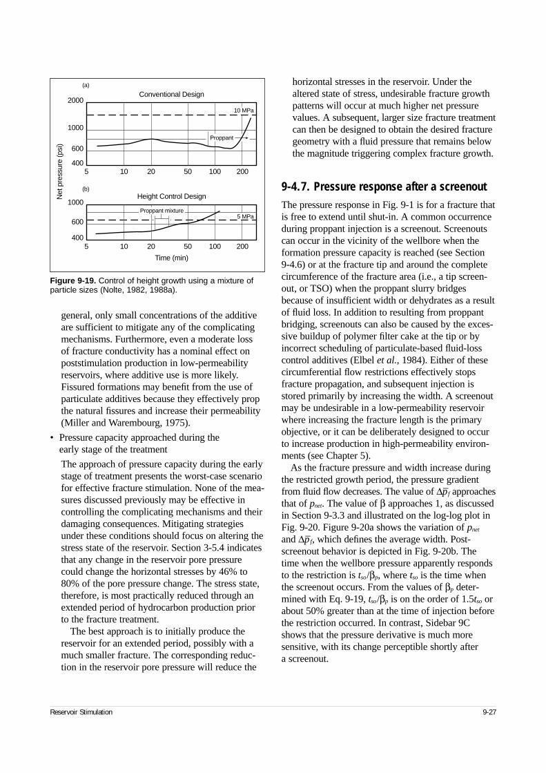
Reservoir Stimulation 9-27

general, only small concentrations of the additiveare sufficient to mitigate any of the complicatingmechanisms. Furthermore, even a moderate loss of fracture conductivity has a nominal effect onpoststimulation production in low-permeabilityreservoirs, where additive use is more likely.Fissured formations may benefit from the use ofparticulate additives because they effectively propthe natural fissures and increase their permeability(Miller and Warembourg, 1975).

• Pressure capacity approached during the early stage of the treatment

The approach of pressure capacity during the earlystage of treatment presents the worst-case scenariofor effective fracture stimulation. None of the mea-sures discussed previously may be effective incontrolling the complicating mechanisms and theirdamaging consequences. Mitigating strategiesunder these conditions should focus on altering thestress state of the reservoir. Section 3-5.4 indicatesthat any change in the reservoir pore pressurecould change the horizontal stresses by 46% to80% of the pore pressure change. The stress state,therefore, is most practically reduced through anextended period of hydrocarbon production priorto the fracture treatment.

The best approach is to initially produce thereservoir for an extended period, possibly with amuch smaller fracture. The corresponding reduc-tion in the reservoir pore pressure will reduce the

horizontal stresses in the reservoir. Under thealtered state of stress, undesirable fracture growthpatterns will occur at much higher net pressurevalues. A subsequent, larger size fracture treatmentcan then be designed to obtain the desired fracturegeometry with a fluid pressure that remains belowthe magnitude triggering complex fracture growth.

9-4.7. Pressure response after a screenoutThe pressure response in Fig. 9-1 is for a fracture thatis free to extend until shut-in. A common occurrenceduring proppant injection is a screenout. Screenoutscan occur in the vicinity of the wellbore when theformation pressure capacity is reached (see Section 9-4.6) or at the fracture tip and around the completecircumference of the fracture area (i.e., a tip screen-out, or TSO) when the proppant slurry bridgesbecause of insufficient width or dehydrates as a resultof fluid loss. In addition to resulting from proppantbridging, screenouts can also be caused by the exces-sive buildup of polymer filter cake at the tip or byincorrect scheduling of particulate-based fluid-losscontrol additives (Elbel et al., 1984). Either of thesecircumferential flow restrictions effectively stopsfracture propagation, and subsequent injection isstored primarily by increasing the width. A screenoutmay be undesirable in a low-permeability reservoirwhere increasing the fracture length is the primaryobjective, or it can be deliberately designed to occurto increase production in high-permeability environ-ments (see Chapter 5).

As the fracture pressure and width increase duringthe restricted growth period, the pressure gradientfrom fluid flow decreases. The value of ∆p–f approachesthat of pnet. The value of β approaches 1, as discussedin Section 9-3.3 and illustrated on the log-log plot inFig. 9-20. Figure 9-20a shows the variation of pnet

and ∆p–f, which defines the average width. Post-screenout behavior is depicted in Fig. 9-20b. Thetime when the wellbore pressure apparently respondsto the restriction is tso/βp, where tso is the time whenthe screenout occurs. From the values of βp deter-mined with Eq. 9-19, tso/βp is on the order of 1.5tso orabout 50% greater than at the time of injection beforethe restriction occurred. In contrast, Sidebar 9Cshows that the pressure derivative is much moresensitive, with its change perceptible shortly after a screenout.

Figure 9-19. Control of height growth using a mixture ofparticle sizes (Nolte, 1982, 1988a).

Conventional Design

Height Control Design

Time (min)

5 10 20 50 100 200

5 10 20 50 100 200

Proppant

Proppant mixture

10 MPa

5 MPa

2000

1000

600

400

1000

600

400

Net

pre

ssur

e (p

si)

(a)

(b)

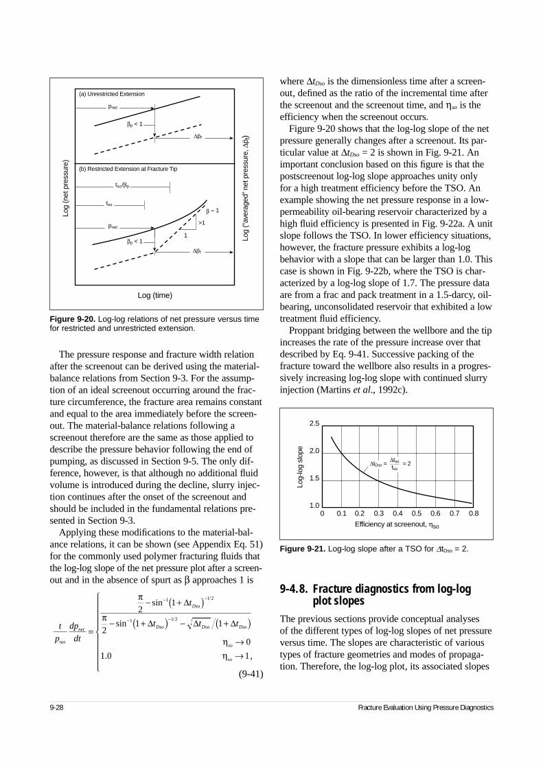
9-28 Fracture Evaluation Using Pressure Diagnostics

The pressure response and fracture width relationafter the screenout can be derived using the material-balance relations from Section 9-3. For the assump-tion of an ideal screenout occurring around the frac-ture circumference, the fracture area remains constantand equal to the area immediately before the screen-out. The material-balance relations following ascreenout therefore are the same as those applied todescribe the pressure behavior following the end ofpumping, as discussed in Section 9-5. The only dif-ference, however, is that although no additional fluidvolume is introduced during the decline, slurry injec-tion continues after the onset of the screenout andshould be included in the fundamental relations pre-sented in Section 9-3.

Applying these modifications to the material-bal-ance relations, it can be shown (see Appendix Eq. 51)for the commonly used polymer fracturing fluids thatthe log-log slope of the net pressure plot after a screen-out and in the absence of spurt as β approaches 1 is

(9-41)

where ∆tDso is the dimensionless time after a screen-out, defined as the ratio of the incremental time afterthe screenout and the screenout time, and ηso is theefficiency when the screenout occurs.

Figure 9-20 shows that the log-log slope of the netpressure generally changes after a screenout. Its par-ticular value at ∆tDso = 2 is shown in Fig. 9-21. Animportant conclusion based on this figure is that thepostscreenout log-log slope approaches unity only for a high treatment efficiency before the TSO. Anexample showing the net pressure response in a low-permeability oil-bearing reservoir characterized by ahigh fluid efficiency is presented in Fig. 9-22a. A unitslope follows the TSO. In lower efficiency situations,however, the fracture pressure exhibits a log-logbehavior with a slope that can be larger than 1.0. Thiscase is shown in Fig. 9-22b, where the TSO is char-acterized by a log-log slope of 1.7. The pressure dataare from a frac and pack treatment in a 1.5-darcy, oil-bearing, unconsolidated reservoir that exhibited a lowtreatment fluid efficiency.

Proppant bridging between the wellbore and the tipincreases the rate of the pressure increase over thatdescribed by Eq. 9-41. Successive packing of thefracture toward the wellbore also results in a progres-sively increasing log-log slope with continued slurryinjection (Martins et al., 1992c).

9-4.8. Fracture diagnostics from log-log plot slopes

The previous sections provide conceptual analyses of the different types of log-log slopes of net pressureversus time. The slopes are characteristic of varioustypes of fracture geometries and modes of propaga-tion. Therefore, the log-log plot, its associated slopes

Figure 9-20. Log-log relations of net pressure versus timefor restricted and unrestricted extension.

Log

(net

pre

ssur

e)

Log (time)

Log

(“av

erag

ed” n

et p

ress

ure,

∆p f

)

(b) Restricted Extension at Fracture Tip

(a) Unrestricted Extension

pnet

pnet

tso

tso/βp

β ≈ 1

>1

1

∆pf

∆pf

βp < 1

βp < 1

t

p

dp

dt

t

t t t

net

net

Dso

Dso Dso Dso

so

so

=

− +( )− +( ) − +( )

→→

− −

− −

π

π

ηη

21

21 1

0

1 0 1

1 1 2

1 1 2

sin

sin

. ,

/

/

∆

∆ ∆ ∆

Figure 9-21. Log-log slope after a TSO for ∆tDso = 2.

2.5

2.0

1.5

1.0

Log-

log

slop

e

0 0.1 0.2 0.3 0.4 0.5 0.6 0.7 0.8

Efficiency at screenout, ηso

∆tDso = = 2∆tso

tso

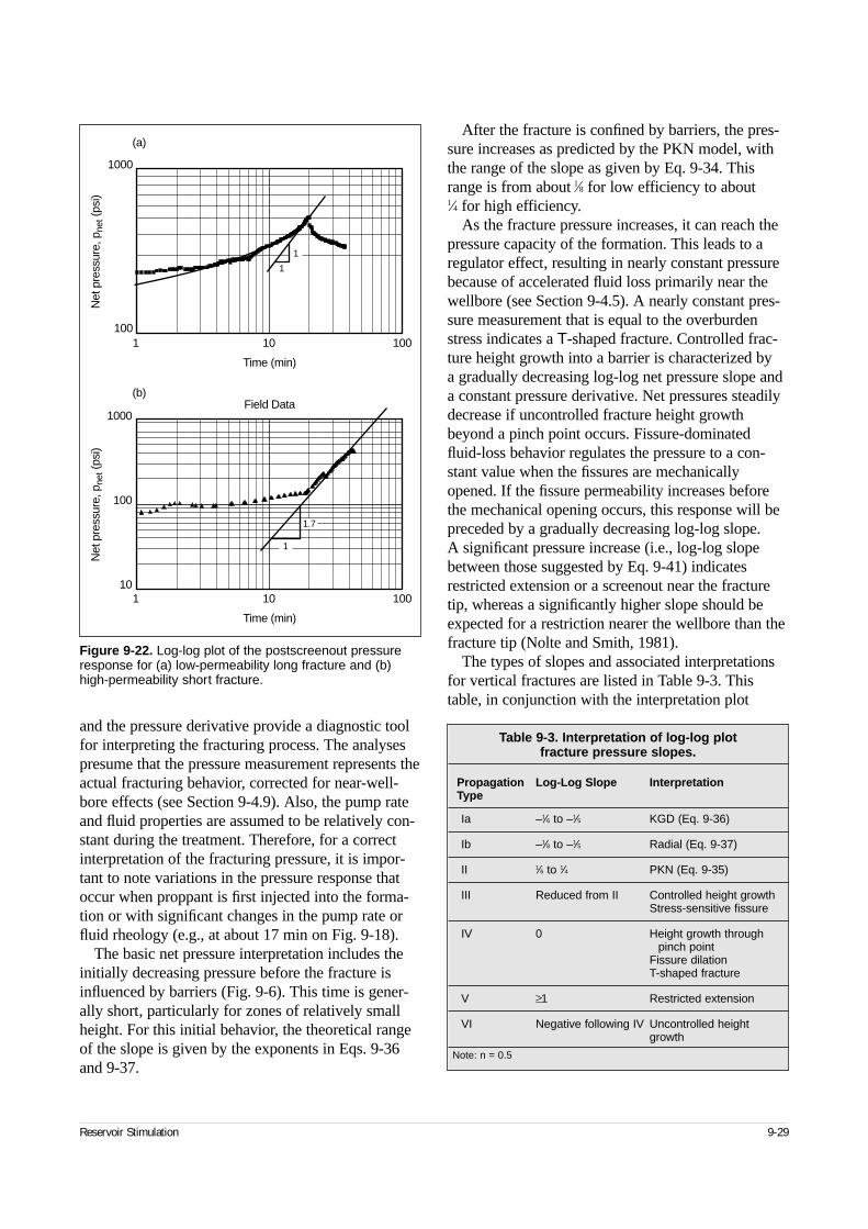
Reservoir Stimulation 9-29

and the pressure derivative provide a diagnostic toolfor interpreting the fracturing process. The analysespresume that the pressure measurement represents theactual fracturing behavior, corrected for near-well-bore effects (see Section 9-4.9). Also, the pump rateand fluid properties are assumed to be relatively con-stant during the treatment. Therefore, for a correctinterpretation of the fracturing pressure, it is impor-tant to note variations in the pressure response thatoccur when proppant is first injected into the forma-tion or with significant changes in the pump rate orfluid rheology (e.g., at about 17 min on Fig. 9-18).

The basic net pressure interpretation includes theinitially decreasing pressure before the fracture isinfluenced by barriers (Fig. 9-6). This time is gener-ally short, particularly for zones of relatively smallheight. For this initial behavior, the theoretical rangeof the slope is given by the exponents in Eqs. 9-36and 9-37.

After the fracture is confined by barriers, the pres-sure increases as predicted by the PKN model, withthe range of the slope as given by Eq. 9-34. Thisrange is from about l⁄8 for low efficiency to about 1⁄4 for high efficiency.

As the fracture pressure increases, it can reach thepressure capacity of the formation. This leads to aregulator effect, resulting in nearly constant pressurebecause of accelerated fluid loss primarily near thewellbore (see Section 9-4.5). A nearly constant pres-sure measurement that is equal to the overburdenstress indicates a T-shaped fracture. Controlled frac-ture height growth into a barrier is characterized by a gradually decreasing log-log net pressure slope anda constant pressure derivative. Net pressures steadilydecrease if uncontrolled fracture height growthbeyond a pinch point occurs. Fissure-dominatedfluid-loss behavior regulates the pressure to a con-stant value when the fissures are mechanicallyopened. If the fissure permeability increases beforethe mechanical opening occurs, this response will bepreceded by a gradually decreasing log-log slope. A significant pressure increase (i.e., log-log slopebetween those suggested by Eq. 9-41) indicatesrestricted extension or a screenout near the fracturetip, whereas a significantly higher slope should beexpected for a restriction nearer the wellbore than thefracture tip (Nolte and Smith, 1981).

The types of slopes and associated interpretationsfor vertical fractures are listed in Table 9-3. Thistable, in conjunction with the interpretation plot

Figure 9-22. Log-log plot of the postscreenout pressureresponse for (a) low-permeability long fracture and (b)high-permeability short fracture.

1000

100

10

Net

pre

ssur

e, p

net (

psi)

1000

100

Net

pre

ssur

e, p

net (

psi)

1 10 100

Time (min)

1 10 100

Time (min)

Field Data(b)

(a)

1

1

1

1.7

Table 9-3. Interpretation of log-log plot fracture pressure slopes.

Propagation Log-Log Slope InterpretationType

Ia –1⁄6 to –1⁄5 KGD (Eq. 9-36)

Ib –1⁄8 to –1⁄5 Radial (Eq. 9-37)

II 1⁄6 to 1⁄4 PKN (Eq. 9-35)

III Reduced from II Controlled height growthStress-sensitive fissure

IV 0 Height growth through pinch point

Fissure dilationT-shaped fracture

V ≥1 Restricted extension

VI Negative following IV Uncontrolled height growth

Note: n = 0.5

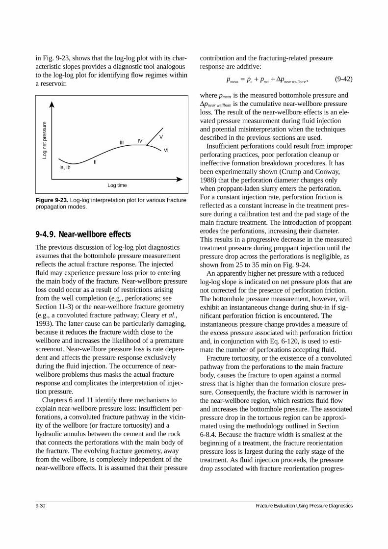
9-30 Fracture Evaluation Using Pressure Diagnostics

in Fig. 9-23, shows that the log-log plot with its char-acteristic slopes provides a diagnostic tool analogousto the log-log plot for identifying flow regimes withina reservoir.

9-4.9. Near-wellbore effectsThe previous discussion of log-log plot diagnosticsassumes that the bottomhole pressure measurementreflects the actual fracture response. The injectedfluid may experience pressure loss prior to enteringthe main body of the fracture. Near-wellbore pressureloss could occur as a result of restrictions arisingfrom the well completion (e.g., perforations; seeSection 11-3) or the near-wellbore fracture geometry(e.g., a convoluted fracture pathway; Cleary et al.,1993). The latter cause can be particularly damaging,because it reduces the fracture width close to thewellbore and increases the likelihood of a prematurescreenout. Near-wellbore pressure loss is rate depen-dent and affects the pressure response exclusivelyduring the fluid injection. The occurrence of near-wellbore problems thus masks the actual fractureresponse and complicates the interpretation of injec-tion pressure.

Chapters 6 and 11 identify three mechanisms toexplain near-wellbore pressure loss: insufficient per-forations, a convoluted fracture pathway in the vicin-ity of the wellbore (or fracture tortuosity) and ahydraulic annulus between the cement and the rockthat connects the perforations with the main body ofthe fracture. The evolving fracture geometry, awayfrom the wellbore, is completely independent of thenear-wellbore effects. It is assumed that their pressure

contribution and the fracturing-related pressureresponse are additive:

(9-42)

where pmeas is the measured bottomhole pressure and∆pnear wellbore is the cumulative near-wellbore pressureloss. The result of the near-wellbore effects is an ele-vated pressure measurement during fluid injectionand potential misinterpretation when the techniquesdescribed in the previous sections are used.

Insufficient perforations could result from improperperforating practices, poor perforation cleanup orineffective formation breakdown procedures. It hasbeen experimentally shown (Crump and Conway,1988) that the perforation diameter changes onlywhen proppant-laden slurry enters the perforation.For a constant injection rate, perforation friction isreflected as a constant increase in the treatment pres-sure during a calibration test and the pad stage of themain fracture treatment. The introduction of proppanterodes the perforations, increasing their diameter.This results in a progressive decrease in the measuredtreatment pressure during proppant injection until thepressure drop across the perforations is negligible, asshown from 25 to 35 min on Fig. 9-24.

An apparently higher net pressure with a reducedlog-log slope is indicated on net pressure plots that arenot corrected for the presence of perforation friction.The bottomhole pressure measurement, however, willexhibit an instantaneous change during shut-in if sig-nificant perforation friction is encountered. Theinstantaneous pressure change provides a measure ofthe excess pressure associated with perforation frictionand, in conjunction with Eq. 6-120, is used to esti-mate the number of perforations accepting fluid.

Fracture tortuosity, or the existence of a convolutedpathway from the perforations to the main fracturebody, causes the fracture to open against a normalstress that is higher than the formation closure pres-sure. Consequently, the fracture width is narrower inthe near-wellbore region, which restricts fluid flowand increases the bottomhole pressure. The associatedpressure drop in the tortuous region can be approxi-mated using the methodology outlined in Section 6-8.4. Because the fracture width is smallest at thebeginning of a treatment, the fracture reorientationpressure loss is largest during the early stage of thetreatment. As fluid injection proceeds, the pressuredrop associated with fracture reorientation progres-

p p p pmeas c net near wellbore= + + ∆ ,

Figure 9-23. Log-log interpretation plot for various fracturepropagation modes.

Ia, IbII

III IVV

VI

Log time

Log

net p

ress

ure

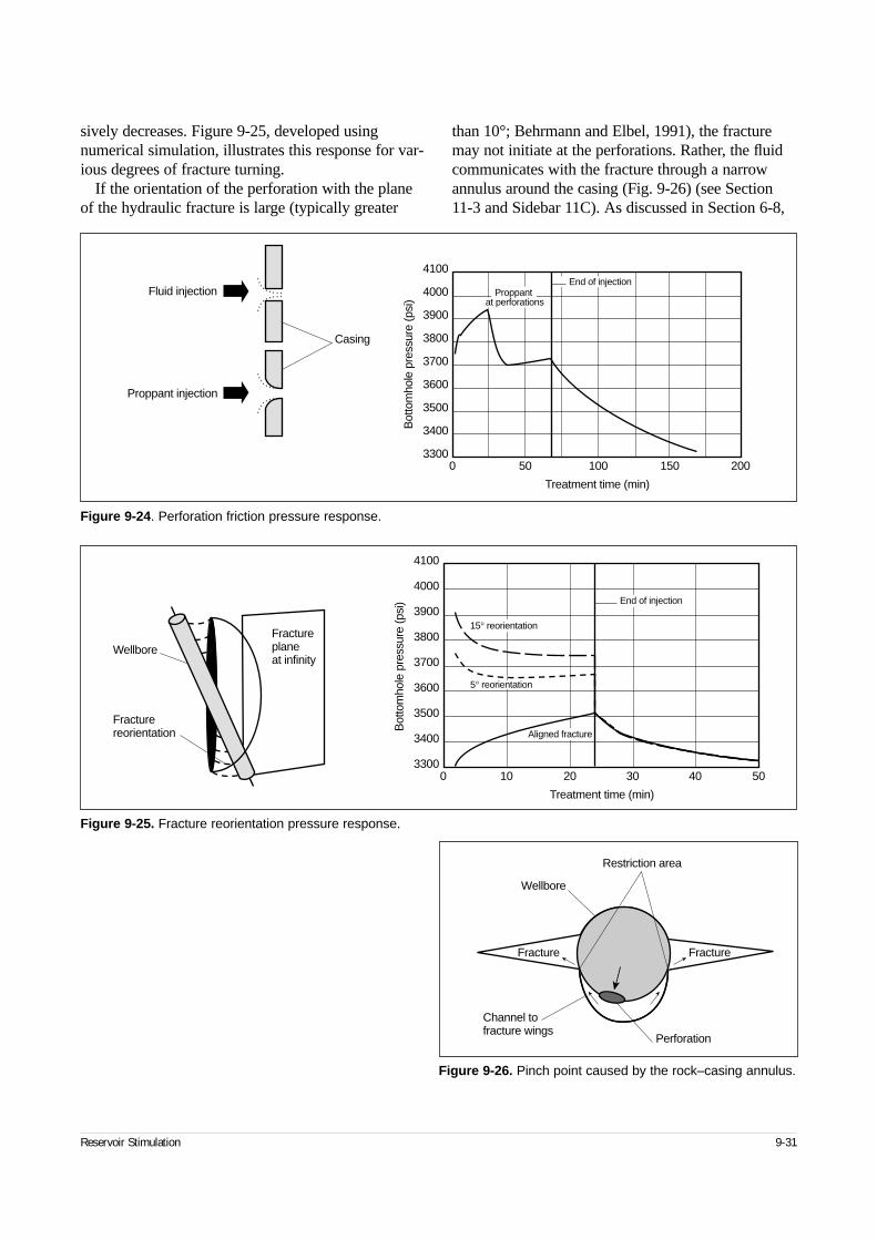
Reservoir Stimulation 9-31

sively decreases. Figure 9-25, developed usingnumerical simulation, illustrates this response for var-ious degrees of fracture turning.

If the orientation of the perforation with the planeof the hydraulic fracture is large (typically greater

than 10°; Behrmann and Elbel, 1991), the fracturemay not initiate at the perforations. Rather, the fluidcommunicates with the fracture through a narrowannulus around the casing (Fig. 9-26) (see Section11-3 and Sidebar 11C). As discussed in Section 6-8,

Figure 9-24. Perforation friction pressure response.

0 50 100 150 200

4100

4000

3900

3800

3700

3600

3500

3400

3300

Bot

tom

hole

pre

ssur

e (p

si)

Treatment time (min)

Proppantat perforations

Casing

Fluid injection

Proppant injection

End of injection

Figure 9-25. Fracture reorientation pressure response.

0 10 20 30 40 50

4100

4000

3900

3800

3700

3600

3500

3400

3300

Bot

tom

hole

pre

ssur

e (p

si)

Treatment time (min)

Fractureplaneat infinity

Wellbore

Fracturereorientation Aligned fracture

5° reorientation

15° reorientation

End of injection

Figure 9-26. Pinch point caused by the rock–casing annulus.

Channel tofracture wings

Perforation

Wellbore

Restriction area

Fracture Fracture

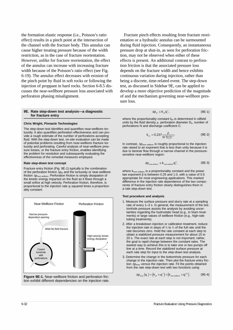
9-32 Fracture Evaluation Using Pressure Diagnostics

the formation elastic response (i.e., Poisson’s ratioeffect) results in a pinch point at the intersection ofthe channel with the fracture body. This annulus cancause higher treating pressure because of the widthrestriction, as in the case of fracture reorientation.However, unlike for fracture reorientation, the effectof the annulus can increase with increasing fracturewidth because of the Poisson’s ratio effect (see Fig.6-19). The annulus effect decreases with erosion ofthe pinch point by fluid in soft rocks or following theinjection of proppant in hard rocks. Section 6-8.5 dis-cusses the near-wellbore pressure loss associated withperforation phasing misalignment.

Fracture pinch effects resulting from fracture reori-entation or a hydraulic annulus can be surmountedduring fluid injection. Consequently, an instantaneouspressure drop at shut-in, as seen for perforation fric-tion, may not be observed when either of theseeffects is present. An additional contrast to perfora-tion friction is that the associated pressure lossdepends on the fracture width and hence exhibitscontinuous variation during injection, rather thanbeing a discrete, time-related event. The step-downtest, as discussed in Sidebar 9E, can be applied todevelop a more objective prediction of the magnitudeof and the mechanism governing near-wellbore pres-sure loss.

9E. Rate step-down test analysis—a diagnostic for fracture entry

Chris Wright, Pinnacle Technologies

The step-down test identifies and quantifies near-wellbore tor-tuosity. It also quantifies perforation effectiveness and can pro-vide a rough estimate of the number of perforations acceptingfluid. With the step-down test, on-site evaluation can be madeof potential problems resulting from near-wellbore fracture tor-tuosity and perforating. Careful analysis of near-wellbore pres-sure losses, or the fracture entry friction, enables identifyingthe problem for resolution and subsequently evaluating theeffectiveness of the remedial measures employed.

Rate step-down test concept

Fracture entry friction (Fig. 9E-1) typically is the combination of the perforation friction ∆ppf and the tortuosity or near-wellborefriction ∆pnear wellbore. Perforation friction is simply dissipation ofthe kinetic energy imparted on the fluid as it flows through asmall orifice at high velocity. Perforation friction, therefore, isproportional to the injection rate qi squared times a proportion-ality constant:

(9E-1)

where the proportionality constant kpf is determined in oilfieldunits by the fluid density ρ, perforation diameter Dp, number ofperforations N and discharge coefficient C:

(9E-2)

In contrast, ∆pnear wellbore is roughly proportional to the injectionrate raised to an exponent that is less than unity because it isdue to laminar flow through a narrow channel in the pressure-sensitive near-wellbore region:

(9E-3)

where knear wellbore is a proportionality constant and the powerlaw exponent β is between 0.25 and 1.0, with a value of 0.5appropriate for most engineering applications. This markeddifference in the injection rate dependence of the two compo-nents of fracture entry friction clearly distinguishes them in a rate step-down test.

Test procedure and analysis

1. Measure the surface pressure and slurry rate at a samplingrate of every 1–3 s. In general, the measurement of the bot-tomhole pressure assists the analysis by avoiding uncer-tainties regarding the hydrostatic head (e.g., in foam treat-ments) or large values of wellbore friction (e.g., high-ratetubing treatments).

2. After a breakdown injection or calibration treatment, reducethe injection rate in steps of 1⁄5 to 1⁄3 of the full rate until therate becomes zero. Hold the rate constant at each step toobtain a stabilized pressure measurement for about 15 to20 s. The exact rate at each step is not important; rather,the goal is rapid change between the constant rates. Theeasiest way to achieve this is to take one or two pumps offline at a time. Record the stabilized surface pressure ateach rate step for input to the step-down test analysis.

3. Determine the change in the bottomhole pressure for eachchange in the injection rate. Then plot the fracture entry fric-tion ∆pentry versus the injection rate. Fit the points obtainedfrom the rate step-down test with two functions using

(9E-4)Figure 9E-1. Near-wellbore friction and perforation fric-tion exhibit different dependencies on the injection rate.

Perforation FrictionNear-Wellbore Friction

High-velocity kineticenergy dissipation

Narrow pressure-dependent opening

Wide far-field fracture

Casedborehole

withperforations

∆p k qpf pf i≅ 2 ,

kN D Cpf

p

= 0 2372 4 2

. .ρ

∆p k qnear wellbore near wellbore i≅ β ,

∆p q k q k qentry i pf i near wellbore i( ) = ×( ) + ×( )2 1 2/ .

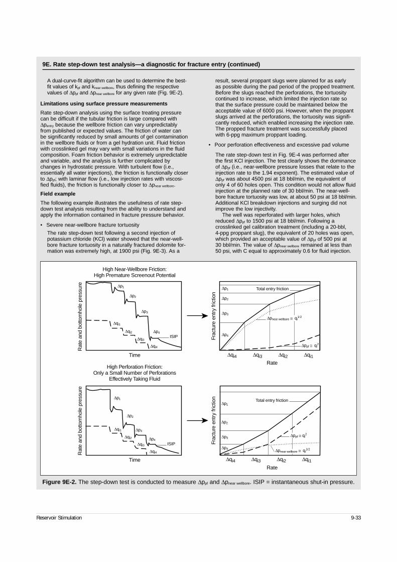
Reservoir Stimulation 9-33

A dual-curve-fit algorithm can be used to determine the best-fit values of kpf and knear wellbore, thus defining the respectivevalues of ∆ppf and ∆pnear wellbore for any given rate (Fig. 9E-2).

Limitations using surface pressure measurements

Rate step-down analysis using the surface treating pressurecan be difficult if the tubular friction is large compared with∆pentry because the wellbore friction can vary unpredictablyfrom published or expected values. The friction of water canbe significantly reduced by small amounts of gel contaminationin the wellbore fluids or from a gel hydration unit. Fluid frictionwith crosslinked gel may vary with small variations in the fluidcomposition. Foam friction behavior is extremely unpredictableand variable, and the analysis is further complicated bychanges in hydrostatic pressure. With turbulent flow (i.e.,essentially all water injections), the friction is functionally closerto ∆ppf; with laminar flow (i.e., low injection rates with viscosi-fied fluids), the friction is functionally closer to ∆pnear wellbore.

Field example

The following example illustrates the usefulness of rate step-down test analysis resulting from the ability to understand andapply the information contained in fracture pressure behavior.

• Severe near-wellbore fracture tortuosity

The rate step-down test following a second injection ofpotassium chloride (KCl) water showed that the near-well-bore fracture tortuosity in a naturally fractured dolomite for-mation was extremely high, at 1900 psi (Fig. 9E-3). As a

result, several proppant slugs were planned for as early as possible during the pad period of the propped treatment.Before the slugs reached the perforations, the tortuositycontinued to increase, which limited the injection rate sothat the surface pressure could be maintained below theacceptable value of 6000 psi. However, when the proppantslugs arrived at the perforations, the tortuosity was signifi-cantly reduced, which enabled increasing the injection rate.The propped fracture treatment was successfully placedwith 6-ppg maximum proppant loading.

• Poor perforation effectiveness and excessive pad volume

The rate step-down test in Fig. 9E-4 was performed afterthe first KCl injection. The test clearly shows the dominanceof ∆ppf (i.e., near-wellbore pressure losses that relate to theinjection rate to the 1.94 exponent). The estimated value of∆ppf was about 4500 psi at 18 bbl/min, the equivalent ofonly 4 of 60 holes open. This condition would not allow fluidinjection at the planned rate of 30 bbl/min. The near-well-bore fracture tortuosity was low, at about 50 psi at 18 bbl/min.Additional KCl breakdown injections and surging did notimprove the low injectivity.

The well was reperforated with larger holes, whichreduced ∆ppf to 1500 psi at 18 bbl/min. Following acrosslinked gel calibration treatment (including a 20-bbl, 4-ppg proppant slug), the equivalent of 20 holes was open,which provided an acceptable value of ∆ppf of 500 psi at 30 bbl/min. The value of ∆pnear wellbore remained at less than50 psi, with C equal to approximately 0.6 for fluid injection.

Figure 9E-2. The step-down test is conducted to measure ∆ppf and ∆pnear wellbore. ISIP = instantaneous shut-in pressure.

Rat

e an

d bo

ttom

hole

pre

ssur

e

Time

∆qi1

∆qi2

∆p3

∆p2

∆p1

∆p4

∆qi3

∆qi4

ISIP

Rat

e an

d bo

ttom

hole

pre

ssur

e

Time

∆qi1

∆qi2

∆p3

∆p2

∆p1

∆p4

∆qi3

∆qi4

ISIP

Frac

ture

ent

ry fr

ictio

n

∆p3

∆p4

∆qi4 ∆qi3 ∆qi2 ∆qi1

∆ppf ≅ qi2

∆pnear wellbore ≅ qi1⁄2

Total entry friction

∆p2

∆p1

Frac

ture

ent

ry fr

ictio

n

∆p3

∆p4

∆qi4 ∆qi3 ∆qi2 ∆qi1

∆ppf ≅ qi2

Total entry friction

∆p2

∆p1

High Near-Wellbore Friction:High Premature Screenout Potential

High Perforation Friction:Only a Small Number of Perforations

Effectively Taking Fluid

Rate

Rate

∆pnear wellbore ≅ qi1⁄2

9E. Rate step-down test analysis—a diagnostic for fracture entry (continued)

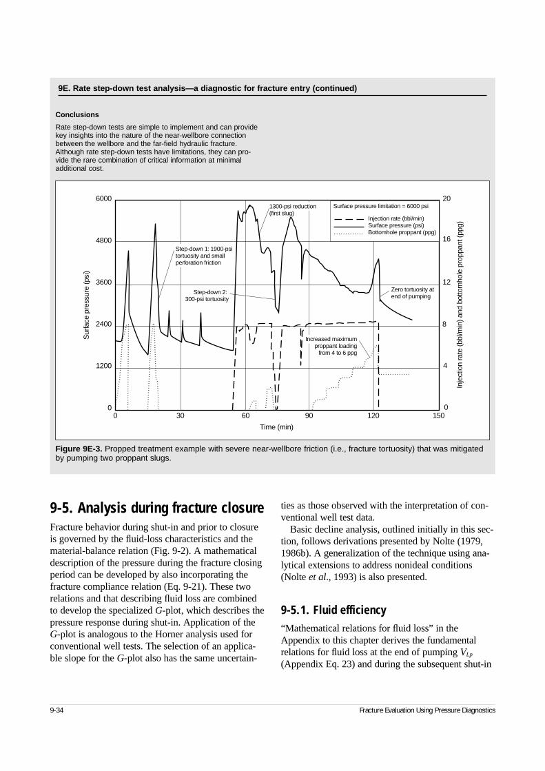
9-5. Analysis during fracture closureFracture behavior during shut-in and prior to closureis governed by the fluid-loss characteristics and thematerial-balance relation (Fig. 9-2). A mathematicaldescription of the pressure during the fracture closingperiod can be developed by also incorporating thefracture compliance relation (Eq. 9-21). These tworelations and that describing fluid loss are combinedto develop the specialized G-plot, which describes thepressure response during shut-in. Application of theG-plot is analogous to the Horner analysis used forconventional well tests. The selection of an applica-ble slope for the G-plot also has the same uncertain-

ties as those observed with the interpretation of con-ventional well test data.

Basic decline analysis, outlined initially in this sec-tion, follows derivations presented by Nolte (1979,1986b). A generalization of the technique using ana-lytical extensions to address nonideal conditions(Nolte et al., 1993) is also presented.

9-5.1. Fluid efficiency“Mathematical relations for fluid loss” in theAppendix to this chapter derives the fundamentalrelations for fluid loss at the end of pumping VLp

(Appendix Eq. 23) and during the subsequent shut-in

9-34 Fracture Evaluation Using Pressure Diagnostics

Conclusions

Rate step-down tests are simple to implement and can providekey insights into the nature of the near-wellbore connectionbetween the wellbore and the far-field hydraulic fracture.Although rate step-down tests have limitations, they can pro-vide the rare combination of critical information at minimaladditional cost.

Figure 9E-3. Propped treatment example with severe near-wellbore friction (i.e., fracture tortuosity) that was mitigatedby pumping two proppant slugs.

15012090

Time (min)

603000

1200

2400

3600

4800

6000

Step-down 1: 1900-psi tortuosity and small perforation friction

Increased maximumproppant loading

from 4 to 6 ppg

Step-down 2: 300-psi tortuosity

Zero tortuosity at end of pumping

1300-psi reduction (first slug)

Sur

face

pre

ssur

e (p

si)

Inje

ctio

n ra

te (b

bl/m

in) a

nd b

otto

mho

le p

ropp

ant (

ppg)

0

4

8

12

16

20Surface pressure limitation = 6000 psi

Injection rate (bbl/min)Surface pressure (psi)Bottomhole proppant (ppg)

9E. Rate step-down test analysis—a diagnostic for fracture entry (continued)

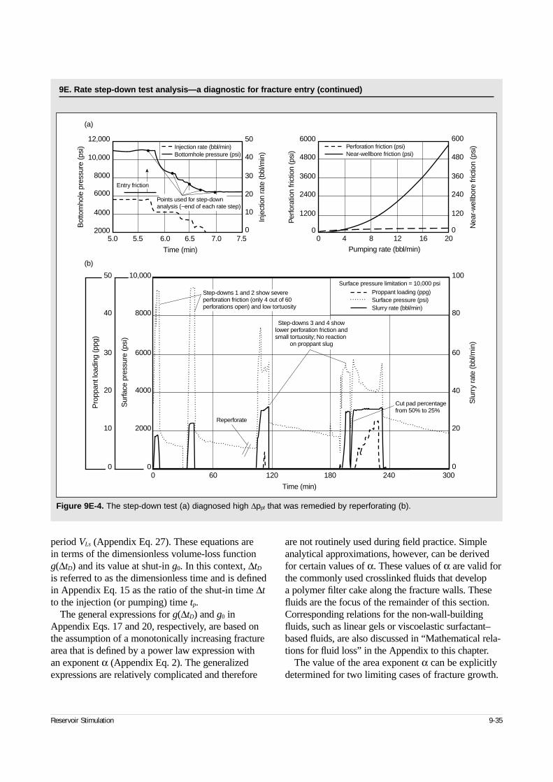
Reservoir Stimulation 9-35

period VLs (Appendix Eq. 27). These equations are in terms of the dimensionless volume-loss functiong(∆tD) and its value at shut-in g0. In this context, ∆tD

is referred to as the dimensionless time and is definedin Appendix Eq. 15 as the ratio of the shut-in time ∆tto the injection (or pumping) time tp.

The general expressions for g(∆tD) and g0 inAppendix Eqs. 17 and 20, respectively, are based onthe assumption of a monotonically increasing fracturearea that is defined by a power law expression with an exponent α (Appendix Eq. 2). The generalizedexpressions are relatively complicated and therefore

are not routinely used during field practice. Simpleanalytical approximations, however, can be derivedfor certain values of α. These values of α are valid forthe commonly used crosslinked fluids that develop a polymer filter cake along the fracture walls. Thesefluids are the focus of the remainder of this section.Corresponding relations for the non-wall-buildingfluids, such as linear gels or viscoelastic surfactant–based fluids, are also discussed in “Mathematical rela-tions for fluid loss” in the Appendix to this chapter.

The value of the area exponent α can be explicitlydetermined for two limiting cases of fracture growth.

9E. Rate step-down test analysis—a diagnostic for fracture entry (continued)

Figure 9E-4. The step-down test (a) diagnosed high ∆ppf that was remedied by reperforating (b).

300240180

Time (min)

Sur

face

pre

ssur

e (p

si)

Slu

rry

rate

(bbl

/min

)120

5.02000 0

10

20

30

40

50

0

120

240

360

480

600

4000

6000

8000

10,000

12,000

(a)

(b)

5.5 6.0 6.5

Time (min)

Bot

tom

hole

pre

ssur

e (p

si)

Inje

ctio

n ra

te (b

bl/m

in)

Per

fora

tion

fric

tion

(psi

)

Nea

r-w

ellb

ore

fric

tion

(psi

)

7.0 7.5 0 4 8 12

Pumping rate (bbl/min)

16 20

600

2000

4000

6000

8000

Pro

ppan

t loa

ding

(ppg

)

10

20

30

40

Cut pad percentage from 50% to 25%

Reperforate

Step-downs 1 and 2 show severe perforation friction (only 4 out of 60 perforations open) and low tortuosity

Step-downs 3 and 4 show lower perforation friction and small tortuosity; No reaction

on proppant slug

Points used for step-down analysis (~end of each rate step)

Entry friction

0

1200

2400

3600

4800

6000

0

20

40

60

80

100Surface pressure limitation = 10,000 psi

Proppant loading (ppg)Surface pressure (psi)Slurry rate (bbl/min)

Perforation friction (psi)Near-wellbore friction (psi)

Injection rate (bbl/min)Bottomhole pressure (psi)

10,00050

00

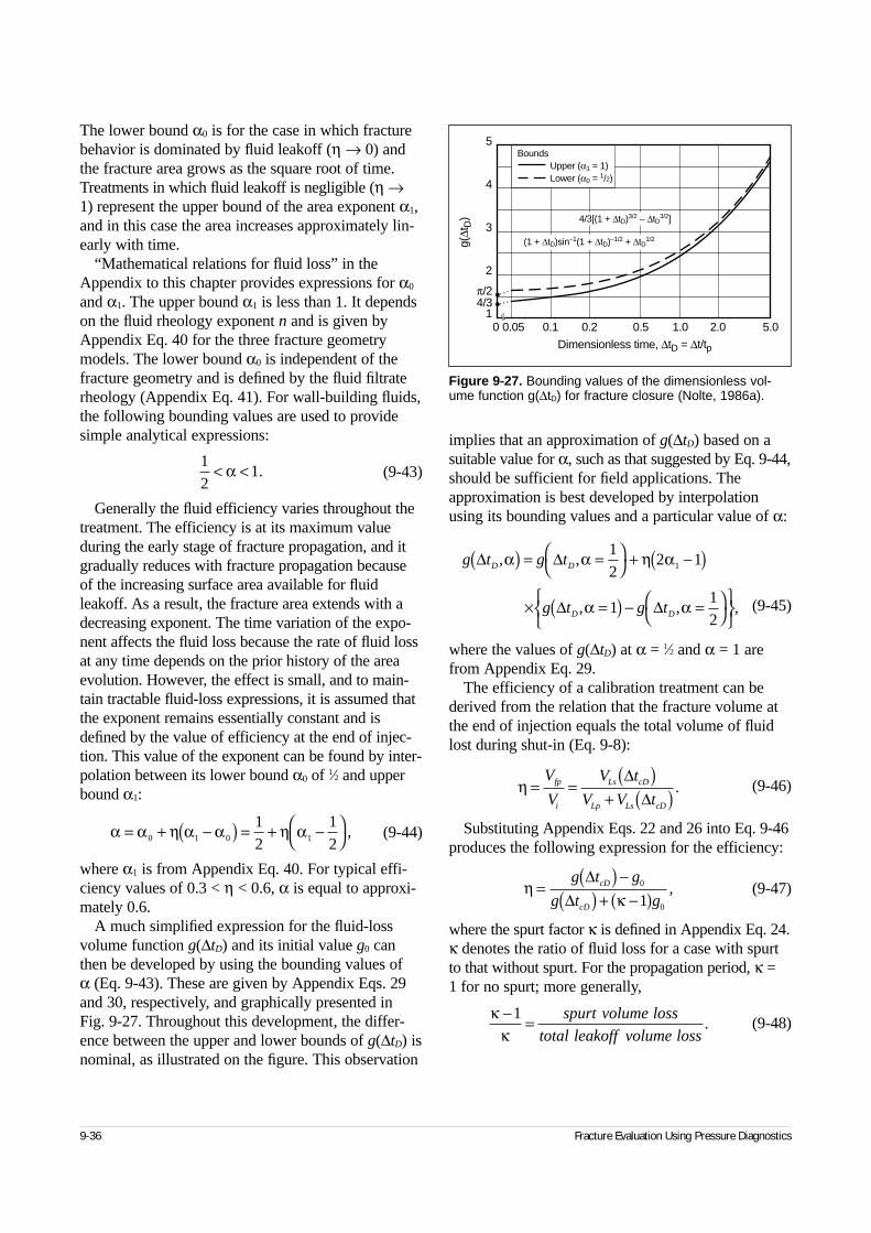
The lower bound α0 is for the case in which fracturebehavior is dominated by fluid leakoff (η → 0) andthe fracture area grows as the square root of time.Treatments in which fluid leakoff is negligible (η →1) represent the upper bound of the area exponent α1,and in this case the area increases approximately lin-early with time.

“Mathematical relations for fluid loss” in theAppendix to this chapter provides expressions for α0

and α1. The upper bound α1 is less than 1. It dependson the fluid rheology exponent n and is given byAppendix Eq. 40 for the three fracture geometrymodels. The lower bound α0 is independent of thefracture geometry and is defined by the fluid filtraterheology (Appendix Eq. 41). For wall-building fluids,the following bounding values are used to providesimple analytical expressions:

(9-43)

Generally the fluid efficiency varies throughout thetreatment. The efficiency is at its maximum valueduring the early stage of fracture propagation, and itgradually reduces with fracture propagation becauseof the increasing surface area available for fluidleakoff. As a result, the fracture area extends with adecreasing exponent. The time variation of the expo-nent affects the fluid loss because the rate of fluid lossat any time depends on the prior history of the areaevolution. However, the effect is small, and to main-tain tractable fluid-loss expressions, it is assumed thatthe exponent remains essentially constant and isdefined by the value of efficiency at the end of injec-tion. This value of the exponent can be found by inter-polation between its lower bound α0 of 1⁄2 and upperbound α1:

(9-44)

where α1 is from Appendix Eq. 40. For typical effi-ciency values of 0.3 < η < 0.6, α is equal to approxi-mately 0.6.

A much simplified expression for the fluid-lossvolume function g(∆tD) and its initial value g0 canthen be developed by using the bounding values of α (Eq. 9-43). These are given by Appendix Eqs. 29and 30, respectively, and graphically presented in Fig. 9-27. Throughout this development, the differ-ence between the upper and lower bounds of g(∆tD) isnominal, as illustrated on the figure. This observation

implies that an approximation of g(∆tD) based on asuitable value for α, such as that suggested by Eq. 9-44,should be sufficient for field applications. Theapproximation is best developed by interpolationusing its bounding values and a particular value of α:

(9-45)

where the values of g(∆tD) at α = 1⁄2 and α = 1 arefrom Appendix Eq. 29.

The efficiency of a calibration treatment can bederived from the relation that the fracture volume atthe end of injection equals the total volume of fluidlost during shut-in (Eq. 9-8):

(9-46)

Substituting Appendix Eqs. 22 and 26 into Eq. 9-46produces the following expression for the efficiency:

(9-47)

where the spurt factor κ is defined in Appendix Eq. 24.κ denotes the ratio of fluid loss for a case with spurtto that without spurt. For the propagation period, κ =1 for no spurt; more generally,

(9-48)

9-36 Fracture Evaluation Using Pressure Diagnostics

12

1< <α .

g t g t

g t g t

D D

D D

∆ ∆

∆ ∆

, ,

, , ,

α α η α

α α

( ) = =

+ −( )

× =( ) − =

12

2 1

112

1

η = = ( )+ ( )

V

V

V t

V V tfp

i

Ls cD

Lp Ls cD

∆∆

.

ηκ

= ( ) −( ) + −( )

g t g

g t gcD

cD

∆∆

0

01,

κκ− =1 spurt volume loss

total leakoff volume loss.

α α η α α η α= + −( ) = + −

0 1 0 1

12

12

,

Figure 9-27. Bounding values of the dimensionless vol-ume function g(∆tD) for fracture closure (Nolte, 1986a).

5

4

3

2

1

g(∆t

D)

0 0.05 0.1 0.2 0.5 1.0 2.0 5.0

Dimensionless time, ∆tD = ∆t/tp

BoundsUpper (α1 = 1)Lower (α0 = 1/2)

π/24/3

(1 + ∆tD)sin–1(1 + ∆tD)–1/2 + ∆tD1/2

4/3[(1 + ∆tD)3/2 – ∆tD3/2]

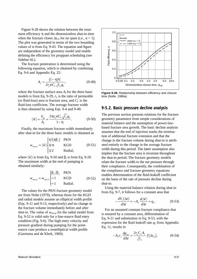
Figure 9-28 shows the relation between the treat-ment efficiency η and the dimensionless shut-in timewhen the fracture closes ∆tcD for no spurt (i.e., κ = 1).The plot was generated in terms of the two boundingvalues of α from Eq. 9-43. The equation and figureare independent of the geometry model and enabledefining the efficiency for proppant scheduling (seeSidebar 6L).

The fracture penetration is determined using thefollowing equation, which is obtained by combiningEq. 9-6 and Appendix Eq. 22:

(9-49)

where the fracture surface area Af for the three basicmodels is from Eq. 9-29, rp is the ratio of permeable(or fluid-loss) area to fracture area, and CL is thefluid-loss coefficient. The average fracture width is then obtained by using Eqs. 9-4 and 9-49:

(9-50)

Finally, the maximum fracture width immediatelyafter shut-in for the three basic models is obtained as

(9-51)

where ⟨w–⟩ is from Eq. 9-50 and βs is from Eq. 9-20.The maximum width at the end of pumping isobtained similarly:

(9-52)

The values for the PKN fracture geometry modelare from Nolte (1979), whereas those for the KGDand radial models assume an elliptical width profile(Eqs. 9-11 and 9-13, respectively) and no change inthe fracture volume immediately before and aftershut-in. The value of wmax,p for the radial model fromEq. 9-52 is valid only for a line-source fluid entrycondition (Fig. 9-6). The high entry velocity andpressure gradient during pumping for the point-source case produce a nonelliptical width profile(Geertsma and de Klerk, 1969).

9-5.2. Basic pressure decline analysisThe previous section presents relations for the fracturegeometry parameters from simple considerations ofmaterial balance and the assumption of power-law-based fracture area growth. The basic decline analysisassumes that the end of injection marks the termina-tion of additional fracture extension and that thechange in the fracture volume during shut-in is attrib-uted entirely to the change in the average fracturewidth during this period. The latter assumption alsoimplies that the fracture area is invariant throughoutthe shut-in period. The fracture geometry modelsrelate the fracture width to the net pressure throughtheir compliance. Consequently, the combination ofthe compliance and fracture geometry equationsenables determination of the fluid-leakoff coefficienton the basis of the rate of pressure decline duringshut-in.

Using the material-balance relation during shut-infrom Eq. 9-7, it follows for a constant area that

(9-53)

For an assumed constant fracture compliance thatis ensured by a constant area, differentiation of Eq. 9-21 and substitution in Eq. 9-53, with theexpression for the fluid leakoff rate qL from AppendixEq. 11, results in

(9-54)

Reservoir Stimulation 9-37

AV

r C t gfi

p L p

=−( )1

2 0

ηκ

,

wV

A

r C t gfp

f

p L p= =−

2

10η κ

η.

w wmax,si

s

=( )

4

4

3 2

πβπ

PKN

KGD

Radial,

Figure 9-28. Relationship between efficiency and closuretime (Nolte, 1986a).

1.0

0.8

0.6

0.4

0.2

0

Flu

id e

ffici

ency

, η

0 0.05 0.1 0.2 0.5 1.0 2.0 5.0 10.0

Dimensionless closure time, ∆tcD

κ = 1

BoundsUpper (α1 = 1)Lower (α0 = 1⁄2)

w wmax,p max,si

s p

= ≈≈

β β PKN

KGD1

1 Radial.

−( )

= − =dV t

d tA

d w

d tqf

f L

∆∆ ∆

.

− = ( )A cdp

d t

r C A

tf tf f

net p L f

p

D∆∆

2,

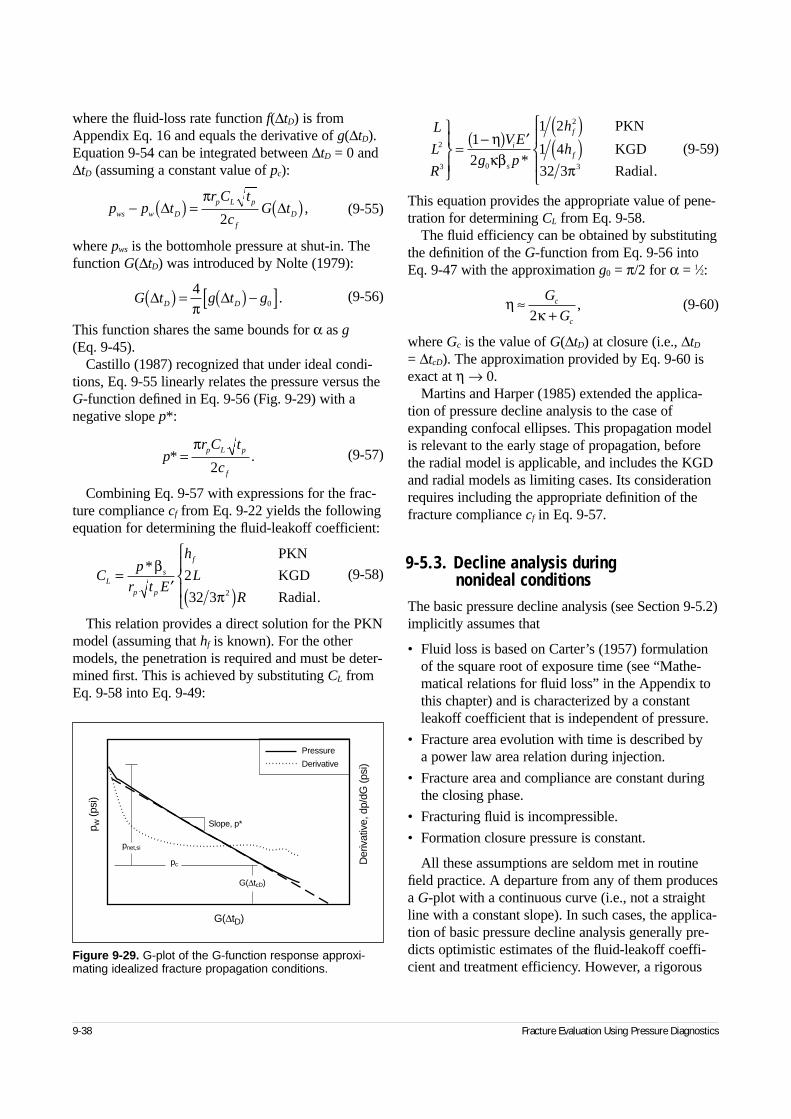
where the fluid-loss rate function f(∆tD) is fromAppendix Eq. 16 and equals the derivative of g(∆tD).Equation 9-54 can be integrated between ∆tD = 0 and∆tD (assuming a constant value of pc):

(9-55)

where pws is the bottomhole pressure at shut-in. Thefunction G(∆tD) was introduced by Nolte (1979):

(9-56)

This function shares the same bounds for α as g(Eq. 9-45).

Castillo (1987) recognized that under ideal condi-tions, Eq. 9-55 linearly relates the pressure versus theG-function defined in Eq. 9-56 (Fig. 9-29) with anegative slope p*:

(9-57)

Combining Eq. 9-57 with expressions for the frac-ture compliance cf from Eq. 9-22 yields the followingequation for determining the fluid-leakoff coefficient:

(9-58)

This relation provides a direct solution for the PKNmodel (assuming that hf is known). For the othermodels, the penetration is required and must be deter-mined first. This is achieved by substituting CL fromEq. 9-58 into Eq. 9-49:

(9-59)

This equation provides the appropriate value of pene-tration for determining CL from Eq. 9-58.

The fluid efficiency can be obtained by substitutingthe definition of the G-function from Eq. 9-56 intoEq. 9-47 with the approximation g0 = π/2 for α = 1⁄2:

(9-60)

where Gc is the value of G(∆tD) at closure (i.e., ∆tD

= ∆tcD). The approximation provided by Eq. 9-60 isexact at η → 0.

Martins and Harper (1985) extended the applica-tion of pressure decline analysis to the case ofexpanding confocal ellipses. This propagation modelis relevant to the early stage of propagation, beforethe radial model is applicable, and includes the KGDand radial models as limiting cases. Its considerationrequires including the appropriate definition of thefracture compliance cf in Eq. 9-57.

9-5.3. Decline analysis during nonideal conditions

The basic pressure decline analysis (see Section 9-5.2)implicitly assumes that

• Fluid loss is based on Carter’s (1957) formulationof the square root of exposure time (see “Mathe-matical relations for fluid loss” in the Appendix tothis chapter) and is characterized by a constantleakoff coefficient that is independent of pressure.

• Fracture area evolution with time is described by a power law area relation during injection.

• Fracture area and compliance are constant duringthe closing phase.

• Fracturing fluid is incompressible.

• Formation closure pressure is constant.

All these assumptions are seldom met in routinefield practice. A departure from any of them producesa G-plot with a continuous curve (i.e., not a straightline with a constant slope). In such cases, the applica-tion of basic pressure decline analysis generally pre-dicts optimistic estimates of the fluid-leakoff coeffi-cient and treatment efficiency. However, a rigorous

9-38 Fracture Evaluation Using Pressure Diagnostics

p p tr C t

cG tws w D

p L p

f

D− ( ) = ( )∆ ∆π

2,

G t g t gD D∆ ∆( ) = ( ) −[ ]40π

.

pr C t

cp L p

f

* .=π

2

Cp

r t E

h

L

RL

s

p p

f

=′ ( )

*β

π

PKN

KGD

Radial.

2

32 3 2

L

L

R

V E

g p

h

hi

s

f

f2

3 0

2

3

1

2

1 2

1 4

32 3

=

−( ) ′( )( )

ηκβ

π*

PKN

KGD

Radial.

ηκ

≈+

G

Gc

c2,

Figure 9-29. G-plot of the G-function response approxi-mating idealized fracture propagation conditions.

p w (p

si)

Der

ivat

ive,

dp/

dG (p

si)

G(∆tD)

Pressure

Derivative

Slope, p*

G(∆tcD)

pnet,si

pc

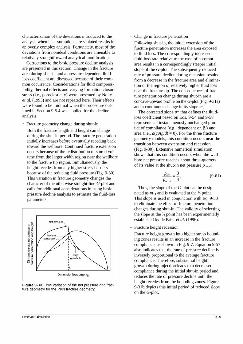
characterization of the deviations introduced to theanalysis when its assumptions are violated results inan overly complex analysis. Fortunately, most of thedeviations from nonideal conditions are amenable torelatively straightforward analytical modifications.

Corrections to the basic pressure decline analysisare presented in this section. Change in the fracturearea during shut-in and a pressure-dependent fluid-loss coefficient are discussed because of their com-mon occurrence. Considerations for fluid compress-ibility, thermal effects and varying formation closurestress (i.e., poroelasticity) were presented by Nolte et al. (1993) and are not repeated here. Their effectswere found to be minimal when the procedure out-lined in Section 9-5.4 was applied for the declineanalysis.

• Fracture geometry change during shut-in

Both the fracture length and height can changeduring the shut-in period. The fracture penetrationinitially increases before eventually receding backtoward the wellbore. Continued fracture extensionoccurs because of the redistribution of stored vol-ume from the larger width region near the wellboreto the fracture tip region. Simultaneously, theheight recedes from any higher stress barriersbecause of the reducing fluid pressure (Fig. 9-30).This variation in fracture geometry changes thecharacter of the otherwise straight-line G-plot andcalls for additional considerations in using basicpressure decline analysis to estimate the fluid-lossparameters.

– Change in fracture penetration

Following shut-in, the initial extension of thefracture penetration increases the area exposedto fluid loss. The correspondingly increasedfluid-loss rate relative to the case of constantarea results in a correspondingly steeper initialslope of the G-plot. The subsequently reducedrate of pressure decline during recession resultsfrom a decrease in the fracture area and elimina-tion of the region of relatively higher fluid lossnear the fracture tip. The consequences of frac-ture penetration change during shut-in are aconcave-upward profile on the G-plot (Fig. 9-31a)and a continuous change in its slope mG.

The corrected slope p* that defines the fluid-loss coefficient based on Eqs. 9-54 and 9-58represents an instantaneously unchanged prod-uct of compliance (e.g., dependent on βs) andarea (i.e., d(cfAf)/dt = 0). For the three fracturegeometry models, this condition occurs near thetransition between extension and recession (Fig. 9-30). Extensive numerical simulationshows that this condition occurs when the well-bore net pressure reaches about three-quartersof its value at the shut-in net pressure pnet,si:

(9-61)

Thus, the slope of the G-plot can be desig-nated as m3⁄4 and is evaluated at the 3⁄4 point.This slope is used in conjunction with Eq. 9-58to eliminate the effect of fracture penetrationchanges during shut-in. The validity of selectingthe slope at the 3⁄4 point has been experimentallyestablished by de Pater et al. (1996).

– Fracture height recession

Fracture height growth into higher stress bound-ing zones results in an increase in the fracturecompliance, as shown in Fig. 9-7. Equation 9-57also indicates that the rate of pressure decline isinversely proportional to the average fracturecompliance. Therefore, substantial heightgrowth during injection leads to a decreasedcompliance during the initial shut-in period andreduces the rate of pressure decline until theheight recedes from the bounding zones. Figure9-31b depicts this initial period of reduced slopeon the G-plot.

Reservoir Stimulation 9-39

Figure 9-30. Time variation of the net pressure and frac-ture geometry for the PKN fracture geometry.

Dim

ensi

onle

ss n

et p

ress

ure,

fract

ure

pene

tratio

n an

d he

ight

Dimensionless time, tD

Fracturepenetration, L

Net pressure

Heightgrowth, h

tp

p

pnet

net si,

.= 34

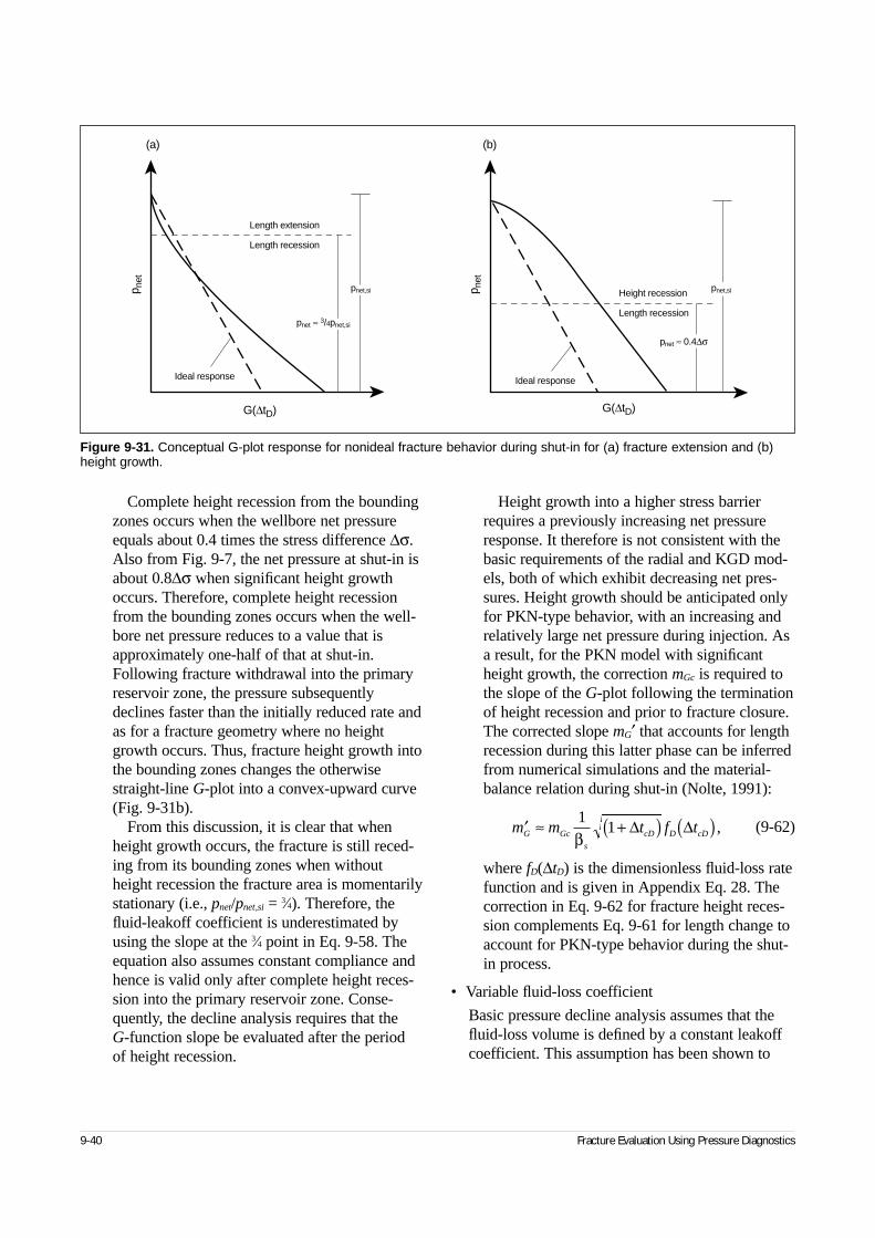
Complete height recession from the boundingzones occurs when the wellbore net pressureequals about 0.4 times the stress difference ∆σ.Also from Fig. 9-7, the net pressure at shut-in isabout 0.8∆σ when significant height growthoccurs. Therefore, complete height recessionfrom the bounding zones occurs when the well-bore net pressure reduces to a value that isapproximately one-half of that at shut-in.Following fracture withdrawal into the primaryreservoir zone, the pressure subsequentlydeclines faster than the initially reduced rate andas for a fracture geometry where no heightgrowth occurs. Thus, fracture height growth intothe bounding zones changes the otherwisestraight-line G-plot into a convex-upward curve(Fig. 9-31b).

From this discussion, it is clear that whenheight growth occurs, the fracture is still reced-ing from its bounding zones when withoutheight recession the fracture area is momentarilystationary (i.e., pnet/pnet,si = 3⁄4). Therefore, thefluid-leakoff coefficient is underestimated byusing the slope at the 3⁄4 point in Eq. 9-58. Theequation also assumes constant compliance andhence is valid only after complete height reces-sion into the primary reservoir zone. Conse-quently, the decline analysis requires that the G-function slope be evaluated after the period of height recession.

Height growth into a higher stress barrierrequires a previously increasing net pressureresponse. It therefore is not consistent with thebasic requirements of the radial and KGD mod-els, both of which exhibit decreasing net pres-sures. Height growth should be anticipated onlyfor PKN-type behavior, with an increasing andrelatively large net pressure during injection. Asa result, for the PKN model with significantheight growth, the correction mGc is required tothe slope of the G-plot following the terminationof height recession and prior to fracture closure.The corrected slope mG′ that accounts for lengthrecession during this latter phase can be inferredfrom numerical simulations and the material-balance relation during shut-in (Nolte, 1991):

(9-62)

where fD(∆tD) is the dimensionless fluid-loss ratefunction and is given in Appendix Eq. 28. Thecorrection in Eq. 9-62 for fracture height reces-sion complements Eq. 9-61 for length change toaccount for PKN-type behavior during the shut-in process.

• Variable fluid-loss coefficient

Basic pressure decline analysis assumes that thefluid-loss volume is defined by a constant leakoffcoefficient. This assumption has been shown to

9-40 Fracture Evaluation Using Pressure Diagnostics

Figure 9-31. Conceptual G-plot response for nonideal fracture behavior during shut-in for (a) fracture extension and (b)height growth.

G(∆tD) G(∆tD)

p net

p net

Ideal responseIdeal response

Length recession

Length extension

Length recession

Height recession

(a) (b)

pnet ≈ 3/4pnet,si

pnet,si

pnet ≈ 0.4∆σ

pnet,si

′ ≈ +( ) ( )m m t f tG Gc

s

cD D cD

11

β∆ ∆ ,

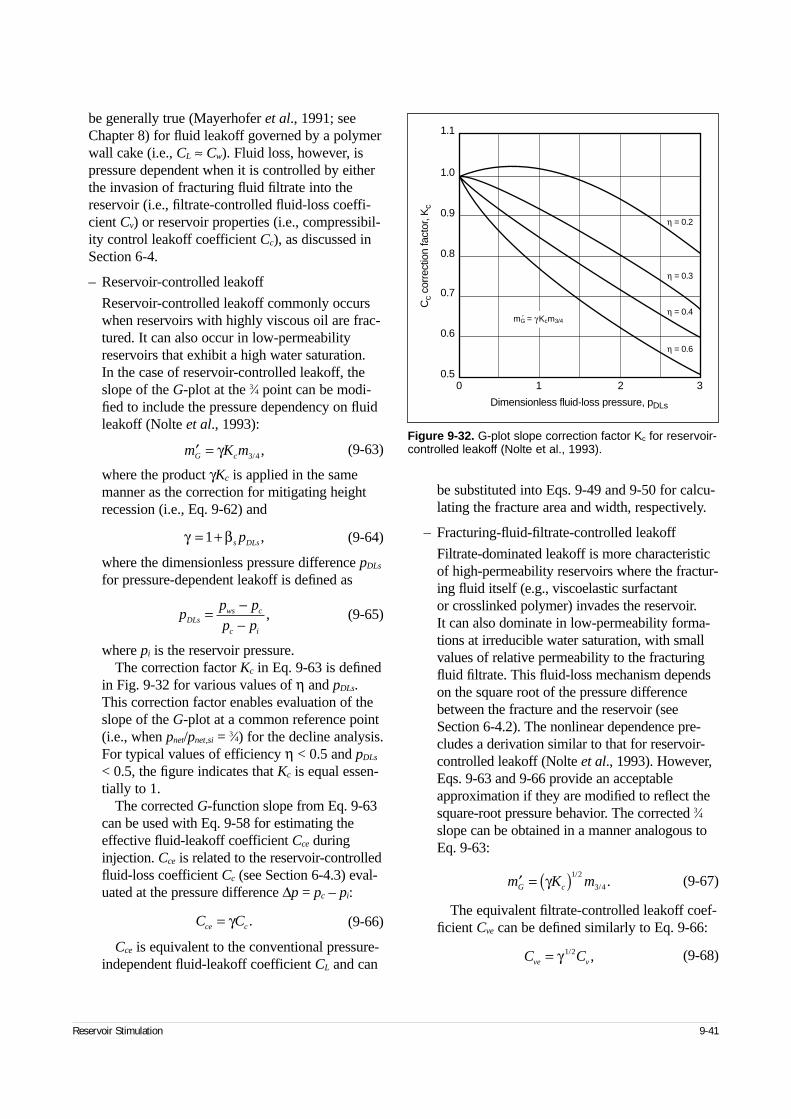
be generally true (Mayerhofer et al., 1991; seeChapter 8) for fluid leakoff governed by a polymerwall cake (i.e., CL ≈ Cw). Fluid loss, however, ispressure dependent when it is controlled by eitherthe invasion of fracturing fluid filtrate into thereservoir (i.e., filtrate-controlled fluid-loss coeffi-cient Cv) or reservoir properties (i.e., compressibil-ity control leakoff coefficient Cc), as discussed inSection 6-4.

– Reservoir-controlled leakoff

Reservoir-controlled leakoff commonly occurswhen reservoirs with highly viscous oil are frac-tured. It can also occur in low-permeabilityreservoirs that exhibit a high water saturation. In the case of reservoir-controlled leakoff, theslope of the G-plot at the 3⁄4 point can be modi-fied to include the pressure dependency on fluidleakoff (Nolte et al., 1993):

(9-63)

where the product γKc is applied in the samemanner as the correction for mitigating heightrecession (i.e., Eq. 9-62) and

(9-64)

where the dimensionless pressure difference pDLs

for pressure-dependent leakoff is defined as

(9-65)

where pi is the reservoir pressure.The correction factor Kc in Eq. 9-63 is defined

in Fig. 9-32 for various values of η and pDLs.This correction factor enables evaluation of theslope of the G-plot at a common reference point(i.e., when pnet/pnet,si = 3⁄4) for the decline analysis.For typical values of efficiency η < 0.5 and pDLs

< 0.5, the figure indicates that Kc is equal essen-tially to 1.

The corrected G-function slope from Eq. 9-63can be used with Eq. 9-58 for estimating theeffective fluid-leakoff coefficient Cce duringinjection. Cce is related to the reservoir-controlledfluid-loss coefficient Cc (see Section 6-4.3) eval-uated at the pressure difference ∆p = pc – pi:

(9-66)

Cce is equivalent to the conventional pressure-independent fluid-leakoff coefficient CL and can

be substituted into Eqs. 9-49 and 9-50 for calcu-lating the fracture area and width, respectively.

– Fracturing-fluid-filtrate-controlled leakoff

Filtrate-dominated leakoff is more characteristicof high-permeability reservoirs where the fractur-ing fluid itself (e.g., viscoelastic surfactant or crosslinked polymer) invades the reservoir. It can also dominate in low-permeability forma-tions at irreducible water saturation, with smallvalues of relative permeability to the fracturingfluid filtrate. This fluid-loss mechanism dependson the square root of the pressure differencebetween the fracture and the reservoir (seeSection 6-4.2). The nonlinear dependence pre-cludes a derivation similar to that for reservoir-controlled leakoff (Nolte et al., 1993). However,Eqs. 9-63 and 9-66 provide an acceptableapproximation if they are modified to reflect thesquare-root pressure behavior. The corrected 3⁄4slope can be obtained in a manner analogous toEq. 9-63:

(9-67)

The equivalent filtrate-controlled leakoff coef-ficient Cve can be defined similarly to Eq. 9-66:

(9-68)

Reservoir Stimulation 9-41

′ =m K mG cγ 3 4/ ,

γ β= +1 s DLsp ,

pp p

p pDLsws c

c i

= −−

,

C Cce c= γ .

Figure 9-32. G-plot slope correction factor Kc for reservoir-controlled leakoff (Nolte et al., 1993).

1.1

1.0

0.9

0.8

0.7

0.6

0.5

Cc

corr

ectio

n fa

ctor

, Kc

0 1 2 3

Dimensionless fluid-loss pressure, pDLs

η = 0.2

η = 0.3

η = 0.4

η = 0.6

mǴ = γKcm3/4

′ = ( )m K mG cγ 1 2

3 4

/

/ .

C Cve v= γ 1 2/ ,

where γ is defined by Eq. 9-64 and Cv is the vis-cosity control leakoff coefficient (see Section 6-4.3) evaluated at ∆p = pc – pi. Like for Eq. 9-63, the correction factor Kc is obtainedfrom Fig. 9-32.

In summary, for fluid loss governed by a poly-mer filter cake, the fluid-loss behavior is inde-pendent of pressure, and the analysis presentedfor Eq. 9-61 or 9-62 is used. Closed-form cor-rections of the type presented in Eq. 9-63 extendthe basic decline analysis for the reservoir-con-trolled fluid-loss mechanism, such as for heavy-oil-bearing reservoirs. Filtrate-controlled behav-ior, which is more common in the stimulation ofhigh-permeability reservoirs, shows a nonlineardependence on pressure. The corrections devel-oped for the reservoir-controlled leakoff casecan be adapted to quantify these effects.

9-5.4. Generalized pressure decline analysisAs discussed in the preceding section, commonlyoccurring nonideal conditions modify the otherwisestraight-line behavior of the G-plot. The 3⁄4 point (i.e.,pnet /pnet,si = 3⁄4) provides a reference to extend basicpressure decline analysis for effects resulting fromchange in the fracture length. In addition, the correc-tion for recession following fracture height closure orpressure-dependent leakoff complements the 3⁄4-pointslope with the following unified methodology for theanalysis of shut-in pressure decline before fractureclosure:

1. For all geometry models, find the slope at pnet /pnet,si

= 3⁄4 (i.e., m3⁄4).

2. If the PKN model is applicable (determined by theanalysis of pumping pressure) and pressure-depen-dent leakoff is not expected, determine the slope atclosure mGc. Obtain the corrected slope at closuremG′ using Eq. 9-62.

3. The value of p* is selected from the followingequation on the basis of the applicable fracturegeometry model:

(9-69)

4. Gc is corrected to include effects resulting fromnonideal conditions on the G-plot by defining acorrected value of G at closure:

(9-70)

where pnet,si is the net pressure at shut-in.

5. The fluid efficiency is determined by modifyingEq. 9-60:

(9-71)

6. Finally, CL is estimated by applying Eq. 9-58 withp* determined using Eq. 9-69.

In the absence of height growth and pressure-dependent fluid loss, m3⁄4 and mG′ are expected to beequal. With height growth but no pressure-dependentfluid loss, mG′ is expected to be greater than m3⁄4 andprovide a better estimate for p*. Alternatively, for nosignificant height growth but with pressure-dependentfluid loss, m3⁄4 is expected to be greater than mG′(Eq. 9-62) and provide a better estimate for p*.

The relative magnitudes for m3⁄4 and mG′ providea diagnostic to infer the occurrence of pressure-dependent leakoff. An alternative diagnostic is the G-function semilog derivative, discussed in Sidebar 9F.If pressure-dependent leakoff conditions occur, Eqs. 9-63 through 9-68 should be used to determinethe effective fluid-leakoff coefficient. The primarydeficiency of this method is the selection of an appro-priate slope when both significant height growth andpressure-dependent fluid loss occur.

The 3⁄4 point provides a common reference point,where the slope of the G-plot can be used to accountfor nonideal effects. Accordingly, this generalizedevaluation methodology is commonly referred to asthe 3⁄4 rule for pressure decline analysis.

• Example field application of PKN fracture decline analysis

Shut-in pressures monitored during the calibrationtreatment described in Section 9-4.4 are analyzedin this example to illustrate the application ofdecline analysis to a PKN-type fracture (Fig. 9-8).The relevant formation mechanical parameters arelisted in Table 9-1.

The plane strain modulus E′ is derived from Eand ν:

9-42 Fracture Evaluation Using Pressure Diagnostics

p

m m

m

m

G

*

max ,/

/

/

=′( )

3 4

3 4

3 4

PKN

KGD

Radial.

Gp

pnet si*

*,,=

ηκ

=+

G

G

**

.2

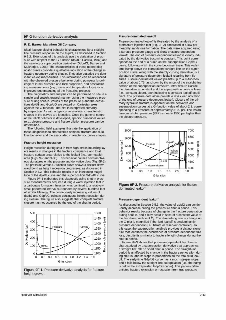
Reservoir Stimulation 9-43

9F. G-function derivative analysis

R. D. Barree, Marathon Oil Company

Ideal fracture closing behavior is characterized by a straight-line pressure response on the G-plot, as described in Section9-5.2. Extensions of this analysis use the derivative of pres-sure with respect to the G-function (dp/dG; Castillo, 1987) andthe semilog or superposition derivative (Gdp/dG; Barree andMukherjee, 1996). The characteristics of these added diag-nostic curves provide a qualitative indication of the change infracture geometry during shut-in. They also describe the dom-inant leakoff mechanisms. This information can be reconciledwith the observed pressure behavior during pumping, knowl-edge of in-situ stresses and rock properties, and postfractur-ing measurements (e.g., tracer and temperature logs) for animproved understanding of the fracturing process.

The diagnostics and analysis can be performed on site in asimple and straightforward manner using the measured pres-sure during shut-in. Values of the pressure p and the deriva-tives dp/dG and Gdp/dG are plotted on Cartesian axesagainst the G-function. The plot is interpreted primarily by inspection. As with a type-curve analysis, characteristicshapes in the curves are identified. Once the general natureof the falloff behavior is developed, specific numerical values(e.g., closure pressure and fissure dilation pressure) can bedetermined.

The following field examples illustrate the application ofthese diagnostics to characterize nonideal fracture and fluid-loss behavior and the associated characteristic curve shapes.

Fracture height recession

Height recession during shut-in from high-stress bounding lay-ers results in changes in the fracture compliance and totalfracture surface area relative to the leakoff (i.e., permeable)area (Figs. 9-7 and 9-36). This behavior causes several obvi-ous signatures on the pressure and derivative plots (Fig. 9F-1).The pressure versus G-function curve shows a distinct down-ward bend as height recession progresses, as discussed inSection 9-5.3. This behavior results in an increasing magni-tude of the dp/dG curve and the superposition Gdp/dG curve.

Figure 9F-1 elaborates this diagnostic using shut-in pres-sure measurements acquired during a water injection test in a carbonate formation. Injection was confined to a relativelysmall perforated interval surrounded by several hundred feetof similar lithology. The continuously increasing values ofdp/dG and Gdp/dG indicate continuous height recession dur-ing closure. The figure also suggests that complete fractureclosure has not occurred by the end of the shut-in period.

Fissure-dominated leakoff

Fissure-dominated leakoff is illustrated by the analysis of aprefracture injection test (Fig. 9F-2) conducted in a low-per-meability sandstone formation. The data were acquired usinga surface pressure gauge and show pressure-dependentleakoff. The end of pressure-dependent leakoff is clearly indi-cated by the derivative becoming constant. This point corre-sponds to the end of a hump on the superposition Gdp/dGcurve, following which the curve becomes linear. This early-time hump above the extrapolated straight line on the super-position curve, along with the sharply curving derivative, is asignature of pressure-dependent leakoff resulting from fis-sures. Fissure-dominated leakoff presists up to a G-functionvalue of about 0.75, as shown by the onset of the straight-linesection of the superposition derivative. After fissure closurethe derivative is constant and the superposition curve is linear(i.e., constant slope), both indicating a constant leakoff coeffi-cient. The pressure data alone provide a less clear indicationof the end of pressure-dependent leakoff. Closure of the pri-mary hydraulic fracture is apparent on the derivative andsuperposition curves at a G-function value of about 2.3, corre-sponding to a pressure of approximately 5100 psi. The instan-taneous shut-in pressure (ISIP) is nearly 1500 psi higher thanthe closure pressure.

Pressure-dependent leakoff

As discussed in Section 9-5.3, the value of dp/dG can contin-uously decrease during the preclosure shut-in period. Thisbehavior results because of change in the fracture penetrationduring shut-in, and it may occur in spite of a constant value ofthe fluid-loss coefficient CL. The diminishing rate of change onthe G-plot is magnified if the fluid leakoff is predominantlypressure dependent (i.e., filtrate or reservoir controlled). Inthis case, the superposition analysis provides a distinct signa-ture that identifies the occurrence of pressure-dependent fluidloss, despite its similarity to fracture length change during theshut-in period.

Figure 9F-3 shows that pressure-dependent fluid loss ischaracterized by a superposition derivative that approaches a straight line after a short shut-in period. The straight-lineperiod is unaffected by change in the fracture penetration dur-ing shut-in, and its slope is proportional to the total fluid leak-off. The early-time Gdp/dG curve has a much steeper slope,and it falls below the straight-line extrapolation (i.e., the humpis below the extrapolated Gdp/dG curve). This pattern differ-entiates fracture extension or recession from true pressure-Figure 9F-1. Pressure derivative analysis for fracture

height growth.

500

400

300

200

100

0

Der

ivat

ives

(ps

i)

1500

1450

1400

1350

1300

1250

1200

1150

1100

Bot

tom

hole

pre

ssur

e (p

si)

0 0.2 0.4 0.6 0.8 1.0 1.2 1.4 1.6

G-function

Pressure

dp/dG

Gdp/dG

Figure 9F-2. Pressure derivative analysis for fissure-dominated leakoff.

2000

1600

1200

800

400

0

Der

ivat

ives

(ps

i)

7000

6500

6000

5500

5000

4500

4000

Pre

ssur

e (p

si)

0 0.5 1.0 1.5 2.0 2.5 3.0

G-function

dp/dG

PressureGdp/dG

Fissure closure

Fractureclosure

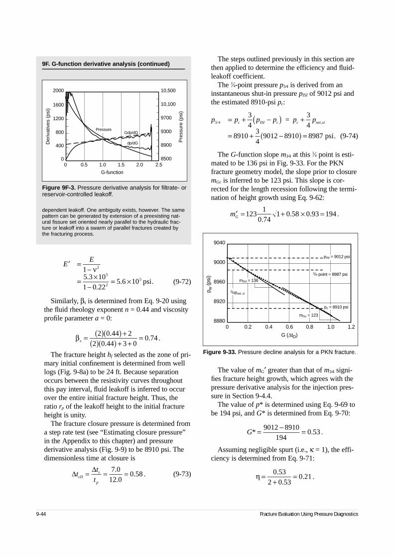
(9-72)

Similarly, βs is determined from Eq. 9-20 usingthe fluid rheology exponent n = 0.44 and viscosityprofile parameter a = 0:

The fracture height hf selected as the zone of pri-mary initial confinement is determined from welllogs (Fig. 9-8a) to be 24 ft. Because separationoccurs between the resistivity curves throughoutthis pay interval, fluid leakoff is inferred to occurover the entire initial fracture height. Thus, theratio rp of the leakoff height to the initial fractureheight is unity.

The fracture closure pressure is determined froma step rate test (see “Estimating closure pressure”in the Appendix to this chapter) and pressurederivative analysis (Fig. 9-9) to be 8910 psi. Thedimensionless time at closure is

(9-73)

The steps outlined previously in this section arethen applied to determine the efficiency and fluid-leakoff coefficient.

The 3⁄4-point pressure p3⁄4 is derived from aninstantaneous shut-in pressure pISI of 9012 psi andthe estimated 8910-psi pc:

(9-74)

The G-function slope m3⁄4 at this 3⁄4 point is esti-mated to be 136 psi in Fig. 9-33. For the PKNfracture geometry model, the slope prior to closuremGc is inferred to be 123 psi. This slope is cor-rected for the length recession following the termi-nation of height growth using Eq. 9-62:

The value of mG′ greater than that of m3⁄4 signi-fies fracture height growth, which agrees with thepressure derivative analysis for the injection pres-sure in Section 9-4.4.

The value of p* is determined using Eq. 9-69 tobe 194 psi, and G* is determined from Eq. 9-70:

Assuming negligible spurt (i.e., κ = 1), the effi-ciency is determined from Eq. 9-71:

9-44 Fracture Evaluation Using Pressure Diagnostics

Figure 9-33. Pressure decline analysis for a PKN fracture.

0 0.2 0.4 0.6 0.8 1.0 1.2

9040

9000

8960

8920

8880

p w (p

si)

G (∆tD)

pc = 8910 psi

3/4 point = 8987 psi

pISI = 9012 psi

3/4pnet, si

m3/4 = 136

mGc = 123

G* . .= − =9012 8910194

0 53

η =+

=0 532 0 53

0 21.

.. .

9F. G-function derivative analysis (continued)

dependent leakoff. One ambiguity exists, however. The samepattern can be generated by extension of a preexisting nat-ural fissure set oriented nearly parallel to the hydraulic frac-ture or leakoff into a swarm of parallel fractures created bythe fracturing process.

Figure 9F-3. Pressure derivative analysis for filtrate- orreservoir-controlled leakoff.

2000

1600

1200

800

400

0

Der

ivat

ives

(ps

i)

10,500

10,100

9700

9300

8900

8500

Pre

ssur

e (p

si)

0 0.5 1.0 1.5 2.0 2.5

G-function

dp/dG

Gdp/dGPressure

′ =−

= ×−

= ×

EE

15 3 101 0 22

5 6 10

2

5

2

5

ν.

.. psi.

∆ ∆t

t

tcDc

p

= = =7 012 0

0 58..

. .

p p p p p pc ISI c c net si3 4

34

34

891034

9012 8910 8987

/ ,= + −( ) +

= + −( ) =

=

psi.

βs = ( )( ) +( )( ) + +

=2 0 44 22 0 44 3 0

0 74.

.. .

′ = + × =mG 1231

0 741 0 58 0 93 194

.. . .

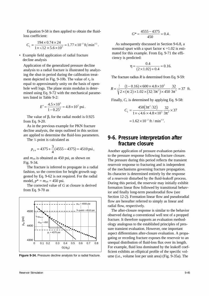
Equation 9-58 is then applied to obtain the fluid-loss coefficient:

• Example field application of radial fracture decline analysis

Application of the generalized pressure declineanalysis to a radial fracture is illustrated by analyz-ing the shut-in period during the calibration treat-ment depicted in Fig. 9-10b. The value of rp isequal to approximately unity on the basis of open-hole well logs. The plane strain modulus is deter-mined using Eq. 9-72 with the mechanical parame-ters listed in Table 9-2:

The value of βs for the radial model is 0.925from Eq. 9-20.

As in the previous example for PKN fracturedecline analysis, the steps outlined in this sectionare applied to determine the fluid-loss parameters.

The 3⁄4 point is calculated as

and m3⁄4 is obtained as 450 psi, as shown on Fig. 9-34.

The fracture is inferred to propagate in a radialfashion, so the correction for height growth sug-gested by Eq. 9-62 is not required. For the radialmodel, p* = m3⁄4 = 450 psi.

The corrected value of G at closure is derivedfrom Eq. 9-70 as

As subsequently discussed in Section 9-6.8, anominal spurt with a spurt factor κ =1.02 is esti-mated for this example. From Eq. 9-71 the effi-ciency is predicted:

The fracture radius R is determined from Eq. 9-59:

Finally, CL is determined by applying Eq. 9-58:

9-6. Pressure interpretation after fracture closure

Another application of pressure evaluation pertains to the pressure response following fracture closure.The pressure during this period reflects the transientreservoir response to fracturing and is independent of the mechanisms governing fracture propagation.Its character is determined entirely by the response of a reservoir disturbed by the fluid-leakoff process.During this period, the reservoir may initially exhibitformation linear flow followed by transitional behav-ior and finally long-term pseudoradial flow (seeSection 12-2). Formation linear flow and pseudoradialflow are hereafter referred to simply as linear andradial flow, respectively.

The after-closure response is similar to the behaviorobserved during a conventional well test of a proppedfracture. It therefore supports an evaluation method-ology analogous to the established principles of pres-sure transient evaluation. However, one importantaspect differentiates after-closure evaluation. A propa-gating or receding fracture exposes the reservoir to anunequal distribution of fluid-loss flux over its length.For example, fluid loss dominated by the leakoff coef-ficient exhibits an elliptical profile of the specific vol-ume (i.e., volume lost per unit area) (Fig. 9-35a). The

Reservoir Stimulation 9-45

p3 4 437534

4555 4375 4510/ = + −( ) = psi ,

G* . .= − =4555 4375450

0 4

η =×( ) +

=0 42 1 02 0 4

0 16.

. .. .

R = −( ) × × ×× ( ) × × ( ) ×

=1 0 16 600 4 8 102 2 1 02 32 3 450

323

375

2 33

. ..π π π

ft.

CL =( )

× × ××

= × −

450 3 32

1 4 6 4 8 10323

37

1 62 10

2

5 2

2

ππ. .

. .ft / min1/2

CL = × ×× × ×

= × −194 0 74 241 12 5 6 10

1 77 105

3..

. .ft min1/2

′ = ×−

= ×E4 5 101 0 25

4 8 105

2

5..

. psi .

Figure 9-34. Pressure decline analysis for a radial fracture.

4500

4400

43000 0.1 0.2 0.3 0.4 0.5 0.6 0.7 0.8

p w (p

si)

G(∆tD)

pc = 4375 psi

pISI = 4555 psi

3⁄4 point = 4510 psi

3⁄4 pnet,si

m3⁄4 = 450

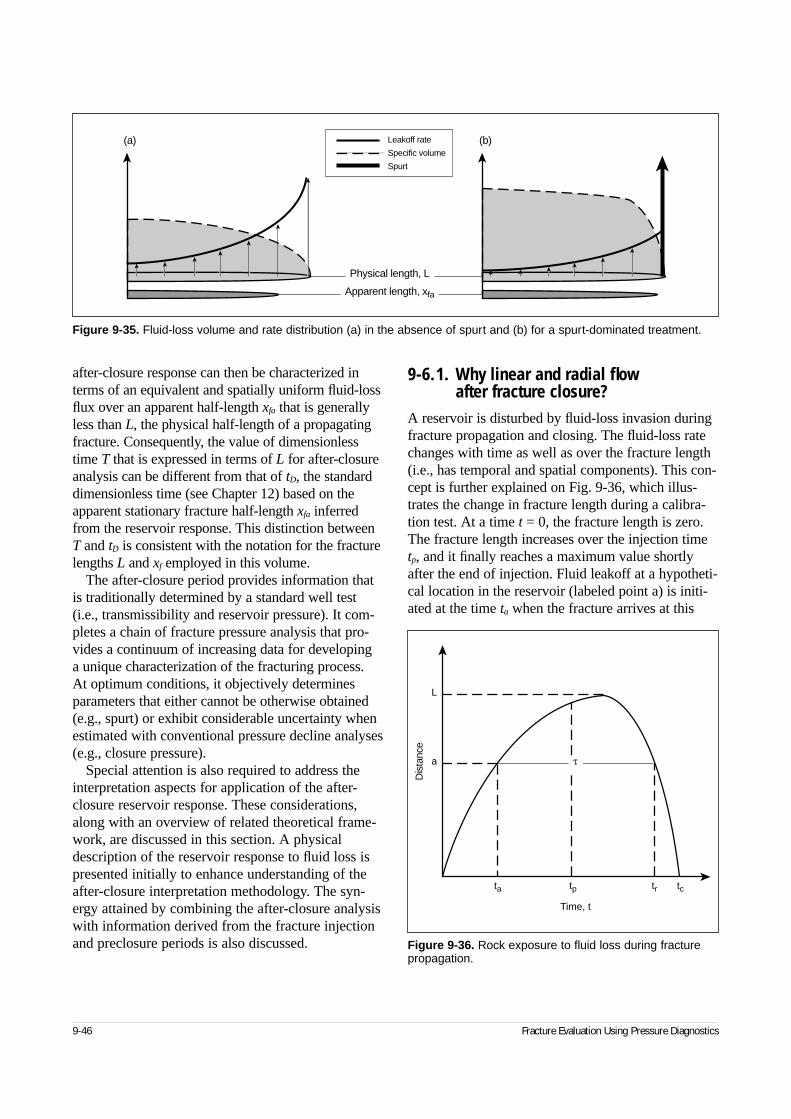
after-closure response can then be characterized interms of an equivalent and spatially uniform fluid-lossflux over an apparent half-length xfa that is generallyless than L, the physical half-length of a propagatingfracture. Consequently, the value of dimensionlesstime T that is expressed in terms of L for after-closureanalysis can be different from that of tD, the standarddimensionless time (see Chapter 12) based on theapparent stationary fracture half-length xfa inferredfrom the reservoir response. This distinction betweenT and tD is consistent with the notation for the fracturelengths L and xf employed in this volume.

The after-closure period provides information thatis traditionally determined by a standard well test(i.e., transmissibility and reservoir pressure). It com-pletes a chain of fracture pressure analysis that pro-vides a continuum of increasing data for developing a unique characterization of the fracturing process. At optimum conditions, it objectively determinesparameters that either cannot be otherwise obtained(e.g., spurt) or exhibit considerable uncertainty whenestimated with conventional pressure decline analyses(e.g., closure pressure).

Special attention is also required to address theinterpretation aspects for application of the after-closure reservoir response. These considerations,along with an overview of related theoretical frame-work, are discussed in this section. A physicaldescription of the reservoir response to fluid loss ispresented initially to enhance understanding of theafter-closure interpretation methodology. The syn-ergy attained by combining the after-closure analysiswith information derived from the fracture injectionand preclosure periods is also discussed.

9-6.1. Why linear and radial flow after fracture closure?

A reservoir is disturbed by fluid-loss invasion duringfracture propagation and closing. The fluid-loss ratechanges with time as well as over the fracture length(i.e., has temporal and spatial components). This con-cept is further explained on Fig. 9-36, which illus-trates the change in fracture length during a calibra-tion test. At a time t = 0, the fracture length is zero.The fracture length increases over the injection timetp, and it finally reaches a maximum value shortlyafter the end of injection. Fluid leakoff at a hypotheti-cal location in the reservoir (labeled point a) is initi-ated at the time ta when the fracture arrives at this

9-46 Fracture Evaluation Using Pressure Diagnostics

Figure 9-36. Rock exposure to fluid loss during fracturepropagation.

L

a τ

ta tp

Time, t

tr tc

Dis

tanc

e

Figure 9-35. Fluid-loss volume and rate distribution (a) in the absence of spurt and (b) for a spurt-dominated treatment.

Physical length, L

Apparent length, xfa

Leakoff rate

Specific volume

Spurt

(a) (b)

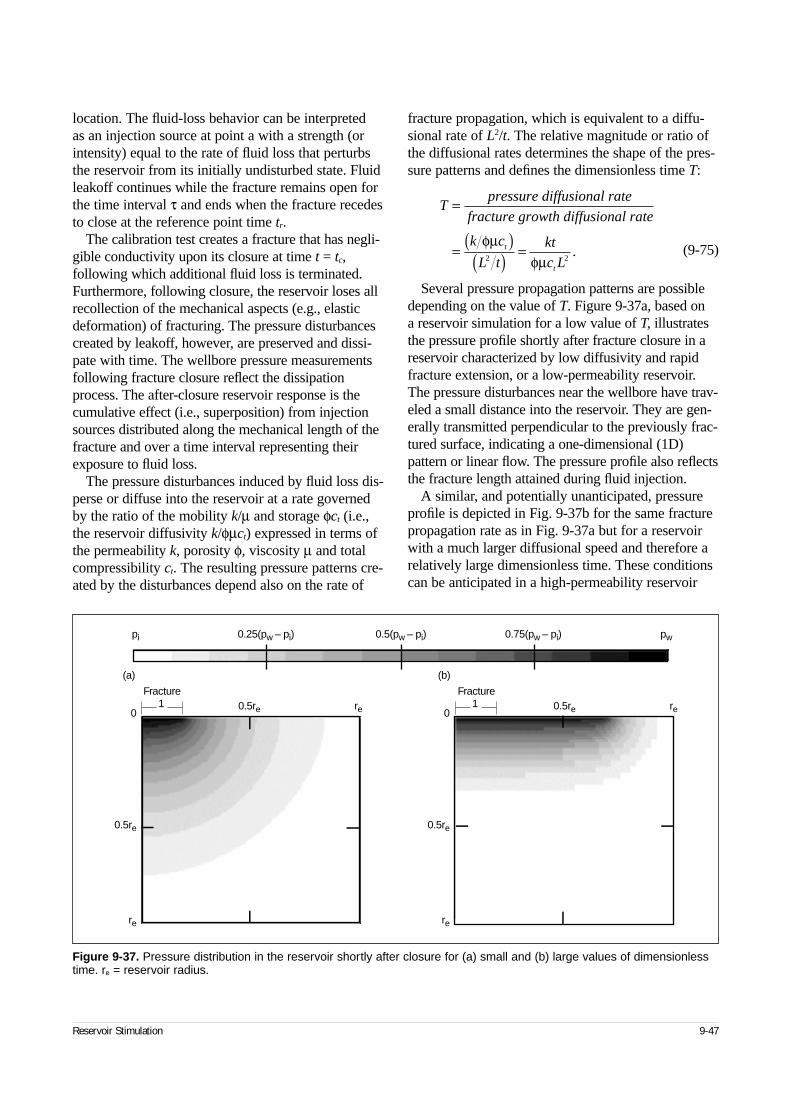
location. The fluid-loss behavior can be interpreted as an injection source at point a with a strength (orintensity) equal to the rate of fluid loss that perturbsthe reservoir from its initially undisturbed state. Fluidleakoff continues while the fracture remains open forthe time interval τ and ends when the fracture recedesto close at the reference point time tr.

The calibration test creates a fracture that has negli-gible conductivity upon its closure at time t = tc,following which additional fluid loss is terminated.Furthermore, following closure, the reservoir loses allrecollection of the mechanical aspects (e.g., elasticdeformation) of fracturing. The pressure disturbancescreated by leakoff, however, are preserved and dissi-pate with time. The wellbore pressure measurementsfollowing fracture closure reflect the dissipationprocess. The after-closure reservoir response is thecumulative effect (i.e., superposition) from injectionsources distributed along the mechanical length of thefracture and over a time interval representing theirexposure to fluid loss.

The pressure disturbances induced by fluid loss dis-perse or diffuse into the reservoir at a rate governedby the ratio of the mobility k/µ and storage φct (i.e.,the reservoir diffusivity k/φµct) expressed in terms ofthe permeability k, porosity φ, viscosity µ and totalcompressibility ct. The resulting pressure patterns cre-ated by the disturbances depend also on the rate of

fracture propagation, which is equivalent to a diffu-sional rate of L2/t. The relative magnitude or ratio ofthe diffusional rates determines the shape of the pres-sure patterns and defines the dimensionless time T:

(9-75)

Several pressure propagation patterns are possibledepending on the value of T. Figure 9-37a, based on a reservoir simulation for a low value of T, illustratesthe pressure profile shortly after fracture closure in areservoir characterized by low diffusivity and rapidfracture extension, or a low-permeability reservoir.The pressure disturbances near the wellbore have trav-eled a small distance into the reservoir. They are gen-erally transmitted perpendicular to the previously frac-tured surface, indicating a one-dimensional (1D)pattern or linear flow. The pressure profile also reflectsthe fracture length attained during fluid injection.

A similar, and potentially unanticipated, pressureprofile is depicted in Fig. 9-37b for the same fracturepropagation rate as in Fig. 9-37a but for a reservoirwith a much larger diffusional speed and therefore arelatively large dimensionless time. These conditionscan be anticipated in a high-permeability reservoir

Reservoir Stimulation 9-47

Tpressure diffusional rate

fracture growth diffusional rate

k c

L t

kt

c Lt

t

=

= ( )( ) =

φµφµ2 2

.

Figure 9-37. Pressure distribution in the reservoir shortly after closure for (a) small and (b) large values of dimensionlesstime. re = reservoir radius.

pi 0.25(pw – pi)

0.5re re

0.5(pw – pi) 0.75(pw – pi) pw

1Fracture

(a)

0

0.5re

re

0.5re re1Fracture

(b)

0

0.5re

re

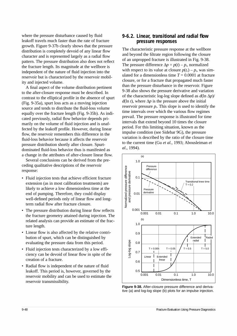
where the pressure disturbance caused by fluidleakoff travels much faster than the rate of fracturegrowth. Figure 9-37b clearly shows that the pressuredistribution is completely devoid of any linear flowcharacter and is represented largely as a radial flowpattern. The pressure distribution also does not reflectthe fracture length. Its magnitude at the wellbore isindependent of the nature of fluid injection into thereservoir but is characterized by the reservoir mobil-ity and injected volume.

A final aspect of the volume distribution pertinentto the after-closure response must be described. Incontrast to the elliptical profile in the absence of spurt(Fig. 9-35a), spurt loss acts as a moving injectionsource and tends to distribute the fluid-loss volumeequally over the fracture length (Fig. 9-35b). As indi-cated previously, radial flow behavior depends pri-marily on the volume of fluid injection and is unaf-fected by the leakoff profile. However, during linearflow, the reservoir remembers this difference in thefluid-loss behavior because it affects the reservoirpressure distribution shortly after closure. Spurt-dominated fluid-loss behavior thus is manifested as a change in the attributes of after-closure linear flow.

Several conclusions can be derived from the pre-ceding qualitative descriptions of the reservoirresponse:

• Fluid injection tests that achieve efficient fractureextension (as in most calibration treatments) arelikely to achieve a low dimensionless time at theend of pumping. Therefore, they could displaywell-defined periods only of linear flow and long-term radial flow after fracture closure.

• The pressure distribution during linear flow reflectsthe fracture geometry attained during injection. Therelated analysis can provide an estimate of the frac-ture length.

• Linear flow is also affected by the relative contri-bution of spurt, which can be distinguished byevaluating the pressure data from this period.

• Fluid injection tests characterized by a low effi-ciency can be devoid of linear flow in spite of thecreation of a fracture.

• Radial flow is independent of the nature of fluidleakoff. This period is, however, governed by thereservoir mobility and can be used to estimate thereservoir transmissibility.

9-6.2. Linear, transitional and radial flow pressure responses

The characteristic pressure response at the wellboreand beyond the filtrate region following the closureof an unpropped fracture is illustrated in Fig. 9-38.The pressure difference ∆p = p(t) – pi, normalizedwith respect to its value at closure p(tc) – pi, was sim-ulated for a dimensionless time T = 0.0001 at fractureclosure, or for a fracture that propagated much fasterthan the pressure disturbance in the reservoir. Figure9-38 also shows the pressure derivative and variationof the characteristic log-log slope defined as d(ln ∆p)/d(ln t), where ∆p is the pressure above the initialreservoir pressure pi. This slope is used to identify thetime intervals over which the various flow regimesprevail. The pressure response is illustrated for timeintervals that extend beyond 10 times the closureperiod. For this limiting situation, known as theimpulse condition (see Sidebar 9G), the pressurevariation is described by the ratio of the closure timeto the current time (Gu et al., 1993; Abousleiman etal., 1994).

9-48 Fracture Evaluation Using Pressure Diagnostics

Figure 9-38. After-closure pressure difference and deriva-tive (a) and log-log slope (b) plots for an impulse injection.

0.001 0.01 0.1 1.0 10.0

1.0

0.1

0.01

0.001

Nor

mal

ized

pre

ssur

e di

ffere

nce

and

pres

sure

der

ivat

ive

Transitional knee timeT = 0.2

0.001 0.01 0.1 1.0 10.0

1.0

0.9

0.8

0.7

0.6

0.5

Log-

log

slop

e

Dimensionless time, T

Extendedradial

Extendedlinear

Linear

Pressuredifference

Pressurederivative

Radial

T = 0.05 T = 0.5 T = 5.0T = 0.005

(a)

(b)

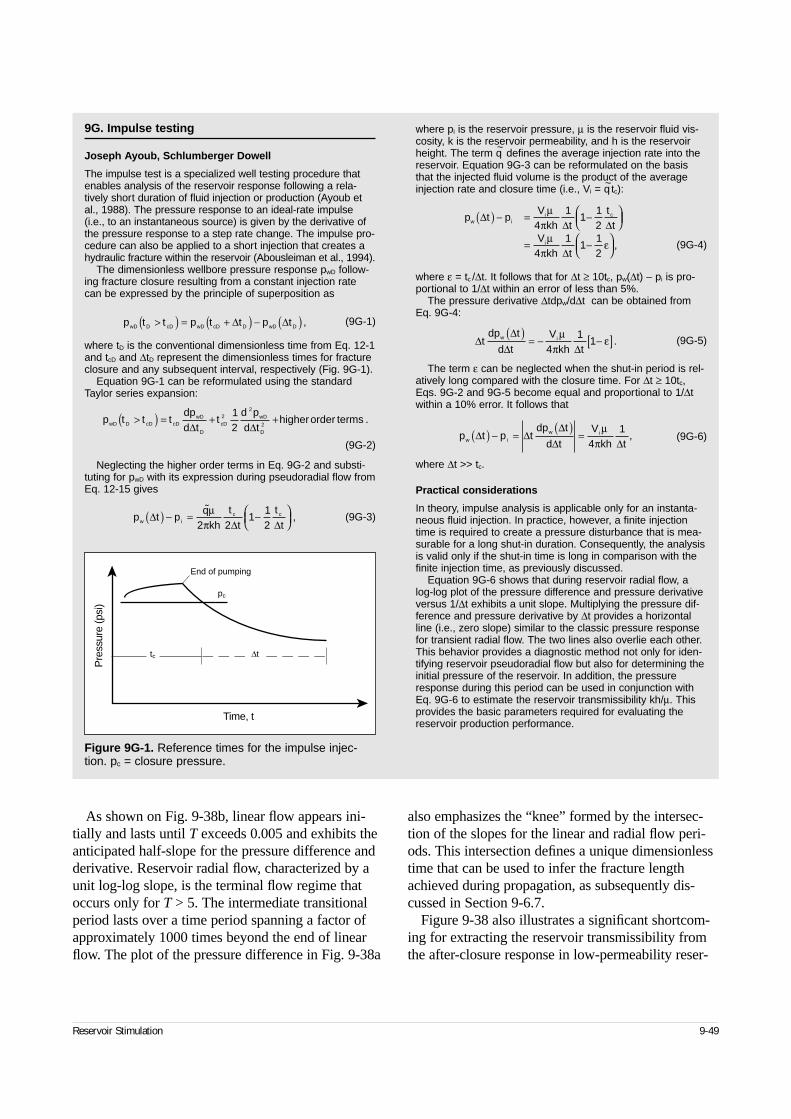
As shown on Fig. 9-38b, linear flow appears ini-tially and lasts until T exceeds 0.005 and exhibits theanticipated half-slope for the pressure difference andderivative. Reservoir radial flow, characterized by aunit log-log slope, is the terminal flow regime thatoccurs only for T > 5. The intermediate transitionalperiod lasts over a time period spanning a factor ofapproximately 1000 times beyond the end of linearflow. The plot of the pressure difference in Fig. 9-38a

also emphasizes the “knee” formed by the intersec-tion of the slopes for the linear and radial flow peri-ods. This intersection defines a unique dimensionlesstime that can be used to infer the fracture lengthachieved during propagation, as subsequently dis-cussed in Section 9-6.7.

Figure 9-38 also illustrates a significant shortcom-ing for extracting the reservoir transmissibility fromthe after-closure response in low-permeability reser-

Reservoir Stimulation 9-49

9G. Impulse testing

Joseph Ayoub, Schlumberger Dowell

The impulse test is a specialized well testing procedure thatenables analysis of the reservoir response following a rela-tively short duration of fluid injection or production (Ayoub etal., 1988). The pressure response to an ideal-rate impulse(i.e., to an instantaneous source) is given by the derivative ofthe pressure response to a step rate change. The impulse pro-cedure can also be applied to a short injection that creates ahydraulic fracture within the reservoir (Abousleiman et al., 1994).

The dimensionless wellbore pressure response pwD follow-ing fracture closure resulting from a constant injection ratecan be expressed by the principle of superposition as

(9G-1)

where tD is the conventional dimensionless time from Eq. 12-1and tcD and ∆tD represent the dimensionless times for fractureclosure and any subsequent interval, respectively (Fig. 9G-1).

Equation 9G-1 can be reformulated using the standardTaylor series expansion:

(9G-2)

Neglecting the higher order terms in Eq. 9G-2 and substi-tuting for pwD with its expression during pseudoradial flow fromEq. 12-15 gives

(9G-3)

where pi is the reservoir pressure, µ is the reservoir fluid vis-cosity, k is the reservoir permeability, and h is the reservoirheight. The term q~ defines the average injection rate into thereservoir. Equation 9G-3 can be reformulated on the basisthat the injected fluid volume is the product of the averageinjection rate and closure time (i.e., Vi = q~tc):

(9G-4)

where ε = tc /∆t. It follows that for ∆t ≥ 10tc, pw(∆t) – pi is pro-portional to 1/∆t within an error of less than 5%.

The pressure derivative ∆tdpw/d∆t can be obtained fromEq. 9G-4:

(9G-5)

The term ε can be neglected when the shut-in period is rel-atively long compared with the closure time. For ∆t ≥ 10tc,Eqs. 9G-2 and 9G-5 become equal and proportional to 1/∆twithin a 10% error. It follows that

(9G-6)

where ∆t >> tc.

Practical considerations

In theory, impulse analysis is applicable only for an instanta-neous fluid injection. In practice, however, a finite injectiontime is required to create a pressure disturbance that is mea-surable for a long shut-in duration. Consequently, the analysisis valid only if the shut-in time is long in comparison with thefinite injection time, as previously discussed.

Equation 9G-6 shows that during reservoir radial flow, alog-log plot of the pressure difference and pressure derivativeversus 1/∆t exhibits a unit slope. Multiplying the pressure dif-ference and pressure derivative by ∆t provides a horizontalline (i.e., zero slope) similar to the classic pressure responsefor transient radial flow. The two lines also overlie each other.This behavior provides a diagnostic method not only for iden-tifying reservoir pseudoradial flow but also for determining theinitial pressure of the reservoir. In addition, the pressureresponse during this period can be used in conjunction withEq. 9G-6 to estimate the reservoir transmissibility kh/µ. Thisprovides the basic parameters required for evaluating thereservoir production performance.

Figure 9G-1. Reference times for the impulse injec-tion. pc = closure pressure.

tc

Time, t

Pre

ssur

e (p

si)

pc

End of pumping

∆t

p t t p t t p twD D cD wD cD D wD D>( ) = +( ) − ( )∆ ∆ ,

p t pV

kh ttt

Vkh t

w ii c

i

∆∆ ∆

∆

( ) − = −

= −

µπ

µπ

ε

41

112

41

112

,

∆∆

∆ ∆t

dp t

d tV

kh tw i( )

= − −[ ]µπ

ε4

11 .

p t p tdp t

d tV

kh tw i

w i∆ ∆∆

∆ ∆( ) − =

( )=

µπ4

1,

p t t tdpd t

td pd twD D cD cD

wD

D

cDwD

D

>( ) = + +∆ ∆

22

2

12

higherorder terms .

p t pq

kh

t

t

t

tw ic c∆∆ ∆

( ) − = −

˜,

µπ2 2

112

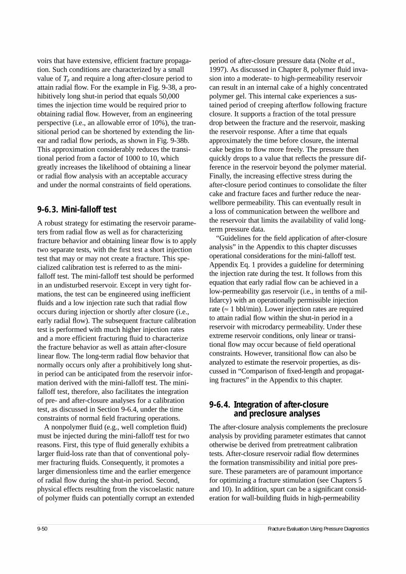
9-50 Fracture Evaluation Using Pressure Diagnostics

voirs that have extensive, efficient fracture propaga-tion. Such conditions are characterized by a smallvalue of Tp and require a long after-closure period toattain radial flow. For the example in Fig. 9-38, a pro-hibitively long shut-in period that equals 50,000times the injection time would be required prior toobtaining radial flow. However, from an engineeringperspective (i.e., an allowable error of 10%), the tran-sitional period can be shortened by extending the lin-ear and radial flow periods, as shown in Fig. 9-38b.This approximation considerably reduces the transi-tional period from a factor of 1000 to 10, whichgreatly increases the likelihood of obtaining a linearor radial flow analysis with an acceptable accuracyand under the normal constraints of field operations.

9-6.3. Mini-falloff testA robust strategy for estimating the reservoir parame-ters from radial flow as well as for characterizingfracture behavior and obtaining linear flow is to applytwo separate tests, with the first test a short injectiontest that may or may not create a fracture. This spe-cialized calibration test is referred to as the mini-falloff test. The mini-falloff test should be performedin an undisturbed reservoir. Except in very tight for-mations, the test can be engineered using inefficientfluids and a low injection rate such that radial flowoccurs during injection or shortly after closure (i.e.,early radial flow). The subsequent fracture calibrationtest is performed with much higher injection ratesand a more efficient fracturing fluid to characterizethe fracture behavior as well as attain after-closurelinear flow. The long-term radial flow behavior thatnormally occurs only after a prohibitively long shut-in period can be anticipated from the reservoir infor-mation derived with the mini-falloff test. The mini-falloff test, therefore, also facilitates the integration of pre- and after-closure analyses for a calibrationtest, as discussed in Section 9-6.4, under the timeconstraints of normal field fracturing operations.

A nonpolymer fluid (e.g., well completion fluid)must be injected during the mini-falloff test for tworeasons. First, this type of fluid generally exhibits alarger fluid-loss rate than that of conventional poly-mer fracturing fluids. Consequently, it promotes alarger dimensionless time and the earlier emergenceof radial flow during the shut-in period. Second,physical effects resulting from the viscoelastic natureof polymer fluids can potentially corrupt an extended

period of after-closure pressure data (Nolte et al.,1997). As discussed in Chapter 8, polymer fluid inva-sion into a moderate- to high-permeability reservoircan result in an internal cake of a highly concentratedpolymer gel. This internal cake experiences a sus-tained period of creeping afterflow following fractureclosure. It supports a fraction of the total pressuredrop between the fracture and the reservoir, maskingthe reservoir response. After a time that equalsapproximately the time before closure, the internalcake begins to flow more freely. The pressure thenquickly drops to a value that reflects the pressure dif-ference in the reservoir beyond the polymer material.Finally, the increasing effective stress during theafter-closure period continues to consolidate the filtercake and fracture faces and further reduce the near-wellbore permeability. This can eventually result in a loss of communication between the wellbore andthe reservoir that limits the availability of valid long-term pressure data.

“Guidelines for the field application of after-closureanalysis” in the Appendix to this chapter discussesoperational considerations for the mini-falloff test.Appendix Eq. 1 provides a guideline for determiningthe injection rate during the test. It follows from thisequation that early radial flow can be achieved in alow-permeability gas reservoir (i.e., in tenths of a mil-lidarcy) with an operationally permissible injectionrate (≈ 1 bbl/min). Lower injection rates are requiredto attain radial flow within the shut-in period in areservoir with microdarcy permeability. Under theseextreme reservoir conditions, only linear or transi-tional flow may occur because of field operationalconstraints. However, transitional flow can also beanalyzed to estimate the reservoir properties, as dis-cussed in “Comparison of fixed-length and propagat-ing fractures” in the Appendix to this chapter.

9-6.4. Integration of after-closure and preclosure analyses

The after-closure analysis complements the preclosureanalysis by providing parameter estimates that cannototherwise be derived from pretreatment calibrationtests. After-closure reservoir radial flow determinesthe formation transmissibility and initial pore pres-sure. These parameters are of paramount importancefor optimizing a fracture stimulation (see Chapters 5and 10). In addition, spurt can be a significant consid-eration for wall-building fluids in high-permeability

Reservoir Stimulation 9-51

fracturing. However, it cannot be estimated from thestandard pressure decline analysis described inSection 9-5. As previously mentioned, spurt influ-ences the linear flow response. Consequently, after-closure linear flow analysis can be used to obtain animproved on-site assessment of spurt over conven-tional core-based laboratory tests.

A significant enhancement provided by after-closure analysis is its potential to validate preclosureanalysis. The reservoir linear flow regime retains twocritical pieces of information concerning the fracturingprocess: the time when fluid loss terminated (i.e., frac-ture closure time) and the fracture length. Cessation offluid loss provides the linear flow period with a moredistinct marker for fracture closure than that obtainedfrom conventional shut-in procedures (see “Estimatingclosure pressure” in the Appendix to this chapter) thatmay exhibit multiple inflection points or a continuous,gradual pressure variation during closing. Fluid-lossdiscontinuity provides the fundamental basis for usingafter-closure analysis to determine the fracture closurepressure (see Section 9-6.8).

The transitional period exhibits a unique dimen-sionless knee time (see Fig. 9-38a) that providesinformation related to the fracture length through Eq. 9-75. The fracture length can also be estimatedfrom the preclosure pressure decline analysis (seeSection 9-5.2). The after-closure linear flow charac-teristics are derived from the principles of transientreservoir flow, which are fundamentally differentfrom the principles of linear elasticity and materialbalance for a fracture that govern the preclosure pres-sure analyses. A consistent calibration evaluation isindicated by agreement between the fracture lengthsestimated by these divergent analyses.

The preceding discussion introduces the interrela-tion between the pre- and after-closure flow periods,which is summarized in Fig. 9-39. The four inputs ofcf, G*, p* and κ are required to determine the fluidleakoff coefficient (Eq. 9-57) and the fluid efficiency(Eq. 9-71). The value of cf is provided by the pressureresponse during injection (see Section 9-7). The pre-closure shut-in period (see Section 9-5) estimates ofG* and p* and the previously discussed after-closureanalysis can be used to predict the spurt factor κ. Thefracture length is independently obtained by thesetwo approaches, and a consistent fracture analysis isindicated by agreement of the two length estimates.Finally, either the after-closure transitional or radialflow period is also used to assess the reservoir pro-

duction parameters. The synergistic, complementarycharacter of the pre- and after-closure pressure analy-ses provides a comprehensive suite of crossvalidatedfracture parameters for the optimized design of frac-ture treatments based on the economic guidelinesprovided in Chapter 10.

9-6.5. Physical and mathematical descriptions

The total pressure difference between the fracture andthe reservoir ∆pT can be divided into three compo-nents, as shown in Fig. 5-17. Of relevance to after-closure analysis is the pressure difference ∆pR in thereservoir beyond the filter cake and filtrate regions.This pressure difference represents the added contri-butions of the two sources of fluid leakoff: a contri-bution from the Carter-based leakoff loss (i.e., the CL

component of fluid loss) ∆pRC and that resulting fromspurt ∆pRS:

(9-76)

As discussed in Section 9-6.3, the pressure changesacross the filter cake and filtrate disappear within ashort time after fracture closure. The subsequent bot-tomhole pressure measurements p(t) then reflect thereservoir response to the pressure changes and fluid-loss distribution induced during the propagation andclosing periods:

(9-77)

Figure 9-39. Interrelation of pre- and after-closure pres-sure analyses.

Pumping

• Fracture model • cf

Fluid loss

• η • CL

Shut-in

• G* • p*

After-closure

• κ • xfa

Fracture geometry

• L

Reservoir

• LAnalyses

agree

∆ ∆ ∆p p pR RC RS= + .

∆ ∆p t p t p t p t tR i c( ) = ( ) = ( ) − > .

A physical and mathematical description for theafter-closure period is in this section. The focus is on∆pRC, the reservoir response to Carter-based leakoff.The effects resulting from spurt loss are addressedseparately in Section 9-6.6.

The two primary changes that the reservoir experi-ences following fracture closure are change in itsboundary condition and change in its representationin reference to the response during production of afixed-length fracture. First, as discussed in “Pressurecharacterization for a propagating fracture” in theAppendix to this chapter, the pressure difference ∆pRC

in the reservoir is constant during fracture propaga-tion. In contrast, the after-closure period is character-ized by cessation of the fluid-loss flux. Consequently,the boundary condition along the closed fracturechanges from one of constant, uniform pressure tozero or constant flux. The change in the boundarycondition is referred to as a mixed-boundary condition.

The second difference between the preclosure andafter-closure periods pertains to the representation ofthe after-closure period, which is analogous to theproblem of a fixed-length fracture used in pressuretransient analysis. The leakoff distribution followingfracture closure is shown in Fig. 9-35. The illustratedvolume profile closely reflects the distributionexpected for a fixed-length, uniform-flux fracture andcan be used to represent the after-closure pressureresponse. This observation contrasts with the pre-closure conditions of a propagating fracture, forwhich the fluid-loss flux distribution is better repre-sented by a fixed-length, uniform-pressure fracture.This distinction is elaborated in “Comparison offixed-length and propagating fractures” in theAppendix to this chapter.

• Apparent fracture length

The previous discussion indicates that the after-closure reservoir response can be analyzed by con-sidering the leakoff flux to be uniformly distrib-uted over an equivalent fixed-length fracture. Theapparent length of the equivalent fracture xfa isgenerally smaller than the physical length Lattained by the fracture during propagation. Itsratio with respect to the physical length is definedas the apparent length fraction:

(9-78)

It follows from Eqs. 9-75, 9-78 and 12-1 that thedimensionless time tD, which corresponds to theapparent length xfa, is related to T as

(9-79)

A general expression for faL in terms of the fluid-loss parameters was given by Nolte et al. (1997):

(9-80)

For the case of inefficient fracture propagation(η → 0) and negligible spurt (κ → 1), g0 = π/2and tc → tp. Equation 9-80 then indicates that faL = π/4 (Fig. 9-35a). For spurt-dominated treat-ments (κ >> 1), the specific volume-loss distri-bution over the fracture length is approximatelyconstant, as illustrated in Fig. 9-35b. As expectedfor this case, Eq. 9-80 indicates that faL approachesunity.

• Linear flow

The similarity between reservoir transient flow andheat transfer arises because of the underlying “dif-fusional” process that governs these two physicalphenomena. The physical concept of heat conduc-tivity is similar to that of reservoir mobility,whereas the heat capacity of a solid body is equiv-alent to the reservoir storage. An expression for∆pRC during the after-closure linear flow period forthe mixed-boundary condition can be adapted froma similar condition presented by Carslaw andJaegar (1959) for heat transfer (Nolte et al., 1997):

(9-81)

where t is the time since fracture initiation.Equation 9-81 is based on 1D heat transfer

through the surface for an infinitely long fracture.It also applies to the wellbore pressure of a finite-length fracture in linear flow because the reservoirsurrounding the wellbore is experiencing 1D reser-voir flow (Fig. 9-37a).

9-52 Fracture Evaluation Using Pressure Diagnostics

fx

LaLfa= .

∆p t Ck c

t t

Ck c

t

tt t

Ck c

t

tt t

RC L

t

c

L

t

cc

L

t

cc

( ) = =

=

>

≈

>

−

πµφπµφ ππµφ π

2sin

,

1

23

T f taL D= 2 .

fg

g t taL

c p

=−( ) −( ) +

0

01 1 2ηκ

κ.

Reservoir Stimulation 9-53

• Radial flow

No relation analogous to Eq. 9-81 for a finite-length fracture with a mixed-boundary conditionapplicable to radial flow has been presented in theliterature. This reservoir response can alternativelybe described by a superposition relation with thelogarithmic time function that is commonly usedto describe the radial flow response for a fixed-length fracture (Eq. 12-15):

(9-82)

The terms preceding the brackets on the right-hand side of Eq. 9-82 are incorporated to ensurethat its long-term asymptotic behavior provides thewell-known response for an impulse test (seeSidebar 9G).

Equation 9-82 also incorporates the apparentclosure time λtc. The apparent production timeused for the mixed-boundary condition in standardpressure transient analysis (Horner, 1951) isdefined as the ratio of the cumulative volume andthe final production rate. This definition of appar-ent time is not applicable for a propagating frac-ture. Rather, the multiplier λ was selected fromnumerical simulations as the value that providesthe shortest after-closure time for the applicationof Eq. 9-82. For the mini-falloff test and its relatedconditions of negligible efficiency and spurt, theoptimized value of λ can be characterized as

(9-83)

Equations 9-82 and 9-83 provide the reservoirtransmissibility with acceptable accuracy signifi-cantly before the actual occurrence of radial flow.For example, for a dimensionless pumping time Tp

= 0.1, the optimized multiplier expression enablesthe application of Eq. 9-82 at a dimensionless timeT = 0.5 as opposed to T = 2 required for a standardradial flow analysis. Furthermore, Eq. 9-83 showsthat λ is equal essentially to unity for well-devel-oped radial flow (i.e., Tp > 5). For these conditions,the effect of the mixed-boundary condition dimin-ishes. The time function in Eq. 9-82 then is equiv-

alent to the standard Horner function used duringpressure transient testing.

9-6.6. Influence of spurt lossThe preceding discussion of the reservoir responsedoes not consider the effect of spurt. Its considera-tion, however, is important because spurt can domi-nate the wall-building fluid-loss behavior of moder-ate- to high-permeability formations.

The role of spurt during either the pre- or after-closure period is difficult to describe with simple ana-lytical concepts. However, characterizing its contribu-tion to the reservoir pressure difference ∆pRS wasfound to be relatively simple, based on the results of numerical simulations (Nolte et al., 1997). Theseindicate that during the linear flow period spurtcauses a time-dependent increase in the pressure. Itspressure response ∆pRS is added to the pressure con-tribution from Carter-based leakoff behavior (Eq. 9-81). The total reservoir pressure difference ∆p during the after-closure linear flow period thatincludes the spurt contribution can be expressed interms of ∆pRC and the spurt factor κ as

(9-84)

In particular, the pressure difference during anextended period of linear flow can be approximatedfrom Eqs. 9-81 and 9-84 as

(9-85)

where the spurt fraction fκ is defined as

(9-86)

The distinctive time behavior exhibited by spurtduring the after-closure period is illustrated in Fig. 9-40, which is based on the linear flow timefunction FL(t/tc) that is subsequently defined in Eq. 9-88. As discussed in Section 9-6.8, this presenta-tion is consistent with the diagnostic log-log plot forflow regime identification. The reservoir pressure dif-ference is normalized with respect to ∆pRC(tc) and iscompared for the conditions of negligible spurt (κ =

λ η κ= + → →10 14

0 1.

, .Tp

∆ ∆p t p tt

t

t

tt tRC c

c pc( ) = ( )

+ −

≥−2 1

21

πκ

sin .

∆p t C fk c

t

tt tL

t

cc( ) ≈ +( )

>12

3κπµφ π

,

ft

tp

c

κπ κ= −( )4

1 .

∆p tkh

V

t

t t t

t t

kh

V

t tt t t

i

c

c c

c

i

c

c c

( ) =+ −( )

−

≈−

>>

µπ λ

λ

µπ

λ

21

2

4

ln

– .

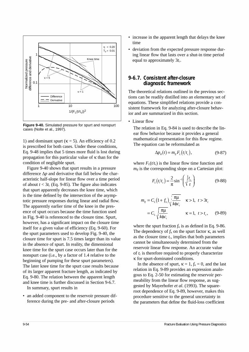
1) and dominant spurt (κ = 5). An efficiency of 0.2 is prescribed for both cases. Under these conditions, Eq. 9-48 implies that 5 times more fluid is lost duringpropagation for this particular value of κ than for thecondition of negligible spurt.

Figure 9-40 shows that spurt results in a pressuredifference ∆p and derivative that fall below the char-acteristic half-slope for linear flow over a time periodof about t < 3tc (Eq. 9-85). The figure also indicatesthat spurt apparently decreases the knee time, whichis the time defined by the intersection of the asymp-totic pressure responses during linear and radial flow.The apparently earlier time of the knee in the pres-ence of spurt occurs because the time function usedin Fig. 9-40 is referenced to the closure time. Spurt,however, has a significant impact on the closure timeitself for a given value of efficiency (Eq. 9-60). Forthe spurt parameters used to develop Fig. 9-40, theclosure time for spurt is 7.5 times larger than its valuein the absence of spurt. In reality, the dimensionalknee time for the spurt case occurs later than for thenonspurt case (i.e., by a factor of 1.4 relative to thebeginning of pumping for these spurt parameters).The later knee time for the spurt case results becauseof its larger apparent fracture length, as indicated byEq. 9-80. The relation between the apparent lengthand knee time is further discussed in Section 9-6.7.

In summary, spurt results in

• an added component to the reservoir pressure dif-ference during the pre- and after-closure periods

• increase in the apparent length that delays the kneetime

• deviation from the expected pressure response dur-ing linear flow that lasts over a shut-in time periodequal to approximately 3tc.

9-6.7. Consistent after-closure diagnostic framework

The theoretical relations outlined in the previous sec-tions can be readily distilled into an elementary set ofequations. These simplified relations provide a con-sistent framework for analyzing after-closure behav-ior and are summarized in this section.

• Linear flow

The relation in Eq. 9-84 is used to describe the lin-ear flow behavior because it provides a generalmathematical representation for this flow regime.The equation can be reformulated as

(9-87)

where FL(t/tc) is the linear flow time function andmlf is the corresponding slope on a Cartesian plot:

(9-88)

(9-89)

where the spurt fraction fκ is as defined in Eq. 9-86.The dependency of fκ on the spurt factor κ, as wellas the closure time tc, implies that both parameterscannot be simultaneously determined from thereservoir linear flow response. An accurate valueof tc is therefore required to properly characterizeκ for spurt-dominated conditions.

In the absence of spurt, κ = 1, fκ = 0, and the lastrelation in Eq. 9-89 provides an expression analo-gous to Eq. 2-50 for estimating the reservoir per-meability from the linear flow response, as sug-gested by Mayerhofer et al. (1993). The square-root dependence of Eq. 9-89, however, makes thisprocedure sensitive to the general uncertainty inthe parameters that define the fluid-loss coefficient

9-54 Fracture Evaluation Using Pressure Diagnostics

∆p t m F t tR lf L c( ) = ( ) ,

F t tt

tL cc( ) =

−2 1

πsin

m C fk c

t t

Ck c

t t

lf L

t

c

L

t

c

= +( ) > >

= = >

1 1 3

1

κπµφ

κ

πµφ

κ

,

, ,

Figure 9-40. Simulated pressure for spurt and nonspurtcases (Nolte et al., 1997).

1

0.1

1 10 100

1/{FL(t/tc)}2

Nor

mal

ized

pre

ssur

e di

ffere

nce

and

deriv

ativ

e

κ = 5

κ = 1

η = 0.20Tp = 0.01

Knee time

DifferenceDerivative

and reservoir storage. Consequently, the techniquecould introduce significant uncertainty in theinferred permeability (Ispas et al., 1998).

• Radial flow

Equation 9-82 provides the general expression of the logarithmic time function that describes thereservoir pressure difference during radial flow.This function can be approximated by the squareof its linear flow counterpart (Eq. 9-88) by intro-ducing a coefficient of π2/8:

(9-90)

where ε is the error introduced by the approxi-mation. The relative error can be based on thepressure derivative because it is the primary mea-sure for after-closure analysis. Thus,

(9-91)

It follows from Eq. 9-91 that the error introducedby the approximation in Eq. 9-90 is at a minimumwhen the apparent time multiplier λ = 4⁄3. As indi-cated by Eq. 9-83, this value of λ corresponds to adimensionless injection time Tp = 0.4, which meetsthe desired condition of a mini-falloff test for earlyradial flow analysis. The approximation, therefore,is well suited for application to the mini-falloff test.More generally, the relative error ε can be shown tobe less than 5% for the after-closure period recom-mended in “Guidelines for the field application ofafter-closure analysis” in the Appendix to thischapter and using the expression for λ providedby Eq. 9-83.

The radial flow period can then be representedby substituting the approximation provided by Eq. 9-90 into Eq. 9-82:

(9-92)

where the function FL(t/tc) is defined in Eq. 9-88and mrf is the corresponding slope on a Cartesianplot:

(9-93)

Equations 9-87 and 9-92 suggest that a log-logdiagnostic plot of the pressure difference and pres-sure derivative based on {FL(t/tc)}2 would providea consistent basis for diagnosing both linear andradial flow. The plot also would provide the half-slope and unit slope behavior during linear flowand radial flow, respectively, as is expected forafter-closure pressure analysis.

• Spurt

Spurt is estimated from the linear flow slope mlf

using Eqs. 9-86 and 9-89:

(9-94)

The spurt factor κ can be related to the spurtcoefficient Sp with Appendix Eq. 24.

• Fracture length

The fracture length is obtained from the dimension-less time corresponding to the knee formed by theintersection of the asymptotic log-log slopes duringlinear and radial flow, in a plot similar to Fig. 9-38a.A general relation for the fracture length can bederived from the pressure response for a fixed-length fracture and relating its behavior to that ofthe propagating fracture using the apparent lengthfraction faL, as discussed in Section 9-6.5.

The fracture length is required to verify the pre-closure analysis for a calibration test, where theuse of a more efficient fracturing fluid generallyleads to a well-defined linear flow response. Theknee subsequently occurs only after a significantlylonger after-closure shut-in period (Fig. 9-38).Under this extended shut-in condition, the after-closure response can be approximated by theimpulse assumption (see Sidebar 9G). The asymp-totic expressions for a fixed-length fracture for lin-ear and radial flow, in terms of the classic dimen-sionless time tD, follow from Eqs. 12-12 and 12-15,respectively. The derivatives during these periodsare

(9-95)

where pD is the standard dimensionless pressure,defined in Eq. 12-2. The knee time tD,knee, or thedimensionless time for the crossing of the two

Reservoir Stimulation 9-55

12

18

21

21

2

λλ π

πεln sin ,+

−

≈

+( )−t

t t

t

tc

c

c

ε λ= −

>4

33

t

tt tc

c∆∆ .

∆p t m F t trf L c( ) = ( ){ }2,

mV

khtrfi

c

= π µ16

.

κπ

φπµ

= + −

1

41

m

C

k c t

tlf

L

t c

p

.

dp

dtt

t

D

D

D

D

=

πLinear flow

Radial flow,

21

2

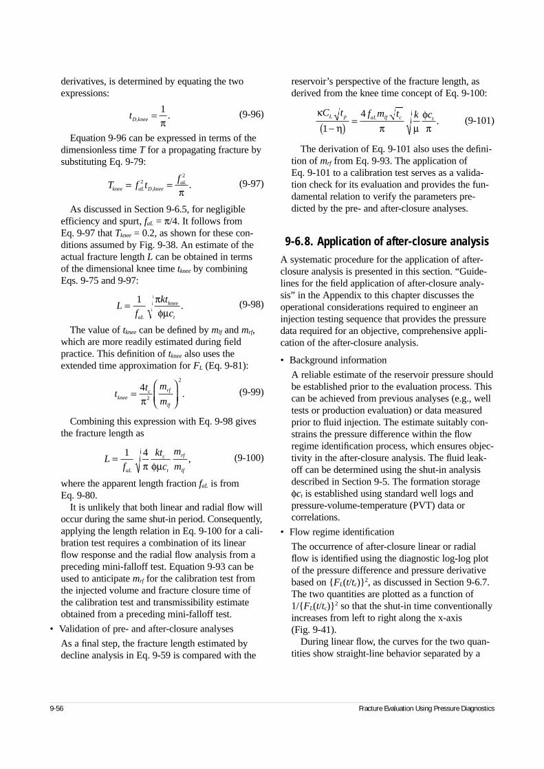
derivatives, is determined by equating the twoexpressions:

(9-96)

Equation 9-96 can be expressed in terms of thedimensionless time T for a propagating fracture bysubstituting Eq. 9-79:

(9-97)

As discussed in Section 9-6.5, for negligibleefficiency and spurt, faL = π/4. It follows from Eq. 9-97 that Tknee = 0.2, as shown for these con-ditions assumed by Fig. 9-38. An estimate of theactual fracture length L can be obtained in terms of the dimensional knee time tknee by combiningEqs. 9-75 and 9-97:

(9-98)

The value of tknee can be defined by mlf and mrf,which are more readily estimated during fieldpractice. This definition of tknee also uses theextended time approximation for FL (Eq. 9-81):

(9-99)

Combining this expression with Eq. 9-98 givesthe fracture length as

(9-100)

where the apparent length fraction faL is from Eq. 9-80.

It is unlikely that both linear and radial flow willoccur during the same shut-in period. Consequently,applying the length relation in Eq. 9-100 for a cali-bration test requires a combination of its linearflow response and the radial flow analysis from apreceding mini-falloff test. Equation 9-93 can beused to anticipate mrf for the calibration test fromthe injected volume and fracture closure time ofthe calibration test and transmissibility estimateobtained from a preceding mini-falloff test.

• Validation of pre- and after-closure analyses

As a final step, the fracture length estimated bydecline analysis in Eq. 9-59 is compared with the

reservoir’s perspective of the fracture length, asderived from the knee time concept of Eq. 9-100:

(9-101)

The derivation of Eq. 9-101 also uses the defini-tion of mrf from Eq. 9-93. The application of Eq. 9-101 to a calibration test serves as a valida-tion check for its evaluation and provides the fun-damental relation to verify the parameters pre-dicted by the pre- and after-closure analyses.

9-6.8. Application of after-closure analysisA systematic procedure for the application of after-closure analysis is presented in this section. “Guide-lines for the field application of after-closure analy-sis” in the Appendix to this chapter discusses theoperational considerations required to engineer aninjection testing sequence that provides the pressuredata required for an objective, comprehensive appli-cation of the after-closure analysis.

• Background information

A reliable estimate of the reservoir pressure shouldbe established prior to the evaluation process. Thiscan be achieved from previous analyses (e.g., welltests or production evaluation) or data measuredprior to fluid injection. The estimate suitably con-strains the pressure difference within the flowregime identification process, which ensures objec-tivity in the after-closure analysis. The fluid leak-off can be determined using the shut-in analysisdescribed in Section 9-5. The formation storage φct is established using standard well logs andpressure-volume-temperature (PVT) data orcorrelations.

• Flow regime identification

The occurrence of after-closure linear or radialflow is identified using the diagnostic log-log plotof the pressure difference and pressure derivativebased on {FL(t/tc)}2, as discussed in Section 9-6.7.The two quantities are plotted as a function of1/{FL(t/tc)}2 so that the shut-in time conventionallyincreases from left to right along the x-axis (Fig. 9-41).

During linear flow, the curves for the two quan-tities show straight-line behavior separated by a

9-56 Fracture Evaluation Using Pressure Diagnostics

Lf

kt

c

m

maL

c

t

rf

lf

= 1 4π φµ

,

κη π µ

φπ

C t f m t k cL p aL lf c t

1

4

−( ) = .tD knee, .= 1π

T f tf

knee aL D kneeaL= =22

, .π

Lf

kt

caL

knee

t

= 1 πφµ

.

tt m

mkneec rf

lf

=

4

2

2

π.

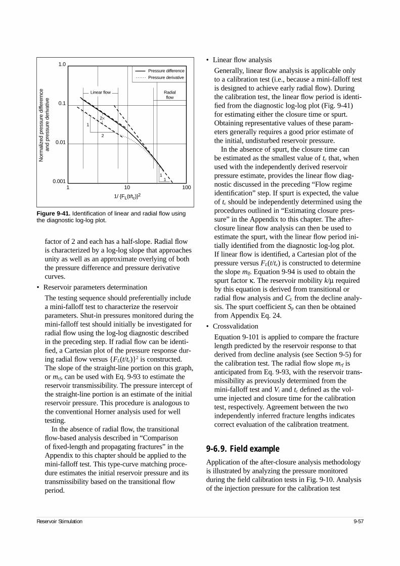
factor of 2 and each has a half-slope. Radial flowis characterized by a log-log slope that approachesunity as well as an approximate overlying of boththe pressure difference and pressure derivativecurves.

• Reservoir parameters determination

The testing sequence should preferentially includea mini-falloff test to characterize the reservoirparameters. Shut-in pressures monitored during themini-falloff test should initially be investigated forradial flow using the log-log diagnostic describedin the preceding step. If radial flow can be identi-fied, a Cartesian plot of the pressure response dur-ing radial flow versus {FL(t/tc)}2 is constructed.The slope of the straight-line portion on this graph,or mrf, can be used with Eq. 9-93 to estimate thereservoir transmissibility. The pressure intercept ofthe straight-line portion is an estimate of the initialreservoir pressure. This procedure is analogous tothe conventional Horner analysis used for welltesting.

In the absence of radial flow, the transitionalflow-based analysis described in “Comparison of fixed-length and propagating fractures” in theAppendix to this chapter should be applied to themini-falloff test. This type-curve matching proce-dure estimates the initial reservoir pressure and itstransmissibility based on the transitional flowperiod.

• Linear flow analysis

Generally, linear flow analysis is applicable only to a calibration test (i.e., because a mini-falloff testis designed to achieve early radial flow). Duringthe calibration test, the linear flow period is identi-fied from the diagnostic log-log plot (Fig. 9-41) for estimating either the closure time or spurt.Obtaining representative values of these param-eters generally requires a good prior estimate ofthe initial, undisturbed reservoir pressure.

In the absence of spurt, the closure time can be estimated as the smallest value of tc that, whenused with the independently derived reservoirpressure estimate, provides the linear flow diag-nostic discussed in the preceding “Flow regimeidentification” step. If spurt is expected, the valueof tc should be independently determined using theprocedures outlined in “Estimating closure pres-sure” in the Appendix to this chapter. The after-closure linear flow analysis can then be used toestimate the spurt, with the linear flow period ini-tially identified from the diagnostic log-log plot. If linear flow is identified, a Cartesian plot of thepressure versus FL(t/tc) is constructed to determinethe slope mlf. Equation 9-94 is used to obtain thespurt factor κ. The reservoir mobility k/µ requiredby this equation is derived from transitional orradial flow analysis and CL from the decline analy-sis. The spurt coefficient Sp can then be obtainedfrom Appendix Eq. 24.

• Crossvalidation

Equation 9-101 is applied to compare the fracturelength predicted by the reservoir response to thatderived from decline analysis (see Section 9-5) forthe calibration test. The radial flow slope mrf isanticipated from Eq. 9-93, with the reservoir trans-missibility as previously determined from themini-falloff test and Vi and tc defined as the vol-ume injected and closure time for the calibrationtest, respectively. Agreement between the twoindependently inferred fracture lengths indicatescorrect evaluation of the calibration treatment.

9-6.9. Field exampleApplication of the after-closure analysis methodologyis illustrated by analyzing the pressure monitoredduring the field calibration tests in Fig. 9-10. Analysisof the injection pressure for the calibration test

Reservoir Stimulation 9-57

Figure 9-41. Identification of linear and radial flow usingthe diagnostic log-log plot.

1.0

0.1

0.01

0.001

Nor

mal

ized

pre

ssur

e di

ffere

rnce

an

d pr

essu

re d

eriv

ativ

e

1 10 100

1/ {FL(t/tc)}2

2×1

11

2

Pressure difference

Pressure derivative

Linear flow Radialflow

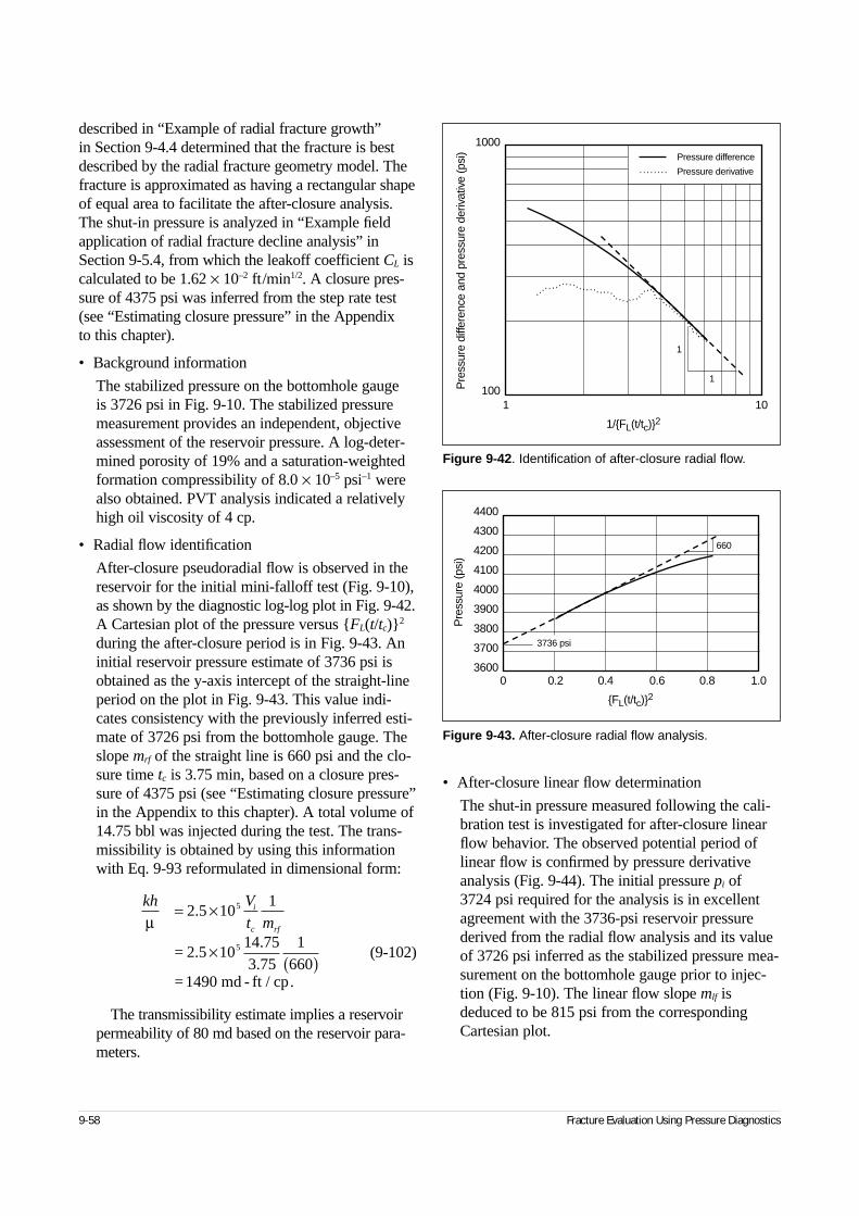
described in “Example of radial fracture growth” in Section 9-4.4 determined that the fracture is bestdescribed by the radial fracture geometry model. Thefracture is approximated as having a rectangular shapeof equal area to facilitate the after-closure analysis.The shut-in pressure is analyzed in “Example fieldapplication of radial fracture decline analysis” inSection 9-5.4, from which the leakoff coefficient CL iscalculated to be 1.62 × 10–2 ft/min1/2. A closure pres-sure of 4375 psi was inferred from the step rate test(see “Estimating closure pressure” in the Appendix to this chapter).

• Background information

The stabilized pressure on the bottomhole gauge is 3726 psi in Fig. 9-10. The stabilized pressuremeasurement provides an independent, objectiveassessment of the reservoir pressure. A log-deter-mined porosity of 19% and a saturation-weightedformation compressibility of 8.0 × 10–5 psi–1 werealso obtained. PVT analysis indicated a relativelyhigh oil viscosity of 4 cp.

• Radial flow identification

After-closure pseudoradial flow is observed in thereservoir for the initial mini-falloff test (Fig. 9-10),as shown by the diagnostic log-log plot in Fig. 9-42.A Cartesian plot of the pressure versus {FL(t/tc)}2

during the after-closure period is in Fig. 9-43. Aninitial reservoir pressure estimate of 3736 psi isobtained as the y-axis intercept of the straight-lineperiod on the plot in Fig. 9-43. This value indi-cates consistency with the previously inferred esti-mate of 3726 psi from the bottomhole gauge. Theslope mrf of the straight line is 660 psi and the clo-sure time tc is 3.75 min, based on a closure pres-sure of 4375 psi (see “Estimating closure pressure”in the Appendix to this chapter). A total volume of14.75 bbl was injected during the test. The trans-missibility is obtained by using this informationwith Eq. 9-93 reformulated in dimensional form:

(9-102)

The transmissibility estimate implies a reservoirpermeability of 80 md based on the reservoir para-meters.

• After-closure linear flow determination

The shut-in pressure measured following the cali-bration test is investigated for after-closure linearflow behavior. The observed potential period oflinear flow is confirmed by pressure derivativeanalysis (Fig. 9-44). The initial pressure pi of3724 psi required for the analysis is in excellentagreement with the 3736-psi reservoir pressurederived from the radial flow analysis and its valueof 3726 psi inferred as the stabilized pressure mea-surement on the bottomhole gauge prior to injec-tion (Fig. 9-10). The linear flow slope mlf isdeduced to be 815 psi from the correspondingCartesian plot.

9-58 Fracture Evaluation Using Pressure Diagnostics

Figure 9-42. Identification of after-closure radial flow.

1000

100Pre

ssur

e di

ffere

nce

and

pres

sure

der

ivat

ive

(psi

)

1 10

1/{FL(t/tc)}2

Pressure difference

Pressure derivative

1

1

Figure 9-43. After-closure radial flow analysis.

4400

4300

4200

4100

4000

3900

3800

3700

3600

Pre

ssur

e (p

si)

0 0.2 0.4 0.6 0.8 1.0

{FL(t/tc)}2

660

3736 psi

kh V

t mi

c rfµ= ×

×( )

2 5 101

2 1014 753 75

1660

1

5

5

.

..

= .5

= 490 md - ft / cp.

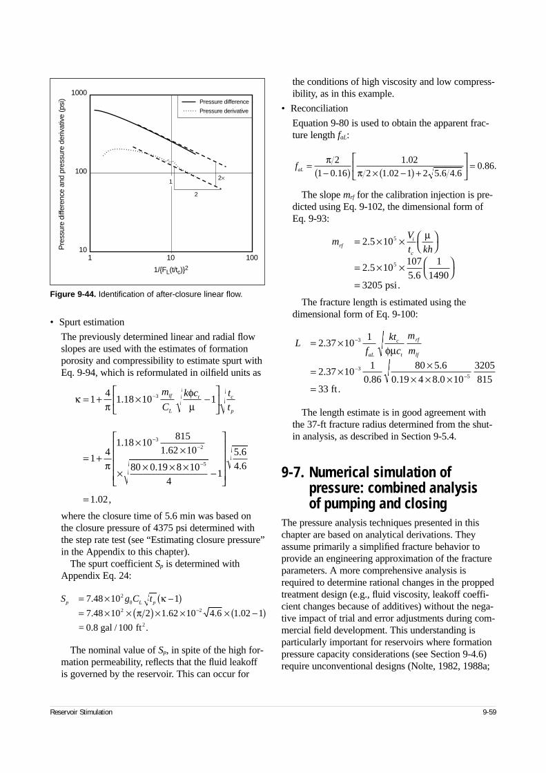
• Spurt estimation

The previously determined linear and radial flowslopes are used with the estimates of formationporosity and compressibility to estimate spurt withEq. 9-94, which is reformulated in oilfield units as

where the closure time of 5.6 min was based onthe closure pressure of 4375 psi determined withthe step rate test (see “Estimating closure pressure”in the Appendix to this chapter).

The spurt coefficient Sp is determined withAppendix Eq. 24:

The nominal value of Sp, in spite of the high for-mation permeability, reflects that the fluid leakoffis governed by the reservoir. This can occur for

the conditions of high viscosity and low compress-ibility, as in this example.

• Reconciliation

Equation 9-80 is used to obtain the apparent frac-ture length faL:

The slope mrf for the calibration injection is pre-dicted using Eq. 9-102, the dimensional form ofEq. 9-93:

The fracture length is estimated using thedimensional form of Eq. 9-100:

The length estimate is in good agreement withthe 37-ft fracture radius determined from the shut-in analysis, as described in Section 9-5.4.

9-7. Numerical simulation of pressure: combined analysis of pumping and closing

The pressure analysis techniques presented in thischapter are based on analytical derivations. Theyassume primarily a simplified fracture behavior toprovide an engineering approximation of the fractureparameters. A more comprehensive analysis isrequired to determine rational changes in the proppedtreatment design (e.g., fluid viscosity, leakoff coeffi-cient changes because of additives) without the nega-tive impact of trial and error adjustments during com-mercial field development. This understanding isparticularly important for reservoirs where formationpressure capacity considerations (see Section 9-4.6)require unconventional designs (Nolte, 1982, 1988a;

Reservoir Stimulation 9-59

Figure 9-44. Identification of after-closure linear flow.

1000

100

10Pre

ssur

e di

ffere

nce

and

pres

sure

der

ivat

ive

(psi

)

1 10 100

1/{FL(t/tc)}2

2×

2

1

Pressure difference

Pressure derivative

κπ

φµ

π

= + × −

= +×

×

× × × × −

=

−

−−

−

14

1 18 10 1

14

1 18 10815

1 62 10

80 0 19 8 104

1

5 64 6

1 02

3

3

2

5

.

..

.

.

.

. ,

m

C

k c t

tlf

L

t c

p

S g C tp L p= × −( )= × × ( ) × × × −( )−

7 48 10 1

7 48 10 2 1 62 10 4 6 1 02 1

0

20

2 2

.

. . . .

.

κπ

= .8 gal / 100 ft2

faL =−( ) × −( ) +

=π

π2

1 0 161 02

2 1 02 1 2 5 6 4 60 86

..

. . .. .

mV

t khrfi

c

= × ×

= × ×

=

2 5 10

2 5 101075 6

11490

3205

5

5

.

..

µ

psi.

Lf

kt

c

m

maL

c

t

rf

lf

= ×

= × ×× × ×

=

−

−−

2 37 101

2 37 101

0 8680 5 6

0 19 4 8 0 103205815

33

3

3

5

.

..

.. .

φµ

ft .

Warpinski and Branagan, 1988) to produce thedesired fracture geometry.

These objectives are best achieved with an appro-priately calibrated numerical simulator that adequatelyreplicates the important processes that occur during afracturing application. The simulator that best meetsthese objectives is most likely not one of the compre-hensive, computationally intensive simulators that arebetter suited to research environments (e.g., Plahn etal., 1997). The description of the overall fracturebehavior required for routine engineering applicationscan generally be satisfied by P3D fracture geometrymodels (see Section 6-3).

9-7.1. Pressure matchingA typical approach for calibrating a numerical frac-ture simulator is through iterative pressure matching.The fracture simulator is executed with varying para-meter inputs to visually match the simulated pressurewith the field measurements. The quality of the pres-sure match is assessed by balancing objectivity, phys-ical insight and constraints from other data sources.However, given the limited number of formationparameters that can be accurately characterized usingwireline logs or laboratory tests, the procedure canrequire significant effort when several parameters arenot known. A large number of unknown parametersmay also compromise the objectivity of the matchingprocedure.

An alternative approach for pressure matchingrelies on an algorithm that repeatedly executes thefracture simulator to improve the estimates of thefracture parameters within specified bounds until thebest match to the field-measured response is obtained.This semiautomated approach, discussed in Section6-12, is based on conventional principles of nonlinearregression analysis for system identification. Thetechnique, initially introduced by Gringarten et al.(1979) for well test analysis, has also been applied to log interpretation and reservoir characterization.

9-7.2. NonuniquenessPressure matching is an inverse problem for whichthe input (i.e., fracture treatment schedule) and output(i.e., fracture pressure) are known and are used todetermine the unknown model parameters (e.g., zonestresses, leakoff coefficient). An inherent limitation

with any inverse problem is the occurrence ofnonunique solutions. With respect to hydraulic frac-turing, nonuniqueness arises when more than onecombination of the unknown parameters can be usedto approximate the observed pressure.

A multitude of parameters govern fracture behaviorin a nonlinear and coupled fashion. Uncertainty insome of the parameters leads to erroneous predictionof the unknown parameters inferred by the pressure-matching process. A nonunique parameter set thatproduces an incorrect prediction of the fracture geom-etry results in an inappropriate redesign of thepropped treatment. This effect is readily apparent in Eq. 9-24, in which the pressure response duringpumping exhibits an approximately first-order inversedependency on the fracture compliance cf. For thecommonly occurring PKN-type fracture, cf ≈ hf/E′(Eq. 9-22). Consequently, an inaccuracy in the valueof the plane strain modulus E′ produces a correspond-ing error in the predicted fracture height hf and there-fore the fracture penetration, without affecting thequality of the pressure match.

Nonuniqueness in pressure matching may alsooccur during periods of controlled and uncontrolledheight growth. During both these conditions, the netpressure response is determined largely by the stressdifference between the bounding zones and the pri-mary interval. The pressure response exhibits a muchreduced sensitivity to other fracture parameters, suchas E′ or CL. Consequently, a reasonable pressurematch during these periods may be attained in spiteof errors in the other fracture parameters.

Nonuniqueness is avoided by preventing arbitrari-ness during the pressure-matching process. This isbest achieved by initially applying the diagnostic pro-cedures outlined in this chapter to obtain a first-orderestimate of the unknown parameters and an approxi-mate understanding of the nature of the fracturegrowth. Only moderate variation of the unknownparameters from these initial estimates should beallowed during the pressure-matching process. Inaddition, the numerical simulator must be adequatelyconstrained so that the simulated fracture geometryconforms to the growth patterns inferred by the pres-sure diagnostics; e.g., the simulator must predict con-trolled height growth if this behavior was concludedfrom pressure derivative analysis.

The pressure-matching process should also includeall independently derived information. For example,nonuniqueness resulting from cf could be overcome

9-60 Fracture Evaluation Using Pressure Diagnostics

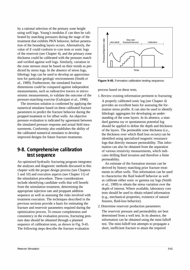
by a rational selection of the primary zone heightusing well logs. Young’s modulus E can then be cali-brated by matching pressures during the stage of thetreatment that exhibits PKN behavior, before penetra-tion of the bounding layers occurs. Alternatively, thevalue of E could conform to core tests or sonic logsof the reservoir (see Chapter 4), and the primary zonethickness could be calibrated with the pressure matchand verified against well logs. Similarly, variation inthe zone stresses must be based on their trends as pre-dicted by stress logs. In the absence of stress logs,lithology logs can be used to develop an approxima-tion for particular geologic environments (Smith etal., 1989). Furthermore, the simulated fracturedimensions could be compared against independentmeasurements, such as radioactive tracers or micro-seismic measurements, to validate the outcome of thepressure-matching exercise (Gulrajani et al., 1998).

The inversion solution is confirmed by applying thenumerical simulator based on these calibrated fractureparameters to predict the fracture behavior during thepropped treatment or for offset wells. An objectivepressure evaluation is indicated by agreement betweenthe simulated pressure response and actual field mea-surements. Conformity also establishes the ability ofthe calibrated numerical simulator to developimproved designs for future fracture treatments.

9-8. Comprehensive calibration test sequence

An optimized hydraulic fracturing program integratesthe analyses and diagnostic methods discussed in thischapter with the proper design process (see Chapters5 and 10) and execution aspects (see Chapter 11) ofthe stimulation procedure. These considerationsinclude identifying candidate wells that will benefitfrom the stimulation treatment, determining theappropriate injection rate and proppant additionsequence as well as assessing the risks involved withtreatment execution. The techniques described in theprevious sections provide a basis for estimating thefracture and reservoir parameters required during theoptimization process. To ensure completeness andconsistency in the evaluation process, fracturing pres-sure data should be obtained through a plannedsequence of calibration tests, as shown in Fig. 9-45.The following steps describe the fracture evaluation

process based on these tests.

1. Review existing information pertinent to fracturing

A properly calibrated sonic log (see Chapter 4)provides an excellent basis for assessing the for-mation stress profile. It can also be used to identifylithologic aggregates for developing an under-standing of the zone layers. In its absence, a stan-dard gamma ray or spontaneous potential logshould be applied to define the depth and thicknessof the layers. The permeable zone thickness (i.e.,the thickness over which fluid loss occurs) can beidentified using specialized magnetic resonancelogs that directly measure permeability. This infor-mation can also be obtained from the separation of various resistivity measurements, which indi-cates drilling fluid invasion and therefore a finitepermeability.

An estimate of the formation stresses can bederived by history matching prior fracture treat-ments in offset wells. This information can be usedto characterize the fluid leakoff behavior as well as calibrate either sonic or gamma ray logs (Smithet al., 1989) to obtain the stress variation over thedepth of interest. Where available, laboratory coretests should be used to obtain related information(e.g., mechanical properties, existence of naturalfissures, fluid-loss behavior).

2. Determine reservoir production parameters

The reservoir pressure and permeability are bestdetermined from a well test. In its absence, theinformation can be obtained using the mini-fallofftest. The mini-falloff test attempts to propagate ashort, inefficient fracture to attain the required

Reservoir Stimulation 9-61

Figure 9-45. Formation calibration testing sequence.

Time

Pre

ssur

e/in

ject

ion

rate

CalibrationStep rate/

flowback/reboundMini-falloff

reservoir transitional or pseudoradial flow (seeSection 9-6) within an acceptable data-recordingperiod. This objective is best achieved by applyingthe operational guidelines provided in “Guidelinesfor the field application of after-closure analysis”in the Appendix to this chapter. Using an a prioriestimate of the reservoir pressure reduces uncer-tainty in the after-closure analysis.

Pore pressure and permeability are the bases ofthe reservoir’s producing potential and are requiredfor an economics-based design (see Chapters 5 and10).

3. Define closure pressure

The preferred method for objectively determiningthe fracture closure pressure is a step rate/flowbacktest (see “Estimating closure pressure” in theAppendix to this chapter). For low to moderatepermeabilities, the step rate test typically followsthe mini-falloff test (Fig. 9-45). In higher perme-ability formations, it follows the calibration testbecause the subsequent loss of completion fluidwith which the step rate test is performed is signif-icantly reduced relative to fluid loss before the cal-ibration test.

4. Characterize fracture geometry

The character of fracture growth is identified dur-ing a calibration test by the analysis of pressureduring pumping (see Section 9-4). The analysisalso defines the formation pressure capacity (seeSection 9-4.6) and can be used to calibrate thefracture compliance through pressure matching.The injection pressure is used to determine thebounding stresses (Eq. 9-39). This additional stressmeasure, in conjunction with an estimate of theclosure pressure, provides the basis for a linearcalibration for correcting a sonic-based stress logfor the particular lithologic setting (Nolte andSmith, 1981; Nolte, 1988a).

5. Identify near-wellbore problems

A short step-down test (see Sidebar 9E) at the endof the injection period can be used to identify themagnitude and severity of near-wellbore problems.Net pressure analyses (e.g., log-log plots) shouldbe based on the bottomhole pressure corrected toreflect measurements of near-wellbore pressurethat is not associated with the fracture behavior.

6. Characterize fluid leakoff

A pressure decline analysis performed during thecalibration test closing period and the previouslycalibrated fracture compliance produce the mostreliable estimate of the fluid-leakoff parameters(see Section 9-5). They also determine the treat-ment efficiency, using an estimate of spurt fromthe after-closure linear flow analysis. The fluid-loss parameters are used to provide a measure ofthe fracture length (see Section 9-5.2).

The shut-in pressure during the closing of a cali-bration test can also be used to infer the closurepressure (see “Estimating closure pressure” in theAppendix to this chapter). This analysis, however,is highly subjective, and caution should be exer-cised during its application.

7. Assess after-closure response

Calibration test shut-in pressure should be moni-tored for a duration that is at least twice that of theclosure time tc. This enhances the prospect that amajority of the recorded after-closure responseperiod is not masked by complications arisingfrom polymer injection and that a well-establishedlinear flow response is obtained. The pressure dur-ing the linear flow period is used to estimate spurt(see Section 9-6.8), which in conjunction with theshut-in analysis provides the treatment efficiency.Linear flow may be completely absent in a high-mobility reservoir.

The operational guidelines outlined in “Guide-lines for the field application of after-closureanalysis” in the Appendix to this chapter should beapplied to prevent additional contaminating effectson the after-closure pressure data, which couldlead to an inconclusive linear flow analysis.

8. Crossvalidate evaluation results

Information derived from the after-closure linearflow response, in combination with the previousestimate of reservoir transmissibility, provides anindependent perspective for the fracture length(see Section 9-6.8). Agreement between this lengthestimate and that determined from the preclosureanalysis indicates consistency in the pressureanalysis.

9-62 Fracture Evaluation Using Pressure Diagnostics

9. Conduct pressure history matching

The previously obtained fracture parameter esti-mates (i.e., zone mechanical parameters and fluidproperties) can be refined through history matchingthe simulated pressure with the pressure measuredduring the calibration test. Care should be taken,however, to prevent the occurrence of nonunique-ness, an inherent limitation in pressure matching(see Section 9-7.2). This shortcoming can be pre-vented by performing a comprehensive evaluationand testing procedure to limit the number ofunknowns as well as eliminate unrealistic solutions.

10. Verify against propped treatment pressureresponse

The evaluation can be further refined for futuretreatments by matching pressures during thepropped treatment and comparing the requiredparameter set for this treatment with that obtainedfrom the calibration treatment. Conformitybetween these two parameter sets provides confi-dence in the fracture parameters. In the case ofdisagreement, a reanalysis should be conductedwith emphasis on deviations from ideal behavior.A more authoritative measure of the correctnessof the predicted parameters is agreement amongparameter sets obtained in offset wells, with suit-able corrections made to account for differencesin the formation thicknesses, well completions,fracturing schedules or fracturing fluid systems.

Reservoir Stimulation 9-63

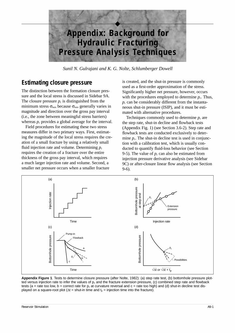
Estimating closure pressureThe distinction between the formation closure pres-sure and the local stress is discussed in Sidebar 9A.The closure pressure pc is distinguished from theminimum stress σmin because σmin generally varies inmagnitude and direction over the gross pay interval(i.e., the zone between meaningful stress barriers)whereas pc provides a global average for the interval.

Field procedures for estimating these two stressmeasures differ in two primary ways. First, estimat-ing the magnitude of the local stress requires the cre-ation of a small fracture by using a relatively smallfluid injection rate and volume. Determining pc

requires the creation of a fracture over the entirethickness of the gross pay interval, which requires a much larger injection rate and volume. Second, asmaller net pressure occurs when a smaller fracture

is created, and the shut-in pressure is commonlyused as a first-order approximation of the stress.Significantly higher net pressure, however, occurswith the procedures employed to determine pc. Thus,pc can be considerably different from the instanta-neous shut-in pressure (ISIP), and it must be esti-mated with alternative procedures.

Techniques commonly used to determine pc arethe step rate, shut-in decline and flowback tests(Appendix Fig. 1) (see Section 3.6-2). Step rate andflowback tests are conducted exclusively to deter-mine pc. The shut-in decline test is used in conjunc-tion with a calibration test, which is usually con-ducted to quantify fluid-loss behavior (see Section9-5). The value of pc can also be estimated frominjection pressure derivative analysis (see Sidebar9C) or after-closure linear flow analysis (see Section9-6).

Reservoir Stimulation A9-1

◆

Appendix: Background for Hydraulic Fracturing

Pressure Analysis Techniques

Appendix Figure 1. Tests to determine closure pressure (after Nolte, 1982): (a) step rate test, (b) bottomhole pressure plot-ted versus injection rate to infer the values of pc and the fracture extension pressure, (c) combined step rate and flowbacktests (a = rate too low, b = correct rate for pc at curvature reversal and c = rate too high) and (d) shut-in decline test dis-played on a square-root plot (∆t = shut-in time and tp = injection time into the fracture).

Inje

ctio

n ra

te

Bot

tom

hole

pre

ssur

e at

ste

p en

d

Bot

tom

hole

pre

ssur

e

Bot

tom

hole

pre

ssur

e

Time Injection rate

Time

(c) (d)

pc

pc

pc

Possibilities

Extensionpressure

Flowback

Pump-in

a

bc

(a) (b)

√∆t or √∆t + tp

Sunil N. Gulrajani and K. G. Nolte, Schlumberger Dowell

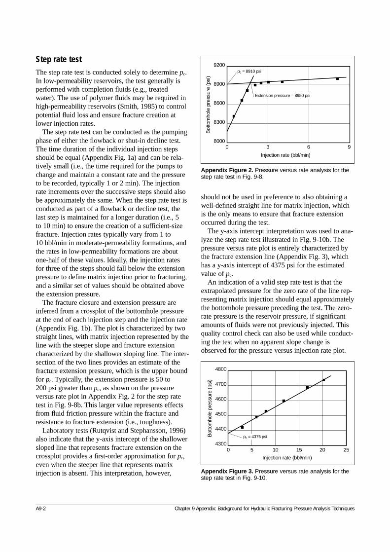
Step rate testThe step rate test is conducted solely to determine pc.In low-permeability reservoirs, the test generally isperformed with completion fluids (e.g., treatedwater). The use of polymer fluids may be required inhigh-permeability reservoirs (Smith, 1985) to controlpotential fluid loss and ensure fracture creation atlower injection rates.

The step rate test can be conducted as the pumpingphase of either the flowback or shut-in decline test.The time duration of the individual injection stepsshould be equal (Appendix Fig. 1a) and can be rela-tively small (i.e., the time required for the pumps tochange and maintain a constant rate and the pressureto be recorded, typically 1 or 2 min). The injectionrate increments over the successive steps should alsobe approximately the same. When the step rate test isconducted as part of a flowback or decline test, thelast step is maintained for a longer duration (i.e., 5 to 10 min) to ensure the creation of a sufficient-sizefracture. Injection rates typically vary from 1 to 10 bbl/min in moderate-permeability formations, andthe rates in low-permeability formations are aboutone-half of these values. Ideally, the injection ratesfor three of the steps should fall below the extensionpressure to define matrix injection prior to fracturing,and a similar set of values should be obtained abovethe extension pressure.

The fracture closure and extension pressure areinferred from a crossplot of the bottomhole pressureat the end of each injection step and the injection rate(Appendix Fig. 1b). The plot is characterized by twostraight lines, with matrix injection represented by theline with the steeper slope and fracture extensioncharacterized by the shallower sloping line. The inter-section of the two lines provides an estimate of thefracture extension pressure, which is the upper boundfor pc. Typically, the extension pressure is 50 to 200 psi greater than pc, as shown on the pressureversus rate plot in Appendix Fig. 2 for the step ratetest in Fig. 9-8b. This larger value represents effectsfrom fluid friction pressure within the fracture andresistance to fracture extension (i.e., toughness).

Laboratory tests (Rutqvist and Stephansson, 1996)also indicate that the y-axis intercept of the shallowersloped line that represents fracture extension on thecrossplot provides a first-order approximation for pc,even when the steeper line that represents matrixinjection is absent. This interpretation, however,

should not be used in preference to also obtaining awell-defined straight line for matrix injection, whichis the only means to ensure that fracture extensionoccurred during the test.

The y-axis intercept interpretation was used to ana-lyze the step rate test illustrated in Fig. 9-10b. Thepressure versus rate plot is entirely characterized bythe fracture extension line (Appendix Fig. 3), whichhas a y-axis intercept of 4375 psi for the estimatedvalue of pc.

An indication of a valid step rate test is that theextrapolated pressure for the zero rate of the line rep-resenting matrix injection should equal approximatelythe bottomhole pressure preceding the test. The zero-rate pressure is the reservoir pressure, if significantamounts of fluids were not previously injected. Thisquality control check can also be used while conduct-ing the test when no apparent slope change isobserved for the pressure versus injection rate plot.

A9-2 Chapter 9 Appendix: Background for Hydraulic Fracturing Pressure Analysis Techniques

Appendix Figure 2. Pressure versus rate analysis for thestep rate test in Fig. 9-8.

0 3 6 9

9200

8900

8600

8300

8000

Bot

tom

hole

pre

ssur

e (p

si)

Injection rate (bbl/min)

pc = 8910 psi

Extension pressure = 8950 psi

Appendix Figure 3. Pressure versus rate analysis for thestep rate test in Fig. 9-10.

0 5 10 15 20 25

4800

4700

4600

4500

4400

4300

Bot

tom

hole

pre

ssur

e (p

si)

Injection rate (bbl/min)

pc = 4375 psi

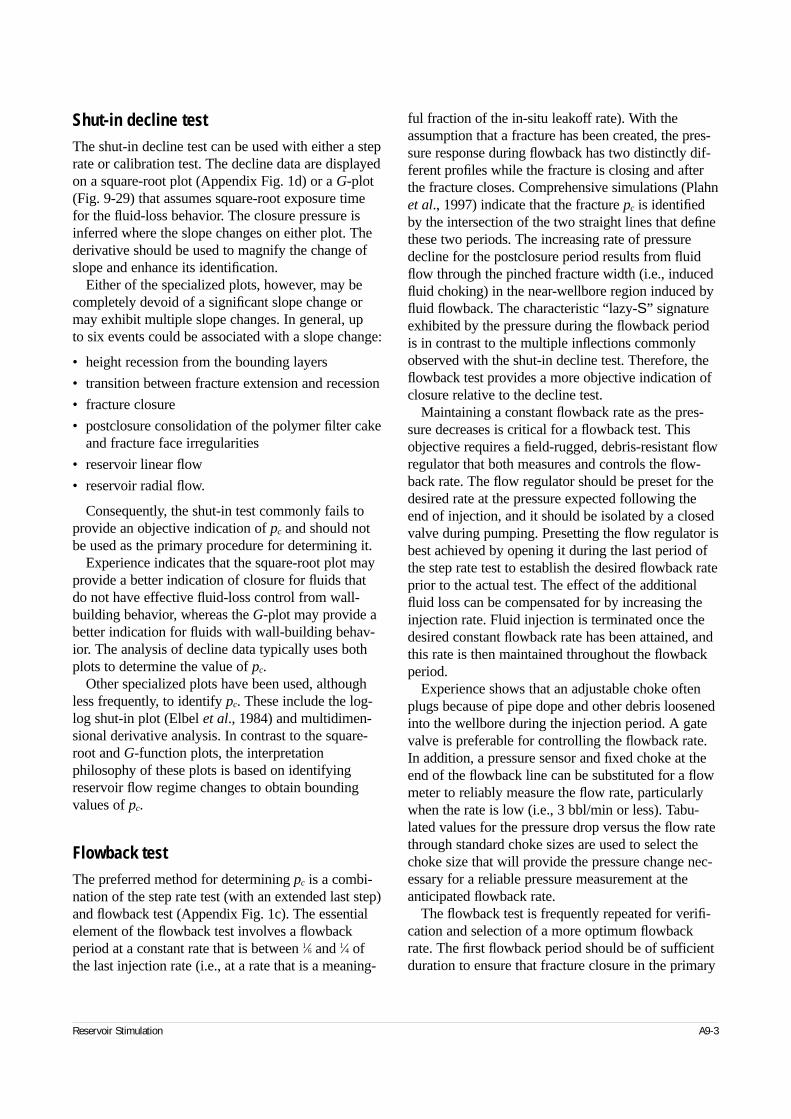
Shut-in decline testThe shut-in decline test can be used with either a steprate or calibration test. The decline data are displayedon a square-root plot (Appendix Fig. 1d) or a G-plot(Fig. 9-29) that assumes square-root exposure timefor the fluid-loss behavior. The closure pressure isinferred where the slope changes on either plot. Thederivative should be used to magnify the change ofslope and enhance its identification.

Either of the specialized plots, however, may becompletely devoid of a significant slope change ormay exhibit multiple slope changes. In general, up to six events could be associated with a slope change:

• height recession from the bounding layers

• transition between fracture extension and recession

• fracture closure

• postclosure consolidation of the polymer filter cakeand fracture face irregularities

• reservoir linear flow

• reservoir radial flow.

Consequently, the shut-in test commonly fails toprovide an objective indication of pc and should notbe used as the primary procedure for determining it.

Experience indicates that the square-root plot mayprovide a better indication of closure for fluids thatdo not have effective fluid-loss control from wall-building behavior, whereas the G-plot may provide abetter indication for fluids with wall-building behav-ior. The analysis of decline data typically uses bothplots to determine the value of pc.

Other specialized plots have been used, althoughless frequently, to identify pc. These include the log-log shut-in plot (Elbel et al., 1984) and multidimen-sional derivative analysis. In contrast to the square-root and G-function plots, the interpretationphilosophy of these plots is based on identifyingreservoir flow regime changes to obtain boundingvalues of pc.

Flowback testThe preferred method for determining pc is a combi-nation of the step rate test (with an extended last step)and flowback test (Appendix Fig. 1c). The essentialelement of the flowback test involves a flowbackperiod at a constant rate that is between 1⁄6 and 1⁄4 ofthe last injection rate (i.e., at a rate that is a meaning-

ful fraction of the in-situ leakoff rate). With theassumption that a fracture has been created, the pres-sure response during flowback has two distinctly dif-ferent profiles while the fracture is closing and afterthe fracture closes. Comprehensive simulations (Plahnet al., 1997) indicate that the fracture pc is identifiedby the intersection of the two straight lines that definethese two periods. The increasing rate of pressuredecline for the postclosure period results from fluidflow through the pinched fracture width (i.e., inducedfluid choking) in the near-wellbore region induced byfluid flowback. The characteristic “lazy-S” signatureexhibited by the pressure during the flowback periodis in contrast to the multiple inflections commonlyobserved with the shut-in decline test. Therefore, theflowback test provides a more objective indication ofclosure relative to the decline test.

Maintaining a constant flowback rate as the pres-sure decreases is critical for a flowback test. Thisobjective requires a field-rugged, debris-resistant flowregulator that both measures and controls the flow-back rate. The flow regulator should be preset for thedesired rate at the pressure expected following theend of injection, and it should be isolated by a closedvalve during pumping. Presetting the flow regulator isbest achieved by opening it during the last period ofthe step rate test to establish the desired flowback rateprior to the actual test. The effect of the additionalfluid loss can be compensated for by increasing theinjection rate. Fluid injection is terminated once thedesired constant flowback rate has been attained, andthis rate is then maintained throughout the flowbackperiod.

Experience shows that an adjustable choke oftenplugs because of pipe dope and other debris loosenedinto the wellbore during the injection period. A gatevalve is preferable for controlling the flowback rate.In addition, a pressure sensor and fixed choke at theend of the flowback line can be substituted for a flowmeter to reliably measure the flow rate, particularlywhen the rate is low (i.e., 3 bbl/min or less). Tabu-lated values for the pressure drop versus the flow ratethrough standard choke sizes are used to select thechoke size that will provide the pressure change nec-essary for a reliable pressure measurement at theanticipated flowback rate.

The flowback test is frequently repeated for verifi-cation and selection of a more optimum flowbackrate. The first flowback period should be of sufficientduration to ensure that fracture closure in the primary

Reservoir Stimulation A9-3

zone is recorded. Pressure during this test, however,should be controlled to prevent the production ofreservoir fluids into the wellbore. The second flow-back test may be preceded by either a step rate test ora constant injection rate and should end after the indi-cation of a curvature reversal that clearly confirms thepc estimate from the first test.

The pressure decline for the second test is limitedto obtain an optimum rebound pressure. The reboundpressure is the nearly constant pressure that occursfollowing a short period of increasing pressure aftershut-in of the flowback test (see Fig. 3-26b). This sta-bilized pressure is generally near to or smaller than pc

and provides its lower bound estimate. The reboundpressure is also an effective tool for estimating pc

when near-wellbore flow restrictions, as discussed inSection 9-4.9, are large. During the flowback period,these near-wellbore effects cause prediction of alower estimate of pc because of the additional flowrestriction in the near-wellbore region. The wellborerebound pressure, however, is unaffected by therestriction and should provide an accurate lowerbound estimate of pc (Plahn et al., 1997).

In conclusion, the combination of the upper boundestimate of pc from the intersection of the matrix andfracture extension lines on a step rate test, the lowerbound of pc determined from the rebound pressureand the estimate of pc from the y-axis intercept of thefracture extension line as well as the intersection ofthe two lines during flowback provides multiple,independent values that establish a firm basis fordefining pc.

Test sequenceBecause the mini-falloff test (see Section 9-6.2) thatcharacterizes the production potential should be con-ducted in an initially undisturbed reservoir, it shouldalways be the first injection within the calibrationtesting sequence (Fig. 9-45). The subsequent applica-tion sequence of the step rate/flowback and calibra-tion/shut-in tests generally depends on the formationfluid-loss characteristics.

For low fluid-loss conditions, the step rate/flow-back test to establish pc should precede the fracturecalibration test where the closure time could be long(e.g., up to 3 times the injection time). This prior esti-mate of pc can be used to ensure that the shut-in pres-sure during the subsequent calibration test is moni-tored during the complete time of fracture closure.

For moderate to high fluid-loss conditions, the cali-bration test generally exhibits a closing period that isless than the injection time, and prior estimate of pc isnot required for a shut-in period that approximatesthe injection period. Conducting the step rate/flow-back test after the fracture calibration test reaps thefollowing advantages from the prior fluid injection:

• Breakdown of the complete gross pay interval isensured.

• Residual fluid-loss control from unbroken polymeror additives in the fracturing fluid enables fractur-ing using moderate injection rates with the com-pletion fluid.

• Because the poroelastic effects have stabilized, thestep rate/flowback test better replicates the stressconditions that occurred during the preceding cali-bration treatment.

Guidelines for the field applicationof after-closure analysisThe reservoir response during linear flow and eitherradial or transitional flow is required to conduct acomprehensive analysis of the after-closure period.Several factors, however, can prevent obtaining infor-mation for one or more of the flow regimes. Forexample, radial flow may be not be attained within areasonable time period for the high injection rates andleakoff-resistant fracture fluids used during conven-tional fracturing operations. In addition, the after-closure pressure data may be compromised becauseof several undesirable communication effectsbetween the wellbore and formation. Therefore, thecalibration testing sequence must be engineered toprovide the requisite pressure data (Talley et al.,1999). The following guidelines increase the likeli-hood of obtaining a comprehensive, objective after-closure analysis.

• Unless a bottomhole shut-off valve is employed,the reservoir pressure should ideally be equal to or greater than the hydrostatic pressure of the well-bore fluid. Vacuum-induced fluid injection violatesthe no-flow assumption of the analysis for theafter-closure period.

• The wellbore must be free of gas to ensure thatcorrect values of the hydrostatic pressure andinjected volume are used in the analysis and to

A9-4 Chapter 9 Appendix: Background for Hydraulic Fracturing Pressure Analysis Techniques

minimize wellbore expansion effects during pres-sure falloff. For gas reservoirs, this can be achievedby conducting the injection test before a productionperiod. Alternatively, the gas should be circulatedfrom the wellbore or bullheaded into the formation.An extended shut-in period can be required afterbullheading to allow the pressure transient to dissi-pate before liquid injection resumes. A relativelysmall volume of gas injection ahead of the fluid isacceptable—e.g., gas is circulated from the inter-mediate casing but remains in the shorter liner.

• Circulating or bullheading (potentially with a longshut-in period) may be similarly required to spotthe fracturing fluid at the perforations for the frac-ture calibration test. The residual reservoir responsefrom injection of a significant volume of low-efficiency wellbore fluid causes the linear flowanalysis to indicate an unrealistically high spurtloss (Talley et al., 1999).

• Like preclosure analysis, after-closure analysis isan inverse problem that is inherently nonunique(see Section 9-7.2). The objectivity of after-closureanalysis can be improved by obtaining an a prioriestimate of the reservoir pressure, particularly if the after-closure period is abbreviated (e.g., beforewellbore vacuum) and either the closure time(Nolte et al., 1997) or spurt loss is inferred. Thereservoir pressure estimate can be obtained

– as the stabilized bottomhole pressure measuredprior to fluid injection into the reservoir

– as the stabilized surface pressure measured priorto fluid injection into an overpressured reservoir

– from the surface pressure and hydrostatic col-umn estimated through an accurate measurementof the fluid injected to completely fill the well-bore for an underpressured reservoir

– from an accurate reservoir pressure gradientestablished for the field.

• In deep or hot reservoirs, bottomhole gauges arenecessary because wellbore fluid expansion fromthe decreasing pressure and increasing temperatureduring shut-in decrease the hydrostatic pressure.Excessive expansion of the fluid may eventuallyviolate the no-flow condition to the degree that thelonger term data are corrupted, particularly forresidual gas in the wellbore. Mitigation of theseeffects, like for a wellbore vacuum, requires adownhole shut-in device.

• It is unlikely that both linear and radial flow willoccur during a decline period (see Section 9-6.2).The testing sequence illustrated in Fig. 9-45 is sug-gested to increase the likelihood of obtaining infor-mation pertinent to both the linear and radial flowperiods. The mini-falloff test should be applied todetermine the radial flow parameters. The subse-quent calibration test is more likely to attain linearflow. The radial flow response for the calibrationtest can be anticipated from the reservoir informa-tion derived from the mini-falloff test (see “Frac-ture length” in Section 9-6.7).

• To attain radial flow within a reasonable timeframe, the mini-falloff test should adhere to the fol-lowing injection rate criterion, presented in con-ventional oilfield units:

(1)

If the fluid loss is controlled by the reservoir, asdesired for the test, the ratio of the fluid-loss coeffi-cients CL and CR becomes unity and a higher injec-tion rate is possible. The equation provides anequality for a dimensionless time of 1.0 (i.e., thebeginning of radial flow during the injection periodon Fig. 9-38). The guideline requires using esti-mates of the reservoir parameters and fluid-losscharacteristics to design the mini-falloff test. Ingeneral, Appendix Eq. 1 provides an operationallyreasonable rate for radial flow with a short moni-toring period in a reservoir with a mobility greaterthan about 5 md/cp. For reservoirs with lower val-ues of mobility, transitional flow resulting frominjection rates greater than guideline can be used to determine the reservoir parameters with a type-curve-based analysis.

• Volume has a minimal effect on dimensionless timeand hence the time for development of radial flowbecause of the quasistationary value of dimension-less time for a constant injection rate. However, aminimum volume must be pumped to ensure anaccurate measure of the volume injected throughthe perforations because the transmissibility is pro-portional to the injected volume (Eq. 9-93).

• If polymer fluids are used (see Section 9-6.3) thepressure data obtained after fracture closure can becorrupted by continued consolidation (i.e., squeez-

Reservoir Stimulation A9-5

q

h

k C

Cp pi

f

L

R

c i

bbl / minft

mdcp

psi( )

( )≤ × ( )

( ) − ( )( )−4 10 6

µ.

A9-6 Chapter 9 Appendix: Background for Hydraulic Fracturing Pressure Analysis Techniques

ing) of the fracture faces and filter cake. The con-solidation period lasts for a time approximating thecombined injection and closing times. The calibra-tion test shut-in pressure should therefore be moni-tored for a time interval that is at least 2 to 3 timesthe total closure time tc. Similarly, the shut-inperiod for a mini-falloff test should be at least 4 to5 times the total closure time. These guidelines forthe shut-in time increase the likelihood that ade-quate, representative pressure data are obtained fora valid after-closure analysis.

Mathematical relations for fluid lossDerived in this section of the Appendix to Chapter 9are the relations used for pressure evaluation prior tofracture closure.

Fluid-loss relationsTwo fundamental relations are required to derive theexpressions for fluid loss. The first relation describesthe nature of fracture growth with respect to time.The second relation is based on the expression forfluid loss introduced by Carter (1957).

The evolution of the fracture area is assumed tofollow a power law relation with time in which thearea monotonically increases with time. The proper-ties of the injected fluid and the pump rate areassumed to be relatively constant. The power lawexpression relates any intermediate fracture area acreated at a time τ to the total fracture area A at thecurrent time t:

(2)

(3)

where α is referred to as the area exponent. Theexponent α is also the log-log slope of A versus t, asshown by differentiating Appendix Eq. 3 with respectto time:

(4)

The value of α depends on the fluid efficiency.Bounding values for α corresponding to low and high

treatment efficiencies are derived subsequently in thisAppendix. The exponent generally decreases through-out the injection time, but the change is relativelysmall and can be ignored. For the commonly usedcrosslinked polymer fluids, the exponent is typically 0.6.

Three mechanisms govern the fluid filtration processduring fracturing, as discussed in Section 6-4. Thesquare root of exposure time relation, introduced byCarter (1957), is applied to predict the cumulativeeffect of these mechanisms on the rate of fluid loss. A more general expression used in this Appendixincludes fluid-loss behavior dominated by a non-Newtonian filtrate. Consequently, in contrast to Eq. 5-1,the flux uL, defined as the rate of fluid loss per unitleakoff area, is expressed as

(5)

where t is the time since the beginning of pumping, CL is the fluid-loss coefficient, and θ is the fluid-lossexponent. The coefficient 2 in Appendix Eq. 5accounts for leakoff over the two walls of the fracture.

The specific fluid-loss volume vL, defined as thefluid-loss volume VL per unit leakoff area, is obtainedby the time integration of Appendix Eq. 5:

(6)

Parlar et al. (1995) showed that θ is related to thepower law exponent nf of the filtrate that invades thereservoir during the leakoff process:

(7)

As discussed in Chapter 8, a filter cake is depositedby a wall-building fluid along the fracture in low-per-meability reservoirs and within the formation in high-permeability reservoirs. A Newtonian filtrate (i.e.,water) is created during the process. Under these con-ditions, nf = 1 and Appendix Eq. 5 reduces to Eq. 5-1,which is Carter’s square root of exposure time rela-tion for the fluid-loss rate (i.e., θ = 1⁄2). Non-wall-building fracturing fluids invade high-permeabilityreservoirs. The resulting filtrate fluid is typically non-Newtonian, with nf < 1 and θ < 1⁄2. In addition, theextensional viscosity behavior of viscoelastic filtratesabove a threshold filtration rate can exhibit relativelylarge values of nf (Chauveteau et al., 1986). Thevalue of θ in this case is greater than 1⁄2 and can

a

A t=

τ α

τ α

t

a

A=

1/

,

α = t

A

dA

dt.

uC

tLL=

−( ) −2

1τ θ ,

v u dtC

t aL L

t

L= = − ( )( )∫0

2θ

τ θ.

θ =+n

nf

f1.

approach unity. A value of θ that is different from 1⁄2 has also been proposed to model the effect ofnatural fissures (Soliman et al., 1990).

Fluid-loss volume with the Carter-basedleakoff modelThe rate of fluid loss associated with Carter-basedleakoff behavior (i.e., the contribution of CL over anelemental leakoff area da) can be obtained by substi-tuting Appendix Eq. 3 into Appendix Eq. 5:

(8)

where rp is the ratio of the fracture surface area avail-able for fluid loss to the gross fracture area and tp isthe injection or pumping time. The dimensionlessparameters tαD and ξ are defined as

(9)

(10)

where Af is the fracture surface area at the end ofpumping.

The total rate of fluid loss is obtained by the inte-gration of Appendix Eq. 8 over the fracture area:

(11)

where the function f(tD,α,θ) is defined as

(12)

An expression for the CL component of the fluid-loss volume VL,C is similarly obtained by substitutingAppendix Eqs. 9 and 10 into Appendix Eq. 6 andintegrating over the area:

(13)

where the function g(tαD,α,θ) is defined as

(14)

The functions f(tαD,α,θ) and g(tαD,α,θ) are usuallypresented in terms of the dimensionless shut-in time

∆tD, which is defined as the ratio of the shut-in time∆t to the pumping time tp:

(15)

The time functions f(tαD,α,θ) and g(tαD,α,θ) can beexpressed in terms of ∆tD:

(16)

(17)

Valkó and Economides (1993b) showed that thefunctions f(tαD,α,θ) and g(tαD,α,θ) are part of thehypergeometric family of functions or their subset of incomplete beta functions (Meyer and Hagel,1989). Either of these function families is relativelycomplicated, but simple analytical expressions can be obtained for a limited set of values, as discussedsubsequently.

Cumulative fluid-loss volumeThe total fluid-loss volume at the end of pumping VLp comprises the cumulative contributions of its CL fluid-loss component VLp,C and spurt VL,S:

(18)

An expression for VLp,C can be obtained by substi-tuting ∆tD = 0 into Appendix Eq. 13:

(19)

where the function g0(α,θ) represents the value of theg-function in Appendix Eq. 17 when ∆tD = 0:

(20)

Spurt occurs only for wall-building fluids. It ac-counts for the fluid-loss volume prior to the creationof a filter cake and is applicable only during the frac-ture propagation period. Following the spurt period,wall-building fluids exhibit a Newtonian filtrate duringthe fluid-loss process (i.e., nf = 1 or θ = 1⁄2). The totalvolume of fluid lost to spurt follows from definition of the spurt coefficient Sp:

Reservoir Stimulation A9-7

q da tr C

t

da

tL

p L

p D

, ,/

( ) =−( )− −

21 1 1θ

αα θ

ξ

tt

tD

p

α =

ξ = a

Af

,

q A tr C A

tf tL f

p L f

p

D, , , ,( ) = ( )−

21 θ α α θ

f td

ttD

D

Dα

αα θ αα θ ξ

ξ, , .

/( ) =

−( )≥−∫ 1 1

0

1

1

V r C t A g tL C p L p f D, , , ,= ( )2 θα α θ

g t t d tD D Dα αα θ

αα θθ

ξ ξ, , ./( ) = −( ) ≥∫111

0

1

∆ ∆t

t t

t

t

ttD

p

p p

D=−

= = −α 1.

f td

ttD

D

D∆∆

∆, ,/

α θ ξξ α θ( ) =

+ −( )≥−∫ 1

01 1

0

1

g t t d tD D D∆ ∆ ∆, , ./α θθ

ξ ξα θ( ) = + −( ) ≥∫11 01

0

1

V V VLp Lp C L S= +, , .

V V t r C t A gLp C L C D p L p f, , , ,= =( ) = ( )∆ 0 2 0θ α θ

g g t dD01

0

1

01

1α θ α θθ

ξ ξα θ, , , ./( ) = =( ) = −( )∫∆

A9-8 Chapter 9 Appendix: Background for Hydraulic Fracturing Pressure Analysis Techniques

(21)

The cumulative fluid-loss volume during injectionis obtained by substituting Appendix Eqs. 19 and 21into Appendix Eq. 18:

(22)

(23)

Appendix Eq. 22 is expressed in terms of the spurtfactor κ, which provides for the increase in fluid lossover the no-spurt condition:

(24)

The rate of increase in the fracture area decreasessignificantly at the end of pumping. Spurt-dependentfluid loss therefore also reduces relatively quickly fol-lowing the cessation of fluid injection and is assumedto terminate at the time t = tp. The total fluid-loss vol-ume during a shut-in period is represented entirely byits CL component VLs,C (∆t):

(25)

An expression for VLs(∆t) results from subtractingAppendix Eq. 19 from Appendix Eq. 13:

(26)

(27)

Newtonian filtrate controlFracturing fluids produce a Newtonian filtrate follow-ing the deposition of a filter cake. For this case, nf = 1,and Appendix Eq. 7 indicates that θ = 1⁄2. Analyticalexpressions for fluid loss can be derived for boundingvalues of α. The lower bound value corresponds tonegligible efficiency and is obtained by substituting

θ = 1⁄2 in Appendix Eq. 41, whereas Appendix Eq. 40provides the upper bound. An upper bound of unity isassumed because it provides simple, closed-formexpressions. The bounding values of α for a wall-building fluid are therefore as in Eq. 9-43:

Analytical equations for f(∆tD,α,θ), g(∆tD,α,θ) andg0(α, θ) are obtained by substituting the boundingvalues of α into Appendix Eqs. 16, 17 and 20,respectively, and integrating the resulting expressions(Nolte, 1979; Smith, 1985):

(28)

(29)

(30)

All these functions are well behaved. Their values atany other value of α can be obtained through simpleinterpolation between bounding values.

Non-Newtonian filtrate controlA non-Newtonian filtrate occurs with fracturing fluidsthat exhibit a power-law-based rheology and do notdevelop an effective filter cake. In this case, nf ≠ 1and if the filtrate controls fluid loss, θ deviates fromits commonly assumed value of 1⁄2. These conditionslimit the general analytical expressions to g0 only.Explicit integration of Appendix Eq. 20 gives

(31)

where Γ(x) is the gamma function.Analytical expressions for the fluid-loss rate and

volume functions (i.e., Appendix Eqs. 16 and 17,

V r S AL S p p f, .= 2

12

1< <α .

g tt t t

t tD

D D D

D D

∆∆ ∆ ∆

∆ ∆( ) =

+( ) +( ) + =

+( ) −( ) =

=

− −

θ

α

α1

2

1 1 2 1 2

3 2 3 2

1 112

43

1 1

sin/ /

/ /

g0 12

212

4 3 1θ

π αα

== =

=

.

g0

1 11

α θ θ αθ α θ

, ,( ) = +( ) +( )+ +( )

Γ ΓΓ

f tt

t tD

D

D D

∆∆

∆ ∆( ) =

+( ) =

+( ) −( ) =

=

− −

θ

α

α12

1 1 2

1 2 1 2

112

2 1 1

sin/

/ /

V r C t A gLp p L p f= =

=2

12

120κ α θ θ,

V r C t A gLp p L p f= ( ) ≠2120

θ α θ θ, .

κα θ

= +=

1120

S

g C t

p

L p,.

V t V tLs Ls C∆ ∆( ) = ( ), .

V t r C t A

g t g

Ls p L f

D

∆

∆

( ) =

× =

− =

=

2

12

12

120, , ,α θ α θ θ

V t r C t A g t gLs p L f D∆ ∆( ) = ( ) − ( )( ) ≠2120

θ α θ α θ θ, , , .

Reservoir Stimulation A9-9

respectively) can be obtained for only select values of their arguments that are applicable to specific fieldapplications. The upper bound of α = 1 applies alsofor θ ≠ 1⁄2, and the corresponding functions are

(32)

(33)

Simple analytical expressions for these functionsalso result for the value of θ approaching unity,which is applicable for time-independent fluid-lossconditions. This fluid-loss behavior can be exhibitedby viscoelastic fluids with a rapidly increasing exten-sional viscosity above a threshold filtration rate:

(34)

(35)

The integral forms for both functions are wellbehaved and therefore can be evaluated by numericalintegration for other values of their arguments.

Bounding values for fluid efficienciesThe fracture penetration and net pressure can be rep-resented for the bounding values of high and lowfluid efficiencies. When the efficiency η → 0, all theinjected volume can be assumed to have leaked off. Itfollows from Eq. 9-5 that

(36)

From the relation Vi = qit and combining AppendixEq. 36 with the generalized expression for fluid lossduring pumping in Appendix Eq. 23:

(37)

For the alternative situation of extremely high fluidefficiencies (η → 1), the fluid-loss volume can beignored. In this case, Eq. 9-5 reduces to

(38)

The evolution of the fracture area for high fluidefficiencies is obtained from this expression as

(39)

where ⟨w—⟩ is the fracture width averaged over thefracture area. The bounding expressions for fracturepenetration in Eqs. 9-32 through 9-34 are derived bycombining Appendix Eqs. 37 and 39 with the fracturewidth relations in Eq. 9-27, for which the fracturearea Af is proportional to the half-length L for thePKN and KGD models and to R2 for the radial model.For the common occurrence of Newtonian fracturingfluid filtrate (i.e., θ = 1⁄2):

PKN

KGD

Radial

The time dependency of the net pressure pnet for thebounding values of η is obtained by combining itsdependency on the fracture penetration for the threefracture geometry models in Eq. 9-25 with the threepreceding equations to produce Eqs. 9-35 through 9-37:

PKN

KGD

Radial

Bounding values for the area exponentThe bounding values for the area exponent α corre-spond to negligible (η → 1) and dominant (η → 0)fluid loss to the formation. The upper bound α1 inEq. 9-43 assumes not only negligible fluid loss butalso a constant fracture width. Because the widthgenerally increases during injection, the upper bound

f t t tD D D∆ ∆ ∆, ,α θθ

θ θ=( ) = +( ) −[ ]11

1

Aq t

wfi= →η 1,

L t

L t n n

∝ →∝ →+( ) +( )

1 2

2 2 2 3

0

1

/ ηη

L t

L t n n

∝ →∝ →+( ) +( )

1 2

1 2

0

1

/ ηη

R t

R t n n

∝ →∝ →+( ) +( )

1 4

2 2 3 6

0

1

/

.

ηη

p t

p tnet

n

netn

∝ →∝ →

+( )

+( )

1 4 1

1 2 3

0

1

/ ηη

p t

p tnet

n n

netn n

∝ →∝ →

− +( )

− +( )

/2 1

2

0

1

ηη

p t

p tnet

n n

netn n

∝ →∝ →

− +( )

− +( )

3 8 1

2

0

1

/

.

ηη

g t t tD D D∆ ∆ ∆, , .α θθ θ

θ θ=( ) =+( )

+( ) −[ ]+ +11

11

1 1

f tD∆ , ,α θ =( ) =1 1

g t tD D∆ ∆, , .α θα

=( ) =+

+11

1

V Vi Lp≈ .

Aq t

r C t gt

fi

p L

= →

∝ −

20

01

θ

θ

η

.

V Vi fp≈ .

A9-10 Chapter 9 Appendix: Background for Hydraulic Fracturing Pressure Analysis Techniques

for the area growth is less than unity and independentof the loss exponent θ. It is derived from the condi-tion of η → 1 in Eqs. 9-32 through 9-34:

(40)

The lower bound α0 follows from Appendix Eq. 37:

(41)

For the typical value of θ = 1⁄2, Appendix Eq. 41shows that α0 = 1⁄2, which is the value used in Eq. 9-43.

Postscreenout pressure relationsThe material-balance relations following a peripheralscreenout (i.e., constant fracture area following ascreenout) can be written in a manner similar to Eq. 9-5 (Nolte, 1990). At any additional time follow-ing a screenout ∆tso, the change in fracture volume isequal to the additional injected slurry volume minusthe volume of fluid lost to the formation throughleakoff:

(42)

where the subscript so identifies the correspondingparameter value at screenout. Similarly, an expressionfor the fracture volume at screenout Vfso can be written as

(43)

where ηso is the fluid efficiency at screenout and Viso

is the volume injected prior to the screenout.For an assumed constant injection rate Viso = qitso,

Eq. 9-6 and Appendix Eq. 43 can be combined:

(44)

where VLp(tso) represents the cumulative volume offluid lost prior to screenout and can be expressed in amanner similar to Appendix Eq. 22 for a wall-buildingfluid:

(45)

where κso is the spurt factor evaluated at tso.Because the same set of conditions as that follow-

ing the end of injection is assumed to exist followinga screenout, the expression for VLp(∆tso) is similar tothat in Appendix Eq. 26:

(46)

where the dimensionless time ∆tDso is defined as theratio of the time after screenout ∆tso to that at theonset of screenout tso.

The change in the area-averaged fracture width fol-lowing a screenout is obtained by dividing the termsin Appendix Eq. 42 with those in Appendix Eq. 44and substituting the fluid-loss expressions fromAppendix Eqs. 45 and 46:

(47)

An expression for the treatment efficiency at anytime after a screenout η(∆tDso) can be obtained bycombining the definition of η from Eq. 9-4 with thewidth multiplier expression in Appendix Eq. 47:

(48)

Appendix Eqs. 47 and 48 are equivalent to Eqs. 6L-6 and 6L-7.

Based on the proportionality between net pressureand width, differentiating Appendix Eq. 47 obtainsthe following expression:

(49)

where pnet,so is the net pressure at the screenout and βis assumed to be unity (Fig. 9-20). From the defini-tion of efficiency, it can be readily shown that

(50)

Combining Appendix Eqs. 49 and 50 produces thefollowing relation for the log-log slope of the netpressure after a screenout (Nolte, 1990):

(51)

α η1

2 2 2 3

1 2

4 4 3 6

1=( ) ( )( ) ( )( ) ( )

→

n n

n n

n n

+ +

+ +

+ +

PKN

KGD

Radial

.

α θ η0 1 0= − → .

∆ ∆ ∆w A q t V tfso i so Lp so= − ( ) ,

V t r A C t g t gLp so p f L p Dso∆ ∆( ) = ( ) −( )2 0 ,

∆ ∆∆w

wt

g t g

gso so

Dso soDso

so

= − −[ ] ( ) −

1

1 0

0ηη

κ.

ηη

κ∆

∆∆

tt

g t g

gDsoso

Dso

Dso

so

( ) = −−( )

+( ) + ( ) −

1

1

11 0

0

.

t

p

t t

p tso so

net so

so

net so

η η

,

.= ( )( )∆∆

t

p

dp

dt

f t g

t g t g g

net so

net so

so Dso so

so Dso Dso so

,

,

.

=

− −[ ] ( ) ( )( )− −[ ] +[ ] + ( ) −( ) ( )( )

1 1

1 1 1 1

0

0 0

η κ

η κ

∆

∆ ∆

1 1

11 1

0

w

d w

dt p

dp t

dt

tf t

g

so net so

net so

so so soDso

so

∆ ∆

∆

= ( )

= − −[ ] ( )

,

,η ηκ

V Vfso so iso= η ,

w A q t V tf so so i so so Lp so so( ) = = ( ) −( )η η η1 ,

V t r C t A gLp so p so L so f( ) = ( )2 0κ α ,

Reservoir Stimulation A9-11

The bounding values of the log-log slope areobtained by substituting the appropriate values for ηand the corresponding relations for f(∆tDso), g(∆tDso)and g0 that can be obtained from Appendix Eqs. 28,29 and 30, respectively.

Comparison of fixed-length and propagating fractures†

Fracture propagation and closure lead to characteristicpressure and fluid-loss distributions along the inter-face between the fracture and the reservoir. The timehistory of these distributions establishes the boundaryconditions for the reservoir response before and afterfracture closure. These conditions are generally dif-ferent from those experienced by fixed-length frac-tures; however, there are also similar conditions thatare shared by these two types of fractures. The simi-lar conditions enable applying established fixed-length relations to a propagating fracture. The back-ground for identifying these differences andsimilarities is reviewed in this section of theAppendix to Chapter 9 along with the fixed-lengthrelations that are applicable to the propagating case.

Specifically, this section of the Appendix provides

• conditions that enable adapting fixed-length relationsto a propagating fracture

• definition of a generalized reservoir leakoff coeffi-cient that is applicable to fracture propagationwithin all flow regimes

• framework for type-curve analysis of the after-closure period.

Throughout this section, the propagating fracture is assumed to have a rectangular shape (i.e., Af = 2hfL)and a square root of time dependency of the fluid loss(i.e., θ = 1⁄2 in Appendix Eq. 5).

Pressure characterization for a propagating fractureThe total pressure difference ∆pT between the fluidpressure in the propagating fracture pf and the initialreservoir pressure pi can be divided into three compo-nents, as proposed by Howard and Fast (1957) andillustrated in Fig. 5-17. The components of interest

†This section by K. G. Nolte, Schlumberger Dowell.

for describing the pressure in the reservoir are thepressure drop caused by the near-face leakoff effects(i.e., filter cake and filtrate) ∆pnf and the pressure dif-ference in the reservoir ∆pR:

(52)

(53)

In general, each of the pressure differences dependson time and position as the fracture propagates andcloses.

As shown in Eq. 9-76, ∆pR is represented by theadded contributions from the two sources of fluidloss: the pressure difference associated with the CL

component of fluid loss ∆pRC and the componentassociated with spurt loss ∆pRS. Nolte et al. (1997)provided the linear flow expression for ∆pR thatincludes the time dependence for ∆pRS in Eq. 9-84,which is applicable both before and after closure. The remainder of this section of the Appendixassumes that near-face effects and spurt loss are neg-ligible and focuses on the CL component of the pres-sure difference:

(54)

Abousleiman et al. (1994) expressed the generalrelation for ∆pRC in terms of an integral equationusing a Green’s function approach and requiringspecification of the fluid-loss history. Anotherapproach for describing ∆pRC is to identify severalsimplifying features for a propagating fracture. Theseare the conditions of approximately constant pressureand dimensionless time during fracture propagation.

Equations 9-23 and 9-24 characterize the pressureprofile within the fracture and its magnitude at thewellbore in terms of net pressure. These equationsindicate that the pressure is only weakly dependenton fracture length and the position in the fracture,with the potential exception of the region near its tip.It can, therefore, be concluded that the overall spatialand temporal pressure variations within a fracture arerelatively small in comparison with the total pressuredrop between the fracturing fluid and the undisturbedreservoir pressure. An approximately constant anduniform pressure is a primary assumption for deriv-ing the individual leakoff coefficients (see Section 6-4)and the primary reason for their successful applica-tion as invariant parameters. This pressure conditionis also reflected in the approximately constant injec-

∆ ∆ ∆p p p p p t tT f i nf R c= − = + <

∆ ∆ ∆p p p t tT R nf c= = >; .0

∆ ∆ ∆ ∆p p p pRC T RS nf= = =; .0

A9-12 Chapter 9 Appendix: Background for Hydraulic Fracturing Pressure Analysis Techniques

tion pressure during propagation at a constant injec-tion rate. The simultaneous condition of constantpressure and constant rate provides one of the pri-mary distinctions between a propagating and a fixed-length fracture. The fixed-length fracture requires anincreasing pressure difference to maintain a constantproduction rate or a decreasing rate for a constant-pressure condition. From the reservoir perspective,this difference occurs because a propagating fracturehas an approximately constant or stationary value ofdimensionless time with its associated condition oftime invariance for pressure and flow rate.

Propagation with a stationary dimensionless timeThe dimensionless time T (Eq. 9-75) can be com-bined with the power law relation for fracture areaversus time (Appendix Eq. 2) and an efficiency-basedapproximation for the area exponent α (Eq. 9-44) toobtain

(55)

where Tp is the dimensionless time at the end ofpumping and the approximation used is α ≈ 0.5 +0.25η, which covers the values given by AppendixEqs. 40 and 41 for typical fracturing conditions.Appendix Eq. 55 shows that T is stationary and equalto its value at the end of pumping for a fracture withvanishing efficiency (i.e., η → 0). The equation alsoshows that T retains only a weak dependence on timefor moderate values of efficiency. For example, for η = 0.5, T decreases only 19% during the second halfof a treatment. Furthermore, Fig. 9-38 shows that a10-fold change in the dimensionless time is requiredbefore any meaningful change occurs in the reservoirflow regime. The reservoir flow regime, therefore, iseven more weakly dependent on dimensional timethan the case for dimensionless time. It can be con-cluded that typical conditions for fracture propagationresult in essentially a stationary dimensionless timeand reservoir flow regime.

The approximately stationary value of T providesanother primary difference between a propagatingfracture and a fixed-length fracture for which dimen-sionless time increases with increasing dimensionaltime. An additional difference for a calibration treat-ment is that it does not retain fracture conductivity,

whereas the fixed-length case is generally associatedwith a conductive fracture.

Fluid-loss characterization for a propagating fractureFigure 9-35 illustrates the spatial distributions of thefluid-loss rate during propagation and the specificloss volume after propagation. The discussion of thisfigure in Section 9-6 observes that the specific vol-ume distribution is similar to that expected from auniform-flux fixed-length fracture. This similarityprovides the basis for the apparent fracture lengthrelation given by Eq. 9-78. A second type of fixed-length fracture assumes uniform pressure, or equiva-lently infinite conductivity. Both of these fixed-lengthfractures were discussed and characterized byGringarten et al. (1974).

The two types of fixed-length fractures can becompared to the after-closure behavior of the impulseinjection shown in Fig. 9-38 for a propagating frac-ture. Sidebar 9G summarizes the impulse descriptionof after-closure radial flow behavior by the timederivative of dimensionless pressure. The impulsedescription can also be applied to linear and transi-tional flow. For a propagating fracture, this applica-tion requires the apparent length relation to transformthe dimensionless time (Eq. 9-79) for defining thedimensionless pressure of a fixed-length fracture. Thederivative of dimensionless pressure is the same forthe two fixed-length fractures in linear and radial flow(Eq. 9-95) and accurately represents the impulsebehavior in Fig. 9-38 for these flow regimes.

However, the fixed-length fractures have differenttransitional flow behaviors (e.g., Gringarten et al.,1974) and represent the transitional behavior in Fig. 9-38 with differing degrees of accuracy. Theuniform-flux fracture has a deviation of less than 5% from the propagating case for the complete timerange shown in the figure (i.e., that applicable to theimpulse representation). The transitional behavior forthe uniform-pressure case deviates by almost 25%from that for the propagating fracture. The maximumdeviation in both cases occurs slightly before theknee time. These quantitative results confirm thecited qualitative inferences from Fig. 9-35, that theafter-closure behavior of a propagating fracture can be represented by a uniform-flux fixed-length fracture.

T

T

t

tp

p=

0 5.

,η

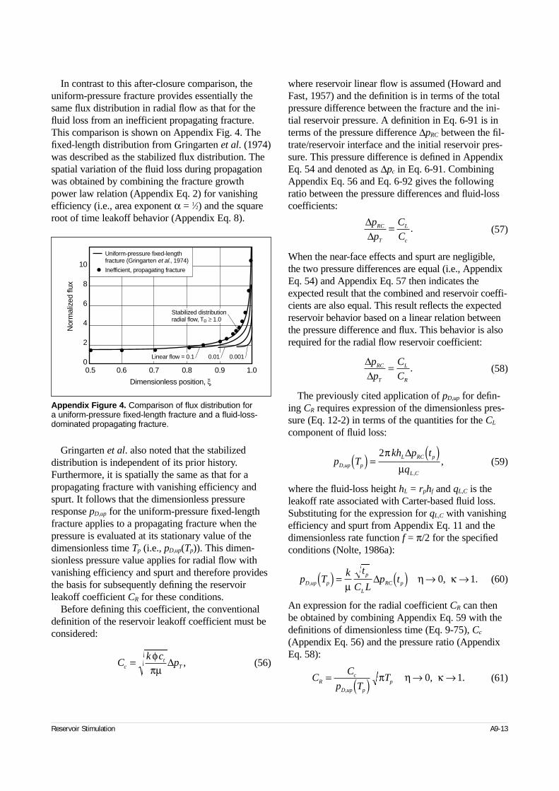
Reservoir Stimulation A9-13

In contrast to this after-closure comparison, theuniform-pressure fracture provides essentially thesame flux distribution in radial flow as that for thefluid loss from an inefficient propagating fracture.This comparison is shown on Appendix Fig. 4. Thefixed-length distribution from Gringarten et al. (1974)was described as the stabilized flux distribution. Thespatial variation of the fluid loss during propagationwas obtained by combining the fracture growthpower law relation (Appendix Eq. 2) for vanishingefficiency (i.e., area exponent α = 1⁄2) and the squareroot of time leakoff behavior (Appendix Eq. 8).

Gringarten et al. also noted that the stabilizeddistribution is independent of its prior history.Furthermore, it is spatially the same as that for apropagating fracture with vanishing efficiency andspurt. It follows that the dimensionless pressureresponse pD,up for the uniform-pressure fixed-lengthfracture applies to a propagating fracture when thepressure is evaluated at its stationary value of thedimensionless time Tp (i.e., pD,up(Tp)). This dimen-sionless pressure value applies for radial flow withvanishing efficiency and spurt and therefore providesthe basis for subsequently defining the reservoirleakoff coefficient CR for these conditions.

Before defining this coefficient, the conventionaldefinition of the reservoir leakoff coefficient must beconsidered:

(56)

where reservoir linear flow is assumed (Howard andFast, 1957) and the definition is in terms of the totalpressure difference between the fracture and the ini-tial reservoir pressure. A definition in Eq. 6-91 is interms of the pressure difference ∆pRC between the fil-trate/reservoir interface and the initial reservoir pres-sure. This pressure difference is defined in AppendixEq. 54 and denoted as ∆pc in Eq. 6-91. CombiningAppendix Eq. 56 and Eq. 6-92 gives the followingratio between the pressure differences and fluid-losscoefficients:

(57)

When the near-face effects and spurt are negligible,the two pressure differences are equal (i.e., AppendixEq. 54) and Appendix Eq. 57 then indicates theexpected result that the combined and reservoir coeffi-cients are also equal. This result reflects the expectedreservoir behavior based on a linear relation betweenthe pressure difference and flux. This behavior is alsorequired for the radial flow reservoir coefficient:

(58)

The previously cited application of pD,up for defin-ing CR requires expression of the dimensionless pres-sure (Eq. 12-2) in terms of the quantities for the CL

component of fluid loss:

(59)

where the fluid-loss height hL = rphf and qL,C is theleakoff rate associated with Carter-based fluid loss.Substituting for the expression for qL,C with vanishingefficiency and spurt from Appendix Eq. 11 and thedimensionless rate function f = π/2 for the specifiedconditions (Nolte, 1986a):

(60)

An expression for the radial coefficient CR can thenbe obtained by combining Appendix Eq. 59 with thedefinitions of dimensionless time (Eq. 9-75), Cc

(Appendix Eq. 56) and the pressure ratio (AppendixEq. 58):

(61)

Ck c

pct

T= φπµ

∆ ,

∆∆p

p

C

CRC

T

L

c

= .

∆∆p

p

C

CRC

T

L

R

= .

p Tkh p t

qD up p

L RC p

L C

,

,

,( ) =( )2π

µ∆

p Tk t

C Lp tD up p

p

L

RC p, , .( ) = ( ) → →µ

η κ∆ 0 1

CC

p TTR

c

D up p

p= ( ) → →,

, .π η κ0 1

Appendix Figure 4. Comparison of flux distribution for a uniform-pressure fixed-length fracture and a fluid-loss-dominated propagating fracture.

0.5 0.6 0.7 0.8 0.9 1.0

10

8

6

4

2

0

Nor

mal

ized

flux

Dimensionless position, ξ

Stabilized distributionradial flow, TD ≥ 1.0

0.0010.01Linear flow = 0.1

Uniform-pressure fixed-lengthfracture (Gringarten et al., 1974)

Inefficient, propagating fracture

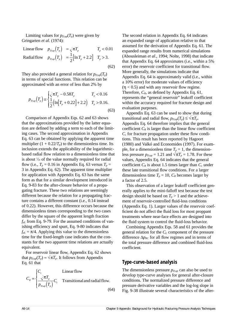
A9-14 Chapter 9 Appendix: Background for Hydraulic Fracturing Pressure Analysis Techniques

Limiting values for pD,up(Tp) were given byGringarten et al. (1974):

(62)

They also provided a general relation for pD,up(Tp)in terms of special functions. This relation can beapproximated with an error of less than 2% by

(63)

Comparison of Appendix Eqs. 62 and 63 showsthat the approximations provided by the latter equa-tion are defined by adding a term to each of the limit-ing cases. The second approximation in AppendixEq. 63 can be obtained by applying the apparent timemultiplier (1 + 0.22/Tp) to the dimensionless time. Itsinclusion extends the applicability of the logarithmic-based radial flow relation to a dimensionless time thatis about 1⁄20 of the value normally required for radialflow (i.e., Tp = 0.16 in Appendix Eq. 63 versus Tp =3 in Appendix Eq. 62). The apparent time multiplier for application with Appendix Eq. 63 has the sameform as that for a similar development introduced inEq. 9-83 for the after-closure behavior of a propa-gating fracture. These two relations are seeminglydifferent because the relation for a propagating frac-ture contains a different constant (i.e., 0.14 instead of 0.22). However, this difference occurs because thedimensionless times corresponding to the two casesdiffer by the square of the apparent length fraction faL from Eq. 9-79. For the assumed conditions of van-ishing efficiency and spurt, Eq. 9-80 indicates that faL = π/4. Applying this value to the dimensionlesstime for the fixed-length case indicates that the con-stants for the two apparent time relations are actuallyequivalent.

For reservoir linear flow, Appendix Eq. 62 showsthat pD,up(Tp) ≈ √πTp. It follows from Appendix Eq. 61 that

(64)

The second relation in Appendix Eq. 64 indicates an expanded range of application relative to thatassumed for the derivation of Appendix Eq. 61. Theexpanded range results from numerical simulations(Abousleiman et al., 1994; Nolte, 1998) that indicatethat Appendix Eq. 64 approximates (i.e., within a 5%error) the reservoir coefficient for transitional flow.More generally, the simulations indicate thatAppendix Eq. 64 is approximately valid (i.e., within a 10% error) for moderate values of efficiency (η < 0.5) and with any reservoir flow regime.Therefore, CR, as defined by Appendix Eq. 61,represents the “general reservoir” leakoff coefficientwithin the accuracy required for fracture design andevaluation purposes.

Appendix Eq. 63 can be used to show that duringtransitional and radial flow, pD,up(Tp) ≤ √πTp.Appendix Eq. 64 therefore implies that the generalcoefficient CR is larger than the linear flow coefficientCc for fracture propagation under these flow condi-tions. This result has been reported by Hagoort(1980) and Valkó and Economides (1997). For exam-ple, for a dimensionless time Tp = 1, the dimension-less pressure pD,up = 1.21 and √πTp = 1.78. For thesevalues, Appendix Eq. 64 indicates that the generalcoefficient CR is about 1.5 times larger than Cc underthese late transitional flow conditions. For a largerdimensionless time Tp = 10, CR becomes larger by a factor of 2.5.

This observation of a larger leakoff coefficient gen-erally applies to the mini-falloff test because the testdesign should be based on Tp > 1 and the achieve-ment of reservoir-controlled fluid-loss conditions(Appendix Eq. 1). Larger values of the reservoir coef-ficient do not affect the fluid loss for most proppanttreatments where near-face effects are designed intothe fluid system to control the fluid-loss behavior.

Combining Appendix Eqs. 58 and 61 provides thegeneral relation for the CL component of the pressuredifference ∆pRC for all flow regimes and in terms ofthe total pressure difference and combined fluid-losscoefficient.

Type-curve-based analysisThe dimensionless pressure pD,up can also be used todevelop type-curve analyses for general after-closureconditions. The normalized pressure difference andpressure derivative variables and the log-log slope inFig. 9-38 illustrate several characteristics of the after-

Linear flow

Radial flow

p T T T

p T T T

D up p p p

D up p p p

,

,

.

ln . .

( ) = <

( ) = +[ ] >

π 0 0112

2 2 3

p TT T T

T TD up p

p p p

p p

,

. .

ln . . . .( ) ≅

− <

+[ ] +( ) >

π 0 58 0 1612

0 22 2 2 0 16

C

CT

p TCR

c

p

D up p

c

=( )

Linear flow

Transitionaland radial flow.π

,

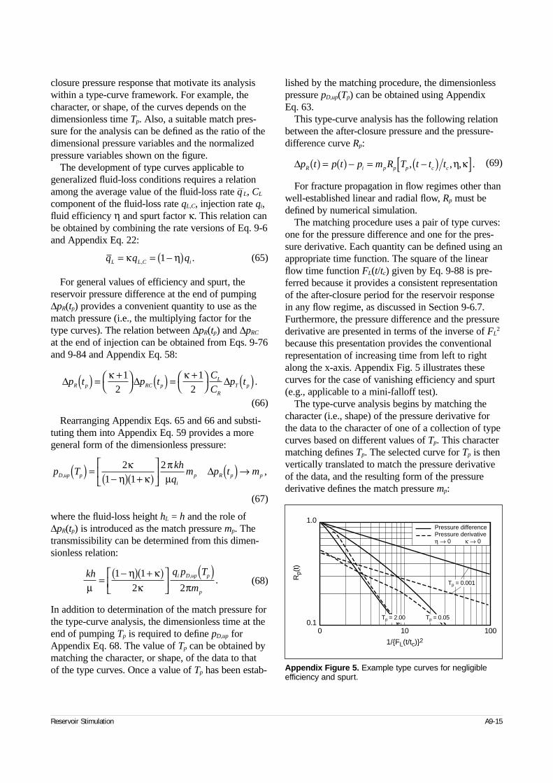
Reservoir Stimulation A9-15

closure pressure response that motivate its analysiswithin a type-curve framework. For example, thecharacter, or shape, of the curves depends on thedimensionless time Tp. Also, a suitable match pres-sure for the analysis can be defined as the ratio of thedimensional pressure variables and the normalizedpressure variables shown on the figure.

The development of type curves applicable togeneralized fluid-loss conditions requires a relationamong the average value of the fluid-loss rate q—L, CL

component of the fluid-loss rate qL,C, injection rate qi,fluid efficiency η and spurt factor κ. This relation canbe obtained by combining the rate versions of Eq. 9-6and Appendix Eq. 22:

(65)

For general values of efficiency and spurt, thereservoir pressure difference at the end of pumping∆pR(tp) provides a convenient quantity to use as thematch pressure (i.e., the multiplying factor for thetype curves). The relation between ∆pR(tp) and ∆pRC

at the end of injection can be obtained from Eqs. 9-76and 9-84 and Appendix Eq. 58:

(66)

Rearranging Appendix Eqs. 65 and 66 and substi-tuting them into Appendix Eq. 59 provides a moregeneral form of the dimensionless pressure:

(67)

where the fluid-loss height hL = h and the role of∆pR(tp) is introduced as the match pressure mp. Thetransmissibility can be determined from this dimen-sionless relation:

(68)

In addition to determination of the match pressure forthe type-curve analysis, the dimensionless time at theend of pumping Tp is required to define pD,up forAppendix Eq. 68. The value of Tp can be obtained bymatching the character, or shape, of the data to that of the type curves. Once a value of Tp has been estab-

lished by the matching procedure, the dimensionlesspressure pD,up(Tp) can be obtained using Appendix Eq. 63.

This type-curve analysis has the following relationbetween the after-closure pressure and the pressure-difference curve Rp:

(69)

For fracture propagation in flow regimes other thanwell-established linear and radial flow, Rp must bedefined by numerical simulation.

The matching procedure uses a pair of type curves:one for the pressure difference and one for the pres-sure derivative. Each quantity can be defined using anappropriate time function. The square of the linearflow time function FL(t/tc) given by Eq. 9-88 is pre-ferred because it provides a consistent representationof the after-closure period for the reservoir responsein any flow regime, as discussed in Section 9-6.7.Furthermore, the pressure difference and the pressurederivative are presented in terms of the inverse of FL

2

because this presentation provides the conventionalrepresentation of increasing time from left to rightalong the x-axis. Appendix Fig. 5 illustrates thesecurves for the case of vanishing efficiency and spurt(e.g., applicable to a mini-falloff test).

The type-curve analysis begins by matching thecharacter (i.e., shape) of the pressure derivative forthe data to the character of one of a collection of typecurves based on different values of Tp. This charactermatching defines Tp. The selected curve for Tp is thenvertically translated to match the pressure derivativeof the data, and the resulting form of the pressurederivative defines the match pressure mp:

q q qL L C i= = −( )κ η, .1

∆p t p t p m R T t t tR i p p p c c( ) = ( ) − = −( )[ ], , , .η κ

∆ ∆ ∆p t p tC

Cp tR p RC p

L

R

T p( ) = +

( ) = +

( )κ κ1

21

2.

p Tkh

qm p t mD up p

i

p R p p, ,( ) =−( ) +( )

( ) →2

1 12κ

η κπµ

∆

kh q p T

mi D up p

pµη κ

κ π=

−( ) +( )

( )1 1

2 2,

.

Appendix Figure 5. Example type curves for negligibleefficiency and spurt.

1/{FL(t/tc)}2

1.0

0.1

Rp(

t)

0 10 100

Tp = 2.00 Tp = 0.05

Tp = 0.001

Pressure differencePressure derivativeη → 0 κ → 0

(70)

The transmissibility is then estimated from AppendixEq. 68 using the two type-curve parameters Tp and mp.The initial reservoir pressure is extracted by applyingAppendix Eq. 69 over the time range of the match.

Additional information concerning the nature ofthe fluid loss can be obtained from the value of mp

(i.e., ∆pR(tp) inferred from the after-closure data).Relative to Appendix Eq. 66, ∆pT(tp) = p(tp) – pi, withp(tp) defined by the ISIP, and when ∆pR(tp) ≈ ∆pT(tp)in the absence of spurt, the reservoir and total leakoffcoefficients are approximately equal. Under theseconditions, essentially the entire pressure difference∆pT is within the reservoir and the reservoir controlsthe fluid-loss behavior. Conversely, when ∆pR(tp) <<∆pT(tp), a negligible fraction of the total pressure dropoccurs in the reservoir, and the reservoir does nothave a meaningful role in controlling fluid leakoff.

A9-16 Chapter 9 Appendix: Background for Hydraulic Fracturing Pressure Analysis Techniques

F t tdp t

d F t tm F t t

dR

d F t tL c

L c

p L cp

L c

( ){ } ( )( ){ }

= ( ){ } ( ){ }

2

2

2

2 .

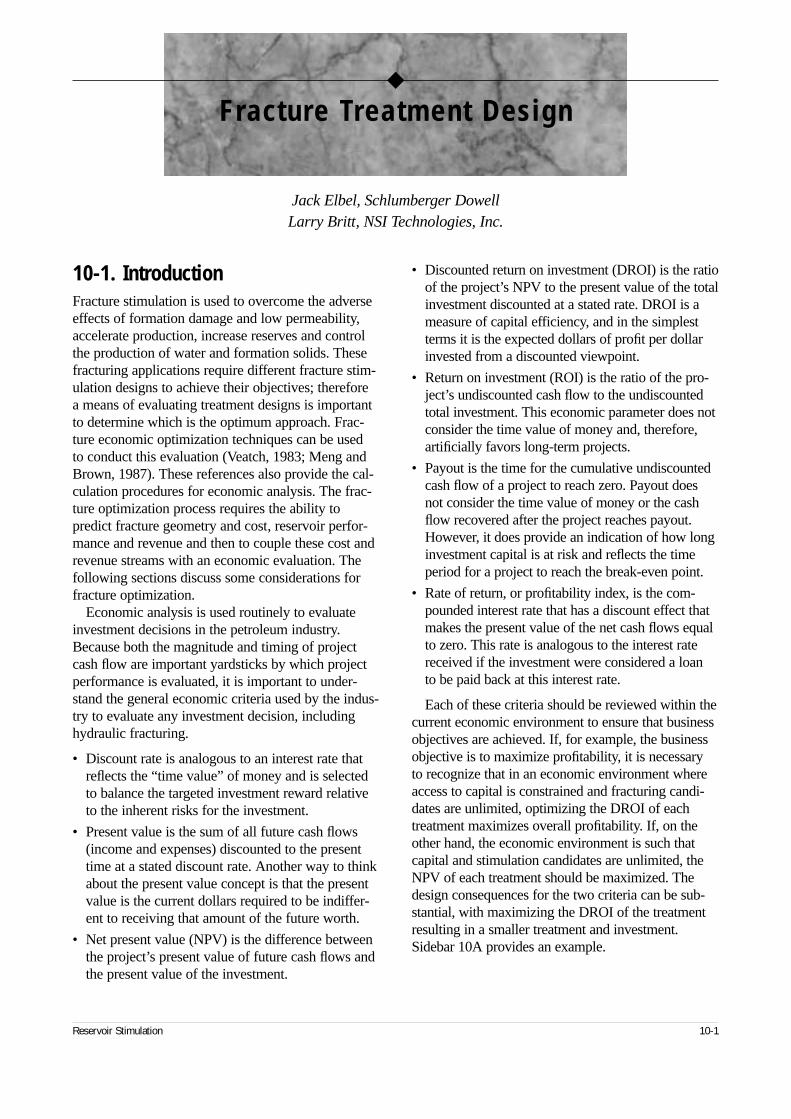
10-1. IntroductionFracture stimulation is used to overcome the adverseeffects of formation damage and low permeability,accelerate production, increase reserves and controlthe production of water and formation solids. Thesefracturing applications require different fracture stim-ulation designs to achieve their objectives; therefore a means of evaluating treatment designs is importantto determine which is the optimum approach. Frac-ture economic optimization techniques can be used to conduct this evaluation (Veatch, 1983; Meng andBrown, 1987). These references also provide the cal-culation procedures for economic analysis. The frac-ture optimization process requires the ability topredict fracture geometry and cost, reservoir perfor-mance and revenue and then to couple these cost andrevenue streams with an economic evaluation. Thefollowing sections discuss some considerations forfracture optimization.

Economic analysis is used routinely to evaluateinvestment decisions in the petroleum industry.Because both the magnitude and timing of projectcash flow are important yardsticks by which projectperformance is evaluated, it is important to under-stand the general economic criteria used by the indus-try to evaluate any investment decision, includinghydraulic fracturing.

• Discount rate is analogous to an interest rate thatreflects the “time value” of money and is selectedto balance the targeted investment reward relativeto the inherent risks for the investment.

• Present value is the sum of all future cash flows(income and expenses) discounted to the presenttime at a stated discount rate. Another way to thinkabout the present value concept is that the presentvalue is the current dollars required to be indiffer-ent to receiving that amount of the future worth.

• Net present value (NPV) is the difference betweenthe project’s present value of future cash flows andthe present value of the investment.

• Discounted return on investment (DROI) is the ratioof the project’s NPV to the present value of the totalinvestment discounted at a stated rate. DROI is ameasure of capital efficiency, and in the simplestterms it is the expected dollars of profit per dollarinvested from a discounted viewpoint.

• Return on investment (ROI) is the ratio of the pro-ject’s undiscounted cash flow to the undiscountedtotal investment. This economic parameter does notconsider the time value of money and, therefore,artificially favors long-term projects.

• Payout is the time for the cumulative undiscountedcash flow of a project to reach zero. Payout doesnot consider the time value of money or the cashflow recovered after the project reaches payout.However, it does provide an indication of how longinvestment capital is at risk and reflects the timeperiod for a project to reach the break-even point.

• Rate of return, or profitability index, is the com-pounded interest rate that has a discount effect thatmakes the present value of the net cash flows equalto zero. This rate is analogous to the interest ratereceived if the investment were considered a loan to be paid back at this interest rate.

Each of these criteria should be reviewed within thecurrent economic environment to ensure that businessobjectives are achieved. If, for example, the businessobjective is to maximize profitability, it is necessary to recognize that in an economic environment whereaccess to capital is constrained and fracturing candi-dates are unlimited, optimizing the DROI of eachtreatment maximizes overall profitability. If, on theother hand, the economic environment is such thatcapital and stimulation candidates are unlimited, theNPV of each treatment should be maximized. Thedesign consequences for the two criteria can be sub-stantial, with maximizing the DROI of the treatmentresulting in a smaller treatment and investment.Sidebar 10A provides an example.

Reservoir Stimulation 10-1

◆

Fracture Treatment Design

Jack Elbel, Schlumberger DowellLarry Britt, NSI Technologies, Inc.

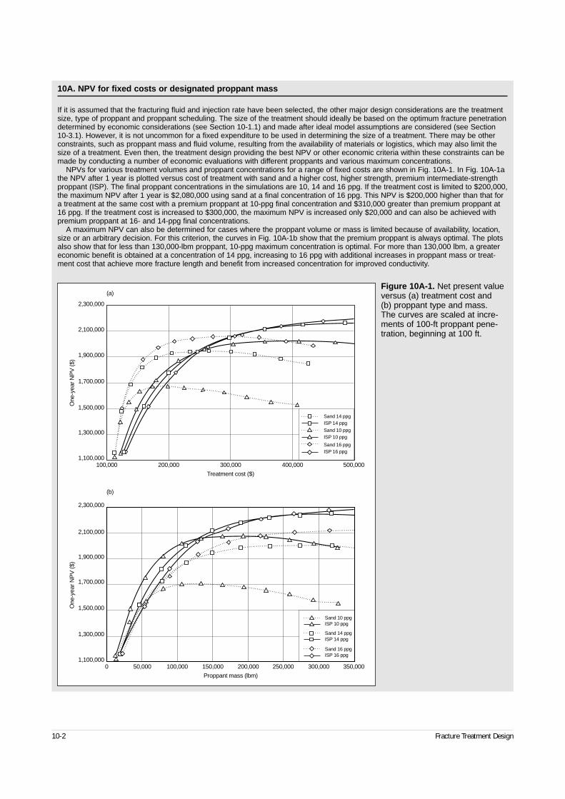
10-2 Fracture Treatment Design

10A. NPV for fixed costs or designated proppant mass

If it is assumed that the fracturing fluid and injection rate have been selected, the other major design considerations are the treatmentsize, type of proppant and proppant scheduling. The size of the treatment should ideally be based on the optimum fracture penetrationdetermined by economic considerations (see Section 10-1.1) and made after ideal model assumptions are considered (see Section10-3.1). However, it is not uncommon for a fixed expenditure to be used in determining the size of a treatment. There may be otherconstraints, such as proppant mass and fluid volume, resulting from the availability of materials or logistics, which may also limit thesize of a treatment. Even then, the treatment design providing the best NPV or other economic criteria within these constraints can bemade by conducting a number of economic evaluations with different proppants and various maximum concentrations.

NPVs for various treatment volumes and proppant concentrations for a range of fixed costs are shown in Fig. 10A-1. In Fig. 10A-1athe NPV after 1 year is plotted versus cost of treatment with sand and a higher cost, higher strength, premium intermediate-strengthproppant (ISP). The final proppant concentrations in the simulations are 10, 14 and 16 ppg. If the treatment cost is limited to $200,000,the maximum NPV after 1 year is $2,080,000 using sand at a final concentration of 16 ppg. This NPV is $200,000 higher than that fora treatment at the same cost with a premium proppant at 10-ppg final concentration and $310,000 greater than premium proppant at16 ppg. If the treatment cost is increased to $300,000, the maximum NPV is increased only $20,000 and can also be achieved withpremium proppant at 16- and 14-ppg final concentrations.

A maximum NPV can also be determined for cases where the proppant volume or mass is limited because of availability, location,size or an arbitrary decision. For this criterion, the curves in Fig. 10A-1b show that the premium proppant is always optimal. The plotsalso show that for less than 130,000-lbm proppant, 10-ppg maximum concentration is optimal. For more than 130,000 lbm, a greatereconomic benefit is obtained at a concentration of 14 ppg, increasing to 16 ppg with additional increases in proppant mass or treat-ment cost that achieve more fracture length and benefit from increased concentration for improved conductivity.

Figure 10A-1. Net present valueversus (a) treatment cost and (b) proppant type and mass. The curves are scaled at incre-ments of 100-ft proppant pene-tration, beginning at 100 ft.

One

-yea

r NP

V ($

)

1,100,000

1,300,000

1,500,000

1,700,000

1,900,000

2,100,000

2,300,000

100,000 200,000 300,000 400,000 500,000

One

-yea

r NP

V ($

)

1,100,000

1,300,000

1,500,000

1,700,000

1,900,000

2,100,000

2,300,000

350,0000 50,000 100,000 150,000 200,000 250,000 300,000

Sand 14 ppgISP 14 ppg

Sand 10 ppgISP 10 ppg

Sand 16 ppgISP 16 ppg

Treatment cost ($)

Proppant mass (lbm)

Sand 14 ppgISP 14 ppgSand 10 ppgISP 10 ppg

Sand 16 ppgISP 16 ppg

(b)

(a)

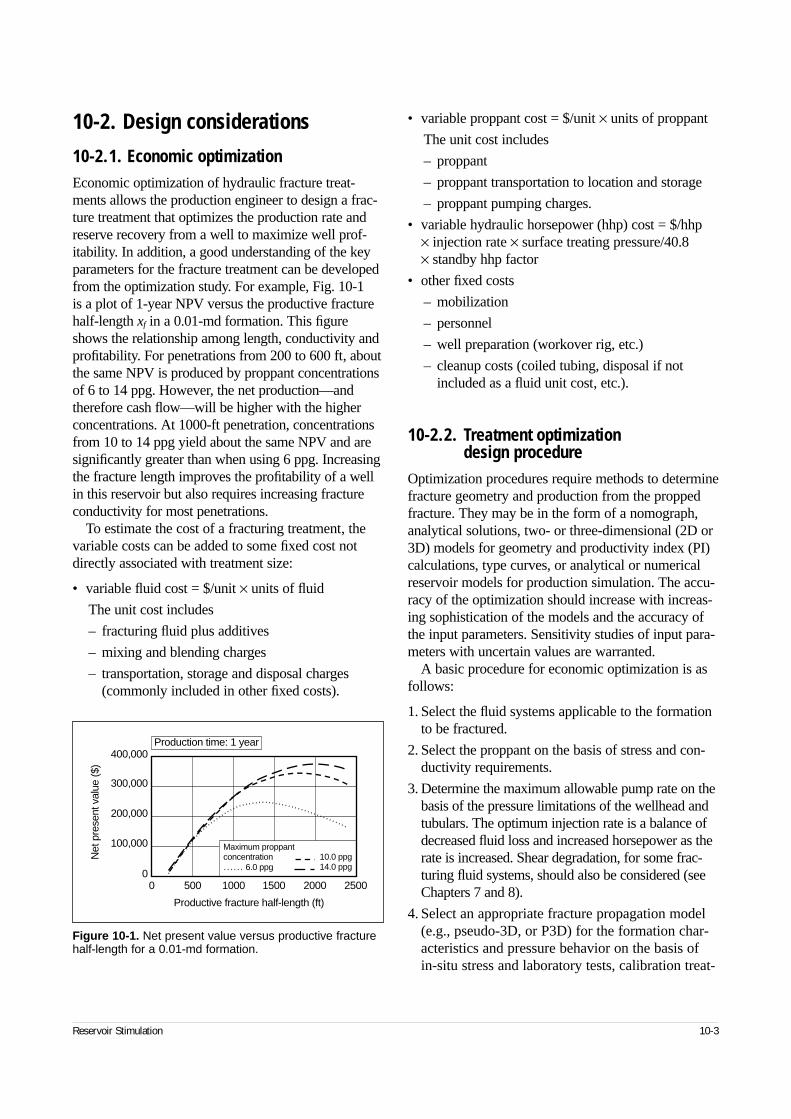
10-2. Design considerations

10-2.1. Economic optimizationEconomic optimization of hydraulic fracture treat-ments allows the production engineer to design a frac-ture treatment that optimizes the production rate andreserve recovery from a well to maximize well prof-itability. In addition, a good understanding of the keyparameters for the fracture treatment can be developedfrom the optimization study. For example, Fig. 10-1 is a plot of 1-year NPV versus the productive fracturehalf-length xf in a 0.01-md formation. This figureshows the relationship among length, conductivity andprofitability. For penetrations from 200 to 600 ft, aboutthe same NPV is produced by proppant concentrationsof 6 to 14 ppg. However, the net production—andtherefore cash flow—will be higher with the higherconcentrations. At 1000-ft penetration, concentrationsfrom 10 to 14 ppg yield about the same NPV and aresignificantly greater than when using 6 ppg. Increasingthe fracture length improves the profitability of a wellin this reservoir but also requires increasing fractureconductivity for most penetrations.

To estimate the cost of a fracturing treatment, thevariable costs can be added to some fixed cost notdirectly associated with treatment size:

• variable fluid cost = $/unit × units of fluid

The unit cost includes

– fracturing fluid plus additives

– mixing and blending charges

– transportation, storage and disposal charges(commonly included in other fixed costs).

• variable proppant cost = $/unit × units of proppant

The unit cost includes

– proppant

– proppant transportation to location and storage

– proppant pumping charges.

• variable hydraulic horsepower (hhp) cost = $/hhp × injection rate × surface treating pressure/40.8 × standby hhp factor

• other fixed costs

– mobilization

– personnel

– well preparation (workover rig, etc.)

– cleanup costs (coiled tubing, disposal if notincluded as a fluid unit cost, etc.).

10-2.2. Treatment optimization design procedure

Optimization procedures require methods to determinefracture geometry and production from the proppedfracture. They may be in the form of a nomograph,analytical solutions, two- or three-dimensional (2D or3D) models for geometry and productivity index (PI)calculations, type curves, or analytical or numericalreservoir models for production simulation. The accu-racy of the optimization should increase with increas-ing sophistication of the models and the accuracy ofthe input parameters. Sensitivity studies of input para-meters with uncertain values are warranted.

A basic procedure for economic optimization is asfollows:

1. Select the fluid systems applicable to the formationto be fractured.

2. Select the proppant on the basis of stress and con-ductivity requirements.

3. Determine the maximum allowable pump rate on thebasis of the pressure limitations of the wellhead andtubulars. The optimum injection rate is a balance ofdecreased fluid loss and increased horsepower as therate is increased. Shear degradation, for some frac-turing fluid systems, should also be considered (seeChapters 7 and 8).

4. Select an appropriate fracture propagation model(e.g., pseudo-3D, or P3D) for the formation char-acteristics and pressure behavior on the basis ofin-situ stress and laboratory tests, calibration treat-

Reservoir Stimulation 10-3

Figure 10-1. Net present value versus productive fracturehalf-length for a 0.01-md formation.

Net

pre

sent

val

ue ($

)

400,000

300,000

200,000

100,000

00 500 1000 1500 2000 2500

Productive fracture half-length (ft)

Maximum proppant concentration

14.0 ppg10.0 ppg

6.0 ppg

Production time: 1 year

10-4 Fracture Treatment Design

ments and log analysis (e.g., stress profile, gammaray) (see Chapters 3, 4 and 9).

5. Develop the input data required for the selectedgeometry model(s).

6. Determine fracture penetration and fracture conduc-tivity for a selected treatment size and proppantconcentration by forward simulation or determinefluid and proppant volumes required and fractureconductivity obtained for a selected penetrationusing inverse simulation (see Chapter 6). Determinethe optimum pad fraction (see Chapters 5 and 6). Ifthe model does not account for polymer conductiv-ity damage, an estimated damaged conductivityshould be used (see Chapters 7 and 8).

7. Determine the production rate and cumulativerecovery over a selected time period for a specificpropped penetration and its corresponding conduc-tivity.

8.Calculate the present value of the net revenue ofthe production based on a discount rate (i.e., thesum of the present values for each year of theselected period).

9.Calculate the total treatment cost including thecosts associated with fluids, proppants andhydraulic horsepower.

10.Calculate the NPV for the fracture by subtractingthe treatment cost from the well’s discounted netrevenue (step 9 minus step 8).

11. Repeat the preceding computational cycle forincremental increases in length until the NPVdecreases or a maximum length is reached.

12.Construct curves showing the fracture NPV orother appropriate economic criteria versus frac-ture penetration. When the NPV starts to declinewith increasing fracture lengths, the cumulativeproduction for the specific lengths will still beincreasing.

The cycle can be repeated for other materials orconditions such as other fluids and additive concen-trations, injection rates, proppant types and maxi-mum proppant concentrations or even with othergeometry models. The process can easily becometime consuming, and the number of iterations shouldbe governed by the accuracy required as well as theaccuracy of the input parameters. The cycles can berepeated for sensitivity to parameters to determinebounds. The most important input parameters and

those with the greatest potential for error are forma-tion permeability and fracture conductivity. Fortun-ately, a number of economic models combinegeometry and reservoir models to allow makingdetailed studies in a reasonable amount of time.

Economic optimization among different fracturingfluids such as oil-base, water-base and foam fluids is difficult. These fluids are usually chosen for com-patibility with formation fluids or cleanup properties,and their economic benefit cannot be quantifiedunless features such as formation damage, polymerdamage to proppant pack and cleanup time can bedetermined by the production models or included by some other means in the analysis. As an example,if it is known that a foam fracturing fluid will reducethe cleanup time, the cost of cleanup can be reducedfor the foam fluid relative to that for a nonfoamfluid. Some risk factor and uncertainty can also beassociated with various input parameters and behav-ioral assumptions (Nolte and Economides, 1991).

10-2.3. Fracture conductivityPlacing the appropriate amount and type of proppantin the fracture is critical to the success of a hydraulicfracturing treatment. Independent of fluid residuedamage, proppant concentration in the fracture andresistance to crushing determine the fracture conduc-tivity over the producing life of the well. Proppantselection is optimized by balancing the potential tocreate fracture conductivity against the additional costor risk of placement. Factors such as proppant proper-ties (strength, particle size, roundness and fines con-tent), closure stress, polymer damage, drawdown rate,embedment and the resultant propped fracture widthaffect the fracture conductivity. Several of these fac-tors are discussed in more detail in Chapters 7 and 8.

For simplicity, the fracture conductivity used forproduction simulation is usually considered to behomogeneous. Advances in geometry and productionmodeling (see Chapter 12) enable simulation withspatial variations in horizontal (Bennett et al., 1983)as well as vertical conductivity (Poe et al., 1992).

Two regions over the vertical profile are affected by different criteria for conductivity. The first is abank buildup region created at the bottom duringplacement where the pack width is equal to thehydraulic width for the region. The second is theoverlying slurried height region at closure where the

propped width and height are affected by the proppantslurry concentration and closure time. Ignoring theeffect of proppant redistribution during closure, Fig. 5-21 gives the percent of “fill” of the proppedwidth relative to the width when pumping stops.

• Stress on proppant

When a hydraulic fracture is created, the minimumin-situ stress must be overcome to open and propa-gate the fracture. When the fracture closes on theproppant after the treatment, the effective closurestress (hereafter termed simply closure stress) onthe proppant is equal to the minimum in-situ stressplus the additional stress induced by the pack widthminus the pore pressure in the proppant pack. Theadditional stress caused by the width can be esti-mated from an appropriate width model (seeChapter 6) using the propped width and the result-ing net pressure as the increased stress. To bringthe well on production, the pressure in the pack at the wellbore must be reduced below that of thereservoir, increasing the stress on the proppant atthis time.

The stress on the proppant changes during thelife of the well. If initiating production requires thatthe well be swabbed, high stresses on the proppantnear the wellbore may occur. If the well is swabbedoff the bottom, the bottomhole producing pressureis essentially zero, creating the maximum stress on the proppant. Cyclic loading tests (Kim andWillingham, 1987; Holditch and Blakely, 1992)show that the conductivity is irreversibly reduced.Therefore, as the reservoir pressure is reducedbecause of depletion and the closure stress isdecreased proportionally (by a ratio of about 1⁄2;see Chapter 3), the permeability of the proppant is not restored to greater than what it was when the maximum stress was applied.

Figure 7-13 shows the effect of closure stress onthe permeability of various propping agents. Whenthe stress on the proppant exceeds 10,000 psi, high-strength proppants (such as sintered bauxite) arerequired. In the range of 5,000 to 10,000 psi, theuse of higher strength, manufactured ceramic prop-pant—commonly called intermediate-strengthproppant (ISP)—should be considered. These pre-mium proppants provide greater conductivity athigher closure stresses, but their cost makes themeconomically unattractive at lower closure stresses.Sand is the most common proppant, and its use is

considered for fracturing formations where stresseson the proppant are less than 6000 psi. The perme-ability of precured resin-coated proppants isbetween that of sand and ISP.

If a well is produced at a constant bottomholeproducing pressure, the minimum stress, and hencethe closure stress on the proppant, decreases duringproduction as the effective reservoir pressuredecreases. If the well is produced at a constant ratesuch that the bottomhole producing pressure mustbe decreased faster than the effective reservoirpressure decreases, the stress on the proppant mayincrease. When the minimum surface producingpressure is reached and the well is produced at a constant pressure, the stress will decrease.

Formations with a high stress (usually associatedwith abnormally high pore pressures) may notalways require high-strength proppants as would be expected. This is the case where the desired pro-duction rate can be maintained at a low drawdownpressure during early production time, minimizingthe effective stress on the proppant. Later, becausethe pore pressure has decreased as a result of pro-duction, the in-situ stress may have decreased to a point where subsequent increased drawdown willnot cause the stress on the sand to become exces-sive. From a practical standpoint (i.e., to enableeconomic production during the period of lowdrawdown), this condition requires relatively highvalues of the permeability-thickness product kh forthe formation and effective fracture characteristics.The incongruity of this scenario for relatively shal-low reservoirs is that if the formation permeabilityis low, high-strength proppants may be required,and if it is high, sand may be sufficient.

• Propped width

Figure 10-2 illustrates the typical relationship offracture conductivity to proppant concentration.Increasing the proppant concentration results inmultiple layers of proppant and an increase in thefracture conductivity. Although maximum conduc-tivity can be obtained by placing proppant in a partial monolayer (a technique developed for hori-zontal fractures), placement of a partial monolayerin a vertical fracture is virtually impossible toachieve. Therefore, fracture treatments are designedfor multiple proppant layers. With multiple layersof proppant, the outer layer may embed in softerformations, allowing only the inner layers to

Reservoir Stimulation 10-5

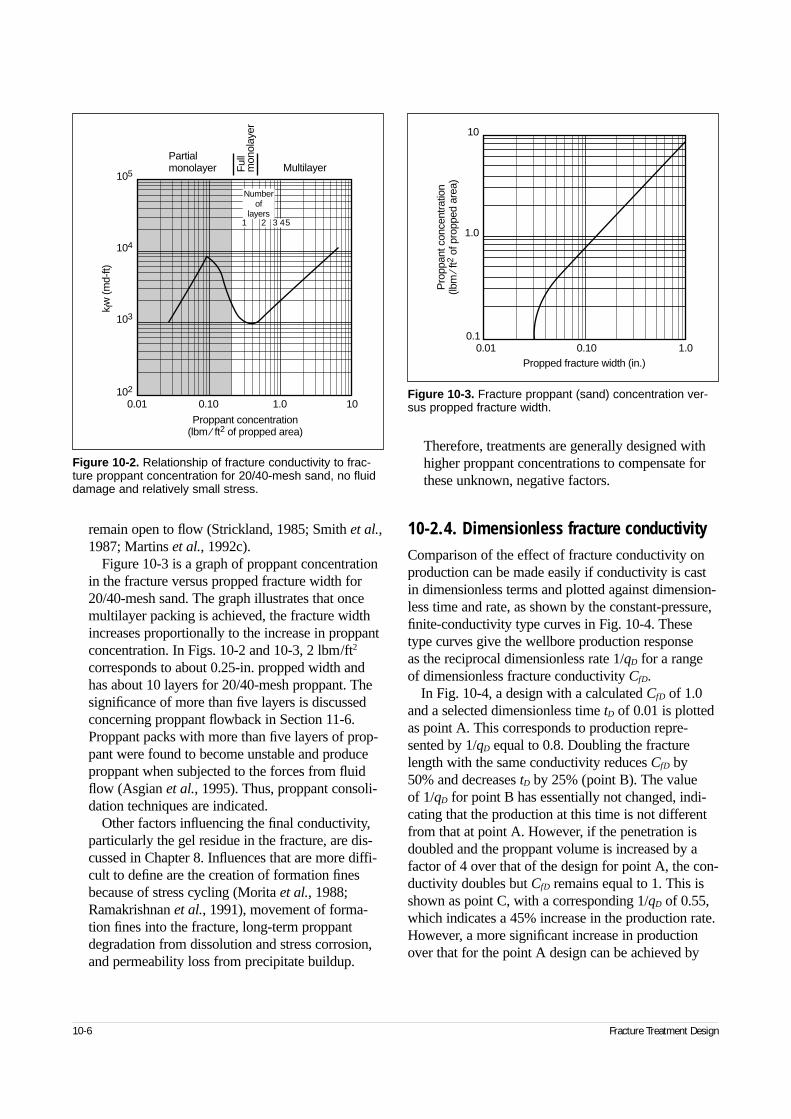
remain open to flow (Strickland, 1985; Smith et al.,1987; Martins et al., 1992c).

Figure 10-3 is a graph of proppant concentrationin the fracture versus propped fracture width for20/40-mesh sand. The graph illustrates that oncemultilayer packing is achieved, the fracture widthincreases proportionally to the increase in proppantconcentration. In Figs. 10-2 and 10-3, 2 lbm/ft2

corresponds to about 0.25-in. propped width andhas about 10 layers for 20/40-mesh proppant. Thesignificance of more than five layers is discussedconcerning proppant flowback in Section 11-6.Proppant packs with more than five layers of prop-pant were found to become unstable and produceproppant when subjected to the forces from fluidflow (Asgian et al., 1995). Thus, proppant consoli-dation techniques are indicated.

Other factors influencing the final conductivity,particularly the gel residue in the fracture, are dis-cussed in Chapter 8. Influences that are more diffi-cult to define are the creation of formation finesbecause of stress cycling (Morita et al., 1988;Ramakrishnan et al., 1991), movement of forma-tion fines into the fracture, long-term proppantdegradation from dissolution and stress corrosion,and permeability loss from precipitate buildup.

Therefore, treatments are generally designed withhigher proppant concentrations to compensate forthese unknown, negative factors.

10-2.4. Dimensionless fracture conductivityComparison of the effect of fracture conductivity onproduction can be made easily if conductivity is castin dimensionless terms and plotted against dimension-less time and rate, as shown by the constant-pressure,finite-conductivity type curves in Fig. 10-4. Thesetype curves give the wellbore production response as the reciprocal dimensionless rate 1/qD for a range of dimensionless fracture conductivity CfD.

In Fig. 10-4, a design with a calculated CfD of 1.0and a selected dimensionless time tD of 0.01 is plottedas point A. This corresponds to production repre-sented by 1/qD equal to 0.8. Doubling the fracturelength with the same conductivity reduces CfD by50% and decreases tD by 25% (point B). The value of 1/qD for point B has essentially not changed, indi-cating that the production at this time is not differentfrom that at point A. However, if the penetration isdoubled and the proppant volume is increased by afactor of 4 over that of the design for point A, the con-ductivity doubles but CfD remains equal to 1. This isshown as point C, with a corresponding 1/qD of 0.55,which indicates a 45% increase in the production rate.However, a more significant increase in productionover that for the point A design can be achieved by

10-6 Fracture Treatment Design

Figure 10-2. Relationship of fracture conductivity to frac-ture proppant concentration for 20/40-mesh sand, no fluiddamage and relatively small stress.

k fw

(md-

ft)

0.01 0.10 1.0 10

Proppant concentration(lbm ⁄ ft2 of propped area)

Partialmonolayer F

ull

mon

olay

er

Multilayer

5

102

103

104

105

4

Numberof

layers31 2

Figure 10-3. Fracture proppant (sand) concentration ver-sus propped fracture width.

Pro

ppan

t con

cent

ratio

n(lb

m⁄ f

t2 o

f pro

pped

are

a)

10

1.0

0.10.01 0.10 1.0

Propped fracture width (in.)

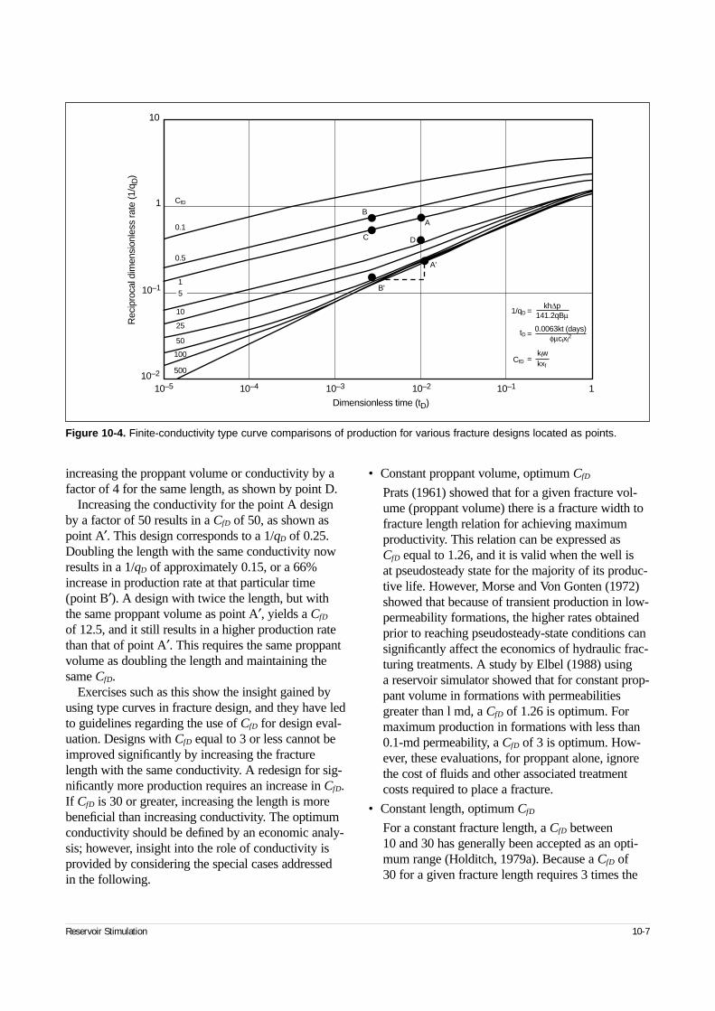
increasing the proppant volume or conductivity by afactor of 4 for the same length, as shown by point D.

Increasing the conductivity for the point A designby a factor of 50 results in a CfD of 50, as shown aspoint A′. This design corresponds to a 1/qD of 0.25.Doubling the length with the same conductivity nowresults in a 1/qD of approximately 0.15, or a 66%increase in production rate at that particular time(point B′). A design with twice the length, but withthe same proppant volume as point A′, yields a CfD

of 12.5, and it still results in a higher production ratethan that of point A′. This requires the same proppantvolume as doubling the length and maintaining thesame CfD.

Exercises such as this show the insight gained byusing type curves in fracture design, and they have ledto guidelines regarding the use of CfD for design eval-uation. Designs with CfD equal to 3 or less cannot beimproved significantly by increasing the fracturelength with the same conductivity. A redesign for sig-nificantly more production requires an increase in CfD.If CfD is 30 or greater, increasing the length is morebeneficial than increasing conductivity. The optimumconductivity should be defined by an economic analy-sis; however, insight into the role of conductivity isprovided by considering the special cases addressed in the following.

• Constant proppant volume, optimum CfD

Prats (1961) showed that for a given fracture vol-ume (proppant volume) there is a fracture width tofracture length relation for achieving maximumproductivity. This relation can be expressed as CfD equal to 1.26, and it is valid when the well is at pseudosteady state for the majority of its produc-tive life. However, Morse and Von Gonten (1972)showed that because of transient production in low-permeability formations, the higher rates obtainedprior to reaching pseudosteady-state conditions cansignificantly affect the economics of hydraulic frac-turing treatments. A study by Elbel (1988) using a reservoir simulator showed that for constant prop-pant volume in formations with permeabilitiesgreater than l md, a CfD of 1.26 is optimum. Formaximum production in formations with less than0.1-md permeability, a CfD of 3 is optimum. How-ever, these evaluations, for proppant alone, ignorethe cost of fluids and other associated treatmentcosts required to place a fracture.

• Constant length, optimum CfD

For a constant fracture length, a CfD between10 and 30 has generally been accepted as an opti-mum range (Holditch, 1979a). Because a CfD of30 for a given fracture length requires 3 times the

Reservoir Stimulation 10-7

Figure 10-4. Finite-conductivity type curve comparisons of production for various fracture designs located as points.

Rec

ipro

cal d

imen

sion

less

rate

(1/q

D)

10

1

10–1

10–2

10–5 10–4 10–3 10–2 10–1 1

Dimensionless time (tD)

kh∆p141.2qBµ1/qD

0.0063kt (days)φµctxf

2tD

kfwkxf

CfD

CfD

0.1

0.5

1

10

25

50

100

500

B

C

A

D

A'

B'5

=

=

=

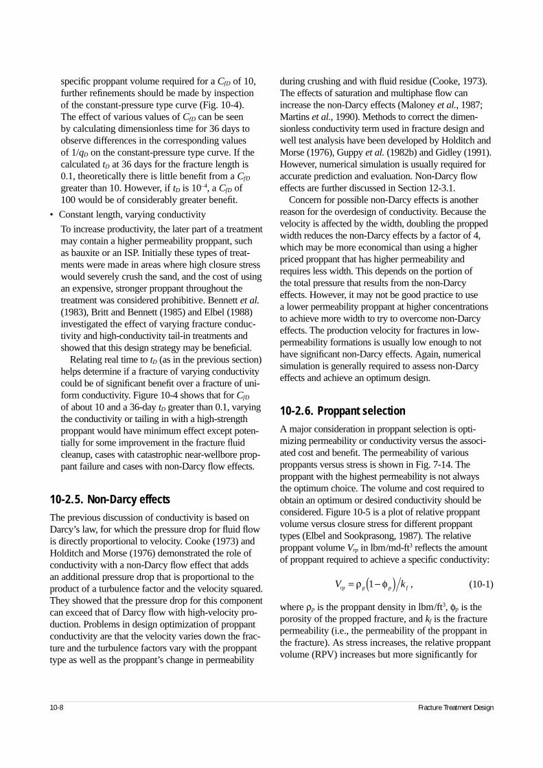
specific proppant volume required for a CfD of 10,further refinements should be made by inspectionof the constant-pressure type curve (Fig. 10-4). The effect of various values of CfD can be seen by calculating dimensionless time for 36 days toobserve differences in the corresponding values of 1/qD on the constant-pressure type curve. If thecalculated tD at 36 days for the fracture length is0.1, theoretically there is little benefit from a CfD

greater than 10. However, if tD is 10–4, a CfD of100 would be of considerably greater benefit.

• Constant length, varying conductivity

To increase productivity, the later part of a treatmentmay contain a higher permeability proppant, such as bauxite or an ISP. Initially these types of treat-ments were made in areas where high closure stresswould severely crush the sand, and the cost of usingan expensive, stronger proppant throughout thetreatment was considered prohibitive. Bennett et al.(1983), Britt and Bennett (1985) and Elbel (1988)investigated the effect of varying fracture conduc-tivity and high-conductivity tail-in treatments andshowed that this design strategy may be beneficial.

Relating real time to tD (as in the previous section)helps determine if a fracture of varying conductivitycould be of significant benefit over a fracture of uni-form conductivity. Figure 10-4 shows that for CfD

of about 10 and a 36-day tD greater than 0.1, varyingthe conductivity or tailing in with a high-strengthproppant would have minimum effect except poten-tially for some improvement in the fracture fluidcleanup, cases with catastrophic near-wellbore prop-pant failure and cases with non-Darcy flow effects.

10-2.5. Non-Darcy effectsThe previous discussion of conductivity is based onDarcy’s law, for which the pressure drop for fluid flowis directly proportional to velocity. Cooke (1973) andHolditch and Morse (1976) demonstrated the role ofconductivity with a non-Darcy flow effect that adds an additional pressure drop that is proportional to theproduct of a turbulence factor and the velocity squared.They showed that the pressure drop for this componentcan exceed that of Darcy flow with high-velocity pro-duction. Problems in design optimization of proppantconductivity are that the velocity varies down the frac-ture and the turbulence factors vary with the proppanttype as well as the proppant’s change in permeability

during crushing and with fluid residue (Cooke, 1973).The effects of saturation and multiphase flow canincrease the non-Darcy effects (Maloney et al., 1987;Martins et al., 1990). Methods to correct the dimen-sionless conductivity term used in fracture design andwell test analysis have been developed by Holditch andMorse (1976), Guppy et al. (1982b) and Gidley (1991).However, numerical simulation is usually required foraccurate prediction and evaluation. Non-Darcy floweffects are further discussed in Section 12-3.1.

Concern for possible non-Darcy effects is anotherreason for the overdesign of conductivity. Because thevelocity is affected by the width, doubling the proppedwidth reduces the non-Darcy effects by a factor of 4,which may be more economical than using a higherpriced proppant that has higher permeability andrequires less width. This depends on the portion of the total pressure that results from the non-Darcyeffects. However, it may not be good practice to use a lower permeability proppant at higher concentrationsto achieve more width to try to overcome non-Darcyeffects. The production velocity for fractures in low-permeability formations is usually low enough to nothave significant non-Darcy effects. Again, numericalsimulation is generally required to assess non-Darcyeffects and achieve an optimum design.

10-2.6. Proppant selectionA major consideration in proppant selection is opti-mizing permeability or conductivity versus the associ-ated cost and benefit. The permeability of variousproppants versus stress is shown in Fig. 7-14. The proppant with the highest permeability is not always the optimum choice. The volume and cost required toobtain an optimum or desired conductivity should beconsidered. Figure 10-5 is a plot of relative proppantvolume versus closure stress for different proppanttypes (Elbel and Sookprasong, 1987). The relativeproppant volume Vrp in lbm/md-ft3 reflects the amountof proppant required to achieve a specific conductivity:

(10-1)

where ρp is the proppant density in lbm/ft3, φp is theporosity of the propped fracture, and kf is the fracturepermeability (i.e., the permeability of the proppant inthe fracture). As stress increases, the relative proppantvolume (RPV) increases but more significantly for

10-8 Fracture Treatment Design

V krp p p f= −( )ρ φ1 ,

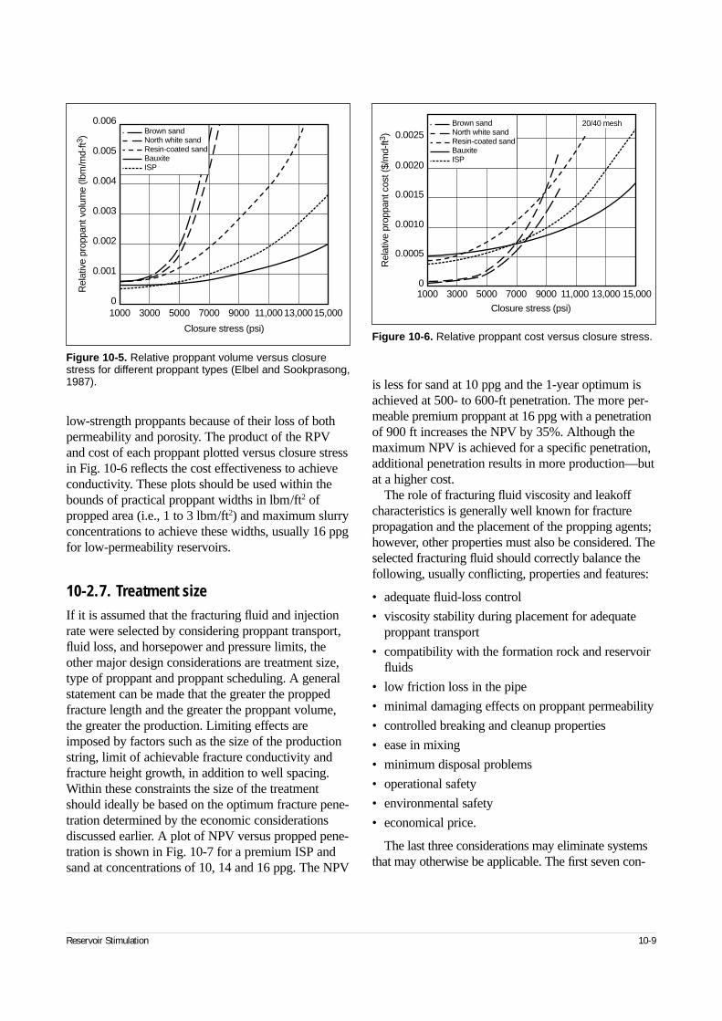
low-strength proppants because of their loss of bothpermeability and porosity. The product of the RPVand cost of each proppant plotted versus closure stressin Fig. 10-6 reflects the cost effectiveness to achieveconductivity. These plots should be used within thebounds of practical proppant widths in lbm/ft2 ofpropped area (i.e., 1 to 3 lbm/ft2) and maximum slurryconcentrations to achieve these widths, usually 16 ppgfor low-permeability reservoirs.

10-2.7. Treatment sizeIf it is assumed that the fracturing fluid and injectionrate were selected by considering proppant transport,fluid loss, and horsepower and pressure limits, theother major design considerations are treatment size,type of proppant and proppant scheduling. A generalstatement can be made that the greater the proppedfracture length and the greater the proppant volume,the greater the production. Limiting effects areimposed by factors such as the size of the productionstring, limit of achievable fracture conductivity andfracture height growth, in addition to well spacing.Within these constraints the size of the treatmentshould ideally be based on the optimum fracture pene-tration determined by the economic considerationsdiscussed earlier. A plot of NPV versus propped pene-tration is shown in Fig. 10-7 for a premium ISP andsand at concentrations of 10, 14 and 16 ppg. The NPV

is less for sand at 10 ppg and the 1-year optimum isachieved at 500- to 600-ft penetration. The more per-meable premium proppant at 16 ppg with a penetrationof 900 ft increases the NPV by 35%. Although themaximum NPV is achieved for a specific penetration,additional penetration results in more production—butat a higher cost.

The role of fracturing fluid viscosity and leakoffcharacteristics is generally well known for fracturepropagation and the placement of the propping agents;however, other properties must also be considered. Theselected fracturing fluid should correctly balance thefollowing, usually conflicting, properties and features:

• adequate fluid-loss control

• viscosity stability during placement for adequateproppant transport

• compatibility with the formation rock and reservoirfluids

• low friction loss in the pipe

• minimal damaging effects on proppant permeability

• controlled breaking and cleanup properties

• ease in mixing

• minimum disposal problems

• operational safety

• environmental safety

• economical price.

The last three considerations may eliminate systemsthat may otherwise be applicable. The first seven con-

Reservoir Stimulation 10-9

Figure 10-5. Relative proppant volume versus closurestress for different proppant types (Elbel and Sookprasong,1987).

10000

0.001

0.002

0.003

0.004

0.005

0.006

3000 5000 7000 9000 11,000 13,00015,000

Rel

ativ

e pr

oppa

nt v

olum

e (lb

m/m

d-ft3

)

Closure stress (psi)

Brown sandNorth white sandResin-coated sandBauxiteISP

Figure 10-6. Relative proppant cost versus closure stress.

1000 3000 5000 7000 9000 11,000 13,000 15,0000

0.0005

0.0010

0.0015

0.0020

0.0025

Rel

ativ

e pr

oppa

nt c

ost (

$/m

d-ft3

)

Closure stress (psi)

Brown sandNorth white sandResin-coated sandBauxiteISP

20/40 mesh

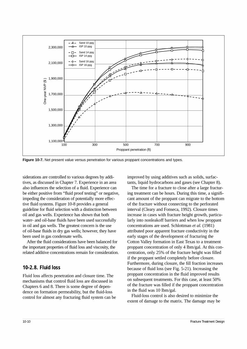
siderations are controlled to various degrees by addi-tives, as discussed in Chapter 7. Experience in an areaalso influences the selection of a fluid. Experience canbe either positive from “fluid proof testing” or negative,impeding the consideration of potentially more effec-tive fluid systems. Figure 10-8 provides a generalguideline for fluid selection with a distinction betweenoil and gas wells. Experience has shown that bothwater- and oil-base fluids have been used successfullyin oil and gas wells. The greatest concern is the use of oil-base fluids in dry gas wells; however, they havebeen used in gas condensate wells.

After the fluid considerations have been balanced forthe important properties of fluid loss and viscosity, therelated additive concentrations remain for consideration.

10-2.8. Fluid lossFluid loss affects penetration and closure time. Themechanisms that control fluid loss are discussed inChapters 6 and 8. There is some degree of depen-dence on formation permeability, but the fluid-losscontrol for almost any fracturing fluid system can be

improved by using additives such as solids, surfac-tants, liquid hydrocarbons and gases (see Chapter 8).

The time for a fracture to close after a large fractur-ing treatment can be hours. During this time, a signifi-cant amount of the proppant can migrate to the bottomof the fracture without connecting to the perforatedinterval (Cleary and Fonseca, 1992). Closure timesincrease in cases with fracture height growth, particu-larly into nonleakoff barriers and when low proppantconcentrations are used. Schlottman et al. (1981)attributed poor apparent fracture conductivity in theearly stages of the development of fracturing theCotton Valley formation in East Texas to a treatmentproppant concentration of only 4 lbm/gal. At this con-centration, only 25% of the fracture height was filledif the proppant settled completely before closure.Furthermore, during closure, the fill fraction increasesbecause of fluid loss (see Fig. 5-21). Increasing theproppant concentration in the fluid improved resultson subsequent treatments. For this case, at least 50%of the fracture was filled if the proppant concentrationin the fluid was 10 lbm/gal.

Fluid-loss control is also desired to minimize theextent of damage to the matrix. The damage may be

10-10 Fracture Treatment Design

Figure 10-7. Net present value versus penetration for various proppant concentrations and types.

One

-yea

r NV

P ($

)2,300,000

2,100,000

1,900,000

1,700,000

1,500,000

1,300,000

1,100,000100 300 500 700 900

Proppant penetration (ft)

Sand 10 ppgISP 10 ppg

Sand 14 ppgISP 14 ppg

Sand 16 ppgISP 16 ppg

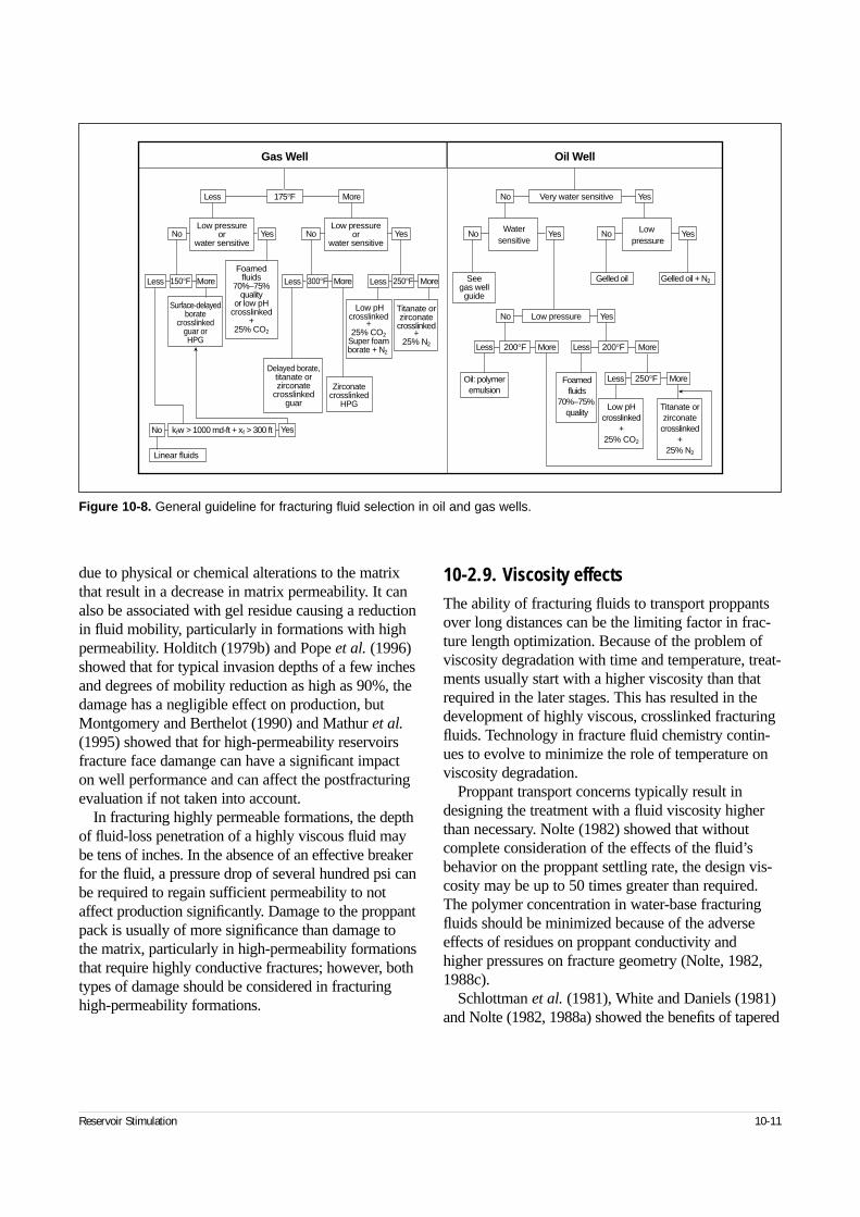
due to physical or chemical alterations to the matrixthat result in a decrease in matrix permeability. It canalso be associated with gel residue causing a reductionin fluid mobility, particularly in formations with highpermeability. Holditch (1979b) and Pope et al. (1996)showed that for typical invasion depths of a few inchesand degrees of mobility reduction as high as 90%, thedamage has a negligible effect on production, butMontgomery and Berthelot (1990) and Mathur et al.(1995) showed that for high-permeability reservoirsfracture face damange can have a significant impacton well performance and can affect the postfracturingevaluation if not taken into account.

In fracturing highly permeable formations, the depthof fluid-loss penetration of a highly viscous fluid maybe tens of inches. In the absence of an effective breakerfor the fluid, a pressure drop of several hundred psi canbe required to regain sufficient permeability to notaffect production significantly. Damage to the proppantpack is usually of more significance than damage tothe matrix, particularly in high-permeability formationsthat require highly conductive fractures; however, bothtypes of damage should be considered in fracturinghigh-permeability formations.

10-2.9. Viscosity effectsThe ability of fracturing fluids to transport proppantsover long distances can be the limiting factor in frac-ture length optimization. Because of the problem ofviscosity degradation with time and temperature, treat-ments usually start with a higher viscosity than thatrequired in the later stages. This has resulted in thedevelopment of highly viscous, crosslinked fracturingfluids. Technology in fracture fluid chemistry contin-ues to evolve to minimize the role of temperature onviscosity degradation.

Proppant transport concerns typically result indesigning the treatment with a fluid viscosity higherthan necessary. Nolte (1982) showed that withoutcomplete consideration of the effects of the fluid’sbehavior on the proppant settling rate, the design vis-cosity may be up to 50 times greater than required.The polymer concentration in water-base fracturingfluids should be minimized because of the adverseeffects of residues on proppant conductivity and higher pressures on fracture geometry (Nolte, 1982,1988c).

Schlottman et al. (1981), White and Daniels (1981)and Nolte (1982, 1988a) showed the benefits of tapered

Reservoir Stimulation 10-11

Figure 10-8. General guideline for fracturing fluid selection in oil and gas wells.

Gas Well

Less 175°F More

No Yes

Yes

Low pressureor

water sensitiveNo Yes

Low pressureor

water sensitive

Less More150°F Less More300°F Less More250°FFoamed

fluids70%–75%

qualityor low pH

crosslinked+

25% CO2

Surface-delayedborate

crosslinkedguar orHPG

Delayed borate,titanate orzirconate

crosslinkedguar

No

Linear fluids

kfw > 1000 md-ft + xf > 300 ft

Low pHcrosslinked

+25% CO2

Super foamborate + N2

Titanate orzirconate

crosslinked+

25% N2

Zirconatecrosslinked

HPG

Oil Well

No Very water sensitive Yes

No Low pressure Yes

Less

Oil: polymeremulsion

Foamedfluids

70%–75%quality

LessMore200°F

Less More250°F

More200°F

No YesWatersensitive

No YesLowpressure

Gelled oilSeegas wellguide

Gelled oil + N2

Low pHcrosslinked

+25% CO2

Titanate orzirconate

crosslinked+

25% N2

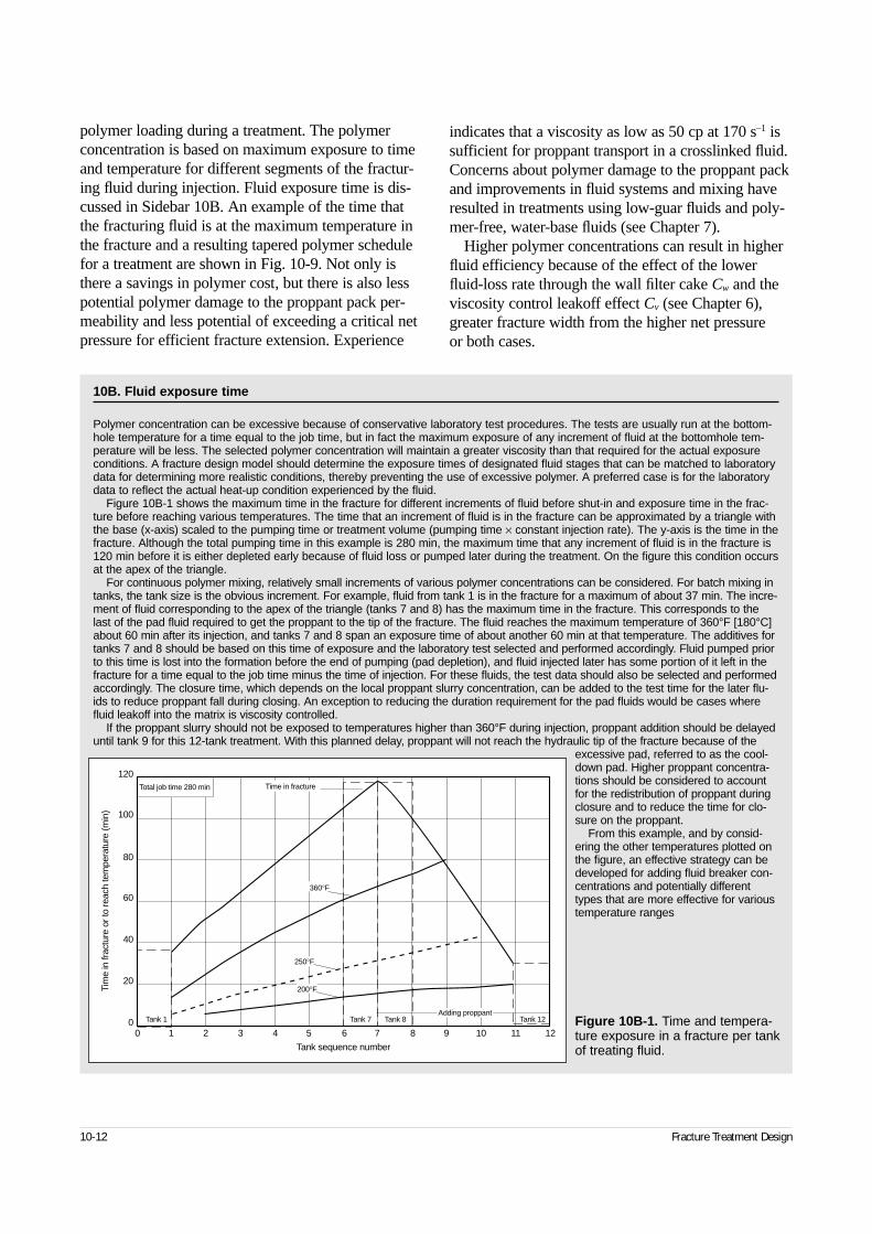
polymer loading during a treatment. The polymerconcentration is based on maximum exposure to timeand temperature for different segments of the fractur-ing fluid during injection. Fluid exposure time is dis-cussed in Sidebar 10B. An example of the time thatthe fracturing fluid is at the maximum temperature inthe fracture and a resulting tapered polymer schedulefor a treatment are shown in Fig. 10-9. Not only isthere a savings in polymer cost, but there is also lesspotential polymer damage to the proppant pack per-meability and less potential of exceeding a critical netpressure for efficient fracture extension. Experience

indicates that a viscosity as low as 50 cp at 170 s–1 issufficient for proppant transport in a crosslinked fluid.Concerns about polymer damage to the proppant packand improvements in fluid systems and mixing haveresulted in treatments using low-guar fluids and poly-mer-free, water-base fluids (see Chapter 7).

Higher polymer concentrations can result in higherfluid efficiency because of the effect of the lowerfluid-loss rate through the wall filter cake Cw and theviscosity control leakoff effect Cv (see Chapter 6),greater fracture width from the higher net pressure or both cases.

10-12 Fracture Treatment Design

10B. Fluid exposure time

Polymer concentration can be excessive because of conservative laboratory test procedures. The tests are usually run at the bottom-hole temperature for a time equal to the job time, but in fact the maximum exposure of any increment of fluid at the bottomhole tem-perature will be less. The selected polymer concentration will maintain a greater viscosity than that required for the actual exposureconditions. A fracture design model should determine the exposure times of designated fluid stages that can be matched to laboratorydata for determining more realistic conditions, thereby preventing the use of excessive polymer. A preferred case is for the laboratorydata to reflect the actual heat-up condition experienced by the fluid.

Figure 10B-1 shows the maximum time in the fracture for different increments of fluid before shut-in and exposure time in the frac-ture before reaching various temperatures. The time that an increment of fluid is in the fracture can be approximated by a triangle withthe base (x-axis) scaled to the pumping time or treatment volume (pumping time × constant injection rate). The y-axis is the time in thefracture. Although the total pumping time in this example is 280 min, the maximum time that any increment of fluid is in the fracture is120 min before it is either depleted early because of fluid loss or pumped later during the treatment. On the figure this condition occursat the apex of the triangle.

For continuous polymer mixing, relatively small increments of various polymer concentrations can be considered. For batch mixing intanks, the tank size is the obvious increment. For example, fluid from tank 1 is in the fracture for a maximum of about 37 min. The incre-ment of fluid corresponding to the apex of the triangle (tanks 7 and 8) has the maximum time in the fracture. This corresponds to thelast of the pad fluid required to get the proppant to the tip of the fracture. The fluid reaches the maximum temperature of 360°F [180°C]about 60 min after its injection, and tanks 7 and 8 span an exposure time of about another 60 min at that temperature. The additives fortanks 7 and 8 should be based on this time of exposure and the laboratory test selected and performed accordingly. Fluid pumped priorto this time is lost into the formation before the end of pumping (pad depletion), and fluid injected later has some portion of it left in thefracture for a time equal to the job time minus the time of injection. For these fluids, the test data should also be selected and performedaccordingly. The closure time, which depends on the local proppant slurry concentration, can be added to the test time for the later flu-ids to reduce proppant fall during closing. An exception to reducing the duration requirement for the pad fluids would be cases wherefluid leakoff into the matrix is viscosity controlled.

If the proppant slurry should not be exposed to temperatures higher than 360°F during injection, proppant addition should be delayeduntil tank 9 for this 12-tank treatment. With this planned delay, proppant will not reach the hydraulic tip of the fracture because of the

excessive pad, referred to as the cool-down pad. Higher proppant concentra-tions should be considered to accountfor the redistribution of proppant duringclosure and to reduce the time for clo-sure on the proppant.

From this example, and by consid-ering the other temperatures plotted onthe figure, an effective strategy can bedeveloped for adding fluid breaker con-centrations and potentially differenttypes that are more effective for varioustemperature ranges

Figure 10B-1. Time and tempera-ture exposure in a fracture per tankof treating fluid.

Tim

e in

frac

ture

or t

o re

ach

tem

pera

ture

(min

)

120

100

80

60

40

20

00 1 2 3 4 7 8 9 10 11 125 6

Tank sequence number

Time in fracture

250°F

360°F

200°F

Tank 1 Tank 7 Tank 8 Tank 12Adding proppant

Total job time 280 min

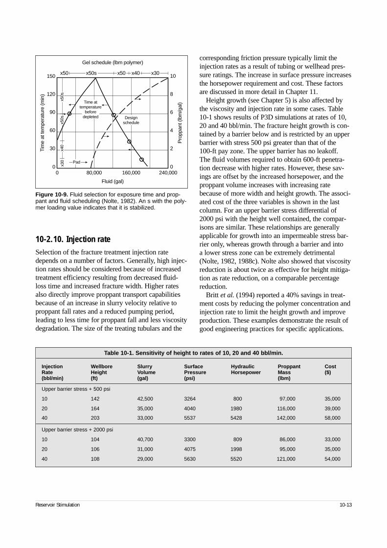
10-2.10. Injection rateSelection of the fracture treatment injection ratedepends on a number of factors. Generally, high injec-tion rates should be considered because of increasedtreatment efficiency resulting from decreased fluid-loss time and increased fracture width. Higher ratesalso directly improve proppant transport capabilitiesbecause of an increase in slurry velocity relative toproppant fall rates and a reduced pumping period,leading to less time for proppant fall and less viscositydegradation. The size of the treating tubulars and the

corresponding friction pressure typically limit theinjection rates as a result of tubing or wellhead pres-sure ratings. The increase in surface pressure increasesthe horsepower requirement and cost. These factorsare discussed in more detail in Chapter 11.

Height growth (see Chapter 5) is also affected bythe viscosity and injection rate in some cases. Table10-1 shows results of P3D simulations at rates of 10,20 and 40 bbl/min. The fracture height growth is con-tained by a barrier below and is restricted by an upperbarrier with stress 500 psi greater than that of the 100-ft pay zone. The upper barrier has no leakoff. The fluid volumes required to obtain 600-ft penetra-tion decrease with higher rates. However, these sav-ings are offset by the increased horsepower, and theproppant volume increases with increasing ratebecause of more width and height growth. The associ-ated cost of the three variables is shown in the lastcolumn. For an upper barrier stress differential of2000 psi with the height well contained, the compar-isons are similar. These relationships are generallyapplicable for growth into an impermeable stress bar-rier only, whereas growth through a barrier and into a lower stress zone can be extremely detrimental(Nolte, 1982, 1988c). Nolte also showed that viscosityreduction is about twice as effective for height mitiga-tion as rate reduction, on a comparable percentagereduction.

Britt et al. (1994) reported a 40% savings in treat-ment costs by reducing the polymer concentration andinjection rate to limit the height growth and improveproduction. These examples demonstrate the result ofgood engineering practices for specific applications.

Reservoir Stimulation 10-13

Figure 10-9. Fluid selection for exposure time and prop-pant and fluid scheduling (Nolte, 1982). An s with the poly-mer loading value indicates that it is stabilized.

0 80,000 160,000 240,000

150

120

90

60

30

0

Tim

e at

tem

pera

ture

(min

)

0

2

4

6

8

10

Pro

ppan

t (lb

m/g

al)

Pad

Fluid (gal)

Designschedule

Time attemperature

beforedepleted

x50s x50 x40 x30x50

x30

x40

x50s

x50s

Gel schedule (lbm polymer)

Table 10-1. Sensitivity of height to rates of 10, 20 and 40 bbl/min.

Injection Wellbore Slurry Surface Hydraulic Proppant CostRate Height Volume Pressure Horsepower Mass ($)(bbl/min) (ft) (gal) (psi) (lbm)

Upper barrier stress + 500 psi

10 142 42,500 3264 800 97,000 35,000

20 164 35,000 4040 1980 116,000 39,000

40 203 33,000 5537 5428 142,000 58,000

Upper barrier stress + 2000 psi

10 104 40,700 3300 809 86,000 33,000

20 106 31,000 4075 1998 95,000 35,000

40 108 29,000 5630 5520 121,000 54,000

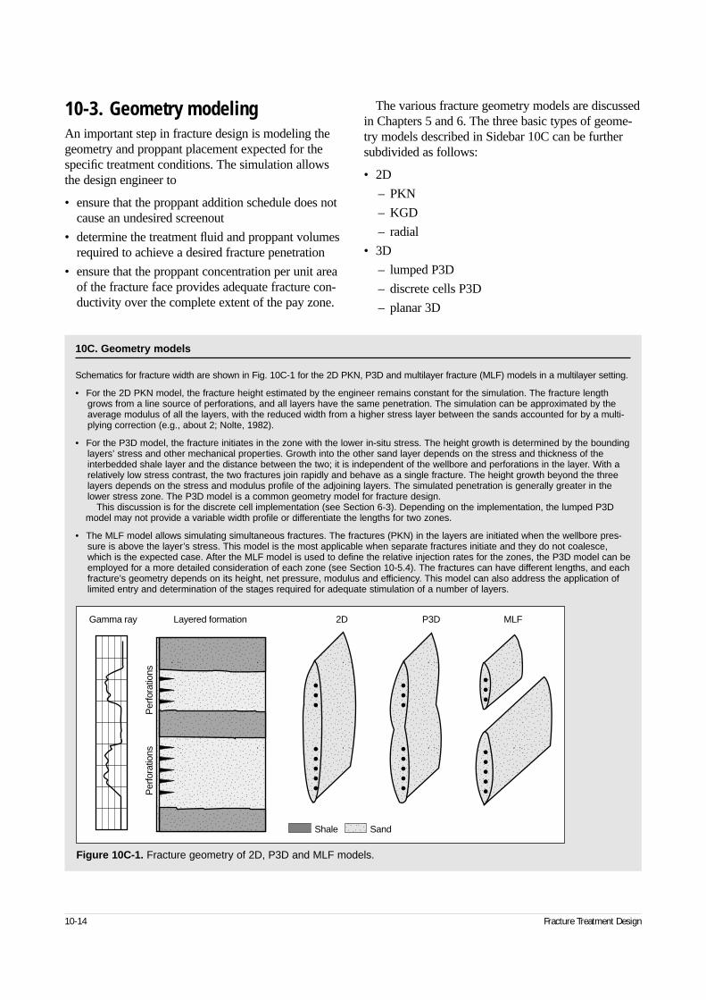
10-3. Geometry modelingAn important step in fracture design is modeling thegeometry and proppant placement expected for thespecific treatment conditions. The simulation allowsthe design engineer to

• ensure that the proppant addition schedule does notcause an undesired screenout

• determine the treatment fluid and proppant volumesrequired to achieve a desired fracture penetration

• ensure that the proppant concentration per unit areaof the fracture face provides adequate fracture con-ductivity over the complete extent of the pay zone.

The various fracture geometry models are discussedin Chapters 5 and 6. The three basic types of geome-try models described in Sidebar 10C can be furthersubdivided as follows:

• 2D

– PKN

– KGD

– radial

• 3D

– lumped P3D

– discrete cells P3D

– planar 3D

10-14 Fracture Treatment Design

10C. Geometry models

Schematics for fracture width are shown in Fig. 10C-1 for the 2D PKN, P3D and multilayer fracture (MLF) models in a multilayer setting.

• For the 2D PKN model, the fracture height estimated by the engineer remains constant for the simulation. The fracture lengthgrows from a line source of perforations, and all layers have the same penetration. The simulation can be approximated by theaverage modulus of all the layers, with the reduced width from a higher stress layer between the sands accounted for by a multi-plying correction (e.g., about 2; Nolte, 1982).

• For the P3D model, the fracture initiates in the zone with the lower in-situ stress. The height growth is determined by the boundinglayers’ stress and other mechanical properties. Growth into the other sand layer depends on the stress and thickness of theinterbedded shale layer and the distance between the two; it is independent of the wellbore and perforations in the layer. With arelatively low stress contrast, the two fractures join rapidly and behave as a single fracture. The height growth beyond the threelayers depends on the stress and modulus profile of the adjoining layers. The simulated penetration is generally greater in thelower stress zone. The P3D model is a common geometry model for fracture design.

This discussion is for the discrete cell implementation (see Section 6-3). Depending on the implementation, the lumped P3Dmodel may not provide a variable width profile or differentiate the lengths for two zones.

• The MLF model allows simulating simultaneous fractures. The fractures (PKN) in the layers are initiated when the wellbore pres-sure is above the layer’s stress. This model is the most applicable when separate fractures initiate and they do not coalesce,which is the expected case. After the MLF model is used to define the relative injection rates for the zones, the P3D model can beemployed for a more detailed consideration of each zone (see Section 10-5.4). The fractures can have different lengths, and eachfracture’s geometry depends on its height, net pressure, modulus and efficiency. This model can also address the application oflimited entry and determination of the stages required for adequate stimulation of a number of layers.

Figure 10C-1. Fracture geometry of 2D, P3D and MLF models.

������

����������

����

���

�����

��

SandShale

Gamma ray Layered formation 2D P3D MLF

Per

fora

tions

Per

fora

tions

������

��

• multilayered

– PKN fractures

– P3D fractures.

They can be further classified as to how they modelfluid loss, postpumping behavior, tip effects, poro-elastcity, various forms of fluid flow (1D and 2D),proppant transport, etc. (see Chapter 6).

10-3.1. Model selectionThe wide range of models and features available canmake selecting a model an overwhelming task. Gen-erally, the model should be selected to match the levelof complexity required for the specific application,quantity and quality of data, allocated time to perform a design and desired level of output.

Modeling hydraulic fracture propagation with a pla-nar 3D model can be time consuming. Not as muchtime is required for 2D modeling, but the results canbe simplistic. P3D models provide a compromise andare most often used in the industry for the evaluationof hydraulic fracturing treatments.

A diagnostic method based on the treating pressurehistory and analysis by history matching (Nolte, 1982,1988c) can be used to identify various modes of prop-agation (see Chapter 9). Using this technique, theengineer selects the appropriate model and uses it toevaluate important fracture parameters such as treat-ment efficiency and net treating pressure. The conceptof history matching a calibration injection test andusing the parameters required for the match in thedesign of the propped fracture treatment forms thefoundation for effective treatment design. By applyingthis method, the engineer becomes familiar with theadvantages and limitations of the various geometrymodels and good engineering practices, which withexperience leads to successful fracturing programs(Martinez et al., 1992; Johnson et al., 1993; Stadulis,1995; Gulrajani and Romero, 1996).

When the controversy between 2D KGD and PKNmodels was high (e.g., Perkins, 1973), it was notuncommon to simulate the treatment design with bothmodels, looking at each for potential problems withthe final design. This practice did not ensure an opti-mum design but was used mainly to minimize prema-ture screenouts by calibrating the fluid-loss coefficienton the basis of the results of prior treatments. Also, assubsequently discussed for Fig. 10-11, the proppant

schedule depends primarily on the efficiency; there-fore, models that provide very different widths canpredict the same schedules by calibrating a differentfluid-loss coefficient for the specific width assump-tions. It is still good practice and not unusual to useseveral models during the design phase; however, thePKN model is a more appropriate approximation forfractures where the length is considerably longer thanthe height, and the KGD model should be used forfractures where the fracture length is of the sameorder or shorter than the fracture height. An example is presented in Section 10-6.3.

Fracture design for a wildcat or high-risk well callsfor the collection of a comprehensive set of designdata and the use of more sophisticated models. This is also the case when treating problems or lower thanexpected production rates occur.

Geometry models are typically validated with welltest analysis and production history matching. Theevaluation of fracture treatments, however, requiressophistication in pressure transient analysis and thedetermination of rock properties for use in the geome-try models (Elbel and Ayoub, 1992). The determina-tion of an average permeability may not be sufficientfor production history matching. Layered reservoirswith large permeability contrasts (Bennett et al., 1986;Camacho-V. et al., 1987) or reservoirs with horizontalpermeability anisotropy (Ben Naceur and Economides,1989) appear to have shorter fractures if the well testmodels used assume a single isotropic layer.

In addition to considering the effects for idealizedreservoir assumptions, Nolte and Economides (1991)discussed and attempted to quantify the effects foridealized assumptions related to the design and place-ment of the fracture. The common assumptions aboutfractures and reservoirs were found to generally resultin a productive length that is less than the designlength. The coupling of the shorter productive lengthand the shorter apparent length (to compensate for thereservoir model assumptions) compounds the prospectthat the actual production will be less than anticipated.An example indicated that an effective reduction ofthe fracture to 33% of the design length would not bean unreasonable condition.

They cast the reservoir and placement effects interms of a design factor that has the role of a safetyfactor used in other engineering fields. General frac-turing practice incorporates these effects in an ad hocmanner and through experience with results that fail tomeet the expected ROI (e.g., increased fracture height,

Reservoir Stimulation 10-15

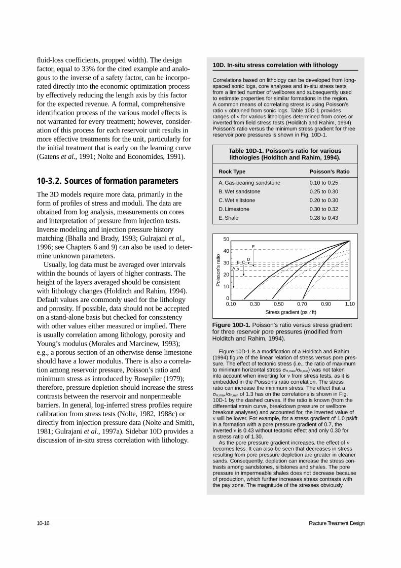
fluid-loss coefficients, propped width). The designfactor, equal to 33% for the cited example and analo-gous to the inverse of a safety factor, can be incorpo-rated directly into the economic optimization processby effectively reducing the length axis by this factorfor the expected revenue. A formal, comprehensiveidentification process of the various model effects isnot warranted for every treatment; however, consider-ation of this process for each reservoir unit results inmore effective treatments for the unit, particularly forthe initial treatment that is early on the learning curve(Gatens et al., 1991; Nolte and Economides, 1991).

10-3.2. Sources of formation parametersThe 3D models require more data, primarily in theform of profiles of stress and moduli. The data areobtained from log analysis, measurements on coresand interpretation of pressure from injection tests.Inverse modeling and injection pressure historymatching (Bhalla and Brady, 1993; Gulrajani et al.,1996; see Chapters 6 and 9) can also be used to deter-mine unknown parameters.

Usually, log data must be averaged over intervalswithin the bounds of layers of higher contrasts. Theheight of the layers averaged should be consistentwith lithology changes (Holditch and Rahim, 1994).Default values are commonly used for the lithologyand porosity. If possible, data should not be acceptedon a stand-alone basis but checked for consistencywith other values either measured or implied. There is usually correlation among lithology, porosity andYoung’s modulus (Morales and Marcinew, 1993); e.g., a porous section of an otherwise dense limestoneshould have a lower modulus. There is also a correla-tion among reservoir pressure, Poisson’s ratio andminimum stress as introduced by Rosepiler (1979);therefore, pressure depletion should increase the stresscontrasts between the reservoir and nonpermeablebarriers. In general, log-inferred stress profiles requirecalibration from stress tests (Nolte, 1982, 1988c) ordirectly from injection pressure data (Nolte and Smith,1981; Gulrajani et al., 1997a). Sidebar 10D provides adiscussion of in-situ stress correlation with lithology.

10-16 Fracture Treatment Design

10D. In-situ stress correlation with lithology

Correlations based on lithology can be developed from long-spaced sonic logs, core analyses and in-situ stress testsfrom a limited number of wellbores and subsequently used to estimate properties for similar formations in the region. A common means of correlating stress is using Poisson’sratio ν obtained from sonic logs. Table 10D-1 providesranges of ν for various lithologies determined from cores orinverted from field stress tests (Holditch and Rahim, 1994).Poisson’s ratio versus the minimum stress gradient for threereservoir pore pressures is shown in Fig. 10D-1.

Figure 10D-1 is a modification of a Holditch and Rahim(1994) figure of the linear relation of stress versus pore pres-sure. The effect of tectonic stress (i.e., the ratio of maximumto minimum horizontal stress σH,max/σh,min) was not taken into account when inverting for ν from stress tests, as it isembedded in the Poisson’s ratio correlation. The stress ratio can increase the minimum stress. The effect that aσH,max/σh,min of 1.3 has on the correlations is shown in Fig.10D-1 by the dashed curves. If the ratio is known (from thedifferential strain curve, breakdown pressure or wellborebreakout analyses) and accounted for, the inverted value of ν will be lower. For example, for a stress gradient of 1.0 psi/ftin a formation with a pore pressure gradient of 0.7, theinverted ν is 0.43 without tectonic effect and only 0.30 for a stress ratio of 1.30.

As the pore pressure gradient increases, the effect of νbecomes less. It can also be seen that decreases in stressresulting from pore pressure depletion are greater in cleanersands. Consequently, depletion can increase the stress con-trasts among sandstones, siltstones and shales. The porepressure in impermeable shales does not decrease becauseof production, which further increases stress contrasts withthe pay zone. The magnitude of the stresses obviously

Table 10D-1. Poisson’s ratio for various lithologies (Holditch and Rahim, 1994).

Rock Type Poisson’s Ratio

A. Gas-bearing sandstone 0.10 to 0.25

B. Wet sandstone 0.25 to 0.30

C.Wet siltstone 0.20 to 0.30

D.Limestone 0.30 to 0.32

E. Shale 0.28 to 0.43

Figure 10D-1. Poisson’s ratio versus stress gradientfor three reservoir pore pressures (modified fromHolditch and Rahim, 1994).

Poi

sson

's ra

tio

50

40

30

20

10

00.10 0.30 0.50 0.70 0.90 1.10

Stress gradient (psi ⁄ ft)

D

E

B CA

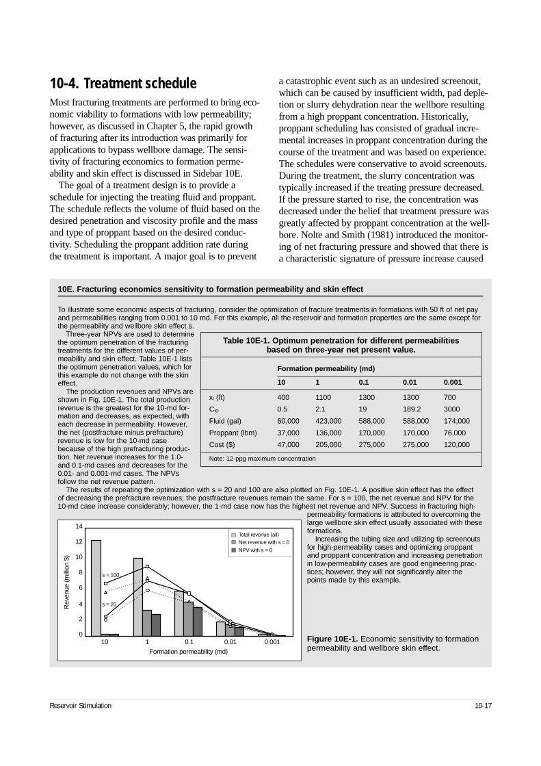
10-4. Treatment scheduleMost fracturing treatments are performed to bring eco-nomic viability to formations with low permeability;however, as discussed in Chapter 5, the rapid growthof fracturing after its introduction was primarily forapplications to bypass wellbore damage. The sensi-tivity of fracturing economics to formation perme-ability and skin effect is discussed in Sidebar 10E.

The goal of a treatment design is to provide aschedule for injecting the treating fluid and proppant.The schedule reflects the volume of fluid based on thedesired penetration and viscosity profile and the massand type of proppant based on the desired conduc-tivity. Scheduling the proppant addition rate duringthe treatment is important. A major goal is to prevent

a catastrophic event such as an undesired screenout,which can be caused by insufficient width, pad deple-tion or slurry dehydration near the wellbore resultingfrom a high proppant concentration. Historically,proppant scheduling has consisted of gradual incre-mental increases in proppant concentration during thecourse of the treatment and was based on experience.The schedules were conservative to avoid screenouts.During the treatment, the slurry concentration wastypically increased if the treating pressure decreased.If the pressure started to rise, the concentration wasdecreased under the belief that treatment pressure wasgreatly affected by proppant concentration at the well-bore. Nolte and Smith (1981) introduced the monitor-ing of net fracturing pressure and showed that there isa characteristic signature of pressure increase caused

Reservoir Stimulation 10-17

10E. Fracturing economics sensitivity to formation permeability and skin effect

To illustrate some economic aspects of fracturing, consider the optimization of fracture treatments in formations with 50 ft of net payand permeabilities ranging from 0.001 to 10 md. For this example, all the reservoir and formation properties are the same except forthe permeability and wellbore skin effect s.

Three-year NPVs are used to determinethe optimum penetration of the fracturingtreatments for the different values of per-meability and skin effect. Table 10E-1 liststhe optimum penetration values, which forthis example do not change with the skineffect.

The production revenues and NPVs areshown in Fig. 10E-1. The total productionrevenue is the greatest for the 10-md for-mation and decreases, as expected, witheach decrease in permeability. However,the net (postfracture minus prefracture)revenue is low for the 10-md casebecause of the high prefracturing produc-tion. Net revenue increases for the 1.0-and 0.1-md cases and decreases for the0.01- and 0.001-md cases. The NPVsfollow the net revenue pattern.

The results of repeating the optimization with s = 20 and 100 are also plotted on Fig. 10E-1. A positive skin effect has the effect of decreasing the prefracture revenues; the postfracture revenues remain the same. For s = 100, the net revenue and NPV for the10-md case increase considerably; however, the 1-md case now has the highest net revenue and NPV. Success in fracturing high-

permeability formations is attributed to overcoming thelarge wellbore skin effect usually associated with theseformations.

Increasing the tubing size and utilizing tip screenoutsfor high-permeability cases and optimizing proppantand proppant concentration and increasing penetrationin low-permeability cases are good engineering prac-tices; however, they will not significantly alter thepoints made by this example.

Table 10E-1. Optimum penetration for different permeabilities based on three-year net present value.

Formation permeability (md)

10 1 0.1 0.01 0.001

xf (ft) 400 1100 1300 1300 700

CfD 0.5 2.1 19 189.2 3000

Fluid (gal) 60,000 423,000 588,000 588,000 174,000

Proppant (lbm) 37,000 136,000 170,000 170,000 76,000

Cost ($) 47,000 205,000 275,000 275,000 120,000

Note: 12-ppg maximum concentration

Figure 10E-1. Economic sensitivity to formationpermeability and wellbore skin effect.

Rev

enue

(mill

ion

$)

14

12

10

8

6

4

2

010 1 0.1 0.01 0.001

Formation permeability (md)

Total revenue (all) Net revenue with s = 0

NPV with s = 0

s = 100

s = 20

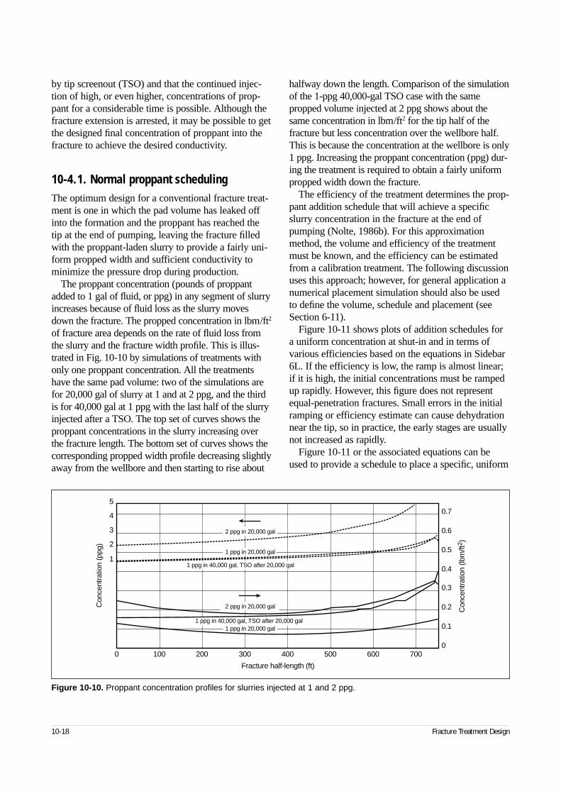
by tip screenout (TSO) and that the continued injec-tion of high, or even higher, concentrations of prop-pant for a considerable time is possible. Although thefracture extension is arrested, it may be possible to getthe designed final concentration of proppant into thefracture to achieve the desired conductivity.

10-4.1. Normal proppant schedulingThe optimum design for a conventional fracture treat-ment is one in which the pad volume has leaked offinto the formation and the proppant has reached thetip at the end of pumping, leaving the fracture filledwith the proppant-laden slurry to provide a fairly uni-form propped width and sufficient conductivity tominimize the pressure drop during production.

The proppant concentration (pounds of proppantadded to 1 gal of fluid, or ppg) in any segment of slurryincreases because of fluid loss as the slurry movesdown the fracture. The propped concentration in lbm/ft2

of fracture area depends on the rate of fluid loss fromthe slurry and the fracture width profile. This is illus-trated in Fig. 10-10 by simulations of treatments withonly one proppant concentration. All the treatmentshave the same pad volume: two of the simulations arefor 20,000 gal of slurry at 1 and at 2 ppg, and the thirdis for 40,000 gal at 1 ppg with the last half of the slurryinjected after a TSO. The top set of curves shows theproppant concentrations in the slurry increasing overthe fracture length. The bottom set of curves shows thecorresponding propped width profile decreasing slightlyaway from the wellbore and then starting to rise about

halfway down the length. Comparison of the simulationof the 1-ppg 40,000-gal TSO case with the samepropped volume injected at 2 ppg shows about thesame concentration in lbm/ft2 for the tip half of thefracture but less concentration over the wellbore half.This is because the concentration at the wellbore is only1 ppg. Increasing the proppant concentration (ppg) dur-ing the treatment is required to obtain a fairly uniformpropped width down the fracture.

The efficiency of the treatment determines the prop-pant addition schedule that will achieve a specificslurry concentration in the fracture at the end ofpumping (Nolte, 1986b). For this approximationmethod, the volume and efficiency of the treatmentmust be known, and the efficiency can be estimatedfrom a calibration treatment. The following discussionuses this approach; however, for general application anumerical placement simulation should also be usedto define the volume, schedule and placement (seeSection 6-11).

Figure 10-11 shows plots of addition schedules fora uniform concentration at shut-in and in terms ofvarious efficiencies based on the equations in Sidebar6L. If the efficiency is low, the ramp is almost linear;if it is high, the initial concentrations must be rampedup rapidly. However, this figure does not representequal-penetration fractures. Small errors in the initialramping or efficiency estimate can cause dehydrationnear the tip, so in practice, the early stages are usuallynot increased as rapidly.

Figure 10-11 or the associated equations can beused to provide a schedule to place a specific, uniform

10-18 Fracture Treatment Design

Figure 10-10. Proppant concentration profiles for slurries injected at 1 and 2 ppg.

2 ppg in 20,000 gal

1 ppg in 20,000 gal

1 ppg in 40,000 gal, TSO after 20,000 gal

2 ppg in 20,000 gal

1 ppg in 20,000 gal

0 100 200 300 400 500 600 700

4

0

0.1

0.2

0.3

0.4

0.5

0.6

0.7

Con

cent

ratio

n (lb

m/ft

2 )

Fracture half-length (ft)

5

3

2

1

Con

cent

ratio

n (p

pg)

1 ppg in 40,000 gal, TSO after 20,000 gal

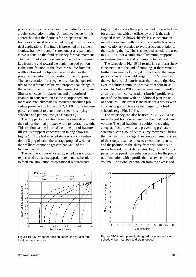
profile of proppant concentration and also to provide a quick calculation routine. An inconvenience for thisapproach is that the figure is for proppant volumefractions and must be converted to ppg units for prac-tical applications. The figure is presented in a dimen-sionless framework and the area under any particularcurve is equal to the fluid efficiency for that treatment.The fraction of area under any segment of a curve—i.e., from the end toward the beginning pad portion—is the same fraction of the fracture volume from thewellbore toward the tip and therefore defines theplacement location of that portion of the proppant.The concentration for a segment can be changed rela-tive to the reference value by a proportional change inthe value of the ordinate for the segment on the figure.Similar concepts for placement and proportionalchanges in concentration can be incorporated into amore accurate, automated numerical scheduling pro-cedure presented by Nolte (1982, 1988c) for a fractureplacement model to determine a specific rampingschedule and pad volume (see Chapter 6).

The proppant concentration in the slurry determinesthe ratio of the final propped width to hydraulic width.This relation can be inferred from the plot of fracturefill versus proppant concentration in ppg shown inFig. 5-21. If the last injected stage is at a concentra-tion of 8 ppg of sand, the average propped width atthe wellbore cannot be greater than 40% of thehydraulic width.

The continuous curve, or ramp, schedule is typicallyrepresented as a stairstepped, incremental schedule to facilitate simulation or operational requirements.

Figure 10-12 shows these proppant addition schedulesfor a treatment with an efficiency of 0.5; the stair-stepped schedule shows slightly less concentrationinitially compared with the ramp and reflects a com-mon cautionary practice to avoid a screenout prior tothe reaching the tip. This stairstepped schedule is usedin Fig. 10-13 for a simulation illustrating proppantmovement from the end of pumping to closure.

The schedule in Fig. 10-13 results in a uniform slurryconcentration at the end of pumping. If there were nofurther movement of slurry during closure, the prop-pant concentration would range from 1.6 lbm/ft2 atthe wellbore to 1.1 lbm/ft2 near the fracture tip. How-ever, the slurry continues to move after shut-in, asshown by Nolte (1986b), and is seen here to result ina fairly uniform concentration (lbm/ft2) profile overmost of the fracture with an additional penetration of about 5%. This result is the basis for a design withconstant ppg at shut-in as a first target for a finalschedule (e.g., Fig. 10-11).

The efficiency can also be used in Eq. 5-22 to esti-mate the pad fraction required for the total treatmentvolume. The pad fraction, in addition to creatingadequate fracture width and preventing prematurescreenout, can also influence slurry movement duringthe fracture closure stage. If excess pad remains ahead of the slurry, it can continue to extend the fracture,and the position of the slurry front will continue tomove forward until it dehydrates. Figure 10-14 com-pares the proppant concentration profile for the previ-ous simulation with a profile that has twice the padvolume. Additional penetration from the excess pad

Reservoir Stimulation 10-19

Figure 10-11. Proppant addition schedules for differenttreatment efficiencies.

0 0.2 0.4 0.6 0.8 10

0.1

Fraction of job time

0.2

0.3

0.4

0.5

0.6

0.7

0.8

0.9

1

Fra

ctio

n of

fina

l con

cent

ratio

n

Efficiency 0.7 0.5 0.3 0.1

0.6 0.4 0.2

Figure 10-12. An optimally designed proppant additionschedule, both ramped and stairstepped.

0 5

10

9

7

6

5

4

3

2

1

0

8

Job time (min)

Slu

rry

conc

entra

tion

(ppg

)

10 15 20 25 30 35 40 45 50

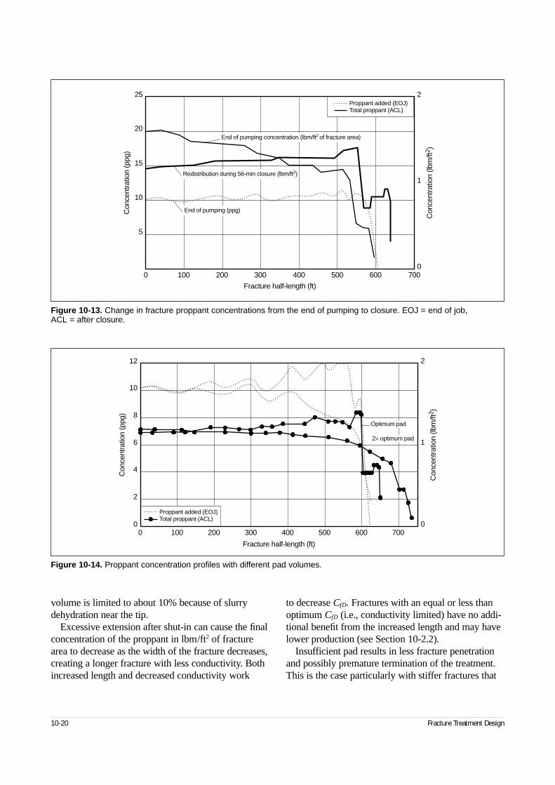
volume is limited to about 10% because of slurrydehydration near the tip.

Excessive extension after shut-in can cause the finalconcentration of the proppant in lbm/ft2 of fracturearea to decrease as the width of the fracture decreases,creating a longer fracture with less conductivity. Bothincreased length and decreased conductivity work

to decrease CfD. Fractures with an equal or less thanoptimum CfD (i.e., conductivity limited) have no addi-tional benefit from the increased length and may havelower production (see Section 10-2.2).

Insufficient pad results in less fracture penetrationand possibly premature termination of the treatment.This is the case particularly with stiffer fractures that

10-20 Fracture Treatment Design

Figure 10-13. Change in fracture proppant concentrations from the end of pumping to closure. EOJ = end of job, ACL = after closure.

Redistribution during 56-min closure (lbm/ft2)

End of pumping (ppg)

End of pumping concentration (lbm/ft2 of fracture area)

0 100 200 300 400 500 600 700

Con

cent

ratio

n (p

pg)

25

20

15

10

5

Fracture half-length (ft)

0

1

2

Con

cent

ratio

n (lb

m/ft

2 )

Proppant added (EOJ)Total proppant (ACL)

Figure 10-14. Proppant concentration profiles with different pad volumes.

Optimum pad

2× optimum pad

Proppant added (EOJ)Total proppant (ACL)

00

2

4

6

8

10

12

Con

cent

ratio

n (p

pg)

100 200 300 400 600 700500

Fracture half-length (ft)

0

1

2

Con

cent

ratio

n (lb

m/ft

2 )

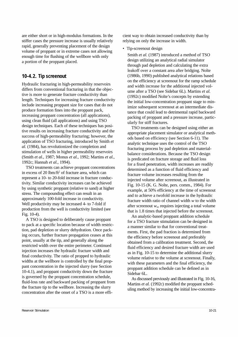
are either short or in high-modulus formations. In thestiffer cases the pressure increase is usually relativelyrapid, generally preventing placement of the designvolume of proppant or in extreme cases not allowingenough time for flushing of the wellbore with only a portion of the proppant placed.

10-4.2. Tip screenoutHydraulic fracturing in high-permeability reservoirsdiffers from conventional fracturing in that the objec-tive is more to generate fracture conductivity thanlength. Techniques for increasing fracture conductivityinclude increasing proppant size for cases that do notproduce formation fines into the proppant pack,increasing proppant concentration (all applications),using clean fluid (all applications) and using TSOdesign techniques. Each of these techniques has posi-tive results on increasing fracture conductivity and thesuccess of high-permeability fracturing; however, theapplication of TSO fracturing, introduced by Smith etal. (1984), has revolutionized the completion andstimulation of wells in higher permeability reservoirs(Smith et al., 1987; Monus et al., 1992; Martins et al.,1992c; Hannah et al., 1994).

TSO treatments can achieve proppant concentrationsin excess of 20 lbm/ft2 of fracture area, which canrepresent a 10- to 20-fold increase in fracture conduc-tivity. Similar conductivity increases can be achievedby using synthetic proppant (relative to sand) at higherstress. The compounding effect can result in anapproximately 100-fold increase in conductivity. Well productivity may be increased 4- to 7-fold if production from the well is conductivity limited (seeFig. 10-4).

A TSO is designed to deliberately cause proppant to pack at a specific location because of width restric-tion, pad depletion or slurry dehydration. Once pack-ing occurs, further fracture propagation ceases at thispoint, usually at the tip, and generally along therestricted width over the entire perimeter. Continuedinjection increases the hydraulic fracture width andfinal conductivity. The ratio of propped to hydraulicwidths at the wellbore is controlled by the final prop-pant concentration in the injected slurry (see Section10-4.1), and proppant conductivity down the fractureis governed by the proppant concentration schedule,fluid-loss rate and backward packing of proppant fromthe fracture tip to the wellbore. Increasing the slurryconcentration after the onset of a TSO is a more effi-

cient way to obtain increased conductivity than byrelying on only the increase in width.

• Tip-screenout design

Smith et al. (1987) introduced a method of TSOdesign utilizing an analytical radial simulatorthrough pad depletion and calculating the extraleakoff over a constant area after bridging. Nolte(1986b, 1990) published analytical relations basedon the efficiency at screenout for the ramp scheduleand width increase for the additional injected vol-ume after a TSO (see Sidebar 6L). Martins et al.(1992c) modified Nolte’s concepts by extending the initial low-concentration proppant stage to min-imize subsequent screenout at an intermediate dis-tance that could lead to detrimental rapid backwardpacking of proppant and a pressure increase, partic-ularly for stiff fractures.

TSO treatments can be designed using either anappropriate placement simulator or analytical meth-ods based on efficiency (see Section 6-11). Theanalytic technique uses the control of the TSOfracturing process by pad depletion and material-balance considerations. Because the TSO design is predicated on fracture storage and fluid loss for a fixed penetration, width increases are readilydetermined as a function of fluid efficiency andfracture volume increases resulting from theinjected volume after screenout, as illustrated in Fig. 10-15 (K. G. Nolte, pers. comm., 1984). Forexample, at 50% efficiency at the time of screenoutand to achieve a twofold increase in the hydraulicfracture width ratio of channel width w to the widthafter screenout wso requires injecting a total volumethat is 1.8 times that injected before the screenout.

An analytic-based proppant addition schedule for a TSO fracture stimulation can be designed in a manner similar to that for conventional treat-ments. First, the pad fraction is determined fromthe efficiency before screenout and preferablyobtained from a calibration treatment. Second, thefluid efficiency and desired fracture width are usedas in Fig. 10-15 to determine the additional slurryvolume relative to the volume at screenout. Finally,with these parameters and the final efficiency, theproppant addition schedule can be defined as inSidebar 6L.

As discussed previously and illustrated in Fig. 10-16,Martins et al. (1992c) modified the proppant sched-uling method by increasing the initial low-concentra-

Reservoir Stimulation 10-21

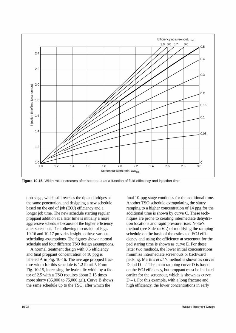
tion stage, which still reaches the tip and bridges atthe same penetration, and designing a new schedulebased on the end of job (EOJ) efficiency and alonger job time. The new schedule starting regularproppant addition at a later time is initially a moreaggressive schedule because of the higher efficiencyafter screenout. The following discussion of Figs.10-16 and 10-17 provides insight to these variousscheduling assumptions. The figures show a normalschedule and four different TSO design assumptions.

A normal treatment design with 0.5 efficiencyand final proppant concentration of 10 ppg islabeled A in Fig. 10-16. The average propped frac-ture width for this schedule is 1.2 lbm/ft2. FromFig. 10-15, increasing the hydraulic width by a fac-tor of 2.5 with a TSO requires about 2.15 timesmore slurry (35,000 to 75,000 gal). Curve B showsthe same schedule up to the TSO, after which the

final 10-ppg stage continues for the additional time.Another TSO schedule extrapolating the slurryramping to a higher concentration of 14 ppg for theadditional time is shown by curve C. These tech-niques are prone to creating intermediate dehydra-tion locations and rapid pressure rises. Nolte’smethod (see Sidebar 6L) of modifying the rampingschedule on the basis of the estimated EOJ effi-ciency and using the efficiency at screenout for thepad staring time is shown as curve E. For theselatter two methods, the lower initial concentrationsminimize intermediate screenouts or backwardpacking. Martins et al.’s method is shown as curvesD and D – i. The main ramping curve D is basedon the EOJ efficiency, but proppant must be initiatedearlier for the screenout, which is shown as curveD – i. For this example, with a long fracture andhigh efficiency, the lower concentrations in early

10-22 Fracture Treatment Design

Figure 10-15. Width ratio increases after screenout as a function of fluid efficiency and injection time.

1.0 1.2 1.4 1.6 1.8 2.0 2.2 2.4 2.6 2.8 3.01.0

1.2

1.4

1.6

1.8

2.0

2.2

2.4

Screenout width ratio, w/wso

Inje

ctio

n tim

e/tim

e to

scr

eeno

ut

0.5

0.4

0.3

0.2

0.1

0.05

0

0.15

0.60.70.81.0

Efficiency at screenout, ηso

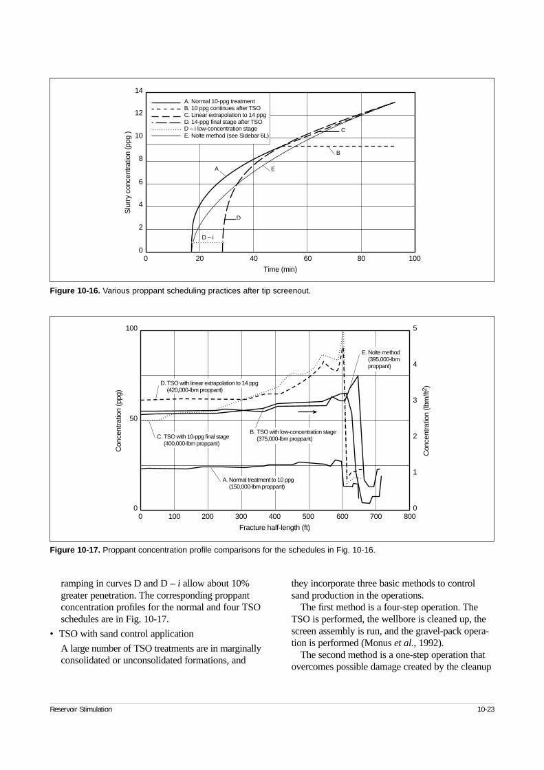
ramping in curves D and D – i allow about 10%greater penetration. The corresponding proppantconcentration profiles for the normal and four TSOschedules are in Fig. 10-17.

• TSO with sand control application

A large number of TSO treatments are in marginallyconsolidated or unconsolidated formations, and

they incorporate three basic methods to controlsand production in the operations.

The first method is a four-step operation. TheTSO is performed, the wellbore is cleaned up, thescreen assembly is run, and the gravel-pack opera-tion is performed (Monus et al., 1992).

The second method is a one-step operation thatovercomes possible damage created by the cleanup

Reservoir Stimulation 10-23

Figure 10-16. Various proppant scheduling practices after tip screenout.

00

14

12

Slu

rry

conc

entra

tion

(ppg

) 10

8

6

4

2

20 40 60 80 100

Time (min)

Normal 10-ppg treatment10 ppg continues after TSOLinear extrapolation to 14 ppg14-ppg final stage after TSO

Nolte method (see Sidebar 6L)

A.B.C.D.

E.

D – i

D

A E

C

B

D – i low-concentration stage

Figure 10-17. Proppant concentration profile comparisons for the schedules in Fig. 10-16.

0 100 200 300 400 500 600 700 8000

100

0

1

2

3

4

50

5

Con

cent

ratio

n (p

pg)

Fracture half-length (ft)

Con

cent

ratio

n (lb

m/ft

2 )

D.TSO with linear extrapolation to 14 ppg(420,000-lbm proppant)

C. TSO with 10-ppg final stage(400,000-lbm proppant)

B. TSO with low-concentration stage(375,000-lbm proppant)

A. Normal treatment to 10 ppg(150,000-lbm proppant)

E. Nolte method(395,000-lbmproppant)

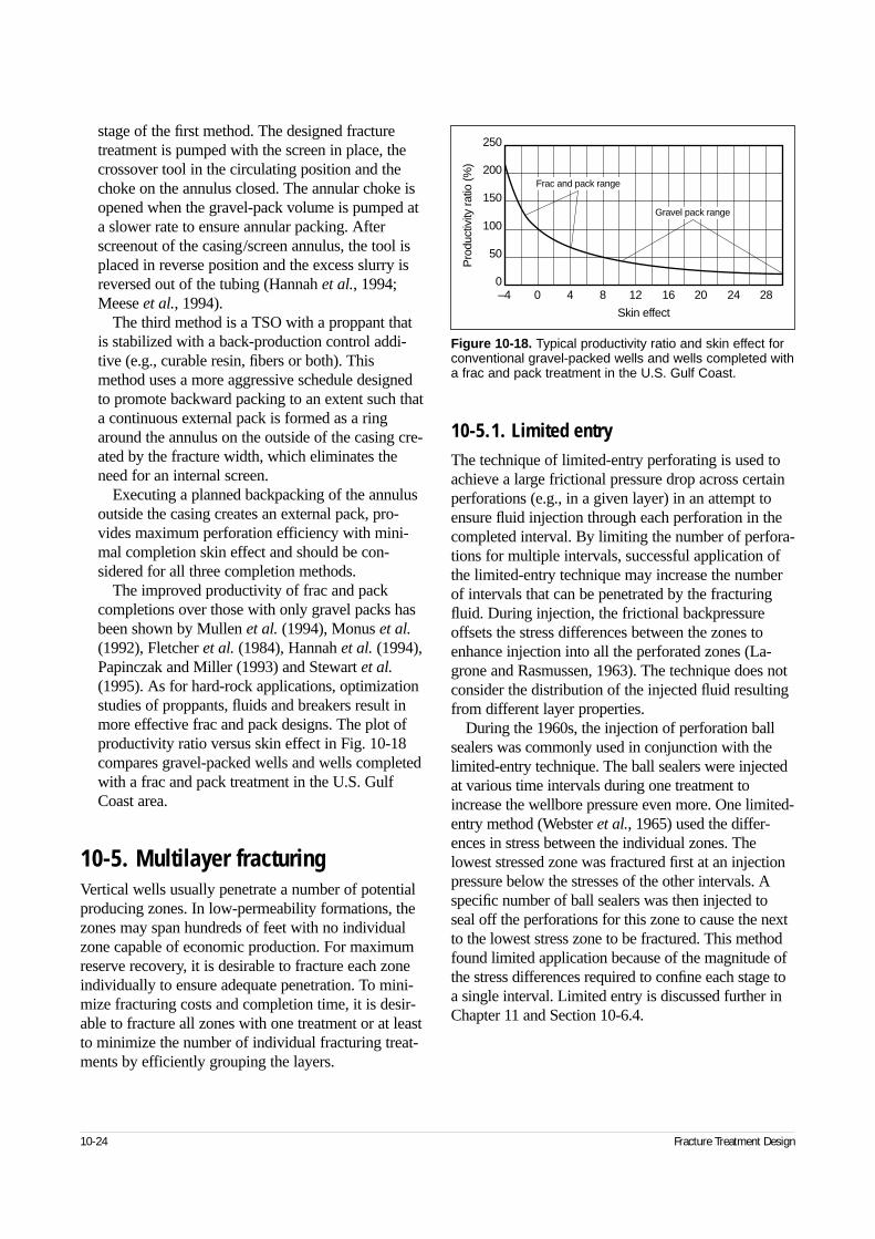
stage of the first method. The designed fracturetreatment is pumped with the screen in place, thecrossover tool in the circulating position and thechoke on the annulus closed. The annular choke isopened when the gravel-pack volume is pumped ata slower rate to ensure annular packing. Afterscreenout of the casing/screen annulus, the tool isplaced in reverse position and the excess slurry isreversed out of the tubing (Hannah et al., 1994;Meese et al., 1994).

The third method is a TSO with a proppant thatis stabilized with a back-production control addi-tive (e.g., curable resin, fibers or both). Thismethod uses a more aggressive schedule designedto promote backward packing to an extent such thata continuous external pack is formed as a ringaround the annulus on the outside of the casing cre-ated by the fracture width, which eliminates theneed for an internal screen.

Executing a planned backpacking of the annulusoutside the casing creates an external pack, pro-vides maximum perforation efficiency with mini-mal completion skin effect and should be con-sidered for all three completion methods.

The improved productivity of frac and packcompletions over those with only gravel packs hasbeen shown by Mullen et al. (1994), Monus et al.(1992), Fletcher et al. (1984), Hannah et al. (1994),Papinczak and Miller (1993) and Stewart et al.(1995). As for hard-rock applications, optimizationstudies of proppants, fluids and breakers result inmore effective frac and pack designs. The plot ofproductivity ratio versus skin effect in Fig. 10-18compares gravel-packed wells and wells completedwith a frac and pack treatment in the U.S. GulfCoast area.

10-5. Multilayer fracturingVertical wells usually penetrate a number of potentialproducing zones. In low-permeability formations, thezones may span hundreds of feet with no individualzone capable of economic production. For maximumreserve recovery, it is desirable to fracture each zoneindividually to ensure adequate penetration. To mini-mize fracturing costs and completion time, it is desir-able to fracture all zones with one treatment or at leastto minimize the number of individual fracturing treat-ments by efficiently grouping the layers.

10-5.1. Limited entryThe technique of limited-entry perforating is used toachieve a large frictional pressure drop across certainperforations (e.g., in a given layer) in an attempt toensure fluid injection through each perforation in thecompleted interval. By limiting the number of perfora-tions for multiple intervals, successful application ofthe limited-entry technique may increase the numberof intervals that can be penetrated by the fracturingfluid. During injection, the frictional backpressureoffsets the stress differences between the zones toenhance injection into all the perforated zones (La-grone and Rasmussen, 1963). The technique does notconsider the distribution of the injected fluid resultingfrom different layer properties.

During the 1960s, the injection of perforation ballsealers was commonly used in conjunction with thelimited-entry technique. The ball sealers were injectedat various time intervals during one treatment toincrease the wellbore pressure even more. One limited-entry method (Webster et al., 1965) used the differ-ences in stress between the individual zones. Thelowest stressed zone was fractured first at an injectionpressure below the stresses of the other intervals. Aspecific number of ball sealers was then injected toseal off the perforations for this zone to cause the nextto the lowest stress zone to be fractured. This methodfound limited application because of the magnitude ofthe stress differences required to confine each stage toa single interval. Limited entry is discussed further inChapter 11 and Section 10-6.4.

10-24 Fracture Treatment Design

Figure 10-18. Typical productivity ratio and skin effect forconventional gravel-packed wells and wells completed witha frac and pack treatment in the U.S. Gulf Coast.

–4 0 4 8 12 16 20 24 28

250

Pro

duct

ivity

ratio

(%)

Skin effect

Gravel pack range

Frac and pack range200

150

100

50

0

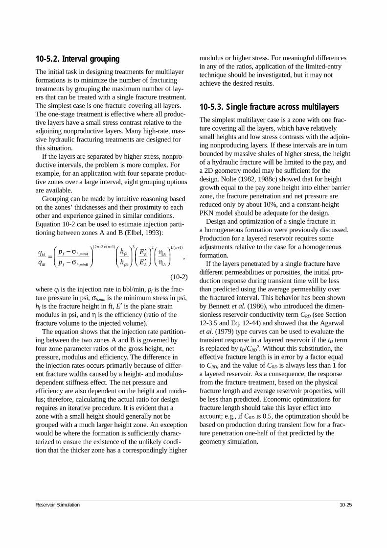
10-5.2. Interval groupingThe initial task in designing treatments for multilayerformations is to minimize the number of fracturingtreatments by grouping the maximum number of lay-ers that can be treated with a single fracture treatment.The simplest case is one fracture covering all layers.The one-stage treatment is effective where all produc-tive layers have a small stress contrast relative to theadjoining nonproductive layers. Many high-rate, mas-sive hydraulic fracturing treatments are designed forthis situation.

If the layers are separated by higher stress, nonpro-ductive intervals, the problem is more complex. Forexample, for an application with four separate produc-tive zones over a large interval, eight grouping optionsare available.

Grouping can be made by intuitive reasoning basedon the zones’ thicknesses and their proximity to eachother and experience gained in similar conditions.Equation 10-2 can be used to estimate injection parti-tioning between zones A and B (Elbel, 1993):

(10-2)

where qi is the injection rate in bbl/min, pf is the frac-ture pressure in psi, σh,min is the minimum stress in psi,hf is the fracture height in ft, E′ is the plane strainmodulus in psi, and η is the efficiency (ratio of thefracture volume to the injected volume).

The equation shows that the injection rate partition-ing between the two zones A and B is governed byfour zone parameter ratios of the gross height, netpressure, modulus and efficiency. The difference inthe injection rates occurs primarily because of differ-ent fracture widths caused by a height- and modulus-dependent stiffness effect. The net pressure andefficiency are also dependent on the height and modu-lus; therefore, calculating the actual ratio for designrequires an iterative procedure. It is evident that azone with a small height should generally not begrouped with a much larger height zone. An exceptionwould be where the formation is sufficiently charac-terized to ensure the existence of the unlikely condi-tion that the thicker zone has a correspondingly higher

modulus or higher stress. For meaningful differencesin any of the ratios, application of the limited-entrytechnique should be investigated, but it may notachieve the desired results.

10-5.3. Single fracture across multilayersThe simplest multilayer case is a zone with one frac-ture covering all the layers, which have relativelysmall heights and low stress contrasts with the adjoin-ing nonproducing layers. If these intervals are in turnbounded by massive shales of higher stress, the heightof a hydraulic fracture will be limited to the pay, and a 2D geometry model may be sufficient for thedesign. Nolte (1982, 1988c) showed that for heightgrowth equal to the pay zone height into either barrierzone, the fracture penetration and net pressure arereduced only by about 10%, and a constant-heightPKN model should be adequate for the design.

Design and optimization of a single fracture in a homogeneous formation were previously discussed.Production for a layered reservoir requires someadjustments relative to the case for a homogeneousformation.

If the layers penetrated by a single fracture havedifferent permeabilities or porosities, the initial pro-duction response during transient time will be lessthan predicted using the average permeability over the fractured interval. This behavior has been shownby Bennett et al. (1986), who introduced the dimen-sionless reservoir conductivity term CRD (see Section12-3.5 and Eq. 12-44) and showed that the Agarwal et al. (1979) type curves can be used to evaluate thetransient response in a layered reservoir if the tD termis replaced by tD/CRD

2. Without this substitution, theeffective fracture length is in error by a factor equal to CRD, and the value of CRD is always less than 1 for a layered reservoir. As a consequence, the responsefrom the fracture treatment, based on the physicalfracture length and average reservoir properties, willbe less than predicted. Economic optimizations forfracture length should take this layer effect intoaccount; e.g., if CRD is 0.5, the optimization should bebased on production during transient flow for a frac-ture penetration one-half of that predicted by thegeometry simulation.

Reservoir Stimulation 10-25

q

q

p

p

h

h

E

EiA

iB

f h minA

f h minB

n n

fA

fB

B

A

B

A

n

=−−

′′

+( ) +( ) +( )σσ

ηη

,

,

/ /

,

2 3 1 3 2 1 1

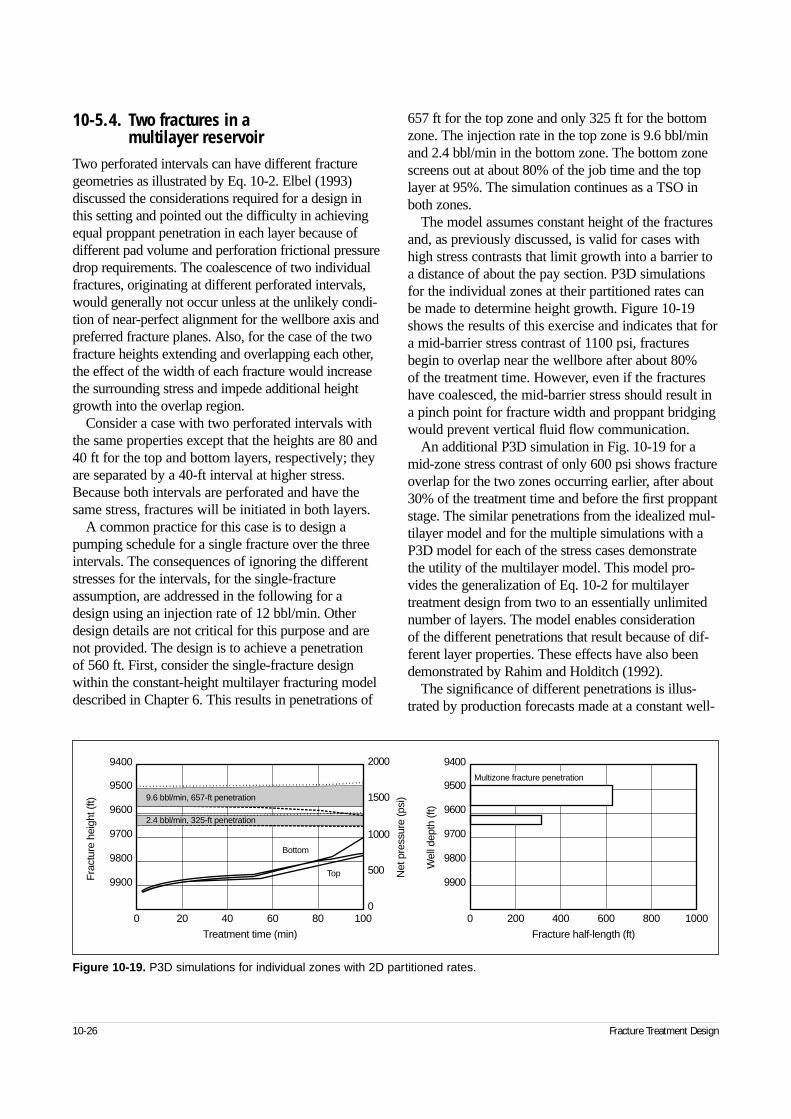
10-5.4. Two fractures in a multilayer reservoir

Two perforated intervals can have different fracturegeometries as illustrated by Eq. 10-2. Elbel (1993)discussed the considerations required for a design inthis setting and pointed out the difficulty in achievingequal proppant penetration in each layer because ofdifferent pad volume and perforation frictional pressuredrop requirements. The coalescence of two individualfractures, originating at different perforated intervals,would generally not occur unless at the unlikely condi-tion of near-perfect alignment for the wellbore axis andpreferred fracture planes. Also, for the case of the twofracture heights extending and overlapping each other,the effect of the width of each fracture would increasethe surrounding stress and impede additional heightgrowth into the overlap region.

Consider a case with two perforated intervals withthe same properties except that the heights are 80 and40 ft for the top and bottom layers, respectively; theyare separated by a 40-ft interval at higher stress.Because both intervals are perforated and have thesame stress, fractures will be initiated in both layers.

A common practice for this case is to design apumping schedule for a single fracture over the threeintervals. The consequences of ignoring the differentstresses for the intervals, for the single-fractureassumption, are addressed in the following for a design using an injection rate of 12 bbl/min. Otherdesign details are not critical for this purpose and arenot provided. The design is to achieve a penetration of 560 ft. First, consider the single-fracture designwithin the constant-height multilayer fracturing modeldescribed in Chapter 6. This results in penetrations of

657 ft for the top zone and only 325 ft for the bottomzone. The injection rate in the top zone is 9.6 bbl/minand 2.4 bbl/min in the bottom zone. The bottom zonescreens out at about 80% of the job time and the toplayer at 95%. The simulation continues as a TSO inboth zones.

The model assumes constant height of the fracturesand, as previously discussed, is valid for cases withhigh stress contrasts that limit growth into a barrier toa distance of about the pay section. P3D simulationsfor the individual zones at their partitioned rates canbe made to determine height growth. Figure 10-19shows the results of this exercise and indicates that fora mid-barrier stress contrast of 1100 psi, fracturesbegin to overlap near the wellbore after about 80% of the treatment time. However, even if the fractureshave coalesced, the mid-barrier stress should result ina pinch point for fracture width and proppant bridgingwould prevent vertical fluid flow communication.

An additional P3D simulation in Fig. 10-19 for amid-zone stress contrast of only 600 psi shows fractureoverlap for the two zones occurring earlier, after about30% of the treatment time and before the first proppantstage. The similar penetrations from the idealized mul-tilayer model and for the multiple simulations with aP3D model for each of the stress cases demonstrate the utility of the multilayer model. This model pro-vides the generalization of Eq. 10-2 for multilayertreatment design from two to an essentially unlimitednumber of layers. The model enables consideration of the different penetrations that result because of dif-ferent layer properties. These effects have also beendemonstrated by Rahim and Holditch (1992).

The significance of different penetrations is illus-trated by production forecasts made at a constant well-

10-26 Fracture Treatment Design

Figure 10-19. P3D simulations for individual zones with 2D partitioned rates.

0

9900

9800

9700

9600

9500

9400

Fra

ctur

e he

ight

(ft)

20 40 60 80 100

Treatment time (min)

0

9900

9800

9700

9600

9500

9400

Wel

l dep

th (f

t)

Net

pre

ssur

e (p

si)

200 400 600 800 1000

Fracture half-length (ft)

0

500

1000

1500

2000

Top

Bottom

9.6 bbl/min, 657-ft penetration

2.4 bbl/min, 325-ft penetration

Multizone fracture penetration

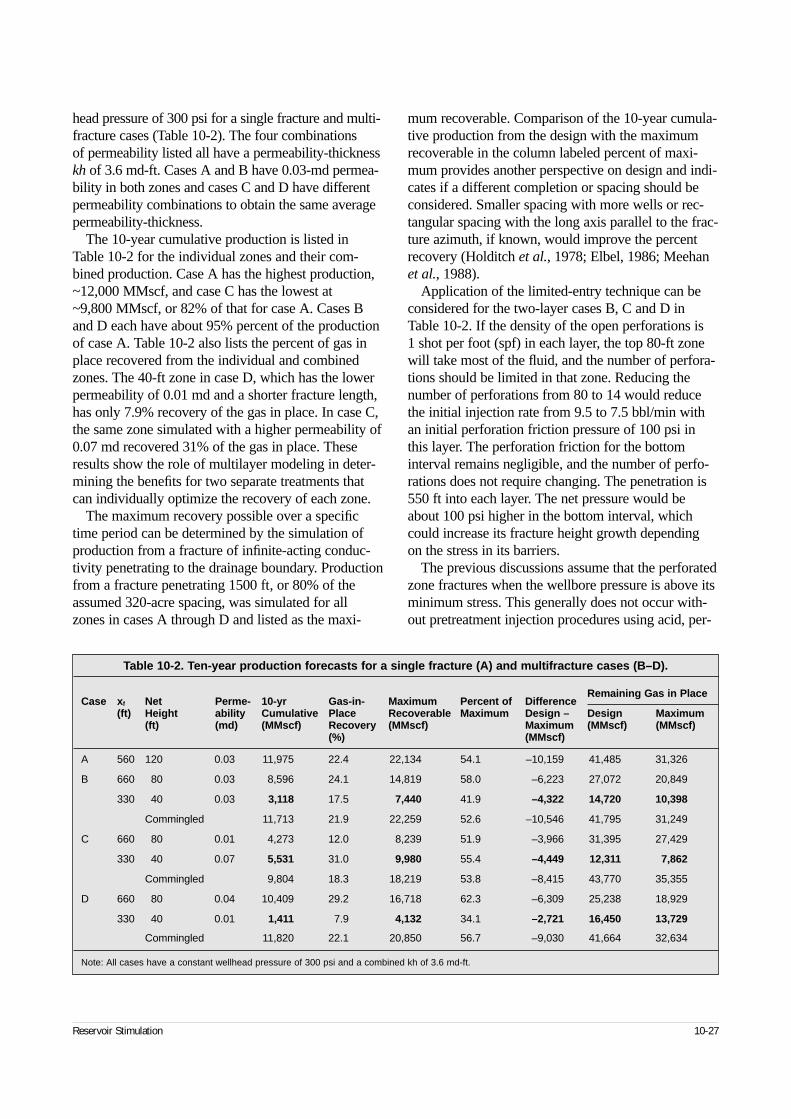
head pressure of 300 psi for a single fracture and multi-fracture cases (Table 10-2). The four combinations of permeability listed all have a permeability-thicknesskh of 3.6 md-ft. Cases A and B have 0.03-md permea-bility in both zones and cases C and D have differentpermeability combinations to obtain the same averagepermeability-thickness.

The 10-year cumulative production is listed in Table 10-2 for the individual zones and their com-bined production. Case A has the highest production,~12,000 MMscf, and case C has the lowest at ~9,800 MMscf, or 82% of that for case A. Cases Band D each have about 95% percent of the productionof case A. Table 10-2 also lists the percent of gas inplace recovered from the individual and combinedzones. The 40-ft zone in case D, which has the lowerpermeability of 0.01 md and a shorter fracture length,has only 7.9% recovery of the gas in place. In case C,the same zone simulated with a higher permeability of0.07 md recovered 31% of the gas in place. Theseresults show the role of multilayer modeling in deter-mining the benefits for two separate treatments thatcan individually optimize the recovery of each zone.

The maximum recovery possible over a specifictime period can be determined by the simulation ofproduction from a fracture of infinite-acting conduc-tivity penetrating to the drainage boundary. Productionfrom a fracture penetrating 1500 ft, or 80% of theassumed 320-acre spacing, was simulated for allzones in cases A through D and listed as the maxi-

mum recoverable. Comparison of the 10-year cumula-tive production from the design with the maximumrecoverable in the column labeled percent of maxi-mum provides another perspective on design and indi-cates if a different completion or spacing should beconsidered. Smaller spacing with more wells or rec-tangular spacing with the long axis parallel to the frac-ture azimuth, if known, would improve the percentrecovery (Holditch et al., 1978; Elbel, 1986; Meehanet al., 1988).

Application of the limited-entry technique can beconsidered for the two-layer cases B, C and D inTable 10-2. If the density of the open perforations is 1 shot per foot (spf) in each layer, the top 80-ft zonewill take most of the fluid, and the number of perfora-tions should be limited in that zone. Reducing thenumber of perforations from 80 to 14 would reducethe initial injection rate from 9.5 to 7.5 bbl/min withan initial perforation friction pressure of 100 psi inthis layer. The perforation friction for the bottominterval remains negligible, and the number of perfo-rations does not require changing. The penetration is550 ft into each layer. The net pressure would beabout 100 psi higher in the bottom interval, whichcould increase its fracture height growth depending on the stress in its barriers.

The previous discussions assume that the perforatedzone fractures when the wellbore pressure is above itsminimum stress. This generally does not occur with-out pretreatment injection procedures using acid, per-

Reservoir Stimulation 10-27

Table 10-2. Ten-year production forecasts for a single fracture (A) and multifracture cases (B–D).

Case xf Net Perme- 10-yr Gas-in- Maximum Percent of DifferenceRemaining Gas in Place

(ft) Height ability Cumulative Place Recoverable Maximum Design – Design Maximum(ft) (md) (MMscf) Recovery (MMscf) Maximum (MMscf) (MMscf)

(%) (MMscf)

A 560 120 0.03 11,975 22.4 22,134 54.1 –10,159 41,485 31,326

B 660 80 0.03 8,596 24.1 14,819 58.0 –6,223 27,072 20,849

330 40 0.03 3,118 17.5 7,440 41.9 –4,322 14,720 10,398

Commingled 11,713 21.9 22,259 52.6 –10,546 41,795 31,249

C 660 80 0.01 4,273 12.0 8,239 51.9 –3,966 31,395 27,429

330 40 0.07 5,531 31.0 9,980 55.4 –4,449 12,311 7,862

Commingled 9,804 18.3 18,219 53.8 –8,415 43,770 35,355

D 660 80 0.04 10,409 29.2 16,718 62.3 –6,309 25,238 18,929

330 40 0.01 1,411 7.9 4,132 34.1 –2,721 16,450 13,729

Commingled 11,820 22.1 20,850 56.7 –9,030 41,664 32,634

Note: All cases have a constant wellhead pressure of 300 psi and a combined kh of 3.6 md-ft.

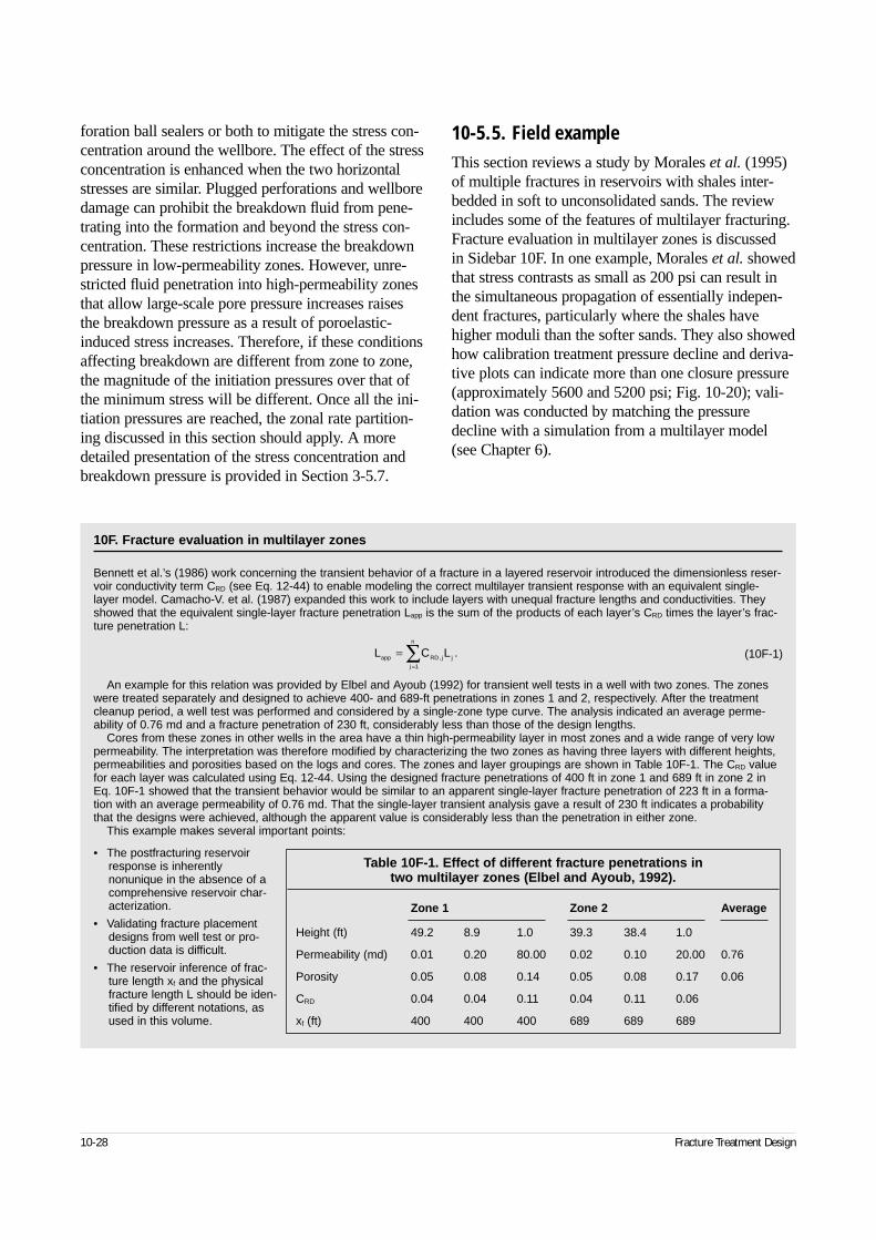
foration ball sealers or both to mitigate the stress con-centration around the wellbore. The effect of the stressconcentration is enhanced when the two horizontalstresses are similar. Plugged perforations and wellboredamage can prohibit the breakdown fluid from pene-trating into the formation and beyond the stress con-centration. These restrictions increase the breakdownpressure in low-permeability zones. However, unre-stricted fluid penetration into high-permeability zonesthat allow large-scale pore pressure increases raisesthe breakdown pressure as a result of poroelastic-induced stress increases. Therefore, if these conditionsaffecting breakdown are different from zone to zone,the magnitude of the initiation pressures over that ofthe minimum stress will be different. Once all the ini-tiation pressures are reached, the zonal rate partition-ing discussed in this section should apply. A moredetailed presentation of the stress concentration andbreakdown pressure is provided in Section 3-5.7.

10-5.5. Field exampleThis section reviews a study by Morales et al. (1995)of multiple fractures in reservoirs with shales inter-bedded in soft to unconsolidated sands. The reviewincludes some of the features of multilayer fracturing.Fracture evaluation in multilayer zones is discussed in Sidebar 10F. In one example, Morales et al. showedthat stress contrasts as small as 200 psi can result inthe simultaneous propagation of essentially indepen-dent fractures, particularly where the shales havehigher moduli than the softer sands. They also showedhow calibration treatment pressure decline and deriva-tive plots can indicate more than one closure pressure(approximately 5600 and 5200 psi; Fig. 10-20); vali-dation was conducted by matching the pressuredecline with a simulation from a multilayer model(see Chapter 6).

10-28 Fracture Treatment Design

10F. Fracture evaluation in multilayer zones

Bennett et al.’s (1986) work concerning the transient behavior of a fracture in a layered reservoir introduced the dimensionless reser-voir conductivity term CRD (see Eq. 12-44) to enable modeling the correct multilayer transient response with an equivalent single-layer model. Camacho-V. et al. (1987) expanded this work to include layers with unequal fracture lengths and conductivities. Theyshowed that the equivalent single-layer fracture penetration Lapp is the sum of the products of each layer’s CRD times the layer’s frac-ture penetration L:

(10F-1)

An example for this relation was provided by Elbel and Ayoub (1992) for transient well tests in a well with two zones. The zoneswere treated separately and designed to achieve 400- and 689-ft penetrations in zones 1 and 2, respectively. After the treatmentcleanup period, a well test was performed and considered by a single-zone type curve. The analysis indicated an average perme-ability of 0.76 md and a fracture penetration of 230 ft, considerably less than those of the design lengths.

Cores from these zones in other wells in the area have a thin high-permeability layer in most zones and a wide range of very lowpermeability. The interpretation was therefore modified by characterizing the two zones as having three layers with different heights,permeabilities and porosities based on the logs and cores. The zones and layer groupings are shown in Table 10F-1. The CRD valuefor each layer was calculated using Eq. 12-44. Using the designed fracture penetrations of 400 ft in zone 1 and 689 ft in zone 2 inEq. 10F-1 showed that the transient behavior would be similar to an apparent single-layer fracture penetration of 223 ft in a forma-tion with an average permeability of 0.76 md. That the single-layer transient analysis gave a result of 230 ft indicates a probabilitythat the designs were achieved, although the apparent value is considerably less than the penetration in either zone.

This example makes several important points:

• The postfracturing reservoirresponse is inherentlynonunique in the absence of acomprehensive reservoir char-acterization.

• Validating fracture placementdesigns from well test or pro-duction data is difficult.

• The reservoir inference of frac-ture length xf and the physicalfracture length L should be iden-tified by different notations, asused in this volume.

Table 10F-1. Effect of different fracture penetrations in two multilayer zones (Elbel and Ayoub, 1992).

Zone 1 Zone 2 Average

Height (ft) 49.2 8.9 1.0 39.3 38.4 1.0

Permeability (md) 0.01 0.20 80.00 0.02 0.10 20.00 0.76

Porosity 0.05 0.08 0.14 0.05 0.08 0.17 0.06

CRD 0.04 0.04 0.11 0.04 0.11 0.06

xf (ft) 400 400 400 689 689 689

L C Lapp RD j j

j

n

==

∑ , .1

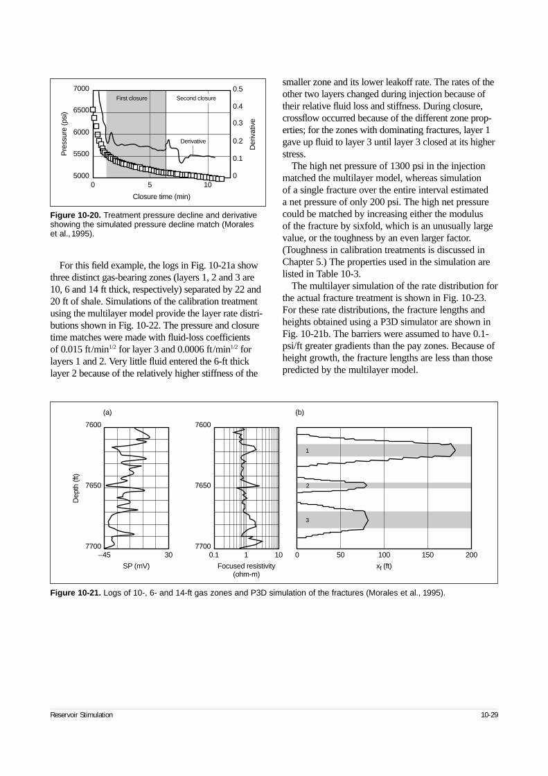
For this field example, the logs in Fig. 10-21a showthree distinct gas-bearing zones (layers 1, 2 and 3 are10, 6 and 14 ft thick, respectively) separated by 22 and20 ft of shale. Simulations of the calibration treatmentusing the multilayer model provide the layer rate distri-butions shown in Fig. 10-22. The pressure and closuretime matches were made with fluid-loss coefficients of 0.015 ft/min1/2 for layer 3 and 0.0006 ft/min1/2 forlayers 1 and 2. Very little fluid entered the 6-ft thicklayer 2 because of the relatively higher stiffness of the

smaller zone and its lower leakoff rate. The rates of theother two layers changed during injection because oftheir relative fluid loss and stiffness. During closure,crossflow occurred because of the different zone prop-erties; for the zones with dominating fractures, layer 1gave up fluid to layer 3 until layer 3 closed at its higherstress.

The high net pressure of 1300 psi in the injectionmatched the multilayer model, whereas simulation of a single fracture over the entire interval estimated a net pressure of only 200 psi. The high net pressurecould be matched by increasing either the modulus of the fracture by sixfold, which is an unusually largevalue, or the toughness by an even larger factor.(Toughness in calibration treatments is discussed inChapter 5.) The properties used in the simulation arelisted in Table 10-3.

The multilayer simulation of the rate distribution forthe actual fracture treatment is shown in Fig. 10-23.For these rate distributions, the fracture lengths andheights obtained using a P3D simulator are shown inFig. 10-21b. The barriers were assumed to have 0.1-psi/ft greater gradients than the pay zones. Because ofheight growth, the fracture lengths are less than thosepredicted by the multilayer model.

Reservoir Stimulation 10-29

Figure 10-20. Treatment pressure decline and derivativeshowing the simulated pressure decline match (Morales et al., 1995).

50001050

0

0.1

0.2

0.3

0.4

0.5

5500

6000

6500

7000

Der

ivat

ive

Closure time (min)

Pre

ssur

e (p

si)

First closure Second closure

Derivative

Figure 10-21. Logs of 10-, 6- and 14-ft gas zones and P3D simulation of the fractures (Morales et al., 1995).

–457700

7600

7650

7700

7600

7650

30 0.1 1 10 0 50 100 150 200

SP (mV) Focused resistivity(ohm-m)

xf (ft)

1

3

(a) (b)

2

Dep

th (f

t)

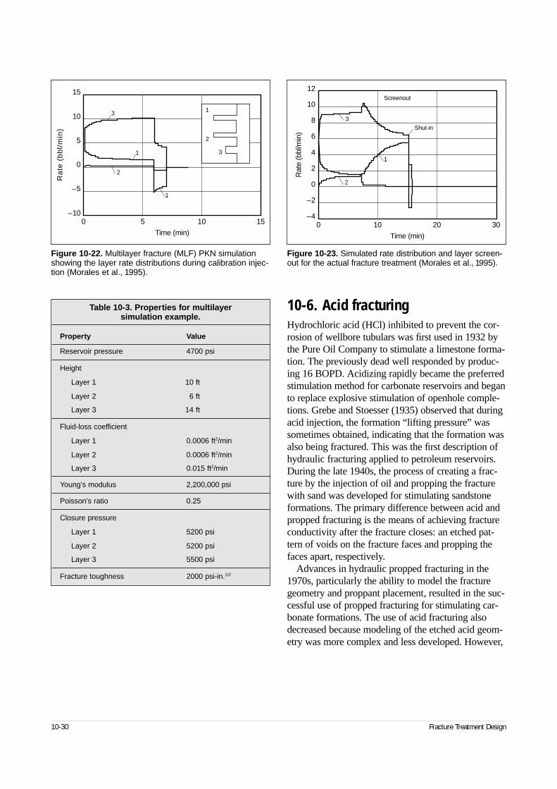
10-6. Acid fracturingHydrochloric acid (HCl) inhibited to prevent the cor-rosion of wellbore tubulars was first used in 1932 bythe Pure Oil Company to stimulate a limestone forma-tion. The previously dead well responded by produc-ing 16 BOPD. Acidizing rapidly became the preferredstimulation method for carbonate reservoirs and beganto replace explosive stimulation of openhole comple-tions. Grebe and Stoesser (1935) observed that duringacid injection, the formation “lifting pressure” wassometimes obtained, indicating that the formation wasalso being fractured. This was the first description ofhydraulic fracturing applied to petroleum reservoirs.During the late 1940s, the process of creating a frac-ture by the injection of oil and propping the fracturewith sand was developed for stimulating sandstoneformations. The primary difference between acid andpropped fracturing is the means of achieving fractureconductivity after the fracture closes: an etched pat-tern of voids on the fracture faces and propping thefaces apart, respectively.

Advances in hydraulic propped fracturing in the1970s, particularly the ability to model the fracturegeometry and proppant placement, resulted in the suc-cessful use of propped fracturing for stimulating car-bonate formations. The use of acid fracturing alsodecreased because modeling of the etched acid geom-etry was more complex and less developed. However,

10-30 Fracture Treatment Design

Figure 10-22. Multilayer fracture (MLF) PKN simulationshowing the layer rate distributions during calibration injec-tion (Morales et al., 1995).

0 5 10 15–10

15

10

5

0

–5

Time (min)

Ra

te (

bb

l/m

in)

1

3

2

1

1

2

3

Figure 10-23. Simulated rate distribution and layer screen-out for the actual fracture treatment (Morales et al., 1995).

0 10

–2

–4

12

10

8

6

4

2

0

Rat

e (b

bl/m

in)

20 30

Time (min)

Screenout

Shut-in

3

2

1

Table 10-3. Properties for multilayer simulation example.

Property Value

Reservoir pressure 4700 psi

Height

Layer 1 10 ft

Layer 2 6 ft

Layer 3 14 ft

Fluid-loss coefficient

Layer 1 0.0006 ft2/min

Layer 2 0.0006 ft2/min

Layer 3 0.015 ft2/min

Young’s modulus 2,200,000 psi

Poisson’s ratio 0.25

Closure pressure

Layer 1 5200 psi

Layer 2 5200 psi

Layer 3 5500 psi

Fracture toughness 2000 psi-in.1/2

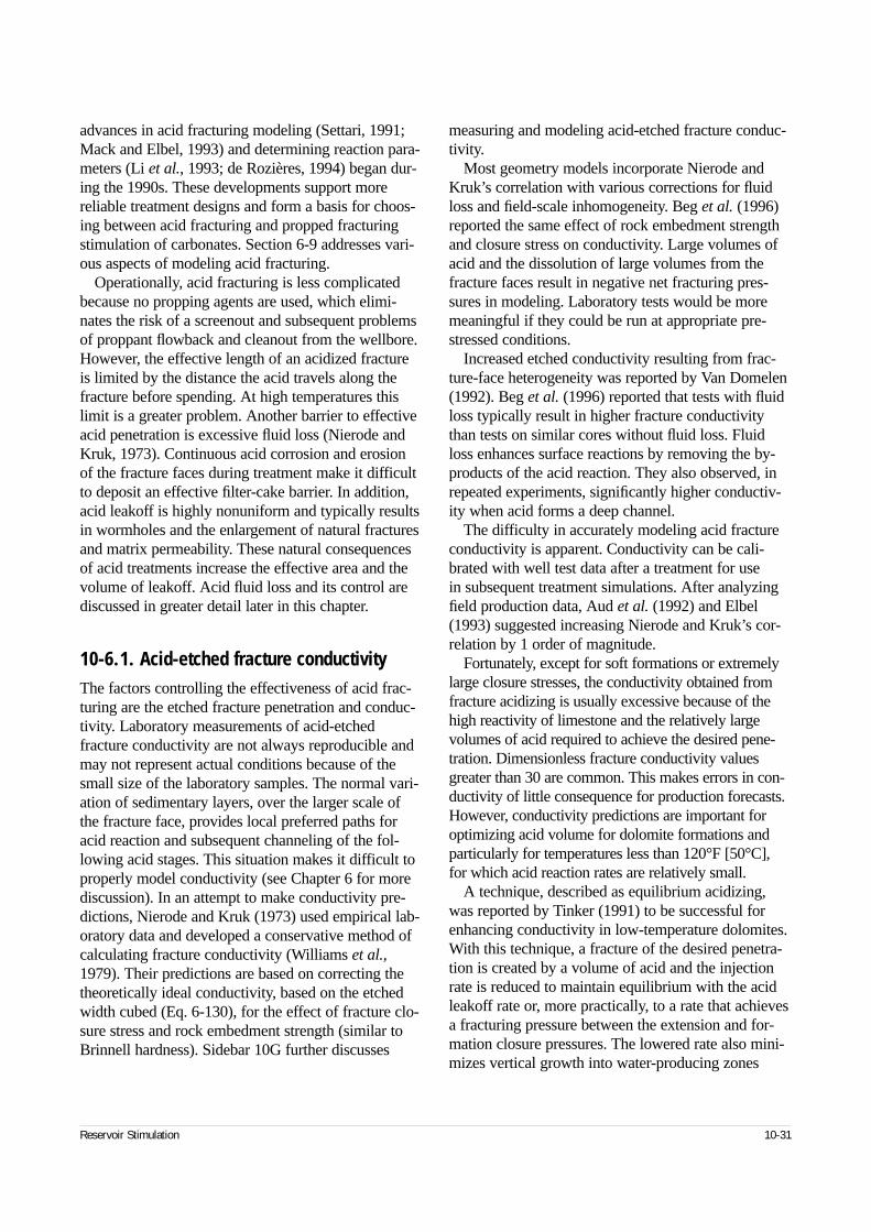
advances in acid fracturing modeling (Settari, 1991;Mack and Elbel, 1993) and determining reaction para-meters (Li et al., 1993; de Rozières, 1994) began dur-ing the 1990s. These developments support morereliable treatment designs and form a basis for choos-ing between acid fracturing and propped fracturingstimulation of carbonates. Section 6-9 addresses vari-ous aspects of modeling acid fracturing.

Operationally, acid fracturing is less complicatedbecause no propping agents are used, which elimi-nates the risk of a screenout and subsequent problemsof proppant flowback and cleanout from the wellbore.However, the effective length of an acidized fractureis limited by the distance the acid travels along thefracture before spending. At high temperatures thislimit is a greater problem. Another barrier to effectiveacid penetration is excessive fluid loss (Nierode andKruk, 1973). Continuous acid corrosion and erosionof the fracture faces during treatment make it difficultto deposit an effective filter-cake barrier. In addition,acid leakoff is highly nonuniform and typically resultsin wormholes and the enlargement of natural fracturesand matrix permeability. These natural consequencesof acid treatments increase the effective area and thevolume of leakoff. Acid fluid loss and its control arediscussed in greater detail later in this chapter.

10-6.1. Acid-etched fracture conductivityThe factors controlling the effectiveness of acid frac-turing are the etched fracture penetration and conduc-tivity. Laboratory measurements of acid-etchedfracture conductivity are not always reproducible andmay not represent actual conditions because of thesmall size of the laboratory samples. The normal vari-ation of sedimentary layers, over the larger scale ofthe fracture face, provides local preferred paths foracid reaction and subsequent channeling of the fol-lowing acid stages. This situation makes it difficult toproperly model conductivity (see Chapter 6 for morediscussion). In an attempt to make conductivity pre-dictions, Nierode and Kruk (1973) used empirical lab-oratory data and developed a conservative method ofcalculating fracture conductivity (Williams et al.,1979). Their predictions are based on correcting thetheoretically ideal conductivity, based on the etchedwidth cubed (Eq. 6-130), for the effect of fracture clo-sure stress and rock embedment strength (similar toBrinnell hardness). Sidebar 10G further discusses

measuring and modeling acid-etched fracture conduc-tivity.

Most geometry models incorporate Nierode andKruk’s correlation with various corrections for fluidloss and field-scale inhomogeneity. Beg et al. (1996)reported the same effect of rock embedment strengthand closure stress on conductivity. Large volumes ofacid and the dissolution of large volumes from thefracture faces result in negative net fracturing pres-sures in modeling. Laboratory tests would be moremeaningful if they could be run at appropriate pre-stressed conditions.

Increased etched conductivity resulting from frac-ture-face heterogeneity was reported by Van Domelen(1992). Beg et al. (1996) reported that tests with fluidloss typically result in higher fracture conductivitythan tests on similar cores without fluid loss. Fluidloss enhances surface reactions by removing the by-products of the acid reaction. They also observed, inrepeated experiments, significantly higher conductiv-ity when acid forms a deep channel.

The difficulty in accurately modeling acid fractureconductivity is apparent. Conductivity can be cali-brated with well test data after a treatment for use in subsequent treatment simulations. After analyzingfield production data, Aud et al. (1992) and Elbel(1993) suggested increasing Nierode and Kruk’s cor-relation by 1 order of magnitude.

Fortunately, except for soft formations or extremelylarge closure stresses, the conductivity obtained fromfracture acidizing is usually excessive because of thehigh reactivity of limestone and the relatively largevolumes of acid required to achieve the desired pene-tration. Dimensionless fracture conductivity valuesgreater than 30 are common. This makes errors in con-ductivity of little consequence for production forecasts.However, conductivity predictions are important foroptimizing acid volume for dolomite formations andparticularly for temperatures less than 120°F [50°C],for which acid reaction rates are relatively small.

A technique, described as equilibrium acidizing,was reported by Tinker (1991) to be successful forenhancing conductivity in low-temperature dolomites.With this technique, a fracture of the desired penetra-tion is created by a volume of acid and the injectionrate is reduced to maintain equilibrium with the acidleakoff rate or, more practically, to a rate that achievesa fracturing pressure between the extension and for-mation closure pressures. The lowered rate also mini-mizes vertical growth into water-producing zones

Reservoir Stimulation 10-31

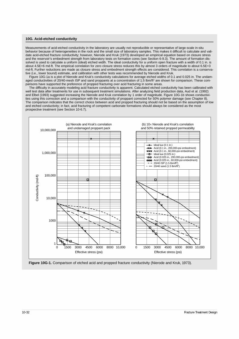
10-32 Fracture Treatment Design

10G. Acid-etched conductivity

Measurements of acid-etched conductivity in the laboratory are usually not reproducible or representative of large-scale in-situbehavior because of heterogeneities in the rock and the small size of laboratory samples. This makes it difficult to calculate and vali-date acid-etched fracture conductivity; however, Nierode and Kruk (1973) developed an empirical equation based on closure stressand the reservoir’s embedment strength from laboratory tests on formation cores (see Section 6-9.3). The amount of formation dis-solved is used to calculate a uniform (ideal) etched width. The ideal conductivity for a uniform open fracture with a width of 0.1 in. isabout 4.5E+6 md-ft. The empirical correlation for zero closure stress reduces this by almost 3 orders of magnitude to about 6.5E+3md-ft. Further reductions are made as closure stress and embedment strength effects are considered. This correlation is a conserva-tive (i.e., lower bound) estimate, and calibration with other tests was recommended by Nierode and Kruk.

Figure 10G-1a is a plot of Nierode and Kruk’s conductivity calculations for average etched widths of 0.1 and 0.025 in. The undam-aged conductivities of 20/40-mesh ISP and sand proppants at a concentration of 1.5 lbm/ft2 are shown for comparison. These com-parisons have supported the preference of propped fracturing over acid fracturing in some areas.

The difficulty in accurately modeling acid fracture conductivity is apparent. Calculated etched conductivity has been calibrated withwell test data after treatments for use in subsequent treatment simulations. After analyzing field production data, Aud et al. (1992)and Elbel (1993) suggested increasing the Nierode and Kruk correlation by 1 order of magnitude. Figure 10G-1b shows conductivi-ties using this correction and a comparison with the conductivity of proppant corrected for 50% polymer damage (see Chapter 8).The comparison indicates that the correct choice between acid and propped fracturing should not be based on the assumption of lowand etched conductivity; in fact, acid fracturing of competent carbonate formations should always be considered as the mostprospective treatment (see Section 10-6.7).

Figure 10G-1. Comparison of etched acid and propped fracture conductivity (Nierode and Kruk, 1973).

01

1500 3000 4500 6000 8000 10,000

10,000,000

1,000,000

100,000

10,000

1000

Con

duct

ivity

(md-

ft)

Effective stress (psi)

0 1500 3000 4500 6000 8000 10,000

Effective stress (psi)

(a) Nierode and Kruk's correlationand undamaged proppant pack

(b) 10× Nierode and Kruk's correlationand 50% retained propped permeability

Ideal kfw (0.1 in.)Acid (0.1 in., 200,000-psi embedment)Acid (0.1 in., 60,000-psi embedment)Ideal kfw (0.025 in.)Acid (0.025 in., 200,000-psi embedment)Acid (0.025 in., 60,000-psi embedment)20/40 ISP (1.5 lbm/ft2)20/40 sand (1.5 lbm/ft2)

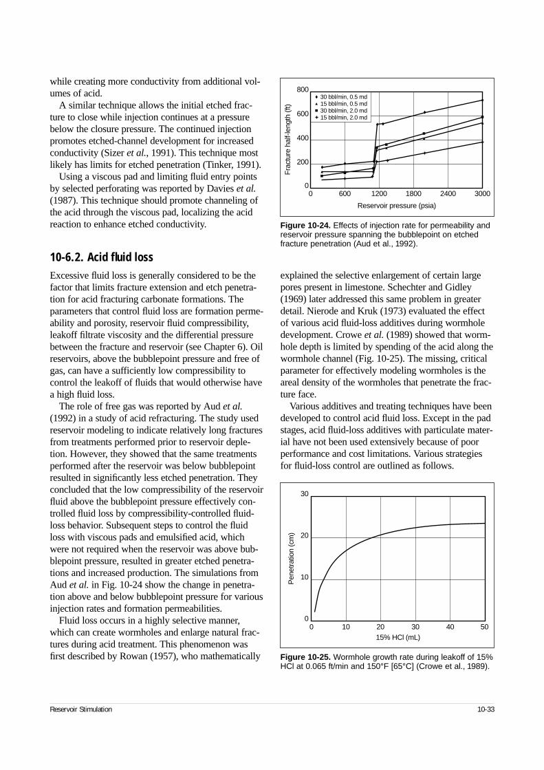
while creating more conductivity from additional vol-umes of acid.

A similar technique allows the initial etched frac-ture to close while injection continues at a pressurebelow the closure pressure. The continued injectionpromotes etched-channel development for increasedconductivity (Sizer et al., 1991). This technique mostlikely has limits for etched penetration (Tinker, 1991).

Using a viscous pad and limiting fluid entry pointsby selected perforating was reported by Davies et al.(1987). This technique should promote channeling ofthe acid through the viscous pad, localizing the acidreaction to enhance etched conductivity.

10-6.2. Acid fluid lossExcessive fluid loss is generally considered to be thefactor that limits fracture extension and etch penetra-tion for acid fracturing carbonate formations. Theparameters that control fluid loss are formation perme-ability and porosity, reservoir fluid compressibility,leakoff filtrate viscosity and the differential pressurebetween the fracture and reservoir (see Chapter 6). Oilreservoirs, above the bubblepoint pressure and free ofgas, can have a sufficiently low compressibility tocontrol the leakoff of fluids that would otherwise havea high fluid loss.

The role of free gas was reported by Aud et al.(1992) in a study of acid refracturing. The study usedreservoir modeling to indicate relatively long fracturesfrom treatments performed prior to reservoir deple-tion. However, they showed that the same treatmentsperformed after the reservoir was below bubblepointresulted in significantly less etched penetration. Theyconcluded that the low compressibility of the reservoirfluid above the bubblepoint pressure effectively con-trolled fluid loss by compressibility-controlled fluid-loss behavior. Subsequent steps to control the fluidloss with viscous pads and emulsified acid, whichwere not required when the reservoir was above bub-blepoint pressure, resulted in greater etched penetra-tions and increased production. The simulations fromAud et al. in Fig. 10-24 show the change in penetra-tion above and below bubblepoint pressure for variousinjection rates and formation permeabilities.

Fluid loss occurs in a highly selective manner,which can create wormholes and enlarge natural frac-tures during acid treatment. This phenomenon wasfirst described by Rowan (1957), who mathematically

explained the selective enlargement of certain largepores present in limestone. Schechter and Gidley(1969) later addressed this same problem in greaterdetail. Nierode and Kruk (1973) evaluated the effectof various acid fluid-loss additives during wormholedevelopment. Crowe et al. (1989) showed that worm-hole depth is limited by spending of the acid along thewormhole channel (Fig. 10-25). The missing, criticalparameter for effectively modeling wormholes is theareal density of the wormholes that penetrate the frac-ture face.

Various additives and treating techniques have beendeveloped to control acid fluid loss. Except in the padstages, acid fluid-loss additives with particulate mater-ial have not been used extensively because of poorperformance and cost limitations. Various strategiesfor fluid-loss control are outlined as follows.

Reservoir Stimulation 10-33

Figure 10-24. Effects of injection rate for permeability andreservoir pressure spanning the bubblepoint on etchedfracture penetration (Aud et al., 1992).

0 600 1200 1800 2400 30000

800

600

400

200

Fra

ctur

e ha

lf-le

ngth

(ft)

Reservoir pressure (psia)

30 bbl/min, 0.5 md15 bbl/min, 0.5 md30 bbl/min, 2.0 md15 bbl/min, 2.0 md

Figure 10-25. Wormhole growth rate during leakoff of 15%HCl at 0.065 ft/min and 150°F [65°C] (Crowe et al., 1989).

0 10 20 30 40 500

10

20

30

15% HCl (mL)

Pen

etra

tion

(cm

)

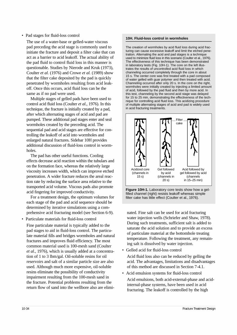
• Pad stages for fluid-loss control

The use of a water-base or gelled-water viscouspad preceding the acid stage is commonly used toinitiate the fracture and deposit a filter cake that canact as a barrier to acid leakoff. The actual ability ofthe pad fluid to control fluid loss in this manner isquestionable. Studies by Nierode and Kruk (1973),Coulter et al. (1976) and Crowe et al. (1989) showthat the filter cake deposited by the pad is quicklypenetrated by wormholes resulting from acid leak-off. Once this occurs, acid fluid loss can be thesame as if no pad were used.

Multiple stages of gelled pads have been used tocontrol acid fluid loss (Coulter et al., 1976). In thistechnique, the fracture is initially created by a pad,after which alternating stages of acid and pad arepumped. These additional pad stages enter and sealwormholes created by the preceding acid. Thesequential pad and acid stages are effective for con-trolling the leakoff of acid into wormholes andenlarged natural fractures. Sidebar 10H providesadditional discussion of fluid-loss control in worm-holes.

The pad has other useful functions. Coolingeffects decrease acid reaction within the tubulars andon the formation face, whereas the relatively largeviscosity increases width, which can improve etchedpenetration. A wider fracture reduces the areal reac-tion rate by reducing the surface area relative to thetransported acid volume. Viscous pads also promoteacid fingering for improved conductivity.

For a treatment design, the optimum volumes foreach stage of the pad and acid sequence should bedetermined by iterative simulations using a com-prehensive acid fracturing model (see Section 6-9).

• Particulate materials for fluid-loss control

Fine particulate material is typically added to thepad stages to aid in fluid-loss control. The particu-late material fills and bridges wormholes and naturalfractures and improves fluid efficiency. The mostcommon material used is 100-mesh sand (Coulteret al., 1976), which is usually added at a concentra-tion of 1 to 3 lbm/gal. Oil-soluble resins for oilreservoirs and salt of a similar particle size are alsoused. Although much more expensive, oil-solubleresins eliminate the possibility of conductivityimpairment resulting from the 100-mesh sand inthe fracture. Potential problems resulting from thereturn flow of sand into the wellbore also are elimi-

nated. Fine salt can be used for acid fracturingwater injection wells (Schriefer and Shaw, 1978).During such treatments, sufficient salt is added tosaturate the acid solution and to provide an excessof particulate material at the bottomhole treatingtemperature. Following the treatment, any remain-ing salt is dissolved by water injection.

• Gelled acid for fluid-loss control

Acid fluid loss also can be reduced by gelling theacid. The advantages, limitations and disadvantagesof this method are discussed in Section 7-4.1.

• Acid emulsion systems for fluid-loss control

Acid emulsions, both acid-external-phase and acid-internal-phase systems, have been used in acidfracturing. The leakoff is controlled by the high

10-34 Fracture Treatment Design

10H. Fluid-loss control in wormholes

The creation of wormholes by acid fluid loss during acid frac-turing can cause excessive leakoff and limit the etched pene-tration. Alternating the acid and pad stages is a techniqueused to minimize fluid loss in this scenario (Coulter et al., 1976).The effectiveness of this technique has been demonstratedin laboratory tests (Fig. 10H-1). The core on the left illus-trates the results of uncontrolled acid fluid loss in whichchanneling occurred completely through the core in about 15 s. The center core was first treated with a pad composedof water gelled with guar polymer and then treated with acid.Channeling occurred after only 20 s. In the core on the right,wormholes were initially created by injecting a limited amountof acid, followed by the pad fluid and then by more acid. Inthis test, channeling by the second acid stage was delayedfor 15 to 25 min, demonstrating the effectiveness of the tech-nique for controlling acid fluid loss. This acidizing procedureof multiple alternating stages of acid and pad is widely usedin acid fracturing treatments.

Figure 10H-1. Laboratory core tests show how a gel-filled channel (right) resists leakoff whereas simplefilter cake has little effect (Coulter et al., 1976).

Acidized core(channels in

15 s)

Gel followedby acid

(channels in20 s)

Acid followed bygel followed by acid

(channelsin 15–25 min)

Filtercake

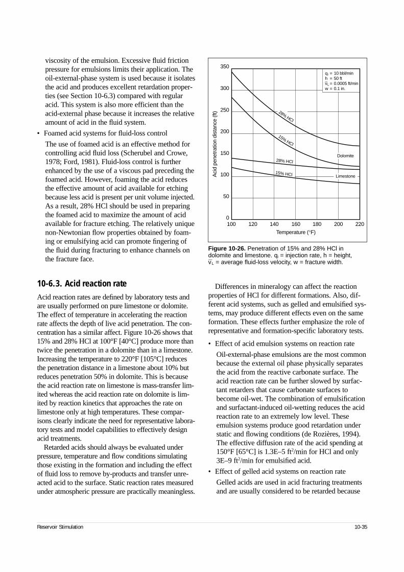
viscosity of the emulsion. Excessive fluid frictionpressure for emulsions limits their application. Theoil-external-phase system is used because it isolatesthe acid and produces excellent retardation proper-ties (see Section 10-6.3) compared with regularacid. This system is also more efficient than theacid-external phase because it increases the relativeamount of acid in the fluid system.

• Foamed acid systems for fluid-loss control

The use of foamed acid is an effective method forcontrolling acid fluid loss (Scherubel and Crowe,1978; Ford, 1981). Fluid-loss control is furtherenhanced by the use of a viscous pad preceding thefoamed acid. However, foaming the acid reducesthe effective amount of acid available for etchingbecause less acid is present per unit volume injected.As a result, 28% HCl should be used in preparingthe foamed acid to maximize the amount of acidavailable for fracture etching. The relatively uniquenon-Newtonian flow properties obtained by foam-ing or emulsifying acid can promote fingering ofthe fluid during fracturing to enhance channels onthe fracture face.

10-6.3. Acid reaction rateAcid reaction rates are defined by laboratory tests andare usually performed on pure limestone or dolomite.The effect of temperature in accelerating the reactionrate affects the depth of live acid penetration. The con-centration has a similar affect. Figure 10-26 shows that15% and 28% HCl at 100°F [40°C] produce more thantwice the penetration in a dolomite than in a limestone.Increasing the temperature to 220°F [105°C] reducesthe penetration distance in a limestone about 10% butreduces penetration 50% in dolomite. This is becausethe acid reaction rate on limestone is mass-transfer lim-ited whereas the acid reaction rate on dolomite is lim-ited by reaction kinetics that approaches the rate onlimestone only at high temperatures. These compar-isons clearly indicate the need for representative labora-tory tests and model capabilities to effectively designacid treatments.

Retarded acids should always be evaluated underpressure, temperature and flow conditions simulatingthose existing in the formation and including the effectof fluid loss to remove by-products and transfer unre-acted acid to the surface. Static reaction rates measuredunder atmospheric pressure are practically meaningless.

Differences in mineralogy can affect the reactionproperties of HCl for different formations. Also, dif-ferent acid systems, such as gelled and emulsified sys-tems, may produce different effects even on the sameformation. These effects further emphasize the role ofrepresentative and formation-specific laboratory tests.

• Effect of acid emulsion systems on reaction rate

Oil-external-phase emulsions are the most commonbecause the external oil phase physically separatesthe acid from the reactive carbonate surface. Theacid reaction rate can be further slowed by surfac-tant retarders that cause carbonate surfaces tobecome oil-wet. The combination of emulsificationand surfactant-induced oil-wetting reduces the acidreaction rate to an extremely low level. Theseemulsion systems produce good retardation understatic and flowing conditions (de Rozières, 1994).The effective diffusion rate of the acid spending at150°F [65°C] is 1.3E–5 ft2/min for HCl and only3E–9 ft2/min for emulsified acid.

• Effect of gelled acid systems on reaction rate

Gelled acids are used in acid fracturing treatmentsand are usually considered to be retarded because

Reservoir Stimulation 10-35

Figure 10-26. Penetration of 15% and 28% HCl indolomite and limestone. qi = injection rate, h = height,v—L = average fluid-loss velocity, w = fracture width.

15%HCl

28% HCl

100 120 140 160 180 200 2200

350

300

250

200

150

100

50

Temperature (°F)

Aci

d pe

netra

tion

dist

ance

(ft)

Dolomite

Limestone

28%HCl

15% HCl

qi = 10 bbl/minh = 50 ftv–L = 0.0005 ft/minw = 0.1 in.

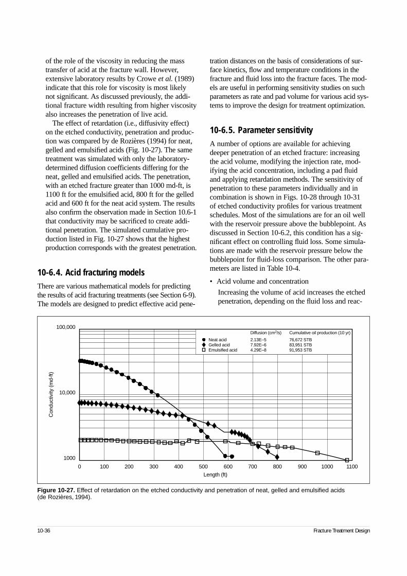
of the role of the viscosity in reducing the masstransfer of acid at the fracture wall. However,extensive laboratory results by Crowe et al. (1989)indicate that this role for viscosity is most likelynot significant. As discussed previously, the addi-tional fracture width resulting from higher viscosityalso increases the penetration of live acid.

The effect of retardation (i.e., diffusivity effect)on the etched conductivity, penetration and produc-tion was compared by de Rozières (1994) for neat,gelled and emulsified acids (Fig. 10-27). The sametreatment was simulated with only the laboratory-determined diffusion coefficients differing for theneat, gelled and emulsified acids. The penetration,with an etched fracture greater than 1000 md-ft, is1100 ft for the emulsified acid, 800 ft for the gelledacid and 600 ft for the neat acid system. The resultsalso confirm the observation made in Section 10.6-1that conductivity may be sacrificed to create addi-tional penetration. The simulated cumulative pro-duction listed in Fig. 10-27 shows that the highestproduction corresponds with the greatest penetration.

10-6.4. Acid fracturing modelsThere are various mathematical models for predictingthe results of acid fracturing treatments (see Section 6-9).The models are designed to predict effective acid pene-

tration distances on the basis of considerations of sur-face kinetics, flow and temperature conditions in thefracture and fluid loss into the fracture faces. The mod-els are useful in performing sensitivity studies on suchparameters as rate and pad volume for various acid sys-tems to improve the design for treatment optimization.

10-6.5. Parameter sensitivityA number of options are available for achievingdeeper penetration of an etched fracture: increasingthe acid volume, modifying the injection rate, mod-ifying the acid concentration, including a pad fluidand applying retardation methods. The sensitivity ofpenetration to these parameters individually and incombination is shown in Figs. 10-28 through 10-31 of etched conductivity profiles for various treatmentschedules. Most of the simulations are for an oil wellwith the reservoir pressure above the bubblepoint. Asdiscussed in Section 10-6.2, this condition has a sig-nificant effect on controlling fluid loss. Some simula-tions are made with the reservoir pressure below thebubblepoint for fluid-loss comparison. The other para-meters are listed in Table 10-4.

• Acid volume and concentration

Increasing the volume of acid increases the etchedpenetration, depending on the fluid loss and reac-

10-36 Fracture Treatment Design

Figure 10-27. Effect of retardation on the etched conductivity and penetration of neat, gelled and emulsified acids (de Rozières, 1994).

110010009008007006005004003002001000

1000

100,000

10,000

Length (ft)

Con

duct

ivity

(md-

ft)

Cumulative oil production (10 yr)

76,672 STB83,951 STB91,953 STB

Diffusion (cm2/s)

2.13E–57.92E–64.29E–8

Neat acidGelled acidEmulsified acid

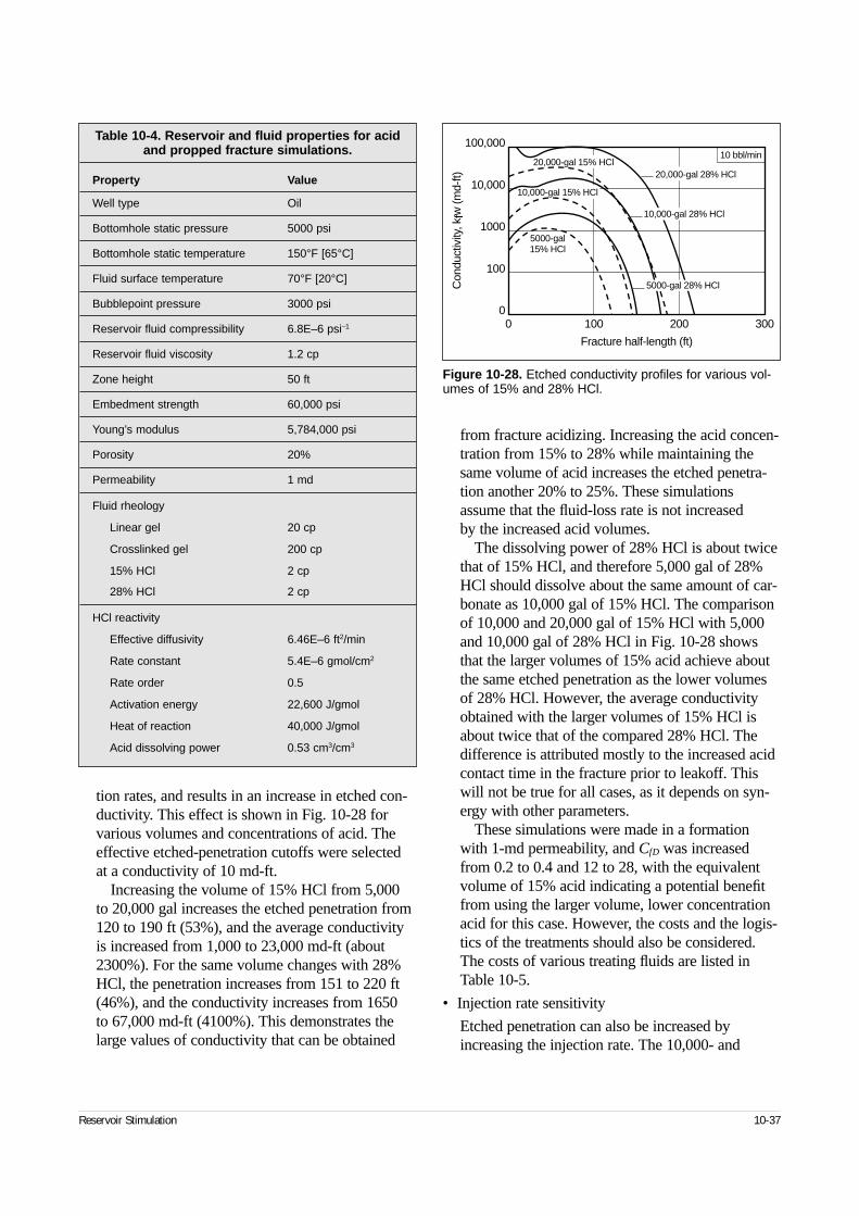
tion rates, and results in an increase in etched con-ductivity. This effect is shown in Fig. 10-28 forvarious volumes and concentrations of acid. Theeffective etched-penetration cutoffs were selected at a conductivity of 10 md-ft.

Increasing the volume of 15% HCl from 5,000 to 20,000 gal increases the etched penetration from120 to 190 ft (53%), and the average conductivityis increased from 1,000 to 23,000 md-ft (about2300%). For the same volume changes with 28%HCl, the penetration increases from 151 to 220 ft(46%), and the conductivity increases from 1650 to 67,000 md-ft (4100%). This demonstrates thelarge values of conductivity that can be obtained

from fracture acidizing. Increasing the acid concen-tration from 15% to 28% while maintaining thesame volume of acid increases the etched penetra-tion another 20% to 25%. These simulationsassume that the fluid-loss rate is not increased by the increased acid volumes.

The dissolving power of 28% HCl is about twicethat of 15% HCl, and therefore 5,000 gal of 28%HCl should dissolve about the same amount of car-bonate as 10,000 gal of 15% HCl. The comparisonof 10,000 and 20,000 gal of 15% HCl with 5,000and 10,000 gal of 28% HCl in Fig. 10-28 showsthat the larger volumes of 15% acid achieve aboutthe same etched penetration as the lower volumes of 28% HCl. However, the average conductivityobtained with the larger volumes of 15% HCl isabout twice that of the compared 28% HCl. Thedifference is attributed mostly to the increased acidcontact time in the fracture prior to leakoff. Thiswill not be true for all cases, as it depends on syn-ergy with other parameters.

These simulations were made in a formationwith 1-md permeability, and CfD was increasedfrom 0.2 to 0.4 and 12 to 28, with the equivalentvolume of 15% acid indicating a potential benefitfrom using the larger volume, lower concentrationacid for this case. However, the costs and the logis-tics of the treatments should also be considered.The costs of various treating fluids are listed inTable 10-5.

• Injection rate sensitivity

Etched penetration can also be increased byincreasing the injection rate. The 10,000- and

Reservoir Stimulation 10-37

Table 10-4. Reservoir and fluid properties for acidand propped fracture simulations.

Property Value

Well type Oil

Bottomhole static pressure 5000 psi

Bottomhole static temperature 150°F [65°C]

Fluid surface temperature 70°F [20°C]

Bubblepoint pressure 3000 psi

Reservoir fluid compressibility 6.8E–6 psi–1

Reservoir fluid viscosity 1.2 cp

Zone height 50 ft

Embedment strength 60,000 psi

Young’s modulus 5,784,000 psi

Porosity 20%

Permeability 1 md

Fluid rheology

Linear gel 20 cp

Crosslinked gel 200 cp

15% HCl 2 cp

28% HCl 2 cp

HCl reactivity

Effective diffusivity 6.46E–6 ft2/min

Rate constant 5.4E–6 gmol/cm2

Rate order 0.5

Activation energy 22,600 J/gmol

Heat of reaction 40,000 J/gmol

Acid dissolving power 0.53 cm3/cm3

Figure 10-28. Etched conductivity profiles for various vol-umes of 15% and 28% HCl.

0 100 200 3000

100

1000

10,000

100,000

Fracture half-length (ft)

Con

duct

ivity

, kfw

(md-

ft)

5000-gal15% HCl

10 bbl/min

20,000-gal 28% HCl

10,000-gal 28% HCl

20,000-gal 15% HCl

10,000-gal 15% HCl

5000-gal 28% HCl

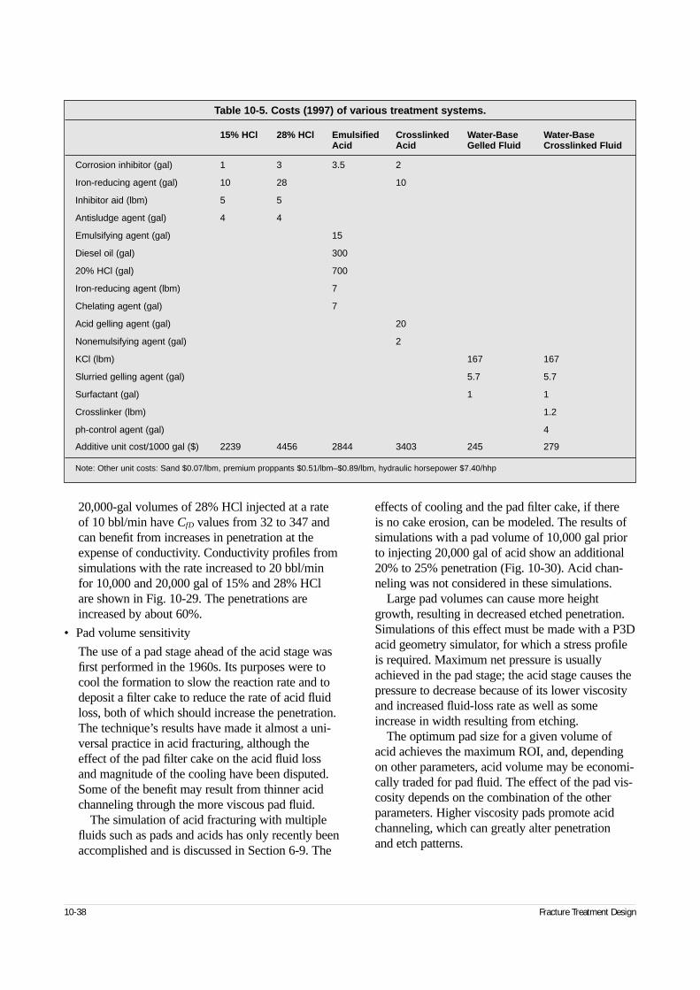
20,000-gal volumes of 28% HCl injected at a rateof 10 bbl/min have CfD values from 32 to 347 andcan benefit from increases in penetration at theexpense of conductivity. Conductivity profiles fromsimulations with the rate increased to 20 bbl/minfor 10,000 and 20,000 gal of 15% and 28% HClare shown in Fig. 10-29. The penetrations areincreased by about 60%.

• Pad volume sensitivity

The use of a pad stage ahead of the acid stage wasfirst performed in the 1960s. Its purposes were tocool the formation to slow the reaction rate and todeposit a filter cake to reduce the rate of acid fluidloss, both of which should increase the penetration.The technique’s results have made it almost a uni-versal practice in acid fracturing, although theeffect of the pad filter cake on the acid fluid lossand magnitude of the cooling have been disputed.Some of the benefit may result from thinner acidchanneling through the more viscous pad fluid.

The simulation of acid fracturing with multiplefluids such as pads and acids has only recently beenaccomplished and is discussed in Section 6-9. The

effects of cooling and the pad filter cake, if there is no cake erosion, can be modeled. The results ofsimulations with a pad volume of 10,000 gal priorto injecting 20,000 gal of acid show an additional20% to 25% penetration (Fig. 10-30). Acid chan-neling was not considered in these simulations.

Large pad volumes can cause more heightgrowth, resulting in decreased etched penetration.Simulations of this effect must be made with a P3Dacid geometry simulator, for which a stress profileis required. Maximum net pressure is usuallyachieved in the pad stage; the acid stage causes thepressure to decrease because of its lower viscosityand increased fluid-loss rate as well as someincrease in width resulting from etching.

The optimum pad size for a given volume ofacid achieves the maximum ROI, and, dependingon other parameters, acid volume may be economi-cally traded for pad fluid. The effect of the pad vis-cosity depends on the combination of the otherparameters. Higher viscosity pads promote acidchanneling, which can greatly alter penetration and etch patterns.

10-38 Fracture Treatment Design

Table 10-5. Costs (1997) of various treatment systems.

15% HCl 28% HCl Emulsified Crosslinked Water-Base Water-BaseAcid Acid Gelled Fluid Crosslinked Fluid

Corrosion inhibitor (gal) 1 3 3.5 2

Iron-reducing agent (gal) 10 28 10

Inhibitor aid (lbm) 5 5

Antisludge agent (gal) 4 4

Emulsifying agent (gal) 15

Diesel oil (gal) 300

20% HCl (gal) 700

Iron-reducing agent (lbm) 7

Chelating agent (gal) 7

Acid gelling agent (gal) 20

Nonemulsifying agent (gal) 2

KCl (lbm) 167 167

Slurried gelling agent (gal) 5.7 5.7

Surfactant (gal) 1 1

Crosslinker (lbm) 1.2

ph-control agent (gal) 4

Additive unit cost/1000 gal ($) 2239 4456 2844 3403 245 279

Note: Other unit costs: Sand $0.07/lbm, premium proppants $0.51/lbm–$0.89/lbm, hydraulic horsepower $7.40/hhp

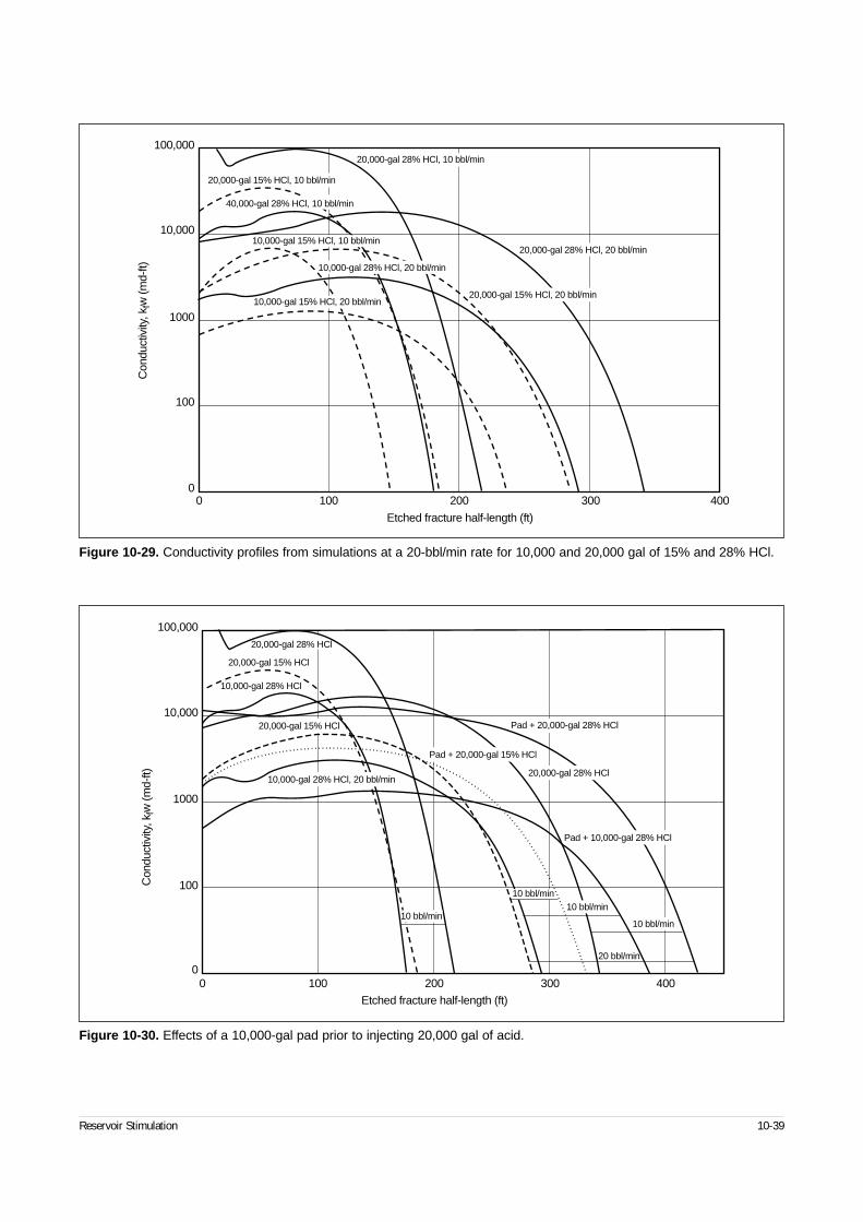
Reservoir Stimulation 10-39

Figure 10-29. Conductivity profiles from simulations at a 20-bbl/min rate for 10,000 and 20,000 gal of 15% and 28% HCl.

0 100 200 300 4000

100

1000

Con

duct

ivity

, kfw

(md-

ft)

Etched fracture half-length (ft)

20,000-gal 28% HCl, 10 bbl/min

20,000-gal 15% HCl, 10 bbl/min

40,000-gal 28% HCl, 10 bbl/min

20,000-gal 28% HCl, 20 bbl/min10,000-gal 15% HCl, 10 bbl/min

10,000-gal 28% HCl, 20 bbl/min

20,000-gal 15% HCl, 20 bbl/min10,000-gal 15% HCl, 20 bbl/min

10,000

100,000

Figure 10-30. Effects of a 10,000-gal pad prior to injecting 20,000 gal of acid.

0 100 200 300 400

Etched fracture half-length (ft)

0

100,000

10,000

1000

100Con

duct

ivity

, kfw

(md-

ft)

20,000-gal 28% HCl

20,000-gal 15% HCl

10,000-gal 28% HCl

20,000-gal 15% HCl

10,000-gal 28% HCl, 20 bbl/min20,000-gal 28% HCl

Pad + 20,000-gal 28% HCl

Pad + 20,000-gal 15% HCl

Pad + 10,000-gal 28% HCl

10 bbl/min

10 bbl/min10 bbl/min

10 bbl/min

20 bbl/min

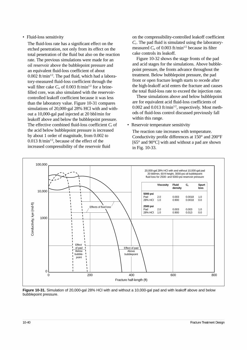
• Fluid-loss sensitivity

The fluid-loss rate has a significant effect on theetched penetration, not only from its effect on thetotal penetration of the fluid but also on the reactionrate. The previous simulations were made for an oil reservoir above the bubblepoint pressure and an equivalent fluid-loss coefficient of about 0.002 ft/min1/2. The pad fluid, which had a labora-tory-measured fluid-loss coefficient through thewall filter cake Cw of 0.003 ft/min1/2 for a brine-filled core, was also simulated with the reservoir-controlled leakoff coefficient because it was lessthan the laboratory value. Figure 10-31 comparessimulations of 20,000-gal 28% HCl with and with-out a 10,000-gal pad injected at 20 bbl/min forleakoff above and below the bubblepoint pressure.The effective combined fluid-loss coefficient Ct ofthe acid below bubblepoint pressure is increased by about 1 order of magnitude, from 0.002 to 0.013 ft/min1/2, because of the effect of theincreased compressibility of the reservoir fluid

on the compressibility-controlled leakoff coefficientCc. The pad fluid is simulated using the laboratory-measured Cw of 0.003 ft/min1/2 because its filtercake controls its leakoff.

Figure 10-32 shows the stage fronts of the padand acid stages for the simulations. Above bubble-point pressure, the fronts advance throughout thetreatment. Below bubblepoint pressure, the padfront or open fracture length starts to recede afterthe high-leakoff acid enters the fracture and causesthe total fluid-loss rate to exceed the injection rate.

These simulations above and below bubblepointare for equivalent acid fluid-loss coefficients of0.002 and 0.013 ft/min1/2, respectively. Most meth-ods of fluid-loss control discussed previously fallwithin this range.

• Reservoir temperature sensitivity

The reaction rate increases with temperature.Conductivity profile differences at 150° and 200°F[65° and 90°C] with and without a pad are shownin Fig. 10-33.

10-40 Fracture Treatment Design

Figure 10-31. Simulation of 20,000-gal 28% HCl with and without a 10,000-gal pad and with leakoff above and belowbubblepoint pressure.

0 200 400 600 8000

1000

10,000

100,000

Con

duct

ivity

, kfw

(md-

ft)

Fracture half-length (ft)

Effect of padBelow

bubble-point

Effect of padAbove

bubblepoint

Effects of fluid loss

20,000-gal 28% HCl with and without 10,000-gal pad20 bbl/min, 60-ft height, 3000-psi oil bubblepoint

fluid loss for 2500- and 5000-psi reservoir pressure

Viscosity Fluid Ct Spurtdensity loss

5000 psiPad 2.0 0.003 0.0018 1.028% HCl 1.0 0.900 0.0018 0.0

2500 psiPad 2.0 0.003 0.003 1.028% HCl 1.0 0.900 0.013 0.0

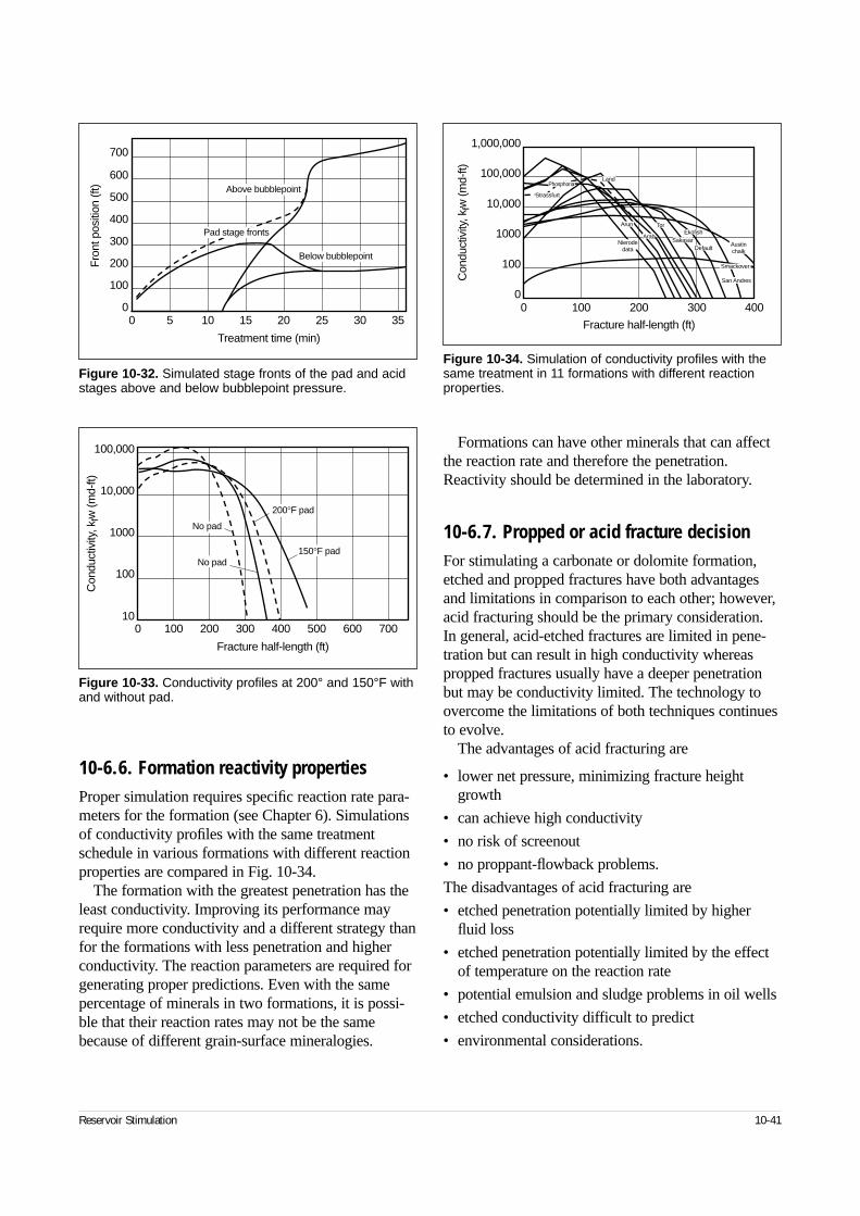
10-6.6. Formation reactivity propertiesProper simulation requires specific reaction rate para-meters for the formation (see Chapter 6). Simulationsof conductivity profiles with the same treatmentschedule in various formations with different reactionproperties are compared in Fig. 10-34.

The formation with the greatest penetration has theleast conductivity. Improving its performance mayrequire more conductivity and a different strategy thanfor the formations with less penetration and higherconductivity. The reaction parameters are required forgenerating proper predictions. Even with the samepercentage of minerals in two formations, it is possi-ble that their reaction rates may not be the samebecause of different grain-surface mineralogies.

Formations can have other minerals that can affectthe reaction rate and therefore the penetration.Reactivity should be determined in the laboratory.

10-6.7. Propped or acid fracture decisionFor stimulating a carbonate or dolomite formation,etched and propped fractures have both advantagesand limitations in comparison to each other; however,acid fracturing should be the primary consideration. In general, acid-etched fractures are limited in pene-tration but can result in high conductivity whereaspropped fractures usually have a deeper penetrationbut may be conductivity limited. The technology toovercome the limitations of both techniques continuesto evolve.

The advantages of acid fracturing are

• lower net pressure, minimizing fracture heightgrowth

• can achieve high conductivity

• no risk of screenout

• no proppant-flowback problems.

The disadvantages of acid fracturing are

• etched penetration potentially limited by higherfluid loss

• etched penetration potentially limited by the effectof temperature on the reaction rate

• potential emulsion and sludge problems in oil wells

• etched conductivity difficult to predict

• environmental considerations.

Reservoir Stimulation 10-41

Figure 10-32. Simulated stage fronts of the pad and acidstages above and below bubblepoint pressure.

0 5 10 15 20 25 30 350

100

200

300

400

500

600

700

Treatment time (min)

Fro

nt p

ositi

on (f

t) Above bubblepoint

Below bubblepoint

Pad stage fronts

Figure 10-33. Conductivity profiles at 200° and 150°F withand without pad.

0 100 200 300 400 500 600 70010

100,000

10,000

1000

100

Con

duct

ivity

, kfw

(md-

ft)

Fracture half-length (ft)

150°F pad

200°F pad

No pad

No pad

Figure 10-34. Simulation of conductivity profiles with thesame treatment in 11 formations with different reactionproperties.

0 2000

1,000,000

100,000

10,000

1000

100

300 400100

Fracture half-length (ft)

Con

duct

ivity

, kfw

(md-

ft)

Nierodedata

San Andres

Smackover

EkofishTor

Default

Arun

Land

Strassfurt

Phosphoria

ArabSakasar

Austinchalk

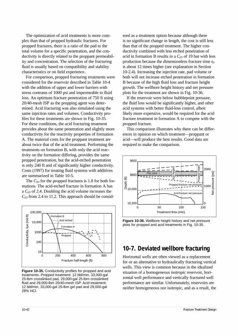
The optimization of acid treatments is more com-plex than that of propped hydraulic fractures. Forpropped fractures, there is a ratio of the pad to thetotal volume for a specific penetration, and the con-ductivity is directly related to the proppant permeabil-ity and concentration. The selection of the fracturingfluid is usually based on compatibility and stabilitycharacteristics or on field experience.

For comparison, propped fracturing treatments wereconsidered for the reservoir described in Table 10-4with the addition of upper and lower barriers withstress contrasts of 1000 psi and impermeable to fluidloss. An optimum fracture penetration of 750 ft using20/40-mesh ISP as the propping agent was deter-mined. Acid fracturing was also simulated using thesame injection rates and volumes. Conductivity pro-files for these treatments are shown in Fig. 10-35. For these conditions, the acid fracturing treatmentprovides about the same penetration and slightly moreconductivity for the reactivity properties of formationA. The material costs for the proppant treatment areabout twice that of the acid treatment. Performing thetreatments on formation B, with only the acid reac-tivity on the formation differing, provides the samepropped penetration, but the acid-etched penetration is only 240 ft and of significantly higher conductivity.Costs (1997) for treating fluid systems with additivesare summarized in Table 10-5.

The CfD for the propped fractures is 1.8 for both for-mations. The acid-etched fracture in formation A hasa CfD of 2.4. Doubling the acid volume increases theCfD from 2.4 to 11.2. This approach should be consid-

ered as a treatment option because although there is no significant change in length, the cost is still lessthan that of the propped treatment. The higher con-ductivity combined with less etched penetration ofacid in formation B results in a CfD of 19 but with lessproduction because the dimensionless fracture time tD

is about 12 times higher (see explanation in Section10-2.4). Increasing the injection rate, pad volume orboth will not increase etched penetration in formationB because of the high fluid loss and fracture heightgrowth. The wellbore height history and net pressureplots for the treatment are shown in Fig. 10-36.

If the reservoir were below bubblepoint pressure,the fluid loss would be significantly higher, and otheracid systems with better fluid-loss control, albeitlikely more expensive, would be required for the acidfracture treatment in formation A to compete with thepropped fracture.

This comparison illustrates why there can be differ-ences in opinion on which treatment—proppant oracid—will produce the best results. Good data arerequired to make the comparison.

10-7. Deviated wellbore fracturingHorizontal wells are often viewed as a replacementfor or an alternative to hydraulically fracturing verticalwells. This view is common because in the idealizedsituation of a homogeneous isotropic reservoir, hori-zontal well performance and vertically fractured wellperformance are similar. Unfortunately, reservoirs areneither homogeneous nor isotropic, and as a result, the

10-42 Fracture Treatment Design

Figure 10-35. Conductivity profiles for propped and acidtreatments. Propped treatment: 12 bbl/min, 33,000-gal 25-lbm crosslinked pad, 29,000-gal 25-lbm crosslinkedfluid and 29,000-lbm 20/40-mesh ISP. Acid treatment: 12 bbl/min, 33,000-gal 25-lbm gel pad and 29,000-gal 28% HCl.

0 20010

100,000

10,000

1000

100

Con

duct

ivity

, kfw

(md-

ft)

Fracture half-length (ft)

400 600 800

Acid etched

Formation B

Propped

Formation A

Figure 10-36. Wellbore height history and net pressureplots for propped and acid treatments in Fig. 10-35.

0 5010,200

9600

9800

10,000Dep

th (f

t)

100 150

Treatment time (min)

0

2000

1000

Net

pre

ssur

e (p

si)

Pro

pped

hei

ght

Pay zoneA

cid

heig

ht

Propped fracture net pressure

Acid fracture net pressure

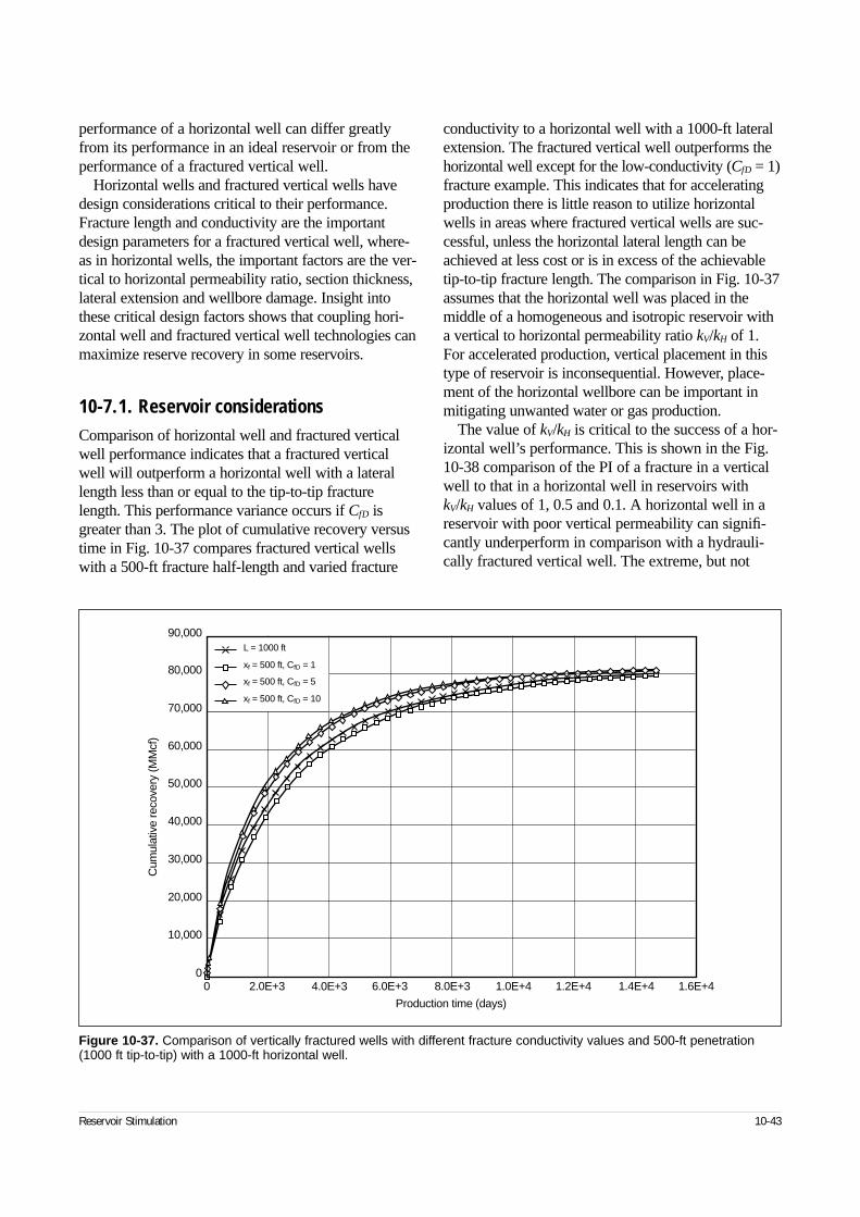
performance of a horizontal well can differ greatlyfrom its performance in an ideal reservoir or from theperformance of a fractured vertical well.

Horizontal wells and fractured vertical wells havedesign considerations critical to their performance.Fracture length and conductivity are the importantdesign parameters for a fractured vertical well, where-as in horizontal wells, the important factors are the ver-tical to horizontal permeability ratio, section thickness,lateral extension and wellbore damage. Insight intothese critical design factors shows that coupling hori-zontal well and fractured vertical well technologies canmaximize reserve recovery in some reservoirs.

10-7.1. Reservoir considerationsComparison of horizontal well and fractured verticalwell performance indicates that a fractured verticalwell will outperform a horizontal well with a laterallength less than or equal to the tip-to-tip fracturelength. This performance variance occurs if CfD isgreater than 3. The plot of cumulative recovery versustime in Fig. 10-37 compares fractured vertical wellswith a 500-ft fracture half-length and varied fracture

conductivity to a horizontal well with a 1000-ft lateralextension. The fractured vertical well outperforms thehorizontal well except for the low-conductivity (CfD = 1)fracture example. This indicates that for acceleratingproduction there is little reason to utilize horizontalwells in areas where fractured vertical wells are suc-cessful, unless the horizontal lateral length can beachieved at less cost or is in excess of the achievabletip-to-tip fracture length. The comparison in Fig. 10-37assumes that the horizontal well was placed in themiddle of a homogeneous and isotropic reservoir witha vertical to horizontal permeability ratio kV/kH of 1.For accelerated production, vertical placement in thistype of reservoir is inconsequential. However, place-ment of the horizontal wellbore can be important inmitigating unwanted water or gas production.

The value of kV/kH is critical to the success of a hor-izontal well’s performance. This is shown in the Fig.10-38 comparison of the PI of a fracture in a verticalwell to that in a horizontal well in reservoirs withkV/kH values of 1, 0.5 and 0.1. A horizontal well in areservoir with poor vertical permeability can signifi-cantly underperform in comparison with a hydrauli-cally fractured vertical well. The extreme, but not

Reservoir Stimulation 10-43

Figure 10-37. Comparison of vertically fractured wells with different fracture conductivity values and 500-ft penetration(1000 ft tip-to-tip) with a 1000-ft horizontal well.

Cum

ulat

ive

reco

very

(MM

cf)

90,000

80,000

70,000

60,000

50,000

40,000

30,000

20,000

10,000

00 2.0E+3 4.0E+3 6.0E+3 8.0E+3 1.0E+4 1.2E+4 1.4E+4 1.6E+4

Production time (days)

L = 1000 ft

xf = 500 ft, CfD = 1

xf = 500 ft, CfD = 5

xf = 500 ft, CfD = 10

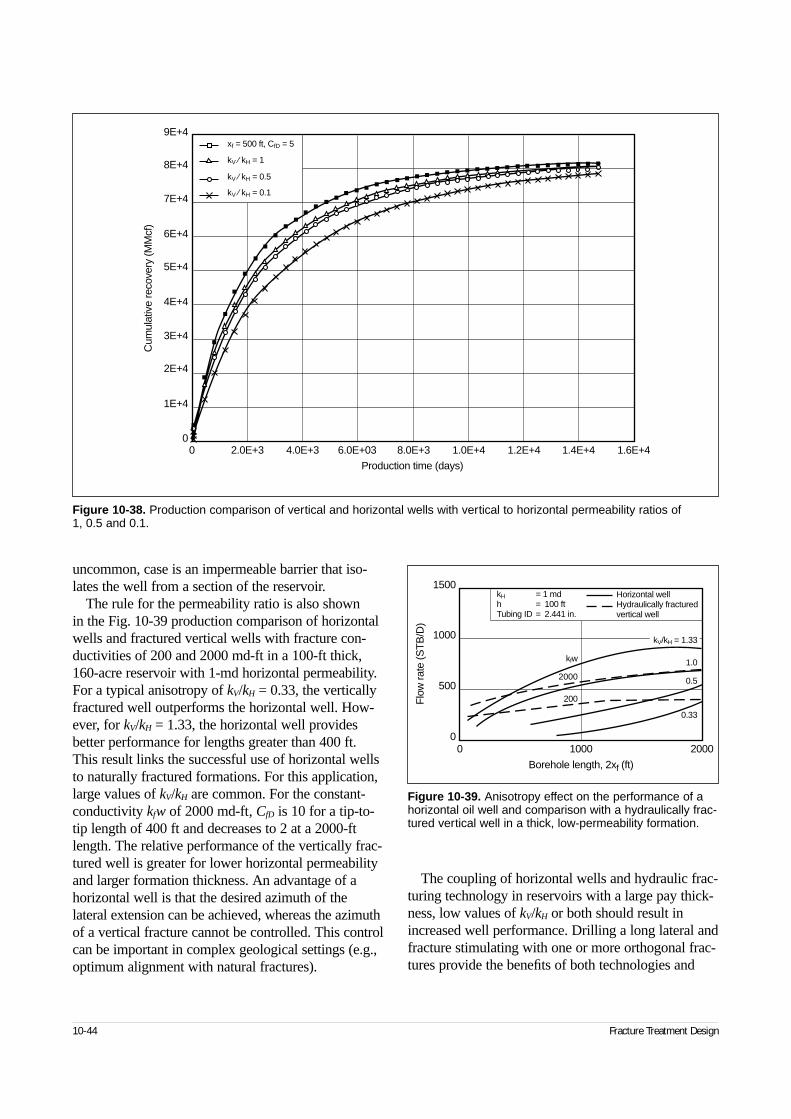
uncommon, case is an impermeable barrier that iso-lates the well from a section of the reservoir.

The rule for the permeability ratio is also shown in the Fig. 10-39 production comparison of horizontalwells and fractured vertical wells with fracture con-ductivities of 200 and 2000 md-ft in a 100-ft thick,160-acre reservoir with 1-md horizontal permeability.For a typical anisotropy of kV/kH = 0.33, the verticallyfractured well outperforms the horizontal well. How-ever, for kV/kH = 1.33, the horizontal well providesbetter performance for lengths greater than 400 ft.This result links the successful use of horizontal wellsto naturally fractured formations. For this application,large values of kV/kH are common. For the constant-conductivity kfw of 2000 md-ft, CfD is 10 for a tip-to-tip length of 400 ft and decreases to 2 at a 2000-ftlength. The relative performance of the vertically frac-tured well is greater for lower horizontal permeabilityand larger formation thickness. An advantage of ahorizontal well is that the desired azimuth of thelateral extension can be achieved, whereas the azimuthof a vertical fracture cannot be controlled. This controlcan be important in complex geological settings (e.g.,optimum alignment with natural fractures).

The coupling of horizontal wells and hydraulic frac-turing technology in reservoirs with a large pay thick-ness, low values of kV/kH or both should result inincreased well performance. Drilling a long lateral andfracture stimulating with one or more orthogonal frac-tures provide the benefits of both technologies and

10-44 Fracture Treatment Design

Figure 10-38. Production comparison of vertical and horizontal wells with vertical to horizontal permeability ratios of 1, 0.5 and 0.1.

Cum

ulat

ive

reco

very

(MM

cf)

9E+4

8E+4

7E+4

6E+4

5E+4

4E+4

3E+4

2E+4

1E+4

00 2.0E+3 4.0E+3 6.0E+03 8.0E+3 1.0E+4 1.2E+4 1.4E+4 1.6E+4

Production time (days)

kV ⁄ kH = 1

kV ⁄ kH = 0.5

kV ⁄ kH = 0.1

xf = 500 ft, CfD = 5

Figure 10-39. Anisotropy effect on the performance of ahorizontal oil well and comparison with a hydraulically frac-tured vertical well in a thick, low-permeability formation.

0 1000 20000

500

1000

1500

Flo

w ra

te (S

TB

/D)

Borehole length, 2xf (ft)

200

2000

kfw

0.33

0.5

1.0

Horizontal wellHydraulically fracturedvertical well

kH = 1 mdh = 100 ftTubing ID = 2.441 in.

kV/kH = 1.33

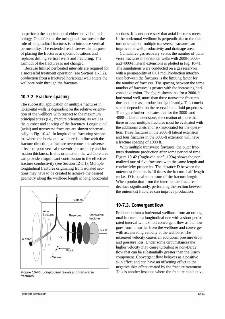
outperform the application of either individual tech-nology. One effect of the orthogonal fractures or therole of longitudinal fractures is to introduce verticalpermeability. The extended reach serves the purposeof placing the fractures at specific locations andreplaces drilling vertical wells and fracturing. Theazimuth of the fractures is not changed.

Because limited perforated intervals are required fora successful treatment operation (see Section 11-3.2),production from a fractured horizontal well enters thewellbore only through the fractures.

10-7.2. Fracture spacingThe successful application of multiple fractures inhorizontal wells is dependent on the relative orienta-tion of the wellbore with respect to the maximumprincipal stress (i.e., fracture orientation) as well asthe number and spacing of the fractures. Longitudinal(axial) and transverse fractures are shown schemati-cally in Fig. 10-40. In longitudinal fracturing scenar-ios where the horizontal wellbore is in line with thefracture direction, a fracture overcomes the adverseeffects of poor vertical reservoir permeability and for-mation thickness. In this orientation, the wellbore areacan provide a significant contribution to the effectivefracture conductivity (see Section 12-5.1). Multiplelongitudinal fractures originating from isolated sec-tions may have to be created to achieve the desiredgeometry along the wellbore length in long horizontal

sections. It is not necessary that axial fractures meet.If the horizontal wellbore is perpendicular to the frac-ture orientation, multiple transverse fractures canimprove the well productivity and drainage area.

Cumulative gas recovery versus the number of trans-verse fractures in horizontal wells with 2000-, 3000-and 4000-ft lateral extensions is plotted in Fig. 10-41.The simulations were conducted on a gas reservoirwith a permeability of 0.01 md. Production interfer-ence between the fractures is the limiting factor for the number of fractures. The spacing between the samenumber of fractures is greater with the increasing hori-zontal extension. The figure shows that for a 2000-fthorizontal well, more than three transverse fracturesdoes not increase production significantly. This conclu-sion is dependent on the reservoir and fluid properties.The figure further indicates that for the 3000- and4000-ft lateral extensions, the creation of more thanthree or four multiple fractures must be evaluated withthe additional costs and risk associated for the opera-tion. Three fractures in the 2000-ft lateral extensionand four fractures in the 3000-ft extension will have a fracture spacing of 1000 ft.

With multiple transverse fractures, the outer frac-tures dominate production after some period of time.Figure 10-42 (Raghavan et al., 1994) shows the nor-malized rate of five fractures with the same length andconductivity properties. The distance D between theoutermost fractures is 10 times the fracture half-lengthxf; i.e., D is equal to the sum of the fracture length.When production from the intermediate fracturesdeclines significantly, perforating the section betweenthe outermost fractures can improve production.

10-7.3. Convergent flowProduction into a horizontal wellbore from an orthog-onal fracture or a longitudinal one with a short perfo-rated interval will exhibit convergent flow as the flowgoes from linear far from the wellbore and convergeswith accelerating velocity at the wellbore. Theincreased velocity causes an additional pressure dropand pressure loss. Under some circumstances thehigher velocity may cause turbulent or non-Darcyflow that can be substantially greater than the Darcycomponent. Convergent flow behaves as a positiveskin effect and can have an offsetting effect to thenegative skin effect created by the fracture treatment.This is another instance where the fracture conductiv-

Reservoir Stimulation 10-45

Figure 10-40. Longitudinal (axial) and transverse fractures.

Surface

Reservoir Transversefractures

Axialfractures

α = 90°

α = 0°

σH,max

σh,min

σv

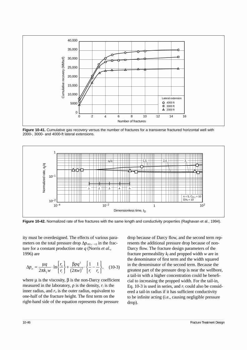
ity must be overdesigned. The effects of various para-meters on the total pressure drop ∆pct(ro – ri) in the frac-ture for a constant production rate q (Norris et al.,1996) are

(10-3)

where µ is the viscosity, β is the non-Darcy coefficientmeasured in the laboratory, ρ is the density, ri is theinner radius, and ro is the outer radius, equivalent toone-half of the fracture height. The first term on theright-hand side of the equation represents the pressure

drop because of Darcy flow, and the second term rep-resents the additional pressure drop because of non-Darcy flow. The fracture design parameters of thefracture permeability kf and propped width w are inthe denominator of first term and the width squared in the denominator of the second term. Because thegreatest part of the pressure drop is near the wellbore,a tail-in with a higher concentration could be benefi-cial to increasing the propped width. For the tail-in,Eq. 10-3 is used in series, and ri could also be consid-ered a tail-in radius if it has sufficient conductivity to be infinite acting (i.e., causing negligible pressuredrop).

10-46 Fracture Treatment Design

Figure 10-41. Cumulative gas recovery versus the number of fractures for a transverse fractured horizontal well with2000-, 3000- and 4000-ft lateral extensions.

0 2 4 6 8 10 12 14 160

40,000

35,000

30,000

25,000

20,000

15,000

10,000

5000

Number of fractures

Cum

ulat

ive

reco

very

(MM

scf)

Lateral extension

4000 ft3000 ft2000 ft

Figure 10-42. Normalized rate of five fractures with the same length and conductivity properties (Raghavan et al., 1994).

10–4 10–2 1 102

Dimensionless time, tD

Nor

mal

ized

rate

, qj/q

10–1

10–2

1

n = 5, CfD,j = 10D/xf = 10

1 2 3 4 5

2,4 31,5qj/q

∆pq

k w

r

r

q

w r rct

f

o

i i o

= ⋅

+( )

⋅ −

µπ

βρπ2 2

1 12

2ln ,

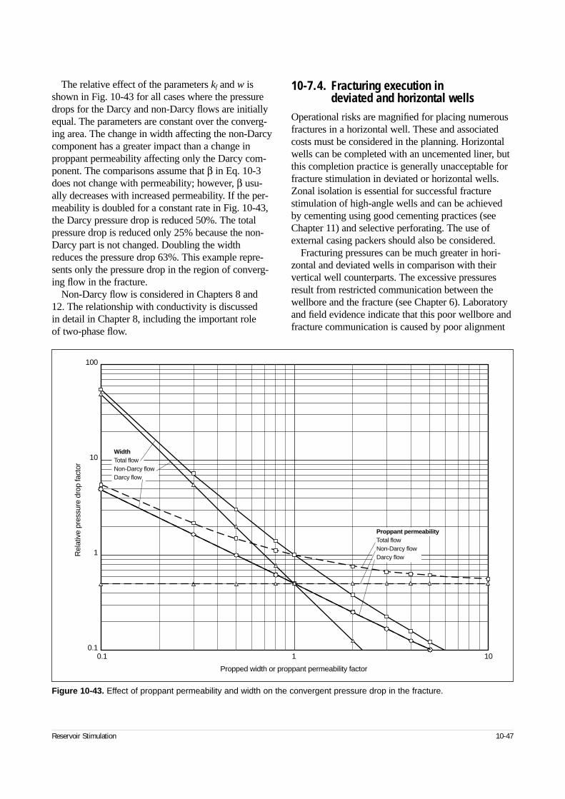
The relative effect of the parameters kf and w isshown in Fig. 10-43 for all cases where the pressuredrops for the Darcy and non-Darcy flows are initiallyequal. The parameters are constant over the converg-ing area. The change in width affecting the non-Darcycomponent has a greater impact than a change inproppant permeability affecting only the Darcy com-ponent. The comparisons assume that β in Eq. 10-3does not change with permeability; however, β usu-ally decreases with increased permeability. If the per-meability is doubled for a constant rate in Fig. 10-43,the Darcy pressure drop is reduced 50%. The totalpressure drop is reduced only 25% because the non-Darcy part is not changed. Doubling the widthreduces the pressure drop 63%. This example repre-sents only the pressure drop in the region of converg-ing flow in the fracture.

Non-Darcy flow is considered in Chapters 8 and 12. The relationship with conductivity is discussed in detail in Chapter 8, including the important role of two-phase flow.

10-7.4. Fracturing execution in deviated and horizontal wells

Operational risks are magnified for placing numerousfractures in a horizontal well. These and associatedcosts must be considered in the planning. Horizontalwells can be completed with an uncemented liner, butthis completion practice is generally unacceptable forfracture stimulation in deviated or horizontal wells.Zonal isolation is essential for successful fracturestimulation of high-angle wells and can be achievedby cementing using good cementing practices (seeChapter 11) and selective perforating. The use ofexternal casing packers should also be considered.

Fracturing pressures can be much greater in hori-zontal and deviated wells in comparison with theirvertical well counterparts. The excessive pressuresresult from restricted communication between thewellbore and the fracture (see Chapter 6). Laboratoryand field evidence indicate that this poor wellbore andfracture communication is caused by poor alignment

Reservoir Stimulation 10-47

Figure 10-43. Effect of proppant permeability and width on the convergent pressure drop in the fracture.

100

10

1

0.1

Rel

ativ

e pr

essu

re d

rop

fact

or

Propped width or proppant permeability factor

0.1 1 10

WidthTotal flowNon-Darcy flowDarcy flow

Proppant permeabilityTotal flowNon-Darcy flowDarcy flow

among the perforations, wellbore and fracture orienta-tion as well as by the creation and propagation ofmultiple fractures. In anticipation of this problem,contingency plans should be made to control exces-sive pressures and establish good communicationbetween the wellbore and main fracture. Some meth-ods are discussed in the following sections.

• Perforation strategy

Perforation plays an extremely important role in theexecution of a hydraulic fracture from a horizontalor deviated well. The perforations represent theonly communication channel between the wellbore(i.e., casing) and the fracture. In horizontal anddeviated well fracturing, as with vertical wells,compromises can be made among the hole size,depth of penetration, shot density and perforationphasing (see Chapter 11).

Perforation alignment with respect to the far-fieldfracture azimuth is the most important aspect ofperforation design. Because in many cases thehydraulic fractures propagate from the base of theperforation tunnel (Behrmann and Elbel, 1992;Morales et al., 1993; Weijers, 1995), the depth ofpenetration is a much less important parameter thanthe diameter of the perforation (see Chapter 11).

For highly deviated wells that are not in the pre-ferred fracture plane, minimizing the length of theperforated interval is used to minimize the creationof multiple fractures (see Chapter 11). One guide-line is that the perforated interval should be limitedto 4 times the wellbore diameter. Thus, for horizon-tal and deviated wells, it is not uncommon to perfo-rate only a 2-ft interval in the wellbore. Extendedperforation intervals can result in multiple frac-tures, putting the fracture stimulation and well per-formance at risk. In the event that a larger intervalis perforated, steps should be taken to attempt tocontrol the creation and propagation of multiplefractures as discussed in the following. Both prop-pant and viscous fluid slugs have been used for thispurpose.

Correctly assessing excessive friction in highlydeviated wells also requires consideration of thepressure drop within the radial region of the frac-ture. This is the injection analog of Eq. 10-3, withthe channel permeability w2/12 substituted for kf

and only the laminar Darcy component applicable.The radically diverging flow component during

injection at high rates and of viscous fluids can be

substantial. Similar to the case of wellbore restric-tions, this component of additional pressure dropdisappears after the shut-in of pumping. An expectedmagnitude for the diverging-flow component canbe obtained from a fracture model that considersthis effect or Eq. 10-3 using the w2/12 substitution.The diverging flow component within a perfectlyconnected fracture can be substantial and may bemisinterpreted as a restriction if this effect is notconsidered.

• Near-wellbore effects

Excessive friction pressure is often cited as evi-dence of multiple fractures, poor wellbore-fracturecommunication or both conditions. It is more com-mon in horizontal or deviated wellbores, which are prone to having high tortuosity resulting frommisalignment and multiple initiation fractures.Techniques used to reduce the excessive pressureare proppant slugs (Cleary et al., 1993; Stadulis,1995), viscous fluid slugs (Aud et al., 1994; Haineyet al., 1995), pretreatment injections and shut-ins,and an extended initial stage of low proppant con-centration to erode restrictions.

Proppant slugs are small volumes of low-concentration proppant slurries that are pumpedahead of or during the main fracture stimulationtreatment. The purpose of the slugs is to screen out some of the multiple fractures so they willcease accepting fluid and propagating. The suc-cessful application of proppant slugs enhances thepropagation of a dominant fracture, which is ofsufficient size (width) and provides the requiredpathway for the fracture treatment slurry. Proppantslugs are pumped at concentrations of up to 4 ppgand are typically overflushed through the perfora-tions. Their role to reduce fracture entry restrictioncan also include erosion effects.

Because excessive friction is considered evi-dence of a near-wellbore problem or multiple frac-tures, the success or failure of proppant slugs ismeasured by the reduction of excess friction pres-sure. The number of proppant slugs pumped shoulddepend on whether the excessive friction is beingreduced. Therefore, the final design of this part ofthe fracturing operation must be performed on loca-tion and requires reliable downhole injection pres-sure data. As long as entry friction pressurereduction occurs, the proppant slugs should be con-tinued. Once no additional reduction of the entry

10-48 Fracture Treatment Design

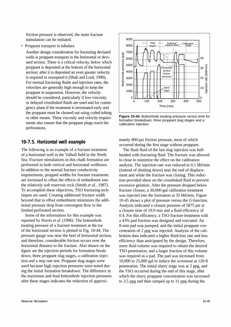
friction pressure is observed, the main fracturestimulation can be initiated.

• Proppant transport in tubulars

Another design consideration for fracturing deviatedwells is proppant transport in the horizontal or devi-ated section. There is a critical velocity, below whichproppant is deposited at the bottom of the horizontalsection; after it is deposited an even greater velocityis required to resuspend it (Shah and Lord, 1990).For normal fracturing fluids and injection rates, thevelocities are generally high enough to keep theproppant in suspension. However, the velocityshould be considered, particularly if low-viscosity or delayed crosslinked fluids are used and for contin-gency plans if the treatment is terminated early andthe proppant must be cleaned out using coiled tubingor other means. These viscosity and velocity require-ments also ensure that the proppant plugs reach theperforations.

10-7.5. Horizontal well exampleThe following is an example of a fracture treatment of a horizontal well in the Valhall field in the NorthSea. Fracture stimulations in this chalk formation areperformed in both vertical and horizontal wellbores.In addition to the normal fracture conductivityrequirements, propped widths for fracture treatmentsare increased to offset the effects of embedment intothe relatively soft reservoir rock (Smith et al., 1987).To accomplish these objectives, TSO fracturing tech-niques are used. Creating additional fracture widthbeyond that to offset embedment minimizes the addi-tional pressure drop from convergent flow to thelimited perforated section.

Some of the information for this example wasreported by Norris et al. (1996). The bottomholetreating pressure of a fracture treatment at the toe of the horizontal section is plotted in Fig. 10-44. Thepressure gauge was near the heel of horizontal section,and therefore, considerable friction occurs over thehorizontal distance to the fracture. Also shown on thefigure are the injection periods for formation break-down, three proppant slug stages, a calibration injec-tion and a step rate test. Proppant slug stages wereused because high injection pressures were noted dur-ing the initial formation breakdown. The difference inthe maximum and final bottomhole injection pressuresafter these stages indicates the reduction of approxi-

mately 800-psi friction pressure, most of whichoccurred during the first stage without proppant.

The flush fluid of the last slug injection was bull-headed with fracturing fluid. The fracture was allowedto close to minimize the effect on the calibrationanalysis. The injection rate was reduced to 0.1 bbl/min(instead of shutting down) near the end of displace-ment and while the fracture was closing. This reduc-tion provided shear on the crosslinked fluid to preventexcessive gelation. After the pressure dropped belowfracture closure, a 30,000-gal calibration treatmentwas injected into the formation at 35 bbl/min. Figure10-45 shows a plot of pressure versus the G-function.Analysis indicated a closure pressure of 5875 psi at a closure time of 19.9 min and a fluid efficiency of0.4. For this efficiency, a TSO fracture treatment witha 43% pad fraction was designed and executed. An 8-min pad was pumped, and the initial proppant con-centration of 2 ppg was injected. Analysis of the cali-bration data indicated a higher fluid-loss rate and lessefficiency than anticipated by the design. Therefore,more fluid volume was required to obtain the desiredTSO penetration, and a larger fraction of this volumewas required as a pad. The pad was increased from10,000 to 25,000 gal to induce the screenout at 120-ftpenetration. The initial slurry stage was at 2 ppg, andthe TSO occurred during the end of this stage, afterwhich the slurry proppant concentration was increasedto 3.5 ppg and then ramped up to 11 ppg during the

Reservoir Stimulation 10-49

Figure 10-44. Bottomhole treating pressure versus time forformation breakdown, three proppant slug stages and acalibration injection.

0 100 200 300 400 5000

1000

2000

4000

5000

6000

7000

8000

9000

3000

Bot

tom

hole

pre

ssur

e (p

si)

Time (min)

0

10

20

30

40

Inje

ctio

n ra

te (b

bl/m

in)

Sandslugs

Slugstages

Calibrationstage

Horizontalsectionfriction

pressure

Bullheadfracture fluid

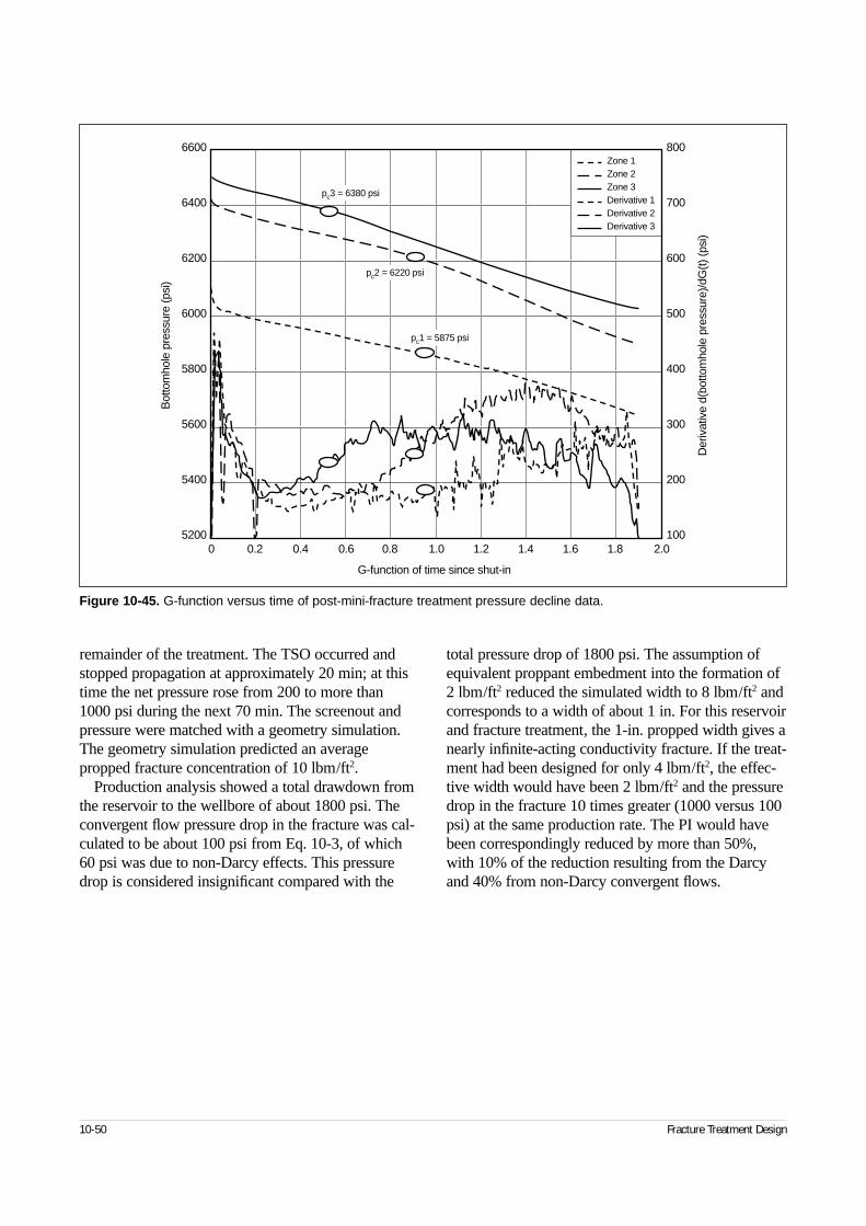
remainder of the treatment. The TSO occurred andstopped propagation at approximately 20 min; at thistime the net pressure rose from 200 to more than 1000 psi during the next 70 min. The screenout andpressure were matched with a geometry simulation.The geometry simulation predicted an averagepropped fracture concentration of 10 lbm/ft2.

Production analysis showed a total drawdown fromthe reservoir to the wellbore of about 1800 psi. Theconvergent flow pressure drop in the fracture was cal-culated to be about 100 psi from Eq. 10-3, of which60 psi was due to non-Darcy effects. This pressuredrop is considered insignificant compared with the

total pressure drop of 1800 psi. The assumption ofequivalent proppant embedment into the formation of2 lbm/ft2 reduced the simulated width to 8 lbm/ft2 andcorresponds to a width of about 1 in. For this reservoirand fracture treatment, the 1-in. propped width gives anearly infinite-acting conductivity fracture. If the treat-ment had been designed for only 4 lbm/ft2, the effec-tive width would have been 2 lbm/ft2 and the pressuredrop in the fracture 10 times greater (1000 versus 100psi) at the same production rate. The PI would havebeen correspondingly reduced by more than 50%,with 10% of the reduction resulting from the Darcyand 40% from non-Darcy convergent flows.

10-50 Fracture Treatment Design

Figure 10-45. G-function versus time of post-mini-fracture treatment pressure decline data.

6600

6400

6200

6000

5800

5600

5400

5200

Bot

tom

hole

pre

ssur

e (p

si)

800

700

600

500

400

300

200

100

Der

ivat

ive

d(bo

ttom

hole

pre

ssur

e)/d

G(t)

(psi

)

0 0.2 0.4 0.6 0.8 1.0 1.2 1.4 1.6 1.8 2.0

G-function of time since shut-in

pc3 = 6380 psi

pc1 = 5875 psi

pc2 = 6220 psi

Zone 1Zone 2Zone 3Derivative 1Derivative 2Derivative 3

11-1. IntroductionHydraulic fracturing is a particularly complicatedenterprise. The purpose of hydraulic fracturing is theplacement of an optimum fracture of a certain geom-etry and conductivity to allow maximum incrementalproduction (over that of the unstimulated well) at thelowest cost. This process combines the interactions of fluid pressure, viscosity and leakoff characteristicswith the elastic properties of the rock, which havebeen the subjects of the preceding chapters.

Accomplishing this, while taking into account allthe presented technology, requires significant atten-tion to the treatment execution involving optimizedcompletion and perforating strategies, appropriatetreatment design, control and monitoring of rate, andpressure and fluid characteristics.

11-2. CompletionsUntil recently, the majority of wellbores have beenvertical and designed to produce from a single pro-duction string. Other types of completions that can be planned and performed are

• deviated wells

• horizontal wells

• multiple completions

• multiple laterals.

The choice of the type of completion shouldaccount for all considerations, ranging from drillingto production to abandonment.

11-2.1. Deviated and S-shaped completionsPrecompletion and drilling planning should be givenserious thought in cases where fracturing may beconsidered for highly deviated wellbores. It is impor-tant to understand the relationship between the well-bore angle, formation in-situ stress fields (dictating

fracture orientation) and potential fracture geometryunder these conditions.

Fracture initiation from wellbores that are notaligned with one of the principal stress directions canbe complex. In these cases, fractures may not be asimple singular planar feature. Misalignment maylead to the initiation of either multiple near-wellborefractures or fractures that that are forced to twist andchange direction to ultimately reorient and align withthe far-field minimum horizontal stress. Potentialproblems can affect the geometry and productivity of the fractures; there may be limited fracture com-munication with the wellbore, and the fracture widthprofile at or near the wellbore may be restricted. A restriction or reduced width can be sufficient tocause proppant bridging during the treatment, poten-tially resulting in an early screenout and restrictedproduction after treatment.

Planning for an S-shaped completion, where theextended reach wellbore is brought back to a morevertical or 90° attitude through the formation, is gen-erally advisable. The connectivity of a well and frac-ture is always important, but it is critical in high-permeability fracturing. Although tortuosity is aproblem that affects all fractures during both execu-tion and production, limited exposure is not a majorissue in low-permeability reservoirs; it is in high-permeability formations. Thus, deviated wellboreswith limited perforated intervals may provide attrac-tive fracture treatments (although S-shaped wells are even better). However, for high-permeabilityfracturing both S-shaped wellbores and 180° phased,oriented perforations or slots cut along the welltrajectory are highly advisable. This approach isintended to safeguard against further reducing a natu-rally small fracture conductivity (Chen and Econo-mides, 1998). Wellbore angles of less than 20° maybe necessary to achieve optimum fracture geometryand performance. In general, production engineeringconsiderations suggest that the wellbore orientationshould coincide with the fracture orientation. The

Reservoir Stimulation 11-1

◆

Fracturing Operations

J. E. Brown and R. W. Thrasher, Schlumberger DowellL. A. Behrmann, Schlumberger Wireline & Testing

wellbore orientation can be either vertical or horizontal.In the horizontal mode, the wellbore must be placed to have either longitudinal or transverse fractures. Iftransverse fractures are created, multiple treatmentswill have to be performed that will require properzonal isolation.

11-2.2.Horizontal and multilateral completions

Effective stimulation of horizontal wellbores requiresspecific completion procedures. In addition to the nor-mal considerations for pressure and flow rates, hori-zontal completions must address the problems associ-ated with treatment placement into or along the zoneor zones of interest. In the case of executing severalhydraulic fracture treatments along a single horizontalwellbore, the completion requirements can be compli-cated and extensive. Zonal isolation for each individ-ual treatment must be part of the completion design.This requires cementing the entire liner, using externalcasing packers, placing permanently installed selective-zone mechanical tools and/or using retrievable zonalisolation tools. Coiled tubing is commonly used toplace and operate zonal isolation tools in deviated andhorizontal wells and multilateral completions.

The use of multilaterals can provide better reservoirdrainage and management. Laterals could conceivablyreplace the need for fracturing in some cases. In othercases, optimum reservoir drainage may require a com-bination of laterals and stimulation. For these compli-cated completions, proper planning is essential. SeeChapter 1 for an extensive discussion of appropriatewell paths to match specific geological flow units.

11-2.3. Slimhole and monobore completionsSlimhole and monobore completions are used tolower drilling and completion costs. Slimhole com-pletions can result in production casing sizes as smallas 2 in. Tubulars, which are generally considered pro-duction tubing, become both casing and productiontubulars. These small diameters can prohibit the use of special stimulation tubulars, which in turn maylimit treating pressures.

The need to drill and complete wells at less cost isevident, but there may be a trade-off when stimulationmust be considered. The small tubulars used in slim-hole and monobore completions can limit the applica-

tion of stimulation. Because of the reduced wellborediameters, surface treating pressures are increasedowing to excessive friction pressures. This limits therate and size of treatments that can be pumped andtherefore reduces the effectiveness of the stimulationtreatment. Small tubulars also limit the application of downhole tools; e.g., the stimulation of multiplezones is prevented because zonal isolation tools can-not be applied.

If it is considered essential to use slimhole com-pletion techniques, the completion design shouldspecify heavy-walled tubing as casing. This allowsusing higher pump rates for the higher treating pres-sure limitations.

11-2.4. Zonal isolationUsually there are several potential producing zonespenetrated by a wellbore that must be hydraulicallyfractured. To ensure that each zone is stimulatedeffectively, these intervals must be isolated from oneanother. Several isolation methods have proved to be effective. These methods can be used only whenthe various formations and intervals are isolated fromeach other behind the casing with cement.

• Importance of the cement sheath

The cement sheath must provide zonal isolationduring both production and stimulation operations.For a producing well, the cement seal between thepipe and formation must be tight to prevent fluidsfrom flowing through the annular area (see Side-bar 11A). The permeability of a set Portlandcement of normal density is in the low microdarcyrange. If the cement does not bond perfectly toeither the pipe or the formation and a small channelremains, the effective cement permeability can besignificantly increased. Large permeabilities mayresult from channel widths that are quite small(Nelson, 1990). For example, a channel width ofonly 1.4 × 10–4 in. is sufficient to create an effectivecement permeability of 1000 md. Channel perme-abilities of this order may allow significant cross-flow between zones.

During hydraulic fracturing these small channels,or microannuli, are relatively insignificant. Theeffective cement permeability does not create ahigh leakoff risk for the fracturing fluid within theannulus. A leakoff rate for a microannulus is lessthan 1 gal/min. If major channels within the cement

11-2 Fracturing Operations

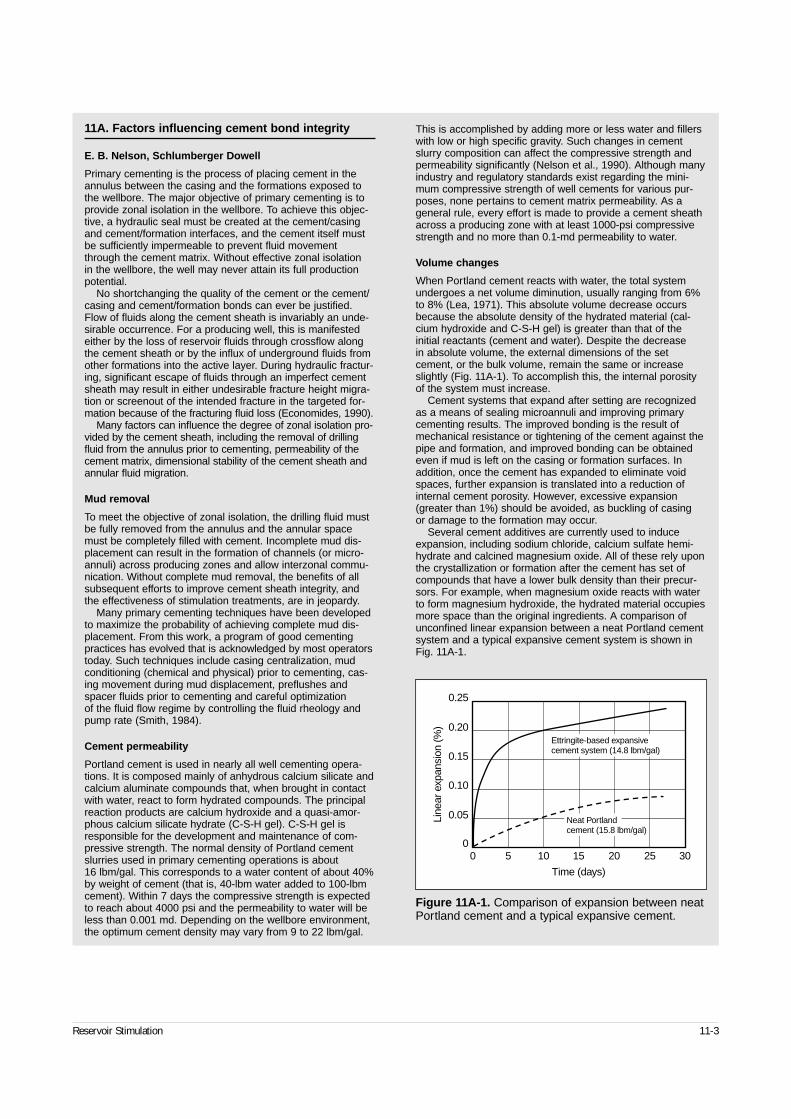
Reservoir Stimulation 11-3

11A. Factors influencing cement bond integrity

E. B. Nelson, Schlumberger Dowell

Primary cementing is the process of placing cement in theannulus between the casing and the formations exposed tothe wellbore. The major objective of primary cementing is toprovide zonal isolation in the wellbore. To achieve this objec-tive, a hydraulic seal must be created at the cement/casingand cement/formation interfaces, and the cement itself mustbe sufficiently impermeable to prevent fluid movementthrough the cement matrix. Without effective zonal isolationin the wellbore, the well may never attain its full productionpotential.

No shortchanging the quality of the cement or the cement/casing and cement/formation bonds can ever be justified.Flow of fluids along the cement sheath is invariably an unde-sirable occurrence. For a producing well, this is manifestedeither by the loss of reservoir fluids through crossflow alongthe cement sheath or by the influx of underground fluids fromother formations into the active layer. During hydraulic fractur-ing, significant escape of fluids through an imperfect cementsheath may result in either undesirable fracture height migra-tion or screenout of the intended fracture in the targeted for-mation because of the fracturing fluid loss (Economides, 1990).

Many factors can influence the degree of zonal isolation pro-vided by the cement sheath, including the removal of drillingfluid from the annulus prior to cementing, permeability of thecement matrix, dimensional stability of the cement sheath andannular fluid migration.

Mud removal

To meet the objective of zonal isolation, the drilling fluid mustbe fully removed from the annulus and the annular spacemust be completely filled with cement. Incomplete mud dis-placement can result in the formation of channels (or micro-annuli) across producing zones and allow interzonal commu-nication. Without complete mud removal, the benefits of allsubsequent efforts to improve cement sheath integrity, andthe effectiveness of stimulation treatments, are in jeopardy.

Many primary cementing techniques have been developedto maximize the probability of achieving complete mud dis-placement. From this work, a program of good cementingpractices has evolved that is acknowledged by most operatorstoday. Such techniques include casing centralization, mudconditioning (chemical and physical) prior to cementing, cas-ing movement during mud displacement, preflushes andspacer fluids prior to cementing and careful optimization of the fluid flow regime by controlling the fluid rheology andpump rate (Smith, 1984).

Cement permeability

Portland cement is used in nearly all well cementing opera-tions. It is composed mainly of anhydrous calcium silicate andcalcium aluminate compounds that, when brought in contactwith water, react to form hydrated compounds. The principalreaction products are calcium hydroxide and a quasi-amor-phous calcium silicate hydrate (C-S-H gel). C-S-H gel isresponsible for the development and maintenance of com-pressive strength. The normal density of Portland cementslurries used in primary cementing operations is about 16 lbm/gal. This corresponds to a water content of about 40% by weight of cement (that is, 40-lbm water added to 100-lbmcement). Within 7 days the compressive strength is expectedto reach about 4000 psi and the permeability to water will beless than 0.001 md. Depending on the wellbore environment,the optimum cement density may vary from 9 to 22 lbm/gal.

This is accomplished by adding more or less water and fillerswith low or high specific gravity. Such changes in cementslurry composition can affect the compressive strength andpermeability significantly (Nelson et al., 1990). Although manyindustry and regulatory standards exist regarding the mini-mum compressive strength of well cements for various pur-poses, none pertains to cement matrix permeability. As ageneral rule, every effort is made to provide a cement sheathacross a producing zone with at least 1000-psi compressivestrength and no more than 0.1-md permeability to water.

Volume changes

When Portland cement reacts with water, the total systemundergoes a net volume diminution, usually ranging from 6%to 8% (Lea, 1971). This absolute volume decrease occursbecause the absolute density of the hydrated material (cal-cium hydroxide and C-S-H gel) is greater than that of theinitial reactants (cement and water). Despite the decrease in absolute volume, the external dimensions of the setcement, or the bulk volume, remain the same or increaseslightly (Fig. 11A-1). To accomplish this, the internal porosityof the system must increase.

Cement systems that expand after setting are recognizedas a means of sealing microannuli and improving primarycementing results. The improved bonding is the result ofmechanical resistance or tightening of the cement against thepipe and formation, and improved bonding can be obtainedeven if mud is left on the casing or formation surfaces. Inaddition, once the cement has expanded to eliminate voidspaces, further expansion is translated into a reduction ofinternal cement porosity. However, excessive expansion(greater than 1%) should be avoided, as buckling of casing or damage to the formation may occur.

Several cement additives are currently used to induceexpansion, including sodium chloride, calcium sulfate hemi-hydrate and calcined magnesium oxide. All of these rely uponthe crystallization or formation after the cement has set ofcompounds that have a lower bulk density than their precur-sors. For example, when magnesium oxide reacts with waterto form magnesium hydroxide, the hydrated material occupiesmore space than the original ingredients. A comparison ofunconfined linear expansion between a neat Portland cementsystem and a typical expansive cement system is shown inFig. 11A-1.

Figure 11A-1. Comparison of expansion between neatPortland cement and a typical expansive cement.

Time (days)

0.05

0

0.10

0.15

0.20

0.25

Line

ar e

xpan

sion

(%)

0 5 10 15 20 25 30

Neat Portlandcement (15.8 lbm/gal)

Ettringite-based expansivecement system (14.8 lbm/gal)

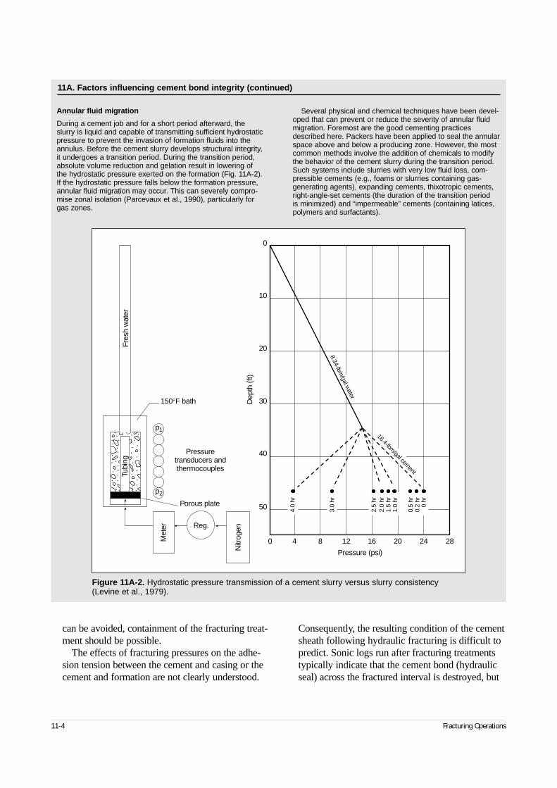
can be avoided, containment of the fracturing treat-ment should be possible.

The effects of fracturing pressures on the adhe-sion tension between the cement and casing or thecement and formation are not clearly understood.

Consequently, the resulting condition of the cementsheath following hydraulic fracturing is difficult topredict. Sonic logs run after fracturing treatmentstypically indicate that the cement bond (hydraulicseal) across the fractured interval is destroyed, but

Annular fluid migration

During a cement job and for a short period afterward, theslurry is liquid and capable of transmitting sufficient hydrostaticpressure to prevent the invasion of formation fluids into theannulus. Before the cement slurry develops structural integrity,it undergoes a transition period. During the transition period,absolute volume reduction and gelation result in lowering ofthe hydrostatic pressure exerted on the formation (Fig. 11A-2).If the hydrostatic pressure falls below the formation pressure,annular fluid migration may occur. This can severely compro-mise zonal isolation (Parcevaux et al., 1990), particularly forgas zones.

Several physical and chemical techniques have been devel-oped that can prevent or reduce the severity of annular fluidmigration. Foremost are the good cementing practicesdescribed here. Packers have been applied to seal the annularspace above and below a producing zone. However, the mostcommon methods involve the addition of chemicals to modifythe behavior of the cement slurry during the transition period.Such systems include slurries with very low fluid loss, com-pressible cements (e.g., foams or slurries containing gas-generating agents), expanding cements, thixotropic cements,right-angle-set cements (the duration of the transition period is minimized) and “impermeable” cements (containing latices,polymers and surfactants).

11-4 Fracturing Operations

Figure 11A-2. Hydrostatic pressure transmission of a cement slurry versus slurry consistency(Levine et al., 1979).

50

40

30

20

10

0

40 8 12 16 20 24 28

Pressure (psi)

Dep

th (f

t)

8.34-lbm/gal w

ater

16.4-lbm/gal cem

ent

2.5

hr2.

0 hr

1.5

hr1.

0 hr

0.5

hr0.

2 hr

0 hr

Nitr

ogen

Met

er Reg.

Pressuretransducers andthermocouples

150°F bath

Porous plate

p1

p2

Tubi

ngFr

esh

wat

er

.......

. .... .... . .

.

.. ....

. ..

. ..

4.0

hr

3.0

hr

11A. Factors influencing cement bond integrity (continued)

the bond farther uphole remains intact. The loss ofthe cement bond across the fractured interval prob-ably does not affect the placement or containmentof the fracturing treatment. Cement of relativelylow compressive strength should prevent the frac-ture from migrating between the casing and theformation; however, alteration of the cement bondmay occur during the treatment. Any failure of thehydraulic seal may result in a microannulus thatwill lead to the crossflow of reservoir fluids.

• Fracture placement control

The most reliable method of controlling the place-ment of fracturing fluids is to limit perforations to a single zone. When several zones of a well are tobe stimulated, the individual zones can be isolatedfrom one another and stimulated individually. Thiscan be accomplished through progressive perfora-tion and stimulation. After a fracturing treatmenthas been placed in the first zone, it is isolated, andanother zone of interest is perforated and treated inanother single stage. Of course, this methodologyworks best when the deepest zone is completed firstand subsequent zones are individually stimulatedby working uphole.

Another effective multizone stimulation tech-nique is coiled tubing–conveyed treatment (seeSidebar 11B). Other multilayer fracturing techniquesthat can be used are discussed in Chapter 10.

• Mechanical bridge plugs

Several mechanical methods are available to pro-vide adequate isolation between perforated zones.The most reliable method is the use of mechanicalbridge plugs, which can be run on tubulars or wire-line. Bridge plugs that are run on tubulars areretrievable and can be moved and reset severaltimes. Wireline bridge plugs cannot be moved onceset, and their removal typically requires millingafter the treatment. Wireline bridge plugs are usedwhen several treatments are attempted in one dayor when a rig is not over the hole during the treat-ment. They can be run in the hole quickly, andcleanout trips are not required between stages. Theretrievable bridge plugs are used when zones areindividually tested before another zone is opened.Any excess proppant must be circulated out of thehole before the tool is moved to prevent the prop-pant from sticking the tool. A typical treatmentinvolves perforation of the bottom zone, hydraulicfracture treatment and zonal isolation by setting

a bridge plug immediately above the perforated in-terval. The next zone is then perforated and fractured.

• Sand plugs

A similar method of isolation can be achieved byusing sand plugs after the fracturing treatment. Thevolume of sand necessary to cover the perforatedinterval is added to the casing. The sand plug istested by applying pressure to the casing, and thenthe next zone is perforated and stimulated. Once allzones have been fracture stimulated, the sand canbe circulated out of the wellbore by using eitherconventional or coiled tubing. The amount of sandrequired above the top perforations is generallysmall and can be calculated by applying Darcy’slaw to linear flow:

(11-1)

where qi is the rate in bbl/min, A is area in ft2, k ispermeability in darcies, ∆p is the pressure drop inpsi, µ is viscosity in cp, and L is the length in ft.Using this expression, 10 ft of 20/40-mesh sand in51⁄2-in. casing will create a pressure drop of morethan 6000 psi for a 40-cp linear gel leaking throughthe sand pack at 0.5 bbl/min. A mixture of sandmeshes can be used if the permeability of the sandpack must be reduced to prevent flow through thepack.

• Frac baffles

Mechanical diversion can also be accomplished byusing frac baffles. Frac baffles are run as part of thecasing string and are placed between individualproducing zones. After the lowest interval is perfo-rated and fractured, a ball is dropped down the cas-ing. The ball seats on the baffle and prevents fluidflow below this point. The next zone can then beperforated and fracture stimulated. When multiplezones are isolated with baffles, care must be takento place the baffles so that the baffle openings pro-gressively decrease in size from top to bottom; i.e.,the bottom frac baffle has the smallest diameteropening. The first ball must be able to pass throughthe upper baffles and still seat in the bottom baffle.Similarly, the second ball must pass through theupper baffles and seat in the second baffle from the bottom, and so on.

All baffles have an inherent weakness owing tothe limited area available in the casing coupling.The pressure differential across the baffle should

Reservoir Stimulation 11-5

qAk p

Li = ×

−7 827 10 4. ,∆

µ

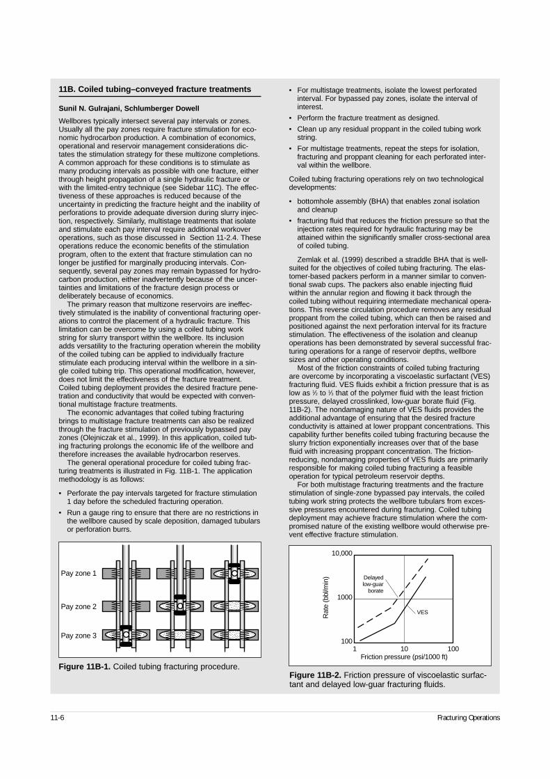
11-6 Fracturing Operations

11B. Coiled tubing–conveyed fracture treatments

Sunil N. Gulrajani, Schlumberger Dowell

Wellbores typically intersect several pay intervals or zones.Usually all the pay zones require fracture stimulation for eco-nomic hydrocarbon production. A combination of economics,operational and reservoir management considerations dic-tates the stimulation strategy for these multizone completions.A common approach for these conditions is to stimulate asmany producing intervals as possible with one fracture, eitherthrough height propagation of a single hydraulic fracture orwith the limited-entry technique (see Sidebar 11C). The effec-tiveness of these approaches is reduced because of theuncertainty in predicting the fracture height and the inability ofperforations to provide adequate diversion during slurry injec-tion, respectively. Similarly, multistage treatments that isolateand stimulate each pay interval require additional workoveroperations, such as those discussed in Section 11-2.4. Theseoperations reduce the economic benefits of the stimulationprogram, often to the extent that fracture stimulation can nolonger be justified for marginally producing intervals. Con-sequently, several pay zones may remain bypassed for hydro-carbon production, either inadvertently because of the uncer-tainties and limitations of the fracture design process ordeliberately because of economics.

The primary reason that multizone reservoirs are ineffec-tively stimulated is the inability of conventional fracturing oper-ations to control the placement of a hydraulic fracture. Thislimitation can be overcome by using a coiled tubing workstring for slurry transport within the wellbore. Its inclusionadds versatility to the fracturing operation wherein the mobilityof the coiled tubing can be applied to individually fracturestimulate each producing interval within the wellbore in a sin-gle coiled tubing trip. This operational modification, however,does not limit the effectiveness of the fracture treatment.Coiled tubing deployment provides the desired fracture pene-tration and conductivity that would be expected with conven-tional multistage fracture treatments.

The economic advantages that coiled tubing fracturingbrings to multistage fracture treatments can also be realizedthrough the fracture stimulation of previously bypassed payzones (Olejniczak et al., 1999). In this application, coiled tub-ing fracturing prolongs the economic life of the wellbore andtherefore increases the available hydrocarbon reserves.

The general operational procedure for coiled tubing frac-turing treatments is illustrated in Fig. 11B-1. The applicationmethodology is as follows:

• Perforate the pay intervals targeted for fracture stimulation1 day before the scheduled fracturing operation.

• Run a gauge ring to ensure that there are no restrictions inthe wellbore caused by scale deposition, damaged tubularsor perforation burrs.

• For multistage treatments, isolate the lowest perforatedinterval. For bypassed pay zones, isolate the interval ofinterest.

• Perform the fracture treatment as designed.

• Clean up any residual proppant in the coiled tubing workstring.

• For multistage treatments, repeat the steps for isolation,fracturing and proppant cleaning for each perforated inter-val within the wellbore.

Coiled tubing fracturing operations rely on two technologicaldevelopments:

• bottomhole assembly (BHA) that enables zonal isolationand cleanup

• fracturing fluid that reduces the friction pressure so that theinjection rates required for hydraulic fracturing may beattained within the significantly smaller cross-sectional areaof coiled tubing.

Zemlak et al. (1999) described a straddle BHA that is well-suited for the objectives of coiled tubing fracturing. The elas-tomer-based packers perform in a manner similar to conven-tional swab cups. The packers also enable injecting fluidwithin the annular region and flowing it back through thecoiled tubing without requiring intermediate mechanical opera-tions. This reverse circulation procedure removes any residualproppant from the coiled tubing, which can then be raised andpositioned against the next perforation interval for its fracturestimulation. The effectiveness of the isolation and cleanupoperations has been demonstrated by several successful frac-turing operations for a range of reservoir depths, wellboresizes and other operating conditions.

Most of the friction constraints of coiled tubing fracturingare overcome by incorporating a viscoelastic surfactant (VES)fracturing fluid. VES fluids exhibit a friction pressure that is aslow as 1⁄2 to 1⁄3 that of the polymer fluid with the least frictionpressure, delayed crosslinked, low-guar borate fluid (Fig. 11B-2). The nondamaging nature of VES fluids provides theadditional advantage of ensuring that the desired fractureconductivity is attained at lower proppant concentrations. Thiscapability further benefits coiled tubing fracturing because theslurry friction exponentially increases over that of the basefluid with increasing proppant concentration. The friction-reducing, nondamaging properties of VES fluids are primarilyresponsible for making coiled tubing fracturing a feasibleoperation for typical petroleum reservoir depths.

For both multistage fracturing treatments and the fracturestimulation of single-zone bypassed pay intervals, the coiledtubing work string protects the wellbore tubulars from exces-sive pressures encountered during fracturing. Coiled tubingdeployment may achieve fracture stimulation where the com-promised nature of the existing wellbore would otherwise pre-vent effective fracture stimulation.

Figure 11B-1. Coiled tubing fracturing procedure.

Pay zone 1

Pay zone 2

Pay zone 3

Figure 11B-2. Friction pressure of viscoelastic surfac-tant and delayed low-guar fracturing fluids.

10,000

1000

1001 10 100

Rat

e (b

bl/m

in)

Friction pressure (psi/1000 ft)

VES

Delayedlow-guar

borate

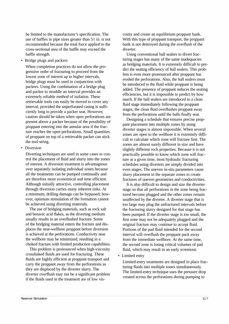
be limited to the manufacturer’s specification. Theuse of baffles in pipe sizes greater than 51⁄2 in. is notrecommended because the total force applied to thecross-sectional area of the baffle may exceed thebaffle strength.

• Bridge plugs and packers

When completion practices do not allow the pro-gressive order of fracturing to proceed from thelowest zone of interest up to higher intervals,bridge plugs must be used in conjunction withpackers. Using the combination of a bridge plugand packer to straddle an interval provides anextremely reliable method of isolation. Theseretrievable tools can easily be moved to cover anyinterval, provided the unperforated casing is suffi-ciently long to provide a packer seat. However,caution should be taken when open perforations arepresent above a packer because of the possibility ofproppant entering into the annular area if the frac-ture reaches the open perforations. Small quantitiesof proppant on top of a retrievable packer can stickthe tool string.

• Diversion

Diverting techniques are used in some cases to con-trol the placement of fluid and slurry into the zonesof interest. A diversion treatment is advantageousover separately isolating individual zones becauseall the treatments can be pumped continually andare therefore more economical and time efficient.Although initially attractive, controlling placementthrough diversion carries many inherent risks. At a minimum, drilling damage can be bypassed; how-ever, optimum stimulation of the formation cannotbe achieved using diverting materials.

The use of bridging materials, such as rock saltand benzoic acid flakes, as the diverting mediumusually results in an overflushed fracture. Some of the bridging material enters the fracture and dis-places the near-wellbore proppant before diversionis achieved at the perforations. Conductivity nearthe wellbore may be minimized, resulting in achoked fracture with limited production capabilities.

This problem is pronounced when high-viscositycrosslinked fluids are used for fracturing. Thesefluids are highly efficient at proppant transport andcarry the proppant away from the perforations asthey are displaced by the diverter slurry. Thediverter overflush may not be a significant problemif the fluids used in the treatment are of low vis-

cosity and create an equilibrium proppant bank.With this type of proppant transport, the proppantbank is not destroyed during the overflush of thediverter.

Using conventional ball sealers to divert frac-turing stages has many of the same inadequacies as bridging materials. It is extremely difficult to pre-dict the seating efficiency of ball sealers. This prob-lem is even more pronounced after proppant haseroded the perforations. Also, the ball sealers mustbe introduced to the fluid while proppant is beingadded. The presence of proppant reduces the seatingefficiencies, but it is impossible to predict by howmuch. If the ball sealers are introduced to a cleanfluid stage immediately following the proppantstages, the clean fluid overflushes proppant awayfrom the perforations until the balls finally seat.

Designing a schedule that ensures precise prop-pant placement into multiple zones by usingdiverter stages is almost impossible. When severalzones are open to the wellbore it is extremely diffi-cult to calculate which zone will fracture first. Thezones are almost surely different in size and haveslightly different rock properties. Because it is notpractically possible to know which zone will frac-ture at a given time, most hydraulic fracturingschedules using diverters are simply divided intoeven stages. The uneven in-situ parameters causeslurry placement in the separate zones to createfractures of uneven geometries and conductivities.

It is also difficult to design and size the diverterstage so that all perforations in the zone being frac-tured become plugged and the other zones remainunaffected by the diverter. A diverter stage that istoo large may plug the unfractured intervals beforethe fracturing slurry designed for that stage hasbeen pumped. If the diverter stage is too small, thefirst zone may not be adequately plugged and theoriginal fracture may continue to accept fluid.Portions of the pad fluid intended for the secondinterval will overflush the proppant pack awayfrom the immediate wellbore. At the same time, the second zone is losing critical volumes of padfluid, which may result in an early screenout.

• Limited entry

Limited-entry treatments are designed to place frac-turing fluids into multiple zones simultaneously.The limited-entry technique uses the pressure dropcreated across the perforations during pumping to

Reservoir Stimulation 11-7

11-8 Fracturing Operations

divert the fracturing fluid into several different per-forated intervals (see Sidebar 11C and Chapter 10).Generally, a 500- to 1000-psi pressure differentialis considered necessary to provide adequate controlover fluid placement.

The total flow of fluid entering a given zone isrestricted by controlling the size and number ofperforations in that interval. The high pressure dropat the perforations forces fluid to go to anotherzone. This diversion technique has proved popularbecause of its simplicity and economics. The diver-sion does not require expensive tools, and it doesnot require running and retrieving tools or makingcleanout trips. The only cost for applying this typeof diversion is the excess hydraulic horsepowerrequired to pump the treatment at higher pressure.

If a limited-entry treatment is not applied cor-rectly, each producing zone may not receive ade-quate treatment. Several factors must be consideredwhen designing a limited-entry treatment. Thenumber and size of perforations are calculated todivert the pad fluid. Smaller zones do not require as much fluid or proppant and therefore requirefewer perforations. Some zones may require fewerthan five perforations to control flow into that sec-tion. With a limited number of perforations avail-able, the importance of the breakdown procedurebecomes obvious. The loss of one or two perfora-tions can significantly alter the flow distributioninto all the zones.

Introducing sand into the fracturing fluid quicklyerodes the perforations and changes the corre-sponding flow coefficient for each perforation.After only 10,000 lbm of proppant, the pressuredrop across the perforations will be greatly reduced.Therefore, diversion of the pad fluids may be suc-cessful, but diversion of the proppant-laden stagescannot be presumed to be successful. After the per-forations have been eroded, one zone is most likelyto accept most of the fluid.

An accurate stress profile of the wellbore is neces-sary to design a successful limited-entry treatment.Each zone has a different fracture gradient and there-fore they break down and fracture at different pres-sures. If great contrast exists among the fracture gra-dients of individual zones, the perforation schememust be designed to reflect this difference.

Limited-entry designs usually do not consider thenet pressure effects of the fracture. It is not uncom-mon for a fracturing treatment to create more than

500 psi in net pressure. An imbalance in net pres-sures between zones can effectively negate the per-foration pressure drop. Fracture height and Young’smodulus are two parameters with a major effect on net pressure. Both parameters should be closelyevaluated prior to the design of a limited-entrytreatment.

The net pressure in the fracture is inversely pro-portional to the gross fracture height. Large zoneshave smaller net pressures and therefore tend toaccept a disproportionate amount of fracturingfluid. Very small zones most likely remain unstimu-lated because they rapidly build high net pressuresand do not accept significant volumes of fracturingfluids. The global Young’s modulus of the zone has a similar effect: the larger the Young’s modu-lus, the narrower the fracture and the higher the net pressure.

The final parameter with significant impact onthe successful placement of fractures using thelimited-entry technique is fluid leakoff. The size of the zone and the rate the fluid is pumped into the zone directly impact the fluid efficiency andhence the fracture penetration. With several zonesaccepting fluid at one time, the total pump rate intoany one interval may be quite low. Zones with thelowest pump rates generally have poor fluid effi-ciency, which may result in an early screenout.

Accurately placing proppant into multiple zonesby using limited entry is extremely difficult. Frac-ture penetration and width are most likely highlyirregular among zones. Smaller zones may notaccept any significant amount of fluid. Theincreased producing capabilities of several stimu-lated zones resulting from isolation and separatetreatments should be carefully examined andweighed against the economic advantages of alimited-entry treatment before the fracturing strat-egy is selected.

11-3. Perforating

11-3.1. BackgroundPerforating provides the means of communicationbetween the wellbore and the reservoir, and during astimulation treatment, the perforation is the fluid con-duit between the fracture and the wellbore (see theAppendix to this chapter). Within this section, frac-

Reservoir Stimulation 11-9

11C. Estimating multizone injection profiles during hydraulic fracturing

J. L. Elbel, Schlumberger Dowell

Wells completed in low-permeability formations typically have a number of layers scattered over a few hundred feet open tothe wellbore. This completion is necessary to make the wellseconomical where no individual layer has sufficient productionto warrant individual completion. These wells usually requirefracturing, and obtaining the desired stimulation for each layeris difficult. The best way to ensure adequate stimulation of eachlayer is to isolate and treat each layer individually; however, thistechnique may be uneconomical considering the productionpotential of the individual layers. A proper economic analysis isimpossible unless the injection rate and proppant penetration ofeach layer can be determined (see Section 10-5).

A common means of stimulating a number of layers is thelimited-entry technique of perforating (Lagrone and Rasmussen,1963). This method relies on high perforation friction, becauseof the limited number of perforations, to ensure that the well-bore pressure during injection is greater than the highest clo-sure stress for all the layers. The number of perforationsassigned to each layer is prorated in an attempt to distributethe injection into each layer at some desired rate. If the stresscontrasts are low, it is usually assumed that the rate into eachzone is governed by the number of perforations allocated tothat zone. This assumption is false because other formationparameters also affect the injection rate into each zone. Theseparameters are the fracture height, formation modulus and cur-rent efficiency, which depends on the height, modulus, fracturefluid-loss rate and fluid-leakoff height. They affect the net pres-sure, which in turn must be added to the layer’s closure stresswhen the desired perforation pressure drop is calculated. Evenif one zone initially accepts all the fluid, a second zone maybegin to accept a portion of the treatment later in the proce-dure. As net pressure in the fracture increases, so does thepressure in the wellbore. At some point the net pressurebecomes sufficiently high to allow a second fracture system toaccept fluid. If this scenario happens during a pad stage, prop-pant placement may be unsuccessful because of insufficientpad. If a second zone opens during the proppant stages, thesecond zone will quickly screen out. Fracture initiation in thescreened-out second zone may not occur, even when a newpad fluid is started after the diverter stage.

Using diverter stages to control the placement of fracturingfluids usually results in uneven fracture geometry, poor conduc-tivity near the wellbore and overall poor well performance.Relying on diverters to place multiple fracturing stages shouldbe avoided unless other isolation methods are not practicallyfeasible.

An expression for determining injection ratios during the frac-turing of individually confined layers assuming PKN geometryfollows. This expression is combined with previously publishedequations for determining fracture geometry, efficiency, pad vol-ume and perforation friction to allow simulation of the fracturegeometry for any number of layers (see Section 6-10).

Parameter relations

The relation of the net pressure (pf – σmin) to the parametersused in simulating the fracture geometry is

(11C-1)

where pf is the fracture pressure, σmin is the minimum stress, µis the viscosity, E´ is the plane strain modulus, qi is the injectionrate, t is the time, and hf is the fracture height.

Nolte (1991) expanded this expression to account for fluid lossand non-Newtonian fluids. It can be shown that the injectionrate qi is proportional to the formation and fracture parameters:

(11C-2)

where n´ is the power law exponent and η is the efficiency.Assuming that injection into each layer begins at the sametime, the ratio of qiA/qiB at any time can be expressed as

(11C-3)

The efficiency η can be determined by

(11C-4)

which is of particular significance because it can be determinedindependently of the injection rate. Equation 11C-4 requires theproperties used in Eq. 11C-3 plus the parameters of the ratio ofthe average to maximum width Fb, fluid-loss height h, fluid-leakoff coefficient CL and spurt loss VS.

Equation 11C-3 shows the relative importance of the variousparameter ratios; the gross height ratio is the most significant.The desired injection rates for zones are commonly normalizedby the zone height. For the same qi /hf, the relation becomes

(11C-5)

and for this condition, the net pressure ratio becomes more sig-nificant than hf. The net pressure ratio can be controlled tosome extent by changing the perforation pressure drop with thelimited-entry technique. Increasing the perforation friction in onelayer will increase the net pressure in the other layer.

For more than two layers, the ratio of the injection rate of anindividual layer qii to the total rate qij for N layers is

(11C-6)

where pfi = pwi – ppfi and pfj = pwi + ∆ph – ppfj (pw is the pressurein the cased wellbore, ppf is the perforation friction pressure,and ph is the hydrostatic pressure). The perforation friction pres-sure is estimated with

(11C-7)

where ρs is the slurry density, nperf is the number of perforations,and dpf is the perforation diameter. The casing friction pressurebetween the layers can be neglected for most cases, where it issmall compared with the net pressures in the fractures.

Equations 11C-1 through 11C-6 are limited to constant-heightfractures; however, it has been reported (Nolte, 1982, 1991)that if the net pressure in the fracture is less than 80% of thestress contrast of the barrier and growth into the barrier is adistance equal to the zone height, then the fracture penetrationand net pressure are reduced by only about 10%. This smallvariation would not change the preceding equations signifi-cantly, and two-dimensional simulation would be within therequired engineering accuracy in cases with moderate heightgrowth.

p E q t hf i f− = ′( )σ µmin 4 46 4 2 6 1 5. / ,

q p h Ei f

n n

f

n∝ −( ) ′( )[ ]′+( ) ′+( ) +( )σ ηmin

2 3 1 3 2 1 1/ / ,

qq

pp

hh

EE

iA

iB

f A

f B

n n

fA

fB

B

A

B

A

n

=−−

′′

′+( ) ′+( ) ′+( )σσ

ηη

min

min

2 3 1 3 2 1 1/ /

.

ησ

σ=

−( ) ′−( ) ′ + +( )

F p h E

F p h E h C t Vb f f

b f f L S

min

min

2

2 1 21 9 0 0017

/

/ . .,

/

q h

q h

pp

hh

EE

i f A

i f B

f A

f B

n n

fA

fB

B

A

B

A

n/

/,

/ /( )( ) =

−−

′′

′+( ) ′+( ) ′+( )σσ

ηη

min

min

2 3 1 2 2 1 1

qq

p h E

p h E

ii

ij

f i

n n

f

n

i

f j

n n

f

n

jj

N=−( ) ′( )[ ]

−( ) ′( )[ ]′+( ) ′+( ) +( )

′+( ) ′+( ) +( )

=∑

σ η

σ η

min

min

2 3 1 3 2 1 1

2 3 1 3 2 1 1

1

/ /

/ /

,

pq

n dpii s

perfi pfi

=2

2 40 323

ρ.

,

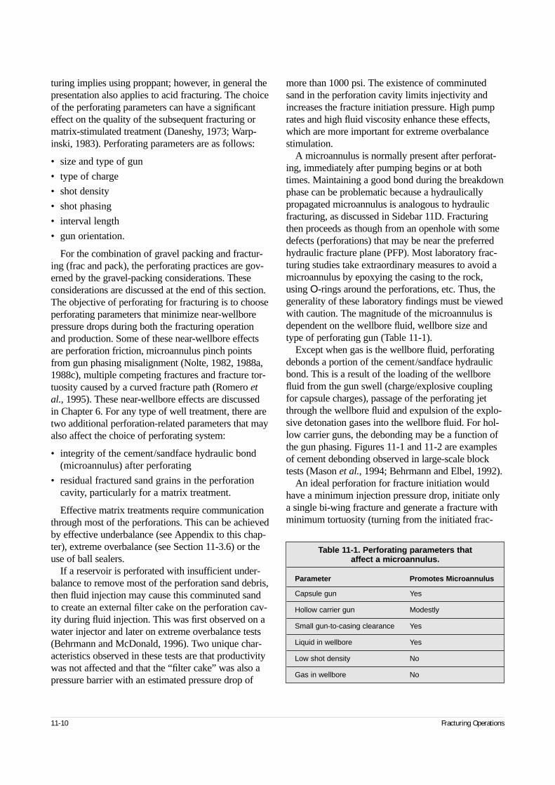
11-10 Fracturing Operations

turing implies using proppant; however, in general thepresentation also applies to acid fracturing. The choiceof the perforating parameters can have a significanteffect on the quality of the subsequent fracturing ormatrix-stimulated treatment (Daneshy, 1973; Warp-inski, 1983). Perforating parameters are as follows:

• size and type of gun

• type of charge

• shot density

• shot phasing

• interval length

• gun orientation.

For the combination of gravel packing and fractur-ing (frac and pack), the perforating practices are gov-erned by the gravel-packing considerations. Theseconsiderations are discussed at the end of this section.The objective of perforating for fracturing is to chooseperforating parameters that minimize near-wellborepressure drops during both the fracturing operationand production. Some of these near-wellbore effectsare perforation friction, microannulus pinch pointsfrom gun phasing misalignment (Nolte, 1982, 1988a,1988c), multiple competing fractures and fracture tor-tuosity caused by a curved fracture path (Romero etal., 1995). These near-wellbore effects are discussedin Chapter 6. For any type of well treatment, there aretwo additional perforation-related parameters that mayalso affect the choice of perforating system:

• integrity of the cement/sandface hydraulic bond(microannulus) after perforating

• residual fractured sand grains in the perforationcavity, particularly for a matrix treatment.

Effective matrix treatments require communicationthrough most of the perforations. This can be achievedby effective underbalance (see Appendix to this chap-ter), extreme overbalance (see Section 11-3.6) or theuse of ball sealers.

If a reservoir is perforated with insufficient under-balance to remove most of the perforation sand debris,then fluid injection may cause this comminuted sandto create an external filter cake on the perforation cav-ity during fluid injection. This was first observed on awater injector and later on extreme overbalance tests(Behrmann and McDonald, 1996). Two unique char-acteristics observed in these tests are that productivitywas not affected and that the “filter cake” was also apressure barrier with an estimated pressure drop of

more than 1000 psi. The existence of comminutedsand in the perforation cavity limits injectivity andincreases the fracture initiation pressure. High pumprates and high fluid viscosity enhance these effects,which are more important for extreme overbalancestimulation.

A microannulus is normally present after perforat-ing, immediately after pumping begins or at bothtimes. Maintaining a good bond during the breakdownphase can be problematic because a hydraulicallypropagated microannulus is analogous to hydraulicfracturing, as discussed in Sidebar 11D. Fracturingthen proceeds as though from an openhole with somedefects (perforations) that may be near the preferredhydraulic fracture plane (PFP). Most laboratory frac-turing studies take extraordinary measures to avoid amicroannulus by epoxying the casing to the rock,using O-rings around the perforations, etc. Thus, thegenerality of these laboratory findings must be viewedwith caution. The magnitude of the microannulus isdependent on the wellbore fluid, wellbore size andtype of perforating gun (Table 11-1).

Except when gas is the wellbore fluid, perforatingdebonds a portion of the cement/sandface hydraulicbond. This is a result of the loading of the wellborefluid from the gun swell (charge/explosive couplingfor capsule charges), passage of the perforating jetthrough the wellbore fluid and expulsion of the explo-sive detonation gases into the wellbore fluid. For hol-low carrier guns, the debonding may be a function ofthe gun phasing. Figures 11-1 and 11-2 are examplesof cement debonding observed in large-scale blocktests (Mason et al., 1994; Behrmann and Elbel, 1992).

An ideal perforation for fracture initiation wouldhave a minimum injection pressure drop, initiate onlya single bi-wing fracture and generate a fracture withminimum tortuosity (turning from the initiated frac-

Table 11-1. Perforating parameters that affect a microannulus.

Parameter Promotes Microannulus

Capsule gun Yes

Hollow carrier gun Modestly

Small gun-to-casing clearance Yes

Liquid in wellbore Yes

Low shot density No

Gas in wellbore No

Reservoir Stimulation 11-11

ture into the PFP) at an achievable fracture initiationpressure. The following sections provide recommen-dations on how best to achieve this ideal perforation.In the following sections, a vertical well is one with adeviation less than 30°.

11-3.2. Perforation phasing for hard-rock hydraulic fracturing

• No microannulus, vertical wellbore

For the following discussion, the PFP is assumed tobe vertical and therefore can connect directly over

a significant distance for a vertical well. When thePFP is not vertical, as can occur near a significantfault, the PFP deviates from the axis of a verticalwell. For this case, “Open microannulus, deviatedand horizontal wellbores/vertical fractures” subse-quently in this section should be consulted.

Dry gas wells, wells swabbed of liquid prior toperforating, wells shot with small hollow carrierguns and wells shot with low-shot-density (1 or 2 shots per foot [spf]) hollow carrier guns arepotential candidates for maintaining good cement/sandface bonds. With a perfect cement bond, frac-tures are forced to initiate from the perforations,

11D. Propagating a microannulus during formation breakdown

K. G. Nolte, Schlumberger Dowell

For normal completion practices, the creation of a microannu-lus should be anticipated during the breakdown process. Themicroannulus results from the same mechanics that govern thepropagation of a hydraulic fracture, but on a smaller scale andconfined to the annular circumference of the cement’s inter-face with the well. The affected annular interface can be that of either the cement/casing or the cement/formation. The for-mation interface is more prospective because of the mudcakeremaining between the cement and formation.

A hydraulic fracture or microannulus can propagate whenfluid of sufficient pressure energizes a prospective flaw and theflaw is embedded in a deformable environment. Flaws of thesetypes exist in the cement interfaces and around perforationtunnels, and they are in communication with the wellbore fluid.These flaws can originate in the mudcake, which can rehy-drate by capillary action from the wellbore fluid, or in a regionof mechanical alteration around the perforation tunnel. As thewellbore is pressurized during breakdown, the fluid in theprospective flaw is also pressurized, increasing the width ofthe flaw by compressing the material surrounding the flaw andallowing more fluid to enter and extend the flaw. For themicroannulus, the relevant surrounding material is the rockcontaining the wellbore and the casing confining the cement.Increased fluid pressure in the annulus compresses the rockand enlarges the wellbore radius. Similarly, the casing radiuschanges as the internal pressure and the external annularpressure change. The deformation of the cement sheath is rel-atively small and could be considered part of the rock contain-ing the wellbore. The annular width results from the combinedradial deformation of the borehole and casing.

The evolution of the flaw’s geometry is similar to thatdescribed in Chapter 9 for a hydraulic fracture originating froma point source of injected fluid.

1. The flaw opens and propagates when the energizing pres-sure exceeds a closure pressure equaling the stress tendingto close the flaw. Sidebar 11A implies that for a typicalcement composition and prior to breakdown, the stress inthe cement sheath is essentially hydrostatic and about equalto the reservoir pressure of the formation. Therefore, fornormally pressured conditions, the flaw’s closure pressure is about the same as the hydrostatic pressure of the com-pletion fluid within the casing, and the flaw can begin topropagate as breakdown begins.

2. The flaw initially extends in a radial geometry from the per-foration tunnel. Actually, extending annular flaws would origi-nate from most of the perforations. The mechanics describ-ing the flaw’s deformation are relatively complex during thisearly stage. The complexity results from the multiple regionsof localized pressure acting on the curved surfaces of thecasing and borehole.

3. After some period, the individual radial patterns coalesceinto one microannulus around the complete circumferenceof the cement sheath. At this stage, the annulus is analo-gous to a confined-height PKN fracture (i.e., height equalsthe circumference of the wellbore) and can begin to extendup, down or both directions along the wellbore until break-down of the formation by a hydraulic fracture.

For the last stage, the mechanics governing the annularwidth in the perforated section become relatively simple. Thesimplicity comes from several sources. The expressions for thechange in radii of the casing and wellbore can be determinedfrom specialized cases for the elastic deformation of a thick-walled cylinder. The multiple-connecting perforations providefluid with minimal pressure gradients in the annulus. As aresult, the pressures inside and outside of the casing becomeessentially equal with no radial change of the casing, and theannular width depends only on the change in radius for theborehole:

(11D-1)

where w is the microannulus width in in., ν is Poisson’s ratio, D is the wellbore diameter in in., E is Young’s modulus in psi,pm is the microannulus pressure in psi, and pp is the far-fieldreservoir pressure in psi.

As an example, consider Eq. 11D-1 for a bottomhole pres-sure increase of 2000 psi over the initial hydrostatic pressure,borehole diameter of 7 in., rock modulus of 1E+6 psi andPoisson’s ratio of 0.2. For these conditions, the hole radiusand microannulus width will increase by about 0.009 in. (or thethickness of four sheets of standard writing paper). Thehydraulic conductivity of such a microannulus is significantwhen coupled with a large pressure differential (e.g., 2000 psi)and a low-viscosity fluid (e.g., <0.4 cp for completion brine atrepresentative bottomhole temperatures).

The conductivity microannulus created during the break-down pressurization provides the same pressure and fractureinitiation environment as an openhole, and for a vertical wellit enhances the creation of a single fracture in the preferredfracture plane.

w D p p Em p= +( ) −( )1 2ν / ,

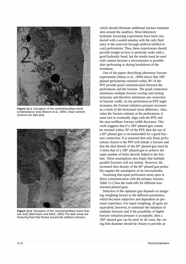
11-12 Fracturing Operations

which should eliminate additional fracture initiationsites around the sandface. Most laboratoryhydraulic fracturing experiments have been con-ducted with a sealed annulus with the only fluidentry to the reservoir through artificial (drilled orcast) perforations. Thus, these experiments shouldprovide insight on how to perforate wells with agood hydraulic bond, but the results must be usedwith caution because a microannulus is possibleafter perforating or during breakdown of the formation.

One of the papers describing laboratory fractureexperiments (Abass et al., 1994) shows that 180°phased perforations oriented within 30° of the PFP provide good communication between theperforations and the fracture. The good connectionminimizes multiple fracture overlap and turningtortuosity and therefore minimizes any restrictionof fracture width. As the perforation-to-PFP angleincreases, the fracture initiation pressure increasesas a result of the horizontal stress difference. Also,when the fracture initiates at the perforations, itmust turn to eventually align with the PFP, and the near-wellbore fracture width decreases. Thiswork suggests that if a 180° phased gun cannot be oriented within 30° of the PFP, then the use of a 60° phased gun is recommended for a good frac-ture connection. It is assumed that only those perfo-rations closest to the PFP will initiate a fracture andthat the shot density of the 60° phased gun must be3 times that of a 180° phased gun to achieve thesame number of holes directly linked to the frac-ture. These assumptions also imply that multipleparallel fractures will not initiate. However, theincreased shot density of the 60° phased gun proba-bly negates the assumption of no microannulus.

Assuming that equal perforation areas open indirect communication with the primary fracture,Table 11-2 lists the trade-offs for different non-oriented phased guns.

Selection of the optimum gun depends on assign-ing weighting factors to the different parameters,which becomes subjective and dependent on per-sonal experience. For equal weighting, all guns areequivalent; however, to minimize the initiation ofmultiple fractures and if the possibility of higherfracture initiation pressure is acceptable, then a180° phased gun can be used. In all cases, the cas-ing hole diameter should be chosen to provide an

Figure 11-1. Disruption of the cement/sandface bond(underbalance test) (Mason et al., 1994). Intact cementsections are light gray.

Figure 11-2. Disruption of the cement/sandface bond (frac-ture test) (Behrmann and Elbel, 1992).The dark areas arefracturing fluid that flowed around the wellbore annulus.

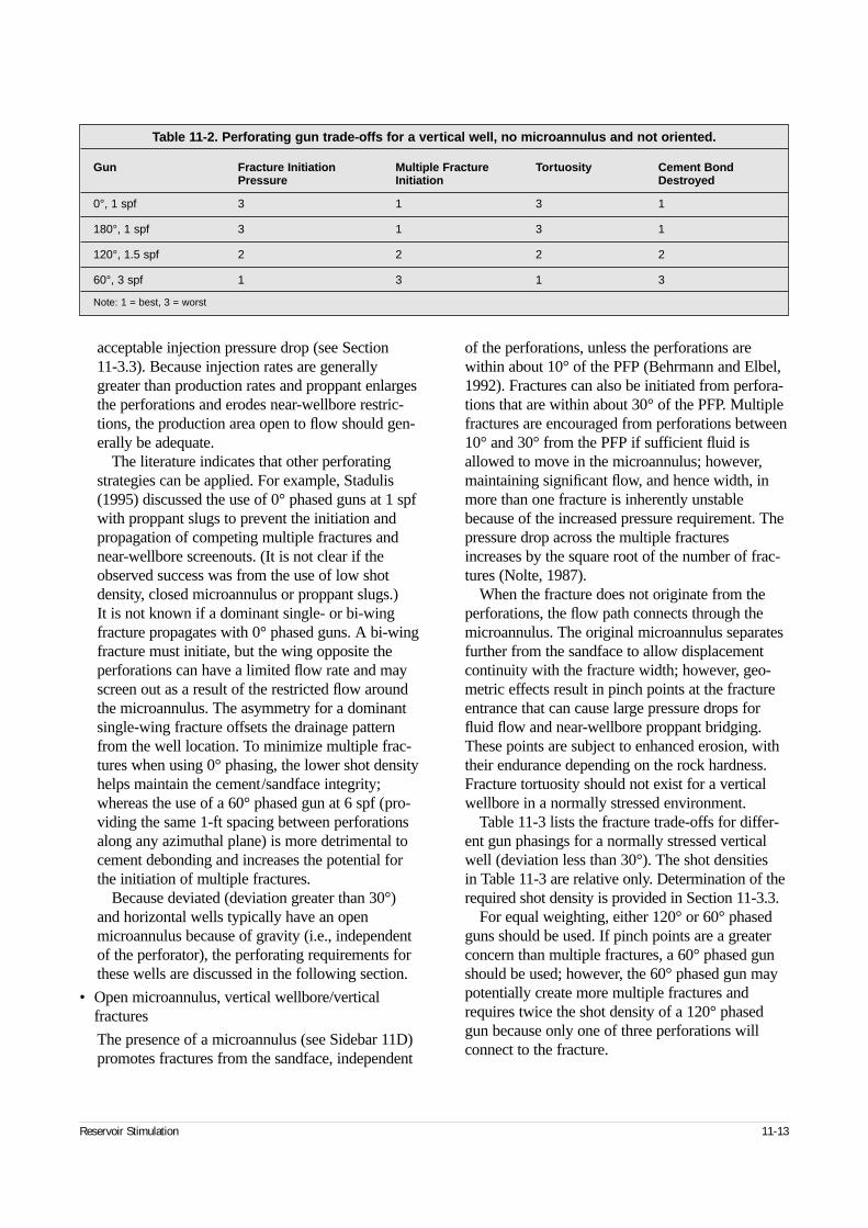
Reservoir Stimulation 11-13

acceptable injection pressure drop (see Section 11-3.3). Because injection rates are generallygreater than production rates and proppant enlargesthe perforations and erodes near-wellbore restric-tions, the production area open to flow should gen-erally be adequate.

The literature indicates that other perforatingstrategies can be applied. For example, Stadulis(1995) discussed the use of 0° phased guns at 1 spfwith proppant slugs to prevent the initiation andpropagation of competing multiple fractures andnear-wellbore screenouts. (It is not clear if theobserved success was from the use of low shotdensity, closed microannulus or proppant slugs.) It is not known if a dominant single- or bi-wingfracture propagates with 0° phased guns. A bi-wingfracture must initiate, but the wing opposite theperforations can have a limited flow rate and mayscreen out as a result of the restricted flow aroundthe microannulus. The asymmetry for a dominantsingle-wing fracture offsets the drainage patternfrom the well location. To minimize multiple frac-tures when using 0° phasing, the lower shot densityhelps maintain the cement/sandface integrity;whereas the use of a 60° phased gun at 6 spf (pro-viding the same 1-ft spacing between perforationsalong any azimuthal plane) is more detrimental tocement debonding and increases the potential forthe initiation of multiple fractures.

Because deviated (deviation greater than 30°)and horizontal wells typically have an openmicroannulus because of gravity (i.e., independentof the perforator), the perforating requirements forthese wells are discussed in the following section.

• Open microannulus, vertical wellbore/vertical fractures

The presence of a microannulus (see Sidebar 11D)promotes fractures from the sandface, independent

of the perforations, unless the perforations arewithin about 10° of the PFP (Behrmann and Elbel,1992). Fractures can also be initiated from perfora-tions that are within about 30° of the PFP. Multiplefractures are encouraged from perforations between10° and 30° from the PFP if sufficient fluid isallowed to move in the microannulus; however,maintaining significant flow, and hence width, inmore than one fracture is inherently unstablebecause of the increased pressure requirement. Thepressure drop across the multiple fracturesincreases by the square root of the number of frac-tures (Nolte, 1987).

When the fracture does not originate from theperforations, the flow path connects through themicroannulus. The original microannulus separatesfurther from the sandface to allow displacementcontinuity with the fracture width; however, geo-metric effects result in pinch points at the fractureentrance that can cause large pressure drops forfluid flow and near-wellbore proppant bridging.These points are subject to enhanced erosion, withtheir endurance depending on the rock hardness.Fracture tortuosity should not exist for a verticalwellbore in a normally stressed environment.

Table 11-3 lists the fracture trade-offs for differ-ent gun phasings for a normally stressed verticalwell (deviation less than 30°). The shot densities in Table 11-3 are relative only. Determination of therequired shot density is provided in Section 11-3.3.

For equal weighting, either 120° or 60° phasedguns should be used. If pinch points are a greaterconcern than multiple fractures, a 60° phased gunshould be used; however, the 60° phased gun maypotentially create more multiple fractures andrequires twice the shot density of a 120° phasedgun because only one of three perforations willconnect to the fracture.

Table 11-2. Perforating gun trade-offs for a vertical well, no microannulus and not oriented.

Gun Fracture Initiation Multiple Fracture Tortuosity Cement BondPressure Initiation Destroyed

0°, 1 spf 3 1 3 1

180°, 1 spf 3 1 3 1

120°, 1.5 spf 2 2 2 2

60°, 3 spf 1 3 1 3

Note: 1 = best, 3 = worst

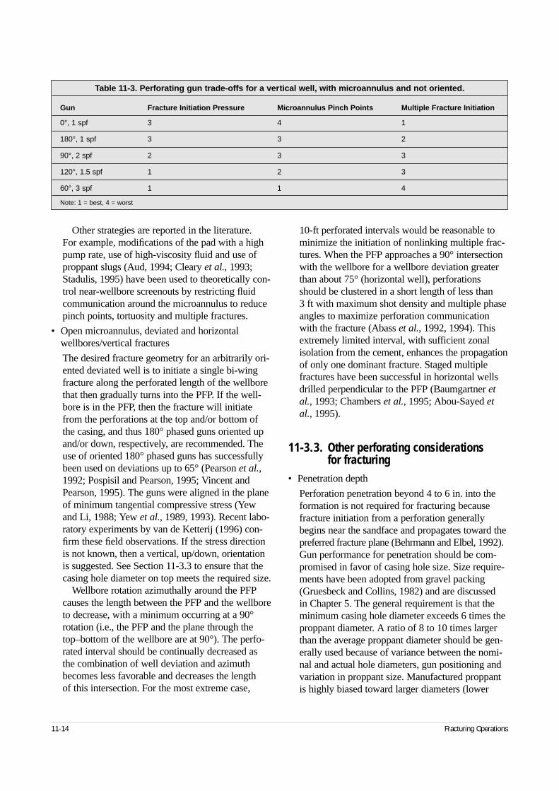
11-14 Fracturing Operations

Other strategies are reported in the literature. For example, modifications of the pad with a highpump rate, use of high-viscosity fluid and use ofproppant slugs (Aud, 1994; Cleary et al., 1993;Stadulis, 1995) have been used to theoretically con-trol near-wellbore screenouts by restricting fluidcommunication around the microannulus to reducepinch points, tortuosity and multiple fractures.

• Open microannulus, deviated and horizontal wellbores/vertical fractures

The desired fracture geometry for an arbitrarily ori-ented deviated well is to initiate a single bi-wingfracture along the perforated length of the wellborethat then gradually turns into the PFP. If the well-bore is in the PFP, then the fracture will initiatefrom the perforations at the top and/or bottom ofthe casing, and thus 180° phased guns oriented upand/or down, respectively, are recommended. Theuse of oriented 180° phased guns has successfullybeen used on deviations up to 65° (Pearson et al.,1992; Pospisil and Pearson, 1995; Vincent andPearson, 1995). The guns were aligned in the planeof minimum tangential compressive stress (Yewand Li, 1988; Yew et al., 1989, 1993). Recent labo-ratory experiments by van de Ketterij (1996) con-firm these field observations. If the stress directionis not known, then a vertical, up/down, orientationis suggested. See Section 11-3.3 to ensure that thecasing hole diameter on top meets the required size.

Wellbore rotation azimuthally around the PFPcauses the length between the PFP and the wellboreto decrease, with a minimum occurring at a 90°rotation (i.e., the PFP and the plane through thetop–bottom of the wellbore are at 90°). The perfo-rated interval should be continually decreased asthe combination of well deviation and azimuthbecomes less favorable and decreases the length of this intersection. For the most extreme case,

10-ft perforated intervals would be reasonable tominimize the initiation of nonlinking multiple frac-tures. When the PFP approaches a 90° intersectionwith the wellbore for a wellbore deviation greaterthan about 75° (horizontal well), perforationsshould be clustered in a short length of less than 3 ft with maximum shot density and multiple phaseangles to maximize perforation communicationwith the fracture (Abass et al., 1992, 1994). Thisextremely limited interval, with sufficient zonalisolation from the cement, enhances the propagationof only one dominant fracture. Staged multiplefractures have been successful in horizontal wellsdrilled perpendicular to the PFP (Baumgartner etal., 1993; Chambers et al., 1995; Abou-Sayed etal., 1995).

11-3.3. Other perforating considerations for fracturing

• Penetration depth

Perforation penetration beyond 4 to 6 in. into theformation is not required for fracturing becausefracture initiation from a perforation generallybegins near the sandface and propagates toward thepreferred fracture plane (Behrmann and Elbel, 1992).Gun performance for penetration should be com-promised in favor of casing hole size. Size require-ments have been adopted from gravel packing(Gruesbeck and Collins, 1982) and are discussed in Chapter 5. The general requirement is that theminimum casing hole diameter exceeds 6 times theproppant diameter. A ratio of 8 to 10 times largerthan the average proppant diameter should be gen-erally used because of variance between the nomi-nal and actual hole diameters, gun positioning andvariation in proppant size. Manufactured proppantis highly biased toward larger diameters (lower

Table 11-3. Perforating gun trade-offs for a vertical well, with microannulus and not oriented.

Gun Fracture Initiation Pressure Microannulus Pinch Points Multiple Fracture Initiation

0°, 1 spf 3 4 1

180°, 1 spf 3 3 2

90°, 2 spf 2 3 3

120°, 1.5 spf 1 2 3

60°, 3 spf 1 1 4

Note: 1 = best, 4 = worst

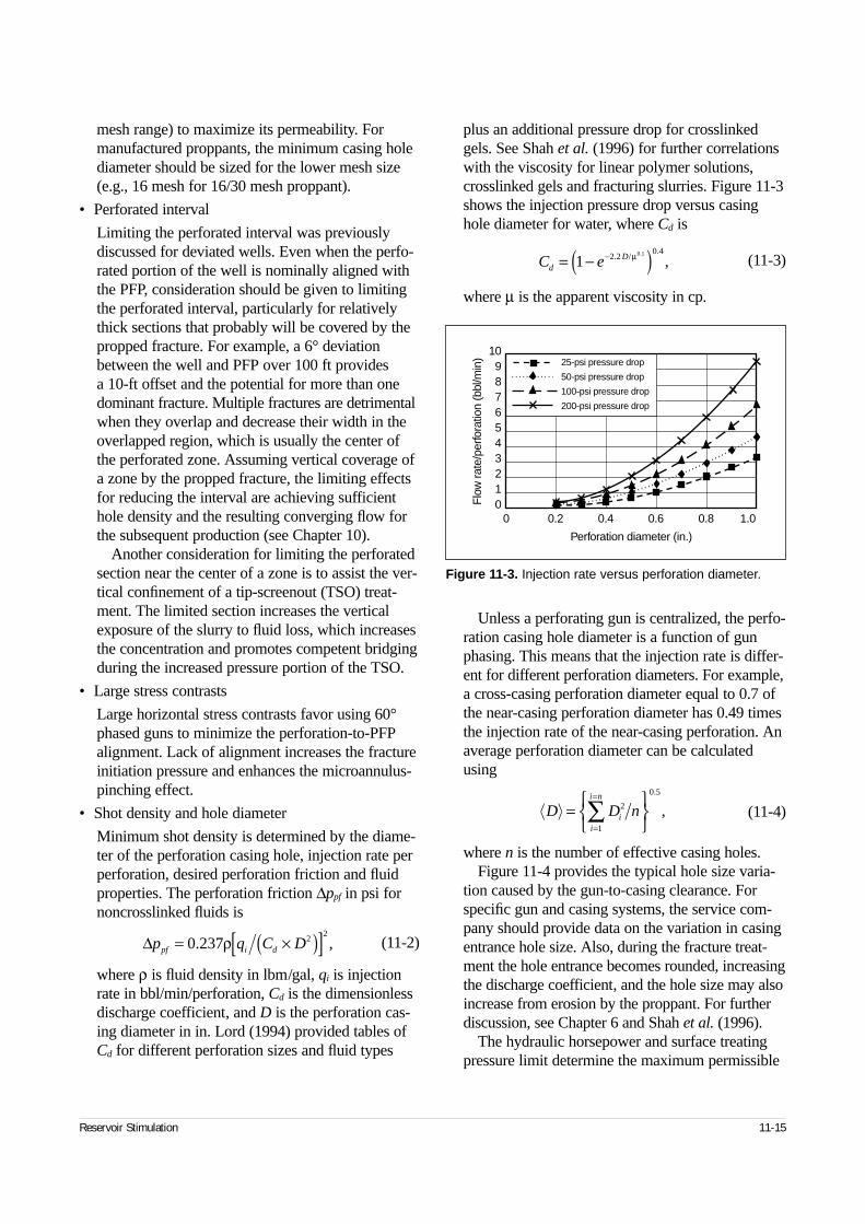
Reservoir Stimulation 11-15

mesh range) to maximize its permeability. Formanufactured proppants, the minimum casing holediameter should be sized for the lower mesh size(e.g., 16 mesh for 16/30 mesh proppant).

• Perforated interval

Limiting the perforated interval was previouslydiscussed for deviated wells. Even when the perfo-rated portion of the well is nominally aligned withthe PFP, consideration should be given to limitingthe perforated interval, particularly for relativelythick sections that probably will be covered by thepropped fracture. For example, a 6° deviationbetween the well and PFP over 100 ft provides a 10-ft offset and the potential for more than onedominant fracture. Multiple fractures are detrimentalwhen they overlap and decrease their width in theoverlapped region, which is usually the center ofthe perforated zone. Assuming vertical coverage ofa zone by the propped fracture, the limiting effectsfor reducing the interval are achieving sufficienthole density and the resulting converging flow forthe subsequent production (see Chapter 10).

Another consideration for limiting the perforatedsection near the center of a zone is to assist the ver-tical confinement of a tip-screenout (TSO) treat-ment. The limited section increases the verticalexposure of the slurry to fluid loss, which increasesthe concentration and promotes competent bridgingduring the increased pressure portion of the TSO.

• Large stress contrasts

Large horizontal stress contrasts favor using 60°phased guns to minimize the perforation-to-PFPalignment. Lack of alignment increases the fractureinitiation pressure and enhances the microannulus-pinching effect.

• Shot density and hole diameter

Minimum shot density is determined by the diame-ter of the perforation casing hole, injection rate perperforation, desired perforation friction and fluidproperties. The perforation friction ∆ppf in psi fornoncrosslinked fluids is

(11-2)

where ρ is fluid density in lbm/gal, qi is injectionrate in bbl/min/perforation, Cd is the dimensionlessdischarge coefficient, and D is the perforation cas-ing diameter in in. Lord (1994) provided tables ofCd for different perforation sizes and fluid types

plus an additional pressure drop for crosslinkedgels. See Shah et al. (1996) for further correlationswith the viscosity for linear polymer solutions,crosslinked gels and fracturing slurries. Figure 11-3shows the injection pressure drop versus casinghole diameter for water, where Cd is

(11-3)

where µ is the apparent viscosity in cp.

Unless a perforating gun is centralized, the perfo-ration casing hole diameter is a function of gunphasing. This means that the injection rate is differ-ent for different perforation diameters. For example,a cross-casing perforation diameter equal to 0.7 ofthe near-casing perforation diameter has 0.49 timesthe injection rate of the near-casing perforation. Anaverage perforation diameter can be calculatedusing

(11-4)

where n is the number of effective casing holes.Figure 11-4 provides the typical hole size varia-

tion caused by the gun-to-casing clearance. Forspecific gun and casing systems, the service com-pany should provide data on the variation in casingentrance hole size. Also, during the fracture treat-ment the hole entrance becomes rounded, increasingthe discharge coefficient, and the hole size may alsoincrease from erosion by the proppant. For furtherdiscussion, see Chapter 6 and Shah et al. (1996).

The hydraulic horsepower and surface treatingpressure limit determine the maximum permissible

∆p q C Dpf i d= ×( )[ ]0 237 22

. ,ρ

C edD= −( )−1 2 2

0 40 1. /..

,µ

Figure 11-3. Injection rate versus perforation diameter.

0 0.2 0.4 0.6 0.8 1.0

Perforation diameter (in.)

109876543210F

low

rate

/per

fora

tion

(bbl

/min

) 25-psi pressure drop

50-psi pressure drop

100-psi pressure drop

200-psi pressure drop

D D nii

i n

=

=

=

∑ 2

1

0 5.

,

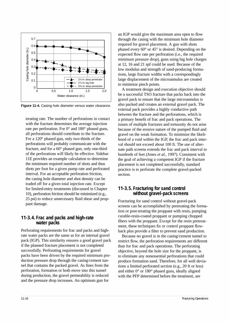
11-16 Fracturing Operations

treating rate. The number of perforations in contactwith the fracture determines the average injectionrate per perforation. For 0° and 180° phased guns,all perforations should contribute to the fracture.For a 120° phased gun, only two-thirds of theperforations will probably communicate with thefracture, and for a 60° phased gun, only one-thirdof the perforations will likely be effective. Sidebar11E provides an example calculation to determinethe minimum required number of shots and thusshots per foot for a given pump rate and perforatedinterval. For an acceptable perforation friction, the casing hole diameter and shot density can betraded off for a given total injection rate. Except for limited-entry treatments (discussed in Chapter10), perforation friction should be minimized (e.g.,25 psi) to reduce unnecessary fluid shear and prop-pant damage.

11-3.4.Frac and packs and high-rate water packs

Perforating requirements for frac and packs and high-rate water packs are the same as for an internal gravelpack (IGP). This similarity ensures a good gravel packif the planned fracture placement is not completedsuccessfully. Perforating requirements for gravelpacks have been driven by the required minimum pro-duction pressure drop through the casing/cement tun-nel that contains the packed gravel. As fines from theperforation, formation or both move into this tunnelduring production, the gravel permeability is reducedand the pressure drop increases. An optimum gun for

an IGP would give the maximum area open to flowthrough the casing with the minimum hole diameterrequired for gravel placement. A gun with shotsphased every 60° or 45° is desired. Depending on theexpected flow rate per perforation (i.e., the requiredminimum pressure drop), guns using big hole chargesat 12, 16 and 21 spf could be used. Because of thelow modulus and strength of sand-producing forma-tions, large fracture widths with a correspondinglylarge displacement of the microannulus are created to minimize pinch points.

A treatment design and execution objective shouldbe a successful TSO fracture that packs back into thegravel pack to ensure that the large microannulus isalso packed and creates an external gravel pack. Theexternal pack provides a highly conductive pathbetween the fracture and the perforations, which is a primary benefit of frac and pack operations. Theissues of multiple fractures and tortuosity do not arisebecause of the erosive nature of the pumped fluid andgravel on the weak formation. To minimize the likeli-hood of a void within the IGP, the frac and pack inter-val should not exceed about 100 ft. The use of alter-nate path screens extends the frac and pack interval tohundreds of feet (Jones et al., 1997). Consistent withthe goal of achieving a competent IGP if the fractureplacement is not completed successfully, standardpractice is to perforate the complete gravel-packedsection.

11-3.5.Fracturing for sand control without gravel-pack screens

Fracturing for sand control without gravel-packscreens can be accomplished by pretreating the forma-tion or post-treating the proppant with resin, pumpingcurable-resin-coated proppant or pumping choppedfibers with the proppant. Except for the resin pretreat-ment, these techniques fix or control proppant flow-back plus provide a filter to prevent sand production.

Because no gravel is in the casing/cement tunnel torestrict flow, the perforation requirements are differentthan for frac and pack operations. The perforatingobjective, beyond the hole size for the proppant, is to eliminate any nonessential perforations that couldproduce formation sand. Therefore, for all well devia-tions a limited perforated section (e.g., 20 ft or less)and either 0° or 180° phased guns, ideally alignedwith the PFP determined before the treatment, are

Figure 11-4. Casing hole diameter versus water clearance.

0 0.5 1.0 1.5 2.00

0.1

0.2

0.3

0.4

0.5

0.6

0.7

Cas

ing

hole

dia

met

er (i

n.)

Water clearance (in.)

21⁄2-in. deep penetrator21⁄2-in. big hole33⁄8-in. deep penetrator

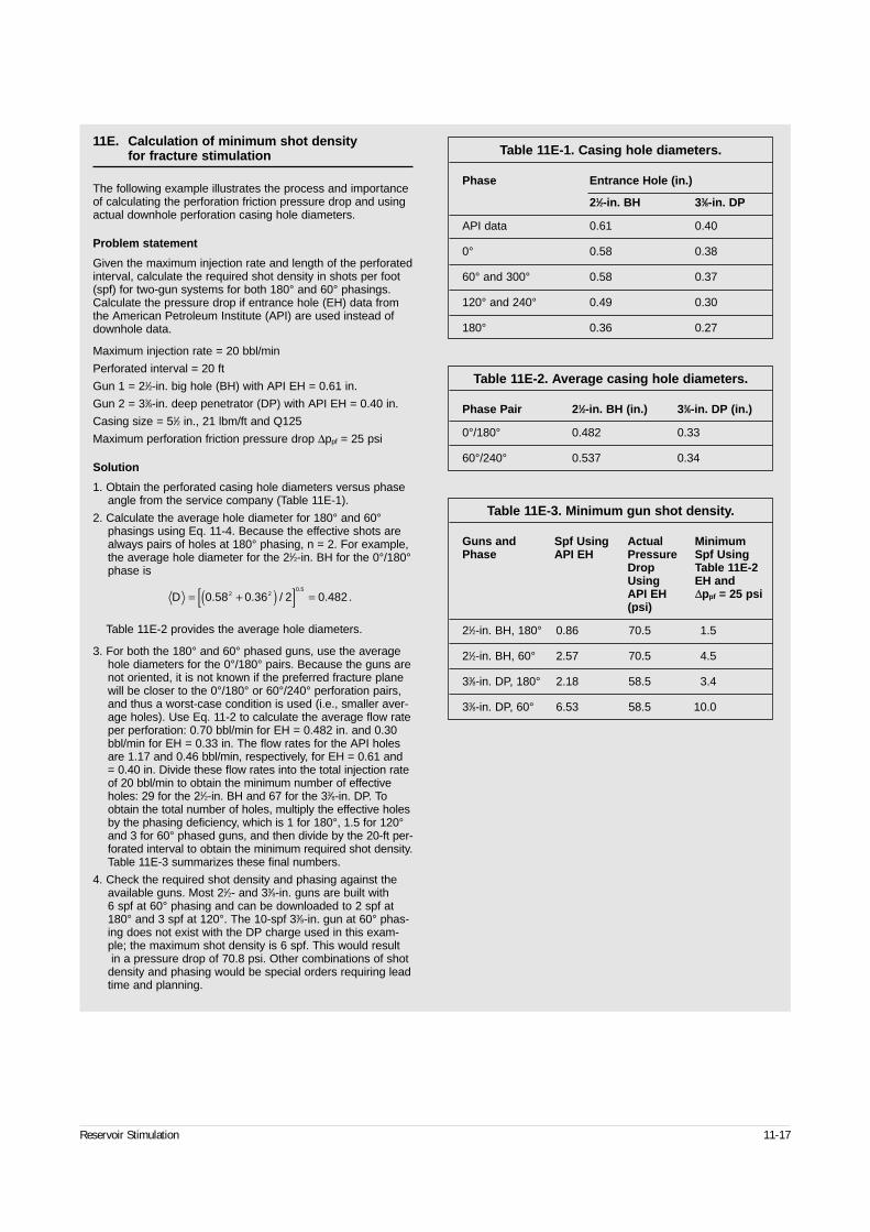
Reservoir Stimulation 11-17

11E. Calculation of minimum shot density for fracture stimulation

The following example illustrates the process and importanceof calculating the perforation friction pressure drop and usingactual downhole perforation casing hole diameters.

Problem statement

Given the maximum injection rate and length of the perforatedinterval, calculate the required shot density in shots per foot(spf) for two-gun systems for both 180° and 60° phasings.Calculate the pressure drop if entrance hole (EH) data fromthe American Petroleum Institute (API) are used instead ofdownhole data.

Maximum injection rate = 20 bbl/min

Perforated interval = 20 ft

Gun 1 = 21⁄2-in. big hole (BH) with API EH = 0.61 in.

Gun 2 = 33⁄8-in. deep penetrator (DP) with API EH = 0.40 in.

Casing size = 51⁄2 in., 21 lbm/ft and Q125

Maximum perforation friction pressure drop ∆ppf = 25 psi

Solution

1. Obtain the perforated casing hole diameters versus phaseangle from the service company (Table 11E-1).

2. Calculate the average hole diameter for 180° and 60°phasings using Eq. 11-4. Because the effective shots arealways pairs of holes at 180° phasing, n = 2. For example,the average hole diameter for the 21⁄2-in. BH for the 0°/180°phase is

Table 11E-2 provides the average hole diameters.

3. For both the 180° and 60° phased guns, use the averagehole diameters for the 0°/180° pairs. Because the guns arenot oriented, it is not known if the preferred fracture planewill be closer to the 0°/180° or 60°/240° perforation pairs,and thus a worst-case condition is used (i.e., smaller aver-age holes). Use Eq. 11-2 to calculate the average flow rateper perforation: 0.70 bbl/min for EH = 0.482 in. and 0.30bbl/min for EH = 0.33 in. The flow rates for the API holesare 1.17 and 0.46 bbl/min, respectively, for EH = 0.61 and = 0.40 in. Divide these flow rates into the total injection rateof 20 bbl/min to obtain the minimum number of effectiveholes: 29 for the 21⁄2-in. BH and 67 for the 33⁄8-in. DP. Toobtain the total number of holes, multiply the effective holesby the phasing deficiency, which is 1 for 180°, 1.5 for 120°and 3 for 60° phased guns, and then divide by the 20-ft per-forated interval to obtain the minimum required shot density.Table 11E-3 summarizes these final numbers.

4. Check the required shot density and phasing against theavailable guns. Most 21⁄2- and 33⁄8-in. guns are built with 6 spf at 60° phasing and can be downloaded to 2 spf at180° and 3 spf at 120°. The 10-spf 33⁄8-in. gun at 60° phas-ing does not exist with the DP charge used in this exam-ple; the maximum shot density is 6 spf. This would resultin a pressure drop of 70.8 psi. Other combinations of shot

density and phasing would be special orders requiring leadtime and planning.

Table 11E-1. Casing hole diameters.

Phase Entrance Hole (in.)

21⁄2-in. BH 33⁄8-in. DP

API data 0.61 0.40

0° 0.58 0.38

60° and 300° 0.58 0.37

120° and 240° 0.49 0.30

180° 0.36 0.27

Table 11E-2. Average casing hole diameters.

Phase Pair 21⁄2-in. BH (in.) 33⁄8-in. DP (in.)

0°/180° 0.482 0.33

60°/240° 0.537 0.34

D = +( )[ ] =0 58 0 36 2 0 4822 20 5

. . / . ..

Table 11E-3. Minimum gun shot density.

Guns and Spf Using Actual MinimumPhase API EH Pressure Spf Using

Drop Table 11E-2Using EH andAPI EH ∆ppf = 25 psi(psi)

21⁄2-in. BH, 180° 0.86 70.5 1.5

21⁄2-in. BH, 60° 2.57 70.5 4.5

33⁄8-in. DP, 180° 2.18 58.5 3.4

33⁄8-in. DP, 60° 6.53 58.5 10.0

11-18 Fracturing Operations

recommended. As with a frac and pack, one of thedesign and execution objectives should be to achievea TSO that packs back to fill the expanded microannu-lus with proppant. For the screenless case, the prop-pant is treated for flowback control to create a compe-tent external pack that controls the formation sand.Again, as a result of the weak rock, the pumped fluidswash away any near-wellbore restrictions. Zero-degree phased guns should be used when the gunscannot be aligned with the PFP to eliminate nonessen-tial perforations.

11-3.6. Extreme overbalance stimulationExtreme overbalance (EOB) has been defined aseither the application of a very high overbalance pres-sure during the perforating process (called extremeoverbalance perforating, or EOP) or the very highpressure “surging” of existing perforations. Othernames for this procedure are rapid overpressuredperforation extension and high-energy stimulation.EOB utilizes pressurized gas (usually nitrogen [N2])to inject various fluid systems into the formation atpressure gradients from 1.4 to 2.0 psi/ft. The primaryobjective is to create fractures either as a pre–hydraulicfracture treatment or as a dynamic fluid diversion(Handren et al., 1993; Dees and Handren, 1993).

Handren et al.’s (1993) early publication suggeststhat effective multiple fractures were created from allperforations. However, additional full-scale laboratoryfracture initiation experiments (Behrmann andMcDonald, 1996; Willson, 1995) plus field tests(Snider, 1996) confirm that although fractures mayinitiate from many perforations, only a single bi-wingfracture is propagated from the perforations nearestthe PFP. Furthermore, there is no evidence of the initi-ation of parallel multiple fractures. All fractures initi-ate from the perforations, with the primary fracturefrom the perforations nearest the PFP. It is assumedthat the sudden pressurization of the wellbore casingcloses any microannulus prior to hydraulic communi-cation away from the perforations. The high fracturepressure gradients required are a result of at least fourevents:

• Dynamic fracture initiation is greater than staticfracture initiation.

• Near-wellbore pore pressure does not increase asmuch as in a static injection.

• Residual “crushed” sand debris in the perforationtunnel restricts both fluid injection and pressuriza-tion of the perforation.

• Lack of a microannulus and the perforations notaligned with the PFP initiate against a larger stress.

These effects result in required pressures that are 2 to 3 times greater than those in conventional hydraulicfracturing.

Because experiments show no microannulus effector parallel multiple fractures, only tortuosity must beconsidered. For a vertical well, a misaligned 0° phasedgun is the least acceptable whereas 60° or 120° phasedguns provide the least tortuous path (Table 11-2).However, Petitjean et al. (1995) reported that theymitigated tortuosity by minimizing the use of liquid to that necessary for fracture initiation and using nitro-gen gas to extend the fracture and erode any near-wellbore tortuosity. This approach should be applica-ble for both vertical and deviated wells. Also, Snider(1996) reported the use of a proppant carrier to erodenear-wellbore tortuosity and improve the near-well-bore fracture conductivity, but the fracture width isgenerally insufficient for proppant entry (Petitjean et al., 1995).

In general, perforating considerations for EOB invertical wells are similar to those in “No microannulus,vertical wellbore” in Section 11-3.2. Similarly, fordeviated and horizontal wells, the perforating recom-mendations in “Open microannulus, vertical wellbore/vertical fractures” in Section 11-3.2 can be used.

A detailed discussion of extreme overbalance perfo-rating was provided by Behrmann et al. (1996).

11-3.7. Well and fracture connectivityThe tortuosity between the initiation of a fracture froma well and the plane of its ultimate propagation hasbeen recognized by many as an important issue duringfracture execution, resulting at least in an undesirableincrease in fracturing pressure or, worse, in a screen-out and even the creation of only one fracture wing.

Well deviation and unacceptable perforation phas-ing have already been addressed in this chapter. Welldeviation can be remedied with an S-shaped well (i.e., turning a deviated well to become vertical uponentering the target formation), and problems with per-foration phasing can be addressed by decreasing thephase angle among the perforation planes. To prevent

Reservoir Stimulation 11-19

the similarly undesirable problem of multiple fractureinitiation, the number of perforations can be reduced,leading to “point source” fracturing.

These solutions, although they usually prove suc-cessful in fracture execution in all types of reservoirsand will not affect well performance in low-permeabilityformations, may prove inadequate in high-permeabilityapplications.

Chen and Economides (1998) demonstrated theeffect of the near-well choke, resulting from inade-quate fracture and well connectivity in low- and high-permeability reservoirs. Although the well perfor-mance reduction from the ideal value in low-permeabilityreservoirs is insignificant, the reduction in high-per-meability reservoirs can be substantial (50% to 75%from the ideal) and the controlling factor in the suc-cess of the treatment. This effect suggests that forhigh-permeability fracturing, S-shaped wells arehighly desirable and that in treating these verticalholes the indicated perforation phasing is 180° butwith the guns oriented to align the perforation planewith the fracture plane. This assumes, of course, thatthe fracture is vertical. Analogous ideas may apply tohorizontal wells for shallow applications where thefractures may be horizontal.

An additional idea, investigated at the time of thiswriting, is to forego perforating altogether for fractur-ing and consider the creation along the well of verticalnotches parallel to the fracture plane by using a jet-cutting technique.

11-4. Surface equipment for fracturing operations

Assembling the surface equipment in a safe, organizedand efficient manner is extremely important for thesuccess of a fracturing treatment. Thorough pretreat-ment planning is essential to the organizational processof coordinating equipment hookup. An inspection ofthe location prior to the treatment allows making dia-grams to optimize the use of available space.

Many steps of the organizational procedures are dri-ven by common sense. Yet, small problems can easilybe overlooked in the rush to get things ready. Pretreat-ment planning can eliminate many small problems thathave the potential to develop into larger problems thatmay ultimately jeopardize the success of the treatment.

Figure 11-5 shows equipment positioning for a frac-turing treatment. Figures 11-6 and 11-7 show fractur-

ing equipment for small and large fracturing treat-ments, respectively.

11-4.1. Wellhead isolationSpecialized isolation tools, or tree savers, can protecta Christmas tree at the wellhead from damage and thepossible failure that results from exposure to highpressure, corrosive fluids or abrasive proppant-ladenfluids. The pressure rating of a wellhead is usuallyless than the pressure required to pump a stimulationtreatment. Replacing the existing tree with one thathas a higher pressure rating is expensive and requireskilling the well with potentially damaging fluids. Evenif the existing tree has a sufficient pressure rating,exposure to high pressures and treating fluids mayleave it in an unsafe condition.

The tree saver is mounted on the existing Christmastree. A mandrel is extended through the valves on thetree and into the tubing. The mandrel has a rubber cupassembly that seals to the walls of the tubing and pre-vents fluid or pressure from directly reaching the tree.Once set, a tree saver can extend the working pressureof a wellhead up to 20,000 psi. Once the stimulationtreatment is completed, the mandrel is pumped backout of the Christmas tree, and the wellhead valves canbe closed.

11-4.2. Treating ironThe size of the high-pressure pipe called treating ironused on a treatment is dictated by both the anticipatedrates and pressures. Smaller lines have a higher maxi-mum treating pressure limitation than the larger sizes.The velocity of the fluid should be limited to 45 ft/s to minimize excessive erosion of the iron. Pumpingabove these rates for any prolonged period of time canerode the treating iron and thereby lower the effectiveworking pressure that the iron could be exposed tobefore a catastrophic failure would occur. If the designtreating rates exceed the rate limits of the iron’s size,then either a larger iron must be used or multiple linesmust be laid to the wellhead.

The treating iron should not have welded seams or exposed threaded connections. To eliminate theseseams and exposed threads, the iron and associatedconnections should be machined from single pieces ofmetal. The connections between two pieces of treatingiron should have nonpressure unions. This style of

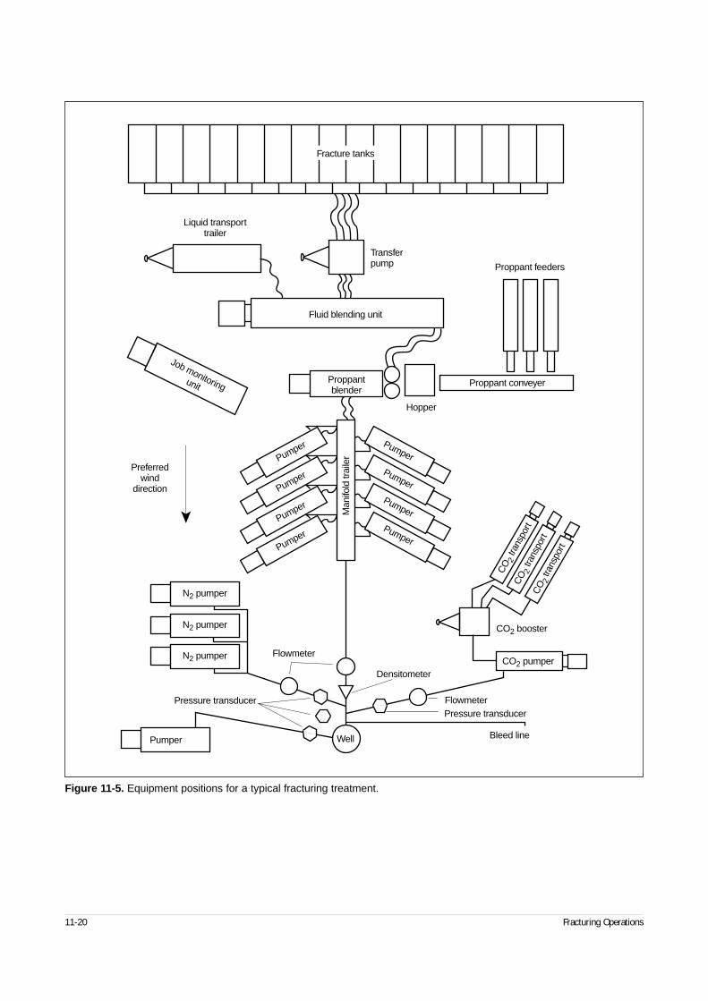
11-20 Fracturing Operations

Figure 11-5. Equipment positions for a typical fracturing treatment.

Liquid transporttrailer

Transferpump Proppant feeders

Proppant conveyerProppantblender

Fluid blending unit

Job monitoringunit

Pumper Pumper

Pumper

Pumper

Pumper

Pumper

Pumper

Pumper

Man

ifold

trai

ler

CO2 booster

CO2 pumperN2 pumper

N2 pumper

N2 pumper

Pumper

Pressure transducer

Flowmeter

Densitometer

FlowmeterPressure transducer

Bleed lineWell

Preferredwind

direction

Hopper

Fracture tanks

CO 2

tran

spor

tC

O 2 tr

ansp

ort

CO 2

trans

port

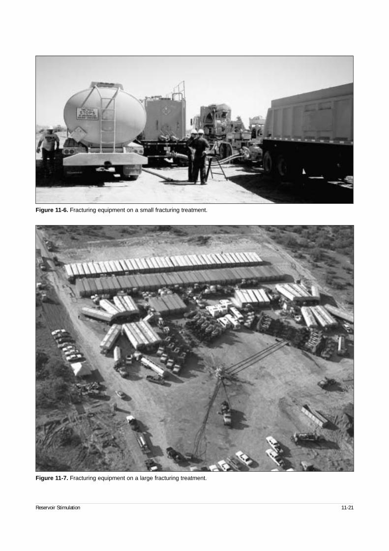
Reservoir Stimulation 11-21

Figure 11-6. Fracturing equipment on a small fracturing treatment.

Figure 11-7. Fracturing equipment on a large fracturing treatment.

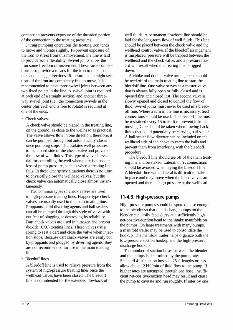
11-22 Fracturing Operations

connection prevents exposure of the threaded portionof the connection to the treating pressures.

During pumping operations the treating iron tendsto move and vibrate slightly. To prevent exposure ofthe iron to stress from this movement, the line is laidto provide some flexibility. Swivel joints allow theiron some freedom of movement. These same connec-tions also provide a means for the iron to make cor-ners and change directions. To ensure that straight sec-tions of the iron are completely free to move, it isrecommended to have three swivel joints between anytwo fixed points in the line. A swivel joint is requiredat each end of a straight section, and another three-way swivel joint (i.e., the connection swivels in thecenter plus each end is free to rotate) is required atone of the ends.

• Check valves

A check valve should be placed in the treating line,on the ground, as close to the wellhead as practical.The valve allows flow in one direction; therefore, itcan be pumped through but automatically closesonce pumping stops. This isolates well pressures to the closed side of the check valve and preventsthe flow of well fluids. This type of valve is essen-tial for controlling the well when there is a suddenloss of pump pressure, such as when a treating linefails. In these emergency situations there is no timeto physically close the wellhead valves, but thecheck valve can automatically close almost instan-taneously.

Two common types of check valves are used in high-pressure treating lines. Flapper-type checkvalves are usually used in the main treating line.Proppants, solid diverting agents and ball sealerscan all be pumped through this style of valve with-out fear of plugging or destroying its reliability.Dart check valves are used in nitrogen and carbondioxide (CO2) treating lines. These valves use aspring to seat a dart and close the valve when injec-tion stops. Because dart check valves are easily cutby proppants and plugged by diverting agents, theyare not recommended for use in the main treatingline.

• Bleedoff lines

A bleedoff line is used to relieve pressure from thesystem of high-pressure treating lines once thewellhead valves have been closed. The bleedoffline is not intended for the extended flowback of

well fluids. A permanent flowback line should belaid for the long-term flow of well fluids. This lineshould be placed between the check valve and thewellhead control valve. If the bleedoff arrangementis misplaced, pressure will be trapped between thewellhead and the check valve, and a pressure haz-ard will result when the treating line is riggeddown.

A choke and double-valve arrangement shouldbe teed off of the main treating line to start thebleedoff line. One valve serves as a master valvethat is always fully open or fully closed and isopened first and closed last. The second valve isslowly opened and closed to control the flow offluid. Swivel joints must never be used in a bleed-off line. Where a turn in the line is necessary, teedconnections should be used. The bleedoff line mustbe restrained every 15 to 20 ft to prevent it frommoving. Care should be taken when flowing backfluids that could potentially be carrying ball sealers.A ball sealer flow diverter can be included on thewellhead side of the choke to catch the balls andprevent them from interfering with the bleedoffprocedure.

The bleedoff line should tee off of the main treat-ing line and be staked. Lateral, or Y, connectionsshould be avoided when laying the bleedoff line. A bleedoff line with a lateral is difficult to stake in place and may move when the bleed valves areopened and there is high pressure at the wellhead.

11-4.3. High-pressure pumpsHigh-pressure pumps should be spotted close enoughto the blender so that the discharge pumps on theblender can easily feed slurry at a sufficiently highnet-positive-suction head to the intake manifolds onthe pumps. On large treatments with many pumps, a manifold trailer may be used to consolidate thehookup. The manifold trailer helps organize both thelow-pressure suction hookup and the high-pressuredischarge hookup.

The number of suction hoses between the blenderand the pumps is determined by the pump rate.Standard 4-in. suction hoses in 25-ft lengths or lessallow about 12 bbl/min of fluid flow to the pump. Ifhigher rates are attempted through one hose, insuffi-cient net-positive-suction head may result and causethe pump to cavitate and run roughly. If rates by one

Reservoir Stimulation 11-23

pump are expected to exceed 12 bbl/min, another suc-tion hose should be used to provide fluid to the intakemanifold.

For low-rate treatments, the hose diameter mayhave to be decreased to maintain a sufficiently highfluid velocity inside the hose, especially on high-proppant-concentration treatments such as a foamfracture treatment. Alternatively, a recirculation linefrom the pump suction manifold to the blender can be used. If the fluid velocity in a hose drops to a pointwhere proppant settling is severe, the hose may plugoff and starve the pump for fluid.

Each pump truck should have an isolation valvewhere it is tied into the main treating line to facilitatemaking minor repairs during pumping operations.Without this valve the pump would always beexposed to the treating pressure. Behind the isolationvalve a bleedoff valve should be installed so that thepressure on the pump can be safely bled off any timethe pump is brought off line.

The size of the iron on the pump should be compat-ible with the rate and pressure capabilities of thepump. If the pump and iron are not performancematched, the effective efficiency of the pump is mini-mized.

Recirculation lines between the blender and thesuction manifold of the high-pressure pump may benecessary when high proppant concentrations arepumped. At high concentrations the proppant maysettle out of the slurry within this manifold. Settlingproblems are more likely to occur at low pump ratesand for low-viscosity fluids. The recirculation linekeeps fluid moving within the suction manifold andprevents proppant from settling out. Fracturing treat-ments using foamed fluids usually require a recircu-lation line.

11-4.4. Blending equipmentProcess-controlled blending equipment that metersand continuously mixes polymer slurry, concentratedpotassium chloride (KCl) solution and liquid additiveshas made continuous-mix operations a viable alterna-tive to batch-mix operations. There are several advan-tages to performing a fracture treatment in continuous-mix mode. Environmental concerns are greatlyreduced because only freshwater residuals remain inthe fracture tanks after a treatment. Besides eliminat-ing the cost of gelled tank bottoms, no tank cleaning

or disposal costs are incurred. In addition, a morepredictable and consistent viscosity is obtainable forlarge treatments, where bacteria can degrade the gelviscosity of a batch-mixed fluid before pumpingbegins. Personnel time and costs can also be greatlyreduced. The continuous-mix process eliminates theneed to have gelling crews precede fracturing opera-tions, resulting in direct savings in time for personneland equipment. Finally, viscosities can be easilychanged throughout the treatment. This allows taper-ing the polymer loading so that fluid damage to prop-pant conductivities can be minimized or a net pressurelimitation can be met.

To ensure that a continuous-mix operation goessmoothly, several requirements must be observed. Thepolymers should be of a liquid or slurried variety toensure that they can be added at precise concentra-tions. Liquid or slurried additives can be pumped andmonitored much more accurately than dry powderedmaterials. These polymers produce an improved,quicker hydration especially when mixed with process-controlled equipment. Specialized mixing and hydra-tion units provide the metering capabilities, propershear environment and sufficient residence time forproper hydration. The hydration process related totime and shear has proved to be extremely importantfor continuous-mix treatments. If the base fluid hasnot progressed sufficiently in the hydration processbefore the fluid is crosslinked, the fluid may experi-ence stability problems.

Process-controlled proppant blenders use computersto meter precise proppant-to-fluid ratios throughoutthe treatment. This precision-blending capability isperfect for ramping proppant, which is considered theideal for optimum proppant placement. The blendersaccurately mix and meter proppant, dry additives,liquid additives and fracturing fluid together at a spec-ified density in a preprogrammed, automatic mode.The proppant concentration can be precisely and safelycontrolled at concentrations higher than 22 lbm/galadded for sand or 32 lbm/gal added for high-strengthproppant. The overall proppant/fluid ratio is con-stantly monitored and controlled in a range of ±0.5%.

11-4.5. Proppant storage and deliveryThe total volume of proppant, rate of proppant deliv-ery and number of different proppants to be used inthe treatment must be considered when choosing the

11-24 Fracturing Operations

proper vessel for storing proppant on location. Smalltreatments may require only dump trucks to deliverthe proppant to the blender. Bobtail dumps and trailerdumps are routinely used throughout the industry.These units are spotted directly over the blender hop-per and gravity feed the proppant at a controlled ratethrough a chute. Care should be taken to ensure thatthe hydraulic lift mechanism is in good working order,allowing the dump to be completely raised. If thedump is not completely raised, the proppant deliveryrate may not be sufficient, especially as the dumpnears empty. This can be critical at high proppant con-centrations, which require the highest delivery rates.To prevent problems with the proppant delivery rate,it is a good idea to bring extra proppant if capacitiesallow. Bobtail units generally haul between 250 and450 ft3 of proppant, and trailer units haul up to 600 ft3.The maximum delivery rate of these units depends onthe chute size and placement but is generally between3000 and 7000 lbm/min of proppant.

Moving proppant dumps during a treatment shouldbe minimized. Even with good operators, it takes 3 to5 min to move a dump into place and raise it for prop-pant delivery. Excessive movement of the proppantdumps increases the chance of not pumping the properproppant concentration. If a treatment is designed withlarge proppant volumes requiring movement of thedump trucks during pumping procedures, other prop-pant storage equipment should be considered.

Upright storage silos can hold up to 4000 ft3 ofproppant. The silos rely on gravity to feed the blenderand do not require hydraulic power to operate. Thistype of storage eliminates moving trucks for mosttreatments because of the quantity of proppant it holds.However, this type of proppant storage requires con-siderable planning because the units are not mobileonce they are spotted. Specialized cranes are requiredto raise these units into place and to lower them fortransportation.

The conveyor-equipped sand bin is the most com-monly used unit for delivering proppants to theblender. These units have several compartments forstoring proppant. Each compartment has a set ofhydraulically controlled doors at the bottom. Whenthe doors are opened, proppant falls from the con-tainer onto a conveyor belt that leads to the blender.The storage capacity of these units ranges between2500 and 4000 ft3. Hydraulically powered conveyorscan unload these units at proppant delivery ratesapproaching 25,000 lbm/min. If extremely large vol-

umes of proppant are required for a treatment, con-veyor-equipped sand bins can be positioned to offloadproppant onto a second conveyor that feeds theblender. Spotting sand bins in this arrangement allowsmillions of pounds of proppant to be easily stored andpumped.

Regardless of the type of bulk proppant storageused, great care and planning must go into treatmentsin which proppant types and sizes will be changedduring the treatment. The time and proceduresrequired to make proppant changes during the treat-ment must be considered in the pretreatment planning.

11-4.6. Vital signs from sensorsThe monitoring of hydraulic fracture treatments hasevolved from simple pressure strip charts to sophisti-cated computer recording and display. The informa-tion displayed by these instruments provides thesupervising engineers with diagnostics on how thetreatment is proceeding. Real-time execution decisionsare made during the treatment based on this information.

Sensors acquire input data to track and account forthe numerous operations taking place on location.Most of the parameters required for evaluating a frac-turing treatment can be followed with sensors.Pressure, density, rate, temperature, pH value and vis-cosity are some of the more common parameters dis-played and recorded.

• Pressure measurement

Pressure transducers measure the deformation of a sensing material to provide a pressure reading.Specially designed strain gauges are bonded toprecision-machined metals that subtly deform asthey are exposed to pressure. The quality of pres-sure transducers varies both in accuracy and reso-lution. The accuracy of a gauge is determined byhow closely it measures pressures over an entirepressure span. The resolution indicates the size ofthe pressure increment required to affect the mea-surement.

It is imperative that treating pressures are accu-rately known during a treatment. The main sensorused to measure the pressure should be placed asnear to the wellhead as practically possible. Careshould be taken to locate the pressure sensor on thewellhead side of the check valve to ensure that anaccurate pressure is available even after pumpingoperations have stopped. Should the transducer

Reservoir Stimulation 11-25

inadvertently be placed on the upstream side of thecheck valve, pressure readings could indicate thatpressures have bled off while actual wellhead pres-sures remain dangerously high.

Generally, several pressure sensors are availablefor monitoring purposes in addition to the primarytransducer at the wellhead. A second transducershould be identified and calibrated to the primarysensor. Pressure measurements from this transducershould be used if the primary sensor fails duringthe treatment. All pump trucks should have a trans-ducer on each high-pressure pump. However, thesesensors should not be used as a backup to the pri-mary pressure transducer because pressure mea-surements will be lost if the pumps are shut in andisolated during the treatment. The pump sensorscan be used to indicate problems associated witheach unit. A pressure that deviates significantlyfrom the other sensors indicates that the pumpshould be shut in and isolated. Once the source ofthe abnormal pressure is located and repaired, thepump can be brought back on line.

• Density measurement

For years radioactive densitometers have been usedto measure density. This technique provides a non-intrusive, continuous density measurement for anyfluid flowing in a pipe. The technique is based onthe absorption of gamma rays by the measuredfluid.

A densitometer consists of

– radioactive source on one side of the pipe

– gamma ray detector on the other side of the pipe

– electronic panel to provide a signal reading.

As fluid passes through the pipe, gamma raysemitted by the source are attenuated in proportionto the fluid density. The detector senses the gammarays transmitted through the fluid and converts thissignal into an electrical signal. The electronic panelprocesses the electrical signal into a density indica-tion. Denser materials absorb more radiation,resulting in the detection of fewer gamma rays.Thus, the signal output of the detector variesinversely with respect to density.

Most densitometers use a radioactive isotopewith an extended half-life. A densitometer using137cesium can function accurately for nearly 30years if the electronic components are maintainedproperly.

A good densitometer is accurate to within 0.1 lbm/gal over a density range of 8.0 to 25 lbm/gal.This remarkable accuracy can still lead to errors,especially when a densitometer is used to detectproppant totals and the treatment goes to a highproppant concentration. If the fluid and proppantdensities vary by 0.1 lbm/gal and the densitometerhas an accuracy level of 0.1 lbm/gal added, an error of nearly 10% can occur at proppant concentrationsgreater than 10 lbm/gal added because the densito-meter is actually measuring radioactive adsorption,which is proportional to the density. The value ofpounds per gallon must be calculated from the den-sity reading. This calculation at higher densities isless accurate because a small change in absolutedensity means a larger change in pounds per gallon.As an example, the density readings comparing noproppant with 3-lbm/gal added sand are 8.43lbm/gal and 10.06 lbm/gal, respectively (a changein density of 1.63 lbm/gal). However, a similarchange in density (1.52 lbm/gal) from 13.96 to15.48 lbm/gal corresponds to a change from 15.0-to 23.5-lbm/gal added.

• Rate measurement

Several styles of rate sensors are used for monitor-ing high-pressure treatments. Commonly used ratesensors include pump stroke counters, turbineflowmeters, magnetic flowmeters and venturiflowmeters for gaseous fluids. Pump stroke coun-ters generally measure the rotational speed of thepump. Each full rotation of the pump moves thepump plunger through one complete cycle. Fromthe volume of each pump stroke, number of pumpstrokes and the pump’s efficiency, a rate can be eas-ily calculated. This type of measurement is advan-tageous for high-pressure pumps that are pumpinghigh volumes of solids, as is the case in pumpingproppants during a fracturing treatment. The pres-ence of solids or varying fluid rheology does notaffect this type of measurement. However, if thepumps are not fully primed, the actual rate may besignificantly lower than that indicated by a strokecounter.

Turbine flowmeters are designed primarily formeasuring clean fluids. As fluid is pumped throughthe flowmeter housing, turbine blades are forced torotate. Each of the blades on the rotor creates asmall pulse as it passes beneath a magnetic pickup.Each revolution of the rotor generates a distinct

11-26 Fracturing Operations

pattern of pulses equal to the number of turbineblades. The rotational speed of the rotor defines theflow rate, and each pulse defines a volume of liquidpassing through the meter. Most turbine meters arecalibrated with fresh water. As the viscosity of themeasured fluid increases, the rotor speed decreasesproportionally. Therefore, a turbine flowmetershould be calibrated with the actual fluid to bemeasured to ensure accuracy. These meters are use-ful for measuring liquid additive rates but have lim-ited value for proppant slurries. Fracturing fluidviscosities often vary throughout a treatment, espe-cially when proppant is introduced. The proppantalso tends to erode the turbine blades, furtherreducing the accuracy of the flow measurement.

Magnetic flowmeters are popular for measuringtreating fluid rates. These flowmeters measure therate of fluid flow in a line, similar to a turbineflowmeter, but they do not have intruding parts thatcan be affected by changing viscosities or proppantaddition. The electromagnetic flowmeter operateson Faraday’s law of electromagnetic induction.When a conductor is moved across a magneticfield, an electromagnetic force is induced in theconductor. The electromagnetic force is orthogonalto both the direction of movement and the magneticfield itself. The electromagnetic flowmeter uses apair of coils mounted on the outside of a nonmag-netic pipe. An electrical current flows through thecoils to produce the magnetic field. The electro-magnetic force is created when fluid (a conductivematerial) passes through the coils. The biggest limi-tation of the electromagnetic flowmeter is that itcannot be used with oil-base fluids.

To accurately measure N2 or CO2 rates, a venturiflowmeter should be used. The velocity of the gasthrough the venturi is determined by measuring thepressure drop across a reduced area. The line pres-sure and temperature must also be measured tocompensate for changes in density.

• Data acquisition and process control

Computer monitoring systems can track and recordnumerous sensor inputs, making them ideal formonitoring complex treatments. These systems canalso use data to create a presentation that makesinterpretation easy. Real-time processing of data is essential when monitoring complex treatments.

These systems not only monitor but also controladditive rates based on a predetermined schedule.

Process control of blending and pumping opera-tions provides a major advancement in treatmentexecution. Proppant schedules can be rampedrather than added in stages. The viscosity of thefracturing fluids can also be changed by processcontrol. Polymer concentrations are tailoredthroughout the job to deliver the desired fluid prop-erties. The computer-controlled execution helpseliminate human-induced errors that can be detri-mental to the treatment.

11-4.7. Equipment placementSeveral considerations must be made when planningthe placement of pumping equipment. Equipmentshould be placed upwind and at least 50 ft from thewellhead. If a service rig is on location, equipmentshould be spotted out of the fall line of the rig mast.Care should also be taken to place the high-pressurepumping equipment where personnel will not beexposed to the fluid end of the pump. If the equipmenton location is to be operated remotely, personnelshould set up in an area protected from potential prob-lems with high-pressure lines. If equipment for N2 orCO2 is on location, it should be spotted at least 60 ftfrom other equipment and the wellhead.

11-5. Bottomhole pressure measurement and analysis

Various modes of fracture propagation can be inferredfrom straight-line periods that develop on log-logplots of net pressure versus time. These modes charac-terize different fracture shapes. Fracture closure andfluid leakoff parameters can be determined from theanalysis of fracturing pressures resulting from closure(pump-in/flowback [PI/FB]) tests. Chapter 9 providesadditional fracturing analysis information.

Collection and analysis of fracturing pressures arefacilitated by the monitoring vehicles provided byservice companies. These vehicles are equipped withcomputer hardware and software that can digitize,display, analyze and record relevant data.

The successful application of any method of frac-turing pressure analysis relies on the accuracy of thefracturing pressure data. For a quantitative analysis of the data, a sensitivity level on the order of 5 psi andan accuracy level on the order of 25 psi are generally

Reservoir Stimulation 11-27

sufficient. In particular, the bottomhole fracturingpressure and magnitude of the least principal stress(fracture closure pressure) must be known before thenet pressure can be calculated. An error in either ofthese can result in an incorrect net pressure and incor-rect fracturing pressure analysis.

The sampling rate affects the amount of data thatmust be acquired. The fastest time is required for col-lecting microfracturing pressures because the pumptimes are typically short and closure can occurquickly. Single injection periods can be as short as 3 min; however, multiple PI/FB tests may be required.In the microfracturing case, a sampling period of 2 sis desirable; 15 to 30 s may be acceptable.

The execution and evaluation phases of a fracturingtreatment tend to last for a significant period of time,and the sampling period can be longer than amicrofracturing sampling period. Fracturing treat-ments typically last 0.5 to 12 hr. One minute per sam-ple is acceptable; however, if adequate memory isavailable, the sampling period should be shorter.

Three types of pressure transducers are used in bot-tomhole pressure gauges:

• strain gauge

• capacitance gauge

• quartz crystal.

Each of these pressure transducers uses mechanicaldisplacement to generate a pressure signal. When pres-sure is applied to the transducer or sensor, an elementis elastically deformed and the displacement convertedto an electrical signal. The electrical signal is measuredand a pressure is inferred. All bottomhole pressuretransducers are packaged with a temperature sensor to enable temperature correction of the transducer.

Several methods are used to measure bottomholepressure: modeling from surface parameters, non-real-time downhole pressure devices (memory gauges) andreal-time gauges conveyed by wireline or coiled tub-ing. The downhole pressure measured includes anyperforation friction pressure and tortuosity effects,which must be accounted for during analysis (seeChapter 9).

Devices are available that transmit real-time databut do not require a physical connection to the surfaceequipment. Prior to the fracturing treatment, the trans-mitter is set below the perforations using wireline.Pressure data are transmitted or telemetered throughthe rock to a receiver at the surface. Because the trans-

mission and decoding rates are much slower than forelectric line transmission, wireless telemetry is notdesirable for fracturing operations.

• Computed bottomhole pressures from surfacemeasurements

Bottomhole pressures can be estimated by extrapo-lating surface pressure measurements. However,these extrapolations are of little value unless theperforation friction, fluid/slurry friction, near-well-bore friction and hydrostatic pressures are knownand accounted for. The degree to which computedbottomhole pressures resemble actual bottomholepressures depends primarily on the accuracy of thefluid/slurry friction data. Fluid friction and its effecton computed bottomhole pressure increase as thepipe diameter decreases; therefore, accurate fluidfriction data are especially necessary for treatmentspumped down tubing.

Improved engineering estimates of closure pres-sure, perforation friction and fluid/slurry friction for determining the bottomhole pressure and netpressure can be computed using a methodologyconsisting of calibration and application phases.The calibration phase is devoted primarily to mea-suring the pipe friction of the fracturing fluids (fluidwith and without proppant). This phase can becompleted in just one fracture treatment, providedthat fluid friction data are required for only one setof fluids in one pipe size. During the applicationphase, the results of the calibration phase are cou-pled with a brief on-site pump test to producemeaningful, real-time net pressure plots.

Surface pressure gauges are present at all frac-turing treatments. It is standard practice to use sur-face measurements to infer bottomhole pressure.Pressure gauges used by service companies areaccurate only to within ±50 psi. This does notinclude temperature-induced errors and offsetscaused by clamping forces and drift, which can besignificant. If surface pressure measurements willbe frequently collected for calculating bottomholepressure data, then the pressure gauge should be of high accuracy. This is particularly true when a packerless completion is used to monitor bottom-hole data (i.e., tubing or annulus used as a “dead-string”).

Significant errors can occur when inferring bot-tomhole pressure from surface pressure measure-ments of deep, hot wells. The change in fluid den-

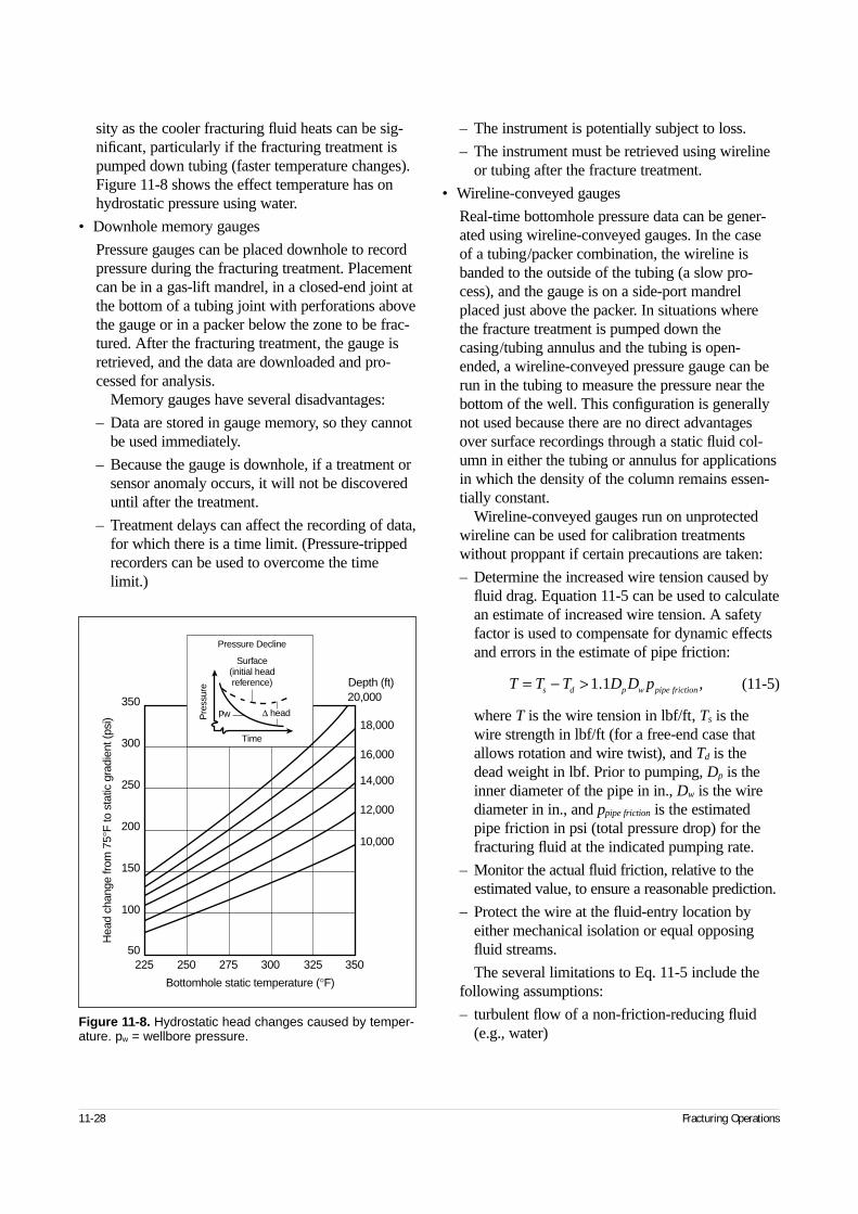
11-28 Fracturing Operations

sity as the cooler fracturing fluid heats can be sig-nificant, particularly if the fracturing treatment ispumped down tubing (faster temperature changes).Figure 11-8 shows the effect temperature has onhydrostatic pressure using water.

• Downhole memory gauges

Pressure gauges can be placed downhole to recordpressure during the fracturing treatment. Placementcan be in a gas-lift mandrel, in a closed-end joint atthe bottom of a tubing joint with perforations abovethe gauge or in a packer below the zone to be frac-tured. After the fracturing treatment, the gauge isretrieved, and the data are downloaded and pro-cessed for analysis.

Memory gauges have several disadvantages:

– Data are stored in gauge memory, so they cannotbe used immediately.

– Because the gauge is downhole, if a treatment orsensor anomaly occurs, it will not be discovereduntil after the treatment.

– Treatment delays can affect the recording of data,for which there is a time limit. (Pressure-trippedrecorders can be used to overcome the timelimit.)

– The instrument is potentially subject to loss.

– The instrument must be retrieved using wirelineor tubing after the fracture treatment.

• Wireline-conveyed gauges

Real-time bottomhole pressure data can be gener-ated using wireline-conveyed gauges. In the case of a tubing/packer combination, the wireline isbanded to the outside of the tubing (a slow pro-cess), and the gauge is on a side-port mandrelplaced just above the packer. In situations wherethe fracture treatment is pumped down thecasing/tubing annulus and the tubing is open-ended, a wireline-conveyed pressure gauge can berun in the tubing to measure the pressure near thebottom of the well. This configuration is generallynot used because there are no direct advantagesover surface recordings through a static fluid col-umn in either the tubing or annulus for applicationsin which the density of the column remains essen-tially constant.

Wireline-conveyed gauges run on unprotectedwireline can be used for calibration treatmentswithout proppant if certain precautions are taken:

– Determine the increased wire tension caused byfluid drag. Equation 11-5 can be used to calculatean estimate of increased wire tension. A safetyfactor is used to compensate for dynamic effectsand errors in the estimate of pipe friction:

(11-5)

where T is the wire tension in lbf/ft, Ts is thewire strength in lbf/ft (for a free-end case thatallows rotation and wire twist), and Td is thedead weight in lbf. Prior to pumping, Dp is theinner diameter of the pipe in in., Dw is the wirediameter in in., and ppipe friction is the estimatedpipe friction in psi (total pressure drop) for thefracturing fluid at the indicated pumping rate.

– Monitor the actual fluid friction, relative to theestimated value, to ensure a reasonable prediction.

– Protect the wire at the fluid-entry location byeither mechanical isolation or equal opposingfluid streams.

The several limitations to Eq. 11-5 include thefollowing assumptions:

– turbulent flow of a non-friction-reducing fluid(e.g., water)

Figure 11-8. Hydrostatic head changes caused by temper-ature. pw = wellbore pressure.

225 250 275 300 325 350

Bottomhole static temperature (°F)

350

300

250

150

200

100

50

Hea

d ch

ange

from

75°

F to

sta

tic g

radi

ent (

psi)

10,000

12,000

14,000

16,000

18,000

20,000Depth (ft)

pw

Time

Pre

ssur

e

Pressure Decline

Surface(initial headreference)

∆ head

T T T D D ps d p w pipe friction= − > 1 1. ,

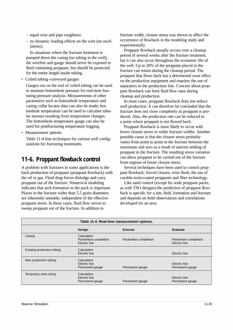
Reservoir Stimulation 11-29

– equal wire and pipe roughness

– no dynamic loading effects on the wire (no oscil-lations).

In situations where the fracture treatment ispumped down the casing (no tubing in the well),the wireline and gauge should never be exposed tofluid containing proppant, but should be protectedfor the entire length inside tubing.

• Coiled tubing–conveyed gauges

Gauges run on the end of coiled tubing can be usedto measure bottomhole pressure for real-time frac-turing pressure analysis. Measurements of otherparameters such as bottomhole temperature andcasing collar locator data can also be made; bot-tomhole temperature can be used to calculate tubu-lar stresses resulting from temperature changes.The bottomhole temperature gauge can also beused for postfracturing temperature logging.

• Measurement options

Table 11-4 lists techniques for various well config-urations for fracturing treatments.

11-6. Proppant flowback controlA problem with fractures in some applications is theback production of proppant (proppant flowback) withthe oil or gas. Fluid drag forces dislodge and carryproppant out of the fracture. Numerical modelingindicates that arch formation in the pack is important.Places in the fracture wider than 5.5 grain diametersare inherently unstable, independent of the effectiveproppant stress. In these cases, fluid flow serves tosweep proppant out of the fracture. In addition to

fracture width, closure stress was shown to affect theoccurrence of flowback in the modeling study andexperimentally.

Proppant flowback usually occurs over a cleanupperiod of several weeks after the fracture treatment,but it can also occur throughout the economic life ofthe well. Up to 20% of the proppant placed in thefracture can return during the cleanup period. Theproppant that flows back has a detrimental wear effecton the production equipment and requires the use ofseparators in the production line. Concern about prop-pant flowback can limit fluid flow rates duringcleanup and production.

In most cases, proppant flowback does not reducewell production. It can therefore be concluded that thefracture does not close completely as proppant is pro-duced. Also, the production rate can be reduced to a point where proppant is not flowed back.

Proppant flowback is more likely to occur withlower closure stress or wider fracture widths. Anotherpossible cause is that the closure stress probablyvaries from point to point in the fracture between themaximum and zero as a result of uneven settling ofproppant in the fracture. The resulting stress variationcan allow proppant to be carried out of the fracturefrom regions of lower closure stress.

Several techniques have been used to control prop-pant flowback: forced closure, resin flush, the use ofcurable-resin-coated proppants and fiber technology.

Like sand control (except for wide proppant packs,as with TSO designs) the prediction of proppant flow-back is specific for a site, field, formation and fractureand depends on field observations and correlationsdeveloped for an area.

Table 11-4. Real-time measurement options.

Design Execute Evaluate

Casing CalculationPackerless completion Packerless completion Packerless completionElectric line Electric line

Existing production tubing CalculationElectric line Electric line

New production tubing CalculationElectric line Electric linePermanent gauge Permanent gauge Permanent gauge

Temporary work string CalculationElectric line Electric linePermanent gauge Permanent gauge Permanent gauge

11-30 Fracturing Operations

11-6.1. Forced closureForced closure is a procedure in which fluid flowbackbegins immediately at the end of pumping. The theo-rized benefits of forced closure are that a “reverse”screenout takes place at the perforations (i.e., the frac-ture width closes to below that required for a stablearch) and that the fracture closes before the proppanthas a chance to settle in the fracture.

11-6.2. Resin flushThe resin flush technique involves pumping a curableresin into the fracture at the end of the job. In theory,the resin coats the proppant in the fracture near thewellbore and cures through a polymer crosslinkingreaction. Additional postflushes are used to ensure thatthe resin does not fill the pores in the proppant pack.The disadvantages of this technology are the difficul-ties in covering the entire interval with resin and thenpumping the postflush through the entire treated vol-ume and the requirement to drill the excess resin outof the wellbore after it cures.

11-6.3. Resin-coated proppantsThe use of curable phenolic resins with proppants is a popular method for controlling proppant flowback.They are used as all or some (tail-in) of the proppantplaced in the fracture. Under sufficient closure stress,shut-in time and temperature, the resin coating is sup-posed to bind the proppant together in the fracture andform a dense aggregate around the perforations. A dis-cussion of resin-coated proppants is in Chapter 7.

11-6.4. Fiber technologyFiber technology was developed to hold the proppantin the fracture during the production of oil, gas or bothand to allow more flexibility in flowback design thanpossible with curable-resin-coated proppants. Theseadditives work by the physical mechanism of randomfiber reinforcement; therefore, chemical curing reac-tions are not necessary to hold the proppant in place.No combination of temperature, pressure or shut-intime is required. Wells can be flowed back at highrates (dependent on the number of perforations). Also,flowback is possible immediately after the fracturingtreatment is completed. The rapid flowback rate

enables increased polymer cleanup early in the flow-back and can result in an increase in the total polymerreturned. Because no curing reactions occur, wellborecleanout is similar to that for normal proppant.Additional information on fiber technology is inSidebar 11F.

11-7. Flowback strategiesProper flowback of a fracturing treatment is designedto recover a maximum amount of the injected fluidswhile removing a minimum amount of proppant fromthe fracture. When to start the flowback and the flow-back rate are the key issues. Variables such as fractureclosure time, fluid break times (influenced by breakerschedule), reservoir energy available to produce thefracturing fluid, formation strength and proppant con-centration in the near-wellbore area affect the flow-back strategy.

The overall goal of a fracturing treatment is toachieve maximum fracture conductivity within thelimits of the designed treatment. The flowback effi-ciency of the stimulation fluid can have a significanteffect on the resultant fracture conductivity. In allcases and especially in the event that early-time prop-pant flowback control techniques are not used, fractur-ing fluid flowback efficiency should be consideredduring the design process.

Typically the fracture is allowed to close beforeflowback is initiated. Fracture closure is required totrap the proppant within the fracture and to preventsubsequent proppant movement through the applica-tion of fracture closure stress on the proppant. How-ever, even the application of closure stress may not besufficient to prevent some degree of proppant flow-back during treatment cleanup and post-treatment pro-duction. In these cases, the application of proppantflowback control techniques may be necessary.

Some fracturing fluids contain gases to foam orenergize the fluids. The gases most commonly used inenergized fluids are N2 and CO2. During flowback fol-lowing a treatment, they provide an efficient source ofconcentrated energy to aid in rapid and more completepost-treatment cleanup, especially in low-bottomhole-pressure wells. Compared with long-term swabbing orpumping operations, energized fluids can be costeffective. Entrained gas in the fracturing fluid is alsobeneficial for fluid-loss control.

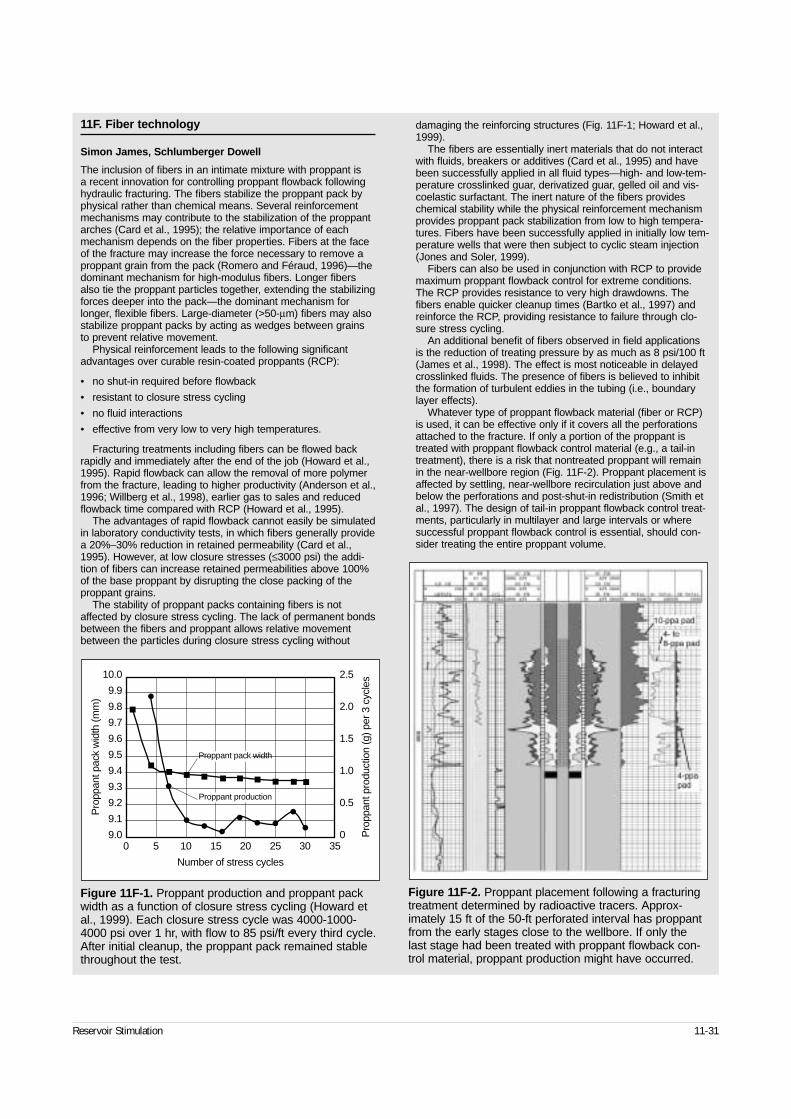
Reservoir Stimulation 11-31

11F. Fiber technology

Simon James, Schlumberger Dowell

The inclusion of fibers in an intimate mixture with proppant is a recent innovation for controlling proppant flowback followinghydraulic fracturing. The fibers stabilize the proppant pack byphysical rather than chemical means. Several reinforcementmechanisms may contribute to the stabilization of the proppantarches (Card et al., 1995); the relative importance of eachmechanism depends on the fiber properties. Fibers at the faceof the fracture may increase the force necessary to remove aproppant grain from the pack (Romero and Féraud, 1996)—thedominant mechanism for high-modulus fibers. Longer fibersalso tie the proppant particles together, extending the stabilizingforces deeper into the pack—the dominant mechanism forlonger, flexible fibers. Large-diameter (>50-µm) fibers may alsostabilize proppant packs by acting as wedges between grainsto prevent relative movement.

Physical reinforcement leads to the following significantadvantages over curable resin-coated proppants (RCP):

• no shut-in required before flowback

• resistant to closure stress cycling

• no fluid interactions

• effective from very low to very high temperatures.

Fracturing treatments including fibers can be flowed backrapidly and immediately after the end of the job (Howard et al.,1995). Rapid flowback can allow the removal of more polymerfrom the fracture, leading to higher productivity (Anderson et al.,1996; Willberg et al., 1998), earlier gas to sales and reducedflowback time compared with RCP (Howard et al., 1995).

The advantages of rapid flowback cannot easily be simulatedin laboratory conductivity tests, in which fibers generally providea 20%–30% reduction in retained permeability (Card et al.,1995). However, at low closure stresses (≤3000 psi) the addi-tion of fibers can increase retained permeabilities above 100%of the base proppant by disrupting the close packing of theproppant grains.

The stability of proppant packs containing fibers is notaffected by closure stress cycling. The lack of permanent bondsbetween the fibers and proppant allows relative movementbetween the particles during closure stress cycling without

damaging the reinforcing structures (Fig. 11F-1; Howard et al.,1999).

The fibers are essentially inert materials that do not interactwith fluids, breakers or additives (Card et al., 1995) and havebeen successfully applied in all fluid types—high- and low-tem-perature crosslinked guar, derivatized guar, gelled oil and vis-coelastic surfactant. The inert nature of the fibers provideschemical stability while the physical reinforcement mechanismprovides proppant pack stabilization from low to high tempera-tures. Fibers have been successfully applied in initially low tem-perature wells that were then subject to cyclic steam injection(Jones and Soler, 1999).

Fibers can also be used in conjunction with RCP to providemaximum proppant flowback control for extreme conditions.The RCP provides resistance to very high drawdowns. Thefibers enable quicker cleanup times (Bartko et al., 1997) andreinforce the RCP, providing resistance to failure through clo-sure stress cycling.

An additional benefit of fibers observed in field applications is the reduction of treating pressure by as much as 8 psi/100 ft(James et al., 1998). The effect is most noticeable in delayedcrosslinked fluids. The presence of fibers is believed to inhibitthe formation of turbulent eddies in the tubing (i.e., boundarylayer effects).

Whatever type of proppant flowback material (fiber or RCP)is used, it can be effective only if it covers all the perforationsattached to the fracture. If only a portion of the proppant istreated with proppant flowback control material (e.g., a tail-intreatment), there is a risk that nontreated proppant will remainin the near-wellbore region (Fig. 11F-2). Proppant placement isaffected by settling, near-wellbore recirculation just above andbelow the perforations and post-shut-in redistribution (Smith etal., 1997). The design of tail-in proppant flowback control treat-ments, particularly in multilayer and large intervals or wheresuccessful proppant flowback control is essential, should con-sider treating the entire proppant volume.

Figure 11F-1. Proppant production and proppant packwidth as a function of closure stress cycling (Howard etal., 1999). Each closure stress cycle was 4000-1000-4000 psi over 1 hr, with flow to 85 psi/ft every third cycle.After initial cleanup, the proppant pack remained stablethroughout the test.

10.0

9.9

9.8

9.7

9.6

9.5

9.4

9.3

9.2

9.1

9.0

2.5

2.0

1.5

1.0

0.5

00 5 10 15 20 25 30 35

Pro

ppan

t pro

duct

ion

(g) p

er 3

cyc

les

Pro

ppan

t pac

k w

idth

(mm

)

Number of stress cycles

Proppant production

Proppant pack width

Figure 11F-2. Proppant placement following a fracturingtreatment determined by radioactive tracers. Approx-imately 15 ft of the 50-ft perforated interval has proppantfrom the early stages close to the wellbore. If only thelast stage had been treated with proppant flowback con-trol material, proppant production might have occurred.

11-32 Fracturing Operations

N2 is inert and relatively immiscible in the fluidwhen added in small amounts and without a surfac-tant. CO2 is soluble in water and becomes a reactivecomponent in the fracturing fluid. CO2 can be con-verted to carbonic acid, which lowers fluid pH valuesand can be incompatible with fracturing fluids.

A large percentage of CO2 goes into solution at typ-ical reservoir conditions, which can be advantageous.As a dissolved gas, CO2 does not easily dissipate intothe formation. During flowback, the dissolved gasevolves from the mixture and imparts a solution-gasdrive to the fracturing fluid.

Energized fluids should be flowed back as soon aspossible while the fluid retains high pressure; how-ever, shut-in times of up to 4 hr can be tolerated with-out a great loss in the energizing medium.

11-8. Quality assurance and quality control

The principal factor in the successful performance ofa fracturing operation is the incorporation of qualityassurance and quality control (QA/QC) into all phasesof the fracturing operation. This can be achieved bythe implementation of a quality management systemthat encompasses all personnel and activities.

A significant effort is made in the design process todetermine an optimum fracturing treatment. An equaleffort in QA ensures that the treatment is executed asdesigned. Simple QA steps can greatly increase theodds of success for a hydraulic fracturing treatment.

11-9. Health, safety and environment

11-9.1. Safety considerationsAt no time should the safety aspects of a treatment becompromised. Safety guidelines have been developedfrom experience derived from previous incidents.Many of these incidents have had great potential toseriously injure personnel or destroy valuable equip-ment. The inherent risk of dealing with high pressurescan be greatly minimized by following simple safetyprocedures. Hydraulic fracturing treatments can neverbe considered a success if an accident results in thedestruction of equipment or injury to personnel.

• Personal safety equipment

Each person on location should wear appropriatesafety equipment to minimize the risk of personalinjury. Hard hats, hard-toed shoes and safetyglasses should be the minimum level of safetyequipment worn on location. Other equipment suchas hearing protection, goggles, fire-retardant fabricsand filter masks should be worn if exposure to theconditions they protect against is a possibility.Wearing safety equipment is a simple step thatcreates a positive safety atmosphere on location.

• Safety meeting

Holding a pretreatment safety meeting ensures thatall personnel on location are aware of specific dan-gers and required procedures relative to the treat-ment. Each person on location should clearlyunderstand his or her role during the treatment aswell as individual responsibility during emergencysituations. A head count must be taken to accountfor everyone on location. An escape route andmeeting place should be agreed upon where all per-sonnel will gather in the event of an emergency sit-uation. Personnel who are not directly involved inthe treatment should have limited location accessduring the actual pumping operations.

Everyone should be aware of the unique dangersof each treatment. Some locations may be in anarea with hydrogen sulfide (H2S) or possibly thefluids being pumped are highly flammable. Asmany of the potential safety problems or concernsas possible should be brought to the attention ofeveryone.

Maximum pressure limits should be set at thistime, and every high-pressure pump operator mustbe aware of these limits. Instructions for pressuretesting the treating iron must also be covered. Thehigh-pressure treating line, up to the wellheadvalve, should be tested to slightly above the antici-pated fracturing pressure. A properly tested lineincludes tests of each pump in addition to the maintreating line. The pressure rating of the wellheadshould be checked to make sure it exceeds thetreating pressure. If the wellhead has a lower pres-sure rating than the anticipated treating pressure, a wellhead isolation tool will be necessary to iso-late the wellhead from this pressure level.

The pretreatment safety meeting is the principalmeans of communication for giving final instruc-

Reservoir Stimulation 11-33

tions to all personnel. A well-organized safetymeeting helps ensure that the treatment is an opera-tional success without being a threat to humansafety.

• Well control at the wellhead

To ensure that well control is always maintained,the valve arrangement at the wellhead should con-sist of at least two valves. A frac or master valveshould be installed above the main wellhead valve.If one valve fails to hold the pressure, the othervalve can quickly be closed to control the well. It ispreferable to have the main wellhead valve flangedto the casing head, rather than using a threadedconnection. If a threaded connection is necessary,the condition of the threads must be thoroughlyinspected for thread wear and proper taper.

• Precautions for flammable fluids

Oil-base fluids should be tested for volatility beforethey are accepted as a fracturing fluid. An oil isgenerally considered safe to pump if it has a Reidvapor pressure less than 1, API gravity less than50° and open-cup flash point of 10°F [–12°C]. How-ever, even if the fluid is considered safe to pump,several additional safety rules should be followedwhen pumping an oil.

Storage tanks for flammable fluids should bediked and spotted at least 150 ft from the wellhead.Spotting the fluids in this manner helps minimizeexposing the wellhead to fire if problems occurduring pumping. Also, all low-pressure hosesshould be enclosed in a hose cover to prevent oilfrom spraying on hot engine components of thetrucks, should a hose leak.

Care must be taken to ensure that there is nosmoking on location. It is a good idea to have allpersonnel check matches and lighters when theyarrive on location to prevent them from unintention-

ally lighting up. Finally, fire-fighting equipmentshould be on location and ready to be operated. Inthis way, a small fire may be contained before it hasa chance to spread and become a major disaster.

• Precautions for energized fluids

N2 and CO2 are the gases most commonly used infoamed and energized fluids. During flowback fol-lowing a treatment, they provide an efficient sourceof concentrated energy to aid rapid, more completepost-treatment cleanup. There are potential hazardsassociated with the use of N2 and CO2. As the fluidexits the flowline during flowback, the gaseousphase expands rapidly. This rapid release of energymust be controlled to avoid a loss of flowback effi-ciency and to ensure personnel safety. Service com-panies have recommended procedures for the flow-back of energized fluids.

Another potential hazard that is often overlookedis asphyxiation. N2 and CO2 can collect in lowareas, displacing breathable air. Personnel shouldavoid these areas and remain upwind at all times.Only one person should be in the vicinity of thewell during flowback operations. The use ofremotely operated valves will increase the marginof safety.

11-9.2. Environmental considerationsFracturing operations should be conducted usingsound environmental practices to minimize the poten-tial for contamination of air, water and soil. All opera-tions should comply with all applicable environmentallaws and regulations.

Hazardous material spills should be cleaned upquickly in accordance with a spill plan. All waste andunused materials should be handled and disposed of in an environmentally safe manner.

IntroductionThe productivity of a cased, perforated well candepend to a large extent on perforation practices.Modern shaped charge perforators can penetrate forsome distance into the formation, overcoming bothdrilling damage and restricted flow through the perfo-rated casing. However, perforated completions fre-quently do not flow as predicted. Penetration differsfrom that in certification and quality control tests,owing to both the character of the formation rock andthe in-situ overburden stress. In addition, laboratorytests (Allen and Worzel, 1957) demonstrate that perfo-ration tunnels are commonly completely filled withdebris, and even debris-free perforations may not flowas predicted from pretest permeability measurements.

Although most relevant to natural completions, theperforating procedure and the condition of the result-ing perforations may affect the performance of post-perforation operations such as fracturing or gravelpacking. In hydraulic fracturing, acid can be used tolower breakdown pressures, presumably because ofsome form of perforation damage. The orientation ofperforations has also been shown to affect breakdownpressure and well performance. For fracture treatmentdesign, the interpretation of pretreatment well testsrequires knowledge of the skin resulting from pene-tration and perforation damage effects. Duringgravel-packing operations, excessive underbalance inunconsolidated formations may actually reduce flowefficiency by damaging the rock (Behrmann et al., 1992).

The factors involved in perforation damage mayinclude mechanical shock damage to the formation,deep filtration of fines from the wellbore or the forma-tion, rock and charge debris in the perforation tunneland multiphase flow effects. Two perforating tech-niques have evolved to avoid or bypass perforationdamage. These are underbalance perforating andextreme overbalance perforating (EOP). For morecomprehensive discussions of the field application of these techniques, the reader is referred to

Section 11-3 and the excellent monograph on perfo-rating by Bell et al. (1995).

Underbalance perforating has evolved from itsearly purpose of preventing the infiltration of well-bore fluids to a method for removing shock-inducedpermeability damage. Surge flow from the reservoirinto the wellbore is thought to clean loose debrisfrom the perforation and flush the rock around theperforation to restore permeability. Although effectivefor certain specific applications, questions remainregarding the limits of its usefulness and the mini-mum underbalance and surge flow volume requiredto obtain maximum well performance. Answers tothese questions can be sought from combined fieldexperience, laboratory measurements and models of perforation cleanup mechanics.

The review provided by this Appendix consists ofa brief discussion of penetration depth, experimentalobservations of the surrounding rock, models for themechanism of underbalance surge cleanup, descrip-tion of laboratory experiments that reveal the timescale and flow volume required for cleanup and a closing discussion of ancillary effects on perfora-tion performance.

Review of penetration depth predictionPenetration depends on the character of the targetrock formation, effective overburden stress (Saucierand Lands, 1978) and, in extreme cases, wellborepressure (Behrmann and Halleck, 1988). In Bereasandstone, penetration can be reduced by as much as 50% with the application of 3000-psi effectiveoverburden stress (Halleck et al., 1988). More typicalreductions are on the order of 20%. Little additionalreduction occurs for effective stresses higher than3000 psi. The nature of the rock affects both penetra-tion and the extent of the stress effect. Higherstrength leads to lower penetration. Conversely, stress

Reservoir Stimulation A11-1

◆

Appendix: Understanding Perforator Penetration and Flow Performance

Phillip M. Halleck, Pennsylvania State University

affects penetration less in harder rocks. Thus, penetra-tion data obtained from a single target material underatmospheric conditions do not reflect actual hole pene-tration. The API standard test (Halleck, 1987, 1988;Section 2 of Recommended Practices for Evaluation ofWell Perforators, [RP 43] 1991) in Berea sandstone at3000-psi effective stress provides a better estimate.

Uniaxial compressive strength has long been used(Thompson, 1962) to correlate ambient-stress pene-tration. This approach is complicated by the lack of a comprehensive penetration theory incorporatingtarget strength, by the change in rock strength witheffective stress (Halleck and Behrmann, 1990) and by active target effects in some rocks (Aseltine, 1985),which are not explained by conventional penetrationtheory. An attempt was made (Ott et al., 1994a) to uselaboratory data to predict downhole penetration fromAPI RP 43 Section 1 certification data. The resultingnomogram provides a simple method for estimatingdownhole penetration in lieu of costly tests in stressedreservoir rock. The method relies on a series of empir-ical correlations among compressive strength, porosityand penetration in rock and concrete targets at atmos-pheric pressure, combined with data in stressed rocktargets. Normalization of the data at 3000 psi, com-bined with statistical scatter in each of the successivecorrelations used, may lead to substantial errors (Colleet al., 1994; Ott et al., 1994b), particularly at effectivestresses less than 3000 psi.

An alternative for penetration estimates is acousticlog data based on direct relations between penetrationand dynamic elastic moduli in stressed rock. Origi-nally proposed by Venghiattis (1963), subsequent data(Halleck et al., 1991) largely support the idea that dif-ferences in acoustic velocity resulting from rock com-position and overburden stress mimic differences inshaped charge penetration.

Because of symmetry requirements, manufacturingtolerances for shaped charges are necessarily strict atall stages. Small variations in dimensions and hetero-geneities in the explosive or liner density can causedisproportionate variations in penetration performance.As a result, each charge type displays a statisticalvariation in measured penetration depth. Sukup et al.(1989) reviewed quality control testing methods thatcan be used to ensure good reliability. King et al.(1986) investigated additional factors that can affectcharge performance, including storage duration andenvironment.

Permeability damage and flow performance

Idealized viewMost discussions of perforation damage refer to debrisin the perforation tunnel and a crushed zone surround-ing the tunnel. The tunnel debris consists of brokenrock, jet metal, explosive products (mostly carbon)and other charge debris. If sufficient underbalance or production flow occurs, this debris is removed,leaving a clean tunnel. In well productivity models(Locke, 1981; Tariq, 1984; Ahmed et al., 1990; Behieand Settari, 1993), the perforation is usually treated as a circular cylinder surrounded by a zone of reducedpermeability variously called the crushed or compactedzone. The zone is usually given (Bell et al., 1972) as0.4 to 0.5 in. thick with permeability on the order of0.1 to 0.2 times the original rock permeability.

In reality, the diameter varies along its length, taper-ing toward the tip, and depends on the rock propertiesand charge design. The damaged zone is easily visiblein perforated samples as lighter colored materialaround the tunnel. Microscopic examination revealsconsiderable grain breakage in this zone, resulting inreduced permeability as the grain-size distributionbroadens and shifts to smaller diameters. Reducedporosity is also thought to play a role.

Pucknell and Behrmann (1991) confirmed earlierobservations made with optical microscopes thatreveal broken grains in this zone. Asadi and Preston(1991) used scanning electron microscopy (SEM) toestimate permeability damage from the size distribu-tion of the broken grains. Appendix Fig. 1 illustratesthis type of data with a comparison of SEM photos at 0.1 and 0.4 in. from the center of a perforation in Berea sandstone performed using underbalanced,liquid-saturated conditions.

Attempts to predict the extent of damage have alsobeen made. Yew and Zhang (1993) applied themethod of characteristics to obtain a solution for theamplitude of the shock waves resulting from theimpact of a shaped charge jet. They assumed cylin-drical radial loading and included poroelastic effects.They confirmed that stress wave amplitude falls offrapidly away from the perforation tunnel, althoughthey did not address the specific amplitudes expected.Papamichos et al. (1993) used this solution to estimatethe extent of grain breakage expected from such stress

A11-2 Chapter 11 Appendix: Understanding Perforator Penetration and Flow Performance

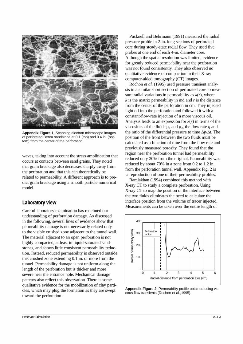
waves, taking into account the stress amplification thatoccurs at contacts between sand grains. They notedthat grain breakage also decreases sharply away fromthe perforation and that this can theoretically berelated to permeability. A different approach is to pre-dict grain breakage using a smooth particle numericalmodel.

Laboratory viewCareful laboratory examination has redefined ourunderstanding of perforation damage. As discussed in the following, several lines of evidence show thatpermeability damage is not necessarily related only to the visible crushed zone adjacent to the tunnel wall.The material adjacent to an open perforation is nothighly compacted, at least in liquid-saturated sand-stones, and shows little consistent permeability reduc-tion. Instead, reduced permeability is observed outsidethis crushed zone extending 0.1 in. or more from thetunnel. Permeability damage is not uniform along thelength of the perforation but is thicker and moresevere near the entrance hole. Mechanical damagepatterns also reflect this observation. There is somequalitative evidence for the mobilization of clay parti-cles, which may plug the formation as they are swepttoward the perforation.

Pucknell and Behrmann (1991) measured the radialpressure profile in 2-in. long sections of perforatedcore during steady-state radial flow. They used fiveprobes at one end of each 4-in. diameter core.Although the spatial resolution was limited, evidencefor greatly reduced permeability near the perforationwas not found consistently. They also observed noqualitative evidence of compaction in their X-raycomputer-aided tomography (CT) images.

Rochon et al. (1995) used pressure transient analy-sis in a similar short section of perforated core to mea-sure radial variations in permeability as k(r), where k is the matrix permeability in md and r is the distancefrom the center of the perforation in cm. They injectedlight oil into the perforation and followed it with aconstant-flow-rate injection of a more viscous oil.Analysis leads to an expression for k(r) in terms of theviscosities of the fluids µ1 and µ2, the flow rate q andthe ratio of the differential pressure to time ∆p/∆t. Theposition of the front between the two fluids must becalculated as a function of time from the flow rate andpreviously measured porosity. They found that theregion near the perforation tunnel had permeabilityreduced only 20% from the original. Permeability wasreduced by about 70% in a zone from 0.2 to 1.2 in.from the perforation tunnel wall. Appendix Fig. 2 isa reproduction of one of their permeability profiles.

Ramlakhan (1994) combined this method with X-ray CT to study a complete perforation. Using X-ray CT to map the position of the interface betweenthe two fluids eliminates the need to calculate theinterface position from the volume of tracer injected.Measurements can be taken over the entire length of

Reservoir Stimulation A11-3

Appendix Figure 1. Scanning electron microscope imagesof perforated Berea sandstone at 0.1 (top) and 0.4 in. (bot-tom) from the center of the perforation.

Appendix Figure 2. Permeability profile obtained using vis-cous flow transients (Rochon et al.,1995).

Radial distance from perforation axis (cm)

400

300

200

100

0

Rad

ial p

erm

eabi

lity

(md)

0 1 2 3 4 5 6

Perforationradius

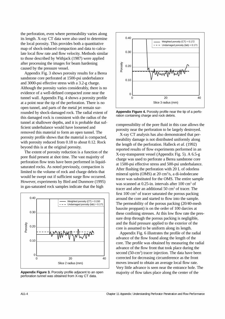
A11-4 Chapter 11 Appendix: Understanding Perforator Penetration and Flow Performance

the perforation, even where permeability varies alongits length. X-ray CT data were also used to determinethe local porosity. This provides both a quantitativemap of shock-induced compaction and data to calcu-late local flow rate and flow velocity. Methods similarto those described by Withjack (1987) were appliedafter processing the images for beam hardeningcaused by the pressure vessel.

Appendix Fig. 3 shows porosity results for a Bereasandstone core perforated at 1500-psi underbalanceand 3000-psi effective stress with a 3.2-g charge.Although the porosity varies considerably, there is noevidence of a well-defined compacted zone near thetunnel wall. Appendix Fig. 4 shows a porosity profileat a point near the tip of the perforation. There is noopen tunnel, and parts of the metal jet remain sur-rounded by shock-damaged rock. The radial extent ofthis damaged rock is consistent with the radius of thetunnel at shallower depths, and it is probable that suf-ficient underbalance would have loosened andremoved this material to form an open tunnel. Theporosity profile shows that the material is compacted,with porosity reduced from 0.18 to about 0.12. Rockbeyond this is at the original porosity.

The extent of porosity reduction is a function of thepore fluid present at shot time. The vast majority ofperforation flow tests have been performed in liquid-saturated rocks. As noted previously, compaction islimited to the volume of rock and charge debris thatwould be swept out if sufficient surge flow occurred.However, experiments by Bird and Dunmore (1995)in gas-saturated rock samples indicate that the high

compressibility of the pore fluid in this case allows theporosity near the perforation to be largely destroyed.

X-ray CT analysis has also demonstrated that per-meability damage is not distributed uniformly alongthe length of the perforation. Halleck et al. (1992)reported results of flow experiments performed in anX-ray-transparent vessel (Appendix Fig. 5). A 6.5-gcharge was used to perforate a Berea sandstone core at 1500-psi effective stress and 500-psi underbalance.After flushing the perforation with 20 L of odorlessmineral spirits (OMS) at 20 cm3/s, a di-iododecanetracer was substituted for the OMS. The entire samplewas scanned at 0.25-in. intervals after 100 cm3 oftracer and after an additional 50 cm3 of tracer. Thefirst 100 cm3 of tracer saturated the porous packingaround the core and started to flow into the sample.The permeability of the porous packing (20/40-meshbauxite proppant) is on the order of 100 darcies atthese confining stresses. At this low flow rate the pres-sure drop through the porous packing is negligible,and the fluid pressure applied to the exterior of thecore is assumed to be uniform along its length.

Appendix Fig. 6 illustrates the profile of the radialadvance of the flow found along the length of thecore. The profile was obtained by measuring the radialadvance of the flow front that took place during thesecond (50-cm3) tracer injection. The data have beencorrected for decreasing circumference as the frontmoves inward to obtain an average local flow rate.Very little advance is seen near the entrance hole. Themajority of flow takes place along the center of theAppendix Figure 3. Porosity profile adjacent to an open

perforation tunnel was obtained from X-ray CT data.

0 20 40

0.40

0.30

0.20

0.10

0

Por

osity

Slice 2 radius (mm)

Weighted porosity (CT) = 0.150Undamaged porosity (lab) = 0.171

Appendix Figure 4. Porosity profile near the tip of a perfo-ration containing charge and rock debris.

0 20 40

0.40

0.30

0.20

0.10

0

Por

osity

Slice 3 radius (mm)

Weighted porosity (CT) = 0.172

Undamaged porosity (lab) = 0.171

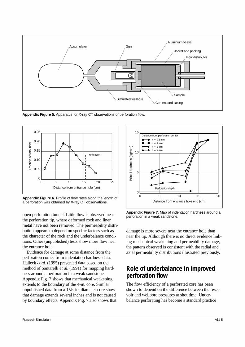
open perforation tunnel. Little flow is observed nearthe perforation tip, where deformed rock and linermetal have not been removed. The permeability distri-bution appears to depend on specific factors such asthe character of the rock and the underbalance condi-tions. Other (unpublished) tests show more flow nearthe entrance hole.

Evidence for damage at some distance from theperforation comes from indentation hardness data.Halleck et al. (1995) presented data based on themethod of Santarelli et al. (1991) for mapping hard-ness around a perforation in a weak sandstone.Appendix Fig. 7 shows that mechanical weakeningextends to the boundary of the 4-in. core. Similarunpublished data from a 151⁄2-in. diameter core showthat damage extends several inches and is not causedby boundary effects. Appendix Fig. 7 also shows that

damage is more severe near the entrance hole thannear the tip. Although there is no direct evidence link-ing mechanical weakening and permeability damage,the pattern observed is consistent with the radial andaxial permeability distributions illustrated previously.

Role of underbalance in improvedperforation flowThe flow efficiency of a perforated core has beenshown to depend on the difference between the reser-voir and wellbore pressures at shot time. Under-balance perforating has become a standard practice

Reservoir Stimulation A11-5

Appendix Figure 6. Profile of flow rates along the length ofa perforation was obtained by X-ray CT observations.

0 5 10 15 20 25

0.25

0.20

0.15

0.10

0.05

0

Distance from entrance hole (cm)

Frac

tion

of to

tal f

low

Perforation

Appendix Figure 7. Map of indentation hardness around aperforation in a weak sandstone.

0 5 10 15 20

15

10

5

0

Distance from entrance hole end (cm)

Brin

ell h

ardn

ess

(kg/

mm

)Distance from perforation center

r = 1.5 cmr = 2 cmr = 3 cmr = 4 cm

Perforation depth

Appendix Figure 5. Apparatus for X-ray CT observations of perforation flow.

Accumulator GunAluminium vessel

Jacket and packing

Flow distributor

Sample

Cement and casingSimulated wellbore

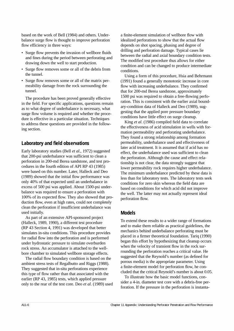
based on the work of Bell (1984) and others. Under-balance surge flow is thought to improve perforationflow efficiency in three ways:

• Surge flow prevents the invasion of wellbore fluidsand fines during the period between perforating anddrawing down the well to start production.

• Surge flow removes some or all of the debris fromthe tunnel.

• Surge flow removes some or all of the matrix per-meability damage from the rock surrounding thetunnel.

The procedure has been proved generally effectivein the field. For specific applications, questions remainas to what degree of underbalance is necessary, whatsurge flow volume is required and whether the proce-dure is effective in a particular situation. Techniquesto address these questions are provided in the follow-ing section.

Laboratory and field observationsEarly laboratory studies (Bell et al., 1972) suggestedthat 200-psi underbalance was sufficient to clean aperforation in 200-md Berea sandstone, and test pro-cedures in the fourth edition of API RP 43 (1985)were based on this number. Later, Halleck and Deo(1989) showed that the initial flow performance wasonly 40% of that expected until an underbalance inexcess of 500 psi was applied. About 1500-psi under-balance was required to ensure a perforation with100% of its expected flow. They also showed that pro-duction flow, even at high rates, could not completelyclean the perforation if insufficient underbalance wasused initially.

As part of an extensive API-sponsored project(Halleck, 1989, 1990), a different test procedure (RP 43 Section 4, 1991) was developed that bettersimulates in-situ conditions. This procedure providesfor radial flow into the perforation and is performedunder hydrostatic pressure to simulate overburdenrock stress. An accumulator is attached to the well-bore chamber to simulated wellbore storage effects.

The radial flow boundary condition is based on theambient stress tests of Regalbutto and Riggs (1988).They suggested that in-situ perforations experiencethis type of flow rather than that associated with theearlier (RP 43, 1985) tests, which applied pressureonly to the rear of the test core. Deo et al. (1989) used

a finite-element simulation of wellbore flow withidealized perforations to show that the actual flowdepends on shot spacing, phasing and degree ofdrilling and perforation damage. Typical cases liebetween the radial and axial boundary condition tests.The modified test procedure thus allows for eithercondition and can be changed to produce intermediateconditions.

Using a form of this procedure, Hsia and Behrmann(1991) found a generally monotonic increase in coreflow with increasing underbalance. They confirmedthat for 200-md Berea sandstone, approximately 1500 psi was required to obtain a free-flowing perfo-ration. This is consistent with the earlier axial bound-ary-condition data of Halleck and Deo (1989), sug-gesting that the applied pore pressure boundaryconditions have little effect on surge cleanup.

King et al. (1986) compiled field data to correlatethe effectiveness of acid stimulation in wells with for-mation permeability and perforating underbalance.They found a strong relationship among formationpermeability, underbalance used and effectiveness oflater acid treatment. It is assumed that if acid has noeffect, the underbalance used was sufficient to cleanthe perforation. Although the cause and effect rela-tionship is not clear, the data strongly suggest thatlower permeability rock requires higher underbalance.The minimum underbalance predicted by these data isless than for laboratory tests. The laboratory tests seekconditions for zero skin whereas the field data arebased on conditions for which acid did not improvethe well. The latter may not actually represent idealperforation flow.

ModelsTo extend these results to a wider range of formationsand to make them reliable as practical guidelines, themechanics behind underbalance perforating must beplaced in a firmer theoretical foundation. Tariq (1990)began this effort by hypothesizing that cleanup occurswhen the velocity of transient flow in the rock sur-rounding the perforation reaches a critical value. Hesuggested that the Reynold’s number (as defined forporous media) is the appropriate parameter. Using a finite-element model for perforation flow, he con-cluded that the critical Reynold’s number is about 0.05.

To illustrate how the basic model functions, con-sider a 4-in. diameter test core with a debris-free per-foration. If the pressure in the perforation is instanta-

A11-6 Chapter 11 Appendix: Understanding Perforator Penetration and Flow Performance

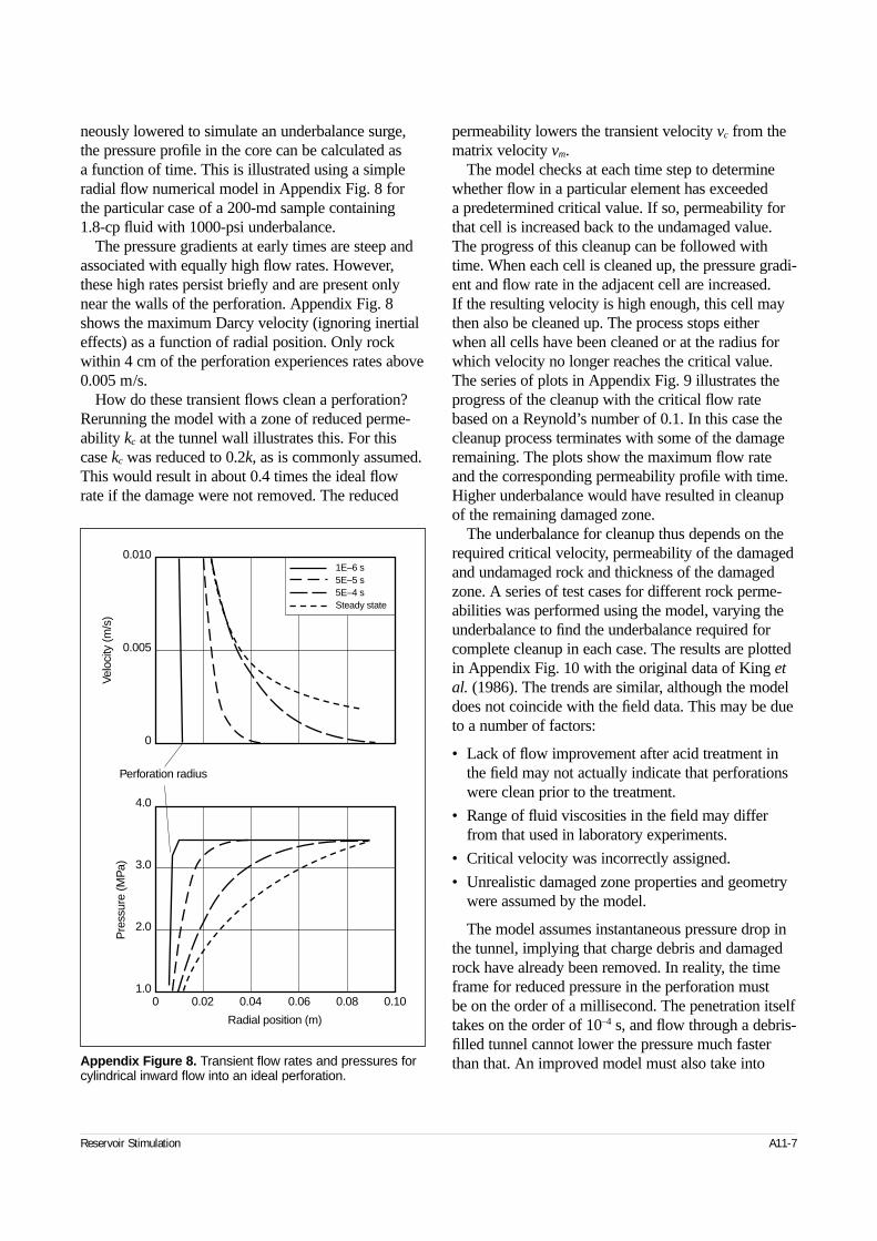
neously lowered to simulate an underbalance surge,the pressure profile in the core can be calculated as a function of time. This is illustrated using a simpleradial flow numerical model in Appendix Fig. 8 forthe particular case of a 200-md sample containing 1.8-cp fluid with 1000-psi underbalance.

The pressure gradients at early times are steep andassociated with equally high flow rates. However,these high rates persist briefly and are present onlynear the walls of the perforation. Appendix Fig. 8shows the maximum Darcy velocity (ignoring inertialeffects) as a function of radial position. Only rockwithin 4 cm of the perforation experiences rates above0.005 m/s.

How do these transient flows clean a perforation?Rerunning the model with a zone of reduced perme-ability kc at the tunnel wall illustrates this. For thiscase kc was reduced to 0.2k, as is commonly assumed.This would result in about 0.4 times the ideal flowrate if the damage were not removed. The reduced

permeability lowers the transient velocity vc from thematrix velocity vm.

The model checks at each time step to determinewhether flow in a particular element has exceeded a predetermined critical value. If so, permeability forthat cell is increased back to the undamaged value.The progress of this cleanup can be followed withtime. When each cell is cleaned up, the pressure gradi-ent and flow rate in the adjacent cell are increased. If the resulting velocity is high enough, this cell maythen also be cleaned up. The process stops eitherwhen all cells have been cleaned or at the radius forwhich velocity no longer reaches the critical value.The series of plots in Appendix Fig. 9 illustrates theprogress of the cleanup with the critical flow ratebased on a Reynold’s number of 0.1. In this case thecleanup process terminates with some of the damageremaining. The plots show the maximum flow rateand the corresponding permeability profile with time.Higher underbalance would have resulted in cleanupof the remaining damaged zone.

The underbalance for cleanup thus depends on therequired critical velocity, permeability of the damagedand undamaged rock and thickness of the damagedzone. A series of test cases for different rock perme-abilities was performed using the model, varying theunderbalance to find the underbalance required forcomplete cleanup in each case. The results are plottedin Appendix Fig. 10 with the original data of King etal. (1986). The trends are similar, although the modeldoes not coincide with the field data. This may be dueto a number of factors:

• Lack of flow improvement after acid treatment inthe field may not actually indicate that perforationswere clean prior to the treatment.

• Range of fluid viscosities in the field may differfrom that used in laboratory experiments.

• Critical velocity was incorrectly assigned.

• Unrealistic damaged zone properties and geometrywere assumed by the model.

The model assumes instantaneous pressure drop inthe tunnel, implying that charge debris and damagedrock have already been removed. In reality, the timeframe for reduced pressure in the perforation must be on the order of a millisecond. The penetration itselftakes on the order of 10–4 s, and flow through a debris-filled tunnel cannot lower the pressure much fasterthan that. An improved model must also take into

Reservoir Stimulation A11-7

Appendix Figure 8. Transient flow rates and pressures forcylindrical inward flow into an ideal perforation.

0 0.02 0.04 0.06 0.08 0.10

0.010

0.005

0

Velo

city

(m/s

)

Perforation radius

4.0

3.0

2.0

1.0

Radial position (m)

Pre

ssur

e (M

Pa)

1E–6 s5E–5 s5E–4 sSteady state

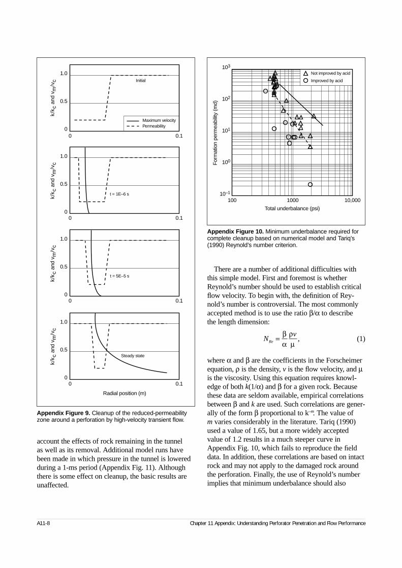
account the effects of rock remaining in the tunnel as well as its removal. Additional model runs havebeen made in which pressure in the tunnel is loweredduring a 1-ms period (Appendix Fig. 11). Althoughthere is some effect on cleanup, the basic results areunaffected.

There are a number of additional difficulties withthis simple model. First and foremost is whetherReynold’s number should be used to establish criticalflow velocity. To begin with, the definition of Rey-nold’s number is controversial. The most commonlyaccepted method is to use the ratio β/α to describe the length dimension:

(1)

where α and β are the coefficients in the Forscheimerequation, ρ is the density, v is the flow velocity, and µis the viscosity. Using this equation requires knowl-edge of both k(1/α) and β for a given rock. Becausethese data are seldom available, empirical correlationsbetween β and k are used. Such correlations are gener-ally of the form β proportional to k–m. The value of m varies considerably in the literature. Tariq (1990)used a value of 1.65, but a more widely acceptedvalue of 1.2 results in a much steeper curve inAppendix Fig. 10, which fails to reproduce the fielddata. In addition, these correlations are based on intactrock and may not apply to the damaged rock aroundthe perforation. Finally, the use of Reynold’s numberimplies that minimum underbalance should also

A11-8 Chapter 11 Appendix: Understanding Perforator Penetration and Flow Performance

Appendix Figure 10. Minimum underbalance required forcomplete cleanup based on numerical model and Tariq’s(1990) Reynold’s number criterion.

100 1000 10,000

103

102

101

100

10–1

Form

atio

n pe

rmea

bilit

y (m

d)Total underbalance (psi)

Not improved by acid

Improved by acid

Nv

Re = βα

ρµ

,

Appendix Figure 9. Cleanup of the reduced-permeabilityzone around a perforation by high-velocity transient flow.

0 0.1

1.0

0.5

0

Radial position (m)

k/k c

and

vm

/vc

0 0.1

1.0

0.5

0

k/k c

and

vm

/vc

0 0.1

0 0.1

1.0

0.5

0

k/k c

and

vm

/vc

1.0

0.5

0

k/k c

and

vm

/vc

Maximum velocityPermeability

Initial

t = 1E–6 s

t = 5E–5 s

Steady state

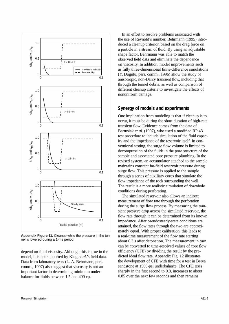
depend on fluid viscosity. Although this is true in themodel, it is not supported by King et al.’s field data.Data from laboratory tests (L. A. Behrmann, pers.comm., 1997) also suggest that viscosity is not animportant factor in determining minimum under-balance for fluids between 1.5 and 400 cp.

In an effort to resolve problems associated with the use of Reynold’s number, Behrmann (1995) intro-duced a cleanup criterion based on the drag force on a particle in a stream of fluid. By using an adjustableshape factor, Behrmann was able to match theobserved field data and eliminate the dependence on viscosity. In addition, model improvements such as fully three-dimensional finite-difference simulations(Y. Dogulu, pers. comm., 1996) allow the study ofanisotropic, non-Darcy transient flow, including thatthrough the tunnel debris, as well as comparison ofdifferent cleanup criteria to investigate the effects ofnonuniform damage.

Synergy of models and experimentsOne implication from modeling is that if cleanup is tooccur, it must be during the short duration of high-ratetransient flow. Evidence comes from the data ofBartusiak et al. (1997), who used a modified RP 43test procedure to include simulation of the fluid capac-ity and the impedance of the reservoir itself. In con-ventional testing, the surge flow volume is limited todecompression of the fluids in the pore structure of thesample and associated pore pressure plumbing. In therevised system, an accumulator attached to the samplemaintains constant far-field reservoir pressure duringsurge flow. This pressure is applied to the samplethrough a series of auxiliary cores that simulate theflow impedance of the rock surrounding the well. The result is a more realistic simulation of downholeconditions during perforating.

The simulated reservoir also allows an indirectmeasurement of flow rate through the perforationduring the surge flow process. By measuring the tran-sient pressure drop across the simulated reservoir, theflow rate through it can be determined from its knownimpedance. After pseudosteady-state conditions areattained, the flow rates through the two are approxi-mately equal. With proper calibration, this leads to a real-time measurement of the flow rate startingabout 0.3 s after detonation. The measurement in turncan be converted to time-resolved values of core flowefficiency (CFE) by dividing the result by the pre-dicted ideal flow rate. Appendix Fig. 12 illustrates the development of CFE with time for a test in Bereasandstone at 1500-psi underbalance. The CFE risessharply in the first second to 0.8, increases to about0.85 over the next few seconds and then remains

Reservoir Stimulation A11-9

Appendix Figure 11. Cleanup while the pressure in the tun-nel is lowered during a 1-ms period.

0 0.1

0 0.1

0 0.1

0 0.1

0

0.5

1.0

0

0.5

1.0

0

0.5

1.0

0

0.5

1.0

Radial position (m)

Maximum velocityPermeability

t = 5E–4 s

t = 1E–4 s

t = 1E–3 s

Steady state

k/k c

and

vm

/vc

k/k c

and

vm

/vc

k/k c

and

vm

/vc

k/k c

and

vm

/vc

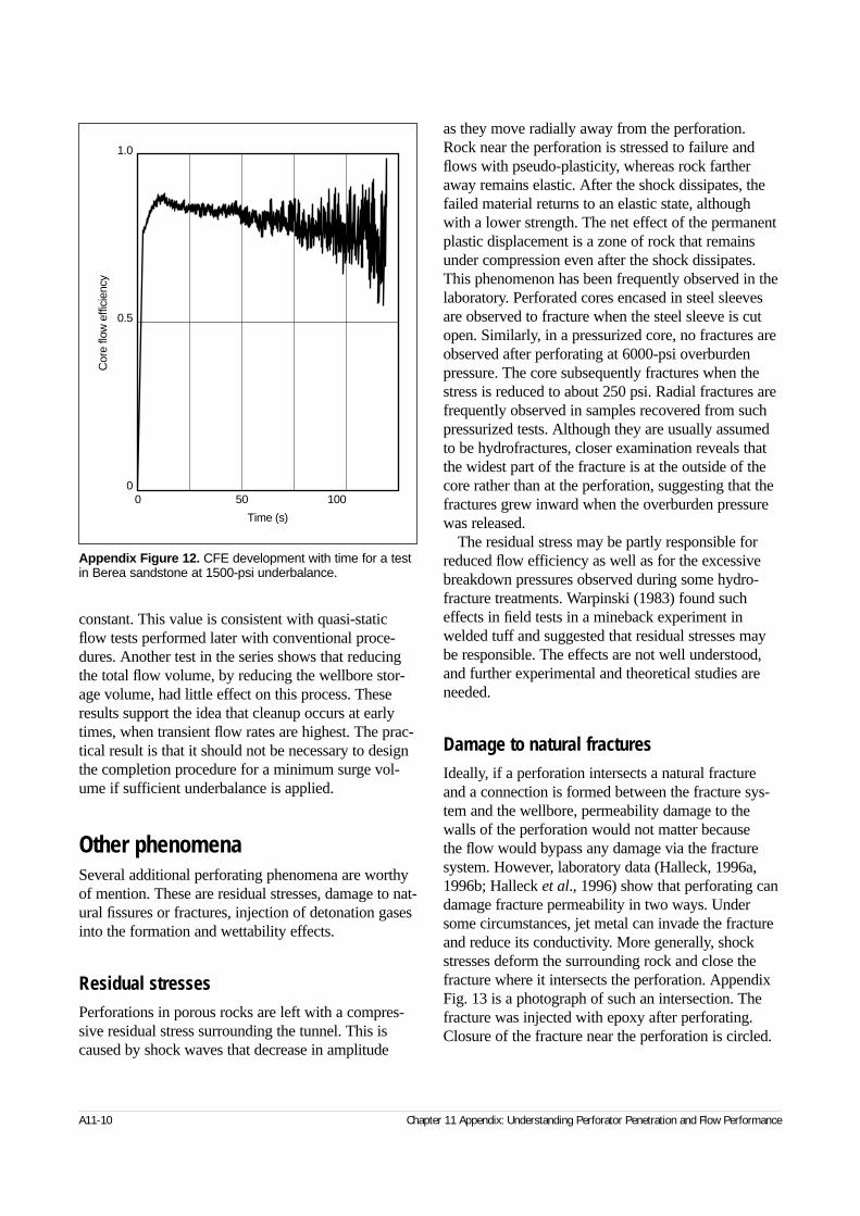
constant. This value is consistent with quasi-staticflow tests performed later with conventional proce-dures. Another test in the series shows that reducingthe total flow volume, by reducing the wellbore stor-age volume, had little effect on this process. Theseresults support the idea that cleanup occurs at earlytimes, when transient flow rates are highest. The prac-tical result is that it should not be necessary to designthe completion procedure for a minimum surge vol-ume if sufficient underbalance is applied.

Other phenomenaSeveral additional perforating phenomena are worthyof mention. These are residual stresses, damage to nat-ural fissures or fractures, injection of detonation gasesinto the formation and wettability effects.

Residual stressesPerforations in porous rocks are left with a compres-sive residual stress surrounding the tunnel. This iscaused by shock waves that decrease in amplitude

as they move radially away from the perforation.Rock near the perforation is stressed to failure andflows with pseudo-plasticity, whereas rock fartheraway remains elastic. After the shock dissipates, thefailed material returns to an elastic state, althoughwith a lower strength. The net effect of the permanentplastic displacement is a zone of rock that remainsunder compression even after the shock dissipates.This phenomenon has been frequently observed in thelaboratory. Perforated cores encased in steel sleevesare observed to fracture when the steel sleeve is cutopen. Similarly, in a pressurized core, no fractures areobserved after perforating at 6000-psi overburdenpressure. The core subsequently fractures when thestress is reduced to about 250 psi. Radial fractures arefrequently observed in samples recovered from suchpressurized tests. Although they are usually assumedto be hydrofractures, closer examination reveals thatthe widest part of the fracture is at the outside of thecore rather than at the perforation, suggesting that thefractures grew inward when the overburden pressurewas released.

The residual stress may be partly responsible forreduced flow efficiency as well as for the excessivebreakdown pressures observed during some hydro-fracture treatments. Warpinski (1983) found sucheffects in field tests in a mineback experiment inwelded tuff and suggested that residual stresses maybe responsible. The effects are not well understood,and further experimental and theoretical studies areneeded.

Damage to natural fracturesIdeally, if a perforation intersects a natural fractureand a connection is formed between the fracture sys-tem and the wellbore, permeability damage to thewalls of the perforation would not matter because the flow would bypass any damage via the fracturesystem. However, laboratory data (Halleck, 1996a,1996b; Halleck et al., 1996) show that perforating candamage fracture permeability in two ways. Undersome circumstances, jet metal can invade the fractureand reduce its conductivity. More generally, shockstresses deform the surrounding rock and close thefracture where it intersects the perforation. AppendixFig. 13 is a photograph of such an intersection. Thefracture was injected with epoxy after perforating.Closure of the fracture near the perforation is circled.

A11-10 Chapter 11 Appendix: Understanding Perforator Penetration and Flow Performance

Appendix Figure 12. CFE development with time for a testin Berea sandstone at 1500-psi underbalance.

1.0

0.5

00 50 100

Time (s)

Cor

e flo

w e

ffici

ency

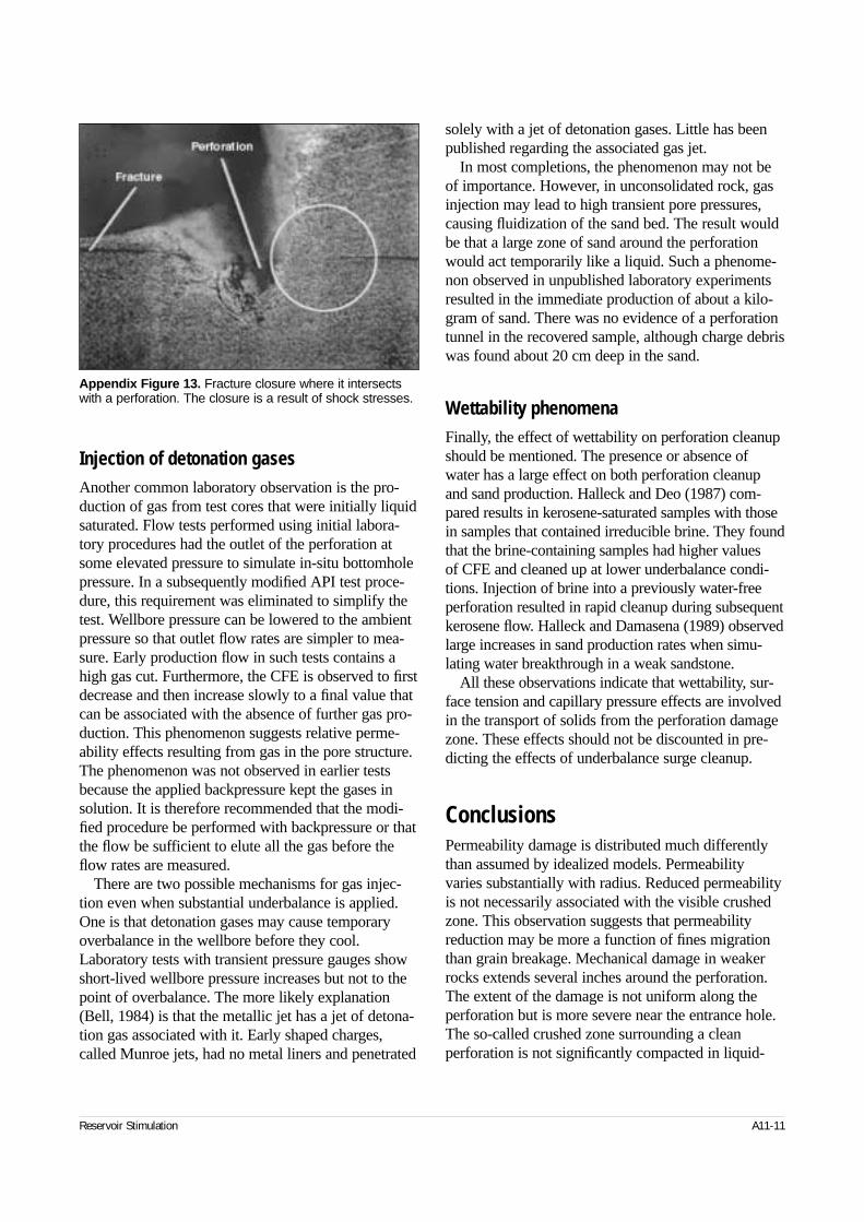
Injection of detonation gasesAnother common laboratory observation is the pro-duction of gas from test cores that were initially liquidsaturated. Flow tests performed using initial labora-tory procedures had the outlet of the perforation atsome elevated pressure to simulate in-situ bottomholepressure. In a subsequently modified API test proce-dure, this requirement was eliminated to simplify thetest. Wellbore pressure can be lowered to the ambientpressure so that outlet flow rates are simpler to mea-sure. Early production flow in such tests contains ahigh gas cut. Furthermore, the CFE is observed to firstdecrease and then increase slowly to a final value thatcan be associated with the absence of further gas pro-duction. This phenomenon suggests relative perme-ability effects resulting from gas in the pore structure.The phenomenon was not observed in earlier testsbecause the applied backpressure kept the gases insolution. It is therefore recommended that the modi-fied procedure be performed with backpressure or thatthe flow be sufficient to elute all the gas before theflow rates are measured.

There are two possible mechanisms for gas injec-tion even when substantial underbalance is applied.One is that detonation gases may cause temporaryoverbalance in the wellbore before they cool.Laboratory tests with transient pressure gauges showshort-lived wellbore pressure increases but not to thepoint of overbalance. The more likely explanation(Bell, 1984) is that the metallic jet has a jet of detona-tion gas associated with it. Early shaped charges,called Munroe jets, had no metal liners and penetrated

solely with a jet of detonation gases. Little has beenpublished regarding the associated gas jet.

In most completions, the phenomenon may not beof importance. However, in unconsolidated rock, gasinjection may lead to high transient pore pressures,causing fluidization of the sand bed. The result wouldbe that a large zone of sand around the perforationwould act temporarily like a liquid. Such a phenome-non observed in unpublished laboratory experimentsresulted in the immediate production of about a kilo-gram of sand. There was no evidence of a perforationtunnel in the recovered sample, although charge debriswas found about 20 cm deep in the sand.

Wettability phenomenaFinally, the effect of wettability on perforation cleanupshould be mentioned. The presence or absence ofwater has a large effect on both perforation cleanupand sand production. Halleck and Deo (1987) com-pared results in kerosene-saturated samples with thosein samples that contained irreducible brine. They foundthat the brine-containing samples had higher valuesof CFE and cleaned up at lower underbalance condi-tions. Injection of brine into a previously water-freeperforation resulted in rapid cleanup during subsequentkerosene flow. Halleck and Damasena (1989) observedlarge increases in sand production rates when simu-lating water breakthrough in a weak sandstone.

All these observations indicate that wettability, sur-face tension and capillary pressure effects are involvedin the transport of solids from the perforation damagezone. These effects should not be discounted in pre-dicting the effects of underbalance surge cleanup.

ConclusionsPermeability damage is distributed much differentlythan assumed by idealized models. Permeabilityvaries substantially with radius. Reduced permeabilityis not necessarily associated with the visible crushedzone. This observation suggests that permeabilityreduction may be more a function of fines migrationthan grain breakage. Mechanical damage in weakerrocks extends several inches around the perforation.The extent of the damage is not uniform along theperforation but is more severe near the entrance hole.The so-called crushed zone surrounding a cleanperforation is not significantly compacted in liquid-

Reservoir Stimulation A11-11

Appendix Figure 13. Fracture closure where it intersectswith a perforation. The closure is a result of shock stresses.

saturated rocks, but it may be in gas-saturated ones.Compacted material exists in the rock near the centerof the perforation, but it is seen only at the perforationtip or in tests with insufficient underbalance to removeit. Perforation cleanup is related to transient flow

velocity through the rock around the perforation andoccurs at early times, when transient rates are highest.Large surge flow volumes should not be necessarywhere sufficient underbalance is applied.

A11-12 Chapter 11 Appendix: Understanding Perforator Penetration and Flow Performance

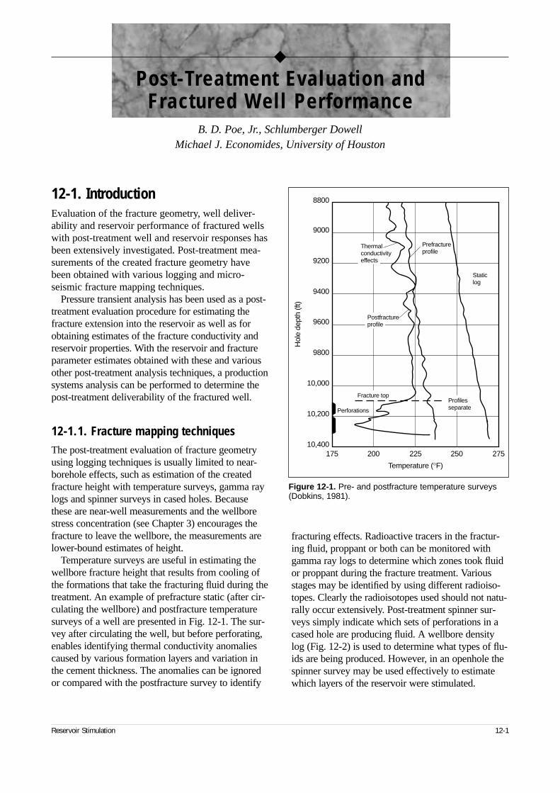
12-1. IntroductionEvaluation of the fracture geometry, well deliver-ability and reservoir performance of fractured wellswith post-treatment well and reservoir responses hasbeen extensively investigated. Post-treatment mea-surements of the created fracture geometry havebeen obtained with various logging and micro-seismic fracture mapping techniques.

Pressure transient analysis has been used as a post-treatment evaluation procedure for estimating thefracture extension into the reservoir as well as forobtaining estimates of the fracture conductivity andreservoir properties. With the reservoir and fractureparameter estimates obtained with these and variousother post-treatment analysis techniques, a productionsystems analysis can be performed to determine thepost-treatment deliverability of the fractured well.

12-1.1. Fracture mapping techniquesThe post-treatment evaluation of fracture geometryusing logging techniques is usually limited to near-borehole effects, such as estimation of the createdfracture height with temperature surveys, gamma raylogs and spinner surveys in cased holes. Becausethese are near-well measurements and the wellborestress concentration (see Chapter 3) encourages thefracture to leave the wellbore, the measurements arelower-bound estimates of height.

Temperature surveys are useful in estimating thewellbore fracture height that results from cooling ofthe formations that take the fracturing fluid during thetreatment. An example of prefracture static (after cir-culating the wellbore) and postfracture temperaturesurveys of a well are presented in Fig. 12-1. The sur-vey after circulating the well, but before perforating,enables identifying thermal conductivity anomaliescaused by various formation layers and variation inthe cement thickness. The anomalies can be ignoredor compared with the postfracture survey to identify

fracturing effects. Radioactive tracers in the fractur-ing fluid, proppant or both can be monitored withgamma ray logs to determine which zones took fluidor proppant during the fracture treatment. Variousstages may be identified by using different radioiso-topes. Clearly the radioisotopes used should not natu-rally occur extensively. Post-treatment spinner sur-veys simply indicate which sets of perforations in acased hole are producing fluid. A wellbore densitylog (Fig. 12-2) is used to determine what types of flu-ids are being produced. However, in an openhole thespinner survey may be used effectively to estimatewhich layers of the reservoir were stimulated.

Reservoir Stimulation 12-1

◆

Post-Treatment Evaluation andFractured Well Performance

B. D. Poe, Jr., Schlumberger DowellMichael J. Economides, University of Houston

Figure 12-1. Pre- and postfracture temperature surveys(Dobkins, 1981).

17510,400

200 225 250 275

10,200

10,000

9800

9600

9400

9200

9000

8800

Temperature (°F)

Hol

e de

pth

(ft)

Thermalconductivityeffects

Prefractureprofile

Staticlog

Perforations

Postfractureprofile

Fracture topProfilesseparate

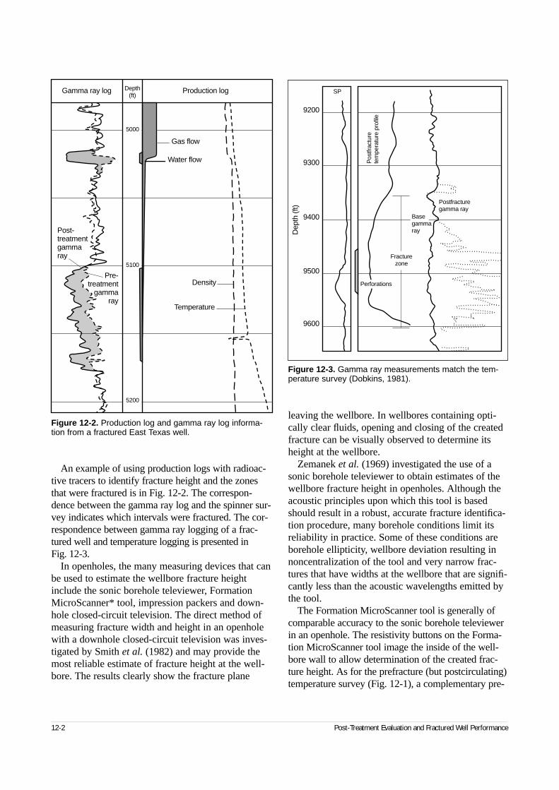
An example of using production logs with radioac-tive tracers to identify fracture height and the zonesthat were fractured is in Fig. 12-2. The correspon-dence between the gamma ray log and the spinner sur-vey indicates which intervals were fractured. The cor-respondence between gamma ray logging of a frac-tured well and temperature logging is presented in Fig. 12-3.

In openholes, the many measuring devices that canbe used to estimate the wellbore fracture heightinclude the sonic borehole televiewer, FormationMicroScanner* tool, impression packers and down-hole closed-circuit television. The direct method ofmeasuring fracture width and height in an openholewith a downhole closed-circuit television was inves-tigated by Smith et al. (1982) and may provide themost reliable estimate of fracture height at the well-bore. The results clearly show the fracture plane

leaving the wellbore. In wellbores containing opti-cally clear fluids, opening and closing of the createdfracture can be visually observed to determine itsheight at the wellbore.

Zemanek et al. (1969) investigated the use of asonic borehole televiewer to obtain estimates of thewellbore fracture height in openholes. Although theacoustic principles upon which this tool is basedshould result in a robust, accurate fracture identifica-tion procedure, many borehole conditions limit itsreliability in practice. Some of these conditions areborehole ellipticity, wellbore deviation resulting innoncentralization of the tool and very narrow frac-tures that have widths at the wellbore that are signifi-cantly less than the acoustic wavelengths emitted bythe tool.

The Formation MicroScanner tool is generally ofcomparable accuracy to the sonic borehole televiewerin an openhole. The resistivity buttons on the Forma-tion MicroScanner tool image the inside of the well-bore wall to allow determination of the created frac-ture height. As for the prefracture (but postcirculating)temperature survey (Fig. 12-1), a complementary pre-

12-2 Post-Treatment Evaluation and Fractured Well Performance

Figure 12-2. Production log and gamma ray log informa-tion from a fractured East Texas well.

Density

Gas flow

Water flow

Temperature

Gamma ray log Depth(ft)

Production log

Post-treatmentgammaray

Pre-treatment

gammaray

5000

5100

5200

Figure 12-3. Gamma ray measurements match the tem-perature survey (Dobkins, 1981).

Postfracturegamma ray

Perforations

Fracturezone

Basegammaray

Pos

tfrac

ture

tem

pera

ture

pro

file

SP

9600

9500

9400

9300

9200

Dep

th (f

t)

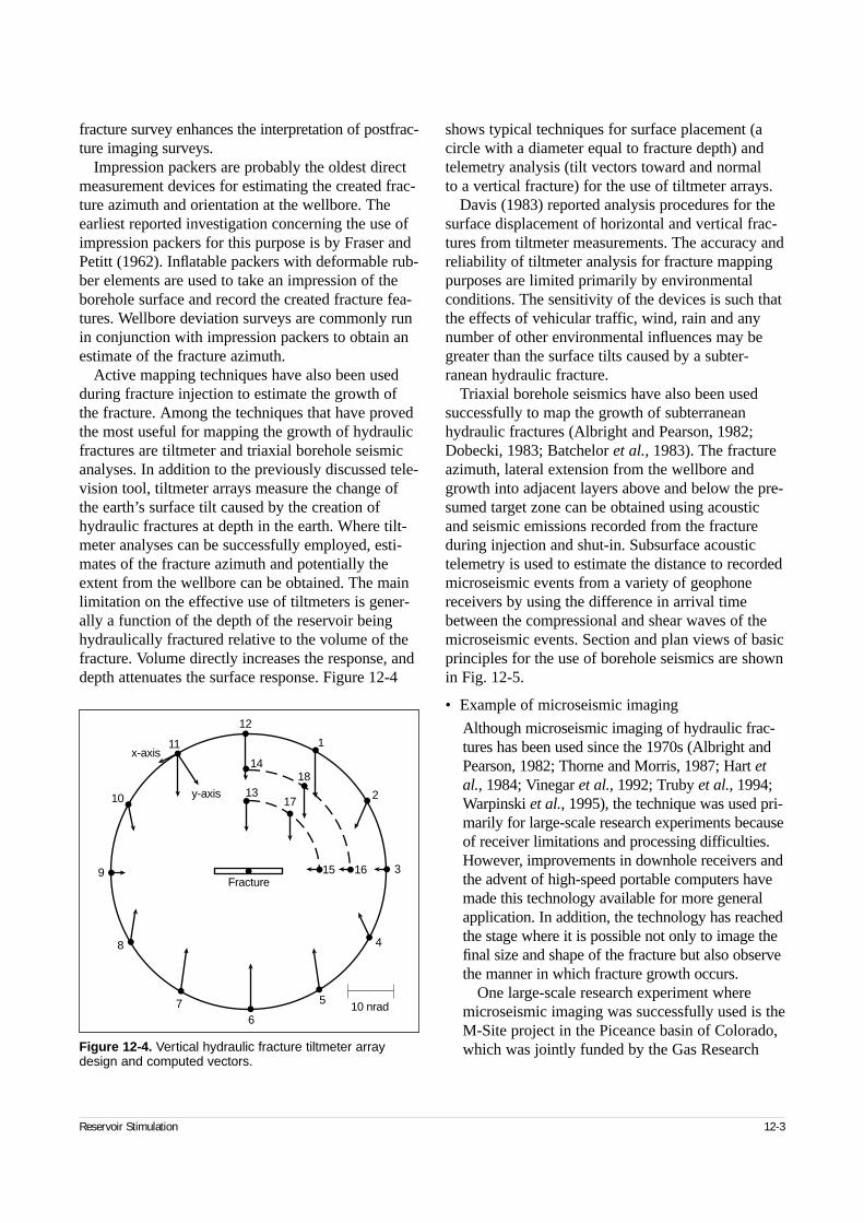
fracture survey enhances the interpretation of postfrac-ture imaging surveys.

Impression packers are probably the oldest directmeasurement devices for estimating the created frac-ture azimuth and orientation at the wellbore. Theearliest reported investigation concerning the use ofimpression packers for this purpose is by Fraser andPetitt (1962). Inflatable packers with deformable rub-ber elements are used to take an impression of theborehole surface and record the created fracture fea-tures. Wellbore deviation surveys are commonly runin conjunction with impression packers to obtain anestimate of the fracture azimuth.

Active mapping techniques have also been usedduring fracture injection to estimate the growth ofthe fracture. Among the techniques that have provedthe most useful for mapping the growth of hydraulicfractures are tiltmeter and triaxial borehole seismicanalyses. In addition to the previously discussed tele-vision tool, tiltmeter arrays measure the change ofthe earth’s surface tilt caused by the creation ofhydraulic fractures at depth in the earth. Where tilt-meter analyses can be successfully employed, esti-mates of the fracture azimuth and potentially theextent from the wellbore can be obtained. The mainlimitation on the effective use of tiltmeters is gener-ally a function of the depth of the reservoir beinghydraulically fractured relative to the volume of thefracture. Volume directly increases the response, anddepth attenuates the surface response. Figure 12-4

shows typical techniques for surface placement (acircle with a diameter equal to fracture depth) andtelemetry analysis (tilt vectors toward and normal to a vertical fracture) for the use of tiltmeter arrays.

Davis (1983) reported analysis procedures for thesurface displacement of horizontal and vertical frac-tures from tiltmeter measurements. The accuracy andreliability of tiltmeter analysis for fracture mappingpurposes are limited primarily by environmentalconditions. The sensitivity of the devices is such thatthe effects of vehicular traffic, wind, rain and anynumber of other environmental influences may begreater than the surface tilts caused by a subter-ranean hydraulic fracture.

Triaxial borehole seismics have also been usedsuccessfully to map the growth of subterraneanhydraulic fractures (Albright and Pearson, 1982;Dobecki, 1983; Batchelor et al., 1983). The fractureazimuth, lateral extension from the wellbore andgrowth into adjacent layers above and below the pre-sumed target zone can be obtained using acousticand seismic emissions recorded from the fractureduring injection and shut-in. Subsurface acoustictelemetry is used to estimate the distance to recordedmicroseismic events from a variety of geophonereceivers by using the difference in arrival timebetween the compressional and shear waves of themicroseismic events. Section and plan views of basicprinciples for the use of borehole seismics are shownin Fig. 12-5.

• Example of microseismic imaging

Although microseismic imaging of hydraulic frac-tures has been used since the 1970s (Albright andPearson, 1982; Thorne and Morris, 1987; Hart etal., 1984; Vinegar et al., 1992; Truby et al., 1994;Warpinski et al., 1995), the technique was used pri-marily for large-scale research experiments becauseof receiver limitations and processing difficulties.However, improvements in downhole receivers andthe advent of high-speed portable computers havemade this technology available for more generalapplication. In addition, the technology has reachedthe stage where it is possible not only to image thefinal size and shape of the fracture but also observethe manner in which fracture growth occurs.

One large-scale research experiment wheremicroseismic imaging was successfully used is theM-Site project in the Piceance basin of Colorado,which was jointly funded by the Gas Research

Reservoir Stimulation 12-3

Figure 12-4. Vertical hydraulic fracture tiltmeter arraydesign and computed vectors.

Fracture

y-axis

x-axis

10 nrad

12

1

39

8

76

5

4

210

11

1418

1317

15 16

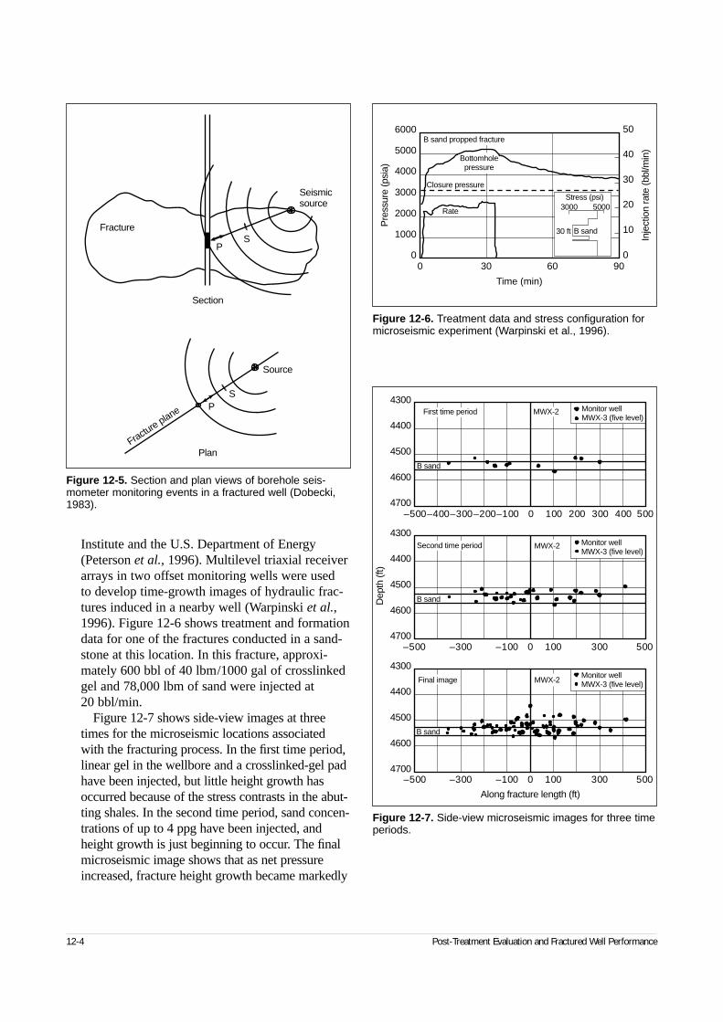
Institute and the U.S. Department of Energy(Peterson et al., 1996). Multilevel triaxial receiverarrays in two offset monitoring wells were used to develop time-growth images of hydraulic frac-tures induced in a nearby well (Warpinski et al.,1996). Figure 12-6 shows treatment and formationdata for one of the fractures conducted in a sand-stone at this location. In this fracture, approxi-mately 600 bbl of 40 lbm/1000 gal of crosslinkedgel and 78,000 lbm of sand were injected at 20 bbl/min.

Figure 12-7 shows side-view images at threetimes for the microseismic locations associatedwith the fracturing process. In the first time period,linear gel in the wellbore and a crosslinked-gel padhave been injected, but little height growth hasoccurred because of the stress contrasts in the abut-ting shales. In the second time period, sand concen-trations of up to 4 ppg have been injected, andheight growth is just beginning to occur. The finalmicroseismic image shows that as net pressureincreased, fracture height growth became markedly

12-4 Post-Treatment Evaluation and Fractured Well Performance

Figure 12-5. Section and plan views of borehole seis-mometer monitoring events in a fractured well (Dobecki,1983).

Fracture

plane

S

S

P

P

Section

Plan

Source

Fracture

Seismicsource

Figure 12-6. Treatment data and stress configuration formicroseismic experiment (Warpinski et al., 1996).

00

1000

2000

3000

4000

5000

6000

0

10

20

30

40

50

30 60 90

Time (min)

Rate

Closure pressure

Bottomholepressure

B sand propped fracture

3000 5000

30 ft B sand

Stress (psi)

Pre

ssur

e (p

sia)

Inje

ctio

n ra

te (b

bl/m

in)

Figure 12-7. Side-view microseismic images for three timeperiods.

Monitor wellMWX-3 (five level)

Monitor wellMWX-3 (five level)

Monitor wellMWX-3 (five level)

MWX-2

MWX-2

MWX-2

First time period

Second time period

Final image

B sand

B sand

B sand

–5004700

4300

4400

4500

4600

4700

4300

4400

4500

4600

4700

4300

4400

4500

4600

–400–300–200–100 0 100 200 300 400 500

–500 –300 –100 0 100 300 500

–500 –300 –100 0 100 300 500

Along fracture length (ft)

Dep

th (f

t)

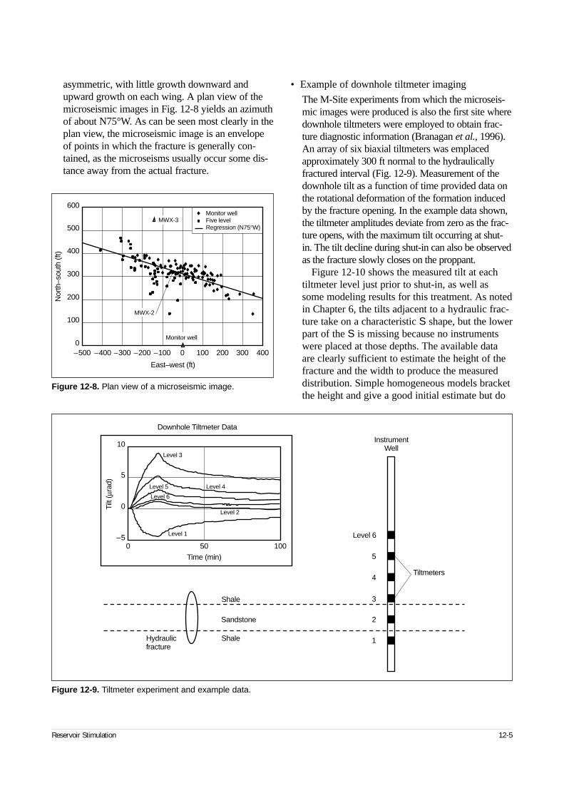
asymmetric, with little growth downward andupward growth on each wing. A plan view of themicroseismic images in Fig. 12-8 yields an azimuthof about N75°W. As can be seen most clearly in theplan view, the microseismic image is an envelopeof points in which the fracture is generally con-tained, as the microseisms usually occur some dis-tance away from the actual fracture.

• Example of downhole tiltmeter imaging

The M-Site experiments from which the microseis-mic images were produced is also the first site wheredownhole tiltmeters were employed to obtain frac-ture diagnostic information (Branagan et al., 1996).An array of six biaxial tiltmeters was emplacedapproximately 300 ft normal to the hydraulicallyfractured interval (Fig. 12-9). Measurement of thedownhole tilt as a function of time provided data onthe rotational deformation of the formation inducedby the fracture opening. In the example data shown,the tiltmeter amplitudes deviate from zero as the frac-ture opens, with the maximum tilt occurring at shut-in. The tilt decline during shut-in can also be observedas the fracture slowly closes on the proppant.

Figure 12-10 shows the measured tilt at eachtiltmeter level just prior to shut-in, as well assome modeling results for this treatment. As notedin Chapter 6, the tilts adjacent to a hydraulic frac-ture take on a characteristic S shape, but the lowerpart of the S is missing because no instrumentswere placed at those depths. The available dataare clearly sufficient to estimate the height of thefracture and the width to produce the measureddistribution. Simple homogeneous models bracketthe height and give a good initial estimate but do

Reservoir Stimulation 12-5

Figure 12-8. Plan view of a microseismic image.

–500 –400 –300 –200 –100 0 100 200 300 4000

100

200

300

400

500

600Monitor wellFive levelRegression (N75°W)

MWX-2

Monitor well

MWX-3

East–west (ft)

Nor

th–s

outh

(ft)

Figure 12-9. Tiltmeter experiment and example data.

0 50 100

10

5

0

–5

Time (min)

Level 3

Level 4

Level 1

Level 2

Level 5

Level 6

Downhole Tiltmeter Data

InstrumentWell

Tiltmeters

Level 6

5

4

3

2

1

Shale

Sandstone

ShaleHydraulicfracture

Tilt

(µra

d)

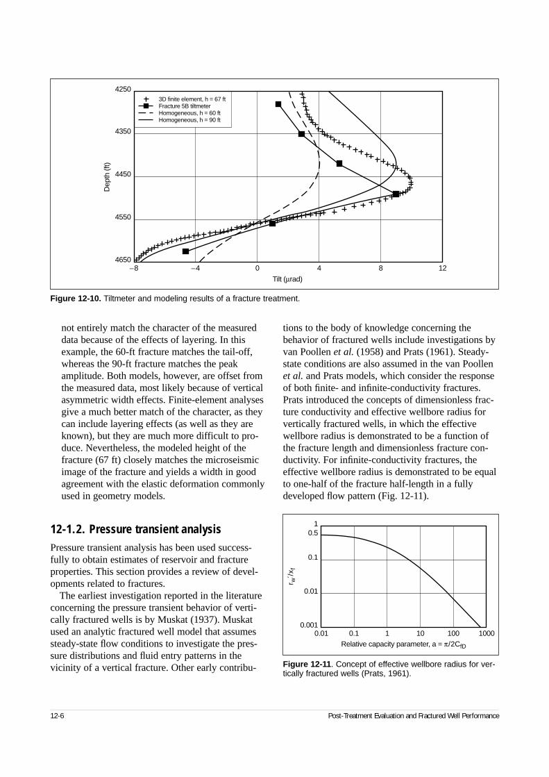
not entirely match the character of the measureddata because of the effects of layering. In thisexample, the 60-ft fracture matches the tail-off,whereas the 90-ft fracture matches the peakamplitude. Both models, however, are offset fromthe measured data, most likely because of verticalasymmetric width effects. Finite-element analysesgive a much better match of the character, as theycan include layering effects (as well as they areknown), but they are much more difficult to pro-duce. Nevertheless, the modeled height of thefracture (67 ft) closely matches the microseismicimage of the fracture and yields a width in goodagreement with the elastic deformation commonlyused in geometry models.

12-1.2. Pressure transient analysisPressure transient analysis has been used success-fully to obtain estimates of reservoir and fractureproperties. This section provides a review of devel-opments related to fractures.

The earliest investigation reported in the literatureconcerning the pressure transient behavior of verti-cally fractured wells is by Muskat (1937). Muskatused an analytic fractured well model that assumessteady-state flow conditions to investigate the pres-sure distributions and fluid entry patterns in thevicinity of a vertical fracture. Other early contribu-

tions to the body of knowledge concerning thebehavior of fractured wells include investigations byvan Poollen et al. (1958) and Prats (1961). Steady-state conditions are also assumed in the van Poollenet al. and Prats models, which consider the responseof both finite- and infinite-conductivity fractures.Prats introduced the concepts of dimensionless frac-ture conductivity and effective wellbore radius forvertically fractured wells, in which the effectivewellbore radius is demonstrated to be a function ofthe fracture length and dimensionless fracture con-ductivity. For infinite-conductivity fractures, theeffective wellbore radius is demonstrated to be equalto one-half of the fracture half-length in a fullydeveloped flow pattern (Fig. 12-11).

12-6 Post-Treatment Evaluation and Fractured Well Performance

Figure 12-10. Tiltmeter and modeling results of a fracture treatment.

3D finite element, h = 67 ftFracture 5B tiltmeterHomogeneous, h = 60 ftHomogeneous, h = 90 ft

–8 –44650

4 8 120

4550

4450

4350

Dep

th (f

t)

4250

Tilt (µrad)

Figure 12-11. Concept of effective wellbore radius for ver-tically fractured wells (Prats, 1961).

0.010.001

0.01

0.1 1 10 100 1000Relative capacity parameter, a = π/2CfD

0.1

0.51

r w´/

x f

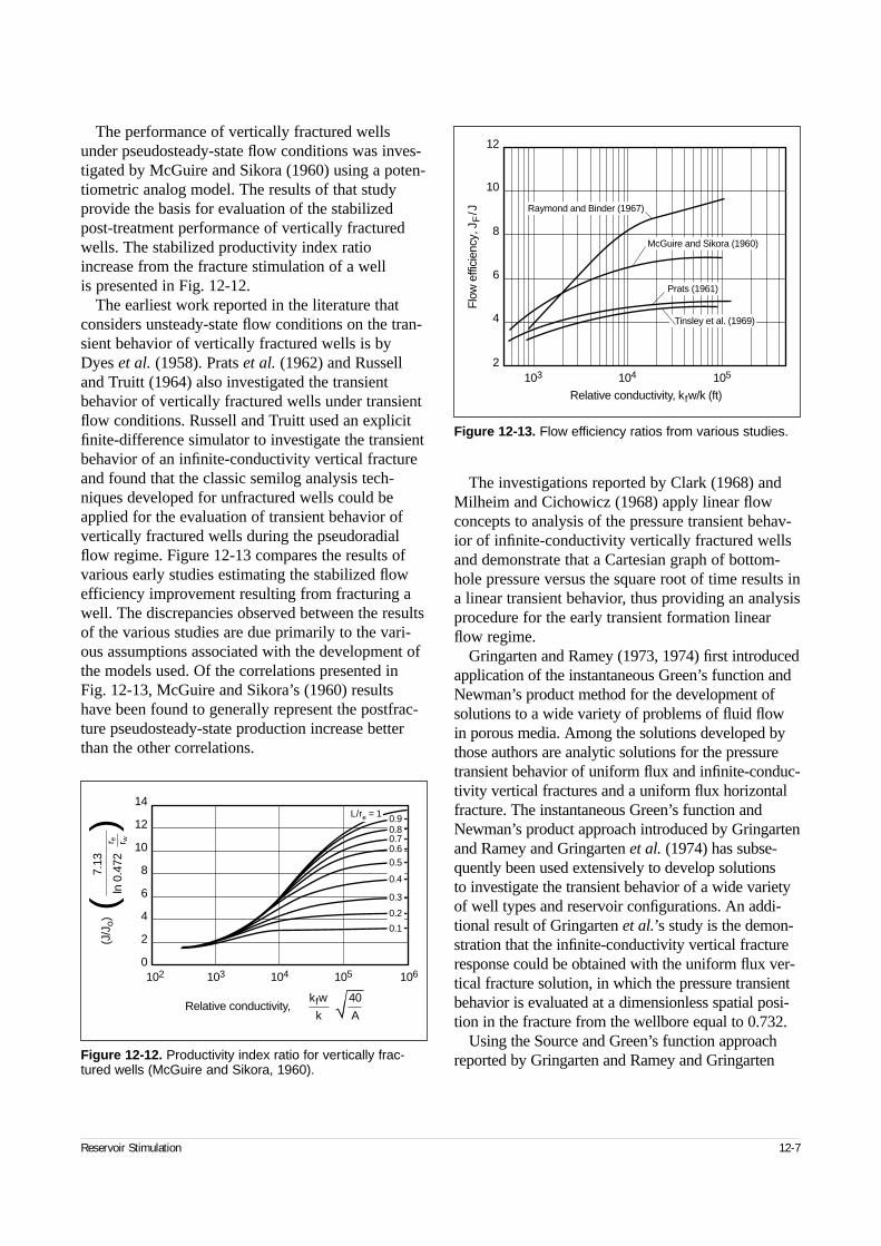
The performance of vertically fractured wellsunder pseudosteady-state flow conditions was inves-tigated by McGuire and Sikora (1960) using a poten-tiometric analog model. The results of that studyprovide the basis for evaluation of the stabilizedpost-treatment performance of vertically fracturedwells. The stabilized productivity index ratioincrease from the fracture stimulation of a well is presented in Fig. 12-12.

The earliest work reported in the literature thatconsiders unsteady-state flow conditions on the tran-sient behavior of vertically fractured wells is byDyes et al. (1958). Prats et al. (1962) and Russelland Truitt (1964) also investigated the transientbehavior of vertically fractured wells under transientflow conditions. Russell and Truitt used an explicitfinite-difference simulator to investigate the transientbehavior of an infinite-conductivity vertical fractureand found that the classic semilog analysis tech-niques developed for unfractured wells could beapplied for the evaluation of transient behavior ofvertically fractured wells during the pseudoradialflow regime. Figure 12-13 compares the results ofvarious early studies estimating the stabilized flowefficiency improvement resulting from fracturing awell. The discrepancies observed between the resultsof the various studies are due primarily to the vari-ous assumptions associated with the development ofthe models used. Of the correlations presented inFig. 12-13, McGuire and Sikora’s (1960) resultshave been found to generally represent the postfrac-ture pseudosteady-state production increase betterthan the other correlations.

The investigations reported by Clark (1968) andMilheim and Cichowicz (1968) apply linear flowconcepts to analysis of the pressure transient behav-ior of infinite-conductivity vertically fractured wellsand demonstrate that a Cartesian graph of bottom-hole pressure versus the square root of time results ina linear transient behavior, thus providing an analysisprocedure for the early transient formation linearflow regime.

Gringarten and Ramey (1973, 1974) first introducedapplication of the instantaneous Green’s function andNewman’s product method for the development ofsolutions to a wide variety of problems of fluid flowin porous media. Among the solutions developed bythose authors are analytic solutions for the pressuretransient behavior of uniform flux and infinite-conduc-tivity vertical fractures and a uniform flux horizontalfracture. The instantaneous Green’s function andNewman’s product approach introduced by Gringartenand Ramey and Gringarten et al. (1974) has subse-quently been used extensively to develop solutions to investigate the transient behavior of a wide varietyof well types and reservoir configurations. An addi-tional result of Gringarten et al.’s study is the demon-stration that the infinite-conductivity vertical fractureresponse could be obtained with the uniform flux ver-tical fracture solution, in which the pressure transientbehavior is evaluated at a dimensionless spatial posi-tion in the fracture from the wellbore equal to 0.732.

Using the Source and Green’s function approachreported by Gringarten and Ramey and Gringarten

Reservoir Stimulation 12-7

Figure 12-12. Productivity index ratio for vertically frac-tured wells (McGuire and Sikora, 1960).

14

12

10

8

6

4

2

0102 103 104 105 106

Relative conductivity,kfw 40

k A√

(

)(J

/Jo)

7.13

ln 0

.472

r e r w

0.90.80.70.60.5

0.4

0.3

0.2

0.1

L/re = 1

Figure 12-13. Flow efficiency ratios from various studies.

1032

104 105

4

6

8

10

12

Relative conductivity, kfw/k (ft)

Flo

w e

ffici

ency

, JF

/J Raymond and Binder (1967)

Tinsley et al. (1969)

Prats (1961)

McGuire and Sikora (1960)

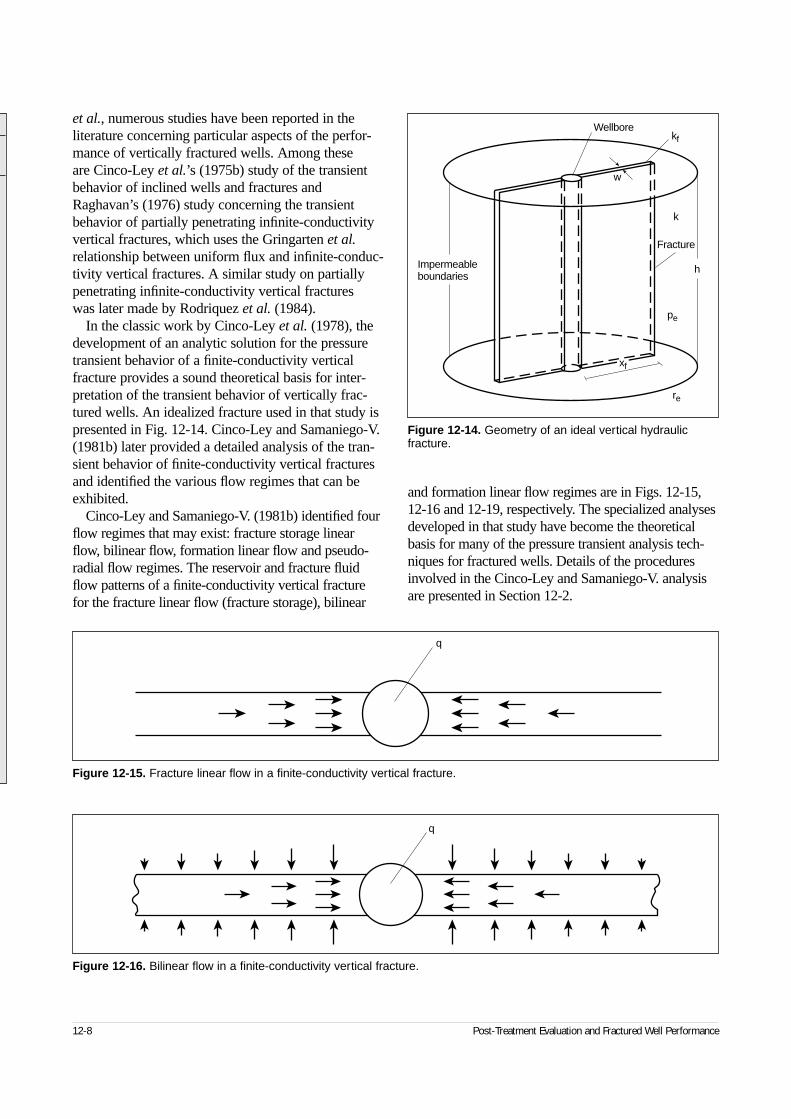
et al., numerous studies have been reported in the literature concerning particular aspects of the perfor-mance of vertically fractured wells. Among these are Cinco-Ley et al.’s (1975b) study of the transientbehavior of inclined wells and fractures andRaghavan’s (1976) study concerning the transientbehavior of partially penetrating infinite-conductivityvertical fractures, which uses the Gringarten et al.relationship between uniform flux and infinite-conduc-tivity vertical fractures. A similar study on partiallypenetrating infinite-conductivity vertical fractures was later made by Rodriquez et al. (1984).

In the classic work by Cinco-Ley et al. (1978), thedevelopment of an analytic solution for the pressuretransient behavior of a finite-conductivity verticalfracture provides a sound theoretical basis for inter-pretation of the transient behavior of vertically frac-tured wells. An idealized fracture used in that study ispresented in Fig. 12-14. Cinco-Ley and Samaniego-V.(1981b) later provided a detailed analysis of the tran-sient behavior of finite-conductivity vertical fracturesand identified the various flow regimes that can beexhibited.

Cinco-Ley and Samaniego-V. (1981b) identified fourflow regimes that may exist: fracture storage linearflow, bilinear flow, formation linear flow and pseudo-radial flow regimes. The reservoir and fracture fluidflow patterns of a finite-conductivity vertical fracturefor the fracture linear flow (fracture storage), bilinear

and formation linear flow regimes are in Figs. 12-15,12-16 and 12-19, respectively. The specialized analysesdeveloped in that study have become the theoreticalbasis for many of the pressure transient analysis tech-niques for fractured wells. Details of the proceduresinvolved in the Cinco-Ley and Samaniego-V. analysisare presented in Section 12-2.

12-8 Post-Treatment Evaluation and Fractured Well Performance

1

Figure 12-14. Geometry of an ideal vertical hydraulicfracture.

pe

re

xf

kf

h

w

Wellbore

Impermeableboundaries

Fracture

k

Figure 12-15. Fracture linear flow in a finite-conductivity vertical fracture.

q

Figure 12-16. Bilinear flow in a finite-conductivity vertical fracture.

q

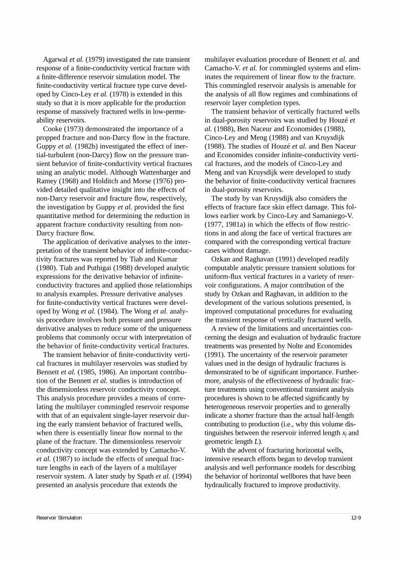
Agarwal et al. (1979) investigated the rate transientresponse of a finite-conductivity vertical fracture witha finite-difference reservoir simulation model. Thefinite-conductivity vertical fracture type curve devel-oped by Cinco-Ley et al. (1978) is extended in thisstudy so that it is more applicable for the productionresponse of massively fractured wells in low-perme-ability reservoirs.

Cooke (1973) demonstrated the importance of apropped fracture and non-Darcy flow in the fracture.Guppy et al. (1982b) investigated the effect of iner-tial-turbulent (non-Darcy) flow on the pressure tran-sient behavior of finite-conductivity vertical fracturesusing an analytic model. Although Wattenbarger andRamey (1968) and Holditch and Morse (1976) pro-vided detailed qualitative insight into the effects ofnon-Darcy reservoir and fracture flow, respectively,the investigation by Guppy et al. provided the firstquantitative method for determining the reduction inapparent fracture conductivity resulting from non-Darcy fracture flow.

The application of derivative analyses to the inter-pretation of the transient behavior of infinite-conduc-tivity fractures was reported by Tiab and Kumar(1980). Tiab and Puthigai (1988) developed analyticexpressions for the derivative behavior of infinite-conductivity fractures and applied those relationshipsto analysis examples. Pressure derivative analysesfor finite-conductivity vertical fractures were devel-oped by Wong et al. (1984). The Wong et al. analy-sis procedure involves both pressure and pressurederivative analyses to reduce some of the uniquenessproblems that commonly occur with interpretation ofthe behavior of finite-conductivity vertical fractures.

The transient behavior of finite-conductivity verti-cal fractures in multilayer reservoirs was studied byBennett et al. (1985, 1986). An important contribu-tion of the Bennett et al. studies is introduction ofthe dimensionless reservoir conductivity concept.This analysis procedure provides a means of corre-lating the multilayer commingled reservoir responsewith that of an equivalent single-layer reservoir dur-ing the early transient behavior of fractured wells,when there is essentially linear flow normal to theplane of the fracture. The dimensionless reservoirconductivity concept was extended by Camacho-V.et al. (1987) to include the effects of unequal frac-ture lengths in each of the layers of a multilayerreservoir system. A later study by Spath et al. (1994)presented an analysis procedure that extends the

multilayer evaluation procedure of Bennett et al. andCamacho-V. et al. for commingled systems and elim-inates the requirement of linear flow to the fracture.This commingled reservoir analysis is amenable forthe analysis of all flow regimes and combinations ofreservoir layer completion types.

The transient behavior of vertically fractured wellsin dual-porosity reservoirs was studied by Houzé etal. (1988), Ben Naceur and Economides (1988),Cinco-Ley and Meng (1988) and van Kruysdijk(1988). The studies of Houzé et al. and Ben Naceurand Economides consider infinite-conductivity verti-cal fractures, and the models of Cinco-Ley andMeng and van Kruysdijk were developed to studythe behavior of finite-conductivity vertical fracturesin dual-porosity reservoirs.

The study by van Kruysdijk also considers theeffects of fracture face skin effect damage. This fol-lows earlier work by Cinco-Ley and Samaniego-V.(1977, 1981a) in which the effects of flow restric-tions in and along the face of vertical fractures arecompared with the corresponding vertical fracturecases without damage.

Ozkan and Raghavan (1991) developed readilycomputable analytic pressure transient solutions foruniform-flux vertical fractures in a variety of reser-voir configurations. A major contribution of thestudy by Ozkan and Raghavan, in addition to thedevelopment of the various solutions presented, isimproved computational procedures for evaluatingthe transient response of vertically fractured wells.

A review of the limitations and uncertainties con-cerning the design and evaluation of hydraulic fracturetreatments was presented by Nolte and Economides(1991). The uncertainty of the reservoir parametervalues used in the design of hydraulic fractures isdemonstrated to be of significant importance. Further-more, analysis of the effectiveness of hydraulic frac-ture treatments using conventional transient analysisprocedures is shown to be affected significantly byheterogeneous reservoir properties and to generallyindicate a shorter fracture than the actual half-lengthcontributing to production (i.e., why this volume dis-tinguishes between the reservoir inferred length xf andgeometric length L).

With the advent of fracturing horizontal wells,intensive research efforts began to develop transientanalysis and well performance models for describingthe behavior of horizontal wellbores that have beenhydraulically fractured to improve productivity.

Reservoir Stimulation 12-9

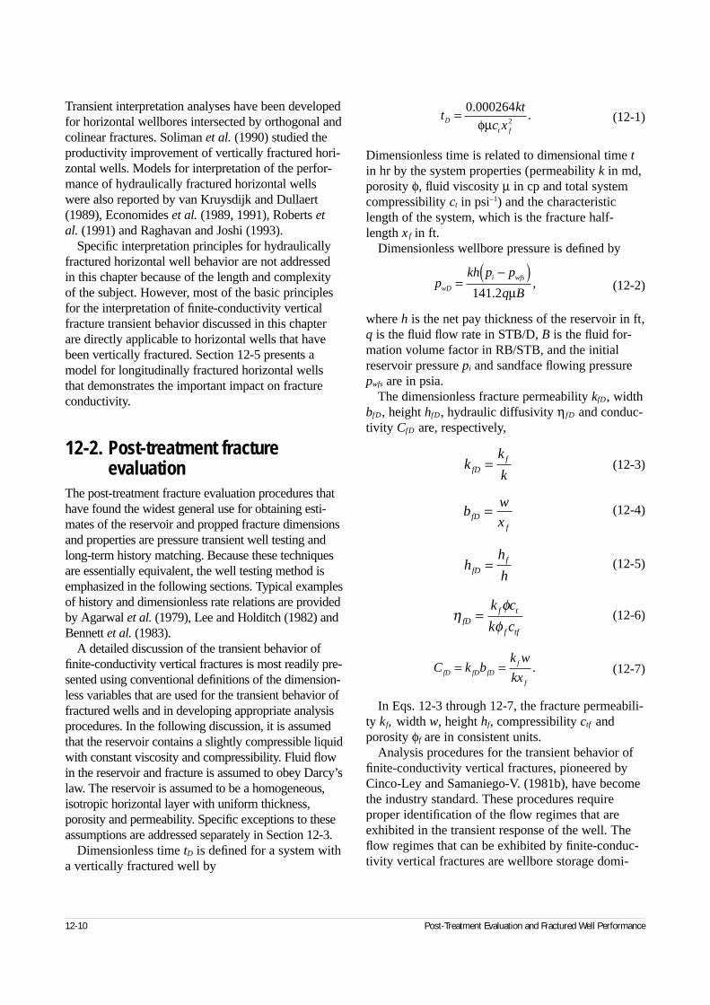
Transient interpretation analyses have been developedfor horizontal wellbores intersected by orthogonal andcolinear fractures. Soliman et al. (1990) studied theproductivity improvement of vertically fractured hori-zontal wells. Models for interpretation of the perfor-mance of hydraulically fractured horizontal wellswere also reported by van Kruysdijk and Dullaert(1989), Economides et al. (1989, 1991), Roberts etal. (1991) and Raghavan and Joshi (1993).

Specific interpretation principles for hydraulicallyfractured horizontal well behavior are not addressed in this chapter because of the length and complexityof the subject. However, most of the basic principlesfor the interpretation of finite-conductivity verticalfracture transient behavior discussed in this chapterare directly applicable to horizontal wells that havebeen vertically fractured. Section 12-5 presents amodel for longitudinally fractured horizontal wellsthat demonstrates the important impact on fractureconductivity.

12-2. Post-treatment fracture evaluation

The post-treatment fracture evaluation procedures thathave found the widest general use for obtaining esti-mates of the reservoir and propped fracture dimensionsand properties are pressure transient well testing andlong-term history matching. Because these techniquesare essentially equivalent, the well testing method isemphasized in the following sections. Typical examplesof history and dimensionless rate relations are providedby Agarwal et al. (1979), Lee and Holditch (1982) andBennett et al. (1983).

A detailed discussion of the transient behavior offinite-conductivity vertical fractures is most readily pre-sented using conventional definitions of the dimension-less variables that are used for the transient behavior offractured wells and in developing appropriate analysisprocedures. In the following discussion, it is assumedthat the reservoir contains a slightly compressible liquidwith constant viscosity and compressibility. Fluid flowin the reservoir and fracture is assumed to obey Darcy’slaw. The reservoir is assumed to be a homogeneous,isotropic horizontal layer with uniform thickness,porosity and permeability. Specific exceptions to theseassumptions are addressed separately in Section 12-3.

Dimensionless time tD is defined for a system witha vertically fractured well by

(12-1)

Dimensionless time is related to dimensional time tin hr by the system properties (permeability k in md,porosity φ, fluid viscosity µ in cp and total systemcompressibility ct in psi–1) and the characteristiclength of the system, which is the fracture half-length x f in ft.

Dimensionless wellbore pressure is defined by

(12-2)

where h is the net pay thickness of the reservoir in ft,q is the fluid flow rate in STB/D, B is the fluid for-mation volume factor in RB/STB, and the initialreservoir pressure pi and sandface flowing pressurepwfs are in psia.

The dimensionless fracture permeability kfD, widthbfD, height hfD, hydraulic diffusivity ηfD and conduc-tivity CfD are, respectively,

(12-3)

(12-4)

(12-5)

(12-6)

(12-7)

In Eqs. 12-3 through 12-7, the fracture permeabili-ty kf, width w, height hf, compressibility ctf andporosity φf are in consistent units.

Analysis procedures for the transient behavior offinite-conductivity vertical fractures, pioneered byCinco-Ley and Samaniego-V. (1981b), have becomethe industry standard. These procedures requireproper identification of the flow regimes that areexhibited in the transient response of the well. Theflow regimes that can be exhibited by finite-conduc-tivity vertical fractures are wellbore storage domi-

12-10 Post-Treatment Evaluation and Fractured Well Performance

tkt

c xD

t f

= 0 0002642

..

φµ

pkh p p

q BwD

i wfs=−( )

141 2.,

µ

kk

kfDf=

bw

xfDf

=

hh

hfDf=

ηφ

φfDf t

f tf

k c

k c=

C k bk w

kxfD fD fDf

f

= = .

nated, fracture storage dominated, bilinear flow, for-mation linear flow, pseudoradial flow and boundarydominated flow regimes. The transient behavior alsoincludes transition regimes that separate each of thepreviously identified flow regimes.

12-2.1. Wellbore storage dominated flow regime

A shut-in (pressure buildup or falloff), in which thewell is shut in at the surface and the wellbore containsa compressible fluid, may be distorted for a significantportion of the early response by the storage effects ofthe wellbore. The duration of wellbore storage effectsis governed primarily by the volume of the wellboreexposed to the completed reservoir and the compress-ibility of the fluids contained in the wellbore. Thus,downhole shut-in for pressure buildup can reducewellbore effects considerably. Pressure drawdown orinjection transients may also result in domination of a significant portion of the transient behavior by well-bore storage distortion if the well is opened for pro-duction or injected into at the surface and the wellborecontains compressible fluids.

Wellbore storage dominated flow is characterizedby a unit slope for both the pressure and pressurederivative behaviors in log-log coordinates. The pres-sure and pressure derivative response of a system witha positive steady-state skin effect and constant well-bore storage is a single unit-slope line (see Chapter 2for a detailed discussion of this issue). Nonideal con-ditions may exist in the system in which the wellborestorage cannot be characterized by a constant value.These conditions are common in wells that simultane-ously produce both oil and gas and in which momen-tum, density and thermal effects result in afterflowand a changing liquid level in the wellbore. Changingwellbore storage effects are also referred to as well-bore phase redistribution effects (Fair, 1981).

12-2.2. Fracture storage linear flow regimeThe initial pressure transient behavior of a finite-conductivity vertical fracture (with negligible well-bore storage effects) is dominated by the fluid stor-age of the fracture itself. In the case of negligiblewellbore storage effects (in practice, this generallyinvolves only wells with downhole isolation tools),the constant-rate drawdown of a well with a finite-

conductivity vertical fracture results in production atthe wellbore that is due primarily to fluid expansionin the fracture.

This linear flow regime is characterized by a one-half slope on a log-log graph of the change in pres-sure ∆p versus the change in time ∆t. The fracturestorage linear flow regime is generally of such shortduration that an analysis of this transient behavior isusually not possible. In cases where wellbore storageeffects are not negligible, they generally distort ormask the fracture storage linear behavior to an extentthat it may not be readily observed in the transientdata. Fluid flow patterns in a fracture for the fracturelinear flow regime are illustrated in Fig. 12-15.

During the fracture linear flow regime, the behaviorof dimensionless wellbore pressure pwD is a functionof the dimensionless fracture conductivity, hydraulicdiffusivity and height, and dimensionless time:

(12-8)

The approximate dimensionless time tDefl at whichthe fracture linear flow behavior ends is also a func-tion of the dimensionless fracture properties:

(12-9)

12-2.3. Bilinear flow regimeA bilinear flow regime may be exhibited in finite-conductivity vertical fractures as a result of two linearflow patterns existing in the system simultaneouslyand the fracture tip effects not influencing the tran-sient behavior of the well. The flow in the reservoir is primarily compressible linear flow to the plane ofthe fracture. Once the fluid crosses the fracture faceinto the fracture, the fluid is conducted down the frac-ture to the wellbore, under essentially incompressiblelinear flow conditions. Flow patterns in the reservoirand fracture during the bilinear flow regime are pre-sented in Fig. 12-16. This fracture flow regime is gov-erned by the fracture conductivity, and bilinear flowprovides the optimum regime for defining conductivity.

Wellbore pressure transient behavior during thebilinear flow regime is expressed by

(12-10)

Reservoir Stimulation 12-11

pC h

twD

fD fD

fD D= 2 πη .

tC h

Defl

fD fD

fD

=( )0 01

2

2

..

η

pC h

twD

fD fD

D= 2 45083 1 4../

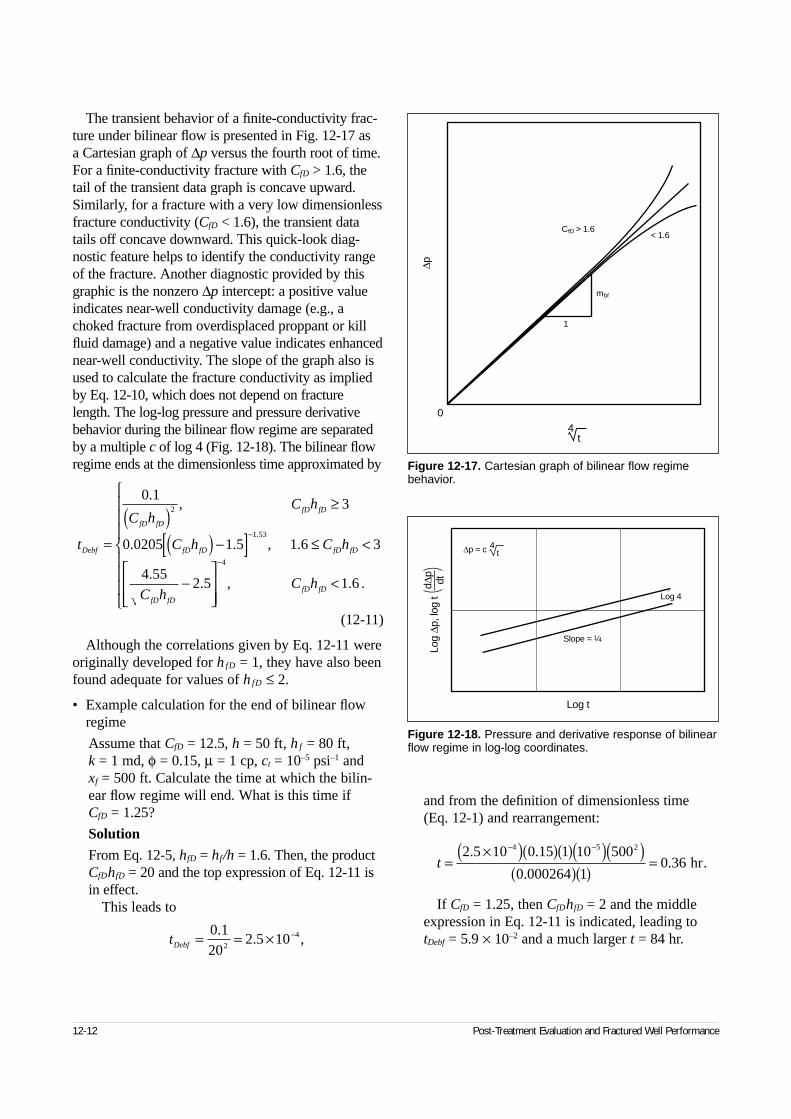
The transient behavior of a finite-conductivity frac-ture under bilinear flow is presented in Fig. 12-17 as a Cartesian graph of ∆p versus the fourth root of time.For a finite-conductivity fracture with CfD > 1.6, thetail of the transient data graph is concave upward.Similarly, for a fracture with a very low dimensionlessfracture conductivity (CfD < 1.6), the transient datatails off concave downward. This quick-look diag-nostic feature helps to identify the conductivity rangeof the fracture. Another diagnostic provided by thisgraphic is the nonzero ∆p intercept: a positive valueindicates near-well conductivity damage (e.g., achoked fracture from overdisplaced proppant or killfluid damage) and a negative value indicates enhancednear-well conductivity. The slope of the graph also isused to calculate the fracture conductivity as impliedby Eq. 12-10, which does not depend on fracturelength. The log-log pressure and pressure derivativebehavior during the bilinear flow regime are separatedby a multiple c of log 4 (Fig. 12-18). The bilinear flowregime ends at the dimensionless time approximated by

(12-11)

Although the correlations given by Eq. 12-11 wereoriginally developed for hfD = 1, they have also beenfound adequate for values of h fD ≤ 2.

• Example calculation for the end of bilinear flowregime

Assume that CfD = 12.5, h = 50 ft, hf = 80 ft, k = 1 md, φ = 0.15, µ = 1 cp, ct = 10–5 psi–1 andxf = 500 ft. Calculate the time at which the bilin-ear flow regime will end. What is this time if CfD = 1.25?

Solution

From Eq. 12-5, hfD = hf/h = 1.6. Then, the productCfDhfD = 20 and the top expression of Eq. 12-11 isin effect.

This leads to

and from the definition of dimensionless time (Eq. 12-1) and rearrangement:

If CfD = 1.25, then CfDhfD = 2 and the middleexpression in Eq. 12-11 is indicated, leading totDebf = 5.9 × 10–2 and a much larger t = 84 hr.

12-12 Post-Treatment Evaluation and Fractured Well Performance

t

C hC h

C h C h

C hC h

Debf

fD fD

fD fD

fD fD fD fD

fD fD

fD fD

=

( )≥

( ) −[ ] ≤ <

−

<

−

−

0 13

0 0205 1 5 1 6 3

4 552 5 1 6

2

1 53

4

.,

. . , .

.. , . .

.

Figure 12-18. Pressure and derivative response of bilinearflow regime in log-log coordinates.

Slope = 1⁄4

Log 4

∆p = c 4t

Log t

Log

∆p, l

og t

d∆p

dt

tDebf = = × −0 120

2 5 102

4.. ,

t =×( )( )( )( )( )

( )( )=

− −2 5 10 0 15 1 10 500

0 000264 10 36

4 5 2. .

.. hr.

Figure 12-17. Cartesian graph of bilinear flow regimebehavior.

0

1

mbf

CfD > 1.6< 1.6

∆p4

t

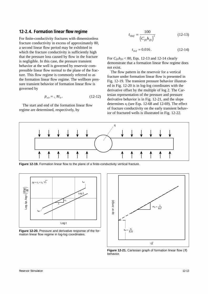
12-2.4. Formation linear flow regimeFor finite-conductivity fractures with dimensionlessfracture conductivity in excess of approximately 80,a second linear flow period may be exhibited inwhich the fracture conductivity is sufficiently highthat the pressure loss caused by flow in the fractureis negligible. In this case, the pressure transientbehavior at the well is governed by reservoir com-pressible linear flow normal to the plane of the frac-ture. This flow regime is commonly referred to asthe formation linear flow regime. The wellbore pres-sure transient behavior of formation linear flow isgoverned by

(12-12)

The start and end of the formation linear flowregime are determined, respectively, by

(12-13)

(12-14)

For CfDhfD < 80, Eqs. 12-13 and 12-14 clearlydemonstrate that a formation linear flow regime doesnot exist.

The flow pattern in the reservoir for a verticalfracture under formation linear flow is presented inFig. 12-19. The transient pressure behavior illustrat-ed in Fig. 12-20 is in log-log coordinates with thederivative offset by the multiple of log 2. The Car-tesian representation of the pressure and pressurederivative behavior is in Fig. 12-21, and the slopedetermines xf (see Eqs. 12-68 and 12-69). The effectof fracture conductivity on the early transient behav-ior of fractured wells is illustrated in Fig. 12-22.

Reservoir Stimulation 12-13

p twD D= π .

tC h

Dblf

fD fD

=( )

1002

tDelf = 0 016. .

Figure 12-19. Formation linear flow to the plane of a finite-conductivity vertical fracture.

q

Figure 12-20. Pressure and derivative response of the for-mation linear flow regime in log-log coordinates.

1⁄2

Log 2

∆p = c1 + c2 t

Log t

Log

∆p, l

og t

d∆p

dt

1

tblf

telf

Figure 12-21. Cartesian graph of formation linear flow ( lf)behavior.

mlf ∝ 1kxf

2

blf ∝ xf

kf w

t

∆p o

r ∆m

(p)

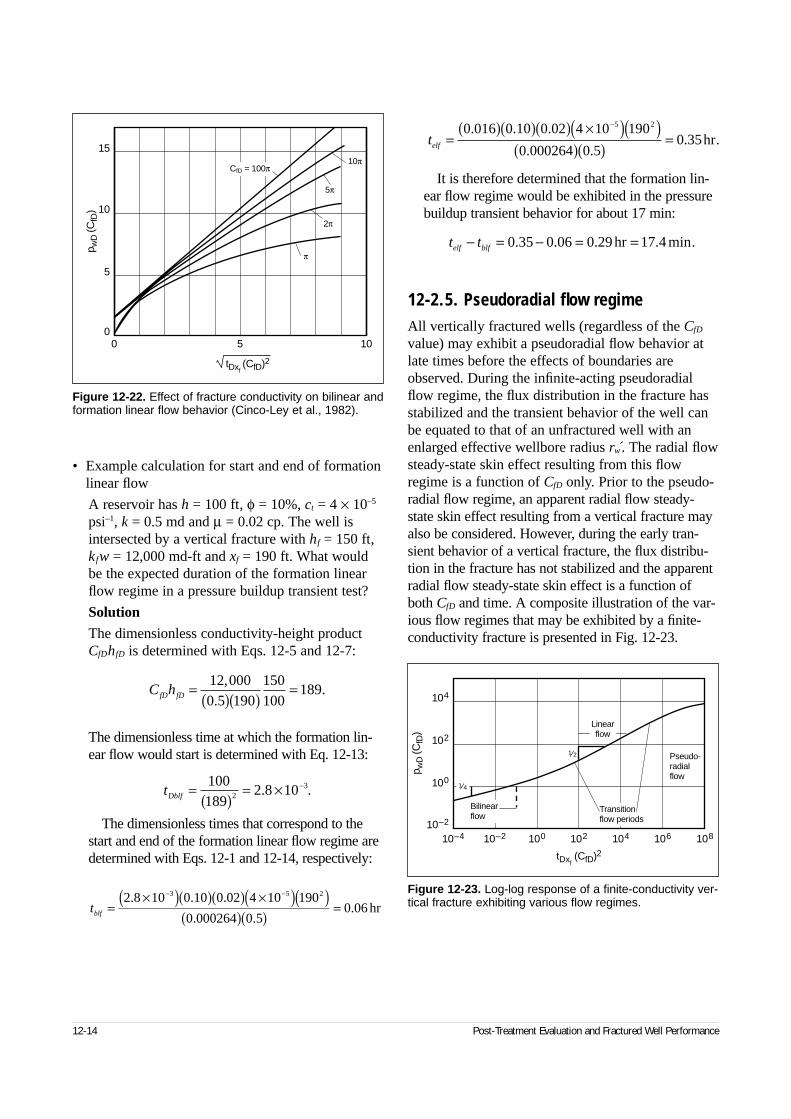
• Example calculation for start and end of formationlinear flow

A reservoir has h = 100 ft, φ = 10%, ct = 4 × 10–5

psi–1, k = 0.5 md and µ = 0.02 cp. The well isintersected by a vertical fracture with hf = 150 ft,kfw = 12,000 md-ft and xf = 190 ft. What wouldbe the expected duration of the formation linearflow regime in a pressure buildup transient test?

Solution

The dimensionless conductivity-height productCfDhfD is determined with Eqs. 12-5 and 12-7:

The dimensionless time at which the formation lin-ear flow would start is determined with Eq. 12-13:

The dimensionless times that correspond to thestart and end of the formation linear flow regime aredetermined with Eqs. 12-1 and 12-14, respectively:

It is therefore determined that the formation lin-ear flow regime would be exhibited in the pressurebuildup transient behavior for about 17 min:

12-2.5. Pseudoradial flow regimeAll vertically fractured wells (regardless of the CfD

value) may exhibit a pseudoradial flow behavior atlate times before the effects of boundaries areobserved. During the infinite-acting pseudoradialflow regime, the flux distribution in the fracture hasstabilized and the transient behavior of the well canbe equated to that of an unfractured well with anenlarged effective wellbore radius rẃ . The radial flowsteady-state skin effect resulting from this flowregime is a function of CfD only. Prior to the pseudo-radial flow regime, an apparent radial flow steady-state skin effect resulting from a vertical fracture mayalso be considered. However, during the early tran-sient behavior of a vertical fracture, the flux distribu-tion in the fracture has not stabilized and the apparentradial flow steady-state skin effect is a function ofboth CfD and time. A composite illustration of the var-ious flow regimes that may be exhibited by a finite-conductivity fracture is presented in Fig. 12-23.

12-14 Post-Treatment Evaluation and Fractured Well Performance

Figure 12-22. Effect of fracture conductivity on bilinear andformation linear flow behavior (Cinco-Ley et al., 1982).

00

5 10

5

10

15

tDxf(CfD)2

p wD

(CfD

)

CfD = 100π10π

5π

2π

π

Figure 12-23. Log-log response of a finite-conductivity ver-tical fracture exhibiting various flow regimes.

10–410–2

10–2 100 102 104 106 108

100

102

104

tDxf(CfD)2

p wD

(CfD

)

Pseudo-radialflow

Linearflow

Transitionflow periods

Bilinearflow

1⁄2

1⁄4

C hfD fD =( )( )

=12 0000 5 190

150100

189,

..

tDblf =( )

= × −100189

2 8 1023. .

tblf =×( )( )( ) ×( )( )

( )( )=

− −2 8 10 0 10 0 02 4 10 190

0 000264 0 50 06

3 5 2. . .

. .. hr

telf =( )( )( ) ×( )( )

( )( )=

−0 016 0 10 0 02 4 10 190

0 000264 0 50 35

5 2. . .

. .. hr.

t telf blf− = − = =0 35 0 06 0 29 17 4. . . .hr min.

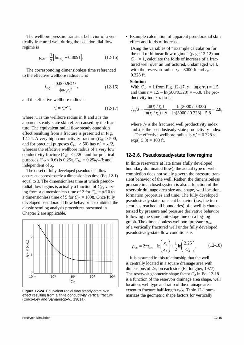
The wellbore pressure transient behavior of a ver-tically fractured well during the pseudoradial flowregime is

(12-15)

The corresponding dimensionless time referencedto the effective wellbore radius rẃ is

(12-16)

and the effective wellbore radius is

(12-17)

where rw is the wellbore radius in ft and s is theapparent steady-state skin effect caused by the frac-ture. The equivalent radial flow steady-state skineffect resulting from a fracture is presented in Fig.12-24. A very high conductivity fracture (CfD > 500,and for practical purposes CfD > 50) has rẃ = xf /2,whereas the effective wellbore radius of a very lowconductivity fracture (CfD < π/20, and for practicalpurposes CfD < 0.6) is 0.25x fC f D = 0.25kfw/k andindependent of xf.

The onset of fully developed pseudoradial flowoccurs at approximately a dimensionless time (Eq. 12-1)equal to 3. The dimensionless time at which pseudo-radial flow begins is actually a function of CfD, vary-ing from a dimensionless time of 2 for CfD = π/10 to a dimensionless time of 5 for CfD = 100π. Once fullydeveloped pseudoradial flow behavior is exhibited, theclassic semilog analysis procedures presented inChapter 2 are applicable.

• Example calculation of apparent pseudoradial skineffect and folds of increase

Using the variables of “Example calculation forthe end of bilinear flow regime” (page 12-12) andCfD = 1, calculate the folds of increase of a frac-tured well over an unfractured, undamaged well,with the reservoir radius re = 3000 ft and rw =0.328 ft.

SolutionWith CfD = 1 from Fig. 12-17, s + ln(xf /rw) = 1.5and thus s = 1.5 – ln(500/0.328) = –5.8. The pro-ductivity index ratio is

where JF is the fractured well productivity indexand J is the pseudosteady-state productivity index.

The effective wellbore radius is rw′ = 0.328 ×exp(+5.8) = 108 ft.

12-2.6. Pseudosteady-state flow regimeIn finite reservoirs at late times (fully developedboundary dominated flow), the actual type of wellcompletion does not solely govern the pressure tran-sient behavior of the well. Rather, the dimensionlesspressure in a closed system is also a function of thereservoir drainage area size and shape, well location,formation properties and time. The fully developedpseudosteady-state transient behavior (i.e., the tran-sient has reached all boundaries) of a well is charac-terized by pressure and pressure derivative behaviorfollowing the same unit-slope line on a log-loggraph. The dimensionless wellbore pressure pwD

of a vertically fractured well under fully developedpseudosteady-state flow conditions is

(12-18)

It is assumed in this relationship that the well is centrally located in a square drainage area withdimensions of 2xe on each side (Earlougher, 1977).The reservoir geometric shape factor CA in Eq. 12-18is a function of the reservoir drainage area shape, welllocation, well type and ratio of the drainage areaextent to fracture half-length xe/xf. Table 12-1 sum-marizes the geometric shape factors for vertically

Reservoir Stimulation 12-15

Figure 12-24. Equivalent radial flow steady-state skineffect resulting from a finite-conductivity vertical fracture(Cinco-Ley and Samaniego-V., 1981a).

10–1 100 101 102 1030

1

2

CfD

s f +

ln (x

f/rw

)

p twD Drw= +[ ]′

12

0 8091ln . .

tkt

c rDrt w

w′=

′0 000264

2

.,

φµ

′ = −r r ew ws , J J

r r

r r sFe w

e w

= ( )( ) +

= ( )( ) −

≈ln

lnln

ln

/

// .

/ . .. ,

3000 0 3283000 0 328 5 8

2 8

p tx

x CwD DAe

f A

= +

+

212

2 25π ln ln.

.

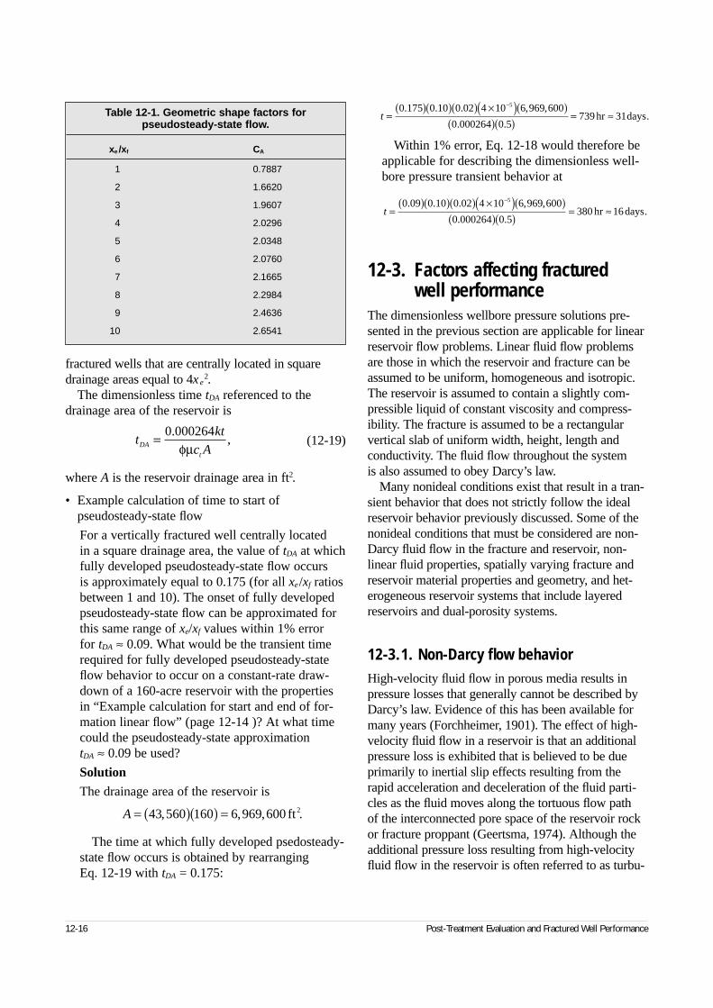
fractured wells that are centrally located in squaredrainage areas equal to 4xe

2.The dimensionless time tDA referenced to the

drainage area of the reservoir is

(12-19)

where A is the reservoir drainage area in ft2.

• Example calculation of time to start ofpseudosteady-state flow

For a vertically fractured well centrally located in a square drainage area, the value of tDA at whichfully developed pseudosteady-state flow occurs is approximately equal to 0.175 (for all xe/xf ratiosbetween 1 and 10). The onset of fully developedpseudosteady-state flow can be approximated forthis same range of xe/xf values within 1% error for tDA ≈ 0.09. What would be the transient timerequired for fully developed pseudosteady-stateflow behavior to occur on a constant-rate draw-down of a 160-acre reservoir with the propertiesin “Example calculation for start and end of for-mation linear flow” (page 12-14 )? At what timecould the pseudosteady-state approximation tDA ≈ 0.09 be used?

Solution

The drainage area of the reservoir is

The time at which fully developed psedosteady-state flow occurs is obtained by rearranging Eq. 12-19 with tDA = 0.175:

Within 1% error, Eq. 12-18 would therefore beapplicable for describing the dimensionless well-bore pressure transient behavior at

12-3. Factors affecting fractured well performance

The dimensionless wellbore pressure solutions pre-sented in the previous section are applicable for linearreservoir flow problems. Linear fluid flow problemsare those in which the reservoir and fracture can beassumed to be uniform, homogeneous and isotropic.The reservoir is assumed to contain a slightly com-pressible liquid of constant viscosity and compress-ibility. The fracture is assumed to be a rectangularvertical slab of uniform width, height, length andconductivity. The fluid flow throughout the system is also assumed to obey Darcy’s law.

Many nonideal conditions exist that result in a tran-sient behavior that does not strictly follow the idealreservoir behavior previously discussed. Some of thenonideal conditions that must be considered are non-Darcy fluid flow in the fracture and reservoir, non-linear fluid properties, spatially varying fracture andreservoir material properties and geometry, and het-erogeneous reservoir systems that include layeredreservoirs and dual-porosity systems.

12-3.1. Non-Darcy flow behaviorHigh-velocity fluid flow in porous media results inpressure losses that generally cannot be described byDarcy’s law. Evidence of this has been available formany years (Forchheimer, 1901). The effect of high-velocity fluid flow in a reservoir is that an additionalpressure loss is exhibited that is believed to be dueprimarily to inertial slip effects resulting from therapid acceleration and deceleration of the fluid parti-cles as the fluid moves along the tortuous flow path of the interconnected pore space of the reservoir rockor fracture proppant (Geertsma, 1974). Although theadditional pressure loss resulting from high-velocityfluid flow in the reservoir is often referred to as turbu-

12-16 Post-Treatment Evaluation and Fractured Well Performance

tkt

c ADA

t

= 0 000264.,

φµ

Table 12-1. Geometric shape factors for pseudosteady-state flow.

xe /xf CA

1 0.7887

2 1.6620

3 1.9607

4 2.0296

5 2.0348

6 2.0760

7 2.1665

8 2.2984

9 2.4636

10 2.6541

A = ( )( ) =43 560 160 6 969 600, , , .ft2

t =( )( )( ) ×( )( )

( )( )= ≈

−0 175 0 10 0 02 4 10 6 969 600

0 000264 0 5739 31

5. . . , ,

. .hr days.

t =( )( )( ) ×( )( )

( )( )= ≈

−0 09 0 10 0 02 4 10 6 969 600

0 000264 0 5380 16

5. . . , ,

. .hr days.

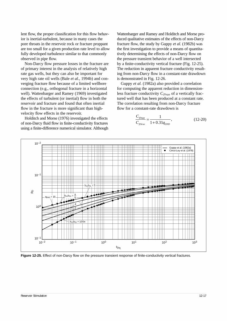
lent flow, the proper classification for this flow behav-ior is inertial-turbulent, because in many cases thepore throats in the reservoir rock or fracture proppantare too small for a given production rate level to allowfully developed turbulence similar to that commonlyobserved in pipe flow.

Non-Darcy flow pressure losses in the fracture areof primary interest in the analysis of relatively highrate gas wells, but they can also be important forvery high rate oil wells (Bale et al., 1994b) and con-verging fracture flow because of a limited wellboreconnection (e.g., orthogonal fracture in a horizontalwell). Wattenbarger and Ramey (1969) investigatedthe effects of turbulent (or inertial) flow in both thereservoir and fracture and found that often inertialflow in the fracture is more significant than high-velocity flow effects in the reservoir.

Holditch and Morse (1976) investigated the effectsof non-Darcy fluid flow in finite-conductivity fracturesusing a finite-difference numerical simulator. Although

Wattenbarger and Ramey and Holditch and Morse pro-duced qualitative estimates of the effects of non-Darcyfracture flow, the study by Guppy et al. (1982b) wasthe first investigation to provide a means of quantita-tively determining the effects of non-Darcy flow onthe pressure transient behavior of a well intersected by a finite-conductivity vertical fracture (Fig. 12-25).The reduction in apparent fracture conductivity result-ing from non-Darcy flow in a constant-rate drawdownis demonstrated in Fig. 12-26.

Guppy et al. (1982a) also provided a correlationfor computing the apparent reduction in dimension-less fracture conductivity CfDapp of a vertically frac-tured well that has been produced at a constant rate.The correlation resulting from non-Darcy fractureflow for a constant-rate drawdown is

(12-20)

Reservoir Stimulation 12-17

Figure 12-25. Effect of non-Darcy flow on the pressure transient response of finite-conductivity vertical fractures.

10–210–1

10–1 100 101 102 103

100

10–1

10–2

tDxf

p D

Guppy et al. (1982a)Cinco-Ley et al. (1978)

qDND = 15

kfDbfD = 5

kfDbfD = 100π

4

0

πkfDbfD = 5

C

C qfDapp

fDtrue DND

=+

11 0 31.

,

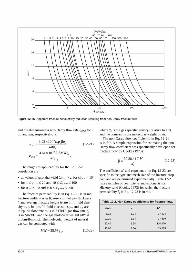
and the dimensionless non-Darcy flow rate qDND foroil and gas, respectively, is

(12-21)

The ranges of applicability for the Eq. 12-20correlation are

• all values of qDND that yield CfDapp > 2, for CfDtrue < 10

• for 1 ≤ qDND ≤ 20 and 10 ≤ CfDtrue ≤ 100

• for qDND ≤ 10 and 100 ≤ CfDtrue ≤ 500.

The fracture permeability kf in Eq. 12-21 is in md,fracture width w is in ft, reservoir net pay thicknessh and average fracture height hf are in ft, fluid den-sity ρo is in lbm/ft3, fluid viscosities µo and µgi arein cp, oil flow rate qo is in STB/D, gas flow rate qg

is in Mscf/D, and the gas molecular weight MW isin lbm/lbm-mol. The molecular weight of natural gas can be computed with

(12-22)

where γg is the gas specific gravity (relative to air)and the constant is the molecular weight of air.

The non-Darcy flow coefficient β in Eq. 12-21 is in ft–1. A simple expression for estimating the non-Darcy flow coefficient was specifically developed forfracture flow by Cooke (1973):

(12-23)

The coefficient b´ and exponent a´ in Eq. 12-23 arespecific to the type and mesh size of the fracture prop-pant and are determined experimentally. Table 12-2lists examples of coefficients and exponents forHickory sand (Cooke, 1973) for which the fracturepermeability kf in Eq. 12-23 is in md.

12-18 Post-Treatment Evaluation and Fractured Well Performance

Figure 12-26. Apparent fracture conductivity reduction resulting from non-Darcy fracture flow.

0.10

1 10 100 1000

4

8

12

16

20 1 1.5 2 3 4 5 6 8 10 15 20 30 40 60 80 100 200 300 400 7 9 50 70 90 150

(kfDbfD)app

(kfDbfD)true

qD

ND

qk q

wh

qk MWq

wh

DNDf o o

o

DNDf g

gi

=×

=×

−

−

1 03 10

4 64 10

15

16

.

..

ρ βµ

βµ

β = × ′′

30 88 106..

b

k fa

MW g= 28 96. ,γ

Table 12-2. Non-Darcy coefficients for fracture flow.

Mesh a′ b′

8/12 1.24 17,424

10/20 1.34 27,539

20/40 1.54 110,470

40/60 1.60 69,405

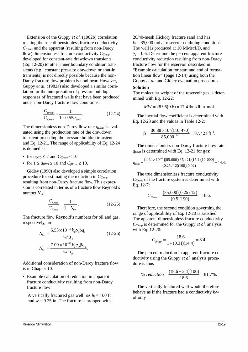
Extension of the Guppy et al. (1982b) correlationrelating the true dimensionless fracture conductivityCfDtrue and the apparent (resulting from non-Darcyflow) dimensionless fracture conductivity CfDapp

developed for constant-rate drawdown transients(Eq. 12-20) to other inner boundary condition tran-sients (e.g., constant pressure drawdown or shut-intransients) is not directly possible because the non-Darcy fracture flow problem is nonlinear. However,Guppy et al. (1982a) also developed a similar corre-lation for the interpretation of pressure buildupresponses of fractured wells that have been producedunder non-Darcy fracture flow conditions:

(12-24)

The dimensionless non-Darcy flow rate qDND is eval-uated using the production rate of the drawdowntransient preceding the pressure buildup transient and Eq. 12-21. The range of applicability of Eq. 12-24is defined as

• for qDND ≤ 2 and CfDtrue < 10

• for 1 ≤ qDND ≤ 10 and CfDtrue ≥ 10.

Gidley (1990) also developed a simple correlationprocedure for estimating the reduction in CfDapp

resulting from non-Darcy fracture flow. This expres-sion is correlated in terms of a fracture flow Reynold’snumber NRe:

(12-25)

The fracture flow Reynold’s numbers for oil and gas,respectively, are

(12-26)

Additional consideration of non-Darcy fracture flowis in Chapter 10.

• Example calculation of reduction in apparentfracture conductivity resulting from non-Darcyfracture flow

A vertically fractured gas well has hf = 100 ft and w = 0.25 in. The fracture is propped with

20/40-mesh Hickory fracture sand and has kf = 85,000 md at reservoir confining conditions. The well is produced at 10 MMscf/D, and γg = 0.6. Determine the percent apparent fractureconductivity reduction resulting from non-Darcyfracture flow for the reservoir described in“Example calculation for start and end of forma-tion linear flow” (page 12-14) using both theGuppy et al. and Gidley evaluation procedures.

SolutionThe molecular weight of the reservoir gas is deter-mined with Eq. 12-22:

The inertial flow coefficient is determined withEq. 12-23 and the values in Table 12-2:

The dimensionless non-Darcy fracture flow rateqDND is determined with Eq. 12-21 for gas:

The true dimensionless fracture conductivityCfDtrue of the fracture system is determined withEq. 12-7:

Therefore, the second condition governing therange of applicability of Eq. 12-20 is satisfied.The apparent dimensionless fracture conductivityCfDapp is determined for the Guppy et al. analysiswith Eq. 12-20:

The percent reduction in apparent fracture con-ductivity using the Guppy et al. analysis proce-dure is thus

The vertically fractured well would thereforebehave as if the fracture had a conductivity kfwof only

Reservoir Stimulation 12-19

C

C qfDapp

fDtrue DND

=+

11 0 55.

.

MW = ( ) =28 96 0 6 17 4. . . lbm/lbm mol.-

β = × ( ) =30 88 10 110 47085 000

87 4216

1 54

. ,,

, ..

ft –1

qDND =×( )( )( )( )( )

( )( )( )=

−4 64 10 85 000 87 421 17 4 10 000

0 25 12 100 0 0214 4

16. , , . ,

. / .. .

CfDtrue = ( )( )( )( )

=85 000 0 25 120 5 190

18 6, . /

.. .

CfDapp =+ ( )( )

=18 61 0 31 14 4

3 4.

. .. .

% reduction = −( )( ) =18 6 3 4 10018 6

81 7. .

.. %.

C

C NfDapp

fDtrue

=+

11 Re

.

Nk q

wh

Nk q

wh

f o o

o

f g g

gi

Re

Re

=×

=×

−

−

5 53 10

7 00 10

16

15

.

..

ρ βµ

γ βµ

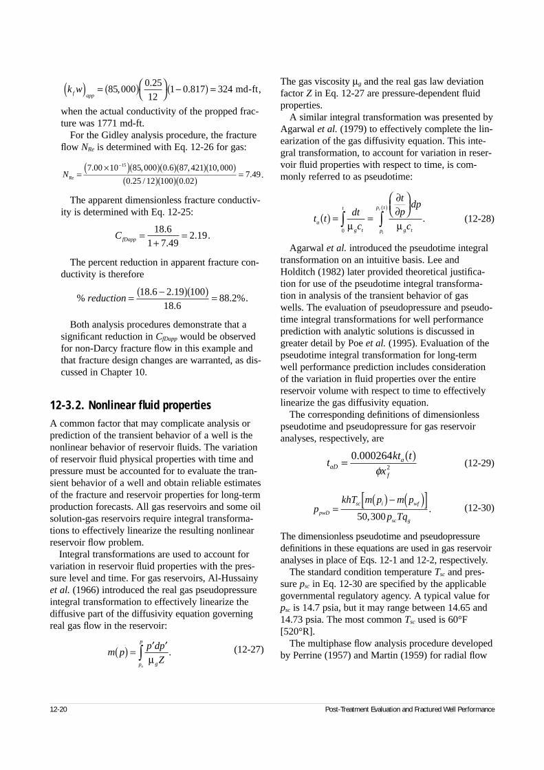
when the actual conductivity of the propped frac-ture was 1771 md-ft.

For the Gidley analysis procedure, the fractureflow NRe is determined with Eq. 12-26 for gas:

The apparent dimensionless fracture conductiv-ity is determined with Eq. 12-25:

The percent reduction in apparent fracture con-ductivity is therefore

Both analysis procedures demonstrate that asignificant reduction in CfDapp would be observedfor non-Darcy fracture flow in this example andthat fracture design changes are warranted, as dis-cussed in Chapter 10.

12-3.2. Nonlinear fluid propertiesA common factor that may complicate analysis orprediction of the transient behavior of a well is thenonlinear behavior of reservoir fluids. The variationof reservoir fluid physical properties with time andpressure must be accounted for to evaluate the tran-sient behavior of a well and obtain reliable estimatesof the fracture and reservoir properties for long-termproduction forecasts. All gas reservoirs and some oilsolution-gas reservoirs require integral transforma-tions to effectively linearize the resulting nonlinearreservoir flow problem.

Integral transformations are used to account forvariation in reservoir fluid properties with the pres-sure level and time. For gas reservoirs, Al-Hussainyet al. (1966) introduced the real gas pseudopressureintegral transformation to effectively linearize thediffusive part of the diffusivity equation governingreal gas flow in the reservoir:

(12-27)

The gas viscosity µg and the real gas law deviationfactor Z in Eq. 12-27 are pressure-dependent fluidproperties.

A similar integral transformation was presented byAgarwal et al. (1979) to effectively complete the lin-earization of the gas diffusivity equation. This inte-gral transformation, to account for variation in reser-voir fluid properties with respect to time, is com-monly referred to as pseudotime:

(12-28)

Agarwal et al. introduced the pseudotime integraltransformation on an intuitive basis. Lee andHolditch (1982) later provided theoretical justifica-tion for use of the pseudotime integral transforma-tion in analysis of the transient behavior of gaswells. The evaluation of pseudopressure and pseudo-time integral transformations for well performanceprediction with analytic solutions is discussed ingreater detail by Poe et al. (1995). Evaluation of thepseudotime integral transformation for long-termwell performance prediction includes considerationof the variation in fluid properties over the entirereservoir volume with respect to time to effectivelylinearize the gas diffusivity equation.

The corresponding definitions of dimensionlesspseudotime and pseudopressure for gas reservoiranalyses, respectively, are

(12-29)

(12-30)

The dimensionless pseudotime and pseudopressuredefinitions in these equations are used in gas reservoiranalyses in place of Eqs. 12-1 and 12-2, respectively.

The standard condition temperature Tsc and pres-sure psc in Eq. 12-30 are specified by the applicablegovernmental regulatory agency. A typical value forpsc is 14.7 psia, but it may range between 14.65 and14.73 psia. The most common Tsc used is 60°F[520°R].

The multiphase flow analysis procedure developedby Perrine (1957) and Martin (1959) for radial flow

12-20 Post-Treatment Evaluation and Fractured Well Performance

k wf app( ) = ( )

−( ) =85 000

0 2512

1 0 817 324,.

. md-ft,

NRe =×( )( )( )( )( )

( )( )( )=

−7 00 10 85 000 0 6 87 421 10 000

0 25 12 100 0 027 49

15. , . , ,

. / .. .

t tdt

c

tp

dp

ca

g t

t

g tp

p t

i

r

( ) = =

∫ ∫( )

µ

∂∂µ

0

.

tkt t

xaDa

f

= ( )0 0002642

.φ

pkhT m p m p

p TqpwD

sc i wf

sc g

=( ) − ( )[ ]

50 300,.

CfDapp =+

=18 61 7 49

2 19..

. .

% reduction = −( )( ) =18 6 2 19 10018 6

88 2. .

.. %.

m pp dp

Zgp

p

o

( ) = ′ ′∫ µ.

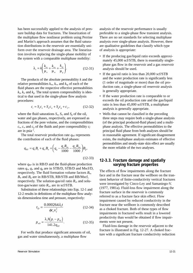
has been successfully applied to the analysis of pres-sure buildup data for fractures. The linearization ofthe multiphase flow nonlinear problem using Perrineand Martin’s approach assumes that the fluid satura-tion distributions in the reservoir are essentially uni-form over the reservoir drainage area. The lineariza-tion involves replacing the single-phase mobility ofthe system with a comparable multiphase mobility:

(12-31)

The products of the absolute permeability k and therelative permeabilities kro, krw and krg of each of thefluid phases are the respective effective permeabilitiesko, kw and kg. The total system compressibility is iden-tical to that used in the single-phase flow analysisprocedures:

(12-32)

where the fluid saturations So, Sw and Sg of the oil,water and gas phases, respectively, are expressed asfractions of the pore volume, and the compressibilitiesco, cw and cg of the fluids and pore compressibility cf

are in psia–1.The total reservoir production rate qRT represents

the contribution of each of the fluid phases:

(12-33)

where qRT is in RB/D and the fluid-phase productionrates qo, qw and qg are in STB/D, STB/D and Mscf/D,respectively. The fluid formation volume factors Bo,Bw and Bg are in RB/STB, RB/STB and RB/Mscf,respectively. The solution-gas/oil ratio Rso and solu-tion-gas/water ratio Rsw are in scf/STB.

Substitution of these relationships into Eqs. 12-1 and12-2 results in definitions of the multiphase flow analy-sis dimensionless time and pressure, respectively:

(12-34)

(12-35)

For wells that produce significant amounts of oil,gas and water simultaneously, a multiphase flow

analysis of the reservoir performance is usuallypreferable to a single-phase flow transient analysis.There are no set standards for selecting multiphaseanalysis over single-phase analysis. However, thereare qualitative guidelines that classify which type of analysis is appropriate:

• If the producing gas/liquid ratio exceeds approxi-mately 45,000 scf/STB, there is essentially single-phase gas flow in the reservoir and a gas reservoiranalysis should be used.

• If the gas/oil ratio is less than 20,000 scf/STB and the water production rate is significantly less(1 order of magnitude or more) than the oil pro-duction rate, a single-phase oil reservoir analysis is generally appropriate.

• If the water production rate is comparable to orexceeds the oil production rate and the gas/liquidratio is less than 45,000 scf/STB, a multiphaseanalysis is generally appropriate.

• Wells that cannot be classified in the precedingthree steps may require both a single-phase analysis(of the principal produced-fluid phase) and a multi-phase analysis. The effective permeabilities to theprincipal fluid phase from both analyses should bein reasonable agreement. If significant disagreementexists, the multiphase analysis estimates of effectivepermeabilities and steady-state skin effect are usuallythe more reliable of the two analyses.

12-3.3. Fracture damage and spatially varying fracture properties

The effects of flow impairments along the fractureface and in the fracture near the wellbore on the tran-sient behavior of finite-conductivity vertical fractureswere investigated by Cinco-Ley and Samaniego-V.(1977, 1981a). Fluid-loss flow impairment along thefracture surface in the reservoir is commonlyreferred to as a fracture face skin effect. Flowimpairment caused by reduced conductivity in thefracture near the wellbore is commonly described as a choked fracture. Both of these types of flowimpairments in fractured wells result in a loweredproductivity than would be obtained if flow impair-ments were not present.

Fluid-loss damage in the reservoir adjacent to thefracture is illustrated in Fig. 12-27. A choked frac-ture with a significant fracture conductivity reduction

Reservoir Stimulation 12-21

λµ µ µt

ro

o

rw

w

rg

g

kk k k

= + +

.

c S c S c S c ct o o w w g g f= + + + ,

q q B q B qq R q R

BRT o o w w go So w Sw

g= + + − −

1000 1000

,

tt

c xDt

t f

= 0 0002642

. λφ

ph p p

qwD

t i wf

RT

=−( )λ

141 2..

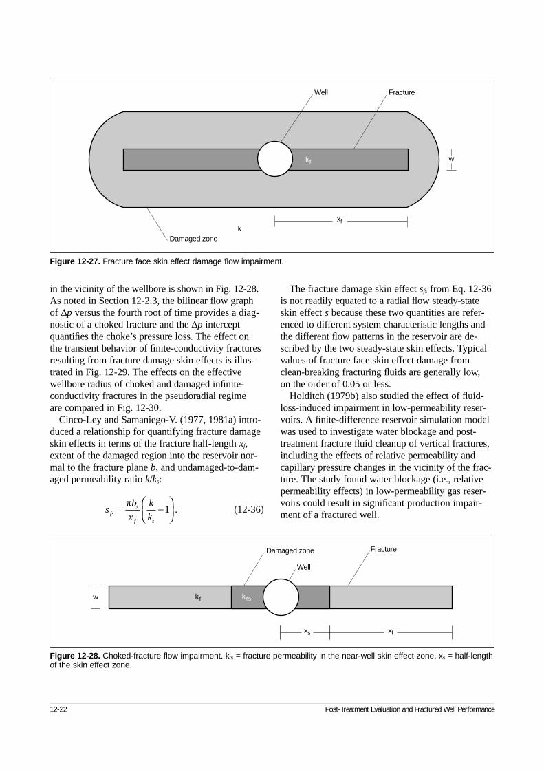
in the vicinity of the wellbore is shown in Fig. 12-28.As noted in Section 12-2.3, the bilinear flow graphof ∆p versus the fourth root of time provides a diag-nostic of a choked fracture and the ∆p interceptquantifies the choke’s pressure loss. The effect on the transient behavior of finite-conductivity fracturesresulting from fracture damage skin effects is illus-trated in Fig. 12-29. The effects on the effectivewellbore radius of choked and damaged infinite-conductivity fractures in the pseudoradial regime are compared in Fig. 12-30.

Cinco-Ley and Samaniego-V. (1977, 1981a) intro-duced a relationship for quantifying fracture damageskin effects in terms of the fracture half-length xf,extent of the damaged region into the reservoir nor-mal to the fracture plane bs and undamaged-to-dam-aged permeability ratio k/ks:

(12-36)

The fracture damage skin effect sfs from Eq. 12-36is not readily equated to a radial flow steady-stateskin effect s because these two quantities are refer-enced to different system characteristic lengths andthe different flow patterns in the reservoir are de-scribed by the two steady-state skin effects. Typicalvalues of fracture face skin effect damage fromclean-breaking fracturing fluids are generally low, on the order of 0.05 or less.

Holditch (1979b) also studied the effect of fluid-loss-induced impairment in low-permeability reser-voirs. A finite-difference reservoir simulation modelwas used to investigate water blockage and post-treatment fracture fluid cleanup of vertical fractures,including the effects of relative permeability andcapillary pressure changes in the vicinity of the frac-ture. The study found water blockage (i.e., relativepermeability effects) in low-permeability gas reser-voirs could result in significant production impair-ment of a fractured well.

12-22 Post-Treatment Evaluation and Fractured Well Performance

Figure 12-27. Fracture face skin effect damage flow impairment.

wkf

xfk

Damaged zone

Well Fracture

Figure 12-28. Choked-fracture flow impairment. kfs = fracture permeability in the near-well skin effect zone, xs = half-lengthof the skin effect zone.

kfs

xs xf

kf

Damaged zone Fracture

Well

w

sb

x

k

kfss

f s

= −

π1 .

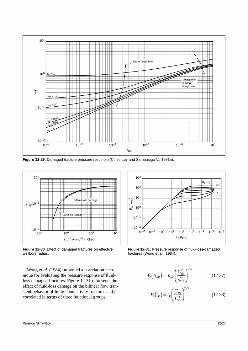
Wong et al. (1984) presented a correlation tech-nique for evaluating the pressure response of fluid-loss-damaged fractures. Figure 12-31 represents theeffect of fluid-loss damage on the bilinear flow tran-sient behavior of finite-conductivity fractures and iscorrelated in terms of three functional groups:

(12-37)

(12-38)

Reservoir Stimulation 12-23

Figure 12-29. Damaged fracture pressure response (Cinco-Ley and Samaniego-V., 1981a).

10–410–2

10–3 10–2 10–1 10–0 101

10–1

100

101

tDxf

p wD

s fs = 0

sfs = 0.01sfs = 0.02

Beginning ofsemilogstraight line

End of linear flow

sfs = 0.2

sfs = 0.1

sfs = 1

Figure 12-30. Effect of damaged fractures on effectivewellbore radius.

10–1 100 101 10210–2

sfs–1 or sfs

–1 choked

Choked fracture

Fluid-loss damage10–1

100

ŕ w x f

Figure 12-31. Pressure response of fluid-loss-damagedfractures (Wong et al., 1984).

10–210–2

10–1 100 101 102 103 104 105

104

106

10–1

100

101

102

103

F2 (tDxf)

F1

(pw

D)

0

F4 (sfs)

F p pC

CwD wDfD

D1

2 1 3

( ) =

/

F t tC

CD DfD

D2 2

2 3

( ) =

/

(12-39)

The dimensionless wellbore storage coefficient CD

used in these functional groups is

(12-40)

where the dimensional wellbore storage C is inbbl/psi. Cinco-Ley and Samaniego-V. (1977, 1981a)investigated the transient behavior of a choked frac-ture with a conductivity reduction in the fracturenear the wellbore. This is one subset of a more gen-eral set of problems involving evaluation of the tran-sient behavior of vertical fractures with spatiallyvarying conductivity.

Bennett et al. (1983) studied the transient behaviorof a vertically fractured well with spatially varyingfracture conductivity. A finite-difference reservoirsimulator was used to investigate the transient per-formance of a fractured well with a stepwise-varyingconductivity distribution. It was found that the initialtransient behavior of a fractured well with this typeof conductivity distribution is governed by the con-ductivity of the fracture nearest the wellbore. At latertransient times, the transient behavior of a well witha monotonically decreasing fracture conductivitywith distance from the wellbore can be correlatedwith the transient behavior of an equivalent uniform-conductivity fracture by using an average of thedimensionless fracture conductivity distribution:

(12-41)

Soliman (1986a, 1986b) also investigated the effectof spatially varying fracture conductivity on the pres-sure transient behavior of a finite-conductivity frac-ture. The results of those studies provide a qualitativereference for the effects of spatially varying fractureconductivity on the transient behavior of vertical frac-tures. The analytic solutions for the pressure transientbehavior of finite-conductivity vertical fractures witharbitrarily varying fracture conductivity and heightwere later developed by Poe et al. (1992). The solu-tions presented by Poe et al. for finite-conductivityvertical fractures include fracture storage effects, aswell as an extension of the model by Cinco-Ley andMeng (1988) to include spatially varying fracture

conductivity, for which the fracture storage effects areassumed negligible.

• Example calculation of fracture face skin effect

A vertical well is hydraulically fractured with 300 bbl of proppant-laden slurry comprisingwater-base gel fracturing fluid and proppant. Thefracture is created using a tip screenout procedure(i.e., proppant is distributed over the entire createdhydraulic fracture length), which results in a sym-metrical fracture with xf = 200 ft, hf = 120 ft (alsothe permeable section for fluid-loss thickness) andan average propped w = 0.25 in. The reservoir initially has ko = 5 md, kro = 0.8 and φ = 10% withan initial oil saturation Soi = 80%. The flushedzone is assumed to have an oil saturation of 25%,for which the relative permeability to oil is 0.1.What would be the steady-state fracture face skineffect observed in a single-phase pressure buildupanalysis of this fractured well? For simplicity,assume that all damage is caused by fluid satura-tion changes only.

Solution

The closed fracture volume is estimated as

The total fracturing fluid lost into the formationis therefore

The distance into the reservoir at which thefracturing fluid has penetrated through each faceof the fracture is estimated volumetrically as

where Sor is the residual oil saturation.The flushed zone effective permeability to oil

is therefore

12-24 Post-Treatment Evaluation and Fractured Well Performance

F ss

C Cfs

fs

fD D

4 2 1 3( ) =( ) / .

CC

c hxD

t f

= 0 892

.,

φ

Ckx

k wdxfD

f

fo

x

= ′∫12

.

V x whf f f=

= ( )( )

= ≈

2

2 2000 2512

120

1000 178

.

ft bbl.3

VL = − ≈300 178 122 bbl.

k k Sk

k Ss r oro

r oi

= ( ) ( )

= ( )

=0 1

50 8

0 625..

. md,

bV

S S hxsL

oi or f

=−( )

= ( )( ) −( )( )( )

= ≈

4

122 5 6154 0 1 0 8 0 25 120 200

0 13 1 6

φ

.. . .

. . ft in.,

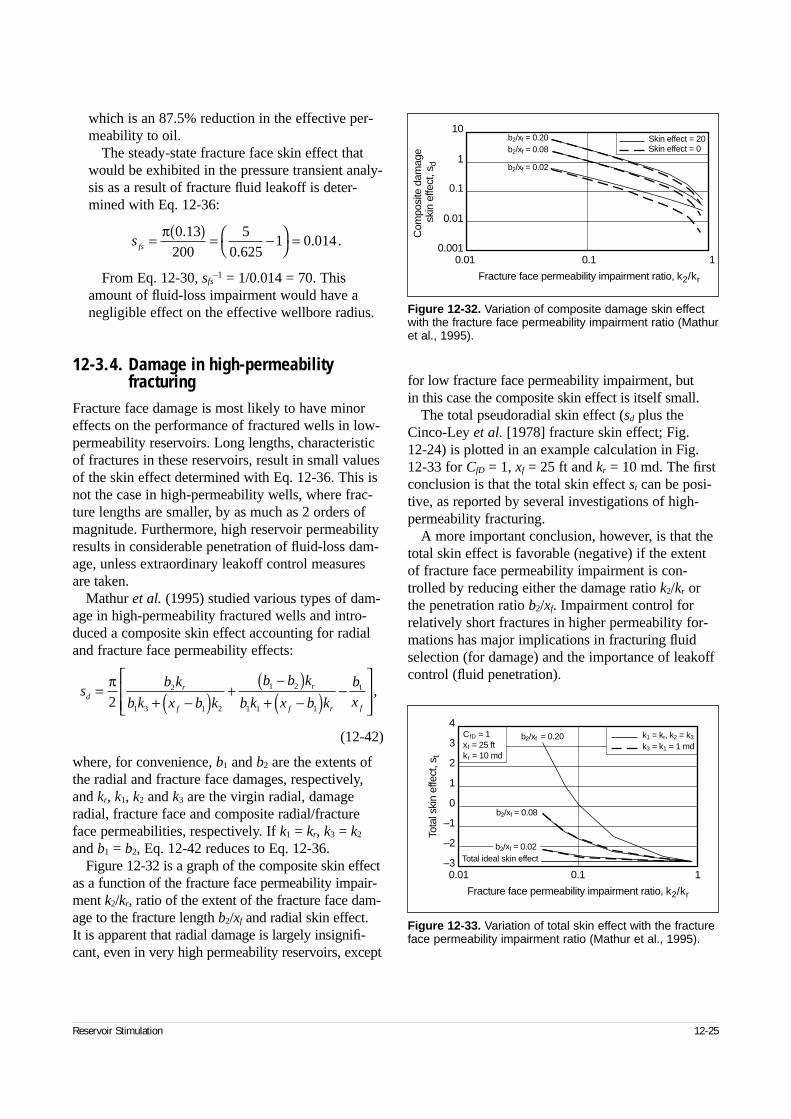
which is an 87.5% reduction in the effective per-meability to oil.

The steady-state fracture face skin effect thatwould be exhibited in the pressure transient analy-sis as a result of fracture fluid leakoff is deter-mined with Eq. 12-36:

From Eq. 12-30, sfs–1 = 1/0.014 = 70. This

amount of fluid-loss impairment would have anegligible effect on the effective wellbore radius.

12-3.4. Damage in high-permeabilityfracturing

Fracture face damage is most likely to have minoreffects on the performance of fractured wells in low-permeability reservoirs. Long lengths, characteristicof fractures in these reservoirs, result in small valuesof the skin effect determined with Eq. 12-36. This isnot the case in high-permeability wells, where frac-ture lengths are smaller, by as much as 2 orders ofmagnitude. Furthermore, high reservoir permeabilityresults in considerable penetration of fluid-loss dam-age, unless extraordinary leakoff control measuresare taken.

Mathur et al. (1995) studied various types of dam-age in high-permeability fractured wells and intro-duced a composite skin effect accounting for radialand fracture face permeability effects:

(12-42)

where, for convenience, b1 and b2 are the extents ofthe radial and fracture face damages, respectively,and kr, k1, k2 and k3 are the virgin radial, damageradial, fracture face and composite radial/fractureface permeabilities, respectively. If k1 = kr, k3 = k2

and b1 = b2, Eq. 12-42 reduces to Eq. 12-36.Figure 12-32 is a graph of the composite skin effect

as a function of the fracture face permeability impair-ment k2/kr, ratio of the extent of the fracture face dam-age to the fracture length b2/xf and radial skin effect. It is apparent that radial damage is largely insignifi-cant, even in very high permeability reservoirs, except

for low fracture face permeability impairment, but in this case the composite skin effect is itself small.

The total pseudoradial skin effect (sd plus theCinco-Ley et al. [1978] fracture skin effect; Fig. 12-24) is plotted in an example calculation in Fig.12-33 for CfD = 1, xf = 25 ft and kr = 10 md. The firstconclusion is that the total skin effect st can be posi-tive, as reported by several investigations of high-permeability fracturing.

A more important conclusion, however, is that thetotal skin effect is favorable (negative) if the extentof fracture face permeability impairment is con-trolled by reducing either the damage ratio k2/kr orthe penetration ratio b2/xf. Impairment control forrelatively short fractures in higher permeability for-mations has major implications in fracturing fluidselection (for damage) and the importance of leakoffcontrol (fluid penetration).

Reservoir Stimulation 12-25

s fs = ( ) = −

=π 0 13

2005

0 6251 0 014

..

. .

sb k

b k x b k

b b k

b k x b k

b

xdr

f

r

f r f

=+ −( ) +

−( )+ −( ) −

π2

2

1 3 1 2

1 2

1 1 1

1 ,

Figure 12-32. Variation of composite damage skin effectwith the fracture face permeability impairment ratio (Mathuret al., 1995).

0.010.001

0.1 1

0.01

0.1

1

10

Fracture face permeability impairment ratio, k2/kr

Com

posi

te d

amag

e sk

in e

ffect

, sd

b2/xf = 0.20b2/xf = 0.08

b2/xf = 0.02

Skin effect = 20Skin effect = 0

Figure 12-33. Variation of total skin effect with the fractureface permeability impairment ratio (Mathur et al., 1995).

0.01–3

0.1 1

–2

–1

0

1

2

3

4

Fracture face permeability impairment ratio, k2/kr

Tota

l ski

n ef

fect

, st

b2/xf = 0.20

b2/xf = 0.08

b2/xf = 0.02Total ideal skin effect

k1 = kr, k2 = k3

k3 = k1 = 1 mdCfD = 1xf = 25 ftkr = 10 md

12-3.5. Heterogeneous systemsThe transient behavior discussed in the preceding sec-tions of this chapter is presented with the assumptionthat the reservoir is homogeneous and isotropic.Spatial variation in reservoir thickness, porosity, per-meability and fluid saturations can be readily consid-ered with finite-difference or finite-element simulationmodels. However, using analytic solutions to evaluatethe transient behavior of vertically fractured wells, ortheir long-term production behavior, may require nor-malization procedures to properly account for spatialvariation in the reservoir properties. Geostatisticaltechniques have been used to normalize spatial varia-tion in reservoir properties and to correlate transientanalysis and reservoir simulation results.

Reservoir permeability anisotropy is another com-mon factor that complicates analysis of the transientbehavior of finite-conductivity fractures. Directionalpermeability anisotropic effects on the transientbehavior of finite-conductivity fractures were studiedby Ben Naceur and Economides (1988). That studyfound that the anisotropy case believed most com-mon is the one in which the direction of maximumpermeability is perpendicular to the direction of min-imum in-situ horizontal stress (i.e., parallel to thefracture plane). For this case, reservoir permeabilityanisotropy has an unfavorable effect on the produc-tivity improvement obtained by fracturing the well.This unfavorable anisotropy ratio in effect results ina shorter apparent fracture half-length than that actu-ally obtained.

For radial flow in anisotropic reservoirs, it is com-mon practice to define an average effective horizon-tal permeability for the system that is the geometricmean of the directional permeabilities kx and ky:

(12-43)

For kx = 10ky, the radial response from a prefracturewell test yields k = 3.1kx, whereas the fractureresponds approximately as if k were only 1.8kx.

Another reservoir heterogeneity that must be con-sidered in analysis of the transient behavior of verti-cally fractured wells and their future production per-formance is the effect of multiple reservoir layers,which may have significantly different formationproperties, pore pressure levels, fracture half-lengthsand drainage areal extents.

Bennett et al. (1986) investigated the transientresponse of hydraulically fractured wells in multi-

layer systems. They determined that fracture half-length is underestimated in a layered commingledreservoir if the layered nature of the formation is notproperly considered. Bennett et al. introduced theconcept of dimensionless reservoir conductivity CRD

to correlate single-layer and multilayer responses:

(12-44)

where CRD is always less than or equal to unity for a multilayer system. For post-treatment analysis offractured well transient behavior, the dimensionlesstime scale is tD/CRD

2, which shifts the fracture half-length scale by a factor of CRD. Ignoring the layeredreservoir nature may result in shorter than actualapparent fracture lengths from the analysis.

Camacho-V. et al. (1987) later extended the workby Bennett et al. on the concept of dimensionlessreservoir conductivity CRD to include the effects ofdiffering fracture half-lengths in multilayer reservoirsystems. The total system net pay thickness h

—is

(12-45)

average system reference permeability k—

is

(12-46)

and average system storage φ— —ct is

(12-47)

The individual layer and composite system averagehydraulic diffusivities are, respectively,

(12-48)

(12-49)

An equivalent system average fracture half-length x—f

is, therefore,

(12-50)

An average fracture conductivity k—

fw—

is

(12-51)

12-26 Post-Treatment Evaluation and Fractured Well Performance

k k kx y= .

Ch k c

h k cRD

t

j j t jj

n

= ( )=

∑1

1φφ ,

h hjj

n

==

∑1

,

kh

k hj jj

n

==

∑1

1

,

φ φch

c ht j tj jj

n

==

∑1

1

.

ηφ µj

j

j tj

k

c=

ηφ µ

= k

ct

.

xkh

k h xf

j j fj

jj

n

==

∑ηη1

.

k wh

k w h Cf fj j j RDjj

n

=

=

∑1

1

2

,

where the individual fracture layer dimensionlessreservoir conductivity CRDj is

(12-52)

The dimensionless reservoir conductivity CRD con-cept of Bennett et al. and Camacho-V. et al. isapplicable only for analysis of the early transientbehavior of finite-conductivity fractures (dimension-less fracture time tDxf < 1) for which there is essen-tially linear flow in the reservoir normal to the planeof the fracture. This correlation technique is notapplicable to pseudoradial or pseudosteady-stateflow regimes.

An entirely general commingled reservoir solutiondeveloped by Spath et al. (1994) using Laplace trans-form solutions of the reservoir performance of eachreservoir layer eliminates the linear flow restriction of the Bennett et al. and Camacho-V. et al. analyses.

12-4. Well test analysis of verticallyfractured wells

Analysis of the transient behavior of a finite-conductivityfracture to obtain reliable estimates of the reservoir andfracture properties requires proper identification of theflow regimes exhibited in the transient data. The analy-sis procedure includes (1) log-log diagnostic analysesof both the pressure and pressure derivative responses,(2) specialized Cartesian analysis and verification ofidentified flow regimes, (3) simulation of the entiretransient history using the determined reservoir andfracture parameter estimates and (4) a final validationcheck of the obtained parameter estimates in conjunc-tion with the flow regime demarcation limits.

A prefracture estimate of the formation average per-meability k is necessary for the interpretation of frac-ture properties in the postfracture transient analysis,unless the transient data contain at least some pseudo-radial flow, for which an estimate of formation perme-ability can be computed directly from the transientdata. Depending on the formation permeability, frac-ture half-length and conductivity, the pseudoradialflow regime may not be exhibited for an extensiveperiod of time, making it impractical to obtain post-fracture estimates of formation permeability with welltests. However, the synergy of history matching long-term production with well test data (e.g., Agarwal etal., 1979) may overcome this limitation.

The uniqueness problem in interpretation of thetransient behavior of finite-conductivity fractures isdue to the fact that the transient performance of afractured well in each of the flow regimes consideredis a function of both reservoir and fracture proper-ties. An independent estimate of formation perme-ability is required to quantify the fracture parameterestimates separately from the combined response ofthe reservoir and fracture.

Evaluation of the drawdown (or injection) tran-sient behavior of a fractured well involves graphicalanalysis of the pressure drawdown ∆p = pi – pwf orthe pressure rise for injection ∆p = pwf – pi, where pi

is the initial pressure and pwf is the bottomhole flow-ing pressure, for liquid or multiphase flow analysisas a function of transient time ∆t. Gas reservoiranalyses are most properly evaluated for drawdowntransients using the appropriate pseudopressure dif-ferences of ∆m(p ) = m(p i) – m(p wf) for a draw-down and ∆m(p ) = m(p wf) – m(pi) for an injectiontransient and the elapsed transient pseudotime ∆ta.For shut-in transients, similar pressure graphingfunctions are used. For pressure buildup transients inoil or multiphase analyses, the pressure buildup riseis ∆p = pws – pwf (∆t = 0), where pws is the bottomholeshut-in pressure. For pressure falloff transients (fol-lowing an injection transient), the appropriate graphfunction is ∆p = pwf (∆t = 0) – pws. For gas reservoiranalyses, the pseudopressure equivalents of thesefunctions are used.

Shut-in transients may be analyzed using draw-down solution type curves and Agarwal et al.’s(1979) “effective” time correlation parameter:

(12-53)

The producing time tp prior to the shut-in transientand shut-in transient elapsed time ∆t correlate theshut-in transient behavior with the drawdown solu-tion. This correlation parameter is derived directlyfrom the superposition-in-time principle for a two-rate transient history in which the last rate step is the shut-in transient. For a multirate production his-tory prior to the final shut-in transient, it is generallypreferred to use continuous superposition of the pro-duction history in the analysis instead of Agarwal etal.’s effective time.

For gas reservoirs, the analysis may be performedeither with dimensional time or preferably with the

Reservoir Stimulation 12-27

Ck h

khRDjj j

j

= ηη

.

∆∆∆

tt t

t tep

p

=+

.

pseudotime equivalent of the time-scale function.The effective pseudotime equivalent of Eq. 12-53 is

(12-54)

Pressure buildup analysis of a pseudoradial flowregime using classic semilog analysis procedures maybe performed with Horner’s (1951) approximation:

(12-55)

where Qp is the cumulative production of the principalfluid phase of the analysis and qlast is the productionrate of the flowing transient immediately prior to theshut-in transient.

12-4.1. Wellbore storage dominated flow analysis

The wellbore storage dominated transient behaviordiscussed in Section 12-2.1 (unit-slope behavior) isdescribed mathematically by

(12-56)

In dimensional units, the log linear behavior of the∆p function versus transient time is

(12-57)

The wellbore storage coefficient C can therefore becomputed directly using the coordinates of any pointon the unit-slope ∆p line (∆tusl, ∆pusl, where the sub-script usl denotes unit-slope line) or from the deriva-tive ∂∆p/∂∆t with

(12-58)

for liquid flow analyses. Either the pressure or pres-sure derivative responses can be used because theyare identical (assuming constant wellbore storage).

A similar relationship for determining the wellborestorage coefficient for gas wells is

(12-59)

12-4.2. Fracture storage linear flow analysis

The fracture storage linear flow regime is generallyexhibited clearly in the transient behavior of finite-conductivity fractures only when wellbore storageeffects are minimized, typically with downhole isola-tion devices. When this behavior is exhibited in thetransient response, an analysis can be performed thatprovides an estimate of the fracture diffusivity/con-ductivity relationship √ηf /kfw. If only fracture stor-age dominated flow behavior is used, the hydraulicdiffusivity and conductivity cannot be determinedseparately. Separation of the quantities is obtained inconjunction with analysis of the other fracture flowregimes exhibited in the data to determine fractureconductivity.

The log-log fracture storage linear flow behaviorof an oil reservoir analysis can be evaluated usingthe pressure derivative response ∆t(∂∆p/∂∆t). Thefracture hydraulic diffusivity can be determined (fora known fracture conductivity) with

(12-60)

where the subscript fsl denotes fracture storage linearflow. Similarly, fracture hydraulic diffusivity may beobtained in a gas reservoir analysis using pseudo-pressure and pseudotime with

(12-61)

Verification graphs can then be constructed bygraphing ∆p versus ∆t1/2 (or ∆m(p) versus ∆ta

1/2 forgas) on a Cartesian scale, for which the fracture stor-age linear flow behavior is characterized by a straightline passing through the origin for oil and gas, respectively:

(12-62)

12-28 Post-Treatment Evaluation and Fractured Well Performance

∆∆

∆t

t t t t

t t t tae

a p a

a p a

=( ) ( )

( ) + ( ).

Cp Tc q

T m pt

p Tc q

T tm p

t

tsc t g

sc usl

auslsc t g

sc a

a usl

ausl= ( ) =( )

14 8 14 8. ..

∆∆

∆∆

∆

∆∂

∂

ηµ

∂∂

ff f

o o o

fsl

fsl

k wh

q B

tp

t

t=

4 06

2

2

.,

∆ ∆∆

∆

η

∂∂

µff f sc

g sc

a

a fsl

afsl gi t

k wh T

q Tp

tm p

t

t c=

( )

1448

2

2

∆∆

∆

∆.

∆ ∆pq B

k whto o o

f f

f= ( )8 13 1 2. /µ η

tQ

qpp

last

= ,

pt

CwDD

D

= .

∆ ∆pqB

Ct=

24.

CqB

pt

qB

tp

t

tusl

usl

usl

usl= =

24 24∆∆

∆ ∆∆

∆∂∂

(12-63)

12-4.3. Bilinear flow analysisThe analysis of transient data that exhibits bilinearflow behavior is performed by a log-log diagnosticanalysis of the pressure and pressure derivativebehavior, with a Cartesian analysis and verificationof the identified flow regime. On a log-log graph of∆p versus ∆t (or ∆m(p) versus ∆ta for gas reservoirs),the bilinear flow regime is identified as that withquarter-slope behavior on both the pressure and pres-sure derivative responses.

The fracture conductivity kfw can be determinedusing any point on the log-log derivative quarter-slope line. The interpretation relationships for oil andgas reservoir analyses, respectively, are

(12-64)

(12-65)

where the subscript bf denotes bilinear flow.Verification graphs are generated on Cartesian

scales using ∆p versus ∆t1/4 for oil reservoir analysesand ∆m(p) versus ∆ta

1/4 for gas reservoir analyses.The straight line is characterized by the relationshipsfor oil and gas reservoir analyses, respectively, as

(12-66)

(12-67)

The Cartesian graphs for the analysis and verifica-tion of bilinear flow also provide additional informa-tion concerning the fracture conductivity. As dis-cussed in Section 12-2.3, the deviation of the tran-sient data from the straight-line flow of the bilinear

and near-wellbore conductivity alternations after theend of the bilinear flow regime clearly indicateswhether the dimensionless fracture conductivity isless than, equal to or greater than 1.6 (Fig. 12-17). If the transient data tail off upward above the bilin-ear flow straight line, CfD > 1.6; if the transient datatrend below the bilinear flow straight line, CfD < 1.6.

12-4.4. Formation linear flow analysisThe formation linear flow regime is exhibited in thetransient behavior of a finite-conductivity fractureonly if CfD > ~80. The fracture half-length can bedetermined from formation linear flow transient datausing log-log pressure derivative behavior for oil andgas reservoir analyses, respectively:

(12-68)

(12-69)

where the subscript lf denotes formation linear flow.Cartesian graphs of ∆p versus ∆t1/2 for oil reser-

voirs or ∆m(p) versus ∆ta1/2 for gas reservoirs are

used to verify that the transient data selected in thelog-log derivative analysis are exhibiting formationlinear flow. The Cartesian graph relations describingthe formation linear flow for oil and gas reservoirs,respectively, are

(12-70)

(12-71)

12-4.5. Pseudoradial flow analysisAnalysis of the pressure transient behavior of a finite-conductivity fracture that exhibits pseudoradial flowbehavior involves log-log analysis of the transient dataand classic semilog analysis procedures. The transientbehavior of a finite-conductivity fractured well duringthe pseudoradial flow regime is discussed in Section12-2.5.

Reservoir Stimulation 12-29

∆ ∆m pq Tp

k wh Tc tg sc

f f sc

f gi t a( ) = ( )2895 1 2η µ

/.

xq B

h tpt

t

c kfo o

lf

o lf

t

=

2 031 2

./

∆ ∆∆

∆∂∂

µφ

xq Tp

T h tm p

t

t

kfg sc

sc a

a lf

alf=( )

7241 2

∆∆

∆

∆∂

∂φ

/

,

∆ ∆p

q B

hx

t

k co o

f

o

t

=

4 061 2

./

µφ

∆ ∆m p

p Tq

T hx

t

ksc g

sc f

a( ) =

14481 2

φ

/

.

k wq B

hh tp

t

t

c kfo o o

fbf

bf

o t

=

11 025

2

1 2.

/µ

∂∂

φµ∆ ∆∆

∆

k wq Tp

hh T tm p

t

t

kfg sc

f sc a

a bf

abf=( )

3927 3

2

1 2.

,/

∆∆

∆

∆∂

∂φ

∆ ∆p

q B

hh k w

t

c ko o o

f f o t

=

44 11 4

./

µφµ

∆ ∆m p

q Tp

T hh k w

t

kg sc

sc f f

a( ) =

15 7101 4

,.

/

φ

The formation permeability can be determineddirectly using any point on the log-log derivativecurve during the pseudoradial flow regime (wherethe dimensionless derivative is a horizontal lineequal to 0.5). The dimensional derivative is also a horizontal line, and the permeability is evaluatedusing the coordinates of a point on this straight linefor oil and gas reservoirs, respectively:

(12-72)

(12-73)

where the subscript pr denotes pseudoradial flow.The apparent steady-state skin effect caused by the

fracture can also be determined from log-log analysisduring the pseudoradial flow regime using a point on the pressure curve (∆tpr, ∆ppr) for oil reservoiranalyses or a point on the pseudopressure curve(∆tapr, ∆m(p)pr) for gas reservoir analyses for oil and gas reservoirs, respectively:

(12-74)

(12-75)

Semilog analysis procedures may also be used toobtain estimates of the formation permeability andapparent steady-state skin effect of vertically frac-tured wells (see Chapter 2).

12-4.6. Well test design considerationsAnalysis of the pressure buildup behavior of a fracturedwell to obtain meaningful and reliable reservoir andfracture parameter estimates requires an accurate recordof the well flow history. The stabilized flow periodimmediately prior to the pressure buildup should be of equal or greater duration than the buildup transient.Otherwise, production time effects are observed in both

the pressure and derivative responses at late times in theshut-in transient. Production time effects appear in thetransient data as a steep increase in the log-log deriva-tive response and a generally smaller (although it canbe significantly greater) increase in the pressure be-havior. Commonly, the derivative response caused by production time effects is greater in magnitude thanthe ∆p response.

Production time effects are due to the simple physi-cal principle that each time there is a unit step changein the well production rate, a new pressure pulse ispropagated away from the well into the reservoir. Thevelocity at which the pressure pulse propagates in thereservoir is a function of the formation properties andtime. In the case of vertically fractured wells, this alsoincludes the effect of fracture length.

If a given reservoir feature (boundaries, reservoir het-erogeneities, interference from offset wells, etc.) orfracture feature that requires the end of bilinear flow(length or conductivity near the top) is of interest, theflow period immediately prior to the shut-in transientmust be of sufficient duration that the distance of inves-tigation from the well for the flow period exceeds thatrequired to see the same reservoir or fracture feature inthe interpreted shut-in transient. The post-treatmentcleanup process must also be completed, as this periodcan be of substantial duration in lower permeabilityreservoirs (Holditch, 1979).

The use of continuous superposition-in-time in thetransient analysis does not remove or eliminate pro-duction time effects in the transient data. They are theactual response of the reservoir, and any interpretationthat includes the identification of a reservoir or frac-ture feature, such as a boundary or fracture length,from data distorted by production time effects isincorrect or highly questionable at best.

To distinguish between what may actually be theeffect of reservoir or fracture limits and productiontime effects, the duration of the flow period immedi-ately prior to the pressure buildup transient can beeasily checked. If the flow period is of greater dura-tion than the pressure buildup, then the responseobserved in the transient data is actually a reservoiror fracture feature. However, if the elapsed shut-intime at which an anomalous behavior in the deriva-tive response occurs corresponds to the duration ofthe stabilized flow period prior to the buildup, thetransient response can be strongly suspected asresulting from production time effects.

12-30 Post-Treatment Evaluation and Fractured Well Performance

kq B

h tp

t

o o o

pr

=

70 6. µ∂∂

∆ ∆∆

kq Tp

hT tm p

t

g sc

sc a

a pr

=( )

25 150,,

∆∆

∆∂

∂

skh p

q B

k t

c rpr

o o o

pr

t w

= −

+

∆ ∆141 2

12

0 0002640 8091

2..

µ φµln

.

skhT m p

p Tq

k t

rsc pr

sc g

apr

w

=( )

−

+

∆ ∆50 300

12

0 0002640 8091

2,. .ln

.

φ

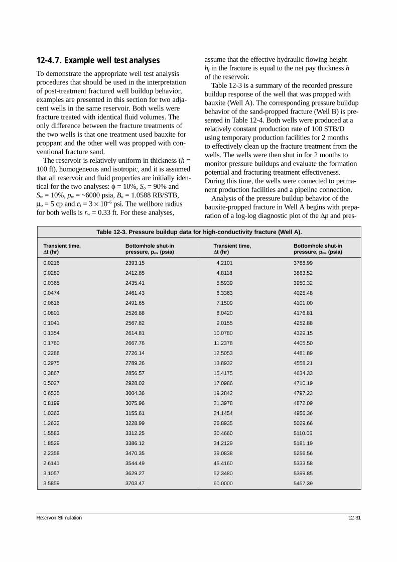
12-4.7. Example well test analysesTo demonstrate the appropriate well test analysisprocedures that should be used in the interpretationof post-treatment fractured well buildup behavior,examples are presented in this section for two adja-cent wells in the same reservoir. Both wells werefracture treated with identical fluid volumes. Theonly difference between the fracture treatments ofthe two wells is that one treatment used bauxite forproppant and the other well was propped with con-ventional fracture sand.

The reservoir is relatively uniform in thickness (h =100 ft), homogeneous and isotropic, and it is assumedthat all reservoir and fluid properties are initially iden-tical for the two analyses: φ = 10%, So = 90% and Sw = 10%, pw = ~6000 psia, Bo = 1.0588 RB/STB, µo = 5 cp and ct = 3 × 10–6 psi. The wellbore radiusfor both wells is rw = 0.33 ft. For these analyses,

assume that the effective hydraulic flowing height hf in the fracture is equal to the net pay thickness hof the reservoir.

Table 12-3 is a summary of the recorded pressurebuildup response of the well that was propped withbauxite (Well A). The corresponding pressure buildupbehavior of the sand-propped fracture (Well B) is pre-sented in Table 12-4. Both wells were produced at arelatively constant production rate of 100 STB/Dusing temporary production facilities for 2 months to effectively clean up the fracture treatment from thewells. The wells were then shut in for 2 months tomonitor pressure buildups and evaluate the formationpotential and fracturing treatment effectiveness.During this time, the wells were connected to perma-nent production facilities and a pipeline connection.

Analysis of the pressure buildup behavior of thebauxite-propped fracture in Well A begins with prepa-ration of a log-log diagnostic plot of the ∆p and pres-

Reservoir Stimulation 12-31

Table 12-3. Pressure buildup data for high-conductivity fracture (Well A).

Transient time, Bottomhole shut-in Transient time, Bottomhole shut-in ∆t (hr) pressure, pws (psia) ∆t (hr) pressure, pws (psia)

0.0216 2393.15

0.0280 2412.85

0.0365 2435.41

0.0474 2461.43

0.0616 2491.65

0.0801 2526.88

0.1041 2567.82

0.1354 2614.81

0.1760 2667.76

0.2288 2726.14

0.2975 2789.26

0.3867 2856.57

0.5027 2928.02

0.6535 3004.36

0.8199 3075.96

1.0363 3155.61

1.2632 3228.99

1.5583 3312.25

1.8529 3386.12

2.2358 3470.35

2.6141 3544.49

3.1057 3629.27

3.5859 3703.47

4.2101 3788.99

4.8118 3863.52

5.5939 3950.32

6.3363 4025.48

7.1509 4101.00

8.0420 4176.81

9.0155 4252.88

10.0780 4329.15

11.2378 4405.50

12.5053 4481.89

13.8932 4558.21

15.4175 4634.33

17.0986 4710.19

19.2842 4797.23

21.3978 4872.09

24.1454 4956.36

26.8935 5029.66

30.4660 5110.06

34.2129 5181.19

39.0838 5256.56

45.4160 5333.58

52.3480 5399.85

60.0000 5457.39

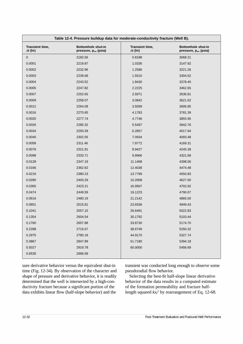
sure derivative behavior versus the equivalent shut-intime (Fig. 12-34). By observation of the character andshape of pressure and derivative behavior, it is readilydetermined that the well is intersected by a high-con-ductivity fracture because a significant portion of thedata exhibits linear flow (half-slope behavior) and the

transient was conducted long enough to observe somepseudoradial flow behavior.

Selecting the best-fit half-slope linear derivativebehavior of the data results in a computed estimateof the formation permeability and fracture half-length squared kxf

2 by rearrangement of Eq. 12-68.

12-32 Post-Treatment Evaluation and Fractured Well Performance

Table 12-4. Pressure buildup data for moderate-conductivity fracture (Well B).

Transient time, Bottomhole shut-in Transient time, Bottomhole shut-in ∆t (hr) pressure, pws (psia) ∆t (hr) pressure, pws (psia)

0 2182.56

0.0001 2219.87

0.0002 2232.96

0.0003 2239.68

0.0004 2243.52

0.0005 2247.82

0.0007 2252.65

0.0009 2258.07

0.0012 2264.08

0.0016 2270.65

0.0020 2277.74

0.0026 2285.32

0.0034 2293.39

0.0045 2302.05

0.0058 2311.46

0.0076 2321.91

0.0098 2333.71

0.0128 2347.19

0.0166 2362.62

0.0216 2380.23

0.0280 2400.29

0.0365 2423.21

0.0474 2449.59

0.0616 2480.19

0.0801 2515.81

0.1041 2557.15

0.1354 2604.54

0.1760 2657.88

0.2288 2716.67

0.2975 2780.18

0.3867 2847.89

0.5027 2919.78

0.6535 2996.59

0.8188 3068.21

1.0336 3147.92

1.2586 3221.26

1.5510 3304.52

1.8430 3378.40

2.2225 3462.65

2.5971 3536.81

3.0842 3621.62

3.5599 3695.85

4.1783 3781.39

4.7746 3855.95

5.5497 3942.76

6.2857 4017.94

7.0934 4093.48

7.9772 4169.31

8.9427 4245.39

9.9966 4321.68

11.1468 4398.06

12.4038 4474.48

13.7799 4550.83

15.2908 4627.00

16.9567 4702.92

19.1223 4790.07

21.2142 4865.00

23.9336 4949.43

26.6491 5022.83

30.1792 5103.44

33.8730 5174.70

38.6749 5250.32

44.9170 5327.74

51.7180 5394.18

60.0000 5456.69

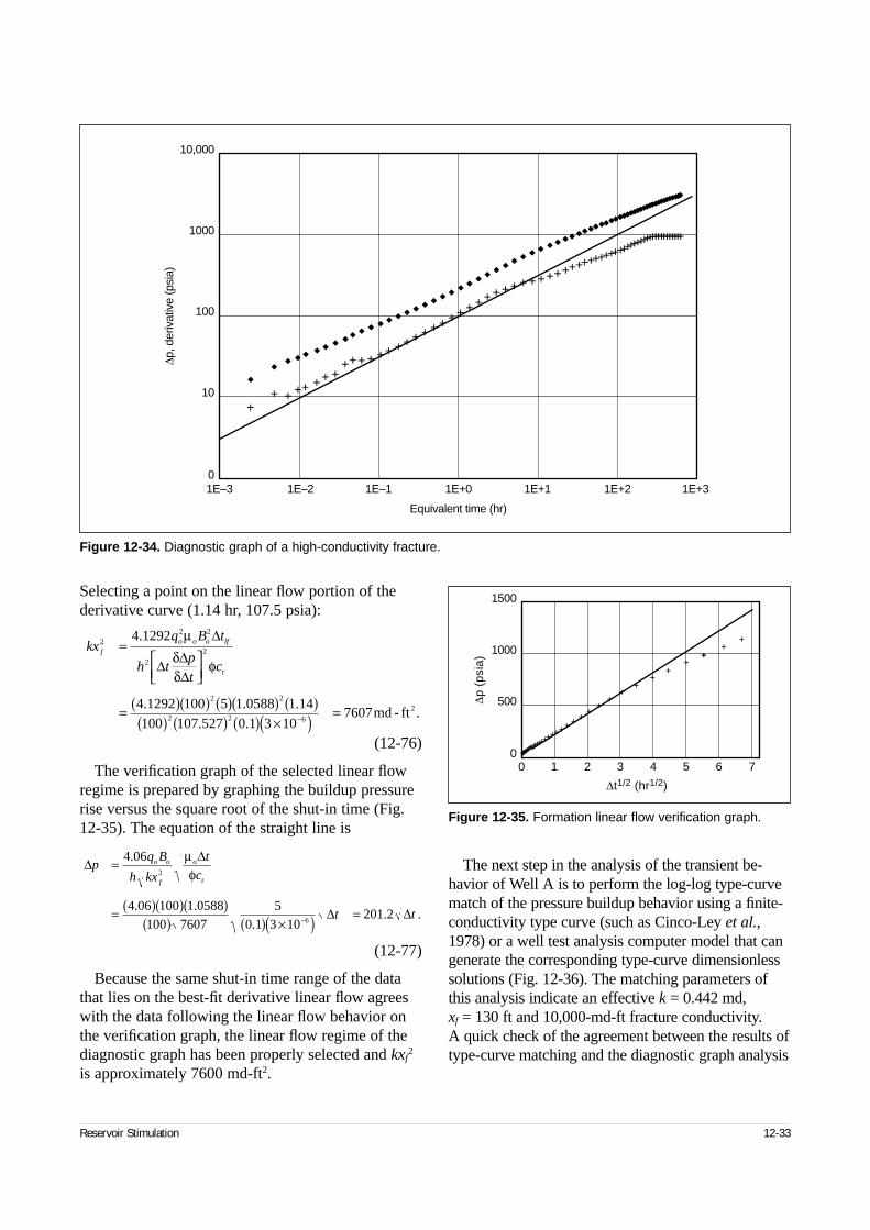
Selecting a point on the linear flow portion of thederivative curve (1.14 hr, 107.5 psia):

(12-76)

The verification graph of the selected linear flowregime is prepared by graphing the buildup pressurerise versus the square root of the shut-in time (Fig.12-35). The equation of the straight line is

(12-77)

Because the same shut-in time range of the datathat lies on the best-fit derivative linear flow agreeswith the data following the linear flow behavior onthe verification graph, the linear flow regime of thediagnostic graph has been properly selected and kxf

2

is approximately 7600 md-ft2.

The next step in the analysis of the transient be-havior of Well A is to perform the log-log type-curvematch of the pressure buildup behavior using a finite-conductivity type curve (such as Cinco-Ley et al.,1978) or a well test analysis computer model that cangenerate the corresponding type-curve dimensionlesssolutions (Fig. 12-36). The matching parameters ofthis analysis indicate an effective k = 0.442 md, xf = 130 ft and 10,000-md-ft fracture conductivity. A quick check of the agreement between the results oftype-curve matching and the diagnostic graph analysis

Reservoir Stimulation 12-33

Figure 12-34. Diagnostic graph of a high-conductivity fracture.

∆p, d

eriv

ativ

e (p

sia)

10,000

1000

100

10

01E–3 1E–2 1E–1 1E+0 1E+1 1E+2 1E+3

Equivalent time (hr)

++

+ ++ ++ ++++ + ++ ++++++

++++++++++++++++++++++

++++++++++++++++++++++

kxq B t

h tpt

cf

o o o lf

t

22 2

2

2

2 2

2 2 6

4 1292

4 1292 100 5 1 0588 1 14100 107 527 0 1 3 10

7607

=

= ( )( ) ( )( ) ( )( ) ( ) ( ) ×( ) =−

.

. . .. .

.

µδδ

φ

∆

∆ ∆∆

md - ft2

∆ ∆

∆ ∆

pq B

h kx

t

c

t t

o o

f

o

t

=

= ( )( )( )( ) ( ) ×( ) =−

4 06

4 06 100 1 0588100 7607

50 1 3 10

201 2

2

6

.

. ..

. .

µφ

Figure 12-35. Formation linear flow verification graph.

∆p (

psia

)

1500

1000

500

00 1 2 3 4 5 6 7

∆t1/2 (hr1/2)

++

++

++

+

+

++

++ +

+++++++++++++++++++++++++++

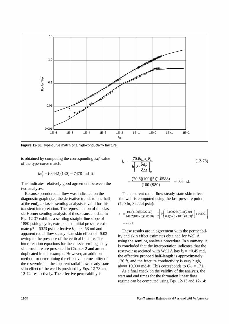
is obtained by computing the corresponding kxf2 value

of the type-curve match:

This indicates relatively good agreement between thetwo analyses.

Because pseudoradial flow was indicated on thediagnostic graph (i.e., the derivative trends to one-halfat the end), a classic semilog analysis is valid for thistransient interpretation. The representation of the clas-sic Horner semilog analysis of these transient data inFig. 12-37 exhibits a semilog straight-line slope of1880 psi/log cycle, extrapolated initial pressure esti-mate p* = 6023 psia, effective ko = 0.458 md andapparent radial flow steady-state skin effect of –5.02owing to the presence of the vertical fracture. Theinterpretation equations for the classic semilog analy-sis procedure are presented in Chapter 2 and are notduplicated in this example. However, an additionalmethod for determining the effective permeability ofthe reservoir and the apparent radial flow steady-stateskin effect of the well is provided by Eqs. 12-78 and12-74, respectively. The effective permeability is

(12-78)

The apparent radial flow steady-state skin effect the well is computed using the last pressure point

(720 hr, 3222.4 psia):

These results are in agreement with the permeabil-ity and skin effect estimates obtained for Well Ausing the semilog analysis procedure. In summary, itis concluded that the interpretation indicates that thereservoir associated with Well A has ko = ~0.45 md,the effective propped half-length is approximately130 ft, and the fracture conductivity is very high,about 10,000 md-ft. This corresponds to CfD = 171.

As a final check on the validity of the analysis, thestart and end times for the formation linear flowregime can be computed using Eqs. 12-13 and 12-14:

12-34 Post-Treatment Evaluation and Fractured Well Performance

kq B

h tp

t

o o o

pr

=

= ( )( )( )( )( )( )

=

70 6

70 6 100 5 1 0588100 980

0 4

.

. ..

µδδ

∆ ∆∆

md.

s = ( )( )( )( )( )( )

− ( )( )( ) ×( )( )

+

= −

−

0 4 100 3222 39141 2 100 5 1 0588

12

0 000264 0 4 7200 1 5 3 10 0 33

0 8091

5 21

6 2

. .. .

ln. .

. ..

. .

kx f2 0 442 130 7470= ( )( ) =. md-ft.

Figure 12-36. Type-curve match of a high-conductivity fracture.

p D, t

D•

p D´

0.1

0.01

0.001

10

1.0

1E–6 1E–5 1E–4 1E–3 1E–2 1E–1 1E+0 1E+1 1E+2tD

++ ++++++

+++++++++++++++++++++++++++++++++++

++++++++++++++++++

++++++++++++++++++++++++++++++++++++++++++++++++++++++++++++++++

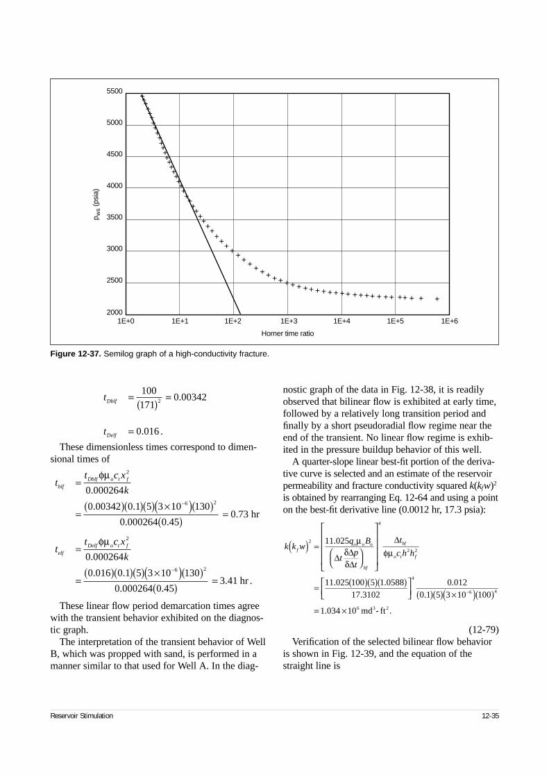
These dimensionless times correspond to dimen-sional times of

These linear flow period demarcation times agreewith the transient behavior exhibited on the diagnos-tic graph.

The interpretation of the transient behavior of WellB, which was propped with sand, is performed in amanner similar to that used for Well A. In the diag-

nostic graph of the data in Fig. 12-38, it is readilyobserved that bilinear flow is exhibited at early time,followed by a relatively long transition period andfinally by a short pseudoradial flow regime near theend of the transient. No linear flow regime is exhib-ited in the pressure buildup behavior of this well.

A quarter-slope linear best-fit portion of the deriva-tive curve is selected and an estimate of the reservoirpermeability and fracture conductivity squared k(kfw)2

is obtained by rearranging Eq. 12-64 and using a pointon the best-fit derivative line (0.0012 hr, 17.3 psia):

(12-79)Verification of the selected bilinear flow behavior

is shown in Fig. 12-39, and the equation of thestraight line is

Reservoir Stimulation 12-35

t

t

Dblf

Delf

=( )

=

=

100171

0 00342

0 016

2 .

. .

k k wq B

tpt

t

c h hfo o o

bf

bf

o t f

( ) =

= ( )( )( )

( )( ) ×( )( )

= ×

−

2

4

2 2

4

6 4

6

11 025

11 025 100 5 1 058817 3102

0 0120 1 5 3 10 100

1 034 10

.

. ..

..

. .

µδδ

φµ∆ ∆∆

∆

md3- ft2

tt c x

k

tt c x

k

blfDblf o t f

elfDelf o t f

=

=( )( )( ) ×( )( )

( )=

=

=( )( )( ) ×( )( )

( )=

−

−

φµ

φµ

2

6 2

2

6 2

0 000264

0 00342 0 1 5 3 10 130

0 000264 0 450 73

0 000264

0 016 0 1 5 3 10 130

0 000264 0 453 41

.

. .

. ..

.

. .

. ..

hr

hr .

Figure 12-37. Semilog graph of a high-conductivity fracture.

p ws

(psi

a)5500

5000

4500

4000

3500

3000

2500

20001E+0 1E+1 1E+2 1E+3 1E+4 1E+5 1E+6

Horner time ratio

++++++++++++++++++++++++++++++++++

+++

+++

+++

+++

+++++

+++

++++++

+++

+

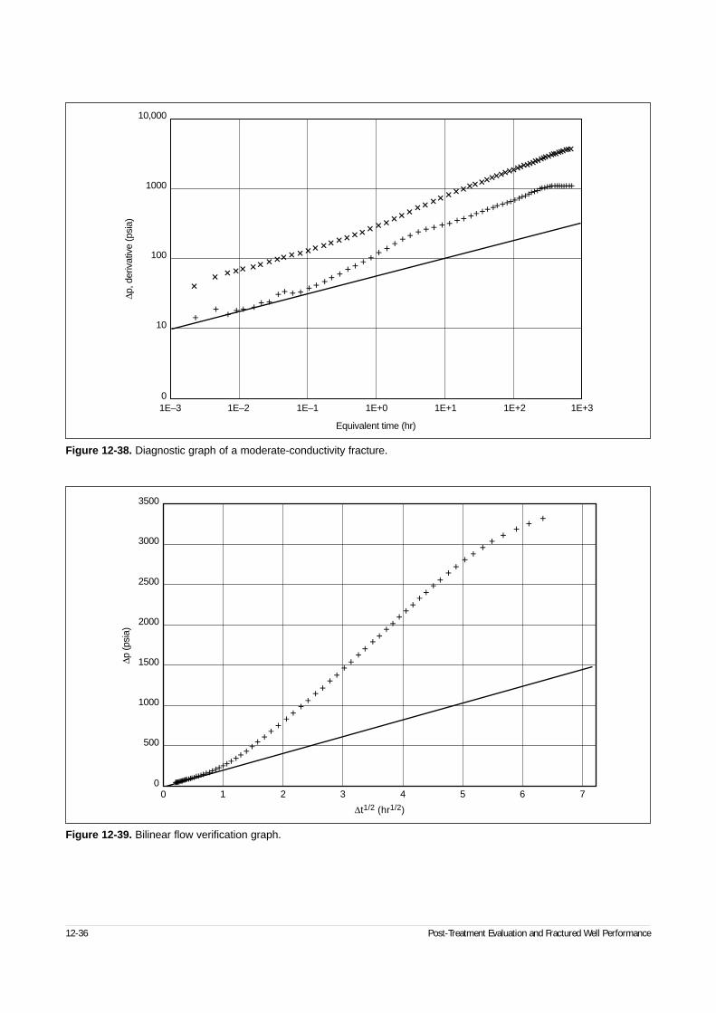
12-36 Post-Treatment Evaluation and Fractured Well Performance

Figure 12-38. Diagnostic graph of a moderate-conductivity fracture.

∆p, d

eriv

ativ

e (p

sia)

10,000

1000

100

10

01E–3 1E–2 1E–1 1E+0 1E+1 1E+2 1E+3

Equivalent time (hr)

++ + ++ ++ +

++ + ++ ++ + ++ + +

++ +

++

+ ++ ++ + +

++ ++ + + + + + + + + ++

++ ++++ ++++ + + ++ + +++

++++++++++++++++++++

+++++++++++++++++++++++++++

+++++++++++++++++

Figure 12-39. Bilinear flow verification graph.

∆p (p

sia)

3000

2500

2000

1500

1000

500

0

3500

0 1 2 3 4 5 6 7

∆t1/2 (hr1/2)

+++++++++++++++++++++++++

+++++++++++++

++++

++++

++++

++++

+++++

++++

+ ++ + + + + +

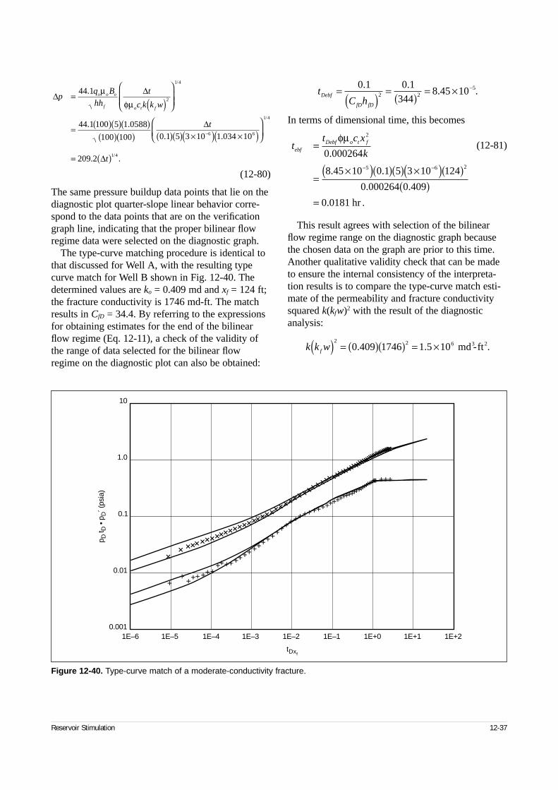
(12-80)

The same pressure buildup data points that lie on thediagnostic plot quarter-slope linear behavior corre-spond to the data points that are on the verificationgraph line, indicating that the proper bilinear flowregime data were selected on the diagnostic graph.

The type-curve matching procedure is identical tothat discussed for Well A, with the resulting typecurve match for Well B shown in Fig. 12-40. Thedetermined values are ko = 0.409 md and xf = 124 ft;the fracture conductivity is 1746 md-ft. The matchresults in CfD = 34.4. By referring to the expressionsfor obtaining estimates for the end of the bilinearflow regime (Eq. 12-11), a check of the validity ofthe range of data selected for the bilinear flowregime on the diagnostic plot can also be obtained:

In terms of dimensional time, this becomes

(12-81)

This result agrees with selection of the bilinearflow regime range on the diagnostic graph becausethe chosen data on the graph are prior to this time.Another qualitative validity check that can be madeto ensure the internal consistency of the interpreta-tion results is to compare the type-curve match esti-mate of the permeability and fracture conductivitysquared k(kfw)2 with the result of the diagnosticanalysis:

Reservoir Stimulation 12-37

∆ ∆

∆

∆

pq B

hh

t

c k k w

t

t

o o o

f o t f

=( )

= ( )( )( )( )( ) ( )( ) ×( ) ×( )

= ( )

−

44 1

44 1 100 5 1 0588

100 100 0 1 5 3 10 1 034 10

209 2

2

1 4

6 6

1 4

1 4

.

. .. .

. .

/

/

/

µφµ

tt c x

kebfDebf o t f=

=×( )( )( ) ×( )( )

( )=

− −

φµ 2

5 6 2

0 000264

8 45 10 0 1 5 3 10 124

0 000264 0 409

0 0181

.

. .

. .

. hr .

k k wf( ) = ( )( ) = ×2 2 60 409 1746 1 5 10. . . md ft3 2-

tC h

Debf

fD fD

=( )

=( )

= × −0 1 0 1344

8 45 102 25. .

. .

Figure 12-40. Type-curve match of a moderate-conductivity fracture.

p Dt D

• p D

́(psi

a)

0.1

0.01

0.001

10

1.0

tDxf

1E–6 1E–5 1E–4 1E–3 1E–2 1E–1 1E+0 1E+1 1E+2

+

+

+

+

+

+++++++++++++++++++

+++++++++++++++++++++++++++++++++

+++++++++++++++++++

+++++

++++++++++

+++++++++++++

+++++++++++++++++++

++

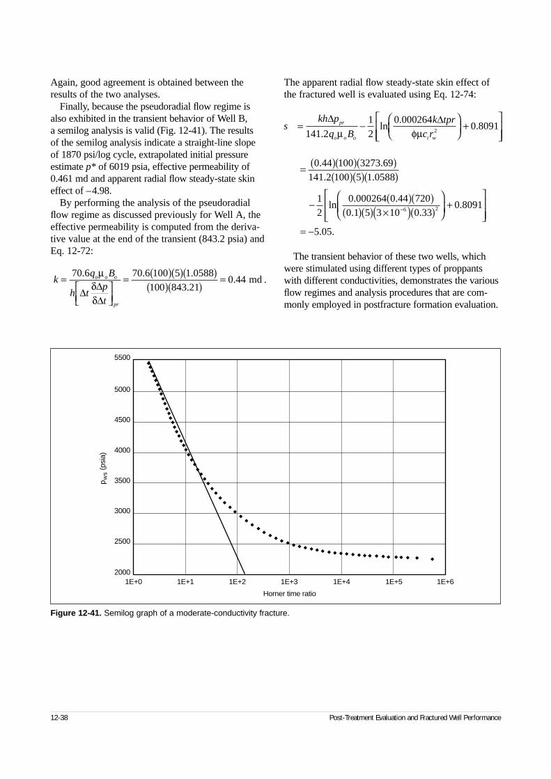
Again, good agreement is obtained between theresults of the two analyses.

Finally, because the pseudoradial flow regime isalso exhibited in the transient behavior of Well B, a semilog analysis is valid (Fig. 12-41). The results of the semilog analysis indicate a straight-line slope of 1870 psi/log cycle, extrapolated initial pressureestimate p* of 6019 psia, effective permeability of0.461 md and apparent radial flow steady-state skineffect of –4.98.

By performing the analysis of the pseudoradialflow regime as discussed previously for Well A, theeffective permeability is computed from the deriva-tive value at the end of the transient (843.2 psia) andEq. 12-72:

The apparent radial flow steady-state skin effect ofthe fractured well is evaluated using Eq. 12-74:

The transient behavior of these two wells, whichwere stimulated using different types of proppantswith different conductivities, demonstrates the variousflow regimes and analysis procedures that are com-monly employed in postfracture formation evaluation.

12-38 Post-Treatment Evaluation and Fractured Well Performance

Figure 12-41. Semilog graph of a moderate-conductivity fracture.

pw

s (p

sia)

5500

5000

4500

4000

3500

3000

2500

20001E+0 1E+1 1E+2 1E+3 1E+4 1E+5 1E+6

Horner time ratio

kq B

h tp

t

o o o

pr

=

= ( )( )( )( )( )

=70 6 70 6 100 5 1 0588100 843 21

0 44. . .

.. .

µδδ

∆ ∆∆

md

skh p

q B

k tpr

c rpr

o o o t w

= −

+

= ( )( )( )( )( )( )

− ( )( )( )( ) ×( )( )

−

∆ ∆141 2

12

0 0002640 8091

0 44 100 3273 69141 2 100 5 1 0588

12

0 000264 0 44 7200 1 5 3 10 0 33

2

6 2

.ln

..

. .. .

ln. .. .

µ φµ

+

= −

0 8091

5 05

.

. .

12-5. Prediction of fractured well performance

Simulation of the future performance of a verticallyfractured well can be performed with a variety of dif-ferent types of reservoir models. The most generaltype of model for estimating the future productionperformance of a fractured well is a conventionalfinite-difference (or finite-element) reservoir simulator.Other types of predictive models for estimating theperformance of vertically fractured wells are numeri-cal models developed using analytic solutions to thediffusivity equation governing fluid flow in the systemand the appropriate initial and boundary conditions.

Reservoir heterogeneities and anisotropy, bound-aries, multiple wells and changing inner boundaryconditions can be readily specified with finite-differ-ence reservoir simulation models to simulate rela-tively realistic production scenarios. Finite-differencemodels are also ideally suited for solving nonlinearproblems such as those associated with nonlinearfluid pressure-volume-temperature (PVT) properties,multiphase flow, non-Darcy fracture and reservoirflow, and stress-dependent fracture conductivity.These effects are important for the long-term (e.g.,20-year) economic analyses commonly used for tightgas wells.

Finite-difference reservoir simulation models aregenerally the preferred method for estimating thefuture performance of vertically fractured wells.Limitations related to the use of a finite-differencemodel are

• quantity and quality of reservoir and fractureinformation that is required as input data for themodel

• generally greater computational expense associ-ated with the use of finite-difference reservoirmodels over analytic techniques.

Numerical models developed using analytic solutionsfor the transient behavior of vertically fractured wellshave been used for many years, largely because ofthese limitations for finite-difference simulation models.

Brown et al. (1984) demonstrated the utility ofanalytic models for future well performance predic-tion. Brown et al. introduced the use of a systemsanalysis approach for estimating the productionbehavior of a well for which the system inner bound-ary condition may be specified at a system locationother than the sandface. An example is the constant

wellhead pressure production condition that requiressimultaneous solution of the reservoir inflow perfor-mance and wellbore outflow analysis to estimate theproductivity of the well.

Meng et al. (1982) applied the production systemsanalysis approach specifically to vertically fracturedwells and developed a correlation technique for esti-mating the inflow performance of finite-conductivityfractures in gas reservoirs. This analysis procedurewas utilized by Hunt (1986) to develop a systemsanalysis procedure for evaluating the rate-transientperformance of fractured gas wells using analyticsolutions.

A more general approach reported by Poe et al.(1995) for estimating the future performance of ver-tically fractured wells incorporates reservoir voidingeffects in the production system analyses. The com-mingled reservoir evaluation procedure of Spath etal. (1994) was used in that study to evaluate the pro-duction performance of multilayer reservoirs usingLaplace space analytic solutions for the transientbehavior of finite-conductivity fractures. The com-mingled reservoir algorithm allows mixed reservoircompletion types, such as a combination of fracturedand unfractured reservoir layers, in the prediction ofthe future performance of the well.

In almost all cases of interest, hydraulic fracturesare vertical and normal to the minimum horizontalstress direction. Horizontal wells can thus be drilledeither normal or longitudinal to the fracture azimuth.The first configuration results in orthogonal fracturesand has been found applicable for relatively low-per-meability formations (Brown and Economides, 1992)and is discussed in Chapter 10 with multiple orthog-onal fractures.

The other configuration, involving longitudinallyfractured horizontal wells, was first studied by Larsenand Hegre (1991). Their work neglects the horizontalflow component and the nonuniformity of the verticalpressure distribution in the fracture. A more generalapproach that is free of these restrictions was intro-duced by Valkó and Economides (1996a). They con-sidered the same reservoir-fracture system as the onestudied by Cinco-Ley and Meng (1988), includingthe possibility of double porosity. In the Valkó andEconomides case, the well is horizontal and locatedin the middle of the fracture (Fig. 12-42). The frac-ture is longitudinal with respect to the well, and com-munication between the fracture and the well is estab-lished along the total fracture length. The height of

Reservoir Stimulation 12-39

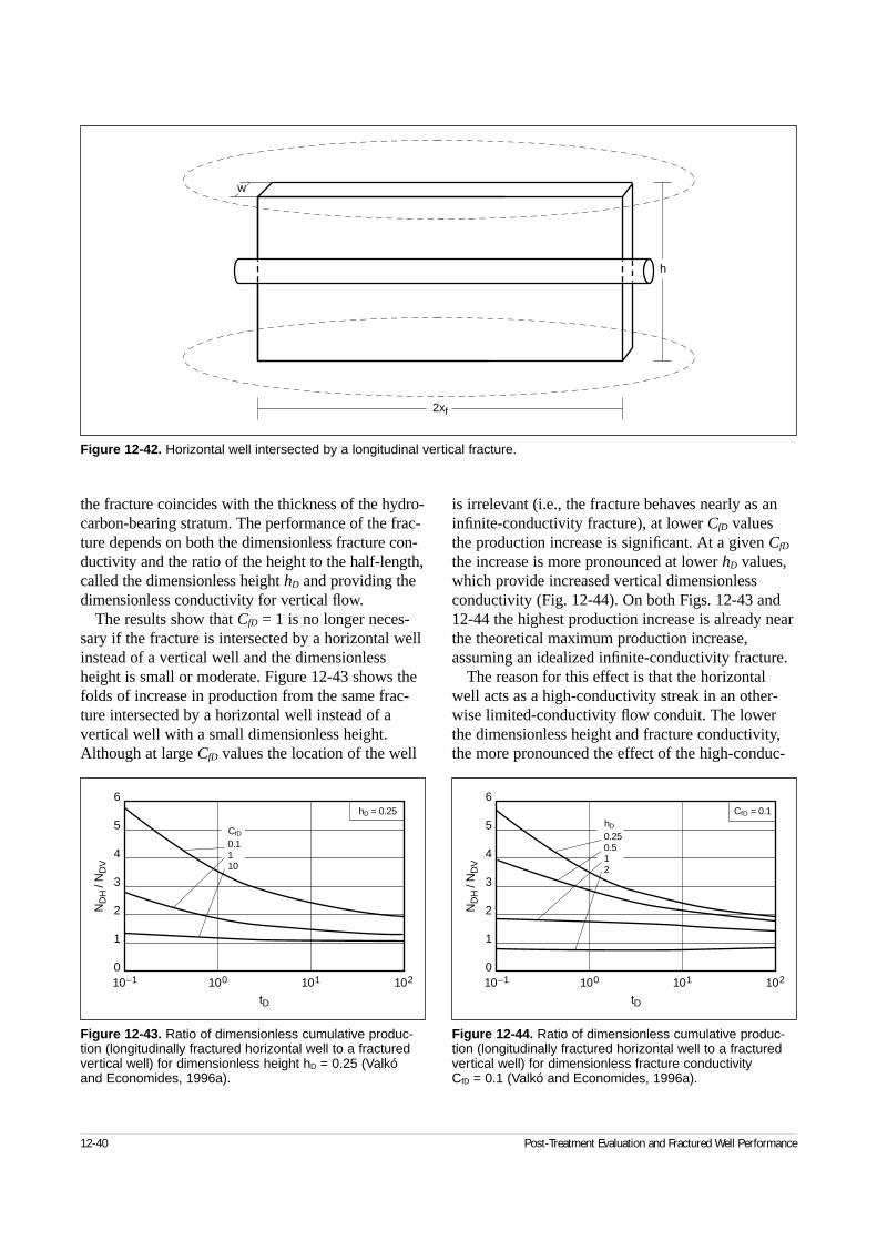
the fracture coincides with the thickness of the hydro-carbon-bearing stratum. The performance of the frac-ture depends on both the dimensionless fracture con-ductivity and the ratio of the height to the half-length,called the dimensionless height hD and providing thedimensionless conductivity for vertical flow.

The results show that CfD = 1 is no longer neces-sary if the fracture is intersected by a horizontal wellinstead of a vertical well and the dimensionlessheight is small or moderate. Figure 12-43 shows thefolds of increase in production from the same frac-ture intersected by a horizontal well instead of avertical well with a small dimensionless height.Although at large CfD values the location of the well

is irrelevant (i.e., the fracture behaves nearly as aninfinite-conductivity fracture), at lower CfD valuesthe production increase is significant. At a given CfD

the increase is more pronounced at lower hD values,which provide increased vertical dimensionlessconductivity (Fig. 12-44). On both Figs. 12-43 and12-44 the highest production increase is already nearthe theoretical maximum production increase,assuming an idealized infinite-conductivity fracture.

The reason for this effect is that the horizontalwell acts as a high-conductivity streak in an other-wise limited-conductivity flow conduit. The lowerthe dimensionless height and fracture conductivity,the more pronounced the effect of the high-conduc-

12-40 Post-Treatment Evaluation and Fractured Well Performance

Figure 12-42. Horizontal well intersected by a longitudinal vertical fracture.

w

h

2xf

Figure 12-43. Ratio of dimensionless cumulative produc-tion (longitudinally fractured horizontal well to a fracturedvertical well) for dimensionless height hD = 0.25 (Valkó and Economides, 1996a).

10–1 100 101 1020

1

2

3

4

5

6

ND

H/ N

DV

tD

CfD

0.1110

hD = 0.25

Figure 12-44. Ratio of dimensionless cumulative produc-tion (longitudinally fractured horizontal well to a fracturedvertical well) for dimensionless fracture conductivity CfD = 0.1 (Valkó and Economides, 1996a).

10–1 100 101 1020

1

2

3

4

5

6

ND

H/ N

DV

tD

hD

0.250.512

CfD = 0.1

tivity streak. The model predicts an almost infiniteconductivity fracture behavior for CfD = 0.1 and hD = 0.25, in contrast to the finite-conductivitybehavior of a vertical well intersected by a similarfracture. For the vertical well, a CfD at least 2 ordersof magnitude higher is required to see the same nearly infinite conductivity behavior. In addition, a large CfD value is difficult to achieve in high per-meability for a long fracture from a vertical well.

The key advantages of a horizontal well combinedwith a longitudinal fracture is that a much smaller frac-ture width (than that suggested for the fractured verticalwell) may be sufficient to achieve a certain productiongoal, reducing the necessity of very wide fractures,which are generally obtained only with the tip screen-out technique. The fracture also overcomes two limita-tions of a conventional horizontal well: removingdrilling-induced damage and mitigating the adverseeffect of the relatively low vertical permeability.

Reservoir Stimulation 12-41

This chapter is dedicated to Alfred R. (Al)Hendrickson, the father of modern-day acidizing. Al made numerous unique discoveries during hiscareer and is best known for his work in sandstoneacidizing. The knowledge he offered the industry isthe cornerstone of acidizing technology today. Hisenergetic personality and technical contributions willforever be appreciated.

13-1. IntroductionMatrix stimulation is a technique that has been usedextensively since the 1930s to improve productionfrom oil and gas wells and to improve injection intoinjection wells. Sidebar 13A discusses the history ofmatrix stimulation. Matrix stimulation is accom-plished by injecting a fluid (e.g., acid or solvent) todissolve and/or disperse materials that impair wellproduction in sandstones or to create new, unimpairedflow channels between the wellbore and a carbonateformation. In matrix stimulation, fluids are injectedbelow the fracturing pressure of the formation(McLeod, 1984). At the time of this writing, it is esti-mated that matrix treatments constitute 75% to 80%of all stimulation treatments (matrix and fracturing)worldwide, but the total expenditure for matrix treat-ments is only 20% to 25% of the total for all stimula-tion treatments. However, because the payout timefor matrix treatments is normally days rather thanmonths as it is for conventional fracturing treatments,engineers should master this technique. Many opera-tors around the world have indicated that an averageof 40% to 50% of their wells have significant dam-age, but routinely only 1% to 2% of their wells aretreated every year.

Substantial production improvements can beachieved with matrix stimulation if treatments areengineered properly. A success rate greater than 90%is reasonable. The systematic approach to stimulationtreatments consists of candidate selection, formationdamage characterization, stimulation technique deter-

mination, treatment design, job execution and treat-ment evaluation. Although many matrix stimulationtreatments are performed in an unsystematic manner,the success of matrix stimulation can be enhancedwhen each of these activities is performed properly.Proper performance of these steps requires the inter-action of numerous individuals with expertise in geo-science, engineering and operations. The remainingchapters in this volume provide detailed discussionsof the state of the art in matrix stimulation. The pur-pose of this chapter is to provide an integratedoverview of the process of engineering successfulmatrix stimulation treatments.

Engineering a matrix treatment includes manytasks and a methodology that are accomplished onthe basis of the best available data and knowledge at hand, which is usually incomplete. This does notmean a treatment will be unsuccessful. The process isa continuous cycle, starting with the diagnostic phaseof the design process and progressing through theexecution and evaluation phases to develop improve-ments. In addition, computer systems with “advisors”are available to assist the process. Advisors are expertsystems with a knowledge base derived from currenttechnology.

13-1.1. Candidate selectionCandidate selection for matrix stimulation is based onfinding wells with impaired productivity and diagnos-ing the cause of the impairment. Failure of a well toobtain economic objectives alone is not evidence ofimpaired productivity. Failure to achieve economicobjectives may be the result of limitations of thereservoir (e.g., pressure, permeability) or wellbore(e.g., artificial lift, inadequate tubing size). Matrixstimulation cannot solve these problems.

Candidate selection requires an accurate assess-ment of what a well can produce without impairmentand the current productivity of the well. Techniquesfor making these assessments rely heavily on knowl-

Reservoir Stimulation 13-1

◆

Introduction toMatrix TreatmentsR. L. Thomas, Schlumberger Dowell

L. N. Morgenthaler, Shell E&P Technology Company

edge of the formation geology and reservoir proper-ties. Methods for assessment of production systemperformance have been developed and are in wideuse. Methods for pressure transient testing of reser-

voirs and well performance analysis have been pub-lished (Earlougher, 1977). These methods enable theengineer to quantify the extent of formation damageand the potential for productivity improvement.

13-2 Introduction to Matrix Treatments

13A. The history of matrix stimulation

“The results gained by the use of acid to increase oil and gasproduction are no longer hypothetical. Wherever productioncomes from essentially limestone reservoirs, its use is indi-cated and recommended.” This quote is from “The Value ofRepeated Acid Treatments” by P. E. Fitzgerald of Dowell Inc.in 1934. Fitzgerald went on to write, “It is recognized now thatevery well is a problem in itself, and must be analyzed individ-ually in order to obtain the best results.” It is interesting tonote that the forefathers of matrix stimulation realized theimportance of proper well diagnosis for treatment success,because it is a key step in the matrix stimulation engineeringprocess used today. In addition, it is interesting that the“acidizing era” began more than 30 years following develop-ment of the concept. It took that long to develop the technol-ogy required to overcome the fundamental problem of acidcorrosion of the tubing and casing. As history indicates, achemical company with a need to stimulate brine wells devel-oped the solution of an acid corrosion inhibitor. With this keyinvention the matrix stimulation era began in full force.

The history of acidizing dates back to 1895, when theOhio Oil Company acidized both oil and gas wells with signifi-cant increases in production; however, the casing wasseverely corroded and the process became unpopular. Oneyear later, a patent was issued to Herman Frasch of StandardOil Company. His patent described the use of hydrochloricacid (HCl) in wells with limestone pay formations but did notaddress the corrosion problem.

Not until 1928 was the use of acid again attempted. Thiswas when the problem of brine disposal, as well as increasedproduction of natural brine, became important. Dr. HerbertDow, early in his career, lowered bottles of acid into brinewells for the purpose of increasing their production. However,the results were not satisfactory, largely on account of the cor-rosion incurred and the expensive materials required to pro-tect the metal equipment. Thus, the Dow Chemical Companyinitiated a project to develop the first acid corrosion inhibitor.

In 1931, Dr. John Grebe of Dow discovered that arsenicacid acted as a corrosion inhibitor. Later, copper salts wereused with arsenic to avoid the formation of calcium arsenateprecipitate, and soon organic inhibitors were found to be farsuperior. Soon after the discovery of the arsenic inhibitor, itwas applied in the field by Dow and Pure Oil Company tosuccessfully treat the latter’s Fox No. 6 well in the GreendalePool, Michigan, in February 1932. Five hundred gallons ofHCl were siphoned into the well, resulting in a previously“dead” well flowing 16 BOPD. Thus, acidizing was reborn,and Dow formed the Dow Well Services Group that soonevolved into Dowell. Three years later, the small companyHalliburton Oil Well Cementing Co. in Duncan, Oklahoma,began commercial acidizing service,

In 1935 Drs. Grebe and Stoesser of Dowell wrote,“Commercial acidization of oil and gas wells—although non-existent four years ago, now is practiced over the entire coun-try. Approximately 6000 oil and gas wells have been treatedby Dowell Incorporated, to give an average increase in pro-duction of 412 percent. In central Michigan alone, one-sixth of the total oil production is the result of acid treatments, thusindicating a net gain of $5,000,000 to the oil companies.”

When this was published in World Petroleum the price of oilwas $1.00 per barrel and acidizing was directed at limestoneformations. Since then acidizing technology has expanded,driven by oil and gas discoveries in a variety of formations, allwith unique problems.

Sandstone acidizing with hydrofluoric acid (HF) was prac-ticed in Texas in 1933 following the issuance of a patent tothe Standard Oil Company; however, the field tests were notsuccessful because of plugging of the formation. Commercialapplication of HF acidizing of sandstones occurred in the GulfCoast of Mexico in 1940 when Dowell introduced mud acid, amixture of HCl and HF. Dowell research indicated that the HClhelped maintain a low pH and decreased the precipitation ofdamaging precipitates. Following this event, the application ofsandstone acidizing grew rapidly.

As the application of acidizing expanded, several chemicaland mechanical problems were addressed. Numerous acidadditives and systems were developed to solve the problemsof acid sludging, acid-induced emulsions, spent acid cleanup,live acid penetration and fines migration. Parallel to this devel-opment was the development of methods to improve zonecoverage during acidizing.

Acidizing has progressed through the following eras:

• 1950s and 1960s—Emphasis was on the development ofadditives to address emulsions, sludge, spent acid returnand zone coverage. In addition, work on the physics ofacidizing in limestones and the secondary reactions ofsandstone acidizing was performed. The emphasis forclay problems shifted from clay swelling to clay migration,and numerous clay control agents were developed. Oil-soluble resins were introduced as diverting agents forimproved zone coverage.

• 1970s—A need for deeper penetration of live HF acid wasaddressed with various systems, including alternatingstages of HCl and HF, fluoboric acid and a mixture ofmethyformate and HF.

• 1980s—Foam diversion and coiled tubing placement wereintroduced to improve zone coverage. Production systemanalysis became a common tool of the design engineer.Computers were used to assist in all phases of the matrixprocess, including candidate selection, treatment design,monitoring of execution (real-time evaluation of skin effectevolution) and post-treatment evaluation.

• 1990s—Computers continued to evolve to faster and moreuser-friendly programs that incorporate improved produc-tion prediction capability, economics software, geochemi-cal models and on-site evaluation techniques. Environ-mentally friendly additives were introduced to meetgovernment regulations along with the development of a better understanding of sandstone acidizing chemistry.Emphasis was placed on the entire matrix process throughmatrix stimulation engineering.

Great advances have been made since the first acidizingtreatment was performed. As wells become deeper, withhigher temperatures and harsher conditions along with longerzones as in horizontal wells, matrix technology will expand tomeet operators’ needs. Matrix stimulation will continue to be a useful, economical tool for production enhancement in theyears to come.

13-1.2. Formation damage characterizationOnce it has been established that a well is producingbelow its potential, an assessment of the cause andlocation of the impairment must be made (Krueger,1986, 1988). Diagnosis can be based on a review of the well and field history, samples of plugging materialrecovered from the field and analyzed, knowledge offormation mineral and fluid (e.g., water and oil) proper-ties, as well as pressure testing and logging evaluation.The process of searching and sifting through the massof data that may provide clues to the problem of a par-ticular well is facilitated by databases and expert sys-tems. In the end, the ingenuity and training of theperson analyzing the data and the application of engi-neering tools are critical to a successful diagnosis. Thechallenge is to recognize the cause of the well impair-ment from the information available. In many cases, itis not possible to characterize the formation damagecompletely. If the diagnosis is uncertain, it is recom-mended to prioritize the probable causes and design atreatment for the most probable scenarios. Thus, multi-ple damage types may be suspected, and all should beconsidered in designing the treatment.

13-1.3. Stimulation technique determinationSelection of the stimulation technique is based on theproductivity target, lithology, operational limitations andvarious other considerations. Normally the productivitytarget dictates the stimulation technique. For example, ifa 90% reduction in skin effect in a sandstone yields thetarget production, then matrix stimulation will probablybe the most cost-effective technique. If matrix stimula-tion cannot be accomplished, then the feasibility ofusing propped fracturing should be evaluated.

In carbonates, acid fracturing, propped fracturing andmatrix acidizing techniques are applicable. However, ifmatrix acidizing yields a final skin effect of –2 to –3, itwill probably be the most cost-effective technique.

13-1.4. Fluid and additive selectionIdentification of the cause and location of the wellimpairment drives the treatment design process. Thechemistry of the stimulation fluids is chosen either todissolve or disperse the impairment or in the case ofcarbonate reservoirs to create high-permeability chan-nels through the damage zone. The treating fluid sys-tem is selected on the basis of field experience and

laboratory testing and can be derived from an expertsystem.

In cases where it is impossible to remove or bypassdamage chemically, a small-volume fracturing treat-ment may be indicated (Fletcher et al., 1995). This isparticularly true today, with the tip-screenout (TSO)technique applied to high-permeability reservoirs.Chemical additives, as well as pre- and postflushes,are selected to enhance the action of the main stimula-tion fluid, prevent acid corrosion or prevent productiv-ity impairment from by-products of the stimulationprocess (see Chapter 15).

13-1.5. Pumping schedule generation and simulation

The volume of each material pumped is based on anassessment of the amount of damage or the requireddepth of treatment and must address the potential inef-ficiency of the placement process. The location of thedamage dictates the placement technique. Bothmechanical methods using tools and fluid mechanicalmethods (e.g., particulate suspensions and foams) canbe used to ensure that the stimulation fluids contactthe formation damage.

Once the volume, composition and sequence of atreatment are established, a treating schedule can bedesigned on the basis of the well and reservoir proper-ties. However, the effect of acidizing on formationstrength may impose an upper limit on the acidstrength and volume in wells that are not gravelpacked. The pumping schedule includes the treatingfluid and diverter sequence and injection rate for eachstage. It can be generated using empirical rules basedon previous field experience. In addition, the schedulecan be optimized to meet specific objectives for eachfluid type by using a single-phase reservoir model(Perthuis et al., 1989).

A field-validated stimulation simulator should beused for the systematic engineering of matrix stimu-lation treatments. A numerical simulator can be avaluable tool for predicting damage removal and eval-uating skin effect evolution, flow profile and wellheadand bottomhole pressures versus injection rate for theproposed pumping schedule. The simulator shouldtake into consideration both the chemistry and damageremoval along with the placement strategy, which isanother important part of the design process. This stepallows the design engineer to fine tune or optimize theschedule to obtain the desired results in the most cost-

Reservoir Stimulation 13-3

effective manner. Because many key parameters in the simulation may not be accurately assessed in thelaboratory, the simulator is most useful for predictingtrends. Comparison to field data is critical to fullyvalidate the simulation model for future design work(Bartko et al., 1996).

13-1.6. Economic evaluationAlthough a preliminary economic analysis is performedduring the candidate selection process, the final analysisshould be conducted once the treatment design is final-ized. Production performance is predicted by using aproduction forecast module and is based on initialand/or final skin effect calculations. Payout time, netpresent value (NPV), cash flow or other financial indi-cators may be determined to evaluate economic justifi-cations (Bartko et al., 1996).

13-1.7. ExecutionExecution of the treatment is an often neglected step by the design engineer but is obviously critical to theprocess. Materials must be monitored to ensure thatthey meet the specifications of the design, equipmentmust be maintained to perform properly, and personnelon site must understand and execute their assignedroles. Quality control (QC) testing and training shouldbe documented as standard practices (Brannon et al.,1987). Modern data acquisition and communicationequipment make it possible to obtain and analyzedetailed data during the well treatment, on and off thewellsite.

13-1.8. EvaluationTreatment evaluation consists of pretreatment, real-time and post-treatment phases. Each is an importantlink to treatment success and the economic impact ofthe stimulation treatment. In addition, technical evalu-ation is required to validate and calibrate the modelsand assumptions used in candidate selection, treatmentdesign and execution. Treatment evaluation uses thesame well evaluation tools and knowledge of potentialwell productivity as candidate selection. Consistentlyfollowing the engineering concepts outlined heremakes stimulation a learning process and drivesimprovement in production performance in the field.

13-2. Candidate selection

13-2.1.Identifying low-productivity wells and stimulation candidates

The process of candidate selection consists of identi-fying wells with low productivity relative to what theyare capable of producing and then evaluating possiblemechanical problems in these wells (Thomas andMilne, 1995).

Geology, petrophysics and reservoir engineering playimportant roles in quantifying the productive potentialof a given well. Ideally, a thorough understanding ofthe reservoir geology and reservoir drive mechanics isrequired to quantify production potential. In many casessuch data are incomplete, and the engineer must rely on comparison to similar wells or the field history toidentify performance norms. The productivity of eachwell can be mapped using a three-dimensional (3D)surface graph to assist the identification of underpro-ducers (i.e., candidates). For oil wells, the productivityindex (PI), productivity index per net pay thicknessPI /h, production rate in barrels of oil per day (BOPD),production rate per reservoir porosity thickness product(BOPD/porosity-ft) or skin effect can be plotted foreach location. The variable selected is a function of thedata available. For example, if limited data are available(e.g., permeability-height kh is unknown) BOPD/poros-ity-ft or h can be plotted. This process allows the engi-neer to pinpoint likely underproducers and determinetheir relationship with other wells in the field.

Once the production potential of a well is established(to the highest certainty possible with the availabledata), it can be compared with the actual production.This is a deceptively simple statement because it hidesthe difficulty in measuring actual production in somecases. A facility’s engineers and operations staff canhelp ensure that an accurate assessment of current wellperformance is obtained.

Once a well is diagnosed as underperforming, thereason or reasons must be determined. Appropriateremedial action must be taken, including the determi-nation of whether artificial lift is required or if theexisting lift is adequate and functioning properly. Insome cases, production is constrained by tubing size,downhole equipment restrictions or other mechanicalreasons. Stimulation will not help in these cases. Oncemechanical reasons are eliminated as a potential causeof poor production, the remaining wells become stim-ulation candidates.

13-4 Introduction to Matrix Treatments

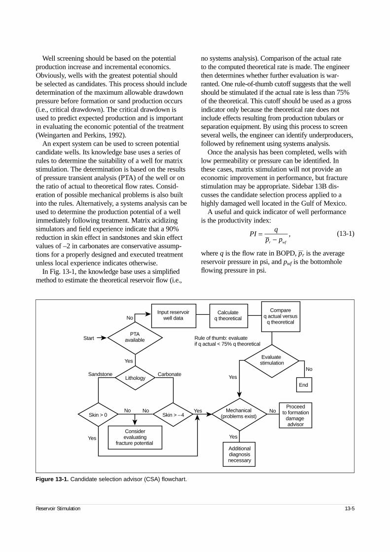
Well screening should be based on the potentialproduction increase and incremental economics.Obviously, wells with the greatest potential should be selected as candidates. This process should includedetermination of the maximum allowable drawdownpressure before formation or sand production occurs(i.e., critical drawdown). The critical drawdown isused to predict expected production and is importantin evaluating the economic potential of the treatment(Weingarten and Perkins, 1992).

An expert system can be used to screen potentialcandidate wells. Its knowledge base uses a series ofrules to determine the suitability of a well for matrixstimulation. The determination is based on the resultsof pressure transient analysis (PTA) of the well or onthe ratio of actual to theoretical flow rates. Consid-eration of possible mechanical problems is also builtinto the rules. Alternatively, a systems analysis can beused to determine the production potential of a wellimmediately following treatment. Matrix acidizingsimulators and field experience indicate that a 90%reduction in skin effect in sandstones and skin effectvalues of –2 in carbonates are conservative assump-tions for a properly designed and executed treatmentunless local experience indicates otherwise.

In Fig. 13-1, the knowledge base uses a simplifiedmethod to estimate the theoretical reservoir flow (i.e.,

no systems analysis). Comparison of the actual rate to the computed theoretical rate is made. The engineerthen determines whether further evaluation is war-ranted. One rule-of-thumb cutoff suggests that the wellshould be stimulated if the actual rate is less than 75%of the theoretical. This cutoff should be used as a grossindicator only because the theoretical rate does notinclude effects resulting from production tubulars orseparation equipment. By using this process to screenseveral wells, the engineer can identify underproducers,followed by refinement using systems analysis.

Once the analysis has been completed, wells withlow permeability or pressure can be identified. Inthese cases, matrix stimulation will not provide aneconomic improvement in performance, but fracturestimulation may be appropriate. Sidebar 13B dis-cusses the candidate selection process applied to ahighly damaged well located in the Gulf of Mexico.

A useful and quick indicator of well performance is the productivity index:

(13-1)

where q is the flow rate in BOPD, p—r is the averagereservoir pressure in psi, and pwf is the bottomholeflowing pressure in psi.

Reservoir Stimulation 13-5

Figure 13-1. Candidate selection advisor (CSA) flowchart.

StartPTA

available

Evaluatestimulation

Proceedto formation

damageadvisor

Additionaldiagnosisnecessary

Considerevaluating

fracture potential

LithologySandstone Carbonate

Skin > 0 Skin > –4Mechanical

(problems exist)

No

No No

No

End

No

Yes

Yes

Yes Yes

Yes

Input reservoirwell data

Calculateq theoretical

Rule of thumb: evaluateif q actual < 75% q theoretical

Compareq actual versus

q theoretical

PIq

p pr wf

=−

,

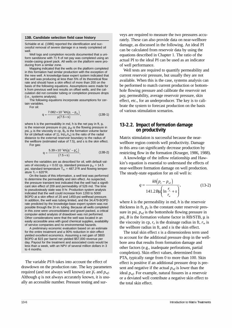
The variable PI/h takes into account the effect ofdrawdown on the production rate. The key parametersrequired (and not always well known) are p—r and pwf.Although q is not always accurately known, it is usu-ally an accessible number. Pressure testing and sur-

veys are required to measure the two pressures accu-rately. These can also provide data on near-wellboredamage, as discussed in the following. An ideal PIcan be calculated from reservoir data by using theequations described in Chapter 1. The ratio of theactual PI to the ideal PI can be used as an indicator of well performance.

Well tests are required to quantify permeability andcurrent reservoir pressure, but usually they are notavailable. When this is the case, systems analysis canbe performed to match current production or bottom-hole flowing pressure and calibrate the reservoir netpay, permeability, average reservoir pressure, skineffect, etc., for an underproducer. The key is to cali-brate the system to forecast production on the basis of various stimulation scenarios.

13-2.2. Impact of formation damage on productivity

Matrix stimulation is successful because the near-wellbore region controls well productivity. Damage in this area can significantly decrease production byrestricting flow in the formation (Krueger, 1986, 1988).

A knowledge of the inflow relationship and Haw-kin’s equation is essential to understand the effects ofnear-wellbore formation damage on well production.The steady-state equation for an oil well is:

(13-2)

where k is the permeability in md, h is the reservoirthickness in ft, pe is the constant outer reservoir pres-sure in psi, pwf is the bottomhole flowing pressure inpsi, B is the formation volume factor in RB/STB, µ isthe viscosity in cp, re is the drainage radius in ft, rw isthe wellbore radius in ft, and s is the skin effect.

The total skin effect s is a dimensionless term usedto account for the additional pressure drop in the well-bore area that results from formation damage andother factors (e.g., inadequate perforations, partialcompletion). Skin effect values, determined fromPTA, typically range from 0 to more than 100. Skineffect is positive if an additional pressure drop is pre-sent and negative if the actual pwf is lower than theideal pwf. For example, natural fissures in a reservoiror a deviated well contribute a negative skin effect tothe total skin effect.

13-6 Introduction to Matrix Treatments

13B. Candidate selection field case history

Schiable et al. (1986) reported the identification and suc-cessful removal of severe damage in a newly completed oilwell.

Well logs and completion records documented that a uni-form sandstone with 71 ft of net pay was completed using aninside-casing gravel pack. All wells on the platform were pro-ducing from a similar zone.

Mapping indicated that the wells on the platform completedin this formation had similar production with the exception ofthe new well. A knowledge-base expert system indicated thatthe well was producing at less than 5% of its theoretical flowrate and should have a skin effect of more than 200 on thebasis of the following equations. Assumptions were made fork from previous well test results on offset wells, and the cal-culation did not consider tubing or completion pressure drops(i.e., systems analysis).

The following equations incorporate assumptions for cer-tain variables.

For oil:

(13B-1)

where k is the permeability in md, h is the net pay in ft, pris the reservoir pressure in psi, pwf is the flowing pressure inpsi, µ is the viscosity in cp, Bo is the formation volume factorfor oil (default value of 1), ln(re /rw) is the ratio of the radialdistance to the external reservoir boundary to the radius ofthe wellbore (estimated value of 7.5), and s is the skin effect.

For gas:

(13B-2)

where the variables are as described for oil, with default val-ues of viscosity µ = 0.02 cp, standard pressure psc = 14.5psi, standard temperature Tsc = 487.3°R and flowing temper-ature Tf = 620°R.

On the basis of this information, a well test was performedto determine the permeability and skin effect. As suspected,the pressure transient test indicated that the well had a signifi-cant skin effect of 209 and permeability of 526 md. The timeto pseudosteady state was 9 hr. Production system analysisindicated that the well could increase from 1200 to 5000BOPD at a skin effect of 20 and 1450-psi wellhead pressure.In addition, the well was tubing limited, and the 34,479-BOPDrate predicted by the knowledge-base expert system was notpossible through the 31⁄2-in. tubing. Because all wells completedin this zone were unconsolidated and gravel packed, a criticalcomputer-aided analysis of drawdown was not performed.Other considerations were that the well was located in aneasily accessible area with good chemical supplies, availabilityof service companies and no environmental hazards.

A preliminary economic evaluation based on an estimatefor the entire treatment and a 90% reduction in skin effectyielded excellent economics. Assuming a net gain of 3800BOPD at $15 per barrel net yielded $57,000 revenue perday. Payout for the treatment and associated costs would beless than a week, with an NPV of several million dollars in 3to 4 months.

qkh p p

sr wf=

× −( )+( )

−7 082 10

7 5

3.

.,

µ

qkh p p

sr wf=

× −( )+( )

−5 39 10

7 5

2 2 2.

.,

qkh p p

Br

rs

e wf

e

w

=−( )

+

141 2.

,

µ ln

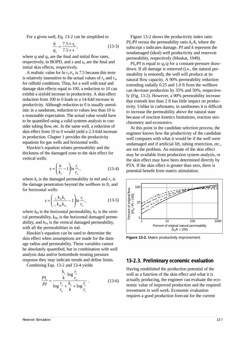
For a given well, Eq. 13-2 can be simplified to

(13-3)

where q and qo are the final and initial flow rates,respectively, in BOPD, and s and so are the final andinitial skin effects, respectively.

A realistic value for ln re/rw is 7.5 because this termis relatively insensitive to the actual values of re and rw

for oilfield conditions. Thus, for a well with total anddamage skin effects equal to 100, a reduction to 10 canexhibit a sixfold increase in productivity. A skin effectreduction from 100 to 0 leads to a 14-fold increase inproductivity. Although reduction to 0 is usually unreal-istic in a sandstone, reduction to values less than 10 is a reasonable expectation. The actual value would haveto be quantified using a valid systems analysis to con-sider tubing flow, etc. In the same well, a reduction ofskin effect from 10 to 0 would yield a 2.3-fold increasein production. Chapter 1 provides the productivityequations for gas wells and horizontal wells.

Hawkin’s equation relates permeability and thethickness of the damaged zone to the skin effect forvertical wells:

(13-4)

where ks is the damaged permeability in md and rs isthe damage penetration beyond the wellbore in ft, andfor horizontal wells:

(13-5)

where kH is the horizontal permeability, kV is the verti-cal permeability, kHs is the horizontal damaged perme-ability, and kVs is the vertical damaged permeability,with all the permeabilities in md.

Hawkin’s equation can be used to determine theskin effect when assumptions are made for the dam-age radius and permeability. These variables cannot be absolutely quantified, but in combination with wellanalysis data and/or bottomhole treating pressureresponse they may indicate trends and define limits.

Combining Eqs. 13-2 and 13-4 yields

(13-6)

Figure 13-2 shows the productivity index ratioPIs/PI versus the permeability ratio ks/k, where thesubscript s indicates damage. PI and k represent thenondamaged (ideal) well productivity and reservoirpermeability, respectively (Muskat, 1949).

PIs/PI is equal to qs/q for a constant-pressure draw-down. If all damage is removed (i.e., the natural per-meability is restored), the well will produce at itsnatural flow capacity. A 90% permeability reductionextending radially 0.25 and 1.0 ft from the wellborecan decrease production by 35% and 50%, respective-ly (Fig. 13-2). However, a 90% permeability increasethat extends less than 2 ft has little impact on produc-tivity. Unlike in carbonates, in sandstones it is difficultto increase the permeability above the natural statebecause of reaction kinetics limitations, reaction stoi-chiometry and economics.

At this point in the candidate selection process, theengineer knows how the productivity of the candidatewell compares with what it would be if the well wereundamaged and if artificial lift, tubing restriction, etc.,are not the problem. An estimate of the skin effectmay be available from production system analysis, orthe skin effect may have been determined directly byPTA. If the skin effect is greater than zero, there ispotential benefit from matrix stimulation.

13-2.3. Preliminary economic evaluationHaving established the production potential of thewell as a function of the skin effect and what it isactually producing, the engineer can evaluate the eco-nomic value of improved production and the requiredinvestment in well work. Economic evaluationrequires a good production forecast for the current

Reservoir Stimulation 13-7

q

q

s

so

o= ++

7 57 5..

,

sk

k

r

rs

s

w

= −

1 ln ,

sk k

k k

r

rH V

Hs Vs

s

w

= −

1 ln ,

PI

PI

k

k

r

rr

r

k

k

r

r

s

s e

w

s

w

s e

s

=+ +

log

log log.

Figure 13-2. Matrix productivity improvement.

Per

cent

of o

rigin

al fl

ow(P

I s⁄ P

I × 1

00)

100

10

11 10 100 1000

Percent of original natural permeability(ks/k × 100)

rs = 2

rs = 0.75

rs = 0.25

rs = 5

well condition and a forecast for the stimulated well,possibly as a function of how successful the stimula-tion is (e.g., post-treatment skin effect). A brief dis-cussion of the methodology follows.

The preliminary economic evaluation requires amodel for production (revenue) and job cost (expense)as a function of skin effect. The engineer must deter-mine the effect of the treatment on well economics onthe basis of the net gain in cumulative oil or gas over a given period of time and the cost associated with thetreatment. The production prediction model shouldinclude material balance, allow analysis under differentouter boundary conditions (infinite acting, no flow andconstant pressure) and forecast on the basis of constantsandface (bottomhole pressure or constant wellheadpressure). The sensitivity of economic performance toskin effect is quantified with this model. The range ofskin effects input should be based on the analysis ofcurrent (presumably damaged) performance andexpected post-stimulation behavior. Post-stimulationskin effect expectations and job costs can be based onfield experience or analysis from a numerical stimula-tion simulator. The numerical stimulation simulator canbe used to evaluate potential skin effect removal as afunction of job design (e.g., volume pumped).

The economics portion of the model must enable theevaluation of cost versus expected revenue. Estimatedcosts should include treatment cost, operation costs,cost of money, applicable taxes and any auxiliary costs.Produced product price, price adjustment factors andtreatment chance (risk) factors should be included tocompute various financial indicators such as the rate ofreturn (ROR), return on investment (ROI), NPV, payout(days) for investment only, payout (days) for invest-ment plus interest and unit cost (investment divided by incremental production).

Several important decisions can be made at thispoint. For example, if the skin effect required to pro-vide an acceptable return is greater than 0 in a sand-stone or –4 in a carbonate, then matrix stimulation ispractical; i.e., fracture stimulation is not required.

In conclusion, from a knowledge of the reservoirand well history coupled with the use of diagnostictools, the engineer should select candidate wells withlow risk and significant potential for economic return.This requires the evaluation of numerous wells and isan important link to matrix stimulation success.

13-3. Formation damage characterization

Damage characterization is the next step in the matrixstimulation engineering process. It is an essential taskprior to treating fluid selection and treatment design.Damage is characterized using laboratory tests, loggingtechniques and well history. Detailed study is necessaryto develop a list of suspected damages from the avail-able data. Multiple types of damage are normallysuspected and are all considered when designing thetreatment. Tables 14-3 through 14-5 list damage types,diagnostic clues and remedial recommendations forcomparison to the condition and characteristics of thecandidate well.

The following sections focus on problems that com-monly occur in the field and discuss how expert sys-tems can guide an engineer through the damagecharacterization process. Expert and advisor systemshave proved especially useful in the damage charac-terization process (Krueger, 1988).

All available information on the well such as welllogs and records, reservoir characteristics and infor-mation on the completion and previous workoversshould be collected. Samples of produced fluids andany solid materials from the well should be analyzed.In some cases, it may be useful to conduct laboratorycompatibility tests of the completion or drilling fluidsand the formation fluid or rocks. Such tests can helpin developing understanding of the problem in thecurrent well and lead to corrective action.

Chemical analysis of solid and liquid samplesretrieved from the well can provide valuable insightsinto damage mechanisms and characteristics. Field test-ing can quantify certain species (e.g., carbonates andoxides are soluble in hydrochloric acid [HCl], paraffinsand asphaltenes float in water, an oil-external-phaseemulsion disperses in diesel). Water analyses are com-monly performed to assist the determination of scalingpotential. The ionic composition of one or two samplescan be used to calculate potential scales based on aminimum Gibb’s free energy or a Stiff-Davis calcula-tion. In addition, gamma logs can be run to comple-ment the water analyses and detect barium andstrontium sulfate scale buildups. Because of traceamounts of the naturally occurring radioactive materials(NORM) radon and radium, barium and strontium sul-fate deposits may exhibit an abnormally high gammacount.

13-8 Introduction to Matrix Treatments

The history of the well should be evaluated in detailto assist damage characterization. All phases of welloperations—including drilling, cementing, perforating,gravel packing, workover operations, stimulationoperations and production or injection—are potentialoriginators of damage (Krueger, 1986).

Expert and advisor systems have been developed to assist damage characterization (Bartko et al., 1996).They provide a guide through a series of questionsdirected at relating the type of damage to the wellbehavior and available data. They can pinpoint keygaps in the available data and recommend additionalrequired diagnostics. A brief discussion of the mostcommon questions the engineer should ask in using an advisor are in Sidebar 13C.

Production logs can be run to quantify the flow perlayer. This information is input into computer pro-grams to determine the formation damage skin effectper layer. The use of a production log is reviewed inthe field case history in Sidebar 13D.

Damage characterization is the basis of treatmentdesign. Chemicals will be selected to remove the sus-pect cause or causes of damage. Treating procedureswill be designed to access the suspected damage withadequate amounts of chemicals to remove enoughdamage to achieve the well productivity goals. Correctdamage characterization is critical to matrix stimula-tion success.

Reservoir Stimulation 13-9

13C. Formation damage characterization field case history

Schiable et al. (1986) performed a detailed laboratory andfield study to characterize formation damage. Some of thequestions and answers resulting from the study follow.

Well history• Is the well newly completed, an old well, huff and puff,

a recent workover and/or a recent stimulation treatment?This is a newly completed gravel-packed well that hasbeen tested.

• Is it an oil, gas or water producer or injector with water orhydrogen sulfide (H2S) production?This oil well produces 29.5°API gravity crude.

• Was the well perforated under- or overbalance?The well was perforated underbalance at 12 shots per foot(spf).

• What type of completion fluid was used?Filtered calcium chloride and potassium chloride comple-tion fluids were used to provide temporary clay control.

• Was the well produced at high drawdown rates?Although newly completed, the well was produced at highdrawdown rates during the well test.

• Has the well responded to previous treatments?No previous treatments were performed on this well, butoffset wells have responded to mud acid treatments.

• Did the production decline slowly or rapidly?Not applicable

• Did the well respond positively to a pump-in test?A pump-in test was not performed because of the associ-ated cost and availability of other data (see “Laboratoryand field testing” section).

• Was there excessive drilling mud loss to the pay zone?No unusual loss of drilling mud occurred when drillingthrough the pay zone.

• Is there fill in the wellbore, produced solids or solids in sur-face equipment? (Obviously, this would be a major prob-lem indicative of gravel-pack failure.)There is no water production to create scale or solids.

Well logging and testing• Are the results of a pressure transient test available?

High skin effect values indicate there is severe formationdamage.

• Does a production log show nonuniform production rates?Although the porosity logs indicate that the pay zone is ahomogeneous sandstone, it is not damaged uniformly.

• Is there fill, a reduction of tubing inner diameter or anincrease in gamma count?There is no indication of any of these.

• Is there water production from a specific zone?There is no water production.

Laboratory and field testing• What is the mineralogy of the pay zone?

Laboratory core testing indicates that the formation iscomposed of approximately 75% quartz, 10% feldspar and10% clay with kaolinite, illite, chlorite and illite-smectitepresent with a 4% to 5% HCl solubility.

• Was a water analysis performed?No, because the well did not produce water.

• What is the composition of samples from the well?No samples other than cores and oil were retrieved fromthe well.

• Is the salinity of the completion fluid lower than that of theformation water?Not applicable

• Does the oil have an emulsion or sludging tendency?Laboratory testing indicates that the crude will not form anemulsion or sludge.

• Do core tests using the completion or stimulation fluidsindicate damage?Laboratory testing indicates that the 2% KCl fluid usedduring gravel packing created a 62% reduction in perme-ability to oil (101 md damaged to 45 md).

• Do core flow tests using stimulation fluids improve thepermeability?Core testing using fluoboric acid stimulation fluid indicatesthat the formation damage can be removed, with 280% ofthe initial permeability to oil obtained.

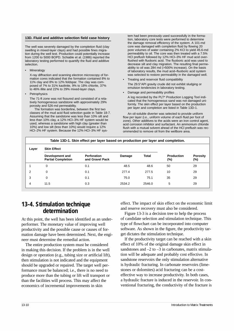
13-4. Stimulation technique determination

At this point, the well has been identified as an under-performer. The monetary value of improving wellproductivity and the possible cause or causes of for-mation damage have been determined. Next, the engi-neer must determine the remedial action.

The entire production system must be considered in making this decision. If the problem is in the welldesign or operation (e.g., tubing size or artificial lift),then stimulation is not indicated and the equipmentshould be upgraded or repaired. The target well per-formance must be balanced; i.e., there is no need toproduce more than the tubing or lift will transport orthan the facilities will process. This may affect theeconomics of incremental improvements in skin

effect. The impact of skin effect on the economic limitand reserve recovery must also be considered.

Figure 13-3 is a decision tree to help the process of candidate selection and stimulation technique. Thistype of flowchart can be incorporated into computersoftware. As shown in the figure, the productivity tar-get dictates the stimulation technique.

If the productivity target can be reached with a skineffect of 10% of the original damage skin effect insandstones and –2 to –3 in carbonates, matrix stimula-tion will be adequate and probably cost effective. Insandstone reservoirs the only stimulation alternative is hydraulic fracturing. In carbonate reservoirs (lime-stones or dolomites) acid fracturing can be a cost-effective way to increase productivity. In both cases, a hydraulic fracture is induced in the reservoir. In con-ventional fracturing, the conductivity of the fracture is

13-10 Introduction to Matrix Treatments

13D. Fluid and additive selection field case history

The well was severely damaged by the completion fluid (clayswelling in mixed-layer clays) and had possible fines migra-tion during the well test. Production could potentially increasefrom 1200 to 5000 BOPD. Schiable et al. (1986) reported thelaboratory testing performed to quantify the fluid and additiveselection.

• Mineralogy

X-ray diffraction and scanning electron microscopy of for-mation cores indicated that the formation contained 8% to11% clay and 8% to 12% feldspar. The clay was com-posed of 7% to 31% kaolinite, 9% to 18% chlorite, 37% to 46% illite and 22% to 29% mixed-layer clays.

• Petrophysics

The 71-ft zone was not fissured and consisted of a rela-tively homogeneous sandstone with approximately 29%porosity and 526-md permeability.

The formation was borderline, between the first twoclasses of the mud acid fluid selection guide in Table 18-7.Assuming that the sandstone was less than 10% silt andless than 10% clay, a 12% HCl–3% HF system would beused, whereas a sandstone with high clay (greater than10%) and low silt (less than 10%) would require a 12%HCl–2% HF system. Because the 12% HCl–3% HF sys-

tem had been previously used successfully in the forma-tion, laboratory core tests were performed to determinethe damage removal efficiency of the system. A 101-mdcore was damaged with completion fluid by flowing 20pore volumes of water containing 2% KCl to yield 45.6-mdpermeability to oil. The core was then treated with a 7.5%HCl preflush followed by 12% HCl–3% HF mud acid over-flushed with fluoboric acid. The fluoboric acid was used todecrease silt and clay migration. The resulting final perme-ability to oil was 284 md (>500% increase). On the basisof laboratory results, the mud acid–fluoboric acid systemwas selected to restore permeability in the damaged well.

• Treating and reservoir fluid compatibility

The 29.5°API gravity crude did not exhibit sludging oremulsion tendencies in laboratory testing.

• Damage and permeability profiles

A log recorded by the PLT* Production Logging Tool indi-cated that the homogeneous sand was not damaged uni-formly. The skin effect per layer based on the productionper layer and completion are listed in Table 13D-1.

An oil-soluble diverter was selected to provide uniformflow per layer (i.e., uniform volume of each fluid per foot ofzone). Other additives to the acids were an iron control agent,acid corrosion inhibitor and surfactant. An ammonium chlorideflush with a mutual solvent ahead of the HCl preflush was rec-ommended to remove oil from the wellbore area.

Table 13D-1. Skin effect per layer based on production per layer and completion.

Layer Skin Effect

Development and Perforation Damage Total Production PorosityPartial Completion and Gravel Pack (%) (%)

1 0 0.1 48.5 48.6 50 29

2 0 0.1 277.4 277.5 10 29

3 0 0.1 75.0 75.1 35 29

4 11.5 0.3 2534.2 2546.0 5 29

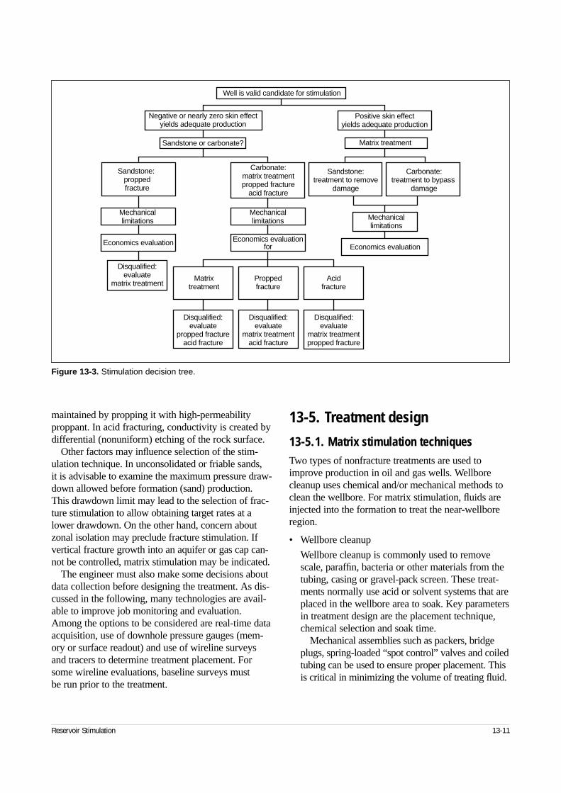
maintained by propping it with high-permeabilityproppant. In acid fracturing, conductivity is created bydifferential (nonuniform) etching of the rock surface.

Other factors may influence selection of the stim-ulation technique. In unconsolidated or friable sands, it is advisable to examine the maximum pressure draw-down allowed before formation (sand) production.This drawdown limit may lead to the selection of frac-ture stimulation to allow obtaining target rates at alower drawdown. On the other hand, concern aboutzonal isolation may preclude fracture stimulation. Ifvertical fracture growth into an aquifer or gas cap can-not be controlled, matrix stimulation may be indicated.

The engineer must also make some decisions aboutdata collection before designing the treatment. As dis-cussed in the following, many technologies are avail-able to improve job monitoring and evaluation.Among the options to be considered are real-time dataacquisition, use of downhole pressure gauges (mem-ory or surface readout) and use of wireline surveysand tracers to determine treatment placement. Forsome wireline evaluations, baseline surveys must be run prior to the treatment.

13-5. Treatment design

13-5.1. Matrix stimulation techniquesTwo types of nonfracture treatments are used toimprove production in oil and gas wells. Wellborecleanup uses chemical and/or mechanical methods toclean the wellbore. For matrix stimulation, fluids areinjected into the formation to treat the near-wellboreregion.

• Wellbore cleanup

Wellbore cleanup is commonly used to removescale, paraffin, bacteria or other materials from thetubing, casing or gravel-pack screen. These treat-ments normally use acid or solvent systems that areplaced in the wellbore area to soak. Key parametersin treatment design are the placement technique,chemical selection and soak time.

Mechanical assemblies such as packers, bridgeplugs, spring-loaded “spot control” valves and coiledtubing can be used to ensure proper placement. Thisis critical in minimizing the volume of treating fluid.

Reservoir Stimulation 13-11

Figure 13-3. Stimulation decision tree.

Well is valid candidate for stimulation

Negative or nearly zero skin effectyields adequate production

Positive skin effectyields adequate production

Matrix treatmentSandstone or carbonate?

Sandstone:proppedfracture

Carbonate:matrix treatmentpropped fracture

acid fracture

Sandstone:treatment to remove

damage

Carbonate:treatment to bypass

damage

Mechanicallimitations

Mechanicallimitations Mechanical

limitations

Economics evaluation Economics evaluationfor Economics evaluation

Disqualified:evaluate

matrix treatmentMatrix

treatmentProppedfracture

Acidfracture

Disqualified:evaluate

propped fractureacid fracture

Disqualified:evaluate

matrix treatmentpropped fracture

Disqualified:evaluate

matrix treatmentacid fracture

Density differences between treating fluids and dis-placement or well control fluids must also be consid-ered when designing a treatment that will stay incontact with the damage for the required soak time.The well cannot be assumed to remain static (nocross flow) during the soak time.

Chemicals should be selected on the basis of theireffectiveness at dissolving the suspected damage.Laboratory tests at bottomhole temperature and, ifpossible, pressure are desirable to determine neces-sary soak times. Because of the small surface area of the exposed damage, the soak time can be hoursto days depending on the type of damage, tempera-ture and damage removal fluid. Agitation or jettingwith coiled tubing can accelerate damage removal.In low-pressure wells, nitrogen (N2) is recommended to assist the removal of reacted treating fluid.

• Matrix stimulation

Matrix stimulation treatments injected below frac-turing pressure down tubing, drillpipe or coiledtubing usually include a sequence of several fluids,referred to as stages. A minimal treatment consistsof a preflush stage with a nondamaging, nonreac-tive fluid to establish an injection rate, a stage ofthe main treating fluid and an overflush stage toclear the main treatment fluid out of the tubing and displace it into the near-wellbore area. In mosttreatments, other auxiliary stages are included toenhance the effectiveness of the treatment. Theselection of chemicals for the stages and the designof the treating sequence (pumping schedule) arereviewed in the following sections.

13-5.2. Treatment fluid selectionTreatment fluid selection is an important step in theengineering process. Multiple fluids (fluid systems),composed of base fluids and additives, are selected on the basis of lithology, damage mechanism and wellcondition. Each fluid in the treating schedule serves aspecial purpose. Although the process of fluid selec-tion is complex because many parameters areinvolved (e.g., damage type, mineralogy), guidelineshave been developed to simplify the process andimprove treatment success.

• Main treating fluid selection

The main treating fluid is selected to dissolve or dis-perse the principal damage in sandstone formations

and to allow soluble products or solids to flow out ofthe well (Smith and Hendrickson, 1965). In the caseof carbonate formations, the goal is to bypass thedamage with acid or dissolve the damage with sol-vents (Hendrickson et al., 1960). The main treatingchemicals fall into the following categories:

– solvents to remove organic deposits (such asparaffin)

– oxidizers to remove damage from polymers

– scale removers to remove sulfate or oxide scales

– acids to remove carbonate and oxide scales,break polymer residues or stimulate carbonateformations

– hydrofluoric acid (HF) to remove aluminosilicatedamage (primarily clays) from sandstone forma-tions.

The main treating fluid is chosen to bypass,dissolve or remove the main damage. If multipledamages are suspected, it may be necessary to useseveral main fluids or to combine the listed functionsinto a single fluid; however, in combining fluids andfunctions, care must be taken to maintain the effec-tiveness of each and avoid incompatibilities.

Solvents are selected when organic deposits aresuspected. If possible, the solvent should be evalu-ated in the laboratory with samples of the deposit.Various oxidizers have been reported for use in wellstimulation. Because the polymer is usually intro-duced into the wellbore during drilling or completionoperations, its identity is well known. An effectiveoxidizer can be evaluated in the laboratory using thisknowledge. In addition, the effect of other fluid com-ponents, well materials and formation minerals onthe oxidizer must be assessed. Scale removers canlikewise be evaluated in the laboratory with samplesof scale deposits. Soak time and chemical concen-tration can be optimized with these tests. One draw-back to these forms of stimulation is that they areeffective against a limited range of damage materi-als. If the damage diagnosis is uncertain, a morebroad-spectrum treatment may be indicated.

Acid stimulation is performed to remove orbypass a variety of damages. When used to removecarbonate scale or polymer residues, acids act simi-larly to the treating chemicals discussed previously.Acids are also used to stimulate the near-wellboreregion of the reservoir. In carbonates, HCl ororganic acids (formic or acetic) are used to etch

13-12 Introduction to Matrix Treatments

conductive paths between the wellbore and the for-mation. In sandstones, mixtures of HCl and HF(mud acids) are used to remove drilling mud, for-mation fines, fines generated during drilling andperforating residue. These materials are usuallymore difficult to define or sample than other formsof damage.

Because acids are effective against several typesof damage and are inexpensive, they are used in thevast majority of matrix stimulations. As a result,more effort has been expended in the engineeringof acid treatments. In the remainder of this chapter,the focus is on engineering matrix acidizing treat-ments, but the concepts discussed apply to all typesof matrix stimulation.

• Fluid formulation for matrix acid stimulation

Formulating fluids for matrix acid stimulationincludes selection of the main acid and identificationof the need for preflushes and overflushes. Figure13-4 shows a decision tree for fluid selection insandstones and carbonates. Fluid selection dependson the damage type, lithology, mineralogy and typeof well. It is also based on field and laboratory expe-rience and can be derived from an expert system(Perthuis et al., 1989). Oil wells are more difficult to treat than gas wells because of potential emulsion,

sludging and wettability problems. To remove dam-age, the treating fluid must be in intimate contactwith the damage. This requires a water-wet forma-tion and oil displacement from the pore throats.Thus, preflushes used in oil wells may include anorganic solvent or ammonium chloride with surfac-tants and/or a mutual solvent to remove heavyhydrocarbons from the wellbore area and ensure a water-wet environment.

The main acid formulation is based on the typeof formation to be stimulated. Formulation guide-lines are based on studies of acid-mineral reactionchemistry. A brief review of the main considera-tions in acid formulations follows.

• Fundamentals of acid-rock chemistry

Chapter 16 presents a detailed discussion of thechemistry and physics associated with acidizing.An appreciation of the key points in the chapter isnecessary to understand the fluid selection process.

– Acid types and kinetics for carbonates

HCl is used for carbonate acidizing because itreadily dissolves calcite and dolomite.

The reaction of limestone (calcium carbonate,or CaCO3) with HCl is

CaCO3 + 2HCl CaCl2 + H2O + CO2

Reservoir Stimulation 13-13

Figure 13-4. Fluid selection flowchart.

Minimumpermeability test

gas wells k > 1 mdoil wells k > 10 md

LithologySandstoneCarbonate

Calcite≥ 20%

Consider fracture or other treatment

Perforatedinterval

≤ 200°F > 200°F

≤ 300°F300°F < T

≤ 400°F > 400°F

Chlorite > 0Glauconite > 0

10% HCI 10% acetic

Perforatedinterval

Bottomholetemperature

Bottomholetemperature

15% HCI or 28% HCI

15% HCI or HCI-acetic

10% HCI or HCI-acetic

Yes

Yes

Yes

No

No

HCI preflush: see Table 18-6HCI/HF: see Table 18-7HCI postflush: same as preflushNH4Cl overflush

Fines migration problem exists

Small problem:Add clay control agentin preflush and overflush fluids

Severe problem:Use fluoboric acid,preflush andoverflush

Start

Minimum permeability test

All volume recommendations

No: mud acid treament

For dolomite, the reaction becomes

CaMg(CO3)2 + 4HCl CaCl2 + MgCl2 + 2H2O + 2CO2

Normally, formation damage is not dissolvedbut rather bypassed to yield new flow channels(wormholes) and/or an etched surface on fissures,resulting in a reduced pressure drop (decrease inskin effect). The wormhole pattern is createdbecause the highly reactive acid enters the largestpore throats, vugs and/or fissures and essentiallyenlarges them. The number of wormholes is afunction of the pore-size distribution (Schechterand Gidley, 1969).

Acid reaction with carbonate reservoirs is gov-erned by three mechanisms: wormholing, compactdissolution and radial flow. Each mode occursunder certain conditions. For example, at lowinjection rates, compact dissolution occurs whenthe formation face is dissolved to enlarge the well-bore. If the flow rate is increased to where thePeclet number (a function of injection rate, acidconcentration and diffusion rate) is approximately1, then wormholing initiates. If the rate is increasedsignificantly, radial flow dominates in a mannersimilar to sandstones. Wormholing probablyoccurs in most treatments owing to the heteroge-neous nature of carbonates; i.e., normally there are thief pores where wormholing initiates.

In cases where the temperature exceeds 400°F[205°C] (where corrosion inhibitors are ineffec-tive in HCl), organic acids (acetic or formic acid)are used.

The reaction of HCl with calcite is diffusionlimited (i.e., mass-transport limited). The limitingstep in the dissolution reaction is the diffusion ofacid (hydronium ion, H3O+) to the surface of thecalcite. Once the H3O+ contacts the surface ofthe calcite, the reaction occurs very fast. Thereaction of HCl with dolomite is diffusion limitedat temperatures greater than 150°F [65°C] andlimited by the surface reaction rate (i.e., diffusionis not the slowest step) below this temperature.Thus, because of the diffusion-limited kinetics of HCl on calcite, wormholes can normally beeasily formed through the damaged zone (2 to 3 ft radially).

– Acid types and kinetics for sandstones

Mud acid mixtures of HF and HCl are used forsandstone acidizing. Unlike carbonate acidizing,

wormholes are not created in sandstones. In atypical sandstone, 80% of the radial flow can bethrough 20% of the pores (the larger pores). Thedamage is removed from the larger pores, result-ing in a skin effect reduction but possibly notrestoration of the natural permeability of theformation.

The primary reaction of HF with quartz grains(pure silica) is expressed in the two following equilibria:

SiO2 + 4HF SiF4 + 2H2O

SiF4 + 2F– SiF62–

In the latter, silicon tetrafluoride combines withfluoride to produce silicon hexafluoride.

The conventional mud acid formulations (12%HCl–3% HF and 6% HCl–1% HF) used inmatrix acidizing dissolve little quartz. The intentof sandstone matrix acidizing is to dissolve claysand other damaging materials, leaving the sand-stone matrix undisturbed.

Although the primary reaction of HF withsilica is simple, the reaction with silt and clay is more complex.

For aluminosilicates (clays and feldspars), theprimary reaction is

MzAlxSiyO(z/2 + 3x/2 + 2y) + 6(x + y)HF →xAlF6

3– + yH2SiF6 + (z/2 + 3x/2 + 2y)H2O +(3x – z)H+ + zM+

where M is a metal atom (e.g., Na or K).The reaction products AlF6

3– and H2SiF6 con-tinue to react with the aluminosilicates to formsilica gel on the surface of the clay (Crowe, 1986).An example of such a secondary reaction is

2yH2O + (x + z)H+ + x/3H2SiF6 +MzAlxSiyO(z/2 + 3x/2 + 2y) →

(y + x/3)Si(OH)4 + xAlF2+ + zM+ +(x/6 + z/2)H2O

Theoretically, other secondary reactions canproduce aluminum fluorosilicate solids, whichmay be damaging. Thus, there is a potential forthe generation of damaging reaction products,although the effects are normally minimal.

Although HCl accelerates the reaction of HFwith siliceous minerals (silt and clay) the reac-tion is far slower compared with that of HClreacting with calcite. The reaction is reaction ratelimited (i.e., numerous collisions of F– with thesurface of the mineral must occur before a reac-

13-14 Introduction to Matrix Treatments

tion occurs) and yet results in most of the HFreacting within the first foot of the wellbore. Thisoccurs because of the large surface area of thesilt and clay. (Five grams of smectite clay has thesurface area of a basketball court.) Retardedacids have been developed to yield deeper liveacid penetration (Thomas and Crowe, 1981).

• Acid and formation compatibility

– Iron hydroxide

Precipitation of iron (ferric, Fe3+) hydroxide(Fe(OH)3) can occur during sandstone and carbon-ate acidizing when the pH value is greater than2.2. Sources of iron in the formation and tubularsare chlorite, siderite, hematite and rust. Ferrousiron (Fe2+) is not a problem in sandstone acidizingbecause ferrous hydroxide does not precipitateuntil the pH value exceeds 7.7. Although fluoridecomplexation of iron increases the pH required for precipitation, iron control agents are recom-mended in all acid stages during sandstone andcarbonate acidizing (Crowe, 1985).

Iron also increases the tendency of oil to formrigid films and emulsions with acids. These prob-lems can result in formation damage and facilityupsets when producing wells after acidizing.

Live acid or partially to completely spent acidoccasionally forms an emulsion with crude oil or condensate, resulting in two-phase flow and a production decrease. In addition, sludging canoccur because of the coagulation of asphaltenesplugging pore throats. Both emulsions and sludg-ing can be avoided by adding the appropriatechemical determined from laboratory testing. Insevere cases, organic acids replace mineral acidsto decrease emulsion and sludging tendencies.Preflushes of solvents or potassium or ammon-ium chloride with mutual solvents are used toseparate the crude oil from the acidic fluids.

– Carbonates

Formulating acids for carbonates is relativelysimple because the majority of the reaction prod-ucts is simply calcium chloride, water and car-bon dioxide, which do not undergo furtherreactions. However, there are numerous minerals(silt and clay) in most carbonates that are insolu-ble in HCl. The insoluble material normallyflows back through large wormholes or fissuresand is not a problem.

In addition, acids selected for carbonate acidiz-ing must be compatible with the formation fluids.Ensuring oil-acid compatibility is discussed laterand in Chapter 15.

– Sandstones

The sensitivity of a sandstone formation to amatrix treatment fluid depends on the mineralogyof the formation, damage type, reaction products,temperature and permeability. As a rule of thumb,the more silt, feldspar and clay and the lower thepermeability, the greater the sensitivity of the for-mation. The amount of precipitate formed is pro-portional to the amount of rapidly HF-solublematerial present, and the impact of the precipitateon plugging is greater at lower permeability. Inaddition, fines migration and the formation of pre-cipitates during a treatment create more problemsin low-permeability formations. Thus, sensitivityis related to chemical and mechanical problems in sandstones.

Although sensitivity cannot be eliminated com-pletely, the goal is to minimize it by selecting flu-ids with the greatest possible compatibility withthe formation. The mineralogy of the formationplays a large role in formation sensitivity and fluidselection. The solubility of the minerals in a sand-stone depends on their location. Authigenic claysare pore lining and come into contact with thetreating fluid, whereas detrital clays were depos-ited with the original sand and are not completelyexposed to the treating fluids. A discussion of themost important reactive minerals in a sandstonefollows.

The solubility of the formation in HCl is nor-mally considered to represent the carbonate con-tent of the sandstone. This assumption is incorrectwhere other acid-soluble species are present (e.g.,chlorite, zeolites, oxides and sulfides). If the acidsolubility is greater than 20%, HF is not recom-mended. Excessive carbonate can react with theHF to precipitate calcium fluoride, and spent HFcan react to form calcium hexafluosilicate.Chlorite clay and some zeolites (hydrous calcium/sodium/potassium aluminum silicates) are partiallysoluble in HCl and can cause severe pluggingfrom the migration of their residue. Special pre-cautions must be taken when treating formationswith these minerals (see Chapter 18). Thus, insandstone acidizing, an HCl (or organic acid)preflush is used ahead of the mud acid.

Reservoir Stimulation 13-15

The silt and clay content can be determined in the laboratory by dissolving a core sample inmud acid. The difference between the mud acidand HCl solubilities is the approximate silt andclay content. Although it is important to knowthe amount and type of silt, feldspar and claypresent, it may be equally important to knowtheir position in the formation.

Secondary reactions can occur to form precipi-tates in the sandstone if precautions are not taken(see the “Design types” discussion in Section 13-5.3). Potential precipitates are as follows.

Fluosilicates (SiF62–) are the most detrimental

precipitates produced in sandstone matrix acid-izing. Sodium, potassium and calcium fluosili-cates (Na2SiF6

2–, K2SiF62– and CaSiF6

2–,respectively) are extremely insoluble and formwhen formation water or any sodium/potassium/calcium brine contacts spent mud acid. They areavoided by preflushing with a compatible fluidsuch as ammonium chloride or HCl and thenoverflushing.

Calcium fluoride forms from the reaction ofHF with calcite if adequate HCl (or organic acid)is not injected ahead of the mud acid. It is notnecessary to dissolve all the calcite. As reportedby Walsh et al. (1982), as much as 6% calcitecan remain and not cause the precipitation ofcalcium fluoride or aluminum fluoride.

Precipitation of the aluminum salts aluminumfluoride (AlF3) and aluminum hydroxide(Al(OH)3) (Walsh et al., 1982) can be avoided by maintaining a low pH (less than 2). In addi-tion, the tertiary reaction of aluminum bifluoridecations with silt and clay can occur very slowlyat temperatures greater than 200°F [95°C] orwith retarded mud acid formulations containingAlCl3. The addition of more Al to the mud acidformulation results in Al saturation and precipita-tion. This process consumes acid, resulting in apH increase and the precipitation of aluminumsilicate and/or fluoride species. Citric acetic acidhas been used successfully in treatments to com-plex aluminum and buffer the pH below 2, thusavoiding precipitation (Rogers et al., 1998).

Hydrated silica precipitate forms in all mudacid treatments but is normally not a problembecause it occurs during the topochemical reac-tion of spent mud acid with the surface of the siltand clay. The precipitate is not mobile like other

precipitates. However, adequate HCl must bepresent to account for this process because itconsumes acid that may result in the precipita-tion of other species.

• Acid selection guidelines for carbonates

– Temperature—Acid selection depends greatly ontemperature because of corrosion inhibition limita-tions. For example, at temperatures greater than300°F [150°C], 28% HCl cannot be used becauseof excessive corrosion whereas 15% HCl can beused. Above 400°F, organic acid or fluids con-taining ethylenediaminetetraacetic acid (EDTA, a non-acid-reactive solvent) can be used. In addi-tion, emulsified acid or HCl with a retarder is usedto increase penetration.

– Mineralogy—Calcite and dolomite react differ-ently with acids. Acid formulation should beoptimized to achieve the desired reaction andpenetration characteristics in each formation.Carbonates commonly contain insoluble minerals(silt and clay) that are released during acidizing.When this occurs, a silt-suspending agent isrequired along with N2 in wells where spent acidwill not flow back naturally (less than 0.46 psi/ftpressure gradient).

– Petrophysics—Acid penetration and the amountof damage depend on the type and distribution of porosity. For example, a highly vugular, high-permeability or fissured carbonate usually isdamaged severely during drilling and completionbecause of solids. Attempts to obtain deep pene-tration (greater than 5 ft) may be difficult, withshort but wide wormholes formed. An emulsi-fied, retarded or foamed acid is required toachieve deep penetration. Because much of theporosity (hydrocarbons in place) is located in the vugular or fissure network, it is essential toremove the damage and restore communicationwith the wellbore. As stated previously, a silt-suspending agent in a gelled or nongelled acidand N2 are recommended to remove drilling mudand completion solids.

• Acid selection guidelines for sandstones

– Temperature—Acid selection depends onlyslightly on temperature because lower acid con-centrations are normally used (i.e., corrosion isnot a major issue). The sensitivity of a sandstoneformation increases with temperature because of

13-16 Introduction to Matrix Treatments

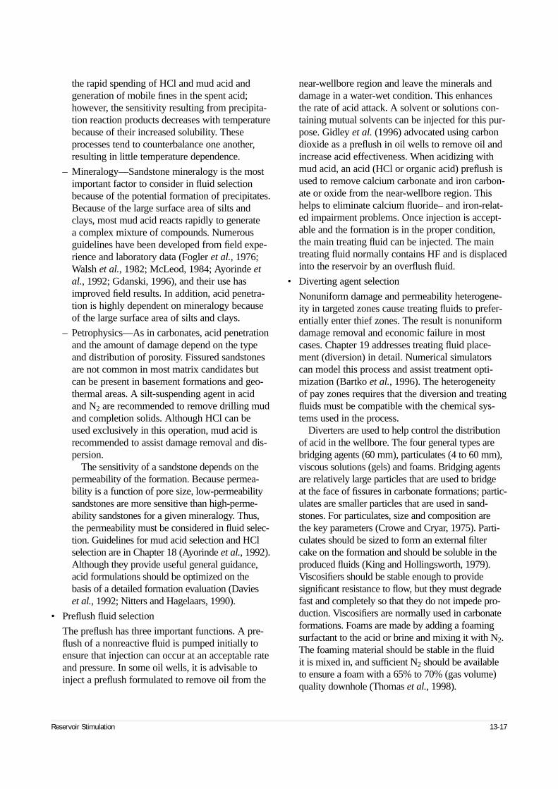
the rapid spending of HCl and mud acid andgeneration of mobile fines in the spent acid;however, the sensitivity resulting from precipita-tion reaction products decreases with temperaturebecause of their increased solubility. Theseprocesses tend to counterbalance one another,resulting in little temperature dependence.

– Mineralogy—Sandstone mineralogy is the mostimportant factor to consider in fluid selectionbecause of the potential formation of precipitates.Because of the large surface area of silts andclays, most mud acid reacts rapidly to generate a complex mixture of compounds. Numerousguidelines have been developed from field expe-rience and laboratory data (Fogler et al., 1976;Walsh et al., 1982; McLeod, 1984; Ayorinde etal., 1992; Gdanski, 1996), and their use hasimproved field results. In addition, acid penetra-tion is highly dependent on mineralogy becauseof the large surface area of silts and clays.

– Petrophysics—As in carbonates, acid penetrationand the amount of damage depend on the typeand distribution of porosity. Fissured sandstonesare not common in most matrix candidates butcan be present in basement formations and geo-thermal areas. A silt-suspending agent in acidand N2 are recommended to remove drilling mudand completion solids. Although HCl can beused exclusively in this operation, mud acid isrecommended to assist damage removal and dis-persion.

The sensitivity of a sandstone depends on thepermeability of the formation. Because permea-bility is a function of pore size, low-permeabilitysandstones are more sensitive than high-perme-ability sandstones for a given mineralogy. Thus,the permeability must be considered in fluid selec-tion. Guidelines for mud acid selection and HClselection are in Chapter 18 (Ayorinde et al., 1992).Although they provide useful general guidance,acid formulations should be optimized on thebasis of a detailed formation evaluation (Davies et al., 1992; Nitters and Hagelaars, 1990).

• Preflush fluid selection

The preflush has three important functions. A pre-flush of a nonreactive fluid is pumped initially toensure that injection can occur at an acceptable rateand pressure. In some oil wells, it is advisable toinject a preflush formulated to remove oil from the

near-wellbore region and leave the minerals anddamage in a water-wet condition. This enhancesthe rate of acid attack. A solvent or solutions con-taining mutual solvents can be injected for this pur-pose. Gidley et al. (1996) advocated using carbondioxide as a preflush in oil wells to remove oil andincrease acid effectiveness. When acidizing withmud acid, an acid (HCl or organic acid) preflush isused to remove calcium carbonate and iron carbon-ate or oxide from the near-wellbore region. Thishelps to eliminate calcium fluoride– and iron-relat-ed impairment problems. Once injection is accept-able and the formation is in the proper condition,the main treating fluid can be injected. The maintreating fluid normally contains HF and is displacedinto the reservoir by an overflush fluid.

• Diverting agent selection

Nonuniform damage and permeability heterogene-ity in targeted zones cause treating fluids to prefer-entially enter thief zones. The result is nonuniformdamage removal and economic failure in mostcases. Chapter 19 addresses treating fluid place-ment (diversion) in detail. Numerical simulatorscan model this process and assist treatment opti-mization (Bartko et al., 1996). The heterogeneity of pay zones requires that the diversion and treatingfluids must be compatible with the chemical sys-tems used in the process.

Diverters are used to help control the distributionof acid in the wellbore. The four general types arebridging agents (60 mm), particulates (4 to 60 mm),viscous solutions (gels) and foams. Bridging agentsare relatively large particles that are used to bridge at the face of fissures in carbonate formations; partic-ulates are smaller particles that are used in sand-stones. For particulates, size and composition are the key parameters (Crowe and Cryar, 1975). Parti-culates should be sized to form an external filtercake on the formation and should be soluble in theproduced fluids (King and Hollingsworth, 1979).Viscosifiers should be stable enough to providesignificant resistance to flow, but they must degradefast and completely so that they do not impede pro-duction. Viscosifiers are normally used in carbonateformations. Foams are made by adding a foamingsurfactant to the acid or brine and mixing it with N2.The foaming material should be stable in the fluid it is mixed in, and sufficient N2 should be available to ensure a foam with a 65% to 70% (gas volume)quality downhole (Thomas et al., 1998).

Reservoir Stimulation 13-17

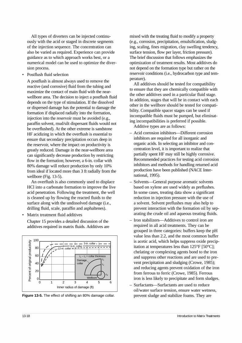
All types of diverters can be injected continu-ously with the acid or staged in discrete segmentsof the injection sequence. The concentration canalso be varied as required. Experience can provideguidance as to which approach works best, or anumerical model can be used to optimize the diver-sion process.

• Postflush fluid selection

A postflush is almost always used to remove thereactive (and corrosive) fluid from the tubing andmaximize the contact of main fluid with the near-wellbore area. The decision to inject a postflush fluiddepends on the type of stimulation. If the dissolvedor dispersed damage has the potential to damage theformation if displaced radially into the formation,injection into the reservoir must be avoided (e.g.,paraffin solvent, mud/silt dispersant fluids would notbe overflushed). At the other extreme is sandstoneHF acidizing in which the overflush is essential toensure that secondary precipitation occurs deep inthe reservoir, where the impact on productivity isgreatly reduced. Damage in the near-wellbore areacan significantly decrease production by restrictingflow in the formation; however, a 6-in. collar with80% damage will reduce production by only 10%from ideal if located more than 3 ft radially from thewellbore (Fig. 13-5).

An overflush is also commonly used to displaceHCl into a carbonate formation to improve the liveacid penetration. Following the treatment, the wellis cleaned up by flowing the reacted fluids to thesurface along with the undissolved damage (i.e.,drilling fluid, scale, paraffin and asphaltenes).

• Matrix treatment fluid additives

Chapter 15 provides a detailed discussion of theadditives required in matrix fluids. Additives are

mixed with the treating fluid to modify a property(e.g., corrosion, precipitation, emulsification, sludg-ing, scaling, fines migration, clay swelling tendency,surface tension, flow per layer, friction pressure).The brief discussion that follows emphasizes theoptimization of treatment results. Most additives donot depend on the formation type but rather on thereservoir conditions (i.e., hydrocarbon type and tem-perature).

All additives should be tested for compatibilityto ensure that they are chemically compatible withthe other additives used in a particular fluid stage.In addition, stages that will be in contact with eachother in the wellbore should be tested for compati-bility. Compatible spacer stages can be used ifincompatible fluids must be pumped, but eliminat-ing incompatibilities is preferred if possible.

Additive types are as follows:

– Acid corrosion inhibitors—Different corrosioninhibitors are required for all inorganic andorganic acids. In selecting an inhibitor and con-centration level, it is important to realize thatpartially spent HF may still be highly corrosive.Recommended practices for testing acid corrosioninhibitors and methods for handling returned acidproduction have been published (NACE Inter-national, 1995).

– Solvents—General purpose aromatic solventsbased on xylene are used widely as preflushes. In some cases, treating data show a significantreduction in injection pressure with the use of a solvent. Solvent preflushes may also help toprevent interaction with the formation oil by sep-arating the crude oil and aqueous treating fluids.

– Iron stabilizers—Additives to control iron arerequired in all acid treatments. They can begrouped in three categories: buffers keep the pHvalue less than 2.2, and the most common bufferis acetic acid, which helps suppress oxide precip-itation at temperatures less than 125°F [50°C];chelating or complexing agents bond to the ironand suppress other reactions and are used to pre-vent precipitation and sludging (Crowe, 1985);and reducing agents prevent oxidation of the ironfrom ferrous to ferric (Crowe, 1985). Ferrousiron is less likely to precipitate and form sludges.

– Surfactants—Surfactants are used to reduceoil/water surface tension, ensure water wetness,prevent sludge and stabilize foams. They are

13-18 Introduction to Matrix Treatments

Figure 13-5. The effect of shifting an 80% damage collar.

Per

cent

of o

rigin

al p

rodu

ctiv

ity 100

80

60

40

20

00 1 2 3 4 5 6

Inner radius of damage (ft)

6-in. collar12-in. collar

Damagecollar

rc – rx = collar thicknessrc

rx

rw

3-in. collar

Wellbore

recommended in most acid treatments to solveone or more potential problems. Small concen-trations (e.g., 0.2% to 1%) of surfactants are suf-ficient. Surfactants are also used as dispersants to keep materials (oil or solids) dispersed in thestimulation fluid and as nonemulsifiers to helpprevent emulsions from oil-acid interaction.

– Mutual solvents—Mutual solvents are used toensure that the formation remains water-wet andto lower surface/interfacial tension. They are rec-ommended in most acid treatments.

– Diverters—Diversion is recommended for allmatrix treatments. The bridging agents benzoicacid and rock salt are used to bridge in perfora-tions and/or fissures in carbonate formations andinjection wells. Oil-soluble resins (OSRs) sized to form an external filter cake on the formationface are typically used as particulate diverters.Small benzoic acid particles can be used in injec-tion wells completed in sandstone and nonfissuredcarbonate reservoirs. Water-soluble polymers usedas gel diverters must be carefully chosen to havethe right combination of stability during the treat-ment yet break sufficiently to prevent formationdamage. They should not be used in sandstones.Foams are formulated with surfactants and a gasphase (usually N2). Surfactants must be compati-ble with other additives included in the foamingsolution (Zerhboub et al., 1991).

– Scale inhibitors—Scale inhibitors are materialsthat suppress the precipitation of inorganic scalesfrom produced fluids. In general, they are retainedon the formation and are more effective at neutralpH values. They are normally applied as an over-flush to an acid treatment or mixed with a brine(with or without N2) and displaced into the reser-voir when scale formation is a problem.

– Clay stabilizers—In treatments of clay-bearingsand formations, these polymeric cationic materi-als decrease clay migration. They are temporarilyeffective at low concentrations. Clay stabilizers donot prevent silt (e.g., feldspar, mica, chert) migra-tion (Ezeukwu et al., 1998). They are available indifferent molecular weight ranges for higher andlower permeability formations, and they must betailored to the formation to avoid causing damagefrom the physical plugging of pore throats. Claystabilizers are recommended where experienceindicates that clay migration is a problem.

– Aluminum stabilizer—This class of chemicalswas introduced in recognition of the role of fluo-roaluminates in secondary precipitation in wellsat temperatures above 200°F in sandstones(Gdanski, 1996). Although new chemicals havebeen introduced to address this problem, citricacid works well and is economical (Rogers etal., 1998).

– Retarders—Numerous systems for delaying acidreaction in carbonates and allowing deeper pene-tration into the reservoir have been developed.Simulations should be performed to quantifytheir benefit.

– Nitrogen—N2 is commonly added to treatingfluids in low-pressure wells to assist in cleanupor to create a foam diverter.

Once the proper treating fluid formulations havebeen selected, the pumping schedule must bedesigned.

13-5.3. Pumping schedule generation and simulation

The pumping schedule includes the treating fluid anddiverter sequence and the injection rate of each stage.It is generated using empirical rules based on previousfield experience or computers.

A numerical simulator can be used to simulate dam-age removal and evaluate skin effect evolution, flowprofile and wellhead or bottomhole pressure versusinjection rate for the proposed pumping schedule. Thesimulator takes into consideration the placement strat-egy, an important part of the design process. Theschedule can be optimized using a single-phase reser-voir model to meet specific objectives for each fluidtype (Bartko et al., 1996). This step allows the designengineer to optimize the schedule to obtain the desiredresults in the most cost-effective manner. A treatmentdesign is not systematically engineered until it is runusing a field-validated simulator. Most treatments arecurrently based on empirical rules of thumb.

The matrix treatment design process includes sev-eral steps. The manual process that is discussed indetail in Chapters 17 through 19 should be understoodbefore using computer-aided design programs. Thissection focuses on computer-generated design, withemphasis on the required input and interpretation ofthe output. A field case history for a sandstone is usedto illustrate the utility of the procedure.

Reservoir Stimulation 13-19

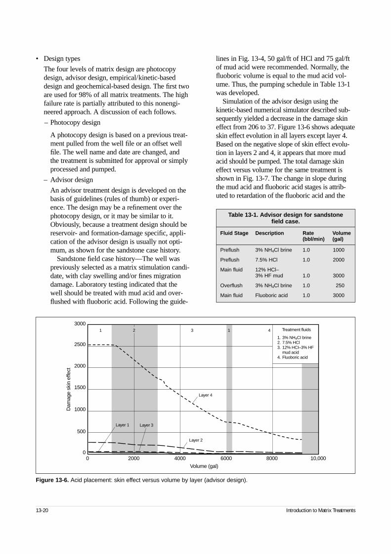
• Design types

The four levels of matrix design are photocopydesign, advisor design, empirical/kinetic-baseddesign and geochemical-based design. The first twoare used for 98% of all matrix treatments. The highfailure rate is partially attributed to this nonengi-neered approach. A discussion of each follows.

– Photocopy design

A photocopy design is based on a previous treat-ment pulled from the well file or an offset wellfile. The well name and date are changed, andthe treatment is submitted for approval or simplyprocessed and pumped.

– Advisor design

An advisor treatment design is developed on thebasis of guidelines (rules of thumb) or experi-ence. The design may be a refinement over thephotocopy design, or it may be similar to it.Obviously, because a treatment design should bereservoir- and formation-damage specific, appli-cation of the advisor design is usually not opti-mum, as shown for the sandstone case history.

Sandstone field case history—The well waspreviously selected as a matrix stimulation candi-date, with clay swelling and/or fines migrationdamage. Laboratory testing indicated that thewell should be treated with mud acid and over-flushed with fluoboric acid. Following the guide-

lines in Fig. 13-4, 50 gal/ft of HCl and 75 gal/ftof mud acid were recommended. Normally, thefluoboric volume is equal to the mud acid vol-ume. Thus, the pumping schedule in Table 13-1was developed.

Simulation of the advisor design using thekinetic-based numerical simulator described sub-sequently yielded a decrease in the damage skineffect from 206 to 37. Figure 13-6 shows adequateskin effect evolution in all layers except layer 4.Based on the negative slope of skin effect evolu-tion in layers 2 and 4, it appears that more mudacid should be pumped. The total damage skineffect versus volume for the same treatment isshown in Fig. 13-7. The change in slope duringthe mud acid and fluoboric acid stages is attrib-uted to retardation of the fluoboric acid and the

13-20 Introduction to Matrix Treatments

Figure 13-6. Acid placement: skin effect versus volume by layer (advisor design).

Dam

age

skin

effe

ct

3000

2500

2000

1500

1000

500

00 2000 4000 6000 8000 10,000

Volume (gal)

Treatment fluids

1. 3% NH4CI brine2. 7.5% HCl3. 12% HCI–3% HF

mud acid4. Fluoboric acid

1 2 3 1 4

Layer 4

Layer 2

Layer 3Layer 1

Table 13-1. Advisor design for sandstone field case.

Fluid Stage Description Rate Volume(bbl/min) (gal)

Preflush 3% NH4Cl brine 1.0 1000

Preflush 7.5% HCl 1.0 2000

Main fluid 12% HCl–3% HF mud 1.0 3000

Overflush 3% NH4Cl brine 1.0 250

Main fluid Fluoboric acid 1.0 3000

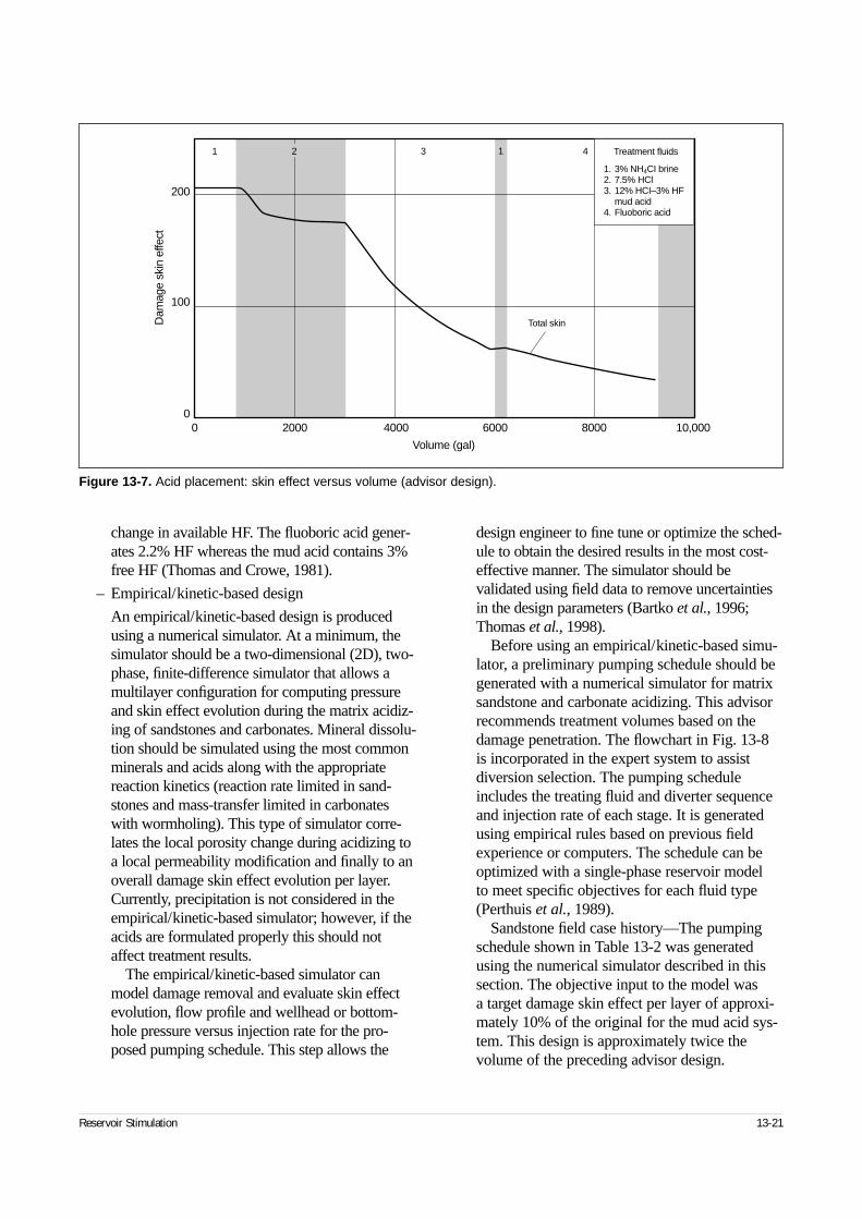
change in available HF. The fluoboric acid gener-ates 2.2% HF whereas the mud acid contains 3%free HF (Thomas and Crowe, 1981).

– Empirical/kinetic-based design

An empirical/kinetic-based design is producedusing a numerical simulator. At a minimum, thesimulator should be a two-dimensional (2D), two-phase, finite-difference simulator that allows amultilayer configuration for computing pressureand skin effect evolution during the matrix acidiz-ing of sandstones and carbonates. Mineral dissolu-tion should be simulated using the most commonminerals and acids along with the appropriatereaction kinetics (reaction rate limited in sand-stones and mass-transfer limited in carbonateswith wormholing). This type of simulator corre-lates the local porosity change during acidizing toa local permeability modification and finally to anoverall damage skin effect evolution per layer.Currently, precipitation is not considered in theempirical/kinetic-based simulator; however, if theacids are formulated properly this should notaffect treatment results.

The empirical/kinetic-based simulator canmodel damage removal and evaluate skin effectevolution, flow profile and wellhead or bottom-hole pressure versus injection rate for the pro-posed pumping schedule. This step allows the

design engineer to fine tune or optimize the sched-ule to obtain the desired results in the most cost-effective manner. The simulator should bevalidated using field data to remove uncertaintiesin the design parameters (Bartko et al., 1996;Thomas et al., 1998).

Before using an empirical/kinetic-based simu-lator, a preliminary pumping schedule should begenerated with a numerical simulator for matrixsandstone and carbonate acidizing. This advisorrecommends treatment volumes based on thedamage penetration. The flowchart in Fig. 13-8 is incorporated in the expert system to assistdiversion selection. The pumping scheduleincludes the treating fluid and diverter sequenceand injection rate of each stage. It is generatedusing empirical rules based on previous fieldexperience or computers. The schedule can beoptimized with a single-phase reservoir model to meet specific objectives for each fluid type(Perthuis et al., 1989).

Sandstone field case history—The pumpingschedule shown in Table 13-2 was generatedusing the numerical simulator described in thissection. The objective input to the model was a target damage skin effect per layer of approxi-mately 10% of the original for the mud acid sys-tem. This design is approximately twice thevolume of the preceding advisor design.

Reservoir Stimulation 13-21

Figure 13-7. Acid placement: skin effect versus volume (advisor design).

Dam

age

skin

effe

ct

200

100

00 2000 4000 6000 8000 10,000

Volume (gal)

1 2 3 1 4

Total skin

Treatment fluids

1. 3% NH4CI brine2. 7.5% HCl3. 12% HCI–3% HF

mud acid4. Fluoboric acid

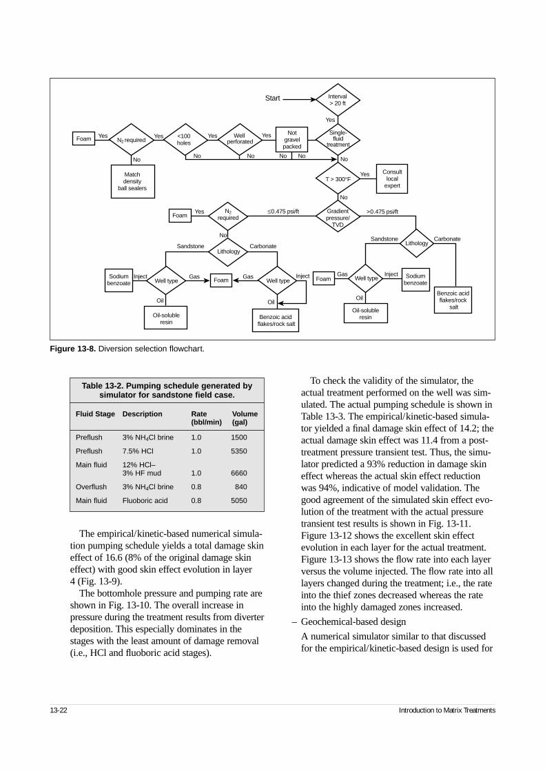
The empirical/kinetic-based numerical simula-tion pumping schedule yields a total damage skineffect of 16.6 (8% of the original damage skineffect) with good skin effect evolution in layer 4 (Fig. 13-9).

The bottomhole pressure and pumping rate areshown in Fig. 13-10. The overall increase inpressure during the treatment results from diverterdeposition. This especially dominates in thestages with the least amount of damage removal(i.e., HCl and fluoboric acid stages).

To check the validity of the simulator, theactual treatment performed on the well was sim-ulated. The actual pumping schedule is shown inTable 13-3. The empirical/kinetic-based simula-tor yielded a final damage skin effect of 14.2; theactual damage skin effect was 11.4 from a post-treatment pressure transient test. Thus, the simu-lator predicted a 93% reduction in damage skineffect whereas the actual skin effect reductionwas 94%, indicative of model validation. Thegood agreement of the simulated skin effect evo-lution of the treatment with the actual pressuretransient test results is shown in Fig. 13-11.Figure 13-12 shows the excellent skin effectevolution in each layer for the actual treatment.Figure 13-13 shows the flow rate into each layerversus the volume injected. The flow rate into alllayers changed during the treatment; i.e., the rateinto the thief zones decreased whereas the rateinto the highly damaged zones increased.

– Geochemical-based design

A numerical simulator similar to that discussedfor the empirical/kinetic-based design is used for

13-22 Introduction to Matrix Treatments

Figure 13-8. Diversion selection flowchart.

Start Interval> 20 ft

Foam

Foam

N2 required<100holes

Well perforated

Single-fluid

treatment

Matchdensity

ball sealers

N2required

T > 300°F

LithologyLithology

Well typeWell type Well typeSodium

benzoateSodium

benzoate

Oil-solubleresinOil-soluble

resin

Benzoic acid flakes/rock

salt

Benzoic acid flakes/rock salt

Gradientpressure/

TVD

FoamFoam

Consultlocal

expert

Notgravelpacked

Yes Yes

NoNo No No No No

No

No

Yes Yes

Yes

Yes

Yes ≤0.475 psi/ft >0.475 psi/ft

SandstoneSandstone

InjectInjectInject GasGasGas

OilOilOil

CarbonateCarbonate

Table 13-2. Pumping schedule generated by simulator for sandstone field case.

Fluid Stage Description Rate Volume(bbl/min) (gal)

Preflush 3% NH4Cl brine 1.0 1500

Preflush 7.5% HCl 1.0 5350

Main fluid 12% HCl–3% HF mud 1.0 6660

Overflush 3% NH4Cl brine 0.8 840

Main fluid Fluoboric acid 0.8 5050

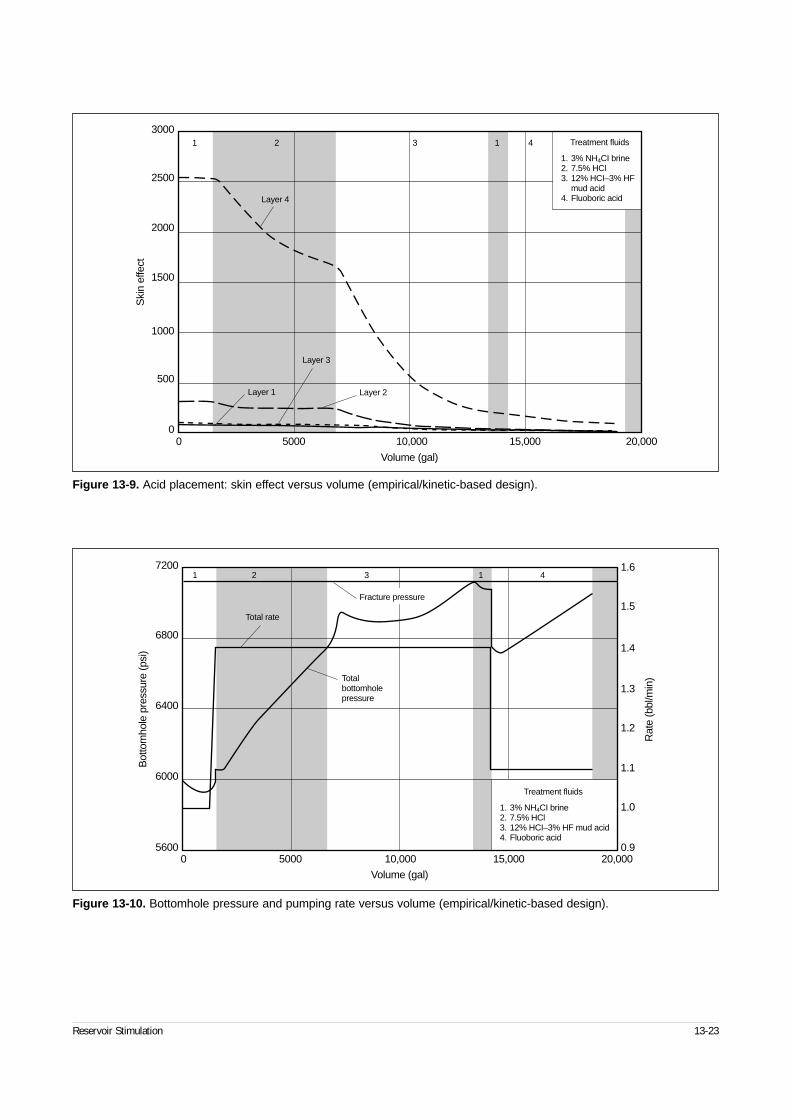
Reservoir Stimulation 13-23

Figure 13-9. Acid placement: skin effect versus volume (empirical/kinetic-based design).

Ski

n ef

fect

3000

2500

2000

1500

1000

500

00 5000 10,000 15,000 20,000

Volume (gal)

1 2 3 1 4

Layer 1 Layer 2

Layer 3

Layer 4

Treatment fluids

1. 3% NH4CI brine2. 7.5% HCl3. 12% HCI–3% HF

mud acid4. Fluoboric acid

Figure 13-10. Bottomhole pressure and pumping rate versus volume (empirical/kinetic-based design).

Bot

tom

hole

pre

ssur

e (p

si)

5600

6000

6400

6800

7200

0 5000 10,000 15,000 20,000

Volume (gal)

Rat

e (b

bl/m

in)

1.6

1.5

1.4

1.3

1.2

1.1

1.0

0.9

1 2 3 1 4

Fracture pressure

Total bottomholepressure

Total rate

Treatment fluids

1. 3% NH4CI brine2. 7.5% HCl3. 12% HCI–3% HF mud acid4. Fluoboric acid

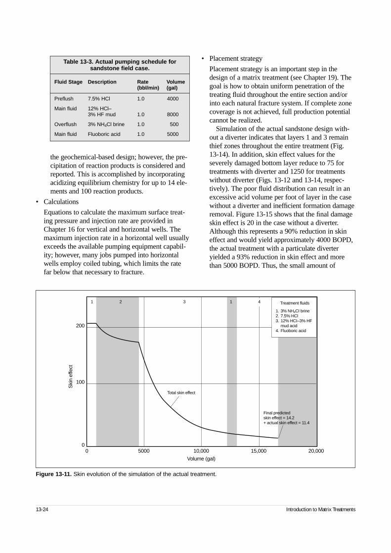
the geochemical-based design; however, the pre-cipitation of reaction products is considered andreported. This is accomplished by incorporatingacidizing equilibrium chemistry for up to 14 ele-ments and 100 reaction products.

• Calculations

Equations to calculate the maximum surface treat-ing pressure and injection rate are provided inChapter 16 for vertical and horizontal wells. Themaximum injection rate in a horizontal well usuallyexceeds the available pumping equipment capabil-ity; however, many jobs pumped into horizontalwells employ coiled tubing, which limits the ratefar below that necessary to fracture.

• Placement strategy

Placement strategy is an important step in thedesign of a matrix treatment (see Chapter 19). Thegoal is how to obtain uniform penetration of thetreating fluid throughout the entire section and/orinto each natural fracture system. If complete zonecoverage is not achieved, full production potentialcannot be realized.

Simulation of the actual sandstone design with-out a diverter indicates that layers 1 and 3 remainthief zones throughout the entire treatment (Fig. 13-14). In addition, skin effect values for theseverely damaged bottom layer reduce to 75 fortreatments with diverter and 1250 for treatmentswithout diverter (Figs. 13-12 and 13-14, respec-tively). The poor fluid distribution can result in anexcessive acid volume per foot of layer in the casewithout a diverter and inefficient formation damageremoval. Figure 13-15 shows that the final damageskin effect is 20 in the case without a diverter.Although this represents a 90% reduction in skineffect and would yield approximately 4000 BOPD,the actual treatment with a particulate diverteryielded a 93% reduction in skin effect and morethan 5000 BOPD. Thus, the small amount of

13-24 Introduction to Matrix Treatments

Table 13-3. Actual pumping schedule for sandstone field case.

Fluid Stage Description Rate Volume(bbl/min) (gal)

Preflush 7.5% HCl 1.0 4000

Main fluid 12% HCl–3% HF mud 1.0 8000

Overflush 3% NH4Cl brine 1.0 500

Main fluid Fluoboric acid 1.0 5000

Figure 13-11. Skin evolution of the simulation of the actual treatment.

Ski

n ef

fect

200

100

00 5000 10,000 15,000 20,000

Volume (gal)

1 2 3 1

Total skin effect

4

Final predictedskin effect = 14.2+ actual skin effect = 11.4

Treatment fluids

1. 3% NH4CI brine2. 7.5% HCl3. 12% HCI–3% HF

mud acid4. Fluoboric acid

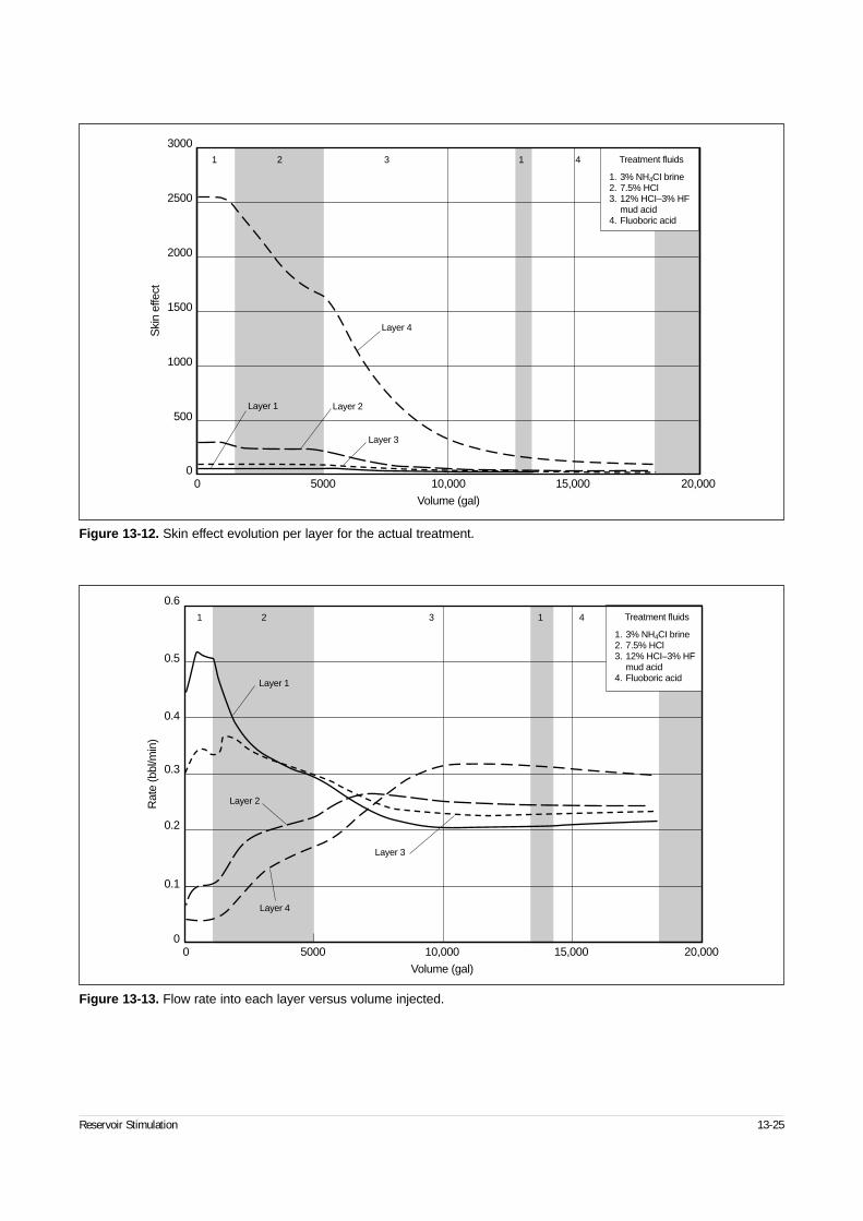
Reservoir Stimulation 13-25

Figure 13-12. Skin effect evolution per layer for the actual treatment.

Ski

n ef

fect

3000

2500

2000

1500

1000

500

00 5000 10,000 15,000 20,000

Volume (gal)

1 2 3 1 4

Layer 1 Layer 2

Layer 4

Layer 3

Treatment fluids

1. 3% NH4CI brine2. 7.5% HCl3. 12% HCI–3% HF

mud acid4. Fluoboric acid

Figure 13-13. Flow rate into each layer versus volume injected.

Rat

e (b

bl/m

in)

0

0.1

0.2

0.3

0.4

0.5

0.6

0 5000 10,000 15,000 20,000

Volume (gal)

1 2 3 1 4

Layer 1

Layer 3

Layer 4

Layer 2

Treatment fluids

1. 3% NH4CI brine2. 7.5% HCl3. 12% HCI–3% HF

mud acid4. Fluoboric acid

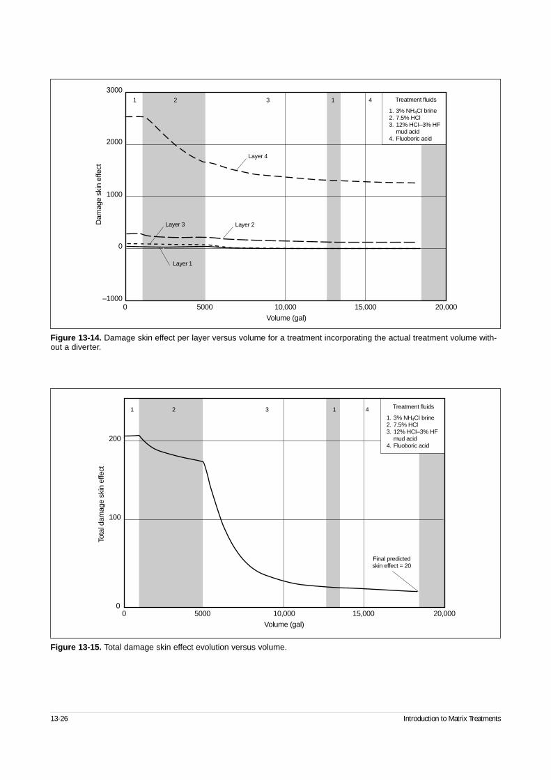
13-26 Introduction to Matrix Treatments

Figure 13-14. Damage skin effect per layer versus volume for a treatment incorporating the actual treatment volume with-out a diverter.

Dam

age

skin

effe

ct3000

2000

1000

0

–10000 5000 10,000 15,000 20,000

Volume (gal)

1 2 3 1 4

Layer 1

Layer 3

Layer 4

Layer 2

Treatment fluids

1. 3% NH4CI brine2. 7.5% HCl3. 12% HCI–3% HF

mud acid4. Fluoboric acid

Figure 13-15. Total damage skin effect evolution versus volume.

Tota

l dam

age

skin

effe

ct

200

100

00 5000 10,000 15,000 20,000

Volume (gal)

1 2 3 1 4

Final predictedskin effect = 20

Treatment fluids

1. 3% NH4CI brine2. 7.5% HCl3. 12% HCI–3% HF

mud acid4. Fluoboric acid

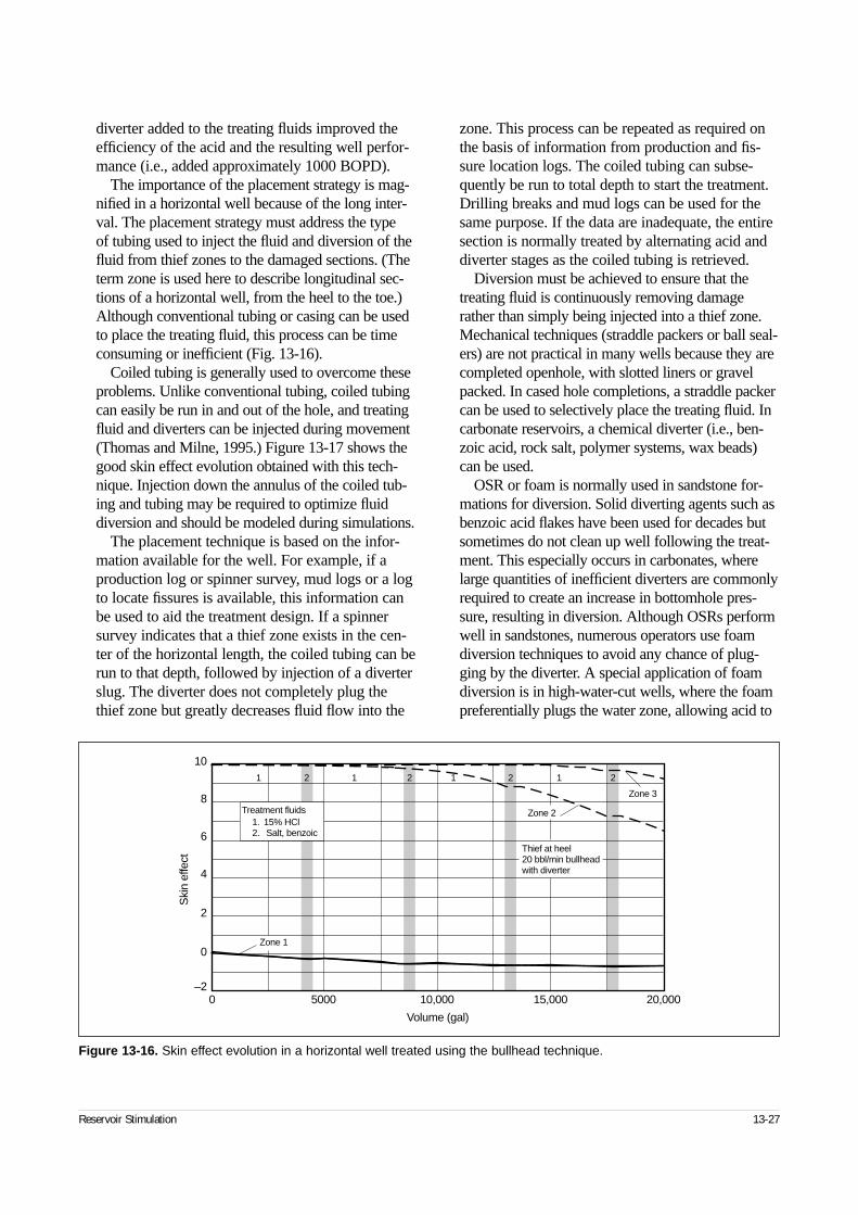
diverter added to the treating fluids improved theefficiency of the acid and the resulting well perfor-mance (i.e., added approximately 1000 BOPD).

The importance of the placement strategy is mag-nified in a horizontal well because of the long inter-val. The placement strategy must address the type of tubing used to inject the fluid and diversion of thefluid from thief zones to the damaged sections. (Theterm zone is used here to describe longitudinal sec-tions of a horizontal well, from the heel to the toe.)Although conventional tubing or casing can be usedto place the treating fluid, this process can be timeconsuming or inefficient (Fig. 13-16).

Coiled tubing is generally used to overcome theseproblems. Unlike conventional tubing, coiled tubingcan easily be run in and out of the hole, and treatingfluid and diverters can be injected during movement(Thomas and Milne, 1995.) Figure 13-17 shows thegood skin effect evolution obtained with this tech-nique. Injection down the annulus of the coiled tub-ing and tubing may be required to optimize fluiddiversion and should be modeled during simulations.

The placement technique is based on the infor-mation available for the well. For example, if aproduction log or spinner survey, mud logs or a logto locate fissures is available, this information canbe used to aid the treatment design. If a spinnersurvey indicates that a thief zone exists in the cen-ter of the horizontal length, the coiled tubing can berun to that depth, followed by injection of a diverterslug. The diverter does not completely plug thethief zone but greatly decreases fluid flow into the

zone. This process can be repeated as required onthe basis of information from production and fis-sure location logs. The coiled tubing can subse-quently be run to total depth to start the treatment.Drilling breaks and mud logs can be used for thesame purpose. If the data are inadequate, the entiresection is normally treated by alternating acid anddiverter stages as the coiled tubing is retrieved.

Diversion must be achieved to ensure that thetreating fluid is continuously removing damagerather than simply being injected into a thief zone.Mechanical techniques (straddle packers or ball seal-ers) are not practical in many wells because they arecompleted openhole, with slotted liners or gravelpacked. In cased hole completions, a straddle packercan be used to selectively place the treating fluid. Incarbonate reservoirs, a chemical diverter (i.e., ben-zoic acid, rock salt, polymer systems, wax beads)can be used.

OSR or foam is normally used in sandstone for-mations for diversion. Solid diverting agents such asbenzoic acid flakes have been used for decades butsometimes do not clean up well following the treat-ment. This especially occurs in carbonates, wherelarge quantities of inefficient diverters are commonlyrequired to create an increase in bottomhole pres-sure, resulting in diversion. Although OSRs performwell in sandstones, numerous operators use foamdiversion techniques to avoid any chance of plug-ging by the diverter. A special application of foamdiversion is in high-water-cut wells, where the foampreferentially plugs the water zone, allowing acid to

Reservoir Stimulation 13-27

Figure 13-16. Skin effect evolution in a horizontal well treated using the bullhead technique.

Treatment fluids1. 15% HCl2. Salt, benzoic

1 1 1 12 2 2 2

Zone 3

Zone 2

Thief at heel20 bbl/min bullheadwith diverter

Zone 1

10

8

6

4

2

0

–20 5000 10,000 15,000 20,000

Volume (gal)

Ski

n ef

fect

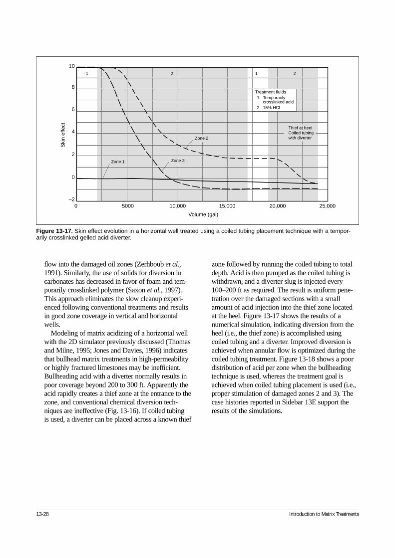
flow into the damaged oil zones (Zerhboub et al.,1991). Similarly, the use of solids for diversion incarbonates has decreased in favor of foam and tem-porarily crosslinked polymer (Saxon et al., 1997).This approach eliminates the slow cleanup experi-enced following conventional treatments and resultsin good zone coverage in vertical and horizontalwells.

Modeling of matrix acidizing of a horizontal wellwith the 2D simulator previously discussed (Thomasand Milne, 1995; Jones and Davies, 1996) indicatesthat bullhead matrix treatments in high-permeabilityor highly fractured limestones may be inefficient.Bullheading acid with a diverter normally results inpoor coverage beyond 200 to 300 ft. Apparently theacid rapidly creates a thief zone at the entrance to thezone, and conventional chemical diversion tech-niques are ineffective (Fig. 13-16). If coiled tubing is used, a diverter can be placed across a known thief

zone followed by running the coiled tubing to totaldepth. Acid is then pumped as the coiled tubing iswithdrawn, and a diverter slug is injected every100–200 ft as required. The result is uniform pene-tration over the damaged sections with a smallamount of acid injection into the thief zone locatedat the heel. Figure 13-17 shows the results of anumerical simulation, indicating diversion from theheel (i.e., the thief zone) is accomplished usingcoiled tubing and a diverter. Improved diversion isachieved when annular flow is optimized during thecoiled tubing treatment. Figure 13-18 shows a poordistribution of acid per zone when the bullheadingtechnique is used, whereas the treatment goal isachieved when coiled tubing placement is used (i.e.,proper stimulation of damaged zones 2 and 3). Thecase histories reported in Sidebar 13E support theresults of the simulations.

13-28 Introduction to Matrix Treatments

Figure 13-17. Skin effect evolution in a horizontal well treated using a coiled tubing placement technique with a tempor-arily crosslinked gelled acid diverter.

0 5000 10,000 15,000 20,000 25,000

10

8

6

4

2

0

–2

Volume (gal)

Ski

n ef

fect

Zone 1

Treatment fluids1. Temporarily

crosslinked acid2. 15% HCl

1 21 2

Thief at heelCoiled tubing with diverter

Zone 3

Zone 2

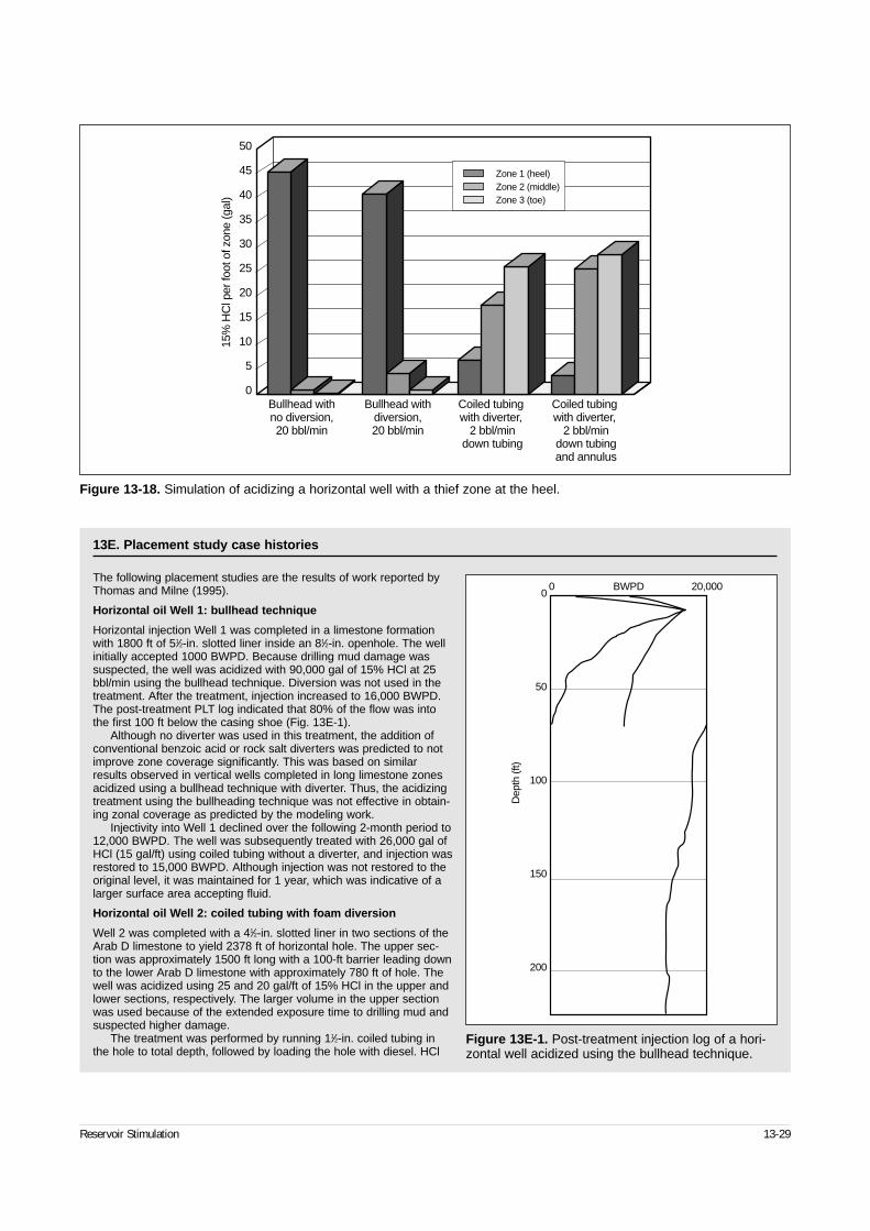
Reservoir Stimulation 13-29

13E. Placement study case histories

The following placement studies are the results of work reported byThomas and Milne (1995).

Horizontal oil Well 1: bullhead technique

Horizontal injection Well 1 was completed in a limestone formationwith 1800 ft of 51⁄2-in. slotted liner inside an 81⁄2-in. openhole. The wellinitially accepted 1000 BWPD. Because drilling mud damage wassuspected, the well was acidized with 90,000 gal of 15% HCl at 25bbl/min using the bullhead technique. Diversion was not used in thetreatment. After the treatment, injection increased to 16,000 BWPD.The post-treatment PLT log indicated that 80% of the flow was intothe first 100 ft below the casing shoe (Fig. 13E-1).

Although no diverter was used in this treatment, the addition ofconventional benzoic acid or rock salt diverters was predicted to notimprove zone coverage significantly. This was based on similarresults observed in vertical wells completed in long limestone zonesacidized using a bullhead technique with diverter. Thus, the acidizingtreatment using the bullheading technique was not effective in obtain-ing zonal coverage as predicted by the modeling work.

Injectivity into Well 1 declined over the following 2-month period to12,000 BWPD. The well was subsequently treated with 26,000 gal ofHCl (15 gal/ft) using coiled tubing without a diverter, and injection wasrestored to 15,000 BWPD. Although injection was not restored to theoriginal level, it was maintained for 1 year, which was indicative of alarger surface area accepting fluid.

Horizontal oil Well 2: coiled tubing with foam diversion

Well 2 was completed with a 41⁄2-in. slotted liner in two sections of theArab D limestone to yield 2378 ft of horizontal hole. The upper sec-tion was approximately 1500 ft long with a 100-ft barrier leading downto the lower Arab D limestone with approximately 780 ft of hole. Thewell was acidized using 25 and 20 gal/ft of 15% HCl in the upper andlower sections, respectively. The larger volume in the upper sectionwas used because of the extended exposure time to drilling mud andsuspected higher damage.

The treatment was performed by running 11⁄2-in. coiled tubing inthe hole to total depth, followed by loading the hole with diesel. HCl

Figure 13E-1. Post-treatment injection log of a hori-zontal well acidized using the bullhead technique.

0

50

100

150

200

0 BWPD 20,000

Dep

th (f

t)

Figure 13-18. Simulation of acidizing a horizontal well with a thief zone at the heel.

50

45

40

35

30

25

20

15

10

5

0

15%

HC

l per

foot

of z

one

(gal

)

Bullhead withno diversion,20 bbl/min

Bullhead withdiversion,20 bbl/min

Coiled tubing with diverter,

2 bbl/mindown tubing

Coiled tubing with diverter,

2 bbl/mindown tubingand annulus

Zone 1 (heel)Zone 2 (middle)Zone 3 (toe)

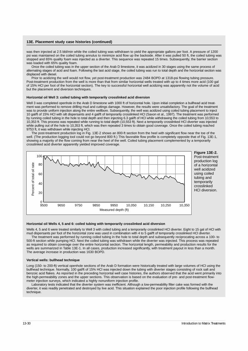
13-30 Introduction to Matrix Treatments

was then injected at 2.5 bbl/min while the coiled tubing was withdrawn to yield the appropriate gallons per foot. A pressure of 1200psi was maintained on the coiled tubing annulus to minimize acid flow up the backside. After it was pulled 50 ft, the coiled tubing wasstopped and 65% quality foam was injected as a diverter. This sequence was repeated 15 times. Subsequently, the barrier sectionwas loaded with 65% quality foam.

Once the coiled tubing was in the upper section of the Arab D limestone, it was acidized in 30 stages using the same process ofalternating stages of acid and foam. Following the last acid stage, the coiled tubing was run to total depth and the horizontal section wasdisplaced with diesel.

Prior to acidizing the well would not flow, yet post-treatment production was 2484 BOPD at 1318-psi flowing tubing pressure.Post-treatment production from the well is more than that from similar horizontal wells treated with up to 4 times more acid (100 galof 15% HCl per foot of the horizontal section). The key to successful horizontal well acidizing was apparently not the volume of acidbut the placement and diversion techniques.

Horizontal oil Well 3: coiled tubing with temporarily crosslinked acid diversion

Well 3 was completed openhole in the Arab D limestone with 1000 ft of horizontal hole. Upon initial completion a bullhead acid treat-ment was performed to remove drilling mud and cuttings damage. However, the results were unsatisfactory. The goal of the treatmentwas to provide uniform injection along the entire wellbore. Subsequently, the well was acidized using coiled tubing placement to inject 10 gal/ft of 15% HCl with silt dispersants and 4 gal/ft of temporarily crosslinked HCl (Saxon et al., 1997). The treatment was performedby running coiled tubing in the hole to total depth and then injecting 6.3 gal/ft of HCl while withdrawing the coiled tubing from 10,553 to10,353 ft. This process was repeated while running to total depth (10,553 ft). Next a temporarily crosslinked HCl diverter was injectedwhile pulling out of the hole to 10,353 ft, which was then repeated 3 times to obtain good coverage. Once the coiled tubing reached9753 ft, it was withdrawn while injecting HCl.

The post-treatment production log in Fig. 13E-2 shows an 800-ft section from the heel with significant flow near the toe of thewell. (The production logging tool could not go beyond 800 ft.) This favorable flow profile is completely opposite that of Fig. 13E-1,showing a majority of the flow coming from near the heel of the well. Coiled tubing placement complemented by a temporarilycrosslinked acid diverter apparently yielded improved coverage.

Horizontal oil Wells 4, 5 and 6: coiled tubing with temporarily crosslinked acid diversion

Wells 4, 5 and 6 were treated similarly to Well 3 with coiled tubing and a temporarily crosslinked HCl diverter. Eight to 15 gal of HCl withmud dispersants per foot of the horizontal zone was used in combination with 4 to 5 gal/ft of temporarily crosslinked HCl diverter.

The treatment was performed by running coiled tubing in the hole to total depth and subsequently reciprocating across a 100- to500-ft section while pumping HCl. Next the coiled tubing was withdrawn while the diverter was injected. This process was repeatedas required to obtain coverage over the entire horizontal section. The horizontal length, permeability and production results for thewells are summarized in Table 13E-1. In all cases, production increased significantly, with treatment payout in less than a month.The average increase in production was 1630 BOPD.

Vertical wells: bullhead technique

Long (150- to 200-ft) vertical openhole sections of the Arab D formation were historically treated with large volumes of HCl using thebullhead technique. Normally, 100 gal/ft of 15% HCl was injected down the tubing with diverter stages consisting of rock salt andbenzoic acid flakes. As reported in the preceding horizontal well case histories, the authors observed that the acid went primarily intothe high-permeability zones and the upper sections. This observation is based on the evaluation of pre- and post-treatment flow-meter injection surveys, which indicated a highly nonuniform injection profile.

Laboratory tests indicated that the diverter system was inefficient. Although a low-permeability filter cake was formed with thediverter, it was readily penetrated and destroyed by live acid. This situation explained the poor injection profile following the bullheadtechnique.

Figure 13E-2.Post-treatmentproduction logof a horizontalwell acidizedusing coiled tubing and temporarilycrosslinkedHCl diversion.

9500 9650 9750 9850 9950 10,050 10,150 10,250 10,350

100

80

60

40

20

0

Measured depth (ft)

Per

cent

of t

otal

oil

rate

13E. Placement study case histories (continued)

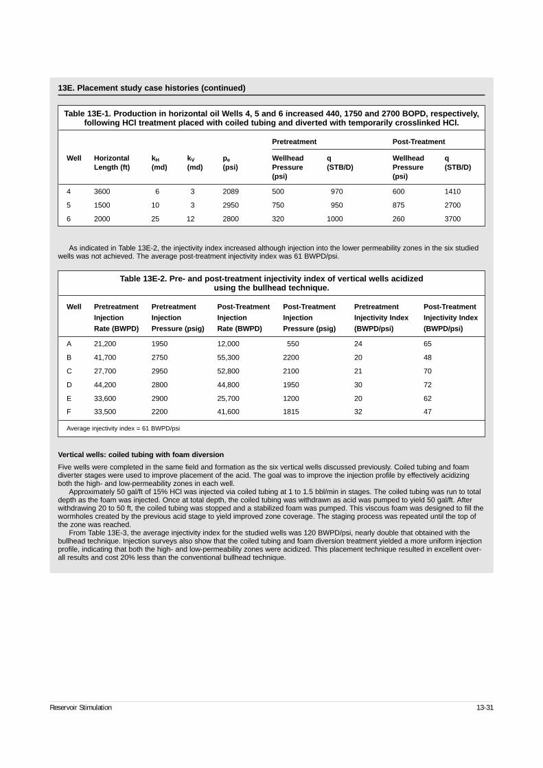
13E. Placement study case histories (continued)

As indicated in Table 13E-2, the injectivity index increased although injection into the lower permeability zones in the six studiedwells was not achieved. The average post-treatment injectivity index was 61 BWPD/psi.

Vertical wells: coiled tubing with foam diversion

Five wells were completed in the same field and formation as the six vertical wells discussed previously. Coiled tubing and foamdiverter stages were used to improve placement of the acid. The goal was to improve the injection profile by effectively acidizingboth the high- and low-permeability zones in each well.

Approximately 50 gal/ft of 15% HCl was injected via coiled tubing at 1 to 1.5 bbl/min in stages. The coiled tubing was run to totaldepth as the foam was injected. Once at total depth, the coiled tubing was withdrawn as acid was pumped to yield 50 gal/ft. Afterwithdrawing 20 to 50 ft, the coiled tubing was stopped and a stabilized foam was pumped. This viscous foam was designed to fill thewormholes created by the previous acid stage to yield improved zone coverage. The staging process was repeated until the top ofthe zone was reached.

From Table 13E-3, the average injectivity index for the studied wells was 120 BWPD/psi, nearly double that obtained with thebullhead technique. Injection surveys also show that the coiled tubing and foam diversion treatment yielded a more uniform injectionprofile, indicating that both the high- and low-permeability zones were acidized. This placement technique resulted in excellent over-all results and cost 20% less than the conventional bullhead technique.

Reservoir Stimulation 13-31

Table 13E-1. Production in horizontal oil Wells 4, 5 and 6 increased 440, 1750 and 2700 BOPD, respectively,following HCl treatment placed with coiled tubing and diverted with temporarily crosslinked HCl.

Pretreatment Post-Treatment

Well Horizontal kH kV pe Wellhead q Wellhead qLength (ft) (md) (md) (psi) Pressure (STB/D) Pressure (STB/D)

(psi) (psi)

4 3600 6 3 2089 500 970 600 1410

5 1500 10 3 2950 750 950 875 2700

6 2000 25 12 2800 320 1000 260 3700

Table 13E-2. Pre- and post-treatment injectivity index of vertical wells acidized using the bullhead technique.

Well Pretreatment Pretreatment Post-Treatment Post-Treatment Pretreatment Post-Treatment

Injection Injection Injection Injection Injectivity Index Injectivity Index

Rate (BWPD) Pressure (psig) Rate (BWPD) Pressure (psig) (BWPD/psi) (BWPD/psi)

A 21,200 1950 12,000 550 24 65

B 41,700 2750 55,300 2200 20 48

C 27,700 2950 52,800 2100 21 70

D 44,200 2800 44,800 1950 30 72

E 33,600 2900 25,700 1200 20 62

F 33,500 2200 41,600 1815 32 47

Average injectivity index = 61 BWPD/psi

13-6. Final economic evaluationAs discussed for the preliminary economic evaluationin Section 13-2.3, an economic analysis is important.A final economic evaluation should be made on thebasis of various treatment scenarios (i.e., advisor-based and empirical/kinetic-based designs). An evalu-ation of the sandstone field case history designs in theprevious section follows.

• Sandstone field case history

The advisor-based design decreased the skin effectfrom 206 to 37 (Fig. 13-7), but the empirical/kinetic-based design decreased the skin effect from 206 to16.6 (Fig. 13-9) to yield an additional 1373 BOPD(3406 versus 4779) and nearly $1.9 million in NPV(almost $2.7 million versus $4.5 million). The actualtreatment resulted in more than 5000 BOPD at alower drawdown, with more than 3 million bbl ofoil produced over the life of the well. Figures 3-19and 3-20 show the economic indicators for theadvisor- and empirical/kinetic-based designs,respectively.

13-7. ExecutionThe execution (pumping operation) must be per-formed as specified by the treatment schedule or oper-ator on location. During this process, QC and datacollection are important. The operational objective isdefined by the design. QC is the process of ensuringthat the materials and equipment meet specificationsand are delivered in proper condition to the wellsite.

Properly trained personnel are the key to success.The wellsite personnel must understand the funda-mentals of the stimulation techniques that will be usedand must know how to use the equipment, softwareand techniques.

13-7.1. Quality controlTwo keys to effective QC are communication anddocumentation. The designer must communicate thedesign expectations to the material suppliers. Becausethese expectations must be consistent with the supplieror manufacturer’s specifications, the specifications

13-32 Introduction to Matrix Treatments

13E. Placement study case histories (continued)

Summary

These case histories illustrate that the key to successful matrix acidizing in carbonate reservoirs is not the amount of acid injectedbut how it is injected. This is also true for sandstone reservoirs. Coiled tubing placement in combination with foam diversion in sand-stones or carbonates appears to be an improved technique. Chapter 17 discusses the self-diverting acid system, which has beenused successfully in long carbonate sections, including horizontal wells. This system is advantageous over foam diversion becauseit does not require nitrogen.

Table 13E-3. Pre- and post-treatment injectivity index of vertical wells acidized using the foam diversion technique.

Well Pretreatment Pretreatment Post-Treatment Post-Treatment Pretreatment Post-Treatment

Injection Injection Injection Injection Injectivity Index Injectivity Index

Rate (BWPD) Pressure (psig) Rate (BWPD) Pressure (psig) (BWPD/psi) (BWPD/psi)

G 5,000 1,300 67,800 1240 4 119

H 26,200 1,550 42,400 1200 26 112

I 10,000 24,000 59,000 1100 5 139

J 0 38,500 934 65

K 5,000 2,000 73,000 1200 3 165

Average injectivity index = 120 BWPD/psi, a 97% increase over the results obtained with the bullhead technique

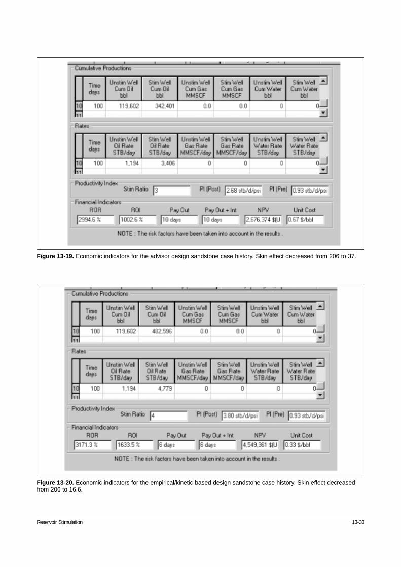
Reservoir Stimulation 13-33

Figure 13-19. Economic indicators for the advisor design sandstone case history. Skin effect decreased from 206 to 37.

Figure 13-20. Economic indicators for the empirical/kinetic-based design sandstone case history. Skin effect decreasedfrom 206 to 16.6.

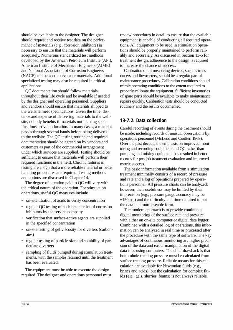
13-34 Introduction to Matrix Treatments

should be available to the designer. The designershould request and receive test data on the perfor-mance of materials (e.g., corrosion inhibitors) asnecessary to ensure that the materials will performadequately. Numerous standardized test methodsdeveloped by the American Petroleum Institute (API),American Institute of Mechanical Engineers (AIME)and National Association of Corrosion Engineers(NACE) can be used to evaluate materials. Additionalspecialized testing may also be required in criticalapplications.

QC documentation should follow materialsthroughout their life cycle and be available if neededby the designer and operating personnel. Suppliersand vendors should ensure that materials shipped tothe wellsite meet specifications. Given the time, dis-tance and expense of delivering materials to the well-site, nobody benefits if materials not meeting spec-ifications arrive on location. In many cases, a materialpasses through several hands before being delivered to the wellsite. The QC testing routine and requireddocumentation should be agreed on by vendors andcustomers as part of the commercial arrangementunder which services are supplied. Testing should besufficient to ensure that materials will perform theirrequired functions in the field. Chronic failures in testing are a sign that a more reliable material or betterhandling procedures are required. Testing methodsand options are discussed in Chapter 14.

The degree of attention paid to QC will vary withthe critical nature of the operation. For stimulationoperations, useful QC measures include

• on-site titration of acids to verify concentration

• regular QC testing of each batch or lot of corrosioninhibitors by the service company

• verification that surface-active agents are suppliedin the specified concentration

• on-site testing of gel viscosity for diverters (carbon-ates)

• regular testing of particle size and solubility of par-ticulate diverters

• sampling of fluids pumped during stimulation treat-ments, with the samples retained until the treatmenthas been evaluated.

The equipment must be able to execute the designrequired. The designer and operations personnel must

review procedures in detail to ensure that the availableequipment is capable of conducting all required opera-tions. All equipment to be used in stimulation opera-tions should be properly maintained to perform reli-ably and accurately. As discussed in Section 13-5 fortreatment design, adherence to the design is requiredto increase the chance of success.

Calibration of all measuring devices, such as trans-ducers and flowmeters, should be a regular part ofmaintenance procedures. Calibration conditions shouldmimic operating conditions to the extent required toproperly calibrate the equipment. Sufficient inventoriesof spare parts should be available to make maintenancerepairs quickly. Calibration tests should be conductedroutinely and the results documented.

13-7.2. Data collectionCareful recording of events during the treatment shouldbe made, including records of unusual observations byoperations personnel (McLeod and Coulter, 1969).Over the past decade, the emphasis on improved moni-toring and recording equipment and QC rather thanpumping and mixing equipment has resulted in betterrecords for postjob treatment evaluation and improvedmatrix success.

The basic information available from a stimulationtreatment minimally consists of a record of pressureand rate and a log of operations prepared by opera-tions personnel. All pressure charts can be analyzed;however, their usefulness may be limited by theirimprecision (e.g., pressure gauge accuracy may be±150 psi) and the difficulty and time required to putthe data in a more useable form.

The modern approach is to provide continuousdigital monitoring of the surface rate and pressurewith either an on-site computer or digital data logger.Combined with a detailed log of operations, this infor-mation can be analyzed in real time or processed afterthe procedure with the same type of software. The keyadvantages of continuous monitoring are higher preci-sion of the data and easier manipulation of the digitaldata files using computers. The chief drawback is thatbottomhole treating pressure must be calculated fromsurface treating pressure. Reliable means for this cal-culation are available for Newtonian fluids (e.g.,brines and acids), but the calculation for complex flu-ids (e.g., gels, slurries, foams) is not always reliable.

Reservoir Stimulation 13-35

A relatively simple solution to this problem is toallow pressure communication between the injectedfluid column and a static fluid column if the reservoirpressure is greater than the hydrostatic pressure result-ing from a column of fluid. The surface pressure ofthe static fluid is measured, and the bottomhole treat-ing pressure is obtained by subtracting the hydrostaticpressure of the static fluid column. The static columnis normally an annulus, either tubing/casing or coiledtubing/tubing. Packer assemblies can be modified toallow pressure communication. The main operationaldrawback is that stimulation fluids may leak into thetubing casing annulus, which necessitates additionaloperations to remove them.

Memory gauges can also be run on treating stringsto record the bottomhole temperature and pressureduring treatment. They are retrieved after the treat-ment and analyzed directly. Their obvious drawback is that real-time analysis is not possible. In runningmemory gauges, it is critical to select a sufficientlylong time interval to record the operation. If similartreatments using gel, foam or slurry diverters are to beperformed on a series of wells, a memory gauge canbe run on the first one and the data used to develop afriction pressure correlation for the diverters. Surfacepressure can then be used with acceptable accuracy on subsequent treatments.

Surface-readout bottomhole pressure recordingdevices are also available. In general, the devices areexpensive and the additional operational difficultiesassociated with running them further increase their cost.However, they are invaluable for stimulation evaluationand also for reservoir evaluation and management.

In addition, where coiled tubing is run, sensor pack-ages to monitor pressure and temperature are used todetermine bottomhole treating pressure for calculationof the skin effect. The temperature profile is determinedprior to a treatment following injection of an inert fluid(e.g., water containing ammonium chloride) to estimatethe flow profile. Another temperature profile can be runafter the treatment to quantify zone coverage.

Technology exists to transmit the job data to the officefrom most locations. This efficient technique allows anengineer to monitor numerous jobs, participate in deci-sion making and direct operations from off site.

13-8. Treatment evaluation

13-8.1. Pretreatment evaluationA step-rate test can be performed prior to the stimu-lation treatment to quantify reservoir pressure, perme-ability and skin effect. The benefit to the operator isimproved real-time evaluation. The test requires injec-tion of an inert fluid into the zone of interest and bot-tomhole pressure calculation and recording. The firstdiagnostic performed determines the reservoir pres-sure using a plot of the bottomhole pressure versusrate. Theoretically, the y-axis intercept at zero rate is the reservoir pressure (1815 psi in Fig. 13-21).

The second diagnostic incorporates PTA of the datausing the Odeh-Jones methodology. Figure 13-22shows the analysis plot used in the process. This waterinjection well exhibits permeability of approximately12.8 md and skin effect of 0.1. The permeability andreservoir pressure determined from the step rate testshould be used in the subsequent real-time evaluation.

13-8.2. Real-time evaluationIn recent years, technology to determine real-time skineffect evolution during a treatment has been developed.Although this technology is not practiced routinely, itcan be a useful diagnostic tool (see Chapter 20). Forexample, if the skin effect is decreasing during an HClstage, an acid-soluble species (e.g., calcium carbonate/oxide, iron carbonate/oxide) created damage. Thisinformation should be complemented by the well his-tory, laboratory testing, etc., to improve understandingof the present problem and assist future work.

One method available to the industry is based onthe steady-state design and evaluation method devel-oped by Paccaloni (1979b). Data can be displayed ona graph of the bottomhole pressure versus injectionrate. Comparison is made with standard curves calcu-lated for fixed values of skin effect to evaluate skineffect evolution.

More advanced programs calculate skin effect evo-lution in real time, taking into account transient effects(Prouvost and Economides, 1989). The reservoir pres-sure response during pumping is computed assuming

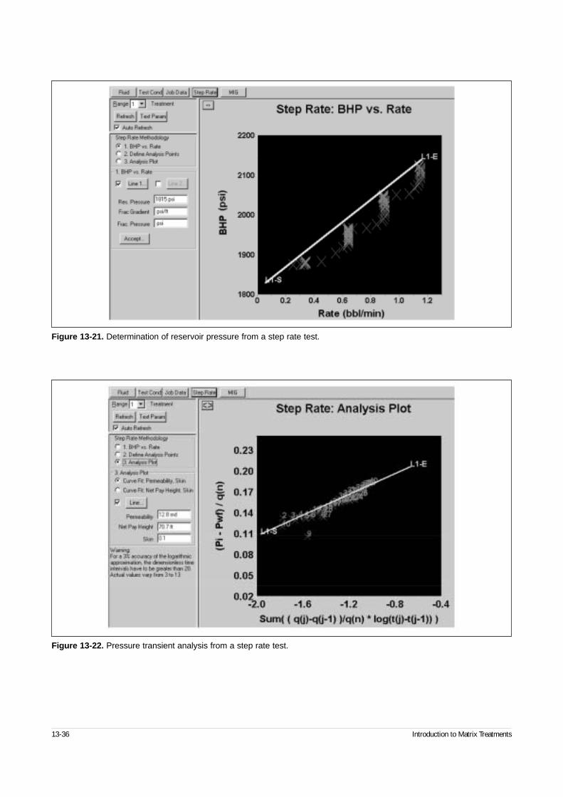
13-36 Introduction to Matrix Treatments

Figure 13-22. Pressure transient analysis from a step rate test.

Figure 13-21. Determination of reservoir pressure from a step rate test.

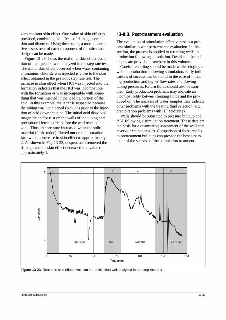
Reservoir Stimulation 13-37

zero constant skin effect. One value of skin effect isprovided, combining the effects of damage, comple-tion and diverters. Using these tools, a more quantita-tive assessment of each component of the stimulationdesign can be made.

Figure 13-23 shows the real-time skin effect evolu-tion of the injection well analyzed in the step rate test.The initial skin effect observed when water containingammonium chloride was injected is close to the skineffect obtained in the previous step rate test. Theincrease in skin effect when HCl was injected into theformation indicates that the HCl was incompatiblewith the formation or was incompatible with some-thing that was injected in the leading portion of theacid. In this example, the latter is suspected becausethe tubing was not cleaned (pickled) prior to the injec-tion of acid down the pipe. The initial acid dissolvedmagnetite and/or rust on the walls of the tubing andprecipitated ferric oxide before the acid reached thezone. Thus, the pressure increased when the solidmaterial (ferric oxide) filtered out on the formationface with an increase in skin effect to approximately2. As shown in Fig. 13-23, unspent acid removed thedamage and the skin effect decreased to a value ofapproximately 1.

13-8.3. Post-treatment evaluationThe evaluation of stimulation effectiveness is a pro-cess similar to well performance evaluation. In thissection, the process is applied to returning wells toproduction following stimulation. Details on the tech-niques are provided elsewhere in this volume.

Careful recording should be made while bringing awell on production following stimulation. Early indi-cations of success can be found in the ease of initiat-ing production and higher flow rates and flowingtubing pressures. Return fluids should also be sam-pled. Early production problems may indicate anincompatibility between treating fluids and the pro-duced oil. The analysis of water samples may indicateother problems with the treating fluid selection (e.g.,precipitation problems with HF acidizing).

Wells should be subjected to pressure buildup andPTA following a stimulation treatment. These data arethe basis for a quantitative assessment of the well andreservoir characteristics. Comparison of these resultsto pretreatment buildups can provide the best assess-ment of the success of the stimulation treatment.

Figure 13-23. Real-time skin effect evolution in the injection well analyzed in the step rate test.

1 26 51 76 101 126 151

–1

2 1 2 4 23

Time (min)

Ski

n ef

fect

3% NH4Cl 3% NH4ClHCl Mud acid

13-38 Introduction to Matrix Treatments

In the final analysis, stimulation treatments are eval-uated at the sales meter. If the treatment results in sus-tained oil production at a higher rate than before andif the revenue generated by the increased productionrepresents an acceptable return on the cost of the stim-ulation, the treatment is considered a success. Thedesigner can learn valuable information from the eval-uation of well performance, regardless of whether thestimulation is an economic success.

In addition to examining oil production response,changes in the total fluid production (oil, water andgas) in reservoir volumes, gas/oil ratio and water/oilratio must be reviewed. Well productivity must alsobe examined. An increase in the productivity of totalfluids may not be economic, but it may indicate thatthe target reservoirs were not stimulated or werewatered-out in the candidate well. This can result in a change in treatment design philosophy (i.e., to sac-rifice total stimulation effectiveness for the selectivetreatment of a limited part of the reservoir).

Correlation of the unwanted results from stimula-tion can provide data for improved performance in thefuture. They may also identify other opportunities toimprove field performance, such as water or gas shut-off. In the end, the data acquired from evaluatingrecently stimulated wells can lead to improved reser-voir management.

Ultimately, a treatment should be evaluated on thebasis of the well performance and economic parame-ters used to justify the treatment. Factors such as rate,flowing bottomhole pressure, reservoir characteriza-tion, artificial lift performance and equipment perfor-mance have been discussed. Several weeks or evenmonths may be required for production to stabilize andestablish a representative trend. In addition, shutting

in the well for pressure buildup is less attractive—andmay not be acceptable—after the well has responded.

Using field data, the engineer can evaluate differ-ences between the design and actual treatment. If anumerical simulator can be rerun with the actual treat-ment parameters, the model can be calibrated by adjust-ing reservoir parameters such as the damage radius,permeability per layer, skin effect per layer, damagemineralogy and diverter efficiency until a match withthe actual treatment profiles is obtained. If a post-treat-ment well test is performed and evaluated, the resultingdata can be used to further calibrate the simulator.

Wireline formation logs and the combination ofradioactive tracers and gamma ray or gamma ray spec-troscopy surveys (where the energy and intensity ofthe gamma rays are measured to enable the discrimina-tion of multiple tracers) can be used to quantify zonecoverage. Of course, the decision to run tracers andbaseline logs must be made while planning the stimu-lation. A pressure transient test (e.g., buildup, four-point) to quantify permeability and skin effect can beperformed. Thus, adequate evaluation tools exist todayto significantly improve matrix treatment success.

Future treatment designs for the well or field can beoptimized with the calibrated model. All results shouldbe compiled in a report with recommendations for allphases of the design, execution and evaluation (i.e.,continuous improvement).

Stimulation operations present the engineer with anopportunity to significantly improve the economic per-formance of the assets under his or her stewardship. Ifproperly designed, executed and evaluated, stimulationoperations can teach the engineer about the current con-dition of the well and reservoir and identify otheropportunities to improve economic performance.

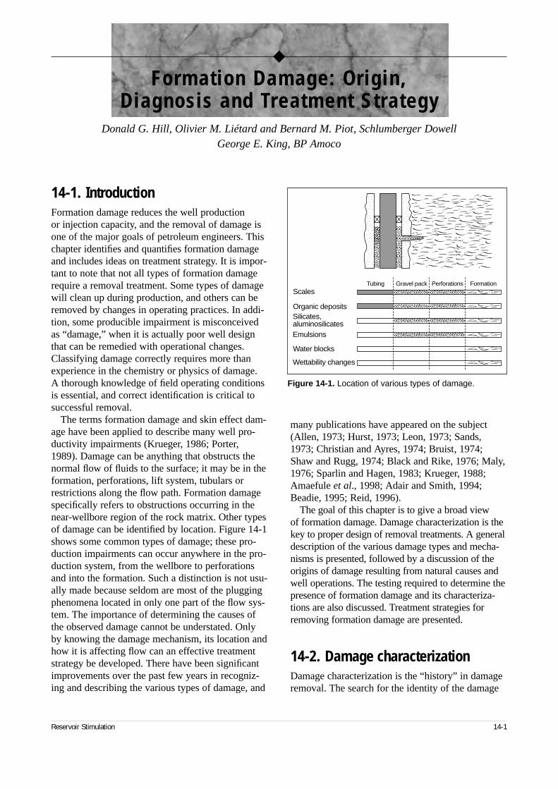
14-1. IntroductionFormation damage reduces the well production or injection capacity, and the removal of damage isone of the major goals of petroleum engineers. Thischapter identifies and quantifies formation damageand includes ideas on treatment strategy. It is impor-tant to note that not all types of formation damagerequire a removal treatment. Some types of damagewill clean up during production, and others can beremoved by changes in operating practices. In addi-tion, some producible impairment is misconceivedas “damage,” when it is actually poor well designthat can be remedied with operational changes.Classifying damage correctly requires more thanexperience in the chemistry or physics of damage. A thorough knowledge of field operating conditionsis essential, and correct identification is critical tosuccessful removal.

The terms formation damage and skin effect dam-age have been applied to describe many well pro-ductivity impairments (Krueger, 1986; Porter,1989). Damage can be anything that obstructs thenormal flow of fluids to the surface; it may be in theformation, perforations, lift system, tubulars orrestrictions along the flow path. Formation damagespecifically refers to obstructions occurring in thenear-wellbore region of the rock matrix. Other typesof damage can be identified by location. Figure 14-1shows some common types of damage; these pro-duction impairments can occur anywhere in the pro-duction system, from the wellbore to perforationsand into the formation. Such a distinction is not usu-ally made because seldom are most of the pluggingphenomena located in only one part of the flow sys-tem. The importance of determining the causes ofthe observed damage cannot be understated. Onlyby knowing the damage mechanism, its location andhow it is affecting flow can an effective treatmentstrategy be developed. There have been significantimprovements over the past few years in recogniz-ing and describing the various types of damage, and

many publications have appeared on the subject(Allen, 1973; Hurst, 1973; Leon, 1973; Sands,1973; Christian and Ayres, 1974; Bruist, 1974;Shaw and Rugg, 1974; Black and Rike, 1976; Maly,1976; Sparlin and Hagen, 1983; Krueger, 1988;Amaefule et al., 1998; Adair and Smith, 1994;Beadie, 1995; Reid, 1996).

The goal of this chapter is to give a broad view of formation damage. Damage characterization is thekey to proper design of removal treatments. A generaldescription of the various damage types and mecha-nisms is presented, followed by a discussion of theorigins of damage resulting from natural causes andwell operations. The testing required to determine thepresence of formation damage and its characteriza-tions are also discussed. Treatment strategies forremoving formation damage are presented.

14-2. Damage characterizationDamage characterization is the “history” in damageremoval. The search for the identity of the damage

Reservoir Stimulation 14-1

Figure 14-1. Location of various types of damage.

�����

��

ScalesTubing Gravel pack Perforations Formation

Organic depositsSilicates,aluminosilicatesEmulsions

Water blocks

Wettability changes

�

◆

Formation Damage: Origin, Diagnosis and Treatment Strategy

Donald G. Hill, Olivier M. Liétard and Bernard M. Piot, Schlumberger DowellGeorge E. King, BP Amoco

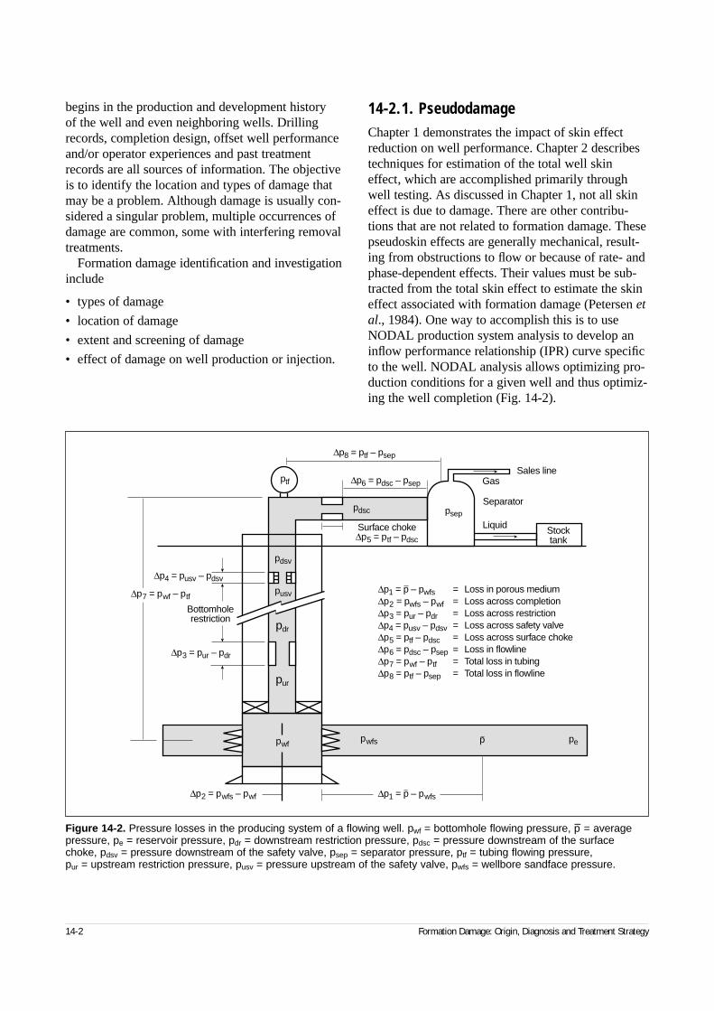
begins in the production and development history of the well and even neighboring wells. Drillingrecords, completion design, offset well performanceand/or operator experiences and past treatmentrecords are all sources of information. The objectiveis to identify the location and types of damage thatmay be a problem. Although damage is usually con-sidered a singular problem, multiple occurrences ofdamage are common, some with interfering removaltreatments.

Formation damage identification and investigationinclude

• types of damage

• location of damage

• extent and screening of damage

• effect of damage on well production or injection.

14-2.1. PseudodamageChapter 1 demonstrates the impact of skin effectreduction on well performance. Chapter 2 describestechniques for estimation of the total well skineffect, which are accomplished primarily throughwell testing. As discussed in Chapter 1, not all skineffect is due to damage. There are other contribu-tions that are not related to formation damage. Thesepseudoskin effects are generally mechanical, result-ing from obstructions to flow or because of rate- andphase-dependent effects. Their values must be sub-tracted from the total skin effect to estimate the skineffect associated with formation damage (Petersen etal., 1984). One way to accomplish this is to useNODAL production system analysis to develop aninflow performance relationship (IPR) curve specificto the well. NODAL analysis allows optimizing pro-duction conditions for a given well and thus optimiz-ing the well completion (Fig. 14-2).

14-2 Formation Damage: Origin, Diagnosis and Treatment Strategy

Figure 14-2. Pressure losses in the producing system of a flowing well. pwf = bottomhole flowing pressure, p– = averagepressure, pe = reservoir pressure, pdr = downstream restriction pressure, pdsc = pressure downstream of the surfacechoke, pdsv = pressure downstream of the safety valve, psep = separator pressure, ptf = tubing flowing pressure, pur = upstream restriction pressure, pusv = pressure upstream of the safety valve, pwfs = wellbore sandface pressure.

∆p1 = p – pwfs = Loss in porous medium∆p2 = pwfs – pwf = Loss across completion∆p3 = pur – pdr = Loss across restriction∆p4 = pusv – pdsv = Loss across safety valve∆p5 = ptf – pdsc = Loss across surface choke∆p6 = pdsc – psep = Loss in flowline∆p7 = pwf – ptf = Total loss in tubing∆p8 = ptf – psep = Total loss in flowline

∆p1 = p – pwfs∆p2 = pwfs – pwf

pwf

pdr

pur

pusv

psep

pdsv

pdsc

ptf

pepwfs p

∆p3 = pur – pdr

∆p7 = pwf – ptf

Bottomholerestriction

∆p4 = pusv – pdsv

Surface choke Liquid

Separator

GasSales line

Stocktank∆p5 = ptf – pdsc

∆p6 = pdsc – psep

∆p8 = ptf – psep

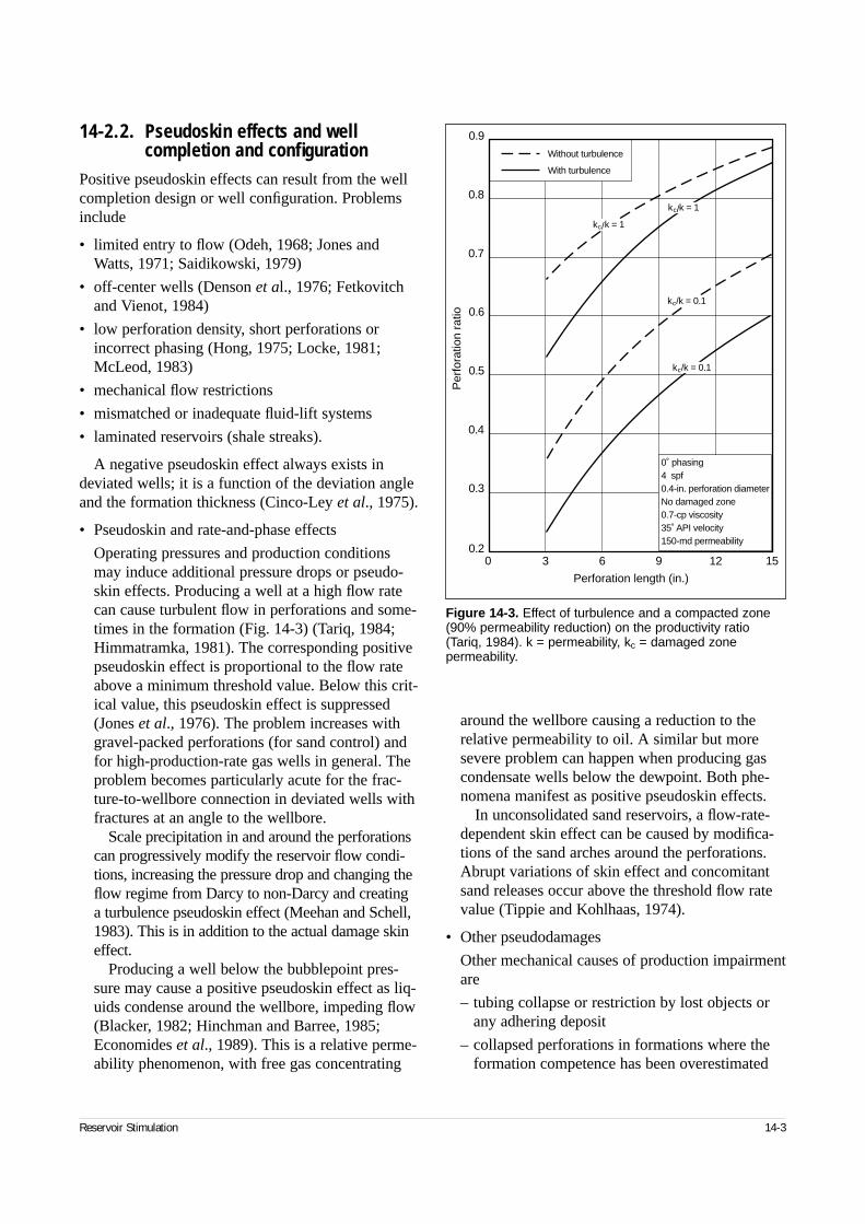
14-2.2. Pseudoskin effects and well completion and configuration

Positive pseudoskin effects can result from the wellcompletion design or well configuration. Problemsinclude

• limited entry to flow (Odeh, 1968; Jones andWatts, 1971; Saidikowski, 1979)

• off-center wells (Denson et al., 1976; Fetkovitchand Vienot, 1984)

• low perforation density, short perforations orincorrect phasing (Hong, 1975; Locke, 1981;McLeod, 1983)

• mechanical flow restrictions

• mismatched or inadequate fluid-lift systems

• laminated reservoirs (shale streaks).

A negative pseudoskin effect always exists indeviated wells; it is a function of the deviation angleand the formation thickness (Cinco-Ley et al., 1975).

• Pseudoskin and rate-and-phase effects

Operating pressures and production conditionsmay induce additional pressure drops or pseudo-skin effects. Producing a well at a high flow ratecan cause turbulent flow in perforations and some-times in the formation (Fig. 14-3) (Tariq, 1984;Himmatramka, 1981). The corresponding positivepseudoskin effect is proportional to the flow rateabove a minimum threshold value. Below this crit-ical value, this pseudoskin effect is suppressed(Jones et al., 1976). The problem increases withgravel-packed perforations (for sand control) andfor high-production-rate gas wells in general. Theproblem becomes particularly acute for the frac-ture-to-wellbore connection in deviated wells withfractures at an angle to the wellbore.

Scale precipitation in and around the perforationscan progressively modify the reservoir flow condi-tions, increasing the pressure drop and changing theflow regime from Darcy to non-Darcy and creating a turbulence pseudoskin effect (Meehan and Schell,1983). This is in addition to the actual damage skineffect.

Producing a well below the bubblepoint pres-sure may cause a positive pseudoskin effect as liq-uids condense around the wellbore, impeding flow(Blacker, 1982; Hinchman and Barree, 1985;Economides et al., 1989). This is a relative perme-ability phenomenon, with free gas concentrating

around the wellbore causing a reduction to therelative permeability to oil. A similar but moresevere problem can happen when producing gascondensate wells below the dewpoint. Both phe-nomena manifest as positive pseudoskin effects.

In unconsolidated sand reservoirs, a flow-rate-dependent skin effect can be caused by modifica-tions of the sand arches around the perforations.Abrupt variations of skin effect and concomitantsand releases occur above the threshold flow ratevalue (Tippie and Kohlhaas, 1974).

• Other pseudodamages

Other mechanical causes of production impairmentare

– tubing collapse or restriction by lost objects orany adhering deposit

– collapsed perforations in formations where theformation competence has been overestimated

Reservoir Stimulation 14-3

Figure 14-3. Effect of turbulence and a compacted zone(90% permeability reduction) on the productivity ratio(Tariq, 1984). k = permeability, kc = damaged zone permeability.

0 3 6 9 12 150.2

0.3

0.4

0.5

0.6

0.7

0.8

0.9

Perforation length (in.)

Per

fora

tion

ratio

Without turbulence

With turbulence

0˚ phasing4 spf0.4-in. perforation diameterNo damaged zone0.7-cp viscosity35˚ API velocity150-md permeability

kc/k = 0.1

kc/k = 0.1

kc/k = 1

kc/k = 1

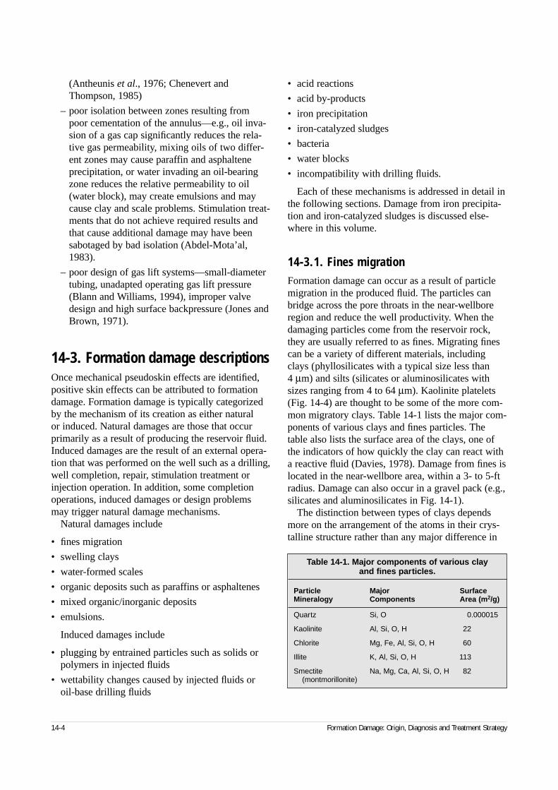
(Antheunis et al., 1976; Chenevert andThompson, 1985)

– poor isolation between zones resulting frompoor cementation of the annulus—e.g., oil inva-sion of a gas cap significantly reduces the rela-tive gas permeability, mixing oils of two differ-ent zones may cause paraffin and asphalteneprecipitation, or water invading an oil-bearingzone reduces the relative permeability to oil(water block), may create emulsions and maycause clay and scale problems. Stimulation treat-ments that do not achieve required results andthat cause additional damage may have beensabotaged by bad isolation (Abdel-Mota’al,1983).

– poor design of gas lift systems—small-diametertubing, unadapted operating gas lift pressure(Blann and Williams, 1994), improper valvedesign and high surface backpressure (Jones andBrown, 1971).

14-3. Formation damage descriptionsOnce mechanical pseudoskin effects are identified,positive skin effects can be attributed to formationdamage. Formation damage is typically categorizedby the mechanism of its creation as either natural or induced. Natural damages are those that occurprimarily as a result of producing the reservoir fluid.Induced damages are the result of an external opera-tion that was performed on the well such as a drilling,well completion, repair, stimulation treatment orinjection operation. In addition, some completionoperations, induced damages or design problemsmay trigger natural damage mechanisms.

Natural damages include

• fines migration

• swelling clays

• water-formed scales

• organic deposits such as paraffins or asphaltenes

• mixed organic/inorganic deposits

• emulsions.

Induced damages include

• plugging by entrained particles such as solids orpolymers in injected fluids

• wettability changes caused by injected fluids oroil-base drilling fluids

• acid reactions

• acid by-products

• iron precipitation

• iron-catalyzed sludges

• bacteria

• water blocks

• incompatibility with drilling fluids.

Each of these mechanisms is addressed in detail inthe following sections. Damage from iron precipita-tion and iron-catalyzed sludges is discussed else-where in this volume.

14-3.1. Fines migrationFormation damage can occur as a result of particlemigration in the produced fluid. The particles canbridge across the pore throats in the near-wellboreregion and reduce the well productivity. When thedamaging particles come from the reservoir rock,they are usually referred to as fines. Migrating finescan be a variety of different materials, includingclays (phyllosilicates with a typical size less than 4 µm) and silts (silicates or aluminosilicates withsizes ranging from 4 to 64 µm). Kaolinite platelets(Fig. 14-4) are thought to be some of the more com-mon migratory clays. Table 14-1 lists the major com-ponents of various clays and fines particles. Thetable also lists the surface area of the clays, one ofthe indicators of how quickly the clay can react witha reactive fluid (Davies, 1978). Damage from fines islocated in the near-wellbore area, within a 3- to 5-ftradius. Damage can also occur in a gravel pack (e.g.,silicates and aluminosilicates in Fig. 14-1).

The distinction between types of clays dependsmore on the arrangement of the atoms in their crys-talline structure rather than any major difference in

14-4 Formation Damage: Origin, Diagnosis and Treatment Strategy

Table 14-1. Major components of various clay and fines particles.

Particle Major SurfaceMineralogy Components Area (m2/g)

Quartz Si, O 0.000015

Kaolinite Al, Si, O, H 22

Chlorite Mg, Fe, Al, Si, O, H 60

Illite K, Al, Si, O, H 113

Smectite Na, Mg, Ca, Al, Si, O, H 82(montmorillonite)

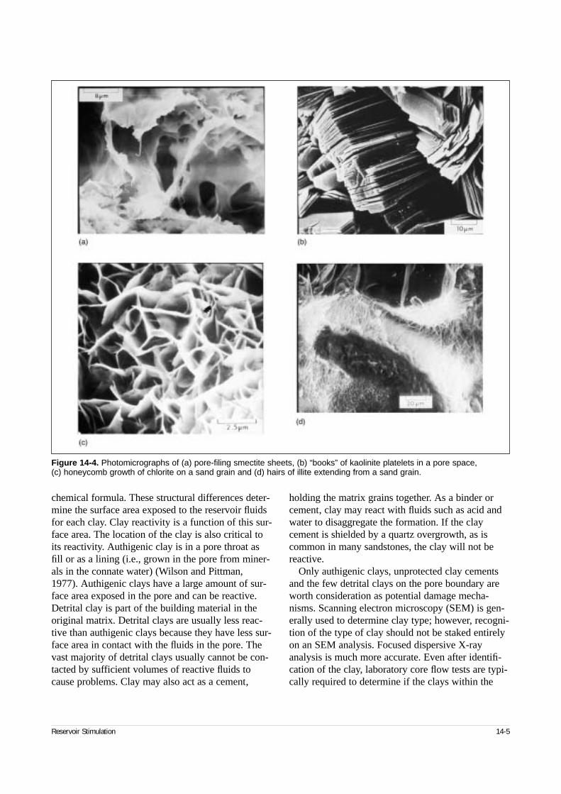
chemical formula. These structural differences deter-mine the surface area exposed to the reservoir fluidsfor each clay. Clay reactivity is a function of this sur-face area. The location of the clay is also critical toits reactivity. Authigenic clay is in a pore throat asfill or as a lining (i.e., grown in the pore from miner-als in the connate water) (Wilson and Pittman,1977). Authigenic clays have a large amount of sur-face area exposed in the pore and can be reactive.Detrital clay is part of the building material in theoriginal matrix. Detrital clays are usually less reac-tive than authigenic clays because they have less sur-face area in contact with the fluids in the pore. Thevast majority of detrital clays usually cannot be con-tacted by sufficient volumes of reactive fluids tocause problems. Clay may also act as a cement,

holding the matrix grains together. As a binder orcement, clay may react with fluids such as acid andwater to disaggregate the formation. If the claycement is shielded by a quartz overgrowth, as iscommon in many sandstones, the clay will not bereactive.

Only authigenic clays, unprotected clay cementsand the few detrital clays on the pore boundary areworth consideration as potential damage mecha-nisms. Scanning electron microscopy (SEM) is gen-erally used to determine clay type; however, recogni-tion of the type of clay should not be staked entirelyon an SEM analysis. Focused dispersive X-rayanalysis is much more accurate. Even after identifi-cation of the clay, laboratory core flow tests are typi-cally required to determine if the clays within the

Reservoir Stimulation 14-5

Figure 14-4. Photomicrographs of (a) pore-filing smectite sheets, (b) “books” of kaolinite platelets in a pore space, (c) honeycomb growth of chlorite on a sand grain and (d) hairs of illite extending from a sand grain.

flow channels are reactive with a given fluid. Thecommon clays that account for most of the real andperceived clay problems are kaolinite, smectite(montmorillonite), illite and chlorite. The structuresof kaolinite, smectite, illite and chlorite are shown inFig. 14-4. Simply because the clay is in the rockdoes not mean that the clay is reactive.

14-3.2. Swelling claysClays may change volume as the salinity of the fluidflowing through the formation changes. Severalauthors have dealt with clay swelling in sandstones,showing either ion exchange, movement or criticalsalt concentration triggering clay dispersion (Azariand Leimkuhler, 1990b; Jones, 1964; Khilar andFogler, 1983; Mungan, 1968; Sharma et al., 1985;Priisholm et al., 1987). Changes in formation perme-ability resulting from the alteration of clay are due tothe amount, location and type of clay minerals with-in the formation. The total quantity of clay inside theformation is a misleading indication of potentialchanges to permeability. It is the arrangement of theclay, its chemical state at the moment of contact andthe location of the clay with respect to the flowingfluids that are responsible for the changes. Predictingthe response of a clay to water flow is almost impos-sible without testing.

The most common swelling clays are smectite andsmectite mixtures. Smectite swells by taking waterinto its structure. It can increase its volume up to600%, significantly reducing permeability. If smec-tite clay occupies only the smaller pore throats andpassages, it will not be a serious problem; however,if it occupies the larger pores and especially the porethroats, then it is capable of creating an almostimpermeable barrier to flow if it swells.

Clays or other solids from drilling, completion orworkover fluids can invade the formation when theseparticles are smaller than the pore throat openings.Any subsequent increase in flow rate through theinvaded zone will force a high concentration of parti-cles into the rock matrix.

14-3.3. ScalesScales are water-soluble chemicals that precipitateout of solution in response to changes in conditionsor the mixing of incompatible waters. They can be

present in the tubing, perforations and formation(Fig. 14-1). The most common oilfield scales are cal-cium carbonate, calcium sulfate and barium sulfate.Water-formed scale deposits are among the mosttroublesome damage problems (Cowen andWeintritt, 1976). Scale usually consists of precipi-tates formed from mixing incompatible waters orupsetting the solution equilibrium of producedwaters. A water that may be stable under reservoirconditions may become supersaturated with an ionwhen the pressure decreases, which allows carbondioxide (CO2) outgassing, or the temperaturechanges. The supersaturated solutions react by pre-cipitating a compound from solution. The depositionof scale is influenced by pressure drop, temperature,dissolved gases, flow viscosity, nucleation sites andmetal type—in short, anything that upsets the solu-tion equilibrium.

The following scales are among the most trouble-some.

• Calcium carbonate or calcite (CaCO3)

CaCO3 is usually formed when the pressure isreduced on waters that are rich in calcium andbicarbonate ions. The deposition can be affected by CO2 outgassing, which raises the pH value andmakes the high concentrations of calcium unstable.

• Gypsum (“gyp”)

Gypsum may be the most common sulfate scale in the oil industry (Cowen and Weintritt, 1976).With a chemical structure of CaSO4 ⋅ 2H2O, itshares a similar composition to the hemihydrateCaSO4 ⋅ 1⁄2H2O, commonly called plaster of parisor by its mineral name, bassonite. It is also formu-laically similar to the evaporite mineral anhydrite(CaSO4).

• Barium sulfate (BaSO4)

BaSO4 is a less common form of sulfate deposit,but it causes extensive problems. Almost any com-bination of barium and sulfate ions causes precipi-tation. It is difficult to remove, as it is not signifi-cantly soluble in acids and solvents unless it isfinely ground or the structure is interrupted withimpurities such as carbonate scale. Like calciumsulfate, barium sulfate is usually thought to be aproduct of mixing incompatible waters, with pre-cipitation accelerated by pressure drop, outgassingor turbulence. Some barium sulfate is radioactive;this is part of naturally occurring radioactive

14-6 Formation Damage: Origin, Diagnosis and Treatment Strategy

material (NORM) scales. The radioactivity resultsfrom a concentration of uranium in the lattice ofthe scale. The buildup of radioactive scale can bemonitored using a gamma ray logging tool. Caremust be exercised when analyzing well debris toavoid mislabeling barite (BaSO4) from drillingmud residue as barium sulfate scale.

Strontium sulfate or celestite (SrSO4) is a com-mon substitute in the barium sulfate crystal lattice.Strontium scale can be associated with radioactivescale (NORM). It may be more soluble than bar-ium sulfate in chemical remover systems.

• Iron scales

Iron scales such as iron carbonate and iron sulfidecan be extremely difficult to remove. They areusually seen in wells that have both a high back-ground iron count and a tendency to precipitatecalcium carbonate. Iron sulfide scales react accord-ing to their structure. Seven different forms of ironsulfide scale have been identified. Only two ofthese iron sulfide forms are readily soluble inhydrochloric acid (HCl). The remaining iron sul-fide scales are either slowly soluble or not signifi-cantly soluble.

• Chloride scales

Chloride scales, such as sodium chloride precipita-tion from water caused by temperature decrease orevaporation of the water, are common. There is noeffective way to prevent salt precipitation, andcleanup has been accomplished using water only.Salt has a limited solubility in acid (1⁄4 lbm/gal in28% HCl), so using acid is not generally consid-ered. Redesigning the mechanical system to avoidtemperature loss and water evaporation is also apossibility.

• Silica scales

Silica scales generally occur as finely crystallizeddeposits of chalcedony or as amorphous opal.They are associated with alkaline or steamfloodprojects and stem from the dissolution of siliceousformation minerals by high-pH fluids (Lieu et al.,1985) or high-temperature steam condensates(Reed, 1980; McCorriston et al., 1981; Amaefuleet al., 1984). This dissolution can cause poorlyconsolidated sandstones to collapse or silica toreprecipitate at a distance from the wellbore wherethe alkalinity, temperature or both of the floods hasdecreased.

14-3.4. Organic depositsOrganic deposits are heavy hydrocarbons (paraffinsor asphaltenes) that precipitate as the pressure ortemperature is reduced. This is a form of distillation.They are typically located in the tubing, perforationsor formation (Fig. 14-1). Although the formationmechanisms of organic deposits are numerous andcomplex (Houchin and Hudson, 1986), the mainmechanism is a change in temperature or pressure in the flowing system. Cooling of the wellbore or theinjection of cold treating fluids has a much more pro-nounced effect.

Organic deposits must not be confused with anoth-er type of deposit called sludge. Sludges are viscousemulsions produced by the reactions between certaincrude oils and strong inorganic acids or some brines.Sludges cannot be easily dissolved.

• Paraffins

Paraffins are the simplest of hydrocarbons. Theyare composed of only carbon and hydrogen atoms,and the carbons occur as an unbranched chain.Carbon chain length associated with formation ofsolid paraffin deposits has a minimum of 16 car-bon atoms per molecule and may have up to 60 ormore. The precipitation of paraffins is triggered bya loss of pressure, loss of temperature or loss ofshort-chain hydrocarbon compounds (i.e., the lightends). The temperature at which the first solidparaffin crystal forms from an all-liquid solution is called the cloud point. Designing the completionso that produced fluid surface temperatures areabove the cloud point and modifying the cloudpoint using chemical methods are accepted prac-tices to prevent paraffin deposition in the tubing.

Melting points increase as the length of theparaffin chain increases. The hardness of the solidparaffin structure also increases with molecularsize. Table 14-2 lists several paraffin chain lengthsand their melting points. Impurities may cause themelting point of a field sample to vary slightly.

Paraffins can form anywhere in the producingsystem when conditions become favorable for pre-cipitation (Cole and Jessen, 1960; Burger et al.,1981; Newberry et al., 1986; Thomas, 1988;Newberry, 1981; Sutton and Roberts, 1974).Paraffins are normally found in the tubing near thesurface, where the temperature and pressure dropsare highest. In cases such as reservoirs that are

Reservoir Stimulation 14-7

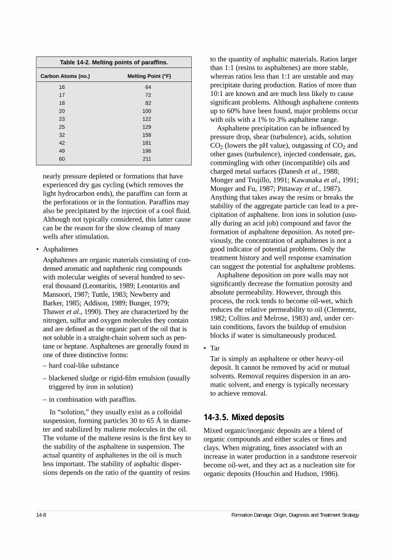
nearly pressure depleted or formations that haveexperienced dry gas cycling (which removes thelight hydrocarbon ends), the paraffins can form atthe perforations or in the formation. Paraffins mayalso be precipitated by the injection of a cool fluid.Although not typically considered, this latter causecan be the reason for the slow cleanup of manywells after stimulation.

• Asphaltenes

Asphaltenes are organic materials consisting of con-densed aromatic and naphthenic ring compoundswith molecular weights of several hundred to sev-eral thousand (Leontaritis, 1989; Leontaritis andMansoori, 1987; Tuttle, 1983; Newberry andBarker, 1985; Addison, 1989; Bunger, 1979;Thawer et al., 1990). They are characterized by thenitrogen, sulfur and oxygen molecules they containand are defined as the organic part of the oil that isnot soluble in a straight-chain solvent such as pen-tane or heptane. Asphaltenes are generally found inone of three distinctive forms:

– hard coal-like substance

– blackened sludge or rigid-film emulsion (usuallytriggered by iron in solution)

– in combination with paraffins.

In “solution,” they usually exist as a colloidalsuspension, forming particles 30 to 65 Å in diame-ter and stabilized by maltene molecules in the oil.The volume of the maltene resins is the first key tothe stability of the asphaltene in suspension. Theactual quantity of asphaltenes in the oil is muchless important. The stability of asphaltic disper-sions depends on the ratio of the quantity of resins

to the quantity of asphaltic materials. Ratios largerthan 1:1 (resins to asphaltenes) are more stable,whereas ratios less than 1:1 are unstable and mayprecipitate during production. Ratios of more than10:1 are known and are much less likely to causesignificant problems. Although asphaltene contentsup to 60% have been found, major problems occurwith oils with a 1% to 3% asphaltene range.

Asphaltene precipitation can be influenced bypressure drop, shear (turbulence), acids, solutionCO2 (lowers the pH value), outgassing of CO2 andother gases (turbulence), injected condensate, gas,commingling with other (incompatible) oils andcharged metal surfaces (Danesh et al., 1988;Monger and Trujillo, 1991; Kawanaka et al., 1991;Monger and Fu, 1987; Pittaway et al., 1987).Anything that takes away the resins or breaks thestability of the aggregate particle can lead to a pre-cipitation of asphaltene. Iron ions in solution (usu-ally during an acid job) compound and favor theformation of asphaltene deposition. As noted pre-viously, the concentration of asphaltenes is not agood indicator of potential problems. Only thetreatment history and well response examinationcan suggest the potential for asphaltene problems.

Asphaltene deposition on pore walls may notsignificantly decrease the formation porosity andabsolute permeability. However, through thisprocess, the rock tends to become oil-wet, whichreduces the relative permeability to oil (Clementz,1982; Collins and Melrose, 1983) and, under cer-tain conditions, favors the buildup of emulsionblocks if water is simultaneously produced.

• Tar

Tar is simply an asphaltene or other heavy-oildeposit. It cannot be removed by acid or mutualsolvents. Removal requires dispersion in an aro-matic solvent, and energy is typically necessary to achieve removal.

14-3.5. Mixed depositsMixed organic/inorganic deposits are a blend oforganic compounds and either scales or fines andclays. When migrating, fines associated with anincrease in water production in a sandstone reservoirbecome oil-wet, and they act as a nucleation site fororganic deposits (Houchin and Hudson, 1986).

14-8 Formation Damage: Origin, Diagnosis and Treatment Strategy

Table 14-2. Melting points of paraffins.

Carbon Atoms (no.) Melting Point (°F)

16 64

17 72

18 82

20 100

23 122

25 129

32 158

42 181

49 196

60 211

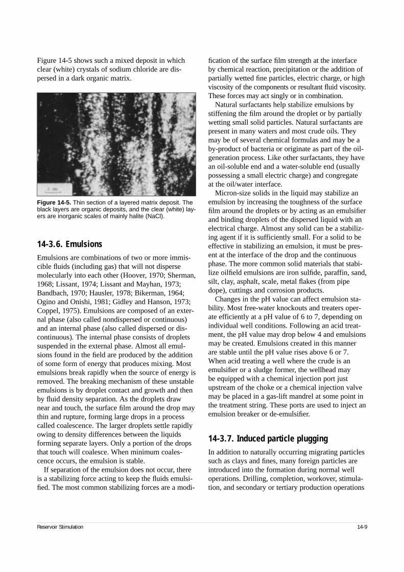
Figure 14-5 shows such a mixed deposit in whichclear (white) crystals of sodium chloride are dis-persed in a dark organic matrix.

14-3.6. EmulsionsEmulsions are combinations of two or more immis-cible fluids (including gas) that will not dispersemolecularly into each other (Hoover, 1970; Sherman,1968; Lissant, 1974; Lissant and Mayhan, 1973;Bandbach, 1970; Hausler, 1978; Bikerman, 1964;Ogino and Onishi, 1981; Gidley and Hanson, 1973;Coppel, 1975). Emulsions are composed of an exter-nal phase (also called nondispersed or continuous)and an internal phase (also called dispersed or dis-continuous). The internal phase consists of dropletssuspended in the external phase. Almost all emul-sions found in the field are produced by the additionof some form of energy that produces mixing. Mostemulsions break rapidly when the source of energy isremoved. The breaking mechanism of these unstableemulsions is by droplet contact and growth and thenby fluid density separation. As the droplets drawnear and touch, the surface film around the drop maythin and rupture, forming large drops in a processcalled coalescence. The larger droplets settle rapidlyowing to density differences between the liquidsforming separate layers. Only a portion of the dropsthat touch will coalesce. When minimum coales-cence occurs, the emulsion is stable.

If separation of the emulsion does not occur, thereis a stabilizing force acting to keep the fluids emulsi-fied. The most common stabilizing forces are a modi-

fication of the surface film strength at the interface by chemical reaction, precipitation or the addition ofpartially wetted fine particles, electric charge, or highviscosity of the components or resultant fluid viscosity.These forces may act singly or in combination.

Natural surfactants help stabilize emulsions bystiffening the film around the droplet or by partiallywetting small solid particles. Natural surfactants arepresent in many waters and most crude oils. Theymay be of several chemical formulas and may be aby-product of bacteria or originate as part of the oil-generation process. Like other surfactants, they havean oil-soluble end and a water-soluble end (usuallypossessing a small electric charge) and congregate at the oil/water interface.

Micron-size solids in the liquid may stabilize anemulsion by increasing the toughness of the surfacefilm around the droplets or by acting as an emulsifierand binding droplets of the dispersed liquid with anelectrical charge. Almost any solid can be a stabiliz-ing agent if it is sufficiently small. For a solid to beeffective in stabilizing an emulsion, it must be pres-ent at the interface of the drop and the continuousphase. The more common solid materials that stabi-lize oilfield emulsions are iron sulfide, paraffin, sand,silt, clay, asphalt, scale, metal flakes (from pipedope), cuttings and corrosion products.

Changes in the pH value can affect emulsion sta-bility. Most free-water knockouts and treaters oper-ate efficiently at a pH value of 6 to 7, depending onindividual well conditions. Following an acid treat-ment, the pH value may drop below 4 and emulsionsmay be created. Emulsions created in this mannerare stable until the pH value rises above 6 or 7.When acid treating a well where the crude is anemulsifier or a sludge former, the wellhead may be equipped with a chemical injection port justupstream of the choke or a chemical injection valvemay be placed in a gas-lift mandrel at some point inthe treatment string. These ports are used to inject anemulsion breaker or de-emulsifier.

14-3.7. Induced particle pluggingIn addition to naturally occurring migrating particlessuch as clays and fines, many foreign particles areintroduced into the formation during normal welloperations. Drilling, completion, workover, stimula-tion, and secondary or tertiary production operations

Reservoir Stimulation 14-9

Figure 14-5. Thin section of a layered matrix deposit. Theblack layers are organic deposits, and the clear (white) lay-ers are inorganic scales of mainly halite (NaCl).

can cause the injection of extraneous particles intothe formation.

Particle damage from injected fluids happens in thenear-wellbore area, plugging formation pore throats.Problems include bridging of the pores, packing ofperforations and the loss of large amounts of high-solids fluid into natural fractures or propped fracturesystems. The best method of avoiding this type ofdamage is to use a clean fluid in a clean flow systemwith a controlled range of particle sizes that will stopfluid loss quickly by bridging at the wellbore.

Induced particles can be composed of a widerange of materials. Particulate materials in drillingfluids that are potentially damaging are clays, cut-tings, weighting agents and loss-control materials,including polymers (Barna and Patton, 1972; Fisheret al., 1973; Sloan et al., 1975). These materials canbe a problem independent of mud type (oil, water orpolymer base). Workover and stimulation fluids canalso contain suspended solids (Rike, 1980; Rike andPledger, 1981) including bacteria and polymerresidues (Tuttle and Barkman, 1974). Kill fluids inparticular use various polymers as weighting agentsor for fluid-loss control. Typical kill-fluid solidsinclude salt pills with polymer, crosslinked poly-mers, hydroxyethylcellulose (HEC) polymers, lost-circulation pills and CaCO3 with polymer.

Particles in stimulation fluids are a result of poorwater quality, tank coatings, tank residuals, and pip-ing and tubing debris (e.g., dried mud, scale and pipedope). The problem with stimulation fluids is thatthey can contain effective cleaners and acids that dis-perse and partially dissolve the debris inside of thetanks and piping on their way to the formation.

Particle damage after stimulation may also occurwhen partially dissolved parts of the formation or thedamage materials come back, through either thepores or the natural fracture or propped fracture sys-tem. The release of fines from the formation is usu-ally brought about by cleaners and mutual solvents.Acid treatments may also cause formation damagebecause of the precipitation of secondary acid reac-tion products. Precipitation products include ironhydroxide, calcium fluoride, potassium fluorsilicateand silica.

Geochemical models can predict the chemicalnature of these by-products, depending on formationrock and treatment fluid compositions on one handand pressure, temperature and contact time on theother (Walsh et al., 1982; Dria et al., 1988). The

models cannot predict the damaging potential ofthese products because they do not include any phys-ical description of the way they are precipitated.Hydrated silica (Crowe, 1985) may precipitate onclay surfaces but is not necessarily damaging. Com-pounds such as borosilicates (Thomas and Crowe,1978) and fluoborates (Bertaux, 1989) can even bebeneficial, probably because they precipitate as filmsthat bind fines to the sand grains. This phenomenon,when purposely produced, leads to efficient fines-stabilization treatments (Thomas and Crowe, 1978;Sharma and Sharma, 1994). However, gelatinousprecipitates, such as ferric hydroxide, can completelyplug pores and can be particularly difficult to remove(Crowe, 1985). Another class of by-products consistsof species such as fluorsilicates (Bertaux, 1989),which precipitate in the form of individual crystalsthat can migrate toward pore throats and produce a“log jam.” Iron sulfide, which precipitates even at lowpH values during the acid treatment of sour wells, isanother compound belonging to this category.

14-3.8. Wettability alterationFormation plugging can be caused by liquid (or gas)changing the relative permeability of the formationrock. Relative permeability can reduce the effectivepermeability of a formation to a particular fluid by asmuch as 80% to 90%. The wettability and relatedrelative permeability of a formation are determinedby the flowing-phase quantity and by coatings of nat-ural and injected surfactants and oils.

If a drop of a liquid is placed on the surface ofanother immiscible liquid or on the surface of a solidthat it cannot dissolve, it may spread out into a thinfilm or it may remain in the form of a drop or a thicklens (Hausler, 1978). If the drop of liquid spreads, itwets the surface; if the drop of liquid does notspread, it does not wet the surface. The surface freeenergy of the two phases and the interfacial tensionbetween them determine whether the liquid spreadsor remains in a deformed drop. Wettability is mea-sured by the contact angle that a droplet of fluidforms on a particular surface. If the angle of contactθ is less than 90°, the drop spreads from the initialball shape and the surface is said to be wetted by theliquid. The smaller the angle, the greater the waterwettability. If the angle is more than 90°, the surfaceis not wetted by the liquid. Wettability can be mea-

14-10 Formation Damage: Origin, Diagnosis and Treatment Strategy

sured with a liquid surrounded by gas or a liquid sur-rounded by an immiscible liquid. Simple wetting haslittle meaning—it is the resultant effect of wetting onfluid flow that is important.

In the natural state, formations may be water-wet,oil-wet or neutral, depending both on the surfaceexposed to the fluid and the natural surfactants in thefluid. There are some instances, such as the Cardiumreservoir in Alberta, Canada, where both oil- andwater-wetting behavior have been reported in differ-ent sections of the reservoir.

When a surface of a pore passage is oil-wet, moreof the passage is occupied by the bound oil (thickermonomolecular layer), and less of the pore is open to flow than in a water-wet pore. Naturally, to get asmuch flow capacity as possible in a formation, it isdesirable to change the wettability to water-wet (inmost cases). Unfortunately, it is impossible to changemost naturally oil-wet surfaces for long. Wettabilitycan be modified by preflushing the formation with awetting surfactant or a solvent that establishes a newcoating on the face of the formation or cleans thecurrent coating from the formation. Regardless of thealtered condition of a surface, the wettability is even-tually decided by the surfactants in the producedfluid. Thus, the water-wet condition of a formationfollowing an acid job can revert to an oil-wet condi-tion after a sufficient volume of strongly oil-wettingcrude is produced.

14-3.9. Acid reactions and acid reaction by-products

Numerous problems that may occur during acidizingtreatments include

• damaging material from the tubing entering theformation

• oil-wetting of the reservoir by surfactants, espe-cially corrosion inhibitors, which can create emul-sion blocks

• water blocks

• asphaltene or paraffin deposition when large vol-umes of acid are injected.

In addition to these common damaging processes,production impairment can result from poor designof an acidizing treatment. Impairments include thefollowing:

• sludges produced by the reaction between acidsand asphaltenes, especially in the presence ofsome additives (particularly surfactants) or dis-solved iron

• by-products precipitated by the reaction of acidswith formation materials. Geochemical simulatorscan predict the chemical nature of the by-products,depending on the formation rock and treatmentfluid compositions and the pressure and tempera-ture. Simulators cannot predict the damagingpotential of the by-products. Hydrated silica mayprecipitate on clay surfaces and is not necessarilydamaging. Compounds such as borosilicates andfluoborates can even be beneficial. Gelatinous pre-cipitates, such as ferric oxide, can completely plugpores and be particularly difficult to remove.Another class of by-products consists of speciessuch as fluorsilicates precipitating in the form ofindividual crystals that can migrate toward porethroats and then bridge in the throats. Iron sulfidethat precipitates, even at very low pH values dur-ing the acidization of sour wells, is another com-pound belonging to this category.

• precipitates formed by the addition of certainsequestering agents to acids to prevent iron prob-lems when the acid is spent and no iron is present

• permeability impairment by residues present incorrosion inhibitors or produced through the ther-mal degradation of polymers, such as frictionreducers.

14-3.10. BacteriaAlthough many microorganisms can be present inthe unsterile world of the oilfield, only a handfulproduce widespread problems (Shuler et al., 1995;Clementz et al., 1982; Crowe, 1968; Carlson et al.,1961; Raleigh and Flock, 1965). Bacteria can be aserious problem in production operations because ofwhat they consume and their by-products. Bacteriacan grow in many different environments and condi-tions: temperatures ranging from 12°F to greaterthan 250°F [–11° to >120°C], pH values rangingfrom 1 to 11, salinities to 30% and pressures to25,000 psi.

Bacteria are classified as follows:

• Aerobic bacteria are bacteria that require oxygen.

Reservoir Stimulation 14-11

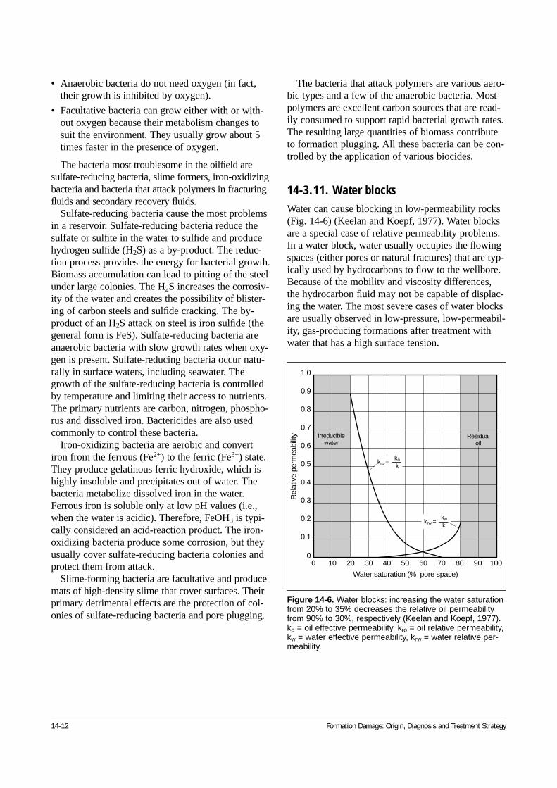
• Anaerobic bacteria do not need oxygen (in fact,their growth is inhibited by oxygen).

• Facultative bacteria can grow either with or with-out oxygen because their metabolism changes tosuit the environment. They usually grow about 5times faster in the presence of oxygen.

The bacteria most troublesome in the oilfield aresulfate-reducing bacteria, slime formers, iron-oxidizingbacteria and bacteria that attack polymers in fracturingfluids and secondary recovery fluids.

Sulfate-reducing bacteria cause the most problemsin a reservoir. Sulfate-reducing bacteria reduce thesulfate or sulfite in the water to sulfide and producehydrogen sulfide (H2S) as a by-product. The reduc-tion process provides the energy for bacterial growth.Biomass accumulation can lead to pitting of the steelunder large colonies. The H2S increases the corrosiv-ity of the water and creates the possibility of blister-ing of carbon steels and sulfide cracking. The by-product of an H2S attack on steel is iron sulfide (thegeneral form is FeS). Sulfate-reducing bacteria areanaerobic bacteria with slow growth rates when oxy-gen is present. Sulfate-reducing bacteria occur natu-rally in surface waters, including seawater. Thegrowth of the sulfate-reducing bacteria is controlledby temperature and limiting their access to nutrients.The primary nutrients are carbon, nitrogen, phospho-rus and dissolved iron. Bactericides are also usedcommonly to control these bacteria.

Iron-oxidizing bacteria are aerobic and convertiron from the ferrous (Fe2+) to the ferric (Fe3+) state.They produce gelatinous ferric hydroxide, which ishighly insoluble and precipitates out of water. Thebacteria metabolize dissolved iron in the water.Ferrous iron is soluble only at low pH values (i.e.,when the water is acidic). Therefore, FeOH3 is typi-cally considered an acid-reaction product. The iron-oxidizing bacteria produce some corrosion, but theyusually cover sulfate-reducing bacteria colonies andprotect them from attack.

Slime-forming bacteria are facultative and producemats of high-density slime that cover surfaces. Theirprimary detrimental effects are the protection of col-onies of sulfate-reducing bacteria and pore plugging.

The bacteria that attack polymers are various aero-bic types and a few of the anaerobic bacteria. Mostpolymers are excellent carbon sources that are read-ily consumed to support rapid bacterial growth rates.The resulting large quantities of biomass contributeto formation plugging. All these bacteria can be con-trolled by the application of various biocides.

14-3.11. Water blocksWater can cause blocking in low-permeability rocks(Fig. 14-6) (Keelan and Koepf, 1977). Water blocksare a special case of relative permeability problems.In a water block, water usually occupies the flowingspaces (either pores or natural fractures) that are typ-ically used by hydrocarbons to flow to the wellbore.Because of the mobility and viscosity differences,the hydrocarbon fluid may not be capable of displac-ing the water. The most severe cases of water blocksare usually observed in low-pressure, low-permeabil-ity, gas-producing formations after treatment withwater that has a high surface tension.

14-12 Formation Damage: Origin, Diagnosis and Treatment Strategy

Figure 14-6. Water blocks: increasing the water saturationfrom 20% to 35% decreases the relative oil permeabilityfrom 90% to 30%, respectively (Keelan and Koepf, 1977).ko = oil effective permeability, kro = oil relative permeability,kw = water effective permeability, krw = water relative per-meability.

krw =kw

k

Irreduciblewater

Residualoil

00

0.1

0.2

0.3

0.4

0.5

0.6

0.7

0.8

0.9

1.0

10 20 30 40 50 60 70 80 90 100

Water saturation (% pore space)

Rel

ativ

e pe

rmea

bilit

y

kro =ko

k

14-3.12. Oil-base drilling fluidsOil-base mud (OBM) is the drilling fluid of choicefor the lubricity required in many highly deviatedwells and for formations that are extremely sensitiveto water-base mud (WBM). Most OBMs, and partic-ularly those with densities greater than 14 lbm/gal,contain sufficient solids to create silt-stabilizedemulsions when mixed with high-salinity brines oracids. These emulsions are viscous and resist break-ing. Some of these emulsions have been shown to bestable for several months, both in the laboratory andin the wellbore. The level of damage caused by theseemulsions can be so severe that an entire pay zonecan be missed. For example, in a South Texas wellthe OBM emulsion created damage so severe thatalmost no flow from the well could be measured.When the damage was removed, the well tested atmore than 12 MMscf/D.

A related problem with OBM is the relative per-meability effects commonly created by the powerfulwetting surfactants used for creating stable OBM.When these materials coat or adsorb onto the forma-tion, the wettability of the formation is altered, andpermeabilities may be only 10% to 20% of whatthey were initially. The most severe problems usuallyoccur with muds weighing more than 14 lbm/gal. The main cause of problems is oil-wetting of thefines from weighting and viscosifying agents andfrom cuttings.

14-4. Origins of formation damageThis section describes the origins of formation dam-age and reviews typical well operations, includingdrilling, cementing, completion, gravel packing, pro-duction, stimulation and injection for enhanced oilrecovery. All are potential sources of damage.Damage is also commonly categorized by its associ-ated well operation (Tables 14-3, 14-4 and 14-5).

14-4.1. Drilling• Mud solids invasion

Mud solids can progressively fill the porosity of the reservoir rock if forced into the pay zone.Subsequent attempts to start production or injec-tion at moderate or high flow rates may cause

these materials to bridge and severely decrease thepermeability of the near-wellbore area.

Such damaging processes are usually limited tothe first few inches around the wellbore (an aver-age value of 3 in. is commonly used), but theresultant permeability reduction can be as high as90%. Invasion of formation rock by drilling fluidsolids is favored by

– large pore size of the formation rock (Brownsonet al., 1980)

– presence of fissures and natural fractures in thereservoir

– small particle size of the solid components of the drilling fluid (the initial particle size ofweighting agents and lost-circulation preventersis usually coarse but can be fragmented by thedrill bit) (Abrams, 1977)

– low drilling rate resulting in mudcake destruc-tion (mud-loss increase) and long formation-to-mud contact time

– high drilling fluid circulation rate (mudcakeerosion)

– high drilling fluid density causing large over-balance pressure (Givens, 1976)

– scraping of mudcake, provoking pressure surgesand increasing formation-to-mud contact timeduring bit trips (Records, 1976).

Using clear brines (containing no particulatematerials) as drilling fluids minimizes formationinvasion by fines but may create a large loss of flu-ids in the rock matrix.

When drilling a formation with natural fractures,some mud loss is expected in the natural fracturesystem. Because natural fractures are important toreservoir flow, avoiding loss of mud to the fracturesystem by using a high-quality fluid-loss controlsystem is crucial. If the natural fractures arealready damaged by mud, the success of thecleanout will depend on how much mud was lostand the type and condition of the mud when it waslost. If a low-solids mud was used in a systemwith minimal overbalance, little damage may haveoccurred. If a high-weight mud system with a largeamount of fines was used or if the drilling over-balance was high (more than 2 lbm/gal overbalanceequivalent), damage may be severe.

Reservoir Stimulation 14-13

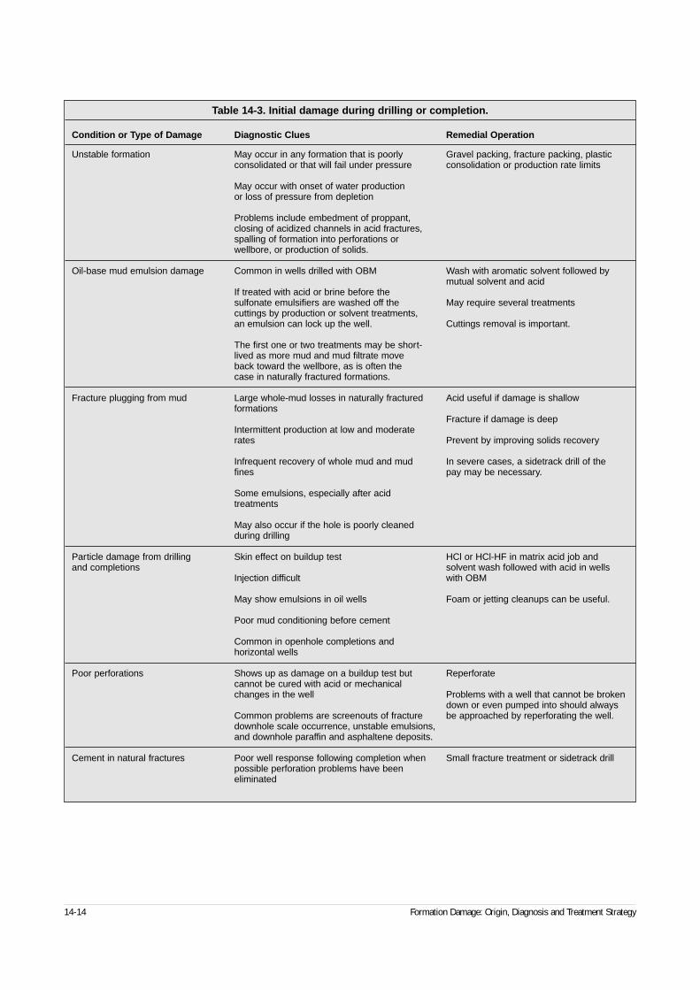
14-14 Formation Damage: Origin, Diagnosis and Treatment Strategy

Table 14-3. Initial damage during drilling or completion.

Condition or Type of Damage Diagnostic Clues Remedial Operation

Unstable formation May occur in any formation that is poorly Gravel packing, fracture packing, plastic consolidated or that will fail under pressure consolidation or production rate limits

May occur with onset of water production or loss of pressure from depletion

Problems include embedment of proppant, closing of acidized channels in acid fractures,spalling of formation into perforations orwellbore, or production of solids.

Oil-base mud emulsion damage Common in wells drilled with OBM Wash with aromatic solvent followed bymutual solvent and acid

If treated with acid or brine before thesulfonate emulsifiers are washed off the May require several treatmentscuttings by production or solvent treatments,an emulsion can lock up the well. Cuttings removal is important.

The first one or two treatments may be short-lived as more mud and mud filtrate move back toward the wellbore, as is often the case in naturally fractured formations.

Fracture plugging from mud Large whole-mud losses in naturally fractured Acid useful if damage is shallowformations

Fracture if damage is deepIntermittent production at low and moderate rates Prevent by improving solids recovery

Infrequent recovery of whole mud and mud In severe cases, a sidetrack drill of the fines pay may be necessary.

Some emulsions, especially after acidtreatments

May also occur if the hole is poorly cleaned during drilling

Particle damage from drilling Skin effect on buildup test HCl or HCl-HF in matrix acid job andand completions solvent wash followed with acid in wells

Injection difficult with OBM

May show emulsions in oil wells Foam or jetting cleanups can be useful.

Poor mud conditioning before cement

Common in openhole completions and horizontal wells

Poor perforations Shows up as damage on a buildup test but Reperforatecannot be cured with acid or mechanical changes in the well Problems with a well that cannot be broken

down or even pumped into should always Common problems are screenouts of fracture be approached by reperforating the well.downhole scale occurrence, unstable emulsions,and downhole paraffin and asphaltene deposits.

Cement in natural fractures Poor well response following completion when Small fracture treatment or sidetrack drillpossible perforation problems have been eliminated

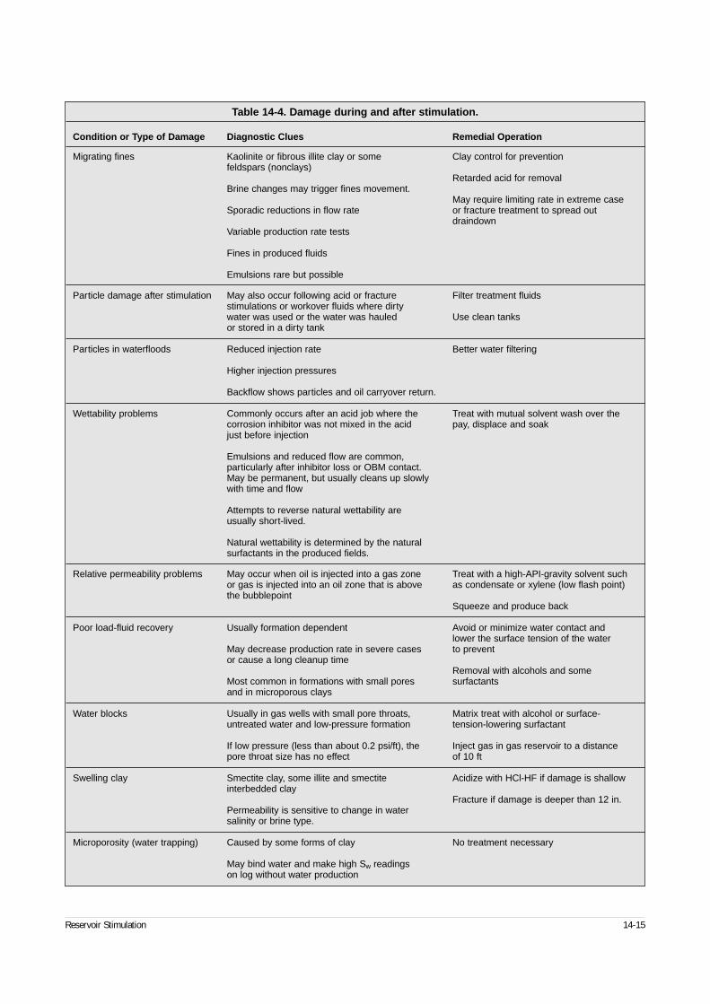
Reservoir Stimulation 14-15

Table 14-4. Damage during and after stimulation.

Condition or Type of Damage Diagnostic Clues Remedial Operation

Migrating fines Kaolinite or fibrous illite clay or some Clay control for preventionfeldspars (nonclays)

Retarded acid for removalBrine changes may trigger fines movement.

May require limiting rate in extreme case Sporadic reductions in flow rate or fracture treatment to spread out

draindownVariable production rate tests

Fines in produced fluids

Emulsions rare but possible

Particle damage after stimulation May also occur following acid or fracture Filter treatment fluidsstimulations or workover fluids where dirty water was used or the water was hauled Use clean tanksor stored in a dirty tank

Particles in waterfloods Reduced injection rate Better water filtering

Higher injection pressures

Backflow shows particles and oil carryover return.

Wettability problems Commonly occurs after an acid job where the Treat with mutual solvent wash over thecorrosion inhibitor was not mixed in the acid pay, displace and soakjust before injection

Emulsions and reduced flow are common, particularly after inhibitor loss or OBM contact.May be permanent, but usually cleans up slowly with time and flow

Attempts to reverse natural wettability are usually short-lived.

Natural wettability is determined by the natural surfactants in the produced fields.

Relative permeability problems May occur when oil is injected into a gas zone Treat with a high-API-gravity solvent suchor gas is injected into an oil zone that is above as condensate or xylene (low flash point)the bubblepoint

Squeeze and produce back

Poor load-fluid recovery Usually formation dependent Avoid or minimize water contact andlower the surface tension of the water

May decrease production rate in severe cases to preventor cause a long cleanup time

Removal with alcohols and some Most common in formations with small pores surfactantsand in microporous clays

Water blocks Usually in gas wells with small pore throats, Matrix treat with alcohol or surface-untreated water and low-pressure formation tension-lowering surfactant

If low pressure (less than about 0.2 psi/ft), the Inject gas in gas reservoir to a distancepore throat size has no effect of 10 ft

Swelling clay Smectite clay, some illite and smectite Acidize with HCl-HF if damage is shallowinterbedded clay

Fracture if damage is deeper than 12 in.Permeability is sensitive to change in water salinity or brine type.

Microporosity (water trapping) Caused by some forms of clay No treatment necessary

May bind water and make high Sw readingson log without water production

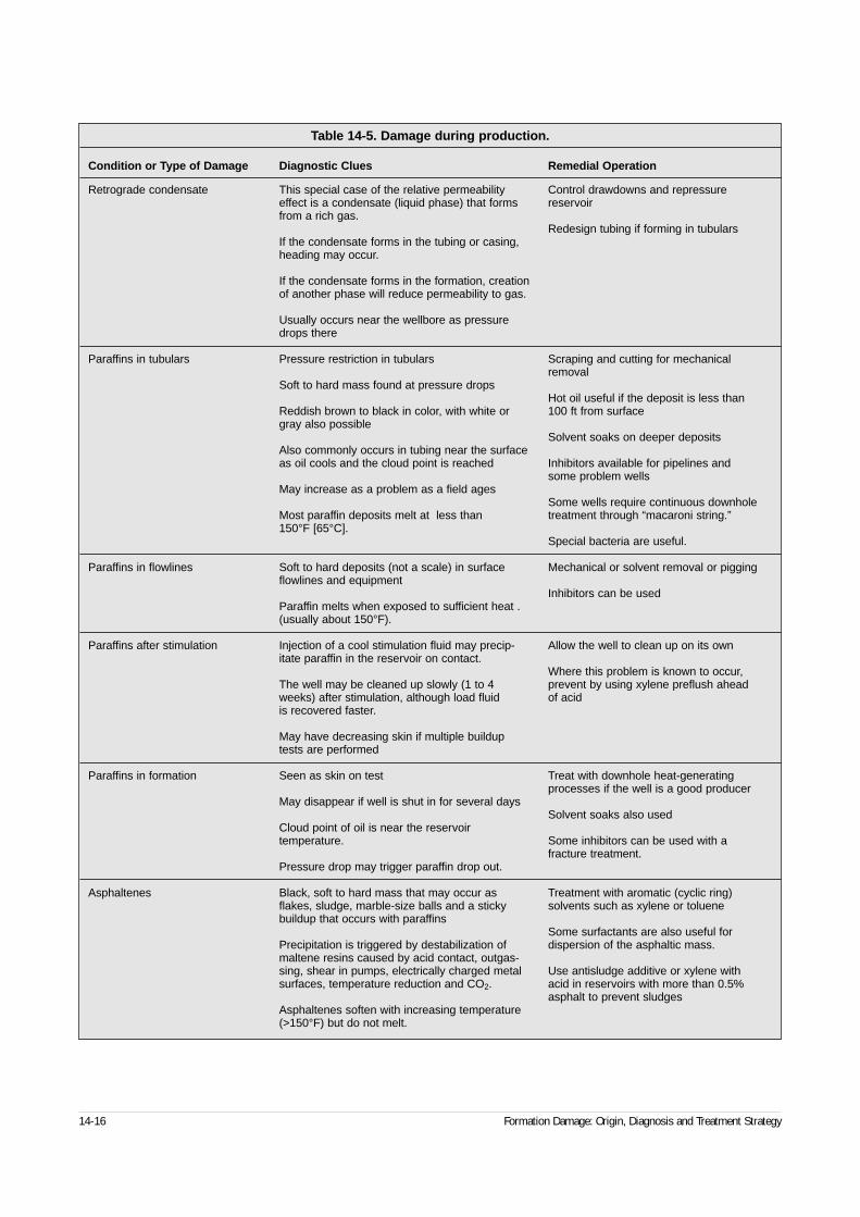
14-16 Formation Damage: Origin, Diagnosis and Treatment Strategy

Table 14-5. Damage during production.

Condition or Type of Damage Diagnostic Clues Remedial Operation

Retrograde condensate This special case of the relative permeability Control drawdowns and repressure effect is a condensate (liquid phase) that forms reservoirfrom a rich gas.

Redesign tubing if forming in tubularsIf the condensate forms in the tubing or casing, heading may occur.

If the condensate forms in the formation, creation of another phase will reduce permeability to gas.

Usually occurs near the wellbore as pressure drops there

Paraffins in tubulars Pressure restriction in tubulars Scraping and cutting for mechanical removal

Soft to hard mass found at pressure drops

Reddish brown to black in color, with white or Hot oil useful if the deposit is less than

gray also possible100 ft from surface

Also commonly occurs in tubing near the surface Solvent soaks on deeper deposits

as oil cools and the cloud point is reached Inhibitors available for pipelines and

May increase as a problem as a field agessome problem wells

Most paraffin deposits melt at less thanSome wells require continuous downhole

150°F [65°C].treatment through “macaroni string.”

Special bacteria are useful.

Paraffins in flowlines Soft to hard deposits (not a scale) in surface Mechanical or solvent removal or piggingflowlines and equipment

Inhibitors can be usedParaffin melts when exposed to sufficient heat .(usually about 150°F).

Paraffins after stimulation Injection of a cool stimulation fluid may precip- Allow the well to clean up on its ownitate paraffin in the reservoir on contact.

Where this problem is known to occur,The well may be cleaned up slowly (1 to 4 prevent by using xylene preflush aheadweeks) after stimulation, although load fluid of acidis recovered faster.

May have decreasing skin if multiple buildup tests are performed

Paraffins in formation Seen as skin on test Treat with downhole heat-generatingprocesses if the well is a good producer

May disappear if well is shut in for several daysSolvent soaks also used

Cloud point of oil is near the reservoir temperature. Some inhibitors can be used with a

fracture treatment.Pressure drop may trigger paraffin drop out.

Asphaltenes Black, soft to hard mass that may occur as Treatment with aromatic (cyclic ring)flakes, sludge, marble-size balls and a sticky solvents such as xylene or toluenebuildup that occurs with paraffins

Some surfactants are also useful forPrecipitation is triggered by destabilization of dispersion of the asphaltic mass.maltene resins caused by acid contact, outgas-sing, shear in pumps, electrically charged metal Use antisludge additive or xylene withsurfaces, temperature reduction and CO2. acid in reservoirs with more than 0.5%

asphalt to prevent sludgesAsphaltenes soften with increasing temperature (>150°F) but do not melt.

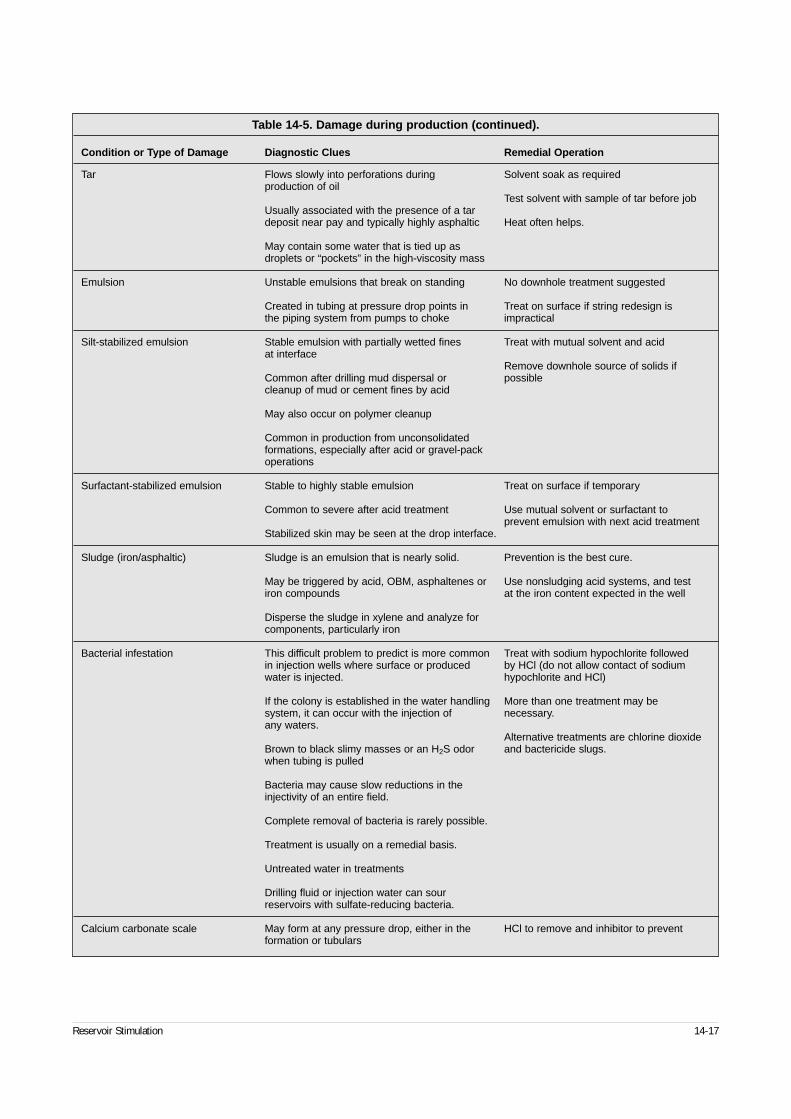
Reservoir Stimulation 14-17

Table 14-5. Damage during production (continued).

Condition or Type of Damage Diagnostic Clues Remedial Operation

Tar Flows slowly into perforations during Solvent soak as requiredproduction of oil

Test solvent with sample of tar before jobUsually associated with the presence of a tardeposit near pay and typically highly asphaltic Heat often helps.

May contain some water that is tied up as droplets or “pockets” in the high-viscosity mass

Emulsion Unstable emulsions that break on standing No downhole treatment suggested

Created in tubing at pressure drop points in Treat on surface if string redesign is the piping system from pumps to choke impractical

Silt-stabilized emulsion Stable emulsion with partially wetted fines Treat with mutual solvent and acidat interface

Remove downhole source of solids if Common after drilling mud dispersal or possiblecleanup of mud or cement fines by acid

May also occur on polymer cleanup

Common in production from unconsolidated formations, especially after acid or gravel-packoperations

Surfactant-stabilized emulsion Stable to highly stable emulsion Treat on surface if temporary

Common to severe after acid treatment Use mutual solvent or surfactant to prevent emulsion with next acid treatment

Stabilized skin may be seen at the drop interface.

Sludge (iron/asphaltic) Sludge is an emulsion that is nearly solid. Prevention is the best cure.

May be triggered by acid, OBM, asphaltenes or Use nonsludging acid systems, and testiron compounds at the iron content expected in the well

Disperse the sludge in xylene and analyze for components, particularly iron

Bacterial infestation This difficult problem to predict is more common Treat with sodium hypochlorite followedin injection wells where surface or produced by HCl (do not allow contact of sodium water is injected. hypochlorite and HCl)

If the colony is established in the water handling More than one treatment may be system, it can occur with the injection of necessary.any waters.

Alternative treatments are chlorine dioxideBrown to black slimy masses or an H2S odor and bactericide slugs.when tubing is pulled

Bacteria may cause slow reductions in the injectivity of an entire field.

Complete removal of bacteria is rarely possible.

Treatment is usually on a remedial basis.

Untreated water in treatments

Drilling fluid or injection water can sour reservoirs with sulfate-reducing bacteria.

Calcium carbonate scale May form at any pressure drop, either in the HCl to remove and inhibitor to preventformation or tubulars

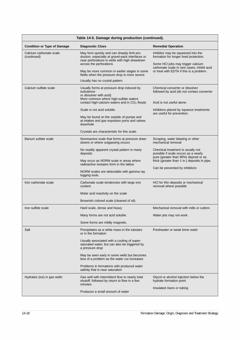
14-18 Formation Damage: Origin, Diagnosis and Treatment Strategy

Table 14-5. Damage during production (continued).

Condition or Type of Damage Diagnostic Clues Remedial Operation

Calcium carbonate scale May form quickly and can sharply limit pro- Inhibitor may be squeezed into the(continued) duction, especially at gravel-pack interfaces or formation for longer lived protection.

near perforations in wells with high drawdown across the perforations Some HCl jobs may trigger calcium

carbonate scale in rare cases; inhibit acidMay be more common in earlier stages in some or treat with EDTA if this is a problem.fields when the pressure drop is more severe

Usually has no crystal pattern

Calcium sulfate scale Usually forms at pressure drop induced by Chemical converter or dissolverturbulence followed by acid (do not contact converter or dissolver with acid)More common where high-sulfate waters contact high-calcium waters and in CO2 floods Acid is not useful alone.

Scale is not acid soluble. Inhibitors placed by squeeze treatmentsare useful for prevention.

May be found on the outside of pumps and at intakes and gas expulsion ports and valves downhole

Crystals are characteristic for this scale.

Barium sulfate scale Nonreactive scale that forms at pressure draw- Scraping, water blasting or other downs or where outgassing occurs mechanical removal

No readily apparent crystal pattern in many Chemical treatment is usually notdeposits possible if scale occurs as a nearly

pure (greater than 90%) deposit or asMay occur as NORM scale in areas where thick (greater than 1⁄4 in.) deposits in pipe.radioactive isotopes form in the lattice

Can be prevented by inhibitorsNORM scales are detectable with gamma ray logging tools.

Iron carbonate scale Carbonate scale tendencies with large iron HCl for thin deposits or mechanicalcontent removal where possible

Molar acid reactivity on the scale

Brownish colored scale (cleaned of oil)

Iron sulfide scale Hard scale, dense and heavy Mechanical removal with mills or cutters

Many forms are not acid soluble. Water jets may not work.

Some forms are mildly magnetic.

Salt Precipitates as a white mass in the tubulars Freshwater or weak brine washor in the formation

Usually associated with a cooling of super-saturated water, but can also be triggered by a pressure drop

May be seen early in some wells but becomes less of a problem as the water cut increases

Problems in formations with produced water salinity that is near saturation

Hydrates (ice) in gas wells Gas well with intermittent flow to nearly total Glycol or alcohol injection below theshutoff, followed by return to flow in a few hydrate formation pointminutes

Insulated risers or tubingProduces a small amount of water

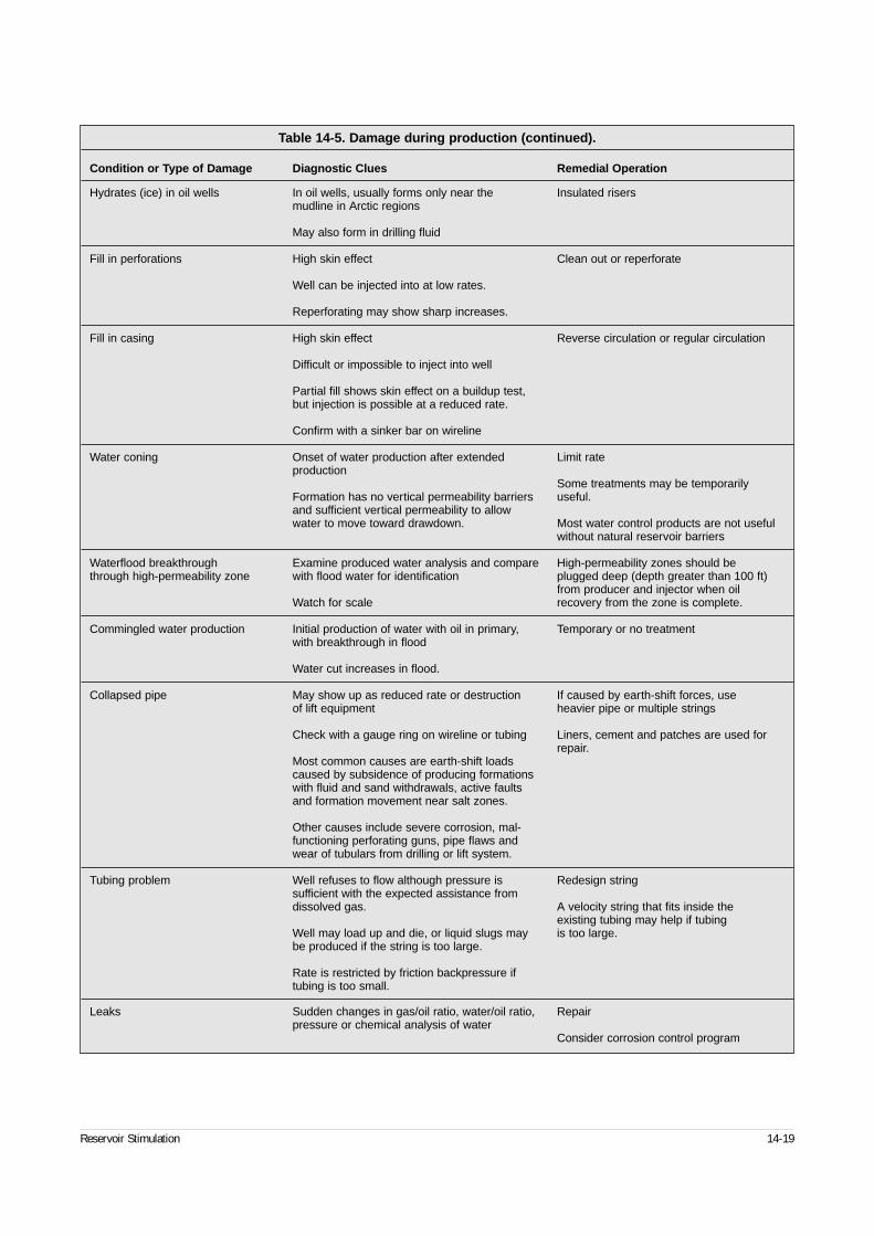
Reservoir Stimulation 14-19

Table 14-5. Damage during production (continued).

Condition or Type of Damage Diagnostic Clues Remedial Operation

Hydrates (ice) in oil wells In oil wells, usually forms only near the Insulated risersmudline in Arctic regions

May also form in drilling fluid

Fill in perforations High skin effect Clean out or reperforate

Well can be injected into at low rates.

Reperforating may show sharp increases.

Fill in casing High skin effect Reverse circulation or regular circulation

Difficult or impossible to inject into well

Partial fill shows skin effect on a buildup test,but injection is possible at a reduced rate.

Confirm with a sinker bar on wireline

Water coning Onset of water production after extended Limit rateproduction

Some treatments may be temporarily Formation has no vertical permeability barriers useful.and sufficient vertical permeability to allow water to move toward drawdown. Most water control products are not useful

without natural reservoir barriers

Waterflood breakthrough Examine produced water analysis and compare High-permeability zones should be through high-permeability zone with flood water for identification plugged deep (depth greater than 100 ft)

from producer and injector when oilWatch for scale recovery from the zone is complete.

Commingled water production Initial production of water with oil in primary, Temporary or no treatmentwith breakthrough in flood

Water cut increases in flood.

Collapsed pipe May show up as reduced rate or destruction If caused by earth-shift forces, useof lift equipment heavier pipe or multiple strings

Check with a gauge ring on wireline or tubing Liners, cement and patches are used forrepair.

Most common causes are earth-shift loads caused by subsidence of producing formations with fluid and sand withdrawals, active faults and formation movement near salt zones.

Other causes include severe corrosion, mal-functioning perforating guns, pipe flaws and wear of tubulars from drilling or lift system.

Tubing problem Well refuses to flow although pressure is Redesign stringsufficient with the expected assistance from dissolved gas. A velocity string that fits inside the

existing tubing may help if tubingWell may load up and die, or liquid slugs may is too large.be produced if the string is too large.

Rate is restricted by friction backpressure if tubing is too small.

Leaks Sudden changes in gas/oil ratio, water/oil ratio, Repairpressure or chemical analysis of water

Consider corrosion control program

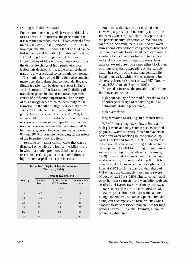
• Drilling fluid filtrate invasion

For economic reasons, wells have to be drilled asfast as possible. To increase the penetration rate, it is tempting to reduce the fluid-loss control of themud (Black et al., 1985; Simpson, 1985a, 1985b;Montogmery, 1985). About 600 bbl of fluid can belost into a typical formation (Kutasov and Bizanti,1985) during the drilling of a 10,000-ft well.Higher values of filtrate invasion may result fromthe deliberate choice of high penetration rates.Before this decision is made, the effect of the fil-trate and any associated solids should be known.

The liquid phase of a drilling fluid also containsmany potentially damaging compounds. Becausefiltrate invasion can be deep, as shown in Table14-6 (Simpson, 1974; Hassen, 1980), drilling fil-trate damage can be one of the most importantcauses of production impairment. The severity of this damage depends on the sensitivity of theformation to the filtrate. High-permeability cleansandstones undergo more invasion than low-permeability reservoirs (Phelps et al., 1984) butare more likely to be less affected when their con-nate water is chemically compatible with the fil-trate. An average permeability reduction of 40%has been suggested; however, any value between0% and 100% is possible, depending on the natureof the formation rock and fluids.

Sensitive formations contain clays that can bedispersed or swollen, are low-permeability rocksin which saturation problems dominate or arereservoirs producing almost saturated brines orhigh-content asphaltene or paraffin oils.

Problems with clays are not detailed here.However, any change in the salinity of the porefluids may affect the stability of clay particles inthe porous medium. In particular, reducing thesalinity or increasing the pH value of the watersurrounding clay particles can promote dispersionof these materials. Destabilized formation fines actsimilarly to mud particles forced into formationrocks. As production or injection starts, finesmigrate toward pore throats and either block themor bridge over them, depending on the particlesize. The severity of the resulting permeabilityimpairment varies with the fines concentration inthe reservoir rock (Krueger et al., 1967; Droddy et al., 1988; Jiao and Sharma, 1992).

Factors that increase the probability of drillingfluid invasion include

– high permeability of the mud filter cake (a resultof either poor design of the drilling fluid ordetrimental drilling procedures)

– high overbalance

– long formation-to-drilling-fluid contact time.

WBM filtrates may have a low salinity and ahigh pH value and may contain dispersants andpolymers. Water is a cause of in-situ clay distur-bance and water blocking in low-permeabilityrocks (Keelan and Koepf, 1977). The numerousdrawbacks of water-base drilling fluids led to thedevelopment of OBM for drilling through sand-stones containing clay (Methven and Kemick,1969). The initial conclusion was that this newmud was a safe, all-purpose drilling fluid. It isnow recognized, however, that although the prob-lems of OBM are less numerous than those ofWBM, they are commonly much more severe(Goode et al., 1984). OBM filtrates contain addi-tives that cause emulsion and wettability problems(Ballard and Dawe, 1988; McKinney and Azar,1988; Sanner and Azar, 1994; Ventresca et al.,1995). Polymer filtrates that are stable at circu-lating temperatures, but already potentially dam-aging, can decompose and form residues whenexposed to static reservoir temperatures for longperiods of time (Tuttle and Barkman, 1974), aspreviously discussed.

14-20 Formation Damage: Origin, Diagnosis and Treatment Strategy

Table 14-6. Depth of filtrate invasion (Simpson, 1974).

Depth of Invasion (in.)

Time (D) Oil-Base Low-Colloid Water-BaseMud Oil-Base Mud Mud

1 1.2 3.3 7.7

5 4.6 11 12

10 7.7 17 18

15 10 21 23

20 12 23 27

25 14 29 31

30 16 32 34

14-4.2. Cementing• Washes and spacers

The removal of drilling mud, while necessary forimproving cement bonding, typically exacerbatesformation damage through either increased fluidloss or incompatibility problems with cementwashes and spacers.

The duration of a cementing job is short com-pared with the duration of drilling through a payzone. The maximum depth of invasion by the fil-trate from either spacers or cement slurries is afew inches, which is negligible compared to thefew feet of drilling mud filtrate invasion. This doesnot mean that cement or spacer fluid loss shouldbe neglected. Poor fluid-loss control can result inpremature job failure by either complete loss ofthe preflush fluids (insufficient volumes) and sub-sequent contamination (and strong gelling) of thecement slurry by the drilling fluid or dehydrationof the cement slurry itself.

• Cement slurries

The broad particle-size distribution of cementgrains, together with the use of high-efficiencyfluid-loss agents, results in limited particle andfiltrate invasion of cement slurries (Jones et al.,1991b). However, there are four cases where largepermeability impairments can occur:

– The relatively high pH value of cement slurryfiltrates is particularly detrimental to formationclay minerals. Calcium ions liberated by cementparticles are quickly exchanged on clays nearthe wellbore, and the resulting modification ofthe filtrate composition makes it a perfect desta-bilizing fluid in terms of dispersing ability(Cunningham and Smith, 1968).

– Cement filtrate that comes into contact with con-nate brines that contain high concentrations ofcalcium can provoke the precipitation of calciumcarbonate, lime (Records and Ritter, 1978) orcalcium silicate hydrate (Krueger, 1986).

– Overdispersed slurries (with no yield value) pro-mote the rapid separation of cement particles atthe bottom and water at the top of the cementcolumn. A large invasion of free water will mostlikely take place, and the resulting water block-age may be significant.

– Loss of cement to the natural fracture system isa catastrophic problem when using a cased andperforated completion through formations withnatural fracture systems. In side-by-side wellcomparisons, cement loss in natural fractures in the pay zone has been shown to decrease pro-duction to the point where the zone cannot floweffectively. Once cement is lost into the fracturesystem, hydraulic fracturing or sidetracking andredrilling the well are the best alternatives. Insome carbonate formations, acid fracturing maybe beneficial.

14-4.3. PerforatingPerforations are the entry point from the formation tothe wellbore, and all flow in a cased, perforated com-pletion must pass through these tunnels. Althoughperforation job quality is at times overlooked in thesearch for reasons why a well does not produce asexpected, any time that formation damage is sus-pected the perforations should be examined first.Perforating is always a cause of additional damage(Suman, 1972). Extreme overbalance (EOB) perfo-rating has been used expressly to reduce damage tothe perforation tunnels (see Chapter 11).

• Perforating mildly overbalance always forces for-mation and gun debris into perforation walls anddecreases the permeability near the perforations(Keese and Oden, 1976).

• Perforating mildly overbalance in fluids that con-tain particles produces a similar effect (Paul andPlonka, 1973; Wendorff, 1974) and also builds adense, impermeable cake on the perforation walls.

• Insufficient perforation penetration does notbypass drilling damage (Klotz et al., 1974; Weeks,1974). Penetration also decreases with formationeffective stress (Saucier and Lands, 1978), a defi-nite concern in deep wells.

• If the underbalance pressure required to achievedamage-free perforations is incorrectly estimated,the insufficient pressure difference will limit dam-age removal (Hsia and Behrmann, 1991;Behrmann, 1995; Bird and Dunmore, 1995),whereas excessive pressure differences lead tosand influx in the wellbore (King et al., 1985;Seanard, 1986).

Reservoir Stimulation 14-21

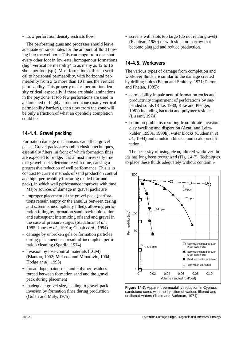
• Low perforation density restricts flow.

The perforating guns and processes should leaveadequate entrance holes for the amount of fluid flow-ing into the wellbore. This can range from one shotevery other foot in low-rate, homogenous formations(high vertical permeability) to as many as 12 to 16shots per foot (spf). Most formations differ in verti-cal to horizontal permeability, with horizontal per-meability from 3 to more than 10 times the verticalpermeability. This property makes perforation den-sity critical, especially if there are shale laminationsin the pay zone. If too few perforations are used in a laminated or highly structured zone (many verticalpermeability barriers), then flow from the zone willbe only a fraction of what an openhole completioncould be.

14-4.4. Gravel packingFormation damage mechanisms can affect gravelpacks. Gravel packs are sand-exclusion techniques,essentially filters, in front of which formation finesare expected to bridge. It is almost universally truethat gravel packs deteriorate with time, causing aprogressive reduction of well performance. This is incontrast to current methods of sand production controland high-permeability fracturing (called frac andpack), in which well performance improves with time.

Major sources of damage in gravel packs are

• improper placement of the gravel pack (perfora-tions remain empty or the annulus between casingand screen is incompletely filled), allowing perfo-ration filling by formation sand, pack fluidizationand subsequent intermixing of sand and gravel inthe case of pressure surges (Stadalman et al.,1985; Jones et al., 1991a; Chuah et al., 1994)

• damage by unbroken gels or formation particlesduring placement as a result of incomplete perfo-ration cleaning (Sparlin, 1974)

• invasion by loss-control materials (LCM)(Blanton, 1992; McLeod and Minarovic, 1994;Hodge et al., 1995)

• thread dope, paint, rust and polymer residuesforced between formation sand and the gravelpack during placement

• inadequate gravel size, leading to gravel-packinvasion by formation fines during production(Gulati and Maly, 1975)

• screens with slots too large (do not retain gravel)(Flanigan, 1980) or with slots too narrow thatbecome plugged and reduce production.

14-4.5. WorkoversThe various types of damage from completion andworkover fluids are similar to the damage created by drilling fluids (Eaton and Smithey, 1971; Pattonand Phelan, 1985):

• permeability impairment of formation rocks andproductivity impairment of perforations by sus-pended solids (Rike, 1980; Rike and Pledger,1981) including bacteria and polymer residues(Lissant, 1974)

• common problems resulting from filtrate invasion:clay swelling and dispersion (Azari and Leim-kuhler, 1990a, 1990b), water blocks (Oudeman etal., 1994) and emulsion blocks, and scale precipi-tation.

The necessity of using clean, filtered workover flu-ids has long been recognized (Fig. 14-7). Techniquesto place these fluids adequately without contamin-

14-22 Formation Damage: Origin, Diagnosis and Treatment Strategy

Figure 14-7. Apparent permeability reduction in Cypresssandstone cores with the injection of various filtered andunfiltered waters (Tuttle and Barkman, 1974).

0

50

100

500

436 ppm

2.5 ppm

26 ppm

94 ppm

Per

mea

bilit

y (m

d)

0 0.02 0.04 0.06 0.08 0.10

Volume injected (gal/perf)

Bay water filtered through 2-µm cotton filter

Bay water filtered through 5-µm cotton filter

Produced water, untreated

Bay water, untreated

ating them with the various particulate or gumlikematerials in the wellbore (including thread dope)have also been proposed (Krause, 1986).

There is a strong requirement for fluid-loss con-trol, especially in depleted reservoirs, and additiveshave been developed for this purpose (Crowe andCryar, 1975; Mahajan and Barron, 1980). Anotherapproach is to use foams, gases (Dahlgaard, 1983) ormists as completion fluids (Millhone, 1983). Insteadof physically reducing the extent of filtrate invasion,the fluid-loss agents can deliberately be removedfrom workover fluids. In this approach, the compati-bility of the fluid with formation minerals and brinemust be carefully studied (Morgenthaler, 1986).

Workover brines (especially high-density brines)usually require inhibitors to control corrosion. Theseproducts can contribute to emulsion-block problemsthrough the wettability modification of formationminerals and sometimes promote iron precipitationin the reservoir (Potter, 1984).

14-4.6. Stimulation and remedial treatments

• Wellbore cleanup

When wells are cleaned to remove deposits or cor-rosion products from the tubing, high concentra-tions of damaging materials may invade the payzone. Extreme care should be devoted to prevent-ing these suspensions from being forced into theporous medium. Particularly dangerous are com-pounds that are soluble in the cleaning fluidbecause they cannot form impermeable cakes thatprevent formation invasion. Rust in acid (Gougleret al., 1985) or paraffins in hot oil (Newberry andBarker, 1985) are the two most typical redissolvedwellbore compounds. They reprecipitate in the for-mation and cause extensive, severe and usuallypermanent damage.

• Acid treatments

Problems already encountered in other phases ofthe life of a well may also occur during acidizingtreatments, especially in cases of inappropriatedesign. These include

– damaging materials from the tubing entering theformation rock

– oil-wetting of the reservoir by surfactants, espe-cially corrosion inhibitors (Crowe and Minor,1982), which can create emulsion blocks

– water blocks

– asphaltene/paraffin deposition when large vol-umes of acid are injected.

In addition to these common damaging pro-cesses, specific production impairment can resultfrom poor design of acidizing treatments. Theseimpairments include the following:

– sludges produced by reaction between acids andasphaltenes (Moore et al., 1965; Houchin et al.,1990), especially in the presence of some addi-tives (particularly surfactants) (Knobloch et al.,1978) or dissolved iron (Jacobs and Thorne,1986)

– deconsolidation of the formation rock caused byexcessive dissolution of the cementing materialsby acids

– precipitation of by-products from the reaction of acids with formation minerals (Boyer andWu, 1983; Gadiyar and Civan, 1994)

– precipitation caused by some sequesteringagents added to acids to prevent iron problems if iron is suspected present (Smith et al., 1969)

– permeability impairment by residues from corro-sion inhibitors (Crowe and Minor, 1985) or pro-duced through the thermal degradation of poly-mers, such as friction reducers (Woodroof andAnderson, 1977)

– dissolution of pack sands, to a limited extent, inhydraulically fractured and gravel-packed wells(Cheung, 1988; Yeager, 1990).

• Fracture treatments

Damage resulting from hydraulic fracturing takestwo distinct forms: damage inside the fractureitself (proppant-pack damage) and damage normalto the fracture intruding into the reservoir (frac-ture-face damage). The first generally occursbecause of inadequate breaking of the fracturingfluid polymer; the second occurs because of exces-sive leakoff. Depending on the reservoir perme-ability, the impact of these two damages varies.

Reservoir Stimulation 14-23

For low reservoir permeability, neither one ismuch of a factor. As the permeability increases,proppant-pack damage (and its avoidance)becomes increasingly important, whereas damageto the reservoir face is relatively unimportant. Athigh permeabilities, both are important, with frac-ture-face damage dominating at very high perme-abilities.

The selection of fracturing fluids, polymer con-centrations and breakers is critical in addressingthese issues. Incomplete breaking of the polymersin fracturing fluid is the most obvious cause ofdamage within hydraulic fractures (Gidley et al.,1992), as well as the poor selection of proppantfracturing fluids (Brannon and Pulsinelli, 1990)and formation rock spalling or creeping into theproppant pack (Strickland, 1985). True damage inthe formation rock is the consequence of excessiveleakoff in high-permeability reservoirs when poly-mer-base gels are used in combination with ineffi-cient fluid-loss agents (Elbel et al., 1995; Parlar etal., 1995). These damages are usually severe andusually cannot be improved with matrix treat-ments. To alleviate this problem, polymer-free,surfactant-base fluids have been proposed (Stewartet al., 1995); however, they cannot be used in theabsence of crude oil, which is required for breakingthe surfactant micelles.

• Poor load-fluid recovery

Typical load-fluid recovery on a stimulation treat-ment or remedial treatment may range from as littleas 20% to 100%. Load fluids can invade andbecome trapped in the formation by entering thesmaller capillary pores during higher injection pres-sures, or they may coat clays with high micro-porosity (a condition in which a large surface areaexists for water coating or trapping). Once theinjection pressure is released, capillary pressureeffects will hold significant volumes of the fluid inthe formation. In some formations, more than 50%of the load fluid can be trapped after a treatment,and yet the formation may not appear damaged.Most of the flow is through the larger pore systemand natural fractures, and these passages usuallyclean out quickly. The smaller pore passages cantrap fluid by imbibing or absorbing it, but they haveno real effect on the flow through the formation.

14-4.7. Normal production or injection operations

• Unconsolidated formations

Formations that are capable of releasing parts ofthe matrix during production or after stimulationpose special treating problems. Although these sit-uations are commonly thought of as sand-controlproblems rather than formation damage, the effectof mobile sand and the pressure drop caused bycollapsed formation tunnels closely resemble theeffect of formation damage. Some reservoirs can-not be produced at high flow rates or large draw-downs without being affected adversely. Per-manent damage, which cannot be removed simplyby the reducing production rate, may be created.

A major problem is the movement of fines in the formation in response to either flow velocity or changes in the salinity of the flowing fluid. Al-though this subject was addressed in Section 14-3.1,it is worth mentioning again, because it is usually asignificant factor in the behavior of unstable forma-tions. Native silts and clays loosely attached to porewalls can be put into motion by high flow rates(Hower, 1974; Holub et al., 1974), especiallywhen two or more immiscible fluids are producedat the same time (Muecke, 1979; Sengupta et al.,1982). Depending on their particle size, they caneither block pore throats in the vicinity of their ini-tial location or migrate toward the wellbore.

Whether migrating particles reach the wellboreor bridge over pore throat entrances depends ontheir original concentration in the formation, theirsize, the extent of the increase of their concentra-tion near the wellbore (because of radial flow) andthe maximum flow rate (Vaidya and Fogler, 1990;Gunter et al., 1992; Oyenenin et al., 1995).Bridging is promoted when one or more of theseparameters are increased. Bridging is less detri-mental than blocking because a short period ofreverse flow, followed by production at a flow ratelower than that at which bridging occurred, maymechanically disperse bridges (Fig. 14-8). How-ever, this cannot be achieved when the bridgingagglomerates were previously cemented by precip-itates (asphaltenes or scales) or chemically stabi-lized through the injection of flocculants (such asclay stabilizers).

14-24 Formation Damage: Origin, Diagnosis and Treatment Strategy

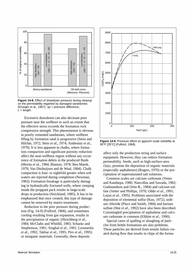
Excessive drawdown can also decrease porepressure near the wellbore to such an extent thatthe effective stress exceeds the formation rockcompressive strength. This phenomenon is obviousin poorly cemented sandstones, where wellborefilling by formation sand is progressive (Stein andHilchie, 1972; Stein et al., 1974; Antheunis et al.,1979). It is less apparent in chalks, where forma-tion compaction and significant porosity reductionaffect the near-wellbore region without any occur-rence of formation debris in the produced fluids(Morita et al., 1984; Blanton, 1978; Ben Marek,1979; Van Ditzhuijzen and de Waal, 1984). Chalkcompaction is four- to eightfold greater when softwaters are injected during completion (Newman,1983). Formation breakage is particularly damag-ing in hydraulically fractured wells, where creepinginside the proppant pack results in large-scaledrops in production (Strickland, 1985). It has to beemphasized that once created, this type of damagecannot be removed by matrix treatments.

Reduction in the pore pressure during produc-tion (Fig. 14-9) (Fulford, 1968), and sometimescooling resulting from gas expansion, results in the precipitation of organic (Hirschberg et al.,1984; McClafin and Whitfill, 1983; Schantz andStephenson, 1991; Singhal et al., 1991; Leontaritiset al., 1992; Takhar et al., 1995; Piro et al., 1995)or inorganic materials. Generally, these deposits

affect only the production string and surfaceequipment. However, they can reduce formationpermeability. Seeds, such as high-surface-areaclays, promote the deposition of organic materials(especially asphaltenes) (Rogers, 1976) or the pre-cipitation of supersaturated salt solutions.

Common scales are calcium carbonate (Vetterand Kandarpa, 1980; Nancollas and Sawada, 1982;Gudmundson and Oritz-R., 1984) and calcium sul-fate (Vetter and Phillips, 1970; Oddo et al., 1991;Lejon et al., 1995). Problems associated with thedeposition of elemental sulfur (Kuo, 1972), sodi-um chloride (Place and Smith, 1984) and bariumsulfate (Wat et al., 1992) have also been described.Commingled precipitation of asphaltene and calci-um carbonate is common (Efthim et al., 1990).

Special cases of spalling or sloughing of parti-cles from brittle formations are also problems.These particles are derived from tensile failure cre-ated during flow that results in chips of the forma-

Reservoir Stimulation 14-25

Figure 14-8. Effect of drawdown pressure during cleanupon the permeability regained by damaged sandstones(Krueger et al., 1967). ∆p = pressure difference, L = length.

0

20

40

60

80

100

Berea sandstone

% o

f orig

inal

per

mea

bilit

y

Hig

h dr

awdo

wn

(∆p/

L =

50)

Hig

h dr

awdo

wn

(∆p/

L =

40)

Oil well cores(Miocene, Pliocene)

Low

dra

wdo

wn

(∆p/

L =

2

5

10

20

50

)

Low

dra

wdo

wn

(∆p/

L =

2

5

10

20

40

)

Figure 14-9. Pressure effect on gypsum scale solubility at95°F [35°C] (Fulford, 1968).

0 100 200 3000

1000

2000

3000

4000

5000

6000

7000

8000

9000

NaCl (g/L)

CaS

O4

(mg/

L)

1980 psig

0 psig

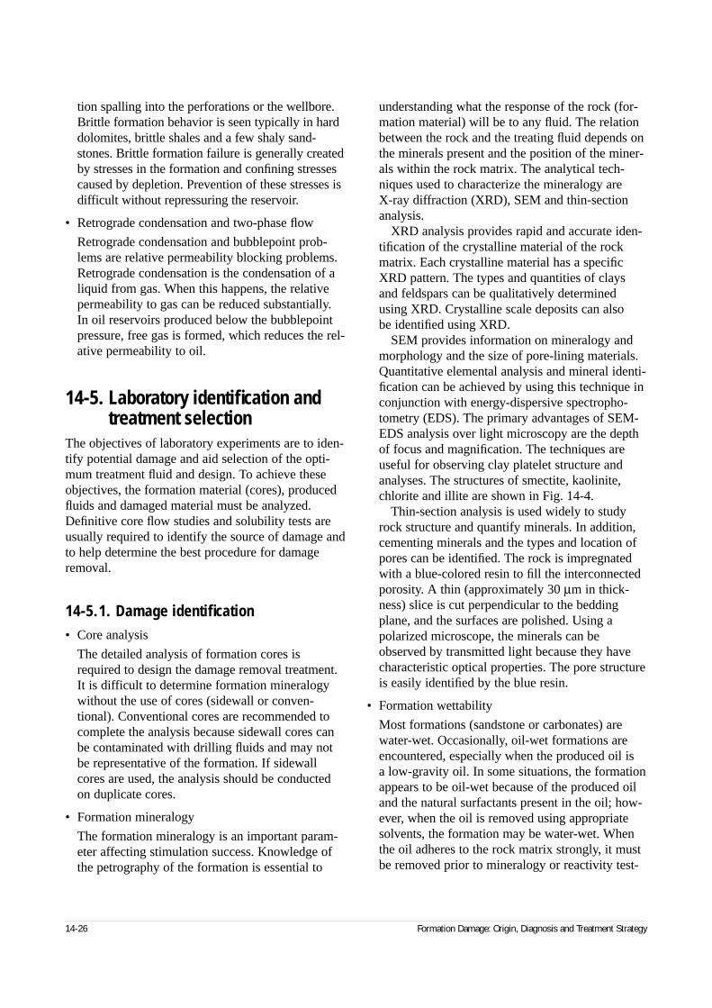
tion spalling into the perforations or the wellbore.Brittle formation behavior is seen typically in harddolomites, brittle shales and a few shaly sand-stones. Brittle formation failure is generally createdby stresses in the formation and confining stressescaused by depletion. Prevention of these stresses isdifficult without repressuring the reservoir.

• Retrograde condensation and two-phase flow

Retrograde condensation and bubblepoint prob-lems are relative permeability blocking problems.Retrograde condensation is the condensation of aliquid from gas. When this happens, the relativepermeability to gas can be reduced substantially.In oil reservoirs produced below the bubblepointpressure, free gas is formed, which reduces the rel-ative permeability to oil.

14-5. Laboratory identification and treatment selection

The objectives of laboratory experiments are to iden-tify potential damage and aid selection of the opti-mum treatment fluid and design. To achieve theseobjectives, the formation material (cores), producedfluids and damaged material must be analyzed.Definitive core flow studies and solubility tests areusually required to identify the source of damage andto help determine the best procedure for damageremoval.

14-5.1. Damage identification• Core analysis

The detailed analysis of formation cores isrequired to design the damage removal treatment.It is difficult to determine formation mineralogywithout the use of cores (sidewall or conven-tional). Conventional cores are recommended tocomplete the analysis because sidewall cores canbe contaminated with drilling fluids and may notbe representative of the formation. If sidewallcores are used, the analysis should be conductedon duplicate cores.

• Formation mineralogy

The formation mineralogy is an important param-eter affecting stimulation success. Knowledge ofthe petrography of the formation is essential to

understanding what the response of the rock (for-mation material) will be to any fluid. The relationbetween the rock and the treating fluid depends onthe minerals present and the position of the miner-als within the rock matrix. The analytical tech-niques used to characterize the mineralogy are X-ray diffraction (XRD), SEM and thin-sectionanalysis.

XRD analysis provides rapid and accurate iden-tification of the crystalline material of the rockmatrix. Each crystalline material has a specificXRD pattern. The types and quantities of claysand feldspars can be qualitatively determinedusing XRD. Crystalline scale deposits can also be identified using XRD.

SEM provides information on mineralogy andmorphology and the size of pore-lining materials.Quantitative elemental analysis and mineral identi-fication can be achieved by using this technique inconjunction with energy-dispersive spectropho-tometry (EDS). The primary advantages of SEM-EDS analysis over light microscopy are the depthof focus and magnification. The techniques areuseful for observing clay platelet structure andanalyses. The structures of smectite, kaolinite,chlorite and illite are shown in Fig. 14-4.

Thin-section analysis is used widely to studyrock structure and quantify minerals. In addition,cementing minerals and the types and location ofpores can be identified. The rock is impregnatedwith a blue-colored resin to fill the interconnectedporosity. A thin (approximately 30 µm in thick-ness) slice is cut perpendicular to the beddingplane, and the surfaces are polished. Using apolarized microscope, the minerals can beobserved by transmitted light because they havecharacteristic optical properties. The pore structureis easily identified by the blue resin.

• Formation wettability

Most formations (sandstone or carbonates) arewater-wet. Occasionally, oil-wet formations areencountered, especially when the produced oil is a low-gravity oil. In some situations, the formationappears to be oil-wet because of the produced oiland the natural surfactants present in the oil; how-ever, when the oil is removed using appropriatesolvents, the formation may be water-wet. Whenthe oil adheres to the rock matrix strongly, it mustbe removed prior to mineralogy or reactivity test-

14-26 Formation Damage: Origin, Diagnosis and Treatment Strategy

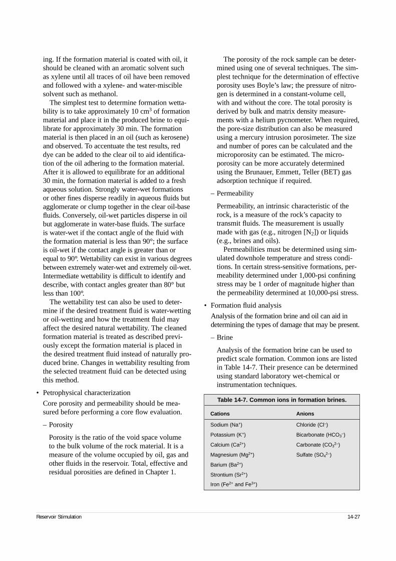
ing. If the formation material is coated with oil, itshould be cleaned with an aromatic solvent suchas xylene until all traces of oil have been removedand followed with a xylene- and water-misciblesolvent such as methanol.

The simplest test to determine formation wetta-bility is to take approximately 10 cm3 of formationmaterial and place it in the produced brine to equi-librate for approximately 30 min. The formationmaterial is then placed in an oil (such as kerosene)and observed. To accentuate the test results, reddye can be added to the clear oil to aid identifica-tion of the oil adhering to the formation material.After it is allowed to equilibrate for an additional30 min, the formation material is added to a freshaqueous solution. Strongly water-wet formations or other fines disperse readily in aqueous fluids butagglomerate or clump together in the clear oil-basefluids. Conversely, oil-wet particles disperse in oilbut agglomerate in water-base fluids. The surface is water-wet if the contact angle of the fluid withthe formation material is less than 90°; the surfaceis oil-wet if the contact angle is greater than orequal to 90°. Wettability can exist in various degreesbetween extremely water-wet and extremely oil-wet.Intermediate wettability is difficult to identify anddescribe, with contact angles greater than 80° butless than 100°.

The wettability test can also be used to deter-mine if the desired treatment fluid is water-wettingor oil-wetting and how the treatment fluid mayaffect the desired natural wettability. The cleanedformation material is treated as described previ-ously except the formation material is placed inthe desired treatment fluid instead of naturally pro-duced brine. Changes in wettability resulting fromthe selected treatment fluid can be detected usingthis method.

• Petrophysical characterization

Core porosity and permeability should be mea-sured before performing a core flow evaluation.

– Porosity

Porosity is the ratio of the void space volume to the bulk volume of the rock material. It is ameasure of the volume occupied by oil, gas andother fluids in the reservoir. Total, effective andresidual porosities are defined in Chapter 1.

The porosity of the rock sample can be deter-mined using one of several techniques. The sim-plest technique for the determination of effectiveporosity uses Boyle’s law; the pressure of nitro-gen is determined in a constant-volume cell,with and without the core. The total porosity isderived by bulk and matrix density measure-ments with a helium pycnometer. When required,the pore-size distribution can also be measuredusing a mercury intrusion porosimeter. The sizeand number of pores can be calculated and themicroporosity can be estimated. The micro-porosity can be more accurately determinedusing the Brunauer, Emmett, Teller (BET) gasadsorption technique if required.

– Permeability

Permeability, an intrinsic characteristic of therock, is a measure of the rock’s capacity totransmit fluids. The measurement is usuallymade with gas (e.g., nitrogen [N2]) or liquids(e.g., brines and oils).

Permeabilities must be determined using sim-ulated downhole temperature and stress condi-tions. In certain stress-sensitive formations, per-meability determined under 1,000-psi confiningstress may be 1 order of magnitude higher thanthe permeability determined at 10,000-psi stress.

• Formation fluid analysis

Analysis of the formation brine and oil can aid indetermining the types of damage that may be present.

– Brine

Analysis of the formation brine can be used topredict scale formation. Common ions are listedin Table 14-7. Their presence can be determinedusing standard laboratory wet-chemical orinstrumentation techniques.

Reservoir Stimulation 14-27

Table 14-7. Common ions in formation brines.

Cations Anions

Sodium (Na+) Chloride (Cl–)

Potassium (K+) Bicarbonate (HCO3–)

Calcium (Ca2+) Carbonate (CO32–)

Magnesium (Mg2+) Sulfate (SO42–)

Barium (Ba2+)

Strontium (Sr2+)

Iron (Fe2+ and Fe3+)

Calculations are available to predict scalingtendencies. The intermixing of produced brineswith spent acid can result in the formation ofinsoluble precipitates. Analysis of these brinedata aids in selecting the treatment fluids andtheir sequence.

– Oil

Analysis and testing of the produced oil can alsohelp stimulation treatment design. The use oftreating fluids that are incompatible with theproduced oil can result in the formation of emul-sions and sludge that will subsequently result in an unacceptable response to the stimulationtreatment. The oil may contain paraffins andasphaltenes that can interact with the treatmentfluid. The quantity of various fractions ofasphaltenes and paraffins and their ratio to eachother are used to assess the possibility of organicprecipitation damage. It is also imperative thatthe identity of deposits recovered from a well bedetermined. This is particularly true of organicdeposits because treatments for paraffin andasphaltene removal are different.

A test of the API gravity is performed on theproduced oil to evaluate sludging tendencies.Certified hydrometers are used to measure thespecific gravity as a function of temperature.

For analysis of the asphaltene content, theproduced oil is centrifuged to separate out emul-sified aqueous fluids. Mixing the crude oil withpentane and centrifuging the sample enablespreferential separation of asphaltenes from theproduced fluid. Repeated extraction is performeduntil all oil has been removed. The precipitatedasphaltene material is collected, and standardlaboratory techniques are used to obtain the con-tent by weight. The oil pentane fraction is savedand the pentane solvent is evaporated. The resid-ual oil is then used to complete the analysis forthe paraffin content.

For analysis of the paraffin content, a sample of vigorously mixed crude oil and acetone is cen-trifuged to enable preferential extraction of theparaffin material into acetone. Repeated extrac-tion and holding at temperatures less than 32°F[0°C] result in precipitation of the paraffins. Theacetone mixture is filtered to remove the paraf-fins, which are dried to remove residual acetone.On the basis of the total composition of the pro-

duced oil used for the analysis, the percentage ofparaffin is determined.

14-5.2. Treatment selectionThe solubility of the formation or damage material,treating fluid compatibility and core flow studiesshould be conducted to aid designing the best treat-ment for damage removal and to select the chemicalproducts that are the most compatible.

• Solubility tests

– Formation material

Calcite, dolomite and ankerite are soluble in HCland mud acid systems. Clay and silt are solubleonly in mud acid systems. Because of their highsurface area, clays and other fines are muchmore reactive with mud acid than sand grainsare. The total solubility of the formation materialis the sum of the solubility of each mineral inthe formation sample. Minerals other than car-bonates are also soluble in HCl; therefore, solu-bilities should be used with caution. These min-erals include sulfates (e.g., anhydrite), ironoxides and halite. The solubilities of commonminerals are shown in Table 14-8.

Solubility tests are performed under ideal lab-oratory conditions and therefore exhibit themaximum formation solubility. The structure ofthe rock and the position of each mineral in rela-tion to the flow paths in the rock matrix mayresult in different solubilities during actualacidizing operations. Solubility determined inthe laboratory is not a definitive value for themaximum solubility that may result during theacidizing process, but it provides guidelines asto which treating fluids are most applicable.

A combination of solubility test results andXRD is commonly used to estimate the carbon-ate, silt and clay minerals and other mineral con-tents in the rock matrix. Determination of theacid solubilities of the various materials in HCland mud acid determines the total solubility.When the results are used in conjunction withXRD analysis, the composition can be deter-mined by the following procedure.

1. The total solubility in HCl is typically usedas an estimate of the total carbonate content.

14-28 Formation Damage: Origin, Diagnosis and Treatment Strategy

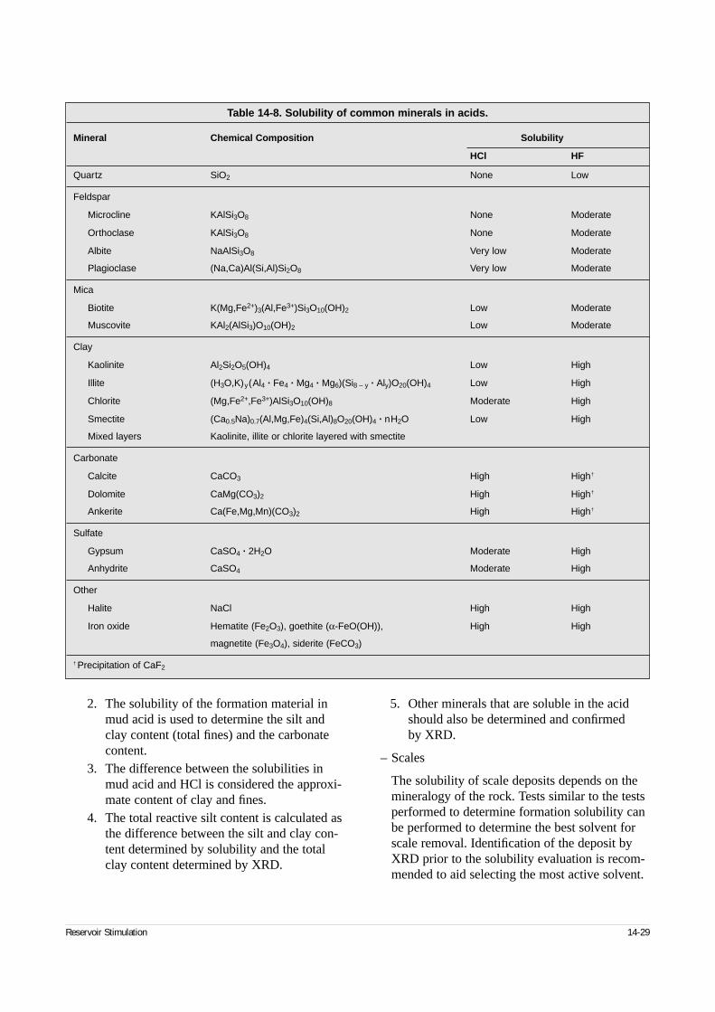
2. The solubility of the formation material inmud acid is used to determine the silt andclay content (total fines) and the carbonatecontent.

3. The difference between the solubilities inmud acid and HCl is considered the approxi-mate content of clay and fines.

4. The total reactive silt content is calculated asthe difference between the silt and clay con-tent determined by solubility and the totalclay content determined by XRD.

5. Other minerals that are soluble in the acidshould also be determined and confirmed by XRD.

– Scales

The solubility of scale deposits depends on themineralogy of the rock. Tests similar to the testsperformed to determine formation solubility canbe performed to determine the best solvent forscale removal. Identification of the deposit byXRD prior to the solubility evaluation is recom-mended to aid selecting the most active solvent.

Reservoir Stimulation 14-29

Table 14-8. Solubility of common minerals in acids.

Mineral Chemical Composition Solubility

HCl HF

Quartz SiO2 None Low

Feldspar

Microcline KAlSi3O8 None Moderate

Orthoclase KAlSi3O8 None Moderate

Albite NaAlSi3O8 Very low Moderate

Plagioclase (Na,Ca)Al(Si,Al)Si2O8 Very low Moderate

Mica

Biotite K(Mg,Fe2+)3(Al,Fe3+)Si3O10(OH)2 Low Moderate

Muscovite KAl2(AlSi3)O10(OH)2 Low Moderate

Clay

Kaolinite Al2Si2O5(OH)4 Low High

Illite (H3O,K)y(Al4 · Fe4 · Mg4 · Mg6)(Si8 – y · Aly)O20(OH)4 Low High

Chlorite (Mg,Fe2+,Fe3+)AlSi3O10(OH)8 Moderate High

Smectite (Ca0.5Na)0.7(Al,Mg,Fe)4(Si,Al)8O20(OH)4 · nH2O Low High

Mixed layers Kaolinite, illite or chlorite layered with smectite

Carbonate

Calcite CaCO3 High High†

Dolomite CaMg(CO3)2 High High†

Ankerite Ca(Fe,Mg,Mn)(CO3)2 High High†

Sulfate

Gypsum CaSO4 · 2H2O Moderate High

Anhydrite CaSO4 Moderate High

Other

Halite NaCl High High

Iron oxide Hematite (Fe2O3), goethite (α-FeO(OH)), High High

magnetite (Fe3O4), siderite (FeCO3)

† Precipitation of CaF2

Typically, acids, chelating agents or mechanicalsystems are used for removal. These tests shouldbe performed under simulated well conditions todetermine the optimum treatment.

– Organic deposits

Solubility tests at temperature and pressure canbe performed to evaluate the most effective sol-vent to remove the plugging deposit. Typically,paraffin, asphaltene and tar deposits are solublein aromatic solvents such as xylene or toluene;however, most deposits are a combined depositand may require a combined treatment of anorganic solvent with acid and other surface-active agents to improve the wettability of thedeposit and enhance the dissolving capacity ofthe selected treatment fluid. Other solvents, suchas mutual solvents and alcohols, may also aidthe removal of an organic deposit.

– Bacterial slime

Bacterial slime is also removed by treating withsolvents. These deposits are soluble in watercontaining oxidizing agents such as sodiumhypochlorite. If required, solubility tests can beperformed to evaluate the efficiency of the oxi-dizing agent. Tests should be performed usingsimulated downhole conditions, if possible.

• Treating fluid–formation compatibility

Preventing emulsion and sludge formation follow-ing a damage-removal treatment requires an opti-mum fluid design to minimize or eliminate theformation of precipitates. The potential for the for-mation of acid and produced crude oil emulsionsand optimization of the de-emulsifier treatment arecurrently evaluated using American PetroleumInstitute (API) Recommended Practices forLaboratory Testing of Surface Active Agents forWell Stimulation (RP 42) (1977).

– Emulsion prevention testing

Prior to a stimulation treatment, the compatibil-ity of the treatment fluid with the produced oilmust be determined. Fine siliceous materials,ferric iron or both can be added to evaluateemulsion stability mechanisms. These fluidinteractions can produce downhole emulsionproblems. The quantity of additives used to con-trol emulsion stability and sludge formation

must be established. Additives such as corrosioninhibitors, surfactants and mutual solvents mustalso be included in the desired acid formulationfor compatibility testing. The concentrations ofthese additives are established by core flow tests,metallurgy and the well conditions that occurduring treatment.

Acid, or another aqueous treating fluid, ismixed with fresh crude oil (at low energy tosimulate downhole mixing) in a glass containerand observed at bottomhole temperature, if pos-sible. The characteristics and time for emulsionbreakout are determined. The quanitity of aque-ous fluid breakout is determined at set timeintervals. The sample that provides the mostrapid emulsion breakout is desired. The acid sys-tem is modified, including the type and quantityof nonemulsifier, until the minimum aqueousbreakout time is achieved. A clean oil/waterinterface and rapid emulsion break (less than 10 min) are desired. The oil phase must also beclear, with no emulsified water draining freelyfrom the glass surface (signifying a water-wetsurface).

Differences in emulsion stability are attributedto more dominant factors such as stabilizationby solids precipitation (organic and inorganic),ferric ion interaction with the asphaltene compo-nent of crude oil and viscosity increase at theinterface. Results presented by Coppel (1975)show that partially spent acids contain potentiallyprecipitable materials in solution. As the pHvalue of the spent acid increases during flowbackand mixes with other produced fluids, materialsprecipitate that can stabilize emulsions. Dunlapand Houchin (1990) recommended using polar-ized microscopy to evaluate return fluids toestablish the cause for a stabilized emulsion.Specific damage mechanisms such as emulsionstabilization by organic deposits, solids and ironmay be detected and identified. Stabilization bysolids can be evaluated by the use of fine silicaor clay in the emulsion test described previously.

Downhole emulsions can be attributed toinadequate prejob compatibility testing becausethe additives used in the acid system may prefer-entially adsorb onto the rock matrix or partitionto the oil phase during production. Alternatetesting procedures have been recommended tosimulate reservoir conditions more accurately.

14-30 Formation Damage: Origin, Diagnosis and Treatment Strategy

Ali et al. (1994) recommended using an alter-nate procedure that better simulates downholeintermixing of the stimulation fluids and the pro-duced crude. The formulated acid containinginhibitor, surfactants, mutual solvents and non-emulsifiers is filtered through a sand pack con-taining 10% silica flour, 10% clays (such asmontmorillonite) and 80% 100-mesh sand priorto completion of the emulsion test. This proce-dure simulates the filtration of the acid systemwithin the rock matrix. Surfactants, such asthose used in nonemulsifiers, are adsorbed ontothe mineral surfaces. This adsorption minimizesthe availability of the surfactants in solution toprevent emulsions.

– Sludge prevention testing

Prior to the stimulation treatment, the compati-bility of the treating fluid with the produced oilmust be determined for sludging tendencies.Interaction of the acid with crude oil can gener-ate the formation of solid precipitates, althoughthe system does not form stable emulsions.These precipitates are sludge and are insolublein the hot formation oil or brine. The sludgingtendencies are aggravated by intermixing withferric iron. If not prevented, precipitated solidscan result in decreased production following anacid treatment.

The sludging evaluation is similar to the emul-sion test previously described. The oil should befree of solids and emulsified water. Followingcompletion of the emulsion test, the acid and oilmixture is maintained at the bottomhole temper-ature for 1 to 4 hr. The mixture is then filteredthrough a 100-mesh screen, and the precipitatedsludge on the filter is identified.

To eliminate the formation of sludge, the acidsystem must contain an antisludge additive. Theconcentration of antisludge additive is increasedin the acid system until formation of the sludgeprecipitate is eliminated.

• Core flow tests

Core flow tests are used to determine the effects oftreatment fluids on formation samples at simulatedwell treating conditions. The structure of the rockand the position of each mineral in relation to theflow channels in the rock matrix may result in dif-ferent solubilities during actual acidizing opera-

tions. Therefore, the permeability changes dependon the dissolution and precipitation reactions thatoccur. Observations that indicate what dissolvesand what precipitates are extremely useful inselecting the best treatment fluid.

The effects of sequential injection of the differenttreatment fluids can also be observed. Fluid injec-tion rates range from 0.2 to 10 mL/min and pres-sures range up to 1500 psi. Flow rates should beselected to ensure that the fluid movement has mini-mal effect on the movement of fines containedwithin the pore structure. The 1-in. diameter, 12-in.long cores are placed in a core holder and confinedunder pressure to simulate reservoir stresses. Toensure fluid flow through the core, the confinementpressure should be greater than the pressurerequired to initiate flow through the core. Testsshould also be performed with backpresssure. Forcore flow studies of acids, a backpressure of at least1000 psi is required to maintain the CO2 producedby acid dissolution of carbonate deposits in solu-tion. For scale and deposit removal, sufficient back-pressure is required to prevent vaporization of thetreating fluid. The diagram of the core flow appara-tus is shown in Fig. 14-10.

The results of these tests are shown by an acidresponse curve (ARC), as illustrated in Fig. 14-11.The evolution of permeability versus the volumeof treating fluids is determined and the effect ofeach fluid on the core permeability is calculatedand displayed. Core holders utilizing multiple pres-sure taps can be used to examine the effect of eachfluid as it penetrates deeper into the formation.

Permeability changes depend on dissolution andprecipitation reactions. Tests to determine whatdissolves and what precipitates are not used todetermine treatment volumes, which depend onthe type and extent of damage. If formation coresare used for the study, they should be cleaned withaqueous alcohol or ethylene glycol monobutylether solutions to remove traces of oil and ensurethat the cores are water-wet.

14-6. Treatment strategies and concerns

Once the damage and its origin have been character-ized, the correct remedial action can be taken. Var-ious types of damage can coexist because almost

Reservoir Stimulation 14-31

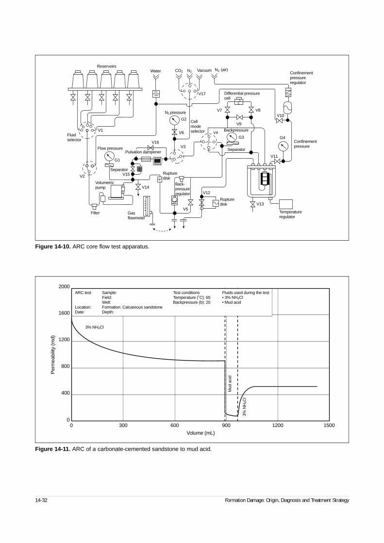
14-32 Formation Damage: Origin, Diagnosis and Treatment Strategy

Figure 14-11. ARC of a carbonate-cemented sandstone to mud acid.

0 300 600 900 1200 15000

400

800

1200

1600

2000

Volume (mL)

Per

mea

bilit

y (m

d)

3% NH4Cl

3% N

H4C

l

Mud

aci

d

ARC test Sample: Test conditions Fluids used during the testField: Temperature (˚C): 65 • 3% NH4ClWell: Backpressure (b): 20 • Mud acid

Location: Formation: Calcareous sandstoneDate: Depth:

Figure 14-10. ARC core flow test apparatus.

ReservoirsWater CO2 N2 N2Vacuum

Confinementpressureregulator

Differential pressurecell

V8V10

G4

V11

V13

V12

G3

V9

V7

Confinementpressure

Temperatureregulator

Rupturedisk

V5

V14

V15

Back-pressureregulator

Gasflowmeter

Rupturedisk

Pulsation dampener

Volumetricpump

Filter

V2

G1

Flow pressure

V1Fluidselector

N2 pressure

Cellmodeselector V4

Separator

Backpressure

V3

V17

G2

Separator

(air)

V6

V16

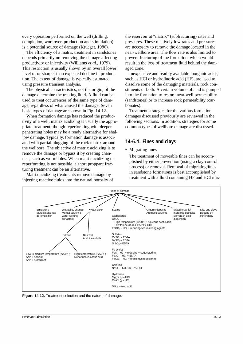
every operation performed on the well (drilling,completion, workover, production and stimulation)is a potential source of damage (Krueger, 1986).

The efficiency of a matrix treatment in sandstonesdepends primarily on removing the damage affectingproductivity or injectivity (Williams et al., 1979).This restriction is usually shown by an overall lowerlevel of or sharper than expected decline in produc-tion. The extent of damage is typically estimatedusing pressure transient analysis.

The physical characteristics, not the origin, of thedamage determine the treating fluid. A fluid can beused to treat occurrences of the same type of dam-age, regardless of what caused the damage. Sevenbasic types of damage are shown in Fig. 14-12.

When formation damage has reduced the produc-tivity of a well, matrix acidizing is usually the appro-priate treatment, though reperforating with deeperpenetrating holes may be a ready alternative for shal-low damage. Typically, formation damage is associ-ated with partial plugging of the rock matrix aroundthe wellbore. The objective of matrix acidizing is toremove the damage or bypass it by creating chan-nels, such as wormholes. When matrix acidizing orreperforating is not possible, a short proppant frac-turing treatment can be an alternative.

Matrix acidizing treatments remove damage byinjecting reactive fluids into the natural porosity of

the reservoir at “matrix” (subfracturing) rates andpressures. These relatively low rates and pressuresare necessary to remove the damage located in thenear-wellbore area. The flow rate is also limited toprevent fracturing of the formation, which wouldresult in the loss of treatment fluid behind the dam-aged zone.

Inexpensive and readily available inorganic acids,such as HCl or hydrofluoric acid (HF), are used todissolve some of the damaging materials, rock con-stituents or both. A certain volume of acid is pumpedinto the formation to restore near-well permeability(sandstones) or to increase rock permeability (car-bonates).

Treatment strategies for the various formationdamages discussed previously are reviewed in thefollowing sections. In addition, strategies for somecommon types of wellbore damage are discussed.

14-6.1. Fines and clays• Migrating fines

The treatment of moveable fines can be accom-plished by either prevention (using a clay-controlprocess) or removal. Removal of migrating finesin sandstone formations is best accomplished bytreatment with a fluid containing HF and HCl mix-

Reservoir Stimulation 14-33

Figure 14-12. Treatment selection and the nature of damage.

Types of damage

EmulsionsMutual solvent ±de-emulsifier

Wettability changeMutual solvent ±water-wettingsurfactant

Water block Scales

CarbonatesCaCO3

High temperature (>250°F): Aqueous acetic acidLow temperature (<250°F): HCl

FeCO3 – HCl + reducing/sequestering agents

SulfatesCaSO4 – EDTABaSO4 – EDTASrSO4 – EDTA

Fe scalesFeS – HCl + reducing + sequesteringFe2O3 – HCl + EDTAFeCO3 – HCl + reducing/sequestering

ChlorideNaCl – H2O, 1%–3% HCl

HydroxideMg(OH)2 – HClCa(OH)2 – HCl

Silica – mud acid

Organic depositsAromatic solvents

Mixed organic/inorganic depositsSolvent in aciddispersion

Silts and claysDepend onmineralogy

Oil well Gas wellAcid + alcohols

Low to medium temperature (≤250°F)Acid + solventAcid + surfactant

High temperature (>250°F)Nonaqueous acetic acid

tures—these are the commonly used mud acids.Deeply penetrating acid systems, containing fluo-boric acid, show a good possibility for particledestruction and extend some potential for clay sta-bilization. Fracturing the formation is also a treat-ment possibility because the effect from linearflow in the walls of the fracture has a less detri-mental effect on production than inward radialflow in an unfractured well. The success of bothclay control and fines removal depends on thedepth extent of the fines movement problem. Inmany cases, tip-screenout (TSO) fracture designusing a short fracture for damage bypass is a betteralternative.

HCl systems are typically used to remove finesdamage in a carbonate formation. Because thefines are not dissolved, but are dispersed in naturalfractures or the wormholes that are created, N2 isusually recommended to aid fines removal whenthe well has a low bottomhole pressure.

• Swelling clays

The removal of smectite is usually accomplishedwith HF or fluoboric acid, depending on the depthof penetration. In the event of deep clay-swellingproblems (more than 2 ft), the best treatment isusually a fracture to bypass the damage.

• Unconsolidated formations

Two basic problems determine the method oftreatment for unconsolidated formations. If the for-mation moves as discrete large particles (i.e., thebuilding blocks of the formation are moving), thenthe problem is a lack of cementation between thegrains for the applied production forces, and theformation is classified as a low-strength formation.Treating low-strength formations can be difficult ifthe cementing materials are reactive with the fluidthat is injected to remove formation damage or toimprove permeability. Fortunately, the cementingmaterials in most formations have a small surfacearea and are less reactive with acids than withfines or clay particles in the pores of the rock.

When formations expel large grains into thewellbore, it may be beneficial to add additionalperforations to reduce the velocity across the sand-face or to design a fracture to reduce the draw-down. (It is common to fracture formations withpermeabilities higher than 100 md.) These frac-tures are usually TSO designs that provide short,highly conductive fractures that can reduce the

drawdown and control sand movement by bothpressure reduction and use of the proppant at theinterface contacts of a gravel pack as an “in-formation” gravel pack.

The treatment of spalling problems is extremelydifficult. Propped fractures may help contain theformation and spread out the drawdown to reducethe spalling force, although totally halting spallingmay be impossible. One of the keys to treatmentselection is whether the spalling is caused by highinitial pressures that will quickly deplete or bycyclic mechanical loads that will recur. If high ini-tial pressure is the problem, a cleanout may suf-fice. If cycling is the problem, a permanent controlmethod is the best solution. Control methodsinclude gravel packing, fracture packing, selectiveperforating (along the fracture axis) and someplastic-bonding methods.

14-6.2. ScalesVarious solvents dissolve scales, depending on theirmineralogy. The most common treatments for thescales in a well are as follows:

• Carbonate scale (CaCO3 and FeCO3)—HCl willreadily dissolve all carbonate scales if the acid canpenetrate to the scale location (Tyler et al., 1985).

• Gypsum (CaSO4 ⋅ 2H2O) or anhydrite (CaSO4)—These calcium sulfate scales are removed withcompounds that convert the sulfate to a hydroxideor other ion form followed by acid or by directdissolvers such as ethylenediamenetetraacetic acid(EDTA) or other types of agents. Following a cal-cium sulfate dissolver with acid may double theamount of scale dissolved because most scales aremixtures of materials and HCl has some ability todissolve the finest particles of calcium sulfate. Thetetrasodium salt of EDTA is preferred because itsdissolution rate is greater at a slightly alkaline pH value; the more acidic disodium salt has alsobeen used, as well as other strong sequestrants ofthe same family, although they do not show amarked difference from the EDTA performance.Care must be used not to over-run the spent scaledissolver or converter solutions with acid becausemassive reprecipitation of the scale will occur.

• Barite (BaSO4) or celestite (SrSO4)—These sulfatescales are much more difficult to remove, but theiroccurrence is more predictable. Barium and stron-

14-34 Formation Damage: Origin, Diagnosis and Treatment Strategy

tium sulfates can also be dissolved with EDTA ifthe temperature is high enough and contact timesare sufficient (typically a 24-hr minimum soakingtime for a 12,000-ft well with a bottomhole tem-perature of about 212°F [100°C]; Clemmit et al.,1985). Barium and strontium sulfate removalmethods are usually mechanical. Most chemicalremovers are only slightly reactive, especially inthick deposits, but mixtures of barium sulfate andother scales can usually be removed by properlyformulated dissolvers with sufficient soak times.Thick deposits should be removed by mechanicalor abrasive methods. Care must be exercised whenanalyzing well debris to avoid mislabeling baritefrom drilling mud residue as barium sulfate scale.

• Sodium chloride (NaCl)—Sodium chloride scale is readily dissolved with fresh water or weakacidic (HCl, acetic) solutions. Redesigning themechanical system to avoid heat loss and waterdrop-out are also treatment possibilities.

• Iron scales, such as iron sulfide (FeS) or iron oxide(Fe2O3)—HCl with reducing and sequestering(EDTA) agents dissolves these scales and preventsthe reprecipitation of by-products, such as ironhydroxides and elemental sulfur (Crowe, 1985).Soak times of 30 min to 4 hr are usually beneficialin removing these scales when using acid. Whereiron sulfide is a thick deposit, mechanical action suchas milling is suggested. Water jetting typically willnot cut an iron sulfide scale except where it is dis-persed with other scales or exists as a thin coating.

• Silica scales—Silica scales generally occur asfinely crystallized deposits of chalcedony or asamorphous opal and are readily dissolved by HF.

• Hydroxide scales: magnesium (Mg(OH)2) or calci-um (Ca(OH)2) hydroxides—HCl or any acid thatcan sufficiently lower the pH value and not precip-itate calcium or magnesium salts can be used toremove these deposits.

Contact time is an important factor in the designof a scale removal treatment. The major concern intreating scale deposits is allowing sufficient time forthe treating fluid to reach and effectively dissolve thebulk of the scale material. The treating fluid mustdissolve most of the scale for the treatment to besuccessful.

14-6.3. Organic depositsOrganic deposits are usually resolubilized by organicsolvents. Blends of solvents can be tailored to a par-ticular problem, but an aromatic solvent is an effi-cient, general-purpose fluid. Environmental concernshave led to the development of alternative solvents(Samuelson, 1992).

Paraffin removal can be accomplished using heat,mechanical scraping or solvents. Heating the tubingwith a hot oiler may be the most common type oftreatment. It may also be the most damaging andleast effective in some cases. Injection of hot oilfrom the surface will melt the paraffin from the wallsof the pipe, but the depth to which the injected fluidstays hot is a function of the well configuration. Ifthe well is allowed to circulate up the annulus whilethe hot oil is injected down the tubing, the heat willnot penetrate more than a few joints of tubing fromthe surface. The heat is quickly transferred throughthe steel tubing to the fluids rising in the annulus andlittle, if any, heat reaches deep in the well. As the hotoil cools, the paraffin picked up in the upper part ofthe well can precipitate. If hot oiling is required atdepths greater than 150 ft, an alternate method ofplacement must be used. Deeper application of heatis available with other processes that feature heatgeneration as part of an exothermic chemical reac-tion. The processes require close control and aregenerally expensive.

Mechanical scraping can be useful in cases whereextensive deposits of paraffin must be removed rou-tinely. Scraping is usually accomplished with slick-line and a cutter. In wells that utilize a rod string,placing scrapers on the string may automaticallyscrape the tubing walls.

Solvent treating to remove paraffin may be basedaround a straight- or aromatic-chain solvent. Themost appropriate solvent depends on the specificparaffin and the location of the deposit. Heat (at leastto 130°F [55°C]) and agitation significantly increasethe rate of removal.

Removal treatments for asphaltenes use aromaticsolvents such as xylene and toluene or solvents con-taining high percentages of aromatics. Naphtha isusually not effective as a solvent. Some materialsbeing tested provide dispersant benefits without sta-bilizing the entire mass of the asphaltene. Solventsoak time, heat and agitation are important consider-ations for treatment.

Reservoir Stimulation 14-35

14-6.4. Mixed depositsCombined deposits require a dual-solvent system,such as dispersion of a hydrocarbon solvent (usuallyaromatic) into an acid.

14-6.5. EmulsionsEmulsions are stabilized by surface-active materials(surfactants) and by foreign or native fines. Gener-ally, mutual solvents, with or without de-emulsifiers,are used for treating emulsion problems. De-emulsi-fiers, which may work well in a laboratory or in aseparator or tank because of the large number ofdroplets in contact per unit volume, may not work by themselves in a porous medium because of mass-transport phenomena in getting the product to whereit should work. Another reason they may not workalone is the mechanism involved in breaking emul-sions, which should provoke the coalescence ofdroplets and then phase separation.

Asphaltic iron-catalyzed sludges are the most dif-ficult emulsions to break. These emulsions are cat-alyzed by dissolved iron in the acid or water andresemble a crosslinked oil polymer in someinstances. Prevention is the best treatment. An effec-tive antisludge treatment for the area and an iron-reducing agent in the acid are the best methods.Removal of an existing asphaltene sludge is usuallyaccomplished by dispersing it in a solvent andattacking the components of the sludge with addi-tives designed for cleanup and removal.

14-6.6. BacteriaPrevention of polymer destruction by bacteria is usu-ally handled with biocides and tank monitoring.Control of bacteria downhole is more difficult andinvolves scraping or treatments with sodiumhypochlorite or other oxidizers followed by acidizingand then treatment with an effective biocide at alevel at least 1.2 times the minimum kill level.Frequent rotation of the type of biocide is also neces-sary to prevent the development of biocide-resistantstrains of bacteria.

14-6.7. Induced particle plugging• Mud solids

To remove shallow mud damage in natural frac-tures, a solvent or cleaner that will disperse themud should be selected on the basis of tests of afield sample of the mud. Energizing the fluid withN2 can assist in removing large masses of drillingmud from a fracture system. Experience withdrilling mud cleanup from natural fracture systemsshows that slugs of drilling mud may flow back on initial treatment, and damage can often reassertitself as mud moves from the outer reaches of thefracture system into the wellbore. This conditioncan require repeated treatments of the same high-efficiency cleaner, plus N2, to get good cleanup ofthe well. Acid may help, but tests of the acid’seffect on the field mud sample are required.

When extremely large volumes of heavyweightmud are lost, it may be beneficial to sidetrack thewell and redrill the pay zone. Whenever possible,the drilling mud overbalance should be minimized,and the mud should be conditioned to reducesolids before the pay zone is drilled. Experiencewith drilling highly fractured formations has led to experimentation with underbalance drilling insome zones. Underbalance drilling can result inonly minimal damage in producing wells in com-parison with the damage created by traditionaldrilling methods. There are dangers, however, inunderbalance drilling, and the risk versus benefitmust be evaluated carefully.

Mudcakes are usually damaging only in open-hole completions without significant fractures(Burton, 1995). In vertical wells, they are usuallyeasily mechanically removed to a great extent bypressure drawdown. In long horizontal wellbores,the necessary drawdown is almost impossible toimpose on any section other than the heel, particu-larly when a compressible fluid is in the hole.Circulations for mudcake removal should be con-ducted with minimum clearance between the washpipe and the borehole to promote turbulence.Residual mudcake in prepacked screens or slottedliners completions is particularly problematicbecause it can plug the screen (Browne et al.,1995; Ryan et al., 1995).

14-36 Formation Damage: Origin, Diagnosis and Treatment Strategy

• Dirty fluids

When particle damage is known to have occurredbecause of the use of unfiltered or poor-quality flu-ids, cleanup depends on finding a solvent or acidthat can either remove the particles or break thestructure of the bridges formed in the formation orfracture system. Surfactants, acids and mutual sol-vents are usually the most beneficial materials.The addition of N2 to provide a high-energy boostmay also be beneficial.

The decision of which surfactant or mutual sol-vent to use should be based on core tests or fieldresponse. Including a gas such as N2 or CO2 isbased on fluid and solids recovery requirementsand wellbore unloading ability. For designingcleanup operations for particulate damage, flowingthe well back quickly after the treatment helps inthe removal of the particles. Lower pressure for-mations may require a gas boost. In higher pres-sure formations, natural flow is usually adequate to unload these solids, especially when a properlydesigned fluid has been used and the solids are nodeeper than the surface of the wellbore face.Mechanical scraping and cleaning can exert influ-ence only as far as the wellbore wall.

• Acidizing

The leading edge of an otherwise effective mutualsolvent and acid system can be loaded with debriscleaned off the walls of the tanks and tubing. Forthis reason, the leading edge of the acid job is usu-ally circulated out of the well using a processcalled pickling the tubing. In this treatment, acidand solvents are injected down the tubing to dis-perse and dissolve iron, pipe dope, mud and otherdebris from the tubing and are then circulated orreversed out of the well without being injectedinto the formation. These jobs are extremely effec-tive when the tubing has not been cleaned or itscondition is unknown. Volumes of both acids andadditive treatments range from 1 to 21⁄2 tubing vol-umes depending on the condition of the tubulars.Minimum acid and solvent volumes typically rangefrom 250 to 500 gal. Coated tubing can reduce ironscale significantly, but other contaminants, such asscale and pipe dope, may still be present.

If load-fluid recovery influences well produc-tion, surfactants or mutual solvents that reducesurface and interfacial tension are usually benefi

cial. The treatment volumes depend on the fluid,formation and amount of load fluid lost.

• Waterfloods

The removal of particles injected during water-flood operations depends on the identity of thematerial and use of a cleaner and an acid to dis-perse the material. One of the best techniques forcleaning up injection wells or disposal wells is tobackflow the well as hard as possible prior to thetreatment. This usually removes enough massfrom the wellbore to eliminate the need for stimu-lation. However, if backflowing does not ade-quately clean the wellbore, acid and a mutual sol-vent in volumes ranging from 50 to 100 gal/ft areusually necessary. When large amounts of solidsare expected, the well should be backflowed afteracidizing. If oil carryover and emulsions are theproblem, acid and a mutual solvent can be injectedand displaced permanently with injection waterbehind the acidizing job.

14-6.8. Oil-base drilling fluidsThe prevention of OBM emulsions is relatively easy.Either a surfactant-base cleaner that is mixed afterspecific OBM testing or a more general xylene washof the zone must be done before contact with eitherhigh-salinity brine or acid. After the cuttings andmud fines have been cleaned and totally water-wetted, the remaining damage problems of wettabilitycan be reversed with a formation cleaner or mutualsolvent. Acid is usually used as a following stageafter cleaning to remove mud particles and clean upformation debris. Removal of known OBM emul-sions resulting from mixing with high-salinity brineor acid usually requires an aromatic solvent wash ora specialized surfactant treatment that targets the silt-stabilized emulsion. Evaluation of any cleanupmechanism or treatment using laboratory samples ofOBM should be avoided. Only field samples of themud are appropriate for designing the removal treat-ment. Treatment fluid volumes range from 15 to 50 gal/ft of aromatic solvent or surfactant mixture,and the agitation and soak times are critical to thesuccess of the treatment. Application difficultiesinclude trapping the treating fluids across the pay ina column of heavyweight fluids where density segre-gation may be rapid. Packers and gelled plugs arethe first line of isolation.

Reservoir Stimulation 14-37

14-6.9. Water blocksRemoval of a water block can be accomplishedusing a surfactant or alcohol applied as a preflush toreduce surface tension, followed by a postflush of N2

or CO2 to remove the water from the near-wellborearea and reestablish gas saturation. Once the waterhas been mixed with the surface-tension-loweringmaterials, removal is easier. The difficulties in thistype of operation are placement of the fluid and get-ting an even distribution of the fluid around the well-bore. Repeated treatments are usually necessary, andselective injection devices are beneficial.

14-6.10. Wettability alterationWettability alteration damage is removed by inject-ing (mutual) solvents to remove the oil-wettinghydrocarbon phase and then injecting strongly water-wetting surfactants. Again, a surfactant by itself willnot work. The oil phase, which is usually precipi-tated asphaltenes or paraffins, must first be removedwith a solvent. (The same applies to an adsorbedoleophilic surfactant.) Then, a strongly water-wettingsurfactant can be injected and adsorbed onto the rockminerals. This reduces the tendency for new hydro-carbon precipitates to stick to the mineral surfacesand oil-wet them again.

For retrograde condensation problems, the mostappropriate treatment technique is the injection of neatnatural gas in a periodic “huff and puff” operation.Condensate is picked up by the gas and transportedinto the reservoir. Reprecipition requires the retrogradeof the process after several months of production.

14-6.11. Wellbore damage• Mechanical damage from drilling

The drilling process itself modifies the localstresses around the wellbore, generating a zone of reduced permeability in the near-wellbore area(Dusseault and Gray, 1992). It has been shownthat such damage affects primarily soft formationswhere the difference between the minimum andmaximum stresses orthogonal to the wellbore islarge. In the worst cases, the extent of the perme-ability decrease can be as large as 21⁄2 wellborediameters (Morales et al., 1995), and perforationsdo not bypass the damaged zone. Because perme-

ability impairment in this case is the result of rockcompaction, acidizing is ineffective. Short prop-pant fracturing treatments are apparently the onlycure, though extreme overbalance perforating maygive positive results in some cases (Petitjean et al.,1995).

• Pipe problems

Whenever well production is reduced, the firstdetermination should be to establish that the tub-ing is open and the lift system is working.Numerous pipe problems from leaks to collapsedpipe can occur, and fill in the tubing is also a pos-sibility. Well conditions change over time, and aneffective completion at the start of the well’s lifemay not be effective after several years of produc-tion as the reservoir pressure declines.

• Poor perforations

The usual treatment for poor perforations is to addadditional perforations. In zones that are extremelylaminated, such as the shaly sands of the U.S. GulfCoast and other areas, 8 to 12 spf is consideredadequate, but perforation breakdowns (i.e., smallfractures) may be required for complete linking.Lower perforation density is possible if the wellwill be fractured. Fracturing will cross the barriersof laminations, and in many field cases has pro-vided extensive productivity increases.

Adding perforations is easy, but the typical 0°phased, small through-tubing guns deliver onlysmall holes and short penetrations. The newerdownhole-deployable guns that provide minimumclearance and phasing are preferred, especiallywhen hydraulic fracturing will be performed.

• Hydrates

Hydrates are mixtures of ice and other elements,principally natural gas, that may resemble a dirtyice deposit. Unlike ice, they can form at tempera-tures greater than 32°F. The formation of hydratesis usually associated with a drop in temperature ora reduction in pressure that may accompany theproduction of fluids. Hydrates may also form ingas-cut drilling mud, particularly when the mud is circulated near the seafloor in cold locations.Hydrate plugging of chokes and valves can be a serious problem. Hydrate particle abrasion ofequipment is also possible.

The most common occurrence of hydrates is in gas wells with a small amount of water produc-

14-38 Formation Damage: Origin, Diagnosis and Treatment Strategy

tion. The quantity of water relative to the quantityof gas production is critical. As the water cutincreases, many hydrate problems disappear.Hydrates are prevented by adding a freezing-pointdepressant such as alcohol or glycol below thehydrate formation point. They may also be con-trolled by temperature preservation in the pro-duced fluid or the elimination of severe pressuredrops that allow expanding gas to chill the liquidsto their freezing points.

• Fill

Debris from formation spalling into the perforationor wellbore can be one of the most serious detri-ments to production. Fill in the wellbore is easilyidentified with a sinker bar on the wireline and isusually easily removed using tubing or coiled tub-ing and N2 or foam unloading practices. Fill in theperforations is more difficult to identify and muchmore difficult to remove. When fill in the perfora-tions is suspected, reperforating the well is gener-ally the most direct method of testing the theoryand restoring the well to productivity. Where thefill is acid soluble, acid injection may be useful;however, injecting acid into a perforation that isfilled with small debris is usually difficult.

• Water problems

Water production is not only a major economicproblem in surface separation, but it also causes amajor reduction in the relative permeability of oiland gas. Water production from the well can leadto significant problems such as corrosion, back-pressure, emulsions and movement of the forma-tion or fines. Water may flow from the bottom(coning), rise through fractures or flow from theedge in fractures through the matrix or in high-permeability streaks. Because of its low viscosity,water flows much easier than oil, and once in the

pores of the rock it is difficult to displace withlow-viscosity fluids such as gas. Shutting off water(water control) is a special technique and is dis-cussed elsewhere in the literature.

• Microporosity

Microporosity is created by a number of clays anda few minerals. It is simply a condition where alarge surface area exists for water coating or trap-ping. Microporosity rarely presents a problemexcept when it occupies the pore throat area of theformation. In these cases, it may trap either debrisor water and obstruct flow. The removal of micro-porosity can generally be accomplished with HF,or deep problems can be bypassed by fracturing.

14-7. ConclusionsTo maximize well performance, the paths from theformation to the pipeline must present the lowestpressure impedance possible. Achieving this condi-tion requires both a well-designed completion and the elimination of formation damage. The tools are an array of stimulation and damage removal tech-niques and chemicals that are readily available. Still,although formation damage removal seems easilyachievable, the goal of a damage-free completion canbe elusive. The problem is not so much one of find-ing a tool, but one of finding the right tool. A littleexperience shows that the right tool can be selectedonly when the problem has been identified. The effortand expense to understand the nature and identity ofthe problem can be the wisest investments.

The most common damage mechanisms and sug-gested methods of removal are listed in Tables 14-3,14-4 and 14-5. It bears repeating that many damageconditions have similar symptoms and that there areno universal treatments.

Reservoir Stimulation 14-39

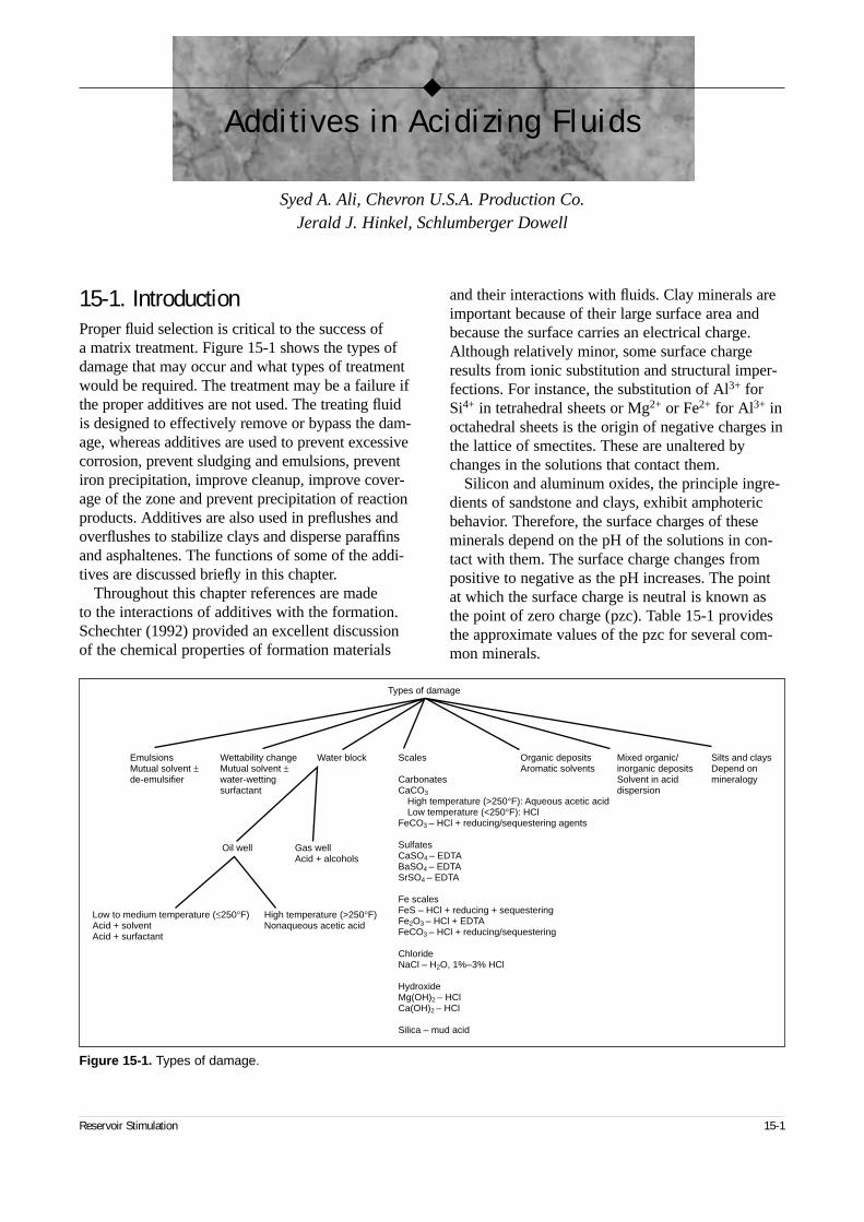
15-1. IntroductionProper fluid selection is critical to the success of a matrix treatment. Figure 15-1 shows the types ofdamage that may occur and what types of treatmentwould be required. The treatment may be a failure ifthe proper additives are not used. The treating fluidis designed to effectively remove or bypass the dam-age, whereas additives are used to prevent excessivecorrosion, prevent sludging and emulsions, preventiron precipitation, improve cleanup, improve cover-age of the zone and prevent precipitation of reactionproducts. Additives are also used in preflushes andoverflushes to stabilize clays and disperse paraffinsand asphaltenes. The functions of some of the addi-tives are discussed briefly in this chapter.

Throughout this chapter references are made to the interactions of additives with the formation.Schechter (1992) provided an excellent discussionof the chemical properties of formation materials

and their interactions with fluids. Clay minerals areimportant because of their large surface area andbecause the surface carries an electrical charge.Although relatively minor, some surface chargeresults from ionic substitution and structural imper-fections. For instance, the substitution of Al3+ forSi4+ in tetrahedral sheets or Mg2+ or Fe2+ for Al3+ inoctahedral sheets is the origin of negative charges inthe lattice of smectites. These are unaltered bychanges in the solutions that contact them.

Silicon and aluminum oxides, the principle ingre-dients of sandstone and clays, exhibit amphotericbehavior. Therefore, the surface charges of theseminerals depend on the pH of the solutions in con-tact with them. The surface charge changes frompositive to negative as the pH increases. The pointat which the surface charge is neutral is known asthe point of zero charge (pzc). Table 15-1 providesthe approximate values of the pzc for several com-mon minerals.

Reservoir Stimulation 15-1

◆

Additives in Acidizing Fluids

Syed A. Ali, Chevron U.S.A. Production Co.Jerald J. Hinkel, Schlumberger Dowell

Figure 15-1. Types of damage.

Types of damage

EmulsionsMutual solvent ±de-emulsifier

Wettability changeMutual solvent ±water-wettingsurfactant

Water block Scales

CarbonatesCaCO3

High temperature (>250°F): Aqueous acetic acidLow temperature (<250°F): HCl

FeCO3 – HCl + reducing/sequestering agents

SulfatesCaSO4 – EDTABaSO4 – EDTASrSO4 – EDTA

Fe scalesFeS – HCl + reducing + sequesteringFe2O3 – HCl + EDTAFeCO3 – HCl + reducing/sequestering

ChlorideNaCl – H2O, 1%–3% HCl

HydroxideMg(OH)2 – HClCa(OH)2 – HCl

Silica – mud acid

Organic depositsAromatic solvents

Mixed organic/inorganic depositsSolvent in aciddispersion

Silts and claysDepend onmineralogy

Oil well Gas wellAcid + alcohols

Low to medium temperature (≤250°F)Acid + solventAcid + surfactant

High temperature (>250°F)Nonaqueous acetic acid

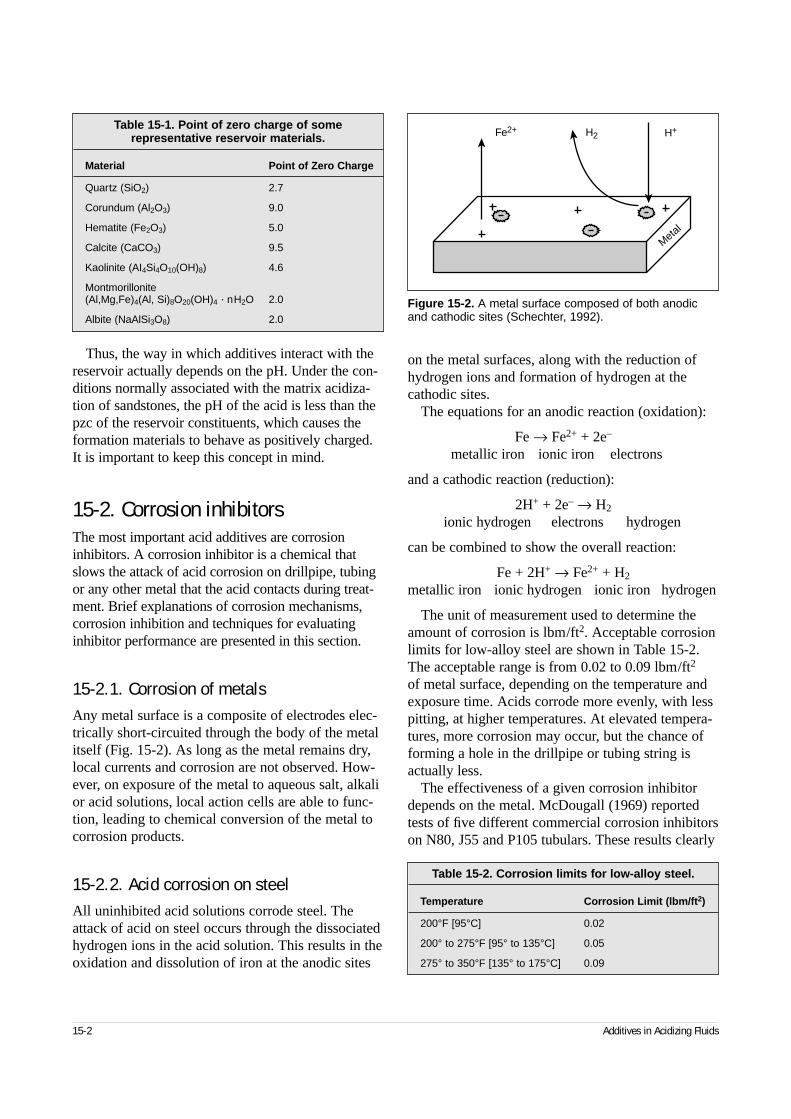
Thus, the way in which additives interact with thereservoir actually depends on the pH. Under the con-ditions normally associated with the matrix acidiza-tion of sandstones, the pH of the acid is less than thepzc of the reservoir constituents, which causes theformation materials to behave as positively charged.It is important to keep this concept in mind.

15-2. Corrosion inhibitorsThe most important acid additives are corrosioninhibitors. A corrosion inhibitor is a chemical thatslows the attack of acid corrosion on drillpipe, tubingor any other metal that the acid contacts during treat-ment. Brief explanations of corrosion mechanisms,corrosion inhibition and techniques for evaluatinginhibitor performance are presented in this section.

15-2.1. Corrosion of metalsAny metal surface is a composite of electrodes elec-trically short-circuited through the body of the metalitself (Fig. 15-2). As long as the metal remains dry,local currents and corrosion are not observed. How-ever, on exposure of the metal to aqueous salt, alkalior acid solutions, local action cells are able to func-tion, leading to chemical conversion of the metal tocorrosion products.

15-2.2. Acid corrosion on steelAll uninhibited acid solutions corrode steel. Theattack of acid on steel occurs through the dissociatedhydrogen ions in the acid solution. This results in theoxidation and dissolution of iron at the anodic sites

on the metal surfaces, along with the reduction ofhydrogen ions and formation of hydrogen at thecathodic sites.

The equations for an anodic reaction (oxidation):

Fe → Fe2+ + 2e–

metallic iron ionic iron electrons

and a cathodic reaction (reduction):

2H+ + 2e– → H2

ionic hydrogen electrons hydrogen

can be combined to show the overall reaction:

Fe + 2H+ → Fe2+ + H2

metallic iron ionic hydrogen ionic iron hydrogen

The unit of measurement used to determine theamount of corrosion is lbm/ft2. Acceptable corrosionlimits for low-alloy steel are shown in Table 15-2.The acceptable range is from 0.02 to 0.09 lbm/ft2

of metal surface, depending on the temperature andexposure time. Acids corrode more evenly, with lesspitting, at higher temperatures. At elevated tempera-tures, more corrosion may occur, but the chance offorming a hole in the drillpipe or tubing string isactually less.

The effectiveness of a given corrosion inhibitordepends on the metal. McDougall (1969) reportedtests of five different commercial corrosion inhibitorson N80, J55 and P105 tubulars. These results clearly

15-2 Additives in Acidizing Fluids

Table 15-1. Point of zero charge of some representative reservoir materials.

Material Point of Zero Charge

Quartz (SiO2) 2.7

Corundum (Al2O3) 9.0

Hematite (Fe2O3) 5.0

Calcite (CaCO3) 9.5

Kaolinite (AI4Si4O10(OH)8) 4.6

Montmorillonite(Al,Mg,Fe)4(Al, Si)8O20(OH)4 · nH2O 2.0

Albite (NaAlSi3O8) 2.0

Figure 15-2. A metal surface composed of both anodicand cathodic sites (Schechter, 1992).

Fe2+ H2 H+

Metal

Table 15-2. Corrosion limits for low-alloy steel.

Temperature Corrosion Limit (lbm/ft2)

200°F [95°C] 0.02

200° to 275°F [95° to 135°C] 0.05

275° to 350°F [135° to 175°C] 0.09

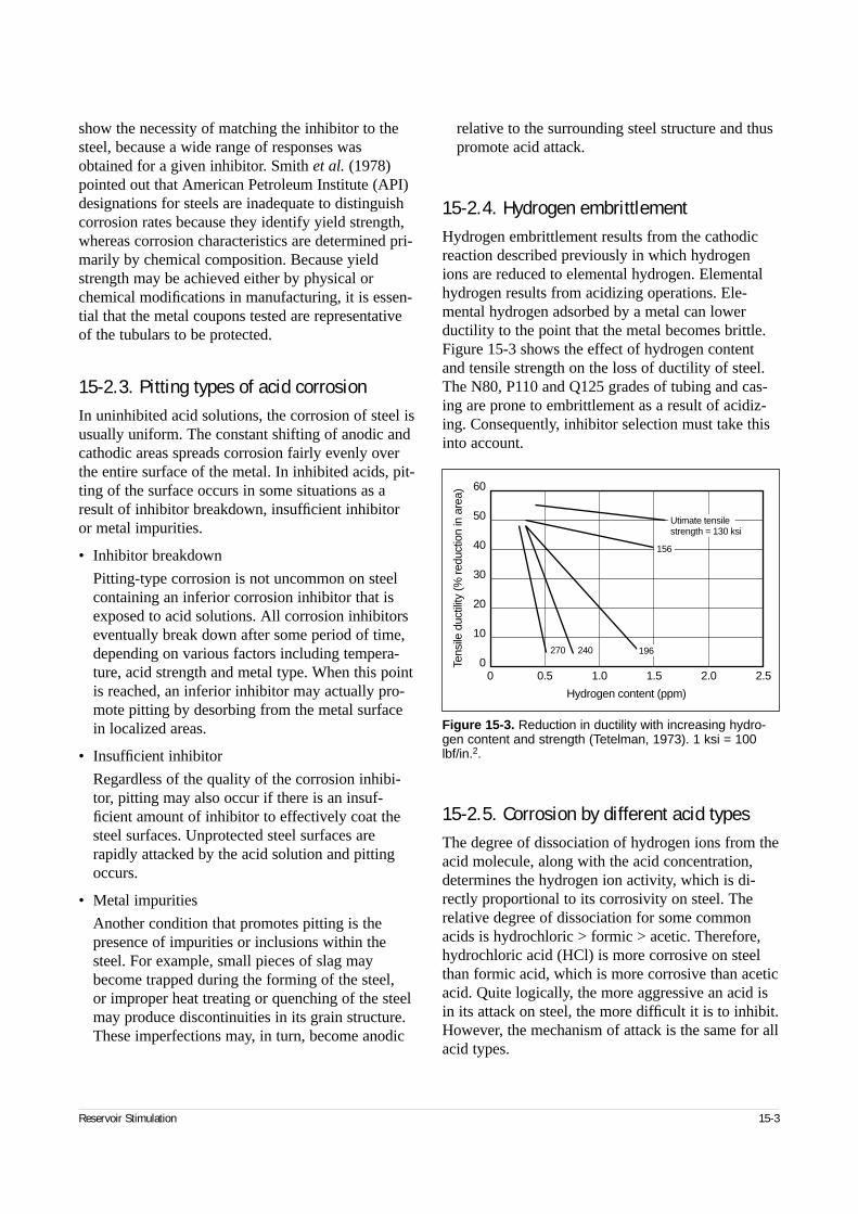
show the necessity of matching the inhibitor to thesteel, because a wide range of responses wasobtained for a given inhibitor. Smith et al. (1978)pointed out that American Petroleum Institute (API)designations for steels are inadequate to distinguishcorrosion rates because they identify yield strength,whereas corrosion characteristics are determined pri-marily by chemical composition. Because yieldstrength may be achieved either by physical orchemical modifications in manufacturing, it is essen-tial that the metal coupons tested are representativeof the tubulars to be protected.

15-2.3. Pitting types of acid corrosionIn uninhibited acid solutions, the corrosion of steel isusually uniform. The constant shifting of anodic andcathodic areas spreads corrosion fairly evenly overthe entire surface of the metal. In inhibited acids, pit-ting of the surface occurs in some situations as aresult of inhibitor breakdown, insufficient inhibitoror metal impurities.

• Inhibitor breakdown

Pitting-type corrosion is not uncommon on steelcontaining an inferior corrosion inhibitor that isexposed to acid solutions. All corrosion inhibitorseventually break down after some period of time,depending on various factors including tempera-ture, acid strength and metal type. When this pointis reached, an inferior inhibitor may actually pro-mote pitting by desorbing from the metal surfacein localized areas.

• Insufficient inhibitor

Regardless of the quality of the corrosion inhibi-tor, pitting may also occur if there is an insuf-ficient amount of inhibitor to effectively coat thesteel surfaces. Unprotected steel surfaces arerapidly attacked by the acid solution and pittingoccurs.

• Metal impurities

Another condition that promotes pitting is thepresence of impurities or inclusions within thesteel. For example, small pieces of slag maybecome trapped during the forming of the steel, or improper heat treating or quenching of the steelmay produce discontinuities in its grain structure.These imperfections may, in turn, become anodic

relative to the surrounding steel structure and thuspromote acid attack.

15-2.4. Hydrogen embrittlementHydrogen embrittlement results from the cathodicreaction described previously in which hydrogenions are reduced to elemental hydrogen. Elementalhydrogen results from acidizing operations. Ele-mental hydrogen adsorbed by a metal can lowerductility to the point that the metal becomes brittle.Figure 15-3 shows the effect of hydrogen contentand tensile strength on the loss of ductility of steel.The N80, P110 and Q125 grades of tubing and cas-ing are prone to embrittlement as a result of acidiz-ing. Consequently, inhibitor selection must take thisinto account.

15-2.5. Corrosion by different acid typesThe degree of dissociation of hydrogen ions from theacid molecule, along with the acid concentration,determines the hydrogen ion activity, which is di-rectly proportional to its corrosivity on steel. Therelative degree of dissociation for some commonacids is hydrochloric > formic > acetic. Therefore,hydrochloric acid (HCl) is more corrosive on steelthan formic acid, which is more corrosive than aceticacid. Quite logically, the more aggressive an acid isin its attack on steel, the more difficult it is to inhibit.However, the mechanism of attack is the same for allacid types.

Reservoir Stimulation 15-3

Figure 15-3. Reduction in ductility with increasing hydro-gen content and strength (Tetelman, 1973). 1 ksi = 100lbf/in.2.

00

10

0.5 1.0 1.5 2.0 2.5

20

30

40

50

60

Hydrogen content (ppm)

Tens

ile d

uctil

ity (%

redu

ctio

n in

are

a)

240270

Utimate tensile strength = 130 ksi

156

196

15-2.6. Inhibitor typesInhibitors function by interfering with the chemicalreactions that occur at the anode or cathode of thecorrosion cell. The two basic types of corrosioninhibitors are inorganic and organic. There are alsoinhibitor aids.

• Inorganic corrosion inhibitors

This class of inhibitors includes the salts of zinc,nickel, copper, arsenic, antimony and various othermetals. Of these, the most widely used are thearsenic compounds. When these arsenic com-pounds are added to an acid solution, they “plateout” at cathodic sites of exposed steel surfaces.The plating decreases the rate of hydrogen ionexchange, because the iron sulfide that formsbetween the steel and the acid acts as a barrier. Itis a dynamic process in which the acid reacts withiron sulfide, rather than the metal.

Some advantages of inorganic inhibitors are thatthey

– work effectively at high temperatures for longcontact times

– cost less than organic inhibitors.

Disadvantages of inorganic inhibitors are thatthey

– tend to lose their effectiveness in acid solutionsstronger than about 17% HCl

– react with hydrogen sulfide (H2S) through theiron sulfide that may be present to form an insol-uble precipitate such as arsenic sulfide

– poison refinery catalysts (such as platinum)

– may liberate toxic arsine gas as a corrosion by-product

– are difficult to mix and unsafe to handle.

• Organic corrosion inhibitors

Organic corrosion inhibitors are composed of polarorganic compounds capable of adsorbing onto themetal surface, thereby establishing a protective filmthat acts as a barrier between the metal and the acidsolution. They usually serve as a cathodic polarizerby limiting hydrogen ion mobility at cathodic sites.Organic inhibitors are composed of rather complexcompounds, with one or more polar groups madeof sulfur, oxygen or nitrogen.

Some advantages of organic inhibitors are thatthey

– can be used in the presence of H2S without theprecipitation of salts such as arsenic sulfide(which can plug the wellbore)

– do not poison refinery catalysts

– work effectively in all acid concentrations.

Disadvantages of organic inhibitors are that they

– chemically degrade with time in the presence ofacid and thus do not readily provide long-termprotection at temperatures above 200°F [95°C](Table 15-3)

– cost more than the inorganic corrosion inhib-itors.

• Inhibitor aids

Although these additives do not function as inhib-itors, they increase the effectiveness of organicinhibitors. The common inhibitor aids are potas-sium iodide, cuprous iodide, cuprous chloride andformic acid. The addition of these materials toexisting organic inhibitor formulations greatlyextends the range of their effectiveness, particularlyin higher temperature applications.

15-2.7. Compatibility with other additivesAny additive that alters the tendency of the corrosioninhibitor to adsorb will also change its effectiveness.For example, surfactants added to acid for variouspurposes may form micelles that solubilize theinhibitor, thereby decreasing the tendency for theinhibitor to adsorb on the metal surface. Inorganicsalts and mutual solvents can also interfere withinhibitor adsorption. If possible, additives that reduce

15-4 Additives in Acidizing Fluids

Table 15-3. Effectiveness of corrosion inhibitors athigh temperatures in 15% HCl.

Inhibitor Inhibitor Temperature ProtectionConcentration (°F) Time†

(%) (hr)

Organic 0.6 200 24

1.0 250 10

2.0 300 2

Inorganic 0.4 200 24

1.2 250 24

2.0 300 12

† Time required for 15% HCl to remove 0.05 lbm/ft2 of exposed metal area

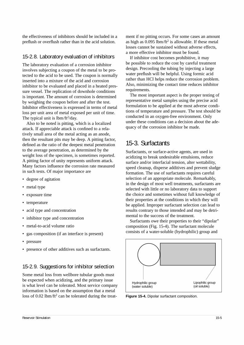
the effectiveness of inhibitors should be included in apreflush or overflush rather than in the acid solution.

15-2.8. Laboratory evaluation of inhibitorsThe laboratory evaluation of a corrosion inhibitorinvolves subjecting a coupon of the metal to be pro-tected to the acid to be used. The coupon is normallyinserted into a mixture of the acid and corrosioninhibitor to be evaluated and placed in a heated pres-sure vessel. The replication of downhole conditionsis important. The amount of corrosion is determinedby weighing the coupon before and after the test.Inhibitor effectiveness is expressed in terms of metalloss per unit area of metal exposed per unit of time.The typical unit is lbm/ft2/day.

Also to be noted is pitting, which is a localizedattack. If appreciable attack is confined to a rela-tively small area of the metal acting as an anode,then the resultant pits may be deep. A pitting factor,defined as the ratio of the deepest metal penetrationto the average penetration, as determined by theweight loss of the specimen, is sometimes reported.A pitting factor of unity represents uniform attack.Many factors influence the corrosion rate measuredin such tests. Of major importance are

• degree of agitation

• metal type

• exposure time

• temperature

• acid type and concentration

• inhibitor type and concentration

• metal-to-acid volume ratio

• gas composition (if an interface is present)

• pressure

• presence of other additives such as surfactants.

15-2.9. Suggestions for inhibitor selectionSome metal loss from wellbore tubular goods mustbe expected when acidizing, and the primary issue is what level can be tolerated. Most service companyinformation is based on the assumption that a metalloss of 0.02 lbm/ft2 can be tolerated during the treat-

ment if no pitting occurs. For some cases an amountas high as 0.095 lbm/ft2 is allowable. If these metallosses cannot be sustained without adverse effects, a more effective inhibitor must be found.

If inhibitor cost becomes prohibitive, it may be possible to reduce the cost by careful treatmentdesign. Precooling the tubing by injecting a largewater preflush will be helpful. Using formic acidrather than HCl helps reduce the corrosion problem.Also, minimizing the contact time reduces inhibitorrequirements.

The most important aspect is the proper testing ofrepresentative metal samples using the precise acidformulation to be applied at the most adverse condi-tions of temperature and pressure. The test should beconducted in an oxygen-free environment. Onlyunder these conditions can a decision about the ade-quacy of the corrosion inhibitor be made.

15-3. SurfactantsSurfactants, or surface-active agents, are used inacidizing to break undesirable emulsions, reducesurface and/or interfacial tension, alter wettability,speed cleanup, disperse additives and prevent sludgeformation. The use of surfactants requires carefulselection of an appropriate molecule. Remarkably, in the design of most well treatments, surfactants areselected with little or no laboratory data to supportthe choice and sometimes without full knowledge oftheir properties at the conditions in which they willbe applied. Improper surfactant selection can lead toresults contrary to those intended and may be detri-mental to the success of the treatment.

Surfactants owe their properties to their “dipolar”composition (Fig. 15-4). The surfactant moleculeconsists of a water-soluble (hydrophilic) group and

Reservoir Stimulation 15-5

Figure 15-4. Dipolar surfactant composition.

Hydrophilic group(water soluble)

Lipophilic group(oil soluble)

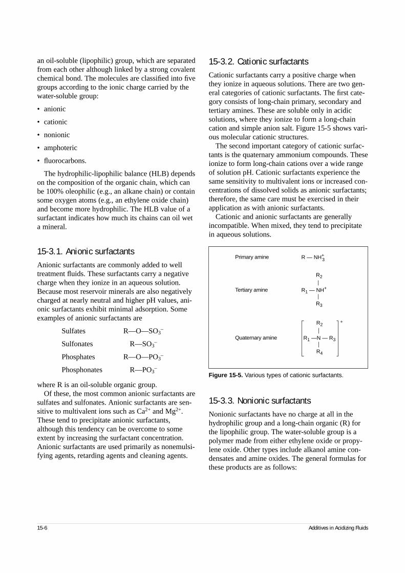
an oil-soluble (lipophilic) group, which are separatedfrom each other although linked by a strong covalentchemical bond. The molecules are classified into fivegroups according to the ionic charge carried by thewater-soluble group:

• anionic

• cationic

• nonionic

• amphoteric

• fluorocarbons.

The hydrophilic-lipophilic balance (HLB) dependson the composition of the organic chain, which canbe 100% oleophilic (e.g., an alkane chain) or containsome oxygen atoms (e.g., an ethylene oxide chain)and become more hydrophilic. The HLB value of asurfactant indicates how much its chains can oil weta mineral.

15-3.1. Anionic surfactantsAnionic surfactants are commonly added to welltreatment fluids. These surfactants carry a negativecharge when they ionize in an aqueous solution.Because most reservoir minerals are also negativelycharged at nearly neutral and higher pH values, ani-onic surfactants exhibit minimal adsorption. Someexamples of anionic surfactants are

Sulfates R—O—SO3–

Sulfonates R—SO3–

Phosphates R—O—PO3–

Phosphonates R—PO3–

where R is an oil-soluble organic group.Of these, the most common anionic surfactants are

sulfates and sulfonates. Anionic surfactants are sen-sitive to multivalent ions such as Ca2+ and Mg2+.These tend to precipitate anionic surfactants,although this tendency can be overcome to someextent by increasing the surfactant concentration.Anionic surfactants are used primarily as nonemulsi-fying agents, retarding agents and cleaning agents.

15-3.2. Cationic surfactantsCationic surfactants carry a positive charge whenthey ionize in aqueous solutions. There are two gen-eral categories of cationic surfactants. The first cate-gory consists of long-chain primary, secondary andtertiary amines. These are soluble only in acidicsolutions, where they ionize to form a long-chaincation and simple anion salt. Figure 15-5 shows vari-ous molecular cationic structures.

The second important category of cationic surfac-tants is the quaternary ammonium compounds. Theseionize to form long-chain cations over a wide rangeof solution pH. Cationic surfactants experience thesame sensitivity to multivalent ions or increased con-centrations of dissolved solids as anionic surfactants;therefore, the same care must be exercised in theirapplication as with anionic surfactants.

Cationic and anionic surfactants are generallyincompatible. When mixed, they tend to precipitatein aqueous solutions.

15-3.3. Nonionic surfactantsNonionic surfactants have no charge at all in thehydrophilic group and a long-chain organic (R) forthe lipophilic group. The water-soluble group is apolymer made from either ethylene oxide or propy-lene oxide. Other types include alkanol amine con-densates and amine oxides. The general formulas forthese products are as follows:

15-6 Additives in Acidizing Fluids

Figure 15-5. Various types of cationic surfactants.

R — NH+Primary amine

R1 — NH+Tertiary amine

3

R2

R3

R1 —N — R3Quaternary amine

R2

R4

+

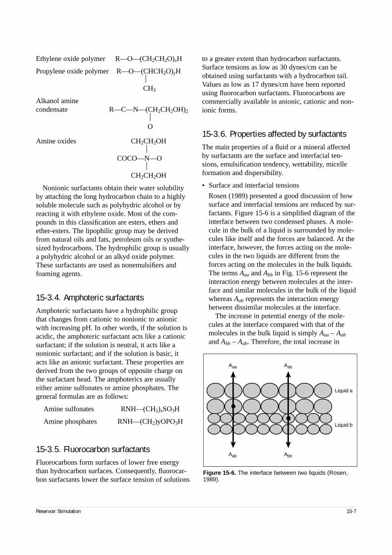
Ethylene oxide polymer R—O—(CH2CH2O)xH

Propylene oxide polymer R—O—(CHCH2O)yHCH3

Alkanol amine condensate R—C—N—(CH2CH2OH)2

O

Amine oxides CH2CH2OH

COCO—N—O

CH2CH2OH

Nonionic surfactants obtain their water solubilityby attaching the long hydrocarbon chain to a highlysoluble molecule such as polyhydric alcohol or byreacting it with ethylene oxide. Most of the com-pounds in this classification are esters, ethers andether-esters. The lipophilic group may be derivedfrom natural oils and fats, petroleum oils or synthe-sized hydrocarbons. The hydrophilic group is usuallya polyhydric alcohol or an alkyd oxide polymer.These surfactants are used as nonemulsifiers andfoaming agents.

15-3.4. Amphoteric surfactantsAmphoteric surfactants have a hydrophilic groupthat changes from cationic to nonionic to anionicwith increasing pH. In other words, if the solution isacidic, the amphoteric surfactant acts like a cationicsurfactant; if the solution is neutral, it acts like anonionic surfactant; and if the solution is basic, itacts like an anionic surfactant. These properties arederived from the two groups of opposite charge onthe surfactant head. The amphoterics are usuallyeither amine sulfonates or amine phosphates. Thegeneral formulas are as follows:

Amine sulfonates RNH—(CH2)xSO3H

Amine phosphates RNH—(CH2)yOPO3H

15-3.5. Fluorocarbon surfactantsFluorocarbons form surfaces of lower free energythan hydrocarbon surfaces. Consequently, fluorocar-bon surfactants lower the surface tension of solutions

to a greater extent than hydrocarbon surfactants.Surface tensions as low as 30 dynes/cm can beobtained using surfactants with a hydrocarbon tail.Values as low as 17 dynes/cm have been reportedusing fluorocarbon surfactants. Fluorocarbons arecommercially available in anionic, cationic and non-ionic forms.

15-3.6. Properties affected by surfactantsThe main properties of a fluid or a mineral affectedby surfactants are the surface and interfacial ten-sions, emulsification tendency, wettability, micelleformation and dispersibility.

• Surface and interfacial tensions

Rosen (1989) presented a good discussion of howsurface and interfacial tensions are reduced by sur-factants. Figure 15-6 is a simplified diagram of theinterface between two condensed phases. A mole-cule in the bulk of a liquid is surrounded by mole-cules like itself and the forces are balanced. At theinterface, however, the forces acting on the mole-cules in the two liquids are different from theforces acting on the molecules in the bulk liquids.The terms Aaa and Abb in Fig. 15-6 represent theinteraction energy between molecules at the inter-face and similar molecules in the bulk of the liquidwhereas Aab represents the interaction energybetween dissimilar molecules at the interface.

The increase in potential energy of the mole-cules at the interface compared with that of themolecules in the bulk liquid is simply Aaa – Aab

and Abb – Aab. Therefore, the total increase in

Reservoir Stimulation 15-7

Figure 15-6. The interface between two liquids (Rosen,1989).

Aab Abb

Aaa Aab

Liquid a

Liquid b

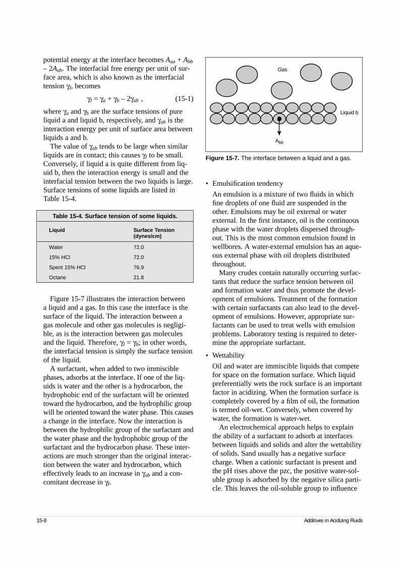
potential energy at the interface becomes Aaa + Abb

– 2Aab. The interfacial free energy per unit of sur-face area, which is also known as the interfacialtension γI, becomes

γI = γa + γb – 2γab , (15-1)

where γa and γb are the surface tensions of pureliquid a and liquid b, respectively, and γab is theinteraction energy per unit of surface area betweenliquids a and b.

The value of γab tends to be large when similarliquids are in contact; this causes γI to be small.Conversely, if liquid a is quite different from liq-uid b, then the interaction energy is small and theinterfacial tension between the two liquids is large.Surface tensions of some liquids are listed in Table 15-4.

Figure 15-7 illustrates the interaction between a liquid and a gas. In this case the interface is thesurface of the liquid. The interaction between agas molecule and other gas molecules is negligi-ble, as is the interaction between gas moleculesand the liquid. Therefore, γI = γb; in other words,the interfacial tension is simply the surface tensionof the liquid.

A surfactant, when added to two immisciblephases, adsorbs at the interface. If one of the liq-uids is water and the other is a hydrocarbon, thehydrophobic end of the surfactant will be orientedtoward the hydrocarbon, and the hydrophilic groupwill be oriented toward the water phase. This causesa change in the interface. Now the interaction isbetween the hydrophilic group of the surfactant andthe water phase and the hydrophobic group of thesurfactant and the hydrocarbon phase. These inter-actions are much stronger than the original interac-tion between the water and hydrocarbon, whicheffectively leads to an increase in γab and a con-comitant decrease in γI.

• Emulsification tendency

An emulsion is a mixture of two fluids in whichfine droplets of one fluid are suspended in theother. Emulsions may be oil external or waterexternal. In the first instance, oil is the continuousphase with the water droplets dispersed through-out. This is the most common emulsion found inwellbores. A water-external emulsion has an aque-ous external phase with oil droplets distributedthroughout.

Many crudes contain naturally occurring surfac-tants that reduce the surface tension between oiland formation water and thus promote the devel-opment of emulsions. Treatment of the formationwith certain surfactants can also lead to the devel-opment of emulsions. However, appropriate sur-factants can be used to treat wells with emulsionproblems. Laboratory testing is required to deter-mine the appropriate surfactant.

• Wettability

Oil and water are immiscible liquids that competefor space on the formation surface. Which liquidpreferentially wets the rock surface is an importantfactor in acidizing. When the formation surface iscompletely covered by a film of oil, the formationis termed oil-wet. Conversely, when covered bywater, the formation is water-wet.

An electrochemical approach helps to explainthe ability of a surfactant to adsorb at interfacesbetween liquids and solids and alter the wettabilityof solids. Sand usually has a negative surfacecharge. When a cationic surfactant is present andthe pH rises above the pzc, the positive water-sol-uble group is adsorbed by the negative silica parti-cle. This leaves the oil-soluble group to influence

15-8 Additives in Acidizing Fluids

Table 15-4. Surface tension of some liquids.

Liquid Surface Tension(dynes/cm)

Water 72.0

15% HCl 72.0

Spent 15% HCl 76.9

Octane 21.8

Figure 15-7. The interface between a liquid and a gas.

Abb

Gas

Liquid b

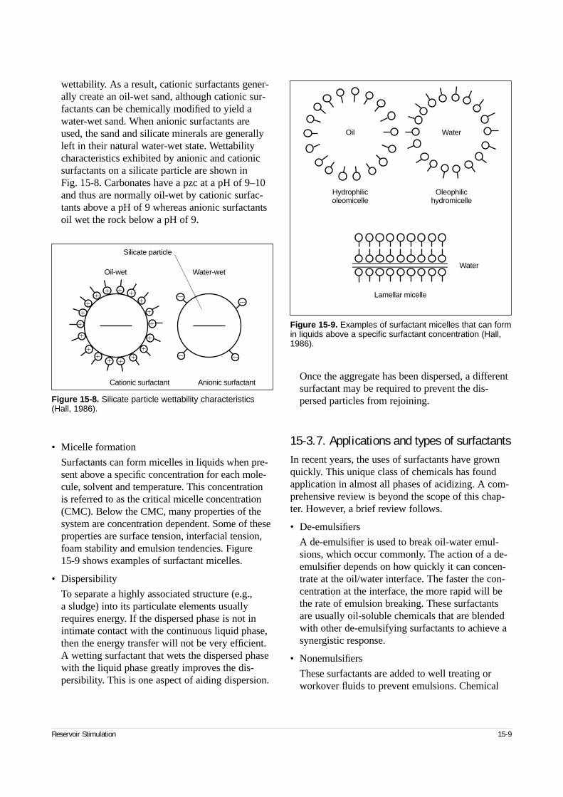
wettability. As a result, cationic surfactants gener-ally create an oil-wet sand, although cationic sur-factants can be chemically modified to yield awater-wet sand. When anionic surfactants areused, the sand and silicate minerals are generallyleft in their natural water-wet state. Wettabilitycharacteristics exhibited by anionic and cationicsurfactants on a silicate particle are shown in Fig. 15-8. Carbonates have a pzc at a pH of 9–10and thus are normally oil-wet by cationic surfac-tants above a pH of 9 whereas anionic surfactantsoil wet the rock below a pH of 9.

• Micelle formation

Surfactants can form micelles in liquids when pre-sent above a specific concentration for each mole-cule, solvent and temperature. This concentration is referred to as the critical micelle concentration(CMC). Below the CMC, many properties of thesystem are concentration dependent. Some of theseproperties are surface tension, interfacial tension,foam stability and emulsion tendencies. Figure 15-9 shows examples of surfactant micelles.

• Dispersibility

To separate a highly associated structure (e.g., a sludge) into its particulate elements usuallyrequires energy. If the dispersed phase is not inintimate contact with the continuous liquid phase,then the energy transfer will not be very efficient.A wetting surfactant that wets the dispersed phasewith the liquid phase greatly improves the dis-persibility. This is one aspect of aiding dispersion.

Once the aggregate has been dispersed, a differentsurfactant may be required to prevent the dis-persed particles from rejoining.

15-3.7. Applications and types of surfactantsIn recent years, the uses of surfactants have grownquickly. This unique class of chemicals has foundapplication in almost all phases of acidizing. A com-prehensive review is beyond the scope of this chap-ter. However, a brief review follows.

• De-emulsifiers

A de-emulsifier is used to break oil-water emul-sions, which occur commonly. The action of a de-emulsifier depends on how quickly it can concen-trate at the oil/water interface. The faster the con-centration at the interface, the more rapid will bethe rate of emulsion breaking. These surfactantsare usually oil-soluble chemicals that are blendedwith other de-emulsifying surfactants to achieve asynergistic response.

• Nonemulsifiers

These surfactants are added to well treating orworkover fluids to prevent emulsions. Chemical

Reservoir Stimulation 15-9

Figure 15-8. Silicate particle wettability characteristics(Hall, 1986).

Oil-wet Water-wet

Anionic surfactantCationic surfactant

Silicate particle

Figure 15-9. Examples of surfactant micelles that can formin liquids above a specific surfactant concentration (Hall,1986).

Oil Water

Water

Hydrophilicoleomicelle

Oleophilichydromicelle

Lamellar micelle

suppliers and service companies have many differ-ent surfactants that are classified as nonemulsifiers.The chemicals are usually mixtures of surfactantsand solvents that are blended to obtain a finalcomposition with broader applications. Normally,the surfactants are chosen so that they will waterwet the formation. They should also mix easilywith treating or workover fluids and prevent theformation of emulsions with the reservoir fluids.

• Emulsifiers

Specialized emulsions are often used as treating flu-ids. Many solvent systems concurrently use aqueousand hydrocarbon phases. Such emulsions may ex-hibit higher viscosity than either base fluid. Emul-sions also have the ability to isolate the internalphase so that it is not as reactive. A common exam-ple of this technology is the use of emulsified acid.

With these properties, emulsions are efficientscale removal systems. When an inorganic scale isdeposited in combination with a hydrocarbon scale(paraffin or asphaltene), an efficient scale removalsystem can be formulated by emulsifying a solventfor the inorganic scale—usually HCl—with thehydrocarbon. Usually, the emulsion has a low vis-cosity with a stability of up to several hours at bot-tomhole conditions. The stability of the emulsion islow to minimize the potential for damaging the wellwith the emulsion during workover. The hydrocar-bon phase ranges from 10% to 30% by volume witha water-base fluid as the external phase. Most emul-sifiers used in this application are nonionic.

• Silt-suspending agents

Surfactants can also be used to remove acid-insol-uble clay and silt during an acidizing treatment. Asurfactant is added that adsorbs onto the clay orsilicate particles and keeps them suspended byelectrostatic repulsion. With this surfactant pre-sent, damaging insoluble residues can be removedwith the spent acid. These particles, if notremoved, can stabilize emulsions or settle out andblock the pore throats of the producing formation.

The mechanism for suspending silt with a surfac-tant can also be best understood by an electrochem-ical approach. Silt particles are minerals, such asquartz, feldspars and clays, that, assuming thetreating fluid has a pH above the pzc, carry a nega-tive surface charge. Silt-suspending surfactants arecationic, and the positively charged end of the mol-ecule adsorbs onto the surface of these minerals.

This normally renders the particles oil-wet andcauses them to act more like droplets of oil thansolid particles. As long as they remain oil-wet, theytend to remain suspended in the spent acid.

Another force working to suspend the silt parti-cles is electrostatic repulsion. Because all the par-ticles carry the same charge, the particles repeleach other and tend to not agglomerate. This com-bination of oil-wetting and electrostatic repulsionmakes an effective silt-suspending system.

• Antisludge agents

When acid contacts some crude oils, a sludge canform at the acid/oil interface. This is most severewith high-strength acid systems (20% or higher).Once formed, the sludge is difficult to redissolveinto the oil. As a result, the sludge accumulates inthe formation and decreases permeability.

To combat the formation of sludge, cationic andanionic surfactants are used to adsorb and providea continuous layer of protection at the acid/oilinterface. Sludge development can often be pre-vented by lowering the acid strength.

• Surface tension reducers

Surfactants are commonly used in treating tightgas wells and in scale removal treatments. Theirmain function is to lower the surface and inter-facial tensions of the treating fluid. This reducesthe capillary pressure, which makes it easier torecover fluid from the capillary pore channels andto prevent oil-wetting films. Lowering the capil-lary pressure aids in cleaning up the well becauseless differential pressure is required to move thefluid through the capillary channels. The maxi-mum differential pressure available to clean up awell is the reservoir pressure less the lowest draw-down that can be achieved at the perforations. Ifthis maximum differential pressure is not highenough to move the liquid out of a pore channel, a block exists and its removal may require a sur-factant that provides a lower surface tension (i.e.,lower capillary pressure).

• Corrosion inhibitors

Corrosion inhibitors function by adsorbing ontothe steel and providing a protective barrierbetween it and the acid. Surfactants that are effec-tive as corrosion inhibitors include certain quater-nary amines and acetylenic nonionics. Generally,these materials contain some cationic species.

15-10 Additives in Acidizing Fluids

• Bactericides

When treating a formation, it is usually desirableto leave it water-wet to aid the production of oil.This is done with an appropriate surfactant. It isalso desirable to leave the formation free of conta-minating bacteria that may have been inadver-tently pumped into the well with the treating fluid.Many cationic surfactants possess this biocidalproperty and are commonly used in conjunctionwith other wetting surfactants.

• Clay treaters

Drilling muds commonly contain the highly waterswelling clay smectite (bentonite). While a well isbeing drilled and completed, some of the clay mayinvade the producing zone and decrease formationproductivity. Several chemical solutions are usedfor the removal of this invading clay.

The swelling properties of smectite may bechanged by chemical reactions, because all claysare negatively charged at pH values above theirpzc values. Thus, positively charged cations (cal-cium, sodium, potassium and hydrogen) may beattracted to the clay and are known as exchange-able cations. The particular cation and the quantitypresent in a clay system govern the degree ofwater swelling or clay expansion. For example,hydrogen smectite swells less in water thansodium smectite. By reacting sodium smectite(bentonite) with acid, hydrogen ions will replacethe sodium ions by the cation-exchange process.Because hydrogen clay retains less water thansodium clay, the treatment of drilling mud withacid can shrink smectite and clean up mud filtercake. However, acid may also cause clay particlesto flocculate. This flocculation results in largerclay particles that may be more difficult to removefrom the well.

Surfactants have been developed to inhibit theflocculation of clays, even in solutions of highionic strength. This is accomplished by using asurfactant that effectively disperses clay particlesand minimizes the formation of aggregates. Inaddition, smaller particles are easier to suspend,resulting in more efficient removal from the well.

• Foaming agents

Surfactants are used to generate a stable foam. Thefollowing guidelines are usually applicable for sur-factant application:

– nonionic—stable foam with acid or brine; be-cause of cloud point problems, nonionics nor-mally cannot be used above 200° to 250°F [95° to 120°C]

– anionic—stable foam with brine; can be used upto 300°F [150°C]

– cationic—stable foam with acid or brine; can beused up to 300°F

– amphoteric—stable foam with acid or brine; canbe used up to 350°F [175°C].

Foam stability usually can be improved bygelling the liquid.

15-4. Clay stabilizersChemicals used to stabilize clays and fines functionby being adsorbed, usually by electrostatic attractionor ion exchange, on the minerals to be stabilized.Because silicates above their pzc values have a nega-tive charge, the most effective stabilizer has a posi-tive charge (cationic). Common clay stabilizers arehighly charged cations, quaternary surfactants, poly-amines, polyquaternary amines and organosilane.

15-4.1. Highly charged cationsTwo highly charged cations that were once widelyused as clay stabilizers are hydroxyaluminum(Al6(OH)12(H2O)12

6+) and zirconium (Zr4+) added aszirconium oxychloride (ZrOCl2). Solutions contain-ing either stabilizer are usually pumped after variouspreflushes. The stabilizer solution is then overflushedwith a compatible fluid to remove excess clay stabi-lizer from the near-wellbore region, and the well isshut in. These systems do not appreciably affect for-mation wettability.

The primary advantages of these systems are

• inexpensive

• treat for both migration and swelling damage

• can treat a large area of rock.

The disadvantages are

• hydroxyaluminum is not acid resistant

• require shut-in to polymerize

• can cause plugging

Reservoir Stimulation 15-11

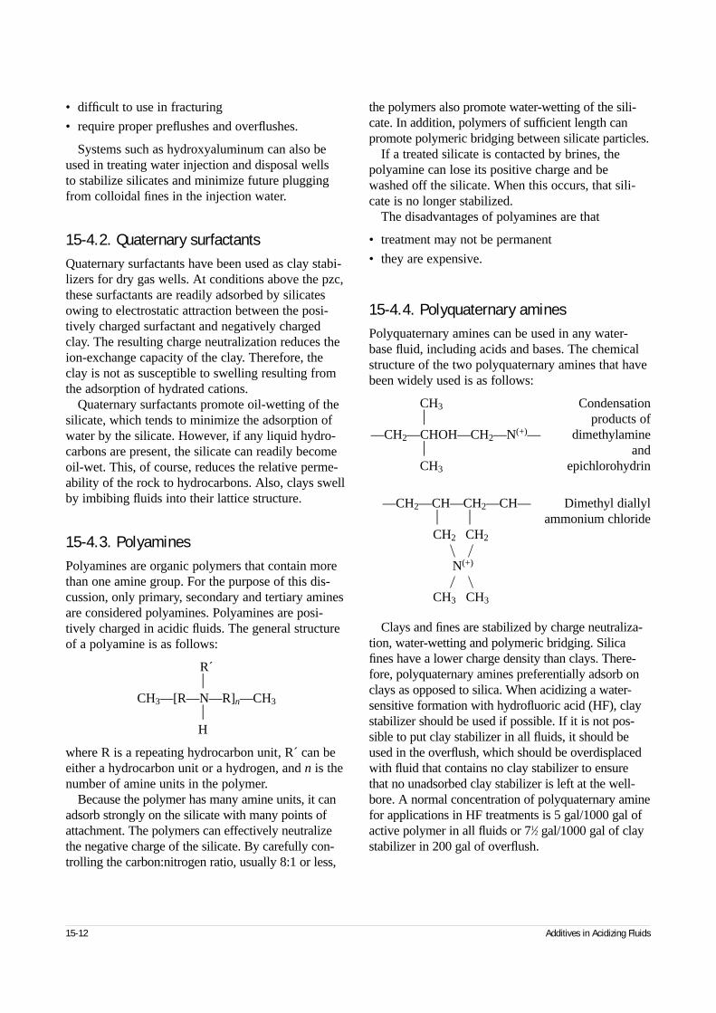
• difficult to use in fracturing

• require proper preflushes and overflushes.

Systems such as hydroxyaluminum can also beused in treating water injection and disposal wells to stabilize silicates and minimize future pluggingfrom colloidal fines in the injection water.

15-4.2. Quaternary surfactantsQuaternary surfactants have been used as clay stabi-lizers for dry gas wells. At conditions above the pzc,these surfactants are readily adsorbed by silicatesowing to electrostatic attraction between the posi-tively charged surfactant and negatively chargedclay. The resulting charge neutralization reduces theion-exchange capacity of the clay. Therefore, theclay is not as susceptible to swelling resulting fromthe adsorption of hydrated cations.

Quaternary surfactants promote oil-wetting of thesilicate, which tends to minimize the adsorption ofwater by the silicate. However, if any liquid hydro-carbons are present, the silicate can readily becomeoil-wet. This, of course, reduces the relative perme-ability of the rock to hydrocarbons. Also, clays swellby imbibing fluids into their lattice structure.

15-4.3. PolyaminesPolyamines are organic polymers that contain morethan one amine group. For the purpose of this dis-cussion, only primary, secondary and tertiary aminesare considered polyamines. Polyamines are posi-tively charged in acidic fluids. The general structureof a polyamine is as follows:

R´

CH3—[R—N—R]n—CH3

H

where R is a repeating hydrocarbon unit, R´ can beeither a hydrocarbon unit or a hydrogen, and n is thenumber of amine units in the polymer.

Because the polymer has many amine units, it canadsorb strongly on the silicate with many points ofattachment. The polymers can effectively neutralizethe negative charge of the silicate. By carefully con-trolling the carbon:nitrogen ratio, usually 8:1 or less,

the polymers also promote water-wetting of the sili-cate. In addition, polymers of sufficient length canpromote polymeric bridging between silicate particles.

If a treated silicate is contacted by brines, thepolyamine can lose its positive charge and bewashed off the silicate. When this occurs, that sili-cate is no longer stabilized.

The disadvantages of polyamines are that

• treatment may not be permanent

• they are expensive.

15-4.4. Polyquaternary aminesPolyquaternary amines can be used in any water-base fluid, including acids and bases. The chemicalstructure of the two polyquaternary amines that havebeen widely used is as follows:

CH3 Condensation products of

—CH2—CHOH—CH2—N(+)— dimethylamine andCH3 epichlorohydrin

—CH2—CH—CH2—CH— Dimethyl diallyl ammonium chlorideCH2 CH2

N(+)

CH3 CH3

Clays and fines are stabilized by charge neutraliza-tion, water-wetting and polymeric bridging. Silicafines have a lower charge density than clays. There-fore, polyquaternary amines preferentially adsorb onclays as opposed to silica. When acidizing a water-sensitive formation with hydrofluoric acid (HF), claystabilizer should be used if possible. If it is not pos-sible to put clay stabilizer in all fluids, it should beused in the overflush, which should be overdisplacedwith fluid that contains no clay stabilizer to ensurethat no unadsorbed clay stabilizer is left at the well-bore. A normal concentration of polyquaternary aminefor applications in HF treatments is 5 gal/1000 gal ofactive polymer in all fluids or 71⁄2 gal/1000 gal of claystabilizer in 200 gal of overflush.

15-12 Additives in Acidizing Fluids

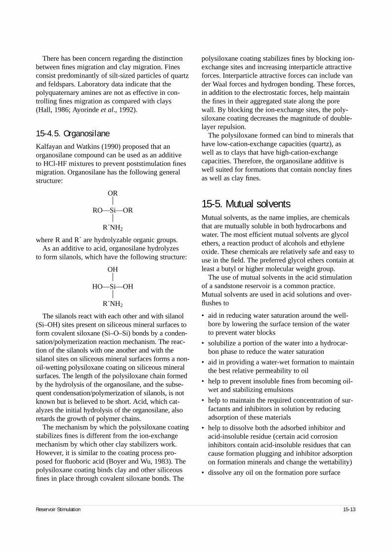
There has been concern regarding the distinctionbetween fines migration and clay migration. Finesconsist predominantly of silt-sized particles of quartzand feldspars. Laboratory data indicate that thepolyquaternary amines are not as effective in con-trolling fines migration as compared with clays(Hall, 1986; Ayorinde et al., 1992).

15-4.5. OrganosilaneKalfayan and Watkins (1990) proposed that anorganosilane compound can be used as an additive to HCl-HF mixtures to prevent poststimulation finesmigration. Organosilane has the following generalstructure:

OR

RO—Si—OR

R´NH2

where R and R´ are hydrolyzable organic groups.As an additive to acid, organosilane hydrolyzes

to form silanols, which have the following structure:

OH

HO—Si—OH

R´NH2

The silanols react with each other and with silanol(Si–OH) sites present on siliceous mineral surfaces toform covalent siloxane (Si–O–Si) bonds by a conden-sation/polymerization reaction mechanism. The reac-tion of the silanols with one another and with thesilanol sites on siliceous mineral surfaces forms a non-oil-wetting polysiloxane coating on siliceous mineralsurfaces. The length of the polysiloxane chain formedby the hydrolysis of the organosilane, and the subse-quent condensation/polymerization of silanols, is notknown but is believed to be short. Acid, which cat-alyzes the initial hydrolysis of the organosilane, alsoretards the growth of polymer chains.

The mechanism by which the polysiloxane coatingstabilizes fines is different from the ion-exchangemechanism by which other clay stabilizers work.However, it is similar to the coating process pro-posed for fluoboric acid (Boyer and Wu, 1983). Thepolysiloxane coating binds clay and other siliceousfines in place through covalent siloxane bonds. The

polysiloxane coating stabilizes fines by blocking ion-exchange sites and increasing interparticle attractiveforces. Interparticle attractive forces can include vander Waal forces and hydrogen bonding. These forces,in addition to the electrostatic forces, help maintainthe fines in their aggregated state along the porewall. By blocking the ion-exchange sites, the poly-siloxane coating decreases the magnitude of double-layer repulsion.

The polysiloxane formed can bind to minerals thathave low-cation-exchange capacities (quartz), aswell as to clays that have high-cation-exchangecapacities. Therefore, the organosilane additive iswell suited for formations that contain nonclay finesas well as clay fines.

15-5. Mutual solventsMutual solvents, as the name implies, are chemicalsthat are mutually soluble in both hydrocarbons andwater. The most efficient mutual solvents are glycolethers, a reaction product of alcohols and ethyleneoxide. These chemicals are relatively safe and easy touse in the field. The preferred glycol ethers contain atleast a butyl or higher molecular weight group.

The use of mutual solvents in the acid stimulationof a sandstone reservoir is a common practice.Mutual solvents are used in acid solutions and over-flushes to

• aid in reducing water saturation around the well-bore by lowering the surface tension of the waterto prevent water blocks

• solubilize a portion of the water into a hydrocar-bon phase to reduce the water saturation

• aid in providing a water-wet formation to maintainthe best relative permeability to oil

• help to prevent insoluble fines from becoming oil-wet and stabilizing emulsions

• help to maintain the required concentration of sur-factants and inhibitors in solution by reducingadsorption of these materials

• help to dissolve both the adsorbed inhibitor andacid-insoluble residue (certain acid corrosioninhibitors contain acid-insoluble residues that cancause formation plugging and inhibitor adsorptionon formation minerals and change the wettability)

• dissolve any oil on the formation pore surface

Reservoir Stimulation 15-13

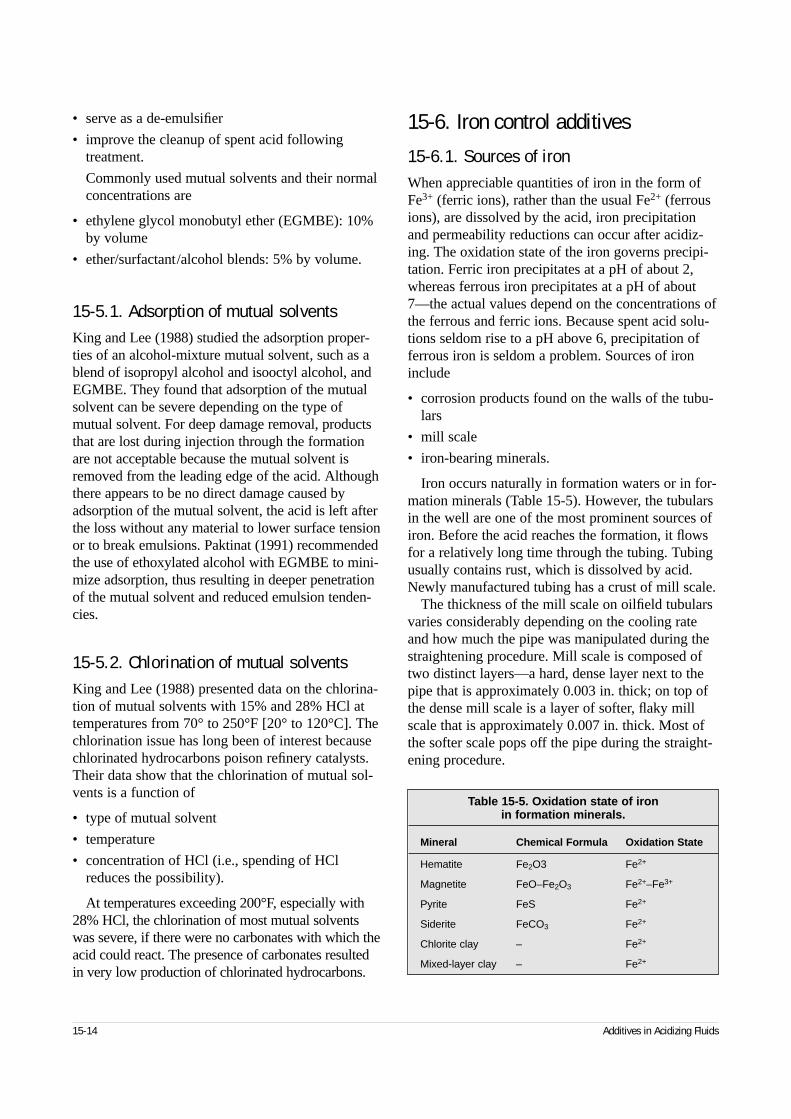
• serve as a de-emulsifier

• improve the cleanup of spent acid followingtreatment.

Commonly used mutual solvents and their normalconcentrations are

• ethylene glycol monobutyl ether (EGMBE): 10%by volume

• ether/surfactant/alcohol blends: 5% by volume.

15-5.1. Adsorption of mutual solventsKing and Lee (1988) studied the adsorption proper-ties of an alcohol-mixture mutual solvent, such as ablend of isopropyl alcohol and isooctyl alcohol, andEGMBE. They found that adsorption of the mutualsolvent can be severe depending on the type ofmutual solvent. For deep damage removal, productsthat are lost during injection through the formationare not acceptable because the mutual solvent isremoved from the leading edge of the acid. Althoughthere appears to be no direct damage caused byadsorption of the mutual solvent, the acid is left afterthe loss without any material to lower surface tensionor to break emulsions. Paktinat (1991) recommendedthe use of ethoxylated alcohol with EGMBE to mini-mize adsorption, thus resulting in deeper penetrationof the mutual solvent and reduced emulsion tenden-cies.

15-5.2. Chlorination of mutual solventsKing and Lee (1988) presented data on the chlorina-tion of mutual solvents with 15% and 28% HCl attemperatures from 70° to 250°F [20° to 120°C]. Thechlorination issue has long been of interest becausechlorinated hydrocarbons poison refinery catalysts.Their data show that the chlorination of mutual sol-vents is a function of

• type of mutual solvent

• temperature

• concentration of HCl (i.e., spending of HClreduces the possibility).

At temperatures exceeding 200°F, especially with28% HCl, the chlorination of most mutual solventswas severe, if there were no carbonates with which theacid could react. The presence of carbonates resultedin very low production of chlorinated hydrocarbons.

15-6. Iron control additives15-6.1. Sources of ironWhen appreciable quantities of iron in the form ofFe3+ (ferric ions), rather than the usual Fe2+ (ferrousions), are dissolved by the acid, iron precipitationand permeability reductions can occur after acidiz-ing. The oxidation state of the iron governs precipi-tation. Ferric iron precipitates at a pH of about 2,whereas ferrous iron precipitates at a pH of about7—the actual values depend on the concentrations ofthe ferrous and ferric ions. Because spent acid solu-tions seldom rise to a pH above 6, precipitation offerrous iron is seldom a problem. Sources of ironinclude

• corrosion products found on the walls of the tubu-lars

• mill scale

• iron-bearing minerals.

Iron occurs naturally in formation waters or in for-mation minerals (Table 15-5). However, the tubularsin the well are one of the most prominent sources ofiron. Before the acid reaches the formation, it flowsfor a relatively long time through the tubing. Tubingusually contains rust, which is dissolved by acid.Newly manufactured tubing has a crust of mill scale.

The thickness of the mill scale on oilfield tubularsvaries considerably depending on the cooling rateand how much the pipe was manipulated during thestraightening procedure. Mill scale is composed oftwo distinct layers—a hard, dense layer next to thepipe that is approximately 0.003 in. thick; on top ofthe dense mill scale is a layer of softer, flaky millscale that is approximately 0.007 in. thick. Most ofthe softer scale pops off the pipe during the straight-ening procedure.

15-14 Additives in Acidizing Fluids

Table 15-5. Oxidation state of iron in formation minerals.

Mineral Chemical Formula Oxidation State

Hematite Fe2O3 Fe2+

Magnetite FeO–Fe2O3 Fe2+–Fe3+

Pyrite FeS Fe2+

Siderite FeCO3 Fe2+

Chlorite clay – Fe2+

Mixed-layer clay – Fe2+

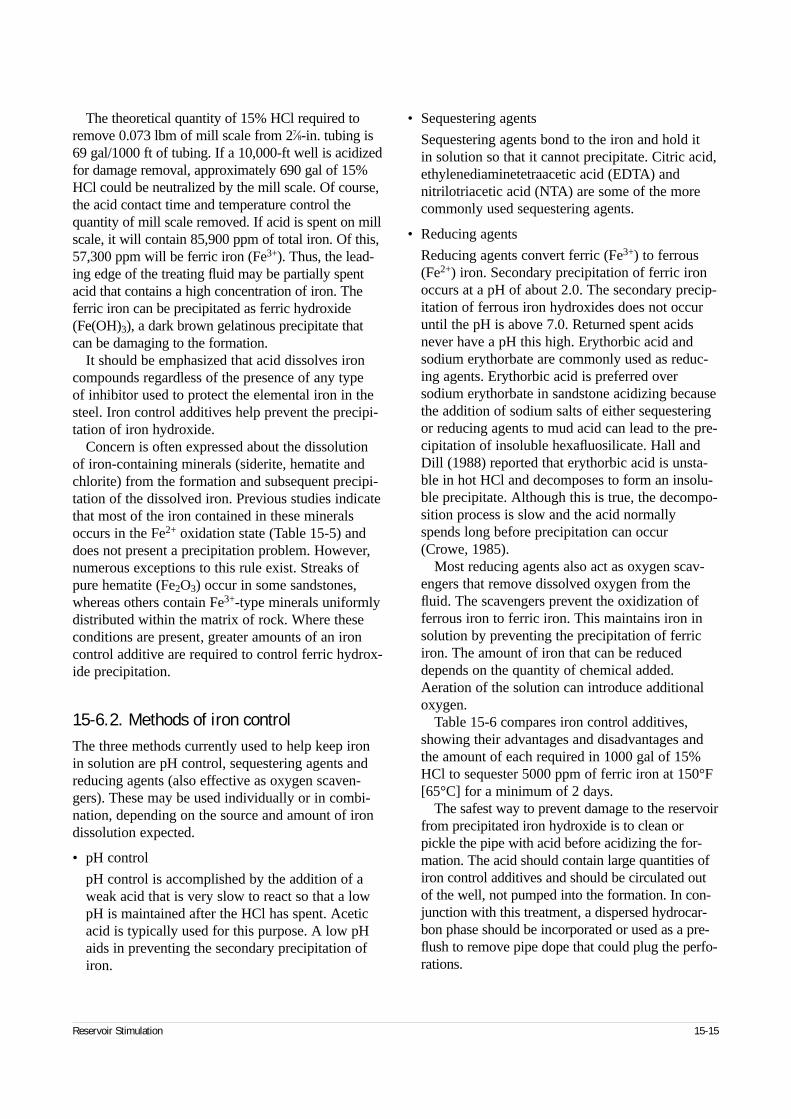
The theoretical quantity of 15% HCl required toremove 0.073 lbm of mill scale from 27⁄8-in. tubing is69 gal/1000 ft of tubing. If a 10,000-ft well is acidizedfor damage removal, approximately 690 gal of 15%HCl could be neutralized by the mill scale. Of course,the acid contact time and temperature control thequantity of mill scale removed. If acid is spent on millscale, it will contain 85,900 ppm of total iron. Of this,57,300 ppm will be ferric iron (Fe3+). Thus, the lead-ing edge of the treating fluid may be partially spentacid that contains a high concentration of iron. Theferric iron can be precipitated as ferric hydroxide(Fe(OH)3), a dark brown gelatinous precipitate thatcan be damaging to the formation.

It should be emphasized that acid dissolves ironcompounds regardless of the presence of any type of inhibitor used to protect the elemental iron in thesteel. Iron control additives help prevent the precipi-tation of iron hydroxide.

Concern is often expressed about the dissolutionof iron-containing minerals (siderite, hematite andchlorite) from the formation and subsequent precipi-tation of the dissolved iron. Previous studies indicatethat most of the iron contained in these mineralsoccurs in the Fe2+ oxidation state (Table 15-5) anddoes not present a precipitation problem. However,numerous exceptions to this rule exist. Streaks ofpure hematite (Fe2O3) occur in some sandstones,whereas others contain Fe3+-type minerals uniformlydistributed within the matrix of rock. Where theseconditions are present, greater amounts of an ironcontrol additive are required to control ferric hydrox-ide precipitation.

15-6.2. Methods of iron controlThe three methods currently used to help keep ironin solution are pH control, sequestering agents andreducing agents (also effective as oxygen scaven-gers). These may be used individually or in combi-nation, depending on the source and amount of irondissolution expected.

• pH control

pH control is accomplished by the addition of aweak acid that is very slow to react so that a lowpH is maintained after the HCl has spent. Aceticacid is typically used for this purpose. A low pHaids in preventing the secondary precipitation ofiron.

• Sequestering agents

Sequestering agents bond to the iron and hold it in solution so that it cannot precipitate. Citric acid,ethylenediaminetetraacetic acid (EDTA) andnitrilotriacetic acid (NTA) are some of the morecommonly used sequestering agents.

• Reducing agents

Reducing agents convert ferric (Fe3+) to ferrous(Fe2+) iron. Secondary precipitation of ferric ironoccurs at a pH of about 2.0. The secondary precip-itation of ferrous iron hydroxides does not occuruntil the pH is above 7.0. Returned spent acidsnever have a pH this high. Erythorbic acid andsodium erythorbate are commonly used as reduc-ing agents. Erythorbic acid is preferred oversodium erythorbate in sandstone acidizing becausethe addition of sodium salts of either sequesteringor reducing agents to mud acid can lead to the pre-cipitation of insoluble hexafluosilicate. Hall andDill (1988) reported that erythorbic acid is unsta-ble in hot HCl and decomposes to form an insolu-ble precipitate. Although this is true, the decompo-sition process is slow and the acid normallyspends long before precipitation can occur(Crowe, 1985).

Most reducing agents also act as oxygen scav-engers that remove dissolved oxygen from thefluid. The scavengers prevent the oxidization offerrous iron to ferric iron. This maintains iron insolution by preventing the precipitation of ferriciron. The amount of iron that can be reduceddepends on the quantity of chemical added.Aeration of the solution can introduce additionaloxygen.

Table 15-6 compares iron control additives,showing their advantages and disadvantages andthe amount of each required in 1000 gal of 15%HCl to sequester 5000 ppm of ferric iron at 150°F[65°C] for a minimum of 2 days.

The safest way to prevent damage to the reservoirfrom precipitated iron hydroxide is to clean orpickle the pipe with acid before acidizing the for-mation. The acid should contain large quantities ofiron control additives and should be circulated outof the well, not pumped into the formation. In con-junction with this treatment, a dispersed hydrocar-bon phase should be incorporated or used as a pre-flush to remove pipe dope that could plug the perfo-rations.

Reservoir Stimulation 15-15

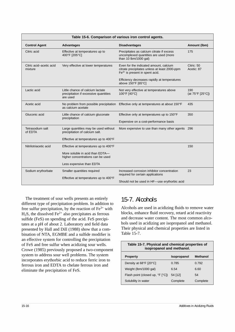
The treatment of sour wells presents an entirelydifferent type of precipitation problem. In addition tofree sulfur precipitation, by the reaction of Fe3+ withH2S, the dissolved Fe2+ also precipitates as ferroussulfide (FeS) on spending of the acid. FeS precipi-tates at a pH of about 2. Laboratory and field datapresented by Hall and Dill (1988) show that a com-bination of NTA, EGMBE and a sulfide modifier isan effective system for controlling the precipitationof FeS and free sulfur when acidizing sour wells.Crowe (1985) previously proposed a two-componentsystem to address sour well problems. The systemincorporates erythorbic acid to reduce ferric iron toferrous iron and EDTA to chelate ferrous iron andeliminate the precipitation of FeS.

15-7. AlcoholsAlcohols are used in acidizing fluids to remove waterblocks, enhance fluid recovery, retard acid reactivityand decrease water content. The most common alco-hols used in acidizing are isopropanol and methanol.Their physical and chemical properties are listed inTable 15-7.

15-16 Additives in Acidizing Fluids

Table 15-6. Comparison of various iron control agents.

Control Agent Advantages Disadvantages Amount (lbm)

Citric acid Effective at temperatures up to Precipitates as calcium citrate if excess 175400°F [205°C] uncomplexed quantities are used (more

than 10 lbm/1000 gal)

Citric acid–acetic acid Very effective at lower temperatures Even for the indicated amount, calcium Citric: 50mixture citrate precipitates unless at least 2000-ppm Acetic: 87

Fe3+ is present in spent acid.

Efficiency decreases rapidly at temperaturesabove 150°F [65°C]

Lactic acid Little chance of calcium lactate Not very effective at temperatures above 190precipitation if excessive quantities 100°F [40°C] (at 75°F [25°C]) are used

Acetic acid No problem from possible precipitation Effective only at temperatures at about 150°F 435as calcium acetate

Gluconic acid Little chance of calcium gluconate Effective only at temperatures up to 150°F 350precipitation

Expensive on a cost-performance basis

Tetrasodium salt Large quantities may be used without More expensive to use than many other agents 296of EDTA precipitation of calcium salt.

Effective at temperatures up to 400°F

Nitrilotriacetic acid Effective at temperatures up to 400°F 150

More soluble in acid than EDTA—higher concentrations can be used

Less expensive than EDTA

Sodium erythorbate Smaller quantities required Increased corrosion inhibitor concentration 23required for certain applications

Effective at temperatures up to 400°FShould not be used in HF—use erythorbic acid

Table 15-7. Physical and chemical properties of isopropanol and methanol.

Property Isopropanol Methanol

Density at 68°F [20°C] 0.785 0.792

Weight (lbm/1000 gal) 6.54 6.60

Flash point (closed up, °F [°C]) 54 [12] 54

Solubility in water Complete Complete

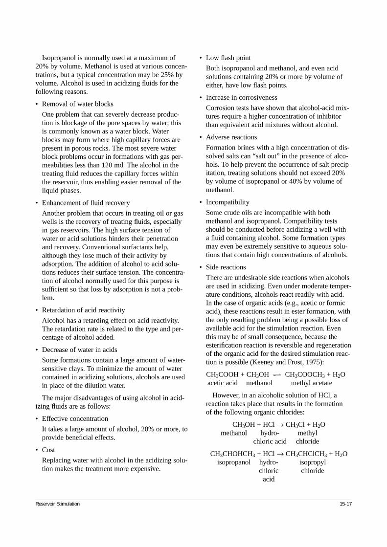
Isopropanol is normally used at a maximum of20% by volume. Methanol is used at various concen-trations, but a typical concentration may be 25% byvolume. Alcohol is used in acidizing fluids for thefollowing reasons.

• Removal of water blocks

One problem that can severely decrease produc-tion is blockage of the pore spaces by water; thisis commonly known as a water block. Waterblocks may form where high capillary forces arepresent in porous rocks. The most severe waterblock problems occur in formations with gas per-meabilities less than 120 md. The alcohol in thetreating fluid reduces the capillary forces withinthe reservoir, thus enabling easier removal of theliquid phases.

• Enhancement of fluid recovery

Another problem that occurs in treating oil or gaswells is the recovery of treating fluids, especiallyin gas reservoirs. The high surface tension ofwater or acid solutions hinders their penetrationand recovery. Conventional surfactants help,although they lose much of their activity byadsorption. The addition of alcohol to acid solu-tions reduces their surface tension. The concentra-tion of alcohol normally used for this purpose issufficient so that loss by adsorption is not a prob-lem.

• Retardation of acid reactivity

Alcohol has a retarding effect on acid reactivity.The retardation rate is related to the type and per-centage of alcohol added.

• Decrease of water in acids

Some formations contain a large amount of water-sensitive clays. To minimize the amount of watercontained in acidizing solutions, alcohols are usedin place of the dilution water.

The major disadvantages of using alcohol in acid-izing fluids are as follows:

• Effective concentration

It takes a large amount of alcohol, 20% or more, toprovide beneficial effects.

• Cost

Replacing water with alcohol in the acidizing solu-tion makes the treatment more expensive.

• Low flash point

Both isopropanol and methanol, and even acidsolutions containing 20% or more by volume ofeither, have low flash points.

• Increase in corrosiveness

Corrosion tests have shown that alcohol-acid mix-tures require a higher concentration of inhibitorthan equivalent acid mixtures without alcohol.

• Adverse reactions

Formation brines with a high concentration of dis-solved salts can “salt out” in the presence of alco-hols. To help prevent the occurrence of salt precip-itation, treating solutions should not exceed 20%by volume of isopropanol or 40% by volume ofmethanol.

• Incompatibility

Some crude oils are incompatible with bothmethanol and isopropanol. Compatibility testsshould be conducted before acidizing a well with a fluid containing alcohol. Some formation typesmay even be extremely sensitive to aqueous solu-tions that contain high concentrations of alcohols.

• Side reactions

There are undesirable side reactions when alcoholsare used in acidizing. Even under moderate temper-ature conditions, alcohols react readily with acid.In the case of organic acids (e.g., acetic or formicacid), these reactions result in ester formation, withthe only resulting problem being a possible loss ofavailable acid for the stimulation reaction. Eventhis may be of small consequence, because theesterification reaction is reversible and regenerationof the organic acid for the desired stimulation reac-tion is possible (Keeney and Frost, 1975):

CH3COOH + CH3OH CH3COOCH3 + H2Oacetic acid methanol methyl acetate

However, in an alcoholic solution of HCl, areaction takes place that results in the formation of the following organic chlorides:

CH3OH + HCl → CH3Cl + H2Omethanol hydro- methyl

chloric acid chloride

CH3CHOHCH3 + HCl → CH3CHClCH3 + H2Oisopropanol hydro- isopropyl

chloric chlorideacid

Reservoir Stimulation 15-17

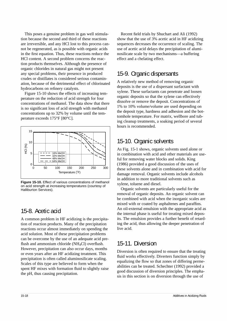
This poses a genuine problem in gas well stimula-tion because the second and third of these reactionsare irreversible, and any HCl lost to this process can-not be regenerated, as is possible with organic acidsin the first equation. Thus, these reactions reduce theHCl content. A second problem concerns the reac-tion products themselves. Although the presence oforganic chlorides in natural gas might not presentany special problems, their presence in producedcrudes or distillates is considered serious contamin-ation, because of the detrimental effect of chlorinatedhydrocarbons on refinery catalysts.

Figure 15-10 shows the effects of increasing tem-perature on the reduction of acid strength for fourconcentrations of methanol. The data show that thereis no significant loss of acid strength with methanolconcentrations up to 32% by volume until the tem-perature exceeds 175°F [80°C].

15-8. Acetic acidA common problem in HF acidizing is the precipita-tion of reaction products. Many of the precipitationreactions occur almost immediately on spending theacid solution. Most of these precipitation problemscan be overcome by the use of an adequate acid pre-flush and ammonium chloride (NH4Cl) overflush.However, precipitation can also occur days, monthsor even years after an HF acidizing treatment. Thisprecipitation is often called aluminosilicate scaling.Scales of this type are believed to form when thespent HF mixes with formation fluid to slightly raisethe pH, thus causing precipitation.

Recent field trials by Shuchart and Ali (1992)show that the use of 3% acetic acid in HF acidizingsequences decreases the occurrence of scaling. Theuse of acetic acid delays the precipitation of alumi-nosilicate scale by two mechanisms—a bufferingeffect and a chelating effect.

15-9. Organic dispersantsA relatively new method of removing organicdeposits is the use of a dispersant surfactant withxylene. These surfactants can penetrate and loosenorganic deposits so that the xylene can effectivelydissolve or remove the deposit. Concentrations of1% to 10% volume/volume are used depending onthe deposit type, hardness and adhesion and the bot-tomhole temperature. For matrix, wellbore and tub-ing cleanup treatments, a soaking period of severalhours is recommended.

15-10. Organic solventsAs Fig. 15-1 shows, organic solvents used alone orin combination with acid and other materials are use-ful for removing water blocks and solids. King(1986) provided a good discussion of the uses ofthese solvents alone and in combination with acid fordamage removal. Organic solvents include alcoholsin addition to more traditional solvents such asxylene, toluene and diesel.

Organic solvents are particularly useful for theremoval of organic deposits. An organic solvent canbe combined with acid when the inorganic scales aremixed with or coated by asphaltenes and paraffins.An oil-external emulsion with the appropriate acid asthe internal phase is useful for treating mixed depos-its. The emulsion provides a further benefit of retard-ing the acid, thus allowing the deeper penetration oflive acid.

15-11. DiversionDiversion is often required to ensure that the treatingfluid works effectively. Diverters function simply byequalizing the flow so that zones of differing perme-abilities can be treated. Schechter (1992) provided agood discussion of diversion principles. The empha-sis in this section is on diversion through the use of

15-18 Additives in Acidizing Fluids

Figure 15-10. Effect of various concentrations of methanolon acid strength at increasing temperatures (courtesy ofHalliburton Services).

00

50 100 150 200 250 300

5

10

15

Temperature (˚F)

HC

l (%

)

16% MeOH32% MeOH48% MeOH64% MeOH

particulates added to the treating fluid and foamsrather than the use of packers or ball sealers.

Ideally the diverter should

• be insoluble in the treating fluid

• form an essentially impermeable layer on the for-mation face without penetrating deeply into theformation

• be easily removed following the treatment.

Generally all, or at least most, of these criteria canbe met using materials such as oil-soluble resins,benzoic acid flakes and other particulates. Particulatediverters may cause damage and can be difficult toclean up as a result.

Foams may also provide effective diversion(Zerhboub et al., 1991). Foamed fluids have theadditional advantage of good cleanup with little orno potential for damaging the formation. The ratio of nitrogen to fluid depends on the bottomhole con-ditions during the treatment. Diversion and fluidplacement strategy are addressed in Chapter 19.

15-12. Additive compatibilityAll additives should be tested in the laboratory.Compatibility of additives with formation fluidsshould be tested using a sandpack method developedby Ali et al. (1994). This procedure is more repre-sentative of downhole conditions and uses more sandthan the test in API Recommended Practices forLaboratory Testing of Surface Active Agents for WellStimulation (RP 42) (1977). The acid system withadditives is drawn through a pack of formation corematerial or a mixture consisting of 10-wt% illite-bentonite, 10-wt% silica flour and 80-wt% 100-meshsand. There are no universal additives for all forma-tion problems. Any potential incompatibilitiesbetween additives and formation fluids must be iden-tified and corrected before acidizing.

15-13. Facility upsets following acid stimulation

15-13.1. Discharge requirementsThe chemicals used in acidizing treatments havebeen linked with oil and water separation facilityupsets, causing noncompliance with environmental

discharge regulations. On flowback, emulsion andoil/water separation problems that occur can poten-tially result in excess oil solubilized in the water bythe formation of microemulsions. Emulsion prob-lems under such circumstances can result in thou-sands of gallons of non-pipeline-quality oil andcould shut down the separation unit and minimizeproduction from these wells. Dehydrated oil andclean discharge water are required to maintain nor-mal uninterrupted production.

Regulations for the disposal of produced water inoffshore operations are becoming increasingly strin-gent. The U.S. National Pollutant DischargeElimination System (NPDES) has established dis-charge levels for oil and grease at a 29-mg/Lmonthly average with a grab sample maximum of 42 mg/L. This is a reduction in the allowable levelsfrom 48 to 29 mg/L. The penalty for noncomplianceby the operator can be severe. These discharge levelsare causing the reevaluation of acidizing treatments.

During the flowback immediately following anacid treatment, significantly higher levels of oil andgrease than those permitted for discharge have alsobeen recorded. During flowback, spikes in the basicsediment and water (BS&W) values occur immedi-ately after an acid treatment. Microemulsions are sus-pected of occurring during flowback. The producedoil is solubilized in the returned spent acid, and thisresults in significantly higher levels of oil and grease.The use of matrix additives is believed to contributeto the solubilization of the oil and additives. Theseadditives should be optimized to minimize emulsionupsets and the levels of oil and grease.

Verification and optimization of the additives usedin acid stimulation treatments have been requestedby operators. Obtaining an answer to treatment facil-ity upsets by additive optimization in matrix treat-ments can have a tremendous impact on acidizingworkover operations. Research by Bansal (1993)determined the following maximum concentrationsof inhibitors, surfactants and mutual solvents thatmay be present in the returned fluids to maintain oiland grease levels below 48 mg/L:

• inhibitors: 80 ppm

• surfactants: 10 ppm

• mutual solvents: 100 ppm.

The common denominator for each of these addi-tives is surface-active compounds (i.e., surfactants).

Reservoir Stimulation 15-19

The surfactants provide acceptable fluid perfor-mance, such as corrosion inhibition, dispersion andwetting properties, as they were initially designed forthe acid treatment. However, if the additives are usedin excessive concentrations, they may exacerbate theemulsification tendencies of fluids during flowback.

The difference in emulsion stability is attributed toother, more dominant factors (e.g., stabilization bysolids precipitation [organic and inorganic], ferricion interaction with the crude oil and viscosityincrease at the interface). Results presented byCoppel (1975) show that acids partially spent on for-mations contain potentially precipitable materials insolution. As the pH of the produced acid increasesduring flowback and mixes with other produced flu-ids, precipitates form that can stabilize emulsions.Dunlap and Houchin (1990) recommended polarizedmicroscopy to evaluate return fluids to establish thecause for a stabilized emulsion. Specific damagemechanisms, such as emulsion stabilization byorganic deposits, solids and iron, could be detectedand identified.

15-13.2. Prevention of facility upsetsPreventing upsets requires optimizing the fluid designto minimize or eliminate the formation of precipitatesand using the optimum de-emulsifier. The potentialfor the formation of emulsions of acid and producedcrude oil while still providing the required downholefunction optimization of the de-emulsifier treatmentis evaluated currently by the procedures recommend-ed in API RP 42 (1977). Vigorous mixing of acidwith fresh crude oil in a glass container is observedunder bottomhole temperatures (hot-water bath) todetermine the characteristics and time for emulsionbreakout. Fine siliceous materials, ferric iron or bothcan be added to evaluate emulsion stability.

These fluid interactions can simulate the downholeemulsion problems encountered; however, these testsfail to accurately predict the interaction of the treatingfluids with the acid-sensitive crudes during flowback.As a result, marginal treatment response is observed.Downhole emulsions and facility upsets may beattributed to inadequate prejob compatibility testing,because the additives employed in the acid systemmay preferentially adsorb out onto the rock matrix orpartition to the oil phase during production.

Alternate testing procedures have been developedto more accurately simulate reservoir conditions. Ali

et al. (1994) recommended an alternate procedurethat better simulates downhole intermixing of thestimulation fluids and the produced crude. The pro-cedure involves filtering formulated acid, containinginhibitor, surfactants, mutual solvents and nonemul-sifiers, through a sandpack containing 10-wt% silicaflour, 10-wt% clays (such as montmorillonite) and80-wt% 100-mesh sand prior to completion of theemulsion test. This procedure simulates the filtrationof the acid system within the rock matrix. Surfact-ants, such as those used in nonemulsifiers, areadsorbed onto mineral surfaces. The adsorptionminimizes the availability of the surfactants in solu-tion to prevent emulsions.

Durham et al. (1995) reported that oil and wateremulsion upsets could be minimized by proper selec-tion of the acidizing additives and surface treatingchemicals. When acid flowbacks are introduced intoa production system, the control of emulsions bychemical treatment can significantly change in com-parison with control during production of the wellprior to treatment. These authors completed exten-sive emulsion breaker and water clarification testswith the desired acid/additive systems and freshcrude oil to duplicate the commingling of the acidwith the oil during flowback. The low pH of thewater in the emulsion rendered the current treatingprogram ineffective until the acid flowback wascompleted. Nonionic de-emulsifiers were found to bemore effective than sulfonate-type additives for treat-ing these emulsions. On-site testing is recommendedto select an effective chemical treatment.

Ali et al. (1997) reported the optimization ofacidizing additives to reduce production facilityupsets. The authors combined additive treatmentoptimization with a new absorption/filtration process.The optimized treatments involved the evaluation ofsurfactants and mutual solvents, which are consid-ered to be the additives primarily responsible foremulsion problems during acid flowback. Elimina-tion of some additives, minimizing the concentra-tions of other additives and using a dual-purposemutual breakout solvent reduced facility upsets. Allrecommendations were based on laboratory testingusing the sandpack method and on-site testing with alaboratory unit. The filtration process used a special-ized absorption medium to aid in lowering oil andgrease levels. This combination of treatment opti-mization with filtration/absorption reduced facilityupsets while not interfering with the efficacy of thetreatment.

15-20 Additives in Acidizing Fluids

16-1. IntroductionMatrix stimulation is a technique in which a solvent is injected into the formation to dissolve some of thematerials present and hence recover or increase thepermeability in the near-wellbore region. Such treat-ments are called “matrix” treatments because the sol-vent is injected at pressures below the parting pressureof the formation so that fractures are not created. Theobjective is to greatly enhance or recover the perme-ability near the wellbore, rather than affect a largeportion of the reservoir.

The most common matrix stimulation treatment is acidizing, in which an acidic solution is injected to dissolve minerals in the formation. However, othersolvents are also used. The next most common fluidsare organic solvents aimed at dissolving waxes, paraf-fins, asphaltenes or other organic damaging materials.Nonacid matrix stimulation is addressed in Chapter 14.This chapter focuses on matrix acidizing; however, thereader should keep in mind that many of the theoriesand calculation procedures presented here can also beapplied to nonacid solvent treatments.

The most common acids are hydrochloric acid(HCl), used primarily to dissolve carbonate minerals,and mixtures of HCl and hydrofluoric acid (HF), usedto attack silicate minerals such as clays and feldspars.Other acids, particularly some weak organic acids,are used in special applications, such as high-temper-ature wells. Matrix acidizing is a near-wellbore treat-ment, with all the acid reacting within about 1 ft ofthe wellbore in sandstone formations and within afew inches to perhaps as much as 10 ft from the well-bore in carbonates.

Matrix acidizing can significantly enhance the pro-ductivity of a well when near-wellbore formationdamage is present and, conversely, is of limited bene-fit in an undamaged well, as shown in Chapter 1.Thus, matrix acidizing generally should be appliedonly when a well has a high skin factor that cannot beattributed to partial penetration, perforation efficiency

or other mechanical aspects of the completion. Twoexceptions to this rule may occur. First, in highly pro-ductive wells, the productivity improvement of about20% that is possible with matrix stimulation of anundamaged well may be economic. Second, in natu-rally fractured or highly vugular carbonate reservoirs,live acid may penetrate to a sufficient distance to yielda productivity enhancement greater than that normallyexpected from a true matrix treatment.

An ideal matrix treatment restores the permeabilityin the near-wellbore region to a value at least as highas the original undamaged permeability; it accom-plishes this over the entire completed interval and itleaves the formation in the treated region with highrelative permeability to the oil and/or gas phase.Designing a treatment should strive to achieve thisideal at the lowest possible cost, which requires con-sideration of the many physical and chemical interac-tions taking place between the injected fluids and thereservoir minerals and fluids. The most important ofthese phenomena are the following:

• mass transfer of acid molecules to the mineral sur-face and subsequent reaction at the surface—Thisfundamental process of acidizing is illustrated inFig. 16-1. Acid reactions with minerals are termedheterogeneous reactions because they occur at aboundary between the solid and the liquid ratherthan in the bulk phases. Before the reaction canoccur, acid must be transported to the mineral sur-face by convection or diffusion. The overall reac-tion rate (i.e., the rate of change of the concentra-tion of one component in the bulk liquid phase)may depend on both the rate of mass transfer andthe rate of surface reaction. Many times, however,one of these processes is much slower than theother and controls the overall rate, in which casethe faster process can be ignored.

• changing pore structure—The physical change inthe pore structure caused by dissolution of some ofthe minerals by acid is the mechanism by which

Reservoir Stimulation 16-1

◆

Fundamentals ofAcid Stimulation

A. Daniel Hill and Robert S. Schechter, University of Texas at Austin

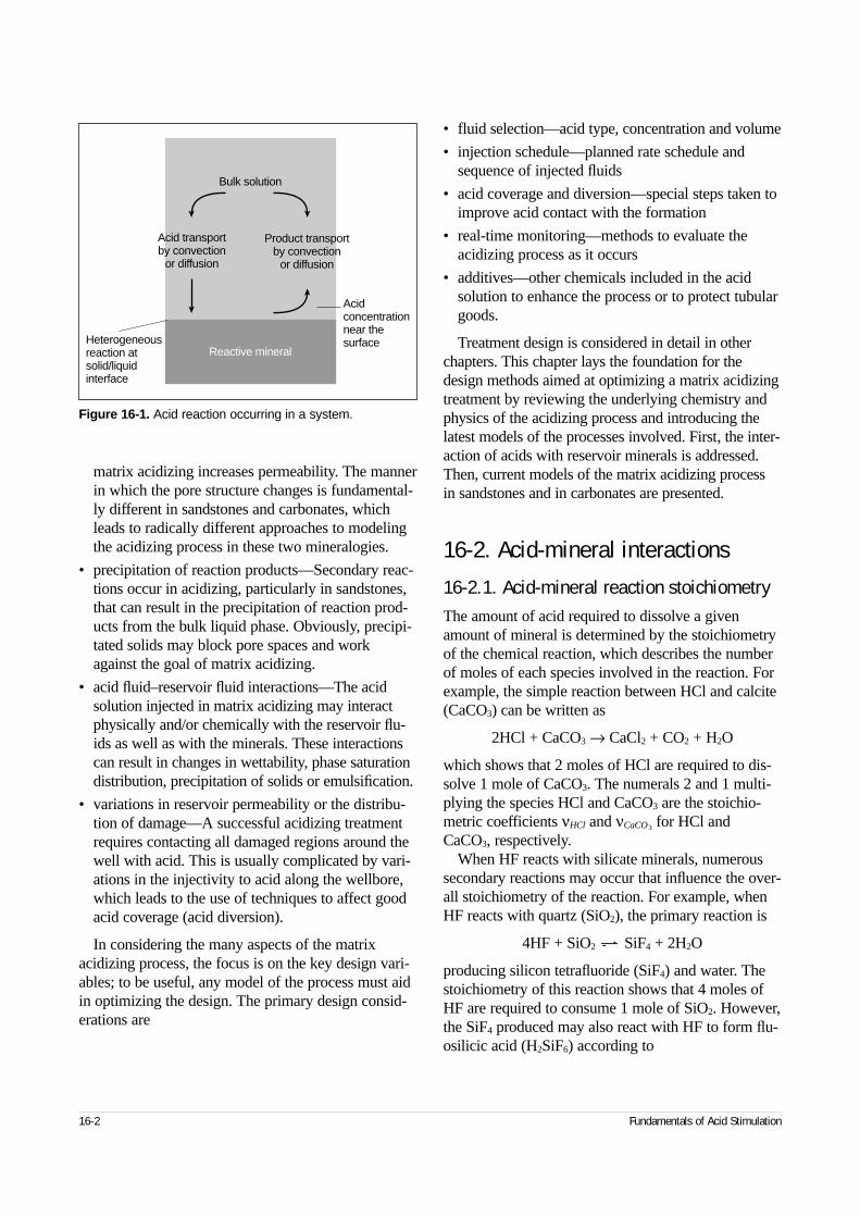
matrix acidizing increases permeability. The mannerin which the pore structure changes is fundamental-ly different in sandstones and carbonates, whichleads to radically different approaches to modelingthe acidizing process in these two mineralogies.

• precipitation of reaction products—Secondary reac-tions occur in acidizing, particularly in sandstones,that can result in the precipitation of reaction prod-ucts from the bulk liquid phase. Obviously, precipi-tated solids may block pore spaces and workagainst the goal of matrix acidizing.

• acid fluid–reservoir fluid interactions—The acidsolution injected in matrix acidizing may interactphysically and/or chemically with the reservoir flu-ids as well as with the minerals. These interactionscan result in changes in wettability, phase saturationdistribution, precipitation of solids or emulsification.

• variations in reservoir permeability or the distribu-tion of damage—A successful acidizing treatmentrequires contacting all damaged regions around thewell with acid. This is usually complicated by vari-ations in the injectivity to acid along the wellbore,which leads to the use of techniques to affect goodacid coverage (acid diversion).

In considering the many aspects of the matrixacidizing process, the focus is on the key design vari-ables; to be useful, any model of the process must aidin optimizing the design. The primary design consid-erations are

• fluid selection—acid type, concentration and volume

• injection schedule—planned rate schedule andsequence of injected fluids

• acid coverage and diversion—special steps taken toimprove acid contact with the formation

• real-time monitoring—methods to evaluate theacidizing process as it occurs

• additives—other chemicals included in the acidsolution to enhance the process or to protect tubulargoods.

Treatment design is considered in detail in otherchapters. This chapter lays the foundation for thedesign methods aimed at optimizing a matrix acidizingtreatment by reviewing the underlying chemistry andphysics of the acidizing process and introducing thelatest models of the processes involved. First, the inter-action of acids with reservoir minerals is addressed.Then, current models of the matrix acidizing process in sandstones and in carbonates are presented.

16-2. Acid-mineral interactions16-2.1. Acid-mineral reaction stoichiometryThe amount of acid required to dissolve a givenamount of mineral is determined by the stoichiometryof the chemical reaction, which describes the numberof moles of each species involved in the reaction. Forexample, the simple reaction between HCl and calcite(CaCO3) can be written as

2HCl + CaCO3 → CaCl2 + CO2 + H2O

which shows that 2 moles of HCl are required to dis-solve 1 mole of CaCO3. The numerals 2 and 1 multi-plying the species HCl and CaCO3 are the stoichio-metric coefficients νHCl and νCaCO3 for HCl andCaCO3, respectively.

When HF reacts with silicate minerals, numeroussecondary reactions may occur that influence the over-all stoichiometry of the reaction. For example, whenHF reacts with quartz (SiO2), the primary reaction is

4HF + SiO2 SiF4 + 2H2O

producing silicon tetrafluoride (SiF4) and water. Thestoichiometry of this reaction shows that 4 moles ofHF are required to consume 1 mole of SiO2. However,the SiF4 produced may also react with HF to form flu-osilicic acid (H2SiF6) according to

16-2 Fundamentals of Acid Stimulation

Figure 16-1. Acid reaction occurring in a system.

Bulk solution

Reactive mineral

Acid transportby convection

or diffusion

Product transportby convection

or diffusion

Acidconcentrationnear the surfaceHeterogeneous

reaction atsolid/liquidinterface

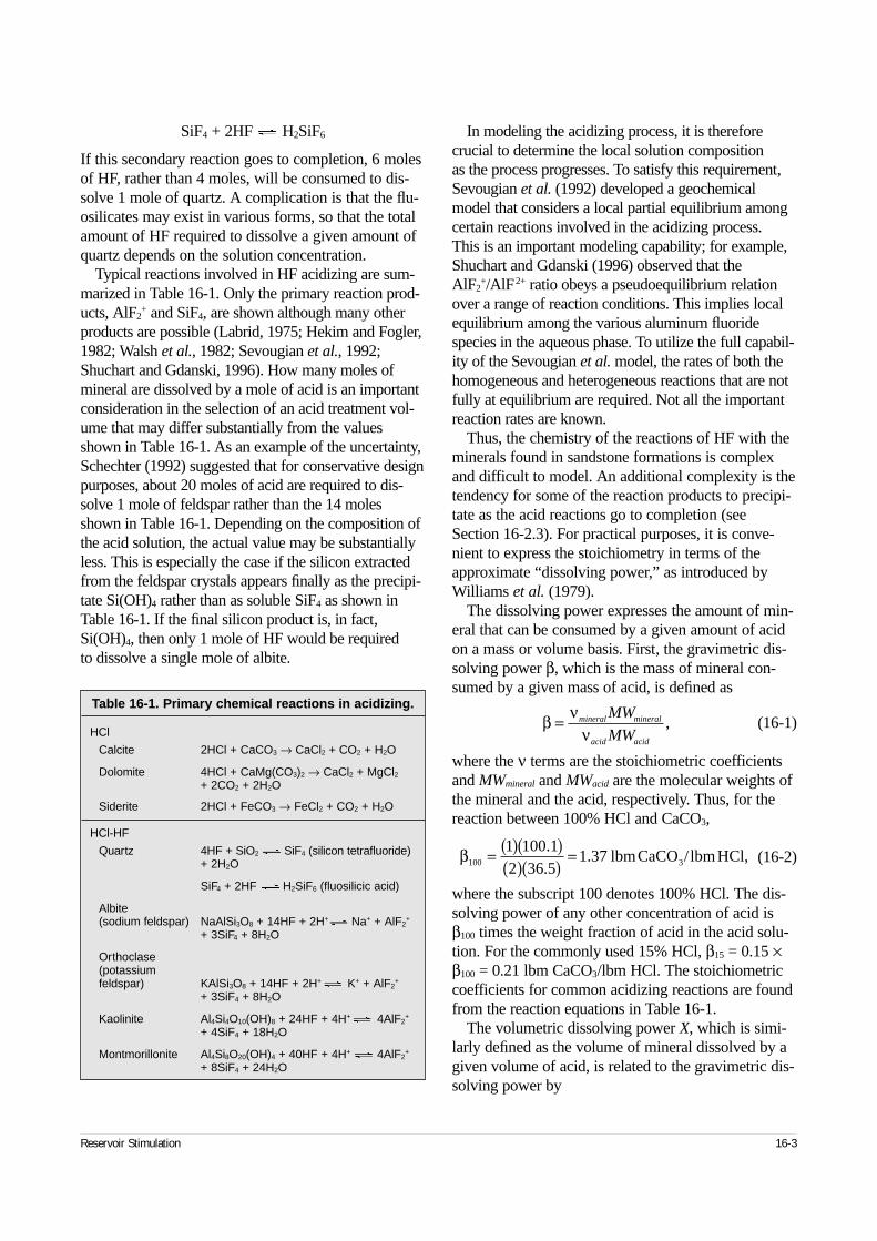
SiF4 + 2HF H2SiF6

If this secondary reaction goes to completion, 6 molesof HF, rather than 4 moles, will be consumed to dis-solve 1 mole of quartz. A complication is that the flu-osilicates may exist in various forms, so that the totalamount of HF required to dissolve a given amount ofquartz depends on the solution concentration.

Typical reactions involved in HF acidizing are sum-marized in Table 16-1. Only the primary reaction prod-ucts, AlF2

+ and SiF4, are shown although many otherproducts are possible (Labrid, 1975; Hekim and Fogler,1982; Walsh et al., 1982; Sevougian et al., 1992;Shuchart and Gdanski, 1996). How many moles ofmineral are dissolved by a mole of acid is an importantconsideration in the selection of an acid treatment vol-ume that may differ substantially from the valuesshown in Table 16-1. As an example of the uncertainty,Schechter (1992) suggested that for conservative designpurposes, about 20 moles of acid are required to dis-solve 1 mole of feldspar rather than the 14 molesshown in Table 16-1. Depending on the composition ofthe acid solution, the actual value may be substantiallyless. This is especially the case if the silicon extractedfrom the feldspar crystals appears finally as the precipi-tate Si(OH)4 rather than as soluble SiF4 as shown inTable 16-1. If the final silicon product is, in fact,Si(OH)4, then only 1 mole of HF would be required to dissolve a single mole of albite.

In modeling the acidizing process, it is thereforecrucial to determine the local solution composition as the process progresses. To satisfy this requirement,Sevougian et al. (1992) developed a geochemicalmodel that considers a local partial equilibrium amongcertain reactions involved in the acidizing process. This is an important modeling capability; for example,Shuchart and Gdanski (1996) observed that theAlF2

+/AlF2+ ratio obeys a pseudoequilibrium relationover a range of reaction conditions. This implies localequilibrium among the various aluminum fluoridespecies in the aqueous phase. To utilize the full capabil-ity of the Sevougian et al. model, the rates of both thehomogeneous and heterogeneous reactions that are notfully at equilibrium are required. Not all the importantreaction rates are known.

Thus, the chemistry of the reactions of HF with theminerals found in sandstone formations is complexand difficult to model. An additional complexity is thetendency for some of the reaction products to precipi-tate as the acid reactions go to completion (seeSection 16-2.3). For practical purposes, it is conve-nient to express the stoichiometry in terms of theapproximate “dissolving power,” as introduced byWilliams et al. (1979).

The dissolving power expresses the amount of min-eral that can be consumed by a given amount of acidon a mass or volume basis. First, the gravimetric dis-solving power β, which is the mass of mineral con-sumed by a given mass of acid, is defined as

(16-1)

where the ν terms are the stoichiometric coefficientsand MWmineral and MWacid are the molecular weights ofthe mineral and the acid, respectively. Thus, for thereaction between 100% HCl and CaCO3,

(16-2)

where the subscript 100 denotes 100% HCl. The dis-solving power of any other concentration of acid isβ100 times the weight fraction of acid in the acid solu-tion. For the commonly used 15% HCl, β15 = 0.15 ×β100 = 0.21 lbm CaCO3/lbm HCl. The stoichiometriccoefficients for common acidizing reactions are foundfrom the reaction equations in Table 16-1.

The volumetric dissolving power X, which is simi-larly defined as the volume of mineral dissolved by agiven volume of acid, is related to the gravimetric dis-solving power by

Reservoir Stimulation 16-3

Table 16-1. Primary chemical reactions in acidizing.

HCl

Calcite 2HCl + CaCO3 → CaCl2 + CO2 + H2O

Dolomite 4HCl + CaMg(CO3)2 → CaCl2 + MgCl2+ 2CO2 + 2H2O

Siderite 2HCl + FeCO3 → FeCl2 + CO2 + H2O

HCl-HF

Quartz 4HF + SiO2 SiF4 (silicon tetrafluoride) + 2H2O

SiF4 + 2HF H2SiF6 (fluosilicic acid)

Albite(sodium feldspar) NaAlSi3O8 + 14HF + 2H+ Na+ + AlF2

+

+ 3SiF4 + 8H2O

Orthoclase (potassiumfeldspar) KAlSi3O8 + 14HF + 2H+ K+ + AlF2

+

+ 3SiF4 + 8H2O

Kaolinite Al4Si4O10(OH)8 + 24HF + 4H+ 4AlF2+

+ 4SiF4 + 18H2O

Montmorillonite Al4Si8O20(OH)4 + 40HF + 4H+ 4AlF2+

+ 8SiF4 + 24H2O

β νν

= mineral mineral

acid acid

MW

MW,

β100

1 100 12 36 5

1 37= ( )( )( )( )

=..

. lbmCaCO /lbmHCl,3

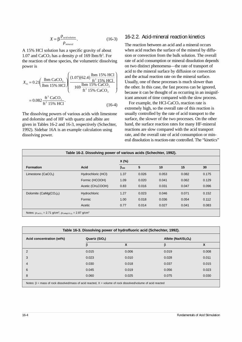
16-4 Fundamentals of Acid Stimulation

(16-3)

A 15% HCl solution has a specific gravity of about1.07 and CaCO3 has a density ρ of 169 lbm/ft3. Forthe reaction of these species, the volumetric dissolvingpower is

(16-4)

The dissolving powers of various acids with limestoneand dolomite and of HF with quartz and albite aregiven in Tables 16-2 and 16-3, respectively (Schechter,1992). Sidebar 16A is an example calculation usingdissolving power.

16-2.2. Acid-mineral reaction kineticsThe reaction between an acid and a mineral occurswhen acid reaches the surface of the mineral by diffu-sion or convection from the bulk solution. The overallrate of acid consumption or mineral dissolution dependson two distinct phenomena—the rate of transport ofacid to the mineral surface by diffusion or convectionand the actual reaction rate on the mineral surface.Usually, one of these processes is much slower than the other. In this case, the fast process can be ignored,because it can be thought of as occurring in an insignif-icant amount of time compared with the slow process.

For example, the HCl-CaCO3 reaction rate isextremely high, so the overall rate of this reaction isusually controlled by the rate of acid transport to thesurface, the slower of the two processes. On the otherhand, the surface reaction rates for many HF-mineralreactions are slow compared with the acid transportrate, and the overall rate of acid consumption or min-eral dissolution is reaction-rate controlled. The “kinetics”

X acid solution

mineral

= βρ

ρ.

X15 0 211 07 62 4

169

0 082

=

( )( )

=

.. .

. .

lbm CaCOlbm 15% HCl

lbm 15% HClft 15% HCl

lbm 15% CaCOft 15% CaCO

ft CaCOft 15% HCl

33

33

3

33

3

Table 16-2. Dissolving power of various acids (Schechter, 1992).

X (%)

Formation Acid β100 5 10 15 30

Limestone (CaCO3) Hydrochloric (HCl) 1.37 0.026 0.053 0.082 0.175

Formic (HCOOH) 1.09 0.020 0.041 0.062 0.129

Acetic (CH3COOH) 0.83 0.016 0.031 0.047 0.096

Dolomite (CaMg(CO3)2) Hydrochloric 1.27 0.023 0.046 0.071 0.152

Formic 1.00 0.018 0.036 0.054 0.112

Acetic 0.77 0.014 0.027 0.041 0.083

Notes: ρCaCO 3 = 2.71 g/cm3, ρCaMg(CO 3)2 = 2.87 g/cm3

Table 16-3. Dissolving power of hydrofluoric acid (Schechter, 1992).

Acid concentration (wt%) Quartz (SiO2) Albite (NaAlSi2O8)

β X β X

2 0.015 0.006 0.019 0.008

3 0.023 0.010 0.028 0.011

4 0.030 0.018 0.037 0.015

6 0.045 0.019 0.056 0.023

8 0.060 0.025 0.075 0.030

Notes: β = mass of rock dissolved/mass of acid reacted, X = volume of rock dissolved/volume of acid reacted

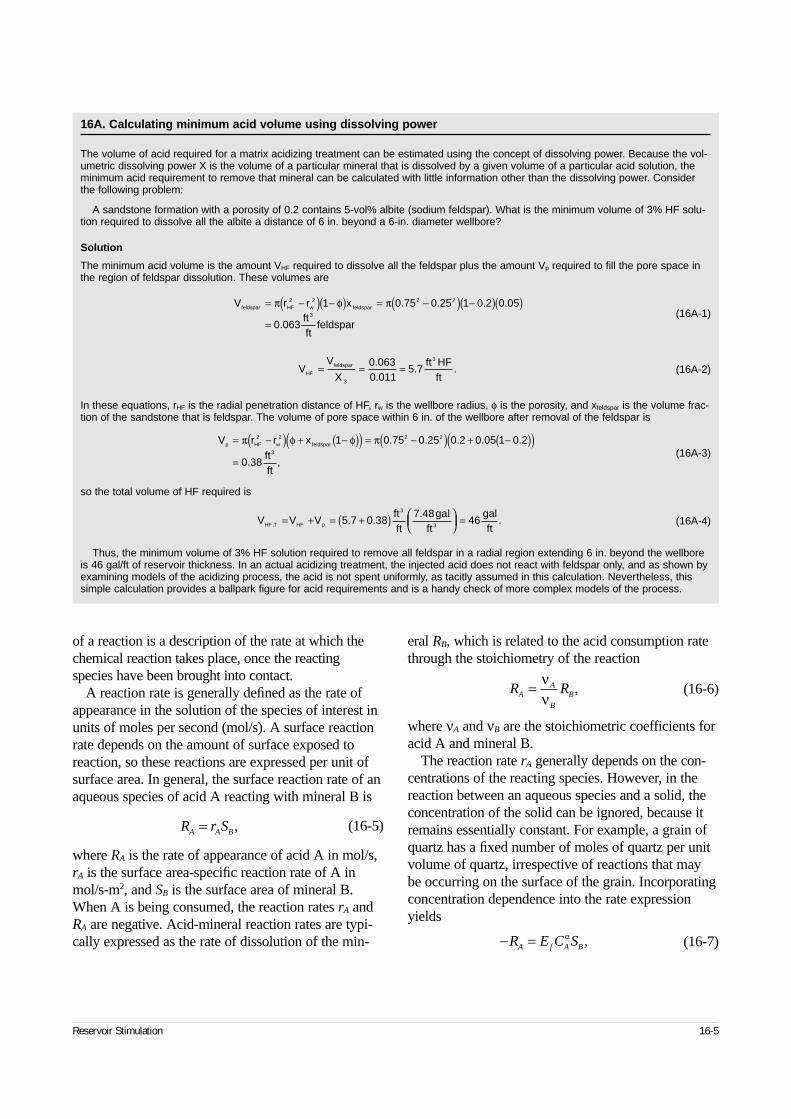
of a reaction is a description of the rate at which thechemical reaction takes place, once the reactingspecies have been brought into contact.

A reaction rate is generally defined as the rate ofappearance in the solution of the species of interest inunits of moles per second (mol/s). A surface reactionrate depends on the amount of surface exposed toreaction, so these reactions are expressed per unit ofsurface area. In general, the surface reaction rate of anaqueous species of acid A reacting with mineral B is

(16-5)

where RA is the rate of appearance of acid A in mol/s,rA is the surface area-specific reaction rate of A inmol/s-m2, and SB is the surface area of mineral B.When A is being consumed, the reaction rates rA andRA are negative. Acid-mineral reaction rates are typi-cally expressed as the rate of dissolution of the min-

eral RB, which is related to the acid consumption ratethrough the stoichiometry of the reaction

(16-6)

where νA and νB are the stoichiometric coefficients foracid A and mineral B.

The reaction rate rA generally depends on the con-centrations of the reacting species. However, in thereaction between an aqueous species and a solid, theconcentration of the solid can be ignored, because itremains essentially constant. For example, a grain ofquartz has a fixed number of moles of quartz per unitvolume of quartz, irrespective of reactions that may be occurring on the surface of the grain. Incorporatingconcentration dependence into the rate expressionyields

(16-7)

Reservoir Stimulation 16-5

16A. Calculating minimum acid volume using dissolving power

The volume of acid required for a matrix acidizing treatment can be estimated using the concept of dissolving power. Because the vol-umetric dissolving power X is the volume of a particular mineral that is dissolved by a given volume of a particular acid solution, theminimum acid requirement to remove that mineral can be calculated with little information other than the dissolving power. Considerthe following problem:

A sandstone formation with a porosity of 0.2 contains 5-vol% albite (sodium feldspar). What is the minimum volume of 3% HF solu-tion required to dissolve all the albite a distance of 6 in. beyond a 6-in. diameter wellbore?

Solution

The minimum acid volume is the amount VHF required to dissolve all the feldspar plus the amount Vp required to fill the pore space inthe region of feldspar dissolution. These volumes are

(16A-1)

(16A-2)

In these equations, rHF is the radial penetration distance of HF, rw is the wellbore radius, φ is the porosity, and xfeldspar is the volume frac-tion of the sandstone that is feldspar. The volume of pore space within 6 in. of the wellbore after removal of the feldspar is

(16A-3)

so the total volume of HF required is

(16A-4)

Thus, the minimum volume of 3% HF solution required to remove all feldspar in a radial region extending 6 in. beyond the wellboreis 46 gal/ft of reservoir thickness. In an actual acidizing treatment, the injected acid does not react with feldspar only, and as shown byexamining models of the acidizing process, the acid is not spent uniformly, as tacitly assumed in this calculation. Nevertheless, thissimple calculation provides a ballpark figure for acid requirements and is a handy check of more complex models of the process.

V r r xfeldspar HF w feldspar= −( ) −( ) = −( ) −( )( )=

π φ π2 2 2 21 0 75 0 25 1 0 2 0 05

0 063

. . . .

.ftft

feldspar3

VV

XHF

feldspar= = =3

0 0630 011

5 7..

. .ft HF

ft

3

V r r xp HF w feldspar= −( ) + −( )( ) = −( ) + −( )( )=

π φ φ π2 2 2 21 0 75 0 25 0 2 0 05 1 0 2

0 38

. . . . .

. ,ftft

3

V V VHF T HF p, . ..

.= + = +( )

=5 7 0 387 48

46ftft

gaft

galft

3

3

l

R r SA A B= ,

R RAA

B

B= νν

,

− =R E C SA f A Bα ,

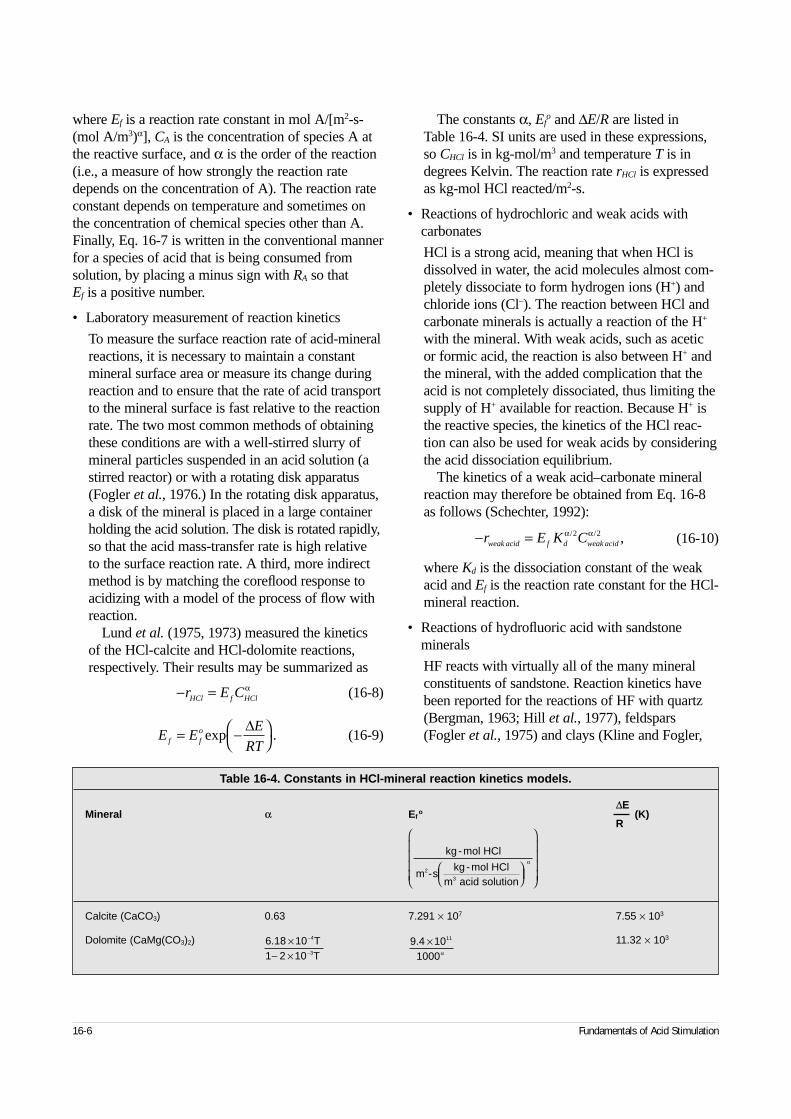
where Ef is a reaction rate constant in mol A/[m2-s-(mol A/m3)α], CA is the concentration of species A atthe reactive surface, and α is the order of the reaction(i.e., a measure of how strongly the reaction ratedepends on the concentration of A). The reaction rateconstant depends on temperature and sometimes onthe concentration of chemical species other than A.Finally, Eq. 16-7 is written in the conventional mannerfor a species of acid that is being consumed fromsolution, by placing a minus sign with RA so that Ef is a positive number.

• Laboratory measurement of reaction kinetics

To measure the surface reaction rate of acid-mineralreactions, it is necessary to maintain a constantmineral surface area or measure its change duringreaction and to ensure that the rate of acid transportto the mineral surface is fast relative to the reactionrate. The two most common methods of obtainingthese conditions are with a well-stirred slurry ofmineral particles suspended in an acid solution (astirred reactor) or with a rotating disk apparatus(Fogler et al., 1976.) In the rotating disk apparatus,a disk of the mineral is placed in a large containerholding the acid solution. The disk is rotated rapidly,so that the acid mass-transfer rate is high relative to the surface reaction rate. A third, more indirectmethod is by matching the coreflood response toacidizing with a model of the process of flow withreaction.

Lund et al. (1975, 1973) measured the kinetics of the HCl-calcite and HCl-dolomite reactions,respectively. Their results may be summarized as

(16-8)

(16-9)

The constants α, Efo and ∆E/R are listed in

Table 16-4. SI units are used in these expressions,so CHCl is in kg-mol/m3 and temperature T is indegrees Kelvin. The reaction rate rHCl is expressedas kg-mol HCl reacted/m2-s.

• Reactions of hydrochloric and weak acids withcarbonates

HCl is a strong acid, meaning that when HCl isdissolved in water, the acid molecules almost com-pletely dissociate to form hydrogen ions (H+) andchloride ions (Cl–). The reaction between HCl andcarbonate minerals is actually a reaction of the H+

with the mineral. With weak acids, such as aceticor formic acid, the reaction is also between H+ andthe mineral, with the added complication that theacid is not completely dissociated, thus limiting thesupply of H+ available for reaction. Because H+ isthe reactive species, the kinetics of the HCl reac-tion can also be used for weak acids by consideringthe acid dissociation equilibrium.

The kinetics of a weak acid–carbonate mineralreaction may therefore be obtained from Eq. 16-8as follows (Schechter, 1992):

(16-10)

where Kd is the dissociation constant of the weakacid and Ef is the reaction rate constant for the HCl-mineral reaction.

• Reactions of hydrofluoric acid with sandstoneminerals

HF reacts with virtually all of the many mineralconstituents of sandstone. Reaction kinetics havebeen reported for the reactions of HF with quartz(Bergman, 1963; Hill et al., 1977), feldspars(Fogler et al., 1975) and clays (Kline and Fogler,

16-6 Fundamentals of Acid Stimulation

− =r E CHCl f HClα

E EE

RTf fo= −

exp

∆.

− =r E K Cweak acid f d weak acidα α/ / ,2 2

Table 16-4. Constants in HCl-mineral reaction kinetics models.

∆EMineral α Ef

o (K)R

Calcite (CaCO3) 0.63 7.291 × 107 7.55 × 103

Dolomite (CaMg(CO3)2) 11.32 × 103

kg -mol HCl

m -skg -mol HCl

m acid solution2

3

α

9 4 101000

11. ×α

6 18 101 2 10

4

3

. ×− ×

−

−

TT

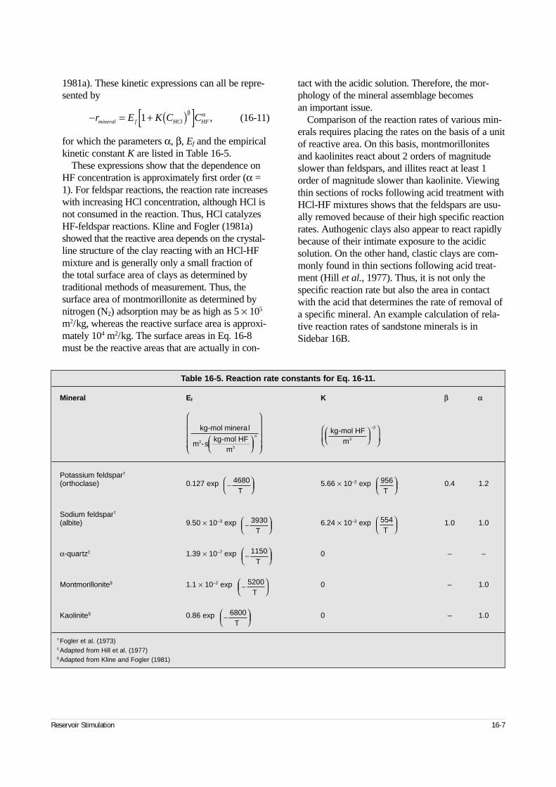
1981a). These kinetic expressions can all be repre-sented by

(16-11)

for which the parameters α, β, Ef and the empiricalkinetic constant K are listed in Table 16-5.

These expressions show that the dependence onHF concentration is approximately first order (α =1). For feldspar reactions, the reaction rate increaseswith increasing HCl concentration, although HCl isnot consumed in the reaction. Thus, HCl catalyzesHF-feldspar reactions. Kline and Fogler (1981a)showed that the reactive area depends on the crystal-line structure of the clay reacting with an HCl-HFmixture and is generally only a small fraction of the total surface area of clays as determined bytraditional methods of measurement. Thus, thesurface area of montmorillonite as determined bynitrogen (N2) adsorption may be as high as 5 × 105

m2/kg, whereas the reactive surface area is approxi-mately 104 m2/kg. The surface areas in Eq. 16-8must be the reactive areas that are actually in con-

tact with the acidic solution. Therefore, the mor-phology of the mineral assemblage becomes an important issue.

Comparison of the reaction rates of various min-erals requires placing the rates on the basis of a unitof reactive area. On this basis, montmorillonitesand kaolinites react about 2 orders of magnitudeslower than feldspars, and illites react at least 1order of magnitude slower than kaolinite. Viewingthin sections of rocks following acid treatment withHCl-HF mixtures shows that the feldspars are usu-ally removed because of their high specific reactionrates. Authogenic clays also appear to react rapidlybecause of their intimate exposure to the acidicsolution. On the other hand, clastic clays are com-monly found in thin sections following acid treat-ment (Hill et al., 1977). Thus, it is not only thespecific reaction rate but also the area in contactwith the acid that determines the rate of removal ofa specific mineral. An example calculation of rela-tive reaction rates of sandstone minerals is inSidebar 16B.

Reservoir Stimulation 16-7

− = + ( )[ ]r E K C Cmineral f HCl HF1β α ,

Table 16-5. Reaction rate constants for Eq. 16-11.

Mineral Ef K β α

Potassium feldspar†

(orthoclase) 0.127 exp 5.66 × 10–2 exp 0.4 1.2

Sodium feldspar†

(albite) 9.50 × 10–3 exp 6.24 × 10–2 exp 1.0 1.0

α-quartz‡ 1.39 × 10–7 exp 0 – –

Montmorillonite§ 1.1 × 10–2 exp 0 – 1.0

Kaolinite§ 0.86 exp 0 – 1.0

† Fogler et al. (1973)‡ Adapted from Hill et al. (1977)§ Adapted from Kline and Fogler (1981)

kg-mol minera l

m -skg-mol HF

m2

3

αkg-mol HF

m3

−β

−

4680T

956T

−

3930T

554T

−

1150T

−

5200T

−

6800T

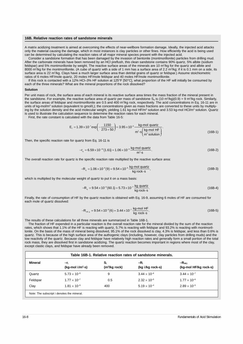
16-8 Fundamentals of Acid Stimulation

16B. Relative reaction rates of sandstone minerals

A matrix acidizing treatment is aimed at overcoming the effects of near-wellbore formation damage. Ideally, the injected acid attacksonly the material causing the damage, which in most instances is clay particles or other fines. How efficiently the acid is being usedcan be determined by calculating the reaction rates of all major mineral species present with the injected acid.

Consider a sandstone formation that has been damaged by the invasion of bentonite (montmorillonite) particles from drilling mud.After the carbonate minerals have been removed by an HCl preflush, this clean sandstone contains 90% quartz, 5% albite (sodiumfeldspar) and 5% montmorillonite by weight. The reactive surface areas of the minerals are 10 m2/kg for the quartz and albite and8000 m2/kg for the montmorillonite. (A cube of quartz with a side of 1 mm has a surface area of 2.2 m2/kg; if it is 0.1 mm on a side, itssurface area is 22 m2/kg. Clays have a much larger surface area than detrital grains of quartz or feldspar.) Assume stoichiometricratios of 6 moles HF/mole quartz, 20 moles HF/mole feldspar and 40 moles HF/mole montmorillonite.

If this rock is contacted with a 12% HCl–3% HF solution at 125°F [50°C], what proportion of the HF will initially be consumed byeach of the three minerals? What are the mineral proportions of the rock dissolved?

Solution

Per unit mass of rock, the surface area of each mineral is its reactive surface area times the mass fraction of the mineral present inthe sandstone. For example, the reactive surface area of quartz per mass of sandstone Sq is (10 m2/kg)(0.9) = 9 m2/kg rock. Similarly,the surface areas of feldspar and montmorillonite are 0.5 and 400 m2/kg rock, respectively. The acid concentrations in Eq. 16-11 are inunits of kg-mol/m3 solution (equivalent to gmol/L); the concentrations given as mass fractions are converted to these units by multiply-ing by the solution density and the acid molecular weight, yielding 1.61 kg-mol HF/m3 solution and 3.53 kg-mol HCl/m3 solution. Quartzis used to illustrate the calculation sequence to determine the reaction rates for each mineral.

First, the rate constant is calculated with the data from Table 16-5:

(16B-1)

Then, the specific reaction rate for quartz from Eq. 16-11 is

(16B-2)

The overall reaction rate for quartz is the specific reaction rate multiplied by the reactive surface area:

(16B-3)

which is multiplied by the molecular weight of quartz to put it on a mass basis:

(16B-4)

Finally, the rate of consumption of HF by the quartz reaction is obtained with Eq. 16-9, assuming 6 moles of HF are consumed foreach mole of quartz dissolved:

(16B-5)

The results of these calculations for all three minerals are summarized in Table 16B-1.The fraction of HF expended in a particular reaction is the overall reaction rate for the mineral divided by the sum of the reaction

rates, which shows that 1.1% of the HF is reacting with quartz, 5.7% is reacting with feldspar and 93.2% is reacting with montmoril-lonite. On the basis of the mass of mineral being dissolved, 95.1% of the rock dissolved is clay, 4.3% is feldspar, and less than 0.6% isquartz. This is because of the high surface area of the authogenic clays (including, however, clay particles from drilling muds) and thelow reactivity of the quartz. Because clay and feldspar have relatively high reaction rates and generally form a small portion of the totalrock mass, they are dissolved first in sandstone acidizing. The quartz reaction becomes important in regions where most of the clay,except clastic clays, and feldspar have already been removed.

Ef = × −+

= ×

− −1 39 101150

273 503 95 107 9. . .exp

kg-mol quartz

m -skg-mol HFm solution

2

3

− = × ( ) = ×− −rq 6 59 10 1 61 1 06 1010 9. . . .kg-mol quartz

m -s2

− = × ( ) = ×− −Rq 1 06 10 9 9 54 109 9. . ,kg-mol quartz

kg rock-s

− = × ( ) = ×− −Rq 9 54 10 60 1 5 73 109 7. . .kg quartzkg rock-s

.

− = × ( ) = ×− −RHF q, . . .9 54 10 6 3 44 109 7 kg-mol HFkg rock-s

Table 16B-1. Relative reaction rates of sandstone minerals.

Mineral –ri Si –Ri –RHF,i

(kg-mol i /m2-s) (m2/kg rock) (kg i /kg rock-s) (kg-mol HF/kg rock-s)

Quartz 5.73 × 10–8 9 3.44 × 10–6 3.44 × 10–7

Feldspar 1.77 × 10–7 0.5 2.32 × 10–5 1.77 × 10–6

Clay 1.81 × 10–9 400 5.19 × 10–4 2.89 × 10–5

Note: The subscript i denotes the mineral.

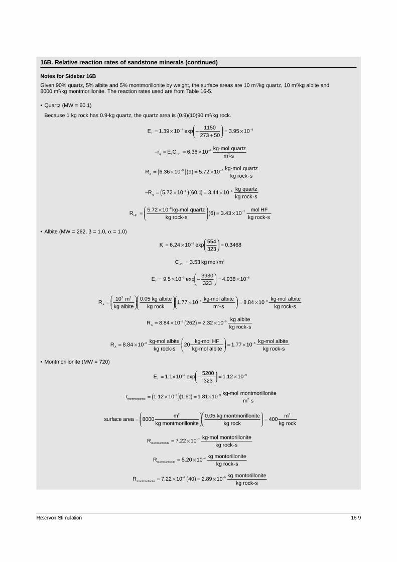
Reservoir Stimulation 16-9

16B. Relative reaction rates of sandstone minerals (continued)

Notes for Sidebar 16B

Given 90% quartz, 5% albite and 5% montmorillonite by weight, the surface areas are 10 m2/kg quartz, 10 m2/kg albite and 8000 m2/kg montmorillonite. The reaction rates used are from Table 16-5.

• Quartz (MW = 60.1)

Because 1 kg rock has 0.9-kg quartz, the quartz area is (0.9)(10)90 m2/kg rock.

• Albite (MW = 262, β = 1.0, α = 1.0)

• Montmorillonite (MW = 720)

Ef = × −+

= ×− −1 39 101150

273 503 95 107 9. .exp

− = = × −r E Cq f HF 6 36 10 9.kg-mol quartz

m -s2

− = ×( )( ) = ×− −Rq 6 36 10 9 5 72 109 8. .kg-mol quartz

kg rock-s

− = ×( )( ) = ×− −Rq 5 72 10 60 1 3 44 108 6. . .kg quartzkg rock-s

K = ×

=−6 24 10 0 34682. .exp554323

CHCl = 3 53. kg mol/m3

Ef = × −

= ×− −9 5 10 4 938 103 8. .exp3930323

RA =

×

= ×− −10 mkg albite

0.05 kg albitekg rock

kg-mol albitem -s

kg-mol albitekg rock-s

3 3

21 77 10 8 84 107 8. .

RA = × ( ) = ×− −8 84 10 262 2 32 108. . 5 kg albitekg rock-s

RA = ×

= ×− −8 84 10 8.kg-mol albite

kg rock-s20

kg-mol HFkg-mol albite

1.77 10kg-mol albite

kg rock-s6

Ef = × −

= ×− −1 1 10 1 12 102 9. .exp5200323

− = ×( )( ) = ×− −rmontmorillonite 1 12 10 1 61 1 81 109 9. . .kg-mol montmorillonite

m -s2

surface area =

=8000m

kg montmorillonite0.05 kg montmorillonite

kg rock400

mkg rock

2 2

Rmontmorillonite = × −7.22 10kg-mol montorillonite

kg rock-s7

Rmontmorillonite = × −5 20 10 4.kg montorillonite

kg rock-s

Rmontmorillonite = × ( ) = ×− −7 22 10 40 2 89 107. . 5 kg montorillonitekg rock-s

RHF = ×

( ) = ×−

−5 72 106 3 43 10

87.

.kg-mol quartz

kg rock-smol HF

kg rock-s

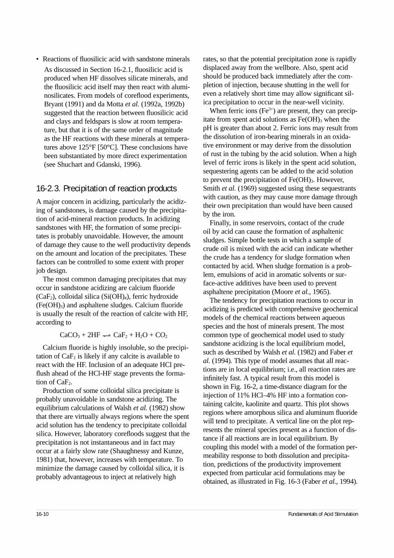
• Reactions of fluosilicic acid with sandstone minerals

As discussed in Section 16-2.1, fluosilicic acid isproduced when HF dissolves silicate minerals, andthe fluosilicic acid itself may then react with alumi-nosilicates. From models of coreflood experiments,Bryant (1991) and da Motta et al. (1992a, 1992b)suggested that the reaction between fluosilicic acidand clays and feldspars is slow at room tempera-ture, but that it is of the same order of magnitude as the HF reactions with these minerals at tempera-tures above 125°F [50°C]. These conclusions havebeen substantiated by more direct experimentation(see Shuchart and Gdanski, 1996).

16-2.3. Precipitation of reaction productsA major concern in acidizing, particularly the acidiz-ing of sandstones, is damage caused by the precipita-tion of acid-mineral reaction products. In acidizingsandstones with HF, the formation of some precipi-tates is probably unavoidable. However, the amount of damage they cause to the well productivity dependson the amount and location of the precipitates. Thesefactors can be controlled to some extent with properjob design.

The most common damaging precipitates that mayoccur in sandstone acidizing are calcium fluoride(CaF2), colloidal silica (Si(OH)4), ferric hydroxide(Fe(OH)3) and asphaltene sludges. Calcium fluoride is usually the result of the reaction of calcite with HF,according to

CaCO3 + 2HF CaF2 + H2O + CO2

Calcium fluoride is highly insoluble, so the precipi-tation of CaF2 is likely if any calcite is available toreact with the HF. Inclusion of an adequate HCl pre-flush ahead of the HCl-HF stage prevents the forma-tion of CaF2.

Production of some colloidal silica precipitate isprobably unavoidable in sandstone acidizing. Theequilibrium calculations of Walsh et al. (1982) showthat there are virtually always regions where the spentacid solution has the tendency to precipitate colloidalsilica. However, laboratory corefloods suggest that theprecipitation is not instantaneous and in fact mayoccur at a fairly slow rate (Shaughnessy and Kunze,1981) that, however, increases with temperature. Tominimize the damage caused by colloidal silica, it isprobably advantageous to inject at relatively high

rates, so that the potential precipitation zone is rapidlydisplaced away from the wellbore. Also, spent acidshould be produced back immediately after the com-pletion of injection, because shutting in the well foreven a relatively short time may allow significant sil-ica precipitation to occur in the near-well vicinity.

When ferric ions (Fe3+) are present, they can precip-itate from spent acid solutions as Fe(OH)3 when thepH is greater than about 2. Ferric ions may result fromthe dissolution of iron-bearing minerals in an oxida-tive environment or may derive from the dissolutionof rust in the tubing by the acid solution. When a highlevel of ferric irons is likely in the spent acid solution,sequestering agents can be added to the acid solutionto prevent the precipitation of Fe(OH)3. However,Smith et al. (1969) suggested using these sequestrantswith caution, as they may cause more damage throughtheir own precipitation than would have been causedby the iron.

Finally, in some reservoirs, contact of the crude oil by acid can cause the formation of asphaltenicsludges. Simple bottle tests in which a sample ofcrude oil is mixed with the acid can indicate whetherthe crude has a tendency for sludge formation whencontacted by acid. When sludge formation is a prob-lem, emulsions of acid in aromatic solvents or sur-face-active additives have been used to preventasphaltene precipitation (Moore et al., 1965).

The tendency for precipitation reactions to occur inacidizing is predicted with comprehensive geochemicalmodels of the chemical reactions between aqueousspecies and the host of minerals present. The mostcommon type of geochemical model used to studysandstone acidizing is the local equilibrium model,such as described by Walsh et al. (1982) and Faber etal. (1994). This type of model assumes that all reac-tions are in local equilibrium; i.e., all reaction rates areinfinitely fast. A typical result from this model isshown in Fig. 16-2, a time-distance diagram for theinjection of 11% HCl–4% HF into a formation con-taining calcite, kaolinite and quartz. This plot showsregions where amorphous silica and aluminum fluoridewill tend to precipitate. A vertical line on the plot rep-resents the mineral species present as a function of dis-tance if all reactions are in local equilibrium. Bycoupling this model with a model of the formation per-meability response to both dissolution and precipita-tion, predictions of the productivity improvementexpected from particular acid formulations may beobtained, as illustrated in Fig. 16-3 (Faber et al., 1994).

16-10 Fundamentals of Acid Stimulation

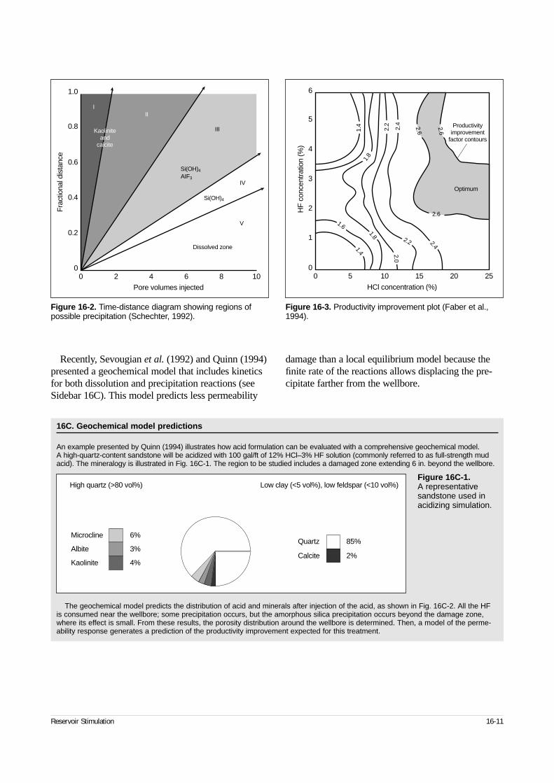
Recently, Sevougian et al. (1992) and Quinn (1994)presented a geochemical model that includes kineticsfor both dissolution and precipitation reactions (seeSidebar 16C). This model predicts less permeability

damage than a local equilibrium model because thefinite rate of the reactions allows displacing the pre-cipitate farther from the wellbore.

Reservoir Stimulation 16-11

Figure 16-2. Time-distance diagram showing regions ofpossible precipitation (Schechter, 1992).

0 20

0.2

0.4

0.6

0.8

1.0

4 6 8 10

Pore volumes injected

Fra

ctio

nal d

ista

nce

Dissolved zone

III

III

IV

V

Si(OH)4

Si(OH)4

AIF3

Kaoliniteand

calcite

Figure 16-3. Productivity improvement plot (Faber et al.,1994).

00

5 10 15 20 25

1

2

3

4

5

6

HCl concentration (%)

HF

con

cent

ratio

n (%

)

Productivityimprovement

factor contours

Optimum

1.4

2.2

2.4

1.8

1.6

1.8

2.4

2.2

2.0

1.4

2.6

2.6

2.6

16C. Geochemical model predictions

An example presented by Quinn (1994) illustrates how acid formulation can be evaluated with a comprehensive geochemical model. A high-quartz-content sandstone will be acidized with 100 gal/ft of 12% HCl–3% HF solution (commonly referred to as full-strength mudacid). The mineralogy is illustrated in Fig. 16C-1. The region to be studied includes a damaged zone extending 6 in. beyond the wellbore.

The geochemical model predicts the distribution of acid and minerals after injection of the acid, as shown in Fig. 16C-2. All the HFis consumed near the wellbore; some precipitation occurs, but the amorphous silica precipitation occurs beyond the damage zone,where its effect is small. From these results, the porosity distribution around the wellbore is determined. Then, a model of the perme-ability response generates a prediction of the productivity improvement expected for this treatment.

Figure 16C-1.A representativesandstone used inacidizing simulation.

Microcline

Albite

Kaolinite

6%

3%

4%

Quartz

Calcite

85%

2%

High quartz (>80 vol%) Low clay (<5 vol%), low feldspar (<10 vol%)

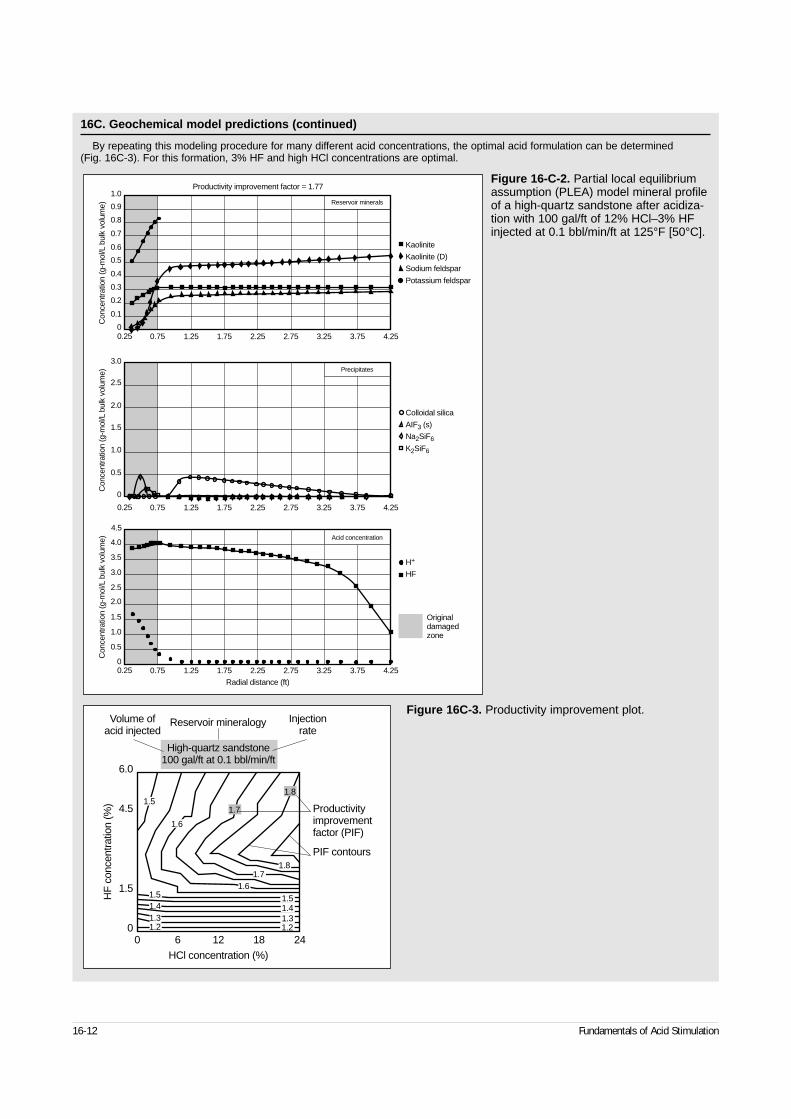
16-12 Fundamentals of Acid Stimulation

16C. Geochemical model predictions (continued)

By repeating this modeling procedure for many different acid concentrations, the optimal acid formulation can be determined(Fig. 16C-3). For this formation, 3% HF and high HCl concentrations are optimal.

Figure 16-C-2. Partial local equilibriumassumption (PLEA) model mineral profileof a high-quartz sandstone after acidiza-tion with 100 gal/ft of 12% HCl–3% HFinjected at 0.1 bbl/min/ft at 125°F [50°C].

0.1

0

2.5

0.2

0.3

0.4

0.5

0.6

0.7

0.8

0.9

1.0

3.0

2.0

1.5

1.0

0.5

0

4.5

4.0

3.5

3.0

2.5

2.0

1.5

1.0

0.5

0

Con

cent

ratio

n (g

-mol

/L b

ulk

volu

me)

Con

cent

ratio

n (g

-mol

/L b

ulk

volu

me)

Con

cent

ratio

n (g

-mol

/L b

ulk

volu

me)

0.25 0.75 1.25 1.75 2.25 2.75 3.25 3.75 4.25

0.25 0.75 1.25 1.75 2.25 2.75 3.25 3.75 4.25

0.25 0.75 1.25 1.75 2.25 2.75 3.25 3.75 4.25

Radial distance (ft)

Productivity improvement factor = 1.77

Reservoir minerals

Precipitates

Acid concentration

Kaolinite

Kaolinite (D)

Sodium feldspar

Potassium feldspar

Colloidal silica

AIF3 (s)

Na2SiF6

H+

HF

K2SiF6

Originaldamagedzone

Figure 16C-3. Productivity improvement plot.

0 6 12 18 240

1.5

4.5

6.0

HCl concentration (%)

HF

con

cent

ratio

n (%

)

1.21.21.31.31.41.41.5

1.61.7

1.8

1.5

1.5

1.6

1.7

1.8

Productivityimprovementfactor (PIF)

PIF contours

Injectionrate

Volume ofacid injected

High-quartz sandstone100 gal/ft at 0.1 bbl/min/ft

Reservoir mineralogy

16-3. Sandstone acidizing16-3.1. IntroductionA typical acid treatment in sandstones consists of theinjection of an HCl preflush, with 50 gal/ft of forma-tion a common preflush volume, followed by theinjection of 50 to 200 gal/ft of HCl-HF mixture. Apostflush of diesel, brine or HCl then displaces theHCl-HF from the tubing or wellbore. Once the treat-ment is completed, the spent acid should be immedi-ately produced back to minimize damage by theprecipitation of reaction products.

A sandstone acidizing treatment design begins withthe selection of the type and concentration of acid to be used. The volumes of preflush, HCl-HF mixture andpostflush required and the desired injection rate(s) areconsidered next. In virtually all acid treatments, theplacement of the acid is an important issue—a strategyto ensure that sufficient volumes of acid contact allproductive parts of the formation should be carefullyplanned. Proper execution of the treatment is critical to acidizing success, so the conduct of the treatment,including the mechanical arrangements for introducingthe acid to the formation and the methods of treatmentmonitoring, should be planned in detail. Finally, numer-ous additives are incorporated with acid solutions forvarious purposes. The types and amounts of additivesto be used in the treatment must be determined on thebasis of the completion, formation and reservoir fluids.These design factors are considered in detail in otherchapters: acid selection in Chapters 13 and 18, treat-ment design (rate and volume) in Chapter 18, fluidplacement and diversion in Chapter 19, treatment moni-toring and evaluation in Chapter 20 and acid additivesin Chapter 15. This section presents models of thesandstone acidizing process that provide a foundationfor the design methods used for field application.

16-3.2. Acid selectionThe type and strength (i.e., concentration) of acid usedin sandstones are selected primarily on the basis offield experience with particular formations. For years,the standard sandstone acidizing formulation consistedof a 12% HCl–3% HF mixture, preceded by a 15%HCl preflush. In fact, the 12% HCl–3% HF mixturehas been so common that it is referred to genericallyas mud acid. In recent years, however, the trend hasbeen toward the use of lower strength HF solutions

(Brannon et al., 1987). The benefits of lower concen-tration HF solutions are a reduction in damaging pre-cipitates from the spent acid and lessened risk ofunconsolidation of the formation around the wellbore.The selection of acidizing fluids should always beginwith an assessment of the formation damagepresent—in general, the damaging material must besoluble in the treating fluids. Geochemical models canbe used to guide acid selection, once the compositionof the damaged formation is determined, as describedin Section 16-2.3. Chapters 17 and 18 provide a com-prehensive treatment of acid selection for sandstoneand carbonate reservoirs, respectively.

16-3.3. Sandstone acidizing models• Two-mineral model

Numerous efforts have been made over the years to develop a comprehensive model of the sandstoneacidizing process that could then be used as adesign aid. The most common model in use today isthe two-mineral model (Hill et al., 1977; Hekim etal., 1982; Taha et al., 1989) that divides all mineralsinto two categories—fast-reacting and slow-reactingspecies. Schechter (1992) categorizes feldspars,authogenic clays and amorphous silica as fast react-ing, and detrital clay particles and quartz grains arethe primary slow-reacting minerals. The model con-sists of material balances applied to the HF acid andreactive minerals, which for linear flow, such as in acoreflood, are

(16-12)

(16-13)

(16-14)

In these equations, CHF is the concentration ofHF in solution and MWHF is its molecular weight, u is the acid flux, s is the distance, SF* and SS* arethe specific surface areas per unit volume of solids,VF and VS are the volume fractions, Ef,F and Ef,S arethe reaction rate constants (based on the rate ofconsumption of HF), MWF and MWS are the molec-

Reservoir Stimulation 16-13

δ φδ

δδ

φC

tu

C

xS V E S V E CHF HF

F F f F S S f S HF

( ) + = − +{ } −( )*,

*, 1

δδ

φβ

ρtV

MW S V E CF

HF F F F f F HF

F

1−( )[ ] =− *

,

δδ

φβ

ρtV

MW S V E CS

HF S S S f S HF

S

1−( )[ ] =− *

, .

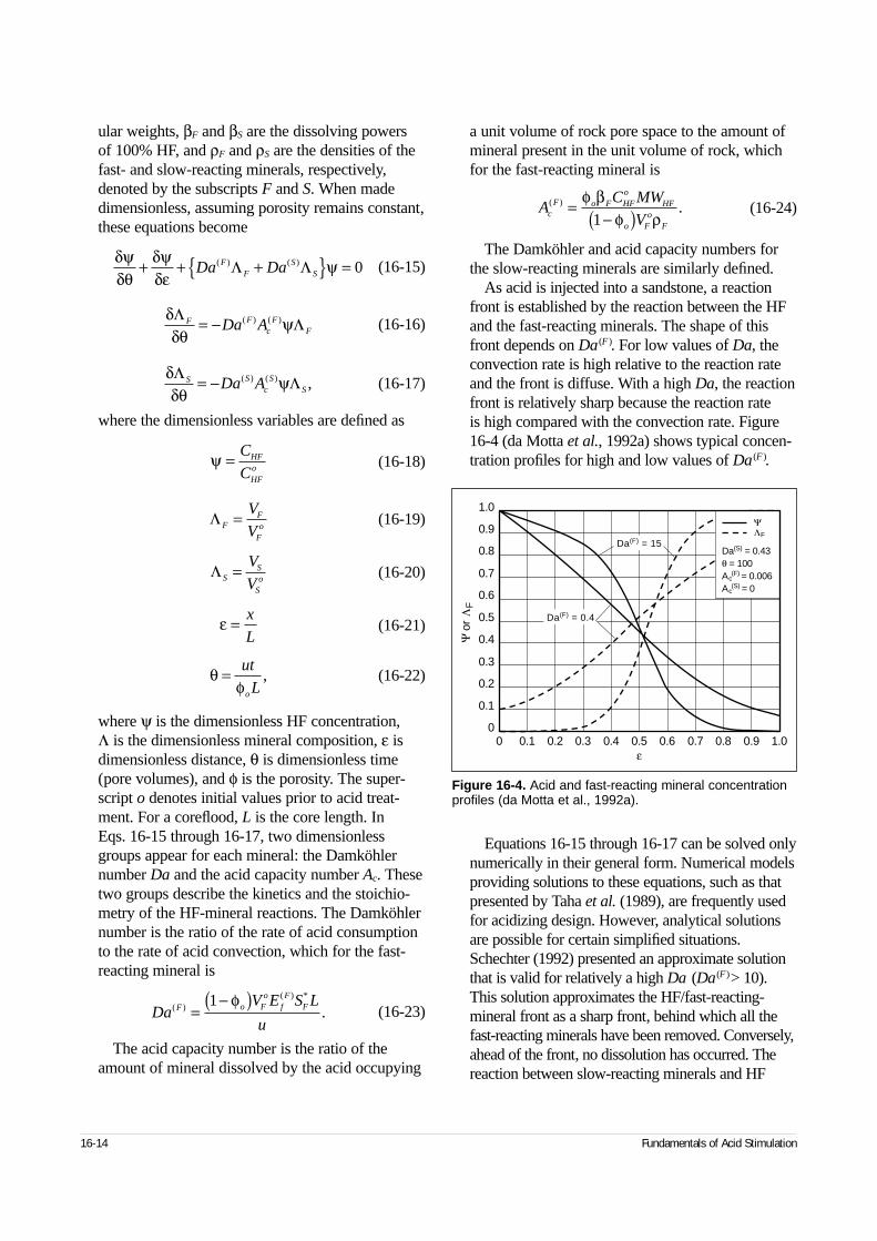
ular weights, βF and βS are the dissolving powers of 100% HF, and ρF and ρS are the densities of thefast- and slow-reacting minerals, respectively,denoted by the subscripts F and S. When madedimensionless, assuming porosity remains constant,these equations become

(16-15)

(16-16)

(16-17)

where the dimensionless variables are defined as

(16-18)

(16-19)

(16-20)

(16-21)

(16-22)

where ψ is the dimensionless HF concentration, Λ is the dimensionless mineral composition, ε isdimensionless distance, θ is dimensionless time(pore volumes), and φ is the porosity. The super-script o denotes initial values prior to acid treat-ment. For a coreflood, L is the core length. In Eqs. 16-15 through 16-17, two dimensionlessgroups appear for each mineral: the Damköhlernumber Da and the acid capacity number Ac. Thesetwo groups describe the kinetics and the stoichio-metry of the HF-mineral reactions. The Damköhlernumber is the ratio of the rate of acid consumptionto the rate of acid convection, which for the fast-reacting mineral is

(16-23)

The acid capacity number is the ratio of theamount of mineral dissolved by the acid occupying

a unit volume of rock pore space to the amount ofmineral present in the unit volume of rock, whichfor the fast-reacting mineral is

(16-24)

The Damköhler and acid capacity numbers forthe slow-reacting minerals are similarly defined.

As acid is injected into a sandstone, a reactionfront is established by the reaction between the HFand the fast-reacting minerals. The shape of thisfront depends on Da(F ). For low values of Da, theconvection rate is high relative to the reaction rateand the front is diffuse. With a high Da, the reactionfront is relatively sharp because the reaction rate is high compared with the convection rate. Figure16-4 (da Motta et al., 1992a) shows typical concen-tration profiles for high and low values of Da(F ).

Equations 16-15 through 16-17 can be solved onlynumerically in their general form. Numerical modelsproviding solutions to these equations, such as thatpresented by Taha et al. (1989), are frequently usedfor acidizing design. However, analytical solutionsare possible for certain simplified situations.Schechter (1992) presented an approximate solutionthat is valid for relatively a high Da (Da(F)> 10).This solution approximates the HF/fast-reacting-mineral front as a sharp front, behind which all thefast-reacting minerals have been removed. Conversely,ahead of the front, no dissolution has occurred. Thereaction between slow-reacting minerals and HF

16-14 Fundamentals of Acid Stimulation

δψδθ

δψδε

ψ+ + +{ } =Da DaFF

SS

( ) ( )Λ Λ 0

δδθ

ψΛ ΛF Fc

FFDa A= − ( ) ( )

δδθ

ψΛ ΛS Sc

SSDa A= − ( ) ( ) ,

ψ = C

CHF

HFo

AC MW

VcF o F HF

oHF

o Fo

F

( ) .=−( )

φ βφ ρ1

ΛFF

Fo

V

V=

ΛSS

So

V

V=

ε = x

L

θφ

= ut

Lo

,

DaV E S L

uF o F

ofF

F( )( ) *

.=−( )1 φ

Figure 16-4. Acid and fast-reacting mineral concentrationprofiles (da Motta et al., 1992a).

0 0.1 0.2 0.3 0.4 0.5 0.6 0.7 0.8 0.9 1.00

0.1

0.2

0.3

0.4

0.5

0.6

0.7

0.8

0.9

1.0

ε

Ψ o

r Λ

F

Da(F) = 15

Da(F) = 0.4

ΨΛF

Da(S) = 0.43θ = 100Ac

(F) = 0.006Ac

(S) = 0

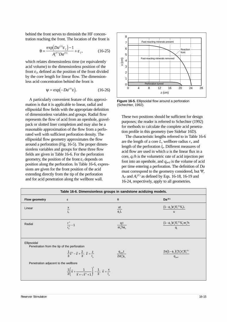
behind the front serves to diminish the HF concen-tration reaching the front. The location of the front is

(16-25)

which relates dimensionless time (or equivalentlyacid volume) to the dimensionless position of thefront ε f, defined as the position of the front dividedby the core length for linear flow. The dimension-less acid concentration behind the front is

(16-26)

A particularly convenient feature of this approxi-mation is that it is applicable to linear, radial andellipsoidal flow fields with the appropriate definitionof dimensionless variables and groups. Radial flowrepresents the flow of acid from an openhole, gravel-pack or slotted liner completion and may also be areasonable approximation of the flow from a perfo-rated well with sufficient perforation density. Theellipsoidal flow geometry approximates the flowaround a perforation (Fig. 16-5). The proper dimen-sionless variables and groups for these three flowfields are given in Table 16-6. For the perforationgeometry, the position of the front ε f depends onposition along the perforation. In Table 16-6, expres-sions are given for the front position of the acidextending directly from the tip of the perforation and for acid penetration along the wellbore wall.

These two positions should be sufficient for designpurposes; the reader is referred to Schechter (1992)for methods to calculate the complete acid penetra-tion profile in this geometry (see Sidebar 16D).

The characteristic lengths referred to in Table 16-6are the length of a core L, wellbore radius rw andlength of the perforation lp. Different measures ofacid flow are used in which u is the linear flux in acore, qi/h is the volumetric rate of acid injection perfoot into an openhole, and qperf is the volume of acidper time entering a perforation. The definition of Damust correspond to the geometry considered, but Ψ,ΛF and Ac

(F) as defined by Eqs. 16-18, 16-19 and 16-24, respectively, apply to all geometries.

Reservoir Stimulation 16-15

Figure 16-5. Ellipsoidal flow around a perforation(Schechter, 1992).

0 4 8 12 16 20 24 280

1

2

3

4

5

6

7

8

z (cm)

x (c

m)

Perforation tunnel

Fast-reacting minerals removed

Fast-reacting minerals present

Reactionfrontθ

εε=

( ) −+

exp Da

A Da

Sf

cF S f

( )

( ) ( ),

1

ψ ε= −( )exp Da S( ) .

Table 16-6. Dimensionless groups in sandstone acidizing models.

Flow geometry ε θ Da (S )

Linear

Radial

EllipsoidalPenetration from the tip of the perforation

Penetration adjacent to the wellbore

13

23

3z z zzl p

− + =;

13

1

1

132

3

xx x

xxl p

++ +

− =;

xL

rrw

2

21−

q t

lperf

p o2 3π φ

utLoφ

q tr h

i

w oπ φ2

2 1 3π φ−( )o p S So

fS

perf

l S V E

q

* ( )

1−( )φo So

fS

SV E S L

u

( ) *

1 2−( )φ πo So

fS

S w

i

V E S r h

q

( ) *

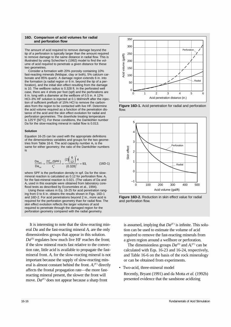
It is interesting to note that the slow-reacting min-eral Da and the fast-reacting mineral Ac are the onlydimensionless groups that appear in this solution.Da(S) regulates how much live HF reaches the front;if the slow mineral reacts fast relative to the convec-tion rate, little acid is available to propagate the fast-mineral front. Ac for the slow-reacting mineral is notimportant because the supply of slow-reacting min-eral is almost constant behind the front. Ac

(F) directlyaffects the frontal propagation rate—the more fast-reacting mineral present, the slower the front willmove. Da(F) does not appear because a sharp front

is assumed, implying that Da(F) is infinite. This solu-tion can be used to estimate the volume of acidrequired to remove the fast-reacting minerals from a given region around a wellbore or perforation.

The dimensionless groups Da(S) and Ac(F) can be

calculated with Eqs. 16-23 and 16-24, respectively,and Table 16-6 on the basis of the rock mineralogyor can be obtained from experiments.

• Two-acid, three-mineral model

Recently, Bryant (1991) and da Motta et al. (1992b)presented evidence that the sandstone acidizing

16-16 Fundamentals of Acid Stimulation

16D. Comparison of acid volumes for radial and perforation flow

The amount of acid required to remove damage beyond thetip of a perforation is typically larger than the amount requiredto remove damage to the same distance in radial flow. This isillustrated by using Schechter’s (1992) model to find the vol-ume of acid required to penetrate a given distance for thesetwo geometries.

Consider a formation with 20% porosity containing 10%fast-reacting minerals (feldspar, clay or both), 5% calcium car-bonate and 85% quartz. A damage region extends 6 in. intothe formation (a radial region or 6 in. beyond the tip of a per-foration), and the initial skin effect resulting from the damageis 10. The wellbore radius is 0.328 ft. In the perforated wellcase, there are 4 shots per foot (spf) and the perforations are6 in. long with a diameter at the wellbore of 0.5 in. A 12%HCl–3% HF solution is injected at 0.1 bbl/min/ft after the injec-tion of sufficient preflush of 15% HCl to remove the carbon-ates from the region to be contacted with live HF. Determinethe acid volume required as a function of the penetration dis-tance of the acid and the skin effect evolution for radial andperforation geometries. The downhole treating temperature is 125°F [50°C]. For these conditions, the Damköhler numberDa for the slow-reacting mineral in radial flow is 0.013.

Solution

Equation 16-25 can be used with the appropriate definitionsof the dimensionless variables and groups for the two geome-tries from Table 16-6. The acid capacity number Ac is thesame for either geometry; the ratio of the Damköhler numbersis

(16D-1)

where SPF is the perforation density in spf. Da for the slow-mineral reaction is calculated as 0.12 for perforation flow. Ac

for the fast-mineral reaction is 0.021. (The values of Da andAc used in this example were obtained from laboratory core-flood tests as described by Economides et al., 1994).

Using these values in Eq. 16-25 for acid penetration rang-ing from 0 to 6 in. obtains the results shown in Figs. 16D-1and 16D-2. For acid penetrations beyond 2 in., more acid isrequired for the perforation geometry than for radial flow. Theskin effect evolution reflects the larger volumes of acidrequired to penetrate through the damaged region for theperforation geometry compared with the radial geometry.

Da

Da

SPF

rperf

rad

perf

w

= =( )

( )=

212

612

4

0 32893

3

2

3

2

( )

.,

Figure 16D-1. Acid penetration for radial and perforationflow.

Figure 16D-2. Reduction in skin effect value for radialand perforation flow.

00

350

300

250

200

150

100

50

1 2 3 4 5 6

Acid penetration distance (in.)

Aci

d vo

lum

e (g

al/ft

)

Perforation

Radial

–1

0

0 100

1

2

3

4

5

200 300 400 500

Acid volume (gal/ft)

Ski

n ef

fect

Perforation

Radial

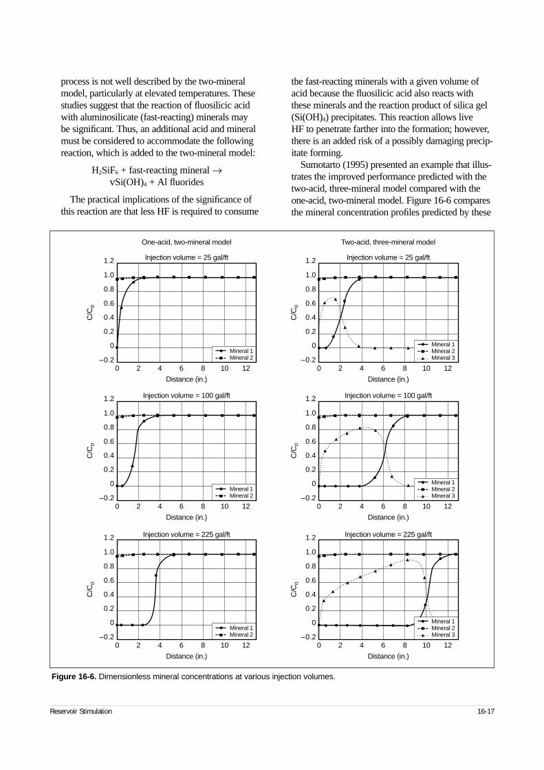
process is not well described by the two-mineralmodel, particularly at elevated temperatures. Thesestudies suggest that the reaction of fluosilicic acidwith aluminosilicate (fast-reacting) minerals may be significant. Thus, an additional acid and mineralmust be considered to accommodate the followingreaction, which is added to the two-mineral model:

H2SiF6 + fast-reacting mineral →νSi(OH)4 + Al fluorides

The practical implications of the significance ofthis reaction are that less HF is required to consume

the fast-reacting minerals with a given volume ofacid because the fluosilicic acid also reacts withthese minerals and the reaction product of silica gel(Si(OH)4) precipitates. This reaction allows live HF to penetrate farther into the formation; however,there is an added risk of a possibly damaging precip-itate forming.

Sumotarto (1995) presented an example that illus-trates the improved performance predicted with thetwo-acid, three-mineral model compared with theone-acid, two-mineral model. Figure 16-6 comparesthe mineral concentration profiles predicted by these

Reservoir Stimulation 16-17

Figure 16-6. Dimensionless mineral concentrations at various injection volumes.

0 2 4 6 8 10 12–0.2

0

0.2

0.4

0.6

0.8

1.0

1.2

Distance (in.)

Injection volume = 25 gal/ft

Mineral 1Mineral 2

0 2 4 6 8 10 12–0.2

0

0.2

0.4

0.6

0.8

1.0

1.2

Distance (in.)

Injection volume = 100 gal/ft

Mineral 1Mineral 2

0 2 4 6 8 10 12–0.2

0

0.2

0.4

0.6

0.8

1.0

1.2

Distance (in.)

Injection volume = 225 gal/ft

Mineral 1Mineral 2

0 2 4 6 8 10 12–0.2

0

0.2

0.4

0.6

0.8

1.0

1.2

C/C

oC

/Co

C/C

o

C/C

oC

/Co

C/C

o

Distance (in.)

Injection volume = 25 gal/ft

0 2 4 6 8 10 12–0.2

0

0.2

0.4

0.6

0.8

1.0

1.2

Distance (in.)

Injection volume = 100 gal/ft

0 2 4 6 8 10 12–0.2

0

0.2

0.4

0.6

0.8

1.0

1.2

Distance (in.)

Injection volume = 225 gal/ft

Mineral 1Mineral 2Mineral 3

Mineral 1Mineral 2Mineral 3

Mineral 1Mineral 2Mineral 3

One-acid, two-mineral model Two-acid, three-mineral model

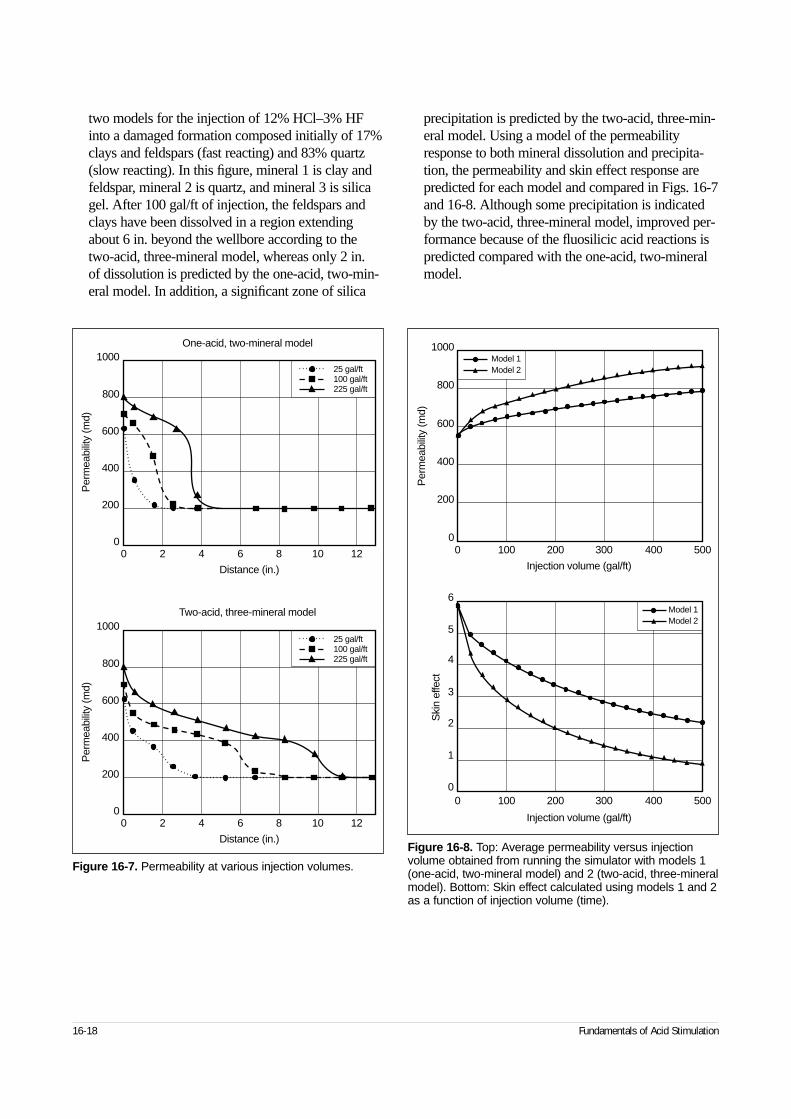
two models for the injection of 12% HCl–3% HFinto a damaged formation composed initially of 17%clays and feldspars (fast reacting) and 83% quartz(slow reacting). In this figure, mineral 1 is clay andfeldspar, mineral 2 is quartz, and mineral 3 is silicagel. After 100 gal/ft of injection, the feldspars andclays have been dissolved in a region extendingabout 6 in. beyond the wellbore according to thetwo-acid, three-mineral model, whereas only 2 in. of dissolution is predicted by the one-acid, two-min-eral model. In addition, a significant zone of silica

precipitation is predicted by the two-acid, three-min-eral model. Using a model of the permeabilityresponse to both mineral dissolution and precipita-tion, the permeability and skin effect response arepredicted for each model and compared in Figs. 16-7and 16-8. Although some precipitation is indicatedby the two-acid, three-mineral model, improved per-formance because of the fluosilicic acid reactions ispredicted compared with the one-acid, two-mineralmodel.

16-18 Fundamentals of Acid Stimulation

Figure 16-7. Permeability at various injection volumes.

0

1000

800

600

400

200

0

1000

800

600

400

200

0 2 4 6 8 10 12

Distance (in.)

0 2 4 6 8 10 12

Distance (in.)

Per

mea

bilit

y (m

d)P

erm

eabi

lity

(md)

25 gal/ft100 gal/ft225 gal/ft

25 gal/ft100 gal/ft225 gal/ft

One-acid, two-mineral model

Two-acid, three-mineral model

Figure 16-8. Top: Average permeability versus injectionvolume obtained from running the simulator with models 1(one-acid, two-mineral model) and 2 (two-acid, three-mineralmodel). Bottom: Skin effect calculated using models 1 and 2as a function of injection volume (time).

0 100 200 300 400 5000

200

Injection volume (gal/ft)

400

600

800

1000

Per

mea

bilit

y (m

d)

Model 1Model 2

0 100 200 300 400 5000

1

Injection volume (gal/ft)

3

2

4

5

6

Ski

n ef

fect

Model 1Model 2

16-3.4. Permeability responseTo predict the response of a formation to acidizing, it isnecessary to predict the change in permeability as aciddissolves some of the formation minerals and otherminerals precipitate. The permeability change as aresult of acidizing is an extremely complicated processbecause it is affected by several different, sometimescompeting phenomena in the porous media. The per-meability increases as the pores and pore throats areenlarged by mineral dissolution. At the same time,small particles are released as cementing material isdissolved, and some of these particles lodge (perhapstemporarily) in pore throats, reducing the permeability.Any precipitates formed also tend to decrease the per-meability. The formation of carbon dioxide (CO2) ascarbonate minerals are dissolved may also cause a tem-porary reduction in the relative permeability to liquids.The result of these competing effects is that the perme-ability in corefloods usually decreases initially; withcontinued acid injection, the permeability eventuallyincreases to values significantly higher than the originalpermeability.

The complex nature of the permeability responsehas made its theoretical prediction for real sandstonesimpractical, though some success has been achievedfor more ideal systems such as sintered disks (Guin etal., 1971). As a result, empirical correlations relatingthe permeability increase to the porosity change dur-ing acidizing are used. The most common correlationsare those of Labrid (1975), Lund and Fogler (1976)and Lambert (1981). The Labrid correlation is

(16-27)

where ko and φo are the initial permeability and porosityand k and φ are the permeability and porosity afteracidizing, respectively. M and n are empirical constants,reported to be 1 and 3, respectively, for Fontainebleausandstone.

The Lund and Fogler correlation is

(16-28)

where M = 7.5 and the difference in maximum por-osity is ∆φmax = 0.08 from best-fit data for Phacoidessandstone.

The Lambert correlation is

(16-29)

The Lambert expression is identical to that of Lundand Fogler when M/∆φmax = 45.7.

Using the values of the constants suggested, theLabrid correlation predicts the smallest permeabilityincrease, followed by the Lambert and then the Lundand Fogler correlations. The best approach in usingthese correlations is to select the empirical constantson the basis of coreflood responses, if available. Ifdata are lacking for a particular formation, the Labridequation will yield the most conservative design.

16-4. Carbonate acidizing16-4.1. Distinctive featuresIn this chapter, sandstone acidizing is distinguishedfrom carbonate acidizing although sedimentary rocksexhibit a spectrum of compositions ranging fromalmost pure calcite or dolomite to very clean sands. The fundamental distinguishing feature is the HCl-soluble fraction. If the HCl solubility of a rock is lessthan 20%, a sandstone treatment using an HCl-HFmixture (for a discussion of such rules of thumb, seeMcLeod, 1984) would most likely be applied. For-mations composed largely of calcite or dolomite,including chalks and marls, are largely soluble in HCland are candidates for carbonate acidizing using HClwithout HF.

Carbonate acidizing with HCl is not complicated bya tendency for precipitates to form, as is the case forsandstone acidization. As shown by the typical reac-tions in Table 16-1, the reaction products CO2 andCaCl2 are both quite water soluble (for a discussion oftheir solubilities, see Shaughnessy and Kunze, 1981;Schechter, 1992). Therefore, the formation of a precipi-tate or a separate CO2-rich phase is generally not aproblem. Even if CaCl2 precipitates or a CO2 phase sep-arates, these phases are readily dissolved when oil (orgas) and water production is resumed. Despite the sim-plified chemistry, HCl acidizing is a difficult process tomodel. The origin of the difficulty is the rate at whichthe reactions take place as compared with those of HFwith the various minerals prevalent in sandstones.Reaction rates are discussed in Section 16-2.2, and it is instructive to compare some of them. HCl reactionswith carbonates are orders of magnitude faster than HFreactions with sand (quartz), clays, etc.

Because of the high reaction rate, HCl tends to etchpreferred pathways in carbonate rocks, apparently fol-lowing local high-permeability streaks (Wang, 1993),

Reservoir Stimulation 16-19

k

kM

o o

n

=

φφ

,

k

kM

o

o

max

= −

expφ φ

φ∆,

k

ko

o= −( )[ ]exp 45 7. .φ φ

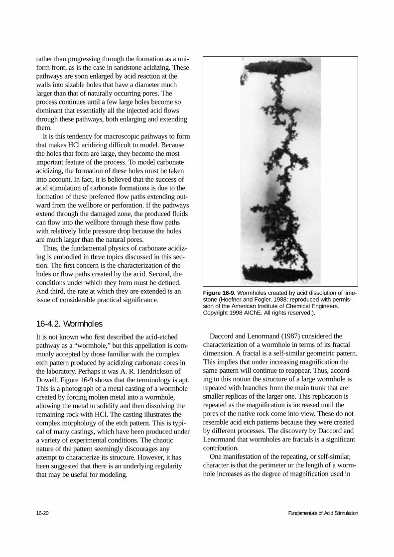
rather than progressing through the formation as a uni-form front, as is the case in sandstone acidizing. Thesepathways are soon enlarged by acid reaction at thewalls into sizable holes that have a diameter muchlarger than that of naturally occurring pores. Theprocess continues until a few large holes become sodominant that essentially all the injected acid flowsthrough these pathways, both enlarging and extendingthem.

It is this tendency for macroscopic pathways to formthat makes HCl acidizing difficult to model. Becausethe holes that form are large, they become the mostimportant feature of the process. To model carbonateacidizing, the formation of these holes must be takeninto account. In fact, it is believed that the success ofacid stimulation of carbonate formations is due to theformation of these preferred flow paths extending out-ward from the wellbore or perforation. If the pathwaysextend through the damaged zone, the produced fluidscan flow into the wellbore through these flow pathswith relatively little pressure drop because the holesare much larger than the natural pores.

Thus, the fundamental physics of carbonate acidiz-ing is embodied in three topics discussed in this sec-tion. The first concern is the characterization of theholes or flow paths created by the acid. Second, theconditions under which they form must be defined.And third, the rate at which they are extended is anissue of considerable practical significance.

16-4.2. WormholesIt is not known who first described the acid-etchedpathway as a “wormhole,” but this appellation is com-monly accepted by those familiar with the complexetch pattern produced by acidizing carbonate cores inthe laboratory. Perhaps it was A. R. Hendrickson ofDowell. Figure 16-9 shows that the terminology is apt.This is a photograph of a metal casting of a wormholecreated by forcing molten metal into a wormhole,allowing the metal to solidify and then dissolving theremaining rock with HCl. The casting illustrates thecomplex morphology of the etch pattern. This is typi-cal of many castings, which have been produced undera variety of experimental conditions. The chaoticnature of the pattern seemingly discourages anyattempt to characterize its structure. However, it hasbeen suggested that there is an underlying regularitythat may be useful for modeling.

Daccord and Lenormand (1987) considered thecharacterization of a wormhole in terms of its fractaldimension. A fractal is a self-similar geometric pattern.This implies that under increasing magnification thesame pattern will continue to reappear. Thus, accord-ing to this notion the structure of a large wormhole isrepeated with branches from the main trunk that aresmaller replicas of the larger one. This replication isrepeated as the magnification is increased until thepores of the native rock come into view. These do notresemble acid etch patterns because they were createdby different processes. The discovery by Daccord andLenormand that wormholes are fractals is a significantcontribution.

One manifestation of the repeating, or self-similar,character is that the perimeter or the length of a worm-hole increases as the degree of magnification used in

16-20 Fundamentals of Acid Stimulation

Figure 16-9. Wormholes created by acid dissolution of lime-stone (Hoefner and Fogler, 1988; reproduced with permis-sion of the American Institute of Chemical Engineers.Copyright 1998 AIChE. All rights reserved.).

its measurement increases. This is because at highermagnification, more of the detailed structure becomesevident and is, therefore, susceptible to measurement.For self-similar systems, the length of a wormholeplotted against the length of a ruler used to measurethe length is a straight line on a log-log plot. The slopeof this line is related to the fractal dimension. In thecase of wormholes, Daccord and Lenormand reportedthat the fractal dimension is 1.6. This implies that thelength of a wormhole is proportional to L1.6 rather thanL, where L is the macroscopic length. Daccord et al.(1989) utilized this fractal dimension in developing afield design method for carbonate acidizing. In theirapproach, the complexity of the wormhole is portrayedby its fractal dimension. This is only a partial charac-terization, because it is not possible to describe theminute details of wormhole geometry.

Although a precise description of a wormhole is notattainable, it is desirable to have a model that providesguidance in determining the best treatment parameters.What should be the injection rate? Should the injectionrate be constant during the entire course of the treat-ment? What acid type and concentration are best?What additives should be included in the acidic solu-tion? These questions relate to controllable variablesand, therefore, must be addressed each time an acidtreatment is designed. Rather than depending solely onpast experience, some theoretical help is welcome fordeveloping the best strategy possible based on theinformation available.

The problem is approached in the following sec-tions by addressing two separate issues, both of whichare relevant to the questions posed. The first concernsthe conditions requisite for the initiation of worm-holes, and the second deals with their growth or prop-agation. Both of these studies provide informationrequired for the design of carbonate acid treatments.The Appendix to this chapter discusses advances in understanding and predicting wormhole formation.

16-4.3. Initiation of wormholesThe fractal, or self-similar, topology of a wormholestructure implies that the mechanism for the initiationof wormholes is a “local” phenomenon that occurscontinuously along its bounding surfaces as well as atits tip. Thus, tiny wormholes may be initiated when-ever live acid enters the pores of the virgin rock irre-spective of the etch pattern already in existence.Experiments have shown that in cases where the acid

flux entering the matrix is quite small, wormhole initi-ation is not prolific, thereby indicating a flow-ratedependence of the initiation process. The proof of thisassertion is based primarily on metal casts of worm-holes, such as that shown by Fig. 16-9. However,adopting the notion of a flow-rate-dependent initiationprocess allows interpreting the results of laboratoryacidizing experiments and understanding the origin ofthe fractals. Furthermore, this approach leads to pre-diction of the optimum injection rate in linear coreexperiments that has been experimentally observed.Thus, the analysis presented here represents a founda-tion upon which the design of acid treatments can bebased, but further work is required to achieve thedesired goal, namely, the ability to predict the stimula-tion resulting from an acid treatment given the essen-tial parameters of acid composition, injection rate,formation temperature and rock properties.

The initiation of wormholes occurs when live acidpenetrates into pores present in the native rock. Thesepores are distributed in size and shape; therefore, theamount of acid flowing through each of the pores dif-fers. The rate at which a given pore is enlarged by theacid depends, of course, on the amount of acid enter-ing that pore and the fraction of the acid reacted at thewalls of the pore before the acid exits and then entersother pores located downstream. Thus, even at thepore level, the processes that contribute to the creationof an etch pattern are complex, involving convection,diffusion and chemical reactions within each of theinvaded pores. It has not been proved practical to con-sider these processes in a single pore and then attemptto consider the collective behavior to derive a macro-scopic etch pattern. Schechter and Gidley (1969) usedthis approach, but to make progress using their resultsrequires knowing in advance the entire distribution ofpore sizes, permeability and porosity of the nativerock to be acidized. Even armed with this knowledge,which is seldom available, prediction of the etch pat-tern is not routine.

The prediction of wormhole initiation is, however,based on a result that emerged from considering thebehavior of each pore in the medium. If a pore is rep-resented as a cylindrical hole with a radius R and alength l, then the rate at which the pore cross-sectionalarea A increases as a result of acid reaction at the porewalls may, in general, be written in the form

(16-30)

Reservoir Stimulation 16-21

dA

dtAn= ψ ,

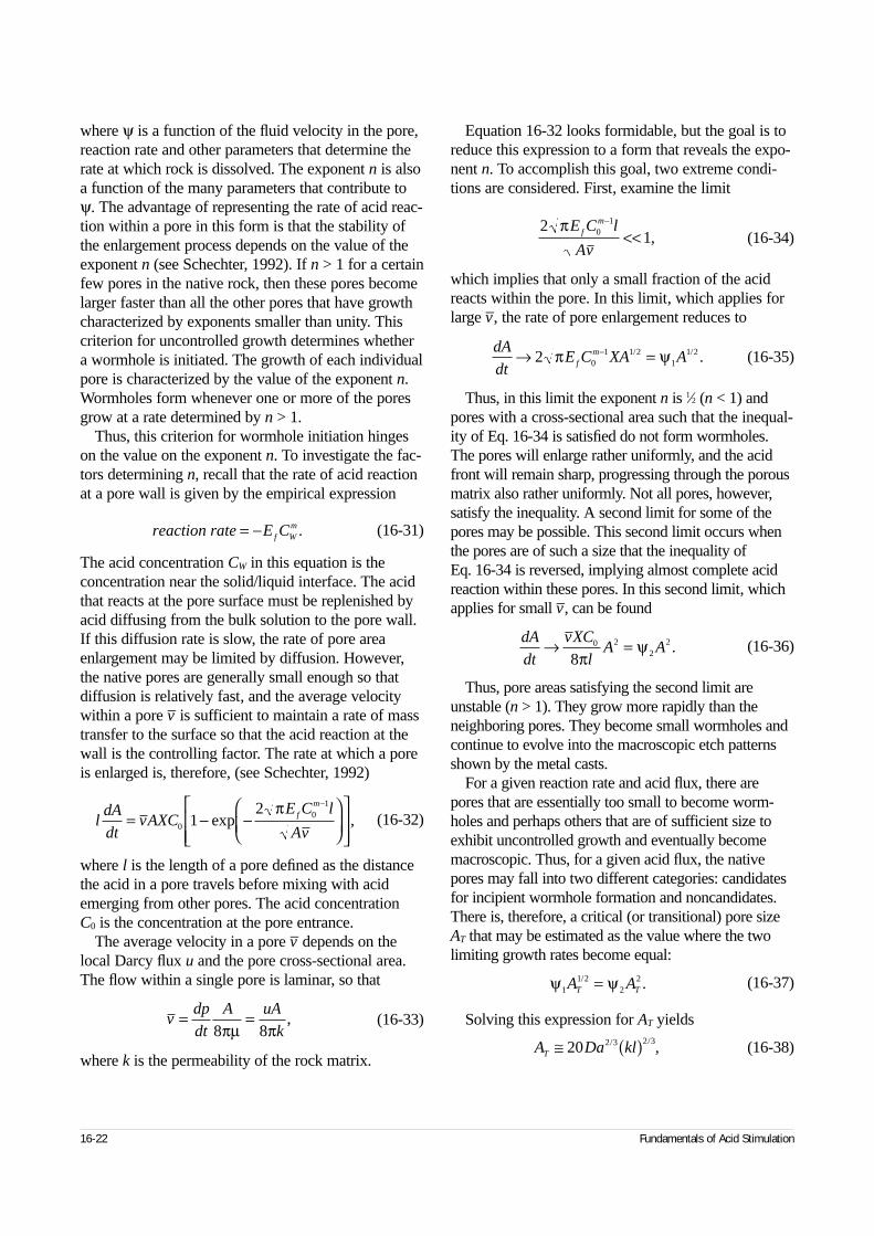
where ψ is a function of the fluid velocity in the pore,reaction rate and other parameters that determine therate at which rock is dissolved. The exponent n is alsoa function of the many parameters that contribute toψ. The advantage of representing the rate of acid reac-tion within a pore in this form is that the stability ofthe enlargement process depends on the value of theexponent n (see Schechter, 1992). If n > 1 for a certainfew pores in the native rock, then these pores becomelarger faster than all the other pores that have growthcharacterized by exponents smaller than unity. Thiscriterion for uncontrolled growth determines whethera wormhole is initiated. The growth of each individualpore is characterized by the value of the exponent n.Wormholes form whenever one or more of the poresgrow at a rate determined by n > 1.

Thus, this criterion for wormhole initiation hingeson the value on the exponent n. To investigate the fac-tors determining n, recall that the rate of acid reactionat a pore wall is given by the empirical expression

(16-31)

The acid concentration CW in this equation is theconcentration near the solid/liquid interface. The acidthat reacts at the pore surface must be replenished byacid diffusing from the bulk solution to the pore wall.If this diffusion rate is slow, the rate of pore areaenlargement may be limited by diffusion. However,the native pores are generally small enough so thatdiffusion is relatively fast, and the average velocitywithin a pore v– is sufficient to maintain a rate of masstransfer to the surface so that the acid reaction at thewall is the controlling factor. The rate at which a poreis enlarged is, therefore, (see Schechter, 1992)

(16-32)

where l is the length of a pore defined as the distancethe acid in a pore travels before mixing with acidemerging from other pores. The acid concentration C0 is the concentration at the pore entrance.

The average velocity in a pore v– depends on thelocal Darcy flux u and the pore cross-sectional area.The flow within a single pore is laminar, so that

(16-33)

where k is the permeability of the rock matrix.

Equation 16-32 looks formidable, but the goal is toreduce this expression to a form that reveals the expo-nent n. To accomplish this goal, two extreme condi-tions are considered. First, examine the limit

(16-34)

which implies that only a small fraction of the acidreacts within the pore. In this limit, which applies forlarge v–, the rate of pore enlargement reduces to

(16-35)

Thus, in this limit the exponent n is 1⁄2 (n < 1) andpores with a cross-sectional area such that the inequal-ity of Eq. 16-34 is satisfied do not form wormholes.The pores will enlarge rather uniformly, and the acidfront will remain sharp, progressing through the porousmatrix also rather uniformly. Not all pores, however,satisfy the inequality. A second limit for some of thepores may be possible. This second limit occurs whenthe pores are of such a size that the inequality of Eq. 16-34 is reversed, implying almost complete acidreaction within these pores. In this second limit, whichapplies for small v–, can be found

(16-36)

Thus, pore areas satisfying the second limit areunstable (n > 1). They grow more rapidly than theneighboring pores. They become small wormholes andcontinue to evolve into the macroscopic etch patternsshown by the metal casts.

For a given reaction rate and acid flux, there arepores that are essentially too small to become worm-holes and perhaps others that are of sufficient size toexhibit uncontrolled growth and eventually becomemacroscopic. Thus, for a given acid flux, the nativepores may fall into two different categories: candidatesfor incipient wormhole formation and noncandidates.There is, therefore, a critical (or transitional) pore sizeAT that may be estimated as the value where the twolimiting growth rates become equal:

(16-37)

Solving this expression for AT yields

(16-38)

16-22 Fundamentals of Acid Stimulation

reaction rate E Cf Wm= − .

ldA

dtvAXC

E C l

Avf

m

= − −

−

00

1

12

exp ,π

vdp

dt

A uA

k= =

8 8πµ π,

210

1πE C l

Avf

m−

<< ,

dA

dtE C XA Af

m→ =−2 01 1 2

11 2π ψ/ / .

dA

dt

vXC

lA A→ =0 2

22

8πψ .

ψ ψ11 2

22A AT T

/ .=

A Da klT ≅ ( )20 2 3 2 3/ / ,

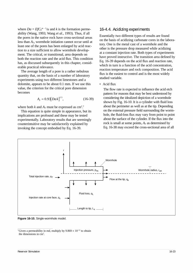
where Da = EfC0m – 1/u and k is the formation perme-

ability (Wang, 1993; Wang et al., 1993). Thus, if allthe pores in the native rock have cross-sectional areasless than AT, wormhole initiation cannot occur until atleast one of the pores has been enlarged by acid reac-tion to a size sufficient to allow wormhole develop-ment. The critical, or transitional, area depends onboth the reaction rate and the acid flux. This conditionhas, as discussed subsequently in this chapter, consid-erable practical relevance.

The average length of a pore is a rather nebulousquantity that, on the basis of a number of laboratoryexperiments using two different limestones and adolomite, appears to be about 0.1 mm. If we use thisvalue, the criterion for the critical pore dimensionbecomes

(16-39)

where both k and AT must be expressed as cm2.†

This equation is quite simple in appearance, but itsimplications are profound and these may be testedexperimentally. Laboratory results that are seeminglycounterintuitive may be satisfactorily explained byinvoking the concept embodied by Eq. 16-39.

16-4.4. Acidizing experimentsEssentially two different types of results are found on the basis of acidizing carbonate cores in the labora-tory. One is the metal cast of a wormhole and theother is the pressure drop measured while acidizing at a constant injection rate. Both types of experimentshave proved instructive. The transition area defined byEq. 16-39 depends on the acid flux and reaction rate,which in turn is a function of the acid concentration,reaction temperature and rock composition. The acidflux is the easiest to control and is the most widelystudied variable.

• Acid flux

The flow rate is expected to influence the acid etchpattern for reasons that may be best understood byconsidering the idealized depiction of a wormholeshown by Fig. 16-10. It is a cylinder with fluid lossabout the perimeter as well as at the tip. Dependingon the external pressure field surrounding the worm-hole, the fluid-loss flux may vary from point to pointabout the surface of the cylinder. If the flux into therock is small at some points, AT as determined byEq. 16-38 may exceed the cross-sectional area of all

Reservoir Stimulation 16-23

A DakT = [ ]0 932 3

. ,/

†Given a permeability in md, multiply by 9.869 × 10–12 to obtainthe dimensions in cm2.

Figure 16-10. Single-wormhole model.

Injection rate at core face, qc

Total injection rate, qTFlow at the tip, qe

Injection pressure, pinj

Fluid loss, qL

r

Wormhole

Length to tip, Le

Wormhole radius, rwh

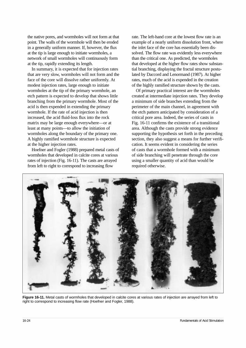
the native pores, and wormholes will not form at thatpoint. The walls of the wormhole will then be erodedin a generally uniform manner. If, however, the fluxat the tip is large enough to initiate wormholes, anetwork of small wormholes will continuously format the tip, rapidly extending its length.

In summary, it is expected that for injection ratesthat are very slow, wormholes will not form and theface of the core will dissolve rather uniformly. Atmodest injection rates, large enough to initiatewormholes at the tip of the primary wormhole, anetch pattern is expected to develop that shows littlebranching from the primary wormhole. Most of theacid is then expended in extending the primarywormhole. If the rate of acid injection is thenincreased, the acid fluid-loss flux into the rockmatrix may be large enough everywhere—or atleast at many points—to allow the initiation ofwormholes along the boundary of the primary one.A highly ramified wormhole structure is expectedat the higher injection rates.

Hoefner and Fogler (1988) prepared metal casts ofwormholes that developed in calcite cores at variousrates of injection (Fig. 16-11). The casts are arrayedfrom left to right to correspond to increasing flow

rate. The left-hand core at the lowest flow rate is anexample of a nearly uniform dissolution front, wherethe inlet face of the core has essentially been dis-solved. The flow rate was evidently less everywherethan the critical one. As predicted, the wormholesthat developed at the higher flow rates show substan-tial branching, displaying the fractal structure postu-lated by Daccord and Lenormand (1987). At higherrates, much of the acid is expended in the creation of the highly ramified structure shown by the casts.

Of primary practical interest are the wormholescreated at intermediate injection rates. They developa minimum of side branches extending from theperimeter of the main channel, in agreement withthe etch pattern anticipated by consideration of acritical pore area. Indeed, the series of casts in Fig. 16-11 confirms the existence of a transitionalarea. Although the casts provide strong evidencesupporting the hypothesis set forth in the precedingsection, they also suggest a means for further verifi-cation. It seems evident in considering the series of casts that a wormhole formed with a minimumof side branching will penetrate through the coreusing a smaller quantity of acid than would berequired otherwise.

16-24 Fundamentals of Acid Stimulation

Figure 16-11. Metal casts of wormholes that developed in calcite cores at various rates of injection are arrayed from left toright to correspond to increasing flow rate (Hoefner and Fogler, 1988).

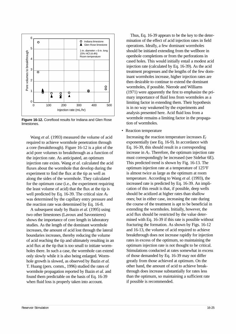
Wang et al. (1993) measured the volume of acidrequired to achieve wormhole penetration througha core (breakthrough). Figure 16-12 is a plot of theacid pore volumes to breakthrough as a function ofthe injection rate. As anticipated, an optimuminjection rate exists. Wang et al. calculated the acidfluxes about the wormhole that develop during theexperiment to find the flux at the tip as well asalong the sides of the wormhole. They calculatedfor the optimum case (i.e., the experiment requiringthe least volume of acid) that the flux at the tip iswell predicted by Eq. 16-39. The critical size AT

was determined by the capillary entry pressure andthe reaction rate was determined by Eq. 16-8.

A subsequent study by Bazin et al. (1995) usingtwo other limestones (Lavoux and Savonnieres)shows the importance of core length in laboratorystudies. As the length of the dominant wormholeincreases, the amount of acid lost through the lateralboundaries increases, thereby reducing the volumeof acid reaching the tip and ultimately resulting in anacid flux at the tip that is too small to initiate worm-holes there. In such a case, the wormhole can extendonly slowly while it is also being enlarged. Worm-hole growth is slowed, as observed by Bazin et al.T. Huang (pers. comm., 1996) studied the rates ofwormhole propagation reported by Bazin et al. andfound them predictable on the basis of Eq. 16-39when fluid loss is properly taken into account.

Thus, Eq. 16-39 appears to be the key to the deter-mination of the effect of acid injection rates in fieldoperations. Ideally, a few dominant wormholesshould be initiated extending from the wellbore inopenhole completions or from the perforations incased holes. This would initially entail a modest acidinjection rate (calculated by Eq. 16-39). As the acidtreatment progresses and the lengths of the few dom-inant wormholes increase, higher injection rates arethen desirable to continue to extend the dominantwormholes, if possible. Nierode and Williams(1971) were apparently the first to emphasize the pri-mary importance of fluid loss from wormholes as alimiting factor in extending them. Their hypothesis is in no way weakened by the experiments andanalysis presented here. Acid fluid loss from awormhole remains a limiting factor in the propaga-tion of wormholes.

• Reaction temperature

Increasing the reaction temperature increases Ef

exponentially (see Eq. 16-9). In accordance withEq. 16-39, this should result in a correspondingincrease in AT. Therefore, the optimum injection ratemust correspondingly be increased (see Sidebar 6E).This predicted trend is shown by Fig. 16-13. Theoptimum injection rate at a temperature of 125°F is almost twice as large as the optimum at roomtemperature. According to Wang et al. (1993), theincreased rate is predicted by Eq. 16-39. An impli-cation of this result is that, if possible, deep wellsshould be acidized at higher rates than shallowones; but in either case, increasing the rate duringthe course of the treatment is apt to be beneficial inextending the wormholes. Initially, however, theacid flux should be restricted by the value deter-mined with Eq. 16-39 if this rate is possible withoutfracturing the formation. As shown by Figs. 16-12and 16-13, the volume of acid required to achievebreakthrough does not increase rapidly for injectionrates in excess of the optimum, so maintaining theoptimum injection rate is not thought to be critical.Stimulations conducted at rates somewhat in excessof those demanded by Eq. 16-39 may not differgreatly from those achieved at optimum. On theother hand, the amount of acid to achieve break-through does increase substantially for rates lessthan the optimum, so maintaining a sufficient rate if possible is recommended.

Reservoir Stimulation 16-25

Figure 16-12. Coreflood results for Indiana and Glen Roselimestones.

0 1000

1

2

3

4

6

500

Injection rate (mL/hr)

Por

e vo

lum

es to

bre

akth

roug

h

Indiana limestoneGlen Rose limestone

1-in. diameter × 6-in. long15% HCl (4.4N)Room temperature

200 300 400

5

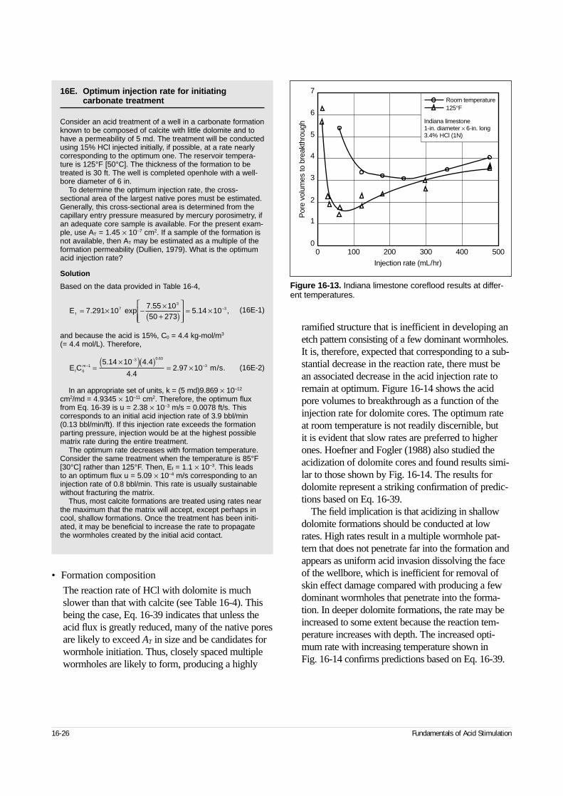
• Formation composition

The reaction rate of HCl with dolomite is muchslower than that with calcite (see Table 16-4). Thisbeing the case, Eq. 16-39 indicates that unless theacid flux is greatly reduced, many of the native poresare likely to exceed AT in size and be candidates forwormhole initiation. Thus, closely spaced multiplewormholes are likely to form, producing a highly

ramified structure that is inefficient in developing anetch pattern consisting of a few dominant wormholes.It is, therefore, expected that corresponding to a sub-stantial decrease in the reaction rate, there must bean associated decrease in the acid injection rate toremain at optimum. Figure 16-14 shows the acidpore volumes to breakthrough as a function of theinjection rate for dolomite cores. The optimum rateat room temperature is not readily discernible, but it is evident that slow rates are preferred to higherones. Hoefner and Fogler (1988) also studied theacidization of dolomite cores and found results simi-lar to those shown by Fig. 16-14. The results fordolomite represent a striking confirmation of predic-tions based on Eq. 16-39.

The field implication is that acidizing in shallowdolomite formations should be conducted at lowrates. High rates result in a multiple wormhole pat-tern that does not penetrate far into the formation andappears as uniform acid invasion dissolving the faceof the wellbore, which is inefficient for removal ofskin effect damage compared with producing a fewdominant wormholes that penetrate into the forma-tion. In deeper dolomite formations, the rate may beincreased to some extent because the reaction tem-perature increases with depth. The increased opti-mum rate with increasing temperature shown in Fig. 16-14 confirms predictions based on Eq. 16-39.

16-26 Fundamentals of Acid Stimulation

16E. Optimum injection rate for initiating carbonate treatment

Consider an acid treatment of a well in a carbonate formationknown to be composed of calcite with little dolomite and tohave a permeability of 5 md. The treatment will be conductedusing 15% HCl injected initially, if possible, at a rate nearlycorresponding to the optimum one. The reservoir tempera-ture is 125°F [50°C]. The thickness of the formation to betreated is 30 ft. The well is completed openhole with a well-bore diameter of 6 in.

To determine the optimum injection rate, the cross-sectional area of the largest native pores must be estimated.Generally, this cross-sectional area is determined from thecapillary entry pressure measured by mercury porosimetry, ifan adequate core sample is available. For the present exam-ple, use AT = 1.45 × 10–7 cm2. If a sample of the formation isnot available, then AT may be estimated as a multiple of theformation permeability (Dullien, 1979). What is the optimumacid injection rate?

Solution

Based on the data provided in Table 16-4,

(16E-1)

and because the acid is 15%, C0 = 4.4 kg-mol/m3

(= 4.4 mol/L). Therefore,

(16E-2)

In an appropriate set of units, k = (5 md)9.869 × 10–12

cm2/md = 4.9345 × 10–11 cm2. Therefore, the optimum fluxfrom Eq. 16-39 is u = 2.38 × 10–3 m/s = 0.0078 ft/s. Thiscorresponds to an initial acid injection rate of 3.9 bbl/min(0.13 bbl/min/ft). If this injection rate exceeds the formationparting pressure, injection would be at the highest possiblematrix rate during the entire treatment.

The optimum rate decreases with formation temperature.Consider the same treatment when the temperature is 85°F[30°C] rather than 125°F. Then, Ef = 1.1 × 10–3. This leads to an optimum flux u = 5.09 × 10–4 m/s corresponding to aninjection rate of 0.8 bbl/min. This rate is usually sustainablewithout fracturing the matrix.

Thus, most calcite formations are treated using rates nearthe maximum that the matrix will accept, except perhaps incool, shallow formations. Once the treatment has been initi-ated, it may be beneficial to increase the rate to propagatethe wormholes created by the initial acid contact.

Ef = × − ×+( )

= × −7 291 107 55 1050 273

5 14 1073

3..

. , exp

E Cfm0

1

3 0 63

35 14 10 4 4

4 42 97 10−

−−=

×( )( )= ×

. .

..

.

m/s.

Figure 16-13. Indiana limestone coreflood results at differ-ent temperatures.

0 1000

1

2

3

4

6

7

500

Injection rate (mL/hr)

Por

e vo

lum

es to

bre

akth

roug

h

Room temperature125°F

Indiana limestone1-in. diameter × 6-in. long3.4% HCl (1N)

200 300 400

5

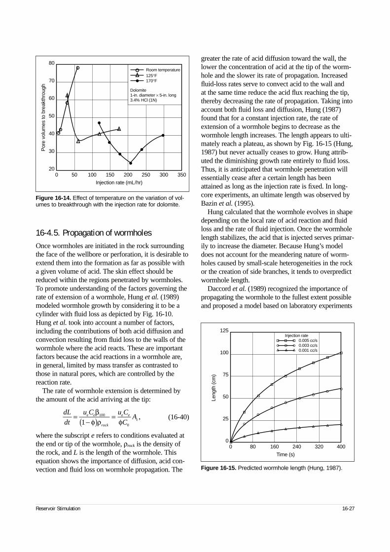
16-4.5. Propagation of wormholesOnce wormholes are initiated in the rock surroundingthe face of the wellbore or perforation, it is desirable toextend them into the formation as far as possible witha given volume of acid. The skin effect should bereduced within the regions penetrated by wormholes.To promote understanding of the factors governing therate of extension of a wormhole, Hung et al. (1989)modeled wormhole growth by considering it to be acylinder with fluid loss as depicted by Fig. 16-10.Hung et al. took into account a number of factors,including the contributions of both acid diffusion andconvection resulting from fluid loss to the walls of thewormhole where the acid reacts. These are importantfactors because the acid reactions in a wormhole are,in general, limited by mass transfer as contrasted tothose in natural pores, which are controlled by thereaction rate.

The rate of wormhole extension is determined bythe amount of the acid arriving at the tip:

(16-40)

where the subscript e refers to conditions evaluated atthe end or tip of the wormhole, ρrock is the density ofthe rock, and L is the length of the wormhole. Thisequation shows the importance of diffusion, acid con-vection and fluid loss on wormhole propagation. The

greater the rate of acid diffusion toward the wall, thelower the concentration of acid at the tip of the worm-hole and the slower its rate of propagation. Increasedfluid-loss rates serve to convect acid to the wall and at the same time reduce the acid flux reaching the tip,thereby decreasing the rate of propagation. Taking intoaccount both fluid loss and diffusion, Hung (1987)found that for a constant injection rate, the rate ofextension of a wormhole begins to decrease as thewormhole length increases. The length appears to ulti-mately reach a plateau, as shown by Fig. 16-15 (Hung,1987) but never actually ceases to grow. Hung attrib-uted the diminishing growth rate entirely to fluid loss.Thus, it is anticipated that wormhole penetration willessentially cease after a certain length has beenattained as long as the injection rate is fixed. In long-core experiments, an ultimate length was observed byBazin et al. (1995).

Hung calculated that the wormhole evolves in shapedepending on the local rate of acid reaction and fluidloss and the rate of fluid injection. Once the wormholelength stabilizes, the acid that is injected serves primar-ily to increase the diameter. Because Hung’s modeldoes not account for the meandering nature of worm-holes caused by small-scale heterogeneities in the rockor the creation of side branches, it tends to overpredictwormhole length.

Daccord et al. (1989) recognized the importance ofpropagating the wormhole to the fullest extent possibleand proposed a model based on laboratory experiments

Reservoir Stimulation 16-27

Figure 16-14. Effect of temperature on the variation of vol-umes to breakthrough with the injection rate for dolomite.

0 5020

30

40

50

60

70

80

100 150 200 250 300 350

Injection rate (mL/hr)

Por

e vo

lum

es to

bre

akth

roug

h

Room temperature125°F170°F

Dolomite1-in. diameter × 5-in. long3.4% HCl (1N)

Figure 16-15. Predicted wormhole length (Hung, 1987).

0 80 160 240 320 400

Time (s)

Leng

th (c

m)

125

100

75

50

25

0

Injection rate0.005 cc/s0.003 cc/s0.001 cc/s

dL

dt

u C u C

CAe e

rock

e ec=

−( ) =βφ ρ φ

100

01,

that differs from that proposed by Hung. Daccord etal.’s expression for the rate of wormhole propagation in linear systems is

(16-41)

where a is a constant determined experimentally, D isthe molecular diffusion coefficient, and A is the cross-sectional area of the wormhole. Daccord et al.’s modelconsiders the influence of acid diffusion but does nottake into account fluid loss; therefore, this equation

does not indicate a plateau value as the wormholelengthens. Thus, the equation is applicable to shortwormholes where fluid loss is not a factor, but itshould not be used for the prediction of wormholepenetration length.

Thus, none of the existing models for the rate ofwormhole propagation is strictly correct. Becausewormhole length is thought to be a crucial factor indetermining stimulation, better models incorporatingthe important features of the ones that have been pro-posed are required.

16-28 Fundamentals of Acid Stimulation

dL

dt

aA

A

q

Dc=

φ

2 3/

,

IntroductionThe transport and reaction of reactive fluids in car-bonate porous media results in the formation of highlyconductive flow channels, or wormholes. Wormholessignificantly influence the flow of reservoir fluidsbecause their conductivity is several orders of magni-tude larger than that of the porous medium. There-fore, the success of carbonate stimulation treatmentsis highly dependent on wormhole formation (i.e.,wormhole formation during matrix acidizing treat-ments and lack thereof during fracture acidizing treat-ments). Wormhole formation is desirable duringmatrix acidizing treatments because the wormholesare capable of bypassing near-wellbore damage. Incontrast, wormhole formation increases fluid leakoffduring fracture acidizing and, consequently, limits thedepth of acid penetration. The structure of the worm-hole channel varies significantly with the flow condi-tions and the properties of the fluid-mineral system.Because the structure ultimately controls the effec-tiveness of the stimulation treatment, a fundamentalunderstanding of the dissolution phenomenon isrequired to design effective treatments.

Wormhole formation occurs because carbonate dis-solution is influenced by mass-transfer processes.Many investigators have recognized the importance ofmass transfer to the phenomenon of wormhole forma-tion in the hydrochloric acid (HCl)-limestone system(Barron et al., 1962; Williams et al., 1970; Nierodeand Williams, 1971; Hoefner and Fogler, 1988;Daccord et al., 1993; Wang et al., 1993; Frick et al.,1994b; Mostofizadeh and Economides, 1994; Bazin et al., 1995; Huang et al., 1997; Fredd and Fogler,1998a). Recent studies demonstrate that in the presenceof weak acids and chelating agents wormhole for-mation is influenced by a variety of transport and reac-tion processes (Fredd and Fogler, 1998b). Thus, toprovide the reader with a full understanding of thedissolution phenomenon, this Appendix to Chapter

16 discusses the various transport and reaction processesthat influence carbonate dissolution in a variety of fluidsystems including strong acids, weak acids and che-lating agents. A brief review of the theories of worm-hole formation is provided, and wormhole formation is discussed in terms of the Damköhler number for flowand reaction. The existence of an optimum Damköhlernumber for effective wormhole formation is demon-strated by laboratory experiments, and a new extensionof the theory is introduced to predict optimum injectionstrategies for matrix acidizing treatments in the field.

Carbonate dissolution

Influence of transport and reactionThe dissolution of carbonate minerals involves a het-erogeneous reaction that may be influenced by avariety of transport and reaction processes. Theseprocesses include the transport of reactants to thesurface, the reversible surface reaction and the trans-port of products away from the surface. The rate-limit-ing process depends on the fluid-mineral system andmay vary significantly in the presence of strong acids,weak acids and chelating agents.

This section demonstrates the interplay between the various transport and reaction processes and sum-marizes results from kinetic studies for a variety of fluid-mineral systems. The results are based on experimentalstudies conducted using a rotating disk apparatus, whichallows the differentiation of the surface reaction kineticsfrom the transport processes because of the well-definedhydrodynamics. From an understanding of the processesthat influence the dissolution, as well as appropriateexpressions for the kinetics of the surface reaction andrate of mass transfer, the overall rate of carbonate disso-lution can be determined as discussed in “Generalizeddescription of carbonate dissolution.”

Reservoir Stimulation A16-1

◆

Appendix: Advances in Understanding and Predicting

Wormhole FormationChristopher N. Fredd, Schlumberger Dowell

• Strong acids

The rate of calcite dissolution has been shown to be mass-transfer limited in a variety of acidicmedia (pH less than about 4) ranging from HCl topseudoseawater (Williams et al., 1970; Lund et al.,1975; Plummer et al., 1978; Sjöberg and Rickard,1984; de Rozières et al., 1994). In strong acidssuch as HCl, calcite is readily dissolved and thereaction may be considered irreversible:

2H+ + CaCO3 → Ca2+ + CO2 + H2O

Because the reaction is essentially irreversible,the products do not influence the rate of dissolu-tion, and the observed mass-transfer limitations aredue to the transport of hydrogen ions to the calcitesurface. The mass-transfer limitations are more sig-nificant when HCl is emulsified or gelled becauseof a reduction in the effective diffusivity (Hoefnerand Fogler, 1985; de Rozières et al., 1994). Thedissolution of calcite by HCl becomes influencedby the kinetics of the surface reaction at tempera-tures below about 32°F [0°C] (Lund et al., 1975).The following rate expression was found todescribe the rate of the surface reaction:

(1)

where Ci is the concentration at the solid/liquidinterface, kr is the surface reaction rate constant,and n is the reaction order. The kinetic parametersare summarized in Table 16-4 (Lund et al., 1975).

The dissolution of dolomite by HCl is mass-transfer limited at temperatures greater than about200°F [95°C] (Lund et al., 1973) and reaction ratelimited at temperatures less than about 125°F[50°C]. Between these two temperatures, the disso-lution is influenced by both the rate of mass trans-fer and the kinetics of the surface reaction. Like forcalcite, the reaction can be considered irreversible,so the influence of mass transfer is due to the trans-port of hydrogen ions to the dolomite surface.

4H+ + CaMg(CO3)2 → Ca2+ + Mg2+

+ 2CO2 + 2H2O

The kinetics of the surface reaction is also describedby Appendix Eq. 1, using the kinetic parameters sum-marized in Table 16-4 (Lund et al., 1973).

• Weak acids

In weak acids (i.e., partially dissociating acids),carbonate dissolution still occurs through hydrogen

ion attack (see the two preceding chemical reac-tions). However, dissolution is complicated by thereversible surface reaction (Chatelain et al., 1976)and the additional influence of the mass transfer ofproducts away from the surface. The dissolution ofcalcite by acetic acid was found to be influenced bythe rate of transport of reactants to the surface andthe rate of transport of products away from the sur-face at ambient temperature (Fredd and Fogler,1998d). The interplay between the two transportprocesses causes transport limitations that are muchmore significant than either limitation independ-ently. This interplay results in an apparent effectivediffusion coefficient that is over an order of magni-tude lower than that of acetic acid. Similar resultswere observed during the dissolution of calcite byformic and maleic acids (Takulpakdee, 1998).

The kinetics of the surface reaction for the disso-lution of calcite by acetic acid was shown to be asignificant limitation at pH values greater thanabout 3.7 (Fredd and Fogler, 1998d). The rate of the surface reaction can be expressed as

(2)

where Ci and Cpi are the reactants and products con-centrations at the solid/liquid interface, respectively,and Keq = Kc/CCOi is the effective equilibrium con-stant. The reactants concentration is the total con-centration of associated and dissociated hydrogenions (i.e., acetic acid and H+), whereas the productsconcentration represents the total concentration ofcalcium-containing species. The total interface con-centration of carbonate species CCOi was found to be independent of the rate of mass transfer (Fredd,1998) and was, therefore, lumped into the effectiveequilibrium constant. The effective equilibriumconstant also includes the conditional equilibriumconstant Kc, which is a complex function of theequilibrium constants for the various equilibriumreactions occurring near the interface.

Kinetic parameters evaluated at 72°F [22°C]using a rotating disk (Fredd and Fogler, 1998d) arelisted in Appendix Table 1. Additional data for var-ious acid concentrations and higher temperatures(125°F) are in the literature (Fredd and Fogler,1998d). These kinetic parameters are influenced bya variety of adsorption processes and equilibriumreactions. Therefore, extrapolation of the parame-ters to significantly higher temperatures requirescareful evaluation of the surface chemistry

A16-2 Chapter 16 Appendix: Advances in Understanding and Predicting Wormhole Formation

r k CD r in= ,

r k C C KD r i pi eq= −( ) ,

involved in the dissolution. The method of approxi-mating the surface reaction rate reported bySchechter (1992) (see Eq. 16-10) provides anorder-of-magnitude estimate of the reaction rateconstant but does not account for the significantcontribution of the reverse reaction.

The rate of dolomite dissolution by weak acids iscurrently not available in the literature. Because thedissolution occurs through hydrogen ion attack, therate of the surface reaction can be estimated fromAppendix Eq. 2 by scaling the surface reaction rateconstant by the ratio of the surface reaction rateconstants of dolomite to calcite for HCl. This scal-ing should provide a reasonable order-of-magnitudeestimate from which the relative influences oftransport and reaction can be determined.

• Chelating agents

In the presence of calcium chelating agents such asethylenediaminetetraacetic acid (EDTA), the rate ofcalcite dissolution is influenced predominantly by

the rate of transport of reactants to the surface andthe kinetics of the surface reactions at ambient tem-perature (Fredd and Fogler, 1998c). Although thereactions are essentially irreversible because of theformation of a stable calcium complex, the reac-tions are influenced by the transport of productsaway from the surface. This influence is due to theblocking of surface sites involved in the dissolu-tion. The dissolution mechanism is different fromconventional acids in that hydrogen ions are notrequired. However, the rate of dissolution isenhanced at low pH as a result of the combinedinfluence of hydrogen ion attack and chelation.

The rate of calcite dissolution varies consider-ably with pH and the type of chelating agentbecause of changes in the ionic form of the chelat-ing agent and the influence of hydrogen ion attack.In general, the rate of calcite dissolution increasesas the number of hydrogen ions associated with thechelating agent increases. As the pH is increasedfrom about 4.5 to 8.5 to 13, EDTA successively

Reservoir Stimulation A16-3

Appendix Table 1. Parameters used to calculate the overall dissolution rate constant at 72ºF.

De Dpe kr Keq

(cm2/s) (cm2/s) (∆E [kcal/mol])

0.25M CDTA (pH = 4.4) 4.5 × 10–6† 3 × 10–6‡ 2.3 × 10–4§ 1 × 1010††

0.25M DTPA (pH = 3.3) 4 × 10–6† 3 × 10–6‡ 7.8 × 10–5§ 1 × 1010††

0.25M DTPA (pH = 4.3) 4 × 10–6† 3 × 10–6‡ 4.8 × 10–5§ 1 × 1010††

0.25M DTPA (pH = 12.5) 4 × 10–6† 3 × 10–6‡ 2.6 × 10–5§ 1 × 1010††

0.25M EDTA (pH = 4) 6 × 10–6‡‡ 4 × 10–6§§ 1.4 × 10–4§ 1 × 1010††

(12)§

0.25M EDTA (pH = 8 to 13) 6 × 10–6§ 4 × 10–6§§ 5.3 × 10–5§ 1 × 1010††

0.5M acetic acid (pH = 2.5) 1.1 × 10–5††† 8 × 10–6‡‡‡ 5 × 10–3§§§ 1.6 × 10–1§§§

0.5M acetic acid (pH = 4.6) 1.1 × 10–5††† 8 × 10–6‡‡‡ 2.1 × 10–4§§§ 2.7 × 10–1§§§

0.5M HCl 3.6 × 10–5†††† 2 × 10–5‡‡‡ 2 × 10–1†††† 1 × 1010††

(15)††††

Note: De = effective diffusion coefficient, Dpe = effective diffusion coefficient for reaction products, kr = effective surface reaction rate constant, ∆E = activation energy, Keq = effective equilibrium constant† Estimated from the Stokes-Einstein equation‡ Assumed on the basis of De and value for Ca-EDTA§ Fredd and Fogler (1998c)†† Assumed on the basis of the irreversibility of surface reactions‡‡ Assumed equal to the diffusion coefficient of EDTA at pH = 13§§ Assumed on the basis of the value for Ru-EDTA (Jiang and Anson, 1992)††† Vitagliano and Lyons (1956)‡‡‡ Estimated from ionic diffusion coefficients (Cussler, 1984)§§§ Fredd and Fogler (1998d)†††† Lund et al. (1975)

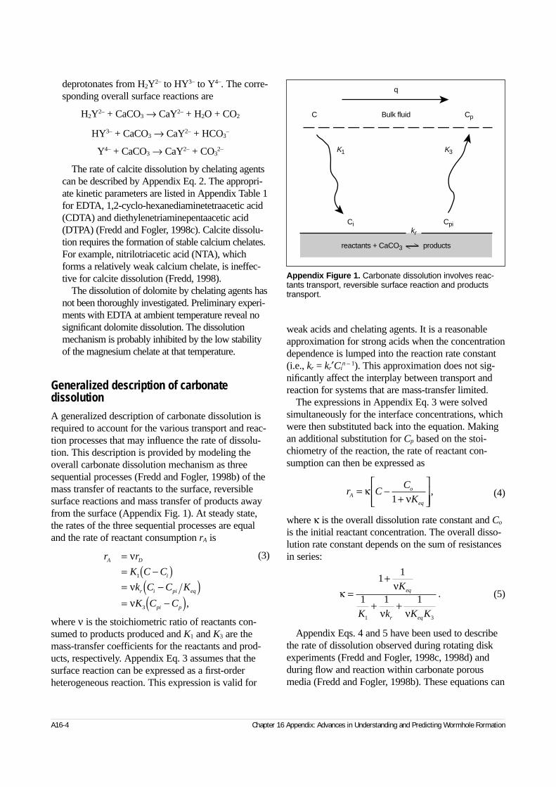
A16-4 Chapter 16 Appendix: Advances in Understanding and Predicting Wormhole Formation

deprotonates from H2Y2– to HY3– to Y4–. The corre-sponding overall surface reactions are

H2Y2– + CaCO3 → CaY2– + H2O + CO2

HY3– + CaCO3 → CaY2– + HCO3–

Y4– + CaCO3 → CaY2– + CO32–

The rate of calcite dissolution by chelating agentscan be described by Appendix Eq. 2. The appropri-ate kinetic parameters are listed in Appendix Table 1for EDTA, 1,2-cyclo-hexanediaminetetraacetic acid(CDTA) and diethylenetriaminepentaacetic acid(DTPA) (Fredd and Fogler, 1998c). Calcite dissolu-tion requires the formation of stable calcium chelates.For example, nitrilotriacetic acid (NTA), whichforms a relatively weak calcium chelate, is ineffec-tive for calcite dissolution (Fredd, 1998).

The dissolution of dolomite by chelating agents hasnot been thoroughly investigated. Preliminary experi-ments with EDTA at ambient temperature reveal nosignificant dolomite dissolution. The dissolutionmechanism is probably inhibited by the low stabilityof the magnesium chelate at that temperature.

Generalized description of carbonate dissolutionA generalized description of carbonate dissolution isrequired to account for the various transport and reac-tion processes that may influence the rate of dissolu-tion. This description is provided by modeling theoverall carbonate dissolution mechanism as threesequential processes (Fredd and Fogler, 1998b) of themass transfer of reactants to the surface, reversiblesurface reactions and mass transfer of products awayfrom the surface (Appendix Fig. 1). At steady state,the rates of the three sequential processes are equaland the rate of reactant consumption rA is

(3)

where ν is the stoichiometric ratio of reactants con-sumed to products produced and K1 and K3 are themass-transfer coefficients for the reactants and prod-ucts, respectively. Appendix Eq. 3 assumes that thesurface reaction can be expressed as a first-orderheterogeneous reaction. This expression is valid for

weak acids and chelating agents. It is a reasonableapproximation for strong acids when the concentrationdependence is lumped into the reaction rate constant(i.e., kr = kr′Ci

n – 1). This approximation does not sig-nificantly affect the interplay between transport andreaction for systems that are mass-transfer limited.

The expressions in Appendix Eq. 3 were solvedsimultaneously for the interface concentrations, whichwere then substituted back into the equation. Makingan additional substitution for Cp based on the stoi-chiometry of the reaction, the rate of reactant con-sumption can then be expressed as

(4)

where κ is the overall dissolution rate constant and Co

is the initial reactant concentration. The overall disso-lution rate constant depends on the sum of resistancesin series:

(5)

Appendix Eqs. 4 and 5 have been used to describethe rate of dissolution observed during rotating diskexperiments (Fredd and Fogler, 1998c, 1998d) andduring flow and reaction within carbonate porousmedia (Fredd and Fogler, 1998b). These equations can

r r

K C C

k C C K

K C C

A D

i

r i pi eq

pi p

== −( )= −( )= −( )

ν

νν

1

3 ,

r CC

KAo

eq

= −+

κν1

,

κν

ν ν

=+

+ +

11

1 1 1

1 3

K

K k K K

eq

r eq

.

Appendix Figure 1. Carbonate dissolution involves reac-tants transport, reversible surface reaction and productstransport.

reactants + CaCO3 products

Bulk fluidC Cp

K3K1

Cpikr

Ci

q

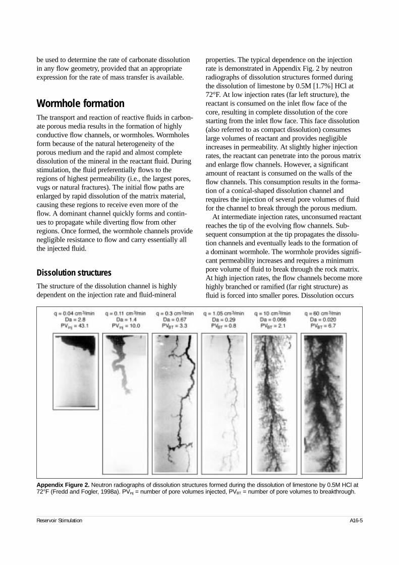
be used to determine the rate of carbonate dissolutionin any flow geometry, provided that an appropriateexpression for the rate of mass transfer is available.

Wormhole formationThe transport and reaction of reactive fluids in carbon-ate porous media results in the formation of highlyconductive flow channels, or wormholes. Wormholesform because of the natural heterogeneity of theporous medium and the rapid and almost completedissolution of the mineral in the reactant fluid. Duringstimulation, the fluid preferentially flows to theregions of highest permeability (i.e., the largest pores,vugs or natural fractures). The initial flow paths areenlarged by rapid dissolution of the matrix material,causing these regions to receive even more of theflow. A dominant channel quickly forms and contin-ues to propagate while diverting flow from otherregions. Once formed, the wormhole channels providenegligible resistance to flow and carry essentially allthe injected fluid.

Dissolution structuresThe structure of the dissolution channel is highlydependent on the injection rate and fluid-mineral

properties. The typical dependence on the injectionrate is demonstrated in Appendix Fig. 2 by neutronradiographs of dissolution structures formed duringthe dissolution of limestone by 0.5M [1.7%] HCl at72°F. At low injection rates (far left structure), thereactant is consumed on the inlet flow face of thecore, resulting in complete dissolution of the corestarting from the inlet flow face. This face dissolution(also referred to as compact dissolution) consumeslarge volumes of reactant and provides negligibleincreases in permeability. At slightly higher injectionrates, the reactant can penetrate into the porous matrixand enlarge flow channels. However, a significantamount of reactant is consumed on the walls of theflow channels. This consumption results in the forma-tion of a conical-shaped dissolution channel andrequires the injection of several pore volumes of fluidfor the channel to break through the porous medium.

At intermediate injection rates, unconsumed reactantreaches the tip of the evolving flow channels. Sub-sequent consumption at the tip propagates the dissolu-tion channels and eventually leads to the formation ofa dominant wormhole. The wormhole provides signifi-cant permeability increases and requires a minimumpore volume of fluid to break through the rock matrix.At high injection rates, the flow channels become morehighly branched or ramified (far right structure) asfluid is forced into smaller pores. Dissolution occurs

Reservoir Stimulation A16-5

Appendix Figure 2. Neutron radiographs of dissolution structures formed during the dissolution of limestone by 0.5M HCl at72°F (Fredd and Fogler, 1998a). PVinj = number of pore volumes injected, PVBT = number of pore volumes to breakthrough.

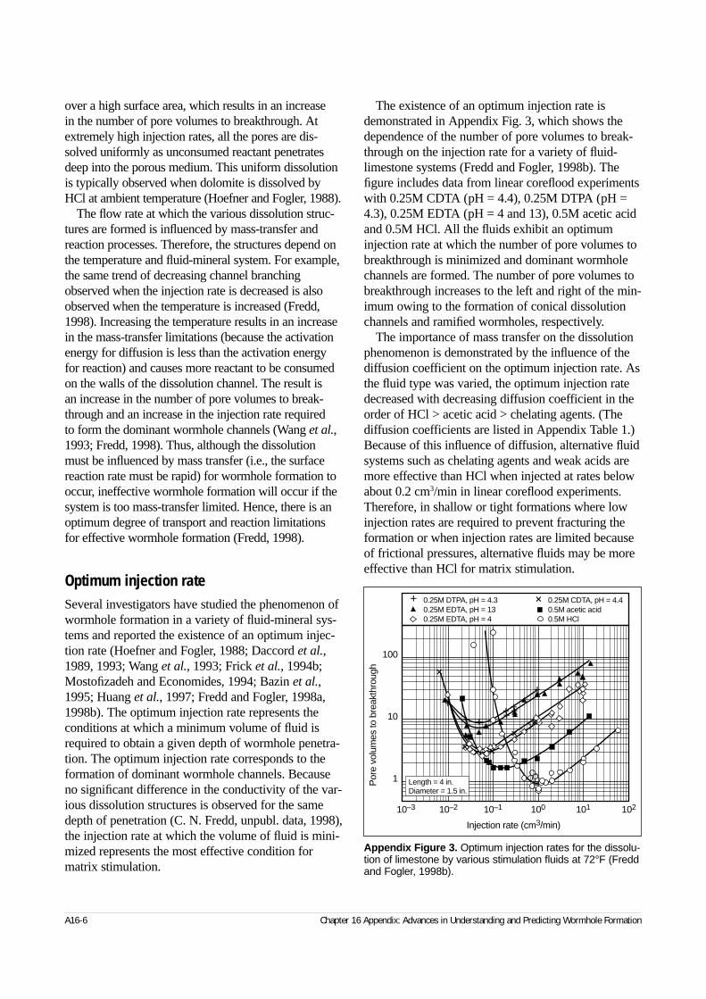
over a high surface area, which results in an increase in the number of pore volumes to breakthrough. Atextremely high injection rates, all the pores are dis-solved uniformly as unconsumed reactant penetratesdeep into the porous medium. This uniform dissolutionis typically observed when dolomite is dissolved byHCl at ambient temperature (Hoefner and Fogler, 1988).

The flow rate at which the various dissolution struc-tures are formed is influenced by mass-transfer andreaction processes. Therefore, the structures depend onthe temperature and fluid-mineral system. For example,the same trend of decreasing channel branchingobserved when the injection rate is decreased is alsoobserved when the temperature is increased (Fredd,1998). Increasing the temperature results in an increasein the mass-transfer limitations (because the activationenergy for diffusion is less than the activation energyfor reaction) and causes more reactant to be consumedon the walls of the dissolution channel. The result is an increase in the number of pore volumes to break-through and an increase in the injection rate required to form the dominant wormhole channels (Wang et al.,1993; Fredd, 1998). Thus, although the dissolutionmust be influenced by mass transfer (i.e., the surfacereaction rate must be rapid) for wormhole formation tooccur, ineffective wormhole formation will occur if thesystem is too mass-transfer limited. Hence, there is anoptimum degree of transport and reaction limitationsfor effective wormhole formation (Fredd, 1998).

Optimum injection rateSeveral investigators have studied the phenomenon ofwormhole formation in a variety of fluid-mineral sys-tems and reported the existence of an optimum injec-tion rate (Hoefner and Fogler, 1988; Daccord et al.,1989, 1993; Wang et al., 1993; Frick et al., 1994b;Mostofizadeh and Economides, 1994; Bazin et al.,1995; Huang et al., 1997; Fredd and Fogler, 1998a,1998b). The optimum injection rate represents theconditions at which a minimum volume of fluid isrequired to obtain a given depth of wormhole penetra-tion. The optimum injection rate corresponds to theformation of dominant wormhole channels. Becauseno significant difference in the conductivity of the var-ious dissolution structures is observed for the samedepth of penetration (C. N. Fredd, unpubl. data, 1998),the injection rate at which the volume of fluid is mini-mized represents the most effective condition formatrix stimulation.

The existence of an optimum injection rate isdemonstrated in Appendix Fig. 3, which shows thedependence of the number of pore volumes to break-through on the injection rate for a variety of fluid-limestone systems (Fredd and Fogler, 1998b). Thefigure includes data from linear coreflood experimentswith 0.25M CDTA (pH = 4.4), 0.25M DTPA (pH =4.3), 0.25M EDTA (pH = 4 and 13), 0.5M acetic acidand 0.5M HCl. All the fluids exhibit an optimuminjection rate at which the number of pore volumes tobreakthrough is minimized and dominant wormholechannels are formed. The number of pore volumes tobreakthrough increases to the left and right of the min-imum owing to the formation of conical dissolutionchannels and ramified wormholes, respectively.

The importance of mass transfer on the dissolutionphenomenon is demonstrated by the influence of thediffusion coefficient on the optimum injection rate. Asthe fluid type was varied, the optimum injection ratedecreased with decreasing diffusion coefficient in theorder of HCl > acetic acid > chelating agents. (Thediffusion coefficients are listed in Appendix Table 1.)Because of this influence of diffusion, alternative fluidsystems such as chelating agents and weak acids aremore effective than HCl when injected at rates belowabout 0.2 cm3/min in linear coreflood experiments.Therefore, in shallow or tight formations where lowinjection rates are required to prevent fracturing theformation or when injection rates are limited becauseof frictional pressures, alternative fluids may be moreeffective than HCl for matrix stimulation.

A16-6 Chapter 16 Appendix: Advances in Understanding and Predicting Wormhole Formation

Appendix Figure 3. Optimum injection rates for the dissolu-tion of limestone by various stimulation fluids at 72°F (Freddand Fogler, 1998b).

100

10

1Por

e vo

lum

es to

bre

akth

roug

h

Injection rate (cm3/min)

0.25M DTPA, pH = 4.30.25M EDTA, pH = 130.25M EDTA, pH = 4

+ 0.25M CDTA, pH = 4.40.5M acetic acid0.5M HCl

+

+

++ +

++

+

+ +

++

++

+

Length = 4 in.Diameter = 1.5 in.

10–3 10–2 10–1 100 101 102

Fundamentals of wormhole formation

Influence of transport and reactionThe obvious importance of wormhole formation on carbonate acidizing has led many investigators tostudy the dissolution phenomenon. Early investigatorsrecognized the significant influence of mass transferon the dissolution of limestone by HCl (Barron et al.,1962; Williams et al., 1970; Nierode and Williams,1971). This influence has served as a basis for manyof the theories describing wormhole formation.

Daccord et al. (1989) investigated a water–plasterof paris system and reported wormhole formation todepend on the Peclet number Pe. Pe is defined as theratio of transport by convection to transport by diffu-sion (see Chapter 17). A similar dependence on Pewas observed for the HCl-limestone system (Daccordet al., 1993; Mostofizadeh and Economides, 1994;Buijse, 1997). Daccord et al. (1993) and Frick et al.(1994b) combined the concepts of fractal geometrywith the dependence on Pe to describe wormhole for-mation in the HCl-limestone system. Bazin et al.(1995) studied the HCl-limestone system and reportedefficient wormhole formation to occur at the transitionbetween convection-limited and mass-transfer-limitedregimes. In contrast, Wang et al. (1993) and Huang etal. (1997) investigated HCl-carbonate systems andproposed that the optimum injection rate occurred at atransition between reaction-rate-limited and fluid-loss-limited regimes (see Chapter 16). Despite the majorinfluence of mass transfer on wormhole formation,diffusion plays only a minor role in their theory.

Hoefner and Fogler (1988) investigated HCl-carbonate systems and found that the phenomenon of wormhole formation is governed by the Damköhlernumber Da for flow and reaction. Da is defined as theratio of the overall rate of dissolution to the rate oftransport by convection. When the overall rate of dis-solution is mass-transfer limited,

(6)

where De is the effective diffusion coefficient, q is theflow rate, l is the pore length, and a is a constant thatdepends on the carbonate core. On the other hand,when the net rate of dissolution is reaction rate limited,

(7)

where d is the pore diameter. The units of a vary fromAppendix Eq. 6 to 7 such that Da is dimensionless.Hoefner and Fogler observed that a minimum volumeof fluid was required for channel breakthrough (i.e.,optimum conditions for wormhole formation) whenDa was varied over several orders of magnitude. Thisobservation is consistent with the existence of an opti-mum injection rate for constant fluid-mineral proper-ties because the value of Da is inversely proportionalto the injection rate.

Recently, a similar dependence on Da was demon-strated for the flow and reaction of chelating agents andweak acids in carbonate porous media (Fredd andFogler, 1998a, 1998b). These alternative fluid systemsare influenced by both transport and reaction processes(as described previously in “Carbonate dissolution”)and therefore cannot be described by theories devel-oped in previous studies. To describe wormhole forma-tion with these fluid systems, the various transport andreaction processes were included in a generalizeddescription of the dissolution phenomenon. A commondependence on Da was observed when the combinedeffects of transport and reaction were taken intoaccount. This common dependence on Da is describedin detail in the sections that follow.

Dependence on the Damköhler numberTo simulate transport and reaction within a wormholechannel, the dissolution of a porous medium wasmodeled as the dissolution of a representative cylin-drical tube (Fredd and Fogler, 1998b). The cylindricaltube represents the dominant flow channels within theporous medium (i.e., the wormholes). Convection andreaction in the tube were included in a reactant massbalance, where Appendix Eq. 4 was used for the rateof reactant consumption. Solution of the reactantmass-balance equation resulted in an expression forthe concentration profile along the length of the chan-nel that is dependent on Da:

(8)

where Da is defined as

(9)

where d and l are the diameter and length of the capil-lary tube, respectively. Because of the dependence on

Reservoir Stimulation A16-7

C

C

K e

Ko

eqDa

eq

=+

+

−1

1

νν

,

Dadl

q= π κ

,

Da aD l qmt e= 2 3/ ,

Da ak dl qrxn r= ,

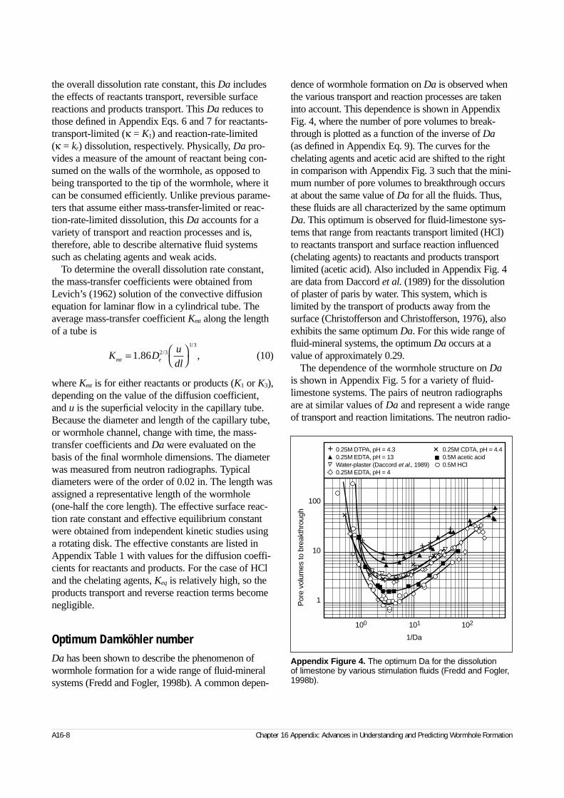
the overall dissolution rate constant, this Da includesthe effects of reactants transport, reversible surfacereactions and products transport. This Da reduces tothose defined in Appendix Eqs. 6 and 7 for reactants-transport-limited (κ = K1) and reaction-rate-limited (κ = kr) dissolution, respectively. Physically, Da pro-vides a measure of the amount of reactant being con-sumed on the walls of the wormhole, as opposed tobeing transported to the tip of the wormhole, where itcan be consumed efficiently. Unlike previous parame-ters that assume either mass-transfer-limited or reac-tion-rate-limited dissolution, this Da accounts for avariety of transport and reaction processes and is,therefore, able to describe alternative fluid systemssuch as chelating agents and weak acids.

To determine the overall dissolution rate constant,the mass-transfer coefficients were obtained fromLevich’s (1962) solution of the convective diffusionequation for laminar flow in a cylindrical tube. Theaverage mass-transfer coefficient Kmt along the lengthof a tube is

(10)

where Kmt is for either reactants or products (K1 or K3),depending on the value of the diffusion coefficient,and u is the superficial velocity in the capillary tube.Because the diameter and length of the capillary tube,or wormhole channel, change with time, the mass-transfer coefficients and Da were evaluated on thebasis of the final wormhole dimensions. The diameterwas measured from neutron radiographs. Typicaldiameters were of the order of 0.02 in. The length wasassigned a representative length of the wormhole(one-half the core length). The effective surface reac-tion rate constant and effective equilibrium constantwere obtained from independent kinetic studies usinga rotating disk. The effective constants are listed inAppendix Table 1 with values for the diffusion coeffi-cients for reactants and products. For the case of HCland the chelating agents, Keq is relatively high, so theproducts transport and reverse reaction terms becomenegligible.

Optimum Damköhler numberDa has been shown to describe the phenomenon ofwormhole formation for a wide range of fluid-mineralsystems (Fredd and Fogler, 1998b). A common depen-

dence of wormhole formation on Da is observed whenthe various transport and reaction processes are takeninto account. This dependence is shown in AppendixFig. 4, where the number of pore volumes to break-through is plotted as a function of the inverse of Da(as defined in Appendix Eq. 9). The curves for thechelating agents and acetic acid are shifted to the rightin comparison with Appendix Fig. 3 such that the mini-mum number of pore volumes to breakthrough occursat about the same value of Da for all the fluids. Thus,these fluids are all characterized by the same optimumDa. This optimum is observed for fluid-limestone sys-tems that range from reactants transport limited (HCl)to reactants transport and surface reaction influenced(chelating agents) to reactants and products transportlimited (acetic acid). Also included in Appendix Fig. 4are data from Daccord et al. (1989) for the dissolutionof plaster of paris by water. This system, which islimited by the transport of products away from thesurface (Christofferson and Christofferson, 1976), alsoexhibits the same optimum Da. For this wide range offluid-mineral systems, the optimum Da occurs at avalue of approximately 0.29.

The dependence of the wormhole structure on Dais shown in Appendix Fig. 5 for a variety of fluid-limestone systems. The pairs of neutron radiographsare at similar values of Da and represent a wide rangeof transport and reaction limitations. The neutron radio-

A16-8 Chapter 16 Appendix: Advances in Understanding and Predicting Wormhole Formation

K Du

dlmt e=

1 86 2 3

1 3

. ,//

Appendix Figure 4. The optimum Da for the dissolution of limestone by various stimulation fluids (Fredd and Fogler,1998b).

100

10

1Por

e vo

lum

es to

bre

akth

roug

h

1/Da

0.25M CDTA, pH = 4.40.5M acetic acid0.5M HCl

0.25M DTPA, pH = 4.30.25M EDTA, pH = 13Water-plaster (Daccord et al., 1989)0.25M EDTA, pH = 4

+ +

++

+

++ +++

100 101 102

+

+

+

++

+

+

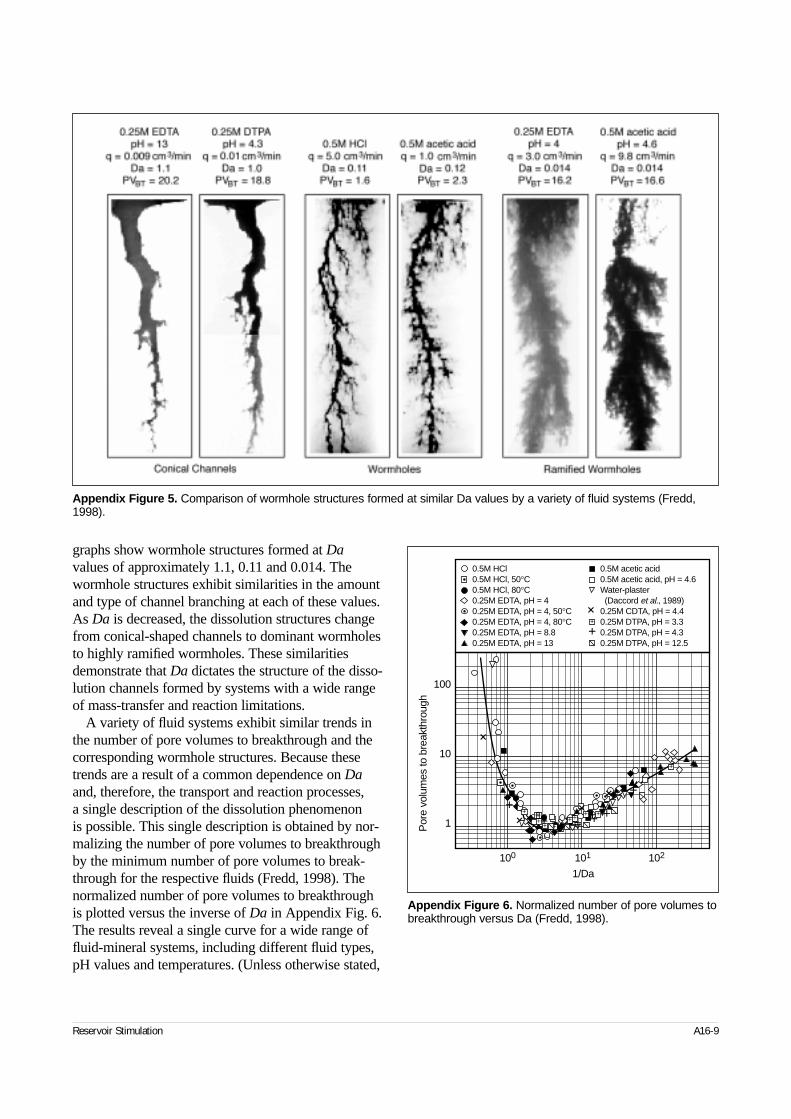
graphs show wormhole structures formed at Davalues of approximately 1.1, 0.11 and 0.014. Thewormhole structures exhibit similarities in the amountand type of channel branching at each of these values.As Da is decreased, the dissolution structures changefrom conical-shaped channels to dominant wormholesto highly ramified wormholes. These similaritiesdemonstrate that Da dictates the structure of the disso-lution channels formed by systems with a wide rangeof mass-transfer and reaction limitations.

A variety of fluid systems exhibit similar trends inthe number of pore volumes to breakthrough and thecorresponding wormhole structures. Because thesetrends are a result of a common dependence on Daand, therefore, the transport and reaction processes, a single description of the dissolution phenomenon is possible. This single description is obtained by nor-malizing the number of pore volumes to breakthroughby the minimum number of pore volumes to break-through for the respective fluids (Fredd, 1998). Thenormalized number of pore volumes to breakthroughis plotted versus the inverse of Da in Appendix Fig. 6.The results reveal a single curve for a wide range offluid-mineral systems, including different fluid types,pH values and temperatures. (Unless otherwise stated,

Reservoir Stimulation A16-9

Appendix Figure 5. Comparison of wormhole structures formed at similar Da values by a variety of fluid systems (Fredd,1998).

Appendix Figure 6. Normalized number of pore volumes tobreakthrough versus Da (Fredd, 1998).

100

10

1Por

e vo

lum

es to

bre

akth

roug

h

1/Da

0.5M acetic acid0.5M acetic acid, pH = 4.6Water-plaster (Daccord et al., 1989)0.25M CDTA, pH = 4.40.25M DTPA, pH = 3.30.25M DTPA, pH = 4.30.25M DTPA, pH = 12.5

+

+

100 101 102

++ ++

+

++ +

+

++

+ ++++ +

++

+

+

++

++

0.5M HCl0.5M HCl, 50°C0.5M HCl, 80°C0.25M EDTA, pH = 40.25M EDTA, pH = 4, 50°C0.25M EDTA, pH = 4, 80°C0.25M EDTA, pH = 8.80.25M EDTA, pH = 13

the data are for the dissolution of limestone at ambienttemperature.) This single curve provides a means ofestimating the entire curve for the number of pore vol-umes to breakthrough and the wormhole structuresfrom a single coreflood experiment near the optimumDa. Thus, the need for exhaustive coreflood studies todetermine the effectiveness of a fluid under particularreservoir conditions is eliminated.

Wormhole formation modelingIn addition to involving a variety of transport andreaction processes, the dissolution of porous media iscomplicated by the stochastic nature in which the flowchannels evolve. The difficulties associated withaccounting for all the complexities of wormhole for-mation have led to many simplifications of the disso-lution phenomenon. These simplifications typicallylimit the models to either mass-transfer-limited orreaction-rate-limited dissolution and include an idealrepresentation of the porous medium. Early investiga-tors simulated mass-transfer-limited dissolution usingmodels of the porous medium that were based on bun-dles of capillary tubes (Nougaro and Labbé, 1955;Rowan, 1959). These simple models were extendedby Schechter and Gidley (1969) to include the effectsof pore merging and either mass-transfer-limited orreaction-rate-limited dissolution. Although the domi-nant pores were observed to grow more rapidly, thesemodels were unable to capture the branching charac-teristics of the dissolution phenomenon.

More recently, Hoefner and Fogler (1988) success-fully modeled the phenomenon of wormhole formationusing a network model. They simulated pore-scale flowand reaction by representing the porous medium as atwo-dimensional network of nodes connected by cylin-drical bonds. The model provided qualitative predic-tions of the dissolution structure (see Fig. 17-1) andcorresponding permeability response for both mass-transfer-limited and reaction-rate-limited dissolution.Similar results were observed by Daccord et al. (1989),who utilized a network model to simulate the mass-transfer-limited dissolution of plaster of paris by water.Although these network models do not include poremerging, they were able to predict the experimentallyobserved trends in wormhole formation because theycapture the effects of pore-level heterogeneity on themacroscopic dissolution phenomenon.

The combined effects of transport and reaction havebeen included in a three-dimensional physically repre-sentative network (PRN) model for flow and reactionin porous media (Fredd and Fogler, 1998b). The PRNmodel is based on a packed-bed description of theporous medium (Bryant et al., 1993; Thompson andFogler, 1997). Although the use of a packed-beddescription of the medium limits the ability of themodel to represent consolidated carbonate porousmedia, it is a major advancement over the capillarytube representations typically used. The model pro-vides a complete topological description of the medi-um and a fundamental description of the pore-scalehydrodynamics. These descriptions serve as a physicalbasis for determining macroscopic parameters, such asthe permeability. Dissolution is simulated by allowingthe spherical particles that compose the bed to shrinkas reactant is consumed. The pores naturally merge asthe spherical particles are dissolved. The simulationsare in qualitative agreement with experimental obser-vations and demonstrate the common dependence ofwormhole formation on Da. More importantly, theexistence of an optimum Da is substantiated by PRNmodel simulations.

Prediction of optimum field conditionsThe ultimate goal of all laboratory studies is to aid thedesign of effective field treatments. Two main designrequirements are predicting the optimum injection rateand selecting the most appropriate stimulation fluid.Unfortunately, the direct application of laboratory datato the field is not straightforward, as noted by severalinvestigators (Daccord et al., 1989; Frick et al., 1994b;Bazin, 1995; Buijse, 1997). Wormhole formation in thefield is complicated by the effects of fluid loss throughthe walls of the wormhole in the radial geometry andby competition among wormholes for the injected fluid(Appendix Fig. 7). The importance of these processeshas been demonstrated theoretically (Nierode andWilliams, 1971; Hung et al., 1989; Buijse, 1997).However, these studies were limited in their ability to predict optimum injection conditions in the fieldbecause of a lack of consideration of the critical para-meters required for effective wormhole formation.

To account for the influence of fluid loss and worm-hole competition on wormhole formation, twoapproaches are the most obvious:

A16-10 Chapter 16 Appendix: Advances in Understanding and Predicting Wormhole Formation

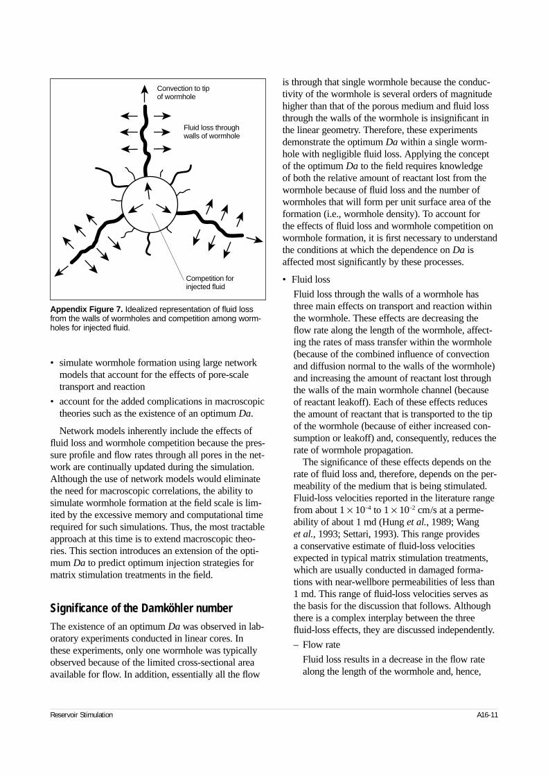
• simulate wormhole formation using large networkmodels that account for the effects of pore-scaletransport and reaction

• account for the added complications in macroscopictheories such as the existence of an optimum Da.

Network models inherently include the effects offluid loss and wormhole competition because the pres-sure profile and flow rates through all pores in the net-work are continually updated during the simulation.Although the use of network models would eliminatethe need for macroscopic correlations, the ability tosimulate wormhole formation at the field scale is lim-ited by the excessive memory and computational timerequired for such simulations. Thus, the most tractableapproach at this time is to extend macroscopic theo-ries. This section introduces an extension of the opti-mum Da to predict optimum injection strategies formatrix stimulation treatments in the field.

Significance of the Damköhler numberThe existence of an optimum Da was observed in lab-oratory experiments conducted in linear cores. Inthese experiments, only one wormhole was typicallyobserved because of the limited cross-sectional areaavailable for flow. In addition, essentially all the flow

is through that single wormhole because the conduc-tivity of the wormhole is several orders of magnitudehigher than that of the porous medium and fluid lossthrough the walls of the wormhole is insignificant inthe linear geometry. Therefore, these experimentsdemonstrate the optimum Da within a single worm-hole with negligible fluid loss. Applying the conceptof the optimum Da to the field requires knowledgeof both the relative amount of reactant lost from thewormhole because of fluid loss and the number ofwormholes that will form per unit surface area of theformation (i.e., wormhole density). To account for the effects of fluid loss and wormhole competition onwormhole formation, it is first necessary to understandthe conditions at which the dependence on Da isaffected most significantly by these processes.

• Fluid loss

Fluid loss through the walls of a wormhole hasthree main effects on transport and reaction withinthe wormhole. These effects are decreasing theflow rate along the length of the wormhole, affect-ing the rates of mass transfer within the wormhole(because of the combined influence of convectionand diffusion normal to the walls of the wormhole)and increasing the amount of reactant lost throughthe walls of the main wormhole channel (becauseof reactant leakoff). Each of these effects reducesthe amount of reactant that is transported to the tipof the wormhole (because of either increased con-sumption or leakoff) and, consequently, reduces therate of wormhole propagation.

The significance of these effects depends on therate of fluid loss and, therefore, depends on the per-meability of the medium that is being stimulated.Fluid-loss velocities reported in the literature rangefrom about 1 × 10–4 to 1 × 10–2 cm/s at a perme-ability of about 1 md (Hung et al., 1989; Wang et al., 1993; Settari, 1993). This range provides a conservative estimate of fluid-loss velocitiesexpected in typical matrix stimulation treatments,which are usually conducted in damaged forma-tions with near-wellbore permeabilities of less than1 md. This range of fluid-loss velocities serves asthe basis for the discussion that follows. Althoughthere is a complex interplay between the threefluid-loss effects, they are discussed independently.

– Flow rate

Fluid loss results in a decrease in the flow ratealong the length of the wormhole and, hence,

Reservoir Stimulation A16-11

Appendix Figure 7. Idealized representation of fluid lossfrom the walls of wormholes and competition among worm-holes for injected fluid.

Competition forinjected fluid

Convection to tipof wormhole

Fluid loss throughwalls of wormhole

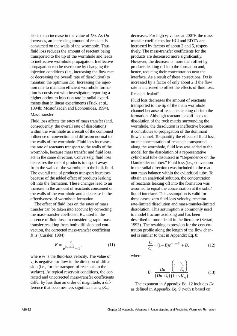
leads to an increase in the value of Da. As Daincreases, an increasing amount of reactant isconsumed on the walls of the wormhole. Thus,fluid loss reduces the amount of reactant beingtransported to the tip of the wormhole and leadsto ineffective wormhole propagation. Ineffectivepropagation can be overcome by changing theinjection conditions (i.e., increasing the flow rateor decreasing the overall rate of dissolution) tomaintain the optimum Da. Increasing the injec-tion rate to maintain efficient wormhole forma-tion is consistent with investigators reporting ahigher optimum injection rate in radial experi-ments than in linear experiments (Frick et al.,1994b; Mostofizadeh and Economides, 1994).

– Mass transfer

Fluid loss affects the rates of mass transfer (and,consequently, the overall rate of dissolution)within the wormhole as a result of the combinedinfluence of convection and diffusion normal tothe walls of the wormhole. Fluid loss increasesthe rate of reactants transport to the walls of thewormhole, because mass transfer and fluid lossact in the same direction. Conversely, fluid lossdecreases the rate of products transport awayfrom the walls of the wormhole to the bulk fluid.The overall rate of products transport increasesbecause of the added effect of products leakingoff into the formation. These changes lead to anincrease in the amount of reactants consumed onthe walls of the wormhole and a decrease in theeffectiveness of wormhole formation.

The effect of fluid loss on the rates of masstransfer can be taken into account by correctingthe mass-transfer coefficient Kmt used in theabsence of fluid loss. In considering rapid masstransfer resulting from both diffusion and con-vection, the corrected mass-transfer coefficient K is (Cussler, 1984)

(11)

where vL is the fluid-loss velocity. The value ofvL is negative for flow in the direction of diffu-sion (i.e., for the transport of reactants to thesurface). At typical reservoir conditions, the cor-rected and uncorrected mass-transfer coefficientsdiffer by less than an order of magnitude, a dif-ference that becomes less significant as vL/Kmt

decreases. For high vL values at 200°F, the mass-transfer coefficients for HCl and EDTA areincreased by factors of about 2 and 5, respec-tively. The mass-transfer coefficients for theproducts are decreased more significantly.However, the decrease is more than offset byproducts leaking off into the formation and,hence, reducing their concentration near theinterface. As a result of these corrections, Da isincreased by a factor of only about 2 if the flowrate is increased to offset the effects of fluid loss.

– Reactant leakoff

Fluid loss decreases the amount of reactantstransported to the tip of the main wormholechannel because of reactants leaking off into theformation. Although reactant leakoff leads todissolution of the rock matrix surrounding thewormhole, the dissolution is ineffective becauseit contributes to propagation of the dominantflow channel. To quantify the effects of fluid losson the concentration of reactants transportedalong the wormhole, fluid loss was added to themodel for the dissolution of a representativecylindrical tube discussed in “Dependence on theDamköhler number.” Fluid loss (i.e., convectionin the radial direction) was included in the reac-tant mass balance within the cylindrical tube. Toobtain an analytical solution, the concentration of reactants leaking off into the formation wasassumed to equal the concentration at the solid/liquid interface. This assumption is valid forthree cases: zero fluid-loss velocity, reaction-rate-limited dissolution and mass-transfer-limiteddissolution. This assumption is commonly usedto model fracture acidizing and has beendescribed in more detail in the literature (Settari,1993). The resulting expression for the concen-tration profile along the length of the flow chan-nel is similar to that in Appendix Eq. 8:

(12)

where

(13)

The exponent in Appendix Eq. 12 includes Daas defined in Appendix Eq. 9 (with κ based on

A16-12 Chapter 16 Appendix: Advances in Understanding and Predicting Wormhole Formation

Kv

eL

v KL mt=

−( ) 1, C

CB e B

o

Da= −( ) +− +( )1 ξ ,

BDa

Da

v

K

K

L

eq

=+( )

−

+( )ξ ν

1

11 .

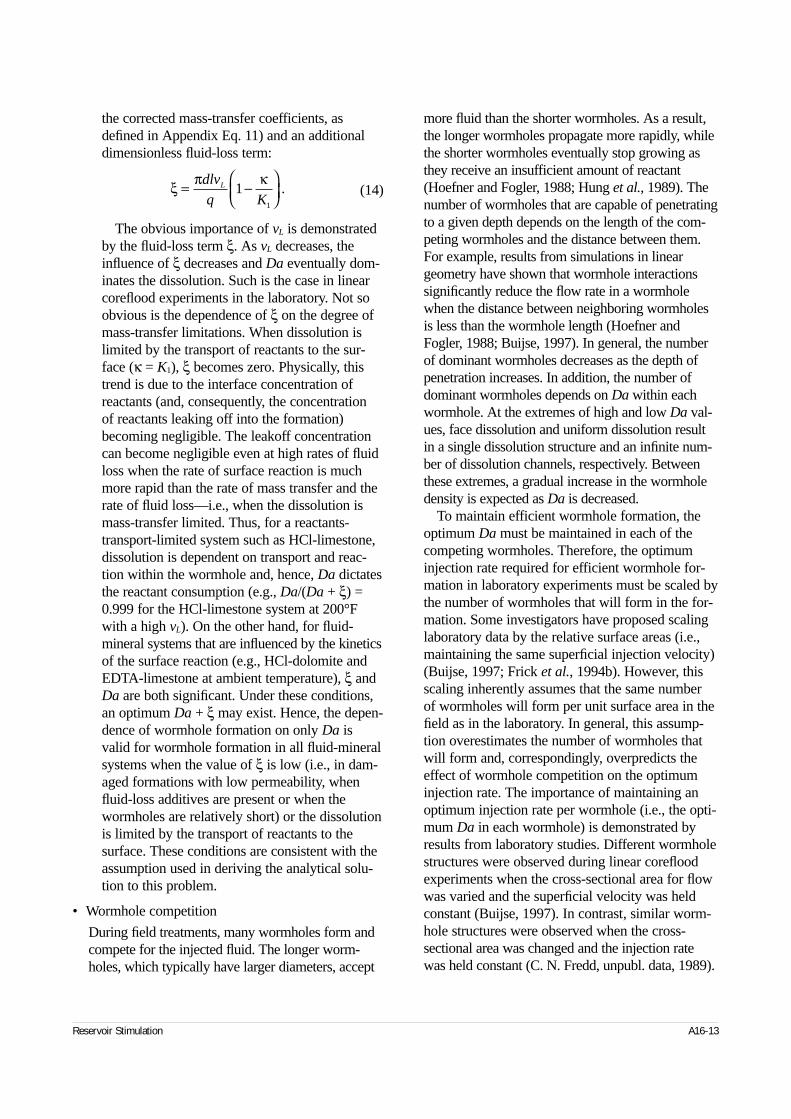
the corrected mass-transfer coefficients, asdefined in Appendix Eq. 11) and an additionaldimensionless fluid-loss term:

(14)

The obvious importance of vL is demonstratedby the fluid-loss term ξ. As vL decreases, theinfluence of ξ decreases and Da eventually dom-inates the dissolution. Such is the case in linearcoreflood experiments in the laboratory. Not soobvious is the dependence of ξ on the degree ofmass-transfer limitations. When dissolution islimited by the transport of reactants to the sur-face (κ = K1), ξ becomes zero. Physically, thistrend is due to the interface concentration ofreactants (and, consequently, the concentration of reactants leaking off into the formation)becoming negligible. The leakoff concentrationcan become negligible even at high rates of fluidloss when the rate of surface reaction is muchmore rapid than the rate of mass transfer and therate of fluid loss—i.e., when the dissolution ismass-transfer limited. Thus, for a reactants-transport-limited system such as HCl-limestone,dissolution is dependent on transport and reac-tion within the wormhole and, hence, Da dictatesthe reactant consumption (e.g., Da/(Da + ξ) =0.999 for the HCl-limestone system at 200°Fwith a high vL). On the other hand, for fluid-mineral systems that are influenced by the kineticsof the surface reaction (e.g., HCl-dolomite andEDTA-limestone at ambient temperature), ξ andDa are both significant. Under these conditions,an optimum Da + ξ may exist. Hence, the depen-dence of wormhole formation on only Da isvalid for wormhole formation in all fluid-mineralsystems when the value of ξ is low (i.e., in dam-aged formations with low permeability, whenfluid-loss additives are present or when thewormholes are relatively short) or the dissolutionis limited by the transport of reactants to thesurface. These conditions are consistent with theassumption used in deriving the analytical solu-tion to this problem.

• Wormhole competition

During field treatments, many wormholes form andcompete for the injected fluid. The longer worm-holes, which typically have larger diameters, accept

more fluid than the shorter wormholes. As a result,the longer wormholes propagate more rapidly, whilethe shorter wormholes eventually stop growing asthey receive an insufficient amount of reactant(Hoefner and Fogler, 1988; Hung et al., 1989). Thenumber of wormholes that are capable of penetratingto a given depth depends on the length of the com-peting wormholes and the distance between them.For example, results from simulations in lineargeometry have shown that wormhole interactionssignificantly reduce the flow rate in a wormholewhen the distance between neighboring wormholesis less than the wormhole length (Hoefner andFogler, 1988; Buijse, 1997). In general, the numberof dominant wormholes decreases as the depth ofpenetration increases. In addition, the number ofdominant wormholes depends on Da within eachwormhole. At the extremes of high and low Da val-ues, face dissolution and uniform dissolution resultin a single dissolution structure and an infinite num-ber of dissolution channels, respectively. Betweenthese extremes, a gradual increase in the wormholedensity is expected as Da is decreased.

To maintain efficient wormhole formation, theoptimum Da must be maintained in each of thecompeting wormholes. Therefore, the optimuminjection rate required for efficient wormhole for-mation in laboratory experiments must be scaled bythe number of wormholes that will form in the for-mation. Some investigators have proposed scalinglaboratory data by the relative surface areas (i.e.,maintaining the same superficial injection velocity)(Buijse, 1997; Frick et al., 1994b). However, thisscaling inherently assumes that the same number of wormholes will form per unit surface area in thefield as in the laboratory. In general, this assump-tion overestimates the number of wormholes thatwill form and, correspondingly, overpredicts theeffect of wormhole competition on the optimuminjection rate. The importance of maintaining anoptimum injection rate per wormhole (i.e., the opti-mum Da in each wormhole) is demonstrated byresults from laboratory studies. Different wormholestructures were observed during linear corefloodexperiments when the cross-sectional area for flowwas varied and the superficial velocity was heldconstant (Buijse, 1997). In contrast, similar worm-hole structures were observed when the cross-sectional area was changed and the injection ratewas held constant (C. N. Fredd, unpubl. data, 1989).

Reservoir Stimulation A16-13

ξ π κ= −

dlv

q KL 1

1

.

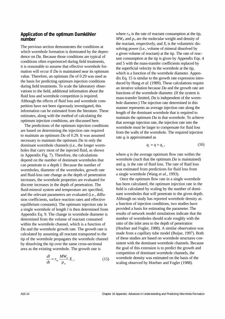
Application of the optimum Damköhler numberThe previous section demonstrates the conditions atwhich wormhole formation is dominated by the depen-dence on Da. Because those conditions are typical ofconditions often experienced during field treatments, it is reasonable to assume that effective wormhole for-mation will occur if Da is maintained near its optimumvalue. Therefore, an optimum Da of 0.29 was used asthe basis for predicting optimum injection conditionsduring field treatments. To scale the laboratory obser-vations to the field, additional information about thefluid loss and wormhole competition is required.Although the effects of fluid loss and wormhole com-petition have not been rigorously investigated, thisinformation can be estimated from the literature. Theseestimates, along with the method of calculating theoptimum injection conditions, are discussed here.

The predictions of the optimum injection conditionsare based on determining the injection rate required to maintain an optimum Da of 0.29. It was assumednecessary to maintain the optimum Da in only thedominant wormhole channels (i.e., the longer worm-holes that carry most of the injected fluid, as shown in Appendix Fig. 7). Therefore, the calculationsdepend on the number of dominant wormholes thatcan penetrate to a depth l. Because the number ofwormholes, diameter of the wormholes, growth rateand fluid-loss rate change as the depth of penetrationincreases, the wormhole properties are evaluated fordiscrete increases in the depth of penetration. Thefluid-mineral system and temperature are specified,and the relevant parameters are evaluated (i.e., diffu-sion coefficients, surface reaction rates and effectiveequilibrium constants). The optimum injection rate ina single wormhole of length l is then determined fromAppendix Eq. 9. The change in wormhole diameter isdetermined from the volume of reactant consumedwithin the wormhole channel, which is a function ofDa and the wormhole growth rate. The growth rate iscalculated by assuming all reactant transported to thetip of the wormhole propagates the wormhole channelby dissolving the tip over the same cross-sectionalarea as the existing wormhole. The growth rate is

(15)

where rAt is the rate of reactant consumption at the tip,MWA and ρA are the molecular weight and density ofthe reactant, respectively, and Xt is the volumetric dis-solving power (i.e., volume of mineral dissolved by a given volume of reactant) at the tip. The rate of reac-tant consumption at the tip is given by Appendix Eqs. 4and 5 with the mass-transfer coefficients replaced bythe superficial velocity in the wormhole at the tip,which is a function of the wormhole diameter. Appen-dix Eq. 15 is similar to the growth rate expression intro-duced by Hung et al. (1989). These calculations requirean iterative solution because Da and the growth rate arefunctions of the wormhole diameter. (If the system ismass-transfer limited, Da is independent of the worm-hole diameter.) The injection rate determined in thismanner represents an average injection rate along thelength of the dominant wormhole that is required tomaintain the optimum Da in that wormhole. To achievethat average injection rate, the injection rate into thewormhole must be larger to compensate for fluid lossfrom the walls of the wormhole. The required injectionrate qi is approximated as

(16)

where q is the average optimum flow rate within thewormhole (such that the optimum Da is maintained)and qL is the rate of fluid loss. The rate of fluid losswas estimated from predictions for fluid loss from a single wormhole (Wang et al., 1993).

Once the optimum flow rate in a single wormholehas been calculated, the optimum injection rate in thefield is calculated by scaling by the number of domi-nant wormholes that will penetrate to the given depth.Although no study has reported wormhole density as a function of injection conditions, two studies haveprovided a basis for estimating the parameter. Theresults of network model simulations indicate that thenumber of wormholes should scale roughly with theratio of the inlet area to the depth of penetration(Hoefner and Fogler, 1988). A similar observation wasmade from a capillary tube model (Buijse, 1997). Bothof these studies are based on wormhole structures con-sistent with the dominant wormhole channels. Becausethe goal of this extension is to predict the growth andcompetition of dominant wormhole channels, thewormhole density was estimated on the basis of thescaling observed by Hoefner and Fogler (1988).

A16-14 Chapter 16 Appendix: Advances in Understanding and Predicting Wormhole Formation

dl

dtr

MWXAt

A

A

t=ρ

,

q q qi L= + ,

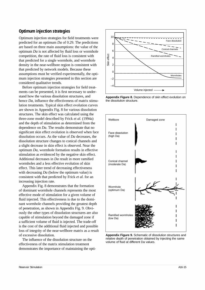
Optimum injection strategiesOptimum injection strategies for field treatments werepredicted for an optimum Da of 0.29. The predictionsare based on three main assumptions: the value of theoptimum Da is not affected by fluid loss or wormholecompetition, the rate of fluid loss is consistent withthat predicted for a single wormhole, and wormholedensity in the near-wellbore region is consistent withthat predicted by network models. Because theseassumptions must be verified experimentally, the opti-mum injection strategies presented in this section areconsidered qualitative trends.

Before optimum injection strategies for field treat-ments can be presented, it is first necessary to under-stand how the various dissolution structures, andhence Da, influence the effectiveness of matrix stimu-lation treatments. Typical skin effect evolution curvesare shown in Appendix Fig. 8 for various dissolutionstructures. The skin effect was calculated using thethree-zone model described by Frick et al. (1994a)and the depth of stimulation as determined from thedependence on Da. The results demonstrate that nosignificant skin effect evolution is observed when facedissolution occurs. As the value of Da decreases, thedissolution structure changes to conical channels anda slight decrease in skin effect is observed. Near theoptimum Da, wormhole formation results in effectivestimulation as evidenced by the negative skin effect.Additional decreases in Da result in more ramifiedwormholes and a less effective evolution of skineffect. This later trend of decreasing effectivenesswith decreasing Da (below the optimum value) isconsistent with that predicted by Frick et al. for anincreasing injection rate.

Appendix Fig. 8 demonstrates that the formation of dominant wormhole channels represents the mosteffective mode of stimulation for a given volume offluid injected. This effectiveness is due to the domi-nant wormhole channels providing the greatest depthof penetration, as shown in Appendix Fig. 9. Obvi-ously the other types of dissolution structures are alsocapable of stimulation beyond the damaged zone if a sufficient volume of fluid is injected. The trade-offis the cost of the additional fluid injected and possibleloss of integrity of the near-wellbore matrix as a resultof excessive dissolution.

The influence of the dissolution structure on theeffectiveness of the matrix stimulation treatmentdemonstrates the importance of maintaining the opti-

Reservoir Stimulation A16-15

Appendix Figure 8. Dependence of skin effect evolution onthe dissolution structure.

10

8

6

4

2

0

–2

–4

Ski

n ef

fect

Volume injected

Wormholes

Conical channels

Ramified wormholes

Face dissolution

Appendix Figure 9. Schematic of dissolution structures andrelative depth of penetration obtained by injecting the samevolume of fluid at different Da values.

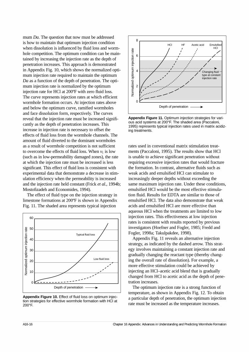
mum Da. The question that now must be addressed is how to maintain that optimum injection conditionwhen dissolution is influenced by fluid loss and worm-hole competition. The optimum condition can be main-tained by increasing the injection rate as the depth ofpenetration increases. This approach is demonstrated in Appendix Fig. 10, which shows the normalized opti-mum injection rate required to maintain the optimumDa as a function of the depth of penetration. The opti-mum injection rate is normalized by the optimuminjection rate for HCl at 200ºF with zero fluid loss. The curve represents injection rates at which efficientwormhole formation occurs. At injection rates aboveand below the optimum curve, ramified wormholesand face dissolution form, respectively. The curvesreveal that the injection rate must be increased signifi-cantly as the depth of penetration increases. Thisincrease in injection rate is necessary to offset theeffects of fluid loss from the wormhole channels. Theamount of fluid diverted to the dominant wormholes as a result of wormhole competition is not sufficient to overcome the effects of fluid loss. When vL is low(such as in low-permeability damaged zones), the rateat which the injection rate must be increased is lesssignificant. This effect of fluid loss is consistent withexperimental data that demonstrate a decrease in stim-ulation efficiency when the permeability is increasedand the injection rate held constant (Frick et al., 1994b;Mostofizadeh and Economides, 1994).

The effect of fluid type on the injection strategy inlimestone formations at 200ºF is shown in AppendixFig. 11. The shaded area represents typical injection

rates used in conventional matrix stimulation treat-ments (Paccaloni, 1995). The results show that HCl is unable to achieve significant penetration withoutrequiring excessive injection rates that would fracturethe formation. In contrast, alternative fluids such asweak acids and emulsified HCl can stimulate toincreasingly deeper depths without exceeding thesame maximum injection rate. Under these conditions,emulsified HCl would be the most effective stimula-tion fluid. Results for EDTA are similar to those ofemulsified HCl. The data also demonstrate that weakacids and emulsified HCl are more effective thanaqueous HCl when the treatments are limited to lowinjection rates. This effectiveness at low injectionrates is consistent with results reported by previousinvestigators (Hoefner and Fogler, 1985; Fredd andFogler, 1998a; Takulpakdee, 1998).

Appendix Fig. 11 reveals an alternative injectionstrategy, as indicated by the dashed arrow. This strat-egy involves maintaining a constant injection rate andgradually changing the reactant type (thereby chang-ing the overall rate of dissolution). For example, amore effective stimulation could be achieved byinjecting an HCl–acetic acid blend that is graduallychanged from HCl to acetic acid as the depth of pene-tration increases.

The optimum injection rate is a strong function oftemperature, as shown in Appendix Fig. 12. To obtaina particular depth of penetration, the optimum injectionrate must be increased as the temperature increases.

A16-16 Chapter 16 Appendix: Advances in Understanding and Predicting Wormhole Formation

Appendix Figure 10. Effect of fluid loss on optimum injec-tion strategies for effective wormhole formation with HCl at200°F.

60

50

40

30

20

10

0

Nor

mal

ized

opt

imum

inje

ctio

n ra

te

Depth of penetration

Low fluid loss

Typical fluid loss

Appendix Figure 11. Optimum injection strategies for vari-ous acid systems at 200°F. The shaded area (Paccaloni,1995) represents typical injection rates used in matrix acidiz-ing treatments.

8

6

4

2

0

Nor

mal

ized

opt

imum

inje

ctio

n ra

te

Depth of penetration

Changing fluidtype at constantinjection rate

HCl HF Acetic acid EmulsifiedHCl

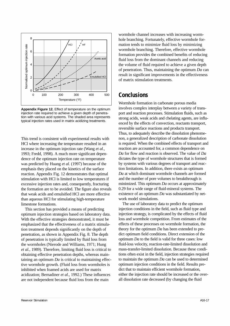
This trend is consistent with experimental results withHCl where increasing the temperature resulted in anincrease in the optimum injection rate (Wang et al.,1993; Fredd, 1998). A much more significant depen-dence of the optimum injection rate on temperaturewas predicted by Huang et al. (1997) because of theemphasis they placed on the kinetics of the surfacereaction. Appendix Fig. 12 demonstrates that optimalstimulation with HCl is limited to low temperatures ifexcessive injection rates and, consequently, fracturingthe formation are to be avoided. The figure also revealsthat weak acids and emulsified HCl are more effectivethan aqueous HCl for stimulating high-temperaturelimestone formations.

This section has provided a means of predictingoptimum injection strategies based on laboratory data.With the effective strategies demonstrated, it must beemphasized that the effectiveness of a matrix stimula-tion treatment depends significantly on the depth ofpenetration, as shown in Appendix Fig. 8. The depthof penetration is typically limited by fluid loss fromthe wormholes (Nierode and Williams, 1971; Hung et al., 1989). Therefore, limiting fluid loss is critical toobtaining effective penetration depths, whereas main-taining an optimum Da is critical to maintaining effec-tive wormhole growth. (Fluid loss from wormholes isinhibited when foamed acids are used for matrixacidization; Bernadiner et al., 1992.) These influencesare not independent because fluid loss from the main

wormhole channel increases with increasing worm-hole branching. Fortunately, effective wormhole for-mation tends to minimize fluid loss by minimizingwormhole branching. Therefore, effective wormholeformation provides the combined benefits of reducingfluid loss from the dominant channels and reducingthe volume of fluid required to achieve a given depthof penetration. Thus, maintaining the optimum Da canresult in significant improvements in the effectivenessof matrix stimulation treatments.

ConclusionsWormhole formation in carbonate porous mediainvolves complex interplay between a variety of trans-port and reaction processes. Stimulation fluids, such asstrong acids, weak acids and chelating agents, are influ-enced by the effects of convection, reactants transport,reversible surface reactions and products transport.Thus, to adequately describe the dissolution phenome-non, a generalized description of carbonate dissolutionis required. When the combined effects of transport andreaction are accounted for, a common dependence onDa for flow and reaction is observed. The value of Dadictates the type of wormhole structures that is formedby systems with various degrees of transport and reac-tion limitations. In addition, there exists an optimumDa at which dominant wormhole channels are formedand the number of pore volumes to breakthrough isminimized. This optimum Da occurs at approximately0.29 for a wide range of fluid-mineral systems. Theexistence of an optimum Da was substantiated by net-work model simulations.

The use of laboratory data to predict the optimuminjection conditions in the field, such as fluid type andinjection strategy, is complicated by the effects of fluidloss and wormhole competition. From estimates of theeffects of these processes on wormhole formation, thetheory for the optimum Da has been extended to pre-dict optimum field conditions. Direct extension of theoptimum Da to the field is valid for three cases: lowfluid-loss velocity, reaction-rate-limited dissolution andmass-transfer-limited dissolution. Because these condi-tions often exist in the field, injection strategies requiredto maintain the optimum Da can be used to determinedoptimum injection conditions in the field. Results pre-dict that to maintain efficient wormhole formation,either the injection rate should be increased or the over-all dissolution rate decreased (by changing the fluid

Reservoir Stimulation A16-17

Appendix Figure 12. Effect of temperature on the optimuminjection rate required to achieve a given depth of penetra-tion with various acid systems. The shaded area representstypical injection rates used in matrix acidizing treatments.

8

6

4

2

0

Nor

mal

ized

opt

imum

inje

ctio

n ra

te

0 100 200 300 400 500

Temperature (°F)

Acetic acid

Emulsified HCl

HCl HF

type) as the depth of penetration increases. At the injec-tion rates commonly used for matrix acidizing, conven-tional treatments with HCl are optimal only in low-temperature formations. Fluids such as weak acids andemulsified HCl provide effective alternatives to HCl athigh temperatures and low injection rates. The resultsdiscussed in this Appendix to Chapter 16 provide quali-tative predictions of optimum injection strategies thatare in agreement with experimental observations. Arigorous investigation of the effects of fluid loss andwormhole competition on wormhole formation willenable more quantitative predictions of the optimuminjection conditions.

A16-18 Chapter 16 Appendix: Advances in Understanding and Predicting Wormhole Formation

17-1. IntroductionCarbonate rocks, by definition, contain more than50% carbonate minerals. The most common carbon-ate minerals are calcite (calcium carbonate, CaCO3)and dolomite, a single mineral associating 1 mole ofCaCO3 with 1 mole of MgCO3. Carbonate rocks aretypically classified by the calcite:dolomite ratio, andthose with a ratio higher than 50% are generallycalled limestones. Carbonate rocks present singularphysical characteristics, such as double porosity orhigh permeability contrasts, which are inheritedfrom their process of formation.

Hydrochloric acid (HCl) is usually selected forcarbonate acidizing. It reacts readily with carbonateminerals and is available in large quantities at a rel-atively low price. Whereas the purpose of sandstoneacidizing is to dissolve the damage, acid is used incarbonate formations to dissolve the matrix andbypass the damage. For this reason, both damageand rock characteristics must be taken into accountwhen designing the treatment.

17-2. Rock and damage character-istics in carbonate formations

17-2.1. Rock characteristicsCarbonate rocks are sedimentary rocks resultingmostly from organic activity. The vast majority ofthese sediments is composed of skeletons of marineorganisms that vary in size from a few microns toseveral centimeters. Some carbonate sediments areformed by the chemical precipitation of CaCO3.

Because they consist of noneroded, homogeneousmaterials, carbonate sediments usually have a highinitial porosity. Conversely, because the permeabil-ity of sediments depends mainly on grain size, car-bonate rocks present a wide range of permeabilities.For example, chalks formed from sediments of

microscopic fossils have low permeabilities in com-parison with those of oolithic limestones, althoughthey can have similar porosities.

After deposition, carbonate sediments are subjectto chemical and physical transformation (diagenesis).Chemical modifications consist primarily of the evo-lution of the sediments to stable forms such as cal-cite and dolomite. This process is called neomor-phism. Dolomites result from evolution under long-term contact with fluids with a high magnesium con-tent. Dolomitization usually increases porosity butimpairs permeability by precipitating dolomite crys-tals. When dolomites are in contact with rainwater,the inverse process of dedolomitization can occur.

Modifications of permeability and porosity canalso result from other chemical transformations suchas dissolution, reprecipitation and cementation whilein contact with subterranean water or molecular dif-fusion during severe subsurface conditions. Stressand pressure modifications occurring upon burial of the sediments may also entail a lithologic change,with porosity and permeability reductions. High in-situ pressures result in grain compaction, with lossof most of the interstitial water. Higher pressurestrigger physical dissolution with immediate repre-cipitation causing pore lining. If the interstitial watercan be expelled, grain joints are also dissolved andreprecipitated, decreasing the rock porosity to nearlyzero and creating fissures of residual circulation.Carbonate sediments are much more sensitive tothese phenomena than sandstones are. For example,a chalky mud becomes a compact calcitic rock atdepths greater than 6500 ft if all the interstitialwater escapes. Mechanical stress modifications alsoinduce fractures, which are important for the eco-nomic viability of carbonate reservoirs.

Carbonate reservoirs present a wide range ofporosities and permeabilities, depending on thedegree of reprecipitation and cementation. Manycarbonate reservoirs are fissured under the action oftectonic stresses and behave like homogeneous, pri-

Reservoir Stimulation 17-1

◆

Carbonate Acidizing Design

J. A. Robert and C. W. Crowe, Schlumberger Dowell

17-2 Carbonate Acidizing Design

mary porosity reservoirs, with an apparent perme-ability several orders of magnitude higher than therock permeability.

17-2.2. Damage characteristicsDamage identification is a prerequisite to the properdesign of a carbonate acidizing treatment. In forma-tions that are highly sensitive to acid, nonacidic for-mulations should be used, and the choice of thetreating fluid is usually determined by the type ofdamage. Furthermore, the volume of treating fluiddepends on the extent and location of the damage.

All the types of damage that occur in sandstoneformations (see Chapter 14) can occur in carbonateformations, except those related to the presence ofclay particles in the matrix. In addition, poorlycemented chalks can be permanently impaired byacidic water-base fluids, which can easily dissolvethe calcitic cement material, resulting in formationcompaction from a loss of mechanical strength.

Problems related to fluid surface tension (i.e.,water blocks) are not expected in fissured reservoirswith low matrix permeabilities. In this type of for-mation, induced damage is concentrated in the fis-sures, and a greater invasion depth is expected thanin a homogeneous reservoir. Pressure variation in thefissures can also result in the precipitation of mineral(scales) and hydrocarbon (asphaltenes) deposits.

17-3. Carbonate acidizing with hydrochloric acid

17-3.1. IntroductionHCl is generally selected for carbonate acidizing. Itcan be replaced by organic acids, mainly to minimizecorrosion problems at temperatures greater than400°F [205°C]. The purpose of acidizing with HCl iseither to bypass the damage by creating high-conduc-tivity channels (also called wormholes) or to etch par-tially plugged fissures in low-permeability fissuredformations. Although mere permeability restoration is usually targeted for sandstone formations (zerodamage skin effect), carbonate acidizing commonlyresults in negative skin effects. This is due to thereopening of natural fissures and creation of high-permeability wormholes in the near-wellbore area.

HCl can be retarded through the use of emulsionsor microemulsions to prevent rock deconsolidation.In this case the wormholes are replaced by a moreuniform increase of pore size throughout the stimu-lated zone. Deep penetration of live acid is obtainedby reducing the contact area between the acid andthe rock.

17-3.2. Historical backgroundAcidizing was one of the earliest methods developedfor increasing well productivity, along with nitroshooting. The technique was first used in 1895, withpatents issued in 1896. The original Frasch (1896)patent describes a technique in which HCl is injectedinto a limestone formation, where it reacts to createchannels within the rock. Frasch did not envision theuse of corrosion inhibitors, and his process requiredpipe lined with rubber or some other corrosion-resis-tant coating.

Although the early acidizing treatments producedsome impressive results, their actual use declinedwithin a few years, possibly because of corrosionproblems resulting from the uninhibited acid. About30 years later, the Gypsy Oil Company performed anumber of well treatments in sandstone formationsin which inhibited HCl was used in an attempt toremove “gyp” deposits (calcium sulfate). The inhib-itor used had been developed earlier in the steelindustry for the acid pickling of metals. The treat-ment results were mostly unimpressive, and nopatents were filed on the process.

The modern era of acidizing began on February11, 1932, when the Dow Chemical Companysiphoned 500 gal of HCl containing 2 gal of anarsenic inhibitor into a well owned by the Pure OilCompany and displaced it with an oil flush. This wasthe first use of an inhibited acid on a limestone for-mation. The previously dead well responded by pro-ducing 16 BOPD.

The first treatments were apparently done in anattempt to dispose of surplus HCl. However, it wassoon noted that these acid disposal wells acceptedfluid at an increasing rate. Treatments performedlater on brine-producing wells at the Dow plant inMidland, Michigan, resulted in increased brine flow,prompting the idea that the process might also haveapplication for oil wells.

The use of inhibited acid to treat oil wells spreadquickly, and the Dow Well Service Group was

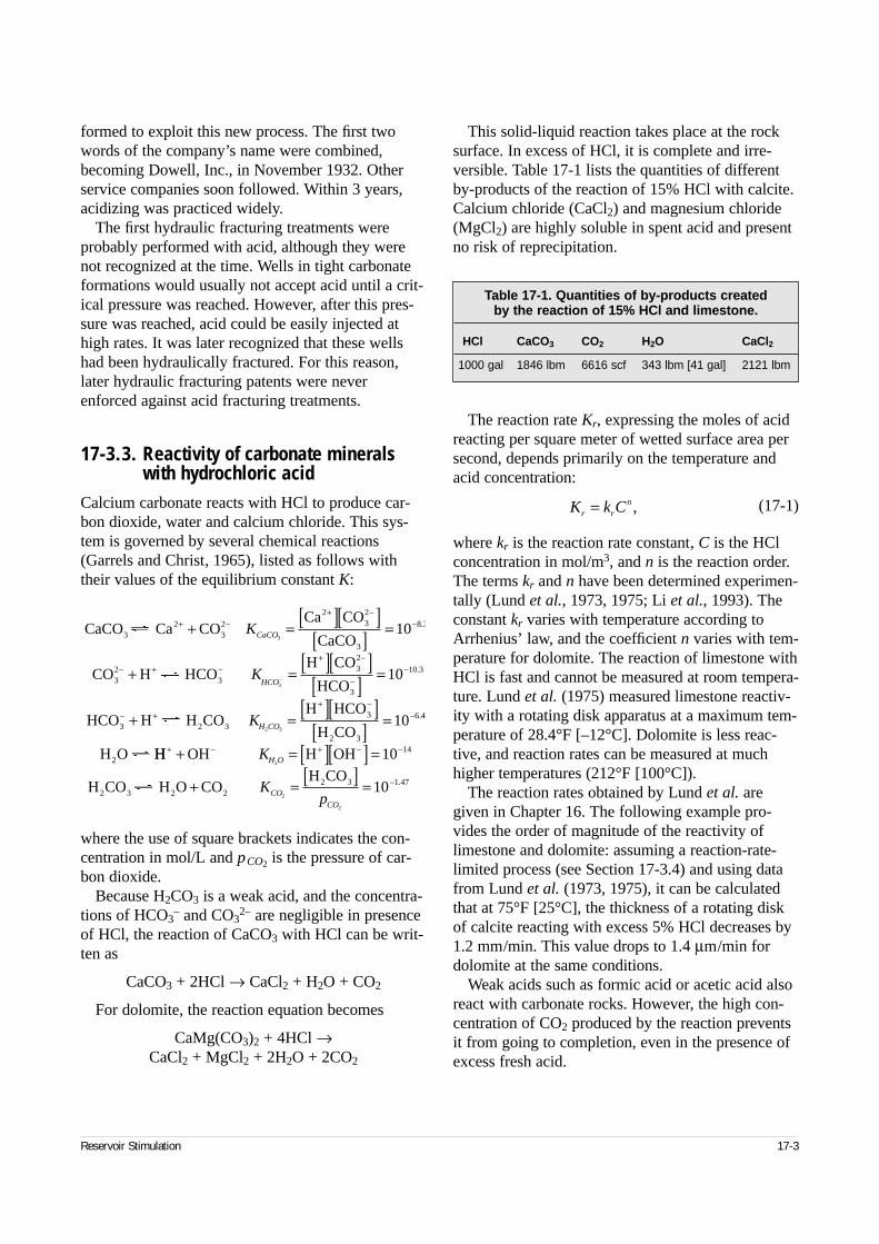
formed to exploit this new process. The first twowords of the company’s name were combined,becoming Dowell, Inc., in November 1932. Otherservice companies soon followed. Within 3 years,acidizing was practiced widely.

The first hydraulic fracturing treatments wereprobably performed with acid, although they werenot recognized at the time. Wells in tight carbonateformations would usually not accept acid until a crit-ical pressure was reached. However, after this pres-sure was reached, acid could be easily injected athigh rates. It was later recognized that these wellshad been hydraulically fractured. For this reason,later hydraulic fracturing patents were neverenforced against acid fracturing treatments.

17-3.3. Reactivity of carbonate minerals with hydrochloric acid

Calcium carbonate reacts with HCl to produce car-bon dioxide, water and calcium chloride. This sys-tem is governed by several chemical reactions(Garrels and Christ, 1965), listed as follows withtheir values of the equilibrium constant K:

where the use of square brackets indicates the con-centration in mol/L and pCO2 is the pressure of car-bon dioxide.

Because H2CO3 is a weak acid, and the concentra-tions of HCO3

– and CO32– are negligible in presence

of HCl, the reaction of CaCO3 with HCl can be writ-ten as

CaCO3 + 2HCl → CaCl2 + H2O + CO2

For dolomite, the reaction equation becomes

CaMg(CO3)2 + 4HCl →CaCl2 + MgCl2 + 2H2O + 2CO2

This solid-liquid reaction takes place at the rocksurface. In excess of HCl, it is complete and irre-versible. Table 17-1 lists the quantities of differentby-products of the reaction of 15% HCl with calcite.Calcium chloride (CaCl2) and magnesium chloride(MgCl2) are highly soluble in spent acid and presentno risk of reprecipitation.

The reaction rate Kr, expressing the moles of acidreacting per square meter of wetted surface area persecond, depends primarily on the temperature andacid concentration:

(17-1)

where kr is the reaction rate constant, C is the HClconcentration in mol/m3, and n is the reaction order.The terms kr and n have been determined experimen-tally (Lund et al., 1973, 1975; Li et al., 1993). Theconstant kr varies with temperature according toArrhenius’ law, and the coefficient n varies with tem-perature for dolomite. The reaction of limestone withHCl is fast and cannot be measured at room tempera-ture. Lund et al. (1975) measured limestone reactiv-ity with a rotating disk apparatus at a maximum tem-perature of 28.4°F [–12°C]. Dolomite is less reac-tive, and reaction rates can be measured at muchhigher temperatures (212°F [100°C]).

The reaction rates obtained by Lund et al. aregiven in Chapter 16. The following example pro-vides the order of magnitude of the reactivity oflimestone and dolomite: assuming a reaction-rate-limited process (see Section 17-3.4) and using datafrom Lund et al. (1973, 1975), it can be calculatedthat at 75°F [25°C], the thickness of a rotating diskof calcite reacting with excess 5% HCl decreases by1.2 mm/min. This value drops to 1.4 µm/min fordolomite at the same conditions.

Weak acids such as formic acid or acetic acid alsoreact with carbonate rocks. However, the high con-centration of CO2 produced by the reaction preventsit from going to completion, even in the presence ofexcess fresh acid.

Reservoir Stimulation 17-3

CaCO Ca COCa CO

CaCO

CO H HCOH CO

HCO

HCO H H COH HCO

H CO

H O

32

32

232

3

32

3

32

3

3 2 3

3

2 3

2

↔ + = [ ][ ][ ] =

+ ↔ = [ ][ ][ ] =

+ ↔ = [ ][ ][ ] =

↔

+ −+ −

−

− + −+ −

−−

− ++ −

−

−

K

K

K

CaCO

HCO

H CO

3

3

2 3

10

10

10

8 3

10 3

6 4

.

.

.

HH OH H OH

H CO H O COH CO

2 3 2 22 3

+ − + − −

−

+ = [ ][ ] =

↔ + = [ ] =

K

Kp

H O

CO

CO

2

2

2

10

10

14

1 47.

Table 17-1. Quantities of by-products created by the reaction of 15% HCl and limestone.

HCl CaCO3 CO2 H2O CaCl2

1000 gal 1846 lbm 6616 scf 343 lbm [41 gal] 2121 lbm

K k Cr rn= ,

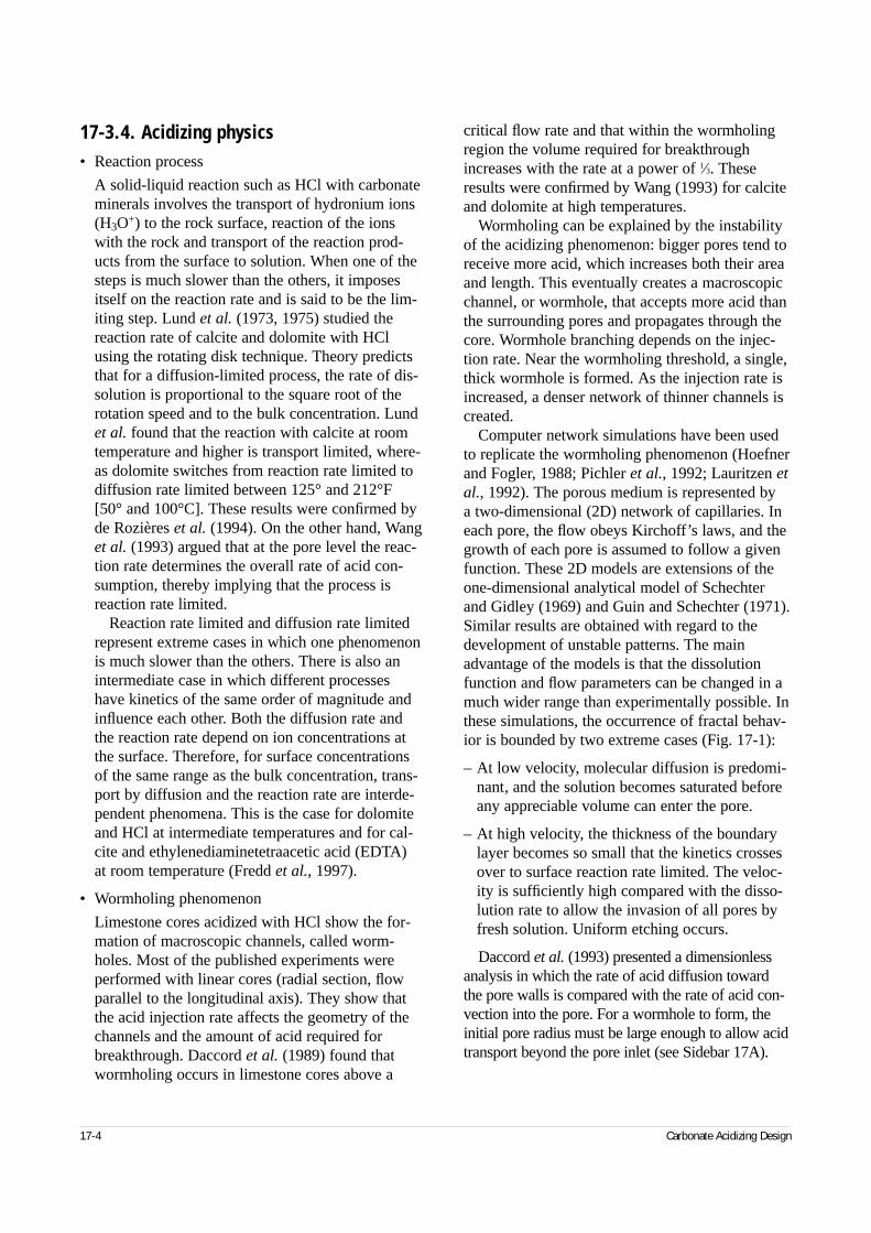
17-3.4. Acidizing physics• Reaction process

A solid-liquid reaction such as HCl with carbonateminerals involves the transport of hydronium ions(H3O+) to the rock surface, reaction of the ionswith the rock and transport of the reaction prod-ucts from the surface to solution. When one of thesteps is much slower than the others, it imposesitself on the reaction rate and is said to be the lim-iting step. Lund et al. (1973, 1975) studied thereaction rate of calcite and dolomite with HClusing the rotating disk technique. Theory predictsthat for a diffusion-limited process, the rate of dis-solution is proportional to the square root of therotation speed and to the bulk concentration. Lundet al. found that the reaction with calcite at roomtemperature and higher is transport limited, where-as dolomite switches from reaction rate limited todiffusion rate limited between 125° and 212°F[50° and 100°C]. These results were confirmed byde Rozières et al. (1994). On the other hand, Wanget al. (1993) argued that at the pore level the reac-tion rate determines the overall rate of acid con-sumption, thereby implying that the process isreaction rate limited.

Reaction rate limited and diffusion rate limitedrepresent extreme cases in which one phenomenonis much slower than the others. There is also anintermediate case in which different processeshave kinetics of the same order of magnitude andinfluence each other. Both the diffusion rate andthe reaction rate depend on ion concentrations atthe surface. Therefore, for surface concentrationsof the same range as the bulk concentration, trans-port by diffusion and the reaction rate are interde-pendent phenomena. This is the case for dolomiteand HCl at intermediate temperatures and for cal-cite and ethylenediaminetetraacetic acid (EDTA)at room temperature (Fredd et al., 1997).

• Wormholing phenomenon

Limestone cores acidized with HCl show the for-mation of macroscopic channels, called worm-holes. Most of the published experiments wereperformed with linear cores (radial section, flowparallel to the longitudinal axis). They show thatthe acid injection rate affects the geometry of thechannels and the amount of acid required forbreakthrough. Daccord et al. (1989) found thatwormholing occurs in limestone cores above a

critical flow rate and that within the wormholingregion the volume required for breakthroughincreases with the rate at a power of 1⁄3. Theseresults were confirmed by Wang (1993) for calciteand dolomite at high temperatures.

Wormholing can be explained by the instabilityof the acidizing phenomenon: bigger pores tend toreceive more acid, which increases both their areaand length. This eventually creates a macroscopicchannel, or wormhole, that accepts more acid thanthe surrounding pores and propagates through thecore. Wormhole branching depends on the injec-tion rate. Near the wormholing threshold, a single,thick wormhole is formed. As the injection rate isincreased, a denser network of thinner channels iscreated.

Computer network simulations have been usedto replicate the wormholing phenomenon (Hoefnerand Fogler, 1988; Pichler et al., 1992; Lauritzen etal., 1992). The porous medium is represented by a two-dimensional (2D) network of capillaries. Ineach pore, the flow obeys Kirchoff’s laws, and thegrowth of each pore is assumed to follow a givenfunction. These 2D models are extensions of theone-dimensional analytical model of Schechterand Gidley (1969) and Guin and Schechter (1971).Similar results are obtained with regard to thedevelopment of unstable patterns. The mainadvantage of the models is that the dissolutionfunction and flow parameters can be changed in amuch wider range than experimentally possible. Inthese simulations, the occurrence of fractal behav-ior is bounded by two extreme cases (Fig. 17-1):

– At low velocity, molecular diffusion is predomi-nant, and the solution becomes saturated beforeany appreciable volume can enter the pore.

– At high velocity, the thickness of the boundarylayer becomes so small that the kinetics crossesover to surface reaction rate limited. The veloc-ity is sufficiently high compared with the disso-lution rate to allow the invasion of all pores byfresh solution. Uniform etching occurs.

Daccord et al. (1993) presented a dimensionlessanalysis in which the rate of acid diffusion towardthe pore walls is compared with the rate of acid con-vection into the pore. For a wormhole to form, theinitial pore radius must be large enough to allow acidtransport beyond the pore inlet (see Sidebar 17A).

17-4 Carbonate Acidizing Design

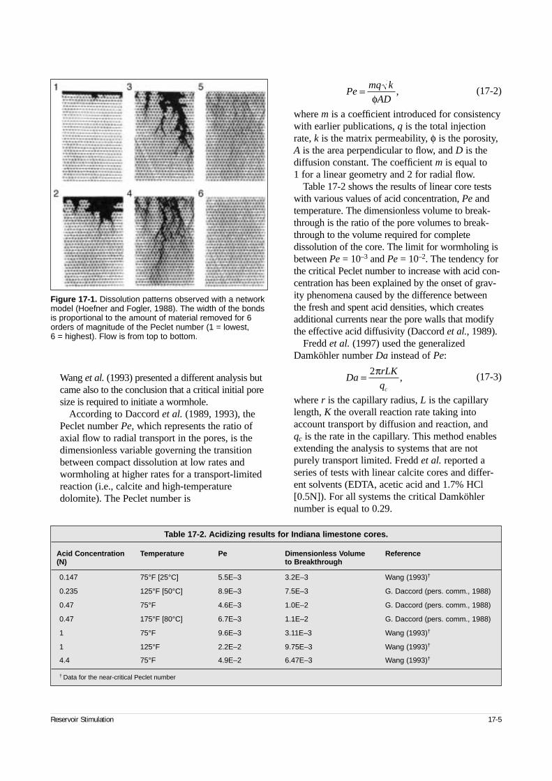
Wang et al. (1993) presented a different analysis butcame also to the conclusion that a critical initial poresize is required to initiate a wormhole.

According to Daccord et al. (1989, 1993), thePeclet number Pe, which represents the ratio ofaxial flow to radial transport in the pores, is thedimensionless variable governing the transitionbetween compact dissolution at low rates andwormholing at higher rates for a transport-limitedreaction (i.e., calcite and high-temperaturedolomite). The Peclet number is

(17-2)

where m is a coefficient introduced for consistencywith earlier publications, q is the total injectionrate, k is the matrix permeability, φ is the porosity,A is the area perpendicular to flow, and D is thediffusion constant. The coefficient m is equal to 1 for a linear geometry and 2 for radial flow.

Table 17-2 shows the results of linear core testswith various values of acid concentration, Pe andtemperature. The dimensionless volume to break-through is the ratio of the pore volumes to break-through to the volume required for complete dissolution of the core. The limit for wormholing isbetween Pe = 10–3 and Pe = 10–2. The tendency forthe critical Peclet number to increase with acid con-centration has been explained by the onset of grav-ity phenomena caused by the difference betweenthe fresh and spent acid densities, which createsadditional currents near the pore walls that modifythe effective acid diffusivity (Daccord et al., 1989).

Fredd et al. (1997) used the generalizedDamköhler number Da instead of Pe:

(17-3)

where r is the capillary radius, L is the capillarylength, K the overall reaction rate taking intoaccount transport by diffusion and reaction, and qc is the rate in the capillary. This method enablesextending the analysis to systems that are notpurely transport limited. Fredd et al. reported aseries of tests with linear calcite cores and differ-ent solvents (EDTA, acetic acid and 1.7% HCl[0.5N]). For all systems the critical Damköhlernumber is equal to 0.29.

Reservoir Stimulation 17-5

Figure 17-1. Dissolution patterns observed with a networkmodel (Hoefner and Fogler, 1988). The width of the bondsis proportional to the amount of material removed for 6orders of magnitude of the Peclet number (1 = lowest, 6 = highest). Flow is from top to bottom.

Pemq k

AD=

φ,

DarLK

qc

= 2π,

Table 17-2. Acidizing results for Indiana limestone cores.

Acid Concentration Temperature Pe Dimensionless Volume Reference(N) to Breakthrough

0.147 75°F [25°C] 5.5E–3 3.2E–3 Wang (1993)†

0.235 125°F [50°C] 8.9E–3 7.5E–3 G. Daccord (pers. comm., 1988)

0.47 75°F 4.6E–3 1.0E–2 G. Daccord (pers. comm., 1988)

0.47 175°F [80°C] 6.7E–3 1.1E–2 G. Daccord (pers. comm., 1988)

1 75°F 9.6E–3 3.11E–3 Wang (1993)†

1 125°F 2.2E–2 9.75E–3 Wang (1993)†

4.4 75°F 4.9E–2 6.47E–3 Wang (1993)†

† Data for the near-critical Peclet number

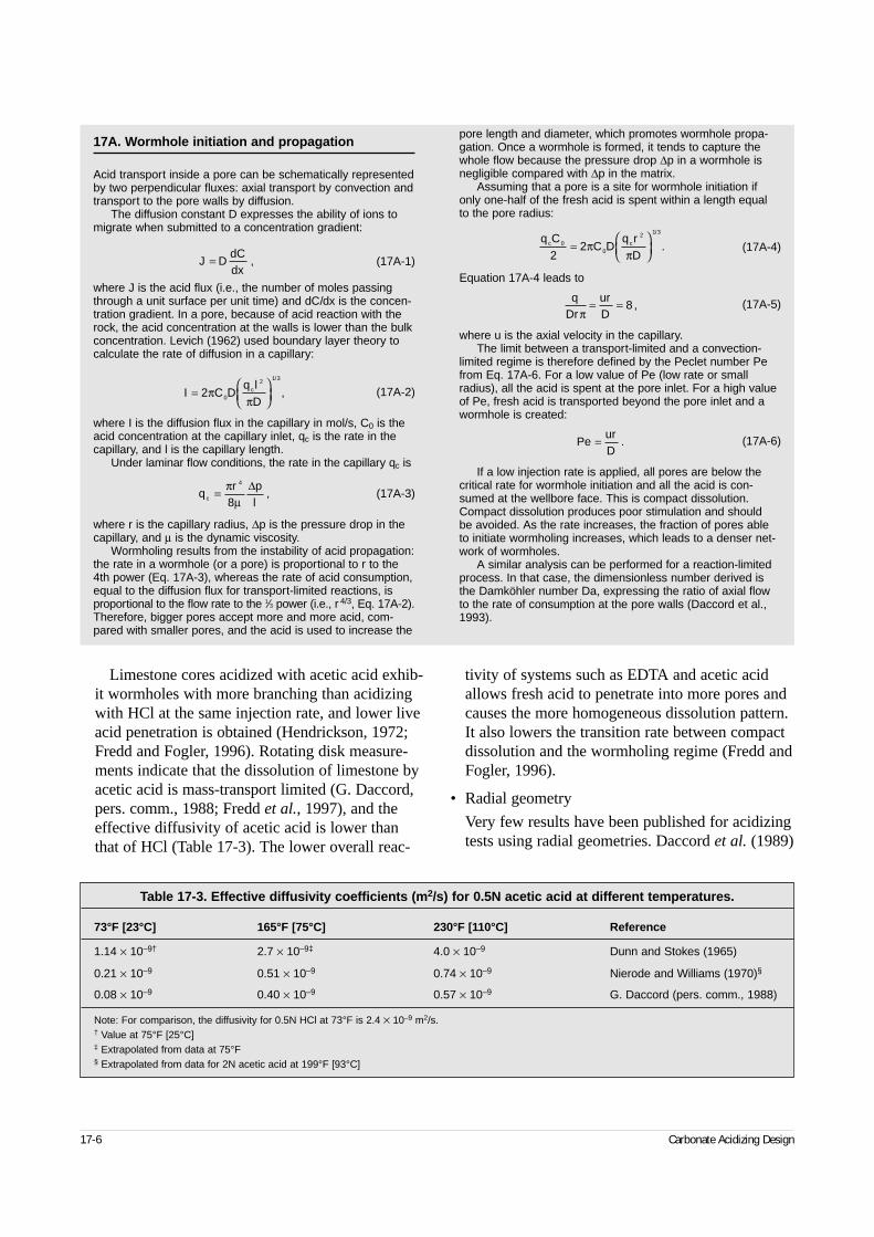
Limestone cores acidized with acetic acid exhib-it wormholes with more branching than acidizingwith HCl at the same injection rate, and lower liveacid penetration is obtained (Hendrickson, 1972;Fredd and Fogler, 1996). Rotating disk measure-ments indicate that the dissolution of limestone byacetic acid is mass-transport limited (G. Daccord,pers. comm., 1988; Fredd et al., 1997), and theeffective diffusivity of acetic acid is lower thanthat of HCl (Table 17-3). The lower overall reac-

tivity of systems such as EDTA and acetic acidallows fresh acid to penetrate into more pores andcauses the more homogeneous dissolution pattern.It also lowers the transition rate between compactdissolution and the wormholing regime (Fredd andFogler, 1996).

• Radial geometry

Very few results have been published for acidizingtests using radial geometries. Daccord et al. (1989)

17-6 Carbonate Acidizing Design

17A. Wormhole initiation and propagation

Acid transport inside a pore can be schematically representedby two perpendicular fluxes: axial transport by convection andtransport to the pore walls by diffusion.

The diffusion constant D expresses the ability of ions tomigrate when submitted to a concentration gradient:

(17A-1)

where J is the acid flux (i.e., the number of moles passingthrough a unit surface per unit time) and dC/dx is the concen-tration gradient. In a pore, because of acid reaction with therock, the acid concentration at the walls is lower than the bulkconcentration. Levich (1962) used boundary layer theory tocalculate the rate of diffusion in a capillary:

(17A-2)

where I is the diffusion flux in the capillary in mol/s, C0 is theacid concentration at the capillary inlet, qc is the rate in thecapillary, and l is the capillary length.

Under laminar flow conditions, the rate in the capillary qc is

(17A-3)

where r is the capillary radius, ∆p is the pressure drop in thecapillary, and µ is the dynamic viscosity.

Wormholing results from the instability of acid propagation:the rate in a wormhole (or a pore) is proportional to r to the4th power (Eq. 17A-3), whereas the rate of acid consumption,equal to the diffusion flux for transport-limited reactions, isproportional to the flow rate to the 1⁄3 power (i.e., r 4/3, Eq. 17A-2).Therefore, bigger pores accept more and more acid, com-pared with smaller pores, and the acid is used to increase the

pore length and diameter, which promotes wormhole propa-gation. Once a wormhole is formed, it tends to capture thewhole flow because the pressure drop ∆p in a wormhole isnegligible compared with ∆p in the matrix.

Assuming that a pore is a site for wormhole initiation ifonly one-half of the fresh acid is spent within a length equal to the pore radius:

(17A-4)

Equation 17A-4 leads to

(17A-5)

where u is the axial velocity in the capillary.The limit between a transport-limited and a convection-

limited regime is therefore defined by the Peclet number Pefrom Eq. 17A-6. For a low value of Pe (low rate or smallradius), all the acid is spent at the pore inlet. For a high valueof Pe, fresh acid is transported beyond the pore inlet and awormhole is created:

(17A-6)

If a low injection rate is applied, all pores are below thecritical rate for wormhole initiation and all the acid is con-sumed at the wellbore face. This is compact dissolution.Compact dissolution produces poor stimulation and should be avoided. As the rate increases, the fraction of pores ableto initiate wormholing increases, which leads to a denser net-work of wormholes.

A similar analysis can be performed for a reaction-limitedprocess. In that case, the dimensionless number derived isthe Damköhler number Da, expressing the ratio of axial flowto the rate of consumption at the pore walls (Daccord et al.,1993).

J DdCdx

= ,

qDr

urDπ

= = 8 ,

PeurD

= .

I C Dq l

Dc=

2 0

2 1 3

ππ

/

,

qr p

lc = πµ

4

8∆

,

q CC D

q r

Dc c0

0

2 1 3

22=

ππ

/

.

Table 17-3. Effective diffusivity coefficients (m2/s) for 0.5N acetic acid at different temperatures.

73°F [23°C] 165°F [75°C] 230°F [110°C] Reference

1.14 × 10–9† 2.7 × 10–9‡ 4.0 × 10–9 Dunn and Stokes (1965)

0.21 × 10–9 0.51 × 10–9 0.74 × 10–9 Nierode and Williams (1970)§

0.08 × 10–9 0.40 × 10–9 0.57 × 10–9 G. Daccord (pers. comm., 1988)

Note: For comparison, the diffusivity for 0.5N HCl at 73°F is 2.4 × 10–9 m2/s.† Value at 75°F [25°C]‡ Extrapolated from data at 75°F§ Extrapolated from data for 2N acetic acid at 199°F [93°C]

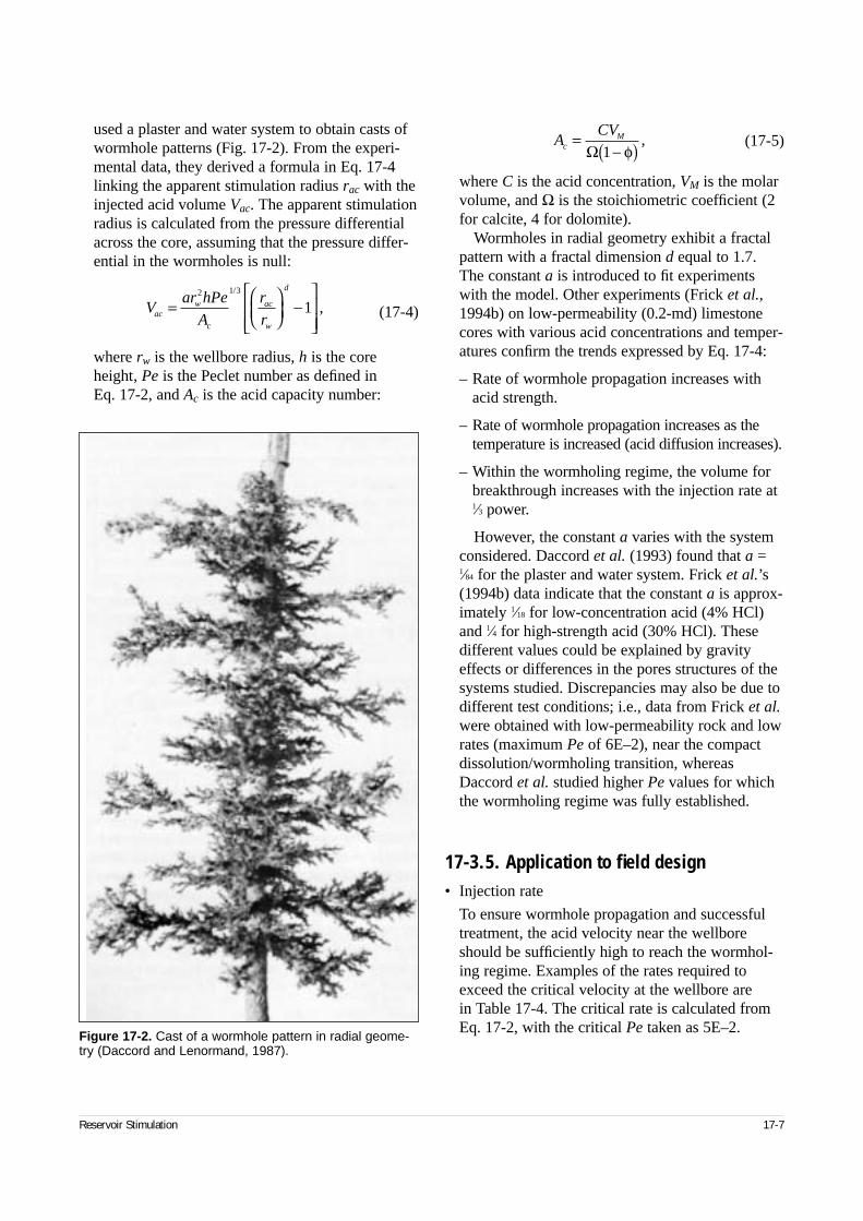
used a plaster and water system to obtain casts ofwormhole patterns (Fig. 17-2). From the experi-mental data, they derived a formula in Eq. 17-4linking the apparent stimulation radius rac with theinjected acid volume Vac. The apparent stimulationradius is calculated from the pressure differentialacross the core, assuming that the pressure differ-ential in the wormholes is null:

(17-4)

where rw is the wellbore radius, h is the coreheight, Pe is the Peclet number as defined in Eq. 17-2, and Ac is the acid capacity number:

(17-5)

where C is the acid concentration, VM is the molarvolume, and Ω is the stoichiometric coefficient (2for calcite, 4 for dolomite).

Wormholes in radial geometry exhibit a fractalpattern with a fractal dimension d equal to 1.7.The constant a is introduced to fit experimentswith the model. Other experiments (Frick et al.,1994b) on low-permeability (0.2-md) limestonecores with various acid concentrations and temper-atures confirm the trends expressed by Eq. 17-4:

– Rate of wormhole propagation increases withacid strength.

– Rate of wormhole propagation increases as thetemperature is increased (acid diffusion increases).

– Within the wormholing regime, the volume forbreakthrough increases with the injection rate at1⁄3 power.

However, the constant a varies with the systemconsidered. Daccord et al. (1993) found that a =1⁄84 for the plaster and water system. Frick et al.’s(1994b) data indicate that the constant a is approx-imately 1⁄18 for low-concentration acid (4% HCl)and 1⁄4 for high-strength acid (30% HCl). Thesedifferent values could be explained by gravityeffects or differences in the pores structures of thesystems studied. Discrepancies may also be due todifferent test conditions; i.e., data from Frick et al.were obtained with low-permeability rock and lowrates (maximum Pe of 6E–2), near the compactdissolution/wormholing transition, whereasDaccord et al. studied higher Pe values for whichthe wormholing regime was fully established.

17-3.5. Application to field design• Injection rate

To ensure wormhole propagation and successfultreatment, the acid velocity near the wellboreshould be sufficiently high to reach the wormhol-ing regime. Examples of the rates required toexceed the critical velocity at the wellbore are in Table 17-4. The critical rate is calculated from Eq. 17-2, with the critical Pe taken as 5E–2.

Reservoir Stimulation 17-7

Figure 17-2. Cast of a wormhole pattern in radial geome-try (Daccord and Lenormand, 1987).

Var hPe

A

r

racw

c

ac

w

d

=

−

2 1 3

1/

,

ACV

cM=

−( )Ω 1 φ,

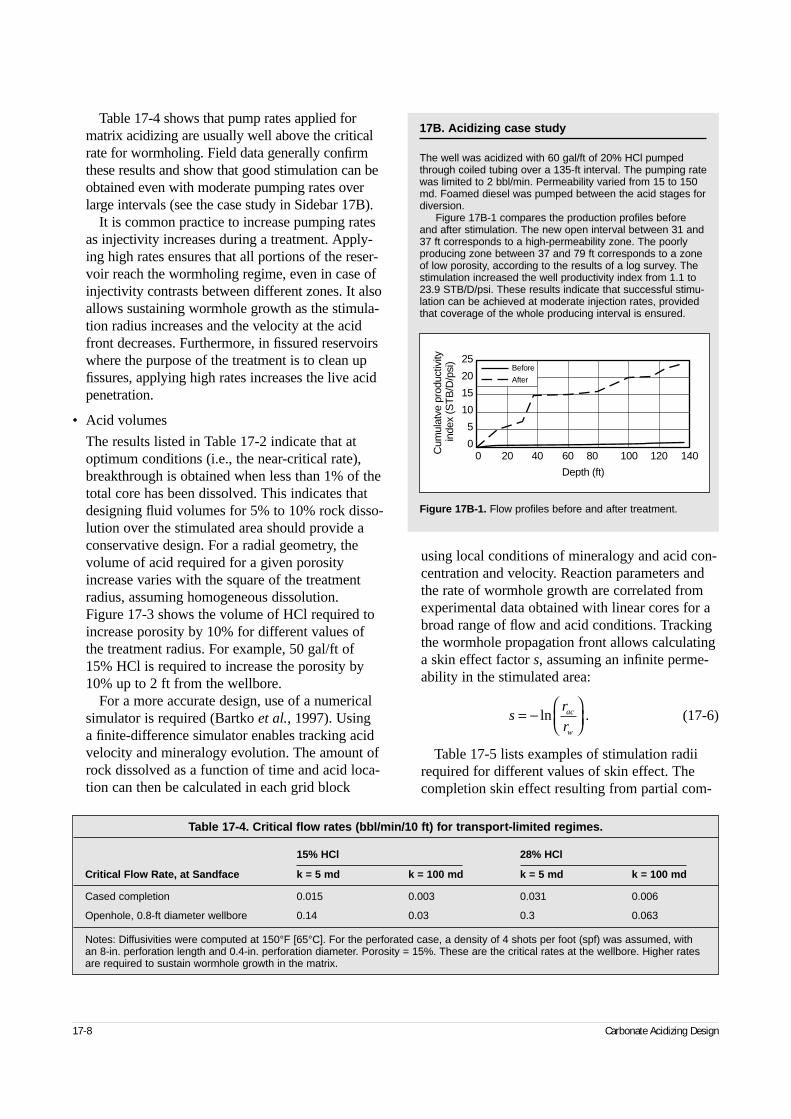
Table 17-4 shows that pump rates applied formatrix acidizing are usually well above the criticalrate for wormholing. Field data generally confirmthese results and show that good stimulation can beobtained even with moderate pumping rates overlarge intervals (see the case study in Sidebar 17B).

It is common practice to increase pumping ratesas injectivity increases during a treatment. Apply-ing high rates ensures that all portions of the reser-voir reach the wormholing regime, even in case ofinjectivity contrasts between different zones. It alsoallows sustaining wormhole growth as the stimula-tion radius increases and the velocity at the acidfront decreases. Furthermore, in fissured reservoirswhere the purpose of the treatment is to clean upfissures, applying high rates increases the live acidpenetration.

• Acid volumes

The results listed in Table 17-2 indicate that atoptimum conditions (i.e., the near-critical rate),breakthrough is obtained when less than 1% of thetotal core has been dissolved. This indicates thatdesigning fluid volumes for 5% to 10% rock disso-lution over the stimulated area should provide aconservative design. For a radial geometry, thevolume of acid required for a given porosityincrease varies with the square of the treatmentradius, assuming homogeneous dissolution. Figure 17-3 shows the volume of HCl required toincrease porosity by 10% for different values ofthe treatment radius. For example, 50 gal/ft of15% HCl is required to increase the porosity by10% up to 2 ft from the wellbore.

For a more accurate design, use of a numericalsimulator is required (Bartko et al., 1997). Using a finite-difference simulator enables tracking acidvelocity and mineralogy evolution. The amount ofrock dissolved as a function of time and acid loca-tion can then be calculated in each grid block

using local conditions of mineralogy and acid con-centration and velocity. Reaction parameters andthe rate of wormhole growth are correlated fromexperimental data obtained with linear cores for abroad range of flow and acid conditions. Trackingthe wormhole propagation front allows calculatinga skin effect factor s, assuming an infinite perme-ability in the stimulated area:

(17-6)

Table 17-5 lists examples of stimulation radiirequired for different values of skin effect. Thecompletion skin effect resulting from partial com-

17-8 Carbonate Acidizing Design

Table 17-4. Critical flow rates (bbl/min/10 ft) for transport-limited regimes.

15% HCl 28% HCl

Critical Flow Rate, at Sandface k = 5 md k = 100 md k = 5 md k = 100 md

Cased completion 0.015 0.003 0.031 0.006

Openhole, 0.8-ft diameter wellbore 0.14 0.03 0.3 0.063

Notes: Diffusivities were computed at 150°F [65°C]. For the perforated case, a density of 4 shots per foot (spf) was assumed, withan 8-in. perforation length and 0.4-in. perforation diameter. Porosity = 15%. These are the critical rates at the wellbore. Higher ratesare required to sustain wormhole growth in the matrix.

17B. Acidizing case study

The well was acidized with 60 gal/ft of 20% HCl pumpedthrough coiled tubing over a 135-ft interval. The pumping ratewas limited to 2 bbl/min. Permeability varied from 15 to 150md. Foamed diesel was pumped between the acid stages fordiversion.

Figure 17B-1 compares the production profiles beforeand after stimulation. The new open interval between 31 and37 ft corresponds to a high-permeability zone. The poorlyproducing zone between 37 and 79 ft corresponds to a zoneof low porosity, according to the results of a log survey. Thestimulation increased the well productivity index from 1.1 to23.9 STB/D/psi. These results indicate that successful stimu-lation can be achieved at moderate injection rates, providedthat coverage of the whole producing interval is ensured.

Figure 17B-1. Flow profiles before and after treatment.

0 20 40 60 80 100 120 140

Depth (ft)

25

20

15

10

5

0C

umul

atve

pro

duct

ivity

in

dex

(ST

B/D

/psi

)

Before

After

sr

rac

w

= −

ln .

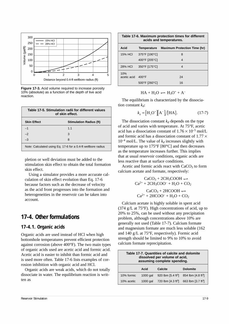
pletion or well deviation must be added to thestimulation skin effect to obtain the total formationskin effect.

Using a simulator provides a more accurate cal-culation of skin effect evolution than Eq. 17-6because factors such as the decrease of velocity as the acid front progresses into the formation andheterogeneities in the reservoir can be taken intoaccount.

17-4. Other formulations

17-4.1. Organic acidsOrganic acids are used instead of HCl when highbottomhole temperatures prevent efficient protectionagainst corrosion (above 400°F). The two main typesof organic acids used are acetic acid and formic acid.Acetic acid is easier to inhibit than formic acid andis used more often. Table 17-6 lists examples of cor-rosion inhibition with organic acid and HCl.

Organic acids are weak acids, which do not totallydissociate in water. The equilibrium reaction is writ-ten as

HA + H2O H3O+ + A–

The equilibrium is characterized by the dissocia-tion constant kd:

(17-7)

The dissociation constant kd depends on the typeof acid and varies with temperature. At 75°F, aceticacid has a dissociation constant of 1.76 × 10–5 mol/Land formic acid has a dissociation constant of 1.77 ×10–4 mol/L. The value of kd increases slightly withtemperature up to 175°F [80°C] and then decreasesas the temperature increases further. This impliesthat at usual reservoir conditions, organic acids areless reactive than at surface conditions.

Acetic and formic acids react with CaCO3 to formcalcium acetate and formate, respectively:

CaCO3 + 2CH3COOHCa2+ + 2CH3COO– + H2O + CO2

CaCO3 + 2HCOOHCa2+ + 2HCOO– + H2O + CO2

Calcium acetate is highly soluble in spent acid(374 g/L at 75°F). High concentrations of acid, up to20% to 25%, can be used without any precipitationproblem, although concentrations above 10% aregenerally not used (Table 17-7). Calcium formateand magnesium formate are much less soluble (162and 140 g/L at 75°F, respectively). Formic acidstrength should be limited to 9% to 10% to avoidcalcium formate reprecipitation.

Reservoir Stimulation 17-9

Figure 17-3. Acid volume required to increase porosity10% (absolute) as a function of the depth of live acidreaction.

0 1 2 3 4 5

300

250

200

150

100

50

0

Distance beyond 0.4-ft wellbore radius (ft)

Vol

ume

(gal

/ft)

15% HCl28% HCl

Table 17-5. Stimulation radii for different values of skin effect.

Skin Effect Stimulation Radius (ft)

–1 1.1

–2 3

–3 8

Note: Calculated using Eq. 17-6 for a 0.4-ft wellbore radius

Table 17-6. Maximum protection times for differentacids and temperatures.

Acid Temperature Maximum Protection Time (hr)

15% HCl 375°F [190°C] 8

400°F [205°C] 4

28% HCl 350°F [175°C] 4

10%acetic acid 400°F 24

500°F [260°C] 16

Table 17-7. Quantities of calcite and dolomite dissolved per volume of acid, assuming complete spending.

Acid Calcite Dolomite

10% formic 1000 gal 920 lbm [5.4 ft3] 854 lbm [4.8 ft3]

10% acetic 1000 gal 720 lbm [4.3 ft3] 663 lbm [3.7 ft3]

kd = [ ][ ] [ ]+ −H O A HA3 .

When weak acids attack CaCO3, an equilibrium is established between the chemical species pro-duced by the reaction (see the first five reactions inSection 17-3.3) and the acid species (HA + H2OH3O+ + A–). In static conditions, the degree of com-pletion of the reaction depends on the concentrationof CO2 in solution. For instance, at high-pressureconditions (typically above 1000 psi), only one-halfof 10% acetic acid reacts with limestone at 150°F[65°C]). In similar conditions, 80% of 10% formicacid reacts. Although some live acid remains oncethe reaction reaches equilibrium, a low pH is notmaintained because of buffering by the reactionproducts. Acetic acid is also beneficial for preventingferric hydroxide precipitates, because it creates aweak complex with the iron in solution and thusincreases the pH at which hydroxide precipitationoccurs (Crowe, 1985). This effect is particularly sig-nificant at low temperatures (i.e., below 125°F). Athigher temperatures, some delay of ferric hydroxideprecipitation is expected.

Formic and acetic acids can be pumped together,but usually only one acid is selected. Mixtures oforganic acid and HCl are also used. The design vol-ume depends on the suspected damage extent aroundthe wellbore. Because organic acids react morehomogeneously than HCl, larger volumes arerequired. Good results have been reported with vol-umes of the order of 100 gal/ft of 20% acid mixtureif proper placement is ensured (Ridwan and Cannan,1990). Organic acids are much more expensive thanHCl per unit volume of rock dissolved. The econom-ics of the treatment must be taken into account forthe design.

Acetic acid has other specific applications.Combined either with an aromatic solvent and amutual solvent to obtain a clear solution or withmethanol, it is used to remove water blocks andbreak emulsions. Combined with a highly concen-trated corrosion inhibitor, it can be used as comple-tion fluid to keep the pH low near the wellbore andprevent clay swelling or as a perforating fluid. In thelatter case, organic acids are preferred to HCl at tem-peratures above 200°F [95°C] because their reducedreactivity at higher temperatures enables good corro-sion protection for several days.

17-4.2. Gelled acidsGelled acids were developed primarily for fracturingbut have found some applications in matrix acidiz-ing. They are used in acid fracturing to increase theviscosity and decrease the leakoff rate. The sameprinciple applies to matrix acidizing conditions infissured or vugular formations with low primaryporosity. In this case, gelled acids are used mainly to clean up the high-permeability channels and mini-mize fluid loss in the lower permeability matrix.Gelled acids can also be used as a carrier fluid forball sealers or particulate diverters (flakes).

In the design of gelled acid treatments, the stabil-ity of the gelling agent at bottomhole temperaturesmust be checked carefully. Several types of gellingagents are used. Xantham gums are adequate formoderate conditions (i.e., temperatures up to 230°F[110°C]), with the acid strength limited to 15%(Crowe et al., 1981). Under more severe conditions,synthetic polymers are more appropriate for use upto 400° to 450°F [205° to 230°C].

Crowe et al. (1990) showed that under dynamicconditions gelled HCl exhibits the same reaction ratewith limestones as ungelled acid. In some cases,reaction rates are accelerated. The reaction rate mea-sured is the rate of calcite consumption. It is theoverall reaction rate, determined by the limiting step,which is acid transport by diffusion. It is generallyagreed (Muhr and Blanshard, 1982) that the rate ofdiffusion depends on the solvent viscosity and is notmodified by the presence of polymers, at least aslong as the distance between the polymer chains islarge compared with the size of the ions in solution.

The interaction between polymer chains and therock surface can affect the overall reaction rate andlive acid penetration. If the gel exhibits a non-Newtonian behavior, the shear rate at the rock sur-face can be modified, which may increase the masstransfer and result in a higher reaction rate. Asidefrom this effect, the polymer can plug the smallerpores, acting as a fluid-loss agent. This effect wasstudied by Nierode and Kruk (1973), who found thatthe growth rate of wormholes is maximum for asmall concentration of fluid-loss agent.

HCl is usually the acid component of gelled mix-tures. Acid strength varies typically from 5% to

17-10 Carbonate Acidizing Design

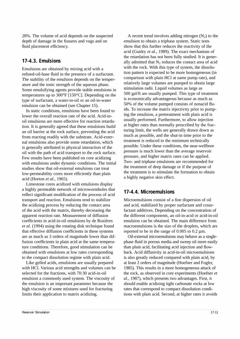
28%. The volume of acid depends on the suspecteddepth of damage in the fissures and vugs and onfluid placement efficiency.

17-4.3. EmulsionsEmulsions are obtained by mixing acid with arefined-oil-base fluid in the presence of a surfactant.The stability of the emulsion depends on the temper-ature and the ionic strength of the aqueous phase.Some emulsifying agents provide stable emulsions intemperatures up to 300°F [150°C]. Depending on thetype of surfactant, a water-in-oil or an oil-in-wateremulsion can be obtained (see Chapter 15).

In static conditions, emulsions have been found tolower the overall reaction rate of the acid. Acid-in-oil emulsions are more effective for reaction retarda-tion. It is generally agreed that these emulsions buildan oil barrier at the rock surface, preventing the acidfrom reacting readily with the substrate. Acid-exter-nal emulsions also provide some retardation, whichis generally attributed to physical interaction of theoil with the path of acid transport to the rock surface.Few results have been published on core acidizingwith emulsions under dynamic conditions. The initialstudies show that oil-external emulsions can treatlow-permeability cores more efficiently than plainacid (Horton et al., 1965).

Limestone cores acidized with emulsions display a highly permeable network of microwormholes thatreflect significant modification of the process of acidtransport and reaction. Emulsions tend to stabilizethe acidizing process by reducing the contact area of the acid with the matrix, thereby decreasing theapparent reaction rate. Measurement of diffusioncoefficients in acid-in-oil emulsions by de Rozièreset al. (1994) using the rotating disk technique foundthat effective diffusion coefficients in these systemsare as much as 3 orders of magnitude lower than dif-fusion coefficients in plain acid at the same tempera-ture conditions. Therefore, good stimulation can beobtained with emulsions at low rates correspondingto the compact dissolution regime with plain acid.

Like gelled acids, emulsions are usually preparedwith HCl. Various acid strengths and volumes can beselected for the fractions, with 70:30 acid-in-oilemulsion a commonly used system. The viscosity ofthe emulsion is an important parameter because thehigh viscosity of some mixtures used for fracturinglimits their application to matrix acidizing.

A recent trend involves adding nitrogen (N2) to theemulsion to obtain a triphase system. Static testsshow that this further reduces the reactivity of theacid (Guidry et al., 1989). The exact mechanism ofthe retardation has not been fully studied. It is gener-ally admitted that N2 reduces the contact area of acidwith the rock. With this type of system, the dissolu-tion pattern is expected to be more homogeneous (incomparison with plain HCl at same pump rate), andrelatively large volumes are pumped to obtain largestimulation radii. Liquid volumes as large as 500 gal/ft are usually pumped. This type of treatmentis economically advantageous because as much as50% of the volume pumped consists of nonacid flu-ids. To increase the matrix injectivity prior to pump-ing the emulsion, a pretreatment with plain acid isusually performed. Furthermore, to allow injection at higher rates than normally prescribed by the frac-turing limit, the wells are generally drawn down asmuch as possible, and the shut-in time prior to thetreatment is reduced to the minimum technicallypossible. Under these conditions, the near-wellborepressure is much lower than the average reservoirpressure, and higher matrix rates can be applied.Two- and triphase emulsions are recommended forthe treatment of deep damage or if the purpose of the treatment is to stimulate the formation to obtain a highly negative skin effect.

17-4.4. MicroemulsionsMicroemulsions consist of a fine dispersion of oiland acid, stabilized by proper surfactant and cosur-factant additives. Depending on the concentration ofthe different components, an oil-in-acid or acid-in-oilemulsion can be obtained. The main difference frommacroemulsions is the size of the droplets, which arereported to be in the range of 0.005 to 0.2 µm.

Oil-external microemulsions may behave as a single-phase fluid in porous media and sweep oil more easilythan plain acid, facilitating acid injection and flow-back. Acid diffusivity in acid-in-oil microemulsionsis also greatly reduced compared with plain acid, byat least 2 orders of magnitude (Hoefner and Fogler,1985). This results in a more homogeneous attack ofthe rock, as observed in core experiments (Hoefner etal., 1987), which presents two advantages. First, itshould enable acidizing tight carbonate rocks at lowrates that correspond to compact dissolution condi-tions with plain acid. Second, at higher rates it avoids

Reservoir Stimulation 17-11

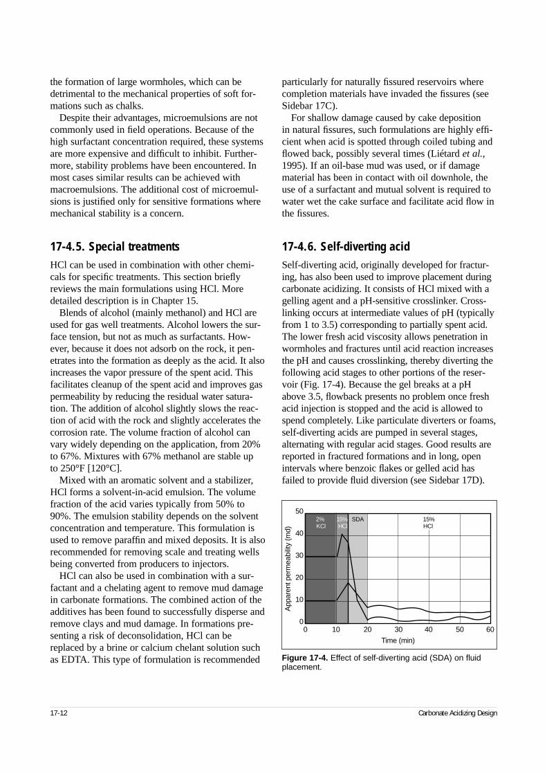
17-12 Carbonate Acidizing Design

the formation of large wormholes, which can bedetrimental to the mechanical properties of soft for-mations such as chalks.

Despite their advantages, microemulsions are notcommonly used in field operations. Because of thehigh surfactant concentration required, these systemsare more expensive and difficult to inhibit. Further-more, stability problems have been encountered. Inmost cases similar results can be achieved withmacroemulsions. The additional cost of microemul-sions is justified only for sensitive formations wheremechanical stability is a concern.

17-4.5. Special treatmentsHCl can be used in combination with other chemi-cals for specific treatments. This section brieflyreviews the main formulations using HCl. Moredetailed description is in Chapter 15.

Blends of alcohol (mainly methanol) and HCl areused for gas well treatments. Alcohol lowers the sur-face tension, but not as much as surfactants. How-ever, because it does not adsorb on the rock, it pen-etrates into the formation as deeply as the acid. It alsoincreases the vapor pressure of the spent acid. Thisfacilitates cleanup of the spent acid and improves gaspermeability by reducing the residual water satura-tion. The addition of alcohol slightly slows the reac-tion of acid with the rock and slightly accelerates thecorrosion rate. The volume fraction of alcohol canvary widely depending on the application, from 20%to 67%. Mixtures with 67% methanol are stable up to 250°F [120°C].

Mixed with an aromatic solvent and a stabilizer,HCl forms a solvent-in-acid emulsion. The volumefraction of the acid varies typically from 50% to90%. The emulsion stability depends on the solventconcentration and temperature. This formulation isused to remove paraffin and mixed deposits. It is alsorecommended for removing scale and treating wellsbeing converted from producers to injectors.

HCl can also be used in combination with a sur-factant and a chelating agent to remove mud damagein carbonate formations. The combined action of theadditives has been found to successfully disperse andremove clays and mud damage. In formations pre-senting a risk of deconsolidation, HCl can bereplaced by a brine or calcium chelant solution suchas EDTA. This type of formulation is recommended

particularly for naturally fissured reservoirs wherecompletion materials have invaded the fissures (seeSidebar 17C).

For shallow damage caused by cake deposition in natural fissures, such formulations are highly effi-cient when acid is spotted through coiled tubing andflowed back, possibly several times (Liétard et al.,1995). If an oil-base mud was used, or if damagematerial has been in contact with oil downhole, theuse of a surfactant and mutual solvent is required towater wet the cake surface and facilitate acid flow inthe fissures.

17-4.6. Self-diverting acidSelf-diverting acid, originally developed for fractur-ing, has also been used to improve placement duringcarbonate acidizing. It consists of HCl mixed with agelling agent and a pH-sensitive crosslinker. Cross-linking occurs at intermediate values of pH (typicallyfrom 1 to 3.5) corresponding to partially spent acid.The lower fresh acid viscosity allows penetration inwormholes and fractures until acid reaction increasesthe pH and causes crosslinking, thereby diverting thefollowing acid stages to other portions of the reser-voir (Fig. 17-4). Because the gel breaks at a pHabove 3.5, flowback presents no problem once freshacid injection is stopped and the acid is allowed tospend completely. Like particulate diverters or foams,self-diverting acids are pumped in several stages,alternating with regular acid stages. Good results arereported in fractured formations and in long, openintervals where benzoic flakes or gelled acid hasfailed to provide fluid diversion (see Sidebar 17D).

Figure 17-4. Effect of self-diverting acid (SDA) on fluidplacement.

0 10 20 30 40 50 60

50

40

30

20

10

0

Time (min)

App

aren

t per

mea

bilit

y (m

d)

2%KCl

15%HCl

SDA 15%HCl

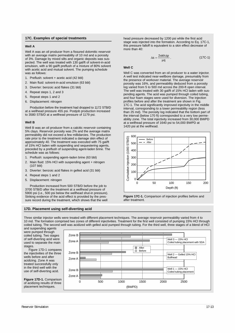
Reservoir Stimulation 17-13

17C. Examples of special treatments

Well A

Well A was an oil producer from a fissured dolomitic reservoirwith an average matrix permeability of 10 md and a porosityof 3%. Damage by mixed silts and organic deposits was sus-pected. The well was treated with 130 gal/ft of solvent-in-acidemulsion, with a 90 gal/ft preflush of a mixture of 80% solventwith acetic acid and mutual solvent. The pumping schedulewas as follows:

1. Preflush: solvent + acetic acid (42 bbl)

2. Main fluid: solvent-in-acid emulsion (63 bbl)

3. Diverter: benzoic acid flakes (31 bbl)

4. Repeat steps 1, 2 and 3

5. Repeat steps 1 and 2

6. Displacement: nitrogen

Production before the treatment had dropped to 1172 STB/Dat a wellhead pressure 455 psi. Postjob production increasedto 3580 STB/D at a wellhead pressure of 1179 psi.

Well B

Well B was an oil producer from a calcitic reservoir containing5% clays. Reservoir porosity was 2% and the average matrixpermeability did not exceed a few millidarcies. The productionrate prior to the treatment indicated a damage skin effect ofapproximately 40. The treatment was executed with 75 gal/ftof 15% HCl laden with suspending and sequestering agents,preceded by a preflush of suspending agent-laden brine. Theschedule was as follows:

1. Preflush: suspending agent–laden brine (63 bbl)

2. Main fluid: 15% HCl with suspending agent + nitrogen(107 bbl)

3. Diverter: benzoic acid flakes in gelled acid (31 bbl)

4. Repeat steps 1 and 2

5. Displacement: nitrogen

Production increased from 500 STB/D before the job to 3700 STB/D after the treatment at a wellhead pressure of 5900 psi (i.e., 500 psi below the wellhead shut-in pressure).Striking evidence of the acid effect is provided by the pres-sure record during the treatment, which shows that the well

head pressure decreased by 1200 psi while the first acidstage was injected into the formation. According to Eq. 17C-1,this pressure falloff is equivalent to a skin effect decrease ofmore than 40:

(17C-1)

Well C

Well C was converted from an oil producer to a water injector.A well test indicated near-wellbore damage, presumably fromthe presence of workover material. The average reservoirporosity was 16%, and permeability deduced from a porositylog varied from 5 to 500 md across the 200-ft open interval.The well was treated with 30 gal/ft of 15% HCl laden with sus-pending agents. The acid was pumped through coiled tubing,and four foam stages were used for diversion. The injectionprofiles before and after the treatment are shown in Fig. 17C-1. The acid significantly improved injectivity in the middleinterval, corresponding to a lower permeability region (lessthan 25 md). The porosity log indicated that the bottom part ofthe interval (below 170 ft) corresponded to a very low perme-ability zone. The total injectivity increased from 30,000 BWPDat a wellhead pressure of 1640 psi to 54,000 BWPD at 1420 psi at the wellhead.

Figure 17C-1. Comparison of injection profiles before andafter treatment.

00

100

200

300

400

500

600

50 100 150 200

Depth (ft)

Cum

ulat

ive

inje

ctio

n (1

000

ST

B/D

)

BeforeAfter

∆ ∆s

kh pq

= 2πµ

.

17D. Placement using self-diverting acid

Three similar injector wells were treated with different placement techniques. The average reservoir permeability varied from 4 to 10 md. The formation comprised two zones of different injectivities. Treatment for the first well consisted of pumping 15% HCl throughcoiled tubing. The second well was acidized with gelled acid pumped through tubing. For the third well, three stages of a blend of HCland suspending agentswere pumped throughcoiled tubing. Two stagesof self-diverting acid wereused to separate the mainstages.

Figure 17D-1 comparesthe injectivities of the threewells before and afteracidizing. Zone A wastreated successfully only in the third well with theuse of self-diverting acid.

Figure 17D-1. Comparisonof acidizing results of threeplacement techniques.

0 500 1000 1500 2000 2500

Zone A

Zone B

Zone A

Zone B

Zone A

Zone B

(BWPD)

AfterBefore

Well 1 — 15% HClCoiled tubing placement

Well 2 — Gelled 15% HClBullhead

Well 3 — 15% HClCoiled tubing placement with SDA

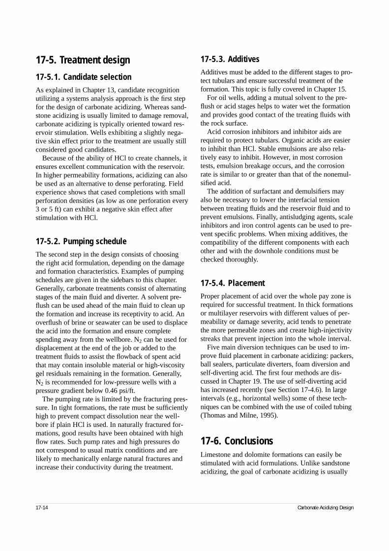
17-5. Treatment design

17-5.1. Candidate selectionAs explained in Chapter 13, candidate recognitionutilizing a systems analysis approach is the first stepfor the design of carbonate acidizing. Whereas sand-stone acidizing is usually limited to damage removal,carbonate acidizing is typically oriented toward res-ervoir stimulation. Wells exhibiting a slightly nega-tive skin effect prior to the treatment are usually stillconsidered good candidates.

Because of the ability of HCl to create channels, itensures excellent communication with the reservoir.In higher permeability formations, acidizing can alsobe used as an alternative to dense perforating. Fieldexperience shows that cased completions with smallperforation densities (as low as one perforation every3 or 5 ft) can exhibit a negative skin effect afterstimulation with HCl.

17-5.2. Pumping scheduleThe second step in the design consists of choosingthe right acid formulation, depending on the damageand formation characteristics. Examples of pumpingschedules are given in the sidebars to this chapter.Generally, carbonate treatments consist of alternatingstages of the main fluid and diverter. A solvent pre-flush can be used ahead of the main fluid to clean upthe formation and increase its receptivity to acid. Anoverflush of brine or seawater can be used to displacethe acid into the formation and ensure completespending away from the wellbore. N2 can be used fordisplacement at the end of the job or added to thetreatment fluids to assist the flowback of spent acidthat may contain insoluble material or high-viscositygel residuals remaining in the formation. Generally,N2 is recommended for low-pressure wells with apressure gradient below 0.46 psi/ft.

The pumping rate is limited by the fracturing pres-sure. In tight formations, the rate must be sufficientlyhigh to prevent compact dissolution near the well-bore if plain HCl is used. In naturally fractured for-mations, good results have been obtained with highflow rates. Such pump rates and high pressures donot correspond to usual matrix conditions and arelikely to mechanically enlarge natural fractures andincrease their conductivity during the treatment.

17-5.3. AdditivesAdditives must be added to the different stages to pro-tect tubulars and ensure successful treatment of theformation. This topic is fully covered in Chapter 15.

For oil wells, adding a mutual solvent to the pre-flush or acid stages helps to water wet the formationand provides good contact of the treating fluids withthe rock surface.

Acid corrosion inhibitors and inhibitor aids arerequired to protect tubulars. Organic acids are easierto inhibit than HCl. Stable emulsions are also rela-tively easy to inhibit. However, in most corrosiontests, emulsion breakage occurs, and the corrosionrate is similar to or greater than that of the nonemul-sified acid.

The addition of surfactant and demulsifiers mayalso be necessary to lower the interfacial tensionbetween treating fluids and the reservoir fluid and toprevent emulsions. Finally, antisludging agents, scaleinhibitors and iron control agents can be used to pre-vent specific problems. When mixing additives, thecompatibility of the different components with eachother and with the downhole conditions must bechecked thoroughly.

17-5.4. PlacementProper placement of acid over the whole pay zone isrequired for successful treatment. In thick formationsor multilayer reservoirs with different values of per-meability or damage severity, acid tends to penetratethe more permeable zones and create high-injectivitystreaks that prevent injection into the whole interval.

Five main diversion techniques can be used to im-prove fluid placement in carbonate acidizing: packers,ball sealers, particulate diverters, foam diversion andself-diverting acid. The first four methods are dis-cussed in Chapter 19. The use of self-diverting acidhas increased recently (see Section 17-4.6). In largeintervals (e.g., horizontal wells) some of these tech-niques can be combined with the use of coiled tubing(Thomas and Milne, 1995).

17-6. ConclusionsLimestone and dolomite formations can easily bestimulated with acid formulations. Unlike sandstoneacidizing, the goal of carbonate acidizing is usually

17-14 Carbonate Acidizing Design

to bypass the damage rather than dissolve it. HCl is typically used for carbonate acidizing. In case ofincompatibility with the formation or the completion(i.e., risk of corrosion), other formulations are used,such as emulsions or organic acids. Suspendingagents or solvents can also be used if required by the type of damage.

The high reactivity of acid with limestones andhigh-temperature dolomites results in the creation ofwormholes, which considerably increase the apparentpermeability around the wellbore. When wormholesextend beyond the damaged zone or connect withnatural fissures in the formation, a negative skineffect is obtained.

An engineering approach should be adopted todesign effective carbonate treatments. As in sand-

stone acidizing, proper placement of the acid overthe whole interval is necessary for successful treat-ment and usually requires employing placementtechniques. Foam diversion and self-diverting acidare two methods that are increasingly used, withgood results.

AcknowledgmentsSome of the material in this chapter was previouslyauthored by G. Daccord and published in the secondedition of this volume. The authors also thank G.Daccord, C. Fredd, R. Marcinew, A. Saxon and R.Thomas for reviewing this chapter.

Reservoir Stimulation 17-15

18-1. IntroductionSandstone matrix acidizing is distinguished from car-bonate acidizing in that it involves the dissolution ofdamage that is blocking or bridging the pore throatsin the formation matrix, thus ideally recovering theoriginal reservoir permeability. Carbonate acidizingdissolves the formation minerals around the damage,creating new permeability. The mineral acids requiredto dissolve the damage are usually highly reactivewith the numerous formation minerals. The resultingchemical complexes can become insoluble in theenvironment created and can precipitate, yieldinggelatinous or solid particles. Because the formationand the damage can have complicated crystallinestructures that can yield a variety of reaction prod-ucts, sandstone acidizing success requires a signifi-cantly better understanding of chemistry than doescarbonate acidizing. As discussed in Chapter 13, 75% of well-engineered sandstone acid treatmentsshould be successful, resulting in significant produc-tion enhancement.

The descriptor “sandstone” is derived from thegeologic classification of rocks with a high quartz sil-ica content. Besides the obvious quartz component,they contain other minerals such as aluminosilicates,metallic oxides, sulfates, chlorides, carbonates andnoncrystalline (amorphous) siliceous material. Theminerals deposited in the original sediment are calleddetrital species. Most have a high degree of associ-ated water. As fluids are produced through the matrixof the rock, the drag forces can move some of theseminerals, clogging the pore throats.

Connate water in a sandstone contains many of thedissolved native mineral species. This is due to equi-librium and partial pressures of gaseous solvents(such as carbon dioxide [CO2]) and the presence ofother ionic species. As fluids are produced, the asso-ciated pressure drop can disturb this equilibrium andthe normal ionic content of the formation brines,resulting in precipitation and possible pore-throatrestriction. This type of diagenesis yields authigenic

species (e.g., scales such as calcium carbonates aswell as some clay species such as zeolites, illites,kaolinites and smectites).

Various well operations can result in formation dam-age (see Chapter 14). For example, drilling mud andcompletion fluid usually penetrate sandstone forma-tions. This invasion of filtrate can introduce an entirelydifferent chemical environment, which the acid treat-ment must address. Additional formation damage mayoccur during perforating, gravel packing, and normalproduction or injection operations. Acid dissolves avariety of damaging materials along with most forma-tion minerals. An understanding of the chemistry isbasic to the selection of the acid type and concentration.

This chapter includes the reaction chemistry of theprimary solvent used in sandstone acidizing, hydro-fluoric acid (HF). Acid systems that contain mixturesof hydrofluoric and hydrochloric acid (HCl) are com-monly called mud acids because they were first usedto remove mud damage.

18-2. Treating fluids

18-2.1. Hydrochloric acid chemistryHCl reactions are discussed in Chapter 17, and detailsof the reaction and by-products are omitted in thischapter except for how they relate to sandstone min-erals. The compatibility of the HF blends used in thisprocess is twofold; these mixtures must meet bothcompatibility standards for the formation mineralogyand dissolution of the damage mineralogy. HF mix-tures are preceded by HCl to avoid precipitation ofthe slightly soluble and insoluble reaction products of HF with certain chemical species. The chemistryof HCl with carbonate minerals is discussed in a pre-vious chapter, so the focus here is on the chemistry of the HF systems. Although the chemistry of thereaction of HCl with carbonate or calcite is simple,the chemistry of the reaction of HF and siliceousminerals is complex.

Reservoir Stimulation 18-1

◆

Sandstone Acidizing

Harry O. McLeod, Conoco, USAWilliam David Norman, Schlumberger Dowell

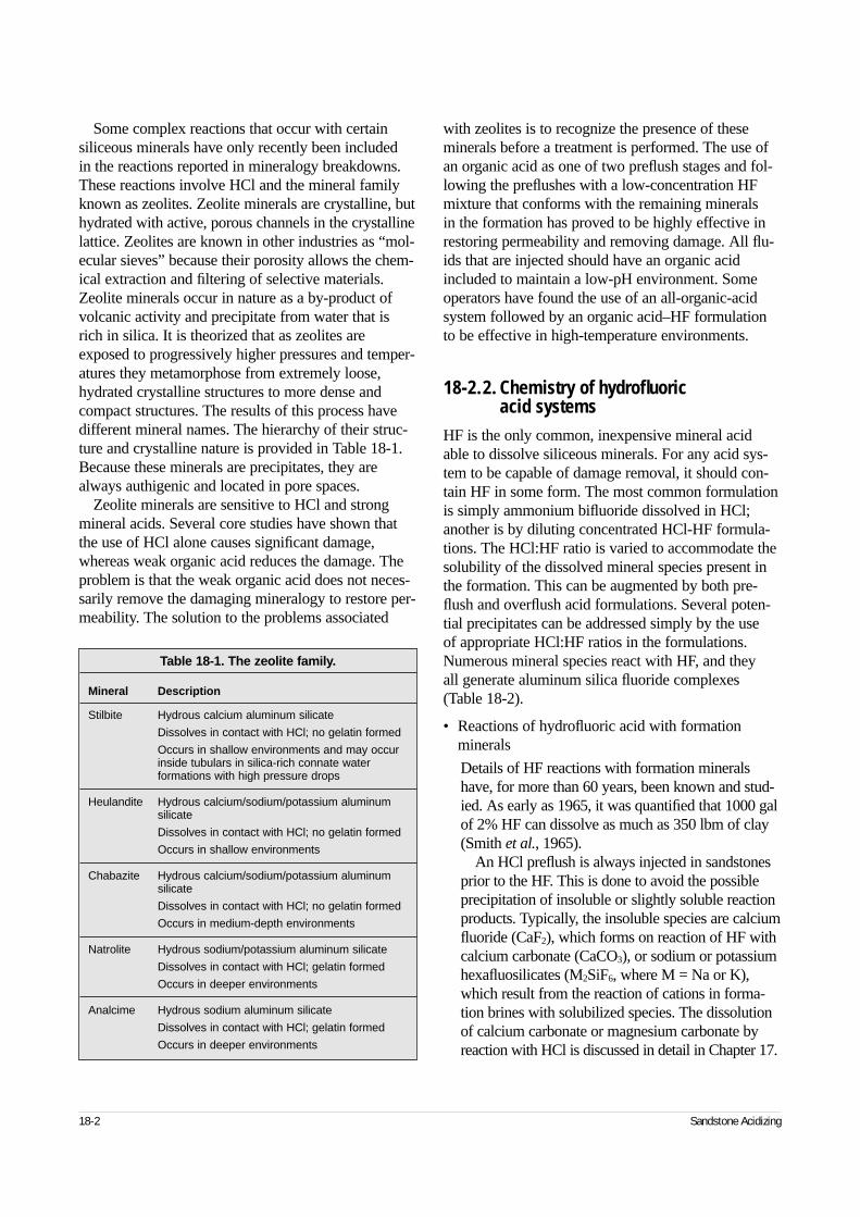
Some complex reactions that occur with certainsiliceous minerals have only recently been included in the reactions reported in mineralogy breakdowns.These reactions involve HCl and the mineral familyknown as zeolites. Zeolite minerals are crystalline, buthydrated with active, porous channels in the crystallinelattice. Zeolites are known in other industries as “mol-ecular sieves” because their porosity allows the chem-ical extraction and filtering of selective materials.Zeolite minerals occur in nature as a by-product ofvolcanic activity and precipitate from water that isrich in silica. It is theorized that as zeolites areexposed to progressively higher pressures and temper-atures they metamorphose from extremely loose,hydrated crystalline structures to more dense andcompact structures. The results of this process havedifferent mineral names. The hierarchy of their struc-ture and crystalline nature is provided in Table 18-1.Because these minerals are precipitates, they arealways authigenic and located in pore spaces.

Zeolite minerals are sensitive to HCl and strongmineral acids. Several core studies have shown thatthe use of HCl alone causes significant damage,whereas weak organic acid reduces the damage. Theproblem is that the weak organic acid does not neces-sarily remove the damaging mineralogy to restore per-meability. The solution to the problems associated

with zeolites is to recognize the presence of theseminerals before a treatment is performed. The use ofan organic acid as one of two preflush stages and fol-lowing the preflushes with a low-concentration HFmixture that conforms with the remaining minerals in the formation has proved to be highly effective inrestoring permeability and removing damage. All flu-ids that are injected should have an organic acidincluded to maintain a low-pH environment. Someoperators have found the use of an all-organic-acidsystem followed by an organic acid–HF formulationto be effective in high-temperature environments.

18-2.2.Chemistry of hydrofluoric acid systems

HF is the only common, inexpensive mineral acidable to dissolve siliceous minerals. For any acid sys-tem to be capable of damage removal, it should con-tain HF in some form. The most common formulationis simply ammonium bifluoride dissolved in HCl;another is by diluting concentrated HCl-HF formula-tions. The HCl:HF ratio is varied to accommodate thesolubility of the dissolved mineral species present inthe formation. This can be augmented by both pre-flush and overflush acid formulations. Several poten-tial precipitates can be addressed simply by the use of appropriate HCl:HF ratios in the formulations.Numerous mineral species react with HF, and they all generate aluminum silica fluoride complexes(Table 18-2).

• Reactions of hydrofluoric acid with formation minerals

Details of HF reactions with formation mineralshave, for more than 60 years, been known and stud-ied. As early as 1965, it was quantified that 1000 galof 2% HF can dissolve as much as 350 lbm of clay(Smith et al., 1965).

An HCl preflush is always injected in sandstonesprior to the HF. This is done to avoid the possibleprecipitation of insoluble or slightly soluble reactionproducts. Typically, the insoluble species are calciumfluoride (CaF2), which forms on reaction of HF withcalcium carbonate (CaCO3), or sodium or potassiumhexafluosilicates (M2SiF6, where M = Na or K),which result from the reaction of cations in forma-tion brines with solubilized species. The dissolutionof calcium carbonate or magnesium carbonate byreaction with HCl is discussed in detail in Chapter 17.

18-2 Sandstone Acidizing

Table 18-1. The zeolite family.

Mineral Description

Stilbite Hydrous calcium aluminum silicate

Dissolves in contact with HCl; no gelatin formed

Occurs in shallow environments and may occur inside tubulars in silica-rich connate waterformations with high pressure drops

Heulandite Hydrous calcium/sodium/potassium aluminum silicate

Dissolves in contact with HCl; no gelatin formed

Occurs in shallow environments

Chabazite Hydrous calcium/sodium/potassium aluminum silicate

Dissolves in contact with HCl; no gelatin formed

Occurs in medium-depth environments

Natrolite Hydrous sodium/potassium aluminum silicate

Dissolves in contact with HCl; gelatin formed

Occurs in deeper environments

Analcime Hydrous sodium aluminum silicate

Dissolves in contact with HCl; gelatin formed

Occurs in deeper environments

• Stoichiometric equations

Reactions of mud acid with the aluminosilicatecomponents of sandstones are those of HF; how-ever, HF is a weak acid and, because of the equili-brated reaction, is only slightly dissociated whenmixed with HCl:

HF + H2O H3O+ + F–

Ka = 10–3.2 at 75°F [25°C]

where Ka is the acid equilibrium constant.HF can also combine and form complexes, but

this reaction must be taken into account (Fogler etal., 1976) only when the HF concentration is suffi-ciently high (less than 10M) to allow numerouscollisions to occur between the fluoride species.This occurs only in the case of ultra mud acid (25% HCl–20% HF) formulations:

HF + F– HF2–

K = 3.86 at 75°F

The reaction of HF with quartz grains (pure sil-ica) is expressed in the following two equilibria:

SiO2 + 4HF SiF4 + 2H2O

SiF4 + 2F– SiF62–

The intermediate silicon complex, SiF5–, which isnot stable in aqueous solution, is not considered. Thefirst step of silica dissolution consists of the chemi-sorption of the fluoride anion at the silica surface(Iler, 1979). Kline and Fogler (1981b), on the con-trary, showed that it is the molecular HF rather thanthe fluoride anion that adsorbs (see Section 18-4).

Gaseous silicon tetrafluoride usually remains dis-solved in the liquid phase at bottomhole pressure, asCO2 does in the case of carbonate acidization, so theequilibrium is shifted toward the formation of siliconhexafluoride anions and the remaining SiF4 does notrepresent more than 1% of the total dissolved silicon(Labrid, 1971).

Silicon hexafluoride anions can be hydrolyzed fur-ther into monosilicic acid with the evolution of heat:

SiF62– + 8H2O Si(OH)4 + 4H3O+ + 6F–

K = 1.2 × 10–27 at 75°F

When the silicon concentration increases in theaqueous phase, part of the hexafluorosilicate anionsare also transformed into the acidic form of fluosili-cic acid according to the reaction

SiF62– + 2H3O+ H2SiF6 + 2H2O

K = 6.7 × 10–4 at 75°F

Reservoir Stimulation 18-3

Table 18-2. Chemical composition of typical sandstone minerals.

Classification Mineral Chemical Composition

Quartz SiO2

Feldspar Microcline KAlSi3O8

Orthoclase KAlSi3O8

Albite NaAlSi3O8

Plagioclase (Na,Ca)Al(Si,Al)Si2O8

Mica Biotite K(Mg,Fe2+)3(Al,Fe3+)Si3O10(OH)2

Muscovite KAl2(AlSi3)O10(OH)2

Chlorite (Mg,Fe2+,Fe3+)AlSi3O10(OH)8

Clay Kaolinite Al2Si2O5(OH)4

Illite (H3,O,K)y (Al4 ⋅ Fe4 ⋅ Mg4 ⋅ Mg6)(Si8 – y ⋅ Aly)O20(OH)4

Smectite (Ca0.5Na)0.7(Al,Mg,Fe)4(Si,Al)8O20(OH)4 ⋅ nH2O

Chlorite (Mg,Fe2+,Fe3+)AlSi3O10(OH)8

Carbonate Calcite CaCO3

Dolomite CaMg(CO3)2

Ankerite Ca(Fe,Mg,Mn)(CO3)2

Siderite FeCO3

Sulfate Gypsum CaSO4 ⋅ 2H2O

Anhydrite CaSO4

Chloride Halite NaCl

Metallic oxide Iron oxides FeO, Fe2O3, Fe3O4

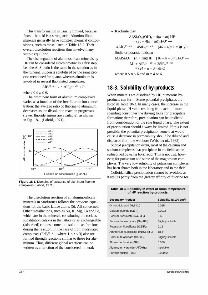
This transformation is usually limited, becausefluosilicic acid is a strong acid. Aluminosilicateminerals generally have complex chemical compo-sitions, such as those listed in Table 18-2. Theiroverall dissolution reactions thus involve manysimple equilibria.

The disintegration of aluminosilicate minerals byHF can be considered stoichiometric as a first step;i.e., the Al:Si ratio is the same in the solution as inthe mineral. Silicon is solubilized by the same pro-cess mentioned for quartz, whereas aluminum isinvolved in several fluorinated complexes:

AlFn(3 – n )+ AlFn

(4 – n )+ + F–

where 0 ≤ n ≤ 6.The prominent form of aluminum complexed

varies as a function of the free fluoride ion concen-tration: the average ratio of fluorine to aluminumdecreases as the dissolution reaction progresses(fewer fluoride anions are available), as shown in Fig. 18-1 (Labrid, 1971).

The dissolution reaction of all aluminosilicateminerals in sandstones follows the previous equa-tions for the basic lattice atoms (Si, Al) concerned.Other metallic ions, such as Na, K, Mg, Ca and Fe,which are in the minerals constituting the rock assubstitution cations in the lattice or as exchangeable(adsorbed) cations, come into solution as free ionsduring the reaction. In the case of iron, fluorinatedcomplexes (FeFz

(3 – z )+, where 1 < z < 3) also areformed through reactions similar to those for alu-minum. Thus, different global reactions can bewritten as a function of the considered mineral:

– Kaolinite clay

Al4Si4O10(OH)8 + 4(n + m) HF + (28 – 4(n + m))H3O+

4AlFn(3 – n )+ + 4SiFm

(4 – m )– + (46 – 4(n + m))H2O

– Sodic or potassic feldspar

MAlSi3O8 + (n + 3m)HF + (16 – n – 3m)H3O+

M+ + AlFn(3 – n )+ + 3SiFm

(4 – m )–

+ (24 – n – 3m)H2O

where 0 ≤ n < 6 and m = 4 or 6.

18-3. Solubility of by-productsWhen minerals are dissolved by HF, numerous by-products can form. Some potential precipitates arelisted in Table 18-3. In many cases, the increase in theliquid-phase pH value resulting from acid mixturespending constitutes the driving force for precipitateformation; therefore, precipitation can be predictedfrom consideration of the sole liquid phase. The extentof precipitation should always be limited. If this is notpossible, the potential precipitation zone that wouldcause a decrease in permeability should be diluted anddisplaced from the wellbore (Walsh et al., 1982).

Should precipitation occur, most of the calcium andsodium complexes that precipitate in the field can beredissolved by using boric acid. This is not true, how-ever, for potassium and some of the magnesium com-plexes. The very low solubility of potassium complexeshas been shown both in the laboratory and in the field.

Colloidal silica precipitation cannot be avoided, asit results partly from the greater affinity of fluorine for

18-4 Sandstone Acidizing

Figure 18-1. Domains of existence of aluminum-fluorinecomplexes (Labrid, 1971).

AIF

con

cent

ratio

n (%

) 100

50

10–4 10–3 10–2

Fluoride ion concentration (g ion ⁄ L)

AIF5

AIF4

AIF3

AIF2

AIF

Table 18-3. Solubility in water at room temperature of HF reaction by-products.

Secondary Product Solubility (g/100 cm3)

Orthosilicic acid (H4SiO4) 0.015

Calcium fluoride (CaF2) 0.0016

Sodium fluosilicate (Na2SiF6) 0.65

Sodium fluoaluminate (Na3AlF6) Slightly soluble

Potassium fluosilicate (K2SiF6) 0.12

Ammonium fluosilicate ((NH4)2SiF6) 18.6

Calcium fluosilicate (CaSiF6) Slightly soluble

Aluminum fluoride (AlF3) 0.559

Aluminum hydroxide (Al(OH)3) Insoluble

Ferrous sulfide (FeS) 0.00062

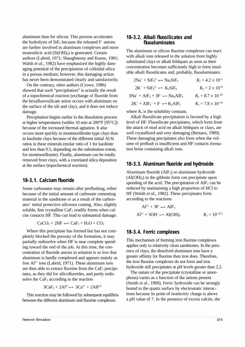
aluminum than for silicon. This process acceleratesthe hydrolysis of SiF6 because the released F– anionsare further involved in aluminum complexes and moremonosilicic acid (Si(OH)4) is generated. Certainauthors (Labrid, 1971; Shaughnessy and Kunze, 1981;Walsh et al., 1982) have emphasized the highly dam-aging potential of the precipitation of colloidal silicain a porous medium; however, this damaging actionhas never been demonstrated clearly and satisfactorily.

On the contrary, other authors (Crowe, 1986)showed that such “precipitation” is actually the resultof a topochemical reaction (exchange of fluoride fromthe hexafluorosilicate anion occurs with aluminum onthe surface of the silt and clay), and it does not inducedamage.

Precipitation begins earlier in the dissolution processat higher temperatures (within 10 min at 200°F [95°C])because of the increased thermal agitation. It alsooccurs more quickly in montmorillonite-type clays than in kaolinite clays because of the different initial Al:Siratios in these minerals (molar ratio of 1 for kaoliniteand less than 0.5, depending on the substitution extent,for montmorillonite). Finally, aluminum can be totallyremoved from clays, with a correlated silica depositionat the surface (topochemical reaction).

18-3.1. Calcium fluorideSome carbonates may remain after preflushing, eitherbecause of the initial amount of carbonate cementingmaterial in the sandstone or as a result of the carbon-ates’ initial protective siliceous coating. Also, slightlysoluble, fine crystalline CaF2 readily forms when cal-cite contacts HF. This can lead to substantial damage:

CaCO3 + 2HF CaF2 + H2O + CO2

Where this precipitate has formed but has not com-pletely blocked the porosity of the formation, it maypartially redissolve when HF is near complete spend-ing toward the end of the job. At this time, the con-centration of fluoride anions in solution is so low thataluminum is hardly complexed and appears mainly asfree Al3+ ions (Labrid, 1971). These aluminum ionsare then able to extract fluorine from the CaF2 precipi-tates, as they did for silicofluorides, and partly redis-solve the CaF2 according to the reaction

3CaF2 + 2Al3+ 3Ca2+ + 2AlF2+

This reaction may be followed by subsequent equilibriabetween the different aluminum and fluorine complexes.

18-3.2. Alkali fluosilicates and fluoaluminates

The aluminum or silicon fluorine complexes can reactwith alkali ions released in the solution from highlysubstituted clays or alkali feldspars as soon as theirconcentration becomes sufficiently high to form insol-uble alkali fluosilicates and, probably, fluoaluminates:

2Na+ + SiF62– Na2SiF6 Ks = 4.2 × 10–5

2K+ + SiF62– K2SiF6 Ks = 2 × 10–8

3Na+ + AlF3 + 3F– Na3AlF6 Ks = 8.7 × 10–18

2K+ + AlF4– + F– K2AlF5 Ks = 7.8 × 10–10

where Ks is the solubility constant.Alkali fluosilicate precipitation is favored by a high

level of HF. Fluosilicate precipitates, which form fromthe attack of mud acid on alkali feldspars or clays, arewell crystallized and very damaging (Bertaux, 1989).These damaging precipitates also form when the vol-ume of preflush is insufficient and HF contacts forma-tion brine containing alkali ions.

18-3.3. Aluminum fluoride and hydroxideAluminum fluoride (AlF3) or aluminum hydroxide(Al(OH)3) in the gibbsite form can precipitate uponspending of the acid. The precipitation of AlF3 can bereduced by maintaining a high proportion of HCl toHF (Walsh et al., 1982). These precipitates formaccording to the reactions

Al3+ + 3F– AlF3

Al3+ + 3OH– Al(OH)3 Ks = 10–32.5

18-3.4. Ferric complexesThis mechanism of forming iron fluorine complexesapplies only to relatively clean sandstones. In the pres-ence of clays, the dissolved aluminum ions have agreater affinity for fluorine than iron does. Therefore,the iron fluorine complexes do not form and ironhydroxide still precipitates at pH levels greater than 2.2.

The nature of the precipitate (crystalline or amor-phous) varies as a function of the anions present(Smith et al., 1969). Ferric hydroxide can be stronglybound to the quartz surface by electrostatic interac-tions because its point of isoelectric charge is above a pH value of 7. In the presence of excess calcite, the

Reservoir Stimulation 18-5

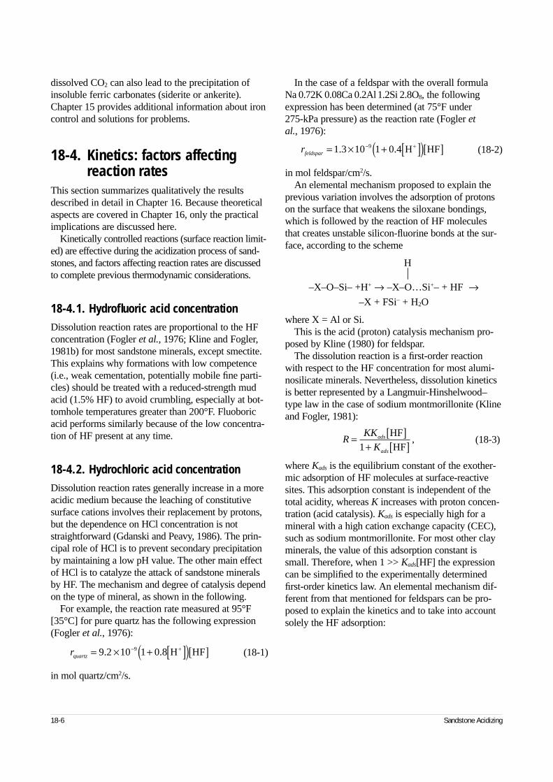
dissolved CO2 can also lead to the precipitation ofinsoluble ferric carbonates (siderite or ankerite).Chapter 15 provides additional information about ironcontrol and solutions for problems.

18-4. Kinetics: factors affecting reaction rates

This section summarizes qualitatively the resultsdescribed in detail in Chapter 16. Because theoreticalaspects are covered in Chapter 16, only the practicalimplications are discussed here.

Kinetically controlled reactions (surface reaction limit-ed) are effective during the acidization process of sand-stones, and factors affecting reaction rates are discussedto complete previous thermodynamic considerations.

18-4.1. Hydrofluoric acid concentrationDissolution reaction rates are proportional to the HFconcentration (Fogler et al., 1976; Kline and Fogler,1981b) for most sandstone minerals, except smectite.This explains why formations with low competence(i.e., weak cementation, potentially mobile fine parti-cles) should be treated with a reduced-strength mudacid (1.5% HF) to avoid crumbling, especially at bot-tomhole temperatures greater than 200°F. Fluoboricacid performs similarly because of the low concentra-tion of HF present at any time.

18-4.2. Hydrochloric acid concentrationDissolution reaction rates generally increase in a moreacidic medium because the leaching of constitutivesurface cations involves their replacement by protons,but the dependence on HCl concentration is notstraightforward (Gdanski and Peavy, 1986). The prin-cipal role of HCl is to prevent secondary precipitationby maintaining a low pH value. The other main effectof HCl is to catalyze the attack of sandstone mineralsby HF. The mechanism and degree of catalysis dependon the type of mineral, as shown in the following.

For example, the reaction rate measured at 95°F[35°C] for pure quartz has the following expression(Fogler et al., 1976):

(18-1)

in mol quartz/cm2/s.

In the case of a feldspar with the overall formula Na 0.72K 0.08Ca 0.2Al1.2Si 2.8O8, the followingexpression has been determined (at 75°F under 275-kPa pressure) as the reaction rate (Fogler etal., 1976):

(18-2)

in mol feldspar/cm2/s.An elemental mechanism proposed to explain the

previous variation involves the adsorption of protonson the surface that weakens the siloxane bondings,which is followed by the reaction of HF moleculesthat creates unstable silicon-fluorine bonds at the sur-face, according to the scheme

H

–X–O–Si– +H+ → –X–O…Si+– + HF →–X + FSi– + H2O

where X = Al or Si.This is the acid (proton) catalysis mechanism pro-

posed by Kline (1980) for feldspar.The dissolution reaction is a first-order reaction

with respect to the HF concentration for most alumi-nosilicate minerals. Nevertheless, dissolution kineticsis better represented by a Langmuir-Hinshelwood–type law in the case of sodium montmorillonite (Klineand Fogler, 1981):

(18-3)

where Kads is the equilibrium constant of the exother-mic adsorption of HF molecules at surface-reactivesites. This adsorption constant is independent of thetotal acidity, whereas K increases with proton concen-tration (acid catalysis). Kads is especially high for amineral with a high cation exchange capacity (CEC),such as sodium montmorillonite. For most other clayminerals, the value of this adsorption constant issmall. Therefore, when 1 >> Kads[HF] the expressioncan be simplified to the experimentally determinedfirst-order kinetics law. An elemental mechanism dif-ferent from that mentioned for feldspars can be pro-posed to explain the kinetics and to take into accountsolely the HF adsorption:

18-6 Sandstone Acidizing

rquartz = × + [ ]( )[ ]− +9 2 10 1 0 89. . H HF

rfeldspar = × + [ ]( )[ ]− +1 3 10 1 0 49. . H HF

RKK

Kads

ads

= [ ]+ [ ]

HFHF1

,

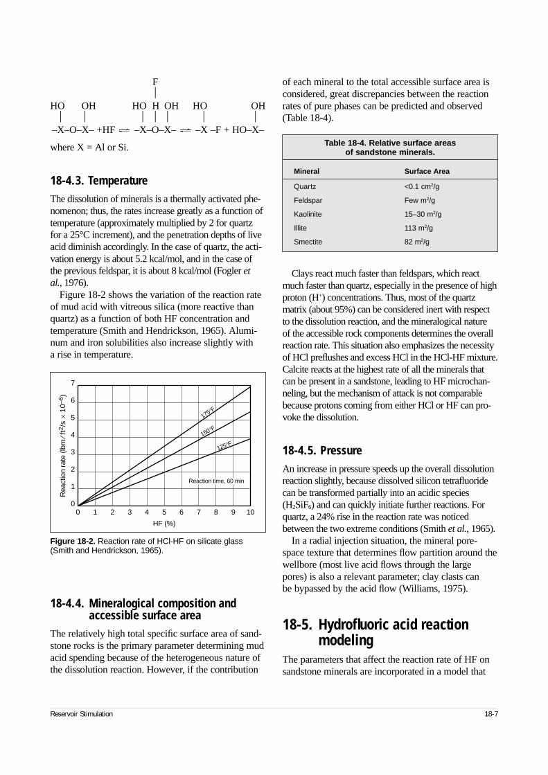
F

HO OH HO H OH HO OH

–X–O–X– +HF –X–O–X– –X –F + HO–X–

where X = Al or Si.

18-4.3. TemperatureThe dissolution of minerals is a thermally activated phe-nomenon; thus, the rates increase greatly as a function oftemperature (approximately multiplied by 2 for quartzfor a 25°C increment), and the penetration depths of liveacid diminish accordingly. In the case of quartz, the acti-vation energy is about 5.2 kcal/mol, and in the case ofthe previous feldspar, it is about 8 kcal/mol (Fogler etal., 1976).

Figure 18-2 shows the variation of the reaction rateof mud acid with vitreous silica (more reactive thanquartz) as a function of both HF concentration andtemperature (Smith and Hendrickson, 1965). Alumi-num and iron solubilities also increase slightly with a rise in temperature.

18-4.4. Mineralogical composition and accessible surface area

The relatively high total specific surface area of sand-stone rocks is the primary parameter determining mudacid spending because of the heterogeneous nature ofthe dissolution reaction. However, if the contribution

of each mineral to the total accessible surface area isconsidered, great discrepancies between the reactionrates of pure phases can be predicted and observed(Table 18-4).

Clays react much faster than feldspars, which reactmuch faster than quartz, especially in the presence of highproton (H+) concentrations. Thus, most of the quartzmatrix (about 95%) can be considered inert with respectto the dissolution reaction, and the mineralogical nature of the accessible rock components determines the overallreaction rate. This situation also emphasizes the necessityof HCl preflushes and excess HCl in the HCl-HF mixture.Calcite reacts at the highest rate of all the minerals thatcan be present in a sandstone, leading to HF microchan-neling, but the mechanism of attack is not comparablebecause protons coming from either HCl or HF can pro-voke the dissolution.

18-4.5. PressureAn increase in pressure speeds up the overall dissolutionreaction slightly, because dissolved silicon tetrafluoridecan be transformed partially into an acidic species(H2SiF6) and can quickly initiate further reactions. Forquartz, a 24% rise in the reaction rate was noticed between the two extreme conditions (Smith et al., 1965).

In a radial injection situation, the mineral pore-space texture that determines flow partition around thewellbore (most live acid flows through the largepores) is also a relevant parameter; clay clasts can be bypassed by the acid flow (Williams, 1975).

18-5. Hydrofluoric acid reaction modeling

The parameters that affect the reaction rate of HF onsandstone minerals are incorporated in a model that

Reservoir Stimulation 18-7

Figure 18-2. Reaction rate of HCl-HF on silicate glass(Smith and Hendrickson, 1965).

Rea

ctio

n ra

te (l

bm ⁄

ft2 /

s×

10–6

)

7

6

5

4

3

2

1

00 1 2 3 4 5 6 7 8 9 10

HF (%)

Reaction time, 60 min

125°F150°F

175°F

Table 18-4. Relative surface areas of sandstone minerals.

Mineral Surface Area

Quartz <0.1 cm2/g

Feldspar Few m2/g

Kaolinite 15–30 m2/g

Illite 113 m2/g

Smectite 82 m2/g

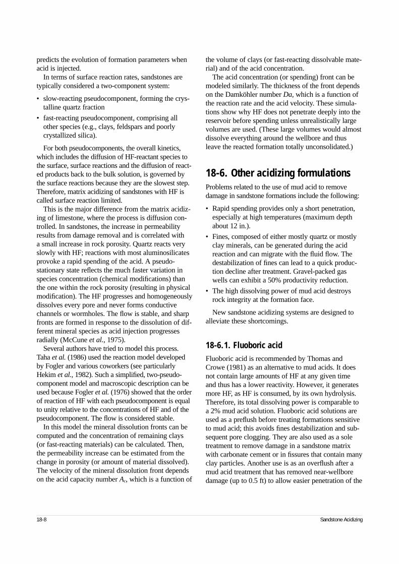
predicts the evolution of formation parameters whenacid is injected.

In terms of surface reaction rates, sandstones aretypically considered a two-component system:

• slow-reacting pseudocomponent, forming the crys-talline quartz fraction

• fast-reacting pseudocomponent, comprising allother species (e.g., clays, feldspars and poorlycrystallized silica).

For both pseudocomponents, the overall kinetics,which includes the diffusion of HF-reactant species tothe surface, surface reactions and the diffusion of react-ed products back to the bulk solution, is governed bythe surface reactions because they are the slowest step.Therefore, matrix acidizing of sandstones with HF iscalled surface reaction limited.

This is the major difference from the matrix acidiz-ing of limestone, where the process is diffusion con-trolled. In sandstones, the increase in permeabilityresults from damage removal and is correlated with a small increase in rock porosity. Quartz reacts veryslowly with HF; reactions with most aluminosilicatesprovoke a rapid spending of the acid. A pseudo-stationary state reflects the much faster variation inspecies concentration (chemical modifications) thanthe one within the rock porosity (resulting in physicalmodification). The HF progresses and homogeneouslydissolves every pore and never forms conductivechannels or wormholes. The flow is stable, and sharpfronts are formed in response to the dissolution of dif-ferent mineral species as acid injection progressesradially (McCune et al., 1975).

Several authors have tried to model this process.Taha et al. (1986) used the reaction model developedby Fogler and various coworkers (see particularlyHekim et al., 1982). Such a simplified, two-pseudo-component model and macroscopic description can beused because Fogler et al. (1976) showed that the orderof reaction of HF with each pseudocomponent is equalto unity relative to the concentrations of HF and of thepseudocomponent. The flow is considered stable.

In this model the mineral dissolution fronts can becomputed and the concentration of remaining clays(or fast-reacting materials) can be calculated. Then,the permeability increase can be estimated from thechange in porosity (or amount of material dissolved).The velocity of the mineral dissolution front dependson the acid capacity number Ac, which is a function of

the volume of clays (or fast-reacting dissolvable mate-rial) and of the acid concentration.

The acid concentration (or spending) front can bemodeled similarly. The thickness of the front dependson the Damköhler number Da, which is a function ofthe reaction rate and the acid velocity. These simula-tions show why HF does not penetrate deeply into thereservoir before spending unless unrealistically largevolumes are used. (These large volumes would almostdissolve everything around the wellbore and thusleave the reacted formation totally unconsolidated.)

18-6. Other acidizing formulationsProblems related to the use of mud acid to removedamage in sandstone formations include the following:

• Rapid spending provides only a short penetration,especially at high temperatures (maximum depthabout 12 in.).

• Fines, composed of either mostly quartz or mostlyclay minerals, can be generated during the acidreaction and can migrate with the fluid flow. Thedestabilization of fines can lead to a quick produc-tion decline after treatment. Gravel-packed gaswells can exhibit a 50% productivity reduction.

• The high dissolving power of mud acid destroysrock integrity at the formation face.

New sandstone acidizing systems are designed toalleviate these shortcomings.

18-6.1. Fluoboric acidFluoboric acid is recommended by Thomas andCrowe (1981) as an alternative to mud acids. It doesnot contain large amounts of HF at any given timeand thus has a lower reactivity. However, it generatesmore HF, as HF is consumed, by its own hydrolysis.Therefore, its total dissolving power is comparable toa 2% mud acid solution. Fluoboric acid solutions areused as a preflush before treating formations sensitiveto mud acid; this avoids fines destabilization and sub-sequent pore clogging. They are also used as a soletreatment to remove damage in a sandstone matrixwith carbonate cement or in fissures that contain manyclay particles. Another use is as an overflush after amud acid treatment that has removed near-wellboredamage (up to 0.5 ft) to allow easier penetration of the

18-8 Sandstone Acidizing

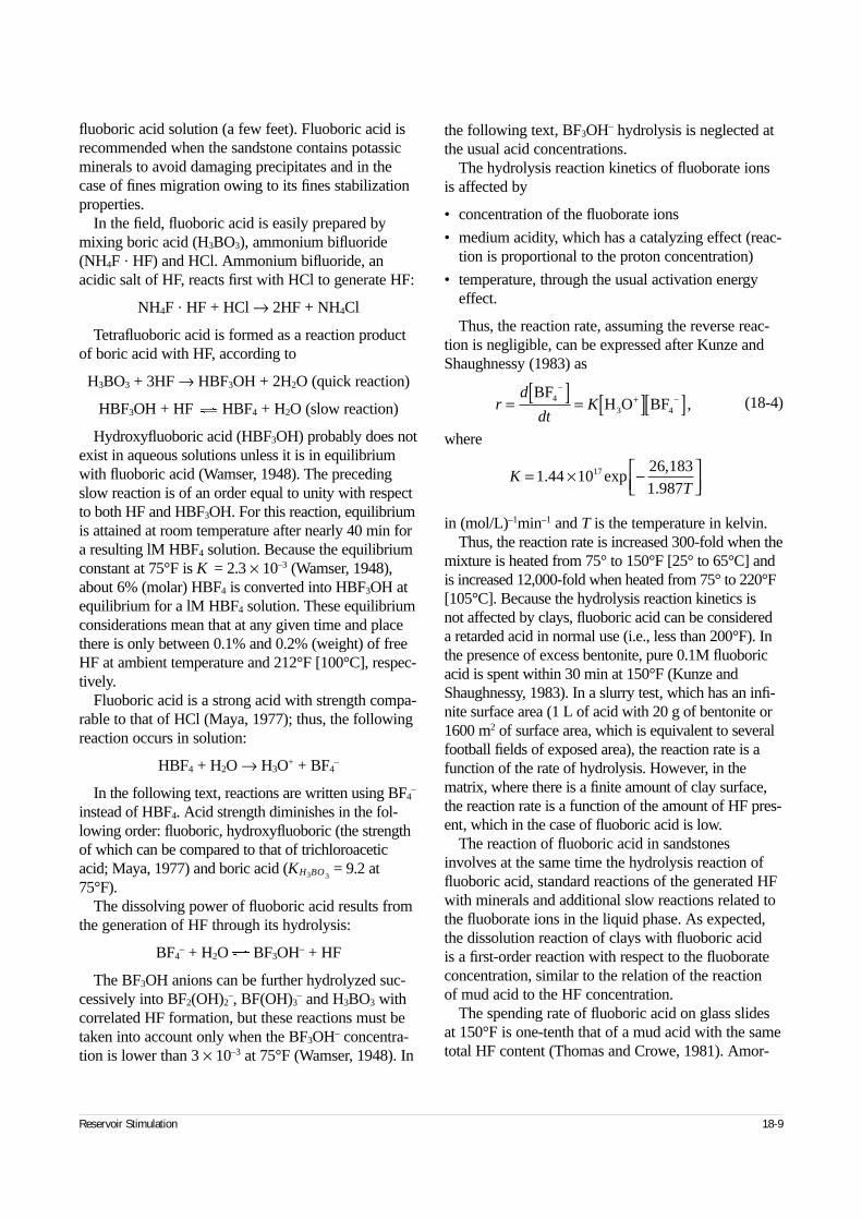
fluoboric acid solution (a few feet). Fluoboric acid isrecommended when the sandstone contains potassicminerals to avoid damaging precipitates and in thecase of fines migration owing to its fines stabilizationproperties.

In the field, fluoboric acid is easily prepared bymixing boric acid (H3BO3), ammonium bifluoride(NH4F ⋅ HF) and HCl. Ammonium bifluoride, anacidic salt of HF, reacts first with HCl to generate HF:

NH4F ⋅ HF + HCl → 2HF + NH4Cl

Tetrafluoboric acid is formed as a reaction productof boric acid with HF, according to

H3BO3 + 3HF → HBF3OH + 2H2O (quick reaction)

HBF3OH + HF HBF4 + H2O (slow reaction)

Hydroxyfluoboric acid (HBF3OH) probably does notexist in aqueous solutions unless it is in equilibriumwith fluoboric acid (Wamser, 1948). The precedingslow reaction is of an order equal to unity with respectto both HF and HBF3OH. For this reaction, equilibriumis attained at room temperature after nearly 40 min fora resulting lM HBF4 solution. Because the equilibriumconstant at 75°F is K = 2.3 × 10–3 (Wamser, 1948),about 6% (molar) HBF4 is converted into HBF3OH atequilibrium for a lM HBF4 solution. These equilibriumconsiderations mean that at any given time and placethere is only between 0.1% and 0.2% (weight) of freeHF at ambient temperature and 212°F [100°C], respec-tively.

Fluoboric acid is a strong acid with strength compa-rable to that of HCl (Maya, 1977); thus, the followingreaction occurs in solution:

HBF4 + H2O → H3O+ + BF4–

In the following text, reactions are written using BF4–

instead of HBF4. Acid strength diminishes in the fol-lowing order: fluoboric, hydroxyfluoboric (the strengthof which can be compared to that of trichloroaceticacid; Maya, 1977) and boric acid (KH3BO3

= 9.2 at75°F).

The dissolving power of fluoboric acid results fromthe generation of HF through its hydrolysis:

BF4– + H2O BF3OH– + HF

The BF3OH anions can be further hydrolyzed suc-cessively into BF2(OH)2

–, BF(OH)3– and H3BO3 with

correlated HF formation, but these reactions must betaken into account only when the BF3OH– concentra-tion is lower than 3 × 10–3 at 75°F (Wamser, 1948). In

the following text, BF3OH– hydrolysis is neglected atthe usual acid concentrations.

The hydrolysis reaction kinetics of fluoborate ionsis affected by

• concentration of the fluoborate ions

• medium acidity, which has a catalyzing effect (reac-tion is proportional to the proton concentration)

• temperature, through the usual activation energyeffect.

Thus, the reaction rate, assuming the reverse reac-tion is negligible, can be expressed after Kunze andShaughnessy (1983) as

(18-4)

where

in (mol/L)–1min–1 and T is the temperature in kelvin.Thus, the reaction rate is increased 300-fold when the

mixture is heated from 75° to 150°F [25° to 65°C] andis increased 12,000-fold when heated from 75° to 220°F[105°C]. Because the hydrolysis reaction kinetics is not affected by clays, fluoboric acid can be considered a retarded acid in normal use (i.e., less than 200°F). Inthe presence of excess bentonite, pure 0.1M fluoboricacid is spent within 30 min at 150°F (Kunze andShaughnessy, 1983). In a slurry test, which has an infi-nite surface area (1 L of acid with 20 g of bentonite or1600 m2 of surface area, which is equivalent to severalfootball fields of exposed area), the reaction rate is afunction of the rate of hydrolysis. However, in thematrix, where there is a finite amount of clay surface,the reaction rate is a function of the amount of HF pres-ent, which in the case of fluoboric acid is low.

The reaction of fluoboric acid in sandstonesinvolves at the same time the hydrolysis reaction offluoboric acid, standard reactions of the generated HFwith minerals and additional slow reactions related tothe fluoborate ions in the liquid phase. As expected,the dissolution reaction of clays with fluoboric acid is a first-order reaction with respect to the fluoborateconcentration, similar to the relation of the reaction of mud acid to the HF concentration.

The spending rate of fluoboric acid on glass slidesat 150°F is one-tenth that of a mud acid with the sametotal HF content (Thomas and Crowe, 1981). Amor-

Reservoir Stimulation 18-9

rd

dtK= [ ] = [ ][ ]

−+ −BF

H O BF43 4 ,

KT

= × −

1 44 1026 1831 987

17.,

.exp

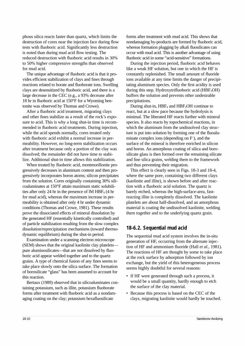
phous silica reacts faster than quartz, which limits thedestruction of cores near the injection face during flowtests with fluoboric acid. Significantly less destructionis noted than during mud acid flow testing. Thereduced destruction with fluoboric acid results in 30%to 50% higher compressive strengths than observedfor mud acid.

The unique advantage of fluoboric acid is that it pro-vides efficient stabilization of clays and fines throughreactions related to borate and fluoborate ions. Swellingclays are desensitized by fluoboric acid, and there is alarge decrease in the CEC (e.g., a 93% decrease after18 hr in fluoboric acid at 150°F for a Wyoming ben-tonite was observed by Thomas and Crowe).

After a fluoboric acid treatment, migrating claysand other fines stabilize as a result of the rock’s expo-sure to acid. This is why a long shut-in time is recom-mended in fluoboric acid treatments. During injection,while the acid spends normally, cores treated onlywith fluoboric acid exhibit a normal increase in per-meability. However, no long-term stabilization occursafter treatment because only a portion of the clay wasdissolved; the remainder did not have time to stabi-lize. Additional shut-in time allows this stabilization.

When treated by fluoboric acid, montmorillonite pro-gressively decreases in aluminum content and then pro-gressively incorporates boron atoms; silicon precipitatesfrom the solution. Cores originally containing 30% sili-coaluminates at 150°F attain maximum static solubili-ties after only 24 hr in the presence of lM HBF4 (4 hrfor mud acid), whereas the maximum increase in per-meability is obtained after only 4 hr under dynamicconditions (Thomas and Crowe, 1981). These resultsprove the dissociated effects of mineral dissolution bythe generated HF (essentially kinetically controlled) andof particle stabilization resulting from the slow complexdissolution/reprecipitation mechanisms (toward thermo-dynamic equilibrium) during the shut-in period.

Examination under a scanning electron microscope(SEM) shows that the original kaolinite clay platelets—pure aluminosilicates—that are not dissolved by fluo-boric acid appear welded together and to the quartzgrains. A type of chemical fusion of any fines seems totake place slowly onto the silica surface. The formationof borosilicate “glass” has been assumed to account forthis reaction.

Bertaux (1989) observed that in silicoaluminates con-taining potassium, such as illite, potassium fluoborateforms after treatment with fluoboric acid as a nondam-aging coating on the clay; potassium hexafluosilicate

forms after treatment with mud acid. This shows thatnondamaging by-products are formed by fluoboric acid,whereas formation plugging by alkali fluosilicates canoccur with mud acid. This is another advantage of usingfluoboric acid in some “acid-sensitive” formations.

During the injection period, fluoboric acid behaveslike a weak HF solution, but one in which the HF isconstantly replenished. The small amount of fluorideions available at any time limits the danger of precipi-tating aluminum species. Only the first acidity is usedduring this step. Hydroxytrifluoboric acid (HBF3OH)buffers the solution and prevents other undesirableprecipitations.

During shut-in, HBF4 and HBF3OH continue toreact, but at a slow pace because the hydrolysis isminimal. The liberated HF reacts further with mineralspecies. It also reacts by topochemical reactions, inwhich the aluminum from the undissolved clay struc-ture is put into solution by forming one of the fluoalu-minate complex ions (depending on F–), and thesurface of the mineral is therefore enriched in siliconand boron. An amorphous coating of silica and boro-silicate glass is then formed over the remaining silicateand fine silica grains, welding them to the frameworkand thus preventing their migration.

This effect is clearly seen in Figs. 18-3 and 18-4,where the same pore, containing two different clays(kaolinite and illite), is shown before and after reac-tion with a fluoboric acid solution. The quartz isbarely etched, whereas the high-surface-area, fast-reacting illite is completely dissolved. The kaoliniteplatelets are about half-dissolved, and an amorphousmaterial is coating the undissolved kaolinite, weldingthem together and to the underlying quartz grain.

18-6.2. Sequential mud acidThe sequential mud acid system involves the in-situgeneration of HF, occurring from the alternate injec-tion of HF and ammonium fluoride (Hall et al., 1981).The reactions of HF are thought by some to take placeat the rock surface by adsorption followed by ionexchange, but the yield of this heterogeneous processseems highly doubtful for several reasons:

• If HF were generated through such a process, itwould be a small quantity, hardly enough to etchthe surface of the clay material.

• Because this process is based on the CEC of theclays, migrating kaolinite would hardly be touched.

18-10 Sandstone Acidizing

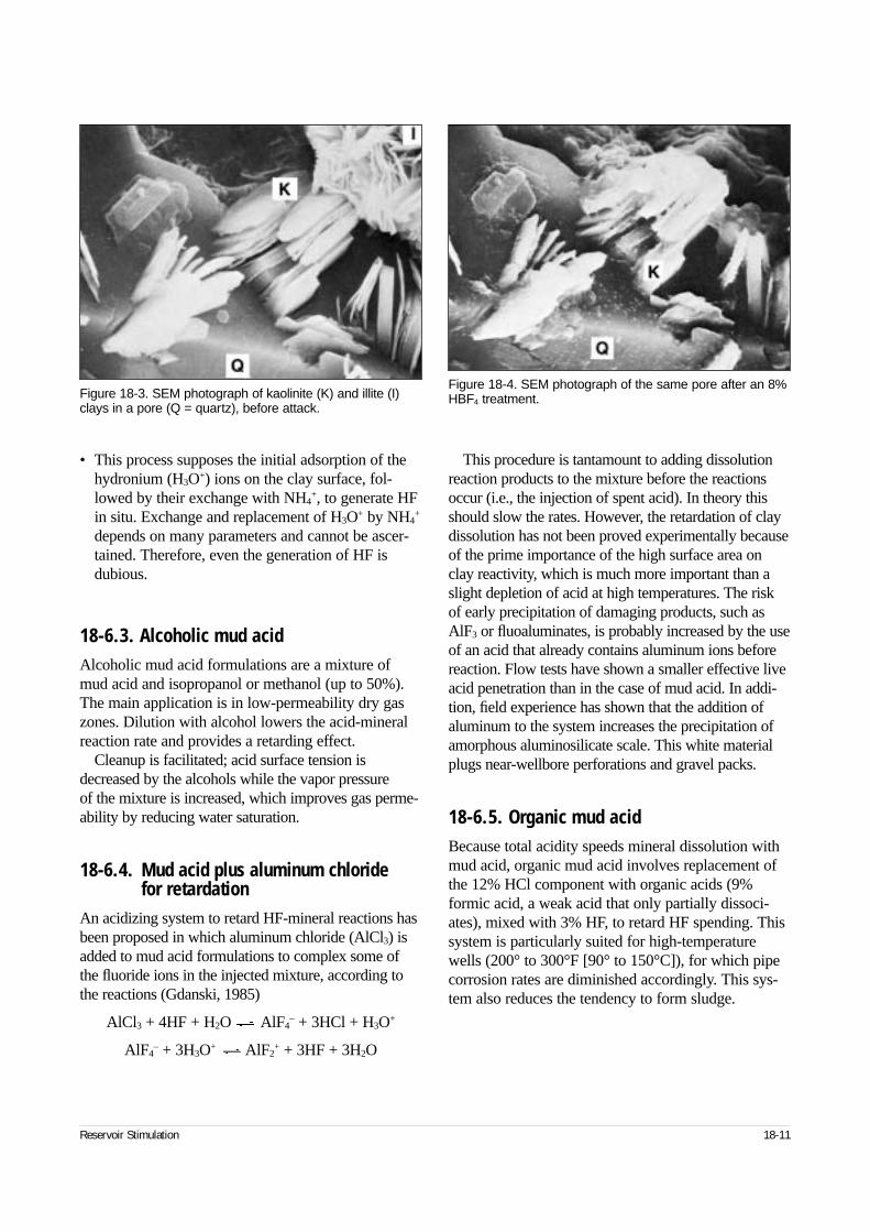
• This process supposes the initial adsorption of thehydronium (H3O+) ions on the clay surface, fol-lowed by their exchange with NH4

+, to generate HFin situ. Exchange and replacement of H3O+ by NH4

+

depends on many parameters and cannot be ascer-tained. Therefore, even the generation of HF isdubious.

18-6.3. Alcoholic mud acidAlcoholic mud acid formulations are a mixture ofmud acid and isopropanol or methanol (up to 50%).The main application is in low-permeability dry gaszones. Dilution with alcohol lowers the acid-mineralreaction rate and provides a retarding effect.

Cleanup is facilitated; acid surface tension isdecreased by the alcohols while the vapor pressure of the mixture is increased, which improves gas perme-ability by reducing water saturation.

18-6.4. Mud acid plus aluminum chloride for retardation

An acidizing system to retard HF-mineral reactions hasbeen proposed in which aluminum chloride (AlCl3) isadded to mud acid formulations to complex some ofthe fluoride ions in the injected mixture, according tothe reactions (Gdanski, 1985)

AlCl3 + 4HF + H2O AlF4– + 3HCl + H3O+

AlF4– + 3H3O+ AlF2

+ + 3HF + 3H2O

This procedure is tantamount to adding dissolutionreaction products to the mixture before the reactionsoccur (i.e., the injection of spent acid). In theory thisshould slow the rates. However, the retardation of claydissolution has not been proved experimentally becauseof the prime importance of the high surface area onclay reactivity, which is much more important than aslight depletion of acid at high temperatures. The riskof early precipitation of damaging products, such asAlF3 or fluoaluminates, is probably increased by the useof an acid that already contains aluminum ions beforereaction. Flow tests have shown a smaller effective liveacid penetration than in the case of mud acid. In addi-tion, field experience has shown that the addition ofaluminum to the system increases the precipitation ofamorphous aluminosilicate scale. This white materialplugs near-wellbore perforations and gravel packs.

18-6.5. Organic mud acidBecause total acidity speeds mineral dissolution withmud acid, organic mud acid involves replacement ofthe 12% HCl component with organic acids (9%formic acid, a weak acid that only partially dissoci-ates), mixed with 3% HF, to retard HF spending. Thissystem is particularly suited for high-temperaturewells (200° to 300°F [90° to 150°C]), for which pipecorrosion rates are diminished accordingly. This sys-tem also reduces the tendency to form sludge.

Reservoir Stimulation 18-11

Figure 18-3. SEM photograph of kaolinite (K) and illite (I)clays in a pore (Q = quartz), before attack.

Figure 18-4. SEM photograph of the same pore after an 8%HBF4 treatment.

18-6.6. Self-generating mud acid systemsSelf-generating acidizing systems were originallydeveloped by Templeton et al. (1975), and their appli-cation was widened by Abrams et al. (1983). Theyinvolve the hydrolysis of organic esters into the corre-sponding carboxylic acids, followed by the reaction ofthese acids with ammonium fluoride to yield HF.Because the hydrolysis reaction is activated by tem-perature and the acidity obtained is not as strong aswith mud acid, a low corrosion rate of tubular goodsand delayed reaction of the progressively generatedHF are expected. The latter would allow deep penetra-tion of live HF.

Depending on the bottomhole temperature, differentorganic esters are used:

• methyl formate between 130° and 180°F [55° and80°C] with the reactions

HCOOCH3 + H2O HCOOH + CH3OH

HCOOH + NH4F NH4+ + HCOO– + HF

(the latter is the slow, rate-controlling reaction).

• ammonium salt of monochloroacetic acid between180°F and 215°F [102°C]:

NH4+ + ClCH2COO– + H2O

HOCH2COOH + NH4+ + Cl–

• methyl acetate between 190° and 280°F [90° and140°C].

The reagent choice is intended to limit at 30%(maximum) the generation of HF during pumping ofthe mixture in the tubing; thus, a minimum of 40 minof spending time seems necessary. However, fieldtests of these systems have not been conclusive. Manyprecipitates form in these low acidic systems, such asralstonite (NH4MgAlF6) and other fluoaluminates(silicates) upon spending of these mixtures on clays;thus, the use of complexing agents or acids, such ascitric acid, is suggested. Furthermore, formation sensi-tivity after treatment has not been tested, and handlingproblems arise from the high flammability of methylformate.

Overall, these systems have many drawbacks. Basedon the hydrolysis of various organic esters, they aretemperature activated. Unlike fluoboric acid, whichgenerates new HF only upon spending, no equilibriumis reached. This means that more HF is generated as thetemperature increases, and the ester can eventually becompletely hydrolyzed long before reaching the final

depth of damage. The true degree of retardation dependson the temperature and pumping time. These esters aremore expensive and more dangerous to handle becauseof their flammability than HCl or inorganic salts. Moreprecipitates are formed as a result of the poor solubilityof the organic by-products. The only advantage overreduced-strength HF is lower corrosion rates.

18-6.7. Buffer-regulated hydrofluoric acid systems

Other high-pH acidizing systems proposed for use up to 360°F [180°C] involve the buffering effect of an organic acid and its ammonium salt, mixed withammonium fluoride, as an HF precursor (Abrams etal., 1983). To minimize corrosion, the use of the sameuninhibited buffer without ammonium fluoride as apreflush has been recommended up to 350°F [175°C].The ammonium salt of the organic acid is generatedfrom the partial neutralization of the acid with ammo-nium hydroxide. The proposed buffered systems are

• formic acid/ammonium formate with pH = 3.5 to 4

• acetic acid/ammonium acetate and citric acid/ammonium citrate with pH = 4.5 to 5.

To extend the application to higher temperatures (up to 550°F [290°C]), an excess of ammonium salt is formed by using a higher ratio of ammoniumhydroxide to organic acid. Because the kinetics of claydissolution increases with the fluoride ion concentra-tion, more ammonium fluoride is added to compensatefor the pH increase (Scheuerman, 1988). Successful in-depth stimulation has been observed with this systemonly for bottomhole temperatures lower than 129°F[54°C]. In most cases using this system, many damag-ing precipitates are noticed (e.g., fluosilicates, fluoalu-minate usually involving ammonium), the formation of which is related to the weak acidity in the near-wellbore area. These systems suffer from the samedrawbacks as the self-generated mud acid system.

18-7. Damage removal mechanismsSelection of a chemical as a treatment fluid for anyapplication depends on the contaminants plugging theformation. HCl does not dissolve pipe dope, paraffinor asphaltenes. These solids or plugging agents areorganic in nature, and their treatment requires aneffective organic solvent (usually an aromatic solvent

18-12 Sandstone Acidizing

such as toluene, xylene or orthonitrotoluene). Becausedifferent plugging solids require a variety of solventsfor their removal, there is no universal solvent forwellbore damage. The proper evaluation of damageand treatment design are illustrated by Clementz et al.(1982) for the successful removal of bacterial damagein water injection wells. Solvent or acid should neverbe pumped into a well until the probable causes ofdamage and the best chemical to remove the damagehave been defined.

Compatibility with formation fluids and mineralogyis extremely important in sandstone acidizing. Thus,determination of the precipitation potential of mudacid mixtures requires close scrutiny of the mineral-ogy and connate water present. Acid reaction productsare not necessarily soluble in the spent solution or incertain ionic environments.

Formation damage is fully discussed in Chapter 14.

18-7.1. Formation response to acidIncompatibilities may occur even if the damage isidentified, an appropriate removal fluid system isavailable and the probable response of the formationfluids and minerals to the acid and spent acid solutionhas been determined. These incompatibilities canresult in solid or gelatinous precipitates, which canplug pores and offset the improvement the acid wasintended to create. Results can range from no harmfuleffects and complete cleanup of the damage to lessthan optimum improvement or plugging of the forma-tion with acid-generated precipitates.

When detailed petrographic core analyses are avail-able, geochemical simulators can be used to estimatepotential problems. This type of simulation requiresdetailed definition of the chemistry of the treatingfluid, formation damage and matrix mineralogy. Therelease of fines and undefined spent-acid precipitatesstill have the potential to damage the formation andare not identified by core testing.

18-7.2. Formation propertiesDamage prevention and dealing with formation responsebefore acidizing are the goals of proper design. Althoughit may be easy to dissolve formation damage, success isdependent on dissolving this material without damagingthe formation. This is possible, yet it is paramount todefine the chemistry of the formation minerals and treat-

ing fluids to predict how the spent acid will react as itpenetrates the formation. Potential incompatibilities canbe prevented by proper log and core evaluation. Becausethe secondary reactions can be just as damaging, definingthe potential problems generated by long-term exposureshould also be evaluated.

Two key formation characteristics for fluid selectionare mineralogy and permeability. Defining formationmineralogy helps to confirm the types of acid systemsand acid concentrations to use. Defining formationpermeability provides the information required to esti-mate the matrix injection rate and the maximumbottomhole pressure allowed before hydraulicallyfracturing the formation.

Pore pressure, temperature and the mechanical condi-tion of the formation are influential in the design. High-pore-pressure formations fracture at much lower pressuredifferentials than depleted formations. Depleted forma-tions have a lower fracture pressure than that originallyobserved. Temperature significantly affects the selectedfluid’s reaction rate with different mineral types. Acidconcentrations are usually lower for higher temperatures.The mechanical integrity of the formation biases the fluidselection in that the acid concentrations are usuallyreduced in less consolidated formations.

18-7.3. Formation brine compatibilityCompatibility with formation brines must be consideredwhen treating with mud acid. Mud acid mixtures canform CaF2 (a solid) when excess Ca2+ ions are present.Similar solid materials are also created with K+ and Na+

ions. The use of clear brines as completion and work-over fluids has increased the necessity of checking theformation waters for compatibility. This brine usage hasalso increased the necessity of ensuring that sufficientcompatible preflush is used to dilute and remove theseionic species prior to injection of the mud acid system.Several available methods have been tested. The salinityof the connate brine is in equilibrium with the nativeminerals and their CEC. When possible, the salinity ofthe preflush and overflush fluids should closely approx-imate that of the connate brine. Historically, the use oflow-salinity brines has rarely presented catastrophicproblems when used in conjunction with acid treatments.

Several additives have been demonstrated to posi-tively affect the formation’s sensitivity to changes insalinity. Other species in connate water have equal, if not more, influence on the success of the treatments.

Reservoir Stimulation 18-13

Each of these species has specialty chemical additivesthat address them individually. While there is documen-tation on the benefits of certain types of additives(Gidley, 1971; Hall, 1975), other authors have reporteddamage caused by a similar system in multiphase-flowenvironments (Muecke, 1979; Davies et al., 1988).Shaughnessy and Kline (1983) showed the difficultieswith high bicarbonate ion content in formation waters.The use of HCl was not sufficient to keep the well fromredamaging itself quickly. They used an ingenioustreatment with a form of ethylenediamenetetraaceticacid (EDTA) to both remove the calcium carbonatescale that had damaged productivity and prevent recur-rence of the scale for long periods of time.

High sulfate ion contents (>1000 ppm) exist in someformation waters. Spending HCl on calcium carbonatesgenerates a high concentration of calcium ions that willprecipitate calcium sulfate when the spent acid mixeswith formation water. This can be prevented by pre-flushing the formation water away from the wellbore.In sandstone formations, water containing ammoniumchloride (NH4Cl) should be used as a preflush fluid.

18-7.4. Crude oil compatibilityAnother serious problem with formation fluids is thereaction of crude oil with acid. Removal of the residualhydrocarbon phase improves the effectiveness of aque-ous acid systems. Some oils, particularly black heavyoils (less than 30°API gravity), react with acid to formeither damaging sludge (precipitated asphaltenes) or astable emulsion. Moore et al. (1965) reported this prob-lem and gave the treatment to prevent it. Sometimessludge preventers and emulsion breakers cannot preventthe formation of stable emulsions. Houchin and Hudson(1986) discussed similar problems with organic deposits.Recent work shows how dissolved iron creates morestable sludges and emulsions with these crude oils. Some“difficult” crude oils require a hydrocarbon solvent bufferbetween the crude oil and the acid that is mutually com-patible with both the crude oil and the acid. The bufferreduces contact between the acid and the problem oiland prevents or reduces the problems with sludge andemulsion. Using this technique in one Wyoming oilfield increased the success rate from 25% to 75%.

Asphaltene particles can precipitate during produc-tion as a result of a pressure drop. Solvents can beused to loosen and partially or completely dispersethem. This action helps the acid do a better job ofdissolving acid-soluble solids. When a well has been

completed with oil-base muds, presoaks with an aro-matic solvent and producing back before acidizing arehelpful. Solvent formulations and surfactant solutionsare available as a pretreatment to clean up oil-basemud filtrates and restore the formation to a water-wetcondition.

Gidley (1985) reported that the use of CO2 as a pre-flush to acid treatments has many benefits, includingreducing the volumes of acid required to generate suc-cessful production increases. This type of preflush hasworked well in core studies to enhance crude oil dis-placement and improve mobility.

18-7.5. Formation mineral compatibilitywith fluid systems

An analysis of the formation minerals is important fordesigning the HCl preflush, mud acid treatment andoverflush in sandstone formations. Basic questionsthat must be answered are listed here.

1. How much of the formation will dissolve in HCl?

Where a high HCl solubility exists (20% or more),mud acid should not be used. This statement is basedon the assumption that HCl-soluble compounds arecarbonate-base minerals. These minerals are thecommon cementing material of sandstone forma-tions. Dissolution of this cementing material releasesparticles that can decrease the permeability. In addi-tion, precipitants exist as small discrete particles thatcannot be produced back through the perforationsand out of the well. The use of mud acid in sand-stones with a high carbonate content producesnumerous precipitates.

Calcium carbonate, magnesium carbonate andiron compounds are soluble in HCl. Even feldsparsand chlorite clay are slightly soluble (Gdanski andPeavy, 1986). Recent investigations of HCl involve-ment in the HF reaction with clays show that theHCl is consumed on the clay surfaces, and thisshould also be accounted for in the preflush volumesand in the HCl:HF ratio of the main fluid stage(Gdanski and Peavy, 1986). Zeolite minerals canproduce gelatinous precipitates when exposed toHCl. This can be avoided by the use of organic acidmixtures, as discussed later in this chapter. Sufficientvolumes of HCl must be injected ahead of the mudacid to dissolve enough of the HCl-soluble materialsbefore the mud acid or spent mud acid reaches them.

18-14 Sandstone Acidizing

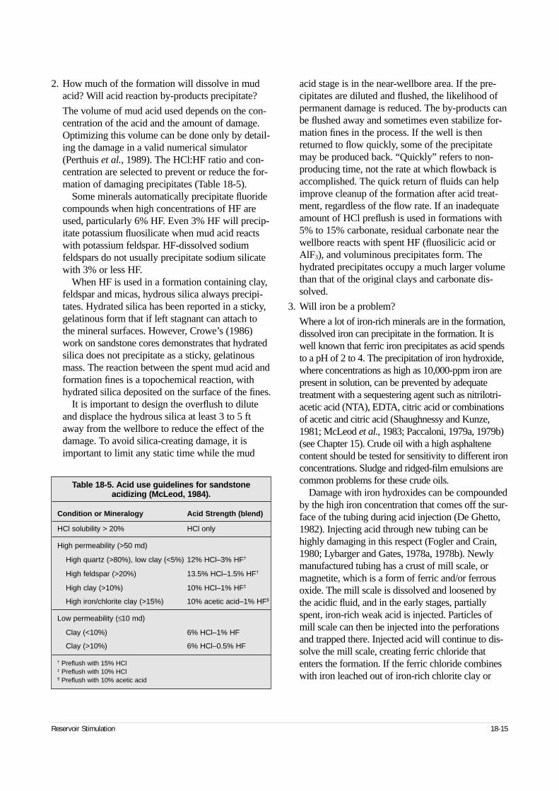
2. How much of the formation will dissolve in mudacid? Will acid reaction by-products precipitate?

The volume of mud acid used depends on the con-centration of the acid and the amount of damage.Optimizing this volume can be done only by detail-ing the damage in a valid numerical simulator(Perthuis et al., 1989). The HCl:HF ratio and con-centration are selected to prevent or reduce the for-mation of damaging precipitates (Table 18-5).

Some minerals automatically precipitate fluoridecompounds when high concentrations of HF areused, particularly 6% HF. Even 3% HF will precip-itate potassium fluosilicate when mud acid reactswith potassium feldspar. HF-dissolved sodiumfeldspars do not usually precipitate sodium silicatewith 3% or less HF.

When HF is used in a formation containing clay,feldspar and micas, hydrous silica always precipi-tates. Hydrated silica has been reported in a sticky,gelatinous form that if left stagnant can attach tothe mineral surfaces. However, Crowe’s (1986)work on sandstone cores demonstrates that hydratedsilica does not precipitate as a sticky, gelatinousmass. The reaction between the spent mud acid andformation fines is a topochemical reaction, withhydrated silica deposited on the surface of the fines.

It is important to design the overflush to diluteand displace the hydrous silica at least 3 to 5 ftaway from the wellbore to reduce the effect of thedamage. To avoid silica-creating damage, it isimportant to limit any static time while the mud

acid stage is in the near-wellbore area. If the pre-cipitates are diluted and flushed, the likelihood ofpermanent damage is reduced. The by-products canbe flushed away and sometimes even stabilize for-mation fines in the process. If the well is thenreturned to flow quickly, some of the precipitatemay be produced back. “Quickly” refers to non-producing time, not the rate at which flowback isaccomplished. The quick return of fluids can helpimprove cleanup of the formation after acid treat-ment, regardless of the flow rate. If an inadequateamount of HCl preflush is used in formations with5% to 15% carbonate, residual carbonate near thewellbore reacts with spent HF (fluosilicic acid orAlF3), and voluminous precipitates form. Thehydrated precipitates occupy a much larger volumethan that of the original clays and carbonate dis-solved.

3. Will iron be a problem?

Where a lot of iron-rich minerals are in the formation,dissolved iron can precipitate in the formation. It iswell known that ferric iron precipitates as acid spendsto a pH of 2 to 4. The precipitation of iron hydroxide,where concentrations as high as 10,000-ppm iron arepresent in solution, can be prevented by adequatetreatment with a sequestering agent such as nitrilotri-acetic acid (NTA), EDTA, citric acid or combinationsof acetic and citric acid (Shaughnessy and Kunze,1981; McLeod et al., 1983; Paccaloni, 1979a, 1979b)(see Chapter 15). Crude oil with a high asphaltenecontent should be tested for sensitivity to different ironconcentrations. Sludge and ridged-film emulsions arecommon problems for these crude oils.

Damage with iron hydroxides can be compoundedby the high iron concentration that comes off the sur-face of the tubing during acid injection (De Ghetto,1982). Injecting acid through new tubing can behighly damaging in this respect (Fogler and Crain,1980; Lybarger and Gates, 1978a, 1978b). Newlymanufactured tubing has a crust of mill scale, ormagnetite, which is a form of ferric and/or ferrousoxide. The mill scale is dissolved and loosened bythe acidic fluid, and in the early stages, partiallyspent, iron-rich weak acid is injected. Particles ofmill scale can then be injected into the perforationsand trapped there. Injected acid will continue to dis-solve the mill scale, creating ferric chloride thatenters the formation. If the ferric chloride combineswith iron leached out of iron-rich chlorite clay or

Reservoir Stimulation 18-15

Table 18-5. Acid use guidelines for sandstone acidizing (McLeod, 1984).

Condition or Mineralogy Acid Strength (blend)

HCl solubility > 20% HCl only

High permeability (>50 md)

High quartz (>80%), low clay (<5%) 12% HCl–3% HF†

High feldspar (>20%) 13.5% HCl–1.5% HF†

High clay (>10%) 10% HCl–1% HF‡

High iron/chlorite clay (>15%) 10% acetic acid–1% HF§

Low permeability (≤10 md)

Clay (<10%) 6% HCl–1% HF

Clay (>10%) 6% HCl–0.5% HF

† Preflush with 15% HCl‡ Preflush with 10% HCl§ Preflush with 10% acetic acid

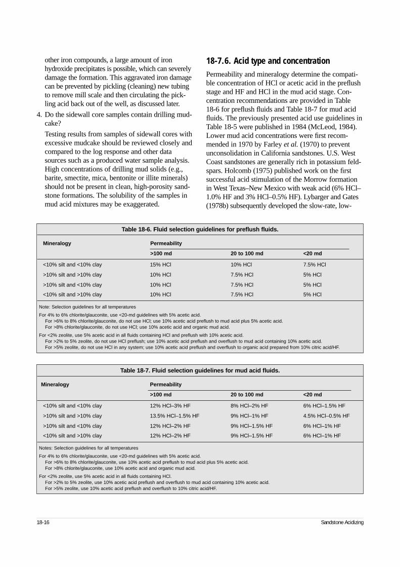
other iron compounds, a large amount of iron hydroxide precipitates is possible, which can severelydamage the formation. This aggravated iron damagecan be prevented by pickling (cleaning) new tubingto remove mill scale and then circulating the pick-ling acid back out of the well, as discussed later.

4. Do the sidewall core samples contain drilling mud-cake?

Testing results from samples of sidewall cores withexcessive mudcake should be reviewed closely andcompared to the log response and other datasources such as a produced water sample analysis.High concentrations of drilling mud solids (e.g.,barite, smectite, mica, bentonite or illite minerals)should not be present in clean, high-porosity sand-stone formations. The solubility of the samples inmud acid mixtures may be exaggerated.

18-7.6. Acid type and concentration Permeability and mineralogy determine the compati-ble concentration of HCl or acetic acid in the preflushstage and HF and HCl in the mud acid stage. Con-centration recommendations are provided in Table 18-6 for preflush fluids and Table 18-7 for mud acidfluids. The previously presented acid use guidelines inTable 18-5 were published in 1984 (McLeod, 1984).Lower mud acid concentrations were first recom-mended in 1970 by Farley et al. (1970) to preventunconsolidation in California sandstones. U.S. WestCoast sandstones are generally rich in potassium feld-spars. Holcomb (1975) published work on the firstsuccessful acid stimulation of the Morrow formationin West Texas–New Mexico with weak acid (6% HCl–1.0% HF and 3% HCl–0.5% HF). Lybarger and Gates(1978b) subsequently developed the slow-rate, low-

18-16 Sandstone Acidizing

Table 18-6. Fluid selection guidelines for preflush fluids.

Mineralogy Permeability

>100 md 20 to 100 md <20 md

<10% silt and <10% clay 15% HCl 10% HCl 7.5% HCl

>10% silt and >10% clay 10% HCl 7.5% HCl 5% HCl

>10% silt and <10% clay 10% HCl 7.5% HCl 5% HCl

<10% silt and >10% clay 10% HCl 7.5% HCl 5% HCl

Note: Selection guidelines for all temperatures

For 4% to 6% chlorite/glauconite, use <20-md guidelines with 5% acetic acid.For >6% to 8% chlorite/glauconite, do not use HCl; use 10% acetic acid preflush to mud acid plus 5% acetic acid.For >8% chlorite/glauconite, do not use HCl; use 10% acetic acid and organic mud acid.

For <2% zeolite, use 5% acetic acid in all fluids containing HCl and preflush with 10% acetic acid.For >2% to 5% zeolite, do not use HCl preflush; use 10% acetic acid preflush and overflush to mud acid containing 10% acetic acid.For >5% zeolite, do not use HCl in any system; use 10% acetic acid preflush and overflush to organic acid prepared from 10% citric acid/HF.

Table 18-7. Fluid selection guidelines for mud acid fluids.

Mineralogy Permeability

>100 md 20 to 100 md <20 md

<10% silt and <10% clay 12% HCl–3% HF 8% HCl–2% HF 6% HCl–1.5% HF

>10% silt and >10% clay 13.5% HCl–1.5% HF 9% HCl–1% HF 4.5% HCl–0.5% HF

>10% silt and <10% clay 12% HCl–2% HF 9% HCl–1.5% HF 6% HCl–1% HF

<10% silt and >10% clay 12% HCl–2% HF 9% HCl–1.5% HF 6% HCl–1% HF

Notes: Selection guidelines for all temperatures

For 4% to 6% chlorite/glauconite, use <20-md guidelines with 5% acetic acid.For >6% to 8% chlorite/glauconite, use 10% acetic acid preflush to mud acid plus 5% acetic acid.For >8% chlorite/glauconite, use 10% acetic acid and organic mud acid.

For <2% zeolite, use 5% acetic acid in all fluids containing HCl.For >2% to 5% zeolite, use 10% acetic acid preflush and overflush to mud acid containing 10% acetic acid.For >5% zeolite, use 10% acetic acid preflush and overflush to 10% citric acid/HF.

pressure injection technique, in which they used 7.5% HCl–1.5% HF for Gulf Coast sandstones.

The guidelines are based on industry practices andthe chemistry of sandstone acidizing from limitedresearch studies; however, many case histories havecorroborated them with high levels of success.

From 1975 through 1980, poor success in acidizingseveral formations such as the Frio and Wilcox inTexas led to the concern that spent acid generateddamaging precipitates. Quick, qualitative laboratorybench tests confirmed that precipitates occur depend-ing on the solubility of the acid reaction products.These same observations were first pointed out bySmith and Hendrickson (1965), in particular the prob-lem with sodium fluosilicate. Labrid (1971) discussedthe precipitation of hydrous silica, which caused someplugging in cores. This damage was later demonstrat-ed by Shaughnessy and Kunze (1981) by leavingspent acid in the core for several hours, a conditionthat occurs in an actual acid job. This allows the slowreaction rate between the spent mud acid and the clayminerals and feldspars (aluminosilicates) to producehydrous silica that decreases the permeability.

Crowe (1986) showed that there was little or noplugging during the injection of spent acid (fluosilicicacid) in a Berea core. This reassuring result matchesthe behavior seen during acid injection; however,plugging conditions are worse during the static condi-tions of shut-in examined by Shaughnessy and Kunze(1981). Crowe’s work does not address shut-in condi-tions or conditions of inadequate preflush with HCl.Walsh et al. (1982) presented theoretical work on theequilibrium of spent acid and showed that pluggingprecipitates are possible with various acid concentra-tions and mineral compositions in sandstones.

Research by Bertaux (1986) addresses reprecipitationand plugging problems in acidizing sandstones contain-ing potassium feldspars. The solubility of potassiumfluosilicate is less than one-half of the solubility of sodi-um fluosilicate, which is why lower mud acid concen-trations are recommended in the presence of potassicfeldspars such as orthoclase or microcline (KAlSi3O8).The amount of potassium in the mineral orthoclase(potassium feldspar) is enough that the solubility ofpotassium fluosilicate is exceeded at normal reservoirtemperatures (less than 200°F) by dissolving pureorthoclase in regular mud acid (12% HCl–3% HF).Bryant and Buller (1990) observed the generation offines by the reaction of HCl with feldspars.

The early work of Smith et al. (1965) in acidizingvarious cores with different permeabilities shows differ-ent responses to mud acid. C. F. Smith (pers. comm.,1979) found it more difficult to stimulate wells produc-ing from sandstones with permeabilities of 10 to 60 md,which are much lower than the usual Berea sandstonepermeability (100 to 300 md) in mud acid experiments.Smith attributed much of the difficulty to the release offines by the acid.

Long-core tests performed by R. D. Gdanski (pers.comm., 1985) in low-permeability sandstone at hightemperatures demonstrate increased permeability withmud acid in the first two 4-in. cores in series anddecreased permeability in the third 4-in. core in a totalcore length of 16 in. Gdanski and Peavy (1986) alsodiscussed the depletion of the preflush HCl in sand-stone acidizing by ion exchange of H+ with K+ or Na+

ions on the formation clay minerals. This gives newinsights into potential problems with sandstones rich in clay minerals with high CECs (smectite and illite).

Simon et al. (1979) showed that HCl attacks chlo-rite clay, extracting the iron and magnesium and leav-ing an amorphous aluminosilicate residue. J. M.Kullman (pers. comm., 1988) observed pluggingproblems with these residues as well as with rim coat-ings of chlorite liberated by HCl in core flow tests.Chlorite is prevalent in the Morrow formation in thesame areas where Holcomb (1975) worked and couldbe the reason why weaker acids worked better in thatenvironment (i.e., they were easier on the chlorite).Thus, weaker acids are recommended for use in sand-stones with significant chlorite content and acetic acidis recommended to dissolve the carbonate and notattack chlorite ahead of the mud acid.

A common misunderstanding about the recom-mended acid concentrations is that they are notabsolute. The guidelines are a conservative approachto avoid problems with spent acid precipitates whenno previous experience exists in acidizing a particularformation. Significant deviation from these guidelinesshould not be necessary. Unless evaluated experienceexists, the guidelines are the most reliable source ofinformation. Also, acid flow tests with cores are reli-able if long cores are used and if the spent acid is leftin a portion of the unacidized core for the same periodof time and at the same temperature that will occur inthe downhole treatment. These tests are expensive andtherefore seldom performed.

Reservoir Stimulation 18-17

18-8. Methods of controlling precipitates

The methods used to control the precipitates causedby acidizing are proper acid staging, lower acid con-centrations, correct usage of preflushes and sufficientoverflushing, as illustrated in the following guidelines.

18-8.1. PreflushPreflush with

1. 5% to 15% HCl

2. acetic acid (see Section 18-3).

The preflush displaces formation brine away fromthe wellbore to prevent it from mixing with reactedmud acid and causing a damaging precipitate. If theformation contains more than 1% to 2% carbonate, an HCl preflush is necessary to dissolve the carbonate,prevent the waste of mud acid and prevent formationof the insoluble precipitate CaF2.

If completion brines such as seawater, potassiumchloride (KCl), calcium chloride (CaCl2) or calciumbromide (CaBr) have been used in the well prior toacidizing, the brines will mix with the mud acid in theformation. Preflushing the mud acid with HCl or brinecontaining ammonium chloride to dilute the brinesand remove them away from the wellbore helps avoidthis problem.

Preflushes can also be used to displace and isolateincompatible formation fluids (either brine or crudeoil), as previously discussed.

18-8.2. Mud acid volume and concentration• Volume

Gidley (1985) reported that for the most successfulmud acid treatment, more than 125 gal/ft of mud acidis required. Less may be used where only shallowdamage exists around new perforations (e.g., 25 to 75 gal/ft is used to remove mud damage or in a spear-head treatment as an aid to perforation breakdownprior to hydraulic fracturing).

When the damage is quantified, a simulator canbe used to optimize the volumes of mud acid mix-tures to be used. Simulators can be used to aid themodification of volumes if several job stages areused (see Chapter 14).

• Concentration

Regular mud acid (12% HCl–3% HF) is the normalconcentration to use to remove damage in cleanquartzose sands. Field experience has shown thatweaker concentrations (0.5% to 1.5% HF) can beeffective for other sands. Mineral composition froma laboratory analysis can also dictate when lessthan 3% HF should be used. If the combined per-centage of clay and feldspar is more than 30%,1.5% HF or less should be used. Field experiencewith some tight sandstones has shown that concen-trations as low as 0.6% HF may be used (e.g., theMorrow formation in Texas and New Mexico;Holcomb, 1975). If the appropriate concentration is in doubt, an acid response test on a typical coreshould be performed if a core sample is available.

18-8.3. Postflush or overflushThe overflush is an important part of a successful sand-stone acidizing treatment. An overflush has severalpurposes:

• to displace nonreacted mud acid into the formation

• to displace mud acid reaction products away fromthe wellbore

• to remove oil-wet relative permeability problemscaused by some corrosion inhibitors.

When overflushing the acid treatment, it is impor-tant to remember that miscible fluids are required toperform these listed functions. Aqueous-base liquidsshould therefore be considered as the first displacingand flushing fluid. Another fluid system can then beused for addressing the other concerns as the condi-tions dictate. This suggests that multiple fluid typesshould be used as overflush stages for a given set ofcircumstances.

Typical overflushes for mud acid treatments are

• water containing 3% to 8% ammonium chloride

• weak acid (3% to 10% HCl)

• diesel oil (oil wells only and only following a wateror weak acid overflush)

• nitrogen (gas wells only and only following a wateror weak acid overflush).

Studies of displacement fronts indicate that thereactivity and fluid character of the overflush have amajor influence on the volume required to displace the

18-18 Sandstone Acidizing

spent mud acid. For most overflush fluids (weak HCland water containing ammonium chloride), volumesless than twice the mud acid stage should be consid-ered inappropriate. The volume of overflush shouldnever provide less than 3 ft of radial penetration. Thismeans that for most situations, the overflush should beat least 200 gal/ft of perforations to push all the spentacid past the critical flow radius of 3 to 5 ft. A largeoverflush is necessary to prevent the near-wellboreprecipitation of amorphous silica, which occurs afterspent HF contacts the clay in the formation. At forma-tion temperatures of 200°F or higher, amorphous sil-ica precipitation occurs while the mud acid is beingpumped into the formation. The precipitate is some-what mobile at first but may set up as a gel after flowstops. If it is kept moving by overflushing with watercontaining ammonium chloride or weak acid, it isdiluted and dispersed far enough away from the well-bore to where it has a less harmful influence.

Recent experience indicates the advantage of includ-ing HCl or acetic acid in the first part of the overflushto maintain a low-pH environment for the displacedspent mud acid stage. This supports the original recom-mendations of Smith and Hendrickson (1965). As thehydrogen ions adsorb on nonreacted clay deeper in theformation, the pH rises unless it is replaced by freshacid in the first part of the overflush. Although the mosteconomic overflush of a mud acid treatment is watercontaining 3% to 8% ammonium chloride with 10%ethylene glycol monobutyl ether (EGMBE) and apolyquarternary amine clay stabilizer, it does notaddress the pH problem without acetic acid addition.Also, certain chemicals can be added to acids to pre-vent or reduce the precipitation of some compounds(e.g., iron complexing agents, sulfate scale inhibitorsand antisludge agents).

An example of the role of reservoir mineralogy waspresented by Boyer and Wu (1983) in evaluating acidtreatments in the Kuparuk River formation in Alaska.Their results indicate that fluoboric acid significantlyreduces the amount of hydrated silica formed in com-parison with conventional HCl-HF systems.

18-9. Acid treatment design considerations

Once a well is determined to be a candidate for amatrix acid treatment, the design should account formany different issues. A systematic approach to the

estimation and calculation of critical parameters isrequired. Pressures, rates and volumes must conformto the constraints of the mechanical conditions of thewell equipment and the available space for surfaceand pumping equipment, along with logistical timeconstraints. The following discussion includes the dif-ferent types of acid sequences, how and why attemptsare made to retard the acid reaction rate, potential con-tamination from various sources and the resultantdamaging precipitation. The basic quality assuranceand quality control (QA/QC) checks and the design of treatments from both a formation compatibility andoperational standpoint are included.

An acid design technique based on the work ofWilliams et al. (1979) for mud acid injection is in theSPE Monograph Acidizing Fundamentals. Althoughthe technique is based on studies of one sandstone, itdoes show the important effects of temperature andinjection rate on live mud acid penetration. Well illus-trated is the small depth of invasion of mud acid insandstone, particularly when formation temperaturesare greater than 200°F. Live mud acid usually pene-trates only about 6 to 12 in. into the sandstone beforespending. This work was extended by Hill et al. (1977),who incorporated the effect of specific mineralogy andadded the reaction kinetics of HF to the slower butfinite quartz reaction rate. They also discussed the dif-ferent reactivities of clay minerals and the importanceof their morphology in the pore network. McElhiney et al. (1979) also reviewed the progress in methods ofpredicting live mud acid penetration and permeabilityincreases in sandstone. These are worthwhile develop-ments, but a simple guideline of wellbore contact timeoffers a practical solution to determining acid volumesto remove near-wellbore damage.

18-9.1. Selection of fluid sequence stagesThe damage type dictates the sequence of acid sys-tems used for each treatment. The preflushes, mainstage and overflush should be matched to the type ofdamage. Diversion should be matched to formationcharacteristics and the type of treating fluid. Diversionguidelines are provided in Chapter 19. Each type ofdiversion technique is addressed as it pertains to sand-stone treatments in this section. The sequence of fluidsthat compose an acid treatment can be the key to mak-ing a treatment successful.

Reservoir Stimulation 18-19

18-9.2. Typical sandstone acid job stagesA preflush stage should be used ahead of the HClespecially when high sulfate ion or high bicarbonateion concentrations exist in the formation connatewater or seawater or when CaCl2, KCl or CaBr com-pletion fluids have been used and calcium carbonate is a formation mineral. HCl dissolution of the calcitegenerates high calcium ion concentrations that mixwith the incompatible formation water and generatescale (calcium sulfate or calcium carbonate).

18-9.3. Tubing pickleOne of the first items to be addressed when matrixtreatments are considered should always be a tubingpickle (cleaning). This one step can have a significantimpact on the success of treatments. Tubulars, regard-less of how new, have scale, rust and other debris thatresult from handling, installation and production andthat can be loosened by the solvents and acid injectedinto the well. The pickling process may be multiplestaged and may involve expensive solvent packages.Typically, a small treatment containing solvent andacid stages will greatly improve, if not completelyeliminate, the problems associated with tubular debris.The pickling process should be included in the proce-dure and time allotted for job execution. The purposeof the pickling process is to

• remove rust, iron oxides and scale

• dissolve oily films and pipe dope that could plugthe downhole equipment and perforations

• limit the amount of iron that gets into the formationand contacts the crude oil.

18-9.4. PreflushesThe sequence of fluids in sandstone treatments isdependent largely on the damage type or types. The useof multiple-stage preflushes should functionally addressthe different types of damage and thereby prepare thesurfaces for the main treatment fluids. Hydrocarbon sol-vents are used to remove oil films and paraffin depositsso the aqueous acid systems can contact the mineralsurfaces. These types of preflushes affect treatment suc-cess and should not be overlooked or demoted inimportance. Acid-compatible brines (e.g., brine contain-ing ammonium chloride) can be used as an excellent

preparatory flush to help remove and dilute acid-incom-patible species (e.g., potassium or calcium). An exam-ple of a preflush sequence is preceding the HCl portionof the preflush with a large quantity of brine containingammonium chloride followed by a hydrocarbon-basesurfactant mixture. The purpose of the brine preflush isto dilute the incompatible species to soluble levels. Thehydrocarbon mixture has the same purpose as men-tioned previously.

The next consideration for preflushes is compatibil-ity with formation fluids. Certain crude oils have ahigh sensitivity to acidic mixtures. These situationsmay require dilution with hydrocarbons or other iso-lating or buffering fluid systems (e.g., foams). Furthercompatibility consideration should be given to theiron content of the initial injection fluids that contactthe crude or condensate, because even low iron con-centrations can cause sludge formation. Displacementof the fluids away from the near-wellbore regionreduces the potential of problems that can reduce pro-duction success and limit or halt the injection process.

HCl preflushes in sandstone acidizing are extremelyimportant. Their function is to remove as much of thecalcareous material as possible prior to injection of themud acid. Strength and volume guidelines are basedon the criteria set in work by Labrid (1971), Fogler etal. (1976), Kline (1980), Kline and Fogler (1981) andWalsh et al. (1982). Their theoretical work was furtherinvestigated and confirmed by field work by Gidley(1985), McLeod (1984), Thomas and Crowe (1981)and others. Table 18-6 provides selection guidelinesfor the appropriate strength of the HCl preflush. Thetable is based on the solubility of the formation in HCland the requirement of minimizing the remaining car-bonate or calcite prior to introducing the mud acid.

Figure 18-5 summarizes Walsh et al.’s (1982) workon the selection of HCl-HF formulations based on theamount of calcite remaining after the preflush. Thefigure illustrates the importance of HCl preflushes.The HCl preflush step should never be neglectedwhen using mud acid mixtures. A few systems con-taining HF can be injected without an HCl preflush,but these are systems with extremely low HF concen-trations, such as fluoboric acid. These systems can beused without an HCl preflush because the HF concen-tration in fluoboric acid is low enough not to present aprecipitation potential.

18-20 Sandstone Acidizing

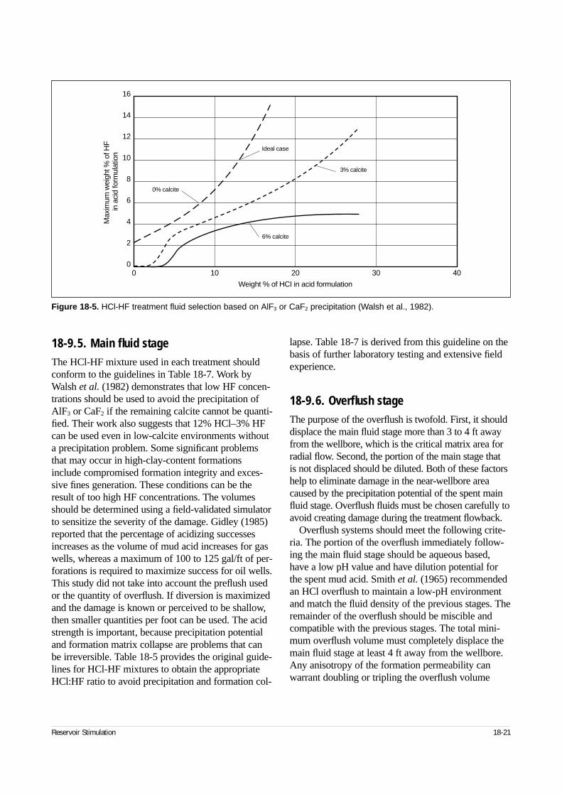
18-9.5. Main fluid stageThe HCl-HF mixture used in each treatment shouldconform to the guidelines in Table 18-7. Work byWalsh et al. (1982) demonstrates that low HF concen-trations should be used to avoid the precipitation ofAlF3 or CaF2 if the remaining calcite cannot be quanti-fied. Their work also suggests that 12% HCl–3% HFcan be used even in low-calcite environments withouta precipitation problem. Some significant problemsthat may occur in high-clay-content formationsinclude compromised formation integrity and exces-sive fines generation. These conditions can be theresult of too high HF concentrations. The volumesshould be determined using a field-validated simulatorto sensitize the severity of the damage. Gidley (1985)reported that the percentage of acidizing successesincreases as the volume of mud acid increases for gaswells, whereas a maximum of 100 to 125 gal/ft of per-forations is required to maximize success for oil wells.This study did not take into account the preflush usedor the quantity of overflush. If diversion is maximizedand the damage is known or perceived to be shallow,then smaller quantities per foot can be used. The acidstrength is important, because precipitation potentialand formation matrix collapse are problems that canbe irreversible. Table 18-5 provides the original guide-lines for HCl-HF mixtures to obtain the appropriateHCl:HF ratio to avoid precipitation and formation col-

lapse. Table 18-7 is derived from this guideline on thebasis of further laboratory testing and extensive fieldexperience.

18-9.6. Overflush stageThe purpose of the overflush is twofold. First, it shoulddisplace the main fluid stage more than 3 to 4 ft awayfrom the wellbore, which is the critical matrix area forradial flow. Second, the portion of the main stage that is not displaced should be diluted. Both of these factorshelp to eliminate damage in the near-wellbore areacaused by the precipitation potential of the spent mainfluid stage. Overflush fluids must be chosen carefully toavoid creating damage during the treatment flowback.

Overflush systems should meet the following crite-ria. The portion of the overflush immediately follow-ing the main fluid stage should be aqueous based,have a low pH value and have dilution potential forthe spent mud acid. Smith et al. (1965) recommendedan HCl overflush to maintain a low-pH environmentand match the fluid density of the previous stages. Theremainder of the overflush should be miscible andcompatible with the previous stages. The total mini-mum overflush volume must completely displace themain fluid stage at least 4 ft away from the wellbore.Any anisotropy of the formation permeability canwarrant doubling or tripling the overflush volume

Reservoir Stimulation 18-21

Figure 18-5. HCl-HF treatment fluid selection based on AlF3 or CaF2 precipitation (Walsh et al., 1982).

Max

imum

wei

ght %

of H

F

in a

cid

form

ulat

ion

0 10 20 30 40

16

14

12

10

8

6

4

2

0

Weight % of HCI in acid formulation

0% calcite

Ideal case

3% calcite

6% calcite

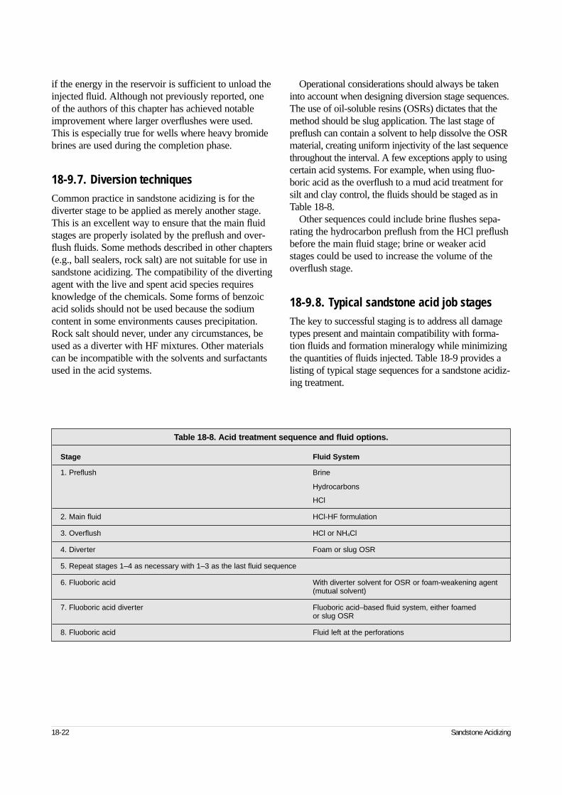
if the energy in the reservoir is sufficient to unload theinjected fluid. Although not previously reported, oneof the authors of this chapter has achieved notableimprovement where larger overflushes were used.This is especially true for wells where heavy bromidebrines are used during the completion phase.

18-9.7. Diversion techniquesCommon practice in sandstone acidizing is for thediverter stage to be applied as merely another stage.This is an excellent way to ensure that the main fluidstages are properly isolated by the preflush and over-flush fluids. Some methods described in other chapters(e.g., ball sealers, rock salt) are not suitable for use insandstone acidizing. The compatibility of the divertingagent with the live and spent acid species requiresknowledge of the chemicals. Some forms of benzoicacid solids should not be used because the sodiumcontent in some environments causes precipitation.Rock salt should never, under any circumstances, beused as a diverter with HF mixtures. Other materialscan be incompatible with the solvents and surfactantsused in the acid systems.

Operational considerations should always be takeninto account when designing diversion stage sequences.The use of oil-soluble resins (OSRs) dictates that themethod should be slug application. The last stage ofpreflush can contain a solvent to help dissolve the OSRmaterial, creating uniform injectivity of the last sequencethroughout the interval. A few exceptions apply to usingcertain acid systems. For example, when using fluo-boric acid as the overflush to a mud acid treatment forsilt and clay control, the fluids should be staged as inTable 18-8.

Other sequences could include brine flushes sepa-rating the hydrocarbon preflush from the HCl preflushbefore the main fluid stage; brine or weaker acidstages could be used to increase the volume of theoverflush stage.

18-9.8. Typical sandstone acid job stagesThe key to successful staging is to address all damagetypes present and maintain compatibility with forma-tion fluids and formation mineralogy while minimizingthe quantities of fluids injected. Table 18-9 provides alisting of typical stage sequences for a sandstone acidiz-ing treatment.

18-22 Sandstone Acidizing

Table 18-8. Acid treatment sequence and fluid options.

Stage Fluid System

1. Preflush Brine

Hydrocarbons

HCl

2. Main fluid HCl-HF formulation

3. Overflush HCl or NH4Cl

4. Diverter Foam or slug OSR

5. Repeat stages 1–4 as necessary with 1–3 as the last fluid sequence

6. Fluoboric acid With diverter solvent for OSR or foam-weakening agent (mutual solvent)

7. Fluoboric acid diverter Fluoboric acid–based fluid system, either foamed or slug OSR

8. Fluoboric acid Fluid left at the perforations

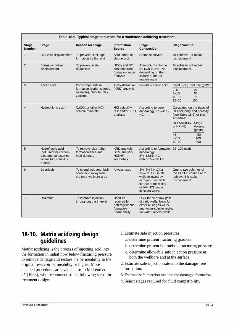
18-10. Matrix acidizing design guidelines

Matrix acidizing is the process of injecting acid intothe formation in radial flow below fracturing pressureto remove damage and restore the permeability to theoriginal reservoir permeability or higher. Moredetailed procedures are available from McLeod etal. (1983), who recommended the following steps fortreatment design:

1. Estimate safe injection pressures:

a. determine present fracturing gradient

b. determine present bottomhole fracturing pressure

c. determine allowable safe injection pressure atboth the wellbore and at the surface.

2. Estimate safe injection rate into the damage-freeformation.

3. Estimate safe injection rate into the damaged formation.

4. Select stages required for fluid compatibility.

Reservoir Stimulation 18-23

Table 18-9. Typical stage sequence for a sandstone acidizing treatment.

Stage Stage Reason for Stage Information Stage Stage VolumeNumber Source Composition

1 Crude oil displacement To prevent oil sludge Acid–crude oil Aromatic solvent To achieve 3-ft radialformation by the acid sludge test displacement

2 Formation water To prevent scale HCO3 and SO4 Ammonium chloride To achieve 3-ft radialdisplacement deposition contents from (NH4Cl) at 3%–8% displacement

formation water depending on theanalysis salinity of the for-

mation water

3 Acetic acid Iron compounds in X-ray-diffraction 3%–10% acetic acid CaCO3 (%) Volume (gal/ft)formation (pyrite, siderite, (XRD) analysis 0–5 25hematite), chlorite, clay, 5–10 50zeolites 10–15 75

15–20 100

4 Hydrochloric acid CaCO3 or other HCl- HCl solubility According to core Calculated on the basis of soluble minerals test and/or XRD mineralogy: 3%–15% HCl solubility and porosity

analysis HCl (see Table 18-5) or this schedule:

HCl Solubility Stageof HF (%) Volume

(gal/ft)

<5 505–10 10010–20 200

5 Hydrofluoric acid To remove clay, other XRD analysis, According to formation 75–100 gal/ft(not used for carbon- formation fines and SEM analysis, mineralogy:ates and sandstones mud damage HCl:HF 3%–13.5% HCl where HCl solubility solubilities with 0.5%–3% HF> 20%)

6 Overflush To spend acid and flush Always used 3%–8% NH4Cl or One to two volumes of spent acid away from 3%–5% HCl in all the HCl:HF volume or to the near-wellbore area wells followed by achieve 5-ft radial

nitrogen (gas wells), displacementkerosene (oil wells) or 5% HCl (water injection wells)

7 Diversion To improve injection Used as OSR for oil or low gas/throughout the interval required for oil ratio wells, foam for

heterogeneous either oil or gas wellsformation and water-soluble resinspermeability for water injector wells

5. Calculate volume of each stage required:

a. crude oil displacement

b. formation brine displacement

c. HCl stage or acetic acid stage

d. mud acid stage

e. overflush stage.

6. Select acid concentrations according to formationmineralogy.

18-10.1. Calculations• Fracturing pressure

Matrix treatments are defined as fluid injectionoccurring below fracturing pressure. If the fluidis injected above fracturing pressure, the acid maybypass the damage. It is important to perform somebasic calculations to ensure that this pressure is notexceeded, and the exercise also provides the pres-sure and rates that may occur. Thorough discussionsof fracturing pressure and bottomhole injectionpressure and how these aspects are derived areprovided in Chapters 3 and 20, respectively.

An important item to keep in mind with matrixtreatments is that fracturing pressure is related tothe pore pressure but is not directly proportional.As the pore pressure declines, so does the fractur-ing pressure. Although this is not a one-to-onerelationship, it can be important when treating low-bottomhole-pressure wells. The hydrostaticpressure exerted by the column of fluid in the tubu-lars can be sufficient to fracture the formation.

• Injection rates

The injection rate can be as significant as the injec-tion pressure. The maximum injection rate thatdoes not fracture the formation can be estimated by

(18-5)

where qi,max is the injection rate in bbl/min, k is theeffective permeability of the undamaged formationin md, h is the net thickness in ft, gf is the fracturegradient in psi/ft, H is the depth in ft, ∆psafe is thesafety margin for the pressure in psi (usually 200 to 500 psi), p is the reservoir pressure in psi, µ is theviscosity of the injected fluid in cp, re is the drainage

radius in ft, rw is the wellbore radius in ft, and s isthe skin effect factor. B is the formation volume fac-tor and has a value of 1 for noncompressible fluids.

Equation 18-5 is a simple way of estimating theinjection rate. However, Eq. 18-5 does not accountfor several factors, which are detailed in Chapter 20for accurately modeling the injection rate. Equation18-5 with zero skin effect and with the estimatedvalue of the skin effect provides respective valuesfor the minimum and a maximum pump rate duringthe job. These values enable allocating appropriateequipment for the treatment. True transient injectionmonitoring can be done in real time on location tomonitor the progress of the job.

• Friction pressure estimation

Accurate fluid friction pressure is a difficult parame-ter to obtain. Because the tubular arrangement canbe different in each case, a fairly accurate number isimportant. The following limited-range equation hasbeen used with relatively good accuracy for estimat-ing friction pressures for Newtonian fluids at ratesless than 9 bbl/min:

(18-6)

where ppipe friction is the friction pressure in psi/1000 ft,ρ is the density of the fluid (specific gravity) in g/cm3,q is the pump rate in bbl/min, and D is the diameter ofthe pipe in in. Coiled tubing friction pressures can alsobe calculated using Eq. 18-6.

• Fluid volumes

If it is assumed that acid flows through porousmedia with a front that is uniform and stable, thenthe injection is piston-like and the first fluid inshould be the last fluid out. To calculate fluid vol-ume, the following equation should be sufficient:

(18-7)

where Vp is the pore volume for the distance s ingal/ft, φ is the fractional porosity, and rs is the dis-tance it is necessary to penetrate the damaged ordisplaced section in ft.

Mud acid treatments do not dissolve much of theformation minerals but rather dissolve the materialsclogging the pore throats. This means that significantchanges in the flow distribution of the injected fluidsoccur during the treatment as the pore-pluggingmaterials are dissolved (see Chapter 19 on diver-

18-24 Sandstone Acidizing

qkh g H p p

Br

rs

i,max

f safe

e

w

=× ×( ) − −[ ]

+

−4 917 10 6.,

∆

µ ln

V r rp s w= −( )[ ]7 48 2 2. ,φ π

pq

Dpipe friction = 518 0 79 1 79 0 207

4 79

ρ µ. . .

.,

sion). Because the acid does not follow the idealmode, adjustments to the injection volumes must bemade. Significant changes in the fluid can also occurin the tubulars, before the fluid reaches the forma-tion. The dilution of stage composition and spendingare just some of the complications that must be addressed by the designer. The use of smaller tubu-lars, such as coiled tubing, during acid treatments cancontribute to a better acid job by facilitating the main-tenance of stage integrity and reducing displacementvolumes. Mechanical limitations associated with arti-ficial lift (e.g., gas lift) are more easily overcome bythe use of coiled tubing. The risks of leaking valves,undiluted acid remaining in the mandrels and acidleaking into the tubing/casing annulus are avoided.The limited injection rate coincidentally controls thecontact time. The pump rate and extraction out ofthe tanks holding the acid can create a bottleneckduring execution. A complete understanding of theoperational aspects is necessary for proper execution.

One of the considerations in selecting the stagevolumes is the tubulars. The volumes of diverter andtheir location in the tubulars while injecting must beconsidered, especially for the use of foam diverters.When using foam diversion techniques, brief shut-downs or momentum changes are called for to maxi-mize diversion. If the foam is in the tubulars whenthe shutdown occurs, phase separation of the foamcan occur, affecting the foam diverter performance.

Another consideration is the preflush activity. If formations do not have much solubility in HCl,operators have tended to lower the volume of acidpreflush and use brine. However, Gdanski andPeavy (1986) reported that this is not a good ideabecause the HCl preflush performs the vital func-tion of cation exchange, which prepares the mineralsurfaces for the HF mixture. The cation exchangemust otherwise be done by the HCl portion of theHF mixture, which raises the pH of the acid systemand induces the precipitation of silicate complexes.As a minimum, the preflush should penetrate thesame distance as the HF mixture (e.g., if the HFblend volume penetrates 2 ft, then the preflushshould penetrate a minimum of 2 ft).

Where the HCl solubility is moderate to high,more HCl is necessary. The following equation isused to calculate this volume and address the HCl-soluble materials:

(18-8)

whereVHCl is the volume of HCl required in gal/ft, XHCl isthe fraction of the bulk rock dissolved by HCl, andβ is the dissolving coefficient expressed as theamount of rock dissolved per gallon of acid and isrelated to the acid strength.

18-10.2. Flowback and cleanup techniquesSelection of the correct flowback procedure is critical.The flowback during multiphase transition periods cancause irreversible damage. The fines loosened duringthe acid job are invariably produced back into thenear-wellbore area. These fines can be removed indiluted concentrations that pass through the comple-tion if small, gradual pressure drops are created. Thiswas demonstrated by Krueger (1986).

The following are key factors to consider for flow-back in sandstone formations:

• The fluids flowing back are more viscous thanthose injected. They are capable of carrying naturalformation fines and other partially dissolved solidsat lower velocities, which can cause pluggingbefore the well cleans up completely.

• The spent acid usually has a higher density than theformation water. The tubing pressure should belower than when connate water is produced, owingto the higher hydrostatic pressure of the spent acid.

• Spent acid has an equilibrium established of poten-tial precipitants, held in place by dissolved gases anddissolved salts. Should these gases (e.g., CO2) beremoved from the spent fluid as a result of creatingan excessive pressure drop, precipitation will occur.

• A minimum velocity is necessary for liquid to bevoided from the tubing without slippage occurring.The minimum velocity to the unload tubing can becalculated. The flow rate and tubing pressure in thiscalculation should include the heavier liquid den-sity. The flow rate should be achieved gradually butsufficiently soon to avoid precipitation in the for-mation. The rate should then be maintained until allinjected fluids are returned and both the tubingpressure and production rate are steady. Plotting thegradual incremental choke changes as pressure andrate stabilize provides insight to the affect of theacid treatments on the formation and completion.

Reservoir Stimulation 18-25

VX r r

HCl

HCl s w=−( ) −[ ]

7 481 2 2

. ,π φ

β

• HF systems should be flowed back immediatelyafter injection of the overflush. The potential dam-aging precipitates that are generated form when thepH increases as the HCl is spent. If the acid isreturned quickly, then the pH change may not reachthe range for precipitation. Many iron precipitatesalso drop out when the pH increases. The exceptionis fluoboric acid treatments. The shut-in timerequired for complete HF generation and fines sta-bilization varies on the basis of temperature.

• The majority of the additives that are injected areproduced back. Because the acidizing additives areby design water soluble, they are partitioned into thewater phase. This can cause separation and floatationequipment problems. The return fluids are also acidic,which creates problems for chemical-electric detec-tion devices in the separation equipment. Local envi-ronmental regulations may dictate water qualitystandards that are difficult to achieve, and disposal of the returned fluids can be cost prohibitive.Alternatives to disposal of the returns as hazardouswaste have been developed, including filtrationthrough inexpensive media (Hebert et al., 1996).

18-11. Acid treatment evaluationMatrix treatment evaluation is the subject of Chapter20. The following is a partial list of the basic ques-tions that should be answered during the evaluation ofan acid treatment to help determine the success or fail-ure of the treatment.

• Was the well damaged? Was there an improvementin the injectivity or transient skin during the treat-ment? Is there evidence that the well was dam-aged?

• Which fluid system or stage accomplished the mostdamage removal? Injectivity values or transientskin values for each of the fluid stages must beevaluated to help identify what damage was caus-ing the most significant production impairment.

• Were emulsions observed during cleanup? Duringthe cleanup of the treatment is when the effective-ness of additives and treatment fluid packagesdemonstrates value. Cleanup time, emulsion prob-lems and facility upset have an economic impactand can be cause for considering different methodsof handling the problems.

• Did any of the treatment fluids or stages create prob-lems during the execution? During the treatmentwere there mixing or handling problems associatedwith any of the additives or the fluid system?

• What are the properties of the formation fluids (i.e.,hydrocarbons and brine) and are these compatiblewith the treating fluids? Post-treatment flowbackinspection and analysis of fluids identifies emul-sions (treating fluid additive formulation), soliddebris (proper acid strength) and other telltale signsof precipitation caused by incompatibilities.

• What is the type of completion injected into andwas this a consideration during the treatment?When injecting into gravel packs or frac and packcompletions, injection rates should be limited if the injected height is limited. Too high an injectionrate through the perforations can evacuate them ofgravel and create an unstable and unsatisfactoryenvironment where the potential exists for forma-tion sand production. This is especially true forhigh-solubility zones where a small percentage of the perforations is taking fluid.

• Was the proper diversion technique or sequencechosen and applied? Most acid treatments requirediversion. The application of proper diversion tech-niques with the selected acid system is vital to theultimate success of the treatment.

• Was the well appropriately prepared before acidiz-ing? When key steps of preparing the wellbore forthe acidizing process are left out (e.g., not picklingthe tubing, not removing the gas lift valves, notremoving the rods or an electrical submersiblepump), the prospects for ultimate success arereduced. Wellbore preparation is especially criticalfor acid treatments. Injection of tubular debris intothe formation can be disastrous, and acid in theannulus of a gas lift completion string is corrosive.

• Were the injected fluids checked using quality con-trol steps? Acid strength and certain additives mustmeet at least threshold ranges for activity and com-patibility limits.

• Was the tubing acid cleaned (pickled)? Rust andmill scale must be removed, even with new pipe.

• Were the pumped fluids sampled and checked forcleanliness and concentration? Although samplesare routinely taken and checked before the jobstarts, samples should be taken during the pumpingof each stage. Many changes in injection behavior

18-26 Sandstone Acidizing

can be explained when these samples are analyzed.Fluctuations in injectivity may be due to a processproblem that was innocently incorporated for oper-ational expedience or safety compliance.

• Was an injection test with the appropriate fluidmade before pumping acid to establish a base injec-tivity before acidizing? Injection testing conductedwith platform or field equipment not intended forthis purpose can produce misleading results. Con-taminated fluids or poorly equipped monitoring canresult in bad data.

• Did the acid response during the injection validatethe damaging substance identified? HCl-solublescale may be revealed as the obvious contributor to the injectivity problem when large pressure dropsoccur when the HCl reaches the formation. If theinjection rate is increased, similar pressure dropscould also be noted when the HCl-HF mixturereaches the formation.

• Did the pressure response indicate good diversion?Pressure increases may be interpreted as diverteraction, but this is not always the case. Diverterresponse should coincide with the use of a diverter; ifnot, other parts of the process should be investigated.

• How long was the spent acid left in the well beforeflowback? Some secondary and tertiary reactionsrequire time to produce precipitates. Quick turn-around for flowback, not high production rates,lessens the potential for these reactions to createdamage. Most of these reactions result in damagethat is detected only after production is initiated.

• Were spent acid samples recovered and analyzed?Flowback fluid samples should be acquired regard-less of the volume of the treatment. These samplesshould be marked, with the date and time, total vol-ume recovered to that point and other pertinentdata, such as choke size, flowing tubing pressure,water cut and produced quantities.

• Were the production results consistent with the acidinjection pressure response? If the injection pres-sure declines too quickly, the acid treatment causesthe well to develop a vacuum. Once the well is

brought back on line, the production does notimprove because of limitations associated with thewellbore construction or production facilities.

• Was a pressure buildup test performed and inter-preted? A pressure test analysis is the definitivemethod to answer whether the treatment is a suc-cess or failure.

18-12. ConclusionsAcidizing sandstone formations is not an impossibletask, but it is not simple either. Success requires amethodical, systematic approach. It can be accom-plished without any detrimental effects by analyzingvital information. The flow chart in Fig. 18-6 showsthe steps the process encompasses.

The following conclusions can be made about sand-stone acidizing:

• Damage identification determines the types of acidsand other solvents to use in a sandstone acidizingtreatment.

• A knowledge of the chemical reactions involvedamong acids and formation minerals and connatefluids provides some guidelines for acid types, con-centrations and the sequence to prevent or reducethe precipitation of insoluble reaction products.

• The selection of appropriate types and volumes ofpreflushes and overflushes also helps prevent incom-patibilities between formation fluids and acid systems.

• A numerical simulator should be used to quantifyacid volumes, although simple guidelines are pro-vided to assist in the selection of treatment vol-umes. The most important factor in successful acidstimulation is to provide clean, filtered acids at theperforations by filtering all fluids and cleaning(pickling) the tubing before the acid treatment is injected into the formation.

• Evaluating the executed acid treatment providesinformation to improve subsequent acid treatmentsin the same or similar formations.

Reservoir Stimulation 18-27

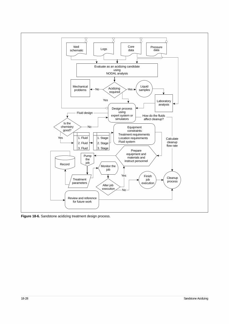
18-28 Sandstone Acidizing

Figure 18-6. Sandstone acidizing treatment design process.

Well schematic

Coredata

PressuredataLogs

Evaluate as an acidizing candidateusing

NODAL analysis

Mechanicalproblems Acidizing

required

Liquidsamples

Laboratoryanalysis

No

No

No

Yes

Yes

Yes

Yes

Design processusing

expert system orsimulators

Equipment constraints:

1. Fluid

2. Fluid

3. Fluid

1. Stage

2. Stage

3. StagePrepare

equipment andmaterials and

instruct personnel

Is thechemistry

good?

How do the fluidsaffect cleanup?

Fluid design

Calculatecleanupflow rate

Record

Treatmentparameters

Monitor thejob

Finishjob

executionAlter job execution

Pumpthejob

Review and referencefor future work

Treatment requirements Location requirements Fluid system

Cleanupprocess

19-1. IntroductionFluid placement is critical to the success of a matrixstimulation treatment (Pye et al., 1970; Cooper andBolland, 1984). Damage, depending often on fluid-rock interactions, may be unevenly distributed alongthe net thickness. Also, the natural reservoir perme-ability may vary considerably, with substantial con-trasts. In this environment, matrix stimulation tendsto remove or bypass the damage that is easier toreach (i.e., a lower degree of damage or higher per-meability) and becomes self-defeating. Each addi-tional volume of stimulation fluid follows the pathof least resistance, and more of it invades the layerwhere it is least required.

Several methods have been developed to improvefluid placement during matrix acidizing. Nonmech-anical methods include the use of particles accumu-lating at the sandface to form a low-permeabilitycake (i.e., particulate diverters). The size of the parti-cles varies from a few tens of micrometers to a fewmillimeters. Other methods involve the use of vis-cous fluid slugs or the use of foam either as stagedslugs or combined with the acid stages (i.e., foamedacid). Each of these methods is based on the tempo-rary impairment of the high-injectivity zones accept-ing most of the diverting material, which results in anincrease of the proportion of fluid going into the low-injectivity zones. It is essential, of course, to avoidpermanently damaging the higher injectivity zones.

Mechanical techniques consist of ball sealers,which are rubber-lined balls added to treating fluidsto plug fluid-taking perforations, and packers, whichenable isolating a given zone during a treatment.Mechanical techniques differ from the other diversionmethods in that they completely shut off a part of thereservoir to direct all the stimulation fluid to a sub-section of the open zone. Another technique is coiledtubing placement in which acid is spotted or injectedacross the zone of interest. This is especially impor-tant in horizontal wells or vertical wells with longproducing zones (Thomas and Milne, 1995).

The last method is specific to carbonate formations.It involves pumping gelled acid, with the viscosityvarying with the degree of spending. Injectivity isreduced in zones containing large volumes of spentacid, and fresh acid is directed to lower injectivityzones. This method has been increasingly used recentlyand has produced good results in terms of placement. Itis described in more detail in Chapter 17.

The choice of the pumping strategy must take intoaccount several parameters, such as producing-intervalthickness, lithology and permeability profile, damagedistribution and the economics of the treatment.

19-2. Choice of pumping strategy

19-2.1. Importance of proper placementMatrix stimulation is almost always performed inmultilayer reservoirs containing zones with, at times,wide injectivity contrasts caused either by differentpermeabilities or by uneven severity of damage.Other phenomena causing vertical heterogeneitieswithin a completion interval include permeabilitygradients in thick reservoirs and selective damage insome perforations. The natural trend of stimulationfluids is to follow the path of least resistance (i.e., to invade the most permeable or least damagedzones). To optimize treatment results, most of theopen interval must be treated, and thus, treating fluidsmust also be injected in significant volumes into theleast permeable and most damaged zones.

In many cases, the use of diverting techniques hasproved successful in improving fluid placement andtreatment results, especially in cases with large vari-ations of initial injectivity throughout the open inter-val (Brannon et al., 1987).

As an example, consider the three-layer reservoirdescribed in Table 19-1. Middle layer 2 is a high-injectivity zone of limited thickness (10% of the totalpay zone) with high permeability and a lower skineffect. A simple calculation, using a steady-state

Reservoir Stimulation 19-1

◆

Fluid Placement andPumping StrategyJ. A. Robert, Schlumberger Dowell

W. R. Rossen, University of Texas at Austin

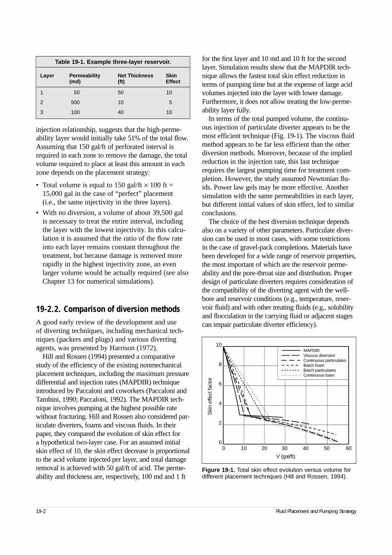
injection relationship, suggests that the high-perme-ability layer would initially take 51% of the total flow.Assuming that 150 gal/ft of perforated interval isrequired in each zone to remove the damage, the totalvolume required to place at least this amount in eachzone depends on the placement strategy:

• Total volume is equal to 150 gal/ft × 100 ft =15,000 gal in the case of “perfect” placement (i.e., the same injectivity in the three layers).

• With no diversion, a volume of about 39,500 gal is necessary to treat the entire interval, includingthe layer with the lowest injectivity. In this calcu-lation it is assumed that the ratio of the flow rateinto each layer remains constant throughout thetreatment, but because damage is removed morerapidly in the highest injectivity zone, an evenlarger volume would be actually required (see alsoChapter 13 for numerical simulations).

19-2.2. Comparison of diversion methods A good early review of the development and use of diverting techniques, including mechanical tech-niques (packers and plugs) and various divertingagents, was presented by Harrison (1972).

Hill and Rossen (1994) presented a comparativestudy of the efficiency of the existing nonmechanicalplacement techniques, including the maximum pressuredifferential and injection rates (MAPDIR) techniqueintroduced by Paccaloni and coworkers (Paccaloni andTambini, 1990; Paccaloni, 1992). The MAPDIR tech-nique involves pumping at the highest possible ratewithout fracturing. Hill and Rossen also considered par-ticulate diverters, foams and viscous fluids. In theirpaper, they compared the evolution of skin effect for a hypothetical two-layer case. For an assumed initialskin effect of 10, the skin effect decrease is proportionalto the acid volume injected per layer, and total damageremoval is achieved with 50 gal/ft of acid. The perme-ability and thickness are, respectively, 100 md and 1 ft

for the first layer and 10 md and 10 ft for the secondlayer. Simulation results show that the MAPDIR tech-nique allows the fastest total skin effect reduction interms of pumping time but at the expense of large acidvolumes injected into the layer with lower damage.Furthermore, it does not allow treating the low-perme-ability layer fully.

In terms of the total pumped volume, the continu-ous injection of particulate diverter appears to be themost efficient technique (Fig. 19-1). The viscous fluidmethod appears to be far less efficient than the otherdiversion methods. Moreover, because of the impliedreduction in the injection rate, this last techniquerequires the largest pumping time for treatment com-pletion. However, the study assumed Newtonian flu-ids. Power law gels may be more effective. Anothersimulation with the same permeabilities in each layer,but different initial values of skin effect, led to similarconclusions.

The choice of the best diversion technique dependsalso on a variety of other parameters. Particulate diver-sion can be used in most cases, with some restrictionsin the case of gravel-pack completions. Materials havebeen developed for a wide range of reservoir properties,the most important of which are the reservoir perme-ability and the pore-throat size and distribution. Properdesign of particulate diverters requires consideration ofthe compatibility of the diverting agent with the well-bore and reservoir conditions (e.g., temperature, reser-voir fluid) and with other treating fluids (e.g., solubilityand flocculation in the carrying fluid or adjacent stagescan impair particulate diverter efficiency).

19-2 Fluid Placement and Pumping Strategy

Figure 19-1. Total skin effect evolution versus volume fordifferent placement techniques (Hill and Rossen, 1994).

10

8

6

4

2

00 10 20 30 40 50 60

V (gal/ft)

Ski

n ef

fect

fact

or

MAPDIRViscous diversionContinuous particulatesBatch foamBatch particulatesContinuous foam

Table 19-1. Example three-layer reservoir.

Layer Permeability Net Thickness Skin (md) (ft) Effect

1 50 50 10

2 500 10 5

3 100 40 10

In the case of gravel-pack completions, large-parti-cle-size chemical diverters are not used. Oil-solubleresin (OSR) may be used, but it must be mixed welland injected continuously with the acid to avoid therisk of plugging the screen or gravel pack (McLeod,1984). Foam diversion is also common for gravel-pack completions and where particulate diverters arenot appropriate.

In the case of oil wells with a well-defined waterzone, foam has been found to plug the water zonesuccessfully and direct acid to the oil-bearing interval.This is due to the detrimental effect of oil on foamformed by certain surfactants. Acidizing with foamdiversion has been reported to improve overall pro-duction in some cases without increasing the watercut, but instead reducing it (Zerhboub et al., 1994).

For cemented and perforated completions, buoyantball sealers have been shown to give good results(Erbstoesser, 1980; Bale, 1983). Conventional ballsealers are generally not recommended for longintervals or high-shot-density completions, as theyrequire a minimum injection rate per perforation toprevent settling in the rathole (McLeod, 1984).

Packers are the most effective means of selectivefluid placement. However, they require the use ofcoiled tubing or rig operations. They can be used aftercompletion or workover, if a rig is already on site.

Coiled tubing has been increasingly used formatrix acidizing over the past few years. Treatmentanalysis shows that coiled tubing is especially help-ful for acidizing long intervals by allowing spottingsuccessive diverter and acid stages throughout theopen interval, thereby ensuring good coverage of theentire producing zone (Economides et al., 1991;Thomas and Milne, 1995).

19-2.3. Fluid placement versus injection rate

Selection of the treatment strategy must be based onthe trade-off between pump rate and fluid placement.Except for the MAPDIR technique, placement meth-ods result in a reduction in the injection rate, even inlow-injectivity zones, with possible loss of treatmentefficiency and creation of precipitation damage.Williams et al. (1979) mentioned that sandstoneacidizing is more efficient at higher rates, both avoid-ing the creation of precipitates near the wellbore andextending the radius of live-acid penetration. McLeod

(1984) and Schechter (1992), however, argued thatthere exists an optimum rate for sandstone acidizing,based on the reaction rate with damage and acidand/or damage contact time. For carbonate acidizing,it has been shown that the injection rate must be highenough to allow wormholes to form and propagate.Pumping below this rate can cause a considerablereduction in treatment effectiveness.

19-2.4. MAPDIR methodThe MAPDIR method suggests pumping treating fluidsas fast as possible below the fracturing limit withoutusing any diversion technique. It allows a decrease ofpumping time and minimizes the risk of treatment fail-ure caused by low pumping rates. However, MAPDIRis not a true diversion technique, as it does not modifythe natural flow profile, nor does it necessarily distrib-ute stimulation fluids or remove all damage.

Paccaloni and coworkers analyzed a large series of matrix-acidizing treatments to identify the factorsleading to success or failure, including pump rate andthe use of diversion (Paccaloni et al., 1988; Paccaloniand Tambini, 1990). Criteria for success or failure werespecific to the authors. With development wells, jobsuccess involved treating the entire interval. On thebasis of the analysis of more than 170 jobs, the authorsclaimed that the MAPDIR technique is sufficient toobtain full coverage of the pay zone if the permeabilitycontrast is less than 300 md and the pay zone does notexceed 200 ft. They concluded that the method actuallygives better results than diverting agents.

In the case of carbonate formations, they reportedthat relatively small volumes of concentrated acid (5 to 10 gal/ft) led to a substantial skin effect reduction,allowing for reasonable injectivity of the zone for fur-ther reduction. This could explain why the MAPDIRmethod can eventually provide full zone coverage: ifthe treatment is maintained long enough to inject thefew gallons required to improve injectivity in the highlydamaged zones, then injectivity contrasts are reducedand the entire interval can be treated. However, thismethod can be applied only for intervals with limitedcontrasts of permeability, and it does not optimize fluidplacement.

For better efficiency, the authors recommended theuse of coiled tubing for preacidizing operations suchas wellbore cleanup, acid circulation for completionstring cleaning and acid spotting in front of the pay

Reservoir Stimulation 19-3

zone. Then a T connection can be used to pump acidthrough both the coiled tubing and tubing string tomaximize the pump rate during matrix injection.

19-3. Chemical diverter techniquesChemical diverters, which are materials insoluble in acid but highly soluble in water or hydrocarbons,have been used either to form a low-permeability filtercake at the sandface or to reduce the injectivity ofhigh-permeability zones with the injection of a vis-cous polymer slug. The first technique has been foundto be more effective and can provide faster cleanup. It has prevailed over the viscous slug technique.

19-3.1. Historical backgroundThe first attempts at fluid placement made use ofchemical additives. Harrison (1972) reported theinjection, as early as 1936, of soap solutions thatcould react with calcium chloride (CaCl2) to formwater-insoluble, but oil-soluble, calcium soaps. Theprecipitate acted as a diverting agent for hydrochlo-ric acid (HCl). The generation of solid precipitates inthe formation was not, of course, desirable, becausethey could cause permanent damage. Thus, in thelate 1930s, more sophisticated systems were used,such as heavy CaCl2 solutions. Diversion effectswere possible by impairing injectivity in the zonesaccepting most of the high-viscosity solution. Othersystems utilized cellophane flakes suspended in awater gel with a bacterial breaker. Later, gels werereplaced by oil-external emulsions.

In 1954, naphthalenes were first used as a blockingmaterial. Oil-soluble naphthalenes were thought to beideal diverters because they sublime above 175°F[80°C]. Also, crushed limestone, sodium tetraborate,oyster shells, gilsonite, perilite, paraformaldehyde and“chicken feed” were used as diverters with mixed suc-cess. These compounds were replaced progressivelyby rock salt, which is partly soluble in the acid butinexpensive and easy to handle.

A major improvement in diversion techniques wasbrought about by completely soluble materials,including wax-polymer blends and hydrocarbonresins in production wells and rock salt and benzoicacid in water-injection wells.

19-3.2. Diverting agent propertiesAn effective diverting agent must meet both physicaland chemical requirements.

• Physical requirements

Cake permeability—Cakes created on the reser-voir walls by agents must be as impermeable aspossible to the acid for the maximum divertingeffect. If the permeability of the diverter cake isgreater than or equal to the permeability of thetightest zone, little or no diversion occurs.

Invasion—Deep invasion of the reservoir rockby the diverter particles must be prevented, regard-less of the nature of the rock, for maximum divertereffectiveness and minimum problems in cleanup.This and the previous requirement suggest that anoptimum particle size must be determined.

Dispersion—Diverting agent particles must beproperly dispersed in the carrying fluid. If floccu-lation occurs, the cake will be thicker but withhigh porosity and permeability.

• Chemical requirements

Compatibility—Diverting agents must be compati-ble with the bulk treatment fluid and with otheradditives, such as corrosion inhibitors, surfactantsand antifoaming agents. They must be inert towardthe carrying fluid at the well treating conditions.

Cleanup—Diverting agents must be soluble ineither the production or injection fluids. Havingacted as diverters, they should undergo a rapidand complete cleanup.

19-3.3. Classification of diverting agentsDiverting agents can be classified, according to theirparticle size, as bridging agents or particulate diverters.

• Bridging and plugging agents

These diverting agents consist of large-size parti-cles, from 10/20 to 100 mesh. They are used asdiverters in carbonate formations, where naturalfractures are common. However, their efficiencyis limited by the high permeability of the cakesthey create. As an example, a cake formed with10-mesh particles has a permeability between20,000 and 40,000 md, whereas a cake createdwith 100-mesh particles has a permeabilitybetween 1,000 and 3,000 md.

19-4 Fluid Placement and Pumping Strategy

When effective diversion is required in fracturedzones, a slug of bridging agent is injected first, fol-lowed by the treating fluid containing a divertingagent. The bridging agent fills the fractures, createsa coating in front of high-permeability formationsor both. If the plugging agent consists of particlessmall enough (e.g., 100 mesh), the diverting agentdoes not penetrate the coating and allows effectivediversion through the development of low-perme-ability cakes.

Bridging agents with various chemical compo-sitions are available:– inert materials, such as silica sand or a mixture

of silica, nonswelling clay and starch (Solublematerials reduce the risk of permanently plug-ging the formation.)

– water-soluble bridging agents, including rocksalt and benzoic acid

– oil-soluble bridging agents, including gradedoil-soluble resins, naphthalenes flakes and beadsmade of wax-polymer blends that are soluble inoil, deformable and temperature degradable.(Their composition can be selected according to the bottomhole temperature.)

• Particulate diverters

Particulate diverters are characterized by verysmall particle sizes, well below 0.004 in. in diam-eter. Both water- and oil-soluble particulate divert-ers are available.– Water-soluble, for injection wells—A fine grade

of benzoic acid is typically used as a water-sol-uble diverting agent. Because this productagglomerates during storage, it is difficult toachieve a constant particle-size distributionbefore injection. For this reason, salts (i.e.,ammonium or sodium benzoate) can be usedinstead. In HCl, the salts are converted to ben-zoic acid. For instance, sodium benzoate reactsaccording to

C6H5COONa + HCl C6H5COOH + Na+ + Cl–

Benzoic acid is only slightly soluble in HCl buthighly soluble in water or alkaline solutions.After acting as a diverter, this compound dis-solves in the injection water. Because benzoicacid particles are hydrophobic, surfactants arerequired to properly disperse the agent in thetreating fluid.

– Oil-soluble, for production wells—Oil-solubleagents are blends of hydrocarbon resins. Theyare totally inert in an acidic medium, yet quicklyand completely dissolve in the produced oil aftertreatment. It is often difficult to disperse theseresins in the acid. They are usually injected asdispersions in aqueous solutions.

19-3.4. Potential problems during diversion treatment

During a diversion treatment several major problemsmay occur.

• Decantation

Bridging agents are subject to gravity effects dur-ing injection. They tend to settle in the fluid thatfills the well, and the best results are thereforeobtained when the solid additives are placed in awater-base gel. Decantation problems rarely occurwith diverting agents because of their small parti-cle size and the low density of their constituentmaterials (1.1 g/cm3 for resin, 1.3 g/cm3 for ben-zoic acid).

• Solubility

Water-soluble agents are also slightly soluble inacid. Therefore, a portion of these additives dis-solves during mixing with the acid. Another por-tion dissolves during injection because of inter-mixing with wellbore fluids and heating. If theplugging agent is injected in slugs, after it isdeposited in the fractures or on the formationwalls it undergoes additional dissolution. Thus,the effectiveness of water-soluble products isalways low, and large initial concentrations arerequired. The dissolution rate during the differentstages of injection must be considered in the jobdesign.

• Particle-size distribution

The particle size of the diverting agent must corre-spond to the petrophysical properties of the treatedzones, such as permeability and pore-size distribu-tion. If bridging agents are used in a reservoir withpermeability from 100 to 1000 md, the resistanceof the diverter cake may not be high enough toavoid fluid penetration in the high-permeabilityzones. On the other hand, if too fine a divertingagent is used, the solid particles migrate through

Reservoir Stimulation 19-5

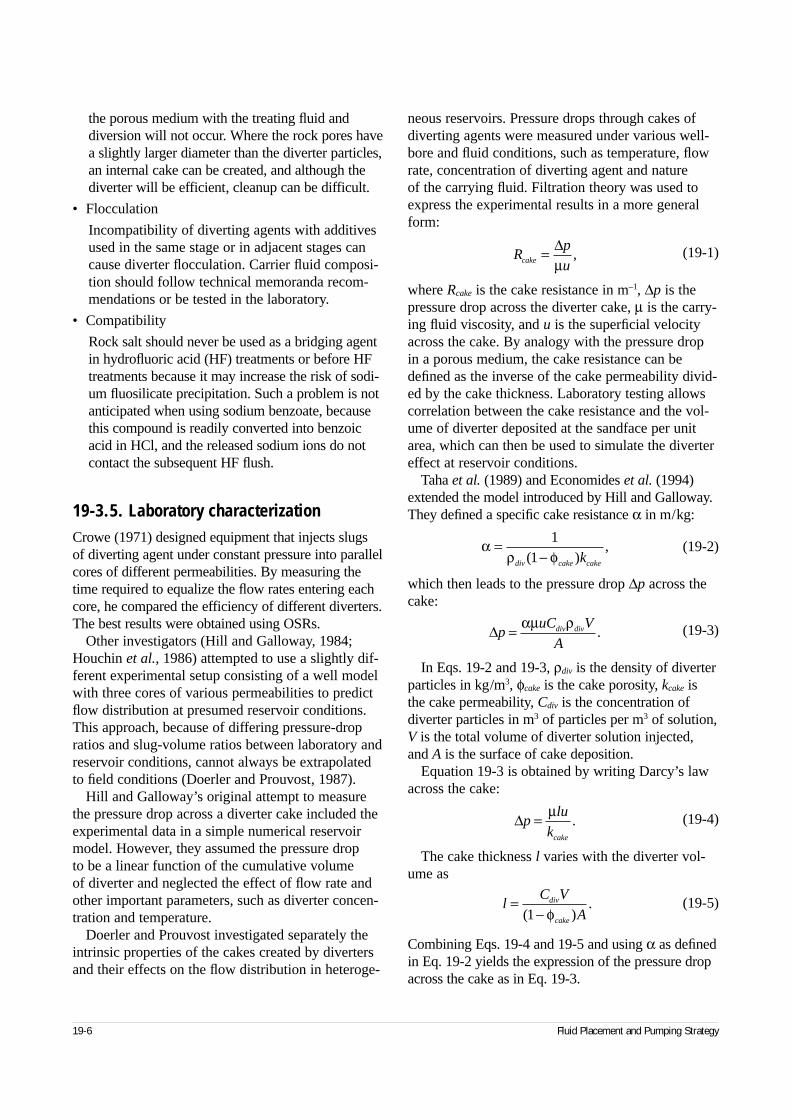
the porous medium with the treating fluid anddiversion will not occur. Where the rock pores havea slightly larger diameter than the diverter particles,an internal cake can be created, and although thediverter will be efficient, cleanup can be difficult.

• Flocculation

Incompatibility of diverting agents with additivesused in the same stage or in adjacent stages cancause diverter flocculation. Carrier fluid composi-tion should follow technical memoranda recom-mendations or be tested in the laboratory.

• Compatibility

Rock salt should never be used as a bridging agentin hydrofluoric acid (HF) treatments or before HFtreatments because it may increase the risk of sodi-um fluosilicate precipitation. Such a problem is notanticipated when using sodium benzoate, becausethis compound is readily converted into benzoicacid in HCl, and the released sodium ions do notcontact the subsequent HF flush.

19-3.5. Laboratory characterizationCrowe (1971) designed equipment that injects slugs of diverting agent under constant pressure into parallelcores of different permeabilities. By measuring thetime required to equalize the flow rates entering eachcore, he compared the efficiency of different diverters.The best results were obtained using OSRs.

Other investigators (Hill and Galloway, 1984;Houchin et al., 1986) attempted to use a slightly dif-ferent experimental setup consisting of a well modelwith three cores of various permeabilities to predictflow distribution at presumed reservoir conditions.This approach, because of differing pressure-dropratios and slug-volume ratios between laboratory andreservoir conditions, cannot always be extrapolatedto field conditions (Doerler and Prouvost, 1987).

Hill and Galloway’s original attempt to measurethe pressure drop across a diverter cake included theexperimental data in a simple numerical reservoirmodel. However, they assumed the pressure drop to be a linear function of the cumulative volume of diverter and neglected the effect of flow rate andother important parameters, such as diverter concen-tration and temperature.

Doerler and Prouvost investigated separately theintrinsic properties of the cakes created by divertersand their effects on the flow distribution in heteroge-

neous reservoirs. Pressure drops through cakes ofdiverting agents were measured under various well-bore and fluid conditions, such as temperature, flowrate, concentration of diverting agent and nature of the carrying fluid. Filtration theory was used toexpress the experimental results in a more generalform:

(19-1)

where Rcake is the cake resistance in m–1, ∆p is thepressure drop across the diverter cake, µ is the carry-ing fluid viscosity, and u is the superficial velocityacross the cake. By analogy with the pressure dropin a porous medium, the cake resistance can bedefined as the inverse of the cake permeability divid-ed by the cake thickness. Laboratory testing allowscorrelation between the cake resistance and the vol-ume of diverter deposited at the sandface per unitarea, which can then be used to simulate the divertereffect at reservoir conditions.

Taha et al. (1989) and Economides et al. (1994)extended the model introduced by Hill and Galloway.They defined a specific cake resistance α in m/kg:

(19-2)

which then leads to the pressure drop ∆p across thecake:

(19-3)

In Eqs. 19-2 and 19-3, ρdiv is the density of diverterparticles in kg/m3, φcake is the cake porosity, kcake isthe cake permeability, Cdiv is the concentration ofdiverter particles in m3 of particles per m3 of solution,V is the total volume of diverter solution injected, and A is the surface of cake deposition.

Equation 19-3 is obtained by writing Darcy’s lawacross the cake:

(19-4)

The cake thickness l varies with the diverter vol-ume as

(19-5)

Combining Eqs. 19-4 and 19-5 and using α as definedin Eq. 19-2 yields the expression of the pressure dropacross the cake as in Eq. 19-3.

19-6 Fluid Placement and Pumping Strategy

Rp

ucake = ∆µ

,

αρ φ

=−

11div cake cakek( )

,

∆puC V

Adiv div= αµ ρ

.

∆plu

kcake

= µ.

lC V

Adiv

cake

=−( )

.1 φ

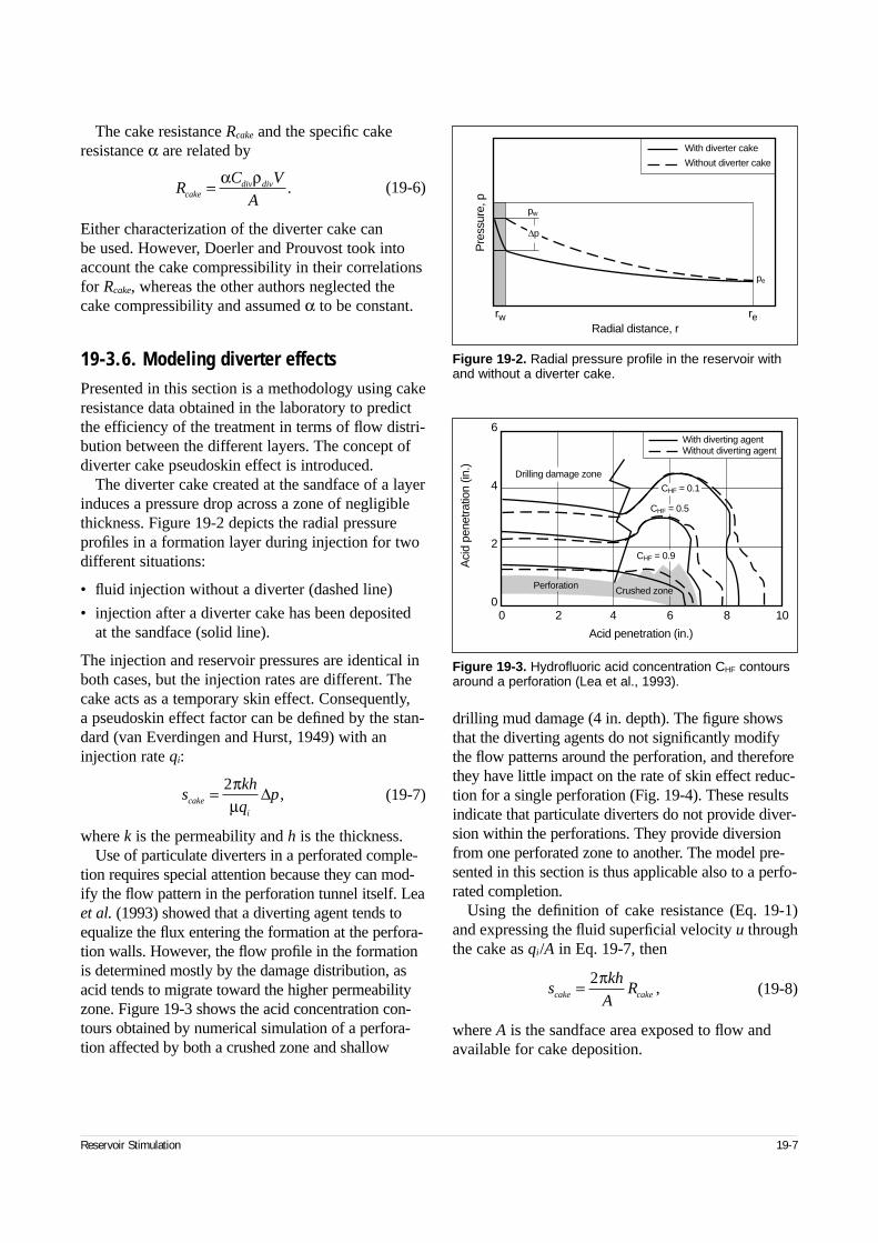
The cake resistance Rcake and the specific cakeresistance α are related by

(19-6)

Either characterization of the diverter cake can be used. However, Doerler and Prouvost took intoaccount the cake compressibility in their correlationsfor Rcake, whereas the other authors neglected thecake compressibility and assumed α to be constant.

19-3.6. Modeling diverter effectsPresented in this section is a methodology using cakeresistance data obtained in the laboratory to predictthe efficiency of the treatment in terms of flow distri-bution between the different layers. The concept ofdiverter cake pseudoskin effect is introduced.

The diverter cake created at the sandface of a layerinduces a pressure drop across a zone of negligiblethickness. Figure 19-2 depicts the radial pressureprofiles in a formation layer during injection for twodifferent situations:

• fluid injection without a diverter (dashed line)

• injection after a diverter cake has been depositedat the sandface (solid line).

The injection and reservoir pressures are identical inboth cases, but the injection rates are different. Thecake acts as a temporary skin effect. Consequently, a pseudoskin effect factor can be defined by the stan-dard (van Everdingen and Hurst, 1949) with aninjection rate qi:

(19-7)

where k is the permeability and h is the thickness.Use of particulate diverters in a perforated comple-

tion requires special attention because they can mod-ify the flow pattern in the perforation tunnel itself. Leaet al. (1993) showed that a diverting agent tends toequalize the flux entering the formation at the perfora-tion walls. However, the flow profile in the formationis determined mostly by the damage distribution, asacid tends to migrate toward the higher permeabilityzone. Figure 19-3 shows the acid concentration con-tours obtained by numerical simulation of a perfora-tion affected by both a crushed zone and shallow

drilling mud damage (4 in. depth). The figure showsthat the diverting agents do not significantly modifythe flow patterns around the perforation, and thereforethey have little impact on the rate of skin effect reduc-tion for a single perforation (Fig. 19-4). These resultsindicate that particulate diverters do not provide diver-sion within the perforations. They provide diversionfrom one perforated zone to another. The model pre-sented in this section is thus applicable also to a perfo-rated completion.

Using the definition of cake resistance (Eq. 19-1)and expressing the fluid superficial velocity u throughthe cake as qi/A in Eq. 19-7, then

(19-8)

where A is the sandface area exposed to flow andavailable for cake deposition.

Reservoir Stimulation 19-7

Figure 19-3. Hydrofluoric acid concentration CHF contoursaround a perforation (Lea et al., 1993).

6

4

2

00 2 4 6 8 10

Acid penetration (in.)

Aci

d pe

netra

tion

(in.)

With diverting agentWithout diverting agent

Perforation

Drilling damage zone

Crushed zone

CHF = 0.1

CHF = 0.5

CHF = 0.9

skh

ARcake cake= 2π

,

RC V

Acakediv div= α ρ

.

skh

qpcake

i

= 2πµ

∆ ,

Figure 19-2. Radial pressure profile in the reservoir withand without a diverter cake.

rw re

pw

pe

Radial distance, r

With diverter cake

Without diverter cake

Pre

ssur

e, p

∆p

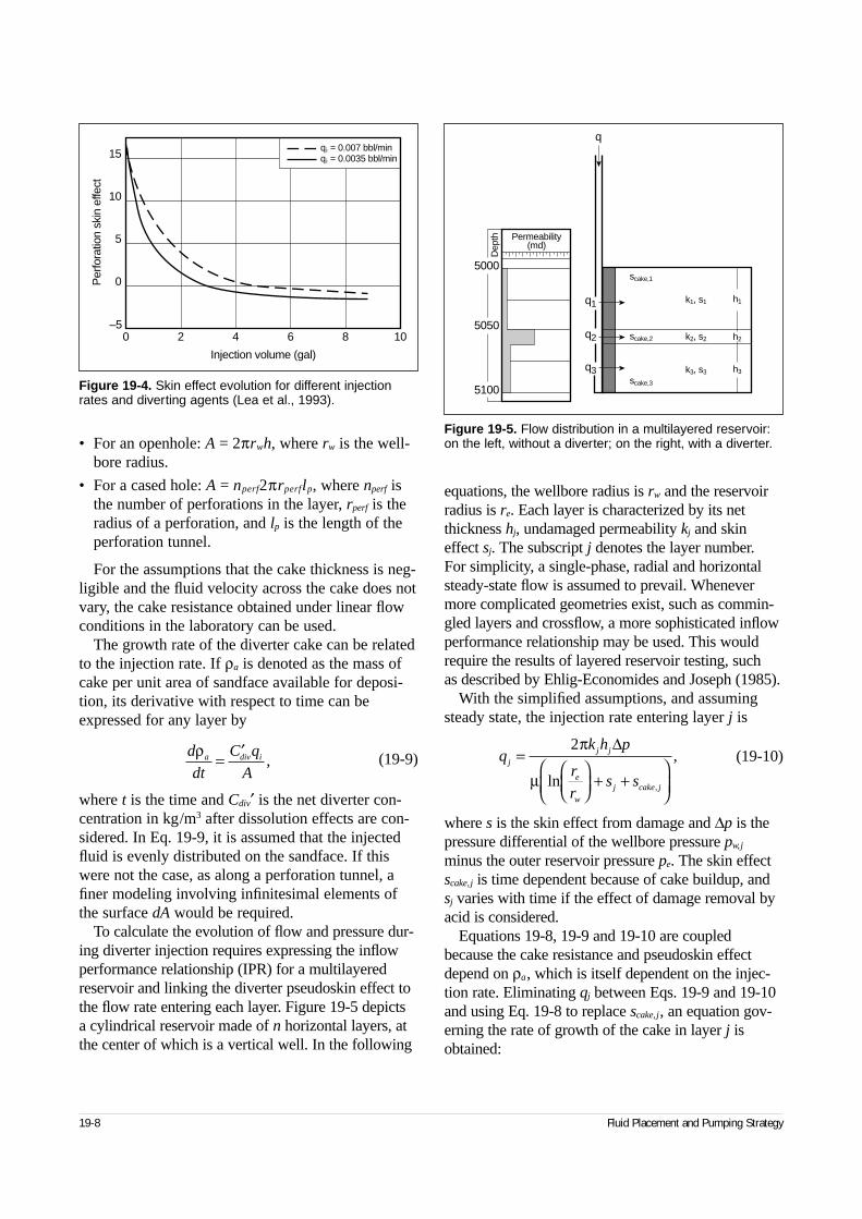
• For an openhole: A = 2πrwh, where rw is the well-bore radius.

• For a cased hole: A = nperf2πrperflp, where nperf isthe number of perforations in the layer, rperf is theradius of a perforation, and lp is the length of theperforation tunnel.

For the assumptions that the cake thickness is neg-ligible and the fluid velocity across the cake does notvary, the cake resistance obtained under linear flowconditions in the laboratory can be used.

The growth rate of the diverter cake can be relatedto the injection rate. If ρa is denoted as the mass ofcake per unit area of sandface available for deposi-tion, its derivative with respect to time can beexpressed for any layer by

(19-9)

where t is the time and Cdiv′ is the net diverter con-centration in kg/m3 after dissolution effects are con-sidered. In Eq. 19-9, it is assumed that the injectedfluid is evenly distributed on the sandface. If thiswere not the case, as along a perforation tunnel, afiner modeling involving infinitesimal elements ofthe surface dA would be required.

To calculate the evolution of flow and pressure dur-ing diverter injection requires expressing the inflowperformance relationship (IPR) for a multilayeredreservoir and linking the diverter pseudoskin effect tothe flow rate entering each layer. Figure 19-5 depicts a cylindrical reservoir made of n horizontal layers, atthe center of which is a vertical well. In the following

equations, the wellbore radius is rw and the reservoirradius is re. Each layer is characterized by its netthickness hj, undamaged permeability kj and skineffect sj. The subscript j denotes the layer number. For simplicity, a single-phase, radial and horizontalsteady-state flow is assumed to prevail. Whenevermore complicated geometries exist, such as commin-gled layers and crossflow, a more sophisticated inflowperformance relationship may be used. This wouldrequire the results of layered reservoir testing, such as described by Ehlig-Economides and Joseph (1985).

With the simplified assumptions, and assumingsteady state, the injection rate entering layer j is

(19-10)

where s is the skin effect from damage and ∆p is thepressure differential of the wellbore pressure pw,j

minus the outer reservoir pressure pe. The skin effectscake,j is time dependent because of cake buildup, and sj varies with time if the effect of damage removal byacid is considered.

Equations 19-8, 19-9 and 19-10 are coupledbecause the cake resistance and pseudoskin effectdepend on ρa, which is itself dependent on the injec-tion rate. Eliminating qj between Eqs. 19-9 and 19-10and using Eq. 19-8 to replace scake,j, an equation gov-erning the rate of growth of the cake in layer j isobtained:

19-8 Fluid Placement and Pumping Strategy

d

dt

C q

Aa div iρ = ′

, qk h p

r

rs s

jj j

e

w

j cake j

=

+ +

2π

µ

∆

ln ,

,

Figure 19-4. Skin effect evolution for different injectionrates and diverting agents (Lea et al., 1993).

0 2 4 6 8 10

Injection volume (gal)

0

5

10

15

–5

Per

fora

tion

skin

effe

ct

qi = 0.007 bbl/min qi = 0.0035 bbl/min

Figure 19-5. Flow distribution in a multilayered reservoir:on the left, without a diverter; on the right, with a diverter.

5000

5050

5100

q1

q2

q3

h1

scake,1

scake,2

scake,3

k1, s1

h2k2, s2

h3k3, s3

q

Permeability(md)

Dep

th

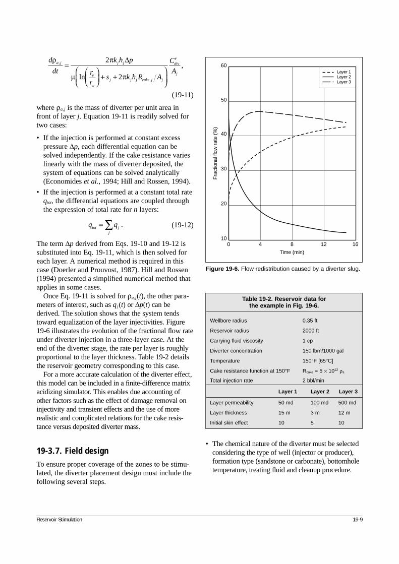
(19-11)

where ρa,j is the mass of diverter per unit area infront of layer j. Equation 19-11 is readily solved fortwo cases:

• If the injection is performed at constant excesspressure ∆p, each differential equation can besolved independently. If the cake resistance varieslinearly with the mass of diverter deposited, thesystem of equations can be solved analytically(Economides et al., 1994; Hill and Rossen, 1994).

• If the injection is performed at a constant total rateqtot, the differential equations are coupled throughthe expression of total rate for n layers:

(19-12)

The term ∆p derived from Eqs. 19-10 and 19-12 issubstituted into Eq. 19-11, which is then solved foreach layer. A numerical method is required in thiscase (Doerler and Prouvost, 1987). Hill and Rossen(1994) presented a simplified numerical method thatapplies in some cases.

Once Eq. 19-11 is solved for ρa,j(t), the other para-meters of interest, such as qj(t) or ∆p(t) can bederived. The solution shows that the system tendstoward equalization of the layer injectivities. Figure19-6 illustrates the evolution of the fractional flow rateunder diverter injection in a three-layer case. At theend of the diverter stage, the rate per layer is roughlyproportional to the layer thickness. Table 19-2 detailsthe reservoir geometry corresponding to this case.

For a more accurate calculation of the diverter effect,this model can be included in a finite-difference matrixacidizing simulator. This enables due accounting ofother factors such as the effect of damage removal oninjectivity and transient effects and the use of morerealistic and complicated relations for the cake resis-tance versus deposited diverter mass.

19-3.7. Field designTo ensure proper coverage of the zones to be stimu-lated, the diverter placement design must include thefollowing several steps.

• The chemical nature of the diverter must be selectedconsidering the type of well (injector or producer),formation type (sandstone or carbonate), bottomholetemperature, treating fluid and cleanup procedure.

Reservoir Stimulation 19-9

d

dt

k h p

r

rs k h R A

C

Aa j j j

e

w

j j j cake j j

div

j

ρ π

µ π

,

,

,=

+ +

′2

2

∆

ln

q qtot jj

= ∑ .

Figure 19-6. Flow redistribution caused by a diverter slug.

010

4 8 12 16

20

30

40

50

60

Time (min)

Fra

ctio

nal f

low

rate

(%)

Layer 1Layer 2Layer 3

Table 19-2. Reservoir data for the example in Fig. 19-6.

Wellbore radius 0.35 ft

Reservoir radius 2000 ft

Carrying fluid viscosity 1 cp

Diverter concentration 150 lbm/1000 gal

Temperature 150°F [65°C]

Cake resistance function at 150°F Rcake = 5 × 1012 ρa

Total injection rate 2 bbl/min

Layer 1 Layer 2 Layer 3

Layer permeability 50 md 100 md 500 md

Layer thickness 15 m 3 m 12 m

Initial skin effect 10 5 10

• The particle-size distribution must be adapted tothe pore size of the formation upon which the cakewill be deposited. This should prevent any inva-sion of the porous medium by diverter particles. In general, the particle size must be adapted to theformation layer with the highest permeability.

• A dispersant must be used to ensure that particleswill not flocculate in the carrying fluid. Althoughnot recommended, bridging agents must be mixedin gel pads to prevent sedimentation in some cases.

• Once the proper material has been selected, thevolume, concentration and injection rate of thediverter must be determined. Generally, concen-trated slugs have been found more effective thancontinuous injection at a lower concentration. Thepumping parameters, namely bottomhole pressureand injection rate, must then be estimated toensure their compliance with field operational con-straints, such as fracturing pressure. The overallinjectivity of the well should not be lowered to thepoint that only small injection rates are possible.

The method described in this section can be used to optimize diverter slugs if the well and reservoirdata are known. Unfortunately, in many cases, criticalparameters such as the exact perforation geometry,pore size near the sandface and distributions of perme-ability and damage are poorly characterized. In thepast, this has limited the use of mathematical modelsfor diverter design. Many practical designs are basedon local experience (i.e., trial and error). With the useof coiled tubing, which greatly decreases the volumeof the injection string, design can be modified on thefly and the pressure response of the well to acid anddiverter slugs can help guide diversion optimization.A flat pressure response to acid indicates that a divert-er is required, and the efficiency of cake buildup canbe assessed from the reservoir response (pressureincrease) to diverter injection. This method of designoptimization based on real-time well response is morereliable than a priori estimates and is most likely to beeffective if facilities are available for on-site stimula-tion monitoring.

19-4. Foam diversion

19-4.1. Historical backgroundFoams have been used for acid diversion since atleast the 1960s (Smith et al., 1969). The acid itself

can be foamed with the addition of gas and surfac-tant, or, more commonly, foam can be injected inalternating slugs with acid. Until recently, there waslittle published information on acid diversion withfoam, in contrast to the extensive literature on foamfor diverting gas flow in improved oil recovery(IOR) processes (Hirasaki, 1989a, 1989b; Schramm,1994; Rossen, 1996). The findings of IOR foamresearch have exerted a strong influence on theunderstanding of foam acid diversion. More recentresearch suggests that although the basic mecha-nisms of the two processes are similar, differences in the flow regime between near-well and reservoirapplications cause significant differences in behavior.This section summarizes the current consensus onfoam behavior and process design. This is an activearea of research, and this consensus may well shiftwithin the next few years.

19-4.2. Foam mechanismsFoams act fundamentally differently as they penetrateand plug the pore space of rock compared with thebehavior of foams used for drilling, cementing, frac-turing or well cleanout. Therefore, analogies to theseother foams can be misleading. For example, foams inpipes are created and maintained by shear forces, andthe resulting bubbles are much smaller than the pipediameter. Within the tiny pores of an oil or gas reser-voir, however, foam bubbles larger than the individualpores are squeezed down into elongated shapes, span-ning several pores, with a liquid film or lamellabetween each pair of bubbles (Ettinger and Radke,1992; Falls et al., 1989). The behavior of foam isdominated by the capillary forces on the lamellae; viscous forces in the conventional sense are relativelyunimportant.

Numerous IOR foam studies agree that foam doesnot directly alter liquid mobility in porous media(Bernard et al., 1965; Friedmann et al., 1991; Huh andHandy, 1989; de Vries and Wit, 1990). In other words,the aqueous-phase relative permeability krw is the samefunction of its saturation Sw as in the absence of foam.(For the remainder of this section, for simplicity theaqueous phase is referred to as water.) Evidently, uponentering rock most of the water leaves the foam andflows through the same network of narrow pores andpore crevices through which it would flow at that sameSw in the absence of foam. As a result, overall mobilitywith foam can be inferred from Darcy’s law if the rela-

19-10 Fluid Placement and Pumping Strategy

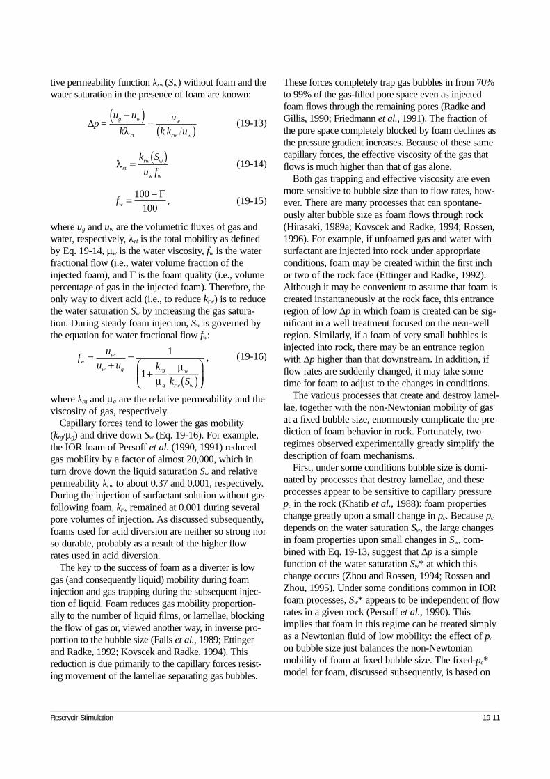
tive permeability function krw (Sw) without foam and thewater saturation in the presence of foam are known:

(19-13)

(19-14)

(19-15)

where ug and uw are the volumetric fluxes of gas andwater, respectively, λrt is the total mobility as definedby Eq. 19-14, µw is the water viscosity, fw is the waterfractional flow (i.e., water volume fraction of theinjected foam), and Γ is the foam quality (i.e., volumepercentage of gas in the injected foam). Therefore, theonly way to divert acid (i.e., to reduce krw) is to reducethe water saturation Sw by increasing the gas satura-tion. During steady foam injection, Sw is governed bythe equation for water fractional flow fw:

(19-16)

where krg and µg are the relative permeability and theviscosity of gas, respectively.

Capillary forces tend to lower the gas mobility(krg/µg) and drive down Sw (Eq. 19-16). For example,the IOR foam of Persoff et al. (1990, 1991) reducedgas mobility by a factor of almost 20,000, which inturn drove down the liquid saturation Sw and relativepermeability krw to about 0.37 and 0.001, respectively.During the injection of surfactant solution without gasfollowing foam, krw remained at 0.001 during severalpore volumes of injection. As discussed subsequently,foams used for acid diversion are neither so strong norso durable, probably as a result of the higher flowrates used in acid diversion.

The key to the success of foam as a diverter is lowgas (and consequently liquid) mobility during foaminjection and gas trapping during the subsequent injec-tion of liquid. Foam reduces gas mobility proportion-ally to the number of liquid films, or lamellae, blockingthe flow of gas or, viewed another way, in inverse pro-portion to the bubble size (Falls et al., 1989; Ettingerand Radke, 1992; Kovscek and Radke, 1994). Thisreduction is due primarily to the capillary forces resist-ing movement of the lamellae separating gas bubbles.

These forces completely trap gas bubbles in from 70%to 99% of the gas-filled pore space even as injectedfoam flows through the remaining pores (Radke andGillis, 1990; Friedmann et al., 1991). The fraction ofthe pore space completely blocked by foam declines asthe pressure gradient increases. Because of these samecapillary forces, the effective viscosity of the gas thatflows is much higher than that of gas alone.

Both gas trapping and effective viscosity are evenmore sensitive to bubble size than to flow rates, how-ever. There are many processes that can spontane-ously alter bubble size as foam flows through rock(Hirasaki, 1989a; Kovscek and Radke, 1994; Rossen,1996). For example, if unfoamed gas and water withsurfactant are injected into rock under appropriateconditions, foam may be created within the first inchor two of the rock face (Ettinger and Radke, 1992).Although it may be convenient to assume that foam iscreated instantaneously at the rock face, this entranceregion of low ∆p in which foam is created can be sig-nificant in a well treatment focused on the near-wellregion. Similarly, if a foam of very small bubbles isinjected into rock, there may be an entrance regionwith ∆p higher than that downstream. In addition, ifflow rates are suddenly changed, it may take sometime for foam to adjust to the changes in conditions.

The various processes that create and destroy lamel-lae, together with the non-Newtonian mobility of gasat a fixed bubble size, enormously complicate the pre-diction of foam behavior in rock. Fortunately, tworegimes observed experimentally greatly simplify thedescription of foam mechanisms.

First, under some conditions bubble size is domi-nated by processes that destroy lamellae, and theseprocesses appear to be sensitive to capillary pressurepc in the rock (Khatib et al., 1988): foam propertieschange greatly upon a small change in pc. Because pc

depends on the water saturation Sw, the large changesin foam properties upon small changes in Sw, com-bined with Eq. 19-13, suggest that ∆p is a simplefunction of the water saturation Sw* at which thischange occurs (Zhou and Rossen, 1994; Rossen andZhou, 1995). Under some conditions common in IORfoam processes, Sw* appears to be independent of flowrates in a given rock (Persoff et al., 1990). Thisimplies that foam in this regime can be treated simplyas a Newtonian fluid of low mobility: the effect of pc

on bubble size just balances the non-Newtonianmobility of foam at fixed bubble size. The fixed-pc*model for foam, discussed subsequently, is based on

Reservoir Stimulation 19-11

∆pu u

k

u

k k ug w

rt

w

rw w

=+( )

= ( )λ

λ rtrw w

w w

k S

u f= ( )

fw = −100100

Γ,

fu

u u k

k S

ww

w g rg

g

w

rw w

=+

=+ ( )

1

1µ

µ,

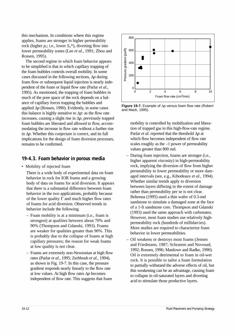
this mechanism. In conditions where this regimeapplies, foams are stronger in higher permeabilityrock (higher pc; i.e., lower Sw*), diverting flow intolower permeability zones (Lee et al., 1991; Zhou andRossen, 1995).

The second regime in which foam behavior appearsto be simplified is that in which capillary trapping ofthe foam bubbles controls overall mobility. In somecases discussed in the following sections, ∆p duringfoam flow or subsequent liquid injection is nearly inde-pendent of the foam or liquid flow rate (Parlar et al.,1995). As mentioned, the trapping of foam bubbles inmuch of the pore space of the rock depends on a bal-ance of capillary forces trapping the bubbles andapplied ∆p (Rossen, 1990). Evidently, in some casesthis balance is highly sensitive to ∆p: as the flow rateincreases, causing a slight rise in ∆p, previously trappedfoam bubbles are liberated and allowed to flow, accom-modating the increase in flow rate without a further risein ∆p. Whether this conjecture is correct, and its fullimplications for the design of foam diversion processes,remains to be confirmed.

19-4.3. Foam behavior in porous media• Mobility of injected foam

There is a wide body of experimental data on foambehavior in rock for IOR foams and a growingbody of data on foams for acid diversion. It appearsthat there is a substantial difference between foambehavior in the two applications, probably becauseof the lower quality Γ and much higher flow ratesof foams for acid diversion. Observed trends inbehavior include the following.

– Foam mobility is at a minimum (i.e., foam isstrongest) at qualities between about 70% and90% (Thompson and Gdanski, 1993). Foamsare weaker for qualities greater than 90%. Thisis probably due to the collapse of foams at highcapillary pressures; the reason for weak foamsat low quality is not clear.

– Foams are extremely non-Newtonian at high flowrates (Parlar et al., 1995; Zerhboub et al., 1994),as shown in Fig. 19-7. In this case, the pressuregradient responds nearly linearly to the flow rateat low values. At high flow rates ∆p becomesindependent of flow rate. This suggests that foam

mobility is controlled by mobilization and libera-tion of trapped gas in this high-flow-rate regime.Parlar et al. reported that the threshold ∆p atwhich flow becomes independent of flow ratescales roughly as the –1⁄2 power of permeabilityvalues greater than 800 md.

– During foam injection, foams are stronger (i.e.,higher apparent viscosity) in high-permeabilityrock, implying the diversion of flow from higherpermeability to lower permeability or more dam-aged intervals (see, e.g., Kibodeaux et al., 1994).Whether similar trends apply to diversionbetween layers differing in the extent of damagerather than permeability per se is not clear.Behenna (1995) used a thin wafer of 0.3-mdsandstone to simulate a damaged zone at the faceof a 1-ft sandstone core. Thompson and Gdanski(1993) used the same approach with carbonates.However, most foam studies use relatively high-permeability rock (hundreds of millidarcies).More studies are required to characterize foambehavior in lower permeabilities.

– Oil weakens or destroys most foams (Jensenand Friedmann, 1987; Schramm and Novosad,1992; Rossen, 1996; Manlowe and Radke, 1990).Oil is extremely detrimental to foam in oil-wetrock. It is possible to tailor a foam formulationto partially withstand the adverse effects of oil, butthis weakening can be an advantage, causing foamto collapse in oil-saturated layers and divertingacid to stimulate those productive layers.

19-12 Fluid Placement and Pumping Strategy

Figure 19-7. Example of ∆p versus foam flow rate (Robertand Mack, 1995).

800

600

400

200

00 2 4 6 8 10

Foam flow rate (cm3/min)

Pre

ssur

e gr

adie

nt (p

si/ft

)

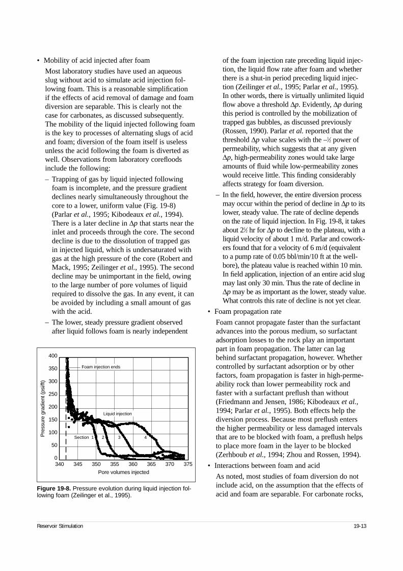
• Mobility of acid injected after foam

Most laboratory studies have used an aqueousslug without acid to simulate acid injection fol-lowing foam. This is a reasonable simplification if the effects of acid removal of damage and foamdiversion are separable. This is clearly not thecase for carbonates, as discussed subsequently.The mobility of the liquid injected following foamis the key to processes of alternating slugs of acidand foam; diversion of the foam itself is uselessunless the acid following the foam is diverted aswell. Observations from laboratory corefloodsinclude the following:

– Trapping of gas by liquid injected followingfoam is incomplete, and the pressure gradientdeclines nearly simultaneously throughout thecore to a lower, uniform value (Fig. 19-8)(Parlar et al., 1995; Kibodeaux et al., 1994).There is a later decline in ∆p that starts near theinlet and proceeds through the core. The seconddecline is due to the dissolution of trapped gasin injected liquid, which is undersaturated withgas at the high pressure of the core (Robert andMack, 1995; Zeilinger et al., 1995). The seconddecline may be unimportant in the field, owingto the large number of pore volumes of liquidrequired to dissolve the gas. In any event, it canbe avoided by including a small amount of gaswith the acid.

– The lower, steady pressure gradient observedafter liquid follows foam is nearly independent

of the foam injection rate preceding liquid injec-tion, the liquid flow rate after foam and whetherthere is a shut-in period preceding liquid injec-tion (Zeilinger et al., 1995; Parlar et al., 1995).In other words, there is virtually unlimited liquidflow above a threshold ∆p. Evidently, ∆p duringthis period is controlled by the mobilization oftrapped gas bubbles, as discussed previously(Rossen, 1990). Parlar et al. reported that thethreshold ∆p value scales with the –1⁄2 power ofpermeability, which suggests that at any given∆p, high-permeability zones would take largeamounts of fluid while low-permeability zoneswould receive little. This finding considerablyaffects strategy for foam diversion.

– In the field, however, the entire diversion processmay occur within the period of decline in ∆p to itslower, steady value. The rate of decline dependson the rate of liquid injection. In Fig. 19-8, it takesabout 21⁄2 hr for ∆p to decline to the plateau, with aliquid velocity of about 1 m/d. Parlar and cowork-ers found that for a velocity of 6 m/d (equivalentto a pump rate of 0.05 bbl/min/10 ft at the well-bore), the plateau value is reached within 10 min.In field application, injection of an entire acid slugmay last only 30 min. Thus the rate of decline in∆p may be as important as the lower, steady value.What controls this rate of decline is not yet clear.

• Foam propagation rate

Foam cannot propagate faster than the surfactantadvances into the porous medium, so surfactantadsorption losses to the rock play an importantpart in foam propagation. The latter can lagbehind surfactant propagation, however. Whethercontrolled by surfactant adsorption or by otherfactors, foam propagation is faster in high-perme-ability rock than lower permeability rock andfaster with a surfactant preflush than without(Friedmann and Jensen, 1986; Kibodeaux et al.,1994; Parlar et al., 1995). Both effects help thediversion process. Because most preflush entersthe higher permeability or less damaged intervalsthat are to be blocked with foam, a preflush helpsto place more foam in the layer to be blocked(Zerhboub et al., 1994; Zhou and Rossen, 1994).

• Interactions between foam and acid

As noted, most studies of foam diversion do notinclude acid, on the assumption that the effects ofacid and foam are separable. For carbonate rocks,

Reservoir Stimulation 19-13

Figure 19-8. Pressure evolution during liquid injection fol-lowing foam (Zeilinger et al., 1995).

340 345 350 355 360 365 370 375

Pore volumes injected

0

50

100

150

200

250

300

350

400

Pre

ssur

e gr

adie

nt (p

si/ft

)

Liquid injection

Section 1 2 3 4

Foam injection ends

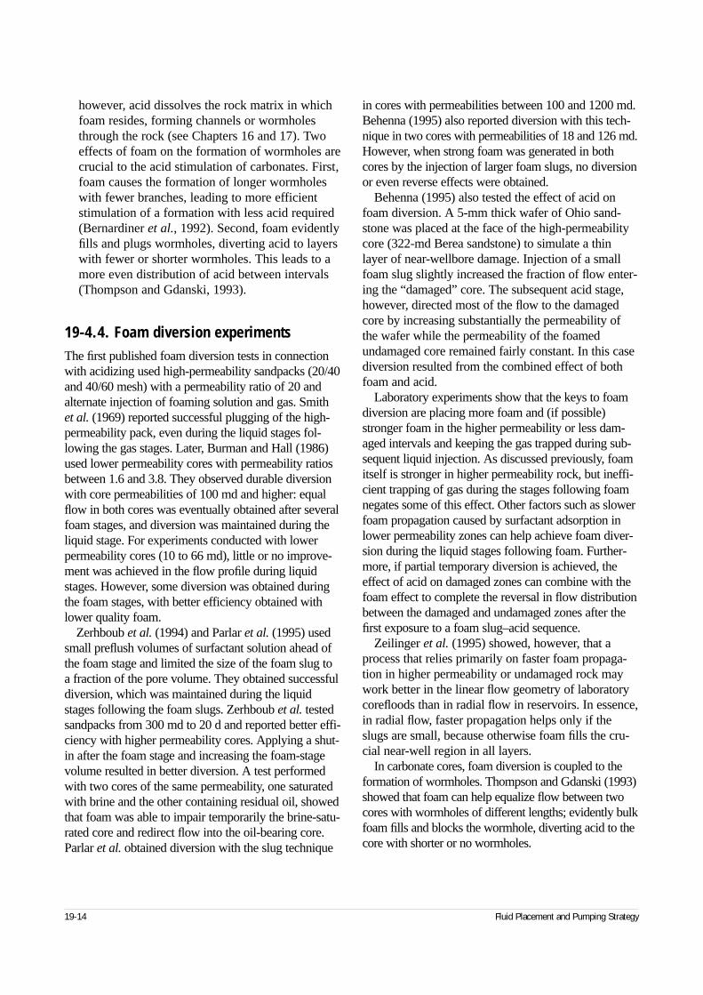
however, acid dissolves the rock matrix in whichfoam resides, forming channels or wormholesthrough the rock (see Chapters 16 and 17). Twoeffects of foam on the formation of wormholes arecrucial to the acid stimulation of carbonates. First,foam causes the formation of longer wormholeswith fewer branches, leading to more efficientstimulation of a formation with less acid required(Bernardiner et al., 1992). Second, foam evidentlyfills and plugs wormholes, diverting acid to layerswith fewer or shorter wormholes. This leads to amore even distribution of acid between intervals(Thompson and Gdanski, 1993).

19-4.4. Foam diversion experimentsThe first published foam diversion tests in connectionwith acidizing used high-permeability sandpacks (20/40and 40/60 mesh) with a permeability ratio of 20 andalternate injection of foaming solution and gas. Smith et al. (1969) reported successful plugging of the high-permeability pack, even during the liquid stages fol-lowing the gas stages. Later, Burman and Hall (1986)used lower permeability cores with permeability ratiosbetween 1.6 and 3.8. They observed durable diversionwith core permeabilities of 100 md and higher: equalflow in both cores was eventually obtained after severalfoam stages, and diversion was maintained during theliquid stage. For experiments conducted with lowerpermeability cores (10 to 66 md), little or no improve-ment was achieved in the flow profile during liquidstages. However, some diversion was obtained duringthe foam stages, with better efficiency obtained withlower quality foam.

Zerhboub et al. (1994) and Parlar et al. (1995) usedsmall preflush volumes of surfactant solution ahead ofthe foam stage and limited the size of the foam slug toa fraction of the pore volume. They obtained successfuldiversion, which was maintained during the liquidstages following the foam slugs. Zerhboub et al. testedsandpacks from 300 md to 20 d and reported better effi-ciency with higher permeability cores. Applying a shut-in after the foam stage and increasing the foam-stagevolume resulted in better diversion. A test performedwith two cores of the same permeability, one saturatedwith brine and the other containing residual oil, showedthat foam was able to impair temporarily the brine-satu-rated core and redirect flow into the oil-bearing core.Parlar et al. obtained diversion with the slug technique

in cores with permeabilities between 100 and 1200 md.Behenna (1995) also reported diversion with this tech-nique in two cores with permeabilities of 18 and 126 md.However, when strong foam was generated in bothcores by the injection of larger foam slugs, no diversionor even reverse effects were obtained.

Behenna (1995) also tested the effect of acid onfoam diversion. A 5-mm thick wafer of Ohio sand-stone was placed at the face of the high-permeabilitycore (322-md Berea sandstone) to simulate a thinlayer of near-wellbore damage. Injection of a smallfoam slug slightly increased the fraction of flow enter-ing the “damaged” core. The subsequent acid stage,however, directed most of the flow to the damagedcore by increasing substantially the permeability ofthe wafer while the permeability of the foamedundamaged core remained fairly constant. In this casediversion resulted from the combined effect of bothfoam and acid.

Laboratory experiments show that the keys to foamdiversion are placing more foam and (if possible)stronger foam in the higher permeability or less dam-aged intervals and keeping the gas trapped during sub-sequent liquid injection. As discussed previously, foamitself is stronger in higher permeability rock, but ineffi-cient trapping of gas during the stages following foamnegates some of this effect. Other factors such as slowerfoam propagation caused by surfactant adsorption inlower permeability zones can help achieve foam diver-sion during the liquid stages following foam. Further-more, if partial temporary diversion is achieved, theeffect of acid on damaged zones can combine with thefoam effect to complete the reversal in flow distributionbetween the damaged and undamaged zones after thefirst exposure to a foam slug–acid sequence.

Zeilinger et al. (1995) showed, however, that aprocess that relies primarily on faster foam propaga-tion in higher permeability or undamaged rock maywork better in the linear flow geometry of laboratorycorefloods than in radial flow in reservoirs. In essence,in radial flow, faster propagation helps only if theslugs are small, because otherwise foam fills the cru-cial near-well region in all layers.

In carbonate cores, foam diversion is coupled to theformation of wormholes. Thompson and Gdanski (1993)showed that foam can help equalize flow between twocores with wormholes of different lengths; evidently bulkfoam fills and blocks the wormhole, diverting acid to thecore with shorter or no wormholes.

19-14 Fluid Placement and Pumping Strategy

19-4.5. Modeling and predicting foam diversion

IOR foam researchers use a variety of mathematicalmodels to describe foams (Kular et al., 1989; Fisher et al., 1990). In principle, the most complete, but alsohighly complex, population balance model (Friedmannet al., 1991; Falls et al., 1989; Kovscek and Radke,1994) attempts to represent all mechanisms of non-Newtonian mobility and processes altering bubble size.There is no published application of this model tofoams for diverting acid.

The much simpler approach of the fixed-pc* model(Rossen and Zhou, 1995; Zhou and Rossen, 1994,1995), focuses on the coalescence of foam as a func-tion of capillary pressure pc or water saturation Sw.Combined with fractional-flow modeling, this foammodel predicts some important aspects of foambehavior: the benefits of a surfactant preflush, theimportance of compatibility of acid and foam slugs,foam diversion between layers differing in perme-ability and differences between diversion processesin linear and radial flow. In this approach, laboratorycorefloods are used to determine the rates of advanceand mobility of foam during the injection of foamand subsequent injection of liquid (Kibodeaux et al.,1994). Mobilities are assumed independent of flowrates. These parameters are then used with equationsfor radial flow such as Eq. 19-10 to predict diversionin a field application. The model identifies the keysto effective foam diversion as the rate of foam prop-agation, foam mobility during injection and foammobility during liquid injection in each layer.

Hill and Rossen (1994) presented an even simplerversion that gives essentially equivalent results formany applications. In this model, the foam skin

effect sfoam,j replaces scake,j in Eq. 19-10. The foamskin effect is

(19-17)

where kj/kfoam,j is the mobility reduction resultingfrom foam (assumed for simplicity to affect onlypermeability) in layer j and rf,j is the radial extent of the foam bank in that layer. Foam advances ineach layer at a constant volumetric rate that reflectspermeability and the volume of preflush in that layer.Upon switching from foam to acid injection in a slugprocess, the mobility reduction factor kj/kfoam,j sud-denly takes a new, usually higher, constant value,and rf,j stays constant during acid injection. An ana-lytical solution is obtained for constant-pressureinjection, and other cases, such as injection at a fixedoverall injection rate, can be derived easily.

This approach uses many simplifying assumptions,of which two now appear to distort predictions offoam performance in the field: assuming mobility isindependent of flow rates and assuming instantaneousattainment of steady-state mobilities upon a change ininjection conditions. As noted previously, foams arestrongly non-Newtonian in the flow regime relevant to acid diversion, and the period of transition betweenhigh ∆p with foam and lower ∆p during liquid injec-tion (Fig. 19-8) may be crucial to the diversion proc-ess. Work to extend this model to account for theseeffects is ongoing.

The simulator described by Robert and Mack(1995) and Bartko et al. (1996) does not make theseassumptions and fits their laboratory corefloods well(Fig. 19-9). This approach is closer to full reservoirsimulation: the computer solves a partial differentialequation for pressure and flow rates as functions of

Reservoir Stimulation 19-15

sk

k

r

rfoam jj

foam j

f j

w

,

,

, ,= −

1 ln

Figure 19-9. Comparison of simulation (right) with laboratory coreflood (actual data, left) (Robert and Mack, 1995).

800

600

400

200

00 100 200 300

Time (min)

Pre

ssur

e gr

adie

nt (p

si/ft

)

Foam Surfactant

0–1 in.1–3 in.3–5 in.5–7 in.7–11 in.9–12 in.

800

600

400

200

00 100 200 300

Time (min)

Pre

ssur

e gr

adie

nt (p

si/ft

)

Foam Surfactant

0–1 in.1–3 in.3–5 in.5–7 in.7–11 in.9–11 in.

position and time, interpolating mobilities from tablesof laboratory data. Local gas and liquid saturations arecomputed from mobilities and local foam flow condi-tions using Eqs. 19-14 and 19-15. A mass balance isthen used to compute the local flow rates for eachphase from the variations of saturation. Both regimesshown in Fig. 19-7—the low-flow-rate regime, inwhich mobilities are roughly Newtonian at constantquality and the constant-pressure-gradient regime athigh flow rates—are included in the simulator foam-mobility model. For liquid injection after a foam stage(i.e., the reimbibition stage), the simulator assumes asharp transition in gas mobility from complete plug-ging to high mobility at the threshold pressure gradi-ent. This tends to maintain the actual pressure gradientat the threshold value during liquid injection, asobserved experimentally. An empirical correlation isused to account for the delay of gas removal (and thecorresponding delay of pressure decrease) observed atlow liquid rates. This is the most difficult part of thecorefloods to model accurately, and in some cases thesimulator tends to overestimate this delay slightly,especially in the downstream section of the cores.Effects of surfactant adsorption, gas compressibilityand gas solubility are also included. In principle, thereis no limit to the complexity of mobility behavior thatcan be incorporated in this approach.

19-4.6. Application to field designRecent laboratory results have led to the developmentof guidelines for foam diversion (Gdanski, 1993;Zerhboub et al., 1994). Foam diversion has been usedincreasingly in recent years, particularly in cases whereother diversion techniques are impractical or less effi-cient such as the application of particulate diverters andball sealers over large intervals. Foams also help incleanup and back-production of treating fluids.

• Choice of surfactant

Traditionally, half-life measurements have beenused to rank the foaming performance of surfac-tants. In these static tests, foam is generated andallowed to decay slowly in a beaker under theaction of liquid drainage and gas migration. Thetime for one-half of the liquid to drain out of thefoam is called the foam half-life. These tests areuseful for determining chemical compatibility andidentifying ineffective foams but not for optimiz-ing surfactant formulation (Rossen, 1996). Foam

formation in porous media is a dynamic process inwhich bubbles (or lamellae) are constantly createdand broken. Surfactant adsorption on the rock sur-face, elasticity of lamellae and kinetics of foamformation are important properties that cannot bemeasured by static half-life tests. Therefore, onlycore flow tests can be used to select the mostappropriate surfactant formulation for diversion.

Laboratory experiments indicate that diversionrequires rapid formation and propagation of strongfoam in higher permeability cores, with delayedfoam formation in the lower permeability zones.This suggests that surfactant adsorption is a criti-cal parameter for diversion. Oil present in the for-mation is another parameter to take into accountfor surfactant selection: the presence of oil canimpair significantly the foam strength or delay theonset of effective foam banks, especially in oil-wet formations.

• Pumping strategy

On the basis of laboratory experiments, Zerhboubet al. (1994) proposed a set of guidelines for foamdiversion. The principle of the method consists ofpretreating the matrix to facilitate the formation ofstrong foam with a minimum foam volume andadding surfactant to acid stages to preserve thefoam bank stability. Experiments on sandstones andcarbonates show that effective and durable diver-sion can be obtained with repetitive slugs of foamand acid. Indeed, once a damaged zone has beenacidized, it must be plugged by foam to redirectacid to zones that have not been treated. Further-more, foam in place tends to undergo slow decay(presumably because of gas dissolution), and peri-odic regeneration of the foam bank is required.

Use of a mutual solvent is recommended aheadof the treatment to reduce interfacial tension andto help sweep oil from the near-wellbore region.For a well-defined water zone, treatment can bestarted with a foam slug aimed at selectively plug-ging the water zone, while the oil prevents strongfoam formation in the hydrocarbon-bearing zone.In that case, a mutual-solvent preflush is not bene-ficial. A gel-based water- or oil-specific divertercan be also used in addition to foam to help plugwater zones (Kennedy et al., 1992).

The size of foam slugs can be extrapolated fromlaboratory studies. As with particulate diverters, thedesign consists of pumping enough foam to plug

19-16 Fluid Placement and Pumping Strategy

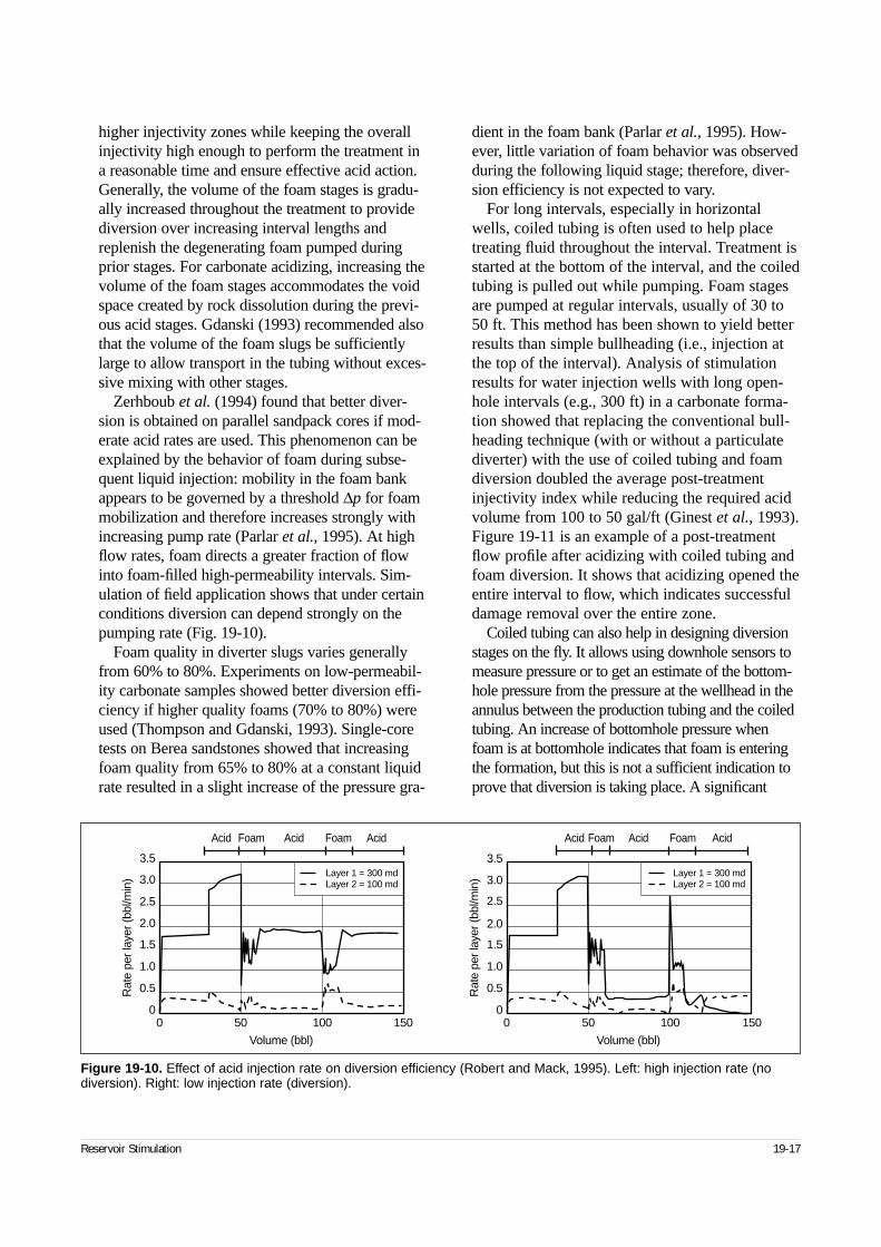
higher injectivity zones while keeping the overallinjectivity high enough to perform the treatment ina reasonable time and ensure effective acid action.Generally, the volume of the foam stages is gradu-ally increased throughout the treatment to providediversion over increasing interval lengths andreplenish the degenerating foam pumped duringprior stages. For carbonate acidizing, increasing thevolume of the foam stages accommodates the voidspace created by rock dissolution during the previ-ous acid stages. Gdanski (1993) recommended alsothat the volume of the foam slugs be sufficientlylarge to allow transport in the tubing without exces-sive mixing with other stages.

Zerhboub et al. (1994) found that better diver-sion is obtained on parallel sandpack cores if mod-erate acid rates are used. This phenomenon can beexplained by the behavior of foam during subse-quent liquid injection: mobility in the foam bankappears to be governed by a threshold ∆p for foammobilization and therefore increases strongly withincreasing pump rate (Parlar et al., 1995). At highflow rates, foam directs a greater fraction of flowinto foam-filled high-permeability intervals. Sim-ulation of field application shows that under certainconditions diversion can depend strongly on thepumping rate (Fig. 19-10).

Foam quality in diverter slugs varies generallyfrom 60% to 80%. Experiments on low-permeabil-ity carbonate samples showed better diversion effi-ciency if higher quality foams (70% to 80%) wereused (Thompson and Gdanski, 1993). Single-coretests on Berea sandstones showed that increasingfoam quality from 65% to 80% at a constant liquidrate resulted in a slight increase of the pressure gra-

dient in the foam bank (Parlar et al., 1995). How-ever, little variation of foam behavior was observedduring the following liquid stage; therefore, diver-sion efficiency is not expected to vary.

For long intervals, especially in horizontalwells, coiled tubing is often used to help placetreating fluid throughout the interval. Treatment isstarted at the bottom of the interval, and the coiledtubing is pulled out while pumping. Foam stagesare pumped at regular intervals, usually of 30 to50 ft. This method has been shown to yield betterresults than simple bullheading (i.e., injection atthe top of the interval). Analysis of stimulationresults for water injection wells with long open-hole intervals (e.g., 300 ft) in a carbonate forma-tion showed that replacing the conventional bull-heading technique (with or without a particulatediverter) with the use of coiled tubing and foamdiversion doubled the average post-treatmentinjectivity index while reducing the required acidvolume from 100 to 50 gal/ft (Ginest et al., 1993).Figure 19-11 is an example of a post-treatmentflow profile after acidizing with coiled tubing andfoam diversion. It shows that acidizing opened theentire interval to flow, which indicates successfuldamage removal over the entire zone.

Coiled tubing can also help in designing diversionstages on the fly. It allows using downhole sensors tomeasure pressure or to get an estimate of the bottom-hole pressure from the pressure at the wellhead in theannulus between the production tubing and the coiledtubing. An increase of bottomhole pressure whenfoam is at bottomhole indicates that foam is enteringthe formation, but this is not a sufficient indication toprove that diversion is taking place. A significant

Reservoir Stimulation 19-17

Figure 19-10. Effect of acid injection rate on diversion efficiency (Robert and Mack, 1995). Left: high injection rate (nodiversion). Right: low injection rate (diversion).

00

50 100 1500 50 100 150

0.5

1.0

1.5

2.0

2.5

3.0

3.5

0

0.5

1.0

1.5

2.0

2.5

3.0

3.5

Rat

e pe

r lay

er (b

bl/m

in)

Rat

e pe

r lay

er (b

bl/m

in)

Volume (bbl)Volume (bbl)

Layer 1 = 300 mdLayer 2 = 100 md

Layer 1 = 300 mdLayer 2 = 100 md

Acid Acid AcidFoam Acid Acid AcidFoam FoamFoam

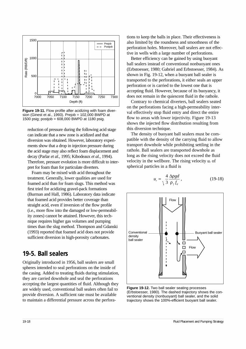
reduction of pressure during the following acid stagecan indicate that a new zone is acidized and thatdiversion was obtained. However, laboratory experi-ments show that a drop in injection pressure duringthe acid stage may also reflect foam displacement anddecay (Parlar et al., 1995; Kibodeaux et al., 1994).Therefore, pressure evolution is more difficult to inter-pret for foam than for particulate diverters.

Foam may be mixed with acid throughout thetreatment. Generally, lower qualities are used forfoamed acid than for foam slugs. This method wasfirst tried for acidizing gravel-pack formations(Burman and Hall, 1986). Laboratory data indicatethat foamed acid provides better coverage thanstraight acid, even if inversion of the flow profile(i.e., more flow into the damaged or low-permeabil-ity zones) cannot be attained. However, this tech-nique requires higher gas volumes and pumpingtimes than the slug method. Thompson and Gdanski(1993) reported that foamed acid does not providesufficient diversion in high-porosity carbonates.

19-5. Ball sealersOriginally introduced in 1956, ball sealers are smallspheres intended to seal perforations on the inside ofthe casing. Added to treating fluids during stimulation,they are carried downhole and seal the perforationsaccepting the largest quantities of fluid. Although theyare widely used, conventional ball sealers often fail toprovide diversion. A sufficient rate must be availableto maintain a differential pressure across the perfora-

tions to keep the balls in place. Their effectiveness isalso limited by the roundness and smoothness of theperforation holes. Moreover, ball sealers are not effec-tive in wells with a large number of perforations.

Better efficiency can be gained by using buoyantball sealers instead of conventional nonbuoyant ones(Erbstoesser, 1980; Gabriel and Erbstoesser, 1984). Asshown in Fig. 19-12, when a buoyant ball sealer istransported to the perforations, it either seals an upperperforation or is carried to the lowest one that isaccepting fluid. However, because of its buoyancy, itdoes not remain in the quiescent fluid in the rathole.

Contrary to chemical diverters, ball sealers seatedon the perforations facing a high-permeability inter-val effectively stop fluid entry and direct the entireflow to areas with lower injectivity. Figure 19-13shows the injected flow distribution resulting fromthis diversion technique.

The density of buoyant ball sealers must be com-patible with the density of the carrying fluid to allowtransport downhole while prohibiting settling in therathole. Ball sealers are transported downhole aslong as the rising velocity does not exceed the fluidvelocity in the wellbore. The rising velocity ur ofspherical particles in a fluid is

(19-18)

19-18 Fluid Placement and Pumping Strategy

Figure 19-12. Two ball sealer seating processes(Erbstoesser, 1980). The dashed trajectory shows the con-ventional density (nonbuoyant) ball sealer, and the solidtrajectory shows the 100%-efficient buoyant ball sealer.

Flow

Flow

Buoyant ball sealerConventionaldensityball sealer

ugd

fr

f d

= 43

∆ρρ

,

Figure 19-11. Flow profile after acidizing with foam diver-sion (Ginest et al., 1993). Prejob = 102,000 BWPD at 1500 psig; postjob = 608,000 BWPD at 1180 psig.

70000

7050 7100 7150 7200 7250 7300

500

1000

1500

Depth (ft)

Rat

e (R

B/D

/ft)

PrejobPostjob

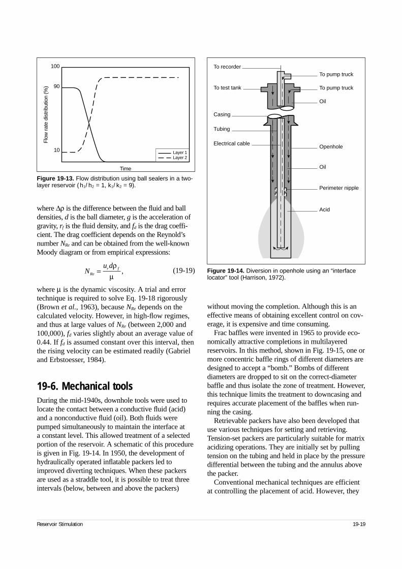
where ∆ρ is the difference between the fluid and balldensities, d is the ball diameter, g is the acceleration ofgravity, rf is the fluid density, and fd is the drag coeffi-cient. The drag coefficient depends on the Reynold’snumber NRe and can be obtained from the well-knownMoody diagram or from empirical expressions:

(19-19)

where µ is the dynamic viscosity. A trial and errortechnique is required to solve Eq. 19-18 rigorously(Brown et al., 1963), because NRe depends on thecalculated velocity. However, in high-flow regimes,and thus at large values of NRe (between 2,000 and100,000), fd varies slightly about an average value of0.44. If fd is assumed constant over this interval, thenthe rising velocity can be estimated readily (Gabrieland Erbstoesser, 1984).

19-6. Mechanical toolsDuring the mid-1940s, downhole tools were used tolocate the contact between a conductive fluid (acid)and a nonconductive fluid (oil). Both fluids werepumped simultaneously to maintain the interface at a constant level. This allowed treatment of a selectedportion of the reservoir. A schematic of this procedureis given in Fig. 19-14. In 1950, the development ofhydraulically operated inflatable packers led toimproved diverting techniques. When these packersare used as a straddle tool, it is possible to treat threeintervals (below, between and above the packers)

without moving the completion. Although this is aneffective means of obtaining excellent control on cov-erage, it is expensive and time consuming.

Frac baffles were invented in 1965 to provide eco-nomically attractive completions in multilayeredreservoirs. In this method, shown in Fig. 19-15, one ormore concentric baffle rings of different diameters aredesigned to accept a “bomb.” Bombs of differentdiameters are dropped to sit on the correct-diameterbaffle and thus isolate the zone of treatment. However,this technique limits the treatment to downcasing andrequires accurate placement of the baffles when run-ning the casing.

Retrievable packers have also been developed thatuse various techniques for setting and retrieving.Tension-set packers are particularly suitable for matrixacidizing operations. They are initially set by pullingtension on the tubing and held in place by the pressuredifferential between the tubing and the annulus abovethe packer.

Conventional mechanical techniques are efficientat controlling the placement of acid. However, they

Reservoir Stimulation 19-19

Figure 19-13. Flow distribution using ball sealers in a two-layer reservoir ( h1/ h2 = 1, k1/ k2 = 9).

100

90

10

Flo

w ra

te d

istri

butio

n (%

)

Time

Layer 1Layer 2

Nu d

Rer f=

ρµ

, Figure 19-14. Diversion in openhole using an “interfacelocator” tool (Harrison, 1972).

To recorder

To test tank

Casing

Tubing

Electrical cable

To pump truck

To pump truck

Oil

Openhole

Oil

Perimeter nipple

Acid

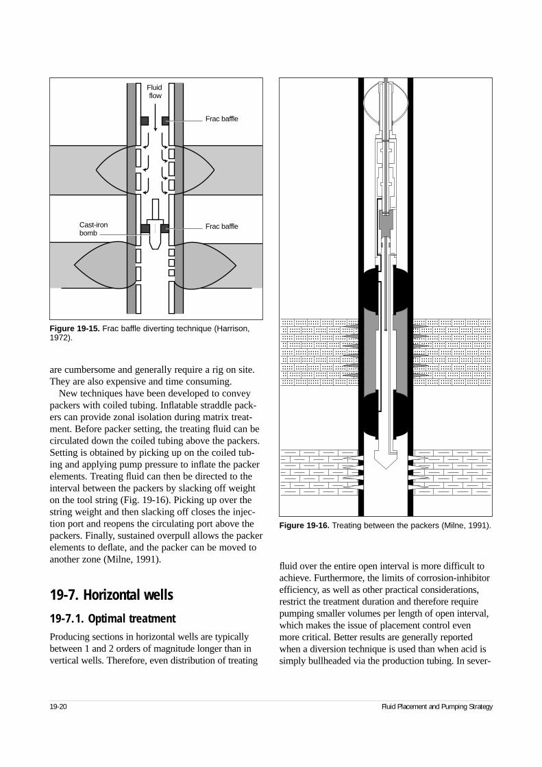
are cumbersome and generally require a rig on site.They are also expensive and time consuming.

New techniques have been developed to conveypackers with coiled tubing. Inflatable straddle pack-ers can provide zonal isolation during matrix treat-ment. Before packer setting, the treating fluid can becirculated down the coiled tubing above the packers.Setting is obtained by picking up on the coiled tub-ing and applying pump pressure to inflate the packerelements. Treating fluid can then be directed to theinterval between the packers by slacking off weighton the tool string (Fig. 19-16). Picking up over thestring weight and then slacking off closes the injec-tion port and reopens the circulating port above thepackers. Finally, sustained overpull allows the packerelements to deflate, and the packer can be moved toanother zone (Milne, 1991).

19-7. Horizontal wells

19-7.1. Optimal treatmentProducing sections in horizontal wells are typicallybetween 1 and 2 orders of magnitude longer than invertical wells. Therefore, even distribution of treating

fluid over the entire open interval is more difficult toachieve. Furthermore, the limits of corrosion-inhibitorefficiency, as well as other practical considerations,restrict the treatment duration and therefore requirepumping smaller volumes per length of open interval,which makes the issue of placement control evenmore critical. Better results are generally reportedwhen a diversion technique is used than when acid issimply bullheaded via the production tubing. In sever-

19-20 Fluid Placement and Pumping Strategy

Figure 19-16. Treating between the packers (Milne, 1991).

.......... .......... .......... .......... .......... .......... .......... .......... .......... .......... .......... .......... .......... .......... .......... ..........

.......... .......... .......... .......... .......... .......... .......... .......... .......... .......... .......... .......... .......... .......... .......... ..........

.......... .......... .......... .......... .......... .......... .......... .......... .......... .......... .......... .......... .......... .......... .......... ..........

.......... .......... .......... .......... .......... .......... .......... .......... .......... .......... .......... .......... .......... .......... .......... ..........

.......... .......... .......... .......... .......... .......... .......... .......... .......... .......... .......... .......... .......... .......... .......... ..........

.... .............. .......... .......... .......... .......... .......... .......... .......... .......... .......... .......... .......... .......... .......... ..........

.... .............. .......... .......... .......... .......... .......... .......... .......... .......... .......... .......... .......... .......... .......... ..........

.... .............. .......... .......... .......... .......... .......... .......... .......... .......... .......... .......... .......... .......... .......... ..........

.... .............. .......... .......... .......... .......... .......... .......... .......... .......... .......... .......... .......... .......... .......... ..........

Figure 19-15. Frac baffle diverting technique (Harrison,1972).

Fluidflow

Frac baffle

Frac baffleCast-ironbomb

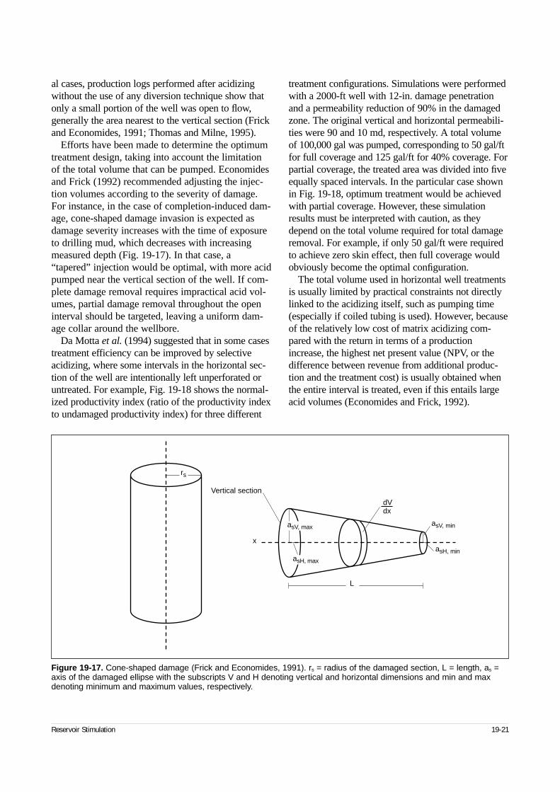
al cases, production logs performed after acidizingwithout the use of any diversion technique show thatonly a small portion of the well was open to flow,generally the area nearest to the vertical section (Frickand Economides, 1991; Thomas and Milne, 1995).

Efforts have been made to determine the optimumtreatment design, taking into account the limitationof the total volume that can be pumped. Economidesand Frick (1992) recommended adjusting the injec-tion volumes according to the severity of damage.For instance, in the case of completion-induced dam-age, cone-shaped damage invasion is expected asdamage severity increases with the time of exposureto drilling mud, which decreases with increasingmeasured depth (Fig. 19-17). In that case, a“tapered” injection would be optimal, with more acidpumped near the vertical section of the well. If com-plete damage removal requires impractical acid vol-umes, partial damage removal throughout the openinterval should be targeted, leaving a uniform dam-age collar around the wellbore.

Da Motta et al. (1994) suggested that in some casestreatment efficiency can be improved by selectiveacidizing, where some intervals in the horizontal sec-tion of the well are intentionally left unperforated oruntreated. For example, Fig. 19-18 shows the normal-ized productivity index (ratio of the productivity indexto undamaged productivity index) for three different

treatment configurations. Simulations were performedwith a 2000-ft well with 12-in. damage penetrationand a permeability reduction of 90% in the damagedzone. The original vertical and horizontal permeabili-ties were 90 and 10 md, respectively. A total volumeof 100,000 gal was pumped, corresponding to 50 gal/ftfor full coverage and 125 gal/ft for 40% coverage. Forpartial coverage, the treated area was divided into fiveequally spaced intervals. In the particular case shownin Fig. 19-18, optimum treatment would be achievedwith partial coverage. However, these simulationresults must be interpreted with caution, as theydepend on the total volume required for total damageremoval. For example, if only 50 gal/ft were requiredto achieve zero skin effect, then full coverage wouldobviously become the optimal configuration.

The total volume used in horizontal well treatmentsis usually limited by practical constraints not directlylinked to the acidizing itself, such as pumping time(especially if coiled tubing is used). However, becauseof the relatively low cost of matrix acidizing com-pared with the return in terms of a productionincrease, the highest net present value (NPV, or thedifference between revenue from additional produc-tion and the treatment cost) is usually obtained whenthe entire interval is treated, even if this entails largeacid volumes (Economides and Frick, 1992).

Reservoir Stimulation 19-21

Figure 19-17. Cone-shaped damage (Frick and Economides, 1991). rs = radius of the damaged section, L = length, as =axis of the damaged ellipse with the subscripts V and H denoting vertical and horizontal dimensions and min and maxdenoting minimum and maximum values, respectively.

rs

L

Vertical section

x

dVdx

asV, min

asH, min

asV, max

asH, max

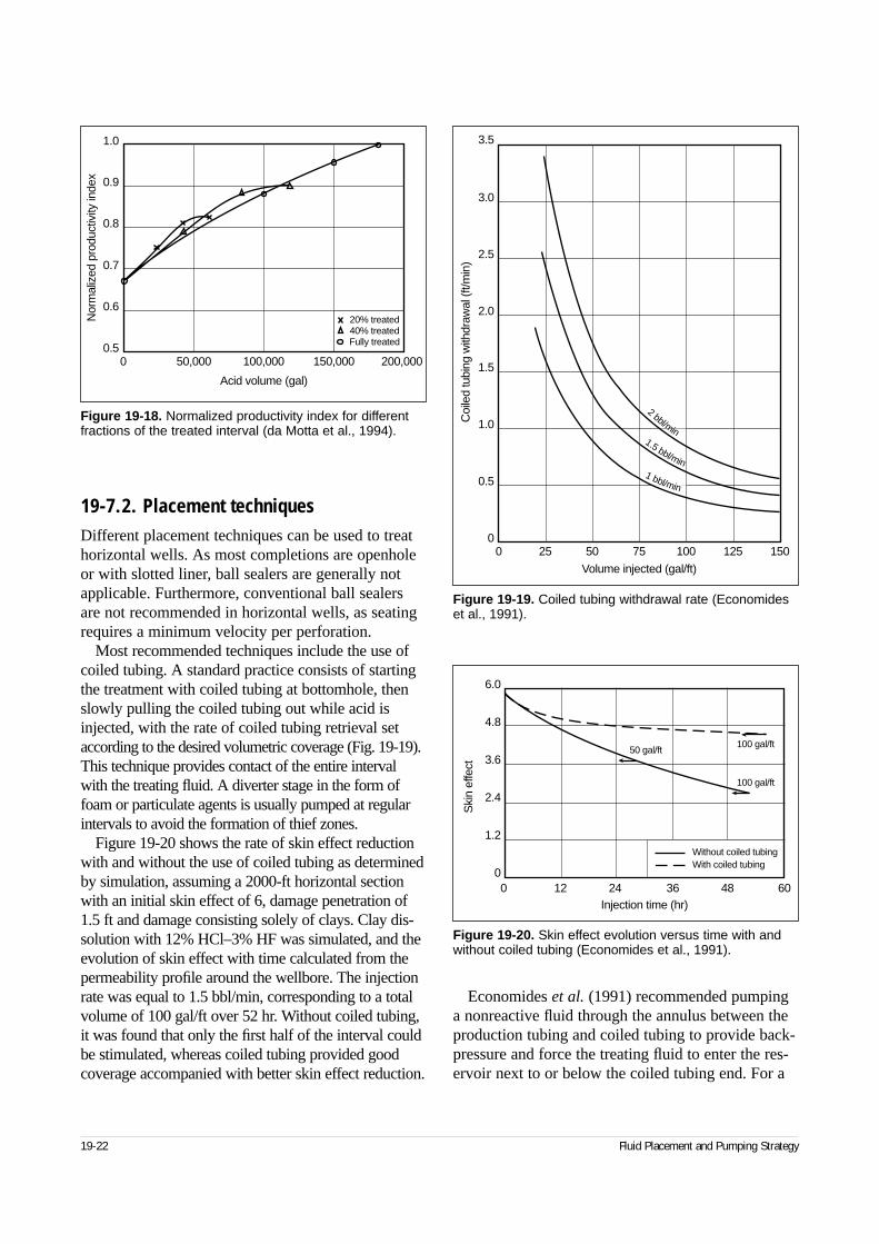
19-7.2. Placement techniquesDifferent placement techniques can be used to treathorizontal wells. As most completions are openholeor with slotted liner, ball sealers are generally notapplicable. Furthermore, conventional ball sealersare not recommended in horizontal wells, as seatingrequires a minimum velocity per perforation.

Most recommended techniques include the use ofcoiled tubing. A standard practice consists of startingthe treatment with coiled tubing at bottomhole, thenslowly pulling the coiled tubing out while acid is injected, with the rate of coiled tubing retrieval setaccording to the desired volumetric coverage (Fig. 19-19).This technique provides contact of the entire intervalwith the treating fluid. A diverter stage in the form offoam or particulate agents is usually pumped at regularintervals to avoid the formation of thief zones.

Figure 19-20 shows the rate of skin effect reductionwith and without the use of coiled tubing as determinedby simulation, assuming a 2000-ft horizontal sectionwith an initial skin effect of 6, damage penetration of1.5 ft and damage consisting solely of clays. Clay dis-solution with 12% HCl–3% HF was simulated, and theevolution of skin effect with time calculated from thepermeability profile around the wellbore. The injectionrate was equal to 1.5 bbl/min, corresponding to a totalvolume of 100 gal/ft over 52 hr. Without coiled tubing,it was found that only the first half of the interval couldbe stimulated, whereas coiled tubing provided goodcoverage accompanied with better skin effect reduction.

Economides et al. (1991) recommended pumpinga nonreactive fluid through the annulus between theproduction tubing and coiled tubing to provide back-pressure and force the treating fluid to enter the res-ervoir next to or below the coiled tubing end. For a

19-22 Fluid Placement and Pumping Strategy

Figure 19-19. Coiled tubing withdrawal rate (Economideset al., 1991).

25

Volume injected (gal/ft)

0

0.5C

oile

d tu

bing

with

draw

al (f

t/min

)

0 50 75 100 125 150

1.0

1.5

2.0

2.5

3.0

3.5

nim/l

bb2

nim/lbb5.1

nim/lbb1

Figure 19-20. Skin effect evolution versus time with andwithout coiled tubing (Economides et al., 1991).

6.0

4.8

3.6

2.4

1.2

00 12 24 36 48 60

Injection time (hr)

Ski

n ef

fect

100 gal/ft

100 gal/ft

50 gal/ft

Without coiled tubingWith coiled tubing

Figure 19-18. Normalized productivity index for differentfractions of the treated interval (da Motta et al., 1994).

00.5

50,000 100,000 150,000 200,000

Acid volume (gal)

0.6

0.7

0.8

0.9

1.0

Nor

mal

ized

pro

duct

ivity

inde

x

20% treated40% treatedFully treated

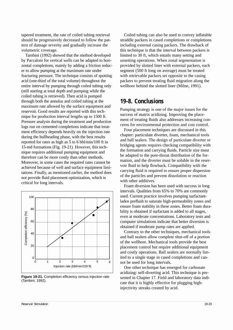
tapered treatment, the rate of coiled tubing retrievalshould be progressively decreased to follow the pat-tern of damage severity and gradually increase thevolumetric coverage.

Tambini (1992) showed that the method developedby Paccaloni for vertical wells can be adapted to hori-zontal completions, mainly by adding a friction reduc-er to allow pumping at the maximum rate underfracturing pressure. The technique consists of spottingacid (one-third of the total volume) throughout theentire interval by pumping through coiled tubing only(still starting at total depth and pumping while thecoiled tubing is retrieved). Then acid is pumpedthrough both the annulus and coiled tubing at themaximum rate allowed by the surface equipment andreservoir. Good results are reported with this tech-nique for production interval lengths up to 1500 ft.Pressure analysis during the treatment and productionlogs run on cemented completions indicate that treat-ment efficiency depends heavily on the injection rateduring the bullheading phase, with the best resultsreported for rates as high as 5 to 6 bbl/min/100 ft in15-md formations (Fig. 19-21). However, this tech-nique requires additional pumping equipment andtherefore can be more costly than other methods.Moreover, in some cases the required rates cannot beachieved because of well and surface equipment limi-tations. Finally, as mentioned earlier, the method doesnot provide fluid placement optimization, which iscritical for long intervals.

Coiled tubing can also be used to convey inflatablestraddle packers in cased completions or completionsincluding external casing packers. The drawback ofthis technique is that the interval between packers islimited to 30 ft, which entails many setting andunsetting operations. When zonal segmentation isprovided by slotted liner with external packers, eachsegment (500 ft long on average) must be treatedwith retrievable packers set opposite to the casingpackers to prevent treating fluid migration along thewellbore behind the slotted liner (Milne, 1991).

19-8. ConclusionsPumping strategy is one of the major issues for thesuccess of matrix acidizing. Improving the place-ment of treating fluids also addresses increasing con-cerns for environmental protection and cost control.

Four placement techniques are discussed in thischapter: particulate diverter, foam, mechanical toolsand ball sealers. The design of particulate diverter orbridging agents requires checking compatibility withthe formation and carrying fluids. Particle size mustbe adapted to the pore-throat distribution of the for-mation, and the diverter must be soluble in the reser-voir fluid to help flowback. Compatibility with thecarrying fluid is required to ensure proper dispersionof the particles and prevent dissolution or reactionwith other additives.

Foam diversion has been used with success in longintervals. Qualities from 65% to 70% are commonlyused. Current practice involves pumping surfactant-laden preflush to saturate high-permeability zones andensure foam stability in these zones. Better foam dura-bility is obtained if surfactant is added to all stages,even at moderate concentrations. Laboratory tests andcomputer simulations indicate that better diversion isobtained if moderate pump rates are applied.

Contrary to the other techniques, mechanical toolsand ball sealers allow complete shut-off of a portionof the wellbore. Mechanical tools provide the bestplacement control but require additional equipmentand costly operations. Ball sealers are normally lim-ited to a single stage in cased completions and can-not be used for long intervals.

One other technique has emerged for carbonateacidizing: self-diverting acid. This technique is pre-sented in Chapter 17. Field and laboratory data indi-cate that it is highly effective for plugging high-injectivity streaks created by acid.

Reservoir Stimulation 19-23

Figure 19-21. Completion efficiency versus injection rate(Tambini, 1992).

0 1

20

2 3 4 5 6Injection rate (bbl/min/100 ft)

0

40

60

80

100

Com

plet

ion

effic

ienc

y (%

)

The application of coiled tubing in matrix stimula-tion has improved results, especially for the stimula-tion of long intervals. Combining most of the place-ment techniques (i.e., particulate diverter, foam,packers) with the use of coiled tubing increases theirefficiency. In long intervals, as in horizontal wells,coiled tubing is run to the well bottom and thenwithdrawn while pumping acid. Diverter stages arepumped between acid stages. This technique allowsspotting acid across the entire interval and minimizesthe effect of thief zones.

AcknowledgmentsSome of the material in this chapter was written byL. P. Prouvost and N. Doerler and previously pub-lished in second edition of this volume. The authorsalso thank O. Liétard and R. Thomas for reviewingthis chapter.

19-24 Fluid Placement and Pumping Strategy

20-1. IntroductionAs for any stimulation operation, it is important toevaluate the effectiveness of a matrix treatment. InChapter 12, the methodology of evaluating hydraulicfracturing through pretreatment and post-treatmentwell tests is outlined. For matrix stimulation, such acomprehensive approach is rarely justified economi-cally. Usually, the effectiveness is gauged by apparentincreases in the productivity index, without the bene-fits of a post-treatment test. Clearly, increases in theproductivity (or injectivity) index, although desirable,may not provide an adequate picture of optimum wellconditions.

Estimation of the well skin effect and identificationof its individual components are covered in Chapter 1.The total skin effect can be determined from a welltest, and test analysis is outlined in Chapter 2. Mech-anical skin effects (such as from partial completion andinadequate perforations) may often overwhelm thedamage skin component. An appropriate productionengineering analysis should enable the identificationand separation of these skin effects. Only the portionof the skin effect resulting from damage can be re-moved by a matrix treatment, which should reduce the total skin effect by that amount. Furthermore, to be cost effective, the injected volume and the pumpingtime should be minimized.

Several attempts have been made to evaluate theeffectiveness of a remedial matrix treatment by moni-toring evolution of the skin effect in real time. Mon-itoring to evaluate whether an adequate fluid volumehas been injected indicates whether the treatmentrequires modification and helps to improve futuredesigns in similar situations.

Techniques for real-time monitoring have beenintroduced by McLeod and Coulter (1969) and Pac-caloni (1979a, 1979b) and further augmented byProuvost and Economides (1987, 1989), Behenna(1994) and Hill and Zhu (1994). They are describedin this chapter.

20-2. Derivation of bottomhole parameters from wellhead measurements

In many matrix stimulation treatments, wellheadpressures and injection rates are recorded. Ideally,these variables should be measured bottomhole.However, the hostile nature of the stimulation fluidsprevents the use of downhole pressure gauges andflowmeters. Thus, bottomhole parameters are oftenextrapolated from measurements made at the surfaceby simple mechanical energy balance applicationsand estimates of the hydrostatic and friction pressurelosses. When stimulation fluids are injected through a conduit such as coiled tubing or rigid tubing, mea-surement of the bottomhole injection pressure can bedone in the “backside” (i.e., at the annulus formedbetween the injection tubing and other well tubulars).Echometers have also been employed to measure thelevel of backside fluids if the wellhead pressure isbelow hydrostatic.

20-3. Monitoring skin effect evolution during treatment

Different attempts have been made to interpretrecorded wellhead pressures (or derived bottomholepressures) and injection rates in terms of progress ofthe remedial treatment. Several techniques have beenused to derive the evolution of the skin effect fromthese records.

20-3.1. McLeod and Coulter techniqueEach stage of injection or shut-in during the treatmentis considered a short, individual well test (McLeodand Coulter, 1969). The transient reservoir pressureresponse to the injection of fluids is analyzed andinterpreted to determine the skin effect and the for-

Reservoir Stimulation 20-1

◆

Matrix StimulationTreatment Evaluation

Carl T. Montgomery, ARCO Exploration and Production TechnologyMichael J. Economides, University of Houston

mation transmissibility. This is accomplished usingconventional pressure transient analysis methods,namely the solution to the diffusivity equation and thesuperposition principle (see Chapters 1 and 2.)

Although the results are presented not in terms ofskin effect but in terms of the permeability and theradius of the damaged zone (i.e., the short-term natureof the test has a limited radius of investigation), theobjective is essentially the same: the skin effect can be related to the properties of the damaged zone. Forexample, if the well is initially injected at a constantrate, a graph of the pressure response plotted against thelogarithm of elapsed time since injection started yieldsthe permeability in both the damaged and undamagedzones and the radial extent of the damaged zone. With a little modification, the same information can beobtained from pressure falloffs when injection stops.

The technique has several drawbacks:

• The analysis of pressure transients is valid only ifthe skin effect factor does not change while a set ofpressure data for one particular interpretation is col-lected. This is not the case when reactive fluids areinjected into the formation to remove damage.Hence, to be correct, this method requires the injec-tion of a slug of inert fluid each time the damageremoval is assessed. This is not usually practical.

• No continuous assessment of the evolution of thetreatment is possible. Skin effect measurements areallowed only at discrete times during the course ofthe treatment, usually before and after the treat-ment. Thus, real-time analysis is not feasible.

20-3.2. Paccaloni techniqueA second method, presented by Paccaloni (1979a,1979b), uses instantaneous pressure and rate values to compute the skin effect at any given time duringthe treatment. This method is based on the equationfor steady-state, single-phase, radial and horizontalflow in the reservoir:

(20-1)

where piw is the bottomhole injection pressure, pe is thereservoir pressure, qi is the injection rate, B is the for-mation volume factor, µ is the viscosity, k is the perme-ability, h is the reservoir thickness, re is the reservoirradius, rw is the wellbore radius, and s is the skin effect.

Paccaloni (1979a) used an arbitrary constant value foran acid bank radius rb and the concept of the effectivewellbore radius rw′ = rwe–s to transform Eq. 20-1 into

(20-2)

Assuming that the permeability-thickness productkh of the reservoir is known, the bottomhole pres-sures, corresponding to the injection rate, can be pre-dicted for any value of the skin effect. The wellheadinjection pressures are then derived from the bottom-hole pressures, and at any time, a match of the mea-sured wellhead pressures with the ones correspondingto different values of the skin effect yields the actualskin effect at that time.

Paccaloni used the concept of a damage ratio DR,which is simply the rewriting of Eq. 20-1 under ideal(s = 0) and real (s ≠ 0) conditions, and obtained theratio of the productivity indices:

(20-3)

• Example application of the Paccaloni method

Figure 20-1 depicts a series of damage ratio curvesfor a range of injection rates and calculated well-head pressures. Table 20-1 lists the well and reser-voir variables used for this construction.

The Paccaloni method (1979a, 1979b) impliesthat as acid is injected, superimposition of the mea-sured wellhead pressure on the graph indicates theprogress of the stimulation. This is shown by thedashed line on the figure.

Among the assumptions listed in the Paccalonimethod, the “steady-state” assumption is one thatmay cause problems and, potentially, errors.Although a steady-state relationship is assumed,transient behavior is in effect for a time duration far exceeding the injection test. For a radial reser-voir, for example, the time to a pseudosteady-statecondition is

(20-4)

where ct is the total compressibility. For a typical oil reservoir (e.g., φ = 0.25, µ = 1 cp, ct = 5 psi–1,k = 50 md and 80-acre spacing or re ≈ 1000 ft), thetime to pseudosteady state (which may be perceivedas a succession of steady states) is more than 50 hr,which is significantly longer than the normal pump-ing times for a typical matrix acidizing job.

20-2 Matrix Stimulation Treatment Evaluation

p pq B

kh

r

rsiw e

i e

w

− = +

141 2.,

µln

p pq B

kh

r

riw ei b

w

− =′

141 2..

µln

DRJ

J

r r s

r rideal

real

e w

e w

= = ( ) +( )

ln

ln.

tc r

kpsst e≈ 1000 2φµ

,

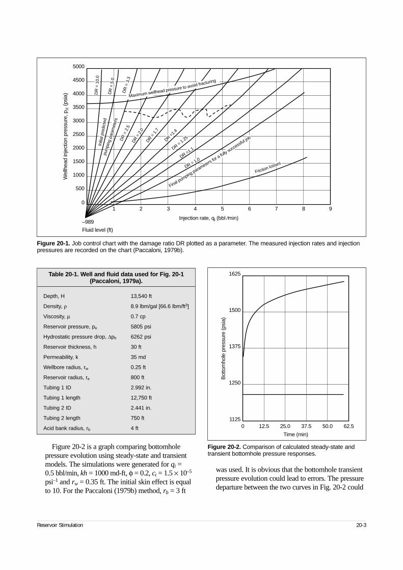
Figure 20-2 is a graph comparing bottomholepressure evolution using steady-state and transientmodels. The simulations were generated for qi =0.5 bbl/min, kh = 1000 md-ft, φ = 0.2, ct = 1.5 × 10–5

psi–1 and rw = 0.35 ft. The initial skin effect is equalto 10. For the Paccaloni (1979b) method, rb = 3 ft

was used. It is obvious that the bottomhole transientpressure evolution could lead to errors. The pressuredeparture between the two curves in Fig. 20-2 could

Reservoir Stimulation 20-3

Figure 20-1. Job control chart with the damage ratio DR plotted as a parameter. The measured injection rates and injectionpressures are recorded on the chart (Paccaloni, 1979b).

Wel

lhea

d in

ject

ion

pres

sure

, pit (p

sia)

5000

4500

4000

3500

3000

2500

2000

1500

1000

500

0

Fluid level (ft)

1 2 3 4 5 6 7 98

Maximum wellhead pressure to avoid fracturing

Injection rate, qi (bbl ⁄min)

DR = 1.0

Final pumping parameters for a fullysucce

ssful jo

b

Friction losses

DR =1.1DR= 1.2

5DR=1

.4

DR=

1.7

DR

=2.

0

DR

=2.

5D

R=

3.3

DR

=5.

0

DR

=10

.0In

itial

pred

icte

d

–989

pum

ping

para

met

ers

Table 20-1. Well and fluid data used for Fig. 20-1(Paccaloni, 1979a).

Depth, H 13,540 ft

Density, ρ 8.9 lbm/gal [66.6 lbm/ft3]

Viscosity, µ 0.7 cp

Reservoir pressure, pe 5805 psi

Hydrostatic pressure drop, ∆ph 6262 psi

Reservoir thickness, h 30 ft

Permeability, k 35 md

Wellbore radius, rw 0.25 ft

Reservoir radius, re 800 ft

Tubing 1 ID 2.992 in.

Tubing 1 length 12,750 ft

Tubing 2 ID 2.441 in.

Tubing 2 length 750 ft

Acid bank radius, rb 4 ft

Figure 20-2. Comparison of calculated steady-state andtransient bottomhole pressure responses.

Bot

tom

hole

pre

ssur

e (p

sia)

1625

1375

1250

1125

1500

0 12.5 25.0 37.5 50.0 62.5

Time (min)

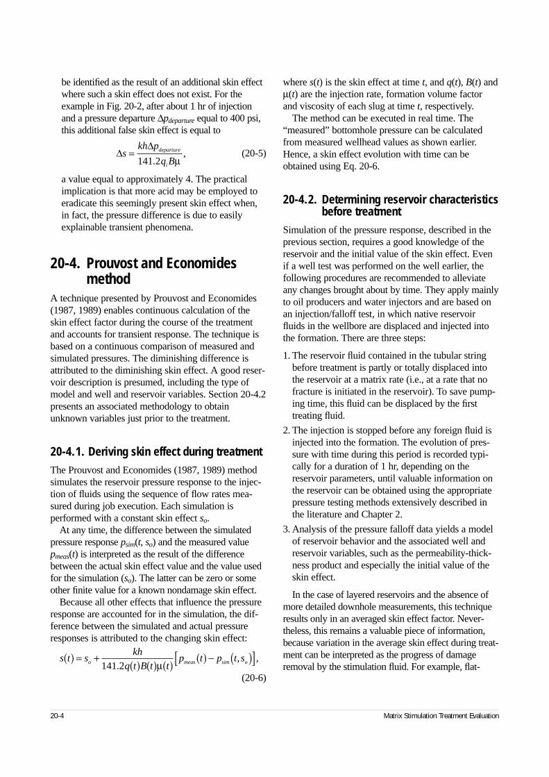
be identified as the result of an additional skin effectwhere such a skin effect does not exist. For theexample in Fig. 20-2, after about 1 hr of injectionand a pressure departure ∆pdeparture equal to 400 psi,this additional false skin effect is equal to

(20-5)

a value equal to approximately 4. The practicalimplication is that more acid may be employed toeradicate this seemingly present skin effect when,in fact, the pressure difference is due to easilyexplainable transient phenomena.

20-4. Prouvost and Economides method

A technique presented by Prouvost and Economides(1987, 1989) enables continuous calculation of theskin effect factor during the course of the treatmentand accounts for transient response. The technique isbased on a continuous comparison of measured andsimulated pressures. The diminishing difference isattributed to the diminishing skin effect. A good reser-voir description is presumed, including the type ofmodel and well and reservoir variables. Section 20-4.2presents an associated methodology to obtainunknown variables just prior to the treatment.

20-4.1. Deriving skin effect during treatmentThe Prouvost and Economides (1987, 1989) methodsimulates the reservoir pressure response to the injec-tion of fluids using the sequence of flow rates mea-sured during job execution. Each simulation isperformed with a constant skin effect so.

At any time, the difference between the simulatedpressure response psim(t, so) and the measured valuepmeas(t) is interpreted as the result of the differencebetween the actual skin effect value and the value usedfor the simulation (so). The latter can be zero or someother finite value for a known nondamage skin effect.

Because all other effects that influence the pressureresponse are accounted for in the simulation, the dif-ference between the simulated and actual pressureresponses is attributed to the changing skin effect:

(20-6)

where s(t) is the skin effect at time t, and q(t), B(t) andµ(t) are the injection rate, formation volume factorand viscosity of each slug at time t, respectively.

The method can be executed in real time. The“measured” bottomhole pressure can be calculatedfrom measured wellhead values as shown earlier.Hence, a skin effect evolution with time can beobtained using Eq. 20-6.

20-4.2. Determining reservoir characteristicsbefore treatment

Simulation of the pressure response, described in theprevious section, requires a good knowledge of thereservoir and the initial value of the skin effect. Evenif a well test was performed on the well earlier, thefollowing procedures are recommended to alleviateany changes brought about by time. They apply mainlyto oil producers and water injectors and are based onan injection/falloff test, in which native reservoirfluids in the wellbore are displaced and injected intothe formation. There are three steps:

1. The reservoir fluid contained in the tubular stringbefore treatment is partly or totally displaced intothe reservoir at a matrix rate (i.e., at a rate that nofracture is initiated in the reservoir). To save pump-ing time, this fluid can be displaced by the firsttreating fluid.

2. The injection is stopped before any foreign fluid isinjected into the formation. The evolution of pres-sure with time during this period is recorded typi-cally for a duration of 1 hr, depending on thereservoir parameters, until valuable information onthe reservoir can be obtained using the appropriatepressure testing methods extensively described inthe literature and Chapter 2.

3. Analysis of the pressure falloff data yields a modelof reservoir behavior and the associated well andreservoir variables, such as the permeability-thick-ness product and especially the initial value of theskin effect.

In the case of layered reservoirs and the absence ofmore detailed downhole measurements, this techniqueresults only in an averaged skin effect factor. Never-theless, this remains a valuable piece of information,because variation in the average skin effect during treat-ment can be interpreted as the progress of damageremoval by the stimulation fluid. For example, flat-

20-4 Matrix Stimulation Treatment Evaluation

∆∆

skh p

q Bdeparture

i

=141 2.

,µ

s t skh

q t B t tp t p t so meas sim o( ) = +

( ) ( ) ( ) ( ) − ( )[ ]141 2.

, ,µ

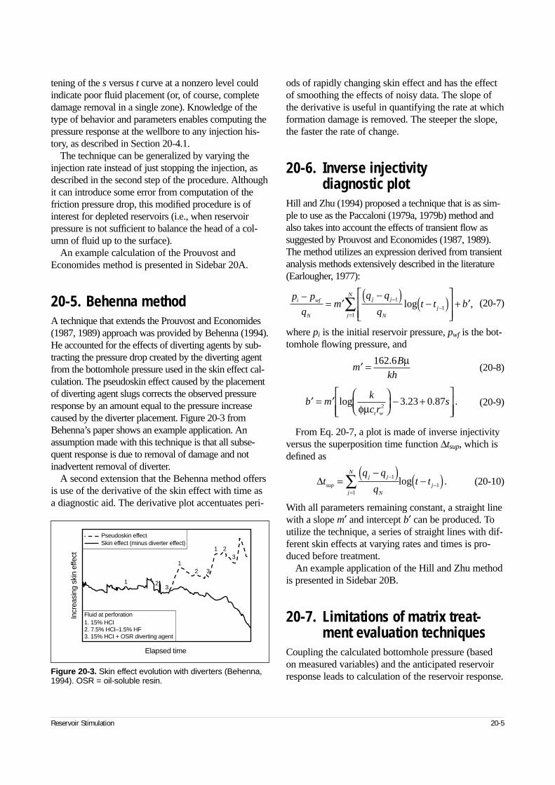
tening of the s versus t curve at a nonzero level couldindicate poor fluid placement (or, of course, completedamage removal in a single zone). Knowledge of thetype of behavior and parameters enables computing thepressure response at the wellbore to any injection his-tory, as described in Section 20-4.1.

The technique can be generalized by varying theinjection rate instead of just stopping the injection, asdescribed in the second step of the procedure. Althoughit can introduce some error from computation of thefriction pressure drop, this modified procedure is ofinterest for depleted reservoirs (i.e., when reservoirpressure is not sufficient to balance the head of a col-umn of fluid up to the surface).

An example calculation of the Prouvost andEconomides method is presented in Sidebar 20A.

20-5. Behenna methodA technique that extends the Prouvost and Economides(1987, 1989) approach was provided by Behenna (1994).He accounted for the effects of diverting agents by sub-tracting the pressure drop created by the diverting agentfrom the bottomhole pressure used in the skin effect cal-culation. The pseudoskin effect caused by the placementof diverting agent slugs corrects the observed pressureresponse by an amount equal to the pressure increasecaused by the diverter placement. Figure 20-3 fromBehenna’s paper shows an example application. Anassumption made with this technique is that all subse-quent response is due to removal of damage and notinadvertent removal of diverter.

A second extension that the Behenna method offersis use of the derivative of the skin effect with time asa diagnostic aid. The derivative plot accentuates peri-

ods of rapidly changing skin effect and has the effectof smoothing the effects of noisy data. The slope ofthe derivative is useful in quantifying the rate at whichformation damage is removed. The steeper the slope,the faster the rate of change.

20-6. Inverse injectivity diagnostic plot

Hill and Zhu (1994) proposed a technique that is as sim-ple to use as the Paccaloni (1979a, 1979b) method andalso takes into account the effects of transient flow assuggested by Prouvost and Economides (1987, 1989).The method utilizes an expression derived from transientanalysis methods extensively described in the literature(Earlougher, 1977):

(20-7)

where pi is the initial reservoir pressure, pwf is the bot-tomhole flowing pressure, and

(20-8)

(20-9)

From Eq. 20-7, a plot is made of inverse injectivityversus the superposition time function ∆tsup, which isdefined as

(20-10)

With all parameters remaining constant, a straight linewith a slope m′ and intercept b′ can be produced. Toutilize the technique, a series of straight lines with dif-ferent skin effects at varying rates and times is pro-duced before treatment.

An example application of the Hill and Zhu methodis presented in Sidebar 20B.

20-7. Limitations of matrix treat-ment evaluation techniques

Coupling the calculated bottomhole pressure (basedon measured variables) and the anticipated reservoirresponse leads to calculation of the reservoir response.

Reservoir Stimulation 20-5

Figure 20-3. Skin effect evolution with diverters (Behenna,1994). OSR = oil-soluble resin.

Incr

easi

ng s

kin

effe

ct

Pseudoskin effectSkin effect (minus diverter effect)

Fluid at perforation

1

1

1

2

2

2

3

3

3

1. 15% HCI2. 7.5% HCl–1.5% HF3. 15% HCI + OSR diverting agent

Elapsed time

p p

qm

q q

qt t bi wf

N

j j

N

jj

N−= ′

−( )−( )

+ ′−−

=∑ 1

11

log ,

′ =mB

kh

162 6. µ

′ = ′

− +

b mk

c rs

t w

logφµ 2

3 23 0 87. . .

∆tq q

qt tsup

j j

Nj

N

j=−( )

−( )−

=−∑ 1

11log .

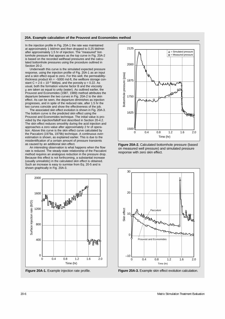
20-6 Matrix Stimulation Treatment Evaluation

In the injection profile in Fig. 20A-1 the rate was maintained at approximately 1 bbl/min and then dropped to 0.25 bbl/minafter approximately 1.5 hr of injection. The “measured” bot-tomhole pressure that appears as the top curve in Fig. 20A-2is based on the recorded wellhead pressures and the calcu-lated bottomhole pressures using the procedure outlined inSection 20-2.

Underneath this curve is the simulated expected pressureresponse, using the injection profile of Fig. 20A-1 as an inputand a skin effect equal to zero. For this well, the permeability-thickness product kh = ~5000 md-ft, the wellbore storage con-stant C = 2.6 × 10–3 bbl/psi, and the porosity φ = 0.22. Asusual, both the formation volume factor B and the viscosity µ are taken as equal to unity (water). As outlined earlier, theProuvost and Economides (1987, 1989) method attributes thedeparture between the two curves in Fig. 20A-2 to the skineffect. As can be seen, the departure diminishes as injectionprogresses, and in spite of the reduced rate, after 1.5 hr thetwo curves coincide and show the effectiveness of the job.

The associated skin effect evolution is shown in Fig. 20A-3.The bottom curve is the predicted skin effect using theProuvost and Economides technique. The initial value is pro-vided by the injection/falloff test described in Section 20-4.2.The skin effect reduces smoothly during the acid injection andapproaches a zero value after approximately 2 hr of opera-tion. Above this curve is the skin effect curve calculated bythe Paccaloni (1979a, 1979b) technique. A continuous over-estimation is shown, as explained earlier. This is due to themisidentification of a certain amount of pressure transients as caused by an additional skin effect.

An interesting observation is what happens when the flowrate is reduced. The steady-state relationship of the Paccalonimethod requires an analogous reduction in the pressure drop.Because this effect is not forthcoming, a substantial increase(usually unrealistic) in the calculated skin effect is obtained.Such an increase is easy to surmise from Eq. 20-5 and isshown graphically in Fig. 20A-3.

Figure 20A-1. Example injection rate profile.

Sur

face

inje

ctio

n ra

te (B

/D)

2000

1600

1200

800

400

00 0.4 0.8 1.2 1.6 2.0

Time (hr)

Figure 20A-3. Example skin effect evolution calculation.

Ski

n ef

fect

30

20

10

0

–100 0.4 0.8 1.2 1.6 2.0

Time (hr)

Prouvost and Economides

Paccaloni

Figure 20A-2. Calculated bottomhole pressure (basedon measured well pressure) and simulated pressureresponse with zero skin effect.

Bot

tom

hole

pre

ssur

e (p

sia)

2125

2000

1875

1750

1625

15000 0.4 0.8 1.2 1.6 2.0

Time (hr)

= Simulated pressure= Measured pressure

20A. Example calculation of the Prouvost and Economides method

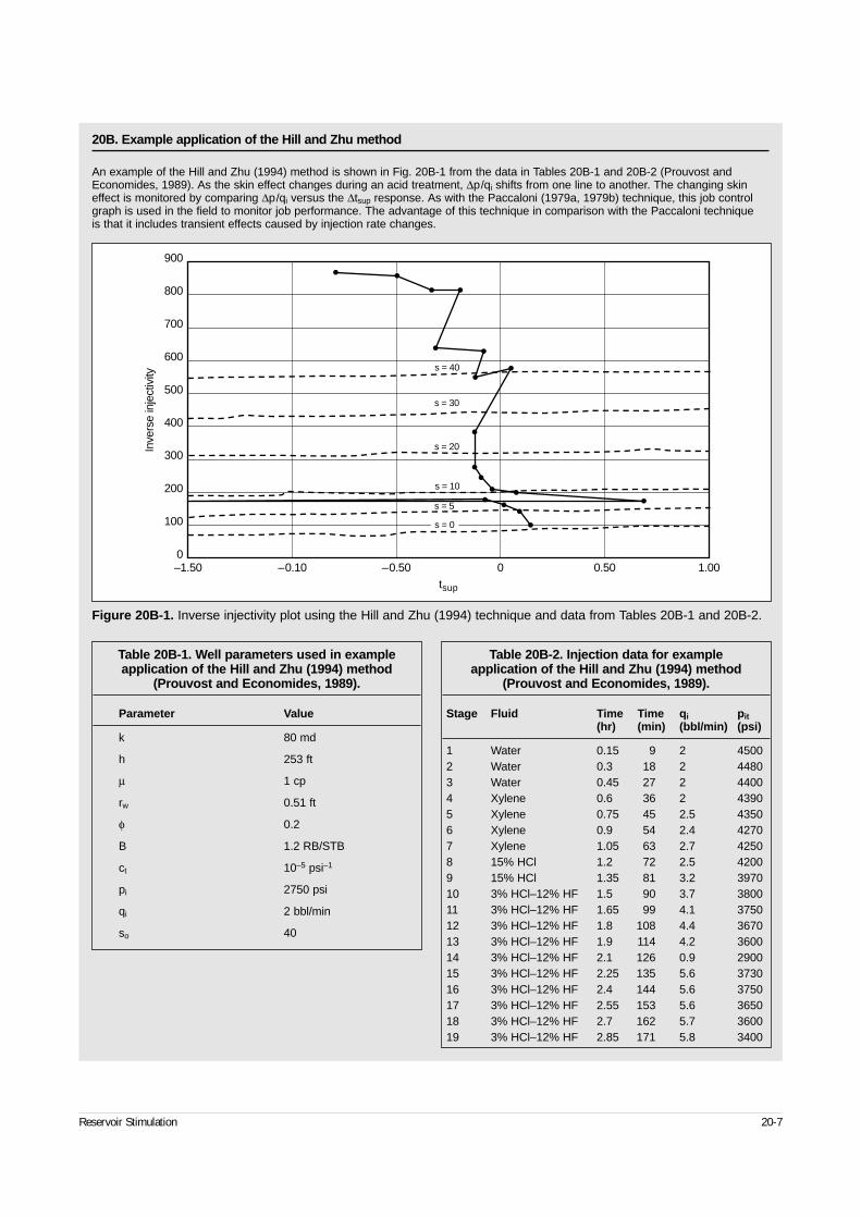
Reservoir Stimulation 20-7

20B. Example application of the Hill and Zhu method

An example of the Hill and Zhu (1994) method is shown in Fig. 20B-1 from the data in Tables 20B-1 and 20B-2 (Prouvost andEconomides, 1989). As the skin effect changes during an acid treatment, ∆p/qi shifts from one line to another. The changing skineffect is monitored by comparing ∆p/qi versus the ∆tsup response. As with the Paccaloni (1979a, 1979b) technique, this job controlgraph is used in the field to monitor job performance. The advantage of this technique in comparison with the Paccaloni techniqueis that it includes transient effects caused by injection rate changes.

Figure 20B-1. Inverse injectivity plot using the Hill and Zhu (1994) technique and data from Tables 20B-1 and 20B-2.

Inve

rse

inje

ctiv

ity

900

800

700

600

500

400

300

200

100

0–1.50 –0.10 –0.50 0 0.50 1.00

tsup

s = 40

s = 30

s = 20

s = 10

s = 5

s = 0

Table 20B-1. Well parameters used in exampleapplication of the Hill and Zhu (1994) method

(Prouvost and Economides, 1989).

Parameter Value

k 80 md

h 253 ft

µ 1 cp

rw 0.51 ft

φ 0.2

B 1.2 RB/STB

ct 10–5 psi–1

pi 2750 psi

qi 2 bbl/min

so 40

Table 20B-2. Injection data for example application of the Hill and Zhu (1994) method

(Prouvost and Economides, 1989).

Stage Fluid Time Time qi pit(hr) (min) (bbl/min) (psi)

1 Water 0.15 9 2 45002 Water 0.3 18 2 44803 Water 0.45 27 2 44004 Xylene 0.6 36 2 43905 Xylene 0.75 45 2.5 43506 Xylene 0.9 54 2.4 42707 Xylene 1.05 63 2.7 42508 15% HCl 1.2 72 2.5 42009 15% HCl 1.35 81 3.2 397010 3% HCl–12% HF 1.5 90 3.7 380011 3% HCl–12% HF 1.65 99 4.1 375012 3% HCl–12% HF 1.8 108 4.4 367013 3% HCl–12% HF 1.9 114 4.2 360014 3% HCl–12% HF 2.1 126 0.9 290015 3% HCl–12% HF 2.25 135 5.6 373016 3% HCl–12% HF 2.4 144 5.6 375017 3% HCl–12% HF 2.55 153 5.6 365018 3% HCl–12% HF 2.7 162 5.7 360019 3% HCl–12% HF 2.85 171 5.8 3400

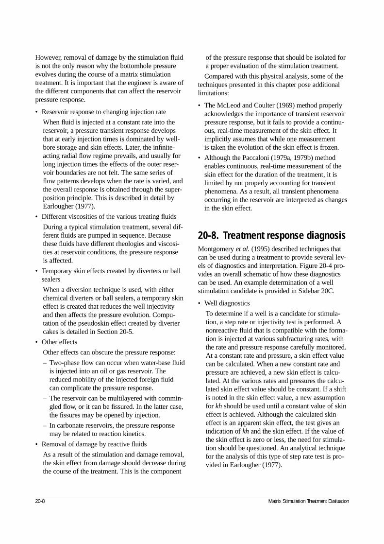
However, removal of damage by the stimulation fluidis not the only reason why the bottomhole pressureevolves during the course of a matrix stimulationtreatment. It is important that the engineer is aware ofthe different components that can affect the reservoirpressure response.

• Reservoir response to changing injection rate

When fluid is injected at a constant rate into thereservoir, a pressure transient response developsthat at early injection times is dominated by well-bore storage and skin effects. Later, the infinite-acting radial flow regime prevails, and usually forlong injection times the effects of the outer reser-voir boundaries are not felt. The same series offlow patterns develops when the rate is varied, andthe overall response is obtained through the super-position principle. This is described in detail byEarlougher (1977).

• Different viscosities of the various treating fluids

During a typical stimulation treatment, several dif-ferent fluids are pumped in sequence. Becausethese fluids have different rheologies and viscosi-ties at reservoir conditions, the pressure response is affected.

• Temporary skin effects created by diverters or ballsealers

When a diversion technique is used, with eitherchemical diverters or ball sealers, a temporary skineffect is created that reduces the well injectivityand then affects the pressure evolution. Compu-tation of the pseudoskin effect created by divertercakes is detailed in Section 20-5.

• Other effects

Other effects can obscure the pressure response:

– Two-phase flow can occur when water-base fluidis injected into an oil or gas reservoir. Thereduced mobility of the injected foreign fluid can complicate the pressure response.

– The reservoir can be multilayered with commin-gled flow, or it can be fissured. In the latter case,the fissures may be opened by injection.

– In carbonate reservoirs, the pressure responsemay be related to reaction kinetics.

• Removal of damage by reactive fluids

As a result of the stimulation and damage removal,the skin effect from damage should decrease duringthe course of the treatment. This is the component

of the pressure response that should be isolated fora proper evaluation of the stimulation treatment.

Compared with this physical analysis, some of thetechniques presented in this chapter pose additionallimitations:

• The McLeod and Coulter (1969) method properlyacknowledges the importance of transient reservoirpressure response, but it fails to provide a continu-ous, real-time measurement of the skin effect. Itimplicitly assumes that while one measurement is taken the evolution of the skin effect is frozen.

• Although the Paccaloni (1979a, 1979b) methodenables continuous, real-time measurement of theskin effect for the duration of the treatment, it islimited by not properly accounting for transientphenomena. As a result, all transient phenomenaoccurring in the reservoir are interpreted as changesin the skin effect.

20-8. Treatment response diagnosisMontgomery et al. (1995) described techniques thatcan be used during a treatment to provide several lev-els of diagnostics and interpretation. Figure 20-4 pro-vides an overall schematic of how these diagnosticscan be used. An example determination of a wellstimulation candidate is provided in Sidebar 20C.

• Well diagnostics

To determine if a well is a candidate for stimula-tion, a step rate or injectivity test is performed. Anonreactive fluid that is compatible with the forma-tion is injected at various subfracturing rates, withthe rate and pressure response carefully monitored.At a constant rate and pressure, a skin effect valuecan be calculated. When a new constant rate andpressure are achieved, a new skin effect is calcu-lated. At the various rates and pressures the calcu-lated skin effect value should be constant. If a shiftis noted in the skin effect value, a new assumptionfor kh should be used until a constant value of skineffect is achieved. Although the calculated skineffect is an apparent skin effect, the test gives anindication of kh and the skin effect. If the value ofthe skin effect is zero or less, the need for stimula-tion should be questioned. An analytical techniquefor the analysis of this type of step rate test is pro-vided in Earlougher (1977).

20-8 Matrix Stimulation Treatment Evaluation

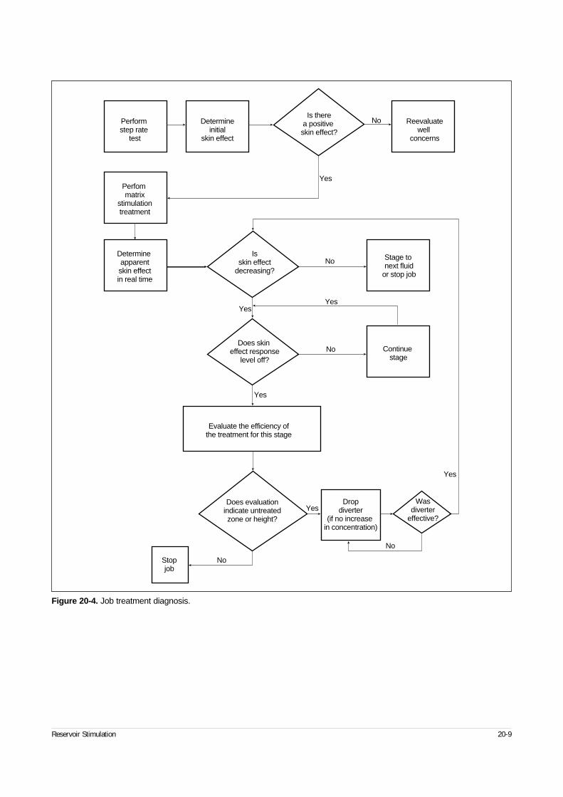
Reservoir Stimulation 20-9

Figure 20-4. Job treatment diagnosis.

Performstep rate

test

Perfommatrix

stimulationtreatment

Determineapparentskin effectin real time

Isskin effect

decreasing?

Does skin effect response

level off?

Does evaluationindicate untreatedzone or height?

Evaluate the efficiency ofthe treatment for this stage

Continuestage

Wasdiverter

effective?

Dropdiverter

(if no increase in concentration)

Stage to next fluid

or stop job

Determineinitial

skin effect

Reevaluatewell

concerns

Is therea positive skin effect?

Stopjob

No

No

No

No

Yes

No

Yes

Yes

Yes

Yes

Yes

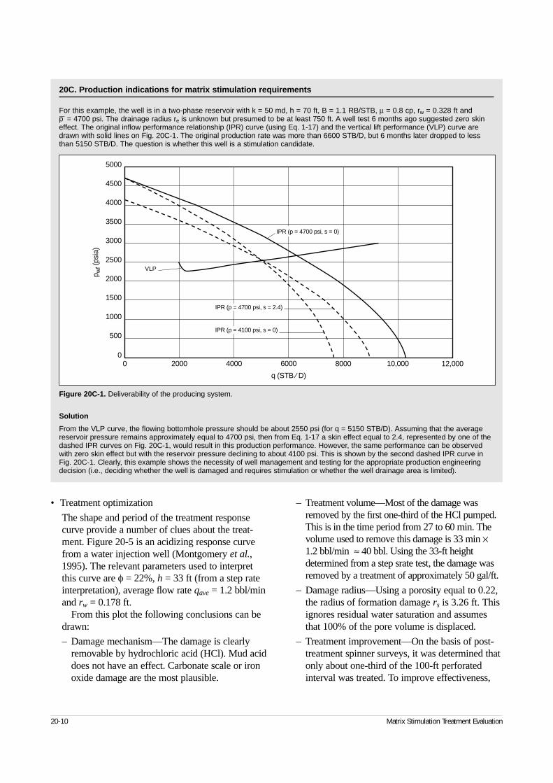
• Treatment optimization

The shape and period of the treatment responsecurve provide a number of clues about the treat-ment. Figure 20-5 is an acidizing response curvefrom a water injection well (Montgomery et al.,1995). The relevant parameters used to interpretthis curve are φ = 22%, h = 33 ft (from a step rateinterpretation), average flow rate qave = 1.2 bbl/minand rw = 0.178 ft.

From this plot the following conclusions can bedrawn:

– Damage mechanism—The damage is clearlyremovable by hydrochloric acid (HCl). Mud aciddoes not have an effect. Carbonate scale or ironoxide damage are the most plausible.

– Treatment volume—Most of the damage wasremoved by the first one-third of the HCl pumped.This is in the time period from 27 to 60 min. Thevolume used to remove this damage is 33 min ×1.2 bbl/min ≈ 40 bbl. Using the 33-ft heightdetermined from a step srate test, the damage wasremoved by a treatment of approximately 50 gal/ft.

– Damage radius—Using a porosity equal to 0.22,the radius of formation damage rs is 3.26 ft. Thisignores residual water saturation and assumesthat 100% of the pore volume is displaced.

– Treatment improvement—On the basis of post-treatment spinner surveys, it was determined thatonly about one-third of the 100-ft perforatedinterval was treated. To improve effectiveness,

20-10 Matrix Stimulation Treatment Evaluation

20C. Production indications for matrix stimulation requirements

For this example, the well is in a two-phase reservoir with k = 50 md, h = 70 ft, B = 1.1 RB/STB, µ = 0.8 cp, rw = 0.328 ft and p— = 4700 psi. The drainage radius re is unknown but presumed to be at least 750 ft. A well test 6 months ago suggested zero skineffect. The original inflow performance relationship (IPR) curve (using Eq. 1-17) and the vertical lift performance (VLP) curve aredrawn with solid lines on Fig. 20C-1. The original production rate was more than 6600 STB/D, but 6 months later dropped to lessthan 5150 STB/D. The question is whether this well is a stimulation candidate.

Solution

From the VLP curve, the flowing bottomhole pressure should be about 2550 psi (for q = 5150 STB/D). Assuming that the averagereservoir pressure remains approximately equal to 4700 psi, then from Eq. 1-17 a skin effect equal to 2.4, represented by one of thedashed IPR curves on Fig. 20C-1, would result in this production performance. However, the same performance can be observedwith zero skin effect but with the reservoir pressure declining to about 4100 psi. This is shown by the second dashed IPR curve inFig. 20C-1. Clearly, this example shows the necessity of well management and testing for the appropriate production engineeringdecision (i.e., deciding whether the well is damaged and requires stimulation or whether the well drainage area is limited).

Figure 20C-1. Deliverability of the producing system.

p wf (

psia

)

5000

4500

4000

3500

3000

2500

2000

1500

1000

500

00 2000 4000 6000 8000 10,000 12,000

q (STB ⁄ D)

VLP

IPR (p = 4700 psi, s = 2.4)

IPR (p = 4100 psi, s = 0)

IPR (p = 4700 psi, s = 0)

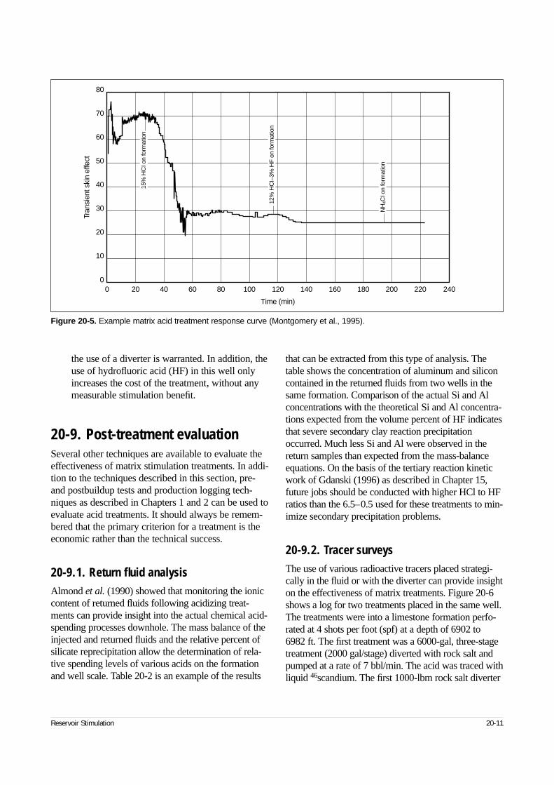
the use of a diverter is warranted. In addition, theuse of hydrofluoric acid (HF) in this well onlyincreases the cost of the treatment, without anymeasurable stimulation benefit.

20-9. Post-treatment evaluationSeveral other techniques are available to evaluate theeffectiveness of matrix stimulation treatments. In addi-tion to the techniques described in this section, pre-and postbuildup tests and production logging tech-niques as described in Chapters 1 and 2 can be used toevaluate acid treatments. It should always be remem-bered that the primary criterion for a treatment is theeconomic rather than the technical success.

20-9.1. Return fluid analysisAlmond et al. (1990) showed that monitoring the ioniccontent of returned fluids following acidizing treat-ments can provide insight into the actual chemical acid-spending processes downhole. The mass balance of theinjected and returned fluids and the relative percent ofsilicate reprecipitation allow the determination of rela-tive spending levels of various acids on the formationand well scale. Table 20-2 is an example of the results

that can be extracted from this type of analysis. Thetable shows the concentration of aluminum and siliconcontained in the returned fluids from two wells in thesame formation. Comparison of the actual Si and Alconcentrations with the theoretical Si and Al concentra-tions expected from the volume percent of HF indicatesthat severe secondary clay reaction precipitationoccurred. Much less Si and Al were observed in thereturn samples than expected from the mass-balanceequations. On the basis of the tertiary reaction kineticwork of Gdanski (1996) as described in Chapter 15,future jobs should be conducted with higher HCl to HFratios than the 6.5–0.5 used for these treatments to min-imize secondary precipitation problems.

20-9.2. Tracer surveysThe use of various radioactive tracers placed strategi-cally in the fluid or with the diverter can provide insighton the effectiveness of matrix treatments. Figure 20-6shows a log for two treatments placed in the same well.The treatments were into a limestone formation perfo-rated at 4 shots per foot (spf) at a depth of 6902 to 6982 ft. The first treatment was a 6000-gal, three-stagetreatment (2000 gal/stage) diverted with rock salt andpumped at a rate of 7 bbl/min. The acid was traced withliquid 46scandium. The first 1000-lbm rock salt diverter

Reservoir Stimulation 20-11

Figure 20-5. Example matrix acid treatment response curve (Montgomery et al., 1995).

Tran

sien

t ski

n ef

fect

80

70

60

50

40

30

20

10

00 20 40 60 80 100 120 140 160 180 200 220 240

Time (min)

15%

HC

I on

form

atio

n

12%

HC

I –3%

HF

on

form

atio

n

NH

4CI o

n fo

rmat

ion

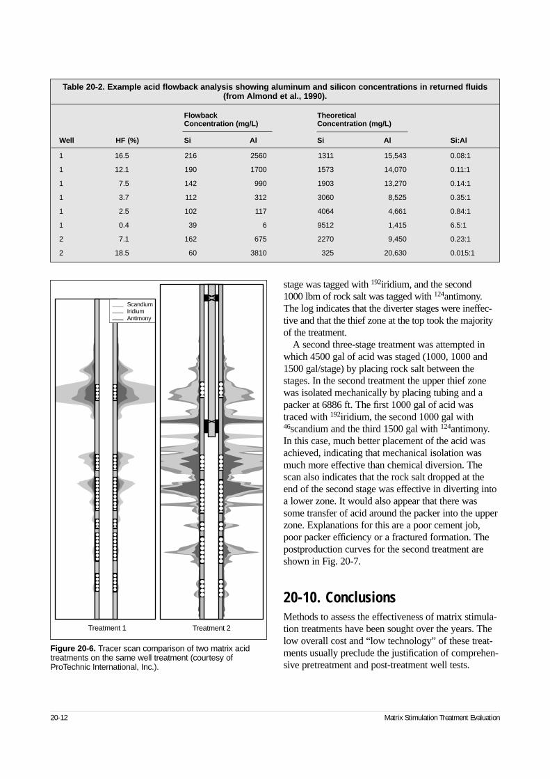
stage was tagged with 192iridium, and the second 1000 lbm of rock salt was tagged with 124antimony.The log indicates that the diverter stages were ineffec-tive and that the thief zone at the top took the majorityof the treatment.

A second three-stage treatment was attempted inwhich 4500 gal of acid was staged (1000, 1000 and1500 gal/stage) by placing rock salt between thestages. In the second treatment the upper thief zonewas isolated mechanically by placing tubing and apacker at 6886 ft. The first 1000 gal of acid wastraced with 192iridium, the second 1000 gal with46scandium and the third 1500 gal with 124antimony.In this case, much better placement of the acid wasachieved, indicating that mechanical isolation wasmuch more effective than chemical diversion. Thescan also indicates that the rock salt dropped at theend of the second stage was effective in diverting intoa lower zone. It would also appear that there wassome transfer of acid around the packer into the upperzone. Explanations for this are a poor cement job,poor packer efficiency or a fractured formation. Thepostproduction curves for the second treatment areshown in Fig. 20-7.

20-10. ConclusionsMethods to assess the effectiveness of matrix stimula-tion treatments have been sought over the years. Thelow overall cost and “low technology” of these treat-ments usually preclude the justification of comprehen-sive pretreatment and post-treatment well tests.

20-12 Matrix Stimulation Treatment Evaluation

Table 20-2. Example acid flowback analysis showing aluminum and silicon concentrations in returned fluids(from Almond et al., 1990).

Flowback TheoreticalConcentration (mg/L) Concentration (mg/L)

Well HF (%) Si Al Si Al Si:Al

1 16.5 216 2560 1311 15,543 0.08:1

1 12.1 190 1700 1573 14,070 0.11:1

1 7.5 142 990 1903 13,270 0.14:1

1 3.7 112 312 3060 8,525 0.35:1

1 2.5 102 117 4064 4,661 0.84:1

1 0.4 39 6 9512 1,415 6.5:1

2 7.1 162 675 2270 9,450 0.23:1

2 18.5 60 3810 325 20,630 0.015:1

Figure 20-6. Tracer scan comparison of two matrix acidtreatments on the same well treatment (courtesy ofProTechnic International, Inc.).

Treatment 1 Treatment 2

ScandiumIridiumAntimony

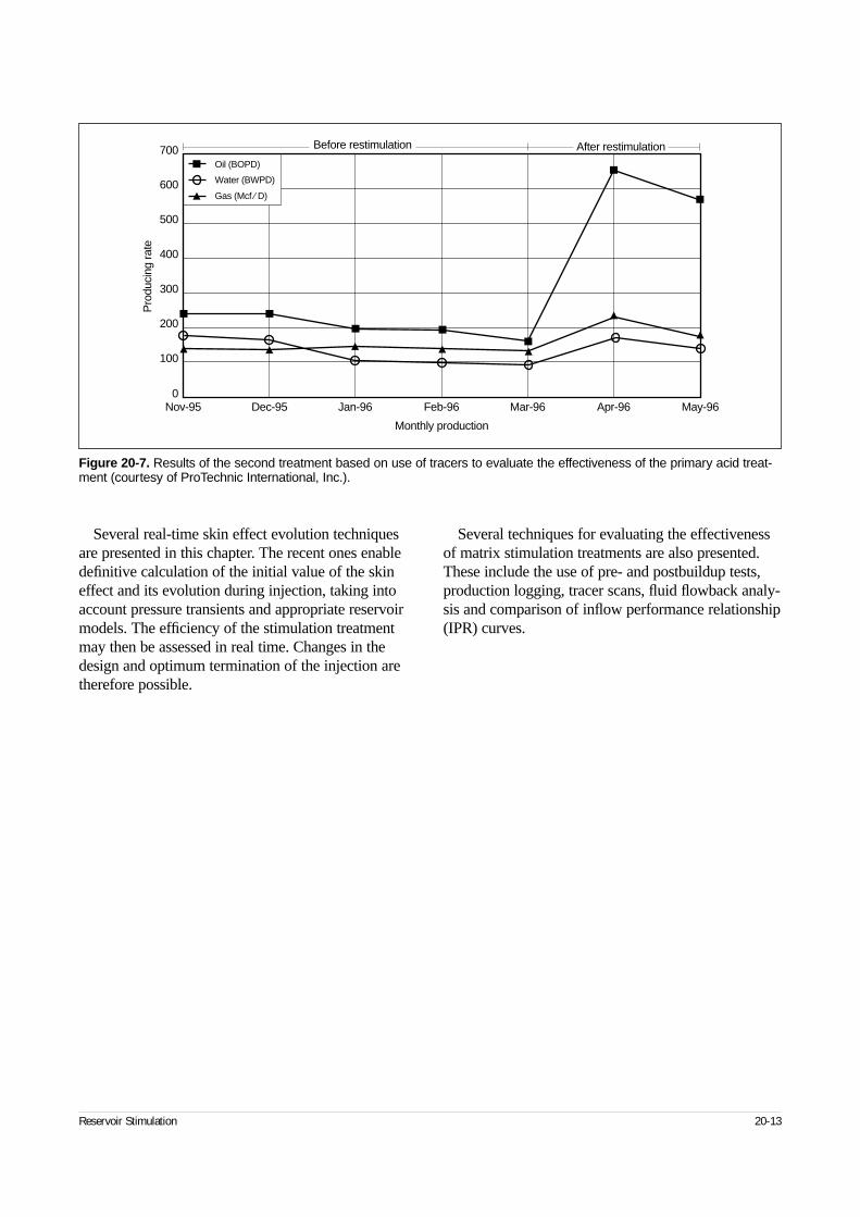
Several real-time skin effect evolution techniquesare presented in this chapter. The recent ones enabledefinitive calculation of the initial value of the skineffect and its evolution during injection, taking intoaccount pressure transients and appropriate reservoirmodels. The efficiency of the stimulation treatmentmay then be assessed in real time. Changes in thedesign and optimum termination of the injection aretherefore possible.

Several techniques for evaluating the effectivenessof matrix stimulation treatments are also presented.These include the use of pre- and postbuildup tests,production logging, tracer scans, fluid flowback analy-sis and comparison of inflow performance relationship(IPR) curves.

Reservoir Stimulation 20-13

Figure 20-7. Results of the second treatment based on use of tracers to evaluate the effectiveness of the primary acid treat-ment (courtesy of ProTechnic International, Inc.).

Pro

duci

ng ra

te700

600

500

400

300

200

100

0Nov-95 Dec-95 Jan-96 Feb-96 Mar-96 Apr-96 May-96

Monthly production

Oil (BOPD)

Water (BWPD)

Gas (Mcf ⁄ D)

After restimulationBefore restimulation

Chapters 1–12Abass, H., Meadows, D., Brumley, J. and Venditto,J.: “Oriented Perforations—A Rock MechanicsView,” paper SPE 28555, presented at the SPEAnnual Technical Conference and Exhibition, NewOrleans, Louisiana, USA (September 25–28, 1994).

Abass, H.H, Saeed, H. and Meadows, D.L.: “Non-planar Fracture Propagation from a HorizontalWellbore: Experimental Study,” paper SPE 24823,presented at the SPE Annual Technical Conferenceand Exhibition, Washington, D.C., USA (October4–7, 1992).

Abdulraheem, A., Roegiers, J.-C. and Zaman, M.:“Mechanics of Pore Collapse and Compaction inWeak Porous Rocks,” Proc., 33rd U.S. Symposiumon Rock Mechanics, Santa Fe, New Mexico, USA(1992), 233–242.

Abou-Sayed, A.S. and Dougherty, R.L.: “Evaluationof the Influence of In Situ Reservoir Conditions onthe Geometry of Hydraulic Fractures Using a 3DSimulator,” paper SPE 13275, presented at the SPEAnnual Technical Conference and Exhibition,Houston, Texas, USA (September 16–19, 1984).

Abou-Sayed, I.S., Schueler, S., Ehrl, E. and Hen-dricks, W.: “Multiple Hydraulic Fracture Stimulationin a Deep Horizontal Tight Gas Well,” paper SPE30532, presented at the SPE Annual TechnicalConference and Exhibition, Dallas, Texas, USA(October 22–25, 1995).

Abousleiman, Y., Cheng, A.H.-D. and Gu, H.:“Formation Permeability Determination by Micro or Mini-Hydraulic Fracturing,” J. Ener. Res. Tech.(June 1994) 116, No. 2, 104–114.

Abramowitz, M. and Stegun, I.A. (eds.): Handbookof Mathematical Functions, ninth edition, New York,New York, USA, Dover (1989).

Acharya, A.R.: “Particle Transport in Viscous andViscoelastic Fracturing Fluids,” paper SPE 13179,SPE Production Engineering (1986), 104.

Acharya, A.R.: “Viscoelasticity of CrosslinkedFracturing Fluids and Proppant Transport,” paperSPE 16221, presented at the SPE ProductionOperations Symposium, Oklahoma City, Oklahoma,USA (March 8–10, 1987); also paper SPE 15937,SPE Production Engineering (November 1988), 483.

Acharya, A.R. and Deysarkar, A.K.: “Rheology ofFracturing Fluids at Low-Shear Conditions,” paperSPE 16917, presented at the SPE Annual TechnicalConference and Exhibition, Dallas, Texas, USA(September 27–30, 1987).

Advani, S.H., Lee, T.S. and Dean, R.H.: “VariationalPrinciples for Hydraulic Fracturing,” Journal ofApplied Mechanics (December 1992) 59, No. 4,819–826.

Advani, S.H., Lee, T.S., Dean, R.H., Pak, C.K. andAvasthi, J.M.: “Consequences of Fracturing FluidLag in Three-Dimensional Hydraulic Fractures,”paper SPE 25888, presented at the SPE RockyMountain Regional/Low Permeability ReservoirsSymposium, Denver, Colorado, USA (April 12–14,1993).

Agarwal, R.G., Al-Hussainy, R. and Ramey, H.J. Jr.:“An Investigation of Wellbore Storage and SkinEffect in Unsteady Liquid Flow: I. AnalyticalTreatment,” paper SPE 2466, SPE Journal(September 1970) 10, No. 3, 279–290.

Agarwal, R.G., Carter, R.D. and Pollock, C.B.:“Evaluation and Performance Prediction of LowPermeability Gas Wells Stimulated by MassiveHydraulic Fracturing,” paper SPE 6838, Journalof Petroleum Technology (March 1979) 31, No. 3, 362–372; also in Trans., AIME (1979) 267.

Reservoir Stimulation R-1

◆

References

Ahmed, G., Horne, R.N. and Brigham, W.E.:“Theoretical Development of Flow into a WellThrough Perforations,” report DE90000251, U.S.DOE (August 1990).

Ahmed, U., Newberry, B.M. and Cannon, D.E.:“Hydraulic Fracture Treatment Design of Wells withMultiple Zones,” paper SPE 13857, presented at theSPE Low Permeability Gas Reservoir Symposium,Denver, Colorado, USA (May 19–22, 1985).

Ainley, B.R.: “Development of Foam Fracturing andCementing Fluids for Use in Tight Gas Sands,” pre-sented at the 1983 AIChE National Meeting, Denver,Colorado, USA (August 28–31, 1983).

Akram, A.H., Fitzpatrick, A.J. and Halford, F.R.: “AModel to Predict Wireline Formation Tester SampleContamination,” paper SPE 48959, presented at theSPE Annual Technical Conference and Exhibition,New Orleans, Louisiana, USA (September 27–30,1998).

Albright, J.N. and Pearson, C.F.: “Acoustic Emissionsas a Tool for Hydraulic Fracture Location: Experienceat the Fenton Hill Hot Dry Rock Site,” paper SPE9509, SPE Journal (August 1982) 22, No. 4, 523–530.

Aleksandrowksi, P., Inderhaug, O.H. and Knapstad,B.: “Tectonic Structures and Wellbore BreakoutOrientation,” Proc., 33rd U.S. Symposium on RockMechanics, Santa Fe, New Mexico, USA (June 3–5,1992).

Al-Hussainy, R. and Ramey, H.J. Jr.: “Application ofReal Gas Theory to Well Testing and DeliverabilityForecasting,” paper SPE 1243-B, Journal of Petrol-eum Technology (May 1966) 18, 637–642.

Al-Hussainy, R., Ramey, H.J. Jr. and Crawford, P.B.:“The Flow of Real Gases Through Porous Media,”paper SPE 1243-A, Journal of Petroleum Technology(May 1966) 18, 624–636.

Allen, L.S., Tittle, C.W., Mills, W.R. and Caldwell,R.L.: “Dual Spaced Neutron Logging for Porosity,”Geophysics (1967), 32, No. 1.

Allen, T.O. and Worzel, H.C.: “Productivity Methodof Evaluating Gun Perforating,” Drilling and Pro-duction Practice 1956, New York, New York, USA,American Petroleum Institute (1957), 112–125.

Almond, S.W., Bland, W.E. and Ripley, H.E.: “TheEffect of Break Mechanisms on Gelling Agent

Residue and Flow Impairment in 20/40 Mesh Sand,”paper CIM 84-35-30, presented at the 35th AnnualTechnical Meeting of Petroleum Society of CIM andCanadian Association of Drilling Engineers, Calgary,Alberta, Canada (June 10–13, 1984).

Almond, S.W. and Garvin, T.R.: “High EfficiencyFracturing Fluids for Low Temperature Reservoirs,”Proc., 31st Annual Southwestern Petroleum ShortCourse, Lubbock, Texas, USA (1984), 76–88.

Amadei, B., Swolfs, H.S. and Savage, W.S.: “GravityInduced Stresses in Stratified Rock Masses,” RockMechanics and Rock Engineering (January 1988) 21,No. 1, 1–20.

Amyx, B., et al.: Petroleum Reservoir EngineeringPhysical Properties, McGraw Hill (1960).

Anderson, A.J., Ashton, P.J.N., Lang, J. and Samuel-son, M.L.: “Production Enhancement ThroughAggressive Flowback Procedures in the CodellFormation,” paper SPE 36468, presented at the SPEAnnual Technical Conference and Exhibition,Denver, Colorado, USA (October 6–9, 1996).

Anderson, B., Barber, T., Druskin, V., Lee, P., Dussan,V.E., Knizhnerman, L. and Davydycheva, S.: “TheResponse of Multiarray Induction Tools in HighlyDipping Formations with Invasion and in Arbitrary3D Geometries,” Transactions of the SPWLA 37thAnnual Logging Symposium (June 16–19, 1996),paper A.

Anderson, E.M.: The Dynamics of Faulting and DykeFormation with Application to Britain, second edition,Edinburgh, Scotland, Oliver and Boyd (1951).

Archie, G.E.: “The Electrical Resistivity Log as anAid in Determining Some Reservoir Characteristics,”Journal of Petroleum Technology (January 1942) 5.

Asadi, M. and Preston, F.W.: “Characterization of the Crushed-Zone Formed During Jet Perforation by Qualitative Scanning Electron Microscopy andQuantitative Image Analysis,” paper SPE 22812, pre-sented at the SPE Annual Technical Conference andExhibition, Dallas, Texas, USA (October 6–9, 1991).

Aseltine, C.: “Flash X-Ray Analysis of theInteraction of Perforators with Different TargetMaterials,” paper SPE 14322, presented at the SPEAnnual Technical Conference and Exhibition, LasVegas, Nevada, USA (September 22–25, 1985).

R-2 References

Asgian, M.I., Cundall, P.A. and Brady, B.H.: “Mech-anical Stability of Propped Hydraulic Fractures: ANumerical Study,” paper SPE 28510, Journal ofPetroleum Technology (March 1995) 47, No. 3,203–208.

Atkinson, B.K. (ed.): Fracture Mechanics of Rock,London, UK, Academic Press (1987).

Atkinson, B.K. and Meredith, P.G.: “ExperimentalFracture Mechanics Data for Rocks and Minerals,”B.K. Atkinson (ed.): Fracture Mechanics of Rock,London, UK, Academic Press (1987), 477–525.

Aud, W.W., Sullivan, R.B., Coalson, E.B., Poulson,T.D. and Warembourg, P.A.: “Acid Refracturing Pro-gram Increases Reserves, Cottonwood Creek Unit,Washakie County, Wyoming,” paper SPE 21821,Journal of Petroleum Technology (January 1992), 11; also presented at the Rocky Mountain RegionalMeeting and Low-Permeability Reservoirs Symposium,Denver, Colorado, USA (April 15–17, 1992).

Aud, W.W., Wright, T.B., Cipolla, C.L., Harkrider,J.D. and Hansen, J.T.: “The Effect of Viscosity onNear-Wellbore Tortuosity and Premature Screenouts,”paper SPE 28492, presented at the SPE AnnualTechnical Conference and Exhibition, New Orleans,Louisiana, USA (September 25–28, 1994).

Ayoub, J.A., Bourdet, D.P. and Chauvel, Y.L.:“Impulse Testing,” paper SPE 15911, SPE FormationEvaluation (September 1988), 534.

Ayoub, J.A., Brown, J.E., Barree, R.D. and Elphick,J.J.: “Diagnosis and Evaluation of Fracturing Treat-ments,” SPE Production Engineering (February1992a), 39.

Ayoub, J.A., Kirksey, J.M., Malone, B.P. andNorman, W.D.: “Hydraulic Fracturing of SoftFormations in the Gulf Coast,” paper SPE 23805,presented at the SPE Formation Damage ControlSymposium, Lafayette, Louisiana, USA (February26–27, 1992b).

Babcock, R.E., Prokop, C.L. and Kehle, R.O.:“Distribution of Propping Agents in Vertical Frac-tures,” Production Monthly (November 1967), 11.

Badon Ghyben, W.: “Nota in Verband Met de Voor-genomen Putboring Nabij Amsterdam,” Tijdschr.Kon. Inst. Ing. (1888–1889), 1988, 8–22.

Baker, H.R., Bolster, R.N., Leach, P.B. and Little,R.C.: “Association Colloids in Nonaqueous Fluids,”Ind. Eng. Chem., Prod. Res. Develop. (1970) 9, No.4, 541–547.

Bale, A., Owren, K. and Smith, M.B.: “ProppedFracturing as a Tool for Sand Control and ReservoirManagement,” paper SPE 24992, presented at theSPE European Petroleum Conference, Cannes,France (November 16–18, 1992); also in SPEProduction & Facilities (February 1994a) 9, No. 1, 19–28.

Bale, A., Smith, M.B. and Settari, A.: “Post-FracProductivity Calculation for Complex Reservoir/Fracture Geometry,” paper SPE 28919, presented atthe European Petroleum Conference, London, UK(October 24-27, 1994b).

Baranet, S.E. and Ainley, B.R.: “Delayed CrosslinkingImproves Performance of Fracturing Fluids in DeepFormations,” paper CIM 85-36-39, presented at the36th Annual Technical Meeting of the PetroleumSociety of CIM, Edmonton, Alberta, Canada (June2–5, 1985).

Barenblatt, G.I.: “Mathematical Theory of EquilibriumCracks,” Advances in Applied Mech. (1962) 7, 56–131.

Barree, R.D.: “A Practical Numerical Simulator forThree-Dimensional Fracture Propagation in Hetero-geneous Media,” paper SPE 12273, presented at theSPE Reservoir Simulation Symposium, San Francisco,California, USA (November 15–18, 1983).

Barree, R.D.: “A New Look at Fracture-Tip Screen-out Behavior,” paper SPE 18955, Journal of Petro-leum Technology (February 1991) 43, No. 2, 138–143.

Barree, R.D. and Conway, M.W.: “Experimental andNumerical Modeling of Convective ProppantTransport,” paper SPE 28564, presented at the SPEAnnual Technical Conference and Exhibition, NewOrleans, Louisiana, USA (September 25–28, 1994);also in Journal of Petroleum Technology (March1995) 47, No. 3, 216–222.

Barree, R.D. and Mukherjee, H.: “Determination ofPressure Dependent Leakoff and Its Effect on FractureGeometry,” paper SPE 36424, presented at the SPEAnnual Technical Conference and Exhibition, Denver,Colorado, USA (October 6–9, 1996).

Reservoir Stimulation R-3

Bartko, K.M., Robertson, B. and Wann, D.: “Imple-menting Fracturing Technology to the UKCSCarboniferous Formation,” paper SPE 38609, pre-sented at the SPE Annual Technical Conference andExhibition, San Antonio, Texas, USA (October 5–8,1997).

Barton, C. and Zoback, M.: “Stress PertubationsAssociated with Active Faults Penetrated by Bore-holes: Evidence for Near Complete Stress Drop and aNew Technique for Stress Magnitude Measurement,”Journal of Geophysical Research (1994) 99, 9373–9390.

Bartusiak, R., Behrmann, L.A. and Halleck, P.M.:“Experimental Investigation of Surge Flow Velocityand Volume Needed to Obtain Perforation Cleanup,”Journal of Petroleum Science & Engineering(February 1997) 13, Nos. 1–2, 19–28.

Batchelor, A.S., Baria, R. and Hearn, K.: “Monitoringthe Effects of Hydraulic Stimulation by MicroseismicEvent Location: A Case Study,” paper SPE 12109,presented at the SPE Annual Technical Conferenceand Exhibition, San Francisco, California, USA(October 5–8, 1983).

Baumgartner, W.E., Shlyapobersky, J., Abou-Sayed,I.S. and Jacquier, R.C.: “Fracture Stimulation of aHorizontal Well in a Deep, Tight Gas Reservoir: ACase History from Offshore The Netherlands,” paperSPE 26795, presented at the Offshore EuropeanConference, Aberdeen, Scotland (September 7–10,1993).

Beg, M.S., Kunak, A., Oguz, G., Ming, Z.D. andHill, A.D.: “A Systematic Experimental Study ofAcid Fracture Conductivity,” paper SPE 31098, pre-sented at the SPE International Symposium onFormation Damage Control, Lafayette, Louisiana,USA (February 14–15, 1996).

Beggs, H.D. and Brill, J.P.: “A Study of Two-PhaseFlow in Inclined Pipes,” paper SPE 4007, Journal ofPetroleum Technology (May 1973) 25, No. 5, 607–617.

Behie, A. and Settari, A.: “Perforation DesignModels for Heterogeneous, Multiphase Flow,” paperSPE 25901, presented at the SPE Rocky MountainRegional/Low Permeability Reservoirs Symposium,Denver, Colorado, USA (April 12–14, 1993).

Behrmann, L. and Elbel, J.: “Effect of Perforations on Fracture Initiation,” paper SPE 20661, Journal ofPetroleum Technology (May 1991) 43, No. 5, 608–615; also presented at the SPE Annual TechnicalConference and Exhibition, New Orleans, Louisiana,USA (September 23–26, 1992).

Behrmann, L., et al.: “Quo Vadis, Extreme Over-balance?” Oilfield Review (Autumn 1996) 8, No. 3, 18–33.

Behrmann, L.A.: “Underbalance Criteria for Mini-mum Perforation Damage,” paper SPE 30081, pre-sented at the SPE Formation Damage Symposium,The Hague, Netherlands (May 15–16, 1995).

Behrmann, L.A. and Halleck, P.M.: “Effects of Well-bore Pressure on Perforator Penetration Depth,” paperSPE 18243, presented at the SPE Annual TechnicalConference and Exhibition, Houston, Texas, USA(October 2–5, 1988).

Behrmann, L.A. and McDonald, B.: “Underbalanceor Extreme Overbalance,” paper SPE 31083, pre-sented at the SPE International Symposium onFormation Damage Control, Lafayette, Louisiana,USA (February 14–15, 1996).

Behrmann, L.A., Pucknell, J.K. and Bishop, S.R.:“Effects of Underbalance and Effective Stress onPerforation Damage in Weak Sandstone: InitialResults,” paper SPE 24770, presented at the SPEAnnual Technical Conference and Exhibition,Washington, D.C., USA (October 4–7, 1992).

Bell, W.T.: “Perforating Underbalanced—EvolvingTechniques,” paper SPE 13413, Journal of PetroleumTechnology (October 1984) 36, No. 11, 1653–1662.

Bell, W.T., Brieger, E.F. and Harrigan, J.W. Jr.:“Laboratory Flow Characteristics of Gun Perfora-tions,” paper SPE 3444, Journal of Petroleum Tech-nology (September 1972) 36, No. 11, 1095–1103.

Bell, W.T., Sukup, R.A. and Tariq, S.M.: Perforating,Henry L. Doherty Monograph Series, Richardson,Texas, USA, Society of Petroleum Engineers (1995)16.

Ben Naceur, K. and Economides, M.J.: “Productionfrom Naturally Fissured Reservoirs Intercepted by aVertical Hydraulic Fracture,” paper SPE 17425, pre-sented at the SPE California Regional Meeting, LongBeach, California, USA (March 23–25, 1988); also in

R-4 References

SPE Formation Evaluation (December 1989) 4, No.4, 550–558.

Ben Naceur, K. and Roegiers, J.-C.: “Design ofFracturing Treatments in Multilayered Formations,”paper SPE 17712, presented at the SPE Gas Tech-nology Symposium, Dallas, Texas, USA (June 13–15,1988); also in SPE Production Engineering (February1990) 5, No. 1, 21–26.

Bennett, C.O., Reynolds, A.C. and Raghavan, R.:“Analysis of Finite-Conductivity Fractures InterceptingMultilayer Commingled Reservoirs,” paper SPE11030, SPE Formation Evaluation (June 1986) 1,259–274.

Bennett, C.O., Rodolpho, C.-V., Reynolds, A.C. andRaghavan, R.: “Approximate Solutions for FracturedWells Producing Layered Reservoirs,” paper SPE11599, SPE Journal (October 1985) 25, 729–742.

Bennett, C.O., Rosato, N.D., Reynolds, A.C. andRaghavan, R.: “Influence of Fracture Heterogeneityand Wing Length on the Response of VerticallyFractured Wells,” paper SPE 9886, SPE Journal(April 1983) 23, 219–230.

Besson, J.: “Performance of Slanted and HorizontalWells on an Anisotropic Medium,” paper SPE 20965,presented at Europec 90, The Hague, Netherlands(October 22–24, 1990).

Bhalla, K. and Brady, B.H.: “Formation and FractureCharacterization by Inversion of Fracture TreatmentRecords,” paper SPE 26526, presented at the SPEAnnual Technical Conference and Exhibition,Houston, Texas, USA (October 3–6, 1993).

Bilhartz, H.L. and Ramey, H.J. Jr.: “The CombinedEffects of Storage, Skin, and Partial Penetration onWell Test Analysis,” paper SPE 6753, presented atthe SPE Annual Technical Conference and Exhi-bition, Denver, Colorado, USA (October 9–12, 1977).

Biot, M.A.: “General Theory of Three-DimensionalConsolidation,” Journal of Applied Physics (February1941) 12, 155–164.

Biot, M.A.: “General Solutions of the Equations ofElasticity and Consolidation for a Porous Material,”Journal of Applied Mechanics (March 1956a) 23, No.1, 91–96.

Biot, M.A.: “Theory of Propagation of Elastic Wavesin a Fluid-Saturated Porous Solid. I. Low FrequencyRange,” J. Acoust. Soc. Am. (1956b) 28, 168–178.

Biot, M.A.: “Theory of Propagation of Elastic Wavesin a Fluid-Saturated Porous Solid. II. High Frequency,”J. Acoust. Soc. Am. (1956c) 28, 179–191.

Bird, K. and Dunmore, S.: “Optimising PerforationPerformance for the Armada Gas CondensateDevelopment,” paper SPE 30083, presented at the1995 European Formation Damage Conference, TheHague, Netherlands (May 15–16, 1995).

Boone, T.J., Kry, P.R., Bharatha, S. and Gronseth,J.M.: “Poroelastic Effects Related to StressDetermination by Micro-Frac Tests in PermeableRock,” Proc., 32nd U.S. Symposium on RockMechanics, Norman, Oklahoma, USA (1991), 25–34.

Boone, T.J., Wawryznek, P.A. and Ingraffea, A.R.:“Simulation of the Fracture Process in Rock withApplication to Hydrofracturing,” InternationalJournal of Rock Mechanics and Mining Sciences & Geomechanics Abstracts (June 1986) 23, No. 3,255–265.

Bourdet, D.: “Pressure Behavior of LayeredReservoirs with Crossflow,” paper SPE 13628, pre-sented at the SPE California Regional Meeting,Bakersfield, California, USA (March 27–29, 1985).

Bourdet, D., Alagoa, A., Ayoub, J.A. and Pirard,Y.M.: “New Type Curves Aid Analysis of FissuredZone Well Tests,” World Oil (April 1984) 198, No. 5, 111–124.

Bourdet, D., Ayoub, J.A. and Pirard, Y.M.: “Use of Pressure Derivative in Well-Test-Interpretation,”paper SPE 12777, SPE Facilities & Engineering(June 1989), 293–302; also in Trans., AIME 287.

Bourdet, D., Whittle, T.M., Douglas, A.A. and Pirard,Y.M.: “A New Set of Type Curves Simplifies WellTest Analysis,” World Oil (May 1983) 196, No. 6,95–106.

Boutéca, M.J., Bary, D., Piau, J.M., Kessler, N.,Boisson, M. and Fourmaintraux, D.: “Contribution of Poroelasticity to Reservoir Engineering: LabExperiments, Application to Core Decompressionand Implication in HP-HT Reservoirs Depletion,”Proc., Eurock ’94 Symposium, Delft, Netherlands(1994), 525–533.

Bradley, W.B.: “Failure of Inclined Boreholes,”Journal of Energy Research Technology (December1979) 101, 232–239.

Reservoir Stimulation R-5

Brady, B.H., Ingraffea, A.R. and Morales, R.H.:“Three-Dimensional Analysis and Visualization ofthe Wellbore and the Fracturing Process in InclinedWells,” paper SPE 25889, presented at the SPERocky Mountain Regional/Low PermeabilityReservoirs Symposium, Denver, Colorado, USA(April 12–14, 1993).

Branagan, P.T., Warpinski, N.R., Engler, B.P. andWilmer, R.: “Measuring the Hydraulic Fracture-Induced Deformation of Reservoirs and AdjacentRocks Employing a Deeply Buried InclinometerArray: GRI/DOE Multi-Site Project,” paper SPE36451, presented at the SPE Annual TechnicalConference and Exhibition, Denver, Colorado, USA(October 6–9, 1996).

Brannon, H.D. and Pulsinelli, R.J.: “Breaker Concen-trations Required to Improve the Permeability ofProppant Packs Damaged by Concentrated Linearand Borate-Crosslinked Fracturing Fluids,” paperSPE 21583, SPE Production Engineering (November1992) 7, No. 4, 338–342.

Brannon, H.D. and Tjon-Jo-Pin, R.M.: “Biotechno-logical Breakthrough Improves Performance ofModerate to High-Temperature Fracturing Appli-cations,” paper SPE 28513, presented at the SPEAnnual Technical Conference and Exhibition, NewOrleans, Louisiana, USA (September 25–28, 1994).

Bratli, R.K. and Risnes, R.: “Stability and Failure ofSand Arches,” paper SPE 8427, SPE Journal (April1981) 21, No. 2, 236–248.

Bratton, T., Bornemann, T., Li, Q., Plumb, R. andRasmus, J.: “Logging-While-Drilling Images forGeomechanical, Geological and PetrophysicalInterpretations,” Transactions of the SPWLA 40thAnnual Logging Symposium, Olso, Norway (June8–10, 1999).

Breckels, I.M. and van Eekelen, H.A.M.: “Rela-tionship Between Horizontal Stress and Depth inSedimentary Basins,” paper SPE 10336, Journal ofPetroleum Technology (September 1982) 34, No. 9,2191–2199.

Brie, A., Endo, T., Johnson, D.L. and Pampuri, F.:“Quantitative Formation Permeability Evaluationfrom Stoneley Waves,” presented at the SPE AnnualTechnical Conference and Exhibition, New Orleans,Louisiana, USA (September 27–30, 1998).

Britt, L.K. and Bennett, C.O.: “Determination ofFracture Conductivity in Moderate-PermeabilityReservoirs Using Bilinear Flow Concepts,” paperSPE 14165, presented at the SPE Annual TechnicalConference and Exhibition, Las Vegas, Nevada, USA(September 22–25, 1985).

Britt, L.K., Hager, C.J. and Thompson, J.W.:“Hydraulic Fracturing in a Naturally Fractured Res-ervoir,” paper SPE 28717, presented at the SPEInternational Petroleum Conference and Exhibition of Mexico, Veracruz, Mexico (October 10–13, 1994).

Brown, E.T. (ed.): Rock Characterization Testing and Monitoring, International Society for RockMechanics, Commission on Testing Methods,Oxford, UK, Pergamon Press (1981).

Brown, J.E. and Economides, M.J.: “An Analysis ofHorizontally Fractured Horizontal Wells,” paper SPE24322, presented at the SPE Rocky MountainRegional Meeting, Casper, Wyoming, USA (May18–22, 1992).

Brown, J.E., King, L.R., Nelson, E.B. and Ali, S.A.:“Use of a Viscoelastic Carrier Fluid in Frac-PackApplications,” paper SPE 31114, presented at theSPE International Symposium on Formation DamageControl, Lafayette, Louisiana, USA (February 14–15,1996).

Brown, K.E., et al.: The Technology of Artificial LiftMethods, Tulsa, Oklahoma, USA, PennWellPublishing Co. (1984).

Bui, H.D.: “An Integral Equations Method forSolving the Problem of a Plane Crack of ArbitraryShape,” J. Mech. Phys. Solids (February 1977) 25,No. 1, 29–39.

Burnham, J.W., Harris, L.E. and McDaniel, B.W.:“Developments in Hydrocarbon Fluids for High-Temperature Fracturing,” paper SPE 7564, presentedat the SPE Annual Technical Conference andExhibition, Houston, Texas, USA (October 1–3,1978); also in Journal of Petroleum Technology(February 1980) 32, No. 2, 217–220.

Camacho-V., R.G., Raghavan, R. and Reynolds,A.C.: “Response of Wells Producing LayeredReservoirs: Unequal Fracture Length,” paper SPE12844, SPE Formation Evaluation (March 1987) 2, 9–28.

R-6 References

Cameron, J.R.: “Rheological Modeling and Scale-Upof a Delayed-Crosslinked Gel in NonhomogeneousFlow,” paper SPE 21858, presented at the SPE RockyMountain Regional Meeting and Low-PermeabilityReservoirs Symposium, Denver, Colorado, USA(April 15–17, 1991); also in SPE Production &Facilities (February 1993), 23.

Cameron, J.R., Joha, R.J. and Veatch, R.W. Jr.: “TheNonhomogeneous Flow Character of a DelayedCrosslinked Gel,” paper SPE 20638, presented at theSPE Annual Technical Conference and Exhibition,New Orleans, Louisiana, USA (September 23–26,1990).

Cameron, J.R. and Prud’homme, R.K.: “Fracturing-Fluid Flow Behavior,” Recent Advances in HydraulicFracturing, J.L. Gidley, S.A. Holditch, D.E. Nierodeand R.W. Veatch Jr. (eds.), Monograph Series,Richardson, Texas, USA, Society of PetroleumEngineers (1989), 177–209.

Cantu, L.A. and Boyd, P.A.: “Laboratory and FieldEvaluation of a Combined Fluid-Loss ControlAdditive and Gel Breaker for Fracturing Fluids,”paper SPE 18211, presented at the SPE AnnualTechnical Conference and Exhibition, Houston,Texas, USA (October 2–5, 1988).

Card, R.J., Howard, P.R. and Féraud, J.-P.: “Controlof Particulate Flowback in Subterranean Wells,” U.S.Patent No. 5,330,005 (July 19, 1994).

Card, R.J., Howard, P.R. and Féraud, J.-P.: “A NovelTechnology to Control Proppant Back Production,”paper SPE 31007, SPE Production & Facilities(November 1995), 271.

Carico, R.D. and Bagshaw, F.R.: “Description andUse of Polymers Used in Drilling, Workovers, andCompletions,” paper SPE 7747, presented at the SPEProduction Technology Symposium, Hobbs, NewMexico, USA (October 30–31, 1978).

Carmen, P.C.: “Fundamental Principles of IndustrialFiltration,” Trans. Inst. Chem. Eng. (1938) 16,168–188.

Carnahan, B., Luther, H.A. and Wilkes, J.O.: AppliedNumerical Methods, New York, New York, USA,John Wiley (1969).

Carslaw, H.S. and Jaeger, J.C.: Conduction of Heat inSolids, second edition, Oxford, UK, Clarendon Press(1959).

Carter, R.D.: “Derivation of the General Equation for Estimating the Extent of the Fractured Area,”Appendix I of “Optimum Fluid Characteristics forFracture Extension,” Drilling and ProductionPractice, G.C. Howard and C.R. Fast, New York,New York, USA, American Petroleum Institute(1957), 261–269.

Castillo, J.L.: “Modified Fracture Pressure DeclineAnalysis Including Pressure-Dependent Leakoff,”paper SPE 16417, presented at the SPE/DOE LowPermeability Reservoirs Symposium, Denver,Colorado, USA (May 18–19, 1987).

Cawiezel, K.E. and Elbel, J.L.: “A New System forControlling the Crosslinking Rate of Borate Frac-turing Fluids,” paper SPE 20077, presented at theSPE California Regional Meeting, Ventura, Cali-fornia, USA (April 4–6, 1990).

Cawiezel, K.E. and Niles, T.D.: “Rheological Prop-erties of Foam Fracturing Fluids Under DownholeConditions,” paper SPE 16191, presented at the SPEHydrocarbon Economics and Evaluation Symposium,Dallas, Texas, USA (March 2–3, 1987).

Cesaro, M., Cheung, P., Etchecopar, A. and Gonfalini,M.: “Shaping Up to Stress in the Appenines,” Italy2000: Value Added Reservoir Characterization (WellEvaluation Conference, Italy), Schlumberger (1997).

Chambers, M.R., Mueller, M.M. and Grossmann, A.:“Well Completion Design and Operations for a DeepHorizontal Well with Multiple Fractures,” paper SPE30417, presented at the Offshore Europe Conference,Aberdeen, Scotland (September 5–8, 1995).

Chaveteau, G.: “Fundamental Criteria in PolymerFlow Through Porous Media and Their RelativeImportance in the Performance Differences ofMobility Control Buffers,” Water Soluble Polymers,J.E. Glass (ed.), Advances in Chemistry Series(1986), 213.

Cheatham, J.B. Jr. and McEver, J.W.: “Behavior ofCasing Subjected to Salt Loading,” paper SPE 828,Journal of Petroleum Technology (September 1964)16, 1069–1075.

Chen, W.F. and Han, D.J.: Plasticity for StructuralEngineers, New York, New York, USA, Springer-Verlag (1988).

Chen, Z. and Economides, M.J.: “The Effect of Near-Wellbore Fracture Geometry on Fracture Execution

Reservoir Stimulation R-7

and Post-Treatment Production of Deviated andHorizontal Wells,” paper SPE 39425, presented at the SPE International Formation Damage ControlConference, Lafayette, Louisiana, USA (February18–19, 1998).

Cheng, C.H. and Johnston, D.H.: “Dynamic andStatic Moduli,” Geophys. Res. Letters (January 1981)8, No. 1, 39–42.

Cherepanov, G.P.: Mechanics of Brittle Fracture,New York, New York, USA, McGraw-Hill (1979).

Chrisp, J.: U.S. Patent No. 3,301,723 (1967).

Cinco-Ley, H. and Meng, H.Z.: “Pressure TransientAnalysis of Wells with Finite Conductivity VerticalFractures in Double Porosity Reservoirs,” paper SPE18172, presented at the SPE Annual Technical Con-ference and Exhibition, Houston, Texas, USA(October 2–5, 1988).

Cinco-Ley, H., Ramey, H.J. Jr. and Miller, F.G.:“Pseudoskin Factors for Partially Penetrating Direc-tionally Drilled Wells,” paper SPE 5589, presented at the SPE Annual Technical Conference and Exhi-bition, Dallas, Texas, USA (September 28–October 1, 1975a).

Cinco-Ley, H., Ramey, H.J. Jr. and Miller, F.G.:“Unsteady-State Pressure Distribution Created by a Well with an Inclined Fracture,” paper SPE 5591,presented at the SPE Annual Technical Conferenceand Exhibition, Dallas, Texas, USA (September28–October 1, 1975b).

Cinco-Ley, H. and Samaniego-V., F.: “Effect ofWellbore Storage and Damage on the TransientPressure Behavior of Vertically Fractured Wells,”paper SPE 6752, presented at the SPE AnnualTechnical Conference and Exhibition, Denver,Colorado, USA (October 9–12, 1977).

Cinco-Ley, H. and Samaniego-V., F.: “TransientPressure Analysis: Finite Conductivity Fracture CaseVersus Damaged Fracture Case,” paper SPE 10179,presented at the SPE Annual Technical Conferenceand Exhibition, San Antonio, Texas, USA (October5–7, 1981a).

Cinco-Ley, H. and Samaniego-V., F.: “TransientPressure Analysis for Fractured Wells,” paper SPE7490, Journal of Petroleum Technology (September1981b) 33, 1749–1766.

Cinco-Ley, H., Samaniego-V., F. and Dominguez, N.:“Transient Pressure Behavior for a Well with a Finite-Conductivity Vertical Fracture,” paper SPE 6014,presented at the SPE Annual Technical Conferenceand Exhibition, New Orleans, Louisiana, USA(October 3–6, 1976); also in SPE Journal (August1978) 18, 253–264.

Clark, J.B.: “A Hydraulic Process for Increasing theProductivity of Wells,” Petroleum Trans., AIME(January 1949) 186, 1–8.

Clark, K.K.: “Transient Pressure Testing of FracturedWater Injection Wells,” paper SPE 1821, Journal ofPetroleum Technology (June 1968) 20, 639–643.

Clark, P.E.: “Stimulation Fluid Rheology—A NewApproach,” paper SPE 8300, presented at the SPEAnnual Technical Conference and Exhibition, LasVegas, Nevada, USA (September 23–26, 1979).

Clark, P.E., Balakrishnan, M. and Sundram, L.:“Crosslinking of Hydroxypropyl Guar with MetalIons,” paper SPE 25208, presented at the SPE Inter-national Symposium on Oilfield Chemistry, NewOrleans, Louisiana, USA (March 2–5, 1993).

Clark, P.E. and Barkat, O.: “Hydraulic FracturingFluids: The Crosslinking of Hydroxypropyl Guarwith Titanium Chelates,” paper SPE 19331, presentedat the SPE Eastern Regional Meeting, Morgantown,West Virginia, USA (October 24–27, 1989).

Clark, P.E. and Courington, T.J.: “Visualization ofFlow Into a Vertical Fracture,” paper SPE 27692,presented at the SPE Permian Basin Oil and GasRecovery Conference, Midland, Texas, USA (March16–18, 1994).

Clark, P.E. and Guler, N.: “Prop Transport in VerticalFractures: Settling Velocity Correlations,” paper SPE11636, presented at the SPE/DOE Symposium onLow Permeability, Denver, Colorado, USA (March14–16, 1983).

Clark, P.E., Halvaci, M., Ghaeli, H. and Parks, C.F.:“Proppant Transport by Xanthan and Xanthan-Hydroxypropylguar Solutions: Alternatives to Cross-linked Fluids,” paper SPE/DOE 13907, presented atthe SPE/DOE Low Permeability Gas ReservoirsConference, Denver, Colorado, USA, (May 19–22,1985).

R-8 References

Clark, P.E., Harkin, M.W., Wahl, H.A. and Sievert,J.A.: “Design of a Large Vertical Prop TransportModel,” paper SPE 6814, presented at the SPEAnnual Technical Conference and Exhibition,Denver, Colorado, USA (October 9–12, 1977).

Clark, P.E., Manning, F.S., Quadir, J.A. and Guler,N.: “Prop Transport in Vertical Fractures,” paper SPE10261, presented at the SPE Annual Technical Con-ference and Exhibition, San Antonio, Texas, USA(October 5–7, 1981).

Clark, P.E. and Zhu, Q.: “Flow Visualization of FlowInto 8 Point-Source Fractures II: The Effect ofFracture Non-Uniformity and Fluid Crosslinking,”paper SPE 29503, presented at the SPE ProductionOperations Symposium, Oklahoma City, OK, USA(April 2–4, 1995a).

Clark, P.E. and Zhu, Q.: “Fluid Flow in VerticalFractures from a Point Source,” paper SPE 28509,presented at the SPE Annual Technical Conferenceand Exhibition, New Orleans, Louisiana, USA(September 25–28, 1994); also in Journal ofPetroleum Technology (March 1995b) 47, No. 3, 209–215.

Cleary, M., Johnson, D., Kogsboll, H., Owens, K.,Perry, K., de Pater, C., Stachel, A., Schmidt, H. andTambini, M.: “Field Implementation of ProppantSlugs to Avoid Premature Screen-Out of HydraulicFractures with Adequate Proppant Concentration,”paper SPE 25892, presented at the SPE RockyMountain Regional/Low Permeability ReservoirsSymposium, Denver, Colorado, USA (April 12–14,1993).

Cleary, M.P.: “Analysis of Mechanisms and Proced-ures for Producing Favourable Shapes of HydraulicFractures,” paper SPE 9260, presented at the SPEAnnual Technical Conference and Exhibition, Dallas,Texas, USA (September 21–24, 1980a).

Cleary, M.P.: “Comprehensive Design Formulae forHydraulic Fracturing,” paper SPE 9259, presented at the SPE Annual Technical Conference and Exhi-bition, Dallas, Texas, USA (September 21–24, 1980b).

Cleary, M.P., Doyle, R.S., Teng, E.Y., Cipolla, C.L.,Meehan, D.N., Massaras, L.V. and Wright, T.B.:“Major New Developments in Hydraulic Fracturing,with Documented Reductions in Job Costs andIncreases in Normalized Production,” paper SPE28565, presented at the SPE Annual Technical

Conference and Exhibition, New Orleans, Louisiana,USA (September 25–28, 1994).

Cleary, M.P. and Fonseca, A.: “Proppant Convectionand Encapsulation in Hydraulic Fracturing: PracticalImplications of Computer Laboratory Simulations,”paper SPE 24825, presented at the SPE AnnualTechnical Conference and Exhibition, Washington,D.C., USA (October 4–7, 1992).

Cleary, M.P., Keck, R.G. and Mear, M.E.: “Micro-computer Models for the Design of HydraulicFractures,” paper SPE 11628, presented at the SPE/DOE Symposium on Low Permeability, Denver,Colorado, USA (March 14–16, 1983).

Cleary, M.P., Wright, C.A. and Wright, T.B.:“Experimental and Modeling Evidence for MajorChanges in Hydraulic Fracturing Design and FieldProcedures,” paper SPE 21494, Proc., SPE GasTechnology Symposium, Houston, Texas, USA(1991), 131–146.

Clifton, R.J. and Abou-Sayed, A.S.: “On the Com-putation of the Three-Dimensional Geometry ofHydraulic Fractures,” paper SPE 7943, presented at the SPE/DOE Low Permeability Gas ReservoirsSymposium, Denver, Colorado, USA (May 20–22,1979).

Clifton, R.J. and Abou-Sayed, A.S.: “A VariationalApproach to the Prediction of the Three-DimensionalGeometry of Hydraulic Fractures,” paper SPE 9879,presented at the SPE Low Permeability Symposium,Denver, Colorado, USA (May 27–29, 1981).

Clifton, R.J. and Wang, J-J.: “Multiple Fluids,Proppant Transport, and Thermal Effects in Three-Dimensional Simulation of Hydraulic Fracturing,”paper SPE 18198, presented at the SPE AnnualTechnical Conference and Exhibition, Houston,Texas, USA (October 2–5, 1988).

Colle, E.A., Halleck, P.M., Saucier, R.J. and Wesson,D.S.: “Discussion of Simple Method PredictsDownhole Shaped-Charge Gun Performance,” SPEProduction & Facilities (November 1994) 9, No. 4,292–293.

Collins, R.E.: Flow of Fluids Through PorousMaterials, New York, New York, USA, Van NostrandReinhold (1961).

Constien, V.G., Brannon, H.D. and Bannister, C.E.:“Continuous Mix Technology Adds New Flexibility

Reservoir Stimulation R-9

to Frac Jobs,” Oil & Gas Journal (June 6, 1988) 86,No. 23, 49–54.

Constien, V.G., Fellin, E.L. and King, M.T.: “Auto-mated Rheology Laboratory—Part 1,” ACS Symp.Ser. (1986) 313, 105.

Conway, M.W., Almond, S.W., Briscoe, J.E. andHarris, L.E.: “Chemical Model for the RheologicalBehavior of Crosslinked Fluid Systems,” paper SPE9334, presented at the SPE Annual TechnicalConference and Exhibition, Dallas, Texas, USA(September 21–24, 1980).

Cook, J.M., Bradford, I.D.R. and Plumb, R.A.: “AStudy of the Physical Mechanisms of Sanding andApplication to Sand Production Prediction,” paperSPE 28852, Proc., European Petroleum Conference,London, UK (1994), 473–480.

Cook, N.G.W.: “The Design of UndergroundExcavations,” Proc., 8th Symposium on RockMechanics, Minneapolis, Minnesota, USA (1967),167–193.

Cooke, C.E. Jr.: “Conductivity of Fracture Proppantsin Multiple Layers,” paper SPE 4117, Journal ofPetroleum Technology (September 1973) 25,1101–1107; also in Trans., AIME (1973) 255.

Cooke, C.E. Jr.: “Effect of Fracturing Fluids onFracture Conductivity,” paper SPE 5114, Journalof Petroleum Technology (October 1975) 27,1273–1282; also in Trans., AIME (1975) 259.

Coon, R.: “Correlation of Engineering Behaviourwith the Classification of In Situ Rock,” PhD disser-tation, University of Illinois, Illinois, USA (1968).

Cotton, F.A. and Wilkinson, G.: Advanced InorganicChemistry, New York, New York, USA, IntersciencePublishers (1972).

Coulter, A.W., Crowe, C.W., Barrett, N.D. andMiller, B.D.: “Alternate Stages of Pad Fluid and AcidProvide Improved Leakoff Control for FractureAcidizing,” paper SPE 6124, presented at the SPEAnnual Technical Conference and Exhibition, NewOrleans, Louisiana, USA (October 3–6, 1976).

Craft, B.C., Kemp, C.E. and Caulde, B.H.: WellDesign: Drilling and Production, Englewood Cliffs,New Jersey, USA, Prentice Hall (1962), 494.

Craigie, L.J.: “A New Method for Determining theRheology of Crosslinked Fracturing Fluids Using

Shear History Simulation,” paper SPE/DOE 11635,presented at the SPE/DOE Symposium on LowPermeability, Denver, Colorado, USA (March 14–16,1983).

Cramer, D.: “Limited Entry Extended to MassiveHydraulic Fracturing,” Oil & Gas Journal (December14, 1987) 85, No. 50, 40–50.

Cramer, D.D., Dawson, J. and Ouabdesselam, M.:“An Improved Gelled Oil System for High-Temperature Fracturing Applications,” paper SPE21859, presented at the Rocky Mountain RegionalMeeting and Low Permeability ReservoirsSymposium, Denver, Colorado, USA.

Crawford, D.L., Earl, R.B. and Monroe, R.F.:“Friction Reducing and Gelling Agent for OrganicLiquids,” U.S. Patent No. 3,757,864 (September 11,1973).

Crockett, A.R., Willis, R.M. and Cleary, M.P.:“Improvement of Hydraulic Fracture Predictions byReal-Time History Matching on Observed Pressures,”SPE Production Engineering (November 1989) 4,No. 4, 408–416.

Crouch, S.L. and Starfield, A.M.: Boundary ElementMethods in Solid Mechanics, London, UK, Allen andUnwin (1983).

Crowe, C.W.: “Clay Stabilization Ups Productivity,”Oil and Gas Suppliers’ Digest (1979) 1, No. 6.

Crowe, C.W., Hutchinson, B.H. and Trittipo, B.L.:“Fluid-Loss Control: The Key to Successful AcidFracturing,” SPE Production Engineering (August1989) 4, No. 3, 215–220.

Crowe, C.W., Martin, R.C. and Michaelis, A.M.:“Evaluation of Acid-Gelling Agents for Use in WellStimulation,” paper SPE 9384, SPE Journal (August1981), 415.

Crowe, C.W., McGowan, G.R. and Baranet, S.E.:“Investigation of Retarded Acids Provides BetterUnderstanding of Their Effectiveness and PotentialBenefits,” paper SPE 1822, SPE ProductionEngineering (May 1990), 166.

Crump, J. and Conway, M.: “Effects of Perforation-Entry Friction on Bottomhole Treating Analysis,”paper SPE 15474, Journal of Petroleum Technology(August 1988) 40, No. 8, 1041–1048.

R-10 References

Daccord, G., Lamanczyk, R. and Vercaemer, C.:“Method for Obtaining Gelled Hydrocarbon Compo-sitions According to Said Method and Their Appli-cation the Hydraulic Fracturing of UndergroundFormations,” U.S. Patent No. 4,507,213 (March 26,1985).

Dake, L.: Fundamentals of Reservoir Engineering,Developments in Petroleum Science, Amsterdam,Netherlands, Elsevier Scientific Publishing Company(1982) 8.

Daneshy, A.A.: “Experimental Investigation ofHydraulic Fracturing Through Perforations,” paperSPE 4333, Journal of Petroleum Technology(October 1973) 25, No. 10, 1201–1206.

Darcy, H.: Les Fontaines Publiques de la Ville de Dijon, Paris, France, Victor Dalmont (1856).

Davidson, B.M., Saunders, B.F. and Holditch, S.A.:“Field Measurement of Hydraulic Fracture Fluids:Case Study,” paper SPE 27694, presented at the SPEPermian Basin Oil and Gas Recovery Conference,Midland, Texas, USA (March 16–18, 1994).

Davies, D.R., Bosma, M.G.R. and de Vries, W.:“Development of Field Design Rules for ViscousFingering in Acid Fracturing Treatments: A Large-Scale Model Study,” paper SPE 15772, presented atthe SPE Middle East Oil Show, Manama, Bahrain(March 7–10, 1987).

Davies, D.R., Lau, H.C., Kamphuis, H. and Rood-hart, L.P.: “Development and Field Testing of aNovel Fracturing Fluid,” paper SPE 23109, presentedat the SPE Offshore Petroleum Conference, Aber-deen, Scotland (September 3–6, 1991).

Davis, P.M.: “Surface Deformation Associated withDipping Hydrofracture,” Journal of GeophysicalResearch (July 10, 1983) 88, No. B7, 5826–5834.

Dawson, J.: “Method and Composition for Delayingthe Gellation of Borated Galactomannons,” U.S.Patent No. 5,082,579 (1992).

Dawson, J.C.: “A Thermodynamic Study of BorateComplexation with Guar and Guar Derivatives,”paper SPE 22837, presented at the SPE AnnualTechnical Conference and Exhibition, Dallas, Texas,USA (October 6–9, 1991).

Dees, J.M. and Handren, P.J.: “A New Method ofOverbalance Perforating and Surging of Resin for

Sand Control,” paper SPE 26545, presented at theSPE Annual Technical Conference and Exhibition,Houston, Texas, USA (October 3–6, 1993).

de Kruijf, A., Roodhart, L.P. and Davies, D.R.: “TheRelation Between Chemistry and Flow Mechanics ofBorate Crosslinked Fracturing Fluids,” paper SPE25206, presented at the SPE International Sympo-sium on Oilfield Chemistry in New Orleans,Louisiana, USA (March 2–5, 1993); also in SPEProduction & Facilities (August 1993), 165.

de Pater, C.J., Desroches, J., Gronenbroom, J. andWeijers, L.: “Physical and Numerical Modelling ofHydraulic Fracture Closure,” paper SPE 28561,presented at the SPE Annual Technical Conferenceand Exhibition, New Orleans, Louisiana, USA(September 25–28, 1994); also in SPE Production & Facilities (May 1996), 122.

de Pater, C.J., Weijers, L., Savic, M., Wolf, K.H.A.A.,van den Hoek, P.J. and Barr, D.T.: “ExperimentalStudy of Nonlinear Effects in Hydraulic FracturePropagation,” paper SPE 25893, presented at the SPE Joint Rocky Mountain Regional Meeting/LowPermeability Reservoirs Symposium, Denver,Colorado, USA (April 12–14, 1993); also in SPEProduction Engineering (November 1994) 9, No. 4, 239–246.

Deo, M., Tariq, S.M. and Halleck, P.M.: “Linear andRadial Flow Targets for Characterizing DownholeFlow in Perforations,” paper SPE 16896, SPE Pro-duction Engineering (August 1989) 4, No. 3, 295–300.

de Rozières, J.: “Measuring Diffusion Coefficients in Acid Fracturing Fluids and Their Application toGelled and Emulsified Acids,” paper SPE 28552, pre-sented at the SPE Annual Technical Conference andExhibition, New Orleans, Louisiana, USA (Sep-tember 25–28, 1994).

Desbrandes, R. and Gualdron, J.: “In Situ RockWettability Determination with Wireline FormationTester Data,” The Log Analyst (July–August 1988)29, No. 4, 244–252.

Desroches, J. and Kurkjian, A: “Applications ofWireline Stress Measurements,” paper SPE 58086,SPE Reservoir Evaluation (October 1999).

Desroches, J., Lenoach, B., Papanastasiou, P. andThiercelin, M.: “On the Modelling of Near Tip

Reservoir Stimulation R-11

Processes in Hydraulic Fracturing,” InternationalJournal of Rock Mechanics and Mining Sciences & Geomechanics Abstracts (1993) 30, No. 7,1127–1134.

Desroches, J. and Thiercelin, M.: “Modelling thePropagation and Closure of Micro-Hydraulic Frac-tures,” International Journal of Rock Mechanics andMining Sciences & Geomechanics Abstracts (1993)30, No. 7, 1231–1234.

Desroches, J. and Woods, T.E.: “Stress Measurementsfor Sand Control,” paper SPE 47247, presented at theSPE/ISRM Eurock ‘98, Trondheim, Norway (July8–10, 1998).

Detournay, E. and Carbonell, R.: “Fracture MechanicsAnalysis of the Breakdown Process in Minifrac orLeak-Off Tests,” paper SPE 28076, presented at theSPE/ISRM Rock Mechanics in Petroleum Engi-neering Conference, Delft, Netherlands (August29–31, 1994).

Detournay, E. and Cheng, A.: “Poroelastic Responseof a Borehole in a Non-Hydrostatic Stress Field,”International Journal of Rock Mechanics and MiningSciences & Geomechanics Abstracts (June 1988) 25,No. 3, 171–182.

Detournay, E. and Cheng, A.: “Plane Strain Analysisof a Stationary Hydraulic Fracture in a PoroelasticMedium,” Int. J. Solids & Structures (March 1991)27, No. 13, 1645–1662.

Detournay, E. and Cheng, A.: “Influence of Pressuri-zation Rate on the Magnitude of the BreakdownPressure,” Proc., 33rd Symposium on RockMechanics, Santa Fe, New Mexico, USA (1992),325–333.

Detournay, E. and Cheng, A.: “Fundamentals ofPoroelasticity,” Comprehensive Rock Engineering,J.A. Hudson (ed.), Oxford, UK, Pergamon Press(1993) 2, 113–171.

Deuel, H. and Neukorn, H.: “Uber die Reacktion von Borsaure und Borax mit Polysacchariden undAnderen Hochmolekularen Polyoxy-Verbindungen,”Makromol. Chem. (1949) 13.

Dewprashad, B., Abass, H.H., Meadows, D.L.,Weaver, J.D. and Bennett, B.J.: “A Method to SelectResin-Coated Proppants,” paper SPE 26523, pre-sented at the SPE Annual Technical Conference and

Exhibition, Houston, Texas, USA (October 3–6,1993).

Dietz, D.N.: “Determination of Average ReservoirPressure from Build-Up Surveys,” paper SPE 1156,Journal of Petroleum Technology (August 1965) 17,No. 8, 955–959.

Dobecki, T.L.: “Hydraulic Fracture Orientation UsingPassive Borehole Seismics,” paper SPE 12110, pre-sented at the SPE Annual Technical Conference andExhibition, San Francisco, California, USA (October5–8, 1983).

Dobkins, T.A.: “Improved Methods to DetermineHydraulic Fracture Height,” paper SPE 8403, Journalof Petroleum Technology (April 1981) 33, No. 4,719–726.

Dovan, H.T. and Hutchins, R.D.: “CrosslinkedHydroxyethylcellulose and Its Uses,” U.S. Patent No. 5,207,934 (May 4, 1993).

Dunand, A., Guillot, D. and Soucemarianadin, A.:“Viscous Properties of Glass-Bead Suspensions andFalling Sphere Experiments in Hydroxypropyl GuarSolutions,” Proc., Ninth International Congress onRheology, Mexico City, Mexico (1984).

Dunning, J.D.: “Surfactants,” Chemtech (June 1980)10, No. 6, 356–359.

Dyes, A.B., Kemp, C.E. and Caudle, B.H.: “Effect of Fractures on Sweep-Out Pattern,” Trans., AIME(1958) 213, 245–249.

Earlougher, R.C. Jr.: Advances in Well Test Analysis,Dallas, Texas, USA, Society of Petroleum Engineers(1977).

Economides, M.J.: “Implications of Cementing onWell Performance,” Well Cementing, E.B. Nelson(ed.), Sugar Land, Texas, USA, Schlumberger (1990),1-1–1-6.

Economides, M.J., Brand, C.W. and Frick, T.P.: “WellConfigurations in Anisotropic Reservoirs,” SPEFormation Evaluation (December 1996) 11, No. 4,257–262.

Economides, M.J., Deimbacher, F.X., Brand, C.W.and Heinemann, Z.E.: “Comprehensive Simulation of Horizontal Well Performance,” SPE FormationEvaluation (December 1991) 6, No. 4, 418–426.

R-12 References

Economides, M.J., Hill, A.D. and Ehlig-Economides,C.A.: Petroleum Production Systems, EnglewoodCliffs, New Jersey, USA, Prentice-Hall (1994).

Economides, M.J., McLennan, J.D., Brown, E. andRoegiers, J.-C.: “Performance and Stimulation ofHorizontal Wells,” World Oil (June–July 1989) 208,No. 6, 41–45, and 209, No. 1, 69–72 and 76–77.

Edimann, K., Somerville, J.M., Smart, B.G.D.,Hamilton, S.A. and Crawford, B.R.: “Predicting RockMechanical Properties from Wireline Porosities,”paper SPE 47344, presented at the SPE/ISRM Eurock‘98, Trondheim, Norway (July 8–10, 1998).

Ehlig-Economides, C.A.: “Implications of the TestArea of Investigation in Nonradial Geometries,” SPEMemorial Series, Richardson, Texas, USA, Society ofPetroleum Engineers (1995) 1, 103–112.

Ehlig-Economides, C.A., Chan, K.S. and Spath, J.B.:“Production Enhancement Strategies for StrongBottomwater Drive Reservoirs,” paper SPE 36613,presented at the SPE Annual Technical Conferenceand Exhibition, Denver, Colorado, USA (October6–9, 1996).

Ehlig-Economides, C.A. and Economides, M.J.:“Pressure Transient Analysis in an Elongated LinearFlow System,” SPE Journal (December 1985) 25,No. 6, 347–360.

Ehlig-Economides, C.A., Joseph, J., Erba, M. andVik, S.A.: “Evaluation of Single-Layer Transients ina Multilayered System,” paper SPE 15860, presentedat the European Petroleum Conference, London, UK(October 20–22, 1986).

Elbel, J.L.: “Designing Hydraulic Fractures forEfficient Reserve Recovery,” paper SPE 15231, pre-sented at the SPE Unconventional Gas TechnologySymposium, Louisville, Kentucky, USA (May 18–21,1986).

Elbel, J.L.: “Considerations for Optimum FractureGeometry Design,” SPE Production Engineering(August 1988) 3, No. 3, 323–327.

Elbel, J.L.: “A Method To Estimate MultizoneInjection Profiles During Hydraulic Fracturing,”paper SPE 21869, presented at the Rocky MountainRegional Meeting and Low-Permeability ReservoirsSymposium, Denver, Colorado, USA (April 15–17,1993).

Elbel, J.L. and Ayoub, J.A.: “Evaluation of ApparentFracture Lens Tip Indicated from Transient Tests,”paper 91-44, presented at the CIM-AOSTRA Tech-nical Conference, Banff, Alberta, Canada (April21–24, 1991); also in Journal of Canadian PetroleumTechnology (December 1992) 31, No. 10, 41–46.

Elbel, J.L., Howard, R.L., Talley, G.R. andMcLaughlin, B.H.: “Stimulation Study of CottageGrove Formation,” paper SPE 11564, Journal ofPetroleum Technology (July 1984), 1199–1205.

Elbel, J.L., Piggott, A.R. and Mack, M.G.:“Numerical Modeling of Multilayer FractureTreatments,” paper SPE 23982, presented at the SPEPermian Basin Oil and Gas Recovery Conference,Midland, Texas, USA (March 18–20, 1992).

Elbel, J.L. and Sookprasong, P.A.: “Use ofCumulative-Production Type Curves in FractureDesign,” SPE Production Engineering (August 1987)2, No. 3, 191–198.

El Rabaa, W.: “Experimental Study of HydraulicFracture Geometry Initiated from Horizontal Wells,”paper SPE 19720, presented at the SPE AnnualTechnical Conference and Exhibition, San Antonio,Texas, USA (October 8–11, 1989).

Ely, J.W.: Stimulation Treatment Handbook, Tulsa,Oklahoma, USA, PennWell Publishing Co. (1985).

Ely, J.W.: “GRI’s Fracture Fluid Rheology Unit—Portable Equipment for Measuring Fluid BehaviorUnder Simulated Downhole Conditions,” In Focus—Tight Gas Sands, Gas Research Institute (September1987) 4, No. 2.

Endo, T., Brie, A. and Badri, M.: “Fracture Evaluationfrom Dipole Shear Anisotropy and Borehole StoneleyWaves,” Transactions of the SPWLA 2nd AnnualLogging Symposium of Japan (1996), paper U.

Engelder, T.: Stress Regimes in the Lithosphere,Princeton, New Jersey, USA, Princeton UniversityPress (1993).

Enzendorfer, C., Harris, R.A., Valkó, P., Economides,M.J., Fokker, P.A. and Davies, D.D.: “Pipe Vis-cometry of Foams,” J. Rheol. (March–April 1995)39, No. 2, 345–358.

Esmersoy, C., Koster, K., Williams, M., Boyd, A. andKane, M.: “Dipole Shear Anisotropy Logging,”

Reservoir Stimulation R-13

R-14 References

Proc., 64th International Meeting of the Society of Exploration Geophysicists (1994), 1139–1142.

Evans, K.F., Engelder, T. and Plumb, R.A.:“Appalachian Stress Study: 1. A Detailed Descriptionof In-Situ Stress Variations in Devonian Shales of theAppalachian Plateau,” Journal of GeophysicalResearch (1989) 94, No. B6, 7129–7154.

Fair, W.B. Jr.: “Pressure Buildup Analysis withWellbore Phase Distribution Effects,” SPE Journal(April 1981) 21, 259–270.

Fan, Y.: “Measurements of Viscous and DegradationProperties of Fracturing Fluids at Insitu Conditions of Shear Rate and Temperature Using FANN 50CViscometer,” PhD dissertation, Texas A&MUniversity, College Station, Texas, USA (1992).

Fan, Y. and Holditch, S.A.: “Testing CrosslinkedFluids on the Fann 50 Viscometer Using the Vol-umetric Average Shear Rate,” paper SPE 26895, pre-sented at the SPE Eastern Regional Conference andExhibition, Pittsburgh, Pennsylvania, USA(November 2–4, 1993).

Farris, R.F.: “Fracturing Formations in Wells,”reissue No. 23,733 of U.S. Patent No. 2,596,843(November 1953).

Fast, C.R., Holman, G.B. and Colvin, R.J.: “TheApplication of Massive Hydraulic Fracturing to theTight Muddy ‘J’ Formation, Wattenberg Field,Colorado,” paper SPE 5624, Journal of PetroleumTechnology (January 1977) 29, 10–17.

Felsenthal, M.: “Step Rate Tests to Determine SafeInjection Pressures in Floods,” Oil & Gas Journal(October 1994), 49–54.

Fenner, R.: “Untersuchen zur Erkentnis desGebirgsdrucks,” Glukauf (1938) 74.

Fletcher, P.A., Montgomery, C.T., Ramos, G.G.,Miller, M.E. and Rich, D.A.: “Using Fracturing as aTechnique for Controlling Formation Failure,” paperSPE 27899, presented at the Western RegionalMeeting, Long Beach, California, USA (March23–25, 1984).

Forchheimer, P.: “Wasserbewegung Durch Boden,”ZVDI (1901) 45, 1781.

Ford, T.F.: “Viscosity Concentration and Fluidity-Concentration Relationships for Suspensions of

Spherical Particles in Newtonian Liquids,” J. Phys.Chem. (1960), 1168–1174.

Ford, W.G.F.: “Foamed Acid—An Effective Stim-ulation Fluid,” paper SPE 9385, Journal of PetroleumTechnology (July 1981) 33, 1203–1210.

Fragachan, F.E., Mack, M.G., Nolte, K.G. and Teggin,D.E.: “Fracture Characterization from Measured andSimulated Bottomhole Pressures,” paper SPE 25848,presented at the SPE Rocky Mountain Regional/LowPermeability Reservoirs Symposium, Denver, Col-orado, USA (April 12–14, 1993).

Franquet, J.A. and Economides, M.J.: “Effect ofStress and Stress Path on Young’s Modulus andPoisson Ratio of Unconsolidated Rocks: A New Ideafor Hydraulic Fracturing,” paper SPE 54012, pre-sented at the SPE Latin America and CaribbeanPetroleum Engineering Conference, Caracas,Venezuela (April 21–23, 1999).

Fraser, C.D. and Petitt, B.E.: “Results of a Field Testto Determine the Type and Orientation of aHydraulically Induced Formation Fracture,” paperSPE 180, Journal of Petroleum Technology (May1962) 14, 463–466.

Frick, T.P. and Economides, M.J.: “Horizontal WellDamage Characterization and Removal,” SPE Pro-duction & Facilities (February 1993) 8, No. 1,15–22.

Friedman, G.M. and Sanders, J.E.: Principles ofSedimentology, John Wiley & Sons, New York, NewYork, USA (1978).

Friedman, M., Handin, J. and Alani, G.: “Fracture-Surface Energy of Rocks,” International Journal ofRock Mechanics and Mining Sciences & Geomech-anics Abstracts (November 1972) 9, No. 6, 757–766.

Frimann-Dahl, C., Irvine-Fortescue, J., Rokke, E.,Vik, S. and Wahl, O.: “Formation Testers Vs. DST—The Cost Effective Use of Transient Analysis to GetReservoir Parameters,” paper SPE 48962, presentedat the SPE Annual Technical Conference andExhibition, New Orleans, Louisiana, USA (Sep-tember 27–30, 1998).

Fung, R.L., Vilajakumar, S. and Cormack, D.E.:“Calculation of Vertical Fracture Containment inLayered Formations,” paper SPE 14707, SPEFormation Evaluation (December 1987) 2, No. 4, 518–523.

Gadala-Maria, F. and Acrivos, A.: “Shear-InducedStructure in a Concentrated Suspension of SolidSpheres,” J. Rheol. (1980) 24, No. 6, 799–814.

Gall, B.L. and Raible, C.J.: “A Method to StudyFracturing Fluid Polymer Degradation Using SizeExclusion Chromatography,” DOE/BETC/RI-83/10(1984).

Gall, B.L. and Raible, C.J.: “Molecular Size Studiesof Degraded Fracturing Fluid Polymers,” paper SPE13566, presented at the SPE Oilfield and GeothermalChemistry Symposium, Phoenix, Arizona, USA(April 9–11, 1985).

Gardner, D.C.: “High Fracturing Pressures for Shalesand Which Tip Effects May Be Responsible,” paperSPE 24852, presented at the SPE Annual TechnicalConference and Exhibition, Washington, D.C., USA(October 4–7, 1992).

Gardner, D.C. and Eikerts, J.V.: “The Effects of Shearand Proppant on the Viscosity of Cross-LinkedFracturing Fluids,” paper SPE 11066, presented at theSPE Annual Technical Conference and Exhibition,New Orleans, Louisiana, USA (September 26–29,1982).

Gatens, J.M., Lee, W.J., Hopkins, C.W. and Lan-caster, D.E.: “The Effect of Permeability Anisotropyon the Evaluation and Design of Hydraulic FractureTreatments and Well Performance,” paper SPE21501, presented at the SPE Gas TechnologySymposium, Houston, Texas, USA (January 23–25,1991).

Gauthier, F., Goldsmith, H.L. and Mason, S.G.:“Particle Motions in Non-Newtonian Media,” Rheol.Acta (September 1971) 10, No. 3, 344–364.

Gdanski, R.D. and Norman, L.R.: “Using theHollow-Core Test to Determine Acid ReactionRates,” paper SPE 12151, SPE ProductionEngineering (March 1986), 111.

Geertsma, J.: “Estimating the Coefficient of InertialResistance in Fluid Flow Through Porous Media,”SPE Journal (October 1974) 14, No. 5, 445–450.

Geertsma, J.: “Some Rock-Mechanical Aspects of Oiland Gas Well Completions,” paper SPE 8073, SPEJournal (December 1985) 25, No. 6, 848–856.

Geertsma, J. and de Klerk, F.: “A Rapid Method ofPredicting Width and Extent of Hydraulic Induced

Fractures,” paper SPE 2458, Journal of PetroleumTechnology (December 1969) 21, 1571–1581.

Geertsma, J. and Haafkens, R.: “A Comparison of theTheories to Predict Width and Extent of Vertical,Hydraulically Induced Fractures,” Trans., AIME(March 1979) 101, 8.

Geilikman, M.B, Dusseault, M.B. and Dullien, F.A.:“Sand Production as a Viscoplastic Granular Flow,”paper SPE 27343, Proc., SPE International Sympo-sium on Formation Damage Control, Lafayette,Louisiana, USA (1994), 41–50.

Germanovich, L.N., Salganik, R.L., Dyskin, A.V. andLee, K.K.: “Mechanisms of Brittle Fracture of Rockwith Pre-Existing Cracks in Compression,” Pure andApplied Geophysics (1994) 143, Nos. 1–3, 117–149.

Gidley, J.L.: “A Method for Correcting DimensionlessFracture Conductivity for Non-Darcy Flow Effects,”paper SPE 20710, presented at the SPE AnnualTechnical Conference and Exhibition, New Orleans,Louisiana, USA (September 23–26, 1990); also inSPE Production Engineering (November 1991) 6,No. 4, 391–394.

Gidley, J.L., Holditch, S.A., Nierode, D.E. andVeatch, R.W. Jr.: Recent Advances in HydraulicFracturing, Monograph Series, Richardson, Texas,USA, Society of Petroleum Engineers (1989).

Gnirk, P.F.: “The Mechanical Behavior of UncasedWellbores Situated in Elastic/Plastic Media UnderHydrostatic Stress,” paper SPE 3224, SPE Journal(February 1972) 12, No. 1, 49–59.

Godbey, J.K. and Hodges, H.D.: “PressureMeasurements During Formation FracturingOperations,” Trans., AIME (1958) 213, 65–69.

Goel, N., Willingham, J.D., Shah, S.N. and Lord,D.L.: “A Comparative Study of Borate-CrosslinkedGel Rheology Using Laboratory and Field ScaleFracturing Simulations,” paper SPE 38618, presentedat the SPE Annual Technical Conference and Exhi-bition, San Antonio, Texas, USA (October 5–8,1997).

Goode, P.A., Pop, J.J. and Murphy, W.F. III:“Multiple-Probe Formation Testing and VerticalReservoir Continuity,” paper SPE 22738, presented at the SPE Annual Technical Conference andExhibition, Dallas, Texas, USA (October 6–9, 1991).

Reservoir Stimulation R-15

R-16 References

Goodman, R.E.: Methods of Geological Engineeringin Discontinuous Rocks, St. Paul, Minnesota, USA,West Publishing (1976).

Graham, J.W., Kiel, O.M., Terry, W.M. and Sinclair,A.R.: “Hydraulic Fracturing Using Petroleum Coke,”U.S. Patent No. 3,664,420 (May 23, 1972).

Grebe, J.J. and Stoesser, M.: “Increasing CrudeProduction 20,000,000 Bbl. from Established Fields,”World Petroleum (August 1935), 473–482.

Griffith, A.A.: “The Phenomena of Rupture and Flowin Solids,” Phil. Trans. Roy. Soc. (1921) 221, 163–198.

Griffith, A.A.: “The Theory of Rupture,” Proc., 1stInternational Congress for Applied Mechanics, Delft,Netherlands (1924), 55–63.

Gringarten, A.C., Bourdet, D.P., Landel, P.A. andKniazeff, V.: “A Comparison Between Different Skinand Wellbore Storage Type-Curves for Early-TimeTransient Analysis,” paper SPE 8205, presented atthe SPE Annual Technical Conference and Exhi-bition, Las Vegas, Nevada, USA (September 23–26, 1979).

Gringarten, A.C. and Ramey, H.J. Jr.: “The Use ofSource and Green’s Functions in Solving UnsteadyFlow Problems in Reservoirs,” SPE Journal (October1973) 13, No. 5, 285–296.

Gringarten, A.C. and Ramey, H.J. Jr.: “Unsteady-State Pressure Distributions Created by a Well with a Single Horizontal Fracture, Partial Penetration, orRestricted Entry,” paper SPE 3819, SPE Journal(August 1974) 14, No. 4, 413–426.

Gringarten, A.C., Ramey, H.J. Jr. and Raghavan, R.:“Unsteady State Pressure Distributions Created by aWell with a Single Infinite-Conductivity VerticalFracture,” paper SPE 4051, SPE Journal (August1974) 14, No. 4, 347–360.

Gross, J.M.: “Gelling Organic Liquids,” U.S. PatentNo. 5,190,675 (March 2, 1993).

Gruesbeck, C. and Collins, R.E.: “Particle TransportThrough Perforations,” paper SPE 7006, presented atthe SPE Symposium on Formation Damage Control,Lafayette, Louisiana, USA (February 15–16, 1978).

Gu, H., Elbel, J.L., Nolte, K.G., Cheng, A.H.-D. andAbousleiman, Y.: “Formation Permeability Deter-mination Using Impulse Fracture Injection,” paper

SPE 25425, presented at the Production OperationsSymposium, Oklahoma City, Oklahoma, USA(March 21–23, 1993).

Guar and Derivatives, Henkel Corporation (1986).

Guenot, A.: “Instability Problems at Great DepthDrilling Boreholes and Wells,” Proc., Rock at GreatDepth, International Symposium of Rock Mechanics,Pau, France (1989), 1199–1208.

Guillot, D. and Dunand, A.: “Rheological Charac-terization of Fracturing Fluids by Using Laser Ane-mometry,” paper SPE 12030, SPE Journal (February1985), 39.

Gulbis, J.: “Dynamic Fluid Loss Study of FracturingFluid,” paper CIM 82-33-18, presented at the 33rdAnnual Technical Meeting of Petroleum Society ofCIM (1982).

Gulbis, J.: “Dynamic Fluid Loss of FracturingFluids,” paper SPE 12154, presented at the SPEAnnual Technical Conference and Exhibition, SanFrancisco, California, USA (October 5–8, 1983).

Gulbis, J., King, M.T., Hawkins, G.W. and Brannon,H.D.: “Encapsulated Breaker for Aqueous PolymericFluids,” SPE Production Engineering (February1992) 7, No. 1, 9–14.

Gulrajani, S.N., Mack, M.G. and Elbel, J.L.:“Pressure History Inversion for Interpretation ofFracture Treatments,” paper SPE 36439, presented at the SPE Annual Technical Conference andExhibition, Denver, Colorado, USA (October 6–9,1996); also in SPE Production & Facilities(November 1998) 13, No. 4, 258–266.

Gulrajani, S.N., Nolte, K.G. and Romero, J.:“Evaluation of the M-Site B-Sand Experiments: TheEvolution of a Pressure Analysis Methodology,”paper SPE 38575, presented at the SPE AnnualTechnical Conference and Exhibition, San Antonio,Texas, USA (October 5–8, 1997a).

Gulrajani, S.N. and Romero, J.: “Evaluation andModification of Fracture Treatments Showing Near-Wellbore Effects,” paper SPE 36901, presented at theSPE European Petroleum Conference, Milan, Italy(October 22–24, 1996).

Gulrajani, S.N., Tibbles, R.J. and Nolte, K.G.:“Evaluation of Calibration Treatments, for Frac-PackCompletions, in Offshore West Africa,” paper SPE

Reservoir Stimulation R-17

38192, presented at the SPE European FormationDamage Symposium, The Hague, Netherlands (June2–3, 1997b).

Guo, F., Morgenstern, N.R. and Scott, J.D.:“Interpretation of Hydraulic Fracturing BreakdownPressure,” International Journal of Rock Mechanicsand Mining Sciences & Geomechanics Abstracts(1993) 30, No. 6, 617–626.

Guppy, K.H., Cinco-Ley, H. and Ramey, H.J. Jr.:“Pressure Buildup Analysis of Fractured WellsProducing at High Flow Rates,” paper SPE 10178,Journal of Petroleum Technology (November 1982a)34, 2656–2666.

Guppy, K.H., Cinco-Ley, H., Ramey, H.J. Jr. andSamaniego-V., F.: “Non-Darcy Flow in Wells withFinite-Conductivity Vertical Fractures,” paper SPE8281, SPE Journal (October 1982b) 22, No. 5,681–698.

Gupta, D.V.S. and Cooney, A.P.: “Encapsulations forTreating Subterranean Formations and Methods forthe Use Thereof,” U.S. Patent No. 5,164,099(November 17, 1992).

Hagedorn, A.R. and Brown, K.E.: “ExperimentalStudy of Pressure Gradients Occurring DuringContinuous Two-Phase Flow in Small-DiameterVertical Conduits,” paper SPE 940, Journal ofPetroleum Technology (April 1965) 17, 475–484.

Hagoort, J.: “Waterflood Induced Hydraulic Frac-turing,” PhD thesis, Delft University of Technology,Delft, Netherlands (1980).

Haimson, B. and Fairhurst, C.: “Hydraulic Fracturingin Porous-Permeable Materials,” paper SPE 2354,Journal of Petroleum Technology (July 1969) 21,811–817.

Haimson, B.C.: “The Hydraulic Fracturing Method of Stress Measurement: Theory and Practice,”Comprehensive Rock Engineering, J. Hudson (ed.),Oxford, UK, Pergamon Press (1993), 3, 297–328.

Haimson, B.C. and Huang, X.: “Hydraulic FracturingBreakdown Pressure and In-Situ Stress at GreatDepth,” Rock at Great Depth, V. Fourmaintraux andD. Maury (eds.), Rotterdam, Netherlands, Balkema(1989), 939–946.

Haimson, B.C. and Zhongliang, Z.: “Effect ofBorehole Size and Pressurization Rate on Hydraulic

Fracturing Breakdown Pressure,” Proc., 32nd U.S.Symposium on Rock Mechanics, Norman, Okla-homa, USA (1991), 191–199.

Hainey, B.W., Weng, X. and Stoisits, R.F.: “Mit-igation of Multiple Fractures from Deviated Well-bores,” paper SPE 30482, presented at the SPEAnnual Technical Conference and Exhibition, Dallas,Texas, USA (October 22–25, 1995).

Hall, B.E. and Houk, S.G.: “Fluid-Loss Control in theNaturally Fractured Buda Formation,” paper SPE12152, presented at the SPE Annual Technical Con-ference and Exhibition, San Francisco, California,USA (October 5–8, 1983).

Hall, C.D. Jr. and Dollarhide, F.E.: “Effects ofFracturing Fluid Velocity on Fluid Loss Agent Per-formance,” paper SPE 736, Journal of PetroleumTechnology (May 1964), 555–560; also in Trans.,AIME (1964) 231.

Hall, C.D. Jr. and Dollarhide, F.E.: “Performance of Fracturing Fluid Loss Agents Under DynamicConditions,” paper SPE 1904, Journal of PetroleumTechnology (July 1968), 763–769.

Halleck, P.M.: “The Effects of Stress and PorePressure on Penetration of Jet Perforators in BereaSandstone,” final report, API Project 86-36, Amer-ican Petroleum Institute (1987).

Halleck, P.M.: “Further Effects of Stress on Pene-tration Flow Performance of Jet Perforations,” finalreport, API Project 87-36, American PetroleumInstitute (1988).

Halleck, P.M.: “Minimum Size and Stress Require-ments for a Possible API Standard Test Target forPerformance Evaluation of Shaped Charge Oil WellPerforators in Stressed Rock,” final report, APIProject 88-36, American Petroleum Institute (1989).

Halleck, P.M.: “The Application of PrototypePenetration and Flow Tests in Stressed Targets toSeveral Perforator Charges and Rocks,” final report,API Project 89-36, American Petroleum Institute(1990).

Halleck, P.M.: “Minimizing Skin in FracturedReservoirs,” final report GRI-95/0472, Contract5094-210-2901, Gas Research Institute (March1996a).

R-18 References

Halleck, P.M.: “Studies Reveal Fractured ReservoirPerforating Damage,” Petroleum EngineeringInternational (April 1996b) 69, No. 4, 35–44.

Halleck, P.M., Atwood, D.C. and Black, A.D.: “X-RayCT Observations of Flow Distribution in a Shaped-Charge Perforation,” paper SPE 24771, presented atthe SPE Annual Technical Conference and Exhibi-tion, Washington, D.C., USA (October 4–7, 1992).

Halleck, P.M. and Behrmann, L.A.: “Penetration ofShaped Charges in Stressed Rock,” Rock MechanicsContributions and Challenges, Rotterdam, Nether-lands, Balkema (1990), 629–636; also presented atthe 31st U.S. Symposium on Rock Mechanics (1990).

Halleck, P.M. and Damasena, E.: “Sand ProductionTests Under Simulated Down Hole PressureConditions Using Shaped-Charge Perforated WellCores,” paper SPE 19748, presented at the SPEAnnual Technical Conference and Exhibition, SanAntonio, Texas, USA (October 8–11, 1989).

Halleck, P.M. and Deo, M.: “The Effect ofUnderbalance on Perforation Flow,” paper SPE16895, presented at the SPE Annual TechnicalConference and Exhibition, Dallas, Texas, USA(September 27–30, 1987); also in Journal ofProduction Engineering (May 1989) 4, No. 2,113–116.

Halleck, P.M., Poyol E. and Santarelli, F.J.:“Estimating Perforation Flow Performance fromVariation in Indentation Hardness,” paper SPE 24769,presented at the SPE Annual Technical Conferenceand Exhibition, Washington, D.C., USA (October4–7, 1992); also in SPE Drilling and Completion(December 1995) 10, No. 4, 271–275.

Halleck, P.M., Safargar, M.S. and Dogulu, Y.S.:“Perforating Naturally Fractured Formations:Fracture Plugging by Jet Metal and Rock Defor-mation,” Turkish Journal of Oil and Gas (1996)2, 20–38.

Halleck, P.M., Saucier, R.J., Behrmann, L.A. andAhrens, T.J.: “Reduction of Jet Perforator Penetrationin Rock Under Stress,” paper SPE 18245, presentedat the SPE Annual Technical Conference and Exhi-bition, Houston, Texas, USA (October 2–5, 1988).

Halleck, P.M., Wesson, D.S., Snider, P.M. andNavarrete, M.: “Prediction of In-Situ Shaped ChargePenetration Using Acoustic and Density Logs,” paper

SPE 22808, presented at the SPE Annual TechnicalConference and Exhibition, Dallas, Texas, USA(October 6–9, 1991).

Handren, P.J., Jupp, T.B. and Dees, J.M.: “OverbalancePerforating and Stimulation Method for Wells,” paperSPE 26515, presented at the SPE Annual TechnicalConference and Exhibition, Houston, Texas, USA(October 3–6, 1993).

Hannah, R.R., Harrington, L.J. and Anderson, R.W.:“Measurement of Dynamic Proppant Fall Rates inFracturing Gels Using a Concentric Cylinder Tester,”paper SPE 7571, presented at the SPE AnnualTechnical Conference and Exhibition, Houston,Texas, USA (October 1–3, 1978).

Hannah, R.R., Harrington, L.J. and Lance, L.C.: “TheReal Time Calculation of Accurate BottomholeFracturing Pressure from Surface Measurements withMeasured Pressure as a Base,” paper SPE 12062, pre-sented at the SPE Annual Technical Conference andExhibition, San Francisco, California, USA (October5–8, 1983).

Hannah, R.R., Park, E.I., Porter, D.A. and Black,J.W.: “Combination Fracturing/Gravel PackingCompletion Technique on the Amberjack, MississippiCanyon 109 Field,” paper SPE 26562, SPE Produc-tion & Facilities (November 1994) 9, No. 4,262–267.

Hannah, R.R. and Walker, E.J.: “Fracturing a High-Permeability Oil Well at Prudhoe Bay, Alaska,” paperSPE 14372, presented at the SPE Annual TechnicalConference and Exhibition, Las Vegas, Nevada, USA(September 22–25, 1985).

Harrington, L. and Hannah, R.R.: “Fracturing DesignUsing Perfect Support Fluids for Selected FractureProppant Concentrations in Vertical Fractures,” paperSPE 5642, presented at the SPE Annual Meeting,Dallas, Texas, USA (September 28–October 1, 1975).

Harrington, L.J., Hannah, R.R. and Williams, D.:“Dynamic Experiments on Proppant Settling inCrosslinked Fracturing Fluids,” paper SPE 8342, pre-sented at the SPE Annual Technical Conference andExhibition, Las Vegas, Nevada, USA (September23–26, 1979).

Harrington, L.J., Whitsitt, N.F. and Hannah, R.R.:“Prediction of the Location and Movement of FluidInterfaces in the Fracture,” Southwestern Petroleum

Reservoir Stimulation R-19

Short Course, Texas Tech University, Lubbock,Texas, USA (April 1973).

Harris, L.E., Holtmyer, M.D. and Pauls, R.W.:“Method for Fracturing Subterranean Formations,”U.S. Patent No. 4,622,155 (November 11, 1986).

Harris, M.H.: “The Effect of Perforating on WellProductivity,” paper SPE 1236, Journal of PetroleumTechnology (April 1966) 18, 518–528.

Harris, P.C.: “Dynamic Fluid-Loss Characteristics of Nitrogen Foam Fracturing Fluids,” Journal ofPetroleum Technology (October 1985) 18, No. 10,1847–1852.

Harris, P.C.: “Chemistry and Rheology of BorateCrosslinked Fluids at Temperatures Up to 300°F,”paper SPE 24339, presented at the SPE RockyMountain Regional Meeting, Casper, Wyoming, USA(May 18–21, 1993).

Harris, P.C. and Heath, S.J.: “Rheology of Cross-linked Foams,” paper SPE 28512-P, SPE Production& Facilities (May 1996) 11, No. 2, 113–116.

Harris, P.C. and Heath, S.J.: “Rheological Propertiesof Low-Gel-Loading Borate Fracture Gels,” paperSPE 52399, SPE Production & Facilities (1998).

Harrison, E., Kieschnick, W.F. Jr. and McGuire, W.J.:“The Mechanics of Fracture Induction and Exten-sion,” Trans., AIME (1954) 201, 252–263.

Hart, C.M., Engi, D., Fleming, R.P. and Morris, H.E.:“Fracture Diagnostics Results for the MultiwellExperiment’s Paludal Zone Stimulation,” paper SPE12852, presented at the SPE/DOW/GRI Uncon-ventional Gas Recovery Symposium, Pittsburgh,Pennsylvania, USA (May 13–15, 1984).

Hashem, M.N., Thomas, E.C., McNeil, R.I. andMullins, O.C.: “Determination of ProducibleHydrocarbon Type and Oil Quality in Wells Drilledwith Synthetic Oil-Based Muds,” paper SPE 39093,presented at the SPE Annual Technical Conferenceand Exhibition, San Antonio, Texas, USA (October5–8, 1997).

Haskin, C.A.: “A Review of Hydroxy AluminumTreatments,” paper SPE 5692, presented at the SPESymposium on Formation Damage Control, Houston,Texas, USA (January 29–30, 1976).

Havlena, D. and Odeh, A.S.: “The Material Balanceas an Equation of a Straight Line,” paper SPE 559,

Journal of Petroleum Technology (August 1963) 15,896–900.

Hawkins, G.W.: “Molecular Weight Reduction andPhysical Consequences of Chemical Degradation ofHydroxypropylguar in Aqueous Brine Solutions,”Proc., ACS Division of Polymeric Materials: Scienceand Engineering (1986) 55.

Hawkins, G.W.: “Laboratory Study of Proppant-PackPermeability Reduction Caused by Fracturing FluidsConcentrated During Closure,” paper SPE 18261,presented at the SPE Annual Technical Conferenceand Exhibition, Houston, Texas, USA (October 2–5,1988).

Hawkins, M.F.: “A Note on the Skin Effect,” Journalof Petroleum Technology (December 1956) 8, 356–357.

Hejjo, H., Fagan, J.E. and Shah, S.N.: “Flow Visual-ization Technique for Investigation of HydraulicFracturing,” paper SPE 38579, presented at the SPEAnnual Technical Conference and Exhibition, SanAntonio, Texas, USA (October 5–8, 1997).

Herron, M.M., Johnson, D.L. and Schwartz, L.M.: “ARobust Permeability Estimator for Siliclastics,” pre-sented at the SPE Annual Technical Conference andExhibition, New Orleans, Louisiana, USA (Sep-tember 27–30, 1998).

Herzberg, A.: “Die Wasserversorgung einigerNordseebaden,” Z. Gasbeleucht. Wasserverzorg.(1901) 44, 815–819, 824–844.

Hilbert, L.B., Hwong, T.K., Cook, N.G.W., Nihei,K.T. and Myer, L.R.: “Effects of Strain Amplitude on the Static and Dynamic Nonlinear Deformation of Berea Sandstone,” Proc., 1st North AmericanSymposium on Rock Mechanics, Austin, Texas, USA(1994), 497–504.

Hill, R.: The Mathematical Theory of Plasticity,Oxford, UK, Clarendon Press (1951).

Himes, R.E. and Vinson, E.F.: “Environmentally SafeSalt Replacement for Fracturing Fluids,” paper SPE23438, presented at the SPE Eastern RegionalMeeting, Lexington, Kentucky, USA (October 2–5,1991).

Hinkel, J.J.: “Breaker System for High ViscosityFluids,” U.S. Patent No. 4,250,044 (February 10,1981).

R-20 References

Hirth, J.P. and Lothe, J.: Theory of Dislocations, NewYork, New York, USA, McGraw-Hill (1968).

Hodge, R.M.: “Hydraulic Fracturing Method UsingDelayed Crosslinker Composition,” U.S. Patent No.4,749,041 (June 7, 1988a).

Hodge, R.M.: “Method of Fracturing a SubterraneanFormation Using Delayed Crosslinker CompositionsContaining Organic Titanium Complexes,” U.S.Patent No. 4,749,040 (June 7, 1988b).

Hodge, R.M. and Baranet, S.E.: “Evaluation of FieldMethods to Determine Crosslink Times of FracturingFluids,” paper SPE 16249, presented at the SPEInternational Symposium on Oilfield Chemistry, SanAntonio, Texas, USA (February 4–6, 1987).

Hodgson, K. and Joughin, N.C.: “The RelationshipBetween Energy Release Rate, Damage and Seis-micity in Deep Mines,” Failure and Breakage ofRock, C. Fairhurst (ed.), Minneapolis, Minnesota,USA, University of Minnesota Press (1967), 194–203.

Holder, J., Morita, N., Kenrick, A.J., Thallak, S. andGray, K.E.: “Measurements of Effective FractureToughness Values for Hydraulic Fracture: Depen-dence on Pressure and Fluid Rheology,” paper SPE25491, presented at the SPE Production OperationsSymposium, Oklahoma City, Oklahoma, USA(March 21–23, 1993).

Holditch, S.A.: “Criteria of Propping Agent Selection,”prepared for the Norton Company (1979a).

Holditch, S.A.: “Factors Affecting Water Blockingand Gas Flow from Hydraulically Fractured GasWells,” Journal of Petroleum Technology (December1979b) 31, No. 12, 1515–1524.

Holditch, S.A. and Blakeley, D.M.: “Flow Char-acteristics of Hydraulic Fracture Proppants Subjectedto Repeated Production Cycles,” paper SPE 19091,SPE Production Engineering (February 1992) 7, No.1, 15–20.

Holditch, S.A., Jennings, J.W., Neuse, S.H. andWyman, R.E.: “The Optimization of Well Spacingand Fracture Length in Low Permeability GasReservoirs,” paper SPE 7496, presented at the SPEAnnual Technical Conference and Exhibition,Houston, Texas, USA (October 1–3, 1978).

Holditch, S.A. and Morse, R.A.: “The Effects ofNon-Darcy Flow on the Behavior of HydraulicallyFractured Gas Wells,” paper SPE 5586, Journal ofPetroleum Technology (October 1976) 28, 1169–1178.

Holditch, S.A. and Rahim, Z.: “Developing Data Setsfor 3D Fracture Propagation Models,” paper SPE26155, SPE Production & Facilities (November1994) 9, No. 4, 257–261.

Hornby, B.E.: “Tomographic Reconstruction of Near-Borehole Slowness Using Refracted Borehole SonicArrivals,” Geophysics (December 1993) 58, No. 12,1726–1738.

Horne, R.N.: Modern Well Test Analysis: Computer-Aided Approach, Palo Alto, California, USA,Petroway (1990).

Horner, D.R.: “Pressure Buildup in Wells,” Proc.,Third World Petroleum Congress, The Hague,Netherlands (1951) Sec. II, 503–523; also in PressureAnalysis Methods, SPE Reprint Series, Richardson,Texas, USA, Society of Petroleum Engineers (1967)9, 25–43.

Houzé, O.P., Horne, R.N. and Ramey, H.J. Jr.:“Pressure-Transient Response of an Infinite-Conductivity Vertical Fracture in a Reservoir withDouble-Porosity Behavior,” paper SPE 16778, SPEFormation Evaluation (September 1988) 3, No. 3,510–518.

Howard, G.C. and Fast, C.R.: “Optimum FluidCharacteristics for Fracture Extension,” Drilling andProduction Practice, New York, New York, USA,American Petroleum Institute (1957) 24, 261–270.(Appendix by E.D. Carter)

Howard, G.C. and Fast, C.R.: Hydraulic Fracturing,Monograph Series, Richardson, Texas, USA, Societyof Petroleum Engineers (1970) 2.

Howard, P.R., James, S.G. and Milton-Tayler, D.:“High Permeability Channels in Proppant PacksContaining Random Fibers,” SPE Production &Facilities (August 1999) 14, No. 3, 197.

Howard, P.R., King, M.T., Morris, M., Féraud, J.-P.,Slusher, G. and Lipari, S.: “Fiber/Proppant MixturesControl Proppant Flowback in South Texas,” paperSPE 30495, presented at the SPE Annual TechnicalConference and Exhibition, Dallas, Texas, USA(October 22–25, 1995).

Reservoir Stimulation R-21

Hsia, T.-Y. and Behrmann, L.A.: “Perforating Skinsas a Function of Rock Permeability and Under-balance,” paper SPE 22810, presented at the SPEAnnual Technical Conference and Exhibition, Dallas,Texas, USA (October 6–9, 1991).

Hubbert, M.K. and Willis, D.G.: “Mechanics ofHydraulic Fracturing,” paper 686-G, presented at theSPE Annual Meeting, Los Angeles, California, USA(October 14–17, 1956); also in Journal of PetroleumTechnology (September 1957) 9, No. 6, 153–168 andTrans., AIME (1957) 210.

Huddleston, D.A.: “Liquid Aluminum Phosphate SaltGelling Agent,” U.S. Patent No. 5,110,485 (May 5,1992).

Hunt, J.L.: “Production Systems Analysis for Frac-tured Wells,” paper SPE 15931, presented at the SPEEastern Regional Meeting, Columbus, Ohio, USA(November 12–14, 1986).

Hunter, J. and Walker, R.N. Jr.: “Clean Frac FluidsImprove Load Recovery, Tight-Gas Production,”World Oil (October 1991) 212, No. 10, 76–78.

International Society for Rock Mechanics Commissionon Testing Methods: Suggested Methods for Deter-mining the Fracture Toughness of Rocks, Lisbon,Portugal, ISRM (1988).

Irwin, G.R.: “Analysis of Stresses and Strains Nearthe End of a Crack Traversing a Plate,” Journal ofApplied Mechanics (September 1957) 24, 361–364.

Ispas, I.N., Britt, L.K., Tiab, D., Valkó, P. andEconomides, M.J.: “Methodology of Fluid LeakoffAnalysis in High Permeability Fracturing,” paperSPE 39476, presented at the SPE Formation DamageConference, Lafayette, Louisiana, USA (February18–19, 1998).

ISRM Commission on Testing Methods: “SuggestedMethods for Determining Mode I Fracture ToughnessUsing Cracked Chevron Notched Brazilian Disc(CCNBD) Specimens,” International Journal of RockMechanics and Mining Sciences & GeomechanicsAbstracts (1995) 32, No. 1, 59–64.

Ito, T. and Hayashi, K.: “Physical Background to theBreakdown Pressure in Hydraulic Fracturing TectonicStress Measurements,” International Journal of RockMechanics and Mining Sciences & GeomechanicsAbstracts (1991) 28, No. 4, 285–293.

James, S.G., Samuelson, M.L., Reed, G.W. andSullivan, S.C.: “Proppant Flowback Control in HighTemperature Wells,” paper SPE 39960, presented atthe SPE Rocky Mountain Regional/Low PermeabilityReservoirs Symposium and Exhibition, Denver,Colorado, USA (April 5–8, 1998).

Jasinski, R., Redwine, D. and Rose, G.: “BoronEquilibria with High Molecular Weight Guar: AnNMR Study,” J. Polymer Science: Part B: PolymerPhysics (1996) 34, 1477–1488.

Jeffrey, R.G.: “The Combined Effect of Fluid Lagand Fracture Toughness on Hydraulic FracturePropagation,” paper SPE 18957, presented at the SPEJoint Rocky Mountain Regional/Low PermeabilityReservoirs Symposium, Denver, Colorado, USA(March 6–8, 1989).

Jennings, A.R.: “Fracturing Fluids—Then and Now,”paper SPE 36166-P, Journal of Petroleum Technology(July 1996) 48, No. 7, 604–611.

Jizba, D. and Nur, A.: “Static and Dynamic Moduliof Tight Gas Sandstones and Their Relation toFormation Properties,” Transactions of the SPWLA31st Annual Logging Symposium, Lafayette,Louisiana, USA (June 24–27, 1990), paper BB.

Johnson, D.E., Wright, T.B., Tambini, M., Moroli, R. and Cleary, M.P.: “Real-Data On-Site Analysis ofHydraulic Fracturing Generates Optimum Proceduresfor Job Design and Execution,” paper SPE 25920,presented at the SPE Rocky Mountain RegionalMeeting, Denver, Colorado, USA (April 12–14,1993).

Johnson, E. and Cleary, M.P.: “Implications of RecentLaboratory Experimental Results for HydraulicFractures,” paper SPE 21846, Proc., Rocky MountainRegional/Low-Permeability Reservoirs Symposium,Denver, Colorado, USA (1991), 413–428.

Jones, J. and Soler, D.: “Fracture Stimulation ofShallow, Unconsolidated Kern River Sands,” paperSPE 54102 (in press).

Jones, L.G., Tibbles, R.J., Myers, L., Bryant, D.,Hardin, J. and Hurst, G.: “Gravel Packing HorizontalWellbores with Leak-Off Using Shunts,” paper SPE38640, presented at the SPE Annual TechnicalConference and Exhibition, San Antonio, Texas,USA (October 5–8, 1997).

R-22 References

Joshi, S.D.: “Augmentation of Well Productivity withSlant and Horizontal Wells,” paper SPE 15375,Journal of Petroleum Technology (June 1988) 40, No.6, 729–739.

Kamphuis, H., Davies, D.R. and Roodhart, L.P.: “A New Simulator for the Calculation of the In-SituTemperature Profile During Well StimulationFracturing Treatments,” paper CIM/SPE 90-46,Journal of Canadian Petroleum Technology (May1993) 30, No. 5, 38–47.

Kanninen, M.F. and Popelar, C.H.: AdvancedFracture Mechanics, New York, New York, USA,Oxford University Press (1985).

Karakas, M. and Tariq, S.: “Semi-AnalyticalProductivity Models for Perforated Completions,”paper SPE 18247, presented at the SPE AnnualTechnical Conference and Exhibition, Houston,Texas, USA (October 2–5, 1988).

Karakas, M., Yokoyama, Y. and Arima, E.: “WellTest Analysis of a Well with Multiple HorizontalDrainholes,” paper SPE 21424, presented at theMiddle East Oil Show, Bahrain (November 16–19,1991).

Kaufman, H. and Falcetta, J.: Introduction to PolymerScience and Technology, John Wiley and Sons, NewYork, New York, USA (1977), 153.

Kern, L.R., Perkins, T.K. and Wyant, R.E.: “TheMechanics of Sand Movement in Fracturing,”Journal of Petroleum Technology (July 1959), 55;also in Trans., AIME (1959) 216, 403–405.

Kesavan, S., Prud’homme, R.K. and Parris, M.D.:“Crosslinked Borate HPG Equilibria and RheologicalCharacterization,” paper SPE 25205, presented at theSPE International Symposium on Oilfield Chemistry,New Orleans, Louisiana, USA (March 2–5, 1993).

Khristianovich, S.A. and Zheltov, Y.P.: “Formation of Vertical Fractures by Means of Highly ViscousLiquid,” Proc., Fourth World Pet. Congress, Rome(1955) 2, 579–586.

Khristianovich, S.A., Zheltov, Y.P., Barenblatt, G.I.and Maximovich, G.K.: “Theoretical Principles ofHydraulic Fracturing of Oil Strata,” Proc., FifthWorld Petroleum Congress, New York (1959).

Kiel, O.M.: “Process of Hydraulic Fracturing withViscous Oil-in-Water Emulsion,” U.S. Patent No.3,552,494 (January 5, 1971).

Kim, C.M. and Willingham, J.R.: “Flow Response of Propped Fracture to Repeated Production Cycles,”paper SPE 16912, presented at the SPE AnnualTechnical Conference and Exhibition, Dallas, Texas,USA (September 27–30, 1987).

King, G.E.: “Foam Stimulation Fluids: What TheyAre, Where They Work,” Pet. Eng. Int. (July 1982)54, No. 8, 52–60.

King, G.E., Bingham, M.D. and Kidder, R.W.:“Factors Affecting Perforating Charge Performanceand Relationship to Port Plug Condition,” paper SPE13128, SPE Production Engineering (September1986) 1, No. 5, 379–387.

King, M.S.: “Static and Dynamic Elastic Propertiesof Rock from the Canadian Shield,” InternationalJournal of Rock Mechanics and Mining Sciences &Geomechanics Abstracts (October 1983) 20, No. 5,237–241.

Kirkby, L.L. and Rockefeller, H.A.: “ProppantSettling Velocities in Nonflowing Slurries,” paperSPE/DOE 13906, presented at the SPE/DOE LowPermeability Gas Reservoirs Symposium, Denver,Colorado, USA (May 19–22, 1985).

Knoll, S.K.: “Wall Slip Evaluation in Steady ShearViscosity Measurements of Hydraulic FracturingFluids,” paper SPE/DOE 13904, presented at theSPE/DOE Low Permeability Gas Reservoirs Sym-posium, Denver, Colorado, USA (May 19–22, 1985).

Kooijman, A.P., Halleck, P.M., de Bree, P. andKenter, C.J: “Large Scale Laboratory Sand Pro-duction Test,” paper SPE 24798, presented at the SPE Annual Technical Conference and Exhibition,Washington, D.C., USA (October 4–7, 1992).

Kowalski, J.: “Formation Strength Parameter fromWell Logs,” Transactions of the SPWLA 16th AnnualLogging Symposium (June 4–7, 1975), paper N.

Kuchuk, F.J., Goode, P.A., Brice, B.W., Sherrard,D.W. and Thambynayagam, R.K.M.: “PressureTransient Analysis and Inflow Performance forHorizontal Wells,” paper SPE 18300, presented at theSPE Annual Technical Conference and Exhibition,Houston, Texas, USA (October 2–5, 1988).

Kulhman, R.D., Heemstra, T.R., Ray, T.G., Lin, P.and Charlez, P.A.: “Field Tests of Downhole Exten-someter Used to Obtain Formation In-Situ StressData,” paper SPE 25905, Proc., Rocky Mountain/

Reservoir Stimulation R-23

Low Permeability Reservoirs Symposium, Denver,Colorado, USA (1993), 625–634.

Labrid, J.C.: “Thermodynamic and Kinetic Aspectsof Argillaceous Sandstone Acidizing,” paper SPE5165, SPE Journal (April 1975), 117–128.

Labuz, J.F., Shah, S.P. and Dowding, C.H.:“Experimental Analysis of Crack Propagation inGranite,” International Journal of Rock Mechanicsand Mining Sciences & Geomechanics Abstracts(April 1985) 22, No. 2, 85–98.

Lagrone, K.W. and Rasmussen, J.W.: “A NewDevelopment in Completion Methods—The LimitedEntry Technique,” paper SPE 530, Journal ofPetroleum Technology (July 1963) 15, 695–702.

Lamb, H.: Hydrodynamics, sixth edition, New York,New York, USA, Dover Publications (1932),581–587.

Lambert, M.E.: “A Statistical Study of ReservoirHeterogeneity,” MS thesis, The University of Texasat Austin, Austin, Texas, USA (1981).

Lane, H.S.: “Numerical Simulation of Mud FiltrateInvasion and Dissipation,” Transactions of theSPWLA 34th Annual Logging Symposium (June13–16, 1993), paper D.

Larsen, L. and Hegre, T.M.: “Pressure-TransientBehavior of Horizontal Wells with Finite-Conductivity Vertical Fractures,” paper SPE 22076,presented at the International Arctic TechnologyConference, Anchorage, Alaska, USA (May 29–31,1991).

Last, N., Plumb, R., Harkness, R., Charlez, P., Alsen,J. and McLean, M.: “An Integrated Approach toEvaluating and Managing Wellbore Instability in theCusiana Field, Colombia, South America,” paperSPE 30464, presented at the SPE Annual TechnicalConference and Exhibition, Dallas, Texas, USA(October 22–25, 1995).

Lea, F.M.: The Chemistry of Cement and Concrete,third edition, New York, New York, USA, ChemicalPublishing Co. (1971).

Lear, T.A.: “Near-Wall Velocity Measurements UsingLaser Doppler Velocimetry in the FFCF Simulator,”MS thesis, University of Oklahoma, Oklahoma, USA(1996).

Lee, M.H. and Roberts, L.D.: “Effect of Heat ofReaction on Temperature Distribution in a Fracture,”paper SPE 7893, SPE Journal (December 1980) 20,No. 12, 501–507.

Lee, M.Y. and Haimson, B.C.: “Statistical Evaluationof Hydraulic Fracturing Stress MeasurementParameters,” International Journal of RockMechanics and Mining Sciences & GeomechanicsAbstracts (December 1989) 26, No. 6, 447–456.

Lee, W.J. and Holditch, S.A.: “Application ofPseudotime to Buildup Test Analysis of Low-Permeability Gas Wells with Long-Duration WellboreStorage Distortion,” paper SPE 9888, Journal ofPetroleum Technology (December 1982) 34, No. 12, 2877–2887.

Leighton, D. and Acrivos, A.: “The Shear-InducedMigration of Particles in Concentrated Suspensions,”J. Fluid Mech. (1987) 181, 415–439.

Lenoach, B.: “Hydraulic Fracture Model Based onAnalytical Near-Tip Solutions,” Computer Methodsand Advances in Geomechanics (1994), 1597–1602.

Lenoach, B.: “The Crack Tip Solution for HydraulicFracturing in a Permeable Solid,” J. Mech. Phys.Solids (1995) 43, No. 7, 1025.

Levine, D.C., Thomas, E.W., Bezner, H.P. and Talle,G.C.: “Annular Gas Flow After Cementing: A Lookat Practical Solutions,” paper SPE 8255, presented atthe SPE Annual Technical Conference and Exhi-bition, Las Vegas, Nevada, USA (September 23–26, 1979).

Li, Y., Sullivan, R.B., de Rozières, J., Gaz, G.L. andHinkel, J.J.: “An Overview of Current Acid Frac-turing Technology with Recent Implications forEmulsified Acids,” paper SPE 26581, presented at theSPE Annual Technical Conference and Exhibition,Houston, Texas, USA (October 3–6, 1993).

Lipton, D. and Burnett, D.B.: “Comparisons ofPolymers Used in Workover and Completion Fluids,”paper SPE 5872, presented at the Improved OilRecovery Symposium, Tulsa, Oklahoma, USA(March 22–24, 1976).

Locke, S.: “An Advanced Method for Predicting theProductivity Ratio of a Perforated Well,” paper SPE8804, Journal of Petroleum Technology (December1981) 33, 2481–2488.

R-24 References

Lord, D.L., Shah, S.N., Rein, R.G. and Lawson, J.T.III: “Study of Perforation Friction PressureEmploying a Large-Scale Fracturing Flow Sim-ulator,” paper SPE 28508, presented at the SPEAnnual Technical Conference and Exhibition, NewOrleans, Louisiana, USA (September 25–28, 1994).

Love, A.E.H.: A Treatise on the Mathematical Theoryof Elasticity, fourth edition, New York, New York,USA, Dover Publications (1927).

Lubinski, A.: “The Theory of Elasticity for PorousBodies Displaying a Strong Pore Structure,” Proc.,2nd U.S. National Congress of Applied Mechanics(1954), 247.

Lund, K. and Fogler, H.S.: “Acidization V. ThePrediction of the Movement of Acid and PermeabilityFronts in Sandstone,” Chemical Engineering Science(1976) 31, No. 5, 381–392.

Mack, M.G. and Elbel, J.L.: “A Simulator forModeling Acid Fracturing Treatments,” Proc., 8thInternational Conference on Computer Methods andAdvances in Geomechanics, Morgantown, WestVirginia, USA (1994).

Mack, M.G., Piggott, A.R. and Elbel, J.L.: “Numer-ical Representation of Multilayer Hydraulic Frac-turing,” Proc., 33rd U.S. Symposium on RockMechanics, Santa Fe, New Mexico, USA (1992),335–344.

Mahoney, J.V., Stubbs, P.B., Schwerer, F.C. III andDobscha, F.X.: “Effects of a No-Proppant FoamStimulation Treatment on a Coal-Seam Degasifi-cation Borehole,” Journal of Petroleum Technology(November 1981), 2227.

Malone, B.P., Moran, J.H., Nasution, R.D., Putra,P.H. and Thurston, F.K.: “Start-Up of a TSO Frac-turing Campaign in Shallow, Heavy Oil Steamflood,”paper SPE 38096, presented at the Asia Pacific Oiland Gas Conference, Kuala Lumpur, Malaysia (April14–16, 1997).

Maloney, D.R., Gall, B.L. and Raible, C.J.: “Non-Darcy Flow Through Propped Fractures: Effect ofPartial Saturation, Gel Damage, and Stress,” paperSPE 16899, presented at the SPE Annual TechnicalConference and Exhibition, Dallas, Texas, USA(September 27–30, 1987).

Martin, J.C.: “Simplified Equations of Flow in GasDrive Reservoirs and the Theoretical Foundation of

Multiphase Pressure Buildup Analyses,” paper SPE1235-G, Journal of Petroleum Technology (October1959) 11, 321–323; also in Trans., AIME (1959) 216.

Martinez, A.D., Pardo, C.W., Ellis, P.D. and Pittman,R.W.: “Determination of Fracture Geometry UsingField Data Coupled with a Fracture Simulator,” paperSPE 24826, presented at the SPE Annual TechnicalConference and Exhibition, Washington, D.C., USA(October 4–7, 1992).

Martins, J.P., Abel, J.C., Dyke, C.G., Michel, C.M.and Stewart, G.: “Deviated Well Fracturing andProppant Production Control in the Prudhoe BayField,” paper SPE 24858, presented at the SPEAnnual Technical Conference and Exhibition,Washington, D.C., USA (October 4–7, 1992a).

Martins, J.P., Collins, P.J., Rylance, M., Ibe, O.E.,Kelly, R.T. and Bartel, P.A.: “Small, Highly Con-ductive Fractures Near Reservoir Fluid Contacts:Application to Prudhoe Bay,” paper SPE 24856,presented at the SPE Annual Technical Conferenceand Exhibition, Washington, D.C., USA (October 4–7, 1992b).

Martins, J.P. and Harper, T.R.: “Mini-Frac PressureDecline Analysis for Fractures Evolving from LongPerforated Intervals and Unaffected by ConfiningStrata,” paper SPE 13869, presented at the SPE/DOELow Permeability Gas Reservoirs Symposium,Denver, Colorado, USA (May 19–22, 1985).

Martins, J.P., Leung, K.H., Jackson, M.R., Stewart,D.R. and Carr, A.H.: “Tip Screen-Out FracturingApplied to the Ravenspurn South Gas Field Devel-opment,” paper SPE 19766, presented at the SPEAnnual Technical Conference and Exhibition, SanAntonio, Texas, USA (October 8–11, 1989; also inSPE Production Engineering (August 1992c) 7, No.3, 252–258.

Martins, J.P., Milton-Tayler, D. and Leung, H.K.:“The Effects of Non-Darcy Flow in ProppedHydraulic Fractures,” paper SPE 20709, presented at the SPE Annual Technical Conference and Exhi-bition, New Orleans, Louisiana, USA (September23–26, 1990).

Mason, J.N., Dees, J.M. and Kessler, N.: “BlockTests Model the Near-Wellbore in a PerforatedSandstone,” paper SPE 28554, presented at the SPEAnnual Technical Conference and Exhibition, NewOrleans, Louisiana, USA (September 25–28, 1994).

Mathur, A.K., Ning, X., Marcinew, R.B., Ehlig-Economides, C.A. and Economides, M.J.: “HydraulicFracture Stimulation of Highly Permeable Forma-tions: The Effect of Critical Fracture Parameters onOilwell Production and Pressure,” paper SPE 30652,presented at the SPE Annual Technical Conferenceand Exhibition, Dallas, Texas, USA (October 22–25, 1995).

Maury, V.: “Rock Failure Mechanisms Identification:A Key for Wellbore Stability and Reservoir Behav-iour Problems,” Proc., Eurock ’94, Rock Mechanicsin Petroleum Engineering, Delft, Netherlands (1994),175–182.

Maury, V., Etchecopar, A. and Pezard, P.A.: “NewBorehole Imagery Techniques: An Aid for FailureModes and In Situ Stress Analysis and for Mini-mizing Drilling Incidents,” Transactions of theSPWLA 40th Annual Logging Symposium, Olso,Norway (June 8–10, 1999).

Mayerhofer, M.J., Economides, M.J. and Ehlig-Economides, C.A.: “Pressure Transient Analysis ofFracture Calibration Tests,” paper SPE 26527, pre-sented at the SPE Annual Technical Meeting andExhibition, Houston, Texas, USA (October 3–6, 1993).

Mayerhofer, M.J., Economides, M.J. and Nolte, K.G.:“An Experimental and Fundamental Interpretation ofFracturing Filter-Cake Fluid Loss,” paper SPE 22873,presented at the SPE Annual Technical Conferenceand Exhibition, Dallas, Texas, USA (October 6–9, 1991).

McCabe, M.A., Terracina, J.M. and Kunzl, R.A.:“Continuously Gelled Diesel Systems for FracturingApplications,” paper CIM/SPE 90-93, presented atthe Petroleum Society of CIM/SPE InternationalTechnical Meeting, Calgary, Alberta, Canada (June10–13, 1990).

McClain, C.: Fluid Flow in Pipes, New York, NewYork, USA, The Industrial Press (1963), 117–128.

McConnell, B.: “Fracturing Fluid High-TemperatureBreaker for Improving Well Performance,” paperSPE 28219, Journal of Petroleum Technology (May1994) 46, No. 5, 382.

McDaniel, R.R., Deysarkar, A.K., Callanan, M.J. andKohlhaas, C.A.: “An Improved Method for Mea-suring Fluid Loss at Simulated Fracture Conditions,”paper SPE 10259, SPE Journal (August 1985), 482.

McGuire, W.J. and Sikora, V.T.: “The Effect of Ver-tical Fractures on Well Productivity,” paper SPE1618-G, Journal of Petroleum Technology (October1960) 12, 72–74; also in Trans., AIME (1960) 219,401–403.

McKenzie, L.F. and Hughes, B.J.: “HydrocarbonGels of Alumino Alkyl Acid Orthophosphates,”paper SPE 9007, presented at the 5th InternationalSymposium on Oilfield and Geothermal Chemistry,Stanford, California, USA (May 28–30, 1980).

Meehan, D.N., Horne, R.N. and Aziz, K.: “Effects of Reservoir Heterogeneity and Fracture Azimuth onOptimization of Fracture Length and Well Spacing,”paper SPE 17606, presented at the SPE InternationalMeeting on Petroleum Engineering, Tianjin, China(November 1–4, 1988).

Meese, C.A., Mullen, M.E. and Barree, R.D.: “Off-shore Hydraulic Fracturing Technique,” paper SPE28159, Journal of Petroleum Technology (March1994) 46, No. 3, 226–229.

Meng, H.Z. and Brown, K.E.: “Coupling of Pro-duction Forecasting, Fracture Geometry Require-ments and Treatment Scheduling in the OptimumHydraulic Fracture Design,” paper SPE 16435, pre-sented at the SPE/DOE Low Permeability ReservoirsSymposium, Denver, Colorado, USA (May 18–19, 1987).

Meng, H.Z., Proano, E.A., Buhidma, I.M. and Mach,J.M.: “Production Systems Analysis of VerticallyFractured Wells,” paper SPE/DOE 10842, presentedat the SPE/DOE Unconventional Gas RecoverySymposium, Pittsburgh, Pennsylvania, USA (May16–18, 1982).

Menjivar, J.: “On the Use of Gelation Theory toCharacterize Metal Crosslinked Polymer Gels,”Proc., ACS Division of Polymer Materials: Scienceand Engineering, Washington, D.C., USA, AmericanChemical Society (1984), 88–95.

Meyer, B.R.: “Design Formulae for 2-D and 3-DVertical Hydraulic Fractures: Model Comparison andParametric Studies,” paper SPE 15240, presented atthe SPE Unconventional Gas Technology Sympo-sium, Louisville, Kentucky, USA (May 18–21, 1986a).

Meyer, B.R.: “Generalized Drag Coefficient Appli-cable for All Flow Regimes,” Oil & Gas Journal(May 1986b), 71–77.

Reservoir Stimulation R-25

Meyer, B.R.: “Heat Transfer in Hydraulic Frac-turing,” paper SPE 17041, presented at the SPEEastern Regional Meeting, Pittsburgh, Pennsylvania,USA (October 21–23, 1987).

Meyer, B.R. and Hagel, M.W.: “Simulated Mini-FracAnalysis,” Journal of Canadian Petroleum Engi-neering (September–October 1989) 28, No. 5, 63–73.

Michels, P.C. and Clark, D.S.: “Pressure Dependenceof Enzyme Catalysis,” Biocatalysis at Extreme Tem-peratures, M.W.W. Adams and R.M. Kelly (eds.),Symposium Series, Washington, D.C., USA, Amer-ican Chemical Society (1992), 498, 108–121.

Miller, B.D. and Warembourg, P.A.: “Prepack Tech-nique Using Fine Sand Improves Results of Frac-turing and Fracture Acidizing Treatments,” paperSPE 5643, presented at the SPE Annual TechnicalConference and Exhibition, Dallas, Texas, USA(September 28–October 1, 1975).

Miller, W.K. II and Smith, M.B.: “Reanalysis of theMWX Fracture Stimulation Data from the PaludalZone of the Mesaverde Formation,” paper SPE19772, SPE Annual Technical Conference and Exhi-bition, San Antonio, Texas, USA (October 8–11, 1989).

Millheim, K.K. and Cichowicz, L.: “Testing andAnalyzing Low-Permeability Fractured Gas Wells,”paper SPE 1768, Journal of Petroleum Technology(February 1968) 20, 193–198; also in Trans., AIME(1968) 243.

Minh, C.C., Freedman, R., Crary, S. and Cannon, D.:“Integration of NMR with Other Openhole Logs forImproved Formation Evaluation,” paper SPE 49012,presented at the SPE Annual Technical Conferenceand Exhibition, New Orleans, Louisiana, USA(September 27–30, 1998).

Misak, M.D.: “Temperature-Stable Aqueous Gels,”U.S. Patent No. 3,922,173 (November 25, 1975).

Mitchell, B.J.: “Viscosity of Foam,” PhD dissertation,Oklahoma University, Norman, Oklahoma, USA(1969).

Mitchell, B.J.: “Test Data Fill Theory Gap on UsingFoam as a Drilling Fluid,” Oil & Gas Journal(September 6, 1971), 96–100.

Mondshine, T.C.: “Crosslinked Fracturing Fluids,”U.S. Patent No. 4,619,776 (October 28, 1986).

Mondshine, T.C.: “Process for Decomposing Poly-saccharides in Alkaline Aqueous Systems,” U.S.Patent No. 5,253,711 (October 19, 1993).

Montgomery, K.T. and Berthelot, J.M.: “Effects ofFracture Fluid Invasion on Cleanup Behavior andPressure Buildup Analysis,” paper SPE 20643, pre-sented at the SPE Annual Technical Conference andExhibition, New Orleans, Louisiana, USA (Sep-tember 23–26, 1990).

Monus, F.L., Broussard, F.W., Ayoub, J.A. andNorman, W.D.: “Fracturing Unconsolidated SandFormations Offshore Gulf of Mexico,” paper SPE24844, presented at the SPE Annual TechnicalConference and Exhibition, Washington, D.C., USA(October 4–7, 1992).

Moore, J.E.: “Clay Mineralogy Problems in OilRecovery,” Petroleum Engineering (1960) B40.

Morales, R.H., Brady, B.H. and Ingraffea, A.R.:“Three-Dimensional Analysis and Visualization ofthe Wellbore and the Fracturing Process in InclinedWells,” paper SPE 25889, presented at the SPERocky Mountain Regional/Low Permeability Reser-voirs Symposium, Denver, Colorado, USA (April12–14, 1993).

Morales, R.H., Brown, J.E., Norman, W.D., DeBonis,V., Mathews, M., Park, E.I. and Brown, D.: “Mech-anical Skin Damage on Wells,” paper SPE 30459,presented at the SPE Annual Technical Conferenceand Exhibition, Dallas, Texas, USA (October 22–25, 1995).

Morales, R.H. and Marcinew, R.P.: “Fracturing ofHigh-Permeability Formations: Mechanical Prop-erties Correlations,” paper SPE 26561, presented at the SPE Annual Technical Conference and Exhi-bition, Houston, Texas, USA (October 3–6, 1993).

Moricca, G., Ripa, G., Sanfilippo, F. and Santarelli,F.J.: “Basin Scale Rock Mechanics: Field Obser-vation of Sand Production,” Proc., Eurock ’94, RockMechanics in Petroleum Engineering, Delft, Nether-lands (1994), 317–328.

Morita, N., Burton, R.C. and Davis, E.: “Fracturing,Frac Packing and Formation Control: Can ScreenlessCompletions Prevent Sand Production,” SPE Drillingand Completion (September 1998), 157–162.

R-26 References

Morita, N., Whitfill, D.L., Fedde, O.P. and Levik,T.H.: “Parametric Study of Sand Production Pre-diction: Analytical Approach,” paper SPE 16990,SPE Production Engineering (February 1989) 4, No.1, 25–33.

Morita, N., Whitfill, D.L. and Wahl, H.A.: “Stress-Intensity Factor and Fracture Cross-Sectional ShapePredictions from a Three-Dimensional Model forHydraulically Induced Fractures,” paper SPE 14262,Journal of Petroleum Technology (October 1988) 40,No. 10, 1329–1342.

Morris, C.W. and Sinclair, A.R.: “Evaluation ofBottomhole Treatment Pressure for Geothermal WellHydraulic Fracture Stimulation,” paper SPE 11157,Journal of Petroleum Technology (May 1984), 829.

Morse, R.A. and Von Gonten, W.D.: “Productivity ofVertically Fractured Wells Prior to Stabilized Flow,”paper SPE 3631, Journal of Petroleum Technology(July 1972) 24, 807–812.

Mukherjee, H., Paoli, B.F., McDonald, T., Cartaya,H. and Anderson, J.A.: “Successful Control of Frac-ture Height Growth by Placement of Artificial Bar-rier,” paper SPE 25917, presented at the SPE RockyMountain Regional/Low Permeability ReservoirsSymposium, Denver, Colorado, USA (April 12–14,1994); also in SPE Production & Facilities (May1995), 89.

Mullen, M.E., Norman, W.D. and Granger, J.C.:“Productivity Comparison of Sand Control Tech-niques Used for Completions in the Vermilion 331Field,” paper SPE 27361, presented at the SPE Inter-national Symposium on Formation Damage Control,Lafayette, Louisiana, USA (February 7–10, 1994).

Muskat, M.: The Flow of Homogeneous FluidsThrough Porous Media, New York, New York, USA,McGraw-Hill Book Co. (1937).

Muskhelishvili, N.I.: Some Basic Problems of theTheory of Elasticity, fourth edition, J.R. Radok (trans.),Groningen, Netherlands, P. Noordhoff (1953).

Navarrete, R.C., Cawiezel, K.E. and Constien, V.G.:“Dynamic Fluid Loss in Hydraulic Fracturing UnderRealistic Shear Conditions in High-PermeabilityRocks,” paper SPE 28529, presented at the SPEAnnual Technical Conference and Exhibition, NewOrleans, Louisiana, USA (September 25–28, 1994);

also paper SPE 28529-P, SPE Production & Facilities(August 1996), 138.

Navarrete, R.C. and Mitchell, J.P.: “Fluid-LossControl for High-Permeability Rocks in HydraulicFracturing Under Realistic Shear Conditions,” paperSPE 29504, presented at the SPE Production Oper-ations Symposium, Oklahoma City, Oklahoma, USA(April 2–4, 1995).

Nelson, E.B.: “Introduction,” Well Cementing, E.B.Nelson (ed.), Houston, Texas, USA, Schlumberger(1990), I-1–I-3.

Nelson, E.B., Baret, J.-F. and Michaux, M.: “CementAdditives and Mechanisms of Action,” WellCementing, E.B. Nelson (ed.), Houston, Texas, USA,Schlumberger (1990), 3-1–3-37.

Nelson, E.B., Constien, V.G. and Cawiezel, K.E.:“Delayed Borate Crosslinked Fracturing FluidHaving Increased Temperature Range,” U.S. PatentNo. 5,658,861 (1997).

Nester, J.H., Jenkins, D.R. and Simon, R.: “Resis-tances to Failure of Oil-Well Casing Subjected toNon-Uniform Transverse Loading,” Drilling andProduction Practice, New York, New York, USA,American Petroleum Institute (1956), 374–378.

Nguyen, H.X. and Larson, D.B.: “Fracture HeightContainment by Creating an Artificial Barrier with a New Additive,” paper SPE 12061, presented at theSPE Annual Technical Conference and Exhibition,San Francisco, California, USA (October 5–8, 1983).

Nierode, D.E. and Kruk, K.F.: “An Evaluation ofAcid Fluid Loss Additives, Retarded Acids, andAcidized Fracture Conductivity,” paper SPE 4549,presented at the SPE Annual Meeting, Las Vegas,Nevada, USA (September 30–October 3, 1973).

Nikolaevskiy, V.N. and Economides, M.J.: “TheNear-Well State of Stress and Induced Rock Dam-age,” paper SPE 58716, presented at the SPE Inter-national Symposium on Formation Damage, Lafay-ette, Louisiana, USA (February 23–24, 2000).

Nimerick, K.H., McConnell, S.B. and Samuelson,M.L.: “Compatibility of Resin-Coated Proppants withCrosslinked Fracturing Fluids,” paper SPE 20639,presented at the SPE Annual Technical Conferenceand Exhibition, New Orleans, Louisiana, USA(September 23–26, 1990); also in SPE ProductionEngineering (February 1992), 29.

Reservoir Stimulation R-27

Nolte, K.G.: “Determination of Fracture Parametersfrom Fracturing Pressure Decline,” paper SPE 8341,presented at the SPE Annual Technical Conferenceand Exhibition, Las Vegas, Nevada, USA (September23–26, 1979).

Nolte, K.G.: “Fracture Design Considerations Basedon Pressure Analysis,” paper SPE 10911, presented atthe SPE Cotton Valley Symposium, Tyler, Texas,USA (May 20, 1982).

Nolte, K.G.: “Fracturing Fluid Breaker System WhichIs Activated by Fracture Closure,” U.S. Patent No.4,506,734 (March 26, 1985).

Nolte, K.G.: “A General Analysis of FracturingPressure Decline Analysis with Application to ThreeModels,” paper SPE 12941, SPE FormationEvaluation (December 1986a) 1, No. 6, 571–583.

Nolte, K.G.: “Determination of Proppant and FluidSchedules from Fracturing Pressure Decline,” paperSPE 13278, SPE Production Engineering (July 1986b)1, No. 4, 255–265.

Nolte, K.G.: “Discussion of Influence of GeologicDiscontinuities on Hydraulic Fracture Propagation,”paper SPE 17011, Journal of Petroleum Technology(August 1987) 39, No. 8, 998.

Nolte, K.G.: “Application of Fracture Design Basedon Pressure Analysis,” paper SPE 13393, SPEProduction Engineering (February 1988a) 3, No. 1, 31–42.

Nolte, K.G.: “Fluid Flow Considerations in HydraulicFracturing,” paper SPE 18537, Proc., SPE EasternRegional Meeting, Charleston, West Virginia, USA(1988b), 145–156.

Nolte, K.G.: “Principles for Fracture Design Basedon Pressure Analysis,” paper SPE 10911, SPEProduction Engineering (February 1988c) 3, No. 1, 22–30.

Nolte, K.G.: “Derivations and Considerations forPressure Decline Analysis,” Appendix J of RecentAdvances in Hydraulic Fracturing, J.L. Gidley, S.A.Holditch, D.E. Nierode and R.W. Veatch Jr. (eds.),Monograph Series, Richardson, Texas, USA, Societyof Petroleum Engineers (1989), 410–415.

Nolte, K.G.: “Fracturing Pressure Analysis for Non-Ideal Behavior,” paper SPE 20704, presented at theSPE Annual Technical Conference and Exhibition,

New Orleans, Louisiana, USA (September 23–26,1990); also in Journal of Petroleum Technology(February 1991) 43, No. 2, 210–218.

Nolte, K.G.: “Background for After-Closure Analysisof Calibration Treatments,” paper SPE 39407 (1998).

Nolte, K.G. and Economides, M.J.: “Fracture Designand Validation with Uncertainty and Model Limi-tations,” paper SPE 18979, Journal of PetroleumTechnology (September 1991) 43, No. 9, 1147–1155.

Nolte, K.G., Mack, M.G. and Lie, W.L.: “A System-atic Method for Applying Fracturing PressureDecline: Part 1,” paper SPE 25845, presented at theSPE Rocky Mountain Regional Meeting and LowPermeability Reservoirs Symposium, Denver,Colorado, USA (April 12–14, 1993).

Nolte, K.G., Maniere, J.L. and Owens, K.A.: “After-Closure Analysis of Fracture Calibration Tests,”paper SPE 38676, presented at the SPE AnnualTechnical Conference and Exhibition, San Antonio,Texas, USA (October 5–8, 1997).

Nolte, K.G. and Smith, M.B.: “Interpretation ofFracturing Pressures,” paper SPE 8297, presented at the SPE Annual Technical Conference and Exhi-bition, Las Vegas, Nevada, USA (September 23–26,1979); also in Journal of Petroleum Technology(September 1981) 33, No. 9, 1767–1775.

Nordgren, R.P.: “Propagation of a Vertical HydraulicFracture,” paper SPE 7834, SPE Journal (August1972) 12, No. 8, 306–314.

Norman, L.R.: “Properties and Early Field Results of a Liquid Gelling Agent for Acid,” paper SPE 7834,presented at the SPE Production Technology Sym-posium, Hobbs, New Mexico, USA (October 30–31, 1978).

Norman, L.R., Hollenbeak, K.H. and Harris, P.C.:“Fracture Conductivity Impairment Removal,” paperSPE 19732, presented at the SPE Annual TechnicalConference and Exhibition, San Antonio, Texas,USA (October 8–11, 1989).

Norman, L.R., Terracina, J.M., McCabe, M.A. andNguyen, P.D.: “Application of Curable Resin-CoatedProppants,” paper SPE 20640, presented at the SPEAnnual Technical Conference and Exhibition, NewOrleans, Louisiana, USA (September 23–26, 1990);also in SPE Production Engineering (November1992), 343.

R-28 References

Reservoir Stimulation R-29

Norman, R.O.C.: Principles of Organic Synthesis,London, UK, Methuen & Co., Ltd. (1968).

Norris, M.R., Berntsen, B.A., Myhre, P. and Winters,W.J.: “Multiple Proppant Fracturing of a HorizontalWellbore: An Integration of Two Technologies,”paper SPE 36899, presented at the SPE EuropeanPetroleum Conference, Milan, Italy (October 22–24, 1996).

Novotny, E.J.: “Proppant Transport,” paper SPE6813, presented at the SPE Annual Technical Con-ference and Exhibition, Denver, Colorado, USA(October 9–12, 1977).

Olejniczak, S.J., Swaren, J.A., Gulrajani, S.N. andOlmstead, C.C.: “Fracturing Bypassed Pay in Tubing-less Completions,” paper SPE 56467, presented at the SPE Annual Technical Conference and Exhi-bition, Houston, Texas, USA (October 3–6, 1999).

Ong, S.H. and Roegiers, J.-C.: “Influence of Aniso-tropies in Borehole Stability,” International Journalof Rock Mechanics and Mining Sciences & Geome-chanics Abstracts (June 1993) 30, No. 7, 1069–1075.

Ott, R.E., Bell, W.T., Golian, T.G. and Harrigan, J.W.Jr.: “Simple Method Predicts Downhole ShapedCharge Gun Performance,” paper SPE 27424, SPEProduction & Facilities (August 1994a) 9, No. 3,171–178.

Ott, R.E., Bell, W.T., Golian, T.G. and Harrigan, J.W.Jr.: “Authors’ Reply to Discussion of Simple MethodPredicts Downhole Shaped Charge Gun Perfor-mance,” paper SPE 30069, SPE Production &Facilities (November 1994b) 9, No. 4, 294–295.

Ouchterlony, F.: “Review of Fracture Toughness inRock,” Solid Mechanics Archives (1982) 7, No. 2,131–211.

Ozkan, E. and Raghavan, R.: “New Solutions forWell Test Analysis Problems: Part I—AnalyticalConsiderations,” paper SPE 18615, SPE FormationEvaluation (September 1991) 6, No. 3, 359–368.

Pacelli Zitha: “Effects of Bridging-Adsorption ofMacromolecules on the Flow of Linear FlexiblePolymer Solutions in Porous Media,” C.R. Acad. Sci.Paris, Serie IIb (1995), 320, 447–453.

Paillet, F.L. and Chang, C.H.: Acoustic Waves inBoreholes: CRC Press, Inc., Boca Raton, Florida,USA (1991).

Palmer, I.D.: “Induced Stresses due to ProppedHydraulic Fracture in Coalbed Methane Wells,” paperSPE 25861, Proc., Rocky Mountain Regional/LowPermeability Reservoirs Symposium, Denver,Colorado, USA (1993), 221–232.

Palmer, I.D. and Veatch, R.W. Jr.: “Abnormally HighFracturing Pressures in Step-Rate Tests,” paper SPE16902, presented at the SPE Annual TechnicalConference and Exhibition, Dallas, Texas, USA(September 27–30, 1987).

Papamichos, E., Vardoulakis, I. and Ouadfel, H.:“Permeability Reduction due to Grain CrushingAround a Perforation,” International Journal of RockMechanics and Mining Sciences & GeomechanicsAbstracts (December 1993), 30, No. 7, 1223–1229.

Papanastasiou, P.: “A Coupled Elasto-PlasticHydraulic Fracturing Model,” International Journalof Rock Mechanics and Mining Sciences & Geome-chanics Abstracts (1997) 34, 240.

Papanastasiou, P. and Thiercelin, M.: “Influence ofInelastic Rock Behavior in Hydraulic Fracturing,”International Journal of Rock Mechanics and MiningSciences & Geomechanics Abstracts (June 1993) 30,No. 7, 1241–1247.

Papanastasiou, P., Thiercelin, M., Cook, J. andDurban, D.: “The Influence of Plastic Yielding onBreakdown Pressure in Hydraulic Fracturing,” Proc.,35th U.S. Symposium on Rock Mechanics, Reno,Nevada, USA (1995), 281–286.

Papinczak, A. and Miller, W.K. II: “Fracture Treat-ment Design to Overcome Severe Near-WellboreDamage in a Moderate Permeability Reservoir,Mereenie Field, Australia,” paper SPE 25379, pre-sented at the Asia Pacific Oil and Gas Conferenceand Exhibition, Singapore (February 8–10, 1993).

Parcevaux, P., Rae, P. and Drecq, P.: “Prevention of Annular Gas Migration,” Well Cementing, E.B.Nelson (ed.), Houston, Texas, USA, Schlumberger(1990), 8-1–8-22.

Parlar, M., Nelson, E.B., Walton, I.C., Park, E. andDebonis, V.: “An Experimental Study on Fluid-LossBehavior of Fracturing Fluids and Formation Damagein High-Permeability Porous Media,” paper SPE30458, presented at the SPE Annual Technical Con-ference and Exhibition, Dallas, Texas, USA (October22–25, 1995).

Pattillo, P.D. and Smith, M.B.: “The Effect ofFormation Flow on the Integrity of PerforatedCasing,” paper SPE 11123, SPE Journal (October1985) 25, No. 5, 637–646.

Payne, K.L. and Harms, S.D.: “Chemical Processesfor Controlling Crosslinking Reaction Rates,” pre-sented at the AIChE National Spring Meeting, Ana-heim, California, USA (May 20, 1984).

Pearson, C.M., Bond, A.J., Eck, M.E. and Schmidt,J.H.: “Results of Stress Oriented and Aligned Perfo-rating in Fracturing Deviated Wells,” paper SPE22836, Journal of Petroleum Technology (January1992) 44, 10–18.

Penny, G.S.: “An Evaluation of the Effects of Envi-ronmental Conditions and Fracturing Fluids upon theLong-Term Conductivity of Proppants,” paper SPE16900, presented at the SPE Annual TechnicalConference and Exhibition, Dallas, Texas, USA(September 27–30, 1987).

Penny, G.S., Conway, M.W. and Lee, W.: “Controland Modeling of Fluid Leakoff During HydraulicFracturing,” paper SPE 12486, Journal of PetroleumTechnology (June 1985) 37, No. 6, 1071–1081.

Penny, G.S. and Jin, L.: “The Development of Lab-oratory Correlations Showing the Impact of Multi-phase Flow, Fluid, and Proppant Selection upon GasWell Productivity,” paper SPE 30494, presented atthe SPE Annual Technical Conference and Exhi-bition, Dallas, Texas, USA (October 22–25, 1995).

Penny, G.S., Soliman, M.Y., Conway, M.W. andBriscoe, J.E.: “Enhanced Load Water-Recovery Tech-nique Improves Stimulation Results,” paper SPE12149, presented at the SPE Annual Technical Con-ference and Exhibition, San Francisco, California,USA (October 5–8, 1983).

Perkins, T.K.: “Discussion of ‘On the Design ofVertical Hydraulic Fractures,’” Journal of PetroleumTechnology (January 1973) 25, No. 1, 80–81; also in Trans., AIME (1973) 255, 93–95.

Perkins, T.K. and Gonzalez, J.A.: “Changes in EarthStresses Around a Wellbore Caused by RadiallySymmetrical Pressure and Temperature Gradients,”paper SPE 10080, SPE Journal (April 1984), 129–140.

Perkins, T.K. and Kern, L.R.: “Widths of HydraulicFractures,” paper SPE 89, Journal of PetroleumTechnology (September 1961) 13, No. 9, 937–949.

Perkins, T.K. and Krech, W.W.: “The Energy BalanceConcept of Hydraulic Fracturing,” paper SPE 1901,SPE Journal (March 1968) 8, No. 1, 1–12.

Perkins, T.K. and Weingarten, J.S.: “Stability andFailure of Spherical Cavities in Unconsolidated Sandand Weakly Consolidated Rock,” paper SPE 18244,presented at the SPE Annual Technical Conferenceand Exhibition, Houston, Texas, USA (October 2–5, 1988).

Perrine, R.L.: “Analysis of Pressure-BuildupCurves,” Drilling and Production Practice 1956,New York, New York, USA, American PetroleumInstitute (1957), 482–509.

Peterson, R.E., Wolhart, S.L., Frohne, K.-H., Warp-inski, N.R., Branagan, P.T. and Wright, T.B.: “Frac-ture Diagnostics Research at the GRI/DOE Multi-SiteProject: Overview of the Concept and Results,” paperSPE 36449, presented at the SPE Annual TechnicalConference and Exhibition, Denver, Colorado, USA(October 6–9, 1996).

Petitjean, L., Couet, B., Abel, J.C., Schmidt, J.H. andFerguson, K.R.: “Well Productivity ImprovementUsing Extreme Overbalanced Perforating andSurging—Case History,” paper SPE 30527, presentedat the SPE Annual Technical Conference and Exhi-bition, Dallas, Texas, USA (October 22–25, 1995).

Pezron, E., Leibler, L., Ricard, A. and Audebert, R.:“Glactomannan-Borate Systems: A ComplexationStudy,” Giol. Synt. Polym. Network, O. Kramer (ed.)(1988a), 113–126.

Pezron, E., Ricard, A., Lafuma, F. and Audebert, R.:“Reversible Gel Formations Induced by Ion Com-plexation,” Macromolecules (1988b) 21, No. 4,1121–1125.

Phelps, G.D., Stewart, G., Peden, J.M. and Heriot-Watt, U.: “The Analysis of the Invaded ZoneCharacteristics and Their Influence on Wireline Logand Well-Test Interpretation,” paper SPE 13287,presented at the SPE Annual Technical Conferenceand Exhibition, Houston, Texas, USA (September16–19, 1984).

R-30 References

Piggott, A.R., Brady, B.H. and Gu, H.: “ReservoirFormation Characterization from Hydraulic Frac-turing Records,” Proc., Eurock ’92 Symposium,London, UK (1992), 360–365.

Plahn, S.V., Nolte, K.G., Thompson, L.G. and Miska,S.: “A Quantitative Investigation of the FracturePump-In/Flowback Test,” paper SPE 30504, pre-sented at the SPE Annual Technical Conference andExhibition, Dallas, Texas, USA (October 22–25,1995); also in SPE Production & Facilities (February1997) 12, No. 1, 20–27.

Plona, T.J. and Cook, J.M.: “Effects of Stress Cycleson Static and Dynamic Young’s Moduli in CastlegateSandstones,” Proc., 35th U.S. Symposium on RockMechanics, Reno, Nevada, USA (1995), 155–160.

Plumb, R.A.: “Influence of Composition and Textureon the Failure Properties of Clastic Rocks,” paperSPE 28022, presented at the SPE/ISRM Rock Mec-hanics in Petroleum Engineering Conference, Delft,Netherlands (August 29–31, 1994a).

Plumb, R.A.: “Variations of the Least HorizontalStress Magnitude in Sedimentary Rocks,” Proc., 1stNorth American Symposium on Rock Mechanics,Austin, Texas, USA (1994b), 71–78.

Plumb, R.A. and Cox, J.W.: “Stress Directions inEastern North American Determined to 4.5 Km fromBorehole Elongation Measurements,” Journal ofGeophysical Research (1987) 92, No. B6, 4805–4816.

Plumb, R.A., Evans, K.F. and Engelder, T.: “Geo-physical Log Responses and Their Correlation withBed-to-Bed Stress Contrasts in Paleozoic Rocks,Appalachian Plateau, New York,” Journal of Geo-physical Research (August 1991) 96, No. B9,14509–14528.

Plumb, R.A. and Hickman, S.H.: “Stress InducedBorehole Elongation: A Comparison Between Four-Arm Dipmeter and the Borehole Televiewer in theAuburn Geothermal Well,” Journal of GeophysicalResearch (1985), 90, No. B7, 5513–5521.

Poe, B.D. Jr., Elbel, J.L., Spath, J.B. and Wiggins,M.L.: “Prediction of Future Well Performance,Including Reservoir Depletion Effects,” paper SPE29465, presented at the SPE Operations Symposium,Denver, Colorado, USA (April 2–4, 1995).

Poe, B.D. Jr., Shah, P.C. and Elbel, J.L.: “PressureTransient Behavior of a Finite-Conductivity FracturedWell with Spatially Varying Fracture Properties,”paper SPE 24707, presented at the SPE Annual Tech-nical Conference and Exhibition, Washington, D.C.,USA (October 4–7, 1992).

Pop, J.J., Badry, R.A., Morris, C.W., Wilkinson, D.J.,Tottrup, P. and Jonas, J.K.: “Vertical InterferenceTesting with a Wireline-Conveyed Straddle-PackerTool,” paper SPE 26481, presented at the SPEAnnual Technical Conference and Exhibition,Houston, Texas, USA (October 3–6, 1993).

Pope, D., Britt, L., Constien, V., Anderson, A. andLeung, L.: “Field Study of Guar Removal fromHydraulic Fractures,” paper SPE 31094, presented at the SPE International Symposium on FormationDamage Control, Lafayette, Louisiana, USA(February 14–15, 1996).

Pope, D.S., Leung, L.K.-W., Gulbis, J. and Constien,V.G.: “Effects of Viscous Fingering on Fracture Con-ductivity,” paper SPE 28511, presented at the SPEAnnual Technical Conference and Exhibition, NewOrleans, Louisiana, USA (September 25–28, 1994).

Pospisil, G., Carpenter, C.C. and Pearson, C.M.:“Impacts of Oriented Perforating on Fracture Stim-ulation Treatments: Kuparuk River Field, Alaska,”paper SPE 29645, presented at the SPE WesternRegional Meeting, Bakersfield, California, USA(March 8–10, 1995).

Poupon, A., Clavier, C., Dumanoir, J., Gaynard, R. and Misk, A.: “Log Analysis of Sand-ShaleSequences: A Systematic Approach,” Journalof Petroleum Technology (July 1970), 867–881.

Power, D.J., Paterson, L. and Boger, D.V.: “TheInfluence of Fluid Properties on the Success ofHydraulic Fracturing Operations,” paper SPE 28804,presented at the SPE Asia Pacific Oil & Gas Con-ference, Melbourne, Australia (November 7–10,1994).

Prats, M.: “Effect of Vertical Fractures on ReservoirBehavior—Incompressible Fluid Case,” paper SPE1575-G, SPE Journal (June 1961) 1, No. 1, 105–118;also in Trans., AIME (1961) 222.

Prats, M.: “Effect of Burial History on the SubsurfaceHorizontal Stresses of Formations Having Different

Reservoir Stimulation R-31

Material Properties,” paper SPE 9017, SPE Journal(December 1981) 21, No. 6, 658–662.

Prats, M., Hazebroek, P. and Strickler, W.R.: “Effectof Vertical Fractures on Reservoir Behavior—Com-pressible Fluid Case,” paper SPE 98, SPE Journal(June 1962) 2, No. 2, 87–94.

Press, W.H., Flannery, B.P., Teukolsky, S.A. andVetterling, W.T.: Numerical Recipes—The Art ofScientific Computing, New York, New York, USA,Cambridge University Press (1986).

Proano, E.A. and Lilley, I.J.: “Derivative of Pressure:Application to Bounded Reservoir Interpretation,”paper SPE 15861, presented at the SPE EuropeanPetroleum Conference, London, UK (October 20–22, 1986).

Prud’homme, R.K.: “Rheological Characterization of Fracturing Fluids,” final report, API PracticesProjects 84-45, 85-45 and 86-45, American Petrol-eum Institute (1984–1986).

Prud’homme, R.K.: “Laboratory Preparation andRheological Characterization of Crosslinked Frac-turing Fluids,” paper SPE 20637 (1990).

Prud’homme, R.K.: “Rheology of Fracturing FluidGels and Slurries,” GRI/API Quarterly ProgressReport (April 1991).

Prud’homme, R.K., Constien, V.G. and Knoll, S.:“The Effects of Shear History on the Rheology ofHydroxypropyl Guar Gels,” Polymers in AqueousMedia, J.E. Glass (ed.), Advances in ChemistrySeries, Washington, D.C., USA, American ChemicalSociety (1989), 223.

Prud’homme, R.K., Ellis, S., Constien, V.G. andKnoll, S.: “Reproducible Rheological Measurementson Crosslinked Fracturing Fluids,” paper SPE 18210,presented at the SPE Annual Technical Conferenceand Exhibition, Houston, Texas, USA (October 2–5, 1988).

Prud’homme, R.K. and Khan, S.A. (eds.): Foams:Theory, Measurements, and Applications, MarcelDekker, Inc. (1996).

Prud’homme, R.K. and Wang, J.K.: “Filter-CakeFormation of Fracturing Fluids,” paper SPE 25207,presented at the SPE International Symposium onOilfield Chemistry, New Orleans, Louisiana, USA(March 2–5, 1993).

Pucknell, J.K. and Behrmann, L.A.: “An Investi-gation of the Damaged Zone Created by Perforating,”paper SPE 22811, presented at the SPE AnnualTechnical Conference and Exhibition, Dallas, Texas,USA (October 6–9, 1991).

Quadir, J.A.: “Particle Transport by Non-NewtonianFluids in Vertical Slots,” MS thesis, The Universityof Tulsa, Tulsa, Oklahoma, USA (1981).

Quirein, J., Kimminau, S., LaVigne, J., Singer, J. andWendel, F.: “A Coherent Framework for Developingand Applying Multiple Formation EvaluationModels,” Transactions of the SPWLA 27th AnnualLogging Symposium (June 9–13, 1986), paper DD.

Raghavan, R.: “Some Practical Considerations in theAnalysis of Pressure Data,” paper SPE 5876, Journalof Petroleum Technology (October 1976) 28, 1256–1268.

Raghavan, R., Chen, C. and Agarwal, B.: “AnAnalysis of Horizontal Wells Intercepted by MultipleFractures,” paper SPE 27652, presented at the SPEPermian Basin Oil and Gas Recovery Conference,Midland, Texas, USA (March 16–18, 1994).

Raghavan, R. and Joshi, S.D.: “Productivity ofMultiple Drainholes or Fractured Horizontal Wells,”paper SPE 21263, SPE Formation Evaluation (March1993) 8, No. 1, 11–16.

Rahim, Z. and Holditch, S.A.: “The Effects ofMechanical Properties and Selection of CompletionInterval upon the Created and Propped FractureDimensions in Layered Reservoirs,” paper SPE24349, presented at the SPE Rocky MountainRegional Meeting, Casper, Wyoming, USA (May18–21, 1992).

Ramakrishnan, T.S., Dave, Y. and Cappiello, A.: “A Laboratory Investigation of Permeability inHemispherical Flow with Application to FormationTesters,” paper SPE 22689, presented at the SPEAnnual Technical Conference and Exhibition, Dallas,Texas, USA (October 6–9, 1991).

Ramlakhan, T.: “Characterization of the Altered ZoneAround a Shaped-Charge Perforation Using X-RayComputerized Tomography,” thesis, PennsylvaniaState University, Pennsylvania, USA (1994).

Ramos, G.G., Katahara, K.W., Gray, J.D. and Knox,D.J.W.: “Sand Production in Vertical and Horizontal

R-32 References

Wells in a Friable Sandstone Formation, North Sea,”Proc., Eurock ’94, Rock Mechanics in PetroleumEngineering, Delft, Netherlands (1994), 309–315

Raymond, L.R. and Binder, G.G.: “Productivity ofWells in Vertically Fractured, Damaged Formations,”paper SPE 1454, Journal of Petroleum Technology(January 1967) 19, 120–130.

Recommended Practice for Standard Procedures forEvaluation of Hydraulic Fracturing Fluids (RP 39),second edition, Dallas, Texas, USA, AmericanPetroleum Institute (1983).

Recommended Practices for Evaluation of WellPerforators (RP 43), fourth edition, New York, NewYork, USA, American Petroleum Institute (August1985).

Recommended Practices for Testing Sand Used inHydraulic Fracturing Operations (RP 56), first edi-tion, Dallas, Texas, USA, American PetroleumInstitute (1983).

Regalbuto, J.A. and Riggs, R.S.: “UnderbalancedPerforation Characteristics as Affected by DifferentialPressure,” paper SPE 15816, SPE Production Engi-neering (February 1988) 3, No. 1, 83–88.

Reidenbach, V.G., Harris, P.C., Lee, Y.N. and Lord,D.L.: “Rheological Study of Foam Fracturing FluidsUsing Nitrogen and Carbon Dioxide,” paper SPE12026, SPE Production Engineering (January 1986)1, No. 1, 31–41.

Reimers, D.R. and Clausen, R.A.: “High-PermeabilityFracturing at Prudhoe Bay, Alaska,” paper SPE22835, presented at the SPE Annual Technical Con-ference and Exhibition, Dallas, Texas, USA (October22–25, 1991).

Rice, J.R.: “Mathematical Analysis in the Mechanicsof Fracture,” Fracture, An Advanced Treatise, NewYork, New York, USA, Academic Press (1968), 2.

Rice, J.R.: “Pore Pressure Effects in Inelastic Con-stitutive Formulations for Fissured Rock Masses,”Advances in Civil Engineering Through EngineeringMechanics, New York, New York, USA, AmericanSociety of Civil Engineers (1977), 295–297.

Risnes, R., Bratli, R.K. and Horsrud, P.: “SandStresses Around a Wellbore,” paper SPE 9650, SPEJournal (December 1982) 22, No. 6, 893–898.

Roberts, B.E., van Engen, H. and van Kruysdijk,C.P.J.W.: “Productivity of Multiply Fractured Hori-zontal Wells in Tight Gas Reservoirs,” paper SPE23113, presented at the SPE Offshore Europe Con-ference, Aberdeen, Scotland (September 3–6, 1991).

Roberts, C.N.: “Fracture Optimization in a Tight GasPlay: Muddy-J Formation, Wattenberg Field, Colo-rado,” paper SPE 9851, presented at the SPE LowPermeability Symposium, Denver, Colorado, USA(May 27–29, 1981).

Robinson, B.M., Holditch, S.A. and Peterson, R.E.:“The Gas Research Institute’s Second Staged FieldExperiment: A Study of Hydraulic Fracturing,” paperSPE 21495, presented at the SPE Gas TechnologySymposium, Houston, Texas, USA (January 23–25,1991).

Robinson, G., Ross-Murphy, S.B. and Morris, E.R.:“Viscosity-Molecular Weight Relationships, IntrinsicChain Flexibility, and Dynamic Solution Properties of Guar Galactomannan,” Carbohydrate Research(1982) 107, 17–32.

Rochon, J., Creusot, M.R., Feugas, D., Thibeau, S.and Bergerot, J-L.: “Viscous Fluids Characterize theCrushed Zone,” paper SPE 27383, SPE Drilling andCompletion (September 1995) 10, No. 3, 198–203.

Rodriguez, F., Horne, R.N. and Cinco-Ley, H.: “Par-tially Penetrating Vertical Fractures: Pressure Trans-ient Behavior of a Finite-Conductivity Fracure,”paper SPE 13057, presented at the SPE Annual Tech-nical Conference and Exhibition, Houston, Texas,USA (September 16–19, 1984).

Romero, J. and Féraud, J.P.: “Stability of ProppantPacks Reinforced with Fiber for Proppant FlowbackControl,” paper SPE 31093, presented at the SPEInternational Symposium on Formation DamageControl, Lafayette, Louisiana, USA (February 14–15,1996).

Romero, J., Mack, M.G. and Elbel, J.L.: “TheoreticalModel and Numerical Investigation of Near-WellboreEffects in Hydraulic Fracturing,” paper SPE 30506,presented at the SPE Annual Technical Conferenceand Exhibition, Dallas, Texas, USA (October 22–25, 1995).

Roodhart, L.P.: “Fracturing Fluids: Fluid-Loss Mea-surements Under Dynamic Conditions,” paper SPE11900, SPE Journal (October 1985a), 629–636.

Reservoir Stimulation R-33

Roodhart, L.P.: “Proppant Settling in Non-NewtonianFracturing Fluids,” paper SPE/DOE 13905, presentedat the SPE/DOE 1985 Low Permeability Gas Reser-voirs Symposium, Denver, Colorado, USA (May 19–22, 1985b).

Roodhart, L.P., Kamphuis, H. and Davies, D.R.:“Improved Acid-Fracturing Treatment Designs Basedon In-Situ Temperature Calculations,” paper SPE26185, presented at the SPE Gas Technology Sym-posium, Calgary, Alberta, Canada (June 28–30,1993).

Roodhart, L., Kulper, T.O.H. and Davies, D.R.:“Proppant Pack and Formation Impairment DuringGas-Well Hydraulic Fracturing,” paper SPE 15629,presented at the SPE Annual Technical Conferenceand Exhibition, New Orleans, Louisiana, USA(October 5–8, 1986).

Rosen, M.J.: “Relation of Structure to Properties inSurfactants,” J. Amer. Oil Chem. Soc. (1972) 49, No.5, 293–297.

Rosepiler, M.J.: “Determination of Principal Stressesand Confinement of Hydraulic Fractures in CottonValley,” paper SPE 8405, presented at the SPEAnnual Technical Conference and Exhibition, LasVegas, Nevada, USA (September 23–26, 1979).

Rowan, G.: “Theory of Acid Treatment of LimestoneFormations,” International Institute Petroleum (1957)45, No. 431.

Royce, T.N., Beck, L.M. and Rickards, A.R.: “Rhe-ological Characteristics of Adjustable CrosslinkedFracturing Fluids,” paper SPE 13178, presented at the SPE Annual Technical Conference and Exhi-bition, Houston, Texas, USA (September 16–19,1984).

Rudnicki, J.W.: “Effect of Pore Fluid Diffusion onDeformation and Failure of Rock,” Mechanics ofGeomaterials, Proc., IUTAM William Prager Sym-posium on Mechanics of Geomaterials: Rocks, Con-crete, Soils, Chichester, UK, Wiley (1985), 315–347.

Rummo, G.J.: “Crosslinking Delay Achieved withGel Additive,” Oil & Gas Journal (September 13,1982) 80, No. 37, 84–89.

Ruseska, I., Robbins, J. and Costerton, J.W.: “BiocideTesting Against Corrosion-Causing Oil-Field BacteriaHelps Control Plugging,” Oil & Gas Journal (March8, 1982) 80, No. 10, 253–264.

Russell, D.G. and Truitt, N.E.: “Transient PressureBehavior in Vertically Fractured Reservoirs,” paperSPE 967, Journal of Petroleum Technology (October1964) 16, 1159–1170.

Rutqvist, J. and Stephansson, O.: “A CyclicHydraulic Jacking Test to Determine the In SituStress Normal to a Fracture,” International Journal of Rock Mechanics and Mining Sciences & Geome-chanics Abstracts (1996) 33, No. 7, 695.

Sack, R.A.: “Extension of Griffith’s Theory ofRupture to Three Dimensions,” Proc. Phys. Soc. of London (1946) 58, 729–736.

Salz, L.B.: “Relationship Between Fracture Propa-gation Pressure and Pore Pressure,” paper SPE 6870,presented at the SPE Annual Technical Conferenceand Exhibition, Denver, Colorado, USA (October9–12, 1977).

Samuel, M., Card, R.J., Nelson, E.B., Brown, J.E.,Vinod, P.S., Temple, H.L., Qu, Q. and Fu, D.K.:“Polymer-Free Fluid for Hydraulic Fracturing,” paperSPE 38622, presented at the SPE Annual TechnicalConference and Exhibition, San Antonio, Texas,USA (October 5–8, 1997).

Santarelli, F.J., Dahen, D., Baroudi, H. and Sliman,K.B.: “Mechanisms of Borehole Instability inHeavily Fractured Rock Media,” InternationalJournal of Rock Mechanics and Mining Sciences & Geomechanics Abstracts (October 1992) 29, No. 5, 457–467.

Santarelli, F.J., Ouadfel, H. and Zundel, J.P.: “Opti-mizing the Completion Procedure to Minimize SandProduction Risk,” paper SPE 22797, presented at theSPE Annual Technical Conference and Exhibition,Dallas, Texas, USA (October 6–9, 1991).

Sattler, A.R., Raible, C.J. and Gall, B.R.: “Integrationof Laboratory and Field Data for Insight on theMultiwell Experiment Paludal Stimulation,” paperSPE 13891, presented at the SPE/DOE 1985 LowPermeability Gas Reservoirs Symposium, Denver,Colorado, USA (May 19–22, 1985).

Saucier, R.J. and Lands, J.F.: “A Laboratory Study of Perforations in Stressed Formations,” paper SPE6758, Journal of Petroleum Technology (September1978) 30, 1447–1353.

Savage, W.Z., Swolfs, H.S. and Powers, P.S.: “Gravi-tational Stresses in Long Symmetric Ridges and

R-34 References

Valleys,” International Journal of Rock Mechanicsand Mining Sciences & Geomechanics Abstracts(October 1985) 22, No. 5, 291–302.

Savins, J.G.: “Generalized Newtonian (Pseudoplastic)Flow and Stationary Pipes and Annuli,” Trans.,AIME (1958) 213, 325.

Schatz, J.F., Olszewski, A.J. and Schraufnagel, R.A.:“Scale Dependence of Mechanical Properties:Application to the Oil and Gas Industry,” paper SPE25904, Proc., Rocky Mountain Regional/LowPermeability Reservoirs Symposium and Exhibition,Denver, Colorado, USA (1993), 615–624.

Schechter, R.S. and Gidley, J.L.: “The Change inPore Size Distribution from Surface Reactions inPorous Media,” AIChE J. (May 1969) 15, 339–350.

Scherubel, G.A. and Crowe, C.W.: “Foamed Acid: A New Concept in Fracture Acidizing,” paper SPE7568, presented at the SPE Annual TechnicalConference and Exhibition, Houston, Texas, USA(October 1–3, 1978).

Schiuma, M., Claverie, M. and Brie, A.: “Hydro-carbon Identification from Shear Sonic Logs in theNewquen Basin, Argentina,” Transactions of theSPWLA 38th Annual Logging Symposium (1997),paper EEE.

Schlottman, B.W., Miller, W.K. II and Lueders, R.K.:“Massive Hydraulic Fracture Design for the EastTexas Cotton Valley Sands,” paper SPE 10133, pre-sented at the SPE Annual Technical Conference andExhibition, San Antonio, Texas, USA (October 5–7, 1981).

Schmidt, R.A.: “Fracture Toughness Testing of Lime-stone,” Exp. Mech. (May 1976) 16, No. 5, 161–167.

Schmidt, R.A. and Huddle, C.W.: “Effect of Con-fining Pressure on Fracture Toughness of IndianaLimestone,” International Journal of Rock Mechanicsand Mining Sciences & Geomechanics Abstracts(November 1977) 14, Nos. 5–6, 289–293.

Schmidt, R.A. and Lutz, T.J.: “Klc and Jlc of WesterlyGranite—Effects of Thickness and In-Plane Dimen-sions,” Fracture Mechanics Applied to BrittleMaterials, S.W. Freidman (ed.), Philadelphia,Pennsylvania, USA, ASTM STP (1979), 166–182.

Schols, R.S. and Visser, W.: “Proppant Bank Buildupin a Vertical Fracture Without Fluid Loss,” paper SPE

4834, presented at the SPE European Spring Meeting,Amsterdam, Netherlands (May 29–30, 1974).

Schriefer, F.E. and Shaw, M.S.: “Use of Fine Salt as a Fluid Loss Material in Acid Fracturing StimulationTreatments,” paper SPE 7570, presented at the SPEAnnual Technical Conference and Exhibition,Houston, Texas, USA (October 1–3, 1978).

SCR Geomechanics Group: “On the Modelling ofNear Tip Processes in Hydraulic Fractures,” Inter-national Journal of Rock Mechanics and MiningSciences & Geomechanics Abstracts (1993) 30, No.7, 1127–1134.

“Section 2,” Recommended Practices for Evaluationof Well Perforators (RP 43), fifth edition, Dallas,Texas, USA, American Petroleum Institute (January1991).

“Section 4,” Recommended Practices for Evaluationof Well Perforators (RP 43), fifth edition, Dallas,Texas, USA, American Petroleum Institute (January1991).

Senseny, T.W. and Pfiefle, T.W.: “Fracture Toughnessof Sandstones and Shales,” Proc., 25th U.S. Sym-posium on Rock Mechanics (1984), 390–397.

Serra, O. and Andreani, M.: Thin Beds, Schlumberger(1991).

Settari, A.: “A New General Model of Fluid Loss in Hydraulic Fracturing,” paper SPE 11625, SPEJournal (August 1985) 25, No. 4, 491–501.

Settari, A.: “Modeling of Acid-Fracturing Treat-ments,” paper SPE 21870, presented at the SPERocky Mountain Regional/Low Permeability Res-ervoirs Symposium, Denver, Colorado, USA (April15–17, 1991); also in SPE Production & Facilities(February 1993) 8, No. 1, 30–38.

Settari, A. and Cleary, M.P.: “Three-DimensionalSimulation of Hydraulic Fracturing,” paper SPE10504, presented at the SPE Symposium on Reser-voir Simulation, New Orleans, Louisiana, USA(January 31–February 3, 1982); also in Journalof Petroleum Technology (July 1984) 36, No. 7,1177–1190.

Shah, S.N.: “Proppant-Settling Correlations for Non-Newtonian Fluids,” paper SPE 13835, SPE Pro-duction Engineering (November 1986), 446.

Reservoir Stimulation R-35

Shah, S.N. and Asadi, M.: “Convection/Encapsulationin Hydraulic Fracture,” paper SPE 39961, presentedat the SPE Rocky Mountain Regional/Low Permea-bility Reservoirs Symposium, Denver, Colorado,USA (April 5–8, 1998).

Shah, S.N., Asadi, M. and Lord, D.L.: “ProppantTransport Characterization of Hydraulic FracturingFluids Using a High Pressure Simulator Integratedwith a Fiber Optic/LED Vision System,” paper SPE49040, presented at the SPE Annual TechnicalConference and Exhibition, New Orleans, Louisiana,USA (September 27–30, 1998).

Shah, S.N. and Lee, Y.N.: “Friction Pressures ofProppant-Laden Hydraulic Fracturing Fluids,” paperSPE 13836, SPE Production Engineering (November1986), 437–445.

Shah, S.N. and Lord, D.L.: “Hydraulic FracturingSlurry Transport in Horizontal Pipes,” paper SPE18994, SPE Drilling Engineering (September 1990)5, No. 3, 225–232.

Shah, S.N. and Subramanian, R.: “Effects of CoiledTubing Shear History on the Rheological andHydraulic Properties of Fracturing Fluids,” paperSPE 38421, presented at the SPE 2nd North Amer-ican Coiled Tubing Roundtable, Montgomery, Texas,USA (April 1–3, 1997).

Shah, S.N., et al.: New Correlations for PerforationPressure Loss, GRI Technical Summary (1996) GRI-96/0208.

Shaly Sands, Reprint Volume, SPWLA (July 1982).

Sharman, W.R., Richards, E.L. and Malcolm, G.N.:“Hydrodynamic Properties of Aqueous Solutions ofGalactomannans,” Biopolymers (1978) 17, 2817–2833.

Sheppard, C.S. and Kamath, V.R.: “Azo and PeroxideFree Radical Initiators: What They Are, How TheyDiffer, and How They Work,” Proc., 33rd AnnualTechnical Conference of Reinforced Plastics/Composites Institute, The Society of the PlasticsIndustry, Inc. (February 7–10, 1978), section 5-D.

Shlyapobersky, J.: “Energy Analysis of HydraulicFracturing,” Proc., 26th U.S. Symposium on RockMechanics, Rapid City, South Dakota, USA (1985),539–546.

Shlyapobersky, J., Walhaug, W.W., Sheffield, R.E.and Huckabee, P.T.: “Field Determination of Frac-turing Parameters for Overpressure Calibrated Designof Hydraulic Fracturing,” paper SPE 18195, pre-sented at the SPE Annual Technical Conference and Exhibition, Houston, Texas, USA (October 2–5, 1988a).

Shlyapobersky, J., Wong, G.K. and Walhaug, W.W.:“Overpressure Calibrated Design of HydraulicFracture Simulations,” paper SPE 18194, presented at the SPE Annual Technical Conference and Exhi-bition, Houston, Texas, USA (October 2–5, 1988b).

Siegfried, R. and Simmons, G.: “Characterization ofOriented Cracks with Differential Strain Analysis,”Journal of Geophysical Research (February 1978) 83,No. B3, 1269–1278.

Sievert, J.A., Wahl, H.A., Clark, P.E. and Harkin,M.W.: “Propped Transport in a Large VerticalModel,” paper SPE 9865, presented at the SPE/DOELow Permeability Symposium, Denver, Colorado,USA (May 27–29, 1981).

Simmons, G. and Brace, W.F.: “Comparison of Staticand Dynamic Measurements of Compressibility ofRocks,” Journal of Geophysical Research (November1965) 70, No. 22, 5649–5656.

Simonson, E.R., Abou-Sayed, A.S. and Clifton, R.J.:“Containment of Massive Hydraulic Fractures,”paper SPE 6089, SPE Journal (February 1978) 18, No. 1, 27–32.

Sinclair A.R.: “Heat Transfer Effects in Deep WellFracturing,” paper SPE 3011, Journal of PetroleumTechnology (November 1971) 23, No. 11, 1484–1492.

Singh, P.K., Agarwal, R.G. and Krase, L.D.: “System-atic Design and Analysis of Step-Rate Tests toDetermine Formation Parting Pressure,” paper SPE16798, presented at the SPE Annual TechnicalConference and Exhibition, Dallas, Texas, USA(September 27–30, 1985).

Sinha, B.K.: “Fluid Leak-Off Under Dynamic andStatic Conditions Utilizing the Same Equipment,”paper SPE 6126, presented at the SPE AnnualTechnical Conference and Exhibition, New Orleans,Louisiana, USA (October 3–6, 1976).

R-36 References

Sizer, J.P., Moullem, A.S. and Abou-Sayed, I.S.:“Evaluation of Closed Fracture Acidizing Performedin a Tight Limestone Formation,” paper SPE 21440,presented at the SPE Middle East Oil Show, Bahrain(November 16–19, 1991).

Skempton, A.W.: “Effective Stress in Soils, Concreteand Rocks,” Proc., Pore Pressure and Suction inSoils, London, UK, Butterworth (1960), 4–16.

Slattery, J.C. and Bird, R.B.: “Non-Newtonian FlowPast a Sphere,” Chem. Eng. Sci. (1961) 16, 231–241.

Smith, M.B.: “Effect of Fracture Azimuth onProduction with Application to the Wattenberg GasField,” paper SPE 8298, presented at the SPE AnnualTechnical Conference and Exhibition, Las Vegas,Nevada, USA (September 23–26, 1979).

Smith, M.B.: “Stimulation Design for Short, PreciseHydraulic Fractures,” paper SPE 10313, SPE Journal(June 1985), 371.

Smith, M.B., Bale, A., Britt, L.K., Hainey, B.E. andKlein, H.K.: “Enhanced 2D Proppant TransportSimulation: The Key to Understanding ProppantFlowback and Post-Frac Productivity,” paper SPE38610, presented at the SPE Annual Technical Con-ference and Exhibition, San Antonio, Texas, USA(October 5–8, 1997).

Smith, M.B. and Hannah, R.R.: “High PermeabilityFracturing: The Evolution of a Technology,” paperSPE 27984-P, Journal of Petroleum Technology (July1996), 628.

Smith, M.B. and Klein, H.H.: “Practical Applicationsof Coupling Fully Numerical 2-D Transport Calcu-lation with a PC-Based Fracture Geometry Simu-lator,” paper SPE 30505, presented at the SPEAnnual Technical Conference and Exhibition, Dallas,Texas, USA (October 22–25, 1995).

Smith, M.B., Miller, W.K. and Haga, J.: “Tip Screen-Out Fracturing: A Technique for Soft, UnstableFormations,” paper SPE 13273, presented at the SPE Annual Technical Conference and Exhibition,Houston, Texas, USA (September 16–19, 1984); alsoin SPE Production Engineering (May 1987) 2, No. 2, 95–103.

Smith, M.B., Reeves, T.L. and Miller, W.K. II:“Multiple Fracture Height Measurements: A CaseHistory,” paper SPE 19092, presented at the SPE Gas

Technology Symposium, Dallas, Texas, USA (June7–9, 1989).

Smith, M.B., Rosenberg, R.J. and Bowen, J.F.:“Fracture Width: Design vs. Measurement,” paperSPE 10965, presented at the SPE Technical Confer-ence and Exhibition, New Orleans, Louisiana, USA(September 26–29, 1982).

Smith, R.C.: “Successful Primary Cementing Can Bea Reality,” paper SPE 13498, Journal of PetroleumTechnology (November 1984) 36, No. 11, 1851–1858.

Smith, V.T., Colt, J.R., Johnson, R.L. II and Sinclair,A.R.: “Proppant Effects on Zirconium CrosslinkedFrac Fluids,” paper SPE 27720, presented at the SPEPermian Basin Oil and Gas Recovery Conference,Midland, Texas, USA (March 16–18, 1994).

Smits, R.M.M., de Waal, J.A. and van Kooten, J.F.C.:“Prediction of Abrupt Reservoir Compaction andSubsurface Subsidence Caused by Pore Collapse in Carbonates,” paper SPE 15642, SPE FormationEvaluation (June 1988) 3, No. 2, 340–346.

Sneddon, I.N.: “The Distribution of Stress in theNeighbourhood of a Crack in an Elastic Solid,” Proc.,Royal Soc. London (1946) 187, Ser. A., 229–260.

Sneddon, I.N. and Elliot, A.A.: “The Opening of aGriffith Crack Under Internal Pressure,” Quarterlyof Appl. Math. (1946) 4, 262–267.

Snider, P.M., Hall, F.R. and Whisonant, R.J.: “Exper-iences with High Energy Stimulations for EnhancingNear-Wellbore Conductivity,” paper SPE 35321,presented at the SPE International Petroleum Con-ference and Exhibition, Villahermosa, Mexico(March 5–7, 1996).

Soliman, M.Y.: “Design and Analysis of a Fracturewith Changing Conductivity,” J. Cdn. Pet. Tech.(September–October 1986a) 25, No. 5, 62–67.

Soliman, M.Y.: “Fracture Conductivity DistributionStudied,” Oil & Gas Journal (February 10, 1986b)84, No. 6, 89–93.

Soliman, M.Y.: “Technique for Considering FluidCompressibility and Temperature Changes in Mini-Frac Analysis,” paper SPE 15370, presented at theSPE Annual Technical Conference and Exhibition,New Orleans, Louisiana, USA (October 5–8, 1986c).

Reservoir Stimulation R-37

Soliman, M.Y., Hunt, J.L. and El Rabaa, A.M.:“Fracturing Aspects of Horizontal Wells,” paper SPE18542, Journal of Petroleum Technology (August1990) 42, No. 8, 966–973.

Soliman, M.Y., Kuhlman, R.D. and Poulsen, D.K.:“Minifrac Analysis for Heterogeneous Reservoirs,”paper SPE 21554, presented at the CIM/SPE Inter-national Technical Meeting, Calgary, Alberta, Canada(June 10–13, 1990).

Souhaite, P., Misk, A. and Poupon, A.: “Rt Determi-nation in the Eastern Hemisphere,” Transactions ofthe SPWLA 16th Annual Logging Symposium (June4–7, 1975), paper LL.

Spath, J.B., Ozkan, E. and Raghavan, R.: “An Effi-cient Algorithm of Well Responses in CommingledReservoirs,” paper SPE 21550, SPE FormationEvaluation (June 1994) 9, No. 2, 115–121.

Stadulis, J.: “Development of a Completion Design to Control Screenouts Caused by Multiple Near-Wellbore Fractures,” paper SPE 29549, presented atthe SPE Rocky Mountain Regional/Low PermeabilityReservoirs Symposium, Denver, Colorado, USA(March 20–22, 1995).

Starfield, A.M., Smith, K.A. and Bleloch, A.L.: Howto Model It—Problem Solving for the Computer Age,New York, New York, USA, McGraw-Hill (1990).

Stewart, B.R., Mullen, M.E., Howard, W.J. andNorman, W.D.: “Use of a Solids-Free ViscousCarrying Fluid in Fracturing Applications: AnEconomic and Productivity Comparison in ShallowCompletions,” paper SPE 30114, presented at theSPE European Formation Damage Conference, TheHague, Netherlands (May 15–16, 1995).

Stewart, G., Heriot-Watt, U. and Ayestaran, L.: “TheInterpretation of Vertical Pressure Gradients Mea-sured at Observation Wells in Developed Reservoirs,”paper SPE 11132, presented at the SPE AnnualTechnical Conference and Exhibition, New Orleans,Louisiana, USA (September 26–29, 1982).

Stiles, D.A.: “Compatibility of Curable Resin-CoatedProppants with Breakers in Crosslinked FracturingFluids,” presented at the 1991 Southwestern Petro-leum Short Course, Lubbock, Texas, USA (April 17–18, 1991).

Strickland, F.G.: “Reasons for Production Decline inthe Diatomite, Belridge Oil Field: A Rock Mechanics

View,” paper SPE 10773, Journal of PetroleumTechnology (March 1985) 37, No. 3, 521–526.

Strickland, F.G. and Ren, N.-K.: “Predicting the In-Situ Stress for Deep Wells Using Differential StrainCurve Analysis,” paper SPE 8954, Proc., SPE/DOESymposium on Unconventional Gas Recovery,Pittsburgh, Pennsylvania, USA (1980), 251–258.

Sukup, R.A., Ott, R.E., Robson, M.K. and Bell, W.T.:“Simple Method Tracks Charge Performance,” paperSPE 17172, Journal of Petroleum Technology(October 1989) 41, No. 10, 1026–1032.

Swanson, P.L. and Spetzler, H.: “Ultrasonic Probingof the Fracture Process Zone in Rock Using SurfaceWaves,” Proc., 25th U.S. Symposium on RockMechanics, Evanston, Illinois, USA (1984), 67–76.

Talley, G.R., Swindell, T.M., Waters, G.A. and Nolte,K.G.: “Field Application of After-Closure Analysis of Fracture Calibration Tests,” paper SPE 52220,presented at the SPE Mid-Continent OperationsSymposium, Oklahoma City, Oklahoma, USA(March 28–31, 1999).

Talobre, J.: La Mécanique des Roches, Paris, France,Dunod (1957).

Talobre, J.: “Dix Ans de Mesures de CompressionInterne des Roches: Progrès et Résultats Pratiques,”Geologie Bauwes. (1958) 25, 148–165.

Tan, H.C., Wesselowski, K.S. and Willingham, J.D.:“Delayed Borate Crosslinked Fluids Minimize PipeFriction Pressure,” paper SPE 24342, presented at theSPE Rocky Mountain Regional Meeting, Casper,Wyoming, USA (May 18–21, 1992).

Tariq, S.M.: “Evaluation of Flow Characteristics ofPerforations Including Nonlinear Effects Using Finite-Element Method,” paper SPE 12781, presented at theSPE California Regional Meeting, Long Beach,California, USA (April 11–13, 1984).

Tariq, S.M.: “New, Generalized Criteria for Deter-mining the Level of Underbalance for ObtainingClean Perforations,” paper SPE 20636, presented at the SPE Annual Technical Conference and Exhi-bition, New Orleans, Louisiana, USA (September 23–26, 1990).

Tehrani, M.A.: “An Experimental Study of ParticleMigration in Pipe Flow of Viscoelastic Fluids,” J.Rheol. (1996) 40, 1057–1077.

R-38 References

Terzaghi, K. van: “Die Berechnung der Durchlassig-keitsziffer des Tones aus dem Verlauf der Hydro-dynamischen Spannungserscheinungen,” Sitzungsber.Akad. Wiss., Wien Math. Naturwiss. Kl. (1923) 132,105–124.

Teufel, L.W.: “Determination of the In-Situ Stressfrom Anelastic Strain Recovery Measurements ofOriented Cores,” paper SPE 11649, Proc., SPE/DOESymposium on Low-Permeability Reservoirs, Denver,Colorado, USA (1983), 421–427.

Teufel, L.W. and Farrell, H.E.: “In-Situ Stress andNatural Fracture Distribution in the Ekofisk Field,North Sea,” presented at the 3rd North Sea ChalkSymposium, Copenhagen, Denmark (June 11–12,1990).

Teufel, L.W. and Rhett, D.W.: “Geomechanical Evi-dence for Shear Failure of Chalk During Productionof the Ekofisk Field,” paper SPE 22755, presented at the SPE Annual Technical Conference and Exhi-bition, Dallas, Texas, USA (October 6–9, 1991).

The Log Analyst, Special Issue on NMR Logging(November–December 1996) 37, No. 6.

The Log Analyst, Special Issue on NMR Logging(March–April 1997) 38, No. 2.

Thiercelin, M.: “Fracture Toughness Under ConfiningPressure Using the Modified Ring Test,” Proc., 20thU.S. Symposium on Rock Mechanics, Tucson,Arizona, USA (June 29–July 1, 1987), 149–156.

Thiercelin, M.: “Fracture Toughness and HydraulicFracturing,” International Journal of Rock Mechanicsand Mining Sciences & Geomechanics Abstracts(July 1989) 26, Nos. 3–4, 177–183.

Thiercelin, M., Desroches, J. and Kurkjian, A.: “OpenHole Stress Test in Shales,” Proc., Eurock ’94 Sym-posium, Delft, Netherlands (1994), 921–928.

Thiercelin, M., Jeffrey, R.G. and Ben Naceur, K.:“Influence of Fracture Toughness on the Geometry of Hydraulic Fractures,” paper SPE 16431, SPEProduction Engineering (November 1989) 4, No. 4, 435–442.

Thiercelin, M. and Plumb, R.A.: “A Core-BasedPrediction of Lithologic Stress Contrasts in EastTexas Formations,” paper SPE 21847, presented atthe SPE Rocky Mountain Regional Meeting/LowPermeability Reservoirs Symposium, Denver,

Colorado, USA (April 15–17, 1991); also in SPEFormation Evaluation (December 1994) 4, No. 4,251–258.

Thiercelin, M., Plumb, R.A., Desroches, J.,Bixenman, B., Jonas, J.K. and Davie, W.: “A NewWireline Tool for In-Situ Stress Measurements,”paper SPE 25906, Proc., Rocky Mountain Regional/Low Permeability Reservoirs Symposium and Exhi-bition, Denver, Colorado, USA (1993), 635–646.

Thiercelin, M. and Roegiers, J.-C.: “ToughnessDetermination with the Modified Ring Test,” Proc.,27th U.S. Symposium on Rock Mechanics, Tusca-loosa, Alabama, USA (1986), 615–622.

Thomas, R.L., Crowe, C.W. and Simpson, B.E.:“Effect of Chemical Treatment upon Formation ClaysIs Revealed by Improved SEM Technique,” paperSPE 6007, presented at the SPE Annual TechnicalConference and Exhibition, New Orleans, Louisiana,USA (October 3–6, 1976).

Thomas, R.L. and Elbel, J.L.: “The Use of ViscosityStabilizers in High-Temperature Fracturing,” paperSPE 8344, presented at the SPE Annual TechnicalConference and Exhibition, Las Vegas, Nevada, USA(September 23–26, 1979).

Thompson, G.D.: Effects of Formation CompressiveStrength on Perforator Performance,” Drilling andProduction Practice, 1962, New York, New York,USA, American Petroleum Institute (1963) 191–197.

Thompson, M. and Willis, J.R.: “A Reformulation of the Equations of Anisotropic Poro-Elasticity,”Journal of Applied Mechanics (September 1991) 58,No. 3, 612–616.

Thorne, B.J. and Morris, H.E.: “Advances in Bore-hole Seismic Fracture Diagnostics,” paper SPE/DOE16405, presented at the SPE/DOE Low PermeabilityReservoirs Symposium, Denver, Colorado, USA(May 18–19, 1987).

Tiab, D. and Kumar, A.: “Application of the pD´Function of Interference Analysis,” paper SPE 6053,Journal of Petroleum Technology (August 1980) 32,1465–1470.

Tiab, D. and Puthigai, S.K.: “Pressure-DerivativeType Curves for Vertically Fractured Wells,” paperSPE 11028, SPE Formation Evaluation (March1988) 3, No. 1, 156–158.

Reservoir Stimulation R-39

Timoshenko, S.P. and Goodier, J.N.: Theory ofElasticity, third edition, New York, New York, USA,McGraw-Hill Book Company (1970).

Timur, A.: “An Investigation of Permeability, Por-osity and Water Saturation Relationships,” Trans-actions of the SPWLA 9th Annual Logging Sym-posium, New Orleans, Louisiana, USA (June 23–26,1968), paper J.

Tinker, S.J.: “Equilibrium Acid Fracturing: A NewFracture Acidizing Technique for Carbonate For-mations,” paper SPE 18883, SPE Production Engi-neering (February 1991) 6, No. 1, 25–32.

Tinsley, J.M., Williams, J.R., Tiner, R.L. and Malone,W.T.: Vertical Fracture Height—Its Effect on SteadyState Production Increase,” paper SPE 1900, Journalof Petroleum Technology (May 1969) 21, 633–638.

Tittman, J. and Wahl, J.S.: “The Physical Foundationsof Formation Density Logging (Gamma/Gamma),”Geophysics (1965) 30, No. 2.

Torrest, R.S.: “Aspects of Slurry and Particle Settlingand Placement for Viscous Gravel Packing (AQUA-PAC),” paper SPE 11009, presented at the SPEAnnual Technical Conference and Exhibition, NewOrleans, Louisiana, USA (September 26–29, 1982).

Trouiller, J.-C., Delhomme, J.-P., Carlin, S. andAnxionnaz, H.: “Thin-Bed Reservoir Analysis fromBorehole Electrical Images,” paper SPE 19578, pre-sented at the SPE Annual Technical Conference andExhibition, San Antonio, Texas, USA (October 8–11, 1989).

Truby, L.S., Keck, R.G. and Withers, R.J.: “DataGathering for a Comprehensive Hydraulic FractureDiagnostic Project: A Case Study,” paper SPE 27506,presented at the IADC/SPE Drilling Conference,Dallas, Texas, USA (February 15–18, 1994).

Turian, R.M.: “An Experimental Investigation of theFlow of Aqueous Non-Newtonian High PolymerSolutions Past a Sphere,” AiChE J. (1967) 13, No. 5, 999–1006.

Underdown, D.R., Das, K. and Nguyen, H.: “GravelPacking Highly Deviated Wells with a CrosslinkedPolymer System,” paper SPE 12481, presented at theSPE Formation Damage Symposium, Bakersfield,California, USA (February 13–14, 1984).

Unwin, A.T. and Hammond, P.S.: “Computer Simula-tions of Proppant Transport in a Hydraulic Fracture,”paper SPE 29649, presented at the SPE WesternRegional Meeting, Bakersfield, California, USA(March 8–10, 1995).

Valkó, P. and Economides, M.J.: “A Continuum-Damage-Mechanics Model of Hydraulic Fracturing,”paper SPE 25304, Journal of Petroleum Technology(March 1993a) 45, No. 3, 198–205.

Valkó, P. and Economides, M.J.: “Fracture HeightContainment with Continuum Damage Mechanics,”paper SPE 26598, presented at the SPE AnnualTechnical Conference and Exhibition, Houston,Texas, USA (October 3–6, 1993b).

Valkó, P. and Economides, M.J.: “Propagation ofHydraulically Induced Fractures—A ContinuumDamage Mechanics Approach,” InternationalJournal of Rock Mechanics and Mining Sciences & Geomechanics Abstracts (June 1994) 31, No. 3,221–229.

Valkó, P. and Economides, M.J.: Hydraulic FractureMechanics, Chichester, UK, Wiley (1995).

Valkó, P. and Economides, M.J.: “Performance of a Longitudinally Fractured Horizontal Well,” paperSPE 31050-P, SPE Journal (March 1996a) 1, No. 1,11–19.

Valkó, P. and Economides, M.J.: “Performance ofFractured Horizontal Wells in High-PermeabilityReservoirs,” paper SPE 31149, presented at the SPEInternational Symposium on Formation DamageControl, Lafayette, Louisiana, USA (February 14–15, 1996b).

Valkó, P. and Economides, M.J.: “Fluid LeakoffDelineation in High-Permeability Fracturing,” paperSPE 37403, presented at the SPE Production Oper-ations Symposium, Oklahoma City, Oklahoma, USA(March 9–11, 1997).

van Dam, D.B., de Pater, C.J. and Romijn, R.:“Analysis of Fracture Closure in Laboratory Exper-iments,” paper SPE 47380, presented at the SPE/ISRM Eurock ’98, Trondheim, Norway (July 8–10, 1998).

Vandamme, L., Jeffrey, R.G. and Curran, J.H.: “Pres-sure Distribution in Three-Dimensional HydraulicFractures,” paper SPE 15265, SPE ProductionEngineering (May 1988), 181.

R-40 References

van de Ketterij, R.G.: “Raw Data of HydraulicFracturing Model Tests—Series 5,” test report, DelftUniversity of Technology, Delft, Netherlands (April1996).

van der Vlis, A.C., Haafkens, R., Schipper, B.A. andVisser, W.: “Criteria for Proppant Placement andFracture Conductivity,” paper SPE 5637, presented at the SPE Annual Technical Conference and Exhi-bition, Dallas, Texas, USA (September 28–October 1, 1975).

Van Domelen, M.S.: “Optimizing Fracture AcidizingTreatment Design by Integrating Core Testing, FieldTesting, and Computer Simulation,” paper SPE22393, presented at the SPE International Meeting on Petroleum Engineering, Beijing, China (March24–27, 1992).

Van Everdingen, A.F. and Hurst, W.: “The Applicationof the Laplace Transformation to Flow Problems inReservoirs,” Trans., AIME (1949) 186, 305–324.

van Heerden, W.L.: “General Relations BetweenStatic and Dynamic Moduli of Rocks,” InternationalJournal of Rock Mechanics and Mining Sciences & Geomechanics Abstracts (1987) 24, No. 6, 381–385.

van Kruysdijk, C.P.J.W.: “Semianalytical Modelingof Pressure Transients in Fractured Reservoirs,” paperSPE 18169, presented at the SPE Annual TechnicalConference and Exhibition, Houston, Texas, USA(October 2–5, 1988).

van Kruysdijk, C.P.J.W. and Dullaert, G.M.: “ABoundary Element Solution to the Transient PressureResponse of Multiple Fractured Horizontal Wells,”presented at the 2nd European Conference on theMathematics of Oil Recovery, Cambridge, UK (July25–27, 1989).

van Poollen, H.K., Tinsley, J.M. and Saunders, C.D.:“Hydraulic Fracturing: Fracture Flow Capacity vs.Well Productivity,” Trans., AIME (1958) 213, 91–95.

Veatch, R.W. Jr.: “Overview of Current HydraulicFracturing Design and Treatment Technology—Part1,” paper SPE 10039, Journal of Petroleum Tech-nology (April 1983) 35, No. 4, 677–687.

Veatch, R.W. Jr.: “Economics of Fracturing: SomeMethods, Examples, and Case Studies,” paper SPE15509, presented at the SPE Annual Technical

Conference and Exhibition, New Orleans, Louisiana,USA (October 5–8, 1986).

Veatch, R.W. Jr. and Crowell, R.F.: “Joint ResearchOperations Programs Accelerate Massive HydraulicFracturing Technology,” paper SPE 9337, Journalof Petroleum Technology (December 1982) 34, No. 2, 2763–2775.

Veeken, C.A.M., Davies, D.R., Kenter, C.J. andKooijman, A.P.: “Sand Production PredictionReview: Developing an Integrated Approach,” paperSPE 22792, presented at the SPE Annual TechnicalConference and Exhibition, Dallas, Texas, USA(October 6–9, 1991).

Veley, C.D.: “How Hydrolyzable Metal Ions Reactwith Clays to Control Formation Water Sensitivity,”paper SPE 2188, Journal of Petroleum Technology(September 1969) 21, No. 9, 1111–1118.

Venghiattis, A.A.: “Prediction of the Efficiency of a Perforator Down-Hole Based on Acoustic LoggingInformation,” paper SPE 422, Journal of PetroleumTechnology (July 1963) 15, No. 6, 761–768.

Vincent, M.C. and Pearson, C.M.: “The RelationshipBetween Fractured Well Performance and HoleDeviation,” paper SPE 29569, presented at the SPERocky Mountain Regional Low-Permeability Res-ervoirs Symposium, Denver, Colorado, USA (March20–22, 1995).

Vinegar, H.J., Wills, P.B., DeMartini, D.C., Shlya-pobersky, J., Deeg, W.F.J., Adair, R.G., Woerpel, J.C.,Fix, J.E. and Sorrells, G.G.: “Active and PassiveSeismic Imaging of a Hydraulic Fracture in Diato-mite,” paper SPE 22756, Journal of PetroleumTechnology (January 1992) 44, 28–34, 88–90.

Vinod, P.L., Flindt, M.L., Card, R.J. and Mitchell,J.P.: “Dynamic Fluid-Loss Studies in Low-Permeability Formations with Natural Fractures,”paper SPE 37486, presented at the SPE ProductionOperations Symposium, Oklahoma City, Oklahoma,USA (March 9–11, 1997).

Vliet, M.R.A. v.: “Size Effect of Concrete and RockUnder Uniaxial Tension,” Delft University of Tech-ology, Delft, Netherlands (1999).

Vogel, J.V.: “Inflow Performance Relationships forSolution-Gas Drive Wells,” paper SPE 1476, Journalof Petroleum Technology (January 1968) 20, 83–92.

Reservoir Stimulation R-41

Voight, B.: “Determination of the Virgin State ofStress in the Vicinity of a Borehole from Measure-ments of a Partial Anelastic Strain Tensor in DrillCores,” Felsmech. Ingenieur Geol. (1968) 6, No. 4,201–215.

Wagoner, J.C. van, Mitchum, R.M., Campion, K.M.and Rahmanian, V.D.: Siliclastic Sequence Stratig-raphy in Well Logs, Core and Outcrops, Tulsa,Oklahoma, USA, American Association of PetroleumGeologists (1990).

Walker, M.L., Shuchart, C.E., Yaritz, J.G. andNorman, L.R.: “Effects of Oxygen on FracturingFluids,” paper SPE 28978, presented at the SPEInternational Symposium on Oilfield Chemistry, SanAntonio, Texas, USA (February 14–17, 1995).

Walles, W.E., Williamson, T.D. and Tomkinson, D.L.:“Method for Testing Subterranean Formations,” U.S.Patent No. 4,741,401 (May 3, 1988).

Walsh, J.B.: “Effect of Pore Pressure and ConfiningPressure on Fracture Permeability,” InternationalJournal of Rock Mechanics and Mining Sciences & Geomechanics Abstracts (1981) 18, 429–435.

Ward, V.L.: “Nitrogen and Carbon Dioxide in the OilField: Stimulation and Completion Applications,”paper SPE 12594, presented at the SPE Permian BasinOil & Gas Recovery Conference, Midland, Texas,USA (March 8–9, 1984).

Warpinski, N.R.: “Investigation on the Accuracy andReliability of In Situ Stress Measurements UsingHydraulic Fracturing in Perforated Cased Holes,”Rock Mechanics: Theory-Experiment-Practice,Proceedings of the 24th U.S. Symposium on RockMechanics (June 1983), 773–776.

Warpinski, N.R.: “Measurement of Width and Pres-sure in a Propagating Hydraulic Fracture,” paper SPE11648, SPE Journal (February 1985) 25, No. 1, 46–54.

Warpinski, N.R.: “Dual Leakoff Behavior inHydraulic Fracturing of Tight, Lenticular Gas Sands,”paper SPE 18259, SPE Production Engineering(August 1990), 243.

Warpinski, N.R.: “Hydraulic Fracturing in Tight,Fissured Media,” paper SPE 21054, Journal ofPetroleum Technology (February 1991) 43, No. 2, 146–152, 208–209.

Warpinski, N.R.: “Interpretation of HydraulicFracture Mapping Experiments,” paper SPE 27985,presented at the University of Tulsa CentennialPetroleum Engineering Symposium, Tulsa,Oklahoma, USA (August 29–31, 1994).

Warpinski, N.R. and Branagan, P.T.: “Altered StressFracturing,” paper SPE 17533, Proc., SPE RockyMountain Regional Meeting, Casper, Wyoming, USA(1988), 465–476.

Warpinski, N.R., Branagan, P.T., Peterson, R.E. andWolhart, S.L.: “An Interpretation of M-Site HydraulicFracture Diagnostic Results,” paper SPE 39950, pre-sented at the SPE Rocky Mountain Regional/LowPermeability Reservoirs Symposium, Denver, Colo-rado, USA (April 5–8, 1998a).

Warpinski, N.R., Branagan, P. and Wilmer, R.: “In-Situ Stress Measurements at the DOE’s MultiwellExperiment Site, Mesaverde Group, Rifle, Colorado,”paper SPE 12142, Journal of Petroleum Technology(March 1985) 37, 527–536.

Warpinski, N.R., Engler, B.P., Young, C.J., Peterson,R.E., Branagan, P.T. and Fix, J.E.: “MicroseismicMapping of Hydraulic Fractures Using Multi-LevelWireline Receivers,” paper SPE 30507, presented atthe SPE Annual Technical Conference and Exhi-bition, Dallas, Texas, USA (October 22–25, 1995).

Warpinski, N.R., Lorenz, J.C., Branagan, P.T., Myal,F.R. and Gall, B.L.: “Examination of a CoredHydraulic Fracture in a Deep Gas Well,” paper SPE22876, SPE Formation Evaluation (September 1993)8, No. 3, 150–158.

Warpinski, N.R., Peterson, R.E., Branagan, P.T.,Engler, B.P. and Wolhart, S.L.: “In Situ Stress andModuli: Comparison of Values Derived from Mul-tiple Techniques,” paper SPE 49190, presented at the SPE Annual Technical Conference and Exhi-bition, New Orleans, Louisiana, USA (September 27–30, 1998b).

Warpinski, N.R. and Teufel, L.W.: “In-Situ Stressesin Low-Permeability, Nonmarine Rocks,” paper SPE16402, Journal of Petroleum Technology (April 1989)41, No. 4, 405–414.

Warpinski, N.R., Wright, T.B., Uhl, J.E., Engler, B.P.,Drozda, P.M., Peterson, R.E. and Branagan, P.T.:“Microseismic Monitoring of the B-Sand HydraulicFracture Experiment at the DOE/GRI Multi-Site Proj-

R-42 References

ect,” paper SPE 36450, presented at the SPE AnnualTechnical Conference and Exhibition, Denver, Colo-rado, USA (October 6–9, 1996).

Watkins, E.K., Wendorff, C.L. and Ainley, B.R.: “ANew Crosslinked Foamed Fracturing Fluid,” paperSPE 12027, presented at the SPE Annual TechnicalConference and Exhibition, San Francisco, Cali-fornia, USA (October 5–8, 1983).

Wattenbarger, R.A. and Ramey, H.J. Jr.: “Gas WellTesting with Turbulence, Damage, and WellboreStorage,” paper SPE 1835, Journal of PetroleumTechnology (August 1968) 20, No. 8, 877–887; alsoin Trans., AIME (1968) 243.

Wattenbarger, R.A. and Ramey, H.J. Jr.: “Well TestInterpretation in Vertically Fractured Gas Wells,”paper SPE 2155, Journal of Petroleum Technology(May 1969) 21, No. 5, 625–632; also in Trans.,AIME (1969) 246.

Webster K.R., Goins, W.C. and Berry S.C. “A Con-tinuous Multistage Fracturing Technique,” paper SPE977, Journal of Petroleum Technology (June 1965)17, No. 6, 619–625.

Weijers, L.: The Near-Wellbore Geometry of Hydrau-lic Fractures Initiated from Horizontal and DeviatedWells, Delft, Netherlands, Delft University Press(1995).

Wendorff, C.L. and Ainley, B.R.: “Massive HydraulicFracturing of High-Temperature Wells with StableFrac Foams,” paper SPE 10257, presented at the SPEAnnual Technical Conference and Exhibition, SanAntonio, Texas, USA (October 5–7, 1981).

Weng, X.: “Incorporation of 2D Fluid Flow into aPseudo-3D Hydraulic Fracturing Simulator,” paperSPE 21849, presented at the SPE Rocky MountainRegional Meeting and Low-Permeability ReservoirsSymposium, Denver, Colorado, USA (April 15–17,1991).

Whistler, R.L. (ed.): Industrial Gums, New York,New York, USA, Academic Press (1959).

White, J.L. and Daniel, E.F.: “Key Factors in MHFDesign,” paper SPE 9065, Journal of PetroleumTechnology (August 1981) 33, No. 8, 1501–1512.

Whitehead, W.S., Hunt, E.R. and Holditch, S.A.:“The Effects of Lithology and Reservoir Pressure onthe In-Situ Stresses in the Waskom (Travis Peak)

Field,” paper SPE 16403, presented at the SPE/DOELow Permeability Reservoirs Symposium, Denver,Colorado, USA (May 18–19, 1987).

Whitsitt, N.F. and Dysart, G.R.: “The Effect of Tem-perature on Stimulation Design,” paper SPE 2497,presented at the SPE Annual Meeting, Denver,Colorado, USA (September 28–October 1, 1969);also in Journal of Petroleum Technology (April1970), 493–502; also in Trans., AIME (1970) 249.

Wilkinson, D.J. and Hammond, P.A.: “A PertubationTheorem for Mixed Boundary Value Problems inPressure Transient Testing,” Transport in PorousMedia (1992) 5, 609–636.

Willberg, D.M., Steinsberger, N., Hoover, R., CardR.J. and Queen, J.: “Optimization of Fracture Clean-up Using Flowback Analysis,” paper SPE 39920,presented at the SPE Rocky Mountain Regional/LowPermeability Reservoirs Symposium and Exhibition,Denver, Colorado, USA (April 5–8, 1998).

Williams, B.B.: “Fluid Loss from HydraulicallyInduced Fractures,” paper SPE 2769, Journal ofPetroleum Technology (July 1970) 22, No. 6, 882–888.

Williams, B.B., Gidley J.L. and Schechter, R.S.:Acidizing Fundamentals, Richardson, Texas, USA,Society of Petroleum Engineers (1979).

Williamson, C.D. and Allenson, S.J: “A New Non-damaging Particulate Fluid-Loss Additive,” paperSPE 18474, presented at the SPE International Sym-posium on Oilfield Chemistry, Houston, Texas, USA(February 8–10, 1989).

Willson, S.M.: “Maximizing Completions EfficiencyThrough High Overbalanced Perforating,” TerraTek(February 1995) CEA 61 Phase I.

Winkler, K.W. and Murphy, W.F. III: “AcousticVelocity and Attenuation in Porous Rocks,” RockPhysics and Phase Relations. A Handbook of Phys-ical Constants, AGU Reference Shelf, Washington,D.C., USA, American Geophysical Union (1995) 3,20–34.

Winkler, W., Valkó, P. and Economides, M.J:“Laminar and Drag-Reduced Polymeric Foam Flow,”J. Rheol. (January–February 1994) 38, No. 1, 111–127.

Reservoir Stimulation R-43

Wiprut, D.J. and Zoback, M.D.: “High HorizontalStress in the Visund Field, Norwegian North Sea:Consequences for Borehole Stability and SandProduction,” paper SPE 47244, presented at theSPE/ISRM Eurock ’98, Trondheim, Norway (July8–10, 1998).

Withjack, E.M.: “Computed Tomography for Rock-Property Determination and Fluid-Flow Visualization,”paper SPE 16951, presented at the SPE AnnualTechnical Conference and Exhibition, Dallas, Texas,USA (September 27–30, 1987).

Wong, D.W., Harrington, A.G. and Cinco-Ley, H.:“Application of the Pressure Derivative Function inthe Pressure Transient Testing of Fractured Wells,”paper SPE 13056, presented at the SPE Annual Tech-nical Conference and Exhibition, Houston, Texas,USA (September 16–19, 1984).

Woo, G.T. and Cramer, P.D.: “Laboratory and FieldEvaluation of Fluid-Loss Additive Systems Used inthe Williston Basin,” paper SPE 12899, presented atthe SPE Rocky Mountain Regional Meeting, Casper,Wyoming, USA (May 21–23, 1984).

Wood, M.D., Smith, M.B., Abbot, R.L., Cox, D. andO’Shea, P.: “Fracture Proppant Mapping by Use ofSurface Superconducting Magnetometers,” paperSPE 11612 (1983).

Worlow, D.W.: “Development and Testing of a Stan-dard Procedure for Determining the Viscous Prop-erties of Crosslinked Fracturing Fluids,” MS thesis,Texas A&M University, College Station, Texas, USA(1987).

Wright, C.A., Weijers, L., Minner, W.A. and Snow,D.M.: “Robust Technique for Real-Time ClosureStress Estimation,” paper SPE 30503, presented atthe SPE Annual Technical Conference and Exhi-bition, Dallas, Texas, USA (October 22–25, 1995).

Wroth, C.: “In-Situ Measurement of Initial Stressesand Deformation Characteristics,” Proc., ACE Spec-ialty Conference in In-Situ Measurements of SoilProperties, Raleigh, North Carolina, USA (1975),181–230.

Wylie, D.J. and Rose, W.D.: “Some Theoretical Con-siderations Related to the Quantitative Evaluation ofPhysical Characteristics of Reservoir Rocks fromElectrical Log Data,” Trans., AIME (1950) 189, 105–108.

Yale, D.P., Nieto, J.A. and Austin, S.P.: “The Effectof Cementation on the Static and Dynamic Mech-anical Properties of the Rotliegendes Sandstone,”Proc., 35th U.S. Symposium on Rock Mechanics,Reno, Nevada, USA (1995), 169–175.

Yeager, R.R. and Bailey, D.E.: “Diesel-Based GelConcentrate Improves Rocky Mountain RegionFracture Treatments,” paper SPE 17535, presented at the SPE Rocky Mountain Regional Meeting,Casper, Wyoming, USA (May 11–13, 1988).

Yew, C.H. and Li, Y.: “Fracturing of a Deviated Well,”paper SPE 16930, SPE Production Engineering(November 1988) 3, No. 4, 429–437.

Yew, C.H. and Liu, G.F.: “Fracture Tip and CriticalStress Intensity Factor of a Hydraulically InducedFracture,” paper SPE 22875, SPE Production &Facilities (August 1993) 8, No. 3, 171–177.

Yew, C.H., Mear, M.E., Chang, C.C. and Zhang,X.C.: “On Perforating and Fracturing of DeviatedCased Wellbores,” paper SPE 26514, presented at the SPE Annual Technical Conference and Exhi-bition, Houston, Texas, USA (October 3–6, 1993).

Yew, C.H., Schmidt, J.H. and Li, Y.: “On FractureDesign of Deviated Wells,” paper SPE 19722, pre-sented at the SPE Annual Technical Conference andExhibition, San Antonio, Texas, USA (October 8–11, 1989).

Yew, C.H. and Zhang, X.: “A Study of the DamageZone Created by Shaped-Charge Perforating,” paperSPE 25902, presented at the Rocky MountainRegional/Low Permeability Reservoirs Symposium,Denver, Colorado, USA (April 12–14, 1993).

Zasadzinski, J.A.N., Kramer, J., Chu, A. andPrud’homme, R.A.: “Transmission Electron Micros-copy of Aqueous Polymer Gel Network Morph-ology,” Chem. Eng. Comm. (1987) 52, 283–289.

Zemanek, J., Caldwell, R.L., Glenn, E.F., Holcomb,S.V, Norton, L.J. and Straus, A.J.D: “The BoreholeTeleviewer—A New Logging Concept for FractureLocation and Other Types of Borehole Inspection,”paper SPE 2402, Journal of Petroleum Technology(June 1969) 21, 762–774; also in Trans., AIME(1969) 246.

Zemlak, W., Lemp, S. and McCollum, R.: “SelectiveHydraulic Fracturing of Multiple Perforated Intervalswith a Coiled Tubing Conduit: A Case History of the

R-44 References

Unique Process, Economic Impact and RelatedProduction Improvements,” paper SPE 54474, pre-sented at the SPE/ICOTA Coiled Tubing Roundtable,Houston, Texas, USA (May 25–26, 1999).

Zhao, X.L., Roegiers, J.-C. and Guo, M.: “TheDetermination of Fracture Toughness of Rocks byChevron-Notched Brazilian Disk Specimens,” 4thAnnual SCA Technical Conference, Dallas, Texas,USA (August 15–16, 1990), paper 9014.

Zhao, Z.-Y., Cui, M., Conway, M.W. and Chang, F.F.:“The Rheology of Chinese XD and ZW BorateCrosslinked Fracturing Fluids and Their ProppantTransport Capability,” paper SPE 29991, presented at the SPE International Meeting on Petroleum Engi-neering, Beijing, People’s Republic of China (No-vember 14–17, 1995).

Zimmerman, R.W., Somerton, W.H. and King, M.S.:“Compressibility of Porous Rock,” Journal of Geo-physical Research (November 1986) 91, No. B12,12765–12777.

Zimmerman, T., MacInnis, J., Hoppe, J., Pop, J. andLong, T.: “Application of Emerging Wireline For-mation Testing Technologies,” paper OSEA 90105,presented at the Offshore South East Asia Confer-ence, Singapore (December 4–7, 1990).

Zoback, M.D., Moos, D. and Mastin, L.: “Well BoreBreakouts and In Situ Stress,” Journal of GeophysicalResearch (1985) 90, No. B7, 5523–5530.

Chapters 13–20Abdel-Mota’al, A.A.: “Detection and Remedy of Behind-Casing Communication During WellCompletion,” paper SPE 11498, presented at the SPE Middle East Oil Technical Conference,Manama, Bahrain (March 14–17, 1983).

Abrams, A.: “Mud Design to Minimize RockImpairment Due to Particle Invasion,” paper SPE5713, Journal of Petroleum Technology (March1977), 586–592.

Abrams, A., Scheuerman, R.F., Templeton, C.C. andRichardson, E.A.: “Higher-pH Acid StimulationSystems,” paper SPE 7892, Journal of PetroleumTechnology (December 1983), 2175–2184.

Adair, P. and Smith, P.S.: “The Miller Field:Appraisal and Development Formation DamageExperiences,” paper SPE 27406, presented at theSPE International Symposium on Formation DamageControl, Lafayette, Louisiana, USA (February 7–10,1994).

Addison, G.E.: “Identification and Treating ofDownhole Organic Deposits,” paper SPE 18894, presented at the SPE Production OperationsSymposium, Oklahoma City, Oklahoma, USA(March 13–14, 1989).

Ali, S.A., Durham, D.K. and Elphingstone, E.A.:“Testing Identifies Acidizing Fluid/CrudeCompatibility Problems,” Oil & Gas Journal(March 1994), 47–51.

Ali, S.A., Hill, D.G., McConnell, S.B. and Johnson,M.R.: “Process, Optimized Acidizing ReduceProduction Facility Upsets,” Oil & Gas Journal(February 1997), 44–48.

Allen, T.O.: “Creative Task Force Attack on ProfitLoss Due to Formation Damage,” paper SPE 4658,presented at the SPE Annual Meeting, Las Vegas,Nevada, USA (September 30–October 3, 1973).

Almond, S.W., Brady, J.L. and Underdown, D.R.:“Prudhoe Bay Field Study—Return Fluid Analysis,”paper SPE 18223, Journal of Petroleum Technology(April 1990) 42, No. 4, 466.

Amaefule, J.O., et al.: “Advances in FormationDamage Assessment and Control Strategies,” paperCIM 88-39-65 (1988).

Amaefule, J.O., Padilla, P.C., McCaffery, F.G. andTeal, S.L.: “Steam Condensate: Formation Damageand Chemical Treatments for Injectivity Improve-ment,” paper SPE 12499, presented at the SPEFormation Damage Control Symposium, Bakersfield,California, USA (February 13–14, 1984).

Antheunis, D., Luque, F.R., van der Vlis, A.C. andVriezen, P.B.: “The Onset of Sand Influx from Gas-Producing Friable Sandstone Formations—Labor-atory Investigations,” paper SPE 8031 (1979).

Antheunis, D., Vriezen, P.B., Schipper, B.A. and van der Vlis, A.C.: “Perforation Collapse: Failure of Perforated Friable Sandstones,” paper SPE 5750,presented at the SPE European Spring Meeting,Amsterdam, Netherlands (April 8–9, 1976).

Reservoir Stimulation R-45

Ayorinde, A., Granger, C. and Thomas, R.L.: “TheApplication of Fluoboric Acid in Sandstone MatrixAcidizing: A Case Study,” paper IPA92-2.3.23,presented at the 21st Annual Indonesian PetroleumAssociation Convention, Jakarta, Indonesia (October1992).

Azari, M. and Leimkuhler, J.: “Completion FluidInvasion Simulation and Permeability Restoration by Sodium- and Potassium-Based Brines,” paperSPE 19431, presented at the SPE Formation DamageControl Symposium, Lafayette, Louisiana, USA(February 22–23, 1990a).

Azari, M. and Leimkuhler, J.: “FormationPermeability Damage Induced by CompletionBrines,” paper SPE 17149, Journal of PetroleumTechnology (April 1990b), 486.

Bale, G.E.: “Matrix Acidizing in Saudi Arabia UsingBuoyant Ball Sealers,” paper SPE 11500, presentedat the SPE Middle East Oil Technical Conference,Manama, Bahrain (March 14–17, 1983).

Ballard, T.J. and Dawe, R.A.: “Wettability AlterationInduced by Oil-Based Drilling Fluid,” paper SPE17160, presented at the SPE Formation DamageControl Symposium, Bakersfield, California, USA(February 8–9, 1988).

Bandbach, P.L.: “The How and Why of Emulsions,”Oil & Gas Journal (September 7, 1970).

Bansal, K.M.: “Effect of Nonproduced Fluids onProduced Water Treatment Equipment Efficiency,”paper SPE 25199, presented at the SPE InternationalSymposium on Oilfield Chemistry, New Orleans,Louisiana, USA (March 2–5, 1993).

Barna, B.A. and Patton, J.T.: “Permeability Damagefrom Drilling Fluid Additives,” paper SPE 3830, pre-sented at the SPE Rocky Mountain Regional Meeting,Denver, Colorado, USA (April 10–12, 1972).

Barron, A.N., Hendrickson, A.R. and Wieland, D.R.:“The Effect of Flow on Acid Reactivity in a Carbon-ate Fracture,” Journal of Petroleum Technology(April 1962), 409–415.

Bartko, K.M., Acock, A.M., Robert, J.A. andThomas, R.L.: “A Field Validated Matrix AcidizingSimulator for Production Enhancement in Sandstoneand Carbonates,” paper SPE 38170, presented at theSPE European Formation Damage Conference, TheHague, Netherlands (June 2–3, 1997).

Bartko, K.M., Montgomery, C.T., Boney, C.L. andWard, V.L.: “Development of a Stimulation Treat-ment Integrated Model,” paper SPE 35991, presentedat the SPE Petroleum Computer Conference, Dallas,Texas, USA (June 2–5, 1996).

Bazin, B., Roque, C. and Bouteca, M.: “A Labor-atory Evaluation of Acid Propagation in Relation toAcid Fracturing: Results and Interpretation,” paperSPE 30085, presented at the SPE EuropeanFormation Damage Conference, The Hague,Netherlands (May 15–16, 1995).

Beadie, G.: “Well Productivity Awareness School(WPAS),” paper SPE 30131, presented at the SPEEuropean Formation Damage Conference, TheHague, Netherlands (May 15–16, 1995).

Behenna, F.R.: “Interpretation of Matrix AcidizingTreatments Using a Continuously Monitored SkinFactor,” paper SPE 27401, presented at the SPEInternational Symposium on Formation DamageControl, Lafayette, Louisiana, USA (February 7–10,1994).

Behenna, F.R.: “Acid Diversion from an Undamagedto a Damaged Core Using Multiple Foam Slugs,”paper SPE 30121, presented at the SPE EuropeanFormation Damage Conference, The Hague,Netherlands (May 15–16, 1995).

Behrmann, L.A.: “Underbalance Criteria for Min-imum Perforation Damage,” paper SPE 30081, pre-sented at the SPE European Formation DamageConference, The Hague, Netherlands (May 15–16,1995).

Ben Marek, F.: “Permeability Loss in Depletion ofReservoirs,” paper SPE 8433, presented at the SPEAnnual Technical Conference and Exhibition, LasVegas, Nevada, USA (September 23–26, 1979).

Bergman, I.: “Silica Powders of Respirable Sizes IV.The Long-Term Dissolution of Silica Powders inDilute Hydrofluoric Acid: An Anisotropic Mech-anism of Dissolution for the Coarser QuartzPowders,” J. Appl. Chem. (August 1963) 3, 356–361.

Bernadiner, M.G., Thompson, K.E. and Fogler, H.S.:“The Effect of Foams Used During CarbonateAcidizing,” paper SPE 21035, SPE ProductionEngineering (November 1992), 350–356.

Bernard, G.G., Holm, L.W. and Jacobs, W.L.:“Effect of Foam on Trapped Gas Saturation and

R-46 References

on Permeability of Porous Media to Water,” SPEJournal (December 1965), 295.

Bertaux, J.: “Treatment Fluid Selection for Sand-stone Acidizing: Permeability Impairment inPotassic Mineral Sandstones,” paper SPE 15884,SPE Production Engineering (February 1989), 41.

Bikerman, J.J.: “Foams and Emulsions—FormationProperties and Breakdowns,” presented at theChemistry and Physics of Interfaces—Symposiumon Interfaces (June 15–16, 1964).

Bird, K. and Dunmore, S.: “Optimising PerforationPerformance for the Armada Gas CondensateDevelopment,” paper SPE 30083, presented at theSPE European Formation Damage Conference, TheHague, Netherlands (May 15–16, 1995).

Black, A.D., Dearing, H.L. and DiBona, B.G.:“Effects of Pore Pressure and Mud Filtration onDrilling Rates in a Permeable Sandstone,” paper SPE12117, Journal of Petroleum Technology (September1985), 1671.

Black, S.J. and Rike, J.L.: “The Role of the Consult-ant in Meeting the Formation Damage Challenge,”paper SPE 5700, presented at the SPE Symposiumon Formation Damage Control, Houston, Texas,USA (January 29–30, 1976).

Blacker, L.K.: “An Analysis of Rate-Sensitive Skinin Oil Wells,” paper SPE 11187, presented at theSPE Annual Technical Conference and Exhibition,New Orleans, Louisiana, USA (September 26–29,1982).

Blann, J.R. and Williams J.D.: “Determining theMost Profitable Gas Injection Pressure for a Gas LiftInstallation,” paper SPE 12202, Journal of Petro-leum Technology (August 1994), 1305.

Blanton, R.J.: “Formation Damage Control DuringUnderreaming and Gravel Packing in an Over-pressured Reservoir,” paper SPE 23804, presented at the SPE International Symposium on FormationDamage Control, Lafayette, Louisiana, USA(February 26–27, 1992).

Blanton, T.L. III: “Deformation of Chalk UnderConfining Pressure and Pore Pressure,” paper SPE8076, presented at the SPE European OffshorePetroleum Conference and Exhibition, London, UK (October 24–27, 1978).

Boyer, R.C. and Wu, C.-H.: “The Role of ReservoirLithology in Design of an Acidization Program:Kuparuk River Formation, North Slope, Alaska,”paper SPE 11722, presented at the SPE CaliforniaRegional Meeting, Ventura, California, USA (March23–25, 1983).

Brannon, D.H., Netters, C.K. and Grimmer, P.J.:“Matrix Acidizing Design and Quality-ControlTechniques Prove Successful in Main Pass AreaSandstone,” paper SPE 14827, Journal of PetroleumTechnology (August 1987), 931–942.

Brannon, H.D. and Pulsinelli, R.J.: “Evaluation ofthe Breaker Concentrations Required to Improve thePermeability of Proppant Packs Damaged byHydraulic Fracturing Fluids,” paper SPE 19402,presented at the SPE Formation Damage ControlSymposium, Lafayette, Louisiana, USA (February22–23, 1990).

Brown, R.W., Neill, G.H. and Loper, R.G.: “FactorsInfluencing Optimum Ball Sealer Performance,”Journal of Petroleum Technology (April 1963),450–454.

Browne, S.V., Ryan, D.F., Chambers, B.D., Oilchrist,J.M. and Bamforth, S.A: “Simple Approach to theClean-Up of Horizontal Wells with Pre-PackedScreen Completions,” paper SPE 30116, presented at the SPE European Formation Damage Conference,The Hague, Netherlands (May 15–16, 1995).

Brownson, G.W., Peyden, J.M. and Heriot-Watt, U.:“A Systematic Approach to Assessing PermeabilityImpairment Due to Drilling Fluids,” paper SPE 9727(November 18, 1980).

Bruist, E.H.: “Better Performance of Gulf CoastWells,” paper SPE 4777, presented at the SPESymposium on Formation Damage Control, NewOrleans, Louisiana, USA (February 7–8, 1974).

Bryant, S.L.: “An Improved Model of Mud Acid/Sandstone Chemistry,” paper SPE 22855, presentedat the SPE Annual Technical Conference andExhibition, Dallas, Texas, USA (October 6–9, 1991).

Bryant, S.L. and Buller, D.C.: “Formation Damagefrom Acid Treatments,” paper SPE 17597, SPEProduction Engineering (November 1990), 455.

Bryant, S.L., Mellor, D.W. and Cade, C.A.: “Physi-cally Representative Network Models of Transport

Reservoir Stimulation R-47

in Porous Media,” AIChE J. (March 1993) 39, No. 3, 387.

Buijse, M.A.: “Understanding Wormholing Mech-anisms Can Improve Acid Treatments in CarbonateFormations,” paper SPE 38166, presented at the SPEEuropean Formation Damage Conference, TheHague, Netherlands (June 2–3, 1997).

Bunger, J.W.: “Chemistry of Asphaltenes—Summaryof Symposium,” Proc., Salt Lake City, Utah, USA(1979), 1028–1031.

Burger, E.D., Perkins, T.K. and Striegler, J.H.:“Studies of Wax Deposition in the Trans AlaskaPipeline,” paper SPE 8788, Journal of PetroleumTechnology (June 1981), 1075–1086.

Burman, J.W. and Hall, B.E.: “Foam as a DivertingTechnique for Matrix Sandstone Stimulation,” paperSPE 15575, presented at the SPE Annual TechnicalConference and Exhibition, New Orleans, Louisiana,USA (October 5–8, 1986).

Burton, B.: “Estimate Formation Damage Effects onHorizontal Wells,” Petroleum Engineer International(August 1995), 29–34.

Carlson, V., Bennett, E.O. and Rowe, J.A. Jr.:“Microbial Flora in a Number of Oilfield Water-Injection Systems,” paper SPE 1553-G, SPE Journal(June 1961), 71.

Chatelain, J.C., Silberberg, I.H. and Schechter, R.S.:“Thermodynamic Limitations in Organic-Acid/Carbonate Systems,” paper SPE 5647, SPE Journal(August 1976), 189–195.

Chenevert, M.E. and Thompson, T.W.: “PerforationStability in Low-Permeability Gas Reservoirs,”paper SPE 13902, presented at the SPE/DOE LowPermeability Gas Reservoirs Symposium, Denver,Colorado, USA (May 19–22, 1985).

Cheung, S.K.: “Effect of Acids on Gravels andProppants,” paper SPE 13842, SPE ProductionEngineering (May 1988), 201.

Christian, W.W. and Ayres, H.J.: “FormationDamage Control in Sand Control and StimulationWork,” paper SPE 4775, presented at the SPESymposium on Formation Damage Control, NewOrleans, Louisiana, USA (February 7–8, 1974).

Christofferson, J. and Christofferson, M.R.: “TheKinetics of Dissolution of Calcium Sulphate Dihy-drate in Water,” J. Crystal Growth (1976) 35, 79–88.

Chuah, B.-S., Hasumi, A.R., Samsudin, N. andMatzain, A.: “Formation Damage in Gravel Packedand Non-Gravel Packed Completions: A Compre-hensive Case Study,” paper SPE 27360, presented at the SPE International Symposium on FormationDamage Control, Lafayette, Louisiana, USA(February 7–10, 1994).

Cinco-Ley, H., Ramey, H.J. Jr. and Miller, F.G.:“Unsteady-State Pressure Distribution Created by a Well with an Inclined Fracture,” paper SPE 5591,presented at the SPE Annual Technical Conferenceand Exhibition, Dallas, Texas, USA (September28–October 1, 1975).

Clementz, D.M.: “Alteration of Rock Properties byAdsorption of Petroleum Heavy Ends: Implicationfor Enhanced Oil Recovery,” paper SPE 10683, pre-sented at the SPE/DOE Third Joint Symposium onEnhanced Oil Recovery, Tulsa, Oklahoma, USA(April 4–7, 1982).

Clementz, D.M., Patterson, D.E., Aseltine, R.J. andYoung, R.E.: “Stimulation of Water Injection Wellsin the Los Angeles Basin by Using Sodium Hypo-chlorite and Mineral Acids,” paper SPE 10624,Journal of Petroleum Technology (September 1982),2087–2096.

Clemmit, A.F., Ballance, D.C. and Hunton, A.G.:“The Dissolution of Scales in Oilfield Systems,”paper SPE 14010, presented at the SPE OffshoreEurope 85 Conference, Aberdeen, Scotland, UK(September 10–13, 1985).

Cole, R.J. and Jessen, F.W.: “Paraffin Deposition,”Oil & Gas Journal (September 19, 1960), 87–91.

Collins, S.H. and Melrose, J.C.: “Adsorption ofAsphaltenes and Water on Reservoir RockMinerals,” paper SPE 11800, presented at the SPEInternational Symposium on Oilfield and GeothermalChemistry, Denver, Colorado, USA (June 1–3,1983).

Cooper, R.E. and Bolland, J.A.: “Effective DiversionDuring Matrix Acidization of Water and InjectionWells,” paper OTC 4795, presented at the OffshoreTechnology Conference, Houston, Texas, USA(1984).

R-48 References

Coppel, C.P.: “Factors Causing Emulsion Upsets in Surface Facilities Following Acid Stimulation,”paper SPE 5154, Journal of Petroleum Technology(September 1975), 1060–1066.

Cowen, J.C. and Weintritt, D.J.: Water Formed ScaleDeposits, Houston, Texas, USA, Gulf Publishing Co.(1976).

Crowe, C.W.: “Evaluation of Oil Soluble ResinMixtures as Diverting Agents for Matrix Acidizing,”paper SPE 3505, presented at the SPE AnnualMeeting, New Orleans, Louisiana, USA (October3–6, 1971).

Crowe, C.W.: “Evaluation of Agents for PreventingPrecipitation of Ferric Hydroxide from SpentTreating Acid,” paper SPE 12497, Journal ofPetroleum Technology (April 1985), 691–695.

Crowe, C.W.: “Precipitation of Hydrated Silica fromSpent Hydrofluoric Acid—How Much of a ProblemIs It?,” paper SPE 13083, Journal of PetroleumTechnology (1986), 1234.

Crowe, C.W. and Cryar, H.B. Jr.: “Development ofOil Soluble Resin Mixture for Control of Fluid Lossin Water Base Workover and Completion Fluids,”paper SPE 5662, presented at the SPE AnnualTechnical Conference and Exhibition, Dallas, Texas,USA (September 28–October 1, 1975).

Crowe, C.W., Martin, R.C. and Michaelis, A.M.:“Evaluation of Acid Gelling Agents for Use in WellStimulation,” paper SPE 9384, SPE Journal (August1981), 415.

Crowe, C.W., McGowan, G.R. and Baranet, S.E.:“Investigation of Retarded Acids Provides BetterUnderstanding of Their Effectiveness and PotentialBenefits,” paper SPE 18222, SPE ProductionEngineering (May 1990), 166.

Crowe, C.W. and Minor, S.S.: “Acid CorrosionInhibitor Adsorption and Its Effect on Matrix Stim-ulation Results,” paper SPE 10650, presented at theSPE Formation Damage Control Symposium,Lafayette, Louisiana, USA (March 24–25, 1982).

Crowe, C.W. and Minor, S.S.: “Effect of Acid Cor-rosion Inhibitors on Matrix Stimulation Results,”paper SPE 11119, Journal of Petroleum Technology(1985), 1853.

Cunningham, W.C. and Smith, D.K.: “Effect of SaltCement Filtrate on Subsurface Formations,” paperSPE 1920, Journal of Petroleum Technology (March1968), 259–264.

Cussler, E.L.: Diffusion: Mass Transfer in FluidSystems, New York, New York, USA, CambridgeUniversity Press (1984).

Daccord, G.: “Acidizing Physics,” ReservoirStimulation, M.J. Economides and K.G. Nolte (eds.),second edition, Englewood Cliffs, New Jersey, USA,Prentice Hall (1989), 13-1–13-13.

Daccord, G. and Lenormand, R.: “Fractal Patternsfrom Chemical Dissolution,” Nature (1987) 325,41–43.

Daccord, G., Lenormand, R. and Liétard, O.:“Chemical Dissolution of a Porous Medium by a Reactive Fluid,” Chemical Engineering Science(1993) 48, No. 1, 169–186.

Daccord, G., Touboul, E. and Lenormand, R.:“Carbonate Acidizing: Toward a Quantitative Modelof the Wormholing Phenomenon,” paper SPE 16887,SPE Production Engineering (February 1989),63–68.

Dahlgaard, C.C.: “Compressed Air and Foam,Cleanout Technique for Old Open HoleCompletions,” paper SPE 11854, presented at theSPE Rocky Mountain Regional Meeting, Salt LakeCity, Utah, USA (May 23–25, 1983).

da Motta, E.P., Hill, A.D. and Sepehrnoori, K.:“Selective Matrix Acidizing of Horizontal Wells,”paper SPE 27399, presented at the SPE InternationalSymposium on Formation Damage Control, Lafay-ette, Louisiana, USA (February 7–10, 1994).

da Motta, E.P., Plavnik, B. and Schechter, R.S.:“Optimizing Sandstone Acidization,” SPE ReservoirEngineering (February 1992a), 149–153.

da Motta, E.P., Plavnik, B., Schechter, R.S. and Hill,A.D.: “The Relationship Between Reservoir Min-eralogy and Optimum Sandstone Acid Treatment,”paper SPE 23802, presented at the SPE InternationalSymposium on Formation Damage Control, Lafay-ette, Louisiana, USA (February 26–27, 1992b).

Danesh, A., et al.: “Asphaltene Deposition inMiscible Gas Flooding of Oil Reservoirs,” Chem.Eng. Res. Des. (July 1988) 66, 339–344.

Reservoir Stimulation R-49

Davies, D.K.: “Clay Technology and Well Stim-ulation,” presented at Southwestern Petroleum ShortCourse, Lubbock, Texas, USA (April 20–21, 1978).

Davies, D.R., Faber, R., Nitters, G. and Ruessink,B.H.: “A Novel Procedure to Increase WellResponse to Matrix Acidising Treatments,” paperSPE 23621, presented at the Second SPE LatinAmerican Petroleum Engineering Conference,Caracas, Venezuela (March 8–11, 1992).

Davies, D.R., Lievaart, L. and Nitters, G.: “TheEffects of Corrosion Inhibitors and Mutual Solventson Matrix Acidizing Treatments,” paper SPE 17153,presented at the SPE Formation Damage ControlSymposium, Bakersfield, California, USA (February8–9, 1988).

De Ghetto, G.: “Chart Eases Field Use of AGIPMatrix-Stimulation Method If Computer ProgramNot Available,” Oil & Gas Journal (November 29,1982), 76–77.

Denson, A.H., Smith, J.T. and Cobb, W.M.: “Deter-mining Well Drainage Pore Volume and Porosityfrom Pressure Buildup Tests,” SPE Journal (August1976), 209–216.

de Rozières, J., Chang, F.F. and Sullivan, R.B.:“Measuring Diffusion Coefficients in Acid Frac-turing Fluids and Their Application to Gelled andEmulsified Acids,” paper SPE 28552, presented atthe SPE Annual Technical Conference and Exhi-bition, New Orleans, Louisiana, USA (September25–28, 1994).

de Vries, A.S. and Wit, K.: “Rheology of Gas/WaterFoam in the Quality Range Relevant to SteamFoam,” SPE Reservoir Engineering (May 1990),185–192.

Doerler, N. and Prouvost, L.P.: “Diverting Agents:Laboratory Study and Modeling of Resultant ZoneInjectivities,” paper SPE 16250, presented at the SPEInternational Symposium on Oilfield Chemistry, SanAntonio, Texas, USA (February 4–6, 1987).

Dria, M.A., Schechter, R.S. and Lake, L.W.: “AnAnalysis of Reservoir Chemical Treatments,” paperSPE 13551, SPE Production Engineering (February1988), 52.

Droddy, M.J., Jones, T.A. and Shaw, D.B.: “DrillFluid and Return Permeability Tests of South TexasWilcox Cores,” paper SPE 17159, presented at the

SPE Formation Damage Control Symposium,Bakersfield, California, USA (February 8–9, 1988).

Dullien, F.A.L.: Porous Media: Fluid Transport and Pore Structure, New York, New York, USA,Academic Press (1979).

Dunlap, D.D. and Houchin, L.R.: “Evaluation ofAcid System Design and Formation Damage UsingPolarized Microscopy,” paper SPE 19425, presentedat the SPE Formation Damage Control Symposium,Lafayette, Louisiana, USA (February 22–23, 1990).

Dunn, L.A. and Stokes, R.H.: “The Diffusion ofMonocarboxylic Acids in Aqueous Solution at 25°,”Aust. J. Chem. (1965) 18, 285–296.

Durham, D.K., Ali, S.A. and Stone, P.J.: “Causesand Solutions to Surface Facilities Upsets FollowingAcid Stimulation in the Gulf of Mexico,” paper SPE29528, presented at the SPE Production OperationsSymposium, Oklahoma City, Oklahoma, USA (April2–4, 1995).

Dusseault, M.B. and Gray, K.E.: “Mechanisms of Stress-Induced Wellbore Damage,” paper SPE23825, presented at the SPE International Sympo-sium on Formation Damage Control, Lafayette,Louisiana, USA (February 26–27, 1992).

Earlougher, R.C. Jr.: Advances in Well Test Analysis,Dallas, Texas, USA, Society of Petroleum Engineers(1977).

Eaton, B.A. and Smithey, M.: “Formation Damagefrom Workover and Completion Fluids,” paper SPE3707, presented at the SPE Annual CaliforniaRegional Meeting, Los Angeles, California, USA,(November 4–5, 1971).

Economides, M.J., Ben Naceur, K. and Klem, R.C.:“Matrix Stimulation Method for Horizontal Wells,”paper SPE 19719, Journal of Petroleum Technology(July 1991), 854–861.

Economides, M.J., Cikes, M., Pforter, H., Udick,T.H. and Uroda, P.: “The Stimulation of a Tight,Very-High-Temperature Gas-Condensate Well,”paper SPE 15239, SPE Formation Evaluation(March 1989), 63.

Economides, M.J. and Frick, T.P.: “Optimization of Horizontal Well Matrix Stimulation Treatments,”paper SPE 22334, presented at the SPE InternationalMeeting on Petroleum Engineering, Beijing, China(March 24–27, 1992).

R-50 References

Economides, M.J., Hill, A.D. and Ehlig-Economides,C.: Petroleum Production Systems, EnglewoodCliffs, New Jersey, USA, Prentice-Hall (1994).

Efthim, F.P., Garner, J.J., Bilden, D.M., Kovacevich,S.T. and Pence, T.C.: “Evaluation and Treatment ofOrganic and Inorganic Damage in an UnconsolidatedAsphaltic Crude Reservoir,” paper SPE 19412,presented at the SPE Formation Damage ControlSymposium, Lafayette, Louisiana, USA (February22–23, 1990).

Ehlig-Economides, C.A. and Joseph, J.A.: “A NewTest for Determination of Individual LayerProperties in a Multilayered Reservoir,” paper SPE14167, presented at the SPE Annual TechnicalConference and Exhibition, Las Vegas, Nevada,USA (September 22–25, 1985).

Elbel, J.L., Navarrete, R.C. and Poe, B.D. Jr.:“Production Effects of Fluid Loss in FracturingHigh-Permeability Formations,” paper SPE 30098,presented at the SPE European Formation DamageConference, The Hague, Netherlands (May 15–16,1995).

Erbstoesser, S.R.: “Improved Ball Sealer Diversion,”paper SPE 8401, Journal of Petroleum Technology(November 1980), 1903.

Ettinger, R.A. and Radke, C.J.: “Influence of Textureon Steady Foam Flow in Berea Sandstone,” paperSPE 19688, SPE Reservoir Engineering (February1992), 83.

Ezeukwu, T., Thomas, R.L. and Gunneroed, T.:“Fines Migration Control in High-Water-CutNigerian Oil Wells: Problems and Solutions,” paperSPE 39482, presented at the SPE InternationalSymposium on Formation Damage Control,Lafayette, Louisiana, USA (February 18–19, 1998).

Faber, M.J., Davies, D.R., Nitters, G. and Ruessink,B.H.: “A Novel Procedure to Increase WellResponse to Matrix Acidising Treatments,” paperSPE 23621, SPE Advanced Technology Series (1994)2, No. 1, 5–14.

Falls, A.H., Musters, I.J. and Ratulowski, J.: “TheApparent Viscosity of Foams in Homogeneous BeadPacks,” paper SPE 16048, SPE Reservoir Engi-neering (May 1989), 1263.

Farley, J.T., Miller, B.M. and Schoettle, V.: “DesignCriteria for Matrix Stimulation with Hydrochloric-

Hydrofluoric Acid,” paper SPE 2621, Journal ofPetroleum Technology (April 1970), 433–440.

Fetkovitch, M.J. and Vienot, M.E.: “Shape Factor,CA, Expressed as Skin, sCA,” paper SPE 13304,Journal of Petroleum Technology (February 1985),321.

Fischer, P.W., Gallus, J.P., Krueger, R.F., Pye, D.S.,Simmons, F.J. and Talley, B.E.: “An Organic ‘ClaySubstitute’ for Nondamaging Water Base Drillingand Completion Fluids,” paper SPE 4651, presentedat the SPE Annual Meeting, Las Vegas, Nevada,USA (September 30–October 3, 1973).

Fisher, A.W., Foulser, R.W.S. and Goodyear, S.G.:“Mathematical Modeling of Foam Flooding,” paperSPE 20195, presented at the SPE/DOE Symposiumon Enhanced Oil Recovery, Tulsa, Oklahoma, USA(April 22–25, 1990).

Flanigan, M.J.: “Smaller Gravel and Coated ScreensEnhance 50-Year-Old Field,” paper SPE 7973,Journal of Petroleum Technology (May 1980),757–763.

Fletcher, P.A., Montgomery, C.T. and Ramos, G.G.:“Optimizing Hydraulic Fracture Length to PreventFormation Failure in Oil and Gas Reservoirs,” Proc.,35th U.S. Rock Mechanics Symposium, Reno,Nevada, USA (June 1995), 293–298.

Fogler, H.S. and Crain, E.R.: “Stimulation of GasStorage Fields to Restore Deliverability,” paper SPE8731, Journal of Petroleum Technology (September1980), 1612–1620.

Fogler, H.S., Lund, K. and McCune, C.C.: “Acid-ization. Part 3. The Kinetics of the Dissolution ofSodium and Potassium Feldspar in HF/HCl AcidMixtures,” Chem. Eng. Sci. (1975) 30, No. 11,1325–1332.

Fogler, H.S., Lund, K. and McCune, C.C.:“Predicting the Flow and Reaction of HCl/HFMixtures in Porous Sandstone Cores,” paper SPE5646, SPE Journal (October 1976), 248–260.

Fogler, H.S., Lund, K., McCune, C.C. and Ault,J.W.: “Dissolution of Selected Minerals in MudAcid,” paper 52C, presented at the AmericanInstitute of Chemical Engineers 74th NationalMeeting, New Orleans, Louisiana, USA (March1973).

Reservoir Stimulation R-51

Frasch, H.: “Increasing the Flow of Oil Wells,” U.S. Patent No. 556,669 (March 17, 1896).

Fredd, C.N.: “The Influence of Transport andReaction on Wormhole Formation in CarbonatePorous Media: A Study of Alternative StimulationFluids,” PhD thesis, University of Michigan, AnnArbor, Michigan, USA (1998).

Fredd, C.N. and Fogler, H.S.: “AlternativeStimulation Fluids and Their Impact on CarbonateAcidizing,” paper SPE 31074, presented at the SPEInternational Symposium on Formation DamageControl, Lafayette, Louisiana, USA (February14–15, 1996).

Fredd, C.N. and Fogler, H.S.: “Alternative Stimula-tion Fluids and Their Impact on Carbonate Acid-izing,” SPE Journal (March 1998a) 13, No. 1, 34.

Fredd, C.N. and Fogler, H.S.: “Influence of Trans-port and Reaction on Wormhole Formation in PorousMedia,” AIChE J. (September 1998b), 1933–1949.

Fredd, C.N. and Fogler, H.S.: “The Influence ofChelating Agents on the Kinetics of Calcite Dissol-ution,” J. Colloid and Interface Science (August1998c) 204, No. 1, 187–197.

Fredd, C.N. and Fogler, H.S.: “The Kinetics ofCalcite Dissolution in Acetic Acid Solutions,” Chem.Eng. Sci. (October 1998d) 53, No. 22, 3863–3894.

Fredd, C.N., Tija, R. and Fogler, H.S.: “TheExistence of an Optimum Damköhler Number forMatrix Stimulation of Carbonate Formations,” paperSPE 38167, presented at the SPE European Forma-tion Damage Control Conference, The Hague,Netherlands (June 2–3, 1997).

Frick, T.P. and Economides, M.J.: “Horizontal WellDamage Characterization and Removal,” paper SPE 21795, presented at the SPE Western RegionalMeeting, Long Beach, California, USA (March20–22, 1991).

Frick, T.P., Kürmayr, M. and Economides, M.J.:“Modeling of Fractal Patterns in Matrix Acidizingand Their Impact on Well Performance,” paper SPE23789, presented at the SPE International Sympo-sium on Formation Damage, Lafayette, Louisiana,USA (February 26–27, 1992); also in SPEProduction & Facilities (February 1994a), 61–68.

Frick, T.P., Mostofizadeh, B. and Economides, M.J.:“Analysis of Radial Core Experiments for Hydro-chloric Acid Interaction with Limestones,” paperSPE 27402, presented at the SPE InternationalSymposium on Formation Damage Control, Lafay-ette, Louisiana, USA (February 7–10, 1994b).

Friedmann, F., Chen, W.H. and Gauglitz, P.A.:“Experimental and Simulation Study of High-Temperature Foam Displacement in Porous Media,”paper SPE 17357, SPE Reservoir Engineering(February 1991), 37–75.

Friedmann, F. and Jensen, J.A.: “Some ParametersInfluencing the Formation and Propagation of Foamsin Porous Media,” paper SPE 15087, presented at theSPE California Regional Meeting, Oakland,California, USA (April 2–4, 1986).

Fulford, R.S.: “Effects of Brine Concentration andPressure Drop on Gypsum Scaling in Oil Wells,”paper SPE 1830, Journal of Petroleum Technology(June 1968), 559–564.

Gabriel, G.A. and Erbstoesser, S.R.: “The Design ofBuoyant Ball Sealer Treatments,” paper SPE 13085,presented at the SPE Annual Technical Conferenceand Exhibition, Houston, Texas, USA (September16–19, 1984).

Gadiyar, B.R. and Civan, F.: “Acidization-InducedFormation Damage: Experimental and ModelingStudies,” paper SPE 27400, presented at the SPEInternational Symposium on Formation DamageControl, Lafayette, Louisiana, USA (February 7–10,1994).

Garrels, R.M. and Christ, C.L.: Solutions, Mineralsand Equilibria, New York, New York, USA, Harper& Row (1965).

Gdanski, R.: “Kinetics of Tertiary Reaction of HF onAlumino-Silicates,” paper SPE 31076, presented atthe SPE International Symposium on FormationDamage Control, Lafayette, Louisiana, USA(February 14–15, 1996).

Gdanski, R.D.: “AlCl3 Retards HF Acid for MoreEffective Stimulations,” Oil & Gas Journal (October28, 1985), 111–115.

Gdanski, R.D.: “Experience and Research Show BestDesigns for Foam-Diverted Acidizing,” Oil & GasJournal (September 1993), 85–89.

R-52 References

Gdanski, R.D. and Peavy, M.A.: “Well ReturnAnalysis Causes Re-Evaluation of HCl Theories,”paper SPE 14825, presented at the SPE Symposiumon Formation Damage Control, Lafayette, Louisiana,USA (February 26–27, 1986).

Gidley, J.L.: “Stimulation of Sandstone Formationswith the Acid-Mutual Solvent Method,” paper SPE3007, Journal of Petroleum Technology (May 1971),551–558.

Gidley, J.L.: “Acidizing Sandstone Formations: ADetailed Examination of Recent Experience,” paperSPE 14164, presented at the SPE Annual TechnicalConference and Exhibition, Las Vegas, Nevada,USA (September 22–25, 1985).

Gidley, J.L., Brezovec, E.J. and King, G.E.: “AnImproved Method for Acidizing Oil Wells in Sand-stone Formations,” paper SPE 26580, SPEProduction & Facilities (February 1996).

Gidley, J.L. and Hanson, H.R.: “Prevention ofCentral Terminal Upsets Related to Stimulation andConsolidation Treatments,” paper SPE 4551, pre-sented at the SPE Annual Meeting, Las Vegas,Nevada, USA (September 30–October 3, 1973).

Gidley, J.L., Penny, G.S. and McDaniel, R.R.:“Effect of Proppant Failure and Fines Migration on Conductivity of Propped Fractures,” paper SPE24008, presented at the SPE Permian Basin Oil andGas Recovery Conference, Midland, Texas, USA(March 18–20, 1992); also in SPE Production &Facilities (February 1995), 20.

Ginest, N.H., Phillips, J.E., Al-Gamber, A.W.A. andWright, D.W.: “Field Evaluation of Acid StimulationDiverter Materials and Placement Methods in Arab-D Injection Wells with Openhole Completions,”paper SPE 25412, presented at the SPE Middle EastOil Technical Conference and Exhibition, Bahrain(April 3–6, 1993).

Givens, J.C.: “Old Idea (with New Application)Increases Oil and Gas Production,” paper SPE 6499(November 1976).

Goode, D.L, Berry, S.D. and Stacy, A.L.: “Aqueous-Based Remedial Treatments for Reservoirs Damagedby Oil-Phase Drilling Muds,” paper SPE 12501, pre-sented at presented at the SPE Formation DamageControl Symposium, Bakersfield, California, USA(February 13–14, 1984).

Gougler, P.D. Jr., Hendrick, J.E. and Coulter, A.W.:“Field Investigation Identifies Source and Magnitudeof Iron Problems,” paper SPE 13812, presented atthe SPE Production Operations Symposium, Okla-homa City, Oklahoma, USA (March 10–12, 1985).

Gudmundson, J.S. and Ortiz-R., J.: “Two-PhaseFlow and Calcite Deposition,” paper SPE 12741,presented at the SPE California Regional Meeting,Long Beach, California, USA (April 11–13, 1984).

Guidry, G.S., Ruiz, G.A. and Saxon, A.: “SXE/N2

Matrix Acidizing,” paper SPE 17951, presented atthe SPE Middle East Oil Technical Conference andExhibition, Manama, Bahrain (March 11–14, 1989).

Guin, J.A. and Schechter, R.S.: “Matrix Acidizationwith Highly Reactive Acids,” SPE Journal(December 1971), 390–398.

Guin, J.A., Schechter, R.S. and Silberberg, I.H.:“Chemically Induced Changes in Porous Media,”Ind. & Eng. Chem. Fund. (February 1971) 10, No. 1, 50–54.

Gulati, M.S. and Maly, G.P.: “Thin-Section andPermeability Studies Call for Smaller Gravels inGravel Packing,” paper SPE 4773, Journal ofPetroleum Technology (January 1975), 107–112.

Gunter, W.D., Zhou, Z. and Perkins, E.H.:“Modeling Formation Damage Caused by Kaolinitefrom 25 to 300 Degrees Centigrade in the Oil SandReservoirs of Alberta,” paper SPE 23786, presentedat the SPE International Symposium on FormationDamage Control, Lafayette, Louisiana, USA(February 26–27, 1992).

Hall, B.E.: “The Effect of Mutual Solvents onAdsorption in Sandstone Acidizing,” Journal ofPetroleum Technology (December 1975), 1439.

Hall, B.E.: “Workover Fluids: Parts 1–5,” World Oil(May–July, October and December 1986), 111–114,64–67, 65–68, 61–63 and 49–50.

Hall, B.E. and Dill, W.R.: “Iron Control Additivesfor Limestone and Sandstone Acidizing of Sweetand Sour Wells,” paper SPE 17159, presented at theSPE Formation Damage Control Symposium,Bakersfield, California, USA (February 8–9, 1988).

Hall, B.E., Tinnemeyer, A.C. and Underwood, P.J.:“Stimulation of the North Coles Levee Field with aRetarded HF-Acid,” paper SPE 9934, presented at

Reservoir Stimulation R-53

the SPE California Regional Meeting, Bakersfield,California, USA (March 25–26, 1981).

Harrison, N.W.: “Diverting Agents—History andApplication,” paper SPE 3653, Journal of PetroleumTechnology (May 1972), 593.

Hassen, B.R.: “New Technique Estimates DrillingFiltrate Invasion,” paper SPE 8791, presented at theSPE Symposium on Formation Damage Control,Bakersfield, California, USA (January 28–29, 1980).

Hausler, R.H.: “Guidelines Help Avoid, Treat OilField Emulsions,” Oil & Gas Journal (September4, 1978).

Hebert, P.B., Khatib, Z.I., Norman, W.D., Acock, A.and Johnson, M: “Novel Filtration Process Elimin-ates System Upset Following Acid StimulationTreatment,” paper SPE 36601, presented at the SPEAnnual Technical Conference and Exhibition,Denver, Colorado, USA (October 6–9, 1996).

Hekim, Y., Fogler, H.S. and McCune, C.C.: “TheRadial Movement of Permeability Fronts and Mul-tiple Reaction Zones in Porous Media,” SPE Journal(February 1982), 99–107.

Hendrickson, A.R.: “Stimulation of CarbonateReservoirs,” Oil and Gas Production from Carbon-ate Rocks, G.V. Chilingar, R.W. Manson and H.H.Ricke (eds.), New York, New York, USA, Elsevier(1972), 309–339.

Hendrickson, A.R., Hurst, R.E. and Wieland, D.R.:“Engineered Guide for Planning Acidizing Treat-ments Based on Specific Reservoir Characteristics,”Trans., AIME (January 1960) 219, 16–23.

Hill, A.D. and Galloway, P.J.: “Laboratory andTheoretical Modeling of Diverting Agent Behavior,”paper SPE 11576, Journal of Petroleum Technology(July 1984), 1157.

Hill, A.D., Lindsay, D.M., Schechter, R.S. andSilberberg, I.H.: “Sandstone Acidizing: The Devel-opment of Design Method,” paper SPE 6607, pre-sented at the SPE-AIME International Symposiumon Oilfield and Geothermal Chemistry, La Jolla,California, USA (June 27–28, 1977).

Hill, A.D. and Rossen, W.R.: “Fluid Placement andDiversion in Matrix Acidizing,” paper SPE 27982,presented at the University of Tulsa CentennialPetroleum Engineering Symposium, Tulsa, Okla-homa, USA (August 29–31, 1994).

Hill, A.D. and Zhu, D.: “Real-Time Monitoring ofMatrix Acidizing Including the Effects of DivertingAgents,” paper SPE 28548, presented at the SPEAnnual Technical Conference and Exhibition, NewOrleans, Louisiana, USA (September 25–28, 1994).

Himmatramka, A.K.: “Analysis of ProductivityReduction Due to Non-Darcy Flow and True Skin inGravel-Packed Wells,” paper SPE 10084, presentedat the SPE Annual Technical Conference and Exhi-bition, San Antonio, Texas, USA (October 5–7,1981).

Hinchman, S.P. and Barree, R.D.: “Productivity Lossin Gas Condensate Reservoirs,” paper SPE 14203,presented at the SPE Annual Technical Conferenceand Exhibition, Las Vegas, Nevada, USA(September 22–25, 1985).

Hirasaki, G.J.: “A Review of Steam-Foam ProcessMechanisms,” paper SPE 19518 (1989a).

Hirasaki, G.J.: “The Steam-Foam Process,” paperSPE 19505, Journal of Petroleum Technology (May1989b), 449–456.

Hirschberg, A., deJong, L.N.J., Schipper, B.A. andMeijer, J.G.: “Influence of Temperature and Pressureon Asphaltenes Flocculation,” paper SPE 11202,SPE Journal (1984), 283.

Hodge, R.M., MacKinlay, W.M. and Landrum, W.R.:“The Selection and Application of Loss ControlMaterials to Minimize Formation Damage in GravelPacked Completions for a North Sea Field,” paperSPE 30119, presented at the SPE European Forma-tion Damage Conference, The Hague, Netherlands(May 15–16, 1995).

Hoefner, M.L. and Fogler, H.S.: “Effective MatrixAcidizing in Carbonates Using Microemulsions,”Chem. Eng. Prog. (May 1985), 40–44.

Hoefner, M.L. and Fogler, H.S.: “Pore Evolution andChannel Formation During Flow and Reaction inPorous Media,” AIChE J. (January 1988) 34, No. 1, 45–54.

Hoefner, M.L., Fogler, H.S., Stenius, P. and Sjöblom,J.: “Role of Acid Diffusion in Matrix Acidizing ofCarbonates,” Journal of Petroleum Technology(February 1987), 203–208.

Holcomb, D.L.: “Low Surface Tension Hydro-chloric-Hydrofluoric Acid Mixtures in Low Porosity,Low Permeability Sandstones,” paper SPE 5411,

R-54 References

presented at the SPE Oklahoma City RegionalMeeting, Oklahoma City, Oklahoma, USA (March24–25, 1975).

Holub, R.W., Maly, G.P., Noel, R.P. and Weinbrandt,R.M.: “Scanning Electron Microscope Pictures ofReservoir Rocks Reveal Ways to Increase OilProduction,” paper SPE 4787, presented at the SPESymposium on Formation Damage Control, NewOrleans, Louisiana, USA (February 7–8, 1974).

Hong, K.C: “Productivity of Perforated Completionsin Formations With or Without Damage,” paper SPE4653, Journal of Petroleum Technology (August1975), 1027–1038.

Hoover, J.E. (ed.): Remington’s PharmaceuticalSciences, 14th edition, Easton, Pennsylvania, USA,Mack Publishing Co. (1970).

Horton, H.L., Hendrickson, A.R. and Crowe, C.W.:“Matrix Acidizing of Limestone Reservoirs,” paperAPI N906-10-F, presented at the Spring Meeting ofthe Southwestern District, Dallas, Texas, USA(March 10–12, 1965).

Houchin, L.R., Dunlap, D.D., Arnold, B.D. andDomke, K.M.: “The Occurrence and Control ofAcid-Induced Asphaltene Sludge,” paper SPE19410, presented at the SPE Formation DamageControl Symposium, Lafayette, Louisiana, USA(February 22–23, 1990).

Houchin, L.R., Dunlap, D.D., Hudson, L.M. andBegnaud, P.C.: “Evaluation of Oil-Soluble Resin asan Acid-Diverting Agent,” paper SPE 15574, pre-sented at the SPE Annual Technical Conference andExhibition, New Orleans, Louisiana, USA (October5–8, 1986).

Houchin, L.R. and Hudson, L.M.: “The Prediction,Evaluation and Treatment of Formation DamageCaused by Organic Deposition,” paper SPE 14818,presented at the SPE Symposium on FormationDamage Control, Lafayette, Louisiana, USA(February 26–27, 1986).

Hower, W.F.: “Influence of Clays on the Productionof Hydrocarbons,” paper SPE 4785, presented at theSPE Symposium on Formation Damage Control,New Orleans, Louisiana, USA (February 7–8, 1974).

Hsia, T-Y. and Behrmann, L.A.: “Perforating Skinsas a Function of Rock Permeability and Under-balance,” paper SPE 22810, presented at the SPE

Annual Technical Conference and Exhibition, Dallas,Texas, USA (October 6–9, 1991).

Huang, T., Hill, A.D. and Schechter, R.S.: “ReactionRate and Fluid Loss: The Keys to Wormhole Initia-tion and Propagation in Carbonate Acidizing,” paperSPE 37312, presented at the SPE InternationalSymposium on Oilfield Chemistry, Houston, Texas,USA (February 18–21, 1997).

Huh, D.G. and Handy, L.L: “Comparison of Steady-and Unsteady-State Flow of Gas and FoamingSolution in Porous Media,” paper SPE 15078, SPEReservoir Engineering (February 1989), 77–84.

Hung, K.M.: “Modeling of Wormhole Behavior inCarbonate Acidizing,” PhD dissertation, The Uni-versity of Texas at Austin, Austin, Texas, USA(1987).

Hung, K.M., Hill, A.D. and Sepehrnoori, K.: “A Mechanistic Model of Wormhole Growth inCarbonate Matrix Acidizing and Acid Fracturing,”paper SPE 16886, Journal of Petroleum Technology(January 1989) 41, No. 1, 59–66.

Hurst, R.E.: “Our Petroleum Reservoirs DeserveBetter Care,” paper SPE 4659, presented at the SPEAnnual Meeting, Las Vegas, Nevada, USA(September 30–October 3, 1973).

Iler, R.K.: The Chemistry of Silica: Solubility, Poly-merization, Colloid and Surface Properties, andBiochemistry, New York, New York, USA, J. Wileyand Sons, Inc. (1979).

Jacobs, I.C. and Thorne, M.A.: “Asphaltene Precip-itation During Acid Stimulation Treatments,” paperSPE 14823, presented at the SPE Symposium onFormation Damage Control, Lafayette, Louisiana,USA (February 26–27, 1986).

Jensen, J.A. and Friedmann, F.: “Physical andChemical Effects of an Oil Phase on the Propagationof Foam in Porous Media,” paper SPE 16375, pre-sented at the SPE California Regional Meeting,Ventura, California, USA (April 8–10, 1987).

Jiang, R. and Anson, F.C.: “Association of Electro-active Counterions with Polyelectrolytes. 4.Coordinative Binding of Ru (EDTA) to Poly (4-Vinylpyridine),” J. Phys. Chem. (1992) 96, 452.

Jiao, D. and Sharma, M.M.: “Formation DamageDue to Static and Dynamic Filtration of Water-BasedMuds,” paper SPE 23823, presented at the SPE

Reservoir Stimulation R-55

International Symposium on Formation DamageControl, Lafayette, Louisiana, USA (February26–27, 1992).

Jones, A.T. and Davies, D.R.: “Qualifying AcidPlacement: The Key to Understanding DamageRemoval in Horizontal Wells,” paper SPE 31146,presented at the SPE International Formation ControlSymposium, Lafayette, Louisiana, USA (February14–15, 1996).

Jones, D.L. and Brown, K.: “Application of SystemsAnalysis Can Increase Production by 200 Percent inHigh Volume Gas Lift Wells,” paper SPE 3547, pre-sented at the SPE Annual Meeting, New Orleans,Louisiana, USA (October 3–6, 1971).

Jones, F.O. Jr.: “Influence of Chemical Compositionof Water on Clay Blocking of Permeability,” paperSPE 631, Journal of Petroleum Technology (April1964), 441.

Jones, L.G., Blount, E.M. and Glaze, O.H.: “Use ofShort Term Multiple Rate Flow Tests to PredictPerformance of Wells Having Turbulence,” paperSPE 6133, presented at the SPE Annual TechnicalConference and Exhibition, New Orleans, Louisiana,USA (October 3–6, 1976).

Jones, L.G. and Watts, J.W.: “Estimating Skin Effectin a Partially Completed Damaged Well,” paper SPE2616, Journal of Petroleum Technology (February1971), 249–252.

Jones, L.G., Yeh, C.S., Yates, T.J., Bryant, D.W.,Doolittle, M.W. and Healy, J.C.: “Alternate PathGravel Packing,” paper SPE 22796, presented at theSPE Annual Technical Conference and Exhibition,Dallas, Texas, USA (October 6–9, 1991a).

Jones, R.R., Carpenter, R.B. and Conway, M.W.: “A Study of Formation Damage Potential DuringCementing Operations,” paper SPE 22777, presentedat the SPE Annual Technical Conference and Exhi-bition, Dallas, Texas, USA (October 6–9, 1991b).

Kalfayan, L.J. and Watkins, D.R.: “A New Methodfor Stabilizing Fines and Controlling DissolutionDuring Sandstone Acidizing,” paper SPE 20076,presented at the SPE California Regional Meeting,Ventura, California, USA (April 4–6, 1990).

Kawanaka, S., Park, S.J. and Mansoori, G.A.:“Organic Deposition from Reservoir Fluids: A

Thermodynamic Predictive Technique,” paper SPE17376, SPE Reservoir Engineering (May 1991), 185.

Keelan, D.K. and Koepf, E.H.: “The Role of Coresand Core Analysis in Evaluation of FormationDamage,” paper SPE 5696, Journal of PetroleumTechnology (May 1977), 482–490.

Keeney, B.R. and Frost, J.G.: “Guidelines Regardingthe Use of Alcohols in Acidic Stimulation Fluids,”paper SPE 5181, Journal of Petroleum Technology(May 1975), 552–554.

Keese, J.A. and Oden, A.L.: “A Comparison of JetPerforating Services: Kern River Field,” paper SPE5690, presented at the SPE Symposium on Forma-tion Damage Control, Houston, Texas, USA (January29–30, 1976).

Kennedy, D.K., Kitziger, F.W. and Hall, O.E.: “CaseStudy on the Effectiveness of Nitrogen Foams andWater-Zone Diverting Agents in Multistage MatrixAcid Treatments,” paper SPE 20621, SPEProduction Engineering (May 1992), 203.

Khatib, Z.I., Hirasaki, G.J. and Falls, A.H.: “Effectsof Capillary Pressure on Coalescence and PhaseMobilities in Foams Flowing Through PorousMedia,” SPE Reservoir Engineering (August 1988),919.

Khilar, K.C. and Fogler, S.H.: “Water Sensitivity ofSandstones,” paper SPE 10103, presented at the SPEAnnual Technical Conference and Exhibition, SanAntonio, Texas, USA (October 5–7, 1981); also inJournal of Petroleum Technology (February 1983),55–64.

Kibodeaux, K.R., Zeilinger, S.C. and Rossen, W.R.:“Sensitivity Study of Foam Diversion Processes forMatrix Acidization,” paper SPE 28550, presented atthe SPE Annual Technical Conference and Exhi-bition, New Orleans, Louisiana, USA (September25–28, 1994).

King, G.E., Anderson, A. and Bingham, M.: “AField Study of Underbalance Pressures Necessary toObtain Clean Perforations Using Tubing-ConveyedPerforating,” paper SPE 14321, presented at the SPEAnnual Technical Conference and Exhibition, LasVegas, Nevada, USA (September 22–25, 1985).

King, G.E. and Hollingsworth, H.F.: “Evaluation ofDiverting Agent Effectiveness and Cleanup Charac-

R-56 References

teristics Using a Dynamic Laboratory Model—HighPermeability Case,” paper SPE 8400, presented atthe SPE Annual Technical Conference and Exhi-bition, Las Vegas, Nevada, USA (September 23–26,1979).

King, G.E. and Lee, R.M.: “Adsorption and Chlor-ination of Mutual Solvents Used in Acidizing,”paper SPE 14432, SPE Production Engineering(May 1988), 205–209.

Kline, W.E.: “The Catalyzed Dissolution of SilicateMaterials by Hydrofluoric Acid,” PhD dissertation,University of Michigan, Michigan, USA (1980).

Kline, W.E. and Fogler, H.S.: “Dissolution Kinetics:The Nature of the Particle Attack of Layered Sili-cates in HF,” Chem. Eng. Sci. (1981a) 36, 871–884.

Kline, W.E. and Fogler, H.S.: “Dissolution of Sili-cate Minerals by Hydrofluoric Acid,” Ind. Eng.Chem. Fundam. (1981b) 20, 155–161.

Klotz, J.A., Krueger, R.F. and Pye, D.S.: “MaximumWell Productivity in Damaged Formations RequiresDeep, Clean Perforations,” paper SPE 4792, present-ed at the SPE Symposium on Formation DamageControl, New Orleans, Louisiana, USA (February7–8, 1974).

Knobloch, T.S., Farouq Ali, S.M. and Diaz, M.J.T.:“The Role of Acid-Additive Mixtures on AsphaltenePrecipitation,” paper SPE 7627, presented at the SPEEastern Regional Meeting, Washington, D.C., USA(November 1–3, 1978).

Kovscek, A.R. and Radke, C.J.: “Fundamentals ofFoam Transport in Porous Media,” Foams: Funda-mentals and Applications in the Petroleum Industry,L.L. Schramm (ed.), ACS Advances in ChemistrySeries, American Chemical Society, Washington,D.C., USA (1994) 3.

Krause, D.C.: “Solids-Free Brines: Efficient Dis-placement Techniques Can Save You Money,” paperSPE 14830, presented at the SPE Symposium onFormation Damage Control, Lafayette, Louisiana,USA (February 26–27, 1986).

Krueger, R.F.: “An Overview of Formation Damageand Well Productivity in Oil Field Operations,”paper SPE 10029, Journal of Petroleum Technology(February 1986), 131–152.

Krueger, R.F.: “An Overview of Formation Damageand Well Productivity in Oilfield Operations: AnUpdate,” paper SPE 17459, presented at the SPECalifornia Regional Meeting, Long Beach,California, USA (March 23–25, 1988).

Krueger, R.G., Vogel, L.C. and Fischer, P.W.: “Effectof Pressure Drawdown on Clean-Up of Clay- or Silt-Blocked Sandstone,” paper SPE 1605, Journal ofPetroleum Technology (March 1967), 397–403.

Kular, G.S., Lowe, K. and Coombe, D.: “FoamApplication in an Oil Sands Steamflood Process,”paper SPE 19690, presented at the Annual TechnicalConference and Exhibition, San Antonio, Texas,USA (October 8–11, 1989).

Kunze, K.R. and Shaughnessy, C.M.: “AcidizingSandstone Formations with Fluoboric Acid,” paperSPE 9387, SPE Journal (February 1983), 65–72.

Kuo, C.H.: “On the Production of Hydrogen Sulfide-Sulfur Mixtures from Deep Formations,” Journal ofPetroleum Technology (September 1972),1142–1146.

Kutasov, I.M. and Bizanti, M.S.: “Fluid LossesWhile Drilling,” paper SPE 13963 (1985).

Labrid, J.C.: “Stimulation Chimique: Etude Theor-ique et Experimentale des Equilibres ChimiquesDecrivant l’Attaque Fluorhydrique d’un GresArgileux,” Revue d’Institut Français du Pétrole(October 1971) 26, No. 10, 855–876.

Labrid, J.C.: “Thermodynamic and Kinetic Aspectsof Argillaceous Sandstone Acidizing,” paper SPE5165, SPE Journal (April 1975), 117–128.

Lambert, M.E.: “A Statistical Study of ReservoirHeterogeneity,” MS thesis, The University of Texasat Austin, Austin, Texas, USA (1981).

Lauritzen, S.E., Odling, N. and Petersen, J.: “Model-ling the Evolution of Channel Networks in Carbon-ate Rocks,” presented at the Eurock Conference(September 1992).

Lea, C.-M., Hill, A.D. and Sepehrnoori, K.: “Effectof Fluid Diversion on the Acid Stimulation of aPerforation,” paper SPE 22853, SPE Production & Facilities (May 1993), 131.

Lee, H.O., Heller, J.P. and Hoofer, A.M.W.: “Changein Apparent Viscosity of CO2 Foam with Rock

Reservoir Stimulation R-57

Permeability,” paper SPE 20194, SPE ReservoirEngineering (November 1991), 421–428.

Lejon, K., Thingvoll, J.T., Vollen, E.A. andHammonds, P.: “Formation Damage Due to Lossesof Ca-Based Brine and How It Was RevealedThrough Post Evaluation of Scale Dissolver andScale Inhibitor Squeeze Treatments,” paper SPE30086, presented at the SPE European FormationDamage Conference, The Hague, Netherlands (May15–16, 1995).

Leon, L.: “The Role of the Service Company inMinimizing and Reducing Formation Contamin-ation,” paper SPE 4660, presented at the SPEAnnual Meeting, Las Vegas, Nevada, USA(September 30–October 3, 1973).

Leontaritis, K.J.: “Asphaltene Deposition: AComprehensive Description of ProblemManifestations and Modeling Approaches,” SPE18892, presented at the SPE Production OperationsSymposium, Oklahoma City, Oklahoma, USA(March 13–14, 1989).

Leontaritis, K.J., Amaefule, J.O. and Charles, R.E.:“A Systematic Approach for the Prevention andTreatment of Formation Damage Caused by Asphal-tene Deposition,” paper SPE 23810, presented at theSPE International Symposium on Formation DamageControl, Lafayette, Louisiana, USA (February26–27, 1992).

Leontaritis, K.J. and Mansoori, G.A.: “AsphalteneFlocculation During Oil Production and Processing:A Thermodynamic Colloidal Model,” paper SPE16258, presented at the SPE InternationalSymposium on Oilfield Chemistry, San Antonio,Texas, USA (February 4–6, 1987).

Levich, V.G.: Physicochemical Hydrodynamics,Englewood Cliffs, New Jersey, USA, Prentice Hall(1962).

Li, Y., Sullivan, R.B., de Rozières, J., Gaz, G.L. andHinkel, J.J.: “An Overview of Current Acid Frac-turing Technology with Recent Implications forEmulsified Acids,” paper SPE 26581, presented atthe SPE Annual Technical Conference and Exhi-bition, Houston, Texas, USA (October 3–6, 1993).

Liétard, O., Bellarby, J. and Holcomb, D.: “Design,Execution, and Evaluation of Acid Treatments ofNaturally Fractured Carbonate, Oil Reservoirs of the

North Sea,” paper SPE 30411, presented at theOffshore Europe Conference, Aberdeen, Scotland(September 5–8, 1995).

Liétard, O. and Daccord, G.: “Acid Wormholing inCarbonate Reservoirs: Validation of ExperimentalGrowth Laws Through Field Data Interpretation,”presented at the 195th National Meeting of theAmerican Chemical Society, Toronto, Ontario,Canada (June 5–11, 1988).

Lieu, V.T., Miller, S.G. and Miller S.: “ChemicalReactions with Reservoir Sand in the Recovery ofPetroleum by Alkaline Flooding,” paper SPE 12561(1983).

Lissant, K.J.: Emulsions and Emulsion Technology,part 1, New York, New York, USA, Dekker, Inc.(1974).

Lissant, K.J. and Mayhan, K.G.: “A Study ofMedium and High Internal Phase Ratio Water/Poly-mer Emulsions,” J. Colloid and Interface Science(January 1973), 201–208.

Locke, S.: “An Advanced Method for Predicting theProductivity Ratio of a Perforated Well,” paper SPE8804, Journal of Petroleum Technology (Decmeber1981), 2481.

Lund, K. and Fogler, H.S.: “Acidization V. ThePrediction of the Movement of Acid and Perme-ability Fronts in Sandstone,” Chemical EngineeringScience (1976) 31, No. 5, 381–392.

Lund, K., Fogler, H.S. and McCune, C.C.:“Acidization I: The Dissolution of Dolomite inHydrochloric Acid,” Chemical Engineering Science(1973) 28, 691–700.

Lund, K., Fogler, H.S., McCune, C.C. and Ault,J.W.: “Acidization II—The Dissolution of Calcite inHydrochloric Acid,” Chemical Engineering Science(1975) 30, 825–835.

Lybarger, J.H. and Gates, H.R.: “SGMA Perfor-mance, Design—Part 1: New Acidizing SystemYields Sustained Production Increase,” Oil & GasJournal (October 16, 1978a), 59–64.

Lybarger, J.H. and Gates, H.R.: “SGMAPerformance, Design—Part 2: Proper ReservoirChoice, Fluid Design Keys to SGMA Success,” Oil& Gas Journal (October 23, 1978b), 137–142.

R-58 References

Mahajan, N.C. and Barron, B.M.: “Bridging ParticleSize Distribution: A Key Factor in the Designing ofNon-Damaging Completion Fluids,” paper SPE8792, presented at the SPE Symposium onFormation Damage Control, Bakersfield, California,USA (January 28–29, 1980).

Maly, G.P.: “Close Attention to the Smallest JobDetails Vital for Minimizing Formation Damage,”paper SPE 5702, presented at the SPE Symposiumon Formation Damage Control, Houston, Texas,USA (January 29–30, 1976).

Manlowe, D.J. and Radke, C.J.: “A Pore-LevelInvestigation of Foam/Oil Interactions in PorousMedia,” paper SPE 18069, SPE ReservoirEngineering (November 1990), 495.

Maya, L.: “Fluoroboric Acid and Its Hydroxy Deriv-atives—Solubility and Spectroscopy,” J. Inorg. Nucl.Chem. (1977) 39, 225–231.

McClaflin, G.G. and Whitfill, D.L.: “Control ofParaffin Deposition in Production Operations,” paperSPE 12204, presented at the SPE Annual TechnicalConference and Exhibition, San Francisco, Cali-fornia, USA (October 5–8, 1983).

McCorriston, L.L., Demby, R.A. and Pease, E.C.:“Study of Reservoir Damage Produced in Heavy OilFormations Due to Steam Injection,” paper SPE10077, presented at the SPE Annual Technical Con-ference and Exhibition, San Antonio, Texas, USA(October 5–7, 1981).

McCune, C.C., Fogler, H.S., Lund, K., Cunningham,J.R. and Ault, J.W: “A New Model of the Physicaland Chemical Changes in Sandstone DuringAcidizing,” paper SPE 5157, SPE Journal (October1975), 361–370.

McDougall, L.A.: “Corrosion Inhibitors for HighTemperature Applications,” Mater. Protection(August 1969), 31–32.

McElhiney, J.E., Schalge, A.L., McKnight, R.S. andRobinson, J.R. 1978: “Coreflood Acidization:Model, Measurement, and Methodology,” paper SPE7891, presented at the SPE International Symposiumon Oilfield and Geothermal Chemistry, Houston,Texas, USA (January 22–24, 1979).

McKinney, L.K. and Azar, J.J.: “Formation DamageDue to Synthetic Oil Mud Filtrates at ElevatedTemperatures and Pressures,” paper SPE 17162, pre-

sented at the SPE Formation Damage ControlSymposium, Bakersfield, California, USA (February8–9, 1988).

McLeod, H.O. Jr.: “The Effect of PerforatingConditions on Well Performance,” paper SPE 10649,Journal of Petroleum Technology (January 1983), 21.

McLeod, H.O. Jr.: “Matrix Acidizing,” paper SPE13752, Journal of Petroleum Technology (December1984) 36, 2055–2069.

McLeod, H.O. and Coulter, A.W.: “The Use ofAlcohol in Gas Well Stimulation,” paper SPE 1663,presented at the SPE Eastern Regional Meeting,Columbus, Ohio, USA (November 10–11, 1966).

McLeod, H.O. Jr. and Coulter, A.W. Jr.: “TheStimulation Treatment Pressure Record—AnOverlooked Formation Evaluation Tool,” paper SPE2287, Journal of Petroleum Technology (August1969) 71, No. 8, 951–960.

McLeod, H.O. Jr., Ledlow, L.B. and Till, M.V.: “ThePlanning, Execution and Evaluation of Acid Treat-ments in Sandstone Formations,” paper SPE 11931,presented at the SPE Annual Technical Conferenceand Exhibition, San Francisco, California, USA(October 5–8, 1983).

McLeod, H.O. Jr. and Minarovic, M.J.: “Monitoringand Analysis of Gravel-Packing Procedures toExplain Well Performance,” paper SPE 27356, pre-sented at the SPE International Symposium onFormation Damage Control, Lafayette, Louisiana,USA (February 9–10, 1994); also in Journal ofPetroleum Technology (October 1994), 878–883.

Meehan, D.N. and Schell, E.J.: “An Analysis ofRate-Sensitive Skin in Gas Wells,” paper SPE12176, presented at the SPE Annual TechnicalConference and Exhibition, San Francisco,California, USA (October 5–8, 1983).

Methven, N.E. and Kemick, J.G.: “Drilling andGravel Packing with an Oil Base Fluid System,”Journal of Petroleum Technology (June 1969),671–679.

Millhone, R.S.: “Completion Fluids for MaximizingProductivity—State of the Art,” paper SPE 10030,Journal of Petroleum Technology (January 1983), 47.

Milne, A.: “Horizontal Well Completion &Stimulation Technology,” Schlumberger Dowell(1991).

Reservoir Stimulation R-59

Monger, T.G. and Fu, J.C.: “The Nature of CO2-Induced Organic Deposition,” paper SPE 16713,presented at the SPE Annual Technical Conferenceand Exhibition, Dallas, Texas, USA (September27–30, 1987).

Monger, T.G. and Trujillo, D.E.: “Organic Deposi-tion During COs and Rich-Gas Flooding,” paper SPE 18063, SPE Reservoir Engineering (February1991), 17.

Montgomery, C.T., Jan, Y.-M. and Niemeyer, B.L.:“Development of a Matrix Acidizing StimulationTreatment Evaluation and Recording System,” paperSPE 26579, presented at the SPE Annual TechnicalConference and Exhibition, Houston, Texas, USA(October 3–6, 1994); also in SPE Production &Facilities (November 1995) 10, No. 6, 219.

Montgomery, M.: “Discussion of the Drilling MudDilemma—Recent Examples,” paper SPE 14481,Journal of Petroleum Technology (July 1985), 1230.

Moore, E.W., Crowe, C.W. and Hendrickson, A.R.:“Formation, Effect and Prevention of AsphalteneSludges During Stimulation Treatments,” paper SPE1163, Journal of Petroleum Technology (September1965), 1023–1028.

Morales, R.H., Brown, E., Norman, W.D., DeBonis,V., Mathews, M., Park, E.I. and Brown, D.: “Mech-anical Skin Damage on Wells,” paper SPE 30459,presented at the SPE Annual Technical Conferenceand Exhibition, Dallas, Texas, USA (October 22–25,1995).

Morgenthaler, L.N.: “Formation Damage Tests ofHigh-Density Brine Completion Fluids,” paper SPE13811, SPE Production Engineering (November1986), 432.

Morita, N., Gray, K.E., Srouji, F.A.A. and Jogi, P.N.:“Rock Property Change During Reservoir Compac-tion,” paper SPE 13099, presented at the SPEAnnual Technical Conference and Exhibition,Houston, Texas, USA (September 16–19, 1984).

Mostofizadeh, B. and Economides, M.J.: “OptimumInjection Rate from Radial Acidizing Experiments,”paper SPE 28547, presented at the SPE AnnualTechnical Conference and Exhibition, New Orleans,Louisiana, USA (September 25–28, 1994).

Muecke, T.W.: “Formation Fines and FactorsControlling Their Movement in Porous Media,”

Journal of Petroleum Technology (February 1979),144–150.

Muhr, A.H. and Blanchard, J.M.V.: “Diffusion inGels,” Polymer (July 1982 Suppl.) 23, 1012–1026.

Mungan, N.: “Permeability Reduction Due toSalinity Changes,” J. Can. Pet. Tech. (July–September 1968), 113–117.

Muskat, M.: Physical Properties of Oil Production:New York, New York, USA, McGraw-Hill BookCompany (1949), 242.

NACE International: Standard RecommendedPractice: Handling and Proper Usage of InhibitedOilfield Acids, NACE Standard RP0273-95, ItemNo. 21009 (1995).

Nancollas, G.H. and Sawada, K.: “Formation ofScales of Calcium Carbonate Polymorphs: TheInfluence of Magnesium Ion and Inhibitors,” paperSPE 8992, Journal of Petroleum Technology (March1982), 645.

Newberry, M.E.: “Chemical Effects on Crude OilPipeline Pressure Problems,” paper SPE 11561,Journal of Petroleum Technology (May 1984), 779.

Newberry, M.E., Addison, G.E. and Barker, K.M.:“Paraffin Control in the Northern Michigan NiagaranReef Trend,” paper SPE 12320, SPE ProductionEngineering (May 1986), 213.

Newberry, M.E. and Barker, K.M.: “FormationDamage Prevention Through the Control of Paraffinand Asphaltene Deposition,” paper SPE 13796, pre-sented at the SPE Production Operations Sympos-ium, Oklahoma City, Oklahoma, USA (March10–12, 1985).

Newman, G.H.: “The Effect of Water Chemistry on the Laboratory Compression and PermeabilityCharacteristics of Some North Sea Chalks,” paperSPE 10203, Journal of Petroleum Technology (May1983), 976.

Nierode, D.E. and Kruk, K.F.: “An Evaluation ofAcid Fluid Loss Additives, Retarded Acids andAcidized Fracture Conductivity,” paper SPE 4549,presented at the SPE Annual Meeting, Las Vegas,Nevada, USA (September 30–October 3, 1973).

Nierode, D.E. and Williams, B.B.: “Characteristicsof Acid Reactions in Limestone Formations,” paperSPE 3101, presented at the SPE Annual Meeting,

R-60 References

Houston, Texas, USA (October 4–7, 1970); also inSPE Journal (December 1971), 406–418.

Nitters, G. and Hagelaars, A.M.P.: “Careful Planningand Sophisticated Support: The Key to ImprovedAcidisation Results,” paper SPE 20967, presented at Europec 90, The Hague, Netherlands (October22–24, 1990).

Nougaro, J. and Labbé, C.: “Etude des Lois deL’Acidification dans le Cas d’un Calcaire Vacu-olaire,” Rev. Fran. Pet. (1955) 10, No. 5, 354.

Oddo, J.E., Smith, J.P. and Tomson, M.B.: “Analysisof and Solutions to the CaCO3 and CaSO4 ScalingProblems Encountered in Wells Offshore Indonesia,”paper SPE 22782, presented at the SPE AnnualTechnical Conference and Exhibition, Dallas, Texas,USA (October 6–9, 1991).

Odeh, A.S.: “Steady-State Flow Capacity of Wellswith Limited Entry to Flow,” paper SPE 1797, SPEJournal (March 1968), 43–51.

Ogino, K. and Onishi, M.: “Interfacial Action ofNatural Surfactants in Oil/Water Systems,” J.Colloid and Interface Science (September 1981) 83,No. 1, 18–25.

Oudeman, P., ter Avest, D., Grodal, E.O., Asheim,H.A. and Meissner, R.J.H.: “Bull Heading to KillLive Gas Wells,” paper SPE 28896, presented at theSPE European Petroleum Conference, London, UK(October 25–27, 1994).

Oyenenin, M.B., Peden, J.M, Hosseini, A. and Ren,G.: “Factors to Consider in the Effective Manage-ment and Control of Fines Migration in High Perme-ability Sands,” paper SPE 30112, presented at theSPE European Formation Damage Conference, TheHague, Netherlands (May 15–16, 1995).

Paccaloni, G.: “Field History Verifies Control, Eval-uation,” Oil & Gas Journal (November 26, 1979a)77, No. 46, 61–65.

Paccaloni, G.: “New Method Proves Value of Stim-ulation Planning,” Oil & Gas Journal (November19, 1979b) 77, No. 45, 155–160.

Paccaloni, G.: “A New, Effective Matrix StimulationDiversion Technique,” paper SPE 24781, presentedat the SPE Annual Technical Conference andExhibition, Washington, D.C., USA (October 4–7,1992); also in SPE Production & Facilities (August1995), 151–156.

Paccaloni, G. and Tambini, M.: “Advances in MatrixStimulation Technology,” paper SPE 20623, pre-sented at the SPE Annual Technical Conference and Exhibition, New Orleans, Louisiana, USA(September 23–26, 1990).

Paccaloni, G., Tambini, M. and Galoppini, M.: “KeyFactors for Enhanced Results of Matrix StimulationTreatments,” paper SPE 17154, presented at the SPEFormation Damage Control Symposium, Bakersfield,California, USA (February 8–9, 1988).

Paktinat, J.: “Reduced Adsorption and EmulsionTendencies in Sandstone Formation Through the Useof Ethoxylates,” paper SPE 21011, presented at theSPE International Symposium on Oilfield Chemistry,Anaheim, California, USA (February 20–22, 1991).

Parlar, M., Nelson, E.B., Walton, I.C., Park, E. andDeBonis, V.: “An Experimental Study on Fluid-LossBehavior of Fracturing Fluids and Formation Dam-age in High-Permeability Porous Media,” paper SPE 30458, presented at the SPE Annual TechnicalConference and Exhibition, Dallas, Texas, USA(October 22–25, 1995).

Parlar, M., Parris, M.D., Jasinski, R.J. and Robert,J.A.: “An Experimental Study of Foam FlowThrough Berea Sandstone with Applications to FoamDiversion in Matrix Acidizing,” paper SPE 29678,presented at the SPE Western Regional Meeting,Bakersfield, California, USA (March 8–10, 1995).

Patton, J.T. and Phelan, P.F.: “Well Damage HazardsAssociated with Conventional Completion Fluids,”paper SPE 13800, presented at the SPE ProductionOperations Symposium, Oklahoma City, Oklahoma,USA (March 10–12, 1985).

Paul, J.R. and Plonka, J.H.: “Solids Free CompletionFluids Maintain Formation Permeability,” paper SPE4655, presented at the SPE Annual Meeting, LasVegas, Nevada, USA (September 30–October 3,1973).

Persoff, P., Pruess, K., Benson, S.M., Wu, Y.S.,Radke, C.J. and Witherspoon, P.A.: “Aqueous Foamsfor Control of Gas Migration and Water Coning inAquifer Gas Storage,” Energy Sources (1990) 12,479–497.

Persoff, P., Radke, C.J., Pruess, K., Benson, S.M.and Witherspoon, P.A.: “A Laboratory Investigationof Foam Flow in Sandstone at Elevated Pressure,”SPE Reservoir Engineering (August 1991), 365–372.

Reservoir Stimulation R-61

Perthuis, H., Touboul, E. and Piot, B.: “AcidReactions and Damage Removal in Sandstones: AModel for Selecting the Acid Formulation,” paperSPE 18469, presented at the SPE InternationalSymposium on Oilfield Chemistry, Houston, Texas,USA (February 8–10, 1989).

Petitjean, L., Couet, B., Abel, J.C., Schmidt, J.H.and Ferguson, K.R.: “Well Productivity Improve-ment Using Extreme Overbalance Perforating andSurging—Case History,” paper SPE 30527, present-ed at the SPE Annual Technical Conference andExhibition, Dallas, Texas, USA (October 22–25,1995).

Phelps, G.D., Stewart, G., Peden, J.M. and Heriot-Watt, U.: “The Analysis of the Invaded ZonesCharacteristics and Their Influence on Wireline Logand Well-Test Interpretation,” paper SPE 13287, pre-sented at the SPE Annual Technical Conference andExhibition, Houston, Texas, USA (September 16–19,1984).

Pichler, T., Frick, T.P., Economides, M.J. andNittmann, J.: “Stochastic Modeling of WormholeGrowth in Carbonate Acidizing with Biased Ran-domness,” paper SPE 25004, presented at the SPEEuropean Petroleum Conference, Cannes, France(November 16–18, 1992).

Piro, G., Barberis Canonico, L., Galbariggi, G.,Bertero, L. and Carniani, C.: “Experimental Studyon Asphaltene Adsorption onto Formation Rock: An Approach to Asphaltene Formation DamagePrevention,” paper SPE 30109, presented at the SPE European Formation Damage Conference, TheHague, Netherlands (May 15–16, 1995).

Pittaway, K.R., Albright, J.C., Hoover, J.W. andMoore, J.S.: “The Maljamar CO2 Pilot: Review andResults,” paper SPE 14940, Journal of PetroleumTechnology (October 1987), 1256.

Place, M.C. Jr. and Smith, J.T.: “An Unusual Case of Salt Plugging in a High-Pressure Sour Gas Well,”paper SPE 13246, presented at the SPE AnnualTechnical Conference and Exhibition, Houston,Texas, USA (September 16–19, 1984).

Plummer, L.N., Wigley, T.M.L. and Parkhurst, D.L.:“The Kinetics of Calcite Dissolution in CO2-WaterSystems at 5° to 60°C and 0.0 to 1.0 atm CO2,” Am.J. Sci. (February 1978) 278, 179–216.

Porter, K.: “An Overview of Formation Damage,”paper SPE 19894, Journal of Petroleum Technology(1989), 780.

Potter, G.F.: “Formation Damage of Brine CorrosionInhibitors,” paper SPE 12495, presented at theFormation Damage Control Symposium, Bakersfield,California, USA (February 13–14, 1984).

Priisholm, S., Nielsen, B.L. and Haslund, O.: “FinesMigration, Blocking, and Clay Swelling of PotentialGeothermal Sandstone Reservoirs, Denmark,” SPEFormation Evaluation (June 1987), 168.

Prouvost, L. and Economides, M.J.: “Real-TimeEvaluation of Matrix Acidizing Treatments,” Pet.Sci. and Eng. (November 1987), 145–154.

Prouvost, L. and Economides, M.J.: “Applications of Real-Time Matrix-Acidizing Evaluation Method,”paper SPE 17156, SPE Production Engineering(November 1989) 4, No. 6, 401–407.

Pye, D.S., Gallus, J.P. and Kemp, J.D.: “PlacementControl Boosts Well-Stimulation Results,” Oil &Gas Journal (November 9, 1970), 76–80.

Quinn, M.A.: “Designing Effective Sandstone Acid-izing Treatments Through Geochemical Modeling,”MS thesis, The University of Texas at Austin,Austin, Texas, USA (1994).

Radke, C.J. and Gillis, J.V.: “A Dual Gas TracerTechnique for Determining Trapped Gas SaturationDuring Steady Foam Flow in Porous Media,” paperSPE 20519, presented at the SPE Annual TechnicalConference and Exhibition, New Orleans, Louisiana,USA (September 23–26, 1990).

Raleigh, J.T. and Flock, D.L.: “A Study of Forma-tion Plugging with Bacteria,” Journal of PetroleumTechnology (February 1965), 201–206.

Recommended Practices for Laboratory Testing ofSurface Active Agents for Well Stimulation (RP 42),second edition, Dallas, Texas, USA, AmericanPetroleum Institute (January 1, 1977).

Records, L.R.: “Drilling Practices that AffectFormation Damage,” paper SPE 5714, presented atthe SPE Symposium on Formation Damage Control,Houston, Texas, USA (January 29–30, 1976).

Records, L.R. and Ritter, J.E.: “Results of Field Useof Very Low Water Loss Oil Well Cements forBetter Production Capability of Oil and Gas Wells,”

R-62 References

paper SPE 7010, presented at the SPE Symposiumon Formation Damage Control, Lafayette, Louisiana,USA (February 15–16, 1978).

Reed, M.G.: “Gravel Pack and Formation SandstoneDissolution During Steam Injection,” Journal ofPetroleum Technology (June 1980), 941–949.

Reid, P.: “Formation Damage,” Drilling Fluids,E. Potts (ed.), Elsevier (1996).

Ridwan, A. and Cannan, W.: “Well StimulationReview for the Arun Limestone Reservoir,” paperOSEA-90140 (1990).

Rike, J.L.: “The Relationship Between Clean Fluidsand Effective Completions,” paper SPE 9426, pre-sented at the SPE Annual Technical Conference andExhibition, Dallas, Texas, USA (September 21–24,1980).

Rike, J.L. and Pledger, T.M.: “Clean Fluids ImproveCompletion Results,” paper SPE 9752, presented atthe SPE Production Operation Symposium, Okla-homa City, Oklahoma, USA (March 1–3, 1981).

Robert, J.A. and Mack, M.G.: “Foam DiversionModeling and Simulation,” paper SPE 29676, pre-sented at the SPE Western Regional Meeting,Bakersfield, California, USA (March 8–10, 1995).

Roberts, L.D. and Guin, J.A.: “The Effect of SurfaceKinetics in Fracture Acidizing,” paper SPE 4349,SPE Journal (August 1974), 385–396; also in Trans.,AIME 257.

Rogers, B.A., Burk, M.K. and Stonecipher, S.A.:“Designing of Remedial Acid Treatment for Gulf of Mexico Deepwater Turbidite Sands ContainingZeolite Cement,” paper SPE 39595, presented at theSPE International Symposium on Formation DamageControl, Lafayette, Louisiana, USA (February18–19, 1998).

Rogers, E.B. Jr.: “Successful Well StimulationProgram Has Revitalized a California Oil Field,”Journal of Petroleum Technology (December 1976),1420–1426.

Rosen, M.J.: Surfactants and Interfacial Phenomena,second edition, John Wiley and Sons (1989), 207.

Rossen, W.R.: “Theory of Minimum PressureGradient of Flowing Foams in Porous Media. I.Incompressible Foam, II. Effect of Compressibility,

III. Asymmetric Lamella Shapes,” J. Colloid andInterface Sci. (1990) 136, 1, 17, 38 and (1990) 139.

Rossen, W.R.: “Foams in Enhanced Oil Recovery,”Foams: Theory, Measurements and Applications,R.K. Prud’homme and S. Khan (eds.), New York,New York, USA, Marcel Dekker (in press).

Rossen, W.R. and Zhou, Z.H.: “Modeling FoamMobility at the Limiting Capillary Pressure,” SPEAdvanced Technology Series (1995) 3, 146.

Rowan, G.: “Theory of Acid Treatment of LimestoneFormations,” J. Inst. Pet. (November 1959) 45, No.431, 321.

Ryan, D.F., Browne, S.V. and Burnham, M.P.: “MudClean-Up in Horizontal Wells: A Major Joint Indus-try Study,” paper SPE 30528, presented at the SPEAnnual Technical Conference and Exhibition, Dallas,Texas, USA (October 22–25, 1995).

Saidikowski, R.M.: “Numerical Simulations of theCombined Effects of Wellbore Damage and PartialPenetration,” paper SPE 8204, presented at the SPEAnnual Technical Conference and Exhibition, LasVegas, Nevada, USA (September 23–26, 1979).

Samuelson, M.L.: “Alternatives to Aromatics forSolvency of Organic Deposits,” paper SPE 23816,presented at the SPE International Symposium onFormation Damage Control, Lafayette, Louisiana,USA (February 26–27, 1992).

Sands, E.E. Jr.: “Good Communications, a Tool forthe Prevention of Formation Damage,” paper SPE4657, presented at the SPE Annual Meeting, LasVegas, Nevada, USA (September 30–October 3,1973).

Sanner, D.O. and Azar, J.J.: “Alteration of ReservoirRock Wettability and Its Flow Properties Caused byOil-Based and Water-Based Drilling Muds,” paperSPE 27354, presented at the SPE InternationalSymposium on Formation Damage Control,Lafayette, Louisiana, USA (February 7–10, 1994).

Saucier, R.J. and Lands, J.F.: “A Laboratory Study of Perforations in Stressed Formations,” paper SPE6758, Journal of Petroleum Technology (September1978) 30, 1447–1353.

Saxon, A., Chariag, B. and Rahman, M.R.A.: “AnEffective Matrix Diversion Technique for Carbonate

Reservoir Stimulation R-63

Formations,” paper SPE 37734, presented at the SPEMiddle East Oil Conference and Exhibition,Manama, Bahrain (March 17–20, 1997).

Schantz, S.S. and Stephenson, W.K.: “AsphalteneDeposition: Development and Application ofPolymeric Asphaltene Dispersants,” paper SPE22783, presented at the SPE Annual TechnicalConference and Exhibition, Dallas, Texas, USA(October 6–9, 1991).

Schechter, R.S.: Oil Well Stimulation, EnglewoodCliffs, New Jersey, USA, Prentice Hall (1992).

Schechter, R.S. and Gidley, J.L.: “The Change inPore Size Distribution from Surface Reactions inPorous Media,” AIChE J. (May 1969) 15, No. 3,339–350.

Scheuerman, R.F.: “A Buffer-Regulated HF Acid forSandstone Acidizing to 550°F,” paper SPE 13563,SPE Production Engineering (February 1988), 13.

Schiable, D.F., Akpan, B. and Ayoub, J.A.: “Identi-fication, Evaluation, and Treatment of FormationDamage, Offshore Louisiana,” paper SPE 14820,presented at the SPE Symposium on FormationControl, Lafayette, Louisiana, USA (February26–27, 1986).

Schramm, L.L. (ed.): Foams: Fundamentals andApplications in the Petroleum Industry, ACSAdvances in Chemistry Series, Washington, D.C.,USA, American Chemical Society (1994) 3, No.242.

Schramm, J.L. and Novosad, J.J.: “The Destabil-ization of Foams for Improved Oil Recovery byCrude Oils: Effect of Nature of the Oil,” J. Petr. Sci.Eng. (1992) 7, 77–90.

Seanard, K.C.: “Underbalanced Perforating in aClosed System,” paper SPE 14828, presented at theSPE Symposium on Formation Damage Control,Lafayette, Louisiana, USA (February 26–27, 1986).

Sengupta, S.K., Hayatdavoudi, A., Tiab, J.O., Kalra,S.K., LeBlanc, J.L. and Schluntz, E.K.: “Effect ofFlow Rate and Rheology on Shear Strength ofMigrating Formation Fines Due to Flow of Pseudo-plastic Fluids,” paper SPE 10669, presented at theSPE Formation Damage Control Symposium,Lafayette, Louisiana, USA (March 24–25, 1982).

Settari, A.: “Modeling of Acid-Fracturing Treat-ments,” paper SPE 21870, presented at the SPERocky Mountain Regional/Low PermeabilityReservoirs Symposium, Denver, Colorado, USA(April 15–17, 1991); also in SPE Production &Facilities (February 1993) 8, No. 1, 30–38.

Sevougian, S.D., Lake, L.W. and Schechter, R.S.: “A New Geochemical Simulator to Design MoreEffective Sandstone Acidizing Treatments,” paperSPE 24780, presented at the SPE Annual TechnicalConference and Exhibition, Washington, D.C., USA(October 4–7, 1992).

Sharma, B.G. and Sharma, M.M.: “PolymerizableUltra-Thin Films: A New Technique for FinesStabilization,” paper SPE 27345, presented at theSPE International Symposium on Formation DamageControl, Lafayette, Louisiana, USA (February 7–10,1994).

Sharma, M.M., Yortsos, Y.C. and Handy, L.L.:“Release and Deposition of Clays in Sandstones,”paper SPE 13562, presented at the InternationalSymposium on Oilfield and Geothermal Chemistry,Phoenix, Arizona, USA (April 9–11, 1985).

Shaughnessy, C.M. and Kline, W.E.: “EDTARemoves Formation Damage at Prudhoe Bay,”Journal of Petroleum Technology (October 1983),1783–1792.

Shaughnessy, C.M. and Kunze, K.R.:“Understanding Sandstone Acidizing Leads toImproved Field Practices,” paper SPE 9388, Journalof Petroleum Technology (July 1981), 1196–1202.

Shaw, R.C. and Rugg, F.E.: “Clean Fluids Lead toBetter Completions,” paper SPE 4778, presented atthe SPE Symposium on Formation Damage Control,New Orleans, Louisiana, USA (February 7–8, 1974).

Sherman, P. (ed.): Emulsion Science, London,England, Academic Press (1968).

Shuchart, C.E. and Ali, S.A.: “Identification ofAluminum Scale with the Aid of SyntheticallyProduced Basic Aluminum Fluoride Complexes,”paper SPE 23812, presented at the SPE InternationalSymposium on Formation Damage Control,Lafayette, Louisiana, USA (February 26–27, 1992).

R-64 References

Shuchart, C.E. and Gdanski, R.D.: “ImprovedSuccess in Acid Stimulations with a New Organic-HF System,” paper SPE 36907, presented at the SPEEuropean Petroleum Conference, Milan, Italy(October 22–24, 1996).

Shuler, P.J., Baudoin, D.A. and Weintritt, D.J.:“Diagnosis and Prevention of NORM at EugeneIsland 341-A,” paper SPE 29711, presented at theSPE/EPA Exploration & Production EnvironmentalConference, Houston, Texas, USA (March 27–29,1995).

Simon, D.E., Kaul, F.W. and Culbertson, J.N.:“Anadarko Basin Morrow-Springer SandstoneStimulation Study,” paper SPE 6757, Journalof Petroleum Technology (June 1979), 683.

Simpson, J.P.: “Drilling Fluid Filtration UnderSimulated Downhole Conditions,” paper SPE 4779,presented at the SPE Formation Damage ControlSymposium, New Orleans, Louisiana, USA(February 7–8, 1974).

Simpson, J.P.: “Author's Reply to Discussion of TheDrilling Mud Dilemma—Recent Examples,” paperSPE 14527, Journal of Petroleum Technology (July1985a), 1230.

Simpson, J.P.: “The Drilling Mud Dilemma—RecentExamples,” paper SPE 13927, Journal of PetroleumTechnology (February 1985b), 201–206.

Singhal, H.K., Sahai, G.C., Pundeer, G.S. andChandra, K.: “Designing and Selecting Wax CrystalModifier for Optimum Field Performance Based onCrude Oil Composition,” paper SPE 22784, present-ed at the SPE Annual Technical Conference andExhibition, Dallas, Texas, USA (October 6–9, 1991).

Sjöberg, E.L. and Rickard, D.T.: “Calcite DissolutionKinetics: Surface Speciation and the Origin of theVariable pH Dependence,” Chem. Geol. (1984) 42,119.

Sloan, J.P., Brooks, J.P. and Dear, S.F. III: “A New,Nondamaging, Acid-Soluble Weighting Material,”paper SPE 4782, Journal of Petroleum Technology(January 1975), 15–20.

Smith, C.F., Crowe, C.W. and Nolan, T.J. III:“Secondary Deposition of Iron CompoundsFollowing Acidizing Treatments,” paper SPE 2358,Journal of Petroleum Technology (September 1969),1121–1129.

Smith, C.F., Dollarhide, F.E. and Byth, N.J.: “AcidCorrosion Inhibitors—Are We Getting What WeNeed?,” paper SPE 5644, Journal of PetroleumTechnology (May 1978), 737–747.

Smith, C.F. and Hendrickson, A.R.: “HydrofluoricAcid Stimulation of Sandstone Reservoirs,” paperSPE 980, Journal of Petroleum Technology(February 1965), 215–222.

Smith, C.F., Ross, W.M. and Hendrickson, A.R.:“Hydrofluoric Acid Stimulation—Developments forField Application,” paper SPE 1284, presented at theSPE Annual Meeting, Denver, Colorado, USA(October 3–6, 1965).

Smith, C.L., Anderson, J.L. and Roberts, P.G.: “NewDiverting Techniques for Acidizing and Fracturing,”paper SPE 2751, presented at the SPE AnnualCalifornia Regional Meeting, San Francisco,California, USA (November 6–7, 1969).

Sparlin, D.D.: “Sand and Gravel: A Study of TheirPermeabilities,” paper SPE 4772, presented at theSPE Symposium on Formation Damage Control,New Orleans, Louisiana, USA (February 7–8, 1974).

Sparlin, D.D. and Hagen, R.W.: “SPE Short Courseon Formation Damage Prevention,” InternationalCompletion Consultants, Inc. (1983).

Stadalman, J.R., Novotny, R.J. and Houchin, L.R.:“Understanding Changing Wellbore PressuresImproves Sand Control Longevity,” paper SPE14160, presented at the SPE Annual TechnicalConference and Exhibition, Las Vegas, Nevada,USA (September 22–25, 1985).

Stein, N. and Hilchie, D.W.: “Estimating theMaximum Production Rate Possible from FriableSandstones Without Using Sand Control,” paper SPE3499, Journal of Petroleum Technology (September1972), 1157–1160.

Stein, N., Odeh, A.S. and Jones, L.G.: “EstimatingMaximum Sand-Free Production Rates from FriableSands for Different Well Completion Geometries,”paper SPE 4534, Journal of Petroleum Technology(October 1974), 1156–1158.

Stewart, B.R., Mullen, M.E., Howard, W.J. andNorman, W.D.: “Use of Solid-Free Viscous CarryingFluid in Fracturing Applications: An Economic andProductivity Comparison in Shallow Completions,”paper SPE 30114, presented at the SPE European

Reservoir Stimulation R-65

Formation Damage Conference, The Hague,Netherlands (May 15–16, 1995).

Strickland, F.G.: “Reasons for Production Decline inthe Diatomite, Belridge Oil Field: A RockMechanics View,” paper SPE 10773, Journal ofPetroleum Technology (March 1985) 37, No. 3,521–526.

Suman, G.O. Jr.: “Perforations—A Prime Source of Well Performance Problems,” paper SPE 3445,Journal of Petroleum Technology (April 1972),399–411.

Sumotarto, U.: “Sandstone Acidizing Simulation:Development of an Expert System,” PhD disserta-tion, The University of Texas at Austin, Austin,Texas, USA (1995).

Sutton, G.D. and Roberts, L.D.: “Paraffin Precip-itation During Fracture Stimulation,” paper SPE4411, Journal of Petroleum Technology (September1974), 997–1006.

Svetgoff, J.: “Paraffin Problems Can Be Resolvedwith Chemicals,” Oil & Gas Journal (February 27,1984), 79–82.

Taha, R., Hill, A.D. and Sepehrnoori, K.: “Simu-lation of Sandstone Matrix Acidizing in Hetero-geneous Reservoirs,” paper SPE 13218, Journalof Petroleum Technology (July 1986), 753.

Taha, R., Hill, A.D. and Sepehrnoori, K.: “SandstoneAcidizing Design with a Generalized Model,” paperSPE 16885, SPE Production Engineering (February1989), 49–55.

Takhar, S., Ravenscroft, P.D. and Nicoll, D.C.A.:“Prediction of Asphaltene Deposition DuringProduction—Model Description and ExperimentalDetails,” paper SPE 30108, presented at the SPEEuropean Formation Damage Conference, TheHague, Netherlands (May 15–16, 1995).

Takulpakdee, S.: “Flow and Reaction of Weak Acidsin Carbonate Porous Media,” MS thesis, Chula-longkorn University, Bangkok, Thailand (1998).

Tambini, M.: “An Effective Matrix StimulationTechnique for Horizontal Wells,” paper SPE 24993,presented at the European Petroleum Conference,Cannes, France (November 16–18, 1992).

Tariq, S.M.: “Evaluation of Flow Characteristics of Perforations Including Nonlinear Effects Using

Finite-Element Method,” paper SPE 12781, pre-sented at the SPE California Regional Meeting, LongBeach, California, USA (April 11–13, 1984).

Templeton, C.C., Richardson, E.A., Karnes, G.T. andLybarger, J.H.: “Self-Generating Mud Acid,” paperSPE 5153, Journal of Petroleum Technology(October 1975), 1199.

Tetelman, A.S.: “Recent Developments in Classical(Internal) Hydrogen Embrittlement,” ASM Sym-posium Series on Hydrogen in Metals (1973).

Thawer, R., Nicoll, D.C.A. and Dick, G.: “Asphal-tene Deposition in Production Facilities,” paper SPE18473, SPE Production Engineering (November1990), 475.

Thomas, D.C.: “Selection of Paraffin ControlProducts and Applications,” paper SPE 17626, pre-sented at the SPE International Meeting onPetroleum Engineering, Tianjin, China (November1–4, 1988).

Thomas, R.L., Ali, S.A., Robert, J.A. and Acock,A.M.: “Field Validation of a Foam Diversion Model:A Matrix Stimulation Case Study,” paper SPE39422, presented at the SPE International Sympo-sium on Formation Damage Control, Lafayette,Louisiana, USA (February 18–19, 1998).

Thomas, R.L. and Crowe, C.W.: “Matrix TreatmentEmploys New Acid System for Stimulation andControl of Fines Migration in Sandstone Forma-tions,” paper SPE 7566, presented at the SPE AnnualTechnical Conference and Exhibition, Houston,Texas, USA (October 1–3, 1978); also in Journal ofPetroleum Technology (August 1981), 1491–1500.

Thomas, R.L. and Milne, A.: “The Use of CoiledTubing During Matrix Acidizing of CarbonateReservoirs,” paper SPE 29266, presented at the SPEAsia Pacific Oil and Gas Conference, Kuala Lumpur,Malaysia (March 20–22, 1995).

Thompson, K.E. and Fogler, H.S.: “Modeling Flowin Disordered Packed Beds from Pore-Scale FluidMechanics,” AIChE J. (1997) 43, No. 6, 1377.

Thompson, K.E. and Gdanski, R.D.: “LaboratoryStudy Provides Guidelines for Diverting Acid withFoam,” paper SPE 23436, SPE Production & Facil-ities (November 1993), 285.

R-66 References

Tippie, D.B. and Kohlhaas, C.A.: “Variation of SkinDamage with Flow Rate Associated with Sand Flowor Stability in Unconsolidated-Sand Reservoirs,”paper SPE 4886, presented at the SPE AnnualCalifornia Regional Meeting, San Francisco,California, USA (April 4–5, 1974).

Tuttle, R.N.: “High-Pour-Point and Asphaltic CrudeOils and Condensates,” paper SPE 10004, Journal ofPetroleum Technology (June 1983), 1192–1196.

Tuttle, R.N. and Barkman, J.H.: “New Nondamagingand Acid-Degradable Drilling and CompletionFluids,” paper SPE 4791, Journal of PetroleumTechnology (November 1974), 1221–1226.

Tyler, T.N., Metzger, R.R. and Twyford, L.R.:“Analysis and Treatment of Formation Damage atPrudhoe Bay, Alaska,” paper SPE 12471, Journalof Petroleum Technology (June 1985), 1010–1018.

Vaidya, R.N. and Fogler, H.S.: “Fines Migration and Formation Damage: Influence of pH and IonExchange,” paper SPE 19413, presented at the SPEFormation Damage Control Symposium, Lafayette,Louisiana, USA (February 22–23, 1990); also inSPE Production Engineering (November 1992), 325.

Van Ditzhuijzen, P.J.D. and de Waal, J.A.: “ReservoirCompaction and Surface Subsidence in the CentralLuconia Gas Bearing Carbonates, Offshore Sarawak,East Malaysia,” paper SPE 12400, presented at theOffshore South East Asia Conference, Singapore(February 21–24, 1984).

Van Everdingen, A.F. and Hurst, W.: “The Appli-cation of the Laplace Transformation to FlowProblems in Reservoirs,” Trans., AIME (1949) 186,305–324.

Ventresca, M.L., Betancourt, J., Castillo, J., Ciguela,S. and Azuaje, C.: “Chemical System for TreatingFormation Damage Induced by Inverted Oil Muds,”paper SPE 30125, presented at the SPE EuropeanFormation Damage Conference, The Hague,Netherlands (May 15–16, 1995).

Vetter, O.J. and Kandarpa, V.: “Prediction of CaCO3

Scale Under Downhole Conditions,” paper SPE8991, presented at the SPE International Symposiumon Oilfield and Geothermal Chemistry, Stanford,California, USA (May 28–30, 1980).

Vetter, O.J.G. and Phillips, R.C.: “Prediction ofDeposition of Calcium Sulfate Scale Under Down-Hole Conditions,” Journal of Petroleum Technology(October 1970), 1299–1308.

Vitagliano, V. and Lyons, P.A.: “Diffusion in Aque-ous Acetic Acid Solutions,” J. Am. Chem. Soc.(1956) 78, 4538.

Walsh, M.P., Lake, L.W. and Schechter, R.S.: “ADescription of Chemical Precipitation Mechanismsand Their Role in Formation Damage DuringStimulation by Hydrofluoric Acid,” paper SPE10625, presented at the SPE Symposium onFormation Damage Control, Lafayette, Louisiana,USA (March 24–25, 1982); also in Journal ofPetroleum Technology (September 1982),2097–2112.

Wamser, C.A.: “Hydrolysis of Fluoboric Acid in Aqueous Solution,” J. Am. Chem. Soc. (March1948), 1209–1215.

Wang, Y.: “Existence of an Optimum Rate inCarbonate Acidizing and the Effect of RockHeterogeneity on Wormholes Patterns,” PhD disser-tation, The University of Texas at Austin, Austin,Texas, USA (1993).

Wang, Y., Hill, A.D. and Schechter, R.S.: “TheOptimum Injection Rate for Matrix Acidizing ofCarbonate Formations,” paper SPE 26578, presentedat the SPE Annual Technical Conference andExhibition, Houston, Texas, USA (October 3–6,1993).

Wat, R.M.S., Sorbie, K.S., Todd, A.C., Ping, C.,Ping, J. and Heriot-Watt, U.: “Kinetics of BaSO4

Crystal Growth and Effect in Formation Damage,”paper SPE 23814, presented at the SPE InternationalSymposium on Formation Damage Control,Lafayette, Louisiana, USA (February 26–27, 1992).

Weeks, S.G.: “Formation Damage or LimitedPerforating Penetration? Test-Well Shooting MayGive a Clue,” Journal of Petroleum Technology(September 1974), 979–984.

Weingarten, J.S. and Perkins, T.K.: “Prediction ofSand Production in Gas Wells: Methods and Gulf ofMexico Case Studies,” paper SPE 24797, presentedat the SPE Annual Technical Conference andExhibition, Washington, D.C., USA (October 4–7,

Reservoir Stimulation R-67

1992); also in Journal of Petroleum Technology (July1995), 596.

Wendorff, C.L.: “New Solids-Free, High DensityBrines Solve Many Workover and CompletionProblems,” paper SPE 4788, presented at the SPESymposium on Formation Damage Control, NewOrleans, Louisiana, USA (February 7–8, 1974).

Williams, B.B.: “Hydrofluoric Acid Reaction withSandstone Formations,” J. Eng. for Ind. (February1975), 252–258.

Williams, B.B., Gidley, J.L, Guin, J.A. andSchechter, R.S.: “Characterization of Liquid-SolidReactions: Hydrochloric Acid–Calcium CarbonateReaction,” Ind. Eng. Chem. Fund. (1970) 9, No. 4,589.

Williams, B.B., Gidley, J.L. and Schechter, R.S.:Acidizing Fundamentals, Monograph Series,Richardson, Texas, USA, Society of PetroleumEngineers (1979) 6.

Wilson, M.D. and Pittman, E.D.: “Authigenic Claysin Sandstones: Recognition and Influence on Reser-voir Properties and Paleoenvironmental Analysis,”Journal of Sedimentary Petrology (March 1977) 47,No. 1.

Woodroof, R.A. Jr. and Anderson, R.W.: “SyntheticPolymer Friction Reducers Can Cause FormationDamage,” paper SPE 6812, presented at the SPEAnnual Technical Conference and Exhibition,Denver, Colorado, USA (October 9–12, 1977).

Yeager, V.J.: “Investigation of Gravel Pack DamageDue to HF Acidizing,” paper SPE 19406, presentedat the SPE Formation Damage Control Symposium,Lafayette, Louisiana, USA (February 22–23, 1990).

Zeilinger, S.C., Wang, M., Kibodeaux, K.R. andRossen, W.R.: “Improved Prediction of Foam Diver-sion in Matrix Acidization,” paper SPE 29529, pre-sented at the SPE Production Operations Symposium,Oklahoma City, Oklahoma, USA (April 2–4, 1995).

Zerhboub, M., Ben-Naceur, K., Touboul, E. andThomas, R.: “Matrix Acidizing: A Novel Approachto Foam Diversion,” paper SPE 22854, presented atthe SPE Annual Technical Conference and Exhi-bition, Washington, D.C., USA (October 4–7, 1992);also Zerhboub, M., Touboul, E., Ben-Naceur, K. andThomas, R.L., in SPE Production & Facilities (May1994), 121–126.

Zhou, Z.H. and Rossen, W.R.: “Applying Fractional-Flow Theory to Foams for Diversion in Matrix Acid-ization,” paper SPE 24660, presented at the SPEAnnual Technical Conference and Exhibition, Wash-ington, D.C., USA (October 4–7, 1992); also in SPEProduction & Facilities (February 1994) 9, 29.

Zhou, Z.H. and Rossen, W.R.: “Applying Fractional-Flow Theory to Foam Processes at the ‘LimitingCapillary Pressure,’” SPE Advanced TechnologySeries (1996) 3, No. 1, 154.

R-68 References

a Prats’ relative capacity parameter

a Archie constant

a ellipse axis, ft, m

a viscosity degradation coefficient

a intermediate area, ft2, m2

ac length scale characteristic

asH,max horizontal axis of the maximum damagedellipse, ft, m

asH,min horizontal axis of the minimum damagedellipse, ft, m

asV,max vertical axis of the maximum damagedellipse, ft, m

asV,min vertical axis of the minimum damagedellipse, ft, m

aX chemical activity of species X

A area, ft2, acre, m2

ABL representative formation property in theboundary layer

Ac acid capacity number

Ae area at the end of an interval

Aelas elastic area

Aetch acid-etched area

Af fracture face surface area, ft2, m2

Afso fracture area at screenout, ft2, m2

Aik influence function

AL leakoff area

APZ representative formation property in the payzone

AT critical transitional pore size

b y-axis intercept for spurt

b channel width

b linear regression constant

b slope of log-log plot of net pressure versus time

bfD dimensionless fracture width

blf linear flow fracture width

bM Mayerhofer et al. (1993) method intercept

bN Nolte method intercept

bs damage extent normal to the fracture plane, ft, m

B formation volume factor, RB/STB, res-ft3/scf,res-m3/m3

B Skempton pore pressure coefficient

B ratio of the inner cup radius to bob radius

Bg formation volume factor for gas, res-ft3/scf,res-m3/m3

Bo formation volume factor for oil, RB/STB, res-m3/m3

Bw formation volume factor for water

cf fracture compliance

cf pore compressibility, psi–1, bar–1

cg compressibility of gas, psi–1, bar–1

co compressibility of oil, psi–1, bar–1

co borate foam viscosity adjustment factor

ct total compressibility, psi–1, bar–1

ctf fracture compressibility, psi–1, bar–1

cw compressibility of water, psi–1, bar–1

C wellbore storage, bbl/psi, m3/bar

C proppant concentration, ft3/ft3, m3/m3

C chemical concentration, mol/L

C constrained modulus, psi, bar, Pa

Reservoir Stimulation N-1

◆

Nomenclature

C discharge coefficient

C rock type and grain size constant

C shape factor accounting for wellbore curvature

C* critical overlap concentration, lbm/1000 gal,dL/g

CA reservoir geometric shape factor

CA acid concentration

Cc compressibility control leakoff coefficient,ft/min1/2, m/s1/2

Cce effective reservoir-controlled fluid-leakoffcoefficient, ft/min1/2, m/s1/2

CCO total interface concentration of carbonatespecies

Ccv combined leakoff coefficient, ft/min1/2, m/s1/2

Cd dimensionless discharge coefficient

CD dimensionless wellbore storage coefficient

Cdiv concentration of diverter particles, lbm/gal,kg/m3

Cdiv´ net concentration of diverter particles afterdissolution effects, lbm/gal, kg/m3

Cdrag drag coefficient

Cdyn dynamic constrained modulus, psi, bar, Pa

Ceqm equilibrium concentration

CfD dimensionless fracture conductivity

CfDapp apparent dimensionless fracture conductivity

CfD,opt optimal dimensionless fracture conductivity

CfDtrue actual dimensionless fracture conductivity

Cgel gel mass concentration in fluid

CH shape factor

CHF concentration of hydrofluoric acid

Ci reactant concentration at the solid/liquid inter-face, mol/L

CL leakoff or fluid-loss coefficient, ft/min1/2,m/s1/2

Co rock cohesion, psi, bar, Pa

Co initial reactant concentration

Cp product concentration

Cpfl fluid heat capacity

Cpi product concentration at the solid/liquid interface, mol/L

CR general reservoir-controlled leakoff coefficient,ft/min1/2, m/s1/2

CRD dimensionless reservoir conductivity

Ct combined fluid-loss coefficient, ft/min1/2, m/s1/2

Cv viscosity-controlled leakoff coefficient,ft/min1/2, m/s1/2

Cve effective filtrate-controlled leakoff coefficient,ft/min1/2, m/s1/2

Cw wall or filter-cake fluid-loss coefficient,ft/min1/2, m/s1/2

CW acid concentration at solid/liquid interface

Cwall surface acid concentration

Cwcv total leakoff coefficient, ft/min1/2, m/s1/2

C0 acid concentration at capillary inlet

C1 external phase constant

CF concentration factor

d diameter, in., m

d distance, ft, in., m

dprop proppant particle diameter, in., m

dsol solid particle diameter, in., m

dtbg tubing diameter, in., m

D diameter, in., m

D distance, ft, in., m

D turbulence coefficient

D diffusion constant, cm2/s

DA molecular diffusion coefficient, cm2/s

De effective acid diffusion coefficient, cm2/s

Deff effective acid diffusion coefficient, ft2/s, m2/s

DH hydraulic diameter, in., m

Dp pipe inner diameter, in., m

Dp perforation diameter, in., m

Dpe effective diffusion coefficient for reactionproducts, cm2/s

N-2 Nomenclature

Dw wire diameter, in., m

Da Damköhler number

Damt mass-transfer-limited Damköhler number

Darxn reaction-rate-limited Damköhler number

De Deborah number

DR damage ratio

E Young’s modulus, psi, bar, Pa

E´ plane strain modulus, psi, bar, Pa

Eav average Young’s modulus, psi, bar, Pa

Edyn dynamic Young’s modulus, psi, bar, Pa

Ef reaction rate constant

En effect of all previous time steps

Es secant Young’s modulus, psi, bar, Pa

Et tangent Young’s modulus, psi, bar, Pa

Et Young’s modulus of a plastic material, psi, bar,Pa

f friction factor

f elastic influence function

faL apparent length fraction

fd drag coefficient

ffL ratio of fracture to loss volume during injection

fLS volume fraction lost to spurt

fp pad volume fraction

fpad pad volume fraction

fs slurry volume fraction

fv volume fraction

fw water fractional flow

fκ spurt fraction

F fill fraction

F formation factor

F force, lbf, N

F fracture development function

Fb ratio of wellbore width or net pressure

Fc critical load

Fi surface flux at the ith time step

FL linear flow function

Fmeas fracture development function for measureddata

Fsim fracture development function for simulateddata

F0 surface flux at time zero

g acceleration of gravity, ft/s2, m/s2

g(∆tD) dimensionless fluid-loss volume function

gf fracture gradient, psi/ft, Pa/m

g0 fluid-loss volume function

G shear modulus, psi, bar, Pa

G(∆tD) dimensionless fluid-loss time function

G* corrected value of G-function at closure

G´ elastic storage modulus, psi, bar, Pa

G´´ viscous loss modulus, psi, bar, Pa

Gc fluid-loss time function G(∆tD) at fractureclosure

Gdyn dynamic shear modulus, psi, bar, Pa

Ge strain energy release rate

GRAPI gamma ray value

h height, ft, m

h formation or reservoir thickness, ft, m

h hardening parameter

h heat transfer coefficient

hcp height at the center of perforations, ft, m

hD dimensionless height

hf fracture height, ft, m

hfD ratio of the leakoff area to the characteristiclength

hfo initial fracture height, ft, m

hL permeable or fluid-loss height, ft, m

hpay height of the pay zone, ft, m

hs penetration into bounding layer, ft, m

hwD dimensionless completion thickness

H depth, ft, m

i injection rate

Reservoir Stimulation N-3

i interest rate

I diffusion flux

I influence function

Iani index of horizontal-to-vertical permeabilityanisotropy

J acid flux

J pseudosteady-state productivity index

JF fractured well productivity index

JH pseudosteady-state productivity index ofhorizontal well

Jideal ideal productivity index

Jo initial productivity index

Jreal real productivity index

JV pseudosteady-state productivity index ofvertical well

k permeability, md

kc damaged zone permeability, md

kcake filter or diverter cake permeability, md

kd dissociation constant

kf fracture permeability, md

kfD dimensionless fracture permeability

kfil relative permeability of the formation tofiltrate, md

kfl thermal conductivity of a fluid

kfoam foam permeability, md

kfs fracture permeability in the near-well skineffect zone, md

kg gas effective permeability, md

kh thermal conductivity, BTU/hr ft°F, J/s m°C

kH horizontal permeability, md

kHs damaged horizontal permeability, md

ki initial permeability, md

knear wellbore near-wellbore friction proportionality constant

ko oil effective permeability, md

ko initial permeability, md

kpf perforation friction proportionality constant

kr relative permeability, md

kr reservoir permeability, md

kr surface reaction rate constant, cm/s

kr,app apparent reservoir permeability, md

krg gas relative permeability, md

kro oil relative permeability, md

krw water relative permeability, md

ks damaged permeability, md

ksph spherical permeability, md

kV vertical permeability, md

kVs damaged vertical permeability, md

kw water effective permeability, md

kx maximum permeability directed parallel to theprincipal permeability axis, md

kx permeability in the x direction, md

ky minimum permeability directed perpendicularto the principal permeability axis, md

ky permeability in the y direction, md

kz vertical permeability, md

k0 reaction rate constant at the referencetemperature

K bulk modulus, psi, bar, Pa

K mass-transfer coefficient, cm/s

K equilibrium constant

K coefficient of earth stress, dimensionless

K empirical kinetic constant

K Mark-Houwink coefficient, dL/g

K power law fluid rheology consistencycoefficient, lbf-sn/ft2

K´ power law effective consistency coefficient,lbf-sn´/ft2

Ka equilibrium constant of acid

Kads equilibrium constant of the exothermic adsorp-tion of molecules at surface reactive sites

Kc conditional equilibrium constant

N-4 Nomenclature

Kc G-plot slope correction factor for pressure-dependent leakoff

Kd dissociation constant

Kdyn dynamic bulk modulus

Keq effective equilibrium constant

Kfoam consistency coefficient for the foam phase

Kg mass-transfer coefficient

KI stress intensity factor, psi/in.1/2, bar/m1/2

KIc critical stress intensity factor, psi/in.1/2,bar/m1/2

KIceff effective fracture toughness, psi/in.1/2,

bar/m1/2

KIclag critical stress intensity factor in the fluid

lag region, psi/in.1/2, bar/m1/2

KIc-apparent apparent fracture toughness, psi/in.1/2,bar/m1/2

KIl stress intensity factor at bottom fracturetip, psi/in.1/2, bar/m1/2

KIu stress intensity factor at top fracture tip,psi/in.1/2, bar/m1/2

Ko coefficient of earth pressure at rest, dimen-sionless

Kpipe consistency index for pipe flow, lbf-sn/ft2

Kr reaction rate

Kr temperature-dependent reaction rate con-stant

Ks bulk modulus of the solid constituents, psi,bar, Pa

Ks solubility constant

Kslot consistency index for slot flow, lbf-sn/ft2

Kv consistency index for a concentric cylinderviscometer, lbf-sn/ft2

l length, ft, in., m

l diverter cake thickness, ft, m

ld length of damaged zone, ft, m

lp perforation channel length, ft, m

L length, ft, m

L fracture half-length, ft, m

L horizontal well length, ft, m

Lapp apparent of equivalent fracture penetration, ft,m

Le length to tip, ft, m

Lp productive length, ft, m

Lt length of the fracture tip region, ft, m

Lv length of filtrate-invaded zone, ft, m

m slope on semilogarithmic straight line,psi/cycle (oil), psi2/cycle or psi2/cp/cycle (gas)

m Archie constant

m linear regression constant

m reaction rate order

m power law turbulence factor

mbf bilinear flow slope, psi/hr1/4, bar/hr1/4

mc early-time slope used to compute the wellborestorage coefficient C

mcf linear flow slope in an elongated reservoir

mepr early pseudoradial flow slope

mG slope of the G-plot, psi, bar, Pa

mGc slope of the G-plot at fracture closure, psi, bar,Pa

mhl linear flow slope of a horizontal well

mlf linear flow slope, psi/hr1/2, bar/hr1/2

mM Mayerhofer et al. (1993) method slope

mn straight-line slope

mN Nolte method slope

mp match pressure, psi, bar, Pa

mpp spherical flow slope

mrf radial flow slope, psi, bar, Pa

m3/4 slope of the G-plot at the 3⁄4 point, psi, bar, Pa

Macid moles of acid per unit rock face area

Mgel specific density of gel mass in the fluid

Mv viscosity average molecular weight, g/mol

MW molecular weight, g/mol

n number or order

n index of time step

Reservoir Stimulation N-5

n power law fluid rheology behavior index,dimensionless

n´ power law effective index, dimensionless

ne index of time step after shut-in

nf power law exponent of the filtrate

nperf number of perforations

NDH dimensionless cumulative recovery from alongitudinally fractured horizontal well

NDV dimensionless cumulative recovery from afractured vertical well

Np oil cumulative production, bbl, m3

NRe Reynold’s number

NSc Schmidt number

NSh Sherwood number

Nϕ coefficient of passive stress

p pressure, psi, bar, Pa

p reservoir pressure, psi, bar, Pa

pb bubblepoint pressure, psi, bar, Pa

pbh borehole pressure, psi, bar, Pa

pc constant confining pressure, psi, bar, Pa

pc closure pressure, psi, bar, Pa

pc capillary pressure, psi, bar, Pa

pcf casing friction pressure, psi, bar, Pa

pcorr pressure corrected for non-plane-strain contri-bution, psi, bar, Pa

pcp pressure at center of the perforations, psi, bar,Pa

pD dimensionless pressure

pD´ dimensionless pressure derivative

pDLs dimensionless pressure difference for pressure-dependent leakoff

pdr downstream restriction pressure, psi, bar, Pa

pdsc pressure downstream of the surface choke, psi,bar, Pa

pdsv pressure downstream of the safety valve, psi,bar, Pa

pD,up dimensionless pressure for a uniform-pressure, fixed-length fracture

pe constant outer reservoir pressure, psi, bar,Pa

pf fissure or fracture pressure, psi, bar, Pa

pf fracturing fluid pressure, psi, bar, Pa

pf far-field pore pressure, psi, bar, Pa

pfc formation capacity

pfo fissure opening pressure, psi, bar, Pa

ph hydrostatic pressure, psi, bar, Pa

phead hydrostatic head of wellbore fluid, psi, bar,Pa

pi initial reservoir pressure, psi, bar, Pa

pif breakdown pressure for fracture initiation,psi, bar, Pa

pinj injection pressure, psi, bar, Pa

pISI instantaneous shut-in pressure, psi, bar, Pa

pit wellhead injection pressure, psi, bar, Pa

piw bottomhole injection pressure, psi, bar, Pa

pm microannulus pressure, psi, bar, Pa

pm mud pressure in the wellbore, psi, bar, Pa

pmeas measured pressure, psi, bar, Pa

pnet net pressure, psi, bar, Pa

pnet,crit critical net pressure, psi, bar, Pa

pnet,fo net pressure required for fissure opening,psi, bar, Pa

pnet,max maximum net pressure, psi, bar, Pa

pnet,si net pressure at shut-in, psi, bar, Pa

pnet,so net pressure at screenout, psi, bar, Pa

po wellbore pressure, psi, bar, Pa

pp far-field reservoir pressure, psi, bar, Pa

ppf perforation friction, psi, bar, Pa

ppipe friction pipe friction pressure, psi, bar, Pa

ppwD dimensionless pseudopressure

pr reservoir pressure, psi, bar, Pa

N-6 Nomenclature

ps pressure at the outer bound of the damagedzone, psi, bar, Pa

psc standard condition pressure, psi, bar, Pa

psep separator pressure, psi, bar, Pa

psim simulated pressure, psi, bar, Pa

psurf surface pressure, psi, bar, Pa

ptf tubing flowing pressure, psi, bar, Pa

ptip net pressure at fracture tip for extension, psi,bar, Pa

pur upstream restriction pressure, psi, bar, Pa

pusv pressure upstream of the safety valve, psi,bar, Pa

pvapor fluid vapor pressure, psi, bar, Pa

pw wellbore pressure, psi, bar, Pa

pwD dimensionless wellbore pressure

pwf bottomhole flowing pressure, psi, bar, Pa

pwf,ideal ideal bottomhole flowing pressure, psi, bar, Pa

pwf,real real bottomhole flowing pressure, psi, bar, Pa

pwfs wellbore sandface flowing pressure, psi, bar,Pa

pwh wellhead flowing pressure, psi, bar, Pa

pws bottomhole shut-in pressure, psi, bar, Pa

p1 hr pressure on extension of semilogarithmicstraight line at t = 1 hr, psi, bar, Pa

p3/4 pressure at the G-plot 3⁄4 point, psi, bar, Pa

Pe Peclet number

PI productivity index, B/D/psi (oil), Mscf/D/psi(gas), m3/d/bar

PIs damaged productivity index, B/D/psi (oil),Mscf/D/psi (gas), m3/d/bar

PVBT number of pore volumes to breakthrough

PVinj number of pore volumes injected

q flow rate, B/D (oil), Mscf/D (gas), m3/d

qapp apparent flow rate, B/D, bbl/min, m3/d, m3/s

qave average flow rate, B/D, bbl/min, m3/d, m3/s

qc flow rate in capillary pores

qc injection rate into core face

qD dimensionless flow rate

qDND dimensionless non-Darcy flow rate

qe flow at tip

qf volume rate of storage in a fracture

qg gas production rate, Mscf/D, m3/d

qi injection rate, B/D, bbl/min, m3/d, m3/s

qi,max maximum injection rate, B/D, bbl/min, m3/d,m3/s

qL rate of fluid loss, B/D, bbl/min, m3/d, m3/s

qlast last flow rate, B/D, bbl/min, m3/d, m3/s

qL,C rate of fluid loss for reservoir-controlledleakoff, B/D, bbl/min, m3/d, m3/s

qn leakoff rate from one wing through two faces,B/D, m3/s

qo initial flow rate, B/D, m3/s

qo oil production rate, B/D, m3/s

qo,max maximum oil production rate at two-phaseflow, B/D, m3/s

qperf flow entering a perforation

qRT total reservoir production rate, B/D, m3/d

qs damaged flow rate

qT total injection rate

qtot constant total injection rate

qw water production rate, B/D, m3/d

Qp cumulative production, B/D, m3/d

r radial distance, ft, m

r reaction rate

rA rate of reactant consumption, mol/cm2/s

rac stimulation radius, ft, m

rb acid bank radius, ft, m

rbob bob radius

rcup cup radius

rD rate of surface reaction, mol/cm2/s

re reservoir radius, ft, m

reH radius of horizontal drainage ellipse formedaround a horizontal well, ft, m

Reservoir Stimulation N-7

rf radial extent of foam bank, ft, m

rfeldspar reaction rate of feldspar, mol feldspar/cm2/s

rHF radial penetration of hydrofluoric acid, ft, m

rhyd hydraulic radius

ri specific reaction rate of mineral i

ri inner radius

ro outer radius

rp ratio of permeable area to fracture area

rp probe radius

rpD dimensionless ratio of permeable area tofracture area

rperf perforation radius, in., m

rquartz reaction rate of quartz, mol quartz/cm2/s

rs radius of damaged or displaced section, ft, m

rv fraction of well drainage volume occupied bythe crest at water breakthrough

rw wellbore radius, ft, m

rw´ effective or apparent wellbore radius, ft, m

rwD´ dimensionless effective wellbore radius

rwh wormhole radius

R pore radius

R reaction rate

R universal gas constant, psi ft3/mol °R, bar m3/mol K

R fracture radius, ft, m

RA rate of appearance of reactant

RAt rate of reactant consumption at the tip

RB rate of mineral dissolution

Rcake diverter cake resistance, m–1

Reff effective radius, ft, m

Rf radial fracture radius, ft, m

Ri overall reaction rate of mineral i

Rmf resistivity of the mud filtrate, ohm-m

Ro resistivity of 100% water-saturated formation,ohm-m

Rp pressure-difference curve, dimensionless

Rso solution-gas/oil ratio

Rsw solution-gas/water ratio

Rt true formation resistivity, ohm-m

Rw resistivity of formation water, ohm-m

Rxo resistivity of the flushed zone, ohm-m

R0 filter-cake resistance, s⋅m–1

R0,app apparent filter-cake resistance, s⋅m–1

s skin effect, dimensionless

s reactive surface area

sc skin effect from partial penetration,dimensionless

sc + θ skin effect due to partial penetration and slant,dimensionless

scake temporary skin effect due to diverter cake,dimensionless

sd skin effect due to damage, dimensionless

(sd)o perforation skin effect in openhole,dimensionless

(sd)p perforation skin effect due to perforationsterminating outside the damaged zone,dimensionless

se vertical eccentricity skin effect, dimensionless

sf skin effect while flowing at pseudoradialconditions, dimensionless

sf fracture stiffness, ft/psi/m

sf skin effect due to a fracture, dimensionless

sfoam foam skin effect, dimensionless

sfs fracture face damage skin effect, dimensionless

sH plane-flow skin effect, dimensionless

so initial skin effect, dimensionless

so constant skin effect, dimensionless

sp skin effect due to perforations, dimensionless

st total skin effect, dimensionless

sV vertical skin effect, dimensionless

swb wellbore skin effect, dimensionless

sx vertical effects skin effect, dimensionless

sθ skin effect due to slant, dimensionless

N-8 Nomenclature

S surface area

SF surface area per unit volume of solids for fast-reacting minerals

Sg gas-phase fluid saturation, fraction

Si reactive surface area of mineral i

So oil-phase fluid saturation, fraction

Soi initial oil saturation, fraction

Sor residual oil saturation, fraction

Sp spurt-loss coefficient, gal/ft2, m3/m2

SRE rock embedment strength

SS surface area per unit volume of solids forslow-reacting minerals

Sw water saturation, fraction

Swc connate water saturation, fraction

Swi irreducible water saturation, fraction

t time, day, hr, min, s

t* reduced time

ta pseudotime

taD dimensionless pseudotime

tBT time of water breakthrough, hr

tc closure time, min

tcD dimensionless closure time

tD dimensionless time

tDA dimensionless time referenced to reservoirdrainage area

tDblf dimensionless time at start of formation linearflow regime

tDebf dimensionless time at end of bilinear flowregime

tDefl dimensionless time at which fracture linearflow behavior ends

tDelf dimensionless time at which formation linearflow behavior ends

tdep time of departure from flow regime trend

tD,knee dimensionless knee time for the pressurederivatives

tDrw′ dimensionless time referenced to the effectivewellbore radius rw′

tDxf dimensionless fracture time

te time at end of pumping or injection, min, s

tend time of the end of dual-porosity behavior

texp time of fracture opening and initial fluidexposure

ti injection time

ti time at the end of the ith step

tknee knee time for the crossing of pressure derivatives

tmin minimum time

tn time at the end of step n, s

ton time of onset of dual-porosity behavior

tp producing time, hr

tp pumping or injection time, hr

tP compressional wave arrival time

tpss time to pseudosteady state, hr

tr time at reference point r

tS time of tip screenout or injection withoutscreenout

tS shear wave arrival time

tso time at screenout

tsp spurt time

t0 reference time

tαD dimensionless ratio of time to pumping time

T temperature, °F, °C, K

T absolute temperature, °R, K

T dimensionless time for after-closure analysis

T constant for tectonic effects on stress

T wire tension, lbf/ft

Td dead weight, lbf

TD dimensionless temperature

Tf flowing temperature, °F, °C

Tfl fluid temperature, °F, °C

Ti fluid temperature at the fracture mouth, °F, °C

Reservoir Stimulation N-9

Tinlet temperature at inlet, °F, °C

Tknee dimensionless knee time for after-closureanalysis

To offset temperature, °F, °C

To tensile strength, psi, bar, Pa

Tp dimensionless time at the end of pumping forafter-closure analysis

Tr reservoir temperature, °F, °C

Tref reference temperature, °F, °C

Ts wire strength, lbf/ft

Tsc standard condition temperature, °F, °C, K

TR tool response

u velocity, ft/s, cm/s

u acid flux

ug volumetric flux of gas

uL leakoff velocity, ft/s, cm/s

uP P-wave velocity, ft/s, m/s

ur rising velocity of spherical particles in a fluid,ft/s, cm/s

uS S-wave velocity, ft/s, m/s

usol solid particle velocity, ft/s, cm/s

ut terminal settling velocity, ft/s, m/s

utip fracture tip velocity, ft/s, cm/s

uw volumetric flux of water

u∞ terminal proppant settling velocity, ft/s, m/s

v flow velocity, ft/s, cm/s

v^ specific volume of foam

vA,x Fick’s law for the velocity of species A

vc damaged zone velocity, ft/s, cm/s

vfall settling rate, ft/s, cm/s

v^ l specific volume of the base liquid

vL fluid-loss velocity, ft/min

vL specific fluid-loss volume

vm matrix velocity, ft/s, cm/s

vx average fluid velocity along the fracture length,ft/s, cm/s

V volume, ft3, m3

Vac acid volume injected, ft3, m3

Vf fracture volume, ft3, m3

Vf fluid volume

VF volume of fast-reacting minerals

Vfp fracture volume at the end of pumping, ft3, m3

Vfso fracture volume at screenout, ft3, m3

VHC volume of hydrocarbons, ft3, m3

VHCl volume of hydrochloric acid, ft3, m3

VHF volume of hydrofluoric acid, ft3, m3

Vi volume of fluid injected, bbl, gal, m3

Viso fluid volume injected at screenout, bbl, gal,ft3, m3

VL leaked-off fluid volume, bbl, gal, m3

VL,C volume of fluid lost due to filtration, bbl, gal,m3

VLp leaked-off volume during pumping, bbl, m3

VLp,C volume of fluid lost due to filtration at theend of pumping, bbl, gal, m3

VLs volume of fluid lost during shut-in, bbl, gal,m3

VL,S fluid-loss component due to spurt, bbl, gal, m3

VLs,C volume of fluid lost due to filtration duringshut-in, bbl, gal, m3

VM molar volume

Vmineral volumetric fraction of a mineral

Vp pore volume, ft3, m3

Vprop bulk proppant volume injected

Vrp relative proppant volume, lbm/md-ft3

VS volume of slow-reacting minerals

VS volume of fluid lost to spurt, gal/100 ft2

Vwall volume of fluid leaked off at the fracture wall

w width, ft, m

w fracture width, ft, in., m

we average fracture width at end of pumping, ft,m

N-10 Nomenclature

wetch acid-etched width, ft, m

wf fracture width, ft, m

wL leakoff width, ft, m

wlost proppant volume lost to the fracture width

wmax maximum width, ft, m

wmax,p maximum fracture width at the end ofpumping, ft, m

wmax,si maximum fracture width immediately aftershut-in, ft, m

wn average fracture width at time step n, ft, m

wo wellbore width, ft, m

wp propped width, ft, m

wp-eff effective propped width, ft, m

wso width at screenout, ft, m

ww width at the wellbore, ft, m

Welas elastic energy stored in a solid

Wext potential energy of exterior forces

Wi weighting factors

Wkin kinetic energy

Ws energy dissipated during propagation of a crack

x linear distance, ft, m

xe well drainage dimension, ft, m

xe,opt optimal well spacing, ft, m

xf productive fracture half-length, ft, m

xfa apparent fracture half-length, ft, m

xfeldspar feldspar volume fraction of a sandstone

xs half-length of the skin effect zone, ft, m

X volumetric dissolving power

XC dissolving power of acid

XHCl bulk rock fraction dissolved by hydrochloricacid

y vertical linear distance, ft, m

z linear distance, ft, m

zTVD true vertical depth, ft, m

zw elevation from reservoir bottom, ft, m

zw standoff from oil-water contact, ft, m

zw elevation of midpoint of perforations from thebottom of the reservoir, ft, m

zwD dimensionless completion elevation

Z gas deviation factor, dimensionless

Symbolsα Forscheimer equation coefficient

α Biot poroelastic constant

α proportionality constant

α specific diverter cake resistance, m/kg

α exponent of fracture area growth, dimensionless

α order of reaction

αbf bilinear flow constant

αc wellbore storage constant

αcf elongated reservoir constant

αf sealing fault constant

αg geometry coefficient

αhl linear flow to a horizontal well constant

αlf linear flow constant

αp dimensionless pressure constant

αpp partial penetration constant

αt dimensionless time constant

αT linear thermal expansion coefficient

α0 lower bound of area exponent, dimensionless

α1 upper bound of area exponent, dimensionless

αθ perforation-phase-dependent variable

β dissolving power coefficient related to acidstrength

β stiffness

β ratio of average to wellbore net pressure orwidth

β Forscheimer equation coefficient

β non-Darcy flow rate coefficient

βp net pressure or width ratio during injection

Reservoir Stimulation N-11

βs net pressure or width ratio during shut-in

γ shear strain

γ channel factor

γ G-plot slope correction factor for pressure-dependent leakoff

γ specific gravity

γ shear rate, s–1

γab interaction energy per unit surface areabetween liquids a and b

γb shear rate at the bob, s–1

γF fracture surface energy

γfluid specific gravity of fluid

γg specific gravity of gas

γI interfacial tension

γprop specific gravity of proppant

γv volume-averaged shear rate, s–1

Γ foam quality, fraction

Γ(d) Euler gamma function

Γ(x) gamma function

δ dip of the formation (angle with the hori-zontal), degree

∆ rate of deformation tensor

∆C change in concentration

∆E activation energy, kcal/mol

∆H heat of reaction

∆MD change in measured depth, ft, m

∆p pressure difference or gradient, psi, bar, Pa

∆pc pressure drop between filtrate/reservoirinterface and far-field reservoir, psi, bar, Pa

∆pcake pressure drop across the filter cake, psi,bar, Pa

∆pct total pressure drop, psi, bar, Pa

∆pdeparture pressure departure, psi, bar, Pa

∆pentry fracture entry pressure, psi, bar, Pa

∆pface pressure drop across fracture face domi-nated by filter cake, psi, bar, Pa

∆pfriction friction pressure ratio with and withoutsolids

∆ph hydrostatic pressure drop, psi, bar, Pa

∆pint difference in the pressure intercept, psi,bar, Pa

∆pmisalign perforation misalignment friction, psi,bar, Pa

∆pnear wellbore near-wellbore pressure loss, psi, bar, Pa

∆pnf pressure difference due to near-faceleakoff effects, psi, bar, Pa

∆ppf friction through the perforation, psi, bar,Pa

∆ppiz pressure drop across a polymer-invadedzone, psi, bar, Pa

∆pr pressure drop in the reservoir, psi, bar,Pa

∆pR total pressure increase in the reservoirbeyond the filtrate invasion region, psi,bar, Pa

∆pRC pressure increase in the reservoir beyondthe filtrate region due to Carter-basedleakoff, psi, bar, Pa

∆pRS pressure increase in the reservoir beyondthe filtrate region due to spurt, psi, bar,Pa

∆psafe pressure safety margin, psi, bar, Pa

∆pT total pressure difference between thefracture pressure and initial reservoirpressure, psi, bar, Pa

∆ptort tortuosity component of pressure, psi,bar, Pa

∆ptotal difference between fracture pressure andfar-field reservoir pressure, psi, bar, Pa

∆pv pressure drop across the filtrate-invadedzone, psi, bar, Pa

∆pw difference in wellbore pressure, psi, bar,Pa

∆pµ viscous pressure contribution, psi, bar,Pa

∆t time difference, hr

∆t sonic transit time in the formation

N-12 Nomenclature

∆t shut-in time, hr, min, s

∆tae effective pseudotime

∆tc closure time

∆tC compressional wave traveltime

∆tcD dimensionless closure time

∆tD dimensionless time difference

∆tD dimensionless shut-in time

∆tDso dimensionless time after a screenout

∆te effective time

∆tma sonic transit time in the rock matrix

∆tS shear wave traveltime

∆tso time following screenout

∆tsup superposition time function

∆Tsurf temperature change at the surface, °F, °C

∆TBT change in true bed thickness, ft, m

∆TVD change in true vertical depth, ft, m

∆V change in volume

∆ρ density difference, lbm/ft3, g/cm3

∆φmax difference in maximum porosity

∆σ stress difference, psi, bar, Pa

∆$n incremental revenue

ε introduced error

ε ratio of closure time to the time interval

ε longitudinal strain

εa axial strain

εe elastic strain

εf acid front position divided by the linear flowcore length

εh minimum tectonic strain

εH maximum tectonic strain

εp plastic strain

εr radial strain

εS specific volume expansion ratio

εV volumetric strain

η poroelastic stress coefficient

η efficiency

η diffusivity constant

ηC efficiency including spurt loss

ηf fracture hydraulic diffusivity

ηfD dimensionless fracture hydraulic diffusivity

ηp efficiency at end of pumping

ηso efficiency at screenout

θ angle, degree

θ fluid-loss exponent

θ dimensionless time

κ opening-time distribution factor

κ ratio of fracture-opening stress to minimumstress

κ spurt effect factor

κ thermal diffusivity

κ overall dissolution rate constant, cm/s

κso spurt correction at screenout

λ interporosity constant

λ experimental coefficient for the tortuosity reori-entation of a fracture path

λ apparent time multiplier

λ characteristic relaxation time

λrt total mobility

λt multiphase mobility

Λ length scale corresponding to pore size

µ viscosity, cp

µa apparent viscosity, cp

µbase viscosity of base fracturing fluid, cp

µeff effective viscosity, cp

µfil viscosity of fracturing fluid filtrate, cp

µfluid fluid viscosity, cp

µg gas viscosity, cp

µgi gas viscosity at initial reservoir pressure andtemperature, cp

µi intrinsic viscosity, cp

Reservoir Stimulation N-13

N-14 Nomenclature

µinh inherent viscosity, cp

µo oil viscosity, cp

µr viscosity ratio

µr viscosity of reservoir fluid, cp

µr relative viscosity, cp

µslurry slurry viscosity, cp

µsp specific viscosity, cp

µw water viscosity, cp

µ0 zero-shear viscosity, cp

µ100 viscosity at 100°F [40°C], cp

µ∞ high-shear-limiting viscosity, cp

ν Poisson’s ratio

ν stoichiometric ratio of reactants to products

νCaCO3stoichiometric coefficient of CaCO3

νdyn dynamic Poisson’s ratio

νHCl stoichiometric coefficient of hydrochloric acid

νu undrained Poisson’s ratio

ξ fluid-loss term

ξ dimensionless area or position

ξf forward rate constant

ξr reverse rate constant

ρ density, lbm/ft3, g/cm3

ρa mass of diverter cake per unit area of avail-able sandface, g/cm3

ρA density of reactant, g/cm3

ρb bulk density, lbm/ft3, g/cm3

ρbrine brine density, lbm/ft3, g/cm3

ρC density of acid solution

ρCaCO3density of calcium carbonate, lbm/ft3, g/cm3

ρdiv density of diverter particles, kg/m3

ρf fluid density, lbm/ft3, g/cm3

ρl liquid density, lbm/ft3, g/cm3

ρma density of matrix components, lbm/ft3, g/cm3

ρo oil density, lbm/ft3, g/cm3

ρp proppant or particle density, lbm/ft3, g/cm3

ρr ratio of slurry density to fluid density

ρrock rock density, lbm/ft3, g/cm3

ρs slurry density, lbm/ft3, g/cm3

ρsol solid particle density, lbm/ft3, g/cm3

σ stress, psi, bar, Pa

σ′ effective stress, psi, bar, Pa

σa axial stress, psi, bar, Pa

σBL stress acting on a bounding layer, psi, bar, Pa

σc uniaxial compressive strength, psi, bar, Pa

σc closure pressure or stress, psi, bar, Pa

σc′ effective confining stress, psi, bar, Pa

σf normal stress across a fissure, psi, bar, Pa

σfailure′ effective ultimate strength, psi, bar, Pa

σh minimum horizontal stress, psi, bar, Pa

σh′ minimum effective horizontal stress, psi, bar,Pa

σH maximum horizontal stress, psi, bar, Pa

σH,max maximum horizontal stress, psi, bar, Pa

σh,min minimum horizontal stress, psi, bar, Pa

σm mean stress, psi, bar, Pa

σmin minimum stress or minimum principal stress,psi, bar, Pa

σn normal stress component, psi, bar, Pa

σn′ effective normal stress, psi, bar, Pa

σo equal-stress constant, psi, bar, Pa

σpay stress of the pay zone, psi, bar, Pa

σPZ stress acting on the pay zone, psi, bar, Pa

σr radial stress, psi, bar, Pa

σref constant state of stress, psi, bar, Pa

σrθ shear stress, psi, bar, Pa

σv vertical stress, psi, bar, Pa

σv′ effective vertical stress, psi, bar, Pa

σ1 maximum principal stress, psi, bar, Pa

σ1′ maximum principal effective stress, psi, bar,Pa

σ2 intermediate principal stress, psi, bar, Pa

σ2′ intermediate principal effective stress, psi, bar,Pa

σ3 minimum principal stress, psi, bar, Pa

σ3′ minimum principal effective stress, psi, bar, Pa

σθ tangential stress, psi, bar, Pa

σθθ circumferential stress, psi, bar, Pa

τ shear stress, psi, bar, Pa

τ time of fracture opening

τ dimensionless slurry time

τc characteristic time for fracture propagation,dimensionless

τo foam yield stress, lbf/ft2, bar, Pa

τoct octahedral shear stress, psi, bar, Pa

τw wall shear stress, lbf/ft2, bar, Pa

τyp yield point, lbf/ft2, bar, Pa

φ porosity, fraction

φ angle of internal friction, degree

φcake diverter cake porosity, fraction

φD porosity from density, fraction

φeff effective porosity, fraction

φf fracture porosity, fraction

φi initial porosity, fraction

φN porosity from neutron, fraction

φp proppant pack porosity, fraction

φS porosity from sonic, fraction

φtotal total porosity, fraction

ϕ angle, degree

Φ channel flow function

ψ change of angle, degree

Ψ dimensionless hydrofluoric acid concentration

Ψ dimensionless rock dissolution rate

ω angular velocity, rad/s, rpm

ω storativity ratio

Ω stoichiometric coefficient

Reservoir Stimulation N-15