FLUVIAL RESERVOIR ARCHITECTURE FROM NEAR ...
177
FLUVIAL RESERVOIR ARCHITECTURE FROM NEAR-SURFACE 3D SEISMIC DATA, BLOCK B8/32, GULF OF THAILAND by Hathaiporn Samorn
-
Upload
khangminh22 -
Category
Documents
-
view
6 -
download
0
Transcript of FLUVIAL RESERVOIR ARCHITECTURE FROM NEAR ...

FLUVIAL RESERVOIR ARCHITECTURE
FROM NEAR-SURFACE 3D SEISMIC DATA,
BLOCK B8/32, GULF OF THAILAND
by
Hathaiporn Samorn

ii

iii
ABSTRACT
The purpose of this study is to document the distribution and internal architecture
of fluvial sand bodies using 3D seismic data from the Gulf of Thailand. Most results were
acquired from seismic time slices at a spacing of 4 msec in a shallow interval from 104-
272 msec. High-resolution time slices and cross sections through the seismic data clearly
image the architecture of valley systems within the Pleistocene to Holocene section.
There is nearly complete preservation of alluvial depositional elements, including incised
valleys, alluvial terraces, channels, neck cutoffs, and point-bars with meander scrolls.
Multiple river systems are imaged in the 3D seismic data. Compiled
measurements from each channel include channel width, channel-belt width, cumulative
length along each channel, channel length, half-meander wavelength, amplitude,
asymmetry, azimuth, sinuosity, point-bar sizes and volumes, channel gradient, thickness
of each channel, width/thickness aspect ratio, and paleocurrent direction. Sinuosity is
defined as the ratio of stream length between 2 points divided by the valley length
between the same 2 points.
Multiple high-amplitude sea-level falls during the Pleistocene to Holocene created
lowstand depositional systems with both incised and unincised fluvial valleys. The most
clearly defined evidence for the existence of incised valleys is the presence of small
tributaries. They suggest incision of the main incised valley when they terminate at the
scarps. Also, incised valleys tend to be deep and wide systems that cut across older
seismic reflectors. All of these features are clearly seen using 3-D seismic data.
Six sequence boundaries are interpreted in this study interval, based on the
presence of six levels of incised valleys. A published study in Indonesia suggested that a
water depth of -110 m is a threshold level, below which the continental shelf would be

iv
fully exposed. However, in the Gulf of Thailand, the -95 m level is more likely. Shelf
topography and local tectonic activity are possible reasons for the differences.
Incised fluvial systems (tributaries to incised valleys and incised valleys) are 9 –
5,000 m (mean=460 m) in width, 10 – 36 m (mean=21 m) in thickness, 8:1 – 71:1
(mean=23:1) in width/thickness aspect ratio, 440 – 11,000 m (mean=2,825 m) in channel
belt width, 7.5 – 181.5 km (mean=45 km) in cumulative channel length, 0.26 – 39 km2
(mean=8 km2) in point-bar size, 0.1 – 0.9 km3 (mean=0.21 km3) (84,100 – 696,500 acre ft
(mean= 168,266 acre ft)) in point-bar volume, 181– 21,450 m (mean=3,000 m) in half-
meander wavelength, 1 – 4 (mean=1.24) in sinuosity, 3 – 11,440 m (mean=770 m) in
amplitude, -0.65 – 1.18 (mean=0.48) in asymmetry, and 0.0019 – 0.088 degrees
(mean=0.036 degrees) (0.03 – 1.54 m/km (mean=0.6 m/km)) in gradient.
Channels in this study that are not tributaries to incised valleys or incised valleys
themselves are classified as unincised fluvial channels. Unincised fluvial systems contain
straight (1.00 -1.10 sinuosity) channels, low-sinuosity (1.11 -1.21) channels, medium-
sinuosity (1.22 - 1.83) channels, and high-sinuosity (1.84 - 2.44) channels. These
channels do not have tributaries. They are also smaller in size, and it is hard to see point
bars and other internal architecture within the seismic data. They are imaged in only a
few successive slices, which means that their thicknesses are significantly less than the
incised-valley systems.
Unincised fluvial systems are 2 – 2,730 m (mean is 377 m) in width, 11 – 23 m
(mean=17 m) in thickness, 7:1 – 64:1 (mean=19:1) in width/thickness aspect ratio, 144 –
2,850 m (mean=1,410 m) in channel belt width, 12 – 103.5 km (mean=42 km) in
cumulative channel length, 0.1 – 9.3 km2 (mean=1 km2) in point-bar size, 0.006 – 0.07
km3 (mean=0.017 km3) (4,500 – 54,300 acre ft (mean=14,040 acre ft)) in point-bar
volume, 65 – 13,000 m (mean=2,250 m) in half-meander wavelength, 1 – 6.7 (mean=1.3)
in sinuosity, 1 – 3,700 m (mean=510 m) in amplitude, -0.5 – 1.05 (mean=0.44) in
asymmetry, and 0.006 – 0.05 degrees (mean=0.028 degrees) (0.1 – 0.8 m/km (mean=0.5
m/km)) in gradient.

v
TABLE OF CONTENTS
ABSTRACT....................................................................................................................... iii
LIST OF FIGURES ......................................................................................................... viii
LIST OF TABLES......................................................................................................... xviii
ACKNOWLEDGEMENTS............................................................................................. xix
CHAPTER 1. INTRODUCTION .......................................................................................1
1.1 Research Objectives...........................................................................................1
1.2 Study Area and Data Set ....................................................................................2
1.3 Previous Work ...................................................................................................4
1.4 Research Contributions......................................................................................6
CHAPTER 2. GEOLOGIC BACKGROUND.....................................................................9
2.1 Structure.............................................................................................................9
2.2 Stratigraphy......................................................................................................15
2.2.1 Pre-Tertiary Basement ......................................................................15
2.2.2 Sequence I.........................................................................................23
2.2.3 Sequence II........................................................................................23
2.2.4 Sequence III ......................................................................................24
2.2.5 Sequence IV......................................................................................24
2.2.6 Sequence V .......................................................................................25
2.2.7 Sequence VI ......................................................................................25
2.2.8 Sequence VII.....................................................................................26
2.2.9 Sediment Source Areas .....................................................................29
2.3 Source Rocks in Gulf of Thailand Sub-basins.................................................37
2.3.1 Gulf of Thailand Basins ....................................................................37

vi
2.3.2 Source-Rock Potential and Organic-Matter
Characterization ................................................................................45
CHAPTER 3. SEISMIC DATA ANALYSIS....................................................................47
3.1 Methods............................................................................................................47
3.2 Results..............................................................................................................54
3.2.1 Channel Parameters ..........................................................................54
3.2.2 Channels Variation Through Time
(Fluvial Sequence Stratigraphic Model) ...........................................56
3.2.3 Statistical Relationships ....................................................................96
3.3 Discussion ......................................................................................................133
3.3.1 Incised VS Unincised Fluvial Systems ...........................................133
3.3.2 Structural Influences on Fluvial Systems .......................................140
3.3.3 Channel Dimensions .......................................................................140
3.3.4 Statistical Relationships ..................................................................146
3.3.5 Internal Architectures of Fluvial Systems.......................................147
CHAPTER 4. CONCLUSIONS AND RECOMMENDATIONS..................................148
4.1 Conclusions....................................................................................................148
4.2 Recommendations..........................................................................................151
REFERENCES ................................................................................................................152
APPENDICES .......................................................................................................CD-ROM
Appendix A Time Slices............................................................................CD-ROM
Appendix B Down-Channel Width (.txt) Files, Channel-Parameter
(.txt) Files, and Morphometrics (.xls) Files ..........................CD-ROM

vii
Appendix C Down-Channel Width (.xls) Files and
Channel-Parameter (.xls) Files..............................................CD-ROM
Appendix D Point-Bar Sizes and Volumes, Gradients,
and Channel Thicknesses......................................................CD-ROM
Appendix E Fault Orientations ..................................................................CD-ROM
Appendix F Paleocurrent Directions..........................................................CD-ROM
Appendix G Statistical tests .......................................................................CD-ROM

viii
LIST OF FIGURES Figure 1.1 Location of study area, Jarmjuree area, Gulf of Thailand...........................3 Figure 1.2 Location of the Pattani basin and North Malay basin .................................5 Figure 2.1 Structural and stratigraphic summary of Block B8/32 ..............................10 Figure 2.2 Structure map showing fault orientation of the study area at
Sequence 4 horizon ....................................................................................11
Figure 2.3 Cross section and structural events of the Gulf of Thailand .....................13 Figure 2.4 Location map of basins in Southeast Asia.................................................14 Figure 2.5 Cross sections across the Pattani and Malay basins ..................................16 Figure 2.6 Seismic line across the North Malay basin................................................20 Figure 2.7 Schematic cross sections based on published well and seismic
reflection data.............................................................................................21
Figure 2.8 Subsidence curves for the depocenters of the Pattani and North Malay basins ....................................................................................22
Figure 2.9 3D seismic cross section shows regional structure and stratigraphy north of the study area ...........................................................27
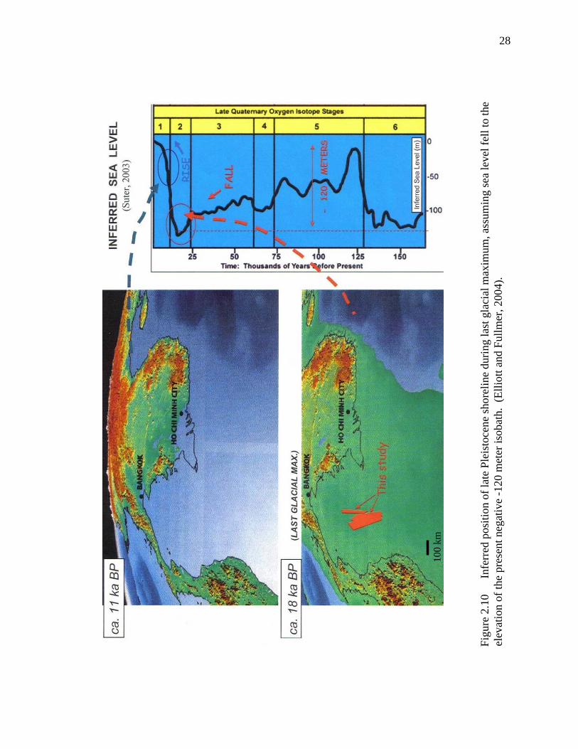
Figure 2.10 Inferred position of late Pleistocene shoreline during last glacial maximum........................................................................................28
Figure 2.11 Map of the principal drainage systems into the northern Gulf of Thailand.........................................................................................30
Figure 2.12 Palaeogeographic evolution of the Gulf of Thailand and North Malay basins ....................................................................................31
Figure 2.13 Gulf of Thailand Tertiary basins ...............................................................38 Figure 2.14 Histogram shows organic carbon content..................................................46

ix
Figure 3.1 Time slice at 132 msec with digitized channel margins and channel belt ................................................................................................48
Figure 3.2 North-south 3D seismic cross section through the study area...................49 Figure 3.3 Time slice at 112 msec (TWTT) with no digitized channels.....................57 Figure 3.4 Time slice at 112 msec (TWTT) with digitized channels..........................58 Figure 3.5 Time slice at 140 msec (TWTT) with no digitized channels.....................59 Figure 3.6 Time slice at 140 msec (TWTT) with digitized channels..........................60 Figure 3.7 Time slice at 184 msec (TWTT) with no digitized channels.....................61 Figure 3.8 Time slice at 184 msec (TWTT) with digitized channels..........................62 Figure 3.9 Time slice at 208 msec (TWTT) with no digitized channels.....................63 Figure 3.10 Time slice at 208 msec (TWTT) with digitized channels..........................64 Figure 3.11 Time slice at 232 msec (TWTT) with no digitized channels.....................65 Figure 3.12 Time slice at 232 msec (TWTT) with digitized channels..........................66 Figure 3.13 Block diagram of a high-sinuosity fluvial system illustrating the facies associations, channel belts, and flood-plain subenvironments ........................................................................................67 Figure 3.14 Satellite image of the Mississippi river shows meandering
channels, meander-neck cutoff, and point bar ...........................................68
Figure 3.15 Time slices at 160 msec and 120 msec (TWTT) show meander- neck cutoffs and point bars in incised valleys, T3 and T1.........................69
Figure 3.16 A present-day meandering channel in Edmonton, Canada, shows scroll bars within each point bar ................................................................71
Figure 3.17 Time slices at 116 msec and 112 msec (TWTT) show scroll bars within each point bar ..........................................................................72

x
Figure 3.18 Time slice at 156 msec (TWTT) shows uninterpreted image with ghosts of former channel locations and interpretation of the growth of meander loops via lateral migration of T3 ..........................73
Figure 3.19 Time slice at 160 msec (TWTT) shows incised valley, T3, with scroll bars and a cartoon shows truncation of point bar ....................74
Figure 3.20 Time slice at 160 msec (TWTT) shows point bars and mud drapes between accretion sets ....................................................................75
Figure 3.21 Time slice at 112 msec (TWTT) shows the location of an A-A’ line and a cross section of an incised valley and tributaries to the incised valley ..................................................................76
Figure 3.22 Comparison of present incised-valley features (air photo of Red Deer River, Alberta, Canada) and seismic time slice.................... 77
Figure 3.23 Comparison of incised-valley features (seismic time slice) and present incised valley features (photos were taken from the plane) ..........78
Figure 3.24 Time slice at 272 msec (TWTT) shows channels, cross section locations, A-A’ and B-B’, and cross sections of incised valleys, T17 and T15, a medium-sinuosity channel, T11, and a straight channel, T13 .................................................79
Figure 3.25 Time slice at 244 msec (TWTT) shows channels and a cross section location, C-C’ and a cross section of
a low-sinuosity channel, T8 .......................................................................80
Figure 3.26 Time slice at 228 msec (TWTT) shows channels and cross section locations, D-D’ and E-E’, which show cross sections of incised valleys, T17, T15, T6, T29, T5, a tributary to incised valley that runs to T5, and
a straight channel, T12...............................................................................81 Figure 3.27 Time slice at 228 msec (TWTT) shows incised valleys and
a DD-DD’ line which shows a cross section of incised valleys, T17, T15, and T6 and a cross-cutting of T17 and T15 ..............................82

xi
Figure 3.28 Time slice at 228 msec (TWTT) shows an incised valley, T6 and EE-EE’ line, which shows a cross section of an uninterpreted image and an interpreted image of valley wall and abandoned channel, base of incised valley, and lateral accretions...............................83
Figure 3.29 Time slice at 192 msec (TWTT) shows channels and F-F’, G-G’, H-H’, and I-I’ lines, which show cross sections of a neck cutoff lobe of T5, an incised valley, and its lateral-accretion features (scroll bars) within the point bar................................................................84
Figure 3.30 Time slice at 192 msec (TWTT) shows channels and F-F’, G-G’, H-H’, and I-I’ lines, which show cross sections of an incised valley, T6 ..................................................................................85
Figure 3.31 Time slice at 172 msec shows channels and a J-J’ line, which shows a cross section of an incised valley, T4................................86
Figure 3.32 Time slice at 136 msec (TWTT) shows channels and K-K’ and L-L’ lines, which show cross sections of a medium- sinuosity channel, T2, a tributary to incised valley, T23, and a high-sinuosity channel, T2_3 ...........................................................87
Figure 3.33 Time slice at 112 msec (TWTT) shows channels and M-M’ and N-N’ lines, which show cross sections of an incised valley, T1 and tributaries to incised valley, T30 and the other tributary on the west side of T1 ........................................................88
Figure 3.34 The evolution of incised-valley fill from sea-level lowstand, through transgression and highstand..........................................................89
Figure 3.35 Time slice at 104 msec (TWTT) shows A-A’, B-B’, C-C’, D-D’, and E-E’ lines for cross sections in Figure 3.111, 3.112, 3.113, 3.114, and 3.115, respectively ...................................................................90
Figure 3.36 Schematic cross section of line A-A’ from 0 to 300 msec (TWTT)
shows channels and sequence boundaries in the study area ......................91
Figure 3.37 Schematic cross section of line B-B’ from 0 to 300 msec (TWTT) shows channels and sequence boundaries in the study area ......................92

xii
Figure 3.38 Schematic cross section of line C-C’ from 0 to 300 msec (TWTT) shows channels and sequence boundaries in the study area ......................93
Figure 3.39 Schematic cross section of line D-D’ from 0 to 300 msec (TWTT) shows channels and sequence boundaries in the study area ......................94
Figure 3.40 Schematic cross section of line E-E’ from 0 to 300 msec (TWTT) shows channels and sequence boundaries in the study area ......................95
Figure 3.41 Frequency histogram shows the distribution of all channel thicknesses (m) ........................................................................97
Figure 3.42 Frequency histogram shows the distribution of unincised fluvial channel thicknesses (m) .................................................97
Figure 3.43 Frequency histogram shows the distribution of incised fluvial channel thicknesses (m) .....................................................98
Figure 3.44 Frequency histogram shows the distribution of channel widths (m) of all channels ............................................................98
Figure 3.45 Frequency histogram shows the distribution of channel widths (m) of unincised fluvial channels......................................99
Figure 3.46 Frequency histogram shows the distribution of channel widths (m) of incised fluvial channels..........................................99
Figure 3.47 Frequency histogram shows the distribution of width/thickness aspect ratios of all channels ...........................................100
Figure 3.48 Frequency histogram shows the distribution of width/thickness aspect ratios of unincised fluvial channels ....................100
Figure 3.49 Frequency histogram shows the distribution of width/thickness aspect ratios of incised fluvial channels ........................101
Figure 3.50 Frequency histogram shows the distribution of Channel-belt widths (m) of all channels ..................................................101
Figure 3.51 Frequency histogram shows the distribution of Channel-belt widths (m) of unincised fluvial channels ...........................102

xiii
Figure 3.52 Frequency histogram shows the distribution of Channel-belt widths (m) of incised fluvial channels ...............................102 Figure 3.53 Frequency histogram shows the distribution of
cumulative channel lengths (m) of all channels.......................................103
Figure 3.54 Frequency histogram shows the distribution of cumulative channel lengths (m) of unincised fluvial channels................103
Figure 3.55 Frequency histogram shows the distribution of cumulative channel length (m) of incised fluvial channels .....................104
Figure 3.56 Frequency histogram shows the distribution of channel length (a straight line) from upstream to downstream of all channels......................................................................104
Figure 3.57 Frequency histogram shows the distribution of channel length (a straight line) from upstream to downstream of unincised fluvial channels...............................................105
Figure 3.58 Frequency histogram shows the distribution of channel length (a straight line) from upstream to downstream of incised fluvial channels...................................................105
Figure 3.59 Frequency histogram shows the distribution of point-bar size of all channels ...................................................................106
Figure 3.60 Frequency histogram shows the distribution of point-bar size of unincised fluvial channels.............................................106
Figure 3.61 Frequency histogram shows the distribution of point-bar size of incised fluvial channels.................................................107
Figure 3.62 Frequency histogram shows the distribution of point-bar volumes (km3) of all channels..................................................107
Figure 3.63 Frequency histogram shows the distribution of point-bar volumes (acre ft) of all channels ..............................................108
Figure 3.64 Frequency histogram shows the distribution of point-bar volumes (km3) of unincised fluvial channels ...........................108

xiv
Figure 3.65 Frequency histogram shows the distribution of point-bar volumes (acre ft) of unincised fluvial channels .......................109
Figure 3.66 Frequency histogram shows the distribution of point-bar volumes (km3) of incised fluvial channels ...............................109
Figure 3.67 Frequency histogram shows the distribution of point-bar volumes (acre ft) of incised fluvial channels ...........................110
Figure 3.68 Frequency histogram shows the distribution of half-meander wavelengths of all channels...............................................110
Figure 3.69 Frequency histogram shows the distribution of half-meander wavelengths of unincised fluvial channels ........................111
Figure 3.70 Frequency histogram shows the distribution of half-meander wavelengths of incised fluvial channels ............................111
Figure 3.71 Frequency histogram shows the distribution of sinuosity of all channels...........................................................................112
Figure 3.72 Frequency histogram shows the distribution of sinuosity of unincised fluvial channels ....................................................112
Figure 3.73 Frequency histogram shows the distribution of sinuosity of incised fluvial channels ........................................................113
Figure 3.74 Frequency histogram shows the distribution of amplitude of all channels .........................................................................113
Figure 3.75 Frequency histogram shows the distribution of amplitude of unincised fluvial channels ..................................................114
Figure 3.76 Frequency histogram shows the distribution of amplitude of incised fluvial channels ......................................................114
Figure 3.77 Frequency histogram shows the distribution of asymmetry of all channels .......................................................................115
Figure 3.78 Frequency histogram shows the distribution of asymmetry of unincised fluvial channels.................................................115

xv
Figure 3.79 Frequency histogram shows the distribution of asymmetry of incised fluvial channels.....................................................116
Figure 3.80 Frequency histogram shows the distribution of gradient (degrees) of all channels ............................................................116
Figure 3.81 Frequency histogram shows the distribution of gradient (degrees) of unincised fluvial channels .....................................117
Figure 3.82 Frequency histogram shows the distribution of gradient (degrees) of incised fluvial channels .........................................117
Figure 3.83 Frequency histogram shows the distribution of gradient (cm/km) of all channels .............................................................118
Figure 3.84 Frequency histogram shows the distribution of gradient (cm/km) of unincised fluvial channels.......................................118
Figure 3.85 Frequency histogram shows the distribution of gradient (cm/km) of incised fluvial channels...........................................119
Figure 3.86 Cross plot between gradient (degrees) and sinuosity of all channels...........................................................................119
Figure 3.87 Cross plot between point-bar size (km2) and sinuosity of all channels...........................................................................120
Figure 3.88 Cross plot between point-bar volume (acre ft) and sinuosity of all channels...........................................................................120
Figure 3.89 Cross plot between point-bar size (km2) and half-meander wavelength (m) of all channels..........................................121
Figure 3.90 Cross plot between point-bar volume (acre ft) and half-meander wavelength (m) of all channels..........................................121
Figure 3.91 Cross plot between point-bar size (km2) and amplitude (m) of all channels ..................................................................122
Figure 3.92 Cross plot between point-bar volume (acre ft) and amplitude (m) of all channels ..................................................................122

xvi
Figure 3.93 Cross plot between thickness (m) and width (margin width) (m) of all channels ................................................123
Figure 3.94 Cross plot between thickness (m) and width (margin width) (m) of unincised fluvial channels .........................123
Figure 3.95 Cross plot between thickness (m) and width (margin width) (m) of incised valleys and tributaries to incised valleys ..........................124
Figure 3.96 Rose diagram shows paleocurrent direction of all channels...............................................................................................124
Figure 3.97 Rose diagram shows paleocurrent direction of all channels except tributaries to incised valleys .....................................125
Figure 3.98 Rose diagram shows paleocurrent direction of straight channels.......................................................................................125
Figure 3.99 Rose diagram shows paleocurrent direction of low-sinuosity channels.............................................................................126
Figure 3.100 Rose diagram shows paleocurrent direction of medium-sinuosity channels......................................................................126
Figure 3.101 Rose diagram shows paleocurrent direction of high-sinuosity channels............................................................................127
Figure 3.102 Rose diagram shows paleocurrent direction of tributaries to incised valleys.....................................................................127
Figure 3.103 Rose diagram shows paleocurrent direction of incised valleys..........................................................................................128
Figure 3.104 Rose diagram shows paleocurrent direction of channels that are below sequence boundary 1 .........................................128
Figure 3.105 Rose diagram shows paleocurrent direction of channels that are above sequence boundary 1 .........................................129
Figure 3.106 Rose diagram shows paleocurrent direction of channels that are above sequence boundary 2 .........................................129
xvii
Figure 3.107 Rose diagram shows paleocurrent direction of channels that are above sequence boundary 3 .........................................130
Figure 3.108 Rose diagram shows paleocurrent direction of channels that are above sequence boundary 4 .........................................130
Figure 3.109 Rose diagram shows paleocurrent direction of channels that are above sequence boundary 5 ........................................131
Figure 3.110 Rose diagram shows paleocurrent direction of channels that are above sequence boundary 6 .........................................131
Figure 3.111 Rose diagram shows fault orientation of the study area at Sequence 4 horizon.......................................................132
Figure 3.112 Late Pleistocene to Holocene sea level curve based on oxygen isotope data ..................................................................134
Figure 3.113 Schematic cross section of the upper Colorado valley.............................137 Figure 3.114 Schematic block diagram of the valley-fill deposits
of the Mississippi River ...........................................................................138
Figure 3.115 Schematic depiction of incised valley and unincised fluvial channel related to sea level fall ....................................................139
Figure 3.116 Summary diagram illustrating the relationships between shoreface and fluvial architecture as a function of base-level change .....................................................................................145

xviii
LIST OF TABLES
Table 3.1 Table of channel parameters ......................................................................55 Table 3.2 Comparison of channel dimensions to other known fluvial information ...................................................................................144

xix
ACKNOWLEDGEMENTS
I would like to express my sincere gratitude to many people and organizations.
Chevron Offshore (Thailand) Ltd. gave me this enormous opportunity and
provided the data for my thesis study. This has been a great educational and life
experience at the Colorado School of Mines. I would not have been able to learn and
gain great amounts of knowledge without sponsorship from Chevron (Thailand).
I thank Dr. Neil F. Hurley, for his kind support through my education, both
academically and personally. To me, he is a wonderful person who always supports
people with his true heart. I truly appreciate the dedication of your time supporting me
with my studies and thesis. Even when you are half way around the world, you still
never stop working for me and other students. Thank you for your words of
encouragement.
I thank my thesis committee, Dr. Piret Plink-Bjorklund and Dr. Timothy R.
McHargue, and also my former advisor, Dr. Michael Gardner, for their excellent advice,
explanations and support.
I thank Chevron ETC, Mr. Erik Davidsen, Mr. Frank Harris, Mr. Timothy
McHargue, Mr. Joseph Hovadik, Mr. Julian Clark, Mr. Andrea Fildani, Mr. Yongjun
Yue, Ms. Marjorie Levy, Mr. Christopher Ainley, Ms. Ciony Lacher, and all the
computer support staff, for their kind support while I was working on my thesis in
Chevron’s San Ramon office during a summer break. Your efforts are truly appreciated.
Special thanks also go to Mr. Joseph Hovadik and Mr. Julian Clark, who dedicated their
valuable time supporting me with the channel-parameter files.
I thank the CSM CoRE staff, Ms. Carlotta (Charlie) Rourke, Dr. Mary Carr, Dr.
James (Jim) Borer, and Dr. David Pyles, for the enormous support. Charlie, you are
always able to find the solution for me with your sincere support. I am thankful for
everything that you have done for me. I also would like to thank Mary and Jim for their

xx
excellent explanations of stratigraphic concepts. Thanks for the long hours that you spent
with me.
I thank the CSM professors and staffs, for their excellent lectures, classes, field
trips, and all the support. Additionally, I thank Dr. Donna Anderson for the assistance in
the point-bar and crevasse-splay field trip in NW Colorado, and for her great advice.
I thank Mr. Dale Watts and Ms. Shauna Gilbert for the Unix and PC support at
school.
I thank Mr. Luca Rigo De Righi, my great mentor, who is now working with
Chevron in Angola, for all of his support in any matter at any time.
I thank Mr. Kenneth Kelsch, my present mentor, for supporting me with geologic
background information for the Gulf of Thailand.
Thanks go to my sweet friend and colleague, Ms. Jutharat Boonyakitsombat, for
supporting me with geologic background information.
I thank all of my friends/colleagues in Chevron (Thailand) for their dedicated
support, both academic and personal.
I appreciated the help I received from Mr. Tom Elliott, Chevron (Houston), who
provided valuable explanations while I attended a Chevron Forum in Houston, 2005, and
the kind support throughout my thesis.
I thank Mr. James Turner, for a great supportive paper and explanation while I
attended a Chevron Forum in Houston, 2005.
I thank Mr. Kosit Fuangswasdi, Mr. Lance Brunsvold, Mr. Greg Cable, and Ms.
Aree Rittipat for your support trying to get the approval for releasing the previous work
reports of the channel-analog study of the Gulf of Thailand.
I thank Dr. Christopher Morley for his support paper for the geologic background
information of the Gulf of Thailand.
I thank Dr. Henry Posamentier for a great conversation about fluvial sequence
stratigraphy while he was giving a presentation at the Colorado School of Mines.

xxi
I thank Mr. Ira Pasternack, for the explanation over the phone about Adobe
Acrobat use.
I thank Ms. Fernanda Schafer, Ms. Melinda Leza, and Ms. Elena Brightwell for
the great support for my stay in the US.
I express special gratitude to my friends, Manuel Paz, Olusola Bakare, Henrikus
Panjaitan, Rexi Esomar, Mirna Slim, Marin Matesic, Martha Lopez, and Burcu Topcam
for the joyful support and for working hard and playing hard together. I also would like
to thank the Thai students at CSM for such an unforgettable experience. They have
always given me both social and moral support whenever I needed it.
I thank my family for the unconditional love and support that they give to me.
Thank you for your patience while waiting for my return with the degree that we all have
been waiting for. Without them, I would not have had a chance to be me today.
I thank my love, John Condry, who is always beside me for all the good and bad
moments. Thank you so much for your time and all the mental and moral support that
you always give to me throughout my education and life here.
My apologies go to anyone who has helped me but whom I forgot to
acknowledge. This thesis would not be done without everyone’s support. Life would
have been difficult without all of you.

1
CHAPTER 1
INTRODUCTION
Observations of shallow 3D seismic data from offshore Thailand indicate the
value of these data as a way to quantify fluvial reservoir architecture. These data provide
the opportunity to document in great detail the distribution of channels and related facies
of a fluvial system. This work should allow us to predict the most accurate well
placement in fluvial channels in oil and gas reservoirs.
Through mapping and visualization of 3D seismic data from the uppermost 300
msec of data below the mud line in the Gulf of Thailand, this thesis documents
architectural complexity and reservoir connectivity. Channel evolution and internal
architecture are well imaged, so sand distribution can be confidently predicted, despite
the absence of well data through this interval. Because multiple channel systems are well
imaged, we have an excellent opportunity to confirm repeatability of observations and
separate what is typical from what is unusual. A study of reservoir connectivity in fluvial
channels from near-surface seismic data can also be an extremely valuable approach to
the study of deep-water sandstone reservoirs.
1.1 Research Objectives
The purpose of this study is to document the distribution and internal architecture
of fluvial sand bodies using shallow 3D seismic data (0 -300 msec) in the Pleistocene to
Holocene section from the Gulf of Thailand. The goal is to be able to predict accurate

2
well placement in fluvial channels in subsurface reservoirs in the underlying Miocene
section. Specifically, the study has the following objectives:
1) Interpret a 3D seismic data set, cross sections and time slices.
2) Acquire channel parameters: channel width, channel belt width,
cumulative channel length along each channel, channel length (a straight
line from upstream to downstream), half-meander wavelength, amplitude,
asymmetry, azimuth, sinuosity, channel gradient, paleocurrent direction,
channel thickness, point-bar size and volume, and width/thickness aspect
ratio.
3) Develop statistical relationships for the mentioned values.
4) See how channels evolved through time, within a sequence-stratigraphic
framework.
5) Obtain fluvial analogs for the Gulf of Thailand and other areas that have
fluvial environments. This analog could benefit further exploration and
production.
6) Provide channel parameters that can be used as input for 3-D model
construction.
1.2 Study Area and Data Set
The study area, known as Jarmjuree, is located in the southern part of Block
B8/32 in the Gulf of Thailand. Water depth is 250 ft (80 m). The area is 125 mi (200
km) offshore, and 225 mi (362 km) from Bangkok (Fig. 1.1). The study area covers
approximately 718 mi2 (1,860 km2).
3D seismic surveys in the Block B8/32 area provide the basis for this study. File
pst16ts.bri, which consists of 3D seismic data, is used for the shallow (0-300 msec)
seismic data interpretation. Edge (Enhanced detection of Geologic Events) processing, a

3
Figure 1.1 Location of study area, Jarmjuree, in the Gulf of Thailand. Line Y-Y’ shows the location of the cross section in Figure 2.9. (Adapted from Chevron Offshore (Thailand) Ltd.).
Cambodia Block A
7/8/9
G4/43
9A
Y Y’

4
proprietary Chevron coherency technique, helps to better detect stratigraphic details in
this shallow section.
The 3D seismic data set has been studied with Landmark and Gocad interpretation
software. All seismic data interpretations and manipulations have been performed
utilizing Seisworks, Gocad, and Chevron geomorphology software to determine
parameters such as channel lengths, widths, and sinuosities. No well data or logs are
available for this shallow study interval.
1.3 Previous Work
There are some previous fluvial analog studies within the Gulf of Thailand.
These include Mountford and Livesay (1996), who worked in Pailin field, and Elliott and
Triamwichanon (1999), who worked in the Arthit area (Fig. 1.2).
The reports of Mountford and Livesay (1996), and of Elliott and Triamwichanon
(1999) both used 3D seismic data, which was shot for exploration and development
purposes. These two analog studies examined the very shallow, near-surface portions of
3D seismic data volumes. These two reports used shallow time slices through 3D
volumes, because this was the only way to produce "map view" images of fluvial analogs
(Elliott, 2006, personal communication).
Miall (2002) described Pleistocene fluvial features in the Arthit area (Fig. 1.2).
His study demonstrated the utility of seismic time-slice images for exploring the
sedimentology and sequence stratigraphy of complex depositional systems. Seismic
cross sections and well data were not released for his study. “An important practical
outcome of his study has been the demonstration of the preservation of the deposits of a
wide variety of fluvial styles over a short stratigraphic interval. These range in scale
from braided systems that are up to 4 km wide to ribbon channels a few hundred meters
in width. Channels of low and high sinuosity and of braided, meandering, straight, and

5
F
CM
MM
L
PI
A Ban
gkok
Gul
f of
Thai
land
Patt
aniB
asin
Nor
th M
alay
Bas
in
Arth
itAr
ea
Anda
man
Se
a
Tha
iland
F
CM
MM
L
PI
A Ban
gkok
Gul
f of
Thai
land
Patt
aniB
asin
Nor
th M
alay
Bas
in
Arth
itAr
ea
Anda
man
Se
a
Tha
iland
Figu
re 1
.2
The
Terti
ary
basi
ns o
f Tha
iland
and
the
loca
tion
of th
e Pa
ttani
bas
in, A
rthit
area
, and
Nor
th M
alay
bas
in.
(Fro
m T
urne
r et a
l., 2
004)
.

6
anastomosed style are present. This considerable variation in channel style and scale
should serve as a warning against simplistic approaches to production modeling and to
the paleohydraulic analysis of ancient river systems” (Miall, 2002).
Elliott and Fullmer (2004) described fluvial analog statistics, collected from map-
view images, to construct fluvial sequence-stratigraphic models. They made a first-pass
survey of bright amplitude anomalies as an input to a subregional assessment of drilling
hazards. Dimensions measured in the shallow, well-imaged Pleistocene fluvial systems
could be used to develop detailed reservoir analogs for the more poorly imaged Miocene
fluvial reservoir targets. Observed ranges of dimensions were as follows:
• Channel widths 40-500 m and channel depths 10-46 m
• Channel-belt widths: 0.1-6.3 km
• Valley widths 0.1-9 km, and valley depths 13-80 m
• Point-bar thicknesses 10-44 m, with areas of 0.7-22 km2
Pleistocene-Holocene fluvial systems are seen to be highly variable in terms of
fluvial styles, dimensions, lateral relationships, and vertical (temporal) successions
(Elliott and Fullmer, 2004).
1.4 Research Contributions
This research contributes to the better understanding of fluvial reservoirs. The
study helps us better understand architectural complexity and reservoir connectivity. In
the 3-D seismic data set from the Gulf of Thailand, channel evolution and internal
architecture are well imaged, so sand distribution can be confidently predicted. This study
quantifies channel widths, channel belt widths, cumulative channel length along each
channel, channel length (a straight line from upstream to downstream), half-meander
wavelength, amplitudes, asymmetries, sinuosities, point-bar sizes and volumes, channel
gradients, the thicknesses of channels, width/thickness aspect ratio, and paleocurrent

7
directions in a manner suitable for 3-D geologic-modeling. The results provide important
input for conditioning subsurface reservoir models. The following are the contributions
from this study:
• Time-slice images and cross sections through 3D seismic amplitude
volumes provide useful information for fluvial geomorphology interpretation and high-
quality images for fluvial depositional-element dimension measurement.
• The multiple high-amplitude sea-level falls during the Pleistocene and
Holocene created lowstand depositional systems, both incised and unincised fluvial
systems, in this study interval in the Gulf of Thailand.
• This study provides fluvial analogs for the Gulf of Thailand and other areas
that have fluvial environments. This analog benefits further exploration and production.
• This study helps to confirm the dimensions of fluvial systems for the
benefit of petroleum exploration and development. The dimensions measured from these
fluvial systems could be used to develop detailed reservoir analogs (models) for the more
poorly imaged, underlying Miocene fluvial reservoir targets.
• The results of statistical cross plots are as follows:
o The higher the gradient, the lower the sinuosity.
o The higher the sinuosity, the larger the point-bar sizes or volumes.
o The larger half-meander wavelengths correspond to larger point-bar
sizes or volumes.
o Higher amplitudes correspond to larger point-bar sizes or volumes.
o Higher thicknesses correspond to greater widths. The width/
thickness aspect ratio commonly is greater for unincised fluvial systems than for
incised fluvial systems.
• Six sequence boundaries are interpreted in this study interval, based on the
presence of incised valleys at six levels. In Indonesia, the water depth of -110 m has
been identified as a threshold level, below which the continental shelf would be fully

8
exposed (Posamentier, 2001). In the Gulf of Thailand, this work shows that the -95 m
level is more likely. Shelf topography and local tectonic activity are possible reasons for
the differences between Indonesia and Thailand.
• There is a wide variety of fluvial styles, dimensions, vertical successions,
and lateral relationships over a short stratigraphic interval, in this study. Exploration and
production efforts in areas of fluvial depositional environments should take this into
account.
• Channels in this study have different sizes and dimensions. The reasons that
make them different could be because of differences in substrate erodibility, and/or
channel discharge (sediment supply and flow rate), and/or length of time during which
lateral cutting occurred, and/or climate, and/or vegetation types and/or relative sea level
change (accommodation space), and/or tectonic control.
• Tectonic tilting may have occurred locally over this study interval because
the paleocurrent directions of channels are variable. However, the main paleocurrent
direction is still mostly in the NW to SE direction. The main fault orientations in the
study area are in a N-S direction.
• Potential reservoir heterogeneities are internal mud drapes between
accretion sets, complex compartment geometries, scoured upper and basal contacts, and
cannibalism and stacking.
• It is important that exploration geologists are able to distinguish between
incised fluvial systems and unincised fluvial systems, be aware of the distinguishing
attributes of each of them, and know reasonable dimensions for each system.
• The results of this study provide the parameters that can be used as input for
3-D model construction.

9
CHAPTER 2
GEOLOGIC BACKGROUND
2.1 Structure
Based on structural studies, there are three major tectonic phases: 1) active early
syn-rift (39.5-25.5 Ma: Upper Eocene to the end of Oligocene), 2) late syn-rift (25.3?-
10.5: Lower Miocene to Late Middle Miocene), and 3) post-rift (Late Mid Miocene to
Recent) (Fig. 2.1). Syn-rift sediments, which consist of five sequences, underlie the Mid-
Miocene unconformity (10.5 Ma). There is a short time gap from 10-10.5 Ma. Post-rift
sedimentation occurred under the influence of regional subsidence and marine
transgression (Chevron, 2002).
Structural history above the basement in the Pattani basin began during the
Oligocene (Lockhart, 1997; Polachan and Sattayarak, 1989). The Tertiary rift basin in the
Pattani basin was developed by approximately E-W extension since the Oligocene,
associated with a sub-horizontal NW-SE to NE-SW σ1 (maximum stress) direction
(Morley et al., 2001). The stresses were likely due to collision of the Indian plate with
Eurasia. N-S trending extensional faults in the syn-rift phase originated under the
influence of movement along regional conjugate fault sets of a strike-slip fault (Fig. 2.2).
Those strike-slip faults were the Mae Ping and Three Pagodas faults, corresponding with
Himalayan escape tectonics (Kornsawan, 2001; Tapponnier et al., 1982, 1986). Many
models have mentioned that the extensional basin is related to pull-apart movement (left-
lateral pull-apart by Tapponnier et al., 1986; right lateral strike-slip faulting by Polachan

10
FIGURE 2.1

11
FIGURE 2.2

12
and Sattayarak, 1989; Hall, 1996). Some divergent views call for oblique extension
associated with pre-existing fabric by left-lateral strike-slip faulting (Haranya, 2000;
Watcharanantakul and Morley, 2000; Kornsawan, 2001), which ceased motion during the
late Oligocene. Extension was interrupted by structural inversion and erosion at the end
of the Oligocene (Jardine, 1997) until the middle Miocene, which terminated the syn-rift
section (Lacassin et al., 1997; Morley et al., 2001). Jardine (1997) proposed that
widespread erosion occurred during the Late-Middle to Early-Upper Miocene and
continued with thermal basin subsidence from the upper Miocene to the present (Fig.
2.3).
The syn-rift section in the Pattani basin is bounded by large-displacement normal
faults, associated with small-displacement faults in half grabens in Oligocene-Middle
Miocene sequences (Kornsawan, 2001). East-dipping faults are dominant and the main
depocenter lies on the eastern side of the basin (Haranya, 2000). Transfer zones between
the major faults are typical. Relay ramps are common features (Haranya, 2000).
Miocene late syn-rift and post-rift structure patterns are strongly influenced by the
deeper faulting from the basement and early syn-rift and transtension movement
(Lockhart et al., 1997). Post-rift faulting exhibits linkage geometry and multiple
depocenters, which were influenced by the pre-rift fault patterns (Haranya, 2000). In the
northern Pattani basin, a few conjugate fault systems with both east- and west-dipping
convergent conjugate fault pairs have a mainly N-S strike with minor N-NE trends. The
conjugate fault system axes have the same trend as the strike of the syn-rift fault that
affected them (Boonyakitsombut, 2003).
Many deep, rapid-subsidence Cenozoic sedimentary basins are found in Southeast
Asia (Fig. 2.4). The Pattani and Malay basins originated as rifts in the Gulf of Thailand.
They formed initially by extension of continental crust. They are also located in a
continental interior setting, and are filled by terrestrial to marginal-marine sediments
(Morley and Westaway, 2006).

13
Topo
grap
hic
varia
tions
NS
SEN
WO
nsho
re T
haila
ndG
ulf o
f Tha
iland
Fang
B
asin
Phra
oBa
sin
Lam
pang
Bas
inPh
itsan
ulok
Bas
inCh
aoPh
raya
Basi
n
Chai
natR
idge
Kra
Basi
nPa
ttani
Basi
nM
alay
Bas
inW
. Nat
una
Basi
n
Dec
reas
ing
effe
cts o
f inv
ersi
on(s
yn-p
ost-r
ift)
Sea
leve
l
Depth/height (m)
2500
2000
1500
1000 50
0 050
010
0015
0020
0025
0030
0035
0040
000
100
200
300
400
500
600
700
800
900
1000
1100
1200
1300
1400
1500
1600
Topo
grap
hy a
bove
top
syn-
rift
Bas
e po
st-ri
ftTo
p sy
n-rif
tK
oPh
aN
gan
Ridg
eK
oK
raR
idge
Bang
kok
Dist
ance
(km
)Th
aila
nd/
Bur
ma
Bor
der
Time (Ma.)
0 5 10 15 20 25
100
m L
i bas
in
Syn-
rift s
ectio
nPo
st-r
ift s
ectio
nD
istan
ce
II
I I
I
I-P
erio
d of
inve
rsio
nM
MU
-M
iddl
e M
ioce
ne u
ncon
form
ityun
conf
orm
ity
II I
??Base post rift?
I
I
I
?20
0 m
1,70
0 m
II
2,50
0 m
4,00
0 m
MM
U
3,00
0 m I I I I I
Topo
grap
hic
varia
tions
NS
SEN
WO
nsho
re T
haila
ndG
ulf o
f Tha
iland
Fang
B
asin
Phra
oBa
sin
Lam
pang
Bas
inPh
itsan
ulok
Bas
inCh
aoPh
raya
Basi
n
Chai
natR
idge
Kra
Basi
nPa
ttani
Basi
nM
alay
Bas
inW
. Nat
una
Basi
n
Dec
reas
ing
effe
cts o
f inv
ersi
on(s
yn-p
ost-r
ift)
Sea
leve
l
Depth/height (m)
2500
2000
1500
1000 50
0 050
010
0015
0020
0025
0030
0035
0040
000
100
200
300
400
500
600
700
800
900
1000
1100
1200
1300
1400
1500
1600
Topo
grap
hy a
bove
top
syn-
rift
Bas
e po
st-ri
ftTo
p sy
n-rif
tK
oPh
aN
gan
Ridg
eK
oK
raR
idge
Bang
kok
Dist
ance
(km
)Th
aila
nd/
Bur
ma
Bor
der
Time (Ma.)
0 5 10 15 20 25
100
m L
i bas
in
Syn-
rift s
ectio
nPo
st-r
ift s
ectio
nD
istan
ce
II
I I
I
I-P
erio
d of
inve
rsio
nM
MU
-M
iddl
e M
ioce
ne u
ncon
form
ityun
conf
orm
ity
II I
??Base post rift?
I
I
I
?20
0 m
1,70
0 m
II
2,50
0 m
4,00
0 m
MM
U
3,00
0 m I I I I I
Figu
re 2
.3
Cro
ss se
ctio
n an
d st
ruct
ural
eve
nts o
f the
Gul
f of T
haila
nd.
(Ada
pted
from
Mor
ley
et a
l., 2
001)
.

14
Figure 2.4 Location map of basins in Southeast Asia. (After Morley and Westaway, 2006). The A-A’, B-B’, C-C’, and D-D’ lines show cross sections in Figure 2.5, the E-E’ line shows a cross section in Figure 2.6, and the F-F’ and G-G’ lines show cross sections in Figure. 2.7.

15
The central Pattani basin reveals a synformal geometry to the base of seismic
penetration (Fig. 2.5b). This seismic section does not show a classic rift geometry,
although normal faults display offsets that increase with depth. However, none of these
can be described as classic half-graben boundary faults. Attempts to determine the
location of a syn-rift to post-rift transition within this Oligocene-Miocene sequence have
proven problematic. Conversely, where the post-rift sequence is thinner, as in the
northern Pattani basin and North Malay basin (Fig. 2.4), the syn-rift sequence is locally
well developed and classic synrift and post-rift interpretations can be made (Figs 2.6 and
2.11) (Morley and Westaway, 2006).
The regional structural setting in the Pleistocene-Holocene interval was
dominated by extensional faulting, similar to the fault systems mapped at Miocene levels.
Movement along some fault systems has continued until the present day. Broad, regional
warping may also have affected the tilt of the coastal plain at various times, resulting in
river systems running in various directions (Fig. 3.1 and Appendix A (CD-ROM)) (Elliott
and Fullmer, 2004).
2.2 Stratigraphy
The stratigraphic framework for the Pattani basin was published by Jardine
(1997). This framework is different from the internal standards used by Chevron
(Offshore) Thailand, Ltd. The comparison of the sequence stratigraphy published by
Jardine (1997) and by Chevron is shown in Figure 2.1 (Boonyakitsombut, 2003). This
study uses the nomenclature proposed by Chevron.
2.2.1 Pre-Tertiary Basement
The basement consists of intrusive igneous rocks, deformed metamorphosed
sediments, limestones, and dolomites of a Late Cretaceous to Early Eocene age (Chevron,

16
Figu
re 2
.5a
Cro
ss s
ectio
n A
-A’ a
cros
s th
e Pa
ttani
bas
in.
The
loca
tion
of th
is c
ross
sec
tion
is s
how
n in
Fig
ure
2.4.
(M
odifi
ed a
fter M
orle
y an
d W
esta
way
, 200
6).
A
A’

17
Figu
re 2
.5b
Cro
ss s
ectio
n B
-B’ a
cros
s th
e Pa
ttani
bas
in.
Arr
ows
mar
k th
e ap
prox
imat
e st
ratig
raph
ic p
ositi
on o
f the
on
set o
f po
st-r
ift s
ubsi
denc
e, a
s su
gges
ted
by W
heel
er a
nd W
hite
(20
00)
(arr
ow1)
and
Wat
char
anan
taku
l and
Mor
ley
(200
0) (
arro
w 2
). T
he a
ctua
l bas
e of
the
post
-rift
sec
tion
is n
ow p
lace
d in
the
Late
Olig
ocen
e (a
rrow
3).
Not
e th
at
none
of t
hese
arr
ows m
arks
a si
gnifi
cant
cha
nge
in b
asin
geo
met
ry o
r unc
onfo
rmity
, unl
ike
the
clea
r syn
-rift
to p
ost-r
ift
trans
ition
sho
wn
in F
ig. 2
.6.
The
loca
tion
of th
is c
ross
sec
tion
is s
how
n in
Fig
ure
2.4.
(A
fter M
orle
y an
d W
esta
way
, 20
06).

18
Figu
re 2
.5c
Cro
ss s
ectio
n C
-C’ a
cros
s th
e Pa
ttani
bas
in.
The
loca
tion
of th
is c
ross
sec
tion
is s
how
n in
Fig
ure
2.4.
(M
odifi
ed a
fter M
orle
y an
d W
esta
way
, 200
6).

19
Figu
re 2
.5d
Cro
ss s
ectio
n D
-D’ a
cros
s th
e M
alay
bas
in.
The
loca
tion
of th
is c
ross
sec
tion
is s
how
n in
Fig
ure
2.4.
(M
odifi
ed a
fter M
orle
y an
d W
esta
way
, 200
6).

20
E E’
50 km
E E’
50 km
Figure 2.6 Seismic line (from PTTEP) across the North Malay basin. The location of Line E-E’ is shown in Figure 2.4, illustrating a well-defined syn-rift half graben (of Eocene? to Oligocene age), unconformably overlain by post-rift Late Oligocene to earliest Miocene lacustrine shales. The Miocene post-rift sequence onlaps the basement high to the east. (After Morley and Westaway, 2006).

21
Fig. 2.7

22
Figure 2.8 Subsidence curves for the depocenters of the Pattani and North Malay basins based on wells and seismic reflection data (Watcharanantakul and Morley, 2000). See Figs. 2.5b and 2.6 for locations of curves (a) and (b), respectively. Over much of the North Malay basin, the Late Oligocene to Early Miocene sequence exhibits a synformal geometry, typical of post-rift deposits. However, in some localities, expansion into minor normal faults causes greater thicknesses of the sequence and small (~5-10 km wide) half-graben geometries. (After Morley and Westaway, 2006).

23
2002). In seismic data, there are highly variable reflections. Carbonate rocks and granite
show coherent and high-amplitude reflections. Metamorphic rocks give fairly low-
amplitude and discontinuous reflections. Major seismic characteristics are onlap and
angularity (Boonyakitsombut, 2003).
2.2.2 Sequence I
Sequence I started approximately during the Early Oligocene (36-30 Ma).
Depositional environments were lacustrine plain, localized lacustrine facies and alluvial
fans. Sediments attributed to these strata are coarse-grained sandstone, and sandy
conglomerates interbedded with red shales, and claystones. Coals and gray shales occur
locally (Chevron, 2002).
Seismically, this sequence is an opaque section with high amplitude, parallel to
those of Sequence II. Reflections are discernable, but noisy.
Related to faulting, large sand-rich alluvial deposits grade into interbeds of sand
and shale, with more pronounced layering away from the fault escarpment. The sequence
always has a large expanded section on the downthrown side of faults.
Sequence I is found only in the axes of the rifted basin and is not continuous.
Hence, this interval is rarely correlated across the basin (Boonyakitsombut, 2003).
2.2.3 Sequence II
Sequence II deposition occurred during the Late Oligocene (30-25.5 Ma), a period
of highstand of sea level. Extension continued and rifting caused major lake
development. Sediments deposited in a lacustrine environment (with local alluvial fans)
are shale and claystone with minor sandstone and local coals.

24
Related to petroleum, Sequence II is an excellent source rock when it is thermally
mature. In addition, it has a distinctive gamma ray log response (>200 units) where it is
penetrated by wells.
Seismic reflections are persistent, low frequency and high amplitude. These are
distinctive and discernible from both the overlying Sequence III and the underlying
Sequence I. The top of the sequence is indicated by an unconformity with onlap at the
top. Near the margin of the rifted basin, this onlap can be very pronounced
(Boonyakitsombut, 2003).
2.2.4 Sequence III
Sequence III was deposited after the main rifting phase had ceased, but with
continued subsidence. Sequence III was deposited during regression (or lowstand) during
the Early Miocene (25.5 or 25.3?-17.5 Ma). All sediments are red beds, with lacustrine
shales at the top. Sediments consist of interbedded sandstones and claystones with minor
limestones and coal. Fluvial sandstone is mainly fine to medium grained and it is
difficult to correlate individual sands. One marker, especially clearly seen in the central
Pattani basin, is a change of gray claystone to red claystone at the top of Sequence III.
This is the principal reservoir in gas-condensate fields in the central Pattani basin.
In seismic data, parallel reflections with variable amplitude characterize this
sequence. Onlap occurs onto the underlying top of the Sequence II unconformity
(Boonyakitsombut, 2003).
2.2.5 Sequence IV
This sequence was deposited during the Lower Middle Miocene (17.5-13.8 Ma),
during transgression to the south, with slow subsidence. The sediments are red-bed
alluvial plain and sand-shale sequences of lacustrine origin. The depositional

25
environment was lacustrine and alluvial, with carbonates, shales, and a minor amount of
coal interbedded with fine-grained sandstone.
Seismic reflectors are discontinuous and parallel, with variable amplitude.
Affected by faulting, juxtaposition results in poor quality of seal in sand-rich units.
Sandstones faulted against siltstone and shale lithologies appear to be a critical
component for hydrocarbon entrapment (Boonyakitsombut, 2003).
Sequences II and IV are lacustrine plain, with thick shales and claystones
developed in deeper areas, i.e., the axes of basin. Shales and coals were formed in the
shallow part of the lacustrine environment (Boonyakitsombut, 2003).
2.2.6 Sequence V
During the Middle Miocene (13.8-10.5 Ma), marine regression and regional
subsidence occurred. The environment is coastal plain to alluvial plain. Sediments consist
of red beds, interbedded sandstones, claystones, and siltstones with minor limestones and
coals. Claystone varies from red to brown to orange in color. Most of the sandstone is
fluvial in origin, similar to Sequence II. At the top, there is an unconformity with a short
time gap, about 0.5 Ma.
Seismic reflections have high amplitude, variable frequency, and high continuity
in this sequence (Boonyakitsombut, 2003).
2.2.7 Sequence VI
Sequence VI was deposited during the Late Miocene to Early Pliocene (10.5-3.8
Ma). There was slow transgression, simultaneous with the post-rift sag. Intertidal and
marine sediments are interbedded claystones and siltstones with minor sandstones.
Lignite, coal, and coaly shale units indicate a coastal-plain depositional environment.

26
This is the period when extensional tectonics ceased. Seismic reflections are
weak and discontinuous with variable amplitude. Units of coal and lignite have high
amplitudes (Boonyakitsombut, 2003).
2.2.8 Sequence VII
During the Late Pliocene (3.8 Ma) to Recent, marine transgression continued.
The environment became fully marine during the Pleistocene.
Sequence VII is composed of interbedded sand and clay with minor coal in the
lower portion. Numerous gas-charged channel sands exist, which are extremely
hazardous to drilling operations. Overall seismic response in the section is relatively
opaque to discontinuous. Water bottom multiples are common (Boonyakitsombut, 2003;
Fig. 2.9).
Depositional environments in Block B8/32, Gulf of Thailand, during the
Pleistocene-Holocene were controlled chiefly by the effects of sea-level fluctuations,
together with climate changes that probably accompanied them. During the most recent
glacial maximum, approximately 18,000 years ago, most of the continental shelf which
underlies the present North Malay basin was subaerially exposed (Fig. 2.10). This
inference is based on the assumption that the magnitude of sea-level fall was
approximately 394 ft (120 m) below present (Fig. 2.10) (e.g., Suter, 2003). Because the
shelf is shallow and gently sloping, a 394 ft (120 m) drop in sea level would have moved
the shoreline approximately 700 mi (1,127 km) south of Bangkok, to the location of the
present -120m isobath. This created a tremendous area of coastal-plain environments
with fluvio-deltaic deposition. Evidence for widespread fluvial environments is provided
by seismic images of fluvial systems which completely blanket the areas of Block B8/32,
Gulf of Thailand seismic surveys. Lesser falls in sea level would have exposed lesser,
but still significant tracts of the shelf (Elliott and Fullmer, 2004). The ancestral Chao
Praya, Mekong, and other rivers flowed generally southeastwards across this wide coastal

27
Seq
2
Seq
1
Seq
3
Seq
4
Seq
5
Seq
6
Seq
7
Bas
emen
t
EW
Earl
y - L
ate O
ligoc
ene
Lac
ustr
ine
SR.
Earl
y M
ioce
ne
Fluv
ial r
eser
voir
Ear
ly -
Mid
Mio
cene
L
acus
trin
ese
al
Fluv
ial r
eser
voir
Lat
e M
ioce
ne to
Ear
ly P
lioce
ne
Coa
stal
pla
in
Lat
e Pl
ioce
ne (3
.8 M
a) to
rec
ent
Fluv
ial
Lat
e C
reta
ceou
s to
Ear
ly E
ocen
e
Mid
Mio
cene
Early
synr
ift
Late
Syn
rift
Post
rift
MM
U
Y’
Y
Seq
2
Seq
1
Seq
3
Seq
4
Seq
5
Seq
6
Seq
7
Bas
emen
t
EW
Earl
y - L
ate O
ligoc
ene
Lac
ustr
ine
SR.
Earl
y M
ioce
ne
Fluv
ial r
eser
voir
Ear
ly -
Mid
Mio
cene
L
acus
trin
ese
al
Fluv
ial r
eser
voir
Lat
e M
ioce
ne to
Ear
ly P
lioce
ne
Coa
stal
pla
in
Lat
e Pl
ioce
ne (3
.8 M
a) to
rec
ent
Fluv
ial
Lat
e C
reta
ceou
s to
Ear
ly E
ocen
e
Mid
Mio
cene
Early
synr
ift
Late
Syn
rift
Post
rift
MM
U
Y’
Y Figu
re 2
.9
3D se
ism
ic c
ross
sect
ion
(Y-Y
’) sh
ows r
egio
nal s
truct
ure
and
stra
tigra
phy
north
of t
he st
udy
area
.
Loca
tion
of th
is li
ne is
show
n in
Fig
ure
1.1.
(M
odifi
ed fr
om C
hevr
on O
ffsh
ore
(Tha
iland
) Ltd
.).
28
100
km10
0 km
Figu
re 2
.10
Infe
rred
pos
ition
of l
ate
Plei
stoc
ene
shor
elin
e du
ring
last
gla
cial
max
imum
, ass
umin
g se
a le
vel f
ell t
o th
e
ele
vatio
n of
the
pres
ent n
egat
ive
-120
met
er is
obat
h. (
Ellio
tt an
d Fu
llmer
, 200
4).

29
plain to shelf-edge deltas located in the vicinity of the Nam Con Son basin (Dorobek and
Olson, 2001).
2.2.9 Sediment Source Areas
The Chao Phraya River is currently the main river that provides sediment to the
Gulf of Thailand (Fig. 2.11). According to Milliman and Syvitski (1992), in each year,
this drains an area of 61,776 mi2 (160,000 km2) and transports 11 million tons of
sediment. At present, much of this sediment load is deposited in a flood plain around and
inland of Bangkok (the Central Plains basin). Therefore, it does not reach the coastline.
As mentioned in the previous section, the coastline retreated many hundreds of
kilometers to the south, subaerially exposing the present floor of the Gulf of Thailand
(which, at present, has a mean water depth of approximately 158 ft (45m) and a
maximum water depth of approximately 264 ft (80 m)). During glacio-eustatic falls in
sea level, the length of the Chao Phraya river increased downstream by a corresponding
distance (Morley and Westaway, 2006).
The second most important river system, which enters the present Gulf of Thailand
approximately 43.5 mi (70 km) west of the Chao Phraya, is the Maeklaeng/Khwae
(Kwai), which drains a 7,722 mi2 (20,000 km2) area of western Thailand (Fig. 2.11).
During Pleistocene lowstands, this river formed a left-bank tributary of the extended
Chao Phraya system (Morley and Westaway, 2006).
The basins now offshore in the Gulf of Thailand were supplied with sediment
from the north by an ancestral river system known as the ‘palaeo-Chao Phraya’ (Fig.
2.12). This river system seems to have coincided roughly with the modern Maeklaeng/
Kwai and its former downstream continuation, now submerged (Morley and Westaway,
2006).

30
Figure 2.11 Map of the principal drainage systems into the northern Gulf of Thailand, illustrating the relationship between rift basin location and the Chao Phraya river system. Well-established lacustrine systems, which existed during the Miocene, probably meant that at this time the Chao Phraya did not form a throughgoing drainage system. The River Khwae (Kwai) flows SE from the extreme west of Thailand, joining the south flowing Maeklaeng River approximately 62 mi (100 km) NW of Bangkok. (After Morley and Westaway, 2006).

31
Figure 2.12a Eocence-Oligocene paleogeography of the Gulf of Thailand and North Malay basins, illustrating the change in basin type (rift or post-rift basin) and sediment fill with time. Sediment source areas are also indicated. (Modified after Morley and Westaway, 2006). See Figure 2.4 for the index map that shows the location of this figure.

32
Figure 2.12b Late Oligocene paleogeography of the Gulf of Thailand and North Malay basins, illustrating the change in basin type (rift or post-rift basin) and sediment fill with time. Sediment source areas are also indicated. (Modified after Morley and Westaway, 2006). See Figure 2.4 for the index map that shows the location of this figure.

33
Figure 2.12c Early Miocene paleogeography of the Gulf of Thailand and North Malay basins, illustrating the change in basin type (rift or post-rift basin) and sediment fill with time. Sediment source areas are also indicated. (Modified after Morley and Westaway, 2006). See Figure 2.4 for the index map that shows the location of this figure.

34
Figure 2.12d Middle Miocene paleogeography of the Gulf of Thailand and North Malay basins, illustrating the change in basin type (rift or post-rift basin) and sediment fill with time. Sediment source areas are also indicated. (Modified after Morley and Westaway, 2006). See Figure 2.4 for the index map that shows the location of this figure.

35
Figure 2.12e Late Miocene paleogeography of the Gulf of Thailand and North Malay basins, illustrating the change in basin type (rift or post-rift basin) and sediment fill with time. Sediment source areas are also indicated. (Modified after Morley and Westaway, 2006). See Figure 2.4 for the index map that shows the location of this figure.

36
Figure 2.12f Pliocene paleogeography of the Gulf of Thailand and North Malay basins, illustrating the change in basin type (rift or post-rift basin) and sediment fill with time. Sediment source areas are also indicated. (Modified after Morley and Westaway, 2006). See Figure 2.4 for the index map that shows the location of this figure.

37
2.3 Source Rocks in Gulf of Thailand Sub-basins
Several structurally complex trans-tensional basins occur in the Gulf of Thailand.
They are asymmetrical grabens filled with non-marine to marginal marine Tertiary
sediments as old as Eocene. Beneath the graben, sediments are a variety of Paleozoic
marine carbonates, metasediments, and granitic intrusive rocks. Many basins contain
thick sequences of oil-prone source rocks. However, the limited lateral extent of these
deposits, combined with variations in heat flow and depth of burial of the source rocks,
causes the distribution of hydrocarbons to be complex and difficult to predict. Numerous
exploration opportunities remain, but the expectation is for a large number of smaller
discoveries. A current concession map of the Gulf of Thailand from the Thai Department
of Mineral Fuels is shown in Figure 2.13 (Surawit Pradidtan and Robert Dook:
http://www.gregcroft. com/Thailand.ivnu).
2.3.1 Gulf of Thailand Basins
The regional pattern of the grabens and related faults strongly suggests that the
grabens in the Gulf of Thailand are the result of the collision of India with Central Asia
that began during the Eocene.
The Tonle Sap area in Cambodia is the only modern Southeast Asian analog to
the Gulf of Thailand basins during the Tertiary. This large lake is being filled with
lacustrine sands and shales, and in places with fresh-water limestones. These lacustrine
shales are sufficiently rich in organic matter to be excellent oil source rocks. The
combination of deep burial and high thermal gradients make gas the most common
hydrocarbon resource in the Gulf of Thailand (Surawit Pradidtan and Robert Dook:
http://www.gregcroft. com/Thailand.ivnu).
Lacustrine source rocks are inadequate in some basins in the Gulf of Thailand.
The lake that has a limited sediment supply relative to the rate of subsidence is an

38
Figure 2.13 Gulf of Thailand Tertiary basins (Thai waters excluding disputed zone). (From Surawit Pradidtan and Robert Dook, http://www.gregcroft. com/Thailand.ivnu).
50 km

39
important factor in the deposition of lacustrine shale source rocks, because an open lake
can then form. In the Gulf of Thailand, the sediment supply was controlled by the river
systems during the Tertiary. The thick source-rock sequences of the Chumpon, Kra and
North Pattani Basins indicate that the Paleo Chao Phraya River system probably bypassed
them (Surawit Pradidtan and Robert Dook: http://www.gregcroft. com/Thailand.ivnu).
Hydrocarbons migrate laterally in the central parts of rift basins but almost
vertically along the margins of the basins. The basin-bounding faults are the major
reason for this. They are usually active over the basin's history, which cause many
normal and strike-slip faults to form and serve as barriers for lateral migration of
hydrocarbons. Faults are not common in the central parts of the basins, and turbidite
distributary fan lobes act as conduits for hydrocarbon migration toward the basin margins
(Surawit Pradidtan and Robert Dook: http://www.gregcroft. com/Thailand. ivnu).
A common problem in gas reservoirs in the Gulf of Thailand is the carbon dioxide
content. This problem occurs from the Malaysia-Thailand Joint Development Area in the
south up through to Jasmine field in the north. This problem may be due to over mature
source rocks in the Pre-Tertiary section because it is not unique to the deepest parts of the
basins (Surawit Pradidtan and Robert Dook: http://www.gregcroft. com/Thailand. ivnu).
One of the major gas and oil provinces in Southeast Asia is the Pattani and North
Malay basins. These basins are located in the northern Gulf of Thailand. There are
estimated recoverable reserves of more than 25 TCF of gas and 1.3 billion barrels of oil
and condensate in these basins (Maneechai, and Lin, 2006:http://aapg.confex.com/aapg/
2006int/techprogram/A106014.htm).
The collision between the Indian and Eurasian plate since Eocene time created a
structural history for the Gulf of Thailand. The Sunda Land, which covers most parts of
Southeast Asia, is part of an “extrusion tectonic” resulting from the movement of the
Indian plate to the north into the Eurasian plate. The basins in the Gulf of Thailand are
characterized as extensional basins which have a north-south trend. There is no evidence
of inversion structures. Fault-related structural and stratigraphic traps are created from

40
this continuous normal faulting throughout the Tertiary. These traps are filled with
significant gas, condensate, and oil accumulations in both graben trends and isolated
horsts (Maneechai, and Lin, 2006:http://aapg.confex.com/aapg/2006int/techprogram/A
106014.htm).
There are two operating petroleum systems in these basins:
1) A “shallow” (Miocene source-Miocene reservoir) system relating to
most gas condensate. This “shallow” petroleum system was sourced
from Lower or Middle Miocene fluvio-deltaic coals and carbonaceous
shales (gas condensate-prone).
2) A “deep” (Oligocene source-Miocene reservoir) system relating to oil
accumulations in the basins. This “deep” petroleum system involved
the Oligocene syn-rift lacustrine algal sources (oil-prone).
The Lower to Middle Miocene fluivial and deltaic sandstones are primarily target
reservoirs in the basins (Fig. 2.9) (Maneechai, and Lin, 2006:http://aapg.confex.com/
aapg/2006int/ techprogram/A106014.htm).
Malay Basin
A major oil-producing basin in the offshore peninsular Malaysia is the Malay
basin, but it yields mostly gas in Thailand. The Bongkot gas field, Thailand's largest, as
well as recent major gas discoveries in the Arthit area (Fig. 1.2), have added substantially
to Thailand's gas reserve base. These are part of the Malay basin in Thailand. The Malay
basin has more marine influence than the Pattani basin because it is southward and closer
to the paleo-shoreline. Although large volumes of oil are produced from this basin in
Malaysia, the only oil production on the Thai side is from oil rims in shallow gas
reservoirs in the northern part of Bongkot field. These have been developed by horizontal
wells (Surawit Pradidtan and Robert Dook: http://www.gregcroft. com/Thailand. ivnu).

41
Beneath the southern part of Bongkot field and the Malaysia-Thailand Joint
Development Area is the deepest part of the Malay basin. Carbon dioxide content is a
problem in most gas reservoirs in these areas. It is highly variable, but deeper reservoirs
and those further south tend to have higher carbon dioxide content (Surawit Pradidtan
and Robert Dook: http://www.gregcroft. com/Thailand. ivnu).
Pattani Basin
The Pattani basin is an important producer of both oil and gas, with almost all of
the oil production in the northern part of the basin and most of the gas production in the
southern part. The basin is up to a maximum of about 32,810 ft (10 km) thick and
contains marginal-marine and non-marine sediments. The source rocks are buried deep
enough to generate oil and gas. Most gas and condensate are from the southern part of
the basin, which also contains thicker sediments. The northern part of the basin produces
much more oil. This difference could be explained by differences in thermal gradient and
burial depth (the southern part of the basin is deeper and hotter), but it is more likely due
to differences in the source section (Surawit Pradidtan and Robert Dook:
http://www.gregcroft. com/Thailand.ivnu).
Southern Pattani Basin
Erawan field is the largest gas field in the Pattani basin, operated by Unocal (now
Chevron). This basin has structural and stratigraphic complexity. The first development
well of the field was a dry hole after the field had been discovered and delineated.
Therefore, a major 3-D seismic effort followed (one of the first in the world), which led
to successful development (Surawit Pradidtan and Robert Dook: http://www.gregcroft.
com/Thailand.ivnu).
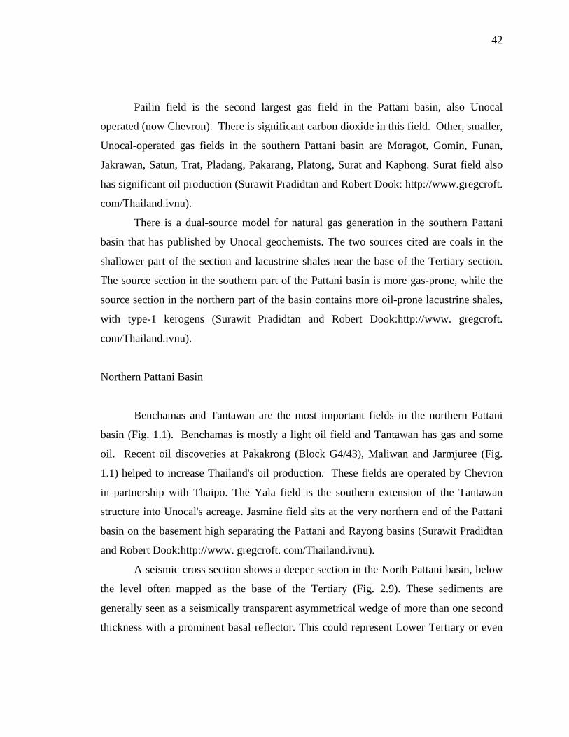
42
Pailin field is the second largest gas field in the Pattani basin, also Unocal
operated (now Chevron). There is significant carbon dioxide in this field. Other, smaller,
Unocal-operated gas fields in the southern Pattani basin are Moragot, Gomin, Funan,
Jakrawan, Satun, Trat, Pladang, Pakarang, Platong, Surat and Kaphong. Surat field also
has significant oil production (Surawit Pradidtan and Robert Dook: http://www.gregcroft.
com/Thailand.ivnu).
There is a dual-source model for natural gas generation in the southern Pattani
basin that has published by Unocal geochemists. The two sources cited are coals in the
shallower part of the section and lacustrine shales near the base of the Tertiary section.
The source section in the southern part of the Pattani basin is more gas-prone, while the
source section in the northern part of the basin contains more oil-prone lacustrine shales,
with type-1 kerogens (Surawit Pradidtan and Robert Dook:http://www. gregcroft.
com/Thailand.ivnu).
Northern Pattani Basin
Benchamas and Tantawan are the most important fields in the northern Pattani
basin (Fig. 1.1). Benchamas is mostly a light oil field and Tantawan has gas and some
oil. Recent oil discoveries at Pakakrong (Block G4/43), Maliwan and Jarmjuree (Fig.
1.1) helped to increase Thailand's oil production. These fields are operated by Chevron
in partnership with Thaipo. The Yala field is the southern extension of the Tantawan
structure into Unocal's acreage. Jasmine field sits at the very northern end of the Pattani
basin on the basement high separating the Pattani and Rayong basins (Surawit Pradidtan
and Robert Dook:http://www. gregcroft. com/Thailand.ivnu).
A seismic cross section shows a deeper section in the North Pattani basin, below
the level often mapped as the base of the Tertiary (Fig. 2.9). These sediments are
generally seen as a seismically transparent asymmetrical wedge of more than one second
thickness with a prominent basal reflector. This could represent Lower Tertiary or even

43
Mesozoic sediments that are the source of the oil in this part of the Pattani basin. This
graben trends north as far as the Jasmine field and dips eastward. Benchamas field is
characterized by a higher proportion of gas on the east flank of the structure, with more
liquids on the west flank. This distribution of hydrocarbons could be explained if the
liquids are being generated in the older graben fill (Surawit Pradidtan and Robert
Dook:http://www. gregcroft. com/Thailand.ivnu).
Post-rift faulting has compartmentalized the reservoirs, requiring a continuous in-
fill and exploration drilling program to maintain production levels. Successful
exploration for additional reserves in adjacent areas of the Gulf of Thailand requires a full
understanding of the regional petroleum systems (Teerman et al., 2000).
The main source rock area is in the deeper graben to the east of the fields, in the
Pattani trough. A regional decrease in thermal gradient from concession areas to the south
puts Benchamas and Tantawan (Block B8/32) in a favorable location for both gas and
liquid generation. Faulting strongly controls migration pathways and seals (Teerman et
al., 2000).
The interpretation of source rock occurrence is limited by the restricted
penetration of potential source rock intervals and lateral facies changes. Both oils and
condensates have variations in isotopic composition and their capillary gas
chromatography character, suggesting differences in source input. Characterization of
Type II and II/III kerogens by pyrolysis and organic petrology indicate the occurrence of
several different source facies and depositional environments (Teerman et al., 2000).
“New source rock data have been generated in collaboration with biostratigraphic
data, to understand the control of depositional environments on source rock distribution
and their age. This information is integrated with stratigraphic and depositional models
developed from wire line logs and 3-D seismic data to produce a predictive source facies
model and to define variations in organic facies. This source model is calibrated with
biomarker data.” (Teerman et al., 2000).

44
Chumpon Basin
There is only one oil field in Chumpon basin. It is called Nang Nuan. This field
produces light oil from vuggy carbonates along a pre-Tertiary ridge in the center of the
basin. This basin is known to have at least 3,280 ft (1 km) of source rock. The light (40°
API) oil produced from Nang Nuan demonstrates the thermal maturity of this source rock
(Surawit Pradidtan and Robert Dook: http://www.gregcroft. com/Thailand.ivnu).
Kra Basin
The Kra basin has over 3,937 ft (1.2 km) of excellent source rock, but oil
discoveries have yet to be made. There was one well that was drilled in this basin, the
B5/27-2. It has tested oil which may have come from Tertiary lacustrine carbonates,
rather than Paleozoic karstified limestones. Good sonic log porosity is displayed in the
reservoir interval in that well, which should not be the case for the Paleozoic. In Angola
(Malongo West and Limba fields) and Brazil's Campos basin (Badejo, Linguado and
Pampo fields), lacustrine carbonates associated with the initial opening of the South
Atlantic during the Cretaceous have produced hundreds of millions of barrels of oil.
These carbonates are coquina (skeletal grainstones) (Surawit Pradidtan and Robert Dook:
http://www.gregcroft. com/Thailand.ivnu).
Songkla Basin
There is no history of oil production in this basin but oil has been tested (Surawit
Pradidtan and Robert Dook: http://www.gregcroft. com/Thailand.ivnu).

45
Western Basin
There was one well that penetrated through a source-rock sequence and had oil
shows. Unfortunately, the well was lost before reaching its objective (Surawit Pradidtan
and Robert Dook: http://www.gregcroft. com/Thailand.ivnu).
Hua Hin Basin
The Hua Hin basin contains sub-basins. There was one well that was drilled in
the northern sub-basin but did not encounter source rock (Surawit Pradidtan and Robert
Dook: http://www.gregcroft. com/Thailand.ivnu).
Rayong Basin
There has been one well that was drilled in the Rayong basin but also did not
encounter source rock (Surawit Pradidtan and Robert Dook: http://www.gregcroft.
com/Thailand.ivnu).
2.3.2 Source-Rock Potential and Organic-Matter Characterization
“Organic carbon content ranged from 0.01 to 68.79 wt.% (Fig. 2.14). About a
quarter of the analyzed samples display above-average levels of organic enrichment
(TOC > 1.0 wt.%; Bissada, 1982). Above-average levels of organic enrichment are
considered one of the prerequisites for classification as a possible oil source rock. Source
rock thresholds as low as 0.5 wt.% TOC are, however, considered possible for gas-prone
systems (Rice and Claypool, 1981). An additional quarter of the population has organic
contents between 0.5 and 1.0 wt.%.” (Katz, 2002).

46
0 10 20 30 40 50 60 70 80Total Organic Carbon (wt.%)
0
50
100
150
200
500
1000
1500
2000N
umbe
r of O
bser
vatio
ns
Figure 2.14 Histogram shows organic carbon content. Data sources include Hydrocarbon Systems Associates, 1999, Core Laboratories, 1999, and the Chevron database. (From Katz, 2002).

47
CHAPTER 3
SEISMIC DATA ANALYSIS
3.1 Methods
The study interval is 104 to 272 msec (Fig. 3.2) from the available 3D seismic
data. The dimensions of 3D seismic data are 19 mi (31 km) in width, 44 mi (71 km) in
length, and 718 mi2 (1,860 km2) in area. There is no channel feature above 104 msec,
which is a muddy interval. Below 272 msec, it is hard to see any channel characteristics
because of poor seismic resolution.
Seismic data were displayed and interpreted using Seisworks 3D (Landmark) and
Gocad software. The approach to seismic interpretation emphasized the careful
integration of horizontal, map-view slices along with vertical seismic sections. Time
slices (with a constant value of two-way time) were generated in conventional, seismic-
amplitude volumes using Seisworks. Stratigraphy below the mud line to 300 msec in the
Gulf of Thailand is very flat, almost parallel to the sea floor. Channel features can be
seen clearly from time slices, slicing through seismic data every 4 msec. Horizon slices
were also generated and the results are very similar to the time slices because of the flat
stratigraphy in the Gulf of Thailand. However, there were some problems loading
horizon slices into Gocad because the size of the files was too large. The amplitude-
extraction maps from each picked horizon and EDGE data were also created, but they
had problems loading into Gocad. The amplitude-extraction maps turned out to be not as
good as the images from time slices. The EDGE data also failed to display any seismic
characteristics after being loaded into Gocad. Because of these reasons, I decided to

48
Figure 3.1 Time slice at 132 msec with digitized channel margins (color lines) and channel belt (black dashed lines) from Gocad. In order to obtain channel parameters for the whole channel from Gocad, margins need to be drawn continuously and extrapolated over the edge of the area as shown on the east side of the area for channel T3. Note that river systems run in various directions. The main paleocurrent direction is NW – SE. The N-S X-X’ line shows line 4200 for the cross section in Figure 3.2. See Figure 2.2 for the key UTM coordinates of this study area.

49
X X’
Horizon 1
Horizon 2
Horizon 3
Horizon 4
Horizon 5
msec (TWTT)
X X’
Horizon 1
Horizon 2
Horizon 3
Horizon 4
Horizon 5
msec (TWTT)
Figure 3.2 3D seismic cross section at line 4200 (X-X’), N-S orientation through the study area. The study interval ranges from 104 – 272 msec (TWTT) and there are 5 interpreted horizons. Location of this line is shown in Figure 3.1.
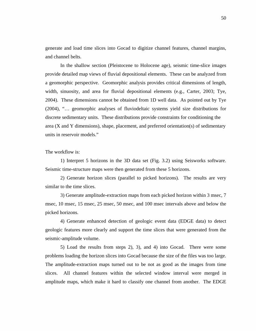
50
generate and load time slices into Gocad to digitize channel features, channel margins,
and channel belts.
In the shallow section (Pleistocene to Holocene age), seismic time-slice images
provide detailed map views of fluvial depositional elements. These can be analyzed from
a geomorphic perspective. Geomorphic analysis provides critical dimensions of length,
width, sinuosity, and area for fluvial depositional elements (e.g., Carter, 2003; Tye,
2004). These dimensions cannot be obtained from 1D well data. As pointed out by Tye
(2004), “… geomorphic analyses of fluviodeltaic systems yield size distributions for
discrete sedimentary units. These distributions provide constraints for conditioning the
area (X and Y dimensions), shape, placement, and preferred orientation(s) of sedimentary
units in reservoir models.”
The workflow is:
1) Interpret 5 horizons in the 3D data set (Fig. 3.2) using Seisworks software.
Seismic time-structure maps were then generated from these 5 horizons.
2) Generate horizon slices (parallel to picked horizons). The results are very
similar to the time slices.
3) Generate amplitude-extraction maps from each picked horizon within 3 msec, 7
msec, 10 msec, 15 msec, 25 msec, 50 msec, and 100 msec intervals above and below the
picked horizons.
4) Generate enhanced detection of geologic event data (EDGE data) to detect
geologic features more clearly and support the time slices that were generated from the
seismic-amplitude volume.
5) Load the results from steps 2), 3), and 4) into Gocad. There were some
problems loading the horizon slices into Gocad because the size of the files was too large.
The amplitude-extraction maps turned out to be not as good as the images from time
slices. All channel features within the selected window interval were merged in
amplitude maps, which make it hard to classify one channel from another. The EDGE
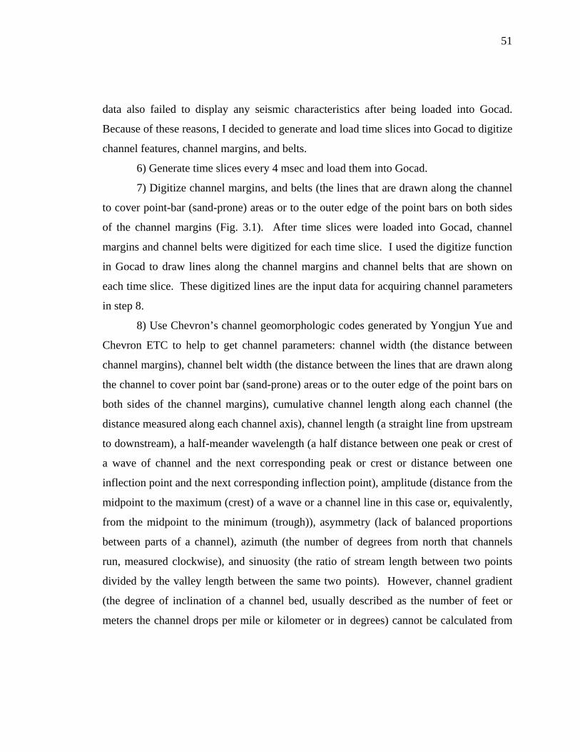
51
data also failed to display any seismic characteristics after being loaded into Gocad.
Because of these reasons, I decided to generate and load time slices into Gocad to digitize
channel features, channel margins, and belts.
6) Generate time slices every 4 msec and load them into Gocad.
7) Digitize channel margins, and belts (the lines that are drawn along the channel
to cover point-bar (sand-prone) areas or to the outer edge of the point bars on both sides
of the channel margins (Fig. 3.1). After time slices were loaded into Gocad, channel
margins and channel belts were digitized for each time slice. I used the digitize function
in Gocad to draw lines along the channel margins and channel belts that are shown on
each time slice. These digitized lines are the input data for acquiring channel parameters
in step 8.
8) Use Chevron’s channel geomorphologic codes generated by Yongjun Yue and
Chevron ETC to help to get channel parameters: channel width (the distance between
channel margins), channel belt width (the distance between the lines that are drawn along
the channel to cover point bar (sand-prone) areas or to the outer edge of the point bars on
both sides of the channel margins), cumulative channel length along each channel (the
distance measured along each channel axis), channel length (a straight line from upstream
to downstream), a half-meander wavelength (a half distance between one peak or crest of
a wave of channel and the next corresponding peak or crest or distance between one
inflection point and the next corresponding inflection point), amplitude (distance from the
midpoint to the maximum (crest) of a wave or a channel line in this case or, equivalently,
from the midpoint to the minimum (trough)), asymmetry (lack of balanced proportions
between parts of a channel), azimuth (the number of degrees from north that channels
run, measured clockwise), and sinuosity (the ratio of stream length between two points
divided by the valley length between the same two points). However, channel gradient
(the degree of inclination of a channel bed, usually described as the number of feet or
meters the channel drops per mile or kilometer or in degrees) cannot be calculated from

52
time slices because time slices represent seismic data at one time value (constant value of
two-way time).
9) Manually measure channel gradients from seismic cross sections. Cut cross
sections along each channel thalweg. Paleocurrent direction can also be confirmed from
cross sections of the channels. Get the depth of the upstream point and downstream point
(TWTT) of the same channel from the seismic cross sections. Then, convert the depth in
TWTT to one-way travel time (OWTT) by dividing by 2. Subtract downstream depth
(OWTT) from upstream depth (OWTT) to get the number of msec that the channel drops
from upstream to downstream. The definition of channel gradient is the degree of
inclination of a channel bed, usually described as the number of feet or meters the
channel drops per mile or kilometer or in degrees (http://en.wikipedia.org/wiki/
Stream_gradient). The channel-elevation drop in msec (OWTT) needs to be converted
into meters. Based on regional comparisons of the shallow seismic section in the Gulf of
Thailand, seismic velocities are estimated at 1,600 m/sec (Miall, 2000). Therefore, the
channel-elevation drop in msec is converted to meters by using this velocity. Measure
the distance in meters (straight distance) from the upstream point to the downstream
point. Then, divide the height of channel drop in meters by the distance from upstream to
downstream in meters to get the channel gradient. Gradient in degrees can also be
computed.
Channel gradient = Downstream depth (TWTT/2) – Upstream depth (TWTT/2) (msec)
Distance from Upstream to Downstream (meters)
Or = D
L
Channel gradient = OWTT (msec)
Distance from Upstream to Downstream (meters)

53
Because velocity is 1,600 m/sec,
1,000 msec = 1,600 meters
OWTT msec = OWTT msec * 1,600 meters
1,000 msec
= OWTT * 1.6 (meters)
Channel gradient = OWTT * 1.6 (meters)
Distance from Upstream to Downstream (meters)
Channel gradient = D = tan θ
L
Channel gradient (degree) (θ) = tan-1 D
L
The sea bottom, a horizontal line at the scale of this study, is used as the datum.
10) Manually measure the thickness of each channel from seismic cross sections.
Get the depth of the top and bottom of the channel (TWTT) at an upstream location and
downstream location. Convert TWTT to OWTT by dividing by 2. Subtract bottom depth
(OWTT) from top depth (OWTT) to get the thickness of the channel (msec). Then,
convert the thickness of the channel in msec to meters by using the same calculation as in
step 9) to get the thickness of the channel in meters. The thicknesses of channels for both
upstream and downstream locations are then averaged.
11) Manually measure point-bar sizes for each channel. Use SeisWorks to
measure the area of point-bars in square kilometers (km2) for each channel. These areas
are measured from time slices. Average point-bar size for each channel is used to
calculate average point-bar volume for that channel by multiplying average point-bar size
by channel thickness to get point-bar volume (km3 and acre feet).
12) Measure the orientation of faults from the sequence 4 horizon structure map
of the study area (Fig. 2.2) by drawing a line on top of each fault in Microsoft
PowerPoint. This line fits the fault orientation. Then, use “Format AutoShape” function

54
in Microsoft PowerPoint to measure the rotation degrees of that line from North, which is
the direction of fault orientation. This same method is used for the paleocurrent direction
measurement of each channel. The straight line is drawn from an upstream to a
downstream point to get the orientation of the paleocurrent direction. Channel gradient
calculations (Step 9) help determine which direction is upstream vs. downstream.
13) Plot all values in graphs and rose diagrams to get statistical relationships.
14) Make schematic cross sections for the 104 – 272 msec interval of the study
area to see how channels evolved through time.
3.2 Results
This section presents the results of the interpretation and analysis of fluvial
systems in the study area. The results are divided into sections for channel parameters,
channels variation through time (fluvial sequence-stratigraphic model), and statistical
relationships.
3.2.1 Channel Parameters
All channel parameters are shown in Table 3.1, Appendix B (CD-ROM), and C
(CD-ROM). This table shows recommended parameters that a modeler could use for
modeling fluvial systems that are similar to this study. It also shows that Pleistocene-
Holocene fluvial systems have a high variation of styles and dimensions. I would like to
acknowledge here that each channel interpreted in this study is a partial channel. Most of
them are truncated by the edges of the seismic volume. Therefore, some attributes, such
as length are partial measurements. Other attributes, such as sinuosity, gradient, etc are
valid even for partial channels measured here. Modelers should be aware of the
limitations of this dataset for certain parameters that are limited by the fixed area of the
seismic dataset.

55
Table 3.1 Table of channel parameters. 17x11 paper

56
3.2.2 Channels Variation Through Time (Fluvial Sequence Stratigraphic Model)
A succession of 43 time slices covers the entire study area from 104 msec to 272
msec (TWTT). Selected examples of time slices, with and without digitized channels, are
shown in Figures 3.3 to 3.12. Appendix A (CD-ROM) has all of the time slices. The
naming of channels that are interpreted on each time slice is not age related, nor does it
follow any specific order. I observed a total of 35 channel systems, of which 21 are
interpreted as incised fluvial systems and 14 are interpreted as unincised fluvial systems.
These time slices illustrate the geomorphologic evolution of the Pleistocene to Holocene
section beneath the Gulf of Thailand.
A block diagram of a high-sinuosity fluvial system, illustrating the facies
associations, channel belts and flood-plain subenvironments, is shown in Fig. 3.13. The
channel belt is confined within a raised alluvial ridge. The character of the channel fill
may be highly variable. Channels may migrate laterally to develop tabular to sheet-like
sand bodies separated by fine-grained overbank and flood-plain sediments, or deposition
may be confined by channel plugs, resulting in ribbon sand bodies. In these cases, the
width-to-depth ratios may be variable. The stacking patterns of channel sand bodies will
be affected significantly by rates of flood-plain subsidence (accommodation space)
(Emery and Myers, 2003).
Most of the channels that appear in the time slices in this study are similar to
modern rivers such as the Mississippi River. Figure 3.14 is a satellite image of the
Mississippi River that shows how a modern river looks compared to the channels in this
study.
Meander-neck cutoffs and point bars of channels can be seen clearly throughout
most of the time slices in this study. Figure 3.15 is an example of a meander-neck cutoff
and point bars that are seen from incised valleys. Scroll bars (ghosts of former channel
locations) (Elliott and Fullmer, 2004) provide internal architecture within point bars.
These scroll bars are arcuate bar-form deposits that are associated with meander-loop

57
Fig. 3.3 to 3.12

58

59

60

61

62

63

64

65

66

67
Figure 3.13 Block diagram of a high-sinuosity fluvial system illustrating the facies associations, channel belts and flood-plain subenvironments. The channel belt is confined within a raised alluvial ridge. The character of the channel-fill may be highly variable. Channels may migrate laterally to develop tabular to sheet-like sand bodies separated by fine-grained overbank and flood-plain sediments, or deposition may be confined by channel plugs, resulting in ribbon sand bodies. In these cases, the width-to-depth ratios may be variable. The stacking patterns of channel sand bodies will be affected significantly by rates of flood-plain subsidence (accommodation space). After Emery and Myers (2003).

68
Figu
re 3
.14
A sa
telli
te im
age
of th
e M
issi
ssip
pi R
iver
show
s mea
nder
ing
chan
nels
, mea
nder
-nec
k cu
toff
as l
abel
ed
by a
red
dash
ed c
ircle
, and
poi
nt b
ar a
s lab
eled
by
a ye
llow
das
hed
circ
le.
From
http
://m
aps.g
oogl
e.co
m/ .

69
Figu
re 3
.15
Tim
e sl
ices
at 1
60 m
sec
(TW
TT) (
on th
e le
ft ha
nd si
de) a
nd 1
20 m
sec
(TW
TT) (
on th
e rig
ht h
and
side
) sh
ow m
eand
er-n
eck
cuto
ffs,
as la
bele
d by
red
dash
ed c
ircle
s, an
d po
int b
ars a
s lab
eled
by
yello
w d
ashe
d ci
rcle
s in
in
cise
d va
lleys
, T3
(on
the
left
hand
side
) and
T1
(on
the
right
han
d si
de).
See
poi
nt-b
ar p
aram
eter
s in
Tabl
e 3.
1. T
he
gree
n ar
row
s ind
icat
e pa
leoc
urre
nt d
irect
ions
.
2,50
0 m

70
migration (Posamentier, 2001), or they are indications of channel growth via lateral
migrations (Fig. 3.16 to 3.19). The paleocurrent directions of channels can be told from
the truncation of point bars (Fig. 3.19).
Tributaries to incised valleys provide important evidence because they suggest
incision of the main incised valley when they terminate at the scarps (Figs. 3.21, 3.22,
and 3.23). These tributaries to incised valleys are bigger and deeper than common
tributaries that feed unincised fluvial channels. (Figs. 3.3 to 3.12 and Appendix A (CD-
ROM)).
Cross sections of channels have been made through the study interval (Figs. 3.24
to 3.33). These cross sections illustrate internal architectures of both incised and
unincised fluvial channels and their vertical successions through time.
Figure 3.34 shows the evolution of an incised-valley fill from the time of
maximum sea-level lowstand. This is characterized by fluvial deposition through the
time of rapid transgression with filling by traction and hemipelagic sedimentation.
Finally, the time of sea-level highstand and deposition of hemipelagic drape over the
entire area.
Schematic cross sections from 0 to 300 msec (TWTT) through NS and EW
directions of the study area show channels and sequence boundaries (Figs. 3.36 to 3.40)
within the study interval. Six sequence boundaries are interpreted in this study interval at
the base of 6 major incised valley systems. Tributaries provide the most clearly defined
evidence for the existence of incised valleys. They suggest incision of the main incised
valley when they terminate at the scarps. These tributaries to incised valleys are also
bigger and deeper than common tributaries that feed unincised fluvial channels.
Tributaries cannot commonly be recognized in fluvial systems because of the
discontinuous nature of most forms of data other than 3-D seismic data. Channels that
are neither incised valleys nor tributaries to incised valleys are classified as unincised
fluvial channels. They may be straight (sinuosity=1.00-1.10) channels, low-sinuosity
(sinuosity=1.11-1.21) channels, medium-sinuosity (sinuosity=1.22-1.83) channels, or

71
Figu
re 3
.16
A p
rese
nt m
eand
erin
g ch
anne
l in
Edm
onto
n, C
anad
a, sh
ows s
crol
l bar
s (th
e da
shed
lin
es) w
ithin
eac
h po
int b
ar.
Afte
r Elli
son
(200
4).

72
Figu
re 3
.17
Tim
e sl
ices
at 1
16 m
sec
(TW
TT) (
on th
e le
ft ha
nd si
de) a
nd 1
12 m
sec
(TW
TT) (
on th
e rig
ht
hand
side
) sho
w sc
roll
bars
with
in e
ach
poin
t bar
. Th
e gr
een
arro
ws i
ndic
ate
pale
ocur
rent
dire
ctio
ns.

73
Figu
re 3
.18
Tim
e sl
ices
at 1
56 m
sec
(TW
TT)
show
uni
nter
pret
ed im
age
with
gre
en d
ashe
d ar
row
s whi
ch sh
ow
ghos
ts o
f for
mer
cha
nnel
loca
tions
(on
the
left
hand
side
) and
inte
rpre
tatio
n of
the
grow
th o
f mea
nder
loop
s via
late
ral
mig
ratio
n of
T3
inci
sed
valle
y (o
n th
e rig
ht h
and
side
). N
umbe
rs 1
, 2, 3
, and
4, a
s lab
eled
on
the
right
pic
ture
, re
pres
ent t
imes
of m
igra
tion.
1 re
pres
ents
the
olde
st ti
me
and
4 re
pres
ents
the
youn
gest
tim
e. T
he g
reen
-fill
ed a
rrow
s in
dica
te p
aleo
curr
ent d
irect
ions
.
12
34
12
34
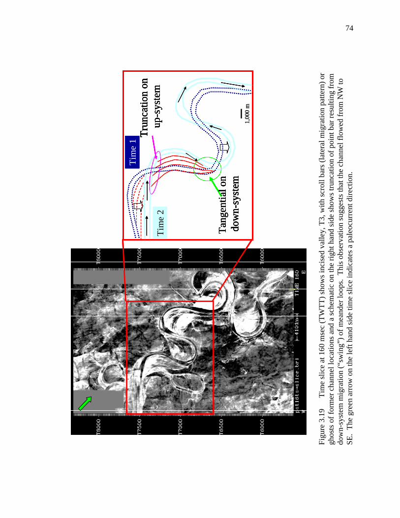
74
Tim
e 1
Tim
e 2
Trun
catio
n on
up
-sys
tem
Tang
entia
l on
dow
n-sy
stem
1,00
0 m
Tim
e 1
Tim
e 2
Trun
catio
n on
up
-sys
tem
Tang
entia
l on
dow
n-sy
stem
Tim
e 1
Tim
e 2
Trun
catio
n on
up
-sys
tem
Tang
entia
l on
dow
n-sy
stem
Tim
e 1
Tim
e 2
Trun
catio
n on
up
-sys
tem
Tang
entia
l on
dow
n-sy
stem
1,00
0 m
Figu
re 3
.19
Tim
e sl
ice
at 1
60 m
sec
(TW
TT) s
how
s inc
ised
val
ley,
T3,
with
scro
ll ba
rs (l
ater
al m
igra
tion
patte
rn) o
r gh
osts
of f
orm
er c
hann
el lo
catio
ns a
nd a
sche
mat
ic o
n th
e rig
ht h
and
side
show
s tru
ncat
ion
of p
oint
bar
resu
lting
from
do
wn-
syst
em m
igra
tion
(“sw
ing”
) of m
eand
er lo
ops.
Thi
s obs
erva
tion
sugg
ests
that
the
chan
nel f
low
ed fr
om N
W to
SE
. Th
e gr
een
arro
w o
n th
e le
ft ha
nd si
de ti
me
slic
e in
dica
tes a
pal
eocu
rren
t dire
ctio
n.

75
Figu
re 3
.20
Tim
e sl
ice
at 1
60 m
sec
(TW
TT) s
how
s poi
nt b
ars,
each
of t
hem
cov
erin
g ab
out 4
mi2
(10
km2 ).
San
d bo
dy m
ay b
e co
mpa
rtmen
taliz
ed b
y m
ud d
rape
s bet
wee
n ac
cret
ion
sets
, as l
abel
ed b
y th
e br
own
dash
ed li
nes.
The
gr
een
arro
ws i
ndic
ate
pale
ocur
rent
dire
ctio
ns.
(Mod
ified
from
Elli
ott a
nd F
ullm
er, 2
004)
.

76
AA
’
A
A’
100
200
AA
’
A
A’
A
A’
100
200
Figu
re 3
.21
Tim
e sl
ice
at 1
12 m
sec
(TW
TT) (
on th
e le
ft) sh
ows t
he lo
catio
n of
an
A-A
’ cro
ss se
ctio
n w
hich
is sh
own
on th
e rig
ht h
and
side
. A
n in
cise
d va
lley
and
tribu
tarie
s to
inci
sed
valle
y ar
e la
bele
d in
yel
low
and
blu
e ci
rcle
s,
resp
ectiv
ely.
Trib
utar
ies s
ugge
st in
cisi
on o
f the
mai
n va
lley
as la
bele
d in
a y
ello
w c
ircle
. Th
is is
the
youn
gest
le
vel o
f inc
isio
n in
the
stud
y ar
ea.
Mos
t trib
utar
ies t
o in
cise
d va
lleys
ent
er fr
om th
e ea
st, s
ugge
stin
g te
cton
ic ti
lting
.
The
gree
n ar
row
indi
cate
s a p
aleo
curr
ent d
irect
ion.
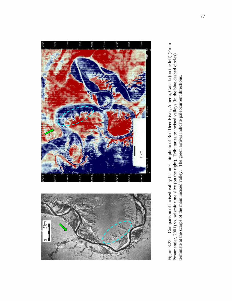
77
1 km
1 km
1 km
Figu
re 3
.22
Com
paris
on o
f inc
ised
-val
ley
feat
ures
: air
phot
o of
Red
Dee
r Riv
er, A
lber
ta, C
anad
a (o
n th
e le
ft) (F
rom
Po
sam
entie
r, 20
01) v
s. se
ism
ic ti
me
slic
e (o
n th
e rig
ht).
Trib
utar
ies t
o in
cise
d va
lleys
(in
the
blue
das
hed
circ
les)
te
rmin
ate
at th
e sc
arps
of t
he m
ain
inci
sed
valle
y.
The
gree
n ar
row
s ind
icat
e pa
leoc
urre
nt d
irect
ions
.

78
Figu
re 3
.23
Com
paris
on o
f inc
ised
-val
ley
feat
ures
: sei
smic
tim
e sl
ice
at 1
12 m
sec
(TW
TT) (
A) s
how
s trib
utar
ies
to in
cise
d va
lley
(in th
e bl
ue d
ashe
d ci
rcle
) vs.
pres
ent i
ncis
ed v
alle
ys a
nd tr
ibut
arie
s to
inci
sed
valle
ys (i
n th
e bl
ue
dash
ed c
ircle
s) in
(C),
(D),
and
(E) p
hoto
s. T
hese
pho
tos w
ere
take
n on
Los
Ang
eles
to D
enve
r flig
ht, 2
006.
Th
e m
ap
that
show
s the
flig
ht ro
ute
is sh
own
in (B
). T
he g
reen
arr
ow in
dica
tes a
pal
eocu
rren
t dire
ctio
n.
NW
112
mse
c
5 km
.
NN
W
NW
N
(A)
(B)
(C)
(D)
(E)
N
NW
112
mse
c
5 km
.
NN
W
NW
N
(A)
(B)
(C)
(D)
(E)
N

79
Figu
re 3
.24
Tim
e sl
ice
at 2
72 m
sec
(TW
TT) (
on th
e le
ft ha
nd si
de) s
how
s cha
nnel
s and
cro
ss se
ctio
n lo
catio
ns, A
- A
’ and
B-B
’. O
n th
e rig
ht h
and
side
, A-A
’ sho
ws
a cr
oss
sect
ion
of in
cise
d va
lleys
, T17
and
T15
and
B-B
’ sho
ws
a cr
oss s
ectio
n of
a m
ediu
m-s
inuo
sity
cha
nnel
, T11
, and
a st
raig
ht c
hann
el, T
13.
Alth
ough
bot
h ch
anne
ls a
re im
aged
at
the
sam
e tim
e sl
ice,
they
cro
sscu
t eac
h ot
her a
nd a
re n
ot e
xact
ly th
e sa
me
age,
as s
how
n in
the
B-B
’ cro
ss se
ctio
n.

80
Figu
re 3
.25
Tim
e sl
ice
at 2
44 m
sec
(TW
TT) (
on th
e le
ft ha
nd si
de) s
how
s cha
nnel
s and
a c
ross
sect
ion
loca
tion,
C-
C’.
On
the
right
han
d si
de, C
-C’ s
how
s a c
ross
sect
ion
of a
low
-sin
uosi
ty c
hann
el, T
8.

81
Figu
re 3
.26
Tim
e sl
ice
at 2
28 m
sec
(TW
TT) (
on th
e le
ft ha
nd s
ide)
sho
ws
chan
nels
and
cro
ss s
ectio
n lo
catio
ns, D
-D
’ an
d E
-E’.
On
the
right
han
d si
de, D
-D’
show
s a
cros
s se
ctio
n of
inci
sed
valle
ys, T
17, T
15, T
6 an
d T2
9.
E-E’
sh
ows
a cr
oss
sect
ion
of a
n in
cise
d va
lley,
T5,
a tr
ibut
ary
to a
n in
cise
d va
lley
(T5)
in b
lue,
and
a s
traig
ht c
hann
el,
T12.

82
Figu
re 3
.27
Tim
e sl
ice
at 2
28 m
sec
(TW
TT) (
on th
e le
ft ha
nd s
ide)
sho
ws
T17,
T15
, and
T6
inci
sed
valle
ys a
nd a
cr
oss
sect
ion
loca
tion,
DD
-DD
’. O
n th
e rig
ht h
and
side
, DD
-DD
’ sho
ws
a cr
oss
sect
ion
of in
cise
d va
lleys
, T17
, T15
, an
d T6
. T1
7 is
the
olde
st in
cise
d va
lley
and
T6 is
the
youn
gest
inci
sed
valle
y. C
ross
-cut
ting
occu
rs in
that
the
poin
t ba
r of T
17 w
as p
artly
rem
oved
by
a la
ter T
15 c
hann
el, a
s sho
wn
in re
d an
d ye
llow
fill
abov
e, re
spec
tivel
y.
DD
’
DD
T6
T17
T15
DD
DD
’
T6
T17T15
Aba
ndon
ed (m
ud-p
lugg
ed?)
cha
nnel
s
Val
ley
wal
l
Bas
al sc
our
DD
’
DD
T6
T17
T15
DD
DD
’
T6
T17T15
Aba
ndon
ed (m
ud-p
lugg
ed?)
cha
nnel
s
Val
ley
wal
l
Bas
al sc
our

83
Figu
re 3
.28
Tim
e sl
ice
at 2
28 m
sec
(TW
TT) (
on th
e le
ft ha
nd s
ide)
sho
ws
an in
cise
d va
lley,
T6
and
a cr
oss
sect
ion
loca
tion,
EE-
EE’.
On
the
right
han
d si
de, E
E-EE
’ sh
ows
a cr
oss
sect
ion
of a
n un
inte
rpre
ted
imag
e (o
n to
p) a
nd a
n in
terp
rete
d im
age
(at
the
botto
m).
Val
ley
wal
l an
d ab
ando
ned
chan
nel
are
labe
led
in w
hite
and
blu
e ci
rcle
s, re
spec
tivel
y.
Bas
e of
inci
sed
valle
y (b
asal
sco
ur)
is la
bele
d by
a b
lack
das
hed
line.
La
tera
l-acc
retio
n su
rfac
es d
ip
tow
ard
the
aban
done
d ch
anne
l, as
labe
led
by g
reen
arr
ows.
EEE
E’
T6
Late
ral a
ccre
tions
dip
tow
ard
the
chan
nel
EE
EE
’
Bas
e of
inci
sed
valle
y (b
asal
scou
r)
EE
EE
’
EEE
E’
T6
EEE
E’
T6
Late
ral a
ccre
tions
dip
tow
ard
the
chan
nel
EE
EE
’
Bas
e of
inci
sed
valle
y (b
asal
scou
r)
EE
EE
’

84
Figu
re 3
.29
Tim
e sl
ice
at 1
92 m
sec
(TW
TT) (
on th
e le
ft ha
nd s
ide)
sho
ws
chan
nels
and
cro
ss s
ectio
n lo
catio
ns, F
-F’
, G-G
’, H
-H’,
and
I-I’
. O
n th
e rig
ht h
and
side
, F-F
’ sho
ws
a cr
oss
sect
ion
of a
nec
k cu
toff
lobe
of T
5, a
n in
cise
d va
lley,
and
its
late
ral a
ccre
tion
feat
ures
(sc
roll
bars
) w
ithin
the
poin
t bar
, as
labe
led
by th
e da
shed
arr
ows.
The
se
accr
etio
n se
ts d
ip to
war
ds th
e ch
anne
l.

85
Figu
re 3
.30
Tim
e sl
ice
at 1
92 m
sec
(TW
TT) (
on th
e le
ft ha
nd s
ide)
sho
ws
chan
nels
and
cro
ss s
ectio
n lo
catio
ns, F
-F’
, G-G
’, H
-H’,
and
I-I’
. O
n th
e rig
ht h
and
side
, G-G
’, H
-H’,
and
I-I’
show
cro
ss se
ctio
ns o
f an
inci
sed
valle
y, T
6.

86
Figu
re 3
.31
Tim
e sl
ice
at 1
72 m
sec
(TW
TT) (
on th
e le
ft ha
nd s
ide)
sho
ws
chan
nels
and
a c
ross
sec
tion
loca
tion,
J-
J’.
On
the
right
han
d si
de, J
-J’ s
how
s a
cros
s se
ctio
n of
an
inci
sed
valle
y, T
4, w
ith a
poi
nt b
ar a
ttach
ed to
it o
n th
e rig
ht.

87
Figu
re 3
.32
Tim
e sl
ice
at 1
36 m
sec
(TW
TT) (
on th
e le
ft ha
nd si
de) s
how
s cha
nnel
s and
cro
ss se
ctio
n lo
catio
ns, K
-K’
and
L-L’
. O
n th
e rig
ht h
and
side
, K-K
’ sho
ws a
cro
ss se
ctio
n of
a m
ediu
m-s
inuo
sity
cha
nnel
, T2
and
a tri
buta
ry to
an
inci
sed
valle
y, T
23.
L-L’
show
s a c
ross
sect
ion
of a
hig
h-si
nuos
ity c
hann
el, T
2_3.
LL
’
T2_3
T23
T2
KK
’
LL
’
T2_3
LL
’
T2_3
T23
T2
KK
’
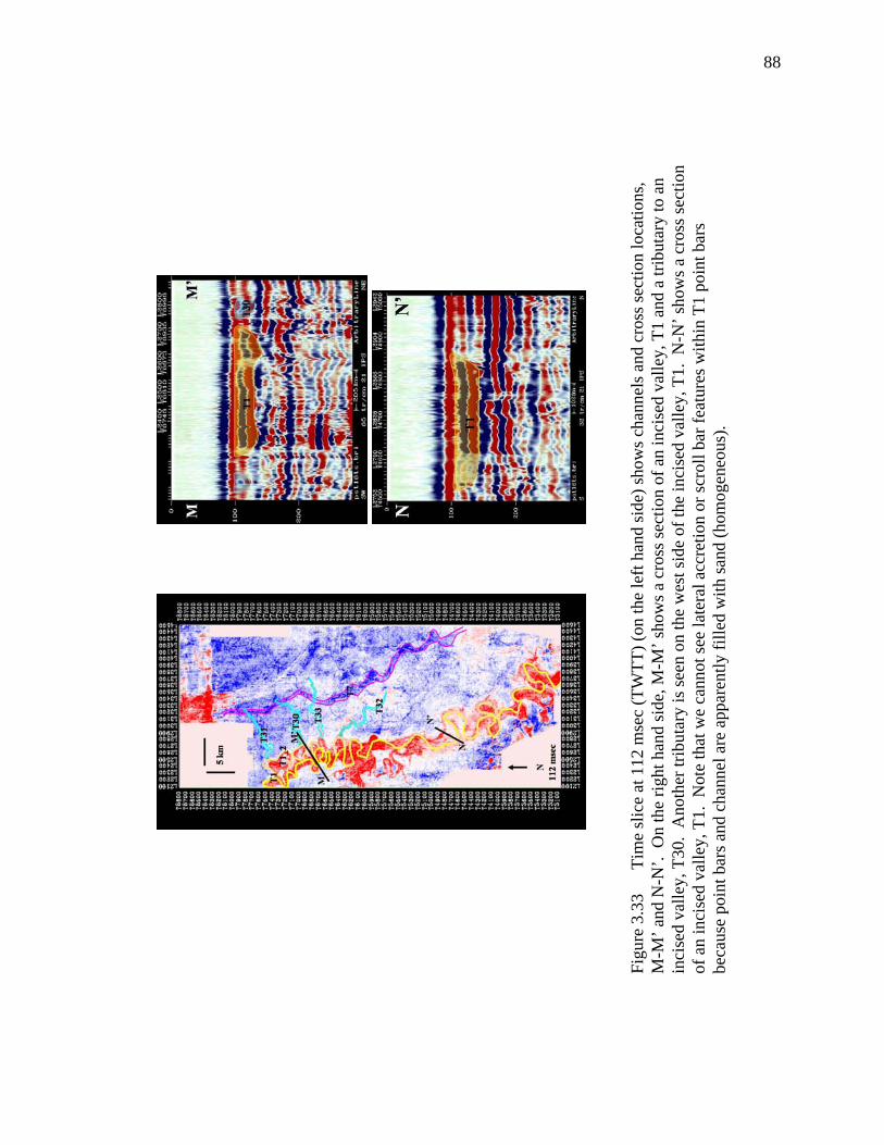
88
Figu
re 3
.33
Tim
e sl
ice
at 1
12 m
sec
(TW
TT) (
on th
e le
ft ha
nd si
de) s
how
s cha
nnel
s and
cro
ss se
ctio
n lo
catio
ns,
M-M
’ and
N-N
’. O
n th
e rig
ht h
and
side
, M-M
’ sho
ws a
cro
ss se
ctio
n of
an
inci
sed
valle
y, T
1 an
d a
tribu
tary
to a
n
inci
sed
valle
y, T
30.
Ano
ther
trib
utar
y is
seen
on
the
wes
t sid
e of
the
inci
sed
valle
y, T
1. N
-N’ s
how
s a c
ross
sect
ion
of
an
inci
sed
valle
y, T
1. N
ote
that
we
cann
ot se
e la
tera
l acc
retio
n or
scro
ll ba
r fea
ture
s with
in T
1 po
int b
ars
beca
use
poin
t bar
s and
cha
nnel
are
app
aren
tly fi
lled
with
sand
(hom
ogen
eous
).

89
Figu
re 3
.34
The
evol
utio
n of
inci
sed
valle
y fil
l fro
m th
e tim
e of
max
imum
sea-
leve
l low
stan
d, c
hara
cter
ized
by
flu
vial
dep
ositi
on (
A)
thro
ugh
the
time
of r
apid
tran
sgre
ssio
n an
d fil
ling
by tr
actio
n an
d he
mip
elag
ic s
edim
enta
tion,
an
d fin
ally
the
tim
e of
sea
-leve
l hi
ghst
and
and
depo
sitio
n of
hem
ipel
agic
dra
pe o
ver
the
entir
e ar
ea (
B).
Afte
r Po
sam
entie
r (20
01).

90
Figure 3.35 Time slice at 104 msec (TWTT) shows locations of cross sections, A-A’, B-B’, C-C’, D-D’, and E-E’ in Figures 3.36, 3.37, 3.38, 3.39, and 3.40, respectively.

91
Figu
re 3
.36
Sche
mat
ic c
ross
sect
ion
of li
ne A
-A’ f
rom
0 to
300
mse
c (T
WTT
) sho
ws c
hann
els a
nd se
quen
ce
boun
darie
s in
the
stud
y ar
ea.
The
diag
onal
line
s in
chan
nels
are
sche
mat
ic la
tera
l acc
retio
n su
rfac
es.
See
the
cros
s se
ctio
n lo
catio
n in
Fig
ure
3.35
.
300
T15
300
T19
T21
T12
T11
T8
T27
T32
T33
T30
T31
T1
T1
T1
T3
T4
T5
T29
T6
T17
SB 6
SB 5
SB 3
SB 4
SB 2
SB 1
Inci
sed
valle
ys
Low
-sin
uosi
ty c
hann
els (
1.1
-1.2
1 si
nuos
ity)
Med
ium
-sin
uosi
ty c
hann
els (
1.22
–1.
83 si
nuos
ity)
Hig
h-si
nuos
ity c
hann
els (
1.84
–2.
44 si
nuos
ity)
Stra
ight
cha
nnel
s
Trib
utar
ies t
o in
cise
d va
lleys
LE
GE
ND
SB =
Seq
uenc
e B
ound
ary
AA
’
300
T15
T19
T21
T12
T11
T8
T27
T32
T33
T30
T31
T1
T1
T1
T3
T4
T5
T29
T6
T17
SB 6
SB 5
SB 3
SB 4
SB 2
SB 1
5 km
300
T15
TWTT (msec)
T19
T21
T12
T11
T8
T27
T32
T33
T30
T31
T1
T1
T1
T3
T4
T5
T29
T6
T17
SB 6
SB 5
SB 3
SB 4
SB 2
SB 1
200
200
200
100
100
100
100
100
100
200
200
200
300
T15
300
T19
T21
T12
T11
T8
T27
T32
T33
T30
T31
T1
T1
T1
T3
T4
T5
T29
T6
T17
SB 6
SB 5
SB 3
SB 4
SB 2
SB 1
Inci
sed
valle
ys
Low
-sin
uosi
ty c
hann
els (
1.1
-1.2
1 si
nuos
ity)
Med
ium
-sin
uosi
ty c
hann
els (
1.22
–1.
83 si
nuos
ity)
Hig
h-si
nuos
ity c
hann
els (
1.84
–2.
44 si
nuos
ity)
Stra
ight
cha
nnel
s
Trib
utar
ies t
o in
cise
d va
lleys
LE
GE
ND
SB =
Seq
uenc
e B
ound
ary
AA
’
300
T15
T19
T21
T12
T11
T8
T27
T32
T33
T30
T31
T1
T1
T1
T3
T4
T5
T29
T6
T17
SB 6
SB 5
SB 3
SB 4
SB 2
SB 1
5 km
300
T15
TWTT (msec)
T19
T21
T12
T11
T8
T27
T32
T33
T30
T31
T1
T1
T1
T3
T4
T5
T29
T6
T17
SB 6
SB 5
SB 3
SB 4
SB 2
SB 1
200
200
200
100
100
100
100
100
100
200
200
200

92
Figu
re 3
.37
Sche
mat
ic c
ross
sect
ion
of li
ne B
-B’ f
rom
0 to
300
mse
c (T
WTT
) sho
ws c
hann
els a
nd se
quen
ce
boun
darie
s in
the
stud
y ar
ea. T
he d
iago
nal l
ines
in c
hann
els a
re sc
hem
atic
late
ral a
ccre
tion
surf
aces
. Se
e th
e cr
oss
sect
ion
loca
tion
in F
igur
e 3.
35.
Inci
sed
valle
ys
Low
-sin
uosi
ty c
hann
els (
1.1
-1.2
1 si
nuos
ity)
Med
ium
-sin
uosi
ty c
hann
els (
1.22
–1.
83 si
nuos
ity)
Hig
h-si
nuos
ity c
hann
els (
1.84
–2.
44 si
nuos
ity)
Stra
ight
cha
nnel
s
Trib
utar
ies t
o in
cise
d va
lleys
LE
GE
ND
SB =
Seq
uenc
e B
ound
ary
5 km
100
200
300
T2_
3
T18
TWTT (msec)
100
300
T1
T4
200
T11
T12
SB 6
SB 5 SB
2SB
1
SB 4
SB 3
T9
T29
T6
T24
T14
T1
T23
T2
T33
T2_
2T
2
T16
T28
T28
T29
T17
T15
T19
T3
T3
T8
T5
T5
B’
B
Inci
sed
valle
ys
Low
-sin
uosi
ty c
hann
els (
1.1
-1.2
1 si
nuos
ity)
Med
ium
-sin
uosi
ty c
hann
els (
1.22
–1.
83 si
nuos
ity)
Hig
h-si
nuos
ity c
hann
els (
1.84
–2.
44 si
nuos
ity)
Stra
ight
cha
nnel
s
Trib
utar
ies t
o in
cise
d va
lleys
LE
GE
ND
SB =
Seq
uenc
e B
ound
ary
5 km
Inci
sed
valle
ys
Low
-sin
uosi
ty c
hann
els (
1.1
-1.2
1 si
nuos
ity)
Med
ium
-sin
uosi
ty c
hann
els (
1.22
–1.
83 si
nuos
ity)
Hig
h-si
nuos
ity c
hann
els (
1.84
–2.
44 si
nuos
ity)
Stra
ight
cha
nnel
s
Trib
utar
ies t
o in
cise
d va
lleys
LE
GE
ND
SB =
Seq
uenc
e B
ound
ary
5 km
100
200
300
T2_
3
T18
TWTT (msec)
100
300
T1
T4
200
T11
T12
SB 6
SB 5 SB
2SB
1
SB 4
SB 3
T9
T29
T6
T24
T14
T1
T23
T2
T33
T2_
2T
2
T16
T28
T28
T29
T17
T15
T19
T3
T3
T8
T5
T5
B’
B

93
100
TWTT (msec)
T15
T17
T28
200
300
1000
T1_
2T
1T
3T
2
T29
T6
SB 4
SB 3 SB
1
SB 5
CC
’
T2_
2
SB 2
SB 6
5 km Inci
sed
valle
ys
Low
-sin
uosit
y ch
anne
ls (1
.1 -
1.21
sin
uosit
y)
Med
ium
-sin
uosit
y ch
anne
ls (1
.22
–1.
83 si
nuos
ity)
Hig
h-si
nuos
ity c
hann
els (
1.84
–2.
44 si
nuos
ity)
Stra
ight
cha
nnel
s
Trib
utar
ies t
o in
cise
d va
lleys
LE
GE
ND
SB =
Seq
uenc
e B
ound
ary
5 km Inci
sed
valle
ys
Low
-sin
uosit
y ch
anne
ls (1
.1 -
1.21
sin
uosit
y)
Med
ium
-sin
uosit
y ch
anne
ls (1
.22
–1.
83 si
nuos
ity)
Hig
h-si
nuos
ity c
hann
els (
1.84
–2.
44 si
nuos
ity)
Stra
ight
cha
nnel
s
Trib
utar
ies t
o in
cise
d va
lleys
LE
GE
ND
SB =
Seq
uenc
e B
ound
ary
Figu
re 3
.38
Sche
mat
ic c
ross
sect
ion
of li
ne C
-C’ f
rom
0 to
300
mse
c (T
WTT
) sho
ws c
hann
els a
nd se
quen
ce
boun
darie
s in
the
stud
y ar
ea.
The
diag
onal
line
s in
chan
nels
are
sche
mat
ic la
tera
l acc
retio
n su
rfac
es.
See
the
cros
s se
ctio
n lo
catio
n in
Fig
ure
3.35
.

94
Figu
re 3
.39
Sche
mat
ic c
ross
sect
ion
of li
ne D
-D’ f
rom
0 to
300
mse
c (T
WTT
) sho
ws c
hann
els a
nd se
quen
ce
boun
darie
s in
the
stud
y ar
ea.
The
diag
onal
line
s in
chan
nels
are
sche
mat
ic la
tera
l acc
retio
n su
rfac
es.
See
the
cros
s se
ctio
n lo
catio
n in
Fig
ure
3.35
.
100
200
300
T27
T22
T20
T29
T8
TWTT (msec)
SB 6 SB
5SB
3SB
2 SB 1
0
T3
T2
T6
SB 4
T1
T19
100
200
300
T22
T29
T8
SB 6 SB
5SB
3SB
2 SB 1
T3
T2
T6
SB 4
T1
T19
100
200
300
T27
T22
T29
T8
SB 6 SB
5SB
3SB
2 SB 1
T3
T2
T6
SB 4
T1
T19
5 km
Inci
sed
valle
ys
Low
-sin
uosi
ty c
hann
els (
1.1
-1.2
1 si
nuos
ity)
Med
ium
-sin
uosi
ty c
hann
els (
1.22
–1.
83 si
nuos
ity)
Hig
h-si
nuos
ity c
hann
els (
1.84
–2.
44 si
nuos
ity)
Stra
ight
cha
nnel
s
Trib
utar
ies t
o in
cise
d va
lleys
LE
GE
ND
SB =
Seq
uenc
e B
ound
ary
DD
’
T27
T20
T20
100
200
300
T27
T22
T20
T29
T8
TWTT (msec)
SB 6 SB
5SB
3SB
2 SB 1
0
T3
T2
T6
SB 4
T1
T19
100
200
300
T27
T22
T20
T29
T8
TWTT (msec)
SB 6 SB
5SB
3SB
2 SB 1
0
T3
T2
T6
SB 4
T1
T19
100
200
300
T22
T29
T8
SB 6 SB
5SB
3SB
2 SB 1
T3
T2
T6
SB 4
T1
T19
100
200
300
T27
T22
T29
T8
SB 6 SB
5SB
3SB
2 SB 1
T3
T2
T6
SB 4
T1
T19
5 km
Inci
sed
valle
ys
Low
-sin
uosi
ty c
hann
els (
1.1
-1.2
1 si
nuos
ity)
Med
ium
-sin
uosi
ty c
hann
els (
1.22
–1.
83 si
nuos
ity)
Hig
h-si
nuos
ity c
hann
els (
1.84
–2.
44 si
nuos
ity)
Stra
ight
cha
nnel
s
Trib
utar
ies t
o in
cise
d va
lleys
LE
GE
ND
SB =
Seq
uenc
e B
ound
ary
DD
’
T27
T20
T20

95
Figu
re 3
.40
Sche
mat
ic c
ross
sect
ion
of li
ne E
-E’ f
rom
0 to
300
mse
c (T
WTT
) sho
ws c
hann
els a
nd se
quen
ce
boun
darie
s in
the
stud
y ar
ea. T
he d
iago
nal l
ines
in c
hann
els a
re sc
hem
atic
late
ral a
ccre
tion
surf
aces
. Se
e th
e cr
oss
sect
ion
loca
tion
in F
igur
e 3.
35.
100
200
300
T2
T13
TWTT (msec)
0
SB 6
SB 5
SB 2
SB 1
SB 4
SB 3
T5
T1
T25
T23
EE
’
5 km Inci
sed
valle
ys
Low
-sin
uosi
ty c
hann
els (
1.1
-1.2
1 si
nuos
ity)
Med
ium
-sin
uosi
ty c
hann
els (
1.22
–1.
83 si
nuos
ity)
Hig
h-si
nuos
ity c
hann
els (
1.84
–2.
44 si
nuos
ity)
Stra
ight
cha
nnel
s
Trib
utar
ies t
o in
cise
d va
lleys
LE
GE
ND
SB =
Seq
uenc
e B
ound
ary
5 km Inci
sed
valle
ys
Low
-sin
uosi
ty c
hann
els (
1.1
-1.2
1 si
nuos
ity)
Med
ium
-sin
uosi
ty c
hann
els (
1.22
–1.
83 si
nuos
ity)
Hig
h-si
nuos
ity c
hann
els (
1.84
–2.
44 si
nuos
ity)
Stra
ight
cha
nnel
s
Trib
utar
ies t
o in
cise
d va
lleys
LE
GE
ND
SB =
Seq
uenc
e B
ound
ary

96
high-sinuosity (sinuosity=1.84-2.44) channels. These channels are different from
incised-valley channels because they do not have tributaries associated with them. They
are also smaller in size, and it is hard to see point bars and other internal architecture with
this seismic resolution. Their thicknesses are significantly less than in the incised-valley
systems.
3.2.3 Statistical Relationships
All values derived from the measurements are plotted as frequency histograms,
cross plots, and rose diagrams to get statistical relationships (Figs. 3.41 to 3.111). These
values are channel width (the distance between channel margins), channel belt width (the
distance between the lines that are drawn along the channel to cover point bar (sand-
prone) areas or to the outer edge of the point bars on both sides of the channel margins),
cumulative channel length along each channel (the distance measured along each channel
axis), channel length (a straight line from upstream to downstream), half-meander
wavelength (a half distance between one peak or crest, of a wave of channel and the next
corresponding peak or crest or distance between one inflection point and the next
corresponding inflection point), amplitude (distance from the midpoint to the crest or
trough of a wave, or a channel line), asymmetry (absence of balanced proportions
between parts of a channel), azimuth (the number of degrees from north that channels
run, measured clockwise), sinuosity (the ratio of stream length between two points
divided by the valley length between the same two points), point-bar sizes (the areas of
point bars in square kilometers (km2)) and volumes (average point-bar size multiply by
channel thickness (km3 and acre feet)), channel gradient (the degree of inclination of a
channel bed, usually described as the number of feet or meters the channel drops per mile
or kilometer or in degrees), the thickness of each channel, width/thickness aspect ratio,
and paleocurrent directions.

97
Figure 3.41 Frequency histogram shows the distribution of all channel thicknesses (m). N = 35, mean value = 19 m, mode = 18 m, and skewness = 0.96.
Figure 3.42 Frequency histogram shows the distribution of unincised fluvial channel thicknesses (m). N = 13, mean value = 17 m, mode = 17 m, and skewness = -0.25. See Appendix G for the level of confident of thickness data between incised and unicised fluvial systems.
Frequency
Thickness (m)
Frequency
Thickness (m)

98
Figure 3.43 Frequency histogram shows the distribution of incised fluvial channel thicknesses (m). N = 22, mean value = 21 m, mode = 25 m, and skewness = 0.72. See Appendix G for the level of confident of thickness data between incised and unicised fluvial systems.
Figure 3.44 Frequency histogram shows the distribution of channel width (m) of all channels. N = 36, mean value = 428 m, mode = 350 m, and skewness = 1.9.
Frequency
Frequency
Thickness (m)
Width (m)

99
Figure 3.45 Frequency histogram shows the distribution of channel width (m) of unincised fluvial channels. N = 14, mean value = 377 m, bimodal = 150 m and 350 m, and skewness = 1.9. See Appendix G for the level of confident of width data between incised and unicised fluvial systems.
Figure 3.46 Frequency histogram shows the distribution of channel width (m) of incised fluvial channels. N = 22, mean value = 460 m, bimodal = 350 m and 525 m, and skewness = 3.12. See Appendix G for the level of confident of width data between incised and unicised fluvial systems.
Frequency
Frequency
Width (m)
Width (m)

100
Figure 3.47 Frequency histogram shows the distribution of width/thickness aspect ratio of all channels. N = 35, mean value = 21, mode = 13, and skewness = 2.07.
Figure 3.48 Frequency histogram shows the distribution of width/thickness aspect ratio of unincised fluvial channels. N = 13, mean value = 19, bimodal = 8 and 18, and skewness = 2.4.
Frequency
Frequency
Width/Thickness aspect ratio
Width/Thickness aspect ratio

101
Figure 49 Frequency histogram shows the distribution of width/thickness aspect ratio of incised fluvial channels. N = 22, mean value = 23, mode = 13, and skewness = 2.4.
Figure 3.50 Frequency histogram shows the distribution of channel belt width (m) of all channels. N = 21, mean value = 2,150 m, mode = 1,800 m, and skewness = 1.
Frequency
Frequency
Width/Thickness aspect ratio
Belt width (m)
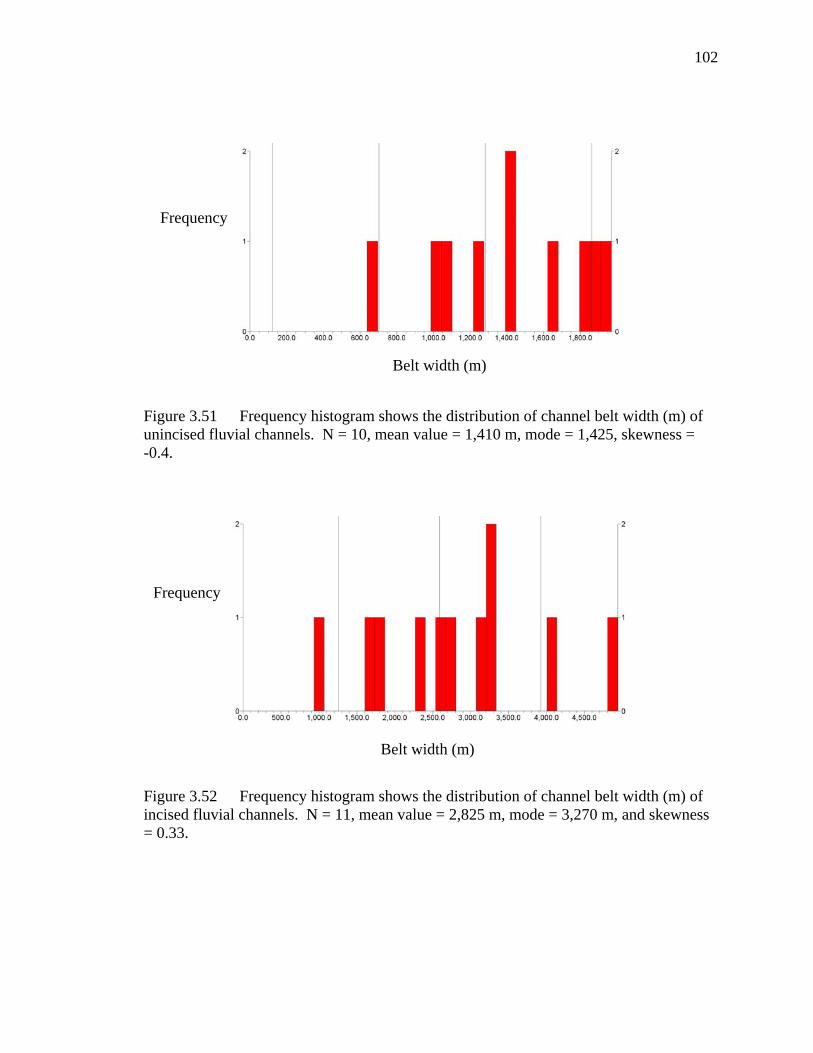
102
Figure 3.51 Frequency histogram shows the distribution of channel belt width (m) of unincised fluvial channels. N = 10, mean value = 1,410 m, mode = 1,425, skewness = -0.4.
Figure 3.52 Frequency histogram shows the distribution of channel belt width (m) of incised fluvial channels. N = 11, mean value = 2,825 m, mode = 3,270 m, and skewness = 0.33.
Frequency
Frequency
Belt width (m)
Belt width (m)

103
Figure 3.53 Frequency histogram shows the distribution of cumulative channel length (m) of all channels. N = 36, mean value = 44,200 m, bimodal = 27,500 m and 35,000 m, and skewness = 2.
Figure 3.54 Frequency histogram shows the distribution of cumulative channel length (m) of unincised fluvial channels. N = 14, mean value = 42,300 m, mode = 26,000 m, and skewness = 1.45.
Frequency
Frequency
Cumulative channel length (m)
Cumulative channel length (m)

104
Figure 3.55 Frequency histogram shows the distribution of cumulative channel length (m) of incised fluvial channels. N = 22, mean value = 45,400 m, mode = 15,000 m, and skewness = 1.9.
Figure 3.56 Frequency histogram shows the distribution of channel length (a straight line) from upstream to downstream end of all channels. N = 36, mean value = 20,150 m, mode = 17,000 m, and skewness = 1.2.
Frequency
Frequency
Cumulative channel length (m)
Channel length (m)

105
Figure 3.57 Frequency histogram shows the distribution of channel length (a straight line) from upstream to downstream end of unincised fluvial channels. N = 14, mean value = 18,600 m, mode = 13,500 m, and skewness = 1.3.
Figure 3.58 Frequency histogram shows the distribution of channel length (a straight line) from upstream to downstream end of incised fluvial channels. N = 22, mean value = 21,150 m, and skewness = 1.1.
Frequency
Frequency
Channel length (m)
Channel length (m)

106
Figure 3.59 Frequency histogram shows the distribution of point-bar size of all channels. N = 233, mean value = 3.75 km2, mode = 1 km2, and skewness = 3.2. See Appendix D (CD-ROM) for all point-bar sizes.
Figure 3.60 Frequency histogram shows the distribution of point-bar size of unincised fluvial channels. N = 142, mean value = 1 km2, mode = 0.3 km2, and skewness = 3.2. See Appendix D (CD-ROM) for all point-bar sizes.
Frequency
Frequency
Point-bar size (km2)
Point-bar size (km2)

107
Figure 3.61 Frequency histogram shows the distribution of point-bar size of incised fluvial channels. N = 91, mean value = 8 km2, mode = 2.5 km2, and skewness = 2. See Appendix D (CD-ROM) for all point-bar sizes.
Figure 3.62 Frequency histogram shows the distribution of point-bar volume of all channels. N = 233, mean value = 0.09 km3, mode = 0.02 km3, and skewness = 4.14. See Appendix D (CD-ROM) for all point-bar volumes.
Frequency
Frequency
Point-bar size (km2)
Point-bar volume (km3)

108
Figure 3.63 Frequency histogram shows the distribution of point-bar volume of all channels. N = 233, mean value = 74,274 acre ft, mode = 10,000 acre ft, and skewness = 4.14. See Appendix D (CD-ROM) for all point-bar volumes.
Figure 3.64 Frequency histogram shows the distribution of point-bar volume of unincised fluvial channels. N = 142, mean value = 0.017 km3, mode = 0.005 km3, and skewness = 3.5. See Appendix D (CD-ROM) for all point-bar volumes.
Frequency
Frequency
Point-bar volume (acre ft)
Point-bar volume (km3)

109
Figure 3.65 Frequency histogram shows the distribution of point-bar volume of unincised fluvial channels. N = 142, mean value = 14,040 acre ft, mode = 5,000 acre ft, and skewness = 3.5. See Appendix D (CD-ROM) for all point-bar volumes.
Figure 3.66 Frequency histogram shows the distribution of point-bar volumes of incised fluvial channels. N = 91, mean value = 0.21 km3, mode = 0.05 km3, and skewness = 2.7. See Appendix D (CD-ROM) for all point-bar volumes.
Frequency
Frequency
Point-bar volume (acre ft)
Point-bar volume (km3)

110
Figure 3.67 Frequency histogram shows the distribution of point-bar volumes of incised fluvial channels. N = 91, mean value = 168,266 acre ft, mode = 25,000 acre ft, and skewness = 2.7. See Appendix D (CD-ROM) for all point-bar volumes.
Figure 3.68 Frequency histogram shows the distribution of half-meander wavelength of all channels. N = 36, mean value = 2,700 m, mode = 800 m, and skewness = 1.2.
Frequency
Frequency
Point-bar volume (acre ft)
Half-meander wavelength (m)

111
Figure 3.69 Frequency histogram shows the distribution of half-meander wavelength of unincised fluvial channels. N = 14, mean value = 2,250 m, mode = 900 m , and skewness = 1.28.
Figure 3.70 Frequency histogram shows the distribution of half-meander wavelength of incised fluvial channels. N = 22, mean value = 3,000 m, mode = 700 m, and skewness = 0.92.
Frequency
Frequency
Half-meander wavelength (m)
Half-meander wavelength (m)

112
Figure 3.71 Frequency histogram shows the distribution of sinuosity of all channels. N = 36, mean value = 1.27, mode = 1.07, and skewness = 2.81.
Figure 3.72 Frequency histogram shows the distribution of sinuosity of unincised fluvial channels. N = 14, mean value = 1.3, bimodal = 1.13 and 1.25, and skewness = 2.74.
Frequency
Frequency
Sinuosity
Sinuosity

113
Figure 3.73 Frequency histogram shows the distribution of sinuosity of incised fluvial channels. N = 22, mean value = 1.24, bimodal = 1.07 and 1.17, and skewness = 1.24.
Figure 3.74 Frequency histogram shows the distribution of amplitude of all channels. N = 36, mean value = 670 m, mode = 100 m, and skewness = 1.95.
Frequency
Frequency
Sinuosity
Amplitude (m)

114
Figure 3.75 Frequency histogram shows the distribution of amplitude of unincised fluvial channels. N = 14, mean value = 510 m, mode = 230m, and skewness = 1.18.
Figure 3.76 Frequency histogram shows the distribution of amplitude of incised fluvial channels. N = 22, mean value = 770 m, mode = 150 m, and skewness = 1.54.
Frequency
Frequency
Amplitude (m)
Amplitude (m)
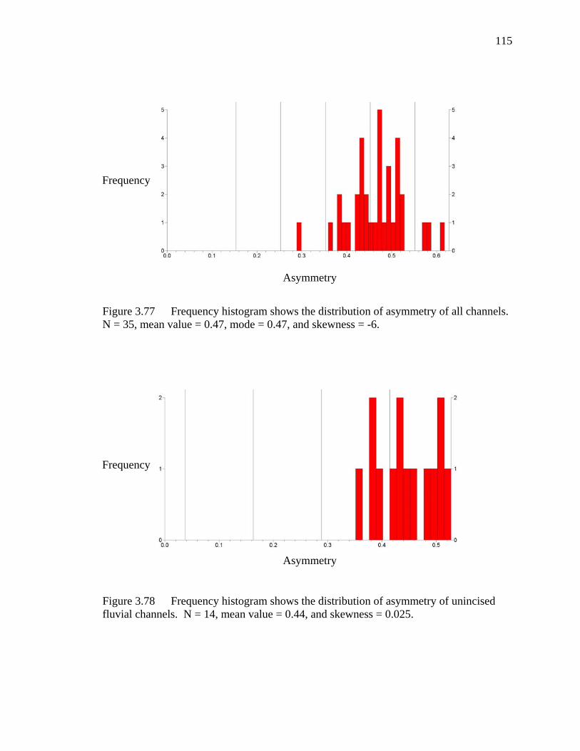
115
Figure 3.77 Frequency histogram shows the distribution of asymmetry of all channels. N = 35, mean value = 0.47, mode = 0.47, and skewness = -6.
Figure 3.78 Frequency histogram shows the distribution of asymmetry of unincised fluvial channels. N = 14, mean value = 0.44, and skewness = 0.025.
Frequency
Frequency
Asymmetry
Asymmetry

116
Figure 3.79 Frequency histogram shows the distribution of asymmetry of incised fluvial channels. N = 21, mean value = 0.48, mode = 0.48, and skewness = -4.7.
Figure 3.80 Frequency histogram shows the distribution of gradient (degrees) of all channels. N = 35, mean value = 0.033 degrees, mode = 0.03 degrees, and skewness = 0.72.
Frequency
Frequency
Asymmetry
Gradient (degrees)

117
Figure 3.81 Frequency histogram shows the distribution of gradient (degrees) of unincised fluvial channels. N = 13, mean value = 0.028 degrees, mode = 0.045 degrees, and skewness = -0.22.
Figure 3.82 Frequency histogram shows the distribution of gradient (degrees) of incised fluvial channels. N = 22, mean value = 0.036 degrees, mode = 0.03, and skewness = 0.67.
Frequency
Frequency
Gradient (degrees)
Gradient (degrees)

118
Figure 3.83 Frequency histogram shows the distribution of gradient (cm/km) of all channels. N = 35, mean value = 57 cm/km, bimodal = 55 cm/km and 77 cm/km, and skewness = 0.72.
Figure 3.84 Frequency histogram shows the distribution of gradient (cm/km) of unincised fluvial channels. N = 13, mean value = 49 cm/km, mode = 78 cm/km, and skewness = -0.22.
Frequency
Frequency
Gradient (cm/km)
Gradient (cm/km)

119
Figure 3.85 Frequency histogram shows the distribution of gradient (cm/km) of incised fluvial channels. N = 22, mean value = 62.5 cm/km, mode = 53 cm/km, and skewness = 0.67.
y = -1.8833x + 1.3387R2 = 0.0194
1.001.101.201.301.401.501.601.701.801.902.002.102.202.302.402.50
0 0.02 0.04 0.06 0.08 0.1
Gradient (degrees)
Sinu
osity
Figure 3.86 Cross plot between gradient (degrees) and sinuosity of all channels.
Frequency
Gradient (cm/km)

120
y = 0.0055x + 1.2176R2 = 0.0086
0
0.5
1
1.5
2
2.5
3
0 5 10 15 20 25
Point-bar size (square km)
Sin
uosi
ty
Figure 3.87 Cross plot between point-bar size (km2) and sinuosity of all channels.
y = 2E-07x + 1.2224R2 = 0.0069
0.00
0.50
1.00
1.50
2.00
2.50
3.00
0 100,000
200,000
300,000
400,000
500,000
600,000
700,000
800,000
Point-bar volume (acre ft)
Sinu
osity
Figure 3.88 Cross plot between point-bar volume (acre ft) and sinuosity of all channels.

121
y = 349.3x + 1464.1R2 = 0.6763
0
2000
4000
6000
8000
10000
12000
0.00 5.00 10.00 15.00 20.00 25.00
Point-bar size (square km)
Hal
f-mea
nder
wav
elen
gth
(m)
Figure 3.89 Cross plot between point-bar size (km2) and half-meander wavelength (m) of all channels.
y = 0.0124x + 1790.4R2 = 0.5104
0
2,000
4,000
6,000
8,000
10,000
12,000
0 100,000
200,000
300,000
400,000
500,000
600,000
700,000
800,000
Point-bar volume (acre ft)
Half-
mea
nder
wav
elen
gth
(m)
Figure 3.90 Cross plot between point-bar volume (acre ft) and half-meander wavelength (m) of all channels.

122
y = 97.837x + 324.14R2 = 0.603
0500
100015002000250030003500
0.00 5.00 10.00 15.00 20.00 25.00
Point-bar size (square km)
Am
plitu
de (m
)
Figure 3.91 Cross plot between point-bar size (km2) and amplitude (m) of all channels.
y = 0.0036x + 404.38R2 = 0.4994
0.00
500.00
1,000.00
1,500.00
2,000.00
2,500.00
3,000.00
3,500.00
0 100,000
200,000
300,000
400,000
500,000
600,000
700,000
800,000
Point-bar volume (acre ft)
Am
plitu
de (m
)
Figure 3.92 Cross plot between point-bar volume (acre ft) and amplitude (m) of all channels.
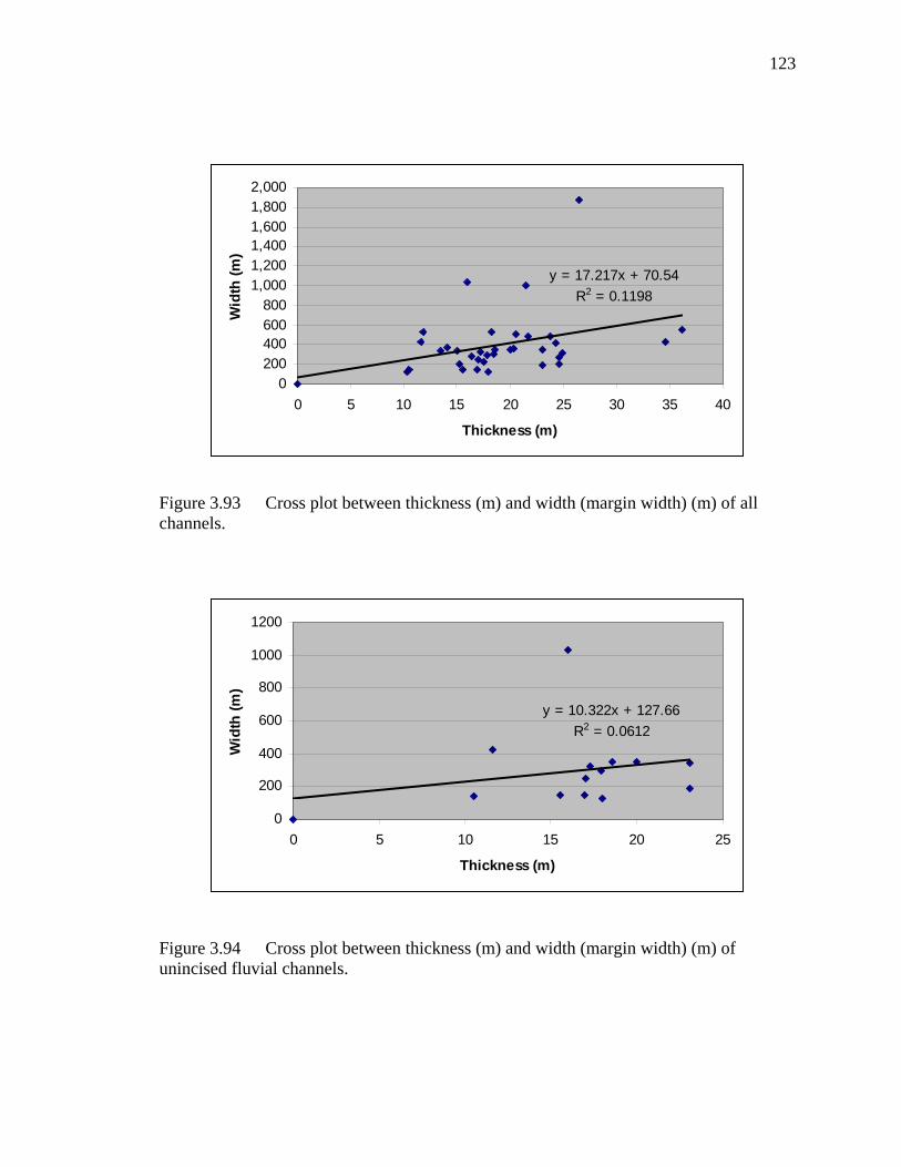
123
y = 17.217x + 70.54R2 = 0.1198
0200400600800
1,0001,2001,4001,6001,8002,000
0 5 10 15 20 25 30 35 40
Thickness (m)
Wid
th (m
)
Figure 3.93 Cross plot between thickness (m) and width (margin width) (m) of all channels.
y = 10.322x + 127.66R2 = 0.0612
0
200
400
600
800
1000
1200
0 5 10 15 20 25
Thickness (m)
Wid
th (m
)
Figure 3.94 Cross plot between thickness (m) and width (margin width) (m) of unincised fluvial channels.

124
y = 18.463x + 75.692R2 = 0.1508
0200400600800
100012001400160018002000
0 5 10 15 20 25 30 35 40
Thickness (m)
Wid
th (m
)
Figure 3.95 Cross plot between thickness (m) and width (margin width) (m) of incised valleys and tributaries to incised valleys.
Figure 3.96 Rose diagram shows paleocurrent direction of all channels. N = 35 and vector mean = 165°. See Appendix F (CD-ROM) for paleocurrent directions.

125
Figure 3.97 Rose diagram shows paleocurrent direction of all channels except tributaries to incised valleys. N = 24 and vector mean = 149°. See Appendix F (CD- ROM) for paleocurrent directions.
Figure 3.98 Rose diagram shows paleocurrent direction of straight channels. N = 3 and vector mean = 209°. See Appendix F (CD-ROM) for paleocurrent directions.

126
Figure 3.99 Rose diagram shows paleocurrent direction of low-sinuosity channels. N = 4 and vector mean = 126°. See Appendix F (CD-ROM) for paleocurrent directions.
Figure 3.100 Rose diagram shows paleocurrent direction of medium-sinuosity channels. N = 6 and vector mean = 192°. See Appendix F (CD-ROM) for paleocurrent directions.

127
Figure 3.101 Rose diagram shows paleocurrent direction of high-sinuosity channels. N = 1 and vector mean = 150°. See Appendix F (CD-ROM) for paleocurrent directions.
Figure 3.102 Rose diagram shows paleocurrent direction of tributaries to incised valleys. N = 11 and vector mean = 227°. See Appendix F (CD-ROM) for paleocurrent directions.

128
Figure 3.103 Rose diagram shows paleocurrent direction of incised valleys. N = 11 and vector mean = 135°. See Appendix F (CD-ROM) for paleocurrent directions.
Figure 3.104 Rose diagram shows paleocurrent direction of channels that are below sequence boundary 1 (SB 1), T11, T12, and T13. See Figures 3.111 to 3.115 for locations of SB 1 to SB 6. N = 3 and vector mean = 247°. See Appendix F (CD-ROM) for paleocurrent directions.

129
Figure 3.105 Rose diagram shows paleocurrent direction of channels that are above sequence boundary 1 (SB 1) and below sequence boundary 2 (SB 2), T8, T9, T10, T15, and T17. See Figures 3.111 to 3.115 for locations of SB 1 to SB 6. N = 5 and vector mean = 132°. See Appendix F (CD-ROM) for paleocurrent directions.
Figure 3.106 Rose diagram shows paleocurrent direction of channels that are above sequence boundary 2 (SB 2) and below sequence boundary 3 (SB 3), T6, T16, T18, T28, and T29. See Figures 3.111 to 3.115 for locations of SB 1 to SB 6. N = 5 and vector mean = 145°. See Appendix F (CD-ROM) for paleocurrent directions.
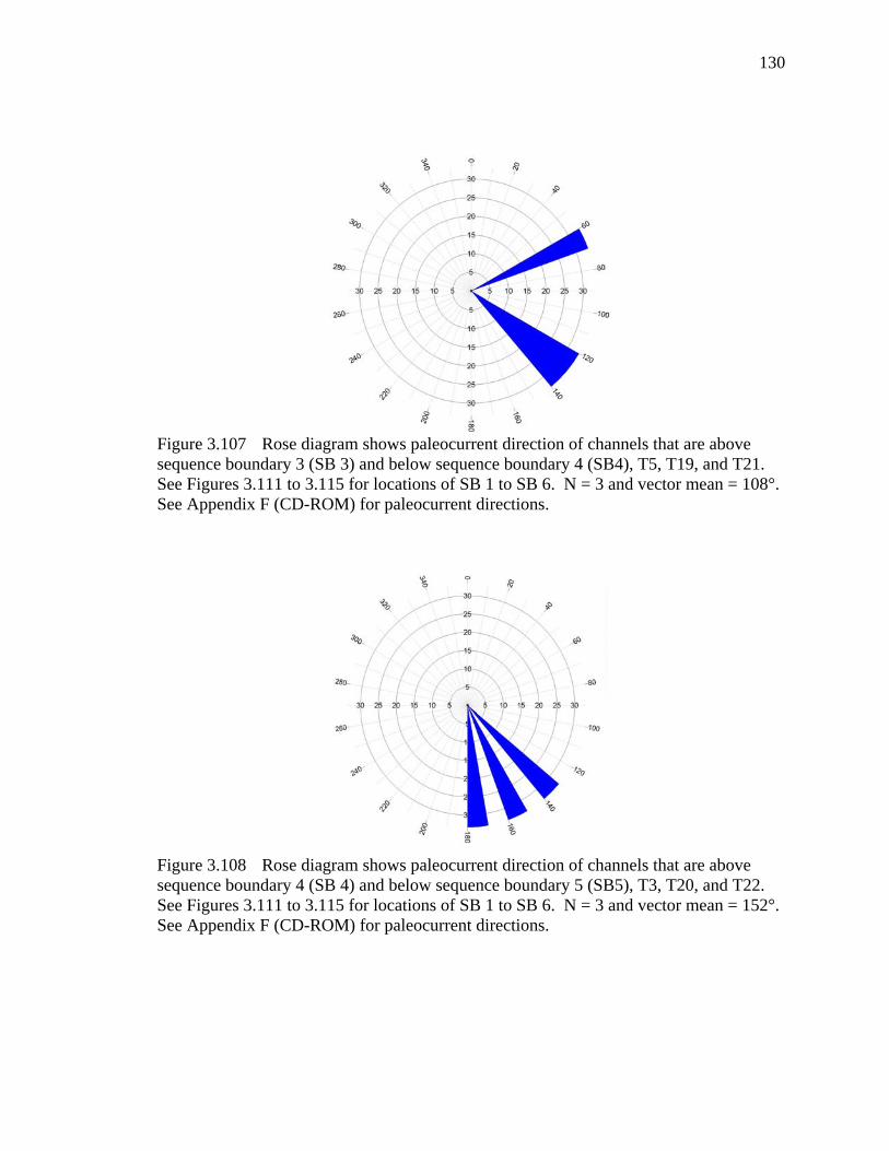
130
Figure 3.107 Rose diagram shows paleocurrent direction of channels that are above sequence boundary 3 (SB 3) and below sequence boundary 4 (SB4), T5, T19, and T21. See Figures 3.111 to 3.115 for locations of SB 1 to SB 6. N = 3 and vector mean = 108°. See Appendix F (CD-ROM) for paleocurrent directions.
Figure 3.108 Rose diagram shows paleocurrent direction of channels that are above sequence boundary 4 (SB 4) and below sequence boundary 5 (SB5), T3, T20, and T22. See Figures 3.111 to 3.115 for locations of SB 1 to SB 6. N = 3 and vector mean = 152°. See Appendix F (CD-ROM) for paleocurrent directions.

131
Figure 3.109 Rose diagram shows paleocurrent direction of channels that are above sequence boundary 5 (SB 5) and below sequence boundary 6 (SB6), T2, T2_2, T2_3, T4, T14, T23, T24, T25, and T26. See Figures 3.111 to 3.115 for locations of SB 1 to SB 6. N = 9 and vector mean = 176°. See Appendix F (CD-ROM) for paleocurrent directions.
Figure 3.110 Rose diagram shows paleocurrent direction of channels that are above sequence boundary 6 (SB 6), T1, T7, T27, T30, T31, T32, and T33. See Figures 3.111 to 3.115 for locations of SB 1 to SB 6. N = 7 and vector mean = 213°. See Appendix F (CD-ROM) for paleocurrent directions.

132
Figure 3.111 Rose diagram shows fault orientation of the study area at Sequence 4 horizon. See Figure 2.9 for the location of Sequence 4 in the cross section view and Figure 2.2 for a structure map at Sequence 4 horizon. See Appendix E (CD-ROM) for fault orientation data. N = 151 and vector mean = 176°. See Appendix F (CD-ROM) for paleocurrent directions.

133
Each channel interpreted in this study is a partial channel. Most of them are
truncated by the edges of the seismic volume. Therefore, some attributes, such as length,
are partial measurements. Other attributes, such as sinuosity, gradient, and amplitude are
valid, even for partial channels measured here. Modelers should be aware of the
limitations of this dataset for certain parameters that are limited by the fixed area of the
seismic data.
The statistical tests have been done to prove that the populations, width and
thickness of incised fluvial systems and unincised fluvial systems are different. See
appendix G for the calculations.
3.3 Discussion
This section discusses the results of the interpretation and analysis of fluvial
systems in the study area. The discussions are divided into sections for incised vs.
unincised fluvial systems, structural influences on fluvial systems, channel dimensions,
statistical relationships, and internal architectures of fluvial systems.
3.3.1 Incised vs. Unincised Fluvial Systems
Late Pleistocene to Holocene sea-level curves indicate that there were many
periods of relative sea-level lowstand (Fig. 3.112) (Posamentier, 2001). These multiple
high-amplitude sea-level falls created lowstand depositional systems, both incised and
unincised fluvial systems, in this study interval in the Gulf of Thailand. To develop an
incised valley by sea-level drop, the shelf must be fully exposed. If the shelf is only
partially exposed, unincised fluvial systems develop (Figs. 3.112 and 3.115). Six
sequence boundaries are interpreted in this study interval, based on the presence of
incised valleys at six levels. In Indonesia, the water depth of -110 m has been identified

134
Figure 3.112 (A) A late Pleistocene to Holocene sea-level curve based on oxygen- isotope data (Bard et al., 1990). In Indonesia, the water depth of -110 m has been identified as a threshold level, below which the continental shelf would be fully exposed. However, in the Gulf of Thailand, the -95 m level (the red line) is more likely. (B) If sea-level fall is less than 110 m (95 m in Thailand), then unincised fluvial channel systems form; if sea level fall exceeds 110 m (95 m in Thailand), then incised fluvial channel systems form. (Modified from Posamentier, 2001).
- 95 m
- 95 m

135
as a threshold level, below which the continental shelf would be fully exposed. However,
in the Gulf of Thailand, the -95 m level is more likely (Fig. 3.112). Shelf topography and
local tectonic activity are possible reasons for the differences between Indonesia and
Thailand. The incised valley concept was originally applied to petroleum exploration by
Harms (1966) to evaluate the Lower Cretaceous Muddy Formation in the Denver basin.
Valley-fill reservoirs have been used as an exploration concept during subsequent
years. In addition, many productive fluvial sandstone trends have been reinterpreted as
incised valley-fill deposits (Bowen et al., 1993). An incised valley occurs when a river
has cut into its flood plain deeply enough to not let the flow overtop the riverbanks, even
when it is at the flood stage. Therefore, the formerly active flood plains are abandoned
and act as interfluves. Some incised valleys have extreme depths of up to several
hundred meters and also extreme widths of tens of kilometers (Posamentier, 2001). The
areal extent of any incised valley is based on the duration of the period of sea-level fall,
erodibility of the substrate (lithology being cut by the channels), and fluvial discharge
(Posamentier, 2001).
Tributaries to incised valleys are developed on the abandoned flood plain, which
is now the interfluve, and they feed the main incised valley. The length of these
tributaries to incised valleys depends upon the length of time over which this system
evolves, as well as on the erodibility of the substrate and the amount of fluvial discharge
(Posamentier, 2001).
Incised-valley formation can occur in at least three principal ways:
1) Sea-level or base-level fall
2) Tectonic tilting of alluvial settings
3) Significant decrease in fluvial discharge
More than one of these factors can be involved at any given time while incised
valleys are forming. The incised valleys in this study are thought to be associated with
sea-level change and tectonic tilting (Figs. 2.10 and 3.21, respectively).

136
There have been many studies of incised valleys based on outcrop, well-log, and
core data. The recognition of incised valleys has been based on the presence of
multistory channel fill, the presence of a significant time break at the channel base, or the
absence of a transitional facies between the channel/valley fill and the underlying
substrate. The schematic cross sections of the Colorado River are shown in Figure 3.113
as examples of internal architecture of an incised valley. Figure 3.114 shows the
schematic block diagram of the valley-fill deposits of the Mississippi River.
However, the most clearly defined evidence for the existence of incised valleys,
the presence of small tributaries to incised valleys, has not been commonly used. The
reason might be that the presence of tributaries to incised valleys cannot commonly be
recognized because of the discontinuous nature of most forms of data other than 3-D
seismic data (Posamentier, 2001).
Channels in this study that are not tributaries to incised valleys and incised valleys
are classified as unincised fluvial channels. Unincised fluvial systems contain straight
channels (1.00 -1.10 sinuosity), low-sinuosity channels (1.11 -1.21 sinuosity), medium-
sinuosity channels (1.22 - 1.83 sinuosity), and high-sinuosity channels (1.84 - 2.44
sinuosity). These channels are different from incised-valley channels because they do not
have tributaries associated with them. They are also smaller in size and it is hard to see
point bars and other internal architecture with this seismic resolution. They are imaged
on only a few successive slices, which means that their thicknesses are significantly less
than in the incised-valley systems (Posamentier, 2001). During the time of the unincised
fluvial channels, the entire shelf was not fully subaerially exposed, and lowstand fluvial
systems did not incise (Fig. 3.115) (Posamentier, 2001 and Posamentier and Allen, 1999).
Generally, the incised fluvial system is a significantly more complex system than
the unincised fluvial system. The incised fluvial system contains depositional
environments that can range from alluvial to open marine. Unincised fluvial systems
tend to have a simpler stratigraphic architecture (Posamentier, 2001).

137
Fig. 3.113 11” by 17”

138
Figure 3.114 Schematic block diagram of the valley-fill deposits of the Mississippi River. The basal bounding discontinuity of the valley formed during the Pleistocene lowstand of sea level, when the river incised bedrock to adjust itself to a lower base level. As sea level rose, following glaciation, the valley filled first with coarse sands deposited in a braided-stream environment, and then with lower-energy meandering-stream deposits. Many ancient valley-fill alluvial successions formed in this way. In some, the uppermost deposits are estuarine to marine in depositional environment, and may be followed by widespread transgressive-marine blanket deposits. (From Walker and James, 2004 and Weimer, 1986; based on the work of H. Fisk).

139
Figure 3.115 Schematic depiction of (A) incised valley formed where sea-level fall fully exposes the shelf, and (B) unincised fluvial channel system formed where sea-level fall does not fully expose the shelf. (After Posamentier, 2001 and Posamentier and Allen, 1999).

140
3.3.2 Structural Influences on Fluvial Systems
Tectonic tilting may have occurred locally over this study interval because the
paleocurrent directions of channels varied (Figs. 3.3 to 3.12, Appendix A (CD-ROM),
Appendix F (CD-ROM), and Figs. 3.96 to 3.110). However, the main paleocurrent
direction is still mostly NW to SE (Figs. 3.96 to 3.110 and Appendix F (CD-ROM)),
which may have been partially controlled by the fact that the main fault orientations in
this study area have a N-S direction (Figs. 2.2, 3.111, and Appendix E (CD-ROM)).
3.3.3 Channel Dimensions
Ranges of fluvial system dimensions from this study are as follows:
• Unincised fluvial systems
Channel widths: 2 – 2,730 m (mean is 377 m) (Fig. 3.45).
Channel depths (thickness): 11 – 23 m (mean is 17 m) (Fig.
3.42).
Width/thickness aspect ratio: 7:1 – 64:1 (mean is 19:1) (Fig.
3.48). See comments in the following discussion.
Channel belt widths: 144 – 2,850 m (mean is 1,410 m) (Fig.
3.51).
Cumulative channel lengths: 12 – 103.5 km (mean is 42 km)
(Fig. 3.54).
A straight distance from upstream to downstream point: 6 –
47 km (mean is 19 km) (Fig. 3.57).
Point-bar sizes: 0.1 – 9.3 km2 (mean is 1 km2) (Fig. 3.60)
Point-bar volumes: 0.006 – 0.07 km3 (mean is 0.017 km3)
(4,500 – 54,300 acre ft (mean is 14,040 acre ft)) (Figs. 3.64 and 3.65)

141
Half-meander wavelengths: 65 – 13,000 m (mean is 2,250 m)
(Fig. 3.69)
Sinuosities: 1 – 6.7 (mean is 1.3) (Fig. 3.72).
Amplitudes: 1 – 3,700 m (mean is 510 m) (Fig. 3.75).
Asymmetries: -0.5 – 1.05 (mean is 0.44) (Fig. 3.78)
Gradients: 0.006 – 0.05 degrees (mean is 0.028 degrees) (0.1
– 0.8 m/km (mean is 0.5 m/km)) (Figs. 3.81 and 3.84).
• Incised fluvial systems
Channel widths: 9 – 5,000 m (mean is 460 m) (Fig. 3.46).
Channel depths (thickness): 10 – 36 m (mean is 21 m) (Fig.
3.43).
Width/thickness aspect ratio: 8:1 – 71:1 (mean is 23:1) (Fig.
3.49) see comments in the following discussion.
Channel belt widths: 440 – 11,000 m (mean is 2,825 m) (Fig.
3.52).
Cumulative channel lengths: 7.5 – 181.5 km (mean is 45 km)
(Fig. 3.55).
A straight distance from upstream to downstream point:
3.9 – 59 km (mean is 21 km) (Fig. 3.58).
Point-bar sizes: 0.26 – 39 km2 (mean is 8 km2) (Fig. 3.61).
Point-bar volumes: 0.1 – 0.9 km3 (mean is 0.21 km3) (84,100
– 696,500 acre ft (mean is 168,266 acre ft) (Figs. 3.66 and 3.92).
Half-meander wavelengths: 181– 21,450 m (mean is 3,000
m) (Fig. 3.70).
Sinuosities: 1 – 4 (mean is 1.24) (Fig. 3.73).
Amplitudes: 3 – 11,440 m (mean is 770 m) (Fig. 3.76)
Asymmetries: -0.65 – 1.18 (mean is 0.48) (Fig. 3.79)

142
Gradients: 0.0019 – 0.088 degrees (mean is 0.036 degrees)
(0.03 – 1.54 m/km (mean is 0.6 m/km)) (Figs. 3.82 and 3.85).
Observed ranges of dimensions from the Elliott and Fullmer (2004) study were as
follows:
• Channel widths 40-500 m and channel depths 10-46 m.
• Channel-belt widths: 0.1-6.3 km.
• Valley widths 0.1-9 km, and valley depths 13-80 m.
• Point-bar thicknesses 10-44 m, with areas of 0.7-22 km2.
Posamentier (2001) reported widths of channels that range from 100 to 250 m,
meander belt widths that range from 2 to 6 km, and incised valleys that range from 0.5 to
5 km wide, 14-41 m deep, 200 km long. Tributaries to incised valleys are an order of
magnitude narrower and are characterized by well-developed dendritic drainage patterns.
In most instances, they extend only short distances away from the main valley, and the
maximum length of tributaries to incised valleys is 15 - 20 km (Posamentier, 2001). The
width/thickness aspect ratio commonly is greater for unincised fluvial systems than for
incised fluvial systems. However, in this study the result of the width/thickness aspect
ratio for unincised fluvial systems (19:1) (Fig. 3.48) is smaller than the width/thickness
aspect ratio of incised fluvial systems, which includes tributaries to incised valleys and
incised valleys (23:1) (Fig. 3.49). This is because the tributaries to incised valleys are
thin compared to their widths. Therefore, they have high width/thickness aspect ratios.
Because of this, the width/thickness aspect ratios of tributaries to incised valleys are not
included in this comparison. Therefore, the width/thickness aspect ratio is slightly
greater for unincised fluvial systems (19.13:1) than for incised fluvial systems with only
incised valleys (18.78:1).
Reynolds (1999) obtained data from a study of 671 paralic sandstone bodies that
were collected from examples in the published literature and collated from studies
commissioned by British Petroleum and reported the dimensions as follows:

143
Widths of incised valleys ranged from 0.5 to 63 km (mean is 10 km) and
thicknesses ranged from 2 to 152 m (mean is 30 m) (Reynolds, 1999).
Widths of fluvial channels (unincised fluvial channels) ranged from 0.057 to 1.4
km (mean is 0.8 km) and thickness ranged from 2.5 to 24 m (mean is 9 m) (Reynolds,
1999).
“The gradient of the lower Mississippi River is very gentle, 0.1 m/km or less”
(http://www.cox-internet.com/coop/deltawebpage.html). The unincised fluvial system’s
gradients of this study range from 0.1 to 0.8 m/km (mean is 0.49 m/km) (Fig. 3.84).
Incised fluvial system gradients range from 0.03 to 1.54 m/km (mean is 0.62 m/km) (Fig.
3.85). Staff at Itasca State Park, the Mississippi's headwaters, say the Mississippi is
2,552 mi (4,107 km) long. The US Geologic Survey has published a number of 2,300 mi
(3,705 km), the EPA says it is 2,320 mi (3,734 km) long, the Mississippi National River
and Recreation Area maintains its length at 2,350 mi (3,782 km) (http://www.nps.gov/
miss/features/factoids/), and 3,896 mi (6,270 km) (http://en.wikipedia.org/wiki/Mississip
pi_River). The width of the Mississippi River is between 20-30 ft (6 – 9 m) wide at the
narrowest stretch for its entire length, and more than 4 mi (6.4 km) wide at its widest
point. The depth at its headwaters is less than 3 ft (0.9 m) deep. The river's deepest depth
is 200 ft (61 m) (http://www.nps.gov/miss/ features/factoids/). Comparison of the
information of channel dimensions mentioned above is in Table 3.2.
The channel parameter table (Table 3.1) shows that channels in this study have
different sizes and dimensions. The reasons that make them different could be because of
differences in substrate erodibility, and/or channel discharge (sediment supply and flow
rate), and/or length of time during which lateral cutting occurred (Posamentier, 2001),
and/or climate, and/or vegetation types that cover the channel area, and/or relative sea-
level change (accommodation space) (Fig. 3.116), and/or tectonic control.

144
Table 3.2 in 11” by 17” page
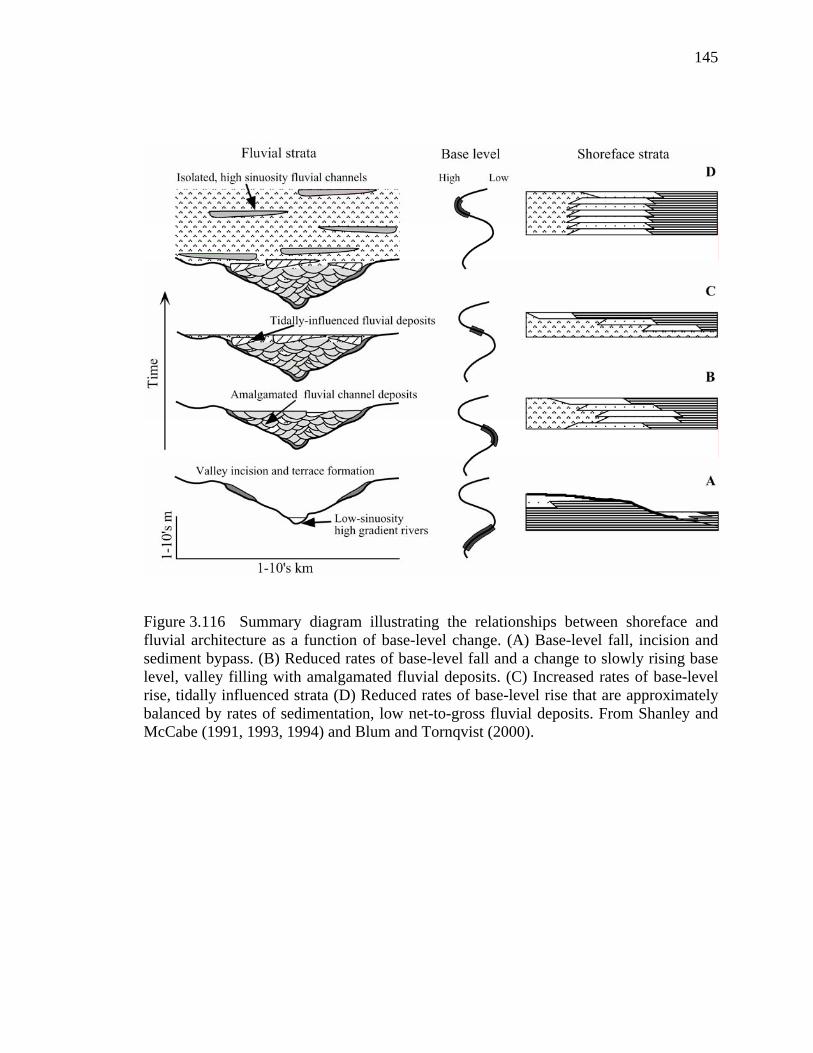
145
Figure 3.116 Summary diagram illustrating the relationships between shoreface and fluvial architecture as a function of base-level change. (A) Base-level fall, incision and sediment bypass. (B) Reduced rates of base-level fall and a change to slowly rising base level, valley filling with amalgamated fluvial deposits. (C) Increased rates of base-level rise, tidally influenced strata (D) Reduced rates of base-level rise that are approximately balanced by rates of sedimentation, low net-to-gross fluvial deposits. From Shanley and McCabe (1991, 1993, 1994) and Blum and Tornqvist (2000).

146
3.3.4 Statistical Relationships
The cross plot between gradient and sinuosity of all channels (Fig. 3.86) shows
that the higher the gradient, the lower the sinuosity. This result supports the idea that the
low gradient significantly lowers the river’s velocity. With a lower velocity, the river
carries more fine-grained sediments in suspension and coarser-grained sediments as bed-
load.
When this occurs, pronounced, sinuous curves called meanders tend to develop
(high-sinuosity channels develop) (http://www.cox-internet.com/coop/deltawebpage.
html).
Cross plots between point-bar size (km2) and/or volume (acre ft) and sinuosity of
all channels (Figs. 3.87 and 3.88) illustrate that channels that have higher sinuosity tend
to have larger point-bar sizes and volumes.
Cross plots between point-bar size (km2) and/or volume (acre ft) and half-
meander wavelength of all channels (Figs. 3.89 and 3.90) illustrate that channels that
have larger half-meander wavelength tend to have larger point-bar sizes and volumes.
Cross plots between point-bar size (km2) and/or volume (acre ft) and amplitude of
all channels (Figs. 3.91 and 3.92) illustrate that channels that have higher amplitude tend
to have larger point-bar sizes and volumes.
The cross plot between thickness (m) and width (margin width) of all channels,
unincised fluvial channels, and incised fluvial channels (Figs. 3.93 to 3.95) illustrates that
channels that have higher thicknesses have greater widths. The width/thickness aspect
ratio commonly is greater for unincised fluvial systems than for incised fluvial systems.
However, in this study the result of the width/thickness aspect ratio for unincised fluvial
system (19:1) (Fig. 3.48) is smaller than the width/thickness aspect ratio of incised fluvial
system, which includes both tributaries to incised valleys and incised valleys (23:1) (Fig.
3.49). This is because the tributaries to incised valleys are thin compared to their widths.
Therefore, they have a high width/thickness aspect ratio. Because of this; the

147
width/thickness aspect ratios of tributaries to incised valleys are not included in this
comparison. Therefore, the width/thickness aspect ratio is slightly greater for unincised
fluvial systems (19.1:1) than for incised fluvial systems with no tributaries included
(18.8:1).
3.3.5 Internal Architectures of Fluvial Systems
The high-resolution time slices and cross sections through the seismic data in this
study allow us to see the architecture of incised valleys within the Pleistocene to
Holocene section and reveal near complete preservation of alluvial depositional elements
within the incised valleys, alluvial terraces, channels, neck cutoffs, and point bars with
meander scrolls (Figs. 3.15, 3.17 to 3.20, and 3.27 to 3.29). This suggests that fluvial
depositional elements are well preserved in this system. There are two reasons for this
excellent preservation:
1) Rapid transgression, which characterized the period between the lowest sea-
level position approximately 16,000 years ago and the early Holocene, approximately
10,000 years ago, may have caused any high-energy environment located in the area of
the coastline to rapidly pass across the area, therefore minimizing the impact of erosion
(Posamentier, 2001).
2) If the environmental energy associated with the transgressing coastline (i.e.,
waves and tides) was low, the preservation potential of the incised valley fluvial deposits
would be high (Posamentier, 2001).
There are potential subseismic-scale reservoir heterogeneities that need to be
considered in reservoir management. They are internal mud drapes between accretion
sets (Fig. 3.20), complex compartment geometries, scoured upper and basal contacts (Fig.
3.27 and 3.28), and cannibalism and stacking (Elliott and Fullmer, 2004).
148
CHAPTER 4
CONCLUSIONS AND RECOMMENDATIONS
4.1 Conclusions
In a 3-D seismic data set from the Gulf of Thailand, channel evolution and
internal architecture are well imaged, so sand distribution can be confidently predicted.
This study quantifies channel widths, channel-belt widths, cumulative channel length
along each channel, channel length (a straight line from upstream to downstream), half-
meander wavelength, amplitudes, asymmetries, sinuosities, point-bar sizes and volumes,
channel gradients, the thicknesses of channels, width/thickness aspect ratios, and
paleocurrent directions in a manner suitable for 3-D geologic modeling. The results
provide important input for conditioning subsurface reservoir models. The conclusions
from this study are:
• Multiple high-amplitude sea-level falls during the Pleistocene and Holocene created
lowstand depositional systems, both incised and unincised fluvial systems, in this
study interval in the Gulf of Thailand.
• Time-slice images and cross sections through 3D seismic amplitude volumes provide
useful information for fluvial geomorphology interpretation and allow quantitative
measurement of depositional elements.
• Six sequence boundaries are interpreted in this study interval, based on the presence
of incised valleys at six levels. In Indonesia, the water depth of -110 m has been
identified as a threshold level, below which the continental shelf would be fully
exposed (Posamentier, 2001). However, in the Gulf of Thailand, the -95 m level is
more likely. Shelf topography and local tectonic activity are possible reasons for the
differences between Indonesia and Thailand.

149
• Tributaries provide the most clearly defined evidence for the existence of incised
valleys. They suggest incision of the main incised valley when they terminate at the
scarps. These tributaries to incised valleys are also bigger and deeper than any
tributaries that feed unincised fluvial channels. Tributaries cannot commonly be
recognized in fluvial systems because of the discontinuous nature of most forms of
data other than 3-D seismic data.
• Channels that are neither incised valleys nor tributaries to incised valleys are
classified as unincised fluvial channels. They may be straight channels
(sinuosity=1.00-1.10), low-sinuosity channels (sinuosity=1.11-1.21), medium-
sinuosity channels (sinuosity=1.22-1.83), or high-sinuosity channels
(sinuosity=1.84-2.44). These channels are different from incised-valley channels
because they do not have tributaries associated with them. They are also smaller in
size, and it is hard to see point bars and other internal architecture with this seismic
resolution. Their thicknesses are significantly less than in the incised-valley
systems.
• This study provides the dimensions of fluvial systems for the benefit of petroleum
exploration and development. The dimensions measured from these fluvial systems
could be used to develop detailed reservoir analogs (models) for other fluvial
reservoir targets. Ranges of fluvial system dimensions are:
• Unincised fluvial systems
Channel widths: 2 – 2,730 m, average 377 m
Channel depths (thickness): 11 – 23 m, average 17 m
Width/thickness aspect ratio: 7:1 – 64:1, average 19:1
Channel belt widths: 144 – 2,850 m, average 1,410 m
Cumulative channel lengths: 12 – 103.5 km, average 42 km
A straight distance from upstream to downstream point: 6 – 47 km,
average 19 km

150
Point-bar sizes: 0.1 – 9.3 km2, average 1 km2
Point-bar volumes: 0.006 – 0.07 km3, average 0.017 km3 (4,500 –
54,300 acre ft, average 14,040 acre ft)
Half-meander wavelengths: 65 – 13,000 m, average 2,250 m
Sinuosities: 1 – 6.7, average 1.3
Amplitudes: 1 – 3,700 m, average 510 m
Asymmetries: -0.5 – 1.05, average 0.44
Gradients: 0.006 – 0.05 degrees, average 0.028 degrees) (0.1 – 0.8
m/km, average 0.5 m/km)
• Incised fluvial systems
Channel widths: 9 – 5,000 m, average 460 m
Channel depths (thickness): 10 – 36 m, average 21 m
Width/thickness aspect ratio: 8:1 – 71:1, average 23:1
Channel belt widths: 440 – 11,000 m, average 2,825 m
Cumulative channel lengths: 7.5 – 181.5 km, average 45 km
A straight distance from upstream to downstream point: 3.9 – 59 km,
average 21 km
Point-bar sizes: 0.26 – 39 km2, average 8 km2
Point-bar volumes: 0.1 – 0.9 km3, average 0.21 km3) (84,100 – 696,500
acre ft, average 168,266 acre ft)
Half-meander wavelengths: 181– 21,450 m, average 3,000 m
Sinuosities: 1 – 4, average 1.24
Amplitudes: 3 – 11,440 m, average 770 m
Asymmetries: -0.65 – 1.18, average 0.48
Gradients: 0.0019 – 0.088 degrees, average 0.036 degrees (0.03 – 1.54
m/km, average 0.6 m/km)
• The results of statistical cross plots are as follows:
The higher the gradient, the lower the sinuosity.

151
The higher the sinuosity, the larger the point-bar sizes and volumes.
The larger the half-meander wavelength, the larger the point-bar sizes and
volumes.
The higher the amplitude, the larger the point-bar sizes and volumes.
The higher the thicknesses, the greater the widths. The width/thickness aspect
ratio is greater for unincised fluvial systems than for incised fluvial systems.
• Tectonic tilting may have occurred locally over this study interval because the
paleocurrent directions of channels are variable. However, the main paleocurrent
direction is still mostly in the NW to SE direction. The main fault orientations in
the study area are in a N-S direction.
4.2 Recommendations
Recommendations for future work include:
• Acquire log, core, and cuttings data for the shallow section from the sea floor to about
500 msec and correlate this to seismic interpretations. Biostratigraphic data will help
to confirm the interpreted sequence stratigraphy of the Pleistocene to Holocene
section of the Gulf of Thailand.
• Study the influence of climate on channel styles by developing a climate-change
sequence-stratigraphic model.
• Interpret a more areally extensive 3-D seismic data set to cover the NW and SE sides
of the Jarmjuree area, to extend to the upstream and downstream areas of channels.
This will help to get a broader view of the Gulf of Thailand channel evolution.
• Build a 3-D geologic model of the shallow section of the Gulf of Thailand by using
the statistical results from this study.

152
REFERENCES
Bard, B., Hamelin, R. G., and Fairbanks, R. G., 1990, U-Th obtained by mass spectrometry in corals from Barbados: Sea level during the past 130,000 years: Nature, v. 346, p. 456–458.
Bissada, K. K. , 1982, Geochemical constraints on petroleum generation and migration –
a review: Proceedings Asian Council on Petroleum Conference and Exhibition, p. 69-87.
Blum, M. D., 1993, Genesis and architecture of incised valley fill sequences: A Late
Quaternary example from the Colorado River, Gulf Coastal plain of Texas, in Weimer, P., and Posamentier, H. W., eds., Siliciclastic Sequence Stratigraphy: Recent Developments and Applications: AAPG Memoir 58, p. 259–283.
Blum, M.D., and Tornqvist, T.E., 2000, Fluvial response to climate and sea-level change: A review and look forward: Sedimentology, v. 47, p. 2-48.
Blum, M. D., and Valastro, S., Jr., 1992, Quaternary stratigraphy and geoarchaeology of
the Colorado and Concho Rivers, west Texas: Geoarchaeology, v. 7, p. 419-448. Boonyakitsombut, J., 2003, Investigation of the relationship between basement structure
and Miocene conjugate fault systems from 3D seismic data, Chongko area, North Pattani basin, Gulf of Thailand: Unpublished M.S. thesis, University of Brunei Darussalam, Brunei, 110 p.
Bowen, D. W., Weimer, P., and Scott, A. J., 1993, The relative success of siliciclastic
sequence stratigraphic concepts in exploration: Example from incised valley fill and turbidite systems reservoirs, in Weimer, P., and Posamentier, H., W., eds., Siliciclastic Sequence Stratigraphy: Recent Developments and Applications: AAPG Memoir 58, p. 15-42.
Carter, D. C., 2003, 3-D seismic geomorphology: Insights into fluvial reservoir deposition and performance, Widuri field, Java Sea: AAPG Bulletin, v. 87, p. 909-934.
Dorobek, S. L., and Olson, C. C., 2001, Timing of major uplift in the Eastern Tibetan Plateau as recorded by Neogene deposits in the paleo-Mekong delta, offshore Vietnam (abs.): AAPG Bulletin., v. 85, No. 13 (Supplement).
153
Elliott, T., L., and Fullmer, S. M., 2004, 3D seismic geomorphology of Pleistocene fluvial deposits, Offshore Vietnam, Block 52 and Kim Long Areas: Unpublished Company Report, Unocal Thailand, 162 p.
Elliott, T. L., and Triamwichanon, H., 1999, 3D seismic interpretation of fluvio-deltaic
facies and stratigraphy in selected intervals, Block 14-15-16, Arthit Project (Phase 2), Gulf of Thailand: Unpublished Company report, Unocal Resource Technology Div. and PTT-EP, 29 p.
Ellison, A. I., 2004, Numerical modeling of heterogeneity within a fluvial point-bar deposit using outcrop and lidar data: Williams Fork Formation, Piceance basin,
Colorado: Unpublished M.S. thesis, University of Colorado, Boulder, 249 p.
Emery, D., and Myers, K. J., 2003, Sequence stratigraphy in Emery and Myers, eds., Stratigraphic Research International, UK, p. 111-133.
Hall, R., 1996, Reconstructing Cenozoic SE Asia, in Hall, R. and Blundell, D.J., eds.,
Tectonic Evolution of Southeast Asia: Geological Society of London, Special Publication, v. 106, p. 203-224.
Haq, B. U., 1988, Fluctuating Mesozoic and Cenozoic sea levels and implications for
stratigraphy (abs.): AAPG Bulletin., v. 72, p. 1521. Haq, B.U., Hardenbol, J., and Vail, P. R., 1988, Mesozoic and Cenozoic
chronostratigraphy and eustatic cycles of sea-level change, in Wilgus, C. K., Hastings, B. S., Kendall, C. G. S. C., Posamentier, H. W., Ross, C. A., and Van Wagoner, J. C, eds., Sea Level Research: An Integrated Approach: SEPM Special Publication 42, p. 71-108.
Haranya, C., 2000, Regional study of the structural geology of the Pattani Basin, Gulf of
Thailand: Unpublished M.S. thesis, University of Brunei Darussalam, Brunei, 157 p.
Harms, J. C., 1966, Stratigraphic traps in a valley fill, western Nebraska: AAPG Bulletin,
v. 50, p. 2119-2149. Jardine, E., 1997, Dual petroleum systems governing the prolific Pattani Basin, Offshore
Thailand: Indonesian Petroleum Association, Proceedings of the Petroleum Systems of SE Asia and Australia Conference, p. 351-363.

154
Katz, B. J., 2002, Geochemical aspects of hydrocarbon charge in the Gulf of Thailand, with emphasis on the Pattani Trough, Part 1 – Source Rock Attributes and Thermal Maturity: Unpublished report, ERTC-TR, 66 p.
Kornsawan, A., 2001, The origin and evolution of complex transfer zones (graben shifts)
in conjugate fault systems around the Funan field, Pattani Basin, Gulf of Thailand: Unpublished M.S. thesis, University of Brunei Darussalam, Brunei, 100 p.
Lacassin, R., Hinthong, C., Siribhakdi, K., Chauviroj, S., Charoenravat, R., Maluski, H.,
Leoup, P. H., and Tapponnier, P., 1997, Tertiary diachronic extrusion and deformation of Western Indo-china; structure and 40Ar/39Ar evidence from NW Thailand: Journal of Geophysical Research, v. 102, p. 10013-10037.
Lockhart, B.E., Chinoroje, O., Enomoto, C. B., and Hollomon, G. A. 1997, Early Tertiary
deposition in the southern Pattani Trough, Gulf of Thailand, in Hayes, D. E., ed., The International Conference on Stratigraphy and Tectonic Evolution of Southeast Asia and the South Pacific, Bangkok, Thailand: Journal of the Geological Society, London, v. 151, p. 476-490.
Maneechai, K., and Lin, R., 2006, Petroleum systems of the Pattani and North Malay
basins, Gulf of Thailand (abs.): AAPG International Conference and Exhibition, supplement.
Miall, A. D., 2002, Architecture and sequence stratigraphy of Pleistocene fluvial systems
in the Malay Basin, based on seismic time-slice analysis: AAPG Bulletin, v. 86, p. 1201-1216.
Morley, C. K., 2001, Combined escape tectonics and subduction rollback-back arc extension: A model for the evolution of Tertiary rift basins in Thailand, Malaysia and Laos: Journal of the Geological Society, London, v. 158, p. 461-474.
Morley, C. K., and Westaway, R., 2006, Subsidence in the super-deep Pattani and Malay
basins of Southeast Asia: A coupled model incorporating lower-crustal flow in response to post-rift sediment loading: Basin Research, v. 18, p. 51-84.
Morley, C. K., Woganan, N., Sankumarn, N., Hoon, T. B., Alief, A., and Simmons, M.,
2001, Late Oligocene-Recent stress evolution in rift basins of northern and central Thailand: Implications for escape tectonics: Tectonophysics, v. 334, p. 115-150.

155
Mountford, N., and Livesay, G., 1996, Pailin field: Near-surface depositional systems: Unpublished Company Report, Unocal Thailand, 58 p.
Polachan, S., and Sattayarak, N., 1989, Strike-slip tectonics and the development of
Tertiary basins in Thailand: International Symposium on Intermontane Basins: Geology and Resources Chiang Mai, Thailand: Journal of the Geological Society, London, v. 146, p. 243-253.
Posamentier, H. W., and G. P. Allen, 1999, Silisiclastic sequence stratigraphy: Concepts
and applications: SEPM Concepts in Sedimentology and Paleontology, v. 9, 210 p.
Posamentier, H. W., 2001, Lowstand alluvial bypass systems: Incised vs. unincised:
AAPG Bulletin, v. 85, p. 1771-1793. Reynolds, A. D., 1999, Dimensions of paralic sandstone bodies: AAPG Bulletin, v. 83, p.
211-229. Shanley, K. W., and McCabe, P. J., 1994, Perspectives on the sequence stratigraphy of
continental strata: AAPG Bulletin, v. 78, p. 544-568. Suter, J. R., 2003, Late Quaternary shelf margin deltas, northern Gulf of Mexico, in shelf
margin deltas and linked down slope petroleum systems: Gulf Coast Section SEPM Foundation Bob F. Perkins 23rd Annual Research Conference, December 7-10, Houston, Texas, USA, p. 27-44.
Tapponnier, P., Peltzer, G., Le Dain, A. Y., Armijo, R., and Cobbold, P., 1982,
Propagating extrusion tectonics in Asia; New insights from simple experiments with plasticine: Geology, v. 10, p. 611-616.
Tapponnier, P., Peltzer, G., and Armijo, R., 1986, On the mechanism of collision
between India and Asia, in Coward, M. P., and Ries, A. C., eds., Collision Tectonics: Geological Society of London, Special Publication, v. 19, p. 115-157.
Teerman, S., C., Smith, L., N., Denison, C., N., and Marzi, R., W., 2000, An integrated
petroleum system study, northern Gulf of Thailand: applications to the Block B8/32 area (abs.): AAPG International Conference, Bali, Indonesia: AAPG Bulletin., v. 84, supplement.

156
Turner, J. W., Gonecome, Y., Thanatit, S., Prachukbunchong, P., and Triamwichanon, H., 2004, Sand distribution and reservoir development in the Arthit Area, 8th PTTEP Technical Forum: Unpublished Company Report, Unocal Thailand, 31 p.
Tye, R. S., 2004, Geomorphology: An approach to determining subsurface reservoir
dimensions: AAPG Bulletin, v. 88, p. 1123-1147. Walker, R. G., and James, N. P., 2004, Facies models response to sea level change:
Geological Association of Canada, p. 119 – 142. Watcharanantakul, R., and Morley, C. K., 2000, Syn-rift and post-rift modeling of the
Pattani Basin, Thailand: Evidence for a ramp flat detachment: Marine and Petroleum Geology, v. 17, p. 937-958.
Weimer, R. J., 1986, Relationship of unconformities, tectonics, and sea level change in
the Cretaceous of the Western Interior, United States, in Peterson, J.A., ed., Paleotectonics and sedimentation in the Rocky Mountain region, United States: AAPG Memoir 41, p. 397 – 422.
Wheeler, P. and White, N., 2000, Quest for dynamic topography: Observations from
Southeast Asia: Geology, v. 28, p. 963-966.