LATERAL RESERVOIR HETEROGENEITIES AND THEIR ...
184
LATERAL RESERVOIR HETEROGENEITIES AND THEIR IMPACTS ON STRESS SHADOWING IN THE EAGLE FORD RESERVOIR by Ahmed Ali Alrashed
-
Upload
khangminh22 -
Category
Documents
-
view
2 -
download
0
Transcript of LATERAL RESERVOIR HETEROGENEITIES AND THEIR ...
LATERAL RESERVOIR HETEROGENEITIES AND THEIR IMPACTS ON STRESS
SHADOWING IN THE EAGLE FORD RESERVOIR
by
Ahmed Ali Alrashed

© Copyright by Ahmed Ali Alrashed, 2018
All Rights Reserved

ii
A thesis submitted to the Faculty and the Board of Trustees of the Colorado School of
Mines in partial fulfillment of the requirements for the degree of Master of Science (Petroleum
Engineering).
Golden, Colorado
Date
Signed:
Ahmed Ali Alrashed
Signed:
Dr. Jennifer Miskimins
Thesis Advisor
Golden, Colorado
Date
Signed:
Dr. Erdal Ozkan
Professor and Head
Department of Petroleum Engineering
iii
ABSTRACT
Optimizing hydraulic fracture spacing in horizontal wells of unconventional reservoirs
requires investigating the extent of stress shadowing and the influence of rock quality lateral
variations. For that purpose, a base hydraulic fracture model was created for a well in the Eagle
Ford reservoir. Fiber optic distributed acoustic sensing (DAS) data analysis was utilized to find
the individual perforation cluster contribution based on the total proppant placed in each cluster.
The modeled well cluster contribution and production data were matched with actual data.
Reservoir and geomechanical properties for certain fracturing stages of the horizontal
wellbore were altered from the base model to address the effect of rock quality lateral variations.
The sensitized properties include matrix permeability, Poisson’s ratio, Young’s modulus, and
Biot’s coefficient. In response to these changes, the new flowing fracture lengths of the four
simulated stages were calculated and compared to the base model values. It was found that
fracturing stages with a higher matrix permeability of 0.0023 mD, compared to a base case value
of 0.00023 mD, were able to create fractures with larger flowing fracture length by 69%, 68%, and
48% in the heel, middle, and toe clusters, respectively. Increasing Poisson’s ratio from 0.28 to 0.33
caused changes in the flowing fracture lengths by 32%, 41%, and -1.4% in the heel, middle, and
toe clusters, respectively. Compared to a Young’s modulus base case value of 5.5 MMpsi, a 6.5
MMpsi value resulted in decreasing the flowing fracture lengths at rates of -8%, -3%, and -24% in
the heel, middle, and toe clusters, respectively. Decreasing Biot’s coefficient from 0.9 to 0.1
reduced the flowing fracture lengths in the heel, middle, and toe clusters at rates of -44%, -32%,
and -39%, respectively. Overall, the rate of increase in flowing fracture length at the performed

iv
sensitivity analyses was more pronounced in the heel and middle clusters and less evident in the
toe clusters.
Four scenarios of 57’ (Scenario 1), 76’ (Scenario 2), 100’ (Scenario 3), and 142’ (Scenario
4) spacing between perforation clusters were run to address the effects of stress shadowing.
Simulations showed that the tightest spacing scenario (Scenario 1) yielded the largest fracture
network volume due to the higher number of clusters. However, these created fractures were less
conductive than the ones created with wider spacing scenarios. Scenario 1 average cluster
contributions based on fracture conductivity were 56%, 29%, and 15% for the heel, middle, and
toe clusters, respectively, compared to more uniform contributions of 36%, 28%, and 36% for the
heel, middle, and toe clusters, respectively, in Scenario 4. In terms of production, Scenario 1
forecasted the highest cumulative oil production of 355,000 STB in 30 years compared to 256,000
STB production of Scenario 4. Therefore, the created fracture network volume, which is an
indication of reservoir contact, was more influential on production than fracture conductivity for
the studied case.

v
TABLE OF CONTENTS
ABSTRACT ................................................................................................................................... iii
LIST OF FIGURES ..................................................................................................................... viii
LIST OF TABLES ....................................................................................................................... xix
NOMENCLATURE .................................................................................................................... xxi
ACKNOWLEDGMENTS ......................................................................................................... xxiv
DEDICATION ........................................................................................................................... xxvi
CHAPTER 1 INTRODUCTION .................................................................................................... 1
1.1 Motivation of the Study......................................................................................................... 2
1.2 Problem Statement ................................................................................................................ 2
1.3 Research Objectives .............................................................................................................. 2
1.4 Eagle Ford Play Overview .................................................................................................... 3
1.4.1 Geology .......................................................................................................................... 3
1.4.2 Project Focus Area.......................................................................................................... 6
1.4.3 Available Data ................................................................................................................ 6
CHAPTER 2 LITERATURE REVIEW ....................................................................................... 10
2.1 Rock Mechanics Fundamentals ........................................................................................... 10
2.1.1 Stress and Strain ........................................................................................................... 10
2.1.2 Young’s Modulus and Poisson’s Ratio ........................................................................ 11
2.1.3 In-Situ Stresses ............................................................................................................. 13
2.2 Unconventional Reservoirs ................................................................................................. 16
2.3.1 Types of Hydraulic Fractures in Horizontal Wells ....................................................... 17
2.3.2 Hydraulic Fracture Modes ............................................................................................ 18
2.3.3 Hydraulic Fracture Modeling ....................................................................................... 18
vi
2.3.4 Natural Fractures .......................................................................................................... 21
2.3.5 Design and Treatment Schedule ................................................................................... 22
2.3.6 Hydraulic Fracture Monitoring ..................................................................................... 25
2.3.7 Stress Shadow Phenomenon ......................................................................................... 29
2.3.8 Pressures Associated with Hydraulic Fracturing .......................................................... 33
2.3.9 Engineered Completion ................................................................................................ 36
2.3.10 Spacing Optimization ................................................................................................. 37
CHAPTER 3 METHODOLOGY ................................................................................................. 40
3.1 Base Case Model Development .......................................................................................... 40
3.1.1 Log Processing ............................................................................................................. 41
3.1.2 DFIT and Log Calibration ............................................................................................ 46
3.1.3 Treatments .................................................................................................................... 55
3.1.4 Production History Matching ....................................................................................... 67
3.2 Sensitivity Analyses Creation ............................................................................................. 68
CHAPTER 4 MODEL RESULTS AND DISCUSSION.............................................................. 73
4.1 Parameter Sensitivity Analyses ........................................................................................... 73
4.1.1 Matrix Permeability Sensitivity .................................................................................... 74
4.1.2 Poisson’s Ratio Sensitivity ........................................................................................... 79
4.1.3 Young’s Modulus Sensitivity ....................................................................................... 80
4.1.4 Biot’s Coefficient Sensitivity ....................................................................................... 81
4.1.5 Cluster Spacing Sensitivity ........................................................................................... 82
4.1.6 Fluid and Proppant Type Sensitivity .......................................................................... 112
4.2 Natural Fracture Density ................................................................................................... 114
CHAPTER 5 CONCLUSIONS AND RECOMMENDATIONS ............................................... 129
5.1 Conclusions ....................................................................................................................... 129

vii
5.2 Recommendations ............................................................................................................. 133
REFERENCES ........................................................................................................................... 134
APPENDIX A MATCHED TREATING PRESSURE PLOTS ................................................. 142
APPENDIX B PREDICT-KTM INPUT DATA .......................................................................... 156

viii
LIST OF FIGURES
Figure 1.1 Eagle Ford play location and boundary map (from U.S. Energy Information
Administration 2014). ............................................................................................... 4
Figure 1.2 Eagle Ford stratigraphic column (from Ratcliffe et al. 2012). .................................. 5
Figure 1.3 Relative locations of Wells A, B, and C (only Wells A and C are used in this
research). The cross signs represent the surface locations of the wells. The
horizontal section of the target well (Well A) was drilled in the northwest
direction. ................................................................................................................... 7
Figure 1.4 Eagle Ford lithology (from Breyer et al. 2013). Upper Eagle Ford lithology is
more to the right side of the upper bar in the graph (more calcite than clay),
whereas the lower Eagle Ford lithology is more to the left side (more clay than
calcite). Well A primarily targets the Eagle Ford Marl (between shale and
limestone in the lithology bar). ................................................................................. 8
Figure 1.5 Eagle Ford shale play (Western Gulf Basin) petroleum windows (from EIA
2010). Formation is dipping down from NW to SE direction. ................................. 9
Figure 2.1 Stress and strain relationship showing both elastic and plastic regions (from
Cyberphysics Website 2018). The relationship is linear until the limit of
proportionality point. Once the stress exceeds the yield point, the material
deforms plastically where the strain is permanent (point A returns to point B not
to the original curve if stress is released). The fracture point represents the
maximum strain reached before the material ruptures. ........................................... 12
Figure 2.2 Left: material before applying stress; Right: material after applying stress (from
Fjar et al. 2008). Stress caused the material to shrink parallel to stress direction
and stretch perpendicular to it. Poisson’s ratio represents the negative ratio of transverse strain to longitudinal strain. ................................................................... 13
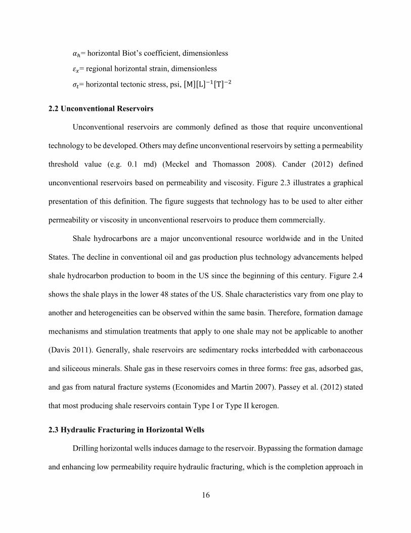
Figure 2.3 Unconventional resources versus conventional resources (from Cander 2012).
Unconventional reservoirs are characterized with low permeability/viscosity
ratio where either permeability or viscosity need to be altered for them to be
produced commercially. .......................................................................................... 17
Figure 2.4 US lower 48 states shale oil and gas plays (from EIA 2016). ................................ 19
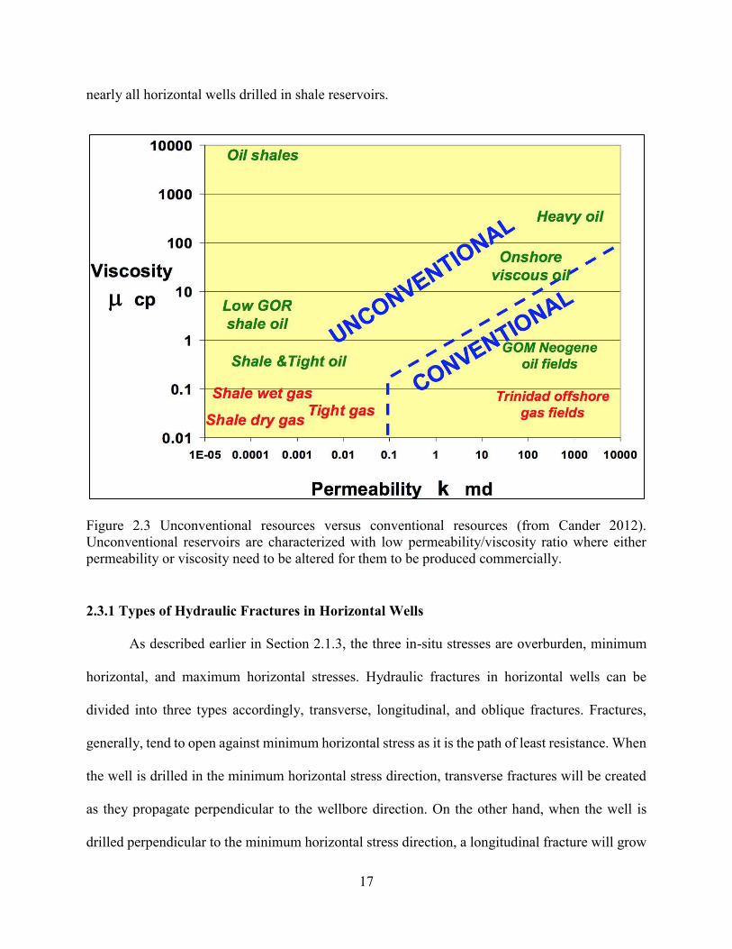
Figure 2.5 Hydraulic fracture types in horizontal wells based on their growth direction
(from EPT International 2015). .............................................................................. 20
ix
Figure 2.6 Hydraulic fracture modes: (a) Mode I, opening or tensile mode; (b) Mode II,
sliding or in-plane shearing mode; (c) Mode III, tearing or anti-plane shearing
mode (from Kanninen and Popelar 1985). .............................................................. 21
Figure 2.7 PKN versus KGD 2D hydraulic fracture models (from Montgomery and Smith
2010). The PKN model (left) assumes elliptical fracture in wellbore and through
formation. The KGD model (right) assumes rectangular fracture in wellbore and
through formation. .................................................................................................. 22
Figure 2.8 Fracture complexity levels (from Warpinski et al. 2008). Top left: simple planar
fracture; Top right: planar fracture with added complexity such as roughness
and waviness; Bottom left: complex fracture connected with natural fractures;
Bottom right; primary and secondary fractures connected to create a complex
fracture network. ..................................................................................................... 23
Figure 2.9 Proppant conductivity pyramid for different types of proppant (from Gallagher
2011). Top of pyramid represents the highest conductivity (ceramic). Bottom of
pyramid represents the lowest conductivity (sand). ................................................ 26
Figure 2.10 Generic DFIT procedure (from Barree et al. 2015). The black curve represents
the fluid rate that starts low then increases before it ends with a step down until
shut-in. The red curve represents the surface pressure. .......................................... 28
Figure 2.11 DAS/DTS data (from Wheaton et al. 2016). Top: DTS data changes with time
(warmer colors denote higher temperatures); Middle: DAS data changes with
time (warmer colors denote higher acoustic activity); Bottom: treatment plot
showing different curves versus time (black curve represents rate, dark blue
curve represents surface pressure, light blue curve represents bottomhole
pressure, and green curves represents surface and bottomhole proppant
concentrations). ....................................................................................................... 30
Figure 2.12 Effect of stress shadowing in multiple transverse fractures (from Fisher et al.
2004). Top part shows a top view of a hydraulic fracture where fracture length
propagation is limited by stress shadowing. Bottom part shows a side view of a
hydraulic fracture where fracture height is limited by stress shadowing. .............. 32
Figure 2.13 Stress shadow effect minimized by lateral heterogeneity between propagating
fractures (from Manchanda et al. 2016). Left two windows show Young’s modulus effect. Right two windows show Poisson’s ratio effect. .......................... 32
Figure 2.14 Effect of net pressure on fracture spacing (from Morrill and Miskimins 2012).
As fluid net pressure increases, the induced stress shadow increases and so
should the hydraulic fracture spacing required to eliminate stress shadow
effects. ..................................................................................................................... 33
Figure 2.15 Stress shadow effect diminishes in later stages of fracturing (from Daneshy
2017). The reduction in the curve slope implies lower additional induced stress
in the later stages of fracturing. Minimum horizontal stress, maximum

x
horizontal stress, and initial closing fracture width coefficient values shown in
the plot. ................................................................................................................... 34
Figure 2.16 Effect of cluster spacing on fracture propagation due to stress shadow (left: 10m
spacing vs. right: 50m spacing) (from Lu 2016). SDEG means scalar stiffness
degradation variable (SDEG), which is a measure of how damaged the element
is. Outer fractures are dominant in the 10 m spacing case, whereas all fractures
are equal in terms of dominance in the 50 m spacing case. .................................... 38
Figure 2.17 Engineered completion (Track 1 from the top) vs. geometric completion (Track
2 from the top), and their respective quality evaluations and logs (from Ajisafe
et al. 2014). Engineered completion spacing planned based on the below
respective quality logs (e.g. porosity, resistivity, Young’s modulus, etc.). Geometric completion has the fracturing stages equally spaced with no
considerations of any horizontal reservoir quality logs. ......................................... 39
Figure 3.1 Left: dynamic Young’s modulus log showing different curves (YMERESIST: calculated based on resistivity; YMEPHIA: based on average porosity;
YMEGR: based on GR; YMEACT: based on DTC & DTS logs; YMEDTC:
based on DTC log). Right: dynamic Poisson’s ratio log showing different curves (same YME abbreviation meanings apply to PR). ................................................. 44
Figure 3.2 Well C processed logs. Tracks from left to right (Track 1: density, resistivity,
effective porosity, and GR; Track 2: static Young’s modulus, process zone stress, Poisson’s ratio, and permeability; Track 3: total stress, pore pressure, and caliper; Track 4: lithology volumes). Top Eagle Ford (primary target and zone
where Well A is placed) and bottom Eagle Ford (secondary target) zones are
highlighted. ............................................................................................................. 47
Figure 3.3 Geosteering to convert logs from Well C to Well A. GR signatures of Well C
vertical and Well A horizontal logs overlap as indicated in the top left window
of the figure. ............................................................................................................ 48
Figure 3.4 DFIT rate and pressure data plot showing the fracture extension and falloff
periods. .................................................................................................................... 49
Figure 3.5 ISIP pick from DFIT data. The regression line was extrapolated to the shut-in
time to pick ISIP at 4545 psi and eliminate the toe tortuosity effects. ................... 49
Figure 3.6 Well A DFIT G-function plot showing the bottomhole pressure, pressure first
derivative (dP/dG), and pressure semilog derivative (GdP/dG) curves versus G
time. The closure pressure was picked to be 9563 psi at G=35.726. ...................... 51
Figure 3.7 Well A DFIT square-root of time plot showing the bottomhole pressure,
pressure first derivative (dP/d(dt)2), and pressure semilog derivative ((dt)2
dP/d(dt)2) curves versus (dt)2. The closure pressure was picked to be 9563 psi at
(dt)2=44.282 min2.................................................................................................... 52

xi
Figure 3.8 Well A DFIT log-log plot showing dP, its first derivative (d(dP)/d(dt)), and its
pressure semilog derivative (dt d(dP)/d(dt)) curves versus (dt). The closure
pressure was picked to be 9563 psi at (dt)=1960.905 min...................................... 53
Figure 3.9 After-closure linear analysis plot of bottomhole pressure versus time showing
pore pressure determination at 9434 psi ................................................................. 54
Figure 3.10 Fissure leakoff analysis plot of leakoff ratio versus bottomhole pressure
showing leakoff coefficient determination at 0.0039 1/psi. .................................... 55
Figure 3.11 Well A with actual perforation locations shown as green dots. A total of 14
fracturing stages (64 perforation clusters) were treated. ......................................... 57
Figure 3.12 Stage 11 treatment data with a matched pressure between model and actual
values. Dotted pressure curve represents the actual surface treating pressure
(surface pressure in the legend), whereas the connected pressure curve
represents the model surface treating pressure (well pressure in the legend). ........ 58
Figure 3.13 Total proppant displaced at each perforation cluster of the 14 stages calculated
from DAS data (from OptaSense 2015). Each color denotes a perforation cluster
(e.g. red color represents Cluster 2 in all stages). Cluster 1 in any stage is the
deepest at that stage (i.e. closest to toe) and is the far left in the plot. .................... 59
Figure 3.14 Modeled individual cluster contribution to production based on modeled
proppant concentration. Error difference between the model and actual values
in each cluster is represented by the black curve. ................................................... 60
Figure 3.15 Transverse view of the proppant concentration grid for Cluster 5 (heel cluster)
in Stage 11. Formation tops and lithology are shown on the left whereas, the
grid scale is shown on the right. ............................................................................. 61
Figure 3.16 Transverse view of the proppant concentration grid for Cluster 4 (middle
cluster) in Stage 11. Formation tops and lithology are shown on the left, whereas
the grid scale is shown on the right. ........................................................................ 62
Figure 3.17 Transverse view of the proppant concentration grid for Cluster 3 (middle
cluster) in Stage 11. Formation tops and lithology are shown on the left, whereas
the grid scale is shown on the right. ........................................................................ 63
Figure 3.18 Transverse view of the proppant concentration grid for Cluster 2 (middle
cluster) in Stage 11. Formation tops and lithology are shown on the left, whereas
the grid scale is shown on the right. ........................................................................ 64
Figure 3.19 Transverse view of the proppant concentration grid for Cluster 1 (toe cluster) in
Stage 11. Formation tops and lithology are shown on the left, whereas the grid
scale is shown on the right. ..................................................................................... 65

xii
Figure 3.20 A top view of the entire wellbore of Well A showing the created fracture planes
in all 14 stages. The shown property grid is proppant concentration in lb/ ft2
(scale on the right). ................................................................................................. 66
Figure 3.21 A side view of the entire wellbore of Well A showing the created fracture planes
in all 14 stages. The shown property grid is proppant concentration in lb/ft2
(scale on the right). ................................................................................................. 67
Figure 3.22 Type curve plot showing the model dimensionless pressure and its derivative
establish a good fit with actual data. ....................................................................... 69
Figure 3.23 A fitted pseudo pressure plot of dp/q versus time showing the representative
estimated ultimate recovery (EUR), drainage area, and aspect ratio. ..................... 70
Figure 3.24 A fitted semi-log plot of dp/q versus time showing the representative
permeability, transmissivity, skin, and fracture half-length. .................................. 71
Figure 3.25 Model production history matched with actual production. The matched curves
include bottomhole pressure, oil rate, water rate, cumulative oil production, and
cumulative water production. Matching was established for the available
production data of around 470 days. ....................................................................... 72
Figure 4.1 Matrix Permeability grid showing how Stages 3, 7, 9, and 13 permeability
values are different from the rest of the wellbore stages. Case 5 (0.0023 mD
permeability) is used here as an example. .............................................................. 75
Figure 4.2 Stage 3 matrix permeability sensitivity plot showing the change in flowing
fracture length as permeability changes. Each colored curve represents a
perforation cluster in Stage 3 with Cluster 3.1 being the closest to the toe and
Cluster 3.5 being the closest to the heel. Black ellipse represents the base case
matrix permeability (0.00023 mD). ........................................................................ 76
Figure 4.3 Stage 7 matrix permeability sensitivity plot showing the change in flowing
fracture length as permeability changes. Each colored curve represents a
perforation cluster in Stage 7 with Cluster 7.1 being the closest to the toe and
Cluster 7.5 being the closest to the heel. Black ellipse represents the base case
matrix permeability (0.00023 mD). ........................................................................ 77
Figure 4.4 Stage 9 matrix permeability sensitivity plot showing the change in flowing
fracture length as permeability changes. Each colored curve represents a
perforation Cluster in Stage 9 with Cluster 9.1 being the closest to the toe and
Cluster 9.4 being the closest to the heel. Black ellipse represents the base case
matrix permeability (0.00023 mD). ........................................................................ 78
Figure 4.5 Stage 13 matrix permeability sensitivity plot showing the change in flowing
fracture length as permeability changes. Each colored curve represents a
perforation cluster in Stage 13 with Cluster 13.1 being the closest to the toe and

xiii
Cluster 13.5 being the closest to the heel. Black ellipse represents the base case
matrix permeability (0.00023 mD). ........................................................................ 79
Figure 4.6 Poisson’s ratio grid showing how Stages 3, 7, 9, and 13 PR values are different from the rest of the wellbore stages. Case 2 (0.2 Poisson’s ratio) is used here as an example. ............................................................................................................. 83
Figure 4.7 Stage 3 Poisson’s ratio sensitivity plot showing the change in flowing fracture length as Poisson’s ratio changes. Each colored curve represents a perforation cluster in Stage 3 with Cluster 3.1 being the closest to the toe and Cluster 3.5
being the closest to the heel. Black ellipse represents the base case Poisson’s ratio (0.28). ............................................................................................................. 84
Figure 4.8 Stage 7 Poisson’s ratio sensitivity plot showing the change in flowing fracture
length as Poisson’s ratio changes. Each colored curve represents a perforation cluster in Stage 7 with Cluster 7.1 being the closest to the toe and Cluster 7.5
being the closest to the heel. Black ellipse represents the base case Poisson’s ratio (0.28). ............................................................................................................. 85
Figure 4.9 Stage 9 Poisson’s ratio sensitivity plot showing the change in flowing fracture length as Poisson’s ratio changes. Each colored curve represents a perforation
cluster in Stage 9 with Cluster 9.1 being the closest to the toe and Cluster 9.4
being the closest to the heel. Black ellipse represents the base case Poisson’s ratio (0.28). ............................................................................................................. 86
Figure 4.10 Stage 13 Poisson’s ratio sensitivity plot showing the change in flowing fracture length as Poisson’s ratio changes. Each colored curve represents a perforation cluster in Stage 13 with Cluster 13.1 being the closest to the toe and Cluster 13.5
being the closest to the heel. Black ellipse represents the base case Poisson’s ratio (0.28). ............................................................................................................. 87
Figure 4.11 Young’s modulus grid showing how Stages 3, 7, 9, and 13 YM values are different from the rest of the wellbore stages. Case 1 (2.5 MMpsi Young’s modulus) is used here as an example. ..................................................................... 88
Figure 4.12 Stage 3 Young’s modulus sensitivity plot showing the change in flowing fracture length as Young’s modulus changes. Each colored curve represents a perforation cluster in Stage 3 with Cluster 3.1 being the closest to the toe and
Cluster 3.5 being the closest to the heel. Black ellipse represents the base case
Young’s modulus (5.5 MMpsi). ............................................................................. 89
Figure 4.13 Stage 7 Young’s modulus sensitivity plot showing the change in flowing fracture length as Young’s modulus changes. Each colored curve represents a perforation cluster in Stage 7 with Cluster 7.1 being the closest to the toe and
Cluster 7.5 being the closest to the heel. Black ellipse represents the base case
Young’s modulus (5.5 MMpsi). ............................................................................. 90
xiv
Figure 4.14 Stage 9 Young’s modulus sensitivity plot showing the change in flowing
fracture length as Young’s modulus changes. Each colored curve represents a perforation cluster in Stage 9 with Cluster 9.1 being the closest to the toe and
Cluster 9.4 being the closest to the heel. Black ellipse represents the base case
Young’s modulus (5.5 MMpsi). ............................................................................. 91
Figure 4.15 Stage 13 Young’s modulus sensitivity plot showing the change in flowing fracture length as Young’s modulus changes. Each colored curve represents a
perforation cluster in Stage 13 with Cluster 13.1 being the closest to the toe and
Cluster 13.5 being the closest to the heel. Black ellipse represents the base case
Young’s modulus (5.5 MMpsi). ............................................................................. 92
Figure 4.16 Biot’s coefficient grid showing how Stages 3, 7, 9, and 13 Biot’s coefficient values are different from the rest of the wellbore stages. Case 4 (0.7 Biot’s coefficient) is used here as an example. ................................................................. 93
Figure 4.17 Stage 3 Biot’s coefficient sensitivity plot showing the change in flowing fracture length as Biot’s coefficient changes. Each colored curve represents a perforation cluster in Stage 3 with Cluster 3.1 being the closest to the toe and Cluster 3.5
being the closest to the heel. Black ellipse represents the base case Biot’s coefficient (0.9). ...................................................................................................... 94
Figure 4.18 Stage 7 Biot’s coefficient sensitivity plot showing the change in flowing fracture
length as Biot’s coefficient changes. Each colored curve represents a perforation cluster in Stage 7 with Cluster 7.1 being the closest to the toe and Cluster 7.5
being the closest to the heel. Black ellipse represents the base case Biot’s coefficient (0.9). ...................................................................................................... 95
Figure 4.19 Stage 9 Biot’s coefficient sensitivity plot showing the change in flowing fracture length as Biot’s coefficient changes. Each colored curve represents a perforation
cluster in Stage 9 with Cluster 9.1 being the closest to the toe and Cluster 9.4
being the closest to the heel. Black ellipse represents the base case Biot’s coefficient (0.9). ...................................................................................................... 96
Figure 4.20 Stage 13 Biot’s coefficient sensitivity plot showing the change in flowing fracture length as Biot’s coefficient changes. Each colored curve represents a perforation cluster in Stage 13 with Cluster 13.1 being the closest to the toe and
Cluster 13.5 being the closest to the heel. Black ellipse represents the base case
Biot’s coefficient (0.9). ........................................................................................... 97
Figure 4.21 Well A trajectory plot showing 84 perforation clusters (green dots) with a cluster
spacing of 57 ft. This plot represents Scenario 1 from Table 4.5. .......................... 98
Figure 4.22 Well A trajectory plot showing 64 perforation clusters (green dots) with an
average cluster spacing of 76 ft. This plot represents Scenario 2 from Table 4.5
(actual treatment scenario). ..................................................................................... 99
xv
Figure 4.23 Well A trajectory plot showing 49 perforation clusters (green dots) with a cluster
spacing of 100 ft. This plot represents Scenario 3 from Table 4.5. ...................... 100
Figure 4.24 Well A trajectory plot showing 35 perforation clusters (green dots) with a cluster
spacing of 142 ft. This plot represents Scenario 4 from Table 4.5. ...................... 101
Figure 4.25 Change in fracture conductivity (left axis) and fracture network volume (right
axis) as a function of changing cluster spacing. The base scenario of 76 ft cluster
spacing is highlighted by the black ellipse. Fracture network volume, in the
figure, is defined as the flowing fracture length multiplied by fracture height and
average fracture width. ......................................................................................... 104
Figure 4.26 Change in total proppant placed (left axis) and fracture network volume (right
axis) as a function of changing cluster spacing. The base scenario of 76 ft cluster
spacing is highlighted by the black ellipse. Fracture network volume, in the
figure, is defined as the flowing fracture length multiplied by fracture height and
average fracture width. ......................................................................................... 105
Figure 4.27 Average fracture conductivity distribution between the heel, middle, and toe
clusters of all 14 fracturing stages in all simulated spacing scenarios. ................. 106
Figure 4.28 Maximum fracture conductivity distribution between the heel, middle, and toe
clusters of all 14 fracturing stages in all simulated spacing scenarios. ................. 107
Figure 4.29 Minimum fracture conductivity distribution between the heel, middle, and toe
clusters of all 14 fracturing stages in all simulated spacing scenarios. ................. 108
Figure 4.30 Standard deviation fracture conductivity distribution between the heel, middle,
and toe clusters of all 14 fracturing stages in all simulated spacing scenarios. .... 109
Figure 4.31 Forecasted oil production rate for the different cluster spacing scenarios for 30
years. The actual production rate is represented by the green curve and shown
for the available data period of 470 days. ............................................................. 110
Figure 4.32 A zoomed-in plot of the forecasted oil production rate for the different cluster
spacing scenarios for 30 years. The actual production rate is represented by the
green curve and shown for the available data period of 470 days. ....................... 111
Figure 4.33 Forecasted cumulative oil production for the different cluster spacing scenarios
for 30 years. The actual cumulative production is represented by the green curve
and shown for the available data period of 470 days overlapping the 32
contributing fractures (base scenario) curve. ........................................................ 112
Figure 4.34 Proppant concentration grid for Cluster 5 of Stage 3. The simulated fracturing
fluid type is 2% KCl (base case). .......................................................................... 116
Figure 4.35 Proppant concentration grid for Cluster 5 of Stage 3. The simulated fracturing
fluid type is 50# CMHPG-Zr. ............................................................................... 117
xvi
Figure 4.36 Proppant concentration grid for Cluster 5 of Stage 3. The simulated fracturing
fluid type is 45# Guar-Borate 2. ........................................................................... 118
Figure 4.37 Forecasted cumulative oil production for different fracturing fluid types for 30
years. The current production was matched as seen in the 2% KCl curve during
470 days. ............................................................................................................... 119
Figure 4.38 Proppant concentration grid for Cluster 5 of Stage 3. The simulated proppant
type is Sand A 30/50 (base case). ......................................................................... 120
Figure 4.39 Proppant concentration grid for Cluster 5 of Stage 3. The simulated proppant
type is Sand B 30/50. ............................................................................................ 121
Figure 4.40 Proppant concentration grid for Cluster 5 of Stage 3. The simulated proppant
type is Ceramic A 30/50. ...................................................................................... 122
Figure 4.41 Proppant concentration grid for Cluster 5 of Stage 3. The simulated proppant
type is Ceramic B 30/50. ....................................................................................... 123
Figure 4.42 Dynamic proppant conductivity for the simulated proppant types plotted against
formation stress. Eagle Ford stress is pointed in the figure. ................................. 124
Figure 4.43 Forecasted cumulative oil production for different proppant types for 30 years.
The current production was matched as seen in Sand A curve during 470 days. . 125
Figure 4.44 Natural fracture density plotted versus Well A measured depth. The shaded
yellow boxes refer to the location of the 14 stages whereas the red dots represent
the depths of the individual perforation clusters. .................................................. 126
Figure 4.45 DTS data recorded during hydraulic fracturing for Stages 1-7 indicating
communication between some stages (modified from OptaSense 2015). The x-
axis represents time, whereas the y-axis represents the measured depth. The
inter-stage communication is represented by the red squares. Clusters 3 of Stage
4 and Cluster 4 of Stage 6 are highlighted. ........................................................... 127
Figure 4.46 DTS data recorded during hydraulic fracturing for Stages 8-14 indicating
communication between some stages (modified from OptaSense 2015). The x-
axis represents time, whereas the y-axis represents the measured depth. The
inter-stage communication is represented by the red squares. .............................. 128
Figure A.1 Base case Stage 1 treatment data with a matched pressure between model and
actual values. Dotted pressure curve represents the actual surface treating
pressure (surface pressure in the plot legend), whereas the connected pressure
curve represents the model surface treating pressure (well pressure in the plot
legend). ................................................................................................................. 142
Figure A.2 Base case Stage 2 treatment data with a matched pressure between model and
actual values. Dotted pressure curve represents the actual surface treating
xvii
pressure (surface pressure in the plot legend), whereas the connected pressure
curve represents the model surface treating pressure (well pressure in the plot
legend). ................................................................................................................. 143
Figure A.3 Base case Stage 3 treatment data with a matched pressure between model and
actual values. Dotted pressure curve represents the actual surface treating
pressure (surface pressure in the plot legend), whereas the connected pressure
curve represents the model surface treating pressure (well pressure in the plot
legend). ................................................................................................................. 144
Figure A.4 Base case Stage 4 treatment data with a matched pressure between model and
actual values. Dotted pressure curve represents the actual surface treating
pressure (surface pressure in the plot legend), whereas the connected pressure
curve represents the model surface treating pressure (well pressure in the plot
legend). ................................................................................................................. 145
Figure A.5 Base case Stage 5 treatment data with a matched pressure between model and
actual values. Dotted pressure curve represents the actual surface treating
pressure (surface pressure in the plot legend), whereas the connected pressure
curve represents the model surface treating pressure (well pressure in the plot
legend). ................................................................................................................. 146
Figure A.6 Base case Stage 6 treatment data with a matched pressure between model and
actual values. Dotted pressure curve represents the actual surface treating
pressure (surface pressure in the plot legend), whereas the connected pressure
curve represents the model surface treating pressure (well pressure in the plot
legend). ................................................................................................................. 147
Figure A.7 Base case Stage 7 treatment data with a matched pressure between model and
actual values. Dotted pressure curve represents the actual surface treating
pressure (surface pressure in the plot legend), whereas the connected pressure
curve represents the model surface treating pressure (well pressure in the plot
legend). ................................................................................................................. 148
Figure A.8 Base case Stage 8 treatment data with a matched pressure between model and
actual values. Dotted pressure curve represents the actual surface treating
pressure (surface pressure in the plot legend), whereas the connected pressure
curve represents the model surface treating pressure (well pressure in the plot
legend). ................................................................................................................. 149
Figure A.9 Base case Stage 9 treatment data with a matched pressure between model and
actual values. Dotted pressure curve represents the actual surface treating
pressure (surface pressure in the plot legend), whereas the connected pressure
curve represents the model surface treating pressure (well pressure in the plot
legend). ................................................................................................................. 150
Figure A.10 Base case Stage 10 treatment data with a matched pressure between model and
actual values. Dotted pressure curve represents the actual surface treating

xviii
pressure (surface pressure in the plot legend), whereas the connected pressure
curve represents the model surface treating pressure (well pressure in the plot
legend). ................................................................................................................. 151
Figure A.11 Base case Stage 11 treatment data with a matched pressure between model and
actual values. Dotted pressure curve represents the actual surface treating
pressure (surface pressure in the plot legend), whereas the connected pressure
curve represents the model surface treating pressure (well pressure in the plot
legend). ................................................................................................................. 152
Figure A.12 Base case Stage 12 treatment data with a matched pressure between model and
actual values. Dotted pressure curve represents the actual surface treating
pressure (surface pressure in the plot legend), whereas the connected pressure
curve represents the model surface treating pressure (well pressure in the plot
legend). ................................................................................................................. 153
Figure A.13 Base case Stage 13 treatment data with a matched pressure between model and
actual values. Dotted pressure curve represents the actual surface treating
pressure (surface pressure in the plot legend), whereas the connected pressure
curve represents the model surface treating pressure (well pressure in the plot
legend). ................................................................................................................. 154
Figure A.14 Base case Stage 14 treatment data with a matched pressure between model and
actual values. Dotted pressure curve represents the actual surface treating
pressure (surface pressure in the plot legend), whereas the connected pressure
curve represents the model surface treating pressure (well pressure in the plot
legend). ................................................................................................................. 155

xix
LIST OF TABLES
Table 1.1 Project Main Data ..................................................................................................... 9
Table 2.1 Faulting Regimes Based on Stress State (modified from Golombek 1985) ........... 15
Table 2.2 Permeability-based Options for Fracturing Gas Wells (modified from
Economides and Martin 2007) ................................................................................ 18
Table 2.3 Water and Oil Based Fracturing Fluids (modified from Miskimins 2017) ............ 26
Table 2.4 Fracturing Fluid Additives (modified from Abass 2016) ....................................... 27
Table 2.5 Pressure terms associated with hydraulic fracturing (modified from Economides
and Martin 2007; Miskimins 2017) ........................................................................ 34
Table 3.1 DFIT Results Showing the Main Reservoir Parameters ......................................... 50
Table 3.2 Representative Treatment Schedule of Performed Treatments in Well A .............. 56
Table 3.3 Created Sensitivity Runs ......................................................................................... 68
Table 4.1 Matrix Permeability Sensitivity Cases .................................................................... 76
Table 4.2 Poisson’s Ratio Sensitivity Cases ........................................................................... 80
Table 4.3 Young’s Modulus Sensitivity Cases ....................................................................... 81
Table 4.4 Biot’s coefficient Sensitivity Cases ........................................................................ 82
Table 4.5 Cluster Spacing (Number of Clusters) Sensitivity Scenarios ................................. 82
Table 4.6 Cluster Spacing (Number of Contributing Clusters) Sensitivity Scenarios .......... 105
Table 4.7 Fracturing Fluid Type Sensitivity Cases ............................................................... 114
Table 4.8 Proppant Type Sensitivity Cases .......................................................................... 114
Table B.1 Reservoir Properties Input into Predict-KTM Production Model .......................... 156
Table B.2 Well Properties Input into Predict-KTM Production Model .................................. 156
Table B.3 Fluid Properties Input into Predict-KTM Production Model .................................. 157

xx
Table B.4 Fracture Properties and Model Parameters Input into Predict-KTM Production
Model .................................................................................................................... 157

xxi
NOMENCLATURE
= area, in2, [L]
= acceleration due to gravity, in/s2, [L][�]−
= fracture width, ft, [L] = bottomhole treating pressure, psi, [M][L]− [�]−
= dimensionless fracture conductivity, dimensionless
= critical fissure opening pressure, psi, [M][L]− [�]−
= coefficient of discharge, dimensionless
= perforation diameter, in, [L] = compressional travel time, µsec/ft, [�][L]−
= shear travel time, µsec/ft, [�][L]−
= Young’s modulus, psi, [M][L]− [�]−
= dynamic Young’s modulus, MMpsi, [M][L]− [�]−
= force, lbs, [M][L][�]−
= G-time function, dimensionless � = dimensionless time function, dimensionless � = � at shut in time, dimensionless
= instantaneous shut in pressure, psi, [M][L]− [�]−
= matrix permeability, mD, [L]
= permeability exponent, dimensionless
= formation permeability, mD, [L]
= fracture permeability, mD, [L]
= permeability multiplier, mD, [L] ∆ = deformation (new length – original length), ft, [L] = fracture half-length, ft, [L]

xxii
= original length, ft, [L] = number of perforations, dimensionless
= fracture closure pressure (min horizontal stress), psi, [M][L]− [�]−
ℎ = hydrostatic pressure, psi, [M][L]− [�]− ∆ = near wellbore pressure loss, psi, [M][L]− [�]−
= reservoir pore pressure, psi, [M][L]− [�]− ∆ = friction loss across the perforations, psi, [M][L]− [�]−
= fluid friction pressure inside the pipe, psi, [M][L]− [�]− ∆ = pressure loss due to tortuosity, psi, [M][L]− [�]−
= process zone stress, psi, [M][L]− [�]−
= total flow rate, bbl/min, [L] [�]−
= square of shear to compressional travel time ratio, dimensionless � = elapsed time, minutes, [�] ∆� = dimensionless pumping time, dimensionless � = total pumping time, minutes, [�] = true vertical depth, ft, [L]
ℎ = shale volume fraction, dimensionless
= wellhead pressure, psi, [M][L]− [�]−
= depth, in, [L] �= Biot’s coefficient, dimensionless �ℎ= horizontal Biot’s coefficient, dimensionless � = vertical Biot’s coefficient, dimensionless � =strain, dimensionless � =longitudinal strain, dimensionless � =transverse strain, dimensionless � = strain at the x direction or regional horizontal strain, dimensionless � = Poisson’s ratio, dimensionless � = dynamic Poisson’s ratio, dimensionless
xxiii
�= overlying rock density, lbm/in3, [M][L]− � =log measurement of formation bulk density (RHOB), g/cm3, [M][L]− � = fluid density, lb/gal or gm/ cm3, [M][L]− � = matrix grain density, g/cm3, [M][L]− � = stress, psi, [M][L]− [�]− � = effective stress, psi, [M][L]− [�]− ��= max horizontal stress, psi, [M][L]− [�]− �ℎ= min horizontal stress, psi, [M][L]− [�]− � = horizontal tectonic stress, psi, [M][L]− [�]− � = overburden stress (vertical stress), psi, [M][L]− [�]− � = stress at the x direction, psi, [M][L]− [�]− � = stress at the y direction perpendicular to x and z directions, psi, [M][L]− [�]− � = stress at the z direction perpendicular to x and y directions, psi, [M][L]− [�]− ∅ = total porosity, dimensionless ∅ = density-derived porosity, dimensionless ∅ = effective porosity, dimensionless

xxiv
ACKNOWLEDGMENTS
I would like to thank God for granting me the health, the right conditions, and the right
time to pursue my Masters of Science degree at the right place, Colorado School of Mines.
Foremost, I would like to thank my advisor Dr. Jennifer Miskimins for her tremendous support
throughout the past year. She accepted to advise me despite the many students she was advising at
the time I asked her. She was always offering support by all means through daily office hours and
emails since the first day I started working with her. She also was responsive to emails immediately
even during the weekends. Dr. Miskimins was very kind that I did not hesitate to ask her any
question even the easy one. This research would not have been completed without her guidance
and continuous support until the end. Because of her support and motivating words, I believed
more in myself and gained more confidence to complete this project. I cannot thank Dr. Miskimins
enough and I was truly lucky to be mentored by her.
I would like to thank my committee members Dr. Azra Tutuncu and Dr. Mansur Ermila
who always offered the support and guidance whenever needed. They were helpful and
cooperative during the whole journey starting from the research proposal to recently scheduling
my thesis defense presentation. I also would like to thank Dr. Ali Tura, the director of the RCP
Consortium, who gave me the opportunity to work with the project data and always provided the
needed support and feedback during RCP weekly meetings. Thanks are also extended to my ex-
advisor Dr. Hazim Abass who supported me during my first year at Colorado School of Mines and
made that year an easier one.
I would like to thank my sponsor employer Saudi Aramco for their support in all matters
during my overseas journey. I also would like to thank the Petroleum Engineering Department

xxv
faculty and staff here at Colorado School of Mines for their continuous help. Special thanks go to
Denise Winn-Bower for her support in all administrative and logistical matters. Thanks are
extended to my colleagues in both consortia, FAST and RCP, for offering the help whenever
needed.
Last but not least, I want to thank my parents, my wife, the whole family, and friends for
their endless support at all times. I could not have made it to this point without them.

xxvi
To my beloved family
1
CHAPTER 1
INTRODUCTION
Horizontal wells with multistage hydraulic fracturing represent the most common and
effective completion technique to produce unconventional shale reservoirs. However, generating
a connective fracture network is a challenging task, especially in shale formations. One of the
recurring challenges is the unbalanced contribution of multiple hydraulic fracturing stages to
production. This is applicable to different hydraulic fracturing stages not contributing evenly to
production or different perforation clusters within a single stage not contributing equally to the
stage production. Significant literature attributes this unequal contribution mainly to the stress
shadow phenomenon.
Stress shadow, the additional stress induced by creating a hydraulic fracture, affects
adjacent hydraulic fractures in way that hinders fracture propagation. The stress shadow is
concentrated on the fracture and its magnitude diminishes further from it. Therefore, minimizing
the stress shadow effect requires further spacing between hydraulic fractures (Fisher et al. 2004;
Ingram et al. 2014). Nonetheless, excessively increasing the spacing may result in keeping portions
of the reservoir unstimulated. Another consideration of fracture stage placement is the rock quality
variations along the lateral (Manchanda et al. 2016). Unconventional shales are characterized with
lateral heterogeneity in reservoir properties, which affects stimulation and production results.
Therefore, finding the optimum hydraulic fracture spacing that aims to eliminate the stress shadow
effect and ensure placing hydraulic fractures in the best quality reservoir rock is of interest to the
industry.

2
1.1 Motivation of the Study
The uneven contribution of multiple transverse hydraulic fractures to production is
discussed broadly in the literature. As most of the research attributes this behavior to the stress
shadow phenomenon and attempts to unravel it by optimizing hydraulic fracture spacing, few
articles examine the effect that reservoir quality lateral variations may have. This paper aims to
undertake both factors of stress shadowing and reservoir lateral variations and incorporate them to
optimize hydraulic fracture spacing in unconventional reservoirs.
1.2 Problem Statement
To address non-uniform cluster/stage contribution to production, two considerations are
studied which are stress shadow effects and reservoir lateral heterogeneity effects. The stress
shadow problem is approached by running different cluster spacing scenarios. Fracture network
volume and fracture conductivity are used to evaluate the performance of each scenario. On the
other hand, the reservoir lateral heterogeneity problem is addressed by running sensitivity analyses
on different reservoir and geomechanical parameters. Consequently, the change in flowing fracture
length and other parameters are documented.
1.3 Research Objectives
This research aims to provide a better understanding of the causes behind the uneven
contribution of multiple transverse hydraulic fractures to production through:
Optimizing hydraulic fracture spacing by considering stress shadowing and reservoir
lateral heterogeneity effects;
Studying how different parameters can play a role in altering the reservoir quality along
the horizontal wellbore;

3
Determining the effects of running engineered completions (horizontal logs that
characterize the reservoir lateral variations); and,
Correlating the perforation cluster spacing to created optimum fracture network volume
and fracture conductivity.
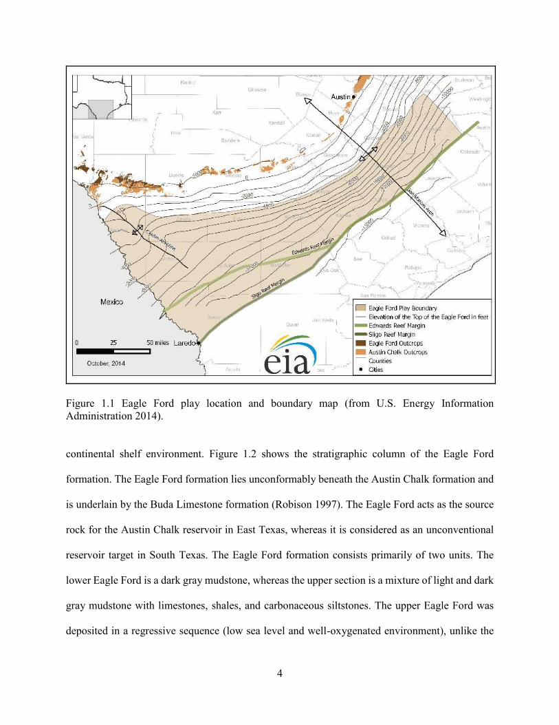
1.4 Eagle Ford Play Overview
The Eagle Ford is one of the top active oil and gas shale plays in the United States and is
the focus area of this study. The name is derived from the town of Eagle Ford in Texas, the home
where this shale outcrop formed (Eagle Ford Shale Overview 2017). Located in Southern Texas,
the play covers an area that is 50 miles wide and 400 miles long and extends from the Texas-
Mexico border southwest to above the San Marcos Arch northeast, as demonstrated in Figure 1.1.
The first discovery well in the Eagle Ford, drilled by Petrohawk Energy, dates back to 2008 in La
Salle County, Texas (Universal Royalty Company 2013). Three years later, the Eagle Ford was
considered one of the most active shale plays in the world with promptly increasing drilling
activities (Institute for Energy Research 2012). January 2018 reports showed that Eagle Ford shale
was producing at an average of more than 800,000 bbls per day during the year of 2017 (Texas
Railroad Commission 2018).
Eagle Ford depths vary from 1500 ft to 14000 ft TVD with formation thicknesses between
50 ft and 330 ft (Martin et al. 2011). The Eagle Ford formation has its highest thickness in the
Maverick Basin (southwest) and thins towards the San Marcos arch (northeast) (Hentz and Ruppel
2010).
1.4.1 Geology
The Eagle Ford formation is a sedimentary rock formation formed around 90 million years
ago in the late Cretaceous (Cenomanian-Turonian) age. The formation was deposited in a marine
4
Figure 1.1 Eagle Ford play location and boundary map (from U.S. Energy Information
Administration 2014).
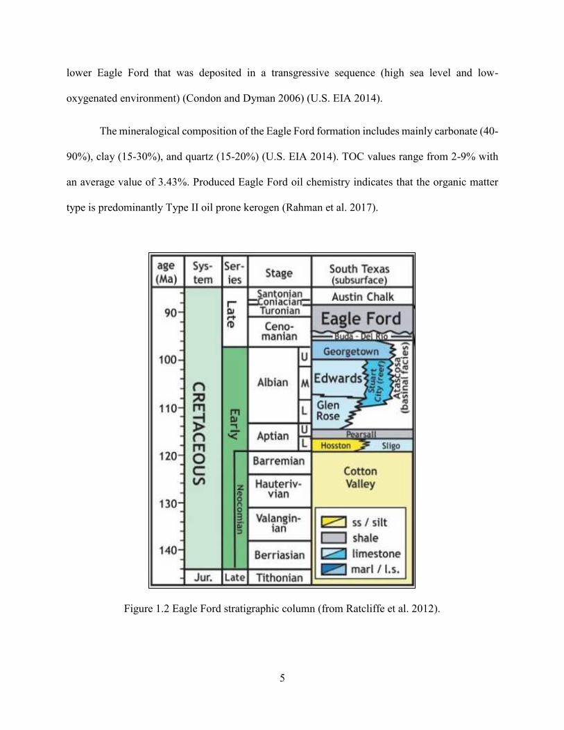
continental shelf environment. Figure 1.2 shows the stratigraphic column of the Eagle Ford
formation. The Eagle Ford formation lies unconformably beneath the Austin Chalk formation and
is underlain by the Buda Limestone formation (Robison 1997). The Eagle Ford acts as the source
rock for the Austin Chalk reservoir in East Texas, whereas it is considered as an unconventional
reservoir target in South Texas. The Eagle Ford formation consists primarily of two units. The
lower Eagle Ford is a dark gray mudstone, whereas the upper section is a mixture of light and dark
gray mudstone with limestones, shales, and carbonaceous siltstones. The upper Eagle Ford was
deposited in a regressive sequence (low sea level and well-oxygenated environment), unlike the
5
lower Eagle Ford that was deposited in a transgressive sequence (high sea level and low-
oxygenated environment) (Condon and Dyman 2006) (U.S. EIA 2014).
The mineralogical composition of the Eagle Ford formation includes mainly carbonate (40-
90%), clay (15-30%), and quartz (15-20%) (U.S. EIA 2014). TOC values range from 2-9% with
an average value of 3.43%. Produced Eagle Ford oil chemistry indicates that the organic matter
type is predominantly Type II oil prone kerogen (Rahman et al. 2017).
Figure 1.2 Eagle Ford stratigraphic column (from Ratcliffe et al. 2012).
6
1.4.2 Project Focus Area
Two wells, Well A and Well C, are used in this project. These wells were drilled in Lavaca
County, Texas. Well A targets the upper Eagle Ford/lower Austin Chalk formation, whereas the
horizontal section of Well C targets the lower Eagle Ford formation. The pilot hole of Well C
deepens down to the Del Rio formation. It is worth noting that the target for Well A can be
considered either the Lower Austin Chalk or the Upper Eagle Ford Marl, as it is hard to
differentiate between the two formations in this area due to the unconformities. Figure 1.3 indicates
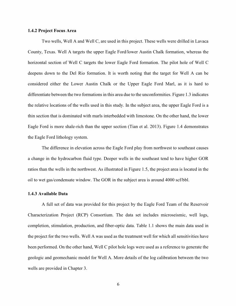
the relative locations of the wells used in this study. In the subject area, the upper Eagle Ford is a
thin section that is dominated with marls interbedded with limestone. On the other hand, the lower
Eagle Ford is more shale-rich than the upper section (Tian et al. 2013). Figure 1.4 demonstrates
the Eagle Ford lithology system.
The difference in elevation across the Eagle Ford play from northwest to southeast causes
a change in the hydrocarbon fluid type. Deeper wells in the southeast tend to have higher GOR
ratios than the wells in the northwest. As illustrated in Figure 1.5, the project area is located in the
oil to wet gas/condensate window. The GOR in the subject area is around 4000 scf/bbl.
1.4.3 Available Data
A full set of data was provided for this project by the Eagle Ford Team of the Reservoir
Characterization Project (RCP) Consortium. The data set includes microseismic, well logs,
completion, stimulation, production, and fiber-optic data. Table 1.1 shows the main data used in
the project for the two wells. Well A was used as the treatment well for which all sensitivities have
been performed. On the other hand, Well C pilot hole logs were used as a reference to generate the
geologic and geomechanic model for Well A. More details of the log calibration between the two
wells are provided in Chapter 3.
7
Figure 1.3 Relative locations of Wells A, B, and C (only Wells A and C are used in this research).
The cross signs represent the surface locations of the wells. The horizontal section of the target
well (Well A) was drilled in the northwest direction.

8
Figure 1.4 Eagle Ford lithology (from Breyer et al. 2013). Upper Eagle Ford lithology is more to
the right side of the upper bar in the graph (more calcite than clay), whereas the lower Eagle Ford
lithology is more to the left side (more clay than calcite). Well A primarily targets the Eagle Ford
Marl (between shale and limestone in the lithology bar).

9
Figure 1.5 Eagle Ford shale play (Western Gulf Basin) petroleum windows (from EIA 2010).
Formation is dipping down from NW to SE direction.
Table 1.1 Project Main Data
Well A data Well C pilot hole data
MWD logs MWD logs
Wireline logs Wireline logs
Mud logs Mud logs
Image logs Formation tops
Wellbore survey Wellbore survey
Treatment details of all 14 stages
Daily production
Fiber-optic DAS/DTS data (hydraulic
fracturing and production)

10
CHAPTER 2
LITERATURE REVIEW
This chapter focuses on the main concepts related to this research including rock
mechanics, unconventional reservoirs, and hydraulic fracturing.
2.1 Rock Mechanics Fundamentals
Rock mechanics or geomechanics is not a single field that is studied separately from other
fields of the petroleum engineering. It is rather associated with the whole process of petroleum
field development including exploration, drilling and completion, stimulation, EOR, and
production. Tutuncu (2016) defined geomechanics as “studying the response of rocks and fluids
to different factors through applying physics, solid mechanics, and mathematics”. This section
discusses the basic principles of geomechanics with a focus on the aspects related to hydraulic
fracturing.
2.1.1 Stress and Strain
Stress is defined as the force (F) applied to a surface of a cross sectional area (A), and
calculated as per Equation 2.1 (Aadnoy and Looyeh 2011). The stress component acting
perpendicular to the surface is known as the normal stress, whereas the shear stress is the
component acting parallel to the surface. If stress was the action, the reaction from the rock to that
applied stress is known as strain. Strain is defined as the resulting deformation (change in length)
divided by the original length before applying the stress and can be calculated using Equation 2.2
(Aadnoy and Looyeh 2011). The applied stress can be in the form of tension or compression where
each form results in a different strain response. Elongation of the rock is caused by tensile stress

11
whereas compressive stress causes rock shortening. The relationship between stress and strain
showing both elastic and plastic regions is demonstrated in Figure 2.1 (Cyberphysics Website
2018).
� = � (2.1)
� = ∆0 (2.2)
Where, � = stress, psi, [M][L]− [�]−
= force, lbs, [M][L][�]−
= area, in2, [L] � =strain, dimensionless ∆ = deformation (new length – original length), ft, [L] = original length, ft, [L]
2.1.2 Young’s Modulus and Poisson’s Ratio
Young’s modulus and Poisson’s ratio are two important elastic parameters that are used in
hydraulic fracture design. Young’s modulus or modulus of elasticity, E, is a material property that
indicates its stiffness. The relationship between Young’s modulus, stress, and strain is governed
by Hooke’s law as presented in Equation 2.3 (Fjar et al. 2008). This relationship represents the
slope in the stress/strain plot (refer to Figure 2.1). Under the same amount of stress, materials with
higher E will undergo a smaller deformation than materials with lower E. Economides and Martin
(2007) stated that high Young’s modulus materials are more brittle than low Young’s modulus
materials.
12
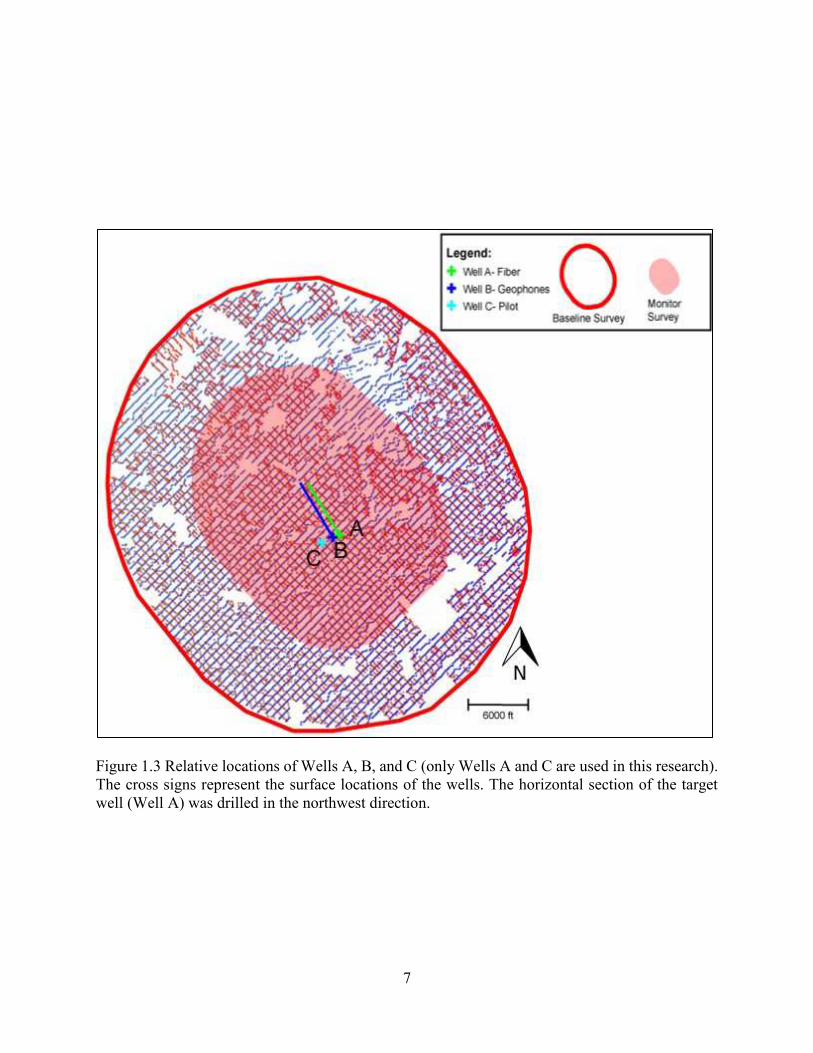
Figure 2.1 Stress and strain relationship showing both elastic and plastic regions (from
Cyberphysics Website 2018). The relationship is linear until the limit of proportionality point.
Once the stress exceeds the yield point, the material deforms plastically where the strain is
permanent (point A returns to point B not to the original curve if stress is released). The fracture
point represents the maximum strain reached before the material ruptures.
Poisson’s ratio, �, is an indication of the resulting strain in the direction perpendicular to
the applied stress compared to the strain parallel to the applied stress. Equation 2.4 is used to
calculate Poisson’s ratio, and Figure 2.2 illustrates its definition (Fjar et al. 2008).
Applying the stress will cause the material to shrink longitudinally and stretch transversely. Hence,
the strain ratio will be negative and Poisson’s ratio will be positive. Theoretically, the values of
Poisson’s ratio range from 0 to 0.5. However, negative values of Poisson’s ratio have been
observed in single crystals where compression occurs along the applied stress axis and all other
directions (Svetlov et al. 1988; Christensen 1996). Measurements of Young’s modulus and
Poisson’s ratio can be static (lab measurements) or dynamic (log measurements).

13
= �� (2.3) � = − �� � � (2.4)
Where,
= Young’s modulus, psi, [M][L]− [�]− � = Poisson’s ratio, dimensionless � =transverse strain, dimensionless � =longitudinal strain, dimensionless
Figure 2.2 Left: material before applying stress; Right: material after applying stress (from Fjar et
al. 2008). Stress caused the material to shrink parallel to stress direction and stretch perpendicular
to it. Poisson’s ratio represents the negative ratio of transverse strain to longitudinal strain.
2.1.3 In-Situ Stresses
This section presents the main stresses and pressures that affect the formation and should
be accounted for in hydraulic fracture designs.

14
2.1.3.1 Overburden Stress
Overburden stress or vertical stress, � , accounts for the weight of the overlying rock and
fluid. It can be calculated using Equation 2.5 (Varela-Pineda et al. 2015). The weight increases
with depth and so does the overburden stress. Rock density is generally obtained from a density
log.
� = ∫ � � (2.5)
Where,
� = overburden stress, psi, [M][L]− [�]− �= overlying rock density, lbm/in3, [M][L]−
= acceleration due to gravity, in/s2, [L][�]−
= depth, in, [L] 2.1.3.2 Horizontal Stresses
Maximum horizontal stress, ��, and minimum horizontal stress, �ℎ, are the stresses acting
on the formation horizontally in the x-y plane perpendicular to the overburden stress. The three
mutually-perpendicular stresses are related through Hooke’s law as presented in Equation 2.6
(Economides and Martin 2007). The relationship between these stresses also defines the in-situ
stress state. Table 2.1 indicates the different faulting regimes according to the relationship between
the three normal stresses (Golombek 1985). Knowing the stress state is essential for the placement
of horizontal wells that are planned to be hydraulically fractured.
� = [� − � � + � ] (2.6)
Where,
� = strain at the x direction, dimensionless � = stress at the x direction, psi, [M][L]− [�]−
15
� = stress at the y direction perpendicular to x and z directions, psi, [M][L]− [�]− � = stress at the z direction perpendicular to x and y directions, psi, [M][L]− [�]−
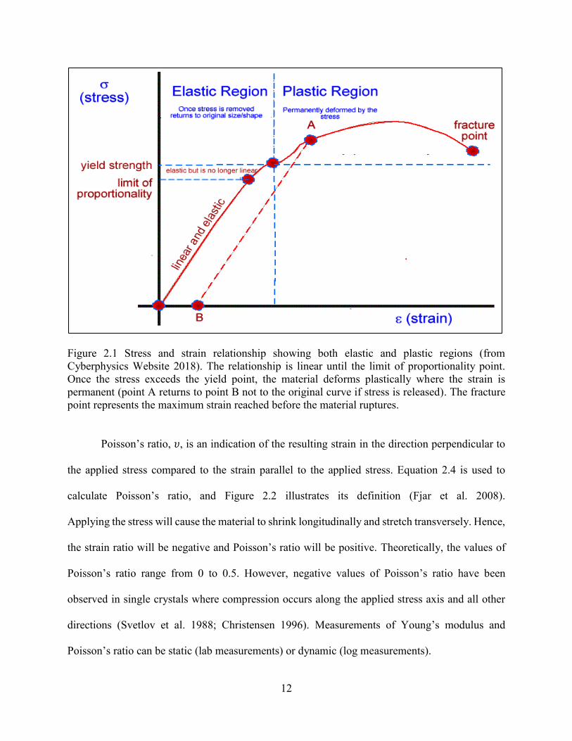
Table 2.1 Faulting Regimes Based on Stress State (modified from Golombek 1985)
Stress state Faulting regime � > �� > �ℎ Normal faulting �� > �ℎ > � Reverse faulting �� > � > �ℎ Strike-slip faulting
2.1.3.3 Pore Pressure
Pore pressure, , accounts for the fluid pressure existent in the porous rock. Knowing the
pore pressure is important in calculating the effective stress using Terzaghi’s law as per Equation
2.7 (Terzaghi 1925). Biot’s coefficient (Biot 1941) or poroelastic constant, �, determines how
much pore pressure influences the effective stress. It ranges between 0 and 1. Knowledge of the
in-situ stresses, pressures, and elastic parameters are critical in determining fracture closure
pressure as per Equation 2.8 (Barree et al. 2009). Fracture closure pressure, , below which the
hydraulic fracture closes, is equivalent to the minimum horizontal stress, �ℎ, as the fracture opens
against �ℎ direction.
� = � − � (2.7) = − [� − � ] + �ℎ + � + � (2.8)
Where,
= fracture closure pressure, psi, [M][L]− [�]−
� = effective stress, psi, [M][L]− [�]− �= Biot’s coefficient, dimensionless
= reservoir pore pressure, psi, [M][L]− [�]− � = vertical Biot’s coefficient, dimensionless
16
�ℎ= horizontal Biot’s coefficient, dimensionless � = regional horizontal strain, dimensionless � = horizontal tectonic stress, psi, [M][L]− [�]−
2.2 Unconventional Reservoirs
Unconventional reservoirs are commonly defined as those that require unconventional
technology to be developed. Others may define unconventional reservoirs by setting a permeability
threshold value (e.g. 0.1 md) (Meckel and Thomasson 2008). Cander (2012) defined
unconventional reservoirs based on permeability and viscosity. Figure 2.3 illustrates a graphical
presentation of this definition. The figure suggests that technology has to be used to alter either
permeability or viscosity in unconventional reservoirs to produce them commercially.
Shale hydrocarbons are a major unconventional resource worldwide and in the United
States. The decline in conventional oil and gas production plus technology advancements helped
shale hydrocarbon production to boom in the US since the beginning of this century. Figure 2.4
shows the shale plays in the lower 48 states of the US. Shale characteristics vary from one play to
another and heterogeneities can be observed within the same basin. Therefore, formation damage
mechanisms and stimulation treatments that apply to one shale may not be applicable to another
(Davis 2011). Generally, shale reservoirs are sedimentary rocks interbedded with carbonaceous
and siliceous minerals. Shale gas in these reservoirs comes in three forms: free gas, adsorbed gas,
and gas from natural fracture systems (Economides and Martin 2007). Passey et al. (2012) stated
that most producing shale reservoirs contain Type I or Type II kerogen.
2.3 Hydraulic Fracturing in Horizontal Wells
Drilling horizontal wells induces damage to the reservoir. Bypassing the formation damage
and enhancing low permeability require hydraulic fracturing, which is the completion approach in
17
nearly all horizontal wells drilled in shale reservoirs.
Figure 2.3 Unconventional resources versus conventional resources (from Cander 2012).
Unconventional reservoirs are characterized with low permeability/viscosity ratio where either
permeability or viscosity need to be altered for them to be produced commercially.
2.3.1 Types of Hydraulic Fractures in Horizontal Wells
As described earlier in Section 2.1.3, the three in-situ stresses are overburden, minimum
horizontal, and maximum horizontal stresses. Hydraulic fractures in horizontal wells can be
divided into three types accordingly, transverse, longitudinal, and oblique fractures. Fractures,
generally, tend to open against minimum horizontal stress as it is the path of least resistance. When
the well is drilled in the minimum horizontal stress direction, transverse fractures will be created
as they propagate perpendicular to the wellbore direction. On the other hand, when the well is
drilled perpendicular to the minimum horizontal stress direction, a longitudinal fracture will grow

18
along the direction of the horizontal lateral. Oblique fractures occur when the well is drilled
orthogonal to the minimum and maximum horizontal stress directions. Figure 2.5 demonstrates
the three types of hydraulic fractures in horizontal wells based on their direction of growth. The
most common completion technique in horizontal shale wells is the creation of multiple transverse
fractures. However, Economides and Martin (2007) presented a criterion shown in Table 2.2 for
selecting the type of fracture based on gas reservoir permeability. Both transverse and longitudinal
fractures are single planar fractures. Most shale reservoirs, however, contain complex fracture
networks that involve natural fractures.
Table 2.2 Permeability-based Options for Fracturing Gas Wells (modified from Economides and
Martin 2007)
Permeability range, md Best technical solution > Horizontal wellbore, longitudinal fractures . �� Horizontal wellbore, longitudinal fractures or
vertical wellbore with fracture . �� . Horizontal wellbore, transverse fractures < . Horizontal wellbore, transverse fractures or
vertical wellbore with fracture
2.3.2 Hydraulic Fracture Modes
There are three fracture modes that are characterized based on the force that caused the
crack to open. These modes are Mode I (opening or tensile), Mode II (sliding or in-plane shearing),
and Mode III (tearing or anti-plane shearing). Figure 2.6 shows the three fracture modes. In Mode
I, fractures open against minimum horizontal stress. Modes II and III include shear fractures and
faults (Kanninen and Popelar 1985).
2.3.3 Hydraulic Fracture Modeling
Hydraulic fracture models are constructed to help design fracture stimulation treatments in
a way that they can predict fracture geometry, fracture cleanup, or long-term fractured well

19
performance (Nghiem et al. 1984). Hydraulic fracture models can be broadly categorized into two-
dimensional (2D) and three-dimensional (3D) models (Rahman and Rahman 2010).
Figure 2.4 US lower 48 states shale oil and gas plays (from EIA 2016).
2.3.3.1 2D Fracture Models
2D fracture models assume that fracture is contained, thus only fracture width and length
are the varying dimensions as fracture height is kept constant. Two of the early main 2D fracture
models are the Perkins-Kern-Nordgren (PKN) (Perkins and Kern 1961) and the Khristianovich-
Geertsma-DeKlerk (KGD) (Khristianovich and Zheltov 1955) models. Figure 2.7 illustrates the
difference between the two models. In the PKN model, strain is in the vertical plane. Meaning,
hydraulic fracture width changes with fracture height. The PKN model assumes an elliptical
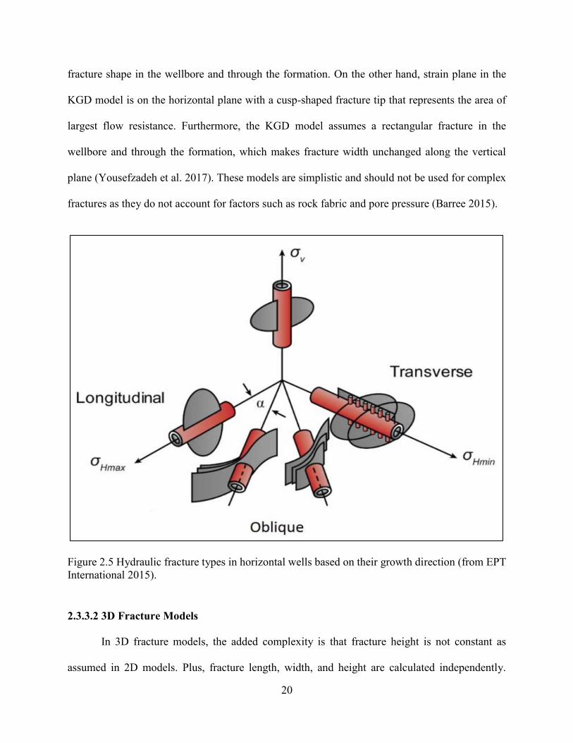
20
fracture shape in the wellbore and through the formation. On the other hand, strain plane in the
KGD model is on the horizontal plane with a cusp-shaped fracture tip that represents the area of
largest flow resistance. Furthermore, the KGD model assumes a rectangular fracture in the
wellbore and through the formation, which makes fracture width unchanged along the vertical
plane (Yousefzadeh et al. 2017). These models are simplistic and should not be used for complex
fractures as they do not account for factors such as rock fabric and pore pressure (Barree 2015).
Figure 2.5 Hydraulic fracture types in horizontal wells based on their growth direction (from EPT
International 2015).
2.3.3.2 3D Fracture Models
In 3D fracture models, the added complexity is that fracture height is not constant as
assumed in 2D models. Plus, fracture length, width, and height are calculated independently.

21
Therefore, blocks can be assigned unlike pseudo 3D models where only layers can be assigned
and no lateral changes are accounted for. Some 3D fracture models allow for de-coupling to
account for shear slippage (Mode II and III fractures). 3D fracture models use finite difference
(FD) solution or finite element (FE) solutions (Miskimins 2017).
Figure 2.6 Hydraulic fracture modes: (a) Mode I, opening or tensile mode; (b) Mode II, sliding or
in-plane shearing mode; (c) Mode III, tearing or anti-plane shearing mode (from Kanninen and
Popelar 1985).
2.3.4 Natural Fractures
Natural fractures refer to pre-existing fractures that were created over geologic time
(millions of years). The presence of natural fractures increases porosity and can enhance
permeability if these fractures are interconnected. In unconventional reservoirs, multi-stage
hydraulic fracturing of horizontal wells is sought to rejuvenate natural fractures, thus creating a
larger fracture network (Kazemi 2017). However, connecting to natural fractures in low-
permeability reservoirs can cause a high fluid leakoff (Yew and Wing 2014). Simulating natural
fractures requires utilizing discrete fracture network (DFN) models. Natural fractures are very

22
common in shale reservoirs, which makes the fracture network more complex due to their
interaction with hydraulic fractures, as presented in Figure 2.8.
Figure 2.7 PKN versus KGD 2D hydraulic fracture models (from Montgomery and Smith 2010).
The PKN model (left) assumes elliptical fracture in wellbore and through formation. The KGD
model (right) assumes rectangular fracture in wellbore and through formation.
2.3.5 Design and Treatment Schedule
Hydraulic fracture design is a critical step in the stimulation process. It involves many
variables such as fluid selection, proppant selection, types of additives, fluid and proppant rates,
volumes, and concentrations. These variables differ from field to field and even within the same
field based on the target reservoir. Hydraulic fracturing aims at removing the skin, initiating or
enhancing productivity, and ultimately increasing net present value (NPV). One of the important
parameters that reflects the success of a fracturing treatment is the dimensionless fracture
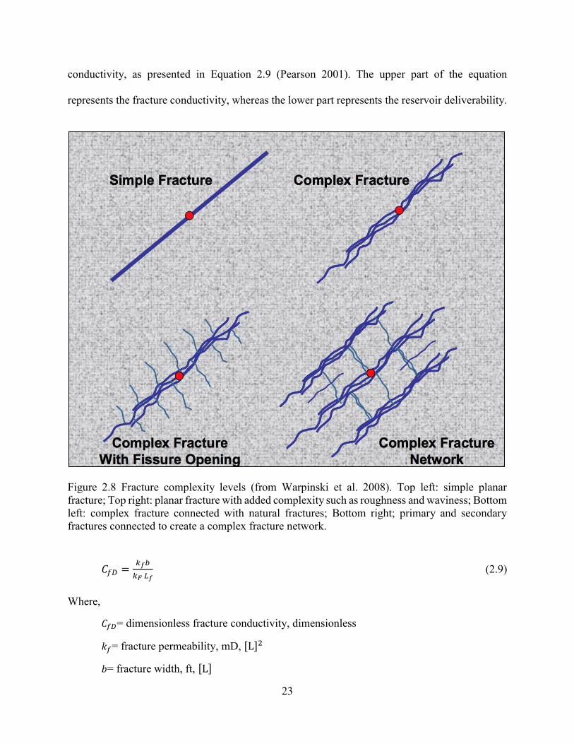
23
conductivity, as presented in Equation 2.9 (Pearson 2001). The upper part of the equation
represents the fracture conductivity, whereas the lower part represents the reservoir deliverability.
Figure 2.8 Fracture complexity levels (from Warpinski et al. 2008). Top left: simple planar
fracture; Top right: planar fracture with added complexity such as roughness and waviness; Bottom
left: complex fracture connected with natural fractures; Bottom right; primary and secondary
fractures connected to create a complex fracture network.
= � (2.9)
Where,
= dimensionless fracture conductivity, dimensionless
= fracture permeability, mD, [L]
= fracture width, ft, [L]

24
= formation permeability, mD, [L]
= fracture half-length, ft, [L]
Proppant fracturing is usually associated with sandstones whereas acid fracturing is
associated with carbonates. A typical proppant fracturing treatment consists of four primary stages.
The first one is the pre-pad stage which aims at cooling the wellbore and conditioning the
formation. The second stage is the pad stage where the main fracturing fluid is injected along with
the required additives. The third one is the proppant laden where the proppant get transported and
placed into the fracture. The last one is the flush stage where any remaining slurry in the wellbore
gets displaced into the formation (Abass 2016).
2.3.5.1 Fracturing Fluid Selection
Fracturing fluids can be water-based, oil-based, or a mixture of both. The properties that
qualify a fluid to be selected for fracturing are formation compatibility, rheology, fluid loss,
breaking capability (viscosity reduction), proppant-carrying capacity (sufficient viscosity), residue
in the proppant pack, and filter-cake residue (Economides et al. 1998). As the main function of the
fluid besides creating the fracture is transporting the proppant, there are two proppant
transportation mechanisms. The first one is through utilizing highly viscous fluids for transporting
the proppant. This method is usually used in low to moderate permeability reservoirs. The other
method, which is used in low permeability reservoirs, is utilizing velocity instead of viscosity
where the fracturing fluid (usually water) is pumped at a high velocity (Al-Muntasheri 2014). In
this case, the most common fracturing fluid is fresh water or slickwater. Additives for viscous
systems include gelling agents, friction reducers, clay control agents, crosslinkers, breakers, iron
control agents, corrosion and scale inhibitors, surfactants, buffers, and biocides/bactericides
(Montgomery 2013). Table 2.3 presents the most common water-based and oil-based fracturing

25
fluids and their characteristics. Table 2.4 shows different types of fracturing fluid additives, their
functions, and examples of each.
2.3.5.2 Proppant Selection
After generating the hydraulic fracture and the fracture pressure is released, the purpose of
the pumped proppant is to provide conductivity in the created fracture. Proppants can be of a basic
type such as sand and ceramic or a modified type such as resin coated proppant (RCP) and
lightweight proppant (Liang et al. 2016). The proppant selection criterion is based on different
factors such as cost, associated fluid system, and conductivity requirements in the formation
(Palisch 2012). The proppant quality can measured in the lab by conducting different proppant
pack conductivity tests such as API RP61 (API 1989) and API RP19D (API 2008) (Duenckel et
al. 2016). Figure 2.9 illustrates the variations in conductivity among different types of proppants.
Usually, the proppant pack conductivity tests yield optimistic results compared to the later field
performance. This difference is attributed to different damage mechanisms. These damage
mechanisms include non-Darcy flow, multiphase flow, reduced proppant concentration, gravity
and viscous segregation, filter-cake and gel residue, embedment, and spalling (Barree et al. 2003;
Palisch et al. 2007).
2.3.6 Hydraulic Fracture Monitoring
There are various techniques to monitor and map hydraulic fracture jobs and the reservoir
response to them. These techniques include diagnostic fracture injection tests (DFITs), tracers
(radioactive and non-radioactive), surface and downhole tiltmeters, fiber optics (DTS and DAS),
and microseismic monitoring (Bhatnagar 2016). This section reviews DFITs and the distributed
acoustic sensing (DAS)/distributed temperature sensing (DTS), which utilize fiber optics, due to
their relevance to the thesis topic.
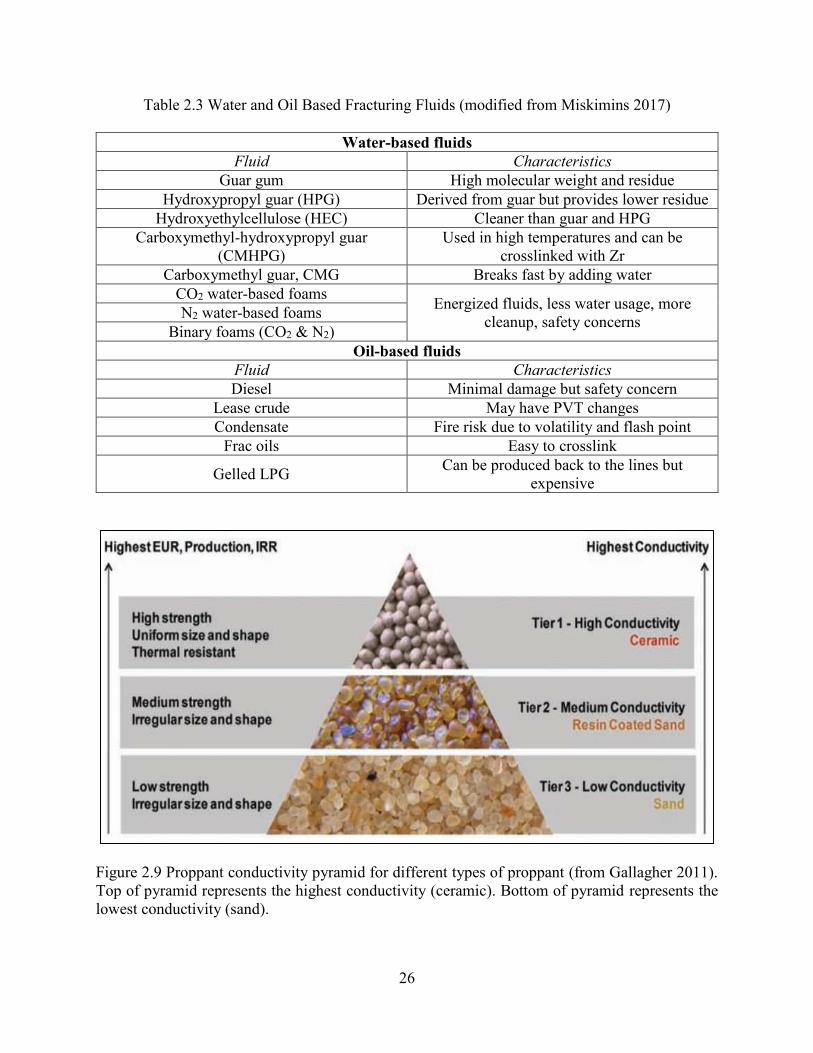
26
Table 2.3 Water and Oil Based Fracturing Fluids (modified from Miskimins 2017)
Water-based fluids
Fluid Characteristics
Guar gum High molecular weight and residue
Hydroxypropyl guar (HPG) Derived from guar but provides lower residue
Hydroxyethylcellulose (HEC) Cleaner than guar and HPG
Carboxymethyl-hydroxypropyl guar
(CMHPG)
Used in high temperatures and can be
crosslinked with Zr
Carboxymethyl guar, CMG Breaks fast by adding water
CO2 water-based foams Energized fluids, less water usage, more
cleanup, safety concerns N2 water-based foams
Binary foams (CO2 & N2)
Oil-based fluids
Fluid Characteristics
Diesel Minimal damage but safety concern
Lease crude May have PVT changes
Condensate Fire risk due to volatility and flash point
Frac oils Easy to crosslink
Gelled LPG Can be produced back to the lines but
expensive
Figure 2.9 Proppant conductivity pyramid for different types of proppant (from Gallagher 2011).
Top of pyramid represents the highest conductivity (ceramic). Bottom of pyramid represents the
lowest conductivity (sand).

27
Table 2.4 Fracturing Fluid Additives (modified from Abass 2016)
Additive Purpose Examples
Gelling agent Provides viscosity for
proppant transportation Linear gel, Guar, HEC
Crosslinker Provides even greater
viscosity for shearing Borate, zirconate
Breaker Breaks the crosslinked gel for
cleanup
Enzymes, acids,
oxidizers
Surfactant Reduces friction and polymer
residue Methanol, isopropanol
Friction reducer Reduces friction at high
velocity Polyacrylamide
Clay control agent Prevents clay swelling KCl
Iron control agent Prevents precipitation Citric acid
Fluid loss control agent Provides less filtration CaCO3
pH buffer Controls pH to condition fluid
for additives Acetic acid
Corrosion inhibitor Prevents corrosion n-dimethyl formamide
Scale inhibitor Prevents scale precipitation Ammonium chloride
Biocides/bactericides Prevents growth of organisms Gluteraldehyde
2.3.6.1 Diagnostic Fracture Injection Tests (DFITs)
A DFIT is a test pumped prior to performing the main hydraulic fracture for the purpose
of acquiring data about treatment parameters and characterizing the target reservoir. The reservoir
characterization part is what makes DFITs different from traditional mini-frac tests. DFITs are
very common in unconventional reservoirs as they substitute conventional transient analysis tests,
which take long time to run, by providing the falloff data (Barree et al. 2015). A DFIT procedure
starts with pumping at a certain rate to breakdown. Then, the rate is increased and kept constant
for few minutes. Rate step down data can be gathered to determine near wellbore frictions and
fracture extension pressure. Lastly, the falloff portion is used to determine closure pressure and
leakoff mechanism (Barree et al. 2015). Figure 2.10 demonstrates the procedure of a generic DFIT.
DFITs are analyzed using different techniques for closure and after closure parts of the test.
The closure analysis includes G-time function plot of pressure and its derivatives, square root of

28
time plot of pressure and its derivatives, and log-log plot of pressure change and its derivatives
after shut-in (Barree et al. 2009). Each of these plots has its unique signature to determine closure
pressure for the four leakoff mechanisms which are normal leakoff, pressure dependent leakoff
(PDL), fracture tip extension, and height recession or transverse storage (Barree et al. 2009). The
after closure analysis is used to determine reservoir transmissibility and pore pressure.
Figure 2.10 Generic DFIT procedure (from Barree et al. 2015). The black curve represents the
fluid rate that starts low then increases before it ends with a step down until shut-in. The red curve
represents the surface pressure.
2.3.6.2 DAS/DTS Surveys
Distributed acoustic sensing (DAS) and distributed temperature sensing (DTS) surveys are
determined from fiber optic cables that can be deployed in coiled tubing or a by wireline or can be
permanently installed along the back of the casing and cemented in place (Huckabee 2009;
Bhatnagar 2016). A DTS survey is run for the purpose of collecting temperature traces along the
29
wellbore at different times (e.g. completion, stimulation, production) where these temperature
recordings can be later correlated to flow allocation in the reservoir (Kalia et al. 2014). Moreover,
DTS surveys can help identify zonal isolation and fluid communications between stages by
detecting plug leakages in a plug and perf completion (Holley and Kalia 2015; Wheaton et al.
2016).
DAS surveys record the acoustic activities during the different stages of the well life. These
recordings in turn can provide information such as fluid and proppant distributions for different
perforation clusters along the wellbore at stimulation time (Molenaar et al. 2011). Using the
acoustic response, computer algorithms are used to generate quantitative data that present DAS
flow rate total placed proppant in each cluster. Such analysis can be used to assess cluster
efficiency and identify, if any, the existence of clusters that were not effectively stimulated (Holley
and Kalia 2015). Figure 2.11 shows an example of DAS/DTS data captured during a hydraulic
fracturing stimulation treatment. Cooler colors in the DTS test imply fracturing fluids passing
through the cluster. On the other hand, warmer colors in the DAS test refer to high acoustic activity
which implies fluid and proppant passing through the cluster.
2.3.7 Stress Shadow Phenomenon
Introducing a crack or a hydraulic fracture in a rock requires the tensile failure of the subject
rock, which results in changing the stress state around the created crack. The difference between
the pressure of the fracturing fluids and the in-situ minimum horizontal stress constitutes the net
pressure inside the fracture which applies a compressive stress on the surrounding rock. The newly
induced additional stress surrounding the fracture is referred to as a “stress shadow” (Fisher et al.
2004).

30
Figure 2.11 DAS/DTS data (from Wheaton et al. 2016). Top: DTS data changes with time (warmer
colors denote higher temperatures); Middle: DAS data changes with time (warmer colors denote
higher acoustic activity); Bottom: treatment plot showing different curves versus time (black curve
represents rate, dark blue curve represents surface pressure, light blue curve represents bottomhole
pressure, and green curves represents surface and bottomhole proppant concentrations).
2.3.7.1 Impact of Stress Shadowing on Fracture Propagation
In the case of multiple transverse fractures in a horizontal well, the first hydraulic fracture
will open against a minimum horizontal stress of a specific magnitude. The creation of this fracture
will increase the magnitude of the minimum horizontal stress around it. Therefore, a second
hydraulic fracture within the stress shadow extent will need to open against a larger closure
pressure which will limit its growth. A third hydraulic fracture will try to open against a closure
stress whose magnitude is affected by the cumulative stress shadow from both preceding fractures
31
(Fisher et al. 2004; Daneshy 2017). Adding fractures in the stress shadow area of extent will result
in subsequent fractures with limited propagation and less productivity than desired. The
propagation of the middle fractures in a horizontal wellbore will be reduced as they experience
larger magnitudes of closure pressure than the heel and toe fractures. Therefore, the middle
fractures are not expected to contribute to production as much as the outer fractures (Fisher et al.
2004; Wheaton et al. 2014; Barree 2015; Manchanda et al. 2016). Figure 2.12 demonstrates how
the propagation of the middle fractures is hampered by the stress shadow of the heel and toe
fractures. Stress shadowing and fracture propagation are always associated with hydraulic fracture
spacing due its effect on determining the severity of stress shadowing (Ingram et al. 2014).
Hydraulic fracture spacing optimization is discussed in Section 2.3.10.
2.3.7.2 Factors Influencing Stress Shadowing
Studies show that many variables can play a role in altering the stress state, magnitude and
orientation, around a fracture, thus impacting the hydraulic fracture propagation. These variables
include cluster spacing, number of clusters, perforation parameters, reservoir permeability,
mechanical properties, vertical and lateral heterogeneity, reservoir depletion, net pressure, fracture
geometry, original in-situ minimum/maximum horizontal stress ratio, and shut-in time between
stages (Roussel and Sharma 2011; Morrill and Miskimins 2012; Manchanda et al. 2016; Daneshy
2017). Figure 2.13 illustrates the importance of lateral heterogeneity in influencing the stress
shadow. The fractures that propagate in a zone of larger Young’s modulus and a much larger
Poisson’s ratio were able to propagate further even if they were middle fractures. This explains
how the stress shadow effect was minimized by the lateral heterogeneity between the propagating
fractures (Manchanda et al. 2016).

32
Figure 2.12 Effect of stress shadowing in multiple transverse fractures (from Fisher et al. 2004).
Top part shows a top view of a hydraulic fracture where fracture length propagation is limited by
stress shadowing. Bottom part shows a side view of a hydraulic fracture where fracture height is
limited by stress shadowing.
Figure 2.13 Stress shadow effect minimized by lateral heterogeneity between propagating fractures
(from Manchanda et al. 2016). Left two windows show Young’s modulus effect. Right two windows show Poisson’s ratio effect.
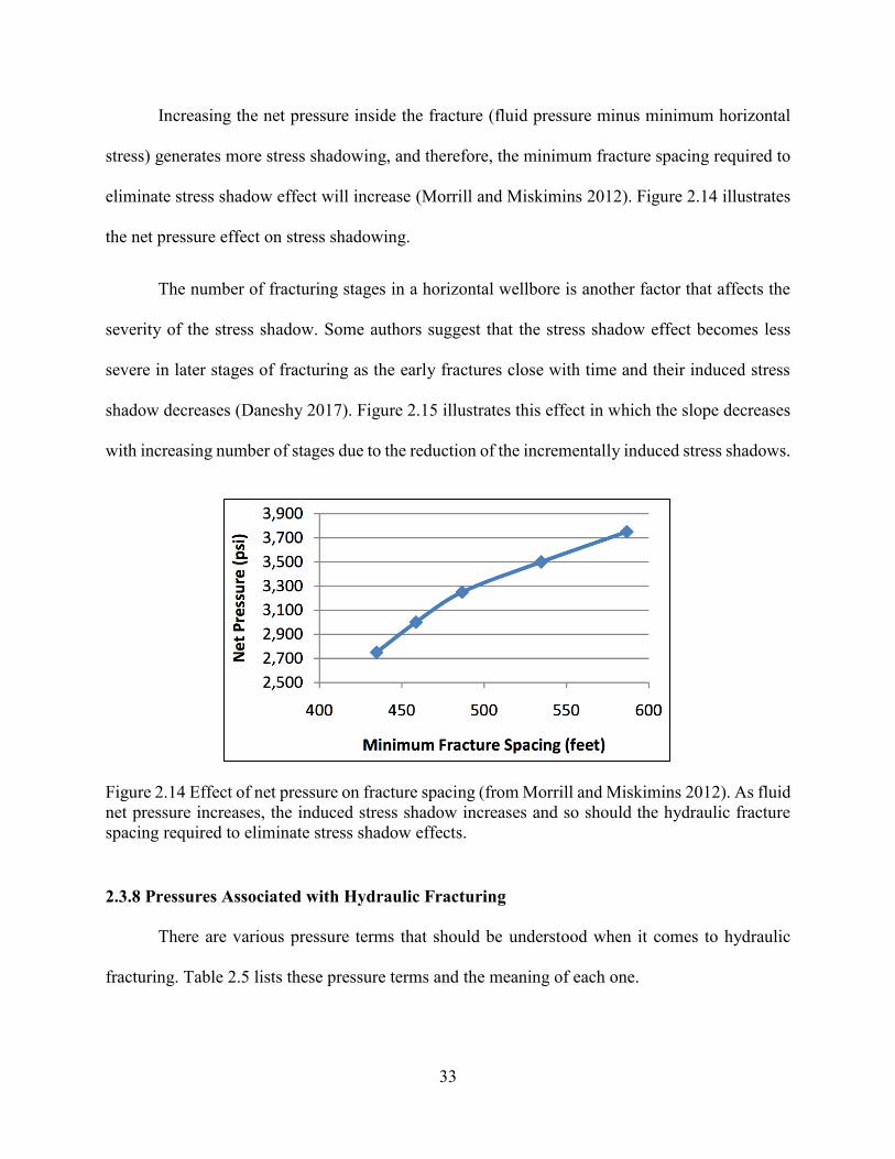
33
Increasing the net pressure inside the fracture (fluid pressure minus minimum horizontal
stress) generates more stress shadowing, and therefore, the minimum fracture spacing required to
eliminate stress shadow effect will increase (Morrill and Miskimins 2012). Figure 2.14 illustrates
the net pressure effect on stress shadowing.
The number of fracturing stages in a horizontal wellbore is another factor that affects the
severity of the stress shadow. Some authors suggest that the stress shadow effect becomes less
severe in later stages of fracturing as the early fractures close with time and their induced stress
shadow decreases (Daneshy 2017). Figure 2.15 illustrates this effect in which the slope decreases
with increasing number of stages due to the reduction of the incrementally induced stress shadows.
Figure 2.14 Effect of net pressure on fracture spacing (from Morrill and Miskimins 2012). As fluid
net pressure increases, the induced stress shadow increases and so should the hydraulic fracture
spacing required to eliminate stress shadow effects.
2.3.8 Pressures Associated with Hydraulic Fracturing
There are various pressure terms that should be understood when it comes to hydraulic
fracturing. Table 2.5 lists these pressure terms and the meaning of each one.
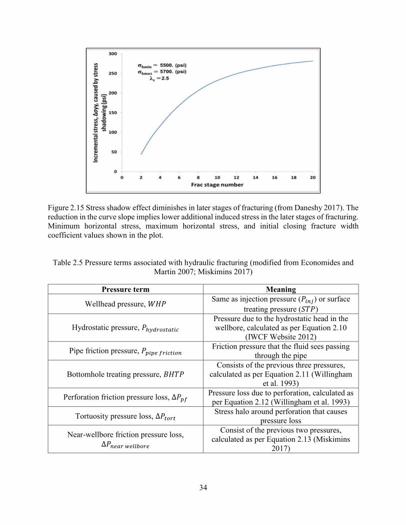
34
Figure 2.15 Stress shadow effect diminishes in later stages of fracturing (from Daneshy 2017). The
reduction in the curve slope implies lower additional induced stress in the later stages of fracturing.
Minimum horizontal stress, maximum horizontal stress, and initial closing fracture width
coefficient values shown in the plot.
Table 2.5 Pressure terms associated with hydraulic fracturing (modified from Economides and
Martin 2007; Miskimins 2017)
Pressure term Meaning
Wellhead pressure, Same as injection pressure ( ) or surface
treating pressure ( )
Hydrostatic pressure, ℎ Pressure due to the hydrostatic head in the
wellbore, calculated as per Equation 2.10
(IWCF Website 2012)
Pipe friction pressure, Friction pressure that the fluid sees passing
through the pipe
Bottomhole treating pressure,
Consists of the previous three pressures,
calculated as per Equation 2.11 (Willingham
et al. 1993)
Perforation friction pressure loss, ∆ Pressure loss due to perforation, calculated as
per Equation 2.12 (Willingham et al. 1993)
Tortuosity pressure loss, ∆ Stress halo around perforation that causes
pressure loss
Near-wellbore friction pressure loss, ∆
Consist of the previous two pressures,
calculated as per Equation 2.13 (Miskimins
2017)
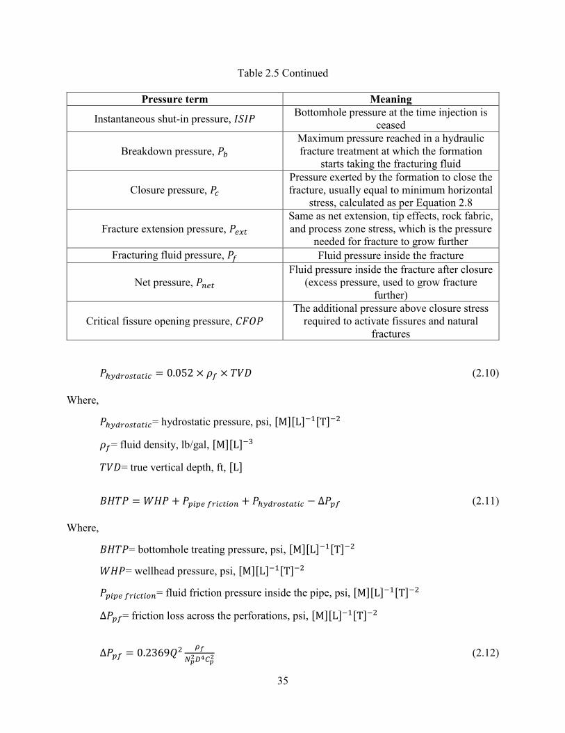
35
Table 2.5 Continued
Pressure term Meaning
Instantaneous shut-in pressure, Bottomhole pressure at the time injection is
ceased
Breakdown pressure,
Maximum pressure reached in a hydraulic
fracture treatment at which the formation
starts taking the fracturing fluid
Closure pressure,
Pressure exerted by the formation to close the
fracture, usually equal to minimum horizontal
stress, calculated as per Equation 2.8
Fracture extension pressure,
Same as net extension, tip effects, rock fabric,
and process zone stress, which is the pressure
needed for fracture to grow further
Fracturing fluid pressure, Fluid pressure inside the fracture
Net pressure,
Fluid pressure inside the fracture after closure
(excess pressure, used to grow fracture
further)
Critical fissure opening pressure,
The additional pressure above closure stress
required to activate fissures and natural
fractures
ℎ = . × � × (2.10)
Where,
ℎ = hydrostatic pressure, psi, [M][L]− [�]− � = fluid density, lb/gal, [M][L]−
= true vertical depth, ft, [L] = + + ℎ − ∆ (2.11)
Where,
= bottomhole treating pressure, psi, [M][L]− [�]−
= wellhead pressure, psi, [M][L]− [�]−
= fluid friction pressure inside the pipe, psi, [M][L]− [�]− ∆ = friction loss across the perforations, psi, [M][L]− [�]−
∆ = . 9 �2 4 2 (2.12)
36
Where,
= total flow rate, bbl/min, [L] [�]−
= number of perforations, dimensionless
= perforation diameter, in, [L] = coefficient of discharge, dimensionless
∆ = ∆ + ∆ (2.13)
Where,
∆ = near wellbore pressure loss, psi, [M][L]− [�]− ∆ = pressure loss due to tortuosity, psi, [M][L]− [�]−
2.3.9 Engineered Completion
The traditional way of completing horizontal wells in unconventional shale reservoirs
applies geometric designs in spacing perforation clusters. Geometric completion designs place
perforation clusters or fracture stages in a uniform spacing pattern without accounting for the
lateral heterogeneity of reservoir properties along the horizontal wellbore. However, these lateral
variations can play a vital role in stimulation results and production performance of horizontal
wells (Ajisafe et al. 2014). Besides stress shadowing, geometric completion design is another
possible reason for the uneven contribution of perforation clusters or fracture stages to production.
As a result, recent designs deployed engineered completion as a replacement of geometric
completion.
Engineered completions seek to optimize hydraulic fracture staging and perforation cluster
spacing by considering the petrophysical and geomechanical variations of the adjoining rocks
along the lateral. By acquiring characteristic log data along the lateral, an engineered completion
workflow can be applied to quantify rock quality and completion quality. This is performed
through the calculation of parameters such as breakdown pressure, productivity index, and

37
fracability index from the raw log data (Anifowoshe et al. 2016; Sarmah et al. 2016).
Consequently, engineered completion workflow places perforation clusters in the best quality
rocks. It may not lead to uniform spacing but should result in a more uniform contribution to
production from perforation clusters. DAS/DTS tests run in fiber optic cables can be used in
engineered completions to corroborate the feasibility of the design by quantifying each
stage/cluster individual contribution to production. These tests showed a 30% increase in
production performance of wells completed with the engineered approach compared to the ones
completed with the geometric approach (Sun et al. 2015). Engineered completions are also more
cost-efficient as they reduce the number of perforation clusters by excluding the poor-quality rock
from the perforation process.
2.3.10 Spacing Optimization
The induced stress created by the net pressure inside the hydraulic fracture has its
maximum value at the fracture face. The magnitude of the stress shadow diminishes when moving
away from the fracture face as that energy dissipates with distance (Fisher et al. 2004). Therefore,
placing hydraulic fractures far apart will minimize or eliminate the stress shadow effect. However,
further placement of these fractures could leave parts of the reservoir unstimulated. Therefore, it
is very critical to find the fracture spacing that accounts for both factors. Figure 2.16 shows how
different values of cluster spacing can affect fracture propagation due to stress interference (Lu
2016). The 10 m spacing shows a clear dominance of the outer fractures on the middle one whereas
the 50 m spacing shows almost even propagation in all fractures. The colored scale represents the
scalar stiffness degradation variable (SDEG), which is a measure of how damaged the element is.
Zero SDEG means that the element is not damaged, which implies no fracture extension to the

38
subject zone, whereas a value of 1 SDEG indicates that the element is totally damaged (i.e. the
fracture is completely open).
Considering only the stress shadow effect is not sufficient to obtain the optimum hydraulic
fracture or perforation cluster spacing. Uniform spacing with minimized stress interference will
still show uneven production contribution if reservoir rock quality is not considered. Therefore,
the stress shadow effect has to be coupled with reservoir rock quality lateral variations in order to
come up with the most optimized fracture spacing. This can be achieved through the application
of engineered completion design. Figure 2.17 illustrates a comparison between geometric
completion and engineered completion along with respective logs and other calculated parameters
(Ajisafe et al. 2014). Overall, the engineered completion showed a uniform contribution to
production from perforation clusters when compared to the geometric completion.
Figure 2.16 Effect of cluster spacing on fracture propagation due to stress shadow (left: 10m
spacing vs. right: 50m spacing) (from Lu 2016). SDEG means scalar stiffness degradation variable
(SDEG), which is a measure of how damaged the element is. Outer fractures are dominant in the
10 m spacing case, whereas all fractures are equal in terms of dominance in the 50 m spacing case.
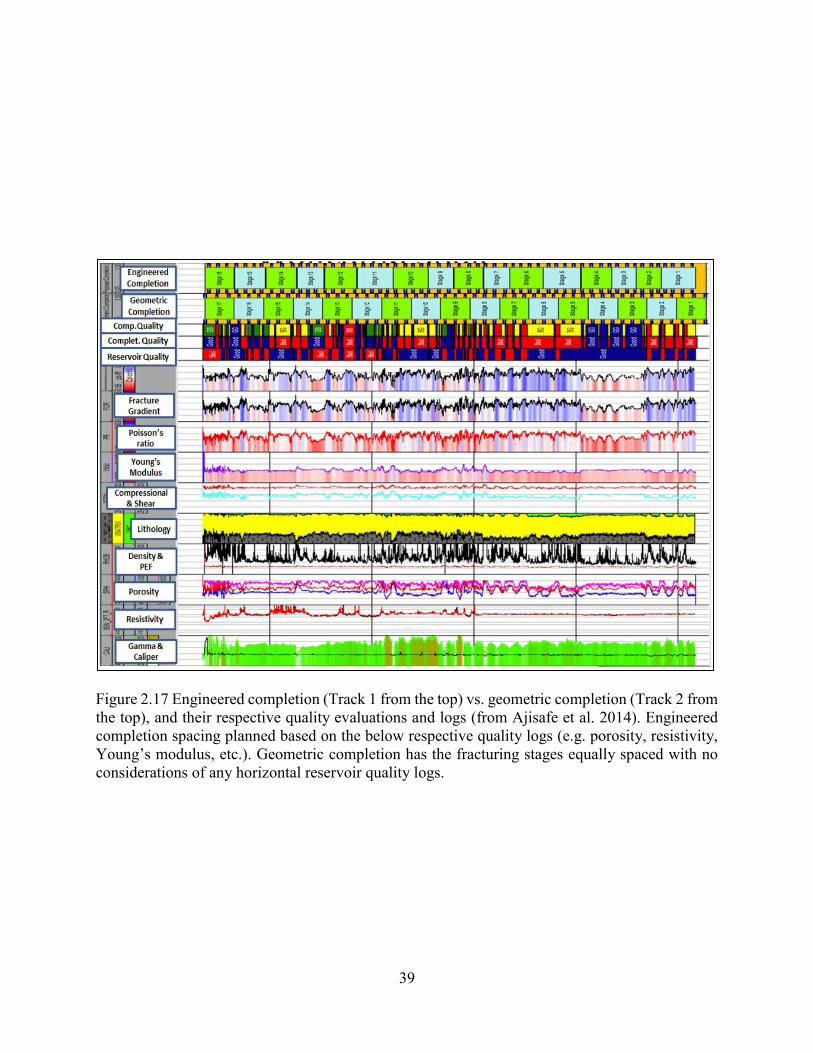
39
Figure 2.17 Engineered completion (Track 1 from the top) vs. geometric completion (Track 2 from
the top), and their respective quality evaluations and logs (from Ajisafe et al. 2014). Engineered
completion spacing planned based on the below respective quality logs (e.g. porosity, resistivity,
Young’s modulus, etc.). Geometric completion has the fracturing stages equally spaced with no considerations of any horizontal reservoir quality logs.
40
CHAPTER 3
METHODOLOGY
To achieve the objectives of the research, a hydraulic fracture model was constructed using
the Grid Oriented Hydraulic Fracture Extension Replicator (GOHFERTM) commercial simulator.
This software is capable of creating a geomechanical model, simulating hydraulic fracture
treatments, performing different pressure diagnostics, forecasting, and analyzing production.
GOHFERTM was developed by Dr. Robert D. Barree as a PhD product at the Colorado School of
Mines (Barree 1984) and continues to be updated by Barree & Associates LLC. Also, Predict-KTM
(Core Laboratories 2018) production prediction simulator was used to conduct fluid and proppant
sensitivity analyses and perform production prediction runs. This software is capable of
incorporating the effects of fracturing fluid type, proppant type, and proppant concentration into
the production model.
The methodology used for this project includes creating the base case model, validating
the model using DFIT and DAS data, and performing different sensitivity runs. The following
sections describe the details of each performed step.
3.1 Base Case Model Development
The first step in this research was to build a base case by modeling the Eagle Ford treatment
well (Well A) and generating treatment and production outputs that match the actual field results.
The vertical reference well (Well C) logs were utilized to calculate geomechanical properties and
build the stress model. These logs and geomechanical properties were calibrated to the Well A
through geosteering. Diagnostic fracture injection tests (DFITs) were analyzed to calculate
reservoir parameters (e.g. pore pressure, closure stress, etc.) and calibrate them with the log output.
41
The actual treatment stages (perforations and pumping schedules) of Well A were entered in the
model, then the resultant treating pressure was calibrated with the actual pressure by modifying
the frictional parameters such as pipe friction and tortuosity factors. Cluster contributions based
on total placed proppant for each cluster were calibrated with the DAS results by adjusting the
perforation parameters. Finally, production results were obtained from the model and history-
matched with the actual production of Well A.
3.1.1 Log Processing
Logs from Well C were uploaded into the model including gamma ray (GR), density
(RHOB), resistivity, sonic (DTC & DTS), and neutron porosity (NPHI). For Well A, wireline GR
and caliper logs were uploaded in addition to the directional survey. Sections 3.1.1.1 – 3.1.1.3
explain the calculation procedure of the main reservoir and geomechanical parameters including
effective porosity, permeability, Young’s modulus, Poisson’s ratio, Biot’s coefficient, pore
pressure, and closure stress.
3.1.1.1 Effective Porosity and Permeability
Effective porosity was calculated by subtracting the shale pore volume from the total pore
volume as indicated in Equation 3.1 (Al-Ruwaili and Al-Waheed 2004). The total porosity in the
equation was obtained by averaging both density and neutron porosities. Since neutron porosity is
a raw log measurement, Equation 3.2 was used to calculate density porosity. As the modeled Eagle
Ford section is lithologically dominated by limestone, the matrix density is 2.71 g/cm3 whereas
the fluid density is 1 g/cm3 (Asquith and Krygowski 2004). The resultant effective porosity is
around 5%. This value is very comparable to the mean value of the effective porosity range (3% -
10%) of the Eagle Ford-Austin Chalk systems (Martin et al. 2011).
∅ = ∅ − ∅ ℎ (3.1)
42
Where, ∅ = effective porosity, dimensionless ∅ = total porosity, dimensionless
ℎ = shale volume fraction, dimensionless
∅ = −− (3.2)
Where, ∅ = density-derived porosity, dimensionless � = matrix grain density, g/cm3, [M][L]− � =log measurement of formation bulk density (RHOB), g/cm3, [M][L]− � =fluid density, g/cm3, [M][L]−
Matrix permeability was estimated from effective porosity by applying a permeability
multiplier and a permeability exponent as indicated in Equation 3.3. For shale, the permeability
multiplier and exponent were initially assumed to be 2 and 3, respectively. The resultant matrix
permeability is 230 nD. This value is within the range of the matrix permeability range (3 nD –
405 nD) of the Eagle Ford-Austin Chalk systems (Martin et al. 2011; Kamari et al. 2017). The
effective permeability was eventually calibrated to DFIT results as discussed in Section 3.1.2.
= × ∅ � (3.3)
Where,
= matrix permeability, mD, [L]
= permeability multiplier, mD, [L]
= permeability exponent, dimensionless
3.1.1.2 Geomechanical Properties
To calculate Young’s modulus and Poisson’s ratio, both compressional and shear sonic
logs were used to obtain the ratio R in Equation 3.4. Then, dynamic Poisson’s ratio and dynamic

43
Young’s modulus were calculated as per Equations 3.5 and 3.6, respectively (Barree et al. 2009).
Dynamic Young’s modulus and Poisson’s ratio from GR, DTC, average porosity, and resistivity
logs were also calculated using synthetic correlations (Barree et al. 2009). All calculated values
were averaged to obtain the final dynamic Young’s modulus and Poisson’s ratio. Figure 3.1
demonstrates the averaged values of dynamic Young’s modulus and Poisson’s ratio from the log.
= 22 (3.4)
Where,
= square of shear to compressional travel time ratio, dimensionless
= shear travel time, µsec/ft, [�][L]−
= compressional travel time, µsec/ft, [�][L]−
� = −− (3.5)
Where, � = dynamic Poisson’s ratio, dimensionless
= � −2 − (3.6)
Where,
= dynamic Young’s modulus, MMpsi, [M][L]− [�]−
For purposes of the model, the static Young’s modulus was determined using the modified
Eissa and Kazi (1988) correlation. The Poisson’s ratio dynamic to static correlation was assumed
to be one.
The Biot’s poroelastic constant (�) was estimated from effective porosity using the
correlation in Equation 3.7 (Crain’s Petrophysical Handbook Website 2015) which is used in the
case of low-quality shear sonic data, which is the case in this suite of logs.

44
Figure 3.1 Left: dynamic Young’s modulus log showing different curves (YMERESIST: calculated based on resistivity; YMEPHIA: based on average porosity; YMEGR: based on GR;
YMEACT: based on DTC & DTS logs; YMEDTC: based on DTC log). Right: dynamic Poisson’s ratio log showing different curves (same YME abbreviation meanings apply to PR).
45
� = . + .9 ∅ (3.7)
Where, � = Biot’s coefficient, dimensionless
3.1.1.3 Pore Pressure and Minimum Horizontal Stress
Pore pressure gradients range from 0.4 to 0.8 psi/ft in the Eagle Ford shale (Kamari et al.
2017). In the subject area, the Eagle Ford is an overpressured zone. Based on the DFIT data
analysis that is discussed in Section 3.1.2, an additional pressure offset of around 3900 psi was
applied to the Eagle Ford and Lower Austin Chalk zones to match DFIT results. This additional
pressure offset resulted in a pore pressure gradient of 0.75 psi/ft. Since Young’s modulus,
Poisson’s ratio, Biot’s coefficient, and pore pressure were all determined, the minimum horizontal
stress or closure stress can be calculated as per the aforementioned Equation 2.8 in Section 2.1.3.3.
Horizontal Biot’s coefficient was assumed to be 1 whereas the overburden pressure gradient was
assumed to be 1.04 psi/ft based on the raw density log. Regional strain and stress values were
assumed to be zero initially before any stress calibration.
3.1.1.4 Grid Setup and Geosteering
After all necessary reservoir and geomechanical property logs were calculated for Well C,
various property grids were generated. Figure 3.2 indicates the main raw and processed logs used
to create the grids. The Eagle Ford Marl/Lower Austin Chalk target zone, where Well A was landed
and geosteered, is highlighted in Figure 3.2. Since the logs were generated initially using Well C
vertical section data, they were converted to fit the Well A horizontal section through geosteering,
which was performed by following similar GR signatures in the horizontal section and staying in
the same zone to match the actual geosteer data. Figure 3.3 represents a snap shot of the geosteering
process performed in the simulator.
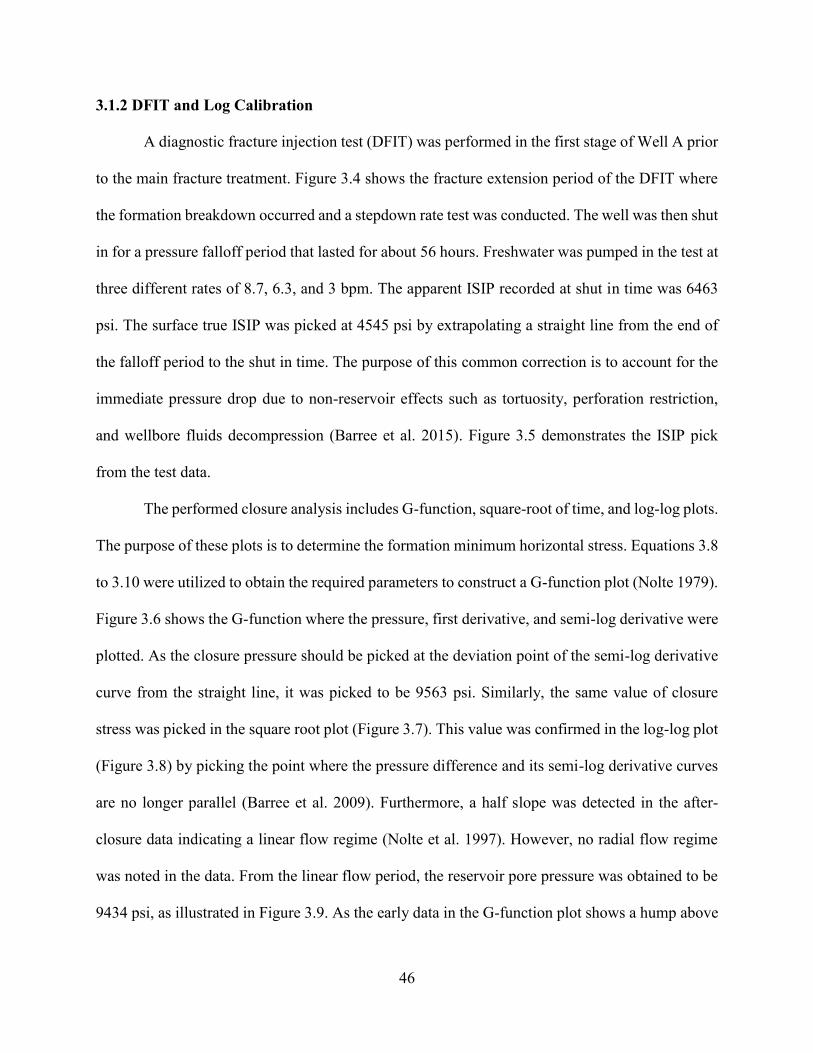
46
3.1.2 DFIT and Log Calibration
A diagnostic fracture injection test (DFIT) was performed in the first stage of Well A prior
to the main fracture treatment. Figure 3.4 shows the fracture extension period of the DFIT where
the formation breakdown occurred and a stepdown rate test was conducted. The well was then shut
in for a pressure falloff period that lasted for about 56 hours. Freshwater was pumped in the test at
three different rates of 8.7, 6.3, and 3 bpm. The apparent ISIP recorded at shut in time was 6463
psi. The surface true ISIP was picked at 4545 psi by extrapolating a straight line from the end of
the falloff period to the shut in time. The purpose of this common correction is to account for the
immediate pressure drop due to non-reservoir effects such as tortuosity, perforation restriction,
and wellbore fluids decompression (Barree et al. 2015). Figure 3.5 demonstrates the ISIP pick
from the test data.
The performed closure analysis includes G-function, square-root of time, and log-log plots.
The purpose of these plots is to determine the formation minimum horizontal stress. Equations 3.8
to 3.10 were utilized to obtain the required parameters to construct a G-function plot (Nolte 1979).
Figure 3.6 shows the G-function where the pressure, first derivative, and semi-log derivative were
plotted. As the closure pressure should be picked at the deviation point of the semi-log derivative
curve from the straight line, it was picked to be 9563 psi. Similarly, the same value of closure
stress was picked in the square root plot (Figure 3.7). This value was confirmed in the log-log plot
(Figure 3.8) by picking the point where the pressure difference and its semi-log derivative curves
are no longer parallel (Barree et al. 2009). Furthermore, a half slope was detected in the after-
closure data indicating a linear flow regime (Nolte et al. 1997). However, no radial flow regime
was noted in the data. From the linear flow period, the reservoir pore pressure was obtained to be
9434 psi, as illustrated in Figure 3.9. As the early data in the G-function plot shows a hump above

47
Figure 3.2 Well C processed logs. Tracks from left to right (Track 1: density, resistivity, effective porosity, and GR; Track 2: static
Young’s modulus, process zone stress, Poisson’s ratio, and permeability; Track 3: total stress, pore pressure, and caliper; Track 4: lithology volumes). Top Eagle Ford (primary target and zone where Well A is placed) and bottom Eagle Ford (secondary target) zones
are highlighted.
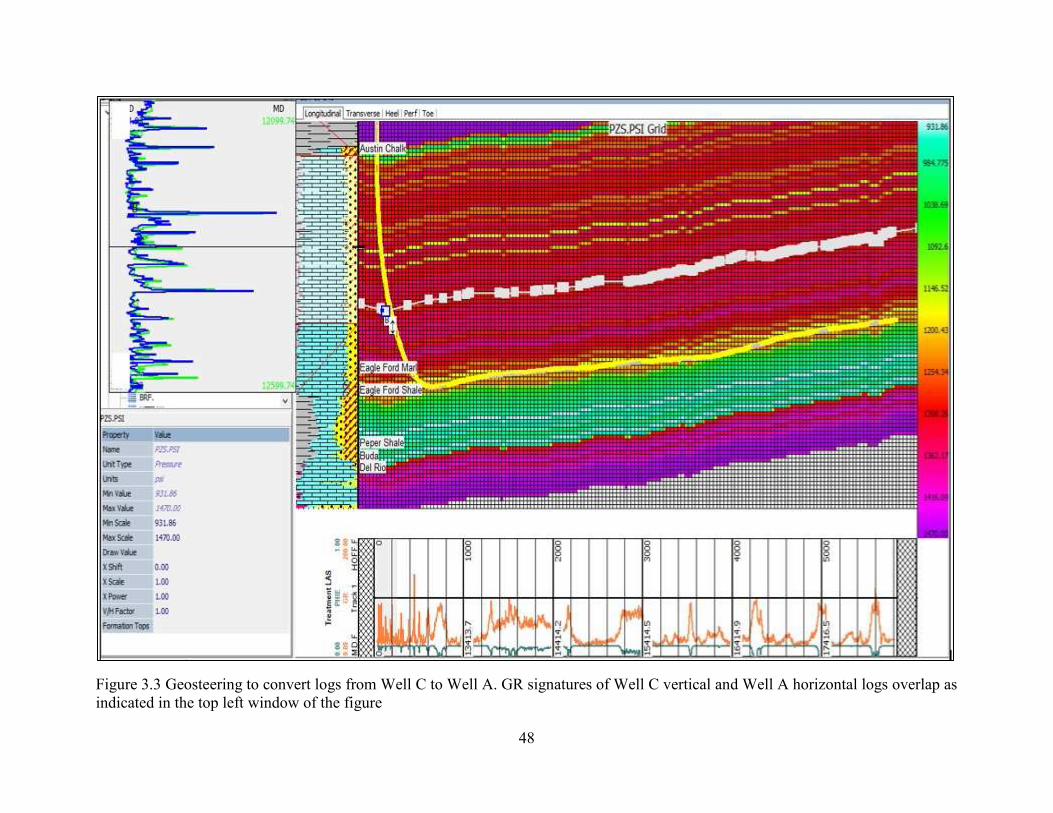
48
Figure 3.3 Geosteering to convert logs from Well C to Well A. GR signatures of Well C vertical and Well A horizontal logs overlap as
indicated in the top left window of the figure

49
the straight line, the expected leakoff mechanism is pressure-dependent leakoff (PDL) with a PDL
coefficient determined to be 0.0039 1/psi, as demonstrated in Figure 3.10.
Figure 3.4 DFIT rate and pressure data plot showing the fracture extension and falloff periods.
Figure 3.5 ISIP pick from DFIT data. The regression line was extrapolated to the shut-in time to
pick ISIP at 4545 psi and eliminate the toe tortuosity effects.

50
∆� = − (3.8)
� ∆� = + ∆� . − ∆� . (3.9) ∆� = � ∆� − � (3.10)
Where, ∆� = dimensionless pumping time, dimensionless � = elapsed time, minutes, [�] � = total pumping time, minutes, [�] � = dimensionless time function, dimensionless
= G-time function, dimensionless � = � at shut in time, dimensionless
Table 3.1 shows the main reservoir parameters obtained from the DFIT. As described in
Section 3.1.1.3, the reservoir pore pressure was updated in the grids so it matches the value from
the DFIT. To calibrate the stress log data to the DFIT, a tectonic strain of -200 microstrains and a
stress offset of -300 psi were incorporated in the total stress equation (Equation 2.8 in Section
2.1.3.3). It is worth noting that uncertainty is associated with the DFIT results due to the test raw
data not being clean. Moreover, the first stage where the DFIT was pumped may not be
representative of the rest of the stages in the subject well.
Table 3.1 DFIT Results Showing the Main Reservoir Parameters
Parameter Value Parameter Value
BH ISIP 9960 psi Fluid efficiency 94%
Fracture gradient 0.80 psi/ft CFOP 97 psi
BH closure stress 9563 psi PDL coefficient 0.0039 1/psi
Closure gradient 0.76 psi/ft Reservoir pressure 9434 psi
Permeability 0.2 µD Pore pressure gradient 0.75 psi/ft
PZS 407 psi

51
Figure 3.6 Well A DFIT G-function plot showing the bottomhole pressure, pressure first derivative
(dP/dG), and pressure semilog derivative (GdP/dG) curves versus G time. The closure pressure
was picked to be 9563 psi at G=35.726.

52
Figure 3.7 Well A DFIT square-root of time plot showing the bottomhole pressure, pressure first
derivative (dP/d(dt)2), and pressure semilog derivative ((dt)2 dP/d(dt)2) curves versus (dt)2. The
closure pressure was picked to be 9563 psi at (dt)2=44.282 min2.
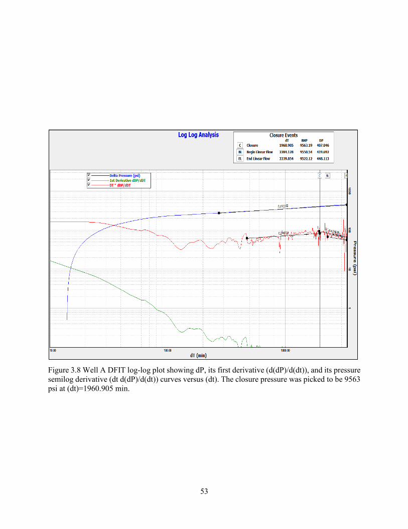
53
Figure 3.8 Well A DFIT log-log plot showing dP, its first derivative (d(dP)/d(dt)), and its pressure
semilog derivative (dt d(dP)/d(dt)) curves versus (dt). The closure pressure was picked to be 9563
psi at (dt)=1960.905 min.
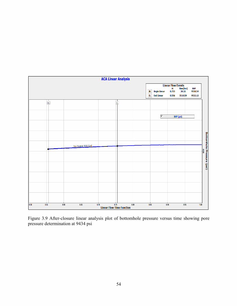
54
Figure 3.9 After-closure linear analysis plot of bottomhole pressure versus time showing pore
pressure determination at 9434 psi

55
Figure 3.10 Fissure leakoff analysis plot of leakoff ratio versus bottomhole pressure showing
leakoff coefficient determination at 0.0039 1/psi.
3.1.3 Treatments
A total of 14 hydraulic fracturing treatments were performed along the horizontal section
of Well A. Figure 3.11 shows the wellbore with locations of the perforation clusters. The treatment
design including the pumped fluids and proppants for a single stage is summarized in Table 3.2.
In most of the treatment stages, three pad stages are pumped with acid, spacer, and diverter in
between these stages.
The model treating pressure was calibrated with the actual treating pressure until a
reasonable match was achieved for the treatment stages. This was performed by adjusting some
design parameters in each stage such as the PDL coefficient, relative permeability factor, tortuosity

56
factor, friction factor, tortuosity erosion factor, and the width exponent. Figure 3.12 illustrates the
treating pressure match for one of the 14 stages (Stage 11). The treatment plots for all stages are
provided in the Appendix A, Figures A.1 to A.14.
To perform more accurate analyses, cluster proppant distributions were calculated based
on the total amount of proppant placed in each cluster. These distributions were matched with
actual values obtained from DAS data by modifying the perforation factors for different clusters.
The initial variation could be due to horizontal reservoir quality differences from cluster to cluster
or due to difference in perforation efficiency. Figure 3.13 demonstrates the actual DAS analysis
with the total proppant placed in every cluster. Figure 3.14 shows the model values with an
indication of the error difference between the model and actual data. The maximum error
difference seen in any cluster is 5%. Figures 3.15 – 3.19 show the proppant concentration for the
five perforation clusters of Stage 11, as an example. Figures 3.20 and 3.21 illustrate a top view and
a side view of the entire wellbore showing proppant concentrations in the created fracture planes,
respectively.
Table 3.2 Representative Treatment Schedule of Performed Treatments in Well A
# Stage description Fluid & proppant
1 Breakdown Slickwater
2 Acid 15% HCl
3 Pre-pad Slickwater
4 Main pad 20# water with 100 mesh white sand & 20# Hypor G with
30/50 white sand
5 Acid 15% HCl
6 Pre-pad Slickwater
7 Main pad 20# water with 100 mesh white sand & 20# Hypor G with
30/50 white sand
8 Acid 15% HCl
9 Pre-pad Slickwater
10 Main pad 20# water with 100 mesh white sand & 20# Hypor G with
30/50 white sand
11 Flush Slickwater

57
Figure 3.11 Well A with actual perforation locations shown as green dots. A total of 14 fracturing
stages (64 perforation clusters) were treated.

58
Figure 3.12 Stage 11 treatment data with a matched pressure between model and actual values.
Dotted pressure curve represents the actual surface treating pressure (surface pressure in the
legend), whereas the connected pressure curve represents the model surface treating pressure (well
pressure in the legend).
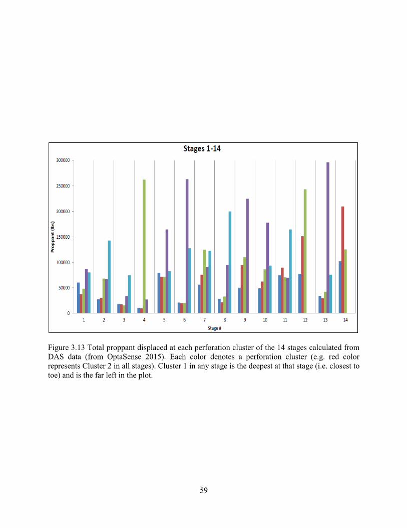
59
Figure 3.13 Total proppant displaced at each perforation cluster of the 14 stages calculated from
DAS data (from OptaSense 2015). Each color denotes a perforation cluster (e.g. red color
represents Cluster 2 in all stages). Cluster 1 in any stage is the deepest at that stage (i.e. closest to
toe) and is the far left in the plot.
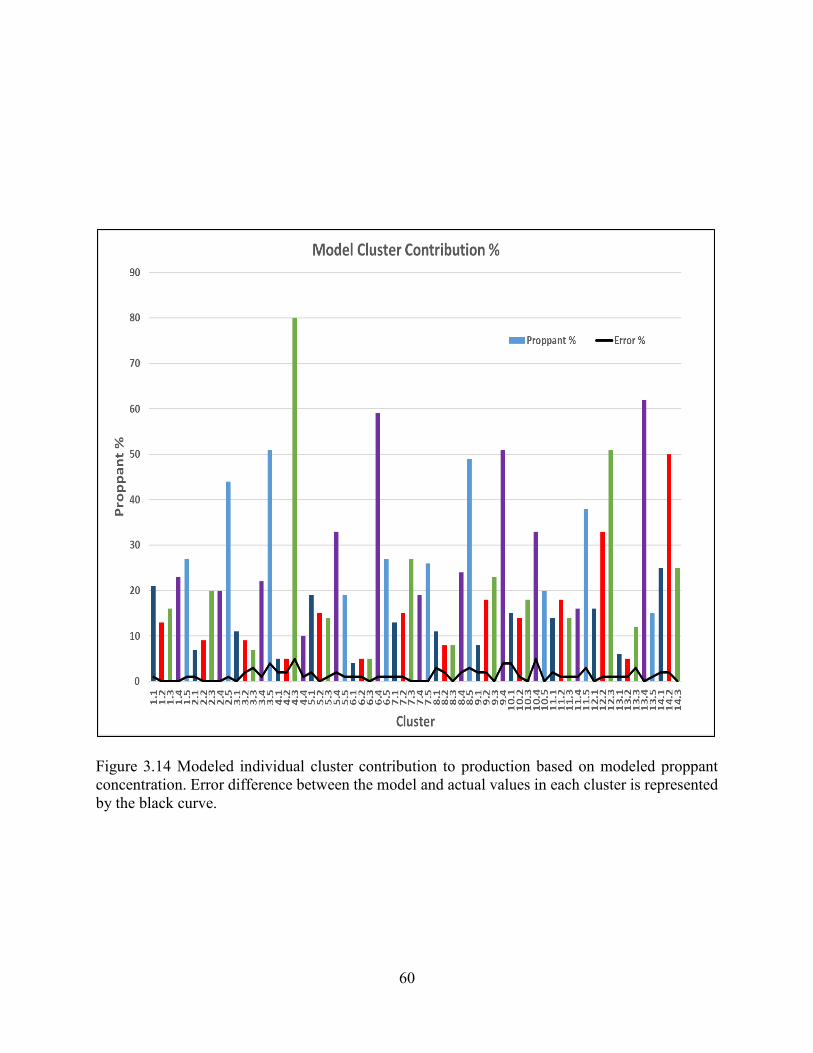
60
Figure 3.14 Modeled individual cluster contribution to production based on modeled proppant
concentration. Error difference between the model and actual values in each cluster is represented
by the black curve.

61
Figure 3.15 Transverse view of the proppant concentration grid for Cluster 5 (heel cluster) in Stage 11. Formation tops and lithology
are shown on the left whereas, the grid scale is shown on the right.

62
Figure 3.16 Transverse view of the proppant concentration grid for Cluster 4 (middle cluster) in Stage 11. Formation tops and lithology
are shown on the left, whereas the grid scale is shown on the right.
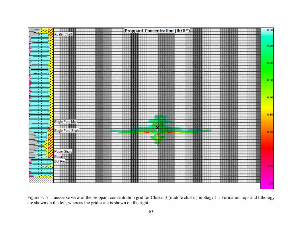
63
Figure 3.17 Transverse view of the proppant concentration grid for Cluster 3 (middle cluster) in Stage 11. Formation tops and lithology
are shown on the left, whereas the grid scale is shown on the right.
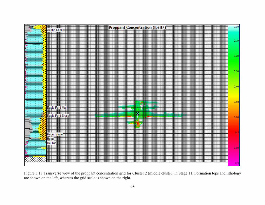
64
Figure 3.18 Transverse view of the proppant concentration grid for Cluster 2 (middle cluster) in Stage 11. Formation tops and lithology
are shown on the left, whereas the grid scale is shown on the right.

65
Figure 3.19 Transverse view of the proppant concentration grid for Cluster 1 (toe cluster) in Stage 11. Formation tops and lithology are
shown on the left, whereas the grid scale is shown on the right.
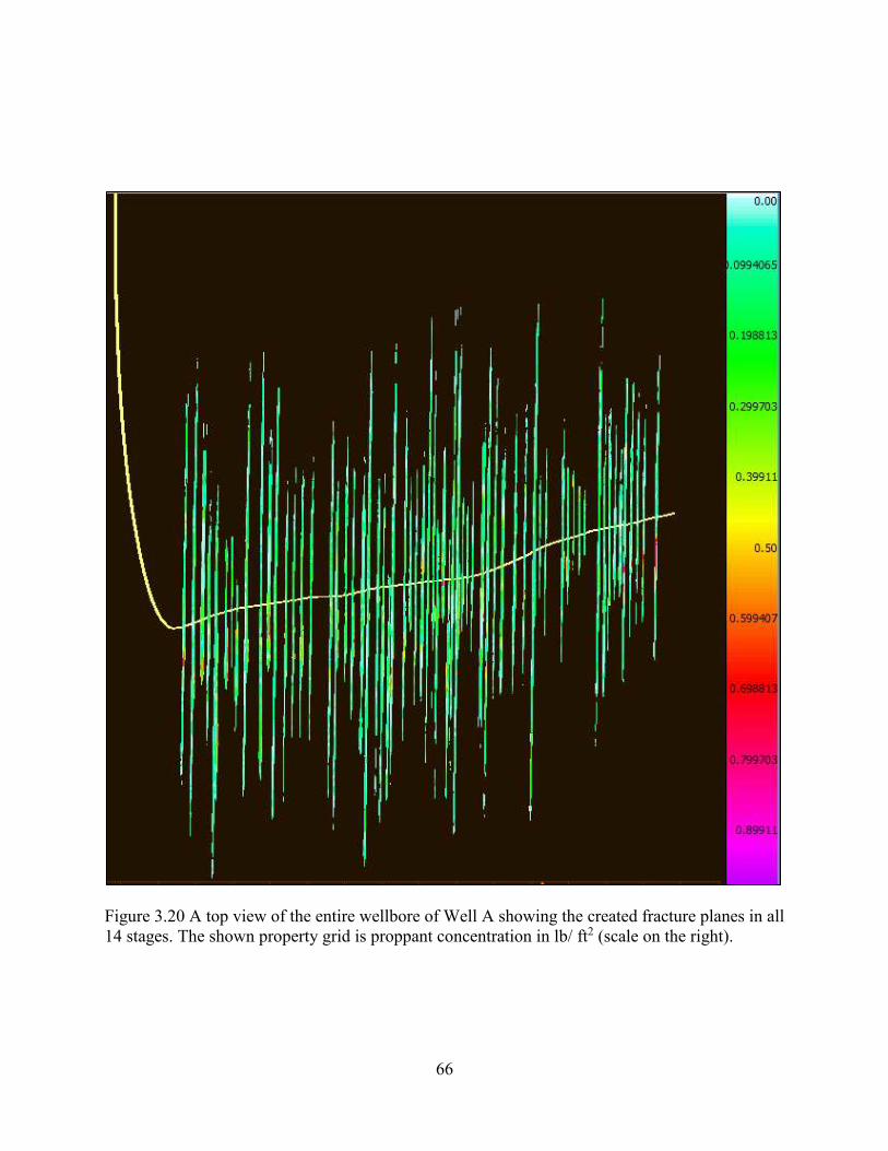
66
Figure 3.20 A top view of the entire wellbore of Well A showing the created fracture planes in all
14 stages. The shown property grid is proppant concentration in lb/ ft2 (scale on the right).

67
Figure 3.21 A side view of the entire wellbore of Well A showing the created fracture planes in all
14 stages. The shown property grid is proppant concentration in lb/ft2 (scale on the right).
3.1.4 Production History Matching
After matching treating pressures and cluster proppant distributions, production runs were
performed assuming uniform fracturing stages. From the actual production data, type curve plots
were generated to determine various parameters to help achieve the match. The three pressure-
time plots, including the dimensionless type curve plot, pseudo-plot, and semi-log plot, are
illustrated in Figures 3.22 – 3.24, respectively. From these plots, parameters such as Kh, fracture
half-length, aspect ratio, and drainage area were found and plugged in the production model. As a
result, a good production history match using pressure as the control variable was achieved, as

68
demonstrated in Figure 3.25. It is worth noting that the wells in the subject area utilize gas lift
mechanisms to produce oil as they are located in a high GOR area.
3.2 Sensitivity Analyses Creation
A base case model with calibrated logs, matched treating pressures, matched cluster
contributions based on proppant distribution, and history-matched production was constructed.
Such a reliable model now allows for conducting sensitivity analyses. Different parameters from
the base case were altered including matrix permeability, Young’s modulus, Poisson’s ratio, Biot’s
coefficient, cluster spacing, fracturing fluid type, and proppant type as shown in Table 3.3.
Changes in well performance in response to these changes were recorded. Results of the sensitivity
analyses are described in Chapter 4.
Table 3.3 Created Sensitivity Runs
# Sensitized parameter Sensitized fracturing stage(s)
1 Matrix permeability Stages 3, 7, 9, and 13
2 Poisson’s ratio Stages 3, 7, 9, and 13
3 Young’s modulus Stages 3, 7, 9, and 13
4 Biot’s coefficient Stages 3, 7, 9, and 13
5 Perforation cluster spacing Entire wellbore
6 Fracturing fluid type Stage 3
7 Proppant type Stage 3
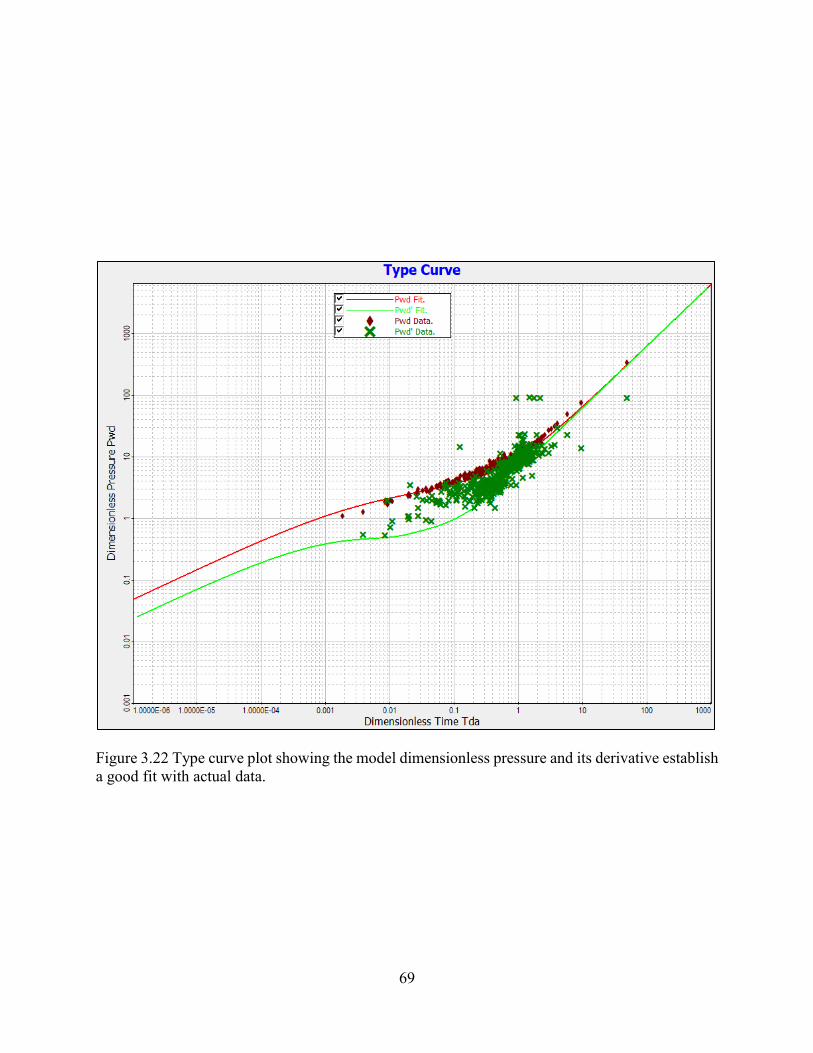
69
Figure 3.22 Type curve plot showing the model dimensionless pressure and its derivative establish
a good fit with actual data.

70
Figure 3.23 A fitted pseudo pressure plot of dp/q versus time showing the representative estimated
ultimate recovery (EUR), drainage area, and aspect ratio.

71
Figure 3.24 A fitted semi-log plot of dp/q versus time showing the representative permeability,
transmissivity, skin, and fracture half-length.

72
Figure 3.25 Model production history matched with actual production. The matched curves include
bottomhole pressure, oil rate, water rate, cumulative oil production, and cumulative water
production. Matching was established for the available production data of around 470 days.

73
CHAPTER 4
MODEL RESULTS AND DISCUSSION
This chapter summarizes the results of the multiple sensitivity analyses performed on the
base case model. The sensitivity analyses were implemented for different parameters on different
fracturing stages of Well A. In addition, the natural fracture density was obtained from image logs
and used to evaluate reservoir quality lateral variations in some stages.
4.1 Parameter Sensitivity Analyses
Sensitivity analyses of different parameters were conducted to address the effect of
reservoir lateral variations on the performance of Well A. Such sensitivity analyses will determine
the effects of running an engineered completion as opposed to the geometric completion run on
the actual base case. The sensitized parameters include matrix permeability, Poisson’s ratio,
Young’s modulus, and Biot’s poroelastic coefficient as shown in Table 3.3. In the base case model,
the value of each parameter is basically identical along the horizontal wellbore (minimal to no
lateral variations). The changes to these parameters were applied to different stages of the wellbore
to measure the extent of these changes. In each sensitivity analysis of these parameters, the
estimated flowing fracture length was the comparison factor between the different sensitivities.
The simulated stages for the aforementioned four parameters are Stages 3, 7, 9, and 13. In addition,
spacing between perforation clusters was altered from the base model to address the effect of stress
shadowing. Created fracture volume, fracture conductivity, and cumulative oil production were
the comparison factors in the cluster spacing sensitivity cases. Various fluid and proppant types
were analyzed and compared to those used in the base case. Consequently, cumulative oil

74
production was found and compared for each fluid/proppant type case. In all of the sensitivity runs,
the number of fracturing stages was kept unchanged so that the amount of fluid and proppant
pumped was the same in all stages. This is to avoid running the economic differences of pumping
larger amounts of fluids and proppants, thus providing a more realistic comparison. Also in all
sensitivity runs, only one parameter was changed at a time to allow for comparisons based on that
parameter alone.
4.1.1 Matrix Permeability Sensitivity
In the model grids, the matrix permeability values were varied for the nodes of fracturing
Stages 3, 7, 9, and 13, in the primary target reservoir only (Eagle Ford Marl). Figure 4.1
demonstrates how the permeability values were modified for selective multiple nodes representing
the simulated four stages. Table 4.1 indicates the simulated five cases for permeability sensitivity
analysis. In each case, the same permeability was applied to the simulated four cases and their
flowing fracture length was obtained and compared to that of the base model. Figures 4.2 – 4.5
illustrate the change in flowing fracture length as matrix permeability changes in Stages 3, 7, 9,
and 13, respectively. In all stages, the general trend for the flowing fracture length is to increase
in most clusters as permeability increases. The rate of improvement in the flowing fracture length
is more pronounced in the heel clusters compared to slower improvement in the toe clusters.
Moreover, the toe cluster in Stages 7 and 9 showed a declining trend in flowing fracture length
while increasing the permeability. This attenuation can be ascribed to the high magnitude of stress
shadow that reaches up to 1700 psi in the toe cluster compared to values around 500 psi in the heel
cluster. Overall, the increase in permeability results in enhancing the flowing fracture length. The
response of clusters with less stress shadowing to changing permeability is more distinct than that
of clusters with larger stress shadow magnitudes.

75
Figure 4.1 Matrix Permeability grid showing how Stages 3, 7, 9, and 13 permeability values are different from the rest of the wellbore
stages. Case 5 (0.0023 mD permeability) is used here as an example.

76
Table 4.1 Matrix Permeability Sensitivity Cases
Case Permeability (mD)
1 0.000023
2 0.0001
3 (base case) 0.00023
4 0.0005
5 0.0023
Figure 4.2 Stage 3 matrix permeability sensitivity plot showing the change in flowing fracture
length as permeability changes. Each colored curve represents a perforation cluster in Stage 3 with
Cluster 3.1 being the closest to the toe and Cluster 3.5 being the closest to the heel. Black ellipse
represents the base case matrix permeability (0.00023 mD).
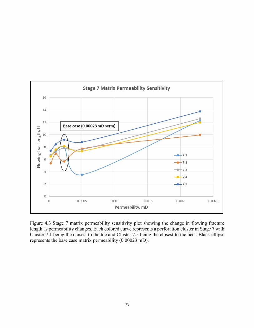
77
Figure 4.3 Stage 7 matrix permeability sensitivity plot showing the change in flowing fracture
length as permeability changes. Each colored curve represents a perforation cluster in Stage 7 with
Cluster 7.1 being the closest to the toe and Cluster 7.5 being the closest to the heel. Black ellipse
represents the base case matrix permeability (0.00023 mD).

78
Figure 4.4 Stage 9 matrix permeability sensitivity plot showing the change in flowing fracture
length as permeability changes. Each colored curve represents a perforation Cluster in Stage 9 with
Cluster 9.1 being the closest to the toe and Cluster 9.4 being the closest to the heel. Black ellipse
represents the base case matrix permeability (0.00023 mD).

79
Figure 4.5 Stage 13 matrix permeability sensitivity plot showing the change in flowing fracture
length as permeability changes. Each colored curve represents a perforation cluster in Stage 13
with Cluster 13.1 being the closest to the toe and Cluster 13.5 being the closest to the heel. Black
ellipse represents the base case matrix permeability (0.00023 mD).
4.1.2 Poisson’s Ratio Sensitivity
Sensitivity of the Poisson’s ratio was performed in Stages 3, 7, 9, and 13. Poisson’s ratio
of the Eagle Ford Marl was edited in the grid for the simulated four stages as shown in Figure 4.6.
Four different values of Poisson’s ratio were tested, as summarized in Table 4.2. In each case,
flowing fracture length was acquired as a simulation output and the results were compared against
each other. Figures 4.7 – 4.10 show the change in flowing fracture length as a function of Poisson’s
ratio in stages 3, 7, 9, and 13, respectively. As Poisson’s ratio increases, the general trend for
flowing fracture length is to increase in most perforation clusters. However, the amount of increase
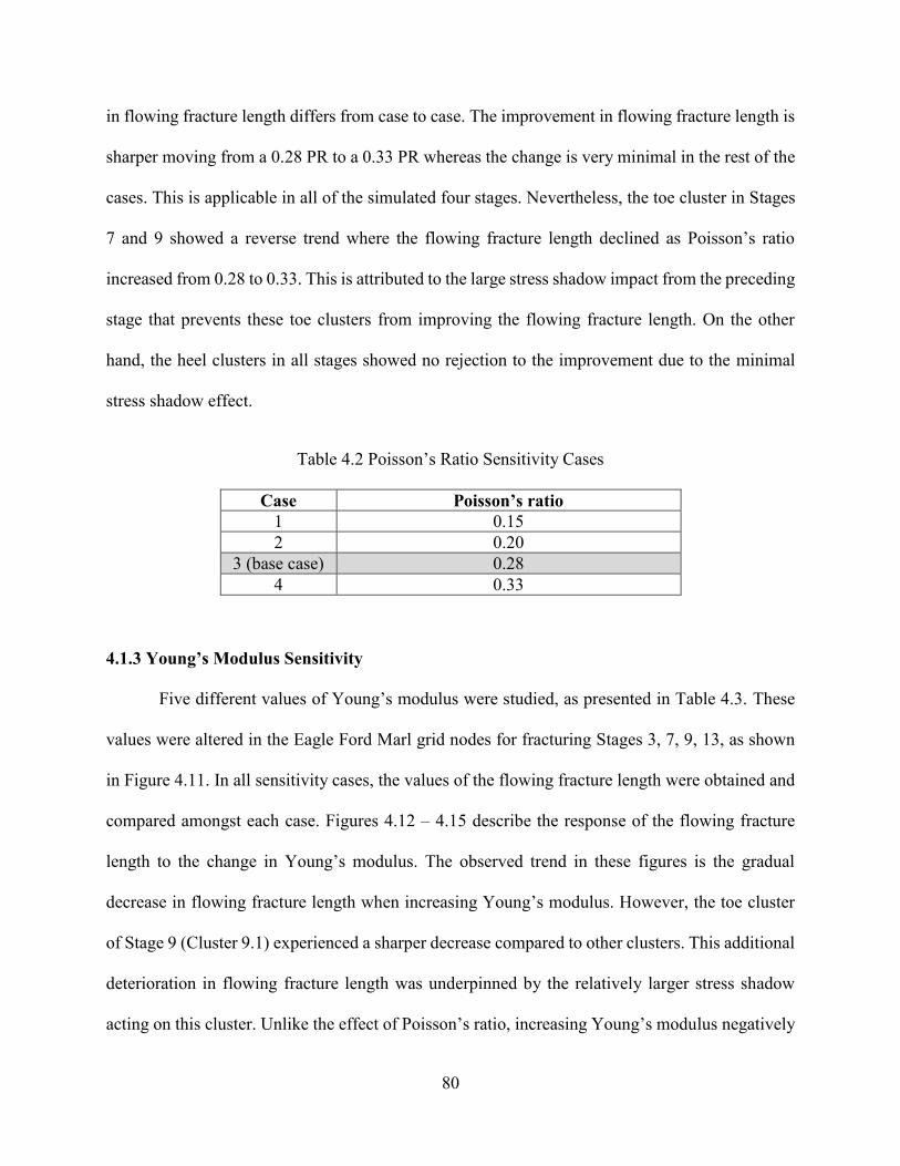
80
in flowing fracture length differs from case to case. The improvement in flowing fracture length is
sharper moving from a 0.28 PR to a 0.33 PR whereas the change is very minimal in the rest of the
cases. This is applicable in all of the simulated four stages. Nevertheless, the toe cluster in Stages
7 and 9 showed a reverse trend where the flowing fracture length declined as Poisson’s ratio
increased from 0.28 to 0.33. This is attributed to the large stress shadow impact from the preceding
stage that prevents these toe clusters from improving the flowing fracture length. On the other
hand, the heel clusters in all stages showed no rejection to the improvement due to the minimal
stress shadow effect.
Table 4.2 Poisson’s Ratio Sensitivity Cases
Case Poisson’s ratio
1 0.15
2 0.20
3 (base case) 0.28
4 0.33
4.1.3 Young’s Modulus Sensitivity
Five different values of Young’s modulus were studied, as presented in Table 4.3. These
values were altered in the Eagle Ford Marl grid nodes for fracturing Stages 3, 7, 9, 13, as shown
in Figure 4.11. In all sensitivity cases, the values of the flowing fracture length were obtained and
compared amongst each case. Figures 4.12 – 4.15 describe the response of the flowing fracture
length to the change in Young’s modulus. The observed trend in these figures is the gradual
decrease in flowing fracture length when increasing Young’s modulus. However, the toe cluster
of Stage 9 (Cluster 9.1) experienced a sharper decrease compared to other clusters. This additional
deterioration in flowing fracture length was underpinned by the relatively larger stress shadow
acting on this cluster. Unlike the effect of Poisson’s ratio, increasing Young’s modulus negatively

81
impacted the flowing fracture length. It is worth noting that Young’s modulus was multiplied by
a negative strain offset in the total stress equation to calibrate the stress model to the DFIT data
which have caused the reverse effect of Young’s modulus.
Table 4.3 Young’s Modulus Sensitivity Cases
Case Young’s modulus (MMpsi) 1 2.5
2 3.5
3 4.5
4 (base case) 5.5
5 6.5
4.1.4 Biot’s Coefficient Sensitivity
For Well A, the value of Biot’s coefficient was found to be high (0.9) due to the low
effective porosity. Therefore, four lower values were used to perform the sensitivity analysis of
Biot’s coefficient, as indicated in Table 4.4. Biot’s coefficient values were changed for the Eagle
Ford Marl in Stages 3, 7, 9, and 13 as shown in Figure 4.16. Consequently, the flowing fracture
length was found and compared between the five simulated cases. Figures 4.17 – 4.20 illustrate
the change in flowing fracture length as a response to changing Biot’s coefficient. Similar to
permeability and Poisson’s ratio, the general trend for the flowing fracture length was to increase
when increasing Biot’s coefficient. However, the toe clusters (first and second clusters) in most
stages did not have a stable trend as it showed a fluctuating behavior while changing Biot’s
coefficient.
The sensitized three parameters (Poisson’s ratio, Young’s modulus, and Biot’s coefficient)
are all components of the total stress equation. Changes that caused the total stress to increase also
caused the flowing fracture length to improve. The increase in total stress created a large

82
differential stress vertically which caused most of the fracture energy to be dissipated in the
transverse direction, hence, increasing the flowing fracture length.
Table 4.4 Biot’s coefficient Sensitivity Cases
Case Biot’s coefficient 1 0.1
2 0.3
3 0.5
4 0.7
5 (base case) 0.9
4.1.5 Cluster Spacing Sensitivity
To address the effect of stress shadowing and its relationship to fracture spacing,
sensitivities of spacing between perforation clusters have been conducted. Since the total wellbore
length and the number of fracturing stages are fixed, changing cluster spacing implies changing
the number of perforation clusters. Four different scenarios of cluster spacing were run, as
presented in Table 4.5. Figures 4.21 – 4.24 demonstrate the wellbore trajectory showing the
spacing and number of clusters in Scenarios 1, 2, 3, and 4, respectively.
Table 4.5 Cluster Spacing (Number of Clusters) Sensitivity Scenarios
Scenario Cluster spacing (number of clusters)
1 57 ft spacing (84 clusters)
2 (base scenario) 76 ft spacing (64 clusters)
3 100 ft spacing (49 clusters)
4 142 ft spacing (35 clusters)

83
Figure 4.6 Poisson’s ratio grid showing how Stages 3, 7, 9, and 13 PR values are different from the rest of the wellbore stages. Case 2 (0.2 Poisson’s ratio) is used here as an example.
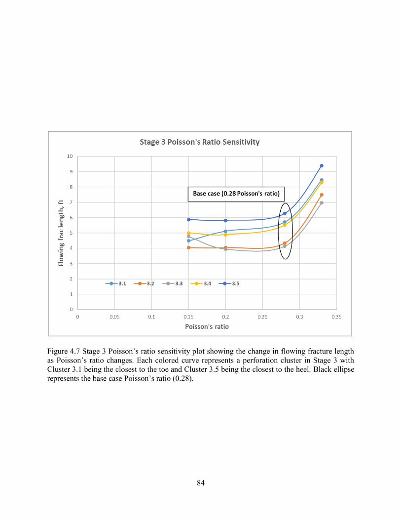
84
Figure 4.7 Stage 3 Poisson’s ratio sensitivity plot showing the change in flowing fracture length
as Poisson’s ratio changes. Each colored curve represents a perforation cluster in Stage 3 with
Cluster 3.1 being the closest to the toe and Cluster 3.5 being the closest to the heel. Black ellipse
represents the base case Poisson’s ratio (0.28).

85
Figure 4.8 Stage 7 Poisson’s ratio sensitivity plot showing the change in flowing fracture length as Poisson’s ratio changes. Each colored curve represents a perforation cluster in Stage 7 with
Cluster 7.1 being the closest to the toe and Cluster 7.5 being the closest to the heel. Black ellipse
represents the base case Poisson’s ratio (0.28).

86
Figure 4.9 Stage 9 Poisson’s ratio sensitivity plot showing the change in flowing fracture length
as Poisson’s ratio changes. Each colored curve represents a perforation cluster in Stage 9 with
Cluster 9.1 being the closest to the toe and Cluster 9.4 being the closest to the heel. Black ellipse
represents the base case Poisson’s ratio (0.28).
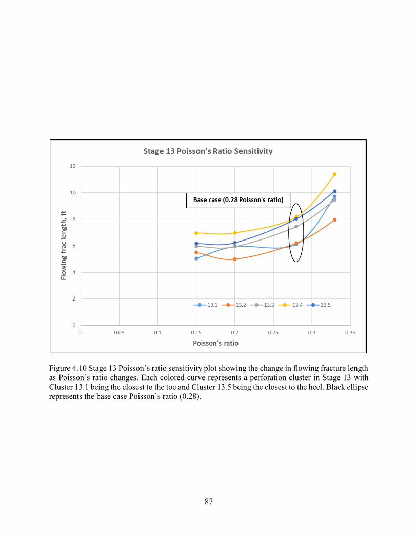
87
Figure 4.10 Stage 13 Poisson’s ratio sensitivity plot showing the change in flowing fracture length as Poisson’s ratio changes. Each colored curve represents a perforation cluster in Stage 13 with
Cluster 13.1 being the closest to the toe and Cluster 13.5 being the closest to the heel. Black ellipse
represents the base case Poisson’s ratio (0.28).
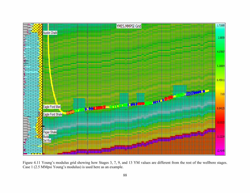
88
Figure 4.11 Young’s modulus grid showing how Stages 3, 7, 9, and 13 YM values are different from the rest of the wellbore stages.
Case 1 (2.5 MMpsi Young’s modulus) is used here as an example.

89
Figure 4.12 Stage 3 Young’s modulus sensitivity plot showing the change in flowing fracture length as Young’s modulus changes. Each colored curve represents a perforation cluster in Stage
3 with Cluster 3.1 being the closest to the toe and Cluster 3.5 being the closest to the heel. Black
ellipse represents the base case Young’s modulus (5.5 MMpsi).
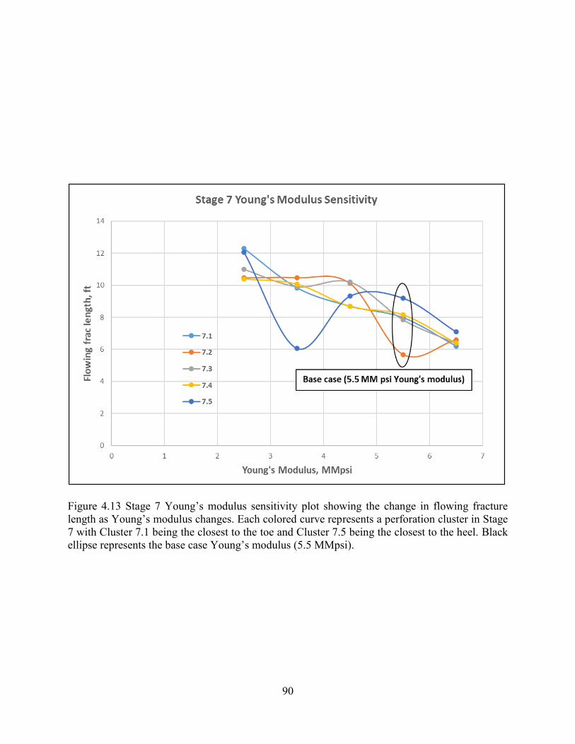
90
Figure 4.13 Stage 7 Young’s modulus sensitivity plot showing the change in flowing fracture length as Young’s modulus changes. Each colored curve represents a perforation cluster in Stage
7 with Cluster 7.1 being the closest to the toe and Cluster 7.5 being the closest to the heel. Black
ellipse represents the base case Young’s modulus (5.5 MMpsi).

91
Figure 4.14 Stage 9 Young’s modulus sensitivity plot showing the change in flowing fracture length as Young’s modulus changes. Each colored curve represents a perforation cluster in Stage
9 with Cluster 9.1 being the closest to the toe and Cluster 9.4 being the closest to the heel. Black
ellipse represents the base case Young’s modulus (5.5 MMpsi).

92
Figure 4.15 Stage 13 Young’s modulus sensitivity plot showing the change in flowing fracture length as Young’s modulus changes. Each colored curve represents a perforation cluster in Stage
13 with Cluster 13.1 being the closest to the toe and Cluster 13.5 being the closest to the heel.
Black ellipse represents the base case Young’s modulus (5.5 MMpsi).

93
Figure 4.16 Biot’s coefficient grid showing how Stages 3, 7, 9, and 13 Biot’s coefficient values are different from the rest of the wellbore
stages. Case 4 (0.7 Biot’s coefficient) is used here as an example.

94
Figure 4.17 Stage 3 Biot’s coefficient sensitivity plot showing the change in flowing fracture length as Biot’s coefficient changes. Each colored curve represents a perforation cluster in Stage
3 with Cluster 3.1 being the closest to the toe and Cluster 3.5 being the closest to the heel. Black
ellipse represents the base case Biot’s coefficient (0.9).

95
Figure 4.18 Stage 7 Biot’s coefficient sensitivity plot showing the change in flowing fracture length as Biot’s coefficient changes. Each colored curve represents a perforation cluster in Stage
7 with Cluster 7.1 being the closest to the toe and Cluster 7.5 being the closest to the heel. Black
ellipse represents the base case Biot’s coefficient (0.9).

96
Figure 4.19 Stage 9 Biot’s coefficient sensitivity plot showing the change in flowing fracture
length as Biot’s coefficient changes. Each colored curve represents a perforation cluster in Stage
9 with Cluster 9.1 being the closest to the toe and Cluster 9.4 being the closest to the heel. Black
ellipse represents the base case Biot’s coefficient (0.9).

97
Figure 4.20 Stage 13 Biot’s coefficient sensitivity plot showing the change in flowing fracture length as Biot’s coefficient changes. Each colored curve represents a perforation cluster in Stage
13 with Cluster 13.1 being the closest to the toe and Cluster 13.5 being the closest to the heel.
Black ellipse represents the base case Biot’s coefficient (0.9).

98
Figure 4.21 Well A trajectory plot showing 84 perforation clusters (green dots) with a cluster
spacing of 57 ft. This plot represents Scenario 1 from Table 4.5.

99
Figure 4.22 Well A trajectory plot showing 64 perforation clusters (green dots) with an average
cluster spacing of 76 ft. This plot represents Scenario 2 from Table 4.5 (actual treatment scenario).
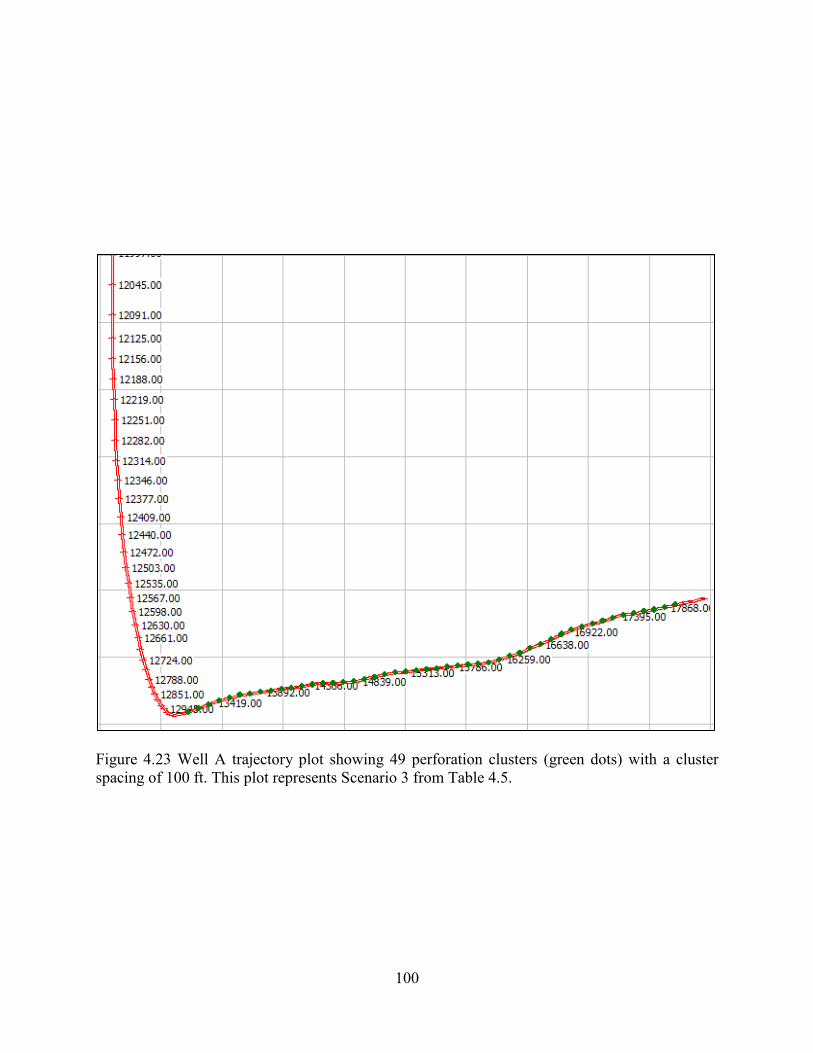
100
Figure 4.23 Well A trajectory plot showing 49 perforation clusters (green dots) with a cluster
spacing of 100 ft. This plot represents Scenario 3 from Table 4.5.

101
Figure 4.24 Well A trajectory plot showing 35 perforation clusters (green dots) with a cluster
spacing of 142 ft. This plot represents Scenario 4 from Table 4.5.
In all four of the simulated spacing scenarios, the flowing fracture volume for each cluster
was obtained by multiplying flowing fracture length, fracture height, and average fracture width,
then the resultant flowing fracture volumes were summed to obtain the total created fracture
network volume for each scenario. Moreover, effective fracture conductivity was obtained as a
simulation output for each cluster. The effective fracture conductivity values were averaged for
the heel clusters, middle cluster, and toe clusters for each scenario. Both properties of flowing
fracture volume and fracture conductivity were plotted against cluster spacing for all scenarios in
Figure 4.25. Similarly, the total amount of proppant placed in each cluster was found as a

102
simulation output for each cluster and averaged for the heel clusters, middle clusters, and toe
clusters for each scenario. Consequently, total proppant and fracture volume were plotted against
cluster spacing for all scenarios in Figure 4.26. Completing the well with a larger number of
perforation clusters (tighter spacing) will create a larger fracture network volume. However, the
fracture conductivity and the total amount of placed proppant per fracture will decline. Also, the
dominance of the heel clusters becomes much more evident. On the other hand, the larger spacing
scenarios result in a smaller fracture network volume but a more conductive one. Moreover, the
fracture conductivity values of the clusters become fairly close to each other indicating a
potentially more uniform contribution from the clusters. As observed in the toe clusters curve, the
fracture conductivity jumped from 5 mD.ft to 21 mD.ft equaling the conductivity value of the heel
clusters. The rate of improvement in fracture conductivity is more pronounced in the toe clusters
as they released the large stress shadow acting on them when the spacing increased. Nonetheless,
the rate of conductivity improvement is less in the heel clusters as they were under relatively lower
stress shadowing effects.
In addition to the obtained average conductivity values for the heel, middle, and toe
clusters, the maximum, minimum, and standard deviation of fracture conductivity values were
calculated for all spacing scenarios. Figures 4.27 – 4.30 present column charts of the average,
maximum, minimum, and standard deviation values of fracture conductivity, respectively, for the
heel, middle, and toe clusters in all spacing scenarios. From Figure 4.27, it can be seen that the
average fracture conductivity distribution becomes more uniform as fracture spacing increases.
The maximum fracture conductivity established was found to be 83.3 mD.ft in scenario 3 (100 ft
cluster spacing). Conversely, the minimum fracture conductivity was found to be 1.169 mD.ft in
Scenario 1 (57 ft cluster spacing). Figure 4.30 suggests that the heel cluster fracture conductivity
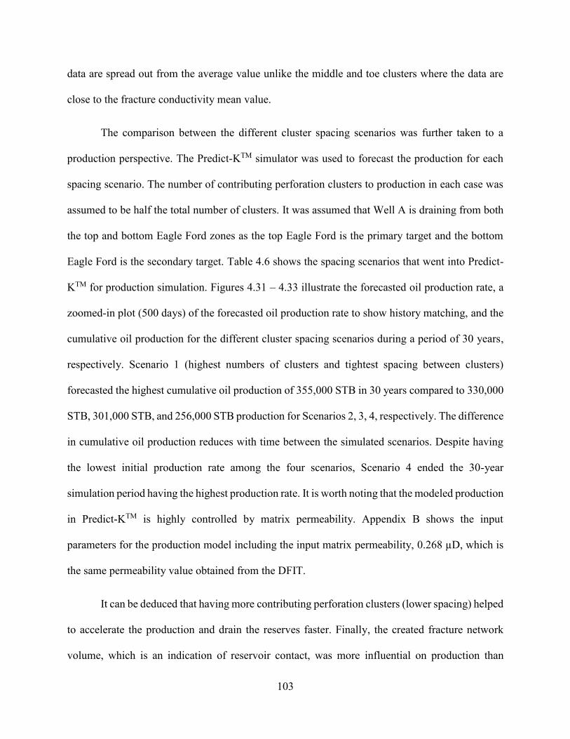
103
data are spread out from the average value unlike the middle and toe clusters where the data are
close to the fracture conductivity mean value.
The comparison between the different cluster spacing scenarios was further taken to a
production perspective. The Predict-KTM simulator was used to forecast the production for each
spacing scenario. The number of contributing perforation clusters to production in each case was
assumed to be half the total number of clusters. It was assumed that Well A is draining from both
the top and bottom Eagle Ford zones as the top Eagle Ford is the primary target and the bottom
Eagle Ford is the secondary target. Table 4.6 shows the spacing scenarios that went into Predict-
KTM for production simulation. Figures 4.31 – 4.33 illustrate the forecasted oil production rate, a
zoomed-in plot (500 days) of the forecasted oil production rate to show history matching, and the
cumulative oil production for the different cluster spacing scenarios during a period of 30 years,
respectively. Scenario 1 (highest numbers of clusters and tightest spacing between clusters)
forecasted the highest cumulative oil production of 355,000 STB in 30 years compared to 330,000
STB, 301,000 STB, and 256,000 STB production for Scenarios 2, 3, 4, respectively. The difference
in cumulative oil production reduces with time between the simulated scenarios. Despite having
the lowest initial production rate among the four scenarios, Scenario 4 ended the 30-year
simulation period having the highest production rate. It is worth noting that the modeled production
in Predict-KTM is highly controlled by matrix permeability. Appendix B shows the input
parameters for the production model including the input matrix permeability, 0.268 µD, which is
the same permeability value obtained from the DFIT.
It can be deduced that having more contributing perforation clusters (lower spacing) helped
to accelerate the production and drain the reserves faster. Finally, the created fracture network
volume, which is an indication of reservoir contact, was more influential on production than

104
fracture conductivity for the studied case. However, this may not be the case in other reservoirs
where fracture conductivity can be as important as reservoir contact. These results agree with
literature papers which suggest that hydraulic fracture designs in low-permeability reservoirs focus
more on increasing fracture surface area than increasing fracture conductivity as the created
fracture network volume strongly influences production (Liang et al. 2016).
Figure 4.25 Change in fracture conductivity (left axis) and fracture network volume (right axis) as
a function of changing cluster spacing. The base scenario of 76 ft cluster spacing is highlighted by
the black ellipse. Fracture network volume, in the figure, is defined as the flowing fracture length
multiplied by fracture height and average fracture width.
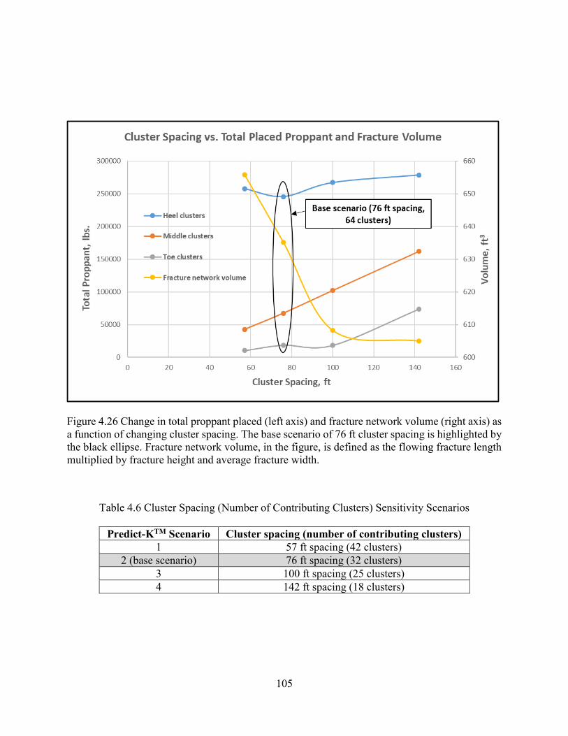
105
Figure 4.26 Change in total proppant placed (left axis) and fracture network volume (right axis) as
a function of changing cluster spacing. The base scenario of 76 ft cluster spacing is highlighted by
the black ellipse. Fracture network volume, in the figure, is defined as the flowing fracture length
multiplied by fracture height and average fracture width.
Table 4.6 Cluster Spacing (Number of Contributing Clusters) Sensitivity Scenarios
Predict-KTM Scenario Cluster spacing (number of contributing clusters)
1 57 ft spacing (42 clusters)
2 (base scenario) 76 ft spacing (32 clusters)
3 100 ft spacing (25 clusters)
4 142 ft spacing (18 clusters)

106
Figure 4.27 Average fracture conductivity distribution between the heel, middle, and toe clusters
of all 14 fracturing stages in all simulated spacing scenarios.

107
Figure 4.28 Maximum fracture conductivity distribution between the heel, middle, and toe clusters
of all 14 fracturing stages in all simulated spacing scenarios.
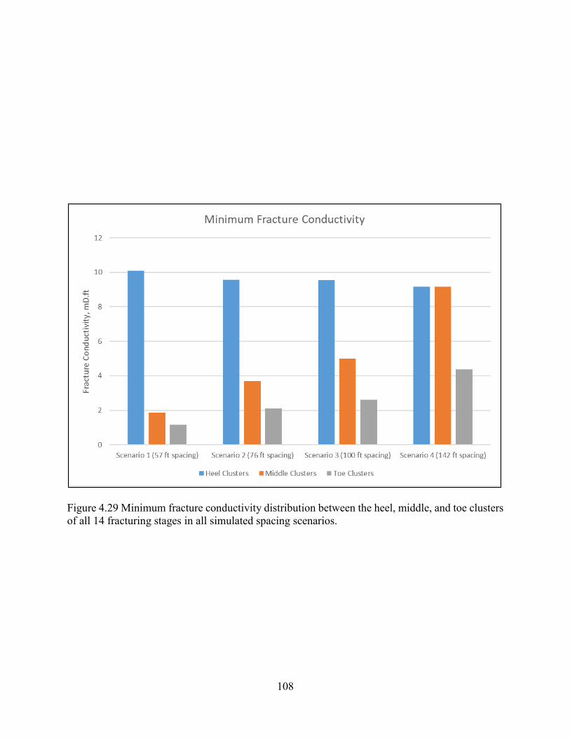
108
Figure 4.29 Minimum fracture conductivity distribution between the heel, middle, and toe clusters
of all 14 fracturing stages in all simulated spacing scenarios.
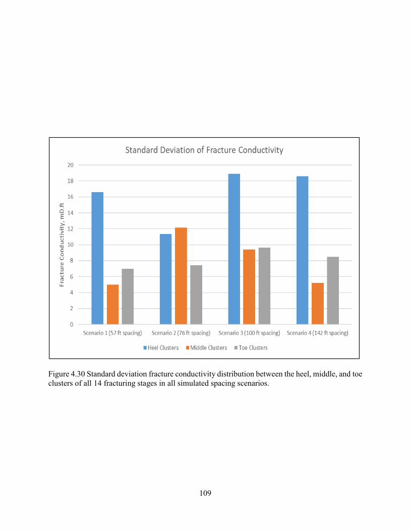
109
Figure 4.30 Standard deviation fracture conductivity distribution between the heel, middle, and toe
clusters of all 14 fracturing stages in all simulated spacing scenarios.

110
Figure 4.31 Forecasted oil production rate for the different cluster spacing scenarios for 30 years.
The actual production rate is represented by the green curve and shown for the available data
period of 470 days.

111
Figure 4.32 A zoomed-in plot of the forecasted oil production rate for the different cluster spacing
scenarios for 30 years. The actual production rate is represented by the green curve and shown for
the available data period of 470 days.
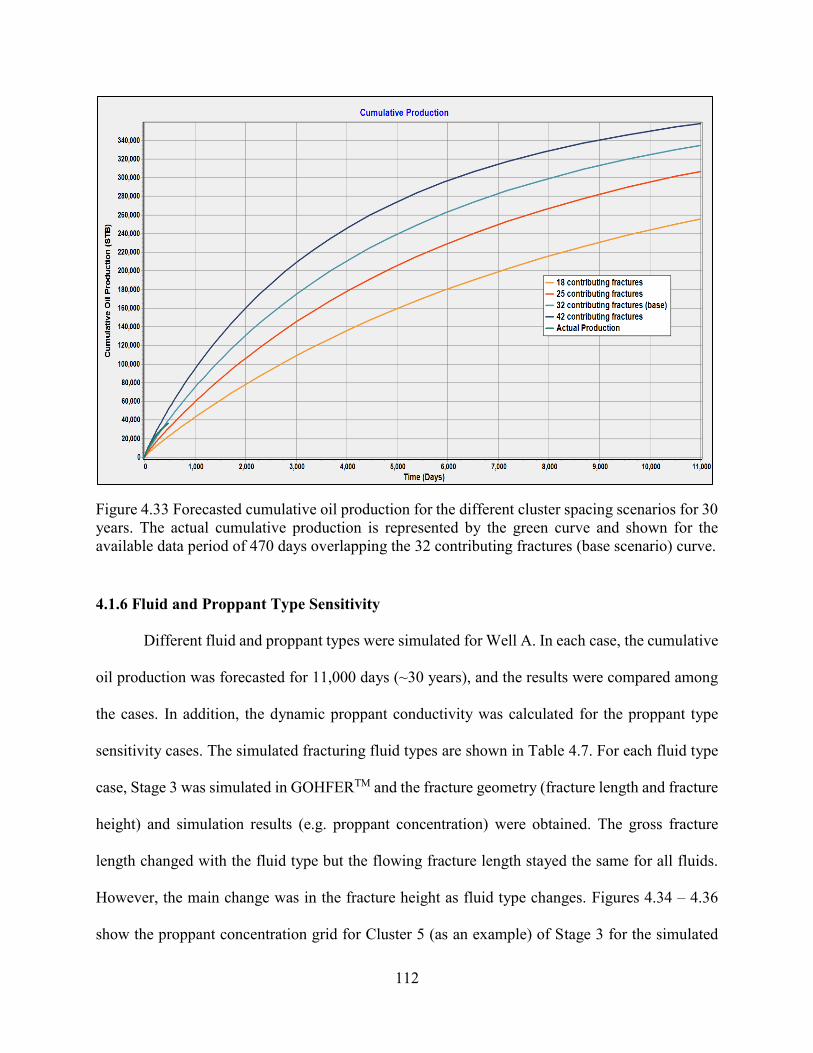
112
Figure 4.33 Forecasted cumulative oil production for the different cluster spacing scenarios for 30
years. The actual cumulative production is represented by the green curve and shown for the
available data period of 470 days overlapping the 32 contributing fractures (base scenario) curve.
4.1.6 Fluid and Proppant Type Sensitivity
Different fluid and proppant types were simulated for Well A. In each case, the cumulative
oil production was forecasted for 11,000 days (~30 years), and the results were compared among
the cases. In addition, the dynamic proppant conductivity was calculated for the proppant type
sensitivity cases. The simulated fracturing fluid types are shown in Table 4.7. For each fluid type
case, Stage 3 was simulated in GOHFERTM and the fracture geometry (fracture length and fracture
height) and simulation results (e.g. proppant concentration) were obtained. The gross fracture
length changed with the fluid type but the flowing fracture length stayed the same for all fluids.
However, the main change was in the fracture height as fluid type changes. Figures 4.34 – 4.36
show the proppant concentration grid for Cluster 5 (as an example) of Stage 3 for the simulated

113
fracturing fluid types. Fracturing fluid 50# CMHPG-Zr showed the largest fracture height growth
of around 200 ft compared to 148 ft and 74 ft fracture height for 2% KCl and 45# Guar-Borate 2
fracturing fluids, respectively. GOHFERTM simulation results for the different fracturing fluid
types were exported into Predict-KTM and a production forecast for 30 years was run for every
fluid type case. For the production runs, it was assumed that both the top and bottom Eagle Ford
zones are targets of Well A. Figure 4.37 demonstrates the cumulative oil production curves for the
simulated fracturing fluid types. Fracturing fluid 50# CMHPG-Zr that showed the largest fracture
growth also forecasted the highest 30-year cumulative oil production of 430,000 STB compared
to 330,000 STB and 183,000 STB for 2% KCl and 45# Guar-Borate 2 fracturing fluids,
respectively. Two commercial types of sand and two commercial types of ceramic were simulated
for proppant type sensitivity analysis. The mesh size of all of these proppants was kept fixed at
30/50 to provide a more realistic comparison. The simulated types of proppant are summarized in
Table 4.8.
Stage 3 was simulated in GOHFERTM for each proppant type and the results were taken to
Predict-KTM for production analysis. Figures 4.38 – 4.41 show the proppant concentration grid for
each proppant type case from GOHFERTM. The base case proppant (Sand A) generated the highest
fracture growth with 148 ft fracture height compared to 116 ft, 110 ft, and 106 ft values for Sand
B, Ceramic A, and Ceramic B, respectively. Figures 4.42 and 4.43 illustrate the dynamic proppant
conductivity and cumulative oil production plots for the simulated proppant types. Under the Eagle
Ford stress value of 9600 psi, the difference in proppant conductivity between the simulated
proppant types is minimal with the ceramic types having a slightly higher conductivity than the
sand types. The production runs showed that Sand A (largest fracture height growth) forecasted
the highest 30-year cumulative oil production of 330,000 STB compared to 285,000 STB, 274,000
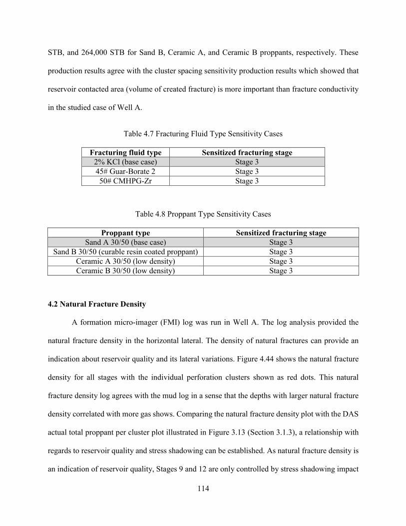
114
STB, and 264,000 STB for Sand B, Ceramic A, and Ceramic B proppants, respectively. These
production results agree with the cluster spacing sensitivity production results which showed that
reservoir contacted area (volume of created fracture) is more important than fracture conductivity
in the studied case of Well A.
Table 4.7 Fracturing Fluid Type Sensitivity Cases
Fracturing fluid type Sensitized fracturing stage
2% KCl (base case) Stage 3
45# Guar-Borate 2 Stage 3
50# CMHPG-Zr Stage 3
Table 4.8 Proppant Type Sensitivity Cases
Proppant type Sensitized fracturing stage
Sand A 30/50 (base case) Stage 3
Sand B 30/50 (curable resin coated proppant) Stage 3
Ceramic A 30/50 (low density) Stage 3
Ceramic B 30/50 (low density) Stage 3
4.2 Natural Fracture Density
A formation micro-imager (FMI) log was run in Well A. The log analysis provided the
natural fracture density in the horizontal lateral. The density of natural fractures can provide an
indication about reservoir quality and its lateral variations. Figure 4.44 shows the natural fracture
density for all stages with the individual perforation clusters shown as red dots. This natural
fracture density log agrees with the mud log in a sense that the depths with larger natural fracture
density correlated with more gas shows. Comparing the natural fracture density plot with the DAS
actual total proppant per cluster plot illustrated in Figure 3.13 (Section 3.1.3), a relationship with
regards to reservoir quality and stress shadowing can be established. As natural fracture density is
an indication of reservoir quality, Stages 9 and 12 are only controlled by stress shadowing impact

115
as they have no fracture density recorded and hence no reservoir quality differences. From Figure
4.44, Stages 9 and 12 show the normal behavior under stress shadowing where the heel clusters
were the dominant ones in terms of total placed proppant and the toe clusters were having the
lowest total placed proppant values. This observation confirms that these clusters are only affected
by stress shadowing where no reservoir quality variations played a role in changing the cluster
total proppant distribution.
Something to be noted that may affected the outcome of the of the fiber optic analysis
results is the plug leakage or the inter-stage communication behind the casing which was captured
by the DTS data. Figures 4.45 and 4.46 demonstrate the DTS data for Stages 1-7 and 8-14
respectively. The communication between some stages is observed as the cooling effect during a
stage hydraulic fracturing shows to extend to the previous stage. Inter-stage communication is
observed in Stages 1-2, 4-5, 5-6, 6-7, 8-9, 9-10, 10-11, 11-12, 12-13, and 13-14. Cluster 3 of Stage
4 and Cluster 4 of Stage 6, which showed a large amount of total placed proppant from DAS data
(Figure 3.13 in Section 3.1.3), might be affected by inter-stage communication as appears during
fracturing of Stages 5 and 7 in DTS data (Figure 4.45).

116
Figure 4.34 Proppant concentration grid for Cluster 5 of Stage 3. The simulated fracturing fluid type is 2% KCl (base case).
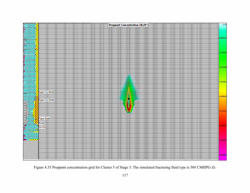
117
Figure 4.35 Proppant concentration grid for Cluster 5 of Stage 3. The simulated fracturing fluid type is 50# CMHPG-Zr.
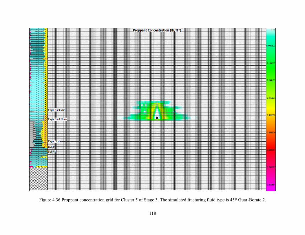
118
Figure 4.36 Proppant concentration grid for Cluster 5 of Stage 3. The simulated fracturing fluid type is 45# Guar-Borate 2.
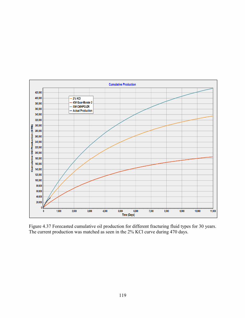
119
Figure 4.37 Forecasted cumulative oil production for different fracturing fluid types for 30 years.
The current production was matched as seen in the 2% KCl curve during 470 days.
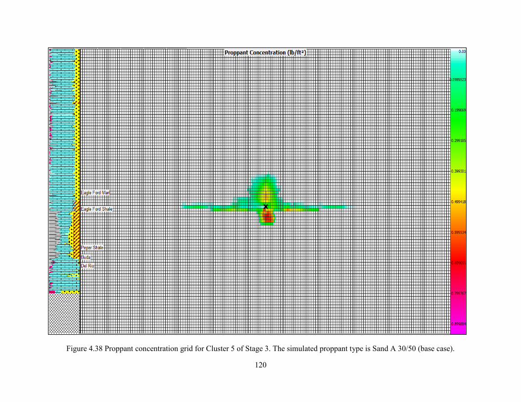
120
Figure 4.38 Proppant concentration grid for Cluster 5 of Stage 3. The simulated proppant type is Sand A 30/50 (base case).

121
Figure 4.39 Proppant concentration grid for Cluster 5 of Stage 3. The simulated proppant type is Sand B 30/50.

122
Figure 4.40 Proppant concentration grid for Cluster 5 of Stage 3. The simulated proppant type is Ceramic A 30/50.

123
Figure 4.41 Proppant concentration grid for Cluster 5 of Stage 3. The simulated proppant type is Ceramic B 30/50.

124
Figure 4.42 Dynamic proppant conductivity for the simulated proppant types plotted against
formation stress. Eagle Ford stress is pointed in the figure.
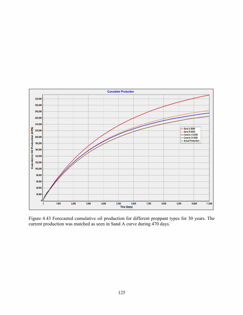
125
Figure 4.43 Forecasted cumulative oil production for different proppant types for 30 years. The
current production was matched as seen in Sand A curve during 470 days.

126
Figure 4.44 Natural fracture density plotted versus Well A measured depth. The shaded yellow
boxes refer to the location of the 14 stages whereas the red dots represent the depths of the
individual perforation clusters.

127
Figure 4.45 DTS data recorded during hydraulic fracturing for Stages 1-7 indicating communication between some stages (modified
from OptaSense 2015). The x-axis represents time, whereas the y-axis represents the measured depth. The inter-stage communication is
represented by the red squares. Clusters 3 of Stage 4 and Cluster 4 of Stage 6 are highlighted.

128
Figure 4.46 DTS data recorded during hydraulic fracturing for Stages 8-14 indicating communication between some stages (modified
from OptaSense 2015). The x-axis represents time, whereas the y-axis represents the measured depth. The inter-stage communication is
represented by the red squares.
129
CHAPTER 5
CONCLUSIONS AND RECOMMENDATIONS
This chapter summarizes the main findings of the study and suggests recommendations for
future work using the already accomplished results as a baseline.
5.1 Conclusions
This research investigated the extent of the induced stress shadow due to hydraulic
fracturing, examined the influence of rock quality lateral variations in horizontal wellbores, and
consequently studied how these two factors can play a role in optimizing hydraulic fracture spacing
in unconventional reservoirs. A hydraulic fracture model was constructed via GOHFERTM to
achieve the purpose of the research, and Predict-KTM was used to forecast production behaviors.
Data from two wells targeting the Eagle Ford reservoir were provided by the RCP Consortium and
utilized for this study. Raw data logs were processed and geomechanical and reservoir properties
were calculated. The diagnostic fracture injection test (DFIT) performed on the simulated well was
analyzed and results were calibrated with the log outputs. As a result, a stress model that
encompasses both the log data and the DFIT analysis was developed. Fourteen treatment stages
were created to simulate the actual well treatments then the treating pressures were matched
accordingly for all stages. The individual cluster contribution to stage production was measured
based on the total placed proppant in every cluster. These contributions were matched with the
results from fiber optic distributed acoustic sensing (DAS) hydraulic fracture profiling analysis by
adjusting the perforation factors of these clusters. The cumulative oil production, water production,
and bottomhole pressure were history matched with the actual well production data.

130
After creating a matched stimulation and production base model, sensitivity analyses were
performed on that model. The sensitivity analyses included matrix permeability, Poisson’s ratio,
Young’s modulus, Biot’s coefficient, fracturing fluid, and proppant type. Four scenarios of
different perforation cluster spacing were simulated. The purpose of the parameter sensitivity
analysis was to address the effect of reservoir lateral variations whereas the purpose of the spacing
analysis was to address the effect of stress shadow phenomenon. Finally, the natural fracture
density results from the image log were correlated with reservoir lateral variations and stress
shadow effect. Based on the performed analyses, the following conclusions can be drawn:
1. To design hydraulic fracture spacing in unconventional reservoirs, both stress
shadowing and reservoir quality lateral variations have to be considered. In this study,
lateral variation sensitivity runs were shown to affect the fracture geometry results.
Cluster spacing sensitivity runs showed different stimulation and production results.
2. Fracturing stages with higher matrix permeability were able to create fractures with
larger flowing fracture length because increasing permeability enhances reservoir
quality. Increasing the matrix permeability from the base model value (0.00023 mD)
to 0.0023 mD caused 69%, 68%, and 48% increase in the flowing fracture length of the
heel clusters, middle clusters, and toe clusters, respectively.
3. An improvement in flowing fracture length was observed in most clusters when
increasing the Poisson’s ratio in the simulated stages. When changing the Poisson’s
ratio from a base model value of 0.28 to 0.33, rates of 32%, 41%, and -1.4% of change
in flowing fracture length were measured in the heel clusters, middle clusters, and toe
clusters, respectively. Toe clusters were able to improve flowing fracture length in
Stages 3 and 13 but not Stages 7 and 9.
131
4. Increasing the Young’s modulus from a base model value of 5.5 MMpsi to 6.5 MMpsi
decreased the flowing fracture length of the heel clusters, middle clusters, and toe
clusters at rates of -8%, -3%, and -24%, respectively.
5. Reduction in Biot’s coefficient from 0.9 (base model value) to 0.1 resulted in lower
flowing fracture lengths of the heel clusters, middle clusters, and toe clusters at rates of
-44%, -32%, and -39%, respectively.
6. Overall, the average rate of improvement in flowing fracture length was more
pronounced at the heel and middle clusters, whereas the average rate of deterioration
in flowing fracture length was more evident in the toe clusters. This is attributed to the
fact that the toe clusters are subject to larger stress shadow magnitudes as they are
closer in distance to the previous fracturing stage. This larger stress shadow impact
hinders further enhancement of flowing fracture length.
7. The observed changes in flowing fracture length as a result of changing reservoir and
geomechanical parameters implies that running engineered completions in horizontal
wells can be important to better optimize hydraulic fracture staging design, if effective
stimulation can be achieved.
8. Scenario 1 of the simulated spacing scenarios (tight cluster spacing of 57 ft and 84
perforation clusters) resulted in the largest fracture network volume (656 ft3) among
the four simulated scenarios. However, the average cluster contributions based on
fracture conductivity were 56%, 29%, and 15% for the heel clusters, middle clusters,
and toe clusters, respectively.
9. Scenario 4 of the simulated spacing scenarios (wide cluster spacing of 142 ft and 35
perforation clusters) resulted in the smallest fracture network volume (605 ft3) among
132
the four simulated scenarios. The average cluster contributions based on fracture
conductivity were 36%, 28%, and 36% for the heel clusters, middle clusters, and toe
clusters, respectively.
10. Overall, larger cluster spacing resulted in a smaller fracture network volume but more
conductive fractures with higher amounts of total placed proppant and more uniform
contribution to production from the perforation clusters.
11. Productions forecast runs showed that scenarios with more perforation clusters showed
higher cumulative oil production which implies that reservoir contact (created fracture
network volume) is more influential on production than fracture conductivity for the
studied case. This may not be always the case in other reservoirs where fracture
conductivity could be as important as volume of created fracture.
12. Simulation of different fracturing fluid and proppant types showed that the fluid or
proppant type that created larger fracture height growth resulted in higher cumulative
oil production in the simulated period of 30 years. Fracturing fluid 50# CMHPG-Zr
(best case) showed 135% higher 30-year cumulative oil production than fracturing fluid
45# Guar-Borate 2 (worst case). Sand A (best case) forecasted 25% higher 30-year
cumulative oil production than Ceramic B (worst case).
13. The density of natural fractures calculated from image logs can be a sign of reservoir
quality. When compared to the DAS hydraulic fracture profiling results, stages with
zero natural fracture density (Stages 9 and 12) showed a normal behavior of cluster
contribution with heel clusters being the dominant ones which means they were only
affected by stress shadow interference. Other stages, however, did not show that
133
behavior as they were affected by both stress shadowing and reservoir quality lateral
variations.
It is worth noting that the stated conclusions were based on the simulated and studied data
set and may not be applicable to any other data. Overall, these conclusions can be utilized by the
industry to evaluate the effectiveness of running engineered completion (horizontal logs) and the
impact of stress shadowing on production in unconventional reservoirs.
5.2 Recommendations
Based on the achieved outcome of this study, the research work can be further expanded
in the future as per the following recommendations:
1. Expand the project to a reservoir-wide basis by constructing a reservoir flow model and
including more wells and reservoir features such as natural fractures to help optimize
the accuracy of fracture leakoff parameters (PDL coefficient and transverse storage
coefficient) as well as fracture leakoff to the matrix.
2. Horizontal well log data can be included, as available, to provide a more deep study
about the effects of lateral variations on stimulation results and well performance.
3. Incorporate wells that applied engineered completions to the study in order to evaluate
its effectiveness in characterizing reservoir lateral variations and ultimately optimizing
hydraulic fracture spacing.
4. Study seismic inversion attributes to characterize reservoir lateral variations and
compare the results with those from engineered completion logs.
5. Build an economic model that accounts for the cost of adding more fractures to allow
for a better comparison between the different hydraulic fracture spacing cases.

134
REFERENCES
Aadnoy, B. and Looyeh, R. 2011. Petroleum Rock Mechanics: Drilling Operations and Well
Design, first edition. Gulf Professional Publishing.
Abass, H. H. 2016. PEGN 598A: Formation Damage (Class Notes) Fall 2016.
Ajisafe, F., Pope, T., Azike, O. et al. 2014. Engineered Completion Workflow Increases Reservoir
Contact and Production in the Wolfcamp Shale, West Texas. Presented at the SPE Annual
Technical Conference and Exhibition, Amsterdam, The Netherlands, 27–29 October. SPE-
170718-MS. https://doi.org/10.2118/170718-MS.
Al-Muntasheri, G. A. 2014. A Critical Review of Hydraulic Fracturing Fluids over the Last
Decade. Presented at the SPE Western North American and Rocky Mountain Joint
Meeting, Denver, Colorado, 17–18 April. SPE-169552-MS.
https://doi.org/10.2118/169552-MS.
Al-Ruwaili, S. B. and Al-Waheed, H. H. 2004. Improved Petrophysical Methods and Techniques
for Shaly Sands Evaluation. Presented at the SPE Annual Technical Conference and
Exhibition, Houston, Texas, 26–29 September. SPE-89735-MS.
https://doi.org/10.2118/89735-MS.
Anifowoshe, O., Yates, M., Xu, L. et al. 2016. Improving Wellbore Stimulation Coverage in the
Marcellus: Integrating Lateral Measurements with Enhanced Engineered Completion
Design and Fiber Optic Evaluation. Presented at the SPE Eastern Regional Meeting,
Canton, Ohio, 13–15 September. SPE-184051-MS. https://doi.org/10.2118/184051-MS.
API RP 61, Recommended Practices for Evaluating Short Term Proppant Pack
Conductivity. 1989. Washington, DC: API.
API RP 19D, Recommended Practice for Measuring the Long-term Conductivity of Proppants.
2008. Washington, DC: API.
Asquith, G. B., Krygowski, D., and Gibson, C. R. 2004. Basic Well Log Analysis, second edition.
Vol. 16. Tulsa: The American Association of Petroleum Geologists.
Barree, R. D. 1984. Development of a Numerical Simulator for Three-dimensional Hydraulic
Fracture Propagation in Heterogeneous Media. Ph.D. Dissertation, Colorado School of
Mines, Golden, Colorado (April 1984).
Barree, R. D., Cox, S. A., Barree, V. L. et al. 2003. Realistic Assessment of Proppant Pack
Conductivity for Material Selection. Presented at the SPE Annual Technical Conference
and Exhibition, Denver, Colorado, 5–8 October. SPE-84306-MS.
https://doi.org/10.2118/84306-MS.

135
Barree, R. D., Barree, V. L., and Craig, D. 2009. Holistic Fracture Diagnostics: Consistent
Interpretation of Prefrac Injection Tests Using Multiple Analysis Methods. SPE Prod &
Oper 24 (3): 396–406. SPE-107877-PA.
https://doi.org/10.2118/107877-PA.
Barree, R. D., Gilbert, J. V., and Conway, M. 2009. Stress and rock property profiling for
unconventional reservoir stimulation. Presented at the SPE Hydraulic Fracturing
Technology Conference. The Woodlands, Texas, 19-21 January. SPE-118703-MS.
https://doi.org/10.2118/118703-MS.
Barree, R. D. 2015. Stress Shadowing and Fracture Interference in GOHFER. Barree &
Associates, May 2015, http://barree.net/images/documents/GOHFER%20-
%20Stress%20Shadowing%20&%20Fracture%20Interference%20White%20Paper.pdf
(accessed 13 October 2017).
Barree, R. D., Miskimins, J., and Gilbert, J. 2015. Diagnostic Fracture Injection Tests: Common
Mistakes, Misfires, and Misdiagnoses. SPE Prod & Oper 30 (2): 84–98. SPE-169539-PA.
https://doi.org/10.2118/169539-PA.
Barree & Associates. 2018. GOHFERTM Manual. Golden, Colorado.
Bhatnagar, A. 2016. Overcoming Challenges in Fracture Stimulation through Advanced Fracture
Diagnostics. Presented at the SPE Asia Pacific Hydraulic Fracturing Conference, Beijing,
China, 24–26 August. SPE-181802-MS.
https://doi.org/10.2118/181802-MS.
Biot, M. A. 1941. General Theory of Three‐Dimensional Consolidation. Journal of Applied
Physics 12 (2): 155–164. https://doi.org/10.1063/1.1712886.
Breyer, J. A., Denne, R., Funk, J. et al. 2013. Stratigraphy and Sedimentary Facies of the Eagle
Ford Shale (Cretaceous) between the Maverick Basin and the San Marcos Arch, Texas,
USA. Search and Discovery article 50899 (posted December 2013).
Cander, H. 2012. What Are Unconventional Resources? A Simple Definition Using Viscosity and
Permeability. Search and Discovery article 80217 (posted May 2012).
Christensen, N. I. 1996. Poisson's Ratio and Crustal Seismology. Journal of Geophysical
Research: Solid Earth 101 (B2): 3139–3156.
Condon, S. M. and Dyman, T. S. 2006. 2003 Geologic Assessment of Undiscovered Conventional
Oil and Gas Resources in the Upper Cretaceous Navarro and Taylor Groups, Western Gulf
Province, Texas. US Geological Survey Digital Data Series DDS-69-H: 2–42.
Core Laboratories. 2018. Predict-K, https://www.corelab.com/stimlab/Predict-K (accessed 26
April 2018).

136
Crain’s Petrophysical Handbook Website. 2015. Calculating Elastic Constants/Mechanical
Constants, https://www.spec2000.net/10-mechprop.htm (accessed 26 April 2018).
Cyberphysics Website. 2018. The Young Modulus E – The Modulus of Elasticity,
http://www.cyberphysics.co.uk/topics/forces/young_modulus.htm (accessed 26 April
2018).
Daneshy, A. 2017. Analysis of Front and Tail Stress Shadowing in Horizontal Well Fracturing:
Their Consequences with Case History. Presented at the SPE Annual Technical Conference
and Exhibition, The Woodlands, Texas, 24–26 January. SPE-184818-MS.
https://doi.org/10.2118/184818-MS.
Davis, B. 2011. Mythbusters: Formation Damage Myths Exposed!. Presented at the SPE European
Formation Damage Conference, Noordwijk, The Netherlands, 7–10 June. SPE-143435.
Duenckel, R., Moore, N., O’Connell, L. et al. 2016. The Science of Proppant Conductivity Testing-
Lessons Learned and Best Practices. Presented at the SPE Hydraulic Fracturing
Technology Conference, The Woodlands, Texas, 19-11 February. SPE-179125-MS.
https://doi.org/10.2118/179125-MS.
Eagle Ford Shale Website. 2017. https://eaglefordshale.com/ (accessed 26 April 2018).
Economides, M. J., Watters, L. T., and Shari, D. N. 1998. Petroleum Well Construction. John
Wiley & Sons.
Economides, M. J. and Martin, T. 2007. Modern Fracturing Enhancing Natural Gas
Production. Energy Tribune Publishing Inc.
Eissa, E. A., and Kazi, A. 1988. Relation between Static and Dynamic Young's Moduli of
Rocks. International Journal of Rock Mechanics and Mining & Geomechanics
Abstracts 25 (6).
EPT International Website. 2015. Hydraulic Fracturing Design and Execution, http://ept-
int.com/services/production-enhancement/hydraulic-fracturing-design-and-execution/
(accessed 26 April 2018).
Fisher, M. K., Heinze, J. R., Harris, C. D. et al. 2004. Optimizing Horizontal Completion
Techniques in the Barnett Shale Using Microseismic Fracture Mapping. Presented at the
SPE Annual Technical Conference and Exhibition, Houston, Texas, 26–29 September.
SPE-90051-MS. https://doi.org/10.2118/90051-MS.
Fjar, E., Holt, R. M., Raaen, A. M. et al. 2008. Petroleum Related Rock Mechanics. Vol. 53.
Elsevier.

137
Gallagher, D. G. 2011. The Hierarchy of Oily Conductivity. J Pet Technol 63 (4): 18–19. SPE-
0411-0018-JPT. https://doi.org/10.2118/0411-0018-JPT.
Golombek, M. P. 1985. Fault Type Predictions from Stress Distributions on Planetary Surfaces:
Importance of Fault Initiation Depth. Journal of Geophysical Research: Solid Earth 90
(B4): 3065-3074.
Hentz, T. F. and Ruppel, S. C. 2010. Regional Lithostratigraphy of the Eagle Ford Shale: Maverick
Basin to East Texas Basin. Gulf Coast Association of Geological Societies.
Holley, E. H. and Kalia, N. 2015. Fiber-optic Monitoring: Stimulation Results from
Unconventional Reservoirs. Presented at the
Unconventional Resources Technology Conference, San Antonio, Texas, 20–22 July.
URTEC-2151906-MS. https://doi.org/10.15530/URTEC-2015-2151906.
Huckabee, P. T. 2009. Optic Fiber Distributed Temperature for Fracture Stimulation Diagnostics
and Well Performance Evaluation. Presented at the SPE Hydraulic Fracturing Technology
Conference, The Woodlands, Texas, 19–21 January. SPE-118831-MS.
https://doi.org/10.2118/118831-MS.
Ingram, S. R., Lahman, M., and Persac, S. 2014. Methods Improve Stimulation Efficiency of
Perforation Clusters in Completions. J Pet Technol 66 (4): 173–184. SPE-0414-0032-JPT.
https://doi.org/10.2118/0414-0032-JPT.
Institute for Energy and Research Website. 2012. http://instituteforenergyresearch.org/wp-
content/uploads/2012/08/Eagle-Ford-Shale-Fact-Sheet_Final-MKM.pdf (accessed 26
April 2018).
IWCF Website. 2012. Formula Sheets,
http://www.iwcf.org/images/pdfs/formula_sheets/drilling/QA-RD7AE-
V8_English_API_Formula_Sheet.pdf (accessed 26 April 2018).
Kalia, N., Gorgi, S., Holley, E. et al. 2014. Wellbore Monitoring in Unconventional Reservoirs:
Value of Accurate DTS Interpretation and Risks Involved. Presented at the SPE
Unconventional Resources Conference, The Woodlands, Texas, 1–3 April. SPE-168995-
MS. https://doi.org/10.2118/168995-MS.
Kamari, A., Li, L., and Sheng, J. J. In press. Effects of Rock Pore Sizes on the PVT Properties of
Oil and Gas-Condensates in Shale and Tight Reservoirs. Petroleum. (accepted 16 June
2017).
Kanninen, M. F. and Popelar, C. L. 1985. Advanced Fracture Mechanics, first edition. Oxford
University Press.
Kazemi, H. 2017. PEGN 620A: Naturally Fractured Reservoirs (Class Notes) Spring 2017.
138
Khristianovic, S. A. and Zheltov, A. K.1955. Formation of Vertical Fractures by Means of Highly
Viscous Liquid. Presented at World Petroleum Congress Conference.
Liang, F., Sayed, M., Al-Muntasheri, G. A. et al. 2016. A Comprehensive Review on Proppant
Technologies. Petroleum 2 (1): 26–39.
Liu, C. H. 2016. Optimizing Hydraulic Fracture Spacing and Lateral Well Spacing in
Tight/Unconventional Resource Development Through Fully Coupling Stress Shadowing
Effects and Fluid Flow – An Integrated Approach. Ph.D. Dissertation, Colorado School of
Mines, Golden, Colorado.
Lu, Q. 2016. Unconventional Reservoir Perforating Cluster Spacing Optimization Method for
Staged-Fracturing Horizontal Well. Presented at the SPE Annual Technical Conference
and Exhibition, Dubai, UAE, 26–28 September. SPE-184483-STU.
https://doi.org/10.2118/184483-STU.
Manchanda, R., Bryant, E. C., Bhardwaj, P. et al. 2016. Strategies for Effective Stimulation of
Multiple Perforation Clusters in Horizontal Wells. Presented at the SPE Hydraulic
Fracturing Technology Conference, The Woodlands, Texas, 9–11 February. SPE-179126-
MS. https://doi.org/10.2118/179126-MS.
Martin, R., Baihly, J. D., Malpani, R. et al. 2011. Understanding Production from Eagle Ford-
Austin chalk System. Presented at the SPE Annual Technical Conference and Exhibition.
Denver, Colorado, 30 October–2 November. SPE-145117-MS.
https://doi.org/10.2118/145117-MS.
Meckel, L. D. and Thomasson, M. R. 2008. Pervasive Tight-Gas Sandstone Reservoirs: An
Overview. In Understanding, Exploring, and Developing Tight-Gas Sands. S. P. Cumella,
K. W. Shanley, and W. K. Camp, Chap. 2, 13–27. Vail, Colorado: AAPG Hedberg Series,
No. 3.
Miskimins, J. L. 2017. PEGN 522: Advanced Reservoir Stimulation (Class Notes) Fall 2017.
Molenaar, M. M, Hill, D., Webster, P. et al. 2011. First Downhole Application of Distributed
Acoustic Sensing (DAS) for Hydraulic Fracturing Monitoring and Diagnostics. Presented
at the SPE Hydraulic Fracturing Technology Conference, The Woodlands, Texas, 24–26
January. SPE-140561-MS. https://doi.org/10.2118/140561-MS.
Montgomery, C. T. and Smith, M. B. 2010. Hydraulic Fracturing: History of an Enduring
Technology. J Pet Technol 62 (12): 26–40. SPE-1210-0026-JPT.
https://doi.org/10.2118/1210-0026-JPT.
Montgomery, C. 2013. Fracturing Fluid Components, Effective and Sustainable Hydraulic
Fracturing, Dr. Rob Jeffrey.

139
Morrill, J. C. 2011. Optimization of Hydraulic Fracture Spacing in Horizontal Wellbores in
Unconventional Shale Reservoirs. MS Thesis, Colorado School of Mines, Golden,
Colorado.
Morrill, J. C. and Miskimins, J. L. 2012. Optimizing Hydraulic Fracture Spacing in
Unconventional Shales. Presented at the SPE Hydraulic Fracturing Technology
Conference, The Woodlands, Texas, 6–8 February. SPE-152595-MS.
https://doi.org/10.2118/152595-MS.
Nghiem, L. X., Forsyth Jr, P. A., and Behie, A. 1984. A Fully Implicit Hydraulic Fracture Model. J
Pet Technol 36 (7): 1–191. SPE-10506-PA. https://doi.org/10.2118/10506-PA
Nolte, K. G. 1979. Determination of Fracture Parameters From Fracturing Pressure Decline.
Presented at the SPE Annual Technical Conference and Exhibition, Las Vegas, Nevada,
23–26 September. SPE-8341-MS. https://doi.org/10.2118/8341-MS.
Nolte, K. G., Maniere, J. L., and Owens, K. A. 1997. After-Closure Analysis of Fracture
Calibration Tests. Presented at the SPE Annual Technical Conference and Exhibition, San
Antonio, Texas, 5–8 October. SPE-38676-MS. https://doi.org/10.2118/38676-MS.
OptaSense Company, 2015.
Palisch, T., Duenckel, R. J. Bazan, L. W. et al. 2007. Determining Realistic Fracture Conductivity
and Understanding its Impact on Well Performance - Theory and Field Examples.
Presented at the SPE Hydraulic Fracturing Technology Conference, College Station,
Texas, 29–31 January. SPE-106301-MS. https://doi.org/10.2118/106301-MS.
Palisch, T. 2012. Proppant Selection in Unconventional Reservoirs,
http://www.zenzebra.net/palisch/proppants.pdf (accessed 26 April 2018).
Passey, Q. R., Bohacs, K. M., Esch, W. L. et al. 2012. My Source Rock is Now My Reservoir:
Geologic and Petrophysical Characterization of Shale-Gas reservoirs. Search and
Discovery article 80231 (posted June 2012).
Pearson, C. M. 2001. Dimensionless Fracture Conductivity: Better Input Values Make Better
Wells. J Pet Technol 53 (1): 59–63. SPE-60184-JPT. https://doi.org/10.2118/60184-JPT.
Perkins, T. K., and Kern, L. R. 1961. Widths of Hydraulic Fractures. J Pet Technol 13 (9): 937–949. SPE-89-PA. https://doi.org/10.2118/89-PA.
Rahman, M. M. and Rahman, M. K. 2010. A Review of Hydraulic Fracture Models and
Development of an Improved Pseudo-3D Model for Stimulating Tight Oil/Gas
Sand. Energy Sources, Part A: Recovery, Utilization, and Environmental Effects 32 (15):
1416–1436.
140
Rahman, M. W., Hull, D., Chapman, P. et al. 2017. Organic Facies and Reservoir Characterization
of Eagle Ford Shale as Determined by Stratigraphy, Source Rocks, and Oil Geochemistry.
Presented at the AAPG Annual Convention and Exhibition, Houston, Texas, 4 April.
Ratcliffe, K. T., Wright, A. M., and Schmidt, K. 2012. Application of Inorganic Whole-Rock
Geochemistry to Shale Resource Plays: An Example from the Eagle Ford Shale Formation,
Texas. The Sedimentary Record 10 (2): 4–9.
Robison, C. R. 1997. Hydrocarbon Source Rock Variability within the Austin Chalk and Eagle
Ford Shale (Upper Cretaceous), East Texas, USA. International Journal of Coal
Geology 34 (3-4): 287–305.
Roussel, N. P. and Sharma, M. M. 2011. Optimizing Fracture Spacing and Sequencing in
Horizontal-Well Fracturing. SPE Prod & Oper 26 (2): 32–36. SPE-127986-PA.
https://doi.org/10.2118/127986-PA.
Sarmah, B. B., Garrison, N., Fisher, R. et al. 2016. Evaluating the Effectiveness of an Engineered
Completion Design Based on Lateral Reservoir Characterization in Unconventional
Resource Plays: An Eagle Ford Case Study. Presented at the SPE Eastern Regional
Meeting, Canton, Ohio, 13–15 September. SPE-184055-MS.
https://doi.org/10.2118/184055-MS.
Sun, T., Merletti, G., Patel, H. et al. 2015. Advanced Petrophysical, Geological, Geophysical and
Geomechanical Reservoir Characterization – Key to the Successful Implementation of a
Geo-Engineered Completion Optimization Program in the Eagle Ford Shale. Presented at
the Unconventional Resources Technology Conference, San Antonio, Texas, 20–22 July.
SPE-178524-MS/URTeC:2152246. https://doi.org/10.15530/URTEC-2015-2152246.
Svetlov, I. L., Epishin, A. I., Krivko, A. I. et al. 1988. Anisotropy of Poisson's Ratio of Single
Crystals of Nickl Alloy. In Soviet Physics Doklady, Vol. 33, 771.
Terzaghi, K. 1925. Erdbaumechanik auf bodenphysikalischer Grundlage.
Texas Railroad Commission Website. 2018.
http://www.rrc.state.tx.us/media/41519/eaglefordproduction_oil_perday.pdf (accessed 26
April 2018).
Tian, Y., Ayers, W. B., and McCain Jr, D. 2013. The Eagle Ford Shale play, South Texas: Regional
Variations in Fluid Types, Hydrocarbon Production and Reservoir Properties. Presented at
the IPTC 2013: International Petroleum Technology Conference.
Tutuncu, A. N. 2016. PEGN 590: Reservoir Geomechanics (Class Notes) Fall 2016.
141
Universal Royalty Company Website. 2013.
http://www.universalroyaltyco.com/resources/history-eagle-ford-shale/ (accessed 26 April
2018).
U.S. Energy Information Administration Website. 2010. Updates to the Eagle Ford Play Maps,
https://www.eia.gov/maps/pdf/eagleford122914.pdf (accessed 26 April 2018).
U.S. Energy Information Administration Website. 2014. Updates to the Eagle Ford Play Maps,
https://www.eia.gov/maps/pdf/eagleford122914.pdf (accessed 26 April 2018).
U.S. Energy Information Administration Website. 2016. Lower 48 States Shale Plays,
https://www.eia.gov/maps/images/shale_gas_lower48.pdf (accessed 26 April 2018).
Varela-Pineda, A., Khan, K., Mutairi, S. M., and Hutheli, A. H. 2015. Reservoir Geomechanics:
An Important Component To Better Understand Reservoir Behavior. Presented at the SPE
Saudi Arabia Section Annual Technical Symposium and Exhibition, Al-Khobar, Saudi
Arabia, 21–23 April. SPE-178010-MS. https://doi.org/10.2118/178010-MS.
Warpinski, N. R., Mayerhofer, M. J., Vincent, M. C. et al. 2008. Stimulating Unconventional
Reservoirs: Maximizing Network Growth While Optimizing Fracture Conductivity.
Presented at the SPE Unconventional Reservoirs Conference, Keystone, Colorado, 10–12
February. SPE-114173-MS. https://doi.org/10.2118/114173-MS.
Wheaton, B., Miskimins, J., Wood, D. et al. 2014. Integration of Distributed Temperature and
Distributed Acoustic Survey Results with Hydraulic Fracture Modeling: A Case Study in
the Woodford Shale. Presented at the Unconventional Resources Technology Conference,
Denver, Colorado, 25–27 August. URTEC-1922140-MS.
https://doi.org/10.15530/URTEC-2014-1922140.
Wheaton, B., Haustveit, K., Deeg, W. et al. 2016. A Case Study of Completion Effectiveness in
the Eagle Ford Shale Using DAS/DTS Observations and Hydraulic Fracture Modeling.
Presented at the SPE Hydraulic Fracturing Technology Conference, The Woodlands,
Texas, 9–11 February. SPE-179149-MS. https://doi.org/10.2118/179149-MS.
Willingham, J. D., Tan, H. C., and Norman, L. R. 1993. Perforation Friction Pressure of Fracturing
Fluid Slurries. Presented at the Low Permeability Reservoirs Symposium, Denver,
Colorado, 26–28 April. SPE-25891-MS. https://doi.org/10.2118/25891-MS.
Yew, C. H. and Weng, X. 2014. Mechanics of Hydraulic Fracturing, second edition. Gulf
Professional Publishing.
Yousefzadeh, A., Li, Q., Virues, C. et al. 2017. Comparison of PKN, KGD, Pseudo3D, and
Diffusivity Models for Hydraulic Fracturing of the Horn River Basin Shale Gas Formations
Using Microseismic Data. Presented at the SPE Unconventional Resources Conference,
Calgary, Canada, 15–16 February. SPE-185057-MS. https://doi.org/10.2118/185057-MS.

142
APPENDIX A
MATCHED TREATING PRESSURE PLOTS
Figure A.1 Base case Stage 1 treatment data with a matched pressure between model and actual
values. Dotted pressure curve represents the actual surface treating pressure (surface pressure in
the plot legend), whereas the connected pressure curve represents the model surface treating
pressure (well pressure in the plot legend).

143
Figure A.2 Base case Stage 2 treatment data with a matched pressure between model and actual
values. Dotted pressure curve represents the actual surface treating pressure (surface pressure in
the plot legend), whereas the connected pressure curve represents the model surface treating
pressure (well pressure in the plot legend).
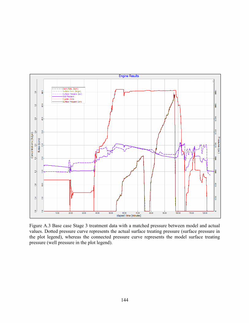
144
Figure A.3 Base case Stage 3 treatment data with a matched pressure between model and actual
values. Dotted pressure curve represents the actual surface treating pressure (surface pressure in
the plot legend), whereas the connected pressure curve represents the model surface treating
pressure (well pressure in the plot legend).
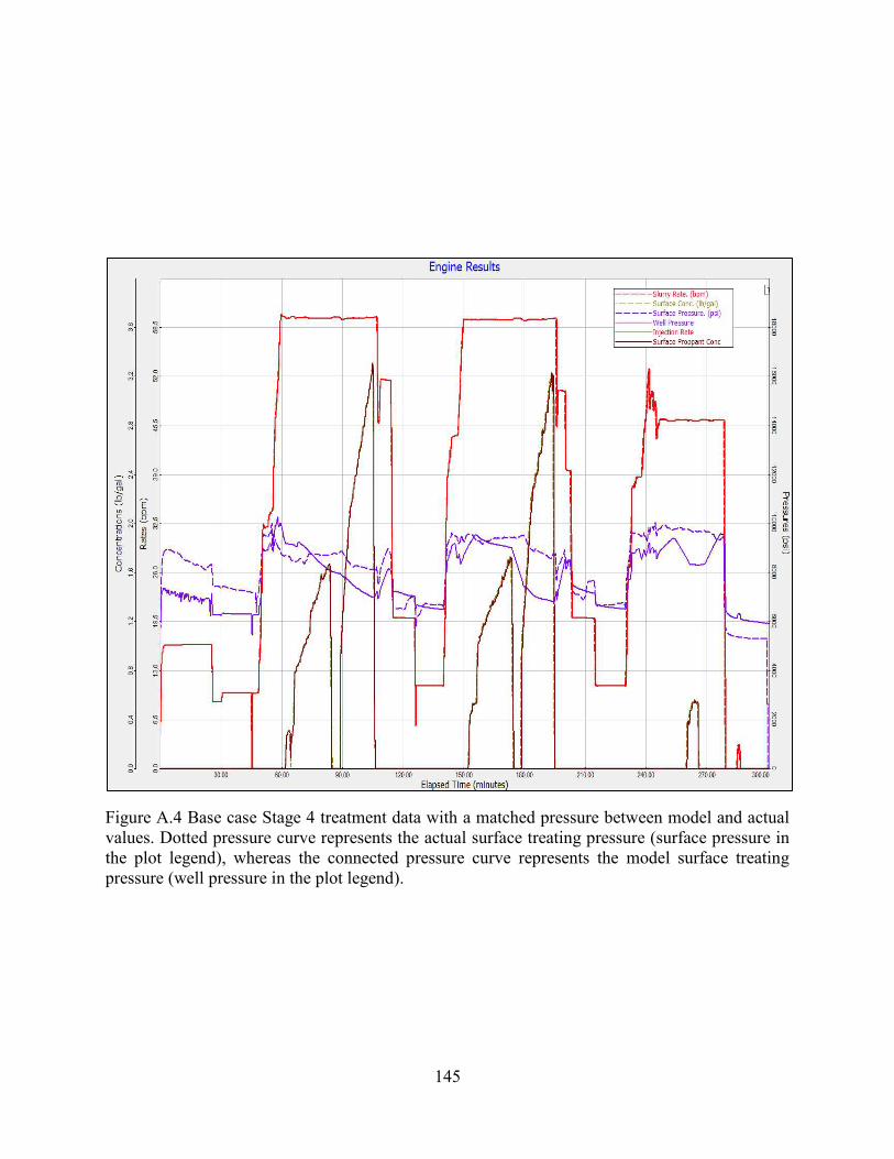
145
Figure A.4 Base case Stage 4 treatment data with a matched pressure between model and actual
values. Dotted pressure curve represents the actual surface treating pressure (surface pressure in
the plot legend), whereas the connected pressure curve represents the model surface treating
pressure (well pressure in the plot legend).

146
Figure A.5 Base case Stage 5 treatment data with a matched pressure between model and actual
values. Dotted pressure curve represents the actual surface treating pressure (surface pressure in
the plot legend), whereas the connected pressure curve represents the model surface treating
pressure (well pressure in the plot legend).

147
Figure A.6 Base case Stage 6 treatment data with a matched pressure between model and actual
values. Dotted pressure curve represents the actual surface treating pressure (surface pressure in
the plot legend), whereas the connected pressure curve represents the model surface treating
pressure (well pressure in the plot legend).

148
Figure A.7 Base case Stage 7 treatment data with a matched pressure between model and actual
values. Dotted pressure curve represents the actual surface treating pressure (surface pressure in
the plot legend), whereas the connected pressure curve represents the model surface treating
pressure (well pressure in the plot legend).

149
Figure A.8 Base case Stage 8 treatment data with a matched pressure between model and actual
values. Dotted pressure curve represents the actual surface treating pressure (surface pressure in
the plot legend), whereas the connected pressure curve represents the model surface treating
pressure (well pressure in the plot legend).
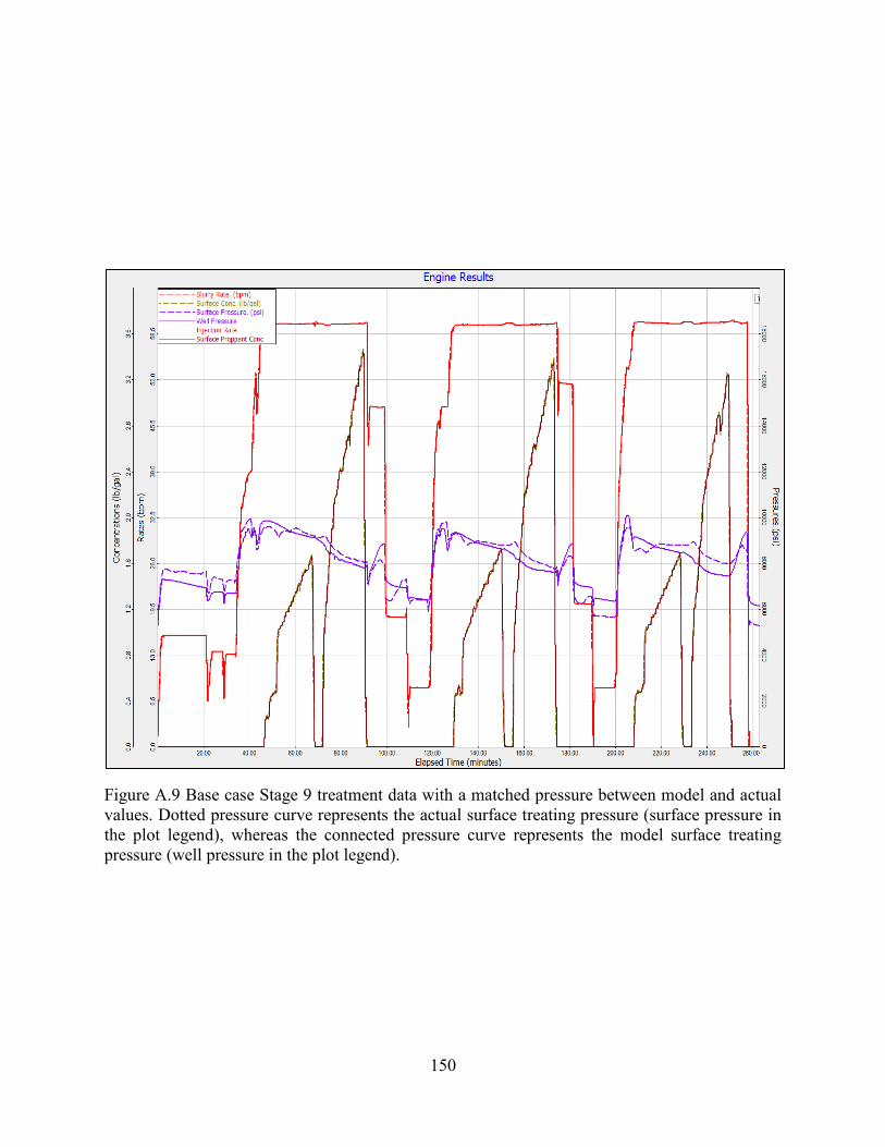
150
Figure A.9 Base case Stage 9 treatment data with a matched pressure between model and actual
values. Dotted pressure curve represents the actual surface treating pressure (surface pressure in
the plot legend), whereas the connected pressure curve represents the model surface treating
pressure (well pressure in the plot legend).
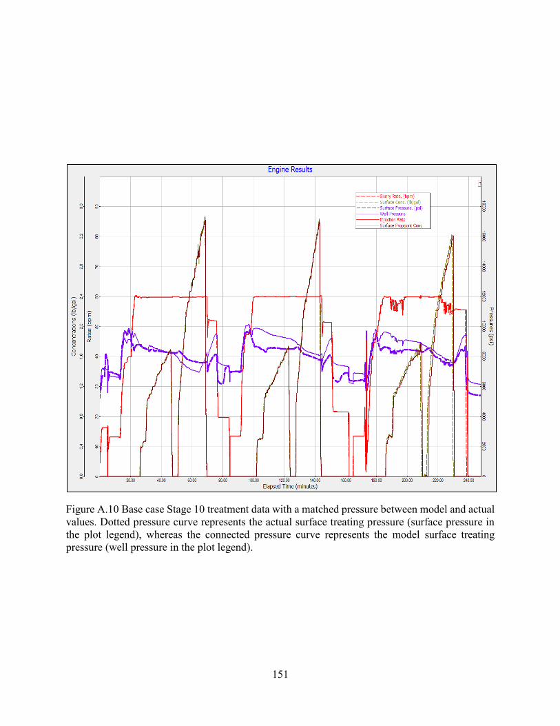
151
Figure A.10 Base case Stage 10 treatment data with a matched pressure between model and actual
values. Dotted pressure curve represents the actual surface treating pressure (surface pressure in
the plot legend), whereas the connected pressure curve represents the model surface treating
pressure (well pressure in the plot legend).

152
Figure A.11 Base case Stage 11 treatment data with a matched pressure between model and actual
values. Dotted pressure curve represents the actual surface treating pressure (surface pressure in
the plot legend), whereas the connected pressure curve represents the model surface treating
pressure (well pressure in the plot legend).

153
Figure A.12 Base case Stage 12 treatment data with a matched pressure between model and actual
values. Dotted pressure curve represents the actual surface treating pressure (surface pressure in
the plot legend), whereas the connected pressure curve represents the model surface treating
pressure (well pressure in the plot legend).
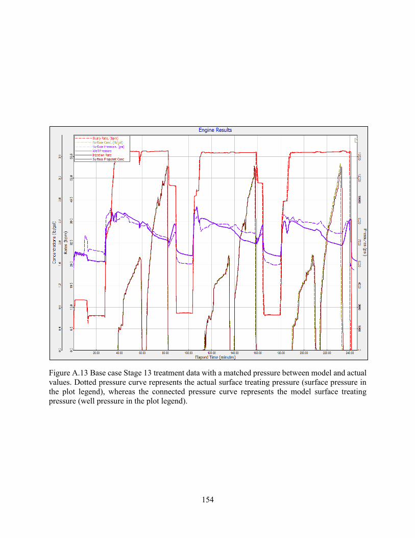
154
Figure A.13 Base case Stage 13 treatment data with a matched pressure between model and actual
values. Dotted pressure curve represents the actual surface treating pressure (surface pressure in
the plot legend), whereas the connected pressure curve represents the model surface treating
pressure (well pressure in the plot legend).
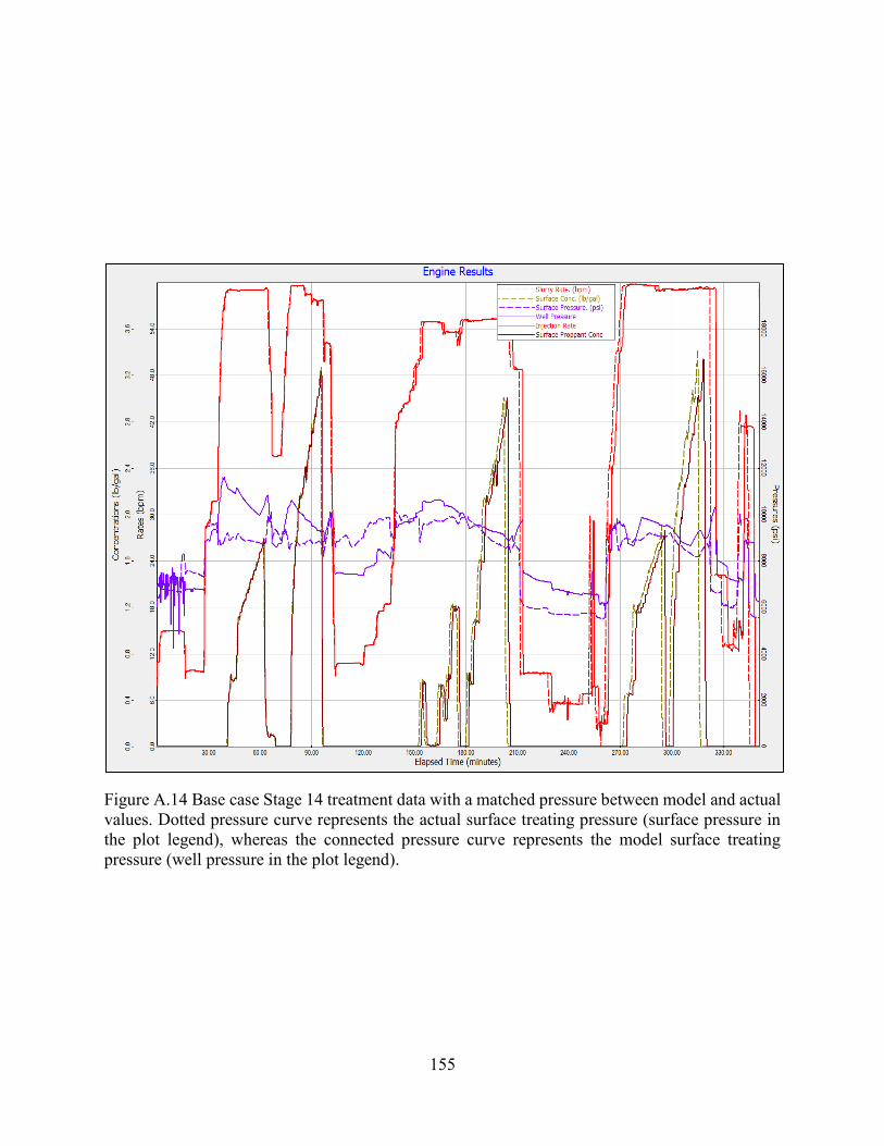
155
Figure A.14 Base case Stage 14 treatment data with a matched pressure between model and actual
values. Dotted pressure curve represents the actual surface treating pressure (surface pressure in
the plot legend), whereas the connected pressure curve represents the model surface treating
pressure (well pressure in the plot legend).

156
APPENDIX B
PREDICT-KTM INPUT DATA
Table B.1 Reservoir Properties Input into Predict-KTM Production Model
Reservoir property Value
Fracture drainage area 1.75 acres
Formation compressibility 8E-6 1/psi
Formation thickness 200 ft
Reservoir pressure 9500 psi
Permeability 0.000268 mD
Total porosity 0.07
Water saturation 0.35
Young’s modulus 5.50 MMpsi
X offset 0.50
Y offset 0.20
Aspect ratio 1.00
Table B.2 Well Properties Input into Predict-KTM Production Model
Well property Value
Wellbore radius 0.325 ft
Tube inner diameter 4.67 in
Tube length 15900 ft
Absolute pipe roughness 0.0006 in
Kv / Kh 0.01
Well temperature 70 ºF
Bottomhole temperature 311.8 ºF
Oilwell GOR 2000 scf/bbl
Lateral length 4928 ft
Lateral vertical position 0.5
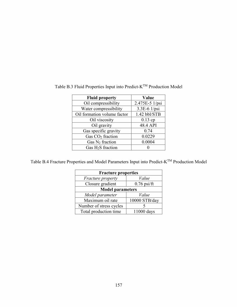
157
Table B.3 Fluid Properties Input into Predict-KTM Production Model
Fluid property Value
Oil compressibility 2.475E-5 1/psi
Water compressibility 3.3E-6 1/psi
Oil formation volume factor 1.42 bbl/STB
Oil viscosity 0.13 cp
Oil gravity 48.4 API
Gas specific gravity 0.74
Gas CO2 fraction 0.0229
Gas N2 fraction 0.0004
Gas H2S fraction 0
Table B.4 Fracture Properties and Model Parameters Input into Predict-KTM Production Model
Fracture properties
Fracture property Value
Closure gradient 0.76 psi/ft
Model parameters
Model parameter Value
Maximum oil rate 10000 STB/day
Number of stress cycles 5
Total production time 11000 days