ED211: Laboratoire des Fluides Complexes et leurs Reservoirs

Doctor of PhilosophySpeciality: Fluid Mechanics

presented by

Martin Petitfrere

EOS based simulations of thermal and compositionalflows in porous media

Directed by Dan V. Nichita and Igor Bogdanov

Defended on 12th September 2014 with a Jury:

M. Igor Bogdanov CHLOE Co-Director

M. Jean-Luc Daridon UPPA Examiner

M. Eric Hendriks SHELL Reporter

M. Jean-Noel Jaubert ENSIC Nancy Reporter

M. Claude Leibovici CFL CONSULTANT Examiner

M. Francois Montel TOTAL Examiner

M. Dan Vladimir Nichita CNRS/UPPA Director

M. Denis Voskov STANFORD University Examiner

acknowledgements

I would first thank all the jury members for accepting to evaluate my work.

Along this thesis, I have been working within different organisms; the LFCR (Laboratoire des Fluides

Complexes et de leurs Rservoirs), within the UPPA (Universit de Pau et des Pays de lAdours), TOTAL S.A.

and CHLOE (Centre dhuiles Lourdes ouvertes et exprimentales). I naturally acknowledge all those organisms

which made this work possible.

In the LFCR, I would naturally thank D.V. Nichita, my PhD director. I arrived at the beginning with

almost no knowledge on thermodynamics, Dan succeeded in teaching me the different aspects. He directed

the thesis really well, implying himself in every chapter, giving good advices even outside thermodynamics,

and pushing me when he had to. He oriented the work perfectly to work on feasible subjects and challenging

works. Finally I would like to thank him for the conferences, the moments we spent on top of the hill, and all

the fun we had during this period.

I would like to thank the members of the LFCR department: the professors, and especially Guillaume

Galliero for his advices and Jean-Luc Daridon, in charge of the structure. I would like to thank all the

students with whom I spent some really good time and finally a special thank to Catherine and Veronique for

all the work I made them do.

Besides, I stayed in the CHLOE laboratory for 2 years and a half. I found a really nice team I really

got along with. First, I would like to thank Arian Kamp, the former manager of CHLOE for creating, and

organizing the beginning of the thesis. I would like to thank Igor for the technical advices along my thesis,

for the chapter 5, in which he helped me a lot. I would like to thank Alain for the organization after the

departure of Arian. A special thanks to Mareylise, Alfredo for there advices in heavy oils, for the fun we

had and the cakes you made for us! Muchas gracias por el viernes de espanol. Finally I would like to thank

Brigitte, Isabelle and Delphine for their sympathy and all for the administrative tasks they have been doing

for me. Thank you Delphine who has always been there to open the door to someone who was always

forgetting its badge.. A special thank to Sebastien and Clement for the mathematical discussions and for all

the discussions and football we made! (Ps: thank you Clement for the latex/inskape help !!). I will miss the

football bets, even if i loose against interns (Mathieu...), working in CHLOE was a lot of fun.

Finally within Total, I have been working within three different departments. I would like to thank Xavier

Britsch who supervised the whole thesis from the beginning. Always giving good ideas and directing me

really well. My industrial supervisor was Franois Montel. He taught me a lot in thermodynamics, explaining

me different thermodynamics aspects. He gave me really good ideas and a good supervision, leaving me

a good freedom in my work. I have learned a lot from him in many different aspects. He seems to know

everything and it was really nice working with him.

Finally I would like to thank the intersim for the nice atmosphere. I would like to thank Bernard Faissat

and Gilles Darshes for accepting me within the department. I would like to acknowledge the whole team but

more specifically Corentin Rossignon for its expertise in computer science, even if the valgrind faults were not

mine.. And thank you for teaching me Inkscape (my favourite software now!) Leonardo Pattachini for all the

advices in reservoir simulation and equilibrium flash calculations. He was here to guide the orientation of the

thesis and I thank him. It was nice working around him.

Finally a really special thank to Alexandre Lapene. He was there to supervise my thesis as well. He

gave me really good advices especially for the thermal part of the reservoirs. He is the one who initiated the

collaboration with Stanford.

Last but not least, I would like to acknowledge Stanford University, for allowing me to come to Stanford

i

ii

and to use AD-GPRS for the presented thesis. More particularly I would like to thank D.Voskov and

R.Zaydullin for the exchanges and the collaboration that has been created. And for all the extra work

(restaurants, meal at Deniss place, wine testing). Hope the collaboration will go on!

Finally, I would like to thank my family and my friends. My parents have always been there and I owe

them a lot. I wouldn’t have come to the Total interview without them. They’ve always helped me in the

difficult situations. It was also really nice to spend these years close to my brothers and sisters. They are

always there for me too, and it was nice to be around them. I would like to thank my best friends : Jeremy

and Guillaume who supported me in the difficult times. Sophie, for the Reunion team building! The friends

from the badminton who helped me evacuating pressure, stress (special thanks to my partner Julien, Orni

and Alex, Pierrot, Elo, JB, Audrey, Romain). The friends from the UPPA who I spent a lot of time with:

Angie, Pamela, Ariane, Georgia, the two Erics, Julien, Julek, Magalie. All the lunch and parties we had were

really nice, and i hope we will keep on seeing each other!

Abstract

EOS based simulations of thermal and compositional flows in porous media

Three to four phase equilibrium calculations are in the heart of tertiary recovery simulations. In gas

injection, micro-emulsion flooding, steam-injections processes, additional phases emerging from the oil-

gas system are added to the set and have a significant impact on the oil recovery. The most important

computational effort in many chemical process simulators and in petroleum compositional reservoir simulations

is required by phase equilibrium and thermodynamic properties calculations. In chemical process simulators,

the high number of components to deal with makes the equilibrium calculations time-consuming; in reservoir

simulations, the number of components is limited (typically to a dozen), but a huge number of phase

equilibrium calculations is required in field scale simulations. Generally, pseudo-components are generated to

decrease the dimensionality of the system leading to approximations of the original problem. For all these

reasons, calculation algorithms must be robust and time-saving. In the literature, many simulators based on

different equations of state (EoS) have been designed but few of them are applicable to thermal recovery

processes such as steam injection. To the best of our knowledge, no fully compositional thermal simulation of

the steam injection process has been proposed with extra-heavy oils; these simulations are essential and will

offer improved tools for predictive studies of the heavy oil fields. Thus, in this thesis different algorithms

of improved efficiency and robustness for multiphase equilibrium calculations are proposed, able to handle

conditions encountered during the simulation of steam injection for heavy oil mixtures.

Most of the phase equilibrium calculations are based on the Newton method and use conventional

independent variables. These algorithms are first investigated and different improvements are proposed.

Michelsens (Fluid Phase Equilibria 9 (1982) 21-40) method for multiphase-split problems is modified in order

to take full advantage of symmetry (in the construction of the Jacobian matrix and the resolution of the

linear system). The reduction methods introduced by Michelsen (Ind. Eng. Chem. Process Des. Dev. 25

(1986) 184-188) and Hendriks (Ind. Eng. Chem. Res. 27 (1988) 1728-1732) enable to reduce the space of

study from nc (the number of components) for conventional variables to M (with M << nc) and are already

used in some commercial reservoir simulators. A reduction method based on the multi-linear expression of

the logarithm of fugacity coefficients (Nichita and Graciaa, Fluid Phase Equilibria. 302 (2011) 226-233) is

extended to phase stability analysis and multiphase-split calculations. Unlike previous reduction methods,

the set of variables is unbounded and the convergence path is the same as in conventional methods using the

logarithm of equilibrium constants as variables.

The Newton method requires a positive definite Hessian for convergence. Other kinds of minimization

methods are investigated which overcome this constraint; the Quasi-Newton and Trust-region methods always

guarantee a descent direction. These methods represent an interesting alternative since they can reach

supra-linear steps even when the Hessian is non-positive definite, and can reach quadratic steps (Trust-Region)

or nearly quadratic steps (Quasi-Newton) otherwise. A new set of independent variables is proposed (designed

to ensure a better scaling of the problem) for a modified BFGS (which ensures the positive definiteness of

the approximation of the Hessian matrix) algorithm and a Trust-Region method is also proposed for the

stability-testing and phase-split problems.

Subsequently, by assuming the fluid composition as semi-continuous, a methodology based on a Gaussian

quadrature is proposed to mathematically compute a set of pseudo-components capable of representing the

fluid behavior. The methodology can be seen as a lumping-delumping procedure, applicable to any number

of quadrature points and to any feed distribution (even in cases when no distribution function can model the

feed composition, or several distribution functions are needed to model different portions of the mixture.).

iii

iv

In a last part, a general multiphase flash procedure implementing all the developed algorithms is presented,

and tested against experimental and literature data. Three- and four phase CO2 injection simulations

demonstrate the capability of the program to handle any number of phases. Simulations of steam flooding are

performed for highly heterogeneous reservoirs. Finally, a fully compositional simulation of the steam assisted

gravity drainage (SAGD) process is realized. To the best of our knowledge, this is the first simulation of the

kind for heavy oil mixtures.

Keywords : phase equilibrium calculations, multiphase flash, reduction method, trust-region, quasi-

Newton, convergence, number of iteration, robustness, semi-continuous, Gaussian quadrature, characterization,

thermodynamics, SAGD, compositional, thermal, simulation, heavy oil, steam, injection, steam flooding

Simulation compositionnelle thermique d’ecoulements en milieux poreux,

utilisant une equation d’etat

Les calculs d’equilibres triphasiques et quadriphasiques sont au coeur des simulations de reservoirs

impliquant des processus de recuperations tertiaires. Dans les procedes d’injection de gaz, de balayage par

microemulsion et d’injection de vapeur, le systeme huile-gaz est enrichi d’une phase additionnelle qui joue un

role important dans la recuperation de l’huile en place. Les calculs d’equilibres de phases representent la majeur

partie des temps de calculs dans les simulateurs de procedes chimiques de par le grand nombre de composants

impliques, ainsi que dans les simulations de reservoir compositionnelles qui, contrairement aux simulations de

procedes, ne requierent qu’un nombre limite de composants (typiquement une dizaine), mais impliquent un

nombre consequent de calculs d’equilibre. En general, des pseudo-composants permettant d’approximer le

comportement du fluide sont generes, afin de reduire la dimensionnalite du systeme. Pour toutes ces raisons,

il est important de concevoir des algorithmes de calculs d’equilibre qui soient fiables, robustes et rapides.

Dans la litterature de nombreux simulateurs de reservoirs bases sur des equations d’etat ont ete concus,

mais peu d’entre eux sont applicables aux procedes de recuperation thermique tels que l’injection de vapeur.

A notre connaissance, il n’existe pas de simulation thermique completement compositionnelle du procede

d’injection de vapeur pour des cas d’applications aux huiles lourdes. Ces simulations apparaissent essentielles

et pourraient offrir des outils ameliores pour aider la recuperation amelioree de certains champs petroliers.

Finalement, dans cette these, des algorithmes robustes et efficaces de calculs des equilibres multiphasiques

sont proposes permettant de surmonter les difficultes rencontres durant les simulations d’injection de vapeur

pour des huiles lourdes.

La plupart des algorithmes d’equilibre de phases sont bases sur la methode de Newton et utilisent les

variables conventionnelles comme variables independantes. Dans un premier temps, des ameliorations de ces

algorithmes sont proposees. Les variables reduites introduites par Michelsen (Ind. Eng. Chem. Process Des.

Dev. 25 (1986) 184-188) et Hendriks (Ind. Eng. Chem. Res. 27 (1988) 1728-1732), permettent de reduire la

dimensionnalite du systeme de nc (le nombre de composants) dans le cas des variables conventionnelles, a M

(avec M << nc), et sont deja utilisees dans certains simulateurs de reservoirs commerciaux. Une methode de

reduction basee sur l’expression multilineaire du logarithme des coefficients de fugacites (Nichita and Graciaa,

Fluid Phase Equilibria. 302 (2011) 226-233) est etendue a l’analyse de stabilite et aux calculs d’equilibres

multiphasiques. A l’inverse des precedentes methodes de reduction, les variables ne sont pas bornees et

le chemin de convergence est le meme que pour les methodes conventionnelles utilisant le logarithme des

constantes d’equilibres comme variables independantes.

La methode de Newton necessite une Hessienne definie positive pour pouvoir etre utilisee. D’autres

methodes de minimisations sont testees qui permettent de s’affranchir de cette contrainte; les methodes Quasi-

Newton et Trust-Region garantissent une direction de descente a chaque iteration. Ces methodes presentent

un grand interet puisqu’elles permettent de realiser des pas supra-lineaires meme lorsque la Hessienne n’est pas

definie positive, et de realiser des pas quadratiques (Trust-Region) ou proches de quadratiques (Quasi-Newton)

v

dans le cas contraire. Un nouveau vecteur de variables independantes est propose (construit afin d’obtenir une

meilleure mise echelle du probleme) et utilise au sein d’un algorithme BFGS modifie (qui, par construction,

approxime la matrice Hessienne par une matrice definie positive). De meme, une methode de Trust-Region

est developpee pour les problemes de tests de stabilites et d’equilibres multiphasiques.

Ensuite, considerant le fluide comme semi-continu, une methodologie basee sur une procedure de quadrature

Gaussienne est proposee pour calculer mathematiquement des pseudo-composants capables de representer le

comportement du fluide. La methodologie peut etre vue comme une procedure de groupement/degroupement,

applicable pour tout nombre de points de quadratures et toute composition du melange (meme dans les cas

ou aucune distribution ne peut modeliser la composition du melange, ou lorsque plusieurs distributions sont

necessaires afin de modeliser les differentes portions de melange). Dans une derniere partie, un algorithme

general pour le calcul des equilibres multiphasiques est presente incluant tous les algorithmes developpes. Cet

algorithme est aussi teste et valide pour des donnees experimentales et de la litterature. Des simulations

triphasiques et quadriphasiques d’injection de CO2 demontrent la capacite du programme a traiter un nombre

arbitraire de phases. Des simulations de balayages par la vapeur sont realisees pour des reservoirs montrant

d’importantes heterogeneites. Finalement, une simulation totalement compositionnelle du processus de Steam

Assisted Gravity Drainage (SAGD) est realisee. A notre connaissance, il s’agit de la premiere simulation de

la sorte pour des cas d’applications d’huiles lourdes.

Mots cles: calculs d’equilibres, multiphasiques, methode de reduction, trust-region, quasi-Newton,

convergence, nombre d’iterations, robustesse, semi-continue, quadrature Gaussienne, caracterisation, thermo-

dynamique, SAGD, compositionnelle, thermique, simulation, huile lourde, vapeur, injection, balayage par la

vapeur

Contents

Acknowledgements i

Abstract iii

Contents vi

French description of the thesis 1

0 Introduction . . . . . . . . . . . . . . . . . . . . . . . . . . . . . . . . . . . . . . . . . . . . . . 1

0.1 Les huiles lourdes comme un moyen de repondre a la demande denergie croissante . . 1

0.2 Recuperation assistee du petrole . . . . . . . . . . . . . . . . . . . . . . . . . . . . . . 1

0.3 Amelioration de la thermodynamique et des simulateurs de reservoirs existant . . . . . 3

0.3.1 Un besoin d’ameliorer les simulateurs de reservoirs . . . . . . . . . . . . . . . 3

0.3.2 Calculs d’equilibre multiphasiques . . . . . . . . . . . . . . . . . . . . . . . . 3

0.4 Plan de these . . . . . . . . . . . . . . . . . . . . . . . . . . . . . . . . . . . . . . . . . 4

1 Chapitre 1: Thermodynamique fondamentale . . . . . . . . . . . . . . . . . . . . . . . . . . . 6

2 Chapitre 2: La procedure globale de calculs d’equilibre multiphasiques . . . . . . . . . . . . . 6

3 Chapitre 3: Amelioration des calculs d’equilibre . . . . . . . . . . . . . . . . . . . . . . . . . . 7

4 Chapitre 4: Amelioration de la caracterisation des huiles lourdes par la thermodynamique

semi-continue . . . . . . . . . . . . . . . . . . . . . . . . . . . . . . . . . . . . . . . . . . . . . 7

5 Chapitre 5 : Simulation de reservoir . . . . . . . . . . . . . . . . . . . . . . . . . . . . . . . . 9

6 Conclusions et Perspectives . . . . . . . . . . . . . . . . . . . . . . . . . . . . . . . . . . . . . 11

6.1 Conclusions . . . . . . . . . . . . . . . . . . . . . . . . . . . . . . . . . . . . . . . . . . 11

6.2 Perspectives . . . . . . . . . . . . . . . . . . . . . . . . . . . . . . . . . . . . . . . . . . 13

Introduction 15

1 The heavy oils, a viable alternative to the increasing energy demand . . . . . . . . . . . . . . 15

2 Enhanced oil recovery . . . . . . . . . . . . . . . . . . . . . . . . . . . . . . . . . . . . . . . . 16

3 Improved reservoir simulation and thermodynamics . . . . . . . . . . . . . . . . . . . . . . . . 17

3.1 A need to improve the reservoir simulators . . . . . . . . . . . . . . . . . . . . . . . . 17

3.2 Multiphase equilibrium calculations . . . . . . . . . . . . . . . . . . . . . . . . . . . . 19

4 Overview of the thesis . . . . . . . . . . . . . . . . . . . . . . . . . . . . . . . . . . . . . . . . 20

1 Fundamental thermodynamics 22

1.1 Thermodynamics functions . . . . . . . . . . . . . . . . . . . . . . . . . . . . . . . . . . . . . 22

1.1.1 Internal Energy . . . . . . . . . . . . . . . . . . . . . . . . . . . . . . . . . . . . . . . . 22

1.1.1.1 First Law . . . . . . . . . . . . . . . . . . . . . . . . . . . . . . . . . . . . . . 22

1.1.1.2 Second law . . . . . . . . . . . . . . . . . . . . . . . . . . . . . . . . . . . . . 23

1.1.2 Gibbs free energy . . . . . . . . . . . . . . . . . . . . . . . . . . . . . . . . . . . . . . . 24

1.1.3 Helmholtz free energy . . . . . . . . . . . . . . . . . . . . . . . . . . . . . . . . . . . . 25

1.1.4 Enthalpy . . . . . . . . . . . . . . . . . . . . . . . . . . . . . . . . . . . . . . . . . . . 25

1.1.5 Residual energy . . . . . . . . . . . . . . . . . . . . . . . . . . . . . . . . . . . . . . . . 25

1.1.6 Maximization of the entropy . . . . . . . . . . . . . . . . . . . . . . . . . . . . . . . . 25

1.1.7 Fugacity and fugacity coefficients . . . . . . . . . . . . . . . . . . . . . . . . . . . . . . 26

CONTENTS vi

CONTENTS vii

1.1.8 Condition for equilibrium at constant pressure and temperature . . . . . . . . . . . . . 28

1.2 Equation of State Calculations . . . . . . . . . . . . . . . . . . . . . . . . . . . . . . . . . . . 29

1.2.1 Introduction . . . . . . . . . . . . . . . . . . . . . . . . . . . . . . . . . . . . . . . . . 29

1.2.2 Cubic equations of state . . . . . . . . . . . . . . . . . . . . . . . . . . . . . . . . . . . 29

1.2.2.1 Solving the cubic polynomial equation . . . . . . . . . . . . . . . . . . . . . . 30

1.2.3 Fugacity coefficient . . . . . . . . . . . . . . . . . . . . . . . . . . . . . . . . . . . . . . 31

1.2.4 Molar Gibbs free energy . . . . . . . . . . . . . . . . . . . . . . . . . . . . . . . . . . . 31

2 Global multiphase flash procedure 32

2.1 Introduction . . . . . . . . . . . . . . . . . . . . . . . . . . . . . . . . . . . . . . . . . . . . . . 32

2.2 Stability Analysis . . . . . . . . . . . . . . . . . . . . . . . . . . . . . . . . . . . . . . . . . . . 33

2.2.1 The stationary points . . . . . . . . . . . . . . . . . . . . . . . . . . . . . . . . . . . . 34

2.2.2 Initial guesses . . . . . . . . . . . . . . . . . . . . . . . . . . . . . . . . . . . . . . . . . 35

2.2.3 General minimization algorithm . . . . . . . . . . . . . . . . . . . . . . . . . . . . . . 36

2.2.4 Bypass acceleration method . . . . . . . . . . . . . . . . . . . . . . . . . . . . . . . . . 36

2.3 Multiphase-split calculations . . . . . . . . . . . . . . . . . . . . . . . . . . . . . . . . . . . . 37

2.3.1 Solving the Rachford-Rice equation . . . . . . . . . . . . . . . . . . . . . . . . . . . . . 39

2.3.1.1 Two phase-split calculations . . . . . . . . . . . . . . . . . . . . . . . . . . . 39

2.3.1.2 Multiphase equilibrium calculations . . . . . . . . . . . . . . . . . . . . . . . 40

2.3.2 Phase-split calculations . . . . . . . . . . . . . . . . . . . . . . . . . . . . . . . . . . . 42

2.4 General multiphase equilibrium algorithm . . . . . . . . . . . . . . . . . . . . . . . . . . . . . 43

3 Improvements in equilibrium calculations 44

3.1 Presentation of conventional methods . . . . . . . . . . . . . . . . . . . . . . . . . . . . . . . 45

3.1.1 Stability testing . . . . . . . . . . . . . . . . . . . . . . . . . . . . . . . . . . . . . . . 45

3.1.1.1 Mole numbers as independent variables . . . . . . . . . . . . . . . . . . . . . 45

3.1.1.2 lnYi as independent variables . . . . . . . . . . . . . . . . . . . . . . . . . . . 46

3.1.1.3 alpha as independent variable . . . . . . . . . . . . . . . . . . . . . . . . . . 46

3.1.2 Multiphase flash calculations . . . . . . . . . . . . . . . . . . . . . . . . . . . . . . . . 47

3.1.2.1 Mole numbers as independent variables . . . . . . . . . . . . . . . . . . . . . 48

3.1.2.2 Improved mole numbers as independent variables . . . . . . . . . . . . . . . 49

3.1.2.3 ln K as independent variables . . . . . . . . . . . . . . . . . . . . . . . . . . . 49

3.2 Reduction methods . . . . . . . . . . . . . . . . . . . . . . . . . . . . . . . . . . . . . . . . . . 51

3.2.1 Presentation of existing reduction based methods . . . . . . . . . . . . . . . . . . . . . 52

3.2.1.1 Reduction parameters . . . . . . . . . . . . . . . . . . . . . . . . . . . . . . . 52

3.2.1.2 Two phase-split calculations in the reduction approach . . . . . . . . . . . . 54

3.2.1.3 Phase stability in the reduction approach . . . . . . . . . . . . . . . . . . . . 55

3.2.1.4 Pseudo-reduces methods . . . . . . . . . . . . . . . . . . . . . . . . . . . . . 55

3.2.2 A new reduction method for the stability analysis problem . . . . . . . . . . . . . . . 56

3.2.2.1 Introduction . . . . . . . . . . . . . . . . . . . . . . . . . . . . . . . . . . . . 56

3.2.2.2 Proposed reduction method . . . . . . . . . . . . . . . . . . . . . . . . . . . . 57

3.2.2.3 Results . . . . . . . . . . . . . . . . . . . . . . . . . . . . . . . . . . . . . . . 61

3.2.2.4 Discussion . . . . . . . . . . . . . . . . . . . . . . . . . . . . . . . . . . . . . 64

3.2.2.5 Conclusion . . . . . . . . . . . . . . . . . . . . . . . . . . . . . . . . . . . . . 66

3.2.3 A comparison of conventional and reduction approaches for phase equilibrium calculations 66

3.2.3.1 Introduction . . . . . . . . . . . . . . . . . . . . . . . . . . . . . . . . . . . . 66

3.2.3.2 Results . . . . . . . . . . . . . . . . . . . . . . . . . . . . . . . . . . . . . . . 67

3.2.3.3 Discussion . . . . . . . . . . . . . . . . . . . . . . . . . . . . . . . . . . . . . 77

3.2.3.4 Conclusion . . . . . . . . . . . . . . . . . . . . . . . . . . . . . . . . . . . . . 79

CONTENTS viii

3.2.4 A new reduction method for multiphase equilibrium calculations . . . . . . . . . . . . 80

3.2.4.1 Introduction . . . . . . . . . . . . . . . . . . . . . . . . . . . . . . . . . . . . 80

3.2.4.2 Reduction multiphase flash . . . . . . . . . . . . . . . . . . . . . . . . . . . . 81

3.2.4.3 Results . . . . . . . . . . . . . . . . . . . . . . . . . . . . . . . . . . . . . . . 85

3.2.4.4 Discussion . . . . . . . . . . . . . . . . . . . . . . . . . . . . . . . . . . . . . 90

3.2.4.5 Conclusions . . . . . . . . . . . . . . . . . . . . . . . . . . . . . . . . . . . . . 92

3.3 Phase equilibrium calculations with quasi-Newton methods . . . . . . . . . . . . . . . . . . . 93

3.3.1 Introduction . . . . . . . . . . . . . . . . . . . . . . . . . . . . . . . . . . . . . . . . . 93

3.3.2 The BFGS quasi-Newton method . . . . . . . . . . . . . . . . . . . . . . . . . . . . . . 93

3.3.2.1 Newton . . . . . . . . . . . . . . . . . . . . . . . . . . . . . . . . . . . . . . . 93

3.3.2.2 The BFGS update . . . . . . . . . . . . . . . . . . . . . . . . . . . . . . . . . 94

3.3.2.3 The Line search procedure . . . . . . . . . . . . . . . . . . . . . . . . . . . . 94

3.3.2.4 Ammar and Renon BFGS implementation . . . . . . . . . . . . . . . . . . . 96

3.3.3 Proposed method . . . . . . . . . . . . . . . . . . . . . . . . . . . . . . . . . . . . . . . 98

3.3.3.1 Two-phase split calculations . . . . . . . . . . . . . . . . . . . . . . . . . . . 98

3.3.3.2 Stability analysis . . . . . . . . . . . . . . . . . . . . . . . . . . . . . . . . . . 100

3.3.4 Results . . . . . . . . . . . . . . . . . . . . . . . . . . . . . . . . . . . . . . . . . . . . 100

3.3.4.1 Tests on different BFGS methods . . . . . . . . . . . . . . . . . . . . . . . . 101

3.3.4.2 Mixtures used in this study . . . . . . . . . . . . . . . . . . . . . . . . . . . . 101

3.3.4.3 Error and stopping criteria . . . . . . . . . . . . . . . . . . . . . . . . . . . . 101

3.3.4.4 Results . . . . . . . . . . . . . . . . . . . . . . . . . . . . . . . . . . . . . . . 101

3.3.4.5 Discussion . . . . . . . . . . . . . . . . . . . . . . . . . . . . . . . . . . . . . 107

3.3.4.6 Conclusions/Perspectives . . . . . . . . . . . . . . . . . . . . . . . . . . . . . 108

3.4 Robust and efficient Trust-Region based stability analysis and multiphase flash calculations . 108

3.4.1 Introduction . . . . . . . . . . . . . . . . . . . . . . . . . . . . . . . . . . . . . . . . . 108

3.4.2 Trust-Region methods . . . . . . . . . . . . . . . . . . . . . . . . . . . . . . . . . . . . 109

3.4.2.1 The Trust-Region subproblem . . . . . . . . . . . . . . . . . . . . . . . . . . 110

3.4.2.2 Solving the Trust-Region subproblem . . . . . . . . . . . . . . . . . . . . . . 110

3.4.2.3 Algorithm for the Trust-Region subproblem . . . . . . . . . . . . . . . . . . . 114

3.4.2.4 The Trust-Region size . . . . . . . . . . . . . . . . . . . . . . . . . . . . . . . 115

3.4.3 Results . . . . . . . . . . . . . . . . . . . . . . . . . . . . . . . . . . . . . . . . . . . . 117

3.4.3.1 Phase stability testing . . . . . . . . . . . . . . . . . . . . . . . . . . . . . . . 118

3.4.3.2 Multiphase flash calculations . . . . . . . . . . . . . . . . . . . . . . . . . . . 121

3.4.4 Conclusions . . . . . . . . . . . . . . . . . . . . . . . . . . . . . . . . . . . . . . . . . . 130

3.5 Multiphase flash, using ln K and phase mole fractions as independent variables . . . . . . . . 130

3.5.1 Introduction . . . . . . . . . . . . . . . . . . . . . . . . . . . . . . . . . . . . . . . . . 130

3.5.2 New proposed method . . . . . . . . . . . . . . . . . . . . . . . . . . . . . . . . . . . . 130

3.5.3 Results . . . . . . . . . . . . . . . . . . . . . . . . . . . . . . . . . . . . . . . . . . . . 132

3.5.3.1 Computational time . . . . . . . . . . . . . . . . . . . . . . . . . . . . . . . . 133

3.5.3.2 Convergence behavior . . . . . . . . . . . . . . . . . . . . . . . . . . . . . . . 134

3.5.3.3 Discussion . . . . . . . . . . . . . . . . . . . . . . . . . . . . . . . . . . . . . 135

4 Improvements in the characterization of heavy oils : Semi-continuous thermodynamics136

4.1 Introduction . . . . . . . . . . . . . . . . . . . . . . . . . . . . . . . . . . . . . . . . . . . . . . 136

4.2 A new distribution function . . . . . . . . . . . . . . . . . . . . . . . . . . . . . . . . . . . . . 138

4.3 Gaussian quadrature . . . . . . . . . . . . . . . . . . . . . . . . . . . . . . . . . . . . . . . . . 140

4.4 Semi-continuous description . . . . . . . . . . . . . . . . . . . . . . . . . . . . . . . . . . . . . 141

4.5 Calculation procedure . . . . . . . . . . . . . . . . . . . . . . . . . . . . . . . . . . . . . . . . 144

4.5.1 Discrete equilibrium flash calculations . . . . . . . . . . . . . . . . . . . . . . . . . . . 144

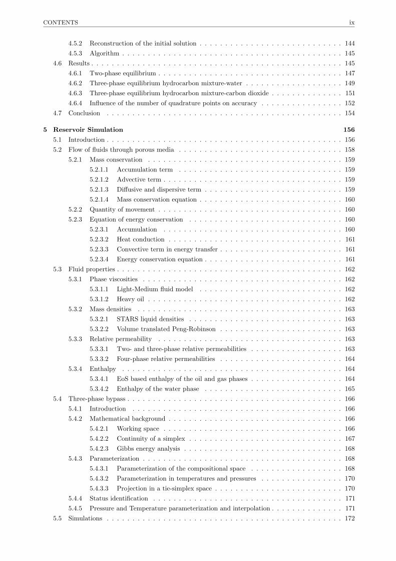
CONTENTS ix

4.5.2 Reconstruction of the initial solution . . . . . . . . . . . . . . . . . . . . . . . . . . . . 144

4.5.3 Algorithm . . . . . . . . . . . . . . . . . . . . . . . . . . . . . . . . . . . . . . . . . . . 145

4.6 Results . . . . . . . . . . . . . . . . . . . . . . . . . . . . . . . . . . . . . . . . . . . . . . . . . 145

4.6.1 Two-phase equilibrium . . . . . . . . . . . . . . . . . . . . . . . . . . . . . . . . . . . . 147

4.6.2 Three-phase equilibrium hydrocarbon mixture-water . . . . . . . . . . . . . . . . . . . 149

4.6.3 Three-phase equilibrium hydrocarbon mixture-carbon dioxide . . . . . . . . . . . . . . 151

4.6.4 Influence of the number of quadrature points on accuracy . . . . . . . . . . . . . . . . 152

4.7 Conclusion . . . . . . . . . . . . . . . . . . . . . . . . . . . . . . . . . . . . . . . . . . . . . . 154

5 Reservoir Simulation 156

5.1 Introduction . . . . . . . . . . . . . . . . . . . . . . . . . . . . . . . . . . . . . . . . . . . . . . 156

5.2 Flow of fluids through porous media . . . . . . . . . . . . . . . . . . . . . . . . . . . . . . . . 158

5.2.1 Mass conservation . . . . . . . . . . . . . . . . . . . . . . . . . . . . . . . . . . . . . . 159

5.2.1.1 Accumulation term . . . . . . . . . . . . . . . . . . . . . . . . . . . . . . . . 159

5.2.1.2 Advective term . . . . . . . . . . . . . . . . . . . . . . . . . . . . . . . . . . . 159

5.2.1.3 Diffusive and dispersive term . . . . . . . . . . . . . . . . . . . . . . . . . . . 159

5.2.1.4 Mass conservation equation . . . . . . . . . . . . . . . . . . . . . . . . . . . . 160

5.2.2 Quantity of movement . . . . . . . . . . . . . . . . . . . . . . . . . . . . . . . . . . . . 160

5.2.3 Equation of energy conservation . . . . . . . . . . . . . . . . . . . . . . . . . . . . . . 160

5.2.3.1 Accumulation . . . . . . . . . . . . . . . . . . . . . . . . . . . . . . . . . . . 160

5.2.3.2 Heat conduction . . . . . . . . . . . . . . . . . . . . . . . . . . . . . . . . . . 161

5.2.3.3 Convective term in energy transfer . . . . . . . . . . . . . . . . . . . . . . . . 161

5.2.3.4 Energy conservation equation . . . . . . . . . . . . . . . . . . . . . . . . . . . 161

5.3 Fluid properties . . . . . . . . . . . . . . . . . . . . . . . . . . . . . . . . . . . . . . . . . . . . 162

5.3.1 Phase viscosities . . . . . . . . . . . . . . . . . . . . . . . . . . . . . . . . . . . . . . . 162

5.3.1.1 Light-Medium fluid model . . . . . . . . . . . . . . . . . . . . . . . . . . . . 162

5.3.1.2 Heavy oil . . . . . . . . . . . . . . . . . . . . . . . . . . . . . . . . . . . . . . 162

5.3.2 Mass densities . . . . . . . . . . . . . . . . . . . . . . . . . . . . . . . . . . . . . . . . 163

5.3.2.1 STARS liquid densities . . . . . . . . . . . . . . . . . . . . . . . . . . . . . . 163

5.3.2.2 Volume translated Peng-Robinson . . . . . . . . . . . . . . . . . . . . . . . . 163

5.3.3 Relative permeability . . . . . . . . . . . . . . . . . . . . . . . . . . . . . . . . . . . . 163

5.3.3.1 Two- and three-phase relative permeabilities . . . . . . . . . . . . . . . . . . 163

5.3.3.2 Four-phase relative permeabilities . . . . . . . . . . . . . . . . . . . . . . . . 164

5.3.4 Enthalpy . . . . . . . . . . . . . . . . . . . . . . . . . . . . . . . . . . . . . . . . . . . 164

5.3.4.1 EoS based enthalpy of the oil and gas phases . . . . . . . . . . . . . . . . . . 164

5.3.4.2 Enthalpy of the water phase . . . . . . . . . . . . . . . . . . . . . . . . . . . 165

5.4 Three-phase bypass . . . . . . . . . . . . . . . . . . . . . . . . . . . . . . . . . . . . . . . . . . 166

5.4.1 Introduction . . . . . . . . . . . . . . . . . . . . . . . . . . . . . . . . . . . . . . . . . 166

5.4.2 Mathematical background . . . . . . . . . . . . . . . . . . . . . . . . . . . . . . . . . . 166

5.4.2.1 Working space . . . . . . . . . . . . . . . . . . . . . . . . . . . . . . . . . . . 166

5.4.2.2 Continuity of a simplex . . . . . . . . . . . . . . . . . . . . . . . . . . . . . . 167

5.4.2.3 Gibbs energy analysis . . . . . . . . . . . . . . . . . . . . . . . . . . . . . . . 168

5.4.3 Parameterization . . . . . . . . . . . . . . . . . . . . . . . . . . . . . . . . . . . . . . . 168

5.4.3.1 Parameterization of the compositional space . . . . . . . . . . . . . . . . . . 168

5.4.3.2 Parameterization in temperatures and pressures . . . . . . . . . . . . . . . . 170

5.4.3.3 Projection in a tie-simplex space . . . . . . . . . . . . . . . . . . . . . . . . . 170

5.4.4 Status identification . . . . . . . . . . . . . . . . . . . . . . . . . . . . . . . . . . . . . 171

5.4.5 Pressure and Temperature parameterization and interpolation . . . . . . . . . . . . . . 171

5.5 Simulations . . . . . . . . . . . . . . . . . . . . . . . . . . . . . . . . . . . . . . . . . . . . . . 172

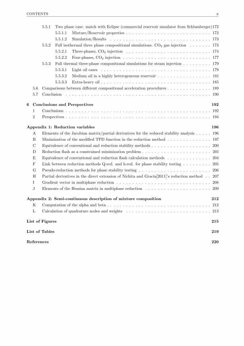
CONTENTS x

5.5.1 Two phase case: match with Eclipse (commercial reservoir simulator from Schlumberger)172

5.5.1.1 Mixture/Reservoir properties . . . . . . . . . . . . . . . . . . . . . . . . . . . 172

5.5.1.2 Simulation/Results . . . . . . . . . . . . . . . . . . . . . . . . . . . . . . . . 173

5.5.2 Full isothermal three phase compositional simulations: CO2 gas injection . . . . . . . 173

5.5.2.1 Three-phases, CO2 injection . . . . . . . . . . . . . . . . . . . . . . . . . . . 174

5.5.2.2 Four-phases, CO2 injection . . . . . . . . . . . . . . . . . . . . . . . . . . . . 177

5.5.3 Full thermal three-phase compositional simulations for steam injection . . . . . . . . . 179

5.5.3.1 Light oil cases . . . . . . . . . . . . . . . . . . . . . . . . . . . . . . . . . . . 179

5.5.3.2 Medium oil in a highly heterogeneous reservoir . . . . . . . . . . . . . . . . . 181

5.5.3.3 Extra-heavy oil . . . . . . . . . . . . . . . . . . . . . . . . . . . . . . . . . . . 185

5.6 Comparisons between different compositional acceleration procedures . . . . . . . . . . . . . . 189

5.7 Conclusion . . . . . . . . . . . . . . . . . . . . . . . . . . . . . . . . . . . . . . . . . . . . . . 190

6 Conclusions and Perspectives 192

1 Conclusions . . . . . . . . . . . . . . . . . . . . . . . . . . . . . . . . . . . . . . . . . . . . . . 192

2 Perspectives . . . . . . . . . . . . . . . . . . . . . . . . . . . . . . . . . . . . . . . . . . . . . . 194

Appendix 1: Reduction variables 196

A Elements of the Jacobian matrix/partial derivatives for the reduced stability analysis . . . . . 196

B Minimization of the modified TPD function in the reduction method . . . . . . . . . . . . . . 197

C Equivalence of conventional and reduction stability methods . . . . . . . . . . . . . . . . . . . 200

D Reduction flash as a constrained minimization problem . . . . . . . . . . . . . . . . . . . . . . 201

E Equivalence of conventional and reduction flash calculation methods . . . . . . . . . . . . . . 204

F Link between reduction methods Q-red. and h-red. for phase stability testing . . . . . . . . . 205

G Pseudo-reduction methods for phase stability testing . . . . . . . . . . . . . . . . . . . . . . . 206

H Partial derivatives in the direct extension of Nichita and Gracia[2011]’s reduction method . . 207

I Gradient vector in multiphase reduction . . . . . . . . . . . . . . . . . . . . . . . . . . . . . . 208

J Elements of the Hessian matrix in multiphase reduction . . . . . . . . . . . . . . . . . . . . . 209

Appendix 2: Semi-continuous description of mixture composition 212

K Computation of the alpha and beta . . . . . . . . . . . . . . . . . . . . . . . . . . . . . . . . . 212

L Calculation of quadrature nodes and weights . . . . . . . . . . . . . . . . . . . . . . . . . . . 213

List of Figures 215

List of Tables 219

References 220

French description of the thesis

0 Introduction

0.1 Les huiles lourdes comme un moyen de repondre a la demande denergie

croissante

Les besoins en energie des economies emergentes, et particulierement en Asie (Chine, Inde) sont de plus en

plus importants. Dans ce contexte, la production d’energie s’accroit chaque annee, et l’IEO2013 (International

Energy Outlook 2013) projette que la consommation d’energie mondiale augmentera de 56% entre 2010 et

2040. Les energies fossiles representent la plus grande source d’energie, et leur production doit etre augmentee

pour satisfaire a la hasse en demande d’energie.

Les huiles peuvent etre classifiees en differentes categories selon leur API gravity; qui est une mesure du

poids de l’huile par rapport a celui de l’eau:

• Si elle est plus grande que 10, l’huile est moins dense que l’eau et flotte.

• Si elle est plus petite, l’huile coule;

Les huiles conventionnelles ont un degre API superieur a 25. Due a leur faible densite et viscosite, elles

peuvent generalement etre recuperees facilement et leur coup de production reste assez faible. C’est pourquoi

elles ont ete exploitees jusqu’a present. Cependant, les huiles conventionnelles deviennent de plus en plus

rares. Leur production decroit de 5% par an et les reserves prouvees peuvent encore subvenir a 40 ans de

productions en gardant le meme debit.

Les huiles lourdes ont souvent un degre API se situant entre 5 et 22 (voir fig. 1). Due a leur importante

viscosite, des methodes d’EoR (Enhanced Oil Recovery) doivent etre utilisees afin d’obtenir un rendement

suffisant, ce qui les rend leur cot de production plus couteuses que pour des huiles conventionnelles. Cependant,

le prix du baril augmentant avec la demande, l’exploitations de champs d’huiles lourdes devient de plus en

plus rentable et pourrait jouer un role important dans le futur. Avec un volume d’huile en place estime entre

3000 et 4000 milliards de barils et des reserves potentielles autour de 500 000 milliards de barils, les huiles

lourdes representent pres de 60% des reserves globales en huiles conventionnelles et representent 20 a 25%

des ressources de petrole globales. Leur exploitation pourrait etendre les reserves d’energies mondiales pour

environ 15 ans. Differentes methodes d’EOR existent pour permettre la recuperation d’huiles lourdes.

0.2 Recuperation assistee du petrole

Le developpement de methodes d’EOR modernes est aujourd’hui vu comme un moyen d’etendre la production

des reserves recuperables. Des estimations ont montre qu’une simple augmentation de 1% de la recuperation

d’huile pourrait augmenter les reserves d’huiles conventionnelles autour de 88 000 milliards de barils (3 fois la

production actuelle).

De plus, non seulement les methodes d’EOR permettent d’etendre la production d’huiles conventionnelles

(qui etaient traditionnellement operees par le biais de methodes de recuperations primaires ou secondaires

(fig. 2)), mais elles pourraient aussi etre utilisees a la production d’huiles non-conventionnelles telles que les

French description of the thesis 1

0. INTRODUCTION 2

huiles lourdes, qui ne peuvent etre recuperees directement par simple pompage.

Differentes methodes d’EOR existent (quelques-unes sont listees fig. 2), les principales methodes sont:

• L’injection de gaz: en injectant du CO2 ou du N2 dans un reservoir, le gaz se dissous dans l’huile. La

viscosite de l’huile diminue, ce qui rend l’huile mobile et plus simple a recuperer.

• Les methodes chimiques

– L’injection de surfactant peut creer de la microemulsion a l’interface entre l’huile et l’eau, ce qui

reduit la tension interfaciale et mobilise l’huile residuelle. Ce mecanisme permet entre autre de

recuperer une partie de l’huile residuelle localisee dans les pores.

– L’injection de polymeres est une amelioration du processus de recuperation par injection d’eau.

En co-injectant du polymere, la mobilite de l’huile est reduite ce qui cree un front plus large et qui

permet une plus grande zone de balayage.

• Les methodes thermiques representent la plupart des projets d’huiles lourdes. Elles sont actuellement

en production et joueront surement un role important dans le futur. En augmentant la temperature,

l’huile est chauffee, ce qui reduit sa viscosite. Ce procede augmente la mobilite (fig. 3) en reduisant

la tension de surface et en augmentant la permeabilite. L’huile chauffee peut aussi se vaporiser et

condenser pour creer une huile amelioree, plus facile a recuperer. Les methodes thermiques les plus

utilisees sont la combustion In-Situ, l’injection continue de fluides chauds tels que la vapeur, de l’eau ou

des gaz ainsi que les methodes cycliques. Au sein de ces methodes, l’injection de vapeur represente la

principale methode de recuperation thermique d’huiles.

Trois methodes d’injection de vapeur existent principalement dans l’industrie:

– Avec deux puits verticaux (un producteur et un injecteur) separes par une certaine distance. Ce

processus fonctionne pour des huiles a viscosites moyennes (fig. 4a). Differentes regions peuvent

etre observee fig. 4b.

∗ Dans la zone de vapeur, pres du puit injecteur, trois phases coexistent: le gaz, l’huile et l’eau.

La temperature est assez uniforme, de meme que la saturation en huile.

∗ Un peu plus loin, la temperature decroit, l’eau et les composants legers de l’huile condensent

au contact de la matrice froide.

∗ Ensuite, l’huile est deplacee par l’eau (balayage par l’eau) dans une troisieme zone.

∗ Enfin, loin du front d’injection, les conditions sont identiques a celle du reservoir initial.

– Avec un puit vertical qui joue a la foi le role de producteur et d’injecteur. Le procede est appele

stimulation cyclique de vapeur (methode Huff and Puff) et est assez efficace pour des huiles a

hautes viscosites. Dans un premier temps, de la vapeur est injectee pour chauffer l’huile et reduire

sa viscosite. Ensuite, l’huile est produite par flux naturelles et par pompage. Ces deux phases sont

repetees alternativement.

– Enfin, le procede SAGD (Steam Assisted Gravity Drainage) est tres efficace pour recuperer les

huiles lourdes avec une tres grande viscosite. Le procede existe deja en production. Le procede

SAGD est represente fig. 5a. La vapeur est injectee dans le puit injecteur (situe au-dessus du puit

producteur). Avec la temperature, la viscosite de l’huile diminue et l’huile devient mobile. Par

gravite, l’huile coule le long de la chambre de vapeur vers le puit producteur (fig. 5b).

0. INTRODUCTION 3

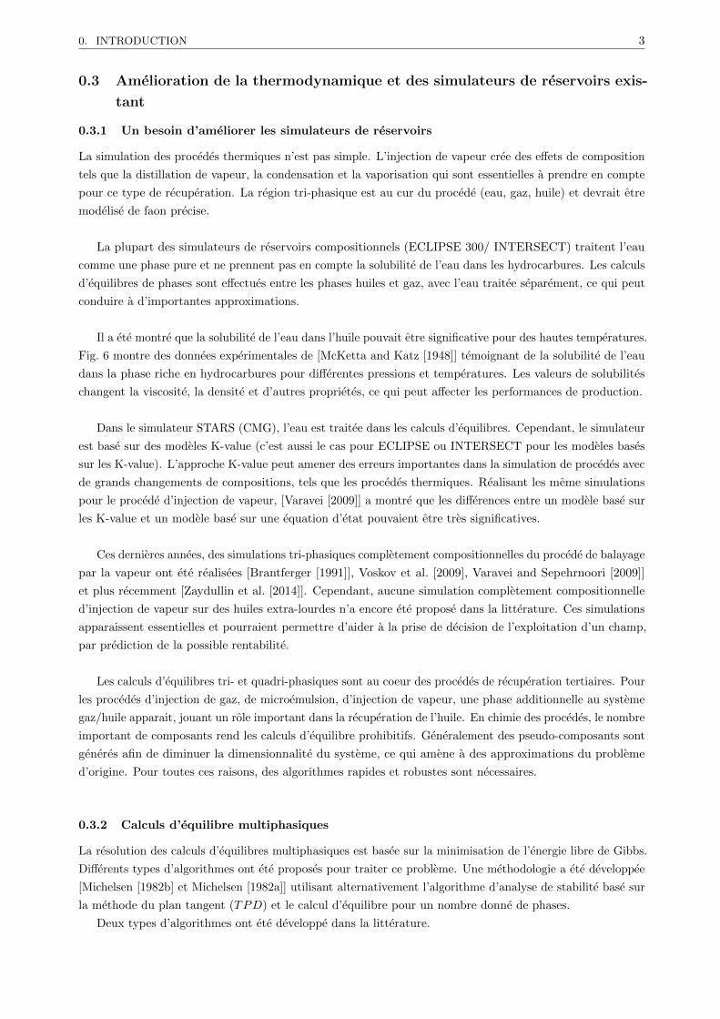
0.3 Amelioration de la thermodynamique et des simulateurs de reservoirs exis-

tant

0.3.1 Un besoin d’ameliorer les simulateurs de reservoirs

La simulation des procedes thermiques n’est pas simple. L’injection de vapeur cree des effets de composition

tels que la distillation de vapeur, la condensation et la vaporisation qui sont essentielles a prendre en compte

pour ce type de recuperation. La region tri-phasique est au cur du procede (eau, gaz, huile) et devrait etre

modelise de faon precise.

La plupart des simulateurs de reservoirs compositionnels (ECLIPSE 300/ INTERSECT) traitent l’eau

comme une phase pure et ne prennent pas en compte la solubilite de l’eau dans les hydrocarbures. Les calculs

d’equilibres de phases sont effectues entre les phases huiles et gaz, avec l’eau traitee separement, ce qui peut

conduire a d’importantes approximations.

Il a ete montre que la solubilite de l’eau dans l’huile pouvait etre significative pour des hautes temperatures.

Fig. 6 montre des donnees experimentales de [McKetta and Katz [1948]] temoignant de la solubilite de l’eau

dans la phase riche en hydrocarbures pour differentes pressions et temperatures. Les valeurs de solubilites

changent la viscosite, la densite et d’autres proprietes, ce qui peut affecter les performances de production.

Dans le simulateur STARS (CMG), l’eau est traitee dans les calculs d’equilibres. Cependant, le simulateur

est base sur des modeles K-value (c’est aussi le cas pour ECLIPSE ou INTERSECT pour les modeles bases

sur les K-value). L’approche K-value peut amener des erreurs importantes dans la simulation de procedes avec

de grands changements de compositions, tels que les procedes thermiques. Realisant les meme simulations

pour le procede d’injection de vapeur, [Varavei [2009]] a montre que les differences entre un modele base sur

les K-value et un modele base sur une equation d’etat pouvaient etre tres significatives.

Ces dernieres annees, des simulations tri-phasiques completement compositionnelles du procede de balayage

par la vapeur ont ete realisees [Brantferger [1991]], Voskov et al. [2009], Varavei and Sepehrnoori [2009]]

et plus recemment [Zaydullin et al. [2014]]. Cependant, aucune simulation completement compositionnelle

d’injection de vapeur sur des huiles extra-lourdes n’a encore ete propose dans la litterature. Ces simulations

apparaissent essentielles et pourraient permettre d’aider a la prise de decision de l’exploitation d’un champ,

par prediction de la possible rentabilite.

Les calculs d’equilibres tri- et quadri-phasiques sont au coeur des procedes de recuperation tertiaires. Pour

les procedes d’injection de gaz, de microemulsion, d’injection de vapeur, une phase additionnelle au systeme

gaz/huile apparait, jouant un role important dans la recuperation de l’huile. En chimie des procedes, le nombre

important de composants rend les calculs d’equilibre prohibitifs. Generalement des pseudo-composants sont

generes afin de diminuer la dimensionnalite du systeme, ce qui amene a des approximations du probleme

d’origine. Pour toutes ces raisons, des algorithmes rapides et robustes sont necessaires.

0.3.2 Calculs d’equilibre multiphasiques

La resolution des calculs d’equilibres multiphasiques est basee sur la minimisation de l’energie libre de Gibbs.

Differents types d’algorithmes ont ete proposes pour traiter ce probleme. Une methodologie a ete developpee

[Michelsen [1982b] et Michelsen [1982a]] utilisant alternativement l’algorithme d’analyse de stabilite base sur

la methode du plan tangent (TPD) et le calcul d’equilibre pour un nombre donne de phases.

Deux types d’algorithmes ont ete developpe dans la litterature.

0. INTRODUCTION 4

• La premiere plus sure, mais plus couteuse utilise est base sur une procedure de minimisation globale.

[Sun and Seider [1995]] a developpe une methode basee sur les intervalles-Newton et garantie de

trouver le minimum global. [Stadtherr et al. [1995]] a developpe une methode basee sur une methode

homotopique. [Lucia et al. [2000]] a utilise le calcul du plan tangent minimise a l’aide dune methode

SQP (Sequential Quadratic Programming), pour tester toutes les paires de composants. [Nichita et al.

[2002]] ont developpe une methode de tunneling.

• Les methodes de minimisation locales sont plus rapides, mais requierent des initialisations specifiques

et multiples pour garantir une certaine probabilite d’obtenir le minimum global. Pour les calculs

d’equilibres, [Michelsen [1982a]] proposa une procedure qui converge generalement vers le minimum

global. Dans un contexte ou les temps de calculs doivent etre extremement restreints, cette methodologie

est aujourd’hui la plus utilisee en simulation de reservoir.

Les calculs d’equilibres multiphasiques ont ete ameliores afin d’assurer la convergence dans des regions

tres difficiles (comme proches de singularites: points critiques pour les calculs d’equilibres, la limite du

locus de stabilite pour l’analyse de stabilite). [Risnes et al. [1981]] fut le premier a proposer la methode de

substitution successives (SS) pour les calculs multiphasiques. Depuis de nombreux auteurs ont travaille sur le

sujet ([Nghiem and Heidemann [1982]], [Mehra et al. [1982]], [Michelsen [1994]]). [Michelsen [1982b]] fournit

un ensemble de solutions initiales pour les calculs d’equilibres multiphasiques qui furent ensuite etendues par

[Li and Firoozabadi [2012]] qui proposerent une strategie generale pour traiter des calculs multiphasiques pour

2 et 3 phases. Cependant des ameliorations sont encore necessaires, et particulierement pres des conditions

difficiles ou les algorithmes actuels ont des difficultes.

Le travail de recherche effectue au cours de cette these s’est concentre principalement sur l’amelioration

des calculs d’equilibres de phases afin de pouvoir proposer des simulations completement compositionnelles

d’injection de vapeur avec des huiles extra-lourdes, sous des temps raisonnables.

0.4 Plan de these

Dans la simulation de reservoir, les equations de conservations doivent etre resolues a chaque pas de temps.

Des equilibres locaux sont consideres au sein de chaque cellule et un nombre important de calculs d’equilibres

de phases est requis, base sur la minimisation de l’energie de Gibbs. Une erreur dans l’obtention du minimum

peut ensuite etre propagee, menant a des solutions non physiques. Il est donc imperatif de developper des

algorithmes efficaces et robustes. Dans cette these, des ameliorations de calculs d’equilibre multiphasiques

sont proposes afin de simuler le proceder d’injection de vapeur. Cette these est organisee en cinq parties.

Le premier chapitre presente rapidement les equations thermodynamiques a resoudre dans les calculs

d’equilibre ainsi que le modele d’equations cubiques utilise pour ce travail. Les equations d’etat cubiques

fournissent une description raisonnable du comportement de phases pour les composants pures et les melanges,

ne necessitant que les proprietes critiques et les facteurs acentriques de chaque composant. Ces modeles sont

tres utilises dans la simulation de reservoir.

Dans un deuxieme chapitre, l’algorithme de minimisation de l’energie de Gibbs est presente ( [Michelsen

[1982a]]) . Le test de stabilite et les calculs d’equilibre sont decrits de meme que la procedure globale de

minimisation.

Dans un troisieme chapitre, des ameliorations aux algorithmes de calculs d’equilibres sont presentees. La

plupart des algorithmes sont bases sur la methode de Newton-Raphson et utilisent les variables conventionnelles

comme variables independantes. Dans un premier temps des ameliorations directes de ces algorithmes sont

proposees. Le logarithme des constantes d’equilibres (ln K) semble etre le meilleur choix de variables

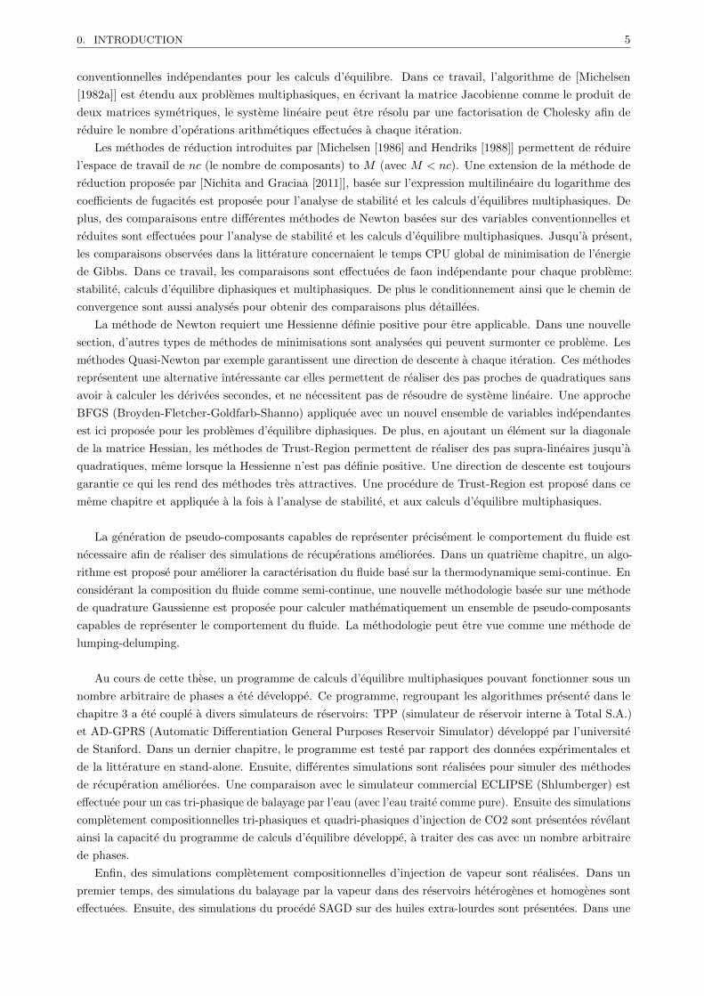
0. INTRODUCTION 5

conventionnelles independantes pour les calculs d’equilibre. Dans ce travail, l’algorithme de [Michelsen

[1982a]] est etendu aux problemes multiphasiques, en ecrivant la matrice Jacobienne comme le produit de

deux matrices symetriques, le systeme lineaire peut etre resolu par une factorisation de Cholesky afin de

reduire le nombre d’operations arithmetiques effectuees a chaque iteration.

Les methodes de reduction introduites par [Michelsen [1986] and Hendriks [1988]] permettent de reduire

l’espace de travail de nc (le nombre de composants) to M (avec M < nc). Une extension de la methode de

reduction proposee par [Nichita and Graciaa [2011]], basee sur l’expression multilineaire du logarithme des

coefficients de fugacites est proposee pour l’analyse de stabilite et les calculs d’equilibres multiphasiques. De

plus, des comparaisons entre differentes methodes de Newton basees sur des variables conventionnelles et

reduites sont effectuees pour l’analyse de stabilite et les calculs d’equilibre multiphasiques. Jusqu’a present,

les comparaisons observees dans la litterature concernaient le temps CPU global de minimisation de l’energie

de Gibbs. Dans ce travail, les comparaisons sont effectuees de faon independante pour chaque probleme:

stabilite, calculs d’equilibre diphasiques et multiphasiques. De plus le conditionnement ainsi que le chemin de

convergence sont aussi analyses pour obtenir des comparaisons plus detaillees.

La methode de Newton requiert une Hessienne definie positive pour etre applicable. Dans une nouvelle

section, d’autres types de methodes de minimisations sont analysees qui peuvent surmonter ce probleme. Les

methodes Quasi-Newton par exemple garantissent une direction de descente a chaque iteration. Ces methodes

representent une alternative interessante car elles permettent de realiser des pas proches de quadratiques sans

avoir a calculer les derivees secondes, et ne necessitent pas de resoudre de systeme lineaire. Une approche

BFGS (Broyden-Fletcher-Goldfarb-Shanno) appliquee avec un nouvel ensemble de variables independantes

est ici proposee pour les problemes d’equilibre diphasiques. De plus, en ajoutant un element sur la diagonale

de la matrice Hessian, les methodes de Trust-Region permettent de realiser des pas supra-lineaires jusqu’a

quadratiques, meme lorsque la Hessienne n’est pas definie positive. Une direction de descente est toujours

garantie ce qui les rend des methodes tres attractives. Une procedure de Trust-Region est propose dans ce

meme chapitre et appliquee a la fois a l’analyse de stabilite, et aux calculs d’equilibre multiphasiques.

La generation de pseudo-composants capables de representer precisement le comportement du fluide est

necessaire afin de realiser des simulations de recuperations ameliorees. Dans un quatrieme chapitre, un algo-

rithme est propose pour ameliorer la caracterisation du fluide base sur la thermodynamique semi-continue. En

considerant la composition du fluide comme semi-continue, une nouvelle methodologie basee sur une methode

de quadrature Gaussienne est proposee pour calculer mathematiquement un ensemble de pseudo-composants

capables de representer le comportement du fluide. La methodologie peut etre vue comme une methode de

lumping-delumping.

Au cours de cette these, un programme de calculs d’equilibre multiphasiques pouvant fonctionner sous un

nombre arbitraire de phases a ete developpe. Ce programme, regroupant les algorithmes presente dans le

chapitre 3 a ete couple a divers simulateurs de reservoirs: TPP (simulateur de reservoir interne a Total S.A.)

et AD-GPRS (Automatic Differentiation General Purposes Reservoir Simulator) developpe par l’universite

de Stanford. Dans un dernier chapitre, le programme est teste par rapport des donnees experimentales et

de la litterature en stand-alone. Ensuite, differentes simulations sont realisees pour simuler des methodes

de recuperation ameliorees. Une comparaison avec le simulateur commercial ECLIPSE (Shlumberger) est

effectuee pour un cas tri-phasique de balayage par l’eau (avec l’eau traite comme pure). Ensuite des simulations

completement compositionnelles tri-phasiques et quadri-phasiques d’injection de CO2 sont presentees revelant

ainsi la capacite du programme de calculs d’equilibre developpe, a traiter des cas avec un nombre arbitraire

de phases.

Enfin, des simulations completement compositionnelles d’injection de vapeur sont realisees. Dans un

premier temps, des simulations du balayage par la vapeur dans des reservoirs heterogenes et homogenes sont

effectuees. Ensuite, des simulations du procede SAGD sur des huiles extra-lourdes sont presentees. Dans une

1. CHAPITRE 1: THERMODYNAMIQUE FONDAMENTALE 6

derniere partie, le programme de calculs d’equilibre est teste contre differentes techniques qui permettent de

s’affranchir des calculs de stabilites dans le cadre de la simulation de reservoir. Les temps de calculs sont

presentes pour les differents cas traites.

1 Chapitre 1: Thermodynamique fondamentale

La thermodynamique est au coeur des procedes de recuperation thermiques. Dans ce chapitre, une description

des differentes fonctions thermodynamiques utilisees dans cette these est developpee.

Commenant par les premieres et secondes lois, les expressions de l’energie interne, des energies libres de

Gibbs et d’Helmholtz sont derivees.

Les conditions d’equilibres sont aussi obtenues en recherchant le minimum de l’energie libre de Gibbs.

Enfin, la correcte modelisation des differentes phases est un parametre important dans la simulation de

reservoir. De nombreuses equations d’etat existent qui relient les differentes variables thermodynamiques

pour une phase donnee. Dans cette these, nous proposons le developement d’algorithmes globaux pour

resoudres les calculs d’equilibres multiphasiques. Les equations d’etats cubiques representent un moyen

efficace pour modeliser les differentes proprietes thermodynamiques requisent dans la simulation de reservoir

(envelopes de phases, enthalpies, densites...) et permettent d’obtenir des resultats convenables pour des

melanges hydrocarbons. Dans un contexte ou les temps de calculs sont importants, les equations cubiques

offrent un bon compromis entre efficacite et precision. Ces equations d’etats sont donc aujourd’hui au coeur

de tous les simulateurs compositionels, et en particulier sont celles utilisees dans cette these. Au cours de ce

chapitre une description des equations d’etat cubiques est effectuee.

2 Chapitre 2: La procedure globale de calculs d’equilibre multi-

phasiques

Un calcul d’equilibre P − T consiste a calculer les fractions molaires de phases θ, ainsi que les compositions x

qui minimisent l’energie libre de Gibbs pour une composition globale z, une temperature T et une pression p

(voir fig. 2.1).

Dans la simulation de reservoir, un nombre tres important de calculs d’equilibres doivent etre effectues.

Les outils de minimisation globale ne peuvent etre utilises car les temps de calculs associes y sont tres eleves.

Ainsi les algorithmes de minimisation locale sont preferes. Une methodologie proposee par [Michelsen [1982a]]

est basee sur ce dernier type d’optimisation. Elle combine l’analyse de stabilite et les calculs d’equilibre et est

aujourd’hui le standard utilise dans l’industrie.

• L’analyse de stabilite [Michelsen [1982b]] permet de savoir si un melange est stable pour un nombre

donne de phases, ou s’il devrait se scinder en un plus grand nombre de phases.

• Les calculs d’equilibre calculent les compositions x et les fractions molaires de phases θ qui minimisent

l’energie libre de Gibbs pour un nombre donne de phases.

Cette procedure mene generalement au minimum global et est particulierement efficace. Elle est aujourd’hui

implementee dans la plupart des simulateurs de reservoir compositionnels et est utilise dans ce travail. Dans

ce chapitre, les deux problemes seront presentes en details. La methodologie globale des calculs d’equilibre de

phases pour minimiser l’energie libre de Gibbs sera aussi presentee.

3. CHAPITRE 3: AMELIORATION DES CALCULS D’EQUILIBRE 7

3 Chapitre 3: Amelioration des calculs d’equilibre

Les calculs d’equilibre multiphasiques (calculs d’equilibres, analyse de stabilite) jouent un role majeur dans la

chimie des procedes et les reservoirs petroliers. En effet, dans ces deux procedes, ils representent la majeure

partie du temps de calcul. De plus, la moindre erreur est susceptible d’affecter les resultats ou de mener a

la non-convergence d’une simulation. Dans ce contexte, il devient essentiel de developper des algorithmes

qui soient a la fois robustes et rapides, et d’utiliser des algorithmes adaptes pour chaque cas. En simulation

de reservoir, le nombre de composants est tres limite (souvent moins de douze) et un nombre important de

calculs sont effectues. A l’inverse, en chimie des procedes, le nombre de composants peut etre tres important

(de l’ordre de la centaine).

Dans ce chapitre, des ameliorations relatives aux algorithmes de calculs d’equilibre sont proposees.

Dans un premier temps, un algorithme developpe par [Michelsen [1982a]] permet d’utiliser une factorisation

de Cholesky pour resoudre le systeme lineaire obtenu par la methode de Newton, en utilisant le logarithme

des constantes d’equilibres comme variables independantes. Cette methodologie est ici etendu aux calculs

d’equilibre multiphasiques et est aussi appliquee a la methode proposee par [Haugen et al. [2011]], ou les

fractions molaires de phases et les constantes d’equilibres sont utilises comme variables independantes.

De plus, les methodes de reductions permettent de reduire l’espace de travail de nc (le nombre de

composants) a M (avec M < nc). Une nouvelle methode est ici proposee a la fois pour l’analyse de stabilite et

pour les calculs d’equilibre multiphasiques, basee sur l’expression multilineaire du logarithme des coefficients

de fugacite. Ensuite, des comparaisons de differentes methodes de Newton basees sur differentes variables

conventionnelles et reduites sont presentees. Les tests portent a la fois sur les temps de calculs, mais aussi sur

le conditionnement et le chemin de convergence. De plus, chaque probleme est traite de faon independante

(stabilite, calculs d’equilibres diphasiques et multiphasiques).

Dans un souci de developper un programme qui se veut modulaire et general, des algorithmes independants

de l’equation d’Etat sont aussi testes. Une methode BFGS (Broyden-Fletcher-Goldfarb-Shanno) est appliquee

pour les calculs d’equilibre diphasiques avec un nouveau vecteur de variables independantes. De plus, une

methode de Trust-Region est appliquee a l’analyse de stabilite et les calculs d’equilibre multiphasiques.

4 Chapitre 4: Amelioration de la caracterisation des huiles lour-

des par la thermodynamique semi-continue

Differents melanges d’interets dans l’industrie, tels que les melanges d’hydrocarbures contiennent un nom-

bre tres important de composants. Parce qu (i) un grand nombre de composants peut rendre les calculs

d’equilibres couteux (par exemple dans la simulation de reservoir) et (ii) il est impossible d’identifier tous les

composants par des analyses chimiques standards (les fractions lourdes sont les plus difficiles a caracteriser),

des pseudo-composants (obtenus en regroupant differents composants individuels) sont utilises afin de diminuer

la dimensionnalite du probleme de calculs d’equilibres.

Generalement, un melange est lumpe en pseudo-composants en utilisant des criteres de proximite pour

regrouper les composants [Montel and Gouel [1984], Newley and Merrill [1991], Lin et al. [2008]]. Les

proprietes critiques (temperature et pression critiques, facteurs acentriques) et les parametres d’interactions

des particules (BIPs) sont calcules en moyennant les proprietes pour chaque pseudo-composant.

Une alternative elegante aux methodes classiques de lumping est l’utilisation de la thermodynamique

semi-continue, qui est basee sur une approximation de la composition du melange par une distribution

continue. En thermodynamique semi-continue, les composants individuels sont traites de faon discrete (en

4. CHAPITRE 4: AMELIORATION DE LA CARACTERISATION DES HUILES LOURDES PAR LATHERMODYNAMIQUE SEMI-CONTINUE 8

general, les fractions legeres d’hydrocarbures et les composants non-hydrocarbures: CO2, N2, H2S, H2O, etc),

alors que les composants restants sont traites de faon continue. Les principes de thermodynamique continue

et semi-continue furent en premier temps developpes par [Ratzsch and Kehlen [1983] et par Cotterman and

Prausnitz [1985]] respectivement. Apres les annees 1980, differents auteurs travaillerent a developper des

algorithmes de calculs d’equilibres bases sur ces types de thermodynamique: [Cotterman et al. [1985], Behrens

and Sandler [1986], Shibata et al. [1986], Willman and A.S. [1986], Willman and A.S. [1987a], Willman and

A.S. [1987b], Ratzsch et al. [1988]]. Ensuite la thermodynamique semi-continue a ete appliquee a une variete

de calculs d’equilibres: les calculs d’equilibres sous differentes specifications [Chou and J.M. [1986]], l’analyse

de stabilite en utilisant la methode du plan tangent [Browarzik et al. [1998], Monteagudo et al. [2001b]], les

calculs de points critiques [Rochocz et al. [1997]], les gradients de compositions [Lira-Galeana et al. [1994],

Esposito et al. [2000]], les equilibres liquides-solides [Labadie and Luks [2003]], la precipitation d’asphaltenes

[Monteagudo et al. [2001a]], les calculs d’equilibre liquides-vapeurs en utilisant des equations d’etat avec des

contributions de groupes [Baer et al. [1997]], etc.

Les methodes les plus utilisees se basent sur une quadrature generalisee de Gauss-Laguerre pour convertir

la concentration molaire (distribution continue) en distribution discrete. Plus recemment, des methodes ont

ete presentees utilisant des methodes plus specifiques, telle que la quadrature generale de Gauss-Stieltjes qui

permet de calculer des points et poids de quadratures pour n’importe quelle distribution [Nichita et al. [2001]],

des polynomes orthogonaux [Liu and Wong [1997]], ou la methode de quadrature basee sur les moments [Lage

[2007]].

Cependant, la plupart des approches presentees dans la litterature sont basees sur des distributions

standards. Si la composition globale du melange ne peut pas etre modelisee par une distribution standard,

ou si elle irreguliere, la plupart des methodes ne fonctionne pas correctement. La methode semi-continue

basee sur la methode des moments developpee par [Lage [2007]], utilise la composition globale du melange

comme fonction poids et fonctionne avec n’importe quelle composition. Cependant, dans la formulation de la

methode QMoM, la quadrature est resolue en utilisant un algorithme de Gordon PDA (Product-Difference

Algorithm) [Gordon [1968]], qui ne fonctionne de faon precise que pour un nombre restreint de points de

quadratures. [John and Thein [2012]] a compare les performances de la methode QMoM en utilisant le

PDA avec une methode LQMDA (long quotient-modified difference algorithm) [Sack and Donovan [1972]] et

l’algorithme de Golub-Welsch [Golub and Welsch [1969]]. Ils ont montre que dans certaines situations, la

procedure de PDA echouait a calculer les points de quadrature (a partir de 8 points de quadratures dans leurs

exemples) alors que les deux autres methodes testees fonctionnaient correctement. [Gautschi [2004]] a montre

que le probleme est mal conditionne et que le nombre de conditionnement grandissait exponentiellement avec

le nombre de points de quadratures.

Dans ce travail, la methode QMoM est applique aux calculs d’equilibres multiphasiques pour des melanges

reels en utilisant une equation d’Etat cubique avec des BIPs non-nuls. Le calcul de la quadrature se base sur

la procedure proposee par [Gautschi [1994]] (ORTHOPOL), qui permet d’eviter le mauvais conditionnement

(intrinseque au probleme) et qui est adapte pour tous les nombres de points de quadratures (a l’inverse de la

methode QMoM couplee avec l’algorithme PDA). Dans certaines applications, il est important d’utiliser un

nombre de pseudo-composants superieur a sept (ce qui semble etre la limite pour l’algorithme PDA).

Le chapitre se structure comme suit: dans un premier temps, une nouvelle distribution est introduite; apres

un bref rappel sur les quadratures gaussiennes, la description du fluide semi-continue est effectuee. Ensuite,

l’algorithme general est presente, pour enfin montrer des resultats obtenus pour des calculs d’equilibres

diphasiques et tri-phasiques sur une huiles lourdes melangee a du dioxyde de carbone et de l’eau. Les details

du calcul de la quadrature sont donnes en appendices.

5. CHAPITRE 5 : SIMULATION DE RESERVOIR 9

5 Chapitre 5 : Simulation de reservoir

L’un des objectifs de cette these est de realiser des simulations completement compositionnelles du procede de

balayage par la vapeur. Les premiers simulateurs de reservoir traitant de ce processus ont ete conus dans les

annees soixante (Spillette and Nielsen [1968], Shutler [1969]], Shutler [1970]]). Les premiers modeles etaient

bases sur un modele lineaire tri-phasique [Shutler [1969]], puis etendue a deux dimensions [Shutler [1970]].

Plus tard [Vinsome [1974]], introduisit une methode IMPES pour simuler le processus de balayage par la

vapeur. [Coats [1976]] proposa le premier simulateur modelisant a la fois la partie thermique et la composition.

[Coats [1978]] presenta une extension de [Coats [1976]], developpant un simulateur compositionnel en trois

dimensions pour simuler l’injection de vapeur . Plus tard, [Ishimoto [1985]] proposerent de calculer les

proprietes des hydrocarbures et de l’huile au moyen d’ une equation d’etat. La loi de Raoult etait utilisee pour

calculer la solubilite de l’eau dans l’huile. Puis, [ citeChein] developpa un simulateur compositionnel general

qui pouvait traiter avec des options thermiques . Le simulateur etait base sur deux modeles compositionnelles:

l’un base sur une EOS, l’autre sur un modele K-value. Une fois de plus, la phase aqueuse etait supposee

ideale.

Plus recemment, [Cicek and Ertekin [1996] et plus tard Cicek [2005]] developperent un simulateur com-

positionnel multiphasique et Fully Implicit pour simuler les problemes d’injection de vapeur. Dans leur

formulation, l’eau est traitee au sein des calculs d’equilibre de phases. Le simulateur est base sur un modele

K-value. Generalement les tables de K-value sont fonctions d’un seul composant huile, la pression et la

temperature. L’approche K-value ne permet pas d’obtenir les solubilites des composes hydrocarbures dans

l’eau et la solubilite de l’eau dans la phase hydrocarbure de faon precise.

Cependant, il a ete observe (fig. 6) que pour des hautes temperatures, la solubilite du composant eau

dans la phase riche en hydrocarbure n’etait pas negligeable. Les simulateurs commerciaux actuels font

des approximations pour simuler les problemes d’injection de vapeur. Ces approximations sont meme plus

importantes dans le cadre d’huiles lourdes. ECLIPSE 500 et INTERSECT par exemple, sont des simulateurs

thermiques fonctionnant avec des modeles K-value, ou (pour INTERSECT) qui traitent l’eau separement des

calculs d’equilibres, ce qui conduit a des approximations.

Pour ces raisons, des auteurs ont commence a developper des simulateurs bases sur des equations d’etats

pour realiser des simulations compositionnelles thermiques du procede d’injection de vapeur. En utilisant

le fait que la solubilite des hydrocarbures dans l’eau est negligeable pour une certaine gamme de pressions-

temperatures, des modeles free-water de calculs d’equilibres ont ete developpes [Luo and Barrufet [2005]], et

plus recemment appliques pour les problemes d’huiles lourdes [Heidari [2014]]. La meme methodologie a ete

appliquee pour traiter de l’upgrading In-Situ [Lapene [2010]].

Pour des problemes d’injection de CO2 froid, les simulateurs de reservoirs ont ete etendus pour integrer

des calculs d’equilibres multiphasiques (quatre phases) [Varavei and Sepehrnoori [2009] et Okuno [2009]].

Dans leur cas, ils n’ont pas inclus l’eau dans les calculs d’equilibre.

Cependant, l’eau issue des reservoirs est generalement plus proche d’une eau salee que d’une eau pure et

l’hypothese free-water n’est donc pas toujours valide. [Brantferger [1991]] developpa un simulateur base sur

une equation d’etat pour calculer les proprietes thermodynamiques de chaque phase (meme la phase eau). Ils

proposerent de traiter le probleme avec un flash isenthalpique, choisissant l’enthalpie comme variable primaire

au lieu d’utiliser la temperature. [Voskov et al. [2009]] developperent un simulateur general y integrant

une methode d’acceleration aux calculs de stabilites, en parametrant l’espaces des tie-lines. [Varavei and

Sepehrnoori [2009]] et plus recemment [Zaydullin et al. [2014]] proposerent des simulations tri-phasiques

d’injection de vapeur.

5. CHAPITRE 5 : SIMULATION DE RESERVOIR 10

Enfin [Feizabadi [2013]] etendit les simulations compositionnelles pour simuler des procedes d’injection de

solvants quadri-phasiques bases sur une equation d’etat.

Il semblerait qu’il n’existe pas de cas de simulations completement compositionnelles basees sur une

equation d’etat pour simuler le procede d’injection de vapeur sur des huiles lourdes, en traitant l’eau de

faon complete (au sein du calcul d’equilibre, sans hypothese simplificatrice). Ces simulations apparaissent

essentielles et pourraient permettre d’aider a la prise de decision de l’exploitation d’un champ, par prediction

de la possible rentabilite.

Dans ce chapitre, une description des differentes equations utilisees en simulation de reservoirs sont

montrees, ainsi que les differents modeles pour calculer les proprietes du fluide.

Dans le chapitre 3, de nouveaux algorithmes pour resoudre les calculs d’equilibres ont ete presentes.

Un programme (Mflash) a ete developpe combinant ces methodes et un programme de calculs d’equilibres

multiphasiques, pouvant traiter un nombre arbitraire de phases a ete developpe.

Dans un premier temps, des tests en stand-alone sont proposes pour comparer les resultats obtenus avec

Mflash, avec des donnees experimentales et de la litterature, pour ensuite montrer des resultats au sein d’un

simulateur de reservoir. Au cours de cette these, Mflash a ete integre a deux simulateurs de reservoirs: TPP

(simulateur interne a Total S.A.) et AD-GPRS simulateur de l’universite de Stanford [Younis and Aziz [2007],

Voskov et al. [2009], Zhou et al. [2011]].

Differents procedes sont simules dans ce chapitre. Premierement, une simulation diphasique d’injection

de vapeur, ou l’eau est traitee independamment du calcul d’equilibre. Une comparaison avec le simulateur

commercial ECLIPSE est aussi presentee.

Ensuite, des simulations completement compositionnelles, tri-phasiques et quadri-phasiques d’injection de

CO2 sont montrees. Dans differentes simulations, il a ete remarque que la co-injection de solvant avec de la

vapeur pouvait etre a l’origine d’une nouvelle phase riche en solvant. L’importance de cette phase dans la

recuperation de l’huile n’a pas ete analysee, mais dans un but de developper un programme thermodynamique

robuste pour simuler le procede SAGD, une simulation quatre phase a ete realisee et est presente dans ce

chapitre pour un cas d’injection isothermique.

Enfin, des simulations completement compositionnelles du procede de balayage par la vapeur sont realisees

pour des simulateurs heterogenes et homogenes. Enfin, des simulations completement compositionnelles du

procede SAGD pour des huiles lourdes est presentee.

Dans une derniere partie, differentes methodologies pour ameliorer les temps de calculs d’equilibre dans

les simulateurs de reservoirs sont proposes pour tous les cas presentes. Les tests portent sur les variables

reduites utilisees pour l’analyse de stabilite, la procedure de bypass [Rasmussen et al. [2006]] qui evite certains

calculs de stabilites lorsqu’une cellule est dans l’etat monophasique, la procedure developpee par [Voskov

and Tchelepi [2008], Voskov and Tchelepi [2009a], Voskov and Tchelepi [2009b], Iranshahr et al. [2010a]] et

plus recemment [Zaydullin et al. [2013]] ou l’espace d’etude est parametre, pour reutiliser l’information de

precedents calculs thermodynamiques.

6. CONCLUSIONS ET PERSPECTIVES 11

6 Conclusions et Perspectives

6.1 Conclusions

Dans cette these, l’amelioration des algorithmes d’equilibre a rendu possible la realisation de simulations

completement compositionnelles d’injection de vapeur avec des huiles lourdes.

La plupart des calculs d’equilibre sont bases sur la methode de Newton-Raphson et utilisent les variables

conventionnelles comme variables independantes. Des extensions de ces methodes sont ici proposees. Le

logarithme des constantes d’equilibre (lnK) est le meilleur choix de variables independantes conventionnelles

pour les calculs d’equilibre multiphasiques. Ces variables menent vers des systemes les mieux conditionnes et

les methodes de Newton basee sur (lnK) convergent generalement avec moins d’iterations que pour les autres

variables. Dans ce travail, la methode de [Michelsen [1982a]] est etendue aux problemes multiphasiques. La

methode permet d’ecrire la matrice Jacobienne comme produit de deux matrices symetriques et de resoudre

le systeme lineaire par une factorisation de Cholesky. Cette methode a prouve qu’elle pouvait reduire le

temps de calculs d’environ 30% dans la plupart des cas.

Initiees par [Michelsen [1986] et Hendriks [1988]], les methodes de reductions ont ete developpees et ont

prouve etre tres efficaces. Dans ce travail, une nouvelle methode de reduction appliquee au test de stabilite et

les calculs d’equilibre a ete presentee. Elle est basee sur l’expression multilineaire du logarithme des coefficients

de fugacite comme fonctions des coefficients f (variables independantes non-bornees). La dimensionnalite

du probleme ne depend uniquement que du nombre de composants ayant des BIPs differents de zero avec

les autres, et non pas du nombre de composants du melange, comme pour les procedures conventionnelles.

La methode proposee a un rayon de convergence plus large et lalgorithme de Newton peut etre utilisee

directement pour l’analyse de stabilite (sans besoin de substitutions successives). Elle a le meme chemin

de convergence que la procedure conventionnelle utilisant le logarithme des constantes d’equilibres comme

variables independantes, et a montre etre la meilleure methode de Newton pour l’analyse de stabilite (en

terme d’efficacite et de nombre de conditionnement).

Des comparaisons entre differentes methodes conventionnelles et reduites ont ete effectuees pour les

problemes d’analyse de stabilite et des calculs d’equilibres multiphasiques. Jusqu’a present, les comparaisons

observees dans la litterature ne portaient que sur le temps de calcul global pour calculer l’ensemble du probleme

de minimisation de l’energie de Gibbs. Dans ce travail, les comparaisons ont ete effectuees independamment

pour chaque probleme (stabilite, flash diphasiques et multiphasiques). De plus, le nombre de conditionnement

ainsi que le chemin de convergence sont aussi analysees, amenant a des conclusions plus precises:

• Pour le probleme de stabilite, la procedure de reduction proposee est la plus efficace est preferable pour

des applications en simulation de reservoir.

• En revanche, pour les calculs d’equilibres multiphasiques, les methodes basees sur les variables conven-

tionnelles sont plus adaptes pour la simulation de reservoir. Dans le cadre de la chimie des procedes

impliquant un grand nombre de composants, la methode proposee est largement superieure compare

aux autres methodes.

Ensuite, une procedure de Trust-Region (TR) a ete proposee pour traiter des problemes d’analyse de

stabilite et des calculs d’equilibre multiphasiques. TR peut etre vu comme une ’extension’ d’une methode de

Newton. Elle permet de realiser des pas supra-lineaires lorsque la Hessienne n’est pas definie positive et des

pas quadratiques sinon, en ajoutant un element diagonal a la matrice. Une methode hybride a ete proposee.

Au lieu de realiser des iterations TR directement apres l’utilisation d’une methode de premier ordre (SSI),

des iterations de Newton sont testees dans un premier temps et la methode TR n’est utilisee uniquement que

si la fonction objective augmente entre deux iterations successives. La methode hybride a permis de decroitre

6. CONCLUSIONS ET PERSPECTIVES 12

les temps de calculs de faon remarquables, tout en gardant la robustesse intrinseque de la procedure TR. Les

tests ont ete realises sur un ensemble complet de regions multiphasiques et convergence a ete obtenue meme

pour des conditions tres difficiles, telles que proche de points bi-critiques.

De plus, une nouvelle methodologie a ete developpee pour trouver des variables permettant d’obtenir

une matrice Hessienne avec une bonne mise a l’echelle. Cette procedure mene a la variable α introduite par

[Michelsen [1982b]] pour l’analyse de stabilite et vers une nouvelle variable pour les calculs d’equilibres. Une

methode quasi-Newton avec un retour vers SSI (lorsque l’energie de Gibbs s’accroit entre deux iterations) a

ete developpe utilisant cette nouvelle variable et a montre que la convergence etait possible, meme tres proche

des frontieres de phase, ou les algorithmes rencontrent souvent des problemes de convergence. L’algorithme

a montre etre plus efficace (en terme d’iterations et de nombre d’evaluations de fonctions) que le code de

Nocedal LBFGS-B et d’autres methodes BFGS proposees dans la litterature. Par rapport a lalgorithme de

Newton, quelques iterations supplementaires sont necessaires pour obtenir la convergence, ce qui la rend tres

attractive. Cette methode est tres adaptee pour des modeles d’EoS plus complexes.

En combinant tous les algorithmes presentes, un programme general de calculs d’equilibre a ete developpe

(Mflash). Il a ete construit afin de pouvoir traiter un nombre arbitraire de phases. Les resultats obtenus

avec ce programme ont montre etre en accord avec des donnees provenant de la litterature et des donnees

experimentales, validant l’approche proposee.

En plus d’ameliorer la robustesse et l’efficacite des calculs d’equilibre, une nouvelle methodologie pour

generer les pseudo-composants donnant une representation precise du comportement du fluide a ete developpee.

Elle est basee sur la methode de quadrature des moments (QMoM) qui est ici appliquee aux calculs d’equilibre

multiphasiques pour des huiles reelles (combinees avec des composants non-hydrocarbures tels que l’eau,

le dioxyde de carbone), en utilisant une equation d’etat cubique avec des BIPs differents de zero. La

quadrature est resolue a l’aide d’une procedure (ORTHOPOL) qui permet d’eviter les problemes dus au

mauvais conditionnement du probleme. Cette methode est adaptee pour n’importe quel nombre de points de

quadratures (a l’inverse de precedentes formulations).

QMoM permet de relier la composition initiale detaillee et discrete, comportant un grand nombre de

composants a un petit nombre de composants qui approximent la portion continue du fluide. Elle peut etre

vue en un certain sens comme une methode de lumping. Elle peut etre appliquee meme dans les cas ou

aucune distribution standard ne peut modeliser la composition globale, ou lorsque plusieurs distributions

sont necessaires afin de modeliser differentes portions du fluides. Dans ce travail, il a ete montre que cette

methodologie couplee a une methode de delumping permettait de representer tres precisement le comportement

de fluides reels.

La methode QMoM dans notre implementation a ete testee pour differentes compositions initiales de

melanges hydrocarbures pour des calculs d’equilibres diphasiques, et en presence d’eau et de dioxyde de

carbone pour des calculs tri-phasiques. Dans tous les cas, les frontieres de phase, les compositions et fractions

molaires de chaque phase etaient bien respectees, en utilisant la procedure semi-continue presentee (permettant

de calculer une dizaine de pseudo-composants). Dans le cadre de la simulation de reservoir, cet outil apparait

essentiel car le temps de calcul pour chaque pas de temps est proportionnel a la puissance trois du nombre

d’equations a resoudre [Burger et al. [1985]].

Ensuite, le programme de calculs d’equilibre a ete implemente au sein de deux simulateurs de reservoirs:

TPP (developpe en interne a Total S.A.) et AD-GPRS (simulateur de Stanford).

Pour des problemes d’injection de vapeur tri-phasiques, les memes courbes de productions pour les

differentes phases ont ete obtenues en utilisant le simulateur ECLIPSE et en utilisant le programme (Mflash)

integre dans TPP. Ceci temoigne de la capacite de Mflash a converger vers la solution correspondant au

6. CONCLUSIONS ET PERSPECTIVES 13

minimum d’energie. De plus, des cas d’injection de CO2 ont ete presentees (connus pour etre difficiles). Des

simulations compositionnelles isothermiques, tri-phasiques et quadri-phasiques ont ete realisees jusqu’a la

percee du CO2. Ces simulations montrent la capacite du code de calcul a traiter plus de trois phases, ce qui

peut etre tres difficile d aux infimes differences d’energies qu’il peut y avoir entre un etat a trois phases et un

etat a quatre phases.

Des simulations d’injection de vapeurs ont aussi etaient realisees. Le reservoir SPE10 (connu pour etre

tres heterogene) a ete utilise pour tester des simulations en trois dimensions de balayage par la vapeur jusqu’a

la percee d’eau. Dans ces conditions (3D, heterogene), un nombre important de chemins thermodynamiques

sont accedes durant la simulation. Encore une fois, ces exemples temoignent de la robustesse de l’algorithme.

Enfin, des simulations completement compositionnelles du procede SAGD ont ete realisees avec des

huiles extra-lourdes. A notre connaissance, il n’existe pas de simulation de la sorte dans la litterature (avec

une modelisation complete de l’eau au sein des calculs d’equilibres). Les simulations thermiques sont tres

complexes car on y observe d’importants changements de conditions (composition, temperature, pression).

De plus, la gravite joue aussi un role sur la composition.

Le developpement du code a aussi ete associe avec differentes methodes d’accelerations telles que la

methode Three-Phase-Bypass presentee par [Zaydullin et al. [2013]]. Des simulations completement composi-

tionnelles, thermiques tri-phasiques ont pu etre realisees pour simuler le procede de balayage par la vapeur.

Les calculs d’equilibres representaient moins de 10% du temps de simulation total a l’aide de cette methode.

L’un des objectifs de la these etait de realiser des simulations completement compositionnelles du probleme

d’injection de vapeur avec un pourcentage des calculs d’equilibres inferieurs a 50% de la simulation totale.

Cet objectif est donc atteint.

Au travers de cette these, trois papiers ont ete publies [Nichita and Petitfrere [2013], Petitfrere and Nichita

[2014a], Petitfrere and Nichita [2014b]]; un quatrieme papier a ete soumis [Petitfrere et al. [2014]] et trois

autres papiers sont en preparation et seront soumis prochainement (ils correspondent aux sections 3.2.4, 3.3

and 3.5).

6.2 Perspectives

A travers le travail realise, de nouvelles perspectives apparaissent. Dans cette these, des algorithmes de

minimisation ont ete implementes et ont montre etre plus efficaces que les methodes preexistantes (Trust-

Region, BFGS). Ces algorithmes sont independants du model d’equation d’etat. Lorsque la complexite du

modele d’equation d’etat augmente, les calculs des fugacites et de leurs derivees deviennent de plus en plus

prohibitifs. Les methodes permettant de diminuer le nombre d’iterations par rapport aux methodes classiques

(exemple: Trust-Region) deviennent donc de plus en plus interessantes. Ainsi, les methodes quasi-Newton et

Trust-Region fonctionneraient plus efficacement avec des modeles d’EoS plus complexes; les methodes de

Trust-Region parce qu’elle diminue le nombre d’iterations et la methode BFGS car elle ne requiert pas les

derivees de la fugacite.

Ensuite, la methode de BFGS a ete developpee pour les calculs d’equilibres diphasiques et une extension

aux problemes multiphasiques est envisagee. Avec un plus grand nombre de phases, la dimensionnalite du

systeme a resoudre, a chaque iteration de Newton s’accrot, et la procedure de BFGS (ou aucun systeme

lineaire nest resolu) pourrait devenir tres competitive face a la methode de Newton.

De nouvelles perspectives apparaissent aussi dans la simulation de reservoir compositionnelle. Le pro-

gramme de calculs d’equilibre developpe a montre etre tres efficace et robuste et pourrait etre utilise pour

simuler de nouveaux procedes. En ajoutant un terme source aux equations de conservation de masse et

6. CONCLUSIONS ET PERSPECTIVES 14

d’energie, des reactions chimiques irreversibles (basees sur des energies d’activation) pourraient etre modelisees.

Des simulations du procede d’Upgrading In-Situ pourraient etre effectuees en utilisant cette methodologie

[Lapene [2010]].

Differentes methodes d’accelerations ont aussi ete presentees. L’une d’entre elles est la methode Three-

Phase bypass [Zaydullin et al. [2013]] . Elle pourrait etre utilisee pour aider a l’identification des phases.

Lorsque deux phases liquides sont presentes, il est parfois tres difficile d’identifier chacune d’entre elles. La

parametrisation permettrait d’identifier par continuite chaque phase sur l’ensemble de l’espace des composi-

tions.

Une autre methode d’acceleration a ete proposee par [Gaganis and Varotsis [2012]] et pourrait etre tres

efficace dans le cadre de simulations compositionnelles pour des procedes complexes (tel que l’injection de

CO2). En utilisant une methode de machine-learning, ils entrainent le systeme a generer des fonctions

capables de fournir le signe de la fonction du plan tangent a son minimum, en quelques operations. Il pourrait

etre interessant de comparer la methode face a Three-Phase bypass.

Enfin, les simulations presentees pourraient etre ameliorees en utilisant un modele d’equation d’etats plus

precis. Il est bien connu que les parametres volumiques et que la plupart des proprietes derivees ne sont pas

modelisees correctement par les equations d’etat cubiques. Des equations plus complexes pourraient etre

utilisees pour realiser les memes simulations d’injection de vapeur proposees dans ce document.

Introduction

1 The heavy oils, a viable alternative to the increasing energy

demand

Emerging economies, and particularly in Asia such as China and India are more and more energy dependent.

In this context, the need in energy production is rising every year and the International Energy Outlook 2013

(IEO2013) projects that world energy consumption will grow by 56 percent between 2010 and 2040. Fuels repre-

sent the largest source of energy, and their production must be increased to satisfy the growing energy demand.

Oil can be classified in different categories depending on their API gravity; a measure of the weight of

liquid petroleum compared to water:

• If the API gravity is higher than 10, the oil floats on water.

• If it is lower, the oil sinks in water.

API Gravity Liquid Relative Density

0-10

10

10-22

22-38

>33

>55

Extra Heavy Crude Heaviest

Water

Heavy Crude Oil

Medium Crude Oil

Light Crude Oil

Condensates Lightest

Figure 1: API gravity

The conventional oils have an API gravity above 25. Due to their relatively low density and viscosity,

they generally can be recovered easily and their production cost remain quite small. This is why they have

been exploited for many years. Yet, the conventional oils and gas exploration targets become increasingly

rare; there production declines at a rate of about 5 percent and the proved global reserves can provide energy

for the next 40 years at the current production rate.

Heavy oils can be found with an API gravity between 5 and 22 (see fig. 1). Since they have high viscosities,

Enhanced Oil Recovery (EOR) technics have to be used to be able to reach a sufficient yield, which makes

them more expensive than the conventional oils. Nevertheless, the price of the barrel growing with the

demand, the exploitation of heavy oils becomes more and more profit making and could play a role in reserve

replacement. With a volume of oil-in-place estimated between 3 and 4 trillion barrels and potential reserves

of around 500 billion barrels, the heavy oils are equivalent to 60 percent of the global reserves of conventional

crude oil and account for 20 up to 25 percent of the global petroleum resources. Their exploitation could

extend the world’s energy reserves by 15 years. Various EOR technics exist to enable the heavy oils recovery.

Introduction 15

2. ENHANCED OIL RECOVERY 16

2 Enhanced oil recovery

The development and commercial deployment of modern EORs is today seen as the way to extend the

oil production in recoverable reserves. When implemented, EORs make possible to expand the companies’

resources. Some estimates suggest that the growth of just 1 percent of the global Oil Recovery Factor could

increase conventional oil reserves by around 88 billion barrels (three times the current production).

Moreover, not only could EOR methods be a solution to expend the conventional oil production (which

were traditionally operated using Primary or Secondary recoveries (fig. 2)), but they could be used for

non-conventional oils such as heavy oils which cannot be recovered by standard depletion methods (as it has

been mentionned earlier).

PrimaryIRecovery

SecondaryIRecovery

TertiaryIRecovery

NaturalIFlow ArtificialILift

PressureIMaintenanceWaterflooding

Thermal GasIInjection Chemical OtherSteamHotIWaterCombustion Nitrogen

HydrocarbonCO2 Alkali

SurfactantPolynmer Electromagnetic

AcousticMicrobial

50b880b

30850b

GenerallyI<30b

OilIRecovery

Figure 2: Enhanced oil Recovery [Larry [1989]]

Different type of EORs exist (some are listed in fig. 2), the main methods are given by:

• Gas injection: the introduction of CO2 or N2. By injecting one of those gas into the reservoir, the gas

dissolves in oil. The viscosity of any hydrocarbon is then reduces which makes the oil easier to recover.

• Chemical Methods

– Surfactant flooding can create micro emulsions at the interface between crude oil and water, thus

reducing the interfacial tension. This mobilizes the residual oil and allows recovering trapped oil

within porous media.

– Polymer flooding is an augmented water flooding. By co-injecting polymer, the oil/mobility ratio

decreases which creates a larger front, thus sweeping a larger volume of oil.

• Thermal recovery methods represent most of the heavy oil projects, they are currently used in production

and should probably play a huge role in the future. By raising the temperature the oil is heated with

reduces its viscosity. This process increases its mobility (fig. 3) by reducing the surface tension and

increasing the permeability. The heated oil may also vaporize and then condense to form an improved

oil. The most widely used thermal technics are in-situ combustion, continuous injection of hot fluids

such as steam, water or gases, and cyclic operations. Amoung them, the steam injection processes

represent the main type of thermal stimulation of oil reservoirs.

Three main designs of steam injection exists in the industry:

– With two vertical wells (one producer and one injector) separated from a certain distance, for oils

with medium viscosities (fig. 4a). Different regions can be seen in fig. 4b.

∗ In the steam zone, close to the injection well, three phase coexist: the gas, oil and water phase.

The temperature is quite uniform, as well as the oil saturation.

3. IMPROVED RESERVOIR SIMULATION AND THERMODYNAMICS 17

10D000D000

1D000D000

100D000

10D000

1D000

100

10

1

Temperature,DCV

isco

sity

D(cP

)

BitumenDatDVirginDReservoirDCondition

BitumenDunderDSAGD

0 25020015010050

Figure 3: Viscosity versus Temperature

∗ Farther, the temperature decreases, water and the light oil components condense in the contact

of the cold matrix.

∗ Then, the oil is displaced by water (water flooding) in a third zone.

∗ Finally far from the front, the conditions are identical to the initial reservoir conditions. The

fluid contains the original fluid saturation.

Steam Injection

Steam

Hot condensed water

Heated oil

Production Well

(a)

Sw

x

1

0

zone 1

zone 2

zone 3

zone 4

Sg

(b)

Figure 4: a) Steam injection with vertical wells and b) Steam injection analysis [Baker [1969] and Mandl andVolek [1969]]

– With one vertical well plays both the role of producer and injector. The process is called cyclic

steam stimulation (or Huff and Puff method) and is quite efficient for oils with extra heavy

viscosities. First steam is injected to heat the oil to reduce its viscosity. Then oil is produced first

by means of natural flow, then by artificial lift. The two phases are repeated several times.

– Finaly, the SAGD process (Steam Assisted Gravity Drainage), is really efficient for heavy oils

with extremely high viscosities. This process is already used in production. In fig. 5a a SAGD

process is represented. Steam is injected in a well located upper a production well. With the

temperature, the viscosity of the oil decreases and becomes mobile. By gravity, the oil flows

towards the production well along the steam chamber (see fig. 5b).

3 Improved reservoir simulation and thermodynamics

3.1 A need to improve the reservoir simulators

Simulations of thermal processes are not easy. Steam injection creates compositional effects such as steam

distillation, condensation and vaporization which are essential to take into account. Three phase regions are

in the heart of the processes (water, gas, oil) and should be modeled accurately.

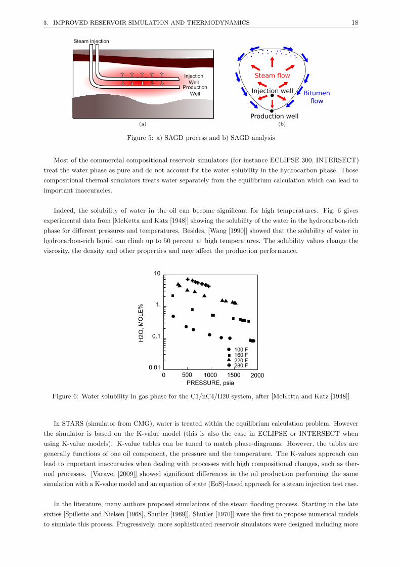
3. IMPROVED RESERVOIR SIMULATION AND THERMODYNAMICS 18

Steam Injection

ProductionWell

InjectionWell

(a)

Injection well

Steam flow

Bitumenflow

Production well(b)

Figure 5: a) SAGD process and b) SAGD analysis

Most of the commercial compositional reservoir simulators (for instance ECLIPSE 300, INTERSECT)

treat the water phase as pure and do not account for the water solubility in the hydrocarbon phase. Those

compositional thermal simulators treats water separately from the equilibrium calculation which can lead to

important inaccuracies.

Indeed, the solubility of water in the oil can become significant for high temperatures. Fig. 6 gives

experimental data from [McKetta and Katz [1948]] showing the solubility of the water in the hydrocarbon-rich

phase for different pressures and temperatures. Besides, [Wang [1990]] showed that the solubility of water in

hydrocarbon-rich liquid can climb up to 50 percent at high temperatures. The solubility values change the

viscosity, the density and other properties and may affect the production performance.

160 F220 F280 F

100 F

0 500 1000 1500 20000.01

1.

10

0.1

PRESSURE, psia

H2O

, MO

LE%

Figure 6: Water solubility in gas phase for the C1/nC4/H20 system, after [McKetta and Katz [1948]]

In STARS (simulator from CMG), water is treated within the equilibrium calculation problem. However

the simulator is based on the K-value model (this is also the case in ECLIPSE or INTERSECT when

using K-value models). K-value tables can be tuned to match phase-diagrams. However, the tables are

generally functions of one oil component, the pressure and the temperature. The K-values approach can

lead to important inaccuracies when dealing with processes with high compositional changes, such as ther-

mal processes. [Varavei [2009]] showed significant differences in the oil production performing the same

simulation with a K-value model and an equation of state (EoS)-based approach for a steam injection test case.

In the literature, many authors proposed simulations of the steam flooding process. Starting in the late

sixties [Spillette and Nielsen [1968], Shutler [1969]], Shutler [1970]] were the first to propose numerical models

to simulate this process. Progressively, more sophisticated reservoir simulators were designed including more

3. IMPROVED RESERVOIR SIMULATION AND THERMODYNAMICS 19

complex physical phenomena and numerical improvements [Coats [1976], Coats [1978]], [Ishimoto [1985],

Chein et al. [1989]]. In most of the simulators, either water was treated as an ideal solution in compositional

simulators or a K-value model was used.

In the last few years, some authors started to perform full three phase compositional simulations of the

steam flooding process. [Brantferger [1991]], Voskov et al. [2009], Varavei and Sepehrnoori [2009]] and more

recently [Zaydullin et al. [2014]] developed full three phase flash simulations and showed simulations of steam

injection problems.

However, no case of fully compositional simulations of extra-heavy oils steam injection or SAGD processes

have been proposed in the literature yet. Those simulations appear essential and will offer better tools to

predict the possible profitability in the exploitation of heavy oil fields.

Three to four phase multiphase calculations are in the heart of tertiary recovery simulations. In gas

injection, micro-emulsion, steam-injections processes, an additional phase from the oil-gas system is added to

the set, which plays a huge impact on the oil recovery. Thermodynamics is in the heart of those processes

and it is important to simulate accurately these multiphase systems. In chemical process simulators, the

high number of components to deal with makes the equilibrium calculations time-consuming. Generally

pseudo-components are generated to decrease the dimensionality of the system leading to approximations of

the original problem. For all these reasons, robust time-saving algorithms are necessary to deal with those

applications.

3.2 Multiphase equilibrium calculations

The resolution of the multiphase phase-split problem is based on the minimization of the Gibbs free energy.

Different types of algorithms have been developed to model this problem. [Michelsen [1982b] and Michelsen

[1982a]] developed a methodology in which stability analysis, based on the tangent plane distance (TPD)

minimization, is used alternatively with a phase-split algorithm.

Two different kinds of algorithms have been developed in the literature.

• A safe but time-consuming procedure uses global minimization algorithms. [Sun and Seider [1995]]

developed an interval-Newton procedure guaranteeing to find the global minimum. [Stadtherr et al.

[1995]] developed a method based on homotopy-continuation functions. [Lucia et al. [2000]] used binary

tangent plane distance to test all pairs of components based on a Sequential Quadratic Programming

(SQP) algorithm. [Nichita et al. [2002]] developed a tunneling based method.

• Local minimization procedures are faster, but they require sculptured initializations. For phase equilib-

rium calculations, [Michelsen [1982a]] proposed a procedure which generally converges to the global

minimium. In a context were time is crucial, this methodology has been widely used in the reservoir

simulation.

In the multiphase equilibrium calculation problem, calculation algorithms were improved ensuring conver-

gence even close to difficult regions (such as in the vicinity of singularities: critical points for flash calculations

and the stability test limit locus for stability analysis) and to increase the probability to converge to the

global minimum. Starting with [Risnes et al. [1981]] who proposed a successive substitution method for

multiphase equilibrium problems, many improvements were proposed to improve multiphase equilibrium

calculations ([Nghiem and Heidemann [1982]], [Mehra et al. [1982]], [Michelsen [1994]]). [Michelsen [1982b]]

provided initial guesses for multiphase problems which were further extended by [Li and Firoozabadi [2012]]

who proposed a general strategy for Stability Testing and Phase-split Calculations in two and three phases.

However, new improvements are still necessary, namely in the difficult regions, where a high number of

iterations are still required by the current equilibrium algorithms to reach convergence.

4. OVERVIEW OF THE THESIS 20

The research work undertaken in this thesis focuses on multiphase equilibrium calculations able to simulate

different compositional simulation problems such as steam injection with extra-heavy oils, within acceptable

times.

4 Overview of the thesis

In compositional thermal reservoir simulations, conservation equations must be solved at each time step.

Local equilibrium is assumed in each cell and a huge amount of phase equilibrium calculations is involved,

based on the minimization of the Gibbs free energy. A, a single failure may cause significant error propagation

leading to false solutions. Thus, it is imperative that calculation algorithms are efficient and highly robust:

reliability has to be kept ensuring in the same time a reasonably fast convergence even in very difficult cases.

In this thesis, improvements in multiphase equilibrium calculations are proposed in order to simulate the

steam injection process. The thesis is organized in five parts

The first chapter briefly presents some fundamental thermodynamics and the Cubic EoS model. The cubic

equations of state provide a reasonable description of the volumetric and phase behavior of pure components

and mixtures, requiring only the critical properties and the acentric factors of each component. They have

been widely used in the reservoir simulation framework and there are also used in this work.

In a second chapter, the minimization algorithm (from [Michelsen [1982a]]) is presented. The stability

testing and the phase-split problems are described as well as the general multiphase equilibrium calculation

procedure to minimize the Gibbs free energy.

In a third chapter, multiphase equilibrium algorithms improvements are presented. Most of the equilibrium

calculations are based on the Newton-Raphson method and use conventional independent variables. These

algorithms are first investigated and different extensions are proposed. The logarithm of the equilibrium

constants (ln K) seems to be the best choice of conventional independent variables for multiphase equilibrium

calculations. In this work, by extending [Michelsen [1982a]] to multiphase-split problems, we propose to

calculate the Jacobian matrix as a product of two symmetric matrices, and to solve the linear system using a

Cholesky factorization in order to reduce the number of arithmetic operations for each iteration.

The reduction methods introduced by [Michelsen [1986] and Hendriks [1988]] enable to reduce the space of

study from nc (the number of components) for conventional varibles to M (with M < nc). An extension of the

new reduction method proposed by [Nichita and Graciaa [2011]], based on the multi-linear expression of the

logarithm of fugacity coefficients is done for stability analysis and multiphase-split calculations. Furthermore,

comparisons between different conventional and reduction methods are performed for the stability testing

and the multiphase-split calculation problems. Until now, the comparisons from the literature have focused

on the global CPU times to compute the whole multiphase equilibrium problem. In this work, comparisons

are performed independently for each problem (stability analysis, two phase-split and multiphase-split

calculations). Besides, the condition number and convergence paths are also investigated leading to more

detailed and extensive comparisons.

The Newton method requires a positive definite Hessian to be applicable. In a new section, other kinds

of minimization methods are investigated which could overcome this constraint and be applicable for each

iteration. The Quasi-Newton procedures for example guarantee a descent direction for each iteration. These

methods represent an interesting alternative since they approach second order methods without the need

to compute the second derivatives and no linear system needs to be solved explicitly. A BFGS (Broyden-

Fletcher-Goldfarb-Shanno) approach applied with a new set of variables is here proposed for two-phase split

calculations. By adding a diagonal element to the Hessian, the Trust-Region methods enable to perform

supra-linear up to quadratic steps even when the Hessian is not positive definite. A descent direction is

always guaranteed which makes it an attractive procedure. A Trust Region based method is also proposed in

4. OVERVIEW OF THE THESIS 21

this same chapter and applied both for stability testing and multiphase-split calculation problems.

The generation of pseudo-components capable of representing the fluid behavior accurately is necessary

to obtain accurate simulations of an enhanced oil recovery process. In a forth chapter, an algorithm is

proposed to improve the characterization of a fluid based on the semi-continuous thermodynamics. Assuming

the fluid composition as semi-continuous, a new methodology based on a Gaussian quadrature is proposed

to mathematically compute a set of pseudo-components capable of representing the fluid behavior. The

methodology can be seen as a lumping-delumping procedure.

Through this thesis, a program including all the presented new algorithms has been developed to deal with

multiphase equilibrium calculations with an arbitrary number of phases. Besides, this program was included

within two different reservoir simulator; the TPP platform (internal reservoir simulator from Total S.A.)

and AD-GPRS (Automatic Differentiation General Purpose Reservoir Simulator) from Stanford University.

In the last chapter, tests of the program in stand-alone computations are performed. Comparisons are

presented between the results obtained with the developed program and literature and experimental data.

Then different reservoir simulations are carried out to simulate different enhanced oil recovery processes. A

comparison with ECLIPSE is performed for a three-phase water injection problem (with the water treated

outside the equilibrium calculations). Then fully three- and four-phase compositional reservoir simulations of

isothermal CO2 injection problems are presented revealing the capability of the algorithm to handle more

than three-phase simulations.

Finally, fully compositional thermal simulations of steam injections are carried out. In a first step,

simulations of the steam flooding process in heterogeneous and homogeneous conditions is realized. In a

second step, a simulation of the SAGD process is presented with an extra heavy mixture from Canada. In

this last part, the developed equilibrium program is tested with different stability bypass procedures and

computational times are presented for all the steam injection cases.

Chapter 1

Fundamental thermodynamics

Contents

1.1 Thermodynamics functions . . . . . . . . . . . . . . . . . . . . . . . . . . . . . . 22

1.1.1 Internal Energy . . . . . . . . . . . . . . . . . . . . . . . . . . . . . . . . . . . . . . 22

1.1.2 Gibbs free energy . . . . . . . . . . . . . . . . . . . . . . . . . . . . . . . . . . . . . 24

1.1.3 Helmholtz free energy . . . . . . . . . . . . . . . . . . . . . . . . . . . . . . . . . . 25

1.1.4 Enthalpy . . . . . . . . . . . . . . . . . . . . . . . . . . . . . . . . . . . . . . . . . 25

1.1.5 Residual energy . . . . . . . . . . . . . . . . . . . . . . . . . . . . . . . . . . . . . . 25

1.1.6 Maximization of the entropy . . . . . . . . . . . . . . . . . . . . . . . . . . . . . . 25

1.1.7 Fugacity and fugacity coefficients . . . . . . . . . . . . . . . . . . . . . . . . . . . . 26

1.1.8 Condition for equilibrium at constant pressure and temperature . . . . . . . . . . . 28

1.2 Equation of State Calculations . . . . . . . . . . . . . . . . . . . . . . . . . . . . 29

1.2.1 Introduction . . . . . . . . . . . . . . . . . . . . . . . . . . . . . . . . . . . . . . . 29

1.2.2 Cubic equations of state . . . . . . . . . . . . . . . . . . . . . . . . . . . . . . . . . 29

1.2.3 Fugacity coefficient . . . . . . . . . . . . . . . . . . . . . . . . . . . . . . . . . . . . 31

1.2.4 Molar Gibbs free energy . . . . . . . . . . . . . . . . . . . . . . . . . . . . . . . . . 31

An accurate modeling of the different equilibrium phases is highly important in reservoir simulations.

Many equations of state exist relating the thermodynamic variables. In this thesis, the development of a

general algorithm to solve the multiphase flash problem is proposed. Cubic EoS provide an efficient way to

model the different thermodynamic properties required in a reservoir simulation (enthalpies, densities), as

well as the phase envelope construction and they generally lead to an acceptable accuracy for hydrocarbon

mixtures. In the reservoir simulation context, where computation times should remain acceptable, cubic EoS

have been widely used, and are used in this thesis. A description of the cubic EoS is presented in this chapter

and the multiphase equilibrium calculation framework is presented, as well as the thermodynamic functions

that need to be computed in the reservoir simulation.

1.1 Thermodynamics functions

1.1.1 Internal Energy

1.1.1.1 First Law

The first law of thermodynamics corresponds to the conservation of the energy for a system.

For a closed system, for any processes, an infinitesimal change in the internal energy is considered due to

a combination of heat added to the system Q and work done by the system W . Taking δU as an infinitesimal

change in internal energy, and considering only the internal energy variations, the work done by pressure and

the thermal exchanges, the first law can be written [Vidal [1997]]:

22

1.1. THERMODYNAMICS FUNCTIONS 23

dU = δQ+ δW (1.1)

In case of equilibrium mixtures, only the work due to the pressure is taken into account (electrical forces

are negligible, no mechanical forces,..). It can be expressed as [Vidal [1997]]

δW = −pdV (1.2)

1.1.1.2 Second law

The entropy change is related to the heat added to the system and the temperature. During a transformation,

the entropy variation can be splitted into two different terms [Vidal [1997]]

dS = dSi + dSe (1.3)

where dSe is related to heat exchanges,

dSe =δQ

T(1.4)

For reversible transformations, the second law, states that

dSi ≥ 0 (1.5)

Therefore,

dS ≥ δQ

T(1.6)

Using (eq. 1.1),

dU + PdV − TdS ≤ 0 (1.7)

In a reversible process, an infinitesimal variation of the entropy is due to an infinitesimal variation of heat

divided by the temperature of the system. If the work done to the system is limited to the work done by

pressure one can write [Vidal [1997]]

dS =δQ

T(1.8)

Combining (eq. 1.1, eq. 1.2, eq. 1.8), one obtains

dU = TdS − pdV (1.9)

U is here a function of S and V . The total differential of the internal energy U can be written as:

dU =

(∂U

∂S

)V

dS +

(∂U

∂V

)S

dV (1.10)

which gives by using (eq. 1.9) in (eq. 1.10),(∂U

∂S

)V

= T

(∂U

∂V

)S

= −p (1.11)

For a mixture with different components, the total internal energy of a system can be expressed as a

function of S, V and the mole numbers n = [n1, n2, · · · , nnc] [Vidal [1997]]. By definition the total differential

of the internal energy U can be written as:

1.1. THERMODYNAMICS FUNCTIONS 24

dU =

(∂U

∂S

)V,n

dS +

(∂U

∂V

)S,n

dV +

nc∑i=1

(∂U

∂ni

)S,V,nj 6=i

dni (1.12)

with the chemical potential of the component i given by

µi =

(∂U

∂ni

)nj 6=i,V,S

(1.13)

Moreover, the derivatives in (eq. 1.11) still holds for mixtures since V , S and n are independent variables

of U . (eq. 1.11) becomes (∂U

∂S

)V,n

= T

(∂U

∂V

)S,n

= −p (1.14)

Combining (eq. 1.12, eq. 1.13 and eq. 1.14) leads to

dU = TdS − pdV +

nc∑i=1

µidni (1.15)

Moreover, as all the independent variables of U (S, n and V ) are extensive variables, using Euler’s theorem

with (eq. 1.14) leads to

U(S, V,n) = TS − pV +

nc∑i=1

µini (1.16)

1.1.2 Gibbs free energy

The Gibbs free energy is given in [Vidal [1997]]:

G(p, T,n) = U + pV − TS (1.17)

by differenciating this expression:

dG(p, T,n) = dU + pdV + V dp− TdS − SdT (1.18)

and using (eq. 1.15) in (eq. 1.18), one obtains

dG(p, T,n) =

nc∑i=1

µidni + V dp− SdT (1.19)

which gives in terms of partial derivatives:

(∂G(p, T,n)

∂p

)n,T

= V

(∂G(p, T,n)

∂T

)n,p

= −S(∂G(p, T,n)

∂ni

)p,T,nj 6=i

= µi(p, T,n) (1.20)

Using (eq. 1.16) in (eq. 1.17),

G(p, T,n) =

nc∑i=1

µini (1.21)

and taking the total differentiation of (eq. 1.21),

dG =

nc∑i=1

nidµi +

nc∑i=1

µidni (1.22)

Using (eq. 1.22 and eq. 1.19), the Gibbs-Duhem equation is obtained,

1.1. THERMODYNAMICS FUNCTIONS 25

nc∑i=1

nidµi = V dp− SdT (1.23)

1.1.3 Helmholtz free energy

The Helmholtz free energy is given by [Vidal [1997]]:

A(V, T,n) = U − TS (1.24)

Differentiating this equation, and using (eq. 1.15), one obtains

dA =

nc∑i=1

µidni − SdT − pdV (1.25)

which leads to the following partial derivatives:

(∂A(T, V,n)

∂V

)T,n

= −p(∂A(T, V,n)

∂T

)V,n

= −S(∂A(T, V,n)

∂ni

)T,V,nj 6=i

= µi(T, V,n) (1.26)

1.1.4 Enthalpy

The enthalpy is given by means of a Legendre transformation [Vidal [1997]]

H(p, S,n) = U + pV (1.27)

1.1.5 Residual energy

A residual quantity (Mr) is the difference between the property of a real mixture (M) and that of an ideal gas

at the same pressure, temperature and composition (M∗) (or at the same conditions of volume temperature

and composition):

M(T, p,n) = M∗(T, p,n) +Mr(T, p,n) (1.28)

M(T, V,n) = M∗(T, V,n) +Mr(T, V,n) (1.29)

1.1.6 Maximization of the entropy

The second law states that

dS ≥ O (1.30)

At equilibrium in an isolated system, the system does not exchange heat or work with the surrondings,

dW = 0 dQ = 0 (1.31)

Therefore,

dU = 0 dV = 0 (1.32)

Following [Vidal [1997]] procedure, let split the system within two subsystems A and B separated with an

’artificial barrier’, we have

1.1. THERMODYNAMICS FUNCTIONS 26

dU = dUA + dUB = 0 dS = dSA + dSB (1.33)

and

dVA + dVB = 0 (1.34)

Using (eq. 1.15), one obtains

dS =

(1

TA− 1

TB

)dUA +

(PATA− PBTB

)dVA (1.35)

At equilibrium, dS = 0, the second law states that equilibrium is obtained at the maximum of the entropy,

which corresponds here to the equality of the temperatures and pressures.

Moreover, using (eq. 1.7) at constant pressure and temperature, it leads to

dG ≤ 0 (1.36)

At equilibrium,

dG = 0 (1.37)

Using (eq. 1.36) and (eq. 1.37), the equilibrium corresponds to the minimum of the Gibbs free energy.

1.1.7 Fugacity and fugacity coefficients

In the case of an ideal gas, the ideal gas law can be applied:

V =nRT

p(1.38)

Moreover, using (eq. 1.20), the Maxwell relation gives:(∂µ

∂p

)T

=

(∂V

∂n

)T

(1.39)

Considering the fluid as a pure component, the left side of the equation (eq. 1.39) corresponds to the

molar volume Vm. For a perfect gas, Vm = RT/p, (eq. 1.39) becomes at constant temperature∫ p

p0

dµ =

∫ p

p0

RT

pdp (1.40)

Which leads to

µ∗(T, p) = µ∗(T, p0) +RT lnp

p0(1.41)

In case of real fluid, [Lewis and Randall [1923]] introduced the fugacity f to act as an effective pressure.

The fugacity represents the value that must be substituted for pressure in order to preserve the expressions

for ideal gas [Vidal [1997]]. The relation (eq. 1.40) becomes for real fluids [Michelsen and Mollerup [2007]]

µ(T, p)− µ∗(T, p0) = RT lnf(T, p)

p0(1.42)

which gives taking the difference of (eq. 1.42) and (eq. 1.41),

µ(T, p)− µ∗(T, p) = RT lnf(T, p)

p(1.43)

The term within the logarithm corresponds to the fugacity coefficient:

1.1. THERMODYNAMICS FUNCTIONS 27

φ =f

p(1.44)

which is the ratio that indicates how the fugacity of a real substance deviates from that of an ideal gas.

For ideal mixtures, the partial pressure is given by [Vidal [1997]] pi = xip, this gives

µ∗i (T, p) = µ∗(T, p0) +RT lnxip

p0(1.45)

For real mixtures, the expression of the fugacity is given for each components:

µi(T, p,n) = µ∗(T, p0) +RT lnfi(T, p,n)

p0(1.46)

Taking the difference (eq. 1.46 - eq. 1.45),

µi(T, p,n) = µ∗i (T, p) +RT lnfixip

(1.47)

The expression of the fugacity coefficient is generalized to

φi =fi(T, p,n)

xip(1.48)

Using the expression of partial derivatives for ideal mixtures pi = xip, one can write

µ∗i (T, p) = µ∗(T, p) +RT lnxip

p= µ∗(T, p) +RT lnxi (1.49)

Using (eq. 1.47, 1.49),

µi(p, T,n) = RT lnφi + µ∗i (T, p) +RT lnxi = RT ln fi + µ∗i (T, p0)−RT ln p0 (1.50)

Now let’s find an expression for the fugacity coefficient, taking the Gibbs-Duhem equation (eq. 1.23) for a

single component fluid, at constant temperature,

dµ = Vmdp Vm = V/n (1.51)

Moreover, by definition of the fugacity, at constant temperature, it can easily be shown that [Vidal [1997]]

dµ = RTd ln f (1.52)

which means that by definition of the coefficients (eq. 1.44),

RTd lnφ = Vmdp−RTd ln p = Vmdp−RTdp

p(1.53)

When p→ 0, the fluid becomes an ideal state and φ→ 1, therefore, by integrating (eq. 1.53),∫ p

p0

d lnφ =

∫ p

p0

(VmRT− 1

p

)dp (1.54)

Taking p0 = 0,

lnφ =

∫ p

0

(V

nRT− 1

p

)dp (1.55)

For mixtures, at constant temperature, the fugacity definition gives

dµi = RTd ln fi (1.56)

1.1. THERMODYNAMICS FUNCTIONS 28

Moreover, using the Maxwell relation with the Gibbs free energy,(∂µi∂V

)T,n

= −(∂P

∂ni

)T,V,nj 6=i

(1.57)

which leads to

dµi = −(∂P

∂ni

)T,V,nj 6=i

dV (1.58)

Combining (eq. 1.56, eq. 1.58), and eq. 1.48),

RTd lnφi = −(∂P

∂ni

)T,V,nj 6=i

dV −RTd ln pxi (1.59)

with the compressibility factor Z which indicates the deviation from the ideal gas behavior:

Z =pV

nRT(1.60)

RTd lnφi = −(∂P

∂ni

)T,V,nj 6=i

dV +RTd lnV −RTd ln (nRT

xi)−RTd lnZ (1.61)

when V →∞, the system acts as a perfect gas, φi → 1 and Z → 1, with d lnV = dV/V , it can be shown

that

lnφi =1

RT

∫ V

∞

[RT

V−(∂P

∂ni

)T,V,nj 6=i

]dV − lnZ (1.62)

1.1.8 Condition for equilibrium at constant pressure and temperature

The Gibbs free energy is given by:

G(p, T,n) =

nc∑i=1

µini (1.63)

For a closed system, at constant pressure and temperature, the equilibrium is obtained for the state giving

the minimum Gibbs free energy. Using equation (eq. 1.50) in (eq. 1.63), minimizing the Gibbs free energy at

constant p and T is equivalent to minimize:

G(n)

RT=

nc∑i=1

ni ln fi (1.64)

Which can be extended for multiphase problems:

G(n)

RT=

np∑j=1

nc∑i=1

nij ln fij (1.65)

In this subsection, the mole numbers and taken as independent variables. For each phase, the Gibbs-Duhem

relation (eq. 1.23) leads at constant pressures and temperatures,

nc∑i=1

nij∂ ln fij∂nkl

= 0 ∀k = 1, nc ∀l, j = 1, np (1.66)

Let zi be the feed composition of the component i. Taking np as the phase of reference,

ni,np = zi −np−1∑j=1

nij (1.67)

1.2. EQUATION OF STATE CALCULATIONS 29

the minimum is found when the elements of the gradient vector are equal to zero.

∂

nij

(G(n)

RT

)= ln fij − ln fi,np = 0 ∀j = 1, np− 1 ∀i = 1, nc (1.68)

And therefore, at the equilibrium,

fij = fi,np ∀j = 1, np− 1 ∀i = 1, nc (1.69)

1.2 Equation of State Calculations

1.2.1 Introduction

For a real mixture, the compressibility factor Z indicates the deviation from the ideal gas behavior. In the

equilibrium problems, at a given temperature and pressure, one needs to compute Z. However, V is unknown.

One equation is missing to close the system.

Cubic equations of state (EoS) have been introduced in this attempt. They are simple equations relating

pressure, volume and temperature (pVT). They provide a reasonable description of the volumetric and phase

behavior of pure compounds and mixtures, requiring only critical properties and acentric factors of each

component.

Through this thesis, a program was developed to solve multiphase calculations problem. Cubic equations

of state were used in this study, but the program was designed so that other Eos models could be integrated.

1.2.2 Cubic equations of state

The general form of two-cubic EoS is

p =RT

ν − b− a

(ν + δ1b)(ν + δ2b)(1.70)

where δ1 = 0 and δ2 = 1 for the SRK Eos [Soave [1972], Redlich and Kwong [1949]] and δ1,2 = 1±√

2 for

the PR EoS [Peng and Robinson [1976]].

The implicit form (in compressibility factor Z) of the Eos is obtained by substituting A = apR2T 2 , B = bp

RT

and Z = pνRT into (eq. 1.70).

Z3 + [(δ1 + δ2 − 1)B − 1]Z2 +[A+ δ1δ2B

2 − (δ1 + δ2)B(B + 1)]Z

−[AB + δ1δ2B

2(B + 1)]

= 0 (1.71)

The van der Waals one-fluid mixing rules are used for the energy A, and for the volume B, parameters of

the cubic EoS

A =

nc∑i=1

nc∑j=1

xixjAij (1.72)

and

B =

nc∑i=1

Bixi (1.73)

where

Aij =√Ai√Aj (1− Cij) ; i, j = 1, nc (1.74)

1.2. EQUATION OF STATE CALCULATIONS 30

Ai = ΩapriT 2ri

[1 +m(ωi)

(1−

√Tri

)]2i = 1, nc (1.75)

and

Bi = ΩbpriTri

; i = 1, nc (1.76)

Cij is an element of the binary interaction parameter matrix (BIP). Tri = TTci

is the reduced temperature

(with Tci the critical temperature), pri = ppci

, the reduced pressure and ωi the acentric factor of the component

i.

For the PR EoS, Ωa = 0.45724, Ωb = 0.0778, m(ω) = 0.37464 + 1.54226ω − 0.26992ω2 for w ≤ 0.49, and

m(ω) = 0.379642 + 1.48503ω − 0.164423ω2 + 0.016667ω3 for w > 0.49 [Robinson and Peng [1978]]. For the

SRK EoS, Ωa = 0.42748, Ωb = 0.08664 and m(ω) = 0.48 + 1.574ω − 0.176ω2.

1.2.2.1 Solving the cubic polynomial equation

The Cardan procedure enables to compute analytically the roots of the third order polynomial:

Z3 + a1Z2 + a2Z + a3 = 0 (1.77)

Taking

Q =3a2 − a2

1

9(1.78)

R =a2a1

6− a3

2− 2a3

1

27(1.79)

the Discrimant is given by:

D = Q3 +R2 (1.80)

• If D > 0, there is only one real root:

Z =√

3R+√D +

√3R−

√D − a1

3(1.81)

• If D = 0, there are three real roots, with two equal:

Z1 = 2√

3R− a1

3(1.82)

Z2 = Z3 = −√

3R− a1

3(1.83)

• Else if D < 0 there are three real roots:

Introducing θ

θ = arccos

(R√−Q3

)(1.84)

the expression of the roots becomes

1.2. EQUATION OF STATE CALCULATIONS 31

Z1 = 2√−Q cos

(θ

3

)− a1

3(1.85)

Z2 = 2√−Q cos

(θ

3+

2π

3

)− a1

3(1.86)

Z3 = 2√−Q cos

(θ

3+

4π

3

)− a1

3(1.87)

However, even if the Cardan method provides an analytical solution, in some situations numerical

instabilities can occur [Monroy-Loperena [2012]]. In these cases, a Newton procedure is used to refine the

roots.

When multiple roots are found, in two phase equilibrium calculations, generally, the smallest root is taken

for liquid and the largest is taken for gas. However, in this work, for multiphase calculations, the root which

minimizes the Gibbs free energy is selected for each phase.

1.2.3 Fugacity coefficient

Combining (eq. 1.62 and eq. 1.70), the fugacity coefficient can be expressed:

lnφi = (Z − 1)BiB− ln(Z −B)− A

(δ1 − δ2)B

∗(

2ψiA− BiB

)ln

(Z + δ1B

Z + δ2B

)(1.88)

with

ψi =

C∑j=1

Aijxj ; i = 1, nc (1.89)

1.2.4 Molar Gibbs free energy

The dimensionless molar Gibbs free energy g can be expressed as the sum of the ideal and excess molar Gibbs

free energy

g = gI + gE (1.90)

with

gI =

nc∑i=1

xi lnxi (1.91)

and

gE =

nc∑i=1

xi lnφi(x) (1.92)

The last expression becomes for cubic EoS models,

gE = (Z − 1)− ln(Z −B)− A

∆BlnE (1.93)

where E = (Z + δ1B)/(Z + δ2B) and ∆ = δ1 − δ2

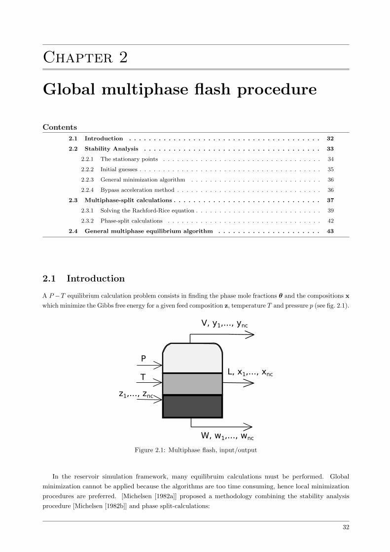
Chapter 2

Global multiphase flash procedure

Contents

2.1 Introduction . . . . . . . . . . . . . . . . . . . . . . . . . . . . . . . . . . . . . . . 32

2.2 Stability Analysis . . . . . . . . . . . . . . . . . . . . . . . . . . . . . . . . . . . . 33

2.2.1 The stationary points . . . . . . . . . . . . . . . . . . . . . . . . . . . . . . . . . . 34

2.2.2 Initial guesses . . . . . . . . . . . . . . . . . . . . . . . . . . . . . . . . . . . . . . . 35

2.2.3 General minimization algorithm . . . . . . . . . . . . . . . . . . . . . . . . . . . . 36

2.2.4 Bypass acceleration method . . . . . . . . . . . . . . . . . . . . . . . . . . . . . . . 36

2.3 Multiphase-split calculations . . . . . . . . . . . . . . . . . . . . . . . . . . . . . . 37

2.3.1 Solving the Rachford-Rice equation . . . . . . . . . . . . . . . . . . . . . . . . . . . 39

2.3.2 Phase-split calculations . . . . . . . . . . . . . . . . . . . . . . . . . . . . . . . . . 42

2.4 General multiphase equilibrium algorithm . . . . . . . . . . . . . . . . . . . . . 43

2.1 Introduction

A P −T equilibrium calculation problem consists in finding the phase mole fractions θ and the compositions x

which minimize the Gibbs free energy for a given feed composition z, temperature T and pressure p (see fig. 2.1).

V, y1,..., ync

L, x1,..., xnc

W, w1,..., wnc

P

T

z1,..., znc

Figure 2.1: Multiphase flash, input/output

In the reservoir simulation framework, many equilibruim calculations must be performed. Global

minimization cannot be applied because the algorithms are too time consuming, hence local minimization

procedures are preferred. [Michelsen [1982a]] proposed a methodology combining the stability analysis

procedure [Michelsen [1982b]] and phase split-calculations:

32

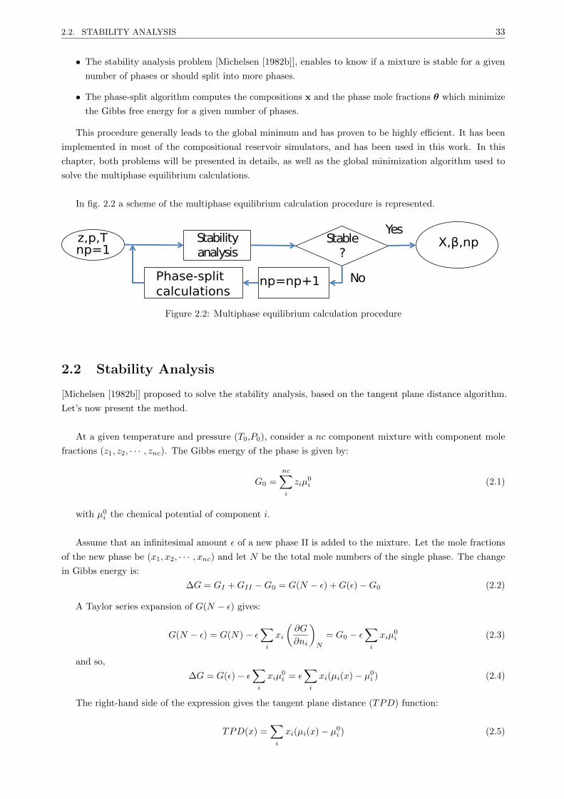
2.2. STABILITY ANALYSIS 33

• The stability analysis problem [Michelsen [1982b]], enables to know if a mixture is stable for a given

number of phases or should split into more phases.

• The phase-split algorithm computes the compositions x and the phase mole fractions θ which minimize

the Gibbs free energy for a given number of phases.

This procedure generally leads to the global minimum and has proven to be highly efficient. It has been

implemented in most of the compositional reservoir simulators, and has been used in this work. In this

chapter, both problems will be presented in details, as well as the global minimization algorithm used to

solve the multiphase equilibrium calculations.

In fig. 2.2 a scheme of the multiphase equilibrium calculation procedure is represented.

Stabilityanalysis

Stable?

Yes

NoPhase-splitcalculations

z,p,T X,β,np

np=np+1

np=1

Figure 2.2: Multiphase equilibrium calculation procedure

2.2 Stability Analysis

[Michelsen [1982b]] proposed to solve the stability analysis, based on the tangent plane distance algorithm.

Let’s now present the method.

At a given temperature and pressure (T0,P0), consider a nc component mixture with component mole

fractions (z1, z2, · · · , znc). The Gibbs energy of the phase is given by:

G0 =

nc∑i

ziµ0i (2.1)

with µ0i the chemical potential of component i.

Assume that an infinitesimal amount ε of a new phase II is added to the mixture. Let the mole fractions

of the new phase be (x1, x2, · · · , xnc) and let N be the total mole numbers of the single phase. The change

in Gibbs energy is:

∆G = GI +GII −G0 = G(N − ε) +G(ε)−G0 (2.2)

A Taylor series expansion of G(N − ε) gives:

G(N − ε) = G(N)− ε∑i

xi

(∂G

∂ni

)N

= G0 − ε∑i

xiµ0i (2.3)

and so,

∆G = G(ε)− ε∑i

xiµ0i = ε

∑i

xi(µi(x)− µ0i ) (2.4)

The right-hand side of the expression gives the tangent plane distance (TPD) function:

TPD(x) =∑i

xi(µi(x)− µ0i ) (2.5)

2.2. STABILITY ANALYSIS 34

The system always tries to minimize the energy. This means that if ∆G is negative, the system will

change to a two phase system. On the other hand, if ∆G ≥ 0, the system will remain in one phase. From (eq.

1.50), the dimensionless TPD function becomes [Michelsen [1982b]]

D(x) =

NC∑i=1

xi (lnxi + lnφi(x)− di(z)) (2.6)

with

di = ln(zi) + ln(φi(z)); (2.7)

If at all stationary points the TPD function is non negative, the system remains in one phase. When

reaching the stationary point:

ln(xi) + ln(φi)− di = k ∀i = 1, · · · , nc (2.8)

By changing the variable: Yi = xie−k, it can be noticed that

xi =YiYT

(2.9)

with YT =∑i=1 Yi, thus Yi can be viewed formally as mole numbers. (eq. 2.8) becomes:

ln(Yi) + ln(φi)− di = 0 ∀i = 1, · · · , nc (2.10)

Instead of minimizing the tangent plane distance, [Michelsen [1982b]] proposed a modified TPD function:

D∗ =

(1−

NC∑i=1

Yi

)+

NC∑i=1

Yi (lnYi + lnφi(Y)− di) (2.11)

The function D∗ has the same stationary points and the same sign as the original TPD function D

[Michelsen [1982b]]. When testing if a monophasic fluid is stable, the stability is applied to the feed mole

fractions z. For mixtures with M phases, only one phase need to be tested to assume the mixture as

stable/unstable in M phases. In this work, following [Li and Firoozabadi [2012]], the phase selected is the

one with the highest molecular weight.

2.2.1 The stationary points

At the solution, the stationary points (xSP ) are obtained.

• if minxSPTPD(xSP ) < 0, the mixture is unstable, a new phase y 6= z is found which will be used as

initial guess for the equilibrium

• if minxSPTPD(xSP ) = 0, at the phase boundary, the minimum of the TPD is found for a phase y 6= z.

The mixture is stable.

• if minxSPTPD(xSP ) > 0, the minimum of the TPD is found for a phase y 6= z. The mixture is stable.

• if minxSPTPD(xSP ) = 0, far from the phase boundary, the minimum of the TPD corresponds to the

trial solution z. The mixture is stable.

An example is given in fig. 2.3a where the tangent plane distance function is plotted at the solution of the

stability analysis for the vapor trial phase, for the Y8 mixture [Yarborough [1972]]. In fig. 2.3b, the tangent

plane distance of the liquid trial phase is given. In light grey (respectively dark grey) the area converging to

a stationary solution (xSP ) leading to a negative TPD function (respectively positive TPD function, with a

non-trivial solution) is represented. Elsewhere, the problem converges to the trivial solution.

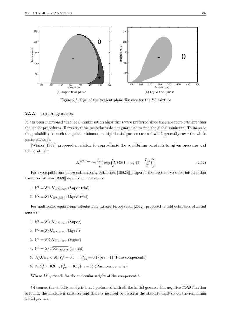
2.2. STABILITY ANALYSIS 35

Pressure, bar

Temperature,K

150 200 250 300 350 400 450 500

50

100

150

200

250

-

+

0

(a) vapor trial phase

Pressure, bar

Temperature,K

150 200 250 300 350 400 450 500

50

100

150

200

250

- 0

(b) liquid trial phase

Figure 2.3: Sign of the tangent plane distance for the Y8 mixture

2.2.2 Initial guesses

It has been mentioned that local minimization algorithms were preferred since they are more efficient than

the global procedures. However, these procedures do not guarantee to find the global minimum. To increase

the probability to reach the global minimum, multiple initial guesses are used which generally cover the whole

phase envelope.

[Wilson [1969]] proposed a relation to approximate the equilibrium constants for given pressures and

temperatures:

KWhilsoni =

pc,ip

exp

(5.373(1 + wi)(1−

Tc,iT

)

)(2.12)

For two equilibrium phase calculations, [Michelsen [1982b]] proposed the use the two-sided initialization

based on [Wilson [1969]] equilibrium constants:

1. Y 1 = Z ∗KWhilson (Vapor trial)

2. Y 2 = Z/KWhilson (Liquid trial)

For multiphase equilibrium calculations, [Li and Firoozabadi [2012]] proposed to add other sets of initial

guesses:

1. Y 1 = Z ∗KWhilson (Vapor)

2. Y 2 = Z/KWhilson (Liquid)

3. Y 3 = Z 3√KWhilson (Vapor)

4. Y 4 = Z/ 3√KWhilson (Liquid)

5. ∀i/Mwi < 50, Y ki = 0.9 , Y kj 6=i = 0.1/(nc− 1) (Pure components)

6. ∀i, Y ki = 0.9 , Y kj 6=i = 0.1/(nc− 1) (Pure components)

Where Mwi stands for the molecular weight of the component i.

Of course, the stability analysis is not performed with all the initial guesses. If a negative TPD function

is found, the mixture is unstable and there is no need to perform the stability analysis on the remaining

initial guesses.

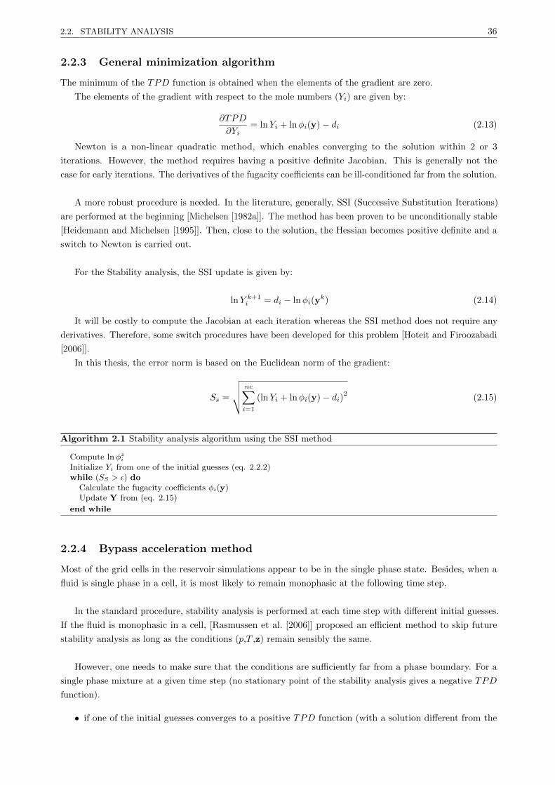
2.2. STABILITY ANALYSIS 36

2.2.3 General minimization algorithm

The minimum of the TPD function is obtained when the elements of the gradient are zero.

The elements of the gradient with respect to the mole numbers (Yi) are given by:

∂TPD

∂Yi= lnYi + lnφi(y)− di (2.13)

Newton is a non-linear quadratic method, which enables converging to the solution within 2 or 3

iterations. However, the method requires having a positive definite Jacobian. This is generally not the

case for early iterations. The derivatives of the fugacity coefficients can be ill-conditioned far from the solution.

A more robust procedure is needed. In the literature, generally, SSI (Successive Substitution Iterations)

are performed at the beginning [Michelsen [1982a]]. The method has been proven to be unconditionally stable

[Heidemann and Michelsen [1995]]. Then, close to the solution, the Hessian becomes positive definite and a

switch to Newton is carried out.

For the Stability analysis, the SSI update is given by:

lnY k+1i = di − lnφi(y

k) (2.14)

It will be costly to compute the Jacobian at each iteration whereas the SSI method does not require any

derivatives. Therefore, some switch procedures have been developed for this problem [Hoteit and Firoozabadi

[2006]].

In this thesis, the error norm is based on the Euclidean norm of the gradient:

Ss =

√√√√ nc∑i=1

(lnYi + lnφi(y)− di)2(2.15)

Algorithm 2.1 Stability analysis algorithm using the SSI method

Compute lnφziInitialize Yi from one of the initial guesses (eq. 2.2.2)while (SS > ε) do

Calculate the fugacity coefficients φi(y)Update Y from (eq. 2.15)

end while

2.2.4 Bypass acceleration method

Most of the grid cells in the reservoir simulations appear to be in the single phase state. Besides, when a

fluid is single phase in a cell, it is most likely to remain monophasic at the following time step.

In the standard procedure, stability analysis is performed at each time step with different initial guesses.

If the fluid is monophasic in a cell, [Rasmussen et al. [2006]] proposed an efficient method to skip future

stability analysis as long as the conditions (p,T ,z) remain sensibly the same.

However, one needs to make sure that the conditions are sufficiently far from a phase boundary. For a

single phase mixture at a given time step (no stationary point of the stability analysis gives a negative TPD

function).

• if one of the initial guesses converges to a positive TPD function (with a solution different from the

2.3. MULTIPHASE-SPLIT CALCULATIONS 37

trivial solution), the conditions are close to a phase boundary and no stability can be bypassed in the

future step.

• if all the stationary points converge to the trivial solution, [Michelsen [1982a]] provides a function to

evaluate the distance with a two phase boundary:

Hij = δij +√ninj

(∂ lnφi∂nj

)P,T

(2.16)

At the solution, the minimum eigenvalue b of the matrix is computed. Then at the next time step in

the reservoir, if the conditions remain sensibly the same, stability analysis can be bypassed because the

system is most likely to remain as a one phase mixture.

The conditions to skip calculations are:

|zni − zn−1i | ≥ bn−1

10(2.17)

|Pn − Pn−1| ≥ bn−1Pn

10(2.18)

|Tn − Tn−1| ≥ 10bn−1 (2.19)

In fig. 2.4, the minimum of the smallest eigenvalue b of the Hessian (eq. 2.16) is given at the solution of

both stability analysis (two sided Wilson initialization), for the Y8 mixture [Yarborough [1972]]. It can be

noticed that getting away from the two phase boundary, b becomes smaller.

Pressure, bar

Tempe

rature,K

150 200 250 300 350 400 450 500

50

100

150

200

250

0

0.1

0.2

0.3

0.4

0.5

0.6

0.7

0.8

0.9

1

Figure 2.4: Smallest eigenvalue of (eq. 2.16), for the Y8 mixture

2.3 Multiphase-split calculations

Given

• z the feed composition of each component

• T the temperature

• P the pressure

• A number of phases np

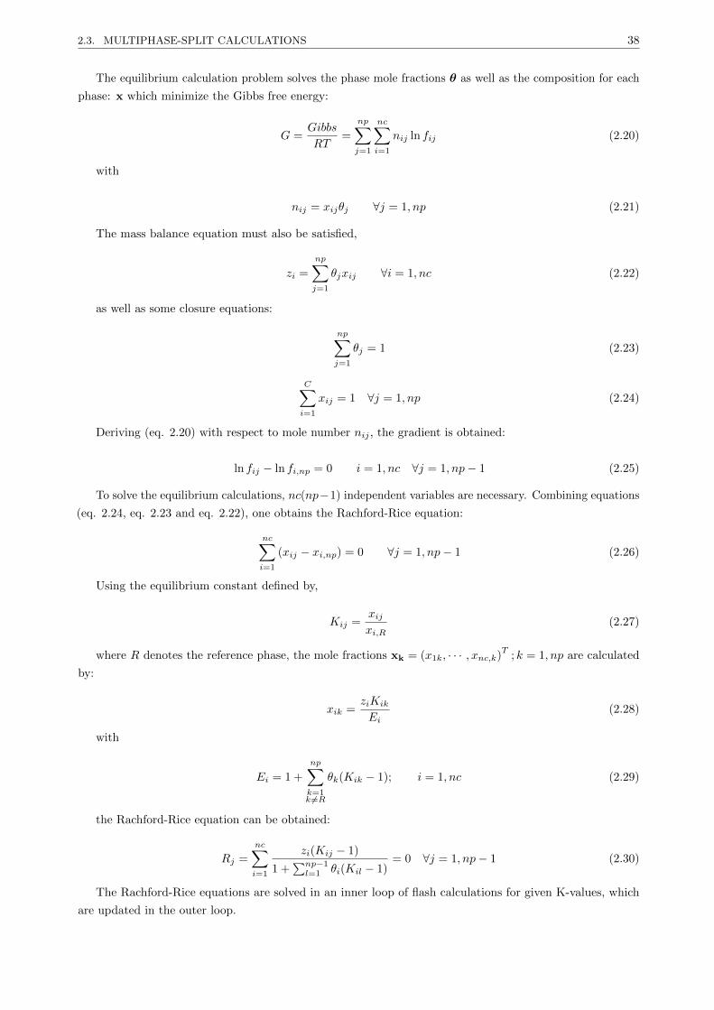
2.3. MULTIPHASE-SPLIT CALCULATIONS 38

The equilibrium calculation problem solves the phase mole fractions θ as well as the composition for each

phase: x which minimize the Gibbs free energy:

G =Gibbs

RT=

np∑j=1

nc∑i=1

nij ln fij (2.20)

with

nij = xijθj ∀j = 1, np (2.21)

The mass balance equation must also be satisfied,

zi =

np∑j=1

θjxij ∀i = 1, nc (2.22)

as well as some closure equations:

np∑j=1

θj = 1 (2.23)

C∑i=1

xij = 1 ∀j = 1, np (2.24)

Deriving (eq. 2.20) with respect to mole number nij , the gradient is obtained:

ln fij − ln fi,np = 0 i = 1, nc ∀j = 1, np− 1 (2.25)

To solve the equilibrium calculations, nc(np−1) independent variables are necessary. Combining equations

(eq. 2.24, eq. 2.23 and eq. 2.22), one obtains the Rachford-Rice equation:

nc∑i=1

(xij − xi,np) = 0 ∀j = 1, np− 1 (2.26)

Using the equilibrium constant defined by,

Kij =xijxi,R

(2.27)

where R denotes the reference phase, the mole fractions xk = (x1k, · · · , xnc,k)T

; k = 1, np are calculated

by:

xik =ziKik

Ei(2.28)

with

Ei = 1 +

np∑k=1k 6=R

θk(Kik − 1); i = 1, nc (2.29)

the Rachford-Rice equation can be obtained:

Rj =

nc∑i=1

zi(Kij − 1)

1 +∑np−1l=1 θi(Kil − 1)

= 0 ∀j = 1, np− 1 (2.30)

The Rachford-Rice equations are solved in an inner loop of flash calculations for given K-values, which

are updated in the outer loop.

2.3. MULTIPHASE-SPLIT CALCULATIONS 39

2.3.1 Solving the Rachford-Rice equation

2.3.1.1 Two phase-split calculations

The Rachford-Rice is a function of the phase mole fractions θ. An iterative procedure enables to solve the

equation for θ. At the end of the calculation, the composition x of each phase can be calculated from the

mass balance equation.

In two phases, let xi stands for the liquid composition of the component i, yi the vapor composition of

the component i and θ the vapor mole fraction. The equation becomes,

h(θ) =

C∑i=1

zi(Ki − 1)

1 + θ(Ki − 1)= 0 (2.31)

The function represents a strictly decreasing function within the negative flash window.

𝜷

𝒉(𝜷)

Figure 2.5: Rachford-Rice function

To solve this equation [Michelsen and Mollerup [2007]] proposes the Newton procedure coupled with the

dichotomy method. The gradient of the function is given by:

h′(θ) = −C∑i=1

zi(Ki − 1)2

[1 + θ(Ki − 1)]2 (2.32)

When θ has been computed, the compositions can be recovered:

xi =zi

1− θ + θKi; yi = xiKi (2.33)

[Nichita and Leibovici [2013]] proposed a new algorithm (used in this thesis) which proved to be really

2.3. MULTIPHASE-SPLIT CALCULATIONS 40

efficient. The method is now presented.

By introducing:

ci =1

1−Kia =

θ − c1cn − θ

(2.34)

with c1 (respectively cn) corresponding to the maximum (respectively minimum) equilibrium constant

(c1 = 11−Kmax ) and

di =c1 − cicn − c1

∀i = 2, nc− 1 (2.35)

d1 = 0 (2.36)

dn = −1 (2.37)

Using a change of variables, the Rachford-Rice equation can be rewritten:

h(a) = z1 +

nc−1∑i=2

zia

di + a(1 + di)− zna = 0 (2.38)

Moreover, for a 6= 0, c1 6= θ and cn 6= θ, a new function was introduced

G(a) =a+ 1

ah(a) (2.39)

∀a > 0, G(a) is convex and monotonically decreasing within the negative flash window, and G(a)G′′(a) >

0 ∀a0 ∈ [0, a∗]. With a0 the initial a and a∗ the root G(a) = 0. Furthermore, a new function was introduced:

L(a) = −ah(a) (2.40)

∀a > 0, L(a) is convex within the negative flash window and that L(a)L′′(a) > 0 ∀a0 ∈ [a∗,∞]. With a0

the initial a and a∗ the root L(a) = 0. Based on h, G and L, an algorithm was proposed to switch between

both pairs of convex functions( G and L). No bisection method is necessary in this case.

Moreover, in the procedure, θ is bounded (θ ∈ [θmin, θmax] [Leibovici and Neoschil [1992]]). In the paper,

[Nichita and Leibovici [2013]], decrease the window by finding initial boundaries for the variable a ∈ [aL, aR]:

aL =z1

1− z1aR =

1− znzn

(2.41)

with aL and aR independent of the equilibrium constants.

2.3.1.2 Multiphase equilibrium calculations

2.3.1.2.1 Multiphase positive Rachford-Rice [Michelsen [1994]]

[Michelsen [1994]] proposed an elegant way to solve the Rachford-Rice equation for multiphase problems.

He introduced a function proposed to replace the resolution of the nonlinear system (eq. 2.30) by the

minimization of a convex function Q over the set of variables θ (written in terms of constant equilibrium

ratios [Leibovici and Nichita [2008]])

Q(θ) =

np∑j=1

θj −C∑i=1

zi lnEi (2.42)

subject to θm ≥ 0; m = 1, np, with

Ei =

np∑k=1

θkφik

(2.43)

2.3. MULTIPHASE-SPLIT CALCULATIONS 41

Algorithm 2.2 Algorithm FGH [Nichita and Leibovici [2013]]

Calculate the solution window, aL and aRCalculate the initial guess a = a0

NOTCONV = TRUEwhile NOTCONV do

Calculate h(a) and h′(a)INWIND = FALSEif F ′(a) ≤ 0 then

Newton step ak+1 = ak − h(ak)/h′(ak)Test convergenceif ‖h(a)‖ < ε, V ∗ = V (a∗) then

NOTCONV = FALSESTOP

end ifif ak+1 ∈ [aL, aR] thenINWIND = TRUE

end ifend ifif INWIND = FALSE then

if F (a) > 0 thenak+1 = ak −G(ak)/G′(ak)

elseak+1 = ak − L(ak)/L′(ak)

end ifend if

end while

A Newton procedure is used with an approximated line search method to guarantee convergence. The

gradient is given by :

∂Q

∂θi= 1−

nc∑k=1

zkEkφki

(2.44)

and the Hessian is

∂2Q

∂θiθj=

nc∑k=1

zkE2kφkiφkj

(2.45)

The minimum of Q subject to the constraints θj ≥ 0 is given by:

∂Q

∂θj= 0 θj ≥ 0

∂Q

∂θj> 0 θj = 0 (2.46)

A procedure of appearance/disappearance of the phases is used to keep all the molar phase fractions in

the physical boundaries ([0, 1]). It is based on (eq. 2.46). At each iteration, if a phase mole fraction θi goes

out of the physical bound, it is removed from the set. At the convergence, a phase is ’re-activated’ if

∂Q

∂θj≤ 0 (2.47)

At the solution, x can be calculated from

xij =zi

Eiφij∀i = 1, nc; ∀j = 1, np (2.48)

Multiphase positive procedures enable converging to liquid/liquid systems. The equilibrium calculation

generally converges to a liquid/liquid state by performing a three phase calculation which then converges to

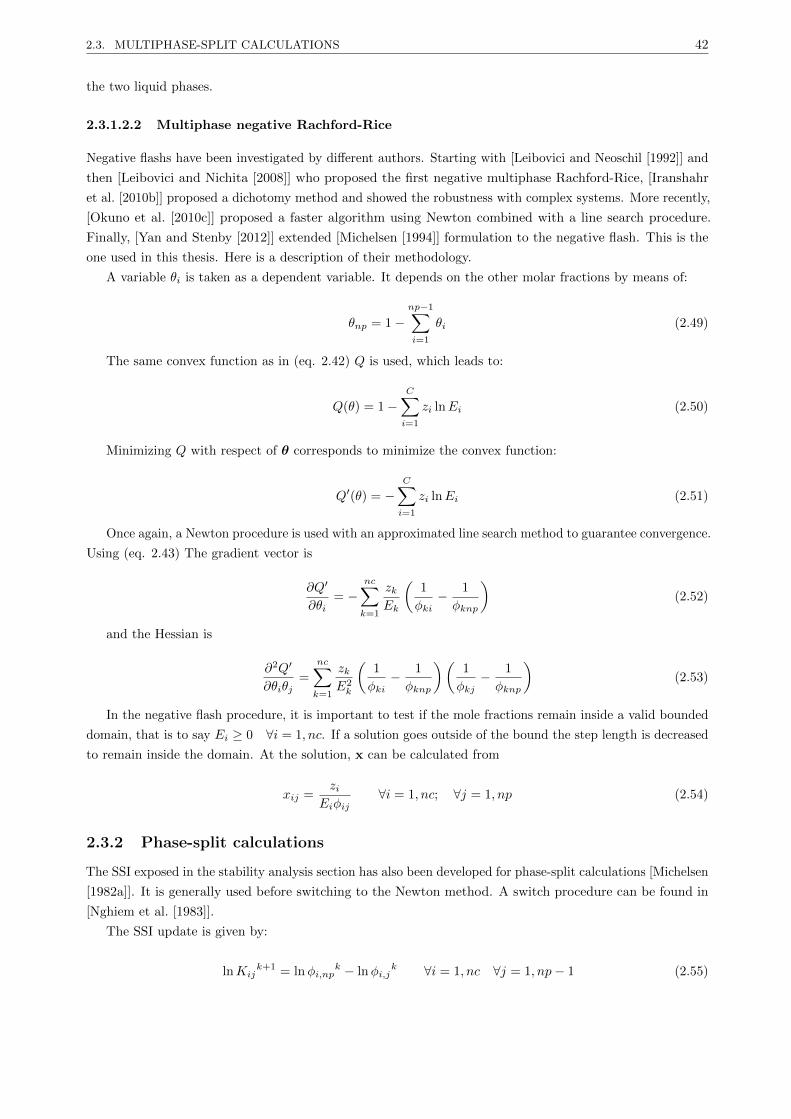
2.3. MULTIPHASE-SPLIT CALCULATIONS 42

the two liquid phases.

2.3.1.2.2 Multiphase negative Rachford-Rice

Negative flashs have been investigated by different authors. Starting with [Leibovici and Neoschil [1992]] and

then [Leibovici and Nichita [2008]] who proposed the first negative multiphase Rachford-Rice, [Iranshahr

et al. [2010b]] proposed a dichotomy method and showed the robustness with complex systems. More recently,

[Okuno et al. [2010c]] proposed a faster algorithm using Newton combined with a line search procedure.

Finally, [Yan and Stenby [2012]] extended [Michelsen [1994]] formulation to the negative flash. This is the

one used in this thesis. Here is a description of their methodology.

A variable θi is taken as a dependent variable. It depends on the other molar fractions by means of:

θnp = 1−np−1∑i=1

θi (2.49)

The same convex function as in (eq. 2.42) Q is used, which leads to:

Q(θ) = 1−C∑i=1

zi lnEi (2.50)

Minimizing Q with respect of θ corresponds to minimize the convex function:

Q′(θ) = −C∑i=1

zi lnEi (2.51)

Once again, a Newton procedure is used with an approximated line search method to guarantee convergence.

Using (eq. 2.43) The gradient vector is

∂Q′

∂θi= −

nc∑k=1

zkEk

(1

φki− 1

φknp

)(2.52)

and the Hessian is

∂2Q′

∂θiθj=

nc∑k=1

zkE2k

(1

φki− 1

φknp

)(1

φkj− 1

φknp

)(2.53)

In the negative flash procedure, it is important to test if the mole fractions remain inside a valid bounded

domain, that is to say Ei ≥ 0 ∀i = 1, nc. If a solution goes outside of the bound the step length is decreased

to remain inside the domain. At the solution, x can be calculated from

xij =zi

Eiφij∀i = 1, nc; ∀j = 1, np (2.54)

2.3.2 Phase-split calculations

The SSI exposed in the stability analysis section has also been developed for phase-split calculations [Michelsen

[1982a]]. It is generally used before switching to the Newton method. A switch procedure can be found in

[Nghiem et al. [1983]].

The SSI update is given by:

lnKijk+1 = lnφi,np

k − lnφi,jk ∀i = 1, nc ∀j = 1, np− 1 (2.55)

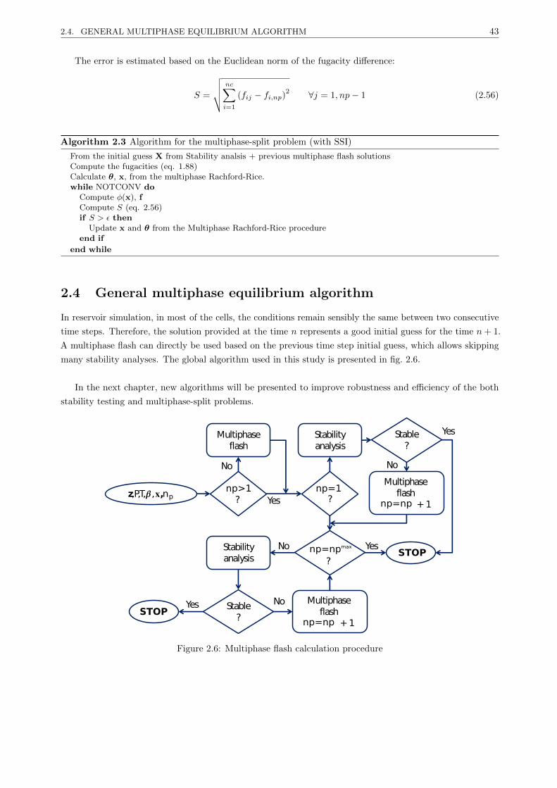
2.4. GENERAL MULTIPHASE EQUILIBRIUM ALGORITHM 43

The error is estimated based on the Euclidean norm of the fugacity difference:

S =

√√√√ nc∑i=1

(fij − fi,np)2 ∀j = 1, np− 1 (2.56)

Algorithm 2.3 Algorithm for the multiphase-split problem (with SSI)

From the initial guess X from Stability analsis + previous multiphase flash solutionsCompute the fugacities (eq. 1.88)Calculate θ, x, from the multiphase Rachford-Rice.while NOTCONV do

Compute φ(x), fCompute S (eq. 2.56)if S > ε then

Update x and θ from the Multiphase Rachford-Rice procedureend if

end while

2.4 General multiphase equilibrium algorithm

In reservoir simulation, in most of the cells, the conditions remain sensibly the same between two consecutive

time steps. Therefore, the solution provided at the time n represents a good initial guess for the time n+ 1.

A multiphase flash can directly be used based on the previous time step initial guess, which allows skipping

many stability analyses. The global algorithm used in this study is presented in fig. 2.6.

In the next chapter, new algorithms will be presented to improve robustness and efficiency of the both

stability testing and multiphase-split problems.

z,P,T,𝜷 ,𝐱,npnp>1?

Multiphaseflash

Stabilityanalysis

np=1

Stable?

Multiphaseflash

np=np +1

Stabilityanalysis

Stable?

np=npmax

?

?

Multiphaseflash

np=np +1STOP

STOP

No

Yes

Yes

No

YesNo

NoYes

Figure 2.6: Multiphase flash calculation procedure

Chapter 3

Improvements in equilibrium

calculations

Contents

3.1 Presentation of conventional methods . . . . . . . . . . . . . . . . . . . . . . . . 45

3.1.1 Stability testing . . . . . . . . . . . . . . . . . . . . . . . . . . . . . . . . . . . . . 45

3.1.2 Multiphase flash calculations . . . . . . . . . . . . . . . . . . . . . . . . . . . . . . 47

3.2 Reduction methods . . . . . . . . . . . . . . . . . . . . . . . . . . . . . . . . . . . 51

3.2.1 Presentation of existing reduction based methods . . . . . . . . . . . . . . . . . . . 52

3.2.2 A new reduction method for the stability analysis problem . . . . . . . . . . . . . 56

3.2.3 A comparison of conventional and reduction approaches for phase equilibrium

calculations . . . . . . . . . . . . . . . . . . . . . . . . . . . . . . . . . . . . . . . . 66

3.2.4 A new reduction method for multiphase equilibrium calculations . . . . . . . . . . 80

3.3 Phase equilibrium calculations with quasi-Newton methods . . . . . . . . . . . 93

3.3.1 Introduction . . . . . . . . . . . . . . . . . . . . . . . . . . . . . . . . . . . . . . . 93

3.3.2 The BFGS quasi-Newton method . . . . . . . . . . . . . . . . . . . . . . . . . . . . 93

3.3.3 Proposed method . . . . . . . . . . . . . . . . . . . . . . . . . . . . . . . . . . . . . 98

3.3.4 Results . . . . . . . . . . . . . . . . . . . . . . . . . . . . . . . . . . . . . . . . . . 100

3.4 Robust and efficient Trust-Region based stability analysis and multiphase

flash calculations . . . . . . . . . . . . . . . . . . . . . . . . . . . . . . . . . . . . . 108

3.4.1 Introduction . . . . . . . . . . . . . . . . . . . . . . . . . . . . . . . . . . . . . . . 108

3.4.2 Trust-Region methods . . . . . . . . . . . . . . . . . . . . . . . . . . . . . . . . . . 109

3.4.3 Results . . . . . . . . . . . . . . . . . . . . . . . . . . . . . . . . . . . . . . . . . . 117

3.4.4 Conclusions . . . . . . . . . . . . . . . . . . . . . . . . . . . . . . . . . . . . . . . . 130

3.5 Multiphase flash, using ln K and phase mole fractions as independent variables130

3.5.1 Introduction . . . . . . . . . . . . . . . . . . . . . . . . . . . . . . . . . . . . . . . 130

3.5.2 New proposed method . . . . . . . . . . . . . . . . . . . . . . . . . . . . . . . . . . 130

3.5.3 Results . . . . . . . . . . . . . . . . . . . . . . . . . . . . . . . . . . . . . . . . . . 132

Phase equilibrium calculations (phase split and stability testing) are very important in chemical process

and petroleum reservoir engineering. In process simulation and reservoir simulation, an important part of the

computational time is spent by phase equilibrium calculations. Moreover, a failure in phase equilibrium rou-

tines may affect the results to a high extent or lead to the non-convergence of the simulation. In this context,

it becomes essential that algorithms for phase equilibrium calculations are both efficient and robust; it is

desirable to use for a given simulation type the most suitable algorithm. In petroleum reservoir compositional

simulation, the number of components in the mixture is limited (typically less than a dozen) and a very large

number of phase equilibrium calculations are performed in full-field scale simulations (in most or all the blocks

44

3.1. PRESENTATION OF CONVENTIONAL METHODS 45

of the discretization network, at each time step and at each iteration level). On the contrary, in process simula-

tions, the number of components can be very large (on the order of hundreds, with several feed mixed together).

In this chapter, improvements relative to equilibrium flash calculations will be described.

First, [Michelsen [1982a]] developed an algorithm which uses the Cholesky factorization to solve the linear

system obtained with Newton taking the logarithm of the equilibrium constants as independent variables.

This methodology will be extended to multiphase calculations, and will then be applied to [Haugen et al.

[2011]]’s method where both the phase mole fractions and the equilibrium constant are updated at each

iteration.

Also, the reduction methods introduced in multiphase equilibrium calculations enable to reduce the space

of study from nc (the number of components) for conventional variables to M (with M < nc). A new

reduction method will be proposed both for stability analysis and multiphase-split calculations, based on the

multi-linear expression of the logarithm of fugacity coefficients.

Moreover, comparisons of different Newton methods based on conventional and reduction variables will be

shown. The tests will focus on the computation time, but also on the condition number and the convergence

path. All the problems (stability analysis, two-phase split and multiphase-split calculations) will be treated

independently.

In an attempt to develop a general program, algorithms independent of the EOS will also be investigated.

A BFGS (Broyden-Fletcher-Goldfarb-Shanno) approach applied with a new set of variables will be proposed

for two-phase split calculations. Besides, a Trust-Region based method which could extend the Newton

method to be applied to more difficult problems will be presented both for the stability testing and the

multiphase-split problems.

3.1 Presentation of conventional methods

3.1.1 Stability testing

A mixture is stable if the TPD function is non-negative at all its stationary points; otherwise, the mixture

splits into two or more phases. Michelsen proposed a modified TPD function [Michelsen [1982b]]

D∗ =

(1−

nc∑i=1

Yi

)+

nc∑i=1

Yi (lnYi + lnφi(Y)− di) (3.1)

3.1.1.1 Mole numbers as independent variables

If Yi are the independent variables, the elements of the gradient vector are

gi =∂D∗

∂Yi= lnYi + lnφi − di ; i = 1, nc (3.2)

The iteration equation in the Newton method is

H∆Y = −g (3.3)

and the elements of the Hessian matrix H are

Hij =∂2D∗

∂Yi∂Yj=∂gi∂Yj

=δijYi

+∂ lnφi∂Yj

; i, j = 1, nc (3.4)

where

3.1. PRESENTATION OF CONVENTIONAL METHODS 46

∂ lnφi∂Yj

=1

YT

[∂ lnφi∂xj

−nc∑k=1

xk∂ lnφi∂xk

](3.5)

and the partial derivative ∂ lnφi∂xj

is evaluated analytically for cubic EoS.

3.1.1.2 lnYi as independent variables

If the nonlinear system of equations g(Y) = 0 is solved with lnYi as independent variables, the Newton

iterations are

J∆ ln Y = HU−1∆ ln Y = −g (3.6)

Where J = HU−1 is the Jacobian matrix with elements

Jij =∂gi

∂ lnYj= δij +

∂ lnφi∂ lnYj

; i, j = 1, nc (3.7)

and

∆ ln Y = U∆Y (3.8)

In this thesis, the Newton method taking lnYi as independent variable will be called lnY. The elements

of the matrix U and of its inverse are

Uij =∂ lnYi∂Yj

=δijYi

; i, j = 1, nc (3.9)

and

U−1ij =

∂Yi∂ lnYj

= δijYi ; i, j = 1, nc (3.10)

The Jacobian matrix is non-symmetric, but a Cholesky decomposition of H can be performed to solve for

∆ ln Y = −UL−TL−1g (3.11)

The equilibrium constants for two-phase flash calculations are defined as: Ki = yi/xi = φiL(x)/φiV (x),

which corresponds to the equilibrium (zero gradient) condition, fiL = fiV . Equilibrium constant for phase

stability, Ki, can be defined in a similar way (that is, fulfilling (eq. 2.14), rather than the ratio of mole

fractions. For liquid phase stability (vapor trial phase)

Ki =Yizi

=φiz(z)

φi(Y)(3.12)

and for vapor phase stability (liquid trial phase)

Ki =ziYi

=φi(Y)

φiz(z)(3.13)

Note that Ki differs from Ki by a factor of YT . In the rest of this thesis, the formalism will be presented

for liquid phase stability; the case of stability testing of a vapor phase is similar.

Using ln K instead of ln Y as independent variables gives identical results, since ∆ ln Y = ∆ ln K and

the gradient and the Hessian are the same for both sets of variables.

3.1.1.3 α as independent variables

In addition to phase stability calculations using the above sets of independent variables, Michelsen’s variables

([Michelsen [1982b]]) αi = 2√Yi were also used to establish a comparison of conventional methods. In this

3.1. PRESENTATION OF CONVENTIONAL METHODS 47

case the Newton equation is H∆α = −g∗, in which the gradient vector is

g∗i =∂D∗

∂αi= gi

√Yi (3.14)

and the Hessian matrix is

Hij =∂2D∗

∂αi∂αj= δij +

√Yi√Yj∂ lnφi∂Yj

+δijg∗i

2(3.15)

in which the second term is of low effective rank (depending on the number of components with non-zero

BIPs) and the last term vanishes at the solution.

Taking the mole numbers as independent variables, for small values of Yi, large diagonal elements are

obtained for the Hessian, which reveals an ill-scaled Hessian. On the contrary, with αi, the Hessian obtained

is well scaled, with diagonal elements close to the identity.

The relationship between g and g, is

g = U−1/2g (3.16)

and the relation between H and H is

H = U−1/2HU−1/2 + D (3.17)

where

Dij =δijg∗i

2(3.18)

The most difficult conditions for phase stability testing are those in the vicinity of the singularity, namely

the stability test limit locus (STLL) [Hoteit and Firoozabadi [2006], Nichita and Petitfrere [2013], Rasmussen

et al. [2006], Nichita et al. [2007c], Petitfrere and Nichita [2014a]], also called ’limit of parallel tangent plane’

Whitson and Michelsen [1990] or limit of the ’shadow region’ [Rasmussen et al. [2006]].

3.1.2 Multiphase flash calculations

The objective function for multiphase flash calculations is the dimensionless Gibbs free energy, given by

G =

nc∑i=1

np∑k=1

nik ln fik (3.19)

The function G has to be minimized with respect to mole numbers. The material balance must be satisfied

at each step, that it to say,

zi =

np∑k=1

θkxik; i = 1, nc (3.20)

with

np∑p=1

θp = 1 (3.21)

For each component i, one phase is taken as reference phase (its mole numbers are dependent variables),

3.1. PRESENTATION OF CONVENTIONAL METHODS 48

niR = zi −np∑k=1k 6=R

nik; i = 1, nc (3.22)

3.1.2.1 Mole numbers as independent variables

The elements of the gradient vector g are:

(gi)m =∂G

∂nim= lnKim + lnφim − lnφiR; i = 1, nc;m = 1, np;m 6= R (3.23)

where the equilibrium constants are Kim = xim/xiR = φiR/φim; i = 1, nc;m = 1, np;m 6= R and the mole

fractions are xim = nim/∑ncj=1 njm; i = 1, nc;m = 1, np

The stationary point condition of G is

∂G

∂nim= 0; i = 1, nc;m = 1, np;m 6= R (3.24)

The iteration equation for the Newton method is

H∆n = −g (3.25)

where n =(nT1 , · · · , nTk , · · · , nTnp

)T; k 6= R, with nk = (n1k, · · · , nnc,k)

T; k = 1, np. and H is the Hessian

matrix

(Hij)mk =∂2G

∂nimnjk= δmk

[1

θm

(δijxim− 1

)+∂ lnφim∂njm

]+

[1

θR

(δijxiR− 1

)+∂ lnφiR∂njR

](3.26)

∀i, j = 1, nc; k,m = 1, np; k,m 6= R

Let V stands for the vapor mole fraction (respectively L the liquid mole fraction). For two-phase cases,

the matrix becomes

Hij =1

LV

(δijzixiyi

− 1

)+∂ lnφiL∂njL

+∂ lnφiV∂njV

(3.27)

The matrix H can be divided into two different terms:

H = U + Φ (3.28)

where

(Φij)mk =∂2GE

∂nim∂njk= δmk

∂ lnφim∂njm

+∂ lnφiR∂njR

(3.29)

and the elements of the matrix U (which is always positive-semidefinite [Mehra et al. [1983], Ammar and

Renon [1987]]) are for the two phase-split problem,

Uij =∂ lnKi

∂niV=

1

V (1− V )

(δijui− 1

); ∀i, j = 1, nc (3.30)

with

ui =xiyizi

(3.31)

In this work, the extension to the multiphase-split problem is proposed:

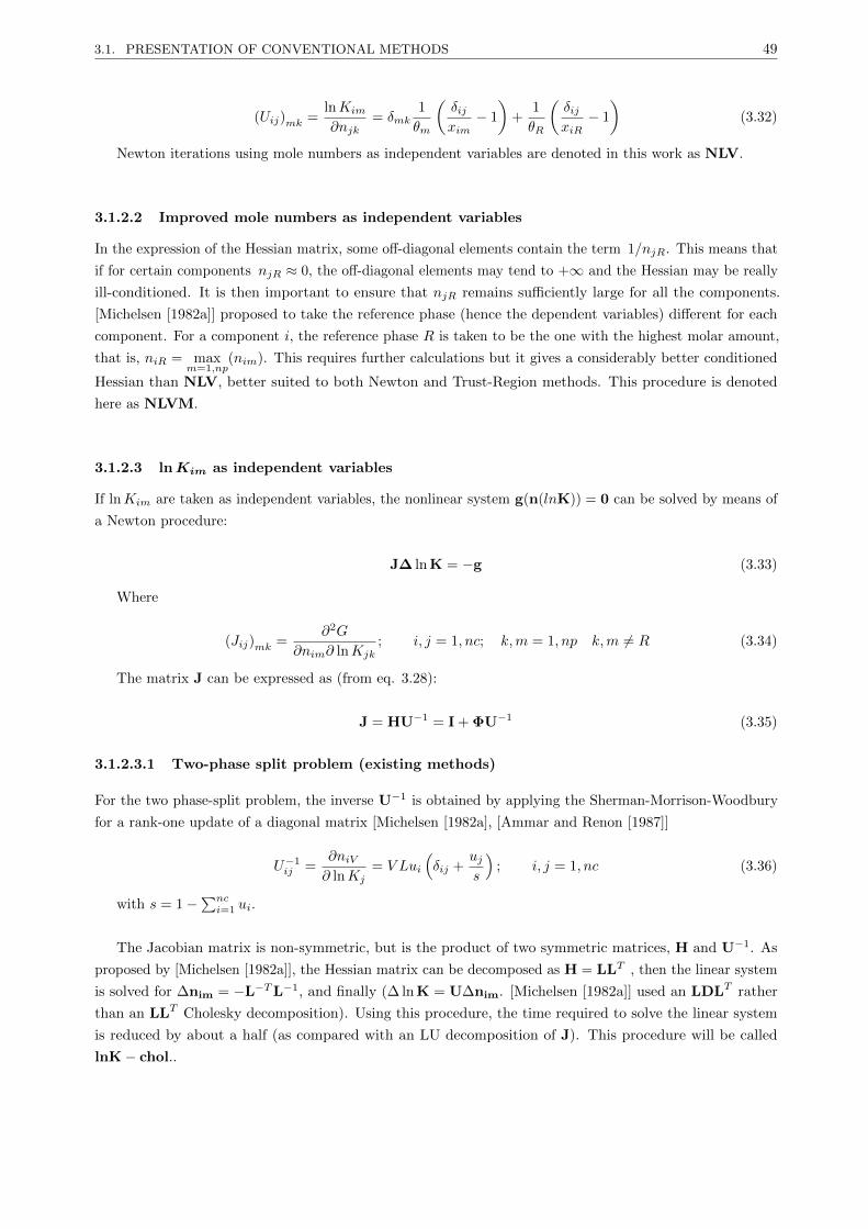
3.1. PRESENTATION OF CONVENTIONAL METHODS 49

(Uij)mk =lnKim

∂njk= δmk

1

θm

(δijxim− 1

)+

1

θR

(δijxiR− 1

)(3.32)

Newton iterations using mole numbers as independent variables are denoted in this work as NLV.

3.1.2.2 Improved mole numbers as independent variables

In the expression of the Hessian matrix, some off-diagonal elements contain the term 1/njR. This means that

if for certain components njR ≈ 0, the off-diagonal elements may tend to +∞ and the Hessian may be really

ill-conditioned. It is then important to ensure that njR remains sufficiently large for all the components.

[Michelsen [1982a]] proposed to take the reference phase (hence the dependent variables) different for each

component. For a component i, the reference phase R is taken to be the one with the highest molar amount,

that is, niR = maxm=1,np

(nim). This requires further calculations but it gives a considerably better conditioned

Hessian than NLV, better suited to both Newton and Trust-Region methods. This procedure is denoted

here as NLVM.

3.1.2.3 lnKim as independent variables

If lnKim are taken as independent variables, the nonlinear system g(n(lnK)) = 0 can be solved by means of

a Newton procedure:

J∆ ln K = −g (3.33)

Where

(Jij)mk =∂2G

∂nim∂ lnKjk; i, j = 1, nc; k,m = 1, np k,m 6= R (3.34)

The matrix J can be expressed as (from eq. 3.28):

J = HU−1 = I + ΦU−1 (3.35)

3.1.2.3.1 Two-phase split problem (existing methods)

For the two phase-split problem, the inverse U−1 is obtained by applying the Sherman-Morrison-Woodbury

for a rank-one update of a diagonal matrix [Michelsen [1982a], [Ammar and Renon [1987]]

U−1ij =

∂niV∂ lnKj

= V Lui

(δij +

ujs

); i, j = 1, nc (3.36)

with s = 1−∑nci=1 ui.

The Jacobian matrix is non-symmetric, but is the product of two symmetric matrices, H and U−1. As

proposed by [Michelsen [1982a]], the Hessian matrix can be decomposed as H = LLT , then the linear system

is solved for ∆nim = −L−TL−1, and finally (∆ ln K = U∆nim. [Michelsen [1982a]] used an LDLT rather

than an LLT Cholesky decomposition). Using this procedure, the time required to solve the linear system

is reduced by about a half (as compared with an LU decomposition of J). This procedure will be called

lnK− chol..

3.1. PRESENTATION OF CONVENTIONAL METHODS 50

3.1.2.3.2 Multiphase-split problem (new proposed procedure)

For the multiphase-split problem, the dimensionality of the problem is nc× (np− 1); Matrices H and J have

a block structure, with (np− 1)× (np− 1) blocks. The Jacobian matrix is non-symmetric, but one can take

advantage of symmetry in constructing it, by calculating only about half of the elements of the symmetric

matrices Φ and U−1. Unlike in two-phase equilibrium, it is very difficult to inverse the matrix U analytically.

The elements of U−1 are

(U−1ij

)kp

=∂nik

∂ lnKjp; ∀i, j = 1, nc; ∀k, p = 1, np; k, p 6= R (3.37)

Using the chain rule

∂nik∂ lnKjp

=

(∂nik

∂ lnKjp

)θ

+

nc∑m=1m 6=R

(∂nik∂θm

)K,θl 6=m

(∂θm

∂ lnKjp

); (3.38)

i, j = 1, nc; k, p = 1, np; k, p 6= R (3.39)

The partial derivatives in the above equation are(∂nik

∂ lnKjp

)θ

= δijnik

(δkp −

nipzi

); i, j = 1, nc; k, p = 1, np; k, p 6= R (3.40)

and (∂nik∂θm

)K,θs 6=m

= δkpxik − nikwip; i, j = 1, nc; k, p = 1, np; k, p 6= R (3.41)

where

wik =xik − xiR

zi; k = 1, np, k 6= R (3.42)

and the partial derivatives ∂θm/∂ lnKjp are obtained by differentiating the Rachford-Rice equations, (eq.

2.30)

nc∑m=1m 6=R

(∂Rk∂θm

)K,θl 6=m

(∂θm

∂ lnKjp

)= −

(∂Rk

∂ lnKjp

)θ

; j = 1, nc; k, p = 1, np; k, p 6= R (3.43)

The linear system of equations is

S

(∂θ

∂ ln K

)jp

= (f)jp ; j = 1, nc; p = 1, np p 6= R (3.44)

The (np− 1)× (np− 1) matrix S is symmetric (since it is a Hessian, corresponding to the minimization

of Michelsen’s Q function (eq. 2.42) with respect to np− 1 θ variables). The matrix S and its decomposition

are already available from the last iteration in the resolution of the Rachford-Rice system of equations; its

elements are

Skm = −(∂Rk∂θm

)K,θs 6=m

=

nc∑i=1

ziwikwim; k,m = 1, np; k,m 6= R (3.45)

and the elements of the RHS vector in (eq. 3.44) are

(fk)jp =

(∂Rk

∂ lnKjp

)θ

= xjR (δkp − θpwjk) ; j = 1, nc; k, p = 1, np; k, p 6= R (3.46)

3.2. REDUCTION METHODS 51

Moreover, from the proposed expression of the matrix U for multiphase problems (eq. 3.32), the procedure

lnK− chol. (from [Michelsen [1982a]], introduced in two phases) can be extended to multiphase calculations.

The same procedure can be used for stability analysis with ln Y variables and will be called lnY −Chol. in

this thesis).

To the best of our knowledge, no reports can be found in the literature on how to use symmetry in

multiphase flash calculations with ln K as independent variables.

The Jacobian matrix J in Newton− lnK iterations is better scaled than the Hessian for NLVM

iterations; the linear system (eq. 3.33) is better conditioned than the system (eq. 3.25).

3.2 Reduction methods

In order to reduce the computer time in equilibrium calculations, an attractive alternative to the widely

used technique of lumping individual components into pseudo-components is given by the so-called reduction

methods. In the reduction method the dimensionality of the phase equilibrium problem can be significantly

lowered, and the number of independent variables does not depend on the number of components in the

mixture, but only on the number of non-zero binary interaction parameters (BIPs) in the equation of state

(EoS): the use of a detailed fluid composition is thus allowed. The reduction methods are particularly efficient

for mixtures with many components and few non-zero BIPs (such as naturally occurring hydrocarbon systems

or certain feeds in refining problems involving several different crude oils that could bring the total number

of fractions to the order of hundreds).

The first reduction method for flash calculations was proposed by [Michelsen [1986]]. Using EoS parameters

as independent variables, together with the fraction of one equilibrium phase instead of conventional variables

used in the compositional space, he obtained a nonlinear system of only three equations, whatever the number

of components in the mixture. Even though this method is not applicable in practical cases (being limited to

all BIPs equal to zero), Michelsen’s simplified flash formulation is very important since it showed for the first

time that the solution phase equilibrium problems can be sought in a space of reduced dimensionality. A few

years later, [Hendriks [1988]] presented the ’Reduction Theorem’, stating the circumstances under which the

dimensionality of several phase equilibrium problems can be reduced; he explained that various formulations

apparently very different reflect a common underlying mathematical structure. In any reduction method for

phase equilibrium calculations with two-parameter cubic EoS, there are M reduction parameters [Hendriks

[1988]], Q = (Q1, Q2, · · · , QM )T , given by

Qα =

nc∑i=1

qαixi ;∀α = 1,M (3.47)

Where qαi are the elements of the reduction matrix [Hendriks [1988]].

Different sets of reduced variables/reduction procedures have been proposed [Hendriks and van Bergen

[1992], Nichita and Minescu [2004], Li and Johns [2006], Nichita and Graciaa [2011], Gaganis and Varotsis

[2013]], and a number of papers have presented calculation procedures for two-phase flash calculations

[Hendriks and van Bergen [1992], Nichita and Minescu [2004], Li and Johns [2006], Nichita and Graciaa

[2011], Jensen and Fredenslund [1987], Kaul and Thrasher [1996], Pan and Firoozabadi [2003], Nichita et al.

[2007a]], phase stability analysis [Firoozabadi and Pan [2002], Nichita et al. [2002], Nichita et al. [2006a],

Hoteit and Firoozabadi [2006]], multiphase flash calculations [Nichita et al. [2006a], Okuno et al. [2010a]],

critical point calculation [Nichita [2005], Nichita [2006b]], phase envelope construction [Nichita [2008]], or the

application of the reduction concept to solve related problems, such as pseudo-component delumping [Nichita

and Leibovici [2006]]. The implementation of reduction methods in compositional reservoir simulators has also

been evaluated for IMPEC simulator [Okuno et al. [2010a], Okuno et al. [2010b]], in fully implicit [Pan and

3.2. REDUCTION METHODS 52

Tchelepi [2011a] and Pan and Tchelepi [2011b]], and is also implemented in INTERSECT. Two- parameter

cubic equations of state are usually used, but it should be noticed that the applicability of the method is

restricted by the mixing rules and not by the form of the equation of state (EoS parameters for mixtures

must be linear forms or decomposable into linear forms [Hendriks [1988]]).

In this work, a presentation of the reduction parameters will be made in a first part. Then, a new

reduction method will be presented for stability analysis and multiphase flash calculations (based on [Nichita

and Graciaa [2011]] methodology (who developed an algorithm for two phases)). Comparisons will be made

with previous variables (conventional and previous reductions) for the different problems.

3.2.1 Presentation of existing reduction based methods

3.2.1.1 Reduction parameters

Any procedure [Hendriks and van Bergen [1992], Nichita and Minescu [2004], Li and Johns [2006], Nichita

and Graciaa [2011], Gaganis and Varotsis [2013]] to decompose the quadratic form A (eq. 1.72, eq. 1.73)

can be used to obtain the reduction parameters and the reduction matrix [Hendriks [1988]]. The spectral

decomposition [Hendriks and van Bergen [1992]] of the matrix C = 1− Ciji,j=1,nc (usually of rank r << nc),

1− Cij =

m∑α=1

λαq′αiq′αj (3.48)

where λα are the m = r non-zero eigenvalues, and q′αi;α = 1,m i = 1, nc are the elements of the

corresponding eigenvectors. The elements of the reduction matrix are related to eigenvectors by qαi =

q′αi√Ai; α = 1,m i = 1, nc. From (eq. 1.74), Aij can be written as

Aij =

m∑α=1

λαqαiqαj (3.49)

and, using (eq. 3.47) for α = 1,m, (eq. 3.49 and eq. 1.72, eq. 1.73), we obtain A(Q)

A =

nc∑i=1

nc∑j=1

xixj

(m∑α=1

λαqαiqαj

)=

m∑α=1

λα

(nc∑i=1

qαixi

) nc∑j=1

qαjxj

=

m∑α=1

λαQ2α (3.50)

and ψi(Q)

ψi =

nc∑i=1

xi

(m∑α=1

λαqαiqαj

)=

m∑α=1

λαqαi

nc∑j=1

qαjxj

=

m∑α=1

λαqαiQα; ∀i = 1, nc (3.51)

is obtained from (eq. 3.47, eq. 3.49 and eq. 1.89).

The last reduction parameter is (eq. 3.47 for α = m+ 1 = M)

QM ≡ B =

nc∑i=1

Bixi (3.52)

h variables were introduced by [Nichita and Minescu [2004]].

By introducing (eq. 3.50, eq. 3.51 and eq. 3.52) in (eq. 1.88), after some arrangement the fugacity

coefficients are obtained as:

lnφi =

M+1∑α=1

qαihα; i = 1, nc (3.53)

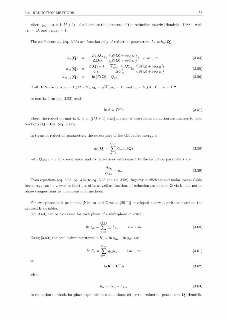
3.2. REDUCTION METHODS 53

where qαi; α = 1,M + 1; i = 1, nc are the elements of the reduction matrix [Hendriks [1988]], with

qMi = Bi and qM+1,i = 1.

The coefficients hα (eq. 3.53) are function only of reduction parameters, hα = hα(Q)

hα(Q) = −2λαQα∆QM

ln

(Z(Q) + δ1QMZ(Q) + δ2QM

); α = 1,m (3.54)

hM (Q) =Z(Q)− 1

QM+

∑mα=1 λαQ

2α

∆Q2M

ln

(Z(Q) + δ1QMZ(Q) + δ2QM

)(3.55)

hM+1(Q) = − ln (Z(Q)−QM ) (3.56)

If all BIPs are zero, m = 1 (M = 2), q1i =√Ai, q2i = Bi and hα = hα(A,B); α = 1, 2.

In matrix form (eq. 3.53) reads

lnφ = CTh (3.57)

where the reduction matrix C is an [(M + 1)× nc] matrix; it also relates reduction parameters to mole

fractions (Q = Cx; (eq. 3.47)).

In terms of reduction parameters, the excess part of the Gibbs free energy is

gE(Q) =

M+1∑α=1

Qαhα(Q) (3.58)

with QM+1 = 1 for convenience, and its derivatives with respect to the reduction parameters are

∂gE∂Qα

= hα (3.59)

From equations (eq. 3.53, eq. 3.54 to eq. 3.56 and eq. 3.58), fugacity coefficients and molar excess Gibbs

free energy can be viewed as functions of h, as well as functions of reduction parameters Q via h, and not on

phase compositions as in conventional methods.

For two phase-split problems, [Nichita and Graciaa [2011]] developed a new algorithm based on the

exposed h variables:

(eq. 3.53) can be expressed for each phase of a multiphase mixture:

lnφik =

M+1∑α=1

qαihkα; i = 1, nc (3.60)

Using [3.60], the equilibrium constants lnKi = lnφiL − lnφiV are

lnKi =

M+1∑α=1

qαihα; i = 1, nc (3.61)

or

ln K = CTh (3.62)

with

hα = hLα − hV α (3.63)

In reduction methods for phase equilibrium calculations, either the reduction parameters Q [Hendriks

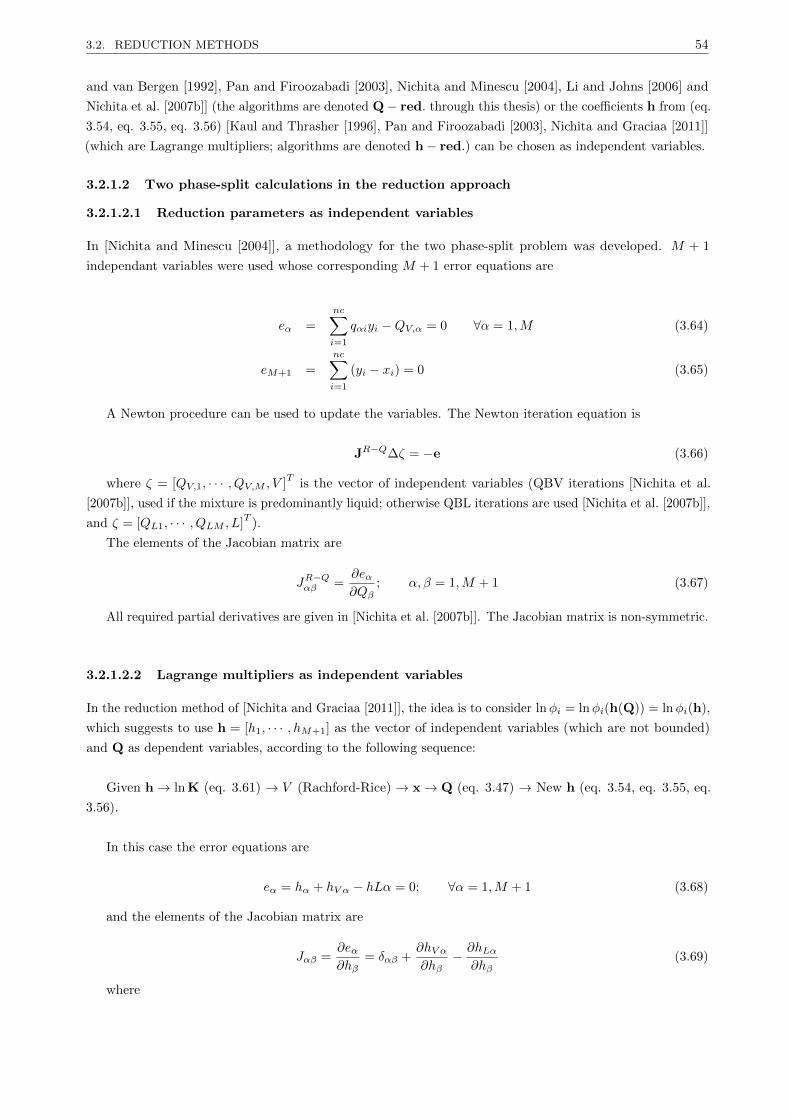
3.2. REDUCTION METHODS 54

and van Bergen [1992], Pan and Firoozabadi [2003], Nichita and Minescu [2004], Li and Johns [2006] and

Nichita et al. [2007b]] (the algorithms are denoted Q− red. through this thesis) or the coefficients h from (eq.

3.54, eq. 3.55, eq. 3.56) [Kaul and Thrasher [1996], Pan and Firoozabadi [2003], Nichita and Graciaa [2011]]

(which are Lagrange multipliers; algorithms are denoted h− red.) can be chosen as independent variables.

3.2.1.2 Two phase-split calculations in the reduction approach

3.2.1.2.1 Reduction parameters as independent variables

In [Nichita and Minescu [2004]], a methodology for the two phase-split problem was developed. M + 1

independant variables were used whose corresponding M + 1 error equations are

eα =

nc∑i=1

qαiyi −QV,α = 0 ∀α = 1,M (3.64)

eM+1 =

nc∑i=1

(yi − xi) = 0 (3.65)

A Newton procedure can be used to update the variables. The Newton iteration equation is

JR−Q∆ζ = −e (3.66)

where ζ = [QV,1, · · · , QV,M , V ]T

is the vector of independent variables (QBV iterations [Nichita et al.

[2007b]], used if the mixture is predominantly liquid; otherwise QBL iterations are used [Nichita et al. [2007b]],

and ζ = [QL1, · · · , QLM , L]T

).

The elements of the Jacobian matrix are

JR−Qαβ =∂eα∂Qβ

; α, β = 1,M + 1 (3.67)

All required partial derivatives are given in [Nichita et al. [2007b]]. The Jacobian matrix is non-symmetric.

3.2.1.2.2 Lagrange multipliers as independent variables

In the reduction method of [Nichita and Graciaa [2011]], the idea is to consider lnφi = lnφi(h(Q)) = lnφi(h),

which suggests to use h = [h1, · · · , hM+1] as the vector of independent variables (which are not bounded)

and Q as dependent variables, according to the following sequence:

Given h→ ln K (eq. 3.61) → V (Rachford-Rice) → x→ Q (eq. 3.47) → New h (eq. 3.54, eq. 3.55, eq.

3.56).

In this case the error equations are

eα = hα + hV α − hLα = 0; ∀α = 1,M + 1 (3.68)

and the elements of the Jacobian matrix are

Jαβ =∂eα∂hβ

= δαβ +∂hV α∂hβ

− ∂hLα∂hβ

(3.69)

where

3.2. REDUCTION METHODS 55

∂hkα∂hβ

=

M∑γ=1

∂hkα∂Qkγ

∂Qkγ∂hβ

; ∀α, β = 1,M + 1, k = L, V (3.70)

The partial derivatives required in (eq. 3.70) can be found in [Nichita and Graciaa [2011]].

Previously, h have been used as independent variables by [Kaul and Thrasher [1996]] (for all BIPs equal

to zero) and [Pan and Firoozabadi [2003]]. [Nichita and Graciaa [2011]] reduction method was used by

[Michelsen et al. [2013b], Haugen and Beckner [2013], Gorucu and Johns [2013], Gorucu and Johns [2014]

and Gaganis and Varotsis [2014]]. In [Nichita and Graciaa [2011]] it was observed (but not proved) that

h− red. Newton iterations have the same convergence path as the conventional Newton iterations with ln Ki

as variables. A proof of this statement is given in Appendix E. In Appendix D, it is shown that the elements

of h are Lagrange multipliers associated to a constrained minimization of the Gibbs free energy with respect

to component mole numbers and subject to linear equality constraints, and that the error equations and the

Jacobian matrix in [Nichita and Graciaa [2011]] are related to this constrained minimization.

3.2.1.3 Phase stability in the reduction approach

3.2.1.3.1 Reduction parameters as independent variables

[Nichita et al. [2006a]] showed that the tangent plane distance (eq. 3.1) could also be considered with the

reduction variables. They showed that (eq. 3.2) was equivalent to the system of M equations, with M

unknowns (Q = [Q1, · · · , QM ]T

):

Fα(Q) =

nc∑i=1

qαiYi −Qαnc∑i=1

Yi = 0 α = 1,M (3.71)

The Newton iteration equation is:

JR−Q∆Q = −F (3.72)

From (eq. 2.14),

∂Yi∂Qβ

= −Yi∂ lnφi(Q)

∂Qβ; i = 1, nc β = 1,M (3.73)

thus,

JR−Qαβ =∂Fα∂Qβ

= δαβ

nc∑i=1

Yi +Qα

nc∑i=1

∂Yi∂Qβ

−nc∑i=1

qαi∂Yi∂Qβ

α, β = 1,M (3.74)

The variables Q are bounded by mini=1,nc qαi; α = 1,M . Only Newton iterations can be performed;

if a variable hits its bounds or if the TPD function increases between two subsequent Newton iterations,

iterations are reverted to SSI [Hoteit and Firoozabadi [2006]].

For the stability analysis problem, the procedure has been developed in this thesis and will be exposed in

the next session.

3.2.1.4 Pseudo-reduces methods

[Michelsen et al. [2013b]] proposed recently a method called here ’pseudo-reduced’. The idea is to build a

system with a reduced dimensionality using some reduction principles, but starting from the gradient vector

and the Hessian matrix constructed in the compositional space.

For flash calculations, the gradient vector with respect to h is

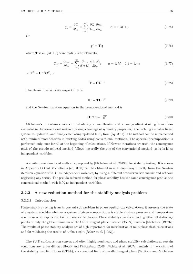
3.2. REDUCTION METHODS 56

g∗α =∂G

∂hα=

nc∑i=1

∂G

∂niv

∂niv∂hα

; α = 1,M + 1 (3.75)

Or

g∗ = T g (3.76)

where T is an (M + 1)× nc matrix with elements:

Tαi =∂niv∂hα

=

nc∑i=1

∂niv∂ lnKi

∂ lnKi

∂hα; α = 1,M + 1, i = 1, nc (3.77)

or TT = U−1CT , or

T = CU−1 (3.78)

The Hessian matrix with respect to h is

H∗ = THTT (3.79)

and the Newton iteration equation in the pseudo-reduced method is

H∗∆h = −g∗ (3.80)

Michelsen’s procedure consists in calculating a new Hessian and a new gradient starting from those

evaluated in the conventional method (taking advantage of symmetry properties), then solving a smaller linear

system to update h, and finally calculating updated lnKi from (eq. 3.61). The method can be implemented

with minimal modifications in existing codes using conventional methods. The spectral decomposition is

performed only once for all at the beginning of calculations. If Newton iterations are used, the convergence

path of the pseudo-reduced method follows naturally the one of the conventional method using ln K as

independent variables.

A similar pseudo-reduced method is proposed by [Michelsen et al. [2013b]] for stability testing. It is shown

in Appendix G that Michelsen’s (eq. 3.80) can be obtained in a different way directly from the Newton

iteration equation with Yi as independent variables, by using a different transformation matrix and without

neglecting any terms. The pseudo-reduced method for phase stability has the same convergence path as the

conventional method with lnYi as independent variables.

3.2.2 A new reduction method for the stability analysis problem

3.2.2.1 Introduction

Phase stability testing is an important sub-problem in phase equilibrium calculations; it assesses the state

of a system, (decides whether a system of given composition z is stable at given pressure and temperature

conditions or if it splits into two or more stable phases). Phase stability consists in finding either all stationary

points or only the global minimum of the Gibbs tangent plane distance (TPD) function [Michelsen [1982b]].

The results of phase stability analysis are of high importance for initialization of multiphase flash calculations

and for validating the results of a phase split [Baker et al. [1982]].

The TPD surface is non-convex and often highly nonlinear, and phase stability calculations at certain

conditions are rather difficult [Hoteit and Firoozabadi [2006], Nichita et al. [2007c]], mainly in the vicinity of

the stability test limit locus (STLL), also denoted limit of parallel tangent plane [Whitson and Michelsen

3.2. REDUCTION METHODS 57

[1990]] or shadow curve [Rasmussen et al. [2006]]. Besides, compositions of many effluents in chemical and

petroleum engineering are characterized by a (very) large number of components, resulting in time-consuming

simulations. In petroleum reservoir compositional simulation, even if the number of components in the mixture

is limited (typically less than ten), a very large number of phase equilibrium calculations are performed

in full-field scale simulations. Depending on the structure of the simulator, flash calculations may be part

of a larger problem, but stability testing must be carried out at any time step in any grid block likely to

experience a phase split; even if stability testing may be bypassed according to some simple criteria [Rasmussen

et al. [2006]], a very large number of calls for the stability routine is expected during a field-scale simulation run.

Recently, [Nichita and Graciaa [2011]] proposed a new reduction method for two-phase flash calculations;

unlike most of the previous reduction methods, the independent variables are not the reduction parameters

and the approach corresponds to the minimization of the Gibbs free energy [Michelsen et al. [2013b], Petitfrere

and Nichita [2014b]], which facilitates the comparison with conventional methods (as recently pointed out by

[Michelsen et al. [2013b]]. Moreover, the number of iterations is the same as in conventional flash calculations

using the natural logarithm of equilibrium constants as independent variables, and the iteration path is

related to that in the conventional method. The present chapter presents a calculation procedure for phase

stability analysis based on the reduction variables proposed in [Nichita and Graciaa [2011]], which exhibits

some very interesting features.

3.2.2.2 Proposed reduction method

One can consider the dependence lnφi = lnφi(Q), which leads to the reduced stability formulation of [Nichita

et al. [2007b]], or to consider lnφi = lnφi(h(Q)) = lnφi(h), which suggests to use h = (h1, · · · , hM+1)T as

the vector of independent variables (in a similar way to the recently reduction method for flash calculations

[Nichita and Graciaa [2011]]), rather than the reduction parameters. The key equation is (eq. 3.53): the

vector of natural logarithms of fugacity coefficients is simply the product between the transposed of the

reduction matrix and the vector h. On the other hand, hα depend only on reduction parameters, directly

and via the compressibility factors, i.e., hα = hα(Q, Z(Q)) = hα(Q); α = 1,M + 1 (eq. 3.54, eq. 3.55, eq.

3.56). This suggests the possibility of updating h according to the following iterative sequence:

Given h→ lnφ (eq. 3.53) → Y (eq. 2.14) → x (eq. 2.9) → Q (eq. 3.47) → New h (eq. 3.54, eq. 3.55,

eq. 3.56)

Note that the new independent variables h are unbounded, unlike the reduction parameters Q (taken as

independent variables in [Nichita et al. [2007a], Hoteit and Firoozabadi [2006]]) which are bounded. This

have a favorable effect on the convergence behavior and finally on the robustness of the method.

The error equations in the proposed method are

eα ≡ hα − hα(Q) = 0; α = 1,M + 1 (3.81)

and the elements of the Jacobian matrix are

JRαβ =∂eα∂hβ

= δαβ −∂hα(Q)

∂hβ; α, β = 1,M + 1 (3.82)

The resulting linear system of equations in the Newton method is

JR(ν)∆h(ν+1) = −e(ν) (3.83)

where ∆h(ν+1) = h(ν+1) − h(ν), ν is the iteration level and e = (e1, · · · , eM+1)T

3.2. REDUCTION METHODS 58

The partial derivatives in (eq. 3.82) are calculated as [Nichita and Graciaa [2011]]

∂hα(Q)

∂hβ=

M∑γ=1

∂hα∂Qγ

∂Qγ∂hβ

; α, β = 1,M + 1 (3.84)

where

∂hα∂Qγ

=

(∂hα∂Qγ

)Z,Qµ6=γ

+

(∂hα∂Z

)Q

∂Z

∂Qγ; α = 1,M + 1; γ = 1,M (3.85)

and

∂Qγ∂hβ

=

nc∑i=1

qγi∂xi∂hβ

; β = 1,M + 1; γ = 1,M (3.86)

The partial derivatives required in (eq. 3.84, eq. 3.85 and eq. 3.86) are given in Appendix A. The partial

derivatives of mole fractions with respect to the primary variables are

∂xi∂hβ

=1

YT

(∂Yi∂hβ

− xinc∑k=1

∂Yk∂hβ

); i = 1, nc; β = 1,M + 1 (3.87)

Where

∂Yi∂hβ

= −qβiYi (3.88)

giving

∂xi∂hβ

= (Qβ − qβi)xi (3.89)

and

∂Qγ∂hβ

= QβQγ −nc∑i=1

qβiqγixi (3.90)

Since qM+1,i = 1,

∂xi∂hM+1

= 0 (3.91)

and

∂hα∂hM+1

= δγ,M+1; α = 1,M + 1 (3.92)

the last column in the Jacobian matrix is (0, · · · , 0, 1)T .

Thus, it is convenient to solve the linear system of equations of dimensionality M ×M

M∑α=1

JRαβ∆hα = −eα; α = 1,M (3.93)

and the last variable is updated at each iteration from

∆hM+1 = −eM+1 −M∑α=1

∂eM+1

∂hα∆hα (3.94)

3.2. REDUCTION METHODS 59

with the cost of a simple summation over M .

The proposed method can be also formulated in terms of equilibrium constants for phase stability Ki

lnKi =

M+1∑α=1

qαihα; i = 1, nc (3.95)

where

hα(Q) = hα(Q)− hαz(Qz); α = 1,M + 1 (3.96)

The second term corresponds to feed composition.

Using h instead of h as independent variables is the same thing, since ∆h = ∆h and gradients and

Hessians are identical.

It is shown in Appendix B that the proposed method for phase stability corresponds to a constrained

minimization of the modified TPD function, with Lagrange multipliers h. In Appendix C, using some matrix

algebra, the link between conventional and reduction methods is established, as well as an equivalence of

convergence path in both hyperspaces.

At the solution, the relation between Jacobian matrices taking Q and h as independent variables is (see

Appendix F)

JRαβ =1

YT

[JR−Qαβ

]T; α, β = 1,M (3.97)

It is clear from (eq. 3.97) that the condition numbers of the Jacobian matrix at the solution are the same

for both reduction methods. This is not the case during iterations, each of the two reduction methods having

its own convergence path.

3.2.2.2.1 Calculation Procedure

The calculation procedure consists in Successive Substitution (SS) iterations, followed by Newton iterations;

however, in the proposed reduction method, one can skip the SS sequence and start directly with Newton

iterations.

3.2.2.2.1.a Initialization

Initial guesses for K-values are obtained from the Wilson relation [Wilson [1969]]. The two-sided initialization

[Michelsen [1982b]] is used: Y(0)i = ziKi (for liquid phase stability) and Y

(0)i = zi/Ki (for vapor phase

stability). Note that in a multiphase context, more initial guesses may be required [Michelsen [1982a]]; several

initialization procedures were proposed [Canas Marın et al. [2007], Li and Firoozabadi [2012]]. [Firoozabadi

and Pan [2002]] used a multilinear regression (as suggested by [Kaul and Thrasher [1996]] for flash calculations)

to initialize h by projecting ln K onto the h space via an equation similar in form to (eq. 3.95) (this requires

the resolution of a linear system of M + 1 equations and a number of summations over nc). In this work, the

reduction parameters are calculated directly from the initial guess at the first iteration.

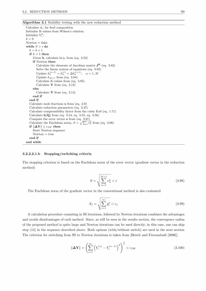
3.2. REDUCTION METHODS 60

Algorithm 3.1 Stability testing with the new reduction method

Calculate di, for feed compositionInitialize K-values from Wilson’s relation;Initialize Y 0

i ;k = 0Newton = falsewhile S > ε dok = k + 1if k > 1 then

Given h, calculate lnφi from (eq. 3.53)if Newton then

Calculate the elements of Jacobian matrix JR (eq. 3.82)Solve the linear system of equations (eq. 3.93)

Update h(ν+1)α = h

(ν)α + ∆h

(ν+1)α ; α = 1,M

Update hM+1 from (eq. 3.94)Calculate K-values from (eq. 3.95)Calculate Y from (eq. 3.12)

elseCalculate Y from (eq. 2.14)

end ifend ifCalculate mole fractions x from (eq. 2.9)Calculate reduction parameters (eq. 3.47)Calculate compressibility factor from the cubic EoS (eq. 1.71)Calculate h(Q) from (eq. 3.54, eq. 3.55, eq. 3.56)Compute the error vector e from (eq. 3.81)Calculate the Euclidean norm, S =

√∑α e

2α from (eq. 3.98)

if ‖∆Y‖ ≤ εSW thenStart Newton sequenceNewton = true

end if

end while

3.2.2.2.1.b Stopping/switching criteria

The stopping criterion is based on the Euclidean norm of the error vector (gradient vector in the reduction

method)

S =

√√√√M+1∑α=1

e2α < ε (3.98)

The Euclidean norm of the gradient vector in the conventional method is also evaluated

Sf =

√√√√ nc∑i=1

g2i < εf (3.99)

A calculation procedure consisting in SS iterations, followed by Newton iterations combines the advantages

and avoids disadvantages of each method. Since, as will be seen in the results section, the convergence radius

of the proposed method is quite large and Newton iterations can be used directly; in this case, one can skip

step (12) in the sequence described above. Both options (with/without switch) are used in the next section.

The criterion for switching from SS to Newton iterations is taken from [Hoteit and Firoozabadi [2006]].

‖∆Y‖ =

(nc∑i=1

(Y

(ν)i − Y (ν−1)

i

)2) 1

2

< εSW (3.100)

3.2. REDUCTION METHODS 61

3.2.2.3 Results

In this section, several conventional and two reduction methods are tested for various test problems. The two

reduction methods considered here are the proposed method (denoted h− red.) and the reduction stability

method of [Nichita et al. [2007b]] (denoted Q− red.), as modified by [Hoteit and Firoozabadi [2006]] (that is,

if a reduced variable Q goes out of its bounds, qαmin ≤ Qα ≤ qαmax , revert to SS iterations). Both methods

have a very interesting particularity: convergence is ensured (except near the STLL) using only Newton

iterations. In the conventional methods, three sets of independent variables are used: Yi, lnYi and αi. The

tolerance used in all calculations is εf = 10−12 in (eq. 3.99); the norms S (eq. 3.98) and Sf (eq. 3.99) have

the same order of magnitude. The tolerance εSW = 10−2 (as suggested in [Hoteit and Firoozabadi [2006]])

is used whenever a switch is performed from SS to Newton iterations. The Peng-Robinson EoS [Peng and

Robinson [1976], Robinson and Peng [1978]] is used in all calculations.

3.2.2.3.1 Y8 mixture

The six-component Y8 mixture [Yarborough [1972]] is a synthetic gas condensate mixture containing normal-

alkanes. All BIPs are taken equal to zero (c = 0, m = 1, λ1 = 6), thus there are only three equations. The

calculated critical point is TC = 293.78 K and pC = 210.67 bar; the phase envelope and the STLL can be

seen in fig. 3.1b from [Nichita et al. [2007c]]. At T = 335 K (in the retrograde condensation region), the

dewpoint pressure is pd = 224.39 bar, and the stability test limit is at p = 225.26 bar.

(a) (b)

Figure 3.1: a) Euclidean norms vs. iteration level; Y8 mixture at T=335 K and P=200 bar b) Number ofiterations for the Y8 mixture at T=335 K in the conventional method

At P = 200 bar, the variations of the Euclidean norm Sf vs. iteration number are plotted in fig. 3.1a

(in two cases: for switching from SS iterations and for direct Newton iterations) for the proposed stability

reduction method and for the conventional method with lnYi as independent variables, as well as the norm S

for the proposed method. The norms Sf are almost identical for lnY and h− red. since the two methods

have the same theoretical convergence path. The number of iterations vs. pressure for vapor phase stability

testing on the isotherm T = 335 K are plotted for various independent variables in the conventional method

(with switch from SS iteration) in fig. 3.1b and for the two reduction methods (only Newton iterations) in

fig. 3.2a. If one starts directly with Newton iterations for the variables αi (fig. 3.2b), the method eventually

converges, but it requires a quite large number of iterations (more than 20) over a wide pressure interval; in

this case, using the variables Yi, the number of iterations is even higher, and severe convergence problems

occur near the STLL, while using lnYi as independent variables, the conventional method converges in

less than 8 iterations, except in the vicinity of the STLL. For liquid phase stability testing, the numbers

of iterations on the same isotherm are plotted in fig. 3.3a for the two reduction methods. The two peaks

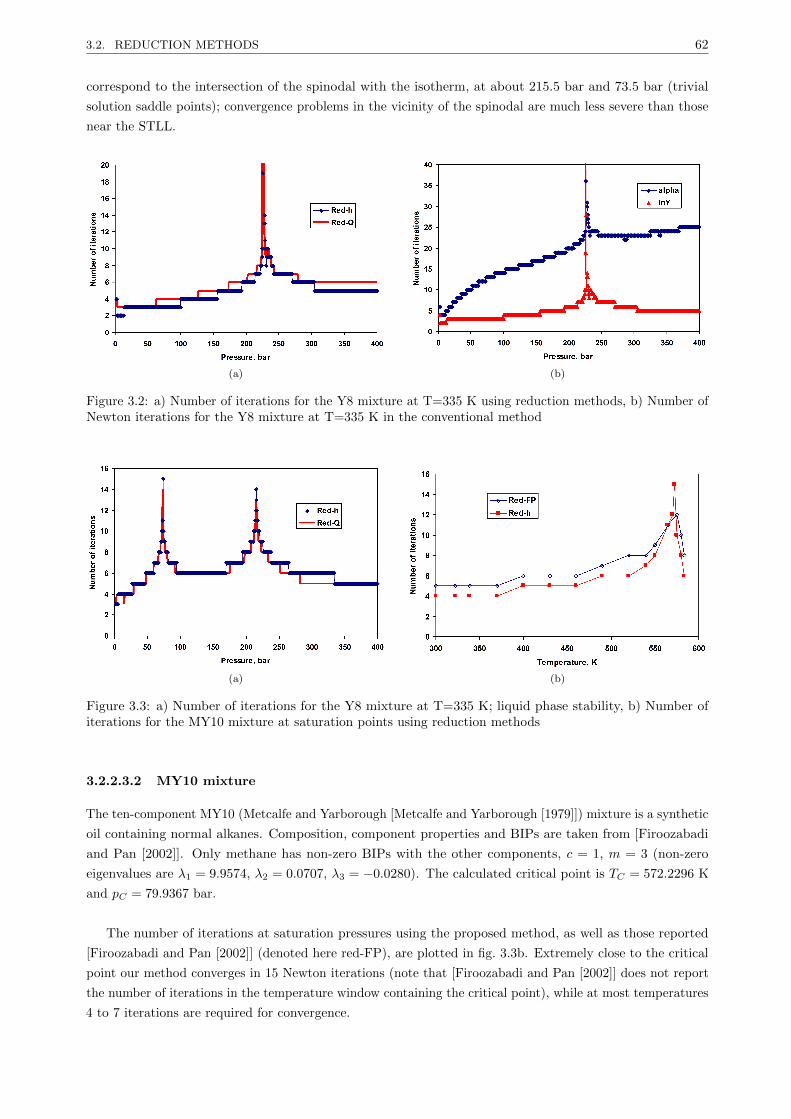
3.2. REDUCTION METHODS 62

correspond to the intersection of the spinodal with the isotherm, at about 215.5 bar and 73.5 bar (trivial

solution saddle points); convergence problems in the vicinity of the spinodal are much less severe than those

near the STLL.

(a) (b)

Figure 3.2: a) Number of iterations for the Y8 mixture at T=335 K using reduction methods, b) Number ofNewton iterations for the Y8 mixture at T=335 K in the conventional method

(a) (b)

Figure 3.3: a) Number of iterations for the Y8 mixture at T=335 K; liquid phase stability, b) Number ofiterations for the MY10 mixture at saturation points using reduction methods

3.2.2.3.2 MY10 mixture

The ten-component MY10 (Metcalfe and Yarborough [Metcalfe and Yarborough [1979]]) mixture is a synthetic

oil containing normal alkanes. Composition, component properties and BIPs are taken from [Firoozabadi

and Pan [2002]]. Only methane has non-zero BIPs with the other components, c = 1, m = 3 (non-zero

eigenvalues are λ1 = 9.9574, λ2 = 0.0707, λ3 = −0.0280). The calculated critical point is TC = 572.2296 K

and pC = 79.9367 bar.

The number of iterations at saturation pressures using the proposed method, as well as those reported

[Firoozabadi and Pan [2002]] (denoted here red-FP), are plotted in fig. 3.3b. Extremely close to the critical

point our method converges in 15 Newton iterations (note that [Firoozabadi and Pan [2002]] does not report

the number of iterations in the temperature window containing the critical point), while at most temperatures

4 to 7 iterations are required for convergence.

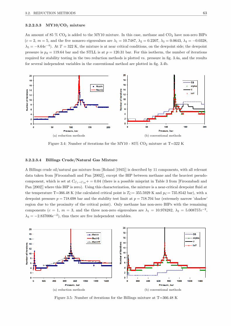
3.2. REDUCTION METHODS 63

3.2.2.3.3 MY10/CO2 mixture

An amount of 85 % CO2 is added to the MY10 mixture. In this case, methane and CO2 have non-zero BIPs

(c = 2, m = 5, and the five nonzero eigenvalues are λ1 = 10.7487, λ2 = 0.2207, λ3 = 0.0643, λ4 = −0.0328,

λ5 = −8.64e−4). At T = 322 K, the mixture is at near critical conditions, on the dewpoint side; the dewpoint

pressure is pd = 119.64 bar and the STLL is at p = 120.31 bar. For this isotherm, the number of iterations

required for stability testing in the two reduction methods is plotted vs. pressure in fig. 3.4a, and the results

for several independent variables in the conventional method are plotted in fig. 3.4b.

(a) reduction methods (b) conventional methods

Figure 3.4: Number of iterations for the MY10 - 85% CO2 mixture at T=322 K

3.2.2.3.4 Billings Crude/Natural Gas Mixture

A Billings crude oil/natural gas mixture from [Roland [1945]] is described by 11 components, with all relevant

data taken from [Firoozabadi and Pan [2002]], except the BIP between methane and the heaviest pseudo-

component, which is set at CC1−C19+ = 0.04 (there is a possible misprint in Table 3 from [Firoozabadi and

Pan [2002]] where this BIP is zero). Using this characterization, the mixture is a near-critical dewpoint fluid at

the temperature T=366.48 K (the calculated critical point is TC= 355.5929 K and pC= 735.8542 bar), with a

dewpoint pressure p = 718.698 bar and the stability test limit at p = 718.704 bar (extremely narrow ’shadow’

region due to the proximity of the critical point). Only methane has non-zero BIPs with the remaining

components (c = 1, m = 3, and the three non-zero eigenvalues are λ1 = 10.978282, λ2 = 5.008757e−2,

λ3 = −2.837006e−2), thus there are five independent variables.

(a) reduction methods (b) conventional methods

Figure 3.5: Number of iterations for the Billings mixture at T=366.48 K

3.2. REDUCTION METHODS 64

The results of stability testing on the isotherm T = 366.48 K (number of iterations vs. pressure) are given

in fig. 3.5a (for the two reduction methods as compared with the results reported in [Firoozabadi and Pan

[2002]]) and in fig. 3.5b (for the conventional method). The peak at a low pressure corresponds to the lower

branch of the spinodal (at p = 21.84 bar).

3.2.2.3.5 Kilgren Reservoir fluid

This is a near-critical reservoir fluid [Kilgren [1966]]. Its characterization by 14 components (with five

pseudo-components in the C7+ fraction) is taken from [Firoozabadi and Pan [2002]]. Three components (C1,

N2 and CO2) have non-zero BIPs with the remaining ones (c = 3). The six nonzero eigenvalues (m = 6)

are: λ1 = 13.561952, λ2 = 0.417676, λ3 = 0.071585, λ4 = −0.043116, λ5 = −0.013293, and λ6 = 0.005196.

According to this reservoir fluid description, at the reservoir temperature T = 399.82 K, the mixture is a

high-shrinkage oil (the calculated critical point is TC= 476.9271 K and pC=842.5883 bar), with a bubble

point pressure of pb = 1053.144 bar (the stability test limit is at p = 1054.545 bar). Fig. 3.6a depicts the

number of iterations required by the two reduction methods (Q− red. and h− red.) as compared to those

reported in [Firoozabadi and Pan [2002]], while the number of iterations for the conventional method using

various independent variables are plotted in fig. 3.6b (note that for this mixture the switching criterion is

satisfied after just one iteration). As for the previous example, the less pronounced peak at a low pressure

corresponds to the lower branch of the spinodal.

(a) reduction methods (b) conventional methods

Figure 3.6: Number of iterations for the Kilgren mixture at T=399.82 K

3.2.2.4 Discussion

It is very important that the independent variables (the elements of h) are unbounded (they are related

to lnφi) while the reduction parameters Q are bounded (they are related to xi ∈ (0, 1)); this is, a major

advantage of the proposed method for phase stability. If Q are independent variables [Pan and Firoozabadi

[2003], Hoteit and Firoozabadi [2006]], they may go out of bounds during Newton iterations; in this case

either a line search procedure is used [Nichita et al. [2007a]], or a switch back to SS iterations is required

[Hoteit and Firoozabadi [2006]] (near the STLL in the single phase region, the line search can be often tedious,

and one may need to revert to SS a very large number of times; note that in the latter case, partial derivatives

are evaluated but not used for updating the variables). In the proposed approach, the reduction parameters

are dependent variables (they are calculated by (eq. 3.47) from mole fractions normalized by (eq. 2.9)), and

it is guaranteed that they are always within their bounds (mini qαi < Q < maxi qαi; α = 1,M ; i = 1, nc).

Previous conventional methods for phase stability used αi = 2√Yi [Michelsen [1982b]] or the formal

3.2. REDUCTION METHODS 65

mole numbers Yi [Hoteit and Firoozabadi [2006]] as independent variables. [Hoteit and Firoozabadi [2006]]

reported that using αi did not add computational efficiency to the Newton method (variables αi are, however,

very important for quasi-Newton methods, which are very sensitive to scaling). In this work we propose

the use of lnYi as independent variables for conventional stability testing. Numerical examples show that

using Yi or αi require almost the same number of Newton iterations (with a small advantage for αi, which

requires one iteration less in some cases); lnYi performs slightly better than αi when Newton iterations

are preceded by a number of SS iterations. However, without SS, the Newton method converges rapidly in

all cases for lnYi, while for αi the Newton method eventually converges, but a large number of iterations

are required (typically more than 20 for the mixtures studied, see for instance fig. 3.2b). This is due

to the fact that for αi the diagonal terms in the Hessian matrix are δij(1 + 1/2g∗i ), as compared to δij

for lnYi. The Hessian for αi is better conditioned at the solution (where gi = 0), but may have a very

bad condition far from the solution (in early stages of the process). In the conventional method, we advo-

cate the use of lnYi as independent variables. If it to choose between the variables Yi and αi, we recommend αi.

Superior performances (smaller numbers of iterations and the possibility to apply directly the Newton

method without the need of SS in the early stages of calculations) of reduction methods [Firoozabadi and

Pan [2002], Nichita et al. [2006a], Hoteit and Firoozabadi [2006]] with respect to the conventional approach

have been attributed [Firoozabadi and Pan [2002], Hoteit and Firoozabadi [2006]] to a relative smoothness

of the TPD surface in the reduced variable hyperplane. In fact, the proposed reduction method have the

same convergence path (and hence the same number of iterations) as in the compositional space with a

specific change of variables (i.e., lnYi), as shown in Appendix C, therefore obtaining the convergence using

only Newton iterations is not a feature of the reduced space as claimed in [Firoozabadi and Pan [2002]].

One can similarly show that the reduced flash of [Nichita and Graciaa [2011]] is linked to conventional flash

calculations using lnKi as independent variables (this was observed but not proved in [Nichita and Graciaa

[2011]]; the proof is given in [Petitfrere and Nichita [2014b]]).

A detailed comparative analysis of conventional and reduction methods, including CPU times, is given

in [Petitfrere and Nichita [2014b]]. It appears that the fastest method in conventional stability is lnKi

with Cholesky decomposition of the Jacobian matrix in the resolution of the linear system, and that both

reduction methods (h− red. and Q− red.) are faster than any conventional method if nc is large enough

and m is small enough (reduction methods are clearly not efficient for mixtures with small nc and full-ranked

BIP matrices). The proposed reduction method is slightly faster than Q− red.. For example, if two

components have non-zero BIPs with the remaining ones (giving 6 independent variables for Q− red. and

7 for h− red.), the CPU time for a Newton iteration is proportional to [Petitfrere and Nichita [2014b]]:

t = 0.0175 + 0.0011nc+ 0.0002nc2 for lnYi (with Cholesky factorization), t = 0.0237 + 0.0025nc for Q− red.,

and t = 0.0269 + 0.0014nc for h− red.. Note that reduction methods exhibit a linear dependence of computa-

tion time vs. the number of components, while for lnYi the quadratic dependence exhibits a small curvature

(as recently reported also by [Michelsen et al. [2013b]]). The CPU time per iteration (for the same number of

iterations required for convergence) for the proposed reduction method is smaller than the one required by

lnY − chol. starting from 8 components. The proposed method is twice as fast for 20 components, about

three times faster for 30 components; for very many components (hundreds, as encountered in some process

simulations), the proposed reduction method can be several orders of magnitude faster than conventional

ones. Note that these observations were made for an optimized solver for linear systems for lnYi; if the

same solver, that is, LU decomposition, is used for both methods, the differences between conventional and

reduction methods are much higher [Petitfrere and Nichita [2014b]].

The proposed set of variables can also be used in the framework of conventional method for stability

testing (with ln Y as primary variables) in order to reduce the dimensionality of the linear system of equations.

3.2. REDUCTION METHODS 66

More precisely, one may keep the lnY Newton implementation in an existing code and use the reduction

concept only to solve a linear system of significantly reduced dimensionality; this can be done with minor

modifications in the code [Petitfrere and Nichita [2014b]], and even if it is less efficient than the full reduction,

such an approach can lead to savings in computer time for large systems (mixtures with many components),

mainly if the number of components with non-zero BIPs is small. While such an approach is not efficient

in the typical component range of reservoir compositional simulation, it can be very useful for process or

transport simulations.

The cause of convergence problems in phase stability calculations is the topology of the TPD surface

(see [Nichita et al. [2007c]] for details, including graphical representations of the TPD surface for a binary

mixture). At the STLL (’shadow curve’), the stationary point of the TPD function is a saddle point (the

Hessian is indefinite and singular at a non-trivial solution with a positive TPD), and the Hessian matrix is

ill-conditioned in the vicinity of the STLL (the most severe problems arise for a pressure interval above the

STLL; there are no convergence problems for pressures just below the STLL). Phase stability calculations

near the STLL are far more difficult than those in the vicinity of a critical point (where the Hessian matrix

is positive semidefinite). Any algorithm will experience difficulties in a pressure domain above the STLL.

It is clear that a change of variables does not eliminate this problem, since the TPD function in the new

hyperspace inherits certain properties from the original one. Considerable research efforts are currently done

to solve this problem and different techniques (other than changing the variables) are being investigated to

eliminate or at least alleviate problems near the STLL; forthcoming papers will treat this issue.

3.2.2.5 Conclusion

A new reduction method for phase stability testing has been proposed in this chapter, based on the multi-linear

expression of the logarithms of fugacity coefficients as functions of the coefficients h (which are taken as

independent variables and are unbounded). The reduction parameters are dependent variables, which, unlike

in previous formulations, are guaranteed to be within their bounds. The dimensionality of the problem

depends only on the number of components having non-zero BIPs with the remaining ones, and not on the

number of components in the mixture, as in the conventional approach.

The proposed method has a high convergence radius and Newton iterations can be used directly (without

the need of using successive substitutions); it has the same convergence path as the conventional approach

using the natural logarithm of formal mole numbers as independent variables (which seems to be the best

choice in the compositional space). It has been shown that the primary variables in our method are Lagrange

multipliers corresponding to a constrained minimization of the modified TPD function with respect to a

specific set of variables. Thus, the proposed method facilitates comparison of reduced and conventional

approaches for phase stability analysis. An apparently hidden formal link between conventional and reduction

methods is revealed.

Several test problems for various synthetic and reservoir mixtures have proved the robustness of the

proposed method and show that it requires systematically less iterations than i) conventional methods using

other independent variables than lnYi, and ii) previous reduction methods.

3.2.3 A comparison of conventional and reduction approaches for phase equi-

librium calculations

3.2.3.1 Introduction

Our recent formulations of reduction methods for flash calculations [Nichita and Graciaa [2011]] and phase

stability testing [Nichita and Petitfrere [2013]] are related to constrained minimizations of the objective

3.2. REDUCTION METHODS 67

functions (Gibbs free energy and a modified TPD function) and thus facilitate comparisons with conventional

methods [Michelsen et al. [2013b]]. Besides, they require simpler partial derivatives in the Newton method.

Several very recent papers ([Michelsen et al. [2013b]], Haugen and Beckner [2013], Gorucu and Johns

[2013]] have questioned on the efficiency of the reduction methods as compared to conventional methods. The

common conclusion of these papers is that reduction methods become faster than conventional ones starting

from a certain number of components in the mixture (about 20 if few components have non-zero BIPs).

In this subsection, we intend to look, besides CPU times required by various conventional and reduction

formulations, at:

• Stability testing and flash calculation separately

• Computation times per iteration and globally

• Condition number of the matrix in the linear system of equations

• The solver for the linear system and the effect of using symmetry

• Formal links between conventional and reduction methods, as well as between different reduction

methods

Numerical experiments are carried out for various formulations and sets of independent variables for

conventional and reduction flash and stability, followed by a discussion and the conclusions. Four Appendices

give: the formulation of the reduction flash as a constrained minimization problem, the equivalence of

conventional and reduction flash methods (convergence path identity), a link between two reduction methods

for phase stability testing and some features of the pseudo-reduced method for phase stability.

3.2.3.2 Results

Numerical experiments have been performed for three mixtures presented in subsection 3.2.2, using the

Peng-Robinson EoS [Peng and Robinson [1976], Robinson and Peng [1978]]:

• Y8 mixture (0 BIP mixture).

• MY10 mixture (1 BIP family mixture).

• MY10+CO2 mixture (2 BIP families mixture). An amount of 16.67% CO2 is added to the MY10

mixture. In this case, methane and CO2 have non-zero BIPs (c = 2, thus m = 5 and M + 1 = 7).

The mixture compositions and the non-zero BIPs are presented in table 3.1. The phase envelopes of the

three mixtures (showing the critical points) are plotted in fig. 3.7.

Components Y8 MY10zi zi CC1−j CCO2−j

C1 0.8097 0.35 - 0.093C2 0.0566 0.03 0.00 0.128C3 0.0306 0.04 0.00 0.123

nC4 - 0.06 0.02 0.136nC5 0.0457 0.04 0.02 0.125nC6 - 0.03 0.025 0.131nC7 0.0330 0.05 0.025 0.120nC8 - 0.05 0.035 0.120nC10 0.0244 0.30 0.045 0.120nC14 - 0.05 0.045 0.120

Table 3.1: Feed composition and BIPs for Y8 and MY10 mixtures

3.2. REDUCTION METHODS 68

100 200 300 400 500 6000

50

100

150

200

250

Pre

ssure

, bar

Temperature, K

Phase boundary

Critical point

Y8MY10+CO2

MY10

Figure 3.7: Phase envelopes of Y8, MY10 and MY10+CO2 mixtures

3.2.3.2.1 Solving the linear system

For flash calculation and stability analysis problems, the linear system is generally small. The matrix (nc×nc)is dense for both problems, where nc exceeds 100 for instance in certain process simulations. Direct solvers

have been applied in this paper as more efficient compared with iterative ones. Two direct solvers have been

used:

• The LU factorization, which is applicable to any system and solves the linear problem in 2/3n3 FLOPs

(FLoating point OPerations).

• The Cholesky factorization, which is applicable to symmetric matrices and takes advantage of the

symmetry to solve the linear problem in n3/3 FLOPs. It is important to note that for a symmetric

matrix (Hessian and U−1), only about half of the matrix (nc× (nc+ 1)/2 entries) needs to be computed

when a Cholesky decomposition is used.

3.2.3.2.2 Independent variables

3.2.3.2.2.a Flash calculations

1. Independent variables leading to symmetric systems solved using Cholesky decomposition

• nL/nV the component mole numbers in liquid or vapor phase are taken as independent variables.

In this case the Rachford-Rice needs not to be solved.

• lnK−Chol. the independent variables are the natural logarithms of the equilibrium constants.

The Hessian matrix is decomposed and the linear system is solved as described in a previous

section.

• Michelsen− red. an (M + 1)× (M + 1) linear system is solved for the independent variables h.

2. Independent variables leading to non-symmetric systems, solved using LU decomposition

• lnK for the lnKi variables, the Jacobian matrix is non-symmetric and the linear system can be

solved directly by means of an LU factorization. Both cases have been tested to see the impact of

the Cholesky solver as compared with an LU factorization for the linear system.

• h− red. Reduction method with h as independent variables.

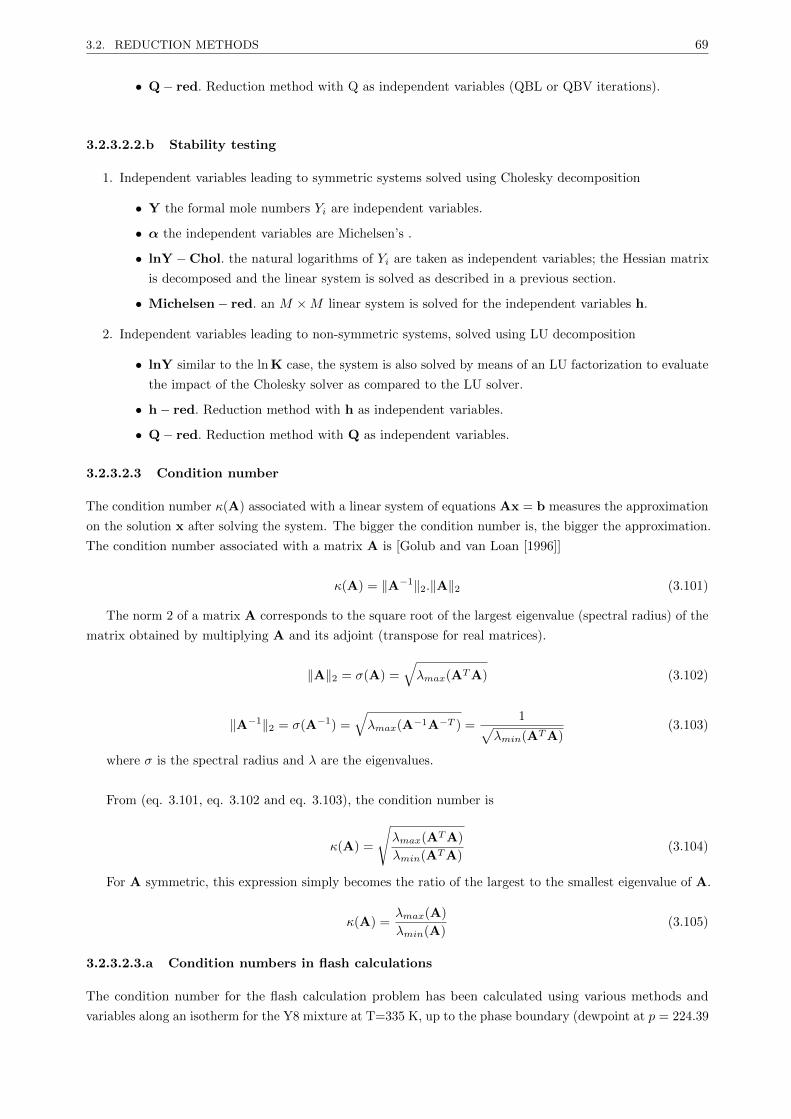
3.2. REDUCTION METHODS 69

• Q− red. Reduction method with Q as independent variables (QBL or QBV iterations).

3.2.3.2.2.b Stability testing

1. Independent variables leading to symmetric systems solved using Cholesky decomposition

• Y the formal mole numbers Yi are independent variables.

• α the independent variables are Michelsen’s .

• lnY −Chol. the natural logarithms of Yi are taken as independent variables; the Hessian matrix

is decomposed and the linear system is solved as described in a previous section.

• Michelsen− red. an M ×M linear system is solved for the independent variables h.

2. Independent variables leading to non-symmetric systems, solved using LU decomposition

• lnY similar to the ln K case, the system is also solved by means of an LU factorization to evaluate

the impact of the Cholesky solver as compared to the LU solver.

• h− red. Reduction method with h as independent variables.

• Q− red. Reduction method with Q as independent variables.

3.2.3.2.3 Condition number

The condition number κ(A) associated with a linear system of equations Ax = b measures the approximation

on the solution x after solving the system. The bigger the condition number is, the bigger the approximation.

The condition number associated with a matrix A is [Golub and van Loan [1996]]

κ(A) = ‖A−1‖2.‖A‖2 (3.101)

The norm 2 of a matrix A corresponds to the square root of the largest eigenvalue (spectral radius) of the

matrix obtained by multiplying A and its adjoint (transpose for real matrices).

‖A‖2 = σ(A) =√λmax(ATA) (3.102)

‖A−1‖2 = σ(A−1) =√λmax(A−1A−T ) =

1√λmin(ATA)

(3.103)

where σ is the spectral radius and λ are the eigenvalues.

From (eq. 3.101, eq. 3.102 and eq. 3.103), the condition number is

κ(A) =

√λmax(ATA)

λmin(ATA)(3.104)

For A symmetric, this expression simply becomes the ratio of the largest to the smallest eigenvalue of A.

κ(A) =λmax(A)

λmin(A)(3.105)

3.2.3.2.3.a Condition numbers in flash calculations

The condition number for the flash calculation problem has been calculated using various methods and

variables along an isotherm for the Y8 mixture at T=335 K, up to the phase boundary (dewpoint at p = 224.39

3.2. REDUCTION METHODS 70

bar) (fig. 3.8a). The condition number of the Jacobian/Hessian matrix is calculated at the solution.

The best condition number is given by the ln K variables. Close to unity for most of the points, it still

gives a good condition number close to the phase boundary. The condition numbers for the mole numbers

nL/nV follow the trend of those for both reduction methods (Q− red. and h− red.) along the two phase

region, with values in the range of 100. However, the system becomes ill-conditioned close to the phase

boundary, which explains the difficulties that can be encountered with this variable in the vicinity of phase

boundaries. The reduction methods are less altered in this region than nl/nv.

Note that in lnK−Chol. the linear system in (eq. 3.25) is solved, thus the approximations will be

potentially more important than by solving the non-symmetric system in (eq. 3.33) by an LU decomposition.

Finally, Michelsen− red. gives a bad condition number all along the two phase region (around 105). In this

method, the decrease of the dimensionality of the space is made at the expense of a severe loss of conditioning.

The singularity for the flash calculation problem is at the critical point (for T 6= Tc, the singularities are

at the convergence locus for the negative flash [Nichita et al. [2007c], Whitson and Michelsen [1990]]), where

two eigenvalues of the Jacobian matrix become zero [Michelsen [1982a]] and the condition number is infinite.

Along the phase boundary, the closer to the critical point, the smaller the minimum eigenvalue, the higher

the condition number.

0 50 100 150 200 25010

0

101

102

103

104

105

106

107

Pressure,hbar

Con

ditio

nnu

mbe

r

nL/n

V

ln KMichelsen−red.h−red.Q−red.

(a) Flash calculations

0 50 100 150 200 25010

0

102

104

106

108

Pressure, bar

Con

ditio

nnu

mbe

r

Yalphaln YMichelsen−red.h−red.Q−red.

(b) Stability analysis

Figure 3.8: Condition number along the isotherm T=335K for the Y8 mixture

3.2.3.2.3.b Condition numbers in stability testing

The condition number has been calculated using various methods and variables for the stability analysis

problem with the same mixture and on the same isotherm at pressures up to 240 bar (fig. 3.8b). The feed is

tested as a vapor phase. At T=335 K, the STLL is located at p = 225.26 bar. At the STLL (the singularity

for stability testing), one of the Jacobian/Hessian’s eigenvalues becomes zero, and the condition number

becomes infinite (represented by an asymptotic line). This is the reason why phase stability calculations can

be really difficult in the vicinity of the STLL.

As for the flash calculation problem, lnY (an analogy can be made with lnK for flash calculations

[Nichita and Petitfrere [2013]] gives a really good condition number all along the isotherm, even when the

STLL is approached. The condition number is around unity up to 150 bar and remains below 200 close

3.2. REDUCTION METHODS 71

to the STLL. Using α gives a better conditioning than lnY; however, far from the solution, especially in

the early iteration stages, the linear system for lnY is better conditioned, allowing a safe earlier switch

from SSI iterations, as discussed in [Nichita and Petitfrere [2013]]. The condition number obtained using

Y is rather high (around 100) all along the isotherm and it increases (around 1000) as the STLL is approached.

Both reduction methods (Q− red. and h− red.) have the same condition number at the solution (see

Appendix F). It remains small up to p = 150 bar, but gets larger than for Y when getting closer to the STLL.

As for the flash calculations, the pseudo-reduced method (Michelsen− red.) gives a really bad condition

number all along the isotherm (around 104) which indicates potentially important approximations when

solving the linear system.

3.2.3.2.4 Computational time

The computational time is a really sensible parameter. It highly depends on many factors, such as computer

features (hardware: processor, memory, etc.), compiler, implementation (cash optimization, vectorization,

etc.). In this thesis, for all calculations, an Intel Xeon ES5405@2.00GHz processor has been used.

The choice of the linear solver is also a really important feature. A specific study has been made over

different sets of linear solvers [Press et al. [1992], Lapack, homemade LU and Cholesky solvers). Some

linear solvers are more adapted for large systems (i.e., Lapack). Some are more adapted for small systems

(home-made). It has been noticed that depending on the solver used, the time spent on the linear solver

ranged from 10% up to 55% of the total time. The homemade LU and Cholseky solvers were used in this paper.

To obtain the same properties for a mixture using a different number of components, some of the com-

ponents were split. Given a mixture with nc components, one of them (different from C1 and CO2) with a

feed composition of zi , by splitting zi into z′i and z′′i , with z′i = z′′i = zi/2 , and assigning to the two new

components the same BIPs and critical properties, a new composition can be created leading to the same

mixture properties.

Two different comparisons were made to test, separately for flash and stability, the time and the efficiency

of each method for various sets of independent variables for mixtures with different number of components: i)

time per iteration and ii) time spent for an entire pressure-temperature domain.

3.2.3.2.4.a Flash calculation

Time spent for one iteration

For a given pressure and temperature in the two-phase region, a switch to Newton iterations is carried out

after performing a certain number of SSI iterations. Then, the Newton iteration is repeated 10000 times for

each set of independent variables. The time spent between the switch to the Newton method and the end of

the 10000 iterations is recorded. This operation is repeated for the three mixtures and for different numbers

of components. This gives the time spent to perform one Newton iteration for different sets of independent

variables, independently of their convergence behavior. This procedure was used for the Y8 mixture (with 0

BIPs) at P=160 bar and T=335 K. The results are given in fig. 3.9a. For calculations performed at P=40

bar and T=550 K, the results are reported in fig. 3.9b for the MY10 mixture (with 1 BIP family) and in

fig. 3.10 for the MY10+CO2 mixture (with 2 BIP families).

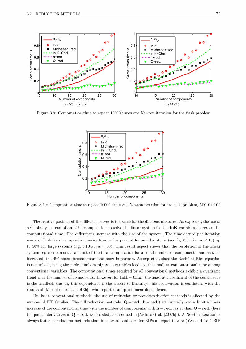
3.2. REDUCTION METHODS 72

5 10 15 20 25 300

0.2

0.4

0.6

0.8

1

Number of components

Com

puta

tion

time,

Ks

nL/n

V

ln KMichelsen−red.ln K−Chol.h−red.Q−red.

(a) Y8 mixture

10 15 20 25 300

0.2

0.4

0.6

0.8

1

NumberKofKcomponents

Com

puta

tionK

time,

Ks

nL/n

V

lnKKMichelsen−red.lnKK−Chol.h−red.Q−red.

(b) MY10

Figure 3.9: Computation time to repeat 10000 times one Newton iteration for the flash problem

10 15 20 25 300

0.2

0.4

0.6

0.8

1

NumberKofKcomponents

Com

puta

tionK

time,

Ks

nL/n

V

lnKKMichelsen−red.lnKK−Chol.h−red.Q−red.

Figure 3.10: Computation time to repeat 10000 times one Newton iteration for the flash problem, MY10+C02

The relative position of the different curves is the same for the different mixtures. As expected, the use of

a Cholesky instead of an LU decomposition to solve the linear system for the lnK variables decreases the

computational time. The differences increase with the size of the system. The time earned per iteration

using a Cholesky decomposition varies from a few percent for small systems (see fig. 3.9a for nc < 10) up

to 50% for large systems (fig. 3.10 at nc = 30). This result aspect shows that the resolution of the linear

system represents a small amount of the total computation for a small number of components, and as nc is

increased, the differences become more and more important. As expected, since the Rachford-Rice equation

is not solved, using the mole numbers nl/nv as variables leads to the smallest computational time among

conventional variables. The computational times required by all conventional methods exhibit a quadratic

trend with the number of components. However, for lnK−Chol. the quadratic coefficient of the dependence

is the smallest, that is, this dependence is the closest to linearity; this observation is consistent with the

results of [Michelsen et al. [2013b]], who reported an quasi-linear dependence.

Unlike in conventional methods, the use of reduction or pseudo-reduction methods is affected by the

number of BIP families. The full reduction methods (Q− red., h− red.) act similarly and exhibit a linear

increase of the computational time with the number of components, with h− red. faster than Q− red. (here

the partial derivatives in Q− red. were coded as described in [Nichita et al. [2007b]]). A Newton iteration is

always faster in reduction methods than in conventional ones for BIPs all equal to zero (Y8) and for 1-BIP

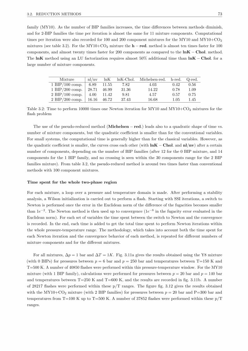
3.2. REDUCTION METHODS 73

family (MY10). As the number of BIP families increases, the time differences between methods diminish,

and for 2-BIP families the time per iteration is almost the same for 11 mixture components. Computational

times per iteration were also recorded for 100 and 200 component mixtures for the MY10 and MY10+CO2

mixtures (see table 3.2). For the MY10+CO2 mixture the h− red. method is almost ten times faster for 100

components, and almost twenty times faster for 200 components as compared to the lnK−Chol. method.

The lnK method using an LU factorization requires almost 50% additional time than lnK−Chol. for a

large number of mixture components.

Mixture nl/nv lnK lnK-Chol. Michelsen-red. h-red. Q-red.1 BIP/100 comp. 6.89 11.55 7.82 4.03 0.42 0.561 BIP/200 comp. 28.71 46.99 31.36 14.22 0.78 1.092 BIP/100 comp. 4.00 11.42 9.81 4.57 0.57 0.752 BIP/200 comp. 16.16 46.72 37.43 16.68 1.05 1.45

Table 3.2: Time to perform 10000 times one Newton iteration for MY10 and MY10+CO2 mixtures for theflash problem

The use of the pseudo-reduced method (Michelsen− red.) leads also to a quadratic shape of time vs.

number of mixture components, but the quadratic coefficient is smaller than for the conventional variables.

For small systems, the computational time is generally higher than for the classical variables. However, as

the quadratic coefficient is smaller, the curves cross each other (with lnK−Chol. and nl/nv) after a certain

number of components, depending on the number of BIP families (after 12 for the 0 BIP mixture, and 14

components for the 1 BIP family, and no crossing is seen within the 30 components range for the 2 BIP

families mixture). From table 3.2, the pseudo-reduced method is around two times faster than conventional

methods with 100 component mixtures.

Time spent for the whole two-phase region

For each mixture, a loop over a pressure and temperature domain is made. After performing a stability

analysis, a Wilson initialization is carried out to perform a flash. Starting with SSI iterations, a switch to

Newton is performed once the error in the Euclidean norm of the difference of the fugacities becomes smaller

than 1e−2. The Newton method is then used up to convergence (1e−8 in the fugacity error evaluated in the

Euclidean norm). For each set of variables the time spent between the switch to Newton and the convergence

is recorded. In the end, each time is added to get the total time spent to perform Newton iterations within

the whole pressure-temperature range. The methodology, which takes into account both the time spent for

each Newton iteration and the convergence behavior of each method, is repeated for different numbers of

mixture components and for the different mixtures.

For all mixtures, ∆p = 1 bar and ∆T = 1K. Fig. 3.11a gives the results obtained using the Y8 mixture

(with 0 BIPs) for pressures between p = 6 bar and p = 250 bar and temperatures between T=150 K and

T=500 K. A number of 40850 flashes were performed within this pressure-temperature window. For the MY10

mixture (with 1 BIP family), calculations were performed for pressures between p = 20 bar and p = 140 bar

and temperatures between T=250 K and T=600 K, and the results are recorded in fig. 3.11b. A number

of 28217 flashes were performed within these p/T ranges. The figure fig. 3.12 gives the results obtained

with the MY10+CO2 mixture (with 2 BIP families) for pressures between p = 20 bar and P=300 bar and

temperatures from T=100 K up to T=500 K. A number of 37852 flashes were performed within these p/T

ranges.

3.2. REDUCTION METHODS 74

5 10 15 20 25 300

1

2

3

4

5

6

7

8

9

Numberloflcomponents

Com

puta

tionl

time,

ls

nL/n

V

lnlKMichelsen−red.lnlK−Chol.h−red.Q−red.

(a) Y8 mixture

10 15 20 25 300

1

2

3

4

5

Numberdofdcomponents

Com

puta

tiond

time,

ds

nL/n

V

lndKMichelsen−red.lndK−Chol.h−red.Q−red.

(b) MY10

Figure 3.11: Computation time for the whole two-phase region for the flash problem

10 15 20 25 300

1

2

3

4

5

6

7

NumberMofMcomponents

Com

puta

tionM

time,

Ms

nL/n

V

lnMKMichelsen−red.lnMK−Chol.h−red.Q−red.

Figure 3.12: Computation time for the whole two-phase region for the flash problem, MY10+C02

The same trend as observed per iteration can be found here for the different curves. The curves

corresponding to conventional and reduction methods cross each other, and starting for a certain number of

components the reduction methods become faster. It appears the reduction method h− red. is more efficient

and stable than the reduction method Q− red. The conventional method using mole numbers as variables,

nl/nv, seems the most efficient but less robust, as will be discussed in the next section.

3.2.3.2.4.b Stability analysis

Time spent for one iteration

The same methodology as for flash calculations is applied for stability analysis. Starting from the [Wilson

[1969]] initialization, five SSI iterations are performed before switching to the Newton method. Fig. 3.13a

plots the results obtained with the Y8 mixture, fig. 3.13b, those obtained with the MY10 mixture and fig. 3.14

the results for the MY10+CO2 mixture. The pressure and the temperature chosen are the same as for the

flash calculations.

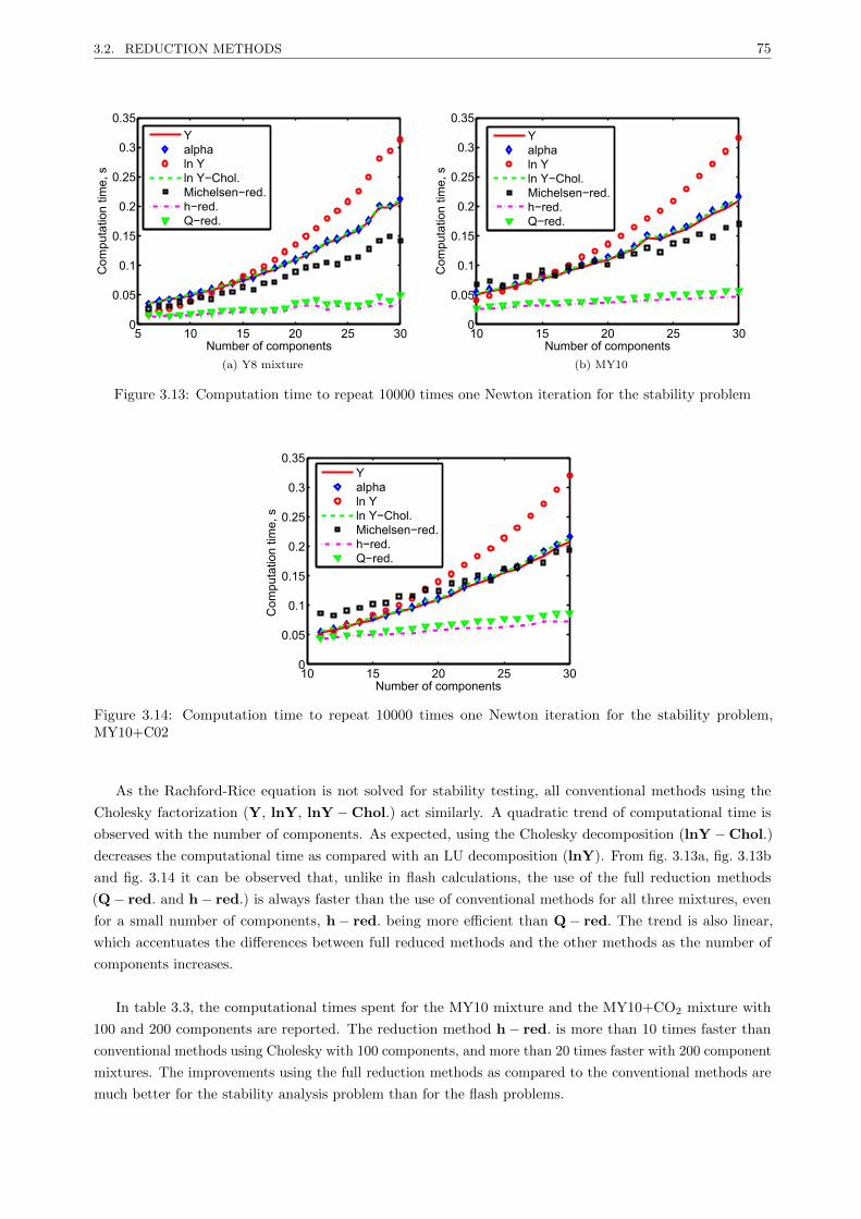
3.2. REDUCTION METHODS 75

5 10 15 20 25 300

0.05

0.1

0.15

0.2

0.25

0.3

0.35

Number of components

Com

puta

tion

time,

s

Yalphaln Yln Y−Chol.Michelsen−red.h−red.Q−red.

(a) Y8 mixture

10 15 20 25 300

0.05

0.1

0.15

0.2

0.25

0.3

0.35

Number of components

Computationtime,s

Yalphaln Yln Y−Chol.Michelsen−red.h−red.Q−red.

(b) MY10

Figure 3.13: Computation time to repeat 10000 times one Newton iteration for the stability problem

10 15 20 25 300

0.05

0.1

0.15

0.2

0.25

0.3

0.35

Number of components

Computationtime,s

Yalphaln Yln Y−Chol.Michelsen−red.h−red.Q−red.

Figure 3.14: Computation time to repeat 10000 times one Newton iteration for the stability problem,MY10+C02

As the Rachford-Rice equation is not solved for stability testing, all conventional methods using the

Cholesky factorization (Y, lnY, lnY −Chol.) act similarly. A quadratic trend of computational time is

observed with the number of components. As expected, using the Cholesky decomposition (lnY −Chol.)

decreases the computational time as compared with an LU decomposition (lnY). From fig. 3.13a, fig. 3.13b

and fig. 3.14 it can be observed that, unlike in flash calculations, the use of the full reduction methods

(Q− red. and h− red.) is always faster than the use of conventional methods for all three mixtures, even

for a small number of components, h− red. being more efficient than Q− red. The trend is also linear,

which accentuates the differences between full reduced methods and the other methods as the number of

components increases.

In table 3.3, the computational times spent for the MY10 mixture and the MY10+CO2 mixture with

100 and 200 components are reported. The reduction method h− red. is more than 10 times faster than

conventional methods using Cholesky with 100 components, and more than 20 times faster with 200 component

mixtures. The improvements using the full reduction methods as compared to the conventional methods are

much better for the stability analysis problem than for the flash problems.

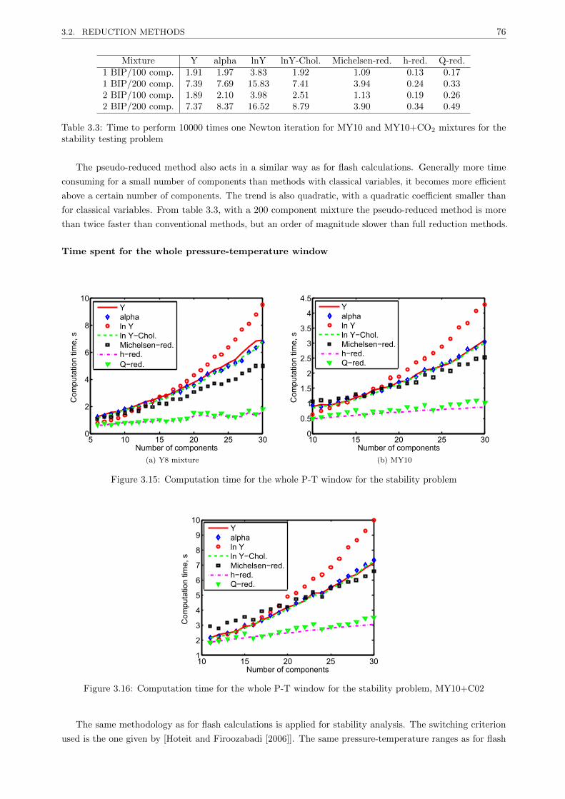
3.2. REDUCTION METHODS 76

Mixture Y alpha lnY lnY-Chol. Michelsen-red. h-red. Q-red.1 BIP/100 comp. 1.91 1.97 3.83 1.92 1.09 0.13 0.171 BIP/200 comp. 7.39 7.69 15.83 7.41 3.94 0.24 0.332 BIP/100 comp. 1.89 2.10 3.98 2.51 1.13 0.19 0.262 BIP/200 comp. 7.37 8.37 16.52 8.79 3.90 0.34 0.49

Table 3.3: Time to perform 10000 times one Newton iteration for MY10 and MY10+CO2 mixtures for thestability testing problem

The pseudo-reduced method also acts in a similar way as for flash calculations. Generally more time

consuming for a small number of components than methods with classical variables, it becomes more efficient

above a certain number of components. The trend is also quadratic, with a quadratic coefficient smaller than

for classical variables. From table 3.3, with a 200 component mixture the pseudo-reduced method is more

than twice faster than conventional methods, but an order of magnitude slower than full reduction methods.

Time spent for the whole pressure-temperature window

5 10 15 20 25 300

2

4

6

8

10

Number of components

Com

puta

tion

time,

ds

Yalphaln Yln Y−Chol.Michelsen−red.h−red.Q−red.

(a) Y8 mixture

10 15 20 25 300

0.5

1

1.5

2

2.5

3

3.5

4

4.5

Number of components

Com

puta

tion

time,

s

Yalphaln Yln Y−Chol.Michelsen−red.h−red.Q−red.

(b) MY10

Figure 3.15: Computation time for the whole P-T window for the stability problem

10 15 20 25 301

2

3

4

5

6

7

8

9

10

Number of components

Com

puta

tion

time,

7s

Yalphaln Yln Y−Chol.Michelsen−red.h−red.Q−red.

Figure 3.16: Computation time for the whole P-T window for the stability problem, MY10+C02

The same methodology as for flash calculations is applied for stability analysis. The switching criterion

used is the one given by [Hoteit and Firoozabadi [2006]]. The same pressure-temperature ranges as for flash

3.2. REDUCTION METHODS 77

calculations are used. This time, the number of stability calculations performed for each mixture is directly

given by the number of tested pressure-temperature conditions. The results for the Y8 mixture are given in

fig. 3.15a, for the MY10 mixture in fig. 3.15b, and for the MY10+CO2 mixture in fig. 3.16.

The same conclusions as for the time per iteration can be given. The maximum number of iterations

has been set to 200. Moreover, as ∆p and ∆T are not very small (1 bar and 1 K), the number of points

in the immediate vicinity of the STLL might be small as compared to the whole set of points. This could

explain why the convergence behavior does not influence much the shape of the curves; only the time per

iterations seems to influence the global result. However, for pressures just above the STLL, lnY and α are

the variables giving a more robust formulation as compared to Y variables (a more detailed discussion can

be found in [Nichita and Petitfrere [2013]]).

3.2.3.3 Discussion

For the flash calculation problem, the use of mole numbers as variables (namely nL/nV) appears to be the

most efficient among the conventional methods, and globally more efficient than reduction methods for a

small number of components. However, this choice of variable does lead to less robustness: in the vicinity of

the phase boundaries (even far from critical points) the nL/nV method has a small convergence ratio and

may require a significantly increased number of iterations (starting from the same switch from SSI iterations)

to achieve convergence, as compared to other conventional formulations, as well as with reduction methods.

The error (Euclidean norm) vs. the iteration level for a two-phase flash of the Y8 mixture at T=366 K and

P=214 bar (very close to the dewpoint pressure in the retrograde condensation region) is plotted for various

methods in fig. 3.17a. The lnK, h− red. and Michelsen− red. Newton methods require only 3 iterations

after the switch. The curves are superposed for lnK and h− red.; only a slight difference can be observed for

the pseudo-reduced method. The nL/nV method requires more than 60 iterations, with a large number of

switches back from Newton to SSI due to an increase in Gibbs free energy between two subsequent iterations

(note that in this case the Jacobian is evaluated and the linear system solved, but this information is not

used since a SSI step is taken). This kind of behavior is typical for nL/nV. Newton iterations near phase

boundaries, and the severity of these problems increases as the critical point is approached. For this choice

of variables, it is recommended the use of a Trust-region method, which highly improves robustness (see

[Petitfrere and Nichita [2014a]] for a detailed discussion on this matter). The Q− red. method also requires

repeated switch-backs, and the total number of iterations is 40; note that after the final switch to Newton

iterations, the Euclidean norm first increases before the method converges quadratically in a few iterations.

0 10 20 30 40 50 60 7010

−12

10−10

10−8

10−6

10−4

10−2

100

NumberMofMiterations

Euc

lidea

nMno

rm

nL/n

V

lnMKMichelsen−red.h−red.Q−red.

(a) Flash

0 10 20 30 4010

−15

10−10

10−5

100

Number of iterations

Euc

lidea

n no

rm

Yalphaln YMichelsen−red.h−red.Q−red.

(b) Stability testing

Figure 3.17: Error v.s. iteration number for various methods, for the Y8 mixture at T=350 K and P=230 bar

The Euclidean norm of the error vector is plotted vs. the iteration level for the stability testing of the

3.2. REDUCTION METHODS 78

Y8 mixture (with Y(0)i = zi/Ki) at T=350 K and P=230 bar (just above the STLL) in fig. 3.17b. The

switching criterion [Hoteit and Firoozabadi [2006]] corresponds in this case to an early switch (except for

the Q− red. method, in which only Newton iterations are performed. Only 6 or 7 iterations are required

for convergence by both reduction methods and by all conventional methods (with lnY, h− red. and

Michelsen− red. following the same convergence path), except Y, which requires almost 40 iterations, with

repeated switch-backs to SSI iterations. At even more severe conditions, hundreds of SSI iterations (on switch

back from Newton iterations or by using a very restrictive switching criterion) may be necessary before the

Newton method converges. It was showed earlier [Nichita and Petitfrere [2013]] that formulations in lnY and

Michelsen’s α variables are more robust than the one using formal mole numbers as variables and that the

use of a Trust-region method highly improves robustness [Petitfrere and Nichita [2014a]] when Yi are used as

independent variables.

For both flash and stability problems, when using classical variables, the use of a Cholesky solver is

recommended. For small systems, the differences with a flash using an LU decomposition are not significant

(especially for flash calculations), but when nc exceeds 10, the differences increase and become quite important.

The reduction based methods do not suffer the use of LU factorization (in the sense that the trend of time

with nc remains linear) since the dimensionality of the system is decreased to a small size.

It is commonly said that in conventional methods the CPU time increases at least with the square of the

number of components. This is observed in this work when an LU decomposition is used to solve the linear

system of equations. However, a weak quadratic trend is revealed if a Cholesky decomposition is used: this

observation is consistent with that of [Michelsen et al. [2013b]], who report an almost linear trend of CPU

time with nc for classical variables (up to nc = 25 components). The choice of the linear solver influence to a

great extent the efficiency of conventional methods, and it is recommended to take advantage of symmetry

whenever possible.

For the flash calculation problem, the curves of CPU time vs. number of components corresponding to

the conventional (lnK−Chol., which is the best conventional method) and reduction methods (h− red. ,

which is the fastest reduction method) cross each other at a certain value of nc, thus, reduction methods

are not more efficient than conventional ones for mixtures with few components (the range of compositional

simulation). This is a common observation of the three recent publications on this matter [Michelsen et al.

[2013b], Haugen and Beckner [2013], Gorucu and Johns [2013]]. Depending on how the comparison was done

and on the implementation, the reported crossing point is around 15 in [Haugen and Beckner [2013]], around

20 in [Michelsen et al. [2013b]] (global time stability and flash using a Trust-region approach) and around 20

in [Gorucu and Johns [2013]]. In this work, the two curves cross each other around 22 components.

It is very important to note that if an LU decomposition is used, the reduction methods are faster than

lnK even for a small number of components; a conventional method is faster than a reduction method only if

full advantage of symmetry is taken (in the construction of the Jacobian matrix and the resolution of the

linear system).

The use of pseudo-reduced methods was found (in this work, as well as in [Michelsen et al. [2013b]])

to be more efficient than conventional methods for flash and stability only for a relatively large number

of components. Here it is also shown that full reduction methods are significantly more efficient than

pseudo-reduced methods, having also a better conditioning of the linear system. We however recommend the

use of the pseudo-reduced methods for mixtures with very many components; since the code can be easily

written with minor modifications to an existing code based on conventional methods.

3.2. REDUCTION METHODS 79

For stability analysis, the full reduction methods are the most efficient for any number of components. The

use of reduction methods, especially h− red. (acting better than Q− red. in terms of speed and robustness),

would be efficient for both reservoir simulation and process design number of components ranges.

Summarizing, conventional methods (when symmetry is used) seems to be more efficient in the range of

number of components encountered in compositional reservoir simulation. With nc increasing, the reduction

flash is more efficient (per iteration and global) above the crossing point. Thus, for any flash calculation

involving mixtures with many components (such as in some process design simulations) both reduction

methods give the best results in terms of efficiency, h− red. being more stable and efficient.

This work reveals that if we look separately at stability testing, stability reduction methods are more

efficient than conventional methods for the entire range of number of components. Therefore, reduction

methods for phase stability testing are suitable for compositional reservoir simulators.

Most of the CPU time in compositional reservoir simulations is spent by phase equilibrium calculations.

Depending on the structure of the simulator, flash calculations may be part of a larger problem, but stability

testing must be carried out in most grid blocks (at any time step and at each iteration level in the solution of

the pressure equation) likely to experience a phase split. Phase equilibrium calculations can be either coupled

with or decoupled from the equations describing the flow though porous media [Michelsen et al. [2013a]]. For

’coupled’ simulators, only the stability testing is performed (except in the multiphase case when a very limited

number of flashes may be required for initialization purposes); even though stability testing may be skipped

in some single-phase blocks according to some simple criteria (using the ’shadow region’ method) [Wong et al.

[1990]], a very large number of calls for the stability routine is expected during a field-scale simulation run.

In the case of ’decoupled’ simulators, both stability testing and phase split are required. To the best of our

knowledge, most of commercial and research compositional reservoir simulators are of a ’coupled’ type, with

no explicit flash calculations required. This is the reason why the observation that reduction methods for

phase stability are more efficient than conventional ones for a small number of components is very important.

3.2.3.4 Conclusion

This work presents a comparison between conventional and reduction methods for phase equilibrium cal-

culations, and is complementary with several recent papers [Michelsen et al. [2013b], Haugen and Beckner

[2013], Gorucu and Johns [2013]] which questioned on the efficiency of the reduction methods as compared

to conventional methods. Here, we have looked separately at the computational time spent by stability

testing and flash calculations (per iteration and global). Besides evaluating the computational effort required

by various conventional and reduction formulations, we also analyzed the condition number of the linear

system of equations, the use of symmetry properties and the influence of the linear solver on efficiency. Some

important links are formally established between conventional and reduced or pseudo-reduced methods and

between different reduction methods.

Numerical experiments are carried out for several mixtures and for various formulations and sets of

independent variables for conventional and reduction methods for flash calculations and stability analysis.

The results show that flash calculations using the reduction methods are more efficient than conventional

methods only for mixtures with many components (more than 20) and few non-zero binary interaction

parameters (this is consistent with observations reported in [Michelsen et al. [2013b], Haugen and Beckner

[2013], Gorucu and Johns [2013]]).

This means that reduction methods for flash calculations are suitable for process simulation (in which

mixtures may contain hundreds of components), but there are not suitable for compositional simulation, where

3.2. REDUCTION METHODS 80

the number of components is usually limited. Pseudo-reduced methods are also found to be more efficient

than conventional methods only for many components, and may be attractive since they require minor modi-

fication in existing codes (pseudo-reduction methods are however far less efficient than full reduction methods).

The main conclusion of this work concerns the range of number of components (less than a dozen) typical

for compositional reservoir simulation. While the reduced flash appears less efficient than conventional flash

in this range (as also reported in several recent studies), the reduced stability is more efficient than the

conventional stability, even for a small number of components. This is extremely important since in most

compositional reservoir simulators only the stability testing is performed, since no explicit phase split is

required, the flash being part of a bigger problem (coupled with flow equations).

3.2.4 A new reduction method for multiphase equilibrium calculations

3.2.4.1 Introduction

Many authors investigated the multiphase-split calculation problem with conventional variables (in the com-

positional space). [Risnes et al. [1981]], showed a successive substitution method for multiphase equilibrium

problems. [Nghiem and Heidemann [1982]] developed an acceleration procedure for multiphase calculation.

The same year, [Mehra et al. [1982]] applied a multiphase flash to compositional simulations. Later on,

[Michelsen [1994]] proposed a multiphase equilibrium procedure, and provided initial guesses for multiphase

problems. More recently, [Li and Firoozabadi [2012]] extended the number of initial guesses for stability

analysis to propose a solution to general systems.

Conventional variables are the most widely used in chemical processing and reservoir simulators. However,

recently, reduction variables have been applied and show a good efficiency for those problems. [Michelsen

[1986]] is the first to introduce reduction space variables with a three independent variables flash setting all

binary interaction parameters (BIPs) to zero. [Jensen and Fredenslund [1987]] used five independent variables

in the case of only one component having non-zero BIPs with the remaining ones. [Li and Johns [2006]]

proposed another version using a least-square fitting of the binary interaction coefficient matrix leading to a

rank two approximated BIP matrix.

[Hendriks [1988]] and [Hendriks and van Bergen [1992]] developed a reduction based on the spectral

decomposition of the quadratic form of the BIP matrix. This decomposition was in the heart of new reduction

variables such as [Nichita and Minescu [2004]], [Nichita [2006a]]. Finally, [Nichita and Graciaa [2011]]

developed a new reduction to deal with two-phase equilibrium calculations. Unlike all previous reduction

method, the proposed set of independent variables allows a direct minimization of the Gibbs free energy

and leads to an unconstrained problem, with unbounded variables. [Nichita and Petitfrere [2013]] proposed

to solve the stability analysis with this new set. [Gorucu and Johns [2014]] extended [Li and Johns [2006]]

method by implementing this new set of reduction variables for the two phase-split case.

Comparisons were made between conventional and classical methods. [Michelsen et al. [2013b]] showed

computational time for different number of components for the global two phase flash (stability plus phase-

split) and compared reduction and conventional variables, in stand-alone calculations. [Haugen and Beckner

[2013]] also made comparisons for reservoir simulation test cases and showed the interest of using reduction

variables. More recently, [Mohebbinia et al. [2013]] applied [Li and Johns [2006]] method to multiphase flash

and showed that the procedure to perform the whole equilibrium flash using the full multiphase reduction

variables was almost always time earning as compared with classical variables for any number of components.

Reduction methods deriving from a spectral decomposition allow to decrease the system from nc× (np−1)

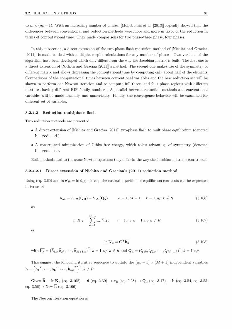
3.2. REDUCTION METHODS 81

to m× (np− 1). With an increasing number of phases, [Mohebbinia et al. [2013]] logically showed that the

differences between conventional and reduction methods were more and more in favor of the reduction in

terms of computational time. They made comparisons for two phase-three phase, four phases.

In this subsection, a direct extension of the two-phase flash reduction method of [Nichita and Graciaa

[2011]] is made to deal with multiphase split calculations for any number of phases. Two versions of the

algorithm have been developed which only differs from the way the Jacobian matrix is built. The first one is

a direct extension of [Nichita and Graciaa [2011]]’s method. The second one makes use of the symmetry of

different matrix and allows decreasing the computational time by computing only about half of the elements.

Comparisons of the computational times between conventional variables and the new reduction set will be

shown to perform one Newton iteration and to compute full three- and four phase regions with different

mixtures having different BIP family numbers. A parallel between reduction methods and conventional

variables will be made formally, and numerically. Finally, the convergence behavior will be examined for

different set of variables.

3.2.4.2 Reduction multiphase flash

Two reduction methods are presented:

• A direct extension of [Nichita and Graciaa [2011]] two-phase flash to multiphase equilibrium (denoted

h− red.− d.)

• A constrained minimization of Gibbs free energy, which takes advantage of symmetry (denoted

h− red.− s.).

Both methods lead to the same Newton equation; they differ in the way the Jacobian matrix is constructed.

3.2.4.2.1 Direct extension of Nichita and Graciaa’s (2011) reduction method

Using (eq. 3.60) and lnKik = lnφiR− lnφik, the natural logarithm of equilibrium constants can be expressed

in terms of

hαk = hαR (QR)− hαk (Qk) ; α = 1,M + 1; k = 1, np; k 6= R (3.106)

as

lnKik =

M+1∑α=1

qαihαk; i = 1, nc; k = 1, np; k 6= R (3.107)

or

ln Kk = CThk (3.108)

with hk =(h1k, h2k, · · · , hM+1,k

)T; k = 1, np; k 6= R and Qk = (Q1k, Q2k, · · · , QM+1,k)

T; k = 1, np.

This suggest the following iterative sequence to update the (np − 1) × (M + 1) independent variables

h =(h1

T, · · · ,hk

T, · · · ,hnp

T)T

; k 6= R:

Given h→ ln Kk (eq. 3.108) → θ (eq. 2.30) → xk (eq. 2.28) → Qk (eq. 3.47) → h (eq. 3.54, eq. 3.55,

eq. 3.56)→ New h (eq. 3.106).

The Newton iteration equation is

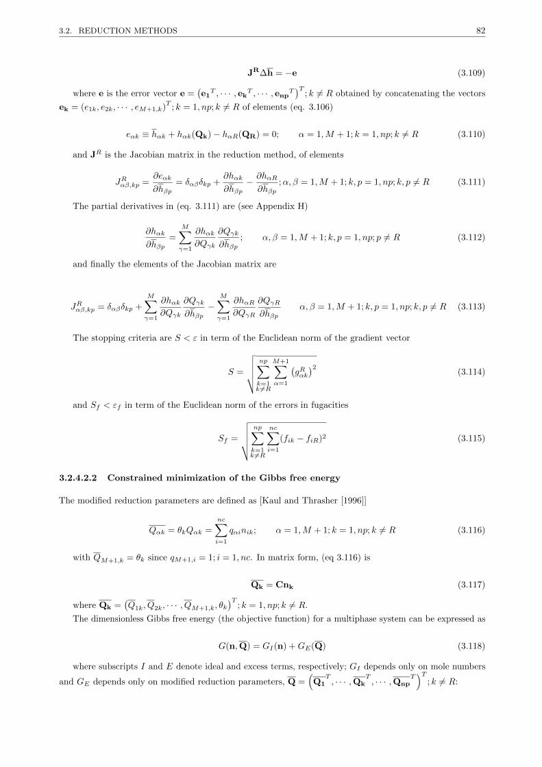
3.2. REDUCTION METHODS 82

JR∆h = −e (3.109)

where e is the error vector e =(e1T , · · · , ek

T , · · · , enpT)T

; k 6= R obtained by concatenating the vectors

ek = (e1k, e2k, · · · , eM+1,k)T

; k = 1, np; k 6= R of elements (eq. 3.106)

eαk ≡ hαk + hαk(Qk)− hαR(QR) = 0; α = 1,M + 1; k = 1, np; k 6= R (3.110)

and JR is the Jacobian matrix in the reduction method, of elements

JRαβ,kp =∂eαk

∂hβp= δαβδkp +

∂hαk

∂hβp− ∂hαR

∂hβp;α, β = 1,M + 1; k, p = 1, np; k, p 6= R (3.111)

The partial derivatives in (eq. 3.111) are (see Appendix H)

∂hαk

∂hβp=

M∑γ=1

∂hαk∂Qγk

∂Qγk

∂hβp; α, β = 1,M + 1; k, p = 1, np; p 6= R (3.112)

and finally the elements of the Jacobian matrix are

JRαβ,kp = δαβδkp +

M∑γ=1

∂hαk∂Qγk

∂Qγk

∂hβp−

M∑γ=1

∂hαR∂QγR

∂QγR

∂hβpα, β = 1,M + 1; k, p = 1, np; k, p 6= R (3.113)

The stopping criteria are S < ε in term of the Euclidean norm of the gradient vector

S =

√√√√√ np∑k=1k 6=R

M+1∑α=1

(gRαk)2

(3.114)

and Sf < εf in term of the Euclidean norm of the errors in fugacities

Sf =

√√√√√ np∑k=1k 6=R

nc∑i=1

(fik − fiR)2 (3.115)

3.2.4.2.2 Constrained minimization of the Gibbs free energy

The modified reduction parameters are defined as [Kaul and Thrasher [1996]]

Qαk = θkQαk =

nc∑i=1

qαinik; α = 1,M + 1; k = 1, np; k 6= R (3.116)

with QM+1,k = θk since qM+1,i = 1; i = 1, nc. In matrix form, (eq 3.116) is

Qk = Cnk (3.117)

where Qk =(Q1k, Q2k, · · · , QM+1,k, θk

)T; k = 1, np; k 6= R.

The dimensionless Gibbs free energy (the objective function) for a multiphase system can be expressed as

G(n,Q) = GI(n) +GE(Q) (3.118)

where subscripts I and E denote ideal and excess terms, respectively; GI depends only on mole numbers

and GE depends only on modified reduction parameters, Q =(Q1

T, · · · ,Qk

T, · · · ,Qnp

T)T

; k 6= R:

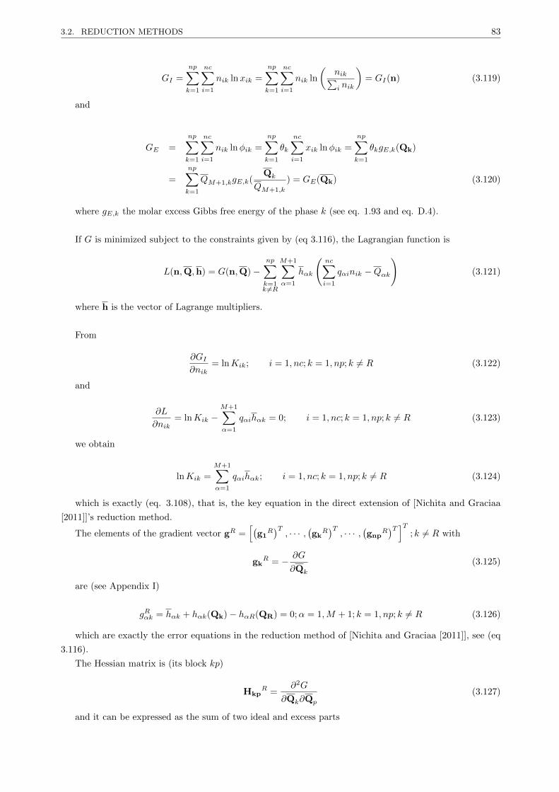
3.2. REDUCTION METHODS 83

GI =

np∑k=1

nc∑i=1

nik lnxik =

np∑k=1

nc∑i=1

nik ln

(nik∑i nik

)= GI(n) (3.119)

and

GE =

np∑k=1

nc∑i=1

nik lnφik =

np∑k=1

θk

nc∑i=1

xik lnφik =

np∑k=1

θkgE,k(Qk)

=

np∑k=1

QM+1,kgE,k(Qk

QM+1,k

) = GE(Qk) (3.120)

where gE,k the molar excess Gibbs free energy of the phase k (see eq. 1.93 and eq. D.4).

If G is minimized subject to the constraints given by (eq 3.116), the Lagrangian function is

L(n,Q,h) = G(n,Q)−np∑k=1k 6=R

M+1∑α=1

hαk

(nc∑i=1

qαinik −Qαk

)(3.121)

where h is the vector of Lagrange multipliers.

From

∂GI∂nik

= lnKik; i = 1, nc; k = 1, np; k 6= R (3.122)

and

∂L

∂nik= lnKik −

M+1∑α=1

qαihαk = 0; i = 1, nc; k = 1, np; k 6= R (3.123)

we obtain

lnKik =

M+1∑α=1

qαihαk; i = 1, nc; k = 1, np; k 6= R (3.124)

which is exactly (eq. 3.108), that is, the key equation in the direct extension of [Nichita and Graciaa

[2011]]’s reduction method.

The elements of the gradient vector gR =[(

g1R)T, · · · ,

(gk

R)T, · · · ,

(gnp

R)T ]T

; k 6= R with

gkR = − ∂G

∂Qk

(3.125)

are (see Appendix I)

gRαk = hαk + hαk(Qk)− hαR(QR) = 0;α = 1,M + 1; k = 1, np; k 6= R (3.126)

which are exactly the error equations in the reduction method of [Nichita and Graciaa [2011]], see (eq

3.116).

The Hessian matrix is (its block kp)

HkpR =

∂2G

∂Qk∂Qp

(3.127)

and it can be expressed as the sum of two ideal and excess parts

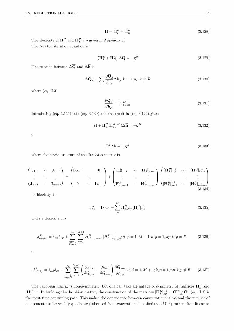
3.2. REDUCTION METHODS 84

H = HRI + HR

E (3.128)

The elements of HRI and HR

E are given in Appendix J.

The Newton iteration equation is

(HRI + HR

E

)∆Q = −gR (3.129)

The relation between ∆Q and ∆h is

∆Qk =∑p

∂Qk

∂hp∆hp; k = 1, np; k 6= R (3.130)

where (eq. J.3)

∂Qk

∂hp= [HR

I ]−1kp (3.131)

Introducing (eq. 3.131) into (eq. 3.130) and the result in (eq. 3.129) gives

(I + HRE [HR

I ]−1)∆h = −gR (3.132)

or

JR∆h = −gR (3.133)

where the block structure of the Jacobian matrix is

J11 · · · J1,nc

.... . .

...

Jnc,1 · · · Jnc,nc

=

IM+1 0

. . .

0 · · · IM+1

+

HRE,1,1 · · · HR

E,1,nc

.... . .

...

HRE,nc,1 · · · HR

E,nc,nc

[HRI ]−1

1,1 · · · [HRI ]−1

1,nc

.... . .

...

[HRI ]−1nc,1 · · · [HR

I ]−1nc,nc

(3.134)

its block kp is

JRkp = IM+1 +

nc∑m

HRE,km[HR

I ]−1mp (3.135)

and its elements are

JRαβ,kp = δαβδkp +

np∑m=1m 6=R

M+1∑γ=1

HRE,αγ,km

[HRI

]−1

γβ,mp;α, β = 1,M + 1; k, p = 1, np; k, p 6= R (3.136)

or

JRαβ,kp = δαβδkp +

np∑m=1m 6=R

M+1∑γ=1

(∂hαk

∂Qγm− ∂hαR

∂Qγm

)∂Qγm

∂hβp;α, β = 1,M + 1; k, p = 1, np; k, p 6= R (3.137)

The Jacobian matrix is non-symmetric, but one can take advantage of symmetry of matrices HRE and

[HRI ]−1. In building the Jacobian matrix, the construction of the matrices [HR

I ]−1kp = CU−1

kp CT (eq. J.3) is

the most time consuming part. This makes the dependence between computational time and the number of

components to be weakly quadratic (inherited from conventional methods via U−1) rather than linear as

3.2. REDUCTION METHODS 85

usually in reduction methods. Instead, we can use the following equations to relate([HR

I ]−1)αβ,kp

to the

partial derivatives ∂Qαk∂hβp

and ∂θk∂hβp

∂Qαk∂hβp

= θk∂Qαk∂hβp

+Qαk∂θk∂hβp

;α = 1,M ;β = 1,M + 1; k, p = 1, np; k, p 6= R (3.138)

and

∂QM+1,k

∂hβp=

∂θk∂hβp

;β = 1,M + 1; k, p = 1, np; k, p 6= R (3.139)

It had been proven [Nichita and Petitfrere [2013], Petitfrere and Nichita [2014b]] that the Newton iterations

in the reduction methods using the Lagrange multipliers as independent variables have the same convergence

paths as the conventional method with ln K variables.

3.2.4.3 Results

3.2.4.3.1 Mixtures

Three mixtures were tested. The Maljamar reservoir oil, the Maljamar separator oil from [Orr et al. [1981]]

and the sour gas mixture from [Robinson et al. [1978]]. All relevant data for these mixtures are taken from

[Li and Firoozabadi [2012]]. These three mixtures are mixed in different proportions with carbon dioxide to

obtain three- and four-phase regions; fig. 3.18a depicts the p-z phase envelope of the Maljamar separator oil

mixed with CO2 at T=305.35 K and fig. 3.18b the p-z phase envelope of the Maljamar reservoir oil mixed

with CO2 at the same temperature. Phase envelopes of the sourgas-CO2 (at T=178.8K) is given in fig. 3.19a.

Finally, taking the sour gas-CO2 mixture at a lower temperature, T=123.15 K, a four phase region can be

seen whose phase boundary is given in fig. 3.19b. It will be called the sourgas4 test case to differentiate from

the three phase sour gas test case at T=305.35 K. Note that all mixtures are exhibiting complicated phase

envelopes; some calculations are performed at extremely difficult conditions, such as the vicinity of bi-critical

points. The Peng-Robinson equation of state is used in all calculations.

CO2%

Pre

ssur

e,ba

r

65 70 75 80 85 90 95

66

68

70

72

74

76

V-L1-L2

L1-L2L1

V-L1

(a) Maljamar separator

CO2%

Pre

ssur

e,ba

r

60 65 70 75 80 85 90 9570

75

80

85

90

95

V-L1-L2

L1-L2

V-L2

(b) Maljamar reservoir

Figure 3.18: Phase envelopes of different mixtures mixed with CO2 at T=305.35 K

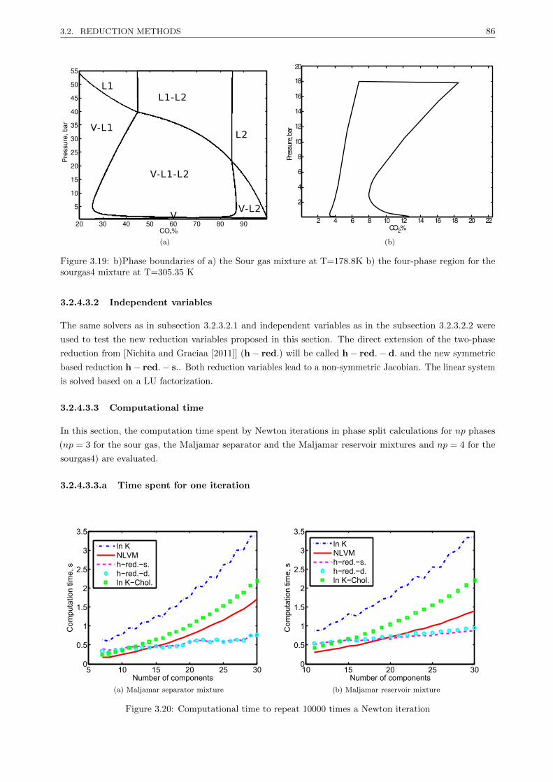
3.2. REDUCTION METHODS 86

CO2%

Pre

ssur

e,ba

r

20 30 40 50 60 70 80 90

5

10

15

20

25

30

35

40

45

50

55

L1-L2L1

V-L1

V-L1-L2

VV-L2

L2

(a)

CO2

Pres

sure

,bar

%2 4 6 8 10 12 14 16 18 20 22

2

4

6

8

10

12

14

16

18

20

(b)

Figure 3.19: b)Phase boundaries of a) the Sour gas mixture at T=178.8K b) the four-phase region for thesourgas4 mixture at T=305.35 K

3.2.4.3.2 Independent variables

The same solvers as in subsection 3.2.3.2.1 and independent variables as in the subsection 3.2.3.2.2 were

used to test the new reduction variables proposed in this section. The direct extension of the two-phase

reduction from [Nichita and Graciaa [2011]] (h− red.) will be called h− red.− d. and the new symmetric

based reduction h− red.− s.. Both reduction variables lead to a non-symmetric Jacobian. The linear system

is solved based on a LU factorization.

3.2.4.3.3 Computational time

In this section, the computation time spent by Newton iterations in phase split calculations for np phases

(np = 3 for the sour gas, the Maljamar separator and the Maljamar reservoir mixtures and np = 4 for the

sourgas4) are evaluated.

3.2.4.3.3.a Time spent for one iteration

5 10 15 20 25 300

0.5

1

1.5

2

2.5

3

3.5

Number of components

Com

puta

tion

time,

s

ln KNLVMh−red.−s.h−red.−d.ln K−Chol.

(a) Maljamar separator mixture

10 15 20 25 300

0.5

1

1.5

2

2.5

3

3.5

Number of components

Com

puta

tion

time,

s

ln KNLVMh−red.−s.h−red.−d.ln K−Chol.

(b) Maljamar reservoir mixture

Figure 3.20: Computational time to repeat 10000 times a Newton iteration

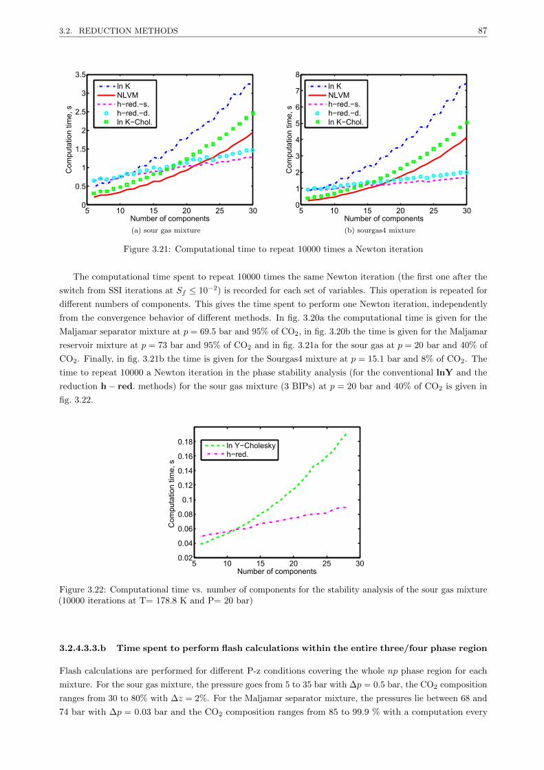
3.2. REDUCTION METHODS 87

5 10 15 20 25 300

0.5

1

1.5

2

2.5

3

3.5

Number of components

Com

puta

tion

time,

s

ln KNLVMh−red.−s.h−red.−d.ln K−Chol.

(a) sour gas mixture

5 10 15 20 25 300

1

2

3

4

5

6

7

8

NumberMofMcomponents

Com

puta

tionM

time,

Ms

lnMKNLVMh−red.−s.h−red.−d.lnMK−Chol.

(b) sourgas4 mixture

Figure 3.21: Computational time to repeat 10000 times a Newton iteration

The computational time spent to repeat 10000 times the same Newton iteration (the first one after the

switch from SSI iterations at Sf ≤ 10−2) is recorded for each set of variables. This operation is repeated for

different numbers of components. This gives the time spent to perform one Newton iteration, independently

from the convergence behavior of different methods. In fig. 3.20a the computational time is given for the

Maljamar separator mixture at p = 69.5 bar and 95% of CO2, in fig. 3.20b the time is given for the Maljamar

reservoir mixture at p = 73 bar and 95% of CO2 and in fig. 3.21a for the sour gas at p = 20 bar and 40% of

CO2. Finally, in fig. 3.21b the time is given for the Sourgas4 mixture at p = 15.1 bar and 8% of CO2. The

time to repeat 10000 a Newton iteration in the phase stability analysis (for the conventional lnY and the

reduction h− red. methods) for the sour gas mixture (3 BIPs) at p = 20 bar and 40% of CO2 is given in

fig. 3.22.

5 10 15 20 25 300.02

0.04

0.06

0.08

0.1

0.12

0.14

0.16

0.18

Numberyofycomponents

Com

puta

tiony

time,

ys

lnyY−Choleskyh−red.

Figure 3.22: Computational time vs. number of components for the stability analysis of the sour gas mixture(10000 iterations at T= 178.8 K and P= 20 bar)

3.2.4.3.3.b Time spent to perform flash calculations within the entire three/four phase region

Flash calculations are performed for different P-z conditions covering the whole np phase region for each

mixture. For the sour gas mixture, the pressure goes from 5 to 35 bar with ∆p = 0.5 bar, the CO2 composition

ranges from 30 to 80% with ∆z = 2%. For the Maljamar separator mixture, the pressures lie between 68 and

74 bar with ∆p = 0.03 bar and the CO2 composition ranges from 85 to 99.9 % with a computation every

3.2. REDUCTION METHODS 88

0.03%. For the Maljamar reservoir, 70 bar ≤ p ≤ 87 bar and ∆p = 0.3 bar and for the CO2 composition, 75 %

≤ zCO2 ≤ 99.9% and ∆z = 0.3%. Finally, for the sourgas4 mixture, the tested pressures lie between p = 0.1

bar and p = 18 bar with ∆p = 0.5 bar and the CO2 composition ranges from 5% to 15% with ∆z = 0.2%.

For each condition and each set of variables, the computational time spent for the Newton iterations is

recorded between the switch from SSI iterations (at Sf ≤ 10−2) and convergence. The iterations are ended as

soon as Sf ≤ 10−7. Since the gradient is different in conventional and reduction methods, for some conditions,

the convergence criterion can be satisfied in the reduced norm (S ≤ 10−10), without being fulfilled in the

conventional norm. In this case, we end up the calculations since the reduction method has converged in its

space, and any gradient based optimization method would not decrease the error any further. Whenever a

Newton step does not decrease the Gibbs free energy, a switch back to the SSI procedure is performed.

Computational times for each p-z point are added to get the global computational time plotted in fig. 3.23a

and fig. 3.23b for the Maljamar mixtures and in fig. 3.24a and fig. 3.24b for the sour gas mixtures. The

average number of iterations to perform flash calculations using lnK, lnK−Chol. and h− red. within the

whole np phase region is given in table 3.4 for the four mixtures.

5 10 15 20 25 300

0.5

1

1.5

2

2.5

Number of components

Com

puta

tion

time,

s

ln KNLVMh−red.−s.h−red.−d.ln K−Chol.

(a) Maljamar separator mixture

10 15 20 25 300

0.2

0.4

0.6

0.8

1

1.2

1.4

NumberMofMcomponents

Com

puta

tionM

time,

Ms

lnMKNLVMh−red.−s.h−red.−d.lnMK−Chol.

(b) Maljamar reservoir mixture

Figure 3.23: Computational time for the entire three phase region

5 10 15 20 25 300

0.5

1

1.5

2

2.5

3

3.5

Number of components

Com

puta

tion

time,

s

ln KNLVMh−red.−s.h−red.−d.ln K− Chol.

(a)

5 10 15 20 25 300

0.5

1

1.5

2

Number of components

Com

puta

tion

time,

s

ln KNLVMh−red.−s.h−red.−d.ln K− Chol.

(b)

Figure 3.24: Computational time for a) the entire three phase region for the sour gas mixture; b) the entirefour phase region for the sourgas4 mixture

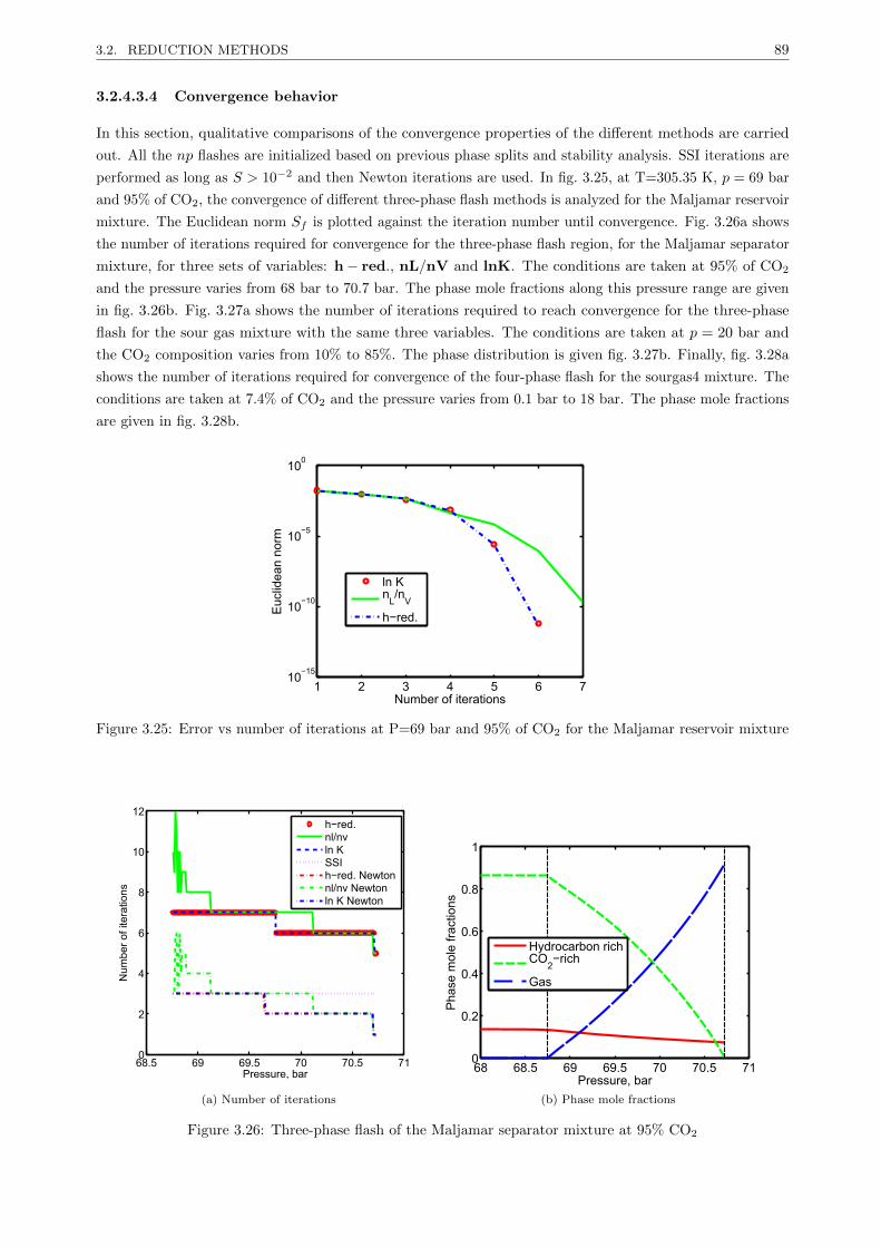
3.2. REDUCTION METHODS 89

3.2.4.3.4 Convergence behavior

In this section, qualitative comparisons of the convergence properties of the different methods are carried

out. All the np flashes are initialized based on previous phase splits and stability analysis. SSI iterations are

performed as long as S > 10−2 and then Newton iterations are used. In fig. 3.25, at T=305.35 K, p = 69 bar

and 95% of CO2, the convergence of different three-phase flash methods is analyzed for the Maljamar reservoir

mixture. The Euclidean norm Sf is plotted against the iteration number until convergence. Fig. 3.26a shows

the number of iterations required for convergence for the three-phase flash region, for the Maljamar separator

mixture, for three sets of variables: h− red., nL/nV and lnK. The conditions are taken at 95% of CO2

and the pressure varies from 68 bar to 70.7 bar. The phase mole fractions along this pressure range are given

in fig. 3.26b. Fig. 3.27a shows the number of iterations required to reach convergence for the three-phase

flash for the sour gas mixture with the same three variables. The conditions are taken at p = 20 bar and

the CO2 composition varies from 10% to 85%. The phase distribution is given fig. 3.27b. Finally, fig. 3.28a

shows the number of iterations required for convergence of the four-phase flash for the sourgas4 mixture. The

conditions are taken at 7.4% of CO2 and the pressure varies from 0.1 bar to 18 bar. The phase mole fractions

are given in fig. 3.28b.

1 2 3 4 5 6 710

−15

10−10

10−5

100

Number.of.iterations

Euc

lidea

n.no

rm

ln.Kn

L/n

V

h−red.

Figure 3.25: Error vs number of iterations at P=69 bar and 95% of CO2 for the Maljamar reservoir mixture

68.5 69 69.5 70 70.5 710

2

4

6

8

10

12

Pressure,Kbar

Num

berK

ofKit

erat

ions

h−red.nl/nvlnKKSSIh−red.KNewtonnl/nvKNewtonlnKKKNewton

(a) Number of iterations

68 68.5 69 69.5 70 70.5 710

0.2

0.4

0.6

0.8

1

Pressure, bar

Phasemolefractions

Hydrocarbon richCO

2−rich

Gas

(b) Phase mole fractions

Figure 3.26: Three-phase flash of the Maljamar separator mixture at 95% CO2

3.2. REDUCTION METHODS 90

30 40 50 60 70 80 900

5

10

15

20

25

30

CO2 %

Numberofiterations

h−red.nl/nvln KSSIh−red. Newtonnl/nv Newtonln K Newton

(a) Number of iterations

30 40 50 60 70 80 900

0.2

0.4

0.6

0.8

1

CO2 %

Phasemolefractions

GasCO

2rich

Hydrocarbon rich

(b) Phase mole fractions

Figure 3.27: Three-phase flash of the sour gas mixture at P=20 bar

0 2 4 6 8 10 12 14 16 181

2

3

4

5

6

7

8

9

10

Pressure,hbar

Num

berh

ofhit

erat

ions

lnhKNLVMh−red.SSIlnhKhNewtonNLVMhNewtonh−red.hNewton

(a) Number of iterations

0 5 10 150

0.2

0.4

0.6

0.8

1

Pressure, bar

Phasemolefractions

Gas

H2S rich

Hydrocarbon rich

CO2 rich

(b) Phase mole fractions

Figure 3.28: Four-phase flash of the sour gas mixture at 7.4% CO2

3.2.4.4 Discussion

From fig. 3.20a to fig. 3.21b and from fig. 3.23a to fig. 3.24b, it is observed that the curves of CPU time vs.

nc are crossing each other at slightly different values of nc if we look at the time per Newton iteration and at

the time to perform Newton iterations over the entire np phase region. There are several explanations for

these differences:

• If a Newton iteration does not decrease the Gibbs free energy, a switch back to SSI is performed (but

the time to compute second-order information and to solve the linear system is recorded)

• Theoretically the convergence path of lnK and h− red. methods is the same (see for instance in

fig. 3.25 that the curves are overlapping at each iteration); in practice, this is the case for most of the

points in the three-phase region.

However, for difficult conditions, h− red. may require more iterations for convergence than the conventional

lnK method (see certain differences in the average number of iterations in table 3.4. This is due to the

approximation errors (the condition number in reduction methods has been revealed by [Petitfrere and

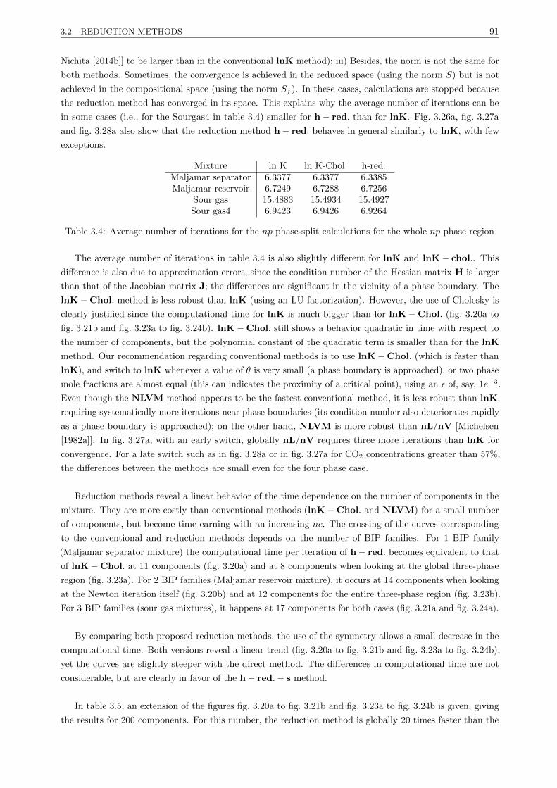
3.2. REDUCTION METHODS 91

Nichita [2014b]] to be larger than in the conventional lnK method); iii) Besides, the norm is not the same for

both methods. Sometimes, the convergence is achieved in the reduced space (using the norm S) but is not

achieved in the compositional space (using the norm Sf ). In these cases, calculations are stopped because

the reduction method has converged in its space. This explains why the average number of iterations can be

in some cases (i.e., for the Sourgas4 in table 3.4) smaller for h− red. than for lnK. Fig. 3.26a, fig. 3.27a

and fig. 3.28a also show that the reduction method h− red. behaves in general similarly to lnK, with few

exceptions.

Mixture ln K ln K-Chol. h-red.Maljamar separator 6.3377 6.3377 6.3385Maljamar reservoir 6.7249 6.7288 6.7256

Sour gas 15.4883 15.4934 15.4927Sour gas4 6.9423 6.9426 6.9264

Table 3.4: Average number of iterations for the np phase-split calculations for the whole np phase region

The average number of iterations in table 3.4 is also slightly different for lnK and lnK− chol.. This

difference is also due to approximation errors, since the condition number of the Hessian matrix H is larger

than that of the Jacobian matrix J; the differences are significant in the vicinity of a phase boundary. The

lnK−Chol. method is less robust than lnK (using an LU factorization). However, the use of Cholesky is

clearly justified since the computational time for lnK is much bigger than for lnK−Chol. (fig. 3.20a to

fig. 3.21b and fig. 3.23a to fig. 3.24b). lnK−Chol. still shows a behavior quadratic in time with respect to

the number of components, but the polynomial constant of the quadratic term is smaller than for the lnK

method. Our recommendation regarding conventional methods is to use lnK−Chol. (which is faster than

lnK), and switch to lnK whenever a value of θ is very small (a phase boundary is approached), or two phase

mole fractions are almost equal (this can indicates the proximity of a critical point), using an ε of, say, 1e−3.

Even though the NLVM method appears to be the fastest conventional method, it is less robust than lnK,

requiring systematically more iterations near phase boundaries (its condition number also deteriorates rapidly

as a phase boundary is approached); on the other hand, NLVM is more robust than nL/nV [Michelsen

[1982a]]. In fig. 3.27a, with an early switch, globally nL/nV requires three more iterations than lnK for

convergence. For a late switch such as in fig. 3.28a or in fig. 3.27a for CO2 concentrations greater than 57%,

the differences between the methods are small even for the four phase case.

Reduction methods reveal a linear behavior of the time dependence on the number of components in the

mixture. They are more costly than conventional methods (lnK−Chol. and NLVM) for a small number

of components, but become time earning with an increasing nc. The crossing of the curves corresponding

to the conventional and reduction methods depends on the number of BIP families. For 1 BIP family

(Maljamar separator mixture) the computational time per iteration of h− red. becomes equivalent to that

of lnK−Chol. at 11 components (fig. 3.20a) and at 8 components when looking at the global three-phase

region (fig. 3.23a). For 2 BIP families (Maljamar reservoir mixture), it occurs at 14 components when looking

at the Newton iteration itself (fig. 3.20b) and at 12 components for the entire three-phase region (fig. 3.23b).

For 3 BIP families (sour gas mixtures), it happens at 17 components for both cases (fig. 3.21a and fig. 3.24a).

By comparing both proposed reduction methods, the use of the symmetry allows a small decrease in the

computational time. Both versions reveal a linear trend (fig. 3.20a to fig. 3.21b and fig. 3.23a to fig. 3.24b),

yet the curves are slightly steeper with the direct method. The differences in computational time are not

considerable, but are clearly in favor of the h− red.− s method.

In table 3.5, an extension of the figures fig. 3.20a to fig. 3.21b and fig. 3.23a to fig. 3.24b is given, giving

the results for 200 components. For this number, the reduction method is globally 20 times faster than the

3.2. REDUCTION METHODS 92

conventional method lnK−Chol. for three phases. For four-phases, it becomes 35 times faster. As expected,

for a system with more phases, conventional and reduction methods become equivalent for a smaller number

of components. For the sour gas mixture in fig. 3.24a with three phases, the crossing occurs at 17 components

and in fig. 3.24b for four phases at 15 components.

Mixture h-red. ln K-Chol.Maljamar separator 3.6 95.27Maljamar reservoir 4.69 101.85

Sour gas 5.87 104.6Sour gas4 7.09 245.03

Table 3.5: Computational time per 10000 iterations for conventional and reduction Newton iterations at 200components

The reduction method is faster than lnK (if symmetry is not used) even for a small number of components.

This shows the importance of the linear solver; when a comparison of conventional and reduction methods

is reported, it is thus mandatory to report also how the symmetry properties were used in the conventional case.

In all examples, only the np phase-split calculation results are exposed. Results for stability analysis

and two phase flash calculations (comparison between conventional and reduction methods) were given in

[Petitfrere and Nichita [2014b]]. The global multiphase calculation procedure follows [Michelsen [1982a]],

that is, one or two stability analysis are performed for the feed composition for the vapor and/or liquid trial

phases. Then alternatively with an np− 1 phase-split calculations, at least 7 initial guesses (from [Li and

Firoozabadi [2012]]) are tried to test the stability of one equilibrium phase. This means that the global time

for a three-phase calculation is given by 7/8 stability analysis, one two-phase flash and one three-phase flash.

It has been shown [Petitfrere and Nichita [2014b]] that h− red. performed the stability analysis faster than

the conventional methods or up to 2 nonzero BIP families. For the sour gas mixture (3 nonzero BIP families),

the computational time for the stability analysis is given fig. 3.22. In this case, h− red. becomes equivalent

to lnK−Chol. in terms of computational time for 12 components. For all mixtures, if we were to add the

time to compute the stability analysis to the time to compute the two and three phase flashes, the crossing

between the curves corresponding to conventional and reduction methods will appear before those exposed

in fig. 3.20a to fig. 3.21b and fig. 3.23a to fig. 3.24b. Moreover, the time spent by SSI iterations before the

switch was not taken into account. (an SSI iteration is faster in reduction methods, since the evaluation of a

quadratic form is avoided). If we took into account all these times, this will tend to bring the crossing of

conventional/reduction curves at smaller values of nc than in fig. 3.20a to fig. 3.21b and fig. 3.23a to fig. 3.24b

(for example, for the sour gas the crossing is expected to occur somewhere in between 12 and 17).

3.2.4.5 Conclusions

In this work, the reduction methodology of [Nichita and Graciaa [2011]] is extended to multiphase flash

calculations with any number of phases. The independent variables are unbounded and derive directly from

a constrained minimization of the Gibbs free energy. Moreover, theoretically it has been proven that the

convergence path was equivalent than for lnK; this was confirmed numerically, except from some difficult

conditions (when the system is not too ill-conditioned).

Two versions of the new method are developed. The first one is a direct extension of the two phase

reduction method from [Nichita and Graciaa [2011]]. The second one makes use of the symmetry and allows

building the Jacobian matrix computing about only half of the elements. The use of the symmetry slightly

decreases the computational time, as compared with the direct method. The reduction methods allow a

linear growth of computational time with respect to the number of components, while a quadratic trend is

observed for conventional formulations. Both versions of the reduction method proved to be more efficient

3.3. PHASE EQUILIBRIUM CALCULATIONS WITH QUASI-NEWTON METHODS 93

than conventional methods after a certain number of components.

For reservoir simulation purposes, the new methodology could be competitive for a small number of BIP

families (< 3). For a large number of components in the mixture (as encountered in chemical processing),

the differences between computational times required by conventional and reduction methods are really

important; reduction variables can have a huge impact on computational time for such problems. Finally, it

is worth mentioning that a big advantage of the reduction methods is that a detailed composition can be

used; no lumping is required (thus no approximations). Lumping may affect to a high extent the location

and size of tiny three-phase regions [Nichita et al. [2006b]].

3.3 Phase equilibrium calculations with quasi-Newton methods

3.3.1 Introduction

The second order Newton methods is the most commonly used in phase equilibrium calculations; however,

their convergence radius can be small, and a number of first order successive substitutions iterations must be

performed before switching to Newton iterations. In this section, we focus on other kinds of minimization

methods: the quasi-Newton ones, which represent interesting alternatives. Their convergence radius is

larger, there is no need to solve a linear system, and the Hessian matrix is approximated with a very low

computational cost. However, quasi-Newton methods are extremely sensitive to scaling; It will be shown that

that physical variables (mole number) are not suited for the quasi-Newton method.

The BFGS method [Broyden [1970], Fletcher [1970], Goldfarb [1970], Shanno [1970]] exhibits a supra-

linear convergence rate. A rank two update of the Hessian matrix at each iteration guarantees its positive

definiteness. The BFGS algorithm has already been applied to both for stability testing and phase-split

problems [Ammar and Renon [1987], Garcia-Sanchez et al. [1996], Garcia-Sanchez et al. [2001], Hoteit and

Firoozabadi [2006]].

For the stability analysis problem, [Michelsen [1982b]] proposed a set of independent variables which

allows a good scaling of the problem and a better conditioned system; using this set, the BFGS method

proved to be quite competitive [Hoteit and Firoozabadi [2006]]. In this work, we develop a methodology for

finding the appropriate change of variables to obtain the best scaling for phase equilibrium problems; applied

to the flash calculation problem, the resulting change of variables lead to a Hessian matrix with a perfect

scaling, i.e., H = I + D + ND, where I is the identity matrix, D is a diagonal matrix with elements vanishing

at the solution, and ND is an effective low-rank matrix with non-diagonal terms.

3.3.2 The BFGS quasi-Newton method

3.3.2.1 Newton

Let f(x) be the function to minimize and x = [x1, · · · , xN ]. Let xk stands for the vector x at the kth iteration.

The minimum is obtained for

g(x) = ∇f(x) = 0 (3.140)

The Newton method enables a quadratic convergence by means of the update:

xk+1 = xk −H−1k gk (3.141)

with gk is the gradient vector and Hk is the Hessian matrix:

3.3. PHASE EQUILIBRIUM CALCULATIONS WITH QUASI-NEWTON METHODS 94

gk = ∇f(xk) Hk = ∇2f(xk) (3.142)

3.3.2.2 The BFGS update

The BFGS algorithm approximates the Hessian matrix H by means of a matrix B, depending on the function

f and the gradient g. The approximation of the Hessian matrix Bk is updated at each iteration by:

Bk+1 = Bk +ykyk

T

ykTpk

− BkpkpkTBk

pkTBkpk

(3.143)

with

yk = ∇f(xk)−∇f(xk−1) (3.144)

and

pk = xk − xk−1 (3.145)

As it is a rank-two update matrix, the Sherman-Morrison formula can be used twice to update directly

the inverse of the matrix:

Bk+1−1 = Bk

−1 +

(pk

Tyk + ykTBk

−1yk

)(pkpk

T )

(ykTpk)

2 − Bk−1ykpk

T + pkykTBk

−1

pkTyk

(3.146)

As the Hessian matrix is approximated, the order of the method is decreased as compared to the Newton

algorithm. The BFGS methods lead to a supra-linear convergence. The update of the variables is given by:

xk+1 = xk −B−1k gk (3.147)

If Bk ≈ Hk, the convergence is nearly quadratic. The first step is carried out choosing B1 = I, which

corresponds to a gradient descent step. This approximation only requires the evaluation of the gradient

(first derivatives of the Gibbs energy, which corresponds here to calculate the fugacities). Besides, as the

inverse of the Hessian is updated directly, no linear system needs to be solved. This can be really time saving

when dealing with multiphase systems with a high number of components. An important feature is that

the construction of BFGS formula guarantees the positive definiteness of the matrix, hence it guarantees a

descent direction (unlike the Newton method, in which the Hessian matrix is not guaranteed to be positive

definite). In practice, a line search procedure is used with quasi-Newton methods:

xk+1 = xk − λB−1k gk (3.148)

with λ a real computed based on a line search procedure.

3.3.2.3 The Line search procedure

We introduce the descent direction vector:

sk = −B−1k gk (3.149)

The line search algorithm solves λ which will sufficiently decrease the Gibbs energy f within the Wolfe

norm. It is a one dimension minimization, the objective function being here considered as a function only of

λ:

f(λ) = f(xk + λsk) (3.150)

3.3. PHASE EQUILIBRIUM CALCULATIONS WITH QUASI-NEWTON METHODS 95

3.3.2.3.1 The Wolfe conditions

The methods to solve for λ are generally iterative. Let λi be the ith iterate on the variable λ , and λ0 = 0.

The vector solution for the line search procedure is

ul = xk + λlsk (3.151)

and let us introduce the notations

fl = f(λl) gl(x) = ∇fl(x) =

[∂fl∂x1

, · · · , ∂fl∂xnc

]g′l = gl

T sk (3.152)

The iterate ul must satisfy the (weak) Wolfe criteriafl ≤ f0 + c1λlg′0

g′l ≤ c2|g′0|

In this work, c1 = 1d− 4 and c2 = 0.9.

Starting from λ1 = 1 (equivalent to procedures without line search), if u1 does not satisfy the Wolfe

conditions, λl+1 is calculated. The iteration procedure to update λ is based on a polynomial interpolation of

the function f [Nocedal and Wright [2006]].

3.3.2.3.2 Second order polynomial interpolation

If λ1 = 1 does not satisfy the Wolfe conditions, in a first step, the function f is approximated with a second

order polynomial function

f(λ) = aλ2 + bλ+ c (3.153)

Using (eq. 3.153) for λl and λ0 = 0, the difference fl − f0 is

fl − f0 = aλ2l + bλl (3.154)

Differentiating (eq.. 3.153) with respect to λ gives:

∂f(λ)

∂λ= 2aλ+ b (3.155)

or,

∂f(λ)

∂λ= gk

T sk = g′k (3.156)

Combining (eq. 3.155) and (eq. 3.156), for λ0 = 0 leads to:

g′0 = b (3.157)

We are looking for the minimum of f with respect to λ, which is obtained for ∂f(λ)∂λ = 0. Combining this

equation with (eq. 3.155) for λl+1, one obtains

2aλl+1 + b = 0 (3.158)

Solving the system based on (eq. 3.154, eq. 3.157 and eq. 3.158) leads to

λl+1 =−g′0λ2

l

2(fl − f0 − g′0λl)(3.159)

3.3. PHASE EQUILIBRIUM CALCULATIONS WITH QUASI-NEWTON METHODS 96

3.3.2.3.3 Third order polynomial interpolation

The function f is now approximated based on a cubic polynomial function:

f(λ) = aλ3 + bλ2 + cλ+ d (3.160)

Using (eq. 3.160) for λl and λ0=0, the difference fl − f0 is

fl − f0 − g′0λl = aλ3l + bλ2

l (3.161)

and using (eq. 3.160) for λl−1 and λ0 = 0, performing the same operation, one obtains

fl−1 − f0 − g′0λl−1 = aλ3l−1 + bλ2

l−1 (3.162)

We look for λl+1 which satisfies

∂f(λ)

∂λ= 3aλ2 + 2bλ+ c = 0 (3.163)

Combining (eq. 3.163) with (eq. 3.156) for λ0 = 0, we get

g′0 = c (3.164)

Besides, we are looking for the minimum of f with respect to λ, which is obtained for ∂f(λ)∂λ = 0. Combining

this equation with (eq. 3.163) for λl+1, one obtains

3aλ2l+1 + 2bλl+1 + c = 0 (3.165)

Combining (eq. 3.161 and eq. 3.162) leads to the following linear system:(λ3l λ2

l

λ3l−1 λ2

l−1

)(a

b

)=

(fl − f0 − g′0fl−1 − f0 − g′0

)(3.166)

The system is solved to obtain a and b and replacing a, b and c in (eq. 3.165), a second order polynomial

equation is solved to obtain λl+1. At each step, it is important to check if λl+1 remains in a correct range.

That is to say λl+1 < 0.5λl and λl+1 > 0.1λl.

In order to develop a reliable algorithm, in this work, a switch back procedure to SSI is performed (see the

BFGS algorithm). As soon as the BFGS update does not decrease the Gibbs free energy, an SSI step is used

instead to guarantee the convergence to the solution. In some situations, it could be more advantageous to

accept steps leading to an increase of the Gibbs energy. However, those methodologies are not totally reliable

for difficult conditions (near the phase boundaries for instance), and could lead to convergence problems.

3.3.2.4 Ammar and Renon BFGS implementation

[Ammar and Renon [1987]] proposed a BFGS implementation based on the logarithm of the equilibrium

constants ln K.From (eq. 3.35) and (eq. 3.33), the Newton iteration equation can be written as

J∆ ln K = HU−1∆ ln K = −g (3.167)

which is equivalent to:

U−1∆ ln K = −H−1g (3.168)

In the BFGS method, since the Hessian matrix H is approximated by the matrix B, the above eaquation

become

3.3. PHASE EQUILIBRIUM CALCULATIONS WITH QUASI-NEWTON METHODS 97

Algorithm 3.2 Line search algorithm

Given xk, f0, skCompute g′0 (eq. 3.156)end = 0λ1 = 1 and l = 1while end = 0 do

ul = xk + λlskCompute fl and g′lif Wolfe conditions are satisfied then

end=1else

if l = 1 thenUse second order interpolation to compute λl+1

elseUse third order interpolation to compute λl+1

end ifend ifif λl+1 > 0.5λl thenλl+1 = 0.5λl

end ifif λl+1 < 0.1λl thenλl+1 = 0.1λl

end ifl = l + 1

end while

Algorithm 3.3 BFGS algorithm

Given x0, B0 = Ik = 0Compute f0, g0

while ‖gk‖ ≤ ε doif k = 0 then

sk = −gk

elsepk = xk − xk−1

yk = gk − gk−1

Update Bk−1 using (eq. 3.146)

sk = −Bk−1gk

end ifSolve λ, xk+1 = xk + λsk (algorithm 3.2)Compute fk+1

if fk+1 > fk thenUpdate xk+1 based on SS iterationCompute fk+1

end ifCompute gk+1

k = k + 1

end while

U−1∆ ln K = −B−1g (3.169)

The vector ln K is updated at each iteration with two sequential updates. First

y = −B−1g (3.170)

and then a line search procedure is used to update ln K:

ln Kk+1 = ln Kk + λUy (3.171)

with the matrix U calculated from (eq. 3.30).

3.3. PHASE EQUILIBRIUM CALCULATIONS WITH QUASI-NEWTON METHODS 98

After each update, the Rachford-Rice equation is solved for the vapor mole fraction V , then composition

and mole numbers for each phase are calculated.

3.3.3 Proposed method

3.3.3.1 Two-phase split calculations

3.3.3.1.1 Alpha variables

Given a change of variables αi = αi(nL), by using the chain rule, the gradient vector is

gi =∂G

∂αi=

∂G

∂niL

∂niL∂αi

(3.172)

and the Hessian matrix is

Hij =∂2G

∂αi∂αj=

∂2G

∂niL∂njL

∂niL∂αi

∂njL∂αj

+∂G

∂niL

∂2niL∂αi∂αj

(3.173)

In order to obtain a well-scaled Hessian, that is, to have the identity matrix I as the first term in the

Hessian matrix expression in (eq. 3.27), the term δij/LV ui (with ui given in (eq. 3.31)) from∂2G

∂niL∂njL

must be multiplied by:∂niL∂αi

∂njL∂αj

, to obtain:

δijLV ui

∂niL∂αi

∂njL∂αj

= δij (3.174)

with

LV√ui√uj =

√niLniVzi

√njLnjVzj

(3.175)

By identification:

∂niL∂αi

=

√niLniVzi

(3.176)

and from (eq. 3.176)

αi =

∫ √zi√

niL(zi − niL)dniL (3.177)

Integration gives

αi = 2√zi arcsin

(√niLzi

)+ Ci (3.178)

Taking Ci = 0,

αi = 2√zi arcsin

(√niLzi

)(3.179)

Since 0 ≤ niL ≤ zi

0 ≤√niLzi≤ 1 (3.180)

The liquid mole fractions can be expressed as a function of αi:

√niL =

√zi sin

(αi

2√zi

)(3.181)

3.3. PHASE EQUILIBRIUM CALCULATIONS WITH QUASI-NEWTON METHODS 99

To ensure a bijective restriction one needs to bound αi:

αi ∈ [0, π√zi] (3.182)

Deriving the Gibbs free energy with respect to this variable leads to the gradient vector:

gi =

√niLniVzi

[(lnniL − lnL+ lnφiL)− (lnniV − lnV + lnφiV )] (3.183)

And the elements of the Hessian matrix are

Hij = δij −√uiuj(1 + LV Φij) + 1/2 δijgi

(niV − niL

zi

)(3.184)

3.3.3.1.2 Beta variables

A similar procedure can be used by deriving with respect of niV , to obtain:

βi = 2√zi arcsin

(√niVzi

)(3.185)

Which leads to the vapor mole numbers:

√niV =

√zi sin

(βi

2√zi

)(3.186)

Let us now establish the relation between αi and βi. Using (eq. 3.181),

niL = zisin2

(αi

2√zi

)(3.187)

The mass balance equation zi = niL + niV enables to compute niV

niV = zicos2

(αi

2√zi

)(3.188)

Similarly, from (eq. 3.186)

niV = zisin2

(βi

2√zi

)(3.189)

niL = zicos2

(βi

2√zi

)(3.190)

From (eq. 3.187) and (eq. 3.190), the following equation is obtained:

cos2

(βi

2√zi

)= sin2

(αi

2√zi

)(3.191)

Since, αi ∈[0, π√zi]

and βi ∈[0, π√zi], , cos

(βi

2√zi

)≥ 0 and sin

(αi

2√zi

)≥ 0

cos

(βi

2√zi

)= sin

(αi

2√zi

)(3.192)

Which leads to

αi = 2√zi arcsin

(cos

(βi

2√zi

))= 2√zi

(π

2− βi

2√zi

)(3.193)

Hence,

αi = π√zi − βi (3.194)

3.3. PHASE EQUILIBRIUM CALCULATIONS WITH QUASI-NEWTON METHODS 100

The gradient and the Hessian matrix using βi as independent variables are directly related to the gradient

and the Hessian matrix using αi as independent variables since

∂βi∂αj

= −δij (3.195)

and

∂2βi∂αj∂αk

= δijδik (3.196)

Hence, the Hessian is the same using both sets of independent variables, and the gradients are related by:

gαi = −gβi (3.197)

3.3.3.2 Stability analysis

The methodology proposed above can be applied to the phase stability problem. Given a change of variables

αi = αi(Y), using the chain rule, the gradient vector is

gi =∂G

∂αi=∂G

∂Yi

∂Yi∂αi

(3.198)

and the Hessian matrix is

Hij =∂2G

∂αi∂αj=

∂2G

∂Yi∂Yj

∂Yi∂αi

∂Yj∂αj

+∂G

∂Yi

∂2Yi∂αi∂αj

(3.199)

The term δij/Yi from ∂2G∂Yi∂Yj

must be multiplied by: ∂Yi∂αi

∂Yj∂αj

, to obtain:

δijYi

∂Yi∂αi

∂Yj∂αj

= δij (3.200)

Which gives by identification:

∂Yi∂αi

=√Yi (3.201)

From (eq. 3.200),

αi =

∫1√YidYi (3.202)

Integration gives

αi = 2√Yi + Ci (3.203)

Taking Ci = 0, the procedure leads to the αi variable introduced by [Michelsen [1982b]]. [Hoteit and

Firoozabadi [2006]] developed an efficient BFGS procedure based on these variables to solve stability analysis

problems.

3.3.4 Results

The BFGS algorithm (developed in a previous section) based on the proposed αi and βi variables has been

implemented. The robustness and the efficiency of the method are tested on two mixtures, providing also

comparisons with various methods from the literature [Ammar and Renon [1987], Liu and Nocedal [1989] and

Nocedal [1980]]. In this study, the Peng-Robinson equation of state was used, but it is important to mention

that the proposed method is independent of the EOS model and any equation of state could be used instead.

3.3. PHASE EQUILIBRIUM CALCULATIONS WITH QUASI-NEWTON METHODS 101

3.3.4.1 Tests on different BFGS methods

The BFGS algorithm has been implemented with different variables: α (called alpha), β (called beta) as

well as the mole numbers nL or nV (denoted nl/nv). Both variables α and β are linked and lead to the same

Hessian, and gαi = −gβi . Independent variables niV and βi are used if the mixture is predominantly liquid

(L > V ); otherwise, component mole numbers in the liquid phase, niL, and αi are taken as independent

variables [Nghiem et al. [1983]]. The procedure has been tested with and without the line search algorithm.

BFGS methods with a line search procedure have been attributed the suffix L (i.e., alpha− L, beta− L).

The procedure from [Ammar and Renon [1987]] is also implemented (it is denoted as lnK− L). We also

compared the results obtained with an open source L-BFGS-B code from Nocedal [Nocedal [1980], Liu and

Nocedal [1989]] against our own implementation of the BFGS method.

To simplify the notations, alpha and beta will be gathered into the same name (α).

3.3.4.2 Mixtures used in this study

Two mixtures were used in this study, the Y8 and the MY10 mixtures presented in subsection 3.2.2. For the

Y8 mixture, calculations on two different isotherms have been performed in this section: at T=285K (T < Tc

and close to the critical point) and T=335 K (T > Tc). For the MY10 mixture, calculations were performed

along an isotherm at T=565 K located close to the critical point.

3.3.4.3 Error and stopping criteria

The Euclidean norm of the of difference of the logarithm of the fugacities is used to evaluate the error for

each iteration:

Sf2 =

√√√√ nc∑i=1

(ln fiL − ln fiV )2

(3.204)

Convergence is assumed when Sf2 < 1e−8.

Moreover, the BFGS matrix is updated based on the differences between the iteration k and k + 1. When

the differences of the Gibbs free energy between two iterations become close to the machine error (fk ≈ fk−1),

convergence can be considered in this case. The same stopping criteria as [Nocedal [1980], Liu and Nocedal

[1989]] is used in this work:

S2 =fk−1 − fk

max (|fk| , |fk−1| , 1)< εεmachine (3.205)

Here, ε = 1d+ 3. The machine error is εmachine = 1d− 16.

3.3.4.4 Results

Two configurations were tested with different switching criteria. First, the BFGS has been used starting

directly from the Wilson initialization [Wilson [1969]]. Then, SSI steps were first performed before switching

to the BFGS method when Sf2 < 1e−2 (which corresponds to a late switch).

3.3.4.4.1 Starting directly without any SSI

In this section, the Wilson relation [Wilson [1969]] is used to initialize the equilibrium constants from which

the initial phase distribution is inferred, then the BFGS algorithm is applied without any previous SSI.

For the Y8 mixture, along the isotherm T=285 K (respectively T=335K), the number of iterations

required to reach convergence is plotted in fig. 3.29a (respectively in fig. 3.30a), with the corresponding

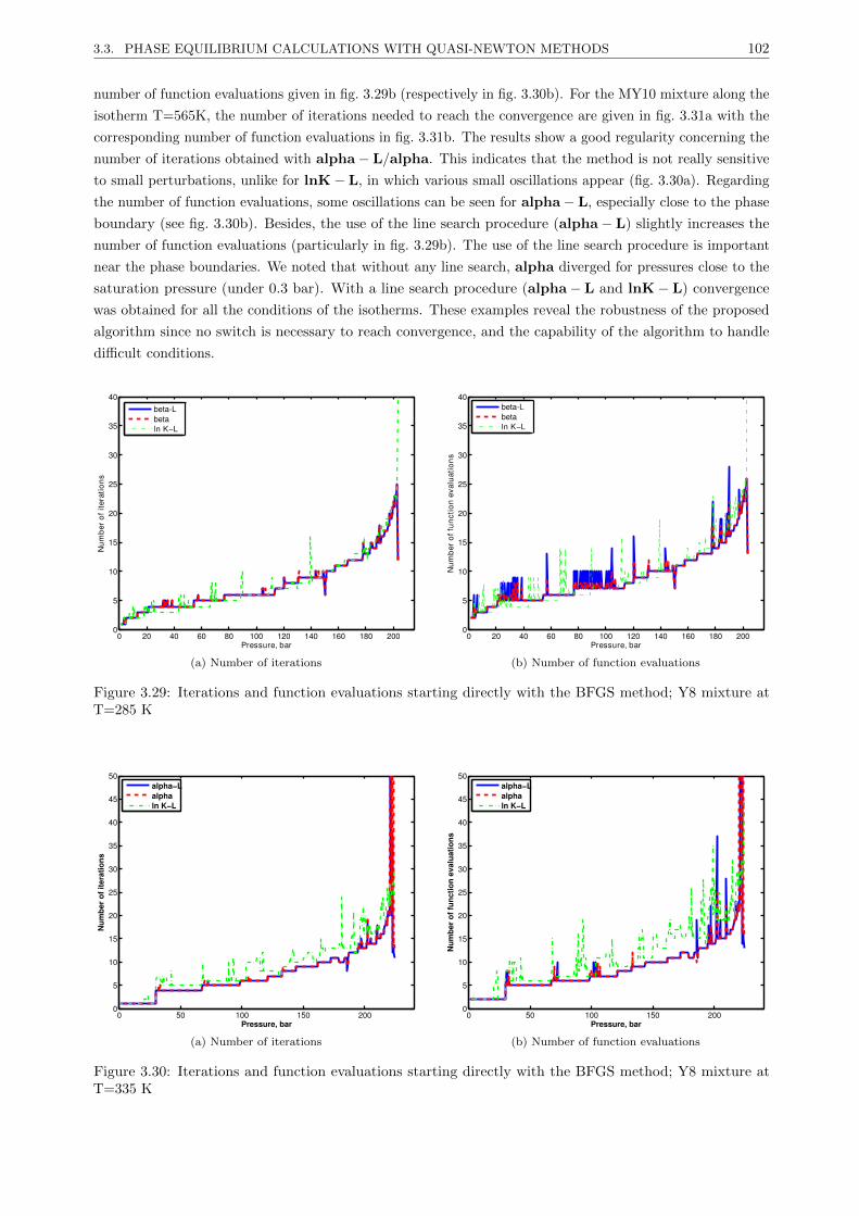
3.3. PHASE EQUILIBRIUM CALCULATIONS WITH QUASI-NEWTON METHODS 102

number of function evaluations given in fig. 3.29b (respectively in fig. 3.30b). For the MY10 mixture along the

isotherm T=565K, the number of iterations needed to reach the convergence are given in fig. 3.31a with the

corresponding number of function evaluations in fig. 3.31b. The results show a good regularity concerning the

number of iterations obtained with alpha− L/alpha. This indicates that the method is not really sensitive

to small perturbations, unlike for lnK− L, in which various small oscillations appear (fig. 3.30a). Regarding

the number of function evaluations, some oscillations can be seen for alpha− L, especially close to the phase

boundary (see fig. 3.30b). Besides, the use of the line search procedure (alpha− L) slightly increases the

number of function evaluations (particularly in fig. 3.29b). The use of the line search procedure is important

near the phase boundaries. We noted that without any line search, alpha diverged for pressures close to the

saturation pressure (under 0.3 bar). With a line search procedure (alpha− L and lnK− L) convergence

was obtained for all the conditions of the isotherms. These examples reveal the robustness of the proposed

algorithm since no switch is necessary to reach convergence, and the capability of the algorithm to handle

difficult conditions.

0 20 40 60 80 100 120 140 160 180 2000

5

10

15

20

25

30

35

40

Pressure, bar

Num

ber

ofite

ratio

ns

beta-Lbetaln K−L

(a) Number of iterations

0 20 40 60 80 100 120 140 160 180 2000

5

10

15

20

25

30

35

40

Pressure, bar

Num

ber

offu

nctio

nev

alua

tions

beta-Lbetaln K−L

(b) Number of function evaluations

Figure 3.29: Iterations and function evaluations starting directly with the BFGS method; Y8 mixture atT=285 K

0 50 100 150 2000

5

10

15

20

25

30

35

40

45

50

Pressure, bar

Num

berof

iteratio

ns

alpha−Lalphaln K−L

(a) Number of iterations

0 50 100 150 2000

5

10

15

20

25

30

35

40

45

50

Pressure, bar

Num

berof

func

tionev

alua

tions

alpha−Lalphaln K−L

(b) Number of function evaluations

Figure 3.30: Iterations and function evaluations starting directly with the BFGS method; Y8 mixture atT=335 K

3.3. PHASE EQUILIBRIUM CALCULATIONS WITH QUASI-NEWTON METHODS 103

30 40 50 60 70 80 900

5

10

15

20

25

30

35

40

45

50

Pressure, bar

Num

ber

ofite

ratio

ns

beta-Lbetaln K−L

(a) Number of iterations

30 40 50 60 70 80 900

10

20

30

40

50

60

70

Pressure, bar

Num

berof

functio

nevaluatio

ns

beta-Lbetaln K−L

(b) Number of function evaluations

Figure 3.31: Iterations and function evaluations starting directly with the BFGS method; MY10 mixture atT=565 K

Except for some low pressures, along the isotherm T=285 K for the Y8 mixture, the number of iterations

are generally smaller for alpha as compared with the lnK− L procedure. For the number of function

evaluations, the results are almost always in favor of the proposed method whatever the conditions, including

those close to the phase boundaries.

0 20 40 60 80 100 120 140 160 180 2000

5

10

15

20

25

30

35

40

Pressure, bar

Num

ber

ofite

ratio

ns

beta-Lbeta Nocedal

(a) Number of iterations

0 20 40 60 80 100 120 140 160 180 2000

5

10

15

20

25

30

35

40

Pressure, bar

Num

ber

offu

nctio

nev

alua

tions

beta-Lbeta Nocedal

(b) Number of function evaluations

Figure 3.32: Comparison between the proposed BFGS algorithm and Nocedal L-BFGS-B for the Y8 mixtureat T=285 K

Taking α or (β) as independent variables, a comparison of the L-BFGS-B code based on [Nocedal [1980],

Liu and Nocedal [1989]] and the proposed implementation of the BFGS method is presented for the Y8

mixture. Fig. 3.32a gives the number of iterations obtained for the Y8 mixture along the isotherm T=285K,

and fig. 3.33a for the isotherm T=335K. The corresponding number of function evaluations are given in

fig. 3.32b along T=285K and in fig. 3.33b along T=335K. In terms of number of iterations, Nocedal’s method

and alpha− L gives close results for pressures located away from the phase boundaries. Close to the phase

boundaries, oscillations can be noticed with Nocedal’s algorithm unlike for the proposed algorithm. Besides,

alpha− L requires less iterations to reach convergence and Nocedal’s algorithm generally requires at least

two more function evaluations to converge than the code based on the proposed method. Close to the

phase boundaries, Nocedal’s algorithm starts oscillating and the differences with the provided algorithm

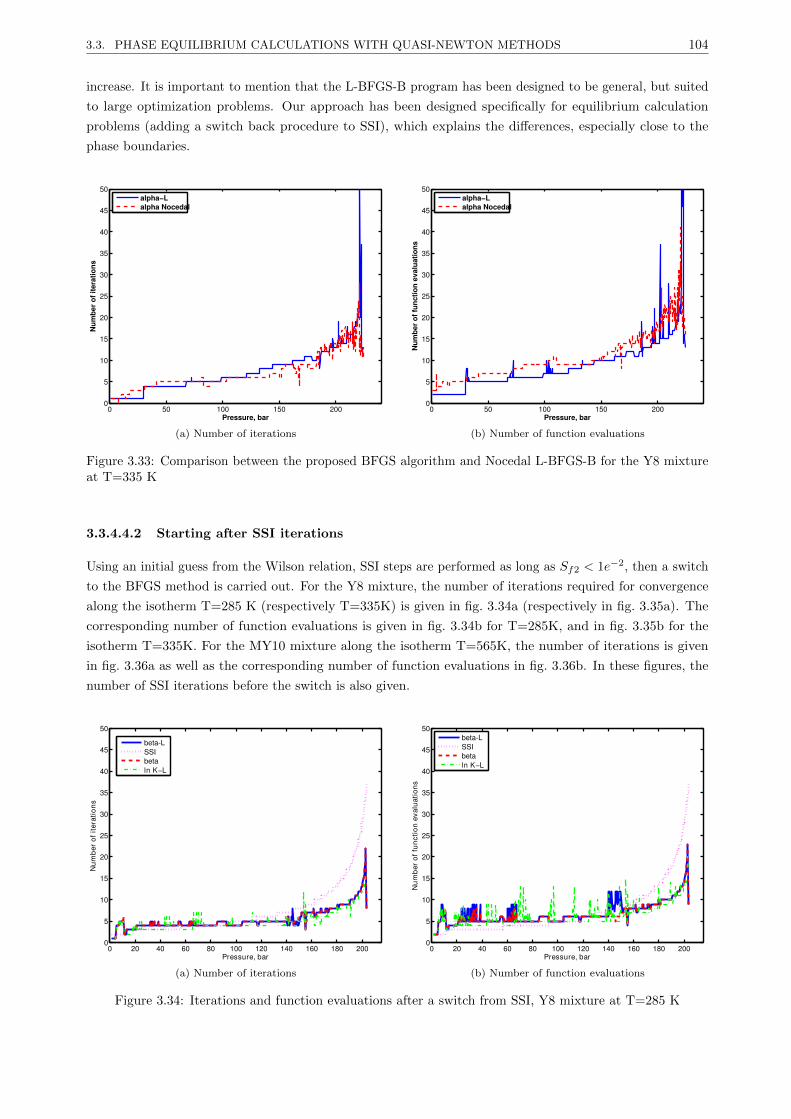
3.3. PHASE EQUILIBRIUM CALCULATIONS WITH QUASI-NEWTON METHODS 104

increase. It is important to mention that the L-BFGS-B program has been designed to be general, but suited

to large optimization problems. Our approach has been designed specifically for equilibrium calculation

problems (adding a switch back procedure to SSI), which explains the differences, especially close to the

phase boundaries.

0 50 100 150 2000

5

10

15

20

25

30

35

40

45

50

Pressure, bar

Num

berof

iteratio

ns

alpha−Lalpha Nocedal

(a) Number of iterations

0 50 100 150 2000

5

10

15

20

25

30

35

40

45

50

Pressure, barNum

berof

func

tionev

alua

tions

alpha−Lalpha Nocedal

(b) Number of function evaluations

Figure 3.33: Comparison between the proposed BFGS algorithm and Nocedal L-BFGS-B for the Y8 mixtureat T=335 K

3.3.4.4.2 Starting after SSI iterations

Using an initial guess from the Wilson relation, SSI steps are performed as long as Sf2 < 1e−2, then a switch

to the BFGS method is carried out. For the Y8 mixture, the number of iterations required for convergence

along the isotherm T=285 K (respectively T=335K) is given in fig. 3.34a (respectively in fig. 3.35a). The

corresponding number of function evaluations is given in fig. 3.34b for T=285K, and in fig. 3.35b for the

isotherm T=335K. For the MY10 mixture along the isotherm T=565K, the number of iterations is given

in fig. 3.36a as well as the corresponding number of function evaluations in fig. 3.36b. In these figures, the

number of SSI iterations before the switch is also given.

0 20 40 60 80 100 120 140 160 180 2000

5

10

15

20

25

30

35

40

45

50

Pressure, bar

Num

ber

ofite

ratio

ns

beta-LSSIbetaln K−L

(a) Number of iterations

0 20 40 60 80 100 120 140 160 180 2000

5

10

15

20

25

30

35

40

45

50

Pressure, bar

Num

berof

functio

nevaluatio

ns

beta-LSSIbetaln K−L

(b) Number of function evaluations

Figure 3.34: Iterations and function evaluations after a switch from SSI, Y8 mixture at T=285 K

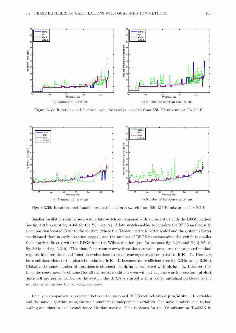
3.3. PHASE EQUILIBRIUM CALCULATIONS WITH QUASI-NEWTON METHODS 105

0 50 100 150 2000

5

10

15

20

25

30

35

40

45

50

Pressure, bar

Num

berof

iteratio

ns

alpha−LSSIalphaln K−L

(a) Number of iterations

0 50 100 150 2000

5

10

15

20

25

30

35

40

45

50

Pressure, bar

Num

berof

func

tionev

alua

tions

alpha−LSSIalphaln K−L

(b) Number of function evaluations

Figure 3.35: Iterations and function evaluations after a switch from SSI, Y8 mixture at T=335 K

30 40 50 60 70 80 900

5

10

15

20

25

30

35

40

45

50

Pressure, bar

Num

berof

iteratio

ns

beta-LSSIbetaln K−L

(a) Number of iterations

30 40 50 60 70 80 900

5

10

15

20

25

30

35

40

45

50

Pressure, bar

Num

ber

offu

nctio

nev

alua

tions

beta-LSSIbetaln K−L

(b) Number of function evaluations

Figure 3.36: Iterations and function evaluations after a switch from SSI, MY10 mixture at T=565 K

Smaller oscillations can be seen with a late switch as compared with a direct start with the BFGS method

(see fig. 3.30b against fig. 3.35b for the Y8 mixture). A late switch enables to initialize the BFGS method with

a composition located closer to the solution (where the Hessian matrix is better scaled and the system is better

conditioned than in early iteration stages), and the number of BFGS iterations after the switch is smaller

than starting directly with the BFGS from the Wilson relation, (see for instance fig. 3.29a and fig. 3.29b vs

fig. 3.34a and fig. 3.34b). This time, for pressures away from the saturation pressures, the proposed method

requires less iterations and function evaluations to reach convergence as compared to lnK− L. However,

for conditions close to the phase boundaries, lnK− L becomes more efficient (see fig. 3.34a to fig. 3.36b).

Globally, the same number of iterations is obtained for alpha as compared with alpha− L. However, this

time, the convergence is obtained for all the tested conditions even without any line search procedure (alpha).

Since SSI are performed before the switch, the BFGS is started with a better initialization closer to the

solution which makes the convergence easier.

Finally, a comparison is presented between the proposed BFGS method with alpha/alpha− L variables

and the same algorithm using the mole numbers as independent variables. The mole numbers lead to bad

scaling and thus to an ill-conditioned Hessian matrix. This is shown for the Y8 mixture at T=335K in

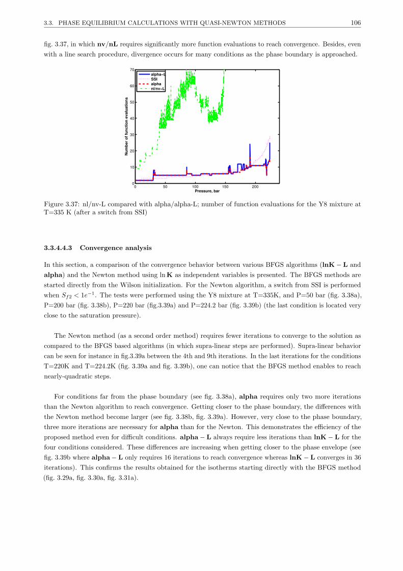
3.3. PHASE EQUILIBRIUM CALCULATIONS WITH QUASI-NEWTON METHODS 106

fig. 3.37, in which nv/nL requires significantly more function evaluations to reach convergence. Besides, even

with a line search procedure, divergence occurs for many conditions as the phase boundary is approached.

0 50 100 150 2000

10

20

30

40

50

60

70

Pressure, bar

Num

berof

func

tionev

alua

tions

alpha−LSSIalphanl/nv−L

Figure 3.37: nl/nv-L compared with alpha/alpha-L; number of function evaluations for the Y8 mixture atT=335 K (after a switch from SSI)

3.3.4.4.3 Convergence analysis

In this section, a comparison of the convergence behavior between various BFGS algorithms (lnK− L and

alpha) and the Newton method using ln K as independent variables is presented. The BFGS methods are

started directly from the Wilson initialization. For the Newton algorithm, a switch from SSI is performed

when Sf2 < 1e−1. The tests were performed using the Y8 mixture at T=335K, and P=50 bar (fig. 3.38a),

P=200 bar (fig. 3.38b), P=220 bar (fig.3.39a) and P=224.2 bar (fig. 3.39b) (the last condition is located very

close to the saturation pressure).

The Newton method (as a second order method) requires fewer iterations to converge to the solution as

compared to the BFGS based algorithms (in which supra-linear steps are performed). Supra-linear behavior

can be seen for instance in fig.3.39a between the 4th and 9th iterations. In the last iterations for the conditions

T=220K and T=224.2K (fig. 3.39a and fig. 3.39b), one can notice that the BFGS method enables to reach

nearly-quadratic steps.

For conditions far from the phase boundary (see fig. 3.38a), alpha requires only two more iterations

than the Newton algorithm to reach convergence. Getting closer to the phase boundary, the differences with

the Newton method become larger (see fig. 3.38b, fig. 3.39a). However, very close to the phase boundary,

three more iterations are necessary for alpha than for the Newton. This demonstrates the efficiency of the

proposed method even for difficult conditions. alpha− L always require less iterations than lnK− L for the

four conditions considered. These differences are increasing when getting closer to the phase envelope (see

fig. 3.39b where alpha− L only requires 16 iterations to reach convergence whereas lnK− L converges in 36

iterations). This confirms the results obtained for the isotherms starting directly with the BFGS method

(fig. 3.29a, fig. 3.30a, fig. 3.31a).

3.3. PHASE EQUILIBRIUM CALCULATIONS WITH QUASI-NEWTON METHODS 107

0 2 4 6 8 10 1210

−14

10−12

10−10

10−8

10−6

10−4

10−2

100

102

Iterations

Euc

lidea

nno

rm

alpha−LNewtonln K−L

(a) P=50 bar

0 5 10 15 20 2510

−14

10−12

10−10

10−8

10−6

10−4

10−2

100

102

Iterations

Euc

lidea

nno

rm

alpha−LNewtonln K−L

(b) P=200 bar

Figure 3.38: Error versus number of iterations for the Y8 mixture at T=335K

0 5 10 15 20 25 30 3510

−14

10−12

10−10

10−8

10−6

10−4

10−2

100

102

Iterations

Euc

lidea

nno

rm

alpha−LNewtonln K−L

(a) P=220 bar

0 5 10 15 20 25 30 35 4010

−16

10−14

10−12

10−10

10−8

10−6

10−4

10−2

100

102

Iterations

Euc

lidea

nno

rm

alpha−LNewtonln K−L

(b) P=224.2 bar

Figure 3.39: Error versus number of iterations for the Y8 mixture at T=335K

3.3.4.5 Discussion

With the use of a line search method, convergence was obtained with the proposed BFGS method for all the

presented conditions; without line search, divergence occurs only near the phase boundaries when starting

directly from Wilson initialization. Globally, the proposed method proved to converge within fewer iterations

and function evaluations than the lnK− L procedure from [Ammar and Renon [1987]].

Oscillations have been noticed with lnK− L. Most of the line search methods interpolate a function

based on polynomial approximations to compute a step which satisfies the Wolfe conditions. In Ammar and

Renon’s method, the gradient of the Gibbs free energy is calculated with the mole numbers as independent

variables. Therefore the line search procedure is the same as for a BFGS method taking the mole numbers

as independent variables. It has been shown that the BFGS methods based on the mole numbers did not

perform well; lnK− L inherits this behavior. With the proposed new set of independent variables, the

gradient and the Hessian derive directly from the Gibbs energy. The line search procedure is more efficient

and convergence to the solution was achieved for all the tested conditions.

For most of the conditions the proposed BFGS based on variables proved to be more efficient (in terms

of number of iterations and function evaluations) as compared to lnK− L. Yet, with a late switch, for

3.4. ROBUST AND EFFICIENT TRUST-REGION BASED STABILITY ANALYSIS AND MULTIPHASE FLASHCALCULATIONS 108

conditions near the phase boundaries, lnK− L was shown to reach convergence within fewer iterations.

The ln K variables lead to a better conditioned systems. When performing a late switch, the norm of the

fugacity derivatives decreases and the off-diagonal elements become smaller, thus improving the scaling and

the condition number of the Hessian. Close to the phase boundary, starting with a good initial guess (after a

switch) lnK− L is based on the most efficient variables and leads to a faster convergence to the solution than

the other methods. However, starting directly from the Wilson relation, a more robust method is necessary;

in this case, lnK− L has been shown to be less stable than the proposed method.

Comparisons with the Newton algorithm were also presented. Generally alpha− L requires a few more

iterations to converge than the second order method. Each BFGS iteration is faster to compute than a

Newton iteration since no fugacity derivatives are required and no linear systems need to be solved. Therefore,

even if the BFGS algorithm requires more iterations to converge, the computation time is not necessarily

increased. Even though the BFGS method may not compete with the Newton method for a small number of

components with a cubic EOS, with a high number of component (in chemical process for instance), the

proposed method could become more efficient in terms of computation time. Moreover, it offers an interesting

alternative for difficult EOS models; when the fugacity derivatives are complex and difficult to calculate

analytically, or there are costly, the BFGS method is really attractive as compared to the Newton method.

3.3.4.6 Conclusions/Perspectives

Since quasi-Newton methods are known to be very sensitive to scaling, a new methodology for finding a set

of variables leading to a good scaling of phase equilibrium problems is proposed. A new set of independent

variables is proposed for the flash calculation problem; fore the phase stability problem, the variables

introduced by [Michelsen [1982a]] are found using the proposed methodology. The BFGS algorithm based on

this new set of independent variables for the two-phase-split problem was developed and tested for robustness

and efficiency. The proposed method was shown to reach convergence for all the testing conditions and to

converge generally within fewer iterations and function evaluations than other BFGS methods. Comparisons

with the second-order Newton method showed that the proposed algorithm requires only few more iterations

for convergence (but the cost per iteration is lower, since no derivatives or resolution of a linear system are

required). The BFGS method is attractive for more complex EOS models in which partial derivatives of

fugacity can be costly and/or difficult to compute analytically (as for instance the SAFT family of EOS). The

proposed variables are also particularly suited for trust-region algorithms [Petitfrere and Nichita [2014a]].

3.4 Robust and efficient Trust-Region based stability analysis and

multiphase flash calculations

3.4.1 Introduction

The resolution of the multiphase flash problem requires the minimization of the Gibbs free energy [Michelsen

[1982a]] and of the tangent-plane distance (TPD) function [Michelsen [1982b]] for phase stability testing.

Traditionally, first-order successive substitution (SSI) iterations are performed before switching to the second-

order Newton method. In most of the cases, the Newton method works fine (convergence to the solution is

achieved in a few iterations) provided the Hessian is positive definite. The most difficult regions in mixture

phase envelopes are in the vicinity of singularities: critical points for multiphase flash calculations, convergence

locus for negative flashes [Whitson and Michelsen [1990]], the stability test limit locus [Whitson and Michelsen

[1990], Hoteit and Firoozabadi [2006], Nichita et al. [2007c]] (or the ’shadow curve’ [Rasmussen et al. [2006]])

for stability analysis. Near these loci, algorithms either become extremely slow of have difficulties to converge.

In the case of a too early switch, the Newton step is rejected and the calculations are switched back to SSI

iterations. Sometimes a very large number of SSI iterations are necessary before the final switch to Newton

iterations very close to singularities. This convergence behavior suggested us to investigate how Trust-Region

3.4. ROBUST AND EFFICIENT TRUST-REGION BASED STABILITY ANALYSIS AND MULTIPHASE FLASHCALCULATIONS 109

methods behave in such situations.

Restricted-step methods or Trust-Region methods were first suggested by [Levenberg [1944] and Marquardt

[1963]] to solve nonlinear least-squares problems. They are often put in comparison with line search techniques,

and they have seen considerable improvements in the past thirty years. The first algorithms were designed

to small systems [Hebden [1973], Gill and Murray [1974], Gill and Murray [1978], Gay [1981], More and

Sorensen [1983],More and Sorensen [1993]]. Then, a second branch of Trust-Region methods started to

see developments since the improvements in computer science enabled to deal with bigger problems: the

method based on high dimension problems, like the conjugate-gradients or generalized Lanczos-Trust-Region

algorithms [Steihaug [1983], Shultz et al. [1985], Byrd et al. [1988]]. Except when dealing with a high number

of components, this category is not suited for phase equilibrium calculations.

The first to introduce a Trust-Region method for equilibrium flash calculations were [Nghiem et al. [1983]].

They applied Powel’s Dogleg method to the two-phase flash calculations. The same method was then used

by [Lucia and Liu [1998]]. The dogleg method is a linear combination between a Cauchy step and Newton

method. [Nghiem et al. [1983]] adapted this method as a linear combination between the SSI and Newton

iterations; the method fails when the Hessian is not positive definite. [Mehra et al. [1982]] extended this

method to multiphase equilibrium calculations.

[Michelsen [1992], Michelsen and Mollerup [2007]] addressed the problem of non-positive definite Hessians

(revealed during decomposition) in phase equilibrium calculations and suggested the use of Trust-Region

methods. If the Hessian matrix H is not positive definite, it is corrected by adding a diagonal element, that

is, H + λI. Then some other authors have been investigating the Trust-Region methods in phase equilibrium

calculations: [Trangenstein [1987]] reported minimization with linear constraints for phase stability and

multiphase flash. [Kaul and Thrasher [1996]] used a Trust-Region procedure similar to [Hebden [1973]] for

two-phase equilibrium flash calculations using a set of reduced variables. [Pan and Firoozabadi [2003]] also

used a Trust-Region method; however, there are certain difficulties in combining the Trust-Region approach

with reduction methods.

[Lucia et al. [1993]] developed a Trust-Region method extending the Powell dogleg strategy to the complex

domain; this method was used by [Gow et al. [1996]] to model the VLE of binary refrigerant mixtures. [Lucia

and Yang [2003]] used a Trust-Region method to calculate downhill directions in terrain global methods;

these methods were used to model the complex phase behavior of normal alkane systems [Lucia et al. [2012]],

or within a multi-scale framework for multiphase flash calculations [Lucia et al. [2005]]. [Alsaifi and Englezos

[2011]] used a Trust-Region Gauss-Newton method for simultaneous stability and flash calculations with the

PC-SAFT equation of state. Recently, [Michelsen et al. [2013b]] reported the use of a Trust-Region method

for phase equilibrium calculations.

In this chapter, a Trust-Region method derived from [More and Sorensen [1983], More and Sorensen

[1993], and Conn et al. [2000]] is adapted and tested successfully for various phase stability analysis and

multiphase flash calculation problems. The section is structured as follows: the proposed Trust-Region

method is presented in detail. The results for phase stability and multiphase flash calculations of various

mixtures with complex phase envelopes and comparisons between the proposed method with Newton methods

using various independent variables are presented before drawing the conclusions.

3.4.2 Trust-Region methods

Trust-Region methods define a region around the current point within which they trust the model to be an

appropriate representation of the objective function. Then, a step is chosen which will minimize the model

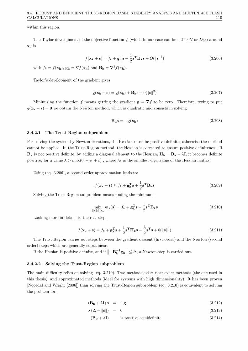
3.4. ROBUST AND EFFICIENT TRUST-REGION BASED STABILITY ANALYSIS AND MULTIPHASE FLASHCALCULATIONS 110

within this region.

The Taylor development of the objective function f (which in our case can be either G or DM ) around

xk is

f(xk + s) = fk + gTk s +

1

2sTBks +O(‖s‖3) (3.206)

with fk = f(xk), gk = ∇f(xk) and Bk = ∇2f(xk).

Taylor’s development of the gradient gives

g(xk + s) = g(xk) + Bks + 0(‖s‖2) (3.207)

Minimizing the function f means getting the gradient g = ∇f to be zero. Therefore, trying to put

g(xk + s) = 0 we obtain the Newton method, which is quadratic and consists in solving

Bks = −g(xk) (3.208)

3.4.2.1 The Trust-Region subproblem

For solving the system by Newton iterations, the Hessian must be positive definite, otherwise the method

cannot be applied. In the Trust-Region method, the Hessian is corrected to ensure positive definiteness. If

Bk is not positive definite, by adding a diagonal element to the Hessian, Hk = Bk + λI, it becomes definite

positive, for a value λ > max(0,−λ1 + ε) , where λ1 is the smallest eigenvalue of the Hessian matrix.

Using (eq. 3.206), a second order approximation leads to:

f(xk + s) ≈ fk + gTk s +

1

2sTBks (3.209)

Solving the Trust-Region subproblem means finding the minimum

min‖s‖≤∆k

mk(s) = fk + gTk s +

1

2sTBks (3.210)

Looking more in details to the real step,

f(xk + s) = fk + gTk s +

1

2sTHks− λ

2sTs + 0(‖s‖3) (3.211)

The Trust Region carries out steps between the gradient descent (first order) and the Newton (second

order) steps which are generally supralinear.

If the Hessian is positive definite, and if∥∥−B−1k gk

∥∥ ≤ ∆, a Newton-step is carried out.

3.4.2.2 Solving the Trust-Region subproblem

The main difficulty relies on solving (eq. 3.210). Two methods exist: near exact methods (the one used in

this thesis), and approximated methods (ideal for systems with high dimensionality). It has been proven

[Nocedal and Wright [2006]] than solving the Trust-Region subproblem (eq. 3.210) is equivalent to solving

the problem for:

(Bk + λI) s = −g (3.212)

λ (∆− ‖s‖) = 0 (3.213)

(Bk + λI) is positive semidefinite (3.214)

3.4. ROBUST AND EFFICIENT TRUST-REGION BASED STABILITY ANALYSIS AND MULTIPHASE FLASHCALCULATIONS 111

For λ ≥ 0 and s feasible.

Three cases can be distinguished.

3.4.2.2.1 Case 1: λ = 0 and ‖s‖ ≤ ∆k

If λ = 0 satisfies (eq. 3.213 and eq. 3.214), with ‖s‖ ≤ ∆, the solution is found (Newton step). Otherwise,

the system (eq. 3.213, eq. 3.214, eq. 3.214) is equivalent to solving∥∥∥(Bk + λI)−1

gk

∥∥∥ = ∆k (3.215)

With (Bk + λI) definite positive.

[Conn et al. [2000]] proposed different examples to illustrate the possible roots of the equation ‖s(λ)‖22 <= ∆

Let’s suppose the problem defined by

g =

1

1

1

1

, B =

1 0 0 0

0 2 0 0

0 0 3 0

0 0 0 4

B is positive definite. In fig. 3.40 ‖s(λ)‖22 is plotted against λ.

The case 1 corresponds to the case where ∆ > 1.5 (dashed red line in the fig. 3.40), the solution λ = 0,

lies inside the Trust-Region radius. And as it corresponds to the Newton step, this is the optimal one.

−6 −4 −2 0 2 40

5

10

15

20

25

30

λ

||s(λ

)||22

solution curve

Figure 3.40: Convex example [Conn et al. [2000]]

3.4.2.2.2 Case 2: qT1 g 6= 0 and λ ∈ (−λ1,+∞)

By noting that s is a function of λ, and

s(λ) = −(Bk + λI)−1gk (3.216)

(eq. 3.215) becomes

‖s(λ)‖ = ∆k (3.217)

If Bk is positive definite, since Bk symmetric, there is an orthogonal matrix Q and a diagonal matrix Λ

such that Bk = QΛQT, where Λ = diag(λ1, λ2, ..., λN ) with λ1 ≤ λ2 ≤ ... ≤ λN are the eigenvalues of Bk

and the matrix Q contains the orthonormal eigenvectors of Bk

3.4. ROBUST AND EFFICIENT TRUST-REGION BASED STABILITY ANALYSIS AND MULTIPHASE FLASHCALCULATIONS 112

Hk = Bk + λI = Q (Λ + λI) QT; ∀λ 6= λj (3.218)

then,

s(λ) = −Q(Λ + λI)−1

QTg = −N∑j=1

qTj g

λj + λqj (3.219)

Where qj denotes the jth column of Q. By orthonormality

‖s(λ)‖22 =

N∑j=1

(qTj g)2

(λj + λ)2 (3.220)

therefore, as long as qT1 g 6= 0,, a unique solution 0 ≤ −λ1 < λ can be found to solve (eq. 3.215).

Solving (eq. 3.217) is equivalent to solve [Hebden [1973]]

ϕ(λ) =1

‖s(λ)‖2− 1

∆k= 0 (3.221)

(eq. 3.221) can be solved with a Newton procedure in one dimension. The derivative of ϕ(λ) is

ϕ′(λ) = −< s(λ),∇λs(λ) >

‖s(λ)‖32(3.222)

If H is definite positive, a Cholesky decomposition can be performed

H = LLT (3.223)

and using H(λ) = Bk + λI the scalar product in (eq. 3.222) can be expressed as

< s(λ),H−1(λ)s(λ) > = < s(λ),L−TL−1s(λ) >= < L−1s(λ),L−1s(λ) >= ‖w‖22 (3.224)

The update is then given by

λk+1 = λk − ϕ(λ)

ϕ′(λ)= λk +

(‖s(λ)‖2 −∆k

∆k

)(‖s(λ)‖22‖w‖22

)(3.225)

[Conn et al. [2000]] proposed a case where B is non-positive definite:

g =

1

1

1

1

, B =

−2 0 0 0

0 −1 0 0

0 0 0 0

0 0 0 1

In fig. 3.41 ‖s(λ)‖22 is plotted against λ for the non-convex example.

The case 2 corresponds to two possible problems:

• In the convex example, if ∆2 ≤ 1.5 (which corresponds to the dashed red line in fig. 3.40), (eq. 3.221)

needs to be solved to reach the optimum and find the correct λ.

• In the non-convex example, as H(λ) must be positive definite, the only values of interest are those

where λ > λ1. With λ1 the minus leftmost eigenvalue. For any values of ∆, a λ can be found to solve

the trust-region subproblem.

3.4. ROBUST AND EFFICIENT TRUST-REGION BASED STABILITY ANALYSIS AND MULTIPHASE FLASHCALCULATIONS 113

−4 −2 0 2 4 60

5

10

15

20

25

30

22

minus leftmosteigenvalue

||s(λ

)||

λFigure 3.41: Non convex example [Conn et al. [2000]]

3.4.2.2.3 Case 3: qT1 g = 0 and λ ∈ (−λ1,+∞)

This problem has been well studied in the literature [Conn et al. [2000], Nocedal and Wright [2006]] and is

referred to as the hard case. It occurs when qT1 g = 0, that is to say, the subspace made with the eigenvectors

corresponding to the most negative eigenvalue of Bk is orthogonal to the gradient.

In this case, if ‖s(−λ1)‖ < ∆k, the problem cannot be solved.

We have (Bk − λ1I)q1 = 0. By calling

s(τ) = −(Bk − λ1I)−1gk + τq1 (3.226)

By orthogonality qTj q1 = 0, for j 6= 1, we get :

s =

N∑j=1λj 6=λ1

qTj g

λj − λ1qj + τq1 (3.227)

For any τ , and for ‖q1‖2 = 1, we get :

‖s‖22 =

N∑j=1λj 6=λ1

(qTj g)2

(λj − λ1)2 + τ2 (3.228)

By calculating the correct τ , it is always possible to get (eq. 3.217).

Once again, [Conn et al. [2000]] proposed an example to illustrate the hard case:

g =

0

1

1

1

, B =

−2 0 0 0

0 −1 0 0

0 0 0 0

0 0 0 1

In fig. 3.42 ‖s(λ)‖22 is plotted against λ for the hard case example.

As H(λ) must be positive definite, λ < 2 is forbidden. However, unlike for the non-convex case, there is

no direct solution for the problem for any values of ∆ > ∆critic (in fig. 3.42, ∆critic = 1.2).

One needs to use the procedure explained earlier to solve the problem

3.4. ROBUST AND EFFICIENT TRUST-REGION BASED STABILITY ANALYSIS AND MULTIPHASE FLASHCALCULATIONS 114

−4 −2 0 2 4 60

5

10

15

20

25

30

22 minus leftmosteigenvalue

||s(λ

)||

λ

Figure 3.42: Hard case example [Conn et al. [2000]]

3.4.2.3 Algorithm for the Trust-Region subproblem

The Newton method to obtain the correct λ is not used directly. Safe-guarding techniques must be applied

to get a robust algorithm. The general algorithm is given below. It follows the algorithms given in chapter

7 of [Conn et al. [2000]], which are directly derived from [More and Sorensen [1983], More and Sorensen [1993]].

Algorithm 3.4 realistic exact trust-Region subproblem [Conn et al. [2000]]

λ = 0Try to factorize H(λ)= LLT

if Failure thenCompute λ1

λ = −λ1 + εFactorize H(λ) = LLT

end ifSolve LTs = −gif ‖s‖2 < ∆ then

if λ = 0 or ‖s‖2 = ∆ thenSTOP : the solution has been found

else Hard caseCompute an eigenvector u1 corresponding to λ1 (e.g., Lanczos or QR)Find the root α of the equation ‖s + αu1‖2 = ∆ which minimizes (eq. 3.210)Replace s by s + αu1

STOP : the solution has been foundend if

end ifwhile |‖s‖2 −∆| > κeasy∆ do

Solve Lw = sReplace λk+1 = λk +

(‖s(λ)‖2−∆

∆

)(‖s(λ)‖22‖w‖22

)Factorize H(λ) = LLT

Solve LTs = −g

end while

In the algorithm, it has been chosen to calculate the eigenvector and eigenvalues explicitly. [Conn et al.

[2000]] proposed another algorithm in which the eigenvector can be approximated. The two methods have

been implemented. As the system is generally small (nc < 12) in the context of reservoir simulators, it is

faster to compute them explicitly. For higher number of components (i.e., chemical processes), the second

method will be more advantageous.

3.4. ROBUST AND EFFICIENT TRUST-REGION BASED STABILITY ANALYSIS AND MULTIPHASE FLASHCALCULATIONS 115

3.4.2.4 The Trust-Region size

The size of the Trust-Region ∆k is critical to the effectiveness of each step. If the region is too small, the

algorithm misses an opportunity to take a step which will get closer to the solution. If it is too large, steps

which should not be acceptable could be accepted.

3.4.2.4.1 Dynamic update of the Trust-Region size

The choice of the Trust-Region size is based on the agreement between the model function mk (see eq. 3.210)

and the objective function f at the previous iterations:

ρk =f(xk)− f(xk + sk)

mk(0)−mk(sk)(3.229)

• If ρk < 0, this means that f(xk) < f(xk + sk), the step is rejected

• If ρk is small, this means that the Trust Region should be decreased (the model is relatively different to

the reality (complex region)).

• If ρk ≈ 1, the Trust Region should be extended, since the model matches the reality and better steps

could be carried out.

3.4.2.4.2 General Algorithm for the Trust Region method

The general algorithm for the Trust Region method is adapted from [Nocedal and Wright [2006]]. Note that

for difficult conditions, mainly in the early iteration stages, the Hessian is so ill-conditioned that the element

added to the diagonal of the Hessian is really high. The Trust-Region radius decreases to a really small value,

and once the Hessian is positive definite, the Trust-Region radius limits the step, and it can take long to

increase it. When λ is too high, the step will be a gradient descent which is smaller than that of an SSI

iteration. Therefore, the algorithm is modified in the sense that if λ ≥ κ and ρk ≤ γ an SSI iteration is

performed. The use of only one SSI iteration is purely empirical. Based on numerical experiments on the

mixtures considered in the results section, it was found that performing two or more SSI iterations at this

stage does not decrease the computation time.

The main steps of the Trust-Region (TR) method are summarized below:

Trust-region methods contain tunable parameters (such as the initial trust-region size, the parameter

controlling the increase/decrease of the trust-region size, etc.). Changing these parameters (which are typically

problem-dependent) might affect to a high extent the convergence properties; their choice is empirical and has

been based on many numerical experiments. The values giving the better results on average were adopted.

In this thesis, the initial trust-region radius is calculated by ∆0 = ‖x‖/10 for flash and by ∆0 =

min (|x‖/10, 1/10) This is the most sensible parameter. It should be chosen not to large (a step not taking

into account the irregularities of the function could be accepted) and not too small (the descent step would

become too small and close to the one of SSI). This choice generally gives good results for the problems

addressed here (multiphase flash and phase stability testing), but it might not be suited for other minimization

problems. The parameter γ is set to zero in the present algorithm; this avoids switching back to SSI too

often when the model function mk is significantly different from the objective function f .

For phase stability testing, the problem becomes singular and any iterative method experience convergence

problems. The Newton method is quadratically convergent only in a vicinity of the solution, which shrinks

as a singularity is approached. In this case, Newton steps are often rejected and a switch back to SSI is

performed (sometimes for a very large number of times). It will be shown later on in this chapter on several

3.4. ROBUST AND EFFICIENT TRUST-REGION BASED STABILITY ANALYSIS AND MULTIPHASE FLASHCALCULATIONS 116

Algorithm 3.5 Trust-Region algorithm: [Nocedal and Wright [2006]]

Given ∆ > 0, ∆0 ∈ (0,∆) and γ ∈ [0, ∆k

4 )for k = 0→ kmax do

Calculate fk, gk

if Error > ε thenCalculate Bk

Calculate ρk solving (eq. 3.210) (TR subproblem)if ρk <

14 then

∆k+1 = ∆k

4else

if ρk >34 and ‖sk‖ = ∆k then

∆k+1 = min (2∆k,∆)end if

end ifif ρk > γ and λ < κ then

xk+1 = xk + skelse

SSI updateend if

end ifend for

examples how the Trust-Region method improves convergence (in some cases spectacularly) near the STLL.

For flash calculations, convergence problems arise near phase boundaries (and particularly near critical

points), and the Trust-Region method also performs better in this region than Newton’s method (as will be

shown on an example). High quality initial guesses for flash calculations from phase stability analysis are

making these convergence problems less important near phase boundaries.

Close to phase boundaries, the trust-region can partially lie outside the feasible composition space if it

is a radial trust-region. If an Yi < 0 (for phase stability), or an nim /∈ (0, zi) (for flash calculations) after

performing a trust-region step, the SSI method is used and ρ is set to 0. Indeed, if a variable goes out of its

bounds it means that the trust-region radius should be decreased to get all the irregularities of the function

and to be able to get closer to the phase boundary without crossing it. This is why ρ is set to 0 (making

ρ < 1/4 and ∆ is decreased).

The presence of trace components in the mixture introduces significant difficulties for phase equilibrium

calculation methods. If the composition of a trace component is well below machine precision the Hessian

matrix becomes very ill-conditioned, leading to highly severe convergence problems. In compositional reservoir

simulators, it is really important to be able to deal with this issue, because trace components can occur in

certain applications. In this thesis this problem is overcome by choosing the dependent variable differently for

each component (as proposed by [Michelsen [1982a]], see section 2.2, NLVM method). This highly improves

the condition number of the system, and it allows dealing with trace components.

It is important to note that, as for Newton and SSI methods, the Trust-Region method does not guarantee

to give the global minimum of the objective function (TPD function or Gibbs free energy). This is a gradient

based local method, which converges to a stationary point of the objective function. To guarantee a global

minimum, either a global optimization method, or a global stability analysis mixed with a local minimization

for the flash calculations should be used. However, these methods are quite slow and cannot be used within

reservoir or process simulators. Here the use of multiple initial guesses for a local minimization of the TPD

function in the stability testing allows to get the global minimum with a high degree of certainty (even if the

solution is not theoretically guaranteed), providing in the same time a sculptured initialization for multiphase

flash calculations.

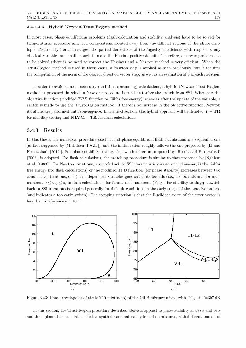
3.4. ROBUST AND EFFICIENT TRUST-REGION BASED STABILITY ANALYSIS AND MULTIPHASE FLASHCALCULATIONS 117

3.4.2.4.3 Hybrid Newton-Trust Region method

In most cases, phase equilibrium problems (flash calculation and stability analysis) have to be solved for

temperatures, pressures and feed compositions located away from the difficult regions of the phase enve-

lope. From early iteration stages, the partial derivatives of the fugacity coefficients with respect to any

classical variables are small enough to make the Hessian positive definite. Therefore, a convex problem has

to be solved (there is no need to correct the Hessian) and a Newton method is very efficient. When the

Trust-Region method is used in those cases, a Newton step is applied as seen previously, but it requires

the computation of the norm of the descent direction vector step, as well as an evaluation of ρ at each iteration.

In order to avoid some unnecessary (and time consuming) calculations, a hybrid (Newton-Trust Region)

method is proposed, in which a Newton procedure is tried first after the switch from SSI. Whenever the

objective function (modified TPD function or Gibbs free energy) increases after the update of the variable, a

switch is made to use the Trust-Region method. If there is no increase in the objective function, Newton

iterations are performed until convergence. In the next section, this hybrid approach will be denoted Y −TR

for stability testing and NLVM−TR for flash calculations.

3.4.3 Results

In this thesis, the numerical procedure used in multiphase equilibrium flash calculations is a sequential one

(as first suggested by [Michelsen [1982a]]), and the initialization roughly follows the one proposed by [Li and

Firoozabadi [2012]]. For phase stability testing, the switch criterion proposed by [Hoteit and Firoozabadi

[2006]] is adopted. For flash calculations, the switching procedure is similar to that proposed by [Nghiem

et al. [1983]]. For Newton iterations, a switch back to SSI iterations is carried out whenever, i) the Gibbs

free energy (for flash calculations) or the modified TPD function (for phase stability) increases between two

consecutive iterations, or ii) an independent variables goes out of its bounds (i.e., the bounds are: for mole

numbers, 0 ≤ nij ≤ zi in flash calculations; for formal mole numbers, (Yi ≥ 0 for stability testing); a switch

back to SSI iterations is required generally for difficult conditions in the early stages of the iterative process

(and indicates a too early switch). The stopping criterion is that the Euclidean norm of the error vector is

less than a tolerance ε = 10−10.

Temperature, K

Pre

ssur

e,ba

r

100 200 300 400 500 600

20

40

60

80

100

120

140

V-L

L

V

(a)

CO2%

Pre

ssur

e,ba

r

50 60 70 80 9065

70

75

80

85

90

95

100

V-L1-L2V-L1

L1-L2L1

(b)

Figure 3.43: Phase envelope a) of the MY10 mixture b) of the Oil B mixture mixed with CO2 at T=307.6K

In this section, the Trust-Region procedure described above is applied to phase stability analysis and two-

and three-phase flash calculations for five synthetic and natural hydrocarbon mixtures, with different amount of

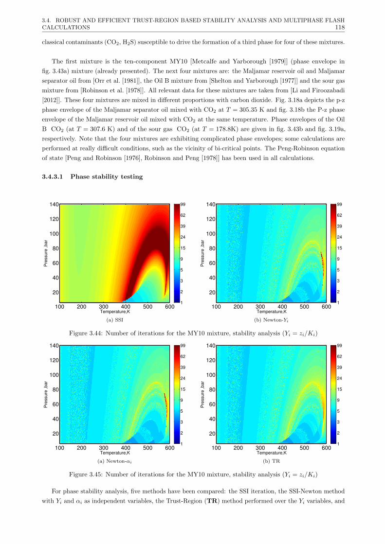
3.4. ROBUST AND EFFICIENT TRUST-REGION BASED STABILITY ANALYSIS AND MULTIPHASE FLASHCALCULATIONS 118

classical contaminants (CO2, H2S) susceptible to drive the formation of a third phase for four of these mixtures.

The first mixture is the ten-component MY10 [Metcalfe and Yarborough [1979]] (phase envelope in

fig. 3.43a) mixture (already presented). The next four mixtures are: the Maljamar reservoir oil and Maljamar

separator oil from [Orr et al. [1981]], the Oil B mixture from [Shelton and Yarborough [1977]] and the sour gas

mixture from [Robinson et al. [1978]]. All relevant data for these mixtures are taken from [Li and Firoozabadi

[2012]]. These four mixtures are mixed in different proportions with carbon dioxide. Fig. 3.18a depicts the p-z

phase envelope of the Maljamar separator oil mixed with CO2 at T = 305.35 K and fig. 3.18b the P-z phase

envelope of the Maljamar reservoir oil mixed with CO2 at the same temperature. Phase envelopes of the Oil

B CO2 (at T = 307.6 K) and of the sour gas CO2 (at T = 178.8K) are given in fig. 3.43b and fig. 3.19a,

respectively. Note that the four mixtures are exhibiting complicated phase envelopes; some calculations are

performed at really difficult conditions, such as the vicinity of bi-critical points. The Peng-Robinson equation

of state [Peng and Robinson [1976], Robinson and Peng [1978]] has been used in all calculations.

3.4.3.1 Phase stability testing

Temperature,K

Pre

ssur

e,b

ar

100 200 300 400 500 600

20

40

60

80

100

120

140

1

2

3

5

9

15

24

39

62

99

(a) SSI

Temperature,K

Pre

ssur

e,b

ar

100 200 300 400 500 600

20

40

60

80

100

120

140

1

2

3

5

9

15

24

39

62

99

(b) Newton-Yi

Figure 3.44: Number of iterations for the MY10 mixture, stability analysis (Yi = zi/Ki)

Temperature,K

Pre

ssur

e,b

ar

100 200 300 400 500 600

20

40

60

80

100

120

140

1

2

3

5

9

15

24

39

62

99

(a) Newton-αi

Temperature,K

Pre

ssur

e,b

ar

100 200 300 400 500 600

20

40

60

80

100

120

140

1

2

3

5

9

15

24

39

62

99

(b) TR

Figure 3.45: Number of iterations for the MY10 mixture, stability analysis (Yi = zi/Ki)

For phase stability analysis, five methods have been compared: the SSI iteration, the SSI-Newton method

with Yi and αi as independent variables, the Trust-Region (TR) method performed over the Yi variables, and

3.4. ROBUST AND EFFICIENT TRUST-REGION BASED STABILITY ANALYSIS AND MULTIPHASE FLASHCALCULATIONS 119

the hybrid Newton−TR method (denoted Y −TR). The number of iterations required by phase stability

testing over the whole P-T diagram of the MY10 mixture is given for different methods, with a liquid trial

phase (Y(0)i = zi/Ki) in fig. 3.44a, fig. 3.44b, fig. 3.45a, fig. 3.45b and with a vapor trial phase (Y

(0)i = ziKi)

in fig. 3.46a to fig. 3.47b. The steps between two P − T points on the phase diagrams are ∆P = 0.1 bar and

∆T = 0.1 K. Less than ten iterations are required for convergence by Newton and TR methods on most

regions of the phase envelope. An increase in the number of iterations can be clearly seen for all methods

around the STLL (in fig. 3.44a to fig. 3.45b for T > TC and in fig. 3.46a to fig. 3.47b for T < TC) and the

spinodal (in fig. 3.44a, to fig. 3.45b for T < TC and in fig. 3.46a to fig. 3.47b for T > TC), which are the

singularities for phase stability. The deterioration of convergence properties as the STLL (non-trivial solution

at a positive TPD function) is approached, is far more severe for Newton and TR methods than near the

spinodal (trivial solution for TPD function equal to zero). It also appears from fig. 3.44a to fig. 3.47b that

near the STLL Newton− αi performs better than Newton−Yi, and that TR is faster than both Newton

versions.

Temperature,K

Pre

ssur

e,b

ar

100 200 300 400 500 600

20

40

60

80

100

120

140

1

2

3

5

9

15

24

39

62

99

(a) SSI

Temperature,K

Pre

ssur

e,b

ar

100 200 300 400 500 600

20

40

60

80

100

120

140

1

2

3

5

9

15

24

39

62

99

(b) Newton-Yi

Figure 3.46: Number of iterations for the MY10 mixture, stability analysis (Yi = ziKi)

Temperature,K

Pre

ssur

e,b

ar

100 200 300 400 500 600

20

40

60

80

100

120

140

1

2

3

5

9

15

24

39

62

99

(a) Newton-αi

Temperature,K

Pre

ssur

e,b

ar

100 200 300 400 500 600

20

40

60

80

100

120

140

1

2

3

5

9

15

24

39

62

99

(b) TR

Figure 3.47: Number of iterations for the MY10 mixture, stability analysis (Yi = ziKi)

The Euclidean norm of the gradient vector is plotted vs. the iteration level for stability testing (Y(0)i = ziKi)

at T = 540.5 K in fig. 3.48a and fig. 3.48b at two pressures above the STLL (103.46 bar). For SSI iterations,

the error curve decreases but exhibits an inflection point; TR performs better than Newton methods (at

p = 112 bar, TR requires about half of the iterations required by Newton methods). Convergence properties

deteriorate as one gets closer to the STLL: at P = 103.5 bar (very close to the STLL) the gradient norm

3.4. ROBUST AND EFFICIENT TRUST-REGION BASED STABILITY ANALYSIS AND MULTIPHASE FLASHCALCULATIONS 120

starts to increase during iterations (see fig. 3.49a) at a certain point (the objective function decreases very

slowly, with about 10−6 per iteration; a descent direction is guaranteed with SSI iterations, since in the

iteration equation of SSI, an always positive semi-definite matrix multiplies the gradient vector [Heidemann

and Michelsen [1995], Ammar and Renon [1987]]). Newton methods fail to converge (the Hessian matrix is

not positive definite anymore) at the given switching conditions, and a switch back is repeatedly required;

eventually quadratic convergence is obtained, but after more than one hundred SSI iterations (most of them

costly, since second-order information is calculated but finally not used). The TR region method converges

in less than 20 iterations. At even more severe conditions, hundreds of SSI iterations (on switch back from

Newton or using a very restrictive switch) may be necessary before the Newton method converges (a plot is

given for T = 530.5 K and P = 108.99 bar in fig. 3.49b), while the TR method manages to handle these

extremely difficult conditions within some twenty iterations, with an almost quadratic convergence behavior.

For phase stability, the critical point is a global minimum, while the STLL is a saddle point; its vicinity is

the most difficult region of the phase envelope for phase stability testing calculations.

0 20 40 60 80 100 12010

−15

10−10

10−5

100

105

Iterations

Euc

lidea

nno

rm

SSIYialphaTR

(a) P=112 bar

0 20 40 60 8010

−15

10−10

10−5

100

105

Iterations

Euc

lidea

nno

rm

SSIYialphaTR

(b) P=116 bar

Figure 3.48: Error vs. iteration level for the stability analysis (liquid trial phase, Yi = ziKi) of the MY10mixture at T=540.5 K

0 50 100 150 20010

−15

10−10

10−5

100

105

Iterations

Euc

lidea

nno

rm

SSIYialphaTR

(a) T=540.5 K and P=103.5 bar

0 100 200 300 400 500 600 70010

−15

10−10

10−5

100

105

Iterations

Euc

lidea

nno

rm

SSIYialphaTR

(b) T=530.5 K and P=108.99 bar

Figure 3.49: Error vs. iteration level for the stability analysis (liquid trial phase, Yi = ziKi) of the MY10mixture

For vapor phase stability, table 3.6 lists the average number of iterations for various methods, and table

3.7 gives the required CPU time (in seconds, for an Intel Xeon CPU Processor X5680, 3.33 GHz). For liquid

phase stability, the average number of iterations is given in table 3.8 and the computer time in table 3.9. The

3.4. ROBUST AND EFFICIENT TRUST-REGION BASED STABILITY ANALYSIS AND MULTIPHASE FLASHCALCULATIONS 121

examined points are those used in constructing fig. 3.18a to fig. 3.19a.

Method MixtureMaljamar Oil (Res) Maljamar Oil (Sep) Oil B Sour gas

Y 8.82 8.54 10.09 5.91α 7.96 7.59 9.70 5.67

TR 8.79 8.39 9.91 6.13Y-TR 7.95 7.69 9.13 5.75

Table 3.6: Average number of iterations for four mixtures and various stability testing methods over the P-zdiagram (initial guess, Yi = ziKi)

Method MixtureMaljamar Oil (Res) Maljamar Oil (Sep) Oil B Sour gas

Y 1.679 4.77 5.248 2.645α 1.565 4.27 5.135 2.735

TR 1.841 5.50 7.835 3.481Y-TR 1.504 4.56 6.762 2.937

Table 3.7: Computation time (in seconds) for four mixtures and various stability testing methods over theP-z diagram (initial guess Yi = ziKi)

Method MixtureMaljamar Oil (Res) Maljamar Oil (Sep) Oil B Sour gas

Y 6.73 8.59 9.17 10.33α 6.74 8.72 8.82 10.18

TR 6.73 8.59 9.16 9.71Y-TR 6.74 8.61 8.82 9.61

Table 3.8: Average number of iterations for four mixtures and various stability testing methods over the P-zdiagram (initial guess, Yi = zi/Ki)

Method MixtureMaljamar Oil (Res) Maljamar Oil (Sep) Oil B Sour gas

Y 1.133 3.965 4.051 4.275α 1.147 4.122 3.823 4.361

TR 1.159 4.181 4.385 4.497Y-TR 1.108 4.109 3.893 4.191

Table 3.9: Computation time (in seconds) for four mixtures and various stability testing methods over theP-z diagram (initial guess Yi = zi/Ki)

In terms of numbers of iterations, Newton− αi performs systematically better than Newton−Yi.

TR requires more iterations than Newton− αi for liquid phase stability ((table 3.6), while the trend is

inversed for vapor phase stability (table 3.7). The hybrid approach Y −TR performs globally better than

both TR and Newton− αi.

In terms of computation time, TR is faster than Newton−Yi, and slower than Newton− αi, (the

cost of an iteration is higher for TR due to additional linear algebra operations), but the hybrid method

Y −TR is globally the fastest method.

3.4.3.2 Multiphase flash calculations

For the equilibrium flash calculations, five methods have been compared: the SSI iteration, the SSI−Newton

method with lnKi as independent variables (abbreviated below as lnK) and with the improved mole number

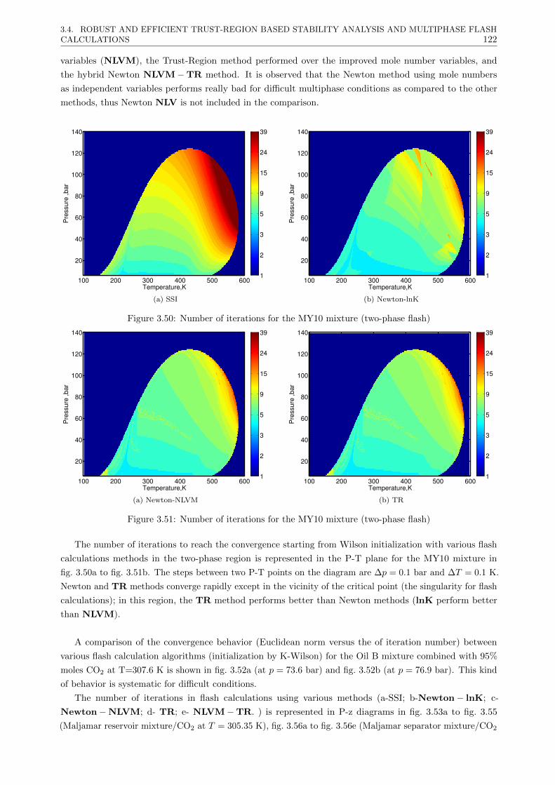
3.4. ROBUST AND EFFICIENT TRUST-REGION BASED STABILITY ANALYSIS AND MULTIPHASE FLASHCALCULATIONS 122

variables (NLVM), the Trust-Region method performed over the improved mole number variables, and

the hybrid Newton NLVM−TR method. It is observed that the Newton method using mole numbers

as independent variables performs really bad for difficult multiphase conditions as compared to the other

methods, thus Newton NLV is not included in the comparison.

Temperature,K

Pre

ssur

e,b

ar

100 200 300 400 500 600

20

40

60

80

100

120

140

1

2

3

5

9

15

24

39

(a) SSI

Temperature,KP

ress

ure

,bar

100 200 300 400 500 600

20

40

60

80

100

120

140

1

2

3

5

9

15

24

39

(b) Newton-lnK

Figure 3.50: Number of iterations for the MY10 mixture (two-phase flash)

Temperature,K

Pre

ssur

e,b

ar

100 200 300 400 500 600

20

40

60

80

100

120

140

1

2

3

5

9

15

24

39

(a) Newton-NLVM

Temperature,K

Pre

ssur

e,b

ar

100 200 300 400 500 600

20

40

60

80

100

120

140

1

2

3

5

9

15

24

39

(b) TR

Figure 3.51: Number of iterations for the MY10 mixture (two-phase flash)

The number of iterations to reach the convergence starting from Wilson initialization with various flash

calculations methods in the two-phase region is represented in the P-T plane for the MY10 mixture in

fig. 3.50a to fig. 3.51b. The steps between two P-T points on the diagram are ∆p = 0.1 bar and ∆T = 0.1 K.

Newton and TR methods converge rapidly except in the vicinity of the critical point (the singularity for flash

calculations); in this region, the TR method performs better than Newton methods (lnK perform better

than NLVM).

A comparison of the convergence behavior (Euclidean norm versus the of iteration number) between

various flash calculation algorithms (initialization by K-Wilson) for the Oil B mixture combined with 95%

moles CO2 at T=307.6 K is shown in fig. 3.52a (at p = 73.6 bar) and fig. 3.52b (at p = 76.9 bar). This kind

of behavior is systematic for difficult conditions.

The number of iterations in flash calculations using various methods (a-SSI; b-Newton− lnK; c-

Newton−NLVM; d- TR; e- NLVM−TR. ) is represented in P-z diagrams in fig. 3.53a to fig. 3.55

(Maljamar reservoir mixture/CO2 at T = 305.35 K), fig. 3.56a to fig. 3.56e (Maljamar separator mixture/CO2

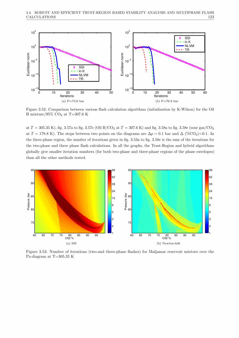
3.4. ROBUST AND EFFICIENT TRUST-REGION BASED STABILITY ANALYSIS AND MULTIPHASE FLASHCALCULATIONS 123

0 10 20 30 40 5010

−15

10−10

10−5

100

105

Iterations

Euc

lidea

nno

rm

SSIln KNLVMTR

(a) P=73.6 bar

0 10 20 30 40 50 6010

−15

10−10

10−5

100

105

Iterations

Euc

lidea

nno

rm

SSIln KNLVMTR

(b) P=76.9 bar

Figure 3.52: Comparison between various flash calculation algorithms (initialization by K-Wilson) for the OilB mixture/95% CO2 at T=307.6 K

at T = 305.35 K), fig. 3.57a to fig. 3.57e (Oil B/CO2 at T = 307.6 K) and fig. 3.58a to fig. 3.58e (sour gas/CO2

at T = 178.8 K). The steps between two points on the diagrams are ∆p = 0.1 bar and ∆ (%CO2)=0.1. In

the three-phase region, the number of iterations given in fig. 3.53a to fig. 3.58e is the sum of the iterations for

the two-phase and three phase flash calculations. In all the graphs, the Trust-Region and hybrid algorithms

globally give smaller iteration numbers (for both two-phase and three-phase regions of the phase envelopes)

than all the other methods tested.

C02 %

Pre

ssur

e,b

ar

60 65 70 75 80 85 90 95

75

80

85

90

95

1

2

3

5

9

15

24

39

62

99

(a) SSI

C02 %

Pre

ssur

e,b

ar

60 65 70 75 80 85 90 95

75

80

85

90

95

1

2

3

5

9

15

24

39

62

99

(b) Newton-lnK

Figure 3.53: Number of iterations (two-and three-phase flashes) for Maljamar reservoir mixture over thePz-diagram at T=305.35 K

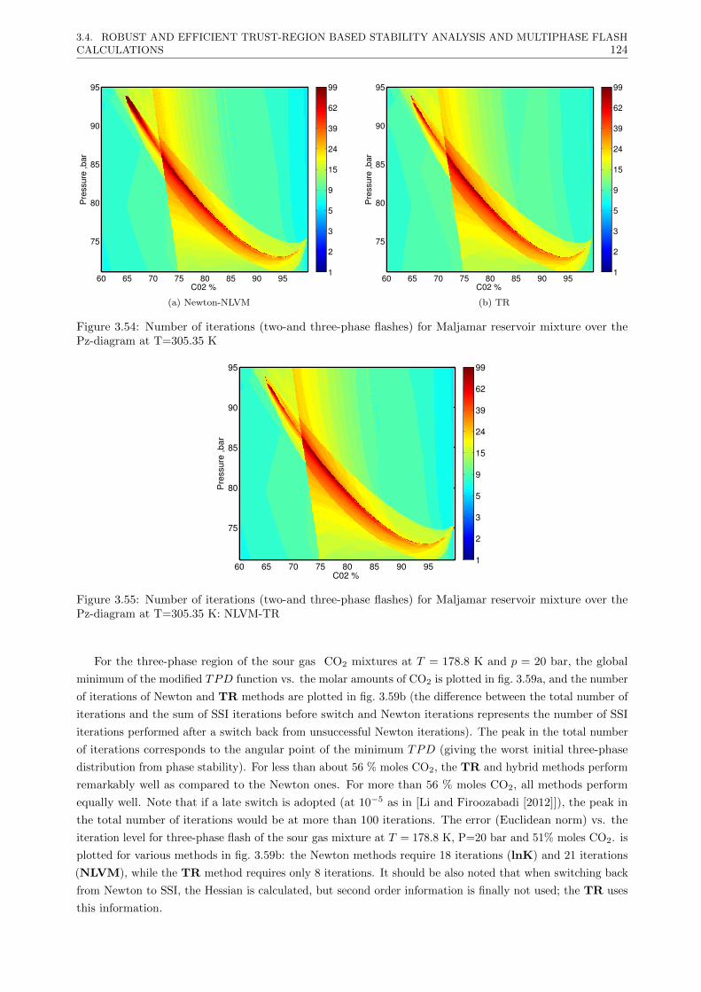
3.4. ROBUST AND EFFICIENT TRUST-REGION BASED STABILITY ANALYSIS AND MULTIPHASE FLASHCALCULATIONS 124

C02 %

Pre

ssur

e,b

ar

60 65 70 75 80 85 90 95

75

80

85

90

95

1

2

3

5

9

15

24

39

62

99

(a) Newton-NLVM

C02 %

Pre

ssur

e,b

ar

60 65 70 75 80 85 90 95

75

80

85

90

95

1

2

3

5

9

15

24

39

62

99

(b) TR

Figure 3.54: Number of iterations (two-and three-phase flashes) for Maljamar reservoir mixture over thePz-diagram at T=305.35 K

C02 %

Pre

ssur

e,b

ar

60 65 70 75 80 85 90 95

75

80

85

90

95

1

2

3

5

9

15

24

39

62

99

Figure 3.55: Number of iterations (two-and three-phase flashes) for Maljamar reservoir mixture over thePz-diagram at T=305.35 K: NLVM-TR

For the three-phase region of the sour gas CO2 mixtures at T = 178.8 K and p = 20 bar, the global

minimum of the modified TPD function vs. the molar amounts of CO2 is plotted in fig. 3.59a, and the number

of iterations of Newton and TR methods are plotted in fig. 3.59b (the difference between the total number of

iterations and the sum of SSI iterations before switch and Newton iterations represents the number of SSI

iterations performed after a switch back from unsuccessful Newton iterations). The peak in the total number

of iterations corresponds to the angular point of the minimum TPD (giving the worst initial three-phase

distribution from phase stability). For less than about 56 % moles CO2, the TR and hybrid methods perform

remarkably well as compared to the Newton ones. For more than 56 % moles CO2, all methods perform

equally well. Note that if a late switch is adopted (at 10−5 as in [Li and Firoozabadi [2012]]), the peak in

the total number of iterations would be at more than 100 iterations. The error (Euclidean norm) vs. the

iteration level for three-phase flash of the sour gas mixture at T = 178.8 K, P=20 bar and 51% moles CO2. is

plotted for various methods in fig. 3.59b: the Newton methods require 18 iterations (lnK) and 21 iterations

(NLVM), while the TR method requires only 8 iterations. It should be also noted that when switching back

from Newton to SSI, the Hessian is calculated, but second order information is finally not used; the TR uses

this information.

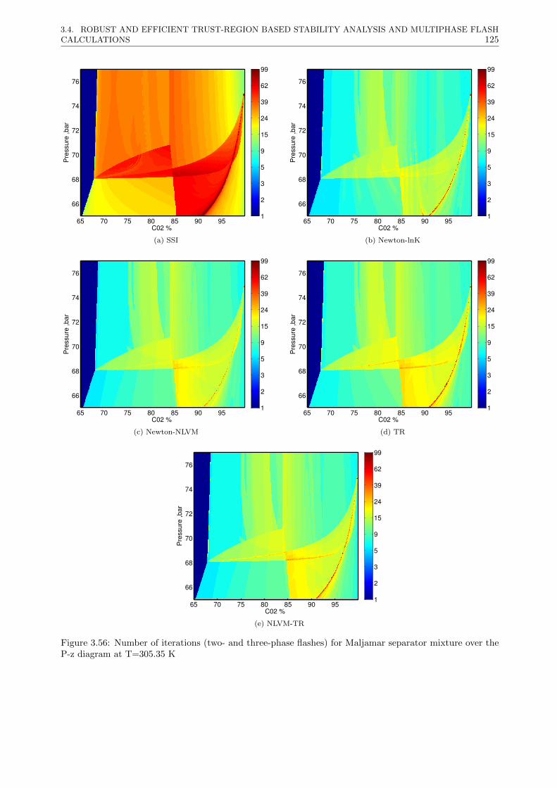
3.4. ROBUST AND EFFICIENT TRUST-REGION BASED STABILITY ANALYSIS AND MULTIPHASE FLASHCALCULATIONS 125

C02 %

Pre

ssur

e,b

ar

65 70 75 80 85 90 95

66

68

70

72

74

76

1

2

3

5

9

15

24

39

62

99

(a) SSI

C02 %

Pre

ssur

e,b

ar

65 70 75 80 85 90 95

66

68

70

72

74

76

1

2

3

5

9

15

24

39

62

99

(b) Newton-lnK

C02 %

Pre

ssur

e,b

ar

65 70 75 80 85 90 95

66

68

70

72

74

76

1

2

3

5

9

15

24

39

62

99

(c) Newton-NLVM

C02 %

Pre

ssur

e,b

ar

65 70 75 80 85 90 95

66

68

70

72

74

76

1

2

3

5

9

15

24

39

62

99

(d) TR

C02 %

Pre

ssur

e,b

ar

65 70 75 80 85 90 95

66

68

70

72

74

76

1

2

3

5

9

15

24

39

62

99

(e) NLVM-TR

Figure 3.56: Number of iterations (two- and three-phase flashes) for Maljamar separator mixture over theP-z diagram at T=305.35 K

3.4. ROBUST AND EFFICIENT TRUST-REGION BASED STABILITY ANALYSIS AND MULTIPHASE FLASHCALCULATIONS 126

C02 %

Pre

ssur

e,b

ar

50 60 70 80 9070

75

80

85

90

95

100

1

2

3

5

9

15

24

39

62

99

(a) SSI

C02 %

Pre

ssur

e,b

ar

50 60 70 80 9070

75

80

85

90

95

100

1

2

3

5

9

15

24

39

62

99

(b) Newton-lnK

C02 %

Pre

ssur

e,b

ar

50 60 70 80 9070

75

80

85

90

95

100

1

2

3

5

9

15

24

39

62

99

(c) Newton-NLVM

C02 %

Pre

ssur

e,b

ar

50 60 70 80 9070

75

80

85

90

95

100

1

2

3

5

9

15

24

39

62

99

(d) TR

C02 %

Pre

ssur

e,b

ar

50 60 70 80 9070

75

80

85

90

95

100

1

2

3

5

9

15

24

39

62

99

(e) NLVM-TR

Figure 3.57: Number of iterations (two-and three-phase flashes) for the Oil B over the P-z diagram at T=307.6K

3.4. ROBUST AND EFFICIENT TRUST-REGION BASED STABILITY ANALYSIS AND MULTIPHASE FLASHCALCULATIONS 127

C02 %

Pre

ssur

e,b

ar

20 30 40 50 60 70 80 90

5

10

15

20

25

30

35

40

45

1

2

3

5

9

15

24

39

62

99

(a) SSI

C02 %

Pre

ssur

e,b

ar

20 30 40 50 60 70 80 90

5

10

15

20

25

30

35

40

45

1

2

3

5

9

15

24

39

62

99

(b) Newton-lnK

C02 %

Pre

ssur

e,b

ar

20 30 40 50 60 70 80 90

5

10

15

20

25

30

35

40

45

1

2

3

5

9

15

24

39

62

99

(c) Newton-NLVM

C02 %

Pre

ssur

e,b

ar

20 30 40 50 60 70 80 90

5

10

15

20

25

30

35

40

45

1

2

3

5

9

15

24

39

62

99

(d) TR

C02 %

Pre

ssur

e,b

ar

20 30 40 50 60 70 80 90

5

10

15

20

25

30

35

40

45

1

2

3

5

9

15

24

39

62

99

(e) NLVM-TR

Figure 3.58: Number of iterations (two- and three-phase flashes) for the sour gas mixture over the P-z diagramat T= 178.8 K

3.4. ROBUST AND EFFICIENT TRUST-REGION BASED STABILITY ANALYSIS AND MULTIPHASE FLASHCALCULATIONS 128

30 40 50 60 70 80 90−0.04

−0.035

−0.03

−0.025

−0.02

−0.015

−0.01

−0.005

0

CO2 %

min

imum

TPD

(a)

30 40 50 60 70 80 900

5

10

15

20

25

30

CO2 %

Num

bero

fite

ratio

ns

SSI before switchln KNLVMTRln K NewtonNLVM NewtonTR Newton

(b)

Figure 3.59: a) Global minimum of the modified TPD function b)Number of iterations of Newton and TRmethods; for sour gas-CO2 mixtures at T=178.8 K and P=20 bar

0 5 10 15 20 2510

−15

10−10

10−5

100

Iterations

Euc

lidea

nno

rm ln KNLVMTR

Figure 3.60: Error vs. iteration level for three-phase flash of the sour gas mixture at T=178.8 K, P=20 barand 51% moles CO2

The average number of iterations for two-phase liquid-vapor flash calculations with several calculation

methods (SSI, lnK, NLVM, TR, and hybrid NLVM−TR) is listed in table 3.10 for four mixtures combined

with CO2. The examined points are those used in constructing the P-z phase diagrams in fig. 3.53a to

fig. 3.58e. Table 3.11 gives the average number of iterations for three-phase flash calculations (including the

liquid-liquid phase split case). The CPU time (in seconds) required by various methods for flash calculations

(cumulated for two- and three-phase flash flashes) is given in table 3.12.

Method MixtureMaljamar Oil (Res) Maljamar Oil (Sep) Oil B Sour gas

SSI 34.017 33.859 39.169 37.143ln K 8.477 8.787 9.280 8.686

NLVM 9.961 9.854 12.151 9.865TR 9.863 9.854 12.149 7.641

NLVM-TR 9.843 9.850 12.147 7.771

Table 3.10: Average number of iterations for four mixtures and various flash calculation methods over theP-z diagram (two-phase flashes)

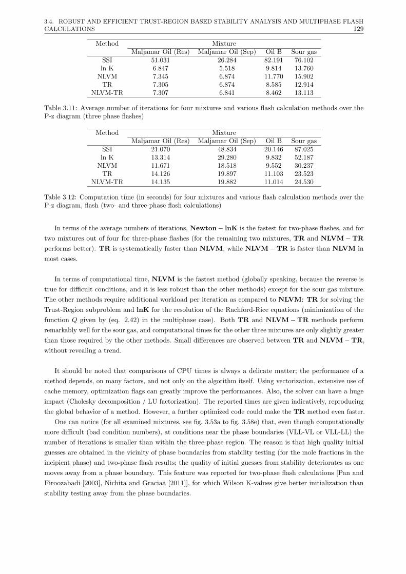
3.4. ROBUST AND EFFICIENT TRUST-REGION BASED STABILITY ANALYSIS AND MULTIPHASE FLASHCALCULATIONS 129

Method MixtureMaljamar Oil (Res) Maljamar Oil (Sep) Oil B Sour gas

SSI 51.031 26.284 82.191 76.102ln K 6.847 5.518 9.814 13.760

NLVM 7.345 6.874 11.770 15.902TR 7.305 6.874 8.585 12.914

NLVM-TR 7.307 6.841 8.462 13.113

Table 3.11: Average number of iterations for four mixtures and various flash calculation methods over theP-z diagram (three phase flashes)

Method MixtureMaljamar Oil (Res) Maljamar Oil (Sep) Oil B Sour gas

SSI 21.070 48.834 20.146 87.025ln K 13.314 29.280 9.832 52.187

NLVM 11.671 18.518 9.552 30.237TR 14.126 19.897 11.103 23.523

NLVM-TR 14.135 19.882 11.014 24.530

Table 3.12: Computation time (in seconds) for four mixtures and various flash calculation methods over theP-z diagram, flash (two- and three-phase flash calculations)

In terms of the average numbers of iterations, Newton− lnK is the fastest for two-phase flashes, and for

two mixtures out of four for three-phase flashes (for the remaining two mixtures, TR and NLVM−TR

performs better). TR is systematically faster than NLVM, while NLVM−TR is faster than NLVM in

most cases.

In terms of computational time, NLVM is the fastest method (globally speaking, because the reverse is

true for difficult conditions, and it is less robust than the other methods) except for the sour gas mixture.

The other methods require additional workload per iteration as compared to NLVM: TR for solving the

Trust-Region subproblem and lnK for the resolution of the Rachford-Rice equations (minimization of the

function Q given by (eq. 2.42) in the multiphase case). Both TR and NLVM−TR methods perform

remarkably well for the sour gas, and computational times for the other three mixtures are only slightly greater

than those required by the other methods. Small differences are observed between TR and NLVM−TR,

without revealing a trend.

It should be noted that comparisons of CPU times is always a delicate matter; the performance of a

method depends, on many factors, and not only on the algorithm itself. Using vectorization, extensive use of

cache memory, optimization flags can greatly improve the performances. Also, the solver can have a huge

impact (Cholesky decomposition / LU factorization). The reported times are given indicatively, reproducing

the global behavior of a method. However, a further optimized code could make the TR method even faster.

One can notice (for all examined mixtures, see fig. 3.53a to fig. 3.58e) that, even though computationally

more difficult (bad condition numbers), at conditions near the phase boundaries (VLL-VL or VLL-LL) the

number of iterations is smaller than within the three-phase region. The reason is that high quality initial

guesses are obtained in the vicinity of phase boundaries from stability testing (for the mole fractions in the

incipient phase) and two-phase flash results; the quality of initial guesses from stability deteriorates as one

moves away from a phase boundary. This feature was reported for two-phase flash calculations [Pan and

Firoozabadi [2003], Nichita and Graciaa [2011]], for which Wilson K-values give better initialization than

stability testing away from the phase boundaries.

3.5. MULTIPHASE FLASH, USING LN K AND PHASE MOLE FRACTIONS AS INDEPENDENT VARIABLES130

3.4.4 Conclusions

In this section, a Trust-Region method has been developed and successfully tested for phase equilibrium

problems: stability analysis and multiphase flash calculations. A hybrid approach is also proposed: instead of

performing TR iterations immediately after the switch from the first-order SSI method, Newton iterations

are first performed, and the TR method is applied only if the objective function value is increasing between

two consecutive iterations.

The proposed Trust-Region and hybrid Newton−TR algorithms have been tested for on a variety of

mixtures involving hydrocarbon components, carbon dioxide and hydrogen sulfide, and exhibiting complicated

phase envelopes. The proposed methods compare favorably to the widely used SSI-Newton methods with

various independent variables.

The TR algorithm is mainly decreasing the number of iterations in some parts of the P − T or P − zdiagrams where the Newton methods do not perform well (some regions close to STLL for stability analysis,

close to critical points, or for conditions in which a poor initial guess is obtained from stability for flash

calculations). In these cases, repeated switch back from Newton methods to the SSI method may be required;

using the TR approach, the second-order information is used to progress towards the solution at a supra-linear

rate. The proposed hybrid Newton−TR algorithm performs generally even better than the TR. The more

difficult a test point is, the more spectacular the algorithm acts from both efficiency and reliability perspectives.

The proposed algorithm for phase equilibrium calculations is applicable to an arbitrary number of equilib-

rium phases and it is not dependent on the thermodynamic model; for more complex EoS and/or mixing

rules, if the expression of the analytical Hessian is not available, the Trust-Region method can be used with a

numerically evaluated Hessian.

In this work, the TR method was implemented for phase equilibrium calculations for conventional variables

(in the compositional space). The next step is the extension to reduction methods [Hendriks [1988]]. A

recently proposed reduction method [Nichita and Graciaa [2011]], allows formulation of flash in the reduced

variables space as the minimization of Gibbs free energy, thus it is suitable for a Trust-Region approach,

unlike previous reduction methods [Michelsen et al. [2013b]].

3.5 Multiphase flash, using ln K and phase mole fractions as in-

dependent variables

3.5.1 Introduction

[Haugen et al. [2011]] proposed a multiphase flash approach (advocated also by [Li and Firoozabadi [2012]])

which updates both the equilibrium constants and the phase mole fractions at each iteration level. Unlike

the lnK approach, there is no explicit resolution of the Rachford-Rice equations, which are solved implicitly

during a Newton update. The resulting linear system is non-symmetric and is solved based on Gaussian

elimination. In a previous chapter, we have shown how symmetry can be efficiently used for multiphase

flashes using ln K as independent variables by using a Cholesky factorization. In this section, it is shown how

symmetry can be taken into account in Haugen’s approach, a new algorithm is proposed in which algebraic

transformations are used to recast Haugen’s in a way that enables the use of a Cholesky factorization.

3.5.2 New proposed method

If lnK and θ are considered as independent variables [Haugen et al. [2011]], the error equations are given by:

3.5. MULTIPHASE FLASH, USING LN K AND PHASE MOLE FRACTIONS AS INDEPENDENT VARIABLES131

gik = lnKik + lnϕik − lnϕiR = 0; i = 1, nc; k = 1, np1 (3.230)

and

Rk =

nc∑i=1

zi(Kik − 1)

1−∑np−1l=1 θl(Kil − 1)

= 0; k = 1, np− 1 (3.231)

The vector of independent variables is ξ =(

ln KT1 , · · · , ln KT

np−1,θT)T

, with ln Ki = (ln K1,i, · · · , ln Knc,i)T

Note that we use here a different, more natural, ordering of variables than in [Haugen et al. [2011]].

The Newton iteration equation is

J∆ξ = −f (3.232)

where J is the Jacobian matrix and f =(gT1 , · · · ,gTnp−1, R1, · · · , Rnp−1

)T, or

∂g1

∂ lnK1· · · ∂g1

∂ lnKnp−1

∂g1

∂θ1· · · ∂g1

∂θnp−1

.... . .

......

. . ....

∂gnp−1

∂ lnK1· · · ∂gnp−1

∂ lnKnp−1

∂gnp−1

∂θ1· · · ∂gnp−1

∂θnp−1

∂R1

∂ lnK1· · · ∂R1

∂ lnKnp−1

∂R1

∂θ1· · · ∂R1

∂θnp−1

.... . .

......

. . ....

∂Rnp−1

∂ lnK1· · · ∂Rnp−1

∂ lnKnp−1

∂Rnp−1

∂θ1· · · ∂Rnp−1

∂θnp−1

∆ ln K1

...

∆ ln Knp−1

∆θ1

...

∆θnp−1

=

g1

...

gnp−1

R1

...

Rnp−1

(3.233)

where

• ∂gk∂ lnKp

are (nc× nc) matrices.

• ∂gk∂θp

are (nc× 1) vectors.

• ∂Rk∂ lnKp

are (1× nc) vectors.

• ∂Rk∂θp

are scalars.

The elements of the Jacobian matrix are:(∂gik

∂ lnKjp

)θ

=

nc∑s=1

(∂gik∂nsk

)θ

(∂nsk

∂ lnKjp

)θ

(3.234)

(∂gik∂θp

)lnK

=

nc∑s=1

(∂gik∂nsk

)lnK

(∂nsk∂θp

)lnK

(3.235)

(∂Rk

∂ lnKjp

)θ

and(∂Rk∂θp

)lnK

, which are given by (eq. 3.46) and (eq. 3.43) respectively.

The Jacobian matrix is non-symmetric. Using the block structure of J, the linear system can be written

as: (A B

C D

)(∆ ln K

∆θ

)= −

(g

R

)(3.236)

or

A∆ ln K + B∆θ = −g (3.237)

3.5. MULTIPHASE FLASH, USING LN K AND PHASE MOLE FRACTIONS AS INDEPENDENT VARIABLES132

C∆ ln K + D∆θ = −R (3.238)

where the dimensions of the matrices are

• (np− 1)nc× (np− 1)nc for A = ∂g∂ lnK

• (np− 1)nc× (np− 1) for B = ∂g∂θ

• (np− 1)× nc(np− 1) for C = ∂R∂ lnK

• (np− 1)× (np− 1) for D = ∂R∂θ

From (eq. 3.238)

∆θ = D−1(−R−C∆ ln K) (3.239)

introducing (eq. 3.239) into (eq. 3.238) gives

(A + BD−1C)∆ ln K = −g + BD−1R (3.240)

or

J∗∆ ln K = −g∗ (3.241)

where J∗ = A + BD−1C is formally identical to J, but has a different (lower) implicitness level.

Finally, note that one can take advantage of symmetry by expressing A and B matrices as

A = I + ΦM(θ) (3.242)

and

B = ΦM(K) (3.243)

with

(M

(θ)ij

)kp

=

(∂nik

∂ lnKjp

)θ

(3.244)

and

(M

(K)i

)kp

=

(∂nik∂θp

)K

(3.245)

In which partial derivatives are given by (eq. 3.41) and (eq. 3.40).

In the proposed formulation of the lnK − θ multiphase flash, the Jacobian matrix is calculated exactly

as in the lnK method (using symmetry in its construction), then a Cholesky decomposition is used for solving

the linear system (eq. 3.237 and eq. 3.238) as described previously, and finally phase mole fractions θ are

updated using (eq. 3.239). In our formulation, the dimensionality of the linear system is not increased and

full advantage of symmetry is taken, leading to a potentially faster Newton lnK − θ iteration.

3.5.3 Results

Three mixtures were used in this study: the Maljamar reservoir oil, the Maljamar separator oil and the sour

gas mixture exposed in section 3.2.4.3.1. In this section, two different kinds of methods have been tested:

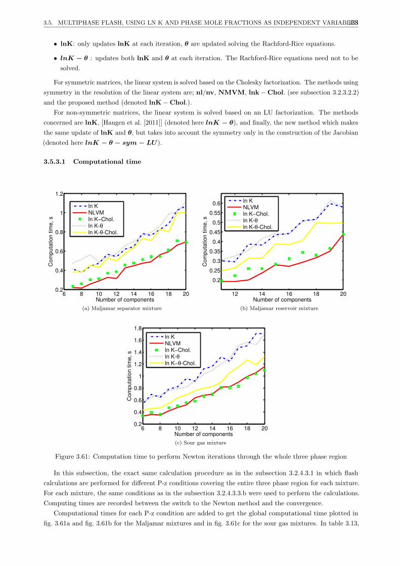
3.5. MULTIPHASE FLASH, USING LN K AND PHASE MOLE FRACTIONS AS INDEPENDENT VARIABLES133

• lnK: only updates lnK at each iteration, θ are updated solving the Rachford-Rice equations.

• lnK − θ : updates both lnK and θ at each iteration. The Rachford-Rice equations need not to be

solved.

For symmetric matrices, the linear system is solved based on the Cholesky factorization. The methods using

symmetry in the resolution of the linear system are; nl/nv, NMVM, lnk−Chol. (see subsection 3.2.3.2.2)

and the proposed method (denoted lnK−Chol.).

For non-symmetric matrices, the linear system is solved based on an LU factorization. The methods

concerned are lnK, [Haugen et al. [2011]] (denoted here lnK − θ), and finally, the new method which makes

the same update of lnK and θ, but takes into account the symmetry only in the construction of the Jacobian

(denoted here lnK − θ − sym− LU).

3.5.3.1 Computational time

6 8 10 12 14 16 18 200.2

0.4

0.6

0.8

1

1.2

Number of components

Com

puta

tion

time,

s

ln KNLVMln K−Chol.ln K-θln K-θ-Chol.

(a) Maljamar separator mixture

12 14 16 18 20

0.2

0.25

0.3

0.35

0.4

0.45

0.5

0.55

0.6

Number of components

Com

puta

tion

time,

sln KNLVMln K−Chol.ln K-θln K-θ-Chol.

(b) Maljamar reservoir mixture

6 8 10 12 14 16 18 200.2

0.4

0.6

0.8

1

1.2

1.4

1.6

1.8

Number of components

Com

puta

tion

time,

s

ln KNLVMln K−Chol.ln K-θln K−θ-Chol.

(c) Sour gas mixture

Figure 3.61: Computation time to perform Newton iterations through the whole three phase region

In this subsection, the exact same calculation procedure as in the subsection 3.2.4.3.1 in which flash

calculations are performed for different P-z conditions covering the entire three phase region for each mixture.

For each mixture, the same conditions as in the subsection 3.2.4.3.3.b were used to perform the calculations.

Computing times are recorded between the switch to the Newton method and the convergence.

Computational times for each P-z condition are added to get the global computational time plotted in

fig. 3.61a and fig. 3.61b for the Maljamar mixtures and in fig. 3.61c for the sour gas mixtures. In table 3.13,

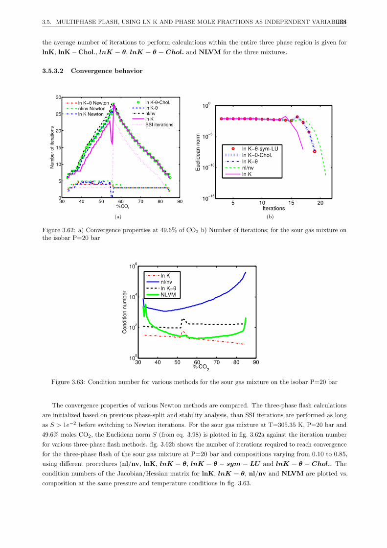
3.5. MULTIPHASE FLASH, USING LN K AND PHASE MOLE FRACTIONS AS INDEPENDENT VARIABLES134

the average number of iterations to perform calculations within the entire three phase region is given for

lnK, lnK−Chol., lnK − θ, lnK − θ − Chol. and NLVM for the three mixtures.

3.5.3.2 Convergence behavior

30 40 50 60 70 80 900

5

10

15

20

25

30

CO2%

Num

bero

fite

ratio

ns

ln K-θ-Chol.ln K-θnl/nvln KSSI iterations

ln K−θ Newtonnl/nv Newtonln K Newton

(a)

5 10 15 2010

−15

10−10

10−5

100

Iterations

Euc

lidea

nno

rm

ln K−θ-sym-LUln K−θ-Chol.ln K−θnl/nvln K

(b)

Figure 3.62: a) Convergence properties at 49.6% of CO2 b) Number of iterations; for the sour gas mixture onthe isobar P=20 bar

30 40 50 60 70 80 90100

102

104

106

Conditionnumber

CO2

%

ln Knl/nvln K−θNLVM

Figure 3.63: Condition number for various methods for the sour gas mixture on the isobar P=20 bar

The convergence properties of various Newton methods are compared. The three-phase flash calculations

are initialized based on previous phase-split and stability analysis, than SSI iterations are performed as long

as S > 1e−2 before switching to Newton iterations. For the sour gas mixture at T=305.35 K, P=20 bar and

49.6% moles CO2, the Euclidean norm S (from eq. 3.98) is plotted in fig. 3.62a against the iteration number

for various three-phase flash methods. fig. 3.62b shows the number of iterations required to reach convergence

for the three-phase flash of the sour gas mixture at P=20 bar and compositions varying from 0.10 to 0.85,

using different procedures (nl/nv, lnK, lnK − θ, lnK − θ − sym− LU and lnK − θ − Chol.. The

condition numbers of the Jacobian/Hessian matrix for lnK, lnK − θ, nl/nv and NLVM are plotted vs.

composition at the same pressure and temperature conditions in fig. 3.63.

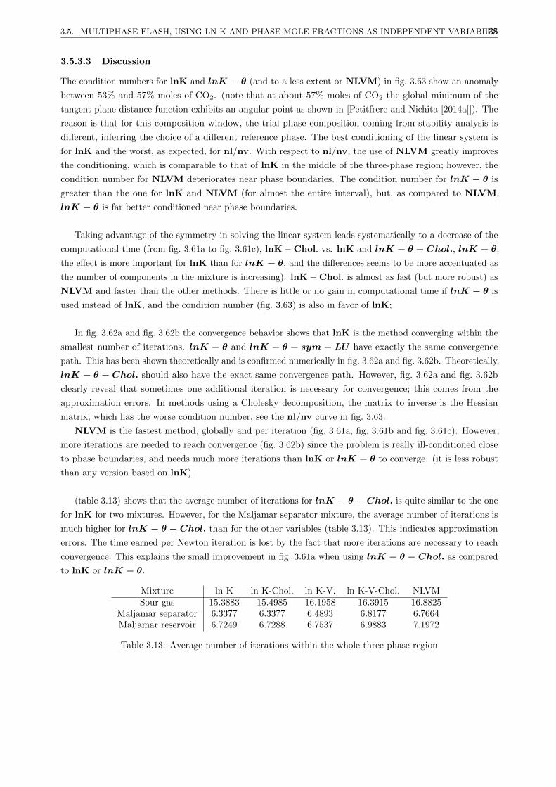
3.5. MULTIPHASE FLASH, USING LN K AND PHASE MOLE FRACTIONS AS INDEPENDENT VARIABLES135

3.5.3.3 Discussion

The condition numbers for lnK and lnK − θ (and to a less extent or NLVM) in fig. 3.63 show an anomaly

between 53% and 57% moles of CO2. (note that at about 57% moles of CO2 the global minimum of the

tangent plane distance function exhibits an angular point as shown in [Petitfrere and Nichita [2014a]]). The

reason is that for this composition window, the trial phase composition coming from stability analysis is

different, inferring the choice of a different reference phase. The best conditioning of the linear system is

for lnK and the worst, as expected, for nl/nv. With respect to nl/nv, the use of NLVM greatly improves

the conditioning, which is comparable to that of lnK in the middle of the three-phase region; however, the

condition number for NLVM deteriorates near phase boundaries. The condition number for lnK − θ is

greater than the one for lnK and NLVM (for almost the entire interval), but, as compared to NLVM,

lnK − θ is far better conditioned near phase boundaries.

Taking advantage of the symmetry in solving the linear system leads systematically to a decrease of the

computational time (from fig. 3.61a to fig. 3.61c), lnK−Chol. vs. lnK and lnK − θ − Chol., lnK − θ;

the effect is more important for lnK than for lnK − θ, and the differences seems to be more accentuated as

the number of components in the mixture is increasing). lnK−Chol. is almost as fast (but more robust) as

NLVM and faster than the other methods. There is little or no gain in computational time if lnK − θ is

used instead of lnK, and the condition number (fig. 3.63) is also in favor of lnK;

In fig. 3.62a and fig. 3.62b the convergence behavior shows that lnK is the method converging within the

smallest number of iterations. lnK − θ and lnK − θ − sym− LU have exactly the same convergence

path. This has been shown theoretically and is confirmed numerically in fig. 3.62a and fig. 3.62b. Theoretically,

lnK − θ − Chol. should also have the exact same convergence path. However, fig. 3.62a and fig. 3.62b

clearly reveal that sometimes one additional iteration is necessary for convergence; this comes from the

approximation errors. In methods using a Cholesky decomposition, the matrix to inverse is the Hessian

matrix, which has the worse condition number, see the nl/nv curve in fig. 3.63.

NLVM is the fastest method, globally and per iteration (fig. 3.61a, fig. 3.61b and fig. 3.61c). However,

more iterations are needed to reach convergence (fig. 3.62b) since the problem is really ill-conditioned close

to phase boundaries, and needs much more iterations than lnK or lnK − θ to converge. (it is less robust

than any version based on lnK).

(table 3.13) shows that the average number of iterations for lnK − θ − Chol. is quite similar to the one

for lnK for two mixtures. However, for the Maljamar separator mixture, the average number of iterations is

much higher for lnK − θ − Chol. than for the other variables (table 3.13). This indicates approximation

errors. The time earned per Newton iteration is lost by the fact that more iterations are necessary to reach

convergence. This explains the small improvement in fig. 3.61a when using lnK − θ − Chol. as compared

to lnK or lnK − θ.

Mixture ln K ln K-Chol. ln K-V. ln K-V-Chol. NLVMSour gas 15.3883 15.4985 16.1958 16.3915 16.8825

Maljamar separator 6.3377 6.3377 6.4893 6.8177 6.7664Maljamar reservoir 6.7249 6.7288 6.7537 6.9883 7.1972

Table 3.13: Average number of iterations within the whole three phase region

Chapter 4

Improvements in the characterization

of heavy oils : Semi-continuous

thermodynamics

Contents

4.1 Introduction . . . . . . . . . . . . . . . . . . . . . . . . . . . . . . . . . . . . . . . 136

4.2 A new distribution function . . . . . . . . . . . . . . . . . . . . . . . . . . . . . . 138

4.3 Gaussian quadrature . . . . . . . . . . . . . . . . . . . . . . . . . . . . . . . . . . 140

4.4 Semi-continuous description . . . . . . . . . . . . . . . . . . . . . . . . . . . . . . 141

4.5 Calculation procedure . . . . . . . . . . . . . . . . . . . . . . . . . . . . . . . . . . 144

4.5.1 Discrete equilibrium flash calculations . . . . . . . . . . . . . . . . . . . . . . . . . 144

4.5.2 Reconstruction of the initial solution . . . . . . . . . . . . . . . . . . . . . . . . . . 144

4.5.3 Algorithm . . . . . . . . . . . . . . . . . . . . . . . . . . . . . . . . . . . . . . . . . 145

4.6 Results . . . . . . . . . . . . . . . . . . . . . . . . . . . . . . . . . . . . . . . . . . . 145

4.6.1 Two-phase equilibrium . . . . . . . . . . . . . . . . . . . . . . . . . . . . . . . . . . 147

4.6.2 Three-phase equilibrium hydrocarbon mixture-water . . . . . . . . . . . . . . . . . 149

4.6.3 Three-phase equilibrium hydrocarbon mixture-carbon dioxide . . . . . . . . . . . . 151

4.6.4 Influence of the number of quadrature points on accuracy . . . . . . . . . . . . . . 152

4.7 Conclusion . . . . . . . . . . . . . . . . . . . . . . . . . . . . . . . . . . . . . . . . 154

4.1 Introduction

Several mixtures for interest in industry, such as naturally occurring hydrocarbon mixtures (crude oils and gas

condensates), feeds encountered in chemical processing, polymer solutions, etc., contain a very large number

of components. Because: (i) a very large number of components can make prohibitive phase equilibrium

calculations (as for instance in petroleum reservoir compositional simulation) and (ii) it is impossible to

identify all components by standard chemical analysis (the heavier fractions are difficult to characterize),

pseudo-components (grouping several individual components or fractions) are used to decrease the dimension-

ality of the phase equilibrium problem.

Usually, a mixture is lumped into pseudo-components using certain proximity criteria to select which

components belong to a given pseudo-component [Montel and Gouel [1984], Newley and Merrill [1991], Lin

et al. [2008]], then pseudo-component properties (critical pressure and temperature, acentric factor) and binary

interaction parameters (BIPs) are assigned using appropriate averaging techniques. This approximation in

fluid composition characterization may lead to significant errors in phase equilibrium calculations.

136

4.1. INTRODUCTION 137

An elegant alternative to classical lumping procedures is the so-called continuous thermodynamics, which is

based on the description of the composition of multicomponent mixtures by approximation with a continuous

distribution function. In the semi-continuous thermodynamics, some of the individual components are treated

discretely (usually light hydrocarbon components and non-hydrocarbon components: CO2, N2, H2S, H2O,

etc.), while the remaining components (usually the heavy components) are included in the continuous part of

the mixture. Continuous and semi-continuous thermodynamics were first developed by [Ratzsch and Kehlen

[1983] and by Cotterman and Prausnitz [1985]], respectively. Soon thereafter in the 80’s, several authors

worked on developing continuous or semi-continuous thermodynamic phase equilibrium calculation procedures:

[Cotterman et al. [1985], Behrens and Sandler [1986], Shibata et al. [1986], Willman and A.S. [1986], Willman

and A.S. [1987a], Willman and A.S. [1987b], Ratzsch et al. [1988]]. Later on, semi-continuous thermodynamics

has been applied to a variety of phase equilibrium problems: flash calculations at different specifications

[Chou and J.M. [1986]], phase stability analysis using the Gibbs tangent plane distance [Browarzik et al.

[1998], Monteagudo et al. [2001b]], critical point calculations [Rochocz et al. [1997]], compositional gradients

[Lira-Galeana et al. [1994], Esposito et al. [2000]], liquid-solid equilibrium [Labadie and Luks [2003]], asphal-

tene precipitation [Monteagudo et al. [2001a]], vapor-liquid equilibrium using equations of state with group

contributions [Baer et al. [1997]], etc.

The most encountered methods use the generalized Gauss-Laguerre quadrature to convert the continuous

distribution of the mole (mass) concentration into a discrete one. More recently presented approaches are

using specific techniques, such as a general Gauss-Stieltjes quadrature method able to calculate nodes and

weights for any distribution function [Nichita et al. [2001]], orthonormal polynomials [Liu and Wong [1997]]

or the quadrature method of moments [Lage [2007]].

However, most of the approaches presented in the literature are based on standard distributions. If the

feed composition cannot be modeled by a standard distribution functions, or if it is simply highly irregular,

most methods would not work properly. The semi-continuous approach based on the quadrature method

of moments developed by [Lage [2007]] uses an optimal quadrature rule by taking the feed composition

distribution as the weight function and it works with arbitrary compositions. However, in the original

formulation of the QMoM, the quadrature is solved using Gordon’s product-difference algorithm (PDA)

[Gordon [1968]], which works well only for a small number of quadrature points. [John and Thein [2012]]

compared the performance of the QMoM using PDA with the long quotient-modified difference algorithm

(LQMDA) [Sack and Donovan [1972]] and the Golub-Welsch algorithm [Golub and Welsch [1969]]. They

found that in certain situations the PDA failed (starting from eight quadrature nodes in their considered

examples) whereas the two other examined methods were successful. [Gautschi [2004]] showed that the

problem is ill conditioned, and the condition number grows exponentially with the number of quadrature points.

In this work, the QMoM is applied to multiphase equilibrium calculations for actual oil mixtures using a

cubic equation of state with non-zero BIPs. The calculation of the quadrature is based on the procedure

proposed by [Gautschi [1994]] (ORTHOPOL), which avoids problems due to the ill-conditioned nature of the

problem and is suitable for an undetermined number of quadrature points (unlike the QMoM with the PDA).

In some applications, it is important to use a number of pseudo-components larger than seven (which seems

to be the limit of applicability of the PDA).

The chapter is structured as follows: first, a new distribution function is introduced; after a brief recall on

Gaussian quadratures the semi-continuous description is presented. The general algorithm is given, then

results for two- and three-phase flash calculations on a heavy oil mixed with carbon dioxide and water are

presented before concluding. The calculation of the quadrature is detailed in two appendices.

4.2. A NEW DISTRIBUTION FUNCTION 138

4.2 A new distribution function

Usually, in semi-continuous thermodynamics, classical distribution functions are used to model the feed

composition, such as the gamma [Cotterman and Prausnitz [1985], Shibata et al. [1986], Willman and A.S.

[1986], Nichita et al. [2001], Whitson [1983]], beta [Park and Kim [1993]], exponential [Behrens and Sandler

[1986], Nichita et al. [2001]] distributions, etc., or even multivariate distributions [Willman and A.S. [1987a],

Willman and A.S. [1987b]]. In this work, a different way to define the distribution function and to use it

within the Gaussian quadrature calculation is presented.

Let us consider the ratio of liquid mole numbers to feed composition

Di =nLizi

=xiL

xiL+ yiV=

1

1 + VLKi

=1

1 + VL exp(lnKi)

(4.1)

Where nLi are the component mole numbers in the liquid phase, L and V are the liquid and vapor phase

mole fractions, respectively, and Ki = yi/xi are the equilibrium constants. From (eq. 4.2), Di is a logistic

function in terms of lnKi For two-parameter cubic equations of state (EoS) and van der Waals mixing rules,

the equilibrium constants can be written [Nichita and Minescu [2004]] as

lnKi = c0 + cbbi + ca√ai +

m∑k=1

ckγk,i (4.2)

Where m is the number of components having non-zero binary interaction parameters (BIPs) with the

remaining components in the mixture, and the terms γk,i = (1 − kik)√ai; i = 1, n; k = 1,m contain the

non-zero BIPs. In (eq. 4.2),√ai, bi and γk,i are the elements of the reduction matrix [Hendriks [1988]] and

ck are functions of the reduction parameters [Hendriks [1988]].

Equilibrium constants can also be expressed as a function of a characterization variable I (which can be

taken as carbon number, molecular weight, true boiling point, or specific gravity; in this work the carbon

number is used as characterization variable):

lnK(I) = c0 + cbb(I) + ca√a(I) +

m∑k=1

ckγk(I) (4.3)

Where γk(I) = (1− kkI )√a(I)

The function K(I) is a strictly decreasing function for the C7+ fraction of a same family; the critical prop-

erties and the acentric factor are monotonic: I > J =⇒ TC(I) > TC(J), pC(I) < pC(J) and ω(I) < ω(J).

It is recommended also to use monotonic BIPs (that is, kkI < kkJ). Therefore, component’ I will be more

present in the liquid phase than the component’ J .

In terms of I, (eq. 4.2), rewritten as

D(I) =nL(I)

z(I)=

x(I)L

x(I)L+ y(I)V=

1

1 + VL exp (lnK(I))

(4.4)

defines a distribution function.

Let us call the distribution D(I) (or (nL/z) the liquid to feed mole ratio (LFMR). The feed composition

of a Canadian heavy oil (denoted Oil S) is plotted against the carbon number in fig. 4.1. Extended analysis

of the C7+ fraction was available, and mixture composition is described by 100 components. To illustrate

4.2. A NEW DISTRIBUTION FUNCTION 139

the shape of the LFMR distribution function, the nLi /zi ratio is plotted vs. carbon number in fig. 4.2a and

fig. 4.2b for various pressures in the two-phase region within a large interval of temperatures (from 300 K to

800 K). In fig. 4.3a, the initial composition of the oil S has been manually altered to give a highly irregular

feed composition; The LFMR function is plotted for the altered composition in fig. 4.3b, showing that the

proposed function is smooth even though the feed composition is far from classical distributions or it could

not even be approximated by a smooth function.

0 20 40 60 80 1000

1

2

3

4

5

Carbon number

initi

alm

olar

com

posi

tion

Figure 4.1: Feed composition vs. carbon numbers for the S. oil

0 20 40 60 800

0.2

0.4

0.6

0.8

1

Carbon number

nil/z

i

(a)

0 20 40 60 800

0.2

0.4

0.6

0.8

1

Carbon number

nil/z

i

(b)

Figure 4.2: LFMR for different pressures and temperatures for the S. oil

0 20 40 60 800

0.005

0.01

0.015

0.02

0.025

0.03

0.035

Carbon number

Feed

com

posi

tion

(a)

0 20 40 60 800

0.2

0.4

0.6

0.8

1

Carbon number

nil/z

i

(b)

Figure 4.3: a) Altered feed composition (oil S) b) LFMR; vs carbon number for the altered oil S

4.3. GAUSSIAN QUADRATURE 140

4.3 Gaussian quadrature

A Gaussian quadrature approximates a definite integral by a discrete sum

b∫a

W (x)f(x)dx ≈n∑i=0

wif(xi) (4.5)

Where n is the number of quadrature points, f ∈ L2([ab]), W ∈ L2([ab]), xi ∈ R, ∀i = 1, n, wi ∈R, ∀i = 1, n.

The construction of the Gaussian quadrature requires the computation of quadrature nodes and weights.

Let pn be a nontrivial polynomial of degree n such that

b∫a

W (x)xkpn(x)dx = 0 (∀)k = 0, 1, ..., n− 1 (4.6)

If xi ∈ ]a, b[ are the n roots of the polynomial pn(x), then there exist n weights wi which make exact

the integral calculated by the Gaussian quadrature for all polynomials q(x) of degree 2n − 1 or less. The

polynomial pn(x) is said to be an orthogonal polynomial of degree n associated to the weight function W (x).

This polynomial is unique and its coefficients must be calculated to solve the quadrature.

The ordinary moments for a given weight function are given by

µr =

b∫a

xrW (x)dx, r = 0, 1, ..., 2n− 1 (4.7)

and the modified moments [Wheeler [1974]] are

vn =

b∫a

pn(x)W (x)dx (4.8)

In the quadrature method of moments, all the moments of the weight function are calculated (ordinary

moments for Gordon’s PDA [Gordon [1968] and Golub and Welsch [1969]] algorithm, and modified mo-

ments for the LQMDA [Sack and Donovan [1972]] and Wheeler’s algorithm [Wheeler [1974]]). Once all

the moments are computed, the computation of the inner products (see Appendix K) becomes straightforward.

[John and Thein [2012]] showed that the PDA is well suited only up to a certain number of nodes (up

to seven in their examples), and is less robust than the Golub-Welsch algorithm and the LQMDA. Besides

the fact that the QMoM with PDA [Gordon [1968]] leads to an ill-conditioned problem when increasing the

number of quadrature points ([Gautschi [2004]] proved that the condition number grows exponentially with

the number of quadrature points), they showed that in certain cases failures are due to the vanishing of

a moment. [John and Thein [2012]] recommended the use of LQMDA or one of its variants (for instance

Wheeler’s algorithm [Wheeler [1974]]) with the QMoM.

In this work, the calculation of the quadrature is based on the procedure proposed by Gautschi (OR-

THOPOL) [Gautschi [1994]], which avoids problems due to the ill-conditioned nature of the problem. The

calculation of the unique orthogonal polynomial associated to the weight function is presented in Appendix K

and the calculation of quadrature nodes and weights is given in Appendix L. This represents the core routine

of the QMoM. The complexity, as well as the difference between different methods consists in computing

the inner products for αn and βn (the coefficients of the recursive formula for orthogonal polynomials), in

4.4. SEMI-CONTINUOUS DESCRIPTION 141

equations (eq. K.2) and (eq. K.3).

4.4 Semi-continuous description

If the composition is discrete, the complementarity relation of feed mole fractions zi can be written by

separating the components which remain discrete in the semi-continuous description from the components

belonging to the continuous part of the mixture

nD∑i=1

zDi +

nc∑i=1

zCi = 1 (4.9)

For the semi-continuous description, (eq. 4.9) writes as

nD∑i=1

zDi +

Imax∫Imin

zC(I)dI = 1 (4.10)

with a continuous integral replacing the second summation, where Imin and Imax are specified and are

related to the minimum and maximum carbon number in the continuous part of the mixture.

0 20 40 60 80 1000

0.01

0.02

0.03

0.04

0.05

Carbon number

Feed

com

posi

tion discrete

continuous

ContinuousDiscrete

Figure 4.4: Feed composition of the semi-continuous mixture (Oil S) after cubic spline interpolation on thecontinuous part

From a discrete feed composition, a cubic spline interpolation can be used to create the continuous

fractions. For the Oil S, there are 6 discrete components (from methane to hexanes fraction; note that normal

and iso intermediary components were grouped together) and 94 components in the continuous part of the

mixture. Feed composition of the semi-continuous mixture (Oil S) is represented in fig. 4.4, showing the

discrete components (the light ones) and the continuous portion of the mixture as obtained after a cubic

spline interpolation. The generation of the continuous part creates a shift in the feed composition (their sum

will not be equal to one anymore), which has to be rescaled as

zC(I) =zC(I)

X(4.11)

with

X =

∫ Imax

IminzC(I)dI

1−∑nD

=1 zDi

(4.12)

Let us consider that the liquid phase composition is described by an arbitrary distribution (not necessarily

the same as for the feed composition). Similar to (eq. 4.10), one can write for the liquid phase

4.4. SEMI-CONTINUOUS DESCRIPTION 142

nD∑i=1

xDi +

Imax∫Imin

xC(I)dI = 1 (4.13)

or, in terms of liquid mole numbers

nD∑i=1

niL +

Imax∫Imin

nL(I)dI = L (4.14)

By multiplying and dividing the integrand with zC(I), (eq. 4.14) writes

nD∑i=1

niL +

Imax∫Imin

zC(I)nL(I)

zC(I)dI = L (4.15)

and one can recognize in the above equation the distribution LFMR, D(I) = nL(I)/zC(I), introduced in

the section 2 of this chapter(and plotted for various temperature-pressure conditions in fig. 4.2a and fig. 4.2b

for the Oil S).

The Gaussian quadrature will be quite accurate as long as the function f(x) can be well approximated by

a polynomial function. It has been seen that nL/z has always the same shape, it is smooth, and thus can

be well approximated by polynomial functions. Polynomial regression tests showed that the error is smaller

than 10−3 for polynomials with order greater than six. In addition, unlike in a classical Gaussian quadrature

(in which the weight function is given), the procedure of [Gautschi [1994]] allows arbitrary weight functions

W (x). Therefore, the feed composition can be used as the weight function.

The integral in (eq. 4.5) can be approximated using

W (I) = zC(I) (4.16)

And

f(I) ≡ D(I) =nL(I)

zC(I)(4.17)

giving

Imax∫Imin

zC(I)nL(I)

zC(I)dI =

nC∑j=1

zjnjL(xj)

zj(4.18)

Or

Imax∫Imin

W (I)f(I)dI =

nC∑j=1

wjf(xj) (4.19)

It is very important to note that f is not used within the Gaussian quadrature calculation. The distribution

nL(I)/zC(I) is not known explicitly before performing a flash calculation; however, it is known that the

shape of this distribution function is always the one of a logistic function and it is well approximated by

a polynomial; this is the only requirement on the function f , in order to get an accurate approximation.

Moreover, one can take f = 1; in this case (eq. 4.19) simply reads

Imax∫Imin

zC(I)dI =

nC∑j=1

zj (4.20)

4.4. SEMI-CONTINUOUS DESCRIPTION 143

The key in Lage’s QMoM is to take the feed composition as a weight function. In fact, Lage’s methodology

might be called the feed-weight quadrature method (FWQM) rather than QMoM (since the quadrature

can be solved also by methods not involving moments directly, see the previous section). In this work, we

have arrived at the same choice in a somewhat different way, by justifying the choice of wi = zi based

on some physics, that is, on the newly introduced LFMR distribution. This choice of the weight func-

tion has been made precisely to obtain the LFMR function (which is smooth for any temperatures and

pressure conditions for a given feed). It is shown above that the given weight function allows to satisfy

the mass balance for the feed, provided f = 1 (the quadrature in (eq. 4.19) is exact for any polynomial

function of order less than 2n − 1). This ensures to compute pseudo-components which will give a really

good representation of the whole continuous fluid and give accurate results for an equilibrium flash calculation.

By solving the above quadrature problem (eq. 4.19), the abscissas (nodes) and the discrete weights

that approximate the continuous integral are obtained. The nodes correspond to the carbon numbers (or

any other characterization variables, as for instance true boiling points) where the quadrature is applied,

and weights give the mole fractions of the pseudo-components. It means that instead of performing the

flash on the semi-continuous mixture, the quadrature calculates N carbon numbers, corresponding to N

pseudo-components, and phase equilibrium calculations can be carried out as for a discrete mixture for

accurately reproduce the fluid behavior.

The procedure presented above can be readily extended if different distributions are used for each

component family or different portions of the continuous part are modeled by different distribution functions,

(eq. 4.9) in the discrete case can be written as

nD∑i=1

zDi +

ndistr∑k=1

nC(k)∑j=1

zCkj = 1 (4.21)

and (eq. 4.10) in the semi-continuous case becomes

nD∑i=1

zDi +

ndistr∑k=1

Imax(k)∫Imin(k)

zCk (I)dI = 1 (4.22)

Where ndistr is the number of distributions used.

The method the most commonly found in the literature is to approximate the feed composition with

a standard distribution and to solve a classical Gaussian quadrature. Generally, the parameters of the

distribution giving the best fit of the feed composition have to be calculated, and then the quadrature can be

applied to the approximated distribution. However, the feed composition is not always regular and can have a

shape far away from any standard distribution. In such cases, this methodology cannot be applied accurately.

In the QMoM, the weight function is arbitrary, and for each calculated pseudo-component, the discrete weight

function corresponds to its feed composition. Moreover, the function to which the quadrature is applied is

always regular and smooth, guaranteeing an efficient and adapted computation of the pseudo-components for

every feed composition.

In our implementation, the code was designed to incorporate two options:

• Discrete weights (feed composition) are directly used in the quadrature, as in Lage’s QMoM;

• Interpolated weight functions are used (for instance by cubic splines as mentioned above).

As it will be seen later in the results section, the first option gives more accurate results; the second

option may be useful if the problem is reformulated in terms of a different characterization variable (say true

4.5. CALCULATION PROCEDURE 144

boiling points from a distillation curve).

4.5 Calculation procedure

4.5.1 Discrete equilibrium flash calculations

After carrying out the quadrature procedure with the arbitrary weights zCk , the abscissas xj (the nodes of the

quadrature) are found. These nodes give the carbon numbers corresponding to the N ’pseudo-components’

in the semi-continuous description of the mixture. The properties required in traditional flash calculations

are then calculated for these carbon numbers, and any flash calculation method can be used as if the system

is discrete.

Pseudo-component properties (critical properties and acentric factor, as well as BIPs between discrete

components and pseudo-components) can be calculated based on any correlation from the literature (in the

present paper, an in-house correlation has been used). The only requirement is to respect the monotonicity

of the critical properties, which is the key point for getting the logistic function. Cubic splines are used

for critical properties, acentric factors and BIPs to create continuous functions of carbon numbers. Then,

the properties are evaluated at each carbon number I to obtain the properties and BIPs for the ’lumped’ system.

A classical equilibrium flash calculation is performed on the discrete composition in which the pseudo-

components corresponding to the continuous part are added. Since pseudo-component properties can be

written as a function of the carbon number, any thermodynamic model (even complex equations of state

with various mixing rules) can be used, as long as the monotonic behavior of K(I) is observed (as in (eq. 4.3)

for cubic equations of state).

In two-phase flash calculations, successive substitution iterations followed by second-order Newton

iterations are used, starting from Wilson’s K-values for initialization. In three-phase flash calculations, the

results of phase stability testing and two-phase flash calculations are used for initialization.

4.5.2 Reconstruction of the initial solution

At the solution of flash calculations on the lumped mixture, it may be needed to calculate the composition of

the full mixture, and not only on the lumped one.

Two methodologies were tested to recover the full composition from the lumped composition:

• The cubic spline interpolation over the lnK vs. carbon number distribution. The distribution is a

really smooth distribution as well, and could be very well interpolated by polynomial functions.

• The delumping (inverse lumping) procedure, as developed by [Nichita and Leibovici [2006] and Nichita

et al. [2006b]] for multiphase systems.

It was observed that when all BIPs are set to zero, the first approach acts better. Conversely, when

non-zero BIPs are used in the cubic EoS, the second method is clearly superior. Thus, the delumping method

is the one used in the paper, and the one advised.

Let us suppose that m < n components in the mixture have non-zero BIPs with all the other components,

that is, kkj = kjk 6= 0 for I, j = k + 1, n and kji = kij = 0 for i, j = m + 1, n. Usually m << n (BIPs are

non-zero for non-hydrocarbon - hydrocarbon pairs, and between light and heavy hydrocarbon components; it

is considered that there are no interactions between components belonging to the continuous portion of the

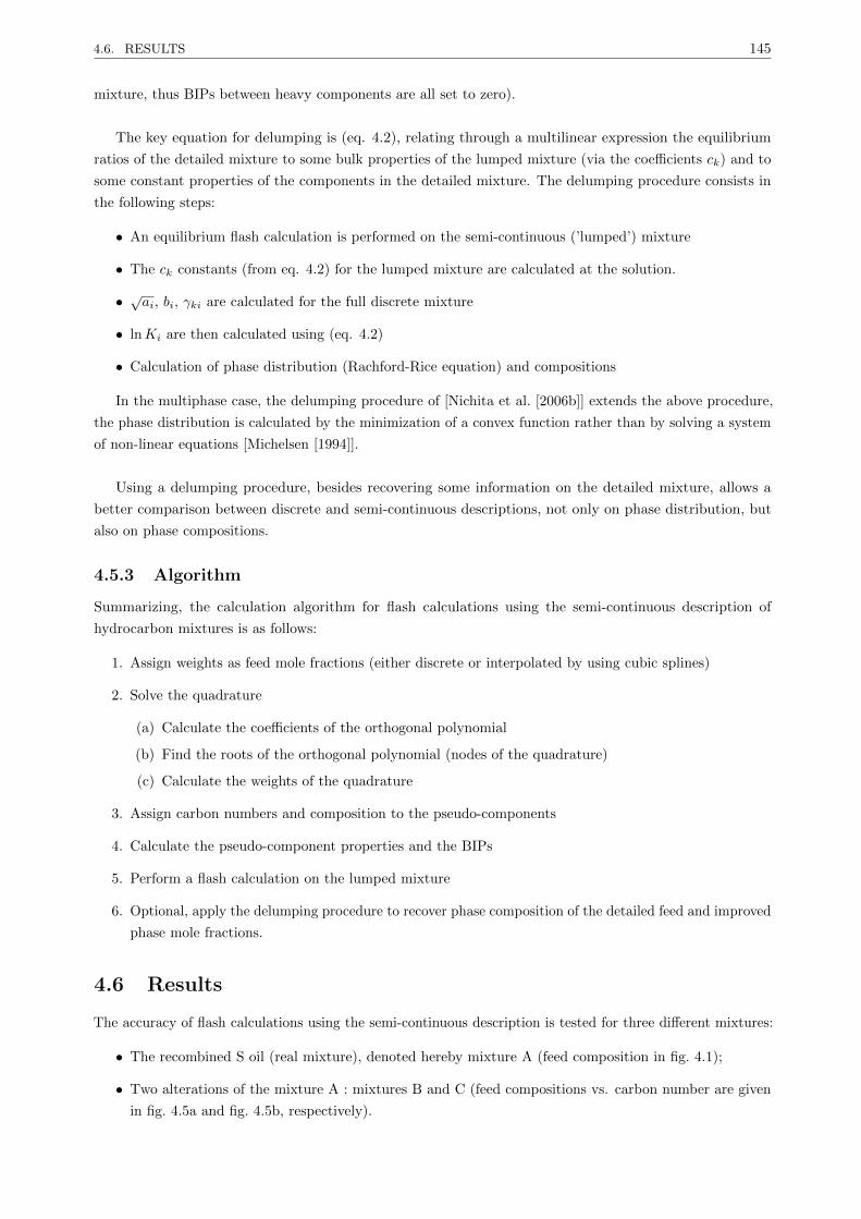
4.6. RESULTS 145

mixture, thus BIPs between heavy components are all set to zero).

The key equation for delumping is (eq. 4.2), relating through a multilinear expression the equilibrium

ratios of the detailed mixture to some bulk properties of the lumped mixture (via the coefficients ck) and to

some constant properties of the components in the detailed mixture. The delumping procedure consists in

the following steps:

• An equilibrium flash calculation is performed on the semi-continuous (’lumped’) mixture

• The ck constants (from eq. 4.2) for the lumped mixture are calculated at the solution.

• √ai, bi, γki are calculated for the full discrete mixture

• lnKi are then calculated using (eq. 4.2)

• Calculation of phase distribution (Rachford-Rice equation) and compositions

In the multiphase case, the delumping procedure of [Nichita et al. [2006b]] extends the above procedure,

the phase distribution is calculated by the minimization of a convex function rather than by solving a system

of non-linear equations [Michelsen [1994]].

Using a delumping procedure, besides recovering some information on the detailed mixture, allows a

better comparison between discrete and semi-continuous descriptions, not only on phase distribution, but

also on phase compositions.

4.5.3 Algorithm

Summarizing, the calculation algorithm for flash calculations using the semi-continuous description of

hydrocarbon mixtures is as follows:

1. Assign weights as feed mole fractions (either discrete or interpolated by using cubic splines)

2. Solve the quadrature

(a) Calculate the coefficients of the orthogonal polynomial

(b) Find the roots of the orthogonal polynomial (nodes of the quadrature)

(c) Calculate the weights of the quadrature

3. Assign carbon numbers and composition to the pseudo-components

4. Calculate the pseudo-component properties and the BIPs

5. Perform a flash calculation on the lumped mixture

6. Optional, apply the delumping procedure to recover phase composition of the detailed feed and improved

phase mole fractions.

4.6 Results

The accuracy of flash calculations using the semi-continuous description is tested for three different mixtures:

• The recombined S oil (real mixture), denoted hereby mixture A (feed composition in fig. 4.1);

• Two alterations of the mixture A : mixtures B and C (feed compositions vs. carbon number are given

in fig. 4.5a and fig. 4.5b, respectively).

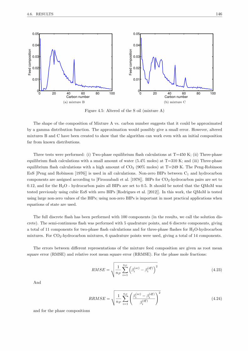
4.6. RESULTS 146

0 20 40 60 80 1000

0.01

0.02

0.03

0.04

0.05

Carbon number

Feed

com

posi

tion

(a) mixture B

0 20 40 60 80 1000

0.01

0.02

0.03

0.04

0.05

Carbon number

Feed

com

posi

tion

(b) mixture C

Figure 4.5: Altered of the S oil (mixture A)

The shape of the composition of Mixture A vs. carbon number suggests that it could be approximated

by a gamma distribution function. The approximation would possibly give a small error. However, altered

mixtures B and C have been created to show that the algorithm can work even with an initial composition

far from known distributions.

Three tests were performed: (i) Two-phase equilibrium flash calculations at T=450 K; (ii) Three-phase

equilibrium flash calculations with a small amount of water (5.4% moles) at T=310 K; and (iii) Three-phase

equilibrium flash calculations with a high amount of CO2 (90% moles) at T=249 K. The Peng-Robinson

EoS [Peng and Robinson [1976]] is used in all calculations. Non-zero BIPs between C1 and hydrocarbon

components are assigned according to [Firoozabadi et al. [1978]]. BIPs for CO2-hydrocarbon pairs are set to

0.12, and for the H2O - hydrocarbon pairs all BIPs are set to 0.5. It should be noted that the QMoM was

tested previously using cubic EoS with zero BIPs [Rodrigues et al. [2012]]. In this work, the QMoM is tested

using large non-zero values of the BIPs; using non-zero BIPs is important in most practical applications when

equations of state are used.

The full discrete flash has been performed with 100 components (in the results, we call the solution dis-

crete). The semi-continuous flash was performed with 5 quadrature points, and 6 discrete components, giving

a total of 11 components for two-phase flash calculations and for three-phase flashes for H2O-hydrocarbon

mixtures. For CO2-hydrocarbon mixtures, 6 quadrature points were used, giving a total of 14 components.

The errors between different representations of the mixture feed composition are given as root mean

square error (RMSE) and relative root mean square error (RRMSE). For the phase mole fractions:

RMSE =

√√√√ 1

nP

nP∑i=1

(β

(sc)i − β(df)

i

)2

(4.23)

And

RRMSE =

√√√√ 1

nP

nP∑i=1

(β

(sc)i − β(df)

i

β(df)i

)2

(4.24)

and for the phase compositions

4.6. RESULTS 147

RMSEi =

√√√√ 1

nP

nP∑j=1

(x

(del)ij − x(df)

ij

)2

; i = 1, n (4.25)

and

RRMSEi =

√√√√√ 1

nP

nP∑j=1

(x

(del)ij − x(df)

ij

x(df)ij

)2

; i = 1, n (4.26)

Where np is the number of phases in equilibrium, βj is the mole fraction of the phase j, xij is the mole

fraction of the component i in the phase j, and superscripts (sc), (df) and (del) denote the semi-continuous,

discrete and delumped feeds, respectively. Calculations were performed using the two options for weight

functions (using the discrete feed compositions as weight function or using an interpolated weight function).

The results are presented only for the first option in fig. 4.6 to fig. 4.17b, because, as can be seen from

fig. 4.18a to fig. 4.20b, it gives more accurate results (usually errors are at least one order of magnitude

lower).

4.6.1 Two-phase equilibrium

2 4 6 8 10 120

0.02

0.04

0.06

0.08

0.1

0.12

Pressure, bar

Pha

sem

ole

fract

ions

gas−delumpedgas−lumpedgas−discrete

Figure 4.6: Mole fraction in the vapor phase for mixture A at T=450 K

2 4 6 8 10 1210

−8

10−6

10−4

10−2

100

Pressure ,bar

Abs

olut

eer

ror(

RM

SE

) delumped phase mole fractionslumped phase mole fractions

(a) Absolute error

0 2 4 6 8 10 12 1410

−8

10−6

10−4

10−2

100

Pressure ,bar

Relativeerror(RRMSE) delumped phase mole fractions

lumped phase mole fractions

(b) Relative error

Figure 4.7: Error in phase mole fractions for mixture A at T=450 K

4.6. RESULTS 148

Two-phase equilibrium flash calculations were performed at T=450 K for the three mixtures. Mixture

A (oil S) is a heavy oil, thus the bubble point pressure is low (12 bar at T=450 K). The mole fractions

in the vapor phase for mixture A are plotted against pressure at T=450 K in fig. 4.6, for the full discrete,

semi-continuous (denoted here ’lumped’) and delumped representations of the feed composition. An excellent

agreement is observed, the absolute (eq. 4.23, see fig. 4.7a) and relative (eq. 4.24, see fig. 4.7b) errors in

phase mole fractions of lumped and delumped results with respect to the discrete results being of the order

of 10−4 or less on the entire pressure interval, except at low pressures.

The absolute errors (eq. 4.25) and relative errors (eq. 4.26) in component mole fractions (between detailed

and delumped feeds) at T=450 K and P=8 bar are plotted against the carbon number in fig. 4.8a and

fig. 4.8b, respectively. The errors are very small for the continuous part of the mixture (RMSE of the order

of 10−6 or less, RRMSE of the order of 10−4). Higher deviations are observed for components in the discrete

part of the semi-continuous mixture. Plots of errors against the carbon number at T=450 K and P=8 bar

are given for mixture B in fig. 4.9a (RMSE) and fig. 4.9b (RRMSE), and for mixture C in fig. 4.10a (RMSE)

and fig. 4.10b (RRMSE). It can be seen from fig. 4.8a to fig. 4.10b that the initial composition affects the

accuracy of the results. The errors in composition are increasing with the irregularities (from mixture A to

mixture C), which is normal because the number of pseudo-components (quadrature points) is too small to

model all the irregularities. However, absolute errors are still very small and relative errors reasonably small

for the highly irregular feed composition of mixture C.

0 20 40 60 80 10010

−15

10−10

10−5

Carbon Number

Abs

olut

eer

ror(

RM

SE

)

(a) Absolute error

0 20 40 60 80 10010

−15

10−10

10−5

100

Carbon Number

Rel

ativ

eer

ror(

RR

MS

E)

(b) Relative error

Figure 4.8: Error in phase compositions for mixture A at T=450 K and P=8 bar

0 20 40 60 80 10010

−15

10−10

10−5

Carbon Number

Abs

olut

eer

ror(

RM

SE

)

(a) Absolute error

0 20 40 60 80 10010

−15

10−10

10−5

100

Carbon Number

Rel

ativ

eer

ror(

RR

MS

E)

(b) Relative error

Figure 4.9: Error in phase compositions for mixture B at T=450 K and P=8 bar

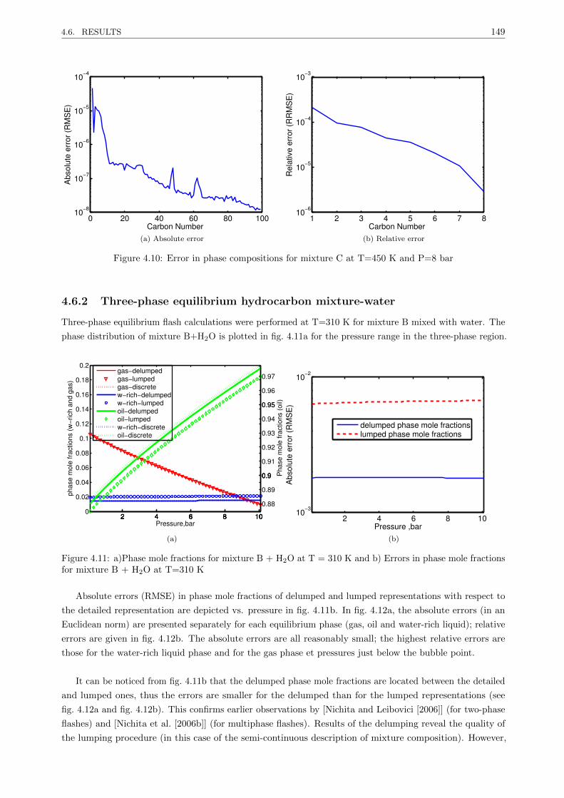
4.6. RESULTS 149

0 20 40 60 80 10010

−8

10−7

10−6

10−5

10−4

Carbon Number

Abs

olut

eer

ror(

RM

SE

)

(a) Absolute error

1 2 3 4 5 6 7 810

−6

10−5

10−4

10−3

Carbon Number

Rel

ativ

eer

ror(

RR

MS

E)

(b) Relative error

Figure 4.10: Error in phase compositions for mixture C at T=450 K and P=8 bar

4.6.2 Three-phase equilibrium hydrocarbon mixture-water

Three-phase equilibrium flash calculations were performed at T=310 K for mixture B mixed with water. The

phase distribution of mixture B+H2O is plotted in fig. 4.11a for the pressure range in the three-phase region.

2 4 6 8 100

0.02

0.04

0.06

0.08

0.1

0.12

0.14

0.16

0.18

0.2

Pressure,bar

phas

em

ole

fract

ions

(w−r

ich

and

gas)

2 4 6 8 10

0.9

0.95

Pha

se m

ole

fract

ions

(oil)

2 4 6 8 10

0.9

2 4 6 8 10

0.88

0.89

0.9

0.91

0.92

0.93

0.94

0.95

0.96

0.97gas−delumpedgas−lumpedgas−discretew−rich−delumpedw−rich−lumpedoil−delumpedoil−lumpedw−rich−discreteoil−discrete

(a)

2 4 6 8 1010

−3

10−2

Pressure ,bar

Abs

oluteerror(RMSE)

delumped phase mole fractionslumped phase mole fractions

(b)

Figure 4.11: a)Phase mole fractions for mixture B + H2O at T = 310 K and b) Errors in phase mole fractionsfor mixture B + H2O at T=310 K

Absolute errors (RMSE) in phase mole fractions of delumped and lumped representations with respect to

the detailed representation are depicted vs. pressure in fig. 4.11b. In fig. 4.12a, the absolute errors (in an

Euclidean norm) are presented separately for each equilibrium phase (gas, oil and water-rich liquid); relative

errors are given in fig. 4.12b. The absolute errors are all reasonably small; the highest relative errors are

those for the water-rich liquid phase and for the gas phase et pressures just below the bubble point.

It can be noticed from fig. 4.11b that the delumped phase mole fractions are located between the detailed

and lumped ones, thus the errors are smaller for the delumped than for the lumped representations (see

fig. 4.12a and fig. 4.12b). This confirms earlier observations by [Nichita and Leibovici [2006]] (for two-phase

flashes) and [Nichita et al. [2006b]] (for multiphase flashes). Results of the delumping reveal the quality of

the lumping procedure (in this case of the semi-continuous description of mixture composition). However,

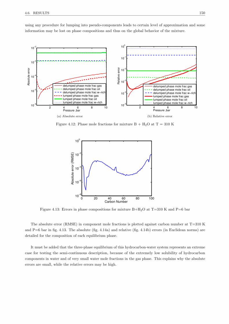
4.6. RESULTS 150

using any procedure for lumping into pseudo-components leads to certain level of approximation and some

information may be lost on phase compositions and thus on the global behavior of the mixture.

2 4 6 8 1010

−6

10−5

10−4

10−3

10−2

Pressure ,bar

Abs

olut

eer

ror

delumped phase mole frac gasdelumped phase mole frac oildelumped phase mole frac w−richlumped phase mole frac gaslumped phase mole frac oillumped phase mole frac w−rich

(a) Absolute error

2 4 6 8 1010

−5

10−4

10−3

10−2

10−1

100

Pressure ,bar

Rel

ativ

eer

ror

delumped phase mole frac gasdelumped phase mole frac oildelumped phase mole frac w−richlumped phase mole frac gaslumped phase mole frac oillumped phase mole frac w−rich

(b) Relative error

Figure 4.12: Phase mole fractions for mixture B + H2O at T = 310 K

0 20 40 60 80 10010

−8

10−6

10−4

10−2

100

Carbon Number

Abs

olut

eer

ror(

RM

SE

)

Figure 4.13: Errors in phase compositions for mixture B+H2O at T=310 K and P=6 bar

The absolute error (RMSE) in component mole fractions is plotted against carbon number at T=310 K

and P=6 bar in fig. 4.13. The absolute (fig. 4.14a) and relative (fig. 4.14b) errors (in Euclidean norms) are

detailed for the composition of each equilibrium phase.

It must be added that the three-phase equilibrium of this hydrocarbon-water system represents an extreme

case for testing the semi-continuous description, because of the extremely low solubility of hydrocarbon

components in water and of very small water mole fractions in the gas phase. This explains why the absolute

errors are small, while the relative errors may be high.

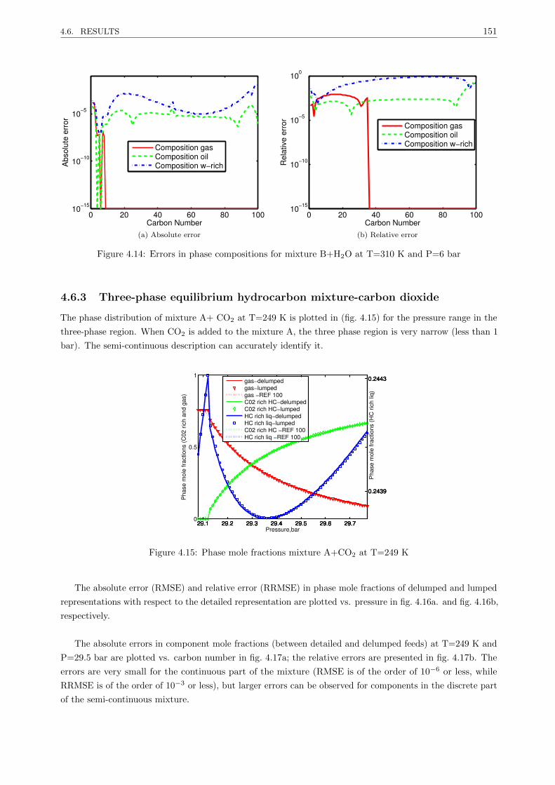
4.6. RESULTS 151

0 20 40 60 80 10010

−15

10−10

10−5

Carbon Number

Abs

olut

eer

ror

Composition gasComposition oilComposition w−rich

(a) Absolute error

0 20 40 60 80 10010

−15

10−10

10−5

100

Carbon Number

Rel

ativ

eer

ror

Composition gasComposition oilComposition w−rich

(b) Relative error

Figure 4.14: Errors in phase compositions for mixture B+H2O at T=310 K and P=6 bar

4.6.3 Three-phase equilibrium hydrocarbon mixture-carbon dioxide

The phase distribution of mixture A+ CO2 at T=249 K is plotted in (fig. 4.15) for the pressure range in the

three-phase region. When CO2 is added to the mixture A, the three phase region is very narrow (less than 1

bar). The semi-continuous description can accurately identify it.

29.1 29.2 29.3 29.4 29.5 29.6 29.70

0.5

1

Pressure,bar

Pha

sem

ole

fract

ions

(C02

rich

and

gas)

29.1 29.2 29.3 29.4 29.5 29.6 29.7

0.2439

0.2443

29.1 29.2 29.3 29.4 29.5 29.6 29.7

0.2439

0.2443

29.1 29.2 29.3 29.4 29.5 29.6 29.7

0.2439

0.2443P

hase

mol

efra

ctio

ns(H

Cric

hliq

)

gas−delumpedgas−lumpedgas −REF 100C02 rich HC−delumpedC02 rich HC−lumpedHC rich liq−delumpedHC rich liq−lumpedC02 rich HC −REF 100HC rich liq −REF 100

Figure 4.15: Phase mole fractions mixture A+CO2 at T=249 K

The absolute error (RMSE) and relative error (RRMSE) in phase mole fractions of delumped and lumped

representations with respect to the detailed representation are plotted vs. pressure in fig. 4.16a. and fig. 4.16b,

respectively.

The absolute errors in component mole fractions (between detailed and delumped feeds) at T=249 K and

P=29.5 bar are plotted vs. carbon number in fig. 4.17a; the relative errors are presented in fig. 4.17b. The

errors are very small for the continuous part of the mixture (RMSE is of the order of 10−6 or less, while

RRMSE is of the order of 10−3 or less), but larger errors can be observed for components in the discrete part

of the semi-continuous mixture.

4.6. RESULTS 152

29.1 29.2 29.3 29.4 29.5 29.6 29.710

−6

10−5

10−4

10−3

Pressure, bar

Absoluteerror(RMSE) delumped system

lumped system

(a) Absolute error

29.1 29.2 29.3 29.4 29.5 29.6 29.710−6

10−5

10−4

10−3

10−2

Pressure, bar

Relativeerror(RRMSE) delumped system

lumped system

(b) Relative error

Figure 4.16: Errors in phase mole fraction, mixture A+CO2 at T=249 K

0 20 40 60 80 10010

−10

10−9

10−8

10−7

10−6

Carbon number

Abs

olut

eer

ror(

RM

SE

)

(a) Absolute error

0 20 40 60 80 10010

−7

10−6

10−5

10−4

10−3

10−2

Carbon number

Rel

ativ

eer

ror(

RR

MS

E)

(b) Relative error

Figure 4.17: Errors in phase compositions for mixture A+CO2 at T=249 K and P=29.5 bar

4.6.4 Influence of the number of quadrature points on accuracy

The influence of the number of quadrature points (pseudo-components) on the accuracy of two- and three-

phase flash calculations is evaluated. First, at a given temperature, errors on phase mole fractions are

evaluated over an entire pressure interval. The root mean square error is given in this case by

RMSE =

√√√√ 1

nptsnP

npts∑j=1

nP∑i=1

(β

(sc)i,j − β

(df)i,j

)2

(4.27)

where npts is the number of pressure points.

Then, errors on phase compositions are evaluated at a given pressure, with an RMSE given by

RMSE =

√√√√ 1

nPn

n∑i=1

nP∑j=1

(x

(sc)ij − x

(del)ij

)2

(4.28)

The absolute errors (RMSE given by eq. 4.27) on phase mole fractions (over the entire two-phase region)

vs. the number of quadrature points are plotted for mixture A at T=450 K in fig. 4.18a. In fig. 4.18b,

4.6. RESULTS 153

absolute errors (RMSE given by eq. 4.28) on phase compositions are represented for mixture A as a function

of the number of quadrature points at P=8 bar. The absolute errors on phase mole fractions (over the entire

three-phase region) are plotted vs. the number of quadrature points in fig. 4.19a for mixture A + H2O at

T=310 K and in fig. 4.20a for mixture A + CO2 at T=249 K. The absolute errors on phase compositions vs.

the number of quadrature points are plotted in fig. 4.19b for mixture A + H2O at T=310 K and P=6 bar

and for mixture A + CO2 at T=249 K and P=29.5 bar.

0 5 10 15 20 25 3010

−8

10−7

10−6

10−5

10−4

10−3

Number of quadrature points

Absoluteerror(RMSE)

interpolated weight functiondiscrete weight function

(a)

0 5 10 15 20 25 3010−9

10−8

10−7

10−6

10−5

10−4

Number of quadrature points

Absoluteerror(RMSE)

interpolated weight functiondiscrete weight function

(b)

Figure 4.18: Errors vs. the number of quadrature points, mixture A at T=450 K. a) In phase mole fractionsin the two-phase region; b) in compositions at P=8 bar

0 5 10 15 20 25 3010

−6

10−5

10−4

10−3

10−2

10−1

Number of quadrature points

Abs

olut

eer

ror(

RM

SE

)

interpolated weight functiondiscrete weight function

(a)

0 5 10 15 20 25 3010

−6

10−5

10−4

10−3

10−2

10−1

Number of quadrature points

Abs

olut

eer

ror(

RM

SE

)

interpolated weight functiondiscrete weight function

(b)

Figure 4.19: Absolute errors vs. the number of quadrature points, mixture A+H2O at T=310 K; a) In phasemole fractions in the three-phase region; b) in compositions at P=6 bar

In Figures fig. 4.18a to fig. 4.20b, errors are plotted for both discrete and interpolated weight functions.

In all cases, the errors are at least one order of magnitude lower for the discrete weight function. It can be

observed from these figures that there is practically no improvement in accuracy for N greater than 6-8 for

the interpolated weight function. However, for the discrete weight function, the decreasing trend is observed

for higher numbers of quadrature points, at least for multiphase flashes.

Theoretically, the error plotted against the number of quadrature points should give a monotonically

decreasing function with a horizontal asymptote (at N → +∞). However, this is not the case, as can be seen

from figures fig. 4.18a to fig. 4.20b (a trend line was added to each of these figures). The discrete mixture has

been transformed into a semi-continuous mixture by means of a cubic spline; this approximation changes

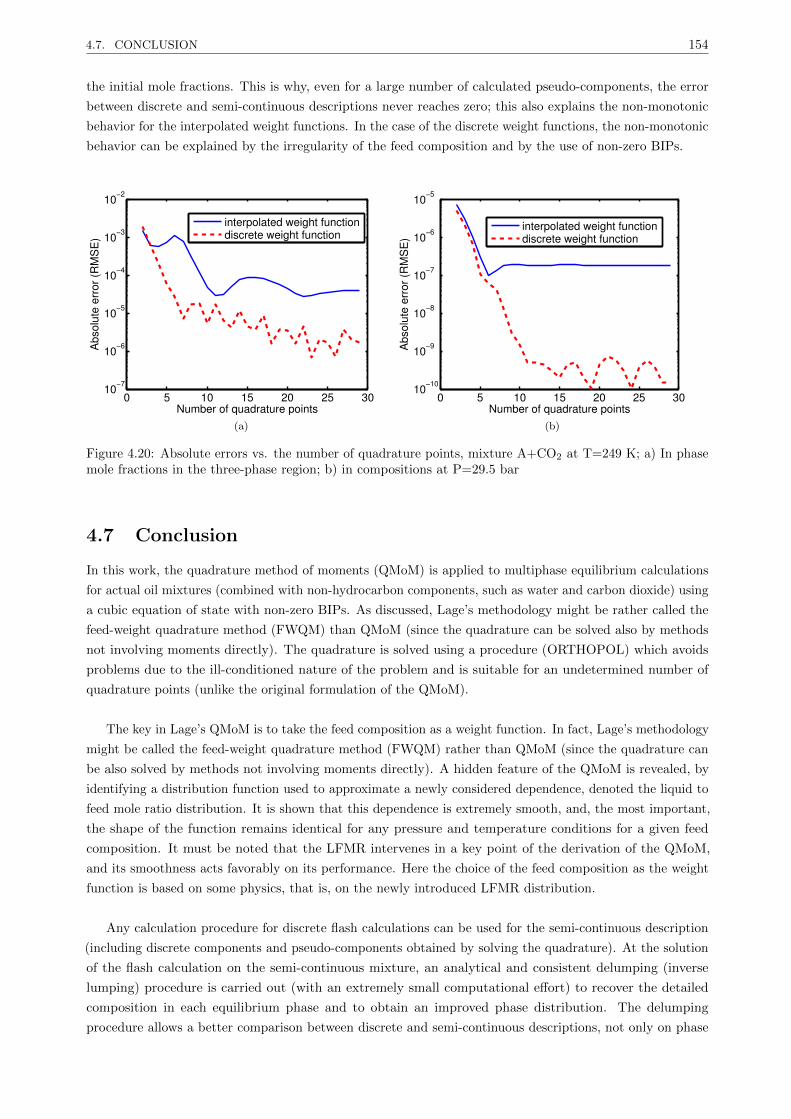
4.7. CONCLUSION 154

the initial mole fractions. This is why, even for a large number of calculated pseudo-components, the error

between discrete and semi-continuous descriptions never reaches zero; this also explains the non-monotonic

behavior for the interpolated weight functions. In the case of the discrete weight functions, the non-monotonic

behavior can be explained by the irregularity of the feed composition and by the use of non-zero BIPs.

0 5 10 15 20 25 3010

−7

10−6

10−5

10−4

10−3

10−2

Number of quadrature points

Absoluteerror(RMSE)

interpolated weight functiondiscrete weight function

(a)

0 5 10 15 20 25 3010

−10

10−9

10−8

10−7

10−6

10−5

Number of quadrature pointsAbsoluteerror(RMSE)

interpolated weight functiondiscrete weight function

(b)

Figure 4.20: Absolute errors vs. the number of quadrature points, mixture A+CO2 at T=249 K; a) In phasemole fractions in the three-phase region; b) in compositions at P=29.5 bar

4.7 Conclusion

In this work, the quadrature method of moments (QMoM) is applied to multiphase equilibrium calculations

for actual oil mixtures (combined with non-hydrocarbon components, such as water and carbon dioxide) using

a cubic equation of state with non-zero BIPs. As discussed, Lage’s methodology might be rather called the

feed-weight quadrature method (FWQM) than QMoM (since the quadrature can be solved also by methods

not involving moments directly). The quadrature is solved using a procedure (ORTHOPOL) which avoids

problems due to the ill-conditioned nature of the problem and is suitable for an undetermined number of

quadrature points (unlike the original formulation of the QMoM).

The key in Lage’s QMoM is to take the feed composition as a weight function. In fact, Lage’s methodology

might be called the feed-weight quadrature method (FWQM) rather than QMoM (since the quadrature can

be also solved by methods not involving moments directly). A hidden feature of the QMoM is revealed, by

identifying a distribution function used to approximate a newly considered dependence, denoted the liquid to

feed mole ratio distribution. It is shown that this dependence is extremely smooth, and, the most important,

the shape of the function remains identical for any pressure and temperature conditions for a given feed

composition. It must be noted that the LFMR intervenes in a key point of the derivation of the QMoM,

and its smoothness acts favorably on its performance. Here the choice of the feed composition as the weight

function is based on some physics, that is, on the newly introduced LFMR distribution.

Any calculation procedure for discrete flash calculations can be used for the semi-continuous description

(including discrete components and pseudo-components obtained by solving the quadrature). At the solution

of the flash calculation on the semi-continuous mixture, an analytical and consistent delumping (inverse

lumping) procedure is carried out (with an extremely small computational effort) to recover the detailed

composition in each equilibrium phase and to obtain an improved phase distribution. The delumping

procedure allows a better comparison between discrete and semi-continuous descriptions, not only on phase

4.7. CONCLUSION 155

distribution, but also on phase compositions.

The QMoM in our implementation has been tested for different initial compositions of a hydrocarbon

mixture for two-phase equilibrium calculations and in the presence of water and carbon dioxide, for three-phase

flash calculations. In all cases, the location of the phase boundaries, the phase distributions and the phase

compositions are well reproduced by the semi-continuous description.

Since the QMoM relates the discrete initial detailed composition having a large number of components to

a small number of components which approximates the continuous portion of the mixture, it can be viewed in

a larger sense as a lumping - delumping procedure. It is generally applicable, even in cases when no standard

distribution function can model the feed composition, or several distribution functions are needed to model

different portions of the mixture or different homologous series. It is proven in this work that [Lage [2007]]’s

methodology coupled with a delumping procedure and using a cubic equation of state with non-zero BIPs

works for actual oil mixtures with good accuracy.

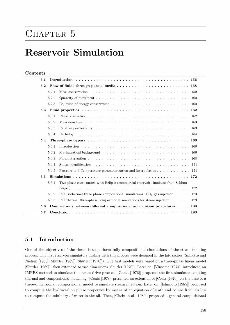
Chapter 5

Reservoir Simulation

Contents

5.1 Introduction . . . . . . . . . . . . . . . . . . . . . . . . . . . . . . . . . . . . . . . 156

5.2 Flow of fluids through porous media . . . . . . . . . . . . . . . . . . . . . . . . . 158

5.2.1 Mass conservation . . . . . . . . . . . . . . . . . . . . . . . . . . . . . . . . . . . . 159

5.2.2 Quantity of movement . . . . . . . . . . . . . . . . . . . . . . . . . . . . . . . . . . 160

5.2.3 Equation of energy conservation . . . . . . . . . . . . . . . . . . . . . . . . . . . . 160

5.3 Fluid properties . . . . . . . . . . . . . . . . . . . . . . . . . . . . . . . . . . . . . 162

5.3.1 Phase viscosities . . . . . . . . . . . . . . . . . . . . . . . . . . . . . . . . . . . . . 162

5.3.2 Mass densities . . . . . . . . . . . . . . . . . . . . . . . . . . . . . . . . . . . . . . 163

5.3.3 Relative permeability . . . . . . . . . . . . . . . . . . . . . . . . . . . . . . . . . . 163

5.3.4 Enthalpy . . . . . . . . . . . . . . . . . . . . . . . . . . . . . . . . . . . . . . . . . 164

5.4 Three-phase bypass . . . . . . . . . . . . . . . . . . . . . . . . . . . . . . . . . . . 166

5.4.1 Introduction . . . . . . . . . . . . . . . . . . . . . . . . . . . . . . . . . . . . . . . 166

5.4.2 Mathematical background . . . . . . . . . . . . . . . . . . . . . . . . . . . . . . . . 166

5.4.3 Parameterization . . . . . . . . . . . . . . . . . . . . . . . . . . . . . . . . . . . . . 168

5.4.4 Status identification . . . . . . . . . . . . . . . . . . . . . . . . . . . . . . . . . . . 171

5.4.5 Pressure and Temperature parameterization and interpolation . . . . . . . . . . . . 171

5.5 Simulations . . . . . . . . . . . . . . . . . . . . . . . . . . . . . . . . . . . . . . . . 172

5.5.1 Two phase case: match with Eclipse (commercial reservoir simulator from Schlum-

berger) . . . . . . . . . . . . . . . . . . . . . . . . . . . . . . . . . . . . . . . . . . 172

5.5.2 Full isothermal three phase compositional simulations: CO2 gas injection . . . . . 173

5.5.3 Full thermal three-phase compositional simulations for steam injection . . . . . . . 179

5.6 Comparisons between different compositional acceleration procedures . . . . 189

5.7 Conclusion . . . . . . . . . . . . . . . . . . . . . . . . . . . . . . . . . . . . . . . . 190

5.1 Introduction

One of the objectives of the thesis is to perform fully compositional simulations of the steam flooding

process. The first reservoir simulators dealing with this process were designed in the late sixties (Spillette and

Nielsen [1968], Shutler [1969]], Shutler [1970]]). The first models were based on a three-phase linear model

[Shutler [1969]], then extended to two dimensions [Shutler [1970]]. Later on, [Vinsome [1974]] introduced an

IMPES method to simulate the steam drive process. [Coats [1976]] proposed the first simulator coupling

thermal and compositional modelling. [Coats [1978]] presented an extension of [Coats [1976]] on the base of a

three-dimensional, compositional model to simulate steam injection. Later on, [Ishimoto [1985]] proposed

to compute the hydrocarbon phase properties by means of an equation of state and to use Raoult’s law

to compute the solubility of water in the oil. Then, [Chein et al. [1989]] proposed a general compositional

156

5.1. INTRODUCTION 157

simulator which could deal with thermal options using both K-value and EOS-based formulations. Once

again, the water phase was assumed to be an ideal solution.

More recently, [Cicek and Ertekin [1996], and later Cicek [2005]] developed a fully implicit compositional

multiphase simulator to simulate steam injection problems. In their formulation, water is treated within

the equilibrium calculations. The simulator is based on K-value models which can be tuned to match

phase-diagrams. However, the tables are generally functions of one oil component, the pressure and the

temperature. The K-values approach generally does not gives correct solubilities of hydrocarbon components

in the water phase and solubilities of water in the hydrocarbon liquid phase.

It has been observed (fig. 6) however, that for high temperatures, the solubility of the water component in

the hydrocarbon rich phase was not negligible. The current commercial softwares make some approximations

to simulate steam injection problems. Those approximations are even more important in case of heavy oils.

ECLIPSE 500 and INTERSECT for instance, are thermal compositional simulators working with K-Values,

or (in case of INTERSECT) which treat water separately from the equilibrium flash calculation; this can

lead to important inaccuracies.

For this reason, some authors started to simulate steam injection with EoS-based full compositional

reservoir simulators. Using the fact that the solubility of hydrocarbons within the water phase is negligible

for some ranges of pressures-temperatures, for steam flooding problems some authors have developed a

free water flash based on this assumption [Luo and Barrufet [2005]] and more recently applied to heavy oil

SAGD problems [Heidari [2014]]. The same methodology has been applied to in-situ upgrading [Lapene [2010]].

For cold CO2 injection problems, no assumption can be made and some authors have extended simulator

models with full four-phase multiphase flash problems. [Varavei and Sepehrnoori [2009] and Okuno [2009]]

developed a four-phase EOS-based simulator. As the solubility of water in hydrocarbons is negligible for

small temperatures, they did not include water within the equilibrium calculations.

However, the reservoir water is generally closer to brine than to pure water and the free-water hypothesis

is not valid anymore. [Brantferger [1991]] developed a simulator using an equation of state to calculate the

thermodynamic properties of each phase (even for the water phase). They proposed an isenthalpic flash,

taking enthalpy as primary variable instead of the temperature. [Voskov et al. [2009]] proposed a general

purpose reservoir simulator. They developed an efficient way to calculate the phase equilibrium based on the

tie-line parameterization of the flash. [Varavei and Sepehrnoori [2009]] and more recently [Zaydullin et al.

[2014]] developed full three phase flash simulations for steam injection problems.

Finally, [Feizabadi [2013]] extended compositional simulations to simulate isothermal solvent injection

problems with a full four-phase EOS-based compositional simulator.

However, to the best of our knowledge, no case of fully EoS based compositional simulations of steam

injection (like the SAGD process) with extra-heavy oil has been proposed in the literature yet, treating

the water phase within the equilibrium calculations (and without any limiting assumption). This kind of

simulations seem to be important and will offer improved tools for predictive studies for the heavy oil fields.

In this chapter, a description of the different equations used in reservoir simulations will be given, as well

as the different models to represent the physical properties of the fluids.

In the previous chapter of this work, new algorithms for the equilibrium calculation problems were

presented. Based on this work, a program dealing with multiphase calculations has been developed integrating

all the presented features (see chapters 2 and 3), called MFlash in this thesis.

5.2. FLOW OF FLUIDS THROUGH POROUS MEDIA 158

The program will be first tested in standalone calculations (i.e. without any reservoir simulator) for

various mixtures, and the results will be compared with literature and experimental data. Then some tests

with different reservoir simulators will be performed to check the program efficiency and robustness.

MFlash has been integrated into two reservoir simulators the T-PP platform (internal reservoir simulator

from Total S.A.) and AD-GPRS from the University of Stanford. The simulator is based on automatic

differentiations [Younis [2009] and Zhou [2012]], which allows a treatment of nonlinear physics [Voskov et al.

[2009d], Voskov and Zhou [2012]]. It is based on flexible discretizations such as Multi-Point Flux Approxima-

tion and on general Adaptive Implicit Method [Zhou et al. [2011]], high performance computing [Zhou et al.

[2011] and Tchelepi and Zhou [2013]], thermal compositional simulations [Iranshahr et al. [2010a], Zaydullin

et al. [2013]]. It also can be coupled with geomechanics [Garipov et al. [2012]] and include ajoint-based

optimization [Kourounis et al. [2010], Volkov and Voskov [2013]].

Different processes will be simulated. First, a two-phase simulation in presence of water treated separately

from the equilibrium calculations, will be tested. A comparison with the ECLIPSE commercial simulator will

also be presented.

Then, three and four-phase fully compositional simulations of CO2 injection problems will be described.

In different simulations, it has been noticed that when co-injecting solvent with the steam, sometimes a

solvent-rich phase could appear. We did not investigate the importance of modelling this phase for the

oil production forecast, but in an attempt to develop a robust thermodynamic package to simulate the

SAGD process, a four-phase simulation has been successfully tested and will be presented for isothermal CO2

injection problems.

Finally, for the thermal processes, fully compositional simulations of the steam-flooding process in hetero-

geneous reservoir as well as fully compositional simulations of the SAGD process will be performed with an

Athabasca bitumen.

In this last part, different methodologies improving computational times in the reservoir simulations will

be compared for all the presented simulations:

• The reduced variables for the stability analysis against conventional variables

• The bypass approach proposed by [Rasmussen et al. [2006]], which avoids stability computations (called

B-R) in this thesis

• The procedure from [Voskov and Tchelepi [2008], Voskov and Tchelepi [2009a], Voskov and Tchelepi

[2009b], Iranshahr et al. [2010a]] and more recently [Zaydullin et al. [2013]] based on the tie-simplex

parameterization of the space will be used together with MFlash.

5.2 Flow of fluids through porous media

At initial conditions, a petroleum reservoir is said to be in hydrostatic equilibrium. All forces (such as

capillarity pressure, gradient pressure, gravity, thermodynamic) are balanced and are in equilibrium. However,

as soon as fluid is injected and/or produced, the forces are not in equilibrium any longer and fluid advection and

diffusion appears. Theoretically, the fluid is not in thermodynamic equilibrium either. However, a generally

accepted assumption in the reservoir simulation framework is to consider the fluid in local thermodynamic

equilibrium. The continuum model can be seen as a large number of differentially small subsystems [Islam

et al. [2010]].

5.2. FLOW OF FLUIDS THROUGH POROUS MEDIA 159

5.2.1 Mass conservation

5.2.1.1 Accumulation term

For a multicomponent system, the total mole number of a component i in control volume dV is given by:

φ

np∑j=1

xijρjSjdV (5.1)

with

• ρj , the molar density of the phase j (mol.m−3) (all the units will be given in S.I.)

ρj =njVj

∀j = 1, np (5.2)

• nj , the mole number of the phase j (mol)

• Sj , the saturation of the phase j :

Sj =Vj∑npl=1 Vl

∀j = 1, np (5.3)

• Vj , the volume of phase j (m3).

• φ, the porosity of the volume dV

Hence, the rate of change of the mole number of component i in dV is given by:

∂

∂t

φ np∑j=1

xijρjSj

dV (5.4)

5.2.1.2 Advective term

A part of the mole accumulation in dV comes from the transport of components within the phases that flows

in and out of the control volume. Let dS be the differential element of the control volume. The rate of inflow

and outflow of the component i across the boundary of the control volume dV is given by

np∑j=1

−n.vjxijρjdS = −∇.

np∑j=1

vjxijρj

dV (5.5)

with vj the velocity of the phase j (m.s−1) and n the vector normal to dS.

5.2.1.3 Diffusive and dispersive term

Diffusion is mathematically treated with a diffusion tensor Dij of component i in phase j. The flux of diffusion

is taken to be

−Dij.∇ρjxij ∀i = 1, nc ∀j = 1, np (5.6)

where Dij is in (m2.s−1)

The total inflow and outflow of component i which goes out of the control volume dV is then given by:

− n.φ

np∑j=1

Dij.∇ρjxijdS = ∇.

φ np∑j=1

Dij.∇ρjxij

dV (5.7)

5.2. FLOW OF FLUIDS THROUGH POROUS MEDIA 160

When a fluid flows through a porous medium, the non-homogeneous velocity encountered at the pore-scale

(different velocity within each pore) increases the molecular mixing. This is called the dispersion [Larry [1989]].

The dispersion coefficient is proportional to the local phase velocity. This term is generally comparable or

greater than molecular diffusion.

Generally high numerical diffusion is observed at the field scale simulation. Therefore, the physical

diffusion and dispersion are generally not taken into account.

5.2.1.4 Mass conservation equation

Neglecting the diffusive and dispersive terms at field scale, the mass conservation equation of the component

i is given by:

∂

∂t

φ np∑j=1

xijρjSj

+∇.

np∑j=1

vjxijρj

+

np∑j=1

ρjqj = 0 ∀i = 1, nc (5.8)

where a source term∑npj=1 ρjqj is added in the unit volume, qj is the reduced source of phase j (reciprocal

of time constant (s−1)).

5.2.2 Quantity of movement

At pore scale where the approximation of continuous media exists, the Navier-Stokes equations can be written

for the quantity of movement conservation. At macroscopic (Darcy) scale, for a 3D flow system with the

gravitational force, the Navier-Stokes equation can be simplified to give the generalized Darcy’s law:

vj = −krjµj

K(∇pj − ρm,j℘∇z) j = 1, np (5.9)

with

• pj phase pressure (Pa), and pij = pi − pj , capillary pressure between phases i and j.

• krj the relative permeability of the phase j.

• ρm,j the mass density of the phase j (kg.m−3).

• ℘∇z gravity acceleration (m.s−2).

• K is the permeability tensor (m2).

• µj is the viscosity of the phase j (Pa.s).

5.2.3 Equation of energy conservation

5.2.3.1 Accumulation

The total energy of a unit volume of the fluid system is given by the sum of the internal energy for each

phase.

np∑j=1

ρjSjUj (5.10)

where Uj is the specific internal energy of the phase j (in J.mol−1). For a porous media, the energy coming

from the rock should be added:

5.2. FLOW OF FLUIDS THROUGH POROUS MEDIA 161

φ

np∑j=1

ρjSjUj + (1− φ) ρrUr (5.11)

where Ur is the rock specific internal energy (here per unit of mass), ρr is rock mass density.

5.2.3.2 Heat conduction

From the Fick’s law, the heat conduction through the reservoir fluid and rock are:

Qf = −λf∇Tf Qr = −λr∇Tr (5.12)

where λf , λr are respectively the coefficient of thermal conductivity of the fluid and the rock (in W.m−1.K−1);

Tf and Tr are respectively, the reservoir fluid temperature and the reservoir rock temperature (in K).

In many cases, the rock and the reservoir fluid temperature can be assumed identical, i.e. Tf = Tr = T ,

as a consequence, the difference between inflow and outflow for the heat flux is then given by:

−∇.(λ∇T ) (5.13)

where λ is bulk thermal conductivity.

5.2.3.3 Convective term in energy transfer

The enthalpy can be viewed as the sum of the internal energy of a fluid and the work performed on the

system.

H = U + PV (5.14)

Using the specific enthalpy of a phase (hj = Hj/nj (in J.mol−1)), the convective term of the energy

equation is given by:

∇.

np∑j=1

vjρjhj

dV (5.15)

5.2.3.4 Energy conservation equation

The energy balance may be given in the form:

0 =∂

∂t

φ∑j

ρjSjUj + (1− φ)ρrUr

+

∇. np∑j=1

ρjhjvj

−∇.(λ∇T ) +

np∑j=1

hjρjqj (5.16)

where∑npj=1 hjρjqj accounts for the source term, and qj is the same as for (eq. 5.8).

5.3. FLUID PROPERTIES 162

5.3 Fluid properties

5.3.1 Phase viscosities

5.3.1.1 Light-Medium fluid model

The LBC (Lohrentz-Bray-Clark) viscosity model [Lohrenz et al. [1964]] (model incorporated in ECLISPE

and INTERSECT) is given by:

µ = µ? +1

ζ

( 4∑k=0

akρkr

)4

exp

(ρr

ρmax,r − ρr

)− 10−4

(5.17)

µ?i =

3.4.10−4 T

0.94ri

ζiif Tri < 1.5

1.778.10−4 (4.58Tri−1.67)5/8

ζiif Tri ≥ 1.5

with

Tri =T

Tciζi = α.T

1/6ci M

−1/2wi P

−2/3ci (5.18)

In the original LBC correlation [Lohrenz et al. [1964]],

µ? =

∑nci=1 xiµ

?i

√Mwi

xi√Mwi

(5.19)

with xi the phase mole fraction of the phase

ρr = ρ

nc∑i=1

xiVci ρmax,r =∞ (5.20)

ζ = α.

[nc∑i=1

xiTci

]1/6 [ nc∑i=1

xiMwi

]−1/2 [ nc∑i=1

xiPci

]−2/3

(5.21)

This model is not suited for heavy oils. In other cases, this model can be used to model the viscosity of

any phase.

5.3.1.2 Heavy oil

For heavy oil applications, other models have been integrated. For the oil phase, an exponential law has been

used for each component:

µi = ai exp

(biT

)(5.22)

The parameters ai and bi are computed solving a least-square problem to fit the experimental data.

For the water phase, the viscosity model is computed using the STARS formulation. Finally for the gas

phase,

µi = ciTdi (5.23)

The parameters ci and di are computed by solving a least-square problem with the experimental data.

In the end, the viscosity of the fluid can be computed for each phase base on the relation

µ =

nc∑i=1

xiµi (5.24)

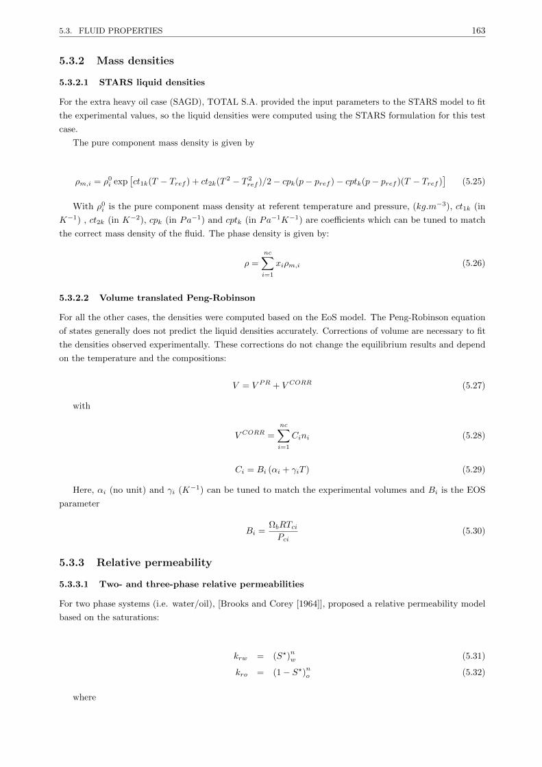
5.3. FLUID PROPERTIES 163

5.3.2 Mass densities

5.3.2.1 STARS liquid densities

For the extra heavy oil case (SAGD), TOTAL S.A. provided the input parameters to the STARS model to fit

the experimental values, so the liquid densities were computed using the STARS formulation for this test

case.

The pure component mass density is given by

ρm,i = ρ0i exp

[ct1k(T − Tref ) + ct2k(T 2 − T 2

ref )/2− cpk(p− pref )− cptk(p− pref )(T − Tref )]

(5.25)

With ρ0i is the pure component mass density at referent temperature and pressure, (kg.m−3), ct1k (in

K−1) , ct2k (in K−2), cpk (in Pa−1) and cptk (in Pa−1K−1) are coefficients which can be tuned to match

the correct mass density of the fluid. The phase density is given by:

ρ =

nc∑i=1

xiρm,i (5.26)

5.3.2.2 Volume translated Peng-Robinson

For all the other cases, the densities were computed based on the EoS model. The Peng-Robinson equation

of states generally does not predict the liquid densities accurately. Corrections of volume are necessary to fit

the densities observed experimentally. These corrections do not change the equilibrium results and depend

on the temperature and the compositions:

V = V PR + V CORR (5.27)

with

V CORR =

nc∑i=1

Cini (5.28)

Ci = Bi (αi + γiT ) (5.29)

Here, αi (no unit) and γi (K−1) can be tuned to match the experimental volumes and Bi is the EOS

parameter

Bi =ΩbRTciPci

(5.30)

5.3.3 Relative permeability

5.3.3.1 Two- and three-phase relative permeabilities

For two phase systems (i.e. water/oil), [Brooks and Corey [1964]], proposed a relative permeability model

based on the saturations:

krw = (S?)nw (5.31)

kro = (1− S?)no (5.32)

where

5.3. FLUID PROPERTIES 164

S? =Sw − Swc

1− Swc − Sor(5.33)

here

• Swc the irreducible critical saturation; the value for which the water start flowing.

• Sor the residual saturation of the oil.

• Sw the saturation of the water phase

For three phase systems, [Stone [1973]] proposed a model which interpolates between the two phase

relative permeabilities.

S?o =So − Som

1− Swc − SomSo ≥ Som (5.34)

S?w =Sw − Swc

1− Swc − SomSw ≥ Swc (5.35)

S?g =Sg

1− Swc − SomSo ≥ Sor (5.36)

Som being the residual saturation of the oil in the three phase system.

[Fayers and Matthews [1984]] proposed to evaluate Som with the following formulas:

Som = αSorw + (1− α)Sorg; α = 1− Sg1− Swc− Sorg

(5.37)

where Sorw is the oil residual saturation in the oil/water system and Sorg is the oil residual saturation in the

oil/gas system.

5.3.3.2 Four-phase relative permeabilities

[Yuan and Pope [2012]] developed new continuous permeability models, which could be used to four phases.

More recently, [Varavei [2009]], [Feizabadi [2013]], choose a [Brooks and Corey [1964]] model to model four

phase relative permeabilities. This model is not physical because each phase moves independently from each

other, which should not be the case. This is the model chosen in this work for the four phase simulation test

cases.

Swe = Sw−Swr1.0−Swr−Sgr krw = k0

rw (Swe)ew

Sge =Sg−Sgr

1.0−Swr−Sgr krg = k0rg (Sge)

2[1− (1− Sge)eg]

Soe = So−Sor1.0−Swr−Sor−Sgr kro = k0

ro (Soe)2

[1− (1− Soe)eo]Sle = Sl−Slr

1.0−Swr−Slr−Sgr krl = k0rl (Sle)

2 [1− (1− Sle)el

] (5.38)

5.3.4 Enthalpy

5.3.4.1 EoS based enthalpy of the oil and gas phases

Let xi be the composition of the component i for a given phase. The enthalpy H of a given phase at a given

pressure and temperature, can be expressed by

H(p, T,n) =

nc∑i=1

xiH?i (T ) +HR(p, T,n) (5.39)

5.3. FLUID PROPERTIES 165

5.3.4.1.1 Ideal heat capacity and ideal enthalpy

The heat capacity of an ideal gas can be approximated with a polynomial function of the temperature [Reid

et al. [1987]]. For an ideal gas, the molar ideal gas heat capacity is given by:

Cp?i (T ) = CpA,i + CpB,iT + CpC,iT2 + CpD,iT

3 (5.40)

[Passut and Danner [1972]] provide data for values of CpA,i to CpD,i for the most common components in

Petroleum Engineering. By definition the molar ideal gas enthalpy of the component i can be calculated from

H?i (T ) =

∫ T

Tref

Cp?i (x) dx (5.41)

which leads to

H?i (T ) = CpAi (T − Tref ) +

CpBi2

(T 2 − T 2

ref

)+CpCi

3

(T 3 − T 3

ref

)+CpDi

4

(T 4 − T 4

ref

)(5.42)

5.3.4.1.2 Residual enthalpy

The residual enthalpy can be computed from the EoS. From [Michelsen and Mollerup [2007]],

HR(T, p,n) = −RT 2nc∑i=1

(∂ lnφi∂T

)p,n

(5.43)

HR(T, p,n) = (Z − 1)RT +T ∂A∂T −A

(δ2 − δ1)Bln

(Z + δ2B

Z + δ1B

)(5.44)

5.3.4.2 Enthalpy of the water phase

The water properties are not really accurate, when computed with a cubic equation of state. Therefore, for

the water phase, another model is used to compute the enthalpy (which is similar to STARS’s model). In

STARS simulator, the molar heat capacity is computed from

Cpg,i(T ) = CpEi + CpFiT + CpGiT2 + CpHiT

3 (5.45)

By integrating with respect to the temperature, the molar gas enthalpy can be obtained:

Hg,i(T ) =

∫ T

TR

Cpg,i(x) dx (5.46)

which gives integrating (5.45) into (eq. 5.46):

Hg,i(T ) = CpEi (T − TR) +CpFi

2

(T 2 − T 2

R

)+CpGi

3

(T 3 − T 3

R

)+CpHi

4

(T 4 − T 4

R

)(5.47)

And the gas enthalpy can be obtained from:

Hg(T,n) =

nc∑i=1

xiHg,i(T ) (5.48)

with xi the composition of the component i in the water phase.

Hg,i(T ) = CpEi (T − TR) +CpFi

2

(T 2 − T 2

R

)+CpGi

3

(T 3 − T 3

R

)+CpHi

4

(T 4 − T 4

R

)(5.49)

For liquids, the enthalpy of vaporization is subtracted from the mixture enthalpy. The vaporization

enthalpy is computed from:

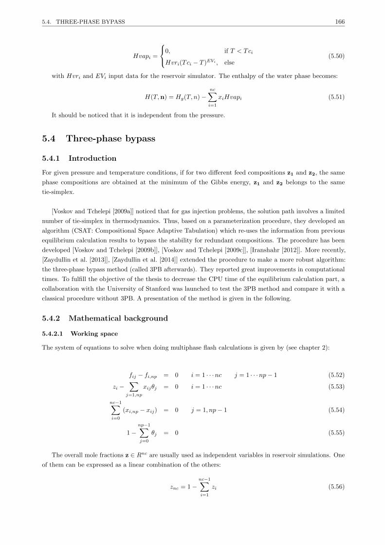
5.4. THREE-PHASE BYPASS 166

Hvapi =

0, if T < Tci

Hvri(Tci − T )EVi , else(5.50)

with Hvri and EVi input data for the reservoir simulator. The enthalpy of the water phase becomes:

H(T,n) = Hg(T, n)−nc∑i=1

xiHvapi (5.51)

It should be noticed that it is independent from the pressure.

5.4 Three-phase bypass

5.4.1 Introduction

For given pressure and temperature conditions, if for two different feed compositions z1 and z2, the same

phase compositions are obtained at the minimum of the Gibbs energy, z1 and z2 belongs to the same

tie-simplex.

[Voskov and Tchelepi [2009a]] noticed that for gas injection problems, the solution path involves a limited

number of tie-simplex in thermodynamics. Thus, based on a parameterization procedure, they developed an

algorithm (CSAT: Compositional Space Adaptive Tabulation) which re-uses the information from previous

equilibrium calculation results to bypass the stability for redundant compositions. The procedure has been

developed [Voskov and Tchelepi [2009b]], [Voskov and Tchelepi [2009c]], [Iranshahr [2012]]. More recently,

[Zaydullin et al. [2013]], [Zaydullin et al. [2014]] extended the procedure to make a more robust algorithm:

the three-phase bypass method (called 3PB afterwards). They reported great improvements in computational

times. To fulfill the objective of the thesis to decrease the CPU time of the equilibrium calculation part, a

collaboration with the University of Stanford was launched to test the 3PB method and compare it with a

classical procedure without 3PB. A presentation of the method is given in the following.

5.4.2 Mathematical background

5.4.2.1 Working space

The system of equations to solve when doing multiphase flash calculations is given by (see chapter 2):

fij − fi,np = 0 i = 1 · · ·nc j = 1 · · ·np− 1 (5.52)

zi −∑

j=1,np

xijθj = 0 i = 1 · · ·nc (5.53)

nc−1∑i=0

(xi,np − xij) = 0 j = 1, np− 1 (5.54)

1−np−1∑j=0

θj = 0 (5.55)

The overall mole fractions z ∈ Rnc are usually used as independent variables in reservoir simulations. One

of them can be expressed as a linear combination of the others:

znc = 1−nc−1∑i=1

zi (5.56)

5.4. THREE-PHASE BYPASS 167

Therefore, the working compositional space is given by:

∆nc−1 =[z ∈ Rnc, zi > 0,

∑zi = 1

](5.57)

The compositional space can be expressed as a linear combination of the mole fractions x (eq. 5.53)

zi =

np∑j=1

θjxij i = 1 · · ·nc− 1 (5.58)

This means that for a given tie-simplex ∆ defined by its composition at the equilibrium (x), each feed

composition which belongs to ∆ is only a function of the phase mole fractions. Therefore, for each tie-simplex,

each feed composition (vector of nc− 1 dimensions) can be parameterized with only np dimensions. The (np)

dimensional tie-simplex is defined by:

∆np =[θ ∈ Rnp, θi > 0,

∑θi = 1

](5.59)

When the dimension np of the tie-simplex is np = 2, the tie-simplex is called a tie-line, when np = 3, it is

called a tie-triangle.

Each tie-simplex ∆np represents a convex geometrical form in the compositional space (such as line,

triangle) where each vertex corresponds to the composition of one of the phases. A ternary diagram (for a

given pressure and temperature) is represented in fig. 5.1. A tie-triangle (corresponding to the three-phase

region of composition [xi, yi, wi]) is represented in grey, and different sets of tie-lines are represented in red,

blue and green (which correspond to different two-phase regions).

[Voskov and Tchelepi [2009c]] showed that for a strictly np-phase system, i.e. for each multiphase region,

the region is convex and there is a unique tie-simplex which intersects a given feed composition.

They also proved [Voskov and Tchelepi [2008]] that a tie-line parameterization of the space is possible for

two phases. Latter on, [Voskov and Tchelepi [2009a]] extended the idea for any number of phases. As long

as the tie-simplex space is not degenerated (i.e. the tie-simplex of dimension N which parameterizes the

space does not becomes a tie-simplex of dimension N − 1), and the phase mole fractions θ can be greater

or smaller than 0, the tie-simplex space can be used to parameterize the equilibrium thermodynamics problem.

Based on [Voskov and Tchelepi [2009a]] observation in which few tie-simplexes are accessed during a

reservoir simulation, this parameterization was proposed in order to skip most of the stability analysis tests

during a simulation.

To illustrate this idea, an example is given in fig. 5.1. To simplify, let’s consider the temperature and

pressure as fixed. Suppose the tie-simplexes represented in fig. 5.1 have been stored and suppose a stability

analysis is required for a composition zi. As zi lies within the parameterized tie-triangle, it can be known

directly that at equilibrium, three phases are present for this composition and stability analysis can be

avoided. In practice the method is more complex and a description of the method is proposed in the next

subsections.

5.4.2.2 Continuity of a simplex

Tie-simplexes can be used to parameterize the whole system because [Iranshahr et al. [2013]] proved that the

tie-simplex parameterization in the compositional space was a continuous function of pressure, temperature

and composition. The continuity property makes a discretization possible.

5.4. THREE-PHASE BYPASS 168

xi

yi

wi

xj

yj

zi

zj

yk

xk

Figure 5.1: Example of parameterization of the tie-simplex space

5.4.2.3 Gibbs energy analysis

Not only is the tie-simplex continuous, but a tie-simplex which parameterizes the thermodynamics in the

tie-simplex space has also been shown to minimize the Gibbs energy [Iranshahr et al. [2012]].

The surface Gibbs energy of a mixture is given by:

F (z) =

nc∑i=1

ziµi (5.60)

[Iranshahr et al. [2012]] showed that the Gibbs free energy G is convex:

G(z) =

F (z) if single phase∑NPj=1 θjF (xj) if inside a tie-simplex j

(5.61)

5.4.3 Parameterization

In this section, the parameterization of the tie-simplex space is presented, first keeping the pressure and

temperature constant and then with the variation of both parameters.

5.4.3.1 Parameterization of the compositional space

5.4.3.1.1 Parameterization of tie-simplex giving the maximum number of phases (∆np)

Starting from a composition z =∑ncj=1

xj

np , in the middle of ∆np (a negative flash is performed to locate the

first tie-simplex leading to the maximum number of phases. An example is given here for three components

and three phases (fig. 5.4a). In this figure, the tie-triangle is represented in red.

The composition x gives the np vertices of the tie-simplex. This composition is stored.

5.4.3.1.2 Parameterization of tie-simplex plane

Starting from the edge of the tie-simplex, in the same plane, a mesh is adaptively created in the space [x, θ]

(see fig. 5.4a). This mesh can be more or less accurate depending on its size.

5.4. THREE-PHASE BYPASS 169

The status (number of phases obtained with the equilibrium program) is saved for each vertex of the

mesh.

The 3PB algorithm simplifies the problem approximating continuous phase envelopes by means of discrete

envelopes (due to the construction of the mesh). In fig. 5.2, a comparison from [Iranshahr et al. [2012]]

between the phase envelope computed with CSAT (previous version of 3PB) is carried out with the real one

(the same applies for 3PB).

p,

bar

xC1

0.8 10.60.40.20

160

180

140

120

100

80

60

40

Oil

Gas-Oil

Gas

Figure 5.2: Comparisons between the exact phase envelope and the one obtained with CSAT after [Iranshahret al. [2012]]

Once the plane of the tie-simplex has been meshed, a new composition (taken to be at a distance d from

the previous plane) is computed. As long as the new composition lies within the tie-simplex in np dimensions,

the whole procedure is repeated (see fig. 5.3)

A

B

C

D

Figure 5.3: Parameterization of different tie-triangle planes

Only a small number of tie-triangles are stored to keep an efficient procedure. The general space is meshed

and interpolations are made.

In most of the cases, the composition does not lie exactly within the plane of a stored tie-triangle. This is

also the case for pressure and temperature.

5.4. THREE-PHASE BYPASS 170

5.4.3.2 Parameterization in temperatures and pressures

A good estimation of the range of pressures and temperatures accessed during the injection process in the

reservoir simulator can be known before the beginning of the simulation.

[Iranshahr et al. [2010a]] developed a parameterization procedure for the pressure and temperature for

CSAT (the same procedure is used in 3PB). Here is a description of the methodology.

For each variables, a discrete grid is created giving regular values of T and p between the a-priori Tmin

and Tmax (pmin and pmax respectively) that will be accessed during the simulation.

For a given number of parameterized temperatures (NT ) and pressures (NP ), a grid is computed with a

step :

∆p =pmax − pminnp− 1

∆T =Tmax − TminNT − 1

(5.62)

During the process, interpolation is performed between two adjacent grid cells: pi < p < pi+1 and

Tj < T < Tj+1.

However, just below the MCP (Minimal Critical Pressure), the parameterization is more difficult. The

MCP is the minimal pressure for which the composition is intersected by a critical tie-line (a critical tie-line

is given by xi = yi; ∀i = 1, nc). Two nearby discrete temperature values may have really distinct MCPs.

This is why a refinement must be applied to avoid bad interpolations. A refinement procedure is used close

to the MCP is used [Iranshahr et al. [2010a]].

If some pressures and temperatures appear outside of their bounds, the parameterization is extended to

include the new equilibrium conditions.

5.4.3.3 Projection in a tie-simplex space

In the parameterization, only few planes of the tie-simplex space are parameterized for memory and CPU time

purposes. Most of the time the compositions z in the tie-simplex space do not belong to any parameterized

plane. To obtain the status for a given composition z, a projection of z is made to the closest parameterized

tie-simplex. The procedure is now presented.

Any point that belongs to the subspace of the tie-simplex is defined by:

Zi(θ) =

np∑j=1

xijθj (5.63)

From a given composition z, a projection is carried out in each tie-simplex to find the closest one (in ∆np).

The solution of this projection gives the phase mole fractions θi . The distance from a feed composition to a

tie-simplex is given by:

F (θ) =

nc∑i=1

(Zi(θ)− zi)2=

nc∑i=1

np∑j=1

xijθj − zi

2

(5.64)

From the tie-simplex giving the smallest distance, if the phase mole fractions θi, i = 1, np are all within

[0, 1], the solution is found. Otherwise, depending on the positive θi, it is easy to locate the face of the

tie-simplex (and then the np− 1 region in which the projection belongs to).

Within this framework,

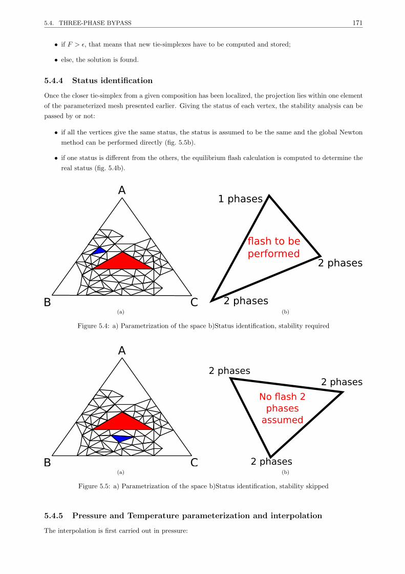
5.4. THREE-PHASE BYPASS 171

• if F > ε, that means that new tie-simplexes have to be computed and stored;

• else, the solution is found.

5.4.4 Status identification

Once the closer tie-simplex from a given composition has been localized, the projection lies within one element

of the parameterized mesh presented earlier. Giving the status of each vertex, the stability analysis can be

passed by or not:

• if all the vertices give the same status, the status is assumed to be the same and the global Newton

method can be performed directly (fig. 5.5b).

• if one status is different from the others, the equilibrium flash calculation is computed to determine the

real status (fig. 5.4b).

A

B C(a)

2 phases

flash to beperformed

1 phases

2 phases(b)

Figure 5.4: a) Parametrization of the space b)Status identification, stability required

A

B C(a)

2 phases

2 phases

2 phases

No flash 2 phases

assumed

(b)

Figure 5.5: a) Parametrization of the space b)Status identification, stability skipped

5.4.5 Pressure and Temperature parameterization and interpolation

The interpolation is first carried out in pressure:

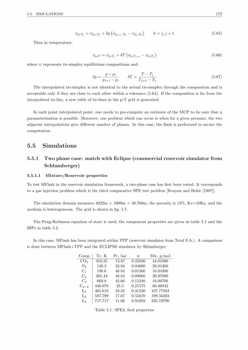
5.5. SIMULATIONS 172

ψp,Tk = ψpi,Tk + δp(ψpi+1,Tk − ψpi,Tk

)k = j, j + 1 (5.65)

Then in temperature:

ψp,T = ψp,Tj + δT(ψp,Tj+1

− ψp,Tj)

(5.66)

where ψ represents tie-simplex equilibrium compositions and:

δp =p− pi

pi+1 − piδT =

T − TjTj+1 − Tj

(5.67)

The interpolated tie-simplex is not identical to the actual tie-simplex through the composition and is

acceptable only if they are close to each other within a tolerance (5.64). If the composition is far from the

interpolated tie-line, a new table of tie-lines in the p-T grid is generated.

In each point interpolated point, one needs to pre-compute an estimate of the MCP to be sure that a

parameterization is possible. Moreover, one problem which can occur is when for a given pressure, the two

adjacent interpolations give different number of phases. In this case, the flash is performed to secure the

computation.

5.5 Simulations

5.5.1 Two phase case: match with Eclipse (commercial reservoir simulator from

Schlumberger)

5.5.1.1 Mixture/Reservoir properties

To test MFlash in the reservoir simulation framework, a two-phase case has first been tested. It corresponds

to a gas injection problem which is the third comparative SPE test problem [Kenyon and Behie [1987]].

The simulation domain measures 4022m × 1609m × 48.768m, the porosity is 13%, Kv=10Kz, and the

medium is heterogeneous. The grid is shown in fig. 5.7.

The Peng-Robinson equation of state is used; the component properties are given in table 5.1 and the

BIPs in table 5.2.

In this case, MFlash has been integrated within TPP (reservoir simulator from Total S.A.). A comparison

is done between MFlash+TPP and the ECLIPSE simulator by Shlumberger.

Comp Tc, K Pc, bar w Mw, g/molCO2 310.25 73.87 0.22500 44.01000N2 126.2 33.94 0.04000 28.01300C1 190.6 46.04 0.01300 16.04300C2 305.43 48.84 0.09860 30.07000C3 669.8 42.66 0.15240 44.09700

C4−6 448.078 35.5 0.21575 66.86942L1 465.618 28.32 0.31230 107.77943L2 587.799 17.07 0.55670 198.56203L3 717.717 11.06 0.91692 335.19790

Table 5.1: SPE3, feed properties

5.5. SIMULATIONS 173

CO2 N2 C1 C2 C3 C4−6 L1 L2

N2 -.0200C1 .1000 .0360C2 .1300 .0500 .000000C3 .1350 .0800 .000000 .000

C4−6 .1277 .1002 .092810 .000 .000L1 .1000 .1000 .130663 .006 .006 .0L2 .1000 .1000 .130663 .006 .006 .0 .0L3 .1000 .1000 .130663 .006 .006 .0 .0 .0

Table 5.2: SPE3, BIP

The injection wells are shown in yellow in fig. 5.7. The production wells are shown in blue in the same

figure. Water is injected at 100 STB/days, gas is produced at a control gas rate of 500 STB/days.

5.5.1.2 Simulation/Results

0.34 0.510.16

WatSat

Figure 5.6: Water saturation at the end of the simulation, SPE3 case

OilSat

0.070.00 0.07 0.14 0.20 0.27

Figure 5.7: Oil saturation at the end of the simulation, SPE3 case

In fig. 5.6 and fig. 5.7, the water saturation (respectively the oil saturation) at the end of the simulations

for MFlash+TPP and ECLIPSE is represented (both simulations lead to the same results). In fig. 5.8 the total

production rates of water, gas and oil are plotted, for the solution generated with ECLIPSE and the solution

generated with MFlash+TPP. The total production rates are identical in the two simulations, validating the

two-phase flash developed in this thesis (see chapter 2 and 3).

The remaining simulations were performed by coupling AD-GPRS and MFlash in the framework of a

collaboration with Stanford University. The simulator was coupled with the developed flash code, used as an

external library. The simulations presented in the following subsections come from this collaboration.

5.5.2 Full isothermal three phase compositional simulations: CO2 gas injection

The phase equilibrium code has been designed to work with np > 1 phases. Multiphase simulations were

carried out, first for CO2-rich/gas/hydrocarbure-rich systems. In this section, three and four phase simulations

of CO2 injection will be presented.

In our simulations, it has been noticed that a solvent-rich phase could appear when co-injecting solvent

with the steam in the reservoir. To develop a robust package, the presence of a fourth phase was necessary to

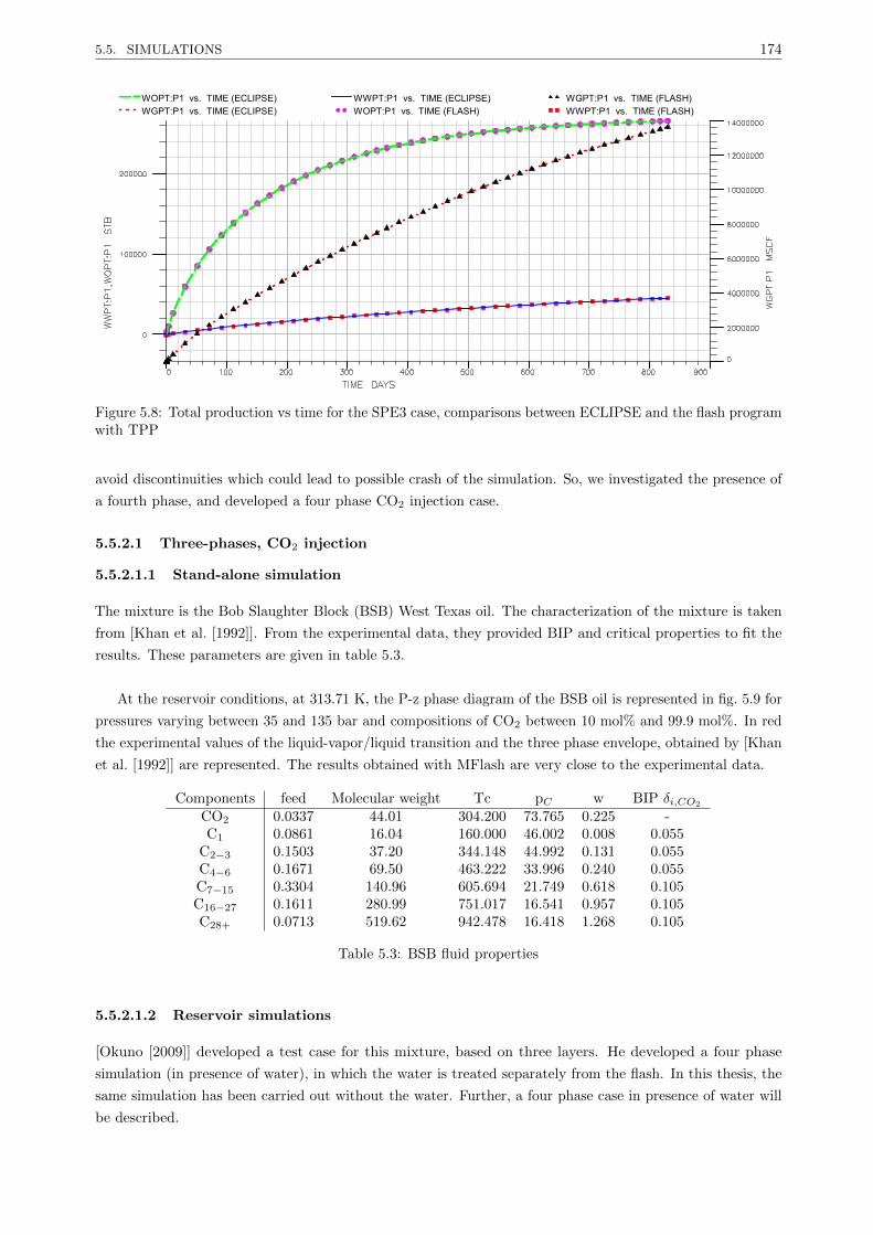
5.5. SIMULATIONS 174

WOPT:P1 vs. TIME (ECLIPSE)WGPT:P1 vs. TIME (ECLIPSE)

WWPT:P1 vs. TIME (ECLIPSE)WOPT:P1 vs. TIME (FLASH)

WGPT:P1 vs. TIME (FLASH)WWPT:P1 vs. TIME (FLASH)

Figure 5.8: Total production vs time for the SPE3 case, comparisons between ECLIPSE and the flash programwith TPP

avoid discontinuities which could lead to possible crash of the simulation. So, we investigated the presence of

a fourth phase, and developed a four phase CO2 injection case.

5.5.2.1 Three-phases, CO2 injection

5.5.2.1.1 Stand-alone simulation

The mixture is the Bob Slaughter Block (BSB) West Texas oil. The characterization of the mixture is taken

from [Khan et al. [1992]]. From the experimental data, they provided BIP and critical properties to fit the

results. These parameters are given in table 5.3.

At the reservoir conditions, at 313.71 K, the P-z phase diagram of the BSB oil is represented in fig. 5.9 for

pressures varying between 35 and 135 bar and compositions of CO2 between 10 mol% and 99.9 mol%. In red

the experimental values of the liquid-vapor/liquid transition and the three phase envelope, obtained by [Khan

et al. [1992]] are represented. The results obtained with MFlash are very close to the experimental data.

Components feed Molecular weight Tc pC w BIP δi,CO2

CO2 0.0337 44.01 304.200 73.765 0.225 -C1 0.0861 16.04 160.000 46.002 0.008 0.055

C2−3 0.1503 37.20 344.148 44.992 0.131 0.055C4−6 0.1671 69.50 463.222 33.996 0.240 0.055C7−15 0.3304 140.96 605.694 21.749 0.618 0.105C16−27 0.1611 280.99 751.017 16.541 0.957 0.105C28+ 0.0713 519.62 942.478 16.418 1.268 0.105

Table 5.3: BSB fluid properties

5.5.2.1.2 Reservoir simulations

[Okuno [2009]] developed a test case for this mixture, based on three layers. He developed a four phase

simulation (in presence of water), in which the water is treated separately from the flash. In this thesis, the

same simulation has been carried out without the water. Further, a four phase case in presence of water will

be described.

5.5. SIMULATIONS 175

CO2%

Press

ure,

bar

L1

V−L1

L1−L

2

L1−L

2−V ++

+++

.

.

.

............................................................................................................................................................

.....................................................................................

.........................................................................................

...............................................................................................

................

10 20 30 40 50 60 70 80 90

40

50

60

70

80

90

100

110

120

130

Figure 5.9: Phase envelope BSB comparisons with experimental values

The BSB test case parameters (as given in [Okuno [2009]]) are shown in table 5.4. The injection well is

located in the left-hand side of the reservoir and the producer is located in the right hand side (see fig. 5.10).

5% of C1 and 95% of CO2 are injected in the injection well at a BHP of 89.63 bar. The producer produces at

a BHP of 62.05 bar. The initial reservoir pressure is 75.84 bar.

Dimensions of a cell 0.762m × 3.048m × 0.762mNumber of grid cells 200 × 1 × 18

Top layer / Middle layer / Bottom layerThickness (m) 6.096 / 3.048 / 4.572

Permeability (mD) 7.0 / 11.2 / 9.8Porosity 0.08 / 0.10 / 0.09

W / O / G / CO2-richResidual saturations 0.40 / 0.20 / 0.05 / 0.05

Endpoint relative permeability model 0.35 / 0.50 / 0.65 / 0.65Exponent 3.0 / 3.0 / 3.0 / 3.0

Table 5.4: BSB reservoir properties

The results obtained by [Okuno [2009]] are given in fig. 5.10. The simulations performed in this thesis

were different; [Okuno [2009]] has not provided any volume shift for the density model of the water and the

viscosity model. The number of cells has been increased in our simulations to improve the accuracy. Finally,

there was no water in the simulation performed for this case. In fig. 5.11a, fig. 5.11b, fig. 5.11c, the results we

obtained with MFlash are represented. Furthermore, except for a more important diffusion effect that can be

noticed with the MFlash, the saturation profiles are similar to those obtained by [Okuno [2009]].

5.5.2.1.3 Results

By injecting gas into the reservoir, close to the injection well, the gas sweeps the oil in place. When getting

closer to the front of saturations, the oil phase has not been totally swept yet and both phases are present.

At this stage, the oil is not well displaced by the gas, because at these conditions both phases are not really

miscible.

5.5. SIMULATIONS 176

TITRE DE LA PRÉSENTATIONSous-titre de la présentation

(a) Gas saturation

TITRE DE LA PRÉSENTATIONSous-titre de la présentation

(b) Oil saturation

(c) CO2 saturation

Figure 5.10: CO2 injection process by[Okuno [2009]]

X,m

Z,m

0

0.2

0.4

0.6

0.8

(a) Gas saturation

0 50 100 1500

2

4

6

8

10

12

X,m

Z,m

0.2

0.4

0.6

0.8

1

(b) Oil saturation

X,m

Z,m

0

0.1

0.2

0.3

0.4

(c) CO2 saturation

Figure 5.11: CO2 injection process, saturations obtained with AD-GPRS + MFLASH

The reservoir pressure is progressively increasing during the injection. Gas and Oil become miscible at

these conditions and a CO2-rich phase appears. The saturation of the oil phase becomes really low, while

the CO2 rich phase saturation is significantly increasing. This indicates an extraction of the oil components

by the CO2 rich phase. Some authors showed that the CO2 injection increase the production due to the

extraction of medium and heavy oil components by the CO2 rich phase [Creek and Sheffield [1993]]. The

density of the CO2 rich phase is close to the density of the oil phase, which increases the miscibility of both

phases and generally helps the extraction of the heavy components. In the same time, the viscosity of the

CO2-rich phase remains generally lower than the viscosity of the oil phase.

5.5. SIMULATIONS 177

5.5.2.2 Four-phases, CO2 injection

5.5.2.2.1 Stand-alone simulations

The phase equilibrium code developed in this thesis has been designed to work with any number of phases.

In this subsection, a four-phase simulations of CO2 injection is presented. By adding water into the BOB

fluid, a four-phase system is obtained.

In this simulation, water is given a composition of zwater = 0.1, and the composition of the BOB oil is

scaled to obtain∑nci=1 = 1. The BIP δwater,i, ∀i 6= w are set to 0.5. The water properties are given in table

5.5.

The p-z phase diagram of the BOB oil in presence of water, at T=313.71 K is given in fig. 5.12.

Feed Molecular weight Tc pC w0.1 18.00 647.35 221.0 0.3434

Table 5.5: BSB water properties

CO2%

Pres

sure

,bar

L1 L2

W − L 1 − L 2 − V

10 30 50 70 90

50

70

90

110

130

W --

W-V-L1

W-L1

Figure 5.12: 4 phase case phase p-z diagram

5.5.2.2.2 Reservoir simulations

The same simulation test case as for the three-phase CO2 injection problem is used here in presence of water.

In fig. 5.13a, fig. 5.13b, fig. 5.13c and fig. 5.13d are represented the saturations of water, gas, CO2 and oil,

respectively after 90 days of simulation. In fig. 5.14, the pressure is given for the same time.

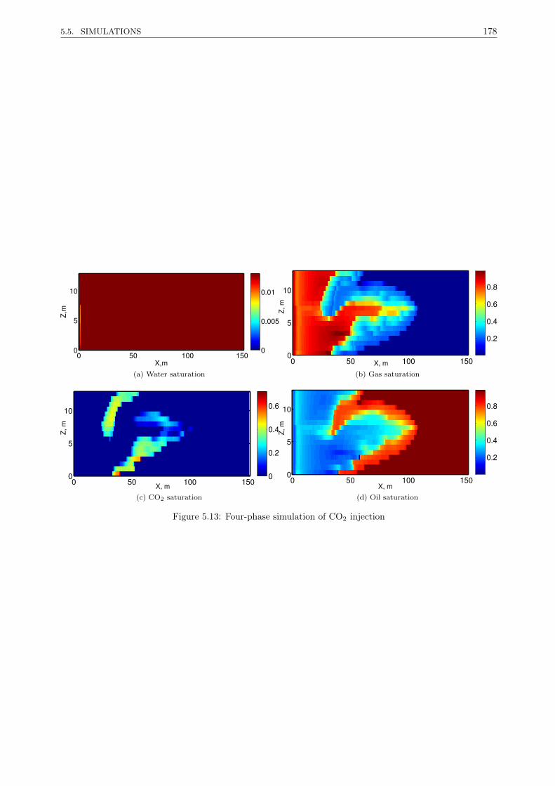
5.5. SIMULATIONS 178

0 50 100 1500

5

10

X,m

Z,m

0

0.005

0.01

(a) Water saturation

0 50 100 1500

5

10

X, m

Z, m

0.2

0.4

0.6

0.8

(b) Gas saturation

0 50 100 1500

5

10

X, m

Z, m

0

0.2

0.4

0.6

(c) CO2 saturation

0 50 100 1500

5

10

X, m

Z, m

0.2

0.4

0.6

0.8

(d) Oil saturation

Figure 5.13: Four-phase simulation of CO2 injection

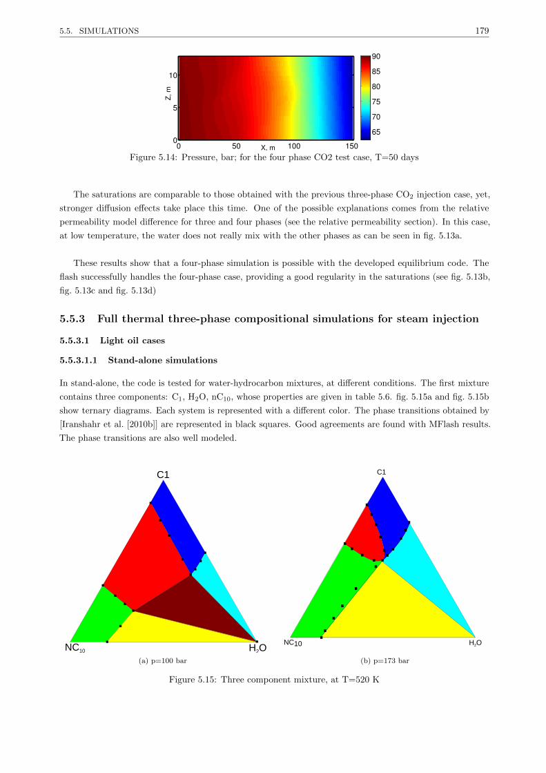
5.5. SIMULATIONS 179

0 50 100 1500

5

10

X, m

Z, m

65

70

75

80

85

90

Figure 5.14: Pressure, bar; for the four phase CO2 test case, T=50 days

The saturations are comparable to those obtained with the previous three-phase CO2 injection case, yet,

stronger diffusion effects take place this time. One of the possible explanations comes from the relative

permeability model difference for three and four phases (see the relative permeability section). In this case,

at low temperature, the water does not really mix with the other phases as can be seen in fig. 5.13a.

These results show that a four-phase simulation is possible with the developed equilibrium code. The

flash successfully handles the four-phase case, providing a good regularity in the saturations (see fig. 5.13b,

fig. 5.13c and fig. 5.13d)

5.5.3 Full thermal three-phase compositional simulations for steam injection

5.5.3.1 Light oil cases

5.5.3.1.1 Stand-alone simulations

In stand-alone, the code is tested for water-hydrocarbon mixtures, at different conditions. The first mixture

contains three components: C1, H2O, nC10, whose properties are given in table 5.6. fig. 5.15a and fig. 5.15b

show ternary diagrams. Each system is represented with a different color. The phase transitions obtained by

[Iranshahr et al. [2010b]] are represented in black squares. Good agreements are found with MFlash results.

The phase transitions are also well modeled.

CO2

WaterOil

C1

H2ONC10

(a) p=100 bar

Gas

WaterOil

C1

H2ONC10

(b) p=173 bar

Figure 5.15: Three component mixture, at T=520 K

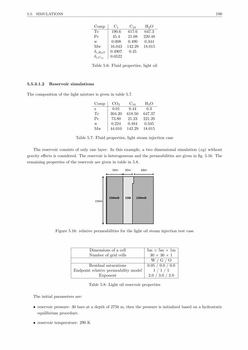
5.5. SIMULATIONS 180

Comp C1 C10 H2OTc 190.6 617.6 647.3Pc 45.4 21.08 220.48w 0.008 0.490 0.344Mw 16.043 142.29 18.015δi,H2O 0.4907 0.45δi,C10 0.0522

Table 5.6: Fluid properties, light oil

5.5.3.1.2 Reservoir simulations

The composition of the light mixture is given in table 5.7.

Comp CO2 C10 H2Oz 0.01 0.44 0.3Tc 304.20 618.50 647.37Pc 73.80 21.23 221.20w 0.224 0.484 0.345Mw 44.010 142.29 18.015

Table 5.7: Fluid properties, light steam injection case

The reservoir consists of only one layer. In this example, a two dimensional simulation (xy) without

gravity effects is considered. The reservoir is heterogeneous and the permeabilities are given in fig. 5.16. The

remaining properties of the reservoir are given in table in 5.8.

50m 30m

150mD

69m

150m15D 150mD

Figure 5.16: relative permeabilities for the light oil steam injection test case

Dimensions of a cell 5m × 5m × 1mNumber of grid cells 30 × 30 × 1

W / G / OResidual saturations 0.05 / 0.0 / 0.0

Endpoint relative permeability model 1 / 1 / 1Exponent 2.0 / 3.0 / 2.0

Table 5.8: Light oil reservoir properties

The initial parameters are:

• reservoir pressure: 30 bars at a depth of 2750 m, then the pressure is initialized based on a hydrostatic

equilibrium procedure.

• reservoir temperature: 290 K

5.5. SIMULATIONS 181

Steam is injected at the bottom left-hand corner, with a production well located at the top right-hand

corner. After 100 years of simulation, the saturations are given in fig. 5.18. The steam displaces the oil to the

production well located at the top right hand corner. The steam chamber does not have the shape of a circle

since the medium is heterogeneous. In the end, the breakthrough can be seen in fig. 5.18.

0 20 40 60 80 100 120 1400

20

40

60

80

100

120

140

X,m

Y,m

0.1

0.2

0.3

0.4

0.5

0.6

0.7

0.8

0.9

(a)

0 20 40 60 80 100 120 1400

20

40

60

80

100

120

140

X,mY,m

0

0.1

0.2

0.3

0.4

0.5

(b)

Figure 5.17: a)Oil Saturation, b)Gas Saturation for the light oil steam injection case

0 20 40 60 80 100 120 1400

20

40

60

80

100

120

140

X,m

Y,m

0.05

0.1

0.15

0.2

0.25

0.3

0.35

0.4

0.45

Figure 5.18: Water saturation

In this case, a comparison with [Lucia et al. [2000]]’s algorithm was done. The results are almost identical.

The computation time (or CPU time) is around 5 times higher for this case with Lucia’s algorithm as

compared to the simulation with MFlash.

The fluid moves along the high permeability area (15D compare with 150mD for the other two pars)

(fig. 5.17 and fig. 5.18). The steam sweeps the oil to the oil producer. After 100 days, the water breakthrough

occurs. Some oil remains in the regions with small permeabilities.

5.5.3.2 Medium oil in a highly heterogeneous reservoir

A simulation with a more complex steam injection problem (the highly heterogeneous SPE10 reservoir test

case) is performed. The mixture is a medium oil whose properties are defined in table 5.9. The reservoir

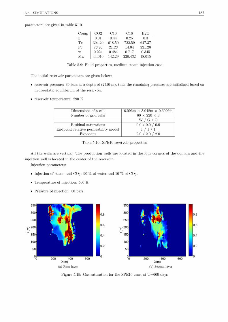
5.5. SIMULATIONS 182

parameters are given in table 5.10.

Comp CO2 C10 C16 H2Oz 0.01 0.44 0.25 0.3Tc 304.20 618.50 722.59 647.37Pc 73.80 21.23 14.04 221.20w 0.224 0.484 0.717 0.345Mw 44.010 142.29 226.432 18.015

Table 5.9: Fluid properties, medium steam injection case

The initial reservoir parameters are given below:

• reservoir pressure: 30 bars at a depth of (2750 m), then the remaining pressures are initialized based on

hydro-static equilibrium of the reservoir.

• reservoir temperature: 290 K

Dimensions of a cell 6.096m × 3.048m × 0.6096mNumber of grid cells 60 × 220 × 3

W / G / OResidual saturations 0.0 / 0.0 / 0.0

Endpoint relative permeability model 1 / 1 / 1Exponent 2.0 / 2.0 / 2.0

Table 5.10: SPE10 reservoir properties

All the wells are vertical. The production wells are located in the four corners of the domain and the

injection well is located in the center of the reservoir.

Injection parameters:

• Injection of steam and CO2: 90 % of water and 10 % of CO2.

• Temperature of injection: 500 K.

• Pressure of injection: 50 bars.

0 200 400 6000

50

100

150

200

250

300

350

X(m)

Y(m

)

0

0.2

0.4

0.6

0.8

(a) First layer

0 200 400 6000

50

100

150

200

250

300

350

X(m)

Y(m

)

0

0.2

0.4

0.6

0.8

(b) Second layer

Figure 5.19: Gas saturation for the SPE10 case, at T=600 days

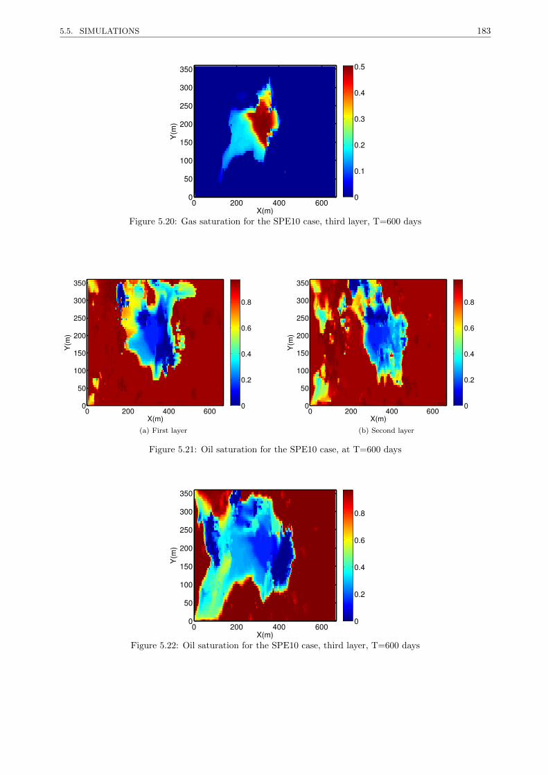
5.5. SIMULATIONS 183

0 200 400 6000

50

100

150

200

250

300

350

X(m)

Y(m

)

0

0.1

0.2

0.3

0.4

0.5

Figure 5.20: Gas saturation for the SPE10 case, third layer, T=600 days

0 200 400 6000

50

100

150

200

250

300

350

X(m)

Y(m

)

0

0.2

0.4

0.6

0.8

(a) First layer

0 200 400 6000

50

100

150

200

250

300

350

X(m)

Y(m

)

0

0.2

0.4

0.6

0.8

(b) Second layer

Figure 5.21: Oil saturation for the SPE10 case, at T=600 days

0 200 400 6000

50

100

150

200

250

300

350

X(m)

Y(m

)

0

0.2

0.4

0.6

0.8

Figure 5.22: Oil saturation for the SPE10 case, third layer, T=600 days

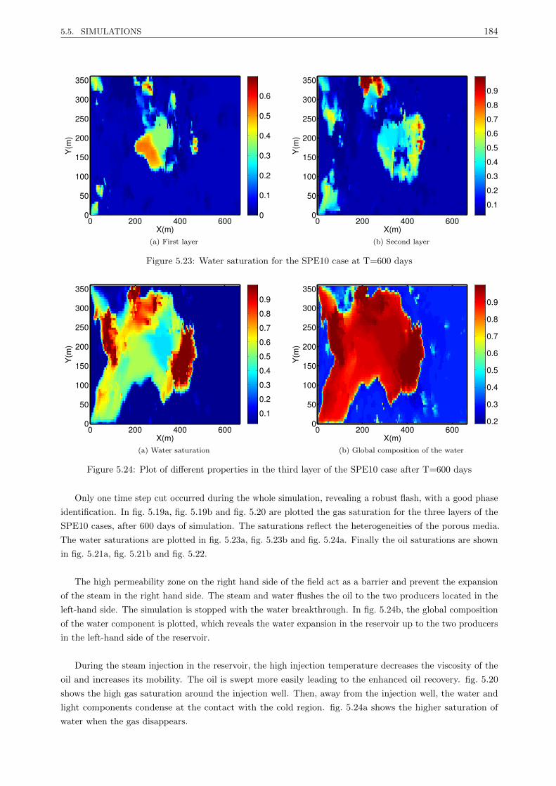
5.5. SIMULATIONS 184

0 200 400 6000

50

100

150

200

250

300

350

X(m)

Y(m

)

0

0.1

0.2

0.3

0.4

0.5

0.6

(a) First layer

0 200 400 6000

50

100

150

200

250

300

350

X(m)

Y(m

)

0.1

0.2

0.3

0.4

0.5

0.6

0.7

0.8

0.9

(b) Second layer

Figure 5.23: Water saturation for the SPE10 case at T=600 days

0 200 400 6000

50

100

150

200

250

300

350

X(m)

Y(m

)

0.1

0.2

0.3

0.4

0.5

0.6

0.7

0.8

0.9

(a) Water saturation

0 200 400 6000

50

100

150

200

250

300

350

X(m)

Y(m

)

0.2

0.3

0.4

0.5

0.6

0.7

0.8

0.9

(b) Global composition of the water

Figure 5.24: Plot of different properties in the third layer of the SPE10 case after T=600 days

Only one time step cut occurred during the whole simulation, revealing a robust flash, with a good phase

identification. In fig. 5.19a, fig. 5.19b and fig. 5.20 are plotted the gas saturation for the three layers of the

SPE10 cases, after 600 days of simulation. The saturations reflect the heterogeneities of the porous media.

The water saturations are plotted in fig. 5.23a, fig. 5.23b and fig. 5.24a. Finally the oil saturations are shown

in fig. 5.21a, fig. 5.21b and fig. 5.22.

The high permeability zone on the right hand side of the field act as a barrier and prevent the expansion

of the steam in the right hand side. The steam and water flushes the oil to the two producers located in the

left-hand side. The simulation is stopped with the water breakthrough. In fig. 5.24b, the global composition

of the water component is plotted, which reveals the water expansion in the reservoir up to the two producers

in the left-hand side of the reservoir.

During the steam injection in the reservoir, the high injection temperature decreases the viscosity of the

oil and increases its mobility. The oil is swept more easily leading to the enhanced oil recovery. fig. 5.20

shows the high gas saturation around the injection well. Then, away from the injection well, the water and

light components condense at the contact with the cold region. fig. 5.24a shows the higher saturation of

water when the gas disappears.

5.5. SIMULATIONS 185

Finally, the major volume of oil has been produced in the left part of the reservoir.

5.5.3.3 Extra-heavy oil

The full compositional simulations of the SAGD case became possible, with the recent developments in

AD-GPRS (by R.Zaydullin and D.Voskov (Stanford University)) and by coupling the simulator with the

MFlash program.

5.5.3.3.1 The SAGD process

Two horizontal wells are located one under the other (the injection well above). As steam is injected, a steam

chamber is formed around the injection well. At the chamber edge, the water and the light oil components

condense. Besides, the elevated temperature decreases the oil viscosity and the oil becomes mobile. The

condensed water and the extra-heavy oil flows to the production well under the gravity.

Two simulations of the SAGD process have been performed. The first consists of a synthetic heavy oil,

initially at T=285 K. The oil is not heated before the steam injection. In the second case, a real Athabasca

bitumen has been modelled. In this case, the oil is pre-heated before the steam injection.

5.5.3.3.2 Synthetic heavy oil

The oil composition is given in table 5.11.

Comp CO2 M0 M2 H2Oz 0.02 0.57 0.2 0.21Tc 304.18 444.19 1073.15 647.35Pc 73.80 36.01 8.10 221.0w 0.23 0.18 0.90 0.3434Mw 44.01 65.56 900.00 18.00

Table 5.11: Fluid properties, synthetic heavy oil

The initial parameters are:

• reservoir pressure: 8.11 bars at the depth 180 m, then the remaining pressure are initialized based on

hydrostatic equilibrium of the reservoir.

• reservoir temperature: 285 K

• the initial oil viscosity oil viscosity at T=285 K is 8.86e+7 cP

The injection well is located at the depth 117.5m and the production well, 5 meters below.

Injection parameters are:

• fraction of steam (99.4 mol%) and CO2-C1 (0.6 mol%).

• injection temperature: 500 K

• injection pressure: 25 bars.

Only half of the steam chamber (SC) cross section is shown in fig. 5.25a. Each cell is a cube of length 0.5

m, the grid dimension is made by 101 × 1 × 52.

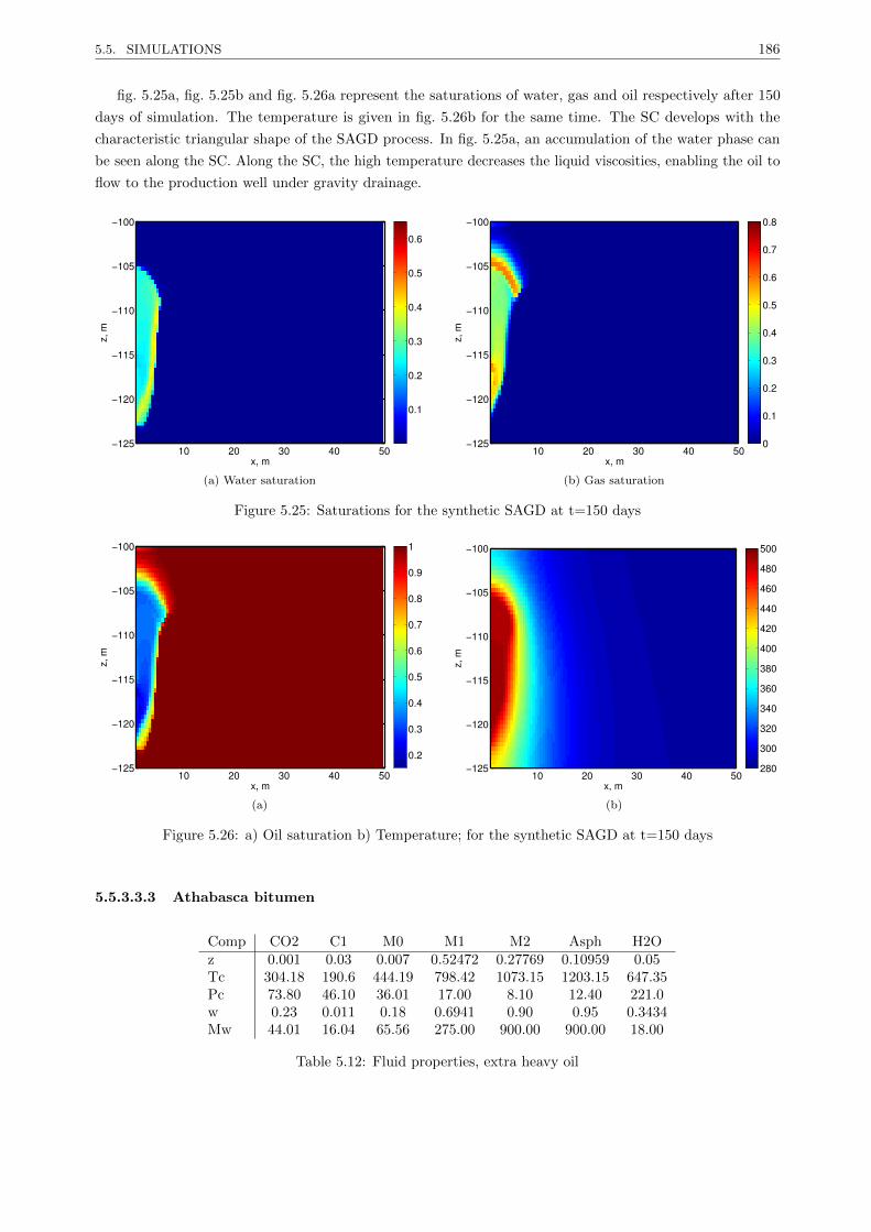
5.5. SIMULATIONS 186

fig. 5.25a, fig. 5.25b and fig. 5.26a represent the saturations of water, gas and oil respectively after 150

days of simulation. The temperature is given in fig. 5.26b for the same time. The SC develops with the

characteristic triangular shape of the SAGD process. In fig. 5.25a, an accumulation of the water phase can

be seen along the SC. Along the SC, the high temperature decreases the liquid viscosities, enabling the oil to

flow to the production well under gravity drainage.

10 20 30 40 50−125

−120

−115

−110

−105

−100

x, m

z,m

0.1

0.2

0.3

0.4

0.5

0.6

(a) Water saturation

10 20 30 40 50−125

−120

−115

−110

−105

−100

x, mz,

m0

0.1

0.2

0.3

0.4

0.5

0.6

0.7

0.8

(b) Gas saturation

Figure 5.25: Saturations for the synthetic SAGD at t=150 days

10 20 30 40 50−125

−120

−115

−110

−105

−100

x, m

z,m

0.2

0.3

0.4

0.5

0.6

0.7

0.8

0.9

1

(a)

10 20 30 40 50−125

−120

−115

−110

−105

−100

x, m

z,m

280

300

320

340

360

380

400

420

440

460

480

500

(b)

Figure 5.26: a) Oil saturation b) Temperature; for the synthetic SAGD at t=150 days

5.5.3.3.3 Athabasca bitumen

Comp CO2 C1 M0 M1 M2 Asph H2Oz 0.001 0.03 0.007 0.52472 0.27769 0.10959 0.05Tc 304.18 190.6 444.19 798.42 1073.15 1203.15 647.35Pc 73.80 46.10 36.01 17.00 8.10 12.40 221.0w 0.23 0.011 0.18 0.6941 0.90 0.95 0.3434Mw 44.01 16.04 65.56 275.00 900.00 900.00 18.00

Table 5.12: Fluid properties, extra heavy oil

5.5. SIMULATIONS 187

The oil used for SAGD modelling, is an Athabasca oil containing extra-heavy components. The fluid

properties are given in table 5.12. The initial parameters and the grid are the same as for the synthetic heavy

oil. At T = 283K, the initial oil viscosity is µ = 6.64e+11 cP. Steam is injected (99.5 mol%) with solvent (0.5

mol%). The solvent is the M0 pseudo-component made of C3-C10 components.

10 20 30 40 50−125

−120

−115

−110

−105

−100

x, m

z,m

0

0.05

0.1

0.15

0.2

0.25

0.3

0.35

0.4

0.45

0.5

(a) Water saturation

10 20 30 40 50−125

−120

−115

−110

−105

−100

x, mz,

m0

0.1

0.2

0.3

0.4

0.5

0.6

(b) Gas saturation

Figure 5.27: Saturations for the Athabasca oil SAGD at t=20 days

10 20 30 40 50−125

−120

−115

−110

−105

−100

x, m

z,m

0

0.05

0.1

0.15

0.2

0.25

0.3

0.35

0.4

0.45

0.5

(a) Water saturation

10 20 30 40 50−125

−120

−115

−110

−105

−100

x, m

z,m

0

0.1

0.2

0.3

0.4

0.5

0.6

(b) Gas saturation

Figure 5.28: Saturations for the Athabasca oil SAGD at t=30 days

fig. 5.27a and fig. 5.27b show the saturation of the water and gas phase respectively at t=20 days. At the

beginning, a connection between the two wells is made. No steam chamber is seen. At t=30 days, the same

saturation fields are shown in fig. 5.28a and fig. 5.28b. This time corresponds to the established connection

between the wells. The injected hot water reaches the producer. Now, the steam chamber is progressively

expanding above the injection well.

fig. 5.29a, fig. 5.29b and fig. 5.30a show the saturation fields (of water/gas and oil respectively) at t=360

days. At this time, the SC has been developed, growing mainly vertically. Water and oil accumulation can

be seen along the steam chamber edge. Both heated liquids are flowing to the production well by gravity

drainage. Moreover, high concentration of gas can be seen at the top of the SC. The light components with a

lower density move to the top of the SC and encounter the liquid phases (oil and water) at the edge of the

chamber. fig. 5.30b shows the temperature profile in the reservoir for the same time.

Due to the gravity effects, the gas mixture moves to the top of the reservoir. Once the steam chamber

5.5. SIMULATIONS 188

reaches the top, it starts growing horizontally.

10 20 30 40 50−125

−120

−115

−110

−105

−100

x, m

z,m

0

0.05

0.1

0.15

0.2

0.25

0.3

0.35

0.4

0.45

0.5

(a) Water saturation

10 20 30 40 50−125

−120

−115

−110

−105

−100

x, m

z,m

0

0.1

0.2

0.3

0.4

0.5

0.6

(b) Gas saturation

Figure 5.29: Saturations for the Athabasca oil SAGD at t=360 days

10 20 30 40 50−125

−120

−115

−110

−105

−100

x, m

z,m

0.2

0.3

0.4

0.5

0.6

0.7

0.8

0.9

1

(a)

10 20 30 40 50−125

−120

−115

−110

−105

−100

x, m

z,m

300

350

400

450

500

(b)

Figure 5.30: a) Oil saturation b)Temperature for the Athabasca oil SAGD at t=360 days

10 20 30 40 50−125

−120

−115

−110

−105

−100

x, m

z,m

0

0.1

0.2

0.3

0.4

0.5

0.6

Figure 5.31: Gas saturation for the Athabasca oil SAGD at t=410 days

Finally, at t=410 days, the steam chamber reaches the top of the reservoir; fig. 5.31 shows the saturation

of the gas phase at this moment.

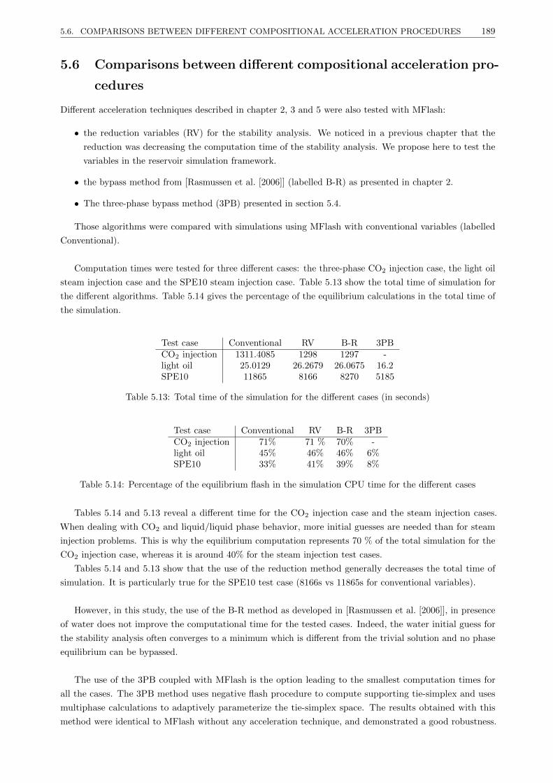
5.6. COMPARISONS BETWEEN DIFFERENT COMPOSITIONAL ACCELERATION PROCEDURES 189

5.6 Comparisons between different compositional acceleration pro-

cedures

Different acceleration techniques described in chapter 2, 3 and 5 were also tested with MFlash:

• the reduction variables (RV) for the stability analysis. We noticed in a previous chapter that the

reduction was decreasing the computation time of the stability analysis. We propose here to test the

variables in the reservoir simulation framework.

• the bypass method from [Rasmussen et al. [2006]] (labelled B-R) as presented in chapter 2.

• The three-phase bypass method (3PB) presented in section 5.4.

Those algorithms were compared with simulations using MFlash with conventional variables (labelled

Conventional).

Computation times were tested for three different cases: the three-phase CO2 injection case, the light oil

steam injection case and the SPE10 steam injection case. Table 5.13 show the total time of simulation for

the different algorithms. Table 5.14 gives the percentage of the equilibrium calculations in the total time of

the simulation.

Test case Conventional RV B-R 3PBCO2 injection 1311.4085 1298 1297 -light oil 25.0129 26.2679 26.0675 16.2SPE10 11865 8166 8270 5185

Table 5.13: Total time of the simulation for the different cases (in seconds)

Test case Conventional RV B-R 3PBCO2 injection 71% 71 % 70% -light oil 45% 46% 46% 6%SPE10 33% 41% 39% 8%

Table 5.14: Percentage of the equilibrium flash in the simulation CPU time for the different cases

Tables 5.14 and 5.13 reveal a different time for the CO2 injection case and the steam injection cases.

When dealing with CO2 and liquid/liquid phase behavior, more initial guesses are needed than for steam

injection problems. This is why the equilibrium computation represents 70 % of the total simulation for the

CO2 injection case, whereas it is around 40% for the steam injection test cases.

Tables 5.14 and 5.13 show that the use of the reduction method generally decreases the total time of

simulation. It is particularly true for the SPE10 test case (8166s vs 11865s for conventional variables).

However, in this study, the use of the B-R method as developed in [Rasmussen et al. [2006]], in presence

of water does not improve the computational time for the tested cases. Indeed, the water initial guess for

the stability analysis often converges to a minimum which is different from the trivial solution and no phase

equilibrium can be bypassed.

The use of the 3PB coupled with MFlash is the option leading to the smallest computation times for

all the cases. The 3PB method uses negative flash procedure to compute supporting tie-simplex and uses

multiphase calculations to adaptively parameterize the tie-simplex space. The results obtained with this

method were identical to MFlash without any acceleration technique, and demonstrated a good robustness.

5.7. CONCLUSION 190

In terms of performances, 3PB re-uses the information from previous equilibrium calculations to pass by

the computation of further stability analysis. Many stability tests can be avoided by using this procedure.

Here, the use of 3PB improves the time of computation from 8 up to 12 times as compared with MFlash. For

the whole simulation, with 3PB the averaged computation time is 1.6 times faster than with MFlash alone.

However, using a flash based on global optimization, or with higher initial guesses, or with a more accurate

EoS model, the differences may increase significantly.

To check the robustness of the 3PB, a comparison was performed for the synthetic oil SAGD test case.

Table 5.15 gives the computational results obtained with MFlash with reduction variables and 3PB for 90

days of simulation. Taking the flash in stand-alone as the reference, the relative error on the oil production

rate for the 3PB simulation remained always under 6%, taking large steps (system ill-conditionned where

convergence problems occur). By taking smaller steps, the error becomes negligible. In this case, the total

computation time with 3PB was much smaller than for MFlash: (2529s versus 3914s), decreasing the fraction

of the equilibrium calculations from 45% to 10% of the total simulation. 3PB seems quite robust and capable

of handling simulations of difficult processes quite efficiently.

RV 3PBTotal simulation time 3914 s 2529 sEquilibrium % of the total simulation 45 10

Table 5.15: Synthetic oil, SAGD computation time for 90 days of simulation

Note that, all the tests were carried out using only one core. In each cell, the equilibrium calculation does

not depend on properties from other cells (local computations), therefore equilibrium calculations can be

efficiently parallelized. Using a parallel procedure, the percentage of the total time spent in the equilibrium

calculations would become much smaller, and the CPU time requiered for equilibrium calculations would

represent a smaller proportion of the total simulation time.

Finally, analyzing all the simulations (except for CO2 injection where more initial guesses are required),

one can see that the time of the equilibrium calculations with or without the use of 3PB always remains

under 50% of the total time, even for the SAGD test case.

5.7 Conclusion

In this chapter, a rigorous validation of the developed phase equilibrium calculations program has been

performed.

Different phase diagrams obtained with the developed equilibrium program showed good agreements

with the experimental and literature data. The good reproduction of various phase diagrams (LLV-LLLV)

illustrates the capability of the program to predict the true phase behavior of such systems. As stand-alone

comparisons can be made for some specific conditions, in order to guarantee the good functionality of the

equilibrium algorithm for a wide variety of conditions, different reservoir simulations were performed.

Reservoir simulations cover a great variation of p-T-z conditions. Phase transitions involve passing

across phase boundaries and/or those supercritical conditions. Any failure in the convergence to the correct

minimum can lead to the divergence of a simulation. The capability to carry out correctly a whole simulation

demonstrates the robustness of the code.

The developed program was first plugged with TPP, to simulate an isothermal water injection process. The

same simulation was also performed with the ECLIPSE simulator by Shlumberger and the same production

rates were obtained for both simulations. The ECLIPSE simulator has been tested against a variety of

5.7. CONCLUSION 191

experimental cases, and is currently used in production division in Total. The good agreement in the results

indicates that the developed algorithm converged to the correct minimum of the Gibbs energy during the

whole simulation.

Another test was performed with a full three phase CO2 injection problem. Comparisons were made with

[Okuno [2009]] which also showed similar saturation profiles. The simulation ran up to the CO2 breakthrough

(450 days). After adding water to the model, the same simulation was carried out and led to four-phase

systems at some conditions. With a high number of phases, the difference in the Gibbs free energy (∆G)

between a system with np phase becomes really small as compared to the system with np+ 1 phases. Robust

stability analysis codes have to be designed to handle the high number of phases. In this work, a four-phase

simulation has been performed during 100 days. This indicates the capability of the algorithm to deal with

small ∆G, and illustrates the robustness of the stability analysis algorithm.

Simulations of steam injection cases were also performed. The highly heterogeneous SPE10 reservoir was

used to perform a 3D steam flooding simulation up to the water breakthrough. With three dimensional

heterogeneous reservoirs, more thermodynamic paths are accessed during a simulation. Once again, this

example reveals the robustness of the developed algorithm.

Moreover, a fully compositional reservoir simulation of the SAGD process was performed with a real extra

heavy oil mixture. To the best of our knowledge, this is the first simulation of the kind in the literature.

Thermal compositional simulations are quite complex because the important change in the conditions is

observed (composition, pressure and temperature). Indeed, for the steam injection process, the steam

distillation and the condensation of the water and the light oil components can be observed. With heavy oils,

the gravity creates concentration gradients which imply many changes in the oil composition.

When injecting steam, the steam flushes progressively all the other components. The phase envelope of

the resulting composition becomes narrow and the multiphase problem approaches ill-conditioning where a

small variation in the conditions can create an important change in the equilibrium state. A simulation of

the SAGD process has been performed up to 410 days revealing the capability of the algorithm to converge

even for difficult (nearly ill-conditioned) problems. The presented simulations show that the developed code

can overcome these difficulties.

The proposed thermodynamic code was also used with different acceleration procedures, namely, based

on the bypass method by [Rasmussen et al. [2006]] and the three-phase bypass by [Zaydullin et al. [2013]].

Without any acceleration technique, the program has taken around 45% of the total CPU time for steam

injection problems. In presence of water for multiphase systems, the bypass method did not perform really

well. However, with 3PB, the CPU time was decreased and reached around 10% of the total time, keeping

the same solution as the thermodynamic program alone.

Last but not least, one of the main objective of the thesis was to perform simulations of steam injection

problems within a CPU time for equilibrium calculations under 50 % of the total simulation time. This

objective has been achieved.

Chapter 6

Conclusions and Perspectives

1 Conclusions

In this thesis, improvements in equilibrium algorithms made possible the realization of fully compositional

simulations of steam injection with heavy oils.

Most of the phase equilibrium calculations are performed based on the Newton-Raphson method and

use conventional independent variables. These algorithms were investigated and different extensions were

proposed. The logarithm of the equilibrium constants (ln K) is the best choice of conventional independent

variables for multiphase equilibrium calculations. This set of variables lead to the best condition number and

Newton methods based on ln K converge in fewer iterations than the other Newton algorithms. In this work,

extending [Michelsen [1982a]]’s method to multiphase-split problem, we proposed to compute the Jacobian

matrix as a product of two symmetric matrices, and to solve the linear system using a Cholesky factorization,

which proved to reduce the computation time by about a third in most of the calculations.

Initiated by [Michelsen [1986] and Hendriks [1988]], reduction methods have been investigated in the

literature and proved to be highly efficient. In this work, a new reduction method for stability testing and

phase-split problems was presented. It is based on the multi-linear expression of the logarithms of fugacity

coefficients as functions of the coefficients h (which are taken as independent variables and are unbounded).

The reduction parameters are dependent variables, which, unlike in previous formulations, are guaranteed

to be within their bounds. The dimensionality of the problem depends only on the number of components

having non-zero BIPs with the remaining ones, and not on the number of components in the mixture, as

in the conventional approach. The proposed method has a large convergence radius and Newton iterations

can be used directly for the stability analysis problem (without the need of using successive substitutions),

it has the same convergence path as the conventional approach using the natural logarithm of formal mole

numbers (for stability analysis) and of the equilibrium constant (for phase-split calculations) as independent

variables. This method was proved to be the best Newton method for the stability analysis problem (in terms

of efficiency and condition number).

Comparisons between different conventional and reduction methods were performed for the stability testing

and the multiphase-split calculation problems. Until now, the comparisons from the literature have focused

on the global CPU times to compute the whole multiphase equilibrium problem. In this work, comparisons

were performed independently for each problem (stability analysis, two phase-split and multiphase-split

calculations). Besides, the condition number and convergence path were also investigated, leading to more

detailed and extensive comparisons and new conclusions:

• For the stability testing problem, in reservoir simulation purposes, the proposed reduction method is

the most efficient, whereas for the multiphase-split problem, the conventional methods require less CPU

times.

• For chemical processes and any problems involving a large number of components, the use of the

proposed reduction method is extremely time earning as compared to conventional Newton methods.

192

1. CONCLUSIONS 193

Furthermore, we proposed a Trust-Region method to handle both stability and phase-split problems.

The Trust-Region (TR) can be viewed as an ’extension’ of the Newton method. TR can reach supra-linear

steps even when the Hessian is non-positive definite, and quadratic steps overwise by adding a diagonal

element to the matrix. An hybrid algorithm was presented. Instead of performing TR iterations immediately

after the switch from the first-order SSI method, Newton iterations are first tested, and the TR method is

applied only if the objective function value is increasing between two consecutive iterations. This hybrid

methodology remarkably decreased the computation time of the method keeping the the high robustness of

the TR method. The tests were performed covering whole multiphase-regions and some calculations were

successfully performed at really difficult conditions, such as the immediate vicinity of bi-critical points.

Moreover, a new methodology has been developed to find variables leading to a well-scaled Hessian in the

BFGS methods. This procedure leads to the α variable introduced by [Michelsen [1982b]] for the stability

analysis and to a new variable for phase-split problems. A quasi-Newton strategy with a safeguarding switch

back procedure (when the Gibbs energy increases between two iterations) was developed based on this

variable and proved to reach convergence even close to phase boundaries were algorithms often encounter

convergence problems. The algorithm compared favorably (in terms of iterations, function evaluations and

robustness) with Nocedal’s LBFGS-B code and existing BFGS implementations, for different mixtures. Only

few additional function evaluations are necessary as compared with a Newton method, which makes it an

attractive method. This procedure is extremely suited for more complex EOS models.

Combining all the developed algorithms, a general equilibrium calculation program was developed. It has

been designed to handle any number of phases. Tests were performed on various systems and comparisons

with numerical examples from other authors, and experimental data, have validated the proposed approach.

In addition to improve the robustness and efficiency of the equilibrium algorithms, a new methodology

to generate pseudo-components giving an accurate representation of a mixture has been developed. The

methodology is based on the quadrature method of moments (QMoM) which is here applied to multiphase

equilibrium calculations for actual oil mixtures (combined with non-hydrocarbon components, such as water

and carbon dioxide) using a cubic equations of state with non-zero BIPs. The quadrature is solved using

a procedure (ORTHOPOL) which avoids problems due to the ill-conditioned nature of the problem and is

suitable for an undetermined number of quadrature points (unlike the original formulation of the QMoM).

The QMoM relates the discrete initial detailed composition having a large number of components to a

small number of components which approximates the continuous portion of the mixture. It can be viewed in

a larger sense as a lumping procedure. It is generally applicable, even in cases when no standard distribution

function can model the feed composition, or several distribution functions are needed to model different

portions of the mixture or different homologous series. It is proven in this work that this methodology coupled

with a delumping procedure and using a cubic equation of state with non-zero BIPs works for actual oil

mixtures with good accuracy.

The QMoM in our implementation has been tested for different initial compositions of a hydrocarbon

mixture for two-phase equilibrium calculations and in the presence of water and carbon dioxide, for three-phase

flash calculations. In all cases, the location of the phase boundaries, the phase distributions and the phase

compositions were well reproduced by the semi-continuous description (however only 10 pseudo-components in

average were necessary). In the reservoir simulation framework this tool appear essential since the computer

time per time step is proportional to the power three of the number of equations to be solved simultaneously

[Burger et al. [1985]] (and each component leads to one more equation).

Subsequently, the developed equilibrium calculation program has been implemented within two different

reservoir simulators: TPP a reservoir simulator developed in Total S.A. and AD-GPRS simulator from the

2. PERSPECTIVES 194

University of Stanford.

For three-phase water injection problems, the exact same production and injection rate curves for the oil,

gas and water phases were obtained with the ECLIPSE reservoir simulator and the developed equilibrium

calculation program plugged in TPP. This reveals the capability of the equilibrium program to converge

to the correct equilibrium solution. Also, simulations of CO2 injection cases were presented (known to be

difficult). Three- and four-phase isothermal compositional reservoir simulations were performed up to the CO2

breakthrough. The simulations showed the capability of the code to handle more than three phases, which can

be highly difficult due to the small differences of the Gibbs energy between three-phase and four-phase systems.

Simulations of steam injection cases were also performed. The highly heterogeneous SPE10 reservoir

was used to test a 3D steam flooding simulation up to the water breakthrough. With three dimensional

heterogeneous reservoirs, more thermodynamic paths are accessed during a simulation. Once again, this

example reveals the robustness of the developed algorithm.

Finally, a fully compositional reservoir simulation of a SAGD process was realized with an extra heavy

oil mixture. To the best of our knowledge, this is the first simulation of the kind in the literature (with a

complete modeling of the water phase within equilibrium calculations). Thermal compositional simulations

are quite complex because important changes in the conditions (composition, pressure and temperature) are

observed. Moreover, the gravity creates concentration gradients which imply many compositional changes.

The developed code was also used in parallel with different acceleration methods such as the three-phase

bypass algorithm (by [Zaydullin et al. [2013]]). Fully thermal compositional three-phase reservoir simulations

of the steam flooding process could then be carried out with the equilibrium calculation time representing

less than 10% of the total CPU time. Last but not least, one of the main objective of the thesis was to reduce

under 50% the computational time for equilibrium flash calculations within simulations of steam injection

problems. This objective has been achieved.

Through this thesis, three papers have been already published [Nichita and Petitfrere [2013], Petitfrere

and Nichita [2014a], Petitfrere and Nichita [2014b]]; a fourth paper was submitted (under review) [Petitfrere

et al. [2014]] and three other papers are in preperation and will be submitted shortly (corresponding to the

subsections 3.2.4, 3.3 and 3.5).

2 Perspectives

Through the proposed work, new perspectives appear. In this thesis, new minimization algorithms were

successfully implemented such as a Trust-Region and a quasi-Newton method. These algorithms are

independent of the EoS model. Procedures leading to a smaller number of iterations become more and more

efficient as the complexity increases (because computing the fugacities and fugacity derivatives becomes

more and more time-consuming). Therefore, both quasi-Newton and Trust-Region methods would perform

more efficiently when using complex model as compared with Newton methods. The Trust-region because

the method converges in less iterations and the BFGS because no derivatives are needed in the Hessian

approximation.

Furthermore, the BFGS procedure has been developed for the two-phase split problem and an extension

to the multiphase-split problem is intended. With more phases, larger systems have to be solved at each

Newton iterations and the BFGS method (which does not solve explicitly linear systems) would perform

more and more efficiently as compared with Newton methods.

New perspective also appear for the compositional reservoir simulation. The developed equilibrium

2. PERSPECTIVES 195

program was shown to be robust and efficient and could be used for other processes. Adding a source term in

the mass balance equations and in the equation of energy, irreversible chemical reactions (based on activation

energies) could also be modeled. Simulations of the in-situ upgrading process were performed using this

methodology [Lapene [2010]].

Different acceleration techniques were presented and tested. One of them, the three-phase bypass [Za-

ydullin et al. [2013]] presents interesting features such as the parameterization of the space. The method

could be used to help phase identifications. When two liquid phases are present, it is sometimes difficult to

identify one another. The parameterization enables a clear identification in the whole compositional space,

thus avoiding discontinuities.

[Gaganis and Varotsis [2012]] proposed another acceleration method that seems to be efficient in the

framework of compositional reservoir simulation of complex processes (such as CO2 injection). Using machine-

learning methods, they train the system to generate discriminating functions capable of providing the sign of

the minimum tangent plane distance within only few operations. It would be interesting to compare the

method against the three-phase bypass method.

Last but not least, the presented simulations could be improved using more accurate models. It is well

known that volumetric parameters and most of the derivatives properties are not modeled correctly based

on cubic equations of state. More suited equations of state could be used to perform simulations of steam

injection processes.

Appendix

Reduction variables

A Elements of the Jacobian matrix/partial derivatives for the re-

duced stability analysis

The partial derivatives required in (eq. 3.84) are (for α, γ = 1,m)(∂hα∂Qγ

)Z,Qµ6=γ

= δαγhαQα

(A.1)

(∂hα∂QM

)Z,Qµ6=M

= − 1

B

(hα + 2λαQα

Z

π

)(A.2)

(∂hM∂Qγ

)Z,Qµ6=γ

=hγQM

(A.3)

(eq. A.1 and eq. A.3) correct misprints in [Nichita and Graciaa [2011]].(∂hM∂QM

)Z,Qµ6=M

=1

B2

[−2hMB − 1 + Z

(1 +

A

π

)](A.4)

(∂hM+1

∂Qγ

)Z,Qµ6=γ

= 0 (A.5)

(∂hM+1

∂QM

)Z,Qµ6=M

=1

Z −B(A.6)

and (∂hα∂Z

)Q

=2λαQαπ

(A.7)

(∂hM∂Z

)Q

=1

B

(1− A

π

)(A.8)

(∂hM+1

∂Z

)Q

= − 1

Z −B(A.9)

where π = (Z + δ1B)(Z + δ2B). One can further substitute Aπ = 1

Z−B − 1 in some of the above equations.

The partial derivatives of the compressibility factor (the phase index is dropped for simplicity) with

respect to the reduced variables are:

∂Z

∂Qβ=∂Z

∂A

∂A

∂Qβ;β = 1,m (A.10)

with

∂A

∂Qβ= 2λβQβ ;β = 1,m (A.11)

196

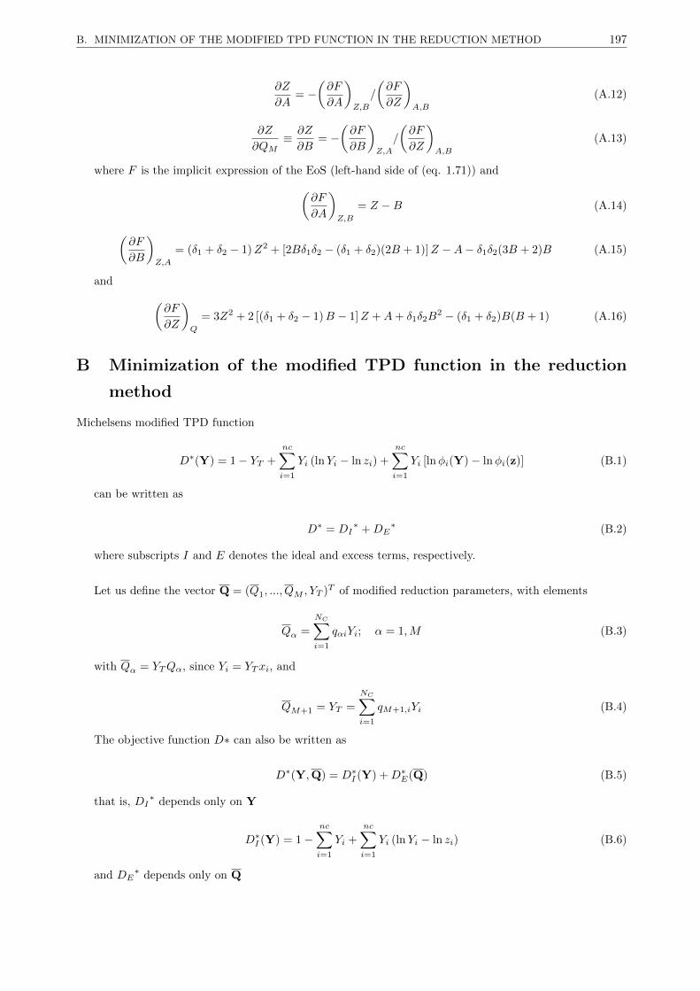
B. MINIMIZATION OF THE MODIFIED TPD FUNCTION IN THE REDUCTION METHOD 197

∂Z

∂A= −

(∂F

∂A

)Z,B

/

(∂F

∂Z

)A,B

(A.12)

∂Z

∂QM≡ ∂Z

∂B= −

(∂F

∂B

)Z,A

/

(∂F

∂Z

)A,B

(A.13)

where F is the implicit expression of the EoS (left-hand side of (eq. 1.71)) and(∂F

∂A

)Z,B

= Z −B (A.14)

(∂F

∂B

)Z,A

= (δ1 + δ2 − 1)Z2 + [2Bδ1δ2 − (δ1 + δ2)(2B + 1)]Z −A− δ1δ2(3B + 2)B (A.15)

and (∂F

∂Z

)Q

= 3Z2 + 2 [(δ1 + δ2 − 1)B − 1]Z +A+ δ1δ2B2 − (δ1 + δ2)B(B + 1) (A.16)

B Minimization of the modified TPD function in the reduction

method

Michelsens modified TPD function

D∗(Y) = 1− YT +

nc∑i=1

Yi (lnYi − ln zi) +

nc∑i=1

Yi [lnφi(Y)− lnφi(z)] (B.1)

can be written as

D∗ = DI∗ +DE

∗ (B.2)

where subscripts I and E denotes the ideal and excess terms, respectively.

Let us define the vector Q = (Q1, ..., QM , YT )T of modified reduction parameters, with elements

Qα =

NC∑i=1

qαiYi; α = 1,M (B.3)

with Qα = YTQα, since Yi = YTxi, and

QM+1 = YT =

NC∑i=1

qM+1,iYi (B.4)

The objective function D∗ can also be written as

D∗(Y,Q) = D∗I (Y) +D∗E(Q) (B.5)

that is, DI∗ depends only on Y

D∗I (Y) = 1−nc∑i=1

Yi +

nc∑i=1

Yi (lnYi − ln zi) (B.6)

and DE∗ depends only on Q

B. MINIMIZATION OF THE MODIFIED TPD FUNCTION IN THE REDUCTION METHOD 198

D∗E(Q) = YT

nc∑i=1

xi [lnφi(Y)− lnφi(z)] = QM+1

[gE(Q)− gEz(Q)

](B.7)

where the molar excess Gibbs free energy is a function of reduction parameters, that is, gE = gE(Q) =

gE(Q/QM+1) = gE(Q).

The objective function D∗(Y,Q) is minimized subject to the constraints

nc∑i=1

qαiYi −Qα = 0;α = 1,M (B.8)

and

nc∑i=1

Yi −QM+1 = 0 (B.9)

The Lagrangian function is defined as

L(Y,Q,h

)= D∗(Y,Q)−

M∑α=1

hα

(nc∑i=1

qαiYi −Qα

)− hM+1

(nc∑i=1

Yi − YT

)(B.10)

where h =(h1, ..., hM , hM+1

)Tis the vector of Lagrange multipliers.

From the theory of constrained optimization it follows that

(∂L

∂Yi

)Q,Yj 6=i

=

(∂D∗I∂Yi

)Q,Yj 6=i

−M∑α=1

hαqαi − hM+1 = lnKi −M+1∑α=1

hαqαi = 0; i = 1, nc (B.11)

since(∂D∗I∂Yi

)Q,Yj 6=i

= lnYi − ln zi = lnKi, and(∂L

∂Qα

)Y,Qβ 6=α

= hα +∂D∗E∂Qα

= 0;α = 1,M + 1 (B.12)

On the other hand

∂D∗I∂Yi

=

M+1∑α=1

∂D∗I∂Qα

∂Qα∂Yi

=

M+1∑α=1

qαi∂D∗I∂Qα

; i = 1, nc (B.13)

where we have used

∂Qα∂Yi

= qαi;α = M + 1, i = 1, nc (B.14)

from (eq. B.3, eq. B.4).

By identification, we obtain from (eq. B.11 and eq. B.13)

∂D∗I∂Qα

= hα;α = 1,M + 1 (B.15)

The partial derivative of the excess part of D∗ with respect to modified reduction parameters is

∂D∗E∂Qα

=1

YT

∂D∗E∂Qα

=∂gE∂Qα

− ∂gEz∂Qα

= hα(Q)− hαz = hα(Q);α = 1,M (B.16)

from (eq. 3.59), and

B. MINIMIZATION OF THE MODIFIED TPD FUNCTION IN THE REDUCTION METHOD 199

∂D∗E∂QM+1

= gE − gEz −M∑α=1

Qα∂gE∂Qα

+

M∑α=1

Qα∂gEz∂Qα

= hM+1(Q)− hM+1,z = hM+1(Q) (B.17)

because gE −M∑α=1

Qα∂gE∂Qα

=M+1∑α=1

Qαhα −M∑α=1

Qαhα = hM+1(Q).

The gradient in the reduction method is (from eq. B.15 and eq. B.16, eq. B.17)

gRα =∂D∗

∂Qα=∂D∗I∂Qα

+∂D∗E∂Qα

= hα + hα(Q);α = 1,M + 1 (B.18)

and the Newton iteration equation is

HR∆Q = −gR (B.19)

The Hessian matrix in the reduction method is

HRαβ =

∂gRα∂Qβ

=∂2D∗

∂Qα∂Qβ;α, β = 1,M + 1 (B.20)

or

HR = HRI + HR

E (B.21)

The ideal part of the Hessian is

[HRI ]αβ =

∂2D∗I∂Qα∂Qβ

=∂

∂Qβ

(∂D∗I∂Qα

)=∂hα

∂Qβ;α, β = 1,M + 1 (B.22)

and its excess part is

[HRE ]αβ =

∂2D∗E∂Qα∂Qβ

;α, β = 1,M + 1 (B.23)

From (eq. B.22)

∆h = HRI ∆Q and ∆Q = [HR

I ]−1∆h (B.24)

and (eq. B.19) can be written as

(I + HRE [HR

I ]−1)∆h = −∂D∗

∂Q(B.25)

Using the chain rule, the inverse of HR is

[HRI ]−1 =

∂Q

∂h=∂Q

∂Y

∂Y

∂ ln K

∂ ln K

∂h= CU−1CT (B.26)

where ∂Q∂Y is given by (eq. B.14), ∂ lnKi

∂Yj= Uij (from eq. 3.9 and eq. 3.12), and ∂ lnKi

∂hα= qiα; i = 1, nc;α =

M + 1, from (eq. 3.95); finally [HRI ]−1 is

[HRI ]−1αβ =

nc∑i=1

qαi

nc∑j=1

qβjYj ;α, β = 1,M + 1 (B.27)

Independent variables h can be used instead of h for solving the system of equations (eq. B.25); the

gradients are the same, From (eq. 3.96) and hα = hαz − hα;α = 1,M + 1

gRα = hα(Q)− hα;α = 1,M + 1 (B.28)

C. EQUIVALENCE OF CONVENTIONAL AND REDUCTION STABILITY METHODS 200

where hα(Q) are given by (eq. 3.54, eq. 3.55, eq. 3.56).

The results are identical with both variables, since ∆h = ∆h and the Hessian matrices with respect to h

and h are also identical.

(eq. B.28) are exactly the error equations (eq. 3.81) in the proposed method. Thus, the calculation

procedure is equivalent to a constrained minimization of the modified TPD function.

The formalism presented in this appendix is related to those presented by [Kaul and Thrasher [1996]] for

two-phase flash calculations and by [Firoozabadi and Pan [2002]]. In this work the modified TPD function

D∗ is minimized with respect to Y and Q = (Q1, ..., QM , YT )T subject to constraints given by (eq. B.3,

eq. B.4), while in [Firoozabadi and Pan [2002]], the TPD function D is minimized with respect to NC − 1

independent mole fractions, subject to the constraints given by (eq. 3.47).

In the present formulation hM+1 is not dependent only of hα; α = 1,M (as in Refs. [Nichita and

Graciaa [2011], Firoozabadi and Pan [2002]]) but also on YT

hM+1 = lnYT − ln

[nc∑i=1

zi exp

(M∑α=1

qαihα

)](B.29)

thus it is treated as an independent variable.

C Equivalence of conventional and reduction stability methods

The gradient in the conventional method can be expressed as

gi =∂D∗

∂Yi=

M+1∑α=1

∂D∗

∂Qα

∂Qα∂Yi

; i = 1, nc (C.1)

or, from (eq. B.14)

gi =

M+1∑α=1

qαi∂D∗

∂Qα=

M+1∑α=1

qαigRα ; i = 1, nc (C.2)

or further, in matrix form

g = CTgR (C.3)

The Hessian matrix in the conventional method can be expressed as

Hij =∂2D∗

∂Yi∂Yj=

M+1∑α=1

qαi

M+1∑β=1

qβj∂2D∗

∂Qα∂Qβ=

M+1∑α=1

qαi

M+1∑β=1

qβjHRαβ ; i, j = 1, nc (C.4)

which in matrix form reads

H = CTHRC (C.5)

Equations (eq. C.3) and (eq. C.5) relate gradients and Hessian matrices in conventional and reduction

methods using the reduction matrix C.

Using (eq. C.3 and eq. C.5), the Newton iteration equation in the conventional method (eq. 3.3) can be

written as

D. REDUCTION FLASH AS A CONSTRAINED MINIMIZATION PROBLEM 201

CTHRC∆Y = −CTgR (C.6)

or, using ∆Y = U−1∆ ln Y (eq. 3.8) and ∆ ln Y = CT∆h

CTHRCU−1CT∆h = −CTgR (C.7)

On the other hand, the Newton iteration equation in the reduction method (eq. B.19 and eq. B.25) is

HR∆Q = JR∆h = −gR (C.8)

where the Jacobian matrix in the reduction method is

JR =∂gR

∂h= HR[HR

I ]−1 (C.9)

Finally, combining (eq. C.7) with (eq. C.8, (eq. C.9 and eq. B.26) and putting ∆h = ∆h, one obtains

HR(CU−1CT)∆h = HR[HRI ]−1∆h = JR∆h = −gR (C.10)

that is, the Newton iteration equation in the reduction method is obtained directly from the Newton

iteration equation in the conventional method by some matrix algebra operations. This means that the

convergence path in the compositional space is related to the convergence path in the reduced space by

∆ ln Y = CT∆h; the number of iterations and Euclidean norms at each iteration level are the same in the

proposed reduction method and in the conventional method with ln Y as independent variables.

D Reduction flash as a constrained minimization problem

The formalism for a two-stage minimization of the Gibbs free energy was first established for zero BIPs

by [Kaul and Thrasher [1996]], and extended later by [Pan and Firoozabadi [2003]] to reduced flash with

non-zero BIPs using spectral decomposition. This Appendix follows the lines in [Pan and Firoozabadi [2003]],

showing the equivalence, in terms of independent variables, gradients and Hessians of the reduction method

of Nichita and Graciaa [Nichita and Graciaa [2011]] with a constrained minimization of the Gibbs free energy.

The dimensionless Gibbs free energy (the objective function) for a two-phase vapor-liquid system can be

expressed as

G = GI +GE (D.1)

where subscripts I and E denote ideal and excess terms, respectively. The two terms in (eq. D.1) are

GI =

nc∑i=1

niV ln yi+

nc∑i=1

niL lnxi (D.2)

and

GE = V gE,V (QV) + LgE,L(QL) (D.3)

where the molar excess Gibbs free energy of the phase k is gEk (xk) =∑nci=1 xik lnφik(xk), or, using

[Michelsen et al. [2013b], Rasmussen et al. [2006]]

gEk (Qk) =

M+1∑α=1

Qkαhkα(Qk) (D.4)

D. REDUCTION FLASH AS A CONSTRAINED MINIMIZATION PROBLEM 202

which depends only on the reduction parameters.

It is more convenient to use the modified reduction parameters QV = (QV 1, ..., QVM , V )T , with

QV α = V QV α =

nc∑i=1

qαiniV ;α = 1,M (D.5)

QV,M+1 = V =

nc∑i=1

qM+1,iniV (D.6)

or

QV = CnV (D.7)

Taking into account that niL = zi − niV , xik = nik/∑i nik and QLα = (QFα − V QV α) /L (with

QFα =∑nci=1 qαizi), the objective function (eq. D.1) can be written as

G(nV,QV) = GI(nV) +GE(QV) (D.8)

that is, GI depends only on mole numbers and GE only on modified reduction parameters.

If G is minimized subject to the constraints given by (eq. D.5, eq. D.6), the Lagrangian function is

L(nV,QV,h) = G(nV,QV)−M+1∑α=1

hα

(nc∑i=1

qαiniV −QV α

)(D.9)

where h = (h1, ..., hM+1)T

is the vector of Lagrange multipliers.

∂L

∂nV i= 0 ⇒ ∂GI

∂nV i=

M+1∑α=1

hαqαi (D.10)

∂L

∂QV α= 0 ⇒ ∂GE

∂QV α+ hα = 0 (D.11)

∂L

∂hα= 0 ⇒ QV α =

M+1∑α=1

qαinV i (D.12)

Or,

∂GI∂nV i

= lnKi ∀i = 1, nc (D.13)

lnKi =

M+1∑α=1

qαihα; i = 1, nc (D.14)

which is exactly (eq. 3.61), which is the key equation in the reduction method of Nichita and Graciaa

[16]. The Lagrange multipliers can be expressed as [Kaul and Thrasher [1996], Pan and Firoozabadi [2003]].

Taking into account that nv(QV), using a chain rule,

∂GI∂nV i

=

M+1∑α=1

∂GI

∂QV α

∂QV α∂nV i

=

M+1∑α=1

qαi∂GI

∂QV α= lnKi (D.15)

By identification with (eq. D.14),

hα =∂GI

∂QV α;α = 1,M + 1 (D.16)

D. REDUCTION FLASH AS A CONSTRAINED MINIMIZATION PROBLEM 203

The partial derivatives of GE with respect to the modified reduction parameters are

∂GE

∂QV α=∂gE,V∂QV α

− ∂gE,L∂QLα

= hV α(QV)− hLα(QL);α = 1,M (D.17)

and

∂GE∂V

= gE,V − gE,L −M∑α=1

QV α∂gE,V∂QV α

+

M∑α=1

QLα∂gE,L∂QLα

= hV,M+1(QV)− hL,M+1(QL) (D.18)

The equality of molar excess Gibbs free energy of a phase and its h-counterpart comes from

gEk −M∑α=1

Qkα∂gEk∂Qkα

=

M+1∑α=1

Qkαhkα −M∑α=1

Qkαhkα = hk,M+1(Qk) (D.19)

Partial derivatives calculated from (eq. D.17 and eq. D.18) are simpler than those calculated in [Pan and

Firoozabadi [2003]].

The elements of the gradient vector in the reduction method are

gRα =∂G

∂QV α=

∂GI

∂QV α+

∂GE

∂QV α;α = 1,M + 1 (D.20)

or, from (eq. D.16, eq. D.17 and eq. D.18)

gRα = hα + hV α(QV)− hLα(QL);α = 1,M + 1 (D.21)

which are exactly the error equations in the reduction method of [Nichita and Graciaa [2011]], see (eq. 3.68).

The Newton iteration equation in the reduction method is

HR∆QV = −gR (D.22)

with the elements of the Hessian matrix

HRαβ =

∂2G

∂QV α∂QV β=

∂gRα∂QV β

;α, β = 1,M + 1 (D.23)

Or

(HR

I + HRE

)∆QV = −gR (D.24)

The ideal part of the Hessian is

[HRI ]αβ =

∂2GI

∂QV α∂QV β=

∂

∂QV β

(∂GI

∂QV α

)=

∂hα

∂QV β;α, β = 1,M + 1 (D.25)

and its excess part is

[HRE ]αβ =

∂2GE

∂QV α∂QV β=

∂

∂QV β

(∂GE

∂QV α

)=∂hV α(QV )

∂QV β− ∂hLα(QL)

∂QV β;α, β = 1,M + 1 (D.26)

From (eq. D.25)

∆h = HRI ∆QV (D.27)

E. EQUIVALENCE OF CONVENTIONAL AND REDUCTION FLASH CALCULATION METHODS 204

thus

∆QV = [HRI ]−1∆h (D.28)

Using (eq. D.28), (eq. D.24) becomes

(I + HRE [HR

I ]−1)∆h = −gR (D.29)

where the Jacobian matrix is

JR = I + HRE [HR

I ]−1 (D.30)

The elements of the inverse matrix [HRI ]−1 are (from eq. D.25)

[HRI ]−1αβ =

∂QV α∂hβ

;α, β = 1,M + 1 (D.31)

and introducing (eq. D.26, eq. D.31) in (eq. D.30), the elements of the Jacobian matrix are

JRαβ = δαβ +

M+1∑γ=1

(∂hV α(QV)

∂QV γ− ∂hLα(QL)

∂QV γ

)∂QV γ∂hβ

=δαβ +∂hV α(QV)

∂hβ− ∂hLα(QL)

∂hβ(D.32)

which are exactly those from the reduction method of [Nichita and Graciaa [2011]], see (eq. 3.69).

Therefore, from (eq. D.21 and eq. D.32), the reduction method of [Nichita and Graciaa [2011]] corresponds

to the constrained minimization of G with respect to Q and subject to the equality constraints given by (eq.

D.5, eq. D.6).

E Equivalence of conventional and reduction flash calculation meth-

ods

The equivalence of conventional and reduction flash calculation methods can be obtained in a similar manner

to that for stability analysis in [Nichita and Petitfrere [2013]].

The gradient in the conventional method can be expressed as

gi =∂G

∂niV=

M+1∑α=1

∂G

∂QV α

∂QV α∂niv

; i = 1, nc (E.1)

or, since ∂QV α/∂niv = qαi (from (eq. D.5 and eq. D.6))

gi =

M+1∑α=1

qαi∂G

∂QV α=

M+1∑α=1

qαigRα ; i = 1, nc (E.2)

or further, in matrix form

g = CTgR (E.3)

The Hessian matrix in the conventional method can be expressed as

Hij =∂2G

∂niV ∂njV=

M+1∑α=1

qαi

M+1∑β=1

qβj∂2G

∂QV α∂QV β=

M+1∑α=1

qαi

M+1∑β=1

qβjHRαβ ; i, j = 1, nc (E.4)

which in matrix form reads

F. LINK BETWEEN REDUCTION METHODS Q-RED. AND H-RED. FOR PHASE STABILITY TESTING205

H = CTHRC (E.5)

Equations (eq. E.3 and E.5) relate gradients and Hessian matrices in conventional and reduction methods

using the reduction matrix C. Introducing these two equations in the Newton iteration equation in the

conventional method (eq. 3.25) one obtains

CTHRC∆nV = −CTgR (E.6)

(eq. E.6) with C∆nV = ∆QV (from eq. D.7) can be obtained from the Newton iteration equation (eq.

D.22) by a simple transformation; therefore, if QV are used as independent variables in the reduction method,

the convergence path is related to that of the conventional method using the variables nV.

Now using ∆nV = U−1∆ ln K (from Eq. 5) and ∆ ln K = CT∆h (from eq. 3.62), (eq. E.6) becomes

CTHRCU−1CT∆h = −CTgR (E.7)

On the other hand, the Newton iteration equation in the reduction method is

HR∆QV = JR∆h = −gR (E.8)

where the Jacobian matrix in the reduction method is (from eq. D.30)

JR =∂gR

∂h= HR[HR

I ]−1 (E.9)

The inverse of HIR is

[HRI ]−1 =

∂QV

∂h=∂QV

∂nV

∂nV

∂ ln K

∂ ln K

∂h= CU−1CT (E.10)

where ∂QV /∂nV = C and ∂ lnK/∂h = CT are obtained by derivation in (eq. D.7) and (eq. 3.62),

respectively.

Finally, combining (eq. E.7, eq. E.8, eq. E.9, eq. E.10), one obtains

HR(CU−1CT )∆h = HR[HRI ]−1∆h = JR∆h = −gR (E.11)

that is, the Newton iteration equation in the reduction method is obtained directly from the Newton

iteration equation in the conventional method by some matrix algebra operations. This means that the

convergence path in the compositional space is related to the convergence path in the reduced space by

∆ ln K = CT∆h, that is, at each iteration level in the reduction method, lnK(ν)i corresponding to h

(ν)α are

the same as those in the conventional lnK method. Thus, the number of iterations and Euclidean norms at

each iteration level are the same in the reduction method and in the conventional lnK method.

F Link between reduction methods Q-red. and h-red. for phase

stability testing

The partial derivatives in (eq. 3.84) can also be expressed as

∂hα(Q)

∂hβ=

nc∑i=1

∂hα [Q(x)]

∂xi

∂xi∂hβ

;α, β = 1,M + 1 (F.1)

Taking into account that [Nichita and Petitfrere [2013]]

G. PSEUDO-REDUCTION METHODS FOR PHASE STABILITY TESTING 206

∂xi∂hβ

= xi (Qβ − qβi) (F.2)

the partial derivatives in (eq. F.1) reads

∂hα∂hβ

= Qβ

nc∑i=1

xi∂hα∂xi−

nc∑i=1

qβixi∂hα∂xi

(F.3)

The following equality holds

∂ lnφi∂Qα

=∂hα∂xi

; α = 1,M ; i = 1, nc (F.4)

Since

∂ lnφi∂Qα

=

M∑γ=1

∂ lnφi∂hγ

∂hγ∂Qα

=

M∑γ=1

qγi∂hγ∂Qα

;α = 1,M ; i = 1, nc (F.5)

And

∂hα∂xi

=

M∑γ=1

∂hα∂Qγ

∂Qγ∂xi

=

M∑γ=1

qγi∂hα∂Qγ

; α = 1,M ; i = 1, nc (F.6)

Combining (eq. F.3) with (eq. F.4) and (eq. 3.73) and putting xi = Yi/YT , one obtains

∂hα∂hβ

= − 1

YT

[Qβ

nc∑i=1

∂Yi∂Qα

−nc∑i=1

qβi∂Yi∂Qα

](F.7)

and the elements of the Jacobian matrix JR are

JRαβ = δαβ −∂hα∂hβ

=1

YT

[δαβ

nc∑i=1

Yi +Qβ

nc∑i=1

∂Yi∂Qα

−nc∑i=1

qβi∂Yi∂Qα

];α, β = 1,M + 1 (F.8)

By comparing (eq. ) with (eq. 3.74), the Jacobian matrices JR(its elements for α, β = 1,M) and JR−Q

are related by

JRαβ =1

YT

[JR−Qαβ

]T ; α, β = 1,M (F.9)

G Pseudo-reduction methods for phase stability testing

The gradient vector in the pseudo-reduced method is [Michelsen et al. [2013b]]

g∗α =∂D

∂hα=

nc∑i=1

∂D

∂αi

∂αi∂hα

; α = 1,M + 1 (G.1)

Or

g∗ = Tg (G.2)

Where

Tαi =∂αi∂hα

=

nc∑i=1

∂αi∂ lnYi

∂ lnYi∂hα

; α = 1,M + 1, i = 1, nc (G.3)

or TT = U−1/2CT, or

H. PARTIAL DERIVATIVES IN THE DIRECT EXTENSION OF NICHITA AND GRACIA[2011]’S REDUCTIONMETHOD 207

T = CU−1/2 (G.4)

The Hessian matrix is

H∗ = THTT (G.5)

and the Newton iteration H∗∆h = −g∗ becomes

THTT∆h = −Tg (G.6)

[Michelsen et al. [2013b]] used an approximation of the Hessian by neglecting g in (eq. G.5). Putting

g = 0 in (eq. 3.17) relating Hessians H and H, from (eq. G.5) we have

H∗ = TU−1/2HU−1/2TT (G.7)

Or

H∗ = VHVT (G.8)

Where

V = CU−1 = TU−1/2 (G.9)

Using (eq. 3.16) relating gradients g and g, (eq. G.6) becomes

VHVT∆h = −Vg (G.10)

Let us start now with the Newton iteration equation (eq. 3.3) for Yi as independent variables. Since

ln Y = CT∆h

HU−1CT∆h = −g (G.11)

By left-multiplying both members of (eq. G.11) with V = CU−1, and taking into account that

U−1CT = VT, we get exactly (eq. G.10). Thus, Michelsens equation is the same as directly obtained from

the Newton equation with Y as independent variables. Note that for evaluating V no square roots are

required. Thus, Michelsens pseudo-reduced method for stability testing is approximate with respect to H

and exact with respect to H.

Finally, one can note that by left-multiplying (eq. 3.83) with [HRI ]−1 the resulting linear system is

identical to that of Michelsen (starting from the conventional method), (eq. G.6), but obtained starting from

the reduced method. The coefficient matrix is symmetric, but the procedure is not efficient, since a matrix

product followed by a Cholesky factorization is slower than an LU factorization.

H Partial derivatives in the direct extension of Nichita and Gra-

cia[2011]’s reduction method

The partial derivatives

∂hαk∂hβp

=

M∑γ=1

∂hαk∂Qγk

∂Qγk∂hβp

;α, β = 1,M + 1; k, p = 1, np; p 6= R (H.1)

are required in the expression of the Jacobian matrix.

I. GRADIENT VECTOR IN MULTIPHASE REDUCTION 208

∂hαk∂Qγk

=

(∂hαk∂Qγk

)Zk,Qµ6=γ,k

+

(∂hαk∂Zk

)Qk

∂Zk∂Qγk

;α = 1,M + 1; γ = 1,M ; k = 1, np (H.2)

are calculated as in [Nichita and Graciaa [2011]] and

∂Qγk∂hβp

=

nc∑i=1

qγi∂xik∂hβp

;β = 1,M + 1; γ = 1,M (H.3)

where

∂xik

∂hβp=

(∂xik∂Kip

)θ

∂Kip

∂hβp+

np∑m=1m 6=R

(∂xik∂θm

)K

∂θm

∂hβp;β = 1,M + 1; i = 1, nc (H.4)

and

∂xik∂Kip

= di (δkp −Kikθp) ; k, p = 1, np, k 6= R (H.5)

∂xiR∂Kip

= −diθp (H.6)

∂xik∂θp

= −diKik (Kip − 1) ; k = 1, np, k 6= R (H.7)

∂xiR∂θp

= di (Kip − 1) ; k = 1, np, k 6= R (H.8)

∂Kip

∂hβp= qβi;β = 1,M + 1; i = 1, nc (H.9)

di =ziE2i

; i = 1, nc (H.10)

From the Rachford-Rice equations

np∑m=1m6=R

(∂Rk∂θm

)K,θs 6=m

∂θm

∂hβp= −

(∂Rk

∂hβp

)θ

;β = 1,M + 1; k, p = 1, np; k, p 6= R (H.11)

Or

S

(∂θ

∂h

)βp

=(fR)βp

;β = 1,M + 1; p = 1, np; p 6= R (H.12)

This implies the resolution of (M + 1)× (np− 1) linear systems of dimensionality (np− 1)× (np− 1). The

matrix S is-evaluated and decomposed once, than only back substitutions are required for the RHS vectors

(fRk)βp

=

(∂Rk

∂hβp

)θ

=

nc∑i=1

qαi

(∂Rk

∂ lnKip

)θ

= δkpQβR − θpnc∑i=1

qαixiRwik (H.13)

I Gradient vector in multiphase reduction

The elements of the gradient vector in the reduction method are

gRαk =∂G

∂Qαk=

∂GI

∂Qαk+∂GE

∂Qαk;α = 1,M + 1 (I.1)

Differentiating GI(n) = GI(Q(n))) with respect to nk gives

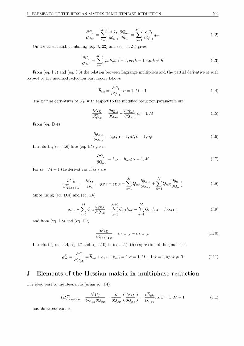
J. ELEMENTS OF THE HESSIAN MATRIX IN MULTIPHASE REDUCTION 209

∂GI∂nik

=

M+1∑α=1

∂GI

∂Qαk

∂Qαk∂nik

=

M+1∑α=1

∂GI

∂Qαkqαi (I.2)

On the other hand, combining (eq. 3.122) and (eq. 3.124) gives

∂GI∂nik

=

M+1∑α=1

qαihαk; i = 1, nc; k = 1, np; k 6= R (I.3)

From (eq. I.2) and (eq. I.3) the relation between Lagrange multipliers and the partial derivative of with

respect to the modified reduction parameters follows

hαk =∂GI

∂Qαk;α = 1,M + 1 (I.4)

The partial derivatives of GE with respect to the modified reduction parameters are

∂GE

∂Qαk=∂gE,k∂Qαk

− ∂gE,R∂QαR

;α = 1,M (I.5)

From (eq. D.4)

∂gE,k∂Qαk

= hαk;α = 1,M ; k = 1, np (I.6)

Introducing (eq. I.6) into (eq. I.5) gives

∂GE

∂Qαk= hαk − hαR;α = 1,M (I.7)

For α = M + 1 the derivatives of GE are

∂GE

∂QM+1,k

=∂GE∂θk

= gE,k − gE,R −M∑α=1

Qαk∂gE,k∂Qαk

+

M∑α=1

QαR∂gE,R∂QαR

(I.8)

Since, using (eq. D.4) and (eq. I.6)

gE,k −M∑α=1

Qαk∂gE,k∂Qαk

=

M+1∑α=1

Qαkhαk −M∑α=1

Qαkhαk = hM+1,k (I.9)

and from (eq. I.8) and (eq. I.9)

∂GE

∂QM+1,k

= hM+1,k − hM+1,R (I.10)

Introducing (eq. I.4, eq. I.7 and eq. I.10) in (eq. I.1), the expression of the gradient is

gRαk =∂G

∂Qαk= hαk + hαk − hαR = 0;α = 1,M + 1; k = 1, np; k 6= R (I.11)

J Elements of the Hessian matrix in multiphase reduction

The ideal part of the Hessian is (using eq. I.4)

(HRI

)αβ,kp

=∂2GI

∂Qαk∂Qβp=

∂

∂Qβp

(∂GI

∂Qαk

)=∂hαk

∂Qβp;α, β = 1,M + 1 (J.1)

and its excess part is

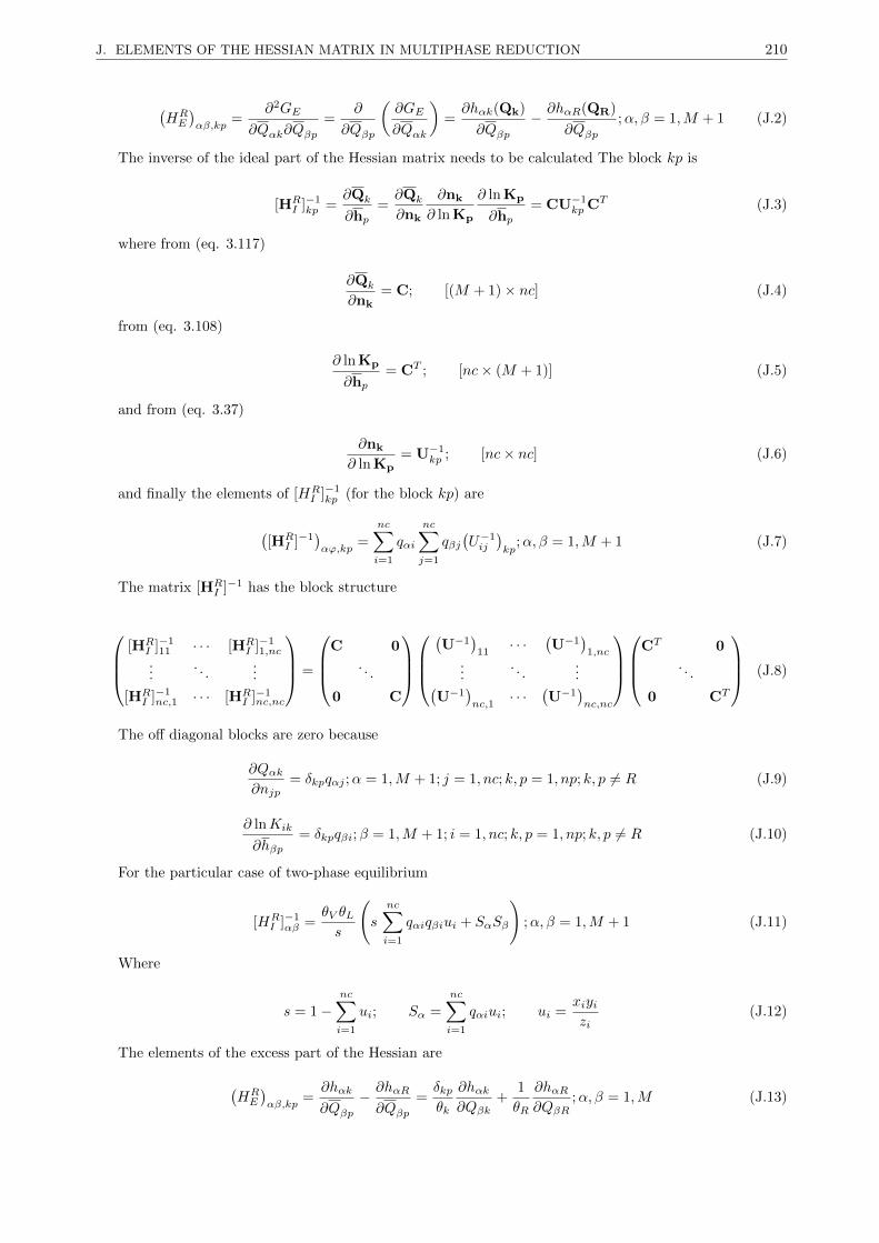
J. ELEMENTS OF THE HESSIAN MATRIX IN MULTIPHASE REDUCTION 210

(HRE

)αβ,kp

=∂2GE

∂Qαk∂Qβp=

∂

∂Qβp

(∂GE

∂Qαk

)=∂hαk(Qk)

∂Qβp− ∂hαR(QR)

∂Qβp;α, β = 1,M + 1 (J.2)

The inverse of the ideal part of the Hessian matrix needs to be calculated The block kp is

[HRI ]−1kp =

∂Qk

∂hp=∂Qk

∂nk

∂nk

∂ ln Kp

∂ ln Kp

∂hp= CU−1

kp CT (J.3)

where from (eq. 3.117)

∂Qk

∂nk= C; [(M + 1)× nc] (J.4)

from (eq. 3.108)

∂ ln Kp

∂hp= CT ; [nc× (M + 1)] (J.5)

and from (eq. 3.37)

∂nk

∂ ln Kp= U−1

kp ; [nc× nc] (J.6)

and finally the elements of [HRI ]−1kp (for the block kp) are

([HR

I ]−1)αϕ,kp

=

nc∑i=1

qαi

nc∑j=1

qβj(U−1ij

)kp

;α, β = 1,M + 1 (J.7)

The matrix [HRI ]−1 has the block structure

[HR

I ]−111 · · · [HR

I ]−11,nc

.... . .

...

[HRI ]−1nc,1 · · · [HR

I ]−1nc,nc

=

C 0

. . .

0 C

(U−1

)11

· · ·(U−1

)1,nc

.... . .

...(U−1

)nc,1

· · ·(U−1

)nc,nc

CT 0

. . .

0 CT

(J.8)

The off diagonal blocks are zero because

∂Qαk∂njp

= δkpqαj ;α = 1,M + 1; j = 1, nc; k, p = 1, np; k, p 6= R (J.9)

∂ lnKik

∂hβp= δkpqβi;β = 1,M + 1; i = 1, nc; k, p = 1, np; k, p 6= R (J.10)

For the particular case of two-phase equilibrium

[HRI ]−1αβ =

θV θLs

(s

nc∑i=1

qαiqβiui + SαSβ

);α, β = 1,M + 1 (J.11)

Where

s = 1−nc∑i=1

ui; Sα =

nc∑i=1

qαiui; ui =xiyizi

(J.12)

The elements of the excess part of the Hessian are

(HRE

)αβ,kp

=∂hαk

∂Qβp− ∂hαR

∂Qβp=δkpθk

∂hαk∂Qβk

+1

θR

∂hαR∂QβR

;α, β = 1,M (J.13)

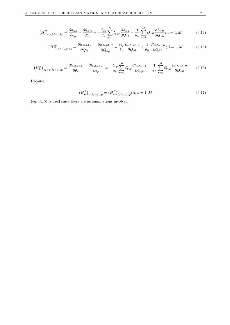
J. ELEMENTS OF THE HESSIAN MATRIX IN MULTIPHASE REDUCTION 211

(HRE

)α,M+1,kp

=∂hαk∂θp

− ∂hαR∂θp

= −δkpθk

M∑γ=1

Qγp∂hαk∂Qγk

− 1

θR

M∑γ=1

QγR∂hαR∂QγR

;α = 1,M (J.14)

(HRE

)M+1,β,kp

=∂hM+1,k

∂Qβp− ∂hM+1,R

∂Qβp=δkpθk

∂hM+1,k

∂Qβk+

1

θR

∂hM+1,R

∂QβR;β = 1,M (J.15)

(HRE

)M+1,M+1,kp

=∂hM+1,k

∂θp− ∂hM+1,R

∂θp= −δkp

θk

M∑γ=1

Qγp∂hM+1,k

∂Qγk− 1

θR

M∑γ=1

QγR∂hM+1,R

∂QγR(J.16)

Because

(HRE

)α,M+1,kp

=(HRE

)M+1,βkp

;α, β = 1,M (J.17)

(eq. J.15) is used since there are no summations involved.

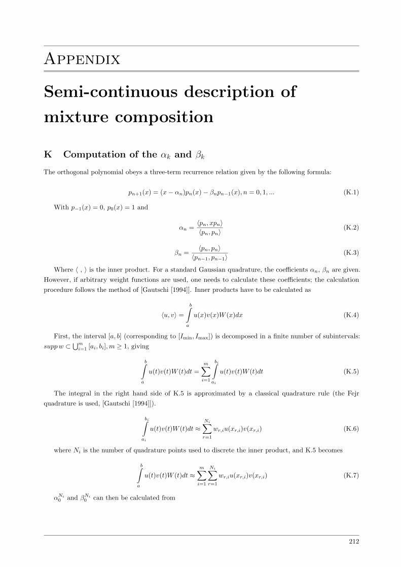
Appendix

Semi-continuous description of

mixture composition

K Computation of the αk and βk

The orthogonal polynomial obeys a three-term recurrence relation given by the following formula:

pn+1(x) = (x− αn)pn(x)− βnpn−1(x), n = 0, 1, ... (K.1)

With p−1(x) = 0, p0(x) = 1 and

αn =〈pn, xpn〉〈pn, pn〉

(K.2)

βn =〈pn, pn〉

〈pn−1, pn−1〉(K.3)

Where 〈 , 〉 is the inner product. For a standard Gaussian quadrature, the coefficients αn, βn are given.

However, if arbitrary weight functions are used, one needs to calculate these coefficients; the calculation

procedure follows the method of [Gautschi [1994]]. Inner products have to be calculated as

〈u, v〉 =

b∫a

u(x)v(x)W (x)dx (K.4)

First, the interval [a, b] (corresponding to [Imin, Imax]) is decomposed in a finite number of subintervals:

suppw ⊂⋃mi=1 [ai, bi],m ≥ 1, giving

b∫a

u(t)v(t)W (t)dt =

m∑i=1

bi∫ai

u(t)v(t)W (t)dt (K.5)

The integral in the right hand side of K.5 is approximated by a classical quadrature rule (the Fejr

quadrature is used, [Gautschi [1994]]).

bi∫ai

u(t)v(t)W (t)dt ≈Ni∑r=1

wr,iu(xr,i)v(xr,i) (K.6)

where Ni is the number of quadrature points used to discrete the inner product, and K.5 becomes

b∫a

u(t)v(t)W (t)dt ≈m∑i=1

Ni∑r=1

wr,iu(xr,i)v(xr,i) (K.7)

αNi0 and βNi0 can then be calculated from

212

L. CALCULATION OF QUADRATURE NODES AND WEIGHTS 213

αNi0 =

b∫a

tW (t)dt

b∫a

W (t)dt

=

m∑i=1

Ni∑r=1

wr,ixr,i

βNi0

(K.8)

βNi0 =

b∫a

W (t)dt =

m∑i=1

Ni∑r=1

wr,i (K.9)

From here, two different methods have been implemented: The first one is the the Stieljes procedure, based

on the direct computation of αNik and βNik from the recurrence (A1); it can give bad condition numbers for

large n(greater than 12 [Press et al. [1992]]). The second method is based on the Lanczos algorithm [Lanczos

[1950]]. It ensures a good condition number for any value of n. For a symmetric matrix A, there exists a

similarity transformation QTAQ = T2. Given the matrix A, the Lanczos algorithm allows to compute the

matrices Q and T2 which satisfy this relation. For the computed nodes xr,i and weights wr,i coming from

the Fejer quadrature, [Gautschi [1994]] showed that there exists a matrix QT1 which satisfies[

1 0T

0 QT1

] [1

√wT

√w ∆

] [1 0

0T Q1

]=

[1

√β0,NeT

1√β0,Ne1 T

](K.10)

Where w =(√w11,

√w12, ...,

√w21, ...,

√wNi,m

)T, diag(∆) = (x11, x12, . . . , x21, · · ·xNi,m) and T is a tri-

diagonal matrix [Golub and Welsch [1969]] which comes from the recursive relation (eq. K.1) (see Appendix E).

Calling the symmetric matrix

A =

[1

√wT

√w ∆

](K.11)

the Lanczos algorithm will compute the matrices Q and T2. Therefore, it will compute the desired αNikand βNik .

[Golub and Welsch [1969]] showed that limNi→+∞

αNik = αk and limNi→+∞

βNik = βk. The procedures start with

a small Ni and Ni is increased until the convergence over αk and βk is obtained (that is,∣∣∣β(Ni)k − β(Ni−1)

k

∣∣∣ ≤εβ

(Ni)k , k = 0, n− 1); usually convergence is achieved in few iterations.

L Calculation of quadrature nodes and weights

Once the coefficients of the polynomials are found, the roots of the polynomial given by K.1 need to be

calculated.[Golub and Welsch [1969]] replace the problem of computing the zeros of orthogonal polynomial

with the equivalent eigenvalue problem. The recursive relation can be written in matrix form as

xP = TP + pnen−1 (K.1)

where, P(x) = (p0(x), ..., pn−1(x))T

, en−1 = (0, ..., 0, 1)T , and T is a tri-diagonal matrix with elements

Tii = αi; i = 0, n− 1, Ti,i+1 = 1, i = 0, n− 2 and Ti−1,i = βi; i = 2, n− 1.

By using a diagonal matrix D with D00 = 1 and Dii =√βi; i = 1, n − 1, the problem can be trans-

formed into solving the eigenvalues and eigenvectors of the Jacobi matrix J = D−1TD. The elements of

the matrix J are Jii = αi; i = 0, n − 1, and Ji,i+1 =√βi, i = 0, n − 2. The matrices T and J have the

same spectrum and eigenvectors, since they are related by a similarity transformation. The matrix J is

L. CALCULATION OF QUADRATURE NODES AND WEIGHTS 214

symmetric tri-diagonal, and finding all its eigenvalues and eigenvectors is relatively efficient [Press et al. [1992]].

Moreover, [Wilf [1962]] showed that if vi is an eigenvector corresponding to the eigenvalue xi, normalized

so that vTv = 1, then the corresponding weight is

wj = µ0v2j,1 (K.2)

where vj,1 is the first component of vj and

µ0 =

b∫a

W (x)dx (K.3)

The calculation procedure can be further speeded, since only the first element of each eigenvector is

required in calculations. It is very important to notice that the function f does not appears in the calculation

of the discrete weights and abscissas.

List of Figures

1 API gravity . . . . . . . . . . . . . . . . . . . . . . . . . . . . . . . . . . . . . . . . . . . . . . 15

2 Enhanced oil Recovery [Larry [1989]] . . . . . . . . . . . . . . . . . . . . . . . . . . . . . . . . 16

3 Viscosity versus Temperature . . . . . . . . . . . . . . . . . . . . . . . . . . . . . . . . . . . . 17

4 a) Steam injection with vertical wells and b) Steam injection analysis [Baker [1969] and Mandl

and Volek [1969]] . . . . . . . . . . . . . . . . . . . . . . . . . . . . . . . . . . . . . . . . . . . 17

5 a) SAGD process and b) SAGD analysis . . . . . . . . . . . . . . . . . . . . . . . . . . . . . . 18

6 Water solubility in gas phase for the C1/nC4/H20 system, after [McKetta and Katz [1948]] . 18

2.1 Multiphase flash, input/output . . . . . . . . . . . . . . . . . . . . . . . . . . . . . . . . . . . 32

2.2 Multiphase equilibrium calculation procedure . . . . . . . . . . . . . . . . . . . . . . . . . . . 33

2.3 Sign of the tangent plane distance for the Y8 mixture . . . . . . . . . . . . . . . . . . . . . . 35

2.4 Smallest eigenvalue of (eq. 2.16), for the Y8 mixture . . . . . . . . . . . . . . . . . . . . . . . 37

2.5 Rachford-Rice function . . . . . . . . . . . . . . . . . . . . . . . . . . . . . . . . . . . . . . . . 39

2.6 Multiphase flash calculation procedure . . . . . . . . . . . . . . . . . . . . . . . . . . . . . . . 43

3.1 a) Euclidean norms vs. iteration level; Y8 mixture at T=335 K and P=200 bar b) Number of

iterations for the Y8 mixture at T=335 K in the conventional method . . . . . . . . . . . . . 61

3.2 a) Number of iterations for the Y8 mixture at T=335 K using reduction methods, b) Number

of Newton iterations for the Y8 mixture at T=335 K in the conventional method . . . . . . . 62

3.3 a) Number of iterations for the Y8 mixture at T=335 K; liquid phase stability, b) Number of

iterations for the MY10 mixture at saturation points using reduction methods . . . . . . . . . 62

3.4 Number of iterations for the MY10 - 85% CO2 mixture at T=322 K . . . . . . . . . . . . . . 63

3.5 Number of iterations for the Billings mixture at T=366.48 K . . . . . . . . . . . . . . . . . . 63

3.6 Number of iterations for the Kilgren mixture at T=399.82 K . . . . . . . . . . . . . . . . . . 64

3.7 Phase envelopes of Y8, MY10 and MY10+CO2 mixtures . . . . . . . . . . . . . . . . . . . . . 68

3.8 Condition number along the isotherm T=335K for the Y8 mixture . . . . . . . . . . . . . . . 70

3.9 Computation time to repeat 10000 times one Newton iteration for the flash problem . . . . . 72

3.10 Computation time to repeat 10000 times one Newton iteration for the flash problem, MY10+C02 72

3.11 Computation time for the whole two-phase region for the flash problem . . . . . . . . . . . . 74

3.12 Computation time for the whole two-phase region for the flash problem, MY10+C02 . . . . . 74

3.13 Computation time to repeat 10000 times one Newton iteration for the stability problem . . . 75

3.14 Computation time to repeat 10000 times one Newton iteration for the stability problem,

MY10+C02 . . . . . . . . . . . . . . . . . . . . . . . . . . . . . . . . . . . . . . . . . . . . . . 75

3.15 Computation time for the whole P-T window for the stability problem . . . . . . . . . . . . . 76

3.16 Computation time for the whole P-T window for the stability problem, MY10+C02 . . . . . 76

3.17 Error v.s. iteration number for various methods, for the Y8 mixture at T=350 K and P=230 bar 77

3.18 Phase envelopes of different mixtures mixed with CO2 at T=305.35 K . . . . . . . . . . . . . 85

3.19 b)Phase boundaries of a) the Sour gas mixture at T=178.8K b) the four-phase region for the

sourgas4 mixture at T=305.35 K . . . . . . . . . . . . . . . . . . . . . . . . . . . . . . . . . . 86

3.20 Computational time to repeat 10000 times a Newton iteration . . . . . . . . . . . . . . . . . . 86

3.21 Computational time to repeat 10000 times a Newton iteration . . . . . . . . . . . . . . . . . . 87

LIST OF FIGURES 215

LIST OF FIGURES 216

3.22 Computational time vs. number of components for the stability analysis of the sour gas mixture

(10000 iterations at T= 178.8 K and P= 20 bar) . . . . . . . . . . . . . . . . . . . . . . . . . 87

3.23 Computational time for the entire three phase region . . . . . . . . . . . . . . . . . . . . . . . 88

3.24 Computational time for a) the entire three phase region for the sour gas mixture; b) the entire

four phase region for the sourgas4 mixture . . . . . . . . . . . . . . . . . . . . . . . . . . . . . 88

3.25 Error vs number of iterations at P=69 bar and 95% of CO2 for the Maljamar reservoir mixture 89

3.26 Three-phase flash of the Maljamar separator mixture at 95% CO2 . . . . . . . . . . . . . . . 89

3.27 Three-phase flash of the sour gas mixture at P=20 bar . . . . . . . . . . . . . . . . . . . . . . 90

3.28 Four-phase flash of the sour gas mixture at 7.4% CO2 . . . . . . . . . . . . . . . . . . . . . . 90

3.29 Iterations and function evaluations starting directly with the BFGS method; Y8 mixture at

T=285 K . . . . . . . . . . . . . . . . . . . . . . . . . . . . . . . . . . . . . . . . . . . . . . . 102

3.30 Iterations and function evaluations starting directly with the BFGS method; Y8 mixture at

T=335 K . . . . . . . . . . . . . . . . . . . . . . . . . . . . . . . . . . . . . . . . . . . . . . . 102

3.31 Iterations and function evaluations starting directly with the BFGS method; MY10 mixture at

T=565 K . . . . . . . . . . . . . . . . . . . . . . . . . . . . . . . . . . . . . . . . . . . . . . . 103

3.32 Comparison between the proposed BFGS algorithm and Nocedal L-BFGS-B for the Y8 mixture

at T=285 K . . . . . . . . . . . . . . . . . . . . . . . . . . . . . . . . . . . . . . . . . . . . . . 103

3.33 Comparison between the proposed BFGS algorithm and Nocedal L-BFGS-B for the Y8 mixture

at T=335 K . . . . . . . . . . . . . . . . . . . . . . . . . . . . . . . . . . . . . . . . . . . . . . 104

3.34 Iterations and function evaluations after a switch from SSI, Y8 mixture at T=285 K . . . . . 104

3.35 Iterations and function evaluations after a switch from SSI, Y8 mixture at T=335 K . . . . . 105

3.36 Iterations and function evaluations after a switch from SSI, MY10 mixture at T=565 K . . . 105

3.37 nl/nv-L compared with alpha/alpha-L; number of function evaluations for the Y8 mixture at

T=335 K (after a switch from SSI) . . . . . . . . . . . . . . . . . . . . . . . . . . . . . . . . . 106

3.38 Error versus number of iterations for the Y8 mixture at T=335K . . . . . . . . . . . . . . . . 107

3.39 Error versus number of iterations for the Y8 mixture at T=335K . . . . . . . . . . . . . . . . 107

3.40 Convex example [Conn et al. [2000]] . . . . . . . . . . . . . . . . . . . . . . . . . . . . . . . . 111

3.41 Non convex example [Conn et al. [2000]] . . . . . . . . . . . . . . . . . . . . . . . . . . . . . . 113

3.42 Hard case example [Conn et al. [2000]] . . . . . . . . . . . . . . . . . . . . . . . . . . . . . . . 114

3.43 Phase envelope a) of the MY10 mixture b) of the Oil B mixture mixed with CO2 at T=307.6K117

3.44 Number of iterations for the MY10 mixture, stability analysis (Yi = zi/Ki) . . . . . . . . . . 118

3.45 Number of iterations for the MY10 mixture, stability analysis (Yi = zi/Ki) . . . . . . . . . . 118

3.46 Number of iterations for the MY10 mixture, stability analysis (Yi = ziKi) . . . . . . . . . . . 119

3.47 Number of iterations for the MY10 mixture, stability analysis (Yi = ziKi) . . . . . . . . . . . 119

3.48 Error vs. iteration level for the stability analysis (liquid trial phase, Yi = ziKi) of the MY10

mixture at T=540.5 K . . . . . . . . . . . . . . . . . . . . . . . . . . . . . . . . . . . . . . . . 120

3.49 Error vs. iteration level for the stability analysis (liquid trial phase, Yi = ziKi) of the MY10

mixture . . . . . . . . . . . . . . . . . . . . . . . . . . . . . . . . . . . . . . . . . . . . . . . . 120

3.50 Number of iterations for the MY10 mixture (two-phase flash) . . . . . . . . . . . . . . . . . . 122

3.51 Number of iterations for the MY10 mixture (two-phase flash) . . . . . . . . . . . . . . . . . . 122

3.52 Comparison between various flash calculation algorithms (initialization by K-Wilson) for the

Oil B mixture/95% CO2 at T=307.6 K . . . . . . . . . . . . . . . . . . . . . . . . . . . . . . . 123

3.53 Number of iterations (two-and three-phase flashes) for Maljamar reservoir mixture over the

Pz-diagram at T=305.35 K . . . . . . . . . . . . . . . . . . . . . . . . . . . . . . . . . . . . . 123

3.54 Number of iterations (two-and three-phase flashes) for Maljamar reservoir mixture over the

Pz-diagram at T=305.35 K . . . . . . . . . . . . . . . . . . . . . . . . . . . . . . . . . . . . . 124

3.55 Number of iterations (two-and three-phase flashes) for Maljamar reservoir mixture over the

Pz-diagram at T=305.35 K: NLVM-TR . . . . . . . . . . . . . . . . . . . . . . . . . . . . . . 124

LIST OF FIGURES 217

3.56 Number of iterations (two- and three-phase flashes) for Maljamar separator mixture over the

P-z diagram at T=305.35 K . . . . . . . . . . . . . . . . . . . . . . . . . . . . . . . . . . . . . 125

3.57 Number of iterations (two-and three-phase flashes) for the Oil B over the P-z diagram at

T=307.6 K . . . . . . . . . . . . . . . . . . . . . . . . . . . . . . . . . . . . . . . . . . . . . . 126

3.58 Number of iterations (two- and three-phase flashes) for the sour gas mixture over the P-z

diagram at T= 178.8 K . . . . . . . . . . . . . . . . . . . . . . . . . . . . . . . . . . . . . . . 127

3.59 a) Global minimum of the modified TPD function b)Number of iterations of Newton and TR

methods; for sour gas-CO2 mixtures at T=178.8 K and P=20 bar . . . . . . . . . . . . . . . . 128

3.60 Error vs. iteration level for three-phase flash of the sour gas mixture at T=178.8 K, P=20 bar

and 51% moles CO2 . . . . . . . . . . . . . . . . . . . . . . . . . . . . . . . . . . . . . . . . . 128

3.61 Computation time to perform Newton iterations through the whole three phase region . . . . 133

3.62 a) Convergence properties at 49.6% of CO2 b) Number of iterations; for the sour gas mixture

on the isobar P=20 bar . . . . . . . . . . . . . . . . . . . . . . . . . . . . . . . . . . . . . . . 134

3.63 Condition number for various methods for the sour gas mixture on the isobar P=20 bar . . . 134

4.1 Feed composition vs. carbon numbers for the S. oil . . . . . . . . . . . . . . . . . . . . . . . . 139

4.2 LFMR for different pressures and temperatures for the S. oil . . . . . . . . . . . . . . . . . . 139

4.3 a) Altered feed composition (oil S) b) LFMR; vs carbon number for the altered oil S . . . . . 139

4.4 Feed composition of the semi-continuous mixture (Oil S) after cubic spline interpolation on

the continuous part . . . . . . . . . . . . . . . . . . . . . . . . . . . . . . . . . . . . . . . . . . 141

4.5 Altered of the S oil (mixture A) . . . . . . . . . . . . . . . . . . . . . . . . . . . . . . . . . . . 146

4.6 Mole fraction in the vapor phase for mixture A at T=450 K . . . . . . . . . . . . . . . . . . . 147

4.7 Error in phase mole fractions for mixture A at T=450 K . . . . . . . . . . . . . . . . . . . . . 147

4.8 Error in phase compositions for mixture A at T=450 K and P=8 bar . . . . . . . . . . . . . . 148

4.9 Error in phase compositions for mixture B at T=450 K and P=8 bar . . . . . . . . . . . . . . 148

4.10 Error in phase compositions for mixture C at T=450 K and P=8 bar . . . . . . . . . . . . . . 149

4.11 a)Phase mole fractions for mixture B + H2O at T = 310 K and b) Errors in phase mole

fractions for mixture B + H2O at T=310 K . . . . . . . . . . . . . . . . . . . . . . . . . . . . 149

4.12 Phase mole fractions for mixture B + H2O at T = 310 K . . . . . . . . . . . . . . . . . . . . 150

4.13 Errors in phase compositions for mixture B+H2O at T=310 K and P=6 bar . . . . . . . . . . 150

4.14 Errors in phase compositions for mixture B+H2O at T=310 K and P=6 bar . . . . . . . . . . 151

4.15 Phase mole fractions mixture A+CO2 at T=249 K . . . . . . . . . . . . . . . . . . . . . . . . 151

4.16 Errors in phase mole fraction, mixture A+CO2 at T=249 K . . . . . . . . . . . . . . . . . . . 152

4.17 Errors in phase compositions for mixture A+CO2 at T=249 K and P=29.5 bar . . . . . . . . 152

4.18 Errors vs. the number of quadrature points, mixture A at T=450 K. a) In phase mole fractions

in the two-phase region; b) in compositions at P=8 bar . . . . . . . . . . . . . . . . . . . . . 153

4.19 Absolute errors vs. the number of quadrature points, mixture A+H2O at T=310 K; a) In

phase mole fractions in the three-phase region; b) in compositions at P=6 bar . . . . . . . . . 153

4.20 Absolute errors vs. the number of quadrature points, mixture A+CO2 at T=249 K; a) In

phase mole fractions in the three-phase region; b) in compositions at P=29.5 bar . . . . . . . 154

5.1 Example of parameterization of the tie-simplex space . . . . . . . . . . . . . . . . . . . . . . . 168

5.2 Comparisons between the exact phase envelope and the one obtained with CSAT after [Iranshahr

et al. [2012]] . . . . . . . . . . . . . . . . . . . . . . . . . . . . . . . . . . . . . . . . . . . . . . 169

5.3 Parameterization of different tie-triangle planes . . . . . . . . . . . . . . . . . . . . . . . . . . 169

5.4 a) Parametrization of the space b)Status identification, stability required . . . . . . . . . . . 171

5.5 a) Parametrization of the space b)Status identification, stability skipped . . . . . . . . . . . . 171

5.6 Water saturation at the end of the simulation, SPE3 case . . . . . . . . . . . . . . . . . . . . 173

5.7 Oil saturation at the end of the simulation, SPE3 case . . . . . . . . . . . . . . . . . . . . . . 173

LIST OF FIGURES 218

5.8 Total production vs time for the SPE3 case, comparisons between ECLIPSE and the flash

program with TPP . . . . . . . . . . . . . . . . . . . . . . . . . . . . . . . . . . . . . . . . . . 174

5.9 Phase envelope BSB comparisons with experimental values . . . . . . . . . . . . . . . . . . . 175

5.10 CO2 injection process by[Okuno [2009]] . . . . . . . . . . . . . . . . . . . . . . . . . . . . . . 176

5.11 CO2 injection process, saturations obtained with AD-GPRS + MFLASH . . . . . . . . . . . 176

5.12 4 phase case phase p-z diagram . . . . . . . . . . . . . . . . . . . . . . . . . . . . . . . . . . . 177

5.13 Four-phase simulation of CO2 injection . . . . . . . . . . . . . . . . . . . . . . . . . . . . . . . 178

5.14 Pressure, bar; for the four phase CO2 test case, T=50 days . . . . . . . . . . . . . . . . . . . 179

5.15 Three component mixture, at T=520 K . . . . . . . . . . . . . . . . . . . . . . . . . . . . . . 179

5.16 relative permeabilities for the light oil steam injection test case . . . . . . . . . . . . . . . . . 180

5.17 a)Oil Saturation, b)Gas Saturation for the light oil steam injection case . . . . . . . . . . . . 181

5.18 Water saturation . . . . . . . . . . . . . . . . . . . . . . . . . . . . . . . . . . . . . . . . . . . 181

5.19 Gas saturation for the SPE10 case, at T=600 days . . . . . . . . . . . . . . . . . . . . . . . . 182

5.20 Gas saturation for the SPE10 case, third layer, T=600 days . . . . . . . . . . . . . . . . . . . 183

5.21 Oil saturation for the SPE10 case, at T=600 days . . . . . . . . . . . . . . . . . . . . . . . . . 183

5.22 Oil saturation for the SPE10 case, third layer, T=600 days . . . . . . . . . . . . . . . . . . . 183

5.23 Water saturation for the SPE10 case at T=600 days . . . . . . . . . . . . . . . . . . . . . . . 184

5.24 Plot of different properties in the third layer of the SPE10 case after T=600 days . . . . . . . 184

5.25 Saturations for the synthetic SAGD at t=150 days . . . . . . . . . . . . . . . . . . . . . . . . 186

5.26 a) Oil saturation b) Temperature; for the synthetic SAGD at t=150 days . . . . . . . . . . . 186

5.27 Saturations for the Athabasca oil SAGD at t=20 days . . . . . . . . . . . . . . . . . . . . . . 187

5.28 Saturations for the Athabasca oil SAGD at t=30 days . . . . . . . . . . . . . . . . . . . . . . 187

5.29 Saturations for the Athabasca oil SAGD at t=360 days . . . . . . . . . . . . . . . . . . . . . 188

5.30 a) Oil saturation b)Temperature for the Athabasca oil SAGD at t=360 days . . . . . . . . . . 188

5.31 Gas saturation for the Athabasca oil SAGD at t=410 days . . . . . . . . . . . . . . . . . . . . 188

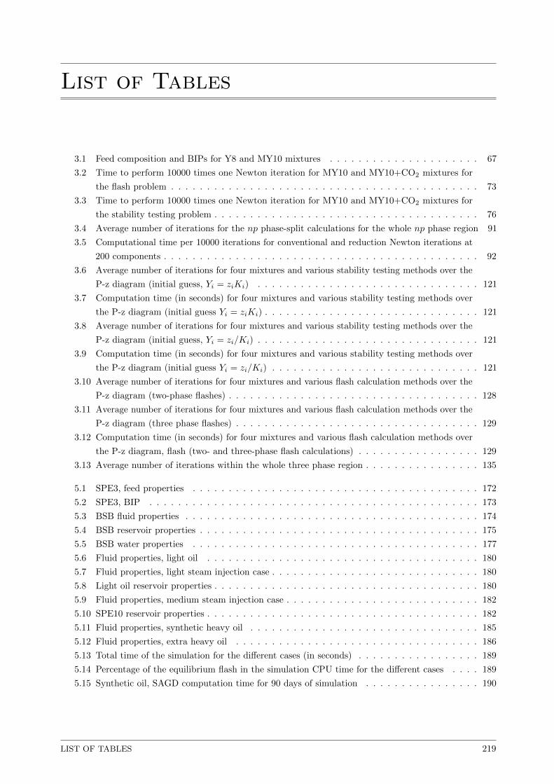
List of Tables

3.1 Feed composition and BIPs for Y8 and MY10 mixtures . . . . . . . . . . . . . . . . . . . . . 67

3.2 Time to perform 10000 times one Newton iteration for MY10 and MY10+CO2 mixtures for

the flash problem . . . . . . . . . . . . . . . . . . . . . . . . . . . . . . . . . . . . . . . . . . . 73

3.3 Time to perform 10000 times one Newton iteration for MY10 and MY10+CO2 mixtures for

the stability testing problem . . . . . . . . . . . . . . . . . . . . . . . . . . . . . . . . . . . . . 76

3.4 Average number of iterations for the np phase-split calculations for the whole np phase region 91

3.5 Computational time per 10000 iterations for conventional and reduction Newton iterations at

200 components . . . . . . . . . . . . . . . . . . . . . . . . . . . . . . . . . . . . . . . . . . . . 92

3.6 Average number of iterations for four mixtures and various stability testing methods over the

P-z diagram (initial guess, Yi = ziKi) . . . . . . . . . . . . . . . . . . . . . . . . . . . . . . . 121

3.7 Computation time (in seconds) for four mixtures and various stability testing methods over

the P-z diagram (initial guess Yi = ziKi) . . . . . . . . . . . . . . . . . . . . . . . . . . . . . . 121

3.8 Average number of iterations for four mixtures and various stability testing methods over the

P-z diagram (initial guess, Yi = zi/Ki) . . . . . . . . . . . . . . . . . . . . . . . . . . . . . . . 121

3.9 Computation time (in seconds) for four mixtures and various stability testing methods over

the P-z diagram (initial guess Yi = zi/Ki) . . . . . . . . . . . . . . . . . . . . . . . . . . . . . 121

3.10 Average number of iterations for four mixtures and various flash calculation methods over the

P-z diagram (two-phase flashes) . . . . . . . . . . . . . . . . . . . . . . . . . . . . . . . . . . . 128

3.11 Average number of iterations for four mixtures and various flash calculation methods over the

P-z diagram (three phase flashes) . . . . . . . . . . . . . . . . . . . . . . . . . . . . . . . . . . 129

3.12 Computation time (in seconds) for four mixtures and various flash calculation methods over

the P-z diagram, flash (two- and three-phase flash calculations) . . . . . . . . . . . . . . . . . 129

3.13 Average number of iterations within the whole three phase region . . . . . . . . . . . . . . . . 135

5.1 SPE3, feed properties . . . . . . . . . . . . . . . . . . . . . . . . . . . . . . . . . . . . . . . . 172

5.2 SPE3, BIP . . . . . . . . . . . . . . . . . . . . . . . . . . . . . . . . . . . . . . . . . . . . . . 173

5.3 BSB fluid properties . . . . . . . . . . . . . . . . . . . . . . . . . . . . . . . . . . . . . . . . . 174

5.4 BSB reservoir properties . . . . . . . . . . . . . . . . . . . . . . . . . . . . . . . . . . . . . . . 175

5.5 BSB water properties . . . . . . . . . . . . . . . . . . . . . . . . . . . . . . . . . . . . . . . . 177

5.6 Fluid properties, light oil . . . . . . . . . . . . . . . . . . . . . . . . . . . . . . . . . . . . . . 180

5.7 Fluid properties, light steam injection case . . . . . . . . . . . . . . . . . . . . . . . . . . . . . 180

5.8 Light oil reservoir properties . . . . . . . . . . . . . . . . . . . . . . . . . . . . . . . . . . . . . 180

5.9 Fluid properties, medium steam injection case . . . . . . . . . . . . . . . . . . . . . . . . . . . 182

5.10 SPE10 reservoir properties . . . . . . . . . . . . . . . . . . . . . . . . . . . . . . . . . . . . . . 182

5.11 Fluid properties, synthetic heavy oil . . . . . . . . . . . . . . . . . . . . . . . . . . . . . . . . 185

5.12 Fluid properties, extra heavy oil . . . . . . . . . . . . . . . . . . . . . . . . . . . . . . . . . . 186

5.13 Total time of the simulation for the different cases (in seconds) . . . . . . . . . . . . . . . . . 189

5.14 Percentage of the equilibrium flash in the simulation CPU time for the different cases . . . . 189

5.15 Synthetic oil, SAGD computation time for 90 days of simulation . . . . . . . . . . . . . . . . 190

LIST OF TABLES 219

References

N.M. Alsaifi and P. Englezos. Prediction of multiphase equilibrium using the pc-saft equation of state and

simultaneous testing of phase stability. Fluid Phase Equilibria, 302:169–178, 2011.

M.N. Ammar and H. Renon. The isothermal flash problem: New methods for phase split calculations. AIChE

J., 33:926–939, 1987.

U. Baer, D. Browarzik, and H. Kehlen. Thermodynamics of semicontinuous mixtures using equations of state

with group contributions. Fluid Phase Equilibria, pages 9–44, 1997.

L.E Baker, A.C. Pierce, and K.D. Luks. Gibbs energy analysis of phase equilibria. SPE Journal, 22:731–742,

1982.

P.E Baker. An experimental study of heat flow in steam flooding. Soc. Petroleum Eng. J., 9:89–99, 1969.

R.A. Behrens and S.I. Sandler. The use of semicontinuous description to model the c7+ fraction in equation

of state calculation. SPE Res. Eng., 3:1041–1047, 1986.

K.M. Brantferger. Development of a Thermodynamically Consistent, Fully Implicit, Compositional, Equation-

Of-State, Steamflood Simulator. PhD thesis, University of Texas at Austin, 1991.

R.H Brooks and A.T. Corey. Hydraulic properties of porous media. Hydrology Papers, 1964.

D. Browarzik, M. Kowalewski, and H. Kehlen. Stability calculations of semicontinuous mixtures based on

equations of state. Fluid Phase Equilibria, 142:149–162, 1998.

C.G. Broyden. The convergence of a class of double-rank minimization algorithms. Journal of the Institute

of Mathematics and Its Applications, pages 76–90, 1970.

J. Burger, P. Sourieau, and M. Combarnous. Thermal methods of oil recovery. Technip Editions, 1985.

Richard H. Byrd, Robert B. Schabel, and Gerald A. Shultz. Approximate solution of the trust region problem

by minimization over two-dimensional subspaces. Mathematical programming, 40:247–263, 1988.

W.A. Canas Marın, J.D. Ortiz-Arango, U.E. Guerrero-Aconcha, and S. Hernandez-Baez. Improved two-sided

tangent plane initialization and two-phase-split calculations. Ind. Eng. Chem. Res., 46:5429–5436, 2007.

M.C.H. Chein, Yardumian H.E., E.Y. Chung, and W.W. Todd. The formulation of a thermal simulation

model in a vectorized, general purpose reservoir simulator. Tenth SPE Symposium on Reservoir Simulation,

Houston, Texas, 1989.

G.F Chou and Prausnitz J.M. Adiabatic flash calculations for continuous or semi-continuous mixtures using

an equation of state. Fluid Phase Equilibria, 30:75–82, 1986.

O. Cicek. Numerical simulation of steam displacement of oil in naturally fractured reservoirs using fully

implicit compositional formulation: A comparative analysis of the effects of capillary and gravitational

forces in matrix/fracture exchange term. SPE Annual Technical Conference and Exhibition, Dallas, Texas,

2005.

O. Cicek and T. Ertekin. Development and testing of a new 3d field scale fully implicit multi-phase

compositional steam injection simulator. SPE European 3D Reservoir Modeling Conference, 1996.

REFERENCES 220

REFERENCES 221

K.H. Coats. Simulation of steamflooding with distillation and solution gas. Soc. Petroleum Eng. J., 16:

235–247, 1976.

K.H. Coats. A highly implicit steamflood model. Soc. Pet. Eng. J., 18:369–383, 1978.

A.R. Conn, N.I.M. Gould, and Ph. L. Toint. Trust-Region Methods. SIAM/MPS Series on Optimization,

2000.

R.L. Cotterman and J.M. Prausnitz. Flash calculations for continuous or semicontinuous mixtures using an

equation of state. Ind. Eng. Chem. Proc. Des. Dev., 24:434–443, 1985.

R.L. Cotterman, R. Bender, and J.M. Prausnitz. Phase equilibria for mixtures containing very many

components. development and application of continuousnthermodyanmics for chemical process design. Ind.

Eng. Chem. Proc. Des. Dev., 24:194–203, 1985.

J.L Creek and J.M. Sheffield. Phase behavior, fluid properties, and displacement characteristics of permian

basin reservoir fluid/co2 systems. SPE Res. Eng., 8:34–42, 1993.

R.O. Esposito, M. Castier, and F.W. Tavares. Phase equilibrium calculations for semi-continuous mixtures

subject to gravitational fields. Ind. Eng. Chem. Res., 39:4415–4421, 2000.

F.J. Fayers and J.D. Matthews. Evaluation of nomalized stone’s methods for estimating three-phase relative

permeabilities. SPE Journal, 24:224–232, 1984.

S.A. Feizabadi. An equation-of-State Based Mathematical Modeling of Four-Phase Flow in Porous Media.

PhD thesis, University of Calgary, 2013.

A Firoozabadi and H Pan. Fast and robust algorithm for compositional modeling: Part i - stability analysis.

SPE Journal, 7:78–89, 2002.

A Firoozabadi, Y. Herim, and D. Katz. Reservoir depletion calculations for gas condensates using extended

analyses in the pengrobinson equation of state. Can. J. Chem. Eng., 56:610–615, 1978.

R. Fletcher. A new approach to variable metric algorithms. Computer Journal, 13:317–322, 1970.

V. Gaganis and N. Varotsis. Non-iterative phase stability calculations for process simulation using discrimi-

nating functions. Fluid Phase Equilibria, 314:69–77, 2012.

V. Gaganis and N. Varotsis. An improved bip matrix decomposition method for reduced flash calculations.

Fluid Phase Equilibria, 340:63–76, 2013.

V. Gaganis and N. Varotsis. An integrated approach for rapid phase behavior calculations in compositional

modeling. J. Petrol. Sci. Eng., 118:74–87, 2014.

J. Garcia-Sanchez, M.N Schwartzentrube, M.N. Ammar, and H. Renon. Modeling of multiphase liquid

equilibria for multicomponent mixtures. Fluid Phase Equilib., 121:207–225, 1996.

J. Garcia-Sanchez, G. Eliosa-Jimenez, A. Salas-Padron, O. Hernandez-Garduza, and D. Apam-Martinez.

Modeling of microemulsion phase diagrams from excess gibbs energy models. Chem. Eng. J., 84:257–274,

2001.

T.T. Garipov, M. Karimi-Fard, and H.A. Tchelepi. Coupled geomechanics and flow in fractured media.

ECMOR Conference paper, 2012.

W. Gautschi. Algorithm 726: Orthopol-a package of routines for generating orthogonal polynomials and

gauss-type quadrature rules. ACM Trans. Math. Software, 20:21–62, 1994.

W. Gautschi. Orthogonal Polynomials: Computation and Approximation. Oxford University Press, 2004.

REFERENCES 222

D.M. Gay. Computing optimal locally constrained steps. SIAM J. Sci. and Stat. Comput., 2:186–197, 1981.

P.E. Gill and W. Murray. Newton type methods for unconstrained and linearly constrained optimization.

Math. Program., 7:311–350, 1974.

P.E. Gill and W. Murray. Algorithms for the solution of the nonlinear least-squares problem. SIAM J. Numer.

Anal., 15:977–992, 1978.

D. Goldfarb. A family of variable metric updates derived by variational means. Mathematics of Computation,

24:23–26, 1970.

G.H. Golub and C.F. van Loan. Matrix Computations. John Hopkins Univerisy Press, third edition, 1996.

G.H. Golub and J.H. Welsch. Calculation of gauss quadrature rules. Math.Comp., 2:221–230, 1969.

R. Gordon. Error bounds in equilibrium statistical mechanics. J. Math. Phys., 9:655–663, 1968.

S.E. Gorucu and R.T. Johns. Comparison of reduced and conventional phase equilibrium calculations. SPE

Reservoir Simulation Symposium, Feb. 18-20, The Woodlands, TX, USA, 2013.

S.E. Gorucu and R.T. Johns. New reduced parameters for flash calculations based on two-parameter bip

formula. J. Petrol. Sci. Eng., 116:50–58, 2014.

A.S Gow, F.P. Stein, X. Guo, and A. Lucia. Simulation of binary refrigerant mixture vapor-liquid equilibria

using a quasi-regular nonrandom fluid theory and local composition mixing rules. Fluid Phase Equilibria,

116:60–67, 1996.

K.B. Haugen and B.L. Beckner. A critical comparison of reduced and conventional eos algorithms. SPE J.,

18:378–388, 2013.

K.B. Haugen, A. Firoozabadi, and L. Sun. Efficient and robust three-phase split computations. AIChE J.,

57:2555–2565, 2011.

M.D. Hebden. An algorithm for minimization using exact second derivatives. Tech. Report TP515. Harwell,

England: Atomic Energy Research Establishment, 1973.

M. Heidari. Equation of State Based Thermal Compositional Reservoir Simulator for Hybrid Solvent/Thermal

Processes. PhD thesis, Department of Chemical and Petroleum Engineering, Calgary University, 2014.

R.A. Heidemann and M.L. Michelsen. Instability of successive substitution. Ind. Eng. Chem. Res., 34:958–966,

1995.

E.M. Hendriks. Reduction theorem for phase equilibria problems. Ind. Eng. Chem. Res., 27:1728–1732, 1988.

E.M. Hendriks and A.R.D. van Bergen. Application of a reduction method to phase equilibrium calculations.

Fluid Phase Equilibria, 74:17–34, 1992.

H. Hoteit and A. Firoozabadi. Simple phase stability-testing algorithm in the reduction method. AIChE J.,

52:2909–2920, 2006.

A. Iranshahr. Tie-Simplex Method For Thermal-Compositional Simulation. PhD thesis, Department of

Energy Resources Enginnering, Stanford University, 2012.

A. Iranshahr, D. Voskov, and H. Tchelepi. Tie-simplex parameterization for eos-based thermal compositional

simulation. Soc. Pet. Eng. J., 2(15):545–556, 2010a.

A. Iranshahr, D. Voskov, and H.A. Tchelepi. Generalized negative-flash method for multiphase multicomponent

systems. Fluid Phase Equilibria, 299:272–284, 2010b.

REFERENCES 223

A. Iranshahr, D. Voskov, and H. Tchelepi. Gibbs energy analysis: Compositional tie-simplex space. Fluid

Phase Equilib., 321:49–58, 2012.

A. Iranshahr, D. Voskov, and H. Tchelepi. Tie-simplex based compositional space parameterization: Continuity

and generalization to multiphase systems. AICHE J., 5(59):1684–1701, 2013.

K. Ishimoto. One-dimensional fully implicit compositional model for steam flooding. Master’s thesis, University

of Texas, Austin, 1985.

M.R. Islam, S.H. Moussavizadegan, S. Mustafiz, and J.H. Abou-Kassem. Advanced Petroleum Reservoir

Simulation. Wiley, 2010.

B.H. Jensen and A. Fredenslund. A simplified flash procedure for multicomponent mixtures containing

hydrocarbons and one non-hydrocarbon using two-parameter cubic equations of state. Ind. Eng. Chem.

Res., 26:2129–2134, 1987.

V. John and F. Thein. On the efficiency and robustness of the core routine of thequadrature method of

moments (qmom). Chem. Eng. Sci., 75:327–333, 2012.

P. Kaul and R.L. Thrasher. A parameter-based approach for two-phase-equilibrium prediction with cubic

equations of state. SPE Reservoir Eng., 11:273–279, 1996.

D. Kenyon and G.A. Behie. Third spe comparative solution project: Gas cycling of retrograde condensate

reservoirs. SPE Engineers, 39:981–997, 1987.

S.A. Khan, G.A. Pope, and K. Sepehrnoori. Fluid characterization of three-phase co2/oil mixtures. Symposium

at the SPE/DOE Enhanced Oil Recovery, Tulsa, Oklahoma, 1992.

K.H. Kilgren. Phase behavior of a high-pressure condensate reservoir fluid. J. Petrol. Technol., 18:1001–1005,

1966.

D. Kourounis, D. Voskov, and K. Aziz. Adjoint methods for multicomponent flow simulation. 12th European

Conference on the Mathematics of Oil Recovery, Oxford, 2010.

J.A. Labadie and K.D. Luks. Solidfluid phase equilibria of compositionally complex mixtures: contrast of

equilibrium and process treatments. Fluid Phase Equilibria, 205:215–232, 2003.

P.L.C. Lage. The quadrature method of moments for continuous thermodynamics. Comput. CHem. Eng., 31:

782–799, 2007.

C. Lanczos. An iteration method for the solution of the eigenvalue problem of linear differential and integral

operators. J. Res. Bur. Std., 45:255–282, 1950.

A. Lapene. Etude Experimentale et Numerique de la Combustion In-Situ d’Huiles Lourdes. PhD thesis,

Universite de Toulouse,Institut de Mecanique des Fluides de Toulouse, 2010.

W.L. Larry. Enhanced oil recovery. Technology and Engineering, 1989.

C.F. Leibovici and J. Neoschil. A new look at the rachford-rice equation. Fluid Phase Equilibria, 74:303–308,

1992.

C.F. Leibovici and D.V Nichita. A new look at multiphase rachford-rice equations for negative flashes. Fluid

Phase Equilibria, 267:127–132, 2008.

K. Levenberg. A method for the solution of certain problems in least squares. Quart. Appl. Math., 2:164–168,

1944.

REFERENCES 224

G.N. Lewis and M. Randall. Thermodynamics and the Free Energy of Chemical Substances. McGraw-Hill

Book Co, 1923.

Y.K. Li and R.T. Johns. Rapid flash calculations for compositional simulation. SPE Reservoir Evaluation

and Engineering, 8:521–529, 2006.

Z. Li and A. Firoozabadi. General strategy for stability testing and phase-split calculations in two and three

phases. SPE Journal, 17:1096–1107, 2012.

B. Lin, C.F. Leibovici, and S.B. Jørgensen. Optimal component lumping: Problem formulation and solution

techniques. Comput. CHem. Eng., 32:1167–1172, 2008.

C. Lira-Galeana, A. Firoozabadi, and J.M. Prausnitz. Computation of compositional grading in hydrocarbon

reservoirs. application of continuous thermodynamics. Fluid Phase Equilibria, 102:143–158, 1994.

D.C. Liu and J. Nocedal. On the limited memory method for large scale optimization. Mathematical

Programming, 45(3):503–528, 1989.

J.L. Liu and D.S.H. Wong. Rigorous implementation of continuous thermodynamics using orthonormal

polynomials. Fluid Phase Equilibria, 129:113–127, 1997.

J. Lohrenz, B.G. Bray, and C.R. Clark. Calculating viscosities of reservoir fluids from their compositions.

Jounral of Petroleum Technology, 915:1171–1176, 1964.

A. Lucia and D. Liu. An acceleration method for dogleg methods in simple singular regions. Ind. Eng. Chem.

Res., 37:1358–1363, 1998.

A. Lucia and F. Yang. Multivariable terrain methods. AIChE J., 49:2553–2563, 2003.

A. Lucia, X. Guo, and X. Wang. Process simulation in the complex domain. AIChE J., 39:461–470, 1993.

A. Lucia, L. Padmanabhan, and S. Venkataraman. Multiphase equilibrium flash calculations. Comp. and

Chem. Eng., 24:2557–2569, 2000.

A. Lucia, P.A. DiMaggio, M.L. Bellows, and L.M. Octavio. The phase behavior of n-alkane systems. Comput.

Chem. Eng., 29:2363–2379, 2005.

A. Lucia, B.M. Bonk, R.R. Waterman, and A. Roy. A multi-scale framework for multi-phase equilibrium

flash. Comput.Chem. Eng., 36:79–98, 2012.

Sh. Luo and M.A. Barrufet. The effect of water-in-oil solubility on oil reservoir in the steam-injection process.

SPE Reservoir Evaluation and Engineering, 8:528–533, 2005.

G. Mandl and C.W. Volek. Heat and mass transport in steam-drive processes. Soc. Petroleum Eng. J., 9:

59–79, 1969.

D. Marquardt. An algorithm for least-squares estimation of nonlinear parameters. SIAM J. Appl. Math., 11:

431–441, 1963.

J.L.Jr McKetta and D.L. Katz. Methane-n-butane-water system in two and three-phase regions. Ind. Eng.

Chem., 40:835, 1948.

R.K. Mehra, R.A. Heidemann, and K. Aziz. Computation of multiphase equilibrium for compositional

simulation. SPE Journal, 22:61–68, 1982.

R.K. Mehra, R.A. Heidemann, and K. Aziz. An accelerated successive substitution algorithm. Can. J. Chem.

Eng., 61:590–596, 1983.

REFERENCES 225

R.S. Metcalfe and L. Yarborough. The effect of phase equilibria on the co2 displacement mechanism. SPE

Journal, 19:242–252, 1979.

M.L. Michelsen. The isothermal flash problem. part ii. phase-split calculation. Fluid Phase Equilibria, 9:

21–40, 1982a.

M.L. Michelsen. The isothermal flash problem. part i. stability. Elsevier Scientific Publishing Company, 9:

1–20, 1982b.

M.L. Michelsen. Simplified flash calculations for cubic equation of state. Ind. Eng. Chem. Process Des. Dev.,

25:184–188, 1986.

M.L. Michelsen. Phase equilibrium calculations. what is easy and what is difficult ? Comput. Chem. Eng.,

16:19–29, 1992.

M.L. Michelsen. Calculation of multiphase equilibrium. Comput. Chem. Eng., 18:545–550, 1994.

M.L Michelsen and J.M. Mollerup. Thermodynamic Models: Fundamentals and Computational Aspects.

Tie-Line Publications, second edition, 2007.

M.L. Michelsen, E.H. Stenby, I. Aavatsmark, A. Belkadi, E. Vignati, W. Yan, E. Moggia, and A. Cominelli.

Speeding up compositional reservoir simulation through an efficient implementation of phase equilibrium

calculation. SPE 163598, 2013a. SPE Reservoir Simulation Symposium, 18-20 February, The Woodlands,

Texas, USA.

M.L. Michelsen, W. Yan, and E.H. Stenby. A comparative study of reduced variables based flash and

conventional flash. SPE Journal, 18:952–959, 2013b.

S. Mohebbinia, K. Sepehrnoori, and R.T. Johns. Four-phase equilibrium calculations of carbon diox-

ide/hydrocarbon/water systems with a reduced method. SPE J., 18:943–951, 2013.

R. Monroy-Loperena. A note on the analytical solution of cubic equations of state in process simulation. Ind.

Eng. Chem. Res., 51:6972–6976, 2012.

J.E.P. Monteagudo, P.L.C. Lage, and K. Rajagopal. Towards a polydisperse molecular thermodynamic model

for asphaltene precipitation in live-oil. Fluid Phase Equilibria, 187-188:443–471, 2001a.

J.E.P. Monteagudo, G.I. Rochocz, P.L.C. Lage, and K. Rajagopal. Extending the gibbs tangent plane

semicontinuous mixtures. Fluid Phase Equilibria, 190:1–13, 2001b.

F. Montel and P. Gouel. A new lumping lumping scheme of analytical data for compositional studies. SPE

13119, the 59th ATCE held in Houston, TX, September 16-19, 1984.

J.J More and D.C. Sorensen. Computing a trust region step. SIAM J. Sci. Statist. Comput., 4:553–572, 1983.

J.J More and D.C. Sorensen. Generalizations of the trust region problem. Optim. Method. Softw., 2:189–209,

1993.

T.M.J. Newley and Jr. Merrill. Pseudocomponent selection for compositional simulation. SPE Res. Eng., 6:

490–496, 1991.

L.X Nghiem and R.A. Heidemann. General acceleration procedure for multiphase flash calculation with

application to oil-gas-water systems. Computer Modelling Group, 1982, 1982.

L.X Nghiem, K. Aziz, and Y.K. Li. A robust iterative method for flash calculations using the soave-redlich-

kwong or the peng-robinson equation of state. SPE Journal, 23:521–530, 1983.

REFERENCES 226

D.V Nichita. Critical points calculation from cubic eos using the reduction method. Fluid Phase Equilibria,

pages 223–231, 2005.

D.V Nichita. A reduction method for phase equilibrium calculation with cubic equations of state. Braz. J.

Chem. Eng., 23:427–434, 2006a.

D.V Nichita. A new method for critical points calculation from cubic eos. AIChE J., 52:1220–1227, 2006b.

D.V Nichita. Phase envelope construction for mixtures with many components. Energy and Fuels, 22:488–495,

2008.

D.V Nichita and A. Graciaa. A new reduction method for phase equilibrium calculations. Fluid Phase

Equilibria, 302:226–233, 2011.

D.V Nichita and C.F. Leibovici. An analytical consistent pseudo-component delumping procedure for

equations of state with non-zero binary interaction parameters. Fluid Phase Equilibria, 245:71–82, 2006.

D.V Nichita and C.F. Leibovici. A rapid and robust method for solving the rachford-rice equation using

convex transformations. Fluid Phase Equilibria, 353:38–49, 2013.

D.V. Nichita and F. Minescu. Efficient phase equilibrium calculation in a reduced flash context. Can. J.

Chem. Eng., 82:1225–1238, 2004.

D.V Nichita and M. Petitfrere. A reduction method for phase stability analysis. Fluid Phase Equilibria, 358:

27–39, 2013.

D.V. Nichita, F. Minescu, and I. Cretu. Regression analysis and c7+ description for accurate pvt data

calculation with equations of state. Petrol. Geosci., 7:181–189, 2001.

D.V. Nichita, S. Gomez, and E. Luna. Phase stability analysis with cubic equations of state using a global

optimization method. Fluid Phase Equilibria, 194-197:411–437, 2002.

D.V Nichita, D. Broseta, and de Hemptinne. Multiphase equilibrium calculation using reduced variables.

Fluid Phase Equilibria, 246:15–27, 2006a.

D.V Nichita, D. Broseta, and C.F. Leibovici. Consistent delumping of multiphase flash results. Comput.

Chem. Eng., 30:1026–1037, 2006b.

D.V Nichita, D. Broseta, J.C de Hemptinne, and V. Lachet. Efficient phase equilibrium calculation for

compositional simulation : The direct reduced flash. Taylor and Francis, pages 315–342, 2007a.

D.V Nichita, D. Broseta, J.C de Hemptinne, and V. Lachet. Efficient phase equilibrium calculation for

compositional simulation: the direct reduced flash. Petrol. Sci. Technol., 25:315–342, 2007b.

D.V Nichita, D. Broseta, and F. Montel. Calculation of convergence pressure/temperature and stability test

limit loci of mixtures with cubic equations of state. Fluid Phase Equilibria, 261:176–184, 2007c.

J. Nocedal. Updating quasi-newton matrices with limited storage. Mathematics of Compuatation, 35:773–782,

1980.

J. Nocedal and S.J. Wright. Numerical Optimization. Springer, second edition, 2006.

R. Okuno. Modeling of Multiphase Behavior for Gas Flooding Simulation. PhD thesis, The University of

Texas at Austin, 2009.

R. Okuno, R.T. Johns, and K. Sepehrnoori. Three-phase flash in compositional simulation using a reduced

method. SPE Journal, 15:689–703, 2010a.

REFERENCES 227

R. Okuno, R.T. Johns, and K. Sepehrnoori. Application of a reduced method in compositional simulation.

SPE Journal, 15:39–49, 2010b.

R. Okuno, R.T. Johns, and K. Sepehrnoori. A new algorithm for rachford-rice for multiphase compositional

simulation. SPE Journal, 15:313–325, 2010c.

F.M. Orr, A.D. Yu, and C.L. Lien. Phase behavior of co2 and crude oil in low-temperature reservoirs. SPE

Journal, 21:480–492, 1981.

H. Pan and A. Firoozabadi. Fast and robust algorithm for compositional modeling: Part ii-two-phase flash

calculations. SPE Journal, 8:380–391, 2003.

H. Pan and H. Tchelepi. Reduced variable method for general-purpose compositional reservoir simulation.

SPE-131737-MS, International Oil and Gas Conference and Exhibition in China, 8-10 June, Beijing, 2011a.

H. Pan and H. Tchelepi. Compositional flow simulation using reduced-variables and stability-analysis

bypassing. SPE 142189, SPE Reservoir Simulation Symposium, 21-23 Feburary, The Woodlands TX,

2011b.

J. Park and H. Kim. Continuous thermodynamics of phase equilibria using the beta distribution function

and an equation of state. Korean J. Chem. Eng., 10:71–77, 1993.

C.A. Passut and R.P. Danner. Correlation of ideal gas enthalpy, heat capacity, and entropy. Ind. Eng. Chem.

Process Des. Develop., 11(4):543–546, 1972.

D.Y. Peng and D.B. Robinson. A new two-constant equation of state. Industrial and Engineering Chemistry,

page 5964, 1976.

M. Petitfrere and D.V. Nichita. Robust and efficient trust-region based stability analysis and multiphase

flash calculations. Fluid Phase Equilib., 362:5168, 2014a.

M. Petitfrere and D.V. Nichita. A comparison of conventional and reduction approaches for phase equilibrium

calculations. submitted to Fluid Phase Equilibria, 2014b.

M. Petitfrere, D.V. Nichita, and F. Montel. Multiphase equilibrium calculations using the semi-continuous

thermodynamics of hydrocarbon mixtures. Fluid Phase Equilib., 362:365–378, 2014.

W.H. Press, S.A. Teukolsky, W.T. Vetterling, and B.P. Flannery. Numerical Recipes. Cambridge University

Press, second edition, 1992.

C.P. Rasmussen, K. Krejbjerg, M. Michelsen, and K.E Bjurstrøm. Increasing the computational speed of

flash calculations with applications of compositional, transient simulations. SPE Reservoir Evaluation and

Engineering, 9:32–38, 2006.

M. Ratzsch and H. Kehlen. Continuous thermodynamics of complex mixtures. Fluid Phase Equilibria, 14:

225–234, 1983.

M. Ratzsch, H. Kehlen, and J. Schumann. Flash calculations for a crude oil by continuous thermodynamics.

Chem. Eng. Commun, 71:113–125, 1988.

Otto Redlich and J.N.S. Kwong. On the thermodynamics of solutions. Chem. Rev, pages 233–244, 1949.

R.C. Reid, J.M. Prausnitz, and B.E. Poling. Properties of Gas and Liquids. Mc-Graw Hill, 1987.

R. Risnes, V. Dalen, and J.I. Jensen. Phase equilibrium calculations in the near-critical region. European

Symposium on Enhanced Oil Recovery, Bournemouth, Great Britain, 1981.

REFERENCES 228

D.B. Robinson and D.Y. Peng. The characterization of the heptanes and heavier fractions for the gpa

peng-robinson programs. Gas Processors Association, Research Report RR-28, 1978.

D.B. Robinson, H. Kalra, and H. Rempis. The equilibrium phase properties of a synthetic sour gas mixture

and a simulated natural gas mixture. Tulsa: GPA Report, 1978.

G.L. Rochocz, M. Castier, and S.I. Sandler. Critical point calculations for semi-continuous mixtures. Fluid

Phase Equilibria, 139:137–153, 1997.

R.C. Rodrigues, V.R.R. Ahon, and P.L.C. Lage. An adaptive characterization scheme for the simulation

of multistage separation of continuous mixtures using the quadrature method of moments. Fluid Phase

Equilibria, 318:1–12, 2012.

C.H. Roland. Vapor-liquid equilibria for natural gas - crude oil mixtures. Ind. Eng. Chem., 37:930–936, 1945.

R.A. Sack and A.F. Donovan. An algorithm for gaussian quadrature given modified moments. Numer. Math.,

18:465–478, 1972.

D. F. Shanno. Conditioning of quasi-newton methods for function minimization. Mathematics of Computation,

24:647–656, 1970.

J.L. Shelton and L. Yarborough. Multiple phase behavior in porous media during co2 or rich-gas flooding. J.

Petrol. Technol., 29:1171–1178, 1977.

S.K. Shibata, R.A. Behrens, and S.I. Sandler. Phase equilibrium calculations for continuous and semicontinuous

mixtures. Chem. Eng. Sci., 42:1977–1987, 1986.

G.A. Shultz, R.B. Schabel, and R.H. Byrd. A family of trust-region-based algorithms for unconstrained

minimization with strong global convergence properties. SCIAM J. Numer. Anal., 22:47–67, 1985.

N.D. Shutler. Numerical three-phase model of the linear steamflood process. Soc. Petroleum Eng., 9:232–246,

1969.

N.D. Shutler. Numerical three-phase model of the two-dimensional steamflood process. Soc. Petroleum Eng.,

10:405–417, 1970.

G Soave. Equilibrium constants from a modified redlichkwong equation of state. Chem. Eng. Sci., 27:

1197–1203, 1972.

A.G. Spillette and R.L. Nielsen. Two-dimensional method for predicting hot waterflood recovery behavior. J.

Petroleum Technol., 20:627–538, 1968.

M.A. Stadtherr, C.A. Schnepper, and J.F. Brennecke. Robust phase stability analysis using interval methods.

AIChE Symp. Ser., 91:356–359, 1995.

T. Steihaug. The conjugate gradient method and trust regions in large scale optimization. SIAM J. Numer.

Anal., 20:626–637, 1983.

H.L. Stone. Estimation of three-phase relative permeability and residual oil data. Journal of Canadian

Petroleum Technology, 12:53–61, 1973.

A.C. Sun and W.D. Seider. Homotopy-continuation method for stability analysis in the global minimization

of the gibbs free energy. Fluid Phase Equil., 103:213–249, 1995.

H. Tchelepi and Y. Zhou. Multi-gpu parallelization of nested factorization for solving large linear systems.

Society of Petroleum Engineers, 2013.

REFERENCES 229

A. Trangenstein. Customized minimization techniques for phase equilibrium computations in reservoir

simulation. Chem. Eng. Sci., 42:2847–2863, 1987.

A. Varavei. Development of an Equation-of-State Thermal Flooding Simulator. PhD thesis, The University of

Texas at Austin, 2009.

A. Varavei and K. Sepehrnoori. An eos-based compositional thermal reservoir simulator. SPE 119154,Reservoir

Simulation Symposium, The Woodlands, Texas, 2009.

J. Vidal. Thermodynamics applications in chemical engineering and the pretroleum industry. Institut Francais

du Petrole Publication, 1997.

P.K.W. Vinsome. A numerical description of hot-water and steam drives by the finite-difference method.

Annu. Fall Meeting of Soc. Petroleum Eng., SPE Paper No 5248, 1974.

O. Volkov and D. Voskov. Advanced strategies of forward simulation for adjoint-based optimization. SPE

163592, RSS, Woodland, TX, 2013.

D. Voskov and H. Tchelepi. Compositional space parameterization for miscible displacement simulation.

Transport in Porous Media, 1(75):111–128, 2008.

D. Voskov and H. Tchelepi. Compositional space parameterization: Multicontact miscible displacements and

extension to multiple phases. Soc. Pet. Eng. J., 3(14):441–449, 2009a.

D. Voskov and H. Tchelepi. Compositional space parameterization: Theory and application for immiscible

displacements. Soc. Pet. Eng. J., 3(14):431–440, 2009b.

D. Voskov and H. Tchelepi. Tie-simplex based mathematical framework for thermodynamical equilibrium

computation of mixtures with an arbitrary number of phases. Fluid Phase Equilib., 1-2(283):111, 2009c.

D. Voskov and Y. Zhou. Technical description of ad-gprs. energy resources engineering. Stanford University,

2012.

D. Voskov, R. Younis, and H. Tchelepi. Comparison of nonlinear formulations for isothermal compositional

flow simulation. SPE 118996. Presented at SPE reservoir simulation symposium, Woodlands, TX, 2009.

D. Voskov, H. Tchelepi, and R. Younis. General nonlinear solution strategies for multi-phase multi-component

eos based simulation. SPE 118996, RSS, Woodland, TX, February, 2009d.

K.C. Wang, Q.and Chao. Vapor-liquid and liquid-liquid equilibria and critical states of water + n-decane

mixtures. Fluid Phase Equilibria, 59:207, 1990.

J.C. Wheeler. Modified moments and gaussian quadratures. Rocky Mt. J. Math., 4:287–296, 1974.

C.H. Whitson. Characterizing hydrocarbon plus fractions. SPE Journal, 23:683–694, 1983.

C.H. Whitson and M.L. Michelsen. The negative flash. Fluid Phase Equilibria, 53:51–72, 1990.

H.S. Wilf. Mathematics for the Physical Sciences. Wiley, 1962.

B. Willman and Teja A.S. Continuous thermodynamics of phase equilibria using a multivariate distribution

function and an equation of state. AIChE J., 32:2067–2076, 1986.

B. Willman and Teja A.S. Prediction of dew points of semicontinuous natural gas and petroleum mixtures. 1.

characterization by use of an effective carbon number and ideal solution prediction. Ind. Eng. Chem. Res.,

26:948–952, 1987a.

REFERENCES 230

B. Willman and Teja A.S. Prediction of dew points of semicontinuous natural gas and petroleum mixtures. 2.

nonideal solution calculations. Ind. Eng. Chem. Res., 26:953–957, 1987b.

G. Wilson. A modified redlich-kwong equation of state, application to general physical data calculations.

paper no. 15C presented at the AIChE 65th National Meeting, Cleveland, Ohio, May 4-7, 1969.

T.W. Wong, A. Firoozabadi, and K. Aziz. Relationship of the volume-balace method of compositional

simulation to the newton-raphson method. SPE J., 5:415–422, 1990.

W. Yan and E.H. Stenby. On multiphase negative flash ideal solutions. Fluid Phase Equilibria, pages 41–47,

2012.

L. Yarborough. Vapor-liquid equilibrium data for multicomponent mixtures containing hydrocarbon and

non-hydrocarbon components. J. CHem. Eng. Data, 19:129–133, 1972.

R.M. Younis. Advances in Modern Computational Methods for Nonlinear Problems; A Generic Efficient

Automatic Differentiation Framework, and Nonlinear Solver that Converge All The Time. PhD thesis,

Stanford University, 2009.

R.M. Younis and K. Aziz. Parallel automatically differentiable data-types for next-generation simulator

development. Proceedings of Reservoir Simulation Symposium, Houston, TX, February, 2007.

C. Yuan and G. Pope. A new method to model relative permeability in compositional simulators to avoid

discontinuous changes caused by phase-identification problems. SPE Journal, 17:1221–1230, 2012.

R. Zaydullin, D. Voskov, and H.A. Tchelepi. Nonlinear formulation based on an equation-of-state free method

for compositional flow simulation. SPE Journal, 2(18):264–273, 2013.

R. Zaydullin, D. Voskov, S.C. James, H. Henley, and A. Lucia. Fully compositional and thermal reservoir

simulation. Comp. and Chem. Eng, 63:51–65, 2014.

Y. Zhou. Parallel general-purpose reservoir simulation with coupled reservoir models and multisegment wells.

PhD thesis, Stanford University, 2012.

Y. Zhou, H.A. Tchelepi, and B.T. Mallison. Automatic differentiation framework for compositional simulation

on unstructured grids with multi-point discretization schemes. SPE Reservoir Simulation Symposium,

21-23 February, The Woodlands, Texas, 2011.