The Compositional Reservoir Simulator: Case I - OnePetro

The Compositional Reservoir Simulator: Case I - The Linear Model

ABSTRACT

I. F. ROEBUCK, JR. MEMBER AlME

G. E. HENDERSON JUNIOR MEMBER AIME

JIM DOUGLAS, JR.

W. T. FORD MEMBER AIME

An implicit numerical method is presented for simulating the differential and algebraic relations governing one-dimensional three-phase flow zn porous media. The method is based upon compositional representation of the hydrocarbon system. Variable physical properties and water-oil capillary forces are included in the formulation; however, the effect of gravity is ignored. The effects of changing composition and mass transfer are considered through the use of known phase behavior concepts and correlations. The differential and algebraic equations and the numeric approximations to these equations are presented, and the computing algorithm is discussed in detail.

This method is used to simulate a single-phase, two hydrocarbon-component gas displacement laboratory experiment. The method is also applied in simulating a solution gas drive and a gas injection problem using a reservoir oil represented as a nine-component mixture. For comparative purposes, the latter two problems also are examined with a one-dimensional volumetric model.

The results of the simulation of the laboratory experiment demonstrate the relevance of this method to problems wherein the effects of mass transfer significantly enter the displacement process. The comparison of the results of the volumetric and compositional methods applied to a reservoir system illustrates not only the advantages and benefits derived from examining the hydrocarbon system composition, but also the neces sity of this approach in application to a general reservoir problem.

Original manuscript received in Society of Petroleum E!1gineers office Feb. 23, 1968. Revised manuscript received Nov. 29, 1968. Paper (SPE 2033) was presented at SPE Symposium on Numerical Simulatiori of Reservoir Performance held in Dallas, Tex., April 22-23, 1968. © Copyright 1969 American Institute of Mining, Metallurgical, and Petroleum Engineers, Inc.

This paper will be printed in Transactions volume 246, which will cover 1969.

MARCH, 1969

CORE LABORATORIES, INC. DALLAS, TEX.

U. OF CHICAGO CHICAGO, ILL. TEXAS TECHNOLOGICAL COLLEGE LUBBOCK, TEX.

INTRODUCTION

The advent of large memory, high-speed digital computers enabled reservoir engineers and mathematicians to pool their know ledge in the development of sophisticated techniques for the prediction of oil and gas reservoir performance. These techniques have progressed from volumetric and trend analysis calculations to the development of "mathematical models", or reservoir simulators. These latter models, in general, utilize finite difference approximations to the rather complex partial differential equations that mathematically describe the physics and thermodynamics of fluid flow in porous media. Many forms of this "model" type are available today, and much of the recent literature has been devoted to either improving known methods or developing new techniques for use in these prediction methods.

The more advanced techniques in use at this time consist of the solution of differential and algebraic relations that describe a reservoir geometry in one, two or three dimensions and that incorporate reservoir hydrocarbon and water fluid systems that obey specified physical laws, having properties that might easily be measured in the laboratory. This type of model utilizes formation volume factors and other volumetric data, expressed directly as functions of pressure, to represent the reservoir fluid system.

Experience gained with this type of simulator, commonly known as a "beta-factor model", has indicated that the approach has many outstanding defects, most of them due to the assumption that those properties measured in the laboratory completely describe the behavior of the fluid system throughout the life of the project under study. The effects of varying hydrocarbon composition and mass transfer between the phases of this hydrocarbon system must, by definition, be ignored.

These defects, which may often be ignored in

115

Dow

nloaded from http://onepetro.org/spejournal/article-pdf/9/01/115/2153194/spe-2033-pa.pdf by guest on 09 January 2022

dealing with essentially "dead" hydrocarbon systems, assume a more serious character in reservoirs with hydrocarbon fluids that might not be put into this classification. Gas injection operations, condensate fluids, and volatile oils must also fall into this latter category.

Recognizing the growing need for a new approach to the simulation of the general reservoir engineering problem, a Jomt-committee project was undertaken with several major petroleum companies for this purpose. The goal of the project was to develop a two-dimensional, three-fluid-phase (oil, gas and water) mathematical model that considered the effects of compressibility, gravity and capillary pressure. The model, when completed, was to be capable of being utilized economically in simulating the performance of any hydrocarbon reserVOIr under prImary depletion and/or fluid injection operations.

The purpose of this paper is to describe the results of the first phase of that project - a linear, compositional, mathematical model.

MATHEMATICS

DIFFERENTIAL AND ALGEBRAIC EQUATIONS GOVERNING FLOW

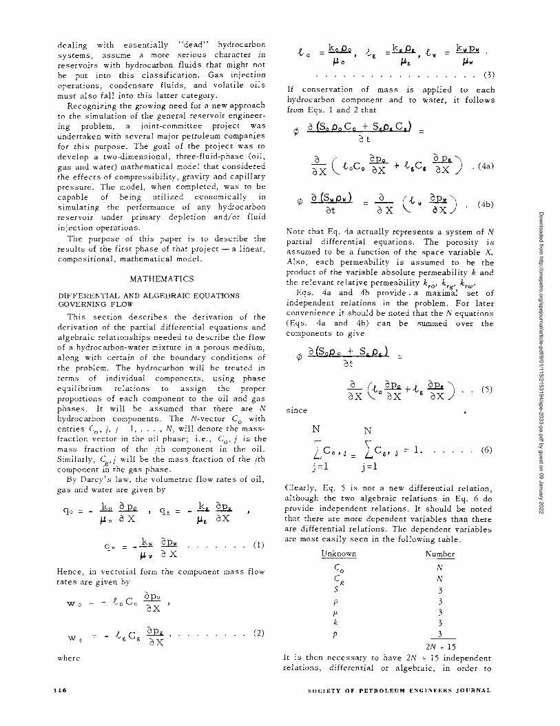
This section describes the derivation of the derivation of the partial differential equations and algebraic relationships needed to describe the flow of a hydrocarbon-water mixture in a porous medium, along with certain of the boundary conditions of the problem. The hydrocarbon will be treated in terms of individual components, us 109 phase equilibrium relations to assign the proper proportions of each component to the oil and gas phases. It will be assumed that there are N hydrocarbon components. The N-vector Co with entries Co, j, j = 1, ... , N, will denote the massfraction vector in the oil phase; i. e., Co' j is the mass fraction of the jth component in the oil. Similarly, C ,j will be the mass fraction of the jth component i~ the gas phase.

By Darcy's law, the volumetric flow rates of oil, gas and water are given by

(1)

Hence, in vectorial form the component mass flow rates are given by

~ Wo = - -toC o aX

Wg , ....... . (2)

where

116

If conservation of mass hydrocarbon component and from Eqs. 1 and 2 that

p =~ 'VII

(3)

IS applied to each to water, it follows

¢ o (Sg Q.g C g + S,Q., C,) at

a ( -toC o ~ ~)

aX aX + -tsC, aX ; . (4a)

¢ o (Sli Q.w} 0 (-t II 2.llit \ ot oX ax) ( 4b)

Note that Eq. 4a actually represents a system of N partial differential equations. The porosity is assumed to be a function of the space variable X. Also, each permeability is assumed to be the product of the variable absolute permeability k and the relevant relative permeability kro' k

rg, krw '

Eqs. 4a and 4b provide. a maximal set of independent relations in the problem. For later convenience it should be noted that the N equations (Eqs. 4a and 4b) can be summed over the components to gIve

¢ 0 (SoQ. 0 + Sg Q.g } ot

.-L (-t ~ +-t ~) (5) oX ~ 0 oX g oX SInce

N N

L Co, J ~ C g , l. (6) =

j =1 j =1

Clearly, Eq. 5 is not a new differential relation, although the two algebraic relations in Eq. 6 do provide independent relations. It should be noted that there are more dependent variables than there are differential relations. The dependent variables are most easily seen in the following table.

Unknown Number

Co N

Cg N S 3 p 3 f.1 3 k 3 P 3

2N + 15 It is then necessary to have 2N + 15 independent relations, differential or algebraic, in order to

SOCIETY OF PETROLEUM E:-iGI:-iEERS JOURNAL

Dow


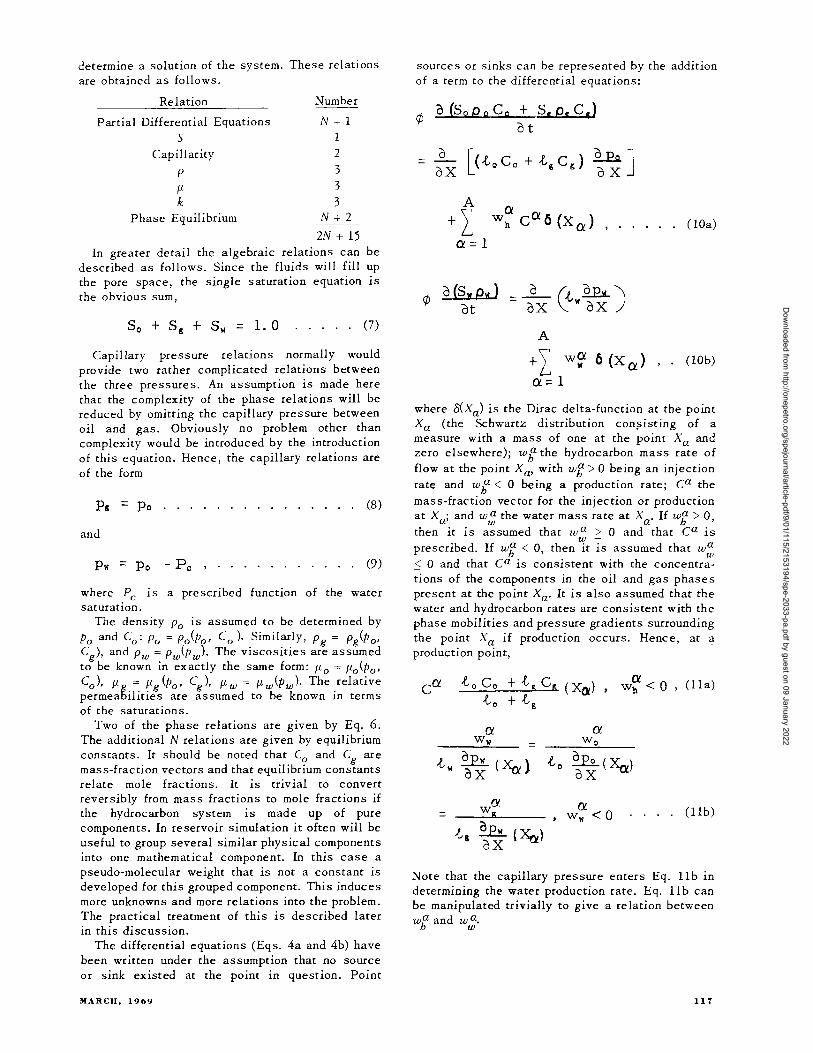
determine a solution of the system. These relations are obtained as follows.

Relation

Partial Differential Equations 5

Capillarity

P fl k

Phase Equilibrium

Number

N+I 1 2 3 3 3

N+2

2N + 15 In greater detail the algebraic relations can be

described as follows. Since the fluids will fill up the pore space, the single saturation equation is the obvious sum,

. (7)

Capillary pressure relations normally would provide two rather complicated relations between the three pressures. An assumption is made here that the complexity of the phase relations will be reduced by omitting the capillary pressure between oil and gas. Obviously no problem other than complexity would be introduced by the introduction of this equation. Hence, the capillary relations are of the form

pg = po (8)

and

Pw = Po - Pc ' ....... . (9)

where Pc is a prescribed function of the water saturation.

The density Po is assumed to be determined by Po and Co: Po = Po(Po' Co), Similarly, Pg = Pg(Po, Cg ), and Pw = Pw(p), The viscosities are assumed to be known in exactly the same form: flo = flo(Po' Co), fl = flg(Po' Cg ), flw = flw(P w)' The relative permea~ilities are assumed to be known in terms of the saturations.

Two of the phase relations are given by Eq. 6. The additional N relations are given by equilibrium constants. It should be noted that Co and Cg are mass-fraction vect.ors and that equilibrium constants relate mole fractions. It is trivial to convert reversibly from mass fractions to mole fractions if the hydrocarbon system is made up of pure components. In reservoir simulation it often will be useful to group several similar physical components into one mathematical component. In this case a pseudo-molecular weight that is not a constant is developed for this grouped component. This induces more unknowns and more relations into the problem. The practical treatment of this is described later in this discussion.

The differential equations (Eqs. 4a and 4b) have been written under the assumption that no source or sink existed at the point in question. Point

MARCH, 1969

sources or sinks can be represented by the addition of a term to the differential equations:

1; 0 (Sopp C Q + S, p. C I )

at

= :X [(toCo + t,c g ) ~~ J

Ci=l

Ci W CCi 0 (x ) h Ci, . . . . . ( lOa)

__ 0 (t £EL) oX ~ 'II ax

A

+ I w~ 0 (XCi) , . (lOb)

Ci=l

where o(Xa) is the Dirac delta-function at the point Xa (the Schwartz distribution con?isting of a measure with a mass of one at the point Xa and zero elsewhere); w{; the hydrocarbon mass rate of flow at the point Xa , with w{; > 0 being an injection rate and wh

a < 0 being a production rate; ca the mass-fraction vector for the injection or production at Xa; and w:; the water mass rate at Xa' If wg > 0, then it is assumed that w a > 0 and that ca is w -prescribed. If wg < 0, then it is assumed that w~ ~ 0 and that ca is consistent with the concentrations of the components in the oil and gas phases present at the point Xa' It is also assumed that the water and hydrocarbon rates are consistent with the phase mobilities and pressure gradients surrounding the point Xa if production occurs. Hence, at a production point,

ex. Wh <0, (lIa)

=

tw ~ (XIV) aX .....

= . . . . (lIb)

Note that the capillary pressure enters Eq. llb in determining the water production rate. Eq. llb can be manipulated trivially to give a re lation between w{; and w:;.

117

Dow


ry = _________ VV~h~ ______ _

+t )~(X) g ax CL

vv~ and vvC; ~ 0 .......... (12)

This completes the treatment of the differential equations and algebraic relationships at an interior point of the region.

DIFFERENTIAL AND ALGEBRAIC EQUATION AT BOUNDARIES

Two types of boundary conditions will be considered here. The first condition is the one that results from the specification of a rate. Again, it will be necessary to distinguish between injection and production.

In the case of injection the boundary condition can be written in the form

. . . . . . . . (13)

where wh' Ww ~ 0, left-hand end

wh' U w S 0, right-hand end

and wh' C and U w are ~ll specified. In the case of production, Eq. 13 holds, but C is not specified. Again, in order to preserve consistency, C, u'h and Ww should be related through Eqs. 11 and 12.

If the pressure Po is specified at an end of the region, this pressure induce s a flow of the fluids within the region. If this pressure at some given time is sufficiently large, then injection is called for. Under this condition it is again necessary to specify what fluid is available to be injected and to require that internal consistency hold as far as possible. Under these conditions it is obvious that exactly one fluid would be in jected at a rate leading to the desired pressure. If, on the other hand, the specified pressure leads to production, then C, wh' Ww should be chosen in accordance with the rules specified in Eqs. 11, 12 and 13, so that the withdrawal produces the desired pressure. Note that in both cases the specification of pressure results in a unique value for flow rate.

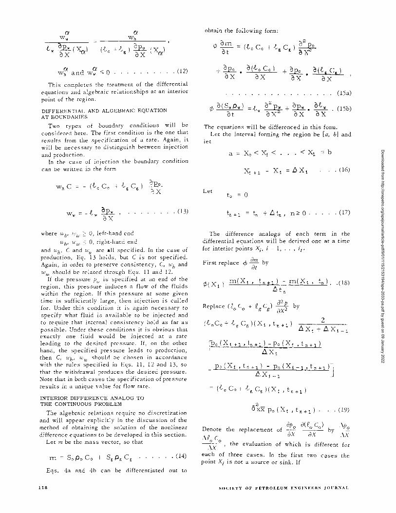
INTERIOR DIFFERENCE ANALOG TO THE CONTINUOUS PROBLEM

The algebraic relations require no discretization and will appear explicitly in the discussion of the method of obtaining the solution of the nonlinear difference equations to be developed in this section.

Let m be the mass vector, so that

. . . . (14)

Eqs. 4a and 4b can be differentiated out to

obtain the following form:

¢om at

+ ~. otto Co)

oX ax

. . . . . . . . (15a)

02 p2_ +~. at ... (15b) AX AX AX

The equations will be differenced in this form. Let the interval forming the region be [a, b] and

let

a = Xo < XI <. . < Xl = b

Let to = 0

tn + 1 = tn + t:. tn, n ~ O· . . . . (17)

The difference analogs of each term in the differential equations will be derived one at a time for interior points Xi, i = 1, .. , it.

First replace ¢ am by at

¢(XI

) m(XI' t n + l ) - m(XI , t n ) •• (18)

.6 t n

Replace (£0 C + £ Cg ) a2 P2 by

a g ax 2

iPo (X I + 1 , tn + 1 ) - Po ( X I , t n + 1 )

, .6. XI

po (X! , t~. + 1) - po (X I - 1 , t n + 1 ) Ji ~XI -1

2 o xx Po ( XI, t n + 1) . (19)

D h apo a(£o Co)\Po

enote t e replacement of - by ax ax .\X

,HoC ~X a , the evaluation of which is different for

each of three cases. In the first two C<;lses the point Xi is not a source or sink. If

118 SOCIETY OF PETROLEUM E,(GI,(EERS JorR,(AL

Dow


and Po (Xi, t n) - po (X i - 1 , t n » 0, . (20)

then

~ AtgC a ) Ax Ax (Xi ,tn+l

=hlX,tJ tnt,)-po(X"t nt ,). AX i

toC o (Xi t 1 , tn +1) -toco (Xi' t n +1 )

AX i

= Y r (X 1 , t n + 1) . . . . . . . . (21)

If

po (X 1 t 1 , t n) - Po (X i , t n ) < ° and

then

= Po (Xi' t n +l.) -Po ( X n -1 ' t n +l)

A X i - 1

toc o (Xi' tn+d -toco (Xi -1' t n + 1 )

A Xi -1

. . . (23)

If the point Xi is a source or sink, then

~ AtoC p (X t ) Ax AX i , n +1

. . (24)

apo aEgCg 6.Po 6.Eg Cg The replacement of ax ----ax by 6.x 6.x is made in a similar fashion, again basing the decision on oil pressure differences. Thus, the original system of N finite difference equations analogous to Eqs. lOa and 15a is

MARCH, 1969

<5 ~x po ( Xi, t n + 1 )

Apo AtoCo(X t ) + t::.x Ax i, nt1

+ A po At. C g (X t ) Ax Ax 1, ntl

. . (25)

where wh(Xi , tn +1) is the hydrocarbon mass flow rate and C(Xi • tn+1 ) is the mass fraction vector at the source or sink at Xi' (If no source or sink exists at Xi' 1l1J (Xi' tn+l) = 0.) In accordance with the results of the last section, wh(Xi , tn+1 ) > 0 corresponds to injection at Xi and C(Xi • tn+1 ) must be known. If 1l1J (Xi' tn+l) <0, production takes place at Xi and C (Xi' tn+1 ) must be determined by Eq.

lla with Xa = Xi' The water equations are discretized in the same

fashion. If

Pw ( Xi t 1 , t n) - Pw ( X 1 , t n ) > ° and

then

Dpw ~t w (X t ) A AX i,nt1 QX t..!

= Pw (X i t 1 , t n + 1) - Pw (X i , t n + 1 )

,6. X 1

t W (X 1 + l' t n +1 ) - t w(X i , t nt1 ) t:. Xi

= y~ (Xi' t nt1 ) .......... (27)

If

and

then

119

Dow


= p" (X i , t n + 1) - p" (X 1 - 1 , t n + 1) •

UX 1 - 1

t,,(X 1 ,t n +d - t,,(X 1 - 1 ,t n +d

LlX i - 1

. . . . . . . . . . (29)

and

~p" ~" (X ~X II X 1 , t n + 1 )

Y~ ( X 1 , t n + 1 ) ]

. . . (30)

The difference equation for water then takes the general form

S"P,,(X 1 ,t n + 1 ) - S"p,,(X 1 ,t n ) = 6t n

IIp,, llt" (X + llx Ax ·1 ,t n + 1 ) + W,,(X 1 ,t n + 1 ),

....... (31)

where ww(Xi , t n+1) must satisfy Eq. 12 for consistency, should it be less than zero.

The sy stem of N + 1 difference equations given by Eqs. 25 and 31 and, where applicable, Eqs. 11 and 12 is the discrete version of the differential system at the interior grid points.

BOUNDARY DIFFERENCE ANALOG TO THE CONTINUOUS PROBLEM

In order to complete the specification of the discrete. problem, it is necessary to reduce the boundary conditions to discrete form. It has been found convenient to consider separately the case of no flow across a boundary, although it is perfectly feasible to use the general case to follow with wh = Ww = O.

If wh = Ww = 0 in Eq. 13 at an endpoint, then Eqs. 15a and I5b reduce to

¢ om = (to Co + t C ) 02

Po ot g g ~ = 0

¢ o(SwP,,) = t" ~ ot OX2 '

. (32)

a2po a2pw The replacement of the and -- can be

ax2 ax2 facilitated by symmetry; i.e., the entire problem

120

can be reflected across the boundary and the value of any variable at a specified distance outside the original domain can be taken equal to its value at the point inside the domain at the same distance from the boundary. Hence, the discrete form of Eq. 32 is either

¢(Xi ) m(X 1 ,tn +1) - m(X1 ,t n ) = At n

(t C + t C ) ( X t ) 2 [po (X 1 + 1 , t n + 1 ) o 0 II II 1, n + 1 (.6 X 1 )2

_ po ( X 1 , t n + 1 ) ]

(l:. Xi )2

¢(X1

)(S"P,,)(X 1 ,t n + 1 ) - (SwPw)(X 1 ,t n )

.6t n

= t w (X 1 ,t n + 1 ) •

2 [p" (X 1 + 1 , t n + 1) - ~w (X 1 , t n + 1 ) ]

(AX1 ) . . . . . . . . . . . . . . . . . . (33)

if Xi corresponds to the left-hand endpoint of the region and wh = Ww = 0, or

2 [po (X 1 - 1 ,t n + 1 )

(Do Xi -1 )2

if Xi corresponds to the right-hand endpoint.

. (34)

If either wh or Ww in Eq. 13 is not zero, then it is preferable to develop a discrete analog of Eq. 4 rather than Eqs. 15a and I5b at the boundary. An "upstream" evaluation of the coefficients eo Co, eg C and ew has proved to give the best results. Let lJ.:i correspond to the left-hand endpoint for the moment. Then consider the half interval from Xi to to Xi-tlh" The flow rate across the right boundary at Xi-tlf, into the half interval is approximated by

po (X 1 + 1 , t n + 1 ) - po (X 1 , t n + 1 )

AX 1

where

SOCIETY OF PETROLEUM ENGINEERS JOURNAL

Dow


I X I + l' if po ( X I + 1 ' t n) -po ( X I , t n ) ;,00

l X \ , if po (X 1+ 1 , t n) -po (X \ , t n ) <0

I X I +1 ' if P.(X\+l' tn) -P.(X\, tn);,oO

= L X \ , if p. (X 1+1' t n) -p w (X I , t n) < 0

(36)

The flow rate across the left-hand boundary at the point Xi into the half interval is given by Wh C and w

W' where C is known in the case of injection

(wh > 0) and satisfies Eq. lla with Xa = Xi in the case of production. Thus, a material balance gives the following boundary relations at the left-hand endpoint.

Z ih.~...i...t,C,)(Xr,I,+,)(p,(X'±l,t .... ....L-PQ(x, .I .• ,)J (AX, )'

+ ZAX, (WhC)(X" I n +,). (AX, )<

_(",S":"r:..:P',-,)C-'(.ccX:...c'-'.' I H ,) - (S,p,)(x,. I,) ¢ (x,) At,

+ ZAX,w, (X,. t'_+1) (AX, )2

, . . . . .... (37)

with Eq. lla satisfied by (wh < 0). Similarly, if Xi is the right-hand endpoint of

the region,

( ) m(X,. I H1 ) - m(X,. In) _

¢ X, Aln -

(t,C,+t,C,)(X,. I n+1 )Lp,(X,-,. tn+1 )-p,(x,. IH,)J z (AX,_,)'

z~t~,~(~~~.~12,~+~,~)[~p~,~(~X~,~_~,~._I~,~+,~)~-~p~,~(_X~,~._I~'~+l~) __ J (AX, _,)"

+ zAx, ,w,(X,.l rt ,) , ••••••• (38) (A x,_,)"

THE IMPLICIT ITERATION, RESOLUTION OF THE DISCRETE ANALOG

The total discrete analog of the continuous problem consists of the finite difference equations for interior points in the section dealing with the interior difference analog, the appropriate discrete boundary conditions at each endpoint from the previous section, the algebraic relations from the first section, and the specification of the initial conditions of the system. It is assumed that the pressures, saturations and mass fraction vectors at each point are consistent (both for the diffe.ential and difference systems) with the component unit masses and the water unit mass specified at the point.

A general flow chart of the computational procedure for each time step is provided in Fig. 1. Basically, this procedure consists of the following steps:

1. initialization 2. inner iteration through the phase package 3. test for convergence 4. modified Newtonian iteration 5. evaluation of coefficients in the difference

equations 6. incrementation of the time step. Step 2 is quite complicated and is explained in

the following section. Steps 3 and 6 are selfexplanatory, except for the choice of E, the convergence tolerance. In practice, it has been found satisfactory to use a choice of the form

pq-(Xi. tnt')

Sq(Xi. tnt')

Cq(X,. tnt')

INITIALIZATION

EstImate

a!l values of i.

CD m(X,.tntil.

(SwPw)(Xi. tnt')

where @ q ~ 2 is Maxi

{

XI , if po (X \ , t n) -po (X \ -1 ' t n );,00

XI-I' ifpo(X\. tn) -PO(X\-l' tn)<O I

:', :,i: ~::~; ~:: 1t:~ ._~~: ::_t:.1t"'01<0 j

I

. . . . . . . (39)

MARCH, 1969

STEP

®TIME

INTERVAL

@ MODIFIED

NEWTONIAN

ITERATION

@ EVALUATE

mq+I{Xj. tn+ll

(SwPwlqt'(Xi. tnt,l

FIG. 1 - THE COMPUTATIONAL PROCEDURE.

121

Dow


In Step 5 the coefficients used in the difference equations are evaluated by using the values of the saturation and mass fraction vectors after the last complete iteration; i. e., from Step 2 and Po q, with

q+~ pw

q +~ =p "2_p o c

where Poq-tlh comes from Step 4, as discussed below. m q+1(X i ,tn+1 ) is calculated using these coefficients, and the pressure differences employed in the difference relations are computed from the values of Poq-tlh and PWq -tl/2. For example, Eq. 25 becomes

~ /X 1) [( toe 0 + t & C 1\ ) q ( X 1 , t n + 1 )

+ [ A po q +i AX

+ A q+~

po

Ax

. . . . . . . . . . . . . . . . . (41)

The type of difference used for !'I.Po / fl.X and fI.(£ C)/ fl.x is chosen according to the rules specified under the third section of the mathematic s portion of this paper, with the decision made on the basis of old time values; Cq(Xi , tn+l) should be made consistent to Eq. lla if necessary. Eq. 31, for water, is modified in an analogous manner.

If the portion of the iteration in Step 4 is deleted (by setting P q+v, = pq), the resulting iteration is exactly successive substitution. Experience with this procedure resulted in the observation that successive substitution converges quite well for small time steps but fails for time steps that would appear practical for the difference equations. A modest simplification of the difference equations leads to the proof that a sufficient condition for convergence of this iteration is that fl.tn /(min i fl.Xi )2 be sufficiently small. This agreed with observed results. Note that, in this case, fl.X i is interpreted as the ratio of fl.X i to the length of the region. Division by (fl.Xi )2 decreases the usable time step.

In order to preclude limitations of this type an iteration procedure, motivated by a Newtonian iteration for a more simplified equation, was inserted into the successive substitution procedure. Consider a difference equation of the form

122

£(p(X 1 , tn+ 3,» -£(p(X t , t n » At

. . . . . . . (42)

with boundary values of p specified. The function f is known and is a scalar function of a single variable such that dfl dp is positive. Then, the system of nonlinear algebraic equations that must be solved at each time step can be written in the vector form

F(p)=O, .. . . . . . (43)

where the components of the vector F are given by

F1 (p) = £1\ £(Pi) - 6~XP1 -q1 ,

q i = ~t £( P ( X 1 , t n » . . (44)

The standard Newtonian iteration for this system is given by the solution of the following linear

system.

;t ( p 1 q) + * (p 1 q + l -p 1 q) }

_ 0 ~ P 1 q + 1 -q 1 = 0 . . . . . .. (45)

or

{ 1 d£ (p q) _ 01cx} p 1 q +1 = At dp

Re-evaluation of the derivative dfl dp after each iteration is not always convenient, rather, it is often evaluated once at the beginning of the iteration and held fixed thereafter. In particular, a modification of the Newtonian process, which is more readily fitted into the much more complicated system arising from Eqs. 25 and 31, is given by

It has been found convenient to evaluate dfl dp numerically as follows.

~! [p(X1 , tn ) ]

£ [p(X1 , t n) ] -£ [p(X1 • tn -l ) J. . (48)

p(X1 • t n) - p(X1 • tn- l)


Dow


It can be shown that the iteration (Eq. 47) is convergent for sufficiently small i'J.tn- Note also that the (i'J.Xi )-2 term has disappeared. In practice the constraint for convergence usually allows any length of time step that is reasonable for other purposes.

In order to make use of this modified Newtonian iteration, it is necessary to find a single scalar equation satisfied by Po, taking as much of the other pertinent information into account as possible. Since the sum of the components in vector Co and Cg is one, the difference relations (Eq. 25) may be summed over the components to give

¢(xd (SoPo+ S.P.) (Xi' t n + 1 ) - (So po + S. P.) (XI. t n) Atn

+ % At 0 (x t ) + ~ At. (XI. tn +1 ) Ax Ax I' n+1 AX AX

. (49)

This equation may be added to the water equation

(Eq. 31) to give

¢(Xi ) m(Xi • tn +1) -m(Xi • tn) Atn

=

+ ~ Ato (X t ) +~ At, A X Ax 1. n + 1 AX AX

(Xi' tn +1 )

+(~ - APc \ At\! (X t ) Ax AX) A Xi' n +1

, . (50)

where

m = So po + Sg pg + Sw Pw ..... (51)

Due to oil-water capillary pressure, Po can be differenced differently in the water term than in the oil and gas terms. Eq. 40 will apply to each interior point. Since the only boundary condition being treated at this time is a specified-rate condition, equations similar to Eq. 50 developed for those difference equations in the third section of the mathematics discussion result at the boundaries. For example, the system given by Eq. 37 reduces to

MARCH, 1969

!?o(X1 ± ) • t n ±, ) - Pc (X1 • tn ± , )

AXi2

• 2

+ 2(AXi f 1[ wdxi • tn +J+ww(X1 • tn+J]

, . . . . . . . . (52)

where Xi corresponds to the left-hand endpoint, ~d lu:.hl + IWwl > O. Note that it is possible that

Xi -f- Xi' Since m is a function of many variables other

than Po, the derivative dml dp is not a definable quantity. The following relation has been found satisfactory.

dm ( )dp Xi. tn = I (So po) (Xi • t n ) - (So po) (Xi • t n- 1) f

Po (Xi' tn) - Po(Xi • tn -1)

+ I (SI; P!i) (Xi' tn)-(Sg pg) (Xi. tn-J Po (Xi' tn) - Po (Xt • t n- 1)

+ I (Swpw)(Xi • t n)- (SwPw) (Xi. t n- 1 ) I Po (Xi' tn) - po (Xi' tn -1) i

. . . . . . . . . . . . . . . . . . (53)

The iteration called for in Step 4 is then defined as

¢ (Xi )mq (Xi' tn +1) Atn

+ [dm q + ~ I dp (Xi. t" ) [ Po 2 (Xi • tnt 1 )

-TJ~ q (Xf • t~~ . .; [AtJ -'

= (tQ +t g +tW )q(Xi J t n+1 )

2_ q+t( ) o XX Po Xi • tn + 1

- t wq

(Xi J tn +1) 02xX P cq(Xi , tn+!)

123

Dow


A q +i + UPO b.X

~ b. q +~

+ PO b.X

b.t,q (X t ) b.x 1 n+l

q q _ b.P g

) ~ (X A X b.X 1

for Xi' an interior point of the grid. There is a corresponding equation for Xi being an endpoint. Eq. 52 becomes

¢ (Xl) mq(X, t tnt,) Atn

+ 2 (A Xl r 1 [ Wh (X 1 t t n + 1) - W w ( X 1 , t n + 1) J .

. . (55)

The superscript q in the foregoing material indicates that the function (or variable) is to be evaluated using the values obtained in the most recent computation of Step 2. The equations generated by Eqs. 54 and 55 or by some other boundary relations form a linear algebraic system. In fact, the system over the entire region is tridiagonal and can be solved by Gaussian elimination. These "half iterate" pressure values are then used as input to Step 5, along with the values obtained from Step 2 as indicated previously. The water pressure Pw q+'h is given by

+" ~ Pwq t=p~q+2_Pc(Swq).

This entire iteration, combining this strongly modified Newtonian iteration successive substitution is not one that has

very with been

treated in standard texts; it ITaS, however, proved satisfactory in practice if the over-all iteration is begun from reasonably good values. Step 1 is used to produce these values.

It is possible to extrapolate virtually any combination of saturation, pressure, and mass

1%4

fractions; however, it has been found in practice that it is much more efficient to extrapolate m(Xj ,

tn+1 ) and then to enter the explicit iteration at Step 2. This is done for n ? 1 by taking

+_A_t-=n_ [rn(X 1 , t n) -rn(X 1 , t n-1)]

At n -),

. (56)

for all values of I. For n = 0, choosing a small time step and using

has been successful. The number of iterations has been determined by two factors. One is, of course, the size of the time step. The other is whether or not some critical saturation, such as the bubble (or dew) point is crossed at some point in the region during the time step. The effect of this second factor is much more noticeable if something other than m is extrapolated for starting values.

EXPLICIT OR PHASE ITERATION

Let us suppose estimates of oil pressures as outlined above have been obtained. These estimates will fail to be consistent with the earlier estimates of the other physical parameters until the convergence of the iterative solution of the problem has been achieved. Thus, it is necessary to establish a complete consistent set of physical parameters.

The first step is to estimate the product (SwPw) by means of Eq. 31. Although this must be estimated separately for each node, subscripting indicative of nodes is omitted in this section since each node is handled similarly and independently.

Next, Eq. 25 is used to estimate the vector m of component masses.

At this point, the variable molecular we ight of the heaviest hydrocarbon component must be taken into account. The average molecular weight of the heaviest component is estimated (if not designated) by the ratio of its component mass to the total number of moles of the heaviest component, where this total number of moles is estimated by an equation representing molal flow by analogy with Eq. 56.

At this point, the total moles in the node is calculated by the formula

N n = ~ rn j / M j . . . . . . . . . . (58)

J = 1

Then, the mole fraction of each component may be calculated by

Z J = rn J / (n M j) . . . . . . . . (59)

As it shall be seen, the variables calculated above may be inconsistent with the pressures estimated. The nodal oil pressure will be adjusted

SOCIETY OF PETROLEUM E:\"GINEERS JOURNAl.

Dow


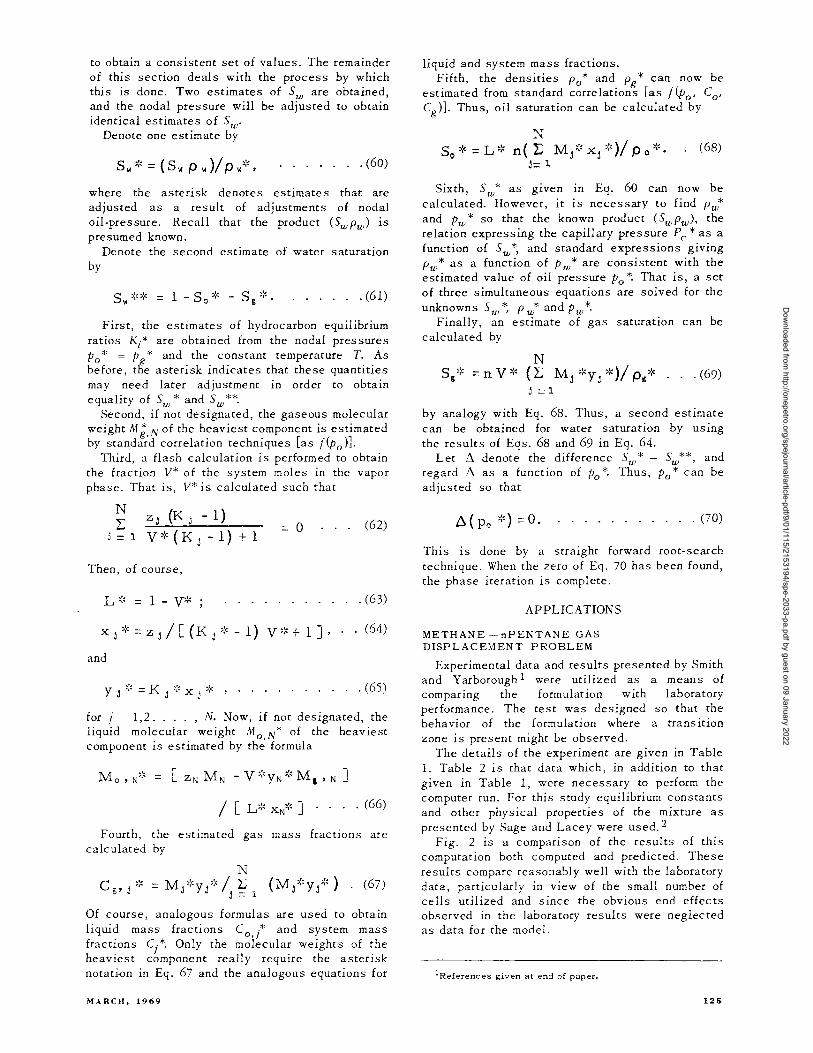
to obtain a consistent set of values. The remainder of this section deals with the process by which this is done. Two estimates of Sw are obtained, and the nodal pressure will be adjusted to obtain identical estimates of Sw'

Denote one estimate by

. . . . . . . (60)

where the asterisk denotes estimate s that are adjusted as a result of adjustments of nodal oil-pressure. Recall that the product (SwPw) is presumed known.

Denote the second estimate of water saturation by

. . . . . . (61)

First, the estimates of hydrocarbon equilibrium ratios Ki* are obtained from the nodal pressures Po * = Pg * and the constant temperature T. As before, tfie asterisk indicates that these quantities may need later adjustment in order to obtain equality of Sw * and Sw **.

Second, if not designated, the gaseous molecular weight M;.N of the heaviest component is estimated by standard correlation techniques [as t(po )].

Third, a flash calculation is performed to obtain the fraction V* of the system moles in the vapor phase. That is, V* is calculated such that

N L

j = 1 V':«K j -1)+1

Then, of course,

o (62)

. (63)

x j ':< = Z j / [(K j ':< - 1) V':< + 1], . (64)

and

. . . . . . . (65)

for j = 1,2 .... , N. Now, if not designated, the liquid molecular weight Mo.N* of the heaviest component is estimated by the formula

. (66)

Fourth, the estimated gas mass fractions are calculated by

N C ':< = M ':<y ':< / L (Mj':<Yj':<)· (67) pj j j j=l

Of course, analogous formulas are used to obtain liquid mass fractions Co.t and system mass fractions C/o Only the molecular weights of the heaviest component really require the asterisk notation in Eq. 67 and the analogous equations for

MARCH, 1969

liquid and system mass fractions. Fifth, the densities Po * and Pg * can now be

estimated from standard correlations [as t(po' Co. Cg )]. Thus, oil saturation can be calculated by

N So"'< = L ':< n(!: M/:< Xj ,:<)/ P 0 *. (68)

.1= 1

Sixth, Sw * as gIven In Eq. 60 can now be calculated. However, it is necessary to find Pw*

and Pw * so that the known product (SwPw )' the relation expressing the capillary pressure Pc * as a function of Sw *, and standard expressions giving Pw * as a function of P w * are consistent with the estimated value of oil pressure Po *. That is, a set of three simultaneous equations are solved for the

unkilOwns Sw ~ P w* and Pw *. Finally, an estimate of gas saturation can be

calculated by

N Sg':< = n V ':< (!: M j ':<y j ,:<)/ Pg':< . . . (69)

.1 = 1

by analogy with Eq. 68. Thus, a second estimate can be obtained for water saturation by using the results of Eqs. 68 and 69 in Eq. 64.

Let L'. denote the difference Sw * - Sw**' and regard L'. as a function of Po *. Thus, Po * can be adjusted so that

. . . . . . . (70)

This is done by a straight forward root-search technique. When the zero of Eq. 70 has been found, the phase iteration is complete .

APPLICA TrONS

METHANE -nPENTANE GAS DISPLACEMENT PROBLEM

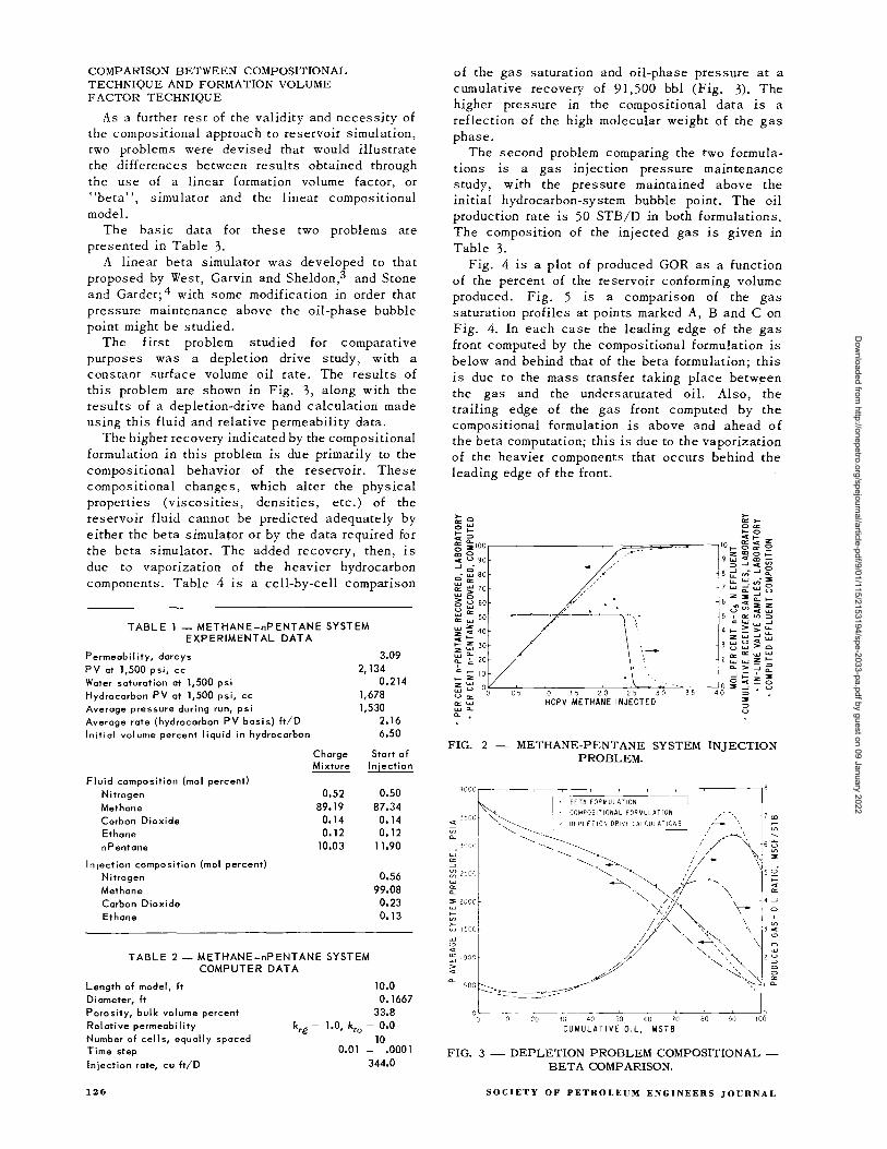
Experimental data and results presented by Smith and Yarborough 1 were utilized as a means of comparing the formulation with laboratory performance. The test was designed so that the behavior of the formulation where a transition zone is present might be observed.

The details of the experiment are given in Table 1. Table 2 is that data which, in addition to that given in Table 1, were necessary to perform the computer run. For this study equilibrium constants and other physical properties of the mixture as presented by Sage and Lacey were used. 2

Fig. 2 is a comparison of the results of this computation both computed and predicted. These results compare reasonably well with the laboratory data, particularly in view of the small number of cells utilized and since the obvious end effects observed in the laboratory results were neglected as data for the model.

lReferences given at end of paper.

125

Dow


COMPARISON BETWEEN COMPOSITIONAL TECHNIQUE AND FORMATION VOLUME F ACTOR TECHNIQUE

As a further test of the validity and necessity of the compositional approach to reservoir simulation, two problems were devised that would illustrate the differences between results obtained through the use of a linear formation volume factor, or "beta", simulator and the linear compositional model.

The basic data for these two problems are presented in Table 3.

A linear beta simulator was developed to that proposed by West, Garvin and Sheldon,3 and Stone and Garder; 4 with some modification in order that pressure maintenance above the oil-phase bubble point might be studied.

The first problem studied for comparative purposes was a depletion drive study, with a constant surface volume oil rate. The results of this problem are shown in Fig. 3, along with the results of a depletion-drive hand calculation made using this fluid and relative permeability data.

The higher recovery indicated by the compositional formulation in this problem is due primarily to the compositional behavior of the reservoir. These compositional changes, which alter the physical properties (viscosities, densities, etc.) of the reservoir fluid cannot be predicted adequately by either the beta simulator or by the data required for the beta simulator. The added recovery, then, is due to vaporization of the heavier hydrocarbon components. Table 4 IS a cell-by-cell comparison

TABLE 1 - METHANE-nPENTANE SYSTEM EXPERIMENTAL DATA

Permeability, darcys PV at 1,500 psi, cc Water saturation at 1,500 psi Hydrocarbon PV at 1,500 psi, cc Average pressure during run, psi

Average rate (hydrocarbon PV basis) ft/D Initial vol ume percent I iquid in hydrocarbon

Fluid composition (mol percent) Nitrogen Methane Carbon Dioxide Ethane nPentane

Injection composition (mol percent) Nitrogen Methane Carbon Dioxide Ethane

Charge Mixture

0.52 89.19

0.14 0.12

10.03

3.09 2,134

0.214 1,678 1,530

2.16 6.50

Start of In jection

0.50 87.34

0.14 0.12

11.90

0.56 99.08

0.23 0.13

TABLE 2 - METHANE-nPENTANE SYSTEM COMPUTER DATA

Length of model, ft Diameter, ft Porosity, bulk volume percent Relative permeability Number of cells, equally spaced Time step Injection rate, cu ft/D

126

10.0 0.1667

33.8 k,g = 1.0, k,o = 0.0

10 0.01 - .0001

344.0

of the gas saturation and oil-phase pressure at a cumulative recovery of 91,500 bbl (Fig. 3). The higher pres sure in the compositional data is a reflection of the high molecular weight of the gas phase.

The second problem comparing the two formulations is a gas lllJection pressure maintenance study, with the pressure maintained above the initial hydrocarbon-system bubble point. The oil production rate is 50 STB/D in both formulations. The composition of the injected gas is given in Table 3.

Fig. 4 is a plot of produced GOR as a function of the percent of the reservoir conforming volume produced. Fig. 5 is a comparison of the gas saturation profiles at points marked A, Band C on Fig. 4. In each case the leading edge of the gas front computed by the compositional formulation is below and behind that of the beta formulation; this is due to the mass transfer taking place between the gas and the undersaturated oil. Also, the trailing edge of the gas front computed by the compositional formulation is above and ahead of the beta computation; this is due to the vaporization of the heavier components that occurs behind the leading edge of the front.

FIG. 2 - METHANE-PENTANE SYSTEM INJECTION PROBLEM.

FIG. 3 - DEPLETION PROBLEM COMPOSITIONALBETA COMPARISON.


Dow


TABLE 3 - BASIC DATA, COMPOSITIONAL - FORMATION VOLUME FACTOR COMPARISON A. Fluid Data

Differential Differential Gas 0,[

Pressure Oil ShrInkage Gas FVF Oil Density Gas Density Solution GOR VISCOSIty Vi scoslty

2sIa VrLV* serbt. 3 LbLn. 3 LbL Ft. 3 SerLBbl C~ c~

3800 .5917 207.6 38.95 12.04 1098 .0253 .226

3400 .6251 189.0 40.09 10.79 932 .0231 .269

3000 .6532 168.7 41.00 9. 51 796 0210 .309

2600 .6776 147.2 41. 76 8.21 681 .0193 .346

2200 .6996 124.7 42.42 6.90 580 .0177 381

1800 .7200 101. 5 43.01 5.61 489 .0165 414

1400 .7396 78. 43.56 4.34 405 .0155 446

1000 . 7593 54. 44.10 3 . 12 323 .0148 .477

600 . 7809 32. 18 44.65 1. 95 240 .0142 .508

200 8129 10.31 45.37 o. 80 142 0134 . 552

15 .9158

* Vr/V = Volume '7Q residual oil at 60°F per volume % reservoir oil at indicated pressure and 240°F

Reservoir Temperature - 240°F

Bubble Point Pressure - 3800 psi Relative Permeabiltty (Krw = O. 0)

Surface Separation at 115 psia and 85°F ~ ~ Kro

Tank at 14.7 psia and 85°F o. .0 .9744

O. 04 .0 .7578 Total

Oil Surface o. OB .0 5977 Pressure Shrinkage GOR

~ STBiRe. B. SCFLSTB o. 12 .00354 .4784

3800 .6539 884 O. 16 01074 388 I

3400 .6901 741 O. 20 .02302 .3174

3000 .7190 622 0.24 .4101 .2598

2600 .7443 521 0.2B .6464 .2107

2200 .7672 431 0.36 1264 . 1292

1800 .7885 350 0.44 . 201 B .06595

1400 .80BB 274 0.52 . 2861 .02504

1000 .8292 201 0.70 5510 .004701

600 .8505 128

C. Compositional Data

B. PhYSical Properties 10- Place Fluid Component

Width, Ft. 2000. Methane .4898

Porosity 0.20 Ethane .0490

Permeability, rod. 40. Propane .0360

Height, Ft. 10. lBo-and Nlrmal- Butanes .0320

Water Saturation 0.169 tso-and NOrInal- Pentanes .0320

Total Reservoir Length, Ft. 1000. Hexane .0338

Number Cells 11. Heptane .0345

Cell Spacing. Ft. 100. Octane .0332

Producing Rate, Constant STB/D 50. N onanes + .2547

Molecular Weight Nonanes + 232.3

Injected Fluid

Methane .900

Ethane .040

Propane .02

tso-and normal Butanes .03

ulo-and normal Pentanes .01

MARCH, 1969 127

Dow


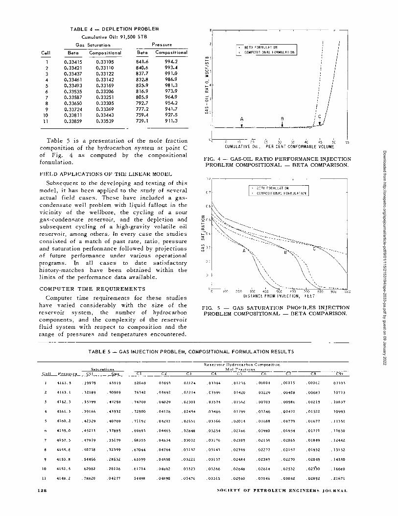
TABLE 4 - DEPLETION PROBLEM

Cumulative Oil: 91,500 STB

Gas Saturation Pressure

Cell Beta Compositional Beta Compositional

0.33415 0.33105 841.6 994.2 2 0.33421 0.33110 840.6 993.4 3 0.33437 0.33122 837.7 991.0 4 0.33461 0.33142 832.8 986.9 5 0.33493 0.33169 825.9 981.3 6 0.33535 0.33206 816.9 973.9 7 0.33587 0.33251 805.9 964.9 8 0.33650 0.33305 792.7 954.2 9 0.33724 0.33369 777.2 941.7

10 0.33811 0.33443 759.4 927.5 11 0.33859 0.33539 739.1 911.3

Table 5 is a presentation of the mole fraction composition of the hydrocarbon system at point C of Fig. 4 as computed by the compositional formulation.

FIELD APPLICATIONS OF THE LINEAR MODEL

Subsequent to the developing and testing of this mode I, it has been applied to the study of several actual field cases. These have included a gascondensate well problem with liquid fallout in the vicinity of the wellbore, the cycling of a sour gas-condensate reservoir, and the depletion and subsequent cycling of a high-gravity volatile oil reservoir, among others; In every case the studies consisted of a match of past rate, ratio, pressure and saturation performance followed by projections of future performance under various operational programs. In all cases to date satisfactory history-matches have been obtained within the limits of the performance data available.

COMPUTER TIME REQUIREMENTS

Computer time requirements for these studies have varied considerably with the size of the reservoir system, the number of hydrocarbon components, and the complexity of the reservoir fluid system with respect to composition and the range of pressures and temperatures encountered.

BETA FORMULATION I COMPOSITIONAL FORMULATION

"'6 ..... en -"-~5 ~ t 0

I ;:::4 « a: ...J oj , I , , en i ;:;1 I

A B :' c i o_,_,~._,_._._~J._.~_-,=.~J ...

O~5--~IO~--~'5~---1~O~~1~5--~3~O--~3'~5--~40~--~45~--5~O~~55

CUMULATIVE OIL, PER CENT CONFORMABLE VOLUME

FIG. 4 - GAS-OIL RATIO PERFORMANCE INJECTION PROBLEM COMPOSITIONAL -- BETA COMPARISON.

08

---~~ BETA FORMULATION

COMPOSITIONAL FORMULATION 07

FIG. 5 -- GAS SATURATION PROFILES INJECTION PROBLEM COMPOSITIONAL -- BETA COMPARISON.

TABLE 5 - GAS INJECTION PROBLEM, COMPOSITIONAL FORMULATION RESULTS

ReserVOir Hydrocarbon CompOSition Saturations Mol FractIOns

Cell Pressure Oil Gas cl C2 C3 C4 C" C6 C7 C8 C9+

41 b3. 5 .19979 .63119 .82069 03993 02124 .03394 .0123b .00004 .00015 . 000 b2 07103

41 b3. 1 .32189 . 50909 · 76742 .03992 .02214 . 03599 .01420 .00229 .00408 .00683 .10713

4162.3 .35799 .47298 .74769 .04029 .02301 .03574 .01582 .00703 .00986 .01219 .10837

4 4161.3 .39166 .43932 .72900 .04128 .02454 .. 03486 .01799 .01246 .01472 .01522 .10993

4160.2 .42329 .40769 .71192 .04283 .02651 .03366 .02014 .01b88 .01779 .01677 · 11351

4159.0 .45213 .37885 .69693 .04465 .02848 .03254 .02186 .01980 .01954 .01771 .11850

4157.5 .47919 .35179 .68355 .04634 .03012 .03176 .02309 .02158 .02065 .01849 · 1.2442

4155.8 . 50738 .32359 .67044 .04764 .03132 .03143 .02398 .02277 .02157 .01932 · 13152

9 4153.8 . 54466 .28632 .65399 .04850 .03221 .03157 .02484 .02389 .02270 .02049 .14180

10 4151.5 .62982 .20116 · b1714 .04892 .03323 .03266 .02648 .02614 .02532 .02330 .16680

11 4148.2 .78820 .04277 · 54498 .04890 .03476 03515 .02960 .03046 .03052 .02892 .21671

128 SOCIETY OF PETROLEUM ENGINEERS JOIJRNAI.

Dow


Certain fluid systems, such as those contaInIng relatively high concentrations of hydrogen sulfide and other contaminants, and certain ranges of pressure conditions in a system, such as passing through dewpoint or bubble-point pressures, can be classified as "difficult" problems. Such problems have proven to be solvable, however, with the proper routines for the "phase package" and with some increase in computer time requirements.

Experience has indicated that the linear model can be a useful tool in the study of actual field problems and that computer time requirements are reasonable in terms of the over-all costs justifiable for such reservoir engineering studies. However, any attempt to generalize about computer time requirements can be quite misleading. In addition to the reservoir size and fluid and pressure characteristics mentioned above, numerous other variables and considerations affect the running speed of a model.

Since any reservoir simulator is only a package of computer routines until assembled into a "model" of a specific reservoir, the final, running version of the model has a great deal to do with running speed. This would encompass (1) the number of cells, (2) the physical dimensions and properties of each cell and the contrasts between cells, (3) the withdrawal and injection rates - absolute and relative to the percent of the total volume of fluid in the reservoir removed during any time stepthat are neces sarily imposed, (4) the degree of constancy of rates, (5) the number and locations of active wells and their constancy of activity, (6) the transmissability characteristics over the system in terms of uniformity and relative to reservoir and cell volumes, (7) the lengths of time steps chosen or imposed due to field operational characteristics as well as model requirements, etc. Of course, the hardware configuration used, the computational flow of the programs (in-core or overlayed), and the volume of printer output desired all have a great deal to do with computer time and costs associated with a given problem.

The examples shown in this paper were run with two "model" versions of the linear compositional reservoir simulator in-core on a 32K CDC 6400 system. Other problems have been run on the same system and on a 131K CDC 6600 and on various IBM 360 systems from Mod 50 through Mod 7S configurations. It has been found on the CDC 6400 system that "normal" reserVOIr engineering problems can be run with equivalent computer CM time of from 0.3 to S sec/cell/year. In the two reservoir-type examples included here (Table 3), the injection case required approximately six times the computer time as the depletion case on a per year basis. Running speed of the depletion case fell near the minimum time requirements cited above with time steps of 30 to 90 day s.

CONCLUSIONS

A numerical method for computing the multiphase

MARCH, 1969

flow of petroleum reservoir fluids has been formulated, tested and applied to studies of actual well and field performance. The method allows the inclusion of the effects of hydrocarbon phase behavior, including mass transfer processes, and of the effects of relative permeability, capillary pressure and the applicable physical properties of reservoir and injected water. Results obtained with the model to date yield the following conclusions.

1. The formulation appears to be a valid representation of the physics and thermodynamics of multiphase flow in porous media.

2. A practical, new iteration procedure has been developed and successfully utilized with the compositional formulation.

3. The compositional formulation, with the new iteration procedure, is suitable for digital computer programming.

4. The recovery performance computed by the compositional approach appears to duplicate more closely reservoir behavior for even slightly volatile systems than does the formation volume factor, or "beta", approach.

S. The linear compositional model can be successfully and economically utilized in the study of a wide range of actual field problems.

Furthermore, experience with the compositional formulation and subsequent experimentation has indicated that there exists an extension to those problems where the effects of gravity must be considered and to two- and three-dimensional reserVOIr representations. Work toward these extensions is now in progress.

NOMENCLATURE

A limit of the space region (1, A)

a, b limits of the space region (a, b)

C mass fraction of a component

f mathematical function notation

P mathematic al function

Pi value of function at point (cell) i k absolute permeability

kg gas (vapor) phase effective permeability

ko oil (liquid) phase effective permeability

kw water effective permeability

K equilibrium ratio, y/x

e mass mobility of a phase, kp/ f1

L moles of liquid/mole of hydrocarbon

m mass vector, all components

mj mass/unit PV, componentj

Mj molecular weight, componentj n number of moles

N number of hydrocarbon components

Pc capillary pressure

p phase pressure

q

S

phase volumetric flow rate

phase saturation

time

129

Dow


T

V w

X

Xa

y

f1 ¢

P T

temperature

moles of vapor/mole of hydrocarbon

phase vectorial mass flow rate

directional dimension

point in space region

mole fraction in liquid phase, componentj

mole fraction in vapor phase, componentj

mole fraction in total system

difference notation

Dirac delta-function

second finite difference operator

convergence tolerance at new time level

first finite difference approximation

phase viscosity

porosity

density

convergence tolerance

SUBSCRIPTS

a point in a region (1, A)

g gas (vapor) phase

h total hydrocarbons l,

i+l, cell number etc.

J component

£ left-hand side n,

n+l, time level etc.

N last or heaviest component

r right-hand side

0 oil (liquid) phase

total or maximum

w water phase

0 (zero) time or space origin

SUPERSCRIPTS

* ** = first and second estimates

130

a

1

q,

space reference, point in the region (1, A)

(prime) refers to one-sided first difference in water

q+l, iterate number etc.

SPECIAL NOTATIONS -OVERMARKS

,-,-, v refer to different positions at which Xi IS

evaluated

ACKNOWLEDGMENTS

The authors are indebted to the individual representatives and management of Atlantic Richfield Co., Core Laboratories, Inc., Esso Production Research Co., Getty Oil Co., Gulf Research and Development Co., Pan American Petroleum Corp., and Sun Oil Co. for their support of this project. Particular acknowledgment must be paid to C. E. Thomas, formerly of Core Laboratories, Inc., and to R. F. Hinds, C. W. Donohoe, Daylon Walton, and those other personnel of Core Laboratories, Inc., for their patience and valuable contributions.

REFERENCES

1. Smith, Lowell R. and Yarborough, Lyman: "Equilibrium Revaporization of Retrograde Condensate by Dry Gas Injection", paper SPE 1813 presented at the 42nd Annual SPE Fall Meeting, Houston, Tex. (Oct. 1-4, 1967).

2. Sage, B. H. and Lacey, W. N.: Thermodynamic Properties of the Lighter Paraffin Hydrocarbons and Nitrogen, API (1950).

3. West, W. J., Garvin, W. W. and Sheldon, J. W.: "Solution of the Equations of Unsteady State TwoPhase Flow in Oil Reservoirs", Trans., AIME (1954) Vol. 201,217-229.

4. Stone, H. L. and Garder, A. 0., Jr.: "Analysis of Gas-Cap or Dissolved-Gas Drive Reservoirs", Trans., AIME (1961) Vol. 222, 92-104.

***

SOCIETY OF PETROLEUM ENGINEERS JOURNA L

Dow


The Compositional Reservoir Simulator: Case I - OnePetro

Documents

Transcript of The Compositional Reservoir Simulator: Case I - OnePetro