CHAPTER 10. ORIGINAL AND REMAINING GAS IN PLACE Martin K. Dubois The definition of volumetric original gas in place (OGIP) at well-to-field scale is an outcome of the Hugoton cellular model and one of the main objectives of HAMP. OGIP is both a tool for reservoir management and for evaluating whether the static model accurately represents the reservoir system. Comparing volumetric OGIP with remaining gas in place (RGIP) at well, multi-well, to more regional scale in 2-D will assist operators in identifying areas where there could be potential for modification of current practices to exploit additional reserves. The same comparisons in 3-D, taking into account producing zones and their respective properties, would add to the usefulness of the model. OGIP/RGIP comparison should also help identify areas where evaluation of current model parameters should be scrutinized, and, potentially, changes made. The current model OGIP appears to accurately represent the reservoir in the central portion of the field, accounting for the majority of the gas produced, but in areas around the perimeter some adjustments to certain model parameters are likely to be needed (e.g., free water level). 10.1 OGIP IN THE STATIC MODEL Martin K. Dubois Prior to this study no rigorous estimation the original gas in place had been made for the entire Wolfcamp reservoir system in Kansas and Oklahoma due to four factors: 1) water saturation from wire-line logs is problematic due to filtrate invasion, 2) petrophysical properties database required for property-based water saturations had not been assembled at the field scale, 3) free-water level is variable and not well defined, and 4) the size of the field requires a very large effort. This study resulted in a fine-cellular model, which at 108-million cells may be the largest model that relies on capillary pressure for water saturation estimates. The model is populated with lithofacies, porosity, permeability, and fluid saturations with one of the principal goals being to estimate the original gas volume. The accuracy and utility of the Hugoton geomodel can be measured by several metrics including prediction accuracy of parameters like lithofacies, petrophysical properties, and OGIP at well-to-field scale. The only direct measure for lithofacies is the comparison of predicted and core-defined lithofacies. We can also qualitatively measure the validity of the lithofacies model by 1) comparing it with earlier work at smaller scales, 2) comparing the three-dimensional lithofacies patterns with depositional models that have been proposed for the area and for upper Paleozoic cyclic depositional systems in general, or 3) evaluating the static model in a dynamic setting through simulation. Measures of accuracy for any parameter at the lease and field scale are constrained by lack of data measured at this scale and the need to compare parameters, such as OGIP, which require integration of many parameters, the product of which may be inaccurate due to error in a single parameter or improper integration of accurate parameters due to improper scaling of properties or the input of a property that was not modeled.

10- 1

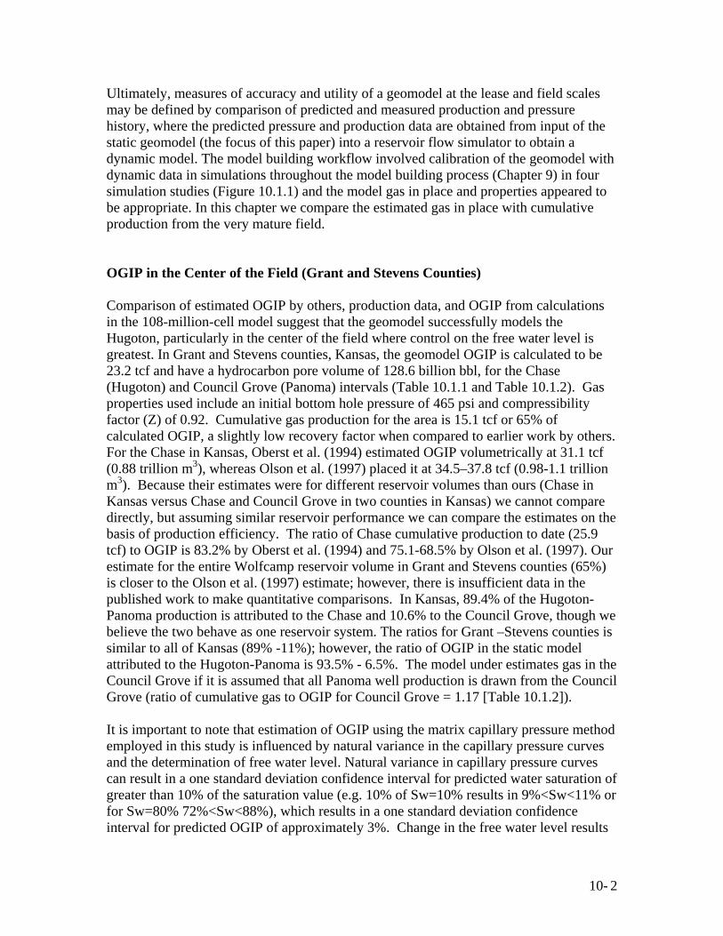
Ultimately, measures of accuracy and utility of a geomodel at the lease and field scales may be defined by comparison of predicted and measured production and pressure history, where the predicted pressure and production data are obtained from input of the static geomodel (the focus of this paper) into a reservoir flow simulator to obtain a dynamic model. The model building workflow involved calibration of the geomodel with dynamic data in simulations throughout the model building process (Chapter 9) in four simulation studies (Figure 10.1.1) and the model gas in place and properties appeared to be appropriate. In this chapter we compare the estimated gas in place with cumulative production from the very mature field. OGIP in the Center of the Field (Grant and Stevens Counties) Comparison of estimated OGIP by others, production data, and OGIP from calculations in the 108-million-cell model suggest that the geomodel successfully models the Hugoton, particularly in the center of the field where control on the free water level is greatest. In Grant and Stevens counties, Kansas, the geomodel OGIP is calculated to be 23.2 tcf and have a hydrocarbon pore volume of 128.6 billion bbl, for the Chase (Hugoton) and Council Grove (Panoma) intervals (Table 10.1.1 and Table 10.1.2). Gas properties used include an initial bottom hole pressure of 465 psi and compressibility factor (Z) of 0.92. Cumulative gas production for the area is 15.1 tcf or 65% of calculated OGIP, a slightly low recovery factor when compared to earlier work by others. For the Chase in Kansas, Oberst et al. (1994) estimated OGIP volumetrically at 31.1 tcf (0.88 trillion m3), whereas Olson et al. (1997) placed it at 34.5–37.8 tcf (0.98-1.1 trillion m3). Because their estimates were for different reservoir volumes than ours (Chase in Kansas versus Chase and Council Grove in two counties in Kansas) we cannot compare directly, but assuming similar reservoir performance we can compare the estimates on the basis of production efficiency. The ratio of Chase cumulative production to date (25.9 tcf) to OGIP is 83.2% by Oberst et al. (1994) and 75.1-68.5% by Olson et al. (1997). Our estimate for the entire Wolfcamp reservoir volume in Grant and Stevens counties (65%) is closer to the Olson et al. (1997) estimate; however, there is insufficient data in the published work to make quantitative comparisons. In Kansas, 89.4% of the Hugoton-Panoma production is attributed to the Chase and 10.6% to the Council Grove, though we believe the two behave as one reservoir system. The ratios for Grant –Stevens counties is similar to all of Kansas (89% -11%); however, the ratio of OGIP in the static model attributed to the Hugoton-Panoma is 93.5% - 6.5%. The model under estimates gas in the Council Grove if it is assumed that all Panoma well production is drawn from the Council Grove (ratio of cumulative gas to OGIP for Council Grove = 1.17 [Table 10.1.2]).

It is important to note that estimation of OGIP using the matrix capillary pressure method employed in this study is influenced by natural variance in the capillary pressure curves and the determination of free water level. Natural variance in capillary pressure curves can result in a one standard deviation confidence interval for predicted water saturation of greater than 10% of the saturation value (e.g. 10% of Sw=10% results in 9%<Sw<11% or for Sw=80% 72%<Sw<88%), which results in a one standard deviation confidence interval for predicted OGIP of approximately 3%. Change in the free water level results

10- 2

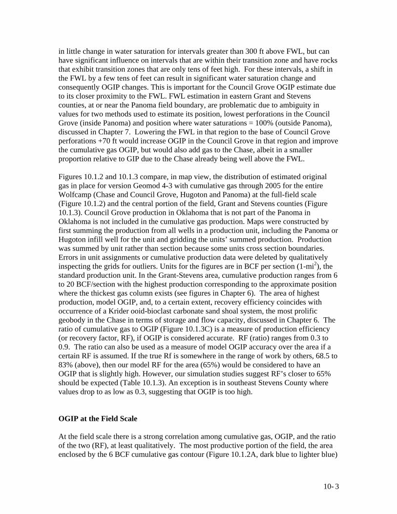
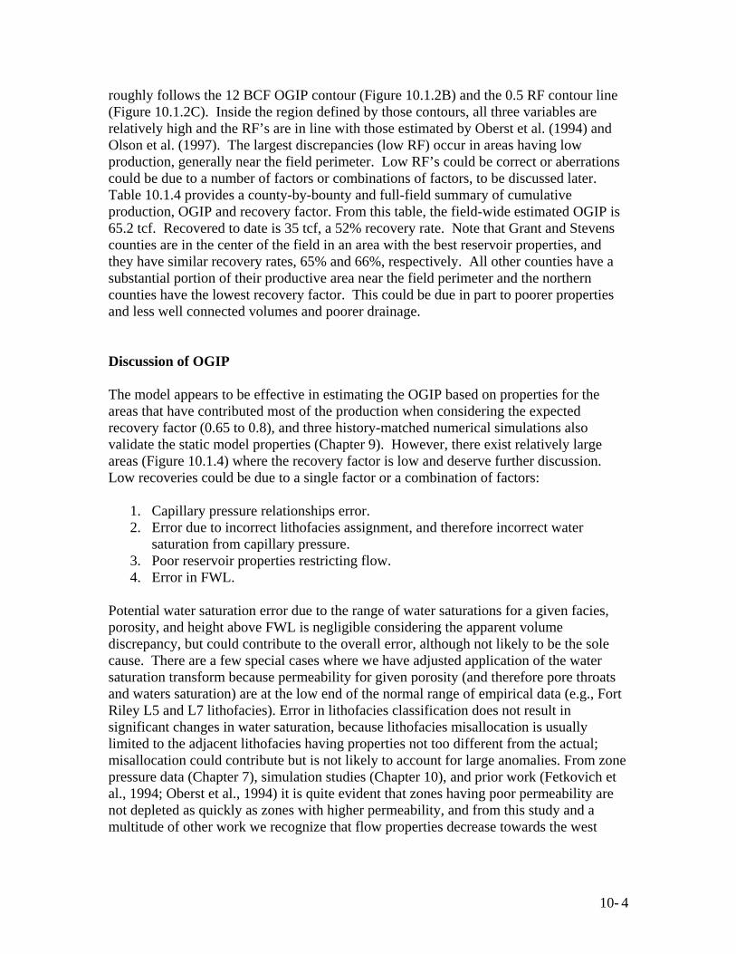
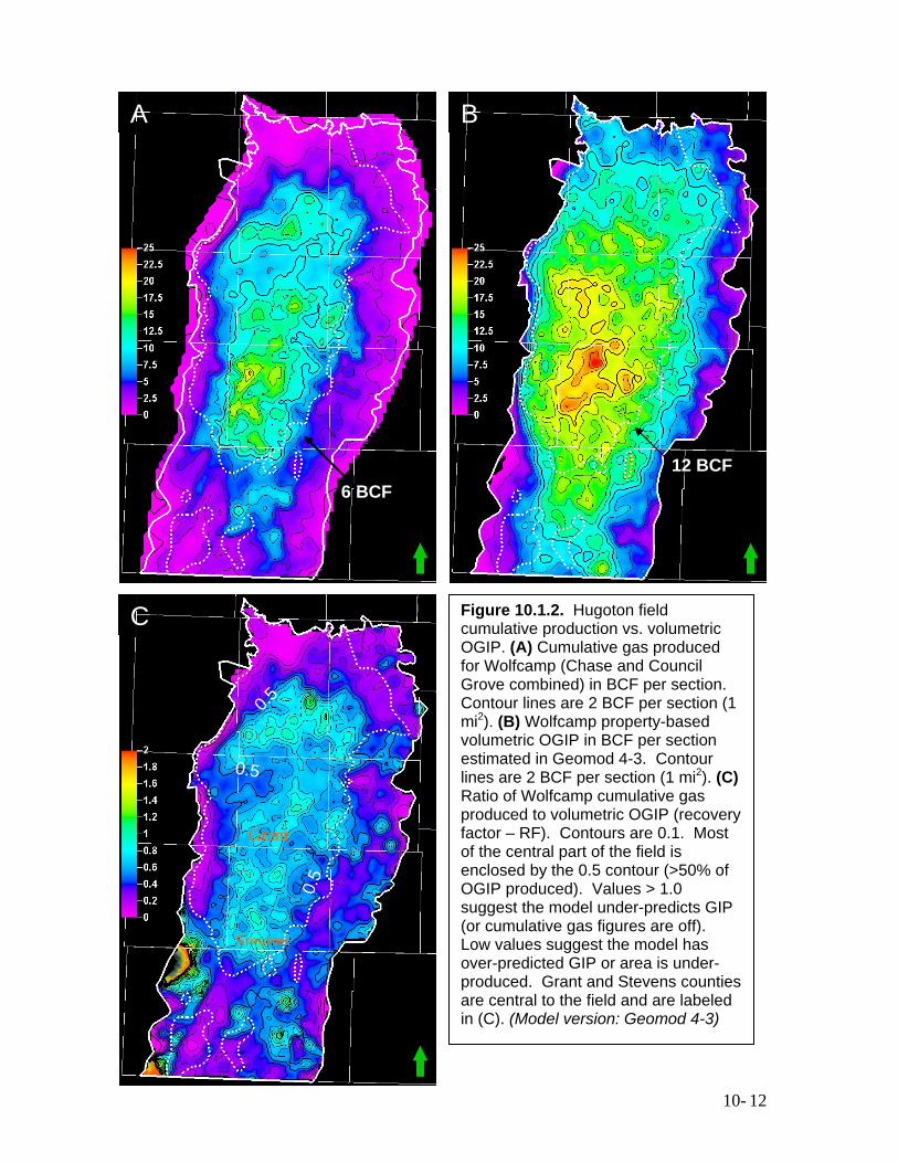
in little change in water saturation for intervals greater than 300 ft above FWL, but can have significant influence on intervals that are within their transition zone and have rocks that exhibit transition zones that are only tens of feet high. For these intervals, a shift in the FWL by a few tens of feet can result in significant water saturation change and consequently OGIP changes. This is important for the Council Grove OGIP estimate due to its closer proximity to the FWL. FWL estimation in eastern Grant and Stevens counties, at or near the Panoma field boundary, are problematic due to ambiguity in values for two methods used to estimate its position, lowest perforations in the Council Grove (inside Panoma) and position where water saturations = 100% (outside Panoma), discussed in Chapter 7. Lowering the FWL in that region to the base of Council Grove perforations +70 ft would increase OGIP in the Council Grove in that region and improve the cumulative gas OGIP, but would also add gas to the Chase, albeit in a smaller proportion relative to GIP due to the Chase already being well above the FWL. Figures 10.1.2 and 10.1.3 compare, in map view, the distribution of estimated original gas in place for version Geomod 4-3 with cumulative gas through 2005 for the entire Wolfcamp (Chase and Council Grove, Hugoton and Panoma) at the full-field scale (Figure 10.1.2) and the central portion of the field, Grant and Stevens counties (Figure 10.1.3). Council Grove production in Oklahoma that is not part of the Panoma in Oklahoma is not included in the cumulative gas production. Maps were constructed by first summing the production from all wells in a production unit, including the Panoma or Hugoton infill well for the unit and gridding the units’ summed production. Production was summed by unit rather than section because some units cross section boundaries. Errors in unit assignments or cumulative production data were deleted by qualitatively inspecting the grids for outliers. Units for the figures are in BCF per section (1-mi2), the standard production unit. In the Grant-Stevens area, cumulative production ranges from 6 to 20 BCF/section with the highest production corresponding to the approximate position where the thickest gas column exists (see figures in Chapter 6). The area of highest production, model OGIP, and, to a certain extent, recovery efficiency coincides with occurrence of a Krider ooid-bioclast carbonate sand shoal system, the most prolific geobody in the Chase in terms of storage and flow capacity, discussed in Chapter 6. The ratio of cumulative gas to OGIP (Figure 10.1.3C) is a measure of production efficiency (or recovery factor, RF), if OGIP is considered accurate. RF (ratio) ranges from 0.3 to 0.9. The ratio can also be used as a measure of model OGIP accuracy over the area if a certain RF is assumed. If the true Rf is somewhere in the range of work by others, 68.5 to 83% (above), then our model RF for the area (65%) would be considered to have an OGIP that is slightly high. However, our simulation studies suggest RF’s closer to 65% should be expected (Table 10.1.3). An exception is in southeast Stevens County where values drop to as low as 0.3, suggesting that OGIP is too high. OGIP at the Field Scale At the field scale there is a strong correlation among cumulative gas, OGIP, and the ratio of the two (RF), at least qualitatively. The most productive portion of the field, the area enclosed by the 6 BCF cumulative gas contour (Figure 10.1.2A, dark blue to lighter blue)

10- 3

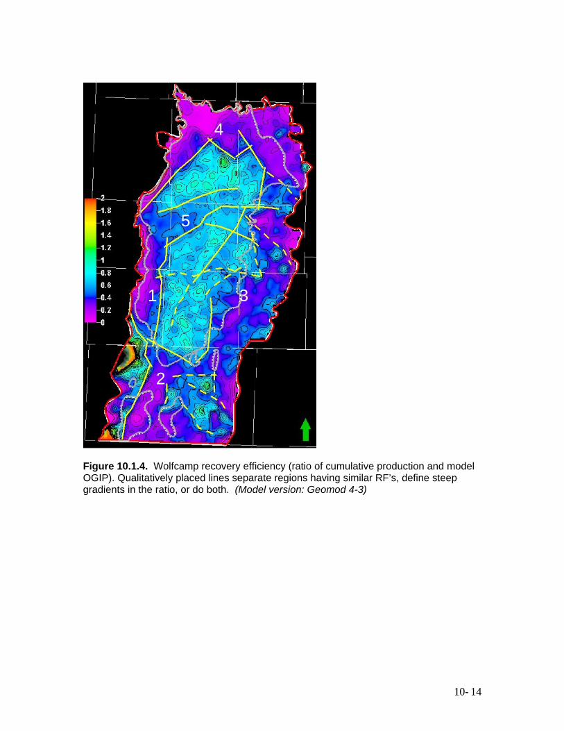
roughly follows the 12 BCF OGIP contour (Figure 10.1.2B) and the 0.5 RF contour line (Figure 10.1.2C). Inside the region defined by those contours, all three variables are relatively high and the RF’s are in line with those estimated by Oberst et al. (1994) and Olson et al. (1997). The largest discrepancies (low RF) occur in areas having low production, generally near the field perimeter. Low RF’s could be correct or aberrations could be due to a number of factors or combinations of factors, to be discussed later. Table 10.1.4 provides a county-by-bounty and full-field summary of cumulative production, OGIP and recovery factor. From this table, the field-wide estimated OGIP is 65.2 tcf. Recovered to date is 35 tcf, a 52% recovery rate. Note that Grant and Stevens counties are in the center of the field in an area with the best reservoir properties, and they have similar recovery rates, 65% and 66%, respectively. All other counties have a substantial portion of their productive area near the field perimeter and the northern counties have the lowest recovery factor. This could be due in part to poorer properties and less well connected volumes and poorer drainage. Discussion of OGIP The model appears to be effective in estimating the OGIP based on properties for the areas that have contributed most of the production when considering the expected recovery factor (0.65 to 0.8), and three history-matched numerical simulations also validate the static model properties (Chapter 9). However, there exist relatively large areas (Figure 10.1.4) where the recovery factor is low and deserve further discussion. Low recoveries could be due to a single factor or a combination of factors:

1. Capillary pressure relationships error. 2. Error due to incorrect lithofacies assignment, and therefore incorrect water

saturation from capillary pressure. 3. Poor reservoir properties restricting flow. 4. Error in FWL.

Potential water saturation error due to the range of water saturations for a given facies, porosity, and height above FWL is negligible considering the apparent volume discrepancy, but could contribute to the overall error, although not likely to be the sole cause. There are a few special cases where we have adjusted application of the water saturation transform because permeability for given porosity (and therefore pore throats and waters saturation) are at the low end of the normal range of empirical data (e.g., Fort Riley L5 and L7 lithofacies). Error in lithofacies classification does not result in significant changes in water saturation, because lithofacies misallocation is usually limited to the adjacent lithofacies having properties not too different from the actual; misallocation could contribute but is not likely to account for large anomalies. From zone pressure data (Chapter 7), simulation studies (Chapter 10), and prior work (Fetkovich et al., 1994; Oberst et al., 1994) it is quite evident that zones having poor permeability are not depleted as quickly as zones with higher permeability, and from this study and a multitude of other work we recognize that flow properties decrease towards the west

10- 4

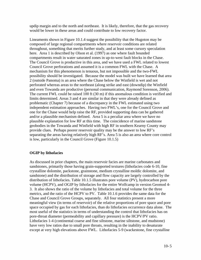
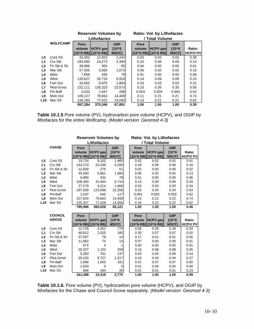
updip margin and to the north and northeast. It is likely, therefore, that the gas recovery would be lower in these areas and could contribute to low recovery factor. Lineaments shown in Figure 10.1.4 suggest the possibility that the Hugoton may be composed of large regional compartments where reservoir conditions are related throughout, something that merits further study, and at least some cursory speculation here. Area 1 is described by Olson et al. (1997) as one where fault bounded compartments result in water saturated zones in up-to-west fault blocks in the Chase. The Council Grove is productive in this area, and we have used a FWL related to lowest Council Grove perforations and assumed it is a common FWL with the Chase. A mechanism for this phenomenon is tenuous, but not impossible and the two-FWL possibility should be investigated. Because the model was built we have learned that area 2 (outside Panoma) is an area where the Chase below the Winfield is wet and not perforated whereas areas to the northeast (along strike and east (downdip) the Winfield and even Towanda are productive (personal communication, Raymond Sorenson, 2006). The current FWL could be raised 100 ft (30 m) if this anomalous condition is verified and limits determined. Areas 3 and 4 are similar in that they were already defined as problematic (Chapter 7) because of a discrepancy in the FWL estimated using two independent estimation approaches. Having two FWL’s, one for the Council Grove and one for the Chase would help raise the RF, provided supporting data can be gathered and/or a plausible mechanism defined. Area 5 is a peculiar area where we have no plausible explanation for low RF at this time. The coincidence of marine sandstone geobodies in the Towanda and Winfield with high RF in southern Kearny County may provide clues. Perhaps poorer reservoir quality may be the answer to low RF’s separating the areas having relatively high RF’s. Area 5 is also an area where core control is low, particularly in the Council Grove (Figure 10.1.5) OGIP by lithofacies As discussed in prior chapters, the main reservoir facies are marine carbonates and sandstones, primarily those having grain-supported textures (lithofacies code 6-10, fine crystalline dolomite, packstone, grainstone, medium crystalline moldic dolomite, and sandstone) and the distribution of storage and flow capacity are largely controlled by the distribution of lithofacies. Table 10.1.5 illustrates pore volume (PV), hydrocarbon pore volume (HCPV), and OGIP by lithofacies for the entire Wolfcamp in version Geomod 4-3. It also shows the ratio of the volume by lithofacies and total volume for the three metrics, and the ratio of the HCPV to PV. Table 10.1.6 provides the same data for the Chase and Council Grove Groups, separately. All four statistics present a more meaningful view (in terms of reservoir) of the relative proportions of pore space and pore space occupied by gas for each lithofacies, than do lithofacies occurrence data alone. The most useful of the statistics in terms of understanding the control that lithofacies has on pore-throat diameter (permeability and capillary pressure) is the HCPV/PV ratio. Lithofacies 1-4 (continental coarse and fine siltstone, marine siltstone, and mudstone) have very low ratios due to small pore throats, resulting in the inability to desaturate except at very high elevations above FWL. Lithofacies 5-9 (wackestone, fine crystalline

10- 5

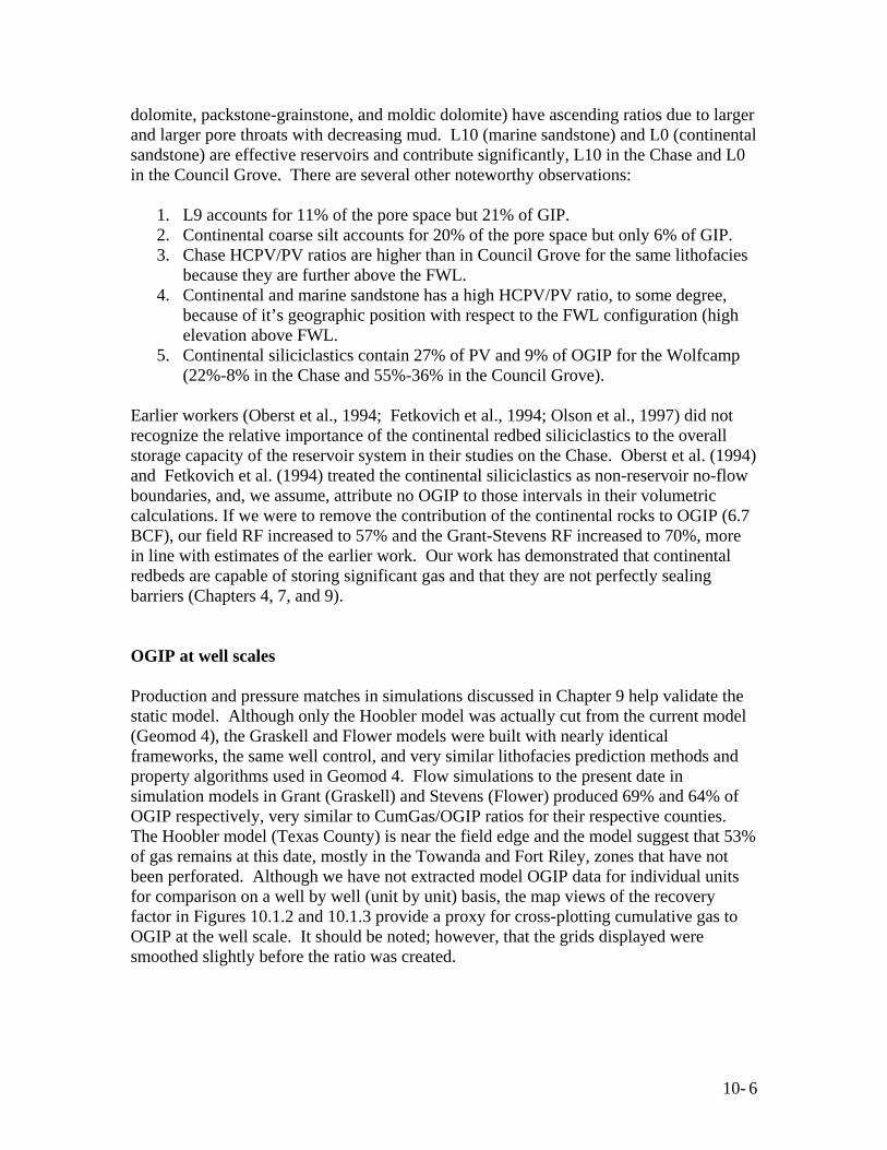
dolomite, packstone-grainstone, and moldic dolomite) have ascending ratios due to larger and larger pore throats with decreasing mud. L10 (marine sandstone) and L0 (continental sandstone) are effective reservoirs and contribute significantly, L10 in the Chase and L0 in the Council Grove. There are several other noteworthy observations:

1. L9 accounts for 11% of the pore space but 21% of GIP. 2. Continental coarse silt accounts for 20% of the pore space but only 6% of GIP. 3. Chase HCPV/PV ratios are higher than in Council Grove for the same lithofacies

because they are further above the FWL. 4. Continental and marine sandstone has a high HCPV/PV ratio, to some degree,

because of it’s geographic position with respect to the FWL configuration (high elevation above FWL.

5. Continental siliciclastics contain 27% of PV and 9% of OGIP for the Wolfcamp (22%-8% in the Chase and 55%-36% in the Council Grove).

Earlier workers (Oberst et al., 1994; Fetkovich et al., 1994; Olson et al., 1997) did not recognize the relative importance of the continental redbed siliciclastics to the overall storage capacity of the reservoir system in their studies on the Chase. Oberst et al. (1994) and Fetkovich et al. (1994) treated the continental siliciclastics as non-reservoir no-flow boundaries, and, we assume, attribute no OGIP to those intervals in their volumetric calculations. If we were to remove the contribution of the continental rocks to OGIP (6.7 BCF), our field RF increased to 57% and the Grant-Stevens RF increased to 70%, more in line with estimates of the earlier work. Our work has demonstrated that continental redbeds are capable of storing significant gas and that they are not perfectly sealing barriers (Chapters 4, 7, and 9). OGIP at well scales Production and pressure matches in simulations discussed in Chapter 9 help validate the static model. Although only the Hoobler model was actually cut from the current model (Geomod 4), the Graskell and Flower models were built with nearly identical frameworks, the same well control, and very similar lithofacies prediction methods and property algorithms used in Geomod 4. Flow simulations to the present date in simulation models in Grant (Graskell) and Stevens (Flower) produced 69% and 64% of OGIP respectively, very similar to CumGas/OGIP ratios for their respective counties. The Hoobler model (Texas County) is near the field edge and the model suggest that 53% of gas remains at this date, mostly in the Towanda and Fort Riley, zones that have not been perforated. Although we have not extracted model OGIP data for individual units for comparison on a well by well (unit by unit) basis, the map views of the recovery factor in Figures 10.1.2 and 10.1.3 provide a proxy for cross-plotting cumulative gas to OGIP at the well scale. It should be noted; however, that the grids displayed were smoothed slightly before the ratio was created.

10- 6

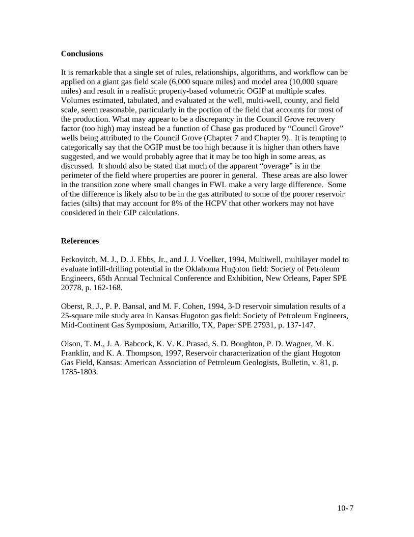
Conclusions It is remarkable that a single set of rules, relationships, algorithms, and workflow can be applied on a giant gas field scale (6,000 square miles) and model area (10,000 square miles) and result in a realistic property-based volumetric OGIP at multiple scales. Volumes estimated, tabulated, and evaluated at the well, multi-well, county, and field scale, seem reasonable, particularly in the portion of the field that accounts for most of the production. What may appear to be a discrepancy in the Council Grove recovery factor (too high) may instead be a function of Chase gas produced by “Council Grove” wells being attributed to the Council Grove (Chapter 7 and Chapter 9). It is tempting to categorically say that the OGIP must be too high because it is higher than others have suggested, and we would probably agree that it may be too high in some areas, as discussed. It should also be stated that much of the apparent “overage” is in the perimeter of the field where properties are poorer in general. These areas are also lower in the transition zone where small changes in FWL make a very large difference. Some of the difference is likely also to be in the gas attributed to some of the poorer reservoir facies (silts) that may account for 8% of the HCPV that other workers may not have considered in their GIP calculations. References Fetkovitch, M. J., D. J. Ebbs, Jr., and J. J. Voelker, 1994, Multiwell, multilayer model to evaluate infill-drilling potential in the Oklahoma Hugoton field: Society of Petroleum Engineers, 65th Annual Technical Conference and Exhibition, New Orleans, Paper SPE 20778, p. 162-168. Oberst, R. J., P. P. Bansal, and M. F. Cohen, 1994, 3-D reservoir simulation results of a 25-square mile study area in Kansas Hugoton gas field: Society of Petroleum Engineers, Mid-Continent Gas Symposium, Amarillo, TX, Paper SPE 27931, p. 137-147. Olson, T. M., J. A. Babcock, K. V. K. Prasad, S. D. Boughton, P. D. Wagner, M. K. Franklin, and K. A. Thompson, 1997, Reservoir characterization of the giant Hugoton Gas Field, Kansas: American Association of Petroleum Geologists, Bulletin, v. 81, p. 1785-1803.

10- 7

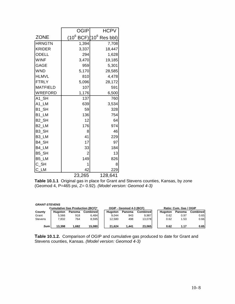
OGIP HCPV ZONE (106 BCF)(106 Res bbl)HRNGTN 1,394 7,708KRIDER 3,337 18,447ODELL 294 1,628WINF 3,470 19,185GAGE 959 5,301WND 5,170 28,585HLMVL 810 4,478FTRLY 5,096 28,172MATFIELD 107 591WREFORD 1,176 6,500A1_SH 137 760A1_LM 639 3,534B1_SH 59 328B1_LM 136 754B2_SH 12 64B2_LM 176 974B3_SH 8 46B3_LM 41 229B4_SH 17 97B4_LM 33 184B5_SH 2 13B5_LM 149 826C_SH 1 8C_LM 42 229

23,265 128,641 Table 10.1.1 Original gas in place for Grant and Stevens counties, Kansas, by zone (Geomod 4, P=465 psi, Z= 0.92). (Model version: Geomod 4-3) GRANT-STEVENS

Cumulative Gas Production (BCF)* OGIP - Geomod 4-3 (BCF) Ratio: Cum. Gas / OGIPCounty Hugoton Panoma Combined Hugoton Panoma Combined Hugoton Panoma CombinedGrant 5,566 918 6,484 9,044 943 9,987 0.62 0.97 0.65Stevens 7,832 764 8,595 12,580 498 13,078 0.62 1.53 0.66

Sum 13,398 1,682 15,080 21,624 1,441 23,065 0.62 1.17 0.65 Table 10.1.2. Comparison of OGIP and cumulative gas produced to date for Grant and Stevens counties, Kansas. (Model version: Geomod 4-3)

10- 8

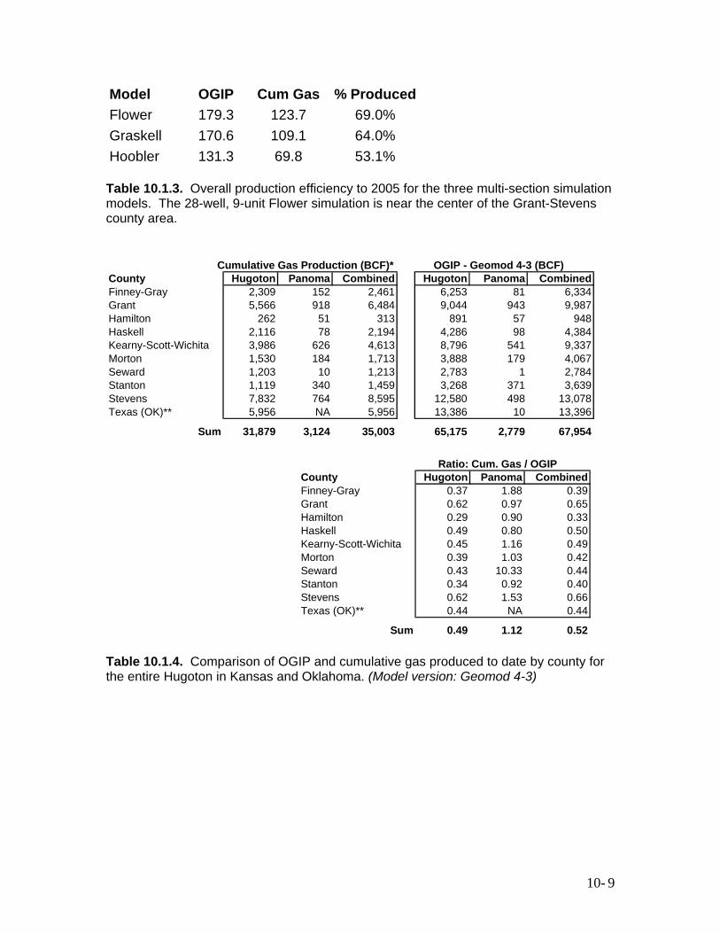
Model OGIP Cum Gas % ProducedFlower 179.3 123.7 69.0%Graskell 170.6 109.1 64.0%Hoobler 131.3 69.8 53.1% Table 10.1.3. Overall production efficiency to 2005 for the three multi-section simulation models. The 28-well, 9-unit Flower simulation is near the center of the Grant-Stevens county area.

Ratio: Cum. Gas / OGIPCounty Hugoton Panoma CombinedFinney-Gray 0.37 1.88 0.39Grant 0.62 0.97 0.65Hamilton 0.29 0.90 0.33Haskell 0.49 0.80 0.50Kearny-Scott-Wichita 0.45 1.16 0.49Morton 0.39 1.03 0.42Seward 0.43 10.33 0.44Stanton 0.34 0.92 0.40Stevens 0.62 1.53 0.66Texas (OK)** 0.44 NA 0.44

Sum 0.49 1.12 0.52

Cumulative Gas Production (BCF)* OGIP - Geomod 4-3 (BCF)County Hugoton Panoma Combined Hugoton Panoma CombinedFinney-Gray 2,309 152 2,461 6,253 81 6,334Grant 5,566 918 6,484 9,044 943 9,987Hamilton 262 51 313 891 57 948Haskell 2,116 78 2,194 4,286 98 4,384Kearny-Scott-Wichita 3,986 626 4,613 8,796 541 9,337Morton 1,530 184 1,713 3,888 179 4,067Seward 1,203 10 1,213 2,783 1 2,784Stanton 1,119 340 1,459 3,268 371 3,639Stevens 7,832 764 8,595 12,580 498 13,078Texas (OK)** 5,956 NA 5,956 13,386 10 13,396

Sum 31,879 3,124 35,003 65,175 2,779 67,954

Table 10.1.4. Comparison of OGIP and cumulative gas produced to date by county for the entire Hugoton in Kansas and Oklahoma. (Model version: Geomod 4-3)

10- 9

WOLFCAMP Pore volume

[10^6 RB]HCPV gas [10^6 RB]

GIIP [10^6

MSCF]

Pore volume

[10^6 RB]HCPV gas [10^6 RB]

GIIP [10^6

MSCF]Ratio:

HCPV/ PVL0 Cont SS 32,452 12,403 2,244 0.03 0.03 0.03 0.38L1 Crs Silt 193,082 24,273 4,390 0.20 0.06 0.06 0.13L2 Fn Silt & Sh 39,896 354 65 0.04 0.00 0.00 0.01L3 Mar Silt 57,555 5,935 1,073 0.06 0.02 0.02 0.10L4 Mdst 7,656 435 79 0.01 0.00 0.00 0.06L5 Wkst 133,627 32,716 5,918 0.14 0.09 0.09 0.24L6 Fxln Dol 32,562 9,975 1,803 0.03 0.03 0.03 0.31L7 Pkst-Grnst 222,111 130,323 23,573 0.23 0.35 0.35 0.59L8 PA-Baff 3,033 1,647 298 0.003 0.004 0.004 0.54L9 Mxln Dol 109,127 79,663 14,408 0.11 0.21 0.21 0.73

L10 Mar SS 126,183 77,622 14,040 0.13 0.21 0.21 0.62957,284 375,346 67,891 1.00 1.00 1.00 0.39

Ratio: Vol. by Lithofacies / Total Volume

Reservoir Volumes by Lithofacies

Table 10.1.5 Pore volume (PV), hydrocarbon pore volume (HCPV), and OGIP by lithofacies for the entire Wolfcamp. (Model version: Geomod 4-3)

CHASE Pore volume

[10^6 RB]HCPV gas [10^6 RB]

GIIP [10^6

MSCF]

Pore volume

[10^6 RB]HCPV gas [10^6 RB]

GIIP [10^6

MSCF]Ratio:

HCPV/ PVL0 Cont SS 19,724 8,102 1,465 0.02 0.02 0.02 0.41L1 Crs Silt 144,270 23,248 4,205 0.18 0.06 0.06 0.16L2 Fn Silt & Sh 12,839 276 51 0.02 0.00 0.00 0.02L3 Mar Silt 45,593 5,861 1,060 0.06 0.02 0.02 0.13L4 Mdst 6,984 431 78 0.01 0.00 0.00 0.06L5 Wkst 108,300 31,564 5,710 0.14 0.09 0.09 0.29L6 Fxln Dol 27,279 9,214 1,666 0.03 0.03 0.03 0.34L7 Pkst-Grnst 197,009 123,596 22,356 0.25 0.34 0.34 0.63L8 PA-Baff 1,037 645 117 0.001 0.002 0.002 0.62L9 Mxln Dol 107,624 79,663 14,408 0.14 0.22 0.22 0.74

L10 Mar SS 125,337 77,428 14,005 0.16 0.22 0.22 0.62795,996 360,028 65,121 1.00 1.00 1.00 0.45

COUNCIL GROVE

Pore volume

[10^6 RB]HCPV gas [10^6 RB]

GIIP [10^6

MSCF]

Pore volume

[10^6 RB]HCPV gas [10^6 RB]

GIIP [10^6

MSCF]Ratio:

HCPV/ PVL0 Cont SS 12,728 4,301 779 0.08 0.28 0.28 0.34L1 Crs Silt 48,812 1,025 185 0.30 0.07 0.07 0.02L2 Fn Silt & Sh 27,057 78 14 0.17 0.01 0.01 0.00L3 Mar Silt 11,962 74 13 0.07 0.00 0.00 0.01L4 Mdst 672 4 1 0.00 0.00 0.00 0.01L5 Wkst 25,327 1,152 208 0.16 0.08 0.08 0.05L6 Fxln Dol 5,283 761 137 0.03 0.05 0.05 0.14L7 Pkst-Grnst 25,102 6,727 1,217 0.16 0.44 0.44 0.27L8 PA-Baff 1,996 1,002 181 0.01 0.07 0.07 0.50L9 Mxln Dol 1,503 0 0 0.01 0.00 0.00 0.00

L10 Mar SS 846 194 35 0.01 0.01 0.01 0.23161,288 15,318 2,770 1.00 1.00 1.00 0.09

Ratio: Vol. by Lithofacies / Total Volume

Reservoir Volumes by Lithofacies

Table 10.1.6. Pore volume (PV), hydrocarbon pore volume (HCPV), and OGIP by lithofacies for the Chase and Council Grove separately. (Model version: Geomod 4-3)

10- 10

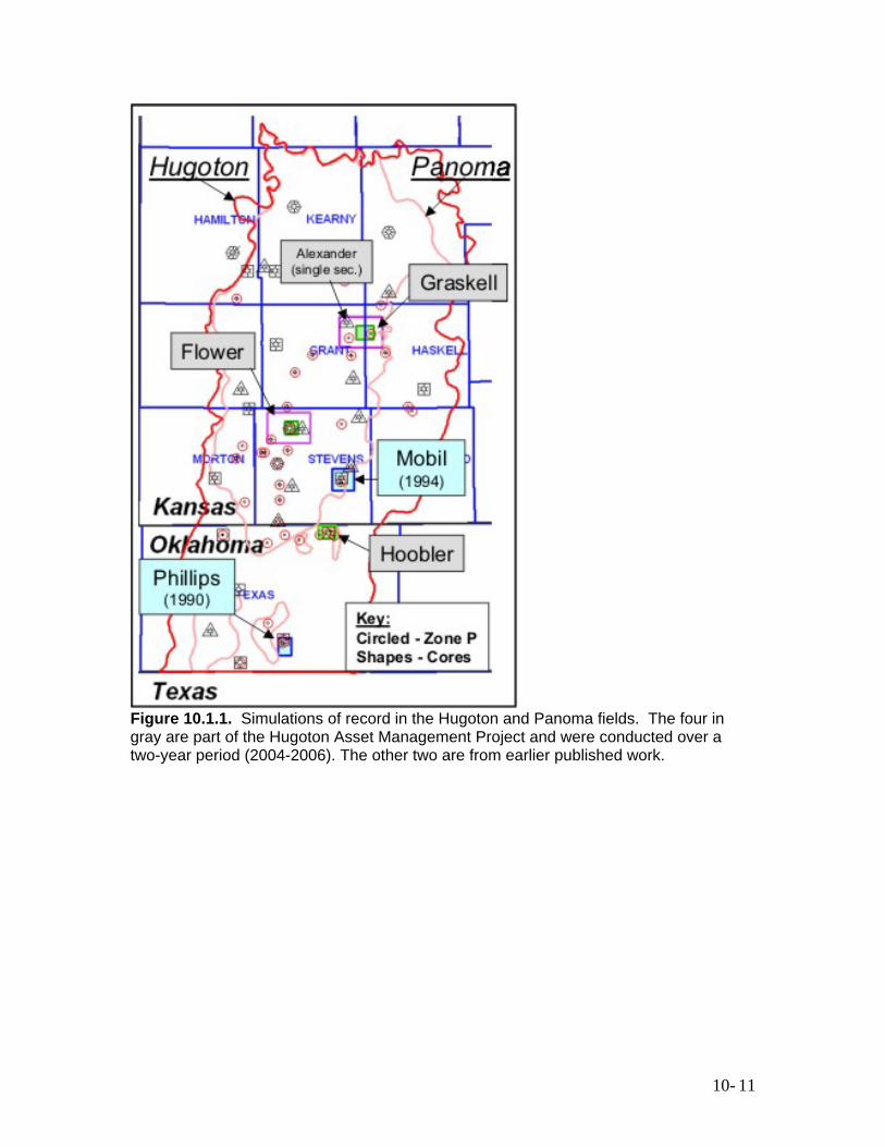
Figure 10.1.1. Simulations of record in the Hugoton and Panoma fields. The four in gray are part of the Hugoton Asset Management Project and were conducted over a two-year period (2004-2006). The other two are from earlier published work.

10- 11

10- 12

Figure 10.1.2. Hugoton field cumulative production vs. volumetric OGIP. (A) Cumulative gas produced for Wolfcamp (Chase and Council Grove combined) in BCF per section. Contour lines are 2 BCF per section (1 mi2). (B) Wolfcamp property-based volumetric OGIP in BCF per section estimated in Geomod 4-3. Contour lines are 2 BCF per section (1 mi2). (C) Ratio of Wolfcamp cumulative gas produced to volumetric OGIP (recovery factor – RF). Contours are 0.1. Most of the central part of the field is enclosed by the 0.5 contour (>50% of OGIP produced). Values > 1.0 suggest the model under-predicts GIP (or cumulative gas figures are off). Low values suggest the model has over-predicted GIP or area is under-produced. Grant and Stevens counties are central to the field and are labeled in (C). (Model version: Geomod 4-3)

0.5

0.5

0.5

0.5

0.5

0.5

C

Grant

Stevens

A

6 BCF

B

12 BCF

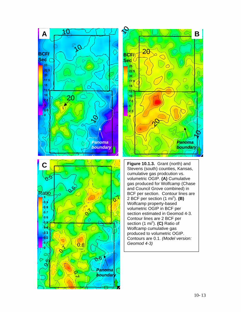
Figure 10.1.3. Grant (north) and Stevens (south) counties, Kansas, cumulative gas prodcution vs. volumetric OGIP. (A) Cumulative gas produced for Wolfcamp (Chase and Council Grove combined) in BCF per section. Contour lines are 2 BCF per section (1 mi2). (B) Wolfcamp property-based volumetric OGIP in BCF per section estimated in Geomod 4-3. Contour lines are 2 BCF per section (1 mi2). (C) Ratio of Wolfcamp cumulative gas produced to volumetric OGIP. Contours are 0.1. (Model version: Geomod 4-3)

20

10

20

10

BCF/Sec

20

10

20

10

BCF/Sec

Panoma boundary

B

0.5

0.5

0.5

0.7

0.7

0.8

0.7

0.5

0.7

Ratio

0.5

0.5

0.5

0.7

0.7

0.8

0.7

0.5

0.7

Ratio

Panoma boundary

C

10

10

BCF/Sec

20

10A

Panoma boundary

10- 13

2

4

31

5

Figure 10.1.4. Wolfcamp recovery efficiency (ratio of cumulative production and model OGIP). Qualitatively placed lines separate regions having similar RF’s, define steep gradients in the ratio, or do both. (Model version: Geomod 4-3)

10- 14

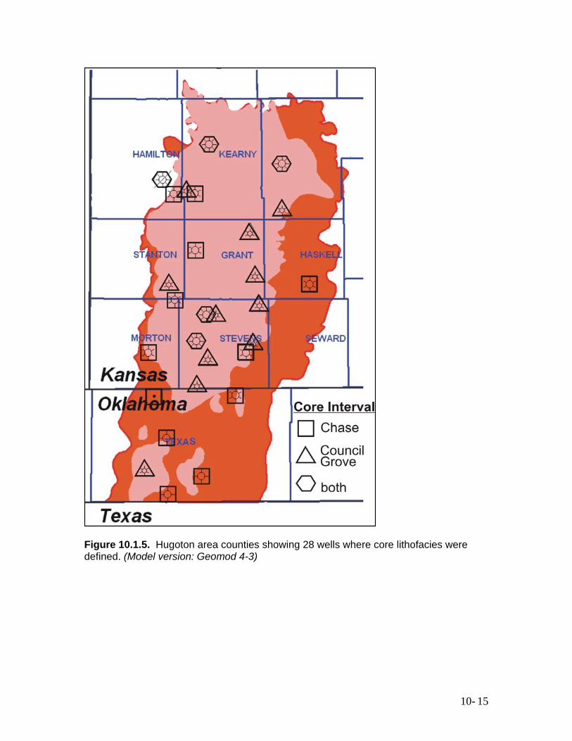
Figure 10.1.5. Hugoton area counties showing 28 wells where core lithofacies were defined. (Model version: Geomod 4-3)

10- 15

10.2 REMAINING GAS IN HUGOTON AND PANOMA Martin K. Dubois Throughout this study a unifying theme has been substantiated: the Hugoton and Panoma reservoir is a layered system that behaves as a single, extremely large reservoir system, although its layers are differentially depleted. Our study confirms some of the conclusions by simulation studies by Fetkovich et al. (1994) and Oberst et al. (1994), particularly that the individual layers of the system have varying flow properties and are depleted at varying rates, but we part on the role of the continental redbed siliciclastics. They treat the redbeds as absolute no-flow boundaries; our simulation work and empirical core data suggest that they have some transmissibility and prefer to treat them as low-flow baffles (see Chapters 4, 7, and 9). With an accurate volumetric OGIP (previous section), identifying where the remaining gas in place resides stratigraphically in the layered reservoir is a simple matter where zone-specific reservoir pressures are known. Therein lies the problem. All production in the field is from wells having multiple (commingled) completions and wellhead shutin pressures taken every two years, by regulation, reflect the pressure of the zone having the highest permeability (lowest pressure). Zone pressures are not possible in casing through packer because all wells are treated with large hydraulic fractures that are effective at communicating several zones. Testing while drilling is expensive and problematic due to filtrate damage in a very under-pressured system. Through literature, searches of public records, and contributions of historic and recently collected data by participants in HAMP, we have compiled a database of 375 zone tests from 38 wells scattered throughout the field (Figure 10.2.1), a significant accomplishment, but a very small sample considering that there are 12,000 wells in the field. Rigorously characterizing and quantifying the remaining gas in the Hugoton in 3-D (geographically and stratigraphically) was not an objective for this study; however, it is of a follow-up study that is underway. This section will review specific examples (simulations) of pressure through time at well to multi-well scale and some preliminary analysis of available pressure data. Combined they provide insight on the current pressure distribution in the layered system and a possible way forward for resolving the task of a more rigorous characterization of remaining gas. Simulation Studies Very limited historical pressure by zone tests and early simulations by Mobil (Fetkovich et al., 1994) and Phillips (Oberst et al., 1994) suggested the differential depletion phenomena, and our simulation studies (Figure 10.1.1) confirm, refine, and expand the concept. Pressure by zone data recently collected by project participants (RFTs and XPTs) generally show similar trends and lower pressures than those taken 10-20 years ago, but they are not as reliable as carefully executed DSTs. Simulation studies (Chapter 9) illustrate the phenomena in dynamic models and their results suggest that the bulk of the remaining gas is contained in intervals that have relatively low permeability. Of the

10- 16

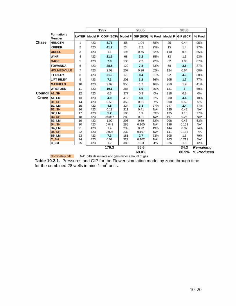
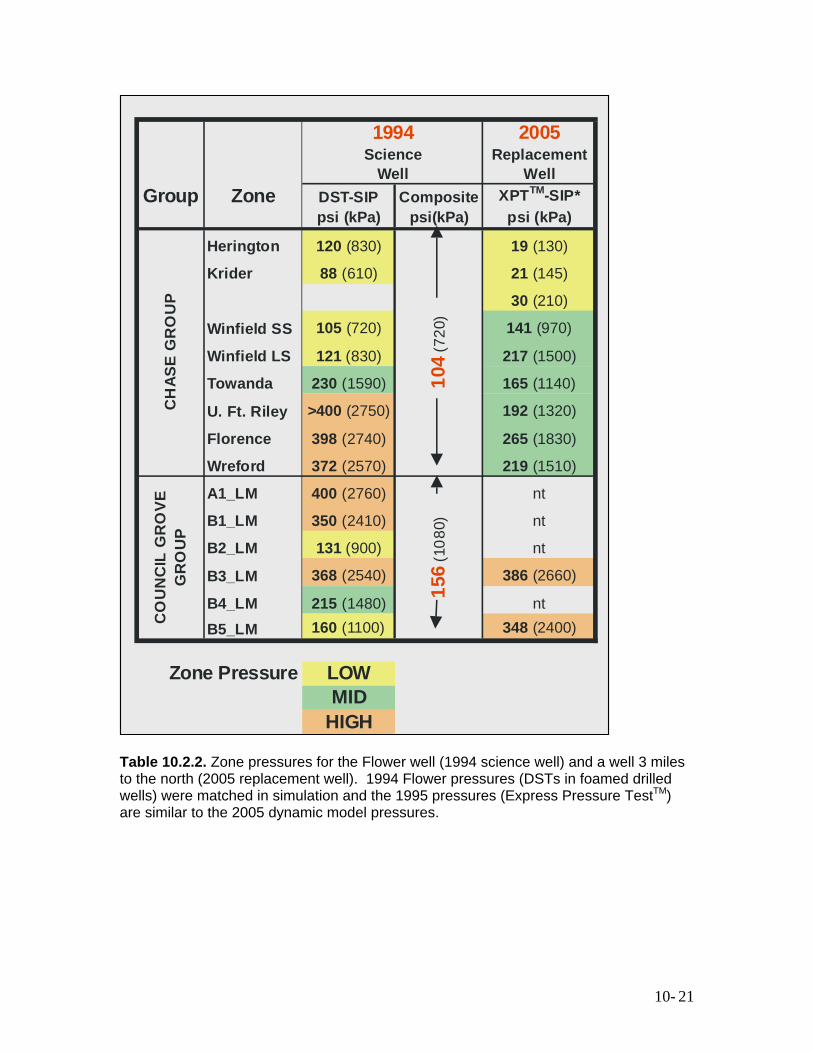
four areas simulated in this study, the Flower was the best constrained by core and high-quality pressure data. The 28-well, 9-unit dynamic model yielded good production and pressure matches and a detailed look at pressure and volumes through time (Table 10.2.1). The upper Chase Krider is the most prolific zone in the area, producing from a dolomitized ooid-bioclast shoal system (highlighted in Chapter 6). Initially (1937), it is estimated to have contained 41.7 BCF gas at 423 psi BHP. In 2005 the Krider pressure was estimated to be 24 psi, 95% depleted (2.2 BCF RGIP). In contrast, the Upper Fort Riley GIP dropped from 21.3 to 8.4 BCF with a pressure decline from 423 psi to 178 psi (61% depleted), and it is estimated to now have more GIP than any other zone. Marine carbonates are the main pay zones and they vary significantly in model pressure in 2005, with many of them having pressure in the 200 psi range, despite wellhead shutin pressures for the area averaging in the 20-30 psi range (the approximate pressure for the Krider). Individual zone pressures from drill-stem tests taken in 1994 in the Flower well were matched, and pressures in 2005 taken while drilling are similar to those in the Flower dynamic model. Predicted future production through 2050 for the 28 Flower model wells, shown in Figure 10.2.2, is 21.3 BCF with average well production estimated to be 21 mcfpd/well. At that point, 45 years into the future, the reservoir is projected to have produced 81% of OGIP and the Fort Riley would have yielded an additional 4.1 BCF, but still be at 92 psi. It is clear in this example that the bulk of the remaining gas in the Hugoton is in zones having high PV but relatively poor permeability, lower half of the Chase (Towanda, Fort Riley and Wreford) and upper Council Grove, while the upper Chase (Krider and Winfield are essentially depleted (Table 10.2.2). Although the lower Chase and upper Council Grove are generally the intervals with the highest remaining volumes, this is not always the case. The Graskell simulation area (Figure 1) is an example where the Krider is one of the zones with low permeability and relatively high remaining gas volumes while the Fort Riley is more depleted. The Hoobler simulation model was the simplest in that only the Chase is productive, yet it revealed some interesting results (Figure 10.2.4). Like the Flower, the Krider and Winfield, the main pay zones, were significantly depleted in the 64 years of production, and two lower zones, the Towanda and Fort Riley presently contain the bulk of the remaining reserves. An interesting note about this particular simulation is that only the upper Chase (Herington, Krider, and Winfield) was perforated in true history, and, for the most part, in the simulation model. Gas was able to move through the continental silts and be produced, albeit constricted, through vertical communication to the Winfield flow unit (see Chapter 9). Pressure by Zone Tests Zone pressure data are critical for calibrating flow simulations and estimating remaining reserves because commingled wellhead SIP is not representative of the true reservoir pressure for wells with commingled zones (all wells in the Hugoton). Unfortunately this information is not often acquired due to expense. The current data set for this study includes pressures from 373 tests from 38 wells (Figure 10.2.1). Tests from nine of the wells are by drill-stem tests, mostly from wells drilled in under-balanced conditions

10- 17

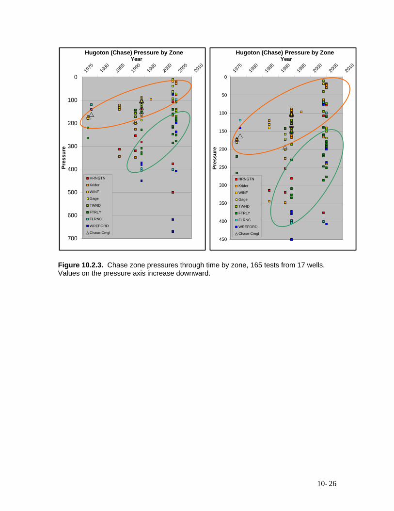
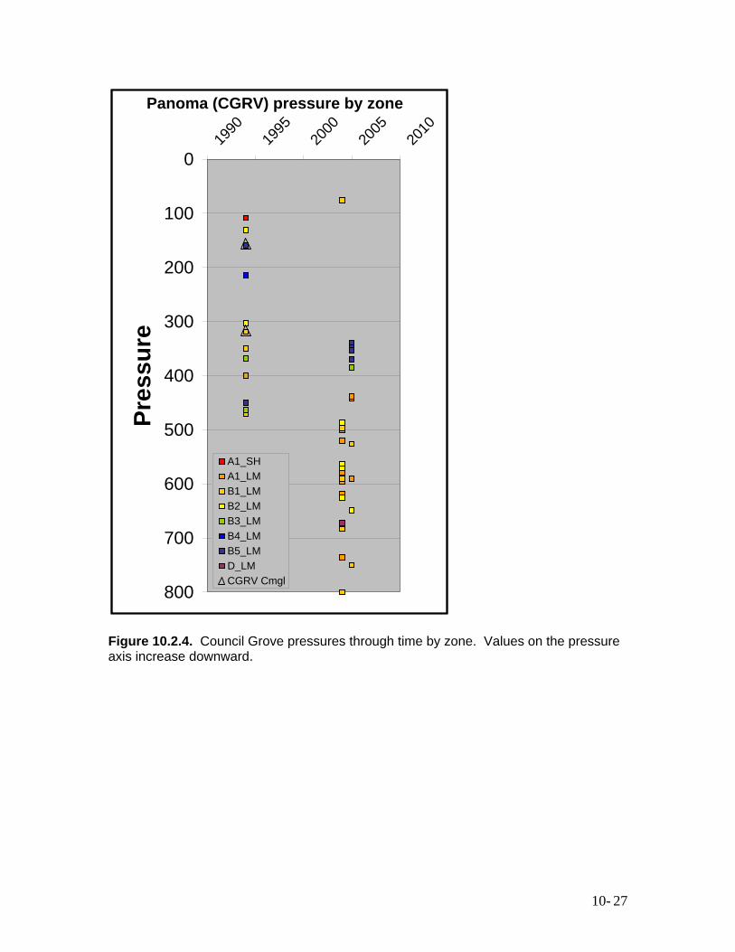
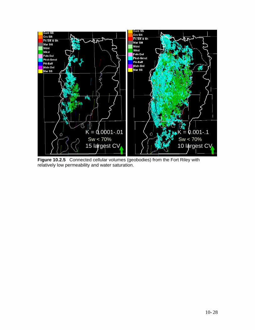
(foam as fluid agent) to prevent formation damage. Pressures in seven wells are from production build-up tests. Participants in the project acquired data from 17 wells in 2004 and 2005 by way of repeat formation tests (RFT) and Express Pressure TestTM (XPT) (235 of the 373 tests). Quality varies from excellent (DST), fair to good (build-up), and fair to questionable (RFT and XPT). Much of the later data are suspect and may yield unlikely high pressures due to supercharge (personal communication with participants) due to very low formation pressure and over-balanced drilling conditions. Some of the data do seem reasonable, however. Figure 10.2.3 illustrates pressure by zone through time for 165 tests in the Chase from 17 wells where the tests have been correlated with zones. Most data prior to 1995 are from carefully executed DSTs and those after 1995 is from RFTs and XPTs. The main upper Chase pay zones, Krider, Winfield, and to a lesser extent Towanda, show on average lower SIP than do other Chase zones and these pressures decrease with time. Pressures >500 psi in later wells are suspect. Figure 10.2.4 is the same type of plot for the Council Grove. Pressures are substantially higher for the later tests and cannot be readily explained, except that most of these tests were taken in areas somewhat downdip from the earlier wells in a position near or below the FWL. Summary statistics by zone are given in Table 10.2.5 for well tests correlated with zones and show the same trends as in the plots presented in a different manner. Characterizing Remaining Gas in Place Simulation exercises discussed above and in more detail in Chapter 9 document the location of remaining gas and, in the Flower simulation, project production 45 years into the future. That simulation suggests that the existing 28 wells, nearly half of which have been producing for nearly 70 years, could conceivably increase recovery from 69% to 80% of OGIP if allowed to produce another 45 years, provided mechanical integrity can be maintained in already old wells. Considering the mechanical integrity and the time-value of money, now is an appropriate time to modify wellbore geometries and/or fracture techniques to access the remaining gas. The cellular Hugoton geomodel, results of simulation studies, and the growing pressure-by-zone database could combine to provide the basis for solving a more rigorous RGIP characterization problem in the 3-D volume. At a minimum, the property model is a tool for qualitatively examining the volume for areas for considering alternative drilling and completion techniques. Figure 10.2.5 demonstrates one possible approach for the Fort Riley, a likely target with a significant amount of remaining gas at relatively high pressures. Shown are connected volumes (geobodies) with two sets of filtering criteria. Figure 10.2.5A shows the 15 largest connected cellular volumes having permeabilities between 0.01 and 0.0001 millidarcies and water saturation <70%. Figure 10.2.5B shows the 10 largest connected volumes for the same range of water saturations but with permeabilities an order of magnitude higher (0.1 and 0.001). Colors are lithofacies with wackestone (green) and packstone-grainstone (blue) dominant. This simple exercise illustrates that the Fort Riley has a significant volume of rock with relatively low permeability and water saturations in the range that could be productive.

10- 18

Adding one more property to the cellular model, pressure, may be feasible, and should be the ultimate goal for future studies that address the depletion question. The approach could be to relate well-screened zone pressures to properties at the well (1/2 ft), model layer (3 ft), and multi-layer (2-4 layers) scales and to develop stratigraphically and/or geographically constrained algorithms that relate pressure to properties. If this could be accomplished pressure could be an additional attribute for each cell in the model. At that point, the task of characterizing the remaining gas in place becomes a much simpler proposition. References: Fetkovitch, M. J., D. J. Ebbs, Jr., and J. J. Voelker, 1994, Multiwell, multilayer model to evaluate infill-drilling potential in the Oklahoma Hugoton field: Society of Petroleum Engineers, 65th Annual Technical Conference and Exhibition, New Orleans, Paper SPE 20778, p. 162-168. Oberst, R. J., P. P. Bansal and M. F. Cohen, 1994, 3-D reservoir simulation results of a 25-square mile study area in Kansas Hugoton gas field: Society of Petroleum Engineers, Mid-Continent Gas Symposium, Amarillo, TX, Paper SPE 27931, p. 137-147.

10- 19

Formation / Member LAYER Model P OGIP (BCF) Model P GIP (BCF) % Prod Model P GIP (BCF) % Prod

Chase HRNGTN 1 423 8.71 58 1.04 88% 25 0.44 95%KRIDER 2 423 41.7 24 2.2 95% 15 1.4 97%ODELL 3 423 1.1 195 0.75 32% 110 0.5 55%WINF 4 423 21.5 68 3.2 85% 33 1.5 93%GAGE 5 423 7.9 130 2.2 72% 62 1.03 87%TOWANDA 6 423 28.5 122 7.8 73% 58 3.6 87%HOLMESVILLE 7 423 2.02 207 0.96 52% 124 0.64 68%FT RILEY 8 423 21.3 178 8.4 61% 92 4.3 80%L/FT RILEY 9 423 7.3 201 3.2 56% 105 1.7 77%MATFIELD 10 423 2.02 355 1.7 16% 259 1.2 41%WREFORD 11 423 10.1 285 6.6 35% 181 4 60%

Council A1_SH 12 423 0.3 377 0.3 0% 318 0.3 0%Grove A1_LM 13 423 4.9 412 4.8 2% 380 4.4 10%

B1_SH 14 423 0.55 359 0.51 7% 300 0.52 5%B1_LM 15 423 4.5 324 3.3 27% 247 2.4 47%B2_SH 16 423 0.18 311 0.41 NA* 235 0.49 NA*B2_LM 17 423 5.2 188 1.9 63% 135 1.18 77%B3_SH 18 423 0.0067 280 0.21 NA* 197 0.26 NA*B3_LM 19 423 1.02 296 0.69 32% 208 0.48 53%B4_SH 20 423 0.049 288 0.105 NA* 198 0.153 NA*B4_LM 21 423 1.4 239 0.72 49% 144 0.37 74%B5_SH 22 423 0.007 232 0.197 NA* 141 0.183 NAB5_LM 23 423 7.3 181 2.7 63% 105 1.5 79%C_SH 24 423 0.02 322 0.102 NA* 263 0.211 NA*C_LM 25 423 1.7 386 1.63 4% 326 1.5 12%

179.3 55.6 34.3 Remaining69.0% 80.9% % Produced

Dominately Silt NA* Silts desaturate and gain minor amount of gas

1937 20502005

Table 10.2.1. Pressures and GIP for the Flower simulation model by zone through time for the combined 28 wells in nine 1-mi2 units.

10- 20

2005Replacement

WellGroup Zone DST-SIP Composite XPTTM-SIP*

psi (kPa) psi(kPa) psi (kPa)

Herington 120 (830) 19 (130)

Krider 88 (610) 21 (145)

30 (210)

Winfield SS 105 (720) 141 (970)

Winfield LS 121 (830) 217 (1500)

Towanda 230 (1590) 165 (1140)

U. Ft. Riley >400 (2750) 192 (1320)

Florence 398 (2740) 265 (1830)

Wreford 372 (2570) 219 (1510)

A1_LM 400 (2760) nt

B1_LM 350 (2410) nt

B2_LM 131 (900) nt

B3_LM 368 (2540) 386 (2660)

B4_LM 215 (1480) nt

B5_LM 160 (1100) 348 (2400)

Zone Pressure LOWMID

HIGH

1994Science

Well

104

(720

)15

6(1

080)

CH

ASE

GR

OU

PC

OU

NC

ILG

RO

VEG

RO

UP

2005Replacement

WellGroup Zone DST-SIP Composite XPTTM-SIP*

psi (kPa) psi(kPa) psi (kPa)

Herington 120 (830) 19 (130)

Krider 88 (610) 21 (145)

30 (210)

Winfield SS 105 (720) 141 (970)

Winfield LS 121 (830) 217 (1500)

Towanda 230 (1590) 165 (1140)

U. Ft. Riley >400 (2750) 192 (1320)

Florence 398 (2740) 265 (1830)

Wreford 372 (2570) 219 (1510)

A1_LM 400 (2760) nt

B1_LM 350 (2410) nt

B2_LM 131 (900) nt

B3_LM 368 (2540) 386 (2660)

B4_LM 215 (1480) nt

B5_LM 160 (1100) 348 (2400)

Zone Pressure LOWMID

HIGH

1994Science

Well

104

(720

)15

6(1

080)

CH

ASE

GR

OU

PC

OU

NC

ILG

RO

VEG

RO

UP

Table 10.2.2. Zone pressures for the Flower well (1994 science well) and a well 3 miles to the north (2005 replacement well). 1994 Flower pressures (DSTs in foamed drilled wells) were matched in simulation and the 1995 pressures (Express Pressure TestTM) are similar to the 2005 dynamic model pressures.

10- 21

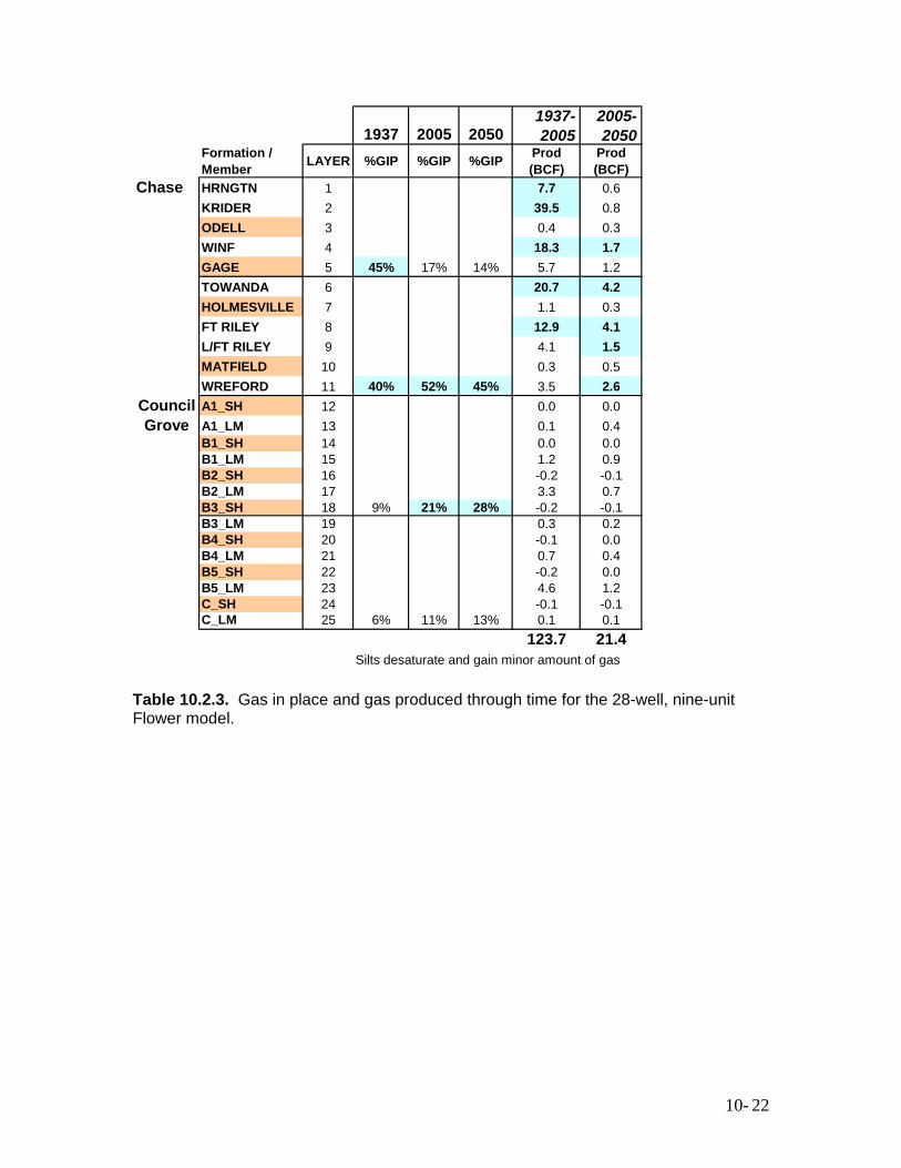
1937 2005 20501937-2005

2005-2050

Formation / Member LAYER %GIP %GIP %GIP Prod

(BCF)Prod (BCF)

Chase HRNGTN 1 7.7 0.6KRIDER 2 39.5 0.8ODELL 3 0WINF 4 18.3 1.7GAGE 5 45% 17% 14% 5.7 1.2TOWANDA 6 20.7 4.2HOLMESVILLE 7 1FT RILEY 8 12.9 4.1L/FT RILEY 9 4 1.5MATFIELD 10 0.3 0.5WREFORD 11 40% 52% 45% 3.5 2.6

Council A1_SH 12 0.0 0.0Grove A1_LM 13 0.1 0.4

B1_SH 14 0.0 0.0B1_LM 15 1.2 0.9B2_SH 16 -0.2 -0.1B2_LM 17 3.3 0.7B3_SH 18 9% 21% 28% -0.2 -0.1B3_LM 19 0.3 0.2B4_SH 20 -0.1 0.0B4_LM 21 0.7 0.4B5_SH 22 -0.2 0.0B5_LM 23 4.6 1.2C_SH 24 -0.1 -0.1C_LM 25 6% 11% 13% 0.1 0.1

123.7 21.4Silts desaturate and gain minor amount of gas

.4 0.3

.1 0.3

.1

Table 10.2.3. Gas in place and gas produced through time for the 28-well, nine-unit Flower model.

10- 22

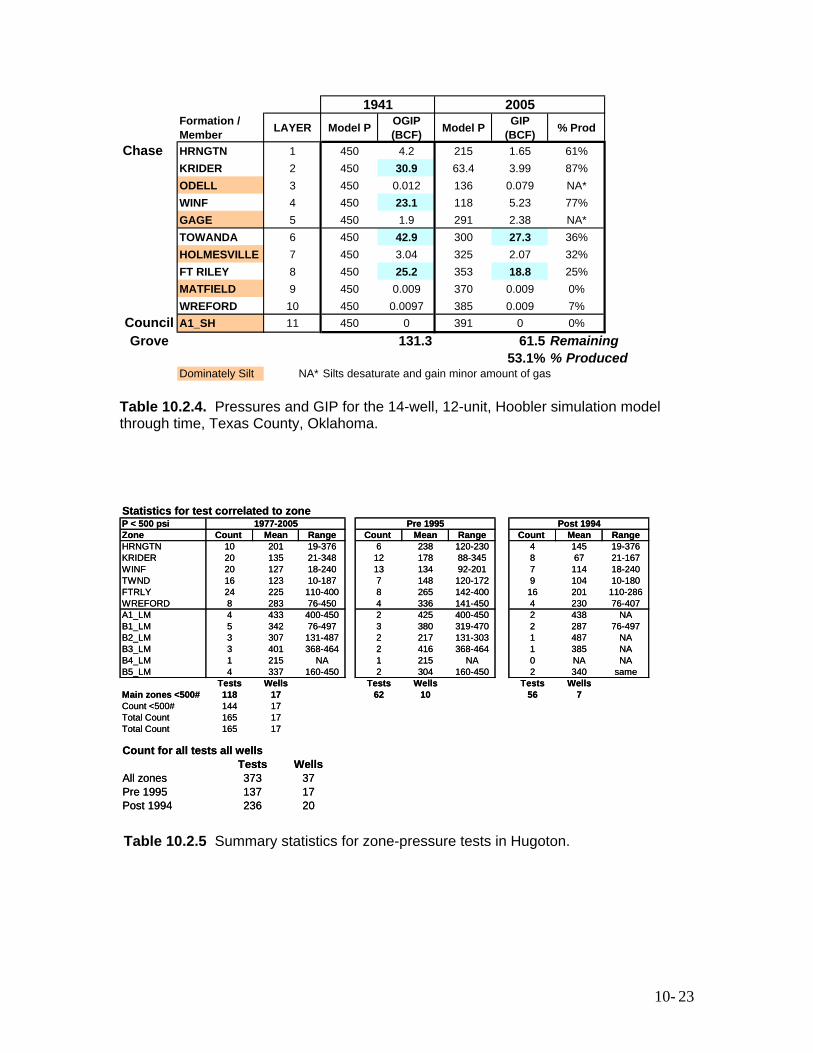
Formation / Member LAYER Model P OGIP

(BCF) Model P GIP (BCF) % Prod

Chase HRNGTN 1 450 4.2 215 1.65 61%KRIDER 2 450 30.9 63.4 3.99 87%ODELL 3 450 0.012 136 0.079 NA*WINF 4 450 23.1 118 5.23 77%GAGE 5 450 1.9 291 2.38 NA*TOWANDA 6 450 42.9 300 27.3 36%HOLMESVILLE 7 450 3.04 325 2.07 32%FT RILEY 8 450 25.2 353 18.8 25%MATFIELD 9 450 0.009 370 0.009 0%WREFORD 10 450 0.0097 385 0.009 7%

Council A1_SH 11 450 0 391 0 0%Grove 131.3 61.5 Remaining

53.1% % ProducedDominately Silt NA* Silts desaturate and gain minor amount of gas

20051941

Table 10.2.4. Pressures and GIP for the 14-well, 12-unit, Hoobler simulation model through time, Texas County, Oklahoma.

Count for all tests all wellsTests Wells

All zones 373 37Pre 1995 137 17Post 1994 236 20

Statistics for test correlated to zoneP < 500 psiZone Count Mean Range Count Mean Range Count Mean RangeHRNGTN 10 201 19-376 6 238 120-230 4 145 19-376KRIDER 20 135 21-348 12 178 88-345 8 67 21-167WINF 20 127 18-240 13 134 92-201 7 114 18-240TWND 16 123 10-187 7 148 120-172 9 104 10-180FTRLY 24 225 110-400 8 265 142-400 16 201 110-286WREFORD 8 283 76-450 4 336 141-450 4 230 76-407A1_LM 4 433 400-450 2 425 400-450 2 438 NAB1_LM 5 342 76-497 3 380 319-470 2 287 76-497B2_LM 3 307 131-487 2 217 131-303 1 487 NAB3_LM 3 401 368-464 2 416 368-464 1 385 NAB4_LM 1 215 NA 1 215 NA 0 NA NAB5_LM 4 337 160-450 2 304 160-450 2 340 same

Tests Wells Tests Wells Tests WellsMain zones <500# 118 17 62 10 56 7Count <500# 144 17Total Count 165 17Total Count 165 17

1977-2005 Pre 1995 Post 1994

Count for all tests all wellsTests Wells

All zones 373 37Pre 1995 137 17Post 1994 236 20

Statistics for test correlated to zoneP < 500 psiZone Count Mean Range Count Mean Range Count Mean RangeHRNGTN 10 201 19-376 6 238 120-230 4 145 19-376KRIDER 20 135 21-348 12 178 88-345 8 67 21-167WINF 20 127 18-240 13 134 92-201 7 114 18-240TWND 16 123 10-187 7 148 120-172 9 104 10-180FTRLY 24 225 110-400 8 265 142-400 16 201 110-286WREFORD 8 283 76-450 4 336 141-450 4 230 76-407A1_LM 4 433 400-450 2 425 400-450 2 438 NAB1_LM 5 342 76-497 3 380 319-470 2 287 76-497B2_LM 3 307 131-487 2 217 131-303 1 487 NAB3_LM 3 401 368-464 2 416 368-464 1 385 NAB4_LM 1 215 NA 1 215 NA 0 NA NAB5_LM 4 337 160-450 2 304 160-450 2 340 same

Tests Wells Tests Wells Tests WellsMain zones <500# 118 17 62 10 56 7Count <500# 144 17Total Count 165 17Total Count 165 17

1977-2005 Pre 1995 Post 1994

Table 10.2.5 Summary statistics for zone-pressure tests in Hugoton.

10- 23

Zone PShapes - Core

Zone PShapes - Core

Zone PShapes - Core

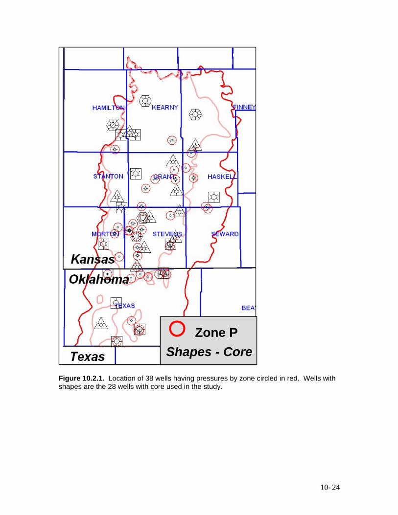
Figure 10.2.1. Location of 38 wells having pressures by zone circled in red. Wells with shapes are the 28 wells with core used in the study.

10- 24

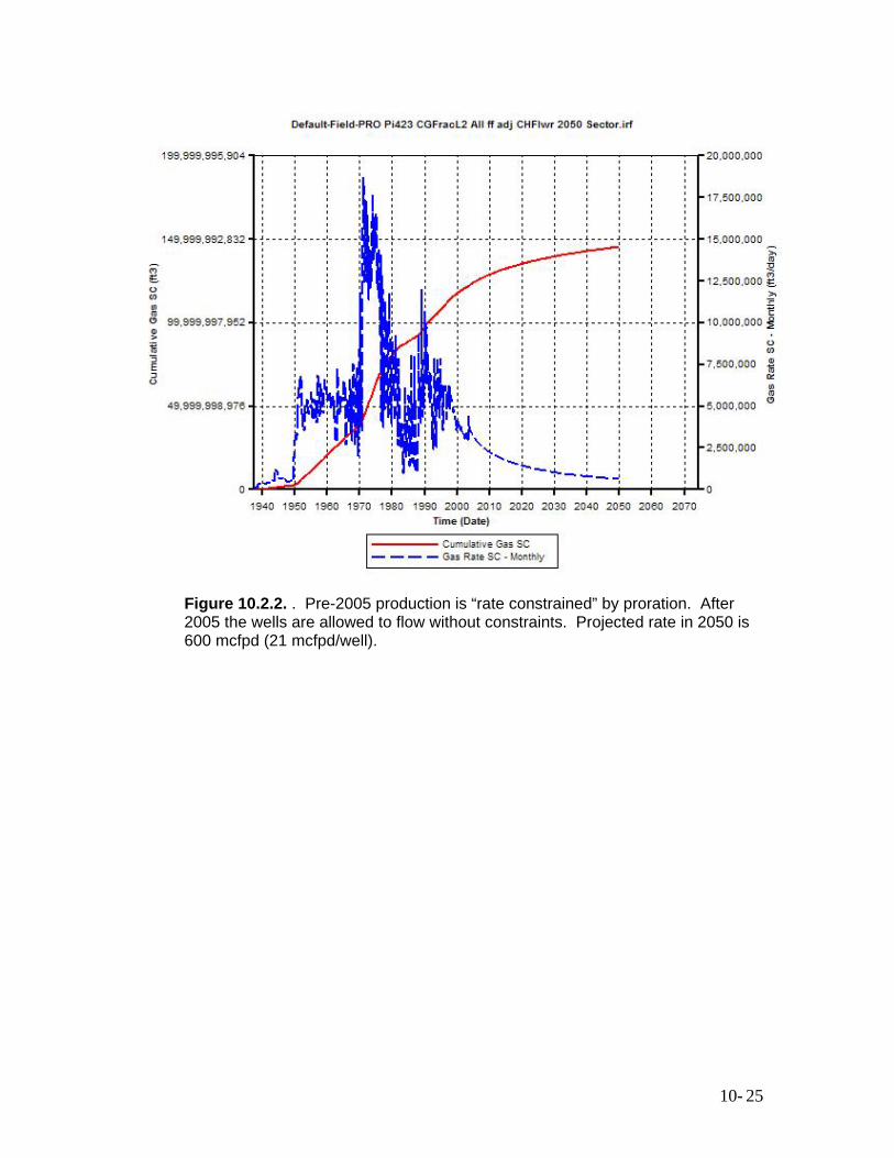
Figure 10.2.2. . Pre-2005 production is “rate constrained” by proration. After 2005 the wells are allowed to flow without constraints. Projected rate in 2050 is 600 mcfpd (21 mcfpd/well).

10- 25

Hugoton (Chase) Pressure by Zone

0

50

100

150

200

250

300

350

400

450

1975

1980

1985

1990

1995

2000

2005

2010

Year

Pres

sure

HRNGTN

Krider

WINF

Gage

TWND

FTRLY

FLRNC

WREFORD

Chase-Cmgl

Hugoton (Chase) Pressure by Zone

0

100

200

300

400

500

600

700

1975

1980

1985

1990

1995

2000

2005

2010

YearPr

essu

re

HRNGTN

Krider

WINF

Gage

TWND

FTRLY

FLRNC

WREFORD

Chase-Cmgl

Hugoton (Chase) Pressure by Zone

0

50

100

150

200

250

300

350

400

450

1975

1980

1985

1990

1995

2000

2005

2010

Year

Pres

sure

HRNGTN

Krider

WINF

Gage

TWND

FTRLY

FLRNC

WREFORD

Chase-Cmgl

Hugoton (Chase) Pressure by Zone

0

100

200

300

400

500

600

700

1975

1980

1985

1990

1995

2000

2005

2010

YearPr

essu

re

HRNGTN

Krider

WINF

Gage

TWND

FTRLY

FLRNC

WREFORD

Chase-Cmgl

Figure 10.2.3. Chase zone pressures through time by zone, 165 tests from 17 wells. Values on the pressure axis increase downward.

10- 26

Panoma (CGRV) pressure by zone

0

100

200

300

400

500

600

700

800

1990

1995

2000

2005

2010

Pres

sure

A1_SHA1_LMB1_LMB2_LMB3_LMB4_LMB5_LMD_LMCGRV Cmgl

Figure 10.2.4. Council Grove pressures through time by zone. Values on the pressure axis increase downward.

10- 27

K = 0.0001-.01Sw>70%15 largest CV

K = 0.001-.1Sw>70%10 largest CV

K = 0.0001-.01Sw>70%15 largest CV

K = 0.001-.1Sw>70%10 largest CV

Sw < 70% Sw < 70%K = 0.0001-.01Sw>70%15 largest CV

K = 0.001-.1Sw>70%10 largest CV

K = 0.0001-.01Sw>70%15 largest CV

K = 0.001-.1Sw>70%10 largest CV

Sw < 70% Sw < 70%

Figure 10.2.5 Connected cellular volumes (geobodies) from the Fort Riley with relatively low permeability and water saturation.

10- 28