Report 9, 1987

ANALYSIS OF RESERVOIR ENGINEERING DATA FROM

WELL KhG-1 KOLVIDARHOLL - ICELAND

Rusmawan H. S. Darwis

UNU Geothermal Training Programme

Nationa l Energy Authority

Grensasvegur 9

108 Reykjavik

ICELAND

Permanent Address:

PERTAMINA

Directorate of Exploration and Produc tion

Geothermal Division

Jalan Kramat Raya 59

Jakarta

INDONESIA

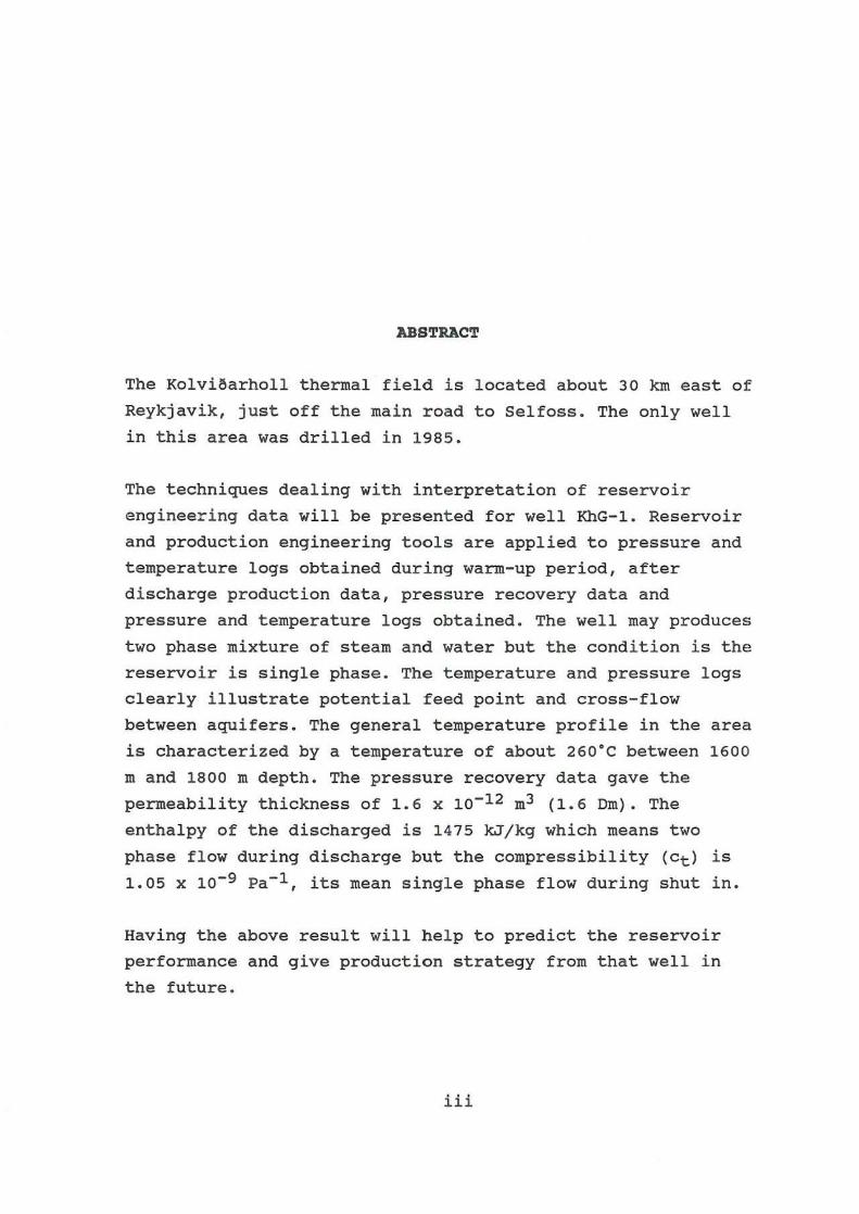
ABSTRACT

The Kolviaarholl thermal field is located about 30 km east of

Reykjavik, just off the main road to Selfoss. The only well

in this area was drilled in 1985.

The techniques dealing with interpretation of reservoir

engineering data will be presented for well KhG-l. Reservoir

and production engineering tools are applied to pressure and

temperature logs obtained during warm-up period, after

discharge production data, pressure recovery data and

pressure and temperature logs obtained. The well may produces

two phase mixture of steam and water but the condition is the

reservoir is single phase . The temperature and pressure logs

clearly illustrate potential feed point and cross-flow

between aquifers. The general temperature profile in the area

is characterized by a temperature of about 260·C between 1600

m and 1800 m depth. The pressure recovery data gave the

permeability thickness of 1.6 x 10-12 m3 (1.6 Dm) . The

entha1py of the discharged is 1475 kJ/kg which means two

phase flow during discharge but the compressibility (Ct) is

1.05 x 10-9 pa-1 , its mean single phase flow during shut in.

Having the above result will help to predict the reservoir

performance and give production strategy from that well in

the future .

iii

iv

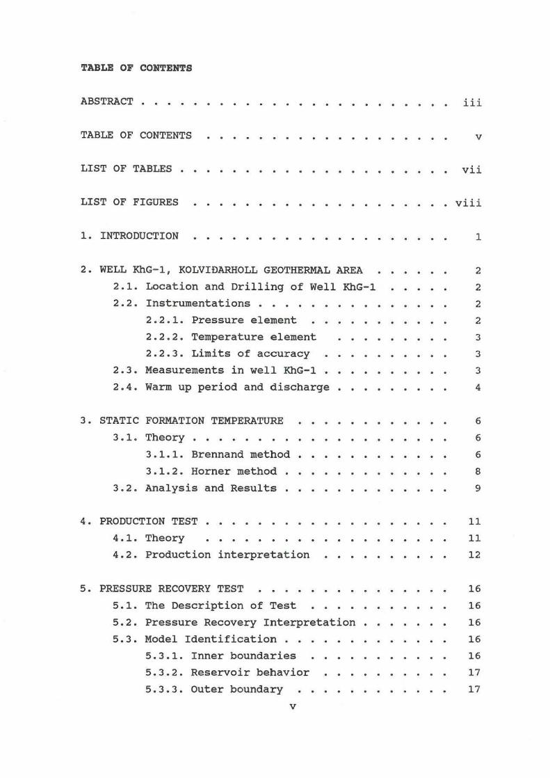
TABLE OF CONTENTS

ABSTRACT . . . . • . . . . . . . . . . . . . . . . . . .

TABLE OF CONTENTS . . . . . . . . . . . . . . . . . . .

LIST OF TABLES

LIST OF FIGURES . . . . . . . . . . . . . . . . . . . .

1. INTRODUCTION . . . . . . . . . . . . . . . . . . . .

2. WELL KhG- 1, KOLVIDARHOLL GEOTHERMAL AREA

2.1 . Location and Drilling of Well KhG-l

2.2. Instrumentations . . . .

2 . 2.1 . Pressure element

2.2.2. Temperature element

2.2.3. Limits of accuracy

2 . 3 . Measurements in well KhG-l

2.4. Warm up period and discharge

3. STATIC FORMATION TEMPERATURE

3 . 1. Theory . . . . . . • .

3 . 1 . 1. Brennand method

3.1.2 . Horner method

3.2. Analysis and Results

4. PRODUCTION TEST .

4.1 . Theory

4.2 . Production interpretation

5 . PRESSURE RECOVERY TEST

5.1 . The Description of Test

5.2 . Pressure Recovery Interpretation

5 . 3. Model Identification . ..

5.3.1. Inner boundaries

5 . 3 . 2. Reservoir behavior

5.3 .3 . Outer boundary

v

iii

v

vii

viii

1

2

2

2

2

3

3

3

4

6

6

6

8

9

11

11

12

16

16

16

16

16

17

17

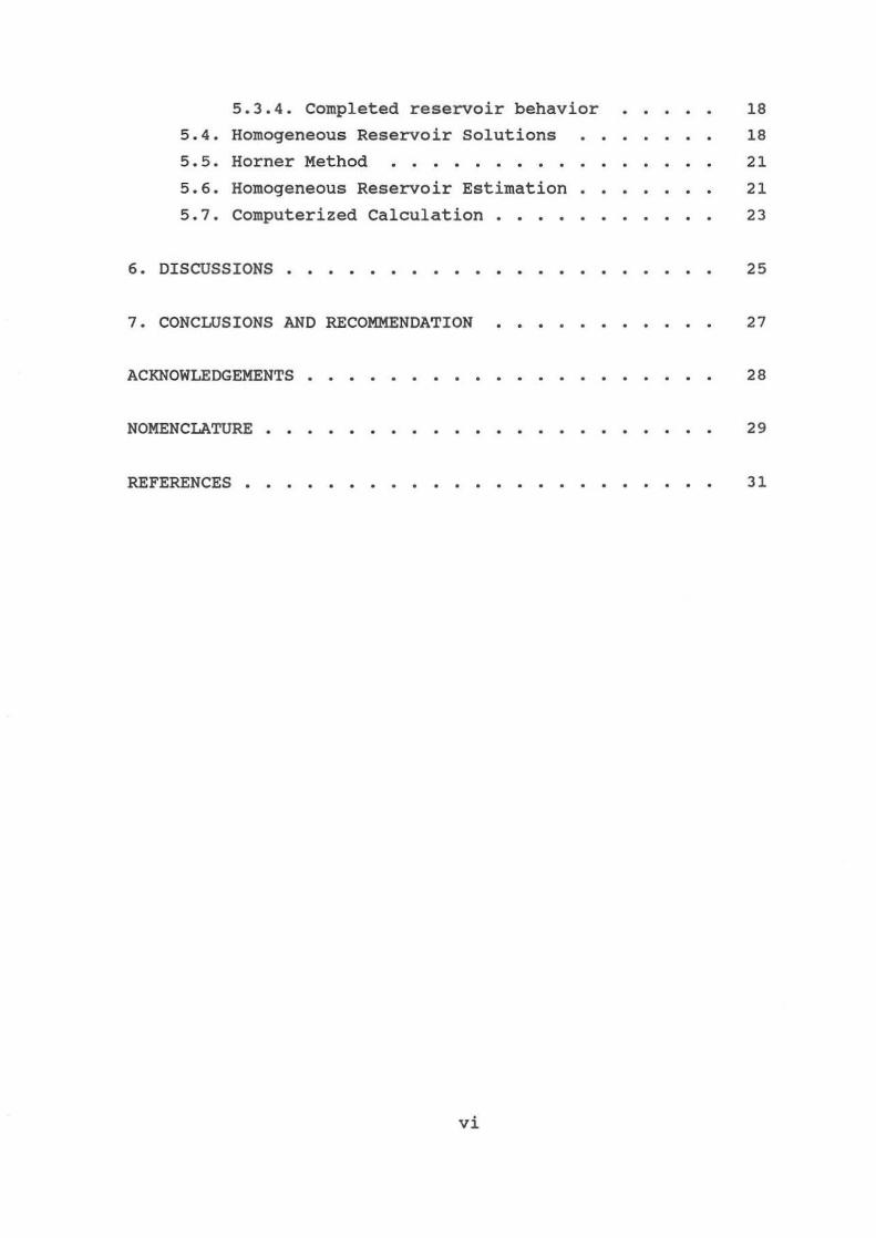
5.3.4. Completed reservoir behavior

5.4. Homogeneous Reservoir Solutions

5.5. Horner Method . ....... .

5.6. Homogeneous Reservoir Estimation

5.7. Computerized Calculation .. . .

18

18

21

21

23

6. DISCUSSIONS. • • • • • • • • • • • • • • • • • • •• 25

7. CONCLUSIONS AND RECOMMENDATION 27

ACKNOWLEDGEMENTS • • • • • • • • • • • • • • • • • • •• 28

NOMENCLATURE • • • • • • • • • • • • • • • • • • • • •• 29

REFERENCES • • • • • • • • • • • • • • • • • • • • • •• 31

vi

LIST OF TABLBS

Table. 1

Table. 2

Temperature and pressure gradient data .. .

Kolvi~arholl well KhG-l, pressure recovery

at 1400 m. Table. 3 Automate result.

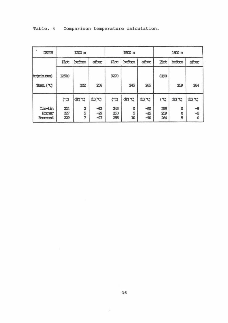
Table. 4 Comparison temperature calcul ation.

Table. 5 KhG-l /Early data by using automate.

Table. 6 KhG-l fAl l data by using automate.

Table. 7 KhG-l /Late data by using automate.

vii

33

34

35

36

37

38

39

LIST OF FIGURES

Figure. 1 Vestur Hengill (Kolvi&arholl Geothermal)

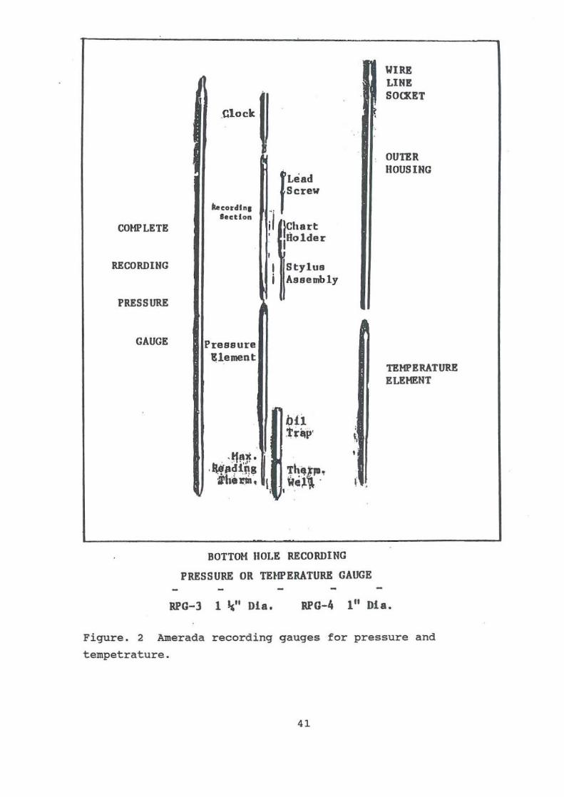
area. 40 Figure. 2 Amerada recording gauges for pressure and

tempetrature. . . . . . . . . . . . . . . . 41

Figure. 3 Cross sections of Arnerada pressure and

temperature. ..... .......... 42

Figure . 4 Kolvi&arholl KhG-l. Temperature 1,2,3,4 and 5

profiles . . . . . . . . . 43

Figure. 5 Kolvi&arholl KhG-l. Pressure 1,3 and 4

profiles. . . . . . . . . 44 Figure. 6 Kolvi&arholl KhG-l. Temperature 6,7 and 8

profiles. . . . . . . . . 45

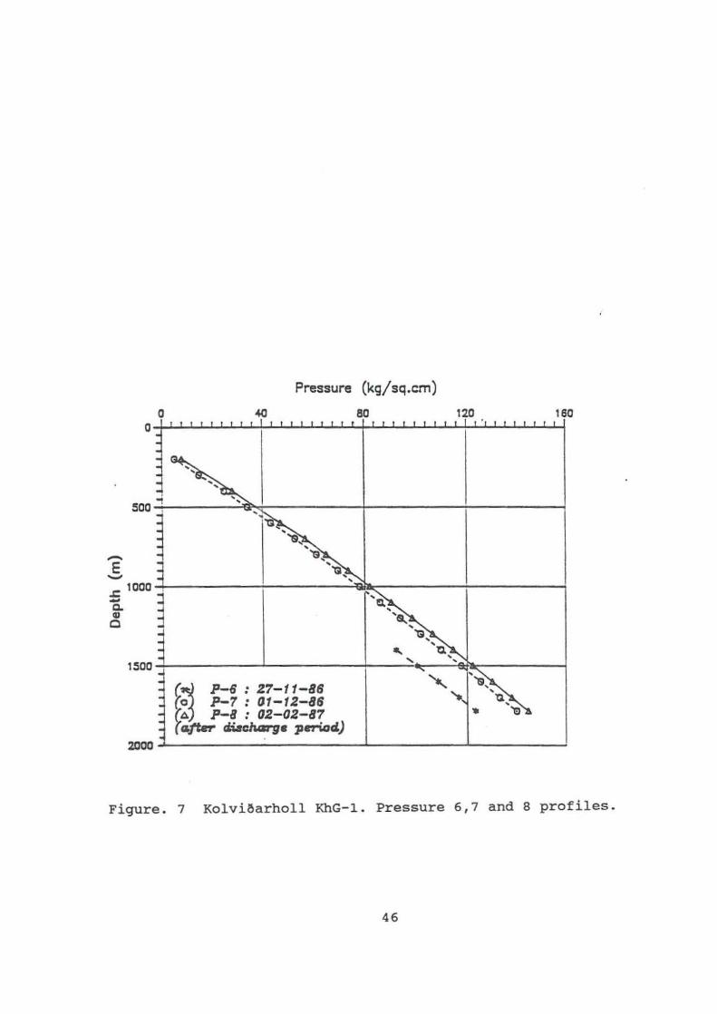
Figure. 7 Kolvi&arholl KhG-l. Pressure 6,7 and 8

profiles. . . . . . . . . . . . . . . . . . . 46

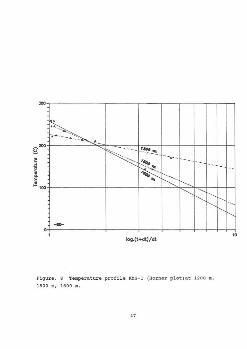
Figure. 8 Temperature profile KhG-1 (Horner plot)at

1200 m, 1500 m, 1600 m. . 47

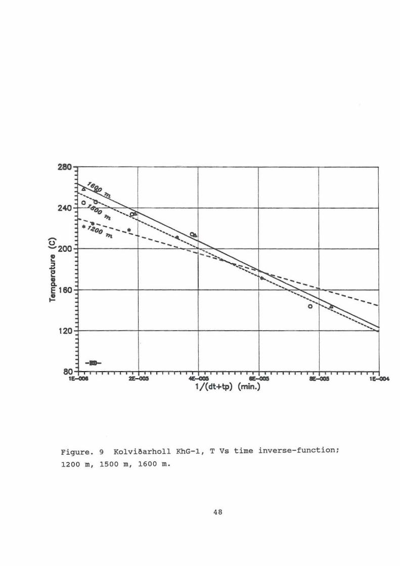
Figure. 9 Kolvi&arholl KhG-l, T Vs time inverse-

function: 1200 rn, 1500 rn, 1600 m ...... . 48

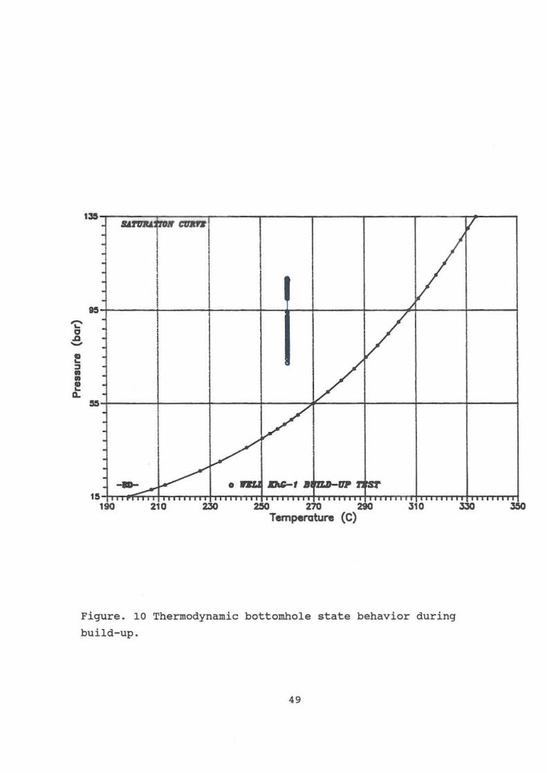
Figure . 10 Thermodynamic bottomhole state behavior

during build-up. . . . • ....•. 49

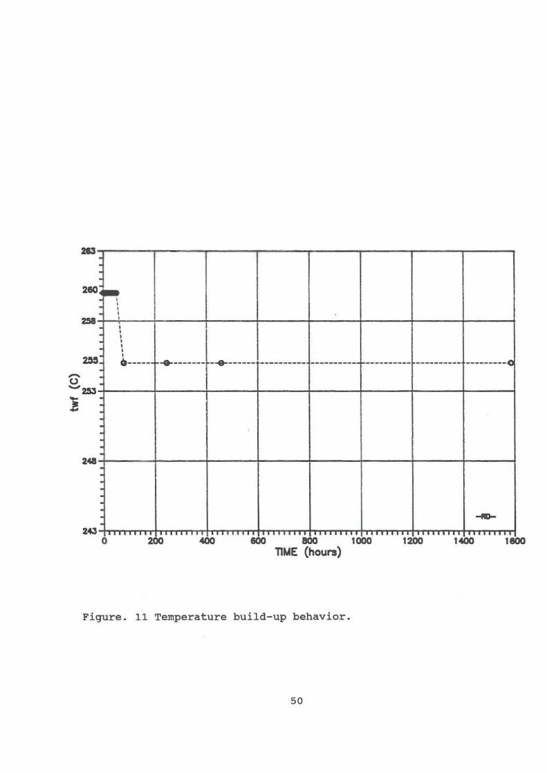
Figure . 11 Temperature build-up behavior. 50

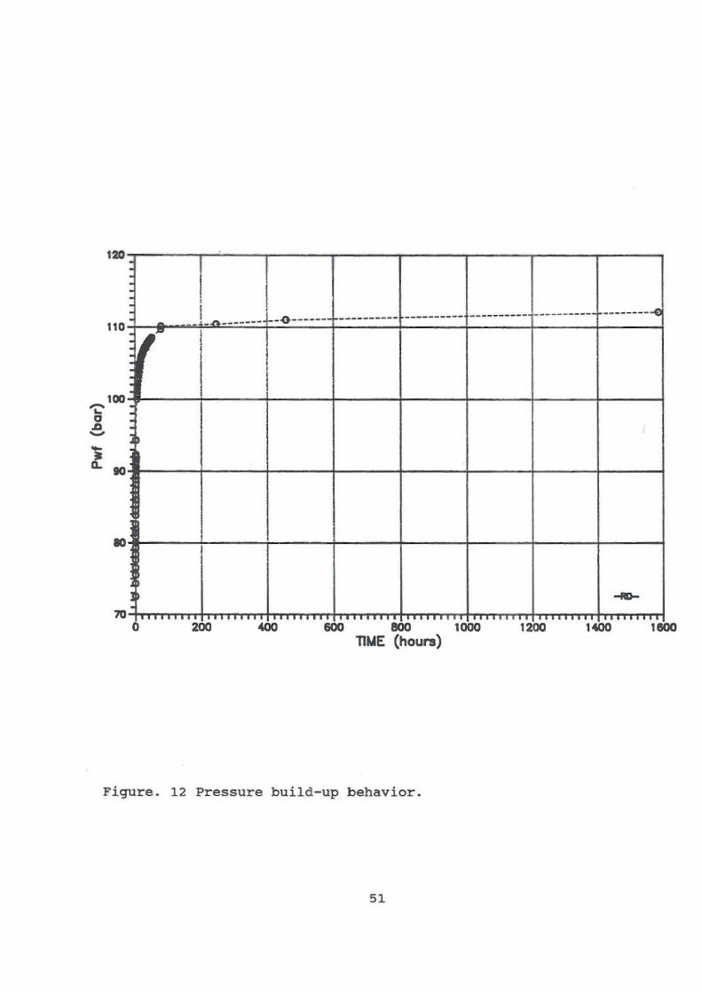
Figure . 12 Pressure build-up behavior. 51

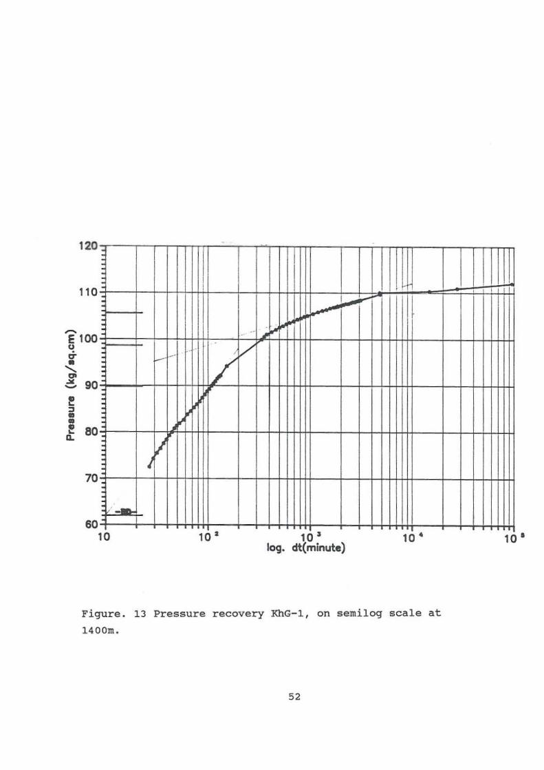
Figure . 13 Pressure recovery KhG-l, on semilog scale at

1400m. •. • ... • . • ........... 52

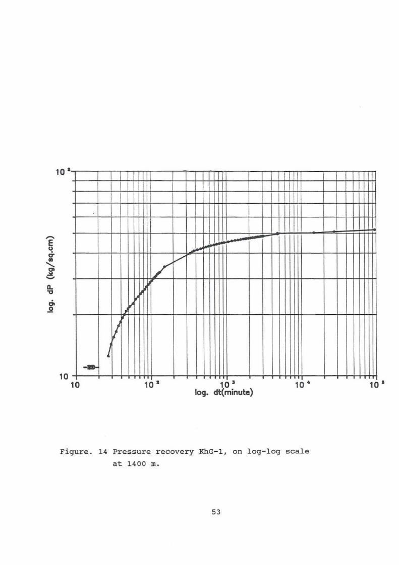
Figure . 14 Pressure recovery KhG-l, on log-log scale

at 1400 m. •.•... • ....... • 53

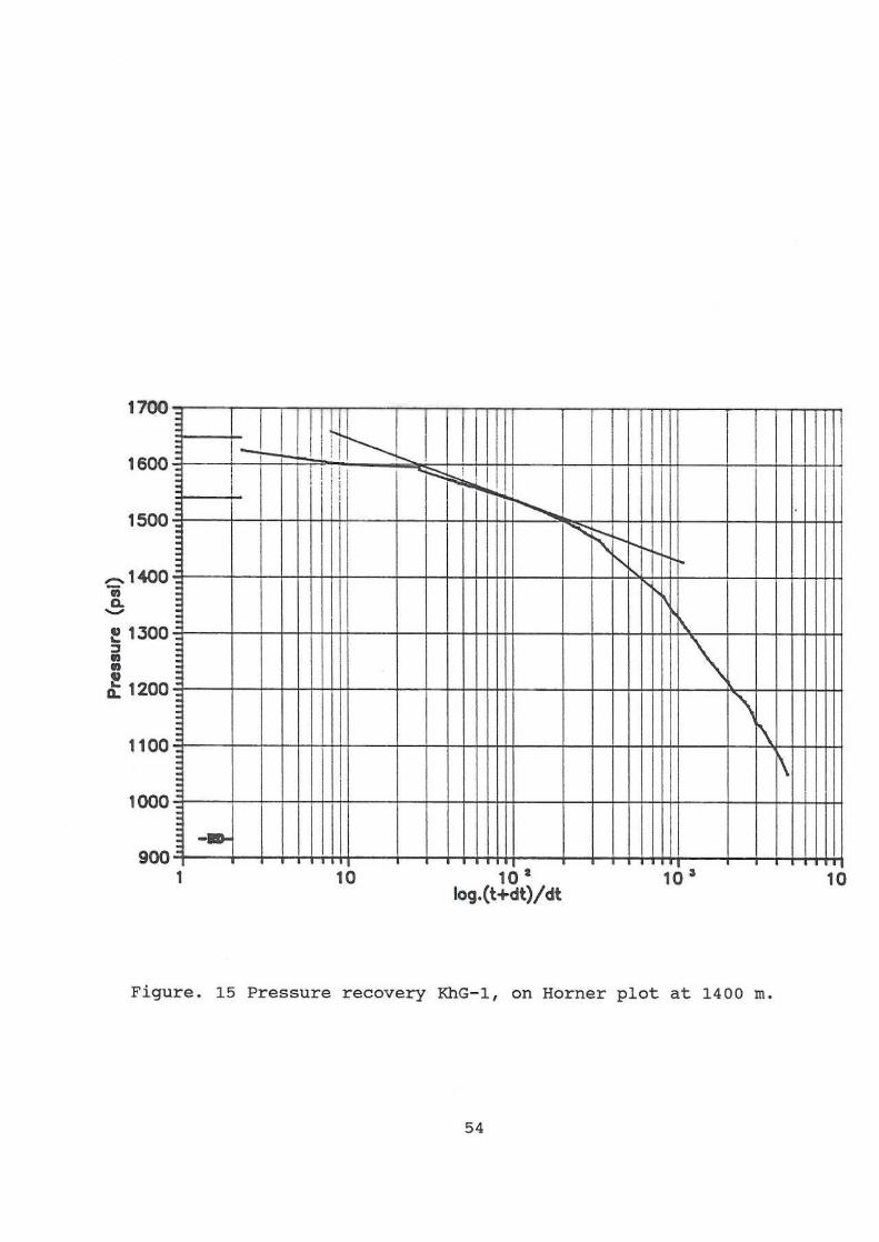
Figure . 15 Pressure recovery KhG-l, on Horner plot at

1400 m. . . . . . . .. . .. • .. . ..

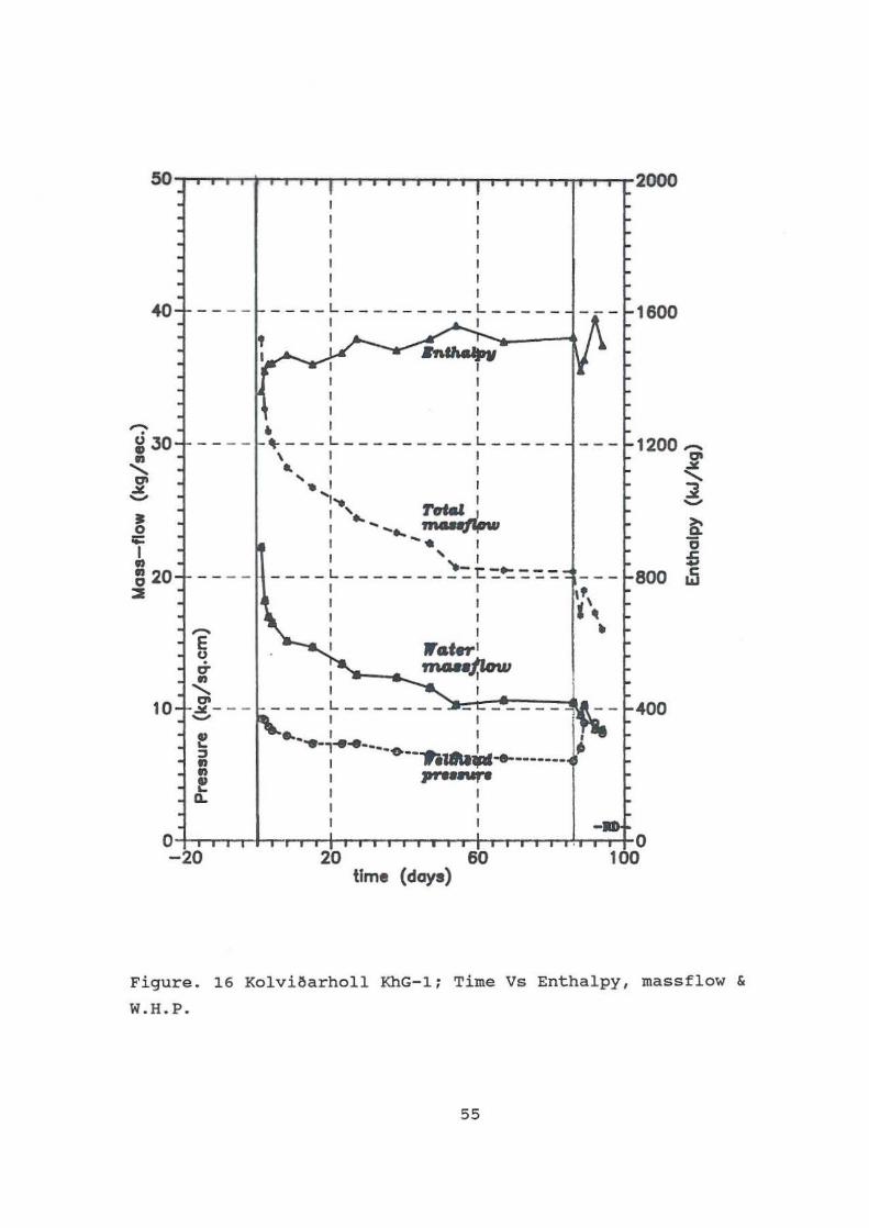
Figure. 16 Kolviearholl KhG-li Time Vs Enthalpy,

massflow & W.H.P .....

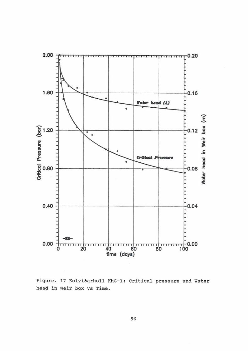
Figure. 17 Kolviearholl KhG-l; critical pressure and

water head in Weir box vs Time.

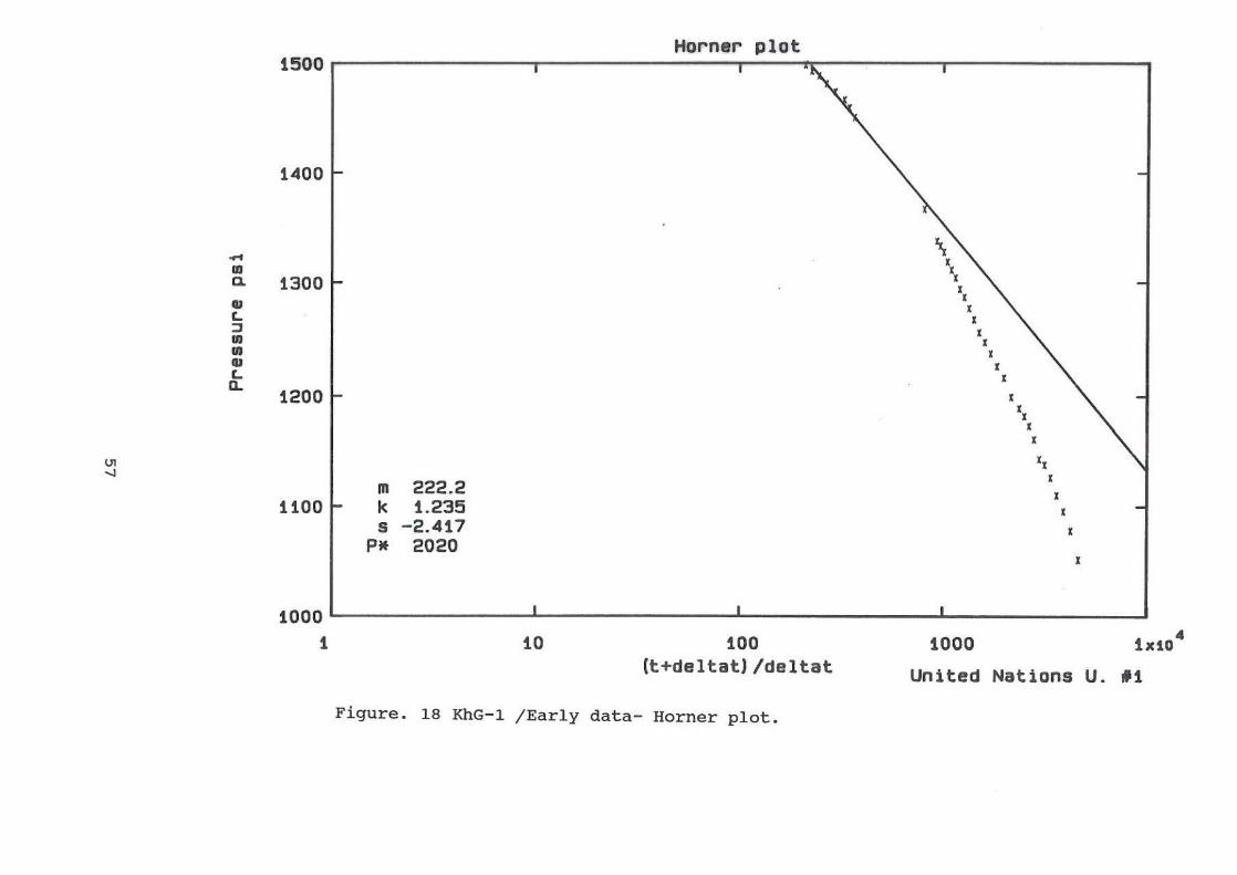
Figure. 18 KhG-1 jEarly data- Horner plot.

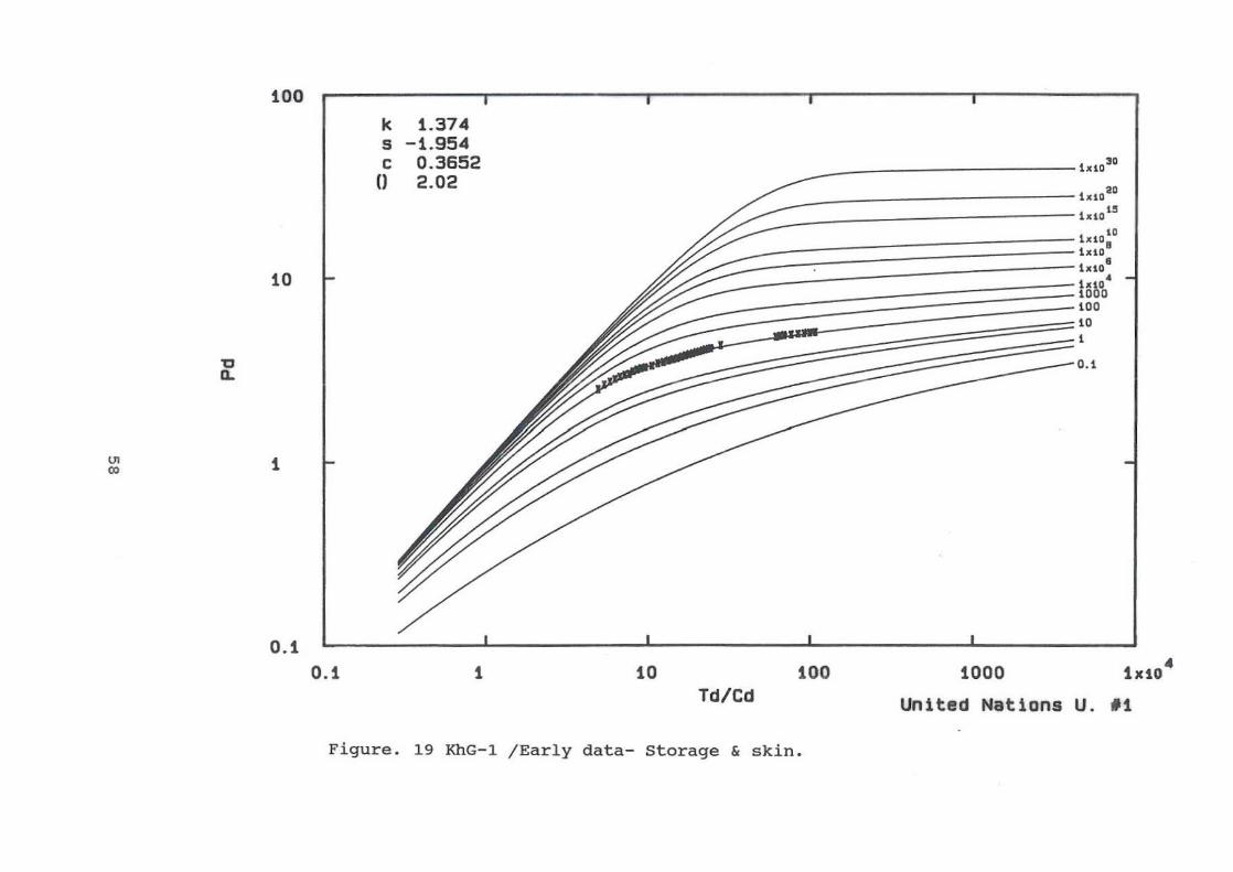
Figure. 19 KhG-l /Early data- storage & skin.

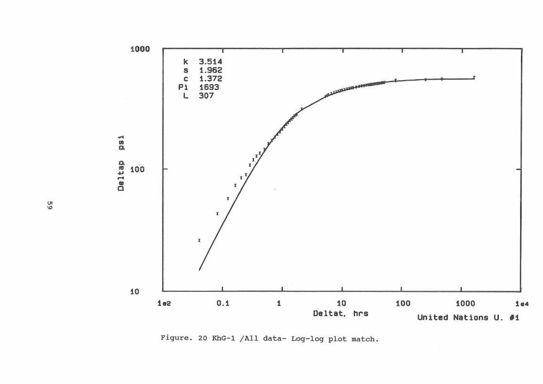
Figure. 20 KhG-1 jAll data- Log-log plot match .

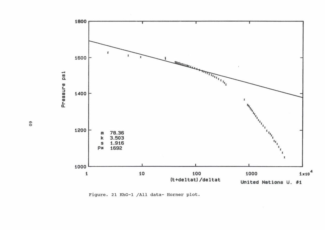
Figure. 21 KhG-1 jAll data- Horner plot.

viii

54

55

56

57

58

59

60

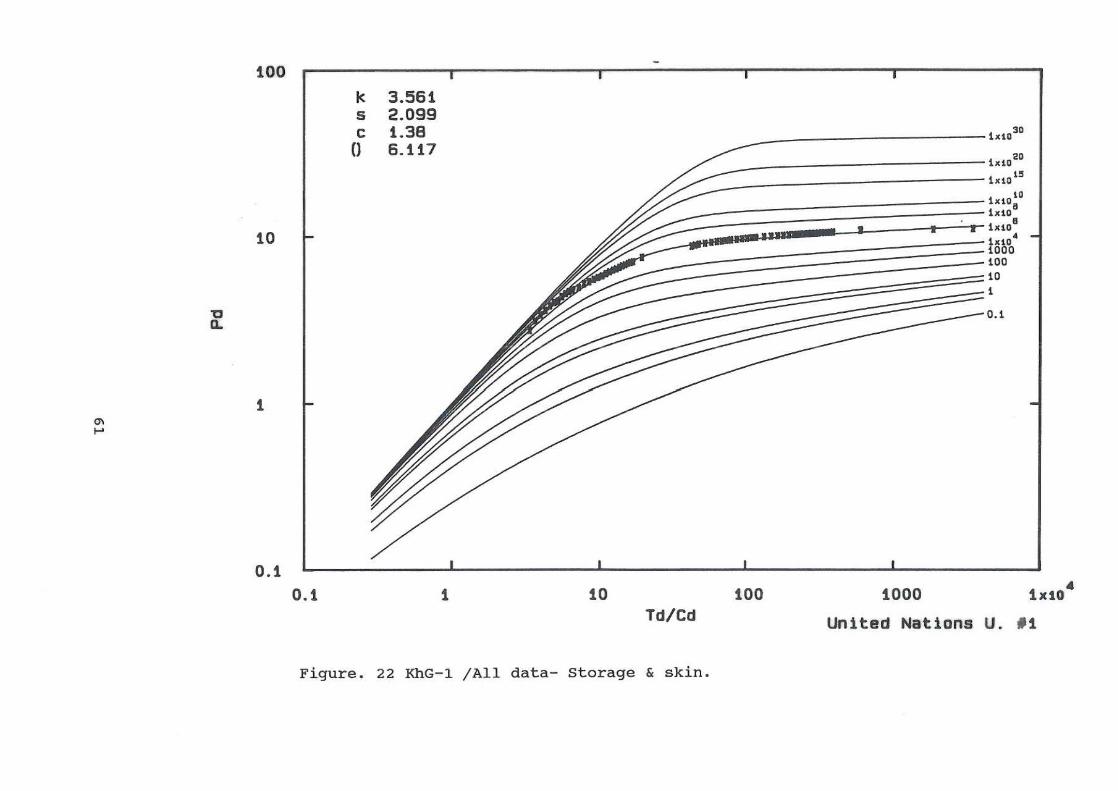
Figure. 22 KhG-1 IAll data- Storage & skin. 61

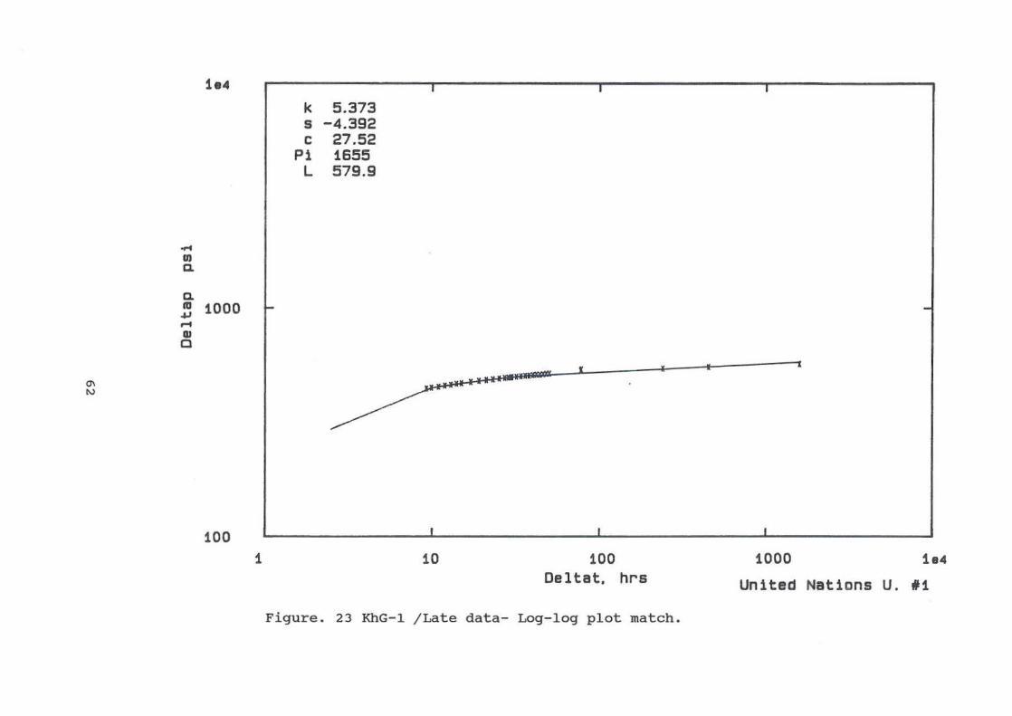
Figure . 23 KhG-1 lLate data- Log-log plot match . 62

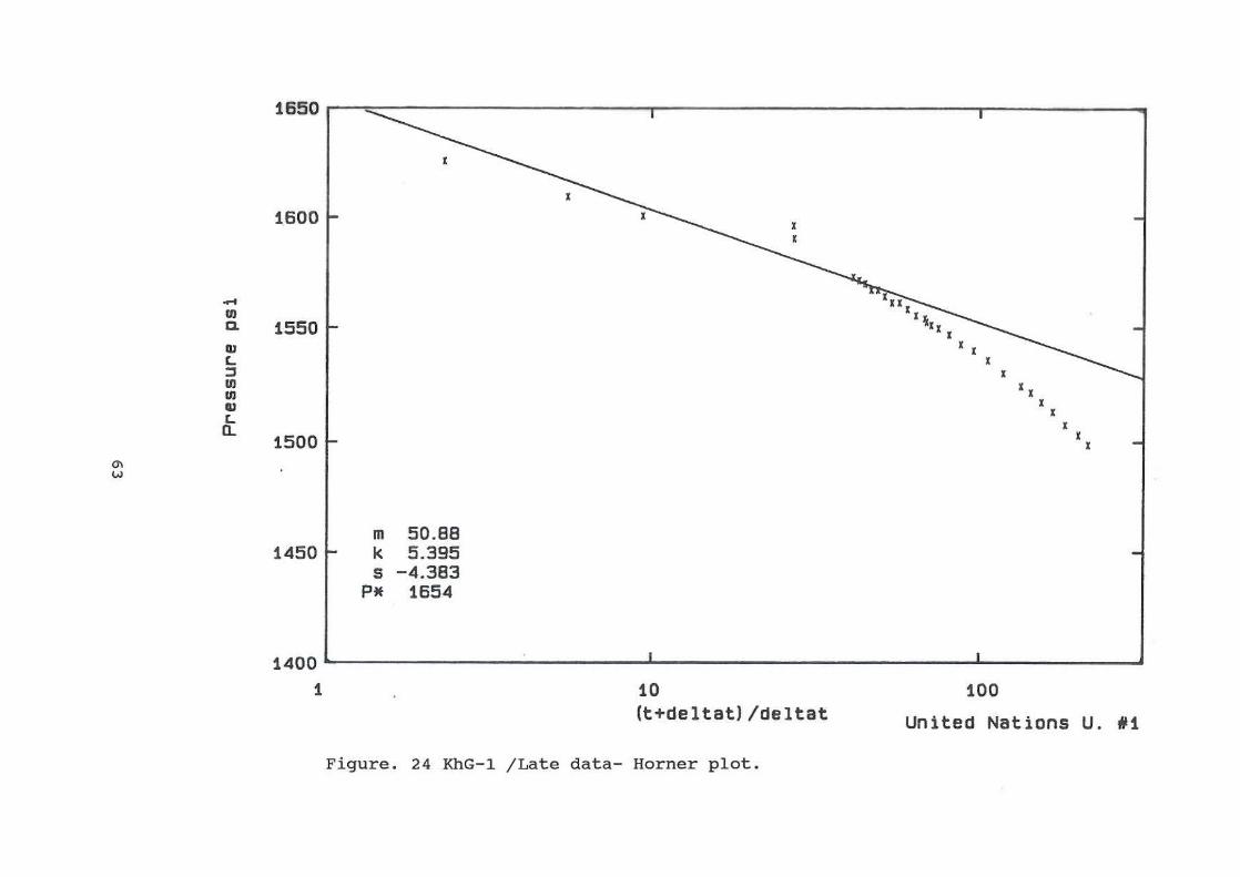
Figure . 24 KhG-1 lLate data- Horner plot. 63

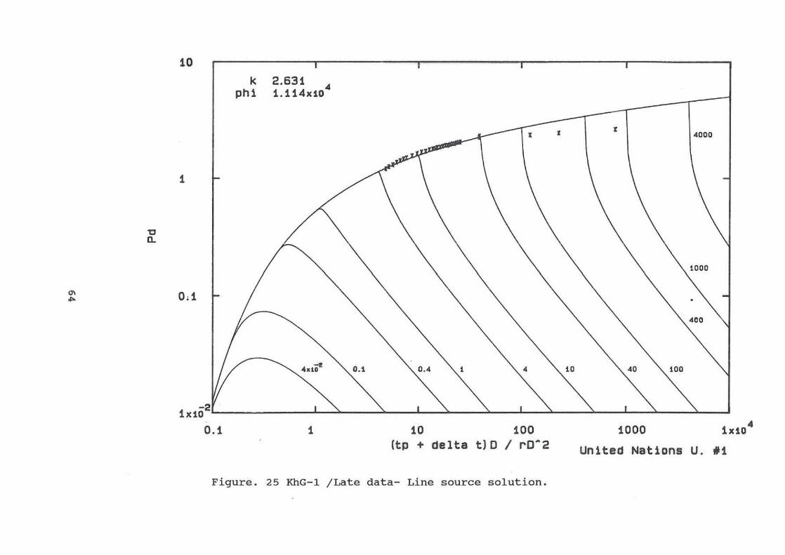
Figure . 25 KhG-1 lLate data- Line source solution. 64

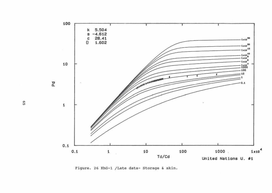
Figure. 26 KhG-1 lLate data- Storage & skin. . . . 65

ix

1. INTRODUCTION

This project report was carried out while the author was

awarded the united Nations University (UNU) Fellowship to

attend the 1987 Geothermal Training Programme at National

Energy Authority of Iceland.

The subject of this report is to interpret and in some cases

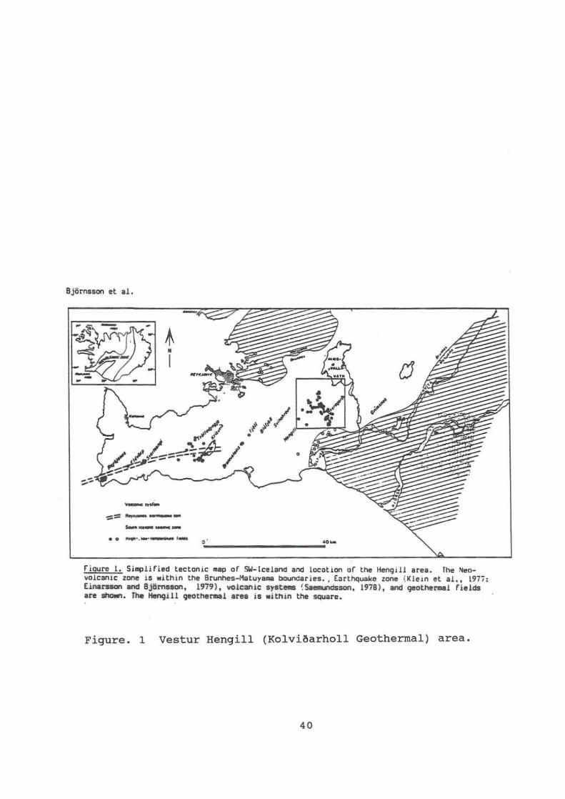
simulate various wellbore measurements carried out in the

well KhG-l in sw - Iceland (Figure. 1). The well is the first

and the only one drilled in a high temperature field located

on the southern margin of the large geothermal system,

Hengill. The Reykjavik District Heating System plants to

operate a Geothermal Power Plant under construction i n the

field and the well is drilled as a final part of a pre­

exploration survey.

Various types of tests have been applied in well KhG-l .

Downhole temperature and pressure were measured frequently in

the well during the warm up period. They are analyzed here in

order to estimate the static formation tempera ture a nd

pressure in the reservoir prior to drilling .

The pressure recovery and production tests were obtained

analyze the reservoir behavior . The results obtained from

those tests give an idea of the reservoir properties, i.e

average value of transmissivity in the drainage well volume,

storage and mean reservoir pressure. They can be used to

predict the well behavior, i . e to indicate whether as the

well is damaged or stimulated and to tell if the shape of

reservoir is homogeneous or heterogeneous . They can help in

making a decision to drill another well or if this well can

produce in the future .

1

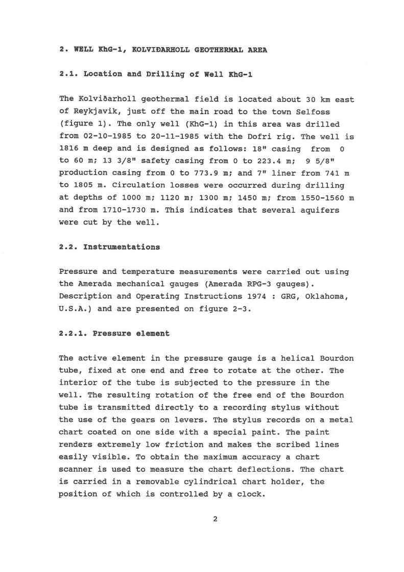
2. WELL KhG-l, KOLVIDARHOLL GEOTHERMAL AREA

2.1. Location and Drillinq of Well KhG-l

The Kolviaarholl geothermal field is located about 30 km east

of Reykjavik, just off the main road to the town Selfoss

(figure 1). The only well (KhG-1) in this area was drilled

from 02-10-1985 to 20-11-1985 with the Dofri rig. The well is

1816 ID deep and is designed as follows: 18" casing from 0

to 60 ID; 13 3/8" safety casing from 0 to 223.4 m; 9 5/8 11

production casing from 0 to 773 . 9 m; and 7" liner from 741 In

to 1805 m. Circulation losses were occurred during drilling

at depths of 1000 m; 1120 In; 1300 In; 1450 m; from 1550-1560 In

and from 1710-1730 m. This indicates that several aquifers were cut by the well.

2.2. Instrumentations

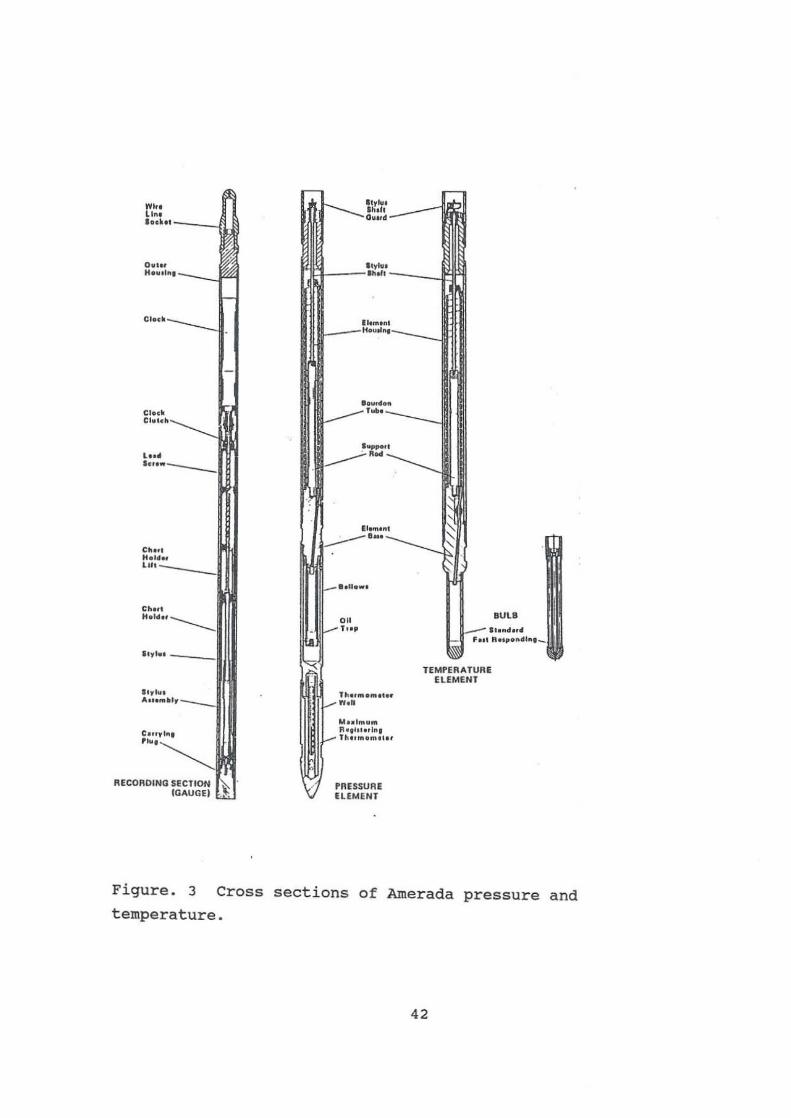
Pressure and temperature measurements were carried out using

the Amerada mechanical gauges (Amerada RPG-3 gauges).

Description and Operating Instructions 1974 : GRG, Oklahoma,

U.S . A.) and are presented on figure 2-3.

2.2.1. Pressure element

The active element in the pressure gauge is a helical Bourdon

tube, fixed at one end and free to rotate at the other. The

interior of the tube is subjected to the pressure in the

well. The resulting rotation of the free end of the Bourdon

tube is transmitted directly to a recording stylus without

the use of the gears on levers. The stylus records on a metal

chart coated on one side with a special paint. The paint

renders extremely low friction and makes the scribed lines

easily visible. To obtain the maximum accuracy a chart

scanner is used to measure the chart deflections. The chart

is carried in a removable cylindrical chart holder, the

position of which is controlled by a clock.

2

2.2.2. Temperature element

For the temperature element the pressure is developed inside

the Bourden tube, and inside a connecting reservoir at the

bottom of the element which is in direct contact with the

well fluids, by a volatile liquid. The vapor pressure of the

enclosed liquid is directly related to its temperature,

making the rotated position of the free end of the Bourdon

tube an usable measure of the temperature of the element.

This rotation is recorded on the gauge chart as described above.

2.2.3. Limits of accuracy

The repeatability of a properly maintained gauge is better

than 0 . 1 % of full range of the pressure element in use,

while the absolute accuracy is 0 . 2 t . Temperature above 79°C

affect the strength of most Bourdon tubes, so calibrations at

temperature above this are necessary to maintain the accuracy

of the instrument . The sensitivity of the gauge is 0.2 % of the full scale deflection.

The absolute accuracy of the temperature gauge is usually

assumed to be 1°C and is related to the calibration and the

operation of the instruments. The sensitivity depends on the

span of the temperature element and whether the temperature

being measured is in the lower or upper part of the span .

2.3. Measurements in well KhG-l

Well KhG-l was drilled in order to estimate the reservoir

conditions and properties of the Vestur Hengill geothermal

field . A series of wellbore measurements were therefore

carried out, both during the warm up period, during discharge

and after shut in . The measurements made are :

3

a) Temperature, pressure and water level measurements

during warm up period (from November, 1985 to August, 1986).

b) Wellhead pressure, massflow and total enthalpy during

production (August-November, 1986).

c) Temperature and pressure recovery at 1400 m depth after shut in.

d) Several downhole pressure and temperature logs (November

1986 - February, 1987).

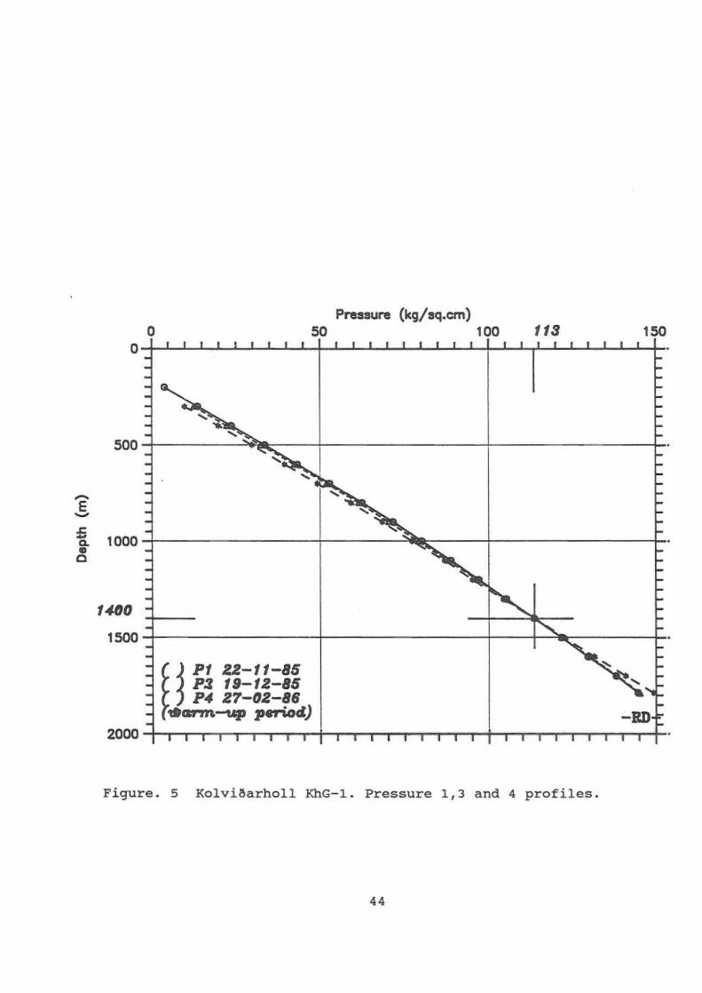
Pressure and temperature logs give important information

about reservoir conditions such as location of aquifers,

reservoir pressure and temperature variations with depth and

heat flow. The repeated pressure logs before and after

discharge give the pressure response of the reservoir due to

production but also the location of major feedzones. They can

give the phase conditions of the reservoir fluid and the

fluid in the well, and the performance of the well . The

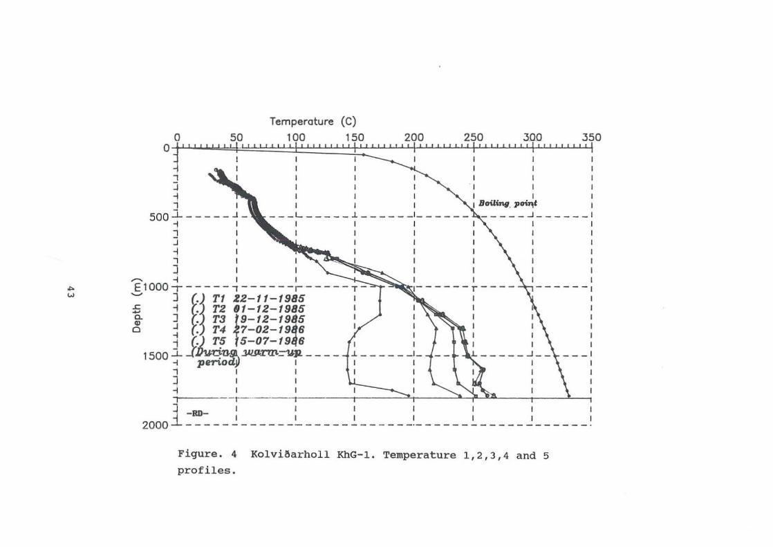
reservoir pressure was about 113 kg/cm2 at 1400 m (figure 5),

and the maximum temperature is about 260·C at 1600-1800 m

depth (figure 4).

2.4. Warm up period and discharge

The temperature and pressure data from the warm up period

showed that relatively cold water zone extended from 200-700

m depth in the well (T < 100 · C). These thermodynamic

conditions were far from saturation and implied that

stimulation methods were necessary to initiate discharge from

the well. Therefore the same stimulation technique was

applied in the well KhG-1 as has been used to initiate

discharge in wells NG-7, NG-10, and NJ-12 at the Nesjavellir

field. Air was pumped into well under 30-40 bar pressure from

July 30th , 1986 to August 25th , 1986. At 14.00 o'clock on

August 25th , 1986 the well was ready to be discharged. Then

master valve was fully opened and a piston was lowered into

the well until it was 10-20 m below water level. The piston

lower then water level in the well. Warmer water could then

4

enter to the well and heat it up to boiling. After 18 cycles

of pulling out the piston, water-steam mixture pulsed out of

the well, and full discharge was obtained after 20 periods of pulling the piston . The well discharged to the air for about

14 hours, but then the massflow was directed to a silencer.

On November 27, 1986 (Report OS-85100/ JHD-56B , November 1985) the well was shut in and the pressure recovery Amerada of the

well measured . Pressure instrument was lowe red to 1400 m

depth and the pressure recorded constantly for two days. The

downhole pressure and temperatures were then measured more

irregularly until February 2nd 1987, when the measurement program was finally terminated. The data is presented in

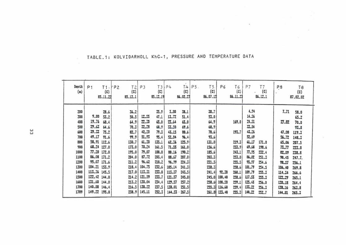
Table . 1 . Pressure and temperature data is also plotted

against the elapsed time (Figure 11 and 12) .

5

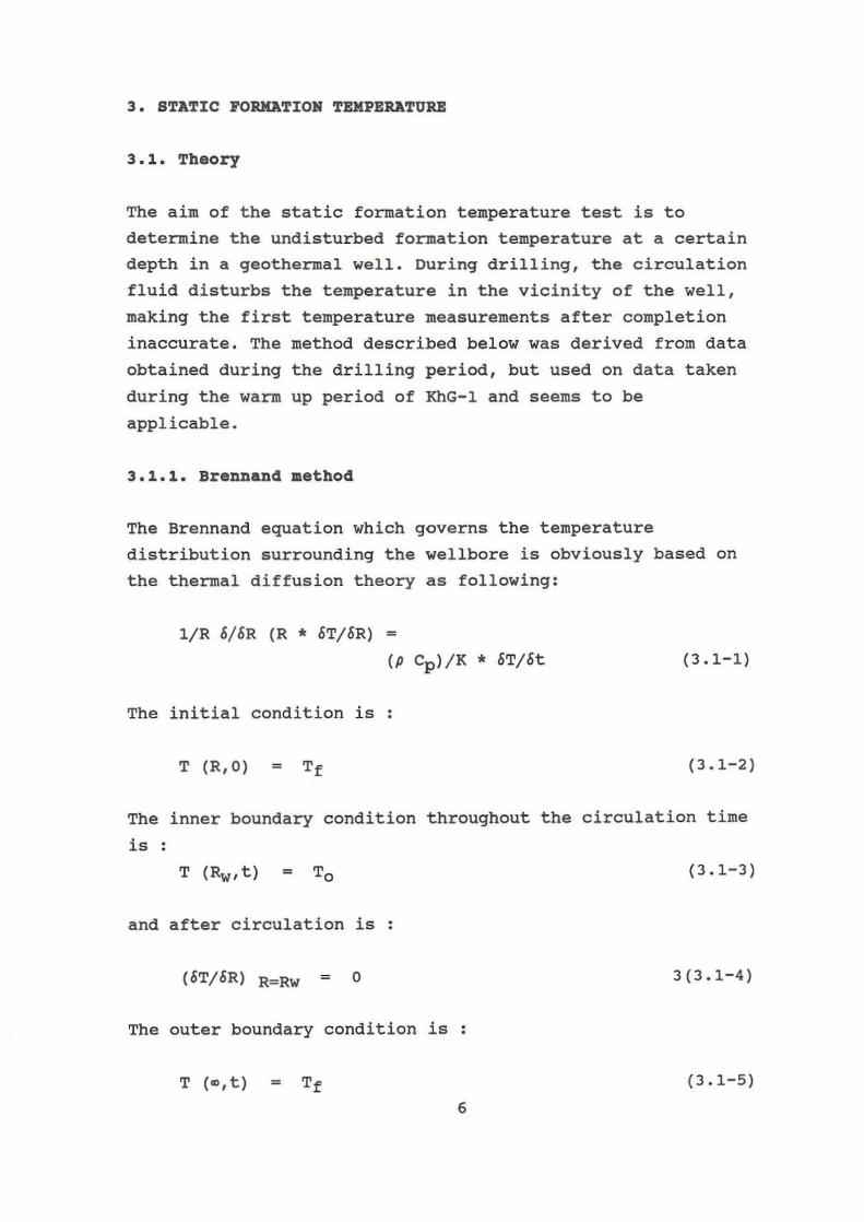
3. STATIC PORMATION TEMPERATURE

3.1. Theory

The aim of the static formation temperature test is to

determine the undisturbed formation temperature at a certain

depth in a geothermal well. During drilling, the circulation

fluid disturbs the temperature in the vicinity of the well,

making the first temperature measurements after completion

inaccurate. The method described below was derived from data

obtained during the drilling period, but used on data taken

during the warm up period of KhG-l and seems to be

applicable.

3.1.1. Brennand method

The Brennand equation which governs the temperature

distribution surrounding the wellbore is obviously based on

the thermal diffusion theory as following:

1/R 6/6R (R • 6T/6R) =

(p Cp)/K • 6T/6t (3.1-1)

The initial condition is

T (R,O) = (3.1-2)

The inner boundary condition throughout the circulation time

is :

= (3.1-3)

and after circulation is

(6T/6R) R=Rw o 3(3.1-4)

The outer boundary condition is

T (<<>, t) = (3.1-5)

6

Equation (3.1-1) and its boundary condition (3.1-2) to (3 . 1-5) are made dimensionless as follows

non dimensional radius : r = R/Rw non dimensional time: r = (tin) non dimensional temperature:

to become: 8 =

where: n = (Cp *P*Rw2 )/K

(Tf-T)/(TCTo)

«l/r)*(6/6r»«r*(68/6r»

with boundary conditions:

8 (r, 0) = 0

8 (~.r) 0

and during circulation:

8 (l,r) 1

and after circulation has ceased :

(68/6r) r =l = o

(3 . 1-6)

Transforming the problem into the Laplace space, the

resulting ordinary differential equation is solved in

conjunction with the initial and outer boundary conditions.

The solution is:

8 (r, s) B*KO* (rjs) (3.1-7)

where B is an unknown constant.

The Laplace transform in equation (3.1-7) can be inverted to

give:

(3.1-8)

which may be rewritten in dimensional form at the wellbore

as : T (Rw,t) = Tf - [<zn(Tf-T»*e-(n/4t) *(l/t))

where:

z = (B/2)

(3.1-9)

If t =tc is circulation time and time since circulation is ot,

7

equation (3.1-9) becomes:

T(Rw,t)=Tf-<zn(Tf-To»*e-<n/4(At+Ptc»*<1/(At+ptc» (3.1-10)

if n " (At+ptc )' then the equation can be simplified to :

(3.1-11)

where: m zn (Tf-To > as a constant.

Therefore a plot of temperature versus <l/(At+ptc » should

produce a straight line of slope m and intercept on formation

temperature . From the slope rn, the formation and the circul­

ation temperatures, it is possible to determine n, and hence

the thermal diffusivity (K/PCp ) of the formation, it be

required .

3.1.2. Horner method

One approach has been to use a Horner plot . The well is

cooled for a time tp is the time that formation, at the depth

under study,has been exposed to circulating fluid. This would

usually be the time since the drill bit passed the particular

depth . Then circulation is halted, and the temperature is

measured at several times et afterward. The data plotted on a

Horner plot and extrapolated to At = ~, that is for

(At+tp)/At=l to obtain an estimate of final temperature.

The validity of the Horner plot is based on the observation

that the equation for heat conduction is :

(p r) ET/Et = K V2 T (3.1-12)

i . e., the diffusion equation, which is of same form as the

pressure transient equation . This governs the cooling and

warming of the well provided that conduction is the dominant

mechanism of heat transfers . I t is not valid at any zone of

fluid loss, at any other permeable zone, or if circulation of

fluid occurs spontaneously in the wellbore past the depth

observation. i.e ., temperature is plotted versus (t+At)/At

8

3.2 . Analysis and Results

The static formation temperature was calculated at three

different depths. Based on measurement taken during the warm

up period (Table 1) at 1200 rn, 1500 m and 1600 m depth .

Horner plots was made (Figure 8) and Brennand plots (Figure

9) or T vs log «t+At)/At> and T vs <1/(tp+At» .

It can be seen from the temperature less (Figure 4) that

internal flow occurs between an aquifer at 1400 m depth and

down to an aquifer at about 1700 m depth. Due to this it is

only possible to use the temperature loss down to 1400 m

depth and the bottomhole temperature to estimate the format i on temper ature.

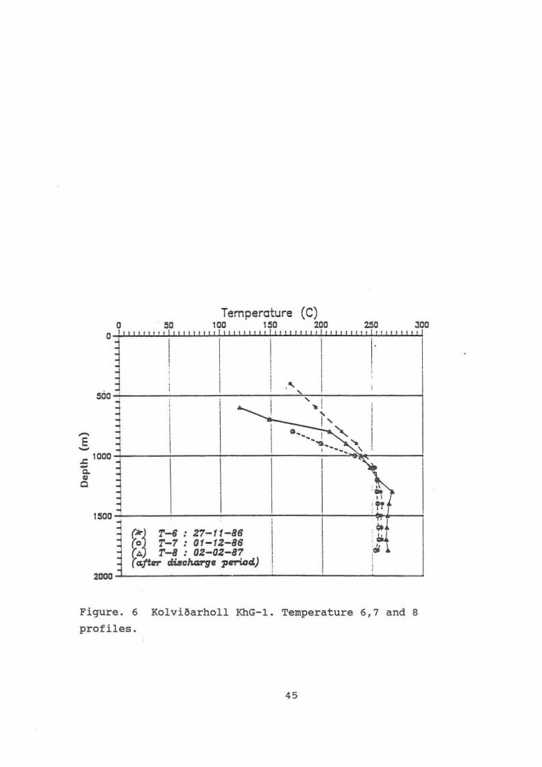
In order to get a good estimation of the reservoir

temperatures around well KhG-1, some logs were run after the

well had discharged. In that case the well was kept open

while the measurement was done. After five days of discharge

the temperature logs showed cooling above 1200 m depth . The

temperature at 1600 m depth was 264°C and the bottomhole temperature was 265°C (Table. 1).

The different between the measured temperatures after

discharge and the calculation temperature using the Horner

and the Brennands methods are also listed in Table 4. The

average difference using the Brennand method between measured

and calculated values is +7 . 3°C, but +3 . 3°C using the Horner

method, when the temperature is measured before discharge.

Using the reference temperature as the one measured after

discharge the average difference using the Brennands method is -12.3°C but - 15 . 7°C using the Horner method .

The average calculated temperature shows that the Brennand

method gives closest result to the real measured static

temperature which has smallest (6T)= -12.3°C. Therefore the

Brennand calculation is used for further predictions .

Brennand equation gives precisely maximum reservoir

temperature at a certain depth. For calculating static

9

formation temperature, the Horner equation is more able to be

used, because it gives the more accurate result. Linear­

linear plot is only capable for a rough value estimation.

Actually it will give the result of maximum temperature as seen the extrapolated temperature by using graphs.

10

4. PRODUCTION TEST

4.1. Theory

The mass flow rate and specific enthalpy of the fluid during

the discharging period (draw down), can be estimated by James

formula, as following:

Pc = Dc O.602 (T/72.2)2.195 for 1BO'C<T<350'C (4 . 1-1)

Where Pc is lip pressure (bar); Dc is inside diameter of the critical notch (m) and T is the feed temperature (·C).

Equation (4 . 1 - 1) has been confirmed in practice James (1984b)

for dry saturated steam as:

where : w is flow rate (kg/s); Dd is inside diameter of the

pipe (m) ; ho is enthalpy of the discharge (kJ/kg),

Substituting (4. 1-1) into (4.1-2) gives:

The liquid water flow rate through a V-notch (90·) weir box

is calculated by an empirical equation (ASME , 1971) :

(4 . 1-4)

where: A is the head of water (m); wl is the water flow­

rate (kg/s) ; v1 is the water specific volume (m3/kg)

The steam fraction x at atmospheric conditions is:

(4.1-5)

where : Ws is the steam flow rate (kg/s) ; ha is the specific

enthalpy of the steam+water (kJ/kg); hl is the liquid water

enthalpy (kJ/kg). Assuming that the stagnation , the steam and

11

water mixture enthalpies are equal (4.1-5) and solving for w

gives:

(4.1-6)

Finally substituting (4.1-4) to (4.1-6) gives for that total

massflow rate:

(4 . 1-7)

The two unknown variables ho and w can now be determined by

solving (4.1-3) and (4.1-7) simultaneously.

4.2. Production interpretation

Three basic parameters were measured at the surface during

the production test (the drawdown period); the wellhead

pressure Pwh, critical lip pressure Pc and head of water in

weir box. The diameter of the discharge pipe was 0.161 m.

The measured quantities were (Figure 16-17):

Pwh = 6.71 bar

Pc 1 . 00 bar

A 0.154 m

The atmospheric pressure at Kolviaarholl is 0.1 MPa, which

gives:

vI 1 . 044*10- 3 m3/kg

h1 419.1 kJ/kg

hs 2675.8 kJ/kg

~l = 2 . 79*10-4 Pa.s

The mass flow rate and the discharge enthalpy can be

calculate using equation (4 . 1-7):

12

w = 1.3345*(A2.475/V1)*(hs-h1)/(hs -ho)

w = 1 .3345*A2 . 475/(1.044*10-3 )*2256.7/(2675.8-hO)

w = 2 . 885(10)6*A2 . 475/(2675 . 8-ho )

(4 . 1-8) and (4.1-2)

By subtracting equation (4.1-8) from equation (4.1-2),

rearranging the terms we get:

R1*(2675 . 8-ho ) *Dd2 * pcO• 96 - (A2 . 475 * ho1.102) = ° where : Rl = 6.489

From the equation above, the discharge enthalpy and massflow

rate can be estimated :

ho = 1475 kJ/kg

w = 23.3 kg/s

The average discharge enthalpy of the well was 1475 kJ/kg

(Figure - 17) which is greater than the enthalpy of the water

at the maximum measured temperature in the well (about

260·C) . This indicates two-phase flow into the well . The

pressure transient analysis for two-phase inflow, should

therefore use mixture densities, viscosities and relative

permeabilities for evaluation of reservoir parameters, when

using pressure drawdown methods.

Dynamic viscosity of the mixture i s defined by Grant et.al

1982:

(4 . 2-1)

the kinematic viscosity by

(4 . 2-2)

The mixture density

13

(4.2-3)

(4.2-4)

(4.2-5)

where : x is the steam fraction; ht is total discharge

enthalpy: Hs is steam enthalpy; hw is water enthalpy; kr is

the relative permeability.

The enthalpy of the steam-water mixture is given by

substituting equation (4.2-2) to equation (4.2-6) and

rearranging to :

krl/krs = (01/05) «hs-ht)/(ht-hl»

= (01/05) * «I-x)/x>

(4.2-6)

(4.2-7)

The mixture density can be determined as follows, applying

equation (4 . 2-4) and (4 . 2-5) . The flowing enthalpy

ht = 1475 kJ/kg . From steam table: at 260'C; hs = 2796 . 4

kJ/kg; hI = 1134.9 kJ/kg; Ps = 23.7 kg/m3 ; PI = 783.9 kg/m3 ;

#1 = 104 . 8*10- 6 Pa.s; ~s = 17 . 9*10- 6 Pa.s; 01 0 . 134*10-6

m2/s ; as = 0.755*10-6 m2/s.

Thus

x = (1475 - 1134.9)/1661.5 = 0 . 205

From equation (4.2-4),

and

I/Pt = (x/PI) + «I-x)/ps>

(0.205/23.7) + (0 . 795/783 . 9)

Pt = 103.48 kg/m3

14

By using eguation (4.2-7)

krl/krs = (ul/us )*«1-x)/X>

= (0.134*10-6 )/(0.755*10-6 ) * «1-0.205)/0.205>

0.69

Assuming Grant relative permeability relation, that is krs + krs = 1, then krs = 0.59 and Krl = 0.41

By using equation (4.2-1) and (4.2-2), the dynamic viscosity

and kinematic viscosity of the mixture can be calculated;

I/Pt = (krl/~l) + (krs/~s)

= <0.41/(104.8*10-6 »+<0.59/(17.9*10-6 »

and

~t = 2.71 * 10-5 Pa.s (dynamic viscosity)

and (kinematic viscosity)

15

5. PRESSURE RECOVERY TEST

5.1. The Description of Test

A pressure recovery or pressure build-up test at well KhG-l

was carried out during a three months period . The production

lasted from August 25th , to November 27th, 1986. For the

first 86 days 132 mm diameter orifice was used but from there

off a 101 . 6 mm orifice was used. On the final day of the

production the master valve controlled the flow.

5.2. Pressure Recovery Interpretation

During pressure recovery test, the temperature and pressure

can be plotted in a diagram of clayperon. Figure 10 shows

measured pressures and temperatures during the recovery at

1400 m depth . Also marked in the figure is the saturation

curve . The figure shows that all the measured data lies in

the liquid region, hence showing that only liquid water

exists at the depth under consideration. This means that when

calculations reservoir parameters based on pressure drawdown

single phase should be assumed.

5.3. Model Identification

The model identification can be divided into inner boundary,

basic behavior and outer boundary, each one influencing each

other. By using Automate Computer Program can be determined characteristic shapes and permits identification at dominant

flow regime.

5.3.1. Inner boundaries

Early time data is identified as inner boundaries. The pressure transient data is interpreted by plotting the

pressure increment (AP) versus (At) the time from shut in

(Figure 14) . The inner boundary effect is observed at early

time with dominant effects such as wellbore storage, skin,

16

fracture and partial penetration (Gringarten 1985).

Wellbore storage is characterized by the effect of fluid

expansion inside the well giving a straight line of unit

slope in the diagnostic plot . Figure 14 , shows a slope of 1,

which indicates that wellbore storage affect the first two hours of the data.

Based on skin effect theory (Gringarten, 1985), if the skin

is positive, then the well has a steady state pressure drop

but it also indicates that the reservoir is damaged in the

walls of the well. On other hand, well KhG-1 has a negative

skin, which means the well stimulated. Figure 19, shows that

Cnexp(2S) ranges between 10-1000, that's mean well is stimulated or not damaged .

Fractures characteristic will give a straight line on a log­

log plot with one half unit slope if the fractures are very

permeable or a very low conductivity depended on one quarter

the unit slope . Unfortunately the first two hours of the data

are dominated by wellbore storage . Therefore fracture effects

are not seen in the data. It is however, likely that the well

intersects one or more fractures.

5.3.2 . Reservoir behavior

Ground water reservoirs are generally divided into two kinds

of reservoirs, homogeneous and heterogeneous (Gringarten,

1985). According to figure 18, that shows that Ap versus At

in the well KhG-l, the reservoir is homogeneous.

The temperature- pressure profile shows a single medium

conductivity affecting the well.

5.3.3 . outer boundary

An outer boundary is indicated from the late time data , either as a no flow boundary or a constant pressure boundary .

The log AP versus log At curve seems to indicates a constant

pressure boundary . By using an automate computer program,

17

this result can be determined as a constant pressure boundary

(Figure 14-20).

5.3.4. completed reservoir behavior

Completed reservoir behavior identification is performed on

early time data, infinite acting data and late time data. The

log-log behavior of the actual reservoir is simply obtained

as the super position of the individual log-log behavior of

each component of the model representing the reservoir

(Gringarten, 1985). Figure 13-20, constructed from a log At

versus AP from the drawdown test in the well KhG-1 shows the

wellbore storage performance within homogeneous reservoir

behavior and the evidence of constant pressure boundary. It

was shown in log-log curve (Figure 14-23) . From the inner

boundary, infinite acting and outer boundary data shows a

well in a homogeneous reservoir which has constant pressure

boundary.

5.4. Homogeneous Reservoir Solutions

The basic equation formulated by Earlougher (1977) describes

that an isothermal radial flow through an isotropic or

homogeneous behavior will follow the equation as below:

+l/r(oP/or)~

(~~Ct/k) (oP/ot) (5.4-1)

The equation is basically as the diffusion equation which is

assumed that the Darcian flow is slightly compressible

throughout a certain thickness will represent a small

pressure gradient. The hydraulic diffusivity performs as

(k/~ct ~) converting the solution of diffusivity equation in constant flow rate production will be confirmed as an

infinite reservoir. The solution can be displayed as:

18

Pi-P(r,t) = (qp/4~kh) <

-Ei(-~Ct~r2/4kt) (5.4-2)

where: Ei = the exponential integral. If the exponential

integral < 0.01, the equation can be showed as:

-Ei (-(~ct~r2/4kt)) =

Ln (4kt/EXp(r)~ct~r2) (5.4-3)

substituting (5.4-3) to (5.4-1) and q=wv, the equation can be

showed as:

Pi-P(r,t) = (wv~/4.kh) Ln (4kt/EXp(r)~ct~r2) (5.4-4)

if r=rwI and it produces from all the reservoir thickness

with the skin factor consideration, the equation can be:

Pwf = Pi-(wv~/4'kh) < Ln(4kt/EXp(r)~ct~rw2)+2S

dimensionless time as:

dimensionless radius as:

the dimensionless pressure can be:

(5.4 - 5)

(5 . 4-6)

(5 . 4-7)

(5.4-8)

with the skin factor consideration put into the dimensionless

the equation can be:

P(l ,te)+S = P(te) + S = (2~kh/wv~) (Pi-Pwf) (5.4-9)

sUbstitute equation (5 . 4-9) into (5.4-5), the equation can

19

be:

(5.4-10)

By using dimensionless time and radius, the equation above

can be:

P(tD) ~ 1/2 (Ln tD + 0.8091) (5.4-11)

If equation (5.4-5) would be used for solving practically,

the skin factor (S) should not be accounted as seen on

equation (5.4-10) and (5.4-11) . In case of production the useful equation is diffusivity either as dimensional or

dimensionless form. By substituting both equation (5.4-5) & (5.4-11) and based on the superposition theorem obtained

formula can be used in total drawdown-build up as the

expression following:

(5.4-12)

substitute (5.4-12) and (5.4-6), the equation can be:

(Pi-Pws) (2.kh/wv~) ~

1/2 Ln«t+ht)/ht» (5 .4-13)

arranging (5.4-13) from Ln type to log type, the equation

becomes:

0 . 1832(wv~/kh) * 1/2 Log «t+ht)/ht) (5.4-14)

when pressure is plotted vs log(t+ht)/ht (Horner method), the

result is a straight line with a slope m where:

m ~ 0.1832 (wv~/kh) (5 . 4-15)

To the skin factor (S) can be estimated by substitute

equation (5.4-9) and (5.4-14), the equation can be changed as

20

follow:

s 1 . 1513 [(Pws(t~1)-Pwf(6t~O))/m +

log (k/~ct~rw2)) - 0.3513 )

«tp+l) ftp) -

(5.4-16)

or can be determined also from (Grant, et . aI, 1982, p . 285) equation, as fo l lowing:

s ~ 1.151 [(6P/m)-log 10 (kt/~ ~ Ct r w2 )+O . 251) (5.4-17)

During pressure recovery test of well KhG-l, the pressure was

monitored by running several pressure logs in the well

(figure 5) . The pivot point was found in the cross flow

interval at 1400 m depth. Note that other feed zone at 1000 rn, 1300 rn, 1450 rn , 1525 rn, and 1725 m. The feed zone at 1450

m is the most permeable aquifer of the well. The thermal

recovery was fast below the pivot point when pumping stopped at the end of drilling.

5.5. Borner Method

The average reservoir pressure can be estimated by Horner

method . From figure 15, the late time can be extrapolated to

intersects the pressure axis. Then log«t+6t)/6t)) ~ 0 and

At )) t The late time straight line can be expressed as:

P(6t)

m log «t+6t)/6t)) (5.5-1)

So, from figure 15, the average reservoir pressure becomes:

P(~) ~ 114.9 bar

5.6 . Homogeneous Reservoir Estimation

Based on the straight line portion of figure. 15 and the

equation (5 . 4-15) above, the transmissivity can be calculated

as follows:

21

m = 113 psi/cycle

7 . 793 bar/cycle 7.793*10 5 Pa

From chapter 4.2, we can be found:

vI = 1.044*10-3 m3/kg

and

~l = 2.79 *10-4 Pa.s

m = 0.1832 (w v ~/kh)

kh 0.1832 (w v ~) /m

= 0.1832(23.3*(1.044*10-3 )2.79*10-4 )/(7.793*105 )

1.6*10-12 m3 ---(1.6 Dm) (Permeability thickness)

(kh/~t) = 1.6*10- 12 / 2.79*10-4

= 5 .7* 10-9 m3/Pa.s (Transmissivity)

The storativity can be estimated by (Grant, et. aI, 1982,

p . 285), equation as following:

~cthe-2S = 2.25 [(kh/~)*(t/r2)*10( -AP/m)]

where: (kh/~): 5.7 x 10-9 m3/pa.s

(t) 3600 second

(rw) : 0.108 m

(AP) : 39.6*105 Pa

(rn) : 7 .793*105 Pa

~ch = 2.25*[(5.7*10-9 )*[3600/(0 . 108)2]*10-(39.6/7.793)

= 3.2 * 10-8 m/Pa

(49 bar = 2 * 10-9 m/Pal

If porosity and thickness are set to ~ = 0.1 and h = 305 m

the compressibility can be estimated as following:

c = 3.2 * 10-8 / (0.1*305)

1.05 * 10-9 Pa-1

According to Grant. et al., (1982, p.5l), who tells about the

comparison of the different compressibilities as following:

22

For single phase : Cl = 1.2

Cs = 3.0

x 10-9

x 10- 7 Pa-1

Pa-1 (water)

(steam)

For two phase Ct = 1.4 x 10-6 Pa-1

So, 1.05 * 10-9 Pa-1 can be determined as single phase flow

in reservoir (1400 m depth).

The skin factor depend on porosity (~), compressibility (Ct)

and reservoir thickness (h) . Using those equation (5.4-16) or

equation (5.4-17), the skin factor value can be calculated:

5 = 1.151 [(AP/m)-log10(kt/~ #crw2)+0.251] = -0.125

(4.3.3-17)

S = Skin factor is negative, that its mean the well KhG-1 as

the stimulated well or non damaged well (Gringarten, 1985).

The transmissivity value is 5.7*10-9 m3/pa . s obtained based

on the pressure recovery test for well KhG-1, and kh is 1.6

Om that mean is still moderate production, if it compared

with kh data from the Nesjavellir field.

5.7. Computerized Calculation

By using the program Automate available in UNU some values of

kh (Table 3) were calculated the following method:

- Line source sol ution (Figure 25)

- Storage and skin (Figure 19, 22 and 26)

- Horner plot (Figure 18, 21 and 24)

Skin effect can be determined by the Horner method and

storage & skin. It can be seen clearly based from the early

time data. The constant pressure boundary in homogeneous

reservoir shown on above of three type curves, which are

initiated from figure/chart in the infinite acting time and

late time.

23

The calculated distance between wellbore and a linear

boundary is about 200 m, has shown on table 6 and 7 of infinite acting and late time data, but by using the late

time data the result seem to be much closer to the condition

because the pressure value is obtained through above

calculation (P = 114.7 bar) is much closer to the reservoir

pressure.

24

6. DISCUSSIONS

The pressure recovery test was carried out in the well KhG-l

at 1400 m depth. Several kind of measurement had been carried out i.e temperature and pressure in order to obtain a data

base . The maximum temperature was measured in 1600 depth

shows the temperature of about 260°C and at about 1800 m

depth about 262°C . The well KhG-l is determined that the

enthalpy is about 1475 kJ/kg and the temperature of 260 'C

during discharging. In this test also have been calculated

the mixture (steam+water) density , the mixture viscosity,

relative permeability for evaluating reservoir parameters . Its used two phase flow equation. The (P versus T) on figure

10, shows that the fluid as a single liquid phase which is in

unsaturated condition at the reservoir temperature-pressure .

The T-P plot shows that KhG-I data is located on the left

side of the saturation line on the graph T-P . The fluid may

flash in the well, but the low enthalpies and steam fraction

suggest that the boiling may happen close to the surface or

totally on the surface. According calculation where the

compressibility (c) = 1 . 05*10-9 Pa-1 as a single phase flow

in reservoir after well shut in .

Figure. 11 shows that the maximum temperature of 260·C was

valid only within 60 hours and then the temperature was

dropped to 255°C as stable temperature (Figure 11) . Even

though the well KhG-1 can be considered as moderate

production well, because it has a low conductivity and

continuous recharged water. Basic on reservoir behavior and

its thermodynamic during build up period (Figure 10) show

that the hot water may flush either within the wellbore or on

the lips of wellhead during discharge .

Cold water zone at the depth interval 800 m - 1000 m may

exist in well KhG-1 affecting to a increased temperature on

uppermost of the well to perform a high temperature

fluxtuation (Figure 6), and Figure . 17, shows the close

stable production rate in the well KhG-l. The water flow rate

25

ranges from 9 -11 kg/s within the total mass flow of about 23

kg/s at well pressure 7 bar.a. Flowing enthalpy is about 1475

kJ/kg and steam fraction 20.5 % gives the suggestJon that KhG-l may able to be used either for electric generating and

direct uses. The stability of the flow rate behavior confirms to the stable at 7 bar.a which is in the smallest changing

pressure.

26

7. CONCLUSIONS AND RECOKKENDATION

The reservoir behavior in well KhG-l is considered to be a

single phase water dominated . Therefore fraction obtained

from production was low, although the well produces two phase

flow during discharge.

The main reservoir is situated at 1400 m depth with the

maximum of 260 · C. It seems to be a single feeding zone in the

well.

Evaluation of the pressure recovery data obtained from well

KhG-l shows a straight line or a single slope on the semi log

graph. It can be interpreted that well as a well having a low

conductivity homogeneous reservoir which has a constant

pressure boundary .

static formation temperature is able to obtain from some ways

of calculation showing range from 260 - 270·C in the well

KhG-l. The Brennand equation was able to predict the

reservoir temperature in that well, but was not corrected to

predict static formation temperature in each certain depth by

using "warm-up period" data of well KhG-l.

27

ACKNOWLEDGEMENTS

The greatful thanks to Mr. Gu&jon Gudmundsson, Mr. Hilmar

Sigvaldason, Mr. Gu&ni Axelsson , Ms.Helga Tulinius, Mr.

Benedikt steingrimsson and the staffs of Borehole Geophysics

Section for the excellent guidance during the training period

and critically evaluating the work presented in this final

report. Also to Mr.Jon steinar Gudmundsson as The Director of

United Nations University, Geothermal Training Programme and

his staffs for the excellent organizing of the training

programme.

The special thanks are due to all fellows which kept good

relation during training in Iceland.

A greatful thank to PERTAMINA (state Oil and Gas Company/

Ministry of Mining and Energy) for the permission to attend

the specialized course in Iceland.

28

NOMENCLATURE

A = Head of water measured at the weir box (m)

B Formation volume factor = reservoir volume/surface volume

c = Compressibility ( l/Pa)

Cp-

C =

D =

H =

h =

h

k =

Ito=

K

L

la =

D =

P =

p =

q =

r =

=

R

R,,=

Specific heat capacity at constant

pressure of rock in situ Wellbore storage

Diameter

Depth

Tickness (reservoir)

Specific enthalpy (+ subscript)

Permeability

(J/kgK)

(m3/pa)

(m)

(m)

(m)

(kJ/kg)

(m2 )

Modified Bessel funtion of the second

kind of order zero

Conductivity of rock in situ (w/mK)

Length to sealing fault (m)

Slope (psi/cycle)

(CpPRw2 )/K (s)

constant

Absolute pressure (MPa)

Volumetric flowrate (m3/s)

Radial distance (m)

(R/Rw) non dimensional radius

Radius from axis of the wellbore (m)

Wellbore radius (m)

s = Laplace transform variable (dimensionless)

S = Skin factor (dimensionless)

T = Temperature ('C)

To= Circulation temperature (·C)

Tt= Undisturbed format i on temperature ( · C)

t = Time (s)

v = Concentration of

v = Specific volume

" = Mass flow rate

X Steam fraction

medium (dimensionless)

(m3/kg)

(kg/s)

(dimensionless)

29

a = Geometrical factor

(J Kinematic Viscosity

(dimensionless)

(Pa.s) 6 Increment or derivative or distance

p = Dynamic Viscosity (Pa . s)

~ Porosity (dimensionless)

B = Temperature= (Tf-T)/(Tf-To) (dimensionless)

8 Laplace transform of temperature (dimensionless)

p Density of rock in situ (kg/ m3 )

I = constant

1 = Time = (K*t)/(PCpRw2 ) (dimensionless)

SUBSCRIPTS

0 = stagnation

c = critical

D = Dimensionless

d = Discharge

f = Most permeability

i = Initial

1 = Liquid

m = Least permeable media

p = Production

s = steam

t = Total

x = Intersection

wf= Bottomhole flowing

vs= Bottomhole static

wh= Wellhead

30

REFERENCES

Agustsson , H. , Sveinbjornsdottir, A. E. , Jonsson, G. ,

Gudmundsson , G. , Hermansson, G. , Frialeifsson, G.O . ,

Gudmundsson, Gi . , Dofra, A. , and Sigurasson , O.: "The

Kolvi5arholl well KhG-l report," OS-85104/JHD-60B, November-

1985 (In Icelandic) .

Axe!sson, G. : II Reservoir Physics or Mass and Heat Transfer in

Hydrothermal Systems, " Lectures in United Nations University,

Geothermal Training Programme, Reykjavik , Icel and, 1985 .

Ambastha , A.K. and Gudmundsson, J . S. : "Geothermal Two-phase

Wellbore Flow: Pressure drop correlations and Flow Pattern

Transitions , " Proceedings Eleventh Workshop on Geothermal

Reservoir Engineering, Stanford university , stanford ,

California, January 21-23, 1986 , SGP-TR-93.

Ambastha, A. K. and Gudmundsson, J . S . : "Pressure Profile in

Two-phase Geothermal Wells: Comparison of Field data and

Model Calculations ," Proceedings Eleventh Workshop on

Geothermal Reservoir Engineering, Stanford University ,

Stanford, California January 21-23, 1986, SGP- TR-93 .

.. • .. • ..• •. , 1971 : "Fluid Meters , Their Theory and

Application , " American Society of Mechanical Engineers

(ASME), New York, U. S . A.

Brennand, A. W., 1984: "A New Method for The Analysis of

Static Formation Temperature Tes t, " Proceedings 6th New

Zealand Geothermal Workshop, The University of Auckland,

Geothermal Institute, Auckland, New Zealand , 1984 .

Earlougher , R. : "Advances in Well Test Analysis, 11 Monograph

Volume 5, SPE of AIME, Da llas, 1977.

31

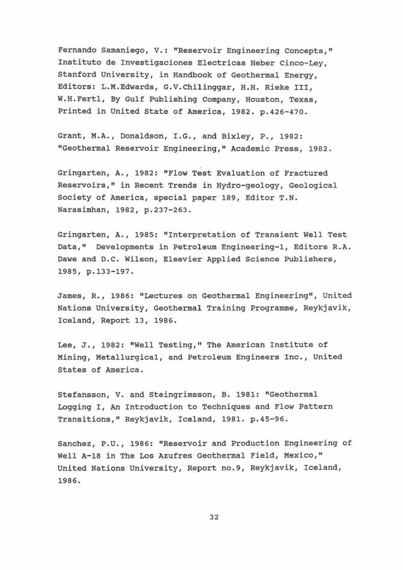
Fernando Samaniego, v.: "Reservoir Engineering Concepts,tI

Instituto de Investigaciones Electricas Heber Cinco-Ley, Stanford University, in Handbook of Geothermal Energy,

Editors: L. M.Edwards, G.V. Chilinggar, H.H. Rieke Ill,

W.H . Fertl, By Gulf Publishing Company , Houston, Texas,

Printed in United state of America, 1982 . p . 426-470.

Grant, M. A., Donaldson, I.G . , and Bixley, P. , 1982:

"Geothermal Reservoir Engineering," Academic Press, 1982.

Gringarten, A., 1982: "Flow Test Evaluation of Fractured

Reservoirs," in Recent Trends in Hydro-geology, Geological

society of America, special paper 189, Editor T.N.

Narasimhan, 1982, p . 237-263 .

Gringarten , A. , 1985: "Interpretation of Transient Well Test Data," Developments in Petroleum Engineering-I, Editors R.A.

Dawe and D.C. Wilson, Elsevier Applied Science Publishers,

1985, p.133-197.

James, R., 1986: "Lectures on Geothermal Engineering tl, united

Nations University, Geothermal Training Programme, Reykjavik,

Iceland, Report 13, 1986 .

Lee, J., 1982: "Well Testing," The American Institute of Mining, Metallurgical, and Petroleum Engineers Inc., united

states of America.

Stefansson, V. and Steingrimsson, B. 1981 : "Geothennal

Logging I, An Introduction to Techniques and Flow Pattern

Transitions,tI Reykjavik, Iceland, 1981. p . 45-96.

Sanchez, P.U . , 1986 : "Reservoir and Production Engineering of Well A-18 in The Los Azufres Geothermal Field, Mexico,"

United Nations University, Report no.9, Reykjavik , Iceland,

1986.

32

co co

0"", (a)

ZOO 100 4QQ

SOO 600 100 BOO !GO

1000 1I00 UOO lIDO 1100 ISOO 16Q0 l700 Im

TABLE . 1: KOLVIOARHOLL KhG - 1, PRESSURE AND TEMPERATURE DATA

P1 T 1 . 'P2 T2 P) nt T4 PS . T5. P6 T6~ P7 T7 (C) (cj (C) (C) (C) (C) . (C)

BS.Il:i: BS. U.I BS.ll.I M.D2.~ 8&.OU 86.11. M.U.I

28.6 36.2 !S.! 1.30 11.1 lB.l 4.14 UO ll.2 SO.S ll.5 IT.I u.n SI. ' ll. O l'-S

17.1' 60.1 64.1 2%.!a !S.D ll.&I !S.O .4.1 1&!.D Zt.!l 27.&:1 64.6 10.1 = 61.7 ~.!Q 11.6 61.' ll.l< 1'1 • .ll 13.2 B2.1 'z.;lI 19.1 IUS BM 11.6 173. 1 4U1 17.11 71.6 n.' ll.!l 95.' 52.3' 96.' 73. 6 17.1' sa.!! lIU 130.1 Il.!a m.1 &%..!& 12S.' Ul.O 21'.1 Il.l1 111.0 6I.Z' 1%7. 0 m.o 711..24 lU.S n.!5 111.0 1S6.6 m., ,,-" 198.6 7T-,~ In.O I!S.O 19.07 Ill.! 80.1& 190.2 W .6 m.1 71.11 m •• BUB 111.2 ZO'.O B7.n ZOl.' 11 •• 7 2D7.D ZOl.l m.D 14.0% 251.1 95.07 111.6 211.Z 96.62 21B.l 96.T9 221. l lZl.S ru.S 'U7 251.6

104.11 Ill.' 21B. 1 10'.13 m.6 lD!l.lI 211.1 llII.l llB.6 101.19 251.S Ill." IIS.S 217.0 lll.ll m.8 lll.l7 lU.S 211.' !Z..3O 2611.1 11l'l.19 m.l m...2 I.U 21' .1 lZI.S7 m.l lZI.~ 1IS.B 1IS.D 1011. 10 llB.6 U7.!l 2ll.l UI. 60 111. 0 21l.1 llD. D' lll.4 m.~ 257.2 l5a.6 lQL!Q m.1 lZl.13 2l6.0 IIUB 146.' 216.S llB.ZZ m.s UII.OI 251.S 2ll. l 116.60 m •• llU% 25U 149.ZZ I!S.B llII. , lIl.1l 252.l lll.!l . 161.5 2.Il.B l7l.1O 2ll.1 llO.l2 252.1

~8 T·a (C)

87.04.02

1.n sa. O 65.Z

27.: 10.0 73.B

I1.QQ 1l7.l lLn II8.l 6l.a& 207.S an m.B 8Z.D7 Zl8.B '11.15 247. 1. !U7 25&.1

IIILIO 267.8 111.1t 266.6 l2%..27 265.1 ua.18 26U ULI6 261.B 114.81 265.l

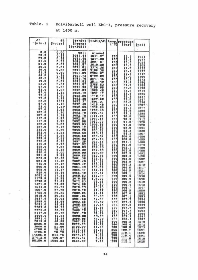
Table. 2

., " _la.I

••• 26.& 29.0 , .. S 34.0 36.5 39.0 ft.e 44 .0 ., .. 5 49.0 n.o 61.0 62.0 61.0 72.0 17 .0 82.0 87.0 92.0 97.0

102.0 tOl.0 112 .0 111.0 122.0 121.0 132.0 162.0 335.0 355.0 318.0 4U.O 458.0 499.0 1540.0 581.0 823.0 681.0 145.0 806.0 868.0 929.0

'062.0 1115.0 1298.0 1121.0 1&44.0 1661. 0 1166.0 1816.0 1831.0 1969.0 2081 .0 2203.0 23%5.0 2Hl.0 2569.0 2891.0 2811.0 2936.0 3060.0 4100.0 41215.0

146S!5.0 21412.0 96160.0

Kolviaarholl well KhG-l, pressure recovery at 1400 m. ., I'P'." l"d'I'.' '''C' rea.urlt Ihour., Dour.

• I' I Ibarl (pall ('p='.SI

0.00 "ell cloaed 0.44 '.51.11 ISII .21 ,. n.s J051 ~ o.te '.51.18 1211.'B 2. 14.3 1011 0.53 1061. IS! SI.t.n 2. lB.S 10915 0.&1 10&1.51 nn.u •• lS. a 110 • 0.81 2051.151 3314 .38 .S 17 .S 1125 0.85 105'.85 IUIJ.n IS 111. • 1131 0.89 2051.81 198'.81 2S 19.3 IIU 0.13 2061.13 1191 .al .. 80.0 IUO 0.18 2051.18 1841.4!I 2S aD.' 1112 0.82 2051.82 UII.I. ' ,. a .. 1 l18i 0.81 2051.81 usa .83 ,. a ... 11. 0.95 2051. '" I1n.95 ,. e2.8 It 98 1.03 205%.03 1988.48 ':: 83.8 1215 1.12 2051.12 1831.11 ,. 84.8 1225 1.10 2052.20 1110.11 ,., 85.3 1231 ioU 2052. ZB 1899.80 ";: '1500 1241 I; :]1 2051.31. 11501. 31 •• 88.8 1256 I. 45 2052.415 lUlL U ,. 87. 4 1281 .... • I .53' 2052.53 · 1338.90 ';l 88.1 1217 1.82 2052,152 1289.40 ":, 88.8 1288 1.10 2052 .10 1201.41 •• 89.3 1295 1.18 2052.18 1151. 31 2.0 90.0 1305 1.87 !OS!.87 1099.55 , .. 90.5 1312 ... 5 2052.915 1.52.11 ••• 91.0 1320 . 2 .• 03 20$3.03 1009.85 ••• tt .• 1328 Z.12 2053.12 In.82 , .. 92.0 .3 :J4 2.20 2053.!0 133.21 2 •• 92 . 3 . 1338

. 2.53· 2053. 53 110.71 ••• 't.3 1381 150 68 2058.58 388.31 ••• 100.0 1450 fr. 92 . 2058.'!IZ 341.83 .6. 100.8 1159 8.28 2051.25 329.18 ••• lOt. I 1488 8.92' 2051.92 291.82 2 •• tol.8 1413 1.83 2058.83 2U .10 '6. to2.1 1180 8.32 2069.32 Ifl.80 ••• 102.8 .t88 9.00 2060.00 128.89 260 102.9 1192 9.88 208o.e8 · 112.e I 2 •• 103.3 1498

10.38 206" 38 198.53 ••• 103. 8 !!ID! 11 . to . 2082. to ta .... 2 •• 103.' . 1501 12.42 ' 2063.42 188.18 '6. 104., 1512 ' 13.43 208 t • 43 153.88 2 •• IOt.8 1517 . 11 ;41 2085.41 142.11 ••• to4., 1521 15.48 2086.48 133.41 ••• 105. 1 1524 11. 53 2068.53 117.98 2 •• 105.5 1530 19.58 2010.58 105.13 2.0 105.' 1638 21.63 2012.83 n .81 ••• 108.2 15to 23.88 2014.88 81.80 26. 1 ••• 1 1!543 26.13 2018 .13 80.10 2 •• 108.1 1541 21.18 2018.11 " .82 2 •• 108.' 1&50 29.25 2080.2!I 71.12 26. 101.0 15112 30.28 2081.28 88.80 2 •• 101. I 1S5' 30.62 20Bl.82 St.19 2 •• 101.2 1.51 32.66 2083.815 83.82 2 •• I.t. , 1658 34.88 2085.88 8". 14 Z •• 101.8 1569 38.12 2081.12 SS.BS 2 •• 101.1 IUt 38.115 Z089.78 83.93 , .. 101.1 lIS 8 2 40.18 2091.18 U.29 ••• 101. , 15 815 42.82 2093.82 48.90 '.0 108. I 1587 44.815 20915.815 n.13 2 •• 108. 1 1S81 18.88 20U.88 ".18 ••• 108.3 11570 48.93 2098 .13 U ... .60 108. t 1512 151.00 2102.00 ".n u. 108.8 11513 18.33 1129.331 U.U ••• 109.1 IUt 18.115 1129.11 11.04 n. 110.1 11598

244.115 22915. n 8.38 2 •• 11 •• I t601 456.87 2501. 81 S.49 'SS 11 ... 161.

1686.83 3838. U t.21 '168 112.1 16215 .' 34

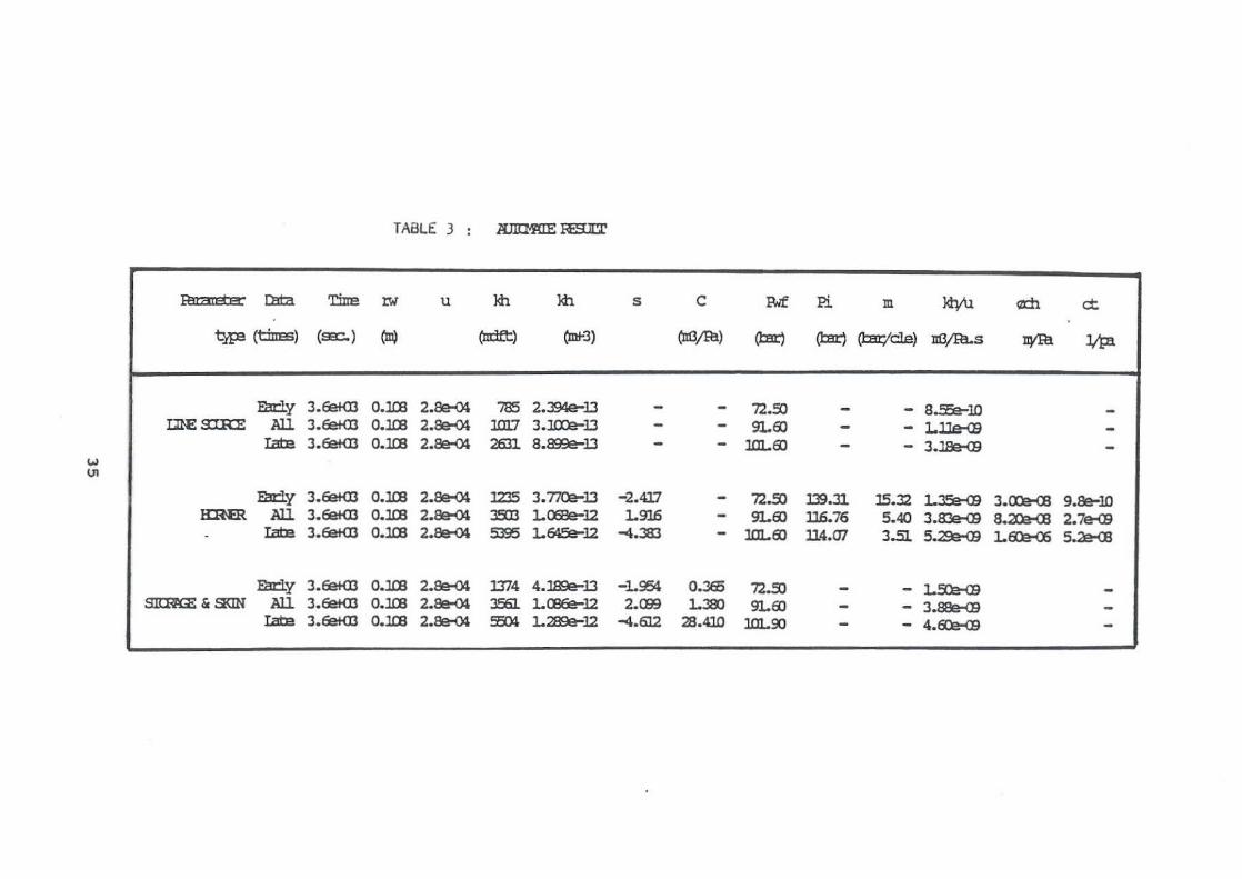
TABLE 3 lUIIM!IE JalIlr

Pit dIE' e lllta 'I:ine IW u H1 H1 s c IWf Pi m ~ om do

t;p! (tinES) (sa:::.) (m) (mlft) (mt3) (lIO!R» (I:m:j (!:Br) (I:m1cle) lI!ljBl..s lIVIli lIfa

E!l::ly 3.feIaJ O.llB 2.8e-OI 785 2.394e-l3 72.:0 - B.:lie-lD I1I£SlRE All 3.fe+03 O.llB 2.8e-OI lDl7 3.:uxe-l3 9l.Ell - 1.JJe-a)

Iaba 3.feIaJ O.llB 2.8e-OI 263l B.89ge-l3 - llll..Ell - 3.llle-OO w U1

E!l::ly 3.feIaJ O.llB 2.8e-OI lZl5 3.770>-l3 -2.<117 72.!!l 139.3l. 15.32 1.3!:e-(9 3.cre<B 9.Be-lD HaER All 3.feIaJ O.llB 2.8e-OI 39J3 1.C6le-12 1.916 9l.Ell 116.76 5.40 3.B3e-Ql B.2Oe<S 2.7e<9

Iaba 3.feIaJ O.llB 2.8e-OI 5395 1.~12 ~.:m - llll..Ell ll4.07 3.51. 5.2ge-<B 1.~ 5.:a.-al

E!l::ly 3.feIaJ O.llB 2.8e-OI 1374 4.lBge-l3 -1.954 0.365 72.!!l - 1.:n.-al SJIHU; & a<IN All 3.feIaJ O.llB 2.8e-OI 3561. l.CIl6e-12 2.C!13 1.380 9l.Ell - 3.B8e-(B

Iaba 3.feIaJ O.llB 2.8e-OI :a» 1.:l2ge-12 ~.612 2B.4lD llll..90 - 4.a::e-a;

Tableo 4 Comparison temperature calculation .

tn'lI! =m "lSXl m lBDm

Pkt - atl:e: Pkt - atl:e: Pkt - atl:e:

~(minb!s) =0 92lO 8l9O

'lllB>c.. (oq 222 256 :1A5 2f5 2!B 261

(~q dr(oq dr(oq Coq drcoq dr(oq (oq dr(oq dr(oq

Lin-JJn 224 2 -32 :1A5 0 -20 2!B 0 -5 lbn!I: ZZI 5 -29 250 5 -15 2!B 0 -5

BaI H "] 229 7 -27 255 ID -ID 261 5 0

36

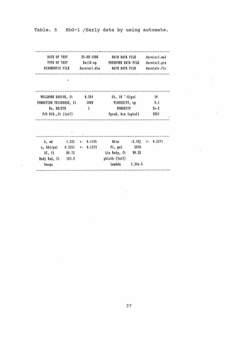
Table. 5 KhG-l /Early data by using automate.

.. - -- ------- ------------_ .. -. -- _ .. _ .. ~- _. ---- ------ -- ------- --_. -_. -_ .. . -. --_.-DIIi Of TEST

TlPI or lIST

DIICMO"'C FILl

MW,BORI RADIUS, It rOinllloM IIICII!!!, It

10, RBISt! PlO DIS"lt Ilntrl

., Id 1.ZZ5 C, bbl/psi o.ml

Il, ft IS.!! hd, bd, (t Ill.!

01P.&1

Z5-0H!8I hi Id·. p

dUlliul.dia

. -.-

D.l51 1000

1

'.!lU O.llI!

HAIM DnA fiLl darvisrl.lli PIESSURI DAT' riLl darvi"I.prs

tATI OArl rILl dl'I/illt,flr

et. 10 -"'psi vUCOstn, c,

'DROSIII Tprod I h. lophll

S. ill -!.JjJ

Pi. pti 2015

Lin Bnd" rt ID.25

plietl Until Lubd. I.llo-5

37

. -

ID 0.1

SeAt 2051

f.Ull

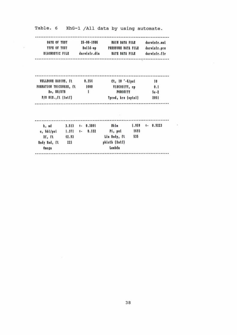
Table. 6 KhG-l JAIl data by using automate.

1111 Of lilT

nil Of lilT

IUCIOSTIC fiLl

llLLIORI IADIU', ft

'OI"AIIOI TIIC.li'S, It 10, II/ITI

'10 DII.,lt II,tll

., Id 1-111 c, bbl/,.l 1-111

H, ft 1I.1l ... , hd, It III

OUC'

n·"· 11II .. lU-.,

hnl.lr.dta

,. ,.

'.lI! lott I

1.1111

'.111

RAil IAIA fiLl d.r.I.I, .•• 1 PIIIIUlI DATI 'ILl .",1.1,.,1.

.ITI tAIA fiLl •• "I.I,.fl,

Ct, U . -5,,11 'UCO!IT', t,

POIOlln Ipro., h. (o,hll

1'1. 1-151 Pi, ,11 UIl

tit ••• " rt III ,lIetl IIoUI

Lllbd.

38

,.

It

'.1 Se -l

IDII

'.1111

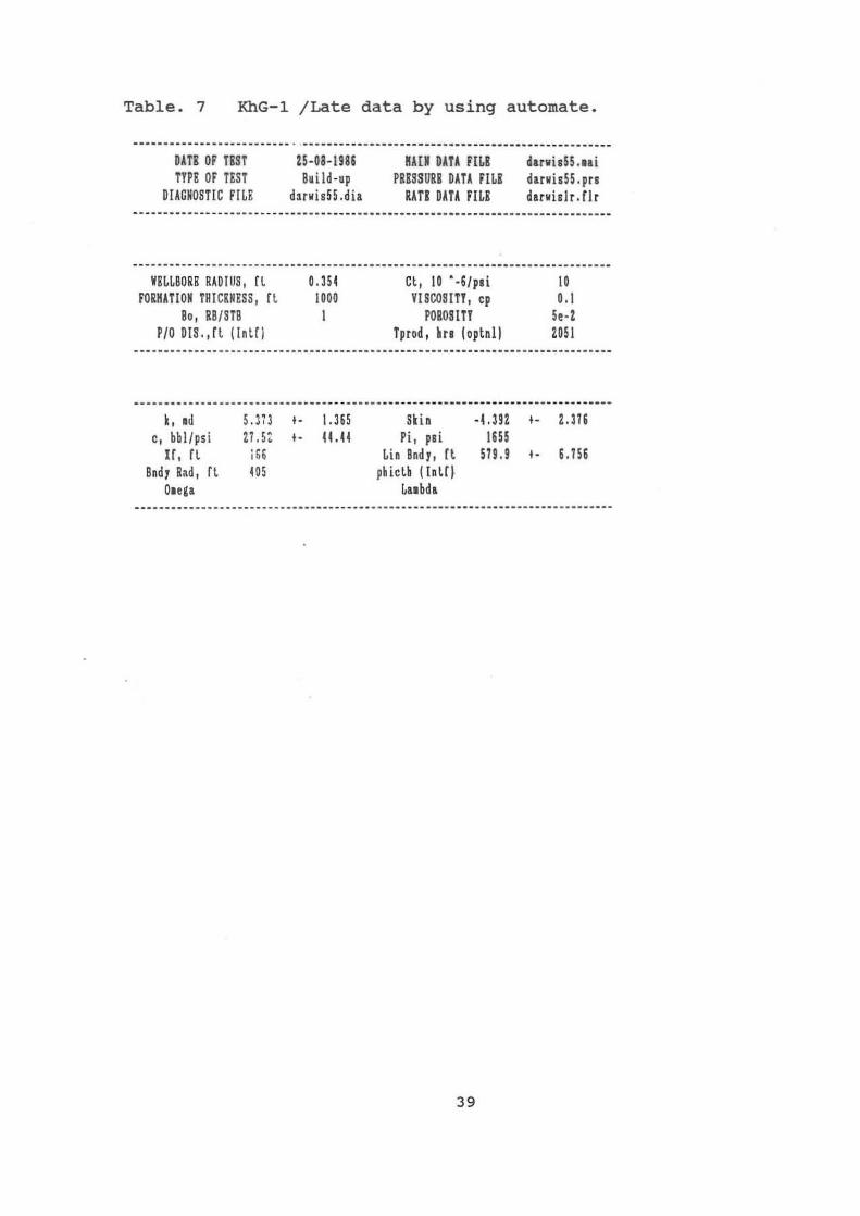
Table. 7 KhG-l I Lat e data by using automate.

om or liST TlPE or TEST

D[AGNOST[C r[LE

IIELLBORH RADIUS, rt rOR"ATION THI CKN ESS , ft

Bo, RB /STB PlO D[S_,ll I[n l l l

k, .d 5. )73 C, bbl / ps i 21.5:

H, Tt i S6 Bnd, Ha.d I fl 105

Oleca

Il -OHm Build-up

dUlli sS5.dia

,-,-

0.3ll 1000 I

1.365 11.41

Km om FILl PRRSSURR DATA rILl

RAT! Dm FILl

Cl, 10 • ·6/pli YlSCOSUY, cp

POROSlTT Tprod , hn (optnll

Skib -4.391 Pi, pai 16ll

Lin Bnd" n 579 .9 phiclb lI.tO

LlIbda

39

dU1lia55.lll dlrvis55.pn darlli.Jr.£Ir

,-,-

10 0.1

5e · l lOll

2.315

1.156

Bjornlson et al.

•

-- ------== ......-------.. -'.---'- ,~.~--------------------..:~ ..

f igure 1. Sil!lplifi.ed tectoni.c III8p of SW-leelond and locotion or the HengllJ area. Ihe ."'eo­volcanic zone i s .ithin the Brunhes-M.atuya.a boundar i es., [arthquake zone (Ktem et al .. 197;; EilVlrsson and Bjomaaon. 1979), volc:ani.c s.,.t .. ~Sa-..w:lsson. 1978), and geother..l fields are sno-n. The Hengill geothe~l area is .ithln the square.

Figure. 1 Vestur Hengill (Kolvi6arholl Geothermal) area.

40

COHPLETE

RECORDING

PRESSURE

GAUGE

.Clock

bcordtnl hctlon

Pressure Element

l\Ii'!I~J!'

fLead

~, Screw

;I IChart . IRolder

Stylua Assembly

.. ,pdillg a'h .. tiI, I.

Th' .. • . . "P' \le~\\ . , . ,

I,

o

BOTTOM HOLE RECORDING

PRESSURE OR TEtlPERATURE GAUGE

WIRE LINE SO(l{ET

OUTER IIOUSING

TEHPERATURE ELEHENT

RPG-J I "" Dia, RPo-4 I" Dh,

Figure. 2 Amerada recording gauges for pressure and

tempetrature .

41

." IIf -flIV , .. ~

I''''''nl .-

.... , ... u'" R." " •. , •• ' h ......... " ..

PRESSURE Ilf.MIENT

BULB

I,u ••.• .. " Ih •• on"", _

TEMPERATURE ElEMENT

Figure. 3 Cross sections of Amerada pressure and temperature .

42

.. w

o o

, ~

50

~ I

Temperature (C)

100 150 200

I I I I

250 3.00

I I I I Boiling. pcri",

350 -'-1

500 .l _____ .J - ___ L _____ ~ ______ I _____ _ _____ ...1 ______ 1

1 I I I I , I

J , , ~

- -I I I E 1000 T - - - - - , - - - - - - r - - - - - T -~ ] (.) TI Z2-11-1985 I

:5 i ~.~ T2 91-12-1985

I I ,'- - - - - - r - - --

I

g. J. T3 19-12-1985 o ~. T4 7-02-191f6

i C·) T5 5-07- 191f6 I I

I I I

1 500 .l .JlrlJ:d;'fl.1A .l'IAr17'=YJI- - - - --i p.nod~ I

..1. ____ __ 1_ ,J.. ____ _ ...J __

I I I 1 I ]

i t- ··_--·, 1--=:::--'::--"" l' b i \ i

2000 1 =~~ __ J _____ _ ~ ___ __ l ______ ; ______ ~ _____ J ______ . Figure. 4 Kolvi8arholl KhG-l. Temperature 1,2,3,4 and 5

profiles.

Pressure (kg/.q.cm) o 50 100 tt3 150

500-r------~~~--_b--------------_+--------------_+_

i 1000~------------------+_------~~~----_4------------------~ c

t4(JO

1500~--------------~------------_+--_1~ __ ------1_

~ j Pt U-tt-85 P3. t9-t2-85 P4 27-02-86

.carm-up period)

Figure. 5 Kolvi~arholl KhG-l . Pressure 1,3 and 4 profiles .

44

-BD

Temperature (C) o O~~~~'~"~ULUL~~~~~~~~~~UL~~~~

! i I, I

100 1:50 200 JOO

500~------~----~------~--~,,~.------------~ 3 i i i . ! , ~ i I j. -:--...!1'~' !

] ~ I I I ~""~ I 1'000 I I -'-- .~

h \ . ~,.

'500~------~----~-------+------~------~t---___

~ (k

J T-6 : 27-11-86 I'

[0 T-7 : 01-12-86

. Qo :fi­<iI i

[.. T-8 : 02-02-87 , raft... d.iaoharg. p..nod.) i 2000 .:L ____________________ ~ ______ .L ______ i~ ____ ....J

Figure . 6 Kolviaarholl KhG-l. Temperature 6,7 and 8

profiles .

4 5

Pressure (kgjsq.cm)

120 o 80 160 o~~~~~~~~ww~~~~~~~~~~

"

_ sOO ~ ",,'11,

~ ~ ''G~ .§, '''Q ..

~ 1000~, ----------~--------~'~~---------L-----------

~ ~ '!l", ,

~ ....... "GJ .... u .... lS00 -j------L-----+--..::,. • .-~8}. __ ---_1

c~ P-6: 27-/ /-86 (.0 1'-7: 0/-/2-86 (PO 1'-8: 02-02-87 (a.fWr Iliachcrrg. p ...... 4)

~~ ________ ~ ______ ~ ________ -L ______ ~

Figure. 7 Kolviearholl KhG-l . Pressure 6,7 and 8 profiles.

46

:lOO

~ -. -- . -- -'" ~

!~ ... --- ------ --.---- I- - __ --........ ~~ ... --, --~ K: -- --..........

~ ........

~ ----

t'----

---o 1

log.(t+dt)/dt

Figure. 8 Temperature profile KhG-l (Horner plot)at 1200 rn,

1500 rn, 1600 rn.

47

-, --

---- ---~

t"--..

10

280

~' .. ". 240

---~ o 1>-__

VOo -- ;;, ... ---., ~ to. _ .. ..4.. .. , --• '.200-- --...... .. ...... ...' -- ~ -- ... .....

t-....... - ---- .... , -' - ..::::.,.~

.. -.:- ... -, '" ~, " ,

" '

120

" 0-

~ " '"

0" " " " ............

'"

-ID-80 10 __ ......,. ........ . .......

1/(dt+tp) (min.)

Figure . 9 Kolvi~arholl KhG-l, T Vs time inverse -func tion:

1200 rn , 15 0 0 rn, 1 6 00 m.

48

10--

-;:-0 .a ~

! " .. .. ! Il.

'35

115

511

.5 ,90

&I. t:rnJn

I I I

/ /

V vV

-ID-..- o JrZrJj DII-, • I 111'~ ., ' . ,

2'0 23() 2:iCl 270 290 J.O Temperature (C)

Figure . 10 Thermodynamic bottomhole state behavior during

build-up .

49

'/

280 , , , , ~-r-+' -----r-------r-------r-------r-------t-------t-------t------~ , , , , , , ,

G----- -a-------- --a------- ---------- ---------- ---------- ---------- ---------e 0-"~~------+_----~------_t------~------t_----~~----_t------~ -.! 2~~----_t------r_----~----_t------r_----~----_t----~

---200 800 IlOO 1000 1200 1400 1800

liME (hours)

Figure. 11 Temperature build-up behavior.

50

120

110

100 -;:-

" ... ~ .. 11. 10

10

70

v~

:

o

, I_~ ____ ---~--<)------ ---------- ---------- ---------- ---------- ---------<

! I , I

I

I

--200 600 IlOO 1000 1200 1400 11100

TIME (hou~)

Figure. 12 Pressure build-up behavior.

51

!! il •

120

110

;

: f- -'

;

,

l - " ).0

1/ v

;. 80

11 : 70

60 10

•

'- 10 • 10 • log. dt(minute) 10 •

Figure . 13 Pressure recovery KhG-l, on sernilog scale at

1400m.

52

I

I

10 •

10 • I I I11 11 1 1 ' 11 11

I 1 I 1111

I I ,

11 I

I

,/ V

lJ i --10

10 10 • 10 • 10 • 109. dt{minute}

Figure. 14 Pressure recov ery KhG-l, on log- log scale

at 14 00 m.

53

I

10 •

~1300~--+-+-~~~--+-+-~~~--+-~~~~\~+-+-~~~ il .. ~1200~--~-+-+~~~---t-+-+~HH~---+~-+~~1+--~~-+~~HH

\ 1100 4--+-+-+-+-++++1

1

-+-++++++++---1-++++-++i+---+--+I\~f\-++H-h

10 10 • log.(t+dt)/dt 10 •

Figure. 15 Pressure recovery KhG-l, on Horner plot at 1400 m.

54

10

40 - - --

- - --

- - --

~

E 0 tT .. "-'" - ~- --~

10

f :I .. .. f

Cl.

o -20

: I , , , , , , , , , , , , , ____ L __ _ _____ _ L _____ .

, .A ,

'''' --'" ,~.J.II ~~ ~ ~, , , , , , , , • , , ~---L--- - -----L-----, , , .. , , , -, ,

'I .. r_ ' , ' .. ~ , ~

~ .. , ~ .. , , , , ___ _ L _______ ~::T:~O::~_::_::, , , , ,

'--, , , , , r.t ... ' , --!,Iow , ,

____ L ______ ._~_

"-.' , ~~ , I ~-,~~----~ I , --"'111111.----------, ,........,.. , , , , , ,

, 20 60

time (days)

2000

A-I- 1600

---I-

is: " :5

-- -I- 800 .5 ", . ~ ,

-

•

--I- 400

-D o

100

Figure . 16 Kolvi6arholl KhG-l~ Time Vs Enthalpy, mass flow &

W.H.P.

55

2.00

1.60

'L" .& 1.20 ~

f ::J .. l g 0.80

'" ;S

0.40

0.00

~

-11)-

--.... • r __ ~ (A)

•

~ ~ ~ •

20 40 60 80' .. 10 time (days)

0.20

0.16

0.12

0.08

0.04

0.00 o

~

E ~

" .&

j .5 ." 0

" s; .. .! 0 ~

Figure. 17 Kolvibarholl KhG- l; critical pressure and Water head in weir box vs Time.

56

1500, Horner plot x~

1400

... - , DJ , Co 1300

, , , .. , <- , :I , DJ , DJ , .. <-Cl.

1200 t- , , , ,

'" " -.l , PI 222.2

1100 t- k 1.235 s -2.417

Pit 2020

1000L'--------------L--------------L------------~L-------------~ 1 10 100 1000 hiO·

(t+deltat)/deltat United Nations U. '1

Figure . 18 KhG-l /Early data- Horner plot.

'" 0)

" 11.

100

10

1

0 . 1

k 1.374 s -1.954 c 0.3652

0 2 .02 ~

l- ~/.---

F~

0.1 1 10 100 Td/Cd

Figure . 19 KhG-l /Early data- storage & skin.

:::

1xl0'O

hlOao

hlOl!!

" hUB hta hlO' • --hbQ 10 0 100 10 1

___ 0.1

1000 • ixl0

United Nations U. '1

1000

... ., a.

a. .. 100 ... ... QI C

'" '"

10

k s c

Pi L

182

3.514 1.962 1.372 1693 307

0 . 1 1 10 Deltat. hrs

Figure . 20 KhG-l IAII data- Log-log plot match .

100 1000 18.

United Nations U. '1

'" o

-.. c. U t. :::J .. .. U t. 0.

1800r�---------------,----------------~--------------,_--------------_,

1600

1400

1200

,

m 78.36 k 3.503 s 1.916

PIf 1692

\, , " ... , ,

... " , , , ,

1000~1--------------~----------------~--------------~---------------J

1 10 100 ~+deltat)/deltat

Figure . 2 1 KhG-l J AIl data- Horner plot.

1000 • hiD

United Netions U. ' 1

'" ....

.., a.

100

10

1

0 . 1

k 3.561 5 2.099 c 1.38

() 6.117

I- d7/______.

I~~

0 . 1 1 10 Td/Cd

Fi.gure. 22 KhG- l fAll data- storage & skin .

---- In

:::

100

hl030

ixlO2O

hlot!!

" hiDe ixlD hlOIl

hlO· 1000 100 10 1

___ 0.1

1000 • htO

United Nations U . • 1

'" '"

.... '" c.

c.

10.

m 1000 .... .... 01 o

100 1

k 5.373 s -4.392 c 27.52

Pi 1655 L 579.9

,.; ... ~.

10

•

100 Oeltat. hr s

Figure . 23 KhG-l / Late data- Log-log plot matc h .

1000 10.

United Nations U. '1

-.. Co

Q)

t. ::J .. .. Q)

t. CL

'" w

1650 I ____

1600

1550 ~

1500 ~ m 50.88

1450 f- k 5 .395 s - 4.383

Pit 1654

-11 ' , !, ,

,

, , ,

" , , , ,

1400~!--------------~---------L--------------------------~-----------A

1 10 (t+deltatJ/deltat

Figure . 24 KhG-l /Late data- Horner plot.

100

United Nations U. *1

'" ...

'C Q.

10

1

0 ,1

k 2.631 4 phi 1. 114x10

<4ltlg2 0.1 0.4 4

I I r 4000

1000

10 40

1 X1021

'\ '\ "" '" ',>

0.1 1 10 100 (tp + delta t)O / rO"2

Figure . 25 KhG-l ILate data- Line source solution.

1000 4 1xiO

United NatiDns U . • 1

'" '"

'D a.

100

10

1

0 . 1

k 5.504 s -4.612 c 2B.41

() 1.602 -----

r dY~ _______

ff~1

0 . 1 1 10 100 Td/Cd

Figure. 26 KhG- l /Late data- storage & skin.

r

1000 ,

hlO3O

hlO211

hlOtS

lD idOl hlO idO'

--hiO· 1000 .00 10

::t. __ 0.1

• 1xiD

United Nations U. '1