A Compositional Axiomatization of Statecharts

Theoretical Computer Science 101 (1992) 289-335

Elsevier

289

A compositional axiomatization of Statecharts’”

J.J.M. Hooman Department of Mathematics and Computing Science, Eindhoven University of Technology,

5600 MB Eindhoven, The Netherlands

S. Ramesh”” Department of Computer Science and Engineering, Indian Institute of Technology,

Bombay 400 076, India

W.P. de Roever Institut fiir Informatik und Praktische Mathematik II, Christian-Albrechts-Universitiit zu Kiel,

2300 Kiel I, German)

Abstract

Hooman, J.J.M., S. Ramesh and W.P. de Roever, A compositional Axiomatization of Statecharts,

Theoretical Computer Science 101 (1992) 289-335.

Statecharts is a behavioural specification language proposed for specifying large real-time, event-

driven, reactive systems. It is a graphical language based on state-transition diagrams for finite

state machines extended with many features like hierarchy, concurrency, broadcast communication

and time-out. We supply Statecharts with a compositional axiomatization for both safety and

liveness properties. By generating external events symbolically, Statecharts can be executed, thereby turning it into a programming language for real-time concurrency (as well as enabling

rapid prototyping). As such it is well suited for compositional program verification. In addition

to our compositional axiomatic system, we give a denotational semantics and prove that the

axiomatization is sound and relatively complete with respect to this semantics.

1. Introduction

This paper deals with formal specification and verification of real-time reactive

systems. Reactive systems [14] are typically event-driven, often have critical time

requirements, and, most importantly, they are continuously interacting with their

environment. Typical examples are telecommunication networks and avionic sys-

tems. Formal specification of real-time reactive systems is an important area of

* This research was supported by Esprit Project 937 (DESCARTES) and Esprit-BRA project 3096 (SPEC).

** The work described here was done while this author was at the Eindhoven University ofTechnology,

partially supported by the Netherlands National Facility for Informatics (NFI). ,

0304.3975/92/$05.00 0 1992-Elsevier Science Publishers B.V. All rights reserved

290 J.J.M. Hooman et al.

research judging by the sheer number of proposed specification languages such as

Statecharts [ll], Esterel [2], Lustre [3] and Signal [9]. All these specification

languages are based on operational descriptions that characterize how a system

evolves. As such they are perfectly suited for simulation purposes to analyze and

to debug the description of the system under development. To achieve additional

confidence in the specification of the intended system, our aim is to complement

behavioural specifications with more abstract property-based specifications. More

precisely, we give a logical specification language and develop a sound and relatively

complete axiomatic system to verify a behavioural specification with respect to a

property-based specification.

In this paper we axiomatize the behavioural specification language Statecharts

[ 111. This visual formalism [ 121 can be considered as an extension of conventional

state-transition diagrams of finite state machines with hierarchy, concurrency and

a communication mechanism. A specification written in the language Statecharts is

called a statechart. Originally, this language has been designed by Hare1 to support

the development of a complex avionics system. Currently the formalism is indeed

used in aircraft industry, but it has been applied successfully in other industrial

development projects as well. See also [6], where it is argued that Statecharts can

be beneficially used as a hardware description language. Statecharts is used in a

computerized graphical tool, called STATEMATE [13], to represent the behavioural

view of the system under development. STATEMATE supports two other views: the

functional view (describing dataflow and activities) and the structural view (describ-

ing the static structure of physical modules and channels). This tool allows us to

simulate the specified system and it incorporates several analysis capabilities, most

of them based on finite state methods. The full Statecharts language, however, allows

the use of variables and hence completely automated verification is impossible.

Furthermore, the limits of automated finite state verification are almost reached

(see, e.g. [32]).

Our aim is to develop an axiomatization of Statecharts which is compositional,

that is, properties of a compound statechart should be derived purely from properties

of its constituents without referring to the internal structure of these constituents.

Compositionality requires syntactic operators for building large statecharts from

smaller ones. Our axiomatization is based on a textual syntax for Statecharts which

has been proposed in [20]. Statecharts are related to our logical specification

language by formulae of the form S sat cp, meaning that statechart S satisfies assertion

cp. Assertions are written in a first-order typed language which is strong enough to

express safety and liveness properties. Safety properties are properties that can be

falsified in finite time, such as, “event e is generated within five steps”. A typical

example of a liveness property is “eventually event e is generated”.

In the literature many axiomatic systems are presented (see [ 1, 16, 18, 19, 27, 31,

341, to mention a few) for deducing properties of real-time or reactive systems. All

these systems deal with CSP-like languages [ 16,231 which lack many of the features

of Statecharts, such as interrupts and broadcast communication. Often ‘sat’-based

A compositional axiomatization @‘Statecharts 291

formalisms are used for specifications [ 1,16, 19,27,34]. Some of the works [ 16, 17,

341 deal with safety properties while others [l, 27, 19,311 derive both safety and

liveness properties. For expressing liveness properties the latter works make use of

temporal logic, and compositionality is achieved in [l, 19,271 by using chop

operators or greatest fixed point operators in the assertion language. In this paper

such operators are avoided by making explicit reference to time and using the

availability of unbounded time. As Lamport already observed in [24], this simplifies

the step from real-time safety to liveness.

In [34,35] it has been shown how the kind of sat-system as developed here can

be turned into a (compositional) generalized Hoare system based on pre- and

post-conditions on computation histories, and into trace-invariant systems in which

concurrency is characterized by a communication interface. The remaining prevalent

styles of compositional specification and proof systems, viz. the assumption-commit-

ment paradigm for distributed computation (tracing back to early work of Misra

and Chandy [26]) as well as the rely-guarantee paradigm (tracing back to early

work of Jones [22]), can be canonically converted into trace-invariant proof systems

as indicated in [36]. Once future research has determined which adaptation of these

three specification styles-generalized Hoare logic, trace-invariant, assumption-

commitment-is most natural to reason about Statecharts, our proof system can

be lifted to suit that style using the canonical proof-transformation techniques

developed by Zwiers et al., cited above. This provides added motivation to our aim

to develop first a compositional axiomatization for Statecharts which is as simple

as possible.

To prove soundness and relative completeness of our axiomatic system, we have

defined a denotational, and hence compositional, semantics for Statecharts. An early

operational, noncompositional, semantics for Statecharts can be found in [15]. In

[20] a compositional semantic model with minimal amount of nonobservable entities

(i.e. a fully abstract semantics) has been presented. The denotations of this semantics

are prefix-closed sets of linear histories; infinite computations are represented by

all their finite prefixes. Our semantics is derived from this model, but since it has

to serve as a basis for our formalism expressing liveness properties, several changes

have been made. Instead of using prefix closed sets, our histories represent complete

(possibly infinite) computations. Furthermore, in [20] the least fixed point is used

to describe a looping construct whereas we use the greatest fixed point to obtain

also infinite computations. A discussion about choices in defining the semantics of

Statecharts can be found in [21]. In [8] a related denotational semantics has been

given for the nongraphical synchronous language Esterel. An operational description

for this language can be found in [2]. A Statechart-like graphical language is

described in [25]. The formal definition of this language uses a process algebra in

combination with notions from Esterel.

This paper is structured as follows. In Section 2 we introduce Statecharts infor-

mally, illustrated by an example of an unreliable device and a mission control

computer in an avionics system. A formal syntax of the language is presented in


Section 3. Section 4 contains a first, straightforward, attempt to axiomatize

Statecharts. We show by examples that this axiomatic system does not completely

correspond to the intended meaning of Statecharts as described in Section 3.

Therefore we slightly modify the specification language, and in Section 5 the final

axiomatization is formulated, consisting of an axiom for each basic statechart and

a rule for each of the syntactic operators. A denotational semantics for Statechart

is defined in Section 6. Section 7 contains details about the property-based

specification language and its formal interpretation. Soundness of the axiomatic

system with respect to the denotational semantics is proved in Section 8. Moreover,

in Section 9 we prove relative completeness of the proof system. Finally, in Section

10, we discuss future extensions.

2. Informal introduction to Statecharts

Realizing the intuitive and pictorial appeal of state-transition diagrams for finite

state machines, Statecharts has been designed on the basis of such diagrams. But

it is free from the limitations of state machines, such as sequentially, unstructuredness

and exponential growth of states when describing concurrency. Indeed, statecharts

are exponentially more succinct than state machines, as has been shown in [5]. This

is achieved by adding hierarchy, concurrency and broadcast communication.

Quoting [ 121,

Statecharts = state-transition diagrams + depth + orthogonality + broadcast.

The language is built upon so-called basic states, like the states in a finite state

machine, and transitions. Depth is obtained by allowing superstates that contain

substates and internal transitions. This leads to a hierarchy of states, corresponding

to AND/OR decomposition. Accordingly, there are two types of superstates, AND-

states and OR-states. If the system is in an AND-state then it is simultaneously in

all its immediate substates. To be in an OR-state means to be in exactly one of its

immediate substates. When a superstate is exited, any computation inside is termin-

ated. The immediate substates of an AND-state are called orthogonal components

and they are executed in parallel. Orthogonal components interact with each other

and with their environment by means of events, i.e. signals without measurable

duration. Transitions have labels to specify when a transition is enabled and which

events are generated when a transition is taken. Events generated by a transition in

one orthogonal component are broadcast, possibly triggering transitions in other

components which, in turn, might produce new events, etc. Thus a single event can

give rise to a whole chain of events.

Execution of a statechart proceeds in (time) steps. In each step a maximal set of

enabled transitions is taken with at most one transition per orthogonal component.

All events generated by these transitions are assumed to take place simultaneously.

This allows us to abstract from the internal chain of transitions and generated events

A compositional axiomatization qf Statecharts 293

within a single step. The general idea is that staying in a state takes some time,

whereas taking a transition is assumed to be instantaneous. This assumption is

essentially Berry’s synchrony hypothesis for the language Esterel[2]. This synchrony

hypothesis might introduce causal paradoxes, like an event causing itself. In Esterel

causal paradoxes are syntactically disallowed whereas in Statecharts causal relation-

ships are respected and paradoxes are removed semantically.

Example 2.1. To introduce and illustrate the language Statecharts, we specify parts

of a generalized avionics system. Our example has been inspired by the description

of such a system in [29] where it was specified in CSP, VDM and temporal logic.

Here we use Statecharts to specify parts of the mission control computer. On request

this control function provides aircraft flight data such as best available aircraft

position, ground speed, true airspeed and altitude. In addition, information is

displayed to the air crew. The requested data is obtained from devices (e.g. radar)

or, if a device is broken, data of sufficient accuracy is computed by means of

previously stored information. Since several devices have the same interface, we

describe the control of a general, abstract, device. First we show, in Fig. 1, how an

unreliable device can be modelled in Statecharts. Note the hierarchy of states in

this statechart, consisting of OR-states and basic states. For instance, superstate

device is an OR-state, since the system is either in state normal or in error. Observe

that if the system is in basic state producing then it is, simultaneously, in the

superstates normal and device.

Fig. 1. Unreliable device

To model the failure of the device and its possible repair, we use external events

fault and repair. The failure hypothesis of the unreliable device can be expressed

as an assumption about the expected occurrences of the events fault and repair.

Event fuurt triggers the transition from normal to error. By taking this transition

superstate normal is exited explicitly and, simultaneously, its current substate (ready

or producing) is implicitly exited. If event repair occurs in basic state error, the

transition to normal is taken and normal is entered explicitly. To indicate which

substate of normal should be entered, there is a default transition, drawn as a


transition with no source state, pointing to ready. Hence, by taking the transition

with label repair both normal and ready are entered. If in state ready event dreq

occurs, expressing an external request for device data, then the transition to producing

is enabled. When this transition is taken event prod is generated and the state

producing is entered. If, subsequently, in the next two steps event prod is not

generated then the time-out event rm( prod, 3) occurs and event ddata is produced.

Transitions have labels of the form “event-expression/action”. The event-expression

is a boolean expression involving atomic events. These events can be generated by

the outside world, as an input to the statechart, as well as by the statechart itself.

The event-expression specifies when the transition is enabled. Let a and b be atomic

events. A transition with event-expression a is enabled when event a is generated

somewhere in the system (i.e. a statechart and its environment). Event part a A b

(resp., a v b) expresses that the transition can be taken in a step if both a and b

(resp., a or b) are generated somewhere in the system in this step. h is a special

event that occurs (by definition) in every step. tm(e, n) denotes a time-out event

that is generated at a particular step if the last occurrence of event e happened n

time steps earlier. In our syntax of event expressions we also allow the negation of

an event e, denoted by le, where e can be A, an atomic event or a time-out event.

The action of a label is a set of atomic events that are generated when the transition

is taken. Henceforth, a singleton is denoted by its element, and the empty set is

omitted. For instance, in our example we use labels dreqlprod and ,fuuft as abbrevi-

ations of, respectively, dreq/{prod} and fault/l?.

For simplicity we do not consider the general syntax of labels as given in [15].

There a label includes an additional condition part and variable assignments are

allowed in actions. Moreover, there are special events to signal entry and exit of a

state. Our axiomatic system can be easily adapted to the general case, see Section

10 for an example of these extended labels. Furthermore, in [15] an action is a list

of the form a,, . , a,, whereas we use a set containing these events.

Example 2.2. The avionics system described in [29] contains a control unit which

should provide a reliable service based on the unreliable device modelled in Fig.

1. After an external request event req this control unit should provide dara within,

say, 30 steps, despite failures of the unreliable device. Therefore it is assumed that,

if the device does not respond in time, data of sufficient accuracy can be computed

from previous data (such as aircraft position, velocity, etc.). Moreover, the control

unit should display the current status of the device and other information to the air

crew. The required behaviour is specified in Fig. 2. Observe that control is an

OR-state, with basic state ofJ‘as its default state. When event start occurs the system

enters state on. As indicated by the two dashed lines, the state on consists of three

orthogonal components. Entering on results in entering all orthogonal components.

By the default transitions this means that the states idle, working and noflush are

entered and all three components are concurrently active.

A compositional axiomatization of Statecharts

-ddata A tm(dreq,4) J compute

----- -_-- ----- -- ------- -_----

-------- ------- --- ---- -------

\

295

Fig. 2. Mission control computer.

Consider the first component and assume the system is in state idle. Event req

triggers the transition to wait and by generating event dreq the device is requested

for data (see Fig. 1). If event ddata is produced within 4 steps then the transition

to idle is taken, generating data and correct. Otherwise, event compute is generated

and computing is entered. The second orthogonal component of on records the

status of the device. This information is displayed to the air crew. If this status

changes from working to broken, or vice versa, internal event change is generated.

This event is used in the third orthogonal component which specifies how the

information is displayed. In case of a change the information is flashed for at least

2 steps. If no new change event occurs after these 2 steps then the crew can trigger

the transition to noflash by means of a switch. Removing lchange in the label of


the transition to noj?zsh would lead to a nondeterministic choice between the two

outgoing transitions of clearahlejlash if the events change and switch occur simul-

taneously. By including ichange we remove this nondeterminism and we give

priority to change. Finally, observe that an explicit exit of on via the transition with

label stop leads to an implicit exit of all orthogonal components.

In general, a state can be entered/exited either explicitly, by taking a transition

connected to the state, or implicitly, because an orthogonal component, superstate

or substate is entered/exited. Entering an AND-state (resp., OR-state) results in

entering all (resp., exactly one) of its immediate substates implicitly. Although not

present in this example, it is possible to enter/exit a state inside an orthogonal

component explicitly. This leads to an implicit entry/exit of the surrounding AND-

state and the other components. Furthermore, more than one orthogonal component

can be entered directly via a single, forked, transition. Transitions between

orthogonal components are not allowed (e.g. in Fig. 2 no transitions are allowed

between idle and working).

Although the meaning of a statechart is usually intuitively clear, there are a few

cases where the specified behaviour is not completely obvious. The first class of

problems has to do with causality and the synchrony hypothesis, i.e. the assumption

that all transitions within a step are instantaneous and occur simultaneously. This

is illustrated by the examples in Fig. 3. By taking a transition with label a/a event

a is generated simultaneously. Hence, one could argue that such a transition can

always be taken, even if a is not generated externally, since the transition generates

its own trigger when it is taken. In our opinion, however, such a transition should

not be taken when a is not generated externally. The second example in Fig. 3

indicates that this problem might occur in more complicated situations. It shows a

causal loop: a causes b whereas b causes a. In our intended semantics no transition

is taken when neither a nor b is generated externally.

-----------

Fig. 3. Causality

The second class of problems is caused by the possibility to use the negation of

events in event-expressions. This might lead to causal paradoxes, as demonstrated

in Fig. 4. Consider the transition with label la/a. If a is not generated externally,

then this transition is enabled. But by taking this transition in a step, event a is

generated in the same step, and then the transition would not be enabled in this

A compositional axiomafizafion of Statecharts 297

Fig. 4. Negation.

step. The examples from Fig. 4 show that the meaning of negation must be defined

carefully. In several papers, e.g. [15,20], “not” is interpreted as “not yet”. In that

approach a single computation step is divided into a sequence of micro-steps,

corresponding to the sequence of transitions taken in that step. Then a transition

with event-expression ia is enabled if a has not been generated earlier in the

sequence. With this interpretation the meaning of a statechart will, in general,

depend on the order in which the transitions inside a step are taken. To obtain a

semantics in which the order of the transitions is irrelevant, we follow the suggestions

given in [30] where “not” means “never”; a transition with event-expression ia is

only enabled in a step if a is never generated inside this step. Hence, in our intended

semantics a transition with label la/a is never taken.

3. Syntax of statecharts

As a basis for our compositional axiomatization, we formulate in this section a

textual syntax for Statecharts. By means of this syntax complete statecharts can be

obtained by means of intermediate objects that may have transitions without either

source or target states (see, for example, the basic element in Fig. 5). Henceforth,

we use the word “statechart” for both these intermediate objects and complete

statecharts. First we informally describe the syntax, starting with the primitive

objects.

l Basic statecharts [I, 0, N], where N is a state name, Z a set of incoming transitions

and 0 a set of pairs of the form (T, E/A), where T is a transition name and

E/A is an event-expression/action pair. Note that only the outgoing transitions

are labelled (see Fig. 5).

Fig. 5. Basic statechart [I, 0, A] with I = { T3, T,,, TX} and 0 = {( Ta, a/b). (T,, la A c/d)}.


We have the following compound constructs, where B is a basic statechart, S, S,,

S2 are statecharts, T, T, , T, are transition names, and a is the name of an atomic event.

StatiJcation Stat( B, S, T) makes B a superstate with S inside it and the incoming

transition T of S as its default (see Fig. 6, where we use a dashed box to represent

an arbitrary statechart). Note that we use the word “statification” different from

earlier versions of [ 1 l] where it has been used for the act of preparing statecharts.

Here it is used for clustering states.

Or-construct Or(S,, S2) leads to a statechart that becomes an OR-state after

statification.

And-construct And( S, , S,) yields an AND-state after statification.

In the constructs above both constituents should not have joint incoming or joint

outgoing transitions with the same name, except for the And-construct where joint

incoming transitions are allowed.

l Connect Connecr(S, T, , T2) results in a statechart identical to S except that

outgoing transition T, and incoming transition T2 of S are connected to form a

single complete transition (see Fig. 7).

l Hide-Closure HiCf(S, a) hides any generation of a by S (Hiding) and makes S

insensitive to any a generated by the environment (Closure).

3.1. Formal syntax of Statecharts

After the informal introduction to the syntax of Statecharts above, we give the

formal syntax. First we define the labels of transitions. Let E, be a set of elementary

To - -

TI -

Fig. 6. Statification

A compositional a.xiomatization of Statecharts 299

,________-_______________,

P-- 3 ,__-__________________---1

Fig. 7. Connection.

atomic events. Recall that A is a special event which occurs in every step. F+J denotes

the set of natural numbers (including 0). The set of event-expressions Exp is defined

inductively as the least set satisfying

l AEEx~,JAEEx~.

l if a E E, then a E Exp, la E Exp.

l if e~Exp, ~GN then tm(e,n)EExp, ltm(e,n)~Exp.

l if e, , e2 E Exp then e, v e2 E Exp, e, A e, E Exp.

The set Lab of all symbols that can label the transitions of a statechart is defined by

Lab={E/AI E E Exp, Ac E,,A is finite}.

Let 2 be the set of state names and 9 be the set of transitions. The set of statecharts

is defined by the following BNF-grammar, with a E E,, {T, T,, T2} c 3, NE 2, I c 3

and 0 c Y x Lab, where I and 0 are finite.

S ::= Disj 1 Conj

Disj ::= Prim 1 Or( Disj, Disj) / Connect( Disj, T, , T2)

Conj ::= Default 1 And( Default, Conj)

Prim ::= Basic I Dgfault I HiCI( S, a)

Default ::= Stat( Basic, S, T)

Basic ::= [I, 0, N].

Unlike [ 111, we attach a default transition to every superstate; so also to AND-states.

For a set 0 G 9 x Lab we use OT for the set of all transitions in 0. For instance,


if 0 = {( T4, a/b), (T,, ia A c/d)} then 0, = {T4, T,}. Henceforth we use = to

denote syntactic equality.

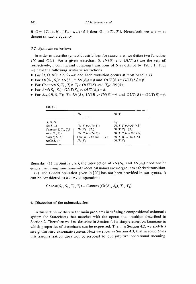
3.2. Syntactic restrictions

In order to describe syntactic restrictions for statecharts, we define two functions

IN and OUT. For a given statechart S, IN(S) and OUT(S) are the sets of,

respectively, incoming and outgoing transitions of S as defined by Table 1. Then

we have the following syntactic restrictions.

l For [I, 0, N]: I n OT = (il and each transition occurs at most once in 0.

l For Or(S,, S,): ZN(S,) n IN(S) =@ and OUT(S,) n OUT(&) =@.

l For Connect(S, T,, T2): T, E OUT(S) and T,E IN(S).

l For And(S,,S,): OUT(S,)nOUT(SJ=Q.

l For Stat(B,S, T): TEIN(S), ZN(B)nZN(S)=@ and OUT(B)nOUT(S)=@

Table 1

[I, 0, Nl WS, > .%) Connect(S, T,, T2) And(S, > .%I .stat( B, s, T) HiCl( S, a ) 1

IN OUT

I 0, IN(S,)u IN($) OUT(S,)u OUT(.$)

IN(S)Fi OUT(S)Fi IN(S,)u IN($) OUT(S,)u OUT(.%)

(IN(B)uIN(S))-{TJ OUT(E)” OUT(S)

IN(S) OUT(S)

Remarks. (1) In And( S, , S?), the intersection of ZN(S,) and IN(&) need not be

empty. Incoming transitions with identical names are merged into a forked transition.

(2) The Concat operation given in [20] has not been provided in our syntax. It

can be considered as a derived operation:

Concat(S,, S2, T,, T2) = Connect( Or(S,, S,), T, , TJ.

4. Discussion of the axiomatization

In this section we discuss the main problems in defining a compositional axiomatic

system for Statecharts that matches with the operational intuition described in

Section 2. Therefore we first describe in Section 4.1 a simple assertion language in

which properties of statecharts can be expressed. Then, in Section 4.2, we sketch a

straightforward axiomatic system. Next we show in Section 4.3, that in some cases

this axiomatization does not correspond to our intuitive operational meaning.

A compositional axiomatization of Statecharts 301

Finally, we describe modifications to the assertion language to deal with these

problems. The resulting axiomatization is then given in the next section.

4.1. Assertion language

To express properties of a statechart we use a first-order assertion language. The

main point in the definition of the assertion language is the choice of the primitives.

They should be such that we can express which events occur in the system at

a certain step and which events are generated by the statechart under consider-

ation. Furthermore we should be able to express entry and exit of a statechart.

Hence, as a first attempt, we use the following primitives to specify properties of

a statechart S:

occ(a, n) to express that event a occurs in step n (generated by S or its

environment);

G(n) to denote the set of events generated by S in step n;

st, ranging over N, denoting the start step, i.e. the step at which S has been entered;

es, ranging over N u {CO}, to denote the exit step or 00 if S is never exited;

in, ranging over Y,,, u {*}, the incoming transition, or * when S is entered implicitly;

out, ranging over .Y(,,,, u {*, I}, the outgoing transition, or * when S is exited

implicitly, or I when S is not exited.

Our assertion language contains two kinds of variables, the above-mentioned reserved

symbols (occ, G, st, es, in, out), and logical variables. We use three types of logical

variables:

l Logical

Typical

l Logical

Typical

l Logical

Typical

N-variables, ranging over the natural numbers.

symbols are k, 1, WI, n, . . .

transition variables, ranging over transition names.

symbols are t, t,, t\, ty, . . . .

G-variables, ranging over functions from N to sets of events.

symbols are g, g,, . . . .

In addition, the assertion language includes first-order arithmetic. Quantification is

only allowed over logical N-variables, and the conventional logical connectives 1,

v, A and + are used. We use p[exp/var] to denote the substitution of each free

occurrence of variable var by expression exp. For this assertion language we have

the following axioms:

l st < es (The start step is less than the exit step, since a state cannot be entered

and exited within a single step.)

l es = oo* out = I (The exit step equals cc if there is no exit.)

l a E G(n) -+ occ(a, n) (If event a is generated in step n then a occurs in step n.)

l Vn: (st s n v n < es) + G(n) = 0. (Nothing is generated before or within the entry

step and after the exit step.)

The formal interpretation of assertions is defined in Section 7, using the semantic

model that will be given in Section 6. The semantic domain will be such that the

axioms above are valid.


As already mentioned in the introduction, we use formulae of the form S sat cp

to express that statechart S satisfies assertion cp. In Section 7 we formally define

when such a correctness formula is valid. Informally, S sat cp is valid if cp holds for

every possible execution of S.

Example 4.1. For the basic statechart with name wait in Fig. 2 we have

[{ Ts}, {( T2, ddatu/{datu, correct}),

( TX, iddata A tm( dreq, 4)/compZete)}, wail]

satin=T,~occ(ddutu,st+1)~our=T,~G(st+1)={dutu,correcr)

~es=sr+l.

Using our assertion language, we can express real-time safety properties such as

“event a occurs within five steps” - 3n < 5: occ(u, sr+ n)

and

“never exit” = es = Co.

But also liveness properties can be expressed, for instance,

“eventually event a will occur” = 3n: occ(u, St + n),

“eventually exit” = es # 00, and

“event a is generated infinitely often” = t/k 3n 3 k: a E G(n).

4.2. Outline of the uxiomurizurion

The axiomatization consists of an axiom schema for basic statecharts, a proof

rule for each of the operators mentioned earlier, and a consequence rule. In this

section we give an outline of a straightforward axiomatization using the assertion

language described above. In Section 4.3 we show that slight modifications are

required for a satisfactory treatment of the examples concerning causality and

negation given in Section 2.

First we have an axiom for a basic statechart [I, 0, N]. Any computation of

[I, 0, N] enters state N either implicitly (denoted by *) or via a transition in Z, and

starts waiting to exit N. Then there are three possible situations: either it waits

forever, not being able to take any of the outgoing transitions (represented by

assertion WAZT( 0, k), defined below), or it exists the statechart at a certain step

either implicitly (denoted by l ), or explicitly by taking an outgoing transition in OT

(represented by FZRE(0, es)). This leads to the following axiom:

Axiom 4.2.

[Z,O,N] sat (inEZvin=*)AVk,sr<k<es: WAZT(O,k)

A[(es=~)v(out=*/\G(es)=@)v FZRE(O,es)].


For a transition t E OT we use E,/A, to denote the label of t in 0. Assertion

WAZT(0, k) describes that the basic statechart waits at step k. During waiting no

event is generated and no transition in 0, can be taken. Hence,

WAIT(0, k) = (G(k) =fl) A /j locc( E,, k), rio,

where occ(E,, k) is a natural extension of occ for an event-expression E,, given by

occ(h, k) = true,

occ(la, k) = locc(a, k),

occ(e, v e,, k) = occ(e,, k) v occ(e,, k),

occ( e, A e,, k) = occ( e, , k) A occ( e2, k),

occ(tm(e, n), k)

-1

occ(e,k-n)AVm,k-n<m<k:locc(e,m) ifkzn,

false if k< n.

Observe that, due to the “never” interpretation of negation, we have a simple

expression for negated events: le occurs in step k iff e does not occur in step k.

Note that

occ(tm(e, 0), k) = occ(e, k).

Furthermore we have defined

occ(tm(e,n),n)-occ(e,O),

since the system is allowed to start at time 0. Assertion FIRE (0, k) expresses the

condition for taking a transition t E 0, at step k. Then occ( E,, k) must hold and all

events in A, are generated by the basic statechart.

FIRE(O,k) = V [(out=t)r\occ(E,,k)r\(G(v)=A,)]. It 0,

Example 4.3. Consider the basic statechart S= [{T,}, {(T,, la/a)}, A]. Then

S sat out # T2, because FIRE({( T,, la/a)}, k) leads to (out = TJ A occ(la, k) A

(G(k) = {a}). Since G(k) = {a} implies occ( a, k), this gives false.

The axiomatic system contains a rule for each of the syntactic operators. We give

an outline of the rules that will be used in this section to explain the main problems

in defining the axiomatization. First consider the And-construct And(S, , S,). Assume

S, sat qj, for j = 1,2. Then at every computation step the G-set of And(S,, S,) is

the union of the G-sets of S, and S,. Furthermore we have to express how the entry

and exit of And(S, , S,) is related to entry and exit of its components S, and S2.

This will be explained in the next section. Concentrating on the G-set we obtain a

rule of the following form, where g, and g2 are fresh logical G-variables.


Rule 4.4 (And).

S, sat n, S2 sat (p?

(cp,k,lG, . . .I A dgz/G.. .I A Wk: G(k) = g,(k) u gz(k)) A. . .) + cp

And( S, , S,) sat cp

The rule for Statilication Stat(B, S, T) is similar to the rule for the And-construct,

except for the way of entering. In the rule for the hiding and closure construct

HKY(S, a) we require that every occurrence of event a inside S must be generated

by S itself. This leads to the condition Vn: occ(a, n) + a E G(n).

4.3. Problems

We show that the axiomatization sketched above does not always correspond to

our operational intuition. Consider statechart S, = [{T,}, {(T,, a/u)}, A] (see also

the first statechart from Fig. 3). If T2 is taken in step k then FZRE({( T,, u/u)}, k)

leads to (out = T,) A occ( a, k) A (G(k) = {a}). Observe that then the requirement in

the rule for HiCZ(S, , a) is fulfilled, and hence we can take T, after hiding and

closure with respect to event a. Thus, in contrast with the intended semantics, T2

can be taken without any external occurrence of a. Note, however, that the generation

of event a by T2 is not observable, since a has been generated already somewhere

in the system. For instance, the environment cannot distinguish between statechart

S, and S2 = [{T,}, {( Tz, u/g)}, A]. Therefore, in our final axiomatization we do not

use G(n), the set of all generated events by a statechart, but a subset F(n). Informally,

an event e is an element of this set F(n) for a statechart S if S is responsible for

the first generation of e in the system in step n. Then firing transition T2 above leads

to occ(u, k) A F(k) = 8, since a must have been generated earlier inside this step.

To make the axiomatic system compositional, the specification of a statechart S

must hold for all potential computations of S. Thus we allow any arbitrary environ-

ment, and when composing S with another statechart a number of these potential

computations can be removed because more information about the environment is

available. For the set F(n) this means that we include all possible subsets of the

set of generated events, as far as they are consistent with the event-expression (e.g.

F(k) = {a} is not consistent with event-expression a). Consider, for instance,

[{ TJ, I( T4, a/b)}, Bl. Then firing T4 leads to either occ(u, k) A F(k) = B or

occ(u, k) A F(k) ={b}.

This example leads to the second problem. Consider the second statechart of Fig.

3 in which there are two transitions with labels u/b and b/u. Taking the transition

with label u/b might lead to occ( a, k) A F(k) = {b}. Similarly, by taking the transition

with label b/u we can obtain occ(b, k) A F(k) = {a}. After applying rules for And

and Statification it is possible to take both transitions with occ(u, k) A occ(b, k) A

F(k) = {a, b}. Now observe that the restrictions for hiding and closure with respect

to a and b are fulfilled, and hence it is possible to take both transitions without

any external a or 6. The problem is that we cannot express the causal relationship

A compositional axiomatization oj’Statecharts 305

between a and b. Therefore we extend our assertion language with a causality relation

a ik b to express that the first generation of a in step k precedes the first generation

of b in step k. Then occ( a, k) A F(k) = {b} leads to a -c, b, because F(k) = {b}

expresses that S, claims to generate b for the first time, and hence a must precede

b. Similarly, occ( b, k) A F(k) = {a} leads to b <,, a. Since the relation <r will be a

strict partial order (i.e. irreflexive and transitive), we cannot have both a <k b and

b <k a, and thus these two possibilities cannot be combined. Hence, F(k) = {a, b}

is impossible and external events are required to trigger these transitions.

5. Compositional axiomatization

In this section we give a compositional axiomatization for Statecharts. We use

the assertion language from Section 4.1 with the modifications from Section 4.3.

Thus G(n) is replaced by F(n) and, for atomic events a and b, we add a <,, b.

Furthermore, instead of logical G-variables we use logical F-variables, ranging

over functions from N to sets of events. Typical symbols are ,f, f,, . . . For two

logical variables f, and fi their point-wise union, denoted by f, cj fi, is defined as

(f, ti f2)( n) = f,( n) u f2( n), for all n E N. The point-wise subtraction of the function

Fandaset~a~,denotedF~~a~,isgivenby(F~~a~)(n)=F(n)-~a~,foralln~~.

Similar to the previous section, we have a number of axioms for the assertion

language. In the properties mentioned in Section 3 the function G is replaced by

F and we add two axioms about the causality relation <,,, expressing that it is a

strict partial order.

st < es,

es=03 - out=I,

a E F(n) + occ(a, n),

Vn: (stdnvn<es) + F(n)=@,

Vn: i(a <n a) (in is irreflexive),

Vn:(a<,,bAbi,,c) + a<,,~ (<, is transitive).

The axiomatic system contains, for any statechart S, the usual consequence rule

by which an assertion can be weakened.

Rule 5.1 (Consequence).

S sat cp, (P+(P)

The axiom for a basic statechart is obtained by a slight modification of Axiom

4.2. Replacing G by F we obtain the following axiom:

J.J.M. Hooman er al

Axiom 5.2 (Basic Statechart).

[I,O,N] sat (inEIvin=*)r\Vk,st<k<es: WAIT(O,k)

Let the label of an outgoing transition t E OT be given by E,/A,. Then

WAIT(0, k) = (F(k)=(d)/\ /j locc(E,, k). ,607

Predicate FIRE now asserts that the F-set is a subset of the generated events.

Furthermore we have to express that certain causal relations exist between newly

generated events and the events that triggered the transition. These relations are

represented by assertion SOC( E,, a, k), for a E A,, defined below. Consequently,

FZRE(O,k) = V (out=t)r,occ(E,,k)/\(F(k)zA,) 110,

A /j (occ(a,k)~[a~F(k)+soc(E,,a,k)]) .

0*A, I

Assertion soc(E,, a, k) provides the necessary causal relation between any event

a E F(k) and the events occurring in E,. For instance, if E, = b then b -C k a, whereas

E, = lb should not lead to a relation between b and a, since b does not occur at

step v. We define sot by

soc(h, a, k) = true,

soc(b, a, k) = {

b<,,a if bfa, faoe

if b=a,

soc(lb, a, k) = locc(b, k),

soc(tm(e, n), a, k) = occ(tm(e, n), k),

soc( e, v ez, a, k) = soc( e, , a, k) v soc( e,, a, k),

soc( e, A e2, a, k) = soc( e, , a, k) A soc( e2, a, k).

Example 5.3. Firing a transition T2 with label a/a in step k leads by the formula

above to

(out = T2) A occ(a, k) A (F(k) c {a})

A (occ( a, k) A [a E F(k) + soc( a, a, k)]).

Since soc(a, a, k) = false, this leads to (out = T2) A occ(a, k) A (F(k) G {a}) A a EZ

F(k). Hence, we obtain (out = T2) A occ( a, k) A F(k) = @, which indeed expresses

that this transition cannot be responsible for the first generation of a in step k.


To formulate a rule for the Or-construct, note that any computation of Or( S, , S,)

is a computation from either S, or S,. Then the rule for the Or-construct is given by

Rule 5.4 (Or).

For the Connect-construct, observe that any execution of Connect(S, T, , T,)

(1) first enters S via a transition different from T2, then

(2) takes transitions inside S, and then possibly exits S either

l via a transition different from T, (and then also exits Connect(S, T,, TJ),

or

l via T, , re-enters S via T,, and repeats (2).

To formulate a rule for this construct, we first define the concatenation of two

assertions cp, and cpz with respect to T, and T2. Informally, this is an assertion

expressing computations that either

l satisfy cp, and do not exit via T,, or

l can be split up in two parts; a computation satisfying cp, that exits via T, at a

certain step m, followed by a computation satisfying cp2 that enters via Tz in the

same step m.

Formally, with fresh logic variables m, f, and f2, we define

conc(cp,, cp2, T,, T2) = (cp, A (out f Td) v (df,lF, T,lout, m/es1

*(F =fi ~_G)).

Now in the rule we use an assertion q(n), which has a free logical N-variable n.

This assertion q(n) represents the behaviour of a sequence of n copies of S that

are connected via T, and T2, allowing arbitrary behaviour after a T,-exit of the last

copy. In particular, ~(0) should express arbitrary behaviour, and hence should be

satisfied by any computation. Thus in the rule below we require that ~(0) is

(universally) valid. Furthermore, assuming S sat 4, we have that

conc(& p(n), T,, T2) -+ cp(n + 1)

must hold, where cp(n + 1) = cp[n + l/n]. Then a computation of Connect(S, T,, T2)

satisfies p(n) for all n. This leads to the following rule.

Rule 5.5

with n a

(Connect).

S sat 4, cp(O), conc(4, p(n), T,, TJ+ cp(n + 1)

Connect(S, T,, T?)sat(in# T,)AVn: p(n) ’

logical N-variable not occurring free in 4.

308 J.J.M. Hooman er al

To explain the rule for And(S,, S,), assume S, sat ‘p, is valid, forj = 1,2. Consider

the primitive expressions occurring in cp, and ‘pz. Observe that the start step st must

have the same value in these two assertions since both components are entered in

the same step. Similarly, they should have the same value for es. Since occ specifies

the events that occur in the complete system, the two specifications must agree on

these occurrences. Similarly, <n expresses relations between events in the total

system and should be equal in both assertions. For the other primitives (in, F and

out), the two components might specify different values. These remaining primitives

are related as follows.

l Entry of And(S, , SJ is done either

- implicitly (notation *), by entering both S, and S7 implicitly, or _ via a joint transition of S, and Sz, or

- via a transition of S, that is not a transition of S,; then S, is entered implicitly.

Similarly for the symmetric case with S, and Sz interchanged.

l At every computation step the F-set of And(S, , S,) is the union of the F-sets of

S, and Sz.

l Concerning the exit of And(S, , S,) we have that either

- both S, and S7 are exited implicitly (denoted by *), or

- it is exited via a transition of S, (S, resp.); then S? (S, resp.) is exited implicitly,

or _ And(S, , S,) is never exited, thus neither S, nor S, are exited (denoted by I).

By substituting logical variables for these last three primitives we can take the

conjunction of both assertions: cp,[ ti/ in, f,/ F, tP/out] A cpz[ ti/ in, f2/ F, tz/out], where

tl,f,, t’;, ti, fi, tY are logical variables. The relations between these primitives, as

described above, are expressed by

and-in = (in = ti = t;) v (in = ti A tk = l ) v (in = t\ A t\ = *), and

and_out = (out=t:‘#IAt!j=*)v(out=t;#IAt’;=*)

v(out=ty=t;=I).

This leads to the following rule.

Rule 5.6 (And).

with tl , ti, t” , , tl fresh logical transition variables, and f, , fi fresh logical F-variables.

The rule for the Statification-construct is similar to the rule for the And-construct,

except for the way of entering. Entry of Stat(B, S, T) can be done either

(1) by entering B (via a transition or implicitly) and then entering S via default

T, or

(2) by entering S via a transition (different from T) and then implicitly entering B.

A compositional axiomatization of Statecharts

Hence, in the rule we use

309

stat_in = (in=t\~t~=T)v(in#*~in#T~in=t~~t’,=*),

srat_out = (out = ty # I A t; = *) v (out = t; # I A ry = *)

v(out=t;=t;=I).

Rule 5.7 (StatiJication).

Bsatv,, S sat ‘pz

(q,[t;/in,,f,/F, t’l/out]r, pJt>/in,f,/F, t(2)/out]~stat_in h stat_out ~(F=f,tif~))+(~

Stat( B, S, T) sat rp

with t\ , ti, ty, 2; fresh logical transition variables, and f, , ,fi fresh logical F-variables.

Next we give a rule for HiCI(S, a). Assume S sat cp is valid. To obtain a

specification cp’ for HXJ(S, a), the possible computations satisfying cp are restricted

to those where S is responsible for every occurrence of a (formally, occ(a, n) implies

a E F(n), for every step n). Next a is hidden; it is removed from F (represented in

the rule by a substitution in cp’) and we require that cp’ should not refer to a. This

leads to the following rule.

Rule 5.8 (Hide-Closure).

S sat cp, (cp~(Vn: ~~~(a,n)~a~F(n)))~cp’[F~(a)/F]

HiCI( S, a) sat cp’

provided a does not occur in cp’.

Example 5.9. Consider the avionics system described by the statecharts from Figs.

1 and 2. We would like to prove that after a request the system provides data within

a certain number of steps. Thus, for some constant K,

occ(req,st+n)+3ks K: occ(data,st+n+k).

(We assume that free logical variables, such as n here, are universally quantified.)

Since in state off all req events are ignored, we can only prove this property if the

system is in state on. Therefore we introduce a predicate instate(on, k, , k,) which

expresses that the system is in state on during the steps k, through k2:

instate( on, k, , k?) = (out # I) A 3rn < k, : occ(start, m)

A Vl, m < 1 s k,: locc(stop, I).

This leads to

[instate(on,st+n,st+n+K)r\occ(req,st+n)]

+3k< K: occ(data,st+n+k).


First we consider a guaranteed quick response in case there are no fault events. We

show that the system satisfies

cp = [(Vm: locc(fault, m)) A instate(on, st+n, st+n+3)

A occ( req, st + n)] + occ(data, st + n +3).

Let D be the statechart from Fig. 1, and define

(Pi = [(Vm: locc(fault, m)) A (out#_l)r\ occ(dreq, st+l+n,)]

+occ(ddata,st+l+n,+3).

(Note that device enters state ready in step st, and thus is willing to receive requests

at step st + 1.) Then the device satisfies (Pi, provided prod is an external event. That

is,

HiCl( D, prod ) sat qd.

Let C be the statechart of Fig. 2. If we assume that occ(dreq, st + 1-t n,) +

occ(ddata, st + 1 + n, + 3) holds, then the transition from wait to computing in C is

never taken. Define

cpc = [(Vn,: occ(dreq,st+l+n,)+occ(ddata,st+l+n,+3))

A instate( on, st + n, st + n + 3) A occ( req, st + n)]

+occ(data,st+n+3),

then C sat cpc.

Now we prove that (Pd[ ty/out] A cpC[ tP/out] A and-out implies cp. Assume

(Vm: iocc(fault, m)) A instate(on, st + n, st + n + 3) A occ( req, st + n)

From instate(on, st + n, st + n + 3) we obtain out f 1, and by and-out this leads to

ty# 1. Together with Vm: locc(fault, m) and (P~[ tP/out] this leads to

Vn,: occ(dreq,st+l+n,)+occ(ddata,st+l+n,+3).

Then from pc[ti/out] we obtain occ(data, st + n +3). Hence we can derive, by the

And Rule, And (HiCI( D, prod), C) sat p.

Next we consider the general case in which faults may occur and we can only

derive a worst case response time, since some of the data might have to be computed.

Define

$ = [ instate( on, st + n, st + n + 3) A occ( req, st + n)]

+ 3k < 27: occ(data, st + n + k).

Then (c, can be proved for the control unit C, independent of D, provided event

compute is not generated externally. Thus HiCI( C, compute) sat +k

311

6. Denotational semantics of Statecharts

As mentioned in the introduction, the semantic model associates with a statechart

a set of maximal computation histories representing all complete executions. It has

been shown in [20] that, besides denotations for events generated in each computa-

tion step (the observabies) and denotations for entry and exit, the following two

additional denotations are necessary and sufficient to obtain a compositional seman-

tics: (1) a set of all events assumed to be generated by the total system (i.e. a

statechart and its environment) at each step and (2) a causality relation between

generated events. More precisely, a computation history h of a statechart S is of

the form h = (.t, i, A o, s) where

l .?E N models the start step.

l i E Yi,, u {*} is either an incoming transition or l to model an implicit entry.

. f:N+{(F, C, c)lFc c and < a strict partial order on C} is a function which

records the state of affairs for every step n by a triple (F, C, <), where

- F is a subset of the events generated by S. An event is an element of F at step

n if S is responsible for the first generation of this event in the chain of

transitions taken in step n in the system. _ C is the set of events generated by the total system in step n. _ < denotes the causal relationship between events generated in the total system.

l 0 E y<,,,, u {*, I} is either an outgoing transition, or l for an implicit exit, or I

when there is no exit.

l s EN u {CO} denotes the exit step.

For a function f as above, the three fields off(n) are denoted by f’( n), f“(n) and

f‘(n). Furthermore, h will denote ($ i,,f; o, s) and similarly for super- and subscripts:

h’ denotes (?, i’,f’, o’, s’), h, denotes (5,) i, ,f, , o, , s,), etc.

Let X={hIs^<s,s=cooo=I and, for all HEN, (.<~nvn<~)-+j’~(r1)=0}.

Then our semantic domain is given by (9, r= ), where 9 = {D 1 D G X} and D, c

D2 iff D, c D2 for all D,, D?E 9. Clearly, this domain is a complete lattice with

bottom element 0 and top element X. We give a denotational semantics of Statecharts

by defining a semantic function J!I that assigns to any statechart S a set of histories,

that is, Ju(S) E 9.

Definition 6.1 (Basic). Consider a basic statechart [I, 0, N]. For a transition j E OT

we denote the label of j in 0 by E,/A,. Using predicates wait and jre, which are

defined below, the semantics of [I, 0, N] is given by

&([I, 0, N])={~E~~I~((Iu{*})A~u,SI<~<S: wait(O,u)

~[(~=CO)v(o=*~f~(s)=(d)vjre(O,s)]}.

Predicate wait( 0, v) characterizes the situation in which none of the transition in

OT. can be taken. Then none of the triggers of these transitions evaluate to true and

no event is generated by the statechart. Consequently, wait is defined as

wait(0, u) = fF(o) =(d~ A linC(E,, v) ;i 0,


where inC( E,, v) gives the condition in which Ej evaluates to true at step ZI. It is

inductively defined as follows:

inC(h, V) = true,

inC(a, 0) = a Ef“(u) for a E E,,

inC(ia, u) = iinC(a, v),

inC(e,ve,, v) = inC(e,, v)vinC(e,, u),

inC(e,r\e,,u) = inC(e,,u)AinC(e,,v),

inC( tm(e, n), 21)

-1

inC(e, U-n)~Vv’, v-n< u’< 0: iinC(e,

false

v’) if 2) 2 n,

if u < n.

Predicate Jive describes the situation in which one of the outgoing transitions can

be taken. Using predicate str, defined below, jire is given by

r $re( 0, U) G ,cl, 10 =j A inC( Ej, U) A (f’(u) G A, ~.f“( v))

A .?, (a ET(u)+ ME,, a, 0)) . 1 The predicate str gives the necessary causal relation between the events constituting

the trigger and the events that are generated as a result of taking the transition. It

is given by

str(A, a, v) = true,

Mb, a, u) = i

(b,a)Efx(v) if bZa, .false

if b=a,

str(tm(e, n), a, u) = inC(tm(e, n), v),

str(lb, a, u) = linC(b, u),

str(e, v e,, a, 21) = str( e, , a, u) v str(e2, a, v),

str( e, A e2, a, 21) = str( e, , a, u) A str( e2, a, u).

Definition 6.2 (Or). The semantics of an Or-construct is the union of the semantics

of its constituents.

JU(Or(S,, &)I = Juts,) u Az(W


Definition 6.3 (Connect). Execution of Connect(S, T, , T,) consists of first (a) enter-

ing S via a transition different from T2 and then (b) taking transitions as specified

by S and possibly exiting S either via a transition different from T,, or via T, and

then re-entering S via T2 and repeating (b). Given two sets of histories D, , Dz, we

define CONC(D,, Dz, T,, T2) as the set of (i) histories of D, that do not exit via

Tl, and (ii) histories that consist of a history from D, with an exit via T, , followed

by a history of D7 with an entry via T,. Formally,

CONC(D,, D,, T, Tz)

={hjh~ D,r,o# T,}

v{h13h,~D,,hz~D,:~=~,r\s,=~~~s=s,r\i=i,

A i, = T2 A o, = T, A o = o2 A (f’ =f;ijf,‘)

A (f’ =f:‘ =f;) A (f’ =f; =f;)}.

To obtain A (Connect (S, T, , T2)) we consider the largest set D satisfying

D = CONC(A(S), D, T,, T,),

that is, the greatest fixed point vx, CONC(&(S), X, T,, T,). In order to have such

a fixed point definition (see, e.g. [4]), CONC is shown to be monotonic in its second

argument. From this set we remove the histories that have an entry via T2. (Note

that such a set D will not contain histories that exit via T, .) This leads to

.&(Connecr(S, T,, T,))=del,(v,.CONC(&(S),X, T,, Tz))

where de/,(D) = {h E D 1 i # T2}.

Since CONC is anti-continuous, this greatest fixed point can be obtained by an

iteration, and the semantics can be given as the intersection of approximations:

A( Connect( S, T, , T2)) = del,

where D,=%Y, and for kEKJ(, DL+,=CONC(&(S), DL, T,, Tz).

Definition 6.4 (And). The semantics of And (S, , S,) is obtained by merging every

pair of histories from S, and S2 that agree on the behaviour of the environment.

More precisely,

A(And(S,, S,))

={h13h,E~(S,),hzE~(S~):S1=~,=~~AA==,=Sz

A (f’ =f:‘ =fi’j A (f’ =f; =f;) A (f’ =f:tif:)

~[(i=i,=i,)v(i=i,Ai~=*)v(i=i,Ai,=*)]

A[(O=0,#~A02=*)V(O=02#~A0,=*)VO=01=O~=~]}.


Definition 6.5 (Statzjkation). The semantics of Stat(B, S, T) is similar to

A(And(B, S)),

except for the way in which the statechart is entered; any entry to B leads to S via

the default arc T and a direct entry via T is no longer possible. Consequently, the

semantics is given as follows:

A( Srat( B, S, T))

={h13h,~~(B),h,~~(S):~=~,=~*ns=s,=s,

A (.f’. =fF =fi’j A (f<’ =f; =fT) A (f’ =ff i/j-i’,

A[(i=i,ni,=T)v(i=i2#T~i#*Ai,=*)]

A [( 0 = 0, # 1 A O2 = *) V (0 = O2 # 1 A 0, = l ) V 0 = 0, = O2 = I]}.

Definition 6.6 (Hide and Close). In the semantics of HZ/( S, a) we first require that

every occurrence of a is generated by S. Next a is hidden by removing it from the

F-set, and by allowing the C- and <-field to be arbitrary with respect to a (to

model occurrences of a that are independent of S). Define the point-wise subtraction

of a set-valued function g and a set A, notation g _L A, as (g L A)( V) = g(u) -A, for

all v E IV For a function f < with, for all Y, f’( V) s E, x E,, we define the restriction

off’ to events different from a, notationf<(,, asferlo =f’- (E, x {a}) - ({a} x E,).

Then the semantics is given by

~(HiC1(S,a))=hide,({h~h~~H(S)~Vv: UE~~(U)+UE~~(IJ)})

where

hide,(D)={hE~l3h,ED:s^=s^,~i=i,~o=o,~s=s,

A (f” =f: -{a)) A (f-‘la =.f,%)

A(f’~~{a}=f:‘~{a})}.

7. Interpretation of specifications

In this section we formally define when a statechart S satisfies an assertion cp,

that is, we define when a formula S sat cp is valid. Therefore we first give the

interpretation of assertions. This interpretation requires a computation history, which

assigns values to reserved variables, and a logical variable environment that assigns

values to logical variables. The value of a logical variable u in a logical environment

y is denoted by y(v). We define the variant of an environment y with respect to a

variable x and a value U, denoted by ( y : x - v), as

(y:x++v)(y)= U 1 if x-y,

Y(Y) if X*Y.

A compositional ariomatization of State-charts 315

Next we define when an assertion cp holds in a history h = (2, i,f, o, s) and a

logical variable environment y, denoted [qjyh. We give the main points from the

definition of this interpretation, leaving the first-order model, relative to which

validity is defined, implicit: it is the standard model of arithmetic throughout this

paper. For instance, quantification is defined as follows: [3n: (p] yh iff there exists

a value u E N such that [cp]( y : n ++ u)h.

The primitives from the assertion language that yield a transition name are

interpreted as:

[in] yh = i, [[ouq yh = 0, U4lYh = Y(f).

Observe that logical variable environment y gives the value of logical transition

variable t. Similarly, we have [f] yh = y(f), for a logical F-variable J:

Next we give the interpretation of primitives yielding a value from N u {co}.

[stl]yh = f, [es] yh = s, Un!lyh = r(n).

This can be extended easily to the definition of [[expj yh, for any expression exp.

Now assume exp denotes an expression yielding a natural number (for expressions

yielding cc we take a default value in the definitions below), then the remaining

primitives have the following meaning:

UF(exp)lyh=fF(UexpI1yh), Uocc(a, exp)]yh holds iff a Ef’([exp] yh),

[a -crrp 61 yh holds iff (a, b) Ef’([exp]yh).

An assertion cp is valid, denoted by +cp, iff [PI yh holds for all y and for all h E X

Since assertions are interpreted in histories of 2? only, we have the following valid

assertions:

+ st < es, + es=02 ++ out=I,

+ Vn: nGstvn>es+F(n)=B, and

+ Vn: a <“b+ occ(u, n) A occ(b, n).

Informally, a formula S sat cp is valid if cp holds in any history from the semantics

of S. Thus S sat p is valid, denoted by k=S sat cp, iff [Ip] yh for all y and for all

h E J%(S).

8. Soundness of the axiomatization

In this section we prove that the axiomatization is sound, that is, every formula

which can be derived is valid. Let ES sat cp denote that S sat cp is derivable using

the axiomatic system from Section 5. Then to prove soundness we have to show

that ES sat cp implies +S sat cp. This is proved below by showing that the Basic

Statechart Axiom yields a valid specification and that all rules preserve validity.

316 J.J.M. Hooman et al

Consequence Rule

Assume i=S sat cp and I= cp + cp’. We prove k=S sat cp’. Let y be arbitrary and consider

h E d(S). Then, by +S sat p, [[cpl yh, and thus, using !=cp + cp’, we obtain [P’I] yh.

Basic Statechart Axiom

To prove that the Basic Statechart Axiom is valid, we first prove the following

lemmas (for all e E Exp, a E E,, expression exp, environment y and history h).

Lemma 8.1. [occ(e, exp)] yh = inC(e, [expl yh).

Proof. Easy, by induction on the structure of e. For instance, for e E E, both sides

evaluate to eEfC‘([expJyh). 0

Lemma 8.2. [soc(e, a, exp)l yh = str(e, a, [expjyh).

Proof. Straightforward, by induction on the structure of e. For instance,

[soc(lb, a, exp)jyh = [locc(b, exp)l yh = l[occ(b, exp)lyh

which equals, by Lemma 8.1, linC(b, [exp]yh), and thus str(+, a, [expjyh). 0

Lemma 8.3. [ WAIT( 0, exp)jyh = wait( 0, [expjyh).

Proof. I[WAIT(O,exp)]yh=[F(exp)=f~~jj,,,, locc( E,, exp)jyh. By the interpre-

tation of assertions and Lemma 8.1 this leads to

f'(Ue-dlrh)=(d~ A ~i~Cb%Ue-vll~h),

and hence wait(0, [expnyh). 0

Lemma 8.4. [FIRE (0, exp)] yh =jre( 0, [IexpJj yh).

Proof. We have

UF~JWO,~V)~Y~

out = 1 A occ( E,, exp) A F( exp) G A,

A .?, (occ(a, exp) A [a E F(ev)+ ~46, a, exp)l) Ill rh.

Using the interpretation of assertions, Lemma 8.1, and Lemma 8.2, this leads to

v [o= f A inC(E,, Uexpll yh) Af’(Uexpllyh)c A, 1t0,

A .!A (a ~fC‘(Uexpllyh) A [a ~fF(U41yh)+ NC, a, UexpihhH) 3 ,

A compositional axiomatiza!ion of Starecharts 317

and thus

A u>A (0 EfF(Uexpbh)+ str(Ejt a, Uedlrh)) 1

which equals fire( 0, [expjyh). Cl

Now we are able to show that the Basic Statechart Axiom is valid. Let y be arbitrary,

and consider h E A([ Z, 0, IV]). Then i E (I u {*}), and thus [in E I v in = *I yh.

Furthermore Vu, s^< v < s: wait( 0, v), which leads by Lemma 8.3 to

[IVk, st < k < es: WAZT( 0, k)jyh.

From the semantics we also obtain (s = a) v (o = * of’ = 0) vjre(0, s). Hence,

using Lemma 8.4,

Together this leads to

[(inEZvin=*)r\Vk,st<k<es: WAZT(O,k)

Or Rule

Assume +S, sat cp, and I=& sat qr. We prove kOr(S,, S2) sat cp, v (p2. Let y be

arbitrary, and consider h E .M( Or( S, , S)). Then h E Ju(S,) u Ju(S,). Hence by our

assumption [p,nyh or [IcpJyh, and thus [[cp, v (pJyh.

Connect Rule

Assume +Ssat 4, kcp(O) and bconc(& q(n), T,, T,)-+cp[n+l/n], i.e.

A F =fi v&)) + cp[n + l/n],

where m, f,, fi are fresh logical variables, and n is a logical variable not occurring

free in $. We prove k Connect(S, T,, TJ sat in # T2 A Vn: p(n). Let y be arbitrary,

and consider h E Jll( Connect(S, T, , T,)). Then h E nkcN Dk with i # T2 and where

Do= FE, and Dk+, = CONC(.d(S), DL, T,, TJ, for k E N. First we prove the follow-

ing lemma.


Lemma 8.5. If h E Dk then [q( n)j( y : n - k)h for all k E N.

Proof. By induction on k.

Basic step: Consider h E D,= 2. Then, by validity of p(O), [cp[O/n]ljyh, and hence

lIcP(n)ll(r: n I--+ O)h. Induction step: Let h E Dk+, = CONC(Ju(S), Dk, T,, Tz). Then there are two

possibilities.

(1) h EA(S) and o # T,. From +Ssat 6 we obtain [[Glyh, and o# T, implies

[our # T,nyh. Since n does not occur in $ A our # T,, this leads to [I$ A our #

T,n(y:n-k)h. Then by Fconc(@,cp(n), T,, T,)-+cp[n+l/n], we obtain [p[n+

l/n]j(r: n H k)h, and thus [p(n)j(r: n H k+l)h.

(2) There exist h, and h2 such that h, E A(S), hzE Dk,

i=i,AO=0~AS1=S1,AS~=~~As=sS2A(fC‘=f:‘=f~)A(f~=f;=f~)

(I)

and i2=Tzno,=T,~(fF=f:Ijf~).

Then, using +S sat $, we obtain [I$jyh, and, by the induction hypothesis,

[q(n)jj(r:n-k)hz. Define r’=(r:f,~ff,f~~f2F,m~s,). Since n does not

occur free in 4, we have [$[f,/F, m/es]n(r’: n H k)h, and, using s, =$,

Ucp(~DW,f,l~llW: n - kh.

Since i2 = Tz and o, = T, , this leads to

U4Ml~ Trlout, ml4llW: n - WG,, i,,(f’,f~,f;>, 0,s)

and

Ucp(n)[mlsr, WWJ~lNr’: n - k)(f, 4 <f’~.f~X?, 02, 4.

Using (1) this can be written as

UCf,lK T/our, ~l4IlW: n - k)(i, i, Cf’,fC‘,fi), 0, s)

and

Ucp(n)[mlsr, T2/~~,.Ll~l%W: n - k)(t, i, (f’,f“,f’L 0, ~1.

Thus [@[f,/F, T,/our, m/es] A q(n)[m/sr, T,/in,f,/F]j/(f: n H k)h. From f’=

f:Gf,F we obtain [F=f, iifJ(r’: n H k)h. Then k conc(& q(n), T,, T2)+

cp[n+l/n] leads to [~[n+l/n]j(~‘:n H k)h. Since the logical variables are fresh,

we can replace y’ by y and obtain [cp[n + l/n]j(r: n - k)h, which is equivalent to

[cp(n)n(r:n H k+l)h. 0

Since h E D,+ for all k E N, Lemma 8.5 implies [[cp( n)n( 7: n ++ k)h for all k E N, and

hence I[Vn: p(n)jyh. Since i # T2 this leads to [in # T2 AVn: cp(n)jyh.

A compositional axiomatization of‘ Statecharts 319

And Rule

Assume +S, sat p, , FS, sat pz, and

~(cp,[t~lin,f,lF, Clout1 A cpz[t~lin,f21E G/out1

A and-in A and-out A (F = f, ti f2)) + cp

where t’,, t\, ty, fh’, ,f, and f2 are fresh logical variables.

We prove k And (S, , S,) sat cp. Let y be arbitrary, and consider

h~&(And(S,, S,)).

Then there exist histories h, E .4(S,) and hz E .4(S) such that

s^=s^,=.C~AS=S,=S2,

(f“=f:‘=f2(‘)A(f~=f~=f~)A(fF=f:CjfZF),

(i=i,=i,)v(i=i,~i,=*)v(i=i~r\i,=*), and

(O=0,#~AOz=*)V(O=02#~A0,=*)V(O=0,=0,=~).

(2)

From +S, sat cp, and KS1 sat cpz we obtain [p,]yh, and [[(~~jyh~.

Define y’ = (y : ti H i,, f, ++ f:, ty - o,, t\ - i,, fi ++ fr, t4 H 02). Then, by the

interpretation of assertions, we obtain lIcPl[~‘llin,f~lF, C’lou~lI~‘~~ and [[q+[ ti/ in, fJ F, tz/out]j y’h,. Observe that in the interpretation of cp,[ t\/ in, f,/ F,

ty/out] and pJt:/in, f2/F, tp/out] only the f-, s-, f “- and f “-components of the

histories h, and h2 are used.

Since the histories h, and h2 are equal in these components, we can replace h,

and h2 by h and obtain

(3)

By the definitions of and-in and and-out we obtain

[and-inn y’h = (i = i, A i2 = l ) v (i = i2 A i, = l ) v (i = i, = iz)

and

[[and_outny’h=(o=o,fI/\o,=*)v(o=o,#Ir\o,=*)vo=o,=o,=I.

Hence, by the definition of the semantics,

[and-in A and_outJy’h. (4)

From f’=frtif[ we obtain

[IF=f,i/f,Jy’h. (5)

Now (3), (4) and (5) lead by (2) to [IpI y’h. Since all logical variables are fresh, the

interpretation of cp does not depend on the values of these variables in y’. Hence

we can replace y’ by y and obtain [[(pj yh.


Statijcation Rule

The soundness proof of the rule for the Stat(B, S, T) construct is similar to the

proof above for the And Rule. The only difference is the way of entering the

construct: if h, E .4(B) and ham &z(S) then we have (i = i, A i2 = T) v

(i = iz # T A i # * A i, = *). Then for h E A(Stat( B, S, T)) and y’ as above we obtain

that

[stat-inn y’h = (i = i, A i2 = T) v (i # * A i # T A i = i2 A i, = *)

is valid.

Hide-Closure Rule

Assume +S sat q~“,

I= cp A (Vn: occ(a, n)+ a E F(n))+ cp’[F-{a}/F] (6)

and a does not occur in cp’. We prove HiCZ(S, a) sat cp’. Let y be arbitrary, and

consider h E .4( HiCI( S, a)).

Using the definition of &, there exists a h, E A(S) such that

Vu: a Ef:‘( v) + a Ef:( v), (7) A ,. S=S,Al=Z,AO=O,AS=S,, (8)

fdla =f;la of” L{a}=f:‘A{a}, (9)

f’=ffA{a}. (10)

Then +S sat cp leads to [q] yh,. From (7) we obtain [Vn: occ(a, n) + a E F(n)] yh,.

Hence, using (6), [q’[ FL {a}/F]l yh,. By (8) this leads to

U~‘[~+4/FlM~, i,fr, 0,s).

Let j, be such that 7: =fr- {a}, f”y =f:‘, 1; =f;. Then [cp’] y($ i,_& , o, s), since

interpreting F A {a} in f, is equivalent to interpreting F in f, .

In an assertion we can only refer to the f’ component of a history by means of

occ(b, exp) for some b E E,. Since event a does not occur in cp’, the only references

to f:‘ in cp’ are of the form occ( b, exp) with b P a. Hence we can replace 5: in

Up’] y($ i, (I:, f:, ?,<), o, s) by f:‘ A {a} without changing the validity. Similarly,

references to f; in cp’ are of the form b i,, c with b f a and c f a. Hence we can

replace 7; by ?;I0 and obtain [cp’i]y($ i, (jr,?:‘-{a}, f”;la), o, s). Using (9) and

(10) we have f”=fr-{a}=?:, fila =f:la =T;lcI and f“-{a}=fF-l-{a}=

7: -{a}. This leads to [cp’] y($, i, (fF,fC’ -{a},f’l,), o, s). Since a does not occur

in cp’, we can replacef“ -{a} byfc‘ andf’l, byf’. Hence [(p’j y($ i,J; o, s) = [Iv’] yh.

9. Relative completeness

In this section we discuss completeness of the axiomatization from Section 5. The

proof system is complete if every valid formula can be derived, i.e. if !=S sat cp then

A compositional axiomatization of’Statecharts 321

kS sat cp. Observe that the application of most of the rules from the axiomatization

of Section 4 requires the proof of (implications between) assertions. Hence a

complete axiomatic system for Statecharts would also require a complete axiomatiz-

ation for assertions. This, however, is impossible by Giidel’s incompleteness result

for first-order arithmetic. Hence the best we can achieve is a relafively complete

axiomatic system, which is complete relative to the proof of assertions. We show

that, indeed, every valid formula S sat p can be derived under the relative complete-

ness assumption that every valid assertion is also derivable.

In the proof of relative completeness below we use the following definitions.

Definition 9.1. For an assertion cp the set of histories satisfying cp, denoted by 191,

is defined as [Iv1 = {h E Xlfor all y, [plrh}.

Observe that +S sat p is equivalent to &z(S) c [cpj.

Definition 9.2. An assertion cp is characteristic for a statechart S if A(S) = [(PD.

Let Events( cp) and Events(S) denote the set of events which syntactically occur

in, respectively, assertion cp and statechart S. FV((p) denotes the set of free logical

variables occurring in cp.

The completeness proof is based on the following theorems.

Theorem 9.3 (General Expressibility). For every statechart S there exists an assertion

cp such that cp is characteristic for S, FV((p) = (d and Events(q) G Events(S).

Theorem 9.4 (Expressibility Connect). For a statechart S, dejine DO = 2Y and Dk+, =

CONC(Ju(S), Dk, T,, T,), for kEN. Then there exists an assertion q(n) such that

for all k E N, cp[ k/ n] is characteristic for Dk and FV((p) = {n}.

The proof of Theorem 9.3 can be found in Section 9.1, and in Section 9.1.3 we

prove Theorem 9.4. These theorems are used (in Section 9.2) to prove the following

theorem.

Theorem 9.5 (Derivability strongest specification). For every statechart S, tS sat cp

where cp is a characteristic assertion for S.

With this theorem relative completeness follows easily. Assume +S sat cp. From

Theorem 9.5 we obtain tS sat cj with $ a characteristic assertion for S. Then

[I$] = A(S) G [IpI, and thus I=4 + cp. By the relative completeness assumption this

implication is provable, and hence by the Consequence Rule we obtain ES sat cp.


9.1. Expressibility

To prove Theorem 9.3, we have to show that for every statechart S there exists

an assertion cp such that A(S) = [PII, FV((p) = 0, and Events(p) G Events(S). In

principle we follow the standard way of proving expressibility: first code the

denotations from the semantics into natural numbers and show that the semantics

of every language construct is recursively enumerable. Next use the fact that

recursively enumerable sets are arithmetical, i.e. expressible by a formula in first-

order arithmetic [33]. (Thus our notion of completeness is in fact arithmetical

completeness in the sense of [lo].) Often it is not possible to code the denotations

directly (e.g. owing to an infinite number of variables), but then it can be shown

that the semantics is determined by a finite part of these denotations (e.g. the finite

set of variables in the program). In our framework we have a similar problem, due

to the f-component of histories:

(a) this function f has an infinite domain (viz. KJ), and

(b) the C- and <-components off(n) can be infinite.

To cope with (a), we consider approximations of histories. Therefore, for k E N,

we define the kth approximation of a history h, denoted by hJk. Informally, hJ,k is

the set of all histories that coincide with h for the first k steps.

Definition 9.6. The kth approximation of a history h is defined as

hJk={h,&Yl(S1>k+i,>k)

~(s^~k+i,=ir\s^,=s^~Vn~k:f,(n)=f(n))

A(s>k+s,>k)/\(sGk+s,=sAo,=o)}.

For a set of histories D c 2Y we define DJ k = UhcL, h&k.

The definition of hJk can be explained by considering three cases:

(1) s^> k, which implies s> k. Then h, is allowed to be arbitrary as long as it

also has a start step and an exit step greater than k.

(2) s^s k < s. Then h, must have the same entry step as h and the values off for

steps up to and including k must coincide. h, is allowed to have a different way of

exiting and arbitrary values for f after step k.

(3) k 2 s. Then h, must be equal to h except for the values of .f at steps after k.

In Section 9.1.1 we prove the following lemma.

Lemma 9.7. For any statechart S, the sequence .A4 (S)J. k, k = 0, 1, . . . , is a nonincreasing

sequence (in the subset ordering) of sets that converges to JR(S), i.e.

A(S) = n A(S)Jk.

Note that convergence is achieved thanks to the absence of any fairness constraints

in Statecharts. (Fairness constraints require higher ordinals transcending w 171.)

A composifional axiomatizarion of Statecharts 323

Although histories in dA(S)Jk have an infinite f-component, they are arbitrary

after k. Hence A(S)ik is characterized by modified histories which have an

f-component that is restricted to (0, . . . , k}.

To deal with problem (b), observe that the C-components are arbitrary outside

Events(S) which is a finite set. The same observation holds for the <-components.

Let EU denote the set Events(S). Then A(S)Jk is determined by histories in which

the C- and <-components are restricted to EU. Note that, by the definition of the

semantics, the F-component is already a subset of EU. This leads to the following

definition.

Definition 9.8. For a history h = (.?, i,J; o, s) and k E N, the restricted history

hJ(k, EU) is defined by hJ(k, EU)=($ i,fi, o,, s,) where the domain of f, is

{O,. . , k}, for all ~1: 0~ us k,ff(v)=fF(v),f:‘(u)=fC‘(v)n EU,f:(v)=f’(v)n

(EU x EU), if s G k then s, = s, o, = o and s, = k + 1, o, = I otherwise.

Next we extend this definition to sets of histories.

Definition 9.9. For a set D, D c X, define

D&(k, EU) = {hJ(k, EU) 1 h E DA s^s k}.

Above we have intuitively argued that A(S)Jk can be characterized by restricted

histories. This is formalized in the following lemma, which is proved in Section 9.1.2.

Lemma 9.10.

.d(S)Jk={h&~h.l(k, EU)~dd(S)i(k, EU)}u{h~%~~>k}.

Observe that {h E RI s^> k} can be characterized by assertion st > k. Hence, to

characterize A(S)Jk by an assertion, we concentrate on JU(S)J(k, EU). Since

hJ(k, EU) is finite, it can be coded into the natural numbers (by Godel numbering).

Let its code be denoted by code(hJ(k, EU)).

Definition 9.11. The coding of A(S)J(k, EU) is defined by

A”(S)J(k, EU)={code(hJ(k, EU))Ihk(k, EU)EAY(S)J(~, EU)}.

Then we prove the following lemma.

Lemma 9.12. For every statechart S, {(I, k)lZE.&‘(S)J(k, EU), kEN,lEN} is a

recursively enumerable set.

Proof. Since

{(I, k)lldd’(S)J(k, EU), IEN, kEN}

=~~~I(I,~)~I~./M’(S)~(~,EU),IEN},


it is sufficient to show that Ju’(S)J(k, EU) IS r.e. for all kEN. Since coding and

decoding of hJ(k, EU) is recursive, it is sufficient to prove that A(S)J(k, EU) is

r.e. for all k E N. Consider h E &(S)J( k, EU). Since S has a finite number of incoming

and outgoing transitions, the fields i and o of h are element of a finite set. Also for

s^ we have a finite number of possibilities, since $E kJ and s^s k. Similarly, since

s d k or s = k + 1, the exit step s is an element of a finite set. Finally observe that

the function f of h has a finite domain ((0, . . . , k}) and for all u, 0 G u s k, the

components f:(v), fF( u) and f;(u) are finite (using that f:(u) E Events(S) and

Events(S) is finite). Hence, for all components of h we have a finite number of

possibilities, thus A(S)J(k, EU) is finite, and consequently A(S)J(k, ELI) is r.e.

for all kEN. 0

Since our assertion language includes first-order arithmetic, recursion theory (see,

e.g. [33]) this leads to the following lemma.

Lemma 9.13. For every statechart S there exists an assertion q!r(n, m) with FV(+) =

{n, m} and Events(+)=@ such thatfor all k, IEN,

b(Cr[k/n, l/m] iffl E A’(S)J(k, EU).

Note that this lemma implies that, for all h and y, [t,!r[k/n, l/m]Jrh iff 1~

JU’(S)J(k, EU). Since our assertion language allows references to all components

of histories and includes first-order arithmetic, we can give an assertion which

describes the coding of histories, as follows.

Lemma 9.14. For every statechart S there exists an assertion x(n, m) with FV(x) =

{n, m} and Events(x) c Events(S) such that for all h, y and k, 1 E N,

[x[k/n, l/m]l-rh iff code(hJ(k, EU)) = 1.

Finally we prove Theorem 9.3. Consider a statechart S. From Lemma 9.13 and

Lemma 9.14 we obtain assertions (cr and x. Define

then FV(p) = {n} and Events(q) G Events(S). Now we prove that, for kE N, cp[k/n]

characterizes _&! (S)J k, that is, [Ip[ k/ n]I = 4 (S)J k. Let y and h e 2? be arbitrary. Then

Udklnllyh iff, by definition of cp,

there exists 1 E N such that [[(cr[ k/ n, l/m]] yh and [x[ k/ n, l/m]] yh, or s^ > k

iff, using Lemmas 9.13 and 9.14,

there exists IE N such that 1 E .A”(S)J,( k, EU) and code( hJ( k, ELI)) = 1, or s^> k

iff

code(hJ(k, EU)) G A’(S)J(k, EU) or s^> k

iff, by Definition 9.11 of A”,

hJ(k, EU)E _H(S)J(k, EU) or s^> k

A compositional axiomatization c$Statecharts 325

iff, using Lemma 9.10 (recall that h E R),

h E ./M(S)&

Hence, using Lemma 9.7, [Itln : p(n)1 =nktN A(S)Jk = AM(S).

Furthermore, FV(Vn: p(n))=@ and Events(Vn: cp(n))~ Events(S). This proves

Theorem 9.3, since t/n: cp(n) satisfies the required conditions.

9.1.1. Proof of Lemma 9.7

First we prove the following lemma.

Lemma 9.15. For any statechart S and history h E Yt?, if there exists a sequence h,,

h,, . . such that hl, E A(S) and h E hkJk for all k G KJ, then h E JR(S).

Proof. Consider ho, h,, . . . with hk E -H(S) and h E h,&k, for all k E N.

If s <co, then choose 1 EN such that 1~ s. From h E h,JI we obtain s, G 1 (since

s, > 1 would imply s > I), and hence s = s, and o = 0,. Since i, < s, s 1, we obtain

i = it, s^=$ and Vv~l:f(v)=f,(v). Thus VVGS: f(v) =5(v). Note that after s

(which is equal to s,) f F and f: are both empty. Since h, E .4(S) and the semantics

contains arbitrary C- and <-components after the exit step, also h E A(S).

If s = 0~ then we prove a stronger property. Let P(S) be the following property:

if for h E 2Y there exists a sequence h ,,,, h,, , . . .

such that j,, < j, < . ., s = 00, and for all k E N: h,, E .4(S),

and h E h,,J,jj,

then h E .4(S).

Note that, for all kc N, s = ~0 implies s>j,, and thus from h E hjlJ,jk we obtain

sj, > j,. Furthermore, since h E 2Y, s = 00 implies o = 1. Then we prove P(S) by

induction on the structure of S.

Basic Statechart. SE [I, 0, N]. Consider m E N such that s^ < m. Since j, < j, <

. . . is an increasing infinite sequence, we can find j, such that m <j,. From h E h,, Jjk

and s^< j, we obtain 3, <j,, s^ = .$, and i = 4,. By the definition of the semantics,

h,l E &([I, 0, N]) implies that wait(0, v) holds for all v with 4, <v < s,~. From

sir > j, > m and .?,, = ?, wait( 0, u) holds for all v with s^ < u < m. By i = ii, we obtain

in (Zu {*}). Hence, for all m EN with s^< m we have Vu, s^< v < m: wait(0, v). Thus

Vu, s^< v < 00: wait( 0, v). Together with i E (I u {*}), s = 00 and o = I, this leads to

h E Ju([Z, 0, NI). Or. S= Or(S,, S,). Assume P(S,) and P(S). Since .4(S)=.&(S,)u.&(S,), there

exists an infinite sequence h,,, h,,, , . . . , which is a subsequence of h,(,, hi,, . . . , and

an i E {1,2} such that h,, E JR( S,), for all k EN. By the induction hypothesis this

leads to h E &(S,), and hence h E &(Or(S,, S,)).

And. S = And (S, , S,). Assume P( S,) and P( S,). Since h, E .I!% (S), we can construct

by means of the sequence h ,,,, h,, , . . . two new sequences h:(), h:, , . . . E .&(S,), and

h;,, hf ,I,... E A(&), such that h:i and hfk can be combined, by the semantic definition

of the And-construct, into h,,. Similar to the construction of these sequences, we


can construct h’ and h’ which by the definition of the semantics of And can be

combined into h, and for which we have h’ E h:,J,jk and h2E hf,Jjk, for all k EN. By

the induction hypothesis, h’ E Jtz(S,), and h2E.4(Sz). Thus hEA(And(S,,&)).

Statification and Hide Closure. The proof for these constructs is similar to the

proof for the And-construct.

Connect. S = Connect (S, , T, , TJ. Assume P( S, ). Consider a sequence h,(], h,, , . , E

A(S) = del,(n,,, 0,). Since h,, E D, for all 1 EN, it suffices to prove that every D,

has the required property.

l Do is trivial, since h E X.

l Consider h,,,, hi,,. . . E D,,, = CONC(.IZ(S,), D,, T,, TJ. Then there exists an

infinite subsequence h,,,,,, h,, , . . such that

(1) either h,,E{hlhEdti(S,)Ao# T,} for all k,

(2) or

h,,E{hl3h,E,~(S,),h,ED,:~=~,~s,=~~

A s = So A i = i, A i2 = T, A o, = T,

AO=02AfF=f;tif;A,fC‘=,f:‘=f;‘Af-'=f;=f;},

for all k.

In the first case we obtain h E D,,, from the induction hypothesis for S,. In the

second case we can prove h E D,,, with the same techniques as have been used for

the And-construct.

This proves Lemma 9.15. 0

Finally we can prove Lemma 9.7, i.e. 4(S) = nhiN Jt(S)Jk, as follows

(1) Assume h E./U(S). Since h E h&k, we obtain h ~_ti(S)Jk for all k. Hence

h E nktN JU(S)Jk. Thus AZ(S) G nkiN &(S)Jk.

(2) Assume h E ,&(S)Jk for all k E N. Then h E %7 and there exists a sequence

h,,h ,,... suchthath,E~(S)andhEh~lkforallkE~.ByLemma9.15,hEJU(S).

Thus nkiN JU(S)JkG .4(S).

9.1.2. Proof of Lemma 9.10

Wehavetoprove~(S)~k={hE~lhl(k,EU)~~(S)~(k,EU)}u{hE~li>k}.

Recall that, by definition, JIZ(S)Jk = U,,I,M(Sj hJk.

(1) Assume h EJU(S)Jk. Since LJks X for all i, we have h E 2 If s^> k then

h ~{h e Xls1> k}. If,?< k thenby Definition9.9, hJ(k, EU)E.&(S)J(~, ED). Hence

h E {h E Xl hJ(k, ED) E &(S)L(k, EL’)}.

(2) Assume h~{h~X~h~(k,EU)~~(S)~(k,EU)}u{h~~~s^>k}. Then there

are two possibilities:

l h E X and s^> k. Observe that, for every S and k, A(S) contains a history h, with

8, > k. From h E 377 and h, E X we obtain s 3 s^> k and s, 3 5, > k. Hence h E h,Jk

and thus h E &(S)j,k.

l h E 3Y and h&(k, ED) E Jt(S)J(k, ED). Then there exists a h, E .4(S) such that

i, G k and hj,( k, ED) = h,.J( k, ELI). By Definition 9.8, this implies s^ = 6,) i = i,,

A composirional axiomatizarion of Statecharts 327

for all q Ocv~k, f:(v)=fF(v), f:‘(v)nEU=f’(v)nEU, f;(v)n

(EUxEU)=f’(v)n(EUxEU) and (s>kAs,>k)v(s=s,~o=o,). Define

A, =f“( v) - EU and R, =f’( v) - (EU x EU). Recall that the semantics of S is

arbitrary outside EU, i.e. contains every, a priori, possible computation. Hence,

since h, E A(S), there exists a history h, E A(S) such that $ = i, , i2 = i, , s2 = s,,

02=01, and for all v, j”r( v) =f:(v), f:‘(u) = (_$( v) n EU) u A,, .fT( V) =

(f;‘(v) n (EU x EU)) u R,. Next we prove h E h,J k by considering the following

cases: _ f2 > k. Since g2 = i, this implies i, > k, which leads to a contradiction with i, c k

above.

- $ck. Then s^,<k, and thus s^=Le,=J’,, i=i,=L, and for all v, Osvsk,

fF(v) =f:(v) =.fF(v),

f”(v) = (f“(v) n EL’) u A, = (f:‘(u) n EU) u A, =fi’(v),

f’(v) = (f’(v) n (ELI x EU)) u R,

=(f,T(v)n(EUxEU))~RL,=fi’(v).

_ s2> k. Then s, > k, and hence s > k.

- s,sk. Thus s,<k, and hence s=s,=s2 and o=o,=o~.

Thus h E hzJk which, by h2~ <B(S), implies h E Jl(S)Jk.

9.1.3. Proof of Expressibility Connect

The proof of Theorem 9.4 proceeds similar to the proof above. Consider a

statechart S. Let, throughout this section, D,= 2’ and Dk+, = COhrC(.k(S),

DL, T,, Tz). We prove that there exists an assertion t(p) such that, for all i E N,

[[i/p] is characteristic for Dj and FV( 5) = {p}.

Lemma 9.16. The sequence D,J k for k = 0, 1, . . , is a nonincreasing sequence (in the

subset ordering) of sets that converges to D,, i.e. D, =n,,_, D,&k.

Proof. This lemma follows directly from the proof of Lemma 9.7 (see Section

9.1.1). 0

Lemma9.17. D,~k={h~X~hJ(k,EU)r D,J(k,EU)}u{hEXls^>k}.

Proof. Similar to the proof of Lemma 9.10, since the properties of d(S) we used

there also hold for D,. 0

Definition 9.18. D:‘J(k, EU) = {code(hJ(k, EU))I hJ(k, EU) E D;J(k, EU)}.

Lemma 9.19. {( 1, k, i) 1 I E Dy$( k, EU), k E N, I E N, i E N} is a recursively enumerable

set.

Proof. Since

328 J.J. M. Hooman et al.

it is sufficient to show that DFJ( k, EU) is r.e. for all k, i E N. Similar to the proof

of Lemma 9.12 this follows from the observation that Di.J(k, EU) is finite, for

all k, iEN. 0

Hence, by recursion theory, we obtain the following lemma.

Lemma 9.20. There exists an assertion +(n, m, p) with FV($) = {n, m, p} such that

for all k, 1, iEN, +$[k/n, l/m, i/p] $1~ D:‘J(k, EU).

Finally we prove Theorem 9.4. Let i E fU From Lemma 9.20 and Lemma 9.14 we

obtain assertions +(n, m, p) and x(n, m). Define

cp(n, P) = Pm: cL(n, m, P) ~x(n, m)) v (st>p),

then FV((p) = {n, p}. Now we prove that for k E N, cp[k/n, i/p] characterizes D,&k,

i.e. [q[k/n, i/p]] = D,Jk. Let envuronment y and h E X be arbitrary. Then

lIq[kln, i/plIrh iff, by definition of cp,

there exists 1 E tV such that [$[ k/ n, I/ m, i/p]lrh and [X[k/n, l/m]lyh, or s^> k

iff using Lemmas 9.20 and 9.14,

there exists 1 EN such that 1 E D:J(k, EU) and code(hJ(k, EU)) = 1, or s^> k

iff

code(hJ(k, EU)) E Dj’J(k, EU) or s^> k

iff, by Definition 9.18,

hJ(k, El/) E DiJ(k, EU) or s^> k

iff, using Lemma 9.17 (recall that h E X),

h E DiJk.

Now define t(p)-Vn: cp(n,p). Then FV(o={p} and[.$[i/p]jj=[Vn: cp(n)[i/p]j=

fIkiN Udkln, i/p11 =fL Q&k = D,, by Lemma 9.16.

9.2. Derivability

Remains to prove Theorem 9.5, that is, for every statechart S we prove t-S sat p

for an assertion cp which is characteristic for S. We strengthen the theorem and

prove by induction on the structure of S that there exists an assertion cp such that

(i) cp is characteristic for S,

(ii) cp does not contain any free logical variables, i.e. FV((p) = 0, and

(iii) +S sat cp.

Basic Statechart. Consider

cp = (inEIvin=*)AVk,st<k<es: WAIT(O,k)

~[(out=~~es=co)v(out=*~F(es)=~)vFZRE(O,es)].

A composifional axiomatization of Statecharts 329

(i) We show that cp is characteristic for [I, 0, N]. From soundness of the Basic

Statechart Axiom we obtain &([I, 0, N]) c [qj. Remains to prove:

Consider h E [Iqj. Let y be arbitrary. Then l[qojrh, and thus, by definition of cp,

i E (I u {*}) and, using Lemma 8.3, Vu, s^< v < s: wait( 0, v). Similarly, by Lemma

8.4, we obtainjire(O,s)v(o=*~f~(s)=Id)vs=~. Thus ~EJU([Z,O, N]).

(ii) Clearly cp does not contain any free logical variables.

(iii) i-[ Z, 0, N] sat cp by the Basic Statechart Axiom.

Or. By the induction hypothesis we obtain ‘p, and cpz for S, and S,, respectively.

(i) Since ‘pl and cpz are characteristic for, respectively, S, and S, we obtain

uc~, v cpzn=ucp,nuucp,n=us,nuus,n =wws,,s2~~. Hence cp, v (p2 is characteristic for Or(S,, S2).

(ii) FV((p, v cpz) = lil, since FV(cp,) = B and FV(cp,) = 0.

(iii) Since ES, sat ‘p, and +S, sat cpr, the Or Rule leads to tOr(S,, &) sat cp, v ‘p2.

Connection. By the induction hypothesis we obtain 4 with FV(G) = 0 such that

ES sat 4, with 6 characteristic for S. From the definition of the semantics,

A( Connect( S, T, , T2)) = del, 4 >

n Dk !. i N

with D,, = X and Dk+, = CONC(.&( S), DL, T, , TJ for k E N. From Theorem 9.4,

there exists an assertion cp( n) in our assertion language such that DL = [cp[k/n]j,

for all kEN.

(i) From soundness of the Connect Rule we obtain

JU(Connect(S, T,, TJ) C [in f T2 A Vn: cp(n)n.

For the reverse inclusion, let y and h be arbitrary, and assume [in # T, A Vn : cp (n)] yh. Then i # T2 and h E DL, for all k E N. Hence

=A(Connect(S, T,, T,)).

Thus in # T,AV~: p(n) is characteristic for Connect(S, T,, Tz).

(ii) FV(in# T2r,Vn: cp(n))=P), since FV(cp(n))={n}.

(iii) To apply the Connect Rule, observe

(1) k-cp(O), since [q(O)j = D,, = 2?. Hence, by the relative completeness assumption,

q(O) is derivable.

(2) We prove bconc(&cp(n), T,, T,)+cp[n+l/n], that is,

k (4 AOUtf T,)

v ($[f,/F, T,lout, v/es] A cP(n)[o/st, TJk.f2/Fl A F=f, G.fJ

+ Po[n + l/n],


where qf, , f2 are fresh logical variables. Let y and h be arbitrary. Suppose y(n) = k

for some constant kEN. Assume

U($ A out f Tr) v (4[fdF, T,lout, m/es1 A cp(n)[mlst, Tdin,fdFl

A F =f, cjfi)Jlrh,

Then there are two possibilities.

(a) [I$ A oul# T,]yh. Since FV($) = (d, we have [I$lyh, for all y, and thus h E [+I=

Ju( S). Furthermore, o # T, , and hence

hE{hlhE&s) A o f T,} c CONC(.A(S), Dk, T,, TJ

Thus h~D~+,=(Iq[k+l/n]j. Since y(n)=k thisleadsto[cp[n+l/n]jyh.

(b) U$[fdE T,lout, mlesl~ cp(nKmlst, T2/in,f,lFlr\ F=f,iif,%yh. Then fF=

r(fi)G r(h). Define

h, = ($ i, (r(f,Lf“,f'), T,, r(m))

and

h,=(y(m), T,, (r(.LJ,f“,f-'A 0, s).

Then from [+[f,/F, T,/out, m/es]jyh and [cp(n)[m/st, TJin, fJF]jyh we obtain

U411rhl and Udn)Ilh. Hence [cp[k/n]nyh2, because r(n) = k. Since FV(@) =

FV(cp[k/n])=& we obtain h,E[G] and h,E[cp[k/n]n.Thus h,Ed(S) and h2E Ok.

By definition of h, and h2 this leads to h E Ok+, , and hence [q[k+ l/n]jyh, that is,

[q[n+l/n]ijrh. This proves +conc(cp,cp(n), T,, T,)+-cp[n+l/n] and thus, by the

relative completeness assumption, conc( cp, p(n), T, , T2) + p[ n + l/n] is derivable.

By the induction hypothesis we obtain bS sat 4. Since FV($) = 0, n does not

occur free in 4. Hence the Connect Rule leads to Connect(S, T,, TJ sat in f T2 A

Vn: q(n).

And. By the induction hypothesis we obtain cp, and pr such that k-S, sat cp, and

+S, sat (p2, with cp, and co2 characteristic for S, and S2, respectively. By Theorem

9.3 there exists an assertion cp such that

(i) cp is characteristic for And(S, , Sz), and

(ii) FV(p) = 0.

(iii) Remains to prove +And(S, , S,) sat cp. To apply the And Rule, we have to

show

+ cp,[tif in, f,f F, tY/out] A cpJt?f in, fi/F, Wout]

A and-in A and-out A F = f, ti f2 + cp.

(By the relative completeness assumption this implication is then also derivable.)

Let y and h be such that [[p,[ti/in, f,/F, ty/out]jyh, [cp2[ti/in, fJF, tz/out]jjyh,

[and-in A and_out]yh and [F = f, ii filyh. Define

h, = (s? r(t:), (r(fi),f“,f-A r(G), ~1

A compositional axiomatization of Starecharts 331

and

hz= ($ Y(6), (r(fi),.KfI Y(G), s).

Then [(~,J-yh, and [cpzJyh,. From FV(cp,) = FV(cp,) =0 we obtain h, E [q,D and ham

[~o,~. Thus CI,EJU(S,) and h,~d($). Since i,- y(t\), o,- y(ty), iz= y(tb), 02=

y( tz) and f’ = y(f,) i, y(fJ, we obtain from [and_in A and_out]yh that

(i=i,=i2)v(i=i,~iZ=*)v(i=iZAi,=*) and

(o=o,#IAo2=*)V(o=o~#IAo,=*)V(o=0,=OZ=I).

Consequently h E _& (And (S, , SJ) and hence, using that cp is characteristic for

And(S, 1 a, udYh.

Statijication. The proof for Stat( B, S, T) is similar to the proof for the And-construct

given above. The only difference is the way of entering the construct.

Hide-Closure. By the induction hypothesis we obtain an assertion cp such that

FV((p) = 0, tS sat cp and cp is characteristic for S. By Theorem 9.3 there exists an

assertion cp’ such that

(i) cp’ is characteristic for HiCI(S, a), and

(ii) FV( cp’) = 0.

(iii) Remains to prove bHiCI(S, a) sat cp’. From Theorem 9.3 we obtain that a

does not occur in cp’, since a @ Events( HiCl( S, a)). In order to apply the Hide-Closure

Rule we have to prove

Let y and h be arbitrary. Assume [PI yh and [Vn: occ(u, n) -+ a E F(n)] yh. Since

FV( cp) = 0, we obtain h E [(pj and thus h E .4(S). Furthermore, Vu: a ~f(‘( v) + a E

f”(u). Let h, such that s^,=?, i,=i, o,=o, s,=s, fr=j”-{a}, f:‘L{u}=f“A{u} and f;la =f’lU. Then h, E .,ti( HiCl(s, a)), thus [[(p’n yh,, and hence

10. Conclusion and future work

The present paper offers a compositional axiomatic system for both safety and

liveness properties which is as simple as we can imagine for Statecharts. As a

consequence, one can object that we merely axiomatize the semantics. The techniques

given in [ 17, l&22,26,34,35,36], however, illustrate that such a simple formalism

can be lifted to a more sophisticated formalism, e.g. based on assumption-commit-

ment or rely-guarantee pairs. Determining which formalism is most elegant for

Statecharts is left to future research. Other future work in the line of, e.g. [28, 341,


is an extension of the axiomatic system to a mixed specification formalism in which

systems are described partly behaviourally and partly in terms of their properties.

One of the main aims in the present work has been to investigate how the elegant

compositional verification techniques for safety properties from Zwiers [34] could

be extended to liveness properties. In discussing this extension with Amir Pnueli,

the issue has been raised as to the exact relationship between proving liveness

properties by means of higher ordinals, and proving liveness on the basis of natural

numbers (using that these are able to code the precise computations). This becomes

especially interesting when we add assignments to variables and boolean tests on

these variables to the language. We illustrate this topic in the context of Statecharts

by an example.

Example 10.1. We extend our version of Statecharts with program variables and,

as in the full language [ 111, labels are of the form E[ b]/A where [b] is the condition

part, consisting of a boolean expression b in terms of the program variables. A

transition with such a label can only be taken if the condition part evaluates to true.

The set of actions A is extended with assignments to program variables. For instance,

a transition with label (a A b)[x = 5]/{c, y := x + 1) can be taken if the events a and

b occur and x has the value 5. When this transition is taken event c is generated

and the assignment y := x + 1 is executed. In the example below we use a label

[x > O]/x := x - 1 as an abbreviation of A [x > 01/(x := x - l}, and a label [x = 0] as

an abbreviation of h [x = 01/O.

We demonstrate that our rule for the Connect-construct can also be used to derive

liveness properties for this extended version of Statecharts. Assume the assertion

language includes x(n) to denote the value of variable x at the end of step n (and

thus at the start of step n + 1).

Consider statechart S = [{To, T2}, {( T,, [x = 0]), (T, , [x > O]/x := x - l)}, A] and

Connect( S, T, , TJ (see, resp., Fig. 8 and Fig. 9).

;m$zz;

Fig. 8. Statechart .S.

TO [x = O]

* Ts

Fig. 9. Connecr(S, T,


We prove Connect( S, T, , 7’>) sat x( st) 2 0 + (out = T3 A es = st + 1 + x( st)). By an

obvious extension of the axiom for basic statecharts we can easily derive S sat 6, with

v(x(st)>OAx(st+1)=x(st)-1 r,out= I-,)]).

Define cp(n)=(n>O~O~x(st)<n)+(out= T,~es=st+l+x(st)).

Clearly, ~(0) holds. Assume conc($, p(n), T,, TJ, which is equivalent to (6 A

outf T,)v(~[T,/out,m/es]r,cp(n)[m/st, TJin]). Thus

(1) X(sf)So + (es=sf+l~X(st)=OAOUt= T3), or

(2) [X(H)30 -+ (m=st+lAX(st)>OAX(st+l)=X(st)-I)]

A[(~>OAO~X(WI)<PI)+(OU~=T,A~~=~+~+X(~))].

We have to prove cp(n+l), i.e. (O~x(st)<n+l)+(out= T,~es=st+l+x(st)).

Assume 0 < x( st) < n + 1.

If (1) above holds, then es = st + 1 A x( st) = 0 A ouf = T3, and thus

out= T,~es=st+l+x(st).

If (2) holds then, using x(st) 2 0, we obtain X(G) > 0. Furthermore, observe that

if n = 0 then 0 < X(G) < n + 1 leads to 0 ~x(st)<l,andthusx(st)=O.Hencen>O.

From 0 G x(st) < n + 1 and x(st) > 0 we obtain 0 G x( st) - 1< n. By m = st + 1 A

x(st+ l)=x(st)-1, this leads to O~x(m)< n. Then, from (2), out= T3h es=

m + 1 +x(m). Thus using m = st + 1, we obtain out = T3 A es = st + 1-t 1-C x(st + l),

andhence,byx(st+l)=x(st)-l,ouf=T,~es=st+1+x(st).Thisprovescp(n+1).

Then the connect rule leads to Vn: p(n) for Connecr(S, T, , T7). Remains to prove

that Vn: cp( n) implies x( st) 3 0 + (out = T3 A es = st + 1 + x(st)). Therefore, assume

x(st)~O, and let k be such that k>x(st). From Vn: p(n), we obtain cp[k/n], and

thus, by definition of cp(n), this leads to

out=T,nes=st+l+x(st)

In this example we have proved liveness properties of a statechart by first expressing

the behaviour of the statechart up to step n after the entry step, and then quantifying

over all n. Current work includes the application of these ideas to the specification

and compositional verification of real-time properties of Occam-like programs.

Acknowledgement

Our thanks goes to the members of AdCAD, the Weizmann Institute of Science,

an the Eindhoven University of Technology which have been associated with Esprit

project DESCARTES. Their comments on the work described here and their participa-

tion in extensive discussions about the semantics of Statecharts are gratefully


acknowledged. We would like to thank the referees for their valuable suggestions

which have led to numerous improvements.

References

[1] H. Barringer, R. Kuiper and A. Pnueli, Now you may compose temporal logic specifications, in:

Proc. 16rh Ann. ACM Syp. on Theor]> of Computing (1984) 51-63.

[2] B. Berry and L. Cosserat, The synchronous programming language Esterel and its mathematical

semantics, in: Proc. CMU Seminar on Concurrency, Lecture Notes in Computer Science, Vol. 197

(Springer, Berlin, 1985) 389-449.

[3] P. Caspi, D. Pilaud, N. Halbwachs and J. Plaice, Lustre: a declarative language for programming

synchronous systems, in: Proc. 14fh ACM Symp. on Principles of Programming Languages (1987)

178-188.

[4] J.W. de Bakker, Mafhemafical Theory o.fProgram Correctness (Prentice-Hall, Englewood Cliffs, NJ, 1980).

[5] D. Drusinsky and D. Harel, On the power of cooperative concurrency, in: Proc. Concurrency ‘88,

Lecture Notes in Computer Science, Vol. 335 (Springer, Berlin, 1988) 74-103.

[6] D. Drusinsky and D. Harel, Using statecharts for hardware description and synthesis, IEEE Trans.

Computer-Aided Design 8 (1989) 798-807.

[7] N. Francez, Fairness (Springer, Berlin, 1986).

[8] G. Gonthier, Stmantiques et modeles d’execution des langages reactifs synchrones; Application a

ESTEREL, Ph.D. thesis, University of Orsay, Paris, 1988.

[9] P. le Guernic and A. Benveniste, Real-time, synchronous, data-flow programming: The language Signal and its mathematical semantics, Technical Report 620, INRIA, Rennes, 1986.

[lo] D. Harel, Firsf-Order Dwamic Logic, Lecture Notes in Computer Science, Vol. 68 (Springer, Berlin,

1979).

[11] D. Harel, Statecharts: A visual formalism for complex systems, Sci. Compuf. Programming S(3)

(1987) 231-274.

[12] D. Hare], On visual formalisms, Comm. ACM 31 (1988) 514-530.

1131 D. Harel, H. Lachover, A. Naamad, A. Pnueli, M. Politi, R. Sherman, A. Shtull-Trauring and M.

Trakhtenbrot, STATEMATE: A working environment for the development of complex reactive

systems, IEEE Trans. Software Eng. 16 (1990) 403-414. :14] D. Hare] and A. Pnueli, On the development of reactive systems, in: Logics and Models of Concurrenf

Systems, NATO, ASI- (Springer, Berlin, 1985) 477-498.

[15] D. Harel, A. Pnueli, J. Pruaan-Schmidt and R. Sherman, On the formal semantics of Statecharts,

in: Proc. Symp. on Logic in Computer Science (1987) 54-64.

1161 C.A.R. Hoare, Communicafing Sequential Processes (Prentice-Hall, Englewood Cliffs, NJ, 1985).

1171 J. Hooman, A compositional proof theory for real-time distributed message passing, in: Parallel

Archifecfures and Languages Europe, Lecture Notes in Computer Science, Vol. 259 (Springer, Berlin,

1987) 315-332. 1181 J. Hooman, Compositional verification of distributed real-time systems, in: Proc. Workshop on

Real-Time Sysfems-Theory and Applications (North-Holland, Amsterdam, 1990) l-20.

[ 191 J. Hooman and J. Widom, A temporal-logic-based compositional proof system for real-time message

passing, in: Parallel Architectures and Language Europe, Vol. II, Lecture Notes in Computer Science,

Vol. 366 (Springer, Berlin, 1989) 424-441. [20] C. Huizing, R. Gerth and W.P. de Roever, Modelling statecharts behaviour in a fully abstract way,

in: Proc. 13th Co//. on Trees in Algebra and Programming, Lecture Notes in Computer Science, Vol.

299 (Springer, Berlin, 1988) 271-294.

[21] C. Huizing and W.P. de Roever, Introduction to design choices in the semantics of statecharts,

Inform. Processing Left. 37 (1991) 205-213. [22] C.B. Jones, Tentative steps towards a development method for interfering programs, ACM Truns.

Prog. Lang. Sys. 5(4) (1983) 596-619.

A compositional a.x%mmtization of Statecharts 335

[23] R. Koymans, R.K. Shyamasundar, W.P. de Roever, R. Gerth and S. Arun-Kumar, Compositional semantics for real-time distributed computing, Inform. and Comput. 79(3) (1988) 210-256.

[24] L. Lamport, What Good is Temporal Logic, in: R.E. Manson, ed., I&rmation Processing (North-

Holland, Amsterdam, 1983) 657-668.

[25] F. Maraninchi, Argonaute: graphical description, semantics and verification of reactive systems by

using a process algebra, in: Proc. Workshop on Automatic VeriJication Methods for Finite State

Swtem.s, Lecture Notes in Computer Science, Vol. 407 (Springer, Berlin, 1989) 38-53.

[26] J. Misra and K.M. Chandy, Proofs of networks of processes, IEEE Trans. Sqftware Eng. 7(7) (1981)

417-426.

[27] V. Nguyen, A. Demers, D. Cries and S. Owicki, A model and temporal proof system for networks of processes, Distrih. Comput. l(1) (1986) 7-25.

[28] E.R. Olderog, Process theory: semantics, specification and verification, in: ESPRIT/LPCAdvanced

School on Current Trends in Concurrency, Lecture Notes in Computer Science, Vol. 194 (Springer,

Berlin, 1985) 509-519.

[29] P. Place, W. Wood and M. Tudball, Survey of formal specification techniques for reactive systems,

Technical Report CMU/SEI-90-TR-5, Software Engineering Institute, Carnegie-Mellon University,

1990.

[30] A. Pnueli and M. Shalev, What is in a step?, Technical report, Department of Applied Mathematics

and Computer Science, The Weizmann Institute of Science, Rehovot, Israel, 1988.

[31] A.U. Shankar and S.S. Lam, Time-dependent distributed systems: proving safety, liveness and

real-time properties, Distrib. Comput. 2 (1987) 61-79

[32] J. Sifakis, ed., Proc. Workshop on Automatic Verification Methodsfor Finite State Systems (Springer,

Berlin, 1989).

[33] K. Weihrauch, Computahilitl: EATCS Monographs on Theoretical Computer Science, Vol. 9

(Springer, Berlin, 1987).

[34] J. Zwiers, CompositionaQ, Concurrenq~ and Partial Correctness, Lecture Notes in Computer Science,

Vol. 321 (Springer, Berlin, 1989). [35] J. Zwiers and W.P. de Roever, Predicates are predicate transformers: a unified compositional theory

for concurrency, in: Proc. 8th ACM .+mp. on PrincipIe.7 of Distributed Computing (1989).

[36] J. Zwiers, W.P. de Roever and P. van Emde Boas, Compositionality and concurrent networks:

soundness and completeness of a proof system, Technical Report 57, University of Nijmegen, The Netherlands. 1984.

A Compositional Axiomatization of Statecharts

Documents

Transcript of A Compositional Axiomatization of Statecharts