
Verification of evolving software via component substitutability analysis
Upload
khangminh22Category
view
0download
0
Compositional design and verification of component-basedinformation systemsCitation for published version (APA):Werf, van der, J. M. E. M. (2011). Compositional design and verification of component-based informationsystems. [Phd Thesis 1 (Research TU/e / Graduation TU/e), Mathematics and Computer Science]. TechnischeUniversiteit Eindhoven. https://doi.org/10.6100/IR693452
DOI:10.6100/IR693452
Document status and date:Published: 01/01/2011
Document Version:Publisher’s PDF, also known as Version of Record (includes final page, issue and volume numbers)
Please check the document version of this publication:
• A submitted manuscript is the version of the article upon submission and before peer-review. There can beimportant differences between the submitted version and the official published version of record. Peopleinterested in the research are advised to contact the author for the final version of the publication, or visit theDOI to the publisher's website.• The final author version and the galley proof are versions of the publication after peer review.• The final published version features the final layout of the paper including the volume, issue and pagenumbers.Link to publication
General rightsCopyright and moral rights for the publications made accessible in the public portal are retained by the authors and/or other copyright ownersand it is a condition of accessing publications that users recognise and abide by the legal requirements associated with these rights.
• Users may download and print one copy of any publication from the public portal for the purpose of private study or research. • You may not further distribute the material or use it for any profit-making activity or commercial gain • You may freely distribute the URL identifying the publication in the public portal.
If the publication is distributed under the terms of Article 25fa of the Dutch Copyright Act, indicated by the “Taverne” license above, pleasefollow below link for the End User Agreement:www.tue.nl/taverne
Take down policyIf you believe that this document breaches copyright please contact us at:[email protected] details and we will investigate your claim.
Download date: 15. Jul. 2022

Jan Martijn van der Werf
Compositional Design and Verification of
Component-Based Information Systems
Compositional Design and Verification of
Component-Based Information Systems
Jan Martijn van der Werf

Copyright c⃝ 2011 by Jan Martijn van der Werf. All Rights Reserved.
CIP-DATA LIBRARY TECHNISCHE UNIVERSITEIT EINDHOVEN
Werf, Jan Martijn van der
Compositional Design and Verification of Component-Based Information Sys-tems / by Jan Martijn van der Werf.Eindhoven: Technische Universiteit Eindhoven, 2011. Proefschrift.
Cover design by Jeroen van de Vijver
A catalogue record is available from the Eindhoven University of TechnologyLibrary
ISBN 978-90-386-2412-9
NUR 993
The work in this thesis has been sponsored by Deloitte Netherlands.
SIKS Dissertation Series No. 2011-03The research reported in this thesis has been carried out under the aus-pices of SIKS, the Dutch Research School for Information and KnowledgeSystems.
Printed by University Press Facilities, Eindhoven
Compositional Design and Verification of
Component-Based Information Systems
PROEFSCHRIFT
ter verkrijging van de graad van doctor aan deTechnische Universiteit Eindhoven, op gezag van derector magnificus, prof.dr.ir. C.J. van Duijn, voor een
commissie aangewezen door het College voorPromoties in het openbaar te verdedigenop dinsdag 15 februari 2011 om 16.00 uur
door
Jan Martinus Evert Maria van der Werf
geboren te Nijmegen

Dit proefschrift is goedgekeurd door de promotoren:
prof.dr. K.M. van HeeenProf. Dr. W. Reisig
Copromotoren:prof.dr. W.J. Scheperendr. N. Sidorova

Compositional Design and Verification of
Component-Based Information Systems
Dissertation
zur Erlangung des akademischen GradesDoktor der Naturwissenschaften
(doctor rerum naturalium, Dr. rer. nat.)im Fach Informatik
eingereicht an derMathematisch-Naturwissenschaftlichen Fakultat II der
Humboldt-Universitat zu Berlin
im Rahmen einer binationalen Promotion mit derTechnische Universiteit Eindhoven, Niederlande
von
Jan Martinus Evert Maria van der Werf, M.Sc.
geboren am 21. Juni 1983 in Nijmegen, Niederlande
Prasident der Humboldt-Universitat zu BerlinProf. Dr. Jan-Hendrik OlbertzDekan der Mathematisch-Naturwissenschaftlichen Fakultat IIProf. Dr. Peter Frensch
1. Gutachter prof.dr. Kees M. van Hee
2. Gutachter Prof. Dr. Wolfgang Reisig
3. Gutachter prof.dr. Wim J. Scheper
4. Gutachter dr. Natalia Sidorova
eingereicht am 20. Dezember 2010
Tag der mundlichen Prufung 15. Februar 2011


Samenvatting
Informatiesystemen ondersteunen steeds complexer wordende organisaties. Deze syste-men worden daarom vaak opgedeeld in componenten: iedere component heeft zijn eigenfunctionaliteit. Organisaties moeten meer en meer samenwerken om hun doelen te kunnenverwezenlijken. De informatiesystemen dienen dus niet enkel de steeds complexer wor-dende organisaties te ondersteunen, maar ook de samenwerkingsverbanden tussen dezeorganisaties. Hierdoor moeten de informatiesystemen van de verschillende organisatiesmeer en meer samenwerken.
Binnen een samenwerkingsverband laten organisaties steeds vaker toe dat compo-nenten van hun informatiesysteem door de andere organisaties binnen het verband wor-den gebruikt. Zo ontstaat er een netwerk van communicerende componenten tussenorganisaties. Mede doordat organisaties niet bekend willen maken met welke andereorganisaties ze samenwerken, vormen de systemen een ecosysteem: een onbekend dy-namisch netwerk van communicerende systemen. Deze systemen communiceren middelsberichten: een component vraagt een dienst van een andere component, welke vervolgenste zijner tijd een antwoord terugstuurt. Communicatie tussen componenten is daaromvan nature asynchroon.
De afgelopen jaren lag de focus vooral op het ontwerpen en verifieren van de internestructuur van componenten, zoals data en gedrag. Momenteel verschuift de focus steedsmeer richting ontwerp en verificatie van de samenhang van en interactie tussen compo-nenten. Van verificatie van asynchroon communicerende componenten is bekend dat heteen moeilijk probleem is. In dit proefschrift ontwikkelen we een raamwerk voor com-ponentgebaseerde informatiesystemen om asynchroon communicerende componenten teontwerpen en te verifieren. Centraal in dit raamwerk is de mogelijkheid om met lokaleeigenschappen terminatie van het gehele systeem te bewijzen.
Petrinetten ondersteunen asynchrone communicatie op natuurlijke wijze. Daaromvormen deze de grondslag van het ontwikkelde raamwerk. Klassieke Petrinetten wor-den gebruikt voor het modelleren van zowel het interne gedrag in een component alsde interactie tussen componenten. We richten ons hierbij op het controleren van desoundness-eigenschap van systemen: een systeem moet altijd correct kunnen eindigen.In dit proefschrift hebben we criteria ontwikkeld die voldoende zijn voor het composi-tioneel controleren van soundness: als iedere component in het systeem sound is, en iederpaar communicerende componenten voldoet aan een extra conditie, dan is het hele sys-

viii
teem sound. Daarnaast biedt het raamwerk constructiemethoden die de soundness vancomponentgebaseerde systemen garanderen. Deze methoden zijn gebaseerd op verfijningvan paren van Petrinetplaatsen door paren van communicerende componenten die soundzijn.
In een informatiesysteem wordt data verwerkt om informatie op te slaan of te tonenaan de gebruikers van het systeem. Daarnaast kan het gebruikt worden om het gedrag, decontrol flow, van componenten te beınvloeden. Klassieke Petrinetten laten data buitenbeschouwing. Om de data te verweven met het gedrag van een component introducerenwe een subklasse van gekleurde Petrinetten welke enerzijds krachtig genoeg is om deberichtenstroom en -correlatie te modeleren, en anderzijds analyseerbaar blijft.
Alle ontwikkelde technieken komen samen in een ontwerpmethode voor component-gebaseerde informatiesystemen waarin het raamwerk wordt gebruikt om een formele spe-cificatie te ontwikkelen uit de gebruikerseisen. Omdat deze specificatie uitvoerbaar is,kan deze direct worden ingezet als prototype. Het tool “Yasper” is ontwikkeld om dezemethodiek te ondersteunen. Daarnaast kunnen process-mining-technieken gebruikt wor-den om het ontwerp van dit soort systemen te ondersteunen, door interne aspecten alsdata, resources en gedrag uit bestaande componenten te extraheren. In dit proefschriftpresenteren we een op integer lineair programmeren gebaseerd algoritme om procesmo-dellen uit logs af te leiden. Omdat dit algoritme ook negatieve voorbeelden die ongewenstgedrag beschrijven aankan is het bijzonder geschikt voor dit doeleinde.
De in dit proefschrift gepresenteerde resultaten zijn eenvoudig te vertalen naar nieuweindustriestandaarden zoals service oriented architectures en cloud computing en kunnendaarmee een brug vormen tussen theorie en praktijk.
Abstract
Compositional Design and Verification ofComponent-Based Information Systems
Information systems have to support more and more complex organizations and thecooperation between organizations. The functionality of these systems is divided in com-ponents: each component has its own dedicated set of functionality. Whereas in pastyears, design and verification mostly focused on the internal aspects of a component,like the data aspect and behavioral aspect, the focus nowadays shifts more and more tothe design and verification of the interaction between systems. Different organizationsprovide systems that need to communicate. Specifically, an organization may allow itscomponents to be used by systems of other organizations. This way, an inter organiza-tional network of communicating components is formed. One of the main aspects of sucha network is that organizations do not want to share with whom they are communicat-ing. This way, the individual systems form a, possibly unknown, large scale ecosystem: adynamic network of communicating components. These systems communicate via mes-sages: a component requests a service from another component, which in turn eventuallysends its answer. Hence, communication between the components is asynchronous bynature. Verification of asynchronously communicating systems is known to be a hardproblem. In this thesis, we develop a framework to design large scale component-basedinformation systems in which components communicate asynchronously. The frameworkallows for verification of local conditions for termination of the complete system.
The formal foundation of the framework is Petri nets, in which communication isasynchronous by nature. Classical Petri nets can be used both for modeling the internalactivities of a component, as well as for the interaction between components. We focus onsoundness of systems: a system should always have a possibility to terminate. We proposesufficient criteria for compositional verification of soundness: if each component in thesystem is sound, and each pair of asynchronously communicating components satisfiessome condition, the whole system is sound. The framework provides methods to designcomponents that are sound by construction. The method uses soundness preservingrefinements of Petri net places in different components by pairs of sound subcomponents.Data can be used to enrich the behavioral aspect, the control flow, of an information

x
system, and data is used to store and present information to the users of the system.Classical Petri nets only focus on the ordering of activities. To integrate the data aspectand behavioral aspect of components, we define a sub class of coloured Petri nets, whichis on the one hand expressive enough to model the flow and correlation of objects andmessages, and on the other hand the possibility of verification remains.
All techniques are combined in a design approach for the development of compo-nent based information systems. The approach uses the framework to develop a formalspecification from user requirements. The developed specification is directly usable asa prototype, as it has execution semantics. The tool “Yasper” is developed to supportthe approach. Process mining techniques can be used to support the design process ofcomponent based information systems, by extracting internal aspects of a component,like data, resources and control flow. In the thesis, we present a process discovery algo-rithm based on integer linear programming, which can be used for this purpose, as it canhandle negative instances that describe undesired behavior.

Kurzfassung
Informationssysteme unterstutzen zunehmend komplexe Organisationen und deren Zu-sammenarbeit. Diese Systeme sind dabei in Komponenten gegliedert: jede Komponentestellt eine spezifische Funktionalitat bereit. Wahrend sich in den letzten Jahren Entwurfund Verifikation hauptsachlich auf die inneren Aspekte einzelner Komponenten wie Da-tenhaltung oder ihre Verhalten konzentrierten, rucken nun Entwurf und Verifikation derInteraktion mehrerer Systeme in den Mittelpunkt. Verschiedene Organisationen stellenSysteme bereit, die miteinander kommunizieren sollen. Insbesondere kann eine Organisa-tion ihre Komponenten zur Nutzung durch Informationssysteme anderer Organisationenfreigeben. Es entsteht ein organisationsbergreifendes Netzwerk miteinander kommunizie-render Komponenten. Dabei ist das Verbergen der Kommunikationspartner einer Orga-nisation ein zentraler Aspekt solcher Netzwerke. Auf diese Weise bilden die einzelnenSysteme ein moglicherweise unbekanntes, großes Okosystem: ein dynamisches Netzwerkkommunizierender Komponenten. Die Komponenten kommunizieren uber Nachrichten:eine Komponente richtet eine Anfrage an eine andere Komponente, die diese schließlichbeantwortet. Daher ist die Kommunikation zwischen Komponenten inharent asynchron.Die Verifikation asynchron kommunizierender Systeme ist als schweres Problem bekannt.In dieser Arbeit entwickeln wir eine Technik, um das Verhalten komponenten-basierterInformationssysteme zu entwerfen. Wir unterstutzen insbesondere die Verifikation lokalerKriterien, die die Terminierung des Gesamtsystems garantieren.
Petrinetze bilden die formale Grundlage unserer Technik. Sie bilden asynchrone Kom-munikation auf naturliche Weise nach. Klassische Petrinetze eignen sich zur Modellierungsowohl der internen Aspekte einer Komponente als auch der Interaktion zwischen Kom-ponenten. Wir konzentrieren uns hierbei auf die Soundness-Eigenschaft von Systemen:ein System soll stets die Moglichkeit haben, terminieren zu konnen. Wir haben hinrei-chende Kriterien entwickelt, um Soundness eines Systems kompositional zu verifizieren.Wenn jede Komponente im System sound ist und je zwei asynchron kommunizieren-de Komponenten bestimmte Bedingungen erfullen, dann ist das Gesamtsystem ebenfallssound. Daruber hinaus bietet unsere Technik eine Methode, Soundness von Komponentenper Konstruktion zu garantieren. Hierzu verwendet die Methode soundness-bewahrendeRegeln, mit denen Petrinetz-Platze verschiedener Komponenten durch Paare von Kom-ponenten verfeinert werden. Daten konnen in einem Informationssystem sowohl benutztwerden, um den Kontrollflussaspekt eines Informationssystems anzureichern, als auch um

xii
Informationen zu speichern oder den Nutzern des Systems zu prasentieren. Klassische Pe-trinetze beschreiben lediglich die Reihenfolge von Aktivitaten. Um Daten und Verhaltenvon Komponenten integriert zu untersuchen, definieren wir eine Subklasse gefarbter Pe-trinetze, die einerseits ausdrucksstark genug ist, Fluss und Korrelation von Objekten undNachrichten zu modellieren und andererseits noch Verifikationstechniken zuganglich ist.
Wir fuhren alle diese Ergebnisse in einer Methode zum Entwurf komponenten-basierterInformationssysteme zusammen. In dieser Entwurfsmethode wird aus Nutzeranforderun-gen heraus eine formale Spezifikation des Systems entwickelt. Die entwickelte Spezifika-tion ist direkt als Prototyp nutzbar, da sie uber eine Ausfuhrungssemantik verfugt. DasWerkzeug “Yasper” unterstutzt diese Entwurfsmethode.
Process-Mining-Techniken konnen den Entwurf komponenten- basierter Informations-systeme unterstutzen, indem interne Aspekte wie Daten, Ressourcen und Kontrollflussaus bestehenden Komponenten extrahiert werden. In dieser Arbeit stellen wir einen Algo-rithmus zum Ableiten von Prozessmodellen aus Logs vor, der auf Integer Linear Program-ming basiert. Der Algorithmus eignet sich fur die Entwurfsmethode, da er insbesondereunerwunschtes Verhalten in Form negativer Instanzen berucksichtigt.

Contents
Samenvatting vii
Abstract ix
Kurzfassung xi
1 Introduction 11.1 Background of Information Systems . . . . . . . . . . . 11.2 Component-based Information Systems . . . . . . . . . . 21.3 Design Process of Information Systems . . . . . . . . . . 31.4 Modeling and Verification . . . . . . . . . . . . . . 51.5 Research Questions . . . . . . . . . . . . . . . . 81.6 Contributions of this Thesis . . . . . . . . . . . . . 9
2 Preliminaries 112.1 Sets, Relations and Functions . . . . . . . . . . . . . 112.2 Vectors, Bags, Sequences and Languages . . . . . . . . . 132.3 Graphs . . . . . . . . . . . . . . . . . . . . 152.4 labeled Transition Systems . . . . . . . . . . . . . . 172.5 Petri Nets . . . . . . . . . . . . . . . . . . . 202.6 Object Models . . . . . . . . . . . . . . . . . 23
I Framework for Component-Based Systems 27
3 Component-Based Architecture Framework 293.1 Introduction . . . . . . . . . . . . . . . . . . 293.2 Component-based Systems . . . . . . . . . . . . . . 303.3 Architectural Framework . . . . . . . . . . . . . . 313.4 Components as Open Petri Nets . . . . . . . . . . . . 363.5 Illustrative Example . . . . . . . . . . . . . . . . 413.6 Conclusions . . . . . . . . . . . . . . . . . . 44
xiv
4 Compositional Verification of Service Trees 454.1 Introduction . . . . . . . . . . . . . . . . . . 454.2 General Framework . . . . . . . . . . . . . . . . 484.3 Identical Communication Pattern . . . . . . . . . . . . 534.4 Alternating Block Communication Pattern . . . . . . . . . 584.5 Elastic Communication Pattern . . . . . . . . . . . . 694.6 Related Work . . . . . . . . . . . . . . . . . . 754.7 Conclusions . . . . . . . . . . . . . . . . . . 76
5 Soundness-Preserving Refinement of Sets of Places 795.1 Introduction . . . . . . . . . . . . . . . . . . 795.2 Place Refinement . . . . . . . . . . . . . . . . 795.3 Synchronizable Places . . . . . . . . . . . . . . . 835.4 Formalization of Synchronizable Places . . . . . . . . . . 875.5 Related Work . . . . . . . . . . . . . . . . . . 955.6 Conclusions . . . . . . . . . . . . . . . . . . 97
6 Correctness-By-Construction 996.1 Introduction . . . . . . . . . . . . . . . . . . 996.2 Construction Rules . . . . . . . . . . . . . . . . 1006.3 Sound Communication Protocols . . . . . . . . . . . . 1066.4 Conclusions . . . . . . . . . . . . . . . . . . 121
II Design Techniques For Component-Based Systems 123
7 Integration of Data and Processes in Components 1257.1 Introduction . . . . . . . . . . . . . . . . . . 1257.2 Petri Nets With Identifiers . . . . . . . . . . . . . . 1257.3 Expressivity of Petri Nets With Identifiers . . . . . . . . . 1317.4 Generation of Database Transactions . . . . . . . . . . 1397.5 Conclusions . . . . . . . . . . . . . . . . . . 149
8 Prototyping Component-Based Information Systems 1518.1 Introduction . . . . . . . . . . . . . . . . . . 1518.2 Running Example . . . . . . . . . . . . . . . . 1528.3 Design Methodology . . . . . . . . . . . . . . . . 1538.4 Modeling Workflows in Yasper . . . . . . . . . . . . 1608.5 Prototyping with YasperWE . . . . . . . . . . . . . 1618.6 Conclusions . . . . . . . . . . . . . . . . . . 162
9 Behavior Discovery using Integer Linear Programming 1659.1 Introduction . . . . . . . . . . . . . . . . . . 1659.2 Process Discovery . . . . . . . . . . . . . . . . 1669.3 Language-Based Theory of Regions . . . . . . . . . . . 1679.4 Integer Linear Programming Formulation . . . . . . . . . 1709.5 Constructing Petri Nets using ILP . . . . . . . . . . . 1759.6 Discovery of Classes of Petri Nets . . . . . . . . . . . 1809.7 Discovery of Extensions on Petri Nets . . . . . . . . . . 1859.8 Conclusions . . . . . . . . . . . . . . . . . . 188

xv
III Conclusions and Outlook 191
10 Conclusions 193
11 Outlook 195
Bibliography 197
Index 202
Acknowledgements 209
Erklarung 211
Curriculum Vitae 213

xvi

1Introduction
Organizations nowadays heavily depend on information systems. An information systemsupports an organization by collecting, storing, and retrieving (business) data, as wellas it supports or executes the processes within the organization. With the ever growingdynamics of society, not only the organization should be agile, but also its informationsystem needs to be easy adaptable to changing requirements. One way to support thisis componentization of information systems: the system is divided into loosely coupled,smaller subsystems called components, each having its own responsibility. Over time,when the focus of an organization changes, only the components involved in the changeneed to be modified, rather than the whole information system. If the information systemis well-designed, only a few components need to be adapted.
In this thesis, we focus on the compositional design and verification of component-based information systems. In a compositional design, the functionality of informationsystems is divided into components, such that each component implements a coherentset of functionalities. Current compositional verification techniques rely on knowing thecomplete structure of the information system. In itself, this is not a new development, asshown in Section 1.1. However, more and more, these structures are unknown to anyone,as we argue in Section 1.2. Therefore, we need new verification methods to guaranteethe correctness of an information system. To position our contribution, we present inSection 1.3 an abstract model of the design process of information systems. In the designof information systems, models are essential. In Section 1.4, we explain the role of modelsin the design process of information systems. Based on these observations, we presentthe goals of this thesis in Section 1.5, and its contributions in Section 1.6.
1.1 Background of Information Systems
Early information systems were collections of monolithic systems, each dedicated to itsown task. Each system was designed to automate a frequently occurring (business)process within an organization, like updating the ledgers in accounting independently ofother processes. Based on the control flow, i.e. the order of actions needed to perform theprocess, a program was constructed that processed an input file, producing other files.These files were totally unrelated, which made it hard to maintain the consistency of thedata sets. A nice example of such a dedicated monolithic system is the mechanical tabularof Hollerith [67], which is considered to be the first automated information system. The
2 Introduction
machine worked with punched cards. It was introduced in 1890 [68], when the census of1890 was estimated not to be completed before 1900. Hollerith, who was a statistician,approached the United States Census Office, and offered to use his mechanical tabular.The use of the mechanical tabular allowed reducing the time needed to publish thefirst results from eight years to only six weeks. The census was completed within twoyears [69].
Although early information systems were highly modularized, each module had itsown dedicated task, and they were not integrated. Processed files were totally unrelated,whereas the records in these files represented different aspects of objects which wererelated. In the sixties of the last century, the focus shifted more and more to the dataaspect of information systems. In 1968, IBM introduced the Information ManagementSystem / Virtual Storage (IMS/VS) [32]. However, it was not until the introduction ofthe relational data model by Codd [38] before specialized database systems were adopted.These database systems not only focused on data storage and retrieval, but also allowedfor more advanced data management, like transaction management and authorization.Instead of monolithic systems that each processed its own data file, all data files wereintegrated in database management systems. In this way, application programs could bedeveloped concurrently as soon as the database was defined.
The introduction of database management systems in information systems improvedthe integration of independent monolithic systems. However, support for changes inthe control flow was minimal, since the control flow was hard-coded in the informationsystems. The introduction of workflow management systems in the nineties of the lastcentury allowed separating the code into control flow and business logic. In other words,the order of the tasks is separated from the internal logic of the task. In turn, this led tothe introduction of Process Aware Information Systems (PAIS). In a PAIS, the controlflow layer is introduced. Hence, a PAIS has three aspects: the data aspect , the controlflow aspect and the business logic aspect . All aspects are designed independently, andthen integrated into a single system.
1.2 Component-based Information Systems
Most organizations are divided into more or less autonomous business units. An orga-nization often cooperates with other organizations to achieve common business goals.Each business unit has its unique position within the organization. Such a cooperatingorganization can be seen as a business unit of a larger organization. Over time, businessunits rearrange their cooperation relationships. In this way, organizations form dynamic,quickly changing networks.
Business units involved in a business process may belong to many different organiza-tions. Therefore, a business unit may want to hide from its partners what other activitiesthey are involved in. In principle, each business unit has its own information system.To cooperate, these systems need to communicate with the information systems of otherbusiness units. Together, these systems form a dynamic large network of communicatingnodes.
Within a single organization, each business unit in principle knows the completestructure. When the information system of the organization is composed in such a waythat each business unit has its own information system, changes within a business unitremain local. Reorganization within an organization entails reorganizing communicatinginformation systems of the business units, or changing their information systems. Ineither case, it is desirable that changes do not trigger changes throughout the whole
3
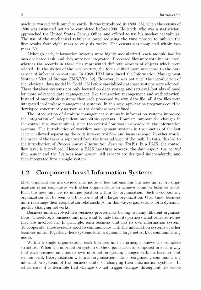
Figure 1.1: Basic principle of Service Oriented Architectures
system. To achieve this, the information system can be separated into components, suchthat each component supports a single business unit. Furthermore, each componentshould not depend on other components. Cross organizational, a business unit wantsto hide the units it cooperates with. Hence, in both cases, the complete network ofcommunicating systems is unknown to any component. In this way, information systemsare behaving more and more like an ecosystem, in which at runtime new components areadded and existing components are deleted or changed.
The information system of the cooperating business units should not become a bot-tleneck to form these dynamic networks. On the contrary, the information systems ofeach business unit should enable and stimulate the creation of these dynamic networks.The information systems of the business units are often built of components. Together,the communicating information systems form themselves a component of a higher level.In this way, the components in the information systems form a dynamic hierarchy.
Within an organization, communication between business units is message driven.A unit sends a message to inform, or to request information from other units. So,communication between business units is asynchronous by nature. Their informationsystems need to support such communication. Thus, the information systems of theunits form a loosely coupled component-based information system.
The paradigm of Service Oriented Architectures (SOA) (cf. [21,89]), in which a com-ponent is called a service, builds on this observation. Figure 1.1 depicts the basic principleof a SOA: a service provider publishes its services at a third party, called the service bro-ker . If a service needs to use a certain service (i.e. it is a service consumer), it consultsthe service broker. The broker provides the details of the service provider that deliversthat service. Then the provider and consumer bind themselves and start a cooperation.In this way, the communicating services form a dynamic network.
In this thesis, we focus on the design and verification of large component-based in-formation systems and the communication between the components within a dynamicnetwork.
1.3 Design Process of Information Systems
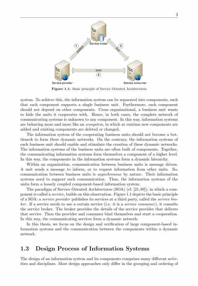
The design of an information system and its components comprises many different activ-ities and disciplines. Most design approaches only differ in the grouping and ordering of
4 Introduction
Real world Requirements
Scoping Formalization
Validation
Composition,Integration,Refinement
Verification
Justification
(Formal) Framework
Instantiation
Informal Formal
Realization
Testing
ModelModelModel System
Deployment
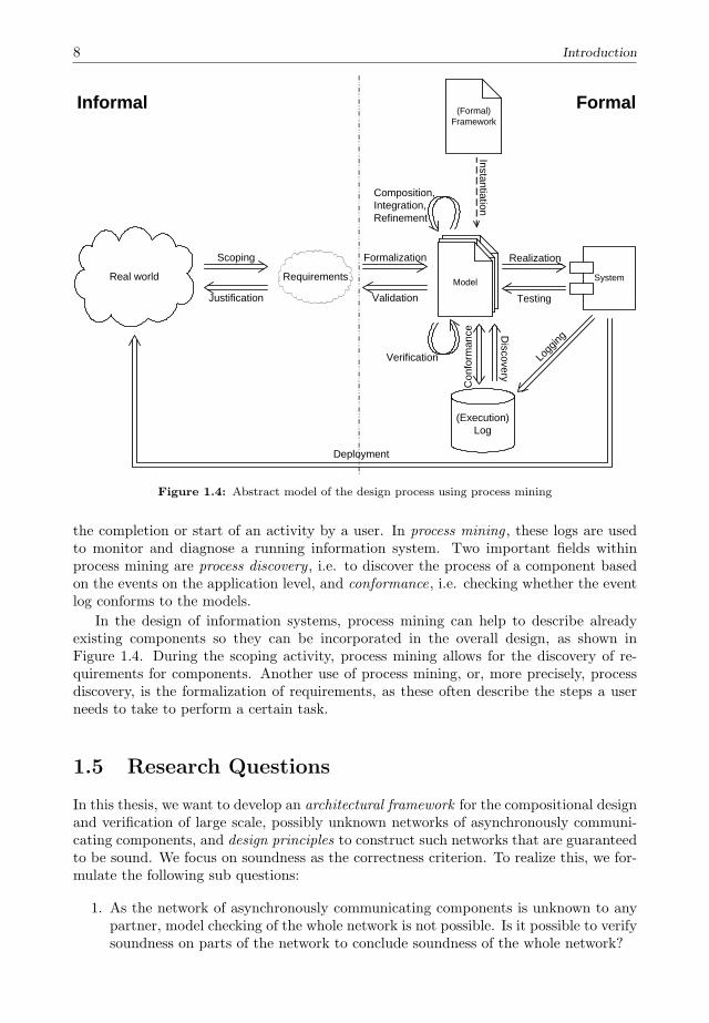
Figure 1.2: Meta-model of design process of an information system
design tasks. In this thesis, we consider an abstract model of the design process. In anydesign process we can distinguish nine important activities, which are executed in someorder. Figure 1.2 depicts an abstract model of the design process. Nodes are objects,either formal or informal, a double arc denotes an activity that creates an object outof the other. Note that the figure does not prescribe any order of the activities, it onlydepicts the relation between the activities.
Scoping and justification The information system needs to support an organizationin the “real world”. This means that terms and activities in the real world needto be translated into formal concepts, as the information system needs to under-stand these. Domain experts need to have a deep understanding of the real world.Together with the requirements engineer , the scope of a component is fixed, de-scribing the boundaries of the component, stakeholders involved in the component,and the functionality of the component. This activity is called scoping . It resultsin a requirements document in terms of the client, i.e. the functionality of thecomponent is described in natural domain-specific language and (mostly) informaldiagrams.
The rationale of each decision taken in the scoping activity need to be justified. Foreach decision, there has to be a reason in the real world. The activity of checkingthe requirements against the real world, we call justification.
Formalization and validation The requirements are still informal, while the com-ponent to be built is formal. The activity of translating the scoped world frominformal requirements to (formal) models is called formalization. Models describethe requirements. All models together form the architecture of the component. Anarchitectural framework is a meta-model that defines for an architecture which typeof models are needed and how these are related. If an architecture is according tosome framework, i.e. it has all the models prescribed by the framework, we say thearchitecture is an instance of the framework.
A model is based on some modeling language. A modeling language defines theconcepts that can be used, and their semantics. The activity of formalization isvery error prone, as requirements are expressed in natural language and informal

5
diagrams. Therefore, the requirements are often ambiguous, and the models needto be checked whether they describe the requirements as intended. This activityis called validation. Validation can be done in many ways. One way is by guidingstakeholders through the model explaining the model. Another often used practiceis by creating a prototype from the models, such that the stakeholders can geta look and feel of the system. In general, validation cannot be automated dueto the informal nature of the requirements. However, this task is crucial duringdevelopment.
Composition, integration, refinement and verification Once the first models arecreated and validated, these models can be integrated into larger models, decom-posed further into smaller models to focus on different aspects, or refined into moreprecise models. Each step should be verified to be correct, i.e. the new collectionof models should have at least the same properties as the original collection. Themain difference between verification and validation is that verification is checkingwhether the model is correct, whereas validation is checking whether it is the cor-rect model. While in refinement the focus lies on extending a model with morespecified functionality, in integration the focus lies on combining different modelsinto new models, in such manner that all properties of the models are preserved,and the composition has some additional properties.
Realization, testing and deployment When the models reach a sufficient degree ofprecision, the component can be realized. In software development, this involves thesearch for existing subcomponents and their configuration, and the construction ofnew subcomponents. All subcomponents are integrated into a single component.To check whether the realized component indeed satisfies the design, it needs to betested against the verified models. When the component is realized and thoroughlytested, it is deployed in the real world.
Note that although the description of the tasks could imply a waterfall like approach,other methods like extreme programming or SCRUM have similar activities, only theorder of activities differs. In this thesis, we will define an architectural framework andsearch for design principles to design and verify component-based information systemsin an ecosystem.
1.4 Modeling and Verification
Models play a central role in the design an information system. A model is an abstractrepresentation of some aspect of a real world system to analyze a set of properties ofthe system. We assume that properties are chosen such that if a property holds in themodel, it also holds in the real world system. The activity of creating these models iscalled modeling. It comprises formalization, integration, composition and refinement.
Models are expressed in a modeling language. Many different modeling languages ex-ist, each focusing on different aspects of the system. Some languages focus on modelingthe data aspect, like Entity-Relationship Diagrams [34], or on the process aspect, likePetri nets [94] and the Business Process Modeling Notation (BPMN) [88]. Other lan-guages focus on the communication between components, such as the Business ProcessExecution Language for web services (BPEL4WS) [22] for defining the order in whichmessages can be sent, and the Web Service Description Language (WSDL) [36] to definethe interfaces and message types.

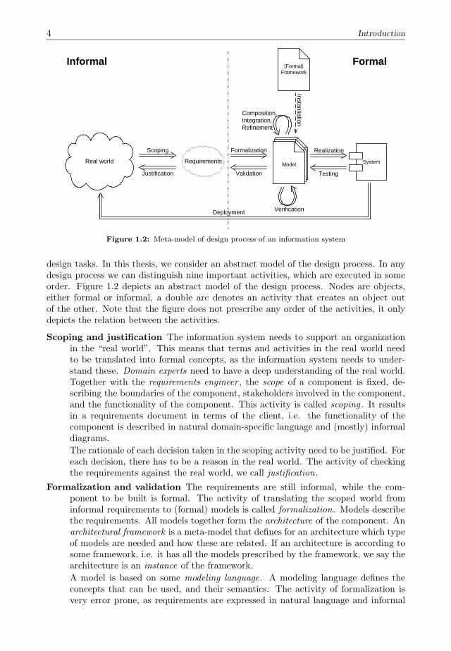
6 Introduction
The Blindmen and the Elephant
It was six men of Indostan, to learning much inclined,
who went to see the elephant (Though all of them were blind),
that each by observation, might satisfy his mind.
The first approached the elephant, and, happening to fall,
against his broad and sturdy side, at once began to bawl:
"God bless me! but the elephant, is nothing but a wall!"
The second feeling of the tusk, cried: "Ho! what have we here,
so very round and smooth and sharp? To me tis mighty clear,
this wonder of an elephant, is very like a spear!"
The third approached the animal, and, happening to take,
the squirming trunk within his hands, "I see," quoth he,
"the elephant is very like a snake!"
The fourth reached out his eager hand, and felt about the knee:
"What most this wondrous beast is like, is mighty plain," quoth he;
"Tis clear enough the elephant is very like a tree."
The fifth, who chanced to touch the ear, Said; "E'en the blindest man
can tell what this resembles most; Deny the fact who can,
This marvel of an elephant, is very like a fan!"
The sixth no sooner had begun, about the beast to grope,
than, seizing on the swinging tail, that fell within his scope,
"I see," quothe he, "the elephant is very like a rope!"
And so these men of Indostan, disputed loud and long,
each in his own opinion, exceeding stiff and strong,
Though each was partly in the right, and all were in the wrong!
So, oft in theologic wars, the disputants, I ween,
tread on in utter ignorance, of what each other mean,
and prate about the elephant, not one of them has seen!
John Godfrey Saxe, 1816 - 1887
Figure 1.3: The Blindmen and the Elephant, John Godfrey Saxe, 1816 - 1887
7
Important in modeling is that the models are consistent with each other. In the poemof Saxe (Figure 1.3), each of the blind men models a single aspect of the elephant. Eachof them has a correct model of the elephant, focusing on some aspects. Together, themodels represent the elephant as a whole. In the design of an information system it islikewise. Each of the models describe some aspects of the system. Together, the modelsrepresent the information system. Therefore, verification in a modeling process does notonly require checking for correctness of each of the models, but also checking for theconsistency between models.
In information systems, both the processes and data objects need to be modeled. Thecomposition of the system into components additionally requires modeling of the commu-nication between components. In this thesis, we develop an architectural framework forthe modeling of data and processes in and between components. The framework mainlyfocuses on the modeling of the internal behavior of components and the communicationprotocols between components. By modeling both the internal behavior of a componentand the communication protocol between components in the same formalism, both sin-gle components and compositions are treated equally in the framework. In this way, theframework supports the hierarchical design of component-based information systems.
For each component, a process model describes the behavior of the component. Animportant property that needs to hold for all components is a general sanity check: itshould always be possible to reach a desired, final state, disregarding the interface. Thisstate may be a kind of idle state, in which the component can start again, or a so-called deadlock state, in which no further actions are possible. We call this propertysoundness. If at some point in time, the final state becomes unreachable, the componentis ill-designed. One can compare the soundness property to a maze: if someone is in amaze, at any position, there should always remain some way out of it.
In a component-based information system, verification is much harder: all compo-nents should reach their final state, and there should not be any pending messages. Onecan compare verification of component-based information systems with a puzzle, suchthat each piece of the puzzle has its own maze. Each maze has a way out, but that doesnot imply that by combining the pieces together, the maze formed by the puzzle alwayshas a way out, as certain passages in the maze can become blocked. As the puzzle is notknown, we need compositional verification: by checking only parts of the maze, we needto conclude whether the complete maze is correct.
The property we consider, soundness, is not a compositional property, i.e. if twocomponents are sound, their composition is not necessarily sound. In other words, todecide soundness, we need to consider the whole network of communicating components.Therefore, we search for verification conditions, considering only components with theirdirect neighbors need to decide soundness of the whole composition.
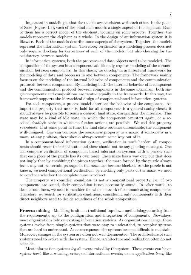
Process mining Modeling is often a traditional top-down methodology, starting fromthe requirements, up to the configuration and integration of components. Nowadays,most organizations rely on existing information systems. As organizations change, thesesystems evolve from simple systems that were easy to understand, to complex systemsthat are hard to understand. As a consequence, the systems become difficult to maintain.Moreover, changes in the system are often not well documented. The architecture of suchsystems need to evolve with the system. Hence, architecture and realization often do notcoincide.
Most information systems log all events raised by the system. These events can be onsystem level, like a warning, error, or informational events, or on application level, like
8 Introduction
Real world Requirements
Scoping Formalization
Validation
Composition,Integration,Refinement
Verification
Justification
(Formal) Framework
Instantiation
Informal Formal
Realization
Testing
ModelModelModel System
(Execution)Log
Con
form
ance D
iscovery
Logg
ing
Deployment
Figure 1.4: Abstract model of the design process using process mining
the completion or start of an activity by a user. In process mining , these logs are usedto monitor and diagnose a running information system. Two important fields withinprocess mining are process discovery , i.e. to discover the process of a component basedon the events on the application level, and conformance, i.e. checking whether the eventlog conforms to the models.
In the design of information systems, process mining can help to describe alreadyexisting components so they can be incorporated in the overall design, as shown inFigure 1.4. During the scoping activity, process mining allows for the discovery of re-quirements for components. Another use of process mining, or, more precisely, processdiscovery, is the formalization of requirements, as these often describe the steps a userneeds to take to perform a certain task.
1.5 Research Questions
In this thesis, we want to develop an architectural framework for the compositional designand verification of large scale, possibly unknown networks of asynchronously communi-cating components, and design principles to construct such networks that are guaranteedto be sound. We focus on soundness as the correctness criterion. To realize this, we for-mulate the following sub questions:
1. As the network of asynchronously communicating components is unknown to anypartner, model checking of the whole network is not possible. Is it possible to verifysoundness on parts of the network to conclude soundness of the whole network?

9
2. Components communicate asynchronously. This makes the development of com-munication protocols error prone. Therefore, can we determine design principles toconstruct networks of communicating components that are sound by constructionand satisfy the conditions for compositional verification?
3. Business processes involve the processing of data. However, including data ne-gatively influences the analyzability of the behavior. Therefore, can we find anapproach that is powerful enough to model both the business processes as well asthe data aspect, yet still allows for the verification of soundness?
4. The design process of information systems is mainly a top-down approach startingfrom the user requirements. However, many organizations already have informationsystems. Process mining enables the analysis of these existing systems. Can weuse these techniques to improve the design process?
The first research question in itself is not a new research question. Much relatedwork exists in which the system is divided into components that use an operator forcomposition that is proven to preserve some property. In an asynchronous setting, suchan operator does not exist for soundness. Therefore, we need a different approach, inwhich we need to check whether two communicating components satisfy some condition,such that we can conclude soundness of the whole network. In the second researchquestion, we focus on the construction of asynchronous network protocols, such thatby their construction it is guaranteed to be sound. Information systems rely on theprocessing of data. Therefore, our approach also needs to take the data aspect intoaccount, while preserving the verification possibilities the framework offers. Processmining has proven to be useful in gaining insights in how information systems supportorganizations. To answer the fourth research question, we try to use these techniques toimprove the design process of information systems.
1.6 Contributions of this Thesis
This thesis is divided into two parts. The first part introduces the architectural frame-work. In the second part, we focus on design principles for component-based informationsystems.
Framework for Component-Based Information Systems
This part focuses on the interaction between components. Chapter 3 introduces anarchitectural framework for the design and verification of component-based informationsystems. The concepts in the framework and their relationships are described in an objectmodel. The framework focuses on the behavioral aspects of an information system.Because of the asynchronous nature of the communication between components, theframework is based on Petri nets extended with interfaces. The framework is based onthe meta-models introduced in [5, 56, 57]. In [12], we presented a similar framework, inwhich we focused on resource authorization.
In Chapter 4, we discuss the possibilities to verify correctness of a given architecture.The main correctness criterion we consider is soundness, i.e. the information systemalways has the possibility to terminate properly. As the networks formed by the compo-nents are very dynamic, and – more important – unknown to any of the participants, wesearch for sufficient conditions to conclude soundness compositionally: given that eachcomponent is correct, and each connected pair of components satisfy a certain condition,
10 Introduction
soundness of the whole network is guaranteed. In particular, we focus on tree structurednetworks which are the result from outsourcing activities to other business units. In [11],we presented a sufficient condition. In this chapter, we show that more liberal conditionsexist.
The compositional approach presented in Chapter 4 assumes the existence of compo-nents to verify the soundness property of their composition. To support the refinementactivity in the development cycle of such systems, we need to be able to refine compo-nents. Given a pair of components, we want to be able to refine the communicationbetween the two components. To enable this, Chapter 5 introduces a new operationto refine sets of places in a Petri net by a refining Petri net, such that the soundnessproperty is preserved. In Chapter 6, we present a soundness-by-construction approachusing the refinement operator on sets of places as introduced in the previous chapter.The refinement procedure has been introduced in [65].
Design Techniques For Component-Based Information Systems
In the second part we focus on principles to design component-based information systems.In the previous part, we did not consider data. Although the process model with dataallows for more expressive power, it has a great cost, as it limits the possibilities foranalysis drastically. In Chapter 7, we introduce a new formalism to handle data objects.The formalism can be used to model database transactions as published in [64]. Theformalism can also be used for modeling message passing between components in ourarchitectural framework. We show that the formalism still allows for verification.
Next, we present in Chapter 8 a methodology using all the introduced design principlesto design a component-based information system. The methodology starts from the userrequirements and delivers a running prototype of the component-based system. Thisprototype can be used to validate the models with the domain experts in the real world,or for realization into a complete system. This methodology is an extension of themethodology described in [57], in which we did not yet consider components as keyconcept.
Finally, in Chapter 9, we focus on the discovery of Petri nets from event logs. Thediscovery technique is based on the theory of regions, which is a well-established field ofPetri net theory to synthesize a marked Petri net from a prefix-closed language. In thechapter we show how the theory of regions can be applied for process discovery usingInteger Linear Programmming, which is a specialization of constraint programming. Theadvantage of this approach is that more constraints can be added to the initial problem,to be able to discover all kinds of subclasses of Petri nets. The new algorithm has beenpublished in [110].

2Preliminaries
In this chapter we introduce the basic mathematical notations used throughout thisthesis.
2.1 Sets, Relations and Functions
Definition 2.1.1 (Set notation)A set is a possibly infinite collection of elements. We denote a finite set by listing itselements between braces. E.g., a set S with elements a, b and c is denoted as a, b, c.The empty set, i.e. the set with no elements, is denoted by ∅. Let A and B be two sets.We define the following operations.
• |A| denotes the number of elements of A.
• An element a is contained in a set A, denoted by a ∈ A.
• The intersection of two sets, denoted by A ∩ B, is a set containing the elementswhich are in both sets: A ∩B = x | x ∈ A ∧ x ∈ B.
• The union of two sets, denoted by A∪B, is the set containing all elements of bothsets: A ∪B = x | x ∈ A ∨ x ∈ B.
• The difference between two sets, denoted by A\B, is the set containing all elementsof A which are not in B: A \B = x | x ∈ A ∧ x ∈ B.
• The set B is a subset of A, denoted by B ⊆ A if all elements of B are also in A:∀x ∈ B : x ∈ A. The set B is called a proper subset, denoted by B ⊂ A, if B ⊆ A,but not A = B. The powerset, denoted by P(A), is the set of all subsets of A:P(A) = A′ | A′ ⊆ A. Note that A ∈ P(A).
The sets A and B are disjoint if A ∩ B = ∅. A partition of a set A is a set P ⊆ P(A)such that A =
∪A′∈P A
′ and ∀A′, A′′ ∈ P : A′ ∩A′′ = ∅ =⇒ A′ = A′′. yWe denote the set of all natural numbers by IN = 0, 1, 2, . . .. The set of all positive
natural numbers is denoted by IN+ = IN \ 0.To relate elements of one set to elements of another set, we introduce the Cartesian
product.
Definition 2.1.2 (Cartesian product)The Cartesian product of two sets A and B is defined as the set A × B = (a, b) | a ∈A ∧ b ∈ B. Set A is called the source set, and set B is called the target set. y

12 Preliminaries
In the Cartesian product A × B of two sets A and B, each element of A is relatedto each element of B. A relation on A and B only relates some elements of A to someelements of B, i.e. a relation is a subset of the Cartesian product of A and B.
Definition 2.1.3 (Relation, domain, range, inverse)Let A and B be two sets. A set R ⊆ A×B is called a relation from A to B. We write aR bfor (a, b) ∈ R. The domain of the relation is the set Dom(R) = a ∈ A | ∃b ∈ B : aR b.Its range is the set Rng(R) = b ∈ B | ∃a ∈ A : aR b. Its inverse is the relationR−1 ⊆ B ×A defined by R−1 = (b, a) | aR b. y
On these relations that have the same source set and target set, we define the notionsof reflexivity, symmetry, transitivity and antisymmetry.
Definition 2.1.4 ((Ir)reflexive, symmetric, transitive, antisymmetric)Let A be a set and let R ⊆ A×A be a relation. R is reflexive if aRa for all a ∈ A, and
it is irreflexive if ¬(aRa) for all a ∈ A. If aR b implies bR a for all a, b ∈ A, the relationis symmetric. If aR b and bR c implies aR c for all a, b, c ∈ A, the relation is transitive.Relation R is antisymmetric if aR b and bR a imply a = b for all a, b ∈ A. y
The reflexive closure of a relation R is the smallest relation that is reflexive andcontains R. The transitive closure of a relation R is defined as the smallest transitiverelation S such that R is contained in it.
Definition 2.1.5 (Reflexive closure, transitive closure)Let A be a set and let R ⊆ A × A be a relation. Its reflexive closure S ⊆ A × A isthe relation such that aS b if and only if a = b or aR b for all a, b ∈ A. Its transitiveclosure T ⊆ A × A is the relation such that R ⊆ T , T is transitive and for all relationsT ′ ⊆ A×A such that R ⊆ T ′ and T ′ is transitive, then T ⊆ T ′. y
Using these definitions, we define orderings and equivalences on sets. Both typesof relations are reflexive and transitive. In addition, an ordering relation is also anti-symmetric, whereas an equivalence relation is symmetric. This leads to the followingdefinitions.
Definition 2.1.6 (Preorder, partial order, total order, least element, top ele-ment, well-ordered)Let A be a set. A relation R ⊆ A×A is a preorder, denoted by (A,R), if R is reflexive
and transitive. A preorder is a partial order if (A,R) is also antisymmetric. A partialorder is called a total order, if in addition aR b or bR a for all a, b ∈ A. An elementa ∈ A is a least element of (A,R) if ∀b ∈ A : bR a =⇒ a = b. It is a top element if∀b ∈ A : aR b =⇒ a = b. If (A,R) is a total order, and every non-empty subset B ⊆ Ahas a least element, (A,R) is well-ordered. y
Note that a total order has at most one least element and at most one top element.A total order also defines a successor function.
Property 2.1.7 (Successor function of total order)Let (A,R) be a total order such that A is countable. Then a unique function S : A→ Aexists such that S(a) = b iff (1) ∀x ∈ A : xRa =⇒ xR b, (2) a = b, and (3)∀x ∈ A \ a : aRx =⇒ bRx. We call S the successor function of (A,R). y
Note that if S(a) = b, then aR b but not bR a.
Definition 2.1.8 (Equivalence relation)Let A be a set. A relation R ⊆ A×A is an equivalence relation if it is reflexive, symmetricand transitive. y
13
Another important class of relations is the class of functions. A relation from A toB is a function if each element of A is related to at most one element of B. A functionis partial if not all elements of A are mapped onto an element of B. If the inverse of afunction is again a function, it is injective; it is surjective if Rng(f) = B.
Definition 2.1.9 ((Partial) function, identity, injection, surjection, bijection)Let A and B be two sets. A relation f ⊆ A × B is a function from A to B, denoted
by f : A → B, if a f b1 and a f b2 imply b1 = b2 for all a ∈ A and b1, b2 ∈ B. We writef(a) = b for a f b. We lift the notation of functions to sets in the standard way: letC ⊆ A. Then f(C) = f(c) | c ∈ C.
A special function is the identity function id : A → A, which is the function thatmaps each element to itself: id(a) = a for all a ∈ A.
A function is called a partial function, denoted by f : A B, if Dom(f) ⊆ A. IfDom(f) = A, the function is called total. When Dom(f) = ∅ the function is called theempty function, denoted by ∅. If f(a1) = f(a2) implies a1 = a2 for all a1, a2 ∈ Dom(f),the function f is an injection. It is a surjection if, for each b ∈ B, an a ∈ Dom(f) existssuch that f(a) = b. An injective and surjective function is called a bijection. We canlist the function values of a function f with domain a, b and range c, d such thatf(a) = c and f(b) = d by f = a 7→ c, b 7→ d. y
In the remainder, we just write function for a total function.
2.2 Vectors, Bags, Sequences and Languages
To create relationships between more than two sets, we introduce the notion of thegeneralized Cartesian product. An element of a generalized Cartesian product is calleda vector. A vector can be seen as a total function over I, where each element i ∈ I ismapped onto a value in some set Ai.
Definition 2.2.1 (Generalized Cartesian product, vector)The generalized Cartesian product for a set I and sets Ai for i ∈ I, is defined as:∏
i∈IAi = f : I →
∪i∈I
Ai | ∀i ∈ I : f(i) ∈ Ai
An element x ∈∏i∈I Ai is called a vector, denoted by x. The length of vector x, denoted
by |x|, is the size of I, i.e. |x| = |I|. On the generalized Cartesian product, we definethe family of projection functions πi :
∏i∈I Ai → Ai by πi(x) = x(i) for all i ∈ I.
The definition of πi is lifted to sets in a standard way: πi(B) = πi(b) | b ∈ B forB ⊆
∏i∈I Ai. Let A be some set. If I = 1, . . . , n for some n ∈ IN , we write An for∏
i∈I A. yA set only indicates whether an element is present or not. In a bag, or multiset, also
the number of occurrences of elements is considered. Note that a bag is a vector, andthe set of all bags over some set is a generalized Cartesian product.
Definition 2.2.2 (Bags)Let S be a set. A bag B over S is a function B : S → IN . For s ∈ S, B(s) denotes thenumber of occurrences of s in the bag B. We write INS for the set of all bags over S.The empty bag, i.e. the bag for which all elements have multiplicity 0, is denoted by ∅.Bags are denoted by listing the occurring elements between square brackets, and we usesuperscripts for the multiplicity of the occurrences. If the multiplicity of an element is 0,

14 Preliminaries
we omit the element. A bag m consisting of two occurrences of a, three occurrences ofb and a single occurrence of c is denoted by m = [a2, b3, c]. The characteristic functionχ : P(S) → INS is defined as χ(S′)(s) = 1 if s ∈ S′ and χ(S′)(s) = 0 otherwise for alls ∈ S and S′ ⊆ S. y
Definition 2.2.3 (Bag notation)Let S be a set, letX,Y ∈ INS , and let s ∈ S. On bags, we define the following operations:
• s ∈ X if and only if X(s) > 0;
• (X + Y )(s) = X(s) + Y (s);
• (X − Y )(s) = max(0, X(s)− Y (s));
• X = Y if and only if ∀t ∈ S : X(t) = Y (t);
• X ≤ Y if and only if ∀t ∈ S : X(t) ≤ Y (t);
• X < Y if and only if X ≤ Y and X = Y .
The projection of X on elements of a set U ⊆ S is a bag X|U ∈ INU , such that X|U (u) =X(u) for all u ∈ U . y
Next, we introduce the notion of sequences. Bags only count the number of occur-rences of elements; a sequence also takes the order of the elements into account.
Definition 2.2.4 (Sequences)Let S be a set. A sequence σ over S of length n ∈ IN is a function σ : 1, . . . , n → S.If n > 0 and σ(i) = ai for i ∈ 1, . . . , n, we write σ = ⟨a1, . . . , an⟩. The length of σ, n,is denoted by |σ|.
The sequence of length 0 is called the empty sequence and is denoted by ϵ. The setof all finite sequences over S is denoted by S∗; the set S is called the alphabet of S∗.
An element s ∈ S is included in a sequence σ ∈ S∗, denoted by s ∈ σ, if σ(i) = s forsome 1 ≤ i ≤ |σ|.
Let µ, ν ∈ S∗. Concatenation, denoted by σ = µ; ν, is defined as σ : 1, . . . |µ|+ |ν|such that for 1 ≤ i ≤ |µ|: σ(i) = ν(i) and for |µ| < i ≤ |µ|+ |ν|: σ(i) = ν(i− |µ|).
The projection of a sequence σ ∈ S∗ on a set U ⊆ S, denoted by σ|U , is inductivelydefined as ϵ|U = ϵ, (⟨t⟩;σ)|U = ⟨t⟩;σ|U if t ∈ U , and (⟨t⟩;σ)|U = σ|U if t ∈ U .
We denote a subsequence of σ ∈ S∗ from index i to j by σ[i..j]. If j < i, then σ[i..j] = ϵ,otherwise σ[i..j] = ⟨σ(i), . . . , σ(k)⟩ where k = min(j, |σ|).
Further, we define a partial order ≤ on sequences by µ ≤ ν if and only if a sequenceρ ∈ S∗ exists such that ν = µ; ρ. y
Taking a projection on R of some projection on U is identical to the projection onthe intersection of R and U . Furthermore, the projection distributes over concatenation.
Corollary 2.2.5Let S be a set, let U,R ⊆ S and µ, ν ∈ S∗. Then (µ|U )|R = µ|U∩R and (µ; ν)|U = µ|U ; ν|U .
y
To denote the number of occurrences of elements in a sequence, we introduce theParikh vector [90], which is a bag representing the number of occurrences of each elementin the sequence.
Definition 2.2.6 (Parikh vector)Let S be a set and let σ ∈ S∗ be a sequence. The Parikh vector of σ, denoted by −→σ , is
inductively defined by −→ϵ = ∅ and−−−→⟨a⟩;σ = [a] +−→σ for all a ∈ S. y

15
Lastly in this section, we introduce the notion of a language. A language is a set ofwords over some alphabet T , a word is a sequence over a set T .
Definition 2.2.7 (Language, prefix-closed language)A subset L ⊆ T ∗ is called a language over T . A sequence w ∈ L in the language is alsoreferred to as word . A language L is prefix-closed if and only if for each word σ′; ⟨a⟩ ∈ Lwe have σ′ ∈ L. y
2.3 Graphs
Graphs play an important role in the design and analysis of information systems. In thissection, we introduce the basic concepts of graph theory.
A graph consists of a set of vertices, and arcs between them. Arcs have a direction,i.e. an arc has a head and a tail. If the set of arcs is symmetric, i.e. if (u, v) is an arc,(v, u) is also an arc, the graph is called undirected. A special class of graphs is the classof bipartite graphs, in which the vertices are partitioned into two sets, and there are noarcs whose tail and head are in the same set.
Definition 2.3.1 ((Un)directed graph, bipartite graph)A graph G is a pair (V,A) with a set V of vertices and a relation A ⊆ V × V called
the arcs. An arc (u, v) ∈ A is directed from the tail u to the head v. If the relation A issymmetric, the graph is undirected. The graph is a bipartite graph if there is a partitionV1, V2 of V such that ∀(u, v) ∈ A : (u ∈ V1 ⇔ v ∈ V2) ∧ (u ∈ V2 ⇔ v ∈ V1). y
Vertices are connected via directed arcs. The direct neighbours of a vertex v areeither in the preset, i.e. the set of all vertices for which there is an arc pointing to v, orin the postset, i.e. the set of all vertices for which there is an arc to starting from v.
Definition 2.3.2 (Preset, postset)Let G = (V,A) be a directed graph. Let u ∈ V be a vertex. The preset of u is the set•G u = v | (v, u) ∈ A. The postset of u is the set u•G = v | (u, v) ∈ A. We lift thepreset and postset to sets, i.e. •
G U =∪u∈U
•G u and U•
G =∪u∈U u
•G for U ⊆ V . If the
context is clear, we omit the subscript. y
Note that in an undirected graph the preset and postset of each vertex are identical.In a graph, we can choose a vertex and from this vertex traverse via the arcs to othervertices, thus creating a path. If we can traverse either way on the arcs of a graph, it isan undirected path. A path is a cycle if the start and end vertices of the path are thesame. If the graph has no cycles, it is an acyclic graph. A circuit is a cycle in which allvertices occur only once.
Definition 2.3.3 ((Un)directed path, cycle, acyclic graph, circuit)Let G = (V,A) be a graph. A sequence p ∈ V ∗ of length k > 0 is a directed path
if (pi−1, pi) ∈ A for all 1 < i ≤ k. It is an undirected path if either (pi−1, pi) ∈ A or(pi, pi−1) ∈ A for all 1 < i ≤ k. A non-empty path p is called a cycle if p1 = pk. Ifa graph does not contain cycles, it is called an acyclic graph. A directed or undirectedpath p is called a circuit if (pk, p1) ∈ A and ∀v ∈ V : −→p (v) ≤ 1. y
A graph is connected if it is possible to reach from each vertex all other vertices,without taking the direction of the arcs into account. It is strongly connected if thisproperty holds while respecting the direction of the arcs.

16 Preliminaries
Definition 2.3.4 ((Strongly) connected graph)Let G = (V,A) be a graph. It is connected if for each two vertices v1, v2 ∈ V anundirected path exists from v1 to v2. It is strongly connected if for every two verticesv1, v2 ∈ V , a directed path exists from v1 to v2. y
An important class of graphs are forests. A forest is a graph not containing circuits.If the forest is also connected, it is a tree.
Definition 2.3.5 (Forest, tree)A graph G = (V,A) is a forest if it does not contain circuits. A connected forest is alsocalled a tree. y
In acyclic graphs, it is possible to order the vertices such that for each vertex occurringin the order, its predecessors are smaller with respect to this order. We call this orderinga topological sort.
Definition 2.3.6 (Topological sort)Let G = (V,A) be an acyclic graph. A topological sort is a partial order of the vertices⊑G ⊆ V × V such that ∀(u, v) ∈ A : u ⊑G v. y
Note that a topological sort is only possible if the graph is acyclic. In order to inspectonly parts of a graph, we introduce the notion of subgraphs. A subgraph generated bya subset of vertices of a graph is called an induced subgraph. If the subgraph is alsomaximal with respect to the connections, it is a component.
Definition 2.3.7 (Subgraph, induced subgraph, component)Let G = (V,A) and G′ = (V ′, A′) be two graphs. The graph G′ is a subgraph ofG, denoted by G′ ⊆ G if V ′ ⊆ V and A′ ⊆ A. The subgraph G′ is induced if A′ =A ∩ (V ′ × V ′). A subgraph G′ is a component if it is a maximal, connected, inducedsubgraph, i.e. there is no larger subgraph G′′ ⊆ G such that G′ ⊆ G′′ and G′′ is aconnected, induced subgraph. y
If a function exists that transforms one graph into another graph, the two graphs areisomorphic.
Definition 2.3.8 (Isomorphic graphs)Let G1 = (V1, A1) and G2 = (V2, A2) be two graphs. A bijective function f : V1 → V2is an isomorphism if (u, v) ∈ A1 ⇔ (f(u), f(v)) ∈ A2 for all u, v ∈ V1. If f is anisomorphism, graphs G1 and G2 are isomorphic with respect to f , denoted by G1
∼=f G2.We say G1 and G2 are isomorphic, denoted by G1
∼= G2, if there is an isomorphismbetween G1 and G2. y
Isomorphism defines an equivalence relation.
Corollary 2.3.9Let G1 = (V1, A1) and G2 = (V2, A2) be two graphs and f : V1 → V2 a bijection suchthat G1 and G2 are isomorphic with respect to f .
The relation f ⊆ (V1 ∪ V2)× (V1 ∪ V2) such that (u, v) ∈ f ⇔ (f(u) = v ∨ f(v) = u)is an equivalence relation. y
Note that since the isomorphism is a bijection, we also have that the inverse holds.
Corollary 2.3.10Let G1 = (V1, A1) and G2 = (V2, A2) be two graphs, and let f : V1 → V2 be anisomorphism between G1 and G2. Then ∀(u, v) ∈ A2 : (f−1(u), f−1(v)) ∈ A1. y
17
If two graphs G1 and G2 are isomorphic and G1 is a bipartite graph, then G2 is alsobipartite, and vice versa.
Corollary 2.3.11Let G1 and G2 be isomorphic. Then G1 is bipartite if and only if G2 is bipartite. y
To label vertices and arcs of a graph, we introduce labeled graphs. In a labeled graph,each vertex and each arc has a label.
Definition 2.3.12 (labeled (un)directed graph)Let Σ and A be two sets. A labeled (un)directed graph G is a 3-tuple (V,A, λ) whereA ⊆ V × A × V , (V, (v, v′) | ∃a ∈ A : (v, a, v′) ∈ A) is a (un)directed graph, and thepartial function λ : V Σ is a vertex labelling function. y
On graphs, we define the operations union, intersection and difference on their con-stituents.
Definition 2.3.13 (Union, intersection, difference)Let G1 = (V1, A1) and G2 = (V2, A2) be two graphs. The union of G1 and G2 isdefined as G1 ∪ G2 = (V1 ∪ V2, A1 ∪ A2). The intersection of G1 and G2 is defined asG1 ∩ G2 = (V1 ∩ V2, A1 ∩ A2). The difference of G1 with G2 is defined as G1 \ G2 =(V1 \ V2, A1 ∩ ((V1 \ V2)× (V1 \ V2))). y
2.4 labeled Transition Systems
To model the behavior of a system, we use a labeled transition system, which is a labeledgraph. A labeled transition system (LTS) consists of a set of states and a set of transitionsbetween states that can be labeled by actions from a set A of action labels. The set ofstates are the vertices of the graph, the transitions are the arcs of the graph. From theoutside, only the action labels from A are visible. A special action is the silent action,denoted by τ . The silent action, also called a τ -step, is not an element of the set ofaction labels. Different from the action labels in A, the silent action is not visible fromthe outside.
Definition 2.4.1 (labeled Transition System)A labeled transition system (LTS) is a 5-tuple (S,A,→, s0,Ω) where
• S is a set of states;
• A is a set of actions;
• →⊆ (S × (A ∪ τ)× S) is a transition relation, where τ ∈ A is the silent action.
• (S,→, ∅) is a labeled directed graph, called the reachability graph;
• s0 ∈ S is the initial state;
• Ω ⊆ S is the set of accepting states.
y
Definition 2.4.2 (Semantics of a LTS)
Let L = (S,A,→, si,Ω) be an LTS. For s, s′ ∈ S and a ∈ A∪τ, we write (L : sa−→ s′)
if and only if (s, a, s′) ∈→. An action a ∈ A ∪ τ is called enabled in a state s ∈ S,
denoted by (L : sa−→) if a state s′ exists such that (L : s
a−→ s′). If (L : sa−→ s′),
we say that state s′ is reachable from s by an action labeled a. A state s ∈ S is calleda deadlock if no action a ∈ A ∪ τ exists such that (L : s
a−→). We define =⇒ as the
18 Preliminaries
smallest relation such that (L : s =⇒ s′) if s = s′ or ∃s′′ ∈ S : (L : s =⇒ s′′τ−→ s′).
As a notational convention, we may writeτ
=⇒ for =⇒. For a ∈ A, we definea
=⇒ as thesmallest relation such that (L : s
a=⇒ s′) if ∃s1, s2 ∈ S : (L : s =⇒ s1
a−→ s2 =⇒ s′). yWe lift the notation of actions to sequences. For the empty sequence ϵ, we have
(L : sϵ−→ s′) if and only if (L : s =⇒ s′). Let σ ∈ A∗ be a sequence of length n > 0,
and let s0, sn ∈ S. Sequence σ is a firing sequence, denoted by (L : s0σ−→ sn), if states
si−1, si ∈ S exist such that (L : si−1σ(i)=⇒ si) for all 1 ≤ i ≤ n. We write (L : s
∗−→ s′)
if a sequence σ ∈ A∗ exists such that (L : sσ−→ s′), and say that s′ is reachable from s.
A firing sequence σ ∈ A∗ from state s ∈ S is an accepting sequence for s if an acceptingstate sf ∈ Ω exists such that (L : s
σ−→ sf ).
Definition 2.4.3 (Reachable states, language of an LTS)Let L = (S,A,→, si,Ω) be an LTS. The reachable states from a state s ∈ S are
the states from the set R(L, s) = s′ | (L : s∗−→ s′). The set of all firing sequences
from the initial state si is denoted by T (L) = σ | ∃s ∈ S : (L : siσ−→ s). The
language of the LTS L, denoted by L(L) ⊆ A∗, is the set of accepting sequences, i.e.
L(L) = σ ∈ A∗ | ∃sf ∈ Ω : (L : siσ−→ sf ). y
Corollary 2.4.4Let L be an LTS. Then T (L) is a prefix-closed language. Furthermore, L(L) ⊆ T (L). y
To compare two LTSs, it is often needed to rename or hide actions. For this purpose,we introduce two operators.
Definition 2.4.5 (Renaming, hiding)Let A and A′ be two sets. Let L = (S,A,→, si,Ω) be an LTS. Let r : A ∪ τ →
(A′ ∪ τ) be a function such that r(τ) = τ . We define the operation ρr on an LTS byρr(L) = (S,A′,→′, si,Ω), where for s, s
′ ∈ S and a ∈ A∪τ we have (s, r(a), s′) ∈→′ ifand only if (s, a, s′) ∈→. A special case of renaming is hiding, in which actions are eitherrenamed to τ , or remain identical. We define the hiding operation on a subset H ⊆ A,denoted by τH(L), by τH(L) = ρh(L), where h(a) = τ for all a ∈ H ∪ τ and h(a) = aotherwise. y
To compare the behavior of LTSs, several notions exist. One notion of behavioralequivalence is trace equivalence. Two LTSs are trace equivalent if their sets of traces areidentical. Trace equivalence does not take the accepting states into account. Languageequivalence strengthens the trace equivalence by taking also the accepting states intoaccount. Two LTSs are language equivalent if their languages are identical.
Definition 2.4.6 (Trace equivalence, language equivalence)Let L and L′ be two LTSs. They are trace equivalent if T (L) = T (L′). The two LTSsare language equivalent if L(L) = L(L′). y
Both trace equivalence and language equivalence have no requirements on the in-termediate states. To take them into account, we introduce several other notions ofequivalence. The strongest notion of equivalence of two LTSs is based on the isomor-phism on their reachability graphs (Corollary 2.3.10). However, this equivalence relationis often too strong. Therefore, we introduce the notion of simulation. An LTS L′ simu-lates an LTS L if in every two related states, each action L can do, LTS L′ can performas well, possibly after some silent steps. If both L′ simulates L and L simulates L′ withsimulation relations R and R−1, we say L and L′ are bisimilar. We identify three classesof simulation: strong, delay and weak simulation. In a weak simulation, if L can perform
19
a visible action, possibly after some silent steps, then L′ can perform the same visibleaction, possibly after some silent steps. A delay simulation strengthens the equivalenceby stating that if L can perform a visible action, then L′ can perform the same visibleaction, possibly after some silent steps. In a strong simulation, no silent intermediatesteps are allowed: L′ should directly be able to perform that action. This leads to thefollowing definitions [50].
Definition 2.4.7 (Strong (bi)simulation)Let L = (S,A,→, si,Ω) and L = (S, A,→′, si, Ω) be two LTSs. The relation Q ⊆ S × Sis a strong simulation, denoted by L s≼Q L, if:
1. siQ si;
2. ∀s, s′ ∈ S, a ∈ A ∪ τ, s ∈ S : ((L : sa−→ s′) ∧ sQ s) =⇒ (∃s′ ∈ S : (L′ : s
a−→s′) ∧ s′Q s′); and
3. ∀s ∈ S, sf ∈ Ω : sf Q s =⇒ s ∈ Ω.
If both Q and Q−1 are strong simulations, Q is a strong bisimulation, which is denotedby L s≃Q L′.
We say L is strongly simulated by L′, denoted by L s≼ L′, if a strong simulation Qexists such that L s≼Q L′. We say L and L′ are strongly bisimilar, denoted by L s≃ L′,if a strong bisimulation Q exists such that L s≃Q L. yDefinition 2.4.8 (Delay (bi)simulation)Let L = (S,A,→, si,Ω) and L = (S, A,→′, si, Ω) be two LTSs. The relation Q ⊆ S × Sis a delay simulation, denoted by L ≼Q L, if:
1. siQ si;
2. ∀s, s′ ∈ S, a ∈ A ∪ τ, s ∈ S : ((L : sa−→ s′) ∧ sQ s) =⇒ (∃s′ ∈ S : (L′ : s
a=⇒
s′) ∧ s′Q s′); and3. ∀s ∈ S, sf ∈ Ω : sf Q s =⇒ s ∈ Ω.
If both Q and Q−1 are delay simulations, Q is a delay bisimulation , denoted by L ≃Q L.We say L is delay simulated by L′, denoted by L ≼ L′, if a delay simulation Q exists
such that L ≼Q L′. We say L and L′ are delay bisimilar, denoted by L ≃ L′, if a delaybisimulation Q exists such that L ≃Q L′. yDefinition 2.4.9 (Weak (bi)simulation)Let L = (S,A,→, si,Ω) and L = (S, A,→′, si, Ω′) be two LTSs. The relation Q ⊆ S× Sis a weak simulation, denoted by L w≼Q L, if:
1. siQ si;
2. ∀s, s′ ∈ S, a ∈ A ∪ τ, s ∈ S : ((L : sa
=⇒ s′) ∧ sQ s) =⇒ (∃s′ ∈ S′ : (L′ : sa
=⇒s′) ∧ s′Q s′); and
3. ∀s ∈ S, sf ∈ Ω : sf Q s =⇒ (∃sf ∈ Ω′ : (L′ : s =⇒ sf ) ∧ sf Q sf ).If both Q and Q−1 are simulations, Q is a weak bisimulation, denoted by L w≃Q L.
We say L is weakly simulated by L′, denoted by L w≼ L′, if a strong simulation Qexists such that L w≼Q L′. We say L and L′ are weakly bisimilar, denoted by L w≃ L′,if a weak bisimulation Q exists such that L w≃Q L′. y
In this thesis, we mostly use delay (bi)simulations. Therefore, if we use the term(bi)simulation, we refer to delay (bi)simulation. When a strong or weak (bi)simulationis meant, this is stated explicitly. For a more elaborate overview of simulation relations,we refer the reader to [50].

20 Preliminaries
2.5 Petri Nets
In an LTS, states are global, i.e. the whole state is inspected to decide which actions areenabled. In a Petri net, this decision is made locally: an action only needs to inspect apart of the state to decide whether it can fire.
Petri nets are very suitable for describing concurrent behavior. A Petri net can berepresented as a directed, bipartite graph where the nodes are partitioned into a set ofplaces, graphically represented as circles, and a set of transitions, which are representedby rectangles. Petri nets are named after C.A. Petri [92].
Definition 2.5.1 (Petri net)A Petri net N is a 3-tuple (P, T, F ) where P is a set of places, T is a set of transitions,such that P ∩ T = ∅, F ⊆ (P × T ) ∪ (T × P ) is the flow relation and (P ∪ T, F ) is adirected graph. If the sets P and T are finite, it is a finite Petri net. Otherwise, we callit an infinite Petri net. y
By default, we assume Petri nets to be finite. If not, we explicitly state that thePetri net is infinite. The graph operations (union, intersection and difference) are liftedto Petri nets in the standard way.
The state of a Petri net, called a marking, is given by the number of tokens in eachplace. A Petri net together with a marking is called a marked Petri net.
Definition 2.5.2 (Marking, marked Petri net)Let N = (P, T, F ) be a Petri net. A marking of N is a bag m ∈ INP , where m(p)denotes the number of tokens in place p ∈ P . If m(p) > 0, place p is called marked inmarking m. A Petri net N with corresponding marking m is written as (N,m) and iscalled a marked Petri net. y
By the definition of a Petri net, both the preset and the postset of a transition tonly consists of places. The places in the preset of a transition are called input places,the places in the postset of a transition are called output places. If a transition fires,it consumes tokens from all its input places and produces in all its output places. Tospecify the initial marking and a set of desired final markings, we introduce the notion ofa system: it is a marked Petri net with a set of final markings. For a system, we definethe semantics using an LTS.
Definition 2.5.3 (System, LTS of a system)A system is a 3-tuple S = (N,m0,Ω) where (N,m0) is a marked Petri net with
N = (P, T, F ) and Ω ⊆ INP is the set of final markings. Its semantics is defined by an LTSN (S) = (INP , T,→,m0,Ω) such that (m, t,m′) ∈→ iff •t ≤ m and m′ + •t = m+ t• for
m,m′ ∈ INP and t ∈ T . We write (N : mt−→ m′), R(N,m0), L(N,m0), and T (N,m0)
as a shorthand notation for (N (N,m0) : mt−→ m′), R(N (N,m0)), L(N (N,m0)), and
T (N (N,m0)), respectively. yThe incidence matrix keeps track of the changes of markings while firing transitions. Itdefines the number of tokens consumed and produced by a transition in a place.
Definition 2.5.4 (Incidence matrix)Let N = (P, T, F ) be a Petri net. The incidence matrix N : (P × T ) → −1, 0, 1 of Nis defined by:
N(p, t) =
−1 if (p, t) ∈ F ∧ (t, p) ∈ F1 if (t, p) ∈ F ∧ (p, t) ∈ F0 otherwise
y
21
The incidence matrix defines the marking a firing sequence reaches from a givenmarking, as shown in the marking equation.
Definition 2.5.5 (Marking equation)Let (N,m0) be a marked Petri net with N = (P, T, F ) and m0 ∈ INP . Let σ ∈ T ∗ and
m ∈ R(N,m0) such that (N : m0σ−→ m). Then m = m0 +N · −→σ . y
In a Petri net we identify special places and transitions. A place that has no tran-sitions in its preset, is called a source. If the place has an empty postset, it is a sink.Similar notions exist for transitions: if a transition has an empty preset, it is enabled inall markings. Then it is called an emitter. If a transition has an empty postset, it onlyremoves tokens, and is therefore called a collector.
Definition 2.5.6 (Source, sink, emitter, collector)Let N = (P, T, F ) be a Petri net. Let p ∈ P be a place and let t ∈ T be a transition.
Place p is called a source if •p = ∅. It is a sink if p• = ∅. If •t = ∅, transition t is anemitter. It is a collector if t• = ∅. y
On marked Petri nets, we define the following behavioral properties. If from everymarking reachable in a marked Petri net, it is possible to reach a marking in whichtransition t is enabled, transition t is called live. If this property holds for all transitions inthe marked Petri net, the marked Petri net is called live. A Petri net is called structurallylive, if a marking exists such that the Petri net with that marking is live.
Definition 2.5.7 (Liveness, deadlock-free, structurally live, quasi live)Let (N,m0) be a marked Petri net with N = (P, T, F ) andm0 ∈ INP . A transition t ∈ Tis live in (N,m0) iff for all reachable markings m ∈ R(N,m0), there is an m′ ∈ R(N,m)
such that (N : m′ t−→). The marked Petri net is live iff all its transitions are live. It isdeadlock-free if N (N) does not contain deadlocks. A Petri net N is structurally live if amarking m ∈ INP exists such that (N,m) is live. A transition t is quasi live in (N,m0)
if a marking m ∈ R(N,m0) exists such that (N : mt−→). If all transitions are quasi live,
the marked Petri net is called quasi live. y
Definition 2.5.8 (Home marking)Let (N,m0) be a marked Petri net where N = (P, T, F ) and m0 ∈ INP . A markingm ∈ R(N,m0) is a home marking if m ∈ R(N,m′) for all m′ ∈ R(N,m0). y
A marked Petri net is bounded if there is an upperbound of the number of tokens forall markings reachable. If this upperbound is 1, the net is called safe.
Definition 2.5.9 (Boundedness, safe)Let (N,m0) be a marked Petri net with N = (P, T, F ) and m0 ∈ INP . If a k ∈ IN
exists such that m(p) ≤ k for all m ∈ R(N,m0) and p ∈ P , it is called k-bounded. Wesay (N,m0) is bounded if a k ∈ IN exists such that (N,m0) is k-bounded. If the markedPetri net is 1-bounded, it is called safe. y
A frequently used property of marked Petri nets is expressed in the monotonicitylemma [44]: if a firing sequence is enabled in a marking, adding more tokens does nothamper the firing sequence.
Lemma 2.5.10 (Monotonicity lemma [44])
Let N = (P, T, F ) be a Petri net and m,m ∈ INP . If (N : mσ−→ m′) for some marking
m′ ∈ INP and firing sequence σ ∈ T ∗, then (N : m+mσ−→ m′ +m). y

22 Preliminaries
If two transitions can fire concurrently, without influencing each other, i.e. the postsetof the first transition and the preset of the second transition are disjoint, the transitionscan be exchanged. This is generalized in the Exchange lemma.
Lemma 2.5.11 (Exchange lemma [44])Let N = (P, T, F ) be a Petri net, and let U, V ⊆ T such that •U ∩ V • = ∅. Let
σ ∈ (U ∪V )∗ be a finite sequence such that (N : mσ−→ m′) for some m,m′ ∈ INP . Then
a marking m′′ ∈ INP exists such that (N : mσ|U−→ m′′ σ|V−→ m). y
For a more elaborate introduction on Petri nets, we refer the reader to [9, 44, 94]. Inthe remainder of this section, we present three important subclasses of Petri nets: statemachines, marked graphs and workflow Petri nets.
The first important subclass of Petri nets is the class of state machines. In a statemachine, each transition has a preset and a postset of size at most 1. The dual of a statemachine is a marked graph. In a marked graph, places have a preset and a postset of sizeat most 1.
Definition 2.5.12 (State machine (S-net), marked graph (T-net))A Petri net N = (P, T, F ) is a state machine (or S-net) if •t ≤ 1 and t• ≤ 1 for all
t ∈ T . It is a marked graph (or T-net) if •p ≤ 1 and p• ≤ 1 for all places p ∈ P . yAn important theorem for state machines is the Boundedness Theorem [44].
Theorem 2.5.13 (Boundedness theorem [44])Let (N,m) be a live state machine where N = (P, T, F ) and m ∈ INP . Then (N,m) isn-bounded if and only if
∑p∈P m(p) ≤ n. y
Another special class of Petri nets is the class of workflow nets. A workflow net [3]has a single source i, called the initial place, and a single sink f , called the final place,and all nodes of the Petri net are on a path from the initial place to the final place.As Petri nets are often used to model procedures and processes to reach a particulargoal, this class of Petri nets is very suitable for modeling this: a token in the final placeindicates the end of the process. A workflow net is classically sound [3] if it is possibleto reach a marking in which the final place is marked from all markings reachable from[i], and all transitions have a purpose, i.e. each of them can fire in at least one firingsequence starting in [i].
Definition 2.5.14 (Workflow net, classical soundness)Let N = (P, T, F ) be a Petri net. It is a workflow net if two places i ∈ P and f ∈ P existsuch that •i = f• = ∅, and all nodes n ∈ (P ∪ T ) are on a path from i to f . The closureof workflow net N , denoted by N∗, is the net N∗ = (P, T ∪ t∗, F ∪ (f, t∗), (t∗, i))where t∗ is a fresh transition (i.e. t∗ ∈ T ). The fused closure of a workflow net, denotedby N+, is the net N+ = (P \ f, T, (F \ (t, f) | t ∈ •
N f) ∪ (t, i) | t ∈ •N f).
A workflow net N is called sound if (1) [f ] is a home marking of (N, [i]), (2) for allreachable markings m ∈ R(N, [i]), if m ≥ [f ] then m = [f ], and (3) (N, [i]) is quasi live.
yIn [63], Lemma 11 shows that the second condition of classical soundness is implied
by the other conditions. A well-known result from [3] is that soundness is equivalent toliveness and boundedness of the closure. For a more elaborate overview of soundness, werefer the reader to [10].
Corollary 2.5.15Let N = (P, T, F ) be a workflow net with initial place i ∈ P . It is sound if and only ifthe marked Petri net (N∗, [i]) is live and bounded. y
23
By the reduction rules of Murata [87], it follows directly that a workflow net N issound if and only if its fused closure is live and bounded.
Corollary 2.5.16Let N = (P, T, F ) be a workflow net with initial place i ∈ P . It is sound if and only ifthe marked Petri net (N+, [i]) is live and bounded. y
Soundness only tests whether a given workflow net is behaving well for a single run.A workflow net is k-sound if for k concurrent runs it is always possible to reach the finalmarking with k tokens in the final place. Generalized soundness [62,63] tests a workflownet whether it is sound for any number of concurrent runs.
Definition 2.5.17 ((Up-to)k-sound, generalized sound)Let N = (P, T, F ) be a workflow net with initial place i ∈ P and final place f ∈ P .Net N is k-sound if [fk] ∈ R(N,m) for all m ∈ R(N, [ik]). It is up-to-k-sound if N isn-sound for all 1 ≤ n ≤ k. Net N is generalized sound if N is n-sound for all n ∈ IN . y
2.6 Object Models
An object model consists of objects, elements or records. Between these objects, asso-ciations exist. Objects belong to an object type, associations belong to a relationshipbetween object types. An object type defines the set of attributes of an object and therelationships the object can have. An object type can inherit from another object type,called the parent object type. If an object type inherits from another object type, it iscalled a child object type. It inherits all attributes and relationships of the parent objecttype. It is not possible to redefine attributes or relationships in child object types. Wedo not allow multiple inheritance.
The cardinality between a relationship r and an object type E defines the numberof associations of type r an object from E can have, specified as a range. In this thesis,we limit the cardinality to the set of ranges C = [0..∗), [1..∗), [0..1], [1..1], where [i..∗)denotes the set of integers n ∈ IN | n ≥ i and [i..j] denotes the set of integers n ∈IN | i ≤ n ≤ j. In the remainder, the brackets for the cardinality are omitted.
Let U be the universe of objects, let Λ be the universe of labels, and let V be theuniverse of attribute values.
Definition 2.6.1 (Object model)An object model is a 6-tuple (O,A, ι,R, σ, τ) where
• O is a set of object types;
• A : O → P(Λ) is a function defining for each object type the set of attributes;
• ι : O O is a partial function defining the inheritance relation. If for an objecttype A ∈ O a B ∈ O exists such that ι(A) = B, we say B is the parent object typeof A. The transitive closure of ι has to be irreflexive;
• R : (O × Λ) O is the set of relationships between object types. Given a rela-tionship r = ((A, l), B) ∈ R, A is called the source type of r, B is called the targettype of r, and l is called the name of r;
• σ : Dom(R) → C defines the source cardinality of each relationship;
• τ : Dom(R) → C defines the target cardinality of each relationship.
For inheritance, we require additionally for allB ∈ ι+(A) and r ∈ Λ thatA(A)∩A(B) = ∅and if (B, r) ∈ Dom(R), then (A, r) ∈ Dom(R), where ι+ is the transitive closure of ι. y

24 Preliminaries
For relationships, the target type is determined by the combination of the source typeand the label of the relationship. Relationships can have an identical name, as long astheir source type is different. As we allow for inheritance, we also need to ensure thatthe naming of relationships is unique in the whole chain of inheriting object types.
An object model can be graphically represented. Object types are depicted as rect-angles, an element ι(A) = B is displayed by an open headed arrow from A to B. Givena relation ((A, r), B), we draw an arrow from A to B. If the source cardinality allowsfor more than one object, a diamant is drawn on the arrow, denoted by R. If the sourcecardinality of a relationship requires that each object of the source entity type is asso-ciated with at least one object of the target object type, a vertical bar is drawn at thefoot of the arrow. Likewise, a vertical bar is drawn at the head of the arrow if the targetcardinality requires each object of the target object type to be associated with at leastone object of the source object type. Table 2.1 depicts some of the possible graphicalnotations for a relationship.
Figure 2.1 depicts an object model with four object types, A, B, C and D. Objecttype A defines one attribute name. Object type C inherits from object type A. Hence,objects of type C also have the name attribute. Relationship f relates object type A toobject type B: each object of type A relates to exactly one object of type B, an objectof type B can have any number of objects of type A related to it. As objects of type Cinherit from object type A, an object of type C can also be related to an object of typeB. Relationship g is a true many-to-many relationship: each pair of objects of type Band D can be related. Relationship h requires each object of type D to be connected toan object of C, whereas objects of type C are related to zero or one element of type D.
An object model can be instantiated with objects, attribute values and associations.An instance of an object model is a set of objects belonging to some type(s), attributesof objects are valuated, and associations between objects belong to relationships.
Definition 2.6.2 (Instance of an object model)Let M = (O,A, ι,R, σ, τ) be an object model. An instance of M is a 3-tuple (IO, IA, IR)where
• IO : O → P(U) defines the available objects. Each object type has a set of objects;
• IA : (U × Λ) V defines for each object the corresponding attribute values;
• IR : Dom(R) → P(U × U) is the set of associations between objects.
Let A ∈ O be an object type, let l ∈ A(O) be an attribute, and let ((A, r), B) ∈ R bea relationship. Given an instance I of M , we write a ∈ A for a ∈ IO(A), a.l = v for((o, l), v) ∈ IA and (a, b) ∈ r for (a, b) ∈ IR(((A, r), B)). The set of all instances of M isdenoted by ℑ(M). y
The definition of an object model instance allow for any combination of objects. It isnot necessarily the case that an instance complies with the constraints imposed by the
C
B
D
f
g
h
Aname
Figure 2.1: An example object model
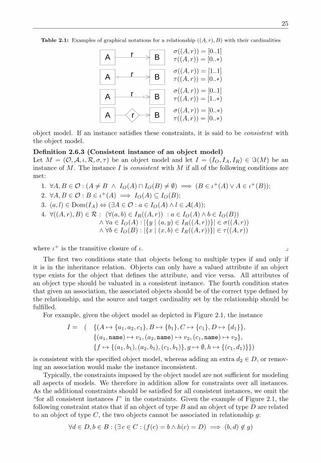
25
Table 2.1: Examples of graphical notations for a relationship ((A, r), B) with their cardinalities
A Br σ((A, r)) = [0..1]τ((A, r)) = [0..∗)
A Br σ((A, r)) = [1..1]τ((A, r)) = [0..∗)
A Br σ((A, r)) = [0..1]τ((A, r)) = [1..∗)
A Brσ((A, r)) = [0..∗)τ((A, r)) = [0..∗)
object model. If an instance satisfies these constraints, it is said to be consistent withthe object model.
Definition 2.6.3 (Consistent instance of an object model)Let M = (O,A, ι,R, σ, τ) be an object model and let I = (IO, IA, IR) ∈ ℑ(M) be aninstance of M . The instance I is consistent with M if all of the following conditions aremet:
1. ∀A,B ∈ O : (A = B ∧ IO(A) ∩ IO(B) = ∅) =⇒ (B ∈ ι+(A) ∨A ∈ ι+(B));
2. ∀A,B ∈ O : B ∈ ι+(A) =⇒ IO(A) ⊆ IO(B);
3. (a, l) ∈ Dom(IA) ⇔ (∃A ∈ O : a ∈ IO(A) ∧ l ∈ A(A));
4. ∀((A, r), B) ∈ R : (∀(a, b) ∈ IR((A, r)) : a ∈ IO(A) ∧ b ∈ IO(B))∧ ∀a ∈ IO(A) : |y | (a, y) ∈ IR((A, r))| ∈ σ((A, r))∧ ∀b ∈ IO(B) : |x | (x, b) ∈ IR((A, r))| ∈ τ((A, r))
where ι+ is the transitive closure of ι. yThe first two conditions state that objects belong to multiple types if and only if
it is in the inheritance relation. Objects can only have a valued attribute if an objecttype exists for the object that defines the attribute, and vice versa. All attributes ofan object type should be valuated in a consistent instance. The fourth condition statesthat given an association, the associated objects should be of the correct type defined bythe relationship, and the source and target cardinality set by the relationship should befulfilled.
For example, given the object model as depicted in Figure 2.1, the instance
I = ( (A 7→ a1, a2, c1, B 7→ b1, C 7→ c1, D 7→ d1,(a1, name) 7→ v1, (a2, name) 7→ v2, (c1, name) 7→ v2,f 7→ (a1, b1), (a2, b1), (c1, b1), g 7→ ∅, h 7→ (c1, d1))
is consistent with the specified object model, whereas adding an extra d2 ∈ D, or remov-ing an association would make the instance inconsistent.
Typically, the constraints imposed by the object model are not sufficient for modelingall aspects of models. We therefore in addition allow for constraints over all instances.As the additional constraints should be satisfied for all consistent instances, we omit the“for all consistent instances I” in the constraints. Given the example of Figure 2.1, thefollowing constraint states that if an object of type B and an object of type D are relatedto an object of type C, the two objects cannot be associated in relationship g:
∀d ∈ D, b ∈ B : (∃ c ∈ C : (f(c) = b ∧ h(c) = D) =⇒ (b, d) ∈ g)

26 Preliminaries
This constraint is translated into:
∀I ∈ ℑ(O) : ( ∀d ∈ IO(D), b ∈ IO(B) :( ∃ c ∈ IO(C) : ( (c, b) ∈ IR((A, f,B)) ∧ (c, d) ∈ IR(C, h,D)
) =⇒ (b, d) ∈ IR((B, g,D))) )
This way, we are able to specify additional constraints over all instances of an objectmodel.
The notion of object models is closely related to relational database schemas definedby Codd [38, 39] and Entity-Relationship diagrams (ERD), which were introduced byChen [34]. Also UML class diagrams [53] in combination with the Object ConstraintLanguage (OCL) [52] allow for data object modeling with constraints and relationshipslike inheritance and association. However, UML class diagrams and OCL are not definedformally, and allow for many different types of relationships.
Part I
Framework forComponent-Based Systems


3Component-Based Architecture Framework
In this chapter, we introduce a formal framework for component-based information sys-tems. The framework both covers the data aspect and the behavioral aspect. We mainlyfocus on the behavioral aspect of such systems.
3.1 Introduction
The design of component-based systems encompasses the decomposition of the function-ality of the system into components. An architecture describes the structure of such asystem. According to one of the most cited definitions [27], an architecture is:
The software architecture of a program or computing system is the structureof structures of the system, which comprise software elements, the externallyvisible properties of those elements and the relationships among them.
According to this definition, an architecture describes the structure of the system,the components of which it is built up, and their functionality. However, this definitionis not precise enough. To be able to assure correctness of the system, we need to showthat each of the requirements are met. To do so, we need models that together describethe functionality of the system. Such a model is called a view. The set of views should beconsistent, i.e. it should not be possible that if a property holds in one view, it does nothold in another view of the same system, since all models together describe the system.A second important aspect is that the set of views should be complete: each requirementshould be covered by one or more views. This leads to a more elaborate definition of anarchitecture [5]:
An architecture of a system is a set of descriptions that present differentviews of the system. The set of views should be consistent and complete.Each view models a set of components of the system, one or more functionsof each component and the relationships between these components.
In an architecture, many different views are needed. An architectural framework isa meta model that specifies the possible views for an architecture. In this chapter, weintroduce an architectural framework that does not only focus on the design of com-ponent based information systems, but also allows for formal verification of terminationconditions. It consists of three views: a component view , a process view , and a data view .
30 Component-Based Architecture Framework
In Section 3.2, we introduce the notion of a component on which we will build the ar-chitectural framework, which is presented in Section 3.3. In Section 3.4, we focus on thebehavioral aspect of component-based information systems, for which we will use Petrinets and their composition. We illustrate the framework by an example in Section 3.5.The chapter is concluded in Section 3.6.
3.2 Component-based Systems
Dividing the functionality of a system into subsystems such that each subsystem imple-ments its own specific functionality is not new. Already in the sixties of the last century,McIlroy [86] suggested to use components to design and implement software systems. Acomponent implements a specific part of the specification, masking its internal design. Itinteracts with other components via interfaces. Although the concept of a component isclear, there is no real consensus on the definition of a component. We adopt the definitionof a component as defined in [105]:
A component is a unit of composition with contractually specified interfacesand explicit context dependencies only. A software component can be de-ployed independently and is subject to composition by third parties.
This definition shows two important aspects of a component. First of all, a component isa subsystem implementing a set of coherent functionalities. Its interfaces to the outsideare listed explicitly in a contract, i.e. it defines how other components can access itsfunctionality via the interfaces. Secondly, a component should be as independent aspossible. A component may need other components, but these dependencies are knownin advance, and they are only accessed via the specified interfaces.
A component is called application specific, if it can be used in a single context only. Ifthe component can be used in many different contexts, the component is called genericor off the shelf (COTS). A good example of a generic component is a database manage-ment system. Such a system is specialized in the storage, retrieval and presentation ofstructured data. Its configuration is a data model specifying the data objects and theirrelationships. Due to its generic nature, it can be deployed in many different contexts.
Important in the design of components, is the granularity of components. The func-tionality of a system can be composed in small grained components, i.e. each componentonly implements a very small part of functionality, or coarse grained components, i.e.in very large parts of functionality. A common approach to compose systems is thetop-down approach. In this approach, the functionality is first split into a few maincomponents. Each component then is further refined into smaller components. Anotherapproach is the bottom-up approach, in which small components are composed into largercomponents until the desired set of functionalities is covered.
A component communicates with its environment only via interfaces. It has manydifferent interfaces. There are not only interfaces to communicate with users or othercomponents, but for example also to configure a component. We identify four types ofinterfaces of a component: the human interface, the configuration interface, the commu-nication interface and the monitor interface.
Human interface The human interface defines the interface of the component withusers, like a graphical user interface of software components. In the example ofa database management system, the user interface allows the user to interactivelyview and manipulate the data the system stores.

31
Component
Human interface
Communication interface
Monitor interface
Configuration interface
Figure 3.1: Component model with four main interfaces
Configuration interface As a component can be used in multiple contexts, it hasparameters to deploy the component in a specific context. The parameters of acomponent can be set using this interface. For example, the configuration interfaceof a database management system consists of parameters to define the concurrentbehavior of transactions, but also the data schema of the data the system manip-ulates is a configuration parameter of the component.
Communication interface The communication interface defines how and what thecomponent can communicate with other components. This interface is often calledthe Application Programming Interface (API) of the component. Consider againthe database management system. It allows other components to manipulate datavia transactions via an ODBC or JDBC connection. Many database managementsystems also allow for more direct manipulation via some programming interface.The connector and the programming interface together form the communicationinterface of the system.
Monitor interface To monitor the use of a component, the monitor interface allowsthe logging of all kinds of events generated by the component, like interface callsby other components, warnings or errors in the component and performance char-acteristics. For example, the monitor interface of a database management systemcan record the queries performed by other components, the average response timeto answer a query, but also memory consumption or system load.
In the design and implementation of a component, all four types of interfaces needto be considered. In this thesis, we focus on the design of communicating informationsystems, where components interact via message passing. Therefore, our architecturalframework only addresses the communication interface. In Chapter 9, we will focus onthe monitor interface.
3.3 Architectural Framework
In this section, we introduce a framework for component-based information systemsthat communicate asynchronously. We introduce the concepts of the framework via anobject model, which is shown in Figure 3.2. The main concept in the framework is thenotion of a component. To group functionality, components can be contained in larger
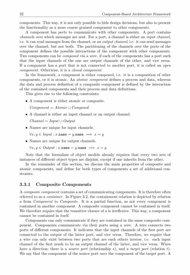
32 Component-Based Architecture Framework
components. This way, it is not only possible to hide design decisions, but also to presentthe functionality as a more coarse grained component to other components.
A component has ports to communicate with other components. A port containschannels over which messages are sent. For a port, a channel is either an input channel,i.e. it can read messages from the channel, or an output channel, i.e. it can send messagesover the channel, but not both. The partitioning of the channels over the ports of thecomponent defines the possible interactions of the component with other components.Two components can be composed via a wire, if each of the components has a port suchthat the input channels of the one are output channels of the other, and vice versa.If a component has a port that is not connected to another port, it is called an opencomponent. Otherwise, it is a closed component.
In the framework, a component is either composed, i.e. it is a composition of othercomponents, or it is atomic. An atomic component defines a process and data, whereasthe data and process definition of a composite component is defined by the interactionof the contained components and their process and data definitions.
This gives rise to the following constraints:
• A component is either atomic or composite.
Component = Atomic ∪ Composed
• A channel is either an input channel or an output channel.
Channel = Input ∪Output
• Names are unique for input channels.
∀x, y ∈ Input : x.name = y.name =⇒ x = y
• Names are unique for output channels.
∀x, y ∈ Output : x.name = y.name =⇒ x = y
Note that the formalism of object models already requires that every two sets ofinstances of different object types are disjoint, except if one inherits from the other.
In the remainder of this section, we discuss the main properties of composite andatomic components, and define for both types of components a set of additional con-straints.
3.3.1 Composite Components
A composite component contains a set of communicating components. It is therefore oftenreferred to as a container . In Figure 3.2, the containment relation is depicted by relationa from Component to Composite. It is a partial function, as not every component iscontained in another component. A composite component cannot be contained in itself.We therefore require that the transitive closure of a is irreflexive. This way, a componentcannot be contained in itself.
Components can only communicate if they are contained in the same composite com-ponent. Components communicate via their ports using a wire. A wire connects twoports of different components. It indicates that the input channels of the first port areconnected to the output of the latter port, and vice versa. Therefore, we require thata wire can only exist between two ports that are each others inverse, i.e. each inputchannel of the first needs to be an output channel of the latter, and vice versa. Wireshave a direction; there is a source port (relationship s), and a target port (relation t).We say that the component of the source port uses the component of the target port. A
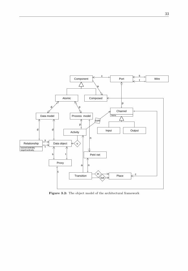
33
Component
Atomic Composed
Port Wire
Channel
OutputInput
Data model Process model
Data objectRelationship
Activity
Proxy
Petri net
Transition Place
s
a
t
c
p
u
com
pd
d d
s
t
s t
cin
out
na
c
p
n
sourceCardinalitytargetCardinality
Name
Figure 3.2: The object model of the architectural framework

34 Component-Based Architecture Framework
component cannot use itself. This leads to the following set of constraints on compositecomponents.
Constraints
• The transitive closure of a should be irreflexive.
• A Wire is between different components.
∀w ∈ Wire : c(s(w)) = c(t(w))
• A Wire can only connect components within the same container.
∀w ∈ Wire : a(c(s(w))) = a(c(t(w)))
• A Wire can only exist if the connected ports are each others inverse.
∀w ∈ Wire : (∀i ∈ Input : p(i) = s(w) : ∃o ∈ Output : p(o) = t(w)∧ i.name = o.name)
∧ (∀o ∈ Output : p(o) = s(w) : ∃i ∈ Input : p(i) = t(w)∧ i.name = o.name)
∧ (∀i ∈ Input : p(i) = t(w) : ∃o ∈ Output : p(o) = s(w)∧ i.name = o.name)
∧ (∀o ∈ Output : p(o) = t(w) : ∃i ∈ Input : p(i) = s(w)∧ i.name = o.name)
3.3.2 Atomic Components
A composite component only defines which components communicate with each other.It does not cover the data aspect nor the process aspect. Only atomic components definethese aspects. In other words, the data aspect and the process aspect of a compositionare determined by the data and process definitions of the atomic components in thecomposition, and the wiring between the components. In our framework, an atomiccomponent consists of two views: a Data model to cover the data aspect, and a Processmodel to cover the behavioral aspect.
A Data model consists of Data objects and Relations between those objects. We onlyallow binary relationships, as we can always create an object type of the association ifmore than two objects need to be associated. These relationships have a source entity anda target entity, which have to be in the same component. In fact, it models a basic objectmodel as presented in the preliminaries (without inheritance). Sometimes, data objectsneed to be shared between components. A data object that points to another data objectis called a Proxy. A Proxy can only exist if the two components are connected via a wire,and the proxy relation should satisfy the order implied by the wire. The dependencyrelation implied by the proxy cannot be circular. Hence, the transitive closure of therelation implied by the object type Proxy needs to be irreflexive.
A component is designed to have certain functionalities, which are divided into activ-ities. The Process model of an atomic component defines the set of Activities an objectcan perform. An activity belongs to exactly one process. It can use the data objectsand relations of the component as defined in the data model. Activities can commu-nicate with other components by sending messages over output channels and collectingmessages from input channels.
In this thesis, we use Petri nets to implement a process. Each process has its ownPetri net. To define the dependencies between transitions and thus the order in which
35
activities can be executed, places are used. Places are also used to represent the channelsbetween components. Each place either represents an input channel, an output channel,or – if the port is connected via a wire – both. If two ports are connected via a wire,for each input channel an output channel exists in the other port and vice versa. Thesepairs of channels should be represented by the same place. But as the input channel is ofthe one component, and the output of the other component, the place representing thischannel is in both Petri nets as well. Therefore, we require for places that all transitionsof the preset of a place (relation out) should be in the same Petri net, and all transitionsof the postset of a place (relation in) should be in the same Petri net as well. As placesrepresent channels, it is not necessarily the case that transitions of the preset and thepostset of a place are within the same Petri net.
Each transition is labeled with at most one activity of the process. If a transitionimplements an activity, i.e. it is labeled with an activity, the transition should be con-nected with the input and output channels as defined by the activity. A transition isonly connected to interface places if it implements an activity that uses some channels.
This leads to the following set of constraints on atomic components.
Constraints
• A Relationship only exists between data objects within the same data model.
∀x ∈ Relationship : d(x) = d(s(x)) = d(t(x))
• A Proxy is between two data objects of different components within the samecontainer.
∀x ∈ Proxy : d(s(x)) = d(t(x)) ∧ a(d(d(s(x)))) = a(d(d(t(x))))
• A Proxy between two data objects can only exist if there is a wire between thecomponents connected via the proxy.
∀x ∈ Proxy : ∃w ∈ Wire : c(s(w)) = d(d(s(x))) ∧ c(t(w)) = d(d(t(x)))
• The transitive closure of the relationship implied by object Proxy should be ir-reflexive.Let R ⊆ DataObject×DataObject such that aR b⇔ ∃p ∈ Proxy : s(p) = a∧ t(p) =b. The transitive closure of R should be irreflexive.
• An activity can only use data objects of the component it belongs to.
∀(x, y) ∈ u : p(p(x)) = d(d(y))
• An activity can only use the channels defined by the component it belongs to.
∀(x, y) ∈ com : p(p(x)) = c(p(y))
• An activity can only use channels of its own component.
∀(x, y) ∈ com : p(x) = c(p(y))
• All transitions that produce in a place are within the same Petri net.
∀t1, t2 ∈ Transition, p ∈ Place : (t1, p), (t2, p) ⊆ out =⇒ n(t1) = n(t2)
• All transitions that consume from a place are within the same Petri net.
∀t1, t2 ∈ Transition, p ∈ Place : (t1, p), (t2, p) ⊆ in =⇒ n(t1) = n(t2)
• A place implements at most two channels: an input channel, and an output channel.The ports of these channels should be connected via a wire.
36 Component-Based Architecture Framework
∀x ∈ Place, y1, y2 ∈ Channel : (c(y1) = c(y2))=⇒ ( (y1 = y2)
∨ (y1.name = y2.name ∧ ∃w ∈ Wire : (s(w) = p(y1) ∧ t(w) = p(y2))∨(s(w) = p(y1) ∧ t(w) = p(y2)) ) )
• If two ports are connected via a wire, channels with the same name should berepresented by the same place.
∀w ∈ Wire, y1, y2 ∈ Channel :( y1.name = y2.name ∧ s(w) = p(y1) ∧ t(w) = p(y2) ) =⇒ c(y1) = c(y2)
• A transition is connected to a place implementing a channel if and only if thetransition implements an activity that communicates with that channel.
∀(x, y) ∈ in ∪ out , z ∈ Channel :c(z) = y ⇔ ( ∃q ∈ Activity : a(x) = q ∧ (q, z) ∈ com )
• If a transition implements an activity it should send and receive messages as definedby the activity.
∀z ∈ Transition, (x, y) ∈ com :a(z) = x⇔ (z, c(y)) ∈ (In ∪Out)
3.4 Components as Open Petri Nets
As described in Section 3.2, a component has four types of interfaces. In this section, weintroduce a formalism to model a component and its communication interface, disregard-ing the other types of interfaces. Although the data aspect is as important in the designof an information system, we mostly focus on the behavioral aspects of components. Aspresented in the previous section, a component has ports which consist of input channelsand output channels to communicate with other components. Communication is doneby message passing, and hence, asynchronous. Therefore, Petri nets are a natural choicefor the modeling of components: it allows both for modeling of the internal behavior ofa component, as well as for modeling the communication between components. In thissection, we define a class of Petri nets, which we call open Petri nets. An Open Petri net(OPN) has internal places to model its internal state and behavior, input places to modelinput channels, and output places to model output channels. The set of all input placesand output places are called the interface places. The interface places are partitionedinto a set of ports. Each interface place is attached to a single port. An OPN can havezero or more ports. If an OPN has no ports, it is called a closed net, to emphasize thefact it cannot communicate with other components. An OPN has an initial markingand a final marking, both markings only mark internal places. We do not require thefinal marking to be a deadlock. Often, the final marking is either identical to the initialmarking, or it is an idle state, indicating that if the component reached the idle state, itis in rest, and can be reused.
Definition 3.4.1 (Open Petri net)An open Petri net (OPN) is an 8-tuple (P, I,O, T, F,G, i, f) where
• ((P ∪ I ∪O, T, F ), i, f) is a system;
• P is a set of internal places;
• I is a set of input places, and •I = ∅;• O is a set of output places, and O• = ∅;

37
• P , I and O are pairwise disjoint;
• G ⊆ P(I ∪ O) is a partitioning of the interface places, an element of G is called aport ,
• i ∈ INP is the initial marking , and
• f ∈ INP is the final marking .
We call the set I ∪ O the interface places of the OPN. Two OPNs N and M are calleddisjoint if (PN ∪ IN ∪ON ∪TN )∩ (PM ∪ IM ∪OM ∪TM ) = ∅. An OPN N is called closedif IN = ON = ∅. The set of all OPNs is denoted by N. As a shorthand notation, wewrite R(N,m) for R((PN ∪ IN ∪ON , TN , FN ),m, fN) for m ∈ INPN∪IN∪ON . y
A transition with an output place in its postset is called a sending transition. If atransition has an input place in its preset, it is called a receiving transition. To denotewhether a transition is sending, receiving or not communicating, we introduce the sign ofa transition. We generalize the sign of a transition to Petri nets. The sign of a transitionis defined based on a given set of places.
Definition 3.4.2 (Sign of a transition and a sequence)Let N = (P, T, F ) be a Petri net, and define G ⊆ P . The sign of a transition, given bythe function λG : T → !, ?, τ, is defined by:
λG(t) =
! if t• ∩G = ∅ ∧ •t ∩G = ∅? if •t ∩G = ∅ ∧ t• ∩G = ∅ if •t ∩G = ∅ ∧ t• ∩G = ∅τ otherwise
where t ∈ T . We lift the sign function to sequences. The function sgnG : T ∗ → !, ?, τ,is defined by:
sgnG(σ) =
τ if ∀t ∈ σ : λG(t) = τ! if ∀t ∈ σ : λG(t) ∈ !, τ ∧ ∃t ∈ σ : λG(t) =!? if ∀t ∈ σ : λG(t) ∈ ?, τ ∧ ∃t ∈ σ : λG(t) =? otherwise
where σ ∈ T ∗. y
The inner behavior of a component, i.e. the control flow of the component, is againa Petri net. To inspect the inner behavior, we introduce the notion of a skeleton. Theskeleton of an OPN is the Petri net formed by removing the interface places.
Definition 3.4.3 (Skeleton)Let N be an OPN. The skeleton of N is defined as the Petri net S(N) = (PN , TN , F )
with F = FN ∩ ((PN × TN ) ∪ (TN × PN )). The skeleton system of N is defined as thesystem S(N) = (S(N), iN , fN). y
An important behavioral property for systems is termination: a component shouldalways have the possibility to terminate properly. We identify two termination properties:weak termination and soundness. The first property states that a component includingall its interface places always has the possibility to reach the final marking, whereas inthe latter property, the interface places are not taken into account. In fact, the latterproperty states that, if all communication is disregarded, the component behaves well.
38 Component-Based Architecture Framework
Definition 3.4.4 (Weak termination and soundness of an OPN)Let N be an OPN. It is weakly terminating , if for each marking m ∈ R(N, iN ), we havefN ∈ R(N,m). It is sound , if the system defined by its skeleton is weakly terminating.
y
Note that soundness is defined as fN ∈ R(S(N),m) for all m ∈ R(S(N)). We do notconsider the second and third condition of classical soundness (Definition 2.5.14). As aconsequence, if an OPN is closed, it is sound if and only if it is weakly terminating.
Corollary 3.4.5Let N be a closed OPN. Then N is sound if and only if N is weakly terminating. y
The definition of soundness allows an unbounded net to be sound. If the secondcondition of classical soundness holds, i.e. if a reachable marking is greater than or equalto the final marking, then it is the final marking, then the net is bounded.
Two OPNs can be composed if they share ports. More specifically, two OPNs arecomposable if (1) the two nets are disjoint except for the interface places they share, (2)the partitioning of the shared places is identical (i.e. the shared ports are the same), and(3) all input places of the first constituent are output places of the second constituent,and vice versa. The result of the operation is again an OPN. Composition is in fact aplace fusion operation: places that are identical are fused. Fused places become internalplaces of the composition.
Definition 3.4.6 (Composition of OPNs)Two OPNs A and B are composable for some n ∈ IN , denoted by A⊕ B, if and only if
there exist an H ⊆ P((IA ∪ IB ∪OA ∪OB)) and H =∪g∈H such that H = GA ∩GB and
(PA ∪ IA ∪OA ∪ TA) ∩ (PB ∪ IB ∪OB ∪ TB) = (IA ∩OB) ∪ (OA ∩ IB) = H.If A and B are composable, their composition results in an OPN A ⊕ B =
(P, I,O, T, F,G, i, f) where• P = PA ∪ PB ∪H;
• I = (IA ∪ IB) \H;
• O = (OA ∪OB) \H;
• T = TA ∪ TB ;• F = FA ∪ FB ;• G = (GA ∪ GB) \ H;
• i = iA + iB ; and
• f = fA + fB
The cardinality of the composition is defined as |H|. If the cardinality of a compositionA⊕ B is 1, we say A and B are elementary composable y
Note that the composition is commutative by definition of the union operator on sets.
Corollary 3.4.7 (Composition is commutative)Let A and B be two composable OPNs. Then A⊕ B = B ⊕ A. y
A second important property of the composition operator is associativity: the orderin which OPNs are connected should not matter. Unfortunately, in general, this is notthe case, as a composition of two OPNs does not necessarily have to exist. However, ifthe composition of three OPNs exists, we have that A ⊕ (B ⊕ C) = (A ⊕ B) ⊕ C, asshown in the next lemma.
39
Lemma 3.4.8 (Composition is associative)Let A,B,C be three OPNs. Composition (A⊕ B)⊕ C exists if and only if A⊕ (B ⊕ C)exists. Furthermore, if the compositions exists, they are identical. yProof. Note that sets of interface places (IA ∪OA)∩ (IB ∪OB), (IB ∪OB)∩ (IC ∪OC)and (IA ∪ OA) ∩ (IC ∪ OC) are pairwise disjoint. The proof then follows directly fromrewriting (A⊕ B)⊕ C and A⊕ (B ⊕ C). 2
The lemma implies that if the composition of a set of OPNs exist, the order in whichthe OPNs are composed does not matter, the resulting composed OPN is always thesame. Hence, the definition of OPNs and the composition operator follow the constraintsimposed by the object model as defined in the previous section: given a set of composableOPNs, the composition operator defines the wiring in compliance with the frameworkdescribed in the previous section. This way, we are allowed to write
⊕O∈A,B,C,DO for
A⊕ B ⊕ C ⊕ D.The definition of composition requires that ports should be their inverse in order to
be able to compose them. However, this is not always the case. In case the ports donot match, but their composition is needed, we can use port modification operators thatallow us to join ports, to split ports, to hide ports and to rename channels (i.e. interfaceplaces) in a port.
The port split operator divides a port of an OPN into smaller ports. It takes asparameters the port to be split and the partitioning in which the port is split. The resultis again an OPN, which directly follows from the fact that the ports are split into apartition. Furthermore, soundness is preserved, since their skeletons are isomorphic.
Definition 3.4.9 (Port split operator)Let N be an OPN, G ∈ GN a port of N , and let X ∈ P(P(G)) be a partitioning ofthe elements of G such that ∅ ∈ X. The port split operator PSG 7→X is defined byPSG 7→X(N) = (PN , IN , ON , TN , FN ,G, iN , fN ) where G = (GN \ G) ∪X. yCorollary 3.4.10Let N be an OPN, G ∈ GN a port of N , and let X ∈ P(P(G)) be a partitioning ofthe elements of G such that ∅ ∈ X. Then PSG 7→X(N) ∈ N and (S(N), in, fN) ∼=(S(PSG 7→X(N)), iN , fN). y
Next, we define the port join operator. It takes an OPN and a set of ports of thisOPN, and joins these ports into a single port. Its result is again an OPN, as the resultingset of ports remains a partitioning of the interface places. The operator also preservessoundness, as the skeletons are isomorphic.
Definition 3.4.11 (Port join operator)Let N be an OPN and let H ⊆ GN be a set of ports of N . We define the port joinoperator PJH by PJH(N) = (PN , IN , ON , TN , FN ,G, iN , fN ) where G = (GN \H)∪Hwith H =
∪G∈HG. y
Corollary 3.4.12Let N be an OPN and let H ⊆ GN be a set of ports of N . Then PJH(N) ∈ N and(S(N), in, fN) ∼= (S(PJH(N)), iN , fN). y
With port hiding, we are able to hide certain communication options of the OPN. Asan argument it takes a set of ports H of an OPN, the result is an OPN in which the portsH do not occur. As a consequence, the interface places in H are removed. The resultingnet is again an OPN. Like the other operators, port hiding also preserves soundness, asthe skeletons are isomorphic.
40 Component-Based Architecture Framework
Definition 3.4.13 (Port hiding operator)Let N be an OPN and let H ⊆ GN be a set of ports of N . We define the port hidingoperator PHH by PHH(N) = (PN , I, O, TN , F,G, iN , fN ) where I = IN \H, O = ON \H,G = (GN \ H), F = FN ∩ (((PN ∪ I)× TN ) ∪ (TN × (PN ∪O))) and H =
∪G∈HG.
We write NG as a shorthand notation for PH GN\G(N). y
Corollary 3.4.14Let N be an OPN and let H ⊆ GN be a set of ports of N . Then PHH(N) ∈ N and(S(N), in, fN) ∼= (S(PHH(N)), iN , fN). y
Corollary 3.4.15Let A and B be two 1-composable OPNs and let G ∈ GA ∩ GB . Then A⊕ B is sound ifand only if AG ⊕ B is sound. y
We define port renaming as an element wise operator on the interface places of anOPN. The actual renaming is done by an injective function. This way, we ensure that theresult of the operation is again an OPN. As the other operators, port renaming preservessoundness, as the skeletons are isomorphic.
Definition 3.4.16 (Port renaming operator)Let N be an OPN, U the universe of places, and let ρ : (IN ∪ ON ) → U be an injectivefunction, such that Rng(ρ) ∩ PN = ∅. We define the port renaming operator PRρ byPRρ(N) = (PN , ρ(IN ), ρ(ON ), TN , F,G, iN , fN ) where F = (ρ(n), ρ(m)) | (n,m) ∈ Fand G = ρ(G) | G ∈ GN with ρ : (PN ∪ TN ∪ IN ∪ ON ) → U ∪ TN such that ρ(n) = nif n ∈ PN ∪ TN and ρ(n) = ρ(n) if n ∈ IN ∪ON . y
Lemma 3.4.17Let N be an OPN, U the universe of places, and let ρ : (I ∪ O) → U be an injec-tive function, such that Rng(ρ) ∩ PN = ∅. Then PRρ(N) ∈ N and (S(N), iN , fN ) ∼=(S(PRρ(N)), iN , fN ). y
In the remainder of this section, we discuss some properties of OPNs, which we willrely on in the next chapters.
The composition of two OPNs only restricts behavior; it is not introducing newbehavior. In fact, it is easy to see that the projection of a composition on either one ofits constituents, is a simulation relation, as shown in the next lemma.
Lemma 3.4.18 (Composition simulated by its constituents)Let A and B be two composable OPNs. Then τTB (N (S(A⊕ B))) ≼Q N (S(A)) whereQ = (m,m|PA
) | m ∈ R(S(A⊕ B)). y
Proof. To prove the lemma, we need to show that Q is a simulation. Define N = A⊕B.
1) By definition of ⊕, we have iN QiA.
2) Let m,m′ ∈ INPN , t ∈ TN and m ∈ INPA such that (S(N) : mt−→ m′) and
mQm. Then either t ∈ TA or t ∈ TB . Suppose the first. Then for all p ∈ PA,•t(p) ≤ m(p) = m(p). Hence, a marking m′ ∈ INPA exists such that (S(A) : m t−→ m′),and m′(p) = m(p) − •t(p) + t•(p) = m′(p) for all p ∈ PA. Thus, m′
|PA= m′, and
hence, m′Qm′. Now suppose t ∈ TB . Then (•t ∪ t•) ⊆ (PB ∪ IB ∪ OB). Hence,m|PA
= m′|PA
= m, and thus, m′Qm.
3) Let m ∈ INPA such that fN Qm. Then fA = fN |PA= m. Hence, (S(A) : m =⇒
fA) and fN QfA. 2

41
As a consequence, if a firing sequence is executable in the composition of two OPNsA and B, the projection of this sequence on a constituent is also a firing sequence. Thisis expressed in the next corollary.
Corollary 3.4.19Let A and B be two composable OPNs. Define N = A ⊕ B. Let m,m′ ∈ R(S(N))
and σ ∈ T ∗N such that (S(N) : m
σ−→ m′). Then (S(A) : m|PA
σ|TA−→ m′|PA
) and
(S(B) : m|PB
σ|TB−→ m′|PB
). y
Furthermore, if a marking is reachable in the composition, the projection of themarking on a constituent is a reachable marking of the constituent.
Corollary 3.4.20Let A and B be two composable OPNs. Let m ∈ R(S(A ⊕ B), iA⊕B). Then m|PA
∈R(S(A)) and m|PB
∈ R(S(B)). y
In component-based approaches like service oriented architectures, the network is notknown in advance. Given a component, in such architectures often referred to as service,it is unknown which components will be composed to it. At runtime, components areconnected and removed. A partner of an OPN S is an OPN R such that S⊕R is sound.An OPN is controllable if it has at least one partner.
Definition 3.4.21 (Partner, controllability)Let N be an OPN. A partner of N is an OPN P such that N ⊕P is weakly terminating.A controllable open net is an open net that has at least one partner. Part(N) is the setof all possible partners of N . y
For properties like substitutability (cf. [103]), we define the property of accordanceon OPNs. An OPN N accords to another OPN M , if all the partners of M are also apartner of N .
Definition 3.4.22 (Accordance)Let N and M be two OPNs. OPN N accords to OPN M , denoted by N ⊑ M if andonly if Part(M) ⊆ Part(N). y
3.5 Illustrative Example
In this section, we illustrate the framework with an example. We consider a networkof three organizations: a consumer, a supplier and a producer. The consumer sends arequest for proposal to the supplier. The supplier answers the request with an offer. Thetwo can negotiate about the terms, after which the consumer either decides to acceptthe offer, or to refuse it. If the offer is accepted, the supplier orders the products atthe producer. The producer delivers the product to the supplier who sends it to thecustomer. The supplier also sends an invoice to the buyer, which eventually will be paid.
Figure 3.3 depicts the component structure of the component-based information sys-tem. It consists of four components: an atomic component Consumer, an atomic com-ponent Supplier, an atomic component Producer, and a composite component System,which contains the three atomic components. The information system is a closed net-work, as the component System does not have ports, and all internal ports are connectedvia wires. Figure 3.4 depicts the data model of the components, Figure 3.5, the composedPetri net of the components.
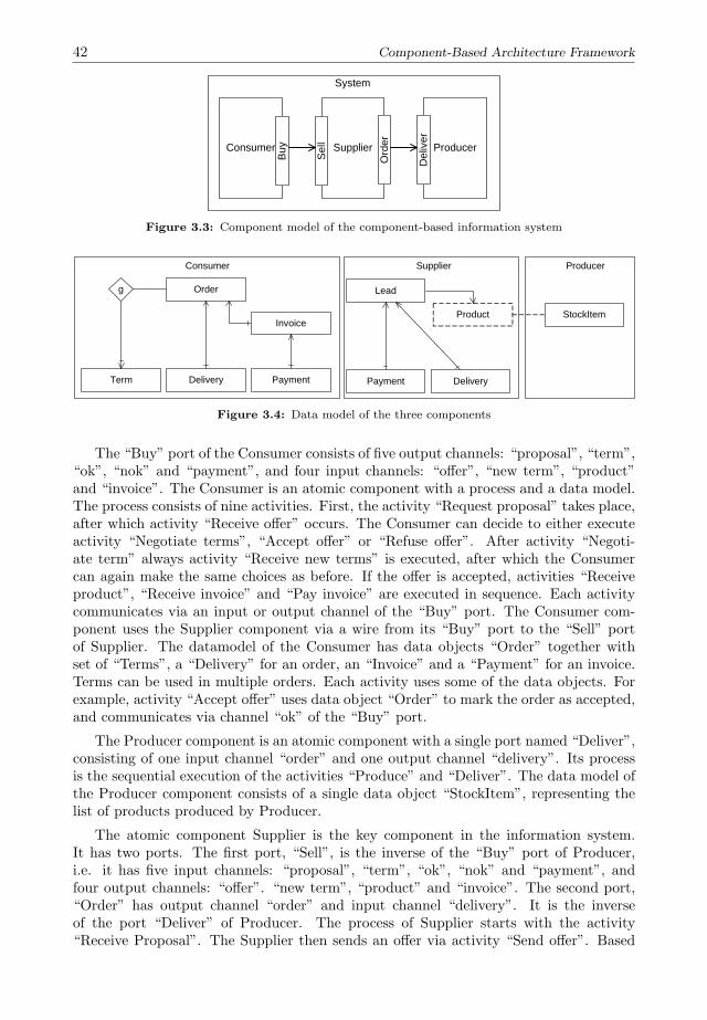
42 Component-Based Architecture Framework
Supplier
Sel
l
Ord
erConsumer
Buy Producer
Del
iver
System
Figure 3.3: Component model of the component-based information system
Order
Term Delivery Payment
g
Invoice
Lead
Payment Delivery
Product StockItem
Consumer Supplier Producer
Figure 3.4: Data model of the three components
The “Buy” port of the Consumer consists of five output channels: “proposal”, “term”,“ok”, “nok” and “payment”, and four input channels: “offer”, “new term”, “product”and “invoice”. The Consumer is an atomic component with a process and a data model.The process consists of nine activities. First, the activity “Request proposal” takes place,after which activity “Receive offer” occurs. The Consumer can decide to either executeactivity “Negotiate terms”, “Accept offer” or “Refuse offer”. After activity “Negoti-ate term” always activity “Receive new terms” is executed, after which the Consumercan again make the same choices as before. If the offer is accepted, activities “Receiveproduct”, “Receive invoice” and “Pay invoice” are executed in sequence. Each activitycommunicates via an input or output channel of the “Buy” port. The Consumer com-ponent uses the Supplier component via a wire from its “Buy” port to the “Sell” portof Supplier. The datamodel of the Consumer has data objects “Order” together withset of “Terms”, a “Delivery” for an order, an “Invoice” and a “Payment” for an invoice.Terms can be used in multiple orders. Each activity uses some of the data objects. Forexample, activity “Accept offer” uses data object “Order” to mark the order as accepted,and communicates via channel “ok” of the “Buy” port.
The Producer component is an atomic component with a single port named “Deliver”,consisting of one input channel “order” and one output channel “delivery”. Its processis the sequential execution of the activities “Produce” and “Deliver”. The data model ofthe Producer component consists of a single data object “StockItem”, representing thelist of products produced by Producer.
The atomic component Supplier is the key component in the information system.It has two ports. The first port, “Sell”, is the inverse of the “Buy” port of Producer,i.e. it has five input channels: “proposal”, “term”, “ok”, “nok” and “payment”, andfour output channels: “offer”. “new term”, “product” and “invoice”. The second port,“Order” has output channel “order” and input channel “delivery”. It is the inverseof the port “Deliver” of Producer. The process of Supplier starts with the activity“Receive Proposal”. The Supplier then sends an offer via activity “Send offer”. Based

43
Request proposal
Receive offer
Receive new terms
Negotiate terms
Refuse offer
Accept offer
Receive product
Receive invoice
Pay invoice
proposal
new term
term
ok
product
invoice
payment
Receive proposal
Send offer
Offer refused
Offer accepted
Receive term
Send new terms
Request product
Receive productSend product
Send Invoice
Receive payment
order
deliver
Produce
Deliver
Producer
Supplier
Consumer Buy Sell
Order Deliver
nok
offer
Figure 3.5: Petri net of the composition of the three components
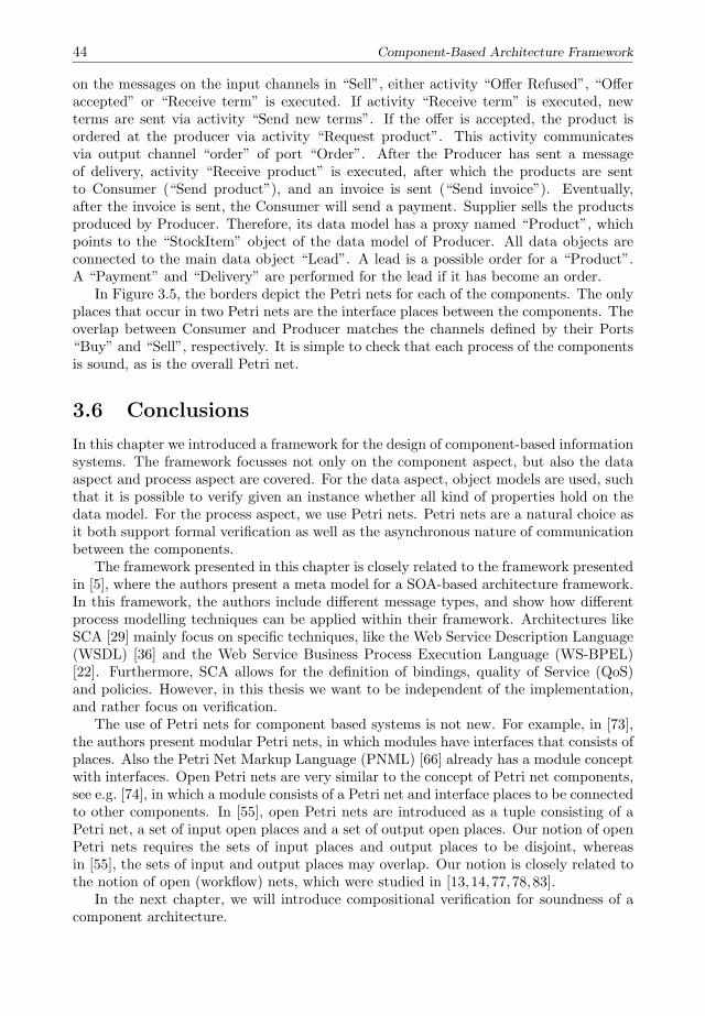
44 Component-Based Architecture Framework
on the messages on the input channels in “Sell”, either activity “Offer Refused”, “Offeraccepted” or “Receive term” is executed. If activity “Receive term” is executed, newterms are sent via activity “Send new terms”. If the offer is accepted, the product isordered at the producer via activity “Request product”. This activity communicatesvia output channel “order” of port “Order”. After the Producer has sent a messageof delivery, activity “Receive product” is executed, after which the products are sentto Consumer (“Send product”), and an invoice is sent (“Send invoice”). Eventually,after the invoice is sent, the Consumer will send a payment. Supplier sells the productsproduced by Producer. Therefore, its data model has a proxy named “Product”, whichpoints to the “StockItem” object of the data model of Producer. All data objects areconnected to the main data object “Lead”. A lead is a possible order for a “Product”.A “Payment” and “Delivery” are performed for the lead if it has become an order.
In Figure 3.5, the borders depict the Petri nets for each of the components. The onlyplaces that occur in two Petri nets are the interface places between the components. Theoverlap between Consumer and Producer matches the channels defined by their Ports“Buy” and “Sell”, respectively. It is simple to check that each process of the componentsis sound, as is the overall Petri net.
3.6 Conclusions
In this chapter we introduced a framework for the design of component-based informationsystems. The framework focusses not only on the component aspect, but also the dataaspect and process aspect are covered. For the data aspect, object models are used, suchthat it is possible to verify given an instance whether all kind of properties hold on thedata model. For the process aspect, we use Petri nets. Petri nets are a natural choice asit both support formal verification as well as the asynchronous nature of communicationbetween the components.
The framework presented in this chapter is closely related to the framework presentedin [5], where the authors present a meta model for a SOA-based architecture framework.In this framework, the authors include different message types, and show how differentprocess modelling techniques can be applied within their framework. Architectures likeSCA [29] mainly focus on specific techniques, like the Web Service Description Language(WSDL) [36] and the Web Service Business Process Execution Language (WS-BPEL)[22]. Furthermore, SCA allows for the definition of bindings, quality of Service (QoS)and policies. However, in this thesis we want to be independent of the implementation,and rather focus on verification.
The use of Petri nets for component based systems is not new. For example, in [73],the authors present modular Petri nets, in which modules have interfaces that consists ofplaces. Also the Petri Net Markup Language (PNML) [66] already has a module conceptwith interfaces. Open Petri nets are very similar to the concept of Petri net components,see e.g. [74], in which a module consists of a Petri net and interface places to be connectedto other components. In [55], open Petri nets are introduced as a tuple consisting of aPetri net, a set of input open places and a set of output open places. Our notion of openPetri nets requires the sets of input places and output places to be disjoint, whereasin [55], the sets of input and output places may overlap. Our notion is closely related tothe notion of open (workflow) nets, which were studied in [13,14,77,78,83].
In the next chapter, we will introduce compositional verification for soundness of acomponent architecture.
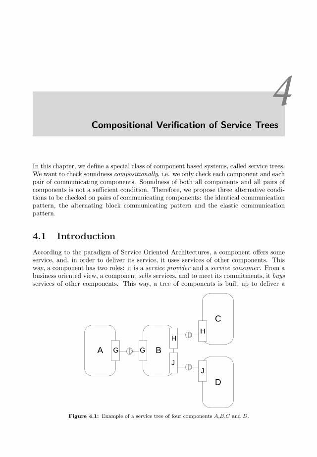
4Compositional Verification of Service Trees
In this chapter, we define a special class of component based systems, called service trees.We want to check soundness compositionally, i.e. we only check each component and eachpair of communicating components. Soundness of both all components and all pairs ofcomponents is not a sufficient condition. Therefore, we propose three alternative condi-tions to be checked on pairs of communicating components: the identical communicationpattern, the alternating block communicating pattern and the elastic communicationpattern.
4.1 Introduction
According to the paradigm of Service Oriented Architectures, a component offers someservice, and, in order to deliver its service, it uses services of other components. Thisway, a component has two roles: it is a service provider and a service consumer . From abusiness oriented view, a component sells services, and to meet its commitments, it buysservices of other components. This way, a tree of components is built up to deliver a
A G
CH
DJ
BG
H
J
Figure 4.1: Example of a service tree of four components A,B,C and D.

46 Compositional Verification of Service Trees
v
t
u
B
A C
G H
Figure 4.2: The composition of three composable OPNs.
service to the initial client. A component requesting a service, does not need to know thatthe component delivering the requested service, itself is a client for several other services.This can be for reasons of privacy, but a more obvious reason is that many componentsprovide the same service, and components take each other services via a third party likea broker. Therefore, the tree is built up dynamically at run-time. At design time, theservice tree is not known. This makes verification of behavioral correctness very hard.Thus, if we want to ensure behavioral correctness, we need a verification method thatonly considers pairwise compositions of components: if each component is sound, and allpairwise connected components satisfy some condition, the whole tree should be sound.
The nature of this class of component based systems is asymmetric. A service providercommits itself to deliver a service. It does not matter what other components thatservice provider needs, as long as it keeps delivering the requested service. Therefore, theconnections between components have a direction: they are initiated by a service client,and accepted by a service provider. Consider the component architecture depicted inFigure 4.1. There are four components, A, B and C, which are connected via ports G, Hand J . The ⃝ operator indicates the direction of the communication. In this example,component B delivers a service to component A over port G, and to do so, it uses theservices of its children C and D.
Just requiring each composition of connected pairs of components to be sound is notsufficient to guarantee the correctness of the whole service tree, as shown in Figure 4.2.In this example, both A⊕B and B⊕C are sound. However the composition A⊕B⊕Chas a deadlock, since this composition introduces a cyclic dependency over the threecomponents: after firing transition v, the system is in deadlock. A sufficient condition toguarantee correctness of the whole tree by only checking pairs of connected components,is accordance, as defined in the previous chapter. If B ⊕ C accords to the compositionB, then all partners of B are also a partner of B ⊕ C. Thus, for every partner A suchthat A⊕ B is sound, also A⊕ (B ⊕ C) is sound.
Theorem 4.1.1 (Accordance sufficient)Let A, B and C be three OPNs such that A and C are disjoint, A and B are elementarycomposable with respect to port G ∈ GA ∩GB , and B and C are elementary composablewith respect to port H ∈ GB∩GC . If (B⊕C)G ⊑ BG and A⊕B is sound then A⊕B⊕Cis sound. y
47
Proof. Since A ⊕ B is sound, its skeleton S(A ⊕ B) is weakly terminating. We haveS(A⊕B) = AG⊕BG. Hence, AG⊕BG is weakly terminating and AG ∈ Part(BG). SinceBG ⊑ (B⊕C)G, also AG ∈ Part((B⊕C)G). Thus, AG⊕ (B⊕C)G is weakly terminatingand since it is closed, it is sound by Corollary 3.4.5. Hence, by Corollary 3.4.15, A⊕B⊕Cis sound. 2
Accordance is not only a sufficient condition, it is also a necessary condition. If Bdoes not accord to the composition B ⊕ C, a partner exists such that the compositionA⊕ B is sound, but the composition A⊕ (B ⊕ C) is not sound.
Theorem 4.1.2 (Accordance necessary)Let B and C be two OPNs that are elementary composable with respect to port H ∈GB ∩ GC . Let G ∈ GB \ GC . If (B ⊕ C)G ⊑ BG then an OPN A exists such that A⊕ Bis sound, but A⊕ B ⊕ C is not sound. y
Proof. Since BG ⊑ (B ⊕ C)G, an A ∈ Part(BG) exists such that A ∈ Part((B ⊕ C)G).Hence, A ⊕ BG is weakly terminating, and by Corollary 3.4.5, it is sound. Since A ∈Part((B⊕C)G), the composition A⊕ (B⊕C)G is not weakly terminating, and thus notsound by Corollary 3.4.5. Hence, by Corollary 3.4.15, A⊕ B ⊕ C is not sound. 2
In [84], the authors prove undecidability of controllability for general open Petri nets.Current research results (cf. [82, 103, 112]) are based on a message bound. As we onlyrequire the final marking to be a home marking, such a message bound may not exist.Although the accordance relation is both a sufficient and a necessary condition, a solutionto decide accordance for livelock-freedom is not available [103]. We therefore search fora sufficient condition such that we can decide soundness. In this chapter, we will presentthree alternative sufficient conditions, which we call communication patterns.
Let A, B and C form a service tree where A is the parent of B, and B the parent ofC. Figure 4.3 shows the relation between the different communication patterns.
Identical Communication Pattern
The identical communication pattern requires C not to hamper B, i.e. the compositionB⊕C should mimic every firing sequence B can execute. Thus, for every firing sequenceσ in B leading to its final marking, a firing sequence σ should exist in the compositionB ⊕ C that leads to the final marking of the composition, and the projection of σ onthe transitions of component B should be equal to σ. This way, component A does notnotice whether it is communicating to component B or to the composition B ⊕ C. Thenotion is closely related to simulation.
Alternating Block Communication Pattern
Every firing sequence can be uniquely split into communication blocks: all communicationtransitions in such a block either have the same sign or do not communicate at all. Thealternating block communication pattern loosens the identical communication pattern byallowing to send or receive messages within a communication block in any order. It can berelated to simulation of hyper transition systems, i.e. a step is now a multi-action insteadof a single transition. Simulation on the general hyper transition systems is shown to bea sufficient condition, but not necessary, and too restrictive. Therefore, we define a quasisimulation, which is based on the switch points in the LTS of an OPN. A switch point is amarking with an important property: the sign of the sequence with which the marking isreached has a different sign than its successor sequence. By definition of communication
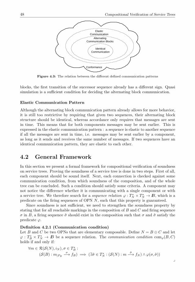
48 Compositional Verification of Service Trees
Conformance
ElasticCommunication
AlternatingCommunication Blocks
IdenticalCommunication
Figure 4.3: The relation between the different defined communication patterns
blocks, the first transition of the successor sequence already has a different sign. Quasisimulation is a sufficient condition for deciding the alternating block communication.
Elastic Communication Pattern
Although the alternating block communication pattern already allows for more behavior,it is still too restrictive by requiring that given two sequences, their alternating blockstructure should be identical, whereas accordance only requires that messages are sentin time. This means that for both components messages may be sent earlier. This isexpressed in the elastic communication pattern : a sequence is elastic to another sequenceif all the messages are sent in time, i.e. messages may be sent earlier by a component,as long as it sends and receives the same number of messages. If two sequences have anidentical communication pattern, they are elastic to each other.
4.2 General Framework
In this section we present a formal framework for compositional verification of soundnesson service trees. Proving the soundness of a service tree is done in two steps. First of all,each component should be sound itself. Next, each connection is checked against somecommunication condition, from which soundness of the composition, and of the wholetree can be concluded. Such a condition should satisfy some criteria. A component maynot notice the difference whether it is communicating with a single component or witha service tree. We therefore search for a sequence relation φ : T ∗
N × T ∗N → IB, which is a
predicate on the firing sequences of OPN N , such that this property is guaranteed.Since soundness is not sufficient, we need to strengthen the soundness property by
stating that for all reachable markings in the composition of B and C and firing sequenceσ in B, a firing sequence σ should exist in the composition such that σ and σ satisfy thepredicate φ.
Definition 4.2.1 (Communication condition)Let B and C be two OPNs that are elementary composable. Define N = B ⊕ C and letφ : T ∗
B × T ∗N → IB be a sequence relation. The communication condition comφ(B,C)
holds if and only if:
∀m ∈ R(S(N), iN ), σ ∈ T ∗B :
(S(B) : m|PB
σ−→ fB) =⇒ (∃σ ∈ T ∗N : (S(N) : m
σ−→ fN ) ∧ φ(σ, σ))y
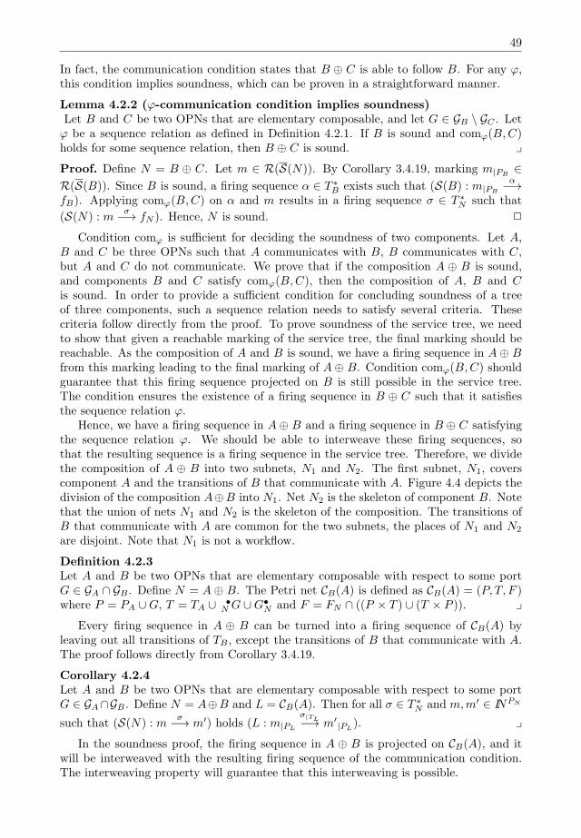
49
In fact, the communication condition states that B ⊕ C is able to follow B. For any φ,this condition implies soundness, which can be proven in a straightforward manner.
Lemma 4.2.2 (φ-communication condition implies soundness)Let B and C be two OPNs that are elementary composable, and let G ∈ GB \ GC . Letφ be a sequence relation as defined in Definition 4.2.1. If B is sound and comφ(B,C)holds for some sequence relation, then B ⊕ C is sound. yProof. Define N = B ⊕ C. Let m ∈ R(S(N)). By Corollary 3.4.19, marking m|PB
∈R(S(B)). Since B is sound, a firing sequence α ∈ T ∗
B exists such that (S(B) : m|PB
α−→fB). Applying comφ(B,C) on α and m results in a firing sequence σ ∈ T ∗
N such that
(S(N) : mσ−→ fN ). Hence, N is sound. 2
Condition comφ is sufficient for deciding the soundness of two components. Let A,B and C be three OPNs such that A communicates with B, B communicates with C,but A and C do not communicate. We prove that if the composition A ⊕ B is sound,and components B and C satisfy comφ(B,C), then the composition of A, B and Cis sound. In order to provide a sufficient condition for concluding soundness of a treeof three components, such a sequence relation needs to satisfy several criteria. Thesecriteria follow directly from the proof. To prove soundness of the service tree, we needto show that given a reachable marking of the service tree, the final marking should bereachable. As the composition of A and B is sound, we have a firing sequence in A⊕ Bfrom this marking leading to the final marking of A⊕ B. Condition comφ(B,C) shouldguarantee that this firing sequence projected on B is still possible in the service tree.The condition ensures the existence of a firing sequence in B ⊕ C such that it satisfiesthe sequence relation φ.
Hence, we have a firing sequence in A⊕ B and a firing sequence in B ⊕ C satisfyingthe sequence relation φ. We should be able to interweave these firing sequences, sothat the resulting sequence is a firing sequence in the service tree. Therefore, we dividethe composition of A ⊕ B into two subnets, N1 and N2. The first subnet, N1, coverscomponent A and the transitions of B that communicate with A. Figure 4.4 depicts thedivision of the composition A⊕B into N1. Net N2 is the skeleton of component B. Notethat the union of nets N1 and N2 is the skeleton of the composition. The transitions ofB that communicate with A are common for the two subnets, the places of N1 and N2
are disjoint. Note that N1 is not a workflow.
Definition 4.2.3Let A and B be two OPNs that are elementary composable with respect to some portG ∈ GA ∩ GB . Define N = A⊕ B. The Petri net CB(A) is defined as CB(A) = (P, T, F )where P = PA ∪G, T = TA ∪ •
NG ∪G•N and F = FN ∩ ((P × T ) ∪ (T × P )). y
Every firing sequence in A ⊕ B can be turned into a firing sequence of CB(A) byleaving out all transitions of TB , except the transitions of B that communicate with A.The proof follows directly from Corollary 3.4.19.
Corollary 4.2.4Let A and B be two OPNs that are elementary composable with respect to some portG ∈ GA∩GB . Define N = A⊕B and L = CB(A). Then for all σ ∈ T ∗
N and m,m′ ∈ INPN
such that (S(N) : mσ−→ m′) holds (L : m|PL
σ|TL−→ m′|PL
). yIn the soundness proof, the firing sequence in A ⊕ B is projected on CB(A), and it
will be interweaved with the resulting firing sequence of the communication condition.The interweaving property will guarantee that this interweaving is possible.
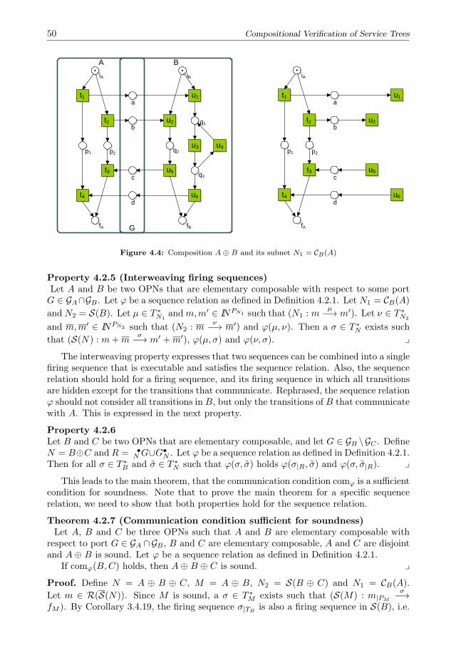
50 Compositional Verification of Service Trees
A B
G
t1
t2
t4
t3
u1
u2
u3 u4
u5
u6
iA iB
fA fB
a
b
c
d
p1 p2
q1
q2
q3
t1
t2
t4
t3
u1
u2
u5
u6
iA
fA
a
b
c
d
p1 p2
Figure 4.4: Composition A⊕ B and its subnet N1 = CB(A)
Property 4.2.5 (Interweaving firing sequences)Let A and B be two OPNs that are elementary composable with respect to some portG ∈ GA∩GB . Let φ be a sequence relation as defined in Definition 4.2.1. Let N1 = CB(A)and N2 = S(B). Let µ ∈ T ∗
N1andm,m′ ∈ INPN1 such that (N1 : m
µ−→ m′). Let ν ∈ T ∗N2
and m,m′ ∈ INPN2 such that (N2 : mν−→ m′) and φ(µ, ν). Then a σ ∈ T ∗
N exists such
that (S(N) : m+mσ−→ m′ +m′), φ(µ, σ) and φ(ν, σ). y
The interweaving property expresses that two sequences can be combined into a singlefiring sequence that is executable and satisfies the sequence relation. Also, the sequencerelation should hold for a firing sequence, and its firing sequence in which all transitionsare hidden except for the transitions that communicate. Rephrased, the sequence relationφ should not consider all transitions in B, but only the transitions of B that communicatewith A. This is expressed in the next property.
Property 4.2.6Let B and C be two OPNs that are elementary composable, and let G ∈ GB \GC . DefineN = B⊕C and R = •
NG∪G•N . Let φ be a sequence relation as defined in Definition 4.2.1.
Then for all σ ∈ T ∗B and σ ∈ T ∗
N such that φ(σ, σ) holds φ(σ|R, σ) and φ(σ, σ|R). yThis leads to the main theorem, that the communication condition comφ is a sufficient
condition for soundness. Note that to prove the main theorem for a specific sequencerelation, we need to show that both properties hold for the sequence relation.
Theorem 4.2.7 (Communication condition sufficient for soundness)Let A, B and C be three OPNs such that A and B are elementary composable with
respect to port G ∈ GA ∩GB , B and C are elementary composable, A and C are disjointand A⊕ B is sound. Let φ be a sequence relation as defined in Definition 4.2.1.
If comφ(B,C) holds, then A⊕ B ⊕ C is sound. yProof. Define N = A ⊕ B ⊕ C, M = A ⊕ B, N2 = S(B ⊕ C) and N1 = CB(A).Let m ∈ R(S(N)). Since M is sound, a σ ∈ T ∗
M exists such that (S(M) : m|PM
σ−→fM ). By Corollary 3.4.19, the firing sequence σ|TB
is also a firing sequence in S(B), i.e.

51
N1 N2
A B CR
Figure 4.5: The composition A⊕ B ⊕ C is split into N1 = CB(A) and N2 = S(B ⊕ C)
(S(B) : m|PB
σ|TB−→ fB). By Corollary 3.4.20, m|PN2∈ R(N2, iM ). Hence, we can apply
the communication condition comφ(B,C) on m|PN2and σ|TB
, which results in a firing
sequence σ ∈ T ∗N2
such that (N2 : m|PN2
σ−→ fN2) and φ(σ|TB, σ). Hence, we have a
firing sequence σ in M and a firing sequence σ in N2, which we need to interweave.
We split the composition N in N1 and N2, as shown in Figure 4.5. By Corollary 4.2.4,
(N1 : m|PN1
σ|TN1−→ fA). By Property 4.2.6, the sequence relation also holds for the pro-jected firing sequence, i.e. φ(σ|TN1
, σ) holds. Then the Interweaving Property (Prop-erty 4.2.5) applied on (N1,m|PN1
) with firing sequence σ|TN1and (N2,m|PN2
) with firing
sequence σ results in a firing sequence σ ∈ T ∗N such that (S(N) : m
σ−→ fA+ fN2 = fN ).Hence, N is sound. 2
From Theorem 4.2.7, it follows that comφ is a sufficient condition to conclude sound-ness of a service tree consisting of three components if Property 4.2.5 and Property 4.2.6hold for the sequence relation. Hence, if two connected components satisfy comφ, thecomposition is guaranteed to be sound, and it can be used for compositional verification.In fact, comφ(A,B) implies a direction in the service tree: component A uses componentB to provide its service on port G, or, rephrased, B provides a service to A.
Definition 4.2.8 (Component uses another component)Let A and B be two composable components with respect to port G ∈ GA ∩ GB , and letφ : T ∗
N × T ∗N → IB be a sequence relation as defined in Definition 4.2.1.
We say A uses B, denoted by A⃝φB, if A⊕ B and comφ(A,B). y
A service tree is a tree of components connected to each other such that componentscan only “subcontract” work to other components. The structure of the tree is defined bythe tree function c. Each node A is a component that delivers a service to its parent c(A)using the services of its children c−1(A). Each component only communicates with itsparent and its children, communication with other components is not allowed. Note thatthe communication implied by this function is asymmetric: the parent uses its childrento deliver the service requested. By requiring that the transitive closure of c is irreflexive,we ensure the service tree to be a tree.

52 Compositional Verification of Service Trees
Definition 4.2.9 (Service tree)A service tree is a pair (O, c) where O is a set of OPNs, and c : O O is a partialfunction called the parent function such that the transitive closure c∗ of c is irreflexive,for all A,B ∈ O:
• c(B) = A =⇒ |GA ∩ GB | = 1 ∧A⃝φB; and
• A ∩B = ∅ =⇒ c(A) = B ∨ c(B) = A.
and for all A ∈ O a B ∈ O exists such that (A,B) ∈ c∗ or (B,A) ∈ c∗. yIn a service tree, each parent should use the services of its children. Hence, if the
root is sound, and each parent uses its children, the service tree should be sound. Thisis expressed in the next theorem. The proof uses the associativity and commutativity ofthe composition operator and Theorem 4.2.7.
Theorem 4.2.10 (Soundness of service trees)Let (O, c) be a service tree. If all OPNs of O are sound, then
⊕X∈OX is sound. y
Proof. Assume all OPNs in O are sound. Observe that (O, c) is a tree. Hence, atopological sort ⊑ exists on the nodes O. Let O = O1, . . . , On such that Oi ⊑ Oi+1
for 1 ≤ i < n. We prove the lemma by induction on i. Let i = 1. For (O1, ∅), thestatement holds trivially.
Now assume 1 < i < n and⊕
X∈O′ X is sound where O′ = O1, . . . , Oi. LetB = Oi+1. Since ⊑ is a topological sort, there exists a unique A ∈ O′ such that A⃝φB,and B is disjoint with all OPNs in O′ \ A.
By associativity and commutativity, we have⊕
X∈O′ X = (⊕
X∈O′\AX)⊕ A, and⊕X∈O′\AX is disjoint with B. As A⃝φB, we have comφ(A,B), and thus by Theo-
rem 4.2.7, (⊕
X∈O′\AX)⊕A⊕B is sound. Again by associativity and commutativity,
(⊕
X∈O′\AX)⊕ A⊕ B =⊕
X∈O′∪BX. Hence, the statement holds. 2
Given two OPNs A and B, the communication condition requires that for every mark-ing in the composition, and for each firing sequence in B from this marking to the finalmarking in B, a firing sequence in the composition B ⊕ C exists with which the compo-sition can reach its final marking, and some communication ϕ needs to hold. In general,both the number of markings to be considered in the composition, as well as the numberof firing sequences in B to be checked, is infinite. However, if the composition is bounded,the communication condition is decidable if the sequence relation is computable.
Lemma 4.2.11Let B and C be two components that are elementary composable. Let G ∈ GB \ GC bea port. The communication condition comφ(B,C) is decidable if B ⊕ C is bounded andφ is computable. yProof. As B and B ⊕ C are sound, the number of states is bounded. But there can bean infinite number of firing sequences in B to be checked. As there are only finitely manystates, infinite firing sequences have loops. Let l be the length of the longest cycle freesequence in B⊕ C. If OPN B has a cycle σ, then it is not necessary for a correspondingfiring sequence σ in B⊕C such that φ(σ, σ) to have a cycle as well. Let a maximal cyclein B have c transitions. Let k = ⌈ lc⌉, i.e. k is the minimal natural number such thatk · c ≥ l. Hence, if σ contains the loop more than k times, then σ must have a cycle.Thus, we only have to check a finite number of firing sequences. 2
In the next sections, we introduce three communication conditions that satisfy Prop-erty 4.2.5 and Property 4.2.6.

53
B
A
C
GH
t1
t2
t3
t5
t4
t6
a
b
c
d
e
f
iB
iA
iC
fCfBfA
q1
p1
p2
p3
p4
p5
q2
q1
q3
q4
q5
u1
u2
u3 u4
u5
u6
u7
u8 u9
v1
v2
Figure 4.6: The composition A⊕ B is sound, and comω(B,C) holds, hence A⊕ B ⊕ C is sound
4.3 Identical Communication Pattern
One of the main principles in the composition of service trees is that adding a componentmay not influence the communication with the other components in the composition.Consider a sound composition of A and B. Connecting a new component C to B shouldnot destroy the soundness of A⊕ B. This might occur if C blocks some execution pathof B, as shown by the example in the introduction of this chapter. Hence, A should notnotice whether it is communicating with B or with the composition B⊕C. As shown inthe previous section, soundness of the composition B⊕C is not a sufficient condition forthe compositional verification, as it does not guarantee correct communication betweenA and B. For example, a firing sequence may get blocked, as shown in Figure 4.2.If B ⊕ C would mimic B, i.e. if B can fire a transition communicating with A, thenthe composition should also be able to fire this transition. If needed, it may fire someinternal transitions, i.e. transitions of component C. This is expressed in the identicalcommunication condition, in which firing sequences of B are related to firing sequencesin the composition B ⊕ C if the firing sequences projected on B are identical.
Definition 4.3.1 (Identical communication condition)Let B and C be two OPNs that are elementary composable, and let G ∈ GB \ GCDefine N = A ⊕ B. The identical sequence relation ωG : T ∗
B × T ∗N → IB is defined by
ωG(µ, ν) ⇔ µ|R = ν|R, where R = •NG ∪G•
N . The identical communication condition isdefined as comωG . y
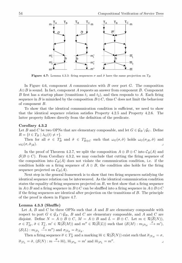
54 Compositional Verification of Service Trees
TA TB TB TC
b
m
~
b
m’
m’
m’
1
2
m
m’’1
m’’2
m’’
TA TB
b
TC m
m1
m
m2
Figure 4.7: Lemma 4.3.3: firing sequences σ and σ have the same projection on TB
In Figure 4.6, component A communicates with B over port G. The compositionA⊕B is sound. In fact, component A requests an answer from component B. ComponentB first has a startup phase (transitions t1 and t2), and then responds to A. Each firingsequence in B is mimicked by the composition B⊕C, thus C does not limit the behaviourof component B.
To show that the identical communication condition is sufficient, we need to showthat the identical sequence relation satisfies Property 4.2.5 and Property 4.2.6. Thelatter property follows directly from the definition of the predicate.
Corollary 4.3.2Let B and C be two OPNs that are elementary composable, and let G ∈ GB \GC . DefineR = t ∈ TB | λG(t) = τ.
Then for all σ ∈ T ∗B and σ ∈ T ∗
B⊕C such that ωG(σ, σ) holds ωG(σ|R, σ) andωG(σ, σ|R). y
In the proof of Theorem 4.2.7, we split the composition A ⊕ B ⊕ C into CB(A) andS(B ⊕ C). From Corollary 4.3.2, we may conclude that cutting the firing sequence ofthe composition into CB(A) does not violate the communication condition, i.e. if thecondition holds on a firing sequence of A ⊕ B, the condition also holds for the firingsequence projected on CB(A).
Next step in the general framework is to show that two firing sequences satisfying theidentical sequence relation can be interweaved. As the identical communication conditionstates the equality of firing sequences projected on B, we first show that a firing sequencein A⊕B and a firing sequence in B⊕C can be shuffled into a firing sequence in A⊕B⊕Cif the firing sequences are identical after projection on the transitions of B. The principleof the proof is shown in Figure 4.7.
Lemma 4.3.3 (Shuffle)Let A, B and C be three OPNs such that A and B are elementary composable with
respect to port G ∈ GA ∩ GB , B and C are elementary composable, and A and C aredisjoint. Define N = A ⊕ B ⊕ C, M = A ⊕ B and L = B ⊕ C. Let m ∈ R(S(N)),
σ ∈ T ∗M , σ ∈ T ∗
L, m′ ∈ R(S(M)) and m′′ ∈ R(S(L)) such that (S(M) : m|PM
σ−→ m′),
(S(L) : m|PL
σ−→ m′′) and σ|TB= σ|TB
.
Then a firing sequence σ ∈ T ∗N and a markingm ∈ R(S(N)) exist such that σ|TM
= σ,
σ|TL= σ, (S(N) : m
σ−→ m), m|PM= m′ and m|PL
= m′′. y
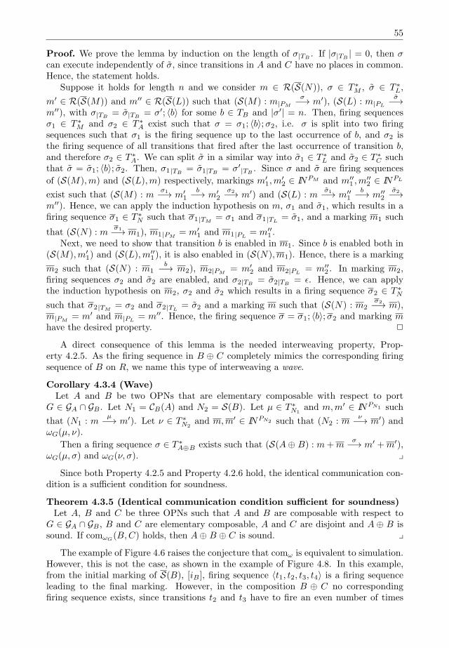
55
Proof. We prove the lemma by induction on the length of σ|TB. If |σ|TB
| = 0, then σcan execute independently of σ, since transitions in A and C have no places in common.Hence, the statement holds.
Suppose it holds for length n and we consider m ∈ R(S(N)), σ ∈ T ∗M , σ ∈ T ∗
L,
m′ ∈ R(S(M)) and m′′ ∈ R(S(L)) such that (S(M) : m|PM
σ−→ m′), (S(L) : m|PL
σ−→m′′), with σ|TB
= σ|TB= σ′; ⟨b⟩ for some b ∈ TB and |σ′| = n. Then, firing sequences
σ1 ∈ T ∗M and σ2 ∈ T ∗
A exist such that σ = σ1; ⟨b⟩;σ2, i.e. σ is split into two firingsequences such that σ1 is the firing sequence up to the last occurrence of b, and σ2 isthe firing sequence of all transitions that fired after the last occurrence of transition b,and therefore σ2 ∈ T ∗
A. We can split σ in a similar way into σ1 ∈ T ∗L and σ2 ∈ T ∗
C suchthat σ = σ1; ⟨b⟩; σ2. Then, σ1|TB
= σ1|TB= σ′
|TB. Since σ and σ are firing sequences
of (S(M),m) and (S(L),m) respectively, markings m′1,m
′2 ∈ INPM and m′′
1 ,m′′2 ∈ INPL
exist such that (S(M) : mσ1−→ m′
1b−→ m′
2σ2−→ m′) and (S(L) : m σ1−→ m′′
1b−→ m′′
2σ2−→
m′′). Hence, we can apply the induction hypothesis on m, σ1 and σ1, which results in afiring sequence σ1 ∈ T ∗
N such that σ1|TM= σ1 and σ1|TL
= σ1, and a marking m1 such
that (S(N) : mσ1−→ m1), m1|PM
= m′1 and m1|PL
= m′′1 .
Next, we need to show that transition b is enabled in m1. Since b is enabled both in(S(M),m′
1) and (S(L),m′′1), it is also enabled in (S(N),m1). Hence, there is a marking
m2 such that (S(N) : m1b−→ m2), m2|PM
= m′2 and m2|PL
= m′′2 . In marking m2,
firing sequences σ2 and σ2 are enabled, and σ2|TB= σ2|TB
= ϵ. Hence, we can applythe induction hypothesis on m2, σ2 and σ2 which results in a firing sequence σ2 ∈ T ∗
N
such that σ2|TM= σ2 and σ2|TL
= σ2 and a marking m such that (S(N) : m2σ2−→ m),
m|PM= m′ and m|PL
= m′′. Hence, the firing sequence σ = σ1; ⟨b⟩;σ2 and marking mhave the desired property. 2
A direct consequence of this lemma is the needed interweaving property, Prop-erty 4.2.5. As the firing sequence in B ⊕ C completely mimics the corresponding firingsequence of B on R, we name this type of interweaving a wave.
Corollary 4.3.4 (Wave)Let A and B be two OPNs that are elementary composable with respect to port
G ∈ GA ∩ GB . Let N1 = CB(A) and N2 = S(B). Let µ ∈ T ∗N1
and m,m′ ∈ INPN1 such
that (N1 : mµ−→ m′). Let ν ∈ T ∗
N2and m,m′ ∈ INPN2 such that (N2 : m
ν−→ m′) andωG(µ, ν).
Then a firing sequence σ ∈ T ∗A⊕B exists such that (S(A⊕ B) : m+m
σ−→ m′ +m′),ωG(µ, σ) and ωG(ν, σ). y
Since both Property 4.2.5 and Property 4.2.6 hold, the identical communication con-dition is a sufficient condition for soundness.
Theorem 4.3.5 (Identical communication condition sufficient for soundness)Let A, B and C be three OPNs such that A and B are composable with respect to
G ∈ GA ∩ GB , B and C are elementary composable, A and C are disjoint and A ⊕ B issound. If comωG(B,C) holds, then A⊕ B ⊕ C is sound. y
The example of Figure 4.6 raises the conjecture that comω is equivalent to simulation.However, this is not the case, as shown in the example of Figure 4.8. In this example,from the initial marking of S(B), [iB ], firing sequence ⟨t1, t2, t3, t4⟩ is a firing sequenceleading to the final marking. However, in the composition B ⊕ C no correspondingfiring sequence exists, since transitions t2 and t3 have to fire an even number of times
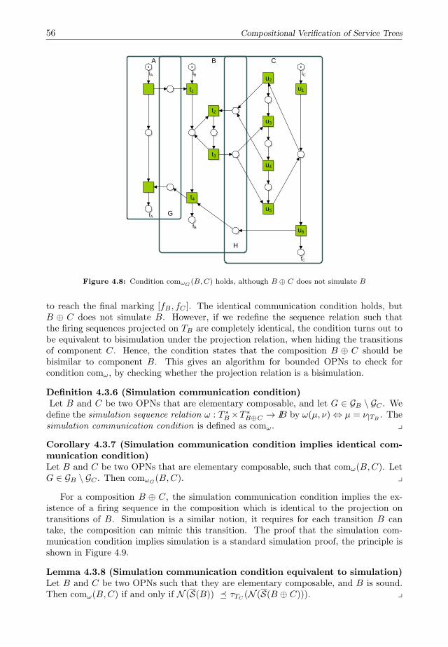
56 Compositional Verification of Service Trees
A B C
G
H
t1
t2
t3
t4
u1
u2
u3
u4
u5
u6
iBiA iC
fB
fA
fC
Figure 4.8: Condition comωG (B,C) holds, although B ⊕ C does not simulate B
to reach the final marking [fB , fC ]. The identical communication condition holds, butB ⊕ C does not simulate B. However, if we redefine the sequence relation such thatthe firing sequences projected on TB are completely identical, the condition turns out tobe equivalent to bisimulation under the projection relation, when hiding the transitionsof component C. Hence, the condition states that the composition B ⊕ C should bebisimilar to component B. This gives an algorithm for bounded OPNs to check forcondition comω, by checking whether the projection relation is a bisimulation.
Definition 4.3.6 (Simulation communication condition)Let B and C be two OPNs that are elementary composable, and let G ∈ GB \ GC . Wedefine the simulation sequence relation ω : T ∗
B×T ∗B⊕C → IB by ω(µ, ν) ⇔ µ = ν|TB
. Thesimulation communication condition is defined as comω. y
Corollary 4.3.7 (Simulation communication condition implies identical com-munication condition)Let B and C be two OPNs that are elementary composable, such that comω(B,C). LetG ∈ GB \ GC . Then comωG(B,C). y
For a composition B ⊕ C, the simulation communication condition implies the ex-istence of a firing sequence in the composition which is identical to the projection ontransitions of B. Simulation is a similar notion, it requires for each transition B cantake, the composition can mimic this transition. The proof that the simulation com-munication condition implies simulation is a standard simulation proof, the principle isshown in Figure 4.9.
Lemma 4.3.8 (Simulation communication condition equivalent to simulation)Let B and C be two OPNs such that they are elementary composable, and B is sound.Then comω(B,C) if and only if N (S(B)) ≼ τTC (N (S(B ⊕ C))). y

57
t
mm
m’’m’
fB fB C
m’
B
~1
~2
t
’
B C
Figure 4.9: Lemma 4.3.8: Simulation condition implies simulation
Proof. Define N = B ⊕ C. We prove that N (S(B)) ≼Q τTC(N (S(B ⊕ C))), where
Q = (m|PB,m) | m ∈ INPN .
(⇒) Assuming comω(B,C), we need to show that Q is a simulation relation.1) By definition of ⊕, we have iB QiN and fB QfN .
2) Let m,m′ ∈ INPB , t ∈ TB and m ∈ INPN such that (S(B) : mt−→ m′) and
mQm. Since B is sound, a firing sequence σ′ ∈ T ∗B exists such that (S(B) : m′ σ′
−→ fB).
Let σ = ⟨t⟩;σ′. Then (S(B) : mσ−→ fB). Note that m|PB
= m. Hence, we canapply comω(B,C) on m and σ, which results in a firing sequence σ ∈ T ∗
N such that
(S(N) : mσ−→ fN ) and ω(σ, σ). Thus, σ|TB
= σ = ⟨t⟩;σ′. Hence, σ first executes zeroor more silent transitions in C, and then it executes transition t, i.e. firing sequencesσ′ ∈ T ∗
C and σ′′ ∈ T ∗N and markings m′,m′′ ∈ INPN exist such that σ = σ′; ⟨t⟩; σ′′ and
(S(N) : mσ′
−→ m′′ t−→ m′). Hence, (S(N) : mt
=⇒ m′).Next, we need to show that the markings m′ and m′ are related. Since σ′ ∈ T ∗
C ,for all places p ∈ PB holds m(p) = m(p) = m′′(p) and m′(p) = m(p) − •t(p) + t•(p) =m′′(p)− •t(p) + t•(p) = m′(p). Thus m′
|PB= m′, and therefore m′Qm′.
3) Let m ∈ INPN such that fB Qm. We have (S(B) : fBϵ−→ fB). Applying
comω(B,C) on ϵ and m, results in a firing sequence σ ∈ T ∗N such that (S(N) : m
σ−→ fN )and σ|TA
= ϵ. Hence (S(N) : m =⇒ fN ) and fB QfN .
(⇐) Assuming Q is a simulation relation, we need to show that comω(B,C) holds.
Let m ∈ R(S(N)) and σ ∈ T ∗B such that (S(B) : m|PB
σ−→ fB). We prove by induction
on the length of σ the existence of a firing sequence σ ∈ T ∗N such that (S(N) : m
σ−→ fN )and σ|TB
= σ.
First, suppose σ = ϵ, i.e. (S(B) : m|PB
ϵ−→ fB). Hence, fB = m|PBand thus fB Qm.
Since Q is a simulation, a sequence σ ∈ T ∗C exists such that (S(N) : m
σ−→ fN ). Thenσ|TB
= ϵ, and hence, the statement holds.
Now, suppose σ = ⟨t⟩;σ′ for some t ∈ TB and σ′ ∈ T ∗B . Then a markingm′ ∈ R(S(B))
exists such that (S(B) : m|PB
t−→ m′ σ′
−→ fB). Since Q is a simulation, a marking
m′ ∈ INPN exists such that (S(N) : mt
=⇒ m′) and m′Qm′. Hence, there is a marking
m′′ ∈ R(S(N)) and a firing sequence σ′ ∈ T ∗C such that (S(N) : m
σ′
−→ m′′ t−→ m′).Applying the induction hypothesis on m′ and σ′ results in a firing sequence σ′′ ∈ T ∗
N
such that σ′′|TB
= σ′ and (S(N) : m′ σ′′
−→ fN ). Hence, σ = σ′; ⟨t⟩; σ′′ is firing sequence
such that (S(N) : mσ−→ fN ) and σ|TB
= σ. 2

58 Compositional Verification of Service Trees
A B
G
iA=fA iB=fB
p1 p2
d
Figure 4.10: Composition A ⊕ B simulates B. Although place d is unbounded, the composition issound
As a consequence of Lemma 3.4.18, we can directly conclude that the identical com-munication pattern is equivalent to delay bisimulation.
Corollary 4.3.9 (Equivalent condition)Let B and C be two OPNs such that they are elementary composable, and B is sound.Define N = B⊕ C. Then comω(A,B) if and only if N (S(B)) ≃Q τTC
(N (S(N))) whereQ = (m|PA
,m) | m ∈ INPN . yHence, to check whether the simulation communication pattern holds, we need to
check whether the projection relation of a composition on one if its constituents is abisimulation. In general, this problem is known to be undecidable [70]. For boundedPetri nets it is decidable.
Consider the example composition in Figure 4.10. Component A is a cycle sending ineach run of the cycle a message to component B. Component B is a cycle only receivingthis message. Clearly A⊕ B simulates A. The initial marking is a home marking: fromevery marking reachable, it is possible to reach the final marking. Hence, although thecomposition is unbounded, it satisfies the identical communication pattern, and hence,it is sound.
4.4 Alternating Block Communication Pattern
In the previous section, the identical communication condition is shown to be equivalentto bisimulation. This is a strong requirement. Consider the example of Figure 4.11.From the initial marking of S(B), [iB ], firing sequence ⟨t1, t3, t2, t4⟩ is a firing sequenceleading to the final marking. However, in the composition B ⊕ C no correspondingfiring sequence exists, since all accepting firing sequences projected on B have the samesequence, ⟨t1, t2, t3, t4⟩. Although comωG
(B,C) does not hold, B accords to B ⊕ C.The example of Figure 4.11 shows that although comω is easy to verify using standard
bisimulation techniques, it is too restrictive. In B, transitions t2 and t3 both send amessage on port G, hence, they have the same sign. In the composition, only silent stepsbetween the two transitions are added. In fact, each firing sequence can be identified byits communication block structure. The communication of a firing sequence can be splitinto several blocks. Each block, i.e. a subsequence, has a sign indicating the direction ofcommunication on port G. The alternating block structure of a sequence is a sequence ofits communication blocks. Two sequences have an identical alternating block structure ifthey have the same number of blocks, and for each two corresponding blocks, the numberof occurrences of transitions communicating via port G should be the same.
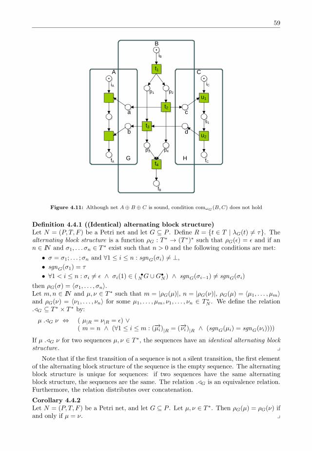
59
A
B
C
t2a
b
G H
t1
t3
t4
iB
iCiA
fA
fB
u1
u2
c
d
fC
p1 p2
p3 p4
s1
Figure 4.11: Although net A⊕ B ⊕ C is sound, condition comωG (B,C) does not hold
Definition 4.4.1 ((Identical) alternating block structure)Let N = (P, T, F ) be a Petri net and let G ⊆ P . Define R = t ∈ T | λG(t) = τ. Thealternating block structure is a function ρG : T ∗ → (T ∗)∗ such that ρG(ϵ) = ϵ and if ann ∈ IN and σ1, . . . σn ∈ T ∗ exist such that n > 0 and the following conditions are met:
• σ = σ1; . . . ;σn and ∀1 ≤ i ≤ n : sgnG(σi) = ⊥,
• sgnG(σ1) = τ
• ∀1 < i ≤ n : σi = ϵ ∧ σi(1) ∈ ( •NG ∪G•
N ) ∧ sgnG(σi−1) = sgnG(σi)
then ρG(σ) = ⟨σ1, . . . , σn⟩.Let m,n ∈ IN and µ, ν ∈ T ∗ such that m = |ρG(µ)|, n = |ρG(ν)|, ρG(µ) = ⟨µ1, . . . , µm⟩and ρG(ν) = ⟨ν1, . . . , νn⟩ for some µ1, . . . , µm, ν1, . . . , νn ∈ T ∗
N . We define the relationG ⊆ T ∗ × T ∗ by:
µ G ν ⇔ ( µ|R = ν|R = ϵ) ∨( m = n ∧ (∀1 ≤ i ≤ m : (−→µi)|R = (−→νi )|R ∧ (sgnG(µi) = sgnG(νi))))
If µ G ν for two sequences µ, ν ∈ T ∗, the sequences have an identical alternating blockstructure. y
Note that if the first transition of a sequence is not a silent transition, the first elementof the alternating block structure of the sequence is the empty sequence. The alternatingblock structure is unique for sequences: if two sequences have the same alternatingblock structure, the sequences are the same. The relation G is an equivalence relation.Furthermore, the relation distributes over concatenation.
Corollary 4.4.2Let N = (P, T, F ) be a Petri net, and let G ⊆ P . Let µ, ν ∈ T ∗. Then ρG(µ) = ρG(ν) ifand only if µ = ν. y
60 Compositional Verification of Service Trees
Corollary 4.4.3Let N = (P, T, F ) be a Petri net and G ⊆ P . Relation G is an equivalence relation. yCorollary 4.4.4 (Relation G distributes over concatenation)Let N = (P, T, F ) be a Petri net and G ⊆ P . Let µ′, µ′′, ν′, ν′′ ∈ T ∗ such that µ′ G ν′
and µ′′ G ν′′. Then (µ′;µ′′) G (ν′; ν′′). yIf the projection on the communicating transitions of two sequences are identical,
they have an identical alternating block structure.
Corollary 4.4.5Let N be a Petri net, G ⊆ P and let R = •G ∪G•. Let µ, ν ∈ T ∗ such that µ|R = ν|R.Then µ G ν. y
The alternating block communication pattern states that for each given reachablemarking m in the composition of B ⊕ C and firing sequence in B from m to fB , a firingsequence in the composition exists with an identical alternating block structure.
Definition 4.4.6 (Alternating block communication condition)Let B and C be two OPNs that are elementary composable, and let G ∈ GB \ GC be aport. The alternating block communication condition is defined as comG(B,C). y
Corollary 4.4.5 directly shows the relation between the identical communication pat-tern and the alternating block communication pattern: if a composition satisfies theidentical communication condition, it also satisfies the alternating blocks communica-tion.
Corollary 4.4.7Let B and C be two OPNs that are elementary composable. Let G ∈ GB \ GC . IfcomωG(B,C) holds then comG(B,C) also holds. y
Consider again the example of Figure 4.11. Transitions t2 and t3 are labeled ! withrespect to port G. The other transitions are silent (label τ) with respect to port G.The firing sequence σ = ⟨t1, t3, t2, t4⟩ gives on port G the communication block structure⟨⟨t1⟩, ⟨t3, t2, t4⟩⟩, subsequence ⟨t1⟩ has sign τ and ⟨t3, t3, t4⟩ has sign ?. In the compositionB ⊕ C, firing sequence σ = ⟨t1, t2, u1, u2, t3, t4⟩ gives on port G the alternating blockstructure ⟨⟨t1⟩, ⟨t2, u1, u2, t3, t4⟩⟩. The first block has sign τ , the second block has sign!. Thus, they have the same number of blocks, and on each subsequence, the transitionscommunicating with G occur with equal frequency. Hence, σ and σ have an identicalalternating block structure.
In order to show that comG is a sufficient condition for compositional verificationof soundness, we need to show the identical alternating block structure satisfies theconditions of Property 4.2.5 and Property 4.2.6. The latter follows directly from thedefinition of the identical alternating block structure.
Corollary 4.4.8Let B and C be two OPNs that are elementary composable, and let G ∈ GB \GC . DefineR = •G ∪ G•. Let σ ∈ T ∗
B and σ ∈ T ∗B⊕C such that σ G σ. Then σ|R G σ and
σ G σ|R. yNext, we need to show that if two sequences have an identical communication block
structure, they can be interweaved into a new firing sequence. The composition A⊕B issplit into two subnets, N1 = CB(A) and N2 = S(B). By definition of CB(A), the transi-tions of B that communicate with A in N1 either have an empty preset or they have anempty postset. With respect to B, if the preset is empty, it is a sending transition, if the
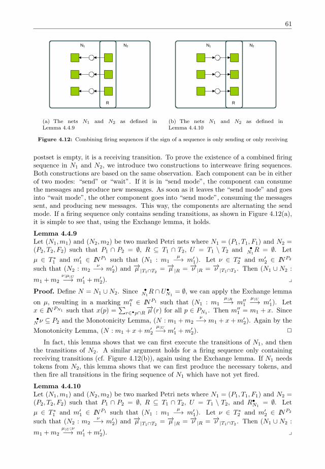
61
R
N1 N2
(a) The nets N1 and N2 as defined inLemma 4.4.9
R
N1 N2
(b) The nets N1 and N2 as defined inLemma 4.4.10
Figure 4.12: Combining firing sequences if the sign of a sequence is only sending or only receiving
postset is empty, it is a receiving transition. To prove the existence of a combined firingsequence in N1 and N2, we introduce two constructions to interweave firing sequences.Both constructions are based on the same observation. Each component can be in eitherof two modes: “send” or “wait”. If it is in “send mode”, the component can consumethe messages and produce new messages. As soon as it leaves the “send mode” and goesinto “wait mode”, the other component goes into “send mode”, consuming the messagessent, and producing new messages. This way, the components are alternating the sendmode. If a firing sequence only contains sending transitions, as shown in Figure 4.12(a),it is simple to see that, using the Exchange lemma, it holds.
Lemma 4.4.9Let (N1,m1) and (N2,m2) be two marked Petri nets where N1 = (P1, T1, F1) and N2 =(P2, T2, F2) such that P1 ∩ P2 = ∅, R ⊆ T1 ∩ T2, U = T1 \ T2 and •
N1R = ∅. Let
µ ∈ T ∗1 and m′
1 ∈ INP1 such that (N1 : m1µ−→ m′
1). Let ν ∈ T ∗2 and m′
2 ∈ INP2
such that (N2 : m2ν−→ m′
2) and −→µ |T1∩T2= −→µ |R = −→ν |R = −→ν |T1∩T2
. Then (N1 ∪ N2 :
m1 +m2
ν;µ|U−→ m′1 +m′
2). yProof. Define N = N1 ∪N2. Since
•N1R ∩ U•
N1= ∅, we can apply the Exchange lemma
on µ, resulting in a marking m′′1 ∈ INP1 such that (N1 : m1
µ|R−→ m′′1
µ|U−→ m′1). Let
x ∈ INPN1 such that x(p) =∑r∈•p∩R
−→µ (r) for all p ∈ PN1 . Then m′′1 = m1 + x. Since
•N ν ⊆ P2 and the Monotonicity Lemma, (N : m1 +m2
ν−→ m1 + x+m′2). Again by the
Monotonicity Lemma, (N : m1 + x+m′2
µ|U−→ m′1 +m′
2). 2
In fact, this lemma shows that we can first execute the transitions of N1, and thenthe transitions of N2. A similar argument holds for a firing sequence only containingreceiving transitions (cf. Figure 4.12(b)), again using the Exchange lemma. If N1 needstokens from N2, this lemma shows that we can first produce the necessary tokens, andthen fire all transitions in the firing sequence of N1 which have not yet fired.
Lemma 4.4.10Let (N1,m1) and (N2,m2) be two marked Petri nets where N1 = (P1, T1, F1) and N2 =(P2, T2, F2) such that P1 ∩ P2 = ∅, R ⊆ T1 ∩ T2, U = T1 \ T2, and R•
N1= ∅. Let
µ ∈ T ∗1 and m′
1 ∈ INP1 such that (N1 : m1µ−→ m′
1). Let ν ∈ T ∗2 and m′
2 ∈ INP2
such that (N2 : m2ν−→ m′
2) and −→µ |T1∩T2= −→µ |R = −→ν |R = −→ν |T1∩T2
. Then (N1 ∪ N2 :
m1 +m2
µ|U ;ν−→ m′
1 +m′2). y
62 Compositional Verification of Service Trees
Proof. Define N = N1 ∪N2. Since•N1U ∩R•
N1= ∅, we can apply the Exchange lemma
on µ, resulting in a marking m′′1 such that (N1 : m1
µ|U−→ m′′1
µ|R−→ m′1). Let x ∈ INPN1
such that x(p) =∑r∈p•∩R
−→µ (r) Then m′′1 = m′
1 + x, since Dom(m′′1) ∩ •R = ∅. Since
•N (µ|U ) ⊆ P1 and by the Monotonicity Lemma, (N : m1 +m2
µ|U−→ m′1 + x+m2). Since
−→µ |R = −→ν |R, if a transition of R fires in ν, the input needed from N1 is already generated.
Thus, (N : m′1 + x+m2
ν−→ m′1 +m′
2). Hence, (N : m1 +m2
µ|U ;ν−→ m′
1 +m′2). 2
The communication block structure alternates sending and receiving blocks. Thus,we can combine the results of Lemma 4.4.9 and Lemma 4.4.10 to show that in general,if for two sequences σ G σ, we can construct a firing sequence by interweaving the two.
Lemma 4.4.11 (Twist)Let A and B be two OPNs that are elementary composable with respect to port
G ∈ GA ∩ GB . Let N1 = CB(A) and N2 = S(B). Let µ ∈ T ∗N1
and m,m′ ∈ INPN1 such
that (N1 : mµ−→ m′). Let ν ∈ T ∗
N2and m,m′ ∈ INPN2 such that (N2 : m
ν−→ m′) and
µ G ν. Then a σ ∈ T ∗N exists such that (S(N) : m +m
σ−→ m′ +m′), µ G σ andν G σ. y
Proof. Let R = TN1 ∩ TN2 . Define k = |ρG(µ)| = |ρG(ν)|. Suppose k ≤ 1. Then µ|R =
ν|R = ϵ. By Lemma 4.3.3, a firing sequence σ exists such that (N : m1+m2σ−→ m′
1+m′2)
and σ|R = µ|R = ν|R. Hence, the statement holds for k ≤ 1.Now suppose k > 1, and let the statement hold for all n < k. Let µ1, . . . , µk ∈ T ∗
N1
and ν1, . . . , νk ∈ T ∗N2
such that ρG(µ) = ⟨µ1, . . . , µk⟩ and ρG(ν) = ⟨ν1, . . . , νk⟩. Let
m′′1 ∈ INPN1 and µ′, µ′′ ∈ T ∗
N1such that µ′ = µ1;µ2, µ = µ′;µ′′ and (N1 : m
µ′
−→ m′′1).
Let m′′2 ∈ INPN1 and ν′, ν′′ ∈ T ∗
N2such that ν′ = ν1; ν2, ν = ν′; ν′′ and (N2 : m2
ν′
−→ m′′2).
Then by construction, ν′ G µ′ and µ′′ G ν′′. There are two cases to consider: eithersgnG(µ
′) = sgnG(ν′) =! or sgnG(µ
′) = sgnG(ν′) =?. If sgnG(µ
′) = sgnG(ν′) =!, then we
apply Lemma 4.4.9, and if sgnG(µ′) = sgnG(ν
′) =?, then we apply Lemma 4.4.10.
Hence, in both cases a σ′ ∈ T ∗N exists such that (S(N) : m1 + m2
σ′
−→ m′′1 + m′′
2).Since µ′′ G ν′′, we can apply the induction hypothesis, resulting in a firing sequence
σ′′ ∈ T ∗N such that (S(N) : m′′
1 +m′′2
σ′′
−→ m′1 +m′
2). Hence, σ = σ′;σ′′ has the desiredproperty. 2
From Corollary 4.4.8 and Lemma 4.4.11 we may conclude that the identical alter-nating block structure satisfies the necessary properties for Theorem 4.2.7. Hence, thealternating block communication condition comG is a sufficient condition for soundness.
Theorem 4.4.12 (Alternating block communication condition sufficient forsoundness)Let A, B and C be three OPNs such that A and B are elementary composable withrespect to G ∈ GA ∩ GB , B and C are elementary composable, A and C are disjoint andA⊕ B is sound. If comG(B,C) holds, then A⊕ B ⊕ C is sound. y
In the previous section, the identical communication pattern is shown to be equivalentto bisimulation of their LTSs. For the alternating block structure we would like tohave a similar result. As the alternating block structure is implied by the identicalcommunication pattern, it is also implied by bisimulation. However, bisimulation is toorestrictive. We therefore search for simulation relations that are more liberal. A firstobservation is that in identical communication we only consider single transition firings,
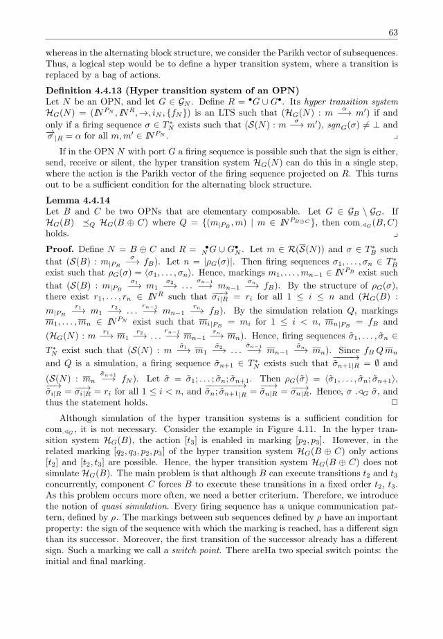
63
whereas in the alternating block structure, we consider the Parikh vector of subsequences.Thus, a logical step would be to define a hyper transition system, where a transition isreplaced by a bag of actions.
Definition 4.4.13 (Hyper transition system of an OPN)Let N be an OPN, and let G ∈ GN . Define R = •G ∪ G•. Its hyper transition systemHG(N) = (INPN , INR,→, iN , fN) is an LTS such that (HG(N) : m
α−→ m′) if and
only if a firing sequence σ ∈ T ∗N exists such that (S(N) : m
σ−→ m′), sgnG(σ) = ⊥ and−→σ |R = α for all m,m′ ∈ INPN . y
If in the OPN N with port G a firing sequence is possible such that the sign is either,send, receive or silent, the hyper transition system HG(N) can do this in a single step,where the action is the Parikh vector of the firing sequence projected on R. This turnsout to be a sufficient condition for the alternating block structure.
Lemma 4.4.14Let B and C be two OPNs that are elementary composable. Let G ∈ GB \ GG. IfHG(B) ≼Q HG(B ⊕ C) where Q = (m|PB
,m) | m ∈ INPB⊕C, then comG(B,C)holds. yProof. Define N = B ⊕ C and R = •
N G ∪ G•N . Let m ∈ R(S(N)) and σ ∈ T ∗
B such
that (S(B) : m|PB
σ−→ fB). Let n = |ρG(σ)|. Then firing sequences σ1, . . . , σn ∈ T ∗B
exist such that ρG(σ) = ⟨σ1, . . . , σn⟩. Hence, markings m1, . . . ,mn−1 ∈ INPB exist such
that (S(B) : m|PB
σ1−→ m1σ2−→ . . .
σn−1−→ mn−1σn−→ fB). By the structure of ρG(σ),
there exist r1, . . . , rn ∈ INR such that −−→σi|R = ri for all 1 ≤ i ≤ n and (HG(B) :
m|PB
r1−→ m1r2−→ . . .
rn−1−→ mn−1rn−→ fB). By the simulation relation Q, markings
m1, . . . ,mn ∈ INPN exist such that mi|PB= mi for 1 ≤ i < n, mn|PB
= fB and
(HG(N) : mr1−→ m1
r2−→ . . .rn−1−→ mn−1
rn−→ mn). Hence, firing sequences σ1, . . . , σn ∈T ∗N exist such that (S(N) : m
σ1−→ m1σ2−→ . . .
σn−1−→ mn−1σn−→ mn). Since fB Qmn
and Q is a simulation, a firing sequence σn+1 ∈ T ∗N exists such that
−−−−→σn+1|R = ∅ and
(S(N) : mnσn+1−→ fN ). Let σ = σ1; . . . ; σn; σn+1. Then ρG(σ) = ⟨σ1, . . . , σn; σn+1⟩,−−→
σi|R = −−→σi|R = ri for all 1 ≤ i < n, and−−−−−−−→σn; σn+1|R =
−−→σn|R = −−→σn|R. Hence, σ G σ, and
thus the statement holds. 2
Although simulation of the hyper transition systems is a sufficient condition forcomG , it is not necessary. Consider the example in Figure 4.11. In the hyper tran-sition system HG(B), the action [t3] is enabled in marking [p2, p3]. However, in therelated marking [q2, q3, p2, p3] of the hyper transition system HG(B ⊕ C) only actions[t2] and [t2, t3] are possible. Hence, the hyper transition system HG(B ⊕ C) does notsimulate HG(B). The main problem is that although B can execute transitions t2 and t3concurrently, component C forces B to execute these transitions in a fixed order t2, t3.As this problem occurs more often, we need a better criterium. Therefore, we introducethe notion of quasi simulation. Every firing sequence has a unique communication pat-tern, defined by ρ. The markings between sub sequences defined by ρ have an importantproperty: the sign of the sequence with which the marking is reached, has a different signthan its successor. Moreover, the first transition of the successor already has a differentsign. Such a marking we call a switch point. There areHa two special switch points: theinitial and final marking.
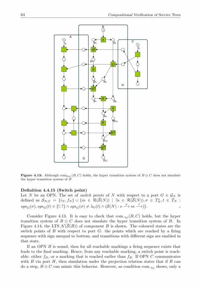
64 Compositional Verification of Service Trees
iA p2 p3
p4
p5 p6
p8p7
p9
p11
p10
p12
a!
c!b
d?
f!
i!
h?
g?
e
xA
B
C
G
H
iC
Figure 4.13: Although comG (B,C) holds, the hyper transition system of B ⊕ C does not simulatethe hyper transition system of B
Definition 4.4.15 (Switch point)Let N be an OPN. The set of switch points of N with respect to a port G ∈ GN isdefined as SN,G = iN , fN ∪ m ∈ R(S(N)) | ∃s ∈ R(S(N)), σ ∈ T ∗
N , t ∈ TN :
sgnG(σ), sgnG(t) ∈ !, ? ∧ sgnG(σ) = λG(t) ∧ (S(N) : sσ−→ m
t−→). y
Consider Figure 4.13. It is easy to check that comG(B,C) holds, but the hypertransition system of B ⊕ C does not simulate the hyper transition system of B. InFigure 4.14, the LTS N (S(B)) of component B is shown. The coloured states are theswitch points of B with respect to port G: the points which are reached by a firingsequence with sign unequal to bottom, and transitions with different sign are enabled inthat state.
If an OPN B is sound, then for all reachable markings a firing sequence exists thatleads to the final marking. Hence, from any reachable marking, a switch point is reach-able: either fB , or a marking that is reached earlier than fB . If OPN C communicateswith B via port H, then simulation under the projection relation states that if B cando a step, B ⊕ C can mimic this behavior. However, as condition comG shows, only a
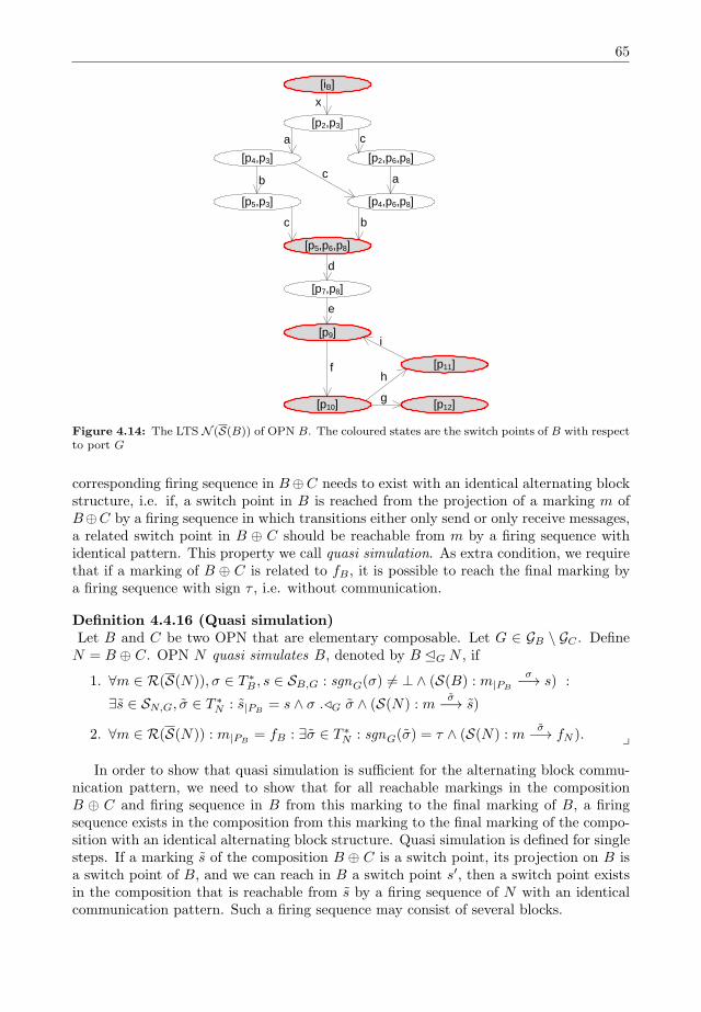
65
[iB]
[p2,p3]
[p4,p3]
x
c[p2,p6,p8]
c
[p5,p3]
b
[p4,p6,p8]
a
[p5,p6,p8]
a
c b
[p7,p8]
[p9]
[p10] [p12]
[p11]
d
e
f
g
h
i
Figure 4.14: The LTS N (S(B)) of OPN B. The coloured states are the switch points of B with respectto port G
corresponding firing sequence in B⊕C needs to exist with an identical alternating blockstructure, i.e. if, a switch point in B is reached from the projection of a marking m ofB⊕C by a firing sequence in which transitions either only send or only receive messages,a related switch point in B ⊕ C should be reachable from m by a firing sequence withidentical pattern. This property we call quasi simulation. As extra condition, we requirethat if a marking of B ⊕ C is related to fB , it is possible to reach the final marking bya firing sequence with sign τ , i.e. without communication.
Definition 4.4.16 (Quasi simulation)Let B and C be two OPN that are elementary composable. Let G ∈ GB \ GC . DefineN = B ⊕ C. OPN N quasi simulates B, denoted by B G N , if
1. ∀m ∈ R(S(N)), σ ∈ T ∗B , s ∈ SB,G : sgnG(σ) = ⊥ ∧ (S(B) : m|PB
σ−→ s) :
∃s ∈ SN,G, σ ∈ T ∗N : s|PB
= s ∧ σ G σ ∧ (S(N) : mσ−→ s)
2. ∀m ∈ R(S(N)) : m|PB= fB : ∃σ ∈ T ∗
N : sgnG(σ) = τ ∧ (S(N) : mσ−→ fN ). y
In order to show that quasi simulation is sufficient for the alternating block commu-nication pattern, we need to show that for all reachable markings in the compositionB ⊕ C and firing sequence in B from this marking to the final marking of B, a firingsequence exists in the composition from this marking to the final marking of the compo-sition with an identical alternating block structure. Quasi simulation is defined for singlesteps. If a marking s of the composition B ⊕ C is a switch point, its projection on B isa switch point of B, and we can reach in B a switch point s′, then a switch point existsin the composition that is reachable from s by a firing sequence of N with an identicalcommunication pattern. Such a firing sequence may consist of several blocks.
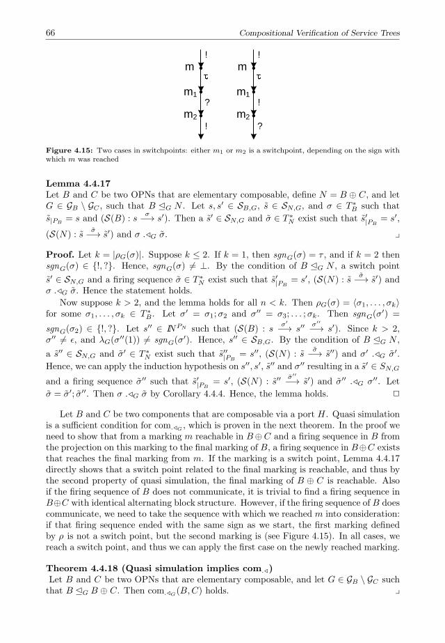
66 Compositional Verification of Service Trees
m
m1
m2
!
!
?
m
m1
m2
!
!
?
Figure 4.15: Two cases in switchpoints: either m1 or m2 is a switchpoint, depending on the sign withwhich m was reached
Lemma 4.4.17Let B and C be two OPNs that are elementary composable, define N = B ⊕ C, and letG ∈ GB \ GC , such that B G N . Let s, s′ ∈ SB,G, s ∈ SN,G, and σ ∈ T ∗
B such that
s|PB= s and (S(B) : s
σ−→ s′). Then a s′ ∈ SN,G and σ ∈ T ∗N exist such that s′|PB
= s′,
(S(N) : sσ−→ s′) and σ G σ. y
Proof. Let k = |ρG(σ)|. Suppose k ≤ 2. If k = 1, then sgnG(σ) = τ , and if k = 2 thensgnG(σ) ∈ !, ?. Hence, sgnG(σ) = ⊥. By the condition of B G N , a switch point
s′ ∈ SN,G and a firing sequence σ ∈ T ∗N exist such that s′|PB
= s′, (S(N) : sσ−→ s′) and
σ G σ. Hence the statement holds.
Now suppose k > 2, and the lemma holds for all n < k. Then ρG(σ) = ⟨σ1, . . . , σk⟩for some σ1, . . . , σk ∈ T ∗
B . Let σ′ = σ1;σ2 and σ′′ = σ3; . . . ;σk. Then sgnG(σ′) =
sgnG(σ2) ∈ !, ?. Let s′′ ∈ INPN such that (S(B) : sσ′
−→ s′′σ′′
−→ s′). Since k > 2,σ′′ = ϵ, and λG(σ
′′(1)) = sgnG(σ′). Hence, s′′ ∈ SB,G. By the condition of B G N ,
a s′′ ∈ SN,G and σ′ ∈ T ∗N exist such that s′′|PB
= s′′, (S(N) : sσ−→ s′′) and σ′ G σ′.
Hence, we can apply the induction hypothesis on s′′, s′, s′′ and σ′′ resulting in a s′ ∈ SN,G
and a firing sequence σ′′ such that s′|PB= s′, (S(N) : s′′
σ′′
−→ s′) and σ′′ G σ′′. Let
σ = σ′; σ′′. Then σ G σ by Corollary 4.4.4. Hence, the lemma holds. 2
Let B and C be two components that are composable via a port H. Quasi simulationis a sufficient condition for comG , which is proven in the next theorem. In the proof weneed to show that from a marking m reachable in B⊕C and a firing sequence in B fromthe projection on this marking to the final marking of B, a firing sequence in B⊕C existsthat reaches the final marking from m. If the marking is a switch point, Lemma 4.4.17directly shows that a switch point related to the final marking is reachable, and thus bythe second property of quasi simulation, the final marking of B ⊕ C is reachable. Alsoif the firing sequence of B does not communicate, it is trivial to find a firing sequence inB⊕C with identical alternating block structure. However, if the firing sequence of B doescommunicate, we need to take the sequence with which we reached m into consideration:if that firing sequence ended with the same sign as we start, the first marking definedby ρ is not a switch point, but the second marking is (see Figure 4.15). In all cases, wereach a switch point, and thus we can apply the first case on the newly reached marking.
Theorem 4.4.18 (Quasi simulation implies com)Let B and C be two OPNs that are elementary composable, and let G ∈ GB \ GC suchthat B G B ⊕ C. Then comG(B,C) holds. y
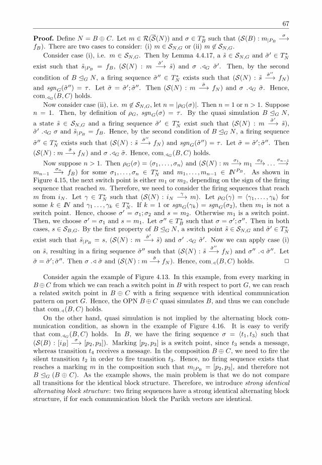
67
Proof. Define N = B ⊕ C. Let m ∈ R(S(N)) and σ ∈ T ∗B such that (S(B) : m|PB
σ−→fB). There are two cases to consider: (i) m ∈ SN,G or (ii) m ∈ SN,G.
Consider case (i), i.e. m ∈ SN,G. Then by Lemma 4.4.17, a s ∈ SN,G and σ′ ∈ T ∗N
exist such that s|PB= fB , (S(N) : m
σ′
−→ s) and σ G σ′. Then, by the second
condition of B G N , a firing sequence σ′′ ∈ T ∗N exists such that (S(N) : s
σ′′
−→ fN )
and sgnG(σ′′) = τ . Let σ = σ′; σ′′. Then (S(N) : m
σ−→ fN ) and σ G σ. Hence,comG(B,C) holds.
Now consider case (ii), i.e. m ∈ SN,G, let n = |ρG(σ)|. Then n = 1 or n > 1. Supposen = 1. Then, by definition of ρG, sgnG(σ) = τ . By the quasi simulation B G N ,
a state s ∈ SN,G and a firing sequence σ′ ∈ T ∗N exist such that (S(N) : m
σ′
−→ s),σ′ G σ and s|PB
= fB . Hence, by the second condition of B G N , a firing sequence
σ′′ ∈ T ∗N exists such that (S(N) : s
σ′′
−→ fN ) and sgnG(σ′′) = τ . Let σ = σ′; σ′′. Then
(S(N) : mσ−→ fN ) and σ G σ. Hence, comG(B,C) holds.
Now suppose n > 1. Then ρG(σ) = ⟨σ1, . . . , σn⟩ and (S(N) : mσ1−→ m1
σ2−→ . . .σn−1−→
mn−1σn−→ fB) for some σ1, . . . , σn ∈ T ∗
N and m1, . . . ,mn−1 ∈ INPB . As shown inFigure 4.15, the next switch point is either m1 or m2, depending on the sign of the firingsequence that reached m. Therefore, we need to consider the firing sequences that reach
m from iN . Let γ ∈ T ∗N such that (S(N) : iN
γ−→ m). Let ρG(γ) = ⟨γ1, . . . , γk⟩ forsome k ∈ IN and γ1 . . . , γk ∈ T ∗
N . If k = 1 or sgnG(γk) = sgnG(σ2), then m1 is not aswitch point. Hence, choose σ′ = σ1;σ2 and s = m2. Otherwise m1 is a switch point.Then, we choose σ′ = σ1 and s = m1. Let σ′′ ∈ T ∗
B such that σ = σ′;σ′′. Then in bothcases, s ∈ SB,G. By the first property of B G N , a switch point s ∈ SN,G and σ′ ∈ T ∗
N
exist such that s|PB= s, (S(N) : m
σ′
−→ s) and σ′ G σ′. Now we can apply case (i)
on s, resulting in a firing sequence σ′′ such that (S(N) : sσ′′
−→ fN ) and σ′′ σ′′. Let
σ = σ′; σ′′. Then σ σ and (S(N) : mσ−→ fN ). Hence, com(B,C) holds. 2
Consider again the example of Figure 4.13. In this example, from every marking inB⊕C from which we can reach a switch point in B with respect to port G, we can reacha related switch point in B ⊕ C with a firing sequence with identical communicationpattern on port G. Hence, the OPN B⊕C quasi simulates B, and thus we can concludethat com(B,C) holds.
On the other hand, quasi simulation is not implied by the alternating block com-munication condition, as shown in the example of Figure 4.16. It is easy to verifythat comG(B,C) holds. In B, we have the firing sequence σ = ⟨t1, t3⟩ such that
(S(B) : [iB ]σ−→ [p2, p3]). Marking [p2, p3] is a switch point, since t3 sends a message,
whereas transition t4 receives a message. In the composition B ⊕ C, we need to fire thesilent transition t2 in order to fire transition t3. Hence, no firing sequence exists thatreaches a marking m in the composition such that m|PB
= [p2, p3], and therefore notB G (B ⊕ C). As the example shows, the main problem is that we do not compareall transitions for the identical block structure. Therefore, we introduce strong identicalalternating block structure: two firing sequences have a strong identical alternating blockstructure, if for each communication block the Parikh vectors are identical.
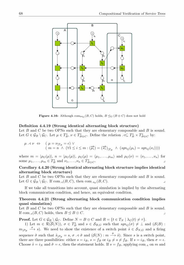
68 Compositional Verification of Service Trees
B
A
C
t1
t3
t2
t4
u1
u2
iB
fB
iC
fC
p1 p2
p3 p4
G
H
t5p5
Figure 4.16: Although comG (B,C) holds, B G (B ⊕ C) does not hold
Definition 4.4.19 (Strong identical alternating block structure)Let B and C be two OPNs such that they are elementary composable and B is sound.Let G ∈ GB \ GC . Let µ ∈ T ∗
B , ν ∈ T ∗B⊕C . Define the relation ⊆ T ∗
B × T ∗B⊕C by:
µ ν ⇔ ( µ = ν|TB= ϵ) ∨
( m = n ∧ (∀1 ≤ i ≤ m : (−→µi) = (−→νi )|TB∧ (sgnG(µi) = sgnG(νi))))
where m = |ρG(µ)|, n = |ρG(µ)|, ρG(µ) = ⟨µ1, . . . , µm⟩ and ρG(ν) = ⟨ν1, . . . , νn⟩ forsome µ1, . . . , µm ∈ T ∗
B and ν1, . . . , νn ∈ T ∗B⊕C . y
Corollary 4.4.20 (Strong identical alternating block structure implies identicalalternating block structure)Let B and C be two OPNs such that they are elementary composable and B is sound.Let G ∈ GB \ GC . If com(B,C), then comG(B,C). y
If we take all transitions into account, quasi simulation is implied by the alternatingblock communication condition, and hence, an equivalent condition.
Theorem 4.4.21 (Strong alternating block communication condition impliesquasi simulation)Let B and C be two OPNs such that they are elementary composable and B is sound.If com(B,C) holds, then B B ⊕ C. yProof. Let G ∈ GB \ GC . Define N = B ⊕ C and R = t ∈ TN | λG(t) = τ.
1) Let m ∈ R(S(N)), σ ∈ T ∗B and s ∈ SB,G such that sgnG(σ) = ⊥ and (S(B) :
m|PB
σ−→ s). We need to show the existence of a switch point s ∈ SN,G and a firing
sequence σ such that s|PB= s, σ σ and (S(N) : m
σ−→ s). Since s is a switch point,there are three possibilities: either s = iB , s = fB or iB = s = fB . If s = iB , then σ = ϵ.Choose s = iN and σ = ϵ, then the statement holds. If s = fB , applying com on m and
69
σ results in a firing sequence σ ∈ T ∗N such that (S(N) : m
σ−→ fN ) and σ σ. Hence,choose s = fB . Then the statement holds.
Otherwise, i.e. iB = s = fB , a transition t ∈ R and marking m′ ∈ INPN exist such
that (S(B) : st−→ m′). Since B is sound, a firing sequence α ∈ T ∗
B exists such that
(S(B) : m′ α−→ fB). Applying com on σ; ⟨t⟩;α and m results in a firing sequence
σ ∈ T ∗N such that (S(N) : m
σ−→ fN ) and (σ; ⟨t⟩;α) σ. Let ρG(µ) = ⟨σ1, . . . , σn⟩ forsome n = |ρG(σ)| and σ1, . . . , σn ∈ T ∗
N .
There are two cases to consider. Either sgnG(σ) = τ or sgnG(σ) ∈ !, ?. Suppose
the first. Then,−→σ1|TB
= −→σ , since σ; ⟨t⟩;α σ and t ∈ R. Hence, σ σ1. Letσ′, σ′′ ∈ T ∗
N such that σ′ = σ1 and σ = σ′;σ′′. Otherwise, sgnG(σ) ∈ !, ?. As s is a
switch point, sgnG(σ) = λG(t). Then n > 2,−→σ1|TB
+−→σ2|TB
= −→σ and sgnG(σ3) = λG(t).Let σ′, σ′′ ∈ T ∗
N such that σ′ = σ1;σ2 and σ = σ′;σ′′. In both cases σ σ′.
Let s ∈ INPN such that (S(N) : mσ′
−→ s). Then s|PB= s. As σ′′(1) ∈ R, s is also a
switch point. Hence, the statement holds for σ = σ′ and s.
2) Let m ∈ R(S(N)) such that m|PB= fB . Hence, (S(B) : m|PB
ϵ−→ fB). Thus, wecan apply com(B,C) on m and ϵ, which results in a firing sequence σ ∈ T ∗
N such that
(S(N) : mσ−→ fN ) and ϵ σ. Since sgnG(ϵ) = τ , also sgnG(σ) = τ . 2
4.5 Elastic Communication Pattern
In the previous section we weakened the communication condition by allowing to per-mute port transitions within a communication block. This condition is still not alwaysnecessary, as shown in the composition of Figure 4.17. It is clear that the compo-sition A ⊕ B is sound. Consider the sequence σ = ⟨t1, t2, t3, t4, t5⟩. Then ρG(σ) =⟨⟨t1⟩, ⟨t2⟩, ⟨t3⟩, ⟨t4, t5⟩⟩. Hence, the communication pattern is τ, !, ?, !. There is no se-quence σ in B ⊕ C such that σ G σ, since the only firing sequences in B ⊕ C are⟨t1, u1, t2, t4, u2, u3, t3, t5⟩ and ⟨u1, t1, t2, t4, u2, u3, t3, t5⟩, both with communication pat-tern τ, !, ?. Hence, condition comG(B,C) does not hold. On the other hand, it is easyto verify that the composition A⊕ B⊕ C is sound. The main problem of the net is thatthe b message is sent too early for some of the sequences, which is not allowed by comG .This example shows that messages may be sent earlier without violating the soundnessproperty. We reflect this in the elastic communication condition.
The condition allows sending transitions to be shuffled, as long as for each receivingtransition at least the same sending transitions occur, or rephrased, sending transitionsmay occur at any position within its communication block, or it can be moved forwardin the firing sequence. Although transitions sending messages may be moved forward inthe firing sequence, the condition ensures that from every marking reachable, the finalmarking is reachable.
The example of Figure 4.17 reflects the weakness of the alternating block commu-nication. Although the alternating block communication pattern allows more behavior,it is still too restrictive as each block should have the same number of occurrences ofcommunicating transitions, whereas accordance only states that communication shouldbe in time, i.e. both components may send messages earlier, as long as they can bothterminate properly. This is expressed in the elastic communication condition.
Consider the composition A⊕B of two OPNs A and B. In the proof of Theorem 4.2.7,the composition is split into two nets, N1 = CB(A) and N2 = S(B), and a firing sequencein N1 is interweaved with a firing sequence in N2. Let µ be a firing sequence in N1 and
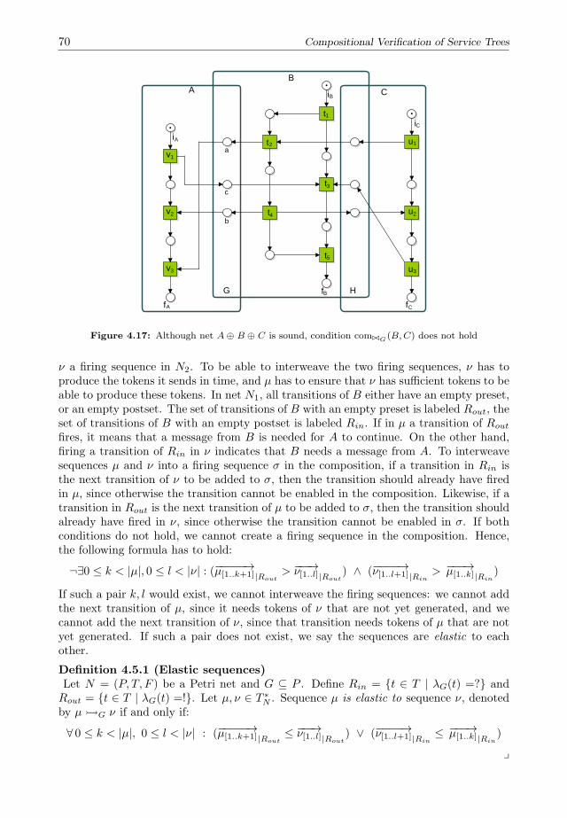
70 Compositional Verification of Service Trees
t1
t2
t4
t3
t5
a
b
c
u1
u2
u3
v1
v2
v3
iA
iB
iC
fC
fBfA
AB
C
G H
Figure 4.17: Although net A⊕ B ⊕ C is sound, condition comG (B,C) does not hold
ν a firing sequence in N2. To be able to interweave the two firing sequences, ν has toproduce the tokens it sends in time, and µ has to ensure that ν has sufficient tokens to beable to produce these tokens. In net N1, all transitions of B either have an empty preset,or an empty postset. The set of transitions of B with an empty preset is labeled Rout, theset of transitions of B with an empty postset is labeled Rin. If in µ a transition of Routfires, it means that a message from B is needed for A to continue. On the other hand,firing a transition of Rin in ν indicates that B needs a message from A. To interweavesequences µ and ν into a firing sequence σ in the composition, if a transition in Rin isthe next transition of ν to be added to σ, then the transition should already have firedin µ, since otherwise the transition cannot be enabled in the composition. Likewise, if atransition in Rout is the next transition of µ to be added to σ, then the transition shouldalready have fired in ν, since otherwise the transition cannot be enabled in σ. If bothconditions do not hold, we cannot create a firing sequence in the composition. Hence,the following formula has to hold:
¬∃0 ≤ k < |µ|, 0 ≤ l < |ν| : (−−−−−→µ[1..k+1]|Rout> −−−→ν[1..l]|Rout
) ∧ (−−−−→ν[1..l+1]|Rin> −−−→µ[1..k]|Rin
)
If such a pair k, l would exist, we cannot interweave the firing sequences: we cannot addthe next transition of µ, since it needs tokens of ν that are not yet generated, and wecannot add the next transition of ν, since that transition needs tokens of µ that are notyet generated. If such a pair does not exist, we say the sequences are elastic to eachother.
Definition 4.5.1 (Elastic sequences)Let N = (P, T, F ) be a Petri net and G ⊆ P . Define Rin = t ∈ T | λG(t) =? andRout = t ∈ T | λG(t) =!. Let µ, ν ∈ T ∗
N . Sequence µ is elastic to sequence ν, denotedby µG ν if and only if:
∀ 0 ≤ k < |µ|, 0 ≤ l < |ν| : (−−−−−→µ[1..k+1]|Rout≤ −−−→ν[1..l]|Rout
) ∨ (−−−−→ν[1..l+1]|Rin≤ −−−→µ[1..k]|Rin
)
y

71
From the definition, it follows directly that two empty sequences are always elasticto each other.
Corollary 4.5.2Let N = (P, T, F ) be a Petri net and G ⊆ P . Then ϵG ϵ. y
Consider the firing sequence σ = ⟨t1, t2, t3, t4, t5⟩ and σ = ⟨t1, u1, t2, t4, u2, u3, t3, t5⟩ inthe example of Figure 4.17. In σ, the firing of transition b is moved forward with respectto σ. Since σ[1..0] = ϵ for each firing sequence σ, we have by definition σ[1..0] G σ[1..0].The index of σ may be increased up to the situation that σ[1..0] G σ[1..6], since thent3 needs to be fired in σ[1..0] = ϵ, which is obviously not the case. Hence, we need toincrease the index of σ, which is allowed up to σ[1..5] G σ[1..6]. Then, it is allowed toincrease the index of σ up to σ[1..5] G σ[1..8]. Hence, σ is elastic to σ. The sequencesnot only should be elastic, but also the number of messages sent and received by bothsequences should match. These two requirements form the elastic sequence relation.
Definition 4.5.3 (Elastic communication condition)Let B and C be two OPNs that are elementary composable, and let G ∈ GB \ GC . Letµ ∈ T ∗
B and ν ∈ T ∗B⊕C . We define the elastic sequence relation ψG : T ∗
B × T ∗B⊕C → IB
by ψG(µ, ν) if and only if −→µ |R = −→ν |R and µ|R G ν, where R = t ∈ TB | λG(t) = τ.The elastic communication condition is defined as comψG(B,C). y
The relation between alternating block communication and elastic communicationfollows directly from their definitions. In alternating block communication for all sendingtransitions in a block, the number of occurrences of receiving transitions is equal, andvice versa. This is identical by stating that the first sequence is elastic to the second,and the second is elastic to the first sequence.
Corollary 4.5.4 (Alternating block structure implies elastic sequence relation)Let N = (P, T, F ) be a Petri net, G ⊆ P and µ, ν ∈ T ∗ be two firing sequences. Thenµ G ν if and only if ψG(µ, ν) and ψG(ν, µ). y
In order to show that the elastic communication condition comψ is a sufficient condi-tion, we need to show that Property 4.2.5 and Property 4.2.6 hold for the elastic sequencerelation. The latter follows directly from the definition of the elastic sequence relation.
Corollary 4.5.5Let B and C be two OPNs that are elementary composable, and let G ∈ GB \GC . DefineN = A⊕ B. Let µ ∈ T ∗
B and ν ∈ T ∗N such that ψG(µ, ν). Define R = •
NG ∪G•N . Then
ψG(µ|R, ν) and ψG(µ, ν|R). y
To combine a firing sequence µ with a firing sequence ν it is elastic to, we needto consider the elasticity, the structure, of the sequences. Hence, in order to proofProperty 4.2.5 for ψ, we need to show that we can interweave firing sequences µ andν. If −−−−−→µ[1..k+1]|Rout
≤ −−−→ν[1..l]|Rout, we concatenate σ and ⟨µ(k + 1)⟩ if µ(k + 1) is not in
Rin or Rout, and if −−−−→ν[1..l+1]|Rin≤ −−−→µ[1..k]|Rin
, we concatenate σ and ⟨ν(l + 1)⟩. Since µ
is elastic to ν, always at least one of the two cases holds for each k < |µ| and l < |ν|.This operation results in the algorithm IsElasticTo. In the algorithm, the If-2-Ficonstruction indicates that if multiple guards are true, non-deterministically one of theguards evaluating true is chosen.
In this algorithm, if both conditions of the if clauses fail, sequence µ cannot be elasticto sequence ν, and hence, variable b becomes false. Otherwise, an interweaved firingsequence σ is returned, such that both µG σ and ν G σ.
72 Compositional Verification of Service Trees
Procedure IsElasticTo(µ,ν)
k :=0;l :=0;σ :=ϵ;b :=True;Inv: b ≡ µ[1..k]G ν[1..l] ∧ µ[1..k]G σ ∧ ν[1..l]G σ while b ∧ (k < |µ| ∨ l < |ν|) do
if k < |µ| ∧ −−−−−→µ[1..k+1]|Rout≤ −−−→ν[1..l]|Rout
then
if µ(k + 1) ∈ (Rin ∪Rout) thenσ := σ; ⟨µ(k + 1)⟩;
fik := k + 1;
2 l < |ν| ∧ −−−−→ν[1..l+1]|Rin≤ −−−→µ[1..k]|Rin
then
σ := σ; ⟨ν(l + 1)⟩;l := l + 1;
elseb :=False;
fi
odif b then
return σelse
return Falsefi
Lemma 4.5.6Let N be an OPN and let G ∈ GN . Let µ, ν ∈ T ∗
N . Then b ≡ µ[1..k]G ν[1..l]∧µ[1..k]G
σ ∧ ν[1..l]G σ is an invariant of the procedure IsElasticTo(µ,ν). y
Proof. Define R = t ∈ TN | λG(t) = τ. Define Ak = t ∈ TN | t ∈ µ[1..k] ∧ t ∈ Rand Bl = t ∈ TN | t ∈ ν[1..l]. The invariant directly follows from the observation thatµ[1..k]|Ak
= σ|Akand ν[1..l]|Bl
= σ|Blfor all k ≤ |µ| and l ≤ |ν|. 2
Next, we need to show that the firing sequence constructed via IsElasticTo is ex-ecutable. Given two OPNs A and B that are composable with respect to port G, wesplit the composition into N1 = CB(A) and N2 = S(B). As shown in Figure 4.18, everymarking in the composition can be split into a marking in S(A), S(B) and some tokensin the interface places G. The marking in the interface G can again be split into placesthat are input for B, which we name x, and places that are output for B, which we namey. As shown in the next lemma, the elastic communication condition ensures that ateach point in time, there are sufficient tokens in the interface places to continue.
Lemma 4.5.7Let A and B be two OPNs such that they are elementary composable with respectto some port G ∈ GA ∩ GB . Define GI = G ∩ IB , GO = G ∩ OB , N1 = CB(A),N2 = S(B) and N = N1∪N2. Let m0 ∈ INPN1 be a marking, and let µ ∈ T ∗
N1be a firing
sequence of length k such that for all 1 ≤ i ≤ |µ|, markings mi−1,mi ∈ INPN1 exist with
(N1 : mi−1µ(i)−→ mi). Let m0 ∈ INPB be a marking, and let ν ∈ T ∗
B be a firing sequenceof length l such that µG ν and for all 1 ≤ i ≤ |ν|, markings mi−1,mi ∈ INPN2 exist
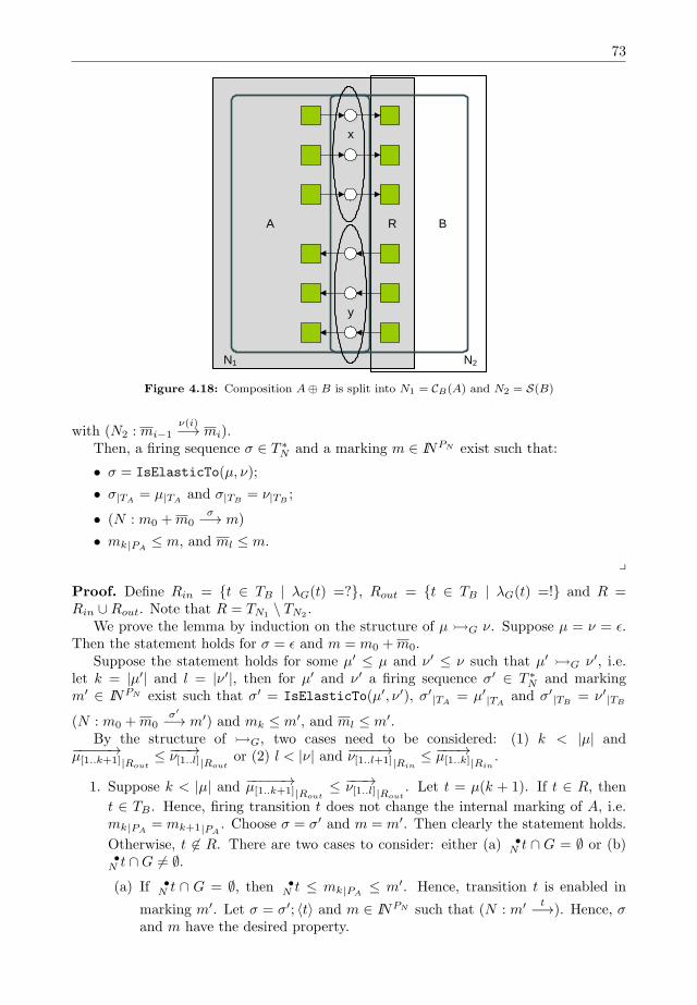
73
R BA
N1 N2
x
y
Figure 4.18: Composition A⊕ B is split into N1 = CB(A) and N2 = S(B)
with (N2 : mi−1ν(i)−→ mi).
Then, a firing sequence σ ∈ T ∗N and a marking m ∈ INPN exist such that:
• σ = IsElasticTo(µ, ν);
• σ|TA= µ|TA
and σ|TB= ν|TB
;
• (N : m0 +m0σ−→ m)
• mk|PA≤ m, and ml ≤ m.
y
Proof. Define Rin = t ∈ TB | λG(t) =?, Rout = t ∈ TB | λG(t) =! and R =Rin ∪Rout. Note that R = TN1 \ TN2 .
We prove the lemma by induction on the structure of µG ν. Suppose µ = ν = ϵ.Then the statement holds for σ = ϵ and m = m0 +m0.
Suppose the statement holds for some µ′ ≤ µ and ν′ ≤ ν such that µ′ G ν′, i.e.let k = |µ′| and l = |ν′|, then for µ′ and ν′ a firing sequence σ′ ∈ T ∗
N and markingm′ ∈ INPN exist such that σ′ = IsElasticTo(µ′, ν′), σ′
|TA= µ′
|TAand σ′
|TB= ν′|TB
(N : m0 +m0σ′
−→ m′) and mk ≤ m′, and ml ≤ m′.By the structure of G, two cases need to be considered: (1) k < |µ| and
−−−−−→µ[1..k+1]|Rout≤ −−−→ν[1..l]|Rout
or (2) l < |ν| and −−−−→ν[1..l+1]|Rin≤ −−−→µ[1..k]|Rin
.
1. Suppose k < |µ| and −−−−−→µ[1..k+1]|Rout≤ −−−→ν[1..l]|Rout
. Let t = µ(k + 1). If t ∈ R, then
t ∈ TB . Hence, firing transition t does not change the internal marking of A, i.e.mk|PA
= mk+1|PA. Choose σ = σ′ and m = m′. Then clearly the statement holds.
Otherwise, t ∈ R. There are two cases to consider: either (a) •N t ∩ G = ∅ or (b)
•N t ∩G = ∅.
(a) If •N t ∩ G = ∅, then •
N t ≤ mk|PA≤ m′. Hence, transition t is enabled in
marking m′. Let σ = σ′; ⟨t⟩ and m ∈ INPN such that (N : m′ t−→). Hence, σand m have the desired property.
74 Compositional Verification of Service Trees
(b) Suppose •N t ∩G = ∅. Then, transition t needs input from some places in the
interface G. Since t ∈ R, we have
−−−→µ[1..k]|Rout= −−−−−→µ[1..k+1]|Rout
≤ −−−→ν[1..l]|Rout=
−→σ′
|Rout
Let p ∈ •N t ∩ G be an interface place in the preset of transition t. Since
transition t is enabled in (N,mk), we have mk(p) > 0. By the markingequation, mk(p) = m0(p) +
∑u∈•p
−−−→µ[1..k](u)−∑u∈p•
−−−→µ[1..k](u). Since place pis an interface place,∑
u∈•p
−−−→µ[1..k](u) =∑u∈•p
−−−→µ[1..k]|Rout(u) ≤
∑u∈•p
−−−→ν[1..l]|Rout(u) =
∑u∈•p
−→σ′
|Rout(u)
Hence,mk(p) ≤ m′(p). Thus, transition t is enabled in (N,m′). Let σ = σ′; ⟨t⟩and m ∈ INPN such that (N : m′ t−→ m). Then the statement holds.
2. Suppose l < |ν| and −−−−→ν[1..l+1]|Rin≤ −−−→µ[1..k]|Rin
. Let t = ν(l + 1). If •N t ∩ G = ∅,
then •N t ≤ ml. Hence, the statement holds for σ = σ′; ⟨t⟩ and m ∈ INPN such that
(N : m′ t−→ m).
Otherwise, •N t ∩ G = ∅. Then λG(t) =? and transition t needs input from A in
order to be enabled in N . Hence, t ∈ Rin and ν[1..l]|Rin(t) < µ[1..k]|Rin
(t). Let
p ∈ •N t ∩G be an interface place in the preset of t. Then
mk(p) = m0(p) +∑u∈•p
−−−→µ[1..k](u)−∑u∈p•
−−−→µ[1..k](u)
= Place p is an interface place, and t ∈ p• m0(p) +
∑u∈•p
−−−→µ[1..k]|TA(u)−
∑u∈•p
−−−→µ[1..k]|Rin(u)
< ν[1..l]|Rin(t) < µ[1..k]|Rin
(t)
m0(p) +∑u∈•p
−−−→µ[1..k]|TA(u)−
∑u∈•p
−−−→ν[1..l]|Rin(u)
= σ|TA= µ[1..k]|TA
and σ|TB= ν[1..l]|TB
m0(p) +∑u∈•p
−→σ (u)−∑u∈•p
−→σ′(u)
= m′(p)
Hence, transition t is enabled in (N,m′). Let σ = σ′; ⟨t⟩ and m ∈ INPN such that
(N : m′ t−→ m). Then clearly, the statement holds.
Hence, the lemma holds. 2
Lemma 4.5.7 shows that a firing sequence and a firing sequence it is elastic to maybe interweaved into a new firing sequence that is elastic to both sequences. As in elas-tic communication the number of occurrences of each communicating transition shouldbe equal, we may directly conclude that Property 4.2.5 holds for the elastic sequencerelation ψ.

75
B
A
C
a
b
c
d
iA iC
iA
fA fB
fC
Figure 4.19: Although net A⊕ B ⊕ C is sound, condition ΨG(B,C) does not hold.
Corollary 4.5.8 (Harlem shuffle)Let A and B be two OPNs that are elementary composable with respect to port
G ∈ GA ∩ GB . Let N1 = CB(A) and N2 = S(B). Let µ ∈ T ∗N1
and m,m′ ∈ INPN1 such
that (N1 : mµ−→ m′). Let ν ∈ T ∗
N2and m,m′ ∈ INPN2 such that (N2 : m
ν−→ m′) and
ψG(µ, ν). Then, a σ ∈ T ∗N exists such that (S(N) : m +m
σ−→ m′ +m′), ψG(µ, σ) andψG(ν, σ). y
From Corollary 4.5.5 and Corollary 4.5.8 we can directly conclude that Conditioncomψ is a sufficient condition for compositional verification.
Theorem 4.5.9 (Elastic communication condition sufficient for soundness)Let A, B and C be three OPNs such that A and B are elementary composable withrespect to G ∈ GA ∩ GB , B and C are elementary composable, A and C are disjoint andA⊕ B is sound. If comψG(B,C) holds, then A⊕ B ⊕ C is sound. y
The elastic communication condition is not necessary, as shown in the example ofFigure 4.19. In this example, component A either receives an a or a b from componentB. In the composition B ⊕ C, component C decides which message will be sent bycomponent B. Consider the marking [iB , d, fC ] of the composition B ⊕ C. In thismarking, the composition can only decide to send message b, whereas if we project thismarking on B, i.e. we consider only the marking [iB ], also message a could be sent.Hence, the condition does not hold for the example.
4.6 Related Work
In [28] the authors give a constructive method preserving the inheritance of behavior. Asshown in [4] this can be used to guarantee the correctness of interorganizational processes.Other formalisms, like I/O automata [81] or interface automata [20] use synchronouscommunication, whereas we focus on asynchronous communication, which is essential forour application domain, since the communication in SOA is asynchronous.
76 Compositional Verification of Service Trees
Kazhamiakin et al. [72] compare the expressiveness of different communication mod-els with respect to their ability to detect errors in service compositions. They definea parametrized state transition system with channels. Depending on the parameterson numbers, sizes, and ordering abilities of the channels, they constitute a hierarchyof communication models and discuss the tradeoff between expressiveness and analysisperformance.
In [107], the author introduces place composition to model asynchronous communi-cation focusing on the question which subnets can be exchanged such that the behaviorof the whole net is preserved. In [78] the authors focus on deciding controllability of anOPN and computing its operating guidelines. Operating guidelines can be used to decidesubstitutability of services [104], or to prove that an implementation of a service meetsits specification [14]. Basically, the notions of controllability and operating guidelinesare devoted to assure behavioral correctness of service compositions very much like ourmain goal. For a complete service tree, where we discard the interface, the notions ofcontrollability and soundness are closely related, but soundness is a stronger correctnesscriterion than deadlock freedom, as it also forbids livelocks.
The major advantage of our approach compared to the operating guideline approachis its compositionality. In our setting it is sufficient to analyze only directly connectedservices of the tree, while the overall operating guidelines of the tree would have to bere-computed before a new service can be checked for a harmless addition to the tree.Moreover, the construction of the service tree remains flexible — each component can bereplaced by another component, provided that the composition of this component withits direct neighbors satisfies our condition. This flexibility comes however with a pricelabel, namely, the condition we define is a sufficient but not necessary condition, i.e. wemight not be able to approve some service trees, although they were sound.
In [43], the authors propose to model choreographies using Interaction Petri nets,which is a special class of Petri nets, where transitions are labeled with the source andtarget component, and the message type being sent. For each of the components, abehavioral interface is extracted. An interaction Petri net is then realizable if the com-position of the behavioral interfaces is branching bisimilar related with the interactionPetri net. To check whether the composition is functioning correctly, the whole net-work of components needs to be checked, whereas in our approach the check is donecompositionally.
4.7 Conclusions
In this chapter, we considered a special class of component-based systems, called servicetrees. Component deliver services, and to do so, they request services of other compo-nents. This way, the components form a tree during run time. A service tree is itselfagain a component, for which we want to verify soundness. As the tree is not knownat design time, we need compositional verification. Although accordance is a sufficientand necessary condition, current research results show that accordance is undecidable forgeneral open Petri nets. Accordance with respect to deadlock freedom for bounded openPetri nets is decidable, and its verification is supported by tools [82]. Accordance on weaktermination is still an open research question for bounded open Petri nets. Therefore, inthis chapter three sufficient communication conditions are proposed. These conditionsare not necessary for deciding soundness.
The first and strongest communication condition is the identical communication pat-tern. For a port, this condition requires the composition to behave identical on the port
77
as its constituent behaves. If all transitions are taken into account, this condition isequivalent to delay bisimulation of the projection relation.
The second communication condition is the alternating block communication pattern.Every firing sequence in an OPN has a unique communication pattern. The alternatingblock communication condition requires that for each firing sequence in a constituent,there should exist a firing sequence in the composition with the same communicationpattern. For this condition we introduce a new notion of simulation called quasi simu-lation. If all transitions are taken into account in the alternating block communication,this condition is equivalent to quasi simulation.
The last communication condition is the most liberal condition. If two firing sequenceshave an identical alternating block structure, a firing sequence can be constructed byalternating the blocks of the two firing sequences, and the resulting firing sequence hasthe same alternating block structure. The elastic communication condition weakens thiscondition by allowing transitions that send messages to occur not only in any orderwithin a block, it may also occur earlier in the firing sequence, as long as it is producedbefore A needs to consume the token. A simple algorithm exists to decide whether afiring sequence is elastic to another firing sequence, and if so, the algorithm returns aninterweaved firing sequence of the two.
All three conditions are sufficient. The identical communication condition impliesthe alternating block communication condition, which in its turn implies the elasticcommunication condition. Elastic communication is a sufficient, but not a necessarycondition. Although the definition of elastic communication is very liberal, the mainrestriction is in the condition itself, which requires that for every marking in a compositionB ⊕ C and for all firing sequences in B leading from this marking to the final marking afiring sequence in the composition should exist.

78 Compositional Verification of Service Trees
5Soundness-Preserving Refinement of Sets of Places
Place refinement is a well-studied subject in Petri net theory (cf. [31,44,62,87]). However,these refinements only focus on the refinement of a single place, and not on the interactionbetween components. In this chapter, we study place refinement in compositions, tosupport top-down design methods for networks of components, which we will present inthe next chapter.
5.1 Introduction
Refinement in Petri net theory is a well-studied discipline. all kinds of reduction rulesand refinement rules, sometimes also referred to as synthesis rules, exist. Berthelotpresents in his thesis [31] several general refinement rules which preserve both livenessand boundedness. As the closure of a classical sound workflow net is live and bounded,these rules also preserve soundness. In [87], Murata presents a nice overview of Petri nets,together with some reduction rules which turn out to have all kinds of nice properties [99],and which are very successful in practice. In [44], the authors present reduction andrefinement rules on free choice Petri nets, based on linear algebraic properties of thesenets. The authors of [62] show that all places may be refined by a generalized soundworkflow net, i.e. a workflow net in which for any number of tokens in the initial place,eventually the same number of tokens are produced in the final place. In this chapter,we focus on this last refinement, and generalize it to the refinement of a set of places.
This chapter is organized as follows. In Section 5.2 we present the classical approachfor place refinement and show how this can be generalized to the refinement of a set ofplaces. In Section 5.3, we present a sufficient condition on the original net and on therefining net such that if these conditions are satisfied, the refinement preserves soundness,which is formalized in Section 5.4. We conclude the chapter in Section 5.6.
5.2 Place Refinement
For Petri nets there already exist many refinement rules, like the rules of Murata [87]and Berthelot [31]. These rules guarantee weak termination: applying them on a weaklyterminating system results again in a weakly terminating system. In [62], the authorsshow that a place in a workflow net may be refined by a generalized sound workflow
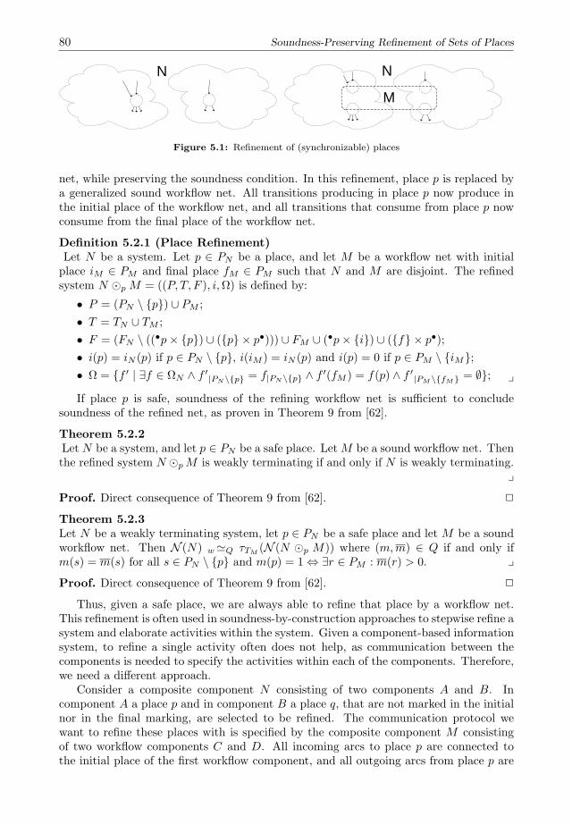
80 Soundness-Preserving Refinement of Sets of Places
N N
M
Figure 5.1: Refinement of (synchronizable) places
net, while preserving the soundness condition. In this refinement, place p is replaced bya generalized sound workflow net. All transitions producing in place p now produce inthe initial place of the workflow net, and all transitions that consume from place p nowconsume from the final place of the workflow net.
Definition 5.2.1 (Place Refinement)Let N be a system. Let p ∈ PN be a place, and let M be a workflow net with initialplace iM ∈ PM and final place fM ∈ PM such that N and M are disjoint. The refinedsystem N ⊙pM = ((P, T, F ), i,Ω) is defined by:
• P = (PN \ p) ∪ PM ;
• T = TN ∪ TM ;
• F = (FN \ ((•p× p) ∪ (p × p•))) ∪ FM ∪ (•p× i) ∪ (f × p•);
• i(p) = iN (p) if p ∈ PN \ p, i(iM ) = iN (p) and i(p) = 0 if p ∈ PM \ iM;• Ω = f ′ | ∃f ∈ ΩN ∧ f ′|PN\p = f|PN\p ∧ f ′(fM ) = f(p) ∧ f ′|PM\fM = ∅; yIf place p is safe, soundness of the refining workflow net is sufficient to conclude
soundness of the refined net, as proven in Theorem 9 from [62].
Theorem 5.2.2Let N be a system, and let p ∈ PN be a safe place. LetM be a sound workflow net. Thenthe refined system N ⊙pM is weakly terminating if and only if N is weakly terminating.
yProof. Direct consequence of Theorem 9 from [62]. 2
Theorem 5.2.3Let N be a weakly terminating system, let p ∈ PN be a safe place and let M be a soundworkflow net. Then N (N) w≃Q τTM (N (N ⊙p M)) where (m,m) ∈ Q if and only ifm(s) = m(s) for all s ∈ PN \ p and m(p) = 1 ⇔ ∃r ∈ PM : m(r) > 0. yProof. Direct consequence of Theorem 9 from [62]. 2
Thus, given a safe place, we are always able to refine that place by a workflow net.This refinement is often used in soundness-by-construction approaches to stepwise refine asystem and elaborate activities within the system. Given a component-based informationsystem, to refine a single activity often does not help, as communication between thecomponents is needed to specify the activities within each of the components. Therefore,we need a different approach.
Consider a composite component N consisting of two components A and B. Incomponent A a place p and in component B a place q, that are not marked in the initialnor in the final marking, are selected to be refined. The communication protocol wewant to refine these places with is specified by the composite component M consistingof two workflow components C and D. All incoming arcs to place p are connected tothe initial place of the first workflow component, and all outgoing arcs from place p are
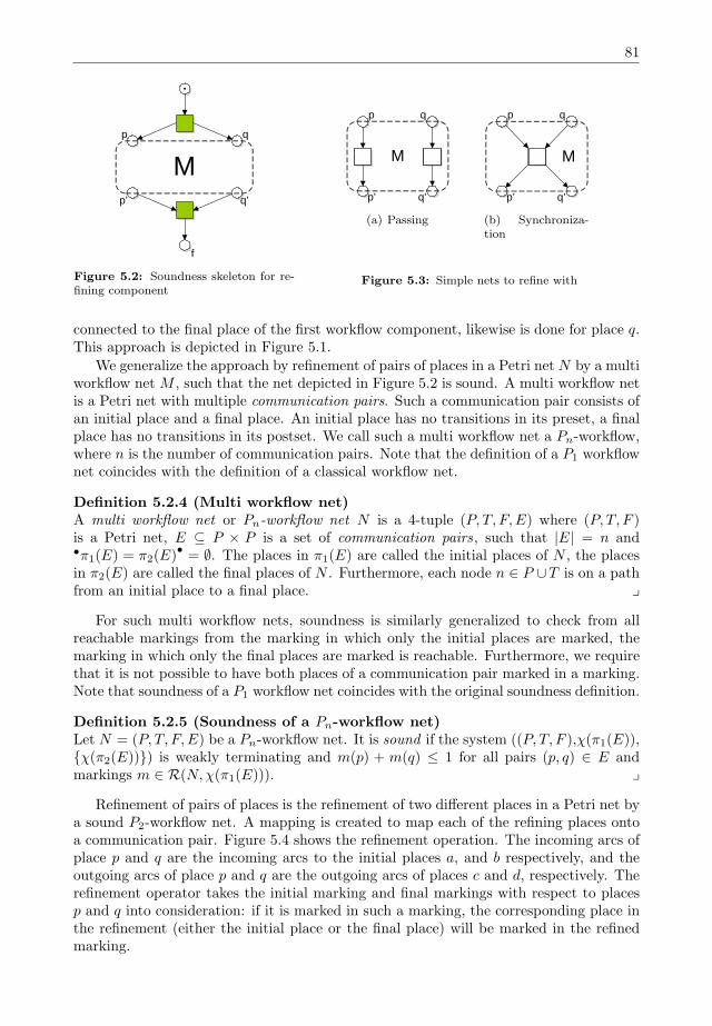
81
Mp
p’
q
q’
f
Figure 5.2: Soundness skeleton for re-fining component
M
p
p’
q
q’
(a) Passing
p
p’
q
q’
M
(b) Synchroniza-tion
Figure 5.3: Simple nets to refine with
connected to the final place of the first workflow component, likewise is done for place q.This approach is depicted in Figure 5.1.
We generalize the approach by refinement of pairs of places in a Petri net N by a multiworkflow net M , such that the net depicted in Figure 5.2 is sound. A multi workflow netis a Petri net with multiple communication pairs. Such a communication pair consists ofan initial place and a final place. An initial place has no transitions in its preset, a finalplace has no transitions in its postset. We call such a multi workflow net a Pn-workflow,where n is the number of communication pairs. Note that the definition of a P1 workflownet coincides with the definition of a classical workflow net.
Definition 5.2.4 (Multi workflow net)A multi workflow net or Pn-workflow net N is a 4-tuple (P, T, F,E) where (P, T, F )is a Petri net, E ⊆ P × P is a set of communication pairs, such that |E| = n and•π1(E) = π2(E)
•= ∅. The places in π1(E) are called the initial places of N , the places
in π2(E) are called the final places of N . Furthermore, each node n ∈ P ∪T is on a pathfrom an initial place to a final place. y
For such multi workflow nets, soundness is similarly generalized to check from allreachable markings from the marking in which only the initial places are marked, themarking in which only the final places are marked is reachable. Furthermore, we requirethat it is not possible to have both places of a communication pair marked in a marking.Note that soundness of a P1 workflow net coincides with the original soundness definition.
Definition 5.2.5 (Soundness of a Pn-workflow net)Let N = (P, T, F,E) be a Pn-workflow net. It is sound if the system ((P, T, F ),χ(π1(E)),χ(π2(E))) is weakly terminating and m(p) + m(q) ≤ 1 for all pairs (p, q) ∈ E andmarkings m ∈ R(N,χ(π1(E))). y
Refinement of pairs of places is the refinement of two different places in a Petri net bya sound P2-workflow net. A mapping is created to map each of the refining places ontoa communication pair. Figure 5.4 shows the refinement operation. The incoming arcs ofplace p and q are the incoming arcs to the initial places a, and b respectively, and theoutgoing arcs of place p and q are the outgoing arcs of places c and d, respectively. Therefinement operator takes the initial marking and final markings with respect to placesp and q into consideration: if it is marked in such a marking, the corresponding place inthe refinement (either the initial place or the final place) will be marked in the refinedmarking.

82 Soundness-Preserving Refinement of Sets of Places
t1 t2 t3 t4
p q
(a) Net N
a b
c d
(b) Net M
a b
c d
t1 t2 t3 t4
(c) Refinement N ⊙ M
Figure 5.4: Example of a refinement of a set of places
t1 t2 t3 t4
p q
(a) Net N
a b
c
(b) Net M
t1 t2 t3 t4
a b
c
(c) Refinement N ⊙ M
Figure 5.5: Example of a wrong refinement

83
Definition 5.2.6 (Refinement of sets of places)Let N be a System. Let D ⊆ PN be a set of places to be refined and define n = |D|. LetM be a Pn-workflow net. Let α : D → EM be a total bijective function. The refinementN ⊙αM is a system (P, T, F, i,Ω) where
• P = (PN \D) ∪ PM ;
• T = TN ∪ TM ;
• F =(FN \
∪p∈D((
•N p× p) ∪ (p × p•N ))
)∪ FM
∪∪p∈D(
•N p× π1(α(p)) ∪ (π2(α(p))× p•N ));
• ∀s ∈ P : i(s) =
iN (s) if s ∈ PN \DiN (d) if ∃d ∈ D : s = π1(α(d))0 otherwise
• ∀s ∈ P, fN ∈ ΩN : ∃f ∈ Ω : f(s) =
fN (s) if s ∈ PN \DfN (d) if ∃d ∈ D : s = π2(α(d))0 otherwise
y
The refinement operator as defined in Definition 5.2.6 is a very liberal definition.Consider the example of Figure 5.5. In this example, net M has communication pairs(a, c) and (b, c). It is a sound P2-workflow net. However, a refinement with this netwill change the behavior of the refinement: whereas in net N transition t1 (t2) andtransition t3 (t4) are concurrent, these transitions are in conflict in the refined net. Wetherefore additionally require |EM | = |π1(E)| = |π2(E)|, i.e. we require relation E to bea bijection. Such a workflow net is called a proper multi workflow net.
Definition 5.2.7 (Proper multi workflow net)Let M be a Pn-workflow net. It is a proper Pn-workflow net if |EM | = |π1(EM )| =|π2(EM )|. y
Such refinements of sets of places do not necessarily preserve weak termination, dueto the asynchronous nature of Petri nets. Taking a closer look to Theorem 5.2.2, there isa condition for the original net N – the system should be weakly terminating, and place pshould be safe – and a condition on netM – it should be sound. In what follows, we studyunder which conditions a set of two places, p and q, can be called synchronizable, i.e.under which conditions the refinement of a set of two places by a P2-workflow preservesweak termination.
5.3 Synchronizable Places
In this section, we search for conditions such that the refinement of a set of placespreserves weak termination. We restrict ourselves to the refinement of pairs of places.Weak termination states that for each marking reachable, there should be a final markingreachable. In the temporal logic CTL (Computational Tree Logic [37]), this property canbe expressed using the “AG EF” pattern, where AG refers to every reachable state, andEF refers to the existence of a firing sequence leading to a final marking.
Given a system N , weak termination of N is a necessary condition. Consider theexample refining net M depicted in Figure 5.3(a). For every system N , the refinementN ⊙ M is equivalent to N – using the fusion of series places reduction of Murata [87].Hence, N needs to be weakly terminating. However, it is not a sufficient condition, as
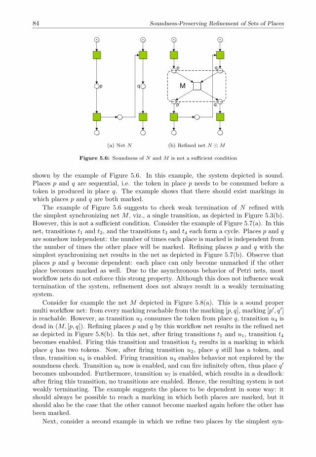
84 Soundness-Preserving Refinement of Sets of Places
p q
(a) Net N
p
p’
q
q’
M
(b) Refined net N ⊙ M
Figure 5.6: Soundness of N and M is not a sufficient condition
shown by the example of Figure 5.6. In this example, the system depicted is sound.Places p and q are sequential, i.e. the token in place p needs to be consumed before atoken is produced in place q. The example shows that there should exist markings inwhich places p and q are both marked.
The example of Figure 5.6 suggests to check weak termination of N refined withthe simplest synchronizing net M , viz., a single transition, as depicted in Figure 5.3(b).However, this is not a sufficient condition. Consider the example of Figure 5.7(a). In thisnet, transitions t1 and t2, and the transitions t3 and t4 each form a cycle. Places p and qare somehow independent: the number of times each place is marked is independent fromthe number of times the other place will be marked. Refining places p and q with thesimplest synchronizing net results in the net as depicted in Figure 5.7(b). Observe thatplaces p and q become dependent: each place can only become unmarked if the otherplace becomes marked as well. Due to the asynchronous behavior of Petri nets, mostworkflow nets do not enforce this strong property. Although this does not influence weaktermination of the system, refinement does not always result in a weakly terminatingsystem.
Consider for example the net M depicted in Figure 5.8(a). This is a sound propermulti workflow net: from every marking reachable from the marking [p, q], marking [p′, q′]is reachable. However, as transition u2 consumes the token from place q, transition u4 isdead in (M, [p, q]). Refining places p and q by this workflow net results in the refined netas depicted in Figure 5.8(b). In this net, after firing transitions t1 and u1, transition t4becomes enabled. Firing this transition and transition t3 results in a marking in whichplace q has two tokens. Now, after firing transition u2, place q still has a token, andthus, transition u4 is enabled. Firing transition u4 enables behavior not explored by thesoundness check. Transition u6 now is enabled, and can fire infinitely often, thus place q′
becomes unbounded. Furthermore, transition u7 is enabled, which results in a deadlock:after firing this transition, no transitions are enabled. Hence, the resulting system is notweakly terminating. The example suggests the places to be dependent in some way: itshould always be possible to reach a marking in which both places are marked, but itshould also be the case that the other cannot become marked again before the other hasbeen marked.
Next, consider a second example in which we refine two places by the simplest syn-
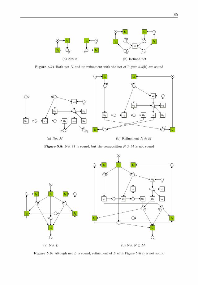
85
p qt2
t1 t3
t4
(a) Net N
p qt2
t1 t3
t4
p’ q’
u
(b) Refined net
Figure 5.7: Both net N and its refinement with the net of Figure 5.3(b) are sound
u1 u2 u3 u5 u6
u4 u7
u8
p
p’
q
q’
(a) Net M
u1 u2 u3 u5 u6
u4 u7
u8
p
p’
q
q’
t1 t3
t2 t4
(b) Refinement N ⊙ M
Figure 5.8: Net M is sound, but the composition N ⊙ M is not sound
p q
t1t5 t6
t3t2
t4
(a) Net L
u1 u2 u3 u5 u6
u4 u7
u8
p
p’
q
q’
t1t5 t6
t3t2
t4
(b) Net N ⊙ M
Figure 5.9: Altough net L is sound, refinement of L with Figure 5.8(a) is not sound

86 Soundness-Preserving Refinement of Sets of Places
p q
t
(a) Net N
p q
t
p’ q’
(b) Refined net
Figure 5.10: Livelock after refinement
chronizing multi workflow net. In the net depicted in Figure 5.9(a), places p and q havethe property suggested by the previous example: each place can only become markedagain after the other has been marked. In this example, net N fires transition t1, followedby an alternation between transitions t3, t6 and t2, t5, and finally transition t6. The netis sound, even after refining places p and q with the component depicted in Figure 5.3(b).However, in the refinement N ⊙M as presented in the previous example, place q can getmarked with two tokens, and hence, the refined net is not weakly terminating.
Thus, the simplest synchronizing net M as depicted in Figure 5.3(b) is not a properapproximation of each sound workflow. For the AG-part of soundness, we conclude thatnet N should not contain transitions (like the ones we have just discovered) that maylead into unexplored behavior.
The examples of Figure 5.7(a) and Figure 5.9 suggest to check that N can onlyproduce and consume tokens from places p and q in a certain order: a transition can onlyproduce a new token in such a place after the other place has been emptied. The LTS asdepicted in Figure 5.11 describes this behavior. Action p (q) indicates the production ofa token in place p (q), action p′ (q′) indicates the consumption of a token from place p(q). For readability reasons, each state is annotated with the number of tokens in placep and q. Without loss of generality, we assume that each transition in the componentperforms at most one action of the LTS. For example, with the reduction rules of Murata,transitions that produce in or consume from both places can be split into two separatetransitions. The initial state is s0, and both solid and dashed transitions are permitted.In particular, in states s4, s5, and s7, the LTS excludes producing a token in q the secondtime before a token has been consumed from p; thus excluding the example of Figure 5.9.
However, the LTS does not give a sufficient condition. Take the refinement depictedin Figure 5.10. In the net N depicted in Figure 5.10(a), transition t is crucial for ter-mination; its firing implies that N has produced a token on p, but not yet on q. NetN only executes actions in the order specified in the LTS depicted in Figure 5.11, butin the refined net, depicted in Figure 5.10(b), the refining net eliminates the path totermination from net N . So, the refining net imposes additional synchronization on netN .

87
S0: 0,0
S1: 1,0 S2: 0,1
S4: 1,1S3: 0,0 S5: 0,0
S6: 0,1 S7: 1,0
p q
pqp’ q’
q pp’ q’
q’p’
Figure 5.11: May/exit transition system for synchronizable places
The examples show that the LTS depicted in Figure 5.11 is not a sufficient condi-tion to conclude weak termination of the refined system. The problem indicated in theexample of Figure 5.10(b) shows that although all sequences of the LTS are allowed, syn-chronization is needed for weak termination. Therefore, for the EF-part of soundness,we conclude that net N should only use transitions that cannot be excluded by any M .This suggests to check that also from every reachable non-final state of N , a final statecan be reached using only the solid transitions in Figure 5.11. In particular, in state s1,this excludes that for termination of net N first a token from p must be consumed beforea token on q has been produced. In the next section, we present a formalism to capturethis behavior, and show that this is a sufficient condition.
5.4 Formalization of Synchronizable Places
The previous section showed the need for a transition system with solid transitions tomodel the behavior to terminate, and dashed transitions for transitions that are allowed,but with which it should not be possible to terminate. This is expressed in a so calledmay/exit transition system. In Figure 5.11, all state transitions are may transitions, andthe solid state transitions are also exit transitions. To prove the may/exit transition sys-tem to be a sufficient condition, the principle idea is that for the AG-part of soundness alltransitions may be used, whereas for the EG-part of soundness, only the exit transitionscan be used. As for LTSs, there is a set of visible actions, A, and a silent action τ ∈ A.
Definition 5.4.1 (May/exit labeled transition system)A may/exit labeled transition system (MELTS) is a 6-tuple (S,A, 99K,−→, s0,Ω) where
• S is a set of states;
• A is the action set ;
• 99K⊆ S × (A ∪ τ)× S is the set of may state transitions;
• −→⊆ S × (A ∪ τ)× S is the set of exit state transitions, and −→⊆99K. y
Let L = (S,A, 99K,−→, s0,Ω) be a MELTS. For s, s′ ∈ S and a ∈ A ∪ τ, we write
(L : sa99K s′) if and only if (s, a, s′) ∈99K, and (L : s
a−→ s′) if and only if (s, a, s′) ∈−→.As for LTSs, we lift the notation to sequences of actions. Let σ ∈ A∗ be a sequence
of length n. We write (L : s0σ99K sn) if and only if states si−1, si ∈ S exist such that
(L : si−1
σ(i)99K si) for all 1 ≤ i ≤ n, and (L : s0
σ−→ sn) if and only if states si−1, si ∈ S
exist such that (L : si−1σ(i)−→ si) for all 1 ≤ i ≤ n. A MELTS is properly completing if

88 Soundness-Preserving Refinement of Sets of Places
for all reachable markings a sequence of only exit transitions exists that reaches a finalmarking.
Definition 5.4.2 (Proper completion of a MELTS)Let L = (S,A, 99K,−→, s0,Ω be a MELTS. It is properly completing if for each state
s ∈ S and sequence σ ∈ A∗ such that (L : s0σ99K s) a sequence υ ∈ A∗ and final marking
f ∈ Ω exist such that (L : sυ−→ f). y
In relation to modal (may/must) transition systems [76], the may transitions corre-spond, whereas the exit transitions and must transitions are unrelated.
Let Sync denote the MELTS as depicted in Figure 5.11. Note that it is properlyterminating: from each state it is possible to reach the final state with only exit statetransitions.
Definition 5.4.3 (Sync)Let Sync = (S,A, 99K,−→, s0, s0) where
S = s0, s1, s2, s3, s4, s5, s6, s7A = p, p′, q, q′
−→ = (s0, τ, s0), (s0, p, s1), (s0, q, s2), (s1, τ, s1), (s1, q, s4), (s2, τ, s2), (s2, p, s4),(s3, τ, s3), (s3, q, s6), (s4, τ, s4), (s4, p
′, s6), (s4, q′, s7), (s5, τ, s5), (s5, p, s7),
(s6, τ, s6), (s6, q′, s0), (s7, τ, s7), (s7, p
′, s0)99K = −→ ∪(s1, p′, s3), (s2, q′, s5)
y
Corollary 5.4.4 (Sync is properly terminating)The MELTS Sync as defined in Definition 5.4.3 is properly terminating. y
In the remainder of this section, we formalize the concept of synchronizable places,and show that it is a sufficient condition for preserving soundness.
Let N be a net. Each state transition in Sync corresponds to the production ofconsumption of a token in the places p and q. A transition either produces a token in p(q) or consumes a token from p (q). We define a mapping function from the transitionsof N to the state transitions of Sync.
Definition 5.4.5Let (N, iN ,ΩN ) be a system, and let p, q ∈ PN such that •p, p•, •q and q• are pairwisedisjoint. We define the function hN,p,q : TN → A ∪ τ by
hN,p,q(t) =
p if p ∈ t•
p′ if p ∈ •tq if q ∈ t•
q′ if q ∈ •tτ otherwise
We lift the notation to sequences. Let σ ∈ T ∗N be a sequence of length n, then hN,p,q(σ) =
⟨hN,p,q(σ(1)), . . . , hN,p,q(σ(n))⟩. If the context is clear, we omit the subscript. y
Next, we define a relation between the markings of N and the states of Sync.
89
Definition 5.4.6Let (N, iN ,ΩN ) be a system with N = (P, T, F ) a Petri net, and let p, q be two places ofN such that •p, p•, •q and q• are pairwise disjoint. Let Sync = (S,A, 99K,−→, s0, s0)be the MELTS as defined in Definition 5.4.3 for places p and q. Let t ∈ T . We definethe relation RN,p,q ⊆ R(N)× S recursively by:
• iN RN,p,q s0,
• fN RN,p,q s0 for all fN ∈ ΩN
• if (N : mt−→ m′) and mRN,p,q s then
– if p ∈ t• and s = s0 then m′RN,p,q s1,
– if p ∈ t• and s = s2 then m′RN,p,q s4,
– if p ∈ t• and s = s5 then m′RN,p,q s7,
– if q ∈ t• and s = s0 then m′RN,p,q s2,
– if q ∈ t• and s = s1 then m′RN,p,q s4,
– if q ∈ t• and s = s3 then m′RN,p,q s6,
– if p ∈ •t and s = s1 then m′RN,p,q s3,
– if p ∈ •t and s = s4 then m′RN,p,q s6,
– if p ∈ •t and s = s7 then m′RN,p,q s0,
– if q ∈ •t and s = s2 then m′RN,p,q s5,
– if q ∈ •t and s = s4 then m′RN,p,q s7,
– if q ∈ •t and s = s6 then m′RN,p,q s0,
– otherwise, m′RN,p,q s.
If the context is clear, we omit the subscript. yIf a system N “follows” Sync, i.e. after transformation, every firing sequence of N
can be replayed in Sync, place p is marked if and only if Sync is in state s1, s4 or s7, andplace q is marked if and only if Sync is in state s2, s4 or s6.
Corollary 5.4.7Let N be a system with two places p and q such that p = q and •p, p•, •q and q• arepairwise disjoint. Let Sync = (S,A, 99K,−→, s0, s0) as defined in Definition 5.4.3.
For all markingsm ∈ R(N, iN ) and s ∈ S, such thatmRN,p,q s4. Then s ∈ s1, s4, s7if and only if m(p) = 1, and s ∈ s2, s4, s6 if and only if m(q) = 1. yCorollary 5.4.8Let N be a system with two places p and q such that p = q and •p, p•, •q and q• arepairwise disjoint. Let Sync = (S,A, 99K,−→, s0, s0) as defined in Definition 5.4.3.
Let σ ∈ T ∗N , m ∈ R(N), µ ∈ (A ∪ τ)∗ and s ∈ S such that (N : iN
σ−→ m),
µ = HN,p,q(σ) and (Sync : s0µ99K s). Then s ∈ s0, s2, s5, s6 if and only if m(p) = 0,
and s ∈ s0, s1, s5, s7 if and only if m(q) = 0. yAs shown in the previous section, the requirements for two places to be synchronizable
are captured in the MELTS Sync. Next, we need to relate it to the behavior of acomponent. Given a firing sequence in a component, this firing sequence should bereplayable in Sync, i.e. the sequence mapped onto the possible actions of Sync shouldbe a firing sequence of Sync consisting of may state transitions. This corresponds to the

90 Soundness-Preserving Refinement of Sets of Places
q
p
Figure 5.12: Places p and q are synchronizable
AG-part of soundness. Next, for the EF-part of soundness, there should exist a firingsequence to the final marking of the component corresponding to a firing sequence inSync consisting of only exit state transitions.
Definition 5.4.9 (Synchronizable places)Let N be a system, and let p, q ∈ PN such that p = q, •p, p•, •q and q• are pairwisedisjoint, and iN (p) = iN (q) = fN (p) = fN (q) = 0. Let Sync = (S,A, 99K,−→, s0, s0)be the MELTS as defined in Definition 5.4.3. Places p and q are synchronizable, denotedby pN q, if:
∀γ ∈ T ∗N , m ∈ R(N) : (N : iN
γ−→ m) : ∃s ∈ S, σ ∈ T ∗N , fN ∈ ΩN :
(Sync : s0h(γ)99K s) ∧ (N : m
σ−→ fN ) ∧ (Sync : sh(σ)−→ s0) y
The definition of synchronizable places encapsulates the definition of weak termina-tion. In fact, the definition is closely related to simulation, it only differs in the may/exitpart of the definition.
Corollary 5.4.10 (synchronizable places implies system is weakly terminating)Let N be a system, and let p, q ∈ PN be two places such that pN q. Then N is weaklyterminating. y
Furthermore, the structure of the MELTS Sync ensures that places p and q are safe:if a firing sequence exists that marks place p or q with two tokens, this firing sequencecannot be replayed in Sync.
Corollary 5.4.11 (Synchronizable places are safe)Let N be a system, and let p, q ∈ PN be two places such that p N q. Then places pand q are safe. y
For modal transition systems [76], a notion called refinement is introduced. A modaltransition system L refines another modal transition system L′ if all the may transitionsof L are also possible in L′, and all must transitions of L′ are also must transitions in L.For synchronizable places, this is a too strong notion, as shown in the example depictedin Figure 5.12. In this figure, states s2 and s7 of Sync are never visited. Hence, the netis not a refinement of Sync.
The definition of synchronizable places satisfies the first necessary condition as de-scribed in the previous section. In the remainder of this section, we prove synchronizableplaces to be a sufficient condition for soundness. Given a system N with two synchroniz-able places p and q, and a sound and proper P2-workflow net M with mapping functionα, we need to check whether the refinement L = N ⊙αM is sound.
To prove soundness of the refined net L = N ⊙αM , we need to prove that from eachmarking reachable in L, it is possible to reach the final marking. Therefore, we map allreachable markings of L to a marking of N using function φ.
91
Definition 5.4.12 (Original net mapping)Let N be a system, let p, q ∈ PN such that p N q. Let M be a sound proper P2
workflow net, and let α : D → EM be a bijective total function. Define L = N ⊙αM .We define the function φN,p,q : IN
PL × T ∗L → INPN by
φN,p,q(m,σ)(s) =
m(s) if s ∈ PN \ p, qiN (s) +
∑t∈•s
−→σ (t)−∑t∈s•
−→σ (t) if s ∈ p, q
If the context is clear, the subscript is omitted. yThe mapping ensures that given a firing sequence with which we reached a marking
in the refined net, the mapped marking onto the original net is reachable as well.
Lemma 5.4.13 (Mapping reachable in projection)Let N be a system, let p, q ∈ PN such that p N q. Let M be a sound proper P2
workflow net, and let α : p, q → EM be a bijective function. Define L = N ⊙αM . Let
σ ∈ T ∗L and m ∈ R(L) such that (L : iL
σ−→ m). Then (N : iNσ|TN−→ φ(m,σ)). y
Proof. We prove the lemma by induction on the length of σ. Let σ = ϵ. Then thestatement holds by definition of ⊙ and φ. Now suppose σ = σ′; ⟨t⟩ for some σ′ ∈ T ∗
L
t ∈ TL and m′ ∈ R(L) such that (L : iLσ′
−→ m′ t−→ m) and (N : iNσ′
|TN−→ φ(m′)).Suppose t ∈ TM . Then σ′
|TN= σ|TN
and φ(m′, σ′) = φ(m,σ). Hence, the statementholds. Next, suppose t ∈ TN . Then the statement directly follows from the firing rule ofPetri nets and the marking equation. 2
Important for weak termination of the refined system, is that after each cycle in whichboth p and q have been marked, and the reached marking corresponds to state s0 in Sync,the refining multi workflow net should be empty. This follows from the soundness of therefining proper multi workflow net.
Lemma 5.4.14Let N be a system, let p, q ∈ PN such that p N q. Let M be a sound and proper P2
workflow net, and let α : p, q → EM be a total bijective function. Define L = N ⊙αM .
Let σ ∈ T ∗L and m ∈ R(L) such that (L : iL
σ−→ m) and φ(m,σ)Rs0. Then m|PM= ∅.y
Proof. Define iM = χ(π1(EM )) and fM = χ(π2(EM )). If φ(m,σ)RN,p,q s0, we have bythe synchronizability of places p and q∑
t∈ •N p
−→σ (t) =∑t∈p•N
−→σ (t) =∑t∈ •
N q
−→σ (t) =∑t∈q•N
−→σ (t)
Let n =∑t∈ •
N p−→σ (t). We prove the lemma by induction on n. Suppose n = 0. Then
the statement holds by definition of ⊙.Now suppose n > 0. Let σ′, σ′′ ∈ T ∗
N , m′ ∈ R(L) and m′ ∈ R(N) such that
m′ = φ(m,σ′), (L : iLσ′
−→ m′ σ′′
−→ ), m′|PM
= ∅, m′Rs0 and∑t∈ •
N p = 1. Define
σ = σ′′|TN
and σ = σ′′|TM
. Since m′|PM
= ∅, and p, q ∈ σ•N , we have (M : iM
σ−→ m)and fM ≤ m for some marking m ∈ R(M, iM ). Since M is sound, we have m = fM .Hence, since also p, q ∈ •
N σ, we have m|PM= ∅. 2
The lemma shows that if the marking of the refined net corresponds to state s0, allplaces of the refining net are empty. We can use this lemma to show that every marking

92 Soundness-Preserving Refinement of Sets of Places
in the refined system L = N ⊙M is related to a reachable marking of the original systemN , as shown in Lemma 5.4.13, and to a reachable marking in the refining net M . Thelemma shows that a marking of the refined system projected on M sometimes needs anextra token in the initial or final places of M , to become reachable a reachable markingof the multi workflow M .
Lemma 5.4.15Let N be a system, let p, q ∈ PN such that p N q. Let M be a sound proper P2
workflow net, and let α : p, q → EM be a bijective function. Define L = N ⊙αM . Let
m ∈ R(L) and σ ∈ T ∗L such that (L : iL
σ−→ m). Define m = φ(m,σ), iM = χ(π1(EM ))and fM = χ(π2(EM )).
• If mR s0 then m|PM= ∅.
• If mR s1 then m|PM+ [π1(α(q))] ∈ R(M, iM ).
• If mR s2 then m|PM+ [π1(α(p))] ∈ R(M, iM ).
• If mR s3 then [π2(α(p))π1(α(q))] ∈ R(M, iM ).
• If mR s4 then m|PM∈ R(M, iM ).
• If mR s5 then [π1(α(p))π2(α(q))] ∈ R(M, iM ).
• If mR s6 then m|PM+ [π2(α(q))] ∈ R(M, iM ).
• If mR s7 then m|PM+ [π2(α(p))] ∈ R(M, iM ). y
Proof. We prove the lemma by induction on the structure of σ. If σ = ϵ, then thestatement holds trivially.
Now suppose σ = σ′; ⟨t⟩ for some t ∈ TL, σ′ ∈ T ∗
L and marking m′ ∈ R(L) such that
(L : iLσ−→ m′ t−→ m), and for m′, the statement holds. Let m′ = φ(m′, σ′). We need
to perform a case analysis.
• Suppose m′Rs0. Then t ∈ TN . If p ∈ t•N , then the statement holds. Otherwise,either p ∈ t•N or q ∈ t•N . First assume p ∈ t•N . Then mR s1 and m|PM
= [π1(α(p))].Then, m|PM
+ [π1(α(q))] = [π1(α(p)), π1(α(q))] = iM . Hence the statement holds.Assuming q ∈ t•N is symmetric to p ∈ t•N .
• Suppose m′Rs1. Then either t ∈ TN or t ∈ TM . In the first case, if q ∈ t•N , thenm|PM
= m′|PM
, and thus, the statement holds. Otherwise, i.e. q ∈ t•, then mR s4and m|PM
= m′|PM
+ [π1(α(q))]. Hence, the statement holds.
In the latter case, since •t ⊆ PM , •t ≤ m′|PM
. Hence, (M : m′|PM
+ [π1(α(q))]t−→
m), and, since π1(α(q)) ∈ •t, we have m(p) = m′(p)− •t(p) + t•(p) = m(p) for allp ∈ PM . Hence, the statement holds.
• Suppose m′Rs2. The proof is symmetric to the case m′Rs1.
• Suppose m′Rs3. Then t ∈ TN . Let σ = σ′′; ⟨u⟩; υ for some σ′′, υ ∈ T ∗L, u ∈ TL and
markings m′′,m′′′ ∈ R(L, iL) such that (L : iLσ′′
−→ m′′ u−→ m′′′ υ−→ m′), p, q ∈ υ•,
p ∈ u•, and φ(m′′, σ′′)Rs0. Then (M : iMυ|TM−→ m) for some m ∈ R(M, iM ). Since
m|PM(π1(α(q))) = 0, we have m = [π2(α(p)), π1(α(q))]. Hence, the statement
holds.
• Suppose m′Rs4. Then either t ∈ TN or t ∈ TM . Assume the first, i.e. t ∈ TN .Then, if p, q ∈ •t, the statement holds since m′
|PM= m|PM
. Otherwise, eitherp ∈ •
N t or q ∈ •N t. Assume p ∈ •
N t. Then m′|PM
(π2(α(p))) > 0, since otherwisetransition t is not enabled in (L,m′). Hence, m′
|PM= m|PM
+ [π2(α(p))], thus thestatement holds. A similar argument holds for q ∈ •
N t.

93
Assume the latter, i.e. t ∈ TM . Then, (M : m′|PM
t−→ m) for some m ∈ R(L, iL)and m(p) = m′
|PM(p) − •t(p) + t•(p) = m(p) for all p ∈ PM . Thus, m = m|PM
.Hence, the statement holds.
• Suppose m′Rs5. The proof is symmetric to the case m′Rs3.
• Suppose m′Rs6. Then either t ∈ TN or t ∈ TM . Assume the first. If q ∈ •N t,
then m′|PM
= m|PM, and thus the statement holds. Otherwise, i.e. if q ∈ •
N t, thenmR s0, and by Lemma 5.4.14, m|PM
= ∅. Hence, the statement holds.
Assume the latter, i.e. t ∈ TM . Then, (M : m′|PM
+ [π2(α(q))]t−→ m) for some
m ∈ R(L, iL) and m(p) = m′|PM
(p) + [π2(α(q))](p) − •t(p) + t•(p) = m(p) for allp ∈ PM . Thus, m = m|PM
+ [π2(α(q))]. Hence, the statement holds.
• Suppose m′Rs7. The proof is symmetric to the case m′Rs6.
Hence, the lemma holds. 2
The lemma proves that every marking in the refined system consists of a reachablemarking in the original net, and a marking in the refining net, which is obvious buttedious to prove. As a consequence, boundedness is preserved by the refinement ofsynchronizable places.
Corollary 5.4.16 (Refinement preserves boundedness)Let N be a system, let p, q ∈ PN such that p N q. Let M be a sound proper P2
workflow net, and let α : p, q → EM be a bijective total function. Define L = N ⊙αM .If N is k-bounded, and M is l-bounded, then L is max(k, l)-bounded. y
As a consequence of the lemma, as soon as a state is reached which corresponds to amarking in which p or q is marked, there always exists a firing sequence that leads to amarking in which all places of the refining net M are empty, except for the final places.Note that in the refined net, one of the final places can already be emptied.
Corollary 5.4.17Let N be a system, let p, q ∈ PN such that p N q. Let M be a sound proper P2
workflow net, and let α : p, q → EM be a bijective function. Define L = N ⊙αM .
For all markings m ∈ R(L), σ ∈ T ∗L and states s ∈ s4, s5, s6 such that (L : iL
σ−→m) and φ(m,σ)Rs, a marking m′ ∈ R(L) and firing sequence α ∈ T ∗
M exist such that
(M : m|PM
α−→ fM ), (L : mα−→ m′), φ(m′, σ;α)Rs and ∅ < m′
|PM≤ fM , where
fM = χ(π2(EM )). y
To prove the refined system to be weakly terminating, we first show that given amarking in L, which maps onto a marking in N corresponding to a state in Sync thatwas reached using an exit transition, due to the soundness of N and the synchronizabilityof p and q, a firing sequence exists that brings L to a final marking.
Lemma 5.4.18Let N be a system, let p, q ∈ PN such that p N q. Let M be a sound proper P2
workflow net, and let α : p, q → EM be a bijective function. Define L = N ⊙αM . LetSync = (S,A, 99K,−→, s0, s0) as defined in Definition 5.4.3.
For all markings m ∈ R(L, iL), s ∈ S \ s3, s5, γ ∈ T ∗L, σ ∈ T ∗
N and fN ∈ ΩN such
that (L : iLγ−→ m), φ(m, γ)Rs, (N : m
σ−→ fN ) and (Sync : sh(σ)−→ s0), a firing sequence
σ ∈ T ∗L and marking f ∈ ΩL exist such that (L : m
σ−→ f) and σ|TN= σ. y
94 Soundness-Preserving Refinement of Sets of Places
Proof. Define iM = χ(π1(EM )) and fM = χ(π2(EM )).Suppose s ∈ s4, s6, s7, then by Corollary 5.4.17, an α ∈ T ∗
M and m′ ∈ R(L)
exist such that (L : mα−→ m′), φ(m′, σ;α)Rs and m|TM
≤ fM . Otherwise, i.e. s ∈s0, s1, s2, choose α = ϵ and m′ = m.
Define γ′ = γ;α. Let m = φ(m′, γ′). By Lemma 5.4.13, m ∈ R(N).Define n = |σ|. Let m0, . . . , mn ∈ R(N, iN ) such that m0 = φ(m′, γ′), mn = fN
and (N : mi−1σ(i)−→ mi) for all 1 ≤ i ≤ n. Since (Sync : s
h(σ)−→ s0), there is no mi suchthat miRN,p,q s3 or miRN,p,q s5, since these states can only be reached by taking a maytransition.
Let ν ∈ T ∗M such that (M : iM
ν−→ fM ). We construct sequence σ = σ1; . . . ;σn suchthat σi = ⟨σ(i)⟩; ν if miRs4 and σi = ⟨σ(i)⟩ otherwise. Next, we show that σ is a firingsequence with the desired property. We prove this by showing that markingsm0 . . . ,mn ∈R(L, iL) exist such that m0 = m′, and for all 0 ≤ i ≤ n, we have (L : mi−1
σi−→ mi)and mi = φ(mi, νi) where νi = γ′;σ1; . . . ;σi, and if miRs with s ∈ s4, s6, s7 thenmi|PM
≤ fM .Suppose i = 0. Choose m0 = m′. Clearly mi = φ(m0, ν0). If m0Rs4, then m
′|PM
≤fM . Since
∑t∈p•
−→νi (t) =∑t∈q•
−→νi (t), we have fM = m′|PM
. Hence, the statement holds.Suppose 0 < i ≤ n, and the statement holds for all 0 ≤ j < i. Let t = σ(i). We need
to consider three cases. Either (1) h(t) = τ , (2) h(t) ∈ p, q or (3) h(t) ∈ p′, q′.
1. Consider the first case, i.e. h(t) = τ . By definition of φ, we have •t(x) ≤ mi−1(x) =mi−1(x) for all x ∈ •t. Hence, •t ≤ mi−1. Thus, a marking mi ∈ R(L) exists such
that (L : mi−1t−→ mi). Since h(t) = τ , we have mi = φ(mi, νi). Hence, the
statement holds.
2. Consider the second case, i.e. h(t) ∈ p, q. Then either p ∈ t• or q ∈ t•. Thenan s ∈ s0, s1, s2 exists such that mi−1Rs. By definition of φ, we have •t(x) ≤mi−1(x) = mi−1(x) for all x ∈ •t. Hence, a marking m′′ ∈ R(L) exists such that
(L : mi−1t−→ m′′). Clearly mi = φ(m′′, νi−1; ⟨t⟩). If s = s0, then σi = ⟨t⟩. Then,
the statement holds for mi = m′′. Otherwise, i.e. if s ∈ s1, s2, then miRs4.Hence, σi = ⟨t⟩; ν and mi(p) = mi(q) = 1. Thus, iM ≤ m′′, and ν is enabled in
(L,m′′). So, a marking mi ∈ R(L) exists such that (L : m′′ ν−→ mi) and by thesoundness of M , we have fM = mi|PM
. Hence, the statement holds.
3. Consider the third case, i.e. h(t) ∈ p′, q′. Then either p ∈ •t or q ∈ •t. Thenan s ∈ s4, s6, s7 exists such that mi−1Rs. By definition of φ, we have •t ≤mi−1(p) = mi−1(p) for all p ∈ •t \ p, q. Since m′
|PM≤ fM , if s ∈ s4, s7, then
mi−1(p) = 1 and thus mi−1(π2(α(p))) = 1, and if s ∈ s4, s6, then mi−1(q) = 1and thus mi−1(π2(α(q))) = 1. Hence, in both cases, •t ≤ mi−1. So, a mark-
ing mi ∈ R(L, iL) exists such that (L : mi−1t−→ mi). Suppose p ∈ •t. Then
φ(mi, νi)(p) = φ(mi−1, νi−1)(p) − p•(t) = mi−1(p) − p•(t) = mi(p). Otherwiseq ∈ •t, and φ(mi, νi)(q) = φ(mi−1, νi−1)(q)− q•(t) = mi−1(q)− q•(t) = mi(q). Inboth cases, mi = φ(mi, νi). Thus, the statement holds.
Hence, we may conclude that sequence σ is a firing sequence. Last, we show thatmn ∈ ΩL. Since mn = φ(mn, σ) and mnRs0, we have fN (x) = mn(x) = mn(x) for allx ∈ PN \ p, q. Furthermore, mn|PM
= ∅. Hence, mn ∈ ΩL. 2
Lemma 5.4.18 shows that if a reachable marking can be mapped onto a marking inthe “normal” states of Sync, a final marking in L is reachable. To prove soundness of therefined net, we also need to show that if we are in an “exception state” (states s3 and

95
s5), it is always possible to reach a marking in L that corresponds to a “normal” state.Due to the synchronizability of places p and q, this is the case. Hence, the refined net issound, as shown in the next theorem.
Theorem 5.4.19 (Refinement of synchronizable places preserves weak termi-nation)Let N be a system, let p, q ∈ PN such that pN q. Let M be a sound proper P2 work-flow net, and let α : D → EM be a bijective total function. Then the system N ⊙αM isweakly terminating. y
Proof. Define L = N ⊙αM , iM = χ(π1(E)) and fM = χ(π2(E)). Let Sync = (S,A, 99K,−→, s0, s0) be the MELTS as defined in Definition 5.4.3.
Let m ∈ R(L, iL). We need to show the existence of a firing sequence σ ∈ T ∗L and a
marking f ∈ ΩL such that (L : mσ−→ f). Let m = φ(m,σ). Then by Lemma 5.4.13,
m ∈ R(N, iN ). Hence, m ∈ Dom(R). Let s ∈ S such that mR s. Since places p andq are synchronizable, N is weakly terminating and there exist a firing sequence σ ∈ T ∗
N
and a marking fN ∈ ΩN such that (N : mσ−→ fN ) and (Sync : s
h(σ)−→ s0).
We need to consider two cases. Either (1) s ∈ s0, s1, s2, s4, s6, s7 or (2) s ∈ s3, s5.
1. Consider the first case. Then, by Lemma 5.4.18, a final marking f ∈ ΩL and firingsequence σ ∈ T ∗
L exist such that (L : mσ−→ f).
2. Next, consider the second case. Let n = |σ|. Since p and q are synchronizable,an 1 ≤ i ≤ n exists such that h(σ(j)) = τ for all 1 ≤ j ≤ i and h(σ(i)) ∈ p, q.Let σ1 = σ[1..i]. Since p, q ∩ •σ1 = ∅, a marking m′ ∈ R(L) exists such that
(L : mσ1−→ m′) and φRs with s ∈ s6, s7. Hence, we can apply the first case
on m′, resulting in a firing sequence σ′ ∈ L∗ and marking f ∈ ΩL such that
(L : m′ σ′
−→ f). Thus, σ = σ1;σ′ has the desired property.
Hence, L is weakly terminating. 2
5.5 Related Work
The notion of synchronizability of places is closely related to the notion of objectivity [95]in condition/event systems. A condition/event system is a subclass of Petri nets, inwhich all places are safe. Instead of interleaving semantics, process semantics is used. Inprocess semantics, an occurrence net specifies the run of a system. An occurrence net isa, possibly infinite, acyclic marked graph. As the net is acyclic, we can define relation <on the nodes of the net which is the transitive irreflexive closure of the flow relation.
p q
p' q’
pq
p' q’
Figure 5.13: LTS of places that are objective
p
q
a
b
c
d
Figure 5.14: Places p and q are synchroniz-able but not objective

96 Soundness-Preserving Refinement of Sets of Places
... ...
... ...
p q
(a)
... ...
... ...
p q
p’ q’
(b)
... ...
... ...
p q
p’ q’
⊕
⊕ ⊕
⊕p q
p’ q’
(c)
⊕
(d) (e)
⊕
(f)
Figure 5.15: Refinement in terms of composition
A coset S is a set of nodes such that neither x < y nor y < x for all x, y ∈ S. Amaximal coset, i.e. no node x can be added to the coset without losing the coset property,defines a marking. A process maps the nodes of the occurrence graph on the nodes ofthe condition/event system. Let p and q be two places of the condition/event system. Iffor all possible processes (all occurrence nets and their mapping on the system), and allcosets S of which all elements are mapped onto places p and q are strongly concurrent,i.e. also •x < y• and •y < x• for all x, y ∈ S, then the places are called objective.Strongly concurrent places, or objective places thus implies that both places need to bemarked before they can get unmarked. In fact, the notion of objectivity is equivalentto the LTS as shown in Figure 5.13. This LTS is a subgraph of the MELTS Sync, asdefined in Definition 5.4.3. As a consequence, if two places are objective, they are alsosynchronizable, as the firing sequences projected on the MELTS Sync only use states s0,s1, s2, s4, s6 and s7. The states s3 and s4, i.e. the states in which place p is alreadyunmarked, but q not yet marked (or vice versa), are never reached. On the other hand, iftwo places are synchronizable, it does not imply the places are objective as well. Considerthe example of Figure 5.14. In this example, places p and q are synchronizable, but notobjective, as •q < p•, since ¬(b < c).
An alternative approach is presented in [58]. The authors show that refinement is anapplication of synchronous composition. Suppose a system N is given with places p andq as in Figure 5.15(a). To separate the incoming and outgoing arcs from these places weapply fusion of series places [87] and obtain Figure 5.15(b). By definition of compositionof asynchronous interfaces, this is equal to Figure 5.15(c).
Thus each system N is equivalent to a similar OPN N ′ composed with the open netfrom Figure 5.3(a). The refinement of system N with an OPN M (with an asynchronousinterface), denoted by N ⊙M , is defined as N ′ ⊕ M . Consider a pair of correspondinginterface places from the two nets as in Figure 5.15(d). After composing them, we applyfusion of series places [87] and obtain Figure 5.15(e). By definition of composition ofsynchronous interfaces, this is equal to Figure 5.15(f). So every asynchronous interfaceplace in the OPNs N ′ andM becomes an internal place that is connected by a transitionto a synchronous interface port.
Refinement of sets of places requires two checks: one on the original net, and one onthe refining net. The theory of maximal partners can be used to, given one of the tests,calculate the other test, as these tests should be their maximal partners.

97
5.6 Conclusions
In this chapter we studied under which conditions the refinement of sets of places by amulti workflow net preserves weak termination. Whereas for the refinement of a singleplace, safety of the refined place is sufficient, the refinement of a set of places requires amore advanced condition, due to the asynchronous nature of Petri nets.
To preserve weak termination, both a condition on the original net as well as on therefining net is needed. For the refining net, we require it to be sound, i.e. from anyreachable marking from the initial marking in which all initial places are marked, it isalways possible to reach the final marking in which all final places are marked. On theoriginal net, we need to test for a more advanced condition on the places we want torefine: they need to be synchronizable.
Intuitively, two places are synchronizable if they are safe, there is a reachable markingin which both are marked, and one cannot become marked again before the other hasbeen marked. Furthermore, we require that from any reachable marking, to reach thefinal marking only a path may be taken in which each of the places only become unmarkedif all were previously marked. To formalize this, we introduced the notions of a may/exittransition system and proper termination.
In the next chapter, we will present an iterative construction method using the re-finement of sets of places that guarantees weak termination in each iteration.

98 Soundness-Preserving Refinement of Sets of Places

6Correctness-By-Construction
In this chapter, we present an approach to construct an architecture of a component-basedinformation system. The construction approach guarantees soundness of the system byconstruction. It uses the refinement of sets of places to refine the communication protocolbetween two components.
6.1 Introduction
In Chapter 4 we studied compositional verification: given a service tree of componentswe pairwise checked the tree for soundness. The approach is a bottom up strategy: itrequires that the components already exist. In this chapter, we study a top-down strategyin system design, based on refinement, as in approaches like event-B [18] or Model DrivenEngineering. In this strategy, a first, abstract model is created for which all kind ofproperties are proven. In several steps, these models are refined until the desired modelis designed. In each step, such a refinement enforces proof obligations which need to holdsuch that for the refined model the same, and, if necessary, additional properties hold.In this chapter, we study a likewise methodology for the design of components with Petrinets. The behavioral property we focus on is soundness.
The methodology consists of three rules and creates a basic communication frameworkfor the component network. Using standard refinement rules like the generalized soundworkflow net refinement [62] each component in the framework can be worked out. Thefirst rule allows for the refinement of existing components by refining a single place bya new component. The second rule, communication refinement, enables the enrichmentof the interaction between components by refining synchronizable places simultaneouslyin different components and refine these by a sound composition. The last rule, theoutsource refinement, allows for the creation of new components as an offspring of anexisting component. These rules create a basic communication framework. On top ofthese rules, we may apply classical refinement rules, e.g., as defined by Murata [87],Berthelot [31], and the workflow refinement rule [62], to refine the internal structure ofthe component.
For the simultaneous refinement of synchronizable places, we need a sound and properP2 multi workflow net. The composition of two open workflow nets is such a net. In thischapter, we define a class of pairs of communicating components that are sound by their
100 Correctness-By-Construction
structure. The class is based on two important subclasses of Petri nets: acyclic markedgraphs and state machines.
This chapter is structured as follows. We present the construction methodology inSection 6.2, and in Section 6.3 we introduce the two base classes of coupled componentsthat are sound by their structure.
6.2 Construction Rules
Although soundness is a behavioral property that is relatively easy to check, it is very timeconsuming to guarantee soundness of a system consisting of asynchronous communicatingcomponents due to the high degree of concurrency of the components. In Chapter 4, a suf-ficient condition has been presented to verify soundness for a tree-structured compositionof components by checking each pair of communicating components. In this section wepresent an approach that guarantees soundness by construction. The approach consistsof three rules to refine a system. The first rule is refinement within a single component.In the second rule, two synchronized places in different components can be refined by apair of communicating components. The last rule involves the creation of a new coupledcomponent in a system.
6.2.1 Refinement within Components
In Section 5.2, we introduced place refinement in Petri nets. Given a weakly terminatingsystem (N, i,Ω), a safe place p in this Petri net N , and a sound workflow net, the refine-ment yields again a weakly terminating system. We redefine this refinement operation oncomponents and refine an internal place p of a component N by a workflow componentM .
Definition 6.2.1 (Open workflow net)Let N be an OPN. It is an open workflow net if and only if S(N) is a workflow net. y
In the refinement, all transitions in the preset of p are connected to the initial placeof M , and all transitions in the postset of p are connected to the final place of M . Placep is then removed from N . The ports of M are added to the ports of N . Figure 6.1depicts the refinement operator for components. Definition 5.2.1 is extended to handlethe interface places and ports of an OPN.
Definition 6.2.2 (Place Refinement in OPNs)Let N be an OPN. Let p ∈ PN be a place, and let M be an OWN with initial place
iM ∈ PM and final place fM ∈ PM such that N and M are disjoint. The refined OPNN ⊙pM = (P, I,O, T, F,G, i, f) is defined by:
• P = (PN \ p) ∪ PM ;
• I = IN ∪ IM ;
• O = ON ∪OM ;
• T = TN ∪ TM ;
• F = (FN \ ((•p× p) ∪ (p × p•))) ∪ FM ∪ (•p× i) ∪ (f × p•);
• G = GN ∪ GG;• i(p) = iN (p) if p ∈ PN \ p, i(iM ) = iN (p) and i(p) = 0 if p ∈ PM \ iM;• f(p) = fN (p) for p ∈ PN \ p, f(fM ) = fN (p) and f(p) = 0 for p ∈ PM \ fM. y
101
p p ) =(
N
M N’
H
G G
H
iM
fM
Figure 6.1: Refinement of place p in N by component M
As a consequence of Theorem 5.2.2, the result of this operation preserves soundness:if the original OPN is sound, place p is safe, and the refining OWN is also sound, theresulting OPN is sound again.
Corollary 6.2.3 (Place refinement in OPNs preserve soundness)Let N be a sound OPN, let p ∈ PN be a safe place and let M be a sound OWN. ThenN ⊙pM is sound. y
The definition of place refinement propagates the ports of the refining componentto the original component. At a first glance, this definition seems to contradict theparadigm of information hiding. However, using the port modification operations, it isalways possible to hide a port to the context.
6.2.2 Refinement over Components
In system construction, component interaction is often established in several cycles. Ineach cycle the interaction is refined, until the desired communication protocol is designed.The first rule, i.e. refinement of a single place in a component, does not suffice, as itonly allows to refine with an open workflow net, whereas a communication protocol is apair of open workflow nets. Thus, it cannot create a more elaborate interaction protocolbetween components, it can only create new interactions. Moreover, we want to refinethe scheme of interacting components. For example, a simple request-response patterncould be refined in a more elaborated negotiation pattern.
The principle idea is based on the refinement of sets of places, as introduced in theprevious chapter. Given a sound composition of components, we select two communicat-ing components A and B, for which we want to refine the communication protocol. Thecommunication between the components is modeled as a composition of two communi-cating workflow components, say C and D. In both component A and B we select twoplaces, say p and q. Place p will be refined by component C and place q will be refinedby component D. This way, we get a composition of two refined nets. The approachis depicted in Figure 6.2. For example, if in the first net, place p represents the state“wait for product”, and in the second net, place q models “producing product”, these

102 Correctness-By-Construction
)=( p q
A
B
Gp
q
C
D
H
iC
fC
iD
fDx
v u
t
w
y
z
w
v
t
u
x
y
z
Figure 6.2: The refinement (A⊕ B)⊙ (C ⊕ D)
places can be refined by a communication protocol that resembles the communicationfor feature requests or possible delivery attempts.
Definition 6.2.4 (Refinement over components)Let A and B be two composable OPNs. Let p ∈ PA and q ∈ PB be two places. LetC and D be two composable OWNs such that A ⊕ B and C ⊕ D are disjoint. Thecommunication refinement p⊙q is defined by (A⊕B)p⊙q (C⊕D) = (A⊙pC)⊕ (B⊙qD).
yIn fact, when only the skeletons are taken into account, the communication refinement
equals the refinement of sets of places, as defined in the previous chapter.
Corollary 6.2.5Let A and B be two composable OPNs, let p ∈ PA and q ∈ PB , and let C and D betwo composable OWNs. Then S((A⊕ B)p⊙q (C ⊕D)) = S(A⊕ B)⊙α S(C ⊕D) whereα = p 7→ (iC , fC), q 7→ (iD, fD). y
Hence, if the places p and q are synchronizable in the skeleton, and the compositionis sound, the refinement preserves soundness.
Theorem 6.2.6Let A and B be two composable OPNs, let p ∈ PA and q ∈ PB , and let C and Dbe two composable OWNs. If A ⊕ B and C ⊕ D are sound, and p A⊕B q, then(A⊕ B)p⊙q (C ⊕ D) is sound. yProof. Observe that S(C ⊕ D) is a sound and proper multi P2 workflow net withcommunication pairs (iC , fC) and (iD, fD). The system S(A⊕B) is weakly terminating,since A⊕B is sound. Hence, by Theorem 5.4.19 and Corollary 6.2.5, (A⊕B)p⊙q (C⊕D)is sound. 2
6.2.3 Creation of New Components
Whereas the first two rules focused on the extension of existing components, the rules donot allow for expansion of the network by adding new components. With the third rule,it is possible to connect new components in a system such that the system remains sound.
103
=( p ) G
N
Gp
iM1
fM1
M1
M2
Gx y x y
Figure 6.3: Extending the composition with a new coupled component
The rule is based on the principle of outsourcing. Consider Figure 6.3. For example, ifplace p has the meaning that when a token resides in it, “an item is produced”, andthe decision is taken to outsource the production activity, we can add two transitions: a“start producing item” and a “finish producing item”. Then the start transition initiatesthe component producing the item, and the finish transition fires if the item is produced.
Creating a new port for these transitions allows the connection of a new component tothe existing system. In fact, we replace place p by a communication protocol between theexisting component and a new component. We generalize this approach in the outsourcerefinement.
Definition 6.2.7 (Outsource refinement)Let N be an OPN, and p ∈ PN be a safe place. Let A and B be two composableOWNs, such that their composition is sound. We define the outsource refinement p byN p (A⊕ B) = (N ⊙p A)⊕ B∗, where B∗ is the fused closure of B. y
In general, soundness is not preserved by the outsource refinement. Consider theexample of Figure 6.4. Although A ⊕ B is sound, refining N with this compositionleads to an unbounded net, as transition u2 can fire infinitely often, and thus place abecomes unbounded. Therefore, we restrict the refinement operator by only allowingthat transitions of B consuming from the initial marking are receiving with respect tothe interface with A.
However, adding the constraint that every transition from the initial place of B shouldbe a receiving transition is not sufficient. Consider the example of Figure 6.5. In thisexample, both N and A⊕B are sound. However, in the refined net, consider the followingfiring sequence: σ = ⟨t1, u1, u2, u3, u4, u6, u5, u7, t2, t1, u1⟩. After firing σ, both placesa and d are marked. Hence, both transitions u8 and u9 are enabled. Firing transitionsu9 and u3 lead to a deadlock. Hence, the refined net is not sound.
These examples suggest to add two constraints: each transition in the postset of theinitial place of B should be a receiving transition, and each transition in the preset ofthe final place of B should be a sending transition. With these additional constraints, wecan prove soundness of the outsource refinement, by showing that a delay bisimulationexists between the original component and the refined component.

104 Correctness-By-Construction
p
t1
t2
(a) OPN N
u1a
A
B
u2
(b) A⊕ B
a
t1
t2
u1 u2
(c) N p (A⊕ B)
Figure 6.4: Outsource refinement of place p in N with A⊕ B gives unboundedness
u1
u3
u5
u7
u2
u4
u6
u8 u9
a
b
c
d
A
B
(a) A⊕ B
u1
u3
u5
u7
u2
u4
u6
u8 u9
a
b
c
d
t1
t2
(b) N p (A⊕ B)
Figure 6.5: Outsource refinement of place p in N with A⊕ B gives a deadlock

105
Theorem 6.2.8Let N be a sound OPN, and place p ∈ PN be safe in S(N). Let A⊕B be two OWNs suchthat they are elementary composable with respect to port G ∈ GA ∩GB , A⊕B is sound,λG(t) =? for all t ∈ iB
• and λG(t) =! for all t ∈ •fB . Then τTA⊕B(S(N p (A⊕ B))) ≃
S(N). y
Proof. Define L = N p (A ⊕ B). Observe that σ(1) ∈ TA and σ(|σ|) ∈ TA for allσ ∈ L(S(M)), since otherwiseM is not sound. As a consequence,m|PA⊕B
∈ R(S(A⊕B))
for all markings m ∈ R(S(L)) such that f(m)(p) > 0.We define the function f : INPL → INPN by:
f(m)(s) =
m(s) if s ∈ PN \ p1 if s = p ∧ ∃r ∈ PM : m(r) > 00 otherwise
We show that the relation R = (m, f(m)) | m ∈ INPL is a delay bisimulation, i.e. bothR and R−1 are delay simulations.We first show that R is a delay simulation.
1) By definition of p, we have iLR iN and fLRfN .
2) Let m,m′ ∈ R(S(L)), m ∈ INPN and t ∈ TL such that (S(L) : mt−→ m′)
and mRm. We need to show the existence of an m′ ∈ INPN such that m′Rm′ and(S(N) : m
t=⇒ m′). If t ∈ TA⊕B , i.e. t is a silent step, then f(m) = f(m′). Hence,
choose m′ = m. Then m′Rm′ and (S(N) : m =⇒ m′).
Otherwise, t ∈ TN . Then •N t ≤ m. Let m′ ∈ INPN such that (S(N) : m
t−→ m′).
Clearly, also f(m′) = m′. Hence, m′Rm′ and (S(N) : mt
=⇒ m′).3) Let m ∈ INPN such that fLRm. Then f(FL) = m, and thus, m = fN . Hence,
(S(N) : m =⇒ fL).Hence, R is a delay simulation.
Next, we show that R−1 is a delay simulation.1) By definition of p, we have iN R
−1 iL and fN R−1 fL.
2) Let m,m′ ∈ R(S(N)), m ∈ INPL and t ∈ TN such that (S(N) : mt−→ m′) and
mR−1m. We need to show the existence of an m′ ∈ INPL such that m′R−1m′ and(S(L) : m
t=⇒ m′). Suppose p ∈ •
N t. Then fA ∈ •L t, and a place r ∈ PA⊕B exists
such that m(r) > 0. Since A ⊕ B is sound, a firing sequence α ∈ T ∗A⊕B and a marking
m′′ ∈ INPL exist such that (S(L) : m α−→ m′′), m′′(fA) = 1, and f(m) = f(m′′). Hence,
a marking m′ ∈ INPN exists such that (S(L) : m′′ t−→ m′′). Since α ∈ T ∗A⊕B , we have
(S(L) : m t=⇒ m′) and m′R−1m′.
3) Let m ∈ INPL such that fN R−1m. If fN (m)(p) = 1, then a place r ∈ PA⊕B exists
such that m(r) > 0. Since A ⊕ B is sound, a firing sequence α ∈ T ∗A⊕B and a marking
m′ ∈ INPL exist such that (S(L) : mα−→ m′), m′(fA) = 1, and f(m) = f(m′). Since
m′(fA) = 1, all other places of A⊕ B are empty. Thus, m′ = fL and (S(L) : m =⇒ fL).Hence, R−1 is also a delay simulation. 2
Corollary 6.2.9Let N be a sound OPN, and place p ∈ PN be safe in S(N). Let A ⊕ B be two OWNssuch that they are elementary composable with respect to port G ∈ GA ∩ GB , A ⊕ B issound, λG(t) =? for all t ∈ iB
• and λG(t) =! for all t ∈ •fB . Then N p (A ⊕ B) issound. y

106 Correctness-By-Construction
6.3 Sound Communication Protocols
In the previous section, we presented a construction approach to build systems that aresound by construction, provided that the refining compositions are sound. These refiningcompositions always consist of two components that communicate, i.e. the constructionapproach builds upon communication protocols between pairs of components. In thissection, we present a class of communication protocols that are guaranteed to be sound.We first present two subclasses that guarantee soundness by their structure. The firstclass is based on acyclic marked graphs, the second class is based on compositions ofisomorphic state machines. Both classes not only guarantee soundness, they also guar-antee the identical communication condition. Based on these classes we define a classof pairs of communicating components that is sound by construction, and satisfies thealternating block communication condition.
6.3.1 Acyclic Marked Graph Components
A special subclass of Petri nets are marked graphs. In a marked graph, or T-net, allplaces have a preset and postset of length at most one. We extend this notion to OWNs:an OWN is a T-OWN if its skeleton is a marked graph, and all interface places areconnected to exactly one transition.
Definition 6.3.1 (T-OWN)An OWN N is called a T-component if S(N) is a marked graph and |•p ∪ p•| = 1 forall places p ∈ IN ∪ON . y
In [62], the authors show that if a T-workflow, i.e. a workflow that is also a T-net,is acyclic, it is generalized sound. We can use these results to obtain a similar result forT-OWNs: if a T-OPWN is acyclic, it is safe and sound.
Lemma 6.3.2 (Soundness and safeness of T-OWNs )Let N be an acyclic T-OWN. Then it is sound and safe. y
Proof. By [62], N is sound. Let i ∈ PN be the initial place of N . Since N is acyclic,we have σ(t) ≤ 1 for all transitions t ∈ T and firing sequences σ ∈ T ∗
N such that
S(N) : iNσ−→ fN . Therefore, for all markings m ∈ R(S(N)) we have for all places
p ∈ P that m(p) ≤ iN (p) + |•p|. Since N is a T-OWN, we have |•p| = 1 and iN (p) = 0for all places p ∈ P \i and |•i| = 0. Hence, m(p) ≤ 1 for all places p ∈ P and markingsm ∈ R(S(N)). Thus N is safe. 2
Furthermore, in an acyclic marked graph, each firing sequence from initial place tothe final place contains all transitions exactly once.
Corollary 6.3.3Let N = (P, T, F ) be an acyclic marked graph workflow net with initial place i ∈ P andfinal place f ∈ P . Then for all sequences σ ∈ L((N, [i], [f ])) holds −→σ = χ(T ). y
By definition of a T-OWN, each interface place has at most one transition connected toit. Hence, if two T-OWNs are composable with respect to some port, in their compositionthese interface places have one transition in their preset and one transition in theirpostset, and thus the composition is again a T-OWN. From Lemma 6.3.2, we may directlyconclude that if the composition of two T-OWNs is acyclic, the composition is sound andsafe.
107
Theorem 6.3.4 (Soundness and safeness for compositions of T-OWNs)Let A and B be two composable T-OWNs such that A ⊕ B is acyclic. Then A ⊕ B issafe and sound. yProof. Let iA ∈ PA denote the initial place of A, iB ∈ PB the initial place of B,fA ∈ PA the final place of A, and fB ∈ PB the final place of B. Let i, f be fresh places,i.e. i, f ∈ PA⊕B ∪ IA⊕B ∪ OA⊕B . We construct OWN N as follows. Let N = (PA⊕B ∪i, f, IA⊕B , OA⊕B , TA⊕B ∪ t1, t2, FA⊕B ∪ (i, t1), (t1, iA), (t1, iB), (fA, t2), (fB , t2),(t2, f), [i], [f ]). Then, net N is a marked graph. By construction, A⊕ B ≃Q N whereQ = (m,m) | m ∈ INPA⊕B ∪ ([iA, iB ], [i]), ([fA, fB ], [f ]). Hence N is sound if andonly if A⊕ B is sound. As N is acyclic, it is sound. Hence A⊕ B is also sound. 2
As a result, we may refine two synchronized places in a composition by an acycliccomposition of T-OWNs. The definitions presented in the previous chapter can be usedto determine the pairs of synchronizable places. However, for T-OWNs, this propertyturns out to be a structural property, which can be decided based on the graph of thePetri net. Therefore, we introduce the notion of causal dependent places. Two placesare causal dependent if a directed path exists in the graph of the Petri net between thetwo.
Definition 6.3.5 (Causal (in)dependent places)Let N = (P, T, F ) be an acyclic marked graph workflow net. Two places p, q ∈ P arecausal dependent if a directed path exists between the two places. If such a path doesnot exist, places p and q are causal independent. y
In all reachable markings of an acyclic marked graph workflow net, if a place ismarked, all places needed to fire the transitions in the preset of this place, are empty.
Lemma 6.3.6Let N = (P, T, F ) be an acyclic marked graph workflow net with initial place i ∈ P .Then m(p) = 0 for all places p, q ∈ P and markings m ∈ R(N, [i]) such that m(q) = 1and p ∈ •(•q). yProof. Let p, q ∈ P be two places and letm ∈ R(N, [i]) be a marking such thatm(q) = 1and p ∈ •(•q). Since N is an acyclic T-OWN, |•q| ≤ 1. Suppose •q = ∅, then thestatement holds trivially.
Suppose •q = t for some t ∈ TN . Then iN (q) = 0. Let γ ∈ T ∗N such that (S(N) :
iNγ−→ m). Then, since N is acyclic, −→γ (t) = 1. Let γ1, γ2 ∈ T ∗
N and m1,m2 ∈ INPN
such that γ = γ1; ⟨t⟩; γ2 and (S(N) : iNγ1−→ m1
t−→ m2γ2−→ m). Then, m1(q) = 0, since
t is the only transition with q ∈ t•.Let p ∈ •t. Then m1(p) = 1, since N is safe and transition t is enabled in m1. Hence,
m2(q) = 1 and m2(p) = 0. Since N is acyclic, p ∈ •γ. Hence m(p) = 0. 2
As a consequence, causal dependent places can never be marked at the same time inan acyclic T-OWN.
Corollary 6.3.7Let N = (P, T, F ) be an acyclic marked graph workflow net with initial place i ∈ P . Letp, q ∈ P be two causal dependent places. If m(p) = 1, then m(q) = 0 and if m(q) = 1,then m(p) = 0 for all markings m ∈ R(N, [i]). y
On the other hand, for each two causal independent places, if one of the two ismarked, then the other place can either become marked (or already is marked), or thefiring sequence with which the current marking has been reached can be reshuffled such

108 Correctness-By-Construction
that a marking is reached in which both places are marked. We first show that if a placep is marked in some marking, and a transition t is enabled does not depend on this placeto fire, all places in the postset of t are causal independent with place p. The desiredresult for causal independent places follows from this lemma.
Lemma 6.3.8Let N = (P, T, F ) be an acyclic marked graph workflow net with initial place i ∈ P . Let
m ∈ R(N, [i]), p ∈ P and t ∈ T such that m(p) = 1, p ∈ •t and (N : mt−→). Then
places p and q are independent for all places q ∈ t•. y
Proof. Let m,m′ ∈ R(N), p ∈ P and t ∈ T such that m(p) = 1, p ∈ •t and (N : mt−→
m′). Let q ∈ t•. First note that i = p, since otherwise no transition t would be enabledwith p ∈ •t. Suppose there is a directed path from place p to place q. Then t has to beon that path, since |•q| = 1. But then, by Corollary 6.3.7, place p cannot be marked.Hence, there is no directed path from p to q.
Now, suppose there is a directed path from q to p. Then, by Lemma 6.3.6, a tokenin place q is needed to mark place p. As place p is already marked, the transition thatmarks p should already have fired, which is not possible since N is acyclic. Thus, nodirected path from q to p exists.
Hence, places p and q are causal independent. 2
Corollary 6.3.9Let N = (P, T, F ) be an acyclic marked graph workflow net with initial place i ∈ P .Let p, q ∈ P be two causal independent places. Let m ∈ R(N, [i]) and γ ∈ T ∗ such that
(N : [i]γ−→ m) and m(s) = 1 for some s ∈ p, q. Then one of the following cases hold:
1. ∃σ ∈ T ∗,m′ ∈ R(N, [i]) : (N : mσ−→ m′) ∧m′(p) = m′(q) = 1
2. ∃σ1, σ2 ∈ T ∗,m′ ∈ R(N, [i]) : −→γ = −→σ1 +−→σ2 ∧ (N : iNσ1−→ m′ σ2−→ m)
∧m′(p) = m′(q) = 1 y
As presented in the previous chapter, it is necessary for synchronizable places, that ifa token from a place is consumed before the other place is marked, there should alwaysbe a firing sequence that leads to a marking in which both places are marked. As aconsequence of Corollary 6.3.7, causal dependent places cannot be synchronizable.
Corollary 6.3.10 (Synchronizable places are causal independent)Let N = (P, T, F ) be an acyclic marked graph workflow net with initial place i ∈ P .Let p, q ∈ P . Then pN q if and only if p and q are causal independent. y
Although it is easy to show that if the composition of two acyclic composable T-OWNs is acyclic, the composition is sound. However, it is not the case that comωG
automatically holds, as illustrated by Figure 4.2. Hence, we need a stronger conditionto imply our condition. Therefore, we introduce the preceeds relation. This relationexpresses the causal dependency between two transitions: in a marked Petri net (N,m),transition t preceeds transition u, if each firing sequence in (N,m) enabling transition ucontains transition t.
Definition 6.3.11 (Preceeds relation)Let (N,m) be a marked Petri net where N = (P, T, F ) and m ∈ INP . Let a, b ∈ T .Then a preceeds b in (N,m), denoted by ((N,m) : a b), if and only if for all sequences
σ ∈ T ∗ and markings m′ such that (N : mσ−→ m′ b−→), then a ∈ σ. y
109
ut
w
v
r
s
B
CA
Figure 6.6: The skeletons of A⊕B and B⊕ C are acyclic marked graphs, but A⊕ B⊕ C is not sound
Note that the preceeds relation is transitive. For acyclic T-OWNs, this relation is astructural property which can be computed in a straightforward manner.
As illustrated in Figure 6.6, the main issue is that the composition may not introducenew causalities between transitions in A. This is expressed in the quadrangle property.It states that if the composition A⊕ B creates a dependency between two transitions inA, this dependency should already exist in A.
Definition 6.3.12 (Quadrangle property)Let A and B be two composable T-OWNs. The composition A⊕ B has the quadrangleproperty if for all transitions a, a′ ∈ TA and b, b′ ∈ TB holds that if (b, r), (r, a) ⊆FA⊕B for some r ∈ (OB ∩ IA), (S(B) : b′ b) and (a′, s), (s, b′) ⊆ FA⊕C for somes ∈ (IB ∩OA) then also (S(A) : a′ a). y
In Figure 6.6, the quadrangle property does not hold. To verify this, note that inB ⊕ C we have the arcs (t, r), (r, u), (v, s) and (s, w). Furthermore, also (S(C) : u v)holds, but not (S(B) : t w). A direct result of the quadrangle property, is that ifthe composition of two T-components is sound, and the quadrangle property holds, thecomposition is acyclic.
Corollary 6.3.13Let N be a T-OWN with the quadrangle property. Then it is acyclic. y
As shown in the next theorem, the quadrangle property is a sufficient condition toconclude the simulation communication condition on T-components. Recall that thesimulation communication condition (Definition 4.3.6) requires that the skeleton of com-position A⊕ B simulates component A.
Theorem 6.3.14Let A and B be two composable acyclic T-components such that the quadrangle propertyholds on their composition A⊕ B. Then comω(A,B) holds. y

110 Correctness-By-Construction
Proof. To prove comω(A,B), it is sufficient to show that S(A) ≼R τTB (S(A ⊕ B)),where R = (m|PA
,m) | m ∈ R(S(A⊕B)). Note that A is sound by Lemma 6.3.2, andsince A⊕ B has the quadrangle property, it is acyclic, and thus sound.
1) By definition of ⊕ we have iAR iA⊕B and fARfA⊕B .
2) Let σ ∈ (TA ∪ TB)∗, m ∈ R(S(A ⊕ B)) such that (A ⊕ B : iA⊕B
σ−→ m) andm|PA
Rm.Let a ∈ TA. Consider the following cases:
• Transition a is enabled in m|PAand needs no input from the interface, then a is
also enabled in m.
• Transition a is enabled in m|PAand needs input from the interface, but the corre-
sponding token is already produced by σ. Then a is also enabled in m.
• Transition a is enabled in m|PAand needs input from transition b ∈ TB , but b has
not yet fired. Define U = b ∪ u ∈ TB | ∃t ∈ U : (S(B),m : u t) ∧ u ∈ σ.Let γ = ⟨u1, . . . un⟩ be a sequence such that u ∈ U ⇔ u ∈ γ and if (S(B) : ui uj) then i < j. By the quadrangle property, γ is executable in A ⊕ B. Hence,
(S(A ⊕ B) : mγ−→ m′ b−→ m′′) for some markings m′,m′′ ∈ R(S(A ⊕ B)). Thus
transition a is enabled in m′′ and the resulting markings are related.
3) Let m ∈ R(S(A ⊕ B)) such that fARm. Since A is acyclic, all transitions of Ahave fired, and no transition is enabled in fA, and thus not in m. As A ⊕ B is acyclicdue to the quadrangle property, and thus sound, a firing sequence σ ∈ (TA ∪ TB)∗ exists
such that (A ⊕ B : mσ−→ fA⊕B). As no transition in A can fire, we have σ ∈ T ∗
B , andhence, (A⊕ B : m =⇒ fA⊕B). 2
6.3.2 Isomorphic State Machine Components
A second subclass of Petri nets are state machines. A state machine is the dual ofa marked graph: each transition has a preset and a postset of length at most one. AnOWN is an S-OWN if its skeleton is a state machine, and each interface place is connectedto exactly one transition.
Definition 6.3.15 (S-OWN)An OWN N is an S-OWN if S(N) is a state machine, and |•p ∪ p•| = 1 for all placesp ∈ IN ∪ON . y
From [62] and the boundedness theorem [44], it is easy to conclude that S-componentsare always sound and safe.
Lemma 6.3.16 (Soundness and safety of S-OWNs)Let N be an S-OWN. Then it is sound and safe. yProof. From [62] we have that N is sound. Then safety follows directly from the initialmarking [i], the liveness of the closure of S(N) and Theorem 2.5.13. 2
Although S-OWNs have a simple structure, their composition is not. ComposingS-OWNs introduces concurrency; it is very simple to compose two S-OWNs such thatthe resulting composition can never reach the final marking, or even has deadlocks. Weillustrate this with some examples. In Figure 6.7 we see a classical example showing thatthe composition of two sound S-OWNs is not sound anymore. The choice A made is notcommunicated to B. Hence, both can make a different choice, thus entering a deadlock.A solution to overcome this problem is to only connect S-OWNs that have isomorphicskeletons, and communicate all choices. However, in Figure 6.8 we see two isomorphic
111
A
B
iA
iB
fB fB
Figure 6.7: Classical problem with pointwhere decision is taken. A receiving givesproblems
A B
G
a
b
c
d
iA iB
fA fB
Figure 6.8: The direction of communi-cation via b and c matters. If both havethe same sign, the composition A ⊕ B isnot sound
S-OWNs and although all choices made by A are communicated, we see that A ⊕ B isnot sound, since in A the loop may be executed more times than OWN B executes theloop. Hence, tokens remain in the composed interface places, and thus the compositionis not sound. Therefore, each loop has to contain both a transition that sends a message,and a transition that receives a message. Note that such nets cannot contain self-loops.
The composition of two T-OWNs resulted in a T-OWN again. A similar property doesnot hold for S-OWNs. The communicating transitions violate the state machine propertyin the composition: in the composition either their preset or their postset contain twoplaces. These examples show that we need strong requirements to allow the compositionof two S-OWNs.
Definition 6.3.17 (Composition agrees on isomorphism)Let A and B be two S-OWNs such that their skeletons are isomorphic with respect toρ. The composition N = A⊕ B agrees on ρ if and only if:
• for all transitions t ∈ TA, t′ ∈ TB , a place s ∈ G exists such that (t, s), (s, t′) ⊆ FN
or (t′, s), (s, t) ⊆ FN if and only if ρ(t) = t′;
• All transitions in the postset of a place have the same sign, i.e. ∀p ∈ PN , t1, t2 ∈p• : λG(t1) = λG(t2);
• For all markings m ∈ R(S(A)) and firing sequences σ ∈ T ∗A such that (S(A) :
mσ−→ m) transitions t, u ∈ σ exist such that λG(t) =! ∧ λG(u) =?. y
Corollary 6.3.18Let A and B be two composable S-OWNs such that their skeletons are isomorphic withrespect to some function ρ. Then A⊕ B agrees on ρ if and only if B ⊕ A agrees on ρ. y
Although isomorphism is a strong requirement, in practice it is often used for protocoldesign between agents. First a state machine is designed that represents the communica-tion between the two agents. In each state of choice, only one agent can make a choice.Then the state machine is copied for both agents, and the communication between the
112 Correctness-By-Construction
transitions is added. Definition 6.3.17 gives a set of rules for asynchronous communi-cation between these transitions such that the composition is always sound, as we willshow in the remainder of this section.
Markings of a composition of two S-OWNs are special. Due to the structural prop-erties, each marking marks a single place of the first component and, by commutativityof the composition operator, the same holds for the second component.
Property 6.3.19Let A and B be two composable S-OWNs such that their skeletons are isomorphic withrespect to some function ρ, and their composition A ⊕ B agrees on ρ. Then m(p) =m(q) = 1 implies p = q for all markings m ∈ R(S(A⊕ B)) and places p, q ∈ PA. y
If the skeletons of two OWNs A and B are isomorphic, and their composition agreeson this isomorphism, the markings reachable in the composition have a special form: eachmarking consists of a marked place of OWN A, a marked place of OWN B and somemarked interface places, such that it is always possible to reach a marking in which onlya place of A and a place of B is marked. Furthermore, if no interface places are markedin a reachable marking, the two marked places are isomorphic. We call this propertythe hook property. The hook property states that from every marking reachable, it ispossible to reach a marking in which all interface places are empty.
Lemma 6.3.20 (Hook property)Let A and B be composable S-OWNs such that their skeletons are isomorphic withrespect to ρ and N = A ⊕ B agrees on ρ. Let G = PN \ (PA ∪ PB). Then, for all
m ∈ R(S(N)) and σ ∈ T ∗N such that (S(N) : iN
σ−→ m), there exist places p ∈ PA andq ∈ PB and a firing sequence σ′ ∈ T ∗
N such that either one of the two cases hold:
1. a firing sequence υ ∈ T ∗B exists such that (S(B) : ρ(p)
υ−→ q), sgnG(υ) = !, m =
[p] + [ρ(p)] + χ(υ•)− χ(•υ), (S(N) : iNσ′
−→ [p] + [ρ(p)]υ−→ m) and σ = σ′; υ
2. a firing sequence υ ∈ T ∗A exists such that (S(A) : ρ−1(q)
υ−→ p), sgnG(υ) = !,
m = [ρ−1(q)] + [q] + χ(υ•) − χ(•υ), (S(N) : iNσ′
−→ [ρ−1(q)] + [q]υ−→ m) and
σ = σ′; υ. yProof. We prove the lemma by structural induction. First consider σ = ϵ. Choose υ = ϵand m = iN . Then the statement trivially holds.
Now let m ∈ R(S(N)) and σ = γ; ⟨t⟩ for some t ∈ TN , γ ∈ T ∗N and m′ ∈ R(S(N))
such that (S(N) : iNγ−→ m′) and for m′ the statement holds. Hence, by the induction
hypothesis, there exist two places p ∈ PA and q ∈ PB such that m′(p) = m′(q) = 1, andtwo firing sequences γ′, υ′ ∈ T ∗
N such that one of the two cases holds.Without loss of generality we may assume case 1 holds for m′, i.e. υ′ ∈ T ∗
B , (S(B) :
ρ(p)υ′
−→ q), sgnG(υ′) = !,m′ = [p]+[ρ(p)]+χ(υ′
•)−χ(•υ′), (S(N) : iN
γ′
−→ [p]+[ρ(p)]υ′
−→m′) and γ = γ′; υ′. There are two subcases to consider. Either (1) t ∈ TA or (2) t ∈ TB .
1. First assume t ∈ TA. If ρ(t) = υ′(1), then another transition u ∈ TA exists suchthat ρ(u) = υ′(1). Since υ′ has sign !, λG(u) =?. As both t and u are enabled in A,•t = •u. Thus also λG(t) =?. But υ′ did not mark transition t. Hence, transitiont cannot be enabled. Thus, ρ(t) = υ′(1).
Let p′ ∈ PA such that t• = p′ and o ∈ IA such that •t = p, o. Then m =m′−•t+t• = [p]+[ρ(p)]+χ(υ′
•)−χ(•υ′)−[p, o]+[p′] = [p′]+[ρ(p′)]+χ(υ•)−χ(•υ),
where υ = υ′[2..|υ′|]. Hence, choose σ′ = γ′; ⟨t⟩, and υ = υ′[2..|υ′|]. Then the statementholds.
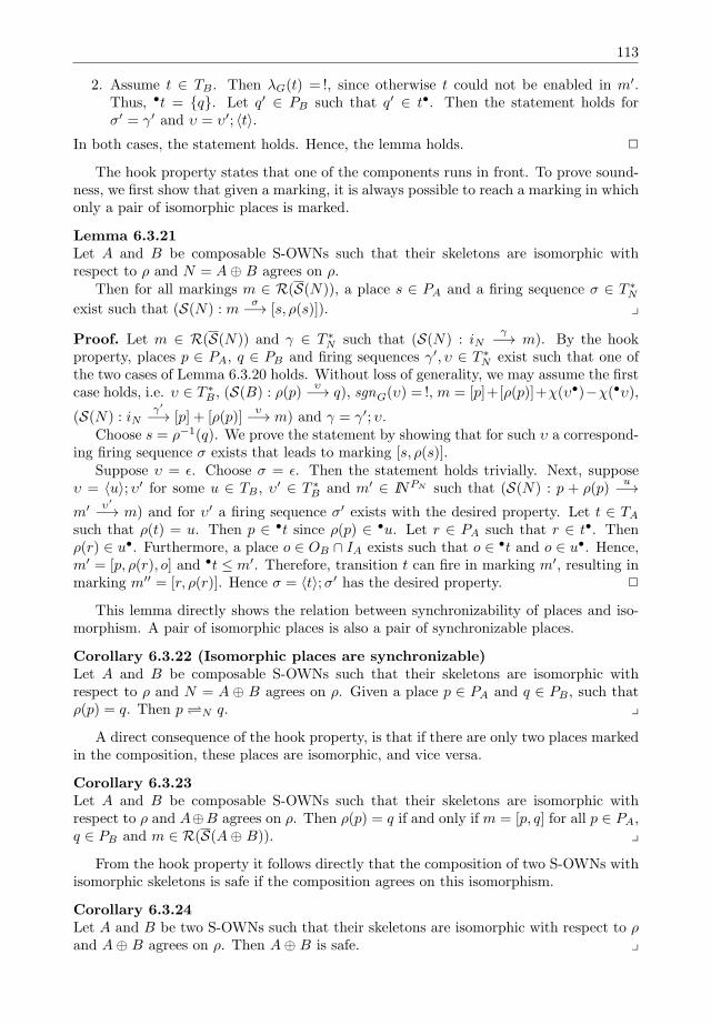
113
2. Assume t ∈ TB . Then λG(t) = !, since otherwise t could not be enabled in m′.Thus, •t = q. Let q′ ∈ PB such that q′ ∈ t•. Then the statement holds forσ′ = γ′ and υ = υ′; ⟨t⟩.
In both cases, the statement holds. Hence, the lemma holds. 2
The hook property states that one of the components runs in front. To prove sound-ness, we first show that given a marking, it is always possible to reach a marking in whichonly a pair of isomorphic places is marked.
Lemma 6.3.21Let A and B be composable S-OWNs such that their skeletons are isomorphic withrespect to ρ and N = A⊕ B agrees on ρ.
Then for all markings m ∈ R(S(N)), a place s ∈ PA and a firing sequence σ ∈ T ∗N
exist such that (S(N) : mσ−→ [s, ρ(s)]). y
Proof. Let m ∈ R(S(N)) and γ ∈ T ∗N such that (S(N) : iN
γ−→ m). By the hookproperty, places p ∈ PA, q ∈ PB and firing sequences γ′, υ ∈ T ∗
N exist such that one ofthe two cases of Lemma 6.3.20 holds. Without loss of generality, we may assume the firstcase holds, i.e. υ ∈ T ∗
B , (S(B) : ρ(p)υ−→ q), sgnG(υ) = !, m = [p]+[ρ(p)]+χ(υ•)−χ(•υ),
(S(N) : iNγ′
−→ [p] + [ρ(p)]υ−→ m) and γ = γ′; υ.
Choose s = ρ−1(q). We prove the statement by showing that for such υ a correspond-ing firing sequence σ exists that leads to marking [s, ρ(s)].
Suppose υ = ϵ. Choose σ = ϵ. Then the statement holds trivially. Next, supposeυ = ⟨u⟩; υ′ for some u ∈ TB , υ
′ ∈ T ∗B and m′ ∈ INPN such that (S(N) : p + ρ(p)
u−→m′ υ′
−→ m) and for υ′ a firing sequence σ′ exists with the desired property. Let t ∈ TAsuch that ρ(t) = u. Then p ∈ •t since ρ(p) ∈ •u. Let r ∈ PA such that r ∈ t•. Thenρ(r) ∈ u•. Furthermore, a place o ∈ OB ∩ IA exists such that o ∈ •t and o ∈ u•. Hence,m′ = [p, ρ(r), o] and •t ≤ m′. Therefore, transition t can fire in marking m′, resulting inmarking m′′ = [r, ρ(r)]. Hence σ = ⟨t⟩;σ′ has the desired property. 2
This lemma directly shows the relation between synchronizability of places and iso-morphism. A pair of isomorphic places is also a pair of synchronizable places.
Corollary 6.3.22 (Isomorphic places are synchronizable)Let A and B be composable S-OWNs such that their skeletons are isomorphic withrespect to ρ and N = A ⊕ B agrees on ρ. Given a place p ∈ PA and q ∈ PB , such thatρ(p) = q. Then pN q. y
A direct consequence of the hook property, is that if there are only two places markedin the composition, these places are isomorphic, and vice versa.
Corollary 6.3.23Let A and B be composable S-OWNs such that their skeletons are isomorphic withrespect to ρ and A⊕B agrees on ρ. Then ρ(p) = q if and only if m = [p, q] for all p ∈ PA,q ∈ PB and m ∈ R(S(A⊕ B)). y
From the hook property it follows directly that the composition of two S-OWNs withisomorphic skeletons is safe if the composition agrees on this isomorphism.
Corollary 6.3.24Let A and B be two S-OWNs such that their skeletons are isomorphic with respect to ρand A⊕ B agrees on ρ. Then A⊕ B is safe. y
114 Correctness-By-Construction
Before we prove that if the composition agrees on the isomorphism of its constituents,it is sound, we show that a firing sequence of a constituent from a place p to a place qcan be replayed in the composition, starting from the marking in which only place p andits isomorphic counterpart is marked.
Lemma 6.3.25Let A and B be composable S-OWNs such that their skeletons are isomorphic withrespect to ρ and A⊕ B agrees on ρ. Let p, q ∈ PA and υ ∈ T ∗
A such that (S(A) : [p] υ−→[q]). Then, a firing sequence σ ∈ T ∗
N exists such that (S(N) : [p, ρ(p)]σ−→ [q, ρ(q)]) and
σ|TA= υ. y
Proof. Define G = p ∈ PN | ∃H ∈ GA∩GB : p ∈ H. We prove the lemma by structuralinduction on υ. Suppose υ = ϵ. Then the lemma holds trivially.
Suppose υ = υ′; ⟨u⟩ for some υ′ ∈ T ∗A, u ∈ TA, and p
′ ∈ PA such that (S(A) : [p] υ′
−→[p′]
u−→ q), and for υ′ a firing sequence σ′ ∈ T ∗N exists such that (S(N) : [p, ρ(p)]
σ′
−→[p′, ρ(p′)]) and σ′
|TN= υ′. Let t = ρ(u). Then a place o ∈ G exists such that either (1)
o ∈ •t ∩ u• or (2) o ∈ •u ∩ t•.Suppose the first, i.e. o ∈ •t ∩ u•. Then, (S(N) : [p′, ρ(p′)]
u−→ [q, ρ(p′), o]t−→
[q, ρ(q)]). Hence σ = σ′; ⟨u, t⟩ has the desired property. Suppose the latter, i.e. o ∈ •u∩t•.Then, (S(N) : [p′, ρ(p′)]
t−→ [q, ρ(p′), o]u−→ [q, ρ(q)]). Hence σ = σ′; ⟨t, u⟩ has the desired
property. 2
Since we only consider S-OWNs, which are always sound, from every place in anS-OWN, it is possible to reach the final marking. Hence, given a reachable marking inthe composition, we first reach a marking in which no interface places are marked, afterwhich we can use the previous lemma to reach the final marking. Thus, we may concludethat if the composition agrees on the isomorphism of its constituents, it is sound.
Lemma 6.3.26 (Soundness of composition of S-OWNs)Let A and B be composable S-OWNs such that their skeletons are isomorphic withrespect to ρ and N = A⊕ B agrees on ρ. Then A⊕ B is sound. yProof. By Lemma 6.3.16, both A and B are sound. Let f1 ∈ PA be the final place ofA, and let f2 ∈ PB be the final place of B.
Let m ∈ R(S(N)). By Lemma 6.3.21, a firing sequence σ1 ∈ T ∗N and a place p ∈ PA
exist such that (S(N) : mσ−→ [p, ρ(p)]). Since A is sound, a firing sequence υ ∈ T ∗
A
exists such that (S(A) : [p] υ−→ [f1]). Then, by Lemma 6.3.25, there is a firing sequence
σ2 ∈ T ∗N such that (S(N) : [p, ρ(p)]
σ2−→ [f1, f2]) and σ2|TA= υ. Since ρ(f1) = f2 and
fN = [f1, f2], we have (S(N) : mσ−→ fN ).
Hence, N is sound. 2
If the composition of two S-OWNs agrees on the isomorphism of its constituents,the composition is both sound and safe. However, it does not guarantee the identicalcommunication condition.
Corollary 6.3.27 (Soundness and safeness of two composed S-OWNs)Let A and B be two composable S-components such that their skeletons are isomorphicwith respect to some bijective function ρ. If the composition A⊕ B agrees on ρ, A⊕ Bis sound and safe. y
Last, we present a necessary and sufficient condition for a composition that agreeson the isomorphism of their constituents to also guarantee the identical communication
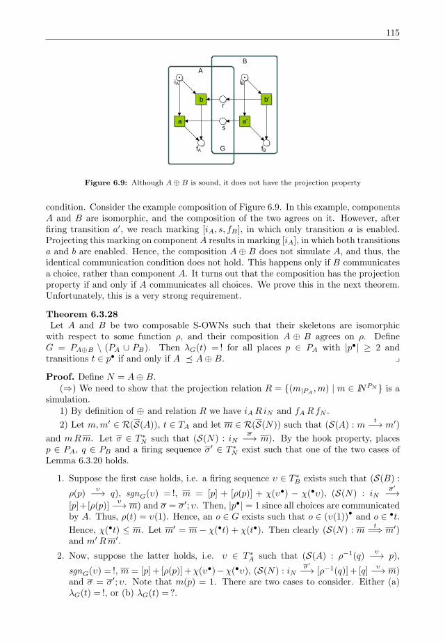
115
AB
G
rb
a a’
b’
s
iA
fA
iB
fB
Figure 6.9: Although A⊕ B is sound, it does not have the projection property
condition. Consider the example composition of Figure 6.9. In this example, componentsA and B are isomorphic, and the composition of the two agrees on it. However, afterfiring transition a′, we reach marking [iA, s, fB ], in which only transition a is enabled.Projecting this marking on componentA results in marking [iA], in which both transitionsa and b are enabled. Hence, the composition A⊕ B does not simulate A, and thus, theidentical communication condition does not hold. This happens only if B communicatesa choice, rather than component A. It turns out that the composition has the projectionproperty if and only if A communicates all choices. We prove this in the next theorem.Unfortunately, this is a very strong requirement.
Theorem 6.3.28Let A and B be two composable S-OWNs such that their skeletons are isomorphicwith respect to some function ρ, and their composition A ⊕ B agrees on ρ. DefineG = PA⊕B \ (PA ∪ PB). Then λG(t) = ! for all places p ∈ PA with |p•| ≥ 2 andtransitions t ∈ p• if and only if A ≼ A⊕ B. y
Proof. Define N = A⊕ B.(⇒) We need to show that the projection relation R = (m|PA
,m) | m ∈ INPN is asimulation.
1) By definition of ⊕ and relation R we have iAR iN and fARfN .
2) Let m,m′ ∈ R(S(A)), t ∈ TA and let m ∈ R(S(N)) such that (S(A) : m t−→ m′)
and mRm. Let σ ∈ T ∗N such that (S(N) : iN
σ−→ m). By the hook property, placesp ∈ PA, q ∈ PB and a firing sequence σ′ ∈ T ∗
N exist such that one of the two cases ofLemma 6.3.20 holds.
1. Suppose the first case holds, i.e. a firing sequence υ ∈ T ∗B exists such that (S(B) :
ρ(p)υ−→ q), sgnG(υ) = !, m = [p] + [ρ(p)] + χ(υ•) − χ(•υ), (S(N) : iN
σ′
−→[p]+[ρ(p)]
υ−→ m) and σ = σ′; υ. Then, |p•| = 1 since all choices are communicatedby A. Thus, ρ(t) = υ(1). Hence, an o ∈ G exists such that o ∈ (υ(1))
•and o ∈ •t.
Hence, χ(•t) ≤ m. Let m′ = m − χ(•t) + χ(t•). Then clearly (S(N) : mt
=⇒ m′)and m′Rm′.
2. Now, suppose the latter holds, i.e. υ ∈ T ∗A such that (S(A) : ρ−1(q)
υ−→ p),
sgnG(υ) = !, m = [p] + [ρ(p)] +χ(υ•)−χ(•υ), (S(N) : iNσ′
−→ [ρ−1(q)] + [q]υ−→ m)
and σ = σ′; υ. Note that m(p) = 1. There are two cases to consider. Either (a)λG(t) = !, or (b) λG(t) = ?.
116 Correctness-By-Construction
(a) Assume the first. Then clearly χ(•t) ≤ m. Let m′ = m− χ(•t) + χ(t•). Then
(S(N) : mt
=⇒ m′) and m′Rm′.
(b) Assume the latter. By Lemma 6.3.21, a firing sequence σ ∈ T ∗B exists such
that (S(N) : mσ−→ m′′), where m′′ = [p, ρ(p)]. Thus, (S(N) : m =⇒ m′′)
and m′Rm′′. Let m′ = m′′ − χ(•t) + χ(t•). Then clearly (S(N) : mt
=⇒ m′)and m′Rm′.
In both cases, a marking m′ ∈ INPN exists such that (S(N) : mt
=⇒ m′) and m′Rm′.Hence, the statement holds.
3) Let m ∈ R(S(N)) and γ ∈ T ∗N such that (S(N) : iN
γ−→ m) and fARm. Then,no transition t ∈ TA is enabled in m, since fA is a deadlock of S(A). By the hookproperty, a place q ∈ PB and firing sequences γ′ ∈ T ∗
N and υ ∈ T ∗A exist such that
(S(A) : [ρ−1(q)]υ−→ [fA]), sgnG(t) = ! and
−→σ =
−−→σ′; υ. Hence, by Lemma 6.3.21, a firing
sequence σ ∈ T ∗N exists such that (S(N) : m
σ−→ [fA, fB ]). Since no transitions of A areenabled, we have σ ∈ T ∗
B . Hence, (S(N) : m =⇒ fN ).(⇐) We prove the statement by showing that if B does make a choice, the projection
property does not hold. Suppose there is a place q ∈ PB such that |q•| ≥ 2 and λG(t) = !for all t ∈ q•. Since B is sound, a firing sequence υ ∈ T ∗
B exists such that (S(B) :
iBυ−→ q). Let q′ ∈ PA such that ρ(q′) = q. Hence, by Lemma 6.3.25, a firing sequence
σ ∈ T ∗N exists such that (S(N) : iN
σ−→ [q, q′]) and σ|TB= υ. Let t1, t2 ∈ TA such
that ρ(t1), ρ(t2) ⊆ q• and t1 = t2. Then both χ(•t1) ≤ [q, q′] and χ(•t2) ≤ [q, q′]. Letm′ = [q, q′]− χ(•ρ(t1)) + χ(ρ(t1)
•). Then m′
|PA= [q, q′]|PA
. Then χ(•t1) ≤ m′, but not
χ(•t1) ≤ m′. Hence, the projection relation is not a simulation. 2
6.3.3 ATIS-nets
Both presented classes are not only sound by construction, also the identical communi-cation condition holds, and the synchronizability of places can be determined based onthe structure of the graph of the Petri net. Refinement of two synchronizable places in asound OPN, like described in the second rule of the construction approach, by a soundcomposition of two OWNs preserves the soundness. In this section, we introduce a classof pairs of communicating components that are sound by their structure. We call thisclass ATIS-nets, based on their main two subclasses: acyclic T-OWNs and isomorphicS-OWNs. The class is closed under the reduction/synthesis rules of Murata (except forthe rule elimination of self-loop places) and the generalized sound workflow reductionrule.
Definition 6.3.29 (ATIS-nets)The class of ATIS-nets is defined as the smallest set of nets AN defined as follows:
1. if N = S1 ⊕ S2 with S1 and S2 two composable S-OWNs such that their skeletonsare isomorphic with respect to some function ρ and their composition agrees on ρ,then N ∈ AN ;
2. if N = T1 ⊕ T2 with T1 and T2 two composable T-OWNs and their compositionhas the quadrangle property, then N ∈ AN ;
3. if N = (A⊕ B)p⊙q (C ⊕ D) with A⊕ B,C ⊕ D ∈ AN , p ∈ PA, q ∈ PB such thatpA⊕B q, then N ∈ AN ;
4. if A⊕ B ∈ AN , and an A′ ∈ N such that A ≃ τH(A′) where H = TA′ \ TA, thenA′ ⊕ B ∈ AN . y

117
G
H
A
B
p q
t1
t3
t2
t4
t5
u1
u2
t6
(a)
C
D
(b)
Figure 6.10: comω(A,B) and comω(C,D) hold, but comω(A⊙p C,B ⊙q D) does not hold
All ATIS-nets are sound, as shown in the next theorem.
Theorem 6.3.30Let N ∈ AN . Then N is sound. yProof. We prove the statement by induction on the structure of N = A⊕B. Suppose Nis a composition of two acyclic T-OWNs such that the composition has the quadrangleproperty, then it is safe and sound by Theorem 6.3.4.
Suppose N is a composition of two S-OWNs having an isomorphic skeleton, and thecomposition agrees on the isomorphism. Then N is safe and sound by Corollary 6.3.27.
Suppose N is a refinement, i.e. there exist two compositions A ⊕ B,C ⊕ D ∈ AN ,and two places p ∈ PA, q ∈ PB such that p A⊕B q, N = (A ⊕ B)p⊙q (C ⊕ D), andboth A⊕ B and C ⊕ D are safe and sound. By Theorem 5.4.19, net N is sound. Sinceplaces p and q are synchronizable, by Corollary 5.4.16, net N is safe.
Suppose there exists an A′ ∈ N such that A′ ⊕ B ∈ AN and A ≃ τH(A′) whereH = TA′ \ TA. Then, since A ≃ τH(A′), A⊕ B is also sound. 2
Although all ATIS-nets are sound by construction, none of the communication con-ditions are preserved, as shown in the example of Figure 6.10. Consider the marking mafter firing transitions t1 and t3. Then transition t4 is enabled in A ⊕ B. However, inthe refinement, transition t4 can only fire if transitions u1 and u2 have fired, and thustransition t2 als needs to fire. Hence, none of the communication conditions as presentedin Chapter 4 hold on the refined net.
The example of Figure 6.10 suggests to add an extra condition to synchronizableplaces to guarantee that one of the communication conditions is preserved. In fact, theproperty of synchronizable places needs to ensure that no communicating transition isneeded to reach a marking in which both places are marked. A sufficient condition is arequest-response pattern, that form a so-called block structure around the synchronizable
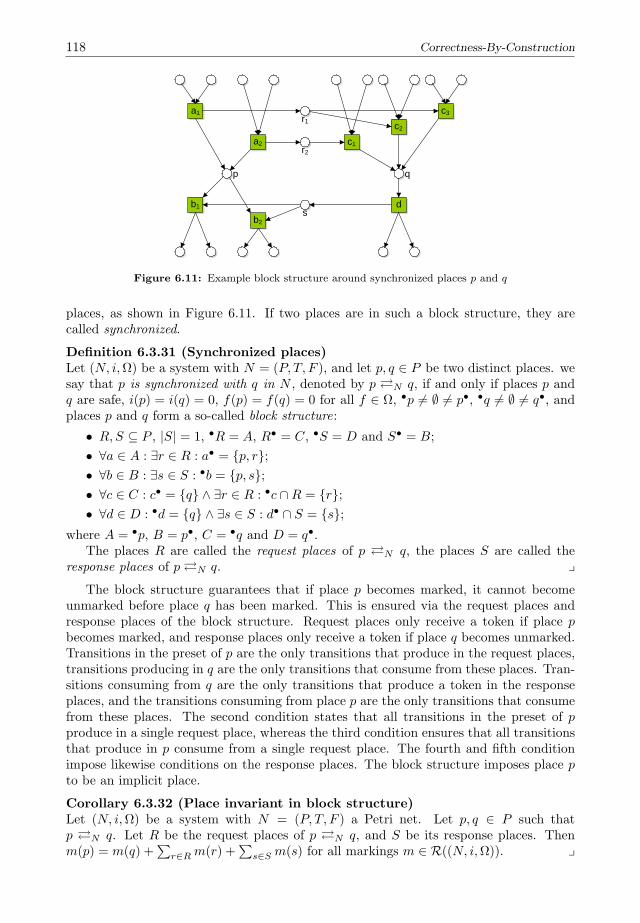
118 Correctness-By-Construction
a1
a2
b1
b2
c1
c2
c3
d
r1
r2
s
p q
Figure 6.11: Example block structure around synchronized places p and q
places, as shown in Figure 6.11. If two places are in such a block structure, they arecalled synchronized.
Definition 6.3.31 (Synchronized places)Let (N, i,Ω) be a system with N = (P, T, F ), and let p, q ∈ P be two distinct places. wesay that p is synchronized with q in N , denoted by p N q, if and only if places p andq are safe, i(p) = i(q) = 0, f(p) = f(q) = 0 for all f ∈ Ω, •p = ∅ = p•, •q = ∅ = q•, andplaces p and q form a so-called block structure:
• R,S ⊆ P , |S| = 1, •R = A, R• = C, •S = D and S• = B;
• ∀a ∈ A : ∃r ∈ R : a• = p, r;• ∀b ∈ B : ∃s ∈ S : •b = p, s;• ∀c ∈ C : c• = q ∧ ∃r ∈ R : •c ∩R = r;• ∀d ∈ D : •d = q ∧ ∃s ∈ S : d• ∩ S = s;
where A = •p, B = p•, C = •q and D = q•.The places R are called the request places of p N q, the places S are called the
response places of pN q. yThe block structure guarantees that if place p becomes marked, it cannot become
unmarked before place q has been marked. This is ensured via the request places andresponse places of the block structure. Request places only receive a token if place pbecomes marked, and response places only receive a token if place q becomes unmarked.Transitions in the preset of p are the only transitions that produce in the request places,transitions producing in q are the only transitions that consume from these places. Tran-sitions consuming from q are the only transitions that produce a token in the responseplaces, and the transitions consuming from place p are the only transitions that consumefrom these places. The second condition states that all transitions in the preset of pproduce in a single request place, whereas the third condition ensures that all transitionsthat produce in p consume from a single request place. The fourth and fifth conditionimpose likewise conditions on the response places. The block structure imposes place pto be an implicit place.
Corollary 6.3.32 (Place invariant in block structure)Let (N, i,Ω) be a system with N = (P, T, F ) a Petri net. Let p, q ∈ P such thatp N q. Let R be the request places of p N q, and S be its response places. Thenm(p) = m(q) +
∑r∈Rm(r) +
∑s∈Sm(s) for all markings m ∈ R((N, i,Ω)). y
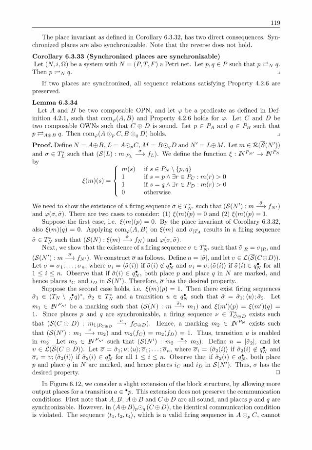
119
The place invariant as defined in Corollary 6.3.32, has two direct consequences. Syn-chronized places are also synchronizable. Note that the reverse does not hold.
Corollary 6.3.33 (Synchronized places are synchronizable)Let (N, i,Ω) be a system with N = (P, T, F ) a Petri net. Let p, q ∈ P such that pN q.Then pN q. y
If two places are synchronized, all sequence relations satisfying Property 4.2.6 arepreserved.
Lemma 6.3.34Let A and B be two composable OPN, and let φ be a predicate as defined in Def-
inition 4.2.1, such that comφ(A,B) and Property 4.2.6 holds for φ. Let C and D betwo composable OWNs such that C ⊕ D is sound. Let p ∈ PA and q ∈ PB such thatpA⊕B q. Then comφ(A⊙p C,B ⊙q D) holds. yProof. DefineN = A⊕B, L = A⊙pC,M = B⊙qD andN ′ = L⊕M . Letm ∈ R(S(N ′))
and σ ∈ T ∗L such that (S(L) : m|PL
σ−→ fL). We define the function ξ : INPN′ → INPN
by
ξ(m)(s) =
m(s) if s ∈ PN \ p, q1 if s = p ∧ ∃r ∈ PC : m(r) > 01 if s = q ∧ ∃r ∈ PD : m(r) > 00 otherwise
We need to show the existence of a firing sequence σ ∈ T ∗N ′ such that (S(N ′) : m
σ−→ fN ′)and φ(σ, σ). There are two cases to consider: (1) ξ(m)(p) = 0 and (2) ξ(m)(p) = 1.
Suppose the first case, i.e. ξ(m)(p) = 0. By the place invariant of Corollary 6.3.32,also ξ(m)(q) = 0. Applying comφ(A,B) on ξ(m) and σ|TA
results in a firing sequence
σ ∈ T ∗N such that (S(N) : ξ(m)
σ−→ fN ) and φ(σ, σ).Next, we show that the existence of a firing sequence σ ∈ T ∗
N ′ such that σ|R = σ|R, and
(S(N ′) : mσ−→ fN ′). We construct σ as follows. Define n = |σ|, and let υ ∈ L(S(C⊕D)).
Let σ = σ1; . . . ;σn, where σi = ⟨σ(i)⟩ if σ(i) ∈ q•N and σi = υ; ⟨σ(i)⟩ if σ(i) ∈ q•N for all1 ≤ i ≤ n. Observe that if σ(i) ∈ q•N , both place p and place q in N are marked, andhence places iC and iD in S(N ′). Therefore, σ has the desired property.
Suppose the second case holds, i.e. ξ(m)(p) = 1. Then there exist firing sequencesσ1 ∈ (TN \ •
N q)∗, σ2 ∈ T ∗
N and a transition u ∈ q•N such that σ = σ1; ⟨u⟩; σ2. Let
m1 ∈ INPN′ be a marking such that (S(N) : mσ1−→ m1) and ξ(m′)(p) = ξ(m′)(q) =
1. Since places p and q are synchronizable, a firing sequence ν ∈ T ∗C⊕D exists such
that (S(C ⊕ D) : m1|PC⊕D
ν−→ fC⊕D). Hence, a marking m2 ∈ INPN exists such
that (S(N ′) : m1ν−→ m2) and m2(fC) = m2(fD) = 1. Thus, transition u is enabled
in m2. Let m3 ∈ INPN′ such that (S(N ′) : m2u−→ m3). Define n = |σ2|, and let
υ ∈ L(S(C ⊕ D)). Let σ = σ1; ν; ⟨u⟩;σ1; . . . ;σn, where σi = ⟨σ2(i)⟩ if σ2(i) ∈ q•N andσi = υ; ⟨σ2(i)⟩ if σ2(i) ∈ q•N for all 1 ≤ i ≤ n. Observe that if σ2(i) ∈ q•N , both placep and place q in N are marked, and hence places iC and iD in S(N ′). Thus, σ has thedesired property. 2
In Figure 6.12, we consider a slight extension of the block structure, by allowing moreoutput places for a transition a ∈ •p. This extension does not preserve the communicationconditions. First note that A,B, A⊕B and C ⊕D are all sound, and places p and q aresynchronizable. However, in (A⊕B)p⊙q (C⊕D), the identical communication conditionis violated. The sequence ⟨t1, t2, t4⟩, which is a valid firing sequence in A ⊙p C, cannot
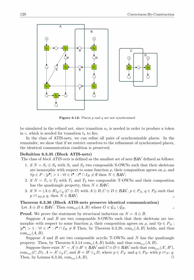
120 Correctness-By-Construction
t1 t2
t3
t4
t5
st7
t6
t8
p q
a
b
c
A
B
C
D
u1 u2
Figure 6.12: Places p and q are not synchronized
be simulated in the refined net, since transition u1 is needed in order to produce a tokenin c, which is needed for transition t4 to fire.
In the class of ATIS-nets, we can refine all pairs of synchronizable places. In theremainder, we show that if we restrict ourselves to the refinement of synchronized places,the identical communication condition is preserved.
Definition 6.3.35 (Block ATIS-nets)The class of block ATIS-nets is defined as the smallest set of nets BAN defined as follows:
1. if N = S1 ⊕ S2 with S1 and S2 two composable S-OWNs such that their skeletonsare isomorphic with respect to some function ρ, their composition agrees on ρ, and∀p ∈ P : |p•| > 1 : ∀t ∈ t• : t• ∩ IB = ∅ then N ∈ BAN ;
2. if N = T1 ⊕ T2 with T1 and T2 two composable T-OWNs and their compositionhas the quadrangle property, then N ∈ BAN ;
3. if N = (A⊕ B)p⊙q (C ⊕D) with A⊕ B,C ⊕D ∈ BAN , p ∈ PA, q ∈ PB such thatpA⊕B q, then N ∈ BAN ; y
Theorem 6.3.36 (Block ATIS-nets preserve identical communication)Let A⊕ B ∈ BAN . Then comωG(A,B) where G ∈ GA \ GB . yProof. We prove the statement by structural induction on N = A⊕ B.
Suppose A and B are two composable S-OWNs such that their skeletons are iso-morphic with respect to some function ρ, their composition agrees on ρ, and ∀p ∈ PA :|p•| > 1 : ∀t ∈ t• : t• ∩ IB = ∅ Then, by Theorem 6.3.28, comω(A,B) holds, and thuscomωG
(A,B).Suppose A and B are two composable acyclic T-OWNs and N has the quadrangle
property. Then, by Theorem 6.3.14 comω(A,B) holds, and thus comωG(A,B).
Suppose there exist N ′ = A′⊕B′ ∈ BAN and C⊕D ∈ BAN such that comωG(A′, B′),
comωG(C,D), A = A′⊙pC, and B = B′⊙qD, where p ∈ PA′ and q ∈ PB′ with pN ′ q.
Then, by Lemma 6.3.34, comωG(A,B). 2

121
6.4 Conclusions
In this chapter, we presented a construction methodology for compositions that guar-antees soundness. The first rule refines a single safe place in a component by a soundworkflow component. This way, the behavior of a single component can be refined. Thesecond rule, communication refinement, takes from two components a place, and if theplaces are synchronizable, these places can be refined by a composition of two workflowcomponents. The last rule, outsource refinement, refines a single safe place by a com-position of two special workflow components: there is one component that initiates thesecond, and this component can only reach the final marking if the second has reachedits final marking.
We defined a class of communication protocols between pairs of components for whichsoundness can be determined based on their structure. This class is built from acyclicmarked graphs and isomorphic state machines. Although the class ensures both sound-ness and the simulation communication condition, the requirements on elements in thisclass are very strong. Unfortunately, these strong requirements are needed to guaranteesoundness by construction.
In [28] the authors give a constructive method preserving the inheritance of behavior,which can be used to guarantee the correctness of interorganizational processes. Otherformalisms, like interface automata [20] use synchronous communication, whereas wefocus on asynchronous communication, which is essential for our application domain,since the communication in SOA is asynchronous.
In [43], the authors propose to model choreographies using Interaction Petri nets,which is a special class of Petri nets, where transitions are labeled with the source andtarget component, and the message type being sent. For each of the components, abehavioral interface is extracted. An interaction Petri net is then realizable if the com-position of the behavioral interfaces is branching bisimilar related with the interactionPetri net. To check whether the composition is functioning correctly, the whole net-work of components needs to be checked, whereas in our approach this is guaranteed byconstruction.
To keep our results at a conceptual level, we present our results on Petri net models.Our method can easily instantiated for industrial languages like BPEL [22], to facilitatethe construction of web services in development environments like Oracle BPEL or IBMWebsphere.

122 Correctness-By-Construction

Part II
Design Techniques ForComponent-Based Systems

7Integration of Data and Processes in Components
7.1 Introduction
In Petri nets, the storage of objects is often modeled as a place holding tokens of acertain object type: the place is a store for objects of a certain type. Transitions thatmanipulate these objects are connected to these places. In a marking, each token ina store represents an object. In components, often the control flow describes the flowof a case: each transition in the component models an activity of the case. Messagesbetween components are related to the cases in each component. In classical Petri nets,the formalism does not take the different objects into account. Hence, we cannot modelthat two transitions need the same object in order to be executed. Therefore, we needcoloured Petri nets [71]. Coloured Petri nets are very powerful to model with, but theanalysis techniques are very limited.
In components, often the actual content of the object does not need to be modeled,only objects and their identity play an important role, rather than the internal structureof the object. To deal with identities, we only need limited operations like equality testingand copying of identities. For message passing, we need not only to compare objects,it is also needed to be able to relate different objects. Therefore, we introduce a classof coloured Petri nets where tokens are vectors of identifiers, and there is a restrictedset of operations on transitions: only testing for equality on identifiers and copying ofidentifiers. On the one hand verification of behavioral properties for this class of colouredPetri nets is easier and on the other hand the class is powerful enough to model not onlyobjects, but also more advanced operations like message passing between components.
This chapter is organised as follows. In Section 7.2, we introduce Petri nets with iden-tifiers (PNIDs), and demonstrate their expressiveness. In Section 7.4 we show how PNIDscan be used to model database transactions. The chapter is concluded in Section 7.5.
7.2 Petri Nets With Identifiers
Components typically model the process around some key object, like the ordering andassembly of configurable products, or the negotiation to establish a contract betweentwo parties. Consider for example the components in Figure 7.1. Component A deliverssome product component B needs. Component C builds the actual product. Component

126 Integration of Data and Processes in Components
t1
t5
t2
t3
t4
t6
t7
u1
u5
u2
u3
u4
u6
a
b
c
d
fh
gv1
v2
E
C
E
C
CC
E
C
A
B
C
Figure 7.1: Communicating components. Places storing the key objects of a component are coloured
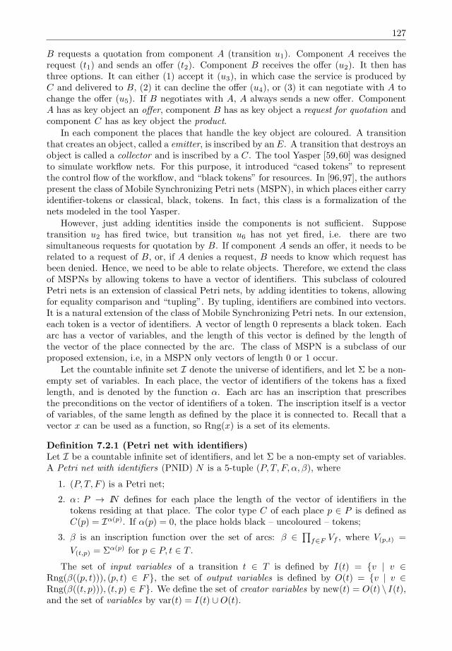
127
B requests a quotation from component A (transition u1). Component A receives therequest (t1) and sends an offer (t2). Component B receives the offer (u2). It then hasthree options. It can either (1) accept it (u3), in which case the service is produced byC and delivered to B, (2) it can decline the offer (u4), or (3) it can negotiate with A tochange the offer (u5). If B negotiates with A, A always sends a new offer. ComponentA has as key object an offer, component B has as key object a request for quotation andcomponent C has as key object the product.
In each component the places that handle the key object are coloured. A transitionthat creates an object, called a emitter, is inscribed by an E. A transition that destroys anobject is called a collector and is inscribed by a C. The tool Yasper [59,60] was designedto simulate workflow nets. For this purpose, it introduced “cased tokens” to representthe control flow of the workflow, and “black tokens” for resources. In [96,97], the authorspresent the class of Mobile Synchronizing Petri nets (MSPN), in which places either carryidentifier-tokens or classical, black, tokens. In fact, this class is a formalization of thenets modeled in the tool Yasper.
However, just adding identities inside the components is not sufficient. Supposetransition u2 has fired twice, but transition u6 has not yet fired, i.e. there are twosimultaneous requests for quotation by B. If component A sends an offer, it needs to berelated to a request of B, or, if A denies a request, B needs to know which request hasbeen denied. Hence, we need to be able to relate objects. Therefore, we extend the classof MSPNs by allowing tokens to have a vector of identifiers. This subclass of colouredPetri nets is an extension of classical Petri nets, by adding identities to tokens, allowingfor equality comparison and “tupling”. By tupling, identifiers are combined into vectors.It is a natural extension of the class of Mobile Synchronizing Petri nets. In our extension,each token is a vector of identifiers. A vector of length 0 represents a black token. Eacharc has a vector of variables, and the length of this vector is defined by the length ofthe vector of the place connected by the arc. The class of MSPN is a subclass of ourproposed extension, i.e, in a MSPN only vectors of length 0 or 1 occur.
Let the countable infinite set I denote the universe of identifiers, and let Σ be a non-empty set of variables. In each place, the vector of identifiers of the tokens has a fixedlength, and is denoted by the function α. Each arc has an inscription that prescribesthe preconditions on the vector of identifiers of a token. The inscription itself is a vectorof variables, of the same length as defined by the place it is connected to. Recall that avector x can be used as a function, so Rng(x) is a set of its elements.
Definition 7.2.1 (Petri net with identifiers)Let I be a countable infinite set of identifiers, and let Σ be a non-empty set of variables.A Petri net with identifiers (PNID) N is a 5-tuple (P, T, F, α, β), where
1. (P, T, F ) is a Petri net;
2. α : P → IN defines for each place the length of the vector of identifiers in thetokens residing at that place. The color type C of each place p ∈ P is defined asC(p) = Iα(p). If α(p) = 0, the place holds black – uncoloured – tokens;
3. β is an inscription function over the set of arcs: β ∈∏f∈F Vf , where V(p,t) =
V(t,p) = Σα(p) for p ∈ P, t ∈ T .
The set of input variables of a transition t ∈ T is defined by I(t) = v | v ∈Rng(β((p, t))), (p, t) ∈ F, the set of output variables is defined by O(t) = v | v ∈Rng(β((t, p))), (t, p) ∈ F. We define the set of creator variables by new(t) = O(t) \ I(t),and the set of variables by var(t) = I(t) ∪O(t).
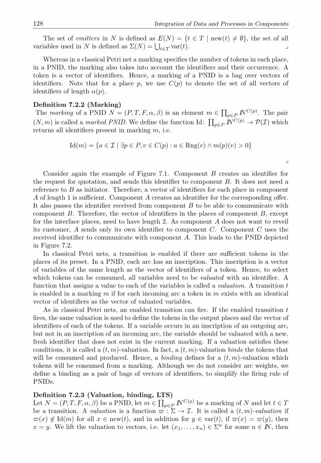
128 Integration of Data and Processes in Components
The set of emitters in N is defined as E(N) = t ∈ T | new(t) = ∅, the set of allvariables used in N is defined as Σ(N) =
∪t∈T var(t). y
Whereas in a classical Petri net a marking specifies the number of tokens in each place,in a PNID, the marking also takes into account the identifiers and their occurrence. Atoken is a vector of identifiers. Hence, a marking of a PNID is a bag over vectors ofidentifiers. Note that for a place p, we use C(p) to denote the set of all vectors ofidentifiers of length α(p).
Definition 7.2.2 (Marking)The marking of a PNID N = (P, T, F, α, β) is an element m ∈
∏p∈P IN
C(p). The pair
(N,m) is called a marked PNID. We define the function Id:∏p∈P IN
C(p) → P(I) whichreturns all identifiers present in marking m, i.e.
Id(m) = a ∈ I | ∃p ∈ P, v ∈ C(p) : a ∈ Rng(v) ∧m(p)(v) > 0
y
Consider again the example of Figure 7.1. Component B creates an identifier forthe request for quotation, and sends this identifier to component B. It does not need areference to B as initiator. Therefore, a vector of identifiers for each place in componentA of length 1 is sufficient. Component A creates an identifier for the corresponding offer.It also passes the identifier received from component B to be able to communicate withcomponent B. Therefore, the vector of identifiers in the places of component B, exceptfor the interface places, need to have length 2. As component A does not want to reveilits customer, A sends only its own identifier to component C. Component C uses thereceived identifier to communicate with component A. This leads to the PNID depictedin Figure 7.2.
In classical Petri nets, a transition is enabled if there are sufficient tokens in theplaces of its preset. In a PNID, each arc has an inscription. This inscription is a vectorof variables of the same length as the vector of identifiers of a token. Hence, to selectwhich tokens can be consumed, all variables need to be valuated with an identifier. Afunction that assigns a value to each of the variables is called a valuation. A transition tis enabled in a marking m if for each incoming arc a token in m exists with an identicalvector of identifiers as the vector of valuated variables.
As in classical Petri nets, an enabled transition can fire. If the enabled transition tfires, the same valuation is used to define the tokens in the output places and the vector ofidentifiers of each of the tokens. If a variable occurs in an inscription of an outgoing arc,but not in an inscription of an incoming arc, the variable should be valuated with a new,fresh identifier that does not exist in the current marking. If a valuation satisfies theseconditions, it is called a (t,m)-valuation. In fact, a (t,m)-valuation binds the tokens thatwill be consumed and produced. Hence, a binding defines for a (t,m)-valuation whichtokens will be consumed from a marking. Although we do not consider arc weights, wedefine a binding as a pair of bags of vectors of identifiers, to simplify the firing rule ofPNIDs.
Definition 7.2.3 (Valuation, binding, LTS)Let N = (P, T, F, α, β) be a PNID, let m ∈
∏p∈P IN
C(p) be a marking of N and let t ∈ Tbe a transition. A valuation is a function ϖ : Σ → I. It is called a (t,m)-valuation ifϖ(x) ∈ Id(m) for all x ∈ new(t), and in addition for y ∈ var(t), if ϖ(x) = ϖ(y), thenx = y. We lift the valuation to vectors, i.e. let (x1, . . . , xn) ∈ Σn for some n ∈ IN , then
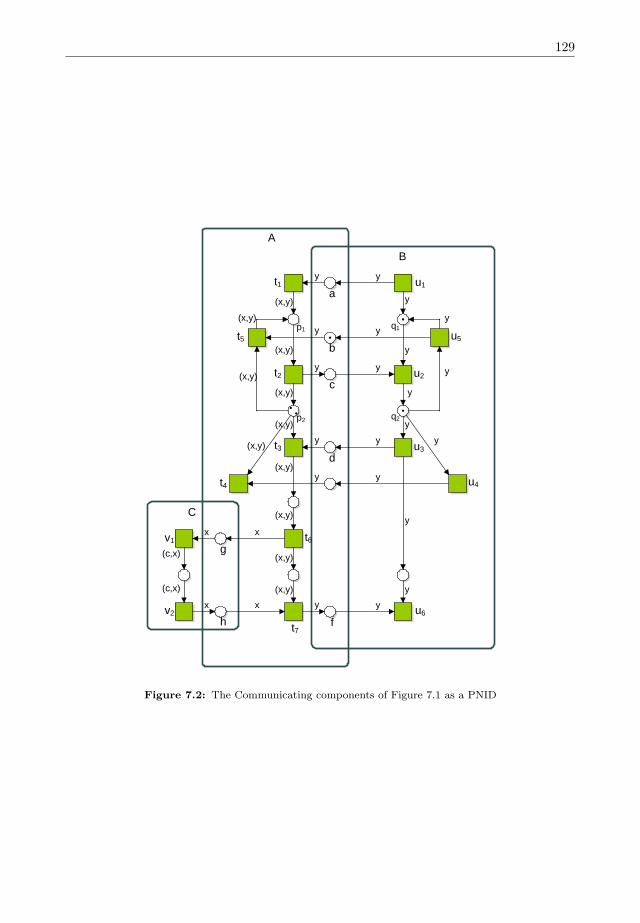
129
t1
t5
t2
t3
t4
t6
t7
u1
u5
u2
u3
u4
u6
a
b
c
d
fh
gv1
v2
A
B
C
(x,y)
(x,y)
(x,y)
(x,y)
(x,y)
(x,y)
(x,y)
(x,y)
(x,y)
(x,y)
(x,y)
y
y
y
y
y
y
y
y
y
y
y
y
y
y
y
y
y
y
y
y
y
x
x
x
x
(c,x)
(c,x)
p2
q1
q2
p1
Figure 7.2: The Communicating components of Figure 7.1 as a PNID
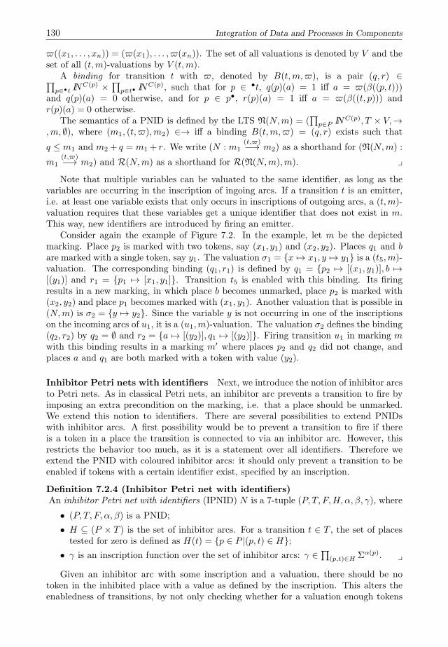
130 Integration of Data and Processes in Components
ϖ((x1, . . . , xn)) = (ϖ(x1), . . . , ϖ(xn)). The set of all valuations is denoted by V and theset of all (t,m)-valuations by V (t,m).
A binding for transition t with ϖ, denoted by B(t,m,ϖ), is a pair (q, r) ∈∏p∈•t IN
C(p) ×∏p∈t• IN
C(p), such that for p ∈ •t, q(p)(a) = 1 iff a = ϖ(β((p, t)))and q(p)(a) = 0 otherwise, and for p ∈ p•, r(p)(a) = 1 iff a = ϖ(β((t, p))) andr(p)(a) = 0 otherwise.
The semantics of a PNID is defined by the LTS N(N,m) = (∏p∈P IN
C(p), T × V,→,m, ∅), where (m1, (t,ϖ),m2) ∈→ iff a binding B(t,m,ϖ) = (q, r) exists such that
q ≤ m1 and m2 + q = m1 + r. We write (N : m1(t,ϖ)−→ m2) as a shorthand for (N(N,m) :
m1(t,ϖ)−→ m2) and R(N,m) as a shorthand for R(N(N,m),m). y
Note that multiple variables can be valuated to the same identifier, as long as thevariables are occurring in the inscription of ingoing arcs. If a transition t is an emitter,i.e. at least one variable exists that only occurs in inscriptions of outgoing arcs, a (t,m)-valuation requires that these variables get a unique identifier that does not exist in m.This way, new identifiers are introduced by firing an emitter.
Consider again the example of Figure 7.2. In the example, let m be the depictedmarking. Place p2 is marked with two tokens, say (x1, y1) and (x2, y2). Places q1 and bare marked with a single token, say y1. The valuation σ1 = x 7→ x1, y 7→ y1 is a (t5,m)-valuation. The corresponding binding (q1, r1) is defined by q1 = p2 7→ [(x1, y1)], b 7→[(y1)] and r1 = p1 7→ [x1, y1]. Transition t5 is enabled with this binding. Its firingresults in a new marking, in which place b becomes unmarked, place p2 is marked with(x2, y2) and place p1 becomes marked with (x1, y1). Another valuation that is possible in(N,m) is σ2 = y 7→ y2. Since the variable y is not occurring in one of the inscriptionson the incoming arcs of u1, it is a (u1,m)-valuation. The valuation σ2 defines the binding(q2, r2) by q2 = ∅ and r2 = a 7→ [(y2)], q1 7→ [(y2)]. Firing transition u1 in marking mwith this binding results in a marking m′ where places p2 and q2 did not change, andplaces a and q1 are both marked with a token with value (y2).
Inhibitor Petri nets with identifiers Next, we introduce the notion of inhibitor arcsto Petri nets. As in classical Petri nets, an inhibitor arc prevents a transition to fire byimposing an extra precondition on the marking, i.e. that a place should be unmarked.We extend this notion to identifiers. There are several possibilities to extend PNIDswith inhibitor arcs. A first possibility would be to prevent a transition to fire if thereis a token in a place the transition is connected to via an inhibitor arc. However, thisrestricts the behavior too much, as it is a statement over all identifiers. Therefore weextend the PNID with coloured inhibitor arcs: it should only prevent a transition to beenabled if tokens with a certain identifier exist, specified by an inscription.
Definition 7.2.4 (Inhibitor Petri net with identifiers)An inhibitor Petri net with identifiers (IPNID) N is a 7-tuple (P, T, F,H, α, β, γ), where
• (P, T, F, α, β) is a PNID;
• H ⊆ (P × T ) is the set of inhibitor arcs. For a transition t ∈ T , the set of placestested for zero is defined as H(t) = p ∈ P |(p, t) ∈ H;
• γ is an inscription function over the set of inhibitor arcs: γ ∈∏
(p,t)∈H Σα(p). y
Given an inhibitor arc with some inscription and a valuation, there should be notoken in the inhibited place with a value as defined by the inscription. This alters theenabledness of transitions, by not only checking whether for a valuation enough tokens

131
t1
p1
(x,y)
x
t2
t3
t4t5
(x,y)
(x,y)
xx
x x
x x
x x x
p2
p4
p3
Figure 7.3: An example of a Petri net with identifiers
are present, but it should not be possible to alter the valuation such that a token exists inthe inhibited place while maintaining the values on the variables used by the transition.
Definition 7.2.5 (Valuation for IPNID)Let N = (P, T, F,H, α, β, γ) be an IPNID. Transition t ∈ T is enabled in marking mwith (t,m)-valuation ϖ and binding (q, r) if q ≤ m and for all p ∈ H(t), no valuationϖ′ : Σ → I exists with ϖ′(x) = ϖ(x) for x ∈ var(t) and ϖ′(γ(p, t)) ∈ m(p). y
Consider the net in Figure 7.3 with marking M satisfying M(p1) = M(p2) =1,M(p3) = (1, 2), using I = IN . Transition t1 in Figure 7.3 is enabled e.g. with val-uation ϖ and binding (∅, p2 7→ 3) if ϖ(x) = 3. It is not enabled with e.g. a valuationϖ′ satisfying ϖ′(x) = 2, since x ∈ new(t1) and ϖ′(x) ∈ Id(M), so ϖ′ is not a (t1,M)-
valuation. For M ′ satisfying M(t,ϖ : M′
−→) we have M ′(p1) = M ′(p2) = 1, 3.In marking M ′, transition t5 is not enabled with any valuation ρ satisfying ρ(x) = 1.However, it is enabled with a valuation ρ satisfying ρ(x) = 3.
7.3 Expressivity of Petri Nets With Identifiers
In this section, we discuss the expressivity of Petri nets with identifiers. More specifi-cally, we focus on the reachability problem. In [96], the authors have shown that for socalled abstract MSPNs, in which the identifiers have no structure at all, the reachabilityproblem is undecidable. The authors have shown, that if the natural numbers are used asidentifiers, such that each time a new identifier is needed, the successor of the last usedidentifier is taken, the reachability problem is decidable. In this section we extend theresults to PNIDs. Therefore, we first introduce the notion of a PNID with counter place.The counter place is in every marking marked with the last identifier created. A PNIDwith counter place can be flattened to a classical Petri net. To prove that reachability isdecidable, we show that for all PNIDs a PNID with counter place exists.
A natural way of flattening the PNID would be to create for each place in the PNIDand each possible vector of identifiers a place in the flattened net. Hence, for each finitesubset of the set of identifiers, this results in a finite set of places. However, given atransition t that is enabled in some marking m with (t,m)-valuation ϖ, one of the mainproblems is that an identifier which already has been used, but not present in the currentmarking, can be assigned to a variable. Therefore, we need to ensure that identifiers cannever be used again.
A way to ensure that identifiers cannot be used twice, is to encode the set of identifiersusing a well-order on the set of identifiers. A well-order always has a successor function,which in turn can be used to create new identifiers. Therefore, we extend PNIDs with a
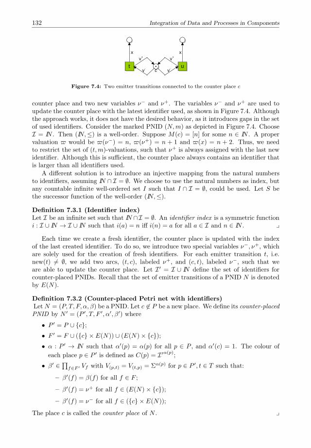
132 Integration of Data and Processes in Components
t uc
x xv+ v+
v- v-
Figure 7.4: Two emitter transitions connected to the counter place c
counter place and two new variables ν− and ν+. The variables ν− and ν+ are used toupdate the counter place with the latest identifier used, as shown in Figure 7.4. Althoughthe approach works, it does not have the desired behavior, as it introduces gaps in the setof used identifiers. Consider the marked PNID (N,m) as depicted in Figure 7.4. ChooseI = IN . Then (IN,≤) is a well-order. Suppose M(c) = [n] for some n ∈ IN . A propervaluation ϖ would be ϖ(ν−) = n, ϖ(ν+) = n + 1 and ϖ(x) = n + 2. Thus, we needto restrict the set of (t,m)-valuations, such that ν+ is always assigned with the last newidentifier. Although this is sufficient, the counter place always contains an identifier thatis larger than all identifiers used.
A different solution is to introduce an injective mapping from the natural numbersto identifiers, assuming IN ∩ I = ∅. We choose to use the natural numbers as index, butany countable infinite well-ordered set I such that I ∩ I = ∅, could be used. Let S bethe successor function of the well-order (IN,≤).
Definition 7.3.1 (Identifier index)Let I be an infinite set such that IN ∩I = ∅. An identifier index is a symmetric functioni : I ∪ IN → I ∪ IN such that i(a) = n iff i(n) = a for all a ∈ I and n ∈ IN . y
Each time we create a fresh identifier, the counter place is updated with the indexof the last created identifier. To do so, we introduce two special variables ν−, ν+, whichare solely used for the creation of fresh identifiers. For each emitter transition t, i.e.new(t) = ∅, we add two arcs, (t, c), labeled ν+, and (c, t), labeled ν−, such that weare able to update the counter place. Let I ′ = I ∪ IN define the set of identifiers forcounter-placed PNIDs. Recall that the set of emitter transitions of a PNID N is denotedby E(N).
Definition 7.3.2 (Counter-placed Petri net with identifiers)LetN = (P, T, F, α, β) be a PNID. Let c ∈ P be a new place. We define its counter-placedPNID by N ′ = (P ′, T, F ′, α′, β′) where
• P ′ = P ∪ c;• F ′ = F ∪ (c × E(N)) ∪ (E(N)× c);• α : P ′ → IN such that α′(p) = α(p) for all p ∈ P , and α′(c) = 1. The colour of
each place p ∈ P ′ is defined as C(p) = I ′α(p);
• β′ ∈∏f∈F ′ Vf with V(p,t) = V(t,p) = Σα(p) for p ∈ P ′, t ∈ T such that:
– β′(f) = β(f) for all f ∈ F ;
– β′(f) = ν+ for all f ∈ (E(N)× c);
– β′(f) = ν− for all f ∈ (c × E(N));
The place c is called the counter place of N . y
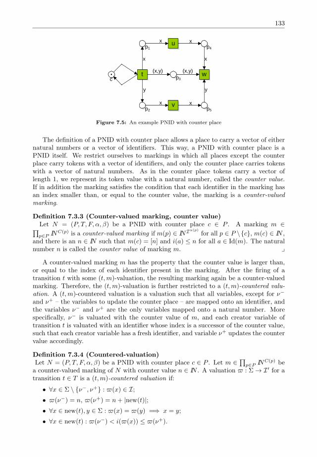
133
u
t
v
wc
p1
p2
p3
p4
p5
(x,y)
x
y
x
(x,y)
x
x
x x
y
Figure 7.5: An example PNID with counter place
The definition of a PNID with counter place allows a place to carry a vector of eithernatural numbers or a vector of identifiers. This way, a PNID with counter place is aPNID itself. We restrict ourselves to markings in which all places except the counterplace carry tokens with a vector of identifiers, and only the counter place carries tokenswith a vector of natural numbers. As in the counter place tokens carry a vector oflength 1, we represent its token value with a natural number, called the counter value.If in addition the marking satisfies the condition that each identifier in the marking hasan index smaller than, or equal to the counter value, the marking is a counter-valuedmarking.
Definition 7.3.3 (Counter-valued marking, counter value)Let N = (P, T, F, α, β) be a PNID with counter place c ∈ P . A marking m ∈∏p∈P IN
C(p) is a counter-valued marking if m(p) ∈ INIα(p)
for all p ∈ P \c, m(c) ∈ IN ,and there is an n ∈ IN such that m(c) = [n] and i(a) ≤ n for all a ∈ Id(m). The naturalnumber n is called the counter value of marking m. y
A counter-valued marking m has the property that the counter value is larger than,or equal to the index of each identifier present in the marking. After the firing of atransition t with some (t,m)-valuation, the resulting marking again be a counter-valuedmarking. Therefore, the (t,m)-valuation is further restricted to a (t,m)-countered valu-ation. A (t,m)-countered valuation is a valuation such that all variables, except for ν−
and ν+ – the variables to update the counter place – are mapped onto an identifier, andthe variables ν− and ν+ are the only variables mapped onto a natural number. Morespecifically, ν− is valuated with the counter value of m, and each creator variable oftransition t is valuated with an identifier whose index is a successor of the counter value,such that each creator variable has a fresh identifier, and variable ν+ updates the countervalue accordingly.
Definition 7.3.4 (Countered-valuation)Let N = (P, T, F, α, β) be a PNID with counter place c ∈ P . Let m ∈
∏p∈P IN
C(p) bea counter-valued marking of N with counter value n ∈ IN . A valuation ϖ : Σ → I ′ for atransition t ∈ T is a (t,m)-countered valuation if:
• ∀x ∈ Σ \ ν−, ν+ : ϖ(x) ∈ I;• ϖ(ν−) = n, ϖ(ν+) = n+ |new(t)|;• ∀x ∈ new(t), y ∈ Σ : ϖ(x) = ϖ(y) =⇒ x = y;
• ∀x ∈ new(t) : ϖ(ν−) < i(ϖ(x)) ≤ ϖ(ν+).
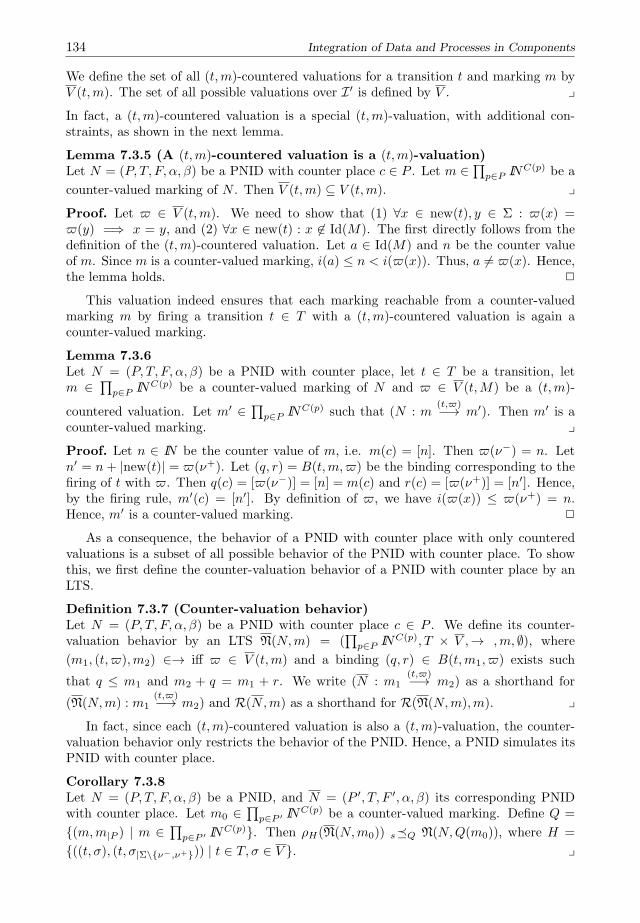
134 Integration of Data and Processes in Components
We define the set of all (t,m)-countered valuations for a transition t and marking m byV (t,m). The set of all possible valuations over I ′ is defined by V . yIn fact, a (t,m)-countered valuation is a special (t,m)-valuation, with additional con-straints, as shown in the next lemma.
Lemma 7.3.5 (A (t,m)-countered valuation is a (t,m)-valuation)Let N = (P, T, F, α, β) be a PNID with counter place c ∈ P . Let m ∈
∏p∈P IN
C(p) be a
counter-valued marking of N . Then V (t,m) ⊆ V (t,m). yProof. Let ϖ ∈ V (t,m). We need to show that (1) ∀x ∈ new(t), y ∈ Σ : ϖ(x) =ϖ(y) =⇒ x = y, and (2) ∀x ∈ new(t) : x ∈ Id(M). The first directly follows from thedefinition of the (t,m)-countered valuation. Let a ∈ Id(M) and n be the counter valueof m. Since m is a counter-valued marking, i(a) ≤ n < i(ϖ(x)). Thus, a = ϖ(x). Hence,the lemma holds. 2
This valuation indeed ensures that each marking reachable from a counter-valuedmarking m by firing a transition t ∈ T with a (t,m)-countered valuation is again acounter-valued marking.
Lemma 7.3.6Let N = (P, T, F, α, β) be a PNID with counter place, let t ∈ T be a transition, letm ∈
∏p∈P IN
C(p) be a counter-valued marking of N and ϖ ∈ V (t,M) be a (t,m)-
countered valuation. Let m′ ∈∏p∈P IN
C(p) such that (N : m(t,ϖ)−→ m′). Then m′ is a
counter-valued marking. yProof. Let n ∈ IN be the counter value of m, i.e. m(c) = [n]. Then ϖ(ν−) = n. Letn′ = n+ |new(t)| = ϖ(ν+). Let (q, r) = B(t,m,ϖ) be the binding corresponding to thefiring of t with ϖ. Then q(c) = [ϖ(ν−)] = [n] = m(c) and r(c) = [ϖ(ν+)] = [n′]. Hence,by the firing rule, m′(c) = [n′]. By definition of ϖ, we have i(ϖ(x)) ≤ ϖ(ν+) = n.Hence, m′ is a counter-valued marking. 2
As a consequence, the behavior of a PNID with counter place with only counteredvaluations is a subset of all possible behavior of the PNID with counter place. To showthis, we first define the counter-valuation behavior of a PNID with counter place by anLTS.
Definition 7.3.7 (Counter-valuation behavior)Let N = (P, T, F, α, β) be a PNID with counter place c ∈ P . We define its counter-valuation behavior by an LTS N(N,m) = (
∏p∈P IN
C(p), T × V ,→ ,m, ∅), where
(m1, (t,ϖ),m2) ∈→ iff ϖ ∈ V (t,m) and a binding (q, r) ∈ B(t,m1, ϖ) exists such
that q ≤ m1 and m2 + q = m1 + r. We write (N : m1(t,ϖ)−→ m2) as a shorthand for
(N(N,m) : m1(t,ϖ)−→ m2) and R(N,m) as a shorthand for R(N(N,m),m). y
In fact, since each (t,m)-countered valuation is also a (t,m)-valuation, the counter-valuation behavior only restricts the behavior of the PNID. Hence, a PNID simulates itsPNID with counter place.
Corollary 7.3.8Let N = (P, T, F, α, β) be a PNID, and N = (P ′, T, F ′, α, β) its corresponding PNIDwith counter place. Let m0 ∈
∏p∈P ′ INC(p) be a counter-valued marking. Define Q =
(m,m|P ) | m ∈∏p∈P ′ INC(p). Then ρH(N(N,m0)) s≼Q N(N,Q(m0)), where H =
((t, σ), (t, σ|Σ\ν−,ν+)) | t ∈ T, σ ∈ V . y
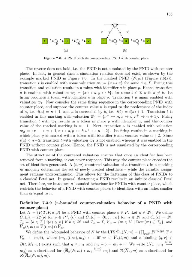
135
t u vp q
x x y y
(a)
t u vp q
x x y y
c
v+ v+v- v-
(b)
Figure 7.6: A PNID with its corresponding PNID with counter place
The reverse does not hold, i.e. the PNID is not simulated by the PNID with counterplace. In fact, in general such a simulation relation does not exist, as shown by theexample marked PNID in Figure 7.6. In the marked PNID (N,m) (Figure 7.6(a)),transition t is enabled with some valuation ϖ1 = x 7→ a for some a ∈ I. Firing thistransition and valuation results in a token with identifier a in place p. Hence, transitionu is enabled with valuation ϖ2 = x 7→ a, y 7→ b, for some b ∈ I with a = b. Itsfiring produces a token with identifier b in place q. Transition t is again enabled withvaluation ϖ1. Now consider the same firing sequence in the corresponding PNID withcounter place, and suppose the counter value n is equal to the predecessor of the indexof a, i.e. i(a) = n + 1, and a is succeeded by b, i.e. i(b) = i(a) + 1. Transition t isenabled in this marking with valuation ϖ1 = ν− 7→ n, x 7→ a, ν+ 7→ n + 1. Firingtransition t with ϖ1 results in a token in place p with identifier a, and the countervalue of the reached marking is n + 1. Next, transition u is enabled with valuationϖ2 = ν− 7→ n + 1, x 7→ a, y 7→ b, ν+ 7→ n + 2. Its firing results in a marking inwhich place q is marked with a token with identifier b and counter value n + 2. Sincei(a) < n+2, transition t with valuation ϖ1 is not enabled, whereas it was enabled in thePNID without counter place. Hence, the PNID is not simulated by the correspondingPNID with counter place.
The structure of the countered valuation ensures that once an identifier has beenremoved from a marking, it can never reappear. This way, the counter place encodes theset of identifiers generated. A (t,m)-countered valuation of a transition t in a markingm uniquely determines the set of newly created identifiers – while the variable assign-ment remains undeterministic. This allows for the flattening of this class of PNIDs toa classical Petri net. In general, flattening a PNID results in an infinite classical Petrinet. Therefore, we introduce n-bounded behaviour for PNIDs with counter place, whichrestricts the behavior of a PNID with counter places to identifiers with an index smallerthan or equal to n.
Definition 7.3.9 (n-bounded counter-valuation behavior of a PNID withcounter place)Let N = (P, T, F, α, β) be a PNID with counter place c ∈ P . Let n ∈ IN . We defineCn(p) = Iαn (p) for p ∈ P \ c and Cn(c) = 0, . . . , n for n ∈ IN and Cω(c) = IN .In = a ∈ I | i(a) ≤ n if n ∈ IN and Iω = I, V n = ϖ ∈ V | Dom(ϖ) ⊆ In, andV n(t,m) = V (t,m) ∩ V n.
We define the n-bounded behavior of N by the LTS Nn(N,m) = (∏p∈P IN
Cn(p), T ×Vn,→ ,m, ∅), where (m1, (t,ϖ),m2) ∈→ iff ϖ ∈ V n(t,m) and a binding (q, r) ∈B(t,M1, ϖ) exists such that q ≤ m1 and m2 + q = m1 + r. We write (Nn : m1
(t,ϖ)−→m2) as a shorthand for (Nn(N,m) : m1
(t,ϖ)−→ m2) and R(Nn,m) as a shorthand forR(Nn(N,m),m). y
136 Integration of Data and Processes in Components
In the flattening, we create for each place p in the PNID a place pa for each possibletoken value a ∈ Iα(p). For each transition t and possible (t,m)-countered valuation ϖ,we create a new transition tϖ, which we connect to the places pa defined by the presetof t and the valuation.
Definition 7.3.10 (Flattening PNID with counter place)Let N = (P, T, F, α, β) be a PNID with counter place. Let n ∈ IN . We define then-bounded flattened Petri net Nn = (P , T , F ) by:
P = pa | p ∈ P ∧ a ∈ Cn(p)T = tϖ | t ∈ T ∧ϖ ∈ VnF = (p
ϖ((p,t)), tϖ) | (p, t) ∈ F ∩ (P × T ) ∧ϖ ∈ Vn
∪ (tϖ, pϖ((p,t))) | (t, p) ∈ F ∩ (T × P ) ∧ϖ ∈ Vn
y
Lemma 7.3.11 (n-bounded flattening is finite)Let N = (P, T, F, α, β) be a PNID with counter place. Let n ∈ IN . Then its flattenednet Nn = (P , T , F ) is finite. y
Proof. To show that Nn is finite, we need to show that both P and T are finite. Wehave |P | =
∑p∈P (n + 1)α(p) and |T | = |T | · (n + 1)|Σ(N)|. As Σ(N) is finite, also |T | is
finite. 2
Consider the example marked PNID with counter place (N,M0) of Figure 7.5. Fig-ure 7.7 shows the flattened net N2. Note that there is no valuation ϖ for transition twith ϖ(ν−) = 1, since then ϖ(ν+) = 3, which is not in I2. Removing all dead partsfrom N2 results in the net depicted in Figure 7.8.
To compare the counter-valuation behavior of the PNID with counter place with thebehavior defined by the flattened classical net, we need to translate the marking of thePNID into a marking of the flattened classical net. Therefore, we introduce the bijectivefunction M that maps each token of the coloured net to the corresponding place in theflattened net.
Definition 7.3.12 (Mapping of markings of a PNID with counter place to itsflattened net)Let n ∈ IN , N = (P, T, F, α, β) be a PNID with counter place c ∈ P , and let Nn =
(P , T , F ) be its flattened Petri net. We define the relation M :∏p∈P IN
Cn(p) → IN P by
M(m) = m⇔ ( ∀p ∈ P, a ∈ Cn(p) : m(p)(a) = m(pa) )
for m ∈∏p∈P IN
Cn(p) and m ∈ IN P . y
An important property of this mapping function is that it distributes over bag addi-tion: the mapping of the sum of two markings is identical to the sum of the mapping ofboth markings, as shown in the next corollary.
Corollary 7.3.13 (Mapping distributes over addition)Let m1,m2 ∈
∏p∈P IN
C(p). Then M(m1 +m2) = M(m1) +M(m2). y

137
c0
c1
c2
t2
t1
p1,0
p1,1
p1,2 p4,2
p4,1
p4,0
p5,2
p5,1
p5,0
p2,2
p2,1
p4,0
p3,(0,0)
p3,(0,1)
p3,(0,2)
p3,(1,0)
p3,(1,1)
p3,(1,2)
p3,(2,0)
p3,(2,1)
p3,(2,2)
u1
u2
u3
v1
v2
v3
w1
w2
w3
w4
w5
w6
w7
w8
w9
Figure 7.7: The flattening of Figure 7.5 for a marking m with Cm = 2 and I = IN
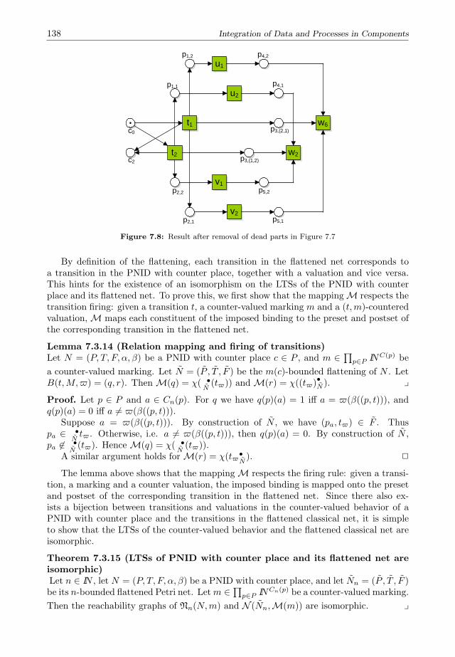
138 Integration of Data and Processes in Components
c0
c2
t2
t1
p1,1
p1,2 p4,2
p4,1
u1
u2
p5,2
p5,1
p2,2
p2,1
v1
v2
p3,(1,2)
p3,(2,1)
w2
w6
Figure 7.8: Result after removal of dead parts in Figure 7.7
By definition of the flattening, each transition in the flattened net corresponds toa transition in the PNID with counter place, together with a valuation and vice versa.This hints for the existence of an isomorphism on the LTSs of the PNID with counterplace and its flattened net. To prove this, we first show that the mapping M respects thetransition firing: given a transition t, a counter-valued marking m and a (t,m)-counteredvaluation, M maps each constituent of the imposed binding to the preset and postset ofthe corresponding transition in the flattened net.
Lemma 7.3.14 (Relation mapping and firing of transitions)Let N = (P, T, F, α, β) be a PNID with counter place c ∈ P , and m ∈
∏p∈P IN
C(p) be
a counter-valued marking. Let N = (P , T , F ) be the m(c)-bounded flattening of N . LetB(t,M,ϖ) = (q, r). Then M(q) = χ( •
N(tϖ)) and M(r) = χ((tϖ)
•N ). y
Proof. Let p ∈ P and a ∈ Cn(p). For q we have q(p)(a) = 1 iff a = ϖ(β((p, t))), andq(p)(a) = 0 iff a = ϖ(β((p, t))).
Suppose a = ϖ(β((p, t))). By construction of N , we have (pa, tϖ) ∈ F . Thuspa ∈ •
Ntϖ. Otherwise, i.e. a = ϖ(β((p, t))), then q(p)(a) = 0. By construction of N ,
pa ∈ •N(tϖ). Hence M(q) = χ( •
N(tϖ)).
A similar argument holds for M(r) = χ(tϖ•N). 2
The lemma above shows that the mapping M respects the firing rule: given a transi-tion, a marking and a counter valuation, the imposed binding is mapped onto the presetand postset of the corresponding transition in the flattened net. Since there also ex-ists a bijection between transitions and valuations in the counter-valued behavior of aPNID with counter place and the transitions in the flattened classical net, it is simpleto show that the LTSs of the counter-valued behavior and the flattened classical net areisomorphic.
Theorem 7.3.15 (LTSs of PNID with counter place and its flattened net areisomorphic)Let n ∈ IN , let N = (P, T, F, α, β) be a PNID with counter place, and let Nn = (P , T , F )be its n-bounded flattened Petri net. Letm ∈
∏p∈P IN
Cn(p) be a counter-valued marking.
Then the reachability graphs of Nn(N,m) and N (Nn,M(m)) are isomorphic. y
139
Proof. Let H = ((t,ϖ), tϖ) | t ∈ T,ϖ ∈ V . Relation H is a total bijective function.Since also relation M is a total bijective function, it is sufficient to prove the theorem byshowing that a transition t ∈ T with a valuation ϖ can fire in N if and only if transitiontϖ can fire in the flattened net N .
Let m1,m2 ∈∏p∈P IN
Cn(p) be two markings of N , t ∈ T a transition of N and
ϖ ∈ Vn(t,m1) be a (t,m1)-countered valuation such that (Nn : m1(t,ϖ)−→ m2). Define
B(t,m1, ϖ) = (q, r). Then
(Nn : m1(t,ϖ)−→ m2)
≡ Definition of firing rule m2 + q = m1 + r
≡ Relation M is a bijective function M(m2 + q) = M(m1 + r)
≡ Relation M distributes over addition M(m2) +M(q) = M(m1) +M(r)
≡ Lemma 7.3.14 M(m2) + χ( •
N(tϖ)) = M(m1) + χ((tϖ)
•N )
≡ Firing rule for Petri nets
(N : M(m1)tϖ−→ M(m2))
2
The theorem above shows that if we bound the counter-valuation behavior of a PNIDwith counter place, the reachability graphs of the PNID and its flattened net are isomor-phic. Therefore, the reachability problem for PNIDs with counter place is decidable.
7.4 Generation of Database Transactions
As shown in Chapter 3, a component consists of a data view and a process view. Acomponent needs to retrieve and update all kinds of data. This requires both concurrenthandling of transactions and maintaining consistency of the data. In this section, we showa method to integrate objects and Petri nets with identifiers. We model objects and theirrelations using object models. An Entity Relationship Diagram (ERD), as introducedby Chen [34] is a subset of the object models, as it does not support inheritance. Givena database instance consisting of entities and relations, each entity belongs to a certainentity type, and each association between two entities is of a certain relation betweentwo entity types. Each entity in an association should be of the right entity type definedby the relation. If this is the case, and the associations do not violate the cardinalityconstraints, the database instance is consistent.
Each ERD has a straightforward translation into a PNID: each entity type E corre-sponds to a place pA with vectors of identifiers of length 1 (i.e. α(pA) = 1), and eachrelation R corresponds to a place pR containing vectors of identifiers of length 2 (i.e.α(pR) = 2), as shown in Figure 7.9. A marking of such a PNID, i.e. the tokens ineach place resemble an entity, if it carries a single identifier, or an association betweentwo entities (a token with a pair of identifiers). This way, the marking of the PNIDrepresents the database instance of the specified ERD. If a transition needs an entity
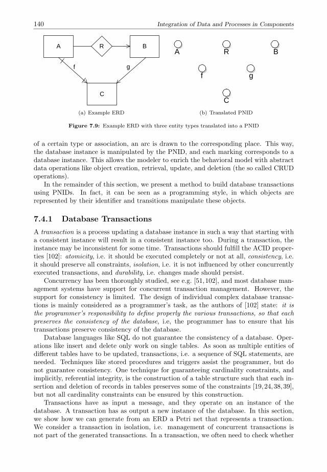
140 Integration of Data and Processes in Components
A BR
C
f g
(a) Example ERD
A R B
C
f g
(b) Translated PNID
Figure 7.9: Example ERD with three entity types translated into a PNID
of a certain type or association, an arc is drawn to the corresponding place. This way,the database instance is manipulated by the PNID, and each marking corresponds to adatabase instance. This allows the modeler to enrich the behavioral model with abstractdata operations like object creation, retrieval, update, and deletion (the so called CRUDoperations).
In the remainder of this section, we present a method to build database transactionsusing PNIDs. In fact, it can be seen as a programming style, in which objects arerepresented by their identifier and transitions manipulate these objects.
7.4.1 Database Transactions
A transaction is a process updating a database instance in such a way that starting witha consistent instance will result in a consistent instance too. During a transaction, theinstance may be inconsistent for some time. Transactions should fulfill the ACID proper-ties [102]: atomicity, i.e. it should be executed completely or not at all, consistency, i.e.it should preserve all constraints, isolation, i.e. it is not influenced by other concurrentlyexecuted transactions, and durability, i.e. changes made should persist.
Concurrency has been thoroughly studied, see e.g. [51,102], and most database man-agement systems have support for concurrent transaction management. However, thesupport for consistency is limited. The design of individual complex database transac-tions is mainly considered as a programmer’s task, as the authors of [102] state: it isthe programmer’s responsibility to define properly the various transactions, so that eachpreserves the consistency of the database, i.e, the programmer has to ensure that histransactions preserve consistency of the database.
Database languages like SQL do not guarantee the consistency of a database. Oper-ations like insert and delete only work on single tables. As soon as multiple entities ofdifferent tables have to be updated, transactions, i.e. a sequence of SQL statements, areneeded. Techniques like stored procedures and triggers assist the programmer, but donot guarantee consistency. One technique for guaranteeing cardinality constraints, andimplicitly, referential integrity, is the construction of a table structure such that each in-sertion and deletion of records in tables preserves some of the constraints [19,24,38,39],but not all cardinality constraints can be ensured by this construction.
Transactions have as input a message, and they operate on an instance of thedatabase. A transaction has as output a new instance of the database. In this section,we show how we can generate from an ERD a Petri net that represents a transaction.We consider a transaction in isolation, i.e. management of concurrent transactions isnot part of the generated transactions. In a transaction, we often need to check whether
141
a specific instance of a relation or entity exists. Therefore, we base a transaction onPNIDs with inhibitor arcs.
Definition 7.4.1 (Transaction)Let S = (O,A, ∅,R, σ, τ) be an ERD, and IS = (IO, IA, IR) be an instance of it. Atransaction on IS is a a marked IPNID (N,m) with N = (Pin∪Pdb∪Ph, T, F,H, α, β, γ),where Pin is the set of input places, Pdb = (E ∪R) is the set of database places, Ph is theset of internal places, and Pin, Pdb and Ph are pairwise disjoint. For all places p ∈ Phholds m(p) = ∅, for all places A ∈ (E ∩ Pdb) holds m(A) = IO(A), and for all placesr ∈ R ∩ Pin holds m(r) = IR(r). y
Note that many transactions share the same Petri net specification, and only differ inthe initial marking.
After the execution of the transaction on a consistent instance, the new instanceshould be consistent again, and there should not be “garbage” in the net and no tran-sitions of the transaction should be enabled, i.e. in the final marking, there are notransitions enabled, and all internal and input places are empty. We call this propertydatabase soundness.
Definition 7.4.2 (Sound transaction)A transaction is called db-sound if and only if it satisfies the following two properties:
1. for all reachable markings, a final marking is reachable in which all internal placesare in their initial state, and the input places are empty,
2. the final database instance satisfies all cardinality constraints, if the initial instancealso satisfied the cardinality constraints. y
We present algorithms in the form of PNIDs that generate, given an ERD, three typesof transactions: (1) delete transactions, (2) update transactions, and (3) complex inserttransactions. In all cases, these transactions will be sound, which can easily be verifiedby inspection of the constructed Petri nets.
7.4.2 Deletion Transactions
When an entity has been deleted, consistency of the newly created instance should beverified. The removal of an entity also requires the removal of the associations it is con-nected to. This can cause the instance to violate the cardinality constraints. If deletion ofthe entity causes the instance to be inconsistent, either the deletion should be canceled,or the deletion should be cascaded to other entities as well. In this subsection, we focuson cascading. Figure 7.10 shows the deletion of an instance. For each relationship r withsource or target entity type A, there is one subnet (depicted by the rectangles). Theprocesses in these subnets can be executed concurrently, denoted by three rectangles;nodes outside the rectangles, connected to a node within the rectangles, are connectedto each subnet. If the cardinality between A and r is 0..∗ or 0..1, the Petri net of Fig-ure 7.10(a) is generated. Otherwise, the Petri net of Figure 7.10(b) is generated. Inboth Petri nets, if a does not exist in the current instance, transition nex A is enabled.Otherwise, transition del A deletes the entity from A and propagates the token to eachsubnet. Next, all associations with a are removed from r by transition del r, until thereare no associations with a left, and transition fin r becomes enabled. Depending on thecardinality of relation r on target entity type B, the associated elements of a need to

142 Integration of Data and Processes in Components
del Adel A
nex A A
a
a
a
a
a
(a,b)
fin r
del ra
(a,b)
r
(a) Cτ (r) ∈ 0..1, 0..∗
del Adel A
nex A A
a
a
a
a
a
(a,b)
fin r
del ra
(a,b)
(a,b)
ex r
b b
b
b
(a,b)
nex r del B
r
(b) Cτ (r) ∈ 1..1, 1..∗
Figure 7.10: Delete transaction for entity A
be deleted. If the relation r is optional for B, i.e. Cτ (r) ∈ 0..∗, 0..1, the constraintsfor the associated elements are not violated, and therefore need no check whether theyshould be removed.If r is mandatory, i.e. Cτ (r) ∈ 1..∗, 1..1, transition del r producesa token with the associated entity b. If b is connected to a different entity of type A, bdoes not violate the cardinality constraints, which is tested by transition ex. If there isno such entity, the associated entity b needs to be deleted as well, and thus, transitionnex is enabled and produces a token with identifier b in place del B. This place is theinitial place of the generated deletion transaction of entity B.
The generated transaction is db-sound, since transition del r can only fire as manytimes as there are associations with entity a, which is a bounded number of times. Worstcase, the procedure can be called for each associated entity, which is again a boundednumber of times. Therefore, eventually, the transaction will reach a marking in whichno transition is enabled, and all places, except the places representing the entity typesand relations, are empty. The second property of soundness is trivial.
Consider again the ERD depicted in Figure 7.9. Deletion of A propagates to deletingassociations from R. As B has zero or more associations of type R, deleting an associ-ation with A does not violate the cardinality constraints. The same holds for removingan association of relation g. When removing an association of relation f , for both en-tity types A and C the instance need to be verified. The resulting PNID is shown inFigure 7.11.
7.4.3 Update Transactions
When an entity is substituted for another entity, all relations the entity is associated with,either as source or as target, need to be updated as well. We focus on the substitutionof a single entity. The update transaction generated uses the construction shown inFigure 7.12. The transaction takes entities a and a′ of type A, where a is the entity tobe substituted, and a′ the entity to substitute with. If a is not present in the currentinstance, transition nex a is enabled. Otherwise, transition ex a is enabled. In the firstcase, the entity to substitute is disregarded. In the latter case, it is checked whether a′
exist in the current instance. If there is no token with identifier a′ in place A, transitionnex a’ is enabled and substitution is no problem. Transition ins a removes token a andinserts token a′. Then, in the subnets defined by Update Relations, all associations witha are transformed into associations with a′.
The subnet Update Relations substitutes entity a by entity a′ for each association withsource a. The rectangle shows the subnet which is repeated for each relation. While an
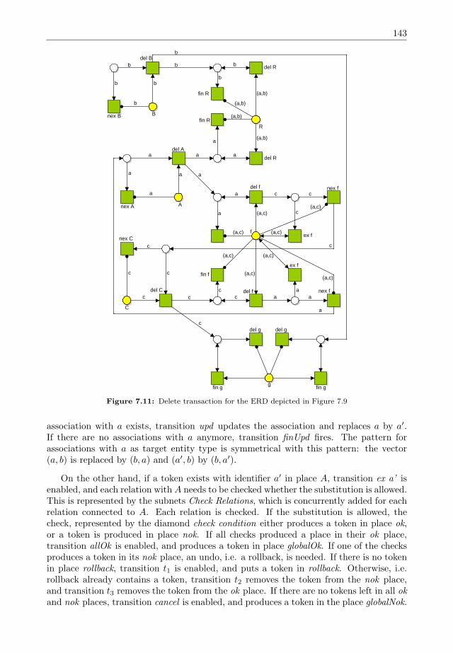
143
b
R
A
C
f
g
del B
nex B
b
b
b
b
b
(a,b)
(a,b)
(a,b)
(a,b)
a
a
aa
a a
a
del A
nex A
b
b
del R
fin R
del R
fin R
a
del f
fin f
a
a
(a,c)
c
(a,c)ex f
nex fc
c(a,c)
(a,c)
cnex C
del C
c
c
c
c
cc
c
(a,c)
(a,c)
(a,c)
(a,c)
a
ex f
nex fa
aa
c
del f
fin g
del g
fin g
del g
B
Figure 7.11: Delete transaction for the ERD depicted in Figure 7.9
association with a exists, transition upd updates the association and replaces a by a′.If there are no associations with a anymore, transition finUpd fires. The pattern forassociations with a as target entity type is symmetrical with this pattern: the vector(a, b) is replaced by (b, a) and (a′, b) by (b, a′).
On the other hand, if a token exists with identifier a′ in place A, transition ex a’ isenabled, and each relation with A needs to be checked whether the substitution is allowed.This is represented by the subnets Check Relations, which is concurrently added for eachrelation connected to A. Each relation is checked. If the substitution is allowed, thecheck, represented by the diamond check condition either produces a token in place ok,or a token is produced in place nok. If all checks produced a place in their ok place,transition allOk is enabled, and produces a token in place globalOk. If one of the checksproduces a token in its nok place, an undo, i.e. a rollback, is needed. If there is no tokenin place rollback, transition t1 is enabled, and puts a token in rollback. Otherwise, i.e.rollback already contains a token, transition t2 removes the token from the nok place,and transition t3 removes the token from the ok place. If there are no tokens left in all okand nok places, transition cancel is enabled, and produces a token in the place globalNok.
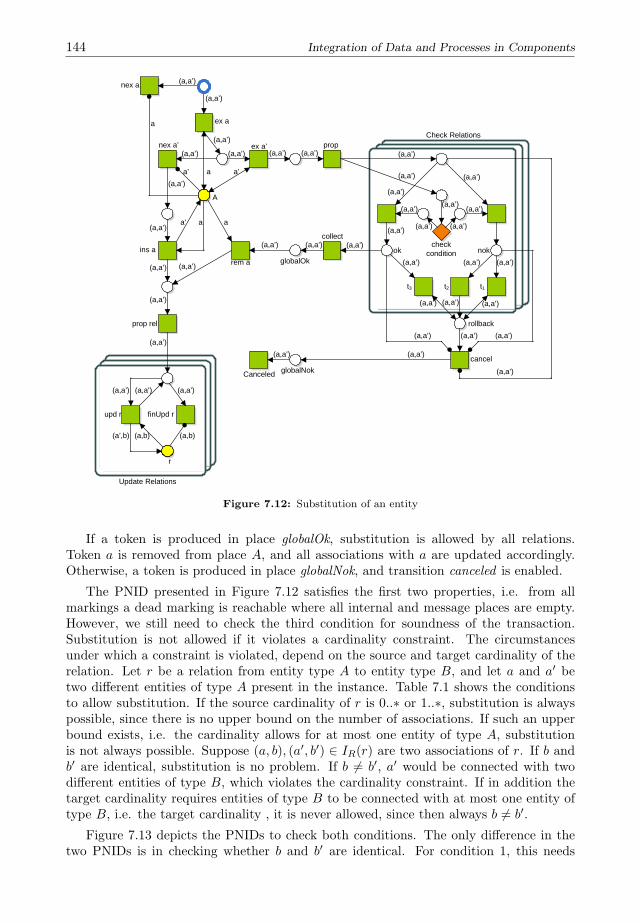
144 Integration of Data and Processes in Components
A
r
(a,a’)
a
a’
(a,a’)
(a,a’)
(a,a’)(a,a’)
aa’
(a,a’)
(a,a’)
(a,a’)
(a,a’)
(a,a’)
(a,a’)
a aa’
nex a
ex a
ex a’nex a’ prop(a,a’) (a,a’) (a,a’)
(a,a’) (a,a’)
rem a globalOk
prop rel
(a,a’)
(a,a’)
(a,a’)(a,a’)
(a,a’) (a,a’)
(a,a’)
(a,a’)
(a,a’)
(a,a’)
(a,a’)
(a,a’)
(a,a’)
(a,a’) (a,a’)
(a,a’)
check condition
t1t2t3
rollback
nokok
globalNok
(a,a’) (a,a’) (a,a’)
(a,a’)
(a,a’)(a,a’)
Canceled
upd r finUpd r
(a,a’) (a,a’) (a,a’)
(a,b)(a,b)(a’,b)
ins a
Update Relations
Check Relations
collect
cancel
Figure 7.12: Substitution of an entity
If a token is produced in place globalOk, substitution is allowed by all relations.Token a is removed from place A, and all associations with a are updated accordingly.Otherwise, a token is produced in place globalNok, and transition canceled is enabled.
The PNID presented in Figure 7.12 satisfies the first two properties, i.e. from allmarkings a dead marking is reachable where all internal and message places are empty.However, we still need to check the third condition for soundness of the transaction.Substitution is not allowed if it violates a cardinality constraint. The circumstancesunder which a constraint is violated, depend on the source and target cardinality of therelation. Let r be a relation from entity type A to entity type B, and let a and a′ betwo different entities of type A present in the instance. Table 7.1 shows the conditionsto allow substitution. If the source cardinality of r is 0..∗ or 1..∗, substitution is alwayspossible, since there is no upper bound on the number of associations. If such an upperbound exists, i.e. the cardinality allows for at most one entity of type A, substitutionis not always possible. Suppose (a, b), (a′, b′) ∈ IR(r) are two associations of r. If b andb′ are identical, substitution is no problem. If b = b′, a′ would be connected with twodifferent entities of type B, which violates the cardinality constraint. If in addition thetarget cardinality requires entities of type B to be connected with at most one entity oftype B, i.e. the target cardinality , it is never allowed, since then always b = b′.
Figure 7.13 depicts the PNIDs to check both conditions. The only difference in thetwo PNIDs is in checking whether b and b′ are identical. For condition 1, this needs
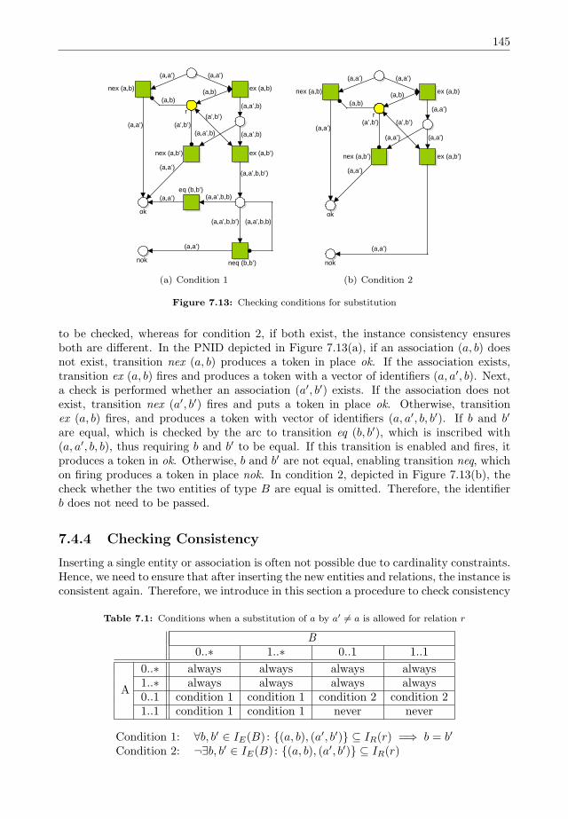
145
r
nex (a,b)
(a,a’) (a,a’)
(a,a’)
(a,a’)
(a,a’)
(a,a’)
ex (a,b)
ex (a,b’)
(a,b)(a,b)
(a,a’,b)
(a,a’,b)(a,a’,b)
(a’,b’)(a’,b’)
(a,a’,b,b’)
(a,a’,b,b’) (a,a’,b,b)
(a,a’,b,b)
nex (a,b’)
eq (b,b’)
neq (b,b’)
ok
nok
(a) Condition 1
nex (a,b)
(a,a’) (a,a’)
(a,a’)
(a,a’)
ex (a,b)
ex (a,b’)
(a,b)(a,b)
(a,a’)
(a,a’)(a,a’)
(a’,b’)
nex (a,b’)
(a’,b’)
ok
nok
r
(a,a’)
(b) Condition 2
Figure 7.13: Checking conditions for substitution
to be checked, whereas for condition 2, if both exist, the instance consistency ensuresboth are different. In the PNID depicted in Figure 7.13(a), if an association (a, b) doesnot exist, transition nex (a, b) produces a token in place ok. If the association exists,transition ex (a, b) fires and produces a token with a vector of identifiers (a, a′, b). Next,a check is performed whether an association (a′, b′) exists. If the association does notexist, transition nex (a′, b′) fires and puts a token in place ok. Otherwise, transitionex (a, b) fires, and produces a token with vector of identifiers (a, a′, b, b′). If b and b′
are equal, which is checked by the arc to transition eq (b, b′), which is inscribed with(a, a′, b, b), thus requiring b and b′ to be equal. If this transition is enabled and fires, itproduces a token in ok. Otherwise, b and b′ are not equal, enabling transition neq, whichon firing produces a token in place nok. In condition 2, depicted in Figure 7.13(b), thecheck whether the two entities of type B are equal is omitted. Therefore, the identifierb does not need to be passed.
7.4.4 Checking Consistency
Inserting a single entity or association is often not possible due to cardinality constraints.Hence, we need to ensure that after inserting the new entities and relations, the instance isconsistent again. Therefore, we introduce in this section a procedure to check consistency
Table 7.1: Conditions when a substitution of a by a′ = a is allowed for relation r
B0..∗ 1..∗ 0..1 1..1
A
0..∗ always always always always1..∗ always always always always0..1 condition 1 condition 1 condition 2 condition 21..1 condition 1 condition 1 never never
Condition 1: ∀b, b′ ∈ IE(B) : (a, b), (a′, b′) ⊆ IR(r) =⇒ b = b′
Condition 2: ¬∃b, b′ ∈ IE(B) : (a, b), (a′, b′) ⊆ IR(r)
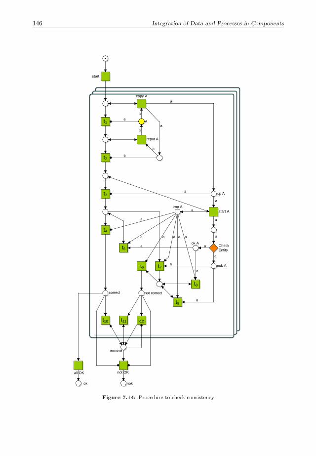
146 Integration of Data and Processes in Components
A
start
copy A
reput A
cp A
tmp Astart A
Check Entity
ok nok
all OK not OK
remove
a
a
aa
a
a
a
t1
t2
t3
t4
t5
t6 t7
t8
t9
t10 t11 t12
a
a
a
a
a
a
a
aaaaa
a
a
a
a
a
ok A
nok A
correct not correct
Figure 7.14: Procedure to check consistency

147
check relations
check condition
ok A nok A
all OK
a
nok r
a
a
a
a
a
ok r
a a a a
aaa a
a
a
a
t1t2t3
a
a
a
a
ca
not OK
Figure 7.15: Check Entity
using PNIDs. The main Petri net is show in Figure 7.14. The model checks for eachentity whether the cardinality constraints are satisfied. If all constraints are satisfied,a token is produced in place ok. Otherwise, a token is produced in place nok. Theprocedure consists of two stages. In the first stage, the tokens present in entity A arecopied to place cp A by transition copy A. If all entities are copied, transition t1 fires,and all entities are placed back in place A by transition reput A. If all entities are placedback, transition t2 is enabled. This construction ensures that after firing of transition t2,place A is marked as in the initial marking. Note that after the firing of transition t2,the marking of place cp A is identical to place A. Furthermore, the construction ensuresthat transition t3 can only fire if the marking of place A and tmp A are identical.
In the next stage, the entities are checked, represented by the diamond Check Entity.The diamond either produces a token in place ok A or in place nok A. The place tmp Akeeps track of the entities that are being checked. The diamond check Entity representsthe choice whether the entity is correct or not. It either produces a token in place ok A,or a token in nok A. Transition t5 removes all checked entities that were correct. If allentities are correct, a token is produced in place correct by transition t4. If all entitieshave a token in correct, the whole instance is correct, and transition all OK is enabled.If an entity was not correct, i.e. the entity violates a cardinality constraint, transitiont7 becomes enabled, and transition t4 cannot become enabled for this entity type. Uponfiring of transition t7, transition t5 cannot become enabled. Transitions t7, t8 and t9clean up all tokens in nok A and ok A. When all tokens have been cleaned up, transitiont6 becomes enabled and produces a token in place incorrect. Since transitions t4 and t6
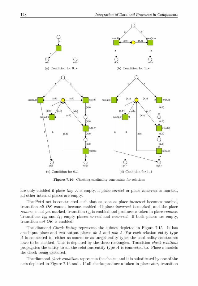
148 Integration of Data and Processes in Components
ok r
a
a
nok r
(a) Condition for 0..∗
r
ok r
a
nok r
a
(a,b) (a,b)
a a
ex(a,b) nex(a,b)
(b) Condition for 1..∗
r
ok r
a
nok r
(a,b)nex(a,b) ex(a,b)
a
(a,b)
(a,b)
(a,b)
(a,b)
(a,b)
(a,b)a a
a
(a,b’)
nex(a,b’)(a,b)
(a,b)(a,b’)
replace
ex(a,b’)
(c) Condition for 0..1
r
ok r
a
nok r
(a,b)nex(a,b) ex(a,b)
a
(a,b)
(a,b)
(a,b)
(a,b)
(a,b)
(a,b)a a
a
(a,b’)
nex(a,b’)(a,b)
(a,b)(a,b’)
replace
ex(a,b’)
(d) Condition for 1..1
Figure 7.16: Checking cardinality constraints for relations
are only enabled if place tmp A is empty, if place correct or place incorrect is marked,all other internal places are empty.
The Petri net is constructed such that as soon as place incorrect becomes marked,transition all OK cannot become enabled. If place incorrect is marked, and the placeremove is not yet marked, transition t12 is enabled and produces a token in place remove.Transitions t10 and t11 empty places correct and incorrect. If both places are empty,transition not OK is enabled.
The diamond Check Entity represents the subnet depicted in Figure 7.15. It hasone input place and two output places ok A and nok A. For each relation entity typeA is connected to, either as source or as target entity type, the cardinality constraintshave to be checked. This is depicted by the three rectangles. Transition check relationspropagates the entity to all the relations entity type A is connected to. Place c modelsthe check being executed.
The diamond check condition represents the choice, and it is substituted by one of thenets depicted in Figure 7.16 and . If all checks produce a token in place ok r, transition
149
all OK is enabled. If one of the checks fail, i.e. a token is produced in place nok r,this transition cannot become enabled. As soon as a token is produced in place nok r,transitions t1, t2 and t3 empty the places nok r and ok r. If for each relation these placesare empty, transition not OK fires, and produces a token in place nok A.
For each entity, we need to check whether the associations in which the entity isinvolved, are consistent with the schema. Each association is checked twice: once for thesource, and once for the target. If for all associations both checks succeed, the associationis correct.
For each of the four possible cardinalities, 0..∗, 1..∗, 0..1 and 1..1 we need a differentcheck, as depicted in Figure 7.16. In case the cardinality is 0..∗, the association is alwayscorrect, and for 1..∗, we only need to ensure the presence of at least one association.In case there is at most one association, if such an association exists, transition ex(a, b)consumes this association from place r. If there does not exist another association witha, transition nex(a, b′) is enabled, and a token is produced in ok r. In case there is asecond association with a, transition ex(a, b′) is enabled. After firing this transition,the association consumed by transition ex(a, b) is placed back in place r, and a token isproduced in place nok r.
The difference between the check for 0..1 and 1..1 is the place transition nex(a, b)produces in. In the first, it produces in ok r, in the latter such an association shouldexist, and hence, transition nex(a, b) produces a token in place nok r.
7.5 Conclusions
In this chapter we studied the integration of data objects and processes. For this, weintroduced the class of Petri nets with Identifiers (PNID), in which each token is labeledwith a vector of identifiers. In this chapter, we have shown that, if we define an indexon the identifiers, and this index is well-ordered, reachability is decidable for a subclassof PNIDs. In this class, we define a special place, called the counter place, which keepsthe index of the identifier created last. For each upper bound on the index, and thus, byrestricting the behavior of the PNID to firings that maintain this property, the numberof identifiers created in the PNID is bounded.
In this chapter, we have shown the applicability of PNIDs to the creation and ma-nipulation of data objects in components. In fact, with PNIDs we are able to model thefour basic data operations: creation, retrieval, update, and deletion. Given an ERD, i.e.an object model without inheritance, we are able to generate transactions for each of thefour basic operations that maintain consistency of the database.
By extending the class of Petri nets with Identifiers with coloured inhibitor arcs, weare able to prevent transitions to fire if tokens with a certain valuation exist. This way,the class is powerful enough to model more complex data operations. Using the colouredinhibitor arcs, we are able to model complex database transactions as Petri nets suchthat cardinality constraints in the database model are maintained.
The ability to combine identifiers using a vector allows the modeler to relate objects,and thus allows for modeling message passing. Although vectors allow for relating iden-tifiers, a vector has a fixed length. The model does not allow constructs in which anynumber of identifiers should be related. Also hierarchy is not taken into account, as eachidentifier represents an object, rather than a class of objects.

150 Integration of Data and Processes in Components

8Prototyping Component-Based Information Systems
In this chapter we present a methodology for the first four phases of the development of acomponent-based information system: (1) user requirements, (2) functional architecture,(3) software architecture, and (4) the prototyping phase. The methodology is supportedby a tool consisting of a Petri net based workflow engine, a standard document managerand a standard database system.
8.1 Introduction
In this chapter we describe a methodology for the early stages of the development of acomponent-based information system, resulting in a prototype of the system. Businessunits in an organization typically handle cases. Typical examples of such cases areclaims in an insurance company, patients in a hospital, trip reservations in a travel agentsystem, sales orders in an auctioning system and orders in a manufacturing company. Ina component-based information system, cases are typically related, like the handling ofan invoice at the financial department and the handling of products at the stock.
In the previous chapter, we introduced the notion of identifiers to model messagepassing. In this chapter, we use these identifiers to handle cases. A case is an instance ofa case type. A case type has two characteristics: (1) a workflow, i.e. a partially orderedset of tasks to be performed, and (2) a case document type, an instance of which is a casedocument. Tasks for a case are performed by actors, which are usually human beings,although software agents are becoming widely used as an alternative. Each task requiresa particular view on the case data, and task execution results in updating this view. Atask of the insurance company can be the registration of a claim; at a hospital it couldbe taking the blood pressure of a patient by a nurse. While handling the case, the casedocument may grow and at the end it contains all relevant information about the case.
Case handling usually also requires data that does not depend on a particular case,so-called global data. Global data concerns background information, such as addressesor a product catalogue, and management information, which is aggregated informationover the cases, such as the number of running cases or the total number of cases havingreached a particular state.
A component-based information system consists of (1) a workflow manager for theexecution of workflow processes, (2) a document manager for retrieving and updating
152 Prototyping Component-Based Information Systems
case documents and (3) a database manager (DBMS) for the manipulation of globaldata. The workflow engine determines for each case which tasks are enabled and sends arelevant view of the case document and the global data to the role that will handle thistask.
The design of such a system requires modeling of workflow processes, case documentsand the global data. The methodology we propose is a continuation of the research pre-sented in [61] where use cases are modeled as workflows. In this chapter, the emphasisis on the integration with the data perspective and the use of the prototyping environ-ment. We developed a tool specifically tuned for modeling and prototyping. The toolconsists of a workflow engine YasperWE that is derived from the Petri net modeling toolYasper [59,60], the commercial document manager Infopath (part of the MS Office suite)and a standard ODBC database manager (in our situation MySQL). The specific com-ponents of the prototyping environment are not particularly relevant but more a proofof concept of the approach, i.e. they can be replaced by similar components.
Related work In literature, information systems that handle cases are named casehandling systems (CHS) [17]. a CHS is considered to be more data-driven than a workflowmanagement system. The authors state that too fine grained activities in workflowsystems are restricting the user too much. As a solution to this problem, they proposea less granulated approach by enabling activities based on case data, and by allowing toskip or to redo activities. In our approach, the workflow manager is used to control theoverall process of coarse grained activities, while the document manager regulates theoperations on the case data by defining rules about data dependencies, such as mandatoryor optional data elements. For example, instead of defining the addition, updating anddeletion of products in an offer as different and successive activities, we consider theorder creation just as one activity.
For modeling workflows the Petri net formalism is very suitable [3, 91, 94]. Sincedocument handling requires data manipulation, the formalism of coloured Petri netsand their supporting tools (e.g. [6, 93]) seem to be a good solution for modeling andprototyping component-based information systems, as proposed in e.g. [35,54]. However,handling case documents requires particular functionality that already is available indocument managers. The same holds for data manipulation functions in a databasemanager. It is not very efficient to imitate this functionality in a coloured Petri net tool.In [75] a more general approach for information systems is described, but it does not useformal methods.
This chapter is organized as follows. In Section 8.2 we introduce a running example.We present our design methodology in Section 8.3. In Section 8.4 we show how the toolYasper can be used to model workflow processes. Next, in Section 8.5, we show howInfopath can be used to model case documents and how the case document and workflowprocesses are integrated using our tool YasperWE. Concluding remarks are given in thelast section.
8.2 Running Example
As a running example we consider the development of a generic web shop system. Theweb shop has to serve as a mediating party between customers and suppliers. Theproducts the web shop offers are composed out of parts delivered by several suppliers.Different suppliers may offer the same part. Also the transportation of orders is performedby third parties. The web shop follows the “make-to-order” principle, which means that

153
Figure 8.1: The web shop and its actors
it has no stock and all components are ordered on demand at the different suppliers.Figure 8.1 depicts the web shop and the actors involved in the system.
The system has no domain specific information and therefore can be used in anybranch. To run the system in a specific context, it has to be configurable. Configurationparameters are not only the name of the shop and contact information, but also thepayment scheme and the information whether there are consultations with suppliers andtransporters to make an offer to the customer. If a consultation is needed, also thedecision which supplier and transporter are selected needs to be flexible, i.e. the lowestprice or the fastest delivery time.
Customers can browse through the catalogue of the web shop and select products.These products consist of compulsory and optional parts. The customer can alter theselected product by adding and removing parts. After filling the shopping cart, thecustomer can request an offer for the products in its shopping cart. The web shop thencontacts all suppliers that offer a part present in the offer to ask its price and deliverytime in order to make a proposal to the customer, and selects the suppliers based on thesystem’s decision rule. Also the transporters are contacted to ask when and for whatprice they can deliver. Based on these answers, the system composes the offer. Thecustomer then has a choice to accept or to reject the offer. Based on the configuration,the customer may have to make an initial payment to confirm the offer acceptation.When the offer is accepted and, if required in the configuration, an initial paymenthas been made, the system confirms the selected offers to the chosen suppliers of thedifferent parts, and rejects the other offers. The selected suppliers are paid according tosome payment scheme. After receiving all components, the product is assembled and thetransporter is contacted to send the order to the customer. The customer might have tomake a payment on delivery, depending on the configuration.
8.3 Design Methodology
We present an approach for the first development phases of a component-based informa-tion system, resulting in a prototype of the system. It is important that no programmingis needed to create a prototype. The development starts with the identification of thecase types. In the further development we identify four phases, the User Requirements,the Functional Architecture, the Software Architecture and the Prototype phase. In theuser requirements phase, the system and its functionality are identified and agreed uponwith the client. These requirements are formalized into process and data models in thefunctional architecture phase. The created models also need to be verified in this phase,to give guarantees on the correctness of the system. In the software architecture phase,the models are combined into a component model, and the case document type is for-malized. The case document model, the global data model and the component model arecombined into a prototype during the prototype phase. The prototype will be used tovalidate the user requirements in experiments with (potential) users. Figure 8.2 depicts

154 Prototyping Component-Based Information Systems
Scenario
Entity list
Actor list
Workflow model
CRUD Matrix
Entity Relation model
Life Cycle
Case Data View
Component model
I/O Specification
Prototype
User requirements Functional architecture Software architecture Prototype
Figure 8.2: Deliverables and their dependencies in the different phases
the different deliverables during the phases, and how these deliverables depend on eachother.
8.3.1 User Requirements
In the user requirements phase we focus on functional requirements. This phase cor-responds to the Scoping and Justification activities in the design process presented inSection 1.3. In user requirements, actors, i.e. persons and systems that interact with thesystem in development, and their actions with the component-based information systemare identified. Use cases describe the functionality of the system. A use case is a pieceof functionality involving one or more actors and identified by a set of scenarios. A sce-nario is a sequence of actions; it can be either a positive scenario, describing the allowedbehaviour, or a negative scenario, describing the undesired behaviour. These scenariosare often decided in consultation with the client. A natural way to model scenarios isusing Message Sequence Charts (MSC) [85], to express what actions are taken by whomand in what order. In the next phase, the use cases are formalized with process models.
Part of the user requirements are the data objects involved in the system. These arethe objects that the actors store, manipulate and retrieve with the system. In the userrequirements phase, different data object types are identified and listed together withtheir attributes and relations.
The output of this phase is a document describing the desired functionality of thesystem in user-understandable terms, and it can be regarded as a contract between theclient and the developer.
In the running example, we only distinct a single notion as case type: the order of acustomer. We can identify the actors “Customer”, “Supplier”, “Transporter”, “Assem-bler”, “Bank” and “System”.
A Customer can browse the catalogue, select products, add or remove parts, add aconfigured product to its shopping cart, request for an offer, and accept or reject anoffer. The supplier can send offers to the system for a part and deliver ordered parts.The transporter can send an offer to the system, pick up orders and deliver them. Theassembler assembles parts into a product. The bank can confirm and make payments.
Use cases of the web shop are e.g. the composition of a product by a customer, therequest for an offer by a customer, the acceptance of an offer by a customer, the orderingof components at the suppliers, and the assembly and delivery of the product.
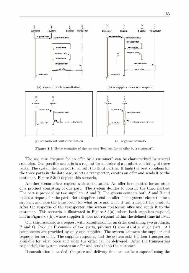
155
(a) scenario with consultation (b) a supplier does not respond
(c) scenario without consultation (d) negative scenario
Figure 8.3: Some scenarios of the use case“Request for an offer by a customer”.
The use case “request for an offer by a customer” can be characterized by severalscenarios. One possible scenario is a request for an order of a product consisting of threeparts. The system decides not to consult the third parties. It finds the best suppliers forthe three parts in the database, selects a transporter, creates an offer and sends it to thecustomer. Figure 8.3(c) depicts this scenario.
Another scenario is a request with consultation. An offer is requested for an orderof a product consisting of one part. The system decides to consult the third parties.The part is provided by two suppliers, A and B. The system contacts both A and B andmakes a request for the part. Both suppliers send an offer. The system selects the bestsupplier, and asks the transporter for what price and when it can transport the product.After the response of the transporter, the system creates an offer and sends it to thecustomer. This scenario is illustrated in Figure 8.3(a), where both suppliers respond,and in Figure 8.3(b), where supplier B does not respond within the defined time interval.
Our third scenario is a request with consultation for an order containing two products,P and Q. Product P consists of two parts, product Q consists of a single part. Allcomponents are provided by only one supplier. The system contacts the supplier andrequests for an offer. The supplier responds, and the system asks the four transportersavailable for what price and when the order can be delivered. After the transportersresponded, the system creates an offer and sends it to the customer.
If consultation is needed, the price and delivery time cannot be computed using the
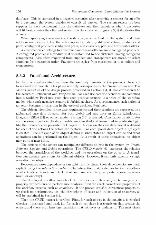
156 Prototyping Component-Based Information Systems
database. This is expressed in a negative scenario: after receiving a request for an offerby a customer, the system decides to consult all parties. The system selects the bestsupplier for each component from the database and then calculates what transporterwill fit best, creates the offer and sends it to the customer. Figure 8.3(d) illustrates thisscenario.
When specifying the scenarios, the data objects involved in the system and theirrelations are identified. For the web shop we can identify different actors, products andparts, configured products, configured parts, and customer, part and transporter offers.
A customer order belongs to a customer and it is an offer for some configured products.A configured product is a product that is customized by the customer, having configuredcomponents. Also offers requested from suppliers and transporters are stored, to selectsuppliers for a customer order. Payments are either from customers or to suppliers andtransporters.
8.3.2 Functional Architecture
In the functional architecture phase the user requirements of the previous phase areformalized into models. This phase not only corresponds to the Formalization and Val-idation activities of the design process presented in Section 1.3, it also corresponds tothe activities Refinement and Verification. For each use case the scenarios are combinedinto a workflow Petri net, such that each positive scenario is a trace of the workflowmodel, while each negative scenario is forbidden there. As a consequence, each action ofan actor becomes a transition in the created workflow Petri net.
The objects identified in the user requirements and their relations are separated intoglobal and case data objects. For both global and case data an Entity-RelationshipDiagram (ERD) [34] or object model (Section 2.6) is created. Constraints on attributesand between objects in the data models are identified and formalized in predicate logic,like the framework we presented in Chapter 3. A view on the case data model is definedfor each of the actions the actors can perform. For each global data object a life cycleis created. The life cycle of an object defines in what states an object can be and whatoperations can be performed on the object. As a result of these operations, an objectmay go to a next state.
The actions of the actors can manipulate different objects in the system by Create,Retrieve, Update, and Delete operations. The CRUD matrix [61] expresses the relationbetween the transitions of the workflow and the operations on the objects. A transi-tion can execute operations for different objects. However, it can only execute a singleoperation per object.
Between use cases dependencies can exist. In this phase, these dependencies are madeexplicit using the interaction matrix . The interaction matrix defines for two workflowswhat activities interact, and the kind of communication (e.g., request-response, synchro-nized, or one-way).
The developed workflow models of the use cases are then subject to analysis, i.e.property verification and performance analysis. First we check correctness properties ofthe workflow process, such as soundness. If the process satisfies correctness properties,we check its performance, i.e. the throughput of cases and utilization of resources, aswill be explained in Section 8.4.
Then the CRUD matrix is verified. First, for each object in the matrix it is checkedwhether it is created and used, i.e. for each object there is a transition that creates theobject, and there is at least one transition that retrieves or updates it. The next check

157
y
y y y y
y
yyy yyy
y
yy y
yyy yyy
y
yy
y
y
Figure 8.4: The workflow that requests an offer to order a product
is whether the retrieve and update operations are only performed between creating anddeleting the object.
In our example, Figure 8.4 shows the result of combining the scenarios of the use case“Request of an offer by a customer”. The scenarios described in the user requirementsshow that any number of suppliers and transporters can be consulted. We create aworkflow in which this feature is modeled using an inhibitor arc (note that soundnessof the workflow then needs to be proven separately). All basic actions of the actorsare represented by a transition. For each transition performed by an actor other than“system”, the role is added in italics.
Figure 8.5 shows the data model of the global and case data. A product consists ofparts; parts can belong to multiple products. Suppliers provide the web shop with parts.Parts can be provided by different suppliers.
An offer is an order that is not yet accepted. An order consists of a configuredproduct, with configured components. All offers of suppliers and transporters are storedrespectively in “SupplierOffer” and “TransporterOffer”. For each component the bestoffer of the suppliers is selected (relation p in the data model). The best offer of atransporter is selected to deliver the order (relation t in the data model). A typicalconstraint of this model is given below, which states that for each order, the selectedtransporter made an offer for that order.
∀x ∈ CustomerOrder : ∃y ∈ TransporterOffer : t(x) = y ∧ s(y) = x
Each actor has its own view. The customer needs a view to create an order withproducts and configured components of the web shop, a view to see the offer and toaccept or reject it. The supplier and transporter need a view to see the components theyhave to make an offer for and to notify a delivery to the system.
8.3.3 Software Architecture
In the next phase, the Software Architecture, a component model is created. This phasecorresponds to the Composition and Integration activities of the design process (Sec-tion 1.3).
In the component model, the different atomic components and their interaction areidentified. In our architectural framework, an atomic component consists of a processmodel and a data model. Combining the approach as presented in Chapter 6 with theuse cases and life cycles developed in the previous phase, the process model of each of
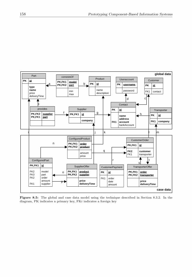
158 Prototyping Component-Based Information Systems
Part
PK id
type name price deliveryTime
Supplier
PK,FK1 id
company
provides
PK,FK2 supplierPK,FK1 part
Customer
PK id
FK1 contact
Useraccount
PK username
password
Transporter
PK id
FK1 company
Contact
PK id
name addressFK1 account bankAccount
a
cd
e
f g
b
h
Product
PK id
name description
consistsOf
PK,FK1 modelPK,FK2 part
min max
CustomerOrder
PK,FK1 id
FK2 customerFK1 transporter
CustomerPayment
PK id
FK1 order date amount
ConfiguredPart
PK,FK1 id
FK2 modelFK3 partFK2 order amountFK1 supplier
SupplierOffer
PK,FK1 productPK,FK2 supplier
price deliveryTime
TransporterOffer
PK,FK1 orderPK,FK2 transporter
price deliveryTime
o
t
p
q
rs
ConfiguredProduct
PK,FK1 orderPK,FK2 product
amount price
n
i j k l m
global data
case data
Figure 8.5: The global and case data model using the technique described in Section 8.3.2. In thediagram, PK indicates a primary key, FKi indicates a foreign key

159
Customer
Supplierreject order
accept order
deliver componentrequest
offer
send
offerreject
offer
accept
offer
ask
paymentpayment order
confirmation
deliverydeliver
order
Order
Managementrequest
offer
reject order
accept order
request offeroffer
offerassemble
order
order
assembled
Transporter
Figure 8.6: Structure diagram of the Web shop system
the components is created. A good practice is to create for each of the use cases and lifecycles a component, and then cluster tasks that belong together. The data model can bedivided over the components based on clustering, using the role types for the activitiesand the data elements used in activities.
The scenarios defined in the user requirements are test cases of the system. Eachpositive scenario should be a proper execution, while each negative scenario should notbe possible. After modeling, the model is verified for correctness.
Next step in this phase is to specify the I/O relations; the manipulations of eachtransition in the integrated system on both the global and case data. For each of theI/O relations it has to be shown that it does not violate the data constraints specifiedin the functional architecture, and that it preserves the CRUD matrix. Using SQL, itmeans that each action corresponds to a query on the corresponding table of the object,i.e. each C action corresponds to an insert query, each R to a select query, each U to anupdate query, and each D to a delete query.
In our example, we could identify five components for our system: Customer, Sup-plier, Transporter, Order and Management. Figure 8.6 shows the components and theircommunication. Figure 8.7 shows how the use case “Request for an offer by a customer”is assigned to different components. As the transitions “request offer” and “receive offer”are actions of the customer, they are assigned to the customer component. The offer sentby the supplier and transporter are assigned respectively to the supplier component andto the transporter component.
8.3.4 Prototyping
In this phase the prototype of the system is created. Prototyping is often used forvalidation. With a prototype, the users of the system can test whether the systemmeets their expectations. As the prototype is a first implementation, an obvious choiceis to let it correspond to the Realization and Testing activities of the design process.However, as the main purpose of the prototype is validation of the formal model withthe requirements, we also correspond it to the Validation activity.
Since the complete system is specified using formal models, we would like to generatethe prototype, rather than program it. By using YasperWE the prototype can be gen-erated, as will be explained in the next section. The potential user can experience how
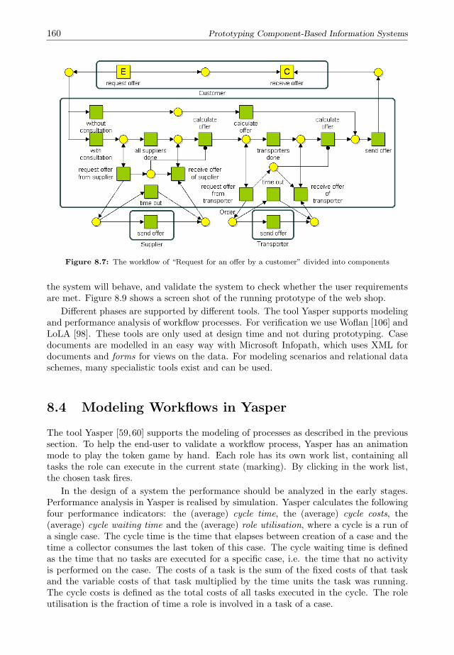
160 Prototyping Component-Based Information Systems
Figure 8.7: The workflow of “Request for an offer by a customer” divided into components
the system will behave, and validate the system to check whether the user requirementsare met. Figure 8.9 shows a screen shot of the running prototype of the web shop.
Different phases are supported by different tools. The tool Yasper supports modelingand performance analysis of workflow processes. For verification we use Woflan [106] andLoLA [98]. These tools are only used at design time and not during prototyping. Casedocuments are modelled in an easy way with Microsoft Infopath, which uses XML fordocuments and forms for views on the data. For modeling scenarios and relational dataschemes, many specialistic tools exist and can be used.
8.4 Modeling Workflows in Yasper
The tool Yasper [59,60] supports the modeling of processes as described in the previoussection. To help the end-user to validate a workflow process, Yasper has an animationmode to play the token game by hand. Each role has its own work list, containing alltasks the role can execute in the current state (marking). By clicking in the work list,the chosen task fires.
In the design of a system the performance should be analyzed in the early stages.Performance analysis in Yasper is realised by simulation. Yasper calculates the followingfour performance indicators: the (average) cycle time, the (average) cycle costs, the(average) cycle waiting time and the (average) role utilisation, where a cycle is a run ofa single case. The cycle time is the time that elapses between creation of a case and thetime a collector consumes the last token of this case. The cycle waiting time is definedas the time that no tasks are executed for a specific case, i.e. the time that no activityis performed on the case. The costs of a task is the sum of the fixed costs of that taskand the variable costs of that task multiplied by the time units the task was running.The cycle costs is defined as the total costs of all tasks executed in the cycle. The roleutilisation is the fraction of time a role is involved in a task of a case.

161
8.5 Prototyping with YasperWE
In the second stage, after identifying the notion of the case, the designer starts modelingthe document type. Microsoft Infopath, part of the Microsoft Office Suite, is a commercialdocument management system. To design component-based information systems, wecreated a generic Infopath template. This template consists of some basic case data,needed to define choices of XOR tasks in the workflow. For a particular component-based information system, the designer only has to extend this template.
8.5.1 Modeling the Case Document Type in Infopath
Infopath uses XML as a data type and offers functionality to design a document as wellas to fill in forms. The combination of a data definition and forms definition is the config-uration of the document manager. In the design mode of Infopath, the designer modelsthe case data in terms of an XML schema. In Infopath, the data is structured usinggroups and fields. A group is a named container, consisting of fields and other groups. Agroup can be seen as a singleton table definition in relational database. Multiple recordsof the same type can be stored by making the group a repeating group. Forms consistof elements from the XML schema and user interface controls, like radio buttons, checkboxes, list boxes, text fields, etc., to interact with the end-user. The data end-users enterin these controls can be validated against rules, which can be set in the control. Alsoconstraints on the data elements based on the case data can be expressed.
An end-user uses the document manager to fill in and alter documents. The submitteddata can be saved locally, or it can be used in other systems, by submitting the data toa program, a database or web service.
8.5.2 Integration by YasperWE
In the prototype phase, the workflow engine (YasperWE), the document manager(Infopath) and the database manager (MySQL) are integrated to realize the componentmodel, the case document type and the global data model. Each task performed by arole, needs a view on the case data. The designer has created the views in the previousstage in Infopath. Yasper is used as the design tool and the configuration tool forYasperWE. So the coupling of tasks to views in Infopath is specified in Yasper and theactual linking is done by YasperWE. When the designer finishes the global data model,the SQL definition of the global data needs to be integrated in YasperWE.
Figure 8.8: Executing a task in YasperWE
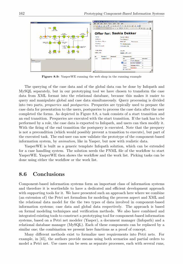
162 Prototyping Component-Based Information Systems
Figure 8.9: YasperWE running the web shop in the running example
The querying of the case data and of the global data can be done by Infopath andMySQL separately, but in our prototyping tool we have chosen to transform the casedata from XML format into the relational database, because this makes it easier toquery and manipulate global and case data simultaneously. Query processing is dividedinto two parts, prequeries and postqueries. Prequeries are typically used to prepare thecase data for presentation to the users, postqueries to process the case data after the usercompleted the forms. As depicted in Figure 8.8, a task consists of a start transition andan end transition. Prequeries are executed with the start transition. If the task has to beperformed by a role, the case data is exported to Infopath, and users can then modify it.With the firing of the end transition the postquery is executed. Note that the prequeryis not a precondition (which would possibly prevent a transition to execute), but part ofthe executed task. The end-user can now validate the prototype of the component-basedinformation system, by animation, like in Yasper, but now with realistic data.
YasperWE is built as a generic template Infopath solution, which can be extendedfor a case handling system. The solution needs the PNML file of the workflow to startYasperWE. YasperWE then shows the workflow and the work list. Picking tasks can bedone using either the workflow or the work list.
8.6 Conclusions
Component-based information systems form an important class of information systemsand therefore it is worthwhile to have a dedicated and efficient development approachwith supporting tools for it. We have presented such an approach here where we combine(an extension of) the Petri net formalism for modeling the process aspect and XML andthe relational data model for the the two types of data involved in component-basedinformation systems; case data and global data respectively. The approach is basedon formal modeling techniques and verification methods. We also have combined andintegrated existing tools to construct a prototyping tool for component-based informationsystems, based on a Petri net modeler (Yasper), a document manager (Infopath) and arelational database manager (MySQL). Each of these components can be replaced by asimilar one; the combination we present here functions as a proof of concept.
Many different methods exist to formalize user requirements into Petri nets. Forexample, in [45], the authors provide means using both scenarios and partial orders tomodel a Petri net. Use cases can be seen as separate processes, each with several runs,

163
or cases. Hence, we can apply the techniques of process discovery, as we will describe inthe next chapter. This way, it is possible to automatically derive workflow models fromthe user requirements. By generating a workflow model, new scenarios can be generatedand handed to the client to be discussed. This way, in several cycles a workflow modelcan be generated automatically for a use case.
We have done a number of experiments with YasperWE in a second-year course at ouruniversity. About a hundred students divided over 20 groups had to build a prototype ofthe web shop presented here as running example within 10 weeks of 6 hours. The studentsmodeled the complete system, from a product offer to delivery and invoice. They usedYasperWE to create the prototype. All groups succeeded in showing a working prototypeof the system. By following our approach they found out that already many problemsare hidden in the development of such a web shop, which they only could find out bymodeling and verifying the system formally.
The experiment with students shows the applicability of the approach. However, weneed to do more case studies to test and improve the approach. At this point in time,verification of the CRUD matrix, which is an important aspect of the approach, has tobe done manually, which is error prone. Therefore, we want to extend the tool supportin this approach, to offer automatic verification and analysis.

164 Prototyping Component-Based Information Systems
9Behavior Discovery using Integer Linear Programming
In this chapter, we propose the use of integer linear programming for the problem ofprocess discovery. In Petri net theory, this problem is often referred to as synthesis.
9.1 Introduction
In the previous part, we developed a formal framework for the formalization and ver-ification of component-based information systems. Mostly, the framework is used in atraditional top-down methodology, starting from the user requirements, up to the config-uration of the component-based information system. Nowadays, most organizations relyon existing information systems. As organizations change, these systems evolved fromsimple systems that were easy to understand to complex systems that are hard to under-stand, and thus difficult to maintain. Moreover, not all changes were documented in theright way, or not at all. The architecture of such systems need to evolve with the system.However, this is often not the case. Hence, architecture and implementation often donot coincide. This raises the question whether the system is working the way the orga-nization thinks it works. This question typically occurs in case the information systemhas some flaws, like performance problems. More important, for organizations to be incontrol, they need to ensure that the system is working according to their specification.
In the framework presented in Chapter 3, each component has a monitor interface.The main purpose of this interface is to record all events raised by the component.We distinguish different types of events in a component. Clicking a button or pressinga key, are events from the human interface, but also the configuration interface cantrigger events, like changing a parameter of the component. The main class of eventsare triggered by the execution of activities in the control flow of the component. Eventsare stored in logs. In this chapter, we focus on the events triggered by the execution ofactivities, i.e. on the execution log of a component.
An execution log contains all kinds of information of an event, e.g. for which activityand process instance, often referred to as case, the event was raised, by which resource,and at what time. Activities can have multiple events, like a start event or complete event.All events of a case form a sequence, which is called a run or trail of the component, andshows what events happen in what order, and at what time. The field of process mininganalyses these logs to check whether a component conforms a given specification, to

166 Behavior Discovery using Integer Linear Programming
Table 9.1: An execution log.
case id activity id originator case id activity id originatorcase 1 activity A John case 5 activity A Suecase 2 activity A John case 4 activity C Carolcase 3 activity A Sue case 1 activity D Petecase 3 activity B Carol case 3 activity C Suecase 1 activity B Mike case 3 activity D Petecase 1 activity C John case 4 activity B Suecase 2 activity C Mike case 5 activity E Clairecase 4 activity A Sue case 5 activity D Clairecase 2 activity B John case 4 activity D Petecase 2 activity D Pete
discover new models, and to enrich existing specification with information from executionlogs.
All kinds of models can be discovered from the execution log. Many algorithms existto discover the control flow from an execution log [16]. In this chapter, we will present adiscovery algorithm based on integer linear programming.
9.2 Process Discovery
In this section, we present some basic notions needed for process discovery. A singleexecution of a model is called a case. If the model is a Petri net, then a single firingsequence that results in a dead marking (a marking where no transition is enabled) isa case. Since most information systems log all kinds of events during execution of aprocess, we establish a link between an execution log of an information system and firingsequences of Petri nets. The basic assumption is that the log contains information aboutspecific transitions executed for specific cases.
Table 9.1 illustrates the basic information needed in an execution log, where it isimportant to realize that we assume that every event recorded is related to a singleexecution of a process. Furthermore, for each event an activity exists. In this example,in case 1 the activities A, B, C and D have been executed in sequence.
Definition 9.2.1 (Case, execution log)Let T be a set of transitions, a sequence σ ∈ T ∗ is a case, and L ⊆ T ∗ is an executionlog if and only if for all t ∈ T a σ ∈ L exists such that t ∈ σ. y
In other words, an execution log is a set of firing sequences of some marked Petrinet (N,m) = ((P, T, F ),m), where P , F and m are unknown and no transition is dead.In Definition 9.2.1, we define an execution log as a set of cases. Note that in real life,execution logs are bags of cases, i.e. a case with a specific order in which transitions areexecuted may occur more than once.
The goal of process discovery is to obtain a Petri net that can reproduce the executionlog under consideration. In literature, this activity is often referred to as synthesis. Thenext lemma states the conditions under which this is the case.
Definition 9.2.2 (Replayable execution log [30])Let (N,m) be a marked Petri net with N = (P, T, F ). Let L ⊆ T ∗ be an execution log.If L ⊆ T (N,m), we say that L can be replayed by (N,m). y
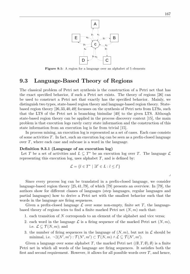
167
c
A
E
D C
By1 x1
y2
x2
x3
y3
y4
x4
x5
y5
Figure 9.1: A region for a language over an alphabet of 5 elements
9.3 Language-Based Theory of Regions
The classical problem of Petri net synthesis is the construction of a Petri net that hasthe exact specified behavior, if such a Petri net exists. The theory of regions [26] canbe used to construct a Petri net that exactly has the specified behavior. Mainly, wedistinguish two types, state-based region theory and language-based region theory. State-based region theory [26,33,40,49] focusses on the synthesis of Petri nets from LTSs, suchthat the LTS of the Petri net is branching bisimilar [40] to the given LTS. Althoughstate-based region theory can be applied in the process discovery context [15], the mainproblem is that execution logs rarely carry state information and the construction of thisstate information from an execution log is far from trivial [15].
In process mining, an execution log is represented as a set of cases. Each case consistsof some activities T . In fact, such an execution log can be seen as a prefix-closed languageover T , where each case and subcase is a word in the language.
Definition 9.3.1 (Language of an execution log)Let T be a set of activities and L ⊆ T ∗ be an execution log over T . The language Lrepresenting this execution log, uses alphabet T , and is defined by:
L = l ∈ T ∗ | ∃l′ ∈ L : l ≤ l′
ySince every process log can be translated in a prefix-closed language, we consider
language-based region theory [25,41,79], of which [79] presents an overview. In [79], theauthors show for different classes of languages (step languages, regular languages andpartial languages) how to derive a Petri net with the smallest behavior such that thewords in the language are firing sequences.
Given a prefix-closed language L over some non-empty, finite set T , the language-based theory of regions tries to find a finite marked Petri net (N,m) such that:
1. each transition of N corresponds to an element of the alphabet and vice versa;
2. each word in the language L is a firing sequence of the marked Petri net (N,m),i.e. L ⊆ T (N,m); and
3. the number of firing sequences in the language of (N,m), but not in L should beminimal, i.e. ¬∃(N ′,m′) : T (N ′,m′) ⊂ T (N,m) ∧ L ⊆ T (N ′,m′).
Given a language over some alphabet T , the marked Petri net ((∅, T, ∅), ∅) is a finitePetri net in which all words of the language are firing sequences. It satisfies both thefirst and second requirement. However, it allows for all possible words over T , and hence,

168 Behavior Discovery using Integer Linear Programming
the third requirement is not satisfied in general. Therefore, the behavior of this Petrinet needs to be reduced, so that the Petri net still allows to reproduce all words in thelanguage, but does not allow for too much additional behavior. The only way to restrictthe behavior of a Petri net is to add places to it. The theory of regions provides a methodto calculate these places, using so called regions.
Definition 9.3.2 (Region)A region of a prefix-closed language L over some set T is a triple (x, y, c) with x, y ∈0, 1T and c ∈ 0, 1, such that for each non-empty sequence w = w′; a ∈ L, wherew′ ∈ L and a ∈ T :
c+∑t∈T
(w′(t) · x(t)− w(t) · y(t)
)≥ 0
This can be rewritten into the inequation system:
c · 1 +A′ · x−A · y ≥ 0
where A and A′ are two |L| × |T | matrices with A(w, t) = w(t), and A′(w, t) = w′(t)for w = w′; a. The set of all regions of a language L is denoted by ℜ(L) and the region(0, 0, 0) is called the trivial region. y
The inequation system can be rewritten to the form [1;A′;−A] · r ≥ 0, which canbe simplified by eliminating duplicate rows. Each solution (x, y, c) of the inequationsystem corresponds to a place in a marked Petri net. Given a region (x, y, c), the vectorx represents the preset, y represents the postset, and c represents the initial marking ofthat place, as shown in Figure 9.1. The inequation system ensures that in all markingsreachable from the initial marking, the number of tokens in the corresponding place isnon-negative. Hence, adding such a place to a marked Petri net does not prevent theacceptance of the language. Therefore, we call such a place feasible.
Definition 9.3.3 (Feasible place)Let L be a prefix-closed language over T and let (N,m) be a marked Petri net withN = (P, T, F ). A place p ∈ P is called feasible if and only if a corresponding region(x, y, c) ∈ ℜ(L) exists such that m(p) = c, x(t) = 1 if and only if t ∈ •p, and y(t) = 1 ifand only if t ∈ p•. y
Corollary 9.3.4 (Addition of feasible places guarantees language acceptance)Let L be a prefix-closed language over T and let ((P, T, F ),m) be a marked Petri net thataccepts L. Let r = (x, y, c) ∈ ℜ(L) be a region of L corresponding to some place p ∈ P .Let N ′ = (P ′, T, F ′) where P ′ = P ∪ p, F ′ = F ∪ (t | x(t) > 0 × p) ∪ (p × t |y(t) > 0). Let m′ ∈ INP ′
such that m′|P = m and m′(p) = c. Then the marked Petri
net (N ′,m′) accepts language L. y
A direct consequence of the definition of feasible places is that if the set of tracesgenerated by a marked Petri net is identical to the prefix-closed language, all places inthe Petri net are feasible.
Corollary 9.3.5Let (N,m) be a marked Petri net. Let L = T (N,m) be the prefix-closed languagegenerated by (N,m). Then each place p ∈ P corresponds to a region rp ∈ ℜ(L). y
Throughout this chapter, we will use the execution log U = ⟨A,C⟩, ⟨A,B,C⟩. Itdefines the prefix closed-language U = ϵ, ⟨A⟩, ⟨A,B⟩, ⟨A,C⟩, ⟨A,B,C⟩. We define
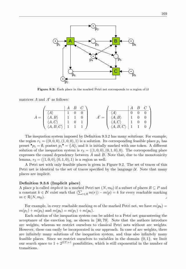
169
A B
C
p3p1
p2
p4
p6
p7
p9
p8
p5
Figure 9.2: Each place in the marked Petri net corresponds to a region of U
matrices A and A′ as follows:
A =
A B C
⟨A⟩ 1 0 0⟨A,B⟩ 1 1 0⟨A,C⟩ 1 0 1⟨A,B,C⟩ 1 1 1
A′ =
A B C
⟨A⟩ 0 0 0⟨A,B⟩ 1 0 0⟨A,C⟩ 1 0 0⟨A,B,C⟩ 1 1 0
The inequation system imposed by Definition 9.3.2 has many solutions. For example,
the region r1 = ((0, 0, 0), (1, 0, 0), 1) is a solution. Its corresponding feasible place p1 haspreset •p1 = ∅, postset p1• = A, and it is initially marked with one token. A differentsolution of the inequation system is r3 = ((1, 0, 0), (0, 1, 0), 0). The corresponding placeexpresses the causal dependency between A and B. Note that, due to the monotonicitylemma, r2 = ((1, 0, 0), (0, 1, 0), 1) is a region as well.
A Petri net with only feasible places is given in Figure 9.2. The set of traces of thisPetri net is identical to the set of traces specified by the language U . Note that manyplaces are implicit.
Definition 9.3.6 (Implicit place)A place p is called implicit in a marked Petri net (N,m0) if a subset of places R ⊆ P anda constant k ∈ IN exist such that (
∑r∈Rm(r))−m(p) = k for every reachable marking
m ∈ R(N,m0). y
For example, in every reachable marking m of the marked Petri net, we have m(p8) =m(p1) +m(p3) and m(p9) = m(p1) +m(p6).
Each solution of the inequation system can be added to a Petri net guaranteeing theacceptance of the exection log, as shown in [30, 79]. Note that the authors introducearc weights, whereas we restrict ourselves to classical Petri nets without arc weights.However, these can easily be incorporated in our approach. In case of arc weights, thereare infinitely many solutions of the inequation system, and thus also infinitely manyfeasible places. Since we restrict ourselves to variables in the domain 0, 1, we limitour search space to 1 + 22|T |+1 possibilities, which is still exponential in the number oftransitions.

170 Behavior Discovery using Integer Linear Programming
9.4 Integer Linear Programming Formulation
In process mining, the main issue is the completeness of execution logs: given an executionlog, we do not know whether we have seen all possible behavior. Therefore, we need aPetri net which abstracts in some way from the log. The size of the discovered Petri netshould be independent of the size of the execution log. Both the basis and the separatingrepresentation construct Petri nets whose size depends on the length of the language.Therefore, we propose a different selection mechanism for the addition of feasible places.Each place should have a function within the Petri net. Therefore, we search for placesthat:
• are more expressive than others, i.e. places with minimal input transitions andmaximal output transitions are favored;
• explicitly express causal dependencies between transitions discovered in the execu-tion log.
In [46], the authors show that a marked Petri net with only “minimal regions” is asolution for the synthesis problem of Petri nets. Minimal regions are regions that cannotbe represented as the sum of two other regions.
Definition 9.4.1 (Minimal region)Let L ⊆ T ∗ be a process log, and let r = (x, y, c) be a region. We say that r is minimal,if there do not exist two non trivial, regions r1 = (x1, y1, c1) and r2 = (x2, y2, c2), suchthat x = x1 + x2, y = y1 + y2 and c = c1 + c2. y
If a region is not minimal, it corresponds to an implicit place, i.e. if the markingof the corresponding place can be expressed as the sum of the markings of some otherplaces, the region is not minimal.
Lemma 9.4.2 (Non minimal region corresponds to an implicit place)Let L be a prefix-closed language over some set T , and let ((P, T, F ),m0) be a markedPetri net such that each place corresponds to a region of L and vice versa. Let p ∈ Pbe a place, and let r ∈ ℜ(L) be its corresponding region. If r is not minimal, then placep ∈ P is implicit. yProof. Define N = (P, T, F ) and r = (x, y, c). As region r is not minimal, regionsr1 = (x1, y1, c1) and r2 = (x2, y2, c2) exist such that x = x1 + x2, y = y1 + y2 andc = c1+c2. As each region corresponds to a place in the Petri net, places p1, p2 ∈ P existthat correspond to r1 and r2, respectively. We show that m(p1)+m(p2)−m(p) = 0 is aninvariant in all reachable markings m ∈ R(N,m0). We prove the statement by induction
on the length of the sequence σ ∈ T ∗ with (N : m0σ−→ m). Suppose σ = ϵ, i.e. m = m0,
then the statement trivially holds, since c = c1+c2. Now let σ = σ′; ⟨t⟩ for some σ′ ∈ T ∗,
t ∈ T and marking m′ ∈ R(N,m0) such that (N : m0σ′
−→ m′ t−→ m). By the inductionhypothesis we have m′(p1) +m′(p2)−m′(p) = 0. Then m(p1) = m′(p1) + x1(t)− y1(t),m(p2) = m′(p2) + x2(t)− y2(t) and m(p) = m′(p) + x1(t) + x2(t)− y1(t)− y2(t). Thus,m(p1) +m(p2)−m(p) = m′(p1) +m′(p2)−m′(p) = 0.
Hence, m(p1) +m(p3)−m(p) = 0 is an invariant, and thus, place p is implicit. 2
Note that the reverse does not hold. Consider the marked Petri net (N,m0) depictedin Figure 9.3. The marked Petri net accepts the language ϵ, ⟨A⟩, ⟨A,B⟩, each region ofthis language corresponds to a place, and vice versa. We have m(s) = m(p)+m(q) for allreachable markings m ∈ R(N,m0), thus place s is implicit. Let (xs, ys, cs), (xp, yp, cp)and (xq, yq, cq) be the corresponding regions of places s, p and q, respectively. Each region
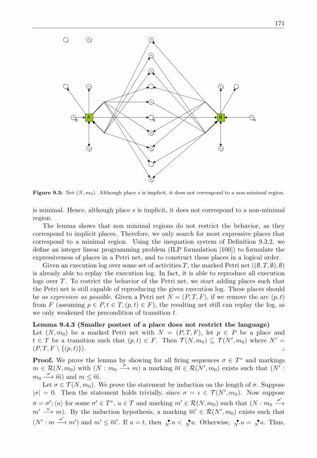
171
A Bp q s
Figure 9.3: Net (N,m0). Although place s is implicit, it does not correspond to a non-minimal region.
is minimal. Hence, although place s is implicit, it does not correspond to a non-minimalregion.
The lemma shows that non minimal regions do not restrict the behavior, as theycorrespond to implicit places. Therefore, we only search for most expressive places thatcorrespond to a minimal region. Using the inequation system of Definition 9.3.2, wedefine an integer linear programming problem (ILP formulation [100]) to formulate theexpressiveness of places in a Petri net, and to construct these places in a logical order.
Given an execution log over some set of activities T , the marked Petri net ((∅, T, ∅), ∅)is already able to replay the execution log. In fact, it is able to reproduce all executionlogs over T . To restrict the behavior of the Petri net, we start adding places such thatthe Petri net is still capable of reproducing the given execution log. These places shouldbe as expressive as possible. Given a Petri net N = (P, T, F ), if we remove the arc (p, t)from F (assuming p ∈ P, t ∈ T, (p, t) ∈ F ), the resulting net still can replay the log, aswe only weakened the precondition of transition t.
Lemma 9.4.3 (Smaller postset of a place does not restrict the language)Let (N,m0) be a marked Petri net with N = (P, T, F ), let p ∈ P be a place andt ∈ T be a transition such that (p, t) ∈ F . Then T (N,m0) ⊆ T (N ′,m0) where N ′ =(P, T, F \ (p, t)). yProof. We prove the lemma by showing for all firing sequences σ ∈ T ∗ and markingsm ∈ R(N,m0) with (N : m0
σ−→ m) a marking m ∈ R(N ′,m0) exists such that (N ′ :
m0σ−→ m) and m ≤ m.
Let σ ∈ T (N,m0). We prove the statement by induction on the length of σ. Suppose|σ| = 0. Then the statement holds trivially, since σ = ϵ ∈ T (N ′,m0). Now suppose
σ = σ′; ⟨u⟩ for some σ′ ∈ T ∗, u ∈ T and marking m′ ∈ R(N,m0) such that (N : m0σ′
−→m′ u−→ m). By the induction hypothesis, a marking m′ ∈ R(N ′,m0) exists such that
(N ′ : mσ′
−→ m′) and m′ ≤ m′. If u = t, then •N ′u < •
N u. Otherwise, •N ′u = •
N u. Thus,

172 Behavior Discovery using Integer Linear Programming
A B Ci p1 p2
p3
Figure 9.4: Sequence σ = ⟨A,B,C⟩ gives f(p1) = f(p2) = f(p3) = 0
•N ′u ≤ •
N u ≤ m′ ≤ m′. Let m = m′− •N ′u+u•N ′ . Then (N : m′ u−→ m). Since u•N ′ = u•N ,
and the firing rule of Petri nets, we have m ≤ m. Hence, the statement holds. 2
Also if we would add a non-existing arc (t, p) to F , with t ∈ T and p ∈ P , the resultingnet still can replay the execution log as it only strengthens the postcondition of t.
Lemma 9.4.4 (Larger preset of a place does not restrict the language)Let (N,m) be a marked Petri net with N = (P, T, F ), let p ∈ P be a place and t ∈ Ta transition such that (t, p) ∈ F . Then T (N,m) ⊆ T (N ′,m) where N ′ = (P, T, F ∪(t, p)). y
Proof. We prove the lemma by showing for all firing sequences σ ∈ T ∗ and markingsm ∈ R(N,m0) with (N : m0
σ−→ m) a marking m ∈ R(N ′,m0) exists such that (N ′ :
m0σ−→ m) and m ≤ m.
Let σ ∈ T (N,m0). We prove the statement by induction on the length of σ. Suppose|σ| = 0. Choose m = m. Then the statement holds trivially, since σ = ϵ ∈ T (N ′,m0).Now suppose σ = σ′; ⟨u⟩ for some σ′ ∈ T ∗, u ∈ T and m′ ∈ R(N,m0) such that
(N : m0σ′
−→ m′ u−→ m). By the induction hypothesis, a marking m′ ∈ R(N ′,m0)
exists such that (N ′ : mσ′
−→ m′) and m′ ≤ m′. We have •N ′u = •
N u ≤ m′ ≤ m′. Let
m = m′ − •N ′u+ u•N ′ . Then (N : m′ u−→ m). Since u•N ≤ u•N ′ , we have m ≤ m. Hence,
the statement holds. 2
These lemmas show that adding an incoming arc to a place, or removing an outgoingarc from a place, does not restrict the behavior in terms of firing sequences. Therefore,we search for places with a maximal postset and a minimal preset. This means thatadding an arc from this place to another transition or removing an arc to this placewould cause the marked Petri net to not accept the language.
In order to transform the linear inequation system of Definition 9.3.2 to an ILPproblem, we need a target function. We have shown that places are most restrictive iftheir preset is minimal and their postset is maximal. A first candidate would be theminimization of the function:
f((x, y, c)) = c+ 1 T · x− 1 T · y
This function encourages the addition of an input arc to the corresponding feasibleplace, as this increases the value of 1 T · x, or the removal of an outgoing arc from thecorresponding feasible place, which also increases the function.
However, it is easy to show that this function does not favor minimal regions. Take forinstance the language ϵ, ⟨A⟩,⟨A,B⟩,⟨A,B,C⟩. An example marked Petri net acceptingthis language is shown in Figure 9.4. In this marked Petri net, the regions correspondingto the places p1, p2 and p3 all give the same result for function f , whereas place p3 isimplicit, and thus it should not be favored as the other places.

173
The example shows that a good target function needs to ensure that it favors theindividual regions, rather than their sum, i.e. if r1, r2 and r3 are regions, such that r3 isthe sum of r1 and r2, the function needs to ensure f ′(r1) < f ′(r3) and f ′(r2) < f ′(r3),while preserving the property that regions corresponding to more expressive feasibleplaces have a lower target value.
For prefix-closed languages L, we have ϵ ∈ L. As a consequence, we cannot rewrite theinequation system directly to the matrix notation as in Definition 9.3.2, since matrix Aonly uses non-empty sequences, while the empty sequence is in L. Consider the followingcalculation:
∀w ∈ L : c+∑t∈T
w(t)(x(t)− y(t)) ≥ 0
≡ Addition property∑w∈L
(c+
∑t∈T
w(t)(x(t)− y(t))
)≥ 0
≡ Rewriting
c+∑
w∈(L\ϵ)
(c+
∑t∈T
w(t)(x(t)− y(t))
)≥ 0
≡ Rewriting, where matrix A as defined in Definition 9.3.2 c+ 1 T(1 · c+A · (x− y)) ≥ 0
Hence, the calculation suggests to take the function τ with τ((x, y, c)) = c+1 T(1 · c+A ·(x− y)) as target function. In fact, this function expresses the number of times a regionwas marked (c+ 1 T(1 · c+A · x)), and how often it was unmarked (1 T ·A · y).
Definition 9.4.5 (Target function)Let L ⊆ T ∗ be a process log and let A be the matrix defined in Definition 9.3.2. Wedefine the function τ : ℜ(L) → IN by
τ((x, y, c)) = c+ 1 T(1 · c+A · (x− y))
y
Consider again the example of Figure 9.4. The regions of places p1 and p2 resultin τ(p1) = τ(p2) = 1, while τ(p3) = 2. We show that minimizing this function indeedsatisfies all criteria, by first proving that the target function is greater than zero fornon-trivial regions.
Lemma 9.4.6 (Target function favors minimal regions)Let L ⊆ T ∗ be a log, and let τ be the function as defined in Definition 9.4.5. Thenτ(r) > 0 for all non-trivial regions r. y
Proof. Let r = (x, y, c) ∈ ℜ(L) be a non-trivial region. By Definition 9.3.2, we haveτ(r) ≥ 0, since A(σ, t) ≥ A′(σ, t) for all σ ∈ L and t ∈ T . We prove the statement byinduction on the structure of r. If x = y = 0, then c = 1, otherwise it was a trivialregion. Then clearly, τ(r) > 0. Hence, the statement holds.
Suppose there is a transition u ∈ T such that x(u) > 0. Then there are sequences
w,w′ ∈ L such that w = w′; ⟨u⟩, and hence, w(u) > w′(u). Thus, we can calculate:

174 Behavior Discovery using Integer Linear Programming
τ(r) = c+ 1 T(1 · c+A · (x− y)) =∑w∈L
(c+
∑t∈T
w(t)(x(t)− y(t))
)= Rewriting ∑
w∈L
c+ w(u)(x(u)− y(u)) +∑
t∈T\u
w(t)(x(t)− y(t))
> w(u)(x(u)− y(u)) > w′(u)x(u)− w(u)y(u)∑
w∈L
c+ w′(u)x(u)− w(u)y(u)) +∑
t∈T\u
w(t)(x(t)− y(t))
= ∀t ∈ T \ u : w(t) = w′(t)∑
w∈L
c+ w′(u)x(u)− w(u)y(u) +∑
t∈T\u
(w′(t)x(t)− w(t)y(t))
= Rewriting ∑
w∈L
(c+
∑t∈T
(w′(t)x(t)− w(t)y(t))
)≥ Definition of region
0
Thus, τ(r) > 0, and hence, the statement holds.Now suppose x = 0. Since r is a non-trivial region, there is a transition u ∈ T such
that y(u) > 0, and a sequence σ ∈ L such that σ(u) > 0.
0 ≤ τ(r)
= Definition ∑w∈L
(c+
∑t∈T
w(t)(x(t)− y(t))
)= x = 0∑
w∈L
(c−
∑t∈T
w(t)y(t)
)= Rewriting
c−∑t∈T
σ(t)y(t) +∑
w∈L\σ
(c−
∑t∈T
w(t)y(t)
)= Rewriting
c− σ(u)y(u)−∑
t∈T\u
σ(t)y(t) +∑
w∈L\σ
(c−
∑t∈T
w(t)y(t)
)
Since σ(u) > 0 and y(u) > 0, we conclude c > 0, and hence, τ(r) > 0. 2

175
Corollary 9.4.7 (Target function favors minimal regions)Let L ⊆ T ∗ be a log, let r1 = (x1, y1, c1), r2 = (x2, y2, c2) and r3 = (x1+x2, y1+y2, c1+c2)be three non-trivial regions. Let τ be the function as defined in Definition 9.4.5. Thenτ(r1) < τ(r3) and τ(r2) < τ(r3). y
The lemma shows that for non-trivial regions minimal regions are favored. Hence,combining the inequation system of Definition 9.3.2 and minimizing the function of Def-inition 9.4.5 results in an integer linear programming formulation.
Definition 9.4.8 (ILP formulation)Let L ⊆ T ∗ be a process log, and let A and A′ be the matrices as defined in Defini-tion 9.3.2. We define the ILP ILPL for process log L as:
Minimize c+ 1 T(1 · c+ ·A · (x− y) Definition 9.4.5
such that c+A′ · x−A · y ≥ 0 Definition 9.3.2
1 T · x+ 1 T · y ≥ 1 There should be at least one edge
0 ≤ x ≤ 1 x ∈ 0, 1|T |
0 ≤ y ≤ 1 y ∈ 0, 1|T |
0 ≤ c ≤ 1 c ∈ 0, 1
y
This ILP problem provides the basis for our process discovery problem. However, anoptimal solution to this ILP only provides a single feasible place with a minimal valuefor the target function. Therefore, in the next section, we show how this ILP problemcan be used as a basis for constructing a Petri net from a log.
9.5 Constructing Petri Nets using ILP
In the previous section we introduced the basis for constructing a Petri net from anexecution log. In this section, we present different algorithms for the generation of Petrinets that accept the language. The first algorithm is based on the partial order on theelements of the set ℜ(L) defined by the target function. The second algorithm uses extrainformation extracted from the execution log to select proper places. Last, we present amethod to refine a given marked Petri net such that it accepts the language.
9.5.1 Generation of Independent Places
The target function of Definition 9.4.5 provides a partial order on all elements of the setℜ(L). In this section, we show how to generate the first n places of a Petri net, that are(1) able to reproduce the execution log under consideration and (2) of which the placesare as expressive as possible.
A trivial approach would be to add each solution found as a negative example tothe ILP problem, i.e. each solution found is explicitly forbidden in the next round.However, it is clear that once a region r has been found and the corresponding feasibleplace is added to the Petri net, we are no longer interested in regions r′ for which thecorresponding feasible place has more tokens, less outgoing arcs or more incoming arcs,i.e. we are only interested in “independent regions”.

176 Behavior Discovery using Integer Linear Programming
A Bp1 p3
Cp2 p4
Figure 9.5: Basic algorithm applied on language U
Definition 9.5.1 (Refining the ILP after each solution)Let L ⊆ T ∗ be a process log and let ILP (L,0) be the ILP problem as defined in Defini-tion 9.4.8. For some i ≥ 0, let ri = (xi, yi, ci) ∈ ℜ(L) be a minimal solution of ILP (L,i).We define ILP (L,i+1) as ILP (L,i) with the additional constraint specifying:
−ci · c+ y T · (1− yi)− x T · xi ≥ −ci + 1− 1 T · xi
y
The additional constraint in fact requires a new solution to have a smaller initialmarking, more outgoing arcs, or fewer incoming arcs, as shown in the next lemma.
Lemma 9.5.2 (Refining yields independent regions)Let L ⊆ T ∗ be an execution log, and let region ri = (xi, yi, ci) be a minimal solutionof ILP (L,i) as defined in Definition 9.5.1. Let r = (x, y, c) be a minimal solution ofILP (L,i+1) following Definition 9.5.1. Then, c < ci or a t ∈ T exists such that x(t) <xi(t) ∨ y(t) > yi(t). y
Proof. Suppose the opposite, i.e. assume that c ≥ ci and x(t) ≥ xi(t), and y(t) ≤ yi(t)for all t ∈ T . Since ci, c ∈ 0, 1 we know ci · c = ci. Similarly, y T · (1 − yi) = 0 andxi
T · x = xiT · 1. Hence −ci · c + y T · (1 − yi) − xi
T · x = −ci − xiT · 1 and since
−ci − xiT · 1 < −ci + 1− 1 T · xi, we know that r is not a solution of ILP (L,i+1), which
is a contradiction. Hence, the lemma holds. 2
This refinement gives a first algorithm to construct a Petri net that is capable ofreplaying a given log, in which each place is as expressive as possible. The places aregenerated in an order which ensures the most expressive places to be found first and eachplaces added has less tokens, more outgoing arcs, or fewer incoming arcs. Furthermore,each solution of a refined ILP is also a solution of the original ILP, since the new solutionsatisfies all constraints of the initial ILP formulation, and some additional constraints.Hence all places constructed using this procedure are feasible places.
Consider again the execution log U . A minimal solution of the initial ILP problemILP (U,0) as shown in Table 9.2, is region r1 = ((0, 0, 0), (1, 0, 0), 1). The target functionhas value τ(r1) = 1. This region results in the addition of the constraint:
−c+ y T ·
011
≥ 0
Region r1 is clearly no solution of this constraint. Adding the constraint to ILP (L,0)
gives ILP (L,1). Figure 9.5 shows the Petri net that was generated after four refinements.

177
Table 9.2: The initial ILP formulation for language U
xA xB xC yA yB yC cminimize 4 2 2 -4 -2 -2 5⟨A⟩: 0 0 0 -1 0 0 1 ≥ 0⟨A,B⟩: 1 0 0 -1 -1 0 1 ≥ 0⟨A,C⟩: 1 0 0 -1 0 -1 1 ≥ 0⟨A,B,C⟩: 1 1 0 -1 -1 -1 1 ≥ 0At least one arc: 1 1 1 1 1 1 0 ≥ 1upper bound 1 1 1 1 1 1 1lower bound 0 0 0 0 0 0 0
The procedure, however, still has the downside that the total number of places isworst-case exponential in the number of transitions. Therefore, we propose to guide thesearch for solutions (i.e. for places) using concepts from the field of process discovery[8, 16,47,108].
9.5.2 Generation of Places Expressing Causal Dependencies
In this chapter, we search for an algorithm that discovers Petri nets from an execution logusing the theory of regions. Up to now, we have only searched for feasible places that are“most expressive”, i.e. places with the smallest initial marking, minimal incoming arcs,and maximal outgoing arcs such that the resulting net accepts the prefix-closed languagedefined by the execution log. However, we did not search for places that explicitly expresscausal dependencies between transitions. In this subsection, we first introduce how thesecausal dependencies can be derived from an execution log. We use these relations incombination with the ILP formulation of Definition 9.4.8 to construct a Petri net.
Definition 9.5.3 (Causal dependency [16])Let L ⊆ T ∗ be an execution log over some set of activities T . If for two activities a, b ∈ Ttraces σ1, σ2 ∈ T ∗ exist such that σ1; ⟨a, b⟩;σ2 ∈ L, we write a >L b. If a >L b and notb >L a in a log L, there is a causal dependency between a and b, denoted by a→L b. y
In [16], it was shown that if a log L satisfies a certain completeness criterion and if aPetri net of a certain class [16] exists that can reproduce this log, then the >L relation issufficient to reconstruct the Petri net from the execution log. However, the completenesscriterion assumes knowledge of the Petri net producing the execution log. As we onlyhave the execution log, it is unknown whether the log is complete or not. Given a systemthat generated some execution log, it is unknown whether the system could generatea new trace, i.e. a sequence which is not in the language defined by the execution log.Nonetheless, we provide the formal definition of the notion of completeness, and we provethat for complete logs, causal dependencies directly relate to places and hence provide agood guide for finding these places.
Definition 9.5.4 (Complete log with respect to a Petri net [16])Let (N,m) be a marked Petri net with N = (P, T, F ) and m ∈ INP . Let L ⊆ T ∗ be anexecution log. The execution log L is called complete with respect to (N,m) if and only
if for all σ, σ1, σ2 ∈ T ∗, a, b ∈ T such that σ = σ1; ⟨a, b⟩;σ2 and (N : mσ−→) we have
a >L b. y
We will restrict our search for Petri nets that are complete with respect to the givenlog. In [16], the proof that a causal dependency corresponds to a place is only given for

178 Behavior Discovery using Integer Linear Programming
A B
p2C
p1
p3
Figure 9.6: Each place in the Petri net expresses a causal dependency of the log U
safe Petri nets. This can however be generalized to general Petri nets.
Lemma 9.5.5 (Causality implies a place)Let (N,m) be a marked Petri net with N = (P, T, F ) and m ∈ INP . Let L ⊆ T ∗ be acomplete execution log of (N,m). For all a, b ∈ T , it holds that if a = b and a→L b thena• ∩ •b = ∅. y
Proof. Suppose such a place does not exist, i.e. assume a →L b and a• ∩ •b = ∅.By definition of >L, there are sequences σ1, σ2 ∈ T ∗ such that (N : m
σ−→) where
σ = σ1; ⟨a, b⟩;σ2. Let s = m+N · −→σ1, then (N : sa−→), but also (N : s
b−→ s′), for somes′ ∈ INP , since a• ∩ •b = ∅.
Further, we have ¬(N : s′a−→), since otherwise a →L b would not hold. Then,
(•b\b•)∩•a = ∅, since otherwise, transition a would be enabled in s′. Let p ∈ (•b\b•)∩•a.Then, s(p) = 1, since if s(p) > 1, then a would be enabled in (N, s′). Hence, transition
b is not enabled after firing σ1; ⟨a⟩. This is a contradiction, since now ¬(N : s⟨a,b⟩−→).
Hence, we may conclude a• ∩ •b = ∅. 2
Lemma 9.5.5 shows that a causal dependency in the log corresponds to a place, ifthe log is complete. Causal dependencies between transitions are used by many processdiscovery algorithms (cf. [8, 16, 47, 108]) and generally provide a good indication as towhich transitions should be connected through places. Furthermore, extensive techniquesare available to derive causal dependencies between transitions using heuristic approaches[16, 47]. However, it is not known whether the log is complete and whether we coveredall causal dependencies. In order to find a place expressing a specific causal dependency,we extend the ILP problem presented in Definition 9.4.8.
Definition 9.5.6 (ILP for causal dependency)Let L ⊆ T ∗ be a process log, and let ILPL be the ILP as defined in Definition 9.4.8.Furthermore, let a, b ∈ T such that a →L b. We define the refined ILP, ILP (L,a→b) asILPL, with two extra bounds specifying that:
x(a) = y(b) = 1
y
A solution of the optimization problem expresses the causal dependency t1 →L t2,and restricts the behavior as much as possible. However, such a solution does not haveto exist, i.e. the ILP might be infeasible, in which case no place is added to the Petri netbeing constructed. Nonetheless, by considering a separate ILP for each causal depen-dency in the log, a Petri net can be constructed, in which each place is as expressive aspossible and expresses at least one dependency derived from the log. With this approach,
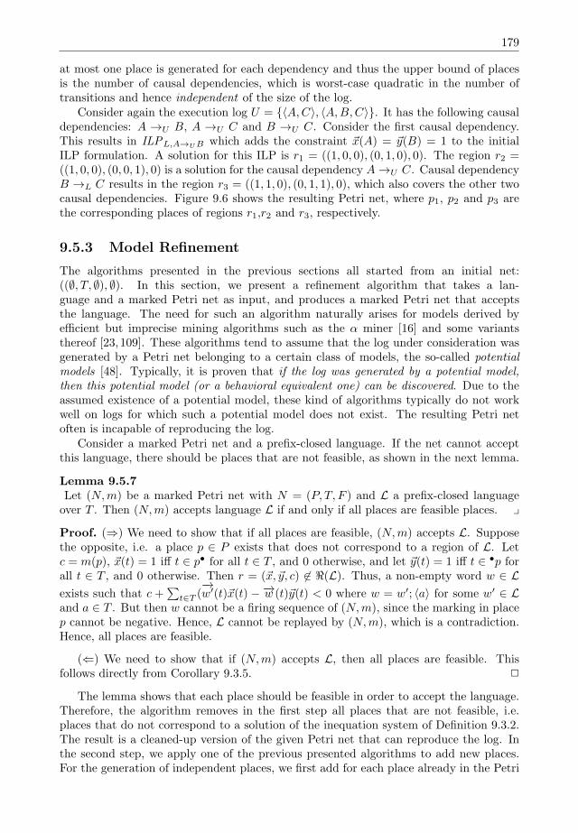
179
at most one place is generated for each dependency and thus the upper bound of placesis the number of causal dependencies, which is worst-case quadratic in the number oftransitions and hence independent of the size of the log.
Consider again the execution log U = ⟨A,C⟩, ⟨A,B,C⟩. It has the following causaldependencies: A →U B, A →U C and B →U C. Consider the first causal dependency.This results in ILPL,A→UB which adds the constraint x(A) = y(B) = 1 to the initialILP formulation. A solution for this ILP is r1 = ((1, 0, 0), (0, 1, 0), 0). The region r2 =((1, 0, 0), (0, 0, 1), 0) is a solution for the causal dependency A→U C. Causal dependencyB →L C results in the region r3 = ((1, 1, 0), (0, 1, 1), 0), which also covers the other twocausal dependencies. Figure 9.6 shows the resulting Petri net, where p1, p2 and p3 arethe corresponding places of regions r1,r2 and r3, respectively.
9.5.3 Model Refinement
The algorithms presented in the previous sections all started from an initial net:((∅, T, ∅), ∅). In this section, we present a refinement algorithm that takes a lan-guage and a marked Petri net as input, and produces a marked Petri net that acceptsthe language. The need for such an algorithm naturally arises for models derived byefficient but imprecise mining algorithms such as the α miner [16] and some variantsthereof [23, 109]. These algorithms tend to assume that the log under consideration wasgenerated by a Petri net belonging to a certain class of models, the so-called potentialmodels [48]. Typically, it is proven that if the log was generated by a potential model,then this potential model (or a behavioral equivalent one) can be discovered. Due to theassumed existence of a potential model, these kind of algorithms typically do not workwell on logs for which such a potential model does not exist. The resulting Petri netoften is incapable of reproducing the log.
Consider a marked Petri net and a prefix-closed language. If the net cannot acceptthis language, there should be places that are not feasible, as shown in the next lemma.
Lemma 9.5.7Let (N,m) be a marked Petri net with N = (P, T, F ) and L a prefix-closed languageover T . Then (N,m) accepts language L if and only if all places are feasible places. y
Proof. (⇒) We need to show that if all places are feasible, (N,m) accepts L. Supposethe opposite, i.e. a place p ∈ P exists that does not correspond to a region of L. Letc = m(p), x(t) = 1 iff t ∈ p• for all t ∈ T , and 0 otherwise, and let y(t) = 1 iff t ∈ •p forall t ∈ T , and 0 otherwise. Then r = (x, y, c) ∈ ℜ(L). Thus, a non-empty word w ∈ Lexists such that c +
∑t∈T (
−→w′(t)x(t) − −→w (t)y(t) < 0 where w = w′; ⟨a⟩ for some w′ ∈ L
and a ∈ T . But then w cannot be a firing sequence of (N,m), since the marking in placep cannot be negative. Hence, L cannot be replayed by (N,m), which is a contradiction.Hence, all places are feasible.
(⇐) We need to show that if (N,m) accepts L, then all places are feasible. Thisfollows directly from Corollary 9.3.5. 2
The lemma shows that each place should be feasible in order to accept the language.Therefore, the algorithm removes in the first step all places that are not feasible, i.e.places that do not correspond to a solution of the inequation system of Definition 9.3.2.The result is a cleaned-up version of the given Petri net that can reproduce the log. Inthe second step, we apply one of the previous presented algorithms to add new places.For the generation of independent places, we first add for each place already in the Petri
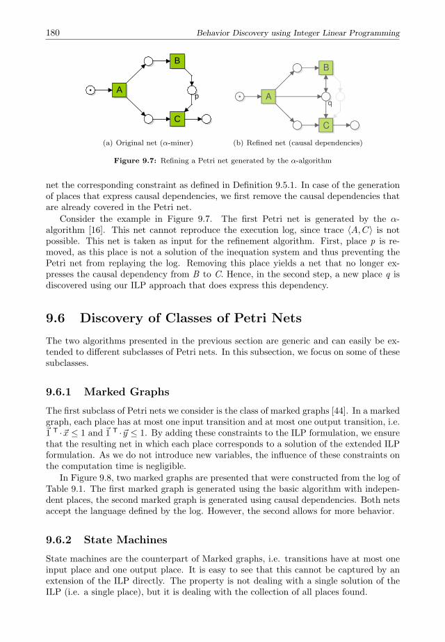
180 Behavior Discovery using Integer Linear Programming
A
B
C
p
(a) Original net (α-miner) (b) Refined net (causal dependencies)
Figure 9.7: Refining a Petri net generated by the α-algorithm
net the corresponding constraint as defined in Definition 9.5.1. In case of the generationof places that express causal dependencies, we first remove the causal dependencies thatare already covered in the Petri net.
Consider the example in Figure 9.7. The first Petri net is generated by the α-algorithm [16]. This net cannot reproduce the execution log, since trace ⟨A,C⟩ is notpossible. This net is taken as input for the refinement algorithm. First, place p is re-moved, as this place is not a solution of the inequation system and thus preventing thePetri net from replaying the log. Removing this place yields a net that no longer ex-presses the causal dependency from B to C. Hence, in the second step, a new place q isdiscovered using our ILP approach that does express this dependency.
9.6 Discovery of Classes of Petri Nets
The two algorithms presented in the previous section are generic and can easily be ex-tended to different subclasses of Petri nets. In this subsection, we focus on some of thesesubclasses.
9.6.1 Marked Graphs
The first subclass of Petri nets we consider is the class of marked graphs [44]. In a markedgraph, each place has at most one input transition and at most one output transition, i.e.1 T · x ≤ 1 and 1 T · y ≤ 1. By adding these constraints to the ILP formulation, we ensurethat the resulting net in which each place corresponds to a solution of the extended ILPformulation. As we do not introduce new variables, the influence of these constraints onthe computation time is negligible.
In Figure 9.8, two marked graphs are presented that were constructed from the log ofTable 9.1. The first marked graph is generated using the basic algorithm with indepen-dent places, the second marked graph is generated using causal dependencies. Both netsaccept the language defined by the log. However, the second allows for more behavior.
9.6.2 State Machines
State machines are the counterpart of Marked graphs, i.e. transitions have at most oneinput place and one output place. It is easy to see that this cannot be captured by anextension of the ILP directly. The property is not dealing with a single solution of theILP (i.e. a single place), but it is dealing with the collection of all places found.
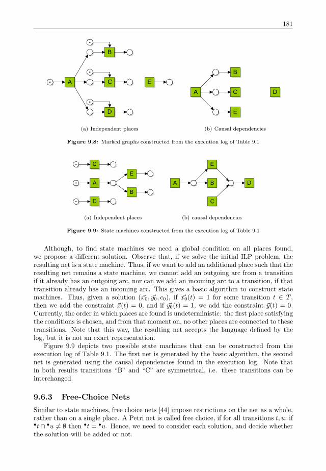
181
A
B
C
D
E
(a) Independent places
A
B
C
E
D
(b) Causal dependencies
Figure 9.8: Marked graphs constructed from the execution log of Table 9.1
A
B
C
D
E
(a) Independent places
A B
C
D
E
(b) causal dependencies
Figure 9.9: State machines constructed from the execution log of Table 9.1
Although, to find state machines we need a global condition on all places found,we propose a different solution. Observe that, if we solve the initial ILP problem, theresulting net is a state machine. Thus, if we want to add an additional place such that theresulting net remains a state machine, we cannot add an outgoing arc from a transitionif it already has an outgoing arc, nor can we add an incoming arc to a transition, if thattransition already has an incoming arc. This gives a basic algorithm to construct statemachines. Thus, given a solution (x0, y0, c0), if x0(t) = 1 for some transition t ∈ T ,then we add the constraint x(t) = 0, and if y0(t) = 1, we add the constraint y(t) = 0.Currently, the order in which places are found is undeterministic: the first place satisfyingthe conditions is chosen, and from that moment on, no other places are connected to thesetransitions. Note that this way, the resulting net accepts the language defined by thelog, but it is not an exact representation.
Figure 9.9 depicts two possible state machines that can be constructed from theexecution log of Table 9.1. The first net is generated by the basic algorithm, the secondnet is generated using the causal dependencies found in the execution log. Note thatin both results transitions “B” and “C” are symmetrical, i.e. these transitions can beinterchanged.
9.6.3 Free-Choice Nets
Similar to state machines, free choice nets [44] impose restrictions on the net as a whole,rather than on a single place. A Petri net is called free choice, if for all transitions t, u, if•t ∩ •u = ∅ then •t = •u. Hence, we need to consider each solution, and decide whetherthe solution will be added or not.

182 Behavior Discovery using Integer Linear Programming
A
B
C
D
E
(a) Independent places
A
B
C
DE
(b) Causal dependencies
Figure 9.10: Free Choice nets constructed from the execution log of Table 9.1
Consider a solution r0 = (x0, y0, c0) of the initial ILP. All new solutions (x, y, c) shouldsatisfy that if two transitions t and u exist such that y0(t) = y0(u) = 1, then these arcsshould also exist in the newly found solution, or not at all. Hence, for these transitionswe add the constraint y(t)− y(u) = 0. If we find a new solution (x, y, c) satisfying theseconstraints, we need to ensure that if the corresponding places share a transition in theirpostsets, vectors y0 and y have to be identical. If not, we need to remove one of thesolutions. As we search for places that are most expressive, we remove the solution withthe fewest outgoing arcs. The newly added constraints ensure that if the newly foundsolution shares some transition in the output, it has at least the same outgoing arcs.Hence, we can remove the old solution.
When the causal dependencies are used to generate the solution, we check whichcausal dependencies were covered by the removed solutions but not by the newly gen-erated solution, and for these we recalculate a solution. This procedure terminates, i.e.places added to a Petri net that call for the removal of existing places always have moreoutgoing arcs than the removed places. Since the number of outgoing arcs is limited bythe number of transitions, there is an upper bound to the number of removals and henceto the number of causal dependencies being rechecked. The algorithm does however puta strain on the computation time, since each causal dependency is investigated as mostas often as the number of different transitions in the log, and hence instead of solvingthe ILP |T |2 times, it might be solved |T |3 times. However, since the added constraintshave a specific form, solving the ILP gets quicker with each iteration (due to reducedcomplexity of the Branch-and-Bound part) [100].
Figure 9.10 shows two free-choice nets accepting the log of Table 9.1. Note thattransitions “B” and “C” are again symmetrical. The first solution basically allows forany order of transitions A, B, C and E, and if transition D fires, all transitions becomedisabled. Note that this behavior is almost similar to the initial net with only transitions.This is a logical consequence of the independency of places. Each new place is “indepen-dent”, and has more outgoing arcs. Hence, in a few iterations, the place in the middle isgenerated. The second net accepts the language, but cannot express the choice betweenB and C in parallel or E. These examples emphasize the importance of choosing theright feasible places to add to the Petri net.
9.6.4 Petri Nets Without Self-loops
Some industrial languages prohibit the use of self-loops, i.e. transitions such that bothconsume from and produce in the same place. A Petri net N = (P, T, F ) without selfloops is called pure, i.e. A net is pure iff •t ∩ t• = ∅ for all transitions t ∈ T . This

183
A
B
C
DE
(a) Independent places
A
B
C
DE
(b) Causal dependencies
Figure 9.11: “Boundedness constraints” on the nets constructed from the execution log of Table 9.1
property can easily be incorporated in the ILP formulation by adding the constraints
∀t ∈ T : x(t) + y(t) ≤ 1
The addition of these constraints slightly increases the size of the ILP problem (withas many constraints as transitions found in the log), thus resulting in a slight increase incomputation time. However, since most logs have far more prefixes than actual transi-tions, the overall effect is negligible.
9.6.5 Bounded Petri Nets
In a bounded Petri net, there is a bound k such that for all reachable markings, thenumber of tokens in a place is less than this bound. By Corollary 9.3.5, if a prefix-closedlanguage is generated by a marked Petri net, each place is a feasible place. From themarking equation, we may directly conclude boundedness of a place if it satisfies someadditional constraints, as shown in the next corollary.
Corollary 9.6.1Let L be the language generated by the marked Petri net (N,m0) where N = (P, T, F ).Let p ∈ P and let r ∈ ℜ(L) be its corresponding region. If for some k ∈ IN region rsatisfies
c+ 1 T ·A · (x− y) ≤ k
then place p is k-bounded. y
Hence, adding the constraints of Corollary 9.6.1, results in places that are k-bounded,provided that the set of traces of the resulting net is identical to the given language.However, if there are firing sequences of the marked Petri net that are not present in thegiven language, the places found may not be bounded. Figure 9.11 depicts to markedPetri nets that are generated by the ILP formulation with the extra constraints of Corol-lary 9.6.1 for k = 1. The first is generated by adding independent places, the second isgenerated using the causal dependencies. Clearly, the first net is bounded. The secondnet also fulfills all requirements. For the firing sequences in the language, the places havean upper bound. However, as transition A can fire infinitely often, the places in whichA produce are all unbounded.
Adding the constraints for boundedness, the problem size doubles (there are twice asmany constraints) and since the execution time is exponential in the size of the problem,the worst-case execution time is squared.
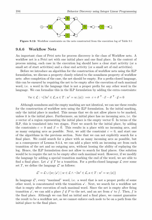
184 Behavior Discovery using Integer Linear Programming
Figure 9.12: Workflow constraints on the nets constructed from the execution log of Table 9.1
9.6.6 Workflow Nets
An important class of Petri nets for process discovery is the class of Workflow nets. Aworkflow net is a Petri net with one initial place and one final place. In the context ofprocess mining, each case in the execution log should have a clear start activity (or asmall set of start activities) and a clear end activity (or a small set of end activities).
Before we introduce an algorithm for the construction of workflow nets using the ILPformulation, we discuss a property closely related to the soundness property of workflownets: after completion of the case, the net should be empty. For a prefix-closed language,this can be ensured by requiring the net to be empty after the execution of each maximalword, i.e. a word in the language that is not a proper prefix for any other word in thelanguage. We can formalize this in the ILP formulation by adding the extra constraints:
∀w ∈ L : ¬(∃w′ ∈ L, a ∈ T : w′ = w; ⟨a⟩) =⇒ c+ σ T · x− σ T · y = 0
Although soundness and the empty marking are not identical, we can use these resultsfor the construction of workflow nets using the ILP formulation. In the initial marking,only the initial place is marked. This means that we do not allow places to be marked,unless it is the initial place. Furthermore, an initial place has no incoming arcs, i.e. thex-vector of a region representing the initial place is the empty vector 0. In terms of theILP, this is translated into two stages. First we search for the initial place, by addingthe constraints c = 0 and x = 0. This results in a place with no incoming arcs, andas many outgoing arcs as possible. Next, we add the constraint c = 0, and start oneof the algorithms in the previous section. Note that we can not explicitly search for afinal place. We could search for a place with as many incoming arcs as possible, butas a consequence of Lemma 9.4.4, we can add a place with an incoming arc from eachtransition of the net and no outgoing arcs, without loosing the ability of replaying thelog. Hence, the ILP formulation does not allow to search for final places. One solutionwould be to require the net to be empty after each maximal word. However, if we modifythe language by adding a special transition marking the end of the word, we are able tofind a final place. Let X ∈ T be a transition. For a prefix-closed language L over someset T , we define the language L′ as follows:
L′ = L ∪ w; ⟨X⟩ | w ∈ L ∧ ¬∃w′ ∈ L, a ∈ T : w′ = w; ⟨a⟩
In language L′, every “maximal” word, i.e. a word that is not a proper prefix of someother word, is concatenated with the transition X. Next, we search for a workflow netthat is empty after execution of each maximal word. Since the net is empty after firingtransition X, we can add a place f ∈ P to the net, and an arc from X to f . Then, f isthe final place. Although we can find an initial and a final place, we cannot guaranteethe result to be a workflow net, as we cannot enforce each node to be on a path from theinitial place to the final place.

185
Figure 9.12 shows the Petri net constructed from the log of Table 9.1. The Petrinet generated by adding independent places is identical to the net constructed using thecausal dependencies found in the execution log.
9.7 Discovery of Extensions on Petri Nets
In the previous section we have shown how the ILP formulation can be used to generateclasses of Petri nets. In this section we consider two of the most popular extensions ofthis class of nets, namely, Petri nets with reset and inhibitor arcs.
Definition 9.7.1 (Petri net with reset and inhibitor arcs)A Petri net with reset and inhibitor arcs N is a 5-tuple N = (P, T, F,R, I), where (1)(P, T, F ) is a Petri net; (2) R ⊆ T × P is the set of reset arcs, and (3) I ⊆ P × T is theset of inhibitor arcs. Given a transition t ∈ T and place p ∈ P , if (p, t) ∈ I, place p is aninhibitor place for t. If (t, p) ∈ R, place p is a reset place of t. y
Similarly to classical Petri nets, semantics of Petri nets with reset and inhibitor arcs isgiven in terms of markings. Inhibitor arcs influence whether a given transition is enabledor not. Formally, a transition t ∈ T is enabled in a marking m ∈ INP if and only if•t ≤ m and m(q) = 0 for all q such that (q, t) ∈ I. Only enabled transitions may fire.Reset arcs are used in determining results of a transition firing: places connected to atransition by reset arcs are emptied (reset) when the transition fires. To formalise thiswe introduce an auxiliary function πt : IN
P → INP defined as πt(m)(p) = 0 if (t, p) ∈ Rand πt(m)(p) = m(p), otherwise. Using this notation we say that a firing of transition tresults in a new marking m′ with m′ = πt(m− •t) + t•.
In the remainder of this section we discuss how reset arcs and inhibitor arcs can beadded to the ILP formulation and how these can be used to discover and refine Petrinets.
9.7.1 Inhibitor Nets
Up to now, the region only expresses regular arcs, i.e. only arcs that consume andproduce tokens in the corresponding place. With the extension of inhibitor arcs, a newclass of arcs is added, and hence, the definition of a region needs to be changed to expressinhibitor arcs. An inhibitor arc between a place and transition prevents the transitionto fire if there is a token present in the place. To express this in the ILP formulation, weadd for each transition t ∈ T an extra variable, ι(t) ∈ 0, ω that expresses the numberof tokens allowed in the corresponding feasible place in order for transition t to fire. Thisextends the definition of a region to:
∀t ∈ T : ∀w; ⟨t⟩ ∈ L : c+ w · x− w · y − ι(t) ≤ 0
If no inhibitor arc is present, the condition is trivially satisfied, otherwise ι(t) = 0 andfiring of t is possible only if the corresponding place is empty. A generalization of inhibitorarcs can be obtained by allowing ι(t) to range between 0 and ω, i.e. the firing of transitiont is possible if the place contains not more than ι(t) tokens (cf. [80]). As ι(t) = ω alwaysholds, in the ILP formulation we need to minimize
∑t∈T ι(t).
Implementation of model refinement in a process mining tool requires solving integerlinear programming problems involving ω. Approximating ω with a very large integer,i.e. MAXINT, results unfortunately in numerically unstable ILP problems: despite the
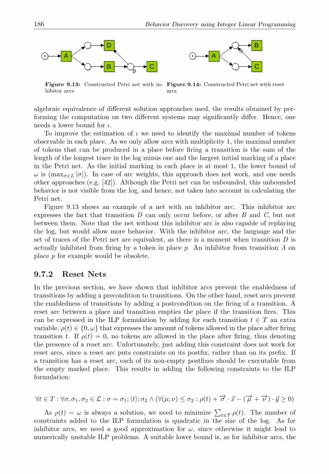
186 Behavior Discovery using Integer Linear Programming
A
B C
D
p
Figure 9.13: Constructed Petri net with in-hibitor arcs
A
B
C
Figure 9.14: Constructed Petri net with resetarcs
algebraic equivalence of different solution approaches used, the results obtained by per-forming the computation on two different systems may significantly differ. Hence, oneneeds a lower bound for ι.
To improve the estimation of ι we need to identify the maximal number of tokensobservable in each place. As we only allow arcs with multiplicity 1, the maximal numberof tokens that can be produced in a place before firing a transition is the sum of thelength of the longest trace in the log minus one and the largest initial marking of a placein the Petri net. As the initial marking in each place is at most 1, the lower bound ofω is (maxσ∈L |σ|). In case of arc weights, this approach does not work, and one needsother approaches (e.g. [42]). Although the Petri net can be unbounded, this unboundedbehavior is not visible from the log, and hence, not taken into account in calculating thePetri net.
Figure 9.13 shows an example of a net with an inhibitor arc. This inhibitor arcexpresses the fact that transition D can only occur before, or after B and C, but notbetween them. Note that the net without this inhibitor arc is also capable of replayingthe log, but would allow more behavior. With the inhibitor arc, the language and theset of traces of the Petri net are equivalent, as there is a moment when transition D isactually inhibited from firing by a token in place p. An inhibitor from transition A onplace p for example would be obsolete.
9.7.2 Reset Nets
In the previous section, we have shown that inhibitor arcs prevent the enabledness oftransitions by adding a precondition to transitions. On the other hand, reset arcs preventthe enabledness of transitions by adding a postcondition on the firing of a transition. Areset arc between a place and transition empties the place if the transition fires. Thiscan be expressed in the ILP formulation by adding for each transition t ∈ T an extravariable, ρ(t) ∈ 0, ω that expresses the amount of tokens allowed in the place after firingtransition t. If ρ(t) = 0, no tokens are allowed in the place after firing, thus denotingthe presence of a reset arc. Unfortunately, just adding this constraint does not work forreset arcs, since a reset arc puts constraints on its postfix, rather than on its prefix. Ifa transition has a reset arc, each of its non-empty postfixes should be executable fromthe empty marked place. This results in adding the following constraints to the ILPformulation:
∀t ∈ T : ∀σ, σ1, σ2 ∈ L : σ = σ1; ⟨t⟩;σ2 ∧ (∀(µ; ν) ≤ σ2 : ρ(t) +−→σ · x− (−→µ +−→ν ) · y ≥ 0)
As ρ(t) = ω is always a solution, we need to minimize∑t∈T ρ(t). The number of
constraints added to the ILP formulation is quadratic in the size of the log. As forinhibitor arcs, we need a good approximation for ω, since otherwise it might lead tonumerically unstable ILP problems. A suitable lower bound is, as for inhibitor arcs, the
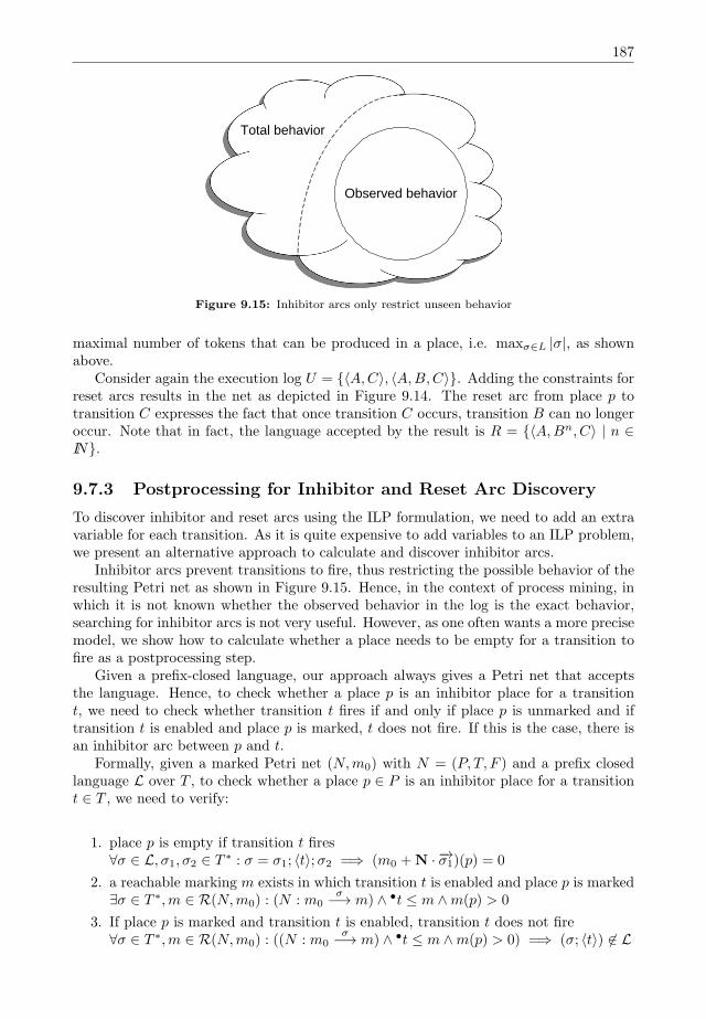
187
Observed behavior
Total behavior
Figure 9.15: Inhibitor arcs only restrict unseen behavior
maximal number of tokens that can be produced in a place, i.e. maxσ∈L |σ|, as shownabove.
Consider again the execution log U = ⟨A,C⟩, ⟨A,B,C⟩. Adding the constraints forreset arcs results in the net as depicted in Figure 9.14. The reset arc from place p totransition C expresses the fact that once transition C occurs, transition B can no longeroccur. Note that in fact, the language accepted by the result is R = ⟨A,Bn, C⟩ | n ∈IN.
9.7.3 Postprocessing for Inhibitor and Reset Arc Discovery
To discover inhibitor and reset arcs using the ILP formulation, we need to add an extravariable for each transition. As it is quite expensive to add variables to an ILP problem,we present an alternative approach to calculate and discover inhibitor arcs.
Inhibitor arcs prevent transitions to fire, thus restricting the possible behavior of theresulting Petri net as shown in Figure 9.15. Hence, in the context of process mining, inwhich it is not known whether the observed behavior in the log is the exact behavior,searching for inhibitor arcs is not very useful. However, as one often wants a more precisemodel, we show how to calculate whether a place needs to be empty for a transition tofire as a postprocessing step.
Given a prefix-closed language, our approach always gives a Petri net that acceptsthe language. Hence, to check whether a place p is an inhibitor place for a transitiont, we need to check whether transition t fires if and only if place p is unmarked and iftransition t is enabled and place p is marked, t does not fire. If this is the case, there isan inhibitor arc between p and t.
Formally, given a marked Petri net (N,m0) with N = (P, T, F ) and a prefix closedlanguage L over T , to check whether a place p ∈ P is an inhibitor place for a transitiont ∈ T , we need to verify:
1. place p is empty if transition t fires∀σ ∈ L, σ1, σ2 ∈ T ∗ : σ = σ1; ⟨t⟩;σ2 =⇒ (m0 +N · −→σ1)(p) = 0
2. a reachable marking m exists in which transition t is enabled and place p is marked∃σ ∈ T ∗,m ∈ R(N,m0) : (N : m0
σ−→ m) ∧ •t ≤ m ∧m(p) > 0
3. If place p is marked and transition t is enabled, transition t does not fire∀σ ∈ T ∗,m ∈ R(N,m0) : ((N : m0
σ−→ m) ∧ •t ≤ m ∧m(p) > 0) =⇒ (σ; ⟨t⟩) ∈ L
188 Behavior Discovery using Integer Linear Programming
Consider again the execution log U = ⟨A,C⟩, ⟨A,B,C⟩, which resulted in the Petri netshown in Figure 9.13. All conditions hold for place p and transition D.
For reset arcs we can apply the same approach. A reset arc empties a place. Givena marked Petri net (N,m0) with N = (P, T, F ) and a prefix closed language L over T ,we want to check whether a place p ∈ P is reset by transition t ∈ T . This means forplace p that it is always empty after the occurrence of transition t. Hence, all words inthe language that end with t should result in an empty marked place p, i.e. we need toverify:
∀(w; ⟨t⟩) ∈ L : (m0 +N · −→w )(p) > 0 ∧ (m0 +N(−→w + t ))(p) = 0
In the example execution log U , for which the resulting Petri net is shown in Fig-ure 9.14, the condition holds for place p and transition C.
9.8 Conclusions
In this chapter, we presented a new method for process discovery using integer linearprogramming (ILP). The main idea is that places restrict the possible firing sequencesof a Petri net. Hence, we search for as many places as possible, such that the resultingPetri net is consistent with the log, i.e. such that the Petri net is able to replay the log.
The well-known theory of regions solves a similar problem for finite prefix-closedlanguages. It synthesizes a Petri net which can reproduce the language as precisely aspossible. In [30, 79] this idea is elaborated and the problem is formalized using a linearinequation system. The authors present two ways to construct finite Petri nets acceptingthe given language with minimal additional firing sequences, the basis representation andthe separating representation. However, the Petri nets synthesized using these approachesscale in the number of events in the language, which is undesirable in process discovery.
In the basis representation, the set of places is chosen such that it is a basis for thenon-negative integer solution space of the linear inequation system. Although such abasis always exists for homogeneous inequation systems, it is worst-case exponential inthe number of equations [79]. By construction of the inequation system, the number ofequations is linear in the number of traces, and thus, the basis representation is worst-case exponential in the number of events in the log. Hence, an event log containingten thousand events, referring to 40 transitions, might result in a Petri net containing ahundred million places connected to those 40 transitions. Although [30] provides someideas on how to remove redundant places from the basis, these procedures still requirethe basis to be constructed fully.
To reduce the theoretical exponential upper bound of the number of places in theresulting Petri net, the authors of [30, 79] propose a separating representation. In thisrepresentation, only places that separate the allowed behavior (specified by the systems)using words not in the language are added to the resulting Petri net, i.e. for each wordw ∈ L and transition t ∈ T such that w; t ∈ L a place is added to the Petri net. Althoughthis representation is no longer exponential in the size of the language, but polynomial,it requires the user to specify undesired behavior, which is in the setting of processdiscovery not possible, since nothing is known about the behavior, except the behaviorseen in the event log. In [30, 79] the authors propose the separating representation forregular and step languages and by this, they maximize the number of places generatedby the number of events in the log times the number of transitions.
189
In process mining, or more precisely, in process discovery, an execution log representsthe traces executed by a system. Such an execution log represents a finite prefix-closedlanguage. In this chapter, we build on the methods proposed in [30, 79]. First of allwe have defined an optimality criterion transforming the inequation system into an ILPformulation. The optimality criterion we defined is such that it guarantees that moreexpressive places are found first, i.e. places with less input arcs and more output arcsare favored.
We presented three different approaches to construct a marked Petri net. The firstapproach generates independent places: we first search for the most expressive place,and then only search for places that have a smaller initial marking, fewer incoming arcsor more outgoing arcs. This way, a Petri net is constructed that exactly represents theprefix-closed language. For this approach, there is no good stopping criterion, other thanto stop when the set of traces defined by the resulting net equals the given language.Therefore, we present a second algorithm. This algorithm uses the causality relationas defined for the alpha algorithm [16]. For each causal dependency, we search a mostexpressive place expressing this causal dependency. This causality relation is generallyaccepted in the field of process discovery and, under the assumption the log is complete,is shown to directly relate to places. Furthermore, the size of the constructed Petri netis independent on the number of events in the log, which makes this approach applicablein more practical situations. The third algorithm takes as input a marked Petri net anda prefix-closed language. It first checks whether each place is feasible, i.e. whether foreach place a corresponding region of the language exists. If such a region does not exist,the place is removed. In the second step, places are added according to one of the otheralgorithms. A prototype has been implemented in the tool ProM [7, 111], which allowsthe user to select the different options as presented in this chapter. All Petri nets in thischapter have been generated using this prototype.
The advantage of integer linear programming is that many tools like [1,2] are special-ized for constraint programming, of which integer linear programming is a specialization.With constraint programming, it is possible to add additional constraints, without hav-ing to change algorithms. Using additional constraints, we can enforce structural netproperties of the discovered Petri net, such as the freedom of choice. It is clear that notall these constraints for structural properties lead to feasible solutions, but nonetheless,we always find a Petri net that is able to replay the log. For all our constraints we providelemmas motivating these constraints. The same approach can be used for the discoveryof inhibitor arcs and reset arcs.

190 Behavior Discovery using Integer Linear Programming

Part III
Conclusions and Outlook


10Conclusions
In this thesis, we have made several contributions to the design and verification ofcomponent-based information systems. Such a system consists of many components thatcommunicate asynchronously. The environment of a component is only partially known,as each component only knows its direct neighbors. This way, the components form alarge scale, possibly unknown network of asynchronously communicating components.Components can be added to or removed from the network at run time. To guaranteecorrectness of such networks, we need compositional verification methods. In this thesis,we consider one universal sanity criterion, called soundness. Soundness is a criterionthat considers only the control flow aspect of a system. A system is called sound if itis possible to reach a desired final state from every reachable state of the system. If asystem is not sound it is most likely that it has serious errors.
Contributions The contributions in this thesis can be summarized as follows.
1. We developed an architectural framework for component-based information sys-tems, founded on Petri nets. In the framework, the communication between com-ponents and their internal behavior is modeled using the same modeling language.This way, both atomic components and compositions are treated equally in theframework. As a consequence, the framework supports the hierarchical design ofcomponent-based information systems.
2. We developed a compositional verification method for soundness, in which we onlyhave to check each pair of communicating components. We presented a condition,the elastic communication condition, for communication to guarantee soundness.Although the condition is sufficient to conclude soundness of the whole system ifeach component is sound and all pairs of communicating components satisfy oneof the conditions, we have not found a necessary and sufficient condition.
3. To assist the modeler, we developed a design method to guarantee soundness byconstruction. The method focuses on designing the components with their com-munication protocols. For the method, we introduced a new refinement rule whichis based on the instantaneous refinement of a set of places. If the set of placessatisfies the condition we formulated, and the refining net is sound, the refinementoperation is proven to preserve the soundness property.
4. Data plays an important role in information systems. We developed a subclass

194 Conclusions
of colored Petri nets that can handle objects and their relationships, yet still itallows for verification. The subclass can be used to model the message passing be-tween components. Furthermore, we presented a method that can model databasetransactions for arbitrary data models in component-based information systems.
5. Based on the architectural framework we introduced a method to design and pro-totype component-based information systems. The method involves for each com-ponent the design of a process model, an object model, the interaction between thetwo, and the forms to interact with the user. Based on these artifacts, automat-ically a working prototype is generated. As a proof of concept, we developed thetool YasperWE.
6. Up to now, the methods are top-down, as each component is designed from scratch.In most cases, organizations already have legacy information systems, which arethen extended with additional components. Therefore, we developed an algorithmthat can discover a process model from the event logs of such a system. Thealgorithm is based on linear integer programming. This way, the algorithm caneasily be extended to pose additional requirements on the discovered process model.

11Outlook
In this thesis, we only focused on a general sanity criterion, soundness. However, toguarantee correctness, many other properties need to be considered, imposed by legalregulations, business policies and best practices. Therefore, compositional verificationmethods should be extended to support these properties as well. For soundness, thereis still a need for necessary and sufficient conditions for the compositional verification ofnetworks of asynchronously communicating components.
Although soundness is an important property, it can be misleading: if a system has asound control flow, its soundness can be destroyed when taking data into account, sincedata can be used in transitions as a precondition that blocks some behavior. On the otherhand, if a system is unsound, preconditions based on data can exclude bad behavior, sothat the system becomes sound. Therefore, it is interesting to consider extensions of thesoundness notion and checks that include the use of data in component-based informationsystems (cf. [101]).
In this thesis, we used process mining for the analysis of existing systems to extractthe control flow of components from event logs. In the future, we see an important op-portunity for process mining to be integrated in the development of information systems.Requirements are often in the form of uses cases with a set of scenarios. Requirements ofthis form can be used as input for process discovery algorithms. This way, the process offormalizing requirements can be partially automated, although validation of the modelsremains essential.
To show the applicability of the approach, we need efficient implementations of ourmethods for the compositional verification methods we introduced in Chapter 4. To as-sist the modeler, we need a tool that implements the design method based on refinementsof sets of places. Although tools like Yasper and YasperWE show the applicability ofthe approach, industrial tools, like IBM Websphere, support the design and implementa-tion of component-based information systems, but lack proper verification methods. Bycombining the best of both worlds, we can put the quality of these systems on a higherlevel.

196 Outlook

Bibliography
[1] LP Solve Reference guide. http://lpsolve.sourceforge.net/5.5/.
[2] ILOG CPLEX, ILOG, Inc., 2006. http://www.ilog.com/products/cplex/.
[3] W.M.P. van der Aalst. Verification of Workflow Nets. In Application and Theory of Petri Nets1997, volume 1248 of Lecture Notes in Computer Science, pages 407 – 426. Springer-Verlag, Berlin,1997.
[4] W.M.P. van der Aalst. Inheritance of Interorganizational Workflows: How to agree to disagreewithout loosing control? Information Technology and Management Journal, 4(4):345–389, 2003.
[5] W.M.P. van der Aalst, M. Beisiegel, K.M. van Hee, D. Konig, and C. Stahl. An SOA-BasedArchitecture Framework. International Journal of Business Process Integration and Management,2(2):91–101, 2007.
[6] W.M.P. van der Aalst, P.J.N. de Crom, R.R.H.M.J. Goverde, K.M. van Hee, W.J. Hofman, et al.ExSpect 6.4 An Executable Specification Tool for Hierarchical Colored Petri Nets. In Applicationand Theory of Petri Nets 2000, volume 1825 of Lecture Notes in Computer Science, pages 455–464.Springer-Verlag, Berlin, 2000.
[7] W.M.P. van der Aalst, B.F. van Dongen, C.W. Gunther, et al. ProM 4.0: Comprehensive Supportfor Real Process Analysis. In Petri Nets and Other Models of Concurrency ICATPN 2007, volume4546 of Lecture Notes in Computer Science, pages 484–494. Springer-Verlag, Berlin, 2007.
[8] W.M.P. van der Aalst, B.F. van Dongen, J. Herbst, L. Maruster, G. Schimm, and A.J.M.M.Weijters. Workflow Mining: A Survey of Issues and Approaches. Data & Knowledge Engineering,47(2):237–267, 2003.
[9] W.M.P. van der Aalst and K.M. van Hee. Workflow Management: Models, Methods and Systems.Academic Service, Schoonhoven, 1997.
[10] W.M.P. van der Aalst, K.M. van Hee, A.H.M. ter Hofstede, N. Sidorova, H.M.W. Verbeek, M.Voorhoeve, and M.T. Wynn. Soundness of workflow nets: classification, decidability, and analysis.Formal Aspects of Computing, pages 1–31, 2010.
[11] W.M.P. van der Aalst, K.M. van Hee, P. Massuthe, N. Sidorova, and J.M.E.M. van der Werf.Compositional Service Trees. In Applications and Theory of Petri Nets 2009, volume 5606 ofLecture Notes in Computer Science, pages 283 – 302. Springer-Verlag, Berlin, 2009.
[12] W.M.P. van der Aalst, K.M. van Hee, J.M.E.M. van der Werf, A. Kumar, and M. Verdonk.Conceptual model for online auditing. Decision Support Systems, 2010. to appear.
[13] W.M.P. van der Aalst, N. Lohmann, P. Massuthe, C. Stahl, and K. Wolf. From Public Views toPrivate Views: Correctness-by-Design for Services. In Web Services and Formal Methods, volume4937 of Lecture Notes in Computer Science, pages 139–153. Springer-Verlag, Berlin, 2008.
[14] W.M.P. van der Aalst, N. Lohmann, P. Massuthe, C. Stahl, and K. Wolf. Multiparty Contracts:Agreeing and Implementing Interorganizational Processes. The Computer Journal, 53(1):90–106,2010.
198 BIBLIOGRAPHY
[15] W.M.P. van der Aalst, V. Rubin, B.F. van Dongen, E. Kindler, and C.W. Gunther. ProcessMining: A Two-Step Approach using Transition Systems and Regions. Acta Informatica, 2007.submitted.
[16] W.M.P. van der Aalst, A.J.M.M. Weijters, and L. Maruster. Workflow Mining: Discovering ProcessModels from Event Logs. Knowledge & Data Engineering, 16(9):1128–1142, 2004.
[17] W.M.P. van der Aalst, M. Weske, and D. Grunbauer. Case handling: a new paradigm for businessprocess support. Data & Knowlegde Engineering, 53(2):129–162, 2005.
[18] J-R. Abrial. Modeling in Event-B. Cambridge University Press, 2010.
[19] A.V. Aho, C. Beeri, and J.D. Ullman. The Theory of Joins in Relational Databases. ACMTransactions on Database Systems (TODS), 4(3):297–314, 1979.
[20] L. de Alfaro and Th. A. Henzinger. Interface automata. SIGSOFT Softw. Eng. Notes, 26(5):109–120, 2001.
[21] G. Alonso, F. Casati, H. Kuno, and V. Machiraju. Web Services – Concepts, Architectures andApplications. Springer-Verlag, Heidelberg, 2004.
[22] A. Alves, A. Arkin, S. Askary, et al. Web Services Business Process Execution Language Version2.0 (OASIS Standard). WS-BPEL TC OASIS, http://docs.oasis-open.org/wsbpel/2.0/wsbpel-v2.0.html, 2007.
[23] A.K. Alves de Medeiros, B.F. van Dongen, W.M.P. van der Aalst, and A.J.M.M. Weijters. ProcessMining for Ubiquitous Mobile Systems: An Overview and a Concrete Algorithm. In UbiquitousMobile Information and Collaboration Systems, volume 3272 of Lecture Notes in Computer Sci-ence, pages 154–168. Springer-Verlag, Berlin, 2004.
[24] W.W. Armstrong. Dependency Structures of Data Base Relationships. In IFIP Congress, pages580–583, 1974.
[25] E. Badouel, L. Bernardinello, and Ph. Darondeau. Polynomial Algorithms for the Synthesis ofBounded Nets. In TAPSOFT ’95: Theory and Practice of Software Development, volume 915 ofLecture Notes in Computer Science, pages 364–378. Springer-Verlag, Berlin, 1995.
[26] E. Badouel and Ph. Darondeau. Theory of regions. In Lectures on Petri Nets I: Basic Models,volume 1491 of Lecture Notes in Computer Science, pages 529–586. springer, 1998.
[27] L. Bass, P. Clements, and R. Kazman. Software Architecture in Practice. Series in SoftwareEngineering. Addison Wesley, Reading, MA, USA, 1998.
[28] T. Basten and W.M.P. van der Aalst. Inheritance of Behavior. Journal of Logic and AlgebraicProgramming, 47(2):47–145, 2001.
[29] M. Beisiegel, K. Khand, A. Karmarkar, S. Patil, and M. Rowley. Service Component ArchitectureAssembly Model Specification Version 1.1, 2010.
[30] R. Bergenthum, J. Desel, R. Lorenz, and S. Mauser. Process mining based on regions of languages.In Business Process Management, volume 4714 of Lecture Notes in Computer Science, pages 375–383. Springer-Verlag, Berlin, 2007.
[31] G. Berthelot. Transformations and Decompositions of Nets. In Petri Nets, central models andtheir properties, volume 254 of Lecture Notes in Computer Science, pages 360–376. Springer-Verlag, Berlin, 1987.
[32] K.R. Blackman. IMS celebrates thirty years as an IBM meeting. IBM Systems Journal, 37(4),1998.
[33] J. Carmona, J. Cortadella, and M. Kishinevsky. A region-based algorithm for discovering Petrinets from event logs. In Business Process Management, volume 5240 of Lecture Notes in ComputerScience, pages 358–373. Springer-Verlag, Berlin, 2008.
[34] P.P. Chen. The Entity-Relationship Model: Towards a unified view of Data. ACM Transactionson Database Systems, 1:9–36, January 1976.
[35] C. Choppy and L. Petrucci. Towards a Methodology for Modeling with Petri Nets. In PracticalUse of Coloured Petri Nets, pages 39–56, 2004.
[36] E. Christensen, F. Curbera, G. Meredith, and S. Weerawarana. Web Services Description Language(WSDL) 1.1. http://www.w3.org/TR/wsdl, 2001.
[37] E. Clarke and E. Emerson. Design and Synthesis of Synchronization Skeletons Using Branching-Time Temporal Logic. In Logics of Programs, volume 131 of Lecture Notes in Computer Science,pages 52–71. Springer-Verlag, Berlin, 1982.
199
[38] E.F. Codd. A relational model of data for large shared data banks. Communications of the ACM,13(6):377–387, 1970.
[39] E.F. Codd. Further Normalization of the Data Base Relational Model. IBM Research Report, SanJose, California, RJ909, 1971.
[40] J. Cortadella, M. Kishinevsky, L. Lavagno, and A. Yakovlev. Deriving Petri nets from FiniteTransition Systems. IEEE Transactions on Computers, 47(8):859–882, August 1998.
[41] Ph. Darondeau. Deriving Unbounded Petri Nets from Formal Languages. In CONCUR’98 Concur-rency Theory, volume 1466 of Lecture Notes in Computer Science, pages 533–548. Springer-Verlag,Berlin, 1998.
[42] Ph. Darondeau. Distributed implementations of ramadge-wonham supervisory control with petrinets. In 44th IEEE Conference on CDC-ECC ’05, pages 2107–2112. IEEE Computer Society,December 2005.
[43] G. Decker and M. Weske. Local Enforceability in Interaction Petri Nets. In Business ProcessManagement, volume 4714 of Lecture Notes in Computer Science, pages 305–319. Springer-Verlag,Berlin, 2007.
[44] J. Desel and J. Esparza. Free Choice Petri Nets, volume 40 of Cambridge Tracts in TheoreticalComputer Science. Cambridge University Press, 1995.
[45] J. Desel and L. Petrucci. Aggregating views for Petri net model construction. In Workshop onPetri Nets and Distributed Systems, pages 17–31, 2008.
[46] J. Desel and W. Reisig. The Synthesis Problem of Petri Nets. Acta Informatica, 33(4):297–315,1996.
[47] B.F. van Dongen. Process Mining and Verification. PhD thesis, Eindhoven University of Technol-ogy, Eindhoven, The Netherlands, 2007.
[48] B.F. van Dongen, A.K. Alves de Medeiros, and L. Wen. Process mining: Overview and outlook ofpetri net discovery algorithms. volume 5460 of Lecture Notes in Computer Science, pages 225–242.Springer-Verlag, Berlin, 2009.
[49] A. Ehrenfeucht and G. Rozenberg. Partial (Set) 2-Structures - Part 1 and Part 2. Acta Informatica,27(4):315–368, 1989.
[50] R.J. van Glabbeek. The Linear Time - Branching Time Spectrum II: The Semantics of SequentialSystems with Silent Moves. In Proceedings of CONCUR 1993, volume 715 of Lecture Notes inComputer Science, pages 66–81. Springer-Verlag, Berlin, 1993.
[51] J. Gray and A. Reuter. Transaction Processing, concepts and techniques. Morgan Kaufmann,1993.
[52] Object Management Group. Object Constraint Language, V2.2. Object Management Group, 2010.
[53] Object Management Group. OMG Unified Modeling LanguageTM (OMG UML), SuperstructureV2.3. Object Management Group, 2010.
[54] C.W. Gunther and Wil M.P. van der Aalst. Modeling the case handling principles with ColoredPetri nets. In Practical Use of Coloured Petri Nets, 2005.
[55] R. Heckel. Open Petri Nets as Semantic Model for Workflow Integration. In Petri Net Technologyfor Communication-Based Systems, volume 2472 of Lecture Notes in Computer Science, pages281–294. Springer-Verlag, Berlin, 2003.
[56] K.M. van Hee. Information System Engineering - A Formal Approach. Cambridge UniversityPress, 1994.
[57] K.M. van Hee, J. Keiren, R.D.J. Post, N. Sidorova, and J.M.E.M. van der Werf. Designing CaseHandling Systems. Transactions on Petri Nets and Other Models of Concurrency, 5100, 2008.
[58] K.M. van Hee, A.J Mooij, N. Sidorova, and J.M.E.M. van der Werf. Soundness-Preserving Refine-ments of Service Compositions. In Web Services and Formal Methods, Lecture Notes in ComputerScience. Springer-Verlag, Berlin, 2010. to appear.
[59] K.M. van Hee, O. Oanea, R.D.J. Post, L.J. Somers, and J.M.E.M. van der Werf. Yasper: a tool forworkflow modeling and analysis. Sixth International Conference on Application of Concurrencyto System Design (ACSD’06), pages 279–282, 2006.
[60] K.M. van Hee, R.D.J. Post, and L.J. Somers. Yet Another Smart Process Editor. In EuropeanSimulation and Modelling Conference 2005, pages 527–530, 2005.
200 BIBLIOGRAPHY
[61] K.M. van Hee, N. Sidorova, L.J. Somers, and M. Voorhoeve. Consistency in model integration.Data & Knowledge Engineering, 56(1):4–22, January 2006.
[62] K.M. van Hee, N. Sidorova, and M. Voorhoeve. Soundness and Separability of Workflow Nets inthe Stepwise Refinement Approach. In Application and Theory of Petri Nets 2003, volume 2679of Lecture Notes in Computer Science, pages 335 – 354. Springer-Verlag, Berlin, 2003.
[63] K.M. van Hee, N. Sidorova, and M. Voorhoeve. Generalised Soundness of Workflow Nets IsDecidable. In Application and Theory of Petri Nets 2004, volume 3099 of Lecture Notes inComputer Science, pages 197 – 215. Springer-Verlag, Berlin, 2004.
[64] K.M. van Hee, N. Sidorova, M. Voorhoeve, and J.M.E.M. van der Werf. Generation of DatabaseTransactions with Petri nets. Fundamenta Informatica, 93(1 – 3):171 – 184, 2009.
[65] K.M. van Hee, N. Sidorova, and J.M.E.M. van der Werf. Construction of Asynchronous Com-municating Systems: Weak Termination Guaranteed! In Software Composition, volume 6144 ofLecture Notes in Computer Science, pages 106 – 121. Springer-Verlag, Berlin, 2010.
[66] L. Hillah, E. Kindler, F. Kordon, L. Petrucci, and N. Treves. A primer on the Petri Net MarkupLanguage and ISO/IEC 15909-2. Petri Net Newsletter, 76:9–28, October 2009.
[67] H. Hollerith. An Electric Tabulating System. The Quarterly, X(16):238–255, April 1889.
[68] H. Hollerith. In connection with the electric tabulation system which has been adopted by U.S.government for the work of the census bureau. PhD thesis, Columbia University School of Mines,1890.
[69] H. Hollerith. The Electrical Tabulating Machine. Journal of the Royal Statistical Society,57(4):678–689, December 1894.
[70] P. Jancar. Undecidability of Bisimilarity for Petri Nets and Related Problems. Theoretical Com-puter Science, (148):281 – 301, 1995.
[71] Kurt Jensen. Coloured Petri nets: basic concepts, analysis methods and practical use, vol. 2.Springer-Verlag, Berlin, 1995.
[72] R. Kazhamiakin, M. Pistore, and L. Santuari. Analysis of communication models in web servicecompositions. In International World Wide Web Conference, pages 267 – 276, New York, NY,USA, 2006. ACM.
[73] E. Kinder and L. Petrucci. Towards a Standard for Modular Petri Nets: A Formalization. InApplication and Theory of Petri Nets 2009, volume 5606 of Lecture Notes in Computer Science,pages 43 – 62. Springer-Verlag, Berlin, 2009.
[74] E. Kindler. A compositional partial order semantics for Petri net components. In Application andTheory of Petri Nets 1997, volume 1248 of Lecture Notes in Computer Science, pages 235–252.Springer-Verlag, Berlin, 1997.
[75] N. Kurbel and K. Schnieder. Integration Issues of Information Engineering Based I-CASE Tools.In Fourth International Conference on Information Systems Development 1994, pages 431–441,1994.
[76] K.G. Larsen and B. Thomsen. A Modal Process Logic. In Logic in Computer Science, pages203–210. IEEE Computer Society, 1988.
[77] N. Lohmann, P. Massuthe, C. Stahl, and D. Weinberg. Analyzing Interacting BPEL Processes. InBusiness Process Management, volume 4102 of Lecture Notes in Computer Science, pages 17–32.Springer-Verlag, Berlin, 2006.
[78] N. Lohmann, P. Massuthe, and K. Wolf. Operating Guidelines for Finite-State Services. In PetriNets and Other Models of Concurrency ICATPN 2007, volume 4546 of Lecture Notes in ComputerScience, pages 321–341. Springer-Verlag, Berlin, 2007.
[79] R. Lorenz and R. Juhas. How to Synthesize Nets from Languages - a Survey. In Proceedings ofthe Wintersimulation Conference (WSC) 2007, 2007.
[80] R. Lorenz, S. Mauser, and R. Bergenthum. Theory of Regions for the Synthesis of Inhibitor Netsfrom Scenarios. In Petri Nets and Other Models of Concurrency ICATPN 2007, volume 4546 ofLecture Notes in Computer Science, pages 342–361. Springer-Verlag, Berlin, 2007.
[81] N.A. Lynch and M. Tuttle. Hierarchical correctness proofs for distributed algorithms. In 6thAnnual ACM Symposium on Principles of Distributed Computing, 1987.
[82] P. Massuthe. Operating Guidelines for Services. PhD thesis, Technische Universiteit Eindhoven,2009.

201
[83] P. Massuthe, W. Reisig, and K. Schmidt. An Operating Guideline Approach to the SOA. Annalsof Mathematics, Computing & Teleinformatics, 1(3):35–43, 2005.
[84] P. Massuthe, A. Serebrenik, N. Sidorova, and K. Wolf. Can I find a partner? Undecidability ofpartner existence for open nets. Information Processing Letters, 108(6):374 – 378, 2008.
[85] S. Mauw and M.A. Reniers. An algebraic semantics of Basic Message Sequence Charts. TheComputer Journal, 37(4):269–277, 1994.
[86] M.D. McIlroy. Mass produced software components. In P. Naur and B. Randell, editors, Proceed-ings of NATA Software Engineering Conference, volume 1, pages 138–150. Garmisch Germany,1968.
[87] T. Murata. Petri Nets: Properties, Analysis and Applications. Proceedings of the IEEE, 77(4):541–580, April 1989.
[88] Object Management Group. Business Process Modeling Notation, V1.1.http://www.omg.org/spec/BPMN/1.1/PDF/, 2008.
[89] M.P. Papazoglou. Web Services: Principles and Technology. Pearson - Prentice Hall, 2007.
[90] R.J. Parikh. On Context-Free Languages. Journal of the ACM, 13(4):570 – 581, October 1966.
[91] J.L. Peterson. Petri net theory and the modeling of systems. Prentice-Hall, Englewood Cliffs,1981.
[92] C.A. Petri. Kommunikation mit Automaten. PhD thesis, Institut fur instrumentelle Mathematik,Bonn, 1962.
[93] A.V. Ratzer, L. Wells, H.M. Lassen, M. Laursen, J.F. Qvortrup, et al. CPN tools for editing,simulating, and analysing coloured petri nets. In Applications and Theory of Petri Nets 2003: 24thInternational Conference, ICATPN 2003, Eindhoven, The Netherlands, volume 2679 of LectureNotes in Computer Science, pages 450–462. Springer-Verlag, Berlin, 2003.
[94] W. Reisig. Petri Nets: An Introduction, volume 4 of Monographs in Theoretical Computer Science:An EATCS Series. Springer-Verlag, Berlin, 1985.
[95] W. Reisig. A strong part of concurrency. In Advances in Petri Nets 1987, volume 266 of LectureNotes in Computer Science, pages 238–272. Springer-Verlag, Berlin, 1987.
[96] F. Rosa-Velardo, D. de Frutos-Escrig, and O. Marroquın-Alonso. On the expressiveness of MobileSynchronizing Petri nets. In Proceedings of the International Workshop on Security and Con-currency (SecCo 2005), volume 180 of Electronic Notes in Theoretical Computer Science, pages77–94. Elsevier, 2007.
[97] F. Rosa-Velardo, O. Marroquın-Alonso, and D. de Frutos-Escrig. Mobile Synchronizing PetriNets: a choreographic approach for coordination in Ubiquitous Systems. In Proceedings of theFirst International Workshop on Methods and Tools for Coordinating Concurrent, Distributedand Mobile Systems (MTCoord 2005), volume 150 of Electronic Notes in Theoretical ComputerScience, pages 103–126. Elsevier, 2006.
[98] K. Schmidt. Distributed Verification with LoLA. Fundamenta Informatica, 54(2-3):253–262, 2003.
[99] Ph. Schnoebelen and N. Sidorova. Bisimulation and the Reduction of Petri Nets. In Applicationand Theory of Petri Nets 2000, volume 1825 of Lecture Notes in Computer Science, pages 409–423.Springer-Verlag, Berlin, 2000.
[100] A. Schrijver. Theory of Linear and Integer programming. Wiley-Interscience, 1986.
[101] N. Sidorova, C. Stahl, and N. Trcka. Workfow Soundness Revisited: Checking Correctness inthe Presence of Data While Staying Conceptual. In Advanced Information Systems Engineering,volume 6051 of Lecture Notes in Computer Science, pages 530–544. Springer-Verlag, Berlin, 2010.
[102] A. Silberschatz, H. Korth, and S. Sudarshan. Database System Concepts. McGraw Hill, 5thedition, 2006.
[103] C. Stahl. Service Substitution. PhD thesis, Technische Universiteit Eindhoven, 2009.
[104] C. Stahl, P. Massuthe, and J. Bretschneider. Deciding Substitutability of Services with OperatingGuidelines. In Transactions on Petri Nets and Other Models of Concurrency II, volume 5460 ofLecture Notes in Computer Science, pages 172–191. Springer-Verlag, Berlin, 2009.
[105] C. Szyperski. Component Software – beyond Object-Oriented Programming. Addison-Wesley andACM Press, 1998.
[106] H.M.W. Verbeek, T. Basten, and Wil M.P. van der Aalst. Diagnosing Workflow Processes usingWoflan. The Computer Journal, 44(4):246–279, 2001.

202 BIBLIOGRAPHY
[107] W. Vogler. Asynchronous communication of petri nets and the refinement of transitions. InAutomata, Languages and Programming, volume 623 of Lecture Notes in Computer Science, pages605 – 616. Springer-Verlag, Berlin, 1992.
[108] A.J.M.M. Weijters and W.M.P. van der Aalst. Rediscovering Workflow Models from Event-BasedData using Little Thumb. Integrated Computer-Aided Engineering, 10(2):151–162, 2003.
[109] L. Wen, W.M.P. van der Aalst, J. Wang, and J. Sun. Mining process models with non-free-choiceconstructs. Data Mining and Knowledge Discovery, 15(2):145–180, 2007.
[110] J.M.E.M. van der Werf, B.F. van Dongen, C.A.J. Hurkens, and A. Serebrenik. Process DiscoveryUsing Integer Linear Programming. Fundamenta Informatica, 94(3 – 4):387 – 412, 2009.
[111] T. van der Wiel. Process Mining using Integer Linear Programming. Master’s thesis, TechnischeUniversiteit Eindhoven, August 2010.
[112] K. Wolf. Does My Service Have Partners? In Transactions on Petri Nets and Other Models ofConcurrency II, Lecture Notes in Computer Science, pages 152 – 171. Springer-Verlag, Berlin,2009.

Index
NG, 40χ(·), 14≃, 19≼, 19τH(·), 18L(·), 18N (·), 20M(·), 136N(·), 130R(·), 18ρh(·), 18S(·), 37S(·), 37s≃, 19
s≼, 19, 118, 90T (·), 18ϖ(·), 128w≃, 19
w≼, 19
Accepting sequence, 18Accordance, 41, 46, 47Action, 17, 154
Enabled, 17Exit, 87May, 87
Action label, 17Actor, 151, 154Alternating block communication condi-
tion, 60Soundness, 62
Alternating block communication pattern,47
Alternating block structure, 59Identical, 59
Architectural framework, 4Architecture, 4, 29
Component view, 29Data view, 29Process view, 29
Architecture framework, 29ATIS-net, 116
Block, 120
Bag, 13Binding, 130Bisimulation
Delay, 19Place refinement, 80Strong, 19Weak, 19
Block ATIS-net, 120Block structure, 118Bottom-up approach, 30Boundedness, 21Boundedness theorem, 22
Cartesian product, 11Case, 125, 151, 165, 166Case type, 151Causal (in)dependent places, 107, 108Causal dependent transitions, 177Channel, 32Characteristic function, 14

204 INDEX
Classical soundness, 22Collector, 21Coloured Petri net, 125Communication condition, 48
Alternating block, 60Elastic, 71Identical, 53Simulation, 56Soundness, 49, 50
Communication pair, 81Communication pattern, 47
Alternating block, 47Elastic, 48Identical, 47
Component, 1, 30, 32Application specific, 30Atomic, 32, 34Channel, 32Communication interface, 31Composed, 32Composite, 32Configuration interface, 31Data aspect, 2, 34Data model, 34Granularity, 30Human interface, 30Logic aspect, 2Monitor interface, 31Off the shelf, 30Outsource refinement, 103Petri net, 34Port, 32Process aspect, 2, 34Process model, 34Refinement over, 102Refinement within, 100S-Component, 110T-Component, 106Usage, 51Wire, 32
Component model, 157Component-based information system, 1Composable, 38Composition, 5, 38
Agrees on isomorphism, 111Associativity, 39Cardinality, 38Commutativity, 38Elementary, 38
Simulation, 40Conformance, 165Container, 32Controllability, 41Counter value, 133Counter-placed Petri net with identifiers,
132Counter-valued marking, 133Countered-valuation, 133CRUD matrix, 156
Data model, 154DB-soundness, 141Deadlock, 17Deadlock-freedom, 21Design process, 4, 153
Elastic communication condition, 71Soundness, 75
Elastic communication pattern, 48Elastic sequence, 70Elementary composition, 38Emitter, 21, 128Equivalence relation, 12Event, 165Event log, 7Exchange lemma, 22, 61, 62Execution log, 166
Completeness, 177Language, 167Replayable, 166
Feasible place, 168, 179Final marking, 37Firing sequence, 18
Accepting, 18Elastic, 70Harlem shuffle, 75Interweaving, 50Shuffle, 54Sign, 37Twist, 62Wave, 55
Formalization, 4, 156Free choice Petri net, 181Function, 13
Bijection, 13Identity, 13Injection, 13Partial, 13

205
Surjection, 13
Generalized Cartesian product, 13Generalized soundness, 23Granularity, 30Graph, 15
Acyclic graph, 15Arc, 15Bipartite graph, 15Circuit, 15Component, 16Connected, 16Cycle, 15Difference, 17Directed graph, 15Directed path, 15Edge, 15Forest, 16Induced subgraph, 16Intersection, 17Isomorphism, 16labeled graph, 17Postset, 15Preset, 15Strongly connected, 16Subgraph, 16Topological sort, 16Tree, 16Undirected path, 15Union, 17Unirected graph, 15Vertex, 15
Harlem shuffle, 75Home marking, 21Hook property, 112Hyper transition system, 63
Identical alternating block structure, 59Strong, 68
Identical communication condition, 53,109, 115, 119, 120
Soundness, 55Identical communication pattern, 47Identical sequence relation, 53Identifier index, 132Implicit place, 169, 170Incidence matrix, 20Information system, 1
Component-based, 1
Inhibitor net, 130, 185Inhibitor Petri net with identifiers, 130Initial marking, 37Input place, 36Integer linear programming, 171
Causal dependency, 178Interaction matrix, 156Interface, 30
Communication, 31Configuration, 31Human, 30Monitor, 31
Internal place, 36Interweaving firing sequence, 50
Harlem shuffle, 75Shuffle, 54Twist, 62Wave, 55
Isomorphism, 16Composition agrees on, 111
Justification, 4, 154
Labeled transition systemMay/exit, 87
labeled transition system, 17Action label, 17Enabled action, 17Hiding, 18Language, 18Renaming, 18Semantics, 17
Language, 15Execution log, 167labeled transition system, 18Prefix-closed, 15Word, 15
Language equivalence, 18Least element, 12Life cycle, 156Live, 21
Quasi, 21Structural, 21
LTS, 17
Marked graph, 22, 106, 180Marked Petri net, 20Marking, 20, 128
Counter-valued, 133Home marking, 21
206 INDEX
Marking equation, 21May/exit labeled transition system, 87MELTS, 87Message passing, 125Minimal region, 170, 173Model, 5Modeling language, 4Monotonicity lemma, 21, 61, 62Multi workflow net, 81
Proper, 83
Object model, 23Consistency, 25Instance, 24
Objective places, 96Occurrence net, 95Open Petri net, 36
Composition, 38Skeleton, 37Skeleton system, 37Soundness, 38Weak termination, 38
Open petri netPlace refinement, 100, 103Refinement set of places, 102
Open Workflow netT-OWN, 106
Open workflow net, 100S-OWN, 110
Output place, 36Outsource refinement, 103OWN, 100
Pn-workflow net, 81Parikh vector, 14Partial order, 12Partner, 41Performance analysis, 160Petri net, 20, 34
Bounded, 21Coloured, 125Free choice, 181Incidence matrix, 20Inhibitor arc, 130, 185Labeled transition system, 20Language, 179Marked, 20Reset arc, 185Safeness, 21Semantics, 20
Synthesis, 167System, 20With identifiers, 127
Petri net with identifiers, 127Binding, 130Bounded counter-valuation behavior,
135Counter place, 132Counter value, 133Counter-valuation behavior, 134Counter-valued marking, 133Countered-valuation, 133Flattening, 136, 138Inhibitor, 130Marking, 128Semantics, 130Valuation, 128, 131
Place, 20Causal (in)dependent, 107Feasible, 168Implicit, 169, 170Objective, 96Refinement, 80, 100Sink, 21Source, 21Store, 125Strongly concurrent, 96Synchronizable, 90
Port, 32, 37Hiding, 40Join, 39Renaming, 40Source port, 32Split, 39Target port, 32
Postset, 15Preceeds relation, 108Preorder, 12Preset, 15Process discovery, 166Process instance, 165Process mining, 8, 165
Conformance, 8Discovery, 8
Process semantics, 95Proper completion, 88Prototype, 159
Quadrangle property, 109Quasi simulation, 65

207
Soundness, 66Strong alternating block communica-
tion, 68
Reachable state, 18Realization, 159Refinement, 5, 156
Place, 80, 100Set of places, 83, 102Synchronizable places, 95
Region, 168Feasible place, 168Integer linear programming, 175Minimal, 170, 173
Relation, 12Antisymmetric, 12Domain, 12Irreflexive, 12Range, 12Reflexive, 12Reflexive closure, 12Symmetric, 12Transitive, 12Transitive closure, 12
Requirements engineering, 4, 154Reset net, 185Run, 165
S-Component, 110S-Net, 22, 110, 180Safeness, 21Scenario, 154
Negative, 154Positive, 154
Scoping, 4, 154Sequence, 14
Concatenation, 14Projection, 14Sign, 37Subsequence, 14
Service, 3Broker, 3Consumer, 3, 45Provider, 3, 45Tree, 45, 52
Service Oriented Architecture, 3, 41, 45Service tree, 45, 52
Soundness, 52Set, 11Shuffle, 54
Sign, 37Simulation
Delay, 19Quasi, 65Strong, 19Weak, 19
Simulation communication condition, 56Soundness, 58
Sink, 21Skeleton, 37
System, 37Soundness, 7, 184
Alternating block communication, 62Classical, 22Communication condition, 49, 50Composition, 107Compositional, 46, 50, 52, 55, 58, 62,
66, 75, 119, 120DB-sound, 141Elastic communication, 75Generalized, 23Identical communication, 55, 109, 115,
119, 120Multi workflow net, 81Open Petri net, 38, 46Place refinement, 80, 101Quasi simulation, 66Service tree, 52Simulation communication, 58
Source, 21State machine, 22, 110, 180Store, 125Strongly concurrent places, 96Successor function, 12Switch point, 64Synchronizable places, 90, 108, 113, 119
Refinement, 95Synchronized places, 118, 119Synthesis, 167System, 20
Skeleton, 37
T-component, 106T-Net, 22, 106, 180T-OWN, 106Target function, 173Testing, 159Theory of regions, 167
Integer linear programming, 175Top element, 12

208 INDEX
Top-down approach, 30Topological sort, 16Total order, 12Trace equivalence, 18Trail, 165Transaction, 141, 156Transition, 20, 34
Causal dependency, 177Collector, 21Emitter, 21, 128Sign, 37
Twist, 62
Use case, 154User requirements, 4, 154
Validation, 5, 156, 159Valuation, 128, 131
Countered, 133Vector, 13Verification, 5, 156
Wave, 55Weak termination, 38Well-ordered, 12Wire, 32Workflow net, 22, 184
Closure, 22Fused closure, 22Multi, 81
Yasper, 127, 160YasperWE, 159, 161
Acknowledgements
Animus pascitur unde laetatur1
Eight years ago, in 2002, Kees van Hee made a call for student assistants during oneof his lectures in “Systeemmodelleren”. I decided to apply for it, and with success.This first introduction to academia tasted morish. So, when he asked me for a PhDposition on a project on business process verification sponsored by Deloitte during thefinal stages of my Master project, it was an obvious choice to accept the offer. Hence,in September 2006 I started my PhD. At the same time, the B.E.S.T (Berlin-Rostock-Eindhoven Service Technology) cooperation started, and I got the opportunity to do myPhD on both the Technische Universiteit Eindhoven and the Humboldt-Universitat zuBerlin.
First of all, I would like to thank Deloitte for sponsoring my PhD position. It wasa good experience for me to see that although theoretical approaches in theory shouldwork, scalability and robustness are really needed to be of any practical value.
This thesis would not have been finished without the help of many people. Firstly,I would like to thank my promotors Kees van Hee and Wolfgang Reisig, and my copro-motors Wim Scheper and Natalia Sidorova. They inspired me with their enthusiasm towork on the topic of compositional design and verification. During a Master study, onelearns to read and write proofs. It is only in your PhD when you master creating proofs.Kees and Natalia, many thanks for guiding me.
I am grateful to Wil van der Aalst, Jorg Desel and Johann-Christoph Freytag fortheir service as committee members, who read my thesis with great care and pointed outsome flaws.
At a certain point in time, writing your thesis makes you reading what you think youwrite, instead of what you actually wrote. Therefore I want to express my gratitude toMatthijs Quaijtaal, Ine van der Ligt and Reinier Post for proofreading my thesis.
I am indebted to Christian Stahl, Dirk Fahland and Birgit Heene for helping me withthe procedures at the Humboldt-Universitat zu Berlin. In Eindhoven, I would not knowwhat to do without our secretaries Riet van Buul and Ine van der Ligt. Many thanks foryour support and help!
It would be impossible to mention all the people I cooperated with. Of course I wouldlike to thank my colleagues and co-authors for the nice cooperation and discussions wehad. However, I would like to thank some people in particular. Marc Voorhoeve for the
1St. Augustine, Confessiones, book 13, xxvii

210
fruitful and inspiring discussions we had. Joost Gabriels, Ivo Raedts and Reinier Postfor the great time I spent at LaQuSo. We had great discussions, and solved nice puzzles!And of course Arya Adriansyah with whom I shared my office last year.
Running your own company next to the more than fulltime job as a PhD studentis hard. Both need their time. Sometimes it was hard to combine the two. Thanks toFrank Buijze for the joyful time we have running FraJa WeB!
There is a thin line between work and private life, especially when doing your PhD.Therefore, a special word of thanks to the Dutch augustinians Paul Clement and WimSleddens, and the augustinians in Berlin and San Gimignano, where I could stay wheneverneeded. I always enjoyed my time being with you!
Already during my time as a student, I joined the student association “Tuna Ciudadde Luz”. Making music together is a welcome change to clear your mind. But it is notonly the music making that binds us together. Many thanks for the great time we spent.A special word of thanks to Casper Beijst, Egbert Teeselink, Jeroen van de Vijver andArjan Welman. Thank you guys for the great time!
Graphical design is not my strongest point. Therefore, I am greatly indebted to Jeroenvan de Vijver, who, after discussing my thesis, understood the fundamental conceptsbehind it, with this cover as a result. Many thanks!
Last, but certainly not least, I would like to thank my family, especially my parentsand my brother, who stayed with me through thick and thin. They supported me witheverything I needed, whenever I needed it. Thank you so much!
Jan Martijn van der WerfEindhoven, December 2010

Erklarung
Ich erklare hiermit, dass
• ich die vorliegende Dissertationsschrift“Compositional Design and Verification of Component-Based Information Sy-stems”selbstandig und ohne unerlaubte Hilfe angefertigt sowie nur die angegebene Lite-ratur verwendet habe,
• ich mich nicht bereits anderwarts um einen Doktorgrad beworben habe oder icheinen solchen besitze und
• mir die Promotionsordnung der Mathematisch-NaturwissenschaftlichenFakultat II der Humboldt-Universitat zu Berlin (veroffentlicht im Amtlichen Mit-teilungsblatt Nr. 34/2006) bekannt ist.
Jan Martinus Evert Maria van der WerfEindhoven, den 20. Dezember 2010

212
Curriculum Vitae
Jan Martinus Evert Maria van der Werf was born on June 21, 1983 in Nijmegen, TheNetherlands. He attended secondary school (Gymnasium Beta) at the Dominicus Collegein Nijmegen. After finishing secondary school in 2001, he started his studies at TechnischeUniversiteit Eindhoven. He obtained a degree (propedeuse) in both Computer Scienceand Mathematics. In 2005 he obtained his bachelor degree in Computer Science, afterwhich he followed the master Business Information Systems. In 2006 he graduated onthe dissertation “Analysis of well-formedness and soundness by reduction techniques andtheir implementation”.
During his studies, he was a student assistant in the Laboratory of Quality Software(LaQuSo), for which he conducted several projects involving the analysis of behavorialmodels. In 2002, he joined the student association “Tuna Ciudad de Luz” for which hewas several years on the board. In 2006, he co-organized the biennial tunafestival inEindhoven with more than 10.000 visitors. In 2005, he founded together with a fellowmaster student the company FraJa WeB, in which he focused on the knowledge transferfrom academia to industry.
Based on the results of his Master’s thesis, Deloitte financed his PhD project atthe department of Mathematics and Computer Science of the Technische UniversiteitEindhoven on design and analysis techniques for the architecture of component basedinformation systems. In 2006 he joined the B.E.S.T (Berlin-Rostock-Eindhoven ServiceTechnology) program, and in particular the dual PhD program with the Theory of Pro-gramming group of the Humboldt-Universitat zu Berlin. For that reason, his work wassupervised by prof.dr. K.M. van Hee, Prof. Dr. W. Reisig, prof.dr. W. Scheper anddr. N. Sidorova. His research led to a number of publications in international journals,as well as on international conferences and workshops. In 2009 he received a best paperaward for his paper Process Diagnostics: a Method Based on Process Mining. He finishedhis studies in September 2010, which resulted in this thesis.
Since October 2010 he is working as a university researcher in the Mathematics andComputer Science Department of the Technische Universiteit Eindhoven. His main re-search topics include modeling and verification of information systems and their archi-tecture, and the use of process mining to the audit these systems.
214
Personliche Daten
Nachname: van der WerfVorname: Jan Martinus Evert MariaRufname: Jan MartijnAdresse: Eerste Lieven de Keylaan 24
5622 GD EindhovenNiederlande
E-Mail: [email protected]: 21. Juni 1983 in Nijmegen, NiederlandeNationalitat: NiederlandischFamilienstand: ledig
Ausbildung
1995 - 2001 VWO (Gymnasium)Dominicus College Nijmegen
2001 - 2005 B.Sc. Computer Science and Technology (Informatik)Technische Universiteit Eindhoven
2004 - 2006 M.Sc. Business Information Systems (Informatik)Technische Universiteit Eindhoven
2006 - Promotionsstudent am Lehrstuhl Architekturen vonInformationssystemen (prof.dr.ir. W.M.P. van der Aalst),Technische Universiteit Eindhoven, undam Lehrstuhl Theorie der Programmierung (Prof. Dr. W. Reisig),Humboldt-Universitat zu Berlin
SIKS Dissertatiereeks
1998
1998-1 Johan van den Akker (CWI) DEGAS - An Active, Temporal Database of Autonomous Objects1998-2 Floris Wiesman (UM) Information Retrieval by Graphically Browsing Meta-Information1998-3 Ans Steuten (TUD) A Contribution to the Linguistic Analysis of Business Conversations within theLanguage/Action Perspectives1998-4 Dennis Breuker (UM) Memory versus Search in Games1998-5 E.W.Oskamp (RUL) Computerondersteuning bij Straftoemeting
1999
1999-1 Mark Sloof (VU) Physiology of Quality Change Modelling; Automated modelling of Quality Change ofAgricultural Products1999-2 Rob Potharst (EUR) Classification using decision trees and neural nets1999-3 Don Beal (UM) The Nature of Minimax Search1999-4 Jacques Penders (UM) The practical Art of Moving Physical Objects1999-5 Aldo de Moor (KUB) Empowering Communities: A Method for the Legitimate User-Driven Specificationof Network Information Systems1999-6 Niek J.E. Wijngaards (VU) Re-design of compositional systems1999-7 David Spelt (UT) Verification support for object database design1999-8 Jacques H.J. Lenting (UM) Informed Gambling: Conception and Analysis of a Multi-Agent Mechanismfor Discrete Reallocation.
2000
2000-1 Frank Niessink (VU) Perspectives on Improving Software Maintenance2000-2 Koen Holtman (TUE) Prototyping of CMS Storage Management2000-3 Carolien M.T. Metselaar (UVA) Sociaal-organisatorische gevolgen van kennistechnologie; een procesbe-nadering en actorperspectief.2000-4 Geert de Haan (VU) ETAG, A Formal Model of Competence Knowledge for User Interface Design2000-5 Ruud van der Pol (UM) Knowledge-based Query Formulation in Information Retrieval.2000-6 Rogier van Eijk (UU) Programming Languages for Agent Communication2000-7 Niels Peek (UU) Decision-theoretic Planning of Clinical Patient Management2000-8 Veerle Coupa (EUR) Sensitivity Analyis of Decision-Theoretic Networks2000-9 Florian Waas (CWI) Principles of Probabilistic Query Optimization2000-10 Niels Nes (CWI) Image Database Management System Design Considerations, Algorithms and Archi-tecture2000-11 Jonas Karlsson (CWI) Scalable Distributed Data Structures for Database Management
2001
2001-1 Silja Renooij (UU) Qualitative Approaches to Quantifying Probabilistic Networks2001-2 Koen Hindriks (UU) Agent Programming Languages: Programming with Mental Models2001-3 Maarten van Someren (UvA) Learning as problem solving2001-4 Evgueni Smirnov (UM) Conjunctive and Disjunctive Version Spaces with Instance-Based Boundary Sets2001-5 Jacco van Ossenbruggen (VU) Processing Structured Hypermedia: A Matter of Style2001-6 Martijn van Welie (VU) Task-based User Interface Design

216
2001-7 Bastiaan Schonhage (VU) Diva: Architectural Perspectives on Information Visualization2001-8 Pascal van Eck (VU) A Compositional Semantic Structure for Multi-Agent Systems Dynamics.2001-9 Pieter Jan ’t Hoen (RUL) Towards Distributed Development of Large Object-Oriented Models, Viewsof Packages as Classes2001-10 Maarten Sierhuis (UvA) Modeling and Simulating Work Practice; BRAHMS: a multiagent modelingand simulation language for work practice analysis and design2001-11 Tom M. van Engers (VUA) Knowledge Management: The Role of Mental Models in Business SystemsDesign
2002
2002-01 Nico Lassing (VU) Architecture-Level Modifiability Analysis2002-02 Roelof van Zwol (UT) Modelling and searching web-based document collections2002-03 Henk Ernst Blok (UT) Database Optimization Aspects for Information Retrieval2002-04 Juan Roberto Castelo Valdueza (UU) The Discrete Acyclic Digraph Markov Model in Data Mining2002-05 Radu Serban (VU) The Private Cyberspace Modeling Electronic Environments inhabited by Privacy-concerned Agents2002-06 Laurens Mommers (UL) Applied legal epistemology; Building a knowledge-based ontology of the legaldomain2002-07 Peter Boncz (CWI) Monet: A Next-Generation DBMS Kernel For Query-Intensive Applications2002-08 Jaap Gordijn (VU) Value Based Requirements Engineering: Exploring Innovative E-Commerce Ideas2002-09 Willem-Jan van den Heuvel(KUB) Integrating Modern Business Applications with Objectified LegacySystems2002-10 Brian Sheppard (UM) Towards Perfect Play of Scrabble2002-11 Wouter C.A. Wijngaards (VU) Agent Based Modelling of Dynamics: Biological and OrganisationalApplications2002-12 Albrecht Schmidt (Uva) Processing XML in Database Systems2002-13 Hongjing Wu (TUE) A Reference Architecture for Adaptive Hypermedia Applications2002-14 Wieke de Vries (UU) Agent Interaction: Abstract Approaches to Modelling, Programming and Veri-fying Multi-Agent Systems2002-15 Rik Eshuis (UT) Semantics and Verification of UML Activity Diagrams for Workflow Modelling2002-16 Pieter van Langen (VU) The Anatomy of Design: Foundations, Models and Applications2002-17 Stefan Manegold (UVA) Understanding, Modeling, and Improving Main-Memory Database Perfor-mance
2003
2003-01 Heiner Stuckenschmidt (VU) Ontology-Based Information Sharing in Weakly Structured Environments2003-02 Jan Broersen (VU) Modal Action Logics for Reasoning About Reactive Systems2003-03 Martijn Schuemie (TUD) Human-Computer Interaction and Presence in Virtual Reality ExposureTherapy2003-04 Milan Petkovic (UT) Content-Based Video Retrieval Supported by Database Technology2003-05 Jos Lehmann (UVA) Causation in Artificial Intelligence and Law - A modelling approach2003-06 Boris van Schooten (UT) Development and specification of virtual environments2003-07 Machiel Jansen (UvA) Formal Explorations of Knowledge Intensive Tasks2003-08 Yongping Ran (UM) Repair Based Scheduling2003-09 Rens Kortmann (UM) The resolution of visually guided behaviour2003-10 Andreas Lincke (UvT) Electronic Business Negotiation: Some experimental studies on the interactionbetween medium, innovation context and culture2003-11 Simon Keizer (UT) Reasoning under Uncertainty in Natural Language Dialogue using Bayesian Net-works2003-12 Roeland Ordelman (UT) Dutch speech recognition in multimedia information retrieval2003-13 Jeroen Donkers (UM) Nosce Hostem - Searching with Opponent Models2003-14 Stijn Hoppenbrouwers (KUN) Freezing Language: Conceptualisation Processes across ICT-SupportedOrganisations2003-15 Mathijs de Weerdt (TUD) Plan Merging in Multi-Agent Systems2003-16 Menzo Windhouwer (CWI) Feature Grammar Systems - Incremental Maintenance of Indexes to DigitalMedia Warehouses2003-17 David Jansen (UT) Extensions of Statecharts with Probability, Time, and Stochastic Timing2003-18 Levente Kocsis (UM) Learning Search Decisions
2004
2004-01 Virginia Dignum (UU) A Model for Organizational Interaction: Based on Agents, Founded in Logic2004-02 Lai Xu (UvT) Monitoring Multi-party Contracts for E-business2004-03 Perry Groot (VU) A Theoretical and Empirical Analysis of Approximation in Symbolic Problem Solving2004-04 Chris van Aart (UVA) Organizational Principles for Multi-Agent Architectures2004-05 Viara Popova (EUR) Knowledge discovery and monotonicity2004-06 Bart-Jan Hommes (TUD) The Evaluation of Business Process Modeling Techniques2004-07 Elise Boltjes (UM) Voorbeeldig onderwijs; voorbeeldgestuurd onderwijs, een opstap naar abstractdenken, vooral voor meisjes2004-08 Joop Verbeek(UM) Politie en de Nieuwe Internationale Informatiemarkt, Grensregionale politialegegevensuitwisseling en digitale expertise
217
2004-09 Martin Caminada (VU) For the Sake of the Argument; explorations into argument-based reasoning2004-10 Suzanne Kabel (UVA) Knowledge-rich indexing of learning-objects2004-11 Michel Klein (VU) Change Management for Distributed Ontologies2004-12 The Duy Bui (UT) Creating emotions and facial expressions for embodied agents2004-13 Wojciech Jamroga (UT) Using Multiple Models of Reality: On Agents who Know how to Play2004-14 Paul Harrenstein (UU) Logic in Conflict. Logical Explorations in Strategic Equilibrium2004-15 Arno Knobbe (UU) Multi-Relational Data Mining2004-16 Federico Divina (VU) Hybrid Genetic Relational Search for Inductive Learning2004-17 Mark Winands (UM) Informed Search in Complex Games2004-18 Vania Bessa Machado (UvA) Supporting the Construction of Qualitative Knowledge Models2004-19 Thijs Westerveld (UT) Using generative probabilistic models for multimedia retrieval2004-20 Madelon Evers (Nyenrode) Learning from Design: facilitating multidisciplinary design teams
2005
2005-01 Floor Verdenius (UVA) Methodological Aspects of Designing Induction-Based Applications2005-02 Erik van der Werf (UM)) AI techniques for the game of Go2005-03 Franc Grootjen (RUN) A Pragmatic Approach to the Conceptualisation of Language2005-04 Nirvana Meratnia (UT) Towards Database Support for Moving Object data2005-05 Gabriel Infante-Lopez (UVA) Two-Level Probabilistic Grammars for Natural Language Parsing2005-06 Pieter Spronck (UM) Adaptive Game AI2005-07 Flavius Frasincar (TUE) Hypermedia Presentation Generation for Semantic Web Information Systems2005-08 Richard Vdovjak (TUE) A Model-driven Approach for Building Distributed Ontology-based WebApplications2005-09 Jeen Broekstra (VU) Storage, Querying and Inferencing for Semantic Web Languages2005-10 Anders Bouwer (UVA) Explaining Behaviour: Using Qualitative Simulation in Interactive LearningEnvironments2005-11 Elth Ogston (VU) Agent Based Matchmaking and Clustering - A Decentralized Approach to Search2005-12 Csaba Boer (EUR) Distributed Simulation in Industry2005-13 Fred Hamburg (UL) Een Computermodel voor het Ondersteunen van Euthanasiebeslissingen2005-14 Borys Omelayenko (VU) Web-Service configuration on the Semantic Web; Exploring how semanticsmeets pragmatics2005-15 Tibor Bosse (VU) Analysis of the Dynamics of Cognitive Processes2005-16 Joris Graaumans (UU) Usability of XML Query Languages2005-17 Boris Shishkov (TUD) Software Specification Based on Re-usable Business Components2005-18 Danielle Sent (UU) Test-selection strategies for probabilistic networks2005-19 Michel van Dartel (UM) Situated Representation2005-20 Cristina Coteanu (UL) Cyber Consumer Law, State of the Art and Perspectives2005-21 Wijnand Derks (UT) Improving Concurrency and Recovery in Database Systems by Exploiting Appli-cation Semantics
2006
2006-01 Samuil Angelov (TUE) Foundations of B2B Electronic Contracting2006-02 Cristina Chisalita (VU) Contextual issues in the design and use of information technology in organi-zations2006-03 Noor Christoph (UVA) The role of metacognitive skills in learning to solve problems2006-04 Marta Sabou (VU) Building Web Service Ontologies2006-05 Cees Pierik (UU) Validation Techniques for Object-Oriented Proof Outlines2006-06 Ziv Baida (VU) Software-aided Service Bundling - Intelligent Methods & Tools for Graphical ServiceModeling2006-07 Marko Smiljanic (UT) XML schema matching – balancing efficiency and effectiveness by means ofclustering2006-08 Eelco Herder (UT) Forward, Back and Home Again - Analyzing User Behavior on the Web2006-09 Mohamed Wahdan (UM) Automatic Formulation of the Auditor’s Opinion2006-10 Ronny Siebes (VU) Semantic Routing in Peer-to-Peer Systems2006-11 Joeri van Ruth (UT) Flattening Queries over Nested Data Types2006-12 Bert Bongers (VU) Interactivation - Towards an e-cology of people, our technological environment,and the arts2006-13 Henk-Jan Lebbink (UU) Dialogue and Decision Games for Information Exchanging Agents2006-14 Johan Hoorn (VU) Software Requirements: Update, Upgrade, Redesign - towards a Theory of Re-quirements Change2006-15 Rainer Malik (UU) CONAN: Text Mining in the Biomedical Domain2006-16 Carsten Riggelsen (UU) Approximation Methods for Efficient Learning of Bayesian Networks2006-17 Stacey Nagata (UU) User Assistance for Multitasking with Interruptions on a Mobile Device2006-18 Valentin Zhizhkun (UVA) Graph transformation for Natural Language Processing2006-19 Birna van Riemsdijk (UU) Cognitive Agent Programming: A Semantic Approach2006-20 Marina Velikova (UvT) Monotone models for prediction in data mining2006-21 Bas van Gils (RUN) Aptness on the Web2006-22 Paul de Vrieze (RUN) Fundaments of Adaptive Personalisation2006-23 Ion Juvina (UU) Development of Cognitive Model for Navigating on the Web2006-24 Laura Hollink (VU) Semantic Annotation for Retrieval of Visual Resources2006-25 Madalina Drugan (UU) Conditional log-likelihood MDL and Evolutionary MCMC
218
2006-26 Vojkan Mihajlovic (UT) Score Region Algebra: A Flexible Framework for Structured InformationRetrieval2006-27 Stefano Bocconi (CWI) Vox Populi: generating video documentaries from semantically annotatedmedia repositories2006-28 Borkur Sigurbjornsson (UVA) Focused Information Access using XML Element Retrieval
2007
2007-01 Kees Leune (UvT) Access Control and Service-Oriented Architectures2007-02 Wouter Teepe (RUG) Reconciling Information Exchange and Confidentiality: A Formal Approach2007-03 Peter Mika (VU) Social Networks and the Semantic Web2007-04 Jurriaan van Diggelen (UU) Achieving Semantic Interoperability in Multi-agent Systems: a dialogue-based approach2007-05 Bart Schermer (UL) Software Agents, Surveillance, and the Right to Privacy: a Legislative Frameworkfor Agent-enabled Surveillance2007-06 Gilad Mishne (UVA) Applied Text Analytics for Blogs2007-07 Natasa Jovanovic’ (UT) To Whom It May Concern - Addressee Identification in Face-to-Face Meetings2007-08 Mark Hoogendoorn (VU) Modeling of Change in Multi-Agent Organizations2007-09 David Mobach (VU) Agent-Based Mediated Service Negotiation2007-10 Huib Aldewereld (UU) Autonomy vs. Conformity: an Institutional Perspective on Norms and Protocols2007-11 Natalia Stash (TUE) Incorporating Cognitive/Learning Styles in a General-Purpose Adaptive Hyper-media System2007-12 Marcel van Gerven (RUN) Bayesian Networks for Clinical Decision Support: A Rational Approach toDynamic Decision-Making under Uncertainty2007-13 Rutger Rienks (UT) Meetings in Smart Environments; Implications of Progressing Technology2007-14 Niek Bergboer (UM) Context-Based Image Analysis2007-15 Joyca Lacroix (UM) NIM: a Situated Computational Memory Model2007-16 Davide Grossi (UU) Designing Invisible Handcuffs. Formal investigations in Institutions and Organi-zations for Multi-agent Systems2007-17 Theodore Charitos (UU) Reasoning with Dynamic Networks in Practice2007-18 Bart Orriens (UvT) On the development an management of adaptive business collaborations2007-19 David Levy (UM) Intimate relationships with artificial partners2007-20 Slinger Jansen (UU) Customer Configuration Updating in a Software Supply Network2007-21 Karianne Vermaas (UU) Fast diffusion and broadening use: A research on residential adoption andusage of broadband internet in the Netherlands between 2001 and 20052007-22 Zlatko Zlatev (UT) Goal-oriented design of value and process models from patterns2007-23 Peter Barna (TUE) Specification of Application Logic in Web Information Systems2007-24 Georgina Ramırez Camps (CWI) Structural Features in XML Retrieval2007-25 Joost Schalken (VU) Empirical Investigations in Software Process Improvement
2008
2008-01 Katalin Boer-Sorban (EUR) Agent-Based Simulation of Financial Markets: A modular, continuous-time approach2008-02 Alexei Sharpanskykh (VU) On Computer-Aided Methods for Modeling and Analysis of Organizations2008-03 Vera Hollink (UVA) Optimizing hierarchical menus: a usage-based approach2008-04 Ander de Keijzer (UT) Management of Uncertain Data - towards unattended integration2008-05 Bela Mutschler (UT) Modeling and simulating causal dependencies on process-aware information sys-tems from a cost perspective2008-06 Arjen Hommersom (RUN) On the Application of Formal Methods to Clinical Guidelines, an ArtificialIntelligence Perspective2008-07 Peter van Rosmalen (OU) Supporting the tutor in the design and support of adaptive e-learning2008-08 Janneke Bolt (UU) Bayesian Networks: Aspects of Approximate Inference2008-09 Christof van Nimwegen (UU) The paradox of the guided user: assistance can be counter-effective2008-10 Wauter Bosma (UT) Discourse oriented summarization2008-11 Vera Kartseva (VU) Designing Controls for Network Organizations: A Value-Based Approach2008-12 Jozsef Farkas (RUN) A Semiotically Oriented Cognitive Model of Knowledge Representation2008-13 Caterina Carraciolo (UVA) Topic Driven Access to Scientific Handbooks2008-14 Arthur van Bunningen (UT) Context-Aware Querying; Better Answers with Less Effort2008-15 Martijn van Otterlo (UT) The Logic of Adaptive Behavior: Knowledge Representation and Algorithmsfor the Markov Decision Process Framework in First-Order Domains.2008-16 Henriette van Vugt (VU) Embodied agents from a user’s perspective2008-17 Martin Op ’t Land (TUD) Applying Architecture and Ontology to the Splitting and Allying of Enter-prises2008-18 Guido de Croon (UM) Adaptive Active Vision2008-19 Henning Rode (UT) From Document to Entity Retrieval: Improving Precision and Performance ofFocused Text Search2008-20 Rex Arendsen (UVA) Geen bericht, goed bericht. Een onderzoek naar de effecten van de introductievan elektronisch berichtenverkeer met de overheid op de administratieve lasten van bedrijven.2008-21 Krisztian Balog (UVA) People Search in the Enterprise2008-22 Henk Koning (UU) Communication of IT-Architecture2008-23 Stefan Visscher (UU) Bayesian network models for the management of ventilator-associated pneumonia2008-24 Zharko Aleksovski (VU) Using background knowledge in ontology matching

219
2008-25 Geert Jonker (UU) Efficient and Equitable Exchange in Air Traffic Management Plan Repair usingSpender-signed Currency2008-26 Marijn Huijbregts (UT) Segmentation, Diarization and Speech Transcription: Surprise Data Unraveled2008-27 Hubert Vogten (OU) Design and Implementation Strategies for IMS Learning Design2008-28 Ildiko Flesch (RUN) On the Use of Independence Relations in Bayesian Networks2008-29 Dennis Reidsma (UT) Annotations and Subjective Machines - Of Annotators, Embodied Agents, Users,and Other Humans2008-30 Wouter van Atteveldt (VU) Semantic Network Analysis: Techniques for Extracting, Representing andQuerying Media Content2008-31 Loes Braun (UM) Pro-Active Medical Information Retrieval2008-32 Trung H. Bui (UT) Toward Affective Dialogue Management using Partially Observable Markov DecisionProcesses2008-33 Frank Terpstra (UVA) Scientific Workflow Design; theoretical and practical issues2008-34 Jeroen de Knijf (UU) Studies in Frequent Tree Mining2008-35 Ben Torben Nielsen (UvT) Dendritic morphologies: function shapes structure
2009
2009-01 Rasa Jurgelenaite (RUN) Symmetric Causal Independence Models2009-02 Willem Robert van Hage (VU) Evaluating Ontology-Alignment Techniques2009-03 Hans Stol (UvT) A Framework for Evidence-based Policy Making Using IT2009-04 Josephine Nabukenya (RUN) Improving the Quality of Organisational Policy Making using Collabo-ration Engineering2009-05 Sietse Overbeek (RUN) Bridging Supply and Demand for Knowledge Intensive Tasks - Based onKnowledge, Cognition, and Quality2009-06 Muhammad Subianto (UU) Understanding Classification2009-07 Ronald Poppe (UT) Discriminative Vision-Based Recovery and Recognition of Human Motion2009-08 Volker Nannen (VU) Evolutionary Agent-Based Policy Analysis in Dynamic Environments2009-09 Benjamin Kanagwa (RUN) Design, Discovery and Construction of Service-oriented Systems2009-10 Jan Wielemaker (UVA) Logic programming for knowledge-intensive interactive applications2009-11 Alexander Boer (UVA) Legal Theory, Sources of Law & the Semantic Web2009-12 Peter Massuthe (TUE, Humboldt-Universitat zu Berlin) Operating Guidelines for Services2009-13 Steven de Jong (UM) Fairness in Multi-Agent Systems2009-14 Maksym Korotkiy (VU) From ontology-enabled services to service-enabled ontologies (making ontolo-gies work in e-science with ONTO-SOA)2009-15 Rinke Hoekstra (UVA) Ontology Representation - Design Patterns and Ontologies that Make Sense2009-16 Fritz Reul (UvT) New Architectures in Computer Chess2009-17 Laurens van der Maaten (UvT) Feature Extraction from Visual Data2009-18 Fabian Groffen (CWI) Armada, An Evolving Database System2009-19 Valentin Robu (CWI) Modeling Preferences, Strategic Reasoning and Collaboration in Agent-MediatedElectronic Markets2009-20 Bob van der Vecht (UU) Adjustable Autonomy: Controling Influences on Decision Making2009-21 Stijn Vanderlooy (UM) Ranking and Reliable Classification2009-22 Pavel Serdyukov (UT) Search For Expertise: Going beyond direct evidence2009-23 Peter Hofgesang (VU) Modelling Web Usage in a Changing Environment2009-24 Annerieke Heuvelink (VUA) Cognitive Models for Training Simulations2009-25 Alex van Ballegooij (CWI) RAM: Array Database Management through Relational Mapping2009-26 Fernando Koch (UU) An Agent-Based Model for the Development of Intelligent Mobile Services2009-27 Christian Glahn (OU) Contextual Support of social Engagement and Reflection on the Web2009-28 Sander Evers (UT) Sensor Data Management with Probabilistic Models2009-29 Stanislav Pokraev (UT) Model-Driven Semantic Integration of Service-Oriented Applications2009-30 Marcin Zukowski (CWI) Balancing vectorized query execution with bandwidth-optimized storage2009-31 Sofiya Katrenko (UVA) A Closer Look at Learning Relations from Text2009-32 Rik Farenhorst (VU) and Remco de Boer (VU) Architectural Knowledge Management: SupportingArchitects and Auditors2009-33 Khiet Truong (UT) How Does Real Affect Affect Affect Recognition In Speech?2009-34 Inge van de Weerd (UU) Advancing in Software Product Management: An Incremental Method Engi-neering Approach2009-35 Wouter Koelewijn (UL) Privacy en Politiegegevens; Over geautomatiseerde normatieve informatie-uitwisseling2009-36 Marco Kalz (OUN) Placement Support for Learners in Learning Networks2009-37 Hendrik Drachsler (OUN) Navigation Support for Learners in Informal Learning Networks2009-38 Riina Vuorikari (OU) Tags and self-organisation: a metadata ecology for learning resources in amultilingual context2009-39 Christian Stahl (TUE, Humboldt-Universitat zu Berlin) Service Substitution – A Behavioral ApproachBased on Petri Nets2009-40 Stephan Raaijmakers (UvT) Multinomial Language Learning: Investigations into the Geometry ofLanguage2009-41 Igor Berezhnyy (UvT) Digital Analysis of Paintings2009-42 Toine Bogers (UvT) Recommender Systems for Social Bookmarking2009-43 Virginia Nunes Leal Franqueira (UT) Finding Multi-step Attacks in Computer Networks using HeuristicSearch and Mobile Ambients2009-44 Roberto Santana Tapia (UT) Assessing Business-IT Alignment in Networked Organizations

220
2009-45 Jilles Vreeken (UU) Making Pattern Mining Useful2009-46 Loredana Afanasiev (UvA) Querying XML: Benchmarks and Recursion
2010
2010-01 Matthijs van Leeuwen (UU) Patterns that Matter2010-02 Ingo Wassink (UT) Work flows in Life Science2010-03 Joost Geurts (CWI) A Document Engineering Model and Processing Framework for Multimedia doc-uments2010-04 Olga Kulyk (UT) Do You Know What I Know? Situational Awareness of Co-located Teams in Multi-display Environments2010-05 Claudia Hauff (UT) Predicting the Effectiveness of Queries and Retrieval Systems2010-06 Sander Bakkes (UvT) Rapid Adaptation of Video Game AI2010-07 Wim Fikkert (UT) Gesture interaction at a Distance2010-08 Krzysztof Siewicz (UL) Towards an Improved Regulatory Framework of Free Software. Protecting userfreedoms in a world of software communities and eGovernments2010-09 Hugo Kielman (UL) A Politiele gegevensverwerking en Privacy, Naar een effectieve waarborging2010-10 Rebecca Ong (UL) Mobile Communication and Protection of Children2010-11 Adriaan Ter Mors (TUD) The world according to MARP: Multi-Agent Route Planning2010-12 Susan van den Braak (UU) Sensemaking software for crime analysis2010-13 Gianluigi Folino (RUN) High Performance Data Mining using Bio-inspired techniques2010-14 Sander van Splunter (VU) Automated Web Service Reconfiguration2010-15 Lianne Bodenstaff (UT) Managing Dependency Relations in Inter-Organizational Models2010-16 Sicco Verwer (TUD) Efficient Identification of Timed Automata, theory and practice2010-17 Spyros Kotoulas (VU) Scalable Discovery of Networked Resources: Algorithms, Infrastructure, Appli-cations2010-18 Charlotte Gerritsen (VU) Caught in the Act: Investigating Crime by Agent-Based Simulation2010-19 Henriette Cramer (UvA) People’s Responses to Autonomous and Adaptive Systems2010-20 Ivo Swartjes (UT) Whose Story Is It Anyway? How Improv Informs Agency and Authorship ofEmergent Narrative2010-21 Harold van Heerde (UT) Privacy-aware data management by means of data degradation2010-22 Michiel Hildebrand (CWI) End-user Support for Access toHeterogeneous Linked Data2010-23 Bas Steunebrink (UU) The Logical Structure of Emotions2010-24 Dmytro Tykhonov Designing Generic and Efficient Negotiation Strategies2010-25 Zulfiqar Ali Memon (VU) Modelling Human-Awareness for Ambient Agents: A Human MindreadingPerspective2010-26 Ying Zhang (CWI) XRPC: Efficient Distributed Query Processing on Heterogeneous XQuery Engines2010-27 Marten Voulon (UL) Automatisch contracteren2010-28 Arne Koopman (UU) Characteristic Relational Patterns2010-29 Stratos Idreos(CWI) Database Cracking: Towards Auto-tuning Database Kernels2010-30 Marieke van Erp (UvT) Accessing Natural History - Discoveries in data cleaning, structuring, andretrieval2010-31 Victor de Boer (UVA) Ontology Enrichment from Heterogeneous Sources on the Web2010-32 Marcel Hiel (UvT) An Adaptive Service Oriented Architecture: Automatically solving InteroperabilityProblems2010-33 Robin Aly (UT) Modeling Representation Uncertainty in Concept-Based Multimedia Retrieval2010-34 Teduh Dirgahayu (UT) Interaction Design in Service Compositions2010-35 Dolf Trieschnigg (UT) Proof of Concept: Concept-based Biomedical Information Retrieval2010-36 Jose Janssen (OU) Paving the Way for Lifelong Learning; Facilitating competence development througha learning path specification2010-37 Niels Lohmann (TUE) Correctness of services and their composition2010-38 Dirk Fahland (TUE) From Scenarios to Components2010-39 Ghazanfar Farooq Siddiqui (VU) Integrative modeling of emotions in virtual agents2010-40 Mark van Assem (VU) Converting and Integrating Vocabularies for the Semantic Web2010-41 Guillaume Chaslot (UM) Monte-Carlo Tree Search2010-42 Sybren de Kinderen (VU) Needs-driven service bundling in a multi-supplier setting - the computationale3-service approach2010-43 Peter van Kranenburg (UU) A Computational Approach to Content-Based Retrieval of Folk SongMelodies2010-44 Pieter Bellekens (TUE) An Approach towards Context-sensitive and User-adapted Access to Hetero-geneous Data Sources, Illustrated in the Television Domain2010-45 Vasilios Andrikopoulos (UvT) A theory and model for the evolution of software services2010-46 Vincent Pijpers (VU) e3alignment: Exploring Inter-Organizational Business-ICT Alignment2010-47 Chen Li (UT) Mining Process Model Variants: Challenges, Techniques, Examples2010-48 Milan Lovric (EUR) Behavioral Finance and Agent-Based Artificial Markets2010-49 Jahn-Takeshi Saito (UM) Solving difficult game positions2010-50 Bouke Huurnink (UVA) Search in Audiovisual Broadcast Archives2010-51 Alia Khairia Amin (CWI) Understanding and supporting information seeking tasks in multiple sources2010-52 Peter-Paul van Maanen (VU) Adaptive Support for Human-Computer Teams: Exploring the Use ofCognitive Models of Trust and Attention2010-53 Edgar Meij (UVA) Combining Concepts and Language Models for Information Access

221
2011
2011-01 Botond Cseke (RUN) Variational Algorithms for Bayesian Inference in Latent Gaussian Models2011-02 Nick Tinnemeier (UU) Organizing Agent Organizations. Syntax and Operational Semantics of anOrganization-Oriented Programming Language2011-03 Jan Martijn van der Werf (TUE) Compositional Design and Verification of Component-Based Infor-mation Systems
Copyright © 2022 FDOKUMEN