August 2009 SPE Reservoir Evaluation & Engineering 639

Innovative Implementation of Compositional Delumping in Integrated

Asset Modeling E. Vignati, A. Cominelli, R. Rossi, and P. Roscini, ENI

Copyright © 2009 Society of Petroleum Engineers

This paper (SPE 113769) was accepted for presentation at the EUROPEC/EAGE Conference and Exhibition, Rome, 9–12 June 2008, and revised for publication. Original manuscript received for review 22 February 2008. Revised manuscript received for review 17 October 2008. Paper peer approved 7 March 2009.

SummaryIn reservoir simulations, it is common practice to use a limited number of components to describe the reservoir fluids, ranging from 2 (black-oil models) to 5–12 [compositional equation-of-state (EOS) based models]. On the opposite, surface models usually require a greater number of components, typically from 15 to 30. The hydrocarbon components used in surface models are usually lumped into pseudocomponents in reservoir simulations. This disparity in the description of the mixture may become an issue whenever integrated asset models are developed, with the aim of linking surface process and reservoir engineering.

In this paper we implemented a consistent integrated simulation workflow from reservoir to process. Process models with detailed compositional formulation were linked to compositionally simpler reservoir models, using Leibovic’s delumping scheme (Leibovic et al. 1996, 2000) to convert fluid composition between EOSs with different component numbers.

The proposed workflow was applied to simulate two different recovery processes, namely a gas injection below the dewpoint in a sour gas/condensate reservoir; and a miscible gas injection in a near-critical volatile oil reservoir. Results of this implementation, in which detailed components are traced in reservoir model, are compared to integrated simulations in which all stages are modeled using detailed composition.

IntroductionThe development of modern oil and gas fields requires more fre-quent integration of the subsurface (reservoir) simulation with sur-face simulation, including gathering network and process facility. Production from sour reservoirs is usually constrained by the need to keep H2S and CO2 within the contractual compositional/contami-nant specifications for export gas or the liquefied natural gas (LNG) process. Then, process plant efficiency is tuned to maximize the sweetening efficiency of the process and to produce a sourer and sourer injection stream. Often, gas production from nearby satellite fields is gathered to the process plan and treated for export, thus further modifying the composition of the injected fluid. The effect on the reservoir is a change in the fluid composition that has an impact on the volumes of injected and exported fluids.

Reservoirs are usually simulated by means of fluid models with limited number of components. Often a two components black-oil model (stock-tank oil and gas) is used because it is adequate to describe the phase behavior in standard recovery processes (e.g., primary depletion or waterflooding), provided that the fluid in place does not exhibit large changes in composition. This approach maintains its applicability also for a gas/condensate reservoir produced with primary depletion and even with gas cycling, if it does not exhibit a composition gradient and the injected gas is the separator gas (Coats 1985). Phase equilibria are performed by means of lookup tables, which are input data for the numerical simulator. More complex fluids and recovery processes (e.g., pro-duction of volatile oil by means of miscible gas injection) require

compositional models with more than two components. Nonethe-less, 5 to 12 components are usually enough to model the mass exchange between liquid and vapor phases at reservoir conditions and to account for the variation in the grid of key quantities such as gas/oil ratio (GOR) and corresponding breakthrough time at wells. Compositional simulators may spend a significant amount of time performing phase stability test and computing vapor/liquid equilibria. Because time spent on thermodynamic computations scales slightly less than the square of the number of the compo-nents, practical reasons put further constraints on thermodynamic resolution of reservoir simulation models.

On the surface plant side, the complexity of process models usu-ally requires a more detailed description of the fluid composition. Fluid streams in process model are subject to wider pressure and temperature conditions in comparison to reservoir simulations.

Typically, process engineers consider iso and normal propane as two distinct components, while this discrimination is useless in the reservoir. This distinction can be applied also for other hydrocarbon components. Hence, process models use a number of components/pseudocomponents that easily span from 15 to 40. The produced fluid is processed by different separation conditions in comparison to the reservoir ones. The process-separation condi-tions may also change with time, while the separation conditions in the reservoir model are fixed in the early stage of the modeling and they usually are kept unchanged for the whole life of the field, for consistency in the fluid in place computation.

In spite of these differences, the success of an integrated approach to field production hinges on the consistency of the fluid model from the subsurface to the surface. Reservoir production is constrained by the surface processing capabilities in terms of field deliverability and composition of the injected fluids, while the output products of the model plant (e.g., stabilized oil, export gas and injection gas), depend on the composition of the reservoir stream. Integrated asset models are being implemented to provide with realistic profiles in terms of sales products.

The problem of delumping reservoir fluid streams to provide an adequate feed to the process model has been an issue since the 90s. When the reservoir is simulated with a black-oil model, it is assumed that the variation of the phase split and the correspond-ing fluid composition is because of pressure only (Weisenborn and Schulte 2000). Hence, black-oil tables can be computed by simulating a depletion experiment [e.g., a differential liberation (DL) or a constant volume depletion (CVD)] with a calibrated EOS, the variation of composition of liquid and vapor phases at reservoir conditions can then be computed using tables of liquid and vapor composition vs. pressure or saturation pressure to post-process well streams. The effectiveness of this method was proven in the framework of integrated asset models, with many black-oil reservoir models connected to compositional surface networks (Gorhayeb et al. 2003).

When the reservoir is simulated with a compositional model, the partition of the components between liquid and vapor at reservoir condition does not depend on pressure/saturation pressure only. Then, it is difficult to take a compositional well-stream consisting of fewer components and get back to a detailed composition, by simple post-processing and depletion composition tables.

Methods to compute phase composition of a mixture using the results of a flash computation on a less detailed fluid description were presented in the 90s (Danesh et al. 1992; Leibovici et al.

640 August 2009 SPE Reservoir Evaluation & Engineering

1996). Leibovici et al. (1996) developed a method, on the basis of the properties of the cubic EOS, to process results of a flash computation and get the equilibrium coefficients (k-value) for the detailed compositions. This method, which will be referred to here as the LSK method, can be used to predict the detailed composition of the well stream in compositional reservoir simulation, provided that a suitable implementation in the simulation code is available. Danesh et al. (1992) described a method based on the correspond-ing state principle to compute the equilibrium coefficients for the detailed components when the equilibrium coefficients for lumped components, reduced temperatures, and acentric factors are known. Faissat and Duzan (1996) proposed a post-processing method on the basis of compositional material balance computed with both lumped and detailed EOSs. The delumping of compositional data is done according to the proportions observed in the lumped material balance. However, these developments were not used in integrated asset models to link compositional reservoir models with surface models that have a more detailed composition. In the published works [e.g., Gorayeb et al. (2003)], constant split between com-ponents is assumed when fluid streams are routed from reservoir to surface models.

The objective of this paper is to investigate the effectiveness of integrated asset modeling, when a dynamic delumping between res-ervoir and process EOSs is included. Our proposed approach offers the advantage to model consistently the hydrocarbon fluid in all the full value chain, without assuming a constant split between compo-nents that are lumped together. We present a workflow for integrated asset modeling of complex fields. Fluid consistency between surface and subsurface modeling hinges on the possibility to trace the com-ponents of the detailed fluid description used in the surface along the flow of the components used in the reservoir simulator, by means of a commercial implementation of the Leibovici method.

This paper is organized as follows: first we describe the LSK method and its application in reservoir simulation, then we sum-marize the basis of the integrated asset modeling in order to present our implementation of the LSK algorithm, and finally we present two applications of this method on real cases.

Delumping a Reservoir SimulationLet assume that a lumped M-components equation of state (EOS) is defined in the reservoir model (R-EOS) and a detailed N-com-ponents EOS is defined for the network and the process (N-EOS), with N > M. The problem can be divided in two steps: first, deter-mine a method to recover the composition for N-EOS given the R-EOS; next, at which level this method should be applied in the reservoir (i.e., field level, well level, or cell level).

Regarding the first step, we applied the LSK algorithm (Lei-bovici et al. 1996), which allows us to delump the results of a single flash calculation. This method is based on the observation that if the mixture parameters of an EOS can be expressed as a linear combination of the pure-component EOS parameters and the molar fractions, then the component equilibrium constant (k-value) can also be expressed as a linear combination of these parameters with coefficients only depending on mixture properties. Thus for a two-parameter EOS, it gives the following equation for the i-th component k-value:

ln( )k C C a C bi i i= + +0 1 2 , . . . . . . . . . . . . . . . . . . . . . . . . . . (1)

where Cj depend only on phase parameters (al, bl, av, bv ), pressure and temperature while ai and bi are the repulsion and attraction parameters for the i-th component, respectively. Eq. 1 is exact only if the binary interaction parameters are all zero. If nonzero interac-tion coefficients are present the relationship is only an approxima-tion, however it still can be used provided that the constants are calculated with a standard least-square-fit method to minimize the error. The LSK algorithm follows this sequence:

1. Perform a standard phase equilibrium calculation with the R-EOS and compute the k-value for each lumped component;

2. Perform a linear regression according to Eq. 1 to calculate the Cj constants using R-EOS component parameters and k-values;

3. Calculate the k-value for each component in N-EOS, using N-EOS parameters and Cj constants;

4. Either assume the vapor molar fraction fv calculated in Step 1 is a good approximation for the N-EOS phase equilibrium, or use the Rachford-Rice equation (Michelsen and Mollerup 2004) to compute it;

Finally, determine the vapor yi and liquid composition xi as:

xz

f k

z k

f kii

v ii

i i

v i

=+ −

=+ −1 1 1 1( ) ( )

, y , . . . . . . . . . . . . . . (2)

where zi is the i-th molar fraction of the feed in the N-EOS. If the vapor molar fraction is not recalculated, phase composition should be normalized to balance some numerical errors that mainly arise from the regression step.

This algorithm gives the possibility to convert the composi-tional information obtained with a phase equilibria calculation performed with a EOS to another one. Moreover, it is interesting to study where this method should be applied.

At a first glance, the LSK algorithm could be used at well sandface, where the coupling with the network simulator is usu-ally done. This approach has the advantage of requiring small computational effort without needing to modify the simulator code. However, it is not possible to implement the algorithm to compute produced mass rates for the N detailed components as a simple post-processing of the well rates and completion pressures. This is because the detailed molar phase fraction can be computed only if the detailed composition—the N-EOS feed—is known. In the reservoir model, the N-EOS fluid molar fraction at well cells can be computed only if the flow rates for the N components from the neighboring cells are known. Thus, knowledge of the detailed fluid composition in all the reservoir cells is required. Because the detailed composition is known only at the beginning of the simula-tion, it is necessary to follow both the lumped and the delumped composition in each cell at every timestep.

Leibovici et al. (2000) proposed an implementation of the LSK approach, where they capitalize on the lumped reservoir simula-tion to recover phase molar fluxes and molar vapor fractions to calculate the fluid detail composition in each cell. Knowing the state of the reservoir at time t and the composition of the injected fluids—both in terms of the detailed and lumped composition—it is possible to update explicitly the compositional information in the reservoir block j at time t + �t

F F t Q Q V Ljt t

jt

ojt

gjt

jkt

jkt

k B j

+

∈

= − + + +( )⎡

⎣∑� �

( )⎢⎢

⎤

⎦⎥ , . . . . . . . . . . . . (3)

where F is the overall number of moles in the gridblock; Q labels the molar fluxes flowing in/out wells; Vjk is the vapor molar flux from cells i to cell k; Ljk is the liquid molar flux from cells j to cell k; and B(j) labels the set of gridblocks that are neighbors to cell j. The detailed composition in the block j at time t + Δt is

z F z F t x Q y Qijt t

jt t

ijt

jt

ijt

ojt

ijt

gjt+ +

′= − +� � � ,(( ) − +( )′∈∑�t y V x Lij

tjkt

ijt

jkt

k B j

, ,( )

. . . . . . . . . . . . . . . . . . . . . . . . (4)

where j� is chosen to give the upstream composition. Finally, the molar production rate produced by a well in the timestep is

Q x Q y Qit

ikt

okt

ikt

gkt

k W

= +∈∑ . . . . . . . . . . . . . . . . . . . . . . . . . . . . . . (5)

Leibovici et al. (2000) implemented Eqs. 1 through 5 by post-processing the output files of a compositional simulations, where the molar phases of all grid cells and the overall compositions are written at the end of each timestep. The detailed compositions are then explicitly updated, with some cares in choosing the timestep. In fact it has to take in account that the timestep constraints may be tighter for the detailed system than for the lumped system. More

August 2009 SPE Reservoir Evaluation & Engineering 641

stringent constraints can be caused by the adaptive implicitness of the compositional simulation, or the fact an increased number of components may induce faster wave speeds.

An implicit version of this method is currently implemented in a commercial simulator (Eclipse®, Schlumberger, Paris, 2007) and was used in this paper. Each component of the N-EOS is treated as a tracer transported within a component of the R-EOS, which acts as a carrier. Fluidodynamic and thermodynamic coupled problem is solved in terms of the R-EOS and the detailed components are transported by solving the mass balance equation for each tracer in a fully implicit way.

Delumping an Integrated Asset ModelIn this work, we followed an explicit approach to surface/subsur-face coupling, in which the different modules—reservoir simula-tor, network simulator, and process model—provide boundary conditions to each other without the need of a fully coupled code (Gorhayeb et al. 2003). This approach is extremely flexible and is used as a general philosophy in the main commercial packages, such as Reservoir to Surface Link (R2SL) (Schlumberger, Paris, 2007) and Resolve, Version 3.0 (Petroleum Experts, Edinburgh, Scotland, UK, 2007). In an integrated asset model, reservoir, network, and process simulators are coupled together through a controller program that keeps a common timeline and equilibrates at user-prescribed-frequency reservoir and network models, with the purpose of defining the optimal wells’ operating condition and to maintain the consistency between different modules. Composi-tional information is passed from reservoir to network for produc-tion wells and from network to reservoir for injection wells.

Network and reservoir models are coupled on a well basis at well sandface (Barroux et al. 2000). At the beginning of the timestep the controller queries the reservoir model for a tabular inflow performance relation (IPR) for each well and then passes these IPR to the network (Kosmala et al. 2003) module. The working point of wells is computed by solving and optimizing the network if optimization capabilities are included in the network

module. Well working points are used to pass well targets to the reservoir simulator and mass rates to the process plant module. At this point, the controller runs the simulation module up to the next equilibration date.

This integrated workflow can be implemented without many technical issues if a single EOS is used for all the simulation mod-ules, which is clearly unpractical. The idea behind this work is that different EOSs can be used in the surface and the subsurface, while the pressure/volume/temperature (PVT) consistency is warranted by the implementation of the LSK algorithm. In the next section we present the implementation of the LSK based integrated asset model workflow.

LSK Based Integrated Asset Model. The purpose of an LSK based integrated asset model is to couple surface modules in which a detailed EOS is defi ned to one or more reservoir models, when the fl uid fl ow is computed using lumped components. It is worth noticing now that, from a methodological point of view, this approach requires a consistency between the EOS used in the reservoir and the EOS used in the surface. Both EOSs must be representative of the same real fl uid at reservoir and surface conditions. This workfl ow is not available in both the two main commercial integrated asset modeling packages, namely Resolve

and R2SL. In the latter package, the user may link the component of the reservoir EOS with the components of the network fl uid model, but consistency is lost if different EOSs are used. In the former solution, different EOS can be used but the delumping ratio is kept constant for the simulation.

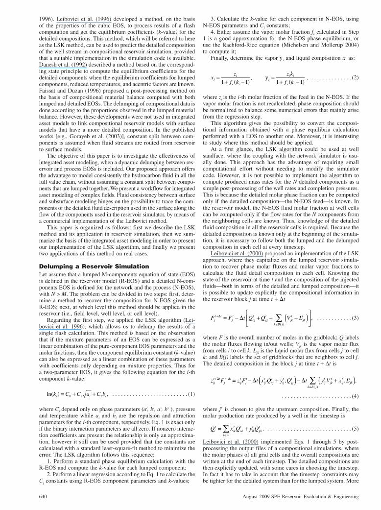
Using a compositional tracer formulation, the reservoir simula-tor solves the model using a lumped EOS, but the components of the detailed EOS can be tracked in the reservoir and in the wells. In the producers, the detailed feed composition is reported as simula-tion time passes, while, at the injector, the detailed composition of the inlet stream must be specified in terms of proportion of detailed components within its carrier. However, both Resolve (see a typical layout in Fig. 1) and R2SL allow interacting with the lumped EOS

Fig. 1—Layout of an integrated asset model aimed at linking the process with the reservoir through the network.

642 August 2009 SPE Reservoir Evaluation & Engineering

only, thus, it is necessary to set up a custom workflow. Resolve is well suited for this purpose for two reasons: (1) custom macros in a high-level language can be run at different stages of the simulation loop, and (2) it is based on a background communication protocol, named OpenServer, that allows retrieving information and sending instructions to the different modules under its control. The basic idea was to implement a suite of scripts able to feed the surface and subsurface modules with the information required to fill the gap between the detailed and the lumped EOS.

Before proceeding further, it may be useful to list the applica-tions which were used in this work:

• Resolve as a global controller,• Eclipse 300 as the reservoir simulator,• Gap (Petroleum Experts, Edinburgh, Scotland, UK, 2007) to

simulate and optimize the network,• A simplified process simulator consisting of an Excel spread-

sheet running a PVT package, namely PvtP, by means of Visual Basic macros calling OpenServer commands.

Although the modeling of the process plant is simplified with respect to a fully flagged process package, such as Hysys (Aspen-Tech, Burlington, Massachusetts, USA, 2007) or Unisim (Honey-well, Morristown, New Jersey, USA, 2007), the approach followed in this work permitted us to highlight some essential features that differentiate the process model from the reservoir simulation, such as the use of an elaborate separation process aimed at maximizing liquid production in the surface and the change in the composition of the injection stream. Moreover, for the scope of this works the use of a fully flagged process model is not essential.

A lumped EOS is defined in the reservoir simulator and in the network injection module, while a detailed EOS is used in the network production and process modules.

At each equilibration timestep defined in the global controller, the following workflow is performed (see Fig. 1):

(1) The global controller collects wells IPR tables in the reser-voir and sends them to the network module,

(2) Before solving the network modules, the global controller macro collects the well streams’ detailed molar fraction as com-puted in the reservoir and overwrites the inflow composition of wells in the network model;

(3) The network production module is solved and optimized;(4) The molar mass rates are passed to the process simulator.

The stream is processed by a surface separation train to improve the liquid production. Next, gas is separated into export and injec-tion streams, which usually have different compositions. Given the detailed composition of the injected gas, the corresponding lumped composition is computed;

(5) The network injection module is solved and optimized to find the volume of gas to inject on a well basis;

(6) The global controller passes the lumped composition of the injected gas to the reservoir module;

(7) The delumped composition of well injection gas is written in a text file as input of the reservoir model to define the partition of the detailed components in the lumped compounds;

(8) The reservoir model is run until the next equilibration date, using the rate targets computed in Step 3, the injection volumes and the lumped composition of the injection streams computed in Step 5 and the detailed gas composition written in text files at Step 7.

The need to use text files in the communication process between the surface and reservoir modules is caused by the fact that the communication controller allows managing only the com-position used in the simulator to solve the coupled fluidodynamic and thermodynamic problem. It is worth noting that the injection composition is updated every time the global controller workflow is executed, thus, an explicit extent in the simulation is introduced. However, this can be controlled by increasing the frequency by which the workflow is performed.

Application to Real Reservoir ModelsIn this section, the results of two real applications are presented. The cases were chosen to highlight two critical problems: partial gas cycling for sour gas storage in a H2S rich gas/condensate reservoir and developing a close-to-critical fluid by means of gas injection.

In both cases, we developed the reservoir fluid model by start-ing from the process EOS by means of successively lumping pairs of detailed components. Pairs of components are chosen accord-ing to reservoir engineering best practices, see, for instance, the approach proposed by Danesh (1998). At each lumping step, qual-ity check is performed by verifying EOS prediction against experi-mental data. In order to test the proposed integrated workflow at the worst condition, we use an EOS with the smallest number of components able to fulfill the quality check.

Great care is taken to verify that the lumped EOS yields a sat-isfactory vapor/liquid ratio result at different pressure-temperature conditions, since vapor fraction for the detail EOS is not recom-puted and the result from lumped EOS is assumed.

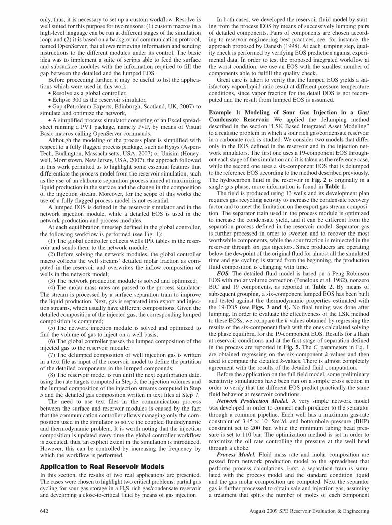
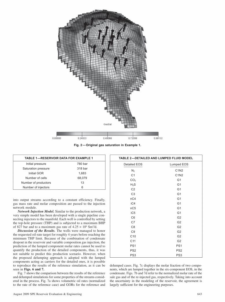
Example 1: Modeling of Sour Gas Injection in a Gas/Condensate Reservoir. We applied the delumping method described in the section “LSK Based Integrated Asset Modeling” to a realistic problem in which a sour rich gas/condensate reservoir in a carbonate rock is studied. We consider two models that differ only in the EOS defi ned in the reservoir and in the injection net-work simulators. The fi rst one uses a 19-component EOS through-out each stage of the simulation and it is taken as the reference case, while the second one uses a six-component EOS that is delumped to the reference EOS according to the method described previously. The hydrocarbon fl uid in the reservoir in Fig. 2 is originally in a single gas phase, more information is found in Table 1.

The field is produced using 13 wells and its development plan requires gas recycling activity to increase the condensate recovery factor and to meet the limitation on the export gas stream composi-tion. The separator train used in the process module is optimized to increase the condensate yield, and it can be different from the separation process defined in the reservoir model. Separator gas is further processed in order to sweeten and to recover the most worthwhile components, while the sour fraction is reinjected in the reservoir through six gas injectors. Since producers are operating below the dewpoint of the original fluid for almost all the simulated time and gas cycling is started from the beginning, the production fluid composition is changing with time.

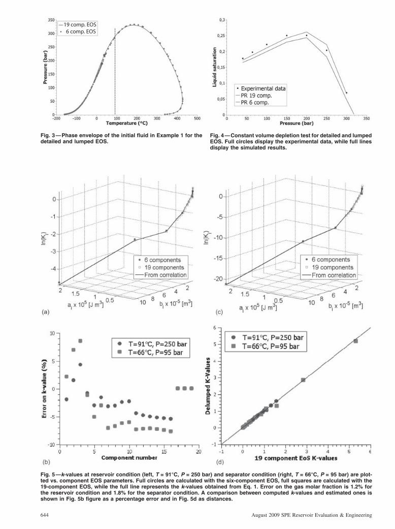
EOS. The detailed fluid model is based on a Peng-Robinson EOS with molar volume correction (Peneloux et al. 1982), nonzero BIC and 19 components, as reported in Table 2. By means of subsequent grouping, a six-component lumped EOS has been built and tested against the thermodynamic properties estimated with the 19-EOS (see Figs. 3 and 4). No final tuning was done after lumping. In order to evaluate the effectiveness of the LSK method to these EOSs, we compare the k-values obtained by regressing the results of the six-component flash with the ones calculated solving the phase equilibria for the 19-component EOS. Results for a flash at reservoir conditions and at the first stage of separation defined in the process are reported in Fig. 5. The Cj parameters in Eq. 1 are obtained regressing on the six-component k-values and then used to compute the detailed k-values. There is almost completely agreement with the results of the detailed fluid computation.

Before the application on the full field model, some preliminary sensitivity simulations have been run on a simple cross section in order to verify that the different EOS predict practically the same fluid behavior at reservoir conditions.

Network Production Model. A very simple network model was developed in order to connect each producer to the separator through a common pipeline. Each well has a maximum gas-rate constraint of 3.45 × 106 Sm3/d, and bottomhole pressure (BHP) constraint set to 200 bar, while the minimum tubing head pres-sure is set to 110 bar. The optimization method is set in order to maximize the oil rate controlling the pressure at the well head through a choke.

Process Model. Fluid mass rate and molar composition are passed from network production model to the spreadsheet that performs process calculations. First, a separation train is simu-lated with the process model and the standard condition liquid and the gas molar composition are computed. Next the separator gas is further processed to obtain sale and injection gas, assuming a treatment that splits the number of moles of each component

August 2009 SPE Reservoir Evaluation & Engineering 643

into output streams according to a constant efficiency. Finally, gas mass rate and molar composition are passed to the injection network module.

Network Injection Model. Similar to the production network, a very simple model has been developed with a single pipeline con-necting injectors to the manifold. Each well is controlled by setting the top-hole pressure (THP) and is subjected to a maximum BHP of 827 bar and to a maximum gas rate of 4.25 × 106 Sm3/d.

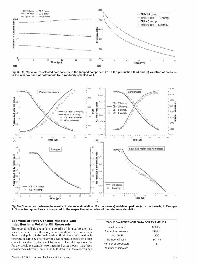
Discussion of the Results. The wells were managed to honor the requested oil-rate target for roughly 4 years before reaching the minimum THP limit. Because of the combination of condensate dropout in the reservoir and variable composition gas injection, the prediction of the lumped component molar rates cannot be used to quantify the production of the detailed components, thus, it was not suitable to predict this production scenario. However, when the proposed delumping approach is adopted with the lumped components acting as carriers for the detailed ones, it is possible to reproduce the results of the reference simulation, as it can be seen in Figs. 6 and 7.

Fig. 7 shows the comparison between the results of the reference and delumped simulations for some properties of the streams consid-ered in the process. Fig. 7a shows volumetric oil rates (normalized to the rate of the reference case) and GORs for the reference and

delumped cases. Fig. 7c displays the molar fraction of two compo-nents, which are lumped together in the six-component EOS, in the condensate. Figs. 7b and 7d refer to the normalized molar rate of the sale gas and of the re-injected gas, respectively. Taking into account the uncertainty in the modeling of the reservoir, the agreement is largely sufficient for the engineering purposes.

Fig. 2—Original gas saturation in Example 1.

TABLE 1—RESERVOIR DATA FOR EXAMPLE 1

Initial pressure 780 bar Saturation pressure 318 bar

Initial GOR 1,683 Number of cells 68,079

Number of productors 13 Number of injectors 6

TABLE 2—DETAILED AND LUMPED FLUID MODEL Detailed EOS Lumped EOS

N2 C1N2 C1 C1N2

CO2 G1 H2S G1 C2 G1 C3 G1

nC4 G1 iC4 G1 nC5 G1 iC5 G1 C6 G2 C7 G2 C8 G2 C9 G2

C10 G2 C11 G2 PS1 PS1 PS2 PS2 PS3 PS3

644 August 2009 SPE Reservoir Evaluation & Engineering

19 comp. EOS 6 comp. EOS

Fig. 3—Phase envelope of the initial fluid in Example 1 for the detailed and lumped EOS.

Fig. 4—Constant volume depletion test for detailed and lumped EOS. Full circles display the experimental data, while full lines display the simulated results.

Fig. 5—k-values at reservoir condition (left, T = 91°C, P = 250 bar) and separator condition (right, T = 66°C, P = 95 bar) are plot-ted vs. component EOS parameters. Full circles are calculated with the six-component EOS, full squares are calculated with the 19-component EOS, while the full line represents the k-values obtained from Eq. 1. Error on the gas molar fraction is 1.2% for the reservoir condition and 1.8% for the separator condition. A comparison between computed k-values and estimated ones is shown in Fig. 5b figure as a percentage error and in Fig. 5d as distances.

August 2009 SPE Reservoir Evaluation & Engineering 645

Example 2: First Contact Miscible Gas Injection in a Volatile Oil ReservoirThe second realistic example is a volatile oil in a carbonate rock reservoir, where the thermodynamic conditions are very near the critical point of the hydrocarbon fluid. More information is reported in Table 3. The reservoir development is based on a first contact miscible displacement by means of crestal injectors. As for the previous example, two integrated asset models have been considered as differing only in the EOS defined in the reservoir and

(a) (b)

Fig. 6—(a) Variation of selected components in the lumped component G1 in the production fluid and (b) variation of pressure in the reservoir and at bottomhole for a randomly selected well.

 

(a) (c)

(b) (d)

Fig. 7—Comparison between the results of reference simulation (19 components) and delumped one (six components) in Example 1. Normalized quantities are compared to the respective initial value of the reference simulation.

TABLE 3—RESERVOIR DATA FOR EXAMPLE 2

Initial pressure 688 bar Saturation pressure 310 bar

Initial GOR 820 Number of cells 84,149

Number of productors 6 Number of injectors 3

646 August 2009 SPE Reservoir Evaluation & Engineering

in the injection network simulators. The reference case is run with a 14-component EOS throughout each stage of the simulation. In the delumped case, six-component EOS has been used.

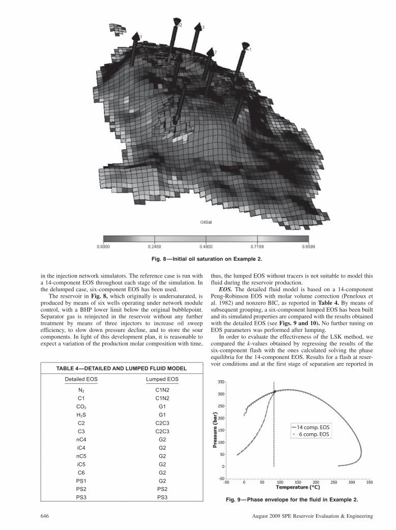
The reservoir in Fig. 8, which originally is undersaturated, is produced by means of six wells operating under network module control, with a BHP lower limit below the original bubblepoint. Separator gas is reinjected in the reservoir without any further treatment by means of three injectors to increase oil sweep efficiency, to slow down pressure decline, and to store the sour components. In light of this development plan, it is reasonable to expect a variation of the production molar composition with time,

thus, the lumped EOS without tracers is not suitable to model this fluid during the reservoir production.

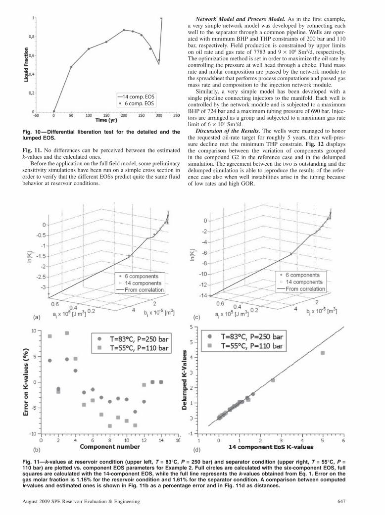
EOS. The detailed fluid model is based on a 14-component Peng-Robinson EOS with molar volume correction (Peneloux et al. 1982) and nonzero BIC, as reported in Table 4. By means of subsequent grouping, a six-component lumped EOS has been built and its simulated properties are compared with the results obtained with the detailed EOS (see Figs. 9 and 10). No further tuning on EOS parameters was performed after lumping.

In order to evaluate the effectiveness of the LSK method, we compared the k-values obtained by regressing the results of the six-component flash with the ones calculated solving the phase equilibria for the 14-component EOS. Results for a flash at reser-voir conditions and at the first stage of separation are reported in

Fig. 8—Initial oil saturation on Example 2.

TABLE 4—DETAILED AND LUMPED FLUID MODEL Detailed EOS Lumped EOS

N2 C1N2 C1 C1N2

CO2 G1 H2S G1 C2 C2C3 C3 C2C3

nC4 G2 iC4 G2 nC5 G2 iC5 G2 C6 G2

PS1 G2 PS2 PS2 PS3 PS3

14 comp. EOS 6 comp. EOS

Fig. 9—Phase envelope for the fluid in Example 2.

August 2009 SPE Reservoir Evaluation & Engineering 647

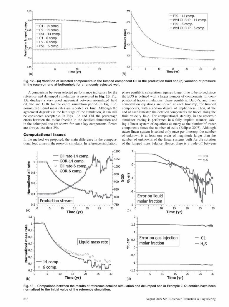
Fig. 11. No differences can be perceived between the estimated k-values and the calculated ones.

Before the application on the full field model, some preliminary sensitivity simulations have been run on a simple cross section in order to verify that the different EOSs predict quite the same fluid behavior at reservoir conditions.

Network Model and Process Model. As in the first example, a very simple network model was developed by connecting each well to the separator through a common pipeline. Wells are oper-ated with minimum BHP and THP constraints of 200 bar and 110 bar, respectively. Field production is constrained by upper limits on oil rate and gas rate of 7783 and 9 × 106 Sm3/d, respectively. The optimization method is set in order to maximize the oil rate by controlling the pressure at well head through a choke. Fluid mass rate and molar composition are passed by the network module to the spreadsheet that performs process computations and passed gas mass rate and composition to the injection network module.

Similarly, a very simple model has been developed with a single pipeline connecting injectors to the manifold. Each well is controlled by the network module and is subjected to a maximum BHP of 724 bar and a maximum tubing pressure of 690 bar. Injec-tors are arranged as a group and subjected to a maximum gas rate limit of 6 × 106 Sm3/d.

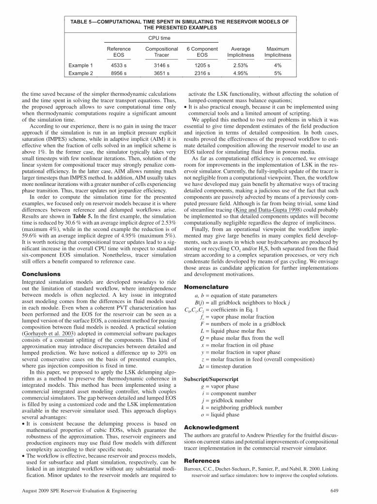
Discussion of the Results. The wells were managed to honor the requested oil-rate target for roughly 5 years, then well-pres-sure decline met the minimum THP constrain. Fig. 12 displays the comparison between the variation of components grouped in the compound G2 in the reference case and in the delumped simulation. The agreement between the two is outstanding and the delumped simulation is able to reproduce the results of the refer-ence case also when well instabilities arise in the tubing because of low rates and high GOR.

14 comp. EOS 6 comp. EOS

Fig. 10—Differential liberation test for the detailed and the lumped EOS.

Fig. 11—k-values at reservoir condition (upper left, T = 83°C, P = 250 bar) and separator condition (upper right, T = 55°C, P = 110 bar) are plotted vs. component EOS parameters for Example 2. Full circles are calculated with the six-component EOS, full squares are calculated with the 14-component EOS, while the full line represents the k-values obtained from Eq. 1. Error on the gas molar fraction is 1.15% for the reservoir condition and 1.61% for the separator condition. A comparison between computed k-values and estimated ones is shown in Fig. 11b as a percentage error and in Fig. 11d as distances.

648 August 2009 SPE Reservoir Evaluation & Engineering

(a) (B)

Fig. 12—(a) Variation of selected components in the lumped component G2 in the production fluid and (b) variation of pressure in the reservoir and at bottomhole for a randomly selected well.

(a) (c)

(b) (d)

Fig. 13—Comparison between the results of reference detailed simulation and delumped one in Example 2. Quantities have been normalized to the initial value of the reference simulation.

A comparison between selected performance indicators for the reference and delumped simulations is presented in Fig. 13. Fig. 13a displays a very good agreement between normalized field oil rate and GOR for the entire simulation period. In Fig. 13b, normalized liquid mass rates are reported vs. time. Although the agreement degrades in the late stage of the simulation, it can still be considered acceptable. In Figs. 13b and 13d, the percentage errors between the molar fraction in the detailed simulation and in the delumped one are shown for some key components. Errors are always less than 3%.

Computational IssuesIn the method we proposed, the main difference in the computa-tional load arises in the reservoir simulator. In reference simulation,

phase equilibria calculation requires longer time to be solved since the EOS is defined with a larger number of components. In com-positional tracer simulations, phase equilibria, Darcy’s, and mass conservation equations are solved at each timestep, for lumped components, with a certain degree of implicitness. Then, at the end of each timestep the detailed components are traced along the fluid velocity field. For computational stability, in the reservoir simulator tracing is performed in a fully implicit manner, solv-ing a linear system of equations as many as the number of tracer components times the number of cells (Eclipse 2007). Although tracer linear system is solved only once per timestep, the number of unknown is at least one order of magnitude larger than the number of unknowns of the linear systems built for the solution of the lumped mass balance. Hence, there is a trade-off between

August 2009 SPE Reservoir Evaluation & Engineering 649

TABLE 5—COMPUTATIONAL TIME SPENT IN SIMULATING THE RESERVOIR MODELS OF THE PRESENTED EXAMPLES

CPU time

Reference EOS

Compositional Tracer

6 Component EOS

Average Implicitness

Maximum Implicitness

Example 1 4533 s 3146 s 1205 s 2.53% 4% Example 2 8956 s 3651 s 2316 s 4.95% 5%

the time saved because of the simpler thermodynamic calculations and the time spent in solving the tracer transport equations. Thus, the proposed approach allows to save computational time only when thermodynamic computations require a significant amount of the simulation time.

According to our experience, there is no gain in using the tracer approach if the simulation is run in an implicit pressure explicit saturation (IMPES) scheme, while in adaptive implicit (AIM) it is effective when the fraction of cells solved in an implicit scheme is above 1%. In the former case, the simulator typically takes very small timesteps with few nonlinear iterations. Then, solution of the linear system for compositional tracer may strongly penalize com-putational efficiency. In the latter case, AIM allows running much larger timesteps than IMPES method. In addition, AIM usually takes more nonlinear iterations with a greater number of cells experiencing phase transition. Thus, tracer updates not jeopardize efficiency.

In order to compute the simulation time for the presented examples, we focused only on reservoir models because it is where differences between reference and delumped workflows arise. Results are shown in Table 5. In the first example, the simulation time is reduced by 30.6 % with an average implicit degree of 2.53% (maximum 4%), while in the second example the reduction is of 59.6% with an average implicit degree of 4.95% (maximum 5%). It is worth noticing that compositional tracer updates lead to a sig-nificant increase in the overall CPU time with respect to standard six-component EOS simulation. Nonetheless, tracer simulation still offers a benefit compared to reference case.

ConclusionsIntegrated simulation models are developed nowadays to ride out the limitation of standard workflow, where interdependence between models is often neglected. A key issue in integrated asset modeling comes from the differences in fluid models used in each module. Even when a coherent PVT characterization has been performed and the EOS for the reservoir can be seen as a lumped version of the surface EOS, a consistent method for passing composition between fluid models is needed. A practical solution (Gorhayeb et al. 2003) adopted in commercial software packages consists of a constant splitting of the components. This kind of approximation may introduce discrepancies between detailed and lumped prediction. We have noticed a difference up to 20% on several conservative cases on the basis of presented examples, where gas injection composition is fixed in time.

In this paper, we proposed to apply the LSK delumping algo-rithm as a method to preserve the thermodynamic coherence in integrated models. This method has been implemented using a commercial integrated asset modeling controller, which couples commercial simulators. The gap between detailed and lumped EOS is filled by using a customized code and the LSK implementation available in the reservoir simulator used. This approach displays several advantages:• It is consistent because the delumping process is based on

mathematical properties of cubic EOSs, which guarantee the robustness of the approximation. Thus, reservoir engineers and production engineers may use fluid flow models with different complexity according to their specific needs;

• The workflow is effective, because reservoir and process models, used for subsurface and plant simulation, respectively, can be linked in an integrated workflow without any substantial modi-fication. Minor updates to the reservoir models are required to

activate the LSK functionality, without affecting the solution of lumped-component mass balance equations;

• It is also practical enough, because it can be implemented using commercial tools and a limited amount of scripting.

We applied this method to two real problems in which it was essential to give time dependent estimates of the field production and injection in terms of detailed composition. In both cases, results proved the effectiveness of the proposed workflow to esti-mate detailed composition allowing the reservoir model to use an EOS tailored for simulating fluid flow in porous media.

As far as computational efficiency is concerned, we envisage room for improvements in the implementation of LSK in the res-ervoir simulator. Currently, the fully-implicit update of the tracer is not negligible from a computational viewpoint. Then, the workflow we have developed may gain benefit by alternative ways of tracing detailed components, making a judicious use of the fact that such components are passively advected by means of a previously com-puted pressure field. Although is far from being trivial, some kind of streamline tracing (King and Datta-Gupta 1998) could probably be implemented so that detailed components updates will become computationally negligible regardless the degree of implicitness.

Finally, from an operational viewpoint the workflow imple-mented may give large benefits in many complex field develop-ments, such as assets in which sour hydrocarbons are produced by storing or recycling CO2 and/or H2S, both separated from the fluid stream according to a complex separation processes, or very rich condensate fields developed by means of gas cycling. We envisage those areas as candidate application for further implementations and development motivations.

Nomenclature a, b = equation of state parameters B(j) = all gridblock neighbors to block j C0,C1,C2 = coeffi cients in Eq. 1 fv = vapor phase molar fraction F = numbers of mole in a gridblock L = liquid phase molar fl ux Q = phase molar fl ux from the well x = molar fraction in oil phase y = molar fraction in vapor phase z = molar fraction in feed (overall composition) �t = timestep duration

Subscript/Superscript g = vapor phase i = component number j = gridblock number k = neighboring gridblock number o = liquid phase

AcknowledgmentThe authors are grateful to Andrew Priestley for the fruitful discus-sions on current status and potential improvements of compositional tracer implementation in the commercial reservoir simulator.

ReferencesBarroux, C.C., Duchet-Suchaux, P., Samier, P., and Nabil, R. 2000. Linking

reservoir and surface simulators: how to improve the coupled solutions.

650 August 2009 SPE Reservoir Evaluation & Engineering

Paper SPE 65159 presented at the SPE European Petroleum Confer-ence, Paris, 24–25 October. DOI: 10.2118/65159-MS.

Coats, K.H. 1985. Simulation of Gas Condensate Reservoir Performance. J. Pet Tech 37 (10): 1870–1886. SPE-10512-PA. DOI: 10.2118/10512-PA.

Danesh, A. 1998. PVT and Phase Behavior of Petroleum Reservoir Fluids, No. 47. Amsterdam: Developments in Petroleum Science, Elsevier Science B.V.

Danesh, A., Xu, D., and Tod, A.C. 1992. A Grouping Method To Opti-mize Oil Description for Compositional Simulation of Gas Injec-tion Processing. SPE Res Eng 7 (3): 343–348. SPE-20745-PA. DOI: 10.2118/20745-PA.

ECLIPSE Technical Description 2007. 2007. Houston: Schlumberger GeoQuest.

Faissat, B. and Duzan, M.C. 1996. Fluid Modelling Consistency in Res-ervoir and Process Simulations. Paper SPE 36932 presented at the European Petroleum Conference, Milan, Italy, 22–24 October. DOI: 10.2118/36932-MS.

Gorhayeb, K. and Holmes, J. 2007. Black-Oil Delumping Techniques Based on Compositional Information from Depletion Processes. SPE Res Eval & Eng 5 (10): 489–499. SPE-96571-PA. DOI: 10.2118/96571-PA.

Gorhayeb, K., Holmes, J., Torrens, R., and Grewal, B. 2003. A Gen-eral Purpose Controller for Coupling Multiple Reservoir Simulations and Surface Facility Networks. Paper SPE 79702 presented at the SPE Reservoir Simulation Symposium, Houston, 3–5 February. DOI: 10.2118/79702-MS.

King, M.J. and Datta-Gupta, A. 1998. Streamline Simulation: A Current Perspective. In Situ 22 (1): 91–140.

Kosmala, A., Aanonsen, S.I., Gajraj, A., Biran, V., Brusdal, K., Stokkenes, A., and Torrens, R. 2003. Coupling of a Surface Network With Res-ervoir Simulation. Paper SPE 84220 presented at the SPE Annual Technical Conference and Exhibition, Denver, 5–8 October. DOI: 10.2118/84220-MS.

Leibovici, C.F., Barker, J.W., and Waché, D. 2000. Method for Delump-ing the Results of Compositional Reservoir Simulation. SPE J. 5 (2): 227–235. SPE-64001-PA. DOI: 10.2118/64001-PA.

Leibovici, C.F., Stenby, E.H., and Knudsen, K. 1996. A consistent pro-cedure for pseudo-component delumping. Fluid Phase Equilibria 17 (1–2): 225–232. DOI: 10.1016/0378-3812(95)02957-5.

Michelsen, M.L. and Mollerup, J.M. 2004. Thermodynamic Models: Funda-mentals and Computational Aspects. Holte, Denmark: Tie-Line Press.

Péneloux, A., Rauzy, E., and Fréze, R. 1982. A consistent correction for Soave-Redlich-Kwong volumes. Fluid Phase Equilibria 8 (1): 7–23. DOI: 10.1016/0378-3812(82)80002-2.

Reservoir to Surface Link (R2SL) Technical Description. 2007. Houston: Schlumberger Technology Corporation.

RESOLVE 3.0 User Guide. 2007. Edinburgh, Scotland: Petroleum Experts.Weisenborn, A.J. and Schulte, A.M. 2000. Compositional integrated

subsurface-surface modeling. Paper SPE 65158 presented at the SPE European Petroleum Conference, Paris, 24–25 October. DOI: 10.2118/65158-MS.

Emanuele Vignati is a reservoir engineer with Eni E&P. Email: emanuele.vignati@eni.it. He holds a PhD degree in science and technology of radiation from the U. Politecnico of Milan and a degree in nuclear engineering from the U. of Milan. Vignati’s current interests include compositional reservoir simulation, integrated asset models, thermodynamics, and EOR/IOR techniques. Alberto Cominelli works as a technical advisor for reservoir modeling with Eni E&P. He is currently involved in different projects in development of computer-aided methods for history matching, optimization issues, compositional reservoir simulation, and numerical approximation of partial differential equations for reservoir simulation and their impact on gridding. Cominelli holds a degree in physics from the U. of Pavia. Roberto Rossi is a team leader of Integrated Asset Modeling with Eni E&P. His interests involve risk analysis, computer assisted history matching, and integrated asset models. He holds a degree in physics from the U. of Milan. Paolo Roscini is a petroleum engineer with Eni E&P. He holds a degree in environment engineering from the U. of Perugia and a master degree in petroleum engineering from the U. of Torino. He is currently involved in reservoir modeling and simulation of complex wells.