Lateral-Torsional Buckling
45
CHAPTER 7 7 Lateral-Torsional Buckling Contents 7.1. Introduction 327 7.2. Differential Equations for Lateral-Torsional Buckling 328 7.3. Generalization of Governing Differential Equations 336 7.4. Lateral-Torsional Buckling for Various Loading and Boundary Conditions 337 7.5. Application of Bessel Function to Lateral-Torsional Buckling Problems 343 7.6. Lateral-Torsional Buckling by Energy Method 347 7.6.1. Uniform Bending 348 7.6.2. One Concentrated Load at Midspan 352 7.6.3. Uniformly Distributed Load 355 7.6.4. Two Concentrated Loads Applied Symmetrically 359 7.7. Design Simplification for Lateral-Torsional Buckling 362 References 368 Problems 369 7.1. INTRODUCTION A transversely (or combined transversely and axially) loaded member that is bent with respect to its major axis may buckle laterally if its compression flange is not sufficiently supported laterally. The reason buckling occurs in a beam at all is that the compression flange or the extreme edge of the compression side of a narrow rectangular beam, which behaves like a column resting on an elastic foundation, becomes unstable. If the flexural rigidity of the beam with respect to the plane of the bending is many times greater than the rigidity of the lateral bending, the beam may buckle and collapse long before the bending stresses reach the yield point. As long as the applied loads remain below the limit value, the beam remains stable; that is, the beam that is slightly twisted and/or bent laterally returns to its original configuration upon the removal of the disturbing force. With increasing load intensity, the restoring forces become smaller and smaller, until a loading is reached at which, in addition to the plane bending equilibrium configuration, an adjacent, deflected, and twisted, equilibrium position becomes equally possible. The original bending configuration is no longer stable, and the lowest load at which such an alternative equilibrium configuration becomes possible is the critical load of the beam. At the critical load, the compression flange tends to bend laterally, exceeding the Stability of Structures Ó 2011 Elsevier Inc. ISBN 978-0-12-385122-2, doi:10.1016/B978-0-12-385122-2.10007-7 All rights reserved. 327 j
-
Upload
khangminh22 -
Category
Documents
-
view
0 -
download
0
Transcript of Lateral-Torsional Buckling
CHAPTER77
Lateral-Torsional BucklingContents7.1. Introduction 3277.2. Differential Equations for Lateral-Torsional Buckling 3287.3. Generalization of Governing Differential Equations 3367.4. Lateral-Torsional Buckling for Various Loading and Boundary Conditions 3377.5. Application of Bessel Function to Lateral-Torsional Buckling Problems 3437.6. Lateral-Torsional Buckling by Energy Method 347
7.6.1. Uniform Bending 3487.6.2. One Concentrated Load at Midspan 3527.6.3. Uniformly Distributed Load 3557.6.4. Two Concentrated Loads Applied Symmetrically 359
7.7. Design Simplification for Lateral-Torsional Buckling 362References 368Problems 369
7.1. INTRODUCTION
A transversely (or combined transversely and axially) loaded member that is
bent with respect to its major axis may buckle laterally if its compression
flange is not sufficiently supported laterally. The reason buckling occurs in
a beam at all is that the compression flange or the extreme edge of the
compression side of a narrow rectangular beam, which behaves like
a column resting on an elastic foundation, becomes unstable. If the flexural
rigidity of the beam with respect to the plane of the bending is many times
greater than the rigidity of the lateral bending, the beam may buckle and
collapse long before the bending stresses reach the yield point. As long as the
applied loads remain below the limit value, the beam remains stable; that is,
the beam that is slightly twisted and/or bent laterally returns to its original
configuration upon the removal of the disturbing force. With increasing
load intensity, the restoring forces become smaller and smaller, until
a loading is reached at which, in addition to the plane bending equilibrium
configuration, an adjacent, deflected, and twisted, equilibrium position
becomes equally possible. The original bending configuration is no longer
stable, and the lowest load at which such an alternative equilibrium
configuration becomes possible is the critical load of the beam. At the
critical load, the compression flange tends to bend laterally, exceeding the
Stability of Structures � 2011 Elsevier Inc.ISBN 978-0-12-385122-2, doi:10.1016/B978-0-12-385122-2.10007-7 All rights reserved. 327 j
328 Chai Yoo
restoring force provided by the remaining portion of the cross section to
cause the section to twist. Lateral buckling is a misnomer, for no lateral
deflection is possible without concurrent twisting of the section.
Bleich (1952) gives credit to Prandtl (1899) and Michell (1899) for
producing the first theoretical studies on the lateral buckling of beams
with long narrow rectangular sections. Similar credit is also extended to
Timoshenko (1910) for deriving the fundamental differential equation of
torsion of symmetrical I-beams and investigating the lateral buckling of
transversely loaded deep I-beams with the derived equation. Since then,
many investigators, including Vlasov (1940), Winter (1943), Hill (1954),
Clark and Hill (1960), and Galambos (1963), have contributed on both
elastic and inelastic lateral-torsional buckling of various shapes. Some of the
early developments of the resisting capacities of steel structural members
leading to the Load and Resistance Factor Design (LRFD) are summarized
by Vincent (1969).
7.2. DIFFERENTIAL EQUATIONS FOR LATERAL-TORSIONALBUCKLING
If transverse loads do not pass through the shear center, they will induce
torsion. In order to avoid this additional torsional moment (thereby
weakening the flexural capacity) in the flexural members, it is customary to
use flexural members of at least singly symmetric sections so that the
transverse loads will pass through the plane of the web as shown in Fig. 7-1.
The section is symmetric about the y-axis, and u and v are the components
of the displacement of the shear center parallel to the axes x and h. The
rotation of the shear center f is taken positive about the z-axis according to
the right-hand screw rule, and the z-axis is perpendicular to the xh plane.
The following assumptions are employed:
1. The beam is prismatic.
2. The member cross section retains its original shape during buckling.
3. The externally applied loads are conservative.
4. The analysis is limited within the elastic limit.
5. The transverse load passes through the axis of symmetry in the plane of
bending.
In the derivation of the governing differential equations of the lateral-
torsional buckling of beams, it is necessary to define two coordinate systems:
one for the undeformed configuration, x, y, z, and the other for the
deformed configuration, x, h, 2 as shown in Fig. 7-1. Hence, the fixed
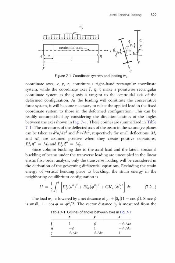
Figure 7-1 Coordinate systems and loading wy
Lateral-Torsional Buckling 329
coordinate axes, x, y, z, constitute a right-hand rectangular coordinate
system, while the coordinate axes x, h, 2 make a pointwise rectangular
coordinate system as the 2 axis is tangent to the centroidal axis of the
deformed configuration. As the loading will constitute the conservative
force system, it will become necessary to relate the applied load in the fixed
coordinate system to those in the deformed configuration. This can be
readily accomplished by considering the direction cosines of the angles
between the axes shown in Fig. 7-1. These cosines are summarized in Table
7-1. The curvatures of the deflected axis of the beam in the xz and yz planes
can be taken as d2u=dz2 and d2v=dz2, respectively for small deflections. Mx
and My are assumed positive when they create positive curvatures;
EIxh00 ¼ Mx and EIy x
00 ¼ My.
Since column buckling due to the axial load and the lateral-torsional
buckling of beams under the transverse loading are uncoupled in the linear
elastic first-order analysis, only the transverse loading will be considered in
the derivation of the governing differential equations. Excluding the strain
energy of vertical bending prior to buckling, the strain energy in the
neighboring equilibrium configuration is
U ¼ 1
2
Z ‘
0
�EIyðu00Þ2 þ EIwðf00Þ2 þGKT ðf0Þ2
�dz (7.2.1)
The load wy , is lowered by a net distance of ys þ jayjð1� cos fÞ. Since fis small, 1� cos f ¼ f2=2. The vector distance ay is measured from the
Table 7-1 Cosines of angles between axes in Fig. 7-1x y z
x 1 f �du/dz
h �f 1 �dv/dz
2 du/dz dv/dz 1
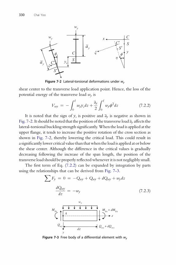
Figure 7-2 Lateral-torsional deformations under wy
330 Chai Yoo
shear center to the transverse load application point. Hence, the loss of the
potential energy of the transverse load wy is
Vwy ¼ �Z ‘
0
wyysdzþay
2
Z ‘
0
wyf2dz (7.2.2)
It is noted that the sign of ys is positive and ay is negative as shown in
Fig. 7-2. It should be noted that the position of the transverse load ay affects the
lateral-torsional buckling strength significantly.When the load is applied at the
upper flange, it tends to increase the positive rotation of the cross section as
shown in Fig. 7-2, thereby lowering the critical load. This could result in
a significantly lower critical value than thatwhen the load is applied at or below
the shear center. Although the difference in the critical values is gradually
decreasing following the increase of the span length, the position of the
transverse load should be properly reflectedwhenever it is not negligibly small.
The first term of Eq. (7.2.2) can be expanded by integration by parts
using the relationships that can be derived from Fig. 7-3.XFy ¼ 0 ¼ �Qwy þQwy þ dQwy þ wydz
dQwy
dz¼ �wy (7.2.3)
wy
bxMbx bxM dM+
wyQwy wyQ dQ+
dz
Az
y
Figure 7-3 Free body of a differential element with wy
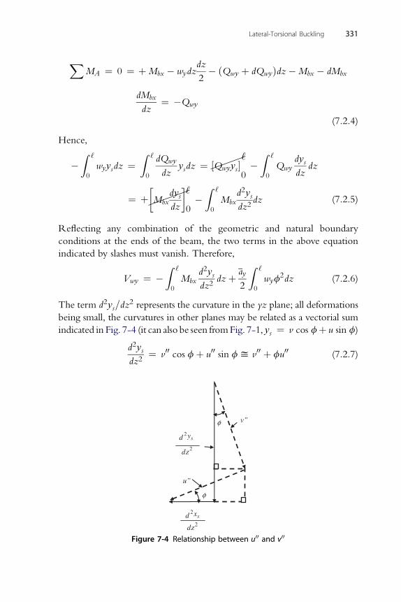
X dz
MA ¼ 0 ¼ þMbx � wydz2� ðQwy þ dQwyÞdz�Mbx � dMbx
dMbx
dz¼ �Qwy
(7.2.4)
Hence,
�Z ‘
0
wyysdz ¼Z ‘
0
dQwy
dzysdz ¼
�
½Qwyys�‘
0�Z ‘
0
Qwydysdz
dz
¼ þ
��Mbx
dysdz
�‘
0�Z ‘
0
Mbxd2ysdz2
dz (7.2.5)
Reflecting any combination of the geometric and natural boundary
conditions at the ends of the beam, the two terms in the above equation
indicated by slashes must vanish. Therefore,
Vwy ¼ �Z ‘
0
Mbxd2ysdz2
dzþ ay
2
Z ‘
0
wyf2dz (7.2.6)
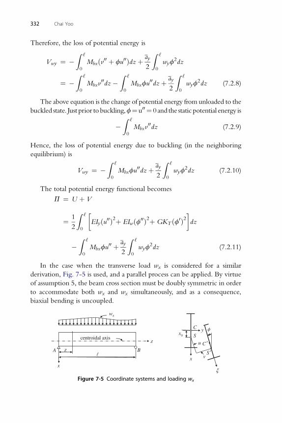
The term d2ys=dz2 represents the curvature in the yz plane; all deformations
being small, the curvatures in other planes may be related as a vectorial sum
indicated in Fig. 7-4 (it can also be seen fromFig. 7-1, ys ¼ v cos fþ u sin f)
d2ysdz2
¼ v00 cos fþ u00 sin fy v00 þ fu00 (7.2.7)
Lateral-Torsional Buckling 331
v”φ
2
2
dz
2dz
yd s
2xd s
u”
φ
Figure 7-4 Relationship between u00 and v00
332 Chai Yoo
Therefore, the loss of potential energy is
Vwy ¼ �Z ‘
0
Mbxðv00 þ fu00Þdzþ ay
2
Z ‘
0
wyf2dz
¼ �Z ‘
0
Mbxv00dz�
Z ‘
0
Mbxfu00dzþ ay
2
Z ‘
0
wyf2dz (7.2.8)
The above equation is the change of potential energy from unloaded to the
buckled state. Just prior tobuckling,f¼u00 ¼ 0 and the static potential energy is
�Z ‘
0
Mbxv00dz (7.2.9)
Hence, the loss of potential energy due to buckling (in the neighboring
equilibrium) is
Vwy ¼ �Z ‘
0
Mbxfu00dzþ ay
2
Z ‘
0
wyf2dz (7.2.10)
The total potential energy functional becomes
P ¼ U þ V
Z ‘ � �
¼ 12 0
EIyðu00Þ2þ EIwðf00Þ2þ GKT ðf0Þ2 dz
�Z ‘
0
Mbxfu00 þ ay
2
Z ‘
0
wyf2dz (7.2.11)
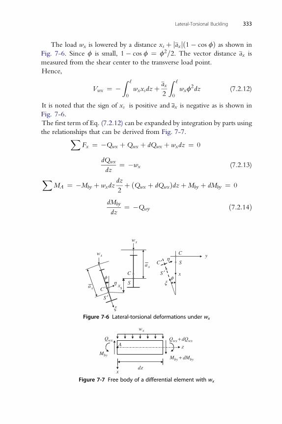
In the case when the transverse load wx is considered for a similar
derivation, Fig. 7-5 is used, and a parallel process can be applied. By virtue
of assumption 5, the beam cross section must be doubly symmetric in order
to accommodate both wx and wx simultaneously, and as a consequence,
biaxial bending is uncoupled.
xw
z
zcentroidal axis
A B
C
S
xx
u
ξ
S
φ
C
v
y0x
Figure 7-5 Coordinate systems and loading wx
Lateral-Torsional Buckling 333
The load wx is lowered by a distance xs þ jaxjð1� cos fÞ as shown in
Fig. 7-6. Since f is small, 1� cos f ¼ f2=2. The vector distance ax is
measured from the shear center to the transverse load point.
Hence,
Vwx ¼ �Z ‘
0
wxxsdzþ ax
2
Z ‘
0
wxf2dz (7.2.12)
It is noted that the sign of xs is positive and ax is negative as is shown in
Fig. 7-6.
The first term of Eq. (7.2.12) can be expanded by integration by parts using
the relationships that can be derived from Fig. 7-7.XFx ¼ �Qwx þQwx þ dQwx þ wxdz ¼ 0
dQwx
dz¼ �wx (7.2.13)
X dz
MA ¼ �Mby þ wxdz2þ ðQwx þ dQwxÞdzþMby þ dMby ¼ 0
dMby
dz¼ �Qwy ð7:2:14Þ
C
SS
x
xw
ξ
y
x
xa
C
Sη
S ′
C ′
xw
η
S ′C ′
φ
xa
φξ
Figure 7-6 Lateral-torsional deformations under wx
xw
QwxQwx dQwx+
dzx
zA
Mby
MbydMby+
Figure 7-7 Free body of a differential element with wx
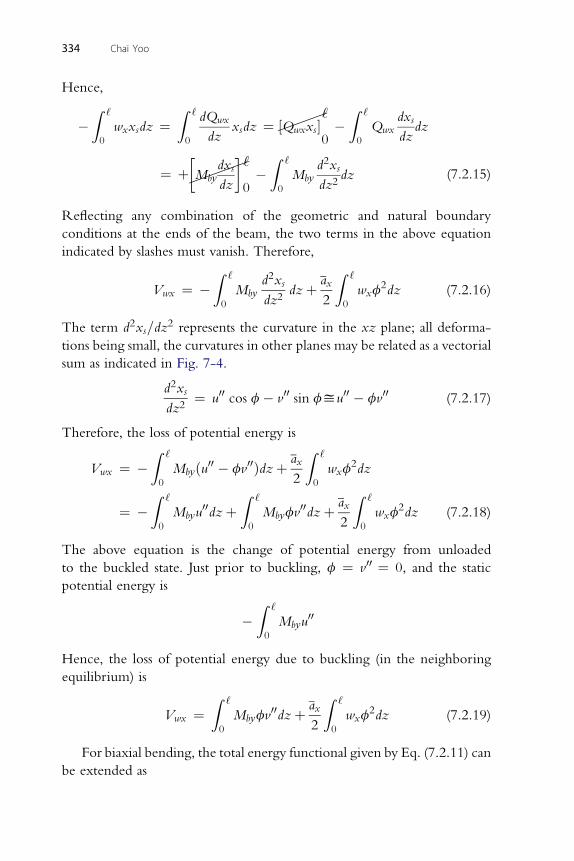
334 Chai Yoo
Hence,
�Z ‘
0
wxxsdz ¼Z ‘
0
dQwx
dzxsdz ¼
�
½Qwxxs�‘
0�Z ‘
0
Qwxdxs
dzdz
¼ þ
��Mby
dxs
dz
�‘
0�Z ‘
0
Mbyd2xs
dz2dz (7.2.15)
Reflecting any combination of the geometric and natural boundary
conditions at the ends of the beam, the two terms in the above equation
indicated by slashes must vanish. Therefore,
Vwx ¼ �Z ‘
0
Mbyd2xs
dz2dzþ ax
2
Z ‘
0
wxf2dz (7.2.16)
The term d2xs=dz2 represents the curvature in the xz plane; all deforma-
tions being small, the curvatures in other planes may be related as a vectorial
sum as indicated in Fig. 7-4.
d2xs
dz2¼ u00 cos f� v00 sin fyu00 � fv00 (7.2.17)
Therefore, the loss of potential energy is
Vwx ¼ �Z ‘
0
Mbyðu00 � fv00Þdzþ ax
2
Z ‘
0
wxf2dz
¼ �Z ‘
0
Mbyu00dzþ
Z ‘
0
Mbyfv00dzþ ax
2
Z ‘
0
wxf2dz (7.2.18)
The above equation is the change of potential energy from unloaded
to the buckled state. Just prior to buckling, f ¼ v00 ¼ 0, and the static
potential energy is
�Z ‘
0
Mbyu00
Hence, the loss of potential energy due to buckling (in the neighboring
equilibrium) is
Vwx ¼Z ‘
0
Mbyfv00dzþ ax
2
Z ‘
0
wxf2dz (7.2.19)
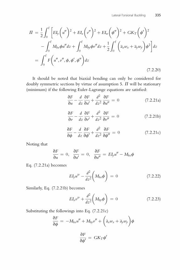
For biaxial bending, the total energy functional given by Eq. (7.2.11) can
be extended as
Lateral-Torsional Buckling 335
P ¼ 1
2
Z ‘
0
�EIy
�u00�2 þ EIx
�v00�2 þ EIw
�f00
�2 þGKT
�f0�2
�Z ‘
0
Mbxfu00dzþ
Z ‘
0
Mbyfv00dzþ 1
2
Z ‘
0
�axwx þ aywy
�f2
�dz
¼Z ‘
0
F
�u00; v00;f;f0;f00
�dz
(7.2.20)
It should be noted that biaxial bending can only be considered for
doubly symmetric sections by virtue of assumption 5. P will be stationary
(minimum) if the following Euler-Lagrange equations are satisfied:
vF
vu� d
dz
vF
vu0þ d2
dz2vF
vu00¼ 0 (7.2.21a)
vF d vF d2 vF
vv�dz vv0
þdz2 vv00
¼ 0 (7.2.21b)
vF d vF d2 vF
vf�dz vf0 þ dz2 vf00 ¼ 0 (7.2.21c)
Noting that
vF
vu¼ 0;
vF
vu0¼ 0;
vF
vu00¼ EIyu
00 �Mbxf
Eq. (7.2.21a) becomes
EIyuiv � d2
dz2
�Mbxf
�¼ 0 (7.2.22)
Similarly, Eq. (7.2.21b) becomes
EIxviv þ d2
dz2
�Mbyf
�¼ 0 (7.2.23)
Substituting the followings into Eq. (7.2.21c)
vF
vf¼ �Mbxu
00 þMbyv00 þ
�axwx þ aywy
�f
vF
vf0 ¼ GKTf0
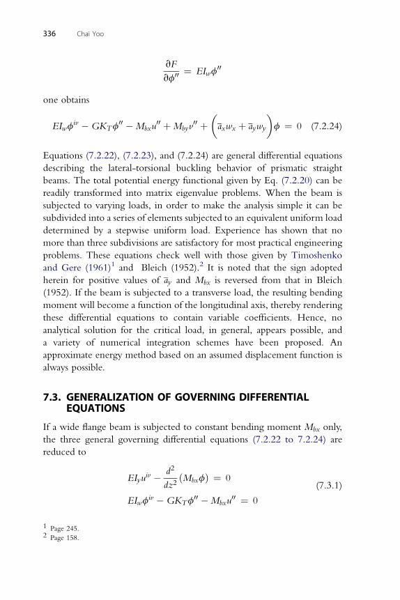
vF 00
vf00 ¼ EIwfone obtains
EIwfiv �GKTf
00 �Mbxu00 þMbyv
00 þ�axwx þ aywy
�f ¼ 0 (7.2.24)
Equations (7.2.22), (7.2.23), and (7.2.24) are general differential equations
describing the lateral-torsional buckling behavior of prismatic straight
beams. The total potential energy functional given by Eq. (7.2.20) can be
readily transformed into matrix eigenvalue problems. When the beam is
subjected to varying loads, in order to make the analysis simple it can be
subdivided into a series of elements subjected to an equivalent uniform load
determined by a stepwise uniform load. Experience has shown that no
more than three subdivisions are satisfactory for most practical engineering
problems. These equations check well with those given by Timoshenko
and Gere (1961)1 and Bleich (1952).2 It is noted that the sign adopted
herein for positive values of ay and Mbx is reversed from that in Bleich
(1952). If the beam is subjected to a transverse load, the resulting bending
moment will become a function of the longitudinal axis, thereby rendering
these differential equations to contain variable coefficients. Hence, no
analytical solution for the critical load, in general, appears possible, and
a variety of numerical integration schemes have been proposed. An
approximate energy method based on an assumed displacement function is
always possible.
336 Chai Yoo
7.3. GENERALIZATION OF GOVERNING DIFFERENTIALEQUATIONS
If a wide flange beam is subjected to constant bending moment Mbx only,
the three general governing differential equations (7.2.22 to 7.2.24) are
reduced to
EIyuiv � d2
dz2ðMbxfÞ ¼ 0
EIwfiv �GKTf
00 �Mbxu00 ¼ 0
(7.3.1)
1 Page 245.2 Page 158.
Lateral-Torsional Buckling 337
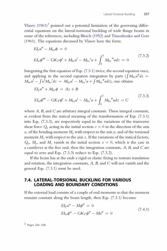
Vlasov (1961)3 pointed out a potential limitation of the governing differ-
ential equations on the lateral-torsional buckling of wide flange beams in
some of the references, including Bleich (1952) and Timoshenko and Gere
(1961). The equations discussed by Vlasov have the form:
EIyu00 �Mbxf ¼ 0
EIwf000 �GKTf
0 þMbxu0 �Mbx
0uþZ ‘
0
Mbx00udz ¼ 0
(7.3.2)
Integrating the first equation of Eqs. (7.3.1) twice, the second equation once,
and applying in the second equation integration by parts (RMbxu
00dz ¼Mbxu
0 � Ru0Mbx
0dz ¼ Mbxu0 �Mbx
0uþRMbx
00udz), one obtains
EIyu00 þMbxf ¼ Azþ B
EIwf000 �GKTf
0 þMbxu0 �Mbx
0uþZ ‘
0
Mbx00udz ¼ C
(7.3.3)
where A, B, and C are arbitrary integral constants. These integral constants,
as evident from the statical meaning of the transformation of Eqs. (7.3.1)
into Eqs. (7.3.3), are respectively equal to the variations of the transverse
shear force Qx acting in the initial section z ¼ 0 in the direction of the axis
x, of the bending momentMy with respect to the axis y, and of the torsional
momentMzwith respect to the axis z. If the variations of the statical factors,
Qx, My, and Mz vanish in the initial section z ¼ 0, which is the case in
a cantilever at the free end, then the integration constants, A, B, and C are
equal to zero and Eqs. (7.3.3) reduce to Eqs. (7.3.2).
If the beam has at the ends a rigid or elastic fixing to restrain translation
and rotation, the integration constants, A, B, and C will not vanish and the
general Eqs. (7.3.1) must be used.
7.4. LATERAL-TORSIONAL BUCKLING FOR VARIOUSLOADING AND BOUNDARY CONDITIONS
If the external load consists of a couple of end moments so that the moment
remains constant along the beam length, then Eqs. (7.3.1) become
EIyuiv �Mf00 ¼ 0
EIwfiv �GKTf
00 �Mu00 ¼ 0(7.4.1)
3 Pages 326–328.
338 Chai Yoo
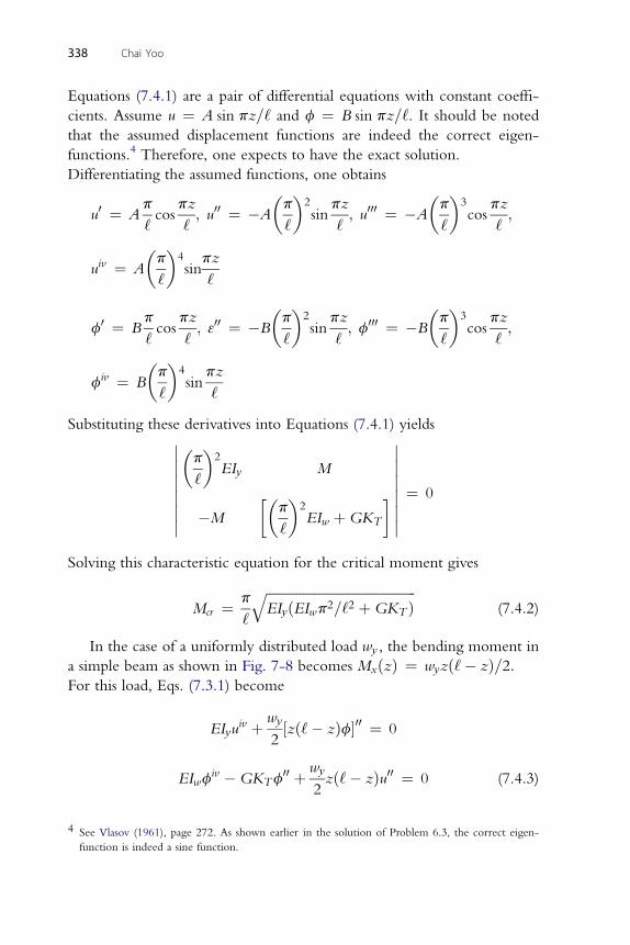
Equations (7.4.1) are a pair of differential equations with constant coeffi-
cients. Assume u ¼ A sin pz=‘ and f ¼ B sin pz=‘. It should be noted
that the assumed displacement functions are indeed the correct eigen-
functions.4 Therefore, one expects to have the exact solution.
Differentiating the assumed functions, one obtains
u0 ¼ Ap
‘cos
pz
‘; u00 ¼ �A
�p
‘
�2sin
pz
‘; u000 ¼ �A
�p
‘
�3cos
pz
‘;
uiv ¼ A
�p
‘
�4sin
pz
‘
p pz�p�2 pz
�p�3 pz
f0 ¼ B‘cos
‘; 300 ¼ �B
‘sin
‘; f000 ¼ �B
‘cos
‘;
fiv ¼ B
�p
‘
�4sin
pz
‘
Substituting these derivatives into Equations (7.4.1) yields�������p
‘
�2EIy M
�M
��p
‘
�2EIw þGKT
������� ¼ 0
Solving this characteristic equation for the critical moment gives
Mcr ¼ p
‘
ffiffiffiffiffiffiffiffiffiffiffiffiffiffiffiffiffiffiffiffiffiffiffiffiffiffiffiffiffiffiffiffiffiffiffiffiffiffiffiffiffiffiffiffiffiEIyðEIwp2=‘2 þGKT Þ
q(7.4.2)
In the case of a uniformly distributed load wy , the bending moment in
a simple beam as shown in Fig. 7-8 becomes MxðzÞ ¼ wyzð‘� zÞ=2:For this load, Eqs. (7.3.1) become
EIyuiv þ wy
2½zð‘� zÞf�00 ¼ 0
iv 00 wy 00
EIwf �GKTf þ2zð‘� zÞu ¼ 0 (7.4.3)4 See Vlasov (1961), page 272. As shown earlier in the solution of Problem 6.3, the correct eigen-
function is indeed a sine function.
yw
z
y
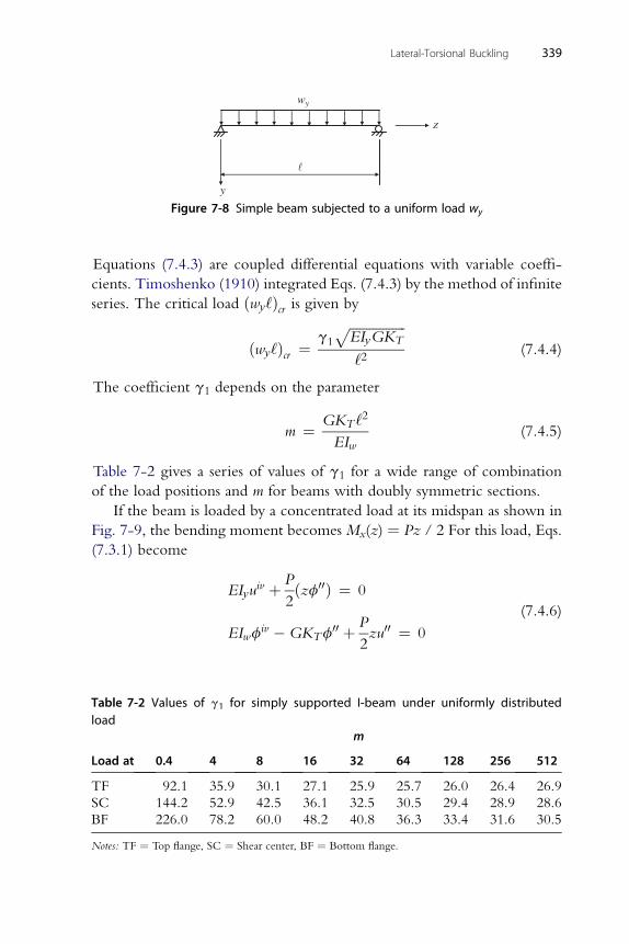
Figure 7-8 Simple beam subjected to a uniform load wy
Lateral-Torsional Buckling 339
Equations (7.4.3) are coupled differential equations with variable coeffi-
cients. Timoshenko (1910) integrated Eqs. (7.4.3) by the method of infinite
series. The critical load ðwy‘Þcr is given by
ðwy‘Þcr ¼ g1
ffiffiffiffiffiffiffiffiffiffiffiffiffiffiffiffiffiEIyGKT
p‘2
(7.4.4)
The coefficient g1 depends on the parameter
m ¼ GKT ‘2
EIw(7.4.5)
Table 7-2 gives a series of values of g1 for a wide range of combination
of the load positions and m for beams with doubly symmetric sections.
If the beam is loaded by a concentrated load at its midspan as shown in
Fig. 7-9, the bending moment becomes Mx(z) ¼ Pz / 2 For this load, Eqs.
(7.3.1) become
EIyuiv þ P
2ðzf00Þ ¼ 0
EIwfiv �GKTf
00 þ P
2zu00 ¼ 0
(7.4.6)
Table 7-2 Values of g1 for simply supported I-beam under uniformly distributedload
Load at
m
0.4 4 8 16 32 64 128 256 512
TF 92.1 35.9 30.1 27.1 25.9 25.7 26.0 26.4 26.9
SC 144.2 52.9 42.5 36.1 32.5 30.5 29.4 28.9 28.6
BF 226.0 78.2 60.0 48.2 40.8 36.3 33.4 31.6 30.5
Notes: TF ¼ Top flange, SC ¼ Shear center, BF ¼ Bottom flange.
P
/2
z
y
Figure 7-9 Simple beam subjected to a concentrated load P
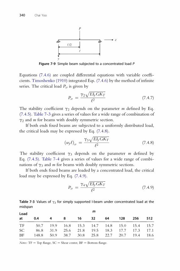
340 Chai Yoo
Equations (7.4.6) are coupled differential equations with variable coeffi-
cients. Timoshenko (1910) integrated Eqs. (7.4.6) by the method of infinite
series. The critical load Pcr is given by
Pcr ¼ g2
ffiffiffiffiffiffiffiffiffiffiffiffiffiffiffiffiffiEIyGKT
p‘2
(7.4.7)
The stability coefficient g2 depends on the parameter m defined by Eq.
(7.4.5). Table 7-3 gives a series of values for a wide range of combination of
g2 and m for beams with doubly symmetric section.
If both ends fixed beams are subjected to a uniformly distributed load,
the critical loads may be expressed by Eq. (7.4.8).
ðwy‘Þcr ¼ g3ffiffiffiffiffiffiffiffiffiffiffiffiffiffiffiffiffiEIyGKT
p‘2
(7.4.8)
The stability coefficient g3 depends on the parameter m defined by
Eq. (7.4.5). Table 7-4 gives a series of values for a wide range of combi-
nations of g3 and m for beams with doubly symmetric sections.
If both ends fixed beams are loaded by a concentrated load, the critical
load may be expressed by Eq. (7.4.9).
Pcr ¼ g4
ffiffiffiffiffiffiffiffiffiffiffiffiffiffiffiffiffiEIyGKT
p‘2
(7.4.9)
Table 7-3 Values of g2 for simply supported I-beam under concentrated load at themidspan
Loadat
m
0.4 4 8 16 32 64 128 256 512
TF 50.7 19.9 16.8 15.3 14.7 14.8 15.0 15.4 15.7
SC 86.8 31.9 25.6 21.8 19.5 18.3 17.7 17.3 17.1
BF 148.8 50.9 38.7 30.8 25.8 22.7 20.7 19.4 18.6
Notes: TF ¼ Top flange, SC ¼ Shear center, BF ¼ Bottom flange.
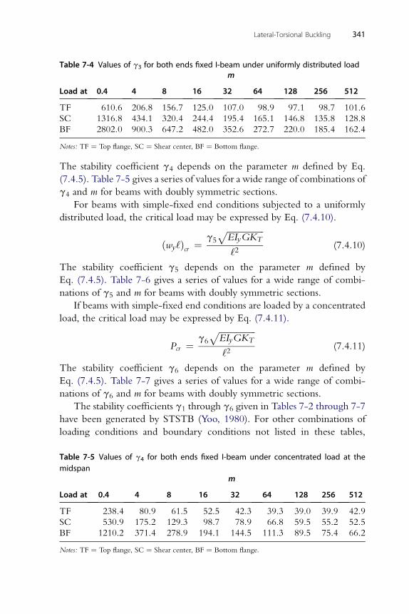
Table 7-4 Values of g3 for both ends fixed I-beam under uniformly distributed load
Load at
m
0.4 4 8 16 32 64 128 256 512
TF 610.6 206.8 156.7 125.0 107.0 98.9 97.1 98.7 101.6
SC 1316.8 434.1 320.4 244.4 195.4 165.1 146.8 135.8 128.8
BF 2802.0 900.3 647.2 482.0 352.6 272.7 220.0 185.4 162.4
Notes: TF ¼ Top flange, SC ¼ Shear center, BF ¼ Bottom flange.
Lateral-Torsional Buckling 341
The stability coefficient g4 depends on the parameter m defined by Eq.
(7.4.5). Table 7-5 gives a series of values for a wide range of combinations of
g4 and m for beams with doubly symmetric sections.
For beams with simple-fixed end conditions subjected to a uniformly
distributed load, the critical load may be expressed by Eq. (7.4.10).
ðwy‘Þcr ¼ g5
ffiffiffiffiffiffiffiffiffiffiffiffiffiffiffiffiffiEIyGKT
p‘2
(7.4.10)
The stability coefficient g5 depends on the parameter m defined by
Eq. (7.4.5). Table 7-6 gives a series of values for a wide range of combi-
nations of g5 and m for beams with doubly symmetric sections.
If beams with simple-fixed end conditions are loaded by a concentrated
load, the critical load may be expressed by Eq. (7.4.11).
Pcr ¼ g6
ffiffiffiffiffiffiffiffiffiffiffiffiffiffiffiffiffiEIyGKT
p‘2
(7.4.11)
The stability coefficient g6 depends on the parameter m defined by
Eq. (7.4.5). Table 7-7 gives a series of values for a wide range of combi-
nations of g6 and m for beams with doubly symmetric sections.
The stability coefficients g1 through g6 given in Tables 7-2 through 7-7
have been generated by STSTB (Yoo, 1980). For other combinations of
loading conditions and boundary conditions not listed in these tables,
Table 7-5 Values of g4 for both ends fixed I-beam under concentrated load at themidspan
Load at
m
0.4 4 8 16 32 64 128 256 512
TF 238.4 80.9 61.5 52.5 42.3 39.3 39.0 39.9 42.9
SC 530.9 175.2 129.3 98.7 78.9 66.8 59.5 55.2 52.5
BF 1210.2 371.4 278.9 194.1 144.5 111.3 89.5 75.4 66.2
Notes: TF ¼ Top flange, SC ¼ Shear center, BF ¼ Bottom flange.
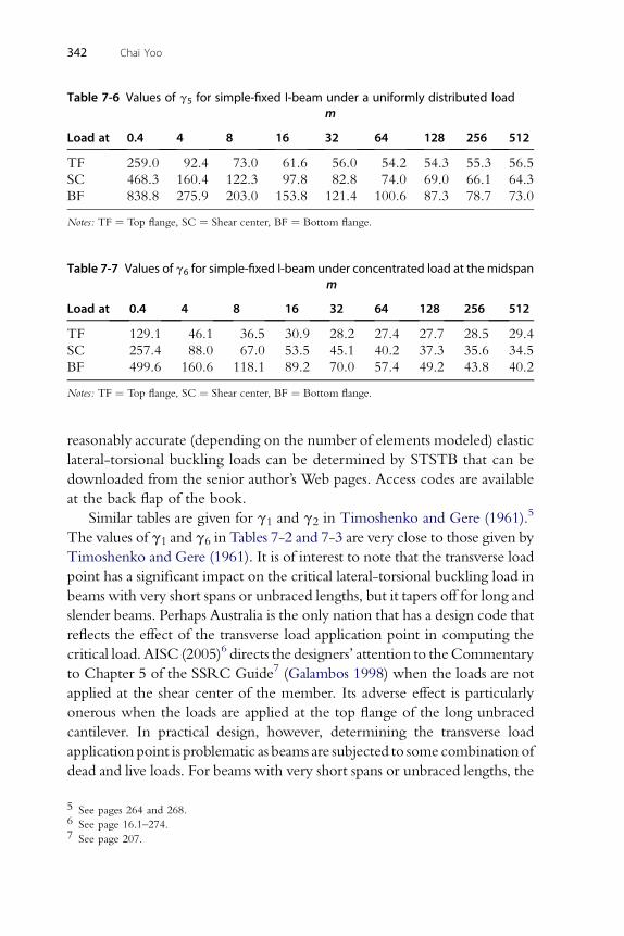
Table 7-6 Values of g5 for simple-fixed I-beam under a uniformly distributed load
Load at
m
0.4 4 8 16 32 64 128 256 512
TF 259.0 92.4 73.0 61.6 56.0 54.2 54.3 55.3 56.5
SC 468.3 160.4 122.3 97.8 82.8 74.0 69.0 66.1 64.3
BF 838.8 275.9 203.0 153.8 121.4 100.6 87.3 78.7 73.0
Notes: TF ¼ Top flange, SC ¼ Shear center, BF ¼ Bottom flange.
Table 7-7 Values of g6 for simple-fixed I-beam under concentrated load at the midspan
Load at
m
0.4 4 8 16 32 64 128 256 512
TF 129.1 46.1 36.5 30.9 28.2 27.4 27.7 28.5 29.4
SC 257.4 88.0 67.0 53.5 45.1 40.2 37.3 35.6 34.5
BF 499.6 160.6 118.1 89.2 70.0 57.4 49.2 43.8 40.2
Notes: TF ¼ Top flange, SC ¼ Shear center, BF ¼ Bottom flange.
342 Chai Yoo
reasonably accurate (depending on the number of elements modeled) elastic
lateral-torsional buckling loads can be determined by STSTB that can be
downloaded from the senior author’s Web pages. Access codes are available
at the back flap of the book.
Similar tables are given for g1 and g2 in Timoshenko and Gere (1961).5
The values of g1 and g6 in Tables 7-2 and 7-3 are very close to those given by
Timoshenko and Gere (1961). It is of interest to note that the transverse load
point has a significant impact on the critical lateral-torsional buckling load in
beams with very short spans or unbraced lengths, but it tapers off for long and
slender beams. Perhaps Australia is the only nation that has a design code that
reflects the effect of the transverse load application point in computing the
critical load. AISC (2005)6 directs the designers’ attention to theCommentary
to Chapter 5 of the SSRC Guide7 (Galambos 1998) when the loads are not
applied at the shear center of the member. Its adverse effect is particularly
onerous when the loads are applied at the top flange of the long unbraced
cantilever. In practical design, however, determining the transverse load
application point is problematic as beams are subjected to some combination of
dead and live loads. For beams with very short spans or unbraced lengths, the
5 See pages 264 and 268.6 See page 16.1–274.7 See page 207.
Lateral-Torsional Buckling 343
implication of this significant difference due to the transverse load points may
become a mute issue because the elastic lateral-torsional buckling moment is
likely to be greater than the full-plastic moment.
7.5. APPLICATION OF BESSEL FUNCTION TO LATERAL-TORSIONAL BUCKLING PROBLEMS
For a uniaxial bending problem, Eq. (7.2.24) takes the form
EIwfiv �GKTf
00 �Mbxu00 þ aywyf ¼ 0 (7.5.1)
There is no closed-form solution available for the coupled equations of
Eqs. (7.2.22) and (7.5.1) if the moment is not constant, and appropriate
numerical solution techniques must be used. For a narrow rectangular
section, or any section of which warping constant, Iw, is equal to zero, it is
only necessary to omit the term in the equation containing the warping
constant.
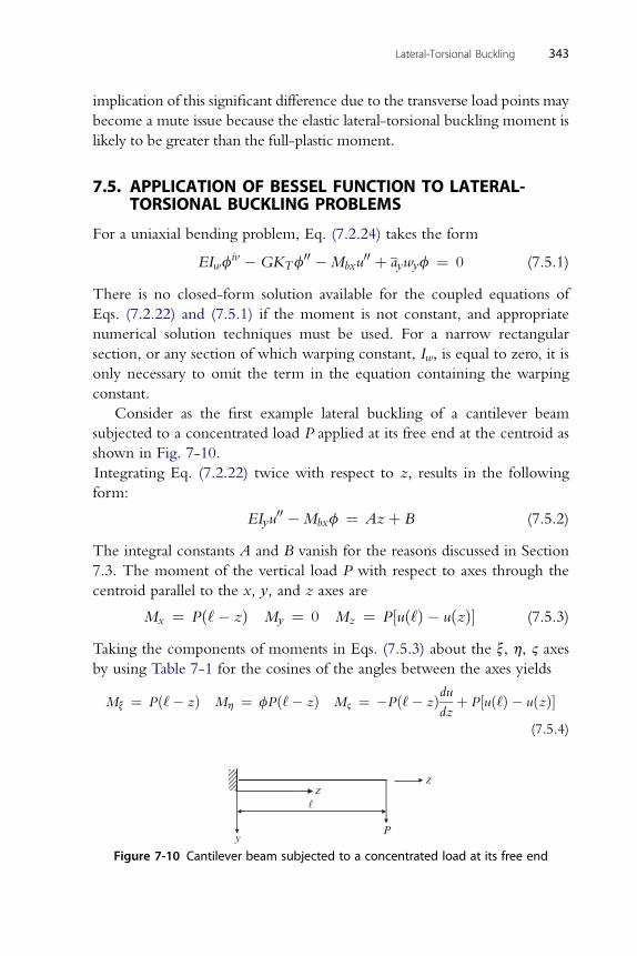
Consider as the first example lateral buckling of a cantilever beam
subjected to a concentrated load P applied at its free end at the centroid as
shown in Fig. 7-10.
Integrating Eq. (7.2.22) twice with respect to z, results in the following
form:
EIyu00 �Mbxf ¼ Azþ B (7.5.2)
The integral constants A and B vanish for the reasons discussed in Section
7.3. The moment of the vertical load P with respect to axes through the
centroid parallel to the x, y, and z axes are
Mx ¼ Pð‘� zÞ My ¼ 0 Mz ¼ P½uð‘Þ � uðzÞ� (7.5.3)
Taking the components of moments in Eqs. (7.5.3) about the x, h, 2 axes
by using Table 7-1 for the cosines of the angles between the axes yields
Mx ¼ Pð‘� zÞ Mh ¼ fPð‘� zÞ M2 ¼ �Pð‘� zÞdudz
þ P½uð‘Þ � uðzÞ�(7.5.4)
P
zz
y
Figure 7-10 Cantilever beam subjected to a concentrated load at its free end
344 Chai Yoo
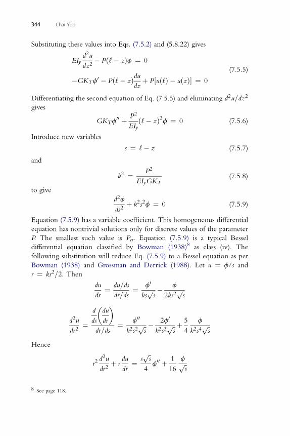
Substituting these values into Eqs. (7.5.2) and (5.8.22) gives
EIyd2u
dz2� Pð‘� zÞf ¼ 0
�GKTf0 � Pð‘� zÞdu
dzþ P½uð‘Þ � uðzÞ� ¼ 0
(7.5.5)
Differentiating the second equation of Eq. (7.5.5) and eliminating d2u=dz2
gives
GKTf00 þ P2
EIyð‘� zÞ2f ¼ 0 (7.5.6)
Introduce new variables
s ¼ ‘� z (7.5.7)
and
k2 ¼ P2
EIyGKT(7.5.8)
to give
d2f
ds2þ k2s2f ¼ 0 (7.5.9)
Equation (7.5.9) has a variable coefficient. This homogeneous differential
equation has nontrivial solutions only for discrete values of the parameter
P. The smallest such value is Pcr. Equation (7.5.9) is a typical Bessel
differential equation classified by Bowman (1938)8 as class (iv). The
following substitution will reduce Eq. (7.5.9) to a Bessel equation as per
Bowman (1938) and Grossman and Derrick (1988). Let u ¼ f/s and
r ¼ ks2=2. Then
du
dr¼ du=ds
dr=ds¼ f0
ksffiffis
p � f
2ks2ffiffis
p
d�du�
d2u
dr2¼ ds dr
dr=ds¼ f00
k2s2ffiffis
p � 2f0
k2s3ffiffis
p þ 5
4
f
k2s4ffiffis
p
Hence
r2d2u
dr2þ r
du
dr¼ s
ffiffis
p4
f00 þ 1
16
fffiffis
p
8 See page 118.
Lateral-Torsional Buckling 345
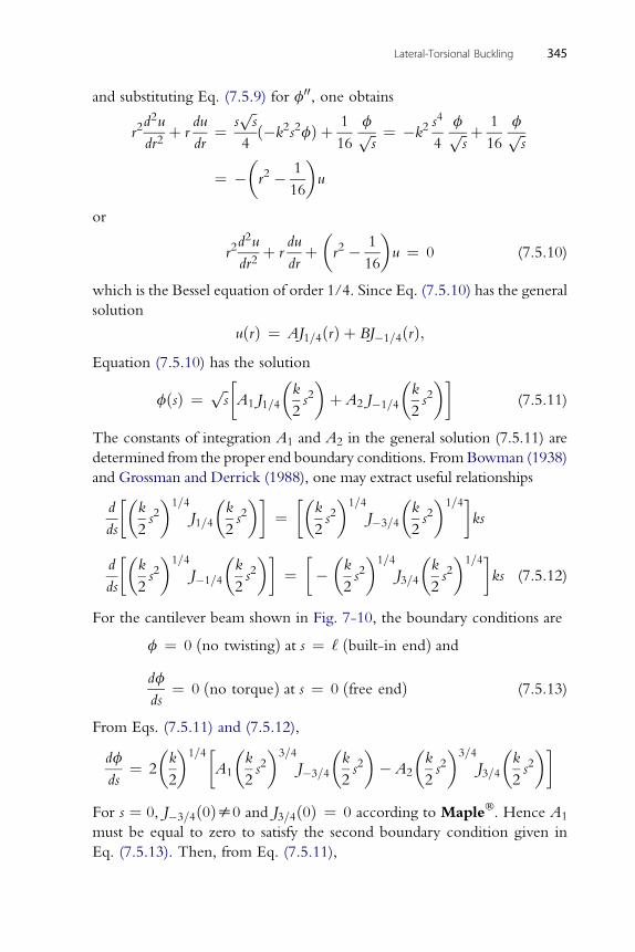
and substituting Eq. (7.5.9) for f00, one obtains
r2d2u
dr2þ r
du
dr¼ s
ffiffis
p4ð�k2s2fÞ þ 1
16
fffiffis
p ¼ �k2s4
4
fffiffis
p þ 1
16
fffiffis
p
¼ ��r2 � 1
16
�u
or
r2d2u
dr2þ r
du
drþ�r2 � 1
16
�u ¼ 0 (7.5.10)
which is the Bessel equation of order 1/4. Since Eq. (7.5.10) has the general
solution
uðrÞ ¼ AJ1=4ðrÞ þ BJ�1=4ðrÞ;Equation (7.5.10) has the solution
fðsÞ ¼ ffiffis
p �A1 J1=4
�k
2s2�þ A2 J�1=4
�k
2s2��
(7.5.11)
The constants of integration A1 and A2 in the general solution (7.5.11) are
determined from the proper end boundary conditions. FromBowman (1938)
and Grossman and Derrick (1988), one may extract useful relationships
d
ds
��k
2s2�1=4
J1=4
�k
2s2��
¼��
k
2s2�1=4
J�3=4
�k
2s2�1=4�
ks
d
ds
��k
2s2�1=4
J�1=4
�k
2s2��
¼���k
2s2�1=4
J3=4
�k
2s2�1=4�
ks (7.5.12)
For the cantilever beam shown in Fig. 7-10, the boundary conditions are
f ¼ 0 ðno twistingÞ at s ¼ ‘ ðbuilt-in endÞ anddf
ds¼ 0 ðno torqueÞ at s ¼ 0 ðfree endÞ (7.5.13)
From Eqs. (7.5.11) and (7.5.12),
df
ds¼ 2
�k
2
�1=4�
A1
�k
2s2�3=4
J�3=4
�k
2s2�� A2
�k
2s2�3=4
J3=4
�k
2s2��
For s ¼ 0, J�3=4ð0Þs0 and J3=4ð0Þ ¼ 0 according to Maple�. Hence A1
must be equal to zero to satisfy the second boundary condition given in
Eq. (7.5.13). Then, from Eq. (7.5.11),
346 Chai Yoo
fðsÞ ¼ ffiffis
pA2J�1=4
�k
2s2�
(7.5.14)
The first boundary condition of Eq. (7.5.13) applied to Eq. (7.5.14) gives
0 ¼ J�1=4
�k
2‘2�
(7.5.15)
The smallest value to satisfy Eq. (7.5.15) according to Maple� is k ‘2/2 ¼2.0063. Then k ¼ 4.0126/‘2. From which
Pcr ¼ 4:0126
‘2ffiffiffiffiffiffiffiffiffiffiffiffiffiffiffiffiffiEIyGKT
p(7.5.16)
This result, Eq. (7.5.16), was obtained by Prandtl (1899).
Consider, as another example of applying the Bessel equation, a simply
supported beam of narrow rectangular section subjected to a concentrated
load applied at the centroid at the midspan as shown in Fig. 7-9. For
convenience, the origin of the coordinate system is moved to the midspan.
The moments with respect to axes through the centroid of the cross section
parallel to the x, y, and z axes are
Mx ¼ �P
2
�‘
2� z
�My ¼ 0 Mz ¼ �P
2½uð0Þ � uðzÞ� (7.5.17)
Taking the components of moments in Eqs. (7.5.17) about the x, h, 2 axes
by using Table 7-1 for the cosines of the angles between the axes yields
Mx ¼ �P
2
�‘
2� z
�Mh ¼ �f
P
2
�‘
2� z
�
M2 ¼ P
2
�‘
2� z
�du
dz� P½uð0Þ � uðzÞ� (7.5.18)
Substituting these values in to Eqs. (7.5.2) and (5.8.22) gives
EIyd2u
dz2þ P
2
�‘
2� z
�f ¼ 0
�GKTf0 þ P
2
�‘
2� z
�du
dz� P
2½uð0Þ � uðzÞ� ¼ 0
(7.5.19)
Eliminating d2u=dz2 in Eqs. (7.5.19) gives
GKTf00 þ P2
4EIy
�‘
2� z
�2
f ¼ 0 (7.5.20)
Lateral-Torsional Buckling 347
Introducing the variable t ¼ ‘/2 � z and the notation
k2 ¼ P2
4EIyGKT(7.5.21)
to give
d2f
dt2þ k2t2f ¼ 0 (7.5.22)
Equation (7.5.22) is identical to Eq. (7.5.9). The general solution of
Eq. (7.5.22) is
f ¼ ffiffit
p ½A1 J1=4ðkt2Þ þ A2 J�1=4ðkt2Þ� (7.5.23)
For a simply supported beam, the proper boundary conditions are
f ¼ 0 at t ¼ 0df
dt¼ 0 at t ¼ ‘
2(7.5.24)
In order to satisfy the first condition of Eq. (7.5.24) ( J�1=4ð0Þs 0;J1=4ð0Þ ¼ 0), A2 ¼ 0. Then,
df
dt¼ 2
�k
2
�1=4
A1
�k
2t2�3=4
J�3=4
�k
2t2�
¼ 0 at t ¼ ‘
2
Hence, J�3=4ððk=8Þ ‘2Þ ¼ 0.
The parameter for the first zero of the Bessel function of order �3/4 is
found from Maple� to be 1.0585, which leads to
Pcr ¼ 16:94ffiffiffiffiffiffiffiffiffiffiffiffiffiffiffiffiffiEIyGKT
p‘2
(7.5.25)
It can be readily recognized that the computer-based modern matrix
structural analysis (such as STSTB) and/or finite element analysis would be
superior to the longhand classical solution techniques with regard to speed
of analysis as well as the versatility on the loadings and boundary conditions
that can be accommodated. Some of the really old classical methods of
analysis are to be viewed as historical interest.
7.6. LATERAL-TORSIONAL BUCKLING BY ENERGY METHOD
The determination of the critical lateral-torsional buckling loads by long-
hand classical methods is very complex and tedious, particularly for
nonuniform bending, as this will result in a system of differential equations
with variable coefficients. In this section, the Rayleigh-Ritz method will be
348 Chai Yoo
used to determine approximately the critical lateral-torsional buckling loads
of beams following the general procedures presented by Winter (1941) and
Chajes (1974). In any energy method, it is required to establish expressions
for the strain energy stored in the elastic body and the loss of potential
energy of the externally applied loads. It is relatively simple to come up with
the expression for the strain energy by
U ¼ ð1=2ÞZv
sT 3dv
wheresT¼ transpose of the stress vector, 3¼ strain vector, and v¼ volume of
the body. Although the loss of the potential energy of the applied loads is
simple in concept as being the negative product of the generalized force and
the corresponding deformation during buckling, the expression for the
corresponding deformation usually requires considerable geometric analyses.
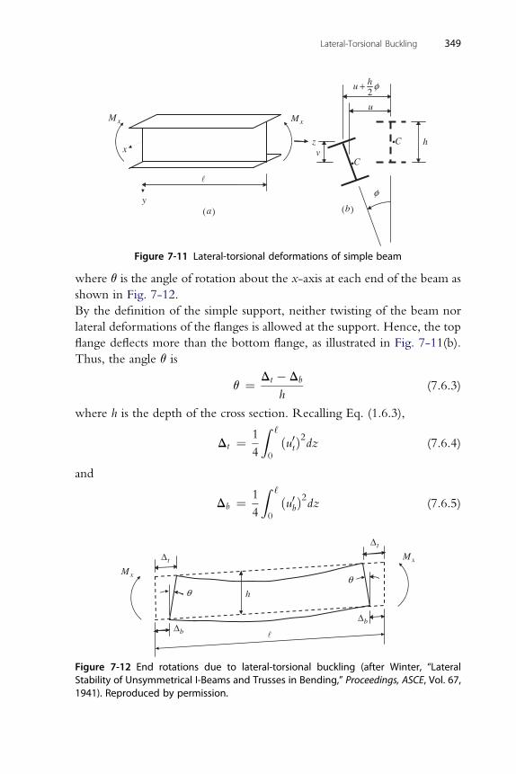
7.6.1. Uniform BendingConsider a prismatic, simply supported doubly symmetric (for simplicity)9
I-beam subjected to a uniform bending moment Mx as shown in Fig. 7-11.
The bendingmomentMx shown is negative as it produces negative curvature.
The notion of the buckling analysis of the beam is to examine equilibrium in
the slightly buckled (lateral-torsional deformations of the beam) configura-
tion. Therefore, the strain energy associated with vertical bending or pre-
buckling static equilibrium should be excluded from Eq. (6.3.3) in the
buckling analysis because it belongs to a totally different equilibrium
configuration. The strain energy stored in the beam during buckling consists
of two parts: the energy associated with bending about the y-axis and the
energy due to twisting about the z-axis. Thus the strain energy is
U ¼ 1
2
Z ‘
0
EIyðu00Þ2dzþ 1
2
Z ‘
0
GKT ðf0Þ2dzþ 1
2
Z ‘
0
EIwðf00Þ2dz (7.6.1)
To form the total potential energy, the potential energy V of the externally
applied loads must be added to the strain energy, Eq. (7.6.1). For a beam
subjected to pure bending, the loss of potential energy V is equal to the
negative product of the applied moments and the corresponding angles due
to buckling. Hence,
V ¼ �2Mxq (7.6.2)
9 Winter (1941) considered a singly symmetric cross section.
2hu φ+
( )b( )a
h
u
v
M Mx
z
x
C
Cx
φy
i
i
Figure 7-11 Lateral-torsional deformations of simple beam
Lateral-Torsional Buckling 349
where q is the angle of rotation about the x-axis at each end of the beam as
shown in Fig. 7-12.
By the definition of the simple support, neither twisting of the beam nor
lateral deformations of the flanges is allowed at the support. Hence, the top
flange deflects more than the bottom flange, as illustrated in Fig. 7-11(b).
Thus, the angle q is
q ¼ Dt � Db
h(7.6.3)
where h is the depth of the cross section. Recalling Eq. (1.6.3),
Dt ¼ 1
4
Z ‘
0
ðu0tÞ2dz (7.6.4)
and
Db ¼ 1
4
Z ‘
0
ðu0bÞ2dz (7.6.5)
xMxM
tΔ
tΔ
bΔ
θ h
bΔ
θ
Figure 7-12 End rotations due to lateral-torsional buckling (after Winter, “LateralStability of Unsymmetrical I-Beams and Trusses in Bending,” Proceedings, ASCE, Vol. 67,1941). Reproduced by permission.
350 Chai Yoo
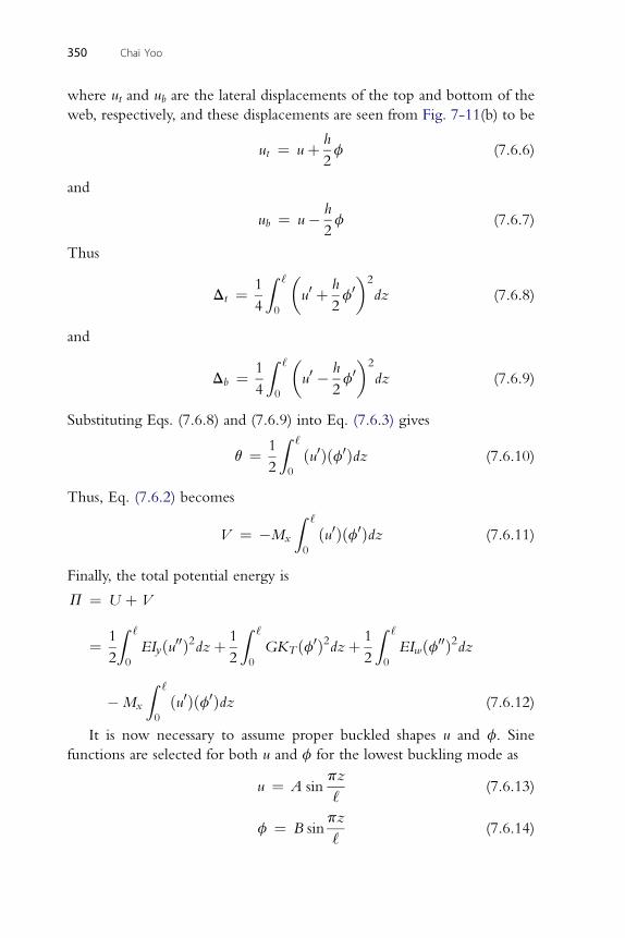
where ut and ub are the lateral displacements of the top and bottom of the
web, respectively, and these displacements are seen from Fig. 7-11(b) to be
ut ¼ uþ h
2f (7.6.6)
and
ub ¼ u� h
2f (7.6.7)
Thus
Dt ¼ 1
4
Z ‘
0
�u0 þ h
2f0�2
dz (7.6.8)
and
Db ¼ 1
4
Z ‘
0
�u0 � h
2f0�2
dz (7.6.9)
Substituting Eqs. (7.6.8) and (7.6.9) into Eq. (7.6.3) gives
q ¼ 1
2
Z ‘
0
ðu0Þðf0Þdz (7.6.10)
Thus, Eq. (7.6.2) becomes
V ¼ �Mx
Z ‘
0
ðu0Þðf0Þdz (7.6.11)
Finally, the total potential energy is
P ¼ U þ V
¼ 1
2
Z ‘
0
EIyðu00Þ2dzþ 1
2
Z ‘
0
GKT ðf0Þ2dzþ 1
2
Z ‘
0
EIwðf00Þ2dz
�Mx
Z ‘
0
ðu0Þðf0Þdz (7.6.12)
It is now necessary to assume proper buckled shapes u and f. Sine
functions are selected for both u and f for the lowest buckling mode as
u ¼ A sinpz
‘(7.6.13)
pz
f ¼ B sin‘(7.6.14)
Lateral-Torsional Buckling 351
As Eqs. (7.6.13) and (7.6.14) satisfy both geometric and natural boundary
conditions, it is expected that the approximate solution will be very close to
the exact solution. When these expressions are substituted into Eq. (7.6.12),
the total potential energy becomes a function of two variables A and B.
Invoking the principle of minimum total potential energy, one can deter-
mine the critical moment by solving the two equations that result if the first
variation of p is made to vanish with respect to both A and B. An alternative
approach is to express A in terms of B. Although the alternative approach
involves fewer computations than the first, the first procedure must be
used if a relation between u and f is not available. Since Mx and My are
defined to be positive when they produce positive curvature, Mx ¼EIxv
00 and My ¼ EIyu00. From Table 7-1, My ¼ Mxf. Thus
f ¼ EIy
Mxu00 (7.6.15)
‘2 M
A ¼ �Bp2
x
EIy(7.6.16)
The assumed function for u can now be written as
u ¼ �B‘2
p2
Mx
EIysin
pz
‘(7.6.17)
Using Eqs. (7.6.14) and (7.6.17), the total potential energy becomes
P ¼ U þ V
¼ 1
2
B2M2x
EIy
Z ‘
0
sin2pz
‘dzþ 1
2GKTB
2 p2
‘2
Z ‘
0
cos2pz
‘dz
þ 1
2EIwB
2 p4
‘4
Z ‘
0
sin2pz
‘dz�M2
xB2
EIy
Z ‘
0
cos2pz
‘dz (7.6.18)
Since Z ‘
0
sin2pz
‘dz ¼
Z ‘
0
cos2pz
‘dz ¼ ‘
2
Equation (7.6.18) reduces to
P ¼ U þ V ¼ 1
4
�GKTB
2p2
‘þ EIwB
2p4
‘3�M2
xB2‘
EIy
�(7.6.19)
352 Chai Yoo
The critical moment is reached when neutral equilibrium (or neighboring
equilibrium) is possible, and the requirement for neutral equilibrium is that
the derivative of P with respect to B vanish. Hence,
dP
dB¼ dðU þ V Þ
dB¼ B
2
�GKTp
2
‘þ EIwp
4
‘3�M2
x ‘
EIy
�¼ 0 (7.6.20)
If neutral equilibrium is to correspond to a buckled configuration, B cannot
be zero. In order to satisfy Eq. (7.6.20), the quantity inside the parentheses
must be equal to zero. Thus,
GKTp2
‘þ EIwp
4
‘3�M2
x ‘
EIy¼ 0 (7.6.21)
From which
Mx cr ¼ �p
‘
ffiffiffiffiffiffiffiffiffiffiffiffiffiffiffiffiffiffiffiffiffiffiffiffiffiffiffiffiffiffiffiffiffiffiffiffiffiffiffiffiffiffiffiffiffiEIyðGKT þ p2EIw=‘2Þ
q(7.6.22)
Equation (7.6.22) gives the critical moment for a simply supported I-beam
subjected to pure bending, and it is identical to Eq. (7.4.2). The � sign in
Eq. (7.6.22) indicates that an identical critical moment will result if the
sign of pure bending is reversed from that shown in Fig. 7-12. It should
also be noticed that the critical moment given by Eq. (7.6.22) is exact
since the assumed displacement functions of Eqs. (7.6.13) and (7.6.14)
happen to be exact eigenfunctions. This can be proved (for example, see
Problem 6.3).
7.6.2. One Concentrated Load at MidspanConsider a simply supported prismatic I-beam subjected to a concentrated
load at midspan. The cross section is assumed to be doubly symmetric, and
the load is applied at the centroid (the shear center) for simplicity. The case
of a concentrated load applied at a point other than the shear center in
a singly symmetric cross section can be handled likewise.
The strain energy stored in the beam during buckling has the same form
given by Eq. (7.6.1). The potential energy of the externally applied load is,
of course, the negative product of the applied load P and the vertical
displacement v0 of P that takes place during buckling. To determine v0, it is
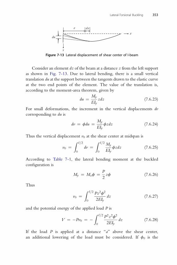
useful to draw the lateral deflection of the shear center (the load point) of the
beam as shown in Fig. 7-13 during buckling, as the vertical displacement
component of the beam during buckling is equal to the product of the
lateral displacement and the twisting angle.
x
du
dz z
z
Figure 7-13 Lateral displacement of shear center of I-beam
Lateral-Torsional Buckling 353
Consider an element dz of the beam at a distance z from the left support
as shown in Fig. 7-13. Due to lateral bending, there is a small vertical
translation du at the support between the tangents drawn to the elastic curve
at the two end points of the element. The value of the translation is,
according to the moment-area theorem, given by
du ¼ My
EIyzdz (7.6.23)
For small deformations, the increment in the vertical displacements dv
corresponding to du is
dv ¼ fdu ¼ My
EIyfzdz (7.6.24)
Thus the vertical displacement v0 at the shear center at midspan is
v0 ¼Z ‘=2
0
dv ¼Z ‘=2
0
My
EIyfzdz (7.6.25)
According to Table 7-1, the lateral bending moment at the buckled
configuration is
My ¼ Mxf ¼ P
2zf (7.6.26)
Thus
v0 ¼Z ‘=2
0
Pz2f2
2EIydz (7.6.27)
and the potential energy of the applied load P is
V ¼ �Pv0 ¼ �Z ‘=2
0
P2z2f2
2EIydz (7.6.28)
If the load P is applied at a distance “a” above the shear center,
an additional lowering of the load must be considered. If f0 is the
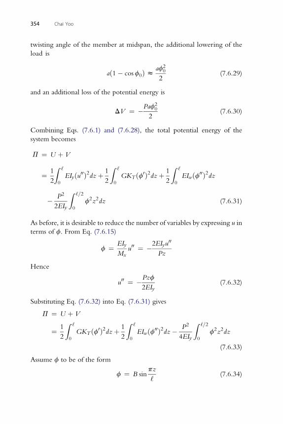
354 Chai Yoo
twisting angle of the member at midspan, the additional lowering of the
load is
að1� cosf0Þ zaf2
0
2(7.6.29)
and an additional loss of the potential energy is
DV ¼ �Paf20
2(7.6.30)
Combining Eqs. (7.6.1) and (7.6.28), the total potential energy of the
system becomes
P ¼ U þ V
¼ 1
2
Z ‘
0
EIyðu00Þ2dzþ 1
2
Z ‘
0
GKT ðf0Þ2dzþ 1
2
Z ‘
0
EIwðf00Þ2dz
� P2
2EIy
Z ‘=2
0
f2z2dz (7.6.31)
As before, it is desirable to reduce the number of variables by expressing u in
terms of f. From Eq. (7.6.15)
f ¼ EIy
Mxu00 ¼ �2EIyu
00
Pz
Hence
u00 ¼ �Pzf
2EIy(7.6.32)
Substituting Eq. (7.6.32) into Eq. (7.6.31) gives
P ¼ U þ V
¼ 1
2
Z ‘
0
GKT ðf0Þ2dzþ 1
2
Z ‘
0
EIwðf00Þ2dz� P2
4EIy
Z ‘=2
0
f2z2dz
(7.6.33)
Assume f to be of the form
f ¼ B sinpz
‘(7.6.34)
Lateral-Torsional Buckling 355
Substituting f and its derivatives into Eq. (7.6.33) yields
U þ V ¼ �P2B2
4EIy
Z ‘=2
0
z2 sin2pz
‘dzþGKTB
2p2
2‘2
Z ‘
0
cos2pz
‘dz
þ EIwB2p4
2‘4
Z ‘
0
sin2pz
‘dz (7.6.35)
Substituting the definite integrals
Z ‘=2
0
z2 sin2pz
‘dz ¼ ‘3
48p2ðp2 þ 6Þ
Z ‘ Z ‘
0
sin2pz
‘dz ¼
0
cos2pz
‘dz ¼ ‘
2(7.6.36)
into Eq. (7.6.35) gives
U þ V ¼ � P2B2‘3
192EIyp2ðp2 þ 6Þ þGKTB
2p2
4‘þ EIwB
2p4
4‘3(7.6.37)
At the critical load, the first variation of U þ V with respect to B must
vanish. Thus,
d
dBðU þ V Þ ¼ B
2
�� P2‘3
48EIyp2ðp2 þ 6Þ þGKTp
2
‘þ EIwp
4
‘3
�¼ 0
which leads to
Pcr ¼ �4p2
‘2
ffiffiffiffiffiffiffiffiffiffiffiffiffiffiffiffiffiffiffiffiffiffiffiffiffiffiffiffiffiffiffiffiffiffiffiffiffiffiffiffiffiffiffiffiffiffiffiffiffiffiffiffiffiffiffi3
p2 þ 6EIy
�GKT þ EIwp2
‘2
�s(7.6.38)
Equation (7.5.38) gives the critical load for a simply supported I-beam
subjected to a concentrated load at midspan. The � sign in Eq. (7.5.38)
indicates that an identical critical load will result if the direction of the load is
reversed from that shown in Fig. 7-9.
7.6.3. Uniformly Distributed LoadThe procedure described above for the case of a concentrated load at
midspan can also be used when the I-beam (Fig. 7-8) carries a uniformly
distributed load. The strain energy given by Eq. (7.6.1) remains unchanged.
However, the expression for the loss of potential energy of the externally
applied load must be determined.
356 Chai Yoo
Assume f to be of the form
f ¼ B sinpz
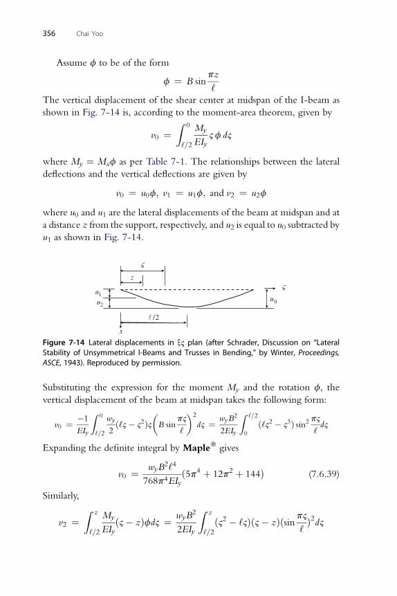
‘The vertical displacement of the shear center at midspan of the I-beam as
shown in Fig. 7-14 is, according to the moment-area theorem, given by
v0 ¼Z 0
‘=2
My
EIy2 f d2
where My ¼ Mxf as per Table 7-1. The relationships between the lateral
deflections and the vertical deflections are given by
v0 ¼ u0f; v1 ¼ u1f; and v2 ¼ u2f
where u0 and u1 are the lateral displacements of the beam at midspan and at
a distance z from the support, respectively, and u2 is equal to u0 subtracted by
u1 as shown in Fig. 7-14.
ς
x
/2
z
2u1u
ς
0u
Figure 7-14 Lateral displacements in x2 plan (after Schrader, Discussion on “LateralStability of Unsymmetrical I-Beams and Trusses in Bending,” by Winter, Proceedings,ASCE, 1943). Reproduced by permission.
Substituting the expression for the moment My and the rotation f, the
vertical displacement of the beam at midspan takes the following form:
v0 ¼ �1
EIy
Z 0
‘=2
wy
2ð‘2� 22Þ2
�B sin
p2
‘
�2
d2 ¼ wyB2
2EIy
Z ‘=2
0
ð‘22 � 23Þ sin2 p2‘d2
Expanding the definite integral by Maple� gives
v0 ¼ wyB2‘4
768p4EIyð5p4 þ 12p2 þ 144Þ (7.6.39)
Similarly,
v2 ¼Z z
‘=2
My
EIyð2� zÞfd2 ¼ wyB
2
2EIy
Z z
‘=2ð22 � ‘2Þð2� zÞðsinp2
‘Þ2d2
wyB2
v2 ¼768p4EIy
�
5p4‘4 � 48p2‘3z� 16‘3p4zþ 12‘4p2 � 96‘2p2z2 cos2pz
‘
þ 48‘2p2z2 þ 144‘4 cos2pz
‘� 96‘4p cos
pz
‘sin
pz
‘
þ 96‘3p2z cos2pz
‘� 16p4z4 þ 32‘p4z3 þ 192p‘3z cos
pz
‘sin
pz
‘
266666664
377777775
ð7:6:40Þ
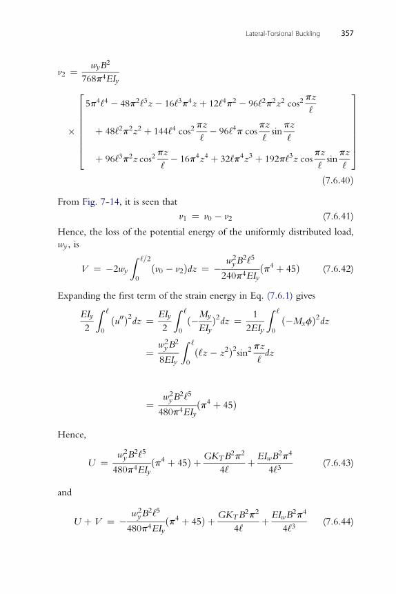
From Fig. 7-14, it is seen that
Lateral-Torsional Buckling 357
v1 ¼ v0 � v2 (7.6.41)
Hence, the loss of the potential energy of the uniformly distributed load,
wy , is
V ¼ �2wy
Z ‘=2
0
ðv0 � v2Þdz ¼ � w2yB
2‘5
240p4EIyðp4 þ 45Þ (7.6.42)
Expanding the first term of the strain energy in Eq. (7.6.1) gives
EIy
2
Z ‘
0
ðu00Þ2dz ¼ EIy
2
Z ‘
0
ð�My
EIyÞ2dz ¼ 1
2EIy
Z ‘
0
ð�MxfÞ2dz
¼ w2yB
2
8EIy
Z ‘
0
ð‘z� z2Þ2sin2 pz‘dz
¼ w2yB
2‘5
480p4EIyðp4 þ 45Þ
Hence,
U ¼ w2yB
2‘5
480p4EIyðp4 þ 45Þ þGKTB
2p2
4‘þ EIwB
2p4
4‘3(7.6.43)
and
U þ V ¼ � w2yB
2‘5
480p4EIyðp4 þ 45Þ þGKTB
2p2
4‘þ EIwB
2p4
4‘3(7.6.44)
358 Chai Yoo
At the critical load, the first variation of U þ V with respect to B must
vanish. Thus,
d
dBðU þ V Þ ¼ B
2
�� w2
y‘5
120EIyp4ðp4 þ 45Þ þGKTp
2
‘þ EIwp
4
‘3
�¼ 0
which leads to
ðwy‘Þcr ¼ �2p3
‘2
ffiffiffiffiffiffiffiffiffiffiffiffiffiffiffiffiffiffiffiffiffiffiffiffiffiffiffiffiffiffiffiffiffiffiffiffiffiffiffiffiffiffiffiffiffiffiffiffiffiffiffiffiffiffiffiffiffiffi30
p4 þ 45EIy
�GKT þ EIwp2
‘2
�s(7.6.45)
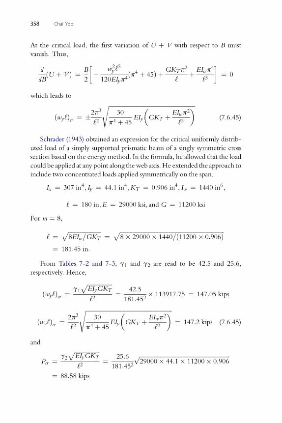
Schrader (1943) obtained an expression for the critical uniformly distrib-
uted load of a simply supported prismatic beam of a singly symmetric cross
section based on the energy method. In the formula, he allowed that the load
could be applied at any point along theweb axis. He extended the approach to
include two concentrated loads applied symmetrically on the span.
Ix ¼ 307 in4; Iy ¼ 44:1 in4;KT ¼ 0:906 in4; Iw ¼ 1440 in6;
‘ ¼ 180 in;E ¼ 29000 ksi; and G ¼ 11200 ksi
For m ¼ 8,
‘ ¼ffiffiffiffiffiffiffiffiffiffiffiffiffiffiffiffiffiffiffiffiffiffi8EIw=GKT
p¼
ffiffiffiffiffiffiffiffiffiffiffiffiffiffiffiffiffiffiffiffiffiffiffiffiffiffiffiffiffiffiffiffiffiffiffiffiffiffiffiffiffiffiffiffiffiffiffiffiffiffiffiffiffiffiffiffiffiffiffiffiffiffiffiffiffiffiffiffiffiffi8� 29000� 1440=ð11200� 0:906Þ
p¼ 181:45 in:
From Tables 7-2 and 7-3, g1 and g2 are read to be 42.5 and 25.6,
respectively. Hence,
ðwy‘Þcr ¼ g1ffiffiffiffiffiffiffiffiffiffiffiffiffiffiffiffiffiEIyGKT
p‘2
¼ 42:5
181:452� 113917:75 ¼ 147:05 kips
3ffiffiffiffiffiffiffiffiffiffiffiffiffiffiffiffiffiffiffiffiffiffiffiffiffiffiffiffiffiffiffiffiffiffiffiffiffiffiffiffiffiffiffiffiffiffiffiffiffiffiffiffiffiffiffiffiffiffi� �s
ðwy‘Þcr ¼ 2p
‘230
p4 þ 45EIy GKT þ EIwp2
‘2¼ 147:2 kips (7.6.45)
and
Pcr ¼ g2
ffiffiffiffiffiffiffiffiffiffiffiffiffiffiffiffiffiEIyGKT
p‘2
¼ 25:6
181:452
ffiffiffiffiffiffiffiffiffiffiffiffiffiffiffiffiffiffiffiffiffiffiffiffiffiffiffiffiffiffiffiffiffiffiffiffiffiffiffiffiffiffiffiffiffiffiffiffiffiffiffiffiffiffiffiffiffiffiffiffiffi29000� 44:1� 11200� 0:906
p
¼ 88:58 kips

2ffiffiffiffiffiffiffiffiffiffiffiffiffiffiffiffiffiffiffiffiffiffiffiffiffiffiffiffiffiffiffiffiffiffiffiffiffiffiffiffiffiffiffiffiffiffiffiffiffiffiffiffiffiffiffiffi�
2�s
Pcr ¼ 4p
‘23
p2 þ 6EIy GKT þ EIwp
‘2¼ 88:76 kips (7.6.38)
7.6.4. Two Concentrated Loads Applied SymmetricallyConsider the case of two concentrated loads applied symmetrically as shown
in Fig. 7-15. From Table 1, My ¼ Mxf. Assume f ¼ B sinpz‘The bending moment is given by
Mx ¼ Pz for 0 � z � a and Mx ¼ Pa for a < z � ‘=2
Expanding the terms of the strain energy in Eq. (7.6.1), one obtains
1
2EIy
Z ‘
0
�u00�2dz ¼ EIy
Z ‘=2
0
�u00�2dz ¼ EIy
Z ‘=2
0
�Mxf
EIy
�2
dz
¼ B2P2
EIy
�Z a
0
z2 sin2pz
‘dzþ a2
Z ‘=2
a
sin2pz
‘dz
�
¼ B2P2
EIy
�Z a
0
z2 sin2pz
‘dzþ a2
Z ‘=2
a
sin2pz
‘dz
�
¼ P2B2EIy
12p3
�� 4p3a3 � 6pa‘2 cos2
pa
‘
þ 3‘3 cospa
‘sin
pa
‘þ 3pa‘2 þ 3p3a2‘
�(7.6.46a)
Z ‘� �2� �
2
Lateral-Torsional Buckling 359
1
2GKT
0
f0 2dz ¼ B ‘
4
p
‘GKT (7.6.46b)
P
1u
x
2u
a
/2
zz
0u
Pa
Figure 7-15 Two concentrated loads (after Schrader, Discussion on “Lateral Stability ofUnsymmetrical I-Beams and Trusses in Bending,” by Winter, Proceedings, ASCE, 1943).Reproduced by permission.
1Z ‘� �
B2‘�p�4
2EIw
0
f00 2dz ¼
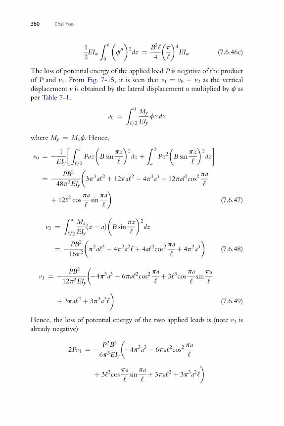
4 ‘EIw (7.6.46c)
The loss of potential energy of the applied load P is negative of the product
of P and v1. From Fig. 7-15, it is seen that v1 ¼ v0 � v2 as the vertical
displacement v is obtained by the lateral displacement u multiplied by f as
per Table 7-1.
v0 ¼Z 0
‘=2
My
EIyfz dz
where My ¼ Mxf. Hence,
v0 ¼ � 1
EIy
�Z a
‘=2Paz
�B sin
pz
‘
�2dzþ
Z 0
a
Pz2�B sin
pz
‘
�2dz
�
¼ � PB2
48p3EIy
�3p3a‘2 þ 12pa‘2 � 4p3a3 � 12pal2cos2
pa
‘
þ 12‘2 cospa
‘sin
pa
‘
�(7.6.47)
Z a M�
pz�2
360 Chai Yoo
v2 ¼‘=2
x
EIyðz� aÞ B sin
‘dz
¼ � PB2
16p2
�p2a‘2 � 4p2a2‘þ 4a‘2cos2
pa
‘þ 4p2a3
�(7.6.48)
PB2�
pa pa pa
v1 ¼ �12p3EIy�4p3a3 � 6pa‘2cos2
‘þ 3‘3cos
‘sin
‘
þ 3pa‘2 þ 3p3a2‘
�(7.6.49)
Hence, the loss of potential energy of the two applied loads is (note v1 is
already negative)
2Pv1 ¼ � P2B2
6p3EIy
��4p3a3 � 6pa‘2cos2
pa
‘
þ 3‘3cospa
‘sin
pa
‘þ 3pa‘2 þ 3p3a2‘
�
P2B2EIy�
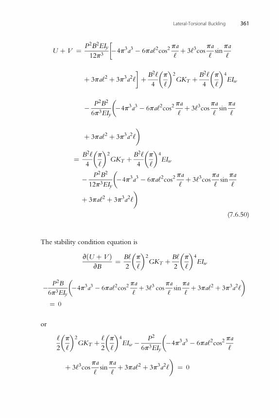
pa pa pa
U þ V ¼12p3�4p3a3 � 6pa‘2cos2
‘þ 3‘3cos
‘sin
‘
þ 3pa‘2 þ 3p3a2‘
�þ B2‘
4
�p
‘
�2GKT þ B2‘
4
�p
‘
�4EIw
� P2B2
6p3EIy
��4p3a3 � 6pa‘2cos2
pa
‘þ 3‘3cos
pa
‘sin
pa
‘
þ 3pa‘2 þ 3p3a2‘
�
¼ B2‘
4
�p
‘
�2GKT þ B2‘
4
�p
‘
�4EIw
� P2B2
12p3EIy
��4p3a3 � 6pa‘2cos2
pa
‘þ 3‘3cos
pa
‘sin
pa
‘
þ 3pa‘2 þ 3p3a2‘
�(7.6.50)
The stability condition equation is
vðU þ V ÞvB
¼ B‘
2
�p
‘
�2GKT þ B‘
2
�p
‘
�4EIw
P2B�
pa pa pa�
Lateral-Torsional Buckling 361
�6p3EIy
�4p3a3 � 6pa‘2cos2‘þ 3‘3 cos
‘sin
‘þ 3pa‘2 þ 3p3a2‘
¼ 0
or
‘
2
�p
‘
�2GKT þ ‘
2
�p
‘
�4EIw � P2
6p3EIy
��4p3a3 � 6pa‘2cos2
pa
‘
þ 3‘3cospa
‘sin
pa
‘þ 3pa‘2 þ 3p3a2‘
�¼ 0
� �p�2�
P2‘ pa
EIy GKT þ EIw‘¼
3p5ð�4p3a3 � 6pa‘2cos2
‘
þ 3‘3cospa
‘sin
pa
‘þ 3pa‘2 þ 3p3a2‘Þ
¼ P2‘
�� 4a3
3p2� 2a‘2
p4cos2
pa
‘
þ ‘3
p5cos
pa
‘sin
pa
‘þ a‘2
p4þ a2‘
p2
�
¼ P2‘
�� 4a3
3p2þ a2‘
p2� a‘2
p4cos
2pa
‘þ ‘3
2p5sin
2pa
‘
�
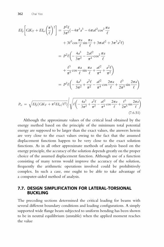
ffiffiffiffiffiffiffiffiffiffiffiffiffiffiffiffiffiffiffiffiffiffiffiffiffiffiffiffiffiffiffiffiffiffiffiffiffiffiffiffiffiffiffiffiffiffiffiffiffiffiffiffiffiffiffiffiffiffiffiffiffiffiffiffiffiffiffiffiffiffiffiffiffiffiffiffiffiffiffiffiffiffiffiffiffiffiffi� �s
362 Chai Yoo
Pcr ¼ffiffiffiffiffiffiffiffiffiffiffiffiffiffiffiffiffiffiffiffiffiffiffiffiffiffiffiffiffiffiffiffiffiffiffiffiffiffiffiffiffiffiffiffiffiEIyðGKT þ p2EIw=‘2Þ
q = ‘ � 4a3
3p2þ a2‘
p2� a‘2
p4cos
2pa
‘þ ‘3
2p5sin
2pa
‘
(7.6.51)
Although the approximate values of the critical load obtained by the
energy method based on the principle of the minimum total potential
energy are supposed to be larger than the exact values, the answers herein
are very close to the exact values owing to the fact that the assumed
displacement functions happen to be very close to the exact solution
functions. As in all other approximate methods of analysis based on the
energy principle, the accuracy of the solution depends greatly on the proper
choice of the assumed displacement function. Although use of a function
consisting of many terms would improve the accuracy of the solution,
frequently the arithmetic operations involved could be prohibitively
complex. In such a case, one ought to be able to take advantage of
a computer-aided method of analysis.
7.7. DESIGN SIMPLIFICATION FOR LATERAL-TORSIONALBUCKLING
The preceding sections determined the critical loading for beams with
several different boundary conditions and loading configurations. A simply
supported wide flange beam subjected to uniform bending has been shown
to be in neutral equilibrium (unstable) when the applied moment reaches
the value

Lateral-Torsional Buckling 363
Mcr ¼ p
‘
ffiffiffiffiffiffiffiffiffiffiffiffiffiffiffiffiffiffiffiffiffiffiffiffiffiffiffiffiffiffiffiffiffiffiffiffiffiffiffiffiffiffiEIy
�GKT þ EIwp2
‘2
�s(7.7.1)
The critical concentrated load applied at midspan of the same beam has been
found by the energy method to be
Pcr ¼ 4p2
‘2
ffiffiffiffiffiffiffiffiffiffiffiffiffiffiffiffiffiffiffiffiffiffiffiffiffiffiffiffiffiffiffiffiffiffiffiffiffiffiffiffiffiffiffiffiffiffiffiffiffiffiffiffiffiffiffi3
p2 þ 6EIy
�GKT þ EIwp2
‘2
�s(7.7.2)
Likewise, the critical uniformly distributed load on the same beam has been
found to be
ðwy‘Þcr ¼ 2p3
‘2
ffiffiffiffiffiffiffiffiffiffiffiffiffiffiffiffiffiffiffiffiffiffiffiffiffiffiffiffiffiffiffiffiffiffiffiffiffiffiffiffiffiffiffiffiffiffiffiffiffiffiffiffiffiffiffiffiffi30
p4 þ 45EIy
�GKT þ EIwp2
‘2
�s(7.7.3)
Converting Eqs. (7.7.2) and (7.7.3) to the form of Eq. (7.7.1) yields
Mcr ¼ Pcr‘
4¼ 1:36
p
‘
ffiffiffiffiffiffiffiffiffiffiffiffiffiffiffiffiffiffiffiffiffiffiffiffiffiffiffiffiffiffiffiffiffiffiffiffiffiffiffiffiffiffiEIy
�GKT þ EIwp2
‘2
�s(7.7.4)
and
Mcr ¼ ðwy‘Þcr‘8
¼ 1:13p
‘
ffiffiffiffiffiffiffiffiffiffiffiffiffiffiffiffiffiffiffiffiffiffiffiffiffiffiffiffiffiffiffiffiffiffiffiffiffiffiffiffiffiffiEIy
�GKT þ EIwp2
‘2
�s(7.7.5)
Examination of these equations reveals that it may be possible to express the
critical moment in the form
Mcr ¼ ap
‘
ffiffiffiffiffiffiffiffiffiffiffiffiffiffiffiffiffiffiffiffiffiffiffiffiffiffiffiffiffiffiffiffiffiffiffiffiffiffiffiffiffiffiEIy
�GKT þ EIwp2
‘2
�s(7.7.6)
where the coefficient a is equal to 1.0 for uniform bending, 1.13 for
a uniformly distributed load, and 1.36 for a concentrated load at applied at
midspan. According to Schrader (1943) and Clark and Hill (1960), a is 1.04
for concentrated loads applied at the third points. The difference in amay be
explainable from the fact that the critical bending moment diagrams of
a simply supported beam are a rectangle, a triangle, and a parabola,
respectively, for uniform bending, a concentrated load at midspan, and a
uniformly distributed load. The area of the critical bending moment
diagram for uniform bending is Mcr‘, which is the largest. Understandably,
364 Chai Yoo
the larger the area of the bending moment diagram, the smaller becomes the
coefficient a. It is of interest to note that concentrated loads applied at the
third points and a uniformly distributed load result in the same area of 2Mcr‘/3.However, the critical moment at the middle is spread wider under two third
point loads than under a uniformly distributed load. This may explain the
smaller value of a (1.04) for the former than that (1.13) of the latter.
Having illustrated that the equation for the critical moment of a simply
supported wide flange beam subjected to uniform bending can be made
applicable for other loadings by means of adjusting the factor a, the next
step is to show that this equation can be made valid for different boundary
conditions as well. The idea here is whether an effective-length concept
analogous to that used in columns can be extended to beam buckling.
Indeed it can be. Numerous researchers including Salvadori (1953, 1955),
Lee (1960), and Vlasov (1961) have shown that the effective-length factor
concept is also applicable to lateral-torsional buckling of beams. Based on
the results given by Vlasov (1961),10 Galambos (1968) lists values of the
effective-length factor for several combinations of end conditions. Salvadori
(1953) found that Eq. (7.7.6) can be made to account for the effect of
moment gradient between the lateral brace points. Various lower-bound
formulas have been proposed for a, but the most commonly accepted are
the following:
Cb ¼ 1:75þ 1:05
�M1
M2
�þ 0:3
�M1
M2
�2
� 2:3 (7.7.7)
Equation (7.7.7) had been used in AISC Specifications since 1961–1993.
Although Eq. (7.7.7) works well when the moment varies linearly between
two adjacent brace points, it was often inadvertently used for nonlinear
moment diagrams. Kirby and Nethercot (1979) present an equation that
applies to various shapes of moment diagrams within the unbraced segment.
Their original equation has been modified slightly to give the following:
Cb ¼ 12:5Mmax
2:5Mmax þ 3MA þ 4MB þ 3MC� 3:0 (7.7.8)
Equation (7.7.8) replaces Eq. (7.7.7) in the 1993 AISC Specifications.MB is
the absolute value of the moment at the centerline, MA and MC are the
absolute values of the quarter point and three quarter-point moments,
10 See pages 292–297.
Lateral-Torsional Buckling 365
respectively, and Mmax is the maximum moment regardless of its location
within the brace points.
The nominal flexural strength of a beam is limited by the lateral-
torsional buckling strength controlled by the unbraced length Lb of the
compression flange. The critical moment equation (Eq. 7.7.6) was derived
under the assumption that the material obeys Hooke’s law. This means that
it cannot be directly applicable to inelastic lateral-torsional buckling.
The credit goes to Lay and Galambos (1965, 1967) for determining the
unbraced length Lp required for compact sections to reach the plastic
bending moment Mp.
Lp ¼ 2:7ry
ffiffiffiffiffiE
sy
s(7.7.9)
where E¼ elastic modulus, ry ¼ radius of gyration with respect to the weak
axis, and sy ¼ mill specified minimum yield stress.
Later on, their simplified design equation was calibrated using experi-
mental data (Bansal, 1971) in order to give compact-section beams adequate
rotational capacity after reaching the plastic moment.
Lp ¼ 1:76ry
ffiffiffiffiffiE
sy
s(7.7.10)
Equation (7.7.10) is identical to Eq. (F2-5) in AISC (2005) Specifications.
In plastic analysis, larger rotation capacities are required to ensure that
successive plastic hinges are formed without inducing excessive lateral-
torsional deformations. Bansal (1971) suggested the following equation
from tests of three-span continuous beams to ensure rotation capacity
greater than or equal to 3:
Lpd ¼�0:12þ 0:076
�M1
M2
���E
sy
�ry (7.7.11)
whereM1 is the smaller moment at the ends of a laterally unbraced segment
(taken positive when moments cause reverse curvature). Equation (7.7.11) is
identical to Eq. (F1-17) in AISC (2001) Specifications.
The limiting value of the unbraced length for girders of compact
sections to buckle in the elastic range is given by Lr. In the presence of
residual stress, the maximum elastic critical moment is defined by
Mcr ¼ Sxðsy � srÞ ¼ 0:7Sxsy ¼ scrSx (7.7.12)
366 Chai Yoo
where Sx ¼ elastic section modulus about the x-axis, sr ¼ residual stress
0.3 sy for both rolled and welded shapes. From Eqs. (7.7.6) and (7.7.12),
scr ¼ Mcr
Sx¼ Cbp
LbSx
ffiffiffiffiffiffiffiffiffiffiffiffiffiffiffiffiffiffiffiffiffiffiffiffiffiffiffiffiffiffiffiffiffiffiffiffiffiffiffiffiffiffiffiffiffiffiffiffiEIyGKT þ
�pE
Lb
�2
IyEIw
s(7.7.13)
Equation (7.7.13) is identical to Eq. (F1-13) in the AISC (1986) LRFD
Specifications. Equation (7.7.13) is rewritten as
scr ¼ Cbp2E�
Lb
rts
�2
ffiffiffiffiffiffiffiffiffiffiffiffiffiffiffiffiffiffiffiffiffiffiffiffiffiffiffiffiffiffiffiffiffiIyGKTL
2b
p2r4tsES2x
þ IyIw
r4tsS2x
s(7.7.14)
where
rts2 ¼
ffiffiffiffiffiffiffiffiffiffiffiIyEIw
pSx
(7.7.15)
Letting h0 be the distance between the flange centroids and substituting
2G=p2E ¼ 0:0779 and Eq. (7.7.14), Eq. (7.7.13) becomes
scr ¼ Cbp2E�
Lb
rts
�2
ffiffiffiffiffiffiffiffiffiffiffiffiffiffiffiffiffiffiffiffiffiffiffiffiffiffiffiffiffiffiffiffiffiffiffiffiffiffiffiffiffiffiffiffiffiffiffi�Lb
rts
�2 IyGKT
p2E
ffiffiffiffiffiffiffiffiIyIw
pSx
S2x
þ 1
vuuut
¼ Cbp2E�
Lb
rts
�2
ffiffiffiffiffiffiffiffiffiffiffiffiffiffiffiffiffiffiffiffiffiffiffiffiffiffiffiffiffiffiffiffiffiffiffiffiffiffiffiffiffiffiffiffi1þ 0:0779
KTc
Sxh0
�Lb
rts
�2
s(7.7.16)
where Iw ¼ Iyh20=4 for doubly symmetric I-beams with rectangular
flanges and c ¼ h0ffiffiffiffiffiffiffiffiffiffiffiIw=Iw
p=2 and hence, c ¼ 1.0 for a doubly symmetric
I-beam. Equation (7.7.16) is identical to Eq. (F2-4) in the AISC (2005)
Specifications. Limiting the maximum critical stress in Eq. (7.7.16) to
0.7sy to account for residual stress sr and solving Eq. (7.7.16) for Lr gives
Lr ¼ 1:95rtsE
0:7sy
ffiffiffiffiffiffiffiffiffiKTc
Sxh0
r ffiffiffiffiffiffiffiffiffiffiffiffiffiffiffiffiffiffiffiffiffiffiffiffiffiffiffiffiffiffiffiffiffiffiffiffiffiffiffiffiffiffiffiffiffiffiffiffiffiffiffiffiffiffiffiffiffiffiffiffiffiffi1þ
ffiffiffiffiffiffiffiffiffiffiffiffiffiffiffiffiffiffiffiffiffiffiffiffiffiffiffiffiffiffiffiffiffiffiffiffiffiffiffiffiffiffiffiffiffiffiffiffiffi1þ 6:767
�0:7syE
Sxh0
KTc
�2
svuut(7.7.17)
Equation (7.7.17) is identical to Eq. (F2-6) in AISC (2005) Specifications.
The calculation of the inelastic critical moment is fairly complex.
Galambos (1963, 1998) has contributed greatly to this subject. In 2005
Lateral-Torsional Buckling 367
AISC Specifications, when Lp < Lb � Lr , the nominal flexural strengthMn
of compact sections is linearly interpolated between the plastic momentMp
and the elastic critical moment Mr ¼ 0:7Sxsy as
Mn ¼ Cb
�Mp � ðMp � 0:7sySxÞ
�Lb � Lp
Lr � Lp
��� Mp (7.7.18)
It should be remembered that local buckling of compression flanges and
web is precluded in the derivation of the unbraced lengths. The mathe-
matical procedure for the solution of local buckling is identical to that of the
lateral-torsional buckling phenomenon, except that the governing differ-
ential equations are now partial differential equations, and so the details of
the solution process are different and complicated, as will be shown in the
next chapter. In order to systematically reflect the effects of local buckling
on the nominal flexural strength, AISC (2005) Specifications categorize
sections into several types depending on the compactness of the flanges and
web (compact, noncompact, or slender).
Also, it needs to be noted that the limiting values for the unbraced length
given by Eqs. (7.7.10), (7.7.11), and (7.7.17) are valid only for bare-steel
members. Composite systems are often utilized tomaximize the efficiency of
structural members. In composite girders, the top flange and concrete slab are
connected with shear studs. Lateral-torsional buckling is not likely to take
place when subjected to positive flexure, as the top compression flange is
continuously braced by the concrete slab.However, the loss of stability should
be checkedwhendesigning composite girders in negativemoment zone.The
steel section of a composite girder will necessarily undergo the deformation
depicted in Fig. 7-16 during buckling due to the restraint provided by the
concrete slab. This type of buckling is referred to as lateral-distortional
buckling. The classical assumption that the member cross section retains its
original shape during buckling is no longer valid in this case. Lateral-
distortional buckling is basically a combined mode of lateral-torsional
buckling (global buckling) and local buckling, and the derivation of a closed-
form solution is, therefore, not straightforward. Limited research, including
Hancock et al. (1980), Bradford and Gao (1992), and Hong et al. (2002), has
shown that the unbraced length requirements for noncomposite girders give
too conservative results for composite girders. A general design rule has yet to
be developed due to lack of comprehensive study. With the advancement of
digital computers, along with highly sophisticated computer programs such
as ABAQUS, NASTRAN, and ADINA just to name a few, performing the
lateral-distortional buckling analysis should present no problem.
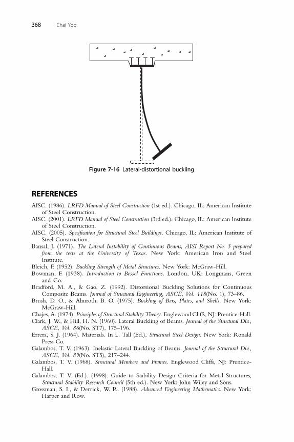
Figure 7-16 Lateral-distortional buckling
368 Chai Yoo
REFERENCESAISC. (1986). LRFD Manual of Steel Construction (1st ed.). Chicago, IL: American Institute
of Steel Construction.AISC. (2001). LRFD Manual of Steel Construction (3rd ed.). Chicago, IL: American Institute
of Steel Construction.AISC. (2005). Specification for Structural Steel Buildings. Chicago, IL: American Institute of
Steel Construction.Bansal, J. (1971). The Lateral Instability of Continuous Beams, AISI Report No. 3 prepared
from the tests at the University of Texas. New York: American Iron and SteelInstitute.
Bleich, F. (1952). Buckling Strength of Metal Structures. New York: McGraw-Hill.Bowman, F. (1938). Introduction to Bessel Functions. London, UK: Longmans, Green
and Co.Bradford, M. A., & Gao, Z. (1992). Distorsional Buckling Solutions for Continuous
Composite Beams. Journal of Structural Engineering, ASCE, Vol. 118(No. 1), 73–86.Brush, D. O., & Almroth, B. O. (1975). Buckling of Bars, Plates, and Shells. New York:
McGraw-Hill.Chajes, A. (1974). Principles of Structural Stability Theory. Englewood Cliffs, NJ: Prentice-Hall.Clark, J. W., & Hill, H. N. (1960). Lateral Buckling of Beams. Journal of the Structural Div.,
ASCE, Vol. 86(No. ST7), 175–196.Errera, S. J. (1964). Materials. In L. Tall (Ed.), Structural Steel Design. New York: Ronald
Press Co.Galambos, T. V. (1963). Inelastic Lateral Buckling of Beams. Journal of the Structural Div.,
ASCE, Vol. 89(No. ST5), 217–244.Galambos, T. V. (1968). Structural Members and Frames. Englewood Cliffs, NJ: Prentice-
Hall.Galambos, T. V. (Ed.). (1998). Guide to Stability Design Criteria for Metal Structures,
Structural Stability Research Council (5th ed.). New York: John Wiley and Sons.Grossman, S. I., & Derrick, W. R. (1988). Advanced Engineering Mathematics. New York:
Harper and Row.
Lateral-Torsional Buckling 369
Hill, H. N. (1954). Lateral Buckling of Channels and Z-Beams. Transactions, ASCE,Vol. 119, pp. 829–841.
Hong, A.R., Lee, D.S., & Lee, S.C. (2002). A Study on Unbraced Length Requirement forComposite Steel I Girder in Negative Bending, Proceedings of 2002 Annual Conference,KSCE, Korea, pp. 70–73 (in Korean).
Kirby, P. A., & Nethercot, D. A. (1979). Design for Structural Stability. New York: John Wileyand Sons.
Lay, M. G., & Galambos, T. V. (1965). Inelastic Steel Beams Under Moment Gradient.Journal of the Structural Div., ASCE, Vol. 91(No. ST6), 67–93.
Lay, M. G., & Galambos, T. V. (1967). Inelastic Beams Under Moment Gradient. Journal ofthe Structural Div., ASCE, Vol. 93(No. ST1), 381–399.
Lee, G.C. (1960). A Survey of the Literature on the Lateral Instability of Beams, WeldingResearch Council Bulletin No. 63, August.
Michell, A. G. M. (1899). Elastic Stability of Long Beams Under Transverse Forces.Philosophic Magazine, Vol. 48, 298.
Prandtl, L. (1899). Kipperscheinungen, Dissertation, Munich Polytechnical Institute.Salmon, C. G., & Johnson, J. E. (1996). Steel Structures, Design and Behavior (4th ed.).
New York: HarperCollins.Salvadori, M.G. (1953). Lateral Buckling of I Beams Under Thrust and Unequal End
Moments, Proceedings, ASCE, Vol. 79(No.291), pp. 1–25, also a transaction paperNo 2773, Lateral Buckling of I-Beams, Transactions, ASCE, Vol. 120, 1955, pp. 1165–1182.
Salvadori, M.G. (1955). Lateral Buckling of Eccentrically Loaded I-Columns, Proceedings,ASCE, Vol. 81, pp. 607–622, also a transaction paper No. 2836 with the same title,Transactions, ASCE, Vol. 121, 1956, pp. 1163–1178.
Schrader, R.K. (1943). Discussion on Lateral Stability of Unsymmetrical I-Beams andTrusses in Bending, by G. Winter, Paper No. 2178, Transactions, ASCE, Vol. 108, 1943,pp. 247–268.
Timoshenko, S. P. (1910). Einige Stabilitats-problme der Elasticitats-theorie. Zeitschrift furMathematik und Phisik, Vol. 58, 337–385.
Timoshenko, S. P., & Gere, J. M. (1961). Theory of Elastic Stability (2nd ed.). New York:McGraw-Hill.
Vincent, G. S. (1969). Tentative Criteria for Load Factor Design of Steel Highway Bridges. AISIReport No. 15. New York: American Iron and Steel Institute.
Vlasov, V. Z. (1940). Tonkostennye uprugie sterzhni (Thin-walled elastic beams), Stroiizdat(in Russian).
Vlasov, V. Z. (1961). Tonkostennye uprugie sterzhni (Thin-walled elastic beams), (2nd ed.),Moscow 1959, translated by Schechtman, Israel Program for Scientific Translation,Jerusalem.
Winter, G. (1941). Lateral Stability of Unsymmetrical I-Beams and Trusses in Bending,Proceedings, ASCE. Vol. 67, pp. 1851–1864, also a transaction paper No. 2178 with thesame title, Transactions, ASCE, Vol. 108, 1943, pp. 247–268.
Yoo, C. H. (1980). Bimoment Contribution to Stability of Thin-Walled Assemblages.Computers and Structures, Vol. 11(No.5), 465–471.
PROBLEMS
7.1 Equation (7.4.2) can be nondimensionalized to investigate the influ-
ence of the various parameters affecting the lateral-torsional buckling
strength.
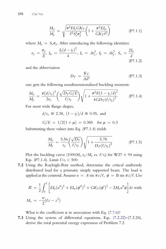
370 Chai Yoo
Mcr
My¼
ffiffiffiffiffiffiffiffiffiffiffiffiffiffiffiffiffiffiffiffiffiffiffiffiffiffiffiffiffiffiffiffiffiffiffiffiffiffiffiffiffiffiffiffiffiffiffiffiffiffiffip2EIyGKT
‘2S2xs2y
�1þ p2EIw
GKT ‘2
�s(P7.1.1)
where My ¼ Sxsy. After introducing the following identities:
3y ¼ sy
E; Iw ¼ Iyðd � tf Þ2
4; Ix ¼ Ar2x ; Iy ¼ Ar2y ; Sx ¼ 2Ix
d
(P7.1.2)
and the abbreviation
DT ¼ KT
Ad2(P7.1.3)
one gets the following nondimensionalized buckling moment:
Mcr
My¼ pðd=rxÞ2
23y
� ffiffiffiffiffiffiffiffiffiffiffiffiffiffiffiffiffiDTG=E
p‘=ry
� ffiffiffiffiffiffiffiffiffiffiffiffiffiffiffiffiffiffiffiffiffiffiffiffiffiffiffiffiffiffiffiffiffiffiffiffiffiffi1þ p2Eð1� tf =dÞ2
4GDT ð‘=ryÞ2
s(P7.1.4)
For most wide flange shapes,
d=rx y 2:38; ð1� tf Þ=d y 0:95; and
G=E ¼ 1=2ð1þ mÞ ¼ 0:385 for m ¼ 0:3
Substituting these values into Eq. (P7.1.4) yields
Mcr
My¼ 5:56
3y
� ffiffiffiffiffiffiffiDT
p‘=ry
� ffiffiffiffiffiffiffiffiffiffiffiffiffiffiffiffiffiffiffiffiffiffiffiffiffiffiffiffi1þ 5:78
DT ð‘=ryÞ2s
(P7.1.5)
Plot the buckling curve (1000Mcr 3y/My vs. ‘/rr) for W27 � 94 using
Eqs. (P7.1.4). Limit ‘/rr < 500.
7.2 Using the Rayleigh-Ritz method, determine the critical uniformly
distributed load for a prismatic simply supported beam. The load is
applied at the centroid. Assume u ¼ A sin pz=‘; f ¼ B sin pz=‘. Use
P ¼ 1
2
Z ‘
0
�EIyðu00Þ2 þ EIwðf00Þ2 þGKT ðf0Þ2 � 2Mxu
00f�dz with
Mx ¼ �w
2ð‘z� z2Þ
What is the coefficient a in association with Eq. (7.7.6)?
7.3 Using the system of differential equations, Eqs. (7.2.22)–(7.2.24),
derive the total potential energy expression of Problem 7.2.
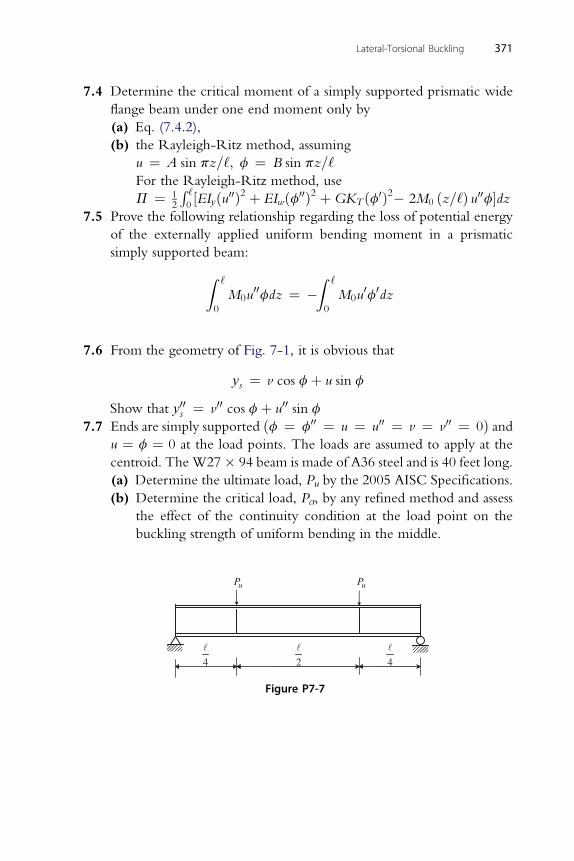
Lateral-Torsional Buckling 371
7.4 Determine the critical moment of a simply supported prismatic wide
flange beam under one end moment only by
(a) Eq. (7.4.2),
(b) the Rayleigh-Ritz method, assuming
u ¼ A sin pz=‘; f ¼ B sin pz=‘For the Rayleigh-Ritz method, use
P ¼ 12
R ‘
0½EIyðu00Þ2 þ EIwðf00Þ2 þGKT ðf0Þ2� 2M0 ðz=‘Þ u00f�dz
7.5 Prove the following relationship regarding the loss of potential energy
of the externally applied uniform bending moment in a prismatic
simply supported beam:
Z ‘
0
M0u00fdz ¼ �
Z ‘
0
M0u0f0dz
7.6 From the geometry of Fig. 7-1, it is obvious that
ys ¼ v cos fþ u sin f
Show that y00s ¼ v00 cos fþ u00 sin f
7.7 Ends are simply supported ðf ¼ f00 ¼ u ¼ u00 ¼ v ¼ v00 ¼ 0Þ andu ¼ f ¼ 0 at the load points. The loads are assumed to apply at the
centroid. The W27� 94 beam is made of A36 steel and is 40 feet long.
(a) Determine the ultimate load, Pu by the 2005 AISC Specifications.
(b) Determine the critical load, Pcr, by any refined method and assess
the effect of the continuity condition at the load point on the
buckling strength of uniform bending in the middle.
uP uP
2 44
Figure P7-7