Introduction to Reservoir Geomechanics - LMCG - UFPE
110
1 Introduction Definitions and some challenges of reservoir geomechanics. Modeling of coupled phenomena. 2 Constitutive Laws: Behavior of Rocks Fundamentals of Pore-Mechanics. 3 Constitutive Laws: Behavior of Fractures Geomechanics of Fractured Media. 4 Reservoir Geomechanics Elements of a geomechanical model and applications. 5 Unconventional Reservoirs Naturally fractured reservoirs, hydraulic fracture, proppant and fracture closure model, validation (microseismicity). 6 Advanced Topics Injection of reactive fluids and rock integrity. Introduction to Reservoir Geomechanics
-
Upload
khangminh22 -
Category
Documents
-
view
2 -
download
0
Transcript of Introduction to Reservoir Geomechanics - LMCG - UFPE

1 IntroductionDefinitions and some challenges of reservoir geomechanics.Modeling of coupled phenomena.
2 Constitutive Laws: Behavior of RocksFundamentals of Pore-Mechanics.
3 Constitutive Laws: Behavior of FracturesGeomechanics of Fractured Media.
4 Reservoir GeomechanicsElements of a geomechanical model and applications.
5 Unconventional ReservoirsNaturally fractured reservoirs, hydraulic fracture, proppant and fracture closure model, validation (microseismicity).
6 Advanced TopicsInjection of reactive fluids and rock integrity.
Introduction to Reservoir Geomechanics

Constitutive Laws
Earth Sciences and Engineering:
Problems Scales
micro lab
wellbore reservoir
basin
Earth

Deformable Porous Media
Stresses
Continuum mechanics deals with deformable bodies.
The stresses considered in continuum mechanics are only those produced by deformationof the body.
Stress is a measure of the average force per unit area of a surface within a deformablebody on which internal forces act.
It is a measure of the intensity of the internal forces acting between particles of adeformable body across imaginary internal surfaces.
These internal forces are produced between the particles in the body as a reaction toexternal forces applied on the body.
In general, stress is not uniformly distributed over the cross-section of a material body,and consequently the stress at a point in a given region is different from the average stressover the entire area.
Therefore, it is necessary to define the stress not over a given area but at a specific pointin the body.

Normal and Shear Stresses:
Definition:
Decomposition of stress vector:
Normal stress:
Shear stress:
stress vector(acting in a infinitesimal surface)
Deformable Porous Media

In 3 dimensions :
Defined for each point for a body in equilibrium, subjected to external load
Stress Representation

Mohr Circle:
3D representation of Mohr Circle:
Stress Representation
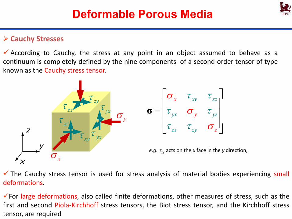
Cauchy Stresses
According to Cauchy, the stress at any point in an object assumed to behave as acontinuum is completely defined by the nine components of a second-order tensor of typeknown as the Cauchy stress tensor.
x
y
z
x
y
xyxz
yx
yzzx zy xy xz
yx
x
yz
zx zy
y
z
σ
The Cauchy stress tensor is used for stress analysis of material bodies experiencing smalldeformations.
For large deformations, also called finite deformations, other measures of stress, such as thefirst and second Piola-Kirchhoff stress tensors, the Biot stress tensor, and the Kirchhoff stresstensor, are required
e.g. xy acts on the x face in the y direction,
Deformable Porous Media

Deformable Porous Media
In Soil/Rock Mechanics compression isconsidered as positive and tension as negative.
+ –
Compressive stresses are positives
Tensile stresses are negatives
Stress Sign Convention

Stress, stress changes in space and time
In 3 dimensions :
Rotation ofreference axes
component remaining the),,min(),,max(
2
3
1
cba
cba
abc
3
2
1
000000
σ
xyzzyzxz
yzyxy
xzxyx
σ
Among the infinite number of triplets ofplanes which satisfy the fundamentalstress Theorem, there is always one set(=abc) on which no shear stress is present.
full tensor diagonal tensor
Principal stresses:

Stress, stress changes in space and time
At every point in a stressed body there are at least three planes, called principal planes, with normal vectors , called principal directions, where the corresponding stress vector is perpendicular to the plane and where there are no normal shear stresses.
The three stresses normal to these principal planes are called principal stresses
The Cauchy stress tensor obeys the tensor transformation law under a change in thesystem of coordinates.
A graphical representation of this transformation law is the Mohr's circle for stress
Principal Stresses
1
2
3
0 00 00 0
σ1 2 3 Principal stresses

Stress state in lab experiments:
1
1
1
000000
σ
000000001
σ
3
3
1
000000
σ
Stress Representation

TRIAXIAL TEST
Mohr-Coulomb criteria for shear strength (minimum 3 samples):
1
F1
a (axial strain)0
F2
F3
1
2 3 s3 = 100 kPa
s3 = 200 kPa
s3 = 300 kPa
3 1
t (shear stress)
s (normal stress) c
f
-

TRIAXIAL TEST
Test s’3(kPa)
(s’1- s’3) (kPa)
s’1 (kPa)
1/2(s’1 - s’3) (kPa)
1/2(s’1 + s’3) (kPa)
1 50 200 250 100 150
2 140 335 475 168 308
3 300 520 760 260 500
c’

Principal stresses and principal planes of stress:Very useful because i) the position of principal surfaces of stress can often be identifiedii) the orientation of structures (faults etc) depends on the position
of the principal stresses
Where are surfaces of principal stresses?
archeffect
tension dueto water load
Stress Fields

In 2D analysis: stress field and displacement field:
Finite element analysis of a tunnel excavation:
Mesh Stress field Displacement field
Stress Fields

Stresses are related to Strains
Example of elasto-plastic behaviour: tensile test (1D) in metals
YieldingFA
FL
B
A
D
C
O
A
0
LL
Y
L0Elastic behavior
Axial behavior

Stresses are related to Strains
3D behavior
εDσ '
CAP Model: Elastoplastic multi-mechanism model
stress-strain relationship
D: constitutive tensor ElasticityVisco-ElasticityPlasticityVisco-PlasticityDamage

Strains are related to Displacements
x
yv
u
x
y
v
u
θ2
θ1
1 12 2
1 12 21 12 2
xy xz
xy yz
xz yz
x
y
z
ε
Strain Tensor
Tuuε 21
Cauchy’s infinitesimal strain tensor:
Compatibility conditions:

Strains
extension/contraction: distortion:

Strains are related to Displacements
x
yv
u
x
y
v
u
θ2
θ12
2
2
x y z
xy xy yx xy yx xy
xz xz zx xz zx xz
yz yz zy yz zy yz
u v wx y z
v ux yw ux zw vy z
Compression + Small deformations :
Strain Tensor
Tuuε 21
or:
Displacement vector u = (u,v,w)T
Component x: uComponent y: vComponent z: w
++
+
+
Symmetric part of thedisplacement gradient tensor

Strains are related to Displacements
x
yv
u
2
2
2
x y z
xy xy yx xy yx xy
xz xz zx xz zx xz
yz yz zy yz zy yz
u v wx y z
v ux yw ux zw vy z
Compression + Small deformations :
Strain Tensor
Tuuε 21
Displacement vector u = (u,v,w)T
Component x: uComponent y: vComponent z: w
or:
zyxv VV u0
zyxv VV u0
Stress Sign Convention:
if positive for compression
volumetric strain:
Note: Tuuε 21
Symmetric part of thedisplacement gradient tensor
Divergence of the displacement vector

Equilibrium Equation
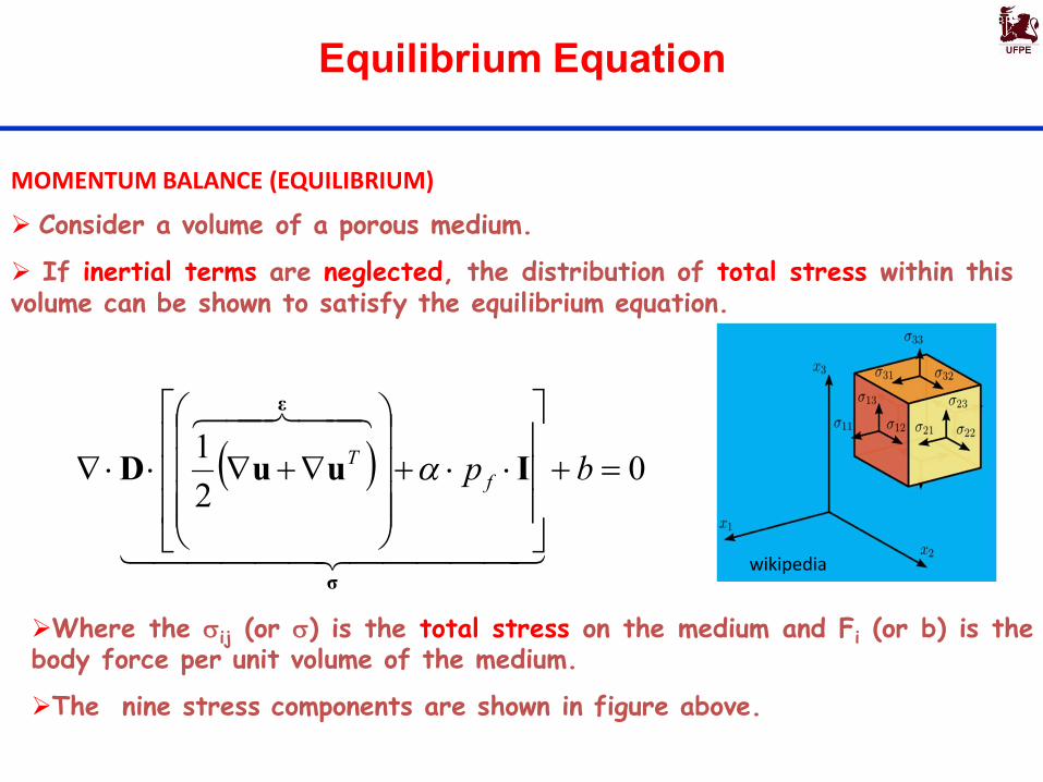
Consider a volume of a porous medium.
If inertial terms are neglected, the distribution of total stress within thisvolume can be shown to satisfy the equilibrium equation.
ij
ij
F 0 i 1, 2, 3x
or
Where the sij (or s) is the total stress on the medium and Fi (or b) is thebody force per unit volume of the medium.
The nine stress components are shown in figure above.
MOMENTUM BALANCE (EQUILIBRIUM)
wikipedia0 bσ

Equilibrium Equation
Consider a volume of a porous medium.
If inertial terms are neglected, the distribution of total stress within thisvolume can be shown to satisfy the equilibrium equation.
ij
ij
F 0 i 1, 2, 3x
or
Where the sij (or s) is the total stress on the medium and Fi (or b) is thebody force per unit volume of the medium.
The nine stress components are shown in figure above.
MOMENTUM BALANCE (EQUILIBRIUM)
wikipedia0)'( bp f
σ
Iσ

Equilibrium Equation
Consider a volume of a porous medium.
If inertial terms are neglected, the distribution of total stress within thisvolume can be shown to satisfy the equilibrium equation.
ij
ij
F 0 i 1, 2, 3x
or
Where the sij (or s) is the total stress on the medium and Fi (or b) is thebody force per unit volume of the medium.
The nine stress components are shown in figure above.
MOMENTUM BALANCE (EQUILIBRIUM)
wikipedia
0)(
'
bp f σ
σ
IεD
Equilibrium Equation
Consider a volume of a porous medium.
If inertial terms are neglected, the distribution of total stress within thisvolume can be shown to satisfy the equilibrium equation.
Where the sij (or s) is the total stress on the medium and Fi (or b) is thebody force per unit volume of the medium.
The nine stress components are shown in figure above.
MOMENTUM BALANCE (EQUILIBRIUM)
wikipedia
021
bp fT
σ
ε
IuuD

Effective Stress Principle
Terzaghi (1936) proposed the principle of effective stress(*), the mostimportant equation in soils mechanics.
The effective stress (s’) is the component of the normal stress takenby the soil skeleton.
It is the effective stress which controls the volume and the strength ofthe soil.
Karl Terzaghi(1883 - 1963)
wus s
Effective Stress
pore water pressuretotal stressefective stress
(*)“All the measurable effects of a change of stress, such as compression, distortion and a change in theshearing resistance are exclusively due to changes in effective stress…every investigation of the stabilityof a saturated body of earth requires the knowledge of both the total and the neutral stresses.”(Terzaghi, 1936)
It is assumed saturated soil, water incompressibility and rigid soil particles.
Pore Water Pressure, Total & Effective Stresses

Effective Stress Principle
Normal Stress in the Stress Tensor:
s s wp
Multiphase material (solid and liquid)
Incorporation of an additional variable: pore pressure
Coupled phenomena (mechanical & hydraulic)

Effective Stress Principle
The concept of effective stress is based on the pioneering work in soil mechanics by Terzaghi (1923) who noted that the behavior of a soil (or a saturated rock) will be controlled by the effective stresses, the differences between total stresses and pore pressure. The so-called “simple” or Terzaghi definition of effective stress is:
Iσσ fp'
EffectiveStressTensor
Total StressTensor
FluidPressure
IdentityTensor

Effective Stress Principle
= +
Saturated soil Solid Skeleton Water
A saturated porous medium comprises twophases:
The strengths of these two phases are very different: the soil skeleton can resist shears. Two basic mechanisms:
• inter particle friction
• particles interlocking
the shear strength of water is zero• water can only sustains isotropic pressure.
• the soil particles
• the pore water

Effective Stress Principle
Physical Interpretation
wp
σ
σ
σ : total stresses externally applied
σ : stresses that act through the contacts between particles (Am)
pw : water pressure (Aw )
At : total area
At = Am + Aw
At
Effective Stress Principle
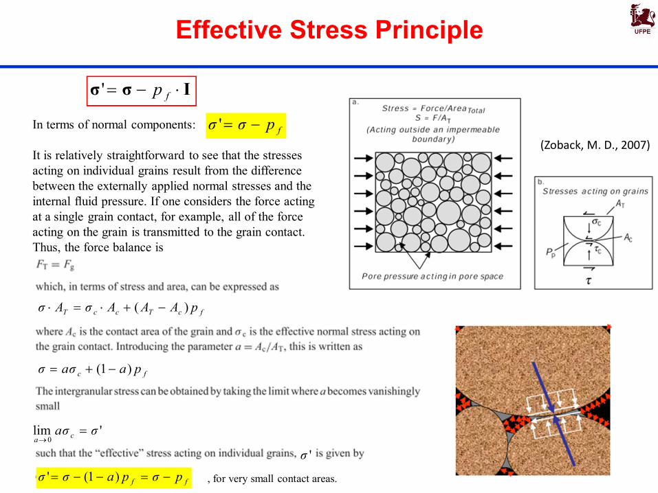
fpσσ 'In terms of normal components:
It is relatively straightforward to see that the stresses acting on individual grains result from the difference between the externally applied normal stresses and the internal fluid pressure. If one considers the force acting at a single grain contact, for example, all of the force acting on the grain is transmitted to the grain contact. Thus, the force balance is
(Zoback, M. D., 2007)
fcTccT pAAAσAσ )(
fc paaσσ )1(
'lim0
σaσ ca
'σ
ff pσpaσσ )1('
Iσσ fp'
, for very small contact areas.

Effective Stress Principle
σ Total Stress
pw
Water pressure
Soils as one phase material
The strength of the soil skeleton and the pore water are sodifferent, therefore it is necessary to consider the stressacting in each phase separately

Effective Stress Principle
Based on experimental information it can be concluded that Terzaghi’sdefinition of effective stresses works well for a number of soils, but forother cases it needs an upgrade.
A more general law for effective stresses can be expressed as:
wps s It is and extension of the one proposed by Terzaghi
where a is a physical constant known as Biot parameter.
Geertsma (1957) and Skempton (1960) suggested:
s
KK
1
where:
K: is the drained bulk modulus of the dry aggregate or rock
(i.e. porous medium skeleton).
Ks: is the bulk modulus of the soil’s/rock’s individual solid grains
Iσσ fp'

Effective Stress Principle
Based on experimental information it can be concluded that Terzaghi’sdefinition of effective stresses works well for a number of soils, but forother cases it needs an upgrade.
A more general law for effective stresses can be expressed as:
Iσσ fp'
sKK /1 Biot’s constant
Solid phase (rock grains) bulk modulusBulk modulus of the overall skeleton
For rocks, it is important to take into account the Biot’s constant. For soils, it is equal to one.For unconsolidated or weak rocks, it is close to one.
11~
1

Effective Stress Principle
It is clear that:
For solid rock (i.e. practically no interconnect pores):
Therefore the pore pressure has no influence on porous media behavior.
0 1
sK K
0lim 0f '
ij ijs s
For a highly porous soil (e.g. soil with an open structure): sK K
1lim 1f 's s ij ij ijp
Therefore the pore pressure has the maximum influence and the Terzaghiprinciple of effective stress is recovered.
sKK /1

Effective Stress Principle
Measured values of (Biot’s parameter) for two porous materials:Biot’s Effective Stresses '
ij ij ijps s
Uncemented Sand
Sandstone
In both cases decreasewith confining pressure
Zoback (2009)

Effective Stress Principle
Biot’s Effective Stresses (Lade & De Boer, 1997)
0 1 1 0
Soil Rock Porosity
Strength

Derivation of Biot’s Constant(Lewis and Schrefler, 1998)
Elasticity (solids):
Poro-elasticity for soils: (incompressible grains)
For rocks, we have to consider that the pore pressure pf induces hydrostaticstress distribution in the solid phase (compressible). The ensuing deformationis a purely volumetric strain:
or in tensorial form
The effective stress causes all relevant deformations of the solid skeleton. The constitutive relationship should be rewritten as
εDσ dd
εDσ dd '
)'( Iσσ fdpdd Incremental form
s
fsv K
dpd
3Iε
s
fsv K
dpdε
)()(' mechanismsother
svTc
sv
e ddddddddd εεDεεεεεDεDσ ...
Elastic strain tensor Total strain tensor

Derivation of Biot’s Constant(Lewis and Schrefler, 1998)
So, considering the deformations of the solid skeleton as new deformationalmechanism:
On the other hand, using Terzaghi’s definition of effective stress:
s
fsv K
dpdddd
3)(' IDεDεεDσ Biot’s definition of
effective stress
εDIσ
IDIεDσ
IIDεDεεDσ
IσσIσσ
ddpKKd
dpK
dd
dpK
dpdddd
dpddp
fs
fs
fs
fsv
ff
1
31
3)(
' '
Correctedeffectivestress!!
Biot’s constant:

Derivation of Biot’s Constant(Lewis and Schrefler, 1998)
Biot´s effective stress:
This is the stress which directly induces rock deformation:
1 εDIσεDIσ ddpdddpKKd ff
s
''σd
f
f
f
pp
dpdd
IσσIσσ
Iσσ
''
''''
εDσ dd ''
Biot’s constant:

Stress Path
1
2
3
Stress path
It is generally complicate to draw the stress path in 3D
We tend to work with invariant if stresses rather with the full stress tensor
We use a lot trixial conditions, in which σ2=σ3
Under this condition we can work in 2D, with σ1 & σ3 only
This is what we generally do with the Mohr circle.
A(σ1,σ2,σ3)ini
B(σ1,σ2,σ3)end
Stress path in 3D
Stress Invariants
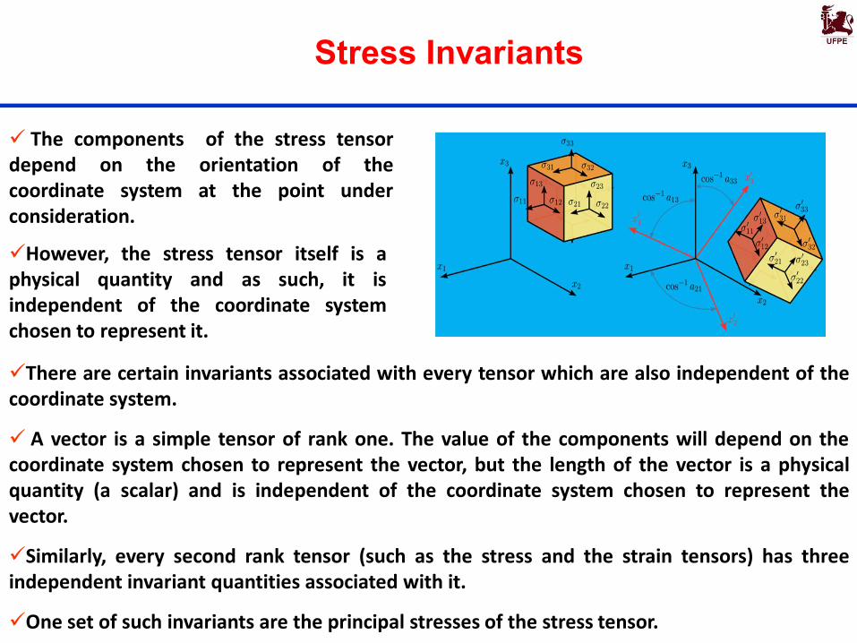
The components of the stress tensordepend on the orientation of thecoordinate system at the point underconsideration.
There are certain invariants associated with every tensor which are also independent of thecoordinate system.
A vector is a simple tensor of rank one. The value of the components will depend on thecoordinate system chosen to represent the vector, but the length of the vector is a physicalquantity (a scalar) and is independent of the coordinate system chosen to represent thevector.
Similarly, every second rank tensor (such as the stress and the strain tensors) has threeindependent invariant quantities associated with it.
One set of such invariants are the principal stresses of the stress tensor.
However, the stress tensor itself is aphysical quantity and as such, it isindependent of the coordinate systemchosen to represent it.

Stress Invariants
321222
3
323121
22222
3211
2det
)(
)()(21
xyzxzyyzxyzxzxyzyx
yzxzxyzyzxyxkkijij
zyxkk
I
I
I
σ
Invariants of the Stress Tensor (σ)
xy xz
yx
x
yz
zx zy
y
z
σ

Stress Invariants
The stress tensor can be expressed as the sum of two other stress tensors:
m σ I s
11 13 3m x y zI
Mean normal stress
0 00 00 0
m
mhydro
m
static
σx m
ydev
xy xz
yx yz
zx zy
m
z m
iator
sσ
Stress Deviator Tensor
A mean hydrostatic stress tensor or volumetric stress tensor or mean normal stress tensor, which tends to change the volume of the stressed body;
A deviatoric component called the stress deviator tensor, S, which tends to distort it.

Stress Invariants
m s σ I
sdet
)()()(61
)(21
)(210
3
222222
222222
2222
1
J
sss
ssssssssJ
J
yzxzxyzyzxyx
yzxzxyzyx
yzxzxyzyzxyxijij
22 2 1
13
J I I
Invariants of the stress deviator tensor
= 0 because , the stress deviator tensor is in a state of pure shear

Stress Invariants
Some stress invariants:
Effective mean stress (volumetric behavior):
Deviatoric tensor (shear behavior):
Deviatoric (shear) stress:
Lode angle:
3'''
' zyxmp
222222 ''')''()''()''(22
zxyzxyzyx pppJ
3
)det(2
33
arcsin31
J
S
S =
3030

Lode angle:
3
)det(2
33
arcsin31
J
S 3030
30
32
triaxialcompression
30
12
triaxialextension

Lode angle:
3
)det(2
33
arcsin31
J
S 3030
30 30
Schematic diagram of a triaxial compression apparatus
Stress state in cylindrical specimens in compression and extension tests
can be varied
during the experiment

Deviatoric plan:
spacediagonal
Stress Invariants
Potts & Zdravkovic (2001)
A
B
J-p’ space(for a fixed Lode Angle)

J-p’ space:
Stress Invariants
A
B

Stress Invariants
Better than this...
J-p’ space:
Material understands J-p’ space but not Cartesian space!
volumetric behavior
shearbehavior

Representation of Constitutive Models
1 3 1 3( ) ( ) sin 2 cos 0F c
Mohr Coulomb Model in terms of Principal Stresses (2D)
1 3
2
tanc
1 3
2
c
3 1
'
tan ' c
'
s’1
s’1
s’3 s’3tf
s’
The relationship between the principal stresses at failure and the shear strength parameters is:
1 3 1 3σ' -σ' = σ' +σ' sin '+2c'cos ' 3 11 3σ +σ c= + sσ - in '2 '
σ2 tan
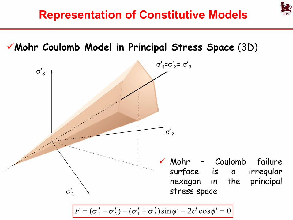
Mohr Coulomb Model in Principal Stress Space (3D)
Mohr – Coulomb failuresurface is a irregularhexagon in the principalstress space
s’3
s’1
s’2
s’1=s’2= s’3
1 3 1 3( ) ( ) sin 2 cos 0F c
Representation of Constitutive Models

Mohr Coulomb Model in Principal Stress Space (3D)
p'
J
p'
JA
A
OO'
6sin3 sin
M
TRIAXIAL COMPRESION TEST (TCT)
For TCT the Lode Angle: Θ = + 30˚
The plane (p',J) is the one that pass thought OO'A
Representation of Constitutive Models

Mohr Coulomb Model in Principal Stress Space (3D)
p'
Jp'
J
F
OO'
F
* 6sin3 sin
M
The plane (p',q) is the one that pass thought OO‘F
TRIAXIAL EXTENSION TEST (TET)
For TET the Lode Angle: Θ = - 30˚
Representation of Constitutive Models

1 3, a c a cb b A
1 3, a c a cb b F
Yielding/failure for TCT (OO’A)corresponds to a stress path with θ=+30˚.
Yielding/failure for TET (OO’F) correspondsto a stress path with θ=-30˚.
We may need to predict yielding or failurefor any stress path (i.e. any θ)
We can use a function g(θ) that generalizethe yield/failure surface to any stress path(i.e. any θ)
( , , )F F p J
sin( ) ;
1 ( )cos sin sin3
( ) ( ) 0;
where
cg a
g
F J p a g
Mohr Coulomb Model in Principal Stress Space (3D)
Representation of Constitutive Models

Mechanical Constitutive Behaviour
More about stress-strain relationship...
εDσ '

Linear Elasticity – Isotropic Materials
Compression test:
Young modulus:
(Zoback, M. D., 2007)(Jandakaew, M. and Chevrom, 2007)
Uniaxial compressiontests in reservoir rocks:

Deformed sample subjected to uniaxial stress:
Poisson ratio:
(Fjaer, E. et al., 2008)
< 0
> 0
Linear Elasticity – Isotropic Materials

(Zoback, M. D., 2007)
Physical interpretation of elastic modulus:
strain c volumetri
modulusbulk stressmean
v
v Kp
Kp
Linear Elasticity – Isotropic Materials

Relationship between elastic modulus:
Lamé constants:
Uniaxial compactionmodulus:
Bulk modulus:
Linear Elasticity – Isotropic Materials

Homogeneous isotropic material:
Using tensorial notation:
where: is the elastic constitutive tensor that relates the stress and strain tensors.
Kronecker delta
or:
εDσ εDσ dd (incremental form)
),( ED
Linear Elasticity – Isotropic Materials
or

Anisotropy
If the elastic response of a material is not independent of the material’s orientation for a givenstress configuration, the material is said to be anisotropic. Thus the elastic moduli of ananisotropic material are different for different directions in the material.
Most rocks are anisotropic to some extent…
The origin of the anisotropy is always heterogeneities on a smaller scale than the volume underinvestigation.
Sedimentary rocks are created during a deposition process where the grains normally are notdeposited randomly. Seasonal variations in the fluid flow rates may result in alternatingmicrolayers of fine and coarser grain size distributions.
Due to its origin, anisotropy of this type is said to be lithological or intrinsic. Another importanttype is anisotropy induced by external stresses. The anisotropy is then normally caused bymicrocracks, generated by a deviatoric stress and predominantlyoriented normal to the lowest principal stress.
Note (Fjaer et al., 2008): In calculations on rock elasticity, anisotropy is often ignored. Thissimplification may be necessary rather than just comfortable, because—as we shall see—ananisotropic description requires much more information about the material—information thatmay not be available. However, by ignoring anisotropy, one may in some cases introduce largeerrors that invalidate the calculations.

Anisotropy
For a general anisotropic material, each stress component is linearly related to every strain component by independent coefficients:
Since the indices i, j, k and l may each take the values 1,2 or 3, there are all together 81 of the constants Cijkl
Some of these vanish and others are equal by symmetry, however, so that the number of independent constants is considerably less: and
with that, the number of independent constants reduces to 21.

Anisotropy: orthorhombic symmetry
Orthorhombic symmetry: Rocks can normally be described reasonably well by assuming that the material has three mutually perpendicular planes of symmetry.
or using vetorial notation of stress and strains:
where:
These stress–strain relations generally describe most types of rocks.
This model describes the elastic properties of any linear elastic material with or-thorhombic or higher symmetry. Thus they may also describe an isotropic rock:

Example: consider the uniaxial stress state defining Young’s modulus and Pois-son’s ratio. In this example, σy = σz = 0 and τxy = τxz = τyz = 0. The stress–strain relations become:
the equations above (2,3) for
(1)(2)(3)(4)(5)(6)
Anisotropy: orthorhombic symmetry

Anisotropy: transverse isotropy
Transverse isotropy: A special type of symmetry, which is relevant for many types of rocks, is full rotational symmetry around one axis. Rocks possessing such symmetry are said to be Transversely isotropic. It implies that the elastic properties are equal for all directions within a plane, but different in the other directions. This extra element of symmetry reduces the number of independent elastic constants to 5.
Transverse isotropy is normally considered to be a representative symmetry for horizon-tally layered sedimentary rocks.
Stress induced anisotropy may often be described by transverse isotropy as well.
Note: linear elasticity
2 constants

Realistic stress-strain relationship
Realistic stress-strain relationships: based on experiments
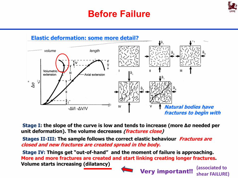
Before Failure
Very important!! (associated to shear FAILURE)

Triaxial testing: typical influence of the confiningpressure on the shape of the differential stress (axial stress minus confining pressure) versus axial strain curves
Rock Failure
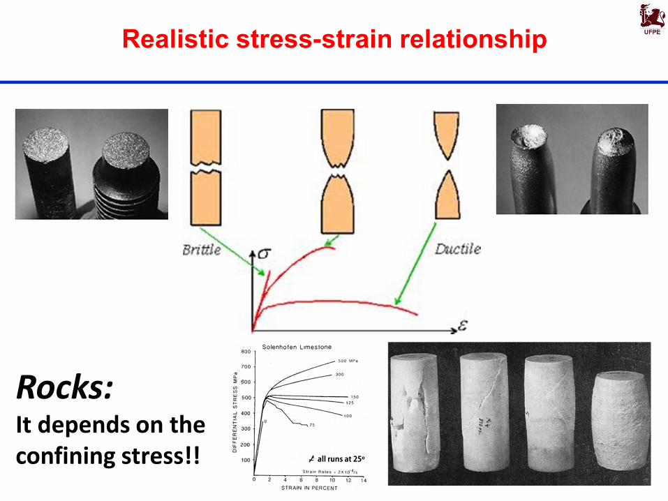
Realistic stress-strain relationship
Rocks:It depends on theconfining stress!!

Rocks:It depends on theconfining stress!!
Schematic representation of brittle failure styles in triaxial tests (Griggs and Handin, 1960a).
a) Extension test.
b) – e) Compression test with confining pressure increasing to the right.

Shear Failure

Rock Volumetric Behavior
(consolidatedgeomaterials)
(unconsolidatedgeomaterials)
Dilation : rock expansion under shear
SoilRock
Importantfor geological
fault reactivation

Tensile Failure
Tensile failure occurs when the effective tensile stress across some plane in the sampleexceeds a critical limit. This limit is called the tensile strength ( T0 ) and has the same unit as stress. The tensile strength is a characteristic property of the rock. Most sedimentary rocks have a rather low tensile strength, typically only a few MPa or less. In fact, it is a standard approximation for several applications that the tensile strength is zero. (Fjaer et al., 2008)
- Brazilian Test: - Incorporation of tensile strength in failure surface:
TENSION cutoff

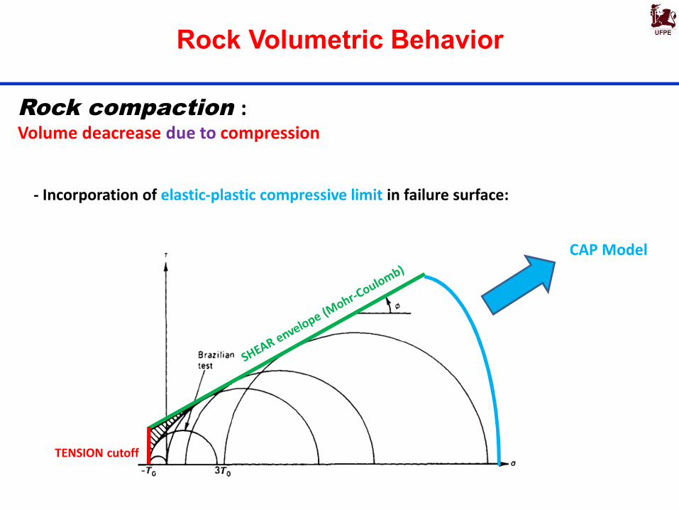
Rock Volumetric Behavior
Important for reservoir compaction
Rock compaction : Volume deacrease due to compression
Normal Consolidation
Line (NCL)Load/UnloadLines
Normal Consolidation Line (NCL):Change of pore structure(LIMIT to plastic compaction: irreversible behavior)
Load/Unload Line: No changes in pore structure(elastic deformation: reversible behavior)
Isotropiccompression ofBringelly shale

Rock Volumetric Behavior
Irreversibility...
Rock Volumetric Behavior
TENSION cutoff
Rock compaction : Volume deacrease due to compression
- Incorporation of elastic-plastic compressive limit in failure surface:
CAP Model

Rock Volumetric Behavior
CAP model: Multi-mechanism model

Rock Volumetric Behavior
CAP model: Multi-mechanism model
pεDilation
pv
Stress path
In situ (initial) stress
pεCompression
pv
pε
Critical point:no volumetric plastic strain

0bσ
Iσσ fp'
HM FORMULATION
I1
J2PORECOLLAPSE
TEN
SIO
N
In Situ Stress
cc
1
3
13
Vargas et. all 2006
FAULT REACTIVATION
RESERVOIR COMPACTIONHYDRAULICFRACTURING

Coupling Between Deformation and Permeability
Hydrostatic Compression: σ1
σ3=σ1
Stress path Plastic strain(only volumetric)
p
Effect of reservoir compaction:Decrease of permeability due to(irreversible) pore colapse.
Interpretation using CAP model
Ex: Kozeny-Carman
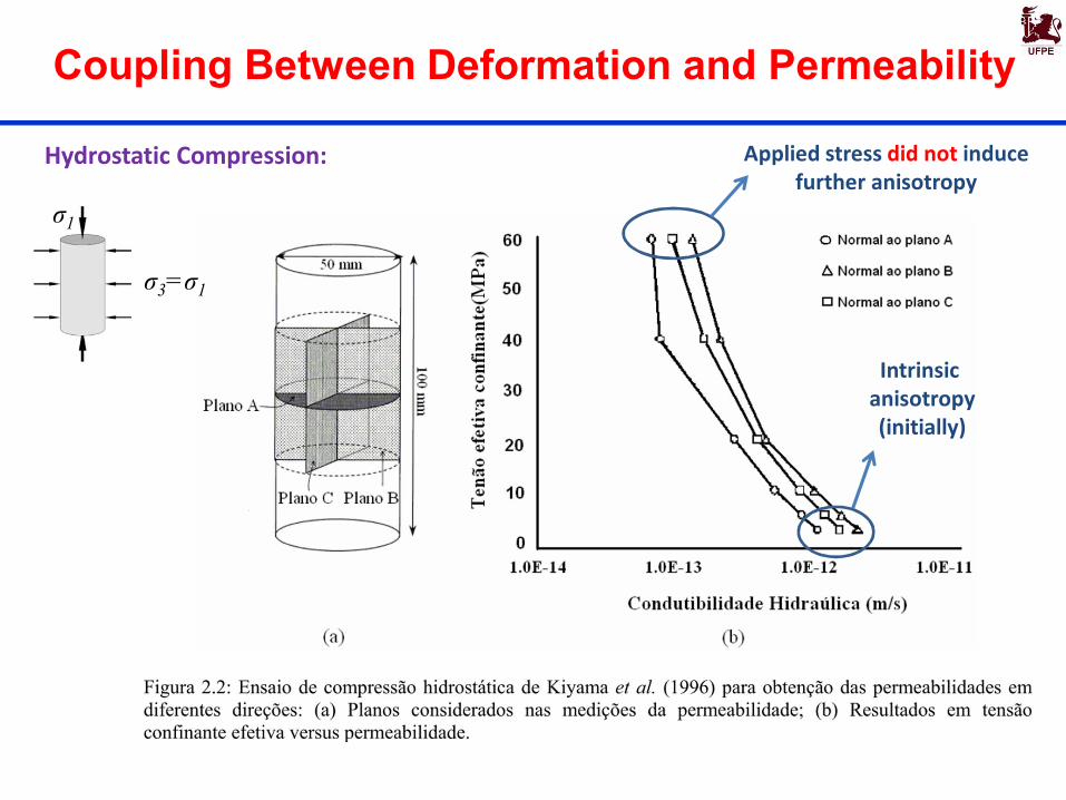
Coupling Between Deformation and Permeability
Hydrostatic Compression:
σ1
σ3=σ1
Intrinsic anisotropy(initially)
Applied stress did not inducefurther anisotropy

Coupling Between Deformation and Permeability
Permeability variation in a brittle rock in a triaxial compression test. This type of stress-strain behavior is widely reported in the literature. We have five distinct regions:
I - closure of pre-existing micro-cracksII - zone of elastic behaviorIII - steady growth of cracks IV - unstable growth of cracks V- post-peak zone characterized by the loss of resistance
(softening followed by rupture) of the material
I
I
II
II
III
IVV
III
IV
V
Anisotropy on permeability:
IntrinsicAnisotropy
StressInduced
Anisotropy
Triaxial Compression:
σ1
σ3
σ1 >σ3
dilatancy

Fluid Flow in Deformable Porous Media
Volumetric strain: u x y zd d d
x
y
z
uuu
u
u
ddt
uu
yx zdd dd
dt dt dt dt
u

Fluid Flow in Deformable Porous Media
1 0 s st
f
j
MASS BALANCE OF SOLID
Mass balance of solid present in the medium is written as:
where s is the mass of solid per unit volume of solid and js is the flux of solid.
f f
1 1 0us st
f
f f f f
1 1 1 0u u uss s s st t
(1)
(2)

Fluid Flow in Deformable Porous Media
MASS BALANCE OF SOLID
(Eulerian description)
A more convenient form of the balance equations is obtained considering the definitions ofmaterial derivate with respect to the solid velocity; which can be expressed generically as:
1 1 0s st
f f
u
.
u
DDt t
When the description of motion is made in terms of thespatial coordinates is called the spatial description orEulerian description,
That is, the current configuration is taken as thereference configuration.
In the Lagrangian description the position and physical properties of the particles aredescribed in terms of the material or referential coordinates & time.
The material derivative (or substantial time derivative) can serve as a link between ‘Eulerian’and ‘Lagrangian’ descriptions of motion
(3)

Fluid Flow in Deformable Porous Media
Definitions:Spatial point: fix point in the space
Material point: a particle.
The particle can be at different spatial points during its movement in time.
Configuration (Ω): space occupied by the particles (that conform the continuum medium) at certain instant ‘t’
t=to is the reference time
Ω0 = initial material or reference configuration.
Ωt = current configuration
Material coordinates (X1, X2, X3)
Spatial coordinates (x1, x2, x3) (current configuration).

Fluid Flow in Deformable Porous Media
The movement of the particles (which conform the continuum medium) can bedescribed by the evolution of their spatial coordinates (or their ‘position vector’) intime.
We need to know a function for each particle (identify by a ‘label’), which providethe spatial coordinates xi (or the corresponding vector) in the successive instantsof time.
As a label, to characterize unequivocally each particle, it is possible to use the‘material coordinates’.
In this manner, the ‘movement equations’ are obtained:
Which provide the spatial coordinates as a function of the material ones.
The ‘inverse movement equations’ are given by:
Which provide the material coordinates as a function of the spatial ones.

Fluid Flow in Deformable Porous Media
Description of the movementMaterial description: A property is described (i.e. density ) using as argumentthe material coordinate.
Note that if we fix X=(X1, X2, X3), we are following the density variationspecific particle.
Because of that the name of ‘material description’(Lagrangian description).
Spatial description: A property is described (i.e. density ) using as argumentthe spatial coordinate (Eulerian description).
Note that if we fix x=(x1, x2, x3), we focus the attention on one point of thespace; and we follow the density evolution for the different particles that arepassing for this fix spatial point.

Fluid Flow in Deformable Porous Media
Olivella and Argelet (2000)

Fluid Flow in Deformable Porous Media
Temporal, local, material and convective derivative.Consider a given property and their respective descriptions material and spatial.
We pass from one description to the other by using the ‘movement equations’
Local derivative: it is the variation of a property in time of a fix point in the space.
It is possible to write this derivative as:
Material derivative: it is the variation of a property in time following a specific particle (material point) of the continuum medium.
It is possible to write this derivative as:
local derivative
material derivative : Dalso denoted asDt

Fluid Flow in Deformable Porous Media
If we start with the spatial description of the property and we consider implicit in this equation the ‘movement equation’:
We can obtain the material derivative (i.e. following the particle) from spatial description:
We can generalized that definition for any property (scalar or vectorial):
Velocity is the derivative of movement equations respect to time:
Finally:
material derivative
material derivative local derivative convective derivative
DDt

Fluid Flow in Deformable Porous Media
Volumetric strain: u x y zd d d
x
y
z
uuu
u
u
ddt
uu
yx zdd dd
dt dt dt dt
u

Fluid Flow in Deformable Porous Media
MASS BALANCE OF SOLID
f f
1 1 0us st
ff
f f f f f
1
1 1 1 0u u u
ss
ss s s s
D DDtDt
t t
.
u
DDt t
f f
f
11 us
s
DDDt Dt
(Eulerian description)
(Lagrangian description)
(Material derivative)
(4)
f
f f f f
1 1 1 0u u uss s s st t
(equation 2)

Fluid Flow in Deformable Porous Media
Volumetric strain:
yx zdd dd
dt dt dt dt
u
(1 1 1 ) s s s
s
ddt
Dt Dt
DD
f
ff
u
Detailed description of solid density variation (including rock compressibility Cr) can be found in Lewis and Schrefler (1998).

Fluid Flow in Deformable Porous Media
Flow Equation – Water Saturated Porous Media
Water Mass Balance Equation
0l l l lt
q u
.. ... 0ll l l ll ll
l
tt
q q u uu
. . . 0l ls
l lll s
lDDt
DDt
q q uUsing (3)
Replacing (4) i.e. solid mass balance in material description
. . . 01
1sl l l l l l l
s
s l DDt
DDt
qu q u
This term considers the velocity of the liquid respect to the solid skeleton (ql) + the velocity of the solidrespect to a fix reference system . This is because the solid is moving now and drag the liquid phasewith it.
u
f f
f
11 us
s
DDDt Dt
u
lqql : velocityrespect tothe solidskeleton

Fluid Flow in Deformable Porous Media
1 . . 0l s sl
s
s ll l l l
DDt
DDt
q qu
1 . 0s l l s sl l l
s
D DDt Dt
u q (Lagrangian descriptionMass Balance of Water)
If liquid density is constant
. 0s ll l l
DDt
u q
If there is a source or sink of water
1 .s l l s sl l l l
s
D D fDt Dt
u q
If solid density is constant
. 0l
u q
Flow Equation – Water Saturated Porous Media
Water Mass Balance Equation

SUMMARY

Specific for each geomaterial
Mechanical problem for geomaterials:
Equilibrium Equation:
Principle of Effective Stresses:
Stress-strain relationship:
0bσ
Iσσ fp'
dσ' D dε
HM FORMULATION

0bσ
Iσσ fp'
HM FORMULATION
I1
J2PORECOLLAPSE
TEN
SIO
N
In Situ Stress
cc
1
3
13
Vargas et. all 2006
FAULT REACTIVATION
RESERVOIR COMPACTIONHYDRAULICFRACTURING

HYDRO-MECHANICAL COUPLINGS:
Rock porosity:
Rock permeability:
0.11 usst
u
tdtd
dt
ddt
ddtd vs
s
11
(mass conservation of solids)
(material derivative )
(porosity update)
ib expikk
HM FORMULATION
Other: Kozeny-Carman
u vv
dtd

owSDt
DSDtSD ss
s
s , 0)1( qu
Hydraulic problem: two phase flow equations for deformable porous media
where:
gkq
pkr
s
u
q
g~
rkk
p
1 oSwS woc ppp
rk
cp
porosityfluid saturationfluid densityDarcy flowphase viscositySolid velocity
permeability tensorfluid relative permeabilityfluid mobilityFluid pressurecapillary pressuregravity
HM FORMULATION

APPLICATION:
Primary Recovery – Reservoir Depletion
Volumetric strain in mass balance equations:
Compaction-driven mechanism
u
)1()1( ss Dt
DDtD
Pressure maintenance
Porositydecrease
qv
Increase of fluidflow apparent velocity
owSDt
DSDtSD ss
s
s , 0)1( qu
Later...

HM FORMULATION
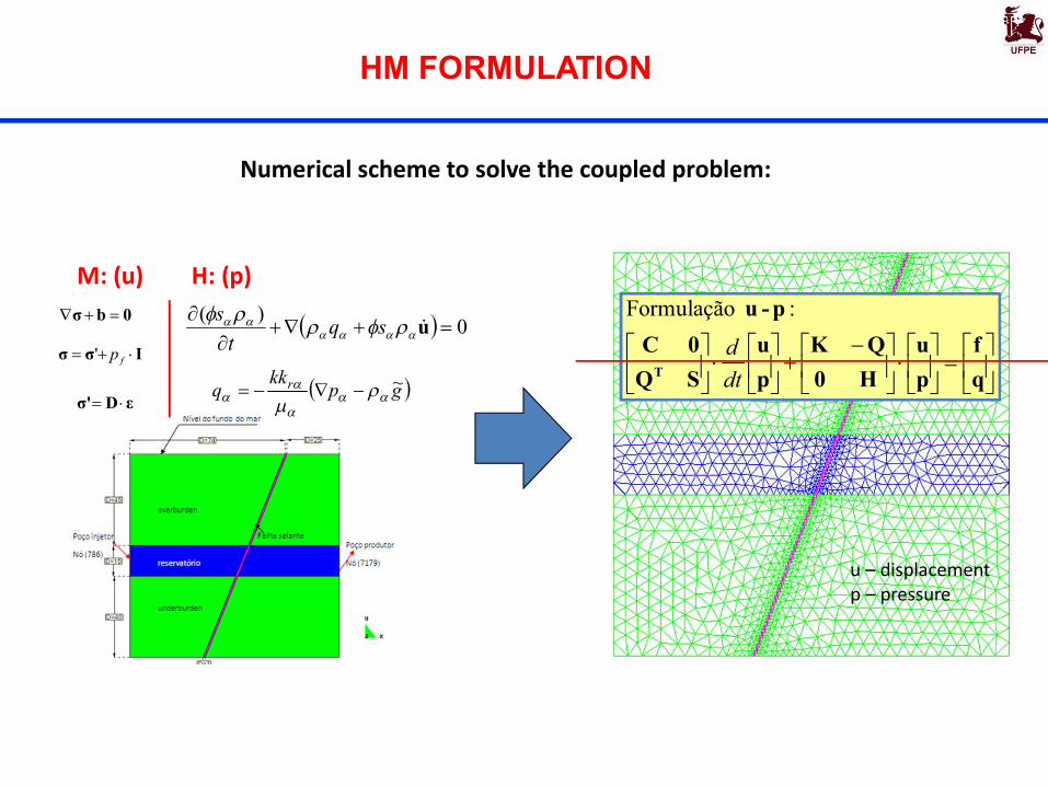
Numerical scheme to solve the coupled problem:
0bσ
Iσσ fp'
εDσ'
0)(
u
sqt
s
gpkk
q r ~
M: (u) H: (p)
qf
pu
H0QK
pu
SQ0C
p-u
T dtd
: Formulação
u – displacementp – pressure
HM FORMULATION

L. C. Pereira (MSc, 2007)
Fluid Flow – Geomechanics Coupling
Pore pressure Transmissivity
Effective stress Permeability
PorosityRock deformation
Geomechanics SimulatorFEM
Reservoir Flow Simulator FDM

L. C. Pereira (MSc, 2007)
Coupling Schemes
Pseudo-couplingIterative
Implicit Explicit

L. C. Pereira (MSc, 2007)
Advantages
Implicit Iterative Explicit Pseudo
Disadvantages
Computational costs
Convergence control
Changes in numerical code
Accuracy
Speed
Iterations
Coupling Schemes

Stress-split Method
Coupling withcommercial
reservoir simulators
Workflows to exchange parameters between individual modules