Steady Fock states via atomic reservoir

F. O. Prado1, W. Rosado2, G. D. de Moraes Neto2, and M. H. Y. Moussa2

1Universidade Federal do ABC, Santo Andre, Sao Paulo, Brazil and

2Instituto de Fısica de Sao Carlos, Universidade de Sao Paulo, Sao Carlos, Sao Paulo, Brazil

In this letter we present a strategy that combines the action of cavity damping

mechanisms with that of an engineered atomic reservoir to drive an initial thermal

distribution to a Fock equilibrium state. The same technique can be used to slice

probability distributions in the Fock space, thus allowing the preparation of a variety

of nonclassical equilibrium states.

PACS numbers: 32.80.-t, 42.50.Ct, 42.50.Dv

The development of strategies to prepare nonclassical states [1] and, in particular, to

circumvent their decoherence —via decoherence-free subspaces [2], dynamical decoupling [3],

and reservoir engineering [4, 5]— have long played a significant role in quantum optics. On

the conceptual side, the need for these states stems from their use in the study of fundamental

quantum processes, such as decoherence [6] and the quantum to classical transition [7].

On the pragmatic side, the advent of quantum computation and communication —which

depends strongly on successfully producing highly nonclassical states and ensuring their

long-term coherence [8]— has certainly put extra pressure on researchers to implement

efficient techniques of engineering and protection of nonclassical states. The proposition

of schemes that enable the generation of nonclassical equilibrium states thus represents an

ideal approach to the current challenges. In this regard, the reservoir engineering technique

proposed in Ref. [4] and experimentally demonstrated in a trapped ion system [9] signals an

important step toward the implementation of quantum information processes [8], a goal that

has recently mobilized practically all areas of low-energy physics. Reservoir engineering,

however, has major limitations, starting with the fact that it prevents, for example, the

generation of Fock equilibrium states (a key goal of the present letter). Moreover, the

protection of a particular state demands the (not-always-easy) engineering of a specific

interaction which the system of interest is forced to perform with other auxiliary quantum

systems.

arX

iv:1

403.

5482

v1 [

quan

t-ph

] 2

1 M

ar 2

014

2

Recently, the generation of Fock states with photon numbers n up to 7 was reported

in cavity QED, where a quantum feedback procedure is employed to correct decoherence-

induced quantum jumps [10]. The resulting photon number distribution assigns a probability

around 0.8 to the generation of number states up to 3, falling to below 0.4 for n = 7.

Nonequilibrium number states up to 2 photons have long been prepared in cavity QED [11],

as well as in most suitable platforms, such as ion traps [12] and, lately, in circuit QED [13],

where number states up to 6 were achieved.

In this letter we present a protocol in which the atomic beam reservoir technique [14] is

exploited to produce high fidelity equilibrium Fock states in cavity QED. The atomic reser-

voir —built up by injecting a beam of atoms that interact, one at a time, with the cavity

mode— prompts the emergence of an engineered Liouvillian superoperator to govern the

cavity field dynamics, alongside that coming from the cavity loss mechanisms. We stress,

from a practical perspective, that atomic reservoirs have for some time been used for the

preparation of the cavity vacuum state [15]. Moreover, this has been theoretically explored,

in close relation to the reservoir engineering technique [4], for the generation of an Einstein-

Podolsky-Rosen steady state comprising two squeezed modes of a high finesse cavity [16].

Our proposal, however, is altogether different from those in Ref. [4, 16]. In contrast to the

assumptions that support the method proposed in [4, 16], our protected Fock state is not

a steady state of a specific engineered Lindbladian Lρ = (Γ/2)(2OρO† −O†Oρ− ρO†O

),

where the only pure steady state of the system is the eigenstate of operator O with a null

eigenvalue. In our protocol, the steady state is driven by a sum of three engineered Lindbla-

dians, two of which act on selected subspaces of the cavity mode space, the mode emitting or

absorbing photons within these subspaces. The third Lindbladian is associated with (non-

selective) photon absorption by the cavity mode, in order to counterbalance the inevitable

emission to the natural (nonengineered) environment. The selective Lindbladians are built

up from engineered selective Jaynes-Cummings (JC) Hamiltonians, while the Lindbladian

for photon absorption follows from a usual JC interaction.

To generate the required Lindbladians, we rely on engineered selective Hamiltonians

[17] and engineered atomic reservoirs [14, 16], the latter demanding a beam of atoms to

cross a high-Q cavity. The selective Lindbladians are engineered by assuming the atomic

level configuration in Fig. 1(a), the emission or absorption process following from the atoms

prepared in the ground |g〉 or excited |e〉 state, respectively. The (non-selective) Lindbladian

3

FIG. 1: Atomic level configurations to engineer (a) selective and (b) non-selective Hamiltonians.

accounting for photon absorption is engineered from the level configuration in Fig. 1(b).

As shown in Fig. 1(a), the cavity mode (ω) is used to promote a Raman-type transition

g ↔ e, helped by two laser beams, ω1 and ω2, out of tune with transitions g ↔ i and e↔ i,

respectively. In the configuration in Fig 1(b) —which follows from that in Fig. 1(a) by

taking advantage of the Stark effect and switching off the laser beams— the cavity mode is

now used to couple resonantly the shifted levels |g〉 and |i〉. When the configuration is that

in Fig 1(a), the atoms are randomly prepared in the states |g〉 and |e〉, and when that in Fig.

1(b), the atoms are prepared at the auxiliary level |i〉. Starting with the engineering of the

selective JC interactions arising from the diagram in Fig. 1(a), we write the Hamiltonian

H = λσiga e−i∆t +Ω1σig ei∆1t +Ω2σie e−i∆2t +H.c., (1)

where σrs = |r〉 〈s|, r and s labelling the atomic states involved, and we define ∆ = ω−ωig,

∆1 = ωig−ω1, and ∆2 = ω2−ωie, with ωi` = ωi−ω` (` = g, e). It is straightforward to verify

that the conditions λ√n+ 1 ∆ and Ωj ∆j (j = 1, 2) lead to the effective interaction

([18])

Heff =(ξa†a−$g

)σgg +$eσee

+(ζa† eiδt σge +H.c.

), (2)

4

where $g = |Ω1|2 /∆1 and $e = |Ω2|2 /∆2 stand for frequency level shifts due to the action

of the classical fields, whereas the strengths ξ = |λ|2 /∆ and ζ = λ∗Ω2

(∆−1 + ∆−1

2

)/2

stand respectively for off- and on-resonant atom-field couplings to be used to engineer the

required selective interactions; finally, δ = ∆ − ∆2 refers to a convenient detuning to be

specified in the following lines. To get selectivity, we first perform the unitary transformation

U = exp−i[(ξa†a+$g

)σgg +$eσee

]t

, which takes Heff into the form

Veff =∑∞

n=1ζn |n+ 1〉 〈n|σge eiφnt +H.c.. (3)

with ζn =√n+ 1ζ and φn = (n+ 1) ξ+ δ−$g −$e. Next, under the strongly off-resonant

regime ξ √k + 2 |ζ| and the condition

φk = 0, (4)

which is easily satisfied by imposing (m+ 1) ξ = $g δ = $e, such that |Ω1| =√(m+ 1) ∆1/∆ |λ|

√∆1/∆2 |Ω2|, we readily eliminate, via RWA, all the terms pro-

portional to ζn =√n+ 1ζ summed in Veff , except when n = k, bringing about the selective

interaction

H1 = (ζk |k + 1〉 〈k|σge +H.c.) , (5)

producing the desired selective g ↔ e transition within the Fock subspace |k〉 , |k + 1〉.

The excellent agreement between this effective selective interaction and the full Hamiltonian

(1) has been analyzed in detail in Ref. [17]. Regarding the Hamiltonian associated with the

diagram in Fig. 1(b), we readily see that switching off the laser field and tuning the cavity

mode to resonance with the atomic transition g ↔ i results in:

H2 = λσiga+H.c.. (6)

Next, following to the reasoning in Ref. [14, 16] for atomic reservoir engineering, we

assume a weak-coupling regime for the interaction parameter associated with H2, i.e., λτ

1, τ being the time during which each atom crosses the cavity. However, it is easily verified

that the Lindblad structure of the superoperator emerging from H1 does not rely on the

weak-coupling regime ζkτ 1, owing to the selective nature of this interaction. When the

atoms are randomly prepared in the ground, excited, and auxiliary states: pgσgg + peσee +

piσii, with the laser detuning ∆L adjusted to produce k = m and l, respectively, we obtain

the master equation [14]

5

dρ

dt=γm2

(2amρa

†m − ρa†mam − a†mamρ

)+γl2

(2a†lρal − ρala

†l − ala

†lρ)

+γ

2

(2a†ρa− ρaa† − aa†ρ

)+ Lρ, (7)

with the effective rates γm = rg (ζmτ)2, γl = re (ζlτ)2, and γ = ri(λτ)2

= εγ (ε < 1

to achieve a steady equilibrium state), where rg, re, and ri are the atomic arrival rates

proportional to the probabilities pg, pe, and pi, respectively. The last term in Eq. (7), Lρ,

stands for the inevitable Liouvillian operator describing the lossy cavity (ω) of damping rate

γ and temperature T = ~ω/kB ln [(1 + n) /n], kB being the Boltzmann constant, irrespective

of the passage of the atoms:

Lρ =γ

2(1 + n)

(2aρa† − ρa†a− a†aρ

)+γ

2n(2a†ρa− ρaa† − aa†ρ

). (8)

From the equation of motion for the number state population, ρnn = 〈n| ρ |n〉, derived from

Eqs. (7) and (8), we obtain the steady state solution (assuming l + 1 < m):

ρnn =

Rnρ0 n ≤ l

RnAlρ0 l + 1 ≤ n ≤ m

RnBl,mρ0 n ≥ m+ 1

, (9)

where Rn = [(ε+ n) /(1 + n)]n and

Al =γl + (l + 1) (ε+ n) γ

(l + 1) (ε+ n) γ, (10a)

Bl,m =(m+ 1)(1 + n)γ

γm + (m+ 1) (1 + n) γAl, (10b)

ρ0 =(1− ε) /(1 + n)

1−Rl+1 +Al (Rl+1 −Rm+1) + Bl,mRm+1

. (10c)

From Eqs. (9) and (10) we clearly see that the distribution function ρnn can be manipu-

lated by an appropriate choice of the engineered parameters γl, γm, and γ. To estimate the

range of validity of these parameters in a microwave cavity QED experiment, we start by

choosing ∆ = ∆1 = (1+10−2)×∆2 = 10√k + 1 |λ|, such that |Ω1| = 10×|Ω2| =

√k + 1 |λ|,

ζk = 10−2√k + 1 |λ|, τ = 102/

√k + 1 |λ| (so that ζkτ = 1 [19]). Therefore, assuming

6

FIG. 2: Truncated thermal distribution from the Fock state m+ 1 = 6. In the inset we present the

Wigner function of the truncated distribution.

m, l ∼ 10 with typical λ ∼ 5 × 105Hz and γ ∼ 7.5Hz, and imposing γ ∼ ri × 10−2 = εγ,

it follows that γk ranges up to the order of 2 × 103γ, with ri = 103ε (i.e., pi = 10−2ε) and

rg, re ranging up to around 104 (pg, pe limited to 1− 2pi).

In order to generate steady Fock states: i) we first observe that a significantly large γm

(relative to γ), with γl = 0 (no atoms crossing the cavity in the excited state), such that

Rm+1Bl,m RmAl, (11)

entails the truncation of the equilibrium distribution ρnn, from the population of state m+1,

as illustrated in Fig. 2, where we have assumed m = 5, with n = 0.05 and ε = 0.8, such

that γ = 0.8γ and γm = 103γ to satisfy Eq. (11). Although the analytical solution in Eqs.

(9) and (10) was crucial to alert us to the possibility of manipulating the populations ρnn

through the appropriate choice of the parameters involved, all the simulations in this letter

were based on Eq. (7), running in QuTIP [20]. In the inset of Fig. 2, we present the Wigner

function of the truncated distribution, which takes no negative values, showing that it is a

purely classical state.

7

FIG. 3: Amplification of the thermal state distributions, from the Fock state l + 1 = 5, with the

corresponding Wigner distribution in the inset.

FIG. 4: Amplification of the thermal state distributions, from the Fock state l+ 1 = 1 , with the

corresponding Wigner distribution in the inset.

8

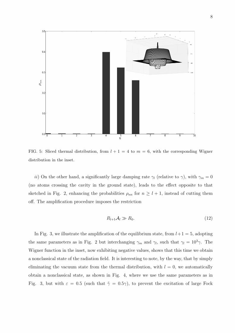
FIG. 5: Sliced thermal distribution, from l + 1 = 4 to m = 6, with the corresponding Wigner

distribution in the inset.

ii) On the other hand, a significantly large damping rate γl (relative to γ), with γm = 0

(no atoms crossing the cavity in the ground state), leads to the effect opposite to that

sketched in Fig. 2, enhancing the probabilities ρnn for n ≥ l + 1, instead of cutting them

off. The amplification procedure imposes the restriction

Rl+1Al R0. (12)

In Fig. 3, we illustrate the amplification of the equilibrium state, from l+1 = 5, adopting

the same parameters as in Fig. 2 but interchanging γm and γl, such that γl = 103γ. The

Wigner function in the inset, now exhibiting negative values, shows that this time we obtain

a nonclassical state of the radiation field. It is interesting to note, by the way, that by simply

eliminating the vacuum state from the thermal distribution, with l = 0, we automatically

obtain a nonclassical state, as shown in Fig. 4, where we use the same parameters as in

Fig. 3, but with ε = 0.5 (such that γ = 0.5γ), to prevent the excitation of large Fock

9

FIG. 6: Steady Fock state |5〉 , with the corresponding Wigner distribution in the inset.

FIG. 7: Steady Fock state |10〉, with the corresponding Wigner distribution in the inset.

10

states. Therefore, the vacuum plays a major role in the intersection between classicality and

nonclassicality.

Another case arises when we put together i) and ii), so as to iii) slice the equilibrium

distribution, from l+1 to m. This is done by ensuring the conditions leading simultaneously

to Eqs. (11) and (12). Fig. 5 shows a sliced steady distribution ranging from l + 1 = 4

to m = 6, again assuming the same parameters as above, but γm = γl = 103γ. The

Wigner function in the inset now exhibits a large region with negative values, strengthening

the nonclassical character of the generated state. Finally, we come to the main point of our

work: the choice m = l+1 allows us to join the subspaces l, l + 1 and m,m+ 1 alongside

one another, so that both sare the same state m. This leads to steady Fock states under

the same conditions established in iii), as seen in Fig. 6, which illustrates the state m = 5,

prepared with exactly the same parameters as in Fig. 5. The fidelity [8] of the prepared Fock

state is around 0.97, as confirmed by the Wigner distribution in the inset, which exhibits

the peculiar feature of the Fock state. We end up with the Fock state m = l+1 = 10 in Fig.

7, reached with the same parameters in Fig. 4, except ε = 0.95, with the fidelity dropped

to around 0.88.

We have thus proposed a scheme to manipulate the steady thermal distribution in such

a way as to produce steady Fock states of the radiation field. Our proposal relies on the

engineering of selective JC Hamiltonians, which thus generate equally selective Lindblad

superoperators that enable us to manipulate the equilibrium thermal distribution, slicing it

so as to prepare steady Fock states. Our technique can be implemented in other contexts

of atom-field interaction, such as trapped ions and circuit QED, where the beam of atoms

simulating the reservoir can be achieved by a pulsed classical field. In the former case,

the classical field is used to couple the vibrational field intermittently with the internal

ionic states, while in the latter case, it is used to bring a cooper-pair box into resonance

with the mode of a superconducting strip. Apart from the preparation of Fock states, other

applications within Hamiltonian, reservoir, and state engineering may arise from the present

protocol, as for example the generation of entangled steady state in a network of quantum

oscillators [21].

Acknowledgements

11

The authors acknowledge financial support from PRP/USP within the Research Support

Center Initiative (NAP Q-NANO) and FAPESP, CNPQ and CAPES, Brazilian agencies.

[1] For the engineering schemes relying on atomi-state measurement, see K. Vogel, V. M. Akulin,

and W. P. Schleich, Phys. Rev. Lett. 71, 1816 (1993); R.M. Serra, N. G. de Almeida, C.

J. Villas-Boas, and M. H. Y. Moussa, Phys. Rev. A 62, 043810 (2000); and for those not

requiring atomi detection, see A. S. Parkins, P. Marte, P. Zoller, and H. J. Kimble, Phys. Rev.

Lett. 71, 3095 (1993); Th. Wellens, A. Buchleitner, B. Kummerer, and H. Maassen, Phys.

Rev. Lett. 85, 3361 (2000).

[2] M. A. de Ponte, S. S. Mizrahi and M. H. Y. Moussa, Phys. Rev. A 84, 012331 (2011); D. A.

Lidar, I. L. Chuang, and K. B. Whaley, Phys. Rev. Lett. 81, 2594 (1998).

[3] L. Viola and E. Knill, Phys. Rev. Lett. 94, 060502 (2005); L. C. Celeri, M. A. de Ponte, C. J.

Villas-Boas, and M. H. Y. Moussa, J. Phys. B 41, 085504 (2008).

[4] J. F. Poyatos, J. I. Cirac, and P. Zoller, Phys. Rev. Lett. 77, 4728 (1996).

[5] F. O. Prado, E. I. Duzzioni, M. H. Y. Moussa, N. G. de Almeida, and C. J. Villas-Boas, Phys.

Rev. Lett. 102, 073008 (2009).

[6] M. Brune, E. Hagley, J. Dreyer, X. Maıtre, A. Maali, C. Wunderlich, J. M. Raimond, and S.

Haroche; Phys. Rev. Lett. 77, 4887–4890 (1996)

[7] M. Brune, J. Bernu, C. Guerlin, S. Dele´glise, C. Sayrin, S. Gleyzes, S. Kuhr, I. Dotsenko,

J.-M. Raimond, and S. Haroche, Phys. Rev. Lett. 101, 240402 (2008).

[8] M. Nielsen, I. Chuang, Quantum Computation and Quantum Information, Cambridge Uni-

versity Press, 2000, 409-416.

[9] C. J. Myatt, B. E. King, Q. A. Turchette, C. A. Sackett. D. Kielpinski, W. M. Itano, C.

Monroe, and D. J. Wineland, Nature 403, 269 (2000).

[10] X. Zhou, I. Dotsenko, B. Peaudecerf, T. Rybarczyk, C. Sayrin, S. Gleyzes, J. M. Raimond,

M. Brune, and S. Haroche, Phys. Rev. Lett. 108, 243602 (2012).

[11] B. T. H. Varcoe, S. Brattke, M. Weidinger, and H. Walther, Nature 403, 743 (2000); P. Bertet,

S. Osnaghi, P. Milman, A. Auffeves, P. Maioli, M. Brune, J. M. Raimond, and S. Haroche,

Phys. Rev. Lett. 88, 143601 (2002).

[12] D. M. Meekhof, C. Monroe, B. E. King, W. M. Itano, and D. J. Wineland, Phys. Rev. Lett.

12

76, 1796 (1996); D. Leibfried, D. M. Meekhof, B. E. King, C. Monroe, W. M. Itano, and D.

J. Wineland, Phys. Rev. Lett. 77, 4281 (1996).

[13] M. Hofheinz, E. M. Weig, M. Ansmann, R. C. Bialczak1, E. Lucero, M. Neeley, A. D.

O’Connell, H. Wang, J. M. Martinis, and A. N. Cleland, Nature 454, 310 (2008).

[14] B.-G. Englert and G. Morigi, in Coherent Evolution in Noisy Environments, edited by A.

Buchleitner and K. Hornberger (Springer, Berlin, 2002), p. 55.

[15] J. M. Raimond, M. Brune, and S. Haroche, Rev. Mod. Phys. 73, 565 (2001).

[16] S. Pielawa, G. Morigi, D. Vitali, and L. Davidovich, Phys. Rev. Lett. 98, 240401 (2007); S.

Pielawa, L. Davidovich, D. Vitali, and G. Morigi, Phys. Rev. A 81, 043802 (2010); S. Pielawa,

G. Morigi, D. Vitali, and L. Davidovich, Phys. Rev. A 85, 022120 (2012).

[17] F. O. Prado, W. Rosado, A. M. Alcalde, and M. H. Y. Moussa, J. Phys. B: At. Mol. Opt.

Phys. 46, 205501 (2013).

[18] O. Gamel and D. F. V. James, Phys. Rev. A 82, 052106 (2010); D. F. V. James and J. Jerke,

Can. J. Phys. 85, 625 (2007).

[19] We performed (following the reasoning in Refs. [14, 16]) a numerical simulation of the passage

of atoms through the cavity, assuming τ = 10−4s in conformity with ζkτ = 1, to confirm that

the cavity mode evolves in excellent agreement with the coarse-graining master equation (7),

and that higher value of τ start to compromise the accuracy of this master equation.

[20] J. R. Johansson, P. D. Nation, and F. Nori, Comput. Phys. Commun. 183, 1760 (2012); ibid.

184, 1234 (2013).

[21] G. D. de Moraes Neto et al., to be published elsewhere.