Investigations into the Multiple Auditory Steady- State Response (MASTER) Technique In Humans

Michael Sasha John

A thesis submitted in conformity with the requirements for the degree of Doctor of Philosophy

Institute of Medical Science University of Toronto

O Copyright 200 1 by Michael Sasha John

National Library 191 ,C,d, Bibliotheque nationale du Canada

Acquisitions and Acquisitions et Bibliographic Services services bibliographiques

395 Wellington Slreet 395. rue Wellington OttawaON KlAON4 Ottawa ON K1 A ON4 Canada Canada

The author has granted a non- L'auteur a accorde une licence non exclusive licence allowing the exclusive permettant a la National Library of Canada to Bibliotheque nationale du Canada de reproduce, loan, distriiute or sell reproduke, prgter, distribuer ou copies of this thesis in microform, vendre des copies de cette these sous paper or electronic formats. la fome de microfiche/film, de

reproduction sur papier ou sur format electronique.

The author retains ownership of the L'auteur conserve la propriete du copyright in this thesis. Neither the droit d'auteur qui protege cette these. thesis nor substantial extracts from it Ni la these ni des extraits substantiels may be printed or otherwise de celle-ci ne doivent 6tre imprimes reproduced without the author' s ou autrernent reproduits sans son permission. aut orisation.

Investigations into the Multiple Auditory Steady-State Response (MASTER) Technique in Humans lMichael Sasha John, Ph.D. Thesis March, 2001

Institute of LMedical Science, University of Toronto

The Multiple Auditory Steady-State Response (MASTER) technique enables the rapid and objective

assessment of hearing by statistically evaluating elecnophysiological responses evoked by multiple tones

which are presented simultaneously. The technique offers several advantages over transient stimuli

techniques used to assess hearing. Firstly, since eight stimuli may be presented simultaneously. in the

time normally required to evaluate one stimulus. MASTER provides a relatively rapid assessment of

hearing. Secondly, the stimuli are more Frequency specific than translent stimuli since steady-state

stimuli contain spectral energy only at the camer frequency and at the sidebands. which occur at spectral

frequencies equal to the difference between the carrier and modulation frequency. Lastly. the technique

reduces the necessiry for expen evaluation of a subject's responses since these are evaluated objectively.

statistically. and automatically by a computer program. The expenments presented here build upon rhe

onginaI work on the technique that occurred only a short time ago (Lins. 1995). and serve to form a

sufficient foundation for the techntque to stan to be evaluated as a viable clinical tool. Chapter 1

demonstrates some limitations of the technique that should be considered when designing test stimuli.

For example. in order to insure that simultaneously presented stimuli do not interact, they should be

separated by at least one octave in normal hearing subjects. Chapter 2 provides a description of the

theory, design. and implementation of a Windows based data acquisition system. In Chapter 3 the use of

both amplitude and frequency modulated stimuli is examined. We show that by using both of these types

of modulation the technique is more efficient, even at threshold intensities. In Chapter 4. the phase values

of the responses are examined and a technique is proposed for accurately converting phases into latencies.

As with amplitude, steady-state phase values are stable over time, show changes with intensity that are

similar to those seen with transtent stimuli. and are unchanged by the presentat~on of multiple stimuli.

The work presented here suggests the M.L\STER technque can function as a useful clinrcal tool in

objective audiometry. and suggests seven1 directions that may be useful for future research. (339 words)

While the work presented here was often difficult and sometimes even painful, it is important to remember that it is always an honor and a privilege to have the opportunity to engage in research. During my thesis research I have been supported by a Medical Research Council Studentship. which was provided by the Medical Research Council of Canada, which obtains its funding from taxes incurred by Canadians. Accordingly, I would like to thank Canadians. and the Canadian government for creating a society where science and education are still supported reasonably well: let us hope that this will continue in the future. Accordingly, I have aied to balance the investigations relating to basic science and physiology with attempting to advance a technique which seems very close to being ready to serve as a useful clinical tool in the near future. Hopefully. Canadians will soon get something useful back from supporting my research in this area.

I would also Iike to thank the Medical Research Council of Canada. James KnowIes and the Baycrest Foundation for funding the research itself.

I would like to thank Terry Picton. Ideally, research should not occur in a vacuum. Sadly. I find that this is more often than not. the exception rather than the rule. especially when it comes to pursuing a Ph.D. Unlike many of my peers I had supervisor who acted as a constant source of support throughout the entire process. Terry Picton is one of the most hard working. thorough. smart. supponive. and fair scientists I have ever met. and it has been a great privilege and quite a bit of fun to work with him over the last 3 years.

The work in this thesis was also largely aided by the hard work of Otavio Lins. Bndget Boucher, Hilmi Dijani, and Patnc~a Van Roon. as well as the helpful advice provided by Martin Regan and Jos Eggemon t.

Lastly. I would like to thank the data. Even a well-destgned expenment w11 not yield the expected results if the physiology doesn't happen to work the way you think i t does. in the words of Endel Tulving "Ln successfuI research you can be at odds with other sclenttsts. In fact t h ~ s IS ofien good, but you can NEVER afford to be at odds with Mother Nature." The data tn this thesrs were often beautiful. told their story loudly, replicated very niceiy. and contamed few outliers. They were a pleasure to work with.

This thesis is dedicated to the incredible fhends I have made uphile livrng in Toronto. to my fellow lab geeks, and to my housemates who have all given me a lifetime of memories over the last few years (most of them good, few of them sane). Of course. this thesis ts also dedicated to my family (especially Josh-the-E3-Guash-man), most of whom have acted as a constant source of support and with whom I still talk to every week.

..And. of course. to Kathmne. .A.K.A. "Huggy Buggy"

ABSTRACT OF THESIS ACKNOWLEDGEMENTS TABLE OF CONTENTS LIST OF TABLES LIST OF FIGURES LIST OF ABBREVIATIONS FOREWORD INTRODUCTION

ii iii iv

vii viii

X

xi xii

CHAPTER 1: MULTIPLE AUDITORY STEADY-STATE RESPONSES (MASTER): STIMULUS AND RECORDNG PARAMETERS 1

-- -

Recording 5 Auditory Stimuli 6

Analyses 12 Statistical Evaluations I 3

Modeling 14

RESULTS IS

Experiment 1 : Interactions between two camer frequencies 15

Experiment 2: lMultiple stimuli in the 70- 1 10 Hz range 27 Experiment 3: Effects of intensity 3 2 Experiment 4: Effects of modulation fiequenc y 3 3

Experiment 5: Noise stimuli 40

Experiment 6: Multiple stimuli in the 30-60 Hz range 41

DISCUSSION 48

Nonlinearities 48

Interactions between Stimuli 5 2

Numbers and Noise 54

Discrimination of Modulation Frequencies 56 Caveats 57

Recommendations for the MASTER Technique 5 9

CHAPTER 2: MASTER: A WINDOWS PROGRAM FOR RECORDING MULTIPLE AUDITORY STEADY-STATE RESPONSES 61

AE~STRACT 62

INTRODUCTION 63

BACKGROUND 64

OVERVIEW OF THE MASTER TECHNIQUE 66

SYSTEM DESCRIPTION 70

Hardware and Peripherals 70

Main Screen 71 Load Protocol Screen 7 1

View Stimulus Screen 7 8 View EEG Screen 80 Data Acquisition Screen 8 1

Process Data Screen 87

COMPUTATIONAL METHODS AND THEORY 9 1

Synchronizing the AD and DA Conversion 9 1

Stimulus Generation 9 3 Choice of Stimuli: AM and AhL/FM stimuli 9 7

Detection of S teady-State Responses. 100

Artifact Rejection 102

Calibration Procedures 106

DATA STORAGE 107

PERFOR~VANCE ISSUES 108

CONCLUSION 109

CHAPTER 3: MULTIPLE AUDITORY STEADY-STATE RESPONSES TO AM, FM, & MM STIMUL~ 11 1

ABSTRACT 112 - - - -- -

INTRODUCTIOK 113

METHODS 116

Subjects 116

Auditory Stimuli 116 Recordings 124

Statist~cal Evaluations of Responses 126

Experlmental Design 127

RESULTS 127

Experiment 1 : Different Amounts of AM and FM 127 Experiment 2: Possible Interactions between AM and FM. 130 Experiment 3: Multiple AM and MM stimuli 131 Experiment 4: Changing the FM phase in the .MM stimulus 138 Experiment 5. Latency estimates for AM and FM stimuli 145 Experiment 6: Independent ampIinrde and frequency modulation (IAFM) 151

Drscusslo~ t 57

PhysiologicaI Processing of AM and FM 157 Clinical Usefulness of the Steady State Reponses 165

CONCLUSIONS 168

CHAPTER 4: AUDITORY STEADY-STATE RESPONSES: PHASE AND LATENCY MEASUREMEKTS 169

ABSTRACT 170

INTRODUCTION 171

METHODS 1 74

Subjects 1 74 Auditory Stimuli 174

Recording 178 Amplitude and Phase Measurements 178

Signal-to-Noise Assessments 179 Experimental Design 180 Statistical Evaluations 182

Converting Phase to Latency 182

Modeling 194

RESULTS 195

Experiment 1 : Monaural Stimulation 80- 100 Hz 195

Expenment 2: monaural Stimulation 150- 190 Hz I99

Experiment 3: Dichotic Stimulation I99

Experiment 4: Effects of Intensity 200

Experiment 5: Effects of MultipIe Stimuli 20 1

Experiment 6: Stability of Phase 20 1

Expenment 7. Small Differences in Modulation Frequency 208

Results of Modeling 208

Discussros 212 Auditory S teady-State Responses 212

Latency of Steady-State Responses 213 Latencies in the Auditory System 22 I

Relations to Otoacoustic Emissions 223 Effects of Intensity 225 Gender effects 227 Effects of Pathology 227

SUMMARY 228

APPESDIS k MODELLING THE DATA FROM EXPERIMEXT 3 OF CHAPTER 1 237 APPESDIS B: THE EQCIVALESCE OF DIFFEREST METHODS FOR MEASURING LATENCY -241

Chapter 1 Table 1- 1: Tone Combinations for Multiple Stimuli 29 Table 1-2: Response Amplitudes During iMultiple Stimulation 3 1

Table 1-3: Effects of Intensity on Interactions between Multiple Stimuli 37

Table 1-4: Spacing of the Modulation-Frequencies 39

Table 1-5: Bandpass Noise as Camer Stimulus 43

Table 1-6: Multiple Stimuli Modulated in the 30-50 Hz Range 47

Chapter 3 Table 3- 1: Interactions between Stimuli (Experiment 2) 13 1

Table 3-2: Phase Delays of AM and IMM Responses 135

Table 3-3: Effects of Combining .kM and FM I44

Table 3 4 : Estimated Latencies (ms) for AM and FM Responses: I SO

Table 3-5: ,Mixed Modulation at a Phase of 90" 1 56

Chapter 4 Table 4-1: Estimated Latencies at Different blodulat~on Frequencies 198

Table 4-2: Effects of Camer Frequency on Response Latency 209 Table 4-3: Effects of Multiple Stimuli on Latency Estimates 209

Table 4 4 : Stability of the Responses over Two Separate Recordins Sessrons 209

vii

Introduction Figure Intr-1: Simple physiological model for the responses to AM stimuli xxi

Chapter f Figure 1 - 1 : Auditory steady-state time waveforms & amplitude spectra 9

Figure 1-2: Noise-reduction in steady-state response recordings 11

Figure 1-3: Interactions between tones with different carrier-frequencies 17

Figure 1 -4: Carrier- frequency interactions 19

Figure 1-5: Carrier-Frequency interactions using narrow-band noise stimuli #I 2 1

Figure 1-6: Carrier-frequency interactions using narrow-band noise stimuli $2 2 3

Figure 1-7: Modeled interactions between stimuli with different carrier-frequencies 2 5 Figure 1-8: Simultaneous stimulation at different intensities 3 5 Figure 1-9: Modulation-frequencies in the 30-50 Hz range 4 5 Figure 1 - 10:Nonlinear distortions due to rectification 5 1

Chapter 2 Figure 2-1 :

Figure 2-2: Figure 2-3:

Figure 2-1: Figure 2-5:

Figure 2-6: Figure 2-7:

Chapter 3 Figure 3- 1:

Figure 3-2:

Figure 3-31 Figure 3-4:

Figure 3-5:

Figure 3-6: Figure 3-7:

Figure 3-8: Figure 3-9:

MASTER system-ovew~ew of components 69

Definrng the paradigm uslng the Load Protocol Screen 7 3

View Stimulus Screen 79

Data Acquisition Screen 8 3 Process Data Screen 8 9

Responses to combined A,WFM ctirnuli 99

Evaluating the effects of nonstationarities in the data 105

AIM and FM stimuli. time waveforms and correspondrng spectra 119

.Mi~ed-~h4oduIation (MM) with different phases of FM 121

Independent amplitude- and frequency-modulation (IAFM) I t 3 Depth of modulation for AIM and FM 129 Effects of MLM on stimuli at different intensities 133 Greater detection of MM responses over time 137 Effects of FM phase on the MM response 141 Diagramatic analysis of mixed modulation responses 143

Effects of FM phase on the MM response 147 Figure 3-10:Latencies of the AAM and FM responses 149 Figure 3-1 1: Multiple auditory steady state responses for 1 subject 153 Figure 3- 12: Response to independent A M & FM ( IhFM ) 155 Figure 3- 13: Effects of stimulus intensity on IAFM responses 159 Figure 3-13: Proposed mechanisms involved in processing A M and Fhi. 163

... Vlll

Chapter 4 Figure 4- 1: Human auditory steady-state responses of a single subject 177 Figure 4-2: Ambiguities in the measurement of phase 185

Figure 4-3: Unwapping of phase 187 Figure 33: Phase-frequency plots 19 1

Figure 4-5: Estimation of preceding cycles (80- 100 Hz) 193 Figure 4-6: Effects of modulation-frequency on amplitude 197 Figure 4-71 Estimation of preceding cycles ( 150- 190 Hz) 203 Figure 4-8: Dichotic stimulation and the results of Experiment 3 205

Figwe 4-9: Effects of intensity on response latency 207 Figure 4- 10: Small differences in modulation-frequency 21 1 Figure 4- 1 1 : Modeling parameters 2 15 Figure 4- 12: Modeling the physioIogica1 processes 2 17

Figure 4- I3 : Modeled latencies: 2 19

List of Abbreviations

AD AM AM/FM ASSR CF m CPU Cz DA dB d f DMA DPOAE EEG E or E ERP EP FFT F, fm

FIFO Fisher LSD FM HL Hz IAFM IC lcHz kOhm &MASTER m :MHz .MM ms MTF pal pa2 PC P-P RAM RMS SOC SPL -r2 v VCN VI's PV nV A f i - S

Analog-to-digital Amplitude modulation Simultaneous A W M modulation Auditory steady-state response (s) Center frequency (usually of an auditory fiber) Cochlear nucleus Central Processor Unit Signifies vertex scalp location in 10-20 system Digital-to-analog DecibeI Degrees of Freedom Direct memory access Distortion Product oto-acoustic emission EIectroencephalogram

Epsilon (estimates covariance between measures) Event related potential Evoked potential Fast Fourier Technique Carrier frequencies modulation frequencies First-in-first-out buffer Fisher's Least Significant Difference post-hoc test Frequency modulation Hearing level Hertz Independent AM and FM modulation Inferior Colliculus Kilohertz ( 1000 Hz) 1000 ohms Multiple auditory steady-state response (s) Megabyte ,Megahertz ,Mixed Modulation (M at same modulation rate ) Millisecond (note: occasionally also 'msec') .Modulation tnnsfer function File or Parameters associated with defining stimuli in the MASTER system File or Parameters associated with defining recording parameters in the MASTER system Persona1 computer Peak-to-peak (measure of amplitude) Random Access lMemory Root-mean-square (measure of amplitude) Superior olivary complex Sound pressure ievel Hotelling's T' test Volts Ventral cochlear nucleus Virtual instruments Microvolts ( 1 voltl I .000,000) Nanovolts Change in frequency above and below a given value Sum of components

Foreword

The idea of automatic and objective evaluation of electrophysiological activity is

fascinating and immediately presents many wonderful challenges! My research has

concerned automatic or computer-aided evaluation of brain activity for some years. In

1991 I finished an honor's thesis in the department of psychology at Reed College

concemed with the automatic detection of deception using a technique which

incorporated multiple stepwise discriminant analysis, in which the computer would

somewhat automatically provide a probability estimate that a person was intentionally

lying. During my graduate work at McGill, where I took my first course in signal

processing and was introduced to MATLAB (possibly the greatest software program ever

written), I began to build more sophisticated computer programs which evaluated brain

activity using signal analysis techniques such as the FFT and the short-time FFT (which

is similar to wavelet analysis). I also became interested in emerging areas such as

adaptive neurostimulation, objective measurement of anesthetic depth, automatic source

analysis of brain activity, objective and quantified measurement of responses to novel

pham~aceutical compounds ("pharmaco-EEG"), and other areas which have led to several

very interesting projects and even one or two patents.

While the research presented in this thesis continues to focus on objective

methods of evaluating brain activity. it also marks the latest stage in my efforts towards

becoming a fairly knowledgeable, well-rounded, and competent scientist. My past

research gave me a foundation in cognitive evoked potentials, QEEG, EEG during rest,

mental load, and sleep: in other words, I was concemed with the brain as a whole. My

work on this thesis gave me the opportunity to focus on a specific primary sensory area

for the first time. I have begun to understand how the cochlea, which I knew nothing

about 3 years ago, performs various tasks which act to provide us with an incredibly

sophisticated hearing machine. To be honest, when I started a thesis on this topic I did not

do it out of interest in the area (after all, why study the keyboard when you can study the

computer?). It was more like taking an acrid medicine: I did it because I thought that it

would be good for me to move away from looking at the system as a whole and learn

about a specific part. I did not think it would be fascinating. I was wrong.

Overview of the Tkeszs

The four chapters of this thesis cover a considerable amount of material. An

overview is important, not only because it will give readers a general feeling for what

will be presented here, but also because it will help to provide some understanding of the

reasoning and processes that acted to shape the direction of the research and the questions

that were asked. The progression of the chapters of this thesis reflects my increasing

familiarity with the MASTER technique. Chapter 1 is the result of research that we

conducted when I first came to Dr. Picton's laboratory in 1997. The research in this

chapter was done using a specialized DOS based system that he had built in Ottawa using

C for a programming language and customized data acquisition boards. Lins and Picton

(1995). building upon some experiments which were done in the visual modality, and

carried out over two decades earlier by David Regan (1970), had recently shown that

multiple auditory steady-state potentials could be evoked by presenting several AM tones

simultaneously. The work in Chapter I represents both their effons to obtain a more

concrete understanding of the technique and the evoked responses (in terms of the types

of interactions that may occur between stimuli) and my efforts to figure out what they

were up to and attempt to determine why it was sensible. In line with this research

dynamic, much of this thesis is a combination of a tension between feeling that I knew

enough about what we were doing to push the technique forward and feeling a bit

hesitant, which would cause me to draw back. check our assumptions, approach the data

slightly differently, and re-evaluate our ideas about the technique. By way of example,

Figure 1-2 of Chapter 1 resulted from the concern about the validity of a dual method

using both averaging and long FFT sweeps in order to provide optimum signal-to-noise

levels in our recordings. The figure shows one of several tests that we carried out during

this thesis work in order to check the basic processes of the technique. As a second

example, we again tested the validity of this dual method. as well as our strategy for

removing anifacts, as is seen in Figure 2-7. In Chapter 1, I also re-evaluated the finding

made in Lins and Picton (1995) that only 4 stimuli should be presented to each ear. Was

this limitation due to the carrier frequencies being too close together or was it a function

of closely spaced modulation frequencies? We found that up to 4 stimuli could be

presented simultaneously provided that the camer frequencies were separated by at least

1 octave (Tables 1 - 1, 1-2, and 1-4 of Chapter 1). Modulation frequencies of adjacent

stimuli, it seemed, could be set very close to each other without decreasing the

amplitudes of the responses (we put this finding to the test again in Chapter 4). Lastly, I

examined both the 40 Hz range and the 80 Hz range since Lins et al. (1995) had

previously shown that the responses above 80 Hz were not attenuated by arousal level or

sleep, which was not the case for the stimuli in the 40 Hz range. By comparing the

results of Tables 1-2 and 1-6 we found that the 80 Hz responses were attenuated less than

those in the 40 Hz range when multiple stimuli were presented. Accordingly, in the

research presented in the subsequent chapters of this thesis, we will always use

modulation rates above 70 Hz. The reminder of the research in Chapter 1 primarily

concerned an area with which I had very little experience: modeling of the data to explain

interactions between stimuli. Initially, this was beyond my comprehension since I had

never heard of things like tuning curves, excitation envelopes, or compressive

rectification. This initial project, therefore, enabled me to obtain some familiarity with

the mechanisms of the cochlea, to discover how one could approach figuring out how

these mechanisms led to the recorded responses, and acted to give me my first real taste

of the extraordinary complication. stunning simplicity. and unquestionable beauty of the

auditory system.

The research in Chapter 1, effectively catapulted me into the world of the multiple

auditory steady-state response (MASTER) technique. I now had a reasonable

appreciation for the power of the technique and understood some of its strengths and

weaknesses: it was time to get my hands a bit dirty. During the experiments of Chapter

1, I had regarded the data acquisition system in the laboratory as a son of black box,

where the stimuli were created and the responses evaluated through a set of very

complicated processes. For several converging practical reasons. but also so that I could

really understand the technique from the ground upwards. we decided i t would be a good

idea if I built a Windows based data collection system Tor using the MASTER technique.

Chapter 2 describes the MASTER data acquisition system which was the result of about 8

months of programming and learning about buffering techniques. timing issues, data

... Xlll

transfer, and other headache-inducing topics. Indeed, the project enabled me to become

well acquainted with the different areas of the MASTER technique from the generation

of stimuli to the statistical evaluation of the responses. Importantly, creating a data

collection system enabled the addition of several features lacking in the original system,

such as the option of saving the raw data, so that it could be re-played or re-analyzed.

This feature enabled our evaluation of data to become dynamic. In other words, results

could be analyzed at different periods of the data collection. Consequently, we have been

able to obtain the type of results seen in Figure 2-6, where response detection over time is

shown, and this also enabled us to perform an in-depth evaluation of the percentage of

false positives and false negatives that occurred as recording sessions progressed. The

MASTER system also enabled us to explore the technique, by allowing us to easily alter

recording parameters or even the way in which data was evaluated, and thereby let us

rapidly confirm hypotheses and explore new areas. The data collected in this chapter

was important not only because it served to validate our statistical methods and artifact

techniques, but also because it led to the next set of experiments. A paper by Cohen et al.

( 199 1 ) had previously demonstrated steady-state responses to stimuli that were both AM

and FM were larger than responses evoked by AM alone. As can be seen in Figure 2-6,

we extended these findings to the multiple stimulus case and showed that at 50 dB SPL,

the stimuli that were both AMEM produced responses that were about 130% larger than

the responses to simple AM stimuli leading to response detection in about % the time

required by the simple AM stimuli. Thus, in addition to evaluating 8 stimuli in the time it

would normally take to evaluate 1, this study provided evidence that the test could be

made even more rapid by using AMEM stimuli.

Chapter 3 was the subsequent logical step due to the data collected in Chapter 2,

and investigated, in more depth. the properties of the responses to stimuli that were AM,

FM, or AM/FM combined ("mixed modulation" or MM). In the first part of the paper,

we examined the responses to different depths of AM and FM and attempted to make

some comparisons between the two types of responses both in terms of amplitude and

phase. Imponantly, we considered the responses in the context of the amplitude spectra

of the AM and FM stimuli and introduced some basic principles which should enable

readers to make more sense of the results. For example, the fact that 50% AM and 50%

FM stimuli have such different spectral characteristics indicated that AM and FM depth

xiv

must be treated somewhat differently. AAer examining AM and FM separately, we

examined MM stimulation. In much of the experiments in this chapter, in the case of

MM, the AM and FM components occur at the same rate (as was the case in Chapter 2),

causing only one response to appear in the amplitude spectrum. By changing the phase of

the FM relative to the AM, we found that the MM response seemed to be the vector sum

of the wo separate responses. Using a very elegant (yet simple) model that was

developed by Dr. Picton, we were then able to model the two responses and formally

demonstrate that the response to MM stimuli could be understood as the simple vector

addition of the response to AM and FM alone. Accordingly, the data collected in this

chapter provided plausible evidence of the independence of these two processing

systems. Another interesting finding of this chapter was that the MM augmentation was

present not only at 50 dB SPL, but also at 40 SPL and 30 dB SPL. This finding indicated

that MM stimuli should help facilitate obtaining responses near threshold, where the

MASTER technique begins to encounter trouble and requires considerably larger

amounts of data for the detection of responses (Herdman and Stapells, 2000). The last

topic of Chapter 3 that will be touched upon here is the idea of independent Ah4 and FM

modulation (IAFM) for the same camer frequency region: in other words, by modulating

the AM and FM at two independent rates, two responses in the amplitude spectra of the

EEG could be evoked. We were originally very excited by this finding because it raised

the possibility of developing a new statistic that could make use of the two responses

evoked in the same area of the cochlea. While our initial attempts did not suggest that this

method would provide more rapid detection of responses than the MM approach (where

AM and FM occur at the same rate), the IAFM method may still be very useful because it

provides information about the processing of the two types of modulation in each

frequency range.

The last set of experiments is contained in Chapter 4, which examines the phase

of the steady-state response. Much of the data presented in this chapter were collected in

1998, but the analysis and interpretation of the data required close to 2 years. In the

words of Dr. Picton, "phase is not easy." I have probably heard him say this over 100

times, and each time it rings more true. tf I knew then what I know now of the non-

linearities of the auditory system, I would never have kept plugging away at the data and

somewhat naively asserting "this has to make sense, we just have to keep at it". In fact,

the subject still often conhses me and makes me question how I ended up in

neuroscience rather than designing the new Bug for VW or opening a surf shop on the

north shore of Waikiki. However, the effort paid off (we think), and the data seem to

make sense most of the time.

The major reason that this topic was intriguing to me was that the phase of the

steady-state response is always available: the FFT will always produce an amplitude

value, which is related to the size of the response, and a phase value, which is related to

the latency of the response. However, except for using phase in a statistical sense, as a

means of detecting the presence of a steady-state response (Dobie, 1993) it is not much

examined. There is good reason for this. Phase is inherently ambiguous because it is a

circular measurement. Phase can be represented a s an angle which defines a number of

degrees or radians of a circle, and since a circle only has 360 degrees, the measure

becomes troublesome if it is less than 0, or greater than 360 (see Figure 2 in Chapter 4).

For example. 1 degrees of phase may in fact be 364, or 724!

Unlike the other chapters. the results of this chapter will not be summarized here

with any detail since these should be approached very slowly. Yet, the rationale that

prompted us to attempt to make sense of the phase data should be mentioned so that the

reader understands why we felt justified in undertaking this task. The phase (latency) of

the steady-state response was investigated because our preliminary data sets suggested

that it was a viable parameter to be studied with the MASTER technique in that it had the

minimum requirements. In other words. we quickly found that phase was stable over

time (intra-subject), was similar between subjects. changed as expected due to changes in

intensity (which had been shown in the case of latency for transient stimuli), and was not

significantly different for single or multiple stimuli. It was trying to sensibly convert

phase into latency that was the challenging aspect of the study.

It should be obvious that the types of experiments found in Chapter 4 would be

far less feasib!e if we had presented each steady-state stimulus separately, since a

tremendous amount of time would be required in order to collect the necessary data from

each subject. For example, due to the issue of non-linear filters or "filter slopes" which

has been raised by Bijl (Bijl and Veringa. 1985), when commenting upon the work of

Diamond (1977), it was very important to collect data for each carrier frequency at each

modulation rate. By consecutively presenting all our carrier frequencies at the same

xvi C

modulation rate, we were able to circumvent any non-linearities which may exist in the

auditory system at different rates of modulation. The MASTER technique allowed the

data for this experiment to be collected in 2 hours rather than 16 (and that was only one

of the seven studies presented in that paper). Another important point is that some of the

experiments done in Chapter 4 would not have been sensibly formulated without the

understandings obtained in Chapters 1-3. Each bit of new knowledge of the MASTER

technique seems to increase its power and versatility. For example, since we were

reasonably certain that modulation rates of adjacent carrier frequencies could be set

closely without causing a reduction in amplitude of the responses, we separated adjacent

modulation frequencies by only 0.24 Hz in the last experiment described in this chapter.

The ability of the auditory system and the central nervous system to successfully produce

one response at 159.912 Hz and another at 160.156 Hz is still awe-evoking to me. It

seems that this chapter nicely combines with the rest of the evidence presented in this

thesis to show the power of this technique, and to demonstrate that this is a relatively

young method that may hold great promise within the near future.

Lastly, the projects in this paper would not have been possible or sensible without

the elegant research of several dedicated scientists who provided important results by

which ours could be contextualized and understood. The work with which I have become

most familiar and which has acted to steer this thesis the most was the following: the

early work of Galambos and Regan on steady-state evoked potentials; the work of Cohen

and Rickards on combined AMEM stimulation and steady-state stimulation of rates as

high as 450 Hz; the studies of Valdes, Cohen, and Dobie on the evaluation of different

statistical techniques for evaluating the response; the work of Meller, Khanna. Saberi,

and Langner with respect to the ways in which the auditory system (post-cochlea)

processes both AM and FM information and modulation in general; and the work of Jos

Eggermont and Brian Moore who basically seem to publish articles on everything! Of

course the work of Dr. Terry Picton and Otavio Lins, and their collaborators has

obviously also acted as a strong pair of shoulders on which this thesis stands.

The MASTER technique is an interesting. powerful, and clinically useful method

of objective audiometry which is generating increasing interest from the scientific

community. Our system is currently used in eight other clinics/research laboratories

around the world, and several more systems will be shipped over this upcoming summer.

xvii

The research in this thesis has provided a firm foundation for this technique and has

hinted at what some of the next steps should be. Most of the work was a lot of fun. I

hope learning about it serves a similar function for those who read these pages.

Overview of the physiology

This thesis focuses upon the development of a technique which permits the

auditory system to be evaluated using different types of stimuli and several methods of

data analysis. While the characteristics of responses that were obtained under various

experimental manipulations are described in detail, a discussion of the origins of these

responses is not taken up in depth. Further, much of the modeling contained herein

emphasizes cochlear processes, rather than central mechanisms, when explaining the

results. Indeed, many of our results may be explained by models that solely incorporate

cochlear processes, thus avoiding the need to also examine the contributions of more

central mechanisms. A consideration of central mechanisms may have resulted more in

complicating our models by several orders of magnitude without necessarily providing a

significantly better fit for the data. However, there are brains inside the heads of our

subjects. and the electrical potentials that we are recording are generated at locations that

are more central than the cochlea. Accordingly. some discussion of the specialized

neuronal mechanisms that are related to the processing of modulated sounds is merited.

Auditory steady-state responses (ASSRs) are relatively simple stimuli which may

be used to investigate how the auditory system processes complex real world sounds such

as speech. The human auditory system is composed of many specialized structures which

aid in the conversion of acoustic stimuli into meaningful neuronal representations. The

processing of sound begins in the outer ear and moves centrally through the middle ear to

the cochlea. The outer and middle ear serve mainly to conduct sounds from the air to the

fluid-based system of the cochlea with little loss of energy. At this peripheral level the

hearing system does not have specialized features for processing moddated tones rather

than pure tone stimuli.

The more specialized processing of modularion. for example AIM, occurs

beginning at the level of the cochlea. As discussed by Lins et al. (1995). AM stimuli will

produce responses in the cochlea that follow the modulation envelope due to the

xviii

rectification of the responses both at the level of the inner hair cells (for loud stimuli, e.g.,

>50 dB SPL) and at the synapse between the inner hair cells and the fibers of the primary

afferent pathway (see Figure Intr-1). The responses of the i ~ e r hair cells are

asymmetric and saturate in one direction more quickly than in the other. Accordingly,

the inner hair cells will both compress and rectify a response at a loud intensity.

Additionally, the responses at the level of the primary afferent fibers are always rectified,

regardless of the intensity of the stimuli, because action potentials are only evoked by

depolarization of the hair cells. Since only by movement of the hair cells in one direction

causes their ion channels to open, leading to depolarization, only half of the acoustic

waveform leads to neurotransmitter release and the resultant excitatory post-synaptic

potentials of the primary auditory nerve afferents: hence, there is half-wave rather than

full-wave rectification. Further the responses, both at the hair cell (i.e., membrane

potentials of the cochlear microphonic) and in the cochlear nerve, saturate at higher

intensity levels (see 2"' and 41h column of Figure Intr-l) leading to a compression of the

final response transmitted by the auditory nerve fibers. In the processing of acoustic

energy, the cochlea and primary afferent nerve fibers therefore act together to form a

compressive half-wave rectification system. In a linear system, the frequency content of

the output will be the same as that of the stimulus. Only in the case of a non-linearity

(e.g., rectification) can a response contain energy at the frequency of modulation.

Rectification is why our responses occur at the modulation frequencies.

In addition to compressive rectification, the neural representation of information

about the AM envelope is ofien enhanced at the level of the cochlea and primary .e

afferents. Intuitively, i t seems sensible to expect the voltage responses of inner hair cells,

in response to AM tones, should be a predictable function of the responses that occur to

low Frequency sounds. For example, both stimuli will be subject to the same rectification

processes, low pass filtering, and peak or envelope detection resulting in the phase

locking of synchronized activity in the cochlear nerve fiber (Smith, 1998). However. the

output of the post synaptic cochlear nerve fiber is not merely a function between that

neuron's static rate-intensity function and the intensity envelope of the AM tone. In fact,

responses to modulated tones are often larger and extend to higher intensities than can be

predicted from the static input-output relationship that is elicited by a pure tone presented

xix

Figure: Intr-I. Simple physiological model for the responses to AM stimuli. The top row represents the events following the presentation of a low-intensity stimulus. The bottom row represents the events following the presentation of a high-intensity stimulus. The sequence of events is shown from left to right. The stimuli (first column), represented both in the time domain and in the frequency domain, pass through a function simulating the inner hair cells (second column). This asymmetric bi-directional compressing exponential function saturates faster when the input increases in one direction than in the other. The output of the inner hair cells (third column) passes through a function simulating the ganglion cells (fourth column). This function is a unidirectional compressing rectifier. The output of the ganglion cells, whose axons constitute most of the afferent axons of the auditory nerve, is shown in the last column. Rectification of the signal introduces a spectral component at the frequency of modulation (as well as at higher harmonics). This explains how auditory steady-state responses can have spectral power at the frequency of modulation when the stimulus has no power at this frequency (Regan, 1994). In a spontaneous firing neuron, the energy will exist in the inhibitory direction (below the x-axis). The model is quite simple and looks only at the hair cells and the auditory-nerve fibers. (from Lins et al, 1995. Reprinted with permission.)

MNER HAIR CELLS GANGLION CELLS

LOUD

'I'

xxi

at different intensities (Smith and Brachmm, 1980). The enhancement of the modulated

response with regard to the original modulated signal may occur due to rapid adaptation

after an onset response (Cooper et al., 1993; Smith, 1998; Giesler, 1998). Another

mechanism that may also play a role in the detection of a rapidly changing stimulus

envelope relies on range fractionation. Several different types of primary afferent neurons

encode the signals generated by the hair cells of the cochlea (e.g., cells with low or high

spontaneous rates). Since information at different intensities is Fractionated by types of

neurons that enable the auditory system to encode over a large range of intensities (as

reviewed by Geisler, 1998), the relatively quick stimulation of the different types of

neurons caused by slope of the AM envelope may help to detect the rapid transitions of

the AM envelope. Because the responses to AM are also enhanced more centrally at the

levels of the cochlear nucleus and the inferior colliculus (Mdler, 1972; Rees and Maller,

1983), modulated tones may evoke larger brainstem responses than pure tones of the

same intensity and therefore. may be detected more rapidly.

A large part of this thesis also considers frequency modulation. The response of a

fiber to the instantaneous frequency of an FM tone is identical to its discharge in response

to a pure tone at the same frequency (Sinex and Geisler, 1981). Studies of the auditory

nerve (Sinex and Geisler, 1981; Khanna and Teich, 1989ab) have shown that while AM

responses follow the AM envelope, the FM responses may occur at both the modulation

frequency and its second harmonic. although the prior response is primary. The

processing of FM is somewhat complicated, but likely results From an FM to AM

transduction. With respect to the activation of the inner hair cells as discussed above, the

energy of an FM stimulus will be processed (and rectified) similarly to that of an AM

signal at the level of the cochlea (Khanna and Teich. 1989b).

The coding of the rectified information about the modulated envelope at the level

of the cochlear nerve relies mostly on the phase locking of primary afferent neurons to

the modulation envelopes of the sound (as tnight be expected in the case of AM since

discharge rates of primary neurons increase with increasing intensity of the stimulus, as

occurs with the AM envelope). By evaluating the size of the phase locked neural

responses as a function of modulation rate, a modulation transfer function (MTF) can be

obtained. .4t the level of the auditory nerve, the MTFs for AM stimuli are reasonably flat

up to the 1500 Hz rate at which point strong attenuation occurs (Joris and Yin, 1992).

xxii

As the auditory nerve fiben transmit the information about the modulated signal

to the cochlear nucleus (CN), a second filtering process occurs, with many of the neurons

of the CN exhibiting a bandpass response with respect to the modulation frequencies.

Early on, M ~ l l e r (1974) showed that CN neurons which process both AM and FM often

demonstrate a preference for a particular rate of modulation, above and below which they

decrease their firing rate (i.e., a bandpass). The MTFs of this region therefore assume the

shape of an upside down "V", the apex of which is known as the best modulation

frequency. The cochlear nucleus not only encodes modulation, but also seems to amplify

the modulated signal, accentuating the peak of the response relative to the original

modulated signal (M~lller, 1972; Smith et al., 1985). The amplification of the AM

envelope occurs in several specialized types of neurons. Frisina et al. (1990a) showed

that in the ventral cochlear nucleus (VCN) the ability to encode amplitude modulation

was best in onset neurons, followed by choppers, although the pimarylike and auditory

nerve fiben also reproduced the modulated signal. The best modulation frequency of the

different units explored by Frisina et al. (1990a) ranged from 180-240 for onset units and

from 80-520 for choppers. The general trend in the amplitude of the steady-state response

MTF is a decrease in amplitude with increasing modulation rate. However. this trend

deviates from a pure decay by containing areas of larger response at the 40 Hz, 80 Hz,

and 120 Hz ranges (Cohen et al., 1991). Possibly, this may be caused by a tendency for

the best modulation frequency to occur at a majority of CN neurons near 40 Hz in

, humans, which could also lead them to fire at the 2"'. and 3" harmonics of this rate.

From the cochlear nucleus, the neuronal signals are transmitted to the superior

olivary complex, and then to the inferior colliculus by way of the lateral Iemniscus. A

series of elegant experiments by Langer (e.g., Langer and Schreiner, 1988) have explored

how AM is encoded, in the cat, at the level of the inferior colliculus. At the level of the

inferior colliculus there exists a topographical order to neuronal populations

demonstrating iso-frequency lamina to different best modulation frequencies which seem

to be onhogonal to those for different carrier frequencies (Langer et a!.. 19%). Low pass

filtering again occurs at lower intensity levels, while showing a bandpass at greater

intensities.

Although there is a transduction of the FM signal into AiM. the activation of the

inner hair cells in response to an FM signal will occur at different latencies than would

xxiii

occur for pure AM. In addition to the units, that have just been described, which process

information about the periodicity of a stimulus, the brain has specialized neuronal

systems that respond specifically to FM stimuli. Groups of neurons from the brainstem

up to the cortex respond both to upward and downward glides, while many show a

preference for upward glides (Tian and ~auschecker, 1994; Ricketts et al., 1998; Gordon

and O'Neill, 1998). This preference is also seen in behavioral data @emany and

Clement, 1998) and electrophysiological data in response to transient FM sweep stimuli

(Kohn et al., 1977). Preference to certain directions and certain rates of FM (but not AM)

has also been shown, and there may be an interaction between rate and directional

preference. For example, Msller (1977), and others (Zhao et al., 1997), have described

FM responsive cells that produced responses to both upward and downward glides for

modulation frequencies below 50 Hz, while these only responded to the upward glides at

higher modulation frequencies. The preference for upward glides may be seen in steady-

state responses as well. For example, in Chapter 3 we interpret our results as suggesting

that larger steady-state responses occurred during upward glides of FM.

The origin of the auditory steady-state responses (ASSRs) is very likely

dependent upon the rate of the modulation frequencies. Modulation frequencies in the 40

Hz range are generated both at the cortex and in the brainstem. Under anesthesia or sleep

the cortical component disappears, while the smaller brainstem component of the

response remains. Since the brainstem is located earlier in the auditory pathway than the

cortex, this latter component is characterized by a shorter apparent latency (Lins et al.,

1995). ASSRs evoked to rates of 80 Hz and above also have shorter apparent latencies

than the 40 Hz steady-state response and are also likely generated in the lower and upper

brainstem.

The origins of the transient evoked brainstem potentials are well known and their

amplitudes and latencies are used to help detect disorders of the auditory system and

central nervous system. Extensive reviews of anatomical basis of these brainstem

potentials exist in the literature (Mdler and Jannetta, 1985). Wave I is thought to be

generated at the distal part of the auditory nerve due to the initiation of action potentials.

Wave I1 occurs mainly at the proximal end of the auditory nerve although there may be a

distal component. Wave I11 occurs at the cochlear nucleus, with a small component from

the nerve fibers entering the nucleus. Wave IV occurs at the superior olivary complex

xxiv

(SOC) with some contribution from the cochlear nucleus. The last peak we will discuss is

the positively going wave V, which occurs at the lateral lemniscus, and which exists in

animals (although this may show up as wave IV in animals -see review by Starr and Don,

1988) even after bilateral ablation of the inferior colliculus (IC), as has been shown by

Wada and Stam (1983). As discussed in Chapter 4, the auditory steady state response can

be reasonably predicted from the superposition of overlapping transient responses, even

more so when appropriate refractory periods and multiple generators are incorporated

into the modeled data (Gutschalk et al., 1999).

Another line of evidence that steady-state potentials are generated in the

brainstem derives From the scalp topography of these responses which suggests a dipole

in the brainstem which points towards the Fronto-central cortex. If the responses at rates

between 80 and 200 Hz were generated closer to the peripheral centers of the auditory

system, such as occurs with wave 1 of the transient response, then a lateralization would

be expected in the scalp topography (as occurs with wave I). In fact, this is not the case

when using the mastoid, rather than the neck, as a reference: since the recorded responses

are smaller rather than larger. as would occur with a dipole source near the ear which was

oriented towards the Cz recording electrode.

Of the multiple components of the brainstem response it is most likely wave V,

originating in the lateral lemniscus, that is the strongest contributor to the steady-state

responses at the modulation frequencies which were used in the thesis. Wave V

amplitude is not affected much by repetition rate of the stimulus and has routinely been

evoked at rates comparable to those of our modulation rates (Jewett and Williston, 197 1).

In contrast, faster repetition rates have been shown to cause decreases in the amplitudes

of the earlier components, possibly by means of forward masking (Kramer and Teas,

1982).

Additional evidence that the faster steady-state responses, such as the 80 Hz

response, are generated in the same areas that produce the transient brainstem responses

and prior to the level of the IC can be found in Chapter 3. In that chapter, we show that

AM and FM are probably generated by independent neuronal populations. The

reductions seen in individual responses evoked by AM and FM (modeled), when these

stimuli are presented together in a mixed modulation stimulus, are small and can be

reasonably explained by considering changes that occur in the energy of the stimulus, and

by cochlear mechanisms alone, rather than by any type of interference (i.e., interaction

between responses that would lead to decreases of these responses) which might occur in

the brainstem. At the level of the IC, information about modulation is being examined

independently of the type of modulation or the Bequency of the camer and AM and FM

responses would likely be processed by the same periodicity area (Langner et al., 1998).

The fact that we did not see much interference in simultaneous presentation of AM and

FM responses suggests that the potentials that we are recording are generated, to a large

degree, in regions that occur earlier than the IC.

Other results discussed in this thesis also suggest that the steady-state responses

are generated prior to the level of the IC. Langer and Schreiner (1988) found that a re-

coding of information occurs at the IC which is more complex than at earlier levels of

processing. At the CN the MTFs from entrained responses shows tuning to the

modulation rate without demonstrating changes in discharge rate that increase with

increasing modulation Frequencies. In the IC, both the MTFs of the synchronized

activity, as well as the mean discharge rate, varies with the modulation rate.

Accordingly, at this level there is a change in the way that the modulation information

has been encoded. In line with the above study, if the steady-state responses were being

generated at the level of the IC, we may have obtained larger responses at higher rates of

modulation. Since we found the opposite, where faster modulation rates tend to cause

decreases in the amplitudes of steady-state responses, this may also be seen as supporting

a generator prior to the IC.

The latency data provided in Chapter 4 provide mixed evidence that the steady-

state responses could be generated in the brainstem source of wave V. Latencies from 16

to Z1 ms were found in the case of the 80-1 00 Hz modulated tones, while the 150- 190 Hz

modulation rates produced latencies in the 7-12 ms range. While the wave V responses

evoked by transient tone stimuli are generally later than the latencies generally associated

with wave V to click stimuli. the latency estimates for the 80-100 Hz data are quite large

to be easily reconciled with the latencies commonly obtained for the transient wave V.

One characteristic of the data in the 80-1 10 Hz range is that the responses have slightly

larger amplitudes than responses at other rates. The fact that these responses were

characterized by both longer latencies and larger amplitudes than might be expected From

a linear filter may be explained by the activation of a multi-synaptic circuit in response to

xxvi

modulations in this range. Indeed, the phase data of Cohen et al. (1988) seem to suggest

a transition in the phase trends that occur at these modulation rates compared to rates

below 80 Hz. The 150-190 Hz modulation rates were chosen so that the superimposition

of responses would be likely to cause transient responses in the 5.2 rns to 6.6 ms range

(i.e., wave V) to overlap since this time range is equal to the periods of these modulation

rates (e.g. 1000/190=5.2 ms). The 8-1 3 ms latency estimates obtained for these faster

modulation rates were thus characterized by response latencies that were much closer

with those associated with the wave V response that is evoked by transient tone stimuli.

Aflnal note on clinical relevance

The MASTER technique offers many advantages to the clinical testing

environment. Objective audiometry is useful when testing babies, or other individuals

who may not be willing or able to give reliable behavioral responses to indicate their

hearing abilities (e.g., thresholds). While oto-acoustic omissions are able to provide an

indication that normal hearing levels exist at 30 dB SPL or more, they are not able to

provide information related to threshold. Frequency-specific auditory brainstem

responses using tone bunt stimuli or single steady-state stimuli techniques can provide

kequency-specific threshold information, but are relatively slow procedures. Hopefully,

the MASTER technique can serve as a useful tool for objective audiometry since it can

evaluate frequency-specific thresholds to multiple stimuli in the time normally required

to test a single stimulus. Because steady-state responses are statistically assessed by the

computer, rather than requiring a subjective and time consuming evaluation by a trained

professional, less specialized training is required on the part of its users. The MASTER

technique can be used not only to assess frequency specific thresholds, but can also

provide information as to the sensitivity of the auditory system to various rates of

stimulation, to types of modulation, and to depths of modulation.

The work in this thesis was done using control subjects with normal hearing

levels. In the application of the MASTER technique to clinical populations several types

of issues may arise. For example. with regard to the interaction of the multiple tones, it is

possible that interactions between stimuli may occur due to the broader tuning curves,

and lack of tuning "tips", that can be present in abnormal cochleas (Harrison, 1981).

Picton et al. (1998) investigated the use of the MASTER technique in infants and

xxvii

children for both aided and unaided hearing. While this initial utilization of the

MASTER technique was able to provide valuable information in many cases, the authors

found a case of aided hearing, where the physiological thresholds were lower in the case

of high frequency stimuli when these were presented alone rather than in combination

with other lower Frequencies. A possible cause of the results produced by that subject

may have been that the higher frequency tuning curves lacked the high sensitivity "tip" at

the characteristic frequency of the hair cell and may have therefore been more susceptible

to an interaction with low frequencies.

The interactions of several tones, as may occur in the MASTER technique with

clinical populations, can also be seen as an advantage of the technique. For example, the

responses to multiple stimuli may be similar to the sensitivity of these individuals to

natural sounds, which will undoubtedly be comprised of complex mixtures of tonal

frequencies. Moreover, by independently adjusting the volume of the MASTER tonal

stimuli, automated procedures could be created relatively easily which could circumvent

any problems which might occur due to presenting multiple stimuli at the same intensity

level. Additionally, even if 3 rather than 4 tones were tested in a single condition (and

the high frequency 1 Wz tone was tested alone) this would still save time for a full

examination.

This thesis did not study clinical populations in its investigation of the MASTER

technique since we were interested in laying a strong foundation with regard to

. understanding the characteristics of multiple steady-state responses. Early clinical

studies indicate that the technique works well (Lins et al., 1996; Picton et al., 1998). The

creation of a portable system will enable other researchers to help us to begin to use the

system in clinical populations and to collect normative values in adults and infants.

Considerable interest has been continuously shown by both our scientific and clinical

colleagues. Accordingly, we are excited about now being in a position to find out quite a

bit about how we may use AM, FM, MM, and IAFM stimuli to provide rapid and

objective measures of various hearing disorders using the MASTER technique and

system.

xxvi i i

MULTIPLE AUDITORY STEADY-STATE RESPONSES (MASTER):

STIMULUS AND RECORDING PARAMETERS

A ponion of this material has previously appeared in MS. John. 0 tins, B Boucher. and T W Picton (I998), Multiple Ruditoty Steadv-State Responses (ICI.4STER): Stitnzdus and Recording Parameters. .4udiology (3 7); 5 9-82. Reprinted with permission

Acknowledgements This research was funded by the Medical Research Council of Canada. The authors would also like to thank James Knowles and the Baycrest Foundation for their support.

Chapter 1 : Stimulus and Recording Parameters

Steady-state responses evoked by simultaneously presented amplitude-modulated tones were

measured by examining the spectral components in the recording that corresponded to the

different modulation-frequencies. When using modulation-frequencies between 70 and 110 Hz

and an intensity of 60 dB SPL, there were significant interactions between two stimuli when the

carrier-frequencies were closer than one half octave apart, with attenuation of the response to the

lower carrier-frequency. However, there were no significant decreases in response-amplitude

with four simultaneous stimuli provided the carrier-frequencies differed by one octave or more.

Higher intensities (70 dB SPL) resulted in greater interactions between the stimuli than when low

intensities (35 dB SPL) were used. Modulation-frequencies could be as closely spaced as 1.3 Hz

without affecting the responses. Using broadband noise as a carrier instead of a pure tone

resulted in a significantly larger response when the stimuli were presented at the same sound

pressure level. At modulation-frequencies between 30 and 50 Hz, there were greater interactions

between stimuli than at faster modulation-frequencies. These results support the following

recommendations for using multiple stimuli in evoked potential audiometry: (i) The multiple

stimulus technique works well for steady-state responses at frequencies between 70 and 110 Hz.

(ii) Up to four stimuli can be simultaneously presented to an ear without significant loss in

amplitude of the response provided the carrier-frequencies separated by an octave and the

intensities are 60 dB SPL or less. (iii) Bandpass noise might serve as a better camer signal than

pure tones.

Chapter 1 : Stimulus and Recording Parameten

A steady-state evoked potential occurs when a repeating stimulus evokes an electrical

waveform whose constituent frequency-components maintain constant amplitude and phase over

prolonged time periods (Regan, 1 989). Steady-state responses are produced when stimuli are

presented at a rate sufficiently rapid that the response to any one stimulus overlaps the responses

to preceding stimuli. After the first few stimuli, the recorded waveform assumes the periodic

waveform of the steady-state response.

Auditory steady-state responses can be obtained using many different stimulus rates

(Rickards and Clark, 1984). The most widely studied auditory steady-state response is evoked by

stimuli presented at rates near 40 Hz (Galambos et a1.,1981; Stapells et a1 1984). This 40-Hz

response can be used to assess hearing (Dauman et al.. i984; Rodriguez et al., 1986). However,

the response decreases in arnpli tude considerably during sleep (Galarnbos et al., 1 98 1 ; Linden, et

al., 1 985; Jerger et al., 1 986). is dramatically attenuated during general anesthesia (Madler and

PoppelJ987; Plourde and Picton, 1990), and is dificult to record in infants (Stapells et

ai., 1988). The auditory steady-state response to stimuli presented at rates of 70-1 10 Hz (Cohen

et al.. 199 1 ; Levi et al, 1993; Aoyagi et al., 1994) are two to three times smaller than those of the

30 Hz response. Nevenheless, these rapid responses are much less affected by arousal (Cohen et

al., 1991 ; Levi et al, 1993; Lins et al., 1995), and are readily recorded in infants (Aoyagi et

al., 1993; Rickards et a].. 1994). The 70-1 10 Hz responses are therefore useful for objective

audiometry in patients who cannot provide reliable behavioral responses (Rance et al., 19%; Lins

et al., 1996).

Recording responses to many different stimuli at the same time would allow objective

audiometry to obtain as much information about hearing as possible in as short a time as

possible. Regan and Cartwright (1970) demonstrated that steady-state responses to several

simultaneous visual stimuli could be recorded and analyzed independently if each stimulus was

Chapter 1 : Stimulus and Recording Parameters 4

modulated at a different rate (Regan, 1989). This was later shown to also be possible in the

auditory modality (Lins et a1.,1995; Picton et a1.,1987; Regan and Regan, 1988). Multiple

carrier- frequencies, each modulated by its own signature modulating- Frequency, evoke multiple

steady-state responses, each measured at the particular frequency at which the carrier is

modulated. Recording multiple responses simultaneously in one session leads to a significant

reduction in recording time since many responses can be recorded in the same time that it takes

to record one. However, the multiple-stimulus technique is only more efficient than the

traditional single-stimulus technique if any reduction in amplitude of the response caused by the

simultaneous presentation of the stimuli is less than the reduction in the EEG noise provided by

the increased time available for recording the responses. Lins and Picton (1995) demonstrated

that there was no loss in the amplitude of the 70-1 10 Hz responses (at 60 dB SPL) provided that

the carrier-frequencies were separated by an octave or were presented in separate ears. Lins et

a1.(1996) further demonstrated that audiometric thresholds could be reliably estimated from

responses to eight simultaneous stimuli (four in each ear).

The Multiple Auditory Steady-state Response (MASTER) technique therefore shows

great promise for objective audiometry. This chapter investigates several parameters that may

affect the amplitude of the responses when multiple auditory stimuli are presented

simultaneously. The results can be considered from both physiological and clinical viewpoints.

The first looks at the physiological interactions that occur in the cochlea and brain when two or

more stimuli are presented simultaneously. The clinical view considers whether evoked potential

audiometry is more efficient when recording multiple responses in a single epoch or recording

single responses in multiple epochs, and determines the parameters within with such increased

efficiency occurs.

Chapter 1 : Stimulus and Recording Parameters

METHODS Subjects

The 30 subjects (I 1 female) were volunteers obtained from laboratory personnel,

colleagues and friends. Their ages ranged between 15 and 52 years. All subjects were screened

for normal hearing for pure tones (range 500-4000 Hz) at 30 dB HL. During the recordings the

subjects sat in a comfortable reclining chair inside a quiet room. Since arousal affects the

amplitude of the 30 Hz responses. subjects were asked to stay awake and read during the

recording of these responses. However, since the 80 Hz response is unaffected by arousal

(Cohen et al., 1991; Lins et al., 1995) subjects were encouraged to relax and fall asleep during

the recording of these more rapid responses. in order to reduce the background noise levels in the

EEG. Most subjects were abie to sleep.

Recording

Gold-plated recording electrodes were placed at the vertex and at the posterior midline of

the neck just below the hair line (7-8 cm below the inion). The ground electrode was placed on

the right side of the neck. The skin beneath the electrodes was abraded to ensure that inter-

electrode impedances were below 5 kOhm at 10 Hz. EEG signals were collected using a

bandpass of 10 to 300 Hz (6 dBioctave).

The timing for the analog-to-digital (AD) conversion was based on a 4 MHz clock. For

recording the 70-1 10 Hz responses. conversion occurred every 5888 ticks of the clock (1.472 ms)

at a rate of 679.35 Hz. This rate was exactly 1/32 the rate of DA conversion.

Recordings continued over multiple sweeps each lasting 12.058 seconds (8 192 time-

points). The number of sweeps varied with the experimental conditions so as to ensure a good

signal-to-noise ratio: usually 48 or 64 when recordins the smaller 80 Hz responses.

Occasionally, when the noise levels were high, up to 96 sweeps were necessary. In order to

allow reasonable artifact-rejection, the recording sweep consisted of 16 sections each lasting

753.66 ms. A section (rather than an entire sweep) was rejected i l the section contained any

Chapter 1 : Stimulus and Recording Parameters 6

potentials with amplitudes greater than i 4 0 pV. If a section was rejected, that part of the

recording sweep was filled in with the next recorded data. This procedure did not violate

assumptions of stationarity because each section consisted of an integer multiple of the

composite frequencies and started with identical phase. Between 0% and 20% of the data

sections were rejected. If artifact-rejection was due to the presence of a large alpha rhythm rather

than movement artifact, adjusting the artifact threshold to *50 pV enabled the recording to

proceed without an inordinate number of rejections. Each recording lasted £iom 7 to 20 minutes,

depending on the number of rejections and the number of sweeps.

For recording the 30-50 Hz responses. the AD conversion rate was reduced by half. This

led to sections and sweeps that were twice the duration of those described for the 70-1 10 Hz

responses. Because of the greater signal to noise ratio for the slower responses, far fewer sweeps

needed to be averaged and the recording time for obtaining a reliable response was halved.

Auditory Stimuli

The stimuli were generated digitally and converted to analog Form with 12-bit resolution

at a digital-to-analog (DA) rate of once every 184 clock ticks (0.046 ms) or 2 1,739.13 Hz. The

analog waveforms were then low-pass filtered (48 &/octave) at 4 kHz (10 kHz when the

experiment used 4 kHz carrier-frequencies) to remove digititation noise and high-pass filtered at

200 Hz to remove any possible electrical artifact at the modulating frequencies. The stimuli were

amplified to a calibration-intensity and then attenuated to achieve the desired dB level. The

stimuli were presented to the subject through insert earphones. The stimuli were calibrated using

a Briiel and Kjaer Model 2230 Sound Level Meter with a DB 0138 2-cm2 coupler. Normal

thresholds tested in a low-noise environment (Lins et al., 1996) were 28, 17, 18, and 18 dB SPL

for camer-frequencies of 500, 1000, 2000. and 4000 Hz. Unless otherwise noted the stimuli

were presented to the right ear.

Chapter 1 : Stimulus and Recording Parameters

Each amplitude-modulated (AM) stimulus was created by multiplying together two sine

waves. The sine wave with the higher Frequency (f,) was the carrier; the sine wave with the

lower Erequency (f,) formed the modulating envelope. The full formula was:

where a was the amplitude of the carrier, m the amount of modulation (from 0.0 to LO), and 8,

and 8, the phases of the two sine waves. With unit amplitude, 100% modulation, and zero

onset-phases, the formula for the signal was thus

The stimuli for multiple stimulation were formed by summing the individual amplitude-

modulated stimuli. If the carrier-frequencies of the different stimuli were the same, the resultant

compound waveform was equivalent to modulating one carrier tone at multiple rates. Figure 1

illustrates sample stimuli viewed in both the time and the Frequency domain. The amplitude

spectra plot the amplitudes at each frequency as the square root of sum of the squares of the real

and imaginary components in the Fast Fourier Transform at that frequency. The figure also

shows the effects of submitting the stimuli to half-wave rectification as a simple example of

nonlinear processing (Regan and Regan, 1988; Regan, 1994). Half-wave rectification causes

energy to show up in the spectrum at frequencies equal to the modulating frequencies and at

other Frequencies formed by adding or subtracting the modulation and carrier- frequencies and

their harmonics (Regan, 1994).

The frequencies of both the carrier and modulation signals were adjusted so that there

were an integer number of cycles within a recording section (753.66 ms). This allowed the

sweeps to be linked together without acoustic artifact and allowed the sections to be

interchangeable during artifact rejection. Thus, a carrier-frequency of 1 000 Hz was adjusted to

1000.45 Hz so that 754 complete cycles occurred within each section, and a modulation-

Chapter 1 : Stimulus and Recording Parameters

Please see next page forjigure

Figure 1-1: Auditory steady-state time waveforms & amplitude spectra. The upper tracings in this figure represent the temporal waveforms of the acoustic signals used in Experiment 2, which investigated the effects of increasing the number of different amplitude-modulated stimuli that were simultaneously presented. Below the time waveforms are shown the amplitude spectra. Each amplitude-modulated tone is represented by energy at the carrier-frequency and at sideband frequencies separated from the carrier by a distance equal to the modulating frequency. The lower ha1 f of the figure represents these signals after they have been rectified. The spectra are now displayed only in the low Frequencies. Rectification causes energy to show up at the modulating frequency. The amount of energy decreases with an increase in the number of modulated signals present. With multiple stimuli, energy is also dispersed into various distortion-product frequencies. The amplitude range for the spectra of the original signals (0- 1 .O) is five times that of the rectified signals (0-0.2).

Chapter 1 : Stimulus and Recording Parameters

Chapter 1 : Stimulus and Recording Parameters

Please see next page for figure

Figure 1-2. Noise-reduction when recording steady-state responses. The noise in a recording can be attenuated by either averaging responses together (as shown in the top half of the figure) or by increasing the duration of the sweep that is submitted to Fourier analysis (lower half of the figure). For each technique the time-domain waveform and the amplitude spectrum are shown. The amount of noise in a recording can be assessed by measuring the amplitude of the activity at frequencies different from that of the steady-state response. As can be seen, the noise level decreases by a factor of 2 with a four-fold increase in either the number of sweeps averaged (Na) or the number of points submitted to Fourier analysis (Ns). Simulated data were used to make this figure.

Chapter 1 : Stimulus and Recording Parameters

Chapter 1 : Stimulus and Recording Parameten .

frequency of 81 Hz was adjusted to 80.938 Hz. For simplicity. the camer-fi-equencies are

henceforth expressed without the decimal and the modulation-frequencies with only one decimal.

In some experiments, white noise served as a carrier stimulus. This was generated

digitally using normally distributed random numbers and then amplitude-modulated by

multiplying by a sinusoidal modulation-frequency. The resultant signal could be bandpass

filtered using a 48-dB/octave filter. For the "narrow-band noise", both the high and the low

cutoff frequencies were set to the same value. The roll-off slope of the filters then passed only

those Frequencies very close to the cutoff setting. The intensities of the stimuli were re-adjusted

after filtering so that all stimuli had the same SPL.

Analyses

As shown in Figure 1-2, noise levels in recordings of the steady-state response can be

reduced either by averaging in the time-domain or by increasing the duration of the data

submitted to Fourier analysis. We used both techniques. The responses were initially analyzed

by averaging together the recorded sweeps in the time-domain. The resultant 12.058-second

(8192-timepoint) averaged sweep was then transformed into the frequency domain using a Fast

Fourier Transform (FFT). An equivalent procedure would have convened each of the recorded

sweeps into the Frequency-domain and then averaged these together paying attention to both

phase and amplitude ("coherent averaging"). The FFT converts the original amplitude-time

waveform into a series of cosine waves with specific frequencies, each having its own amplitude

and phase. The FFT represents these cosine waves as vectors on a two-dimensional plane. The

X-Y coordinates are then commonly transformed into polar coordinates as amplitude and phase.

The amplitude is the length of the vector (Jx' + Y' ) and the phase is the rotation of the vector

in relation to the X-axis as calculated by arctan ( Y I X ) . The amplitudes reported in this chapter

are baseline-to-peak amplitudes and the phases are cosine-onset phase. The specific frequencies

Chapter 1 : Stimulus and Recording Parameten 13

available from the FFT are integer multiples of the lI(Nt) resolution of the FFT. where N is the

number of time-points and t is the time per timepoint. For our analyses the resolution of the FFT

was 0.08293 Hz, and the resultant spectrum spanned from zero to 339.68 Hz (4096 x 0.08293).

Statistical Evaluations

The presence or absence of a response was assessed by the F-technique. This method

evaluates if the response at the frequency of stimulation is different from the noise at adjacent

frequencies (Lins et aL.1996; Wei, 1990; Zurek, 1992; Dobie and Wilson, 1996; Valdes et al.,

1997). An FFT of the whole sweep yields a spectrum with a resolution of 0.083 Hz per EFT bin.

The power at the signal frequency is comprised of both the signal power and the residual noise

power. The F statistic computes the ratio between the power measured at the signal frequency

and the average power in 120 neighboring frequency bins - 60 above and 60 below the signal

frequency (i.e., about 5 Hz on each side of the signal) - used as an estimate of the background

noise. When using the multiple-stimulus technique those frequencies at which another signal is

present were excluded From this calculation. The significance of this F-ratio was evaluated

against critical values for F at 2 and 240 degrees of Freedom. This technique allowed us to

continue averaging until a response was significantly different (~1~0.05) from noise. We also

measured the response in each of the 16 sections within a sweep and calculated the confidence

limits of the 2-dimensional mean of these responses using the circular T' test (Victor and Mast J,

1991; Dobie and Wilson, 1993). This provided us with an estimate of the confidence limits but

was not used for determining the signal to noise ratio.

The main analyses concerned changes in the amplitude of the response with the

experimental manipulations. The statisticai significance of these manipulations was assessed by

repeated-measures analyses of variance (ANOVA). Post-hoc comparisons used the Fisher Least

Significant Difference (LSD) test. The LSD was chosen since comparisons within a single set of

Chapter 1 : Stimulus and Recording Parameten 14

experimental recordings were often independent. Differences were considered signif cant at the

p<0.05 level.

Modeling

In order to understand the results, we attempted to model the effects of different physical

and physiological processes using parameters fiom the literature. The models used in this

chapter derive from models discussed in prior research fiom our laboratory (Lins, et a1.,1995;

Lins and Picton, 1995). They are used informally to illustrate our interpretation of the data rather

than formally to model all of the underlying mechanisms. Three main physiological processes

were modeled.

(i) The first was the basilar membrane traveling wave activation pattern of a single tone

(Robles et a1.,1986). This included both the tip and the tails of the tuning curves. This process

was used to describe which frequencies would activate a local region of the b a s h membrane

neurons.

(ii) The second was the nonlinear processing - compressive rectification - of the hair-

cells. This process provides a mechanism for the nervous system to recognize the modulating

frequency since a rectified signal contains energy at the modulating frequency that is not present

in the unrectified acoustic signal (Lins et a1.. 1995; Regan and Regan, 1988; Regan, 1991). It also

explains the interference that occurs when multiple modulated stimuli are presented

simultaneously: decreased amplitude occurs at the modulation-frequencies (illustrated in Figure

1-1). This is in part related to the loss of energy caused by superposition of the different

frequencies to form beats. However, in the cochlea this will only occur to the extent that the

different frequencies wind up activating the same region of the basilar membrane. This effect

would not be present when two carrier signals were of exactly the same frequency and phase.

When the carrier-frequencies differ, the attenuation would be constant regardless of the

frequencies, unless other distortion products overlap the modulation-frequency. On the basis of

Chapter 1 : Stimulus and Recording Parameters 15

simple rectification models (e-g. Figure 1-1) we assessed the interference effect of two stimuli as

a 30% reduction from the amplitude produced by single stimulus. However, since the

compression that occurs as the intensity increases might decrease this attenuation, we modeled

the interference effect at about 20%. The resultant effect is thus a combination of the traveling-

wave's distribution of a particular Frequency to the region being examined and the nonlinear

distortion.

(iii) A third process is the suppression that occurs when two tones occur together rather

than singly. We modeled this as a large effect when the suppressing tone is of higher Frequency

and within an octave in frequency, and a smaller effect when the suppressing tone has a lower

frequency. This follows the data available From studies of both auditory nerve fibers (Arthur

1971 ; Harris 1979) and basilar membrane motion (Cooper 1996) which shows that at moderate

intensities high to low frequency suppression is more prominent.

We allowed each of these three processes to exert a multipiicative effect on the input.

Any difference between the actual data and the model would then require further explanation.

This model is explored in greater depth later in this chapter and also in appendix A.

RESULTS Experiment 1 : Interactions between two carrier-frequencies

The goal of this experiment was to determine the interactions between stimuli having

different carrier-frequencies. How close together can the carrier- frequencies be before there is a

significant attenuation of the response? What is the nature of this attenuation - does it follow a

pattern that might be expected from mechanical masking caused by the traveling wave or are

other mechanisms involved? Responses were recorded for combinations of two .kM tones, each

of which had an intensity of 60 dB SPL. A probe tone with a modulation-frequency of 80.9 Hz

and a carrier-frequency of 1000 Hz was always present. .4 masker tone had a modulation

Chapter 1 : Stimulus and Recording Parameten

Please see next page for figure

Figure 1-3: Interactions between tones with different carrier-frequencies. This figure shows data fiom one subject in two experimental conditions. In the first condition (upper half of the figure) a probe stimulus with a carrier-frequency of 1000 Hz and a modulating-frequency at 80.9 Hz was presented together with a masker stimulus having a canier-frequency of 750 Hz and a modulation- frequency of 96.9 Hz. In the second condition (the lower half of the figure) everything was the same except the carrier-frequency of the masker stimulus which was changed to 1350 Hz. On the left are shown the amplitude spectra obtained in each experimental condition. The responses to the probe and to the masker are recognizable at their modulation- Frequencies. On the right of the figure the responses at these frequencies are given in polar plots in order to show the phase as well as the amplitude of the response. The figure demonstrates the basic findings, that when two stimuli are presented simultaneously the stimulus with the higher carrier-frequency causes attenuation of the stimulus with the lower carrier-frequency. These results are fiom a single subject.

Chapter 1 : Stimulus and Recording Parameters

Chapter 1 : Stimulus and Recording Parameters

Please see next page for figure

Figure 14. Carrier-frequency interactions. These results graph the mean amplitudes for five subjects when a probe tone with a carrier-frequency of 1000 Hz was presented simultaneously with masker tones with carrier-frequencies that varied from 500 to ZOO0 Hz. The probe response (filled circles) shows the effects of maskers of varying Frequency. The dashed line represents the magnitude of the response to the probe presented alone. The masker response shows the effect of the 1000-Hz probe when the masker had different frequencies. If the response alone has a similar amplitude across carrier-frequencies, and if the interactions are similar at different frequencies, the graph for the masker should be the left-right mirror image of the graph for the probe. On the left of the figure are shown the "least significant differences" (pcO.05) so that the significance of the changes in the graphs can be assessed.

Chapter 1 : Stimulus and Recording Parameters

Chapter 1 : Stimulus and Recording Parameters

Please see next page for figtrre

Figure 1-5. Carrier-frequency interactions using narrow-band noise stimuli. This figure plots the amplitude-spectra for the grandmean data from eight subjects when a probe with a center-frequency of 1 000 Hz was presented alone and then simultaneously with a masker having center-frequencies between 660 and 1500 Hz. Only a portion of the spectra are plotted (60-120 Hz).

Chapter 1 : Stimulus and Recording Parameters

Chapter 1 : Stimulus and Recording Parameters

Please see nert page for figure

Figure 1-6. Carrier-frequency interactions using narrow-band noise stimuli. This graph plots the mean amplitude from the eight subjects involved in the experiment for which the spectra are given in the preceding figure. The graphing format is similar to that in Figure 1-3. The amplitudes in this graph are slightly larger than those shown in the spectra (Figure 1-5), since the measurements here were based upon averaging each subject's amplitude without respect to changes in phase from one subject to the next. On the left of the figure are shown the "least significant differences".

Chapter 1 : Stimulus and Recording Parameters

Chapter 1 : Stimulus and Recording Parameten

Please see u e ~ page for figure

Figure 1-7. Modeled interactions between stimuli with different carrier-frequencies. The upper part of this figure shows the 1000-Hz probe data reported in Figure 1-4 with each subject's data recalculated as percentages of their own response for the 1000-Hz stimulus presented alone. These results were then modeled using three separate components shown sequentially below these results. The first component represents the activation pattern of the traveling wave on the basilar membrane. The second component represents the attenuation of the response caused by nonlinear processing in the hair cell. This occurs when the two stimuli have different frequencies. The third component represents two-tone suppression effects from stimuli of higher frequencies. together with a small suppression-effect of stimuli at lower frequencies. The residual difference after these three components were modeled is shown at the bottom of the figure. This represents some unknown physiological process that appears to enhance the response if a masker is present, with greater effect when the masker has a lower frequency.

Chapter 1 : Stimulus and Recording Parameters

Results

Traveling Wave

Compressive Rectification

Two-Tone Suppression

Residual

0.5 1 .. 7

Masker Frequency (kHz)

Chapter 1 : Stimulus and Recording Parameters 26

frequency of 96.9 Hz and a camer-frequency that varied with the experimental condition: 0.5.

0.75, 0.9, 0.95, 1 .O, 1 .O5, 1 . 1 , 1 2, 1.35, 1.5 and 2.0 kHz. In a baseline condition the probe tone

was presented alone. Five subjects (mean age 35, range 25-49, 1 female) participated in this

experiment. Recordings were obtained on three separate days, with several data points repeated

across days to ensure that the results were consistent from day to day. A subsidiary set of

recordings with 8 (3 common to the initial experiment and 5 new) subjects (mean age 3 1, range

23-40,4 female) used narrow band noise (with identical high and low cutoff-frequencies) instead

of pure tones for both the probe and masker stimuli. For this experiment the masker stimuli had

center-frequencies of 0.66, 0.83, 1, 1 .Z and 1.5 kHz.

Sample results From the pure tone stimuli are shown in Figure 1-3 and the mean

amplitudes can be found in Figure 1-4. The spectra for the mean waveforms and the mean

amplitudes for the noise stimuli are graphed in Figures 5 and 6. The amplitude of the response to

the probe (filled circles) varied sigificantly with the masker frequency (F42.7;df

1 O,1O;p<O.OOl for the tonal data and F=3.8; df 4,B; pc0.05 for the noise data). The amplitude of

the response to the masker (open circles) also varied with frequency (F=6.2;df lO,IO;p<0.001 for

the tonal data and F=43.7;df 4,28;p<0.001 for the noise data). Post-hoc tests showed three

significant aspects of these patterns. First, as can be seen in Figure 1-4, the probe response when

the masker was 500 Hz was significantly larger than the response when there was no masker.

Second, the response when both the probe and masker tones had a frequency of 1.0 kHz was

larger than when the masker had a frequency of 0.95 or 1.05 kHz. Third, as shown in Figure 1-6,

the masker responses when the noise masker was higher in Frequency than the probe were

significantly larger than when the masker was equally lower in fiequency (comparing frequencies

on a logarithmic scale: 1.2 versus 0.83 kHz and 1.5 versus 0.66 Wz). A mirror-image pattern

occurred for the probe amplitudes. Although the same comparisons were not available for the

pure tones, the pattems were quite similar.

Chapter 1 : Stimulus and Recording Parameters

Figure 1-7 presents the results of modeling the physiological processes that might

underlie the interactions noted in Figure 1-4. Three processes are considered: the traveling wave,

the nonlinear processing of the hair cell, and two-tone suppression. Having modeled these

processes, we are then left with an unexplained residual enhancement process, which decreases

monotonically from lower to higher frequencies.

Experiment 2: Multiple stimuli in the 70-1 10 Hz range

Experiment 1 indicated no significant decrease in the responses for two simultaneous

stimuli provided that the carrier- frequencies were separated by more than one-ha1 f octave. The

second experiment examined whether this was true if more than two stimuli were presented

simultaneously. Eleven subjects (mean age 29 years, range 15-36. 2 female) participated in this

experiment. The stimulus combinations are shown in Table 1 - 1. Responses to a single 1000 Hz

tone or a single 2000 Hz tone served as baseline measurements. These tones were then

simultaneous!y presented with other tones to create combinations of 2.4 or 8 tones. Two variants

of the 4-stimulus condition were used: in one the carrier-frequencies were separated by one

octave and in the other by a half-octave. All of the stimuli were individually calibrated to 60 dB

SPL so that the combined stimuli had higher intensities. For example, the h o n e combination

stimulus had an intensity of 67 dB SPL.

Mean amplitudes and mean confidence limits (from the T' test) for the 1 1 subjects are

given in Table 1-2. The amplitudes were analyzed for stimuli with camer-frequencies of 1000

Hz and 2000 Hz in a two-way (carrier-Frequency by condition) repeated-measures ANOVA.

There was a significant main effect for condition (F=13.1; df 4,88, p<0.001) and a significant

interaction between carrier-frequency and condition (F=2.5, df 4,88. pc0.05) but no significant

effect of camer-frequency. Post-hoc tests indicated a significant decrease in amplitude in the two

conditions where the carrier-frequencies were separated by one-half octave.

Chapter 1 : Stimulus and Recording Parameters

Please see nexf page for table

Table 1-1 : Tone combinations for multiple stimuli. The 6 different stimulus- combinations contained the carrier-frequencies indicated in the columns of the table. The modulation-rates for each carrier-frequency are indicated in the cells of the table. A11 tones were presented to right ear only.

Chapter 1 : Stimulus and Recording Parameters

Table 1-1: Tone combinations for Multiple Stimuli

Carrier Frequency (Hz)

Modulation-frequency (Hz) --

Single stimulus

Chapter 1 : Stimulus and Recording Parameters

Please see next page for table

Table 1-2: Response amplitudes during multiple stimulation. Responses elicited by the 70- 110 Hz modulated stimuli are measured in nanovolts. Fint column presents the mean measurements for 12 subjects. Asterisks indicate that the amplitude was significantly (* p<0.05; **p<O.O 1 ) smaller than the response to the single stimulus at this carrier-frequency. The second column gives the average confidence limits (pc0.05). The third column presents the mean of the individual measurements expressed as a percentage of the response in the single-stimulus condition For each subject. The percentages in brackets are based on the mean measurements (in the tint column). The fourth column gives the model percentages (see text).

Chapter 1 : Stimulus and Recording Parameters

Table 1-2 Response Amplitudes During Multiple Stimulation

Condition

single stimulus

2 stimuIi

4 stimuli - octave

3 stimuli - %-octave

8 stimuli - %-octave

mean

1 kHz Response

conf model mean

2kHz Response

conf model

Chapter 1 : Stimulus and Recording Parameters

The interaction resulted from the 2000 Hz response being significantly smaller in the 8-

stimulus condition than in the 4-stimulus condition with one-half octave separation, whereas the

opposite occurred (but not significantly) for the 1000-Hz response.

From the results of the first experiment (paying particular attention to the narrow-band

noise results), we constructed a simple model of the interactions. We estimated that each

stimulus would attenuate responses to stimuli with carrier-frequencies a K-octave lower or higher

to 75% and 85% respectively, would attenuate responses to a stimulus with a carrier-frequency I -

octave lower to 85%, and would enhance responses to a stimulus 1-octave higher to 1 10%.

Beyond one-octave we assumed no effect and we did not consider any iteration. In the 2-

stimulus condition this model would predict that the 1000-Hz and 2000 Hz responses would be

85% and 110% of their baseline measurements. For the 4-stimulus I-octave condition both

responses should be 94%. since each stimulus is in the presence of stimuli 1-octave higher and

lower. For the Cstimulus K-octave condition, the 1000 Hz response should be 54%

(85%x75%~85%), and the 2000 Hz response should be 94% (1 10%x85%). For the 8-stimulus

X-octave conditions, the both responses should be 60% (1 10%x85%~75%~85%). This simple

model fits the data reasonably well for all results except for the ZOO0 Hz response in the 4-

stimulus K-octave condition, which is clearly smaller than might have been expected.

Experiment 3: Effects of intensity

The results of the second experiment are the opposite of what would be predicted from

masking profiles. Psychophysical studies have shown that low-frequency tones attenuate the

response to high-frequency tones rather than vice versa (Egan and Hake, 1950; Moore, 1995). It

is possible that our suprathreshold measurements might have been different from psychophysical

masking effects which are usually obtained with near-threshold probe stimuli. We therefore

decided to evaluate the multiple-stimulus technique using both high and low intensities (75 and

35 dB SPL). Single-stimulus baseline responses were obtained for 1000 and 2000 Hz tones

amplitude-modulated at frequencies of 88.9 and 96.9 Hz respectively. Multiple-stimulus

responses were then obtained when the two stimuli were presented simultaneously, and in a 1-

Chapter 1 : Stimulus and Recording Parameters 33

stimulus condition (with the addition of a 500 Hz tone modulated at 80.9 Hz and a 4000 Hz tone

modulated at 104.8 Hz). Eight subjects (mean age 27 years, range 15-34, 5 female) participated

in this study.

Illustrative results from one subject are shown in Figure 1-8. Table 1-3 presents the mean

amplitudes from the 8 subjects. At 35 dB SPL there were no significant changes. The

amplitudes of the responses were virtually identical when the stimuli were presented alone as

when the stimuli occurred in combination. However, there were significant effects at 75 dB SPL

(at 1000 Hz F=13.5; df 2,14; p<0.001; at 2000 Hz F=17.2; df 2.14; p<0.001). In the 2 stimuli

condition, the 1000 Hz response decreased to 62% of its original value, while the ZOOO Hz

response remained relatively unaffected at 98%. When the 1000 Hz tone was presented with 3

other stimuli it decreased to 56% and the 2000 Hz decreased to 49%. These results are similar in

pattern to those at 60 dB SPL although increased in amount. The decrease in the ZOOO Hz

response only occurs when a 4000 Hz stimulus is included in the stimulus combination. The

results therefore support the conclusion from the previous experiments that a high-frequency tone

attenuates the steady-state response to an amplitude-modulated low-frequency tone. The effects

are larger at higher intensities.

Experiment 1: Effects of rnodulation-frequency

In the preceding experiments. the modulation-frequencies differed by a minimum of 4 Hz.

The fourth experiment was designed to investigate the effects of further decreasing the difference

between adjacent modulation-frequencies. A response to a single 1000 Hz tone modulated at a

frequency of 81.9 Hz served as the baseline. This response was then recorded in the presence of

a 1000 Hz tone modulated at 86.3. 87.6, 90.2 or 92.8 Hz (1.3, 2.6, 5.3 and 7.9 Hz separation),

and then in the presence of both a 3000 Hz tone and a 500 Hz tone with modulations frequencies

separated by the same amount ( 1 -3, 2.6, 5.3 and 7.9 Hz) with the 500 Hz tone having

Chapter 1 : Stimulus and Recording Parameters

Please see nert page for figure

Figure 1-8. Simultaneous stimulation at different intensities. This figure represents the responses obtained in one subject when 1. 2. or 4 stimuli were presented simultaneously at intensities of 75 dB SPL and 35 dB SPL. At 35 dB SPL there are no significant changes between the single-stimulus responses and the multiple-stimulus responses, although there is no clearly recognizable response to the 500 Hz stimulus (bottom line). At 75 dB SPL there is a significant decrease in the amplitude of the responses when stimuli of higher frequency are simultaneously present. The x-axis stms at 20 Hz, since the amplitudes of the lower frequencies were very large.

Chapter 1 : Stimulus and Recording Parameters

Chapter 1 : Stimulus and Recording Parameters

Piease see nert page for table

Table 1-3: Effects of intensity on interactions between multiple stimuli. The higher intensity 75 dB SPL data show an interaction between stimuli that is not seen in the lower intensity results. The attenuation caused by the addition of additional stimuli is also larger than that found for the 60 dB SPL results shown in Table 1-2.

Chapter 1 : Stimulus and Recording Parameters

Table 1-3 Effects of Intensity on Interactions between Multiple Stimuli

Stimuli

1000 Hz 75 dB SPL

35 dB SPL

2000 Hz 75 dB SPL

35 dB SPL

Response Amplitude (nV)

Alone

** different from the response when the stimulus presented alone pc0.01

Chapter 1 : Stimulus and Recording Parameters

Please see n m t page for table

TABLE 1-4: Spacing of the modulation-frequencies. Average baseline response to the 1000 Hz stimulus (AM at 83.9 Hz) was 78 nV

Chapter 1 : Stimulus and Recording Parameters

Table 1-4 Spacing of the modulation-Frequencies

I Spacing

Two Stimuli (1000 and 2000 Hz)

Three Stimuli (500, 1000 and 2000 Hz)

Response Amplitude (nV)

Chapter 1 : Stimulus and Recording Parameters 40

a lower modulation-frequency. Nine subjects (mean age 32, range 33-52, 4 female) participated

in this experiment.

The mean amplitudes are given in Table 1-4. The results (for the 1000 Hz responses)

were initially- analyzed by comparing all the response amplitudes to those obtained when the

1000 Hz stimulus was presented alone. There were no significant differences (F4.5; df 8.64;

p>O. 1 ). Next, the responses for the multiple-stimulus conditions were analyzed using a two-way

(separation of modulation-frequency by number of stimuli) repeated-measures ANOVA. There

was no significant effect of the number of stimuli and no significant interaction. However, there

was a significant effect of separation (F4.6; df 3,48; ~ 4 . 0 1 ) . Post-hoc testing showed that only

the reduction in the amplitude of the 1000-Hz response at separations of 5.3 Hz was significant.

Since closer separations ( 1.3 and 2.6 Hz) caused no attenuation. and since the 2000-Hz responses

was not similarly affected. we considered the effect as caused by chance.

Experiment 5: Noise stimuli

Most of the camer signals in Experiments 1-4 were pure tones. Bandpass noise may offer

advantages as a camer signal since it is less susceptible to problems of harmonic interactions

with the modulation- frequency. Since Esperiment 1 had shown that narrow band noise stimuli

could elicit reliable responses, we further explored the use of bandpass noise as a camer

stimulus. Noise that was filtered at three different bandpass settings (200-8000 Hz, 700-1400 Hz

and 1000-1000 Hz), and a 1000 Hz pure tone were used as carrier stimuli. The intensity of each

stimulus was adjusted to 60 dB SPL. Responses were recorded in I0 subjects (mean age 26,

range 2 1-31. 5 female).

The mean amplitudes and their standard deviations are shown in Table 1-5. There was a

highly significant effect of bandwidth on the amplitude of the response (F=23.2; df 3,27;

Chapter 1 : Stimulus and Recording Parameten 41

p<0.001), with the response to the broadband stimulus being significantly larger than any of the

other responses.

Experiment 6: Multiple stimuli in the 30-60 Hz range

Steady-state responses recorded using stimulus-rates near 40 Hz have also been used as

an objective test of hearing (Daurnan et al., 1981; Rodriguez et al., 1986). Previous results have

shown that the 40-Hz response was reduced to 78% (Picton et al., 1987) or 66% (Lins et al..

1996) when two stimuli with the same carrier-frequency but different modulation-Frequencies

were used. However, interactions between stimuli with different carrier-frequencies have not

been studied. In order to obtain a relevant baseline to which various experimental conditions

could be compared, we recorded the response to a single 1000 Hz probe tone that was amplitude-

modulated at 42.7 Hz. The amplitude of this steady-state response was then compared to the

amplitude of the same response when the tone was presented in various tone combinations. as

summarized in Table 1-6. Each of the tones had an intensity of 60 dB HL. Thirteen subjects

(mean age 27 years, range 23-50 years, 3 female) participated in this experiment.

The results from one subject are shown in Figure 1-9 and the mean amplitudes across the

subjects are shown in Table 1-6. The average amplitude obtained during the baseline recording,

in which a single 1000 Hz was presented to the left ear only, was 0.34 pV. By comparing this

baseline value to the subsequent amplitudes of this response, when the 1000 Hz tone was

presented in combination with other tones, a percentage was formed. An ANOVA comparing

the amplitudes among the baseline measurements and conditions 2-8 showed that the difference

in the response amplitudes across the various stimulus manipulations was significant (F=11 S;df

7,83; p~0.0011. Post-hoc Fisher LSD comparisons indicated a significant decrease in amplitude

from the baseline measurement when two tones were presented to the same ear at the same

frequency (1 000 Hz), when four tones were presented to the left ear (condition 7), and when 8

Chapter 1 : Stimulus and Recording Parameters

Please see nerr page for table

Table 1-5: Bandpass noise as carrier stimulus. While the broad band stimulus evokes a

significantly larger response than the 1000 Hz pure tone. the one-octave noise and the narrow

band noise produce slightly smaller responses, though this was not significant.

Chapter 1 : Stimulus and Recording Parameters

Table 1-5 Bandpass Noise as Carrier Stimulus

Carrier Stimulus

1000 Hz Pure Tone

Broad Band Noise (200-8000 Hz)

One-Octave Noise (700- 1400 Hz)

Narrow Band Noise ( Z 000- 1000 Hz)

Response Amplitude (W

** Significantly different From pure tone response (p~0.0 1 )

Chapter 1 : Stimulus and Recording Parameters

PIease see nexr page for figure

Figure 1-9. ~Modufation-frequencies in the 30-50 Hz range. These results show the amplitude spectra for one typical subject in four of the conditions of Experiment 5. On the right of the figure are shown the polar plots of the responses for the stimulus. with a carrier-frequency of 1000 Hz and a modulation-frequency of 42.7 Hz in each of the four conditions. As can be seen, there is significant attenuation of the response when stimuli are presented simultaneously and this attenuation increases with the number of stimuli.

Chapter 1 : Stimulus and Recording Parameters

Chapter 1 : Stimulus and Recording Parameters

Please see nexr page for table

Table 1-6: Multiple stimuli modulated in the 30-50 Hz range. The upper part of the table shows the stimulus combinations 1 to 8 which were comprised of carrier-frequencies and modulation rates as indicated by the "ett symbol. The lower part of the table (below the double line) shows the measurements of the response to the stimulus with a carrier-frequency of 1000 Hz and a modulation-frequency of 42.7 Hz. The significance represents the statistical comparison between the amplitude in the multiple-stimulus condition and in the baseline condition (the 1000 Hz stimulus presented alone).

Chapter 1 : Stimulus and Recording Parameters

Table 1-6: Multiple Stimuli Modulated in the 30-50 Hz Range

Carrier Modulation Frequency Frequency

Left Ear 500 38.7

1000 42.7

1000 4.7

ZOO0 46.7

4000 50.7

Right Ear 500 40.7

1000 44.7

2000 48.7

4000 52.7

Measurement

Mean Amplitude (pV)

Significance (pc0.05)

Standard Deviation

% of Baseline (0.34 pV)

Condition

1 2 3 4 5 6 7 8

Chapter 1 : Stimulus and Recording Parameters 48

tones were presented to the two ears (condition 8). The other post-hoc comparisons were not

significant, although the pattern of the results is very similar to that noted in Experiment 1: the

1000 Hz response was smaller when the stimulus was combined with a 2000 Hz tone and larger

when combined with a 500 Hz tone.

The experiments described in this chapter were initially designed to test the limits of

using multiple simultaneous stimuli when recording steady-state responses. Our previous studies

(Lins et al., 1996; Lins and Picton. 1995) had shown that the MASTER technique was very

promising. Although the results of the present experiments confirmed most of our impressions

about the technique, some of the results were different from what we had expected. For example,

the two-tone interactions were opposite to what we had expected from our understanding of

masking. Factors that might be considered when the actual differs from the predicted are that

nonlinear processing is occurring. or that the predictive models are not taking into account all

active processes. Since nonlinearities are essential for recording the response to amplitude-

modulated stimuli. we shall start our discussion here.

Non-iinearities

The cochlea functions in a very nonlinear manner (Dallos, 1973; Green, 1976). The hair-

cell responds preferentially to movement of the hairs in one direction. In addition, the

responsiveness saturates with increasing amplitude of the stimulus. The cochlear transfer

function can therefore been described as a compressive rectification with a direct current offset

A sinusoidally amplitude-modulated pure tone contains energy at three frequencies

(Figure 1 - 1 ) - the carrier-frequency plus two other frequencies separated from the carrier by the

modulation-frequency (Regan. 1991). This signal contains no energy at the modulation-

Chapter 1 : Stimulus and Recording Parameters 49

Frequency. However, a nonlinear distortion of this signal will result in energy at frequencies

equal to the sums and differences of the frequencies present and integer multiples of these

frequencies. Prominent among these "distortion products" or "combination tones" will be the

modulation-frequency. Non-linearities in the cochlea thus provide the basis for the detection of

envelopes. Without the distortion, there is no energy at the envelope frequency.

Nonlinear distortions should be distinguished From linear effects which also occur

between combinations of tones. The combination of two tones of different Frequencies results in

a tone whose amplitude beats at a frequency equal to the difference between the Frequencies of

the two tones. Nonlinear distortion of beating stimuli will result in energy at the beat-frequency

(see top of Figure 1-10). Beats are simpler in their Frequency content (two Frequencies) than

sinusoidaily amplitude-modulated tones (three frequencies) and can elicit the same envelope-

following responses as sinusoidally modulated tones (Dolphin et al.. 1994).

Multiple sinusoidally amplitude-modulated tones contain multiple frequencies, all of

which can participate in the formation of distortion products when submitted to nonlinear

distortion. The resultant response will show energy at each of the modulation-frequencies and

also at Frequencies formed by various combinations of the modulation-frequencies and camier-

Frequencies.

A problem arises when these other distortion products overlap with the modulation-

frequency distortion-products and attenuate the modulation-frequency response. The 8-stimulus

response in Figure 1-10 (middle row) shows an esample: two of the modulation-frequencies have

been attenuated by such overlaps. This can often be avoided by judicious choice of modulation

and carrier-frequencies (using as many prime numbers as possible). However, this strategy

becomes difficult with multiple stimuli and with the requirement for integer cycles of both carrier

and modulation-frequency through a recording sweep.

Chapter 1 : Stimulus and Recording Parameten

Please see next page forjigwe

Figure 1-10: Nonlinear distortions. This figure illustrates the effects of simple nonlinear processing (rectification) on some of the stimuli used in the experiments. The spectra at the center of the figure represent the frequencies present in the signal before nonlinear processing. The spectra at the right show the effects of rectification on these signals. These spectra show only the low-frequency regions (0-250 Hz). The amplitude scales are arbitrary but equivalent within an example. When the canier-frequencies are very close together (top example) there are multiple distortion-products. One of these (asterisk) is at difference between the two carrier- frequencies (the beat frequency). Others (arrows) are at the modulation-frequencies. When eight amplitude-modulated tones are presented simultaneously (middle example). there is more attenuation of two of the modulation-frequencies (arrow) compared to the others caused by overlapping higher-order distortion products. The bottom example shows the response to amplitude-modulated noise. In the rectified response, there are low-level distortion-products at all frequencies and one large response at the modulation-frequency.

Chapter 1 : Stimulus and Recording Parameten

Chapter 1 : Stimulus and Recording Parameters

Using noise instead of a pure tone as the carrier signal might circumvent this problem.

Since noise consists of multiple frequencies, the number of distortion products is increased.

However, the energy at each of the distortion products is lower (Figure 1 - 10, bottom example).

Furthermore, these will tend to cancel if the noise changes from sweep to sweep, since averaging

will Further decrease the amplitude of these distortion products. We had initially not considered

noise as a stimulus, due to a concern that phase variability would attenuate the amplitude of

response. However, phase is minimally affected by carrier-frequency provided that modulation-

fkequency is held constant (Cohen et al., 199 1 ; Lins et al., 1995). A travelling-wave delay of 1

ms would translate to a 36-degree change in phase for a modulation-frequency of 100 Hz. As

shown in Experiment 5. an amplitude-modulated broad-band noise elicits a large response that

may prove useful in rapid screening of hearing. An amplitude-modulated narrow-band noise

elicits a response that is similar to that elicited by a tone with fewer problems of overlapping

distortion products.

Interactions between Stimuli

The results shown in Figure 1-4 have important implications for models of auditory

processing. When two amplitude-modulated tones are presented simultaneously and when the

carrier-frequencies are separated by less than one-half octave, the envelope-response to the low-

frequency carrier is attenuated more than the response to the high-frequency carrier. This result

is the opposite of what might be expected From the extensive literature on masking (Egan and

Hake, 1950; Moore, 1995; Delgutte, 1990; Delgutte, 1996). Nevertheless, the results were quite

robust across repeated recordings, and similar findings occurred for both narrowband noise

stimuli and pure tones. Furthermore, the results of Experiments 2 and 3 both clearly show that

high-frequency tones attenuate low-frequency tones. Dolphin and Mountain (1 993) reported very

similar results when studying the response of the gerbil to a sinusoidally amplitude-modulated

"probe" tone in the presence of an "interfering" pure tone. Interfering tones with frequencies

Chapter 1 : Stimulus and Recording Parameters 53

higher than the probe attenuated the response more than interfering tones of lower frequency.

Dolphin and Mountain (1 993) related their findings to two-tone suppression. Accordingly, we

incorporated this process when modeling our results (Figure 1-7). In the modeling, we attempted

to explain as many of the findings as possible by what happens in the cochlea and auditory nerve.

By the time the steady-state responses are generated in the brainstem and cortex, many other

physiological processes may have exerted an effect. Nevertheless, the earlier effects have to be

accounted for:

(i) Traveling wave:

~ t ' the activation patterns of two stimuli overlap, the hair cells located in the area of

overlap will respond to the interactions between the two stimuli in that area. Because of the non-

linearities of the hair cell transduction process. the response to two tones presented

simultaneously will be smaller than the sum of the responses to the same tones presented alone.

The decrease will depend on the differences between the frequencies of the mask and the probe.

and on the relative amplitudes of the two tones at one region of the basilar membrane. The

relative amplitudes will depend on the asymmetrical activation pattern of the traveling wave

(Robles et al., 2986; Rhode and Robles, 1973; Yates, 1995).

(ii) Compressive Rectification

If the masker tone has a slightly different frequency than the probe tone the amplitude of

the response to the probe is less than when the masker has the exactly the same frequency and

phase as the probe tone. This explains the notch in the interaction curve at 1000 Hz. Such a

notch is not present for the noise stimuli since we were adding together two different filtered

noises at 1000 Hz and not identical stimuli. When the masker and the probe have different

frequencies. the compressive rectitication (Russell and Sellick, 1978; Patuzzi and Sellick, 1983)

that occurs at the level of the hair cell will attenuate the response to the modulation-frequencies

lrom what would occur when the signals are presented alone.

Chapter 1 : Stimulus and Recording Parameters 54

(iii' Suppression

Two-tone suppression occurs when the response to one tone is reduced due to the

presence of a second tone (Rupert et al., 1963; Nomoto et a1.,1964; Sachs and Kiang, 1968;

Ruggero, 1992). Two-tone suppression is a cochlear phenomenon since it persists even after

sectioning the auditory nerve central to the site of recording (Kiang et al., 1965). At moderate

intensities, the suppression is greater when the suppressing tone is higher in frequency (Anhur et

al., 1971; Harris, 1979; Cooper, 1996).

(iv) Residual

After modeling these three components, we were still left with an unexplained residual

effect. This represents an amplification that is larger for maskers with lower Frequencies. It is

generalized over a wide range of frequencies. unlike either the travelling wave or two-tone

suppression. This effect is present in most of our data although i t is not present in some (e.g. the

noise probe data in Figures 5 and 6). It is probably a small effect that may or may not be

recognizable in the recording noise. What might it represent? Some process of enhancement

would appear necessary to counter the attenuation of the modulation-frequency response when

multiple AM tones are combined and submitted to distonion (e.g.. the lower set of spectra in

Figure 1 - 1). Unless the intensities are high. there is no such attenuation of the response provided

the carrier-frequencies are an octave or more apart. Accordingly, there may be some facilitatory

process within the brain stem - "synchrony enhancement" - whereby the presence of one tone

increases the envelope detection of another tone.

Numbers and Noise

The advantage of the MASTER technique is that information is obtained about many

stimuli in the time usually taken to measure the response to a single stimulus. .4 similar

approach has been proposed for recording oto-acoustic emissions: the simultaneous presentation

of multiple pairs of stimuli, each pair eliciting distinguishable distonion-product emissions

Chapter 1 : Stimulus and Recording Parameters 55

(Zurek and Rabinowitz. 1995). The advantage of simultaneous stimulation for the evoked

potentials persists as long as the MASTER amplitudes are about the same amplitude as when the

stimuli are presented alone. If the responses decrease in amplitude, the extra time necessary to

obtain an equivalent .signal-to-noise ratio must be balanced against the increased information

obtained because of the multiple responses.

Noise is reduced by a factor equivalent to 1 1 4 ~ where T is the time spent either in

averaging or in increasing the duration of the sweep submitted to Fourier analysis (Figure 1-2).

Since recording N responses using single-stimulus techniques would require N times the amount

of time to obtain information about N stimuli, the multiple stimulus technique remains more

efficient than the single-stimulus technique provided that the amplitude reduction in the response

is less than lid^. Thus a 4-stimulus MASTER technique remains better than a single-stimulus

technique provided that MASTER amplitudes are reduced no less than 50%. If the MASTER

amplitude divided by the single-stimulus response amplitude is A. the time to obtain the same

signal-to-noise ratio using the single-stimulus technique compared to the time for the MASTER

technique is N(A').

As can be seen in Table 1-2, the MASTER technique for the 70-1 10 Hz responses is

significantly more efficient than the single stimulus technique when 3 stimuli are presented at 60

dB SPL to one ear provided the carrier-frequencies are an octave apart. When the camer-

Frequencies become as close as one half octave the MASTER technique is only slightly more

efficient (8 stimuli) than or no different (1 stimuli) from the single-stimulus technique. However

when the intensity was increased to 75 dB SPL (Table 1-3). the efficiency of the MASTER

technique is not significantly different from the single-stimulus technique. This is caused by the

greater interactions between stimuli at this hish intensity. Nevertheless, despite these

interactions, the efficiency is still not less than the single-stimulus technique.

Chapter 1 : Stimulus and Recording Parameters 56

Using a slightly different stimulus technique ("beats" as described in the initial section of

this discussion), Dolphin (1996) found in gerbils a slight decrease in amplitude when increasing

the number of stimuli but this decrease did not eliminate the increased efficiency of recording

with simultaneous rather than single stimuli. These results are similar to our results in human

subjects at intensities above 60 dB SPL where the multiple stimulus technique does reduce the

amplitude of the responses.

Using the MASTER technique with responses in the 30-50 Hz range is not as promising

(Table 1-5). The response amplitudes at 60 dB SPL when using 2, 4, and 8 simultaneous stimuli

(87, 66, 44%) are only slightly greater than the threshold for increased efficiency (71, 50, 36%).

Greater interactions between stimuli may expected at these slower modulation rates, compared to

the faster rates since these are primarily generated in the auditory cortex. While the brainstem

structures often act to disentangle and analyze the various components of a sound stimulus, as the

information moves to the higher levels, where reintegration of the original sound occurs, greater

interactions tend to occur. It may therefore not be worth the trouble to record these responses

using the MASTER technique since other problems affect the multiple-stimulus technique in

addition to the attenuation of the response. In particular, the responses to the various distortion

products may increase the background noise.

Discrimination of Modulation-frequencies

Provided the Fourier analysis has a sufficient resolving power, the modulation-

Frequencies for different carrier signals can be very close together. Experiment 4 shows that

making modulation-frequencies as close as 1.3 Hz does not attenuate the response. In terms of

the audiometric applications of MASTER, this provides considerable freedom in choosing the

modulation-frequencies. It terms of physiology, it indicates that the separation into camer-

frequencies occurs before the recognition of the envelope. Different cells are probably mediating

Chapter 1 : Stimulus and Recording Parameters 57

the envelope-responses to the different carrier-frequencies. No interaction between the different

modulation-frequencies would therefore occur if the modulations are confined to different

carrier-frequencies. Certain cells in the cochlear nucleus ("onset chopper", "chopper" and

"pauser/buildup" units) show a particular sensitivity to amplitude-modulation (Mailer, 1974;

Frisina et al., 1990a; Frisina et a1.. 1990b; Rhode and Greenberg, 1 992). The spectral sensitivity

of these cells is similar to that of the afferent fibers in the auditory nerve. The auditory system

therefore appears to perform an initial frequency analysis (in the cochlea) and subsequently

considers the envelope within the analyzed frequency-bands. The modulation transfer functions

in these cochlear-nucleus cells have a low-pass shape: responses occur at all modulation-

frequencies below an upper cut-off. By the time the information has reached the inferior

colliculus. many of the modulation transfer functions approximate band-pass filters, with the

neurons responding to modulation-frequencies within set ranges (Langner and Schreiner, 1988).

In the medial geniculate. some neurons respond to particular modulation-frequencies

independently of the spectral content of the carrier-stimulus (Preuss and Muller-Preuss, 1990).

At this level. but not before. there might be some interactions between closely spaced

modulation-frequencies.

Caveats

Increasing the intensity of the stimuli may decrease the efficiency of the MASTER

technique. We originally thought that increasing the intensity would bring about the classic

masking effects whereby the response to a high-frequency tone would be attenuated by the

concurrent presence of a low frequency tone. hcreasing the intensity of the stimuli to 75 dB SPL

did increase the interactions between the stimuli. Indeed, the responses when four stimuli are

presented simultaneously at this intensity are sufficiently attenuated that it is no longer clearly

more cfficien t to record the responses simultaneously. However, the pattern of the interactions

Chapter 1 : Stimulus and Recording Parameten 58

followed the same pattern as seen at moderate intensities with the attenuation being greater for

the lower frequency tones.

It is difficult to predict what might occur in patients with hearing impairment due to

cochlear dysfunction. The tuning curves of the auditory nerve fibers coming fiom a hearing-

impaired cochlea are quite different from normal auditory nerve fibers. The tip of the tuning

curve is often attenuated, absent or distorted (Kiang et al., 1976; Dallos and Hanis, 1978). In

these pathological auditory nerve fibers, the response that occurs to a single-stimulus at its

characteristic frequency might not occur in the presence of other stimuli of lower frequency that

activate the response area of the cell and thereby mask its response to stimuli at its characteristic

frequency. Certain discrepancies can therefore exist between the pure tone audiogram obtained

using single-stimuli and the responses obtained using multiple-simultaneous stimuli. However,

since everyday sounds contain multiple frequencies, it is possible that MASTER may provide a

better representation of actual hearing than the responses to single stimuli.

Steady-state responses are evoked by tones that last from seconds to minutes. This differs

fiom the intermittent stimuli used in normal behavioral testing and in most other evoked

potential techniques. Two potential problems should therefore be considered. First, high-

intensity stimuli might cause a temporary threshold shift. Second. there might be adaptation of

the responses over time. Indeed. some of our subjects noted that the 35-dB ZOO0 Hz tone

occasionally became inaudible. Both of these problems would be reduced if the recordings

stopped as soon as a response was recognized as significantly different from the background

noise, rather than, as in our experiments, persisting for approximately ten minutes (chosen to

provide highly reliable recordings).

Alternatively, the occasional inability to hear the 1000 Hz tone may have been due to

minor amounts of adaptation, since the low intensity stimuli (e.g., 35 dB SPL) may have been at,

or even below, either the subject's behavioral threshold, physiological threshold, or both. The

Chapter 1 : Stimulus and Recording Parameters 59

intensity levels that are needed to evoke steady-state responses at the lower and higher carrier

Frequencies (for example. below 1000 Hz and above 3000 Hz) are higher. Accordingly, when

using the MASTER technique for audiometric purposes, investigators should be aware of the

minimum threshold intensities (as a function of frequency) that can evoke responses.

The sinusoidally amplitude-modulated tone is highly restricted in its frequency content.

Acoustically it is much more frequency-specific than other stimuli used in evoked potential

audiometry. The degree of this frequenc y-speci ficity will need to be checked using appropriate

masking procedures (Stapells et al., 1993). AM tones will not be any more place-specific than

pure tones: an amplitude-modulated tone will activate regions of the basilar membrane from the

stapes to the area most responsive to the carrier-frequency in a manner very similar to a pure

tone. These stimuli will therefore cause a spread of activation towards the higher frequencies.

Audiometry using the MASTER technique, like behavioural audiometry with pure tones. is

frequency-specific but not place-specific. Masking techniques to render the responses place-

specific as well as frequency-specific (Stapells et al., 1993) cannot easily be used when multiple

stimuli are presented simultaneously.

We recorded the responses only between the vertex and the neck. This montage is

probably optimal for the 80-Hz responses. However, since the 40-Hz responses are generated,

in-part, from within the auditory cortex, it is possible that other montages may have provided

better recordings. particularly for certain carrier-frequencies. It is also possible the at signal-to-

noise levels could have been more efficiently reduced if recordings from more than one

electrode-combination were considered.

Recommendations for the MASTER Technique

Although the physiological interactions are quite complcs. the audiometric implications

of these results are reasonably clear. The MASTER technique works well for steady-state

Chapter 1 : Stimulus and Recording Parameten 60

responses at frequencies between 70 and 110 Hz. At least four stimuli can be simultaneously

presented to an ear without any significant decrease in the response, provided the carrier-

frequencies separated by an octave and the intensities are 60 dB SPL or less. it is possible we

might use six simultaneous stimuli at each ear, as long as the stimuli are separated by octaves:

250 Hz, 500 Hz, 1 Hz, 2 kHz, 4 kHz and 8 kHz. Previous studies have suggested that 4 stimuli

can be presented to each ear (for a total of 8 stimuli) without loss in amplitude (Lins et al., 1996).

Thus the time to record the responses can be reduced eightfold. Caution must be exercised in

interpreting the responses at higher intensities where greater interactions may occur between the

simultaneous stimuli. Lastly, because of the problems of overlapping distortion products,

bandpass noise might be a better carrier signal than pure tones.

MASTER:

A WINDOWS PROGRAM FOR RECORDING

MULTIPLE AUDITORY STEADY-STATE RESPONSES

.4 portion of this material has previously appeared in M. S. John and T. W. Picton (2000) M4STER: A Cf'indows Program for Recording hfultlple Auditory Sreadv-Sraie Responses. Computer Methods and Programs in Biomedicine (6 1 ), p 125- 150. Reprinted with permission

Chapter 2: MASTER: A Windows Data Acquisition System

Abstract

MASTER is a Windows-based data acquisition system designed to assess human hearing .

by recording auditory steady-state responses. The system simultaneously generates multiple

amplitude-modulated and/or frequency-modulated auditory stimuli, acquires electrophysiological

responses to these stimuli, displays these responses in the frequency-domain, and determines

whether or not the responses are significantly larger than background electroencephalographic

activity. The operator can print out the results, store the data on disk for more extensive analysis

by other programs, review stored data and combine results. The system design follows clear

principles concerning the generation of acoustic signals, the acquisition of artifact-free data, the

analysis of electrophysio logical responses in the frequenc y-domain, and the objective detection

of signals in noise. The instrument uses a popular programming language (LabVIEW) and a

commercial data acquisition board ( AT-MIO- 16E-1 O), both of which are available from National

Instruments.

Chapter 2: MASTER: A Windows Data Acquisition System

1 1 Introduction

This chapter discusses the general principles underlying the Multiple Auditory Steady-

State Response (MASTER) technique and describes a data collection system we designed for

using the technique. As discussed in Chapter I, the MASTER technique provides a rapid and

objective assessment of hearing, which is based upon the statistical evaluation of the

electrophysiological responses evoked by multiple auditory tones presented simultaneously.

These auditory steady-state responses can be recorded From the human scalp intermixed with the

other activity in the electroencephalogram (EEG). As shown in Figure 1-2, a combination of

averaging and frequency-analysis can be used to distinguish the responses From the background

EEG activity.

After reading Chapter 1, the reader should now be familiar with the basics of the

technique. Eight continuous tones can be presented (four to each ear) and each tone is

sinusoidally modulated at a unique frequency. The detection of the interwoven responses

becomes possible after the electrophysioIogical data are transformed into the Frequency domain.

The response to each tone is then identified at the specific frequency at which the tone was

modulated. The technique thus evaluates the responsiveness of the human auditory system to

several different tonal frequencies in the same time it would take to record one response if each

stimulus was presented separately.

Additionally, some advantages of the actual application of the technique should now be

obvious. Electrophysiological responses to sounds are useful when patients are unable or

unwilling to give accurate or reliable behavioral responses (Dobie. 1993). This occurs in

newborn infants, young children, comatose or anesthetized patients, patients who have difficulty

communicating because of neurological or psychiatric disorders. and patients who may be

feigning hearing loss. The auditory steady-state responses have several advantages over other

electrophysiological procedures for assessing audiological responsiveness. For example, data

can be obtained from either awake or sleeping subjects since arousal state has minimal effect on

the steady-state response to stimuli presented at rates of 70 Hz or faster (Cohen et al., 1991; Lins

and Picton, 1995). Responses were found to be rapidly obtained by presenting four simultaneous

stimuli in each ear (a total of eight stimuli), provided the carrier-frequencies (f,) are separated by

Chapter 2: MASTER: A Windows Data Acquisition System 64

at least one half-octave and the modulation-frequencies if,) are separated by at least 1.3 Hz

(Lins and Picton, 1995; Chapter 1, Table 1-2). Moreover, because the stimuli are sinusoidally

modulated tones, the stimulus energy contains less spectral "splatter" than transient stimuli such

as tonepips.

The MASTER system, which includes both software and hardware, can be used with a

PC running Windows95 to collect and analyze auditory steady-state responses. While the system

was primarily designed to facilitate research with the auditory steady-state responses it may also

be used by clinicians and audiologists to assess hearing in patients who require objective

audiometry. Accordingly, it is our hope that over the next several years many types of users will

be able to use the system both clinically and experimentally. Accordingly, in this chapter we

hoped to provide future users with a good understanding of the system design which follows

clear principles concerning the generation of acoustic signals. the acquisition of artifact- free data,

the analysis of electrophysiological responses in the frequency-domain. and the objective

detection of signals in noise.

21 Background

Human auditory steady-state responses were first recorded by Galambos et al. (1981),

using stimuli presented at rates near 40 Hz. Subsequent studies showed that steady-state

responses may be recorded over a wide range of other stimulus rates (Rickards and Clark, 1984;

ins et a]., 1995). Since the 40 Hz responses fluctuate with the level of arousal (Linden et al.,

1985), faster rates (>70 Hz) may be preferable for audiometric purposes because the responses at

these rates are little affected by arousal (Cohen et al.. 1991 : Lins and Picton, 1995). Combining

both amplitude-modulation (AM) and frequency-modulation (Fbl) produces larger auditory

steady-state responses than either type of modulation alone (Cohen et al., 199 1 ). Steady-state

responses can be statistically distinguished from the background electroencephalographic

activity in which they normally occur by means of several frequenc y-domain techniques (Picton

et al., 1987; Victor and Mast, 1992; Zurek. 1992; Dobic and Wilson. 1996; Valdes et al., 1997).

The idea of presenting several stimuli at once was first investigated over three decades ago by

Regan and his colleagues (Regan and Heron, 1969; Regan et al.. 1970) who showed that steady-

state responses elicited by several simultaneously presented visual stimuli could be recorded and

Chapter 2: MASTER: A Windows Data Acquisition System 65

analyzed independently as long as each stimulus was presented at a different rate. More recently,

Lins and Picton (1995) extended these findings into the auditory modality and recorded

responses to multiple amplitude-modulated tones.

One of the most important .applications for the auditory steady-state responses is in

assessing hearing in newborn infants. Oto-acoustic emissions can provide a rapid screening test

for hearing impairment but cannot determine the severity of the hearing loss. Auditory steady-

state responses perform well in this context (Rickards et al., 1994; Rance et al., 1995; Lins et al.,

1996; Rance et al., 1998) and protocols are being developed to monitor the treatment of the

detected hearing impairment (Picton et al., 1998). Accordhgly, we decided to develop a system

which would use standard hardware and a flexible programming system, thus allowing easy

modifications of a general steady-state response program according to evolving techniques.

After reviewing various data acquisition platforms, we chose to create our programs

using LabVIEW" From National Instruments. LabVIEW is a graphical programming language

which lets the user create "virtual instruments" (VIs) that look and act like real instruments

(Poindessault, 1995; Johnson, 1997) and which is tailored to work with a large number of data

acquisition cards. LabVIEW is attractive because it contains a vast number of functions which

enable system control and data acquisition. Other researchers have used it to build systems for

data acquisition and analysis in neurophysiology (Budai et al., 1993; Nordstrom et al., 1995).,

cardio-vascular research (Davis et al., 1997), clinical audiology (Kunov et al., 1997),

neurosurgical monitoring (Bardt et al., 1998), and intraoperative monitoring (Heyer et al., 1995).

We also chose LabVIEW because it operates in a Windows95 environment which supports

communication between programs (e.g. for evaluating data in spreadsheet-programs), and

because it allows the program to be easily modified lor different protocols through the interface

of the Windows operating system. For the data acquisition board we chose National Instruments

AT-MIO- 16E- 10 board, which provides 2 channels of digital-analog (DA) conversion (1 2 bit

resolution), and 16 channels of analog-digital (AD) conversion (also 12 bit resolution). The

present system uses only one of the AD channels because we have not yet finished developing

techniques to evaluate multiple channel recordings. Prior to the development of the MASTER

system, we used a more rudimentary program written in C, the major drawbacks of which were

the lack of real time-processing and display, the need for custom-built interface-boards, and the

lack of user-friendliness due to the non-Windows environment,

Chapter 2: MASTER: A Windows Data Acquisition System

31 Overview of The MASTER Technique

A steady-state evoked response is a repetitive evoked potential "whose constituent

discrete frequency components remain constant in amplitude and time over an infinitely

prolonged time period" (Regan, 1989). In actual practice, an auditory steady-state response may

be elicited by presenting an auditory stimulus at a rate that is sufficiently rapid to cause the

brain's response to any one sound stimulus to overlap the response to the preceding stimulus.

This technique results in a response containing frequencies at the rate of stimulation andlor at

harmonics of this rate. The sinusoidal modulation of the amplitude or frequency of a continuous

carrier-frequency may also be used to evoke steady-state responses (Rickards and Clark, 1984;

Kuwada, et al., 1986; Picton, et a1 1987). Because the modulation-frequency evokes the

responses these have also been called the envelope-following response (Dolphin et al., 1994).

The MASTER technique presents multiple tones, each of which are modulated at a

unique Frequency. The compressive rectification which occurs in the cochlea causes each tone to

evoke a response at the frequency by which it is modulated (Lins et al., 1995). Because the

scalp-recorded activity contains superimposed responses to the multiple components of the

stimulus, it is difficult to distinguish the individual responses in the time domain. However, if

the data are converted into the frequency domain using a Fast Fourier Transform (FFT), the

amplitude and phase of the response to each stimulus can be measured at the specific frequency

at which the tone was modulated.

As well as identifying responses at particular stimulus-modulation frequencies, MASTER

also evaluates a noise estimate that is derived from neighboring frequencies in the spectrum at

which no stimulation occurred. If there were no response, the power at the modulating

frequency would be within the range of the power at these neighboring frequencies. An F-ratio

can estimate the probability that the amplitude of the modulation-frequency of a stimulus (the

signal) is either within the distribution of amplitudes at the neighboring Frequencies (the noise),

or exceeds it (Zurek, 1992; Dobie and Wilson, 1996; Valdes et al., 2997; Lins et al., 1996).

When this probability is less than 0.05, the response is considered significantly different From

noise, and the subject is considered to have heard the tone that was modulated at that Frequency.

In general, as more data is collected the signal-to-noise ratio increases. Several

approaches are used in order to increase the signal to noise ratio ol the recorded data. Averaging

Chapter 2: MASTER: A Windows Data Acquisition System 67

together repeated recordings or "sweeps" reduces the level of activity in the recording that is not

time-locked to the stimuli. Selectively rejecting recordings wherein the noise level is particularly

high (usually because of non-cerebral potentials or "artifacts") prior to averaging also increases

the efficiency of the averaging process (Picton et al., 1983). Artifact rejection protocols are set -

up in MASTER to operate only on individual sections of the recording sweep or "epochs."

Increasing the duration of the activity submitted to the FFT increases the frequency-resolution of

the analysis. Provided the stimulus frequencies are precisely locked to the recording period,

increasing the sweep duration thus reduces the noise level, by distributing the power across more

FFT bins, without affecting the amplitude of the response since it is represented within a single

FFT bin (Chapter I , Figure 1-2).

When converting time series data into the fiequency domain the amount of data

submitted to the FFT becomes an issue. The specific frequencies available from an FFT

operation are integer multiples of the l/(Nt) resolution of the FFT, where N is the number of

time points and t is the time between each data point. During data collection a series of data

sections or "epochs" are collected. In the experiments that will be discussed in this chapter the

digitization of the electrophysiological signals occurred at 1000 Hz and the buffer had a length of

1023 points. Therefore, each epoch lasted 1.024 seconds. Because submitting single epochs to

the FFT analysis would produce a frequency resolution of only 0.98 Hz, the individual epochs

are linked together to f o n longer data windows termed "sweeps". By using 16 epochs in each

sweep, data window of 16.384 time-points were created, producing a frequency resolution of

1/( 16* 1 . O X * . O O 1 ) or .O6 1 Hz in the amplitude spectrum which spanned from zero to 500 Hz (the

Nyquist frequency).

Not all the data that was collected was submitted to the FFT routine. Artifact rejection

was accomplished by rejecting any epoch containing a voltage value that exceeded +50 pV. If

an epoch was rejected. the next epoch which was not rejected was used in its place when linking

the epochs of data into sweeps. This procedure does not cause discontinuities to occur in the

recorded response because each of the stimuli which evoked the responses were constructed so

that each epoch contained an integer multiple of the modulation and carrier-frequencies and

started with identical phases. More detailed discussions of the processes of stimulus generation

and artifact rejection occur later in this chapter (see section 5.2 and 5.5).

In general, as more data is collected the signal-to-noise ratio is improved. We have shown

Chapter 2: MASTER: A Windows Data Acquisition System

Pieose see next page for figure.

Figure 2-1 : MASTER system. The system includes software running on a PC which operates a data-acquisition board. The DA outputs of this board are sent via a connection box to an audiometer which acts to control the intensity and the transduction of the stimuli to the subject. A pre-amplifier is needed to amplify the subject's electrophysiological responses to a level appropriate to the AD input. The program begins with a Main screen which shows the various options which are available to the user. Choosing any button invokes another screen dedicated to the selected option. When the specific task of that screen is completed, the user is returned to the Main screen.

Chapter 2: Master: A Windows Data Acquisition System 69

Chapter 2: MASTER: A Windows Data Acquisition System

that the signal-to-noise ratio can be reduced with similar efficiency by either averaging the data

in the time domain or using the data to increase the duration of the sweep which will be

submitted to FFT analysis (Chapter 1, Figure 1-2). We use both techniques. When enough data

for an entire sweep is obtained, an FFT analysis computes the spectrum. When the next sweep is

collected it is added to the prior sweep in the time domain and the result is again submitted to

FFT analysis. This is more efficient than combining the spectra, which would require vector

averaging, in order to consider phase as well as amplitude. The responses are then evaluated

using the previously described F-ratio technique. When the F-ratio of a response at a particular

modulation-frequency is significant at p<0.05 then the subject is considered to have heard the

carrier-frequency. This technique therefore offers a rapid and objective method to test hearing.

41 System Description

In addition to the digital signal processing that occurs in the MASTER system, recording

the auditory steady-state responses requires analog signal conditioning for both the auditory and

the electroencephalographic signals. The current MASTER system is relatively inexpensive

because it relies upon other instruments, which already exist in most laboratories and audiology

clinics, to amplify and filter these signals (Figure 2-1). In addition to the software the system

includes a connection box which contains a series of input and output connectors and several

resistor bridges for voltage-attenuation. For example, the voltage signals (k10 volts) from the

DA outputs of the board are attenuated by a factor of 10 at two of the terminals so that they may

be connected to the "tape input" of a clinical audiometer. This audiometer enables the operator

to adjust the intensity levels of the stimuli and to select the transducer (e-g., earphone. free field

speaker, bone conduction vibrator, etc.). For the data presented in this chapter, a Grason-Stadler

Model 16 Audiometer was used. Additionally, the electrical activity recorded from the scalp

(usually in the range of r2O pV) must be amplified before reaching the AD input of the data

acquisition board. For the data presented in this chapter, we used a small, battery-operated EEG

amplifier (Model P55, Grass Instruments) with a gain of 10,000, a high-pass filter of 1 Hz and a

low-pass filter of 300 Hz (-3 dB points. 6 dBioctave).

Chapter 2: MASTER: A Windows Data Acquisition System

4.1 Main Screen

When a user starts the MASTER program the Main screen appears (Figure 2-1). The left

side of the screen contains buttons for establishing the experimental protocol and ensuring proper

system performance, and the right hand side concerns options for the collection and analysis of

data.

Although the figures in this chapter appear in black and white, the actual screens use a

simple color scheme to designate the functions of various components. For example, three

shades of blue are used: a light blue to indicate information which is important to the operation

of the screen; a dark blue for buttons that evoke various operations within the program; and a

middle blue for the background. White lettering is used to provide descriptive labels for the

parameters displayed in the screens. Three highlight colours are also used: yellow to highlight

spectral data values at the modulation-frequencies, and to indicate controls that can manipulate

the processing of the recorded data; red to display cautionary information (such as illegal

values); and green to signify that given parameter value is acceptable.

Pressing the "Load Protocol" button invokes a screen for defining experimental

parameters (Figure 2). This screen contains controls that allow the user to generate various

types of stimuli (top section of screen) and configure AD and DA operations (bottom section).

Control values can be modified by mouse-clicking on the arrows that are adjacent to each

control value, by entering the values directly from the computer's keyboard, or by loading a set

of stored values from disk. Since there are numerous parameters for any given experiment, the

user will commonly load values stored in text files that have ".pal" or ".pa2" filename

extensions, e.g. "default.pa1." To create new protocols the user can adjust the parameters and

then store them in a new file by pressing the "write data" button (the use of long file names is

supported under Labview). Both reading and writing from disk are done using standard

Windows dialogue boxes for file operations (e.g., "Open File"). Since pal and pa2 files are text

files, the user can also modify the parameters for an experiment using a standard text editor.

However, it is generally safer to edit parameters from within the MASTER program to ensure

Chapter 2: MASTER: A Windows Data Acquisition System

Please see next page for figure.

Figure 2-2: Load Protocol screen. The top of this screen is used to define up to eight stimuli which may be either amplitude-modulated, frequency-modulated or both. The stimuli defined for the l e h ear are typical of what would be used to record responses. The stimuli defined for the right ear are only to illustrate important aspects of the stimuli, which are displayed in Figure 2-3. The lower part of this screen enables the user to change parameters related to recording the responses.

Chapter 2: Master: A Wmdows Data Acquisition System

Chapter 2: MASTER: A Windows Data Acquisition System 74

that "illegal" values are not chosen. Many of the parameten must conform to certain principles

so that processes like the synchronous timing of the AD and DA conversions occur successfiilly.

As is indicated by the controls located in the top section of the screen, the MASTER

system is currently configured to present a maximum of eight stimuli. The most common testing

protocol utilizes four stimuli in each ear since previous research has shown that using a greater

number of stimuli can decrease the amplitude of the responses (Chapter 1, Table 1-1). This

typical setup is indicated by the titles on the screen which indicate which stimuli will normally

be presented to the leA and right ear. However, in principle, the software can present up to eight

stimuli in one ear if none are presented to the other ear. For each stimulus the user defines the

following options:

DA Channel: determines the DA channel to which the stimuli are sent (0 is for the DAO

output which usually goes to the left ear, and 1 is for DAI output which goes to the right

ear).

Carrier-frequency: determines the center frequency of the stimulus. usually between 0.5

and 8 kHz.

iModulation-frequency: determines the frequency of the modulation envelope, between

80 and 200 Hz for the rapid auditory steady-state responses, or near 30 Hz for the middle

latency steady-state responses.

.AM Percentage: determines the amount of amplitude-modulation expressed as a

percentage (0-100%) according to the formula 100(~,a,-a,in)/(amax+am~n) where a,, is

the maximum amplitude of the signal and amin the minimum amplitude. When amin is zero

the amount of modulation is 100%.

FM Percentage: determines the amount of frequency-modulation expressed as a

percentage (0%-100%) according to the formula 100(fma,-fmin)/fc where f,., is the

maximum frequency of the signal, fmin the minimum frequency, and f, the camer-

frequency. For example. when a carrier-frequency of 1000 Hz is frequency-modulated at

20% the frequency moves between 900 and 1 100 Hz. i.e. = 10?k The other term used to

describe FM is Af which is the excursion between the middle frequency (the carrier) and

either fm.. or fmin. In this example, Af is 100 Hz or 10% of the carrier-frequency.

Chapter 2: MASTER: A Windows Data Acquisition System 75

FM Phase: determines the phase (in degrees) of the frequency-modulation relative to the

amplitude-modulation so that changes in the frequency of the stimuli can occur either in-

phase or out-of-phase with those of the AM. Since the maximum frequency will occur at

180' sine phase, and the maximum amplitude will occur at 90°, a phase setting of -90'

will ensure that the tone that is both amplitude- and frequency-modulated will reach

maximum frequency at the same time as it reaches maximum amplitude (see Figure 2-3).

Amplitude: determines the amplitude of the stimulus expressed as a percentage of the

maximum voltage allowed by the output buffer (+lo volts). Since the stimuli within each

ear are added together, when 4 stimuli are used each of the 4 stimuli should be defined to

use no more than 25% of the total range.

OnIOff: determines if the stimulus will be presented to the subject. This control allows

the operator to select a subset of the stimuli for presentation.

The lower half of the screen enables the user to set the experimental parameters for the

data acquisition and output buffers. The left column permits the user to modify the AD and DA

conversion rates and the buffer sizes. AAer a sampling rate is chosen, the user chooses the size of

the AD buffer. For optimal computational performance (i.e. using the Fast Fourier Transform

rather than a slower discrete Fourier transform) the number of points in the AD buffer should be

set equal to a power of two. While the LabVIEW routines for spectral analysis will perform

correctly even if the number of points is not a power of two, the computational time is

significantly longer. The duration of a buffer is a function of the number of points in the butrer

and the rate at which the buffer is filled or emptied. In the example shown in Figure 2-2, where

the number of points in the buffer is set to 1024 and the input conversion rate is set to 1000 Hz, it

will take 1.024 seconds for the buffer to become filled. Each time the data buffer is filled, one

epoch of the recording is completed. When choosing AD conversion rates, the operator must

consider the range of frequencies that are present in the incoming data. In order to prevent

aliasing, the AD conversion rate should be greater than twice the highest frequency in the input.

Thus, when the low-pass filter of the pre-amplifier is set to 300 Hz, the AD conversion rate

should be at least 600 Hz.

It is essential that the AD and DA buffers have an identical duration (in this example

Chapter 2: MASTER: A Windows Data Acquisition System 76

1.024 seconds) so that the input and output buffers remain synchronized during the recording. In

order to make the duration of these two buffers identical, the parameten for the DA operations

are calculated as a hnction of the AD parameters. Accordingly, the operator enters a "DA

factor." In the example shown in Figure 2-2, the operator has chosen a DA factor of 32, giving a

DA buffer size of 32,768 points and a DA rate of 32,000 Hz. If one wishes to view the spectrum

of the stimuli using the View Stimuli screen, it is helpful to make the DA factor a power of two

so that the FFT algorithm can be used to rapidly calculate the spectrum (provided the size of the

AD buffer is also a power of 2). The screen uses the convention that numbers derived fiom other

inputs (e.g., the DA buffer size which is computed as a function of the AD buffer size and the

DA factor) are shown in light blue on a dark blue background.

Normally we use a mavimum carrier-frequency of 8 kHz in our audiometric testing

procedures and a DA rate of 32 H z , since this will present the stimulus without significant

distortion. Increasing the D/A rate above 32 kHz is not permitted because of the speed

limitations of the AT-MIO-16E-I0 board. The screen provides a warning in the form of a

flashing red indicator if the numbers entered are not possible given the clock resolution and/or

the processing speed of the board. These red indicators occur if the DA conversion exceeds 32

Wz or if the rate of either the AD or DA conversion is not an integer fraction of the board's 20

MHz clock rate. The operator can then change the entered values until the red light is turned off.

Because the MASTER system may be used with different boards in the future, the software has

not been programmed to automatically adjust the values chosen by the user based upon the

limitations of the current board

The central column contains controls which enable the user to modify parameters which

affect the acquisition and scaling of the electrophysiological data. The artifact rejection level

determines the value which must be surpassed in order for a recording epoch to be rejected. The

amplification factor and calibration factor are used so that the data can be scaled and displayed in

the proper units. The AT-MIO-1 6E- 10 data acquisition board has its own onboard amplification

which can be adjusted to a factor of 0.5, 1, 5, 10, 20, 50 or 100. The range of the AD conversion

after the onboard amplifier is +5 V. The optimal configuration occurs when the pre-amplification

and on board amplification are set so that the full 12-bit range of the input buffer is used to

represent the incoming analog signal. When the pre-amplification is set at 10,000, typical EEG

Chapter 2: MASTER: A Windows Data Acquisition System

signals which are ~ 2 0 pV beak-to-peak) becomes +200 mV. Using an onboard gain of 5

increases the incoming signal to k1 V which reproduces the signal well without clipping. The

clipping occurs at k5 V after the onboard amplification, equivalent in this case to =I00 pV in the

EEG.

The two top controls in the third column enable the user to determine the amount of data

that will be collected and the number of data epochs which will be used to compose each data

sweep. By increasing the number of epochs that are concatenated together to form a sweep, the

operator will increase the Frequency-resolution of the FFT. The spectral analysis will utilize the

FFT if the result of multiplying the number of epochs per sweep and the number of points in

each epoch produces a number of points which is a power of two (e.g., 16,384). If the number of

points is not a power of 2, the progarn will run and the amplitude and phase of the responses

will still be calculated correctly but the program will use a discrete Fourier transform, rather than

zero padding the data and using the FFT. In order to maintain a reasonable speed of processing,

we therefore recommend that both the number of points in an epoch and the number of epochs in

a sweep be set to powers of 2.

Since the currently defined AD epoch will last 1.021 seconds and each sweep has been

set to contain 16 epochs, each sweep will last 16.384 seconds. Further, since the user has

indicated that 12 sweeps will be collected, 192 epochs will be collected. causing the recording

session to last about 3.2 minutes. If the user wishes to increase the frequency-resolution of the

amplitude spectrum by using a sweep containing 32 rather than 16 epochs, the program would

automatically adjust all the parameters and internal computations in accordance with this change.

The last control of the third column determines the type of stimuli that will be used

during the recording period. The user selects whether the stimuli are presented according to one

of three modes. In Mode 0 the stimuli have a constant root-mean-square amplitude, while in

Mode 1 the stimuli will have a constant peak-to-peak amplitude. Mode 2 presents stimuli

consisting of only the modulating frequencies (without any carrier-frequencies) which are used

to calibrate the EEG amplifier (see sections 5.2 and 5.6).

Like the srimulus parameters, the recording parameters may also be saved in, and loaded

from. text files. The files for the recording parameters have the filename extension "pa2". The

use of separate pal and pa2 files allows users to mix and match different parameters for stimuli

Chapter 2: MASTER: A Windows Data Acquisition System 78

and recording. For example, one might wish to use the same stimuli with two different pre-

amplifiers, or with different AD conversion rates. Lastly, at the boaom of the screen is a control

which allows the operator to enter a path that determines the directory where the parameter files

are stored and where the raw data, and results obtained during the recording, will be stored.

4.3 View Stimttltrs Screen

The acoustic stimuli used in the MASTER program are carrier-frequencies that may be

either amplitude-modulated, frequency-modulated, or both. Figure 2-3 illustrates the stimuli that

were generated according to the control values displayed in the experimental parameter screen in

Figure 2-2. In the left ear, there are four individual carrier-frequencies (f,), each of which is

amplitude-modulated at a unique modulation-frequency (f,). These four are added together to

create the stimulus that will be presented to the left ear. The time course of this stimulus (for the

first 50 msec) can be seen in the upper graph of the right hand column.

Please see next page f o r m r e

Figure 2-3: View Stimulus screen. Up to eight stimuli can be displayed here and summed together to create the stimulus that will be presented to a subject. Note that only the first 50 milliseconds of each stimulus are shown. The top right hand graph shows a digital representation of the stimulus that was created by adding the tint four stimuli in the left hand column. each of which has been amplitude-modulated at 100% as is indicated by the parameten shown in Figure 2-2. Under this waveform is the amplitude spectrum of the stimulus showing four peaks in the spectrum corresponding to each of the carrier-Frequencies together with flanking side-bands related to the modulation. In order to show the spectra more clearly, the x- axis of the graph has been changed so that extends only to 6 kHz rather than the usual 10 k Hz. The four stimuli presented to the right ear demonstrate what occurs when combining AM and FM. The first stimulus is only frequency-modulated. The phase is set at -90' so that the peak frequency occurs at the same time as the peak amplitude would have occurred if the stimulus were amplitude-modulated (this stimulus can be compared to the first stimulus in the left ear which also has a carrier-frequency of 500 Hz and which is modulated a little more slowly). The second and third stimuli in the right ear are both AM and FM. Because the largest amplitude occurs at the highest frequency, the spectrum is not centered on the carrier-frequency but is shifted upward. This shift is very clear for the second stimulus which is 50% FM, but is more subtle for the third stimulus which is only 25% FM. The fourth stimulus shows a 20% AM stimulus. The amount of modulation is sufficiently small that the side-bands are below the lower limits of the y-axis. The "buffer checks" indicates that the right ear stimulus exceeds the buffer. Even though the sum of the amplitudes (27+22+22+22) is less than 100, the peak amplitudes of the AM stimuli (the second and third in particular) have been increased to maintain the RMS intensity. Unless the stimuli are changed the DA converter will clip.

Chapter 2: Master: A Windows Data Acquisition System

Chapter 2: MASTER: A Windows Data Acquisition System 80

Below that is the amplitude spectrum which indicates that the stimulus is comprised of the

original four carrier-frequencies, each with two side-bands at f, fm. To the right of these plots

is an indicator showing the results of a buffer check. The output buffers are defined so that they

can output values ranging from rlOO (which produces the full *10 volt range of the output

buffer). Since the maximum value of the stimulus which is to be presented to the left ear is

88.39 this stimulus can be successhlly represented in the buffer. However, the stimulus

constructed for the right ear exceeds the maximum. Since all values over 100 would be clipped

at 100, the right-ear stimulus would be significantly distorted if used in an actual experiment.

Because peak-to-peak amplitudes of the stimuli may be altered to maintain a constant RMS in

Mode 0, this buffer check is non-trivial (illustrated in Figure 2-3).

In the figure the left ear stimuli are typical of what might be used to evoke auditory

steady-state responses. The stimuli defined for the right ear were created for demonstration

purposes only and would not be used in an actual experiment. The first stimulus is a carrier-

Frequency that is frequency-modulated at 50%. The second stimulus is a carrier with 100%

amplitude-modulation and 50% frequency-modulation. The phase of the frequency-modulation

has been set to -90' in order to align the maximum frequency of the stimulus with the maximum

amplitude. In the third stimulus 100% AM and 25% FM (phase still -90") were used. The

fourth stimulus shows only 20% AM and no FM.

4.4 View EEG Screen

Before beginning a recording session a user will normally choose to view the incoming

electrophysiological data. Pressing the View EEG button, located in the bottom left comer of the

Main screen, will invoke a simple screen which displays the subject's EEG. On this screen. the

user can change the x and y scales, or the A/D rate, to observe the quality of the incoming EEG

signal For instance, the user may increase the sampling rate to ZOO0 Hz, or more, to ensure that a

slow frequency is not due to the aliasing of a high frequency.

Chapter 2: MASTER: A Windows Data Acquisition System

Figure 2-4 shows the screen used during data acquisition. The data which is displayed in

the figure was obtained from a recording session which presented stimuli to both the left and

right ear. In the upper left section of the screen is a chart labeled "EEG which displays the

incoming electrophysiological signal. Its y-axis spans +I00 pV and its x-axis automatically

adjusts to show the all the data points of the current epoch (with the number of points rounded

down to the nearest 100). If a user wishes to display fewer time points of each sweep, the x-axis

values are configurable, and may be changed by clicking on the value with the mouse and

entering a new value from the keyboard. The horizontal lines that appear at k60 pV on this chart

show the artifact-rejection limits (these are red on the computer screen). If the current epoch

contains values which exceed these limits, it is rejected, i.e. not averaged and not stored in the

raw data file.

In the upper right of the screen is a graph of the amplitude spectrum of the average

response. The amplitude (a) is measured as the base-to-peak amplitude of the cosine wave -

a ecos(2nf) - provided by the FFT. The data submitted to the FFT is the average response of the

subject and is obtained by adding each recorded sweep to a running sum and dividing this by the

number of sweeps collected. Therefore, this display is updated each time enough artifact-free

data epochs have been collected to add an additional sweep to the average. The x-axis normally

spans from 0 to 200 Hz, while the y-axis is automatically scaled according to the highest

amplitude value. The axes may also be configured by the user by clicking the mouse on a value

on the axis and inputting a new value from the keyboard. Additionally, because the lower

frequencies usually have higher amplitudes than higher Frequencies, the user can click on the

button labeled "Auto" to change it to "A>7OW. In this mode, the scaling will set the maximum of

the y-axis to the maximum amplitude of frequencies above 70 Hz. The X-scaling button can also

be used to change the frequency-range of the spectrum. On the computer screen the amplitudes

of the spectrum which occur at frequencies corresponding to the modulation-frequencies are

highlighted in yellow. In Figure 2-4, 6 of the 8 spectral peaks corresponding to the modulation-

frequencies are clearly larger than the background activity.

Below the displays of the EEG and the amplitude spectrum of the average sweep are sev-

eral indicators which allow the operator to monitor, and in some cases control, the data acquisition.

Chapter 2: MASTER: A Windows Data Acquisition System

Please see n a t page for figure.

Figure 2-4: Data Acquisition screen. The incoming EEG is monitored in the upper leR graph. This figure was obtained by reading data from a disk-file, the name of which is presented at the top of the graph. The spectrum of the average responses is shown in the upper right graph. The Frequencies in the spectrum corresponding to the modulating Frequencies are highlighted. For this figure the y-axis of the spectrum was changed to show so that both the responses and the residual EEG spectrum are easily visible. The normal options are to set the y-axis automatically to the maximum value (which would make the responses small) or to the maximum value above 70 Hz (which would clip the lower Frequencies). Another option would be just to display the spectrum above 80 Hz (X-scaling button). A line noise peak can be seen at 60 Hz (in order to avoid phase distortion we chose not to use any analog notch-filtering). Responses can be recognized between the Frequencies 80 and 100 Hz. There are also smaller peaks recognizable at the second harmonics (between 160 and 200 Hz). In the lower half of the screen are shown polar plots of the responses to each of the stimuli. Responses to six of the eight stimuli being presented ro the subject have become significant aRer only about 2 minutes of recording. The significance of the response can be seen visually by seeing whether the circle incorporates the intersection of the axes, or by checking the probability of the F-value (F). The responses to 500 and 750 Hz have not reached significance.

Chapter 2: MASTER: A Windows Data Acquisition System

Sweeps to be Recorded: indicates the number of sweeps required for a complete

recording. This is a control as well as an indicator. During data collection the operator can

thus increase or decrease the number of sweeps according to how well the responses are

being recognized.

Accepted Epochs: indicates the number of epochs that did not exceed the rejection

threshold.

Rejected Epochs: signifies the number of epochs that exceeded the rejection criteria.

Rejected epochs do not enter into the averaging and are not stored with the raw data.

Backlog: shows the amount of data left over in the software buffer after it has been read.

If this number intermittently deviates From zero, or becomes very large for only a moment,

then the experimental protocol may be near the memory and processing capability of the

computer (see section 5 . l for details).

Clipping Level: indicates the level at which the AD converter clips the EEG signal. This

information is useful for setting the anifact-rejection limits (which should be less than the

clipping level), and for checking that the amplifier settings are correct.

Rejection Limits: indicates the current threshold for rejection. This value can be changed

online during the experiment to adjust to different states of the subject.

Sweeps In Spectrum: indicates the number of sweeps in the current average response,

which has been submitted to the FFT routine to give the displayed spectrum.

Y-Scaling: This button determines whether the y-scale of the spectrum display depends

on the whole spectrum or just that part of the spectrum greater than 70Hz.

X-Scaling: This button determines whether the n-scale of the spectrum display starts from

zero, From 80 Hz or from 160 Hz.

The lower half of the figure displays the evaluations of each responses both graphically

and numerically. The lefi four graphical polar plots represent the responses produced by stimuli

presented to the left ear. Each plot shows the magnitude of the response as a vector which

Chapter 2: MASTER: A Windows Data Acquisition System 85

extends from the origin outward. The phase of the response (relative to the phase of the

modulating frequency) is represented as the angle between the line and the x-axis. The 95%

confidence interval for the noise is represented by a circle centered at the end of the vector. As

long as the circle does not include the origin, a response lies outside of the 95% noise estimate.

In other words, there is only a 5% chance that there is no real response and that the measurement

occurred by chance.

This display is based on that used in the Hotelling's T' test (Picton et al., 1987; Victor and

Mast, 1992) which assesses the variability of the average response by making multiple

measurements of the response in subsections of the recording. In the T~ technique the circle

indicates the confidence limits of the mean measurement. The F-test is different because it

measures confidence limits of the activity recorded at frequencies other than the signal (i.e., a

noise estimate). The diagram might therefore more properly show the circle around the origin

and the vector of the response either exceeding or not exceeding the radius of the circle,

respectively, for significant or non-significant responses. However, because the T' and the F-test

yield equivalent results (Dobie and Wilson, 1993), the display uses the plotting convention of the

T' test since this makes it visually easier to see the significance of the response. In this record.

the first four graphs indicate that a significant response has occurred for carrier-frequencies at

6000, 3000, and 1500 Hz. while the 750 Hz tone (far left) does not produce a response than is

significantly different from background noise levels. The second 4 responses due to stimuli

presented in the right ear indicate that the 500 Hz failed to produce a significant response. The

failure of the 500 and 750 Hz tones to evoke a significant response is not unexpected because in

some subjects about 6 minutes of recording is required for these frequencies to produce

significant responses. The scaling of these plots can be changed using either the sliding control

or the digital control located at the bottom of the screen.

The responses are also described numerically in the eight columns of numbers located

below the polar plots. The left four columns show the current results for the left ear stimuli,

while the right four contain data far the right ear. The results for each response are displayed

using 5 values: Carrier-frequency, Modulation-frequency, Amplitude of the response, Phase of

the response, F-ratio level of significance for that frequency. The first two values of each

column describe the stimuli and therefore remain constant, the last three values change as the

recording progresses.

Chapter 2: MASTER: A Windows Data ~cquisition System 86

The user may choose to change the polar graphs to a simpler representations of whether or

not the response is significant. Depressing the button labeled "Graph" under the tabulated results

replaces each of the polar plots with a colored circle. A green circle means that the probability

that the response occurred by chance is less than 5%. An orange circle means that the

probability is 5-lo%, while a red circle indicates that is more than 10%. The ability to change

the display online demonstrates an attractive feature of LabVIEW which does not exist in other

programming languages. LabVIEW offers the ability to toggle the state of any component of a

screen from visible to invisible. This is a powerful feature because entirely different screens can

be created for usen of different skill levels (e.g., scientist, clinician, student), with each of the

screens still using the same source code.

In the lower right corner of the screen are three buttons which can be used to halt the

operation of the program. The button labeled "Stop" is used to halt the entry of new data into the

recording, while the input and output buffers continue their operation. This can be used if the

data acquisition needs to be halted in the middle of a recording session, as might occur if the user

needs to reattach an electrode to subject's scalp because it fell off before the end of the testing

procedure. When the problem has been fixed, the user can then choose "Continue Acquisition"

from the Main screen (Figure 2-1) and the subsequently collected data will be appended to the

data that was already collected. The button labeled "Stop/Save" will stop all input and output

operations, clear the input and output buffers, and save any data that has been collected prior to

that point. This can be used if the user feels that enough data has been collected and wants to

continue on to another recording.

Two features of this screen are only available during the playback of data from disk and

are not available during data collection due to the synchronization requirements of the input and

output buffers. The "Pause" button is used to halt the program only when reviewing data from a

recording that had been previously stored to disk. Additionally, a control labeled "Interval"

which is located above the chart of the incoming EEG data is used during data review. This

control determines how long each data epoch is displayed on the screen before the next epoch is

read from disk.

Chapter 2: MASTER: A Windows Data Acquisition System

4.6 Process Data Screen

After the data has been acquired and stored, the operator may wish to combine these data

sets across subjects or across replications within one subject. The Process Data screen allows the

operator to work on data sets which have already been recorded. Three different subscreen

options are available through this screen: "Review", "Combine" and "Log Results."

The "Review" features are used to examine data that have already been recorded, and to

print out hardcopy figures. The figures are organized in a similar manner to the way the data are

presented on the Data Acquisition screen, except that graph of the incoming EEG is omitted and

the spectrum of the average data is expanded to fill its place. The screen also allows the operator

to choose the number of responses that are graphed, and to enter comments about the data.

The "Combine" routines support either the averaging or subtracting of previously

recorded data sets (Figure 2-5). A user may wish to average data because, for instance, the

results fiom a short recording session may not show a significant response even though the

subject might hear the stimulus. This is usually due to the fact that the noise has not been

sufficiently reduced by averaging and still obscures the responses. The results fiom several

recording sessions must therefore be combined in order to demonstrate a significant response.

As discussed earlier, computing the average of spectral results is accomplished by averaging the

time series waveforms from the different files, and then re-computing the amplitude spectrum.

Sweep-weighted averaging is commonly used when combining different data sets

obtained fiom a single subject using the same stimuli. Weighting is used because the average

waveform from each recording session may have been generated From different numbers of

sweeps. For example. the user might have increased the number of sweeps in one of the sessions

in order to gain slightly more data. In this situation, each sub-average should be weighted during

averaging by the number of sweeps in that sub-average. For two sets of data XI and Xz based on

NI and Nz sweeps respectively, each time point (i=l to the size of the sweep) in the sweep-

weighted average is

and this is then stored as the average of NI+N2 sweeps. These calculations are performed using

double precision in order to attenuate the effects of round-off error if the sum becomes large.

Chapter 2: MASTER: A Windows Data Acquisition System

Pfease see next page for figure

Figure 2-5: Process Data screen. This screen illustrates how stored data can be combined. The operator selects what type of processing to be done. Then he or she enters the name of the file where the processed data should be stored and gives the processing a sequence number. The files to be processed are selected from those present in the path and entered in the listing on the lower right. Once everything is set up, the operator presses the "Process Files" button. The screen shows the set up to perform a weighted average of the data in two files and to put the average data in CondLavg, and then to perform a weighted average of three files and to put the average data in Condlavg.

Chapter 2: Master: A Windows Data Acquisition System 89

2.2.2.2. 2. 2.2.2.:- N N N N N N N 3 3 3 3 s 3 3 3

Chapter 2: MASTER: A Windows Data Acquisition System 90

Alternatively, the operator may opt for non-weighted averaging when combining data

across subjects in order to weight each subject equally. Merely because more data may have

been collected for a particular subject does not mean that this set of data should contribute more

to the average. For non-weighted averaging, the formula for combining two averages is simply

and this is stored as the average of 2 "sweeps". The convention for the number of sweeps is

arbitrary. By using the number of subjects for the number of sweeps, files can easily be

distinguished as a weighted average rather than a non-weighted average. Furthermore, using the

number of subjects allows one to later average together non-weighted averages using sweep-

weighted averaging. For example, the average of the fint eight subjects can be combined with

the average of the next two subjects using weighted averaging to obtain the average of ten

subjects with each subject equally weighted.

Subtracting responses may be necessary when evaluating the effects of masking. The

derived response technique, for example, sequentially subtracts responses recorded using

masking noise at decreasing high-pass cut-off frequencies to determine the responses to the

frequencies between the cut-off Frequencies (Don et al., 1979). Subtraction must be done using

un-weighted calculations. Furthermore, there is no division following the subtraction. When the

diminuend is X1 and the subtrahend is X2, the result of the subtraction (the difference) is

and this is stored as the average of 1 "sweep". Again, the convention is arbitrary.

The screen controlling the routines for averaging and subtracting are organized so that the

operator inputs the required information step by step. The first step is to choose the type of

processing to be used (weighted averaging, non-weighted averaging, or subtraction). The second

step is to enter the name of a file for storing the results of the processing. The third step is to give

the processing a sequence number. This number should be 1 if only one set of files is to be

processed. The fourth step is to select the files for processing. For averaging, any number of

files can be selected, but for subtraction only two files can be selected (fint the minuend and

second the subtrahend). The selected files are then listed using the syntax "results tile - sequence

number - file to be processed". Multiple repetitions of the process can be set up by circling

Chapter 2: MASTER: A Windows Data Acquisition System 91

through steps 2 to 4 and adjusting the sequence number each time. Figure 2-5 shows the screen

that will lead to two separate weighted averages, the first based on two data sets and the second

based on three.

The Log Results routines allow users to export a summary of the experimental results to a

file that can be used in another software application (e.g., for statistical analysis). Different

methods for sorting the data can be chosen and data from different subjects and recording

sessions may be logged together into a single ASCII file. The user may sort the data for a

subject or a set of subjects in order of carrier-frequency, modulation-frequency, stimulus

number, or ear of presentation. Log files therefore provide a convenient method of sorting data

for report generation and statistical analysis of the results.

51 Computational Methods and Theory

The MASTER techniques were developed according to clear principles concerning the

generation of stimuli, data collection. artifact rejection, and response analysis. Violation of any

of these principles would cause the system to work either inefficiently, or not at all. This section

describes some details of the programming that embodies these principles. Real data were used

to illustrate the different principles.

5.1 Svnchronizina the AD and DA Conversion

AD and DA conversion must be perfectly synchronized. The basic unit within the

MASTER technique is the epoch. An epoch of data is created every time the input buffer is

filled. If the input and output buffers are exactly the same duration and they are started together,

then it follows that they will both end at the same time. During continuous recording the buffers

will continue to start and end at the same times, thereby ensuring that each recorded epoch is

evoked by exactly the same stimuli. Every epoch should therefore contain responses with

identical phase and amplitude which can be added together, removed due to artifact rejection, re-

ordered, or re-sampled without changing the responses.

The MASTER system performs synchronized data input and output using a subroutine

based upon a VI that is provided with LabVIEW version 5.0 ("Simul AVAO buffered Trigger (E-

Chapter 2: MASTER: A Windows Data Acquisition System

series MIO.vi)*'). This VI synchronizes the start of signal acquisition and stimulus presentation

using a digital pulse that is sensed by the PFIO pin (programmable h c t i o n input) which acts as a

start trigger for both the DA and AD buffer conversion operations. The original VI required that

the trigger be externally generated. Because we desired the program to start on its own,

MASTER causes the board itself to generate a pulse on the GPCTRO-OUT pin (general purpose

counter) which we have hardwired to PFIO. AAer the AD and DA buffers have been initialized

and after the DA buffer has been filled with values which will produce the acoustic stimuli,

simultaneous AD and DA conversion is initiated using the internally generated pulse. Although

LabVIEW provides users with routines which use software timers (that rely on the CPU clock)

for initiating the AD and DA operations, these were not used because they produce variable

delays of more than 1 ms between the two buffers depending upon system performance

demands. This modified VI permits MASTER to acquire and generate data simultaneously with

no drifts in timing since both AD and DA operations are started by the same pulse and then

controlled by the same hardware clock.

The MASTER sohvare uses a circular buffering technique for both DA and AD buffers.

This means that afler the last point in the buffer is sent out or filled, the next value will be read or

written to the first point in the buffer. During operation, while the output regenerates the same

buffer of data. the input data is constantly changing, which requires that the data is transferred

from the buffer to the computer before new data is written in its place. The "Simul AYAO

buffered Trigger (E-series MIO).vi" also contains a "scan backlog" indicator which shows the

number of data samples that remained in the buffer after the transfer subroutine has executed. If

the backlog value increases steadily. then the data are not being read fast enough to keep up with

the acquisition, and the newly acquired data may overwrite unread data, which would cause the

program to halt and display an appropriate error message. This important feature can indicate

that the computer speed is not fast enough or the amount of RAM insufficient for the protocol

that the user has designed.

As each AD conversion is completed. the value is transferred into a first-in-first-out

(FIFO) buffer. Because the FIFO can collect up to 512 values before any information is lost the

computer can ignore the incoming information for a time equal to the product of the FIFO size

times and sampling rate. LabVIEW software routines manage data transfer between the FIFO on

the board and the direct memory access (DMA) buffer which has been defined in the computer's

Chapter 2: MASTER: A Windows Data Acquisition System 93

memory. While data are transferred from the FIFO into a part of the DMA buffer, the CPU is

removing data from another part of the DMA buffer and processing it (storing it on disk or

averaging it with the previously recorded data). This setup obviates the need for the traditional

use of a double buffer. However, the acquisition parameters and DMA buffer size must be

chosen so that the LabVIEW routines are able to transfer data out of the DMA buffer fast enough

to keep up with the rate at which the FIFO is transferring new data into the buffer. If not, unread

data in the FIFO will be overwritten, and the user would be alerted by the MASTER program

that an error had occurred. The DMA buffer must be large enough to inhibit the FIFO from

overwriting itself, while not being so large as to affect the RAM needs of the CPU. The input

DMA buffer has been set at 16,384 values which is 16 times the values that are read using inputs

of 1024 points each, since this is the default number of points used in data acquisition in the

MASTER program.

The timing of both the AD and DA conversions is determined by counters that wait

through a specified number of ticks of the clock on the AT-MIO- 16E- 1 0 board. Since this is a

20 MHz clock, the time between successive AD and DA conversions (i-e.. Ikonversion rate)

must be an integer multiple of 50 nanoseconds. The timing will drift during the experimental

session if this 50 nanosecond requirement is not met, and will cause the buffers to become

desynchronized. The program therefore permits A/D rates such as 500 or 1000 Hz, but does not

allow 3000 Hz (Figure 2-2). The DA rate also has to be an integer multiple of 50 nanoseconds.

For example, using 1000 Hz for the AD timing and a DA factor of 32 leads to a DA timing of or

3 1,250 nanoseconds (1/32 kHz), which is 625 clock ticks. If the DA factor were set to 30 rather

than 32, the required timing for the DA conversion (30 kHz) is not an integer value of the clock

ticks. The DA timing would be rounded off to an integer and the DA and AD conversion would

become unsynchronized. If the user enters a value in these controls that produces illegal AD or

DA values then a red warning indicator appears on the screen next to the illegal value (s).

The parameters entered in the Load Protocol screen (Figure 2-2) define the stimuli. The

processes by which these stimuli are generated rely on a set of formulae that are reviewed in the

following paragraphs. More intensive discussions of these formulae are available in Hartmann

(1997) and Stanley (1982).

Chapter 2: MASTER: A Windows Data Acquisition System 94

Dividing the AD buffer size by the AD rate gives the epoch time (s), e.g., 1.024 seconds.

The DA conversion time (t) is equal to the reciprocal of the DA rate. Prior to constructing the

stimuli, the stimulus parameters provided by the operator are altered slightly based upon s to

prevent acoustic artifacts. During data acquisition the values in the DA buffer are continuously

converted into- ana1og'siPals. The DA buffer operates in a circular fashion, which means that

after the last value is output from the buffer, the conversion process begins again from the

beginning of the buffer. In order for the transition, fiom the last point in the buffer to the first

point of the buffer, to occur without acoustic artifact, an integer number of cycles for all

modulation-frequencies and carrier-frequencies must occur within the length of the buffer.

Therefore, the frequencies provided by the operator for both carrier and modulation signals are

adjusted to give an integer number of cycles within the buffer using the equation:

f=(in t(sf ))/s

where s is the buffer duration in seconds, f is the actual frequency to be used. f is the

frequency input by the user and int is a function returning the closest integer. For example, a

modulation-frequency of 85 Hz is adjusted to 84.961 Hz when s is equal to 1.024 seconds. As

well as enabling the DA sweeps to be linked together without acoustic artifact, this also ensures

that the frequency of the response is exactly equal to one of the discrete frequencies measured by

the FFT.

The other parameters defined in the Load Protocol screen are then also adjusted in order to

simplify the calculations. First, the modulation indices ma and r n r are calculated from the

percentage modulation values entered for amplitude-modulation m', and frequency-modulation

mtr (rows 4 and 5, respectively, in Figure 2-2):

Note that the index for frequency-modulation varies with both the carrier-frequency and

the modulation-frequency. This is necessary for the calculations. which depend on manipulating

the phase of the camer signal at the modulation-frequency. The use of a percentage of the

carrier-frequency to define the amount of frequency-modulation is not common and is open to

ambiguity: is the numerator the total amount of frequency change from maximum to minimum

Chapter 2: MASTER: A Windows Data Acquisition System 95

or just the change from the canier to either the maximum or minimum frequency (Af)? In

keeping with previous papers in this field (Cohen et a1.J 991 ; Picton et al., 1987), we define the

percentage frequency-modulation as one hundred times the difference, between the maximum

frequency and the minimum frequency, divided by the camer-frequency. Thus, a 1000 Hz signal

that is 20% frequency-modulated will range between 900 and 1 100 Hz.

The amplitude value is adjusted so that a value of 100 equals one half of the range of the

* 1 0 volt DA buffer:

where a' is the amplitude input by the user. The LabVIEW DA conversion routines convert

these voltages into the actual levels used in the converter, which has a 12 bit resolution (4098

levels or 72 dB) and a minimum leveI difference of 48 mV.

A frequency-modulation term is calculated to adjust the phase and thus the instantaneous

frequency of the signal:

where f,,, is the modulation-frequency. t is the time per address in the sweep in seconds, and 8 is

the phase difference between the frequency- and amplitude-modulations expressed in degrees.

The MASTER program provides three different modes of stimulation. Mode 0 calculates

stimuli which maintain their root-mean-square (RMS) pressure constant across the different

amounts of amplitude-modulation (Viemeister, 1979; Sheft and Yost, 1990). Mode 1 calculates

stimuli with a constant peak intensity. Mode 2 (for calibration) uses just the modulating

frequency. The stimulus (s) is thus calculated according to one of the following formulae:

Mode 0 (constant RMS): s(i) = a(l+rn.sin(2xf,ti)sin(21rf,ti+~))l(1+m.~/2)'~

Mode 1 (constant peak): s(i) = a(l+m.sin(2xfmti) sin(2nfcti+P))I(1+m.)

Mode 2 (calibration): s(i) = a(s in(2at i ) )

The MASTER technique combines all the individual stimuli for one ear into a single

Chapter 2: MASTER: A Windows Data Acquisition System

waveform. The traveling wave separates a complex stimulus into its component frequencies with

the higher frequencies activating the more proximal portions of the basilar membrane. Since the

cochlea allocates the different carrier-frequencies to different regions of the basilar membrane,

each carrier-frequency then evokes a separate response. The response occurs at the modulation-

Frequency speci tic to that particular carrier tone (Lins et al., 1995).

For each ear, the AT-MI016-El0 board uses a 12-bit DA buffer which extends over a

range of k10 volts. Because the individual stimuli are summed together to obtain the final

stimulus, the combined stimulus contains amplitudes which vary with the algebraic sum of the

specific peaks and troughs of the individual stimuli. This combined stimulus will almost always

contain amplitudes that are larger than the individual stimuli. The MASTER system defines the

amplitude of its stimuli in terms of a "percentage of buffer". In order to keep the combined

stimulus within the range of the DA converter the amplitudes of the individual stimuli should not

generally exceed 100/N, where N is the number of stimuli within one ear. When N is 4 the

individual stimuli are then represented with only 10-bit accuracy, and the combined stimulus is

represented with the full 12-bit accuracy. Individual stimuli can be represented with a resolution

as low as 6 bits and still evoke reliable responses, but at lower resolutions the acoustic

waveforms are significantly distorted.

In order to ensure that the amplitude of the combined stimulus does not exceed the

maximum value that the buffer can represent, the program checks the maximum amplitude and

produces a warning if the maximum is exceeded (see Figure 2-4, right ear stimuli). The buffer

check routines become non-trivial when using Mode 0, because although the user might define,

for example, four stimuli, each of which has an amplitude that is 25% of the buffer, the

amplitude correction factor (for constant RMS) may modify the signals so that they have

considerably larger peak values. The summation of these new stimuli may then greatly exceed

the buffer maximum, causing significant distortion when these values are clipped at the

maximum value during DA conversion.

Chapter 2: MASTER: A Windows Data Acquisition System

5.3 Choice of Stimuli: AM and AM/FM stimuli

MASTER allows the user to present stimuli using either AM or FM, or both. The

advantage of using both AM and FM has been explored by Cohen et a1.(1991), who

demonstrated that larger responses (gains varying between 1.28 and 2.17 for different

frequencies) could be obtained using both AMEM stimuli over those obtained using either AM

or FM alone. In their study, Cohen et al. (1991) suggested aligning the maximum frequency of

the FM with the maximum amplitude of AM. This choice is supported by studies which have

shown that evoked potentials respond preferentially to transitions from slower to faster

frequencies (Maiste and Picton, 1989; Kohn, et al., 1978). We have extended Cohen's finding

From single stimulus recordings to the multiple stimulus case. Four stimuli were presented at 50

dB SPL to the left ear (0.5, 1, 2, and 4 kHz) and four others to the right ear (0.75, 1.5, 3, and 6

kHz). The stimuli were modulated at frequencies that varied fiom 85 to 95 in 2.5 Hz increments

with the higher carrier- frequencies in one ear having higher modulation- frequencies. The stimuli

were modulated by either AM only (modulation depth 100%) or combined AM and FM

(modulation depths of 1 00% and 25% respectively). The effect of recording-time on the number

of significant responses was investigated in eight subjects using 16.384 second sweeps and

averaging 12 of these sweeps (just over 3 minutes of data). The difference between AM and

AMIFM stimuli can be seen in the bottom of Figure 2-6. The responses to the AMEM stimuli

were significantly larger in amplitude (average gain of 1.35) than the responses to the AM

stimuli (main effect of modulation type F=18.8; df 1,7; pc0.01; no significant interaction with

carrier-frequency). The time required for testing depends upon how rapidly a significant signal-

to-noise ratio can be attained. Since the responses to AM/FM stimuli are significantly larger

than the response to AM stimuli. the testing time can be shortened by using AM/FM stimuli. By

the sixth sweep. 75% of the M M responses (on average 6 out of the 8) are significantly

different fiom noise. The responses to the AM stimuli do not reach this level of significance

until after twelve sweeps have been collected.

The two camer-frequencies that did not produce reliable responses in the three-minute

period were 0.5 kHz and 6 kHz. These responses generally display smaller amplitudes than for

Chapter 2: MASTER: A Windows Data Acquisition System

Please see next page for figure.

Figure 2-6: Combined M F M stimuli. The upper half of the figure shows the change in the responses and the estimated noise levels as the number of sweeps averaged increases from 1 to 12. For these graphs, the results for the AM and AMIFM stimuli have been combined to show the effect of carrier-frequency. For simplicity only the data from the right ear are used. The recorded amplitude drops slightly over the first few sweeps because unaveraged EEG noise contributes to the measurements in these sweeps. The response to the 6000 Hz camer is smaller than the other responses. The upper right of the figure shows the effect of averaging on the estimated noise (background EEG). The noise decreases by the square root of the number of trials. In order for the F-test to be significant, the response has to be about 3 times the estimated background noise. Comparing the upper two graphs shows that the response to 6000 Hz camer is not significantly different from noise even after 12 sweeps have been averaged. The lower left half of the figure shows the comparison between AM and AMEM stimuli, with the data collapsed across camer-frequency. The lower right half of the figure shows the percentage of stimuli that are judged significant as the averaging proceeds. The AM/FM stimuli clearly become significant faster than the AM stimuli. The increase in amplitude caused by the AM/FM modulation results in between seven and eight responses rapidly becoming significant within the three-minute recording period. These data were collected from eight subjects.

Chapter 2: Master: A Windows Data ~cquisition System

Chapter 2: MASTER: A Windows Data Acquisition System 100

the other carrier-frequencies (Lins et al., 1995, and as can be seen in Chapter 4) and often require

twice that amount of time before they become significant. The different amplitudes of the

responses for different carrier-frequencies are shown for the right ear stimuli in the upper part of

Figure 2-6. There is only a slight reduction in the estimated noise (calculated as the mean

amplitude in the 60 frequency bins above and the 60 frequency bins below the response

frequency) with increasing carrier-frequency (and increasing modulation-frequency).

5.4 Detection of Steadv-State Responses.

The F-test enables the program to automatically provide the probability of whether a

signal is present at the frequency of stimulation. This test derives historically from Fisher

(1929), who described a test used by Schuster (1898) to investigate hidden periodicities in

meteorological phenomena. This approach has recently been used to examine whether a

response is present in recordings of the oto-acoustic emissions (Zurek, 1992). The assumption is

that the activity in the adjacent frequency-bins is random with a mean of zero and equal variance

in the real and imaginary dimensions. The ratio of signal power (the sum of the squares of the

response in the two orthogonal dimensions) to the sum of the powers in N adjacent bins is

distributed as F with 2 and 2N- 1 degrees of freedom (Wei, 1990, p. 259, equation 12.1.8 noting

that n equals ZN+2). Since we are not subtracting out the mean, we used 2 and 2N degrees of

Freedom (cf. Lins et al., 1996 and Zurek, 1992). The F-ratio may be computed using:

in which x is the sine term of each polar vector and y is the cosine term, and J is the number of

vectors which are used in the summation operation. We used J of 120 (60 measurements on

either side of the signal). Because the sum of the squares of these sine and cosine terms equals

the square of the amplitude, the equation reduces to:

Chapter 2: MASTER: A Windows Data Acquisition System

where a, is the amplitude at the signal being tested and a,,i is the amplitude at each of the i

adjacent frequencies.

When 120 bins of the FFT are used in the estimate of the noise, the ratio may be

referenced to the F-ratio value for 2 and 239 degrees of fkeedom. The 120 values for the noise

estimate are those which are adjacent to the modulating frequency (60 on either side), omitting

those frequencies at which another response might occur. Valdes et a1.(1997) found that the F-

test performs as well as other techniques such as Hotelling's T~ test (Picton et al., 1987; Victor

and Mast. 1992) or the Rayleigh test which only looks at phase (Liitkenhoner, 199 1).

The F-ratio procedure assumes that the noise is equally distributed across the frequencies.

The noise would then be equally distributed across the FFT-bins. The amplitude of the EEG

decreases (approximately exponentially) with increasing kequency (as can be seen in the

amplitude spectrum in Figure 2-2). This could lead to an over-estimation of the noise levels and

a more conservative test. In order to assess this, we empirically checked the performance of the

F-ratio on real data fiom the experiment described in the preceding section. Using one recording

(12 sweeps) fiom each of 8 subjects we analyzed 400 frequencies to obtain the number of false

positives (i.e., those showing amplitudes larger than expected From the distribution of the

adjacent 120 frequencies at ~ ~ 0 . 0 5 ) . The samples were obtained from consecutive frequencies

starting at 72.99 Hz and increasing to 97.96 Hz, in 0.061 Hz increments (and omitting the

frequencies containing responses). In order to evaluate the responses at the selected modulation-

Frequencies, the value at each frequency was compared to the 120 adjacent frequencies (60 above

and 60 below). The data were also examined in the same way that they are evaluated online

during a testing session: the first sweep (16.384 seconds of the record) was submitted to an FFT

analysis and the number of false positives were calculated, then the average of the first and

second sweep was analyzed, and so on, until all 12 sweeps of the record had been averaged and

evaluated. Across all subjects, and for all the sweep sub-averages in the data set, the average

number of false positives was 4.33% with a maximum of 6.25% and a minimum of 2.75%. The

statistic is therefore slightly conservative when used with real data. There was no trend for the

number of false positives to increase or decrease as the recording duration was increased. This

Chapter 2: MASTER: A Windows Data Acquisition System 102

means that the testing procedure was reliable even for very short recording sessions: false

positives were not more common after only one sweep was analyzed than after 12 sweeps.

Rapid recordings are therefore not prone to increased false positives.

The F-ratio technique was also evaluated using a Kolmogorov-Smimov test which checks

whether a sample of results comes fiom a particular distribution (Press, 1992). We used this test

to compare the cumulative distribution of the probabilities from the F-test against the expected

monotonic increase from 0 to 1 .O. None of the cumulative distributions were significantly

different (0.14<p<0.89) fiom the expected straight line.

A statistical problem not addressed in the present program derives fiom the number of

statistical tests performed as the recording proceeds (Schuster, 1898). It is possible for the

operator to stop the test at any time that a desired significance level is reached. If the operator

makes this decision every time the current sweep average is analyzed, the significance level

resulting from the F-test is incorrect because multiple tests rather than a single test have been

performed. In our laboratory we avoid the problem of repeated measurements by always

collecting a set amount of data and only evaluating the response significance at the end of the

recording period. However, we are beginning to work on algorithms which will allow the test to

be stopped once the required level of significance has been attained. These algorithms will take

the factor of repeated measures into consideration.

5.5 A rrifacr Reiecriort

When data windows or "sweeps" of various lengths are submitted to the FFT routine,

they produce a frequency resolution of 1/(Nt), where N is the number of sample data points and t

is the time between each sample. The longer the sweep the better the frequency resolution. For

our analyses we have used sweeps varying in duration from about 12 to 65 seconds. When a

subject produces high-amplitude artifacts from non-cerebral generators such as movement or

muscle. it has become routine in the analysis of evoked potentials to exclude these data fiom the

analysis. However, if an entire sweep was rejected due to an artifact that lasted only 300 ms, the

testing procedure could become very long. If we build each sweep by linking together shorter

epochs, artifact rejection does not consume too much time. Accordingly, when a data epoch

Chapter 2: MASTER: A Windows Data Acquisition System

contains artifact, it is not appended to the ongoing sweep, and the next artifact-free epoch is

inserted instead.

The concatenation of temporally discontinuous epochs of data causes the recorded data to

be nonstationary. However, this characteristic does not affect the spectral energy at the

frequencies of stimulation since these Frequencies are integer multiples of the epoch rate (the

reciprocal of the epoch's duration). However, the spectral energy in the recorded data and which

was not integer multiples of the epoch rate will be dispersed by the nonstationarity into

frequencies Nfe-fK where f, is the frequency of interest, f, is the epoch rate, and N is integer.

This is illustrated in the top half of Figure 2-7.

In order to examine how significant these nonstationarities might be, we considered both

modeled and real data using a 500 Hz AD rate, a buffer duration of 1024 rns and a total sweep

duration of 16.384 seconds. Nonstatiooarities were modeled by reversing the order of the epochs

in the averaged sweep to give a "jumbled" sweep (causing a jump to occur between each epoch

and its neighbor). The top two lines of Figure 2-7 illustrate the effects of nonstationarity on a

signal that is not an integer multiple of the epoch rate (0.977 Hz). The top row shows only a

portion of the time data in order to illustrate the nonstationarities, one of which occurs at 1024

ms. The second row shows a portion of the spectra for the normal sweep and the jumbled sweep.

We also modeled the effects when a signal at an integer multiple of the epoch rate occurs in

random noise. The signal remains the same but the noise spectrum is changed (at all the

frequencies that are not multiples of the epoch rate). However, there is no change in the estimate

of the noise amplitude over a range of frequencies. In the case of the actual EEG data, there is a

greater energy at low frequencies than at high. The nonstationarity could then cause a

redistribution of the lower noise frequencies toward the higher. This could then increase the

background noise levels estimated from the activity adjacent to the frequencies o l the stimuli. Ln

order to assess this we combined a synthetic response (at 9.8 Hz) with real EEG background

noise (third row of the figure). There is indeed a very small increase in the background activity

near the response. .

Chapter 2: MASTER: A Windows Data Acquisition System

Please see nert page for figure.

Figure 2-7: Effects of nonstationarities in the data. The upper half of this tigure shows the effects of inserting nonstationarities into a simple sine wave. The sine wave had a frequency of 1 1.1 1 Hz. which does not give an integer number of cycles in the recording epoch of 1.024 ms. The nonstationarities were induced by jumbling the order of the 16 epochs which composed a full sweep. There is then a sudden jump in phase at the transitions from one epoch to the next. An example is shown at the upper right at 1.024 ms into the sweep (two arrows). The spectrum of the jumbled signal shows energy at Nfe-fx where N is integer, f, is the epoch rate (0.977 Hz) and f, is the frequency of the sine wave. The maximum peak occurs at 11.35 Hz which is when N=23 (given the proviso that the measured frequency has to be an integer multiple of the frequency resolution for the whole sweep of 0.061 Hz). The third line of the figure shows what happens when EEG noise is jumbled. A modeled signal at exactly 10 cycles per epoch (9.8 Hz) was mixed with the EEG. Jumbling the epochs caused no change in this signal. The nonstationarities change the spectrum of the EEG background. As well as random changes in the microstmcture of the spectrum, there is some spread of energy from the lower Frequencies to the high. The bottom line shows what happens when a recording of four simultaneous responses in the 75-1 00 Hz frequency-range is jumbled. There is no change in the responses (arrows). The nonstationarities change the microstructure of the background EEG spectrum. Because the spectrum is relatively flat in this frequency region, however, there is no significant change in the general estimate of the background noise across frequencies.

Chapter 2: Master: A W~ndows Data ~cquisition System

I.

L, Lfl

h) Lfl

Chapter 2: MASTER: A Windows Data Acquisition System 106

At the frequencies most commonly used for recording the auditory steady-state

responses, the falloff in EEG amplitude with increasing frequency is small. The bottom row of

Figure 2-7 shows the amplitude spectrum of an original recording using four simultaneous

stimuli at modulation rates of 80.1, 85.0, 89.5 and 94.7 Hz. The amplitudes of the four responses

were 1.30, 0.92, 0.78 and 0.43 pV, with F-ratio probabilities less than 0.0001 for the first three

responses and 0.0323 for the fourth response. While the spectrum of the jumbled sweep

demonstrated minor changes in its pattern, the amplitudes at the frequencies of stimulation

remain unchanged. Despite the change in the microstructure of the spectrum, there were no

changes in the F-ratio probabilities before the third decimal place for any of the eight subjects

examined. Therefore, while there was a small redistribution of the noise energy, this is not

significant for the procedures we are using to detect responses (at least in the case of these

relatively high modulation-frequencies). The implementation of a windowing procedure for each

epoch as it is concatenated into the sweep could reduce this effect. However, the effect seems

too small to warrant the use of such windowing and the amplitude recalibration it would entail.

5.6 Calibration Procedrtres

All data acquisition instruments must have calibration procedures so that the operator can

check the accuracy and reliability of the measurements. In order to perform AD calibration, the

user selects Mode 2 in the Recording Protocol screen. The program will then present "stimuli"

which are only the modulation-frequencies of the stimuli that are normally used. During

calibration one of the DA channels is connected to the input of a million-to-one attenuator of the

connection box whose output is sent to the EEG pre-amplifier. This setup enables the user to

quantify both the amplitude and phase effects that the electronic circuitry would produce on the

recorded steady-state responses. If the signals are at an amplitude of 25%, the amplitude

presented from the DA output is 52.5 volts and the responses should show an amplitude of 2.5

pV in the amplitude spectrum display. The calibration factor can be adjusted until this is true.

We usually start the calibration procedure with the calibration factor equal to 1.0 since this

allows an easier estimation of the calibration factor. If the calibration procedure is performed

using different modulation-frequencies, the recorded activity will show changes across these

Frequencies related to the analog filters in the pre-amplifier. Both the amplitude and phase of the

Chapter 2: MASTER: A Windows Data Acquisition System 107

signal may change with frequency. At present we do not change the calibration factor with the

frequency of the response and we therefore recommend that the filter settings should not be too

close to the modulation-frequencies or show too high a slope. As well as checking the pre-

amplifier, the calibration procedure also allows the user to ensure that the DA and AD buffers

are synchronized over time, since no change in phase or amplitude of the spectral peaks at the

modulation-Frequencies should occur during calibration. In practice, whenever a new paradigm

is developed, it is generally a good idea to calibrate the system.

Calibration of the acoustic stimuli is also necessary. The analog signals are sent from the

DA pon through a ten-to-one attenuator in the connection box and then to the tape input of the

audiometer. This instrument accepts an external input with a +/-I volt range which it then

amplifies. attenuates to the chosen decibel level and directs to the selected transducer (e.g.,

EarTone 3A ear-inserts or TDH headphones). Although the MASTER system enables 4 stimuli

to be played in each ear, the DA calibration procedure should be performed on single stimuli.

Using a sound pressure level meter (e.g., Briiel and Kjaer model 2230) and the appropriate

coupler (e.g. a DB0138 2-cm2 coupler in the case of insert earphones) the sound pressure level

(SPL) of each single stimulus is measured. Across-frequency adjustments in intensity can be

made by changing the amplification of the tape input (monitored on the audiometer's Vu-meter).

Frequency-specific adjustments can be made (with due consideration to the resolution of the 12-

bit DA converter) by changing the amplitudes of the stimulus on the Load Protocol screen.

Data Storage

At the termination of a recording session the results are automatically saved to a disk file

having a ".datV filename extension. Additionally, the user is given the option of saving the raw

data as well (using a ".cntH filename extension to denote the continuous recording). The raw data

for a 3 minute recording at an AD rate of 1000 Hz requires about 1.6 Mb (1 80* 1000*9 bytes).

Files that store results of data processing such as averaging (".avg"), subtraction (".sub"), or

summarization (".log") are also labeled by a unique filename extension. Unless the user

specifically chooses a binary format, all data files are written in ASCII format which can be

easily viewed using a word-processor or imponed into analysis programs such as MATLABTM

or ExcelTM. All files contain a header, which displays the information defined in the pal and pa2

Chapter 2: MASTER: A Windows Data Acquisition System 108

files, so that the experimental protocol used during data collection can be immediately

ascertained. Software for reviewing raw data files is provided with the MASTER system. This

is exactly the same as the software for online recording except that the "Record" button in the

Main screen enables the user to load data f?om disk rather than collecting it from the hardware

buffers.

71 Performance Issues

Since MASTER runs under a Window's operating environment, users are able to benefit

From the same features that are common to most Windows based applications. For example,

whole screen images can be sent to a network printer or copied and pasted into a graphics

program. Alternatively, a user can copy any of the specific components of a screen by clicking

the right mouse button while the cursor points to an object and then choosing "copy". The

selected image can then be pasted into a graphics program. Additionally, as with other Windows-

based programs, several programs may be executed concurrently while MASTER is run. The

user may therefore run customized analyses on the data files as soon as they are collected.

Running extensive analyses during actual data collection is. however, not recommended due to

memory demands. While communication with other programs is possible using the A c t i v e P

or dynamic data exchange (DDE) functionality of LabVIEW TM this feature is not used at the

present time by the MASTER program since raw data can be stored to disk. and MASTER

already provides extensive real time analysis of the data. Unlike other Windows-based

programs, the screen displays for MASTER may not be easily resized. MASTER automatically

runs on a full screen setting (800 by 600 pixels) so that the only other screen component is

usually the Window's Taskbar. While the current version of LabVIEW TM supports resizing for

different screen resolutions, we are aware of complaints that this feature has shown problems on

some systems. Accordingly, MASTER warns the user if the computer's display is set

incorrectly.

Our system runs easily on a Pentium 166 with 61 Mb RAM. Attempts to run the system

on cornputen with only 32 Mb RAM have occasionally run into problems. Because of the

inclusion of the "Backlog" indicator on the main data collection screen, usen are warned if the

experimental protocol begins to overload the resources of the system.

Chapter 2: MASTER: A Windows Data Acquisition System

81 Conclusion

The MASTER system is a Windows based instrument for the real-time collection and

analysis of auditory steady-state responses. We have designed it to be flexible, intuitive, and

user-friendly. The system will quickly allow new researchers to study auditory steady-state

responses without having to build and subsequently test their own programs. Further

information, electronic copies of articles and abstracts from our laboratory and from other

investigators using the Master system, demonstration software, and a tutorial are available at

http:/iwww.rotman-baycrest.on.ca!~~e~~/sasha~/m~ter.html.

Chapter 2: MASTER: A Windows Data Acquisition System

This page intentionally left blank

Chapter 3

Multiple Auditory Steady-State Responses to AM, FM, & MM

Stimuli

.4 ponion of the material in this chapter has also been included in the folIowing:

John, M. S.. Deirntrijevic, A., Van Roon, P. and Picton. T. W. Multiple auditan. stea&-stare responses to AM and F M stimuli. Audiology and Neuro-OtoIogy (2000, In Press). Reprinted with permission.

Deimmjevic, A., John, M. S.. Van Roon, P. and Picton. T. W . Htiman Sten&-State responses ro tones independently modulated in bothfiequenc?, and amplitude. Ear and Hearing (2000, In Press). Reprinted with permission.

Some of the data were also presented at the Troms0 meeting of the IERASG, June. 1999.

Chapter 3: Responses to AM, FM, & MM Stimuli

Multiple auditory steady-state responses were recorded using tonal stimuli that were amplitude- -

modulated (AM), frequency-modulated (FM) or modulated simultaneously in both amplitude and

Frequency (termed "mixed modulation", or MM). When the MM stimuli combined 100% AM

and 25% FM (12.5% above and below the carrier frequency) and the maximum frequency

occurred simultaneously with maximum amplitude, the MM response was about one third larger

than the simple AM response. This enhancement was evident at intensities between 50 and 30 dB

SPL and at carrier frequencies between 500 and 4000 Hz. Responses to MM stimuli are therefore

more rapidly detected than responses to simple AM or FM stimuli. The AM and FM components

of an MM stimulus generate independent responses that add together to give the MM response.

Since AM responses generally occur with a slightly later phase delay than FM responses, the

largest MM response is recorded when the maximum frequency of the MM stimulus occurs just

after the maximum amplitude. Independent amplitude- and frequency-modulation (IAFM) of a

camer using two different modulating-Frequencies (one for AM and one for FM) elicits separate

AM and FM responses that are relatively independent of each other.

Chapter 3: Responses to AM, FM, & MM Stimuli

The modulation of one or more parameters of a sustained auditory stimulus has long been

used to study auditory processing (reviewed by Hartmann, 1998; Zwicker and Fastl, 1990). The

ability to detect changes in Frequency or intensity can be evaluated by determining the threshold

at which a fiequency-modulated (FM) or amplitude-modulated (AM) sound can be distinguished

fiom an unmodulated sound. At low modulation rates AM is distinguishable fiom FM but at

rates above a "critical modulation frequency" (about 80 Hz), they become virtually identical in

terms of the perceptual experience and the threshold at which they can be perceived.

The processing of AM is probably largely mediated through regions of the cochlea with

characteristic Frequencies slightly higher than the camer-frequency (Zwicker and Fad . 1990).

This occurs because of the increasing asymmetry of the cochlear excitation pattern with

increasing intensity. In support of this idea, Zwicker (1962) used stimuli which combined both

AM and FM, which he called "mixed modulation" (MM). When the AM and FM components of

the MM were in phase (i.e.. the hishest frequency occurring at the highest amplitude). the

sensation of modulation was greater than when they were out of phase.

The processing olFM remains less well understood. FM might simply move the locus of

activation back and forth on the basilar membrane, thus stimulating each region that it passes

through in a similar manner to an AM stimulus. This simple view does not require any

interaction between regions or any specific FM transduction mechanism. Because of the

asymmetry of the cochlear excitation pattern. regions of the cochlea with characteristic

frequencies lower than the camer-frequency should be most sensitive to FM (Zwicker and Fastl,

1990). However, this does not explain why it is easier to perceive up-going changes in frequency

(also known as an "upward sweep" or "upward glide") than equivalent down-going changes

(Demany and Clement, 1998).

Physiological studies might help disentangle some of the mechanisms involved in

processing modulated stimuli. Studies of the auditory nerve (Sinex and Geisler. 1981; Yates,

1987; Khanna and Teich. 19S9ab; Smith. 1998) have indicated that fiber discharges follow the

modulation-frequency. While FM responses may be at both the modulation-frequency and its

second harmonic, the response at the modulation-frequency is the primary response. Individual

Chapter 3: Responses to AM, FM, & MM Stimuli 1 14

fibers of the primary auditory nerve fire at twice the bequency of FM when the camer-frequency

is at the characteristic Frequency of the fiber, and at the modulation-frequency when the carrier-

Frequency is above or below the characteristic frequency (Khanna and Teich, 1989b). For any

given FM sound, the sound will be different from the characteristic firequency of the majority of

responding hair cells, causing the output of the cochlear system to occur mainly at the

modulation-bequency. Furthermore, FM is subjectively experienced at the modulation-frequency

rather than at the second harmonic.

Moving centrally from the auditory nerve, systems exist that respond to modulation

independently of the frequency of the carrier, providing for the "spectral integration of

periodicity information" (Langner et al., 1998). Psychophysical evidence for these types of

systems can be seen in the interference effects that occur when subjects attempt to detect one

modulated carrier in the presence of another modulated carrier (Yost and Sheft, 1989; Wilson et

al., 1990). The perceptual detection of modulation is likely mediated by central systems that

combine information from all auditory nerve fibers (Mdler, 1972; Saberi and Hafter. 1995;

Moore and Sek, 1994; Sek and Moore, 1996). These systems could use both spectral and time-

based cues to evaluate the modulation envelopes (Edwards and Viemeister, 1994; Moore and

Sek, 1996).

Specialized neuronal systems exist to process FM stimuli. Selective adaptation studies

suggest systems specific to the processing of AM and FM (Kay and Matthews, 1972; Gardner

and Wilson, 1979; Tansley and Regan, 1979; Tansley and Suffield, 1983). Studies of the central

auditory nervous system show neurons that respond specifically to one direction of FM

(Whitfield and Evans, 1965; Erulkar et al., 1968; Meller, 1971; Phillips et al.. 1985; Mendelson

et al., 1993). Some of these mechanisms may play a role in our experiencing FM at the tint

harmonic. For example, in the cerebral cortex, neurons tend to respond to upward rather than to

downward sweeps, although this varies with the rate of frequency change (Tim and Rauschecker,

1993; Ricketts et al., 1998; Gordon and O'Neill, 1998). Moller (1977), and others (Zhao et al.,

1997), have found that FM responsive cells produced responses both to upward and downward

glides for modulation-Frequencies below 50 Hz, and only to the upward glide for higher

modulation-frequencies. The existence of a separate physiological system for the processing of

frequency changes has been supported by the distinctive neuronal morphology of the FM-

Chapter 3: Responses to AM, FM, & Mh4 Stimuli

responsive neurons in the inferior colliculus (Poon et al., 1992).

Human evoked potentials have been used to study the response of the auditory system to

modulation for AM, FM and MM stimuli. Upward glides evoke larger and earlier NLP2

responses than downward glides (Spoor et al., 1969; Jerger and Jerger, 1970; Kohn et al., 1978;

Maiste and Picton, 1989). Auditory steady-state responses can be evoked by sinusoidal AM

across a wide range of modulation-rates (Fbckards and Clark, 1984). Picton et al. (1987) showed

that FM as well as AM stimuli could evoke steady-state responses for modulation-frequencies

near 40 Hz.

Auditory steady-state responses to tones modulated at frequencies between 80 and 100 Hz

are useful in objective audiometry (Lins et al., 1996; Rance et al., 1995; Rickards et al., 1994).

Multiple auditory steady-state potentials can be recorded to simultaneously presented stimuli

without significant loss in the amplitude of any of the responses, as long as the carrier-

Frequencies of the component stimuli are separated by at least an octave in each ear (Lins and

Picton, 1995; Dolphin, 1997; Chapter 1, see Table 1-1). In addition, statistical techniques to

assess whether a response is present or not (Victor and Mast, 1991; Lins et al., 1996; Dobie and

Wilson, 1996; Valdes et al., 1997) allow the procedure to be "objective" (Dobie, 1993) both for

the examiner who is interpreting the responses as well as the subject who is providing them.

Optimizing the stimulus parameters to make the test more rapid would facilitate the use

of auditory steady-state responses in objective audiometry. Using modulation rates above 70 Hz

results in little, if any, decrease in response amplitude when the subject is asleep (Lins and

Picton, 1995; Cohen et al., 1991). These rates therefore provide more reliable responses than

rates near 40 Hz, where the response is significantly decreased during sleep (Levi et al., 1993;

Linden et al., 1985) although still recognizable (Dobie and Wilson, 1998). Cohen et al. (1991)

showed that MM tones produced significantly larger responses than simple AM tones. We

extended the findings of Cohen et al. (1991) into the multiple stimulus case by simultaneously

presenting 4 MM stimuli in each ear at 50 dB SPL, and found that the MM response amplitudes

were increased by an average of 30% over the AM responses (see Chapter 2, Section 5.3). As

averaging progressed, the MM responses became recognizable twice as rapidly as the AM

responses.

Chapter 3: Responses to AM, FM, & MM Stimuli 116

The studies presented in this chapter investigated the human steady-state responses to

AM, FM, and MM stimuli in order to learn more about how these types of stimuli are processed

in the auditory system and to see how we might best use these responses to test hearing. First,

some of the similarities and differences between the responses to AM and FM stimuli were -

explored. Second, we looked for interactions between stimuli by using various combinations of

AM and FM stimuli. Third, we determined whether MM could augment the amplitude of the

steady-state responses at intensities near threshold. Fourth, the relative phases of AM and FM in

the MM stimulus were systematically modified to study both the clinical utility and the

physiological mechanisms of the MM enhancement. Fifth, the relative latencies of the AM and

FM responses were estimated. Lastly, we presented stimuli with AM at one rate and FM at

another rate ("independent amplitude and Frequency modulation" or IAFM) in order to obtain two

responses for each carrier-frequency.

Subjects The 41 subjects (25 female) who participated in these studies were between the ages of 18

and 47 years (mean age was 27). The subjects were volunteers obtained from laboratory

personnel. colleagues. and friends. Twenty-two subjects participated in more than one

experiment. In each experiment roughly half of the subjects were chosen from each gender. All

subjects were screened for normal hearing at 20 dB HL across all the frequencies (500-6000 Hz)

used in the experimental conditions

Auditory Stimuli Stimuli consisted of sinusoidal tones each having a carrier-frequency of f, , which was

sinusoidally modulated at a unique rate. The AM stimuli were created by modulating the

amplitude (a) of the stimulus. The depth of AM (m,) was defined as the ratio of the difference

between the maximum and minimum amplitude of the signal to the sum of the maximum and

minimum amplitude. The minimum amplitude of a 50% AM tone is thus one-third the maximum

amplitude. The FM stimuli were formed by modulating the phase of the carrier-frequency. The

Chapter 3: Responses to AM, FM, & MM Stimuli 117

depth of FM (mr) was defined as the ratio of the difference between the maximum and minimum

frequencies to the camer-frequency. When a 1000 Hz carrier is FM at 25%, the frequency varies

From 875 Hz to 1 125 Hz, (a deviation &12.5% from the carrier-frequency of 1000 Hz).

The formula used for generating the stimuli (s) was based on the formulae of Chapter 2, and was:

where i is the address in the DIA output buffer, t is the time per address at which digital-to-

analog (DA) conversion occurs, 8 is the difference in phase between AM and FM, and fa, and ffm

are the modulation-Frequencies for AM and FM, respectively. The term mrfc/(2ffm) represents the

"modulation index" for FM (usually denoted by a), and the final divisor is used to maintain a

constant root-mean-square amplitude across the different amounts of arnplitude-modulation

(Viemeister, 1979). If mr equals zero the stimulus becomes a simple AM tone. If m, equals zero

the stimulus becomes a simple FM tone. If fa, (the modulation-frequency for AM) equals frm

(the modulation-frequency for FM). the stimulus is simultaneously modulated at the same rate for

both amplitude and fiequency (i.e., "mixed modulation" or MM). The phase of the modulations

as determined by the formula is such that when 0 is -90 degrees and fa, equals frm, the maximum

Frequency occurs at the same time as the maximum amplitude. This is caused by the fact that the

FM is created by altering the rate of change of the Frequency (via the instantaneous phase) rather

than the Frequency. The formula could have been simplified by making the initial two

trigonometric terms 'cos' instead of 'sin', thereby aligning the amplitude and the frequency when

8 is 0 degrees (cf., Hartmann and Hnath, 1982; Ozimek and Sek, 1987). For simplicity's sake

and since the relative phase is arbitrary, we shall henceforth state that the relative phase is O0

when the maximum amplitude coincides with the maximum frequency. In Experiment 6, fa, and

frm were different and the stimulus was a single carrier amplitude-modulated at one rate and

frequency-modulated at a different rate: "independent arnplitude- and frequency-modulation"

(IAFM). Figures 3- 1.3-2 and 3-3 illustrate different types of stimuli used in our experiments.

Chapter 3: Responses to AM, FM, & MM Stimuli

Please see next page for figure

Figure 3-1. AM and FbI Stimuli. The time waveforms of the stimuli and their corresponding spectra are shown on the left and right sides of the figure, respectively. The first stimulus is a pure sine wave and shows a single spectral peak at the frequency of the canier with no sideband energy. The second stimulus is 100% AM, and shows a spectral peak at the carrier-frequency (f,) and 2 sidebands at f,+f,, and f,-fa,. These sidebands are each % the amplitude of the unrnodulated carrier, and the carrier has been reduced to !h its original amplitude. The next stimulus is 50% AM. Here the sidebands are smaller than for the 100% AM stimulus. The fourth stimulus is 50% FM. This stimulus has a large number of sidebands because the frequency of the stimulus roves across a wide range. The largest sidebands appear at fc+2ffm and f,-2fh. The fourth stimulus is 20% FM. The frequency changes are difficult to see in the time-waveform. This stimulus has similar primary sidebands to the 50% AM stimulus but shows a smaller amount of energy at the carrier and an additional two small sidebands which are separated from the carrier-frequency by twice the modulation-frequency. The sixth waveform is an MM stimulus with the maximum Frequency occurring at the same time in the waveform as the maximum amplitude. The spectral peaks are asymmetrical around the carrier-frequency with the sidebands at higher frequencies showing a greater amplitude than homologous sidebands at lower Frequencies.

Chapter 3: Responses to AM. FM. & MM Stmuli

Chapter 3: Responses to AM, FM, & MM stimuli

Please see nert page for figure

Figure 3-2. Mixed Modulation (MM) with different phases of M. While the phase of the AM was always zero, the relative phase of the FM was adjusted so that it was 0. 90. 180 or 270 degrees. The relative phase was set so that at 0 degrees the maximum frequency occured at the same time in the waveform as the maximum amplitude. For illustration purposes, the time waveforms were created using 50% FM since this makes it easier to see the actual changes in the carrier-frequency. In addition to the spectra corresponding to the 50% FM, the spectra for 20% FM are also shown since several of the experiments used FM in the 1025% range. Both sets of spectra show clear asymmetries around the carrier-frequency (f,) when the phase is 0 or 180 degrees. h these two cases the frequency content has shifted above or below the carrier, respectively.

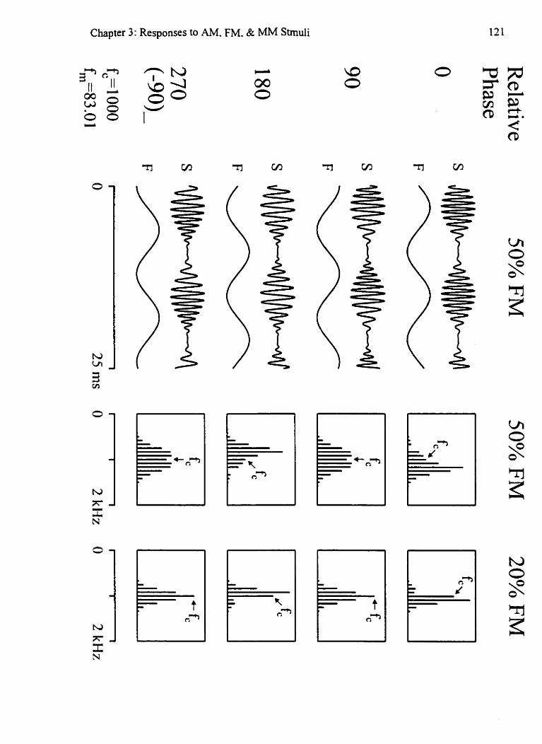
Chapter 3: Responses to AM. FM. & MM Stmuli

Chapter 3: Responses to AM, FM, & MM Stimuli

Please see uext page for figure

Figure 3-3. Independent amplitude and frequency-modulation (IAFM). The upper part of the figure shows the time waveforms for a stimulus with a canier-frequency of 1000 Hz that is 50% AM and 20% FM. The AM occurs at 84.96 Hz. which is slightly faster than the FM. which occurs at 83.01 Hz. The graph in the middle of the figure shows the instantaneous frequency of the sound. As time progresses the maximum frequency shifts increasingly later with respect to the maximum amplitude (see arrows). The lower part of the figure shows the amplitude spectrum of the stimulus over a small range of frequencies near the carrier-frequency. There are two closely spaced sidebands on each side of the carrier. one representing the FM and the other representing the AM (indicated by arrows). There are other small components in the spectrum, which derive from combinations of the two modulating frequencies and the carrier.

Chapter 3: Responses to AM. FM. & MM Stimuli

Chapter 3: Responses to AM, FM, & MM Stimuli 124

Previously we have shown that up to 4 stimuli can be presented to each ear as long as

adjacent stimuli are separated by at least 1 octave (Chapter 1, Table 1-1). Accordingly, in most

of the experiments in this chapter (those using at least 4 simultaneous stimuli in one or both ears)

we used either a "500 Hz octave series" which contained 500, 1000, 2000, and 4000 Hz tones or

a "750 Hz octave series" which contained 750, 1500, 3000, and 6000 Hz tones. For the

experiments in this chapter that presented all of the different 8 tones simultaneousiy, the 500 Hz

octave series was presented to the right ear and the 750 Hz octave series was presented to the left

ear. The right ear stimuli were modulated at 78.13, 83.01, 86.91, and 91.80 Hz and the left ear

stimuli were modulated at 80.08, 84.96, 89.84, and 94.73 Hz. The highly specific frequencies

were due to the requirement for an integer number of cycles of a stimulus within each recording

epoch of 1.024 s (Chapter 2, seaions j.2. 5.5). For MM stimuli, the AM and FM for each carrier-

frequency occurred at the same rate; in other words, for the 500 Hz tone, both the AM and FM

occurred at 78.13 Hz. For the IAFM stimuli we modified the MASTER data acquisition system

(described in Chapter 2) to use one set of moduiation-frequencies for AM and another set for FM

(e.g., the 500 Hz carrier had an AM at 78.13 Hz and an FM at 80.08 Hz). In the remainder of

this Chapter the modulation-Frequencies will be reported with only single digit precision.

The digitally generated auditory stimuli were converted to analog form at a rate of 32 kHz

using 12-bit precision. The analog waveforms were routed to a Grason-Stadler Model 16

audiometer where they were amplified to a calibration-intensity and then attenuated to achieve

the desired intensity levels (60, 50.40, or 30 dB SPL). The stimuli were presented either through

TDH-SOP headphones, calibrated with a Bruel and Kjaer Artificial Ear Type 4152, or through

Emone 3A insert earphones calibrated with a DB 0138 coupler. Both transducers have a

relatively flat intensity response of k3 dB SPL for tones under 4000 Hz, while the 6000 Hz

response is decreased by about 5 dB SPL (headphone) or 20 dB SPL (ear insert). The insert

earphones were not used if the experiment included carrier-frequencies of 6000 Hz. For

simplicity, the attenuation of the 6000 Hz tone is not documented in the figures and tables.

Recordings

Electrophysiological responses were collected from a gold-plated Grass electrode located

at Cz and referenced to the posterior neck (7-8 cm below the inion). An electrode placed over

Chapter 3: Responses to AM, FM, & MM Stimuli .

the clavicle served as ground. All electrode impedances were under 5 kOhrn at 10 Hz.

Recordings occurred in a quiet testing chamber with the subjects lying in a reclining chair.

Because sleeping subjects produce less background noise, we asked our subjects to attempt to

sleep during the experimental session. All subjects slept through most of the experiments. The

responses were amplified using a Grass P50 battery-powered amplifier with the low pass filter set

at 300 Hz, a highpass setting of 1 Hz, and a gain of 10,000. The notch filter was turned off.

The MASTER data acquisition system which was described in Chapter 2 collected most

of the data using an AD conversion rate of 1 kHz with 12-bit precision. Consecutive data epochs

of 1.024 seconds were linked together to form sweeps of 16.384 seconds which were then

submitted to an FFT to produce an amplitude spectrum with a resolution of 0.061 Hz. When an

epoch contained electrophysiological activity over i 9 0 pV, it was rejected and the next

acceptable epoch was used to build the sweep. In each recording period 16 sweeps

(approximately 4 minutes of data) were averaged together. In most of the experiments described

in this chapter, three recording periods were obtained and averaged together during each

condition for each subject. Accordingly, approximately 13- 15 minutes (depending upon the

amount of rejected data) was required to collect data for each condition. However, if the F-ratio

for the average response for a condition did not reach a significance level of ~ ~ 0 . 0 5 for several of

the stimuli (as might occur due to a noisy recording), an additional recording was collected and

the average response was then based on 4 separate recording periods. In Experiments 1 and 2 we

used an older version of the MASTER acquisition system with slightly different parameters

(Chapter 1).

The MASTER system uses the FFT amplitude spectrum to evaluate the evoked response

data in the frequency domain. The components of the spectrum corresponding to the frequencies

of the stimuli each had a specific amplitude and phase. The amplitude of each response was

computed from the square root of the sum of the squares of the real and imaginary components,

with the calculation adjusted to give the baseline-to-peak amplitude of the sine wave. The onset

phase of the response was computed as the angle between the response vector and the real axis.

This phase was adjusted (e.g., converted From sine to cosine) so that it would equal zero when

the response waveform was identical to the stimulus envelope. In order to make the phase more

understandable in terms of the latency of the response, this measurement was converted to "phase

Chapter 3: Responses to AM, FM, & MM Stimuli

delay" by subtracting it from 360 degrees. This is the same as measuring the angle in a clockwise

rather than anti-clockwise direction. Phase measurements were adjusted across the experiments

by subtracting an acoustic delay of 0.9 rns when using ear inserts (and tubes) rather than

headphones. The intricacies and ambiguities of measuring the phase of steady-state responses .

are discussed extensively in Chapter 4

Latencies were estimated from the phase delays measured at multiple modulation-

Frequencies (Experiment 5 ) in two ways. A traditional measure known as "apparent latency"

(Regan, 1966) or "group delay" (Goldstein et al., 1971) was calculated by estimating the slope of

the phase delay versus modulation-frequency graph and dividing this slope by 360. In addition,

the latency was directly estimated using the "preceding cycles" technique (Chapter 4,figures 4.2.

4 . 3 , which calculates the best fit across the different modulation-frequencies for different

numbers of stimulus cycles preceding the response.

Statistical Evaluations of Responses

Jn order to determine if the FFT components at the stimulus modulation-frequencies were

different than backgound EEG activity, the value at each of these Frequencies was compared to

the 120 adjacent frequencies (60 bins above and 60 below the stimulus frequency, or k3.7 Hz,

excluding those frequencies at which other stimuli were modulated) using an F-ratio (Zurek,

1992; Lins et a]., 1996; Dobie and Wilson, 1996; Valdes et al., 1997). As discussed in earlier

chapters, comparing this ratio against the critical values For F at 2 and 240 degrees of freedom

gives the probability of a response being within the distribution of the background noise.

LAFM stimuli evoked two independent responses for each carrier-frequency, one for the

AM response at the Frequency fa, and one for the FM response at the frequency ffm. Two

independent F-tests provided separate probability levels for each of these responses. These were

then combined in order to yield the probability of a response being evoked by a particular carrier-

frequency. This is akin to the meta-analytic procedure, or "Stouffer method", used when

assessing the overall probability of an effect across two separate experiments (as described in

Rosenthal, 199 1, p. 68-70). The equivalent values on the standard normal distribution (2-scores)

for each of the probabilities were added, the resultant value was divided by the square root of 2 to

Chapter 3: Responses to AM, FM, & MM Stimuli

give a combined Z-score, and the probability of this value was obtained from the standard normal

distribution. For example, if the two probabilities are 0.1 1 and 0.09 (neither significant at

p<O.O5), the 2-scores for each of these probabilities are 1.23. and 1.34, and the final Z-score of

(l.23+ 1.34)/1.41 or 1.82 is associated with a probability level of 0.03 (Rosenthal, 199 1, p. 70).

As in the earlier chapters, the amplitude data obtained in the experiments presented in this

chapter were evaluated using repeated measures analyses of variance ANOVA, with Greenhouse-

Geisser corrections where appropriate. Because many of the post-hoc comparisons occumng in a

single experiment were independent (e.g., were due to activation of different regions of the

cochlea), Fisher Least Significant Differences (LSD) were used. Phase data were evaluated using

appropriate tests for circular data (Fisher, 1993). Differences were considered significant when

~ ~ 0 . 0 5 .

Experimental Design Since multiple experiments are reported in this chapter, the experimental designs for each

particular experiment are provided with the results. The experiments presented here are of two

types. Experiments 1, 2 and 3 concern the applied use of M. FM and MM stimuli in

determining thresholds for either modulation depth or intensity. Experiments 1. 5 and 6 were

designed primarily to investigate the physiological processes that underlie the MM response.

Experiment 1: Different Amounts of Ah1 and FM

Eight subjects participated in this experiment. Five levels of modulation were tested for

both AM and FM stimuli. The carrier-frequency was always a 60 dB SPL 1000 Hz tone and the

modulation-frequency was 82.3 Hz. The AM depths were 100, 50, 20, 10, and 5%. The FM

depths were 50, 20, 10, 5, and 2%. The mean amplitudes, vector-averaged phases and incidence

of significant responses at each modulation depth are shown in Figure 3-1. The 50% FM tone

Chapter 3: Responses to AM, FM, & MM Stimuli

Please see nert page for figure

Figure 3-4. Depth of modulation. The left and right sides of the figure show the mean measurements for the AM and FM stimulus, respectively. The top of the figure plots the amplitudes of the responses and the average noise levels (dashed lines), from which the responses were distinguished. The 20% FM evoked a response with a similar amplitude to the response evoked by the 50% AM stimuli. The middle of the figure shows the normalized vector- averaged phases of the responses. The phase data are only plotted for depths of modulation wherein 4 or more subjects showed a significant response amplitude (and were calculated only From the data for these subjects). The phase did not change significantly at different levels of modulation. The bottom of the figure shows the percentage of responses that reached a significance level of p<O.O5.

Chapter 3 : Responses to .a. FM. & MM Stmuli

Chapter 3: Responses to AM, FM, & MM Stimuli . 130

produced a response that was larger than the response at 100% AM. There was no effect of

modulation depth on the phase delay of either response. The phase delay of the response to the

50% AM stimulus was 47 degrees later than the phase delay for the 20% FM stimulus (a

response with a similar amplitude). This difference was significant using nonparametric statistics

(Fisher, 1993, p. 1 14: X2=4.0, df-1 , ~ ~ 0 . 0 5 ) . The average behavioral discrimination limens for

detecting modulation in these stimuli were 5.7% (SD 1.0) for AM and 1.4% (SD 0.4) for FM

(equivalent to a modulation index of 0.085 for FM). The physiological response was detectable

in 50% or more of the subjects at 20% AM and at 5% FM, i.e. at about 10 dB above threshold for

both AM and FM.

Experiment 2: Possible Interactions between AM and FM.

Eight subjects participated in this experiment in order to evaluate the effects of

simultaneously recording responses to two modulated stimuli. AM and FM tones were presented

alone or in combination with other .4M or FM tones. The modulation-frequency was 82.3 Hz for

the 1 kHz carrier and 88.9 Hz for the 2 kHz carrier. [n addition, an MM response was recorded

at 1 kHz with zero phase delay between the AM and the FM, i.e. with the highest frequency

occurring at the highest amplitude. The conditions can be seen in Table 3-1, which also shows

the mean amplitudes of the 1 kHz response (for simplicity the 2 kHz responses are not shown). A

repeated measures ANOVA of the 1 kHz responses indicated a main effect for modulation type

(F=7.85; df=5,9; p<.001) with the MM responses significantly larger than the other types of

response: 28% larger than the simple FM response (pc.01) and 51% larger than the simple AM

response (p<.Ol). The 1 kHz responses at 100% AM and 25% FM were not statistically

different. The response amplitudes did not change significantly when the modulated stimulus

was presented in combination with an AM or FM stimulus at 2 kHz.

Although the AM response was unaffected by the presence of other stimuli, a repeated

measures ANOVA of the I kHz FM responses to stimuli presented either alone and in

combination indicated a main effect (F=10.82; df=3,9; pc.001) with the two tone responses being

significantly smaller than responses to stimuli presented alone. In a separate analysis it was

found that the 2 kHz FM tone was also reduced when presented with a 1 kHz AM tone. Thus,

Chapter 3: Responses to AM, FM, & Stimuli

Table 3-1: Interactions between stimuli (Experiment 2)

- - - - - - -

Stimulus (Carrier ikHz) Other Stimuli Amplitude (nV) Phase Delay (O)

100 % AM none 7W33 177

2kHz 1OO%AM 66*30 204

2 kHz 25% FM 6%30 193

none 83*27 145

2kHz25% FM 66*24 146

MM (1 00% AM, 25% FM) none 106*49 154

while responses to AM stimuli do not decrease when presented with other AM or FM tones, FM

responses show a consistent decrease of about 20% when presented with other FM or AM tones.

The additional stimuli did not significantly affect the phase delay of the response. Once again the

phase delay of the response to the 100% AM stimulus was later than the phase delay for the 25%

FM stimulus. The MM response had a phase delay similar to that of the AM response.

Experiment 3: Multiple AM and Mhl stimuli

Eight subjects participated in each of the 2 paradigms of this experiment. In order to

assess the effects of multiple MM stimulation across a lower range of intensities, we created

stimuli that were either 100% AM or MM (200% AM and 25% FM). The MM stimuli were

created so that the maximum frequency coincided with the maximum amplitude. Eight stimuli

were presented simultaneously, four to each ear. Stimuli were presented at 50,40, and 30 dB

Chapter 3: Responses to AM, FM, & MM Stimuli

Please see neyr page forjigwe

Figure 3-5: Effects of MM on stimuli at different intensities. For the data plotted in the upper half of the figure, the stimuli were 100% AM and 25% FM (&12.5% deviation from carrier-frequency). At 50,40 and 30 dB SPL, the amplitudes were 30%, 49%- and 28% larger for responses evoked by MM compared to those evoked by AM. The increased amplitude for MM was evident at all intensities and frequencies except for 6 kHz. The bottom half of the figure shows the results (from a different group of 8 subjects) when the stimuli were 100% AM and 10% FM (55% deviation from camier-frequency). Amplitudes were 20%. 7%. and 8% larger for responses evoked by MM stimuli compared to AM only stimuli. While 10% FM may be useful in increasing response amplitude at 50 dB SPL, this effect is not evident at lower intensity levels.

Chapter 3: Responses to AM. FM. & MM Stmuli

Chapter 3: Responses to AM, FM, & MM Stimuli 134

SPL during 3 separate recording conditions. The results of this experiment can be seen in Figure

3-5. A repeated measures ANOVA (modulation type x intensity x canier-Erequency) indicated a

main effect for modulation type (F=62.1; df=1,7; pc.001) with the MM responses significantly

larger than the AM responses. Main effects were also found for intensity (F=47.0; df-2,14;

pc.001; ~ = . 5 4 ) with the more intense stimuli evoking larger responses, and carrier-frequency

(F=8.3; df=7,49; pC.00 1 ; ~=.41) with the response being larger at the middle frequencies. The

only significant interaction was found between modulation type and camer-frequency (F=3.7;

df=7,49; pc.05; ~=.60) because the 6000 Hz response failed to be larger for the MM than the

AM stimuli. The lack of any significant interaction between modulation type and intensity level

indicates that the enhanced amplitudes of the MM stimuli persisted across all three intensity

levels. The average MM responses were 35%, 50%, and 30% larger than the AM responses at

50,40, and 30 dB SPL, respectively.

The phase delays of the responses are shown in Table 3-2. Only the results at the higher

intensities are shown, since some of the measurements at 30 dB did not reach significance. The

main finding was that for the carrier-frequencies of 1 kHz and higher, the delays were

consistently later for the AM stimuli than for the MM stimuli. For both AM and MM stimuli, the

phase delays consistently increased with decreasing intensity, with a change equivalent to about

0.7 ms for each 10 dB decrement. As expected, there was a general decrease in phase delay with

increasing carrier-frequency (translating to a decrease in response latency), although these

relative changes may have been slightly exaggerated since the modulation- frequencies also

increased with increasing canier-frequencies.

The larger size of the MM response compared to AM response at 25% FM made its

detection more rapid indicating that the time for the test could be reduced by about a third even at

30 dB. This can be seen in Figure 3-6, which shows the percentage of significant responses that

were evident at 30 dB after different amounts of averaging. The time saved can be estimated by

the horizontal distance behveen the curves.

Chapter 3: Responses to AM, FM, & MM Stimuli . 135

Table 3-2: Phase delays of AM and MM responses (Experiment 3 with 25% FM in MM)

In tensity Carrier-frequency (Hz) Type

(dB SPL) 500 750 1000 1500 2000 3000 4000 6000

Chapter 3: Responses to AM, FM, & MM Stimuli

Please see next page for figure

Figure 3-6. Time for detecting the responses to MM. Data in each graph are from 8 subjects. The graphs show the percentage of the responses, out of 8 different carrier-frequencies (4 in each ear). that reached significance as the number of sweeps averaged increased from 1 to 12. Each sweep contains about 16 seconds of data. The stimuli were presented at 30 dB SPL. The left graph shows data collected for 100% AM and for the MM stimulus with 25% FM. The right graph displays the results (from different subjects) when the FM component of the MM was 10%. MM clearly speeds up the detection of the responses when the FM component is 25% but not when the FM is only 10%.

Chapter 3: Responses to AM. FM. & MM Stmuli

Percentage of Responses Detected

Chapter 3: Responses to AM, FM, & MM Stimuli 138

A second paradigm using an FM depth of only 10% was carried out on a different group

of eight subjects in order to see whether the technique could utilize MM stimuli with greater

frequency-specificity. The results for this experiment can be seen in the lower part of Figure 3-5.

The MM enhancement is clearly less for 10% FM than for 25% FM. A repeated-measures

ANOVA identical to that used in Experiment 2 showed main effects for modulation type

(F=7.8;df=1,7; pc.001; E= 1). intensity level (F45.5; df=2,14; pC.05; ~ = . 7 0 ) , and carrier-

Frequency (F=12.6 ;df=7,49; pc.001; ~= .39) . Unlike the first paradigm, the interaction between

modulation type and carrier-frequency failed to reach significance. The average MM responses

were 20%, 3%, and 12% larger than the responses to the AM stimuli at 50, 40, and 30 dB SPL,

respectively.

Experiment 4: Changing the FM phase in the MM stimulus

Ten subjects participated in each of the 2 paradigms of this experiment. An examination

of the phase results of Experiments 2 and 3 showed that the MM response often had a phase

delay that was shorter than that of the AM response, as though it were tending toward the shorter

phase delay of the FM response. This suggested that the MM response might be the result of the

vector addition of independent AM and FM responses. The largest MM response would then

occur when the phase of the FM stimulus relative to the AM stimulus causes the two components

of the MM stimulus evoked responses to be in phase. Accordingly, we decided to investigate the

effects of changing the relative phase between AM and FM in the MM stimuli. The stimuli in

our first paradigm used the same carrier and modulation-frequencies as in Experiment 3, but

were presented at only 50 dB SPL. In order to determine if changing the phase of the FM

affected the amplitude of the MM response, four different relative phases (0. 90, 180 and 270')

were used in the MM stimuli in four separate conditions. The responses to simple AM and FM

stimuli were also recorded, for a total of six experimental conditions in this paradigm.

The results are shown in Figure 3-7. A repeated measures ANOVA (modulation type x

carrier-frequency) showed main effects for modulation type (F=l I . l 1 ; df=S,55; p<.OO 1 ; ~ = . 4 1)

and carrier-frequency (F=7.23; df=7,77; pc.01; ~ = . 3 8 ) , and a significant interaction (F=4.22;

df=35,385; pc.0 1; E=. 15) due to the divergent response seen at GOO0 Hz. Fisher LSDs indicated

Chapter 3: Responses to AM, FM, & MM Stimuli 139

that MM with FM phases set at 0 (or 360) and 270 (or -90) degrees evoked significantly larger

(10% and 25%. respectively) responses than the AM only condition. MM with FM phases of 90

and 180 degrees evoked responses that were significantly smaller than the simple AM response.

The pure AM response was significantly larger than the pure FM response. The effects of

stimulus phase were consistent for every carrier-frequency except 6000 Hz.

The possibility that the MM response represents the vector addition of the AM and FM

responses is illustrated diagrammatically in Figure 3-8. The relative phase ( cp ) between the AM

and the FM responses can be estimated by fitting a baseline-offset sine wave to the data obtained

for the MM stimuli using different phases between the AM and FM components. This can be

done using either an FFT analysis or an iterative least-mean-square fitting of a sine wave. The

amplitude of the sine wave represents the FM component in the MM response, and the amount of

baseline-offset represents the amplitude of the AM component. Each response may be decreased

a little by the presence of the other. The FM response might be decreased due to the AM

envelope, and the AM response might be decreased due to the loss of synchronization of nerve

fibers as would occur with changes in frequency. Alternatively, the two responses might both be

reduced by overlap of common neural generators. The results of this analysis (Table 3-3)

indicated that the MM response could be reasonably represented as the vector addition of

separate AM and FM responses, with the AM response amplitude reduced by about 10%, and the

FM response amplitude reduced by about 2 1 %. The estimated phase difference was very similar

to the actual phase difference.

Chapter 3: Responses to AM, FM, & MM stimuli

Please see next page for figure

Figure 3-7. Effects of FM phase on the MM response. The four upper graphs show the amplitudes separately for the different carrier-frequencies. The left graphs in this figure compare response amplitudes for stimuli that were evoked by AM or FM alone, while the right graphs show the response amplitudes for the MM stimuli with different phases of FM relative to the AM. The data obtained at 0" are re-plotted at 360'. The responses for the 4 lower carrier- frequencies are shown separately from those for the 1 higher carrier-frequencies so that the individual values can be seen more easily. The bottom set of graphs shows the mean amplitudes across all carrier-frequencies. The dotted line shows how the data can be fit using the technique illustrated in Figure 3-8. For all carrier-frequencies except 6000 Hz the MM response is larger when the phase is 270 or 360 degrees than when it is 90 or 180 degrees.

Chapter 3: Responses to AM. FM. & MM Stmuli

Amplitude (nV)

Chapter 3: Responses to AM, FM, & MM Stimuli

Please see nert page for figure

Figure 3-8. Analysis of mixed modulation responses. This figure shows diagrammatically how the MM response can be considered as the vector addition of independent responses to the AM and FM components of the stimulus. The left diagram shows the vector addition on a polar plot. The AM response is shown as the vector originating at zero. Added to this is an FM response vector of smaller amplitude and with a different phase. These responses (vectors) were evoked by stimuli that had the same phase, i.e. the relative phase between AM and FM stimuli was zero. The relative phases of the responses would be altered by changing the relative phase of the FM stimulus. Increases in the phase of the FM stimulus will rotate the FM response vector clockwise. The response to MM is shown as the dotted-line vector. The FM and AM response vectors will line up to produce the largest MM response when the relative phase between AM and FM equals cp. The right side of the figure illustrates how cp can be derived using the MM amplitudes obtained when the relative phase between the AM and FM stimuli is varied. The amplitudes are fit with a sine wave having a baseline-offset. The size of the baseline-offset is equivalent to the amplitude of the AM response and the amplitude of the sine wave is equivalent to the amplitude of the FM response. The maximum MM amplitude (dotted line) occurs when the relative phase between AM and FM equals cp.

Chapter 3: Responses to AM. FM. & MM Stmuli

Amplitude

Chapter 3: Responses to AM, FM, & MM Stimuli

Table 3-3: Effects of combining AM and FM

-- . . . .

I - 3 3 4 5 6 7 8 9 10 11 Carrier AIM AM FM FM LMM percent MM percent estim. actual

Frequency amp. phase amp. phase .&I AM FM FM phase phase (Hz) (nV) delay (nV) delay amp. alone amp. alone diff. diff.

The data in columns 1-5 are obtained from the experiment, while data in columns 6-10

are derived from the model illustrated in Figure 3-8. Using this model, the data in column 6

represent the estimated response to the AM component of MM. The data in column 7 shows the

estimated amplitude as a percentage of the actual amplitude of the AM responses alone (column

2). Columns 8 and 9 show similar data for the estimated FM responses. The data in column 10

show the phase differences between AM and FM responses that would produce the maximum

amplitude of the MM response, as predicted by the model. The actual differences in phase delay

between the AM and FM responses (column 5 minus column 3) are given for comparison in

column 1 1 and are very close to those predicted for carrier-frequencies from 750 and 4000 Hz.

Chapter 3: Responses to AM. FM, & MM Stimuli 145

Since the results indicated that the MM response was generally largest when the phase

difference between the AM and FM components was between 270 (-90) and 0 degrees, a second

paradigm was studied (with a different set of 10 subjects) to check this range more closely.

Accordingly, the stimuli were the same as in the first part of the experiment except they had

relative phases of 0, 135 270, and 3 15 degrees. Our prediction was that the 3 15 degree condition

would produce the largest responses while the 135 condition should produce the smallest. An

additional fifih condition presented AM only stimuli to provide a baseline. The five conditions

were tested at both 30 and 50 dB SPL. Average results across the two ears are shown in Figure

3-9 for the 50 dB SPL condition. The largest response occurred when the phase was 315

degrees. The optimum phase (9) for the MM stimulus at 500, 1000, 2000 and 4000 Hz,

calculated using the techniques shown in Figure 3-8, resulted in the following estimations: -293.

-58, -40 and -48 degrees at 50 dB SPL, and -220, -37, -42 and -98 degrees at 30 dB SPL.

Experiment 5. Latency estimates for AM and FM stimuli

Eight subjects participated in this experiment. The preceding experiments had

consistently indicated that the AM responses occurred with a later phase delay than the FM

responses. Since phase delay is not directly transformable to latency, we decided to estimate the

latencies of Ai i and FM responses by recording the same responses at different rates (see

Chapter 4, Figwe 4-5). The carrier-frequencies were a 500 Hz octave series and the stimuli were

either 20% FM (left ear) or 100% AM (right ear). The FM rates (left ear) were 80.1, 85.0, 89.8,

and 94.7 Hz and the AM rates (right ear) were 78.1, 83.0, 86.9, and 91.8 Hz. Each carrier was

presented at each modulation-rate across four recording conditions. Stimuli were presented at

50 dB SPL using insert earphones. The vector-averaged phase delays for these subjects are

shown in Figure 3-10. Table 3-4 shows the latencies estimated both by calculating the apparent

latency and by determining the number of preceding cycles. The AM response generally occurred

later than the FM response. The preceding-cycles technique indicated that both kinds of response

were preceded by one cycle of the stimulus (see Chapter 4, Figures 4-2, 4-5).

Chapter 3: Responses to AM, FM, & MM Stimuli

Please see nert page for figure

Figure 3-9. Effects of FM phase on the MM response. This figure shows the average results obtained in the second part of Experiment 4. MM responses were obtained using stimuli with FM phases of 0°, 35", 270". and 3 15'. The data are plotted in the same way as in Figure 3-7 so that the amplitudes obtained with the 0" phase are also re-plotted at 360". For each carrier- frequency. the data have been fit with a sine wave according to the logic illustrated in Figure 3-8.

Chapter 3: Responses to AM. FM. & MM Stmuli

Amplitude (nV)

Chapter 3: Responses to AM, FM, & MM Stimuli

Please see n a t page for figrrre

Figure 3-10. Latencies of the A i i and FM responses. This figure shows the average phase delays obtained for FM and AM stimuli recorded during Experiment 5 . The phase delay increases with increasing modulation rate in an approximately linear fashion. An "apparent latency" can be calculated by measuring the slope of the phase versus modulation rate.

Chapter 3: Responses to AM. FM. & MM Stmuli

Phase Delay (degrees)

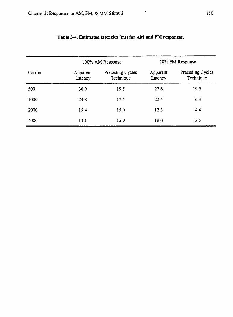
Chapter 3: Responses to AM, FM, & MM Stimuli

Table 3-4. Estimated latencies (ms) for AM and FM responses.

Carrier

100% AM Response 20% FM Response

.Apparent Preceding Cycles Apparent Preceding Cycles Latency Technique Latency Technique

Chapter 3: Responses to AM, FM, & MM Stimuli

Experiment 6: Independent amplitude and frequency-modulation (IAFM)

Ten subjects participated in each of the 2 paradigms of this experiment. In the first

paradigm, the stimuli consisted of the 750 Hz octave series, which was prescnted to the left ear at

50 dB SPL using the same modulation rates that were used in Experiments 3 and 4. Four types of .

stimuli were used: AM, FM, MM, and IAFM. The FM was always 20%. The AM was set at

either 100% or 50% for the AM and LAFM stimuli, thus giving a total of 6 recording conditions.

The relative phases of all FM stimuli were 90 degrees. The maximum frequency in the MM

condition thus occurred one quarter of a cycle before the maximum amplitude (cf. Figure 3-1,

second stimulus). Accordingly, in this paradigm the responses to MM should generally be

smaller than the responses to AM (cf. Figure 3-7).

Sample data From one subject are shown in Figure 3-1 1. The eight stimuli that were

presented to one ear clearly produce eight corresponding spectral peaks in the IAFM response.

The mean amplitudes of the AM. FM and LAFM responses are shown in Figures 3-12. For

carrier-frequencies of 750 and 1500 Hz, the amplitudes of the response to the AM component of

the IAFM response were smaller than the amplitudes of the response to AM alone. The amount

of reduction is similar for both 100% and 50% AM. For the same carrier-frequencies, the

response to the FM component of IAFM is greatly attenuated, when AM is loo%, compared to

when FM is presented alone, but not much when the AM is 50%. The response to the MM

stimulus was, as expected from our choice of phase, smaller than the response to either FM alone

or AM alone. Table 3-5 shows that the amplitudes and phases of the MM response were close to

what would be predicted from vector-addition of the separate AM and FM responses (with some

additional reduction in the amplitude).

Chapter 3: Responses to AM, FM, Sr MM stimuli

Please see neyt page forfigure

Figure 3-11. Multiple auditory steadystate responses. This figure shows the responses obtained in one subject for some of the conditions of Experiment 6. On the left of the figure are shown the responses viewed in the frequency domain. Only part of the amplitude spectrum is shown. At the Frequencies of the stimuli (indicated by arrowheads) the amplitudes measured in the spectrum are higher than the background noise level. On the right of the figure the polar plots of the responses at each of the modulation-frequencies are shown. The circles represent the confidence limits of the noise. If the zero point is not included in the circle, the response can be considered as significantly (p<0.05) different from the background noise. The first set of responses represent those obtained in response to 100% AM. The middle responses are those obtained using 20% FM. The bottom set of responses represent the responses when a single carrier-frequency was independently modulated in both amplitude and frequency (IAFM). These responses tend to be slightly smaller in amplitude than those obtained when only one type of modulation occurred. The phases are quite similar. Note that the phase angle between the vector and the horizontal axis represents the "onset phase" when measured counter-clockwise and the ''phase delay" when measured clockwise.

Chapter 3: Responses to AM. FM. & MM Stmuli

Chapter 3: Responses to AM, FM, & MM Stimuli

Please see next page for figure

Figure 3-12. Response to independent amplitude and frequency-modulation (IAFM). This figure compares the amplitudes of the responses to stimuli that were simply modulated in amplitude or frequency to the same responses when the modulations occurred together in the same stimuli. The amplitude of the response to AM is shown on the left graph and to FM on the right graph. The amplitudes decreased for the IAFM stimuli, with the decrease being larger for the lower carrier- frequencies.

Chapter 3: Responses to AM. FM. & MM Stmuli

Amplitude (nV)

Chapter 3: Responses to AM, FM, & MM Stimuli

Table 3-5 Mixed modulation at a phase of 90"

100% AM 20% FM MM Predicted MM

Camer amplitude phase amplitude phase amplitude phase amplitude phase (Hz) (nv) delay(") (nV) delay(') (nV) delay(") (nV) delay(")

The values for the recorded amplitudes and phases (columns 2-7) were obtained by vector

averaging across subjects. The amplitudes are therefore smaller than those shown in Figure 3-1 1

where the amplitudes were averaged without regard to phase. The values predicted in columns 8

and 9 were obtained by vector summation of the data represented in columns 2-5. The bracketed

data in column 5 represent what the phase delay would be if the FM were at 0° relative to the AM

(making the data homologous to the phase delays in preceding tables).

A second paradigm examined how effectively, compared to 100% AM stimuli, the LAFM

stimuli could produce detectable responses as intensities approached threshold. Stimuli were

presented to the subject's left ear using insert earphones. Two types of stimuli were used. The

first were 100% AM carrier-frequencies of 500, 1000, ZOO0 and 4000 Hz that were modulated at

80.1, 85.0, 89.8, and 94.7 Hz, respectively. The second were LAFM carrier-frequencies that were

both 50% AM, at the previously noted modulation-rates, and 20% FM at 78.1, 83.0, 86.9, and

91.8 Hz. .An AM depth of 50%, rather than 100%, was used since the FM response may have

been previously reduced in amplitude because the ability of FM to evoke a response may have

been decreased during the periods when the amplitude envelope intermittently approached zero.

There were nine experimental conditions: each type of stimulus was presented at 20, 30, 40, 50

dB SPL. A no-stimulus condition provided control estimates of detection probability. The

detectability of the response for each of the stimuli was determined using the F-ratio test on each

Chapter 3: Responses to AM, FM, & MM Stimuli

of the three sub-averages collected in each condition, as well as on the overall average response.

This under-estimated the final significance of the responses, but provided a better evaluation of

the incidence of detectable responses (since 30 separate response probabilities were obtained for

each stimulus and intensity rather than 10). For the LAFM responses, the probabilities of the

significance of the AM and FM responses were combined using the Stouffer method.

The results are shown in Figure 3-13. A three-way (intensity, stimulus-type and carrier-

frequency) repeated-measures ANOVA was used to assess the amplitudes. The amplitudes

increased with increasing intensity (F=22.9; d64,36; pC.00 1 ; E =.3O). The 100% AM responses

were significantly larger than either of the components of the LAFM response (stimulus-type

main effect, F=12.1; df=2,18; pC.01; ~ = . 5 7 ) . The responses were larger at the middle

Frequencies (frequency main-effect: F=9.5; df=3,27; p<.01; ~=..66) , with a significant interaction

between frequency and intensity (pc.01). The percentage of detected responses increased with

increasing intensity. The combined detectability for the two responses to the IAFM stimulus was

similar to the detectability for the 100% AM response and both were significantly larger than

either of the IAFM components alone (comparing the four results over all intensities: %'=34.1,

dk3 ; pc.001). Based on the average results rather than the sub-averages. the average thresholds

for 500, 1000, ZOO0 and 4000 Hz stimuli were 38, 30, 22, and 26 dB for the 100% .4M stimuli

and 3 1,24,21 and 27 dB SPL for the LAFM stimuli using the combined approach.

Physiological Processing of ARI and FhI

The results obtained in these experiments have clear implications about the physiological

mechanisms underlying the perception of AM and FM. For the same carrier-frequency, the

processes that mediate our perception of AM and FM seem quite independent. The response to

MM stimulation is reasonably well explained by the vector-addi tion of the individual responses

to AM and FM (Experiments 3. 4, and 6). The modeled results suggested a reduction in

amplitude for the AM and FM responses of only 10-20% which would indicate little overlap of

the neuronal generators of these responses. Furthermore, these reductions in amplitude may be

reasonably explained by other mechanisms. The FM response is probably reduced somewhat in

Chapter 3: Responses to AM, FM, & MM Stimuli

Please see next page for figure

Figure 3-13. Effects of stimulus intensity on IAFM responses. This figure compares the responses to LAFM stimuli (50% AM and 20% FM) to the responses to 100% AM stimuli. The top set of graphs shows the amplitudes for each of the 4 carrier-frequencies. The dotted line represents the average noise level in the adjacent bins of the FFT. The response amplitudes for the no-sound (NS) condition are at the level of the residual background noise. The amplitude increases with increasing intensity above 20 dB SPL, with the amplitude being larger at the middle frequencies than at 500 or 4000 Hz, and with the amplitude for the 100% AM response being larger than either of the two components of the LAFM response. The lower graphs show the percentage of responses that were considered as significantly ( ~ ~ 0 . 0 5 ) different from the background noise. When there is no response present in the no-sound condition the probability of detecting a response is approximately 5% as would be expected from the statistics of the test. The response to the 100% AM stimulus is more readily detectable than the responses to either of the components of the IAFM response. The dashed line represents the percent of responses detected if the probabilities of the two responses to the IAFM stimulus were combined. The data in these graphs are based upon sub-averages of the response. The actual final percentages of responses detected on the basis of the full average would be significantly higher than that portrayed in these graphs.

Chapter 3: Responses to AM. FM. & MM Stmuli

Percent Detected Amplitude (nV)

Chapter 3: Responses to AM, FM, & MM Stimuli

amplitude by the concomitant modulation of the amplitude of the stimulus, since it is not easy to

follow the frequency of the stimulus when the amplitude intermittently goes to zero. Similarly,

the compound AM response might be slightly reduced if the neuronal responses that contribute to

the compound response come From different regions of the cochlea that are activated at slightly

different latencies.

Probably the most convincing demonstration of the independence of these two processes

occurs in the experiments that used one carrier-frequency with different modulation-frequencies

for AM and FM - independent amplitude and frequency-modulation (Experiment 6). Despite the

fact that the modulations are very close together and the peaks in the response spectra almost

superimposed (Figure 3), the recorded responses show clearly defined steady-state components at

each of the modulation-frequencies.

The usual explanation for how AM and FM stimuli are processed in the cochlea focuses

upon the asymmetry of the cochlear activation pattern (Zwicker and Fastl, 1990). The general

conclusion is that AM is mediated by neurons with characteristic frequencies that are higher than

the carrier-frequency of the modulated tone, whereas FM is mediated by neurons most sensitive

to frequencies lower than the carrier-frequency of the stimulus. However, the cochlear activation

pattern does not always map directly onto neuronal discharge patterns. The discharge rate of

auditory nerve fibers show non-linear relationships to changes in the intensity of the stimuli.

There is saturation at high intensities, and the rate of discharge varies differently with intensity

depending upon the frequency of the stimulus relative to the characteristic fiequency of the

responding fiber. Basically the response versus intensity slope is more rapid when the stimulus

fiequency is at or below the characteristic fiequency of the fiber than when the stimulus

Frequency is higher (Geisler et al.. 1971; Sachs and Abbas, 1974: Yates et al.. 1990). Recent

results have clearly demonstrated that the hair cells and the auditory fiben respond better at a

lower fiequency than the characteristic frequency when the intensity of the stimulus is increased

(Zwislocki, 1991; Smith, 1998). FM stimuli are probably mediated best by hair cells and

neurons with characteristic frequencies lower than the camer-frequency of the stimulus. This

occurs since the higher cut-off slope of the tuning curve makes the responding system

particularly sensitive to fiequency changes at stimulus frequencies above the characteristic

fiequency.

Chapter 3: Responses to AM, FM, & MM Stimuli 161

These concepts can be illustrated by refemng to "iso-rate contours" for the auditory nerve

fibers (Figure 3-14). These diagrams have unfortunately only occasionally been produced (e.g.

Geisler et al., 1974) although they can be derived fiom the more commonly presented iso-

intensity contours (e-g., Rose et al., 1971). Different fibers will show different slopes for the iso- -

rate contours (Winter et al., 1990) but the general idea shown in Figure 3-14 should be consistent

across most fibers. The figure also shows how AM and FM stimuli can be mapped onto such a

diagram. The lines representing the AM and FM stimuli are positioned at locations that show

maximum neuronal activation. In the diagram, the stimulus lines cross the largest number of

rate-contours. The best AM response occurs when the carrier is slightly below the characteristic

frequency of the fiber, whereas the best FM response occurs when the carrier-frequency is

slightly above. If the carrier-frequency of an FM stimulus were located within the neuronal

response area so that the stimulus goes through iso-rate contours on both sides of the response

area, the neuron would respond at twice the modulation-frequency (cf. Khanna and Teich

(1 989b).

The latency data that we obtained for the AM and FM responses do not easily fit with this

view. The AM response occurs with a phase delay that is generally a little later than that of the

FM response. This is confirmed by the estimated latencies in Table 3-4, which try to resolve

some of the general ambiguities associated with determining latency from phase (see Chapter 4,

Figure 4-2). If the travelling wave is a major determinant of the response latency, our results

would suggest that the AM response is mediated at some more distant region of the cochlea than

the FM response, a region concerned with lower frequencies. However, any phase measurement

of the FM signal is arbitrary. We, and the literature, have defined the zero point of the FM

stimulus relative to the high frequencies in the signal. We could just as easily have determined

the phase relative to the low frequencies in the signal. This would have given a response that is a

half-cycle earlier or later than what was measured. This could have shifted the latency that we

measured using the "preceding cycles" technique. However, it should not have affected the

latency as measured by the "apparent latency" or "group delay" technique, since this

measurement is unaffected by where in the cycle the response is initiated. Here, the FM response

Chapter 3: Responses to AM, FM, & MM Stimuli

Please see next page for figure

Figure 3-14. Mechanisms of processing AM and FM. This figure shows a diagrammatic iso- rate contour plot for an auditory nerve fiber. The figure is loosely based on the data of Geisler et al. (1 974). The fiber is most sensitive to low-intensity stimuli at the "characteristic frequency" (CF). Within the shaded response area of the fiber, the contours indicate increasing rates of discharge. The two straight lines on the figure represent stimuli used For AM or FM stimulation. These are positioned at the locations where they would elicit the largest response from the fiber at the Frequency of modulation. The circles represent the carrier- frequencies of these optimal stimuli. The largest response to AM occurs when the carrier-frequency is less than the characteristic frequency of the fiber, whereas the largest response to FM occurs when the camer- frequency is higher. The inset diagram shows optimally responding neurons for AM and FM of a particular carrier-frequency

Chapter 3: Responses to AM. FM. & MM Stmuli

Intensity (dB) -

Chapter 3: Responses to AM, FM, & MM stimuli

also tends to be earlier than the AM response.

The latency of the response may, however, be determined as much by the filtering effect

of the hair cell response-system as by the actual time to move along the basilar membrane. This

idea is discussed more fully in Eggermont (1979), and reviewed in Chapter 4 of this thesis. If

this filtering concept is true, then the response latency will be shorter when the activation occurs

through the edges of a filter rather than at its center. This could explain the earlier latencies that

we measured for the FM responses.

In effect, we are suggesting that the response to FM is mediated by means of AM with a

varying location on the b a s h membrane for the modulation. Saberi and Hafier (1995; and also

Saberi, 1998) have demonstrated that the binaural integration of FM and AM signals can be

explained on the basis of FM-AM conversion at the level of the cochlear bandpass filter.

Although FM is coded mainly as a moving AM at the level of the cochlea, FM must later

produce another set of effects or it would be perceived the same as AM. At the modulation-

frequencies that we are using AM and FM are perceptually very similar, but at low frequencies

they are quite different. The explanation for this used by Zwicker and Fast1 (1990) is that the

information about the phase of the sidebands occurs outside of the critical band mediating the

carrier when the frequency of modulation is high. Although the sidebands are processed (through

other critical bands) the relative phase between the sideband and the carrier (determining the AM

or FM nature of the signal) cannot be perceived. This interpretation of the response in terms of

the amplitude spectrum may be valid for perception where information is integrated over a period

of time of 200 rns or more. but it is not very helpful when explaining a moment-to-moment

following response like the steady-state response.

One reason for the independence of the AM and FM response from the same carrier-

frequency would then be that the responses come from different regions of the cochlea. The AM

response would be mediated at a more apical regon than the FM response. It is possible that this

might be investigated using AM and FM at different carrier-frequencies and bringing these close

together to see where interference occurs. However, the multiple interactions between the

carriers (beats, suppression, masking) would make the results very difficult to understand.

The steady-state responses we are recording probably represent activity at early stages in

Chapter 3: Responses to AM, FM, & MM Stimuli

the analysis of the auditory information. Despite the latencies of between 15 and 20 ms

@receding-cycles technique), the responses probably originate in the brainstem with the delay

caused by several synapses. The responses are probably generated by modulation-sensitive

neurons in the brainstem, generating compound fields that can be recorded at the scalp. We found -

no evidence for large interference between modulations of different camen (Experiment 2). FM

responses were susceptible to the presence of other stimuli, perhaps because they are more easily

masked as they move over a wider range of the basilar membrane. The amplitude decrease in

these FM responses was only about 20% and this still makes it possible to record multiple

responses simultaneously. The majority of the neurons generating the steady-state responses

probably do not integrate across spectral regions or across different types of modulation. This

integration clearly must occur to explain the perceptual interference (Yost and Sheft, 1989;

Wilson et al., 1990) but this is probably at later stages in processing (and might be detectable

through slower steady-state responses). The steady-state responses that we record at high rates of

modulation are similar to the unit responses reported in the dorsal cochlear nucleus where

modulation phase-locking occurs for specific carriers (Zhao and Liang, 1997).

Clinical Usefulness of the Steady-state Responses

Cohen et al. (1991) reported that MM stimuli could evoke significantly larger steady-state

responses than AM stimuli. We previously demonstrated that MM stimuli with 25% FM at 50

dB SPL intensity levels evoked responses that reached significance about twice as rapidly as the

responses to 100% AM stimuli (Chapter 2, Figure 2-6). In the experiments of this chapter, we

show that the enhancement of the response persists at 40 and 30 dB SPL (Figure 3-5). If a

response is 30% larger, then the residual noise in the recording can be 30% larger for the same

signal-to-noise ratio. Theoretically. this would occur when averaging (1 /1 .3)2 or 59% as many

responses. This fits with our results showing the responses to MM stimuli reach the same levels

of significance in about 2/3 the time compared to the responses to simple AM stimuli. For AM

stimuli presented at 50 dB SPL the MASTER technique currently requires between 3 and 6

minutes to obtain significant responses for all eight stimuli, in sleeping adult subjects. Less

intense stimuli produce smaller responses. causing recordings for near-threshold stimuli (20 or

30 dB SPL) to require more time before reaching significance. The savings in time obtained by

Chapter 3: Responses to AM, FM, & MM Stimuli

using MM stimuli can therefore significantly improve testing efficiency.

At about 30 dB SPL the MASTER technique, using AM only stimuli, begins to fail to

show significant responses even though subjects can hear the stimuli. In Experiment 6 we were

able to estimate the electrophysiological thresholds and found levels close to 30 dB SPL. This

fits with data reported previously by Lins et a1 (1996). These thresholds were 10-1 5 dB above

the behavioral thresholds. both behavioral and electrophysiological recordings being obtained in

a quiet room but not one properly sound-attenuated for audiometry. Herdman and Stapells

(2000) found electrophysiological thresholds to Ah4 stimuli near 20 dB SPL, again at about 10

dB above behavioral thresholds. Two factors may have accounted for their lower thresholds:

their use of a properly sound-attenuated chamber, and their use of 5 dB steps. Because MM

stimuli evoke larger responses than AM stimuli even at the near threshold (30 dB SPL) intensity

levels, the use of MM stimuli when evaluating thresholds should make the technique more

efficient and more accurate. The increases found in adults should also be found in infants since

behavioral evidence has suggested that by 1-6 months infants have the ability to process

frequency-modulation (Aslin. 1989; Colombo and Horowitz, 1986; Rickards et al, 1994). The

hypothesized improvement in the MASTER technique for assessing thresholds in both infants

and adults needs to be confirmed.

The MM responses are not always larger than those evoked by 100% AM stimuli. In

order for the MM responses to be larger, the relative phase for the FM component of the MM

stimulus should be between 270 (-90) and 0 degrees for stimuli between 750 and 1000 Hz.

Different phases may be better for the 500 and 6000 Hz stimuli (for example, 35 and -208

respectively). Further study to see how to improve thresholds at these low and high frequencies

is probably required. Different phases for the MM as well as different modulation-frequencies

might be tested to see what parameters are optimal for the response. As discussed by Cohen et a1

(1991), a MM stimulus created by aligning the highest frequencies with the maximum amplitude

will have its spectrum shifted to the higher frequency region (cf. top of Figure 3-2). This can be

compensated in a clinical test by adjusting the carrier-frequency in order to keep the MM

stimulus centered on the frequency of interest. However, it should also be noted that using only

20-25% FM the stimuli remain similar to the spectra produced by a 100% AM stimulus.

Chapter 3: Responses to AM, FM, & MM Stimuli 167

The IAFM stimuli produced 1 responses for each carrier-frequency. Due to the relative

independence of the AM and FM responses we had anticipated that the two LAFM responses

might provide a more efficient evaluation of responsiveness than the single response to 100%

AM stimuli. However, this does not seem to be the case (Figure 3-13). The evaluation of these

responses using the Sbuffer method failed to show that this method would be more useful than

simply using MM stimuli in creating a more rapid hearing test. A major problem was that the

response to the FM component of the IAFM was larger when the AM was 50% than 100%,

which produces a smaller AM response. Since the combined detectability of the LAFM responses

did not differ significantly from the detectability of the 100% AM response, and since the MM

response is more easily detected than the AM response, audiometry is probably best performed

using MM stimuli.

A large amount of work with the auditory steady-state responses has examined at how

well they can estimate hearing thresholds (e.g. Aoyagi, 1994; Rance et ai., 1995; Lins et a!., 1996;

Herdman and Stapeils, 3000). The modulation of a carrier tone provides a signature by which the

system's response to the tone can be detected and the stimulus is then decreased in intensity until

there is no response. The steady-state responses can also estimate how well the auditory system

processes differences in frequency and intensity at supra-threshold intensities. Rather than using

a set amount of modulation and decreasing the intensity of the stimulus, we can use a set

intensity and decrease the amount of modulation to obtain a detection threshold (or limen) for

FM or AM depth. The electrophysiological thresholds for detecting modulation using steady-state

responses (Experiment I ) are close to those obtained behaviorally. These findings suggest that

these responses to rapid AM and FM may provide useful measurements of frequency and

intensity discrimination. Psychophysical studies using slow rates of modulation have found that

FM but not AM can be impaired in hearing-impaired individuals (Lacher-Fourgere and Demany,

1998). These findings might also be demonstrable at higher modulation rates using physiological

rather than psychophysical measurements. In assessing rhe suprathreshold discrimination of

frequency and intensity, the IAFM technique may be very helpful. since it provides two

independent measures of discrimination for each carrier.

The human auditory steady-state response is able to follow at high modulation-

frequencies. Rickards and Clark (1984) recorded steady-state responses at modulation-

Chapter 3: Responses to AM, FM, & MM Stimuli 168

frequencies up to 450 Hz (although data are only graphed to 130 Hz). We have demonstrated

reliable responses in the 160-190 Hz range (see next chapter). The amplitude is smaller than

when the modulation-frequency is in the 80 to 100 Hz range but since the noise is also smaller,

the responses remain significant. The.ability of the auditory system to follow rapid changes in the

frequency or amplitude of the sound is assessed psychophysically by means of temporal

modulation transfer functions (Viemeister, 1979). These functions are abnormal in patients with

sensorineural hearing loss, particularly for higher frequencies of modulation (Bacon and

Viemeister, 1985; Formby, 1987). Evaluating the steady-state responses at faster rates may help

detect individuals who have problems processing rapid formant-transitions in speech (Tallal et

al., 1996). Since the temporal modulation of speech sounds may serve as cues to facilitate the

recognition of consonants (Van Tasell et al., 1987; Shannon et al., 1995). it is possible that the

ability of the steady-state responses to follow rapid modulation-frequencies may relate to the

ability of the auditory system to accurately process speech.

C ~ N C L U ~ I ~ N ~ MM stimuli may be useful in clinical application of the MASTER technique by evoking

larger responses than AM or FM alone at intensities as low as 30 dB SPL. The MM

augmentation can be explained by the simple vector averaging of the AM and FM responses.

which seem to be generated in largely independent systems. Audiometry using the steady-state

responses is therefore best performed using MM stimuli. Stimuli with independent amplitude and

Frequency-modulation (IAFM) provide two separate responses from each carrier-frequency.

They do not yield any better evaluation of threshold than using 100% AM tones. but they may

become useful in objectively evaluating suprathreshold discrimination.

AUDITORY STEADY-STATE RESPONSES:

PHASE AND LATENCY MEASUREMENTS

A portion of this material has already appeared in M. S. John and T. W. Picton (2000) Auditory sleady-state responses: phase and latency measurements. Hearing Research. 14 1 ; 57-79. Reprinted with permission

Some data, in alternative form, were also presented at the meeting of the Neuroscience Society, Los Angeles, November, 1998, and at the meeting of the International Electric Response Audiometry Study Group in Tromsa, Norway, June, 1999.

Chapter 4: Phase and Latency Measurements

Human auditory steady-state responses were recorded to four stimuli, with carrier-

frequencies (f,) of 750, 1500. 3000 and 6000 Hz, presented simultaneously at 60 dB SPL. Each

carrier-frequency was modulated by a specific modulation-frequency (f,) of 80.6, 85.5, 90.3 or

95.2 Hz. By using four different recording conditions, we obtained responses for all

permutations of fm and f,. The phase delays (P) of the responses were unwrapped and converted

to latency (L) using the equation: L = P/(360tf,,,). The number of cycles of the stimulus that

occurred prior to the recorded response was estimated by analyzing the effect of modulation-

frequency on the responses. These calculations provided latencies of 20.7, 17.7, 16.1 and 16.1

rns for camer-frequencies 750, 1500, 3000 and 6000 Hz. The latency-difference of about 4.5 ms,

which exists between low and high camer-frequencies. was also obtained when stimuli were

presented with at faster modulation rates (160-1 80 Hz). both monaurally and binaurally, at

different intensities. alone or in conjunction with other stimuli, and using modulation-frequencies

that were separated by as little as 0.24 Hz. This frequency-related delay is greater than that

measured using transient evoked potentials because of differences in how response-latencies are

determined. Combining the latencies for steady-state responses with the latencies for oto-

acoustic emissions might provide estimates for both transport-time and filter build-up in the

human cochlea.

Chapter 4: Phase and Latency Measurements 171

LYTRODUCTION Physiological responses to auditory stimuli of high frequency generally occur at earlier

latencies than responses to stimuli of low frequency. One reason for this is that auditory stimuli

initiate a "traveling wave" in the basilar membrane of the cochlea (Von Bekesy, 1960). This

traveling wave distributes high frequencies of sound to the regions of the basilar membrane near

the stapes and low frequencies to the regions near the apex of the cochlea. As well as thus

mediating a frequency-to-place coding in the auditory system, the travelling wave also involves a

delay since time is taken to move along the basilar membrane. This frequency-related delay or

"transport-time" is the subject of some controversy (Dancer, 1992), although most evidence

suggests that the delay is in the millisecond range, increases exponentially with increasing

distance along the basilar membrane, and depends upon the passive properties of the basilar

membrane being equivalent for living and dead preparations (Ruggero, 1994).

Another reason for frequency-related delays in the neurophysiological responses is the

filtering that occurs during the transduction of the acoustic energy in the stimulus to electrical

impulses in the auditory nerve fibers (Eggermont, 1979a). The more sharply a filter is tuned, the

longer it takes for the output of the filter to reach maximum amplitude. Since the neural response

is delayed by some Fraction of this rise-time. the neural latency has a "filter-delay" added to the

delay due to the travelling wave. The filter-related delay varies inversely with the frequency to

which the filter is tuned. In the normal cochlea both the transport-time and the filter-delay (often

considered together as the 'Travelling wave delay") contribute to the frequency-related delays of

the physiological responses.

The latencies obtained from physiological measurements are sometimes converted to

"traveling wave velocities" (e.g., Parker and Thornton, 1978; Kim et a]., 1994) on the basis of the

normal length of the basilar membrane and the hypothesized normal locations of frequency-

specific regions on this membrane (von Bekesy, 1963). Since the length of the human basilar

membrane varies From subject to subject. for example being longer for males than females (Sato

et al., 1991 ). and since the exact locations of the different frequency-regions on this membrane

are not accurately known, it seems more valuable to report latencies rather than hypothetical

velocities. In human subjects. these latencies can be measured using oto-acoustic emissions or

evoked potentials.

Chapter 4: Phase and Latency Measurements 172

Oto-acoustic emissions are small acoustic signals generated in the hair cells as they

participate in the active filtering process of cochlea. The movements of the hair cells generate

acoustic energy which is transmitted back along the basilar membrane and out through the

middle ear to the ear canal. Several studies of human oto-acoustic emissions have shown delays

of approximately 8 ms between 10 kHz and 1 lcHz (Kimberley et al., 1993; O'Mahoney and

Kemp, 1995; Bowman et a]., 1997). Since the delay for the oto-acoustic emission represents an

acoustical round trip, one half of the delay is usually taken to measure the travelling wave delay.

Recording auditory nerve action potentials or auditory brainstem responses can also

provide a measure of the travelling wave delay. The auditory nerve responses contain an

additional delay in the synapse between the inner hair cell and the afferent fiber. The auditory

brainstem responses are affected by both this delay and a conduction delay between the auditory

nerve and the generator of the response in the brainstem. Responses specific to particular regions

of the cochlea can be obtained using clicks and derived-band masking (e.g., Don and Eggermont.

1978) or brief tones and notched noise masking (e.g., Picton et al.. 1979). Frequency-related

delays in the responses from the cochlear nerve and auditory bninstem are similar to those

obtained with oto-acoustic emissions (Neely et al., 1988; Eggemont et al., 1996), indicating that

the synaptic and conduction delays that occur between the cochlea and the generator of the

bninstem response are not significantly affected by the frequency of the sound.

Auditory steady-state responses offer several advantages over transient evoked potentials

(Galarnbos et al., 1981; Stapells et al., 1984). Auditory steady-state responses evoked by the

sinusoidai modulation of the amplitude of a tone contain energy only at the carrier-frequency and

sidebands separated from the camer by the Frequency of modulation. These responses are more

Frequency-specific than the responses to transient stimuli which show a broad smearing of

frequencies. Another advantage is that multiple steady-state responses can be evaluated

simultaneously, provided each stimulus has a different modulating frequency. The separate

responses are then measured in the frequency domain at the frequencies equal to the different

modulating frequencies (Lins and Picton, 1995).

A steady-state response is characterized by its amplitude and phase. Even though the

phase data are always available, most experiments have focused only on amplitude. The most

Chapter 4: Phase and Latency Measurements 173

frequent measurement of phase calculates "phase coherence" (Fridman et al., 1984; Stapells et

al., 1987; Dobie and Wilson, 1993; Rance et al., 1995): a response is considered reliable if its

phase remains stable over time rather than varying randomly. Phase is not much used otherwise,

probably because of ambiguities inherent in its measurements. The first ambiguity derives fiom

the fact that phase is a circular rather than linear measurement (Fisher, 1993). When phase

crosses an upper or lower limit (e.g. From 359" to 0°), the discontinuities in the measurement

make normal linear calculations inappropriate. For example, the average of two measurements

with phases of 359" and 1" is O0 rather than 180". The second ambiguity is due to the steady-

state nature of the response. It is impossible, from one measurement, to determine how many

cycles occurred between the stimulus and the measured evoked steady-state response. A delay

equivalent to one, two or more cycles of the modulation-frequency might have intervened

between the stimulus and the response. One approach to this ambiguity is the measurement of

"apparent latency" (the slope of the phase versus Frequency plot) introduced by (Regan, 1966). In

the literature on auditory physiology, apparent latency is described as "group delay" (Goldstein et

al., 1971) and has been used to measure the latency of the motion of the basilar membrane

(Patuzzi. 1 W6), the cochlear microphonic (Dallos and Cheatham, 197 l), the oto-acoustic

emissions (Kimberley et al., 1993; Schneider. 1999), and the discharge of auditory nerve fibers

(Gummer and Johnstone, 1984; Joris and Yin, 1992).

This chapter examines the phases of auditory steady-state responses to discover if they

relate to the acoustic frequencies of the eliciting stimuli in an orderly and stable manner. If these

phases can be sensibly converted into latencies, and if these latencies are related to frequency-

related delays in the cochlea, then auditory steady-state responses might be useful in assessing

travelling wave delays in normal and pathological ears. We used auditory steady-state responses

evoked by tones modulated at rates greater than 75 Hz. As stated in previous chapters, since these

can be reliably recorded in infants (Rickards et al., 1994; Lins et al., 1996) and since they do not

change significantly with sleep (Cohen et al., 1991; Lins and Picton, 1995), these rapid steady-

state responses are clinically more useful than the slower 40 Hz responses.

Subiects The 34 subjects (13 female) participating in these experiments were volunteers obtained

Chapter 4: Phase and Latency Measurements

from laboratory personnel, colleagues, and friends. Their ages ranged between 15 and 36 years.

All subjects were screened for normal hearing for pure tones (range 500-6000 Hz) at 20 dB HL.

During the recordings the subjects lay in a comfortable reclining chair inside a quiet room.

Subjects were encouraged to relax and fall asleep during the recordings in order to reduce the

background noise levels in the EEG. Most subjects slept for the entire recording period. Eight

subjects participated in Experiments 1 and 2. Six of the eight subjects in Experiment 2, had also

been subjects in Experiment 1. Experiment 3 was performed concurrently with Experiments 1

and 2 and used the same subjects. Experiment 4 (10 subjects) and Experiment 5 (8 subjects) used

data that had been recorded for the experiments discussed in Chapter 1. Experiment 6 evaluated

the replicability of the results in 6 of the 8 subjects who had been studied in Experiment 5. In

experiment 7, we increased the number of subjects to 16 (8 female) since we wanted to explore

male/female differences. These experiments with human subjects, which formed part of a larger

research project on "Evoked Potentials Audiometry", were approved by the Research Ethics

Committee of the Baycrest Centre for Geriatric Care.

Auditorv Stimuli The stimuli were generated digitally and converted to analog form with 12-bit resolution.

The digital-to-analog (DA) conversion was based on a 4 MHz clock and occurred at a rate of

once every 100 clock ticks (0.025 ms) or 40 kHz (this was faster than the rate used in Chapter 1

due to the use of 6 kHz stimuli, which made a faster DA rate preferable). The analog waveforms

were then low-pass filtered (48 dB/octave) at 10 kHz to remove digitization noise and high-pass

filtered at 250 Hz to remove any possible electrical artifact at the modulating Frequencies. The

stimuli were amplified to a calibration-intensity and then attenuated to achieve the desired dB

level. In Experiments 4-7, the stimuli were presented to the subject through an arto one^ 3A

insert earphone placed in the right ear. The stimuli were calibrated using a Briiel and Kjaer

Model 2230 Sound Level Meter with a DB 0138 2-cm' coupler. For Experiment 1 to 3, TDH-

SOP headphones were used and calibration was performed using a Briiel and Kjaer Artificial Ear

Type 4152. Both the ear inserts and the headphones show a relatively flat (*3 dB) intensity

response for stimuli of 4000 Hz and below. Stimuli of 6000 Hz were reduced by 20 dB for the

ear insert and by 5 dB for the headphone. (This large change in acoustic energy will be addressed

Chapter 4: Phase and Latency Measurements

in the discussion.)

Each amplitude-modulated (AM) stimulus was created by multiplying together two sine

waves, according to the formula and methods described in Chapter 1. As in Chapter I , the

stimuli for multiple stimulation were formed by summing the individual amplitude-modulated

stimuli (Lins et al., 1995). We have described these signals in both the time and frequency

domains (see Chapter 1, Auditory Stimuli).

The frequencies of both the carrier and modulation signals were adjusted so that an

integer number of cycles o c c u ~ ~ e d within each recording section (usually lasting 409.6 ms). This

allowed the individual sections to be linked together without acoustic artifact and to be

interchangeable during artifact rejection (see Chapter 2, section 5.5). As should now be apparent,

a carrier-frequency of 1000 Hz was adjusted to 1000.98 Hz so that 410 complete cycles occurred

within each section, and a modulation-frequency of 81 Hz was adjusted to 80.566 Hz so that 33

cycles occurred within a section. For simplicity, carrier-frequencies will be hencefonh expressed

to the closesr 10 Hz and the modulation-frequencies with only one digit after the decimal point.

Since we have found that the amplitudes of the individual responses are not significantly affected

when adjacent carrier-frequencies are 1 octave apart (see Chapter 1, Table I - ] ) , the experiments

used tone combinations having octave separations such as 750, 1500, 3000, and 6000 Hz (750

octave series), or 500, 1000,2000. and 4000 Hz (500 octave series).

Chaptt r 4: Phase and Latency Measurements

P[ease see next page forjigwe.

Figure 4-1. Human auditory steadystate responses. This figure presents the data from a single subject in one of the conditions of Experiment 1. Four tones were simultaneously presented. Each tone had its own specific carrier-frequency and modulation-frequency as shown at the top of the figure. The bottom section of the figure displays the amplitude spectrum of the averaged response up to 200 Hz. EEG alpha band activity and potentiais related to movement and eye-blinks appear in the lower spectral frequency region. The peak indicated with the asterisk represents line noise at 60 Hz. The four peaks indicated with the filled triangles occur at the modulation-frequencies of the stimuli and represent the responses specific to each of the four simultaneously presented stimuli. The unfilled triangles point to responses that represent the second harmonics of these responses, which were particularly evident in this subject. Polar plots of the responses at the modulation-frequencies are shown in the center of the figure. The circles represent the pc0.05 confidence limits of the noise in the adjacent frequency bins. For this figure the phase angles of the polar plots have been rotated to compensate for the phase delays caused by the amplifiers and the 90" shift caused by the stimulus being coded sinusoidally and the onset phase of the response being measured as a cosine.

Chapter 4: Phase and Latency Measurements

Chapter 4: Phase and Latency Measurements

Recording

Gold-plated recording electrodes were placed at the vertex and at the posterior midline of

the neck just below the hair line (7-8 cm below the inion). The ground electrode was placed on

the right side of the neck. The skin beneath the electrodes was abraded to ensure that inter-

electrode impedances were below 5 kOhm at 10 Hz. Electroencephalographic (EEG) signals

were collected using a bandpass of 10 to 300 Hz (6dB/octave).

The timing for the analog-to-digital (AD) conversion was based on the same 4 MHz clock

as controlled the DA convenion. Digitization of the EEG occurred every 3200 ticks of the clock

(0.8 ms) at a rate of 1250 Hz (exactly 1/32 the rate of DA conversion).

Recordings continued over multiple sweeps each lasting 6.5536 seconds (8192 time-

points). Averaging was performed over 64 sweeps. Each recording sweep consisted of 16

sections each lasting 409.6 ms. In order to allow reasonable artifact-rejection, a section (rather

than an entire sweep) was rejected if the section contained any potentials with amplitudes greater

than *40 pV. If a section was rejected, that part of the recording sweep was filled in with the

next recorded data. Between 0 and 20% of the sections were rejected. Each recording lasted

from 7 to 8 minutes, depending on the number of rejections. Figure 4-1 shows data recorded

from a typical subject.

The preceding details describe the recording setup for all experiments except the last

(Experiment 7). This experiment used the newer MASTER system (Chapter 2) with the

following settings: an AD convenion rate of 500 Hz, a section size of 2048 points, and 4 sections

per sweep yielding a sweep duration of 16.384 seconds. The modulation-Frequencies were

chosen so that the numbers of cycles within a section (4.096 seconds) were adjacent integers

(e-g.. 328. 329, 330 and 331 giving modulation-frequencies of 80.078, 80.322, 80.566, and

80.81 1 Hz).

Chapter 4: Phase and Latency Measurements

Amplitude and Phase Measurements

Responses were initially analyzed by averaging together the recorded sweeps in the time-

domain. The resultant 6.5536-second (8192-timepoint) averaged sweep was then transformed

into the frequency domain using a Fast Fourier Transform (FFT). The specific frequencies

available from the FFT are integer multiples of the l/(Nt) resolution of the FFT where N is the

number of time-points and t is the time per timepoint. For Experiments 1 to 6, the resolution of

the FFT spectrum was 0.1526 Hz, and the resultant spectrum spanned from zero to 4096 times

this amount or 625 Hz. (For Experiment 7 the resolution was 0.061 Hz)

For each frequency represented in the FFT spectrum, the X-Y (or real and imaginary)

coordinates are then commonly transformed into polar coordinates as amplimde and phase. The

amplitude is the length of the vector (Jx' + Y' ) and the phase is the rotation of the vector in

relation to the X axis as calculated by arctan ( Y I X ) . All phase n~su remen t s were expressed in

terms of degrees rather than radians. When combining values across subjects, vector averaging

procedures were used: each data point was represented as X and Y, averaging was performed

separately for the X and Y values, and the average X and Y values were then used to calculate

the average amplitude and phase. In order to ensure that each subject contributed equally to the

phase measurements, the data were normalized to unit amplitude before vector averaging.

Sienal-to-Noise Assessments

As in the previous Chapters, the presence or absence of a response was assessed by an F-

ratio (Zurek, 1992; Dobie and Wilson, 1996; Lins et al., 1996; Valdes et al., 1997), computed on

the ratio between the power measured at the signal frequency and the average power in the

neighboring Frequency-bins. We again estimated the noise levels using 120 frequency

measurements - 60 above and 60 below the signal frequency (i.e., about 10 Hz on each side of

the signal for experiments 1-6). When using the multiple-stimulus technique those Frequencies at

which another signal is present were, of course, excluded from this calculation. For the data

reported in this Chapter, 91% of the responses reached the pc0.001 level of significance and only

Chapter 4: Phase and Latency Measurements 180

4% did not reach the p<O .05 level . Most of the responses that did not reach significance were

evoked by the low canier-frequencies (500 or 750 Hz). The data which did not reach significance

were still included in the combined measurements, since we were interested in how well the

results represented normal findings (noisy though they might be).

Experimental Desi-gn

Experiment I. Monaural Stimulation 80-100 Hz: In this experiment we used a 750 Hz

octave series of carrier- frequencies and four different modulation-bequencies in the 80- 1 00 Hz

range (80.6, 85.5, 90.3 and 95.2 Hz). The four different carrier-frequencies were presented

simultaneously with each being modulated by a different modulation-frequency. Four separate

recording conditions allowed us to measure the responses to each carrier-frequency as modulated

by each of the modulating frequencies.

Experiment 2. Monaural Stimulation 150-190 Hz: This experiment was the same as

Experiment 1 except modulation-frequencies in the 150 to 180 Hz range were used (1 58.7, 168.5.

178.2, and 187.9 Hz). Six ofthe eight subjects were the same as in Experiment I.

Experiment 3. Dichotic Stimulation: Experiments 1 and 2 each had two additional

conditions in which stimuli were presented dichotically. In the fiat dichotic testing condition a

500 Hz octave series was presented to the left ear using modulation-frequencies of 78.1, 83.0,

87.9, and 92.8 Hz (1 53.8, 163.6, 1 73.34, and 183.1 1 Hz in Experiment 2) while a 750 Hz octave

series was presented to the right ear using modulation-frequencies of 80.5, 85.4, 90.3, and 95.2

Hz (1 58.7, 168.5. 178.2, and 187.9 Hz in Experiment 1). Similar to the monaural conditions, in

the dichotic 500 and 750 conditions the adjacent modulation-frequencies differed by about 5 Hz

in each ear. In the second dichotic testing condition. these stimuli were presented to the opposite

ears. Hence, in each dichotic condition, eight stimuli were simultaneously presented to a subject.

Experiment 4. Effects of Intensity: Since latency increases with decreasing intensity

occur with transient evoked potentials, we examined the effects of intensity on phase using a 500

Chapter 4: Phase and Latency Measurements 181

Hz octave series modulated in the 80 Hz range which was presented at both 35 and 75 dB SPL.

This experiment was described in Chapter t although the phase data were not examined.

Experiment 5. Effects of Multiple Stimuli: This experiment examined the changes in

latency that might be caused by presenting several tones simultaneously, rather than separately,

as has been previously done. Responses to a single 1000 Hz tone or a single 2000 Hz tone

modulated in the 80 Hz range served as baseline measurements. These tones were then

simultaneously presented with other tones in several conditions: two tones (the 1000 Hz and

2000 Hz tones together), four tones in one ear separated by one octave, four tones in one ear

separated by one-half octave, and eight tones in one ear separated by one-half octave. Similar to

Experiment 4, the amplitude data from this experiment were from the experiments described in

Chapter 1

Experiment 6. Stability Over Time: In order to assess the stability of steady-state phase,

6 subjects were recorded at two separate times. 3 to 4 weeks apart, using the 750 Hz octave series

at both the 80-1 00 Hz and 150- 190 Hz modulation rates. (The first recording session was the

same as that in Experiments 1 and 2).

Experiment 7. Small Differences in Modulation-frequency. h Experiments 1 through

6 we attempted to compensate for using different modulation-rates for each carrier. The effects

of modulation-rate can be somewhat removed by a method which uses roughly identical

modulation-rates for all the carriers being tested. In this experiment we used modulation-rates

that were separated by only 0.244 Hz rather than the approximately 5 Hz used in the previous

experiments. The was accomplished by increasing the sweep length in order to obtain 0.061 Hz

resolution in the amplitude spectrum. The increased resolution caused adjacent modulation-

frequencies to be separated by 3 other bins in the amplitude spectrum. A baseline, using only the

1500 Hz carrier-frequency (modulated at 80.312 or 160.156 Hz), was recorded in order to

compare this response to that obtained using multiple stimuli with very small differences

between adjacent modulation-frequencies. Condition 1 of this experiment used modulation-rates

Chapter 4: Phase and Latency Measurements 182

in the 80 Hz range (750 Hz modulated at 80.078, 1500 Hz at 80.322 Hz, 3000 HZ at 80.566, and

6000 Hz at 80.8 1 1). Condition 2 used modulation-rates in the 160 Hz range (1 59.912, 160.156,

160.400, 160.645 Hz). Eight male and eight female subjects participated in this experiment.

Statistical Evaluations

The main analyses concerned changes in the latency or phase of the responses which

occurred due to the experimental manipulations. Prior to analysis, the measured data were

arranged so that the rows of the data set corresponded to a carrier-freguency and the columns

corresponded to modulation rare. The statistical significance of the results was assessed by

repeated-measures analyses of variance (ANOVA) with Greenhouse-Geisser corrections when

appropriate (SPSS version 7.5). Because many of the post-hoc comparisons which occurred in a

single experiment were independent we again chose to use the Fisher Least Significant

Difference (LSD) test (GB-STAT version 5.0). Differences were considered significant at the

pc0.05 level.

Converting Phase to Latencv The recorded phase measurements were adjusted in several steps in order to remove

delays introduced into the recordings by the equipment that generated the stimuli and recorded

the responses. First, there were small delays caused by the 150-Hz high-pass filter that was used

to prevent possible contamination of the stimulus with energy at the modulation-frequencies.

This delay varied with modulation-frequency. Second, there was an acoustic delay of about 0.9

ms, which varied slightly with camer-frequency, in the tube connecting the speaker with the ear-

insert. These time delays were originally measured in milliseconds, using the acoustic

calibration equipment, and converted into phase by multiplying by 360 and then dividing by the

period of the modulation-frequency. Third, the recording amplifiers caused changes in phase

which could be measured by recording the response of the amplifier to a calibration-signal at the

modulation-frequency. Fourth, the measured phase was then adjusted by 90° since the amplitude

spectrum was computed in terms of cosine phase, whereas the stimulus was modulated using a

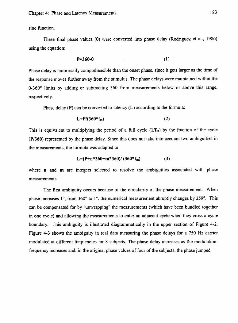
Chapter 4: Phase and Latency Measurements

sine function.

These final phase values (0) were converted into phase delay (Rodriguez et al.. 1986)

using the equation:

Phase delay is more easily comprehensible than the onset phase, since it gets larger as the time of

the response moves further away from the stimulus. The phase delays were maintained within the

0-360" limits by adding or subtracting 360 from measurements below or above this range,

respectively.

Phase delay (P) can be converted to latency (L) according to the formula:

This is equivalent to multiplying the period of a full cycle (llfm) by the fraction of the cycle

(Pl360) represented by the phase delay. Since this does not take into account No ambiguities in

the measurements, the formula was adapted to:

where n and m are integers selected to resolve the ambiguities associated with phase

measurements.

The first ambiguity occurs because of the circularity of the phase measurement. When

phase increases 1 O. From 360" to 1 ". the numerical measurement abruptly changes by 359'. This

can be compensated for by "unwrapping" the measurements (which have been bundled together

in one cycle) and allowing the measurements to enter an adjacent cycle when they cross a cycle

boundary. This ambiguity is illustrated diagrammatically in the upper section of Figure 4-2.

Figure 4-3 shows the ambiguity in real data measuring the phase delays for a 750 Hz carrier

modulated at different frequencies for 8 subjects. The phase delay increases as the modulation-

Frequency increases and, in the original phase values of four of the subjects, the phase jumped

Chapter 4: Phase and Latency Measurements

Please see next page for figure.

Figure 4-2: Ambiguities in the measurement of phase. The upper half of the figure shows the ambiguities that occur because phase is a circular rather than linear measurement. If the phase increases as some other parameter is varied, it may exceed 360" and revert to 0°, causing a sudden fall in the regularly increasing measurements. This can be handled by "unwrapping" the measurements by adding 360" (up-going arrow in the upper right section of the figure). The bottom half of the figure illustrates the ambiguities that occur because the response is recorded in steady-state. The cosine onset-phase of the response recorded in the second line was measured as 150". Phase delay is measured as the phase difference from the stimulus waveform (onset at 0° cosine) to the same part of the response waveform. This is equivalent to 360" minus the measured phase or 2 10'. Translated to latency, this is 2 lO/(36O* 100) or 5.8 rns. Unfortunately there is no way of knowing whether that 0° point of the ongoing stimulus is evoking that part of the response or the same part occumng one or two cycles later (at latencies 15.8 or 25.8 ms for 570" and 930" phase delays). If we record the response at another stimulus rate (and if we can assume that the response has the same latency for the two rates), then we can determine which of the possibilities is most likely. At 85 Hz the phase delay was 130". This gives a latencies of 4.2, 16.0 and 27.8 ms. The measurements of 15.8 and 16.0 ms are the most similar between the two stimulus rates. An "apparent latencytt can also be calculated from the slope of the phase with stimulus frequency divided by 360. For these measurements, this latency is 80/(15*360) or 14.8 ms.

Chapter 4: Phase arid Latency Measurements

Chapter 4: Phase and Latency Measurements

Please see nercr page forjigure.

Figure 4-3: Unwrapping of phase. This figure shows the phase of the response to the 750 Hz tone at different modulation-frequencies in all 8 subjects studied in Experiment I . The original measurements of phase delays were limited to the range 0-360'. In 4 of the subjects this caused a large discontinuities in the course of the lines graphs (dashed lines). These were compensated by adding 360" to the aberrant measurements. For example, in the subject identified using the circles the phase delay jumped from 310" at 85.5 Hz to 14" at 90.3 Hz and then continued to increase to 36' at 95.2 Hz. The latter two measurements were unwrapped to 374" and 396". The figure also illustrates the inter-subject variability in the measurements.

Chapter 4: Phase and Latency Measurements

Phase Delay (O)

Chapter 4: Phase and Latency Measurements 188

back to values close to zero (dashed lines). These values are not far apm from the other values

(between 270" and 360") in terms of circular phase. This ambiguity can be removed by adding

360' to those measurements that were more than 180° lower than adjacent measurements (in

formula (3) n is set to I). We are effectively proposing that a delay corresponding to a full cycle

of the modulation-frequency occurs before the measured responses in these subjects.

The second ambiguity arises from the steady-state nature of the response. Because the

responses are the same From cycle to cycle, the number of cycles of the stimulus that might have

occurred before the measured response is uncertain. The bottom section of Figure 4-2 illustrates

this ambiguity. This ambiguity can be resolved by measuring the response phase when the same

carrier-frequency (and, therefore, probably the same traveling wave latency) is modulated by

several different modulation-frequencies (each in their own recording session). This is illustrated

by the data graphed in Figure 4-4, which shows the effects of modulation-frequency on the

responses at different carrier-frequencies. For a carrier-frequency of 1500 Hz the phase delay

was 152" at a modulation-frequency of 80.6 Hz, and 245" at 95.2 Hz (open circles in left graph of

Figure 4-4). If phase delays were directly converted into latencies according to formula (2) then

latencies of 5.2 and 7.2 ms would be obtained since the period is 12.4 ms for an 80.6 Hz signal

and 10.5 ms for a 95.2 Hz signal. The 2.0 ms difference is similar to the difference between the

periods of the two modulation-frequencies ( 12.4- l0.5=1.9 ms). If we therefore propose that a

delay equivalent to one full cycle occurred before the cycle being measured (m=l in formula (3))

the latencies become 17.6 ms (12.4 6 2 ) and 1 7.7 ms (10.5 +7.2). The measurements are closer

than with no preceding cycles and closer than what would be obtained if we postulated two

preceding cycles (rn=2), which would give latencies of 30.0 and 28.2 ms.

We based the choice of m on the goodness of fit of the collected data when multiple

modulation-frequencies were used with the different carrier-frequencies. This is illustrated in

Figure 4-5. The left graph assumes that no preceding cycles have occurred before the response.

There are significant effects of both carrier-frequency and modulation-frequency. The middle

graph shows the results of adding a cycle (m=I) to the data shown in the upper graph. In this

graph, the different modulation rates yield approximately equivalent estimates of latency. As can

be seen in the right graph, adding a further cycle (m=2) cause the data to diverge again with a

significant effect of modulation-frequency. Once m has been decided on the basis of these

Chapter 4: Phase and Latency Measurements

results, m can be applied to responses recorded using only one modulation-frequency for each

carrier-frequency (e.g., Experiment 3). An ambiguity might arise if there is no clear difference in

the effect of modulation-frequency for two adjacent values of rn

This approach is related to the "apparent latency" calculated by dividing the slope of

phase-delay versus stimulus-frequency by 360 (Regan, 1966; Regan, 1989; van der Tweel and

Verduyn Lunel. 1965). In this particular example, the apparent latency of the two responses to

1500 Hz carriers is (245-152)/(360*(95.2-80.6)) or 17.7 ms. A graphic way of calculating this

measurement was proposed by (Diamond, 1977). The equivalence of these different

measurements of latency is documented in Appendix B. In the auditory literature, apparent

latency is equivalent to "group delay" (Goldstein et al.. 197 1).

Unfortunately, it is often difficult to interpret apparent latency since the phase shifts

occurring in physiological filters are difficult to characterize (Bijl and Veringa, 1985) and the

actual relation of apparent latency to physiological delay is not clear (Hari et al., 1989). A major

problem occurs when the physiological response shows filter effects along the dimension of the

modulation-frequency. The physiological system may only respond to a band of modulation-

frequencies or may respond less to higher modulation-frequencies. A first order low-pass filter

will show a phase shift equal to arctan(f,Jfo) where f is the cut-off Frequency of the filter

(Brown et al., 1982). It might be possible to estimate the effect of such filtering on the responses

from the amplitudes of the responses at the different modulation-frequencies, and then

compensate the phase measurements prior to latency calculations (Regan, 1989, pp29-30). We

performed these calculations for our data based on estimated phase shifis of about 90" per octave,

but these did not significantly alter the results. Another approach is to eliminate these effects by

considering data (for different carrier-frequencies) only at one modulation-frequency. This can

be done \kith multiple measurements (data From Experiments 1 and 2), or by using modulation-

Frequencies so close together that any effect of modulation-frequency would be negligible

(Experiment 7).

Chapter 4: Phase and Latency Measurements

PZease see nesz page for figure.

Figure 4-4 Phase-frequency plots. This figure shows the average data from Experiments 1 and 2. As can be seen in the graphs the phase delay increases regularly with increasing modulation- frequency with a siope that increases with decreasing carrier-frequency. This siope can be used to estimate "apparent latency*' or "group delay".

Chapter 4: Phase and Latency Measurements

Phase Delay (O)

Chapter 4: Phase and Latency Measurements

Please see n a t page for figure.

Figure 4-5: Preceding cycles (80-100 Hz). This figure illustrates a method by which the number of cycles preceding the recorded response can be estimated. The phase delay is converted to latency and then the actual latency from the stimulus is calculated by adding an integer number (m) of cycles of modulation to the estimated latency. Since carrier-frequencies are what should determine the delays in the cochlea, different modulation-frequencies should result in the same latency estimate. As can be seen in the figure, the delays related to each carrier-frequency are most consistent across the different experimental conditions when m=l.

Chapter 4: Phase and Latency Measurements

Latency (ms)

Chapter 4: Phase and Latency Measurements 194

MODELING Some simple modeling was undertaken to determine how the measured latencies might

occur on the basis of h o w n physiological processes. A MATLAB program was constructed to

imitate the effects of four processes. First, the filtering that occurs at the level of the hair cells

was modeled as a gammatone filter using the parameters fiom (Patterson, 1994), see also

(Glasberg and Moore, 1990). Second, the filtered signal was rectified. For simplicity and since

we were not interested in the effects of different intensities, no compression (e.g. Corey and

Hudspeth, 1983; Dallos, 1985) was used in the rectification. Third, we rnodekd the

refractoriness of the auditory nerve fiber discharges using the equations of Carney (1993; see also

Eggennont, 1985) and pvameters approximately equivalent to those recommended in that paper

(an absolute refractory period of 1 ms and then a double exponential return with time constants

of 1 and 25 rns). Since we were estimating population discharges rather than individual fiber

discharges, the rehctoriness was applied with a strength of 40%. This meant that only that

portion of the neurons would fire at any one time and therefore be susceptible to being refractory

the next time. Fourth, we estimated the compound field potentials generated from the population

of neurons in the brain responsible for the scalp potentials. This involved imposing a latency

jitter (arbitrarily set as a rectangular 2 ms hnction) to mimic the variability in the conduction

times between the cochlea and the generator neurons. The field potential of a single fiber

discharge was estimated using the "model unit reponse" of Elberling (1976; see also (Teas et al.,

1962), without the secondary peak. This was then convolved with the estimated population

discharge pattern to give the modeled field potentials.

The latencies of the modeled responses were measured by determininz the latency of the

maximum of the cross-correlation function between the original acoustic signal and the modeled

field potential. Two acoustic signals were analyzed: an AM tone with a modulation-frequency of

80 Hz and carrier-fkequencies between 500 and 8000 Hz, and a click with a duration of .2 ms

presented a rate of SO/seconds.

Chapter 4: Phase and Latency Measurements

Experiment 1 : Monaural StimuIation 80- 1 00 Hz Sample data from one subject in this experiment are shown in F i g w 4-1. Figure 4-3

shows the inter-subject variability of the phase delays at 750 Hz. The left side of Figure 4-4

shows the mean phase delays for all 4 carrier-frequencies and all modulation-frequencies.

A 4 x 4 repeated-measures ANOVA for the phases of the responses to the 750 Hz octave

series modulated at 80- 1 00 Hz, which compared carrier- frequency and modulation- frequenc y,

indicated significant effects of both carrier-frequency (F=33.8; df 3,21; pc0.001) and modulation

rate (F=111.2; df 3,2I; p<0.001), as well as a significant interaction (F=3.9; df 9,63; p<0.05,

~ = . 3 1) due to a flattening of slope as the carrier-frequencies increased.

When converting from phase delay into latency, the data can be modeled as having

occurred afier 0, 1 or 2 preceding cycles by altering the parameter m in equation (3). These

calculations are shown in Figure 4-5. When m=O, the experimental analysis of the latency data

showed main effects of both carrier-frequency (F452.8; df 3,21; p<0.001, ~=.43) and

modulation rate (F=18.3; df 3,21; p<0.001, ~=.42). When m=l, there was a significant change in

latency with carrier-frequency (F=101.2; df 3,21; p<0.001, ~ . 4 3 ) but not with modulation rate

(F=0.56; df 3.2 1; p=0.7). By adding a fhther cycle, so that m=2, the data again became

divergent. and a significant effect of modulation rate again emerged (F=33.8; df 3,21; p<.001,

&=.43).

The best fit for the data, when m=l, yields steady-state response latencies for the 750 Hz

octave series of 20.7, 17.7, 16.1, and 16.1 ms. Post-hoc Fisher LSD tests showed that the

differences in latency between carrier-frequencies were significantly different (p<0.01) except

between 3000 Hz and 6000 Hz. Table 4-1 provides the latencies estimated for each canier-

frequency at each modulation rate when m=l. The apparent latency values for these data were

22.2, 17.5, 13.9, and 12.7 ms.

The amplitudes are plotted in Figure 4-6. There was a no significant effect of carrier-

frequency (F=3.57; df 3.21; p=0.058, ~=.64) or of modulation-frequency (F=2.54; df 3,21;

p=0.13, ~=.50). The 750 and 6000 Hz tones tended to produce smaller responses. Furthermore,

the overall amplitudes across the different carrier-frequencies did show a slight decrease in

Chapter 4: Phase and Latency Measurements

Please see nert page for figure.

Figure 4-6: Effects of modulation-frequency on amplitude. This figure represents the mean data for the 8 subjects evaluated in Experiments 1 and 2. There is a slight decrease in amplitude with increasing modulation-frequency. This was not significant between 80-100 Hz but was significant between 150- 190 Hz. This suggests a small low-pass filtering process.

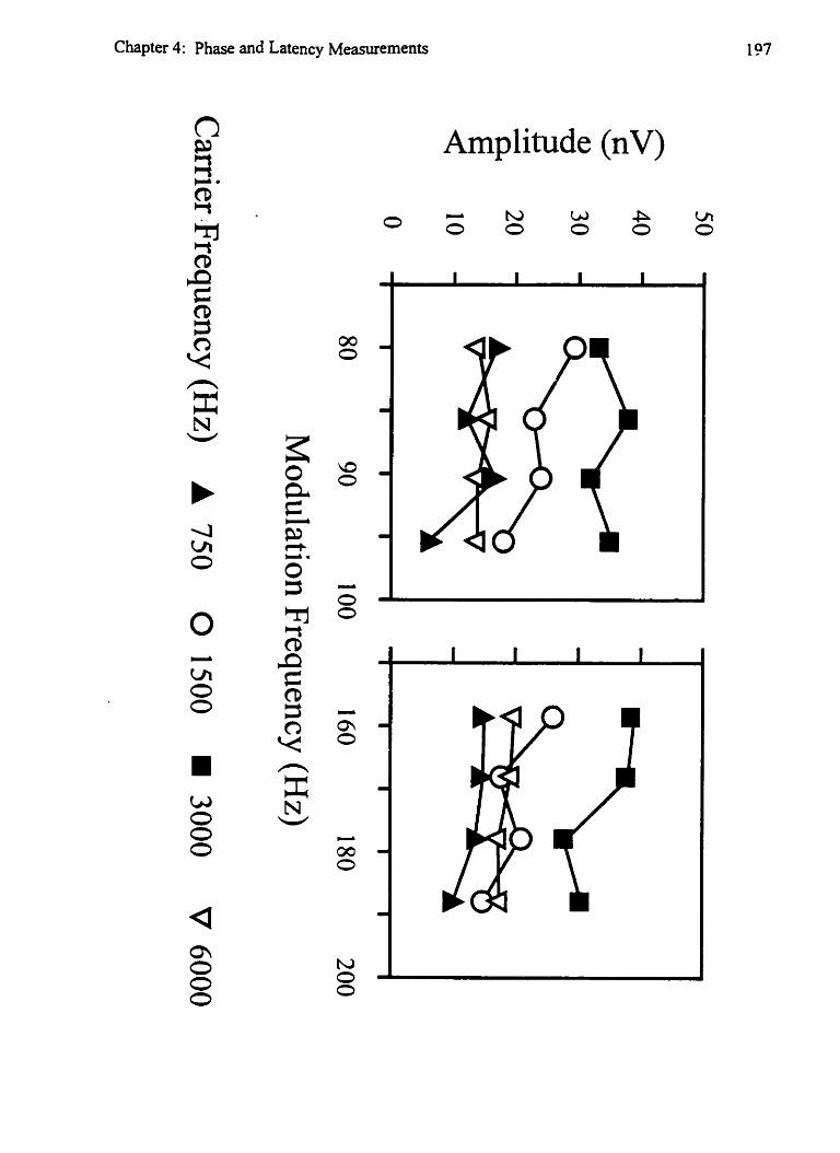
Chapter 4: Phase and Latency Measurements

Amplitude (nV)

Chapter 4: Phase and Latency Measurements

Table 4-1. Estimated Latencies at Different Modulation-frequencies

(Data from Experiments 1 and 2)

Rate (Hzj

80.6

85.5

90.3 "

95.2

158.7

168.5

178.2

190.0

Latency (rns)

750

20.6

20.6

20.8

20.8

11.3

11.0

10.9

12.0

1500

17.6

17.8

17.7

17.7

8.6

8.8

8.8

9.0

3000

16.1

16.3

16.1

15.8

6.6

6.8

7.0

7.0

6000

16.4

16.2

15.9

15.9

6.3

6.5

6.5

6.5

Chapter 4: Phase and Latency Measurements . 199

amplitude (5nV from 80 to 95) with increasing modulation-Erequency that was equivalent to

about 6 dB/octave. Assuming that this may have been associated with a phase shift of 90" per

octave, the phase measurements were adjusted and latencies recalculated. The differences caused

by these calculations were less than 0.2 ms.

Experiment 2: MonauraI Stimulation I SO- 190 Hz The mean phase measurements are shown on the right of Figure 4-4. The data are plotted

with different values of m in Figure 4-7. In the case of the 150 Hz series, for m=O, a 4 x 4

repeated-measures ANOVA showed a main effect of latency for carrier-frequency (F=165.5; df

3.2 1 ; p<.00 1, ~=.48) and also for modulation rate (F=59.6; df 3.2 1 ; pc.001, c=.48). When m=l ,

there was a significant change in latency with carrier-frequency (F46.4; df 3Jl; pc.001, ~= .48 ) ,

but not for modulation rate (F=1.2; df 3 ,X; p=.3). After adding a further cycle so that m=2, the

data again became divergent across both carrier-frequency (F=165.5; df 3 2 1 ; pc.00 1) and

modulation-frequency (F=8.9; df 3,2 1 ; pc.0 1).

The mean latencies for the 750 Hz octave series 150- 180 Hz modulated data were 1 1.3,

8.9, 6.9, and 6.4 ms. Post-hoc Fisher LSD tests within each modulation-frequency showed

significantly (pC0.0 1 ) different latencies across the different carrier-frequencies except for the

difference between 3000 and 6000 M. However, these latencies were significantly different if

the data were collapsed across all modulation rates (F4.9; df 1,14; p<0.001). The apparent

latencies for these data were 15.1, 10.9, 9.5, and 7.5 ms.

The mean amplitudes of these responses are plotted in the right half of Figure 4-6. The

trends seen in the 80 Hz data again appeared here, but now there was a significant effect of

carrier-frequency (F= 8.04; df 3,21; pc.05) and also modulation rate (F=6.74; df 3,21; pc.05).

As in the case of the 80 Hz data, there again was a decrease in the amplitudes of the 750 and

6000 Hz responses and a roughly linear decrease in amplitude as modulation rate increased (7 nV

from 155 to 185 Hz). Again, recalculation of the latencies after compensating the phases for a

possible 90°ioctave shift did not significantly alter the latencies.

Experiment 3 Dichotic Stimulation In the first dichotic condition, a 750 Hz octave series was presented to the right ear while

a 500 Hz octave series was presented to the left ear, and in the second condition these stimuli

were presented to the opposite ears. In order to analyze the data, the results were combined to

Chapter 4: Phase and Latency Measurements 200

provide latency estimates at %octave steps in each ear. The mean data compared between the

ears are plotted in Figure 4-8. The mean and standard deviations across the subjects are provided

in Table 4-2. There are minor differences between Figure 4-7 and the Table 4-2 data since vector

averaging was used to calculate the mean phases for the latencies in the Figure 4-but ordinary -

arithmetic averaging was used to caiculate the latencies for the table (to allow us to obtain

measurements of inter-subject variability).

The responses to the 80 Hz dichotic AM tones showed significant effects for carrier-

frequency (F=7 1.2; df 7.49; pc.001) and no significant effect of ear (F=2.15; df 1,7; p=. 19).

Post-hoc Fisher-LSDs indicated that the differences in latency between all adjacent carrier-

frequencies (%-octave steps) were significant at the .001 level up to the 3000 Hz level. The

responses to the 160 Hz dichotic AM tones showed significant effects for carrier-frequency

(F91.8; df 7,49; p<.OOl) and. again, the responses for the left and right ears failed to show any

significant differences (F=.07; df 1,7; p=.8). Post-hoc Fisher-LSDs again indicated that the

differences in latency between all adjacent carrier frequencies (K-octave steps) were significant

at the .001 level up to the 3000 Hz level. We also compared the responses recorded when stimuli

were presented to the left ear in the monaural condition to those recorded in the left ear during

the dichotic condition. There were no significant differences between monaural and dichotic

response latencies.

Ex~eriment 4: Effects of Intensity. M=8) When the intensity of the stimuli increased fmrn 35 dB SPL to 75 dB SPL (Figure

4-9), the latency of the response in the 80-100 Hz range decreased by an average of 2.4 ms (2.6,

2.5, 2.8. and 1.7 ms for the 500, 1000, 2000, 4000 Hz carrier frequencies). A comparison

between 35 and 75 dB SPL response indicated a significant decrease in latency (F=30.9; df 1,7;

p<.001) and across carrier frequency (F=33.6; df 3,21; pc.001). Although there was a smaller

decrease at the 4 kHz response there were no significant interactions between loudness and

carrier frequency with respect to latency. Post-hoc LSD comparisons indicated that this decrease

was significant for all frequencies at the -05 level.

Experiment 5: Effects of Multiple Stimuli M=lO) In the other experiments presented in this chapter, multiple (4) stimuli were presented in

Chapter 4: Phase and Latency Measurements 201

each ear. Here, we examined the latencies obtained by a 1000 Hz or 2000 Hz tone presented

alone, compared to the latencies obtained when multiple stimuli were used. The latencies of the

1000 Hz and 2000 Hz tones in the different stimulus conditions are shown in Table 4-3. A two-

way (camer frequency by number of simultaneously presented stimuli) repeatedmeasures

ANOVA showed a significant main effect for carrier frequency (F=lO3.2, dF=1,9; pc.001) but

not for number of stimuli (F=2.13; df 4,36; p=.10). However, there was a significant interaction

between carier frequency and number of stimuli (F=7.96; df 4,36; pc.001). Compared to the

single stimulus condition, when adjacent stimuli were separated by less than 1 octave, increased

latency was seen, although post-hoc testing showed this effect was only significant (pC.05) in the

case of the 1000 Hz tone.

Exoeriment 6: Stability of Phase RJ=6) In order to assess the stability of steady-state phase we tested 6 subjects and then tested

them again 3-4 weeks later, at both 80 Hz and 150 Hz modulation rates. In the 80 Hz condition

the average change was -0.1 1 ms (range: -0.66 to +0.67ms). In the 150 Hz condition the average

change was only -0.04 ms (Range: -0.49 to t0.3 1 ms). The results for each carrier frequency are

provided in Table 4-4. For the 80 Hz responses, the change for the difference between 750 and

6000 Hz changed from one recording to the next by 0.15 ms (range: -0.71 to + 1.14 ms). For the

150 Hz responses, this measurement changed by -0.06 ms (range: -0.255 to +0.05 ms).

Chapter 4: Phase and Latency Measurements

Please see next page for figure.

Figure 4-7: Preceding cycles (150-190 Hz). This figure shows how the number of preceding cycles of modulation were estimated for the data recorded with modulation-frequencies of 150- 190 Hz. The figure is similar to Figure 4-4. Again, the data are most consistent across the recording condition when the number (m) of preceding cycles of modulation equals one.

Chapter 4: Phase and Latency Measurements

Latency (ms)

Chapter 4: Phase and Latency Measuments

Please see next page f o r m r e .

Figure 4-8: Dichotic stimulation. This figure shows the results of Experiment 3. Four stimuli with carrier frequencies separated by an octave were presented to one ear and four stimuli at intervening carrier frequencies were presented to the other ear. The data are the latencies derived using m=l from the vector-averaged phase delays across the 8 subjects recorded in this experiment.

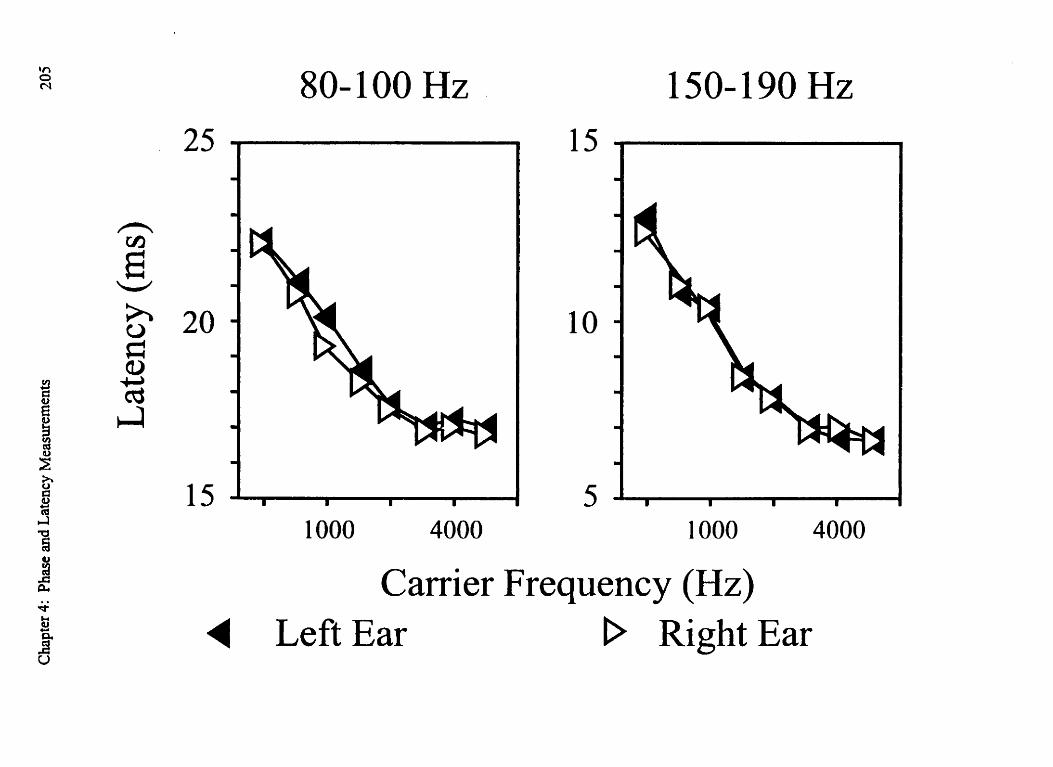
Carrier Frequency (Hz) Left Ear D Right Ear

Chapter 4: Phase and Latency Measurements

Please see mxi page for figtire.

Figure 4-9: Effects of intensity on response latency. These data represent the average results across the 8 subjects paticipating in Experiment 3. They show the decrease (approximately 2 ms) in the estimated latency with increasing intensity.

Chapter 4: Phase and Latency Measurements

Latency (ms)

Chapter 4: Phase and Latency Measurements

Ex~eriment 7. Small Differences in Modulation-fiesuency (N=16) The latencies for this experiment are plotted in Figure 4-10. The differences between the

latency for the 750-Hz canier and the latency for the 6000-Hz carrier were 3.5 and 4.5 ms for the

80 Hz and 160 Hz series, respectively. Like Experiments 1, 2, and 3 the 80 Hz data failed to

show any decrease in latency between the 3000 to 6000 Hz responses, while in the 160 Hz data, a

decrease was apparent. An ANOVA of the all of the data indicated highly significant effects for

carrier frequency (F=107.7; df 3,42; p<.001) and between the 80 and 160 Hz modulation rates

(F=2840.0; df 1.14; pc.001). There was also a significant effect of gender (F=4.6; df 1,M;

p=0.05) with the male subjects showing latencies which were delayed, on average, by 0.78 ms

compared to the female subjects. There was no significant interaction between gender and carrier

Frequency although the difference between 750 and 6000 Hz was slightly greater for males than

for female subjects in the 80 Hz data.

The amplitude and phase of the 1500 Hz tone presented alone was compared to its

amplitude when it was presented simultaneously with the 3 other tones. For the 80-Hz response

the amplitudes were smaller (92%) when the stimulus was presented with the other tones. while

in the case of the 160-Hz the amplitude was larger (I 40%). For both modulation-frequencies the

responses were slightly earlier by 0.4 ms (same for both) when the stimulus was presented with

the other tones.

Results of Modelinq The basic parameters of the model are illustrated in Figure 4-1 1. Figure 4- l t shows how

the model processes two different inputs - an 80-Hz AM tone and a click presented at a rate of

50 Hz. Figure 4-13 graphs the latencies estimated using cross-correlation for these two kinds of

stimuli. The carrier frequency of the AM tone and the characteristic frequency of the hair cell

filter were varied in octave steps form 500 to 8000 Hz. The latency changes over the complete

range were 5.4 ms for the AM tone and 3.2 ms for the click-evoked potential. Estimates of the

difference beween 750 and 6000 Hz were 3.7 ms and 2.4 ms.

Chapter 4: Phase and Latency Measurements .

Table 4-2. Effects of Carrier Frequency on Response Latency (Data from Experiment 3)

Table 4-3. Effects of Multiple Stimuli on Latency Estimates (Data from Experiment 4: means and standard deviations)

L

Modulation Range (Hz)

80 Hz

160 Hz

Table 4-4. Stability of the Responses over Two Separate Recording Sessions (Data from Experiment 6)

mean

sd

mean

sd

Carrier (Hz)

Canier(Hz)

1 Tone (1 Octave)

Modulation

,80-100 HZ

, 150-190Hz

2 Tones (1 Octave)

Carrier

750

t 500

3000

6000

750

1500

3000

6000

3000

16.0

0.5

6.8

0.3

500

21.5

1000

18.9

0.8

10.3

1.1

750

20.2

4 Tones (1 Octave)

4000

16.1

0.7

6.9

0.4

Latency

6000

15.8

0.8

6.6

0.5

1500

17.6

0.6

8.9

1.4

1.6

12.2

t .7

4 Tones (112 Octave)

mean

19.9

17.0

15.4

15.5

10.8

8.8

6.3

6.1

Difference between Sessions

2000

16.7

0.5

7.8

, 0.7

1.5

11.1

1 .O

8 Tones (112 Octave)

sd

0.8

0.6

0.9

0.6

0.8

0.8

0.4

0.4

mean

0.1

0.1

0.2

0.0

0.0

0.0

' 0.0

-0.1

sd

0.4

0.4

0.4

0.6

0.1

0.2

0.2

0.2

min

-0.5

-0.3

-0.4

-0.7

-0.2

-0.3

-0.3

-0.5

max

0.5

0.7

0.6

0.7

0.1

0.3

0.2

0.1 L

Chapter 4: Phase and Latency Measurements

Please see next page for figure.

Figure 4-10: Small differences in modulation-frequency. This figure shows the results of Experiment 7. The estimated latencies were slightly shorter for the 8 female subjects than for the 8 male subjects.

Chapter 4: Phase and Latency Measurements

Latency (ms)

Chapter 4: Phase and Latency Measurements

Auditory Steady-State Responses Human auditory steady-state responses can be recorded using stimulus rates up to several

hundred Hz (Rickards and Clark, 1984). The amplitude of these responses is larger at rates near

40 Hz (Galarnbos et al., 1981) and 80 Hz (Cohen et al., 1991; Lins et al., 1995). Responses at

both these rates have been used as an objective measurement of hearing thresholds (Rance, 1995;

Lins, 1996; Dobie and Wilson, 1998). The more rapid responses are less affected by changes in

sleep or maturation (Cohen et al., 1991; Levi et al., 1993; Lins and Picton, 1995) and might

therefore provide more reliable measurements in children and other difficult-to-test patients. The

results of this chapter indicate that responses in the 150- 190 Hz range might also provide reliable

measurements.

The nature of human auditory steady-state responses has been mainly studied with the

responses evoked at stimulus rates near 40 Hz (Galarnbos et al.. 198 1; Stapells et al.. 1984). If

they largely arise from the same neurons that generate transient evoked potentials, the steady-

state responses can be predicted from the superposition of multiple overlapping transient

responses (Galambos et al., 198 1 ; Hari et al., 1989; Plourde et al.. 199 1 ). However. it is also

possible that rapid stimulation might elicit a separate response from neurons that are specifically

responsible for rhythmic activity and that resonate at the frequency of stimulation (Basar et al.,

1957). These generators might be responsible for spontaneous cortical gamma rhythms.

Discrepancies between the steady-state response and the response predicted by superposition

(Azzena et al., 1995) and the persistence of the response beyond the time when the stimuli are

presented (Santarelli et al., 1995) support the idea of resonance. However. by modeling the

refractory effects and considering multiple generators, one can still explain most of the 40-Hz

response findings on the basis of the superposition of the transient response waveforms

(Gutschalk et al., 1999). We think that it is unlikely that independent rhythmic generators might

account for the steady-state responses at Frequencies above SO Hz. We therefore consider the

responses to be generated by neurons in the brainstem (and possibly cortex) that become locked

to the envelopes of amplitude-modulated tones.

The estimated latencies for the 150-190 Hz responses were about half the latencies for the

80-100 Hz responses (e-g. Table 4-4, Figure 4-8). Our latencies ( 17.7 and 9.0 ms at 1500 Hz) are

Chapter 4: Phase and Latency Measurements 213

similar to those of Cohen ct al. (1 991 ) who reported latencies at 1000 Hz (55 dB HL) of 24.8 ms

for modulation-frequencies of 30-60 Hz and 13.0 ms for 90-125 Hz, given that the latencies

decrease with increasing modulation-frequencies (Rickards and Clark, 1984). Previous work in

our laboratory had provided an apparent latency of 19 rns for 1000 Hz tones modulated between

7 1 - 100 Hz. The latencies at 1 50- 190 Hz suggest that the generators might be at about the same

level of the brainstem as those generating wave V of the auditory brainstem response. The

latencies for the 80-100 Hz responses suggest a generator higher in the brainstem.

Latencv of S teadv-State Responses The phase of a steady-state response is related to delay. Unfortunately, this relationship is

ambiguous and phase cannot be directly translated into latency. By assessing phase at different

stimulus rates, it is often possible to resolve the ambiguities and arrive at a clear estimate of

"apparent latency" (Regan, 1966) or "group delay" (Goldstein et al., 197 1 ).

The distorting effect of physiological filters operating across the different rates of

stimulation remains a problem (Bijl and Veringa, 1985). This is analogous to estimating the

delays related to filter slopes when studying the group delays of tuning curve (Goldstein et al..

197 1 ). The effects of such filters can only be estimated. In the data presented here. these effects

appear small since similar results were obtained when the latency estimates were based on the

same modulation-frequencies rather than different modulation-frequencies. Supporting data

were obtained on separate recordings for the different carrier frequencies with each canier

frequency being modulated by exactly the same modulation-frequency (Experiments 1 and 2, and

Table 4-I), and using modulation-frequencies that were sufficiently close together during

multiple stimulation that any filter-effect would be negligible (Experiment 7).

The physiological interpretation of the latencies of the steady-state responses remains

difficult. The main problem is that the recorded response may not derive fiom a single generator.

Many different regions of the auditory nervous system fiom the auditory nerve to the auditory

cortex generate responses that follow the modulation signal of an amplitude-modulated tone.

Each of these regions can create a response that has a specific phase and latency relationship to

the stimulus. All these responses will overlap to make up the response recorded from the scalp.

The phase and latency characteristics of the scalp-recorded response may be very complex unless

Chapter 4: Phase and Latency Measurements

Please see next page for figure.

Figure 4-1 1: Modeling parameters. This figure shows the parameters used in the four processes for modeling the latencies of the responses to amplitude-modulated tones and clicks. The first process is the cochlear filter which is modeled as a gammatone filter using the parameters of (Patterson, 1994). The second process is synaptic rectification. The third process is to estimate the fiber discharge rates. For this estimation the refractoriness of the fiben was estimated using parameters from (Carney, 1993). The fourth process in the model was to estimate the field potentials generated from the responding units. As well as a jittering of the latency (not illustrated) the response pattern was then convolved with an estimated unit field potential using parameters similar to those of (Elberling, 1976).

Chapter 4: Phase and Latency Measurements

+ Output

+ Amplitude (uV)

0

+ Amplitude (dB)

+ Refractoriness (%)

Chapter 4: Phase and Latency Measurements

Please see next page for figure.

Figure 4-12: Modeling the physiological processes. This figure illustrates the processing of acoustic stimuli through the various steps in the model. The hair cell filter intervenes between the acoustic stimulus and the hair cell potential. Rectification then occurs to give the synaptic potential. The refractoriness of the nerve fibers determines the fiber discharge pattern. The scalp potentials are then determined by both the jitter and the field pattern of the unit discharges.

Chapter 4: Phase and Latency Measurements

Chapter 4: Phase and Latency Measurements

Please see nexf page for figure.

Figure 4-13: Modeled latencies. This figures graphs the latencies obtained for the steady-state response to a pure tone amplitude-modulated (AM) at 80Hz and a click stimulus presented at a rate of 50Hz. The latency change of the steady-state response with changing carrier frequency is almost double that of the click response.

Chapter 4: Phase and Latency Measurements

Delay (ms)

Chapter 4: Phase and Latency Measurements

one of the generators is clearly dominant.

An example may be possible changes in the phase of the steady-state response with

changes in the level of arousal. In a waking subject, the dominant response at 40 Hz may be

fiom the auditory cortex. With sleep, this response may attenuate and the scalp- recorded

response may reflect only those potentials generated in the brainstem. The response during sleep

is therefore much smaller than during wakefulness and occurs earlier (Lins and Picton, 1995).

In our particular case, the amplitude of the responses fiom different generators may vary

differently with the canier-frequency. If so, the phase of the scalp-recorded response that

combines potentials from the different brain generators, may not show a clear and regular

relationship to carrier frequency. Furthermore, such data might provide an apparent latency that

does not fit with an integer number of cycles prior to the recorded response. It is best only to

calculate the apparent latency over regions where there is no change in the slope of the phase-

frequency curve. since this suggests one dominant generator. Different generators at different

frequencies could cause the slope to change (e.g., 750 Hz on the right of Figure 4-4). Another

reason for non-integer preceding cycles would be some undetermined filter delay in the system.

These factors (multiple generators and unknown filters) may explain some of the discrepancies

between our measurements of apparent latency and the estimated latencies obtained by

postulating an integer number of cycles of modulation prior to the recorded response. Although

the latencies were generally concordant. the apparent latencies measured for the 750 Hz carrier

were longer than those estimated using preceding cycles (22.2 versus 20.7 ms at 80-100 Hz and

15.1 versus 1 1.3 ms at 150- 190 Hz).

The advantages of using the "preceding cycles" approach over apparent latency is that

once the number of preceding cycles is estimated by using multiple modulation rates, then only

one rate is needed to make subsequent latency measurements. The disadvantage is that it has no

clear way to handle the possibility of multiple generators, which could then lead to a non-integer

number of preceding cycles. However. although the group delay or apparent latency

measurements allow for such non-integer effects, the interpretation of the results in such a

situation is not clear. In our resulrs, the apparent latency measurements differed slghtly from the

latencies obtained with the preceding cycles approach, pa~~icularly for the low-frequency stimuli

Chapter 4: Phase and Latency Measurements 22 1

(750 Hz). In this situation, one must consider the possibility of overlapping responses with

different latencies, e.g., fkom different brainstem neurons.

We feel that the scalp-recorded potential in response to tones amplitude-modulated at

frequencies 80-100 Hz probably derives mainly from a generator in the hgh brainstem.

Preliminary source analyses in our laboratory support this idea (cf. Mauer and Doring, 1999). If

this generator is clearly dominant over other generators, for example in the auditory nerve or

lower brainstem, the derived latencies should be quite accurate. The relations of the response

phase to carrier frequency should then reflect the effects of transport-time and filter build-up in

the cochlea. For the stimulation rates of 150-190 Hz, the responses that we are recording may

reflect approximately equal contributions From generators in both the high brainstem and lower

brainstem.

Latencies in the Auditory Svstern Five main factors contribute to the latency of a neurophysiological response to an

auditory stimulus:

( i ) Acoustic delay. This is the delay between the production of the stimulus and its arrival

at the oval window after transmission through the air and the middle ear to the tympanic

membrane. This was 0.9 ms for the ear inserts and was instantaneous for the headphones.

(ii) Transport time. This is the delay between the arrival of the acoustic energy at the oval

window and the beginning of activity at the location on the basilar membrane where transduction

occurs for a stimulus of that particular frequency. High frequencies of sound maximally activate

the basilar membrane close to the oval window and low frequencies maximally activate the

regions of the basilar membrane at some distance from the oval window. The transport time

therefore depends upon the frequency of the stimulus. Eggermont ( 1 979b) estimated this

"mechanical time" as fOJ where f is the characteristic frequency.

(iii) Filter built-up time. This is the time taken for the acoustic energy to pass through the

active filtering process ("cochlear filter") of the hair cells that are sensitive to the frequencies of

sound in the stimulus. This time will depend upon the sharpness of the filter, a parameter that can

be measured by the Q10 dB parameter which is the characteristic frequency of the filter divided

Chapter 4: Phase and Latency Measurements 222

by the bandwidth of the filter at an intensity lOdB above the threshold intensity for the filter.

Values for QlOdB in mammalian cochleae vary between 1 and 15 with the filters for lower

Frequency sounds having lower values (Eggexmont, 1979b; Ruggero, 1992). The filter delay is

usually measured in terms of the number of cycles to maximum amplitude and this varies with

the Ql OdB, with delays increasing by 2-3 ms as the stimulus frequency increases from 1 to 10

H z (Eggemont, 1 979b, data compensated by removing I3 as discussed later).

(iv) Synaptic delay. As the hair cells rext to the sounds they synaptically activate the

afferent nerve fibers. The transmission time across the synapse requires somewhere between 0.5

and 1.0 ms. This delay is not frequency-dependent.

(v) Conduction delay. This is the time taken for the neural responses to travel fiom their

point of origin on the afferent fiber terminals to the location from which they are recorded. For

human evoked potentials this time includes some additional synaptic and conduction delays as

the impulses travel to the place where they generate the response recorded from the scalp. The

conduction time can be estimated from studies wherein the auditory nerve fiben are electrically

stimulated. Shirane and Hamson ( 199 1) found a delay of below I ms in the colliculus' response

as the characteristic frequency of the chinchilla afferent fiber being electrically stimulated

decreased From I0 kHz to 1 Wz (compared to about 2 ms when using acoustic clicks).

The latency of the neural response is unfortunately not just a simple sum of these five

delays. The problem centers on the temporal characteristics of neural responsiveness, particularly

mhctory times. and the way in which field potentials are generated. When presented with a

transient stimulus the nerve fibers will respond more to the initial cycles of activation and less to

later cycles. This complex relationship becomes even more complicated if one measures the

combined responses of multiple neurons, such as the compound action potential of the auditory

nerve. The neurons contributing to this combined response will show a significant variance in

their response patterns and this can make the compound response quite different fiom the

individual responses. One of the main effects is to accentuate the response at the onset of a

stimulus. The discharges of many of the neurons will be relatively synchronous at the beginning

of the stimulus and will become less synchronous as the stimulus continues (Elberling, 1976).

Because of these factors, the latency of the neurophysiological response to a transient

Chapter 4: Phase and Latency Measurements 223

stimulus is not as long as the delay caused by the filter build-up. The response occurs sometime

during the build-up of the filter response and this time can vary with other parameters such as

stimulus intensity. In order to account for this effect, Eggermont, (1979b) multiplied the delay by

a factor l3 between 0 and 1.0, in general estimating B at 0.5.

When recording steady-state responses, the neural response patterns have reached a

balance between reactivity and refractoriness and this balance remains constant during the

recording. We therefore suggest that for the steady-state response D is effectively equal to 1.0. If

so, the frequency-related delay of the steady-state response is exactly equal to the sum of the

transport time and the filter build-up time for stimuli with frequencies equal to the carrier

Frequency.

Most studies of the neuronal responses to AM stimulation in animals (e.g. Rees and

Palmer, 1989; Langner, 1992) have not considered the phase of the response patterns. Other

studies (e.g Msller, 1973; Rees and Msller, 1983) have measured changes in the phase of the

discharge pattems with modulation-frequency and how this relates to the temporal modulation

transfer function of the neurons. Joris and Yin (1 992) measured the phases of the neuronal

responses to AM tones in the auditory nerve of the cat and found group delays related to carrier

frequency increasing about 3 ms from 10 kHz to 500 Hz. This was similar to the changes in

group delay estimated From the phase locked responses to pure tones (e.g., Goldstein et al., 197 1;

Gummer and Johnstone, 1984). Our data show a change of 5-6 ms over these frequencies, the

larger delays probably being related to species-differences in the basilar membrane and the

travelling wave velocity, or some frequency-related change in conduction time (see (v) above).

Relations to Oto-acoustic Emissions Kirnberley et al. ( 1993) studied frequency-related delays in cochlear processing using

distortion product oto-acoustic emissions (DPOAE). The latency of these responses is usually

considered in terms of a "round-trip" delay: the acoustic signal must first reach the hair cells and

then the acoustic energy generated by the hair cells must travel back to the external ear canal to

be recorded up by the microphone. Dividing the DPOAE latency by 2 provides latencies that are

roughly equivalent to the latencies of the neurophysiological responses. However, as Kimberley

et al. (1 933) clearly state, this is a simplified view. They point out that the latency of the DPOAE

Chapter 4: Phase and Latency Measurements

"consist [s] of (a) the actual traveling-wave delay to the £2 frequency place, (b) the cochlear filter

delay at the site of generation, near £2, and (c) the backward travel time of the DPOAE from the

generation site to the oval window." The reason for the rough equivalence between % of the

DPOAE latency and the frequency-related latency of the evoked potentials is that D is

approximately 0.5 and the transport time (a and c) is small relative to the filter delay @).

If the travelling wave delay is equal to the backward navel time, the latency of the DPOAE (t)

can be represented by:

where tr is the filter delay and tb is the transport time on the basilar membrane. We are proposing

that the frequency-related delay in the steady-state response (b) is represented by:

Combining these measurements could provide separate estimates for the transport time and the

filter time. The latencies of the oto-acoustic emissions change approximately 7 ms from 10 kHz

to 1 kHz (Kimberley et al., 1993; Moulin and Kemp, 1996a). Our data indicate that the latencies

of the steady-state responses would change by about 5 ms over the same frequency range. This

would suggest that filter build-up causes frequency-related delays of up to 3 ms in the cochlea

and that the transport time varies up to 2 ms.

Although illustrating how latency data for emissions and steady-state responses might be

related, this analysis overly simplifies the nature of the DPOAE delay. Firstly, the forward and

backward transport times are not necessarily equal. Brown et al. (1994) review several different

physiological models in the context of how DPOAE latencies change with development. The

backward travel time may be very brief if it is based on a compression wave (ct , Sutton and

Wilson, 1983). Moulin and Kemp (1996b) have presented evidence supporting the idea that the

return time of the DPOAE is significantly shorter than its forward latency. A second major

difficulty in the analysis concerns the location on the basilar membrane responsible for

generating the DPOAE s. Moulin and Kemp (1996b) demonstrated that different DPOAE s (e.g.,

25%. or ZF2-F1) are likely generated in different cochlear locations. Third, it is not clear that the

return path is direct. Shera and Fuinan (1999) have recently reviewed our understanding of the

delays measured for the DPOAE s. They suggest that the 'sources' of the backward traveling

Chapter 4: Phase and Latency Measurements 225

waves are locations on the basilar membrane characterized by non-linear electromechanical

distortion. In this view, both stimulus frequency and distortion product emissions ultimately

arise from linear reflection at these locations. The reflected energy derives from the stirnulus-

evoked travelling wave for stimulus-evoked emissions and from the nonlinear processing at

regions of overlap between theA and fi sounds for distortion product emissions.

Clearly, we shall have to understand the nature of DPOAE latency more fully before we

can combine it with the latency of the steady-state response to determine the relative

contributions of transport and filtering to cochlear delays. Using the same stimuli to evoke both

the emissions and the steady-sate responses might decrease the number of variables and simplify

the relations between these physiological responses. This approach would lead to examining the

steady-state responses to cochlear distortion products (e.g., Chertoff and Hecox. 1990; Rickman

and Chertoff, 1991) or the emissions evoked by arnplitude-modulated tones.

Effects of Intensitv

The latency of wave V of the click-evoked auditory brainstem response increases from

5.5 ms to 8.5 rns as the intensity is decreased from 70 dB to 20 dB above threshold. Eggermont

and Don (1980) considered this latency change in light of derived response studies. Part of the

change can be attributed to a shift in the region of the cochlea that contributes most prominently

to the response. At high intensities the basal end of the cochlea dominates but at low intensities

the region of the cochlea mediating frequencies near 1000 Hz dominates. However, this can only

account for about 1 ms of the change and there remains an intensity-related change about 2 ms

that occurs for each derived band response. Several factors contribute to this residual latency

change. There might be a small place shift within the narrow band of frequencies responsible for

the response. There might also be some change in the B parameter such that the higher intensity

clicks evoke responses earlier on the rise time of the synaptic activation. There might be further

effects of refractoriness and synchronization (cf. steps 3 and 4 in our model). Finally, there

might be some increased latency in the brainstem pathways due to decreased efticiency of

synaptic transmission when fewer afferent fibers are activated and firing of the postsynaptic cells

is nearer threshold. The steady-state responses show a latency change of 2.4 ms from 75 to 35

dB SPL (roughly equivalent to 65 and 25 dB HL). We have suggested that steady-state responses

are little affected by the D parameter and the effects of refractoriness and synchronization. This

Chapter 4: Phase and Latency Measurements 226

leaves synaptic transmission in the brainstem as a likely cause of the intensity-related delay.

A place shift in the cochlea probably contributes significantly to the change in our

latencies with intensity. Our stimuli were pure tones rather than broad-band stimuli and we did

not q to eliminate the effects of pace shift by using derived response masking techniques (which

would be problematic with the multiple stimulus approach). Studies using the cochlear

microphonic (Honrubia and Ward, 1968) and intracellular recordings from the hair cells

(Zwislocki, 1991) have clearly shown that the activation pattem of a pure tone on the basilar

membrane shifts towards the stapes with increasing intensity.

Latency changes with intensity can also be mediated by changes in rise time of the post-

synaptic potential. With louder sounds, the synaptic potential rises more rapidly either because

the release of synaptic transmitter at each synapse is greater or because of more synapses being

simultaneously activated. The effects of intensity on the latency means that close attention must

be paid to calibrating the stimuli. This is a particular problem when using ear-inserts since the

intensities of the stimuli with carrier Frequencies of 6000 Hz are 20 dB lower than those of with

lower carrier frequencies. In Experiment 7, the data at 6000 Hz (Figure 4-1) probably over-

estimate the actual latencies by 0.5-1.0 ms. One way to eliminate the confounds of intensity

might be to use continuous tones which are partially amplitude-modulated (Moller, 1975,1985).

The ongoing tone maintains the post-synaptic neuron near threshold and the modulation brings it

immediately over or under the threshold. The latency then does not change significantly wit the

intensity of the tone since the post-synaptic neuron does not have to reach threshold from a

resting level. Responses to transient stimuli show much larger latency effects because the silence

between the stimuli allows the post-synaptic membrane to return to resting polarization levels.

Our tones were 100% AM and may have been similar to transient stimuli in this regard. It will

be interesting to see if we can decrease or remove the intensity effects using 30% amplitude-

modulated tones.

The responses with carrier frequencies 500 and 750 Hz tended to be lower in amplitude

than the others. We have obtained similar results in other experiments (Chapters 1 and 2). Part

of this might be caused by the lower effective intensity of these stimuli (since H L thresholds are a

little higher at 500 and 750 Hz than at the higher frequencies). Another contributing factor may

be the fact that these low carrier frequencies evoke an activation pattem on the basilar membrane

that coven a greater spatial extent than the higher carrier frequencies. Because neurons along a

Chapter 4: Phase and Latency Measurements 227

broad area of the basilar membrane all respond to the same low carrier frequency, some of the

neurons responding might be activated significantly earlier than others. The resultant latency-

jitter of the responses might attenuate the amplitude of the compound response.

Gender effects

The auditory brainstem response shows consistent latency differences with gender. Wave

V elicited by clicks is in general 0.2 ms later in males subjects than in female subjects. When

considering derived responses, male subjects show a longer latency difference between the

responses of the basal tum and the responses fiom the apical tum. Don et al. (1993) interpreted

these gender-differences in terms of hvo effects. The first was related to faster cochlear delay

times in females caused by the shorter length (and greater stiffness) of the basilar membrane

(Sato et al., 1991). For the 700-Hz derived response this would account for 0.5 ms difference

between male and females subjects. The second process accounting for a further 0.2 rns

difference could be explained by gender-differences in the size or the length of the auditory

nerve, or by changes in the synchronization of the responses caused by the faster travelling wave

velocity. Our findings for Experiments 5 and 7 also suggested a gender-related difference in

latency with male subjects having longer latencies than female subjects; however, the data

contained considerable inter-subject variability and did not show any clear differences in this

effect across the different carrier- frequencies.

Effects of Patholow

Measuring the phase and latency of auditory steady-state responses should increase our

understanding of the underlying cochlear and neuronal mechanisms. It is also possible that such

measurements may help evaluate patients with cochlear dysfunction. A main problem in such

applications will be the reliability of the data. Close attention to relaxing the subjects and to

eliminating artifacts improves the quality of the data. With experience, our inter-subject variance

has gone down (compare the standard deviations of Table 4-3 fiom earlier studies with those of

Table 4-2). The laterrcy estimates are quite stable fiom one measurement to the next (Table 4-4).

However, the limits of normal (a normal subject may change up to 0.5 ms or more from one

measurement to another) may be greater than the changes that occur due to changing clinical

conditions. For example, Munro et al. (1995) suggested that changes in the range of 0.3 ms may

need to be detected in the case of endolymphatic hydrops-in the treatment of hydrops the

Chapter 4: Phase and Latency Measurements

change in latency would be in the other direction.

In patients with endolymphatic hydrops there may be decreases in the transport time due

to increased pressure levels across the basilar membrane. The general idea is that the increased

stiffness of the basilar membrane will decrease the transport time. Thomton and Farrell (1991)

used the derived auditory brainstem response to measure the latency (and hence the travelling

wave velocity) at different locations on the basilar membrane. They found that the velocity was

greater than normal in the high frequency regions of the cochlea. However, it should also be

noted that sensorineural hearing loss causes a broadening of the tuning curves of the auditory

nerve fibers (e.g., Dallos and Harris, 1978) and this will decrease the filter-time and cause an

earlier response (Eggermont, 1979a; Don et al., in press). It is therefore important in Meniere's

Disease to disentangle the effects of transport time (hydrops) and filter time (hair cell damage).

The latency changes in the physiological responses in patients with Meniere's Disease seem to

occur independently of filter changes that might be caused by hair cell damage (Thomton and

Farrell, 1991 ; Kim et a[., 1994; Donaldson and Ruth, 1996). Nevertheless, reliably measuring

the small latency changes with the ABR is technically very difficult (Munro et al., 1995) and

electro-cochleographic measurements of the relative size of the summating potential and the

action potential (e.g., Margolis et al., 1995) remains the most commonly used

electrophysiological aid to the diagnosis of Meniere's Disease. It is possible that measuring the

latencies of the steady-state responses might provide some diagnostic help in patients with

Meniere's Disease. It is also likely that the application of MASTER to pathological cases will

result in both amplitude and phase abnormalities in the responses, and that these effects can be

disassociated. However, we have not yet determined whether the measurements will be

sufticiently reliable for clinical use.

The latencies of the human auditory steady-state responses to AM tones change

significantly and consistently with the carrier frequency, with the latencies being shorter for

higher carrier frequencies. The latency changes 5.5-6.0 ms when the carrier changes from 500 to

6000 Hz (e.g. Table 4-2). This change appears to be mainly due to two cochlear processes: the

transport time for the acoustic energy to reach the responsive region of the basilar membrane and

the filter buildup time of the hair-cell transduction process.

SUMMARY The research reported in this thesis provides a strong foundation which should

enable researchers in both the clinical and research communities to rapidly advance the

MASTER technique. Several areas of this material may been seen as major contributions

to the field.

The literature contains an increasing number of articles that report larger

responses, for MM compared to AM stimuli, as initially found by Cohen et al. in 199 1.

Since this initial study, there has been little insight into the mechanisms behind this

augmentation of response amplitude. The demonstration that the MM response can be

deconstructed into the vector sum of the individual responses to AM and FM stimuli,

should now enable researchers to use MM stimuli more successfully (by choosing

appropriate phase-values for the carrier-frequencies being tested).

The introduction of [AFM stimuli enables the simultaneous, and relatively

independent, testing of both the AM and FM processing systems. Since AM, FM, and

IAFM stimuli can be presented at rates that approximate the formant transitions found in

natural human speech, it is likely that we will soon be able to develop objective measures

of the processing deficiencies that lead some individuals to experience difficulties in the

discrimination of speech. These objective measurements should help in accurately

diagnosing the pathology of a patient, in monitoring the function of hearing aids, and in

designing better hearing aids, based upon the added knowledge that we may gain with

respect to whether certain types of pathology (e.g., deficiencies in particular bands) are

more related to processing-problems than others.

The latency data of Chapter 4, similarly, are very useful since many authors treat

the issue of phase superficially: making brief references to the phase values, and

returning to the amplitude data as quickly as possible. This is the only study that has

extensively explored the issue of phase with respect to steady-state responses since the

initial studies by Regan, Diamond, and Bijl, which occurred over 15 years ago.

Summary and Future Considerations 230

Researchers may now more sensibly evaluate the phase values that exist in their data and

thereby obtain more useful information from their studies. Clinically, this chapter may

also be usehl if it is found that the Frequency-specific latencies of the steady-state

potentials can be used, similarly to the stacked derived-band ABR technique, to more

accurately detect changes in latency which often occur in the case of acoustic neuromas

and Meniere's disease (Thornton and Farrell, 199 1 ; Don et al. 1997). However, this may

be somewhat difficult as described later in this section.

The most important contribution of this thesis was undoubtedly the creation of the

user-friendly MASTER data collection system using LabVIEW software, as described in

Chapter 2. The ability to easily create various experiments, which would have taken

many additional months of programming only 5 years ago, enabled us to investigate

many aspects of the steady-state technique as fast as we could come up with the ideas for

the experiments. Additionally, the technological capacities of today's PCs easily enabled

us to store the raw data for subsequent analysis rather than having to iteratively change

our programs and repeat experiments.

Further, the system has enabled us to begin to disseminate a valuable tool into the

hands of a larger scientific community. Rather than fitting inside a PC, the original

MASTER data collection system existed in a large metal rack and was, by far, the largest

piece of hardware in our laboratory: i t used a considerable amount of specialized

hardware to do what we now can do much more cost-effectively and efficiently in

software. The creation of a system which is small, inexpensive, and uses commercially

available hardware has enabled us to provide over 9 MASTER data collection systems to

researchers located around the world. As hoped, the technique has already benefited from

the unique talents and specialization of other researchers, and has been used to investigate

such topics as cortical re-organization due to hearing-loss in animal models, and to

evaluate the hearing of various clinical populations.

Summary and Future Considerations

The work in this thesis has Formed the foundations for this young technique. The

Do's and Don'ts are well established. There are obviously many directions that future

research may follow. Several of these are of primary interest to me.

A major challenge of the technique is to reduce the recording time even further.

Currently, determination of threshold requires about 30 minutes. The likelihood that this

technique would be used clinically in a more routine manner, or even as a screening test,

would be greatly increased if the time required was reduced to the 10 or 15 minute range.

Several approaches may possibly work well in this regard. Initial results in our laboratory

indicate that weighting the epochs according to their noise levels seems to shorten the

time required to obtain significant responses.

Another challenge is to design automatic threshold seeking algorithms for the

technique that are sensitive to the statistical problems of multiple comparisons.

Currently, by using a pre-determined amount of time, for example 6 minutes, the

statistical test does not suffer from the same problems as if the test results were evaluated

18 times over that 6 minute duration. In other words, we do not have to correct for the

issue of multiple comparisons by using something akin to a Bonferroni correction factor.

Since the responses are evaluated using running averages, rather than relying on separate

data sets, the statistical objections may possibly be less pronounced, yet these still have to

be addressed satisfactorily.

Within the context of a threshold seeking technique another issue immediately

arises. What if a particular stimulus becomes significant prior to the responses to other

stimuli that are being tested? For example, what if the 1000 Hz stimuli evokes a

significant response prior to the ZOO0 and 4000 Hz stimuli? What is the next step? If the

intensity of the different stimuli were controlled independently, and physically combined

prior to their arrival at the acoustic transducer, then the intensity of stimuli, which had

already produced a significant response, could be independently decreased. However,

Summary and Future Considerations 232

presenting the 1000 Hz tone at 30 dB SPL while the 2000 Hz and 4000 Hz stimuli are

presented at 50 dB SPL may increase the probability of interaction between stimuli due

to, for example, masking. Appropriate studies investigating these possible interactions

are easy to design and will quickly show whether or not these sorts of interactions will

hinder the independent modulation of the intensity of a single tone, within the multiple-

tone stimulus, using the MASTER technique.

The topic of non-linearities is addressed in this thesis mostly with respect to the

compressive rectification which occurs in the cochlea and causes responses to appear at

the frequencies of modulation. Chapter 1 further delves into the issue of non-linearities

by highlighting the fact that non-linearities may act to reduce steady-state response

amplitudes due to interference by energy related to the distortion products (see Figures 1-

1 and 1 - 10). The modulation of multiple narrowband noise-stimuli, rather than tone-

stimuli, may be less prone to the destructive effects of energy from distortion products,

since these will be minimized and will be spread across the spectrum. Accordingly, even

though a single narrow-band noise-stimulus produced a slightly smaller response than the

use of a single pure tone, response amplitudes produced when multiple noise stimuli are

presented simultaneously, may be larger than those evoked by a multiple-tone stimulus.

Additionally, while some of our models incorporate non-linear mechanisms, the

ways in which the components interact is linear, for example, the values From each stage

are added or multiplied together (See Figures 1.7 and 4.1). While our models provided

useful insights, the factors that led to our results may have been further clarified by a

greater consideration of non-linear systems theory. For example, the enhancement that

we noted for upward sweeps over downward sweeps may have possibly been explained

by the phenomenon of non-linear resonance: equal driving forces (for example, the

energy of the upward an downward sweeps) produced two different "solutions" (i-e., the

response amplitudes). Since non-linear resonance occurs due to the history of the

stimulus, the instantaneous energy of the stimulus in the middle of the sweep may have

Summary and Future Considerations 233

resulted in a large amplitude or small amplitude response due to the bi-stability of the

system.

Nevertheless, the findings may be well explained using a linear rather than

nonlinear analysis. Firstly, the vector addition of the AM and FM response seems to

reasonably predict the MM response, in other words it is having the correct phase, rather

than the largest anzplitzide that is the characteristic of the upward sweep FM stimulus that

seems to cause the MM response to be bigger for the upward rather than downward

sweep (See Figures 3-7 and 3-8). Secondly, as is shown in Figure 3-5, the MM stimulus

(where the upward FM sweep was aligned with the maximum of the AM envelope)

created a larger response at all frequencies, except for 6000 Hz. If the upwards FM

sweep was causing the MM stimulus to activate the higher "well" of resonance, then it

seems unlikely that this could occur within each of the rather limited frequency ranges

activated by the 7 carrier-frequencies (each of which demonstrated a larger response for

the upward sweep). Additionally, the results shown in Figure 3-4 of Chapter 3, obtained

to FM depths being decreased from 20% to 2% shows a roughly linear decrease with

modulation depth. The role of non-linear resonance in the processing of FM stimuli

would ostensibly be demonstrated by an exponential decay, or a peak in the amplitude

response curve. In other words, a 20% FM stimulus would have an increased chance of

activating a non-linear resonant response (either in the cochlea or the brainstem),

compared to a stimulus presented at only 2% FM. However, physiologically, upward

sweeps produce larger responses than downward sweeps, and behaviourally, facilitation

is often found. Since upward and downward sweeps contain the same frequency content,

the phenomenon has the classic signature of a non-linear resonant system. Accordingly,

further investigation of this area is merited.

Caveats

Prior to discussing several clinical areas where the MASTER technique may be

applied, some mention should be made about the differences between studying normal

and pathological hearing systems. As discussed in the introduction of this thesis, the data

presented here were collected using individuals with normal hearing. According1 y, the

Summary and Future Considerations 234

data often accurately reflected quite subtle changes in stimulation parameters, such as

small changes in FM or AM depth. When applying the MASTER technique to clinical

populations, the effects of various experimental manipulations may not be as clear (i.e.,

robust) as were obtained in this thesis, using subjects with healthy ears. The statistical

software packages used here provided us with power analyses for each of our

experiments. In investigations concerning pathology, where smaller effects may be

expected, attention should be paid to these power values in order to ensure that negative

results are not occurring due to insufficient sample sizes.

Additionally, in patients with hearing loss, pathological characteristics such as

broad tuning curves may cause their responses to be different than those presented here.

Possibly, the MASTER technique may not perform as well in some patient populations.

If the interactions between stimuli are large, incorrect information, such as false negative

responses, may result. As pointed out in the introduction, in an initial study on young

subjects with normal and aided hearing some responses recorded using the MASTER

technique indicated an effect of interaction between stimuli (Picton et al. 1998).

However, as discussed by these authors, since natural sounds normally have multiple

frequencies, the results obtained using MASTER may reflect what is occumng when a

subject hears sounds outside of the clinic.

Further, dichotic stimulation were used in a number of experiments in this thesis.

For each set of experiments that used dichotic stimulation, we ensured that the parameter

being tested was similar when stimuli were presented to a single ear or to both ears. In

studies of pathology, binaural interaction or the lack thereof, must be determined prior to

simultaneous testing of both ears. The use of dichotic stimulation in patients with

pathological hearing systems, especially if more central mechanisms may be affected,

should be approached with caution.

Lastly, the use of higher intensity stimuli should be approached with caution.

During a pilot investigation of the technique, we recorded responses from a patient with

acoustic neuroma in order to investigate changes in phase (i.e., latency) that may

accompany the presence of a tumor. Several of the patient's responses at 65 dB SPL did

not reach significance, and thus latency data could not be computed on those responses.

Summary and Future Considerations 235

Because steady-state stimuli are continuous, the simple solution of increasing the

intensity to 80 dB SPL or more should be approached with caution since presenting

multiple stimuli at this level for prolonged periods might cause both discomfort to the

subject, and could also lead to threshold shitts. Additionally, in order to compare

pathological responses to normal values, data for healthy subjects would also have to be

collected at these relatively high intensity levels. While the MASTER technique is

clearly very powerful, its development as a clinical assessment tool will likely present

some interesting challenges in the case of certain disorders.

Clinical Applicarions

Several exciting clinical applications of the MASTER technique should be

evaluated. For example, the work in this thesis showed that the AM and FM channels are

relatively independent and can therefore give us two different types of meaninghl

information about the processing of the auditory system. In addition to thresholds of

intensity, thresholds which rely on depth of modulation, using supra-threshold stimuli,

may prove as useful measure in objective evaluations of both AM and FM sensitivity.

In Chapter 3, Figure 3-1 I shows that AM and FM for a particular carrier

Frequency region can both be presented together at different rates. It is attractive to think

about using this type of information, for example, for developing population norms for a

type of FWAM ratio. Since both responses are recorded at the same time, under identical

stimulus conditions, this type of ratio would not be prone to the problems inherent in

recording these responses separately where small changes, such as the position of an

earphone, might cause significant changes in the recorded response. Using both AM and

FM stimuli may enable us to obtain objective information which may be related to

processing of speech, especially at faster rates of modulation or different modulation

depths.

Chapter 4 showed that the phase of the steady-state responses could be reasonably

converted into latency using our proposed preceding-cycles technique. The intra-subject

variability, of the latencies of various carrier frequencies, was fairly low and could serve

as normative values by which to compare clinical populations. Because transient

Summary and Future Considerations 236

techniques, using derived band responses, have been used to detect small acoustic

neuromas (where the latencies are increased, for example, due to associated

dernyelination) and Meniere's disease (where the latencies are decreased due to

compression of the basilar membrane), it is obviously interesting to speculate that the

MASTER technique might be able to demonstrate some success in these areas as well.

Various issues related to these clinical applications of the technique were discussed in

Chapter 4, in the section entitled "Effects of Pathology".

Lastly, as discussed in Chapter 4, we have recorded steady-state responses at rates

near 200 Hz. Although not described in the thesis, a pilot study has provided preliminary

evidence that indicates that, at faster modulation rates, older subjects with hearing loss

show decreased responses. The generation of age related modulation-rate transfer

functions for both AM and FM may prove to be clinically useful in assessing different

kinds of hearing pathology, which currently are studied using such techniques as gap

detection.

Clearly, there are several areas in which the MASTER technique may now be

evaluated relatively easily. While the MASTER technique was originally investigated as

a method of evaluating thresholds for AM stimuli, during the course of this thesis, we

have obtained results that have additionally suggested several equally important

applications of the technique. It is likely that the MASTER technique will continue to

generate exciting findings both inside and outside of the laboratory for some time, and

will soon come to serve as an exciting tool of objective audiometry.

MODELING THE DATA FROM EXPERIlMENT 3 OF CHAPTER 1.

In this appendix we provide additional information concerning the modeling done

in Chapter 1, Figure 1-7. The figure plots the results obtained in Experiment 1, for a

probe tone at 1 kHz, when a masker was presented at different frequencies. We attempted

to understand the results by dividing the curve into components based on known

physiological and physical phenomena. In order to do this we entered data from the

experiment into the first 2 rows of an excel spreadsheet, as is shown in Table A-1. Rows

4-7 contain the values that would result given an input of 1. As the input passes through

each process, the effect was mimicked by letting each value have a multiplicative effect.

Table Appen-1

CF 0.5 0.75 0.9 0.95 1 1.05 1.1 DATA 1.39 1.22 1.12 0.51 0.79 0.48 0.51 INPUT I 1 1 1 1 1 1

6M 0.9 0.83 0.79 0.37 0.46 0.84 0.95 INT 0.79 0.79 0.79 0.79 1 0.79 0.79 SUP 0.9 0.98 1 1 1 0.43 0.41 RES 2.17 1.91 1.80 1-76 1.71 1.68 1.65

MODEL 1.39 1.22 1.12 0.51 0.79 0.48 0.51

KEY: CF = carrier-frequency(kk) AMP = amplitude of probe INT = interference effects BM = basilar membrane

INPUT = input SUP = suppression

IRES = residual MODEL =Result of input with each cell of column.

Table A-1 : The arnpiitude values obtained for the probe at different values of the masker carrier-frequency are shown. The cells were set up in Excel and the cells of the columns were allowed to have a multiplicative affect. Using the first column of data as an example, 0 .9 * 0.79 * 0.9 * 2.17 results in a final value of 1.39, which is the value of the data obtained for the probe when the masker was at 0.5 kHz.

Appendices

The aim of the model is to explain the empirical data by inserting reasonable values

for each row, so that the modeled response will agree with the empirically obtained data.

The first component of the model takes into account the effects of the mechanical motion

of the b a s k membrane (e.g., due to the activation pattern of the traveling wave). The

activation pattern of the traveling wave is asymmetrical. Its amplitude decreases rapidly

toward the low frequency regions of the basilar membrane and more slowly towards the

high frequency regions. When the activation patterns of two stimuli overlap, the

envelopes of their traveling waves add together. The inner hair cells located in an area of

overlap will respond to the result of the interaction between the two stimuli in that area.

The decrease seen for the response to the probe will depend on the differences

between the frequencies of the masker and the probe. Since the traveling wave is

asymmetrical the resultant curve will also be asymmetrical: it should resemble a

horizontal mirror image of the activation pattern of the traveling wave as is suggested by

the mirror image responses of the masker and probe response seen in the noise data of

Figure 1-6. Considering only the effect of the basilar membrane component, the lowest

point on the traveling wave function (the largest decrease in the amplitude of the probe)

should occur when the masker tone has the same Frequency as the probe since that will

cause the greatest interference in the synchronicity. The probe amplitude is modeled as

decreasing to about 65% of the amplitude of the responses obtained when the probe

stimulus was presented alone.

The second component of the model considers the effect of interference between the

acoustic stimuli. It is likely that tones of 0.95, 1 and 1.05 Wz stimulate quite similar

groups of inner hair cells in the basilar membrane. Why might there be a decrease in the

response when the masker is in this range? A possible mechanism is the phenomenon of

wave interference. When two sine waves of different frequencies are added together, the

area occupied by the resultant wave contains beats, and is therefore smaller then the area

occupied by two equal waves of the same frequency and phase added together. In other

words, there will be less energy to be modulated since this has been transferred to the beat

Frequency. For two tones added together, the decrease is about 71% as is shown in this

simple MATLAB program.

Appendices

%program to calculate energy of beat compared to pure tone. t==~:.0001:20; %define sr of 1000 Hz; %Define 2 sine waves sigl=sin(2*pi*98*t); %98EIz sine wave si@=sin(2*pi* 1 OO*t); %I00 Hz sine wave

%Plot sine waves subplot(3,l. 1 ),plot(t(l:8000),sig 1(1:8000)); subplot(3,1,2),plot(t(l:8000),sig2(1:8000));

%create beat sig3=sigl +si@; %create beat by adding sine waves subpiot(3,l,3),plot(t(l:8000),sig3(1:8000));

%RMS of sine wave=.7071 %RMS of sine wave=.707 I %RMS of beat wave=l % RMS of a beat is 1 rather than 2*0.071 or 1.4142, and 1/1.4142=.071.

As more tones are added together there will be further decreases in the energy to be

modulated, since more beats are created. For example, in Chapter 1, Figure 1-1 (column

2, bottom row), some effects of rectification on the energy of a multiple-steady-state

stimulus were modeled: the formation of beats due to the interaction of two (or four)

camer-frequencies causes the energy at the Frequencies of modulation to be decreased.

However, since the experiment done in Chapter 1 only used a probe and a single masiter,

the effect can reasonably be set at 71 %. In our model, we set this interference effect at

79% (about 20% attenuation), rather than 71% (about 30% attenuation), since the

compression that occurs, as the intensity of a stimulus increases, would act to decrease

this attenuation.

The third effect that is considered is the well-known effect of two-tone suppression

which is defined as a reduction in the response to a tone due to the presence of a second

tone (Galambos and Davis. 1943; Sachs and Kiang, 1968). As discussed in the chapter,

two-tone suppression is likely a cochlear phenomenon since it persists after sectioning the

auditory nerve central to the site of recording (Kiang et al, 1965). Two-tone suppression

is also a frequenc y-speci fic phenomenon. Although, maskers with frequencies either

Appendices 240

above or below the frequency of the probe can suppress the response to the probe. at

moderate intensities, the suppression is greater when the suppressing tone is higher in

frequency (Harris, 1979; Arthur 197 1).

3. Residual

When comparing (i.e., subtracting) the data from the three components discussed

above to the actual data, a residual effect persists. The general characteristics of the

effect is of an amplification. This effect is larger for maskers with frequencies lower then

the probe as opposed to two-tone suppression. It appears to be less Frequency specific in

that it is characterized by a wider frequency range than two-tone suppression. As

discussed in Chapter 1. synchrony enhancement has been postulated by other researchers

who have obtained similar results (Dolphin. i 994).

Appendices

THE EQUIVALENCE OF DEFERENT LMETIIODS FOR MEASURING LATENCY.

The basic' technique of apparent latency is to measure the slope of the phase

versus Frequency plot (Regan, 1966; Regan, 1989, p 42). The only constraints are that the

slope should be consistent across the stimulus frequencies examined, and that effects of

physiological filtering on the response phase should be compensated prior to the

calculations (Regan, 1989, p 29). Diamond (1977) proposed a simple graphic way to

estimate apparent latency. This is illustrated schematically in Figure Appen-1 using

modeled data. The latency of a particular peak in the steady-state response is plotted as T

along the x-axis against the interstimulus interval plotted as t along the y-axis. A line

joining the latencies is then extended to intercept the x-axis at a latency L equivalent to

the apparent latency. Using two points (A and B) for simplicity, the slope of the line is:

and the equation for the intercept is

If we substitute into this equation

and

ts= I IFs

where 8 is the phase delay of the response at the chosen peak and F is the frequency of

stimulation, we can simplify the equation to obtain:

L=(8A-88)/(3 60(FA-Fs))

which is the definition of apparent latency.

The technique described in Chapter 4 measures the latency as:

L=8Af(360FA)+N/F.4

Appendices

where N is an integer chosen so that both measurements (A and B) give the same value

This equation can be recast by bringing both phases over to the left, adding OB(FA-

Fe)/360 to both sides and then dividing by Fs(FA-Fe) to give:

This makes the measured latency (on the right) equal the apparent latency. The only

difference between the two techniques is that apparent latency allows non-integer values

of N.

Please see next page forjigure.

Figure Appen-1: Graphic estimation of apparent latency. This figure illustrates the technique used by Diamond (1 977) to estimate the apparent latency of a steady-state response. The responses are plotted on the Y-axis according to the inter-stimulus intervai. A line drawn between homologous peaks in these responses, e.g., A and B, is extended to the X-axis, and the apparent latency (L) is estimated at the intercept.

Appendices

Appendices

THIS PAGE INTENTIONALLY LEFT BLANK

Aoyagi, M, Yoshinori, K, Suzuki, Y. Fuse, T. and Koike, Y.. (1993). Optimal modulation frequency for amplitude-modulation following response in young children during sleep. Hear Res;65:253-26 1 .

Aoyagi, M.. Kiren, T., Furuse, H., Fuse, T.. Suzuki. Y., Yokota, S., and Koike, Y.. (1 994). Pure-tone threshold prediction by 80-Hz amplitude-modulation following response. Acta Otolaryngol Suppl; 5 1 1 ?-I 4.

Arthur, RM. Pfeiffer. RR, and Suga, N., (1971). Properties of 'two-tone inhibition' in primary auditory neurones. J Physiol; 21 2:593-609.

Ash, R. N. (1989). Discrimination of frequency transitions by human infants. JASA 86,582-590.

Azzena, G.B.. Conti, G., Santarelli, R., Ottaviani, F., Paludetti, G., and Maurizi, M., (1995). Generation of human auditory steady-state responses (SSRs). I: Stimulus rate effects. Hear. Res.; 83, 1-8.

Bacon, S.P., and Viemeister. N.F. (1985). Temporal modulation transfer functions in normal-hearing and hearing-impaired listeners. Audiology; 24. 1 17-1 34.

Bardt, T.F., Unterberg, A.W., Kiening, K.L., Schneider, G.H., and Lanksch, W.R., (1 998). Multimodal cerebral monitoring in comatose head-injured patients. Acta Neurochirurgica; 140, 357-365.

Basar, E., Rosen, B., Basar-Eroglu, C., and Greitschus, F., (1987). The associations between 40 Hz-EEG and the middle latency response of the auditory evoked potential. lnt. J. Neurosci.; 33, 103-1 17.

Bijl, G.K., and Veringa, F.. (1985). Neural conduction time and steady-state evoked potentials. Electroencephalogr. Clin. Neurophysiol. ; 62,465-467.

Bowman, D.M., Brown, D.K.. Eggermont, J.J., and Kimberley, B.P., (1997). The effect of sound intensity on fl-sweep and f2-sweep distortion product otoacoustic emissions phase delay estimates in human adults. JASA; 101, 1 550-1 559.

Brown, P.B., Franz. G.N., and Moraff, H.. (1982). Electronics for the modem scientist. Elsevier, Amsterdam.

Budai. D., Kehl, L.J., Poliac. G.I.. and Wilcox, G. L.,(1993). An iconographic program for computer-controlled whole-cell voltage clamp experiments.

Journal of Neuroscience Methods; 48, 65-74.

Carney, L.H., (1993). A model for the responses of low-frequency auditory-nerve fibers in cat. JASA; 93,401 -41 7.

Cohen. L.T., Rickards, F.W. and Clark. G.M., (1991). A comparison of steady-state evoked potentials to modulated tones in awake and sleeping humans. JASA; 90, 246792479.

Colombo, J., and Horowitz, F. D. (1986). Infants' attentional responses to frequency modulated sweeps. Child Dev.; 57, 287-291.

Cooper, NP.. (1996). Two-tone suppression in cochlear mechanics. JASA; 99:3087-3098.

Corey, D.P.. and Hudspeth, A.J., (1983). Analysis of the microphanic potential of the bullfrog's sacculus. J. Neurosci.; 3, 942-961.

Dallos, P., (1973). Nonlinear distortion. In: The auditory periphery. New York: Academic Press, 1973 391-464.

Dallos. P., (1985). Response characteristics of mammalian cochlear hair cells. J. Neurosci.; 5, 1591 -1 608.

Dallos. P., and Cheatham. M.A., (1971). Travel time in the cochlea and its determination from cochlear- microphonic data. JASA 49. Suppl 2:1140+.

Dallos, P., and Harris, D., (1978). Properties of auditory nerve responses in absence of outer hair cells. J. Neurophysiol.; 41, 365-383.

Dancer, A*. (1992). Experimental look at cochlear mechanics. Audiology; 31, 301- 31 2.

Dauman. R.. Szyfter. W.. Charlet de Sauvage, R., and Cazals. Y.. (1984). LOW frequency thresholds assessed with 40 Hz MLR in adults with impaired hearing. Arch Oto-Rhino-Laryngol;240:85-89.

Davis, C.. Manolini, A.. and Murphy, D.. (1997). A new fibre optic sensor for respiratory monitoring. Australasian Physical and Engineering Sciences in Medicine; 20, 2 14-2 1 9.

Delgutte, B., (1990). Physiological mechanisms of psychophysical masking: Observations from auditory-nerve fibers. JASA: 87:791-809.

Delgutte, B.. (1 996). Physiological models for basic auditory percepts. In:

References 247

Hawkins HL, McMullen TA, Popper AN, Fay RR, eds. Auditory Computation. Springer: New York, 1 996:157-220.

Demany. L., and Clement, S. (1998)The perceptual asymmetry of frequency modulation. In Psychophysical and Physiological Advances in Heating, edited by A. R. Palmer,A. Rees, A. Q. Summerfield, and R. Meddis, (Whurr, London, UK. l998), pp. 571-577.

Diamond, A.L., (1977). Latency of the steady state visual evoked potential. Eiectroencephalogr. Clin. Neurophysiol. ; 42, 1 25-1 27.

Dobie, R.A.. and Wilson. M.J.. (1998). Low-level steady-state auditory evoked potentials: effects of rate and sedation on detectability JASA; 104, 3482- 3488.

Dobie, R.A., and Wilson, M.J., (1 996). A comparison of t test, F test, and coherence methods of detecting steady-state auditory-evoked potentials, distortion- product otoacoustic emissions, or other sinusoids. JASA; 1 00, 2236-2246.

Dobie, R.A., (1993). Objective response detection. Ear and Hearing; 14, 31-35.

Dobie, RA, and Wilson MJ. (1993). Objective response detection in the frequency domain. Electroenceph Clin Neurophysiol; 8851 6-524.

Dolphin, W.F., (1996). The envelope following response to multi-envelope component stimuli. Audiology ;35:113.

Dolphin, W.F., (1997). The envelope following response to multiple tone pair stimuli. Hear. Res.; 1 10, 1-14.

Dolphin, WF, and Mountain, DC., (1 993). The envelope following response (EFR) in the Mongolian gerbil to sinusoidally amplitude-modulated signals in the presence of simultaneously gated pure tones. JASA; 94:3215-3226

Dolphin,W.F.. Chertoff. M.E., and Burkard, R., (1994). Comparison of the envelope following response in the Mongolian gerbil using two-tone and sinusoidally amplitude-modulated tones. JASA; 96, 2225-2234.

Don, M., and Eggermont, J.J., (1 978). Analysis of the click-evoked brainstem potentials in man unsing high- pass noise masking. JASA; 63, 1 084-1 092.

Don, M., Eggermont, J.J.. and Brackmann, D.E.. (1979). Reconstruction of the audiogram using brain stem responses and high- pass noise masking. Annals of Otology, Rhinology, and Laryngology Suppl; 57, 1-20.

Don, M., Ponton, C.W., Eggermont, J.J., and Masuda, A., (1993). Gender

differences in cochlear response time: an explanation for gender amplitude differences in the unmasked auditory brain-stem response. JASA; 94, 21 35- 2148.

Don M. Masuda A, Nelson R, and Brackmann D., (1997). Successful detection of small acoustic tumors using the stacked derived-band auditory brain stem response amplitude. Am J Oto1;18(5):608-21; discussion 682-5.

Don, M., Ponton, C.W., Eggenont, J.J., and Kwong, B., (1998). The effects of sensory hearing loss on cochlear filter times estimated from ABR latencies. JASA. ;I 04(4),2280-9.

Donaldson, G.S., and Ruth, R.A., (1996). Derived-band auditory brain-stem response estimates of traveling wave velocity in humans: I I. Subjects with noise-induced hearing loss and Meniere's disease. J. Speech Hear. Res.; 39, 534-545.

Edwards, B. W., and Viemeister, N. F. (1994). Frequency modulation versus amplitude modulation discrimination: evidence for a second frequency modulation encoding mechanism. JASA 96, 733-740.

Egan JP, and Hake HW., (1950). On the masking pattern of a simple auditory stimulus. JASA; 22,622-630.

Eggermont, J. J. (1 979-1 979b). Narrow-band AP latencies in normal and recruiting human ears. JASA 65,463-470.

Eggermont, J.J.. (1 979a). Compound action potentials: tuning cuwes and delay times. Scand. Audio/. Suppl.; 9, 1 29-1 39.

Eggerrnont, J.J., Brown, D.K., Ponton, C.W., and Kimberley, B.P., (1996). Comparison of distortion product otoacoustic emission (DPOAE) and auditory brain stem response (ABR) traveling wave delay measurements suggests frequency-specific synapse maturation. Ear Hear.; 17. 386-394.

Eggermont, J.J., and Don, M., (1 980). Analysis of the click-evoked brainstern potentials in humans using high- pass noise masking. II. Effect of click intensity. JASA 68, 167l-l675.

Elbeding, C., (1976). Modeling action potentials. Rev. Laryngol. Otol. Rhino/. (f30rd.d.) Suppl.; 97, 527-537.

Erulkar, S.D., Butler, R.A., and Gerstein, G.L. (1968). Excitation and inhibition in cochlear nucleus. I I . Frequency-modulated tones. J. Neurophysiol.; 31, 537-548.

Fisher, N.I.. (1 993). Statistical analysis of circular data. Cam bridge University

References

Press, Cambridge.

Fisher, R.A.. (1 929). Tests of significance in harmonic analysis. Proceedings of the Royal Society (London) Series A; 125, 54-59.

Formby, C., (1 987). Modulation threshold functions for chronically impaired Meniere patients. Audiology; 26, 89-1 02.

Fridman, J., Zappulla, R.. Bergelson, M., Greenblatt, E.. Malis. L., Morrell, F., and Hoeppner. T., (1 984). Application of phase spectral analysis for brain stem auditory evoked potential detection in normal subjects and patients with posterior fossa tumors. Audiology; 23, 99-1 1 3.

Frisina RD, Smith RL, and Chamberlain SC., (1990). Encoding of amplitude modulation in the gerbil cochlear nucleus: I. A hierarchy of enhancement. Hear Res; 4499-1 22.

Frisina RD, Smith RL, and Chamberlain SC., (1990). Encoding of amplitude modulation in the gerbil cochlear nucleus: II. Possible neural mechanisms. Hear Res; 44:123-142.

Galambos, R., Makeig, S., and Talmachoff, P.J., (1981). A 40-Hz auditory potential recorded from the human scalp. Pmc. Natl. Acad. Sci. U.S.A.; 78, 2643- 2647.

Gardner, R. B.. and Wilson, J. P. (1979). Evidence for direction-specific channels in the processing of frequency modulation, JASA; 66, 704-709.

Geisler, C. D., Rhode, W. S.. and Kennedy, D. T. (1974). Responses to tonal stimuli of single auditory nerve fibers and their relationship to basilar membrane motion in the squirrel monkey. J. Neurophysioi.; 37, 11 56-1 172.

Geisler. C.D., (1 998). From sound to synapse: physiology of the mammalian ear. New York: Oxford University Press, 1998. pp 169-228

Glasberg, B.R.. and Moore, B.C.. (1990). Derivation of auditory filter shapes from notched-noise data. Hear. Res.; 47, 103-1 38.

Goldstein, J. L.. Baer, T.. and Kiang, N. Y. S. (1971) A theoretical treatment of latency, group delay, and tuning characteristics for auditory-nerve responses to clicks and tones. In Physiology of the auditory system edited by M . B. Sachs. (National Educational Consultants, Baltimore, MD, 1971 ), pp. 133- 141.

Gordon. M.. and O'Neill. W. E. (1998). Temporal processing across frequency channels by FM selective auditory neurons can account for FM rate

selectivity. Hear. Res.; 1 22, 97-1 08.

Green DM.. (1976). An introduction to hearing. New York: Wiley, 1976. Nonlinear distortion: pp 182-1 84 and 235-252.

Gummer, A.W., and Johnstone. B.M., (1 984). Group delay measurement from spiral ganglion cells in the basal turn of the guinea pig cochlea. JASA; 76. 1388-1 400.

Gutschalk, A,, Mase, R., Roth. R., Ille. N., Rupp. A.. Hlhnel, S.. Picton. T.W.. and Scherg. M.. (1 999). Deconvolution of 40 Hz steady-state fields reveals two overlapping source activities of the human auditory cortex. Clin. Neurophysiol.; 110, 856-868.

Hari, R., Hamalainen, M., Joutsiniemi. S.L.. (1989). Neuromagnetic steady-state responses to auditory stimuli. JASA; 86. 1033-1 039.

Harris. DM.. (1979). Action potential suppression, tuning curves and thresholds: comparison with single fiber data. Hear Res;l :I 33-1 54.

Harrison. R.V., Aran J.M.. and Erre, J.P.. (1981). AP tuning curves from nomal and pathological human and guinea pig cochleas. JASA; 69. 1374-1 385.

Harrison. RV, (1988). The Biology of Hearing and Deafness. Illinois. Charles C Thomas, 1988, pp 70.217-219.

Hartrnann. W. M.. (1998). Signals. Sound, and Sensation (Springer-Verlag, New York).

Hartmann. W.M.. (1997). Signals, Sound and Sensation. pp 393-467 (American Institute of Physics. Woodbury. New York. 1997).

Hartmann, W.M.. and Hnath, G.M.. (1982). Detection of mixed modulation. Acustica; 50. 297-31 2.

Herdman, A.T., and Stapells. D.R. (2000). Thresholds determined using the monotic and dichotic auditory steady-state response technique in normal- hearing subjects. Scandinavian Audiology.(l n press)

Heyer. E.J.. Wald. A., and Mencke. A.. (1995). lntraoperative data acquisition for the study of cerebral dysfunction following cardiopulmonary bypass. Journal of Clinical Monitoring; 1 1 . 305-3 1 0.

Jerger J. Chmiel R, Frost. JD Jr, and Coker. N.. (1986). Effect of sleep on the auditory steady state evoked potential. Ear Hear, 7. 240-245.

References 25 1

Jerger, J., and Jerger, S. (1970). Evoked response to intensity and frequency change. ~ r c h r 0tolaryngol.;~91,433-436.

John,

John,

John,

M. S., and Picton, T. W. (2000a). MASTER: A Windows program for recording multiple auditory steady-state responses. Comput. Methods Programs Biomed.; 61, 125-1 50.

M. S., and Picton, T. W. (2000b). Human auditory steady-state responses to amplitude-modulated tones: Phase and latency measurements. Hear. Res.; 141,57079.

MS., Lins, O.G., Boucher, B.L., and Picton., T.W. , (1998). Multiple auditory steady-state responses (MASTER): stimulus and recording parameters. Audiology; 37, 59-82.

Johnson G.W., (1997). LabView Graphical Programming: Practical Applications in Instrumentation and Control. 2 ed. (McGraw-Hill, New York, 1997).

Joris, P.X., and Yin, T.C., (1992). Responses to amplitude-modulated tones in the auditory nerve of the cat. JASA; 91, 21 5-232.

Kay, R. H., and Matthews, D. R. (1972). On the existence in the human auditory pathway of channels selectively tuned to the modulation present in FM tones. J. Physiol. (Lond.); 255, 657-677.

Khanna, S. M., and Teich, M. C. (1989a). Spectral characteristics of the responses of primary auditory-nerve fibers to amplitude-modulated signals. Hear. Res.; 39, 143-1 57.

Khanna, S. M., and Teich, M. C. (1989b). Spectral characteristics of the responses

Kiang

Kiang

of primary auditory-nerve fibers to frequency-modulated signal Hear. Res. ; 39, 159-1 75.

NYS, Liberman MC, and Levine RA., (1976). Auditory-newe activity in cats exposed to ototoxic drugs and high intensity sounds. Ann Otol Rhino1 Laryngol; 85.752-768.

NYS, Watanabe T, Thomas EC. and Clark LF., (1965). Discharge patterns of single fibers in the cat's auditory nerve. MIT Monograph No. 35. Cambridge: MIT Press, 1965.

Kim, Y., Aoyagi, M., and Koike. Y., (1994). Measurement of cochlear basilar membrane traveling wave velocity by derived ABR. Acta Otolaryngol. Suppl.; 51 1,71-76.

Kimberley, B.P., Brown, D.K., and Eggermont, J.J., (1993). Measuring human

cochlear traveling wave delay using distortion product emission phase responses. JASA; 94,1343-1 350.

Kohn M, Lifshitz K, and Litchfield D.. (1978) Averaged evoked potentials and frequency modulation. Electroencephelogr Clin Neurophysioi; 45(2):236-43.

Kunov. H.. Madsen, P.B., and Sokolov, Y., (1997). Single system combines five audiometric devices. Hearing Journal; 50(3), 32-34.

Kuwada, S., Batra, R., and Maher. V.L.. (1986). Scalp potentials of normal and hearing-impaired subjects in response to sinusoidally amplitude-modulated tones. Hearing Research; 21 . 1 79-1 92.

Lacher-Fougere, S., and Demany, 1. (1998). Modulation detection by normal and hearing-impaired listeners. Audiology; 37. 1 09-1 21 .

Langner. G, and Schreiner. CE., (1988). Periodicity coding in the the inferior colliculus of the cat. I. Neuronal mechanisms. J Neurophysioi; 60:1799- 1822.

Langner. G., (1992). Periodicity coding in the auditory system. Hear. Res.; 60. 1 15- 142.

Langner. G.. and Schreiner, C.E.. (1988). Periodicity coding in the inferior colliculus of the cat. JASA; 63, 1799-1 822.

Langner, G.. Schreiner, C. E., and Biebel, U. W.. (1998). Functional implications of frequency and periodicity coding in the auditory midbrain. In Psychophysical and Physiological Advances in Hearing. edited by A. R. Palmer, A. Rees, A. Q. Summerfield, and R. Meddis, (Whurr, London, UK, 1998), pp. 277-285.

Levi, E.C., Folsom, R.C.. and Dobie, R.A., (1 993). Amplitude-modulation following response (AMFR): effects of modulation rate, carrier frequency, age, and state. Hear. Res.; 68, 42-52.

Linden, R.D.. Campbell, K.B.. Hamel, G.. and Picton, TW.. (1 985). Human auditory steady state evoked potentials during sleep. Ear Hear ;6,167-174.

Lins OG, Picton TW, Boucher B, Durieux-Smith A, Champagne SC, Moran LM. Perez-Abalo. MC. Martin V, Savio G., (1996). Frequency-specific audiometry using steady-state responses. Ear Hear ;l7: 81 -96.

Lins, O.G., and Picton, T.W., (1995). Auditory steady-state responses to multiple simultaneous stimuli. Electroencephalogr. Clin. Neurophysioi.; 96, 420-432.

References . 253

Lins, O.G., Picton, P.E., Picton, T.W., Champagne, S.C., Durieux-Smith, A., (1 995). Auditory steady-state responses to tones amplitude-modulated at 80-1 10 HZ. JASA; 97,3051-3063.

Lutkenhoner, B., (1991). Theoretical considerations on the detection of evoked responses by means of the Rayleig h test. Acta Otolaryngologica Supplement; 491 , 52-60.

Madler, C, and Poppel, E., (1987). Auditory evoked potentials indicate the loss of neuronal oscillations during general aneasthesia. Naturwissenschaften; 74:42-43.

Maiste, A., and Picton, T., (1989). Human auditory evoked potentials to frequency- modulated tones. Ear and Hearing; 10. 153-1 60.

Margolis, R.H., Rieks, D., Foumier, E.M., and Levine, S.E., (1995). Tympanic electrocochleography for diagnosis of Meniere's disease. Arch. Otolaryngol. Head Neck Surg.; 121.44-55.

Mauer. G., and Doring, W.H.. (1 999). Generators of amplitude modulation following response (AMFR). Paper presented at the June 1999 meeting of the l nternational Evoked Response Audiometry Study Group, Tromsa. Norway

Mendelson, J.R., Schreiner, C.E., Sutter, M.L., and Grasse, K.L. (1 993). Functional topography of cat primary auditory cortex: responses to frequency- modulated sweeps. Exp. Brain Res.; 94,6587.

Meller. A.R., (1972). Coding of amplitude and frequency modulated sounds in the cochlear nucleus of the rat. Acta Physiol. Scand.; 86, 223-238.

Mdler, A.R., (1974). Response of units in the cochlear nucleus to sinusoidally amplitude-modulated tones. Exp Neurol;45:104-107.

Meller, A.R., (1974). Coding of sounds with rapidly varying spectrum in the cochlear nucleus. JASA; 55, 631-640.

Meller, A.R., (1977). Coding of time-varying sounds in the cochlear nucleus. A ~ d i o l o g ~ 1 7,4460468.

Meller. A-R.. and Jannetta. (1985). Neural Generators of the Auditory Brainstem Resonse. In: Jacobson, JT, ed. The Auditory Brainstem Response, 1985: 13-31.

Moore. B.C.. (1995). Frequency analysis and masking. In: Moore BCJ, ed. Hearing. Handbook of Perception and Cognition, Second Edition. New York: Academic Press:161-205.

Moore. B.C., and Sek. A., (1994). Effects of carrier frequency and background noise on the detection of mixed modulation. JASA; 96, 741-751.

Moore, B.C., and Sek, A., (1996). Detection of frequency modulation at low modulation rates: evidence for a mechanism based on phase locking. JASA; 1 00,2320-233 1.

Moulin, A.. and Kemp, D.T., (1996a). Multicomponent acoustic distortion product otoacoustic emission phase in humans. I. General characteristics. JASA; 100, I61 7-1 639.

Moulin. A.. and Kernp, D.T.. (1996b). Multicomponent acoustic distortion product otoacoustic emission phase in humans. I I. Implications for distortion product otoacoustic emissions generation. JASA; 100,1640-1 662.

Munro, K.J.. Smith, R.. and Thomton, A.R.. (1995). Difficulties experienced in implementing the ABR travelling wave velocity (Delta V) technique with two commercially available systems. Br. J. Audiol.; 29, 23-29.

Neely. S.T.. Norton, S.J.. Gorga. M.P.. and Jesteadt. W.. (1988). Latency of auditory brain-stem responses and otoacoustic emissions using tone-burst stimuli. JASA; 83,652-656.

Nomoto M, Suga N, and Katsuki Y.. (1964). Discharge pattern and inhibition of primary auditory nerve fibers in the monkey. J Neurophysiol; 27:768-787.

Nordstrom, M.A. Mapletoft E.A., and Mi1es.T.S.. (1995). Spike-train acquisition. analysis and real-time experimental control using a graphical programming language (Labview). Journal of Neuroscience Methods; 62,934 02.

O'Mahoney, C., and Kemp, D.T., (1995). Distortion product otoacoustic emission delay measurement in human ears. JASA; 97,l-15.

Ozimek, E.. and Sek. A. (1987). Perception of amplitude and frequency modulated signals (mixed modulation. JASA; 82, 1598-1 603.

Parker. D. J .. and Thomton. A.R., (1 978). Cochlear travelling wave velocities calculated from the derived components of the cochlear nerve and brainstem evoked responses of the human auditory system. Scand. Audiol.; 7.67-70.

Patterson, R., (1994). The sound of a sinusoid: spectral models. JASA; 96. 1409- 1418.

Patuui R, and Sellick PM.. (1 983). A comparison between basilar membrane and inner hair cell receptor potential input-output functions in the guinea pig

References

cochlea. JASA; 74,1734-1 741.

Patuni, R., (1996). Cochlear micromechanics and macromechanics. In: Dallos, P., Popper, A.N., Fay, R.R. (Eds.), Springer handbook of auditory research. Springer, New York, pK 187-223.

Phillips, D. P., Mendelson, J. R., Cynader, M. S., and Douglas. R. M. (1985). Responses of single neurones in cat auditory cortex to time-varying stimuli: frequency-modulated tones of narrow excursion. Exp. Brain Res. 58, 443- 454.

Picton, T.W., Durieux-Smith, A., Champagne, S.C., Whittingham, J., Moran, L.M., Giguere, C., and Beauregard,Y.,(1998). Objective evaluation of aided thresholds using auditory steady-state responses. Joumal of the Ameriademy of Audiology; 9, 3 1 5-33 1 .

Picton, T.W., Linden, R.D., Hamel, G., and Maw, J.T., (1983) . Aspects of averaging. Seminars in Hearing; 4, 327-341.

Picton, T.W ., Ouellette, J., Hamel, G., and Smith, A.D., (1 979). Brainstern evoked potentials to tonepips in notched noise. J. Otolaryngol.; 8, 289-314.

Picton, T.W., Skinner, C.R., Champagne, S.C., Kellett, A.J., and Maiste, A.C. (1987). Potentials evoked by the sinusoidal modulation of the amplitude or frequency of a tone. JASA; 82, 165-1 78

Pict0n.T.W ., Vajsar, J., Rodriguez, R., and Campbell. K.B.. (1 987). Reliability estimates for steady-state evoked potentials. Electroencephalography and Clinical Neurophysiology. 68, 119-131.

Plourde G, and Picton TW., (1990). Human auditory steady-state responses during general anaesthesia. Anaest Analg; 71,460468.

Plourde, G., Stapells, D.R., and Picton, T.W., (1991). The human auditory steady- state evoked potentials. Acta Otolaryngol. Suppl. 49 1 , 1 53-1 59.

Poindessault. J.P., Beauquin, C., and Gaillard, F., (1 995). Stimulation, data acquisition, spikes detection and timelrate analysis with a graphical programming system: an application to vision studies. Journal of Neuroscience Methods; 59, 225-235.

Poon. P.W.. Chen, X., and Cheung, Y.M., (1992). Differences in FM response correlate with morphology of neurons in the rat inferior colliculus. Exp. Brain Res. 9 1 , 94-1 04.

Press, W.H, Teukolsky, S.A.. Vetterling. W.T., and Flannery, B.P., (1992).

Flannery Numerical recipes in C: the art of scientific computing. 2nd ed. pp. 623-626. (Cambridge University Press, Cambridge, 1992)

Preuss, A., and Muller-Preuss P., (1990) Processing of amplitude-modulated sounds in the medial geniculate body of squirrel monkeys. Exp Brain Res; 79,207-21 1.

Rance. G., Rickards,F.W., C0hen.L.T. . De Vidi, S.. and Clark. G.M. (1 995). The automated prediction of hearing thresholds in sleeping subjects using auditory steady-state evoked potentials. Ear and Hearing; 16. 499-507.

Rance.G., Dowell. R.C., Rickards, F.W.. Beer, D.E., and C1ark.G.M.. (1998). Steady-state evoked potential and behavioral hearing threshold in a group of children with absent click-ABR. Ear and Hearing; 1 9. 48-61.

Rees, A., and Mdler, R., (1983). Responses of neurons in the inferior colliculus of the rat to AM and FM tones. Hear. Res.; 10, 301-330.

Rees. A,, and Palmer. A.R., (1989). Neuronal responses to amplitude-modulated and pure-tone stimuli in the guinea pig inferior colliculus, and their modification by broadband noise. JASA; 85. 1978-1994.

Regan D, and Cartwright RE, (1970). A method for measuring t he potentials evoked by simultaneous stimulation of different retinal regions. Electroenceph Clin Neurophysiol; 28,314-31 9.

Regan. D, and Regan, MP., (1988). The transducer characteristics of the hair cells in the human inner ear: A possible objective measure. Brain Res; 438,363- 365.

. Regan. 0.. (1966). Some characteristics of average steady-state and transient responses evoked by modulated light. Eleciroencephalogr. Clin. Neurophysiol.; 20, 238-248.

Regan, 0.. (1 989). Human Brain Electrophysiology: Evoked Potentials and Evoked Magnetic Fields in Science and Medicine. Amsterdam: Elsevier. 1989: pp 34-43, 70-134 and 275-278.

Regan, D.. and Heron, J.R., (1969). Clinical investigation of lesions of the visual pathway: a new objective technique. Journal of Neurology, Neurosurgery and Psychiatrn32.479-483.

Regan, D., Heron, J.R., and Cartwright, R.F., (1 970). Simultaneous analysis of potentials evoked by focal illumination of two retinal areas by flicker and pattern stimuli; application to migraine and to visual field investigations. Electroencephalography and Clinical Neurophysiology; 29, 1 05- 1 06.

References

Regan. M.P., (1994). Linear half-wave rectification of modulated sinusoids. Appl Math Comput;62,61-79.

Rhode W.S., NS Greenberg S., (1992). Physiology of the cochlear nuclei. In: Popper AN, Fay RR, eds. The Mammalian Auditory Pathway: Neurophysiology. New York: Springer Verlag,:94-152

Rhode, W.S.. Robles, L., (1974). Evidence from Mossbauer experiments for nonlinear vibration in the cochlea. JASAer; 55,588-596.

Rickards, F.W., Tan, L.E., Cohen, L.T., Wilson, O.J.. Drew. J.H., and Clark. G.M.,(1994), Auditory steady-state evoked potential in newborns. British Journal of Audiology; 28, 327-337.

Rickards, F.W., and Clark, G.M., (1984). Steady state evoked potentials to amplitude-modulated tones, in Evoked Potentials /I, eds. R.H. Nodar and C.Barber, pp. 163-1 68 (Butterworth, Boston, 1984)

Ricketts, C., Mendelson, J. R., Anand, B., and English, R., (1998). Responses to time-varying stimuli in rat auditory cortex. Hear. Res.; 123, 27-30.

Robles, L., Ruggero, M.A., and Rich, N.C., (1986). Basilar membrane mechanics at the base of the chinchilla cochlea. I. Input-output functions, tuning curves, and response phases. JASA; 80.1 364-1 374.

Rodriguez, R., Picton, T., Linden, D., Hamel, G., and Laframboise, G., (1986). Human auditory steady state responses: effects of intensity and frequency. Ear Hear.; 7,300-3 1 3.

Rose, J.E., Hind, J.E., Anderson, D.J.. and Brugge, J.F. (1 971). Some effects of stimulus intensity on response of auditory nerve fibers in the squirrel monkey. J. Neurophysiol. 34, 685-699.

Rosenthal, R., (1 99 1 ). Meta-Analytic Procedures for Social Research (Sage, London, UK, 1991), Chap. 6, pp. 59-88.

Ruggero, M.A., (1 992). Physiology and coding of sound in the auditory nerve. In: Popper, A.N., Fay, R.R. (Eds.), Springer handbook of auditory research. Springer-Verlag, New York,pp. 35-93.

Ruggero, M.A., (1994). Cochlear delays and traveling waves: comments on 'Experimental look at cochlear mechanics'. Audiology; 33. 131 -1 42.

Rupert A. Moushegian G. and Galambos R. (1963). Unit response to sound from auditory nerve of the cat. J Neurophysiol; 26,449465.

Russell, IJ, and Sellick, PM., (1978). lntracellular studies of hair cells in the mammalian cochlea. J Physio/;284:261-29O.

Saberi, K., (1 998). Modeling interaural-delay sensitivity to frequency modulation at high frequencies. JASA; 103,2551 -2564.

Saberi. K., and Hafter, E.R., (1995). A common neural code for frequency- and amplitude-modulated sounds. Nature; 374, 537-539.

Sachs, M.B., and Abbas, P.J. (1974). Rate versus level functions for auditory-nerve fibers in cats: tone- burst stimuli. JASA 56, 1835-1847.

Sachs, MB, and Kiang NY-S.,(1968). Two-tone inhibition in auditory nerve fibers. JASA; 43:1120-1128.

Santarelli, R., Maurizi, M., Conti, G., Ottaviani, F., Paludetti, G.. and Pettorossi, V.E., (1995). Generation of human auditory steady-state responses (SSRs). 11: Addition of responses to individual stimuli. Hear. Res. 83, 9-1 8.

Sato, H., Sando, I., and Takahashi, H., (1991). Sexual dimorphism and development of the human cochlea. Computer 3-0 measurement. Acta Otolaryngol.; I 1 1 , 1 037-1 040.

Schuster, A., (1 898). On the investigation of hidden periodicities with application to a supposed 26 day period of meteorological phenomena. Terrestrial Magnetism & Atmospheric Electricity; 3, 1 341.

Sek, A,, and Moore, B. C. (1996). Detection of auditory "events" based on amplitude and frequency modulation. JASA; 100.2332-2340.

Shannon, R. V., Zeng, F. G., Kamath, V., Wygonski, J., and Ekelid, M. (1995). Speech recognition with primarily temporal cues. Science; 270, 303-304.

Sheft,S. and Yost, W.A., (1990). Temporal integration in amplitude modulation detection. JASA; 88, 796-805.

Shirane, M., and Harrison, R.V., (1991). The effects of long and short term profound deafness on the responses of inferior colliculus to electrical stimulation of the cochlea. Acta Otolaryngol. Suppi.; 489, 32-40.

Sinex, D. G., and Geisler, C. 0. (1981). Auditory-newe fiber responses to frequency-modulated tones. Hear. Res.; 4, 127-1 48.

Smith RL., M.L. Brachman, and R.D Frisnina (1985). Sensitivity of auditory-nerve fibers to changes in intensity: a dichotomy between decrements and

References

increments. JASA; 78,131 0-1 31 6.

Smith, R.L. (1998). Auditory-nerve responses to amplitude modulation: Some implications for synaptic transmission. In Psychophysical and Physiological Advances in Hearing. edited by A. R. Palmer, A. Rees, A.Q. Summerfield, and R. Meddis, (Whurr, London, UK, 1998), pp. 162-169.

Spoor, A., Timmer, F., and Odenthal, D. (1969). The evoked auditory response (ear) to intensity modulated and frequency modulated tones and tone bursts. Audiology, 8, 4 1 0-4 1 5.

Stanley, W .D., (1 982). Electronic Communication Systems. pp 141 -21 3 (Reston Publishing , Reston, Virginia, 1982).

Stapells. D.R., Linden, D., Suffield, J.B., Hamel, G., and Picton, T.W., (1984). Human auditory steady state potentials. Ear Hear.; 5, 105-1 13.

Stapells, D.R., Makeig, S., and Galambos, R., (1 987). Auditory steady-state responses: threshold prediction using phase coherence. Electroencephalogr. Clin. Neurophysiol.; 67, 260-270.

Stapells, D. R., Picton, T.W ., and Durieux-Smith, A., (1 993). Electrophysiologic measures of frequency-specific auditory function In Principles and Applications of Auditory Evoked Potentials ed. J.T. Jacobson, pp. 251 -283 (Allyn and Bacon, New York, 1993).

Stapells. DR, Galambos R, Costello JA, and Makeig S., (1988). Inconsistency of auditory middle latency and steady-state responses in infants. Electroenceph Clin Neurophysiol; 7 1 :289-295.

Starr A., and Don M. (1988). Brain Potentials Evoked by Acoustic Stimuli. In Human Event-Related Potentials, EEG Handbook (revised series, vol 3) edited by T.W. Picton (Elsevier, Amserdam-New York-London, 1 988) p 97- 157.

Tallal, P. Miller, S. L., Bedi, G., Byma, G. Wang, X., Nagarajan, S. S., Schreiner, C., Jenkins, W. M., and Merzenich, M. M. (1996). Language comprehension in language-learning impaired children improved with acoustically modified speech. Science; 271, 81 -84.

Tansley, B. W., and Regan, D. (1979). Separate auditory channels for unidirectional frequency modulation and unidirectional amplitude modulation. Sens Processes; 3, 1 32-1 40.

Tansley, B. W., and Suffield, J. B. (1 983). Time course of adaptation and recovery

of channels selectively sensitive to frequency and amplitude modulation. JASA; 74, 765-775.

Teas. D.C.. Eldredge, D.H., and Davis, He, (1 962). Cochlear responses to acoustic transients: an interpretation of whole-nerve action potentials. JASA; 34, 1438-1 459.

Thornton, A.R.. and Farrell, G., (1 991 ). Apparent travelling wave velocity changes in cases of endolymphatic hydrops. Scand. Audiol.; 20, 13-1 8.

Tian, 8., and Rauschecker, J. P. (1994). Processing of frequency-modulated sounds in the cat's anterior auditory field. J. Neurophysiol.; 71, 1959-1 975.

Valdes. J. L., Perez-Abalo, M. C., Martin, V., Savio, G., Sierra, C.. Rodriguez, E., and Lins, 0. (1997). Comparison of statistical indicators for the automatic detection of 80 Hz auditory steady state responses. Ear Hear. 18. 420-429.

Van der Tweel, L.H., and Verduyn Lunel, H.F.E., (1965). Human visual responses to sinusoidally modulated light. Electroencephalogr. Clin. Neurophysiol.;l8, 587-598.

Van Tasell. D. J., Soli, S. D.. Kirby, V. M., and Widin. G. P. (1987). Speech waveform envelope cues for consonant recognition. JASA 82, 1 152-1 161.

Victor. J.D. and Mast, J.. (1 991 ). A new statistic for steady-state evoked potentials. EIectroencephalography and Clinical Neurophysiology, 78. 378-388. published erratum appears in Electroencephalography and Clinical Neurophysiology 83 (1 992) 270.

Viemeister, N.F., (1979). Temporal modulation transfer functions based upon modulation thresholds. JASA; 66, 1364-1380.

Von Bekesy, G., (1960). Experiments in hearing. McGraw-Hill, New York.

Von Bekesy, G., (1 963). Hearing theories and complex sounds. JASA 35.588-601.

Wada S.I., and Starr A.. (1983). Generation of auditory brain stem responses (ABRs). Ill. Effects of lesions of the superior olive, lateral lemniscus and inferior colliculus on the ABR in guinea pig. Electroencephalogr Clin Neurophysiot 56(4),352-66

Wei, WWS., (1990). Time series analysis: Univariate and multivariate methods. Redwood City, CA: Addison-Wesley, 1990, Estimation of the spectrum: 256- 287.

References 26 1

Whitfield, I.C., and Evans, E.F., (1965). Responses of auditory cortical neurons to stimuli of changing frequency. J. Neurophysiol.; 28, 655-672.

Wilson, A. S., Hall, J. W., and Grose, J. H. (1990). Detection of frequency modulation (FM) in the presence of a second FM tone. JASA 88, 1333-1 338.

Winter, I.M., Robertson, D., and Yates, G.K. ,(1990). Diversity of characteristic frequency rate-intensity functions in guinea pig auditory nerve fibers. Hear. Res.; 45, 191-202,

Yates, G.K., (1987). Dynamic effects in the inputloutput relationship of auditory nerve. Hear. Res. 27,221 -230.

Yates, G.K., (1995). Cochlear structure and function. In: Moore BCJ, ed. Hearing. Handbook of Perception and Cognition, Second Edition. New York: Academic Press, l995:41-74.

Yates, G.K., Winter, I.M., and Robertson, D., (1990). Basilar membrane nonlinearity determines auditory nerve rate-intensity functions and cochlear dynamic range. Hear. Res. 45, 203-21 9.

Yost. W. A., and Sheft, S. (1989). Across-critical-band processing of amplitude- modulated tones. JASA; 85,848-857.

Zhao, H. 8.. and Liang, 2. A. (1997). Temporal encoding and transmitting of amplitude and frequency modulations in dorsal cochlear nucleus. Hear. Res. 106,83-94.

Zurek PM, and Rabinowitz, WM.,(1995). System for testing adequacy of human hearing. United States Patent 5,413,114. May 9, 1995.

Zurek, P. M. (1992). Detectability of transient and sinusoidal otoacoustic emissions. Ear Hear.; 13, 307-31 0.

Zwicker. E. (1962). Direct comparisons between the sensations produced by frequency modulation and amplitude modulation. JASA; 34, 1425-1430.

Zwicker, E., and Fastl, H. (1990). Psychoacoustics: Facts and Models (Springer- Verlag, New York).

Zwislocki, J.J., (1991). What is the cochlear place code for pitch. Acta Otolaryngol. (Stockholm); 1 1 1.256-262.

And they lived happily ever after.. . The End.