ELECTROMAGNETICS AND RESISTIVITY INVESTIGATIONS

i

OKAFOR PUDENTIANA NGOZI

PG/MSc/02/33734

INTEGRATION OF GEOPHYSICAL TECHNIQUES FOR

GROUNDWATER POTENTIAL INVESTIGATION IN

KATSINA-ALA, BENUE STATE, NIGERIA

APPLICATION OF INFORMATION MANAGEMENT

GEOLOGY

A THESIS SUBMITTED TO THE DEPARTMENT OF GEOLOGY, FACULTY OF

PHYSICAL SCIENCES, UNIVERSITY OF NIGERIA NSUKKA

Webmaster

Digitally Signed by Webmaster’s Name

DN : CN = Webmaster’s name O= University of Nigeria, Nsukka

OU = Innovation Centre

OCTOBER, 2011

ii

TITLE PAGE

INTEGRATION OF GEOPHYSICAL TECHNIQUES FOR

GROUNDWATER POTENTIAL INVESTIGATION IN

KATSINA-ALA, BENUE STATE, NIGERIA

BY

OKAFOR PUDENTIANA NGOZI

PG/MSc/02/33734

A THESIS SUBMITTED TO THE DEPARTMENT OF GEOLOGY,

FACULTY OF PHYSICAL SCIENCES IN PARTIAL FULFILLMENT

OF THE REQUIREMENTS FOR THE AWARD OF THE MASTERS

OF SCIENCE DEGREE IN APPLIED GEOPHYSICS, UNIVERSITY

OF NIGERIA, NSUKKA, NIGERIA

iii

OCTOBER, 2011

CERTIFICATION

Okafor Pudentiana Ngozi, a post graduate student in the Department

of Geology, University of Nigeria Nsukka, has satisfactorily completed the

requirements for the course and project works for the Degree of Masters of

Science (M.Sc. Applied Geophysics) in Geological Sciences.

The works embodied in this project are original and have not been

submitted in part or full for any other Diploma or Degree of this or any other

University.

........................... ...............................

Dr. L .I . Mamah Prof. C.O. Okogbue

Supervisor Head of Department

...............................

External Examiners

iv

DEDICATION

This work is dedicated to my husband Chief Dr. Okafor Innocent

Igwebueze, and my children Ndidi, Kenny, Chinaza, Simon (Jnr), Jane,

Edith and Joshua who were denied a lot of pleasurable moments for the

completion of this work. They made positive contributions by their

encouragements, support and prayers till the completion of the project.

v

ACKNOWLEDGMENTS

I wish to express my unalloyed gratitude to my project supervisor, Dr.

L.I Mamah of Department of Geology University of Nigeria Nsukka and

Professor Mosto Onuoha. Their inclination to perfection, kindness and

tolerance can not be ignored. As a matter of fact, Dr. L I Mamah is one of

the most devoted supervisors I have ever met. I am indeed very grateful to

him.

My special thanks goes to Mr. Ben Anowo of Ministry of Water

Resources Enugu State for his inspiration, ideas and assistance. Mr. Daagu

Jeremiah of Benue State Water and Sanitation Agency, Makurdi for his

tireless efforts in sourcing the field crew, field apparatus: Geonics EM-34-3

and SAS 300C Terrameter. Dr. Olayanju G.M, and Mr Adiat K.A.N of

Federal University of Science and Technology Akure for their professional

assistance. Mr. Maduka Nnaemeka for accommodating me at Benue State

during the course of the field work. I am also indebted to the other lecturers

and staff of the Geology Department, University of Nigeria Nsukka: Dr. C.

C. Ugbor, Dr. Ekwe, Prof. Umeji, Mr. Onwuka, Mr. Anyiam, Mr Oha, Mr.

Ugochukwu who assisted me throughout the course of my stay at University

of Nigeria, Nsukka. I am immensely grateful to Prof Okeke F.I and

Souleman Lamidi who assisted in the final preparation of this work.

The materials and advice provided by my colleagues: Mr. Chidi

Ugwu, Mr. Chidi Okeugo, Mrs Ozioko V. C, Mrs. Uwa, were always

relevant and timely; I thank them immensely.

My indebtedness goes to the following; Dr and Mrs. F.A. Isife, Dr

(Sir) and Lady F.O. Ezugwu, Chief and Mrs. S.U. Okafor, Mr. and Mrs.

Eddy Chibuoke, Mr. and Mrs. Onwudi Emmanuel, Chief (Sir) and Lady

vi

JohnBosco Ugwu, Mr. and Mrs. Jude Maduka, Mr. and Mrs. Agbo Samuel,

Mr. and Mrs. Ezekiel Ike, Mr. and Mrs. T. Ojiego, Mr. and Mrs. Eze Ray for

their moral and financial support.

I am under a deep obligation to my beloved parents, Mr. and Mrs.

Ekwueme Michael C, my brothers Michael (Jnr), Emmanuel, Uchenna and

Ifeanyi for their encouragement and understanding.

Victor A. Nwashili is also acknowledged for arranging this work.

Finally, this piece of work will be devoid of completeness if I fail to

register my utmost gratitude and indebtedness to God almighty for the spirit

of perseverance, strength, wisdom, inspiration and above all protection

throughout this work.

vii

ABSTRACT

Integrated geophysical techniques involving VLF-Electromagnetic and

Electrical Resistivity sounding methods were carried out to investigate the

groundwater potentials of selected areas in Katsina-Ala L.G.A of Benue

State. The area is underlain by the Precambrian basement complex of

northeastern Nigeria with local geology predominantly granite.

Measurements of the ground conductivity were carried out with Geonics EM

34-3 along eight traverses whose lengths varied between 220 and 520m. The

qualitative interpretation of VLF-EM results identified areas of hydro-

geologic importance and form basis for Vertical Electrical Sounding (VES)

investigation. Fifteen Vertical Electrical Soundings (VES) were carried out

across the area using the Schlumberger electrode array configuration, with

current electrode separation (AB) varying from 200m to 340m. The

interpretation of the VES data assisted in the characterization of three to five

geo-electric layers from which the aquifer unit was delineated. The geo-

electric sections obtained from the sounding curves revealed 3-layer, 4-layer

and 5-layer earth models respectively. The 3-layer model with 20%

(percentage) of occurrence, the 4- layer (66.7%) and 5-layer (13.3%) models

show the subsurface layers categorized into the topsoil, sandy-clay/clayey-

sand, weathered/fractured layer and the fresh bedrock. The weathered and/or

the fractured basement are the aquifer types delineated across the area. The

thickness of the weathered aquifer unit varies from 5.3m to 32.8m in the

area. On the basis of geo-electric parameters the study area is zoned into

high, intermediate and low groundwater potential zones.

viii

TABLE OF CONTENTS

TITLE-----------------------------------------------------------------------------ii

CERTIFICATION--------------------------------------------------------------iii

DEDICATION------------------------------------------------------------------iv

ACKNOWLEDGEMENT---------------------------------------------------- v

ABSTRACT--------------------------------------------------------------------viii

TABLE OF CONTENTS -----------------------------------------------------ix

LIST OF FIGURES------------------------------------------------------------xi

LIST OF PLATES

LIST OF TABLES-------------------------------------------------------------xv

CHAPTER ONE INTRODUCTION

1.0 Introduction---------------------------------------------------------------

1.1 Background of the study------------------------------------------------

1.2 Location and Accessibility-------------------------------------------

1.3 Climate and Physiography----------------------------------------------

1.4 Geology of the study area--------------------------------------------

1.5 Hydrogeology----------------------------------------------------------

1.6 Ground water-----------------------------------------------------------

1.6.1 Porosity and Permeability---------------------------------------------

1.7 Aquifer and Aquiclude-------------------------------------------------

1.8 Aims of the present research work------------------------------------

CHAPTER TWO LITERATURE REVIEW

2.1 Previous works-----------------------------

2.2 Review of Geo-electric Techniques----------------------------------

ix

2.2.1 Electromagnetic Survey-----------------------------s

2.2.2 Electrical Resistivity survey--------------------------

2.2.2.1 Theory of Electrical resistivity in rocks-----------------

2.2.2.2 Potential distribution in a homogenous medium----------

2.2.2.3 Solution of Laplace equation and boundary conditions----------

CHAPTER THREE DATA ACQUISITION

3.1 Methodology--------------------------------------------------------

3.1.1 Electromagnetic Equipment (EM34-3) -----------------------

3.1.2 Electrical Resistivity Instrument--------------------------------

3.2 Field Procedures------------------------------------------------------

3.3 Data Presentation-----------------------------------------------------

3.4 Practical Limitations and precautions---------------------------------

CHAPTER FOUR FIELD DATA PROCESSING &

INTERPRETATION

4.1 Field data processing------------------------------------------------------

4.1.1 Electromagnetic data processing-----------------------------------------

4.1.2 Electrical Resistivity data processing-----------------------------------

4.2 Interpretation of results---------------------------------------------------

4.2.1 Analysis of Electromagnetic profiles-----------------------------------

4.2.2 Analysis of Electrical Resistivity results-------------------------------

4.2.2.1 Resistivity sounding curves

4.2.2.2 Geo-electric characterization and lithologic delineation

4.2.2.3 Hydrogeological zoning

4.2.2.3.1 Iso- pach,iso-resistivity and longitudinal conductance maps

CHAPTER FIVE CONCLUSIONS AND RECOMMENDATIONS

5.1 Conclusions----------------------------------------------------------------

5.2 Recommendations---------------------------------------------------------

x

REFERENCES------------------------------------------------------------------

xi

LIST OF FIGURES

FIGURE TITLE PAGE

1.1 Geologic map of Katsina-Ala

1.2 Location map of the study area showing the VES point and

EM points

2.1 Induced current flow (principles of EM)

2.2 General four electrode configuration for resistivity

measurement

3a Conductivity profile along EM traverse 1

3b Vertical and horizontal dipole field gradient along EM

traverse 1

3c Inverted pseudo-section along EM traverse 1



traverse 2




traverse 3




traverse 4




xii

traverse 5




traverse 6




traverse 7




traverse 8


11.1 VES 1 curve

11.2 VES 2 curve

11.3 VES 3 curve

11.4 VES 4 curve

11.5 VES 5 curve

11.6 VES 6 curve

11.7 VES 7 curve

11.8 VES 8 curve

11.9 VES 9 curve

11.10 VES 10 curve

11.11 VES 11 curve

11.12 VES 12 curve

xiii

11.13 VES 13 curve

11.14 VES 14 curve

11.15 VES 15 curve

12.1 Geo-electric section AA1 across VES 9,10,1,2 and 3

12.2 Geo-electric section BB1 across VES 4,14 and 15

12.3 Geo-electric section CC1 across VES 5,7 and 14

12.4 Geo-electric section DD1 across VES 8,7 and 1

12.5 Geo-electric section EE1 across VES 6,15 and 13

12.6 Geo-electric section FF1 across VES 11,12 and 10

13.1a Iso-pach map of the aquifer of the study area

13.1b Iso-resistivity map of the aquifer layer of the study area

13.2a Iso-pach map of the overburden materials of the study area

13.2b Longitudinal unit conductance map of the study area

13.3 Groundwater potential map of the study area

LIST OF PLATES

1.1a EM 34-3 instrument

1.1b Some crew members collecting EM data in horizontal coil

alignment

1.1c Some crew members collecting EM data in vertical coil

alignment

1.2a Electrical resistivity instrument

xiv

1.2b & c Some crew members collecting data at one of the VES

points

LIST OF TABLES

TABLE TITLE PAGE

1 Porosity and permeability of some rocks and sediments

2.1 Field data for EM Traverse one along Depoor

2.2 Field data for EM Traverse two along Depoor

2.3 Field data for EM Traverse three along Imande

2.4 Field data for EM Traverse four along Imande

2.5 Field data for EM Traverse five along Tsekyor

2.6 Field data for EM Traverse six along Tsekyor

2.7 Field data for EM Traverse seven along Amaafu

2.8 Field data for EM Traverse eight along Amaafu

2.9 VES field data for Depoor

2.10 VES field data for Imande

2.11 VES field data for Tsekyor

2.12a VES 1 field data for Amaafu

2.12b VES 2 and VES 3field data for Amaafu

3.1 VES summary

3.2 Summary of geo-electric parameters and model theoretical

resistivity curve types over the study area

xv

3.3 Aquifer parameters of the sounding locations

4.1 Borehole data from Kasar

xvi

CHAPTER ONE

INTRODUCTION

1.1 Background

Groundwater is a mysterious nature’s hidden treasure. Its exploitation has

continued to remain an important issue due to its unalloyed needs. Though there are other

sources of water; streams, rivers ponds, none is as hygienic as groundwater because

groundwater has an excellent natural microbiological quality and generally adequate

chemical quality for most uses (MacDonald et al. 2002).

To unravel the mystery out of groundwater, a detailed geophysical and hydr-

geological understanding of the aquifer type(s), its spatial location are paramount in order

to characterize the hydric zones in an area. To avoid drilling wells in unfavorable

locations, a reliable method is required for assessing formation parameters before drilling

takes place. This may ensure that a prospective productive well is sited where the aquifer

is of adequate thickness and probably good quality (Zaafran, 1981).

Water occurs naturally as moisture in the upper part of the soil profile

(atmosphere) as dew, on the earth’s surface as streams, rivers, oceans, lakes, springs etc,

and beneath the earth’s surface as groundwater. Although it is believed that the greater

percentage of the earth’s surface is composed of water from either, the seas, oceans,

rivers, streams, ponds, springs or otherwise, yet none of these surface water sources is as

much less vulnerable to contamination as groundwater (MacDonald et al, 2005). The

amount of freshwater available for human use is less than 0.08% of all the water on the

planet (BBC Sci./Tech. News, 2000). For this obvious reason, groundwater is

recommended for its natural microbiological quality for most uses. Due to its scarcity,

water related diseases such as cholera, dysentery, and guinea worm infestations are found

in many parts of the world. These infestations are as a result of lack of boreholes which

led people to depend solely on ponds and other existing surface water. Although,

groundwater is less contaminated than surface waters, pollution of this major water

supply has become an increasing concern in industrialized nations (Microsoft®

Encarta®, 2009).

xvii

In view of the on going discussion, there is a need to unravel the mystery out of

groundwater. Though, it is available and close to where it is required, it can be developed

cheaply and progressively to meet the demand with an excellent natural quality and

adequate for portable supply with little or no treatment. A considerable effort may be

needed in some situations to locate suitable sites. In other to achieve this, there is a need

to understand the subsurface stratification, geology and the hydro-geology of the area,

and apply the necessary geophysical technique(s).

Geophysics involves the measurement of contrasts in the physical properties of

materials beneath the surface of the earth and the attempt to deduce the nature and the

distribution of the materials responsible for these observations at the surface. It involves

the application of the principles of physics to the study of the earth. The geophysical

methods: seismic, gravity, magnetic, electrical resistivity, induced polarization,

spontaneous polarization, electromagnetic, radar sensor etc used in the investigation of

the shallow and/or deep features of the earth’s crust vary in accordance with the physical

properties of rocks such as rock density, conductivity (resistivity), susceptibility,

dielectric constant etc.

In seismic method of exploration, seismic waves travel with different speeds

through different materials due to variations in their elastic moduli and densities which

determine the propagation velocity of the seismic waves. Variations of densities in the

subsurface can as well lead to changes in gravitational acceleration at the surface thus:

gravity method. Measurable differences in magnetic field can be obtained at field sites

due to variations in magnetic susceptibility referred to as magnetic method.

Similarly, variations in the electrical conductivities of rocks and sediments can

produce different values of apparent resistivities as the distances between measuring

probes are increased or as the position of the probe is changed on the surface hence;

electrical resistivity method. On the other hand, electromagnetic surveys use the principle

of induction to measure the electrical conductivity of the subsurface materials including

soil, groundwater, rocks, and buried objects. The use of electromagnetic survey was

mostly in the exploration for metallic mineral deposits but many scholars in these recent

years have shown that it could be used as a reconnaissance survey in groundwater

exploration Olaleye (2005), Amadi and Nurudeen (1990), Adiat et al (2009).

xviii

Reconnaissance in the sense that it is fast, and requires less labor, and above all covers a

large area in a short time. Olaleye (2005) opines that electromagnetic survey is best used

in areas of crystalline basement rocks for mapping areas of fractures and/or weathered

materials of the basement complex which are often the significant water bearing layers

directly overlying the fresh basement rocks. Electromagnetic induction can be in

frequency domain, very low frequency domain, or time domain. The frequency domain is

usually considered the most popular technique for ground water survey throughout Africa

and India (MacDonald et al. 2005) using the Geonics EM 34-3 instrument two man

portable (Mc Neill, 1980b) which has stepwise selectable depths from 7.5 meters to

60meters. This instrument employs a transmitter which senses the alternating (primary)

electromagnetic field over and through the ground and measuring the resulting secondary

electromagnetic field produced by a receiver. The time varying electromagnetic field

generated by the transmitter could induce small currents in the earth. These currents

generate a secondary electromagnetic field, which is sensed by the receiver coil. The

ground conductivity (or apparent conductivity) is then calculated by assuming a linear

relation between the ratio of secondary and primary field. Electromagnetic survey can be

used in combination with resistivity survey method to spotlight areas of higher

conductivity where vertical electrical soundings can be carried out for clarity,

conformation and faster assessment of the geometry of the sub-surface. It is on the basis

of this assumption (principles) that the hydro-geophysical investigations of Katsina-Ala

and it’s environ was relied upon.

Electrical resistivity is one of the physical properties which can be used to

distinguish among different rocks. This is because the resistivities of different rocks and

minerals vary widely. Basement (igneous and metamorphic) rocks containing no water

have very high resistivity; metallic ores have very low resistivities (Telford et al. 1990).

The apparent resistivity of the subsurface as measured on the surface is a function of the

magnitude of the current, the recorded potential difference and the electrode array

(Ezema, 2005). The presence of water substantially controls the variation of the

conductivities in the shallow subsurface. The measurements indicate water saturation and

conductivity of pore spaces because water bearing rocks and minerals usually follow the

path of least resistance (Ezema, 2005, Kearey and Brooks, 1991). Resistivity method has

xix

been found successful for locating, assessing and developing groundwater. It is cost

effective and subject to careful study of the lithology, and /or geo-hydrologic model of

the subsurface. Electrical resistivity serves as a predictive tool for estimation of borehole

depth (Omosuyi, 2010). In electrical resistivity survey, a direct current is passed into the

ground through two current electrodes, while two other potential electrodes are used to

measure the resulting potential difference produced by this current. The information

obtained is used to calculate the apparent resistivity of the rocks.

All substances act to retard the flow of electric current so that energy must be

expended to move charged particles. The extent to which a substance restrains this

movement is described by its electrical resistivity. The principal goal of electrical

resistivity surveying is to measure this property (resistivity) as a basis for distinguishing

layering and structure of the earth. The two main types of procedures employed in

resistivity surveys are vertical electrical sounding (VES), and constant separation

traversing (CST). In constant separation traversing, which is used to determine lateral

variation in resistivity, the current and potential electrodes are maintained at a fixed

separation and progressively moved along a profile. In vertical electrical sounding the

current and potential electrodes are progressively expanded about a fixed central point.

By progressively expanding the current electrodes readings of the potential difference are

taken as current reaches to a greater depth. This gives the information on the resistivities

and thicknesses of the underlying horizontal strata. The modern equipment for measuring

the potential difference and the current is the signal averaging system (SAS) Terrameter.

The resistivity of the subsurface material is a function of the magnitude of the current, the

recorded voltage and the geometry of the electrode configuration. The electrical

resistivity obtained is termed “apparent” because it is not likely that the subsurface

materials beneath the survey area are homogenous. The apparent resistivities are subject

to interpretation techniques including the curve matching and/or computer interpretation.

Based on the resistivities and the thicknesses of the underlying formations and the

available geology of the area, the depth to water bearing rocks (aquifer) can be estimated.

1.2 Location and Accessibility

The area under study is an extract from map sheet 272; Katsina-Ala NE (Federal

Surveys Nigeria, 1975) on a scale of 1:100,000. It is bounded by latitudes 7°09' and 7

°20'

xx

north of the equator and longitudes 9°15' and 9

°30' east of the Greenwich Meridian (Fig

1.1). The project areas are generally accessible by major roads and several footpaths,

although the road from Katsina-Ala town to the project area is tarred. In addition to

Zarki-Ibiam- Tsemaka road, the survey locations can equally be accessed through a major

road from Katsina-Ala through Tor-Donga. The global positioning system (GPS) receiver

was used in the field to obtain the spatial locations of the electromagnetic traverses and

vertical electrical sounding points (Fig 1.2).

xxi

1.3 Climate and Physiography

The Katsina-Ala area is generally low lying to gentle undulating terrain though

there is a hill (Depoor) at one of the study areas: Depoor .

The climate is sub-equatorial with average annual rainfall of 2000mm – 2500mm

and a mean temperature of about 27°C – 28

°C (Olayinka, 2000). Virtually all the rainfall

is recorded during the rainy season which lasts from April to October with a peak

between June and August. The peak temperature is recorded between the months of Jan-

March. Most of the rainfall comes in torrential showers resulting in high run-off. In the

flat lying areas, rain water is retained for a long time due to the clayey nature of the soil.

The harmattan season, a season of dusty high winds, unusual cold and extremely dry

conditions, lasts from November to February. It is caused by the tropical continental air

from the Sahara Desert which displaces the tropical Maritime air from the Gulf Guinea

xxii

(Olayinka, 2000). During this period and the succeeding dry season the soil and drainage

channels dry up in the study area. As a matter of fact, water scarcity and its consequences

such as out break of epidemics could set in. The vegetation is semi evergreen forest

(Olayinka, 2000).

The study area (Fig 1.2) is drained by a major river: River Katsina-Ala. There are

however streams running parallel in the area. Also ponds are not left out.

1.4 Geology of the study area

The study area is underlain by the hard rocks of the Precambrian basement complex of

the northeasthern Nigeria comprising of mainly quartzites, siliciferous rocks, migmatite

gneisses, older granites with dolerites and pegmatite and other undifferentiated basement

rocks which are overlain by the Lower Turonian Eze-Aku Shale group (Fig 1.1), which

has a lateral equivalence with Amaseri Sandstone (Reyment, 1965; Dessauvagie, 1975).

According to Reyment, (1965), the sediments of the Eze -Aku Shale group was

formed during the Turonain time, a period of wide marine transgression in Nigeria when

the sea covered large parts of Eastern and Northern Nigeria. The sediments of Eze-Aku

Shale group are mainly flaggy calcareous shale and siltstone, grey or black in color

containing frequent impressions of “Inoceramus”. Minor bands of sandstone and shelly

limestone are also present (Dessauvagie, 1975). There are in many places facie changes

to sandstone or sandy shale as reported by Mamah and Eze, (1988). They were of the

view that the Formation represents a shallow water deposit and comprises hard black

shale and siltstones with frequent facie changes to sandstones or sandy shale. Locally, the

shale pass into thick sandstones such as Amaseri sandstone near Afikpo and the Makurdi

sandstone at Markurdi which consists of massive sandstone with thin beds of arenaecous

shale and calcareous shelly sandstone passing laterally into a shale – limestone sequence

(Reyment, 1965) . The Eze-Aku Shale is approximately 1000-1220 meters in thickness.

Exposures of the rock occurred mostly along the road cuttings of Katsina- Ala – Tsemaka

road towards Amaafu. Another salient feature of the lower Turonian of which Eze-Aku

Shale group belongs to is the concentration of vascoceratids of which Gombeoceras is

mainly a Nigerian genus, which is of importance and comprises moderately evolutes

species with a sub-quadrate whorl section and with costae inner whorls with ventro-

lateral tubercles and a low keel, which breaks into discrete siphonal tubercles at an early

xxiii

ontogenetic stage (Reyment, 1965). He further explained that the Eze-Aku Formation has

rich faunas with excellent index fossils such as ammonites; fossil assemblages of

pelecypods, gastropods, echinoids, fish teeth, decapods fragments and plant fragments

which helped date the formation as Turonian; though, much work has not been published

in the area to reveal its litho-stratigraphic units.

1.5 Hydrogeology

In the study areas: Amaafu, Depoor, Imande, and Tsekyor two geological

formations have been mapped (Fig1): sedimentary formation (Ezeaku-Shale Group)

which is of lower Turonian and occurred in minor extent at Amaafu vicinity, and the

undifferentiated Basement Complex of Nigeria which are thought to be of Precambrian

age.

Although the water bearing rocks in large quantity are the sedimentary rocks, the

basement rocks which underlies the area though hydro-geologically problematic appears

to present relatively good ground water potential thought to be the reliable aquifers for

small scale village, institution, industries and other water supply schemes. Offodile

(1983) explained that the crystalline rocks are poor ground water regions with recorded

average yield of 3960 liters /hrs (880gph) at average depth of 37.3m (123ft) and over

30% failure rate in water borehole drilling. Nevertheless, recent experiences have shown

that with appropriate knowledge of the geology and adequate hydro-geophysical surveys

and improved drilling techniques much better results can be achieved.

1.6 Groundwater

One of the most important natural resources is groundwater (Adetola and Igbedi,

2000); Singh et al. 2006). The liquid water may appear on the planet earth in three forms:

very large, medium and small bodies of standing water which appear in the forms of

oceans, seas, and lakes. Bodies of flowing water appear as rivers rivulets, streams and

springs. Finally the subsurface water includes all forms of water films around grains of

rocks, droplets in rock pore spaces and cavities in rocks filling them partly or completely

over variable areas and creating underground reservoirs (Singh et al. 2006).

Though the greater percentage of the earth is composed of water, there is little

fresh water on the earth (Montgomery, 1990). If the soil on which precipitation falls is

sufficiently permeable infiltration occurs. Gravity drains the water downward until an

xxiv

impermeable rock or soil is reached. The water begins to accumulate above the layer

immediately above the impermeable material as a zone of rock or soil that is water

saturated. This region is known as zone of saturation or the phreatic zone (Montgomery,

1990). Water fills all the accessible pore spaces here. Above the phreatic zone are rocks

in which the pore spaces are partially filled with water and partly with air. This is known

as the zone of aeration or the vadose zone. While subsurface water refers to the water

occupying pore spaces below the ground surface. Groundwater represents the water in the

zone of saturation (phreatic zone) and below the water table. Water table is defined as the

top of the zone of saturation where the saturated zone is not confined by overlying

impermeable rocks. All forms of water including bodies of standing water and flowing

water are collectively referred to as surface water. The water table is not always below

the ground surface. Whenever surface water persists as in a lake or stream, the water

table is locally above the ground surface and the water surface is the water table.

1.6.1 Porosity and Permeability

The two major determinants of the availability, quantity and exploitability of

ground water in any rock unit are the porosity and permeability (Montgomery, 1990).

Porosity is the proportion of void space in a material within mineral grains. It is the

volume of pore spaces compared with the total volume of a soil, rock or sediment

(Chernicoff and Whitney 2002). It may be expressed in percentage. Porosity determines

how much water a material can hold. The spaces between particles in soil, sediments or

sedimentary rocks determine the porosity. The factors that determine the porosity of

rocks includes cracks, fractures, faults and vesicles in volcanic rocks (Moonrey and

Wicander, 2005). Porosity also depends on the type, shape, size and arrangement of rock

materials. From these factors, well rounded grains tend to have large pore spaces and

therefore hold more water. When sediments contain grains of various sizes, it is said to be

poorly sorted.

xxv

The finer particles tend to fill the voids between the coarse particles clogging the pores

and reducing porosity. While cementation converts loose sediments to sedimentary rocks,

the cement fills the pore spaces and further diminishes porosity.

Fine clayey mud holds much more water when saturated than coarse sediments

because clay contains higher percentage of minute pores than the coarse sands. Water is

very difficult to extract from such rocks because of the extremely small size of the pores

(Chernicoff and Whitney, 2002). The tiny pore spaces retard the movement of water. As

the resistivity of sediments and rocks are controlled by the amount of water present and

the salinity (electrolytic conduction), clay minerals, all fine-grained or increasing silt or

clay content in poorly sorted rocks or sediment will reduce resistivity (Burger, 1992).

Thus, in saturated materials, increasing porosity will reduce resistivity.

Porosity generally decreases with depth. In crystalline basement rocks which are

usually found much deeper beneath the earth surface the minerals forming the rocks are

more compacted, consolidated and compressed, hence porosity is reduced. Nevertheless,

fracture as a result of weathering creates cracks, joints, and fissures on the rocks which

make them porous to some extent. In these cases it is the secondary porosity (fracture)

which provides the aquifer permeability and storage, and groundwater, thus, accumulates.

Permeability

Permeability is the measure of how readily fluid passes through materials. It is

related to the extent to which the pores or cracks are interconnected (Moonrey and

Wicander, 2005). Groundwater is stored within pore spaces and fractures in rocks. The

crucial factor that determines the availability of groundwater is not just how much water

the ground can hold, but whether the water can flow easily through the pore spaces.

Water flows slowly through rocks when the pores are very small as in clayey sediments.

Some water molecules may stick as fine films to adjacent particles, slowing the flow even

further. Hence water flows more easily only when the pores are relatively large.

According to Chernicoff and Whitney (2002), the pores between grains of sand

are more than 1000 times greater than the pores in clay, explaining why sand is much

more permeable than clay.

xxvi

Both porosity and permeability play important roles in ground water movement

and recovery. Wet sand dries easily but once clay absorbs water, it may take some days to

dry out because of its low permeability.

However, the porosity and permeability progressively reduces with the

proportion of fine materials such as silt or clay and also with consolidation. Table 1.1

shows the porosities and permeability of some rocks and sediments.

xxvii

Table: 1.1 Porosities and Permeability of some geologic materials (after Montgomery,

(1990).

FOR UNCONSOLIDATED MATERIALS

Geologic materials: Porosity (%): Permeability (m/day)

Clay 45−55 Less than 0.01

Fine sand 30−52 0.01−10

Gravel 25−40 1,000− 10,000

Glacial tilt 25−45 0.001−10

FOR CONSOLIDATED MATERIALS

Sandstone and

Conglomerate 5−30 0.3− 3

Limestone 1−10 0.00003− 0.1

(crystalline and

Un-fractured)

Granite (un-weathered) Less than 1−5 0.0003−0.003

Lava 1−30 (mostly 0.0003− 3

less than 10) Depending on the

presence of

fractures or

interconnecting gas

bubbles

1.7 Aquifer and Aquiclude

An aquifer is the term given to a rock or soil mass which not only contains water

but from which water can be readily abstracted in significant quantities (Hamill and Bell,

1986). The ability of an aquifer to transmit water is governed by its permeability. The

behavior of groundwater is controlled to some extent by the geology and geometry of the

particular aquifer in which it is found (Montgomery, 1990). When the aquifer is directly

overlain only by permeable rocks such as soil, it is described as an unconfined aquifer.

xxviii

xxix

An unconfined aquifer may be recharged by infiltration over the whole area

underlain by that aquifer. A confined aquifer is bounded above and below by low-

permeability rocks. It is an underground layer of water bearing permeable rock or

unconsolidated materials from which ground water can be usefully extracted. The most

effective aquifer (water bearing, rock) is a deposit of well-sorted and well rounded sand

and gravel. Lime stone in which fractures and bedding planes have been enlarged by

solution are also good aquifers. Shale, clay, igneous and metamorphic rocks make poor

aquifers because they are typically impermeable unless fractured. These rocks that do not

easily transport groundwater are known as aquicludes.

1.8 Aims of the present research work

The present research work is aimed at investigating the groundwater potentials of

some selected areas within Katsina-Ala L.G.A of Benue State, Nigeria by

electromagnetic profiling and electrical resistivity prospecting techniques. The work is

anticipated to upgrade our knowledge on groundwater potential of the unconsolidated

materials in the crystalline basement by using EM as a fast and effective reconnaissance

tool for an effective resolution before VES. The research work is also aimed at

establishing the usefulness of VES as a possible tool in solving the complex hydro-

geological problems associated with crystalline basement areas and ultimately enhance

the successful identification and characterization of the aquifer type(s) using integration

of geophysical data (EM, and VES) and geologic data. The implementation of the results

obtained from this work will go a long way in providing back ground information for

future development of groundwater within economic drilling depth.

xxx

CHAPTER TWO

LITERATURE REVIEW

2.1 Previous works

Groundwater resource has been known to occur in three different geologic areas

in Nigeria Basement complex rocks of which the study area: NE of Katsina-Ala, Benue

State belongs. In assessing the groundwater potential in crystalline basement complex

rock areas of Nigeria, the following hydro-geological sub-provinces according to

Offodile (2002) have to be recognized:-

The older granite migmatite gneiss complex area, the metasediments, quartzites

and schists complex areas and the younger granite complex areas, though, he further

explained that a large area of Nigeria crystalline rocky areas is not yet mapped

geologically. The study area falls within the crystalline basement complex of Nigeria

consisting of the older granite, migmatite gneisses and other undifferentiated basement

complex which is overlain by the Eze-Aku Shale group (Fig1). Although a lot of work

has been done on the crystalline basement complex and sedimentary areas of Nigeria

concerning groundwater accumulation, occurrence, exploitation, development, local

tectonism, evaluation, vulnerability to pollution and hydro-geophysical studies, little or

no published facts has been done on the study area.

Several authors have successfully applied different geophysical methods: electrical

resistivity, electromagnetic (both in time domain and very low frequency), aeromagnetic,

magnetic, seismic refraction and even combination of two or more techniques in ground

water exploration and other needs.

Alile et al. (2008) confirmed the suitability of the electrical resistivity method in

groundwater exploration since there was a high correlation between the VES results and

the borehole values obtained from two sites in Edo State, Nigeria. Many borehole sites

have been surveyed across the different geological provinces of Nigeria with the aid of

VES by Selemo et al. (1995) of which appropriate measures were taken in order to

accommodate the problems of equivalence and suppression. The result of their findings

xxxi

revealed that there should be proper understanding of both the general and the local

geology in order to take the final decisions which are based on the aquifer characteristics

of the lithologic units. Vertical electrical resistivity sounding method was successfully

used in locating the site for successful borehole drilling and for the confirmation of the

Bende-Ameki formation in Agbede South-Western Nigeria (Adetola and Igbedi, 2000).

The method was also used in surveying for groundwater in Idemili and Anambra

local government areas of Anambra State (Obiakor, 1984) and for locating a deep water

bearing fracture zone in basement rock at Central Mining Research Institute (C.M.R.I ) in

Dhanband, New Delhi (Singh et al. 2006). Mohammed and Lee (1985) located the proper

sites for borehole drilling in Perlis using the off-Wenner electrical resistivity procedures,

though the similarity of the electrical properties of the bed rocks made the interpretations

more difficult. Mc-Dougal et al. (2003) employed the vertical electrical sounding in the

investigation of subsurface geologic conditions as they relate to ground water flow in

Wyoming. Investigations carried out using nine different sites along the Jhang Branch

Canal revealed that resistivity survey is an expensive method for characterizing

groundwater conditions (Arshed et al. 2007). Here, the interpretations of the resistivity

data demonstrated that the sites which have aquifer depths between 30m and 140m

indicated the existence of large quantity of fresh water. In the assessment of groundwater

of Yola- Jimeta areas, Eduvie (2002) used the method to arrive at the conclusion that the

groundwater potentials of the Bima Sandstone is very high and requires properly

designed and constructed boreholes for maximum yields. On the basis of resistivity

sounding data, it may be possible to demarcate the unproductive zones where prevalence

of clay is indicated (Bose et al. 1972). The productive zones may subsequently be

classified into sub zones according to the order of their groundwater potentials. The

interpreted data of the groundwater exploration using the vertical electrical sounding

technique with Schlumberger configuration which were conducted by Dhakate et al.

(2008) in Wailpally watershed area of Nalgonda district in India were used to develop

maps of groundwater potentials. The maps showed the regions of good, moderate and

poor aquifer zones.

Offodile (1983) in his studies on Nigerian Basement Complex rocks, was of the

opinion that though the crystalline basement rocks are thought to be impermeable and

xxxii

non-water bearing , their groundwater potential appear to improve with induced

secondary permeability derived from fractures, joints, and solution channels. He further

explained that with adequate hydro-geophysical surveys ; aerial remote sensing technique

designed to identify fractures and other features of hydro-geophysical interest and

electrical resistivity method (constant separation profiling) with improved drilling

techniques: down the hole hammer (which has higher penetration and at the same time

opens the fractures intercepted as drilling progresses) deep weathering and fractures

encountered have given higher yields of between 6819 lits/hr (1500gph) to 18,184lit/hr at

an average depth of 39m.

A preliminary geophysical investigation using combined electrical profiling with

Wenner array configuration and vertical electrical sounding with Schlumberger

configuration using ABEM SAS 300 Terrameter with all the accessories was used in

some selected areas of the Federal Polytechnic Ado-Ekiti by Isife et al. (2000) for the

purpose of locating sites for productive water boreholes. They revealed that the

subsurface geo-electric sections and iso-resistivity maps showed that a thick over burden

overlaid a fractured zone in the south eastern, south –western and north-eastern parts of

the area which are diagnostic of a reliable and sustainable groundwater source -suitable

for borehole development at the Polytechnic.

In another development Egwebe et al. (2004) estimated the aquifer potential at

Ivbiaro, Ebesse Edo State using the geo-electrical direct current resistivity technique. The

interpretation of the data indicated a depth of 96-147m to the aquifer (sand) within the

sand /shale sequence of the Mamu Formation. Ariyo et al. (2009) in their work:

electromagnetic very low frequency (VLF) survey for groundwater in a contact terrain

identified fourteen (14) major geological interfaces suspected to be faults /fractured zones

which are suspected target zones for ground water development in the area. Although the

anomalous zones are of high conductivity which is a parameter for characterizing a water

saturated zone, air filled altered or fissured bedrock, or predominantly clayey regolith

may exhibit such anomalies. Nevertheless, electromagnetic profiling is not efficient

enough to determine the groundwater potential (in the study area) as it can only provide a

qualitative interpretation. There is a need for integrated approach.

xxxiii

Furthermore, Amadi and Nuruden (1990) used a frequency of 3.6 kHz for a

slingram electromagnetic technique to delineate the relationship between well yield and

the observed secondary anomalies in the crystalline basement complex of Nigeria. They

are of the view that boreholes located in areas with the most negative anomalies produce

correspondingly high yield of about 0.52 liters per second there by considering slingram

method, a yield enhancement technique of about 90% chance of locating productive

boreholes. A geo-electrical and hydro-geological investigation techniques with ten

Schlumberger VES profiling conducted across Gombi, Hong and Mubi, a part of

Adamawa State, have been interpreted by Nur and Afa (2002) both qualitatively and

quantitatively revealing three electro stratigraphic earth model. The topsoil with an

average thickness of 8.10metres and weathered/fractured basement of an average

thickness 26.70metres and mean resistivity of 176.447ohm meters and finally a third

layer of mean resistivity 356-718 ohm meter. Based on these, the weathered /fractured

basement rocks of the areas which have the least resistivity form the aquifer.

Uniquely, ground magnetic and electrical resistivity methods vis-à-vis vertical

electrical sounding with Schlumberger configuration and horizontal profiling with

Wenner array configuration were carried out to investigate the groundwater occurrence in

the Fobour area of Jos Plateau which is underlain by Precambrian basement rocks by

Ohams et al. (1988). They posit that although ground magnetic method is not a common

geophysical method for groundwater investigation its application was justified by the

geology of the area: to trace contacts between various types of crystalline rocks and to

trace out on the surface the course of dykes and/or other intrusions which may cross the

project area; as these bodies could act as impermeable barriers to water flow, thus

contributing to the accumulation of groundwater. They asserted the thickest portion of the

weathered and fractured zones. The combination of results of the geophysical

measurements also led to an even better resolution of the geologic situation at depth.

In accordance with Ohams et al. (1988), Ugwueke et al. (2005) in their quest for

local tectonics and ground water accumulation in basement terrain, the study of the

North-Eastern part of Guoza area of Borno State, Nigeria, stated that dyke intrusions and

fracturing in the basement rocks induce groundwater accumulation.

xxxiv

In the same vein, Ajayi and Hassan (1990) used resistivity to delineate the

decomposed basement with low resistivity value (20-1000 ohm-meter) which forms the

aquifers that are subject to groundwater development. Their findings were in agreement

with Oyedele and Adeyemo (2001) who are of the opinion that the water bearing aquifer

of the basement terrain of Northern Nigeria has a low resistivity of 80-1860m with a

thickness of 14-28m.

Olaleye (2005) in his report of the soil structure on borehole depth determination

used VES in crystalline basement to assert that the sites selected for VES had their main

aquifer around the depth of 35 to 50m which fall within the fractured basement.

For an effective water planning, Egbu (2000) used VES in Imo State Nigeria to

ascertain that areas with lower resistivity are probable sites for aquifer thus area of

productive borehole sites.

xxxv

In an attempt to elucidate the groundwater conditions for subsequent exploitation

in Ivioghe area of Edo State Nigeria using resistivity investigations, Oteze and David

(2002) observed that at a deeper depth of about 300m, a poor aquifer can be exploited.

Eduvie (2002) evaluated the groundwater resource of the Gundumi Formation using

resistivity survey. He was of the opinion that amongst the multilayered geo-electric

environment, the last layer typical of a sedimentary terrain has the lowest resistivity

which is suggestive of weathered basement complex rocks underlying the sandstone

which is the most prolific aquifer.

Bayode et al. (2006) used resistivity survey with Schlumberger configuration to

characterize aquifer in the basement complex terrain of parts of Osun State, Nigeria. He

delineated three aquifer types namely weathered layer aquifer, weathered/fractured

unconfined aquifer and the weathered/fractured confined aquifer. They also added that

amongst the aquifer types, the weathered layer aquifer constitutes the principal water

bearing unit in the area.

On the same vain, Adelusi and Balogun (2001) also characterized the aquifer

types of Orita Obele area near Akure SW Nigeria with VES employing Wenner array.

They classified the aquifer into weathered basement, fracture unconfined and fracture

confined aquifer types which revealed the hydro-geophysical characteristics of the area.

Iyioriobhe and Ako (1986) are of the view that the Bima Formation of Gombe

Sub-catchments Benue Valley, Nigeria has a good aquifer because of the presence of

fracturing which makes the formation porous and fairly permeable.

Land et al. (2004) invariably used time domain electromagnetic survey to identify

areas of salt water encroachment caused by high volume of discharge from local supply

wells in Eastern North Carolina. Their findings were based on the fact that resistivities

lower than 10Ωm indicate presence of saline formation fluids which can be contradicted

with the presence of clay.

Richards and Troester (1998) used electromagnetic geophysical survey to

estimate the freshwater lens of Isla Dc Mona, Puerto Rico. They suggested that the

freshwater lens has a maximum thickness of 20m in the Southern half of the Island,

marked by the transitional rapid rising in the bulk electrical conductivity from the

freshwater to saline water in the aquifer zone.

xxxvi

Olayinka (1990) after conducting electromagnetic profiling for groundwater in

Precambrian Basement complex area of Nigeria opined that boreholes drilled at high

conductivity anomalies are of economic aquifer, though, contrasting with a

predominantly clayey regolith. Shahid and Nath (2010) took the advantage of GIS

integration of remote sensing and electrical sounding data for hydro-geological

exploration to model the hydro-geological condition of a soft rock terrain in Midnapur

District, West Bengal, India. Weights were assigned to different ranges of resistivity and

thickness values based on their position on the geologic map.

2.2 Review of Geo-electric Techniques.

The geo-electric techniques adopted for this research work are electromagnetic

profiling (very low frequency) and electrical resistivity sounding (vertical electrical

sounding).

2.2.1 Electromagnetic Survey

Electromagnetic (EM) survey methods make use of the responses of the ground to

the propagation of electromagnetic field; which are composed of an alternating electric

intensity and magnetizing force (Kearey and Brooks 1991, Ariyo et al. 2009).

Electromagnetic survey does not require contact with the ground Mamah and Eze,

(1988); McNeill, (1983) therefore the speed with which EM can be operated is much

greater than other electrical methods. In electromagnetic survey, there is a close analogy

between the transmitter, receiver and the buried conductor in the electromagnetic field

situation and a trio of electric circuit coupled by electromagnetic induction (Telford et al.

1990).

Electromagnetic surveys are intended to detect the changes in the bulk

conductivity of the earth with depth at various locations. This is achieved by generating

alternating current (primary electromagnetic fields) through a small coil made up of many

turns of wire or through a large loop of wire (transmitter) and sending it on the

subsurface. The subsurface conductor will respond by generating secondary

electromagnetic fields and the resultant field detected by alternating currents that they

induced to flow in a receiver coil by electromagnetic induction. In other words, the

primary electromagnetic field travels from the transmitter coil (Tx) to the receiver coil

xxxvii

(Rx) through paths above the surface and below the surface as shown in the Figure 2.1

below.

Furthermore, where the subsurface is homogenous there is no difference between

the fields propagated above the surface and through the ground rather a slight reduction

in amplitude on the subsurface propagation. Nevertheless, in the presence of a conducting

body (ore minerals, water, or salt intrusions) the magnetic component of the

electromagnetic field penetrating the ground induces alternating currents or eddy currents

to flow in the conductor.

The eddy currents generate their own secondary electromagnetic fields which

travel and are recorded by the receiver. The receiver then responds to the resultant of both

the arriving primary and secondary fields so that the response differs in both phase and

amplitude. These differences between the transmitted and received electromagnetic fields

reveal the presence of the conducting body and at the same time provide information on

its geometry and electrical properties.

Unlike the electrical resistivity survey, electromagnetic survey needs no physical

contact of either transmitter or receiver with the ground thus making the survey much

more rapid (Ariyo et al.2009, McNeill, 1980b). The depth of penetration according to

Ezema, (2005), Kearey and Brooks, (1991) depends upon its frequency and the electrical

conductivity of the medium through which it is propagating.

xxxviii

Fig. 2.1 Induced current flow (homogeneous half space). (After McNeill, 1980b)

s

Rx Tx

a

xxxix

The EM fields are usually attenuated as they pass through the ground, their

amplitude decreasing exponentially with depth. The depth of penetration “d” is defined as

the depth at which the amplitude of the field “Ad” is decreased by a factor e-1

compared

to its surface amplitude Ao.

Ad = Ao e-1

Where d = 503.8 (σf)-1/2

Hence d is in meters, the conductivity σ of the ground is in Sm-1

and the frequency f of

the field is in Hz. Consequently, the depth of penetration increases as both the frequency

of the electromagnetic field and the conductivity of ground decreases. The maximum

depth hc at which a conductor may lie and still produce a recognizable electromagnetic

anomaly is: hc = 100 (σf)-1/2

. The relationship is approximate as the depth of penetration

depends upon such factors as the nature and magnitude of the effects of near surface

variation in conductivity, the geometry of the subsurface conductor and instrumental

noise. On the other hand, the frequency dependence of depth of penetration places

constraints on the electromagnetic method employed.

The field procedures for electromagnetic surveying may involve Airborne

Electromagnetic Survey, (AEM), Time Domain or Transient Electromagnetic Survey

(TEM) or Very Low Frequency Electromagnetic Survey (VLF). Airborne

xl

electromagnetic surveys are conducted during low-level helicopter passes over selected

areas to measure electrical conductivity of the ground at multiple frequencies using a

helicopter carrying a torpedo-shaped aerial sensor that houses an electromagnetic

transmitter and receiver system (Fitterman and Deszez-Pan 2003). As the system

transmits an electromagnetic field (radio waves) into the ground and then measures the

responses due to the changes on the geology of the earth, the data collected are processed

into mapped images that give geophysicist a composition model of the earth’s subsurface

resistivity (conductivity) condition. It is safely used in mineral exploration and evaluation

of land features and natural resources. It covers a large area within a short period of time

making the procedure the fastest means of electromagnetic surveying.

The transient or time domain technique is a time domain method in which a current

in a transmitter loop is abruptly shut off and the collapse of the electromagnetic field

around the transmitter loop induces a transient current in the ground. The receiver coil

measures the time decay (time-off) of this transient current. Mamah (1984) pointed out

that the decaying eddy currents produce a secondary magnetic field which decays within

a relatively short time depending upon the physical and geometrical properties of the

medium. He further added that the early part of the transient is governed by energy

received from shallow depths while the later part of the response is due to lower

frequency energy which is able to penetrate greater depths. This time domain

electromagnetic survey has a higher penetration up to about 19km on the sub-surfaces. As

the process continues the result is a series of eddy currents that propagate downward and

outward into the subsurface beneath the transmitter loop (Mc Neill, 1994). The intensity

of the eddy currents at specific times and depths is determined by the bulk conductivity

of subsurface rock units and their contained fluids. Transient electromagnetic survey is

useful in delineating subsurface structures in areas where more conventional method such

as seismic reflection fails to give adequate result. In areas which are covered

predominantly by volcanic or metamorphic over thrust, time domain electromagnetic can

be used in conjunction with other methods like gravity and magnetic to form a geological

model of the subsurface. Above all it provides an efficient, inexpensive and semi-

quantitative method of characterizing subsurface conditions and evaluating groundwater

xli

resources in coastal aquifers at fairly high vertical resolution to depths of several hundred

meters on both local and regional scales (Land et al. 2004).

The very low frequency (VLF) method of electromagnetic survey utilizes

electromagnetic radiation sources generated in the low frequency band of 15-25 KHz by

the powerful radio transmitters used in long-range communications and navigational

systems (Kearey and Brooks 1991). This method compares the magnetic field of the

primary signal (transmitter) to that of the secondary signal (induced current flow within

the subsurface electrical conductors). In Nigeria, there are many powerful F.M stations

and their signals can be used for EM surveys within distances of hundreds of kilometers.

At large distances from the source, the magnetic field is vertical to the direction of

propagation. If a conductor lies in the direction of the transmitter the magnetic vector cuts

across it and the induced eddy currents produce a secondary magnetic field.

Consequently, conductors striking at right angles to the direction of propagation are not

cut effectively by the magnetic vector.

2.2.2 Electrical Resistivity Survey

The idea of resistivity surveying was first marked by Conrad Schlumberger near

the beginning of this century by injecting electrical currents into the ground and mapping

the resulting potential field distribution as a technique for mapping subsurface geology

(McNeill, 1980a). Since then, measurement of terrain resistivity has been applied to a

variety of geological problems vis-à-vis, determination of rock lithology and bedrock

depth, location and mapping of aggregates and clay deposits, mapping groundwater

extent and salinity, detecting pollution plumes in groundwater, mapping areas of high ice

content in permafrost regions, locating geothermal areas, mapping archeological sites etc.

The propagation of electric current in rocks and minerals may be in three ways:

electronic (Ohm) conduction, electrolytic conduction and dielectric conduction. Most

geologic materials are composed of minerals which are electrically insulators at the

temperature usually encountered in the near surface environment. Typically some rocks

conduct electricity only through fluid filled pores and fractures (Fitterman and Deszez-

Pan, 2001) while some are electrically conductive due to high content of magnetic

substances.

xlii

Electronic conduction is the normal type of current conduction in metallic

materials which contain free electrons. In electrolytic conduction, current is carried by

ions at comparatively slow rate. Dielectric conduction takes place in poor conductors or

in insulators which have very few or no free charge carriers (Telford et al. 1990, Ezema,

2004, Lowrie, 1997).

2.2.2.1 Theory of Electrical Resistivity in Rocks.

The origin of electrical resistivity theory is the Ohm’s law (Grant and West 1965),

which states that the ratio of potential difference, V, between two ends of a conductor in

an electrical circuit to the current, , flowing through it is a constant.

V= R…………………………………………..........(1)

where R is a constant known as resistance measured in Ohms (Ω). If the

conductor is a homogeneous cylinder of length, L, and cross sectional area, A, the

resistance will be proportional to the length and inversely proportional to the area

(Duffin, 1979).

R=ρLA…………………………………………......(2)

where ρ is the resistivity measured in ohm-meter (Ω-m).

The earth’s material is predominantly made up of silicates which are basically non-

conductors. The presence of water in the pore spaces of the soil and in the rocks enhances

the conductivity of the earth when an electrical current, is passed through it, thus

making the rock a semi-conductor.

Since the earth is not like a straight wire and it is anisotropic, the ohm’s law has to be

modified for use as follows:

Substituting equation (2) in (1):

V=ρL/A…………………………………………….(3)

Current density, j, is defined as /A, then

V = jρL……………………………………………...(4)

If the electrical field generated by the current is E across the length when a

potential difference, V, is applied then the potential difference can be defined (Evwaraye

and Mgbanu, 1993) as:

V = EL……………………………………………...(5)

E = jρ…..…………………………………………...(6)

xliii

where, E is the electric field strength with dimension of volt per meter. If the

current electrode is taken to penetrate a small hemisphere of radius, r then the area of the

hemisphere becomes 2πr2. Substituting for E and integrating equation 5 gives:

∆V = ∫E∙dr∙ (Duffin 1979)…………………………..(7)

Or ∆V = Iρ.2πr……………………………………..(8)

and ρ = ∆V/2πrI ……………………………………..(9)

Since the earth is not homogeneous, equation 9 is used to define an apparent

resistivity, ρa which is the resistivity the earth would have if it were homogeneous (Grant

and West 1965).

Equation 9 can be written in a general form as:

ρa=∆V∙G …………………………………………....(10)

where, G is a geometric factor fixed for a given electrode configuration. The

Schlumberger electrode configuration has been used in this study. In this arrangement,

current is injected into the earth through two electrodes which create a potential field

which is detected by another pair of electrodes. The geometrical factor for the

Schlumberger electrode configuration is given by:

G = π((AB/2)2−MN/2)

2 …………………………....(11)

2(MN/2)

where:

AB = the distance between two current electrodes

MN = the distance between two potential electrodes.

G = the geometric factor for Schlumberger array.

Electrical resistivity (ER) sounding is intended to detect changes in resistivity of

the earth with depth at locations assuming horizontal layering. This is achieved by

successive increase in current electrode spacing. A direct current of low frequency

alternating current signal is driven into the ground with the aid of two current electrodes

(Dobrin, 1985) and the resulting potential difference recorded by a sensitive instrument at

xliv

various locations on the surface of the earth. The information from the data can be used

to deduce the geo-electric section of the earth.

In practice, the system consists of two current electrodes A and B and two

potential electrodes M and N as shown in Fig 2.2.

The current electrodes A and B act as source and sink respectively. At the

detection electrode M, the potential due to the source A is ρІ( 2πrAC) while the potential

due to the sink B is -ρІ (2πrcB). The combined potential at M is:

VM= ρІ/2π (1/rAM−1/rMB)………………………………...(12)

Similarly the resultant potential N is:

VN=ρI2π (1/rAN−1/rNB)..…………....……….............(13)

The potential difference measured by a voltmeter connected between M and N is:

V=ρI2π (1rAM−1/rMB) − (1/rAN−1/rNB)…………...........(14)

The ground apparent resistivity, ρa can be expressed as:

ρa= 2π.∆V/I [ 1/(1/rCM−1/rMB)−(1/rAN−1/rNB)].......................(15)

∴ ρa=G∆V/I............................................................................(16)

where, G is the geometric factor, which depends only on the spatial arrangement of both

the current and potential electrodes. Equation 10 or 16 is of practical importance in the

determination of earth’s resistivity.

The physical quantities measured in field determination of resistivity are current, I

flowing between the two current electrodes, A and B; the difference in potential, ∆V,

between the two measuring potential electrodes, M and N and the distance between the

various electrodes (Keller and Frischknecht, 1966).

The field procedure for electrical resistivity surveying may involve either vertical

electrical sounding (VES) or constant separation traversing (CST). The latter which is

also known as electrical mapping deals with lateral variations of resistivity along the

horizontal ground. It is primarily useful in mineral prospecting and for the location of

faults or shear zones (Kearey and Brooks, 1991).

1

V

rAM rMB

A M N B

xlv

Fig. 2.2: General four- electrodes configuration for resistivity measurement, consisting of

a pair of current electrodes (A,B) and a pair of potential electrodes (M, N) (Adapted from

Lowrie, 1997).

On the other hand, vertical electrical sounding (VES) is particularly used in the

determination of electrical conductivity (resistivity) with depth using the assumption of

xlvi

horizontal profiling. VES has been the most important geophysical method for

groundwater prospecting in many areas (Parasnis, 1986).

The essential idea behind VES is the fact that as the distance between the current

electrodes, A, B is increased the current passing across the potential electrodes carries a

current fraction that has returned to the surface after reaching increasingly deeper levels.

The technique is extensively used in geotechnical surveys to determine overburden

thickness and also in hydrogeology to define horizontal zones of porous strata.

2.2.2.2 Potential distribution in a homogenous medium (theoretical assumption)

The medium is assumed to be homogenous and isotropic. A homogeneous and

isotropic medium implies that the properties are the same in all directions.

Applying Ohm’s law:

Ј.σΕ …………...............................................(17)

where Ј = current density, σ =conductivity and Ε=electric field.

Using that: Ε = - u……..........................................(18)

This means that the electric field is the negative gradient of a scalar potential.

where u is potential,

We obtain that:

Εdѕ = O (for homogenous and isotropic medium; here the field is

conserved as shown above).

Here the current is conserved because there is no sink and no source.

From (17), Ε = Ј

σ

and from (18) Ј = -u ……...................................(19)

Ј = -u………………..........................................(20)

Taking, the divergence of equation (20) we have

`q2.Ј = -•u = 0 ……….............................................(21)

(Since the medium is homogenous and isotropic), equation (21) is equated to zero

because in a homogenous and isotropic medium a field is always conserved, hence the

divergence will indicate neither source nor sink. Also in this case of homogenous and

isotropic medium, the conductivity σ is constant and can be neglected.

xlvii

Equation (21) becomes:

• (U) =0

2 U = 0 (Laplace equation) …................................(22)

2.2.2.3 Solution of Laplace equation and boundary conditions

Laplace equation admits several solutions. For any solution to be meaningful

certain assumptions called boundary conditions or axioms are postulated. The axioms

make the solution to be practical.

Nosal, (1983) noted that the axioms determine the kind of solution that is

ultimately derived, but they are chosen as consistent and reasonable statements about the

general engineering and interpretative expectations. The following conditions are

imposed:

(i) There are two layers of conductivity 1 and 2

(ii) The potentials must be continuous across the boundary

(iii) The normal component of Ј must be continuous across the boundary.

Hence 1 du = 2 du .................................................(23)

dn dn

where: n refers to the normal component.

To obtain the potential distribution due to the point source, it is assumed that the

point source is located at the origin of a spherical co-ordinate system.

In the spherical co-ordinate system, equation (22) becomes

2u = d (r

2 du) + 1 d (sin du) + 1 d

2u = 0 .......…(24a)

dr dr r2sinθ

d dθ r

2Sin

2 dϕ

2

The point source is at the origin of the co-ordinate system, and by so doing the

Laplace of U will depend on r and independent of and ϕ.

Then equation (24a) reduces to:

2u = d (r

2 du) = O ….....................................................(24b)

dr dr

Integrating and solving for U, we obtain

r2 du = C ….........................................................................(24c)

dr

xlviii

du = C dr………….................................................................(25a)

r2

Integrating again we have U = -C + D …..............................(25b)

r

The value of the constant D when r approaches (tends to) infinity is zero.

To determine the constant “D”

U = -C + D………..equation (25b) is a linear equation if r , 1 = O

r r

and D = U. But the potential at infinity = 0 hence D = 0

U = -C ……………………………..................................(26)

r

If the point source delivers a current I to a medium of resistivity, ρ, then, for a closed

surface, S, the current density integral will be:-

I = sЈn• ds = s1 Ends …..............……....................(27a)

ρ

where, Јn is the normal component of the current density vector.

But, I = - du from equation (27)

dr

Hence I = 1 - dr

du ds …………............…......................(27b)

ρ

If the surface enclosing the source has a radius r then, the integral can be evaluated to:

I = 1 r

c2

•ds (from equation 25a) …..........…….........(28)

ρ

∴ I = - C •4π r2…………...................................................(29)

ρr2

Or C = - ρ

4π

And U = ρ • I

4π r………………...............…..........................(30)

xlix

for a half space

U = ρ • I

2π r……………………...........…….......................(31)

and ρ = 2πru

I

But U = R……………………….......……..........................(32)

I

CHAPTER THREE

DATA ACQUISITION

3.1 Instrumentation

Two sets of instruments were used in this survey: Geonics EM34-3 for the

electromagnetic data collection and ABEM Terrameter SAS 300C for the electrical

resistivity data collection.

3.1.1 Electromagnetic Equipment (Geonics EM 34-3)

Geonics EM 34-3 which is two -man portable (McNeill, 1980b) is based on the

principle of electromagnetic induction described in section 2.2.1 and Figure 2.1 of this

study. It has a local d.c power source (12volts) and two coils flexibly connected (Plate

1.1a). A 20m inter - coil cable length was used to connect the transmitter coil with the

receiver coil. This inter coil spacing is measured electronically so that the receiver

operator simply reads a meter to accurately set the coil to the correct spacing (20 meters).

The time varying magnetic field arising from the alternating current in the transmitter coil

induces very small currents in the earth. These currents generate a secondary magnetic

field Hs which is sensed together with the primary field, Hp by the receiver coil.

Consequently, the secondary magnetic field is a complicated functions of the inter-coil

spacing, s, the operating frequency f, and the ground conductivity, .

However, under certain constraints technically defined as “operation at low

values of induction number” the secondary magnetic field is a very simple function of

these variables incorporated in the design of the EM 34-3 (McNeill, 1980b), whence the

secondary magnetic field is calculated thus:

Hs = iωµoσs2

Hp 4 ........................................................................(33).

l

where:

Hs = secondary magnetic field at the receiver coil

Hp = primary magnetic field at the receiver coil

ω = 2f

f = frequency (Hertz)

µ = permeability of free space

= ground conductivity (mho/m)

s = inter coil spacing (m)

i = √-1

The apparent conductivity indicated by the instrument is deduced from equation

(33) as:

= 4/ωµs2 (Hs/Hp)................................................................(34)

To measure the terrain conductivity the search coil is either held horizontally

(measurement in vertical dipole mode) or vertically (measurement in horizontal dipole

mode)Plate 1.1b and 1c respectively.

In either of the modes, the transmitter operator stops at the measurement station,

the receiver operator (the researcher) then moves the receiver coil backwards or forwards

until the meter indicates correct inter- coil spacing (20m). At this point the receiver

operator reads the terrain conductivity from a second meter. The procedure takes about

10 -20 seconds. The measurement is first carried out in the horizontal coil orientation

(vertical dipole mode) and later the corresponding vertical coil orientation (horizontal

dipole mode) along the same profile. The vertical coil orientation gives information about

the shallow subsurface while the horizontal coil orientation penetrates deeper into the

subsurface (McNeill, 1980b).

3.1.2 Electrical Resistivity Instrument (ABEM SAS 300C)

li

The most important equipment used for the resistivity field measurements

includes: ABEM Terrameter (SAS 300C model), suitable source of direct current (d.c) or

low frequency a.c power supply (preferably less than 60Hz or 12 volts battery, four

stainless steel non-polarizing electrodes (ABEM Instrument Manual, 2009), measuring

about 50cm long; two for measuring potential difference and the remaining two for

measuring current, potential cable reefs, hammers for driving in the electrodes, tapes,

recording devices, and cutlasses.

lii

a

b

cFig.3.1:(a)The EM34-3 and the coils (b) crew members during data collection with horizontal coil (c) crew members during data collection with vertical coil at one of the EM Traverses.

b

liii

The ABEM Terrameter SAS 300C (signal averaging system) is a digital

instrument. It has detachable rechargeable battery, both the battery and the Terrameter are

housed in a single casing (Fig 3.2a). The Terrameter has three major operational units:

transmitter, the microprocessor and the receiver. The instrument is designed to measure

both current, and the potential difference, V simultaneously and automatically display

the resistance, R = V/I of the ground in ohm (Ω). The whole process can be described as

a convolution. The input sequence, (the earth function) is transformed to an output

sequence and displayed in digital form. Measurements were taken with the cycle selector

switched for four averaged readings.

3.2 Field procedures

The period for the field work was between March and April when the ground was

considerably moist. This ensured good current conduction between the earth and the

electrodes. Both the electromagnetic and the electrical resistivity measurements were

taken along approximately straight roads and footpaths (Fig.1.2). The data collection was

performed by a four-man crew which included the research reporter. For the EM, the

researcher recorded the readings from the receiver and the other man adjusted the

transmitter. For VES, two men were positioned at the centre of the spread: the researcher

who was controlling the instrument, adjusting readings and recording the data from the

Terrameter and monitors, through the Terrameter’s display, when electrical contact was

poorly established or otherwise. The Terrameter usually displays negative resistance

when signal current to the ground is insufficient. At such stages the instrument observer

adjusts to high current signals.

liv

c

b

a

Fig......(a)Electrical resistivity instrument (b) and (c) Some crew members during data collection at one of the VES points

3.2

lv

The second person at the centre of the spread adjusts the potential electrodes

when necessary and communicates to the rear men when to take the necessary steps of

the observational procedures. This was usually done during lopping. At looping stage,

different resistance readings were taken at the same current electrode separation. The

essence of looping is to permit the detection of near surface in-homogeneities. He also

established communication contact between the instrument controller and the two rear

men especially when they are very far from spread centre. The rear-men are responsible

for maintaining the current electrode spacing, moving and driving the current electrodes

into the ground (Plate 1.2a & b).

Before each EM survey in the study area: Depoore, Imande, Tsekyor and Amaafu;

a quick on the spot inspection was carried out to decide where to run the traverse line.

The traverse was carried out taking readings at each station (20 meters) till the end of the

line. Each reading consists of two values measured for horizontal and vertical coils

coplanar respectively. The same procedure was repeated for each of the eight EM

traverses: T1-T8 using existing roads and footpaths (Figure 1.2). Unlike conventional

resistivity surveying techniques there is no ground contact for the operations (Ariyo et al.

2009, Mamah and Eze, 1988, McNeill, 1983).

In each location, two traverses running perpendicular to each other were created

(Figure1.2). To minimize the effect of coil misalignment and spacing error, the two coils

were maintained as close to coplanar as possible at all times in either mode of operation

(McNeill, 1983). Since conductivity high often correlates with deeply weathered

materials, fractures or conductive bodies which is often the target in hydro-geophysical

investigation (Olayinka, 1990), where identified were priority areas for depth sounding.

This is because electrical resistivity is cheap and has a relatively high diagnostic value

(Ariyo and Adeyemi, 2009) and can furnish information on subsurface geology (Nur and

Kujir, 2006), without the large cost of an extensive programme of drilling (Kearey and

Brooks, 1991). The readings for the EM traverses are shown on Tables 2.1-2.8. The

measurements (data collected) were interpreted qualitatively in the field and at inflexion

points estimates to the depth and probably the thickness to the water units, which

information was not directly provided by the EM 34-3 measurements, were carried out by

lvi

vertical electrical soundings. These electrical resistivity measurements were made on all

the EM traverses.

Though, there are many electrode arrays that could be used in resistivity survey, viz-

Wenner array, Schlumberger array, lee partitioning, pole dipole array and double dipole

array, the Schlumberger electrode configuration was employed for the vertical electrical

sounding conducted in the project area because, field operation is easy. The maximum

current electrode separation (AB) was 340m although much later shorter electrode

separations proved adequate for getting the high resistive values characteristic of

basement rock. The potential electrodes were expanded symmetrically about a fixed

centre of spread (Parasins, 1986, Kearey & Brooks, 1991).

A total of fifteen (15) vertical electrical sounding points were carried out: at two

VES points in each EM traverse in the four locations except at Amaafu where only three

VES points were made in the two EM traverses. The readings for the fifteen VES points

are shown on Tables 2.9 -2.12.2.

3.3 Data Presentation

A total of eight (8) electromagnetic traverses and fifteen (15) vertical electrical

sounding profiles were carried out in the selected communities and presented on Tables

2.1 – 2.12.2.

lvii

Table 2.1 Field Data for EM Traverse 1 (Depoor)

Station No STATION

INTERVAL(m)

Horizontal

coil(Hc),(mS/m)

VERTICAL

Coil(Vc),(mS/m)

1 0 90 80

2 20 92 68

3 40 76 70

4 60 55 82

5 80 50 66

6 100 51 58

7 120 50 76

8 140 52 90

9 160 56 92

10 180 72 94

11 200 80 94

12 220 84 86

13 240 92 92

14 260 110 105

15 280 130 74

16 300 130 105

17 320 85 110

18 340 74 140

19 360 120 140

lviii

Table 2.2:Field Data for EM Traverse 2 (Depoor)

STATION NO Station interval (m) HORIZONTAL Coil

(Hc),(mS/m)

VERTICAL Coil (Vc)

(mS/m)

1 0 67 86

2 20 64 46

3 40 52 78

4 60 50 54

5 80 46 54

6 100 39 48

7 120 34 50

8 140 32 52

9 160 37 54

10 180 50 67

11 200 68 125

12 220 82 62

13 240 83 130

14 260 80 120

15 280 66 70

16 300 47 77

17 320 35 96

18 340 39 98

19 360 58 99

20 380 64 56

21 400 67 100

22 420 56 88

23 440 50 88

24 460 48 72

25 480 50 78

26 500 50 70

27 520 42 68

lix

Table 2.3: Field Data for EM Traverse 3 (Imande)

STATION NO STATION

INTERVAL(m)

HORIZONTAL coil

(Hc),(mS/m)

VERTICAL coil

(Vc),(mS/m)

1 0 170 90

2 20 120 90

3 40 70 70

4 60 50 90

5 80 60 80

6 100 100 60

7 120 90 90

8 140 90 60

9 160 70 80

10 180 80 70

11 200 120 90

12 220 140 60

13 240 100 70

14 260 90 60

15 280 80 70

16 300 60 80

17 320 70 80

18 340 70 60

19 360 60 80

20 380 80 30

21

400 100 70

Table 2.4: Field Data for EM Traverse 4 (Imande)

STATION NO STATION

INTERVAL(m)

HORIZONTAL Coil

(Hc), (mS/m)

VERTICAL Coil

Vc,(mS/m)

1 0 160 110

lx

2 20 160 150

3 40 160 110

4 60 150 170

5 80 160 50

6 100 130 80

7 120 90 130

8 140 120 80

9 160 120 70

10 180 120 90

11 200 90 120

12 220 80 70

13 240- 80 70

14 260 60 80

15 280 70 70

16 300 90 80

17 320 100 90

18 340 90 90

19 360 90 90

Table 2.5: Field Data for EM Traverse 5 (Tsekyor)

STATION NO STATION

INTERVAL (m)

HORIZONTAL Coil,

Hc (mS/m)

VERTICAL Coil, Vc,

(mS/m)

1 0 22 48

2 20 26 48

3 40 34 58

4 60 44 84

5 80 74 80

6 100 120 160

7 120 130 200

8 140 120 180

9 160 140 130

10 180 120 130

11 200 90 140

12 220 90 130

13 240 100 140

14 260 100 130

15 280 100 140

16 300 90 110

17 320 90 100

lxi

Table 2.6: Field Data for EM Traverse 6 (Tsekyor)

STATION NO STATION

INTERVAL (m)

HORIZONTAL Coil,

Hc, (mS/m)

VERTICAL Coil,

Vc,(mS/m)

1 0 180 230

2 20 200 150

3 40 150 180

4 60 130 160

5 80 140 140

6 100 160 160

7 120 150 230

8 140 160 230

9 160 170 220

10 180 190 200

11 200 180 210

12 220 160 220

13 240 150 210

14 260 160 240

15 280 180 270

16 300 190 270

17 320 210 300

18 340 280 340

19 360 280 330

20 380 380 360

21 400 290 370

lxii

22 420 210 390

23 440 200 360

24 460 200 300

25 480 200 260

26 500 260 300

27 520 290 360

Table 2.7: Field Data for EM Traverse 7 (Amaafu)

STATION NO STATION

INTERVAL (m)

HORIZONTAL Coil,

Hc (mS/m)

VERTICAL Coil, Vc

(mS/m)

1 0 18 19

2 20 16 18

3 40 18 17

4 60 15 21

5 80 15 20

6 100 15 23

7 120 18 11

8 140 18 19

9 160 17 21

10 180 16 15

11 200 15 15

12 220 13 13

13 240 14 15

14 260 13 17

Table 2.8: Field Data for EM Traverse 8 (Amaafu)

STATION NO STATION

INTERVAL(m)

HORIZONTAL Coil,

Hc,(mS/m)

VERTICAL Coil, Vc,

(mS/m)

1 0 12 16

2 20 14 18

3 40 20 14

4 60 20 16

5 80 15 18

6 100 15 19

7 120 16 18

8 140 14 17

9 160 13 17

10 180 15 19

11 200 15 15

12 220 15 16

lxiii

Table 2.9: VES Field Data for Depoor

ST

N

A/B

2(m)

M

N/

2

(m

)

G R1

(Ω)

R2

(Ω)

R3

(Ω)

R4

(Ω)

ρa1(Ωm) ρa2(Ωm)) ρa3(Ωm) ρa4(Ωm)

1 1 0.2 7.855 310 800 104.2 265 2435.05 6284 818.49 2081.58

2 1.5 17.66 157.9 328 59.5 120.3 2790.69 5796.99 1051.37 2120.40

3 2 31.42 103.2 180.9 39.7 66.2 3242.54 5683.88 1247.37 2080.00

4 2.5 49.09 70.7 103.7 26.9 38.5 3470.66 5090.63 1320.52 1889.97

5 3 70.69 46.0 59.9 20.2 25.1 3252.2 4234.93 1428.14 1774.57

6 4 125.68 19.35 28.0 10.27 11.21 2340.4 3516.80 1289.91 1407.98

7 5 196.38 11.92 13.91 6.18 5.84 2340.79 2731.58 1213.60 1146.83

lxiv

8 6.5 331.87 6.25 6.41 2.68 2.79 2074.19 2127.29 889.41 925.92

9 8 502.72 3.31 3.14 1.598 1.534 1664.00 1579.55 803.35 771.17

10 10 785.5 1.464 1.685 0.799 0.804 1149.97 1323.576 627.61 631.54

11 8 1.5 67.03 19.33 13.19 7.45 9.2 1295.69 884.13 499.37 616.68

12 10 104.73 8.35 6.9 3.69 4.72 874.52 722.66 386.46 494.34

13 13 176.99 2.69 3.09 1.723 1.936 476.10 546.90 304.95 342.65

14 16 268.12 1.088 1.67 0.945 0.975 291.71 447.76 253.37 261.42

15 20 418.73 0.310 0.704 0.509 0.478 129.67 294.93 213.24 200.25

16 25 654.58 0.105 0.29 0.201 0.314 68.73 189.83 131.57 205.54

17 30 942.60 0.068 0.125 0.109 0.157 64.097 117.82 102.74 147.99

18 25 5 196.38 0.392 1.417 0.656 0.839 76.977 278.3 128.82 164.75

19 30 282.78 0.247 0.67 0.361 0.464 69.85 189.46 102.08 131.21

20 40 502.72 0.153 0.246 0.187 0.289 76.92 123.67 94.01 145.29

21 50 785.50 0.112 0.157 0.144 0.209 87.98 123.32 113.11 164.17

22 65 1327.5 0.081 0.146 0.096 0.136 107.53 193.82 127.44 180.54

23 80 2010.88 0.059 0.114 0.117 0.285 118.65 229.24 235.27 170.92

24 100 3142.00 0.038 0.121 0.075 0.061 119.40 380.18 235 191.66

25 130 5309.98 0.035 0.031 0.071 0.055 185.9 164.61 377.00 292.05

26 160 8043.52 0.020 0.07 0.070 _ 160.9 563.05 563.05 _

lxv

Table 2.10: VES Field Data for Imande

STN AB/

2(m)

MN/

2

(m)

G R1(Ω)

R2(Ω)

R3(Ω)

R4(Ω)

ρa1(Ωm) ρa2(Ωm) ρa3(Ωm) ρa4(Ωm)

1 1 0.2 7.855 207.00 248.0 144.2 180.3 1625.985 1948.04 1132.69 1416.26

2 1.5 ,, 17.66 93.00 129.9 76.3 75.0 1643.659 2294.36 1348.50 1325.53

3 2 ,, 31.42 47.2 78.1 44.2 40.9 1483.024 2453.90 1388.76 1285.08

4 2.5 ,, 49.09 25.9 48.3 28.2 25.7 1271.5281 2371.23 1384.34 1261.71

5 3 ,, 70.69 16.940 29.9 19.52 17.25 1197.5733 2113.78 1380.00 1219.49

6 4 ,, 125.68 7.680 13.98 8.77 6.01 965.2224 1757.01 1101.51 755.34

7 5 ,, 196.38 3.870 7.07 4.44 3.46 759.97125 1388.37 871.905 679.46

8 6.5 ,, 331.87 1.874 2.95 1.620 1.631 621.93141 979.03 537.63 541.29

9 8 ,, 502.72 0.910 1.285 0.601 0.904 457.4752 645.995 302.13 454.46

10 10 ,, 785.5 0.386 0.503 0.235 0.465 303.203 395.11 184.59 365.26

11 8 1.5 67.03 5.430 7.42 4.12 5.75 363.969 497.36 276.16 385.42

12 10 ,, 104.73 2.240 2.75 1.608 2.88 234.603 288.02 168.41 301.63

13 13 ,, 176.99 0.764 .0943 0.599 1.276 180.037 166.91 106.02 225.85

14 16 ,, 268.12 0.442 0.560 0.398 0.719 118.508 150.15 106.71 192.77

15 20 ,, 418.73 0.337 0.410 0.295 0.497 141.18053 171.76 123.58 208.21

16 25 ,, 654.58 0.280 0.312 0.230 0.343 183.2833 204.23 150.55 224.52

17 30 ,, 942.60 0.241 0.251 0.176 0.273 227.167 236.60 165.89 257.33

18 25 5 196.38 0.789 1.062 0.815 1.119 154.939 208.55 160.04 219.74

19 30 ,, 282.78 0.655 0.832 0.617 0.913 185.221 235.27 174.48 258.18

20 40 ,, 502.72 0.509 0.610 0.434 0.668 255.88448 306.59 218.18 335.82

21 50 ,, 785.50 0.433 0.493 0.319 0.523 340.122 387.2 250.57 410.82

22 65 ,, 1327.5 0.348 0.356 0.215 0.370 461.968 472.6 285.411 491.17

23 80 ,, 2010.88 0.283 0.287 0.1577 0.264 177.837 180.35 317.11 530.87

24 100 ,, 3142.00 0.2280 0.217 0.1184 0.1761 223.8675 213.07 372.01 553.31

25 130 ,, 5309.98 0.1648 0.1486 0.0951 0.1220 273.464 246.58 504.98 647.82

26 160 ,, 8043.52 0.1210 0.1029 0.762 0.1027 304.1456 258.65 612.92 826.07

lxvi

Table 2.11: VES Field Data for Tsekyor

ST

N

AB/2

(m)

MN/2

(m) G

R1(Ω)

R2(Ω)

R3(Ω)

R4(Ω)

ρa1(Ωm) ρa2(Ωm) ρa3(Ωm) ρa4(Ωm)

1 1 0.2 7.855 126.8 262 192.0 134.5 996.01 2058 1508.16 1056.50

2 1.5 ,, 17.66 58.5 99.0 65.5 45.7 1033.70 1749.33 1157.39 807.52

3 2 ,, 31.42 30.6 49.9 27.6 17.44 961.45 1567.86 867.19 547.96

4 2.5 ,, 49.09 18.86 26.3 12.02 8.15 925.84 1291.07 590.06 400.08

5 3 ,, 70.69 11.95 15.54 5.59 4.28 844.87 1098.68 395.21 302.60

6 4 ,, 125.68 5.61 6.27 1.456 1.421 704.62 787.51 182.90 178.48

7 5 ,, 196.38 3.01 2.86 0.665 0.637 591.09 561.63 130.59 125.09

8 6.5 ,, 331.87 1.258 0.983 0.281 0.279 417.49 326.23 93.26 92.59

9 8 ,, 502.72 0.580 0.449 0.159 0.1736 291.58 225.72 79.93 87.27

10 10 ,, 785.5 0.220 0.1930 0.091 0.0982 172.81 151.60 71.48 77.14

11 8 1.5 67.03 3.07 2.44 1.13 0.975 205.78 163.55 75.74 65.35

12 10 ,, 104.73 1.127 1.007 0…61 0.537 118.03 105.47 63.89 56.24

13 13 ,, 176.99 0.403 .0382 0.338 0.273 71.33 67.61 59.82 48.32

14 16 ,, 268.12 0.229 0.217 0.178 0.160 61.40 58.18 47.73 42.90

15 20 ,, 418.73 0.1306 0.114 0.149 0.100 54.71 47.76 62.42 41.90

16 25 ,, 654.58 0.0815 0.065 0.065 0.061 53.35 42.55 42.55 39.93

17 30 ,, 942.60 0.0630 0.044 0.076 0.047 59.38 41.47 71.64 44.30

18 25 5 196.38 0.283 0.23 0.355 0.197 55.57 45.36 69.71 38.68

19 30 ,, 282.78 0.250 0.138 0.214 0.146 70.60 39.02 60.51 41.29

20 40 ,, 502.72 0.138 0.077 0.177 0.099 69.38 38.71 88.98 49.77

21 50 ,, 785.50 0.105 0.054 0.054 0.083 82.48 42.42 42.42 65.20

22 65 ,, 1327.5 0.072 0.039 0.047 0.060 95.58 51.77 62.39 79.65

23 80 ,, 2010.88 0.06 0.036 0.026 0.052 120.65 72.39 52.28 104.57

24 100 ,, 3142.00 0.04 0.026 0.009 0.043 125.68 81.692 28.28 135.12

25 130 ,, 5309.98 0.03 0.023 0.023 0.034 159.30 122.13 122.13 180.54

26 160 ,, 8043.52 0.02 0.020 0.011 0.024 160.87 160.87 88.48 193.04

lxvii

Table 2.12.1: VES 1 Field Data For Amaafu

STN AB/2(m) MN/2(m) R(Ω) G ρa(Ωm)

1 1 0.2 19.35 7.855 151.994

2 1.6 “ 5.24 20.108 105.4

3 2.4 “ 1.98 45.24 89.58

4 3.2 “ 0.925 80.435 74.40

5 4.4 “ 0.366 152.1 55.66

6 5.8 “ 0.166 264.24 43.86

7 8.0 “ 0.044 502.72 22.12

8 11.0 “ 0.015 950.45 14.26

9 8.0 1.6 0.8 62.84 50.27

10 11 “ 0.322 118.81 38.26

11 16.0 “ 0.151 251.36 37.95

12 22 “ 0.067 475.23 31.84

13 29 “ 0.041 825.76 33.86

14 36 “ 0.024 1272.51 30.54

15 44 “ 0.017 1946.5 33.0

16 56 “ 0.10 3079.16 30.8

17 44 8.0 0.147 380.18 55.9

18 56 “ 0.0952 615.83 58.63

19 74 “ 0.0562 1075.35 60..43

20 96 “ 0.0343 1809.79 62.08

21 130 “ 0.019 3318.73 63.06

22 170 ,, 0.0122 5675.24 69.24

.

lxviii

Table 2.12.2: VES 2 and VES 3 Field Data For Amaafu.

STN AB/2(m) MN/2(m) G R1(Ω) R2(Ω) ρa1(Ωm) ρa2(Ωm)

1 1 0.2 7.855 65.6 58.4 515.29 458.732

2 1.45 ,, 16.5 32.7 31.8 540.04 525.18

3 2.45 ,, 47.15 12.59 14.31 593.61 674.716

4 3.45 ,, 93.494 4.21 5.95 393.6 556.29

5 4.65 ,, 169.84 1.102 1.97 187.17 334.59

6 6.8 ,, 363.22 0.675 1.301 245.17 472.54

7 6.8 1.45 50.10 5.52 9.27 276.54 464.43

8 10 ,, 108.34 0.663 0.719 71.83 77.899

9 14.5 ,, 227.80 o.244 0.245 55.58 55.81

10 21.5 ,, 500.82 0.083 0.108 41.57 54.09

11 31.5 ,, 1075.05 0.042 0.561 45.15 603.10

12 31.5 6.8 229.24 0.175 0.281 40.12 64.43

13 46.5 ,, 499.54 0.941 0.1373 470.1 68.59

14 68 ,, 1068.28 0.437 0.655 466.84 699.7

15 100 ,, 2310.294 0.227 0.313 524.43 723.12

16 100 21.5 730.70 0.104 0.1011 75.99 73.8

lxix

3.4 Practical Limitations and Precautions

In order to obtain good results, accounts were taken of some practical limitations

to both the electromagnetic and resistivity surveys.

The Electromagnetic survey (method) is a versatile and efficient survey technique

but it suffers from several drawbacks. These drawbacks are either caused by economic

sources with a high conductivity such as ore bodies or from non-economic sources which

are not of interest, yet constitute electromagnetic anomalies. Also superficial layers with

high conductivity such as wet clay, wet sand and graphite bearing rocks may screen the

effects of deeper conductors which might be of interest. Though electromagnetic surveys

suffer much from deeper depth of penetration, the depth to the source target, ground

water was reached. Unless natural fields are used, the maximum penetration in

electromagnetic ground surveys is limited to about 500m and only about 50m in airborne

work (Ezema, 2005, Kearey and Brooks, 1991). The quantitative interpretation of

electromagnetic anomalies is complex thus data were interpreted qualitatively.

Furthermore, the precautions and limitations of the geo-electrical survey were not

left behind. One major problem encountered was limited space for electrodes layout. In

many of the sounding locations, traverses were carried out along approximately straight

roads to have more access to enough electrode length space. This not withstanding, in

some areas we were unable to reach up to our desired spread length of about 400m.

Efforts were made to avoid locating the centre of spread at positions where buildings,

farm lands and other structures could limit the space for the field work.

As the presence of buried pipeline cables and other metallic conductors could constitute

electrical noise to the field data, none of the sounding points was located in vicinity of

such conductors. Although it was generally necessary to carry out the electrical resistivity

work when the ground is relatively moist, the survey work was not carried out on the

lxx

days when there were heavy down pour as water logged soil may result to enormously

high conductivity near the ground surface.

To reduce the effect of topography on the resistivity work, the investigations were

done in areas where there are slight or no undulations. Rugged topography was avoided.

This is because there is no topography correction in resistivity survey as in seismic

exploration (Burger, 1992). Well insulated and light weighted wires of very low

resistance were used. Such wires ensure high quality insulation since leakage between the

current circuit and the measuring circuit is one of the primary sources of errors in

resistivity measurement (Keller and Frischknecht, 1966). Low resistant wires are used

because high resistance, especially in the wires connecting the potential electrodes may

significantly affect the measured resistance.

lxxi

CHAPTER FOUR

FIELD DATA PROCESSING AND INTERPRETATION

4.1 Field Data Processing

Processing of the data started in the field while the field work was still in

progress. The electromagnetic data were plotted in arithmetic graph as the peaks

(conductivity anomaly) were used as the spot areas for the VES profile. The horizontal

and vertical coil data (in milli siemens/meter) were plotted on the same scale against the

station intervals (in meters). Also the geometrical factor, G, for the electrode

configuration and the corresponding apparent resistivity, ρa were calculated using

equations (11) and (16) respectively and shown on Tables 2.2- 2.12a:

The longitudinal unit conductance, S, was calculated using model parameter equation

(35) and shown on Table 3.3:

S =

n

i

ihi1

/ (Abiola et al. 2009) ...................(35)

where: hi and ρi are the layer thickness and resistivity of the ith

layer in the section

respectively.

4.1.1 Electromagnetic data processing

The conductivity profiles of the EM data are shown in Figures 3a-10a, the field

gradients; Figures 3b-10b, and the inverted pseudo sections Figures 3c -10c.

lxxii

0 100 200 300 400

-3

-2

-1

0

1

2

3

Fie

ld g

rad

ien

t (m

Sm

-2)

40

80

120

160

Co

nd

uctivity (

mS

m-1)

40

80

120

160

0 100 200 300 400

Distance (m)

20

16

12

8

4

0

De

pth

(m

)

0 100 200 300 400

Distance (m)

VDP

HDP

a = 18.34 7.01 (mSm-1)

a = 50.41 8.29 (mSm-1)

a = 43.32

14.14 (mSm-1)

a = 70.68

8.62 (mSm-1)

VDP

HDP

a = 65.14

15.43 (mSm-1)

a =

36.1

1

± 2

1.6

9 (

mS

m-1

)

NE

NE

NE SW

SW

SW

lxxiii

0 200 400 600

-4

-2

0

2

4

Fie

ld g

rad

ien

t (m

Sm

-2)

20

40

60

80

100

120

140

Co

nd

uctivity (

mS

m-1)

40

80

120

0 200 400 600Distance (m)

VDP

HDP

0 200 400 600Distance (m)

20

16

12

8

4

0

De

pth

(m

)

a = 38.5373

8.9279 (mSm-1)

a = 11.08

4.70 (mSm-1)

a = 44.09

12.37 (mSm-1)

a = 15.55

7.86 (mSm-1)

a = 36.37

7.10 (mSm-1)

a =

8.6

3

3

.51

(mS

m-1

)

a = 47.28

5.10 (mSm-1

)

a =

15.

22

3

.56

(mS

m-1

)

a =

10.

05

1

.45

(mS

m-1

)

a = 39.45

2.66 (mSm-1)

N

N S

S

lxxiv

0 100 200 300 400

-4

-2

0

2

4

Fie

ld g

rad

ien

t (m

Sm

-2)

0

40

80

120

160

200

Co

nd

uct

ivity

(m

Sm

-1)

0

40

80

120

160

200

0 100 200 300 400

Distance (m)

VDP

HDP

0 100 200 300 400

Distance (m)

25

20

15

10

5

0

De

pth

(m

)

a = 69.04

13.65 (mSm-1)

a = 3.53 1.88 (mSm-1)

NE

NE SW

SW

lxxv

Figure(6a) Conductivity profile, (6b) vertical and horizontal dipole field gradient

and (6c) Inverted pseudo section along EM- traverse 4

0 100 200 300 400

-8

-4

0

4

8

Fie

ld g

rad

ien

t (m

Sm

-2)

40

80

120

160

200C

on

du

ctivity (

mS

m-1)

0

40

80

120

160

200

0 100 200 300 400

Distance (m)

VDP

HDP

0 100 200 300 400

Distance (m)

25

20

15

10

5

0

De

pth

(m

)

a = 107.65

20.61 (mSm-1)

a =

13.

86

7

.99

(mS

m-1

)

a = 79.13

31.54 (mSm-1)

a = 69.04

13.65 (mSm-1)

a = 74.25

13.57 (mSm-1)

a =

69.

04

1

3.65

(mS

m-1

)

a = 86.05

21.12 (mSm-1)

a = 7.92

6.98 (mSm-1)

E

E

E W

W

W

lxxvi

Figure(7a) Conductivity profile, (7b) vertical and horizontal dipole field gradient


0

40

80

120

160

200C

on

du

ctivity (

mS

m-1)

0

40

80

120

160

200

VDP

HDP

0 100 200 300 400

Distance (m)

0 100 200 300 400

-4

-2

0

2

4

Fie

ld g

rad

ien

t (m

Sm

-2)

VDP

HDP

0 100 200 300 400

Distance (m)

20

16

12

8

4

0

De

pth

(m

)

a = 33.58

13.09 (mSm-1)

a = 75.0

2.22 (mSm-1)

a = 62.92

1.76 (mSm-1)

a = 30.30

2.24 (mSm-1)a = 49.50

4.49 (mSm-1)

a =

8.4

2

7

.25

(mS

m-1

)

E W

E W

E W

lxxvii Figure(8a) Conductivity profile, (8b) vertical and horizontal dipole field gradient


0 100 200 300 400 500 600

-6

-4

-2

0

2

4

6

Fie

ld g

rad

ien

t (m

Sm

-2)

100

200

300

400

Co

nd

uctivity (

mS

m-1)

100

200

300

400

VDP

HDP

0 100 200 300

Distance (m)

VDP

HDP

0 200 400 600

Distance (m)

40

30

20

10

0

De

pth

(m

)

a = 80.55

22.61 (mSm-1)

a = 100.84

5.76 (mSm-1)

a = 99.13

3.55 (mSm-1)

a = 73.50

24.64 (mSm-1) a = 135.87

23.98 (mSm-1)

a =

150

.41

35.5

3 (m

Sm-1

)

NW SE

NW SE

NW SE

lxxviii

Figure (9a) Conductivity profile, (9b) vertical and horizontal dipole field gradient


0

10

20

30

40

Co

nd

uctivity (

mS

m-1)

0

10

20

30

40

VDP

HDP

0 100 200 300

Distance (m)

0 100 200 300

-0.8

-0.4

0

0.4

0.8

Fie

ld g

rad

ien

t (m

Sm

-2)

0 100 200 300

Distance (m)

10

8

6

4

2

0

De

pth

(m

)

VDP

HDP

a = 14.59

1.60 (mSm-1)

a = 1.03

0.22 (mSm-1)

N S

N S

N S

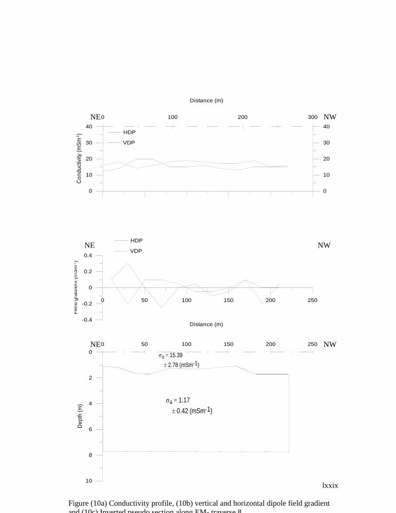
lxxix

Figure (10a) Conductivity profile, (10b) vertical and horizontal dipole field gradient


0

10

20

30

40

Co

nd

uct

ivity

(m

Sm

-1)

0

10

20

30

40

VDP

HDP

0 100 200 300

Distance (m)

0 50 100 150 200 250

-0.4

-0.2

0

0.2

0.4

Fie

ld g

rad

ien

t (m

Sm

-2)

0 50 100 150 200 250

Distance (m)

10

8

6

4

2

0

De

pth

(m

)

VDP

HDP

a = 1.17

0.42 (mSm-1)

a = 15.39

2.78 (mSm-1)

NE NW

NE NW

NE NW

lxxx

4.1.2 Electrical resistivity data processing

The resistivity data were interpreted both qualitatively and quantitatively using

computer based interpretative modelling. The field results were improved upon by

employing an interactive (iterative) computer programme. Finally the interpretation of

the geo-electric parameters (resistivity and thickness) in terms of subsurface geology and

groundwater conditions of the study area were carried out on the basis of the

supplementary geological and lithological information from the area.

Considering the large number of parameters required in the interpretation of

resistivity field data with several horizontal layers, computer based programs had been

designed for easier and more efficient results. In the computer based interacting

modeling, the field data is input into the computer and the computer theoretically

calculated curves are modified by trial and error until a very close match is attained

between the calculated, and the observed resistivity curves (Koefoed, 1979). The

computer displays the resistivity and layer thickness of the model which was adjusted to

approximate or fit the field observations. There are different types of computer soft wares

application that can be used in the interpretation of VES data. These include

DCSCTHUM, Resound, Offix, Applet, IPI2 WIN and so on.

The program used in the interpretation of the VES data is WINRESIST™

(Vander Velpen, 2004). Consequently, the interpreted geo-electric parameters and the

lithologic logs from the boreholes close to the area of study provided valid inferred

lithological and hydro-geological information about the study area. In view of this,

SURFER 8 program was used to provide the iso-pach, iso-resistivity, conductance, and

groundwater potential maps, as the imaging pictures of the subsurface in the form of

contour maps. The field curves generated by the interpreted vertical electrical sounding

data are shown on Figures 12.1-12.15, while the VES summary is given in Table 3.1. The

lxxxi

summary of the geo electric parameters and the geological type curve models are shown

on Table 3.2.

Fig. 12.1: VES 1 curve

lxxxii

Fig. 12.2 VES 2 curve

lxxxiii

Fig. 12.3 VE S 3 curve


lxxxiv



lxxxv



lxxxvi



lxxxvii



lxxxviii



lxxxix


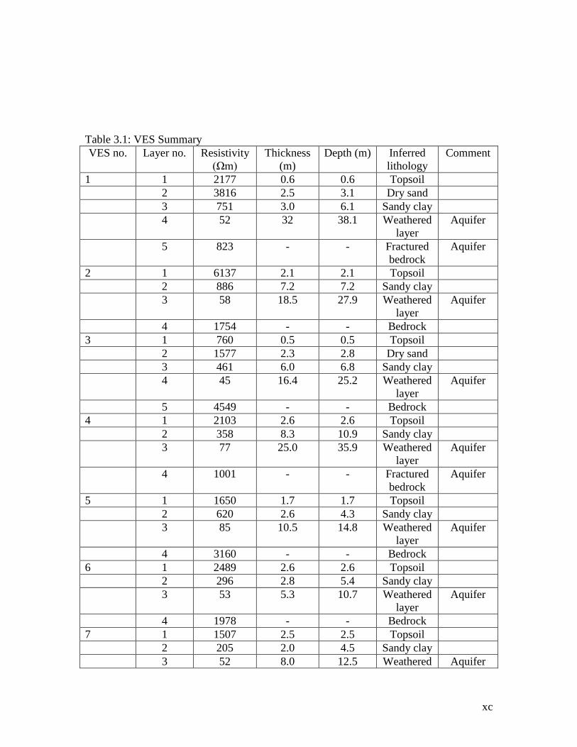
xc

Table 3.1: VES Summary

VES no. Layer no. Resistivity

(Ωm)

Thickness

(m)

Depth (m) Inferred

lithology

Comment

1 1 2177 0.6 0.6 Topsoil

2 3816 2.5 3.1 Dry sand

3 751 3.0 6.1 Sandy clay

4 52 32 38.1 Weathered

layer

Aquifer

5 823 - - Fractured

bedrock

Aquifer

2 1 6137 2.1 2.1 Topsoil

2 886 7.2 7.2 Sandy clay

3 58 18.5 27.9 Weathered

layer

Aquifer

4 1754 - - Bedrock

3 1 760 0.5 0.5 Topsoil

2 1577 2.3 2.8 Dry sand

3 461 6.0 6.8 Sandy clay

4 45 16.4 25.2 Weathered

layer

Aquifer

5 4549 - - Bedrock

4 1 2103 2.6 2.6 Topsoil

2 358 8.3 10.9 Sandy clay

3 77 25.0 35.9 Weathered

layer

Aquifer

4 1001 - - Fractured

bedrock

Aquifer

5 1 1650 1.7 1.7 Topsoil

2 620 2.6 4.3 Sandy clay

3 85 10.5 14.8 Weathered

layer

Aquifer

4 3160 - - Bedrock

6 1 2489 2.6 2.6 Topsoil

2 296 2.8 5.4 Sandy clay

3 53 5.3 10.7 Weathered

layer

Aquifer

4 1978 - - Bedrock

7 1 1507 2.5 2.5 Topsoil

2 205 2.0 4.5 Sandy clay

3 52 8.0 12.5 Weathered Aquifer

xci

layer

4 1167 - - Bedrock

8 1 1445 1.9 1.9 Topsoil

2 401 4.1 6.0 Sandy clay

3 83 6.9 12.9 Weathered

layer

Aquifer

4 1215 - - Bedrock

9 1 1069 2.2 2.2 Topsoil

2 300 2.0 4.2 Sandy clay

3 46 29.2 33.4 Weathered

layer

Aquifer

4 751 - - Fractured

bedrock

Aquifer

10 1 1950 1.7 1.7 Topsoil

2 176 4.5 6.2 Clayey

sand

3 31 32.8 39 Weathered

layer

Aquifer

4 1802 - - Bedrock

11 1 1537 1.2 1.2 Topsoil

2 60 18.9 20.1 Weathered

layer

Aquifer

3 184 - - Fractured

bedrock

Aquifer

12 1 1212 0.9 0.9 Topsoil

2 138 3.0 3.9 Clayey

sand

3 35 25.2 29.1 Weathered

layer

Aquifer

4 1570 - - Bedrock

13 1 323 0.3 0.3 Topsoil

2 103 1.6 1.9 Clayey

sand

3 29 19.4 21.3 Weathered

layer

Aquifer

4 109 - - Fractured

bedrock

Aquifer

14 1 509 3.4 3.4 Topsoil

2 41 10.3 13.7 Weathered

layer

Aquifer

3 4429 - - Bedrock

15 1 527 2.9 2.9 Topsoil

2 28 8.8 11.7 Weathered

layer

Aquifer

3 3444 - - Bedrock

xcii

Table 3.2: Summary of the geo- electric parameters and model theoretical resistivity

curve types over the study area.

Geo-

electric

earth

layer

model

type

Curve

Type

VES

Num

Layer

Resistivity

(Ohm-m)

Layer

Thickness

(m)

No. of

occurre-

nce

Percent. of

occurrence.

(%)

Layer Resistivity

Range (Ohm-m)

Thickness

Range (m)

3-Layer H

H

H

11

14

15

1537,60,184

509,41,4429

527,28,3444

1.2,18.9

3.4,10.3

2.9,8.8

3 20 1

2

3

509-1537

28-60

184-4429

1.2-3.4

8.8-18.9

∞

4-Layer H

H

H

H

H

H

H

H

2

4

5

6

7

8

9

10

6137,886,58,1754

2103,358,77,1001

1650,620,85,3160

2489,296,53,1978

1507,205,52,1167

1445,401,83,1215

1069,300,46,751

1950,176,31,1802

2.1,7.2,18.5

2.6,8.3,25.0

1.7,2.6,10.5

2.6,2.8,5.3

2.5,2.0,8.0

1.9,4.1,6.9

2.2,2.0,29.2

1.7,4.5,32.8

10 66.7 1

2

3

4

323-6137

103-886

29-85

109-3160

0.3-2.6

1.6-8.2

5.3-32.8

∞

xciii

H

H

12

13

1212,138,35,1570

323,103,29,109

0.9,3.0,25.2

0.3,1.6,19.4

5-Layer KH

KH

1

3

2177,3816,751,52,823

760,1577,461,45,4549

0.6,2.5,3.0,3.2

0.5,2.3,6.0,16.4

2 13.3 1

2

3

4

5

760-2177

1577-3816

461-751

45-52

823-4549

0.5-0.6

2.3-2.5

3.0-6.0

3.2-16.4

∞

Table 3.3 Aquifer parameters of the sounding locations

Bulk rest. Aquifer resist. Aquifer Trans. Long.

(ohm-m)ρh (ohm-m)ρa thick (m) resist.Rt cond. (mS/m)

7619 52 32 1664 0.62031003405

8835 58 18.5 1073 0.3274341147712

7392 45 16.4 738 0.3795859889978

3539 77 25.0 1925 0.349096011294

5515 85 10.5 829.5 0.12875326321

4816 53 5.3 280.9 0.110504055682

2931 52 8 416 0.165261176378

3144 83 6.9 572.7 0.094671847913

2166 46 29.2 1343.2 0.643507173496

3959 31 32.8 1016.8 1.08371987743621

1781 60 18.9 1134 0.3157807417046

2955 35 25.2 882 0.7424817046874

564 29 19.4 562.6 0.6854282903497

4979 41 10.3 422.3 0.257899276444

3999 28 8.8 246.4 0.3197885606

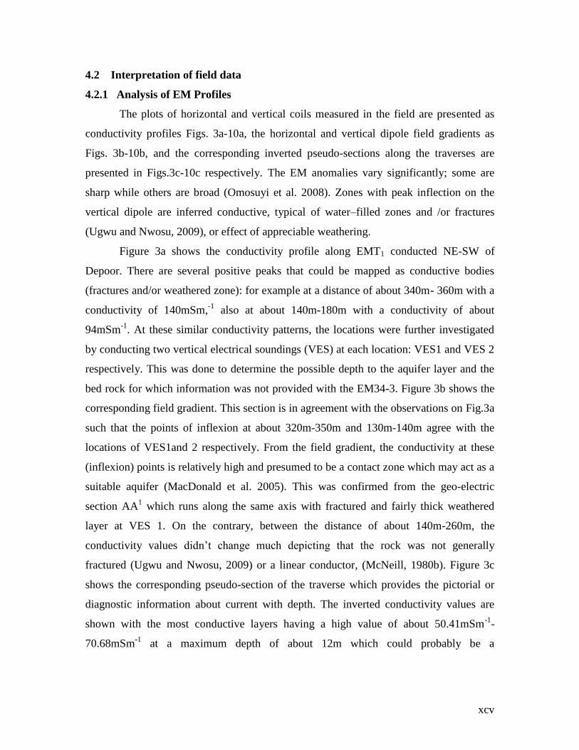
xcv

4.2 Interpretation of field data

4.2.1 Analysis of EM Profiles

The plots of horizontal and vertical coils measured in the field are presented as

conductivity profiles Figs. 3a-10a, the horizontal and vertical dipole field gradients as

Figs. 3b-10b, and the corresponding inverted pseudo-sections along the traverses are

presented in Figs.3c-10c respectively. The EM anomalies vary significantly; some are

sharp while others are broad (Omosuyi et al. 2008). Zones with peak inflection on the

vertical dipole are inferred conductive, typical of water–filled zones and /or fractures

(Ugwu and Nwosu, 2009), or effect of appreciable weathering.

Figure 3a shows the conductivity profile along EMT1 conducted NE-SW of

Depoor. There are several positive peaks that could be mapped as conductive bodies

(fractures and/or weathered zone): for example at a distance of about 340m- 360m with a

conductivity of 140mSm,-1

also at about 140m-180m with a conductivity of about

94mSm-1

. At these similar conductivity patterns, the locations were further investigated

by conducting two vertical electrical soundings (VES) at each location: VES1 and VES 2

respectively. This was done to determine the possible depth to the aquifer layer and the

bed rock for which information was not provided with the EM34-3. Figure 3b shows the

corresponding field gradient. This section is in agreement with the observations on Fig.3a

such that the points of inflexion at about 320m-350m and 130m-140m agree with the

locations of VES1and 2 respectively. From the field gradient, the conductivity at these

(inflexion) points is relatively high and presumed to be a contact zone which may act as a

suitable aquifer (MacDonald et al. 2005). This was confirmed from the geo-electric

section AA1 which runs along the same axis with fractured and fairly thick weathered

layer at VES 1. On the contrary, between the distance of about 140m-260m, the

conductivity values didn’t change much depicting that the rock was not generally

fractured (Ugwu and Nwosu, 2009) or a linear conductor, (McNeill, 1980b). Figure 3c

shows the corresponding pseudo-section of the traverse which provides the pictorial or

diagnostic information about current with depth. The inverted conductivity values are

shown with the most conductive layers having a high value of about 50.41mSm-1

-

70.68mSm-1

at a maximum depth of about 12m which could probably be a

xcvi

fractured/weathered layer. At conductivity of 18.34mSm-1

-36mSm-1

which is lower is

suspected to be fairly weathered zone.

Figure 4a shows the conductivity profile along the second traverse, EMT2 N-S of

(Depoor). There are several positive peaks that could be mapped as fractured or

weathered zones for example at a distance of about 200 and 240m and at about 300m on

the profile. These points could be assumed as zones of interest in groundwater

abstraction. Consequently, VES 3 and 4 were conducted along the traverse. Figure 4b

shows the corresponding field gradient of the traverse. Different zones of varying degree

of conductivity were delineated on the section; for instance between the distance of about

200-220m and about 380m, a conductive body was identified which was shown on the

conductivity profile. Fig 4c shows the corresponding pseudo-section of the profile. The

inverted conductivity values are shown with the most conductive area having a

conductivity of over 44.09mSm-1

at 200-220m at the upper layer and least conductivity of

about 10.05mS/m at a distance of over 400m indicating a resistive zone.

Figure 5a: shows the conductivity profile along EM traverse three (EMT3)

conducted at Imande. The traverse which runs across NE-SW of the area displays

appreciable variations in conductivity except at a distance of about 60m-80m where there

is observable peak of about 90mS/m-100mS/m which could be as a result of weathering.

Consequently VES 5 was conducted to ascertain the possible depth as well infer the

lithology. Also at a distance of about 290-320m along the profile with a broad anomaly,

another depth sounding (VES 6) was carried out. Figure 5b is the corresponding field

gradient of the traverse. From the plot, little observable changes in conductivity at about

60m and 90m respectively were of appreciable conductivity, depicting target zones (VES

5 and 6) respectively. Subsequently, the pseudo-section along the traverse (Fig. 5c)

revealed that there could be a conductive zone in the upper part of the subsurface with

conductivity of about 69.04mS/m depicting a weathered zone and at lower depth with

conductivity of about 3.53mS/m which is suggestive of resistive zone (bedrock).

Conductivity profile, (Fig. 6a), of EMT4 conducted E-W of Imande shows that the

anomaly is at about 60m and 200m. This is presumed to be a conductive zone which was

investigated with depth sounding. In view of this VES7 and 8 were carried out at a

distance of about 60m and 200m respectively to simulate the thickness of the underlying

xcvii

layers and their corresponding resistivity values as the instrument (EM34-3) was not

designed for detailed sounding. The corresponding field gradient, Figure 6b shows an

inflexion point between the vertical and horizontal coil readings at about 60m and 180-

200m respectively. From about 220m to 360m shows a conductor with appreciable

constant low conductivity which is indicative of less conductive layer with similar

characteristics. The pseudo-section along the traverse (Fig.6c) indicates a high

conductivity at these inflection points.

The conductivity profile along EM traverse-5 (Fig. 7a) which runs along E-W of the

study area shows a peak conductivity anomaly at a distance of about 120m and abroad

anomaly at about 200-280m. On this account VES 9 and 10 were conducted along the

profile and VES 9 with peak inflection, typical of water–filled zone and/or fracture

(Ugwu and Nwosu, 2009), or effect of appreciable weathering was confirmed with depth

sounding. Figures 7b and 7c showed similar inference.

The EM profile along traverse 6 (Fig. 8a) shows a broad anomaly at a distance of

about 60-80m, and a peak inflection at about 200-220m. These points were designated

VES 12 and 11 respectively. The depth sounding conducted at these points showed a

fractured zone within VES 11. The field gradient and the pseudo-section along this

profile proved the VES results.

Along N-S of the study area, EM traverse7 (Fig.9a) was conducted on the area.

EM anomaly was inferred at a distance of about 100m and 160m. These points were

designated VES 13 and 14 respectively. The depth sounding conducted along the profile

indicated a zone of appreciable low resistance suspected to be water bearing.

Figure 10a shows the EM traverse 8 along NE-NW direction of the study area.

The profile showed that the conductivity values at about 100-240m didn’t change much

depicting that the rock was not generally fractured, which McNeill, 1980b described as a

linear conductor. VES 15 was conducted at this point to ascertain the lithology and

possibly the depth to the aquifer unit.

Based on the interpreted EM profiles the points of interest designated as VES 1-

15 were further investigated with VES, as VES is used to assess the suitability of the

features because, a variety of subsurface conditions can give rise to similar EM34-3 data

xcviii

and also to predict depth to bed rock which is an important factor in cost control (Beeson

and Jones, 1988).

4.2.2 Analysis of electrical resistivity results

4.2.2.1 Resistivity sounding curves.

The resistivity sounding curves obtained from the surveyed area vary from 3, 4

layer (H type) or 5-layer (KH) as shown in Figures 11.1-11.15. The H-type curve with

about 86.7% of occurrence and KH-type curve with about 13.3% of occurrence were

deduced from the area. Worthington (1977) showed that field curves often mirror image

geo-electrically the nature of the successive lithologic sequence in an area and hence can

be used qualitatively to asses the groundwater prospect of an area. The H and KH curves

which are often associated with groundwater possibilities (Omosuyi, 2010) are pertinent

to the study area. The geo-electric parameters of the lithologic units were delineated from

the interpreted sounding curves.

4.2.2.2 Geo-electric characterization and lithologic delineation

Electrical resistivity methods primarily reflect variations in ground resistivity

(Omosuyi et al. 2008). These variations in ground resistivity exist across lithologic

interfaces or geo-electric boundaries in the subsurface. Their disparity is the yardstick on

which the aquiferous and non aquiferous units can hence be delineated. The 2

dimensional view of the geo-electric parameters (resistivity and thickness) obtained from

the inversion of the electrical resistivity sounding data were used to adjudge the

aquiferous or non aquiferous layers and reliable geological deductions. The geo-electric

sections (Figures12.1-12.6) of the various VES stations in the study area were created to

indicate the various geo-electric layers, their thicknesses within the depths penetrated

with their characteristics resistivity values and probable geo-electric connotations. The

profiles were taken along the NE-SW; (AA1, BB

1), NW-SE; (CC

1, DD

1, EE

1) and NNE-

SSW (FF1) directions.

The geo-electric section AA1 which runs across NE-SW direction of the study

area is made up of data from VES 1, 2, 3, 9 and 10 (Fig. 12.1). The interpretative cross

section AA1 shows four geo-electric layers in VES 2, 9 and 10 and five layers in VES 1

and 3. The topsoil which is relatively thin is characterized by resistivity values ranging

from 760 ohm-m to 2177ohm-meter with a thickness that varies from 0.5m to 2.2m, and

xcix

is composed of predominantly laterite, and clay towards the northeastern part. The second

layer has resistivity values that vary from 1577-6137ohm-m at the northeastern part and

terminated in VES 9 and 10. The next layer with resistivity range of 176-886 ohm-m and

a thickness between 2.0m- 7.2m is presumed to be sandy-clay. It is predominantly wet.

The third layer which is probably conductive and reflects the layer identified as the

aquifer unit characterized by resistivity values between 31 ohm-m and 58 ohm-m with

thickness values of 16.4m−32.8m is diagnostic of extensive weathered bedrock which is

in agreement with Ajayi and Hassan (1990), Oyedele and Adeyemo (2001) who are of

the view that the decomposed basement with resistivity of 20-1000ohm-m and thickness

of 14-28m forms the aquifer which are subject to groundwater development. The last

layer with resistivity values that vary from 751-4549 ohm-m with infinite thickness is

suggestive of fractured or fresh basement respectively.

c

The interpretive geo-electric section BB1 across NE-SW direction

is made up of

data from VES 4, 14 and 15 (Fig. 12.2) .The geo-electric section shows three/four geo-

electric layers, but three distinct lithologic layers. The topsoil along the section has

resistivity values ranging from 509ohm-m to 2310ohm-m characteristic of laterite at the

southwestern part and lateritic clay at the northeastern part. The second geo-electric layer

which is conductive and recognized as the aquifer layer with unit resistivity values

between 28ohm-m to over 358ohm-m with thickness range of 8.3-11.7m is the presumed

weathered layer. The basal unit with resistivity values ranging from 77- 4429ohm-m is

identified as the fractured bedrock at VES 4 which could be another aquifer unit and

fresh bedrock at VES14 and 15 along the section.

The geo-electric section CC1 across NW-SE direction (Fig.12.3) is made up of

data from VES 5, 7 and 14. The cross section shows three to four geo-electric layers. The

topsoil has resistivity value ranging from 509ohm-m to 1650ohm-m with thickness

varying from 1.7m-3.4m characteristic of lateritic sand at the southeastern part and

ci

sandy-clay at VES14. Beneath the topsoil layer towards the southeastern part, the

relatively low resistivity value of 205ohm-m observed under the topsoil which does not

extend to VES 14 is characteristic of clayey-sand. The next layer which is recognized as

the aquifer layer with resistivity range of 41ohm-m – 85 ohm-m with thickness of 8.0m-

10.5m is the presumed weathered layer. The underlying bedrock is characterized by

resistivity values ranging from 1167ohm-m to 4429 ohm-m.

ciii

Across DD1, four/five geo-electric layers underlie the southeast-northwest flank

of the study area, (Fig.12.4). The geo-electric section is made up of VES 1, 7 and 8. The

top soil thickness is relatively thin along this profile and ranges between 0.6-2.5m while

the resistivity values range between 1445 and 2177 ohm-m, which indicate that the

predominant composition of the layer is laterite. The second layer has resistivity value of

3186ohm-m at VES1 and diminished towards the southeastern part of the profile. The

third layer that varies in resistivity from 205ohm-m to 751ohm-m with thickness values

that varies from 2.0-4.1m is diagnostic of sandy-clay. Below this layer is a very low

resistivity layer suspected to be the aquifer unit with resistivity values between 52ohm-m

and 83ohm-m with a thickness value ranging from 6.9m to 32m which indicates high

degree of weathering. The basal unit of resistivity value 823ohm-m to 1215ohm-m is

suggestive of fractured and probably fairly fractured bedrock respectively.

The interpretive cross section EE1, southeast-northwest direction (Fig12.5) is underlain

by four geo-electric layers at VES 6 and 13 and three geo-electric layers at VES 15. The

topsoil which has a resistivity value of 2489 at VES 6 and absent in VES15 and forms a

very thin layer in VES 13 with a resistivity value of 323 is lateritic and clayey

respectively. Beneath this layer, a relatively low resistivity values ranging from 103ohm-

m - 296ohm-m is characteristic of sandy-clay. The underlying layer recognized as the

aquifer layer with unit resistivity values between 28ohm-m to 53ohm-m is the presumed

weathered layer. The bedrock which is fractured at VES 13 with unit resistivity of 109

ohm-m and 1978ohm-m and 3444ohm-m at VES 6 and 15 respectively forms the basal

layer unit along the profile.

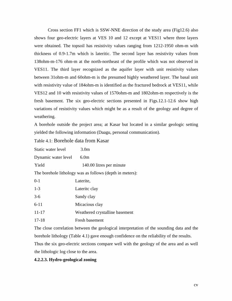
cv

Cross section FF1 which is SSW-NNE direction of the study area (Fig12.6) also

shows four geo-electric layers at VES 10 and 12 except at VES11 where three layers

were obtained. The topsoil has resistivity values ranging from 1212-1950 ohm-m with

thickness of 0.9-1.7m which is lateritic. The second layer has resistivity values from

138ohm-m-176 ohm-m at the north-northeast of the profile which was not observed in

VES11. The third layer recognized as the aquifer layer with unit resistivity values

between 31ohm-m and 60ohm-m is the presumed highly weathered layer. The basal unit

with resistivity value of 184ohm-m is identified as the fractured bedrock at VES11, while

VES12 and 10 with resistivity values of 1570ohm-m and 1802ohm-m respectively is the

fresh basement. The six geo-electric sections presented in Figs.12.1-12.6 show high

variations of resistivity values which might be as a result of the geology and degree of

weathering.

A borehole outside the project area; at Kasar but located in a similar geologic setting

yielded the following information (Daagu, personal communication).

Table 4.1: Borehole data from Kasar

Static water level 3.0m

Dynamic water level 6.0m

Yield 140.00 litres per minute

The borehole lithology was as follows (depth in meters):

0-1 Laterite,

1-3 Lateritc clay

3-6 Sandy clay

6-11 Micacious clay

11-17 Weathered crystalline basement

17-18 Fresh basement

The close correlation between the geological interpretation of the sounding data and the

borehole lithology (Table 4.1) gave enough confidence on the reliability of the results.

Thus the six geo-electric sections compare well with the geology of the area and as well

the lithologic log close to the area.

4.2.2.3. Hydro-geological zoning

cvi

Electrical resistivity depth sounding is useful in locating areas of maximum

aquifer thickness and serves as a good predictive tool for estimation of borehole depth

(Omosuyi, 2010). Ameloko and Rotimi, (2010), Lenkey et al. (2005) took the advantage

of VES to infer that the large thickest weathered materials overlying the basement rocks

constitute the main water bearing layer (the aquifer). To zone the area into groundwater

prospects, the ideas of Ameloko and Rotimi, (2010), Lenkey et al. (2005), and Omosuyi

et al. (2008) were adopted. Several maps were produced using SURFER8 program to

monitor the trend of resistivity, thickness and conductance variation with a view of

assessing the sub-surface lithology suitable for low, intermediate or high groundwater

potentials. Due to the heterogeneous nature of the basement areas, the aforementioned

parameters vary constantly, hence the need for hydro-geological zoning (Omosuyi et al.

2008).

4.2.2.3.1 Isopach, iso-resistivity and longitudinal conductance maps

Based on visual examination of the 2-D geo-electric earth parameters; several

maps: Figures 13.1-13.3 were generated. Figure 13.1(a) shows the isopach map

distribution of the main aquifer unit (weathered layer) that varies from 5.3m to 32.8m.

Based on the weathered layer thickness, the central (Depoor), and south western

(Tsekyor) parts of the area can probably support intermediate-high groundwater

potentials where as the southeastern part (Imande) and a patch of northeastern areas show

an indication of low – intermediate groundwater potential. With regards to significant

role played by thickness in groundwater abstraction (Adiat et al. 2009; Omosuyi et al.

2008) areas characterized by thickness between 10.6 – 32.8m were accorded more

preference in groundwater development.

Figure 13.1(b) is the iso-resistivity map of the layer considered as the main

aquifer in the area. The resistivity value of the layer lies between 28 ohm-m and 83 ohm-

m while the most frequently occurring resistivity values are between 41 ohm-m and 58

ohm-m; typical of clay which may be constantly saturated but poorly permeable to the

interstitial formation water for abstraction (Abiola et al.2009).

Although aquifer thickness alone cannot be considered as the yardstick for

groundwater prospect evaluation, resistivity and lithology amongst others are relevant

considerations. In this study, a correlation between the borehole data close to the area and

cvii

the VES interpretation showed that the weathered layer directly overlying the basement

(bedrock) or fractured bedrock constitute the aquifer unit. This is in agreement with

Ajayi and Hassan (1990) who are of the view that the weathered basement is associated

with low to medium resistivity values suggestive of materials of most likely slight clayey

and/or saturated with water.

Fig.14.1a.Isopach map of the aquifer unit in the area

cviii

Consequently, the longitudinal unit conductance map of the study area (Figure

13.2(b)) was generated from the data calculated from the model parameter S =

n

i

ihi1

/

and shown in Table 3.3 for all the VES locations. The longitudinal unit conductance, S

values obtained from the study area ranged from 0.0947 to 1.083mhos.

From the map (Fig.13.2), the northern and a patch of southwestern region have

over 0.5 mhom. The southeastern and southern parts have conductance values lower than

0.5mhoms which correlates well with the groundwater potential map (Fig.13.3). This is

because the earth medium acts as a conductor especially when it contains fluid. Its ability

to conduct current is a measure of its conductance capacity and invariable its resistive

capacity as well.

4.2.2.3.2 Groundwater potential evaluation

At large the groundwater evaluation of Katsina Ala is based on various categories

of maps: iso-pach and iso resistivity maps of the weathered layer (aquifer), and the

longitudinal unit conductance map of the aquifer unit in preparing the groundwater

Figure 14.1(b): Iso-resistivity map of the aquifer unit in the

area study area

cix

potential map of the area as deduced from the geo-electric parameters (resistivity and

thickness) and longitudinal conductance obtained from interpreted VES results. The

groundwater potential map shown in Figure 13.3 was used to classify the study area into

high, intermediate, and low groundwater potential zones. In view of groundwater

abstraction, areas with intermediate to high notation are accorded more preference to well

development.

cx

Fig..14.2. Longitudinal unit conductance map of the study area

cxi

VES 1

VES 2VES 3

VES 4

VES 5

VES 6VES 7

VES 8

VES 9VES 10

VES 11

VES 12

VES 13

VES 14

VES 15

Tsekyor

Amande

Imande

Tsendele

Gurugu

Zem

KumeDepoor

Yokosi

Amaafu

Amaafu

0 0.6 1.2 1.8 2.4 3 km

A

A1

B

B1

C

C1

D

D1

E

E1

F

F1

9 30 EO '

9 30 EO '

7 20 NO ' 7 20 N

O '

7 15 NO '7 15 N

O '

EMT-1

EMT-6

EMT-5

EMT-4

EMT-3

EMT-2

EMT-7

EMT-8

9 22 30 EO ' ''

9 22 30 EO ' ''

EMT-1

A A1

VES 10

Zem Towns

EM Traverse

Geoelectric Cross Section

VES Locations

Stream

Road

Eze Aku Shale Group

Basement Rock(Quazite and Silicified Rocks)

Low

Intermediate

High

Ground water potential

Figure 14.3: Groundwater potential map of the study area

cxii

CHAPTER FIVE

CONCLUSIONS AND RECOMMENDATIONS

5.1 Conclusions

The geophysical methods: Very Low Frequency Electromagnetic, (VLF-EM) and

Electrical Resistivity (ER) were used in this study to investigate the groundwater

potentials of some selected areas in Katsina-Ala L.G.A, Benue State, Nigeria. A total of

eight (8) electromagnetic traverses and fifteen (15) vertical electrical soundings (VES)

employing Schlumberger array configuration with current electrode spacing, AB of 200-

340m.

The data acquired and analyzed from the study are geophysical, geological and

global positioning system (GPS) data. The GPS values were used to locate the EM and

VES points on the map of the study area. The geophysical data were derived from both

eight EM traverses and fifteen VES points systematically distributed over the area.

The EM data were analyzed qualitatively by plotting conductivity profiles,

gradients and pseudo-sections of both the horizontal and vertical coil orientations; while

the sounding data were analyzed both qualitatively and quantitatively by using Win-

Resist version of computer iterative inverse modeling of Vander Valpen, (2004).

The interpreted electromagnetic data identified zones of high conductivity which

could be fractures and/or weathered zones, and were considered as priority areas for

vertical electrical sounding.

The interpreted VES data results also revealed one to two earth curve model

(type) which varied from simple three layer H type to the complex four or five layers

models KH type curves. Type H and KH curves which are often associated with

groundwater possibilities (Omosuyi, 2010) are pertinent in the area. The H type curve

which is commonly obtained in a basement complex area, (Nur and Afa, 2002; Keller and

Freschneit, 1986) constituted about 83.7% of occurrence in the area.

Furthermore, the geo-electric parameters (resistivity and thickness) obtained from

the inverted vertical electrical resistivity sounding data were used to delineate the aquifer

types of the area as: weathered bedrock and fractured bedrock aquifer types, which are in

agreement with Nur and Afa (2002) who are of the opinion that the weathered and/or

cxiii

fractured rocks in the crystalline basement areas are the only places where water could be

found in the dry seasons.

The geo-electric parameters (resistivity and thickness) obtained from the

interpreted vertical electrical sounding data was used to generate geo-electric sections

and contoured maps: conductance, iso-pach and iso resistivity maps which were analyzed

in terms of hydro-geologic importance of the area. The geo-electric sections showed

three-five geo-electric layers but three lithologic (geologic layers) which were interpreted

based on the geologic data gotten from the lithological logs of drilled boreholes by Benue

State Rural Water Supply and Sanitation Agency (BERWASSA) Markurdi; Benue State.

A correlation between the borehole lithology of Kasar and VES results provided the basis

for the inferred lithology from the geo-electric sections. From the comparison of both

data, the first layer with apparent resistivity range of 509-6137ohm-m which is entirely

lateritic/lateritic clay is underlain by a weathered (aquiferous) layer with varying

resistivity of 28-184ohm-m. The third layer with resistivity between751-4549ohm-m is

the fractured/fresh basement.

Consequently, the maps were used to categorize the study area into three hydric

zones: high, intermediate and low groundwater potentials. The yield capacity of the

weathered layer constituting the main aquifer unit will not only depend on the thickness

but also on the quantity of clay.

5.2 Recommendations

The geophysical surveys carried out in the selected study areas revealed that the

areas could play a significant role in groundwater resource development. In Depoor at

VES 1 within a depth of about 6.1m-39m, and VES 4 within a depth of about 10m – 40m

groundwater could be abstracted. At Tsekyor, groundwater of reasonable quantity can be

developed at VES 10 and 12 within the depths of about 6m-40m. At Amaafu VES 13,

groundwater could be developed within a depth of about 21m.

It is however recommended that more sophisticated instruments such as depth

probing EM instrument (ABEM WADI VLF instrument) which detects fractures, depth

to the conductive zones and its dip, bedrock relief features such as basement troughs

which are of significant hydro-geologic importance (Adiat et al. 2009) could be used for

the EM while SAS 4000/1000 (ABEM LUND IMAGING SYSTEM) for VES could be

cxiv

used for data of better quality which can provide a better resolution of the geologic

situation at depth (ABEM Instruction Manual, 2009).

Also the use of 2-D electrical imaging which is a powerful technique in the study

of subsurface geology (Ameloko and Rotimi, 2010) and bedrock geometry such as down

warping, faulting structures could be used to give a better resolution of hydro-geologic

structures.

For a better and more accurate results, a more sophisticated and effective

geophysical method such as remote sensing (Offodile, 2003), a combination of electrical

imaging and seismic tomography which gives a more accurate result on the layering and

the depths of lithology is recommended.

Nonetheless, this work is worthy of continued research.

cxv

REFERENCES

Abem Instruments (2009). Instructional Manual for ABEM Terrameter SAS

1000/SAS4000. http://www.abem.se. p. 148.

Abiola, O., Enikanselu, P.A., and Oladapo, M. I., (2009). Groundwater potential and

aquifer protective capacity of overburden units in Ado-Ekiti, southwestern

Nigeria. International Journal of Physical Sciences. Vol. 4 (3), pp. 120-132.

Adelusi, A. O., and Balogun, O., (2001). A geo-electric investigation for groundwater

development of Orita-Obele area near Akure SW Nigeria. Global Journal of Pure

and Applied Sciences. Vol. 7 No.4: 707 – 717.

Adetola, B. A and Igbedi, A. O., (2000). The use of electrical resistivity survey in

location of aquifers: A case study in Agbede South Western Nigeria. Journal of

Nigerian Association of Hydro-geologists, Vol. 11: 7-13.

Adiat, K. A. N, Olayanju, G. M., Omosuyi, G. O., and Ako, B. D., (2009).

Electromagnetic profiling and Electrical Resistivity soundings in groundwater

investigation of a typical basement complex - A case study of Oda town

Southwestern Nigeria. Ozean Journal of Applied Science 2(4), pp. 333-359.

Ajayi, C. O., and Hassan, M., (1990). The delineation of aquifer overlying the Basement

Complex in the Western part of the Kubarni Basin of Zaria: Nigeria. Journal of

Mining and Geology Vol. 26, No.I, pp. 117 – 124.

Alile, M. O, Jegede, S.I. and Ehigiator, O. M., (2008). Underground water exploration

using electrical resistivity method in Edo State, Nigeria. Asian Journal of Earth

Sciences. Vol.1, pp 38-43.

Alkali, S. C., Kamfut, N. M., and Yusuf, A. K.,(1997). A Geo-electrical investigation for

groundwater at Kwasauri, near Kano: Northern Nigeria. Water resources-Journal

of NAH Vol.8 No1, pp. 11-18.

Amadi, U. M. P., and Nurudeen, S. I., (1990). Electromagnetic survey and the search for

groundwater in the Crystalline Basement Complex of Nigeria. Journal of Mining

and Geology Vol.26, No I, pp. 45-53.

Ameloko, A. A, and Rotimi, O. J., (2010). 2- D Electrical Imaging And Its Application In

http://www.abem.se/

cxvi

Groundwater Exploration In Part Of Kubanni River Basin-Zaria, Nigeria. World

Rural Observations Vol. 2(2). pp. 72-82.

cxvii

Ariyo, S. O., and Adeyemi, G. O., (2009). Role of Electrical Resistivity Method for

Groundwater Exploration in Hard Rock Areas: A Case Study from

Fidiwo/Ajebo Areas of Southwestern Nigeria. The Pacific Journal of Science and

Technology. Vol. 10. No. 1, pp. 483-486.

Ariyo, S. O., Adeyemi, G. O., and Oyebamiji, A. O, (2009). Electromagnetic VLF survey

for groundwater development in a Contact Terrain: a case study of Ishararemo,

Southwestern Nigeria. Journal of Applied Sciences Research, Vol. 5(a): 1239 –

1246.

Arshad, M., Cheema, J. M. and Ahmed S., (2007). Determination of lithology and

groundwater quality using electrical resistivity survey. Int. J Agric. Biol. Vol.9,

No.1, pp. 143-146. http://www.fspublishers.org

Bayode, S., Ojo, J. S., and Olorunfemi, M. O. (2006). Geo-electric Characterization of

Aquifer types in the Basement Complex Terrain of Parts of Osun State Nigeria.

Global Journal of Pure and Applied Sciences Vol. 12, No3, pp. 377 – 385.

BBC Sci/Tech News (2000). Water arithmetic “doesn’t add up” – Report of the World

Commission on Water for 21ist

Century.

Beeson, S., and Jones, C. R. C. (1988). The combined EMT/VES method for siting

boreholes. GROUNDWATER Vol.26, No1. Pp 54-63.

Bose, R. N., Chattarjee, D. and Sen A. K., (1972). Electrical resistivity surveys for

groundwater in the Auragabad Subdivision, Gaya District Bihir, India. Geo-

exploration, Vol.11, Issues 1-3, 1973, pp 171-181.

Burger, H. R. (1992). Exploration Geophysics of the shallow sub-surface. Prentice Hall,

Inc, Eaglewood Chaff, New Jersey 07632.

Chernicoff and Whitney (2002). An introduction to physical Geology 3rd

ed. Houghton

Mifflin Company New York.

Dessauvagie, T. F. J. (1975). Explanatory notes to the Geological Map of Nigeria.

Journal of Mining and Geology. Vol.9, Nos. I and 2. pp. 3-28.

Dhakate, R., Negi, B. C. and Singh,V. S. (2008). Electrical resistivity survey to delineate

groundwater potential zones in Granite Terrain, Nalgonda District, Idia. Asian

Journal of Water, Environmental and Pollution, Vol.5,No.1 2, 2008.

cxviii

Dobrin, M. B., (1985). Introduction to geophysical prospecting (4th

edition). Mc.Graw

Hill Inc. New York, USA p. 629.

Duffin, W. J., (1979). Electricity and Magnetism.3rd

edition. The English Book Society.

pp. 58-61, 155-156.

Du-Preeze, J. W.,and Barber, W. (1965). The distribution and chemical quality of

groundwater in Northern Nigeria: Geological Survey Bulletin No 36.

Eduvie, M. O. (2002). An hydro-geological geophysical evaluation of groundwater

resources of the Gundumi Formation and around Daura, North Western Nigeria.

Water Resources –Journal of Nigeria Association of Hydro-geologist (NAH),

Vol.13, pp. 46-49.

Egbu, R. N. (2000). A geophysical survey of productive boreholes sites for effective

water planning in Imo State, Nigeria. African Journal of Science and Technology

Vol. 1, No.2 pp. 129-138.

Egwebe, O., Aigbedion, I., and Ifedili, S.O. (2004). A Geo-electric investigation for

groundwater at Ivbiaro Ebesse; Edo State: Nigeria. Journal of Applied Science,

Vol. 22, pp. 146-150.

Evwaraye, A. O., and Mgbenu, E. N., (1993). Electromagnetism and modern physics for

physical sciences. Spectrum Books Ltd. pp. 86-88

Ezema, P. O. (2005). Fundamentals of applied geophysics. Enugu. Rojoint

Communication Services Ltd, Enugu pp. 1-167.

Fitterman, D. V and Deszez–Pan, M. (2003). Estimating water quality along Southwest

Florida Coast for hydrologic models: using Helicopter electromagnetic survey. A

Poster Presented at the greater Everglades Ecosystem Restoration Conference.

Federal Survey Nigeria, (1975). Map Sheet 272 Katsina – Ala.

Geological Survey of Nigeria, (1994). Geologic Map of Nigeria: Published by

Geological Survey Department: Ministry of Petroleum and Mineral Resources

Nigeria.

Grant, F. S and West, G. F. (1965). Interpretation theory in applied geophysics. McGraw

Hill book company pp. 365-443.

Hamill, L. and Bell, F. G. (1986). Groundwater resource development: London.

University Press Cambridge: p. 1 – 344.

cxix

Isife, F. A., Balogun, O., and Adedapo, O, J. (2000). Hydro-geophysical investigation of

the Federal Polytechnic, Ado–Ekiti, Ekiti State, Nigeria. African Journal of

Science and Technology, Vol.1, No. 2, pp. 158-165.

Iyioriobhe, S. E., and Ako., B. D. (1986). The hydrogeology of the Gombe sub

catchments, Benue Valley, Nigeria. Journal of African Earth Sciences Vol. 5, No.

5, pp. 509-518.

Keary, P., and Brooks M. (1991). An introduction to geophysical exploration (2nd

edition).

Oxford .Blackwell Scientific publications, London. p. 254.

Keller, G. V., and Frischknecht, F. C. (1966). Electrical methods in geophysical

prospecting. Pergamon press Oxford. New York. p. 517.

Koefoed, O. (1979). Geo-sounding Principles I, Resistivity sounding measurements.

Elservier. Oxford.

Land, L. A., Lautier, J. C., Wilson, N. C., Chanese, G., and Webb, S. (2004).

Geophysical monitoring and evaluation of coastal plain aquifer: Groundwater,

Vol.42. No1. pp. 59-67.

Lenkey, L., Hamori, Z and Mihalffy, P. (2005). Investigating the hydrogeology of a

water-supply area using direct-current vertical electrical soundings. Geophysics,

Vol.70. No. 4, H1-H19.

Lowrie, W. (1997). Fundamentals of Geophysics. Cambridge University press.pp354.

MacDonald, A., Davies, J., Calow, R., and Chilto, J. (2005). Developing groundwater, A

guide for rural water supply. www.itdgppublishing.org.uk. pp. 1- 358.

MacDonald, A., Davies, J., and Dochartagh, B. E. O. (2002). Simple methods for

assessing groundwater resources in low permeability areas of Africa. British

Geological Survey Commissioned Report, CR/01/168N.

Mamah L. I. (1984). Application of time domain electromagnetic sounding to a rift

system: Nigerian Journal of Mining and Geology Vol. 21 Nos.1 and 2. pp. 151-

155.

Mamah L. I. and Eze, L. C. (1988). Electromagnetic and ground magnetic survey over

zones of lead-zinc mineralization in Wanakom (Cross River State). Journal of

African Earth Sciences, Vol. 7, No.5-6, pp. 749-758.

http://www.itdgppublishing.org.uk/

cxx

McDougal, R. R., Abraham, J. D., and Bisdorf, R. J. (2003). Results of electrical

resistivity data collected near the town of Guernesey, Platte County, Wyoming.

U.S. Geological Survey Open File 2004-1095.

McNeill, J. D. (1980a). Technical Notes: TN-5 - Electrical conductivity of soils a4nd

rocks. Ontario, Canada. pp. 1 – 22.

McNeill, J. D. (1980b). Technical Note: TN-6. Electromagnetic terrain conductivity

measurements at low induction numbers. Ontario. Canada. pp.1-15.

McNeill, J. D. (1983). EM 34-3 Survey interpretation techniques. Technical note: TN-8.

Geonics Ontario. pp. 1-17.

McNeill, J. D. (1994). Technical Note: TN-27: Principles and application of time domain

electromagnetic technique for resistivity sounding. Ontario, Canada. pp. 1-16.

Microsoft Encarata®, (2009). Groundwater, Redmond, W.A Microsoft Corporation.

Mohamed, S. A., and Lee, C. Y. (1985). A resistivity survey for groundwater in Perlis

using offset Wenner technique. Karst Water Resources. IAHS Pub. No.161, 221-

232.

Montgomery, C. W. (1990). Physical Geology 2nd

edition. Wm. C. Brown Publishers

United States of America.

Moonrey, J. and Wicander, R. (2005). Physical Geology exploring the Earth. 5th

edition.

Thomson Learning, Belmon U.S.A.

Nosal, E.A. (1983). Statistical determination of geophysical well log response function.

Geophysics, Vol.48, No.11. pp. 1525-1535.

Nur, A., and Afa, D. E. (2002). Geo-electrical and Hydro-geological investigations in a

part of Adamawa State: Northeastern Nigeria. Water Resources- Journal of

Nigerian Associations of Hydro-geologists (NAH), Vol. 13. pp. 55 – 61.

Nur, A., and Kujir, A. S., (2006). Hydro-geoelectrical study in the northeastern part of

Adamawa State, Nigeria. Journal of Environmental Hydrology Vol. 14. pp1- 7.

Obiakor, I. P. (1984). Resistivity survey for groundwater in Idemili and Anambra local

government areas: Anambra State. An M.Sc thesis presented to the Department of

Physics and Astronomy, University of Nigeria Nsukka.

cxxi

Offodile, M. E. (1976). A review of the geology of the Cretaceous of the Benue valley, In

Geology of Nigeria: Edited by C. A, Kogbe. C.A Elizabeth Publishing Co. pp.

319-330.

Offodile, M. E. (1983). The occurrence and exploitation of groundwater: in Nigerian

Basement rocks. Nigeria Journal of Mining and Geology, Vol. 20 Nos. 1 and 2

pp. 131 – 146.

Offodile, M. E. (2002). Groundwater study and development in Nigeria. Mecon Geology

and Engineering Services Ltd., Jos. pp. 1 - 453.

Ohams, E., Agwunobi and Onuoha, M. K., (1988). Geophysical investigation for

groundwater in hard rock terrain: Experiences from the Fobur area of the Jos

Plateau, Nigeria. Journal of Mining and Geology Vol. 24 Nos. 1 & 2 pp. 45 –

50.

Olaleye, B.M., (2005). Influence of soil structure on borehole depth determination in

Osun State, Nigeria. International Research Journal in Engineering and

Technology (IRJET), Vol. 2, No. 1 pp. 111-119.

Olayinka, A. I., (1990). Electromagnetic profiling for groundwater in Precambrian

Basement Complex areas of Nigeria: Nordic Hydrogeology, Vol. 21 pp. 205 –

216.

Olayinka, B.Y., (2000). Senior Secondary Atlas: Longman. Atlas Nigeria.

Omosuyi, G. O, Adegoke, A. O, and Adelusi, A. O., (2008). Interpretation of

Electromagnetic and Geoelectric Sounding Data for Groundwater Resources

around Obanla-Obakekere, near Akure, Southwestern Nigeria. The Pacific

Journal of Science and Technology. Vol. 9 No. 2. pp. 508-525.

Omosuyi, G.O. (2010). Geoelectric assessment of groundwater prospect and vulnerability

of overburden aquifers at Idanre, Southwestern Nigeria. Ozean Journal of Applied

Sciences Vol. 3. No.1. pp. 19-28.

Oteze, G. E., and David, L .M. (2002). Hydro-geophysical survey of Ivioghe area: Edo

State Nigeria. Water Resources – Journal of Nigerian Association of Hydro-

geologists, (NAH), Vol. 13. pp. 71 – 77.

Oyedele, K. F., and Adeyemo, A. O. (2001). Surface electrical resistivity measurement in

the characterization of groundwater potentials of the typical Basement Terrain,

cxxii

Northern Nigeria. African Journal of Environmental Studies Vol.2 No. 1 pp. 52 -

54.

Parasins, D. S. (1986). Principles of applied geophysics. Chapman and Hall U.S.A.

pp. 1 - 402.

Reyment, R. A. (1965). Aspects of the Geology of Nigeria: Ibadan University Press.

pp. 36 – 43.

Richards, R. T., and Troester, J. W. (1998). An Electromagnetic geophysical survey of

the fresh water lens, of Isla De Mona, Puerto Rico. Journal of Cave and Karsts

Studies, Vol. 60 No. 2, pp. 115 – 120.

Selemo, A. O. I., Okeke, P. O. and Nwankwo, G. I. (1995).An appraisal of the usefulness

of vertical electrical sounding (VES) in groundwater exploration in Nigeria.

Water Resources Vol.6 No1 and 2, pp. 61-67.

Shahid, S., and Nath, S. K. (2010). GIS Integration of Remote Sensing and Electrical

Sounding Data for Hydrogeological Exploration. J. of Spatial Hydrology.Vol.2

No.1. pp. 1-12.

Singh, K. K. K., Singh, K. A., Singh, K. B., and Sinha, A. (2006). 2D resistivity imaging

survey for sitting water supply tube wells in metamorphic terrains: A case study

of CMRI campus, Dhanbad, India. The Leading Edge: 25, pp. 1458-1460.

Telford, W. M., Geldart, I. P., and Sheriff, R. E. (1990). Applied Geophysics, Second

Edition, New York. Cambridge University Press pp.1 – 770.

Ugwu, S. A., and Nwosu, J. I. (2009). Detection of fractures for groundwater

development in Oha-Ukwu using electromagnetic profiling. J.App. Sci. Environ.

Manage. Vol.13 (4) 59-63.

Ugwueke, B. U. D., Nkereuwem, O. T., Utah, E. U., (2005). Local tectonism and

groundwater accumulation in the Basement Terrain: The study of the North –

Eastern part of Gwoza area of Borno State, Nigeria. International Journal of

Environmental Issues, Vol. 3, No. 2 pp. 1-9.

Vander Velpen, B. P. A., (2004). WIN RESIST™. Electrical resistivity inversion

program.

Worthington, P. R. (1977). Geophysical investigations of groundwater resources in the

Kalahari Basin. Geophysics, Vol. 42, No 4, pp. 838-849.

cxxiii

Zaafran, Z. M., (1981). The use of a new resistivity space display technique in

groundwater investigation. Geo-exploration Vol. 18, No. 4. pp. 247 – 258.

ELECTROMAGNETICS AND RESISTIVITY INVESTIGATIONS

Documents

Transcript of ELECTROMAGNETICS AND RESISTIVITY INVESTIGATIONS