3D modelling and sensitivity in DC resistivity using charge density
39
Geophysical Prospecting, 2005, 53, 579–617 3D modelling and sensitivity in DC resistivity using charge density Olivier Boulanger ∗ and Michel Chouteau D´ epartement des G´ enies Civil, G´ eologique et des Mines, Ecole Polytechnique de Montr ´ eal, CP 6079, succ. Centre-Ville, Montr´ eal, H3C 3A7, Canada Received November 2002, revision accepted August 2004 ABSTRACT A three-dimensional (3D) electrical resistivity modelling code is developed to interpret surface and subsurface data. Based on the integral equation, it calculates the charge density caused by conductivity gradients at each interface of the mesh, allowing the estimation of the potential everywhere without the need to interpolate between nodes. Modelling generates a huge matrix, made up of Green’s functions, which is stored by using the method of pyramidal compression. The potential is compared with the analytical and the numerical solutions obtained by finite-difference codes for two models: the two-layer case and the vertical contact case. The integral method is more accurate around the source point and at the limits of the domain for the potential calculation using a pole-pole array. A technique is proposed to calculate the sensitivity (Jacobian) and Hessian matrices in 3D. The sensitivity is based on the derivative with respect to the block conductivity of the potential computed using the integral equation; it is only necessary to compute the electrical field at the source location. A direct extension of this technique allows the determination of the second derivatives. The technique is compared with the analytical solutions and with the calculation of the sensitivity according to the method using the inner product of the current densities calculated at the source and receiver points. Results are very accurate when the Green’s function that includes the source image is used. The calculation of the three components of the electric field on the interfaces of the mesh is carried out simultaneously and quickly, using matrix compression. INTRODUCTION Interpretation of electrical data when the medium is heterogeneous is usually carried out using either finite-difference mod- elling (Brewitt-Taylor and Weaver 1976; Mufti 1978; Dey and Morrison 1979a,b; Scriba 1981; Mundry 1984; Wurmstich and Morgan 1994; Spitzer 1995; Zhang, Mackie and Madden 1995; Zhao and Yedlin 1996; Spitzer and Wurmstich 1999; Wang and Mezzatesta 2001) or finite-element modelling (Coggon 1971; Pridmore et al. 1981; Murai and Kagawa 1985; Sasaki 1992, 1994; LaBrecque et al. 1996, 1999; Lesur, Cuer and Straub 1999; Bing and Greenhalgh 2001). The method using finite differences is the most widespread, since it is relatively simple to program compared with the finite-element method. Even though the integral-equation method has been less used for the interpretation of DC resistivity data, many researchers have contributed to its development, e.g. Alfano (1959, 1960, 1961), Bhattacharya and Patra (1968), Pratt (1972), Raiche (1974), Hohmann (1975), Snyder (1976), Spiegel, Sturdivant and Owen (1980), Ting and Hohmann (1981), Wannamaker, Hohmann and SanFilipo (1984), Schulz (1985), Beasley and Ward (1986), Poirmeur and Vasseur (1988), Li and Oldenburg (1991), Xiong (1989, 1992a,b), Hvozdara and Kaikkonen (1998), among many others. One of the main reasons for its limited use is that the resulting matrices to be solved are large and full; a consequence is that the 3D codes are not developed for a heterogeneous medium with arbitrary ∗ E-mail: [email protected] C 2005 European Association of Geoscientists & Engineers 579
Transcript of 3D modelling and sensitivity in DC resistivity using charge density
Geophysical Prospecting, 2005, 53, 579–617
3D modelling and sensitivity in DC resistivity using charge density
Olivier Boulanger∗ and Michel ChouteauDepartement des Genies Civil, Geologique et des Mines, Ecole Polytechnique de Montreal, CP 6079, succ. Centre-Ville, Montreal, H3C 3A7,Canada
Received November 2002, revision accepted August 2004
ABSTRACTA three-dimensional (3D) electrical resistivity modelling code is developed to interpretsurface and subsurface data. Based on the integral equation, it calculates the chargedensity caused by conductivity gradients at each interface of the mesh, allowing theestimation of the potential everywhere without the need to interpolate between nodes.Modelling generates a huge matrix, made up of Green’s functions, which is stored byusing the method of pyramidal compression. The potential is compared with theanalytical and the numerical solutions obtained by finite-difference codes for twomodels: the two-layer case and the vertical contact case. The integral method is moreaccurate around the source point and at the limits of the domain for the potentialcalculation using a pole-pole array. A technique is proposed to calculate the sensitivity(Jacobian) and Hessian matrices in 3D. The sensitivity is based on the derivativewith respect to the block conductivity of the potential computed using the integralequation; it is only necessary to compute the electrical field at the source location. Adirect extension of this technique allows the determination of the second derivatives.The technique is compared with the analytical solutions and with the calculationof the sensitivity according to the method using the inner product of the currentdensities calculated at the source and receiver points. Results are very accurate whenthe Green’s function that includes the source image is used. The calculation of thethree components of the electric field on the interfaces of the mesh is carried outsimultaneously and quickly, using matrix compression.
I N T R O D U C T I O N
Interpretation of electrical data when the medium is heterogeneous is usually carried out using either finite-difference mod-elling (Brewitt-Taylor and Weaver 1976; Mufti 1978; Dey and Morrison 1979a,b; Scriba 1981; Mundry 1984; Wurmstich andMorgan 1994; Spitzer 1995; Zhang, Mackie and Madden 1995; Zhao and Yedlin 1996; Spitzer and Wurmstich 1999; Wang andMezzatesta 2001) or finite-element modelling (Coggon 1971; Pridmore et al. 1981; Murai and Kagawa 1985; Sasaki 1992, 1994;LaBrecque et al. 1996, 1999; Lesur, Cuer and Straub 1999; Bing and Greenhalgh 2001). The method using finite differencesis the most widespread, since it is relatively simple to program compared with the finite-element method. Even though theintegral-equation method has been less used for the interpretation of DC resistivity data, many researchers have contributed toits development, e.g. Alfano (1959, 1960, 1961), Bhattacharya and Patra (1968), Pratt (1972), Raiche (1974), Hohmann (1975),Snyder (1976), Spiegel, Sturdivant and Owen (1980), Ting and Hohmann (1981), Wannamaker, Hohmann and SanFilipo (1984),Schulz (1985), Beasley and Ward (1986), Poirmeur and Vasseur (1988), Li and Oldenburg (1991), Xiong (1989, 1992a,b),Hvozdara and Kaikkonen (1998), among many others. One of the main reasons for its limited use is that the resulting matricesto be solved are large and full; a consequence is that the 3D codes are not developed for a heterogeneous medium with arbitrary
∗E-mail: [email protected]
C© 2005 European Association of Geoscientists & Engineers 579
580 O. Boulanger and M. Chouteau
conductivity. However, one of the main advantages of the formulation, compared with the finite-element and finite-differencemethods, is that it is possible to calculate the potential at any point in 3D space without the need to interpolate the potentialcomputed at the mesh nodes (Spitzer, Chouteau and Boulanger 1999). We present here a code that uses this latter advantage andextends the integral-equation method beyond its present limitation, i.e. a 3D heterogeneous medium with arbitrary conductivity.A method of calculation of charge densities for an arbitrary 3D heterogeneous medium is developed. The volume is discretizedwith rectangular prisms of different size in a Cartesian system. For a given distribution of conductivity, a system of linear equa-tions is calculated. This system of linear equations, independent of the source position, enables the calculation of the potentialand the current density for all possible configurations. The calculation of the charge density is validated using analytical valuesfound in the literature.
The same approach was used by Snyder (1976), who presented a calculation of the charge density for a 2D domain withan infinite extension. Various integral formulations for the calculation of the electric potential when the medium consists of aprism within a homogeneous or tabular medium are found in the articles of Schulz (1985), Poirmeur and Vasseur (1988) andHvozdara and Kaikkonen (1998). Spiegel et al. (1980) proposed a calculation of the potential using the charge density for a 2Ddomain with topography. Extending the development of Hohmann (1975), Beasley and Ward (1986) evaluated the potential atany point from the electric field computed in each cell. Li and Oldenburg (1991) presented a summary of the calculations of thepotential with charge density.
In the development of a 3D inversion code, the calculation of the 3D electrical sensitivity (first derivatives or Jacobians)and the second derivatives (Hessians) is also of great importance. Several authors have already proposed various techniquesto evaluate the sensitivity coefficients. Boerner and West (1989) calculated Frechet derivatives based on the assumption of aperturbance around a value of average conductivity. McGillivray and Oldenburg (1990) proposed a comparative study for the1D and 2D cases using a pole-pole array. Sasaki (1994) showed a 3D case with a dipole-dipole array and Park and Van (1991) useda 3D distribution associated with an inversion. A theoretical explanation can also be found in the article of Geselowitz (1971).Recently, Spitzer (1998) made a comparative study of the various methods for the 3D sensitivity calculation. In his article, sectionsof sensitivity are shown for various possible configurations of sources and receivers in the case of a homogeneous medium. Acomparison is made using a pole-pole array for a layered earth and a rectangular prism of variable conductivity located in ahomogeneous host medium. Bing and Greenhalgh (1999) also proposed a numerical calculation for the second derivatives in2.5D for different cross-hole measurement configurations.
The integral-equation method leads to a new formulation for the calculation of the sensitivity, comparable to that developedby Park and Van (1991). Its advantage is that it requires only the calculation of the electric field at the point source. Secondderivatives in 3D are evaluated following the same reasoning as in the case of the first derivatives.
The first part of the paper presents the development of the discrete linear system for the calculation of the charge density.In the second part of the paper the sensitivity coefficients are evaluated according to the method of Park and Van (1991) and thenew method. The third section deals with matrix compression in order to store large matrices and speed up the computations.The fourth part is devoted to the calculation of the electric field to enable the fast update of the sensitivity coefficients during theinversion. The results of the code are tested against the responses of simple models, such as a tabular medium with two layers,and the vertical contact model.
T H E O RY
Modelling by the calculation of the charge density
In general, the calculation of the electric potential V(r, rs), at the point r due to a current source I located at the point rs, usingthe integral-equation method for a domain consisting of n bodies, each one having a closed surface i, has been given by Snyder(1976) and Li and Oldenburg (1991) and is written,
V(r, rs) = I4πσs
G(r, rs) + 14π
n∑i=1
∫i
τ (ri )ε0
G(r, ri ) ds, (1)
where τ (ri) and ε0 are the charge density on the surface i and the permittivity of the vacuum, respectively. G(r, rs) and G(r, ri)are the Green’s functions, and ds is an elementary surface.
C© 2005 European Association of Geoscientists & Engineers, Geophysical Prospecting, 53, 579–617
3D resistivity modelling using charge density 581
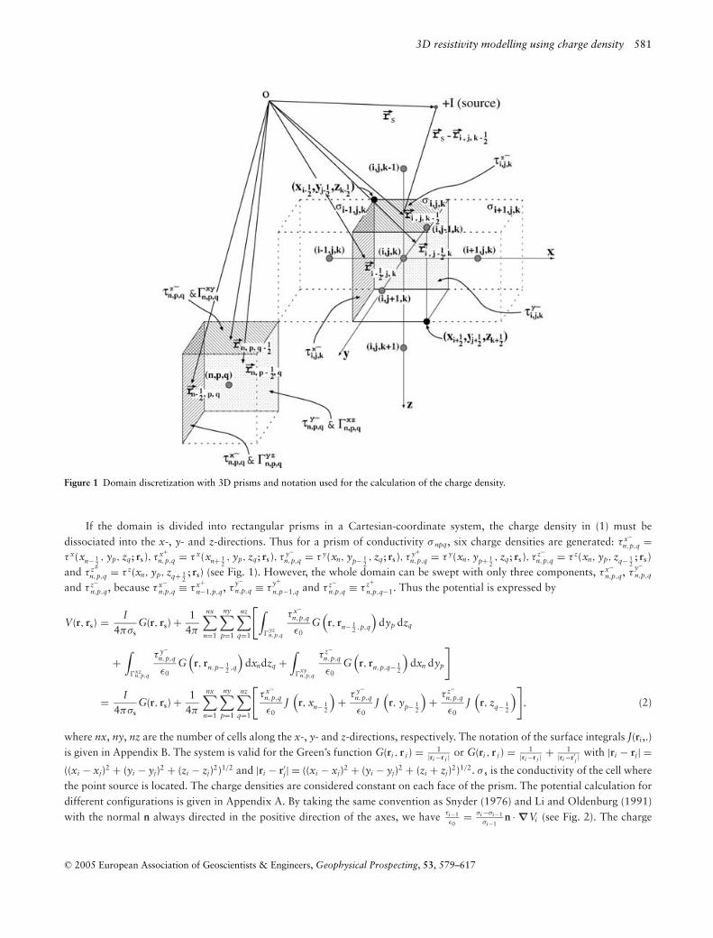
Figure 1 Domain discretization with 3D prisms and notation used for the calculation of the charge density.
If the domain is divided into rectangular prisms in a Cartesian-coordinate system, the charge density in (1) must bedissociated into the x-, y- and z-directions. Thus for a prism of conductivity σ npq, six charge densities are generated: τ x−
n,p,q =τ x(xn− 1
2, yp, zq; rs ), τ x+
n,p,q = τ x(xn+ 12, yp, zq; rs ), τ y−
n,p,q = τ y(xn, yp− 12, zq; rs ), τ y+
n,p,q = τ y(xn, yp+ 12, zq; rs ), τ z−
n,p,q = τ z(xn, yp, zq− 12; rs )
and τ z+n,p,q = τ z(xn, yp, zq+ 1
2; rs) (see Fig. 1). However, the whole domain can be swept with only three components, τ x−
n,p,q, τy−n,p,q
and τ z−n,p,q, because τ x−
n,p,q ≡ τ x+n−1,p,q, τ
y−n,p,q ≡ τ
y+n,p−1,q and τ z−
n,p,q ≡ τ z+n,p,q−1. Thus the potential is expressed by
V(r, rs) = I4πσs
G(r, rs) + 14π
nx∑n=1
ny∑p=1
nz∑q=1
[∫
yzn,p,q
τ x−n,p,q
ε0G
(r, rn− 1
2 ,p,q
)dyp dzq
+∫
xzn,p,q
τ y−n,p,q
ε0G
(r, rn,p− 1
2 ,q
)dxndzq +
∫
xyn,p,q
τ z−n,p,q
ε0G
(r, rn,p,q− 1
2
)dxn dyp
]
= I4πσs
G(r, rs) + 14π
nx∑n=1
ny∑p=1
nz∑q=1
[τ x−
n,p,q
ε0J
(r, xn− 1
2
)+ τ y−
n,p,q
ε0J
(r, yp− 1
2
)+ τ z−
n,p,q
ε0J
(r, zq− 1
2
)], (2)
where nx, ny, nz are the number of cells along the x-, y- and z-directions, respectively. The notation of the surface integrals J(ri,.)is given in Appendix B. The system is valid for the Green’s function G(ri , r j ) = 1
|ri −r j | or G(ri , r j ) = 1|ri −r j | + 1
|ri −r′j |with |ri − rj| =
((xi − xj)2 + (yi − yj)2 + (zi − zj)2)1/2 and |ri − r′j| = ((xi − xj)2 + (yi − yj)2 + (zi + zj)2)1/2. σ s is the conductivity of the cell where
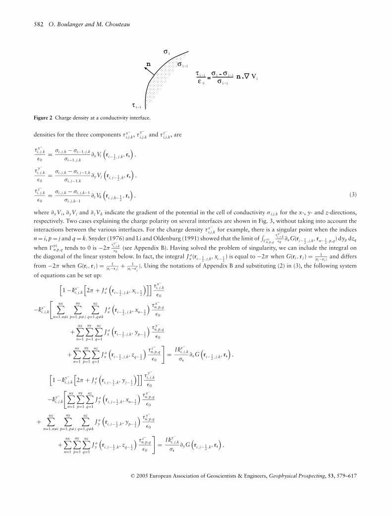
the point source is located. The charge densities are considered constant on each face of the prism. The potential calculation fordifferent configurations is given in Appendix A. By taking the same convention as Snyder (1976) and Li and Oldenburg (1991)with the normal n always directed in the positive direction of the axes, we have τi−1
ε0= σi −σi−1
σi−1n · ∇Vi (see Fig. 2). The charge
C© 2005 European Association of Geoscientists & Engineers, Geophysical Prospecting, 53, 579–617
582 O. Boulanger and M. Chouteau
n
-=σi σi–1
σi–1
σi–1
σi
τi–1
τi–1 n. Viε 0
Figure 2 Charge density at a conductivity interface.
densities for the three components τ x−i,j,k, τ
y−i,j,k and τ z−
i,j,k, are
τ x−i, j,k
ε0= σi, j,k − σi−1, j,k
σi−1, j,k∂xVi
(ri− 1
2 , j,k, rs
),
τy−i, j,k
ε0= σi, j,k − σi, j−1,k
σi, j−1,k∂yVj
(ri, j− 1
2 ,k, rs
),
τ z−i, j,k
ε0= σi, j,k − σi, j,k−1
σi, j,k−1∂zVk
(ri, j,k− 1
2, rs
), (3)
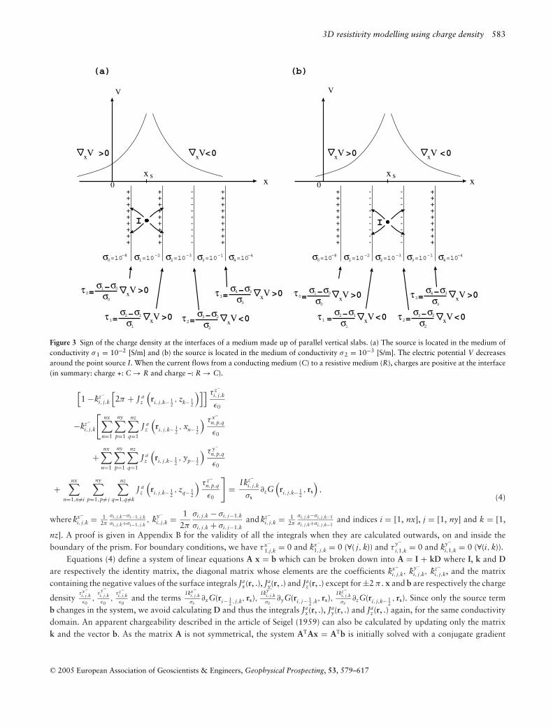
where ∂xVi, ∂yVj and ∂zVk indicate the gradient of the potential in the cell of conductivity σ i,j,k for the x-, y- and z-directions,respectively. Two cases explaining the charge polarity on several interfaces are shown in Fig. 3, without taking into account theinteractions between the various interfaces. For the charge density τ x−
i,j,k for example, there is a singular point when the indices
n = i, p = j and q = k. Snyder (1976) and Li and Oldenburg (1991) showed that the limit of∫
yzn,p,q
τ x−i, j,kε0
∂xG(ri− 12 , j,k, rn− 1
2 ,p,q) dyp dzq
when yzn,p,q tends to 0 is −2π
τ x−i, j,kε0
(see Appendix B). Having solved the problem of singularity, we can include the integral onthe diagonal of the linear system below. In fact, the integral J a
x (ri− 12 , j,k, xi− 1
2) is equal to −2π when G(ri , r j ) = 1
|ri −r j | and differs
from −2π when G(ri , r j ) = 1|ri −r j | + 1
|ri −r′j|. Using the notations of Appendix B and substituting (2) in (3), the following system
of equations can be set up:[1 −kx−
i, j,k
[2π + J a
x
(ri− 1
2 , j,k, xi− 12
)]] τ x−i, j,k
ε0
−kx−i, j,k
[nx∑
n=1,n=i
ny∑p=1,p= j
nz∑q=1,q =k
J ax
(ri− 1
2 , j,k, xn− 12
) τ x−n,p,q
ε0
+nx∑
n=1
ny∑p=1
nz∑q=1
J ax
(ri− 1
2 , j,k, yp− 12
) τ y−n,p,q
ε0
+nx∑
n=1
ny∑p=1
nz∑q=1
J ax
(ri− 1
2 , j,k, zq− 12
) τ z−n,p,q
ε0
]= Ikx−
i, j,k
σs∂xG
(ri− 1
2 , j,k, rs
),
[1 −ky−
i, j,k
[2π + J a
y
(ri, j− 1
2 ,k, yj− 12
)]] τy−i, j,k
ε0
−ky−i, j,k
[nx∑
n=1
ny∑p=1
nz∑q=1
J ay
(ri, j− 1
2 ,k, xn− 12
) τ x−n,p,q
ε0
+nx∑
n=1,n=i
ny∑p=1,p= j
nz∑q=1,q =k
J ay
(ri, j− 1
2 ,k, yp− 12
) τ y−n,p,q
ε0
+nx∑
n=1
ny∑p=1
nz∑q=1
J ay
(ri, j− 1
2 ,k, zq− 12
) τ z−n,p,q
ε0
]= Iky−
i, j,k
σs∂yG
(ri, j− 1
2 ,k, rs
),
C© 2005 European Association of Geoscientists & Engineers, Geophysical Prospecting, 53, 579–617
3D resistivity modelling using charge density 583
x
V
---------
+++++++++
+++++++++
(a)
x0
x s
V
+++++++++
+++++++++
---------
---------
(b)
Vx >0
=
= Vx >0 = Vx <0
= Vx >0 =
= =
=
I
x s0
+++++++++
Vx >0 Vx <0Vx <0
I
–σ1 σ0
σ0
–σ2 σ1
σ1
Vx >0τ0
–σ3 σ2
σ2
–σ4 σ3
σ3
τ1 τ2
τ3
=10–4σ4=10–1σ3=10–3σ2=10–2σ1=10–8σ0 =10–4σ4=10–1σ3=10–3σ2=10–2σ1=10–8σ0
–σ1 σ0
σ0
Vx >0τ0
τ1 Vx <0–σ2 σ1
σ1
Vx <0–σ3 σ2
σ2
τ2
τ3 Vx >0–σ4 σ3
σ3
Figure 3 Sign of the charge density at the interfaces of a medium made up of parallel vertical slabs. (a) The source is located in the medium ofconductivity σ 1 = 10−2 [S/m] and (b) the source is located in the medium of conductivity σ 2 = 10−3 [S/m]. The electric potential V decreasesaround the point source I. When the current flows from a conducting medium (C) to a resistive medium (R), charges are positive at the interface(in summary: charge +: C → R and charge –: R → C).
[1 −kz−
i, j,k
[2π + J a
z
(ri, j,k− 1
2, zk− 1
2
)]] τ z−i, j,k
ε0
−kz−i, j,k
[nx∑
n=1
ny∑p=1
nz∑q=1
J az
(ri, j,k− 1
2, xn− 1
2
) τ x−n,p,q
ε0
+nx∑
n=1
ny∑p=1
nz∑q=1
J az
(ri, j,k− 1
2, yp− 1
2
) τ y−n,p,q
ε0
+nx∑
n=1,n=i
ny∑p=1,p= j
nz∑q=1,q =k
J az
(ri, j,k− 1
2, zq− 1
2
) τ z−n,p,q
ε0
]= Ikz−
i, j,k
σs∂zG
(ri, j,k− 1
2, rs
),
(4)
where kx−i, j,k = 1
2π
σi, j,k−σi−1, j,kσi, j,k+σi−1, j,k
, ky−i, j,k = 1
2π
σi, j,k − σi, j−1,k
σi, j,k + σi, j−1,kand kz−
i, j,k = 12π
σi, j,k−σi, j,k−1σi, j,k+σi, j,k−1
and indices i = [1, nx], j = [1, ny] and k = [1,
nz]. A proof is given in Appendix B for the validity of all the integrals when they are calculated outwards, on and inside theboundary of the prism. For boundary conditions, we have τ x−
1,j,k = 0 and kx−1, j,k = 0 (∀( j, k)) and τ
y−i,1,k = 0 and ky−
i,1,k = 0 (∀(i, k)).Equations (4) define a system of linear equations A x = b which can be broken down into A = I + kD where I, k and D
are respectively the identity matrix, the diagonal matrix whose elements are the coefficients kx−i, j,k, ky−
i, j,k, kz−i, j,k, and the matrix
containing the negative values of the surface integrals Jax(r, .), Ja
y(r, .) and Jaz(r, .) except for ±2 π . x and b are respectively the charge
densityτ x−i, j,kε0
,τ
y−i, j,kε0
,τ z−i, j,kε0
and the termsIkx−
i, j,kσs
∂xG(ri− 12 , j,k, rs),
Iky−i, j,kσs
∂yG(ri, j− 12 ,k, rs),
Ikz−i, j,kσs
∂zG(ri, j,k− 12, rs). Since only the source term
b changes in the system, we avoid calculating D and thus the integrals Jax(r, .), Ja
y(r, .) and Jaz(r, .) again, for the same conductivity
domain. An apparent chargeability described in the article of Seigel (1959) can also be calculated by updating only the matrixk and the vector b. As the matrix A is not symmetrical, the system ATAx = ATb is initially solved with a conjugate gradient
C© 2005 European Association of Geoscientists & Engineers, Geophysical Prospecting, 53, 579–617
584 O. Boulanger and M. Chouteau
h I (x ,y ,z )s s s
σ21σ
air0σ =00τ
1τ
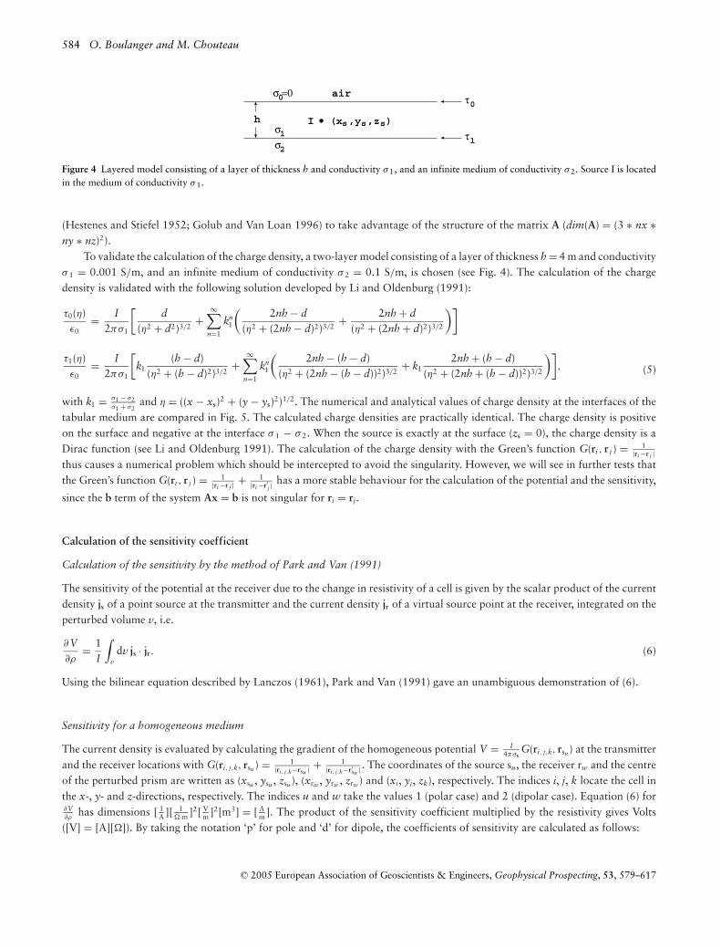
Figure 4 Layered model consisting of a layer of thickness h and conductivity σ 1, and an infinite medium of conductivity σ 2. Source I is locatedin the medium of conductivity σ 1.
(Hestenes and Stiefel 1952; Golub and Van Loan 1996) to take advantage of the structure of the matrix A (dim(A) = (3 ∗ nx ∗ny ∗ nz)2).
To validate the calculation of the charge density, a two-layer model consisting of a layer of thickness h = 4 m and conductivityσ 1 = 0.001 S/m, and an infinite medium of conductivity σ 2 = 0.1 S/m, is chosen (see Fig. 4). The calculation of the chargedensity is validated with the following solution developed by Li and Oldenburg (1991):
τ0(η)ε0
= I2πσ1
[d
(η2 + d2)3/2+
∞∑n=1
kn1
(2nh − d
(η2 + (2nh − d)2)3/2+ 2nh + d
(η2 + (2nh + d)2)3/2
)]
τ1(η)ε0
= I2πσ1
[k1
(h − d)(η2 + (h − d)2)3/2
+∞∑
n=1
kn1
(2nh − (h − d)
(η2 + (2nh − (h − d))2)3/2+ k1
2nh + (h − d)(η2 + (2nh + (h − d))2)3/2
)], (5)
with k1 = σ1 − σ2σ1 + σ2
and η = ((x − xs)2 + (y − ys)2)1/2. The numerical and analytical values of charge density at the interfaces of thetabular medium are compared in Fig. 5. The calculated charge densities are practically identical. The charge density is positiveon the surface and negative at the interface σ 1 − σ 2. When the source is exactly at the surface (zs = 0), the charge density is aDirac function (see Li and Oldenburg 1991). The calculation of the charge density with the Green’s function G(ri , r j ) = 1
|ri −r j |thus causes a numerical problem which should be intercepted to avoid the singularity. However, we will see in further tests thatthe Green’s function G(ri , r j ) = 1
|ri −r j | + 1|ri −r′j |
has a more stable behaviour for the calculation of the potential and the sensitivity,
since the b term of the system Ax = b is not singular for ri = rj.
Calculation of the sensitivity coefficient
Calculation of the sensitivity by the method of Park and Van (1991)
The sensitivity of the potential at the receiver due to the change in resistivity of a cell is given by the scalar product of the currentdensity js of a point source at the transmitter and the current density jr of a virtual source point at the receiver, integrated on theperturbed volume v, i.e.
∂V∂ρ
= 1I
∫v
dv js · jr. (6)
Using the bilinear equation described by Lanczos (1961), Park and Van (1991) gave an unambiguous demonstration of (6).
Sensitivity for a homogeneous medium
The current density is evaluated by calculating the gradient of the homogeneous potential V = I4πσs
G(ri, j,k, rsu ) at the transmitterand the receiver locations with G(ri, j,k, rsu ) = 1
|ri, j,k−rsu | + 1|ri, j,k−r′su | . The coordinates of the source su, the receiver rw and the centre
of the perturbed prism are written as (xsu , ysu , zsu ), (xrw , yrw , zrw ) and (xi, yj, zk), respectively. The indices i, j, k locate the cell inthe x-, y- and z-directions, respectively. The indices u and w take the values 1 (polar case) and 2 (dipolar case). Equation (6) for∂V∂ρ
has dimensions [ 1A ][ 1
·m ]2[ Vm ]2[m3] = [ A
m ]. The product of the sensitivity coefficient multiplied by the resistivity gives Volts([V] = [A][]). By taking the notation ‘p’ for pole and ‘d’ for dipole, the coefficients of sensitivity are calculated as follows:
C© 2005 European Association of Geoscientists & Engineers, Geophysical Prospecting, 53, 579–617

3D resistivity modelling using charge density 585
-10-8-6-4-202468
10
Y [
m]
-10 -8 -6 -4 -2 0 2 4 6 8 10
X [m]
Z = 0 m
τ0/ε0
(a)(A)
-10-8-6-4-202468
10
Y [
m]
-10 -8 -6 -4 -2 0 2 4 6 8 10
X [m]
Z = 4 m
τ1/ε0
(b)
-45-40-35-30-25-20-15-10 -5 0 5 10 15 20 25 30 35
V/m
-10-8-6-4-202468
10
Y [
m]
-10 -8 -6 -4 -2 0 2 4 6 8 10
X [m]
Z = 4 m
τ1/ε0
(b)
-10-8-6-4-202468
10
Y [
m]
-10 -8 -6 -4 -2 0 2 4 6 8 10
X [m]
Z = 0 m
τ0/ε0
(a)(B)
Figure 5 Charge density for the two-layer case with the top layer of 4 m thickness and conductivity 0.0001 S/m, and a lower half-space ofconductivity 0.1 S/m (see (5)). (A) Analytical normalized charge density. (B) Numerical normalized charge density. (a) and (b) correspond to τ0
ε0and τ1
ε0. The black contour indicates zero value. The source is located at (xs, ys, zs) = (−5, 0, 2) m.
∂Vp−p
∂ρ= 1
I
∫v
dvjs1 · jr1 ,
∂Vd−p
∂ρ= 1
I
∫v
dv(js1 − js2
) · jr1 ,
∂Vp−d
∂ρ= 1
I
∫v
dvjs1 · (jr1 − jr2 ),
∂Vd−d
∂ρ= 1
I
∫v
dv(js1 − js2 ) · (jr1 − jr2
). (7)
The current density is expressed for a homogeneous medium in a cell of coordinates (xi, yj, zk) as follows:
jsu =
jxsu= − I
4π∂xi G(ri, j,k, rsu ),
jysu= − I
4π∂yj G(ri, j,k, rsu ),
jzsu= − I
4π∂zkG(ri, j,k, rsu ).
(8)
C© 2005 European Association of Geoscientists & Engineers, Geophysical Prospecting, 53, 579–617
586 O. Boulanger and M. Chouteau
For the receiver point, s is replaced by r and u by w, thus obtaining the current density. The explicit result for any array withfour electrodes in the case of a homogeneous medium is given in Appendix C. To obtain ∂ρa
∂ρ, it is sufficient to take into account
the geometrical factor K and the value of the current I at the point source, that is to say, ∂ρa∂ρ
= KI
∂V∂ρ
.
Calculation of the current density using the charge density
The current density calculated at the centre of the cell (i, j, k) of conductivity σ i,j,k is js(ri,j,k, rs) = σ i,j,kE(ri,j,k, rs). The threecomponents of the electric field E(ri,j,k, rs) = −∇V(ri,j,k, rs) calculated at the centre of the cell (i, j, k) are given by
Ex(ri, j,k, rs) = − 14π
[Iσs
∂xG(ri, j,k, rs
) +nx∑
n=1
ny∑p=1
nz∑q=1
[τ x−
n,p,q
ε0J a
x
(ri, j,k, xn− 1
2
)
+ τ y−n,p,q
ε0J a
x
(ri, j,k, yp− 1
2
)+ τ z−
n,p,q
ε0J a
x
(ri, j,k, zq− 1
2
)]],
Ey(ri, j,k, rs) = − 14π
[Iσs
∂yG(ri, j,k, rs
) +nx∑
n=1
ny∑p=1
nz∑q=1
[τ x−
n,p,q
ε0J a
y
(ri, j,k, xn− 1
2
)
+ τ y−n,p,q
ε0J a
y
(ri, j,k, yp− 1
2
)+ τ z−
n,p,q
ε0J a
y (ri, j,k, zq− 12)
]],
Ez(ri, j,k, rs) = − 14π
[Iσs
∂zG(ri, j,k, rs
) +nx∑
n=1
ny∑p=1
nz∑q=1
[τ x−
n,p,q
ε0J a
z
(ri, j,k, xn− 1
2
)
+ τ y−n,p,q
ε0J a
z
(ri, j,k, yp− 1
2
)+ τ z−
n,p,q
ε0J a
z
(ri, j,k, zq− 1
2
)]]. (9)
By multiplying (9) by the conductivity σ i,j,k, the current density can be broken down into a primary term jPx(ri,j,k, rs) and asecondary term jSx(ri,j,k, rs). The component jx(ri,j,k, rs) = jPx(ri,j,k, rs) + jSx(ri,j,k, rs) is written
jx(ri, j,k, rs) = − I4π
∂xG(ri, j,k, rs) − 14π
[I(σi, j,k − σs
)σs
∂xG(ri, j,k, rs
) + σi, j,k
nx∑n=1
ny∑p=1
nz∑q=1[
τ x−n,p,q
ε0J a
x
(ri, j,k, xn− 1
2
)+ τ y−
n,p,q
ε0J a
x
(ri, j,k, yp− 1
2
)+ τ z−
n,p,q
ε0J a
x
(ri, j,k, zq− 1
2
)]]. (10)
The current density jr for a virtual source located at the point (xr, yr, zr) (r indicates receiver) is written in the same mannerby replacing s by r. The sensitivity coefficient for a heterogeneous medium at the point (i, j, k) and for a pole-pole array with atransmitting point located at (xs, ys, zs) and a receiving point located at (xr, yr, zr) is written,
∂V(rr, rs)∂ρi, j,k
= 1I
∫v
dv[jP(ri, j,k, rs) + jS(ri, j,k, rs)
] · [jP(ri, j,k, rr) + jS(ri, j,k, rr)
]. (11)
Calculation of the sensitivity using the integral equation
To calculate the sensitivity, it is proposed to take the derivative of (2) with respect to the conductivity σ i,j,k of the block (i, j, k)located at (xi, yj, zk) for a pole-pole array with a transmitting point located at (xs, ys, zs) and a receiving point located at (xr, yr,zr). To simplify the writing, the surface elements dypdzq, dxndzq and dxn dyp are all associated with ds, and we can write:
C© 2005 European Association of Geoscientists & Engineers, Geophysical Prospecting, 53, 579–617
3D resistivity modelling using charge density 587
∂V(rr, rs)∂σi, j,k
= 14π
[∫
yzi, j,k
ds G(ri− 1
2 , j,k, rr
) ∂
∂σi, j,k
[τ x−
i, j,k
ε0
]+
∫
yzi, j,k
ds G(ri+ 1
2 , j,k, rr
) ∂
∂σi, j,k
[τ x+
i, j,k
ε0
]
+∫
xzi, j,k
ds G(ri, j− 1
2 ,k, rr
) ∂
∂σi, j,k
[τ
y−i, j,k
ε0
]+
∫xz
i, j,k
ds G(ri, j+ 1
2 ,k, rr
) ∂
∂σi, j,k
[τ
y+i, j,k
ε0
]
+∫
xyi, j,k
ds G(ri, j,k− 1
2, rr
) ∂
∂σi, j,k
[τ z−
i, j,k
ε0
]+
∫
xyi, j,k
ds G(ri, j,k+ 1
2, rr
) ∂
∂σi, j,k
[τ z+
i, j,k
ε0
]]
− I4πσ 2
s
G (rs, rr) δ(xi − xs)δ(yj − ys)δ(zk − zs). (12)
The boundary conditions for the x-direction, with the normal n directed outwards from the cell (i, j, k) (see Fig. 2), are
τ x−i, j,k
ε0= σi−1, j,k − σi, j,k
σi, j,kn · x ∂xVi−1
(ri− 1
2 , j,k, rs
),
τ x+i, j,k
ε0= σi+1, j,k − σi, j,k
σi, j,kn · x ∂xVi+1
(ri+ 1
2 , j,k, rs
). (13)
x corresponds to a unit vector in the x-direction. The partial derivatives with respect to the conductivity σ i,j,k arecalculated using (13). Then with the following relationships σi−1, j,k n · x ∂xVi−1(ri− 1
2 , j,k, rs) = σi, j,k n · x ∂xVi (ri− 12 , j,k, rs) and
σi+1, j,k n · x ∂xVi+1(ri+ 12 , j,k, rs) = σi, j,k n · x ∂xVi (ri+ 1
2 , j,k, rs) and the previously calculated partial derivatives, we can write:
∂
∂σi, j,k
[τ x−
i, j,k
ε0
]= − 1
σi, j,kn · x ∂xVi
(ri− 1
2 , j,k, rs
),
∂
∂σi, j,k
[τ x+
i, j,k
ε0
]= − 1
σi, j,kn · x ∂xVi
(ri+ 1
2 , j,k, rs
).
(14)
By replacing ds n by ds and by substituting (14) in (12), we find
∂V(rr, rs)∂σi, j,k
= −14πσi, j,k
[∫
yzi, j,k
G(ri− 1
2 , j,k, rr
)∂xVi
(ri− 1
2 , j,k, rs
)x · ds +
∫
yzi, j,k
G(ri+ 1
2 , j,k, rr
)∂xVi
(ri+ 1
2 , j,k, rs
)x · ds
+∫
xzi, j,k
G(ri, j− 1
2 ,k, rr
)∂yVj
(ri, j− 1
2 ,k, rs
)y · ds +
∫xz
i, j,k
G(ri, j+ 1
2 ,k, rr
)∂yVj
(ri, j+ 1
2 ,k, rs
)y · ds
+∫
xyi, j,k
G(ri, j,k− 1
2, rr
)∂zVk
(ri, j,k− 1
2, rs
)z · ds +
∫
xyi, j,k
G(ri, j,k+ 1
2, rr
)∂zVk
(ri, j,k+ 1
2, rs
)z · ds
]
− I4πσ 2
sG (rs, rr) δ(xi − xs)δ(yj − ys)δ(zk − zs).
(15)
Equation (15) follows Green’s theorem,∫
S U∇V · ds = ∫V[U∇2V + ∇U · ∇V]dv, for the term between the square brackets.
Therefore, we can write it as
∂V(rr, rs)∂σi, j,k
= −14πσi, j,k
∫Vi, j,k
[G(ri, j,k, rr)∇2V(ri, j,k, rs) + ∇G(ri, j,k, rr) · ∇V(ri, j,k, rs)
]dv
− I4πσ 2
sG(rs, rr) δ(xi − xs)δ(yj − ys)δ(zk − zs).
(16)
The Laplacian of the potential is written ∇2V(ri, j,k, rs) = −∇σi, j,k · ∇V(ri, j,k,rs)σi, j,k
− Iδ(ri, j,k−rs)σi, j,k
. Since a constant conductivity is
considered in each cell, the term ∇σ i,j,k is null. The term − Iδ(ri, j,k−rs)σi, j,k
is null everywhere except at the point source ri,j,k = rs.
Moreover, the integral −14πσi, j,k
∫Vi, j,k
G(ri, j,k, rr)∇2V(ri, j,k, rs) dv at the point source becomes I4πσ2
s
∫Vi, j,k
G(ri, j,k, rr)δ(ri, j,k − rs) dv =
C© 2005 European Association of Geoscientists & Engineers, Geophysical Prospecting, 53, 579–617
588 O. Boulanger and M. Chouteau
I4πσ2
sG(rs, rr)δ(xi − xs)δ(yj − ys)δ(zk − zs). By taking the relationship, ∂V
∂ρi= −σ 2
i∂V∂σi
, into account, the sensitivity for a pole-polearray is simplified and given by
∂V(rr, rs)∂σi, j,k
= −14πσi, j,k
∫Vi, j,k
∇G(ri, j,k, rr) · ∇V(ri, j,k, rs) dv,
∂V(rr, rs)∂ρi, j,k
= 14πρi, j,k
∫Vi, j,k
∇G(ri, j,k, rr) · ∇V(ri, j,k, rs) dv. (17)
The sensitivity for a cell (i, j, k) is thus the scalar product of the electric field resulting from the source point rs and thegradient of the Green’s function resulting from the receiving point rr, calculated at the point ri,j,k. This relationship differs fromthat given by Park and Van (1991) and described by (6). The relationship of Park and Van (1991) requires the calculation of theelectric field at the source and at the receiving positions, while the proposed method only needs the calculation of the electricfield at the source point, thus halving the computation time. Moreover, the sensitivity calculated according to (17) is balancedby the conductivity σ i,j,k (or the resistivity ρ i,j,k) of each cell. Equation (17) has units given by [ ∂V
∂ρ] ≡ [ 1
·m ][ 1m2 ][ V
m ][m3] = [ Am ].
In the case of a homogeneous medium, it is shown below that (6) and (17) are identical. Setting V(ri, j,k, rr) = Iρi, j,k4π
G(ri, j,k, rr),the relationship (6) can be simplified for a cell (i, j, k), giving
∂V(rr, rs)∂ρi, j,k
= 1I
∫Vi, j,k
σi, j,k∇V(ri, j,k, rr) · σi, j,k∇V(ri, j,k, rs) dv,
= 1I
∫Vi, j,k
1ρ2
i, j,k
∇[
Iρi, j,k
4πG(ri, j,k, rr)
]· ∇V(ri, j,k, rs) dv,
= 14πρi, j,k
∫Vi, j,k
∇G(ri, j,k, rr) · ∇V(ri, j,k, rs) dv. (18)
If the charge density is considered constant on each interface and is taken out from the integral in (2), another simplifiedform of the sensitivity can be obtained using the same calculation method, i.e.
∂V(rr, rs)∂ρi, j,k
= 14πρi, j,k
[J
(rr, xi+ 1
2
)∂xVi
(ri+ 1
2 , j,k, rs
)− J
(rr, xi− 1
2
)∂xVi
(ri− 1
2 , j,k, rs
)
+ J(rr, y j+ 1
2
)∂yVj
(ri, j+ 1
2 ,k, rs
)− J
(rr, y j− 1
2
)∂yVj
(ri, j− 1
2 ,k, rs
)
+ J(rr, zk+ 1
2
)∂zVk
(ri, j,k+ 1
2, rs
)− J
(rr, zk− 1
2
)∂zVk
(ri, j,k− 1
2, rs
) ]
+ I4π
G (rs, rr) δ(xi − xs)δ(yj − ys)δ(zk − zs).
(19)
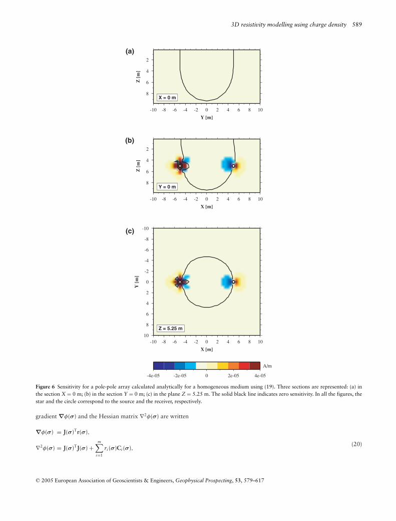
Figure 6 shows the calculation of the sensitivity for a homogeneous medium with a pole-pole array using (19). However,it can be seen that the calculation of the sensitivity with (19) generates an artefact around the source. The artefact persists onvarious scales whatever the cell size. This behaviour is caused because a constant charge density on the interfaces of each prism ischosen. This approximation is valid far from the point of current injection, but becomes invalid close to the source. The volumeof the cell must tend to zero so that the approximation becomes valid. Thus the use of this notation is not recommended for acoarse discretization. Note that this artefact around the source is not present for the sensitivity calculated with (17).
Calculation of the second derivatives using the integral equation
In this section, the calculation of the second derivatives in 3D is proposed for the inverse problem. The minimization of a non-linear least-squares problem can be carried out by the Newton method. It requires the calculation of the gradient and the Hessianmatrix (Bjorck 1996; Nocedal and Wright 2000). We note ri(σ) = Vobs
i − Vi(rr, rs) the error for the ith observation, where Vobsi
and Vi(rr, rs) are the observed and calculated data, respectively (i = 1, . . . , m). By minimizing the function φ(σ) = 12 ||r(σ)||2, the
C© 2005 European Association of Geoscientists & Engineers, Geophysical Prospecting, 53, 579–617
3D resistivity modelling using charge density 589
2
4
6
8
Z [
m]
-10 -8 -6 -4 -2 0 2 4 6 8 10
Y [m]
X = 0 m
(a)
2
4
6
8
Z [
m]
-10 -8 -6 -4 -2 0 2 4 6 8 10
X [m]
Y = 0 m
(b)
-10
-8
-6
-4
-2
0
2
4
6
8
10
Y [
m]
-10 -8 -6 -4 -2 0 2 4 6 8 10
X [m]
Z = 5.25 m
(c)
-4e-05 -2e-05 0 2e-05 4e-05
A/m
Figure 6 Sensitivity for a pole-pole array calculated analytically for a homogeneous medium using (19). Three sections are represented: (a) inthe section X = 0 m; (b) in the section Y = 0 m; (c) in the plane Z = 5.25 m. The solid black line indicates zero sensitivity. In all the figures, thestar and the circle correspond to the source and the receiver, respectively.
gradient ∇φ(σ) and the Hessian matrix ∇2φ(σ) are written
∇φ(σ) = J(σ)Tr(σ),
∇2φ(σ) = J(σ)TJ(σ) +m∑
i=1
ri (σ)Ci (σ),(20)
C© 2005 European Association of Geoscientists & Engineers, Geophysical Prospecting, 53, 579–617
590 O. Boulanger and M. Chouteau
where J (σσσ )i j = ∂ri (σσσ )∂σ j
and Ci (σσσ ) jk = ∂2ri (σσσ )∂σ j ∂σk
are the Frechet and second derivatives of the residual vector r (σσσ ), respectively. Whenthe problem is linearized, the Hessian is often approximated by the first term, e.g. ∇2φ(σ) ≈ J(σ)T J(σ), by neglecting the secondterm. While taking the preceding paragraph as a starting point and by deriving (12) successively with respect to the conductivitiesσ i,j,k, σ i−1,j,k, σ i+1,j,k, σ i,j−1,k, σ i,j+1,k, σ i,j,k−1 and σ i,j,k+1, the coefficients of the second derivative sparse matrix are
∂2V(rr, rs)∂σ 2
i, j,k
= +14πσ 2
i, j,k
∫Vi, j,k
∇G(ri, j,k, rr) · ∇V(ri, j,k, rs) dv
+ I4πσ 3
sG(rs, rr)δ(xi − xs)δ(yj − ys)δ(zk − zs),
(21)
∂2V(rr, rs)∂σi−1, j,k∂σi, j,k
= −14πσi, j,kσi−1, j,k
∫
yzi, j,k
G(ri− 1
2 , j,k, rr
)n · x ∂xVi
(ri− 1
2 , j,k, rs
)dyj dzk,
∂2V(rr, rs)∂σi+1, j,k∂σi, j,k
= −14πσi, j,kσi+1, j,k
∫
yzi, j,k
G(ri+ 1
2 , j,k, rr
)n · x ∂xVi
(ri+ 1
2 , j,k, rs
)dyj dzk,
(22)
∂2V(rr, rs)∂σi, j−1,k∂σi, j,k
= −14πσi, j,kσi, j−1,k
∫xz
i, j,k
G(ri, j− 1
2 ,k, rr
)n · y ∂yVj
(ri, j− 1
2 ,k, rs
)dxi dzk,
∂2V(rr, rs)∂σi, j+1,k∂σi, j,k
= −14πσi, j,kσi, j+1,k
∫xz
i, j,k
G(ri, j+ 1
2 ,k, rr
)n · y ∂yVj
(ri, j+ 1
2 ,k, rs
)dxi dzk,
(23)
∂2V(rr, rs)∂σi, j,k−1∂σi, j,k
= −14πσi, j,kσi, j,k−1
∫
xyi, j,k
G(ri, j,k− 1
2, rr
)n · z ∂zVk
(ri, j,k− 1
2, rs
)dxi dyj ,
∂2V(rr, rs)∂σi, j,k+1∂σi, j,k
= −14πσi, j,kσi, j,k+1
∫
xyi, j,k
G(ri, j,k+ 1
2, rr
)n · z ∂zVk
(ri, j,k+ 1
2, rs
)dxi dyj .
(24)
Similar relationships are found when V(rr, rs) is derived with respect to ρ. The cross terms are obtained with the relation-ship ∂2V
∂ρi ∂ρ j= σ 2
i σ 2j
∂2V∂σi ∂σ j
. The diagonal term is written ∂2V(rr,rs)∂ρ2
i, j,k= +1
4πρ2i, j,k
∫Vi, j,k
∇G(ri, j,k, rr) · ∇V(ri, j,k, rs) dv + I4πρs
G(rs, rr) δ(xi −xs)δ(yj − ys)δ(zk − zs) starting from the relationship ∂2V
∂ρ2i
= 2σ 3i
∂V∂σi
+ σ 4i
∂2V∂σ2
i.
M AT R I X C O M P R E S S I O N
To make the problem of modelling with the integral equation feasible, the matrix A which allows the calculation of the chargedensity is compressed. Li and Oldenburg (1997) used wavelets to compress the sensitivity matrix in a magnetic inversion problem.Portniaguine (1999) selected another method arising from the work of Burt and Adelson (1983) and Losano and Laget (1996)to compress the sensitivity matrix in a gravimetric inversion problem. The second method, known as pyramidal compression,is chosen for reasons of fast implementation and conclusive results. A detailed explanation can be obtained from the thesis ofPortniaguine (1999). Here, we present the method using another form of notation to compress the matrices, and the practicalalgorithms used in the code of pyramidal compression.
Compression and restoration
The compression of a vector column v1 of level 1 on level 2 is written v2 = W1v1 where W1 is the matrix of compression oflevel 1. To compress v1 up to level L, the vectors v2, v3, . . . , vL−1 are successively compressed by the matrix Wk, that is to say,vk+1 = Wkvk where Wk is the matrix compression of level k. Note that the vector vk is pre-multiplied by Wk. The pyramidalcompression of a vector column v1 of level 1 on level L is written,
vL = WL−1 . . . W2W1V1. (25)
C© 2005 European Association of Geoscientists & Engineers, Geophysical Prospecting, 53, 579–617
3D resistivity modelling using charge density 591
Note the following property: each matrix Wk is equal to its inverse, that is to say,
Wk = W−1k . (26)
The restoration of the vector v1 is written by pre-multiplying (25) by the matrices (WL−1. . . W2 W1)−1. By taking intoaccount the preceding property, we thus have
v1 = W1W2 . . . WL−1vL. (27)
If W = WL−1 . . . W2W1 is the product of all the matrices of compression and W−1 = W1W2 . . . WL−1 is the product of allthe matrices of restoration, the product of the matrices of compression and those of restoration is equal to the identity matrix(W−1W = I). The algorithms of creation, i.e. pre- and post-multiplication of the compression matrix Wk on level k, are givenin Appendix F.
The final stage consists of taking only the significant elements of the compressed vector vL compared with a fixed threshold,and cancelling the others. The threshold corresponds to a percentage q of the absolute value of the maximum amplitude of thecompressed vector vL. The resulting vector vL is sparse by carrying out the thresholding
vL(i) =
vL(i), |vL(i)| ≥ q max(|vL|)0, |vL(i)| < q max(|vL|)
, ∀i. (28)
Approaches to compressing a linear system
Portniaguine (1999) proposed two solutions to compress a linear system Ax = b. The first method consists of preconditioning
the linear system WAx = Wb, giving Ax = b after the thresholding. The second, named incomplete factorization of matrix A,is written W−1A = A. The system to be solved is W−1Ax = b. A third method is proposed. Based on the property W−1W = I,the matrix identity I is inserted in the linear system between A and x. The system is written (AW−1)(Wx) = b, giving, afterthresholding,
Ax = b, (29)
with A = AW−1 and x = Wx. The solution of the system is obtained using the relationship x = W−1x. For the dimensions ofthe first and second methods, dim(W) = dim(b). For the third method, the dimension changes since the vector line is compressedinstead of the vector column, therefore dim(W) = dim(x).
Resolution of the system of equations for the integral method
To apply the integral equation to our system of equations, the system ATAx = ATb is initially solved. Whereas the matrices Wand W−1 are not stored, the matrix A is stored in a particular way. A is obtained by post-multiplication of A by W−1, that isto say, A = W−1 + kD where D = DW−1. The compressed system is solved with the conjugate-gradient method:
[(W−1)T + DTk][W−1 + kD]x = [(W−1)T + DTk]b. (30)
It is necessary to store the sparse matrix D and to calculate the products of this matrix and of its transpose by a vectorcolumn. The algorithms for storage and for the product of a sparse matrix and a vector for the sparse row-wise format takenfrom Pissanetzky (1984) are given in Appendix G. This method requires less memory compared with the standard method,which consists of storing two integers and a real for each element of the sparse matrix. The product of the matrix k and a vectorcolumn does not cause a problem, since this matrix is diagonal. The products of both (W−1)T and W−1 by a vector column arecarried out according to the codes of compression and restoration described in Appendix F.
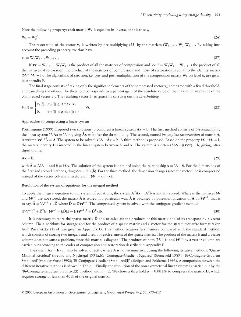
The system Ax = b can also be solved directly, where A is non-symmetrical, using the following iterative methods: ‘Quasi-Minimal Residual’ (Freund and Nachtigal 1991a,b); ‘Conjugate-Gradient Squared’ (Sonneveld 1989); ‘Bi-Conjugate-GradientStabilized’ (van der Vorst 1992); ‘Bi-Conjugate-Gradient Stabilized(l)’ (Sleijpen and Fokkema 1993). A comparison between thedifferent iterative methods is shown in Table 1. Finally, the resolution of the non-symmetrical linear system is carried out by the‘Bi-Conjugate-Gradient Stabilized(l)’ method with l = 2. We chose a threshold q = 0.001% to compress the matrix D, whichrequires storage of less than 40% of the original matrix.
C© 2005 European Association of Geoscientists & Engineers, Geophysical Prospecting, 53, 579–617
592 O. Boulanger and M. Chouteau
Table 1. Comparison between different solvers for the two-layer model consisting of 11 × 11 × 6 cells. The relative tolerance for all solversis 1e-6. The computer is a Dell Inspiron 8100 PIII 733 MHz. The maximum number of iterations is 500. PCG, Preconditioned ConjugateGradient; QMR, Quasi-Minimal Residual; CGS, Conjugate-Gradient Squared; BICGSTAB, Bi-Conjugate-Gradient Stabilized; BICGSTAB(l),Bi-Conjugate-Gradient Stabilized(l) with l = 2
G(ri , r j ) = 1|ri −r j | G(ri , r j ) = 1
|ri −r j | + 1|ri −r′j |
Method Time (s) Iteration Deviation Time (s) Iteration Deviation
PCG 3.26 158 7.58e-7 2.57 155 8.28e-7QMR 90.21 500 1.07e-1 7.69 42 9.79e-7CGS 3.26 19 9.08e-7 2.53 15 7.44e-7BICGSTAB 4.64 20 8.69e-7 3.49 15 5.63e-7BICGSTAB(l) 1.73 8 4.73e-8 1.73 7 2.65e-8
To prevent values different from zero being obtained where the charge density must be null, an additional constraint to thesystem Ax = b is introduced. The indices of the values of x which must be null are gathered as a set N. A matrix IN made up of1 is generated in such a way that IN x = 0 only for x ∈ N. The new compressed system to solve is written, with IN = INW−1, as
[W−1 + kD + IN
]x = b. (31)
E L E C T R I C F I E L D
First method: charge density
Once the charge density has been obtained in the whole space, the three components of the electric field can be calculated onthe interfaces of the prisms. If x is the solution of the linear system (4) ([W−1 + kD] x = b), then the secondary electric fieldES is obtained by multiplying x by the opposite of the matrix D plus one corrective term −2π Ix, since the elements of D areDi i = −[2π + J a
ii ] on the diagonal and Di j = −J ai j on the off-diagonal. The total field E is given by the sum of the primary field
EP and of the secondary field ES (E = EP + ES), as follows:
E = − 14π
[Iσs
∇G + (−Dx − 2π Ix)]. (32)
The electric field at the centre of the cell (i, j, k) is needed; it can be evaluated by interpolating the values of the computedfield at the interfaces of the prisms with a cubic spline (Press et al. 1992). A calculation equivalent to that carried out with (9)can also be used.
Second method: surface integral
The calculation of the electric field, described by Beasley and Ward (1986), for a conducting block located in a homogeneousmedium can be generalized when the model consists of several prisms. The x-component of the gradient of the potential iswritten,
∂xi V(ri− 1
2 , j,k, rs
)= I
4πσs∂xi G
(ri− 1
2 , j,k, rs
)+
nx∑n=1
ny∑p=1
nz∑q=1
[kx−
n,p,q J ax
(ri− 1
2 , j,k, xn− 12
)∂xn V
(rn− 1
2 ,p,q, rs
)
+ ky−n,p,q J a
x
(ri− 1
2 , j,k, yp− 12
)∂yn V
(rn,p− 1
2 ,q, rs
)+ kz−
n,p,q J ax
(ri− 1
2 , j,k, zq− 12
)∂zn V
(rn,p,q− 1
2, rs
)],
(33)
with kx−n,p,q = 1
4π
σn,p,q−σn−1,p,qσn−1,p,q
, ky−n,p,q = 1
4π
σn,p,q−σn,p−1,qσn,p−1,q
et kz−n,p,q = 1
4π
σn,p,q−σn,p,q−1σn,p,q−1
and indices i = [1, nx], j = [1, ny] and k = [1, nz].
The system of equations is written as [ I + Dk] x = b where k is the diagonal matrix of the elements kx−n,p,q, ky−
n,p,q and kz−n,p,q. It is
necessary to pre-multiply [ I + Dk] by W and to solve the system W−1[W + Dk]x = b with D = WD.
C© 2005 European Association of Geoscientists & Engineers, Geophysical Prospecting, 53, 579–617

3D resistivity modelling using charge density 593
T E S T S
Calculation of the electric potential
To validate the calculation of the potential generated by a polar source, the models of the vertical contact and the two-layersubsurface were used. The integral-equation and the finite-difference methods (Spitzer 1995; Spitzer et al. 1999) were comparedwith the analytical solution. The code using the finite-difference method includes the singularity removal described by Lowry,Allen and Shive (1989).
Vertical contact
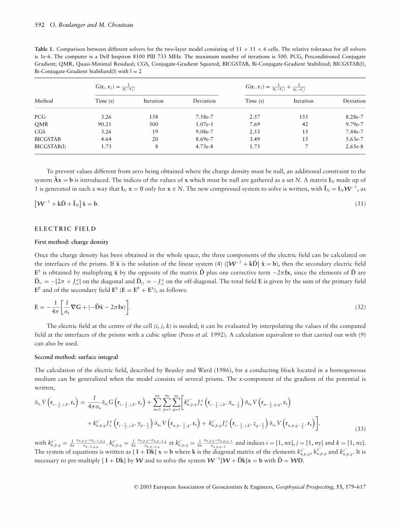
Figure 7 shows the potential as log10(V) analytically calculated for a vertical contact (10 m/1000 m) in the x-, y- andz-directions. The source is located at (−5, 0, 0) m for the analytical solution and the Green’s function G(ri , r j ) = 1
|ri −r j | + 1|ri −r′j |
.
For the Green’s function G(ri , r j ) = 1|ri −r j | , the source is located at (−5, 0, 0.01) m to avoid the singularity. For all tests the black
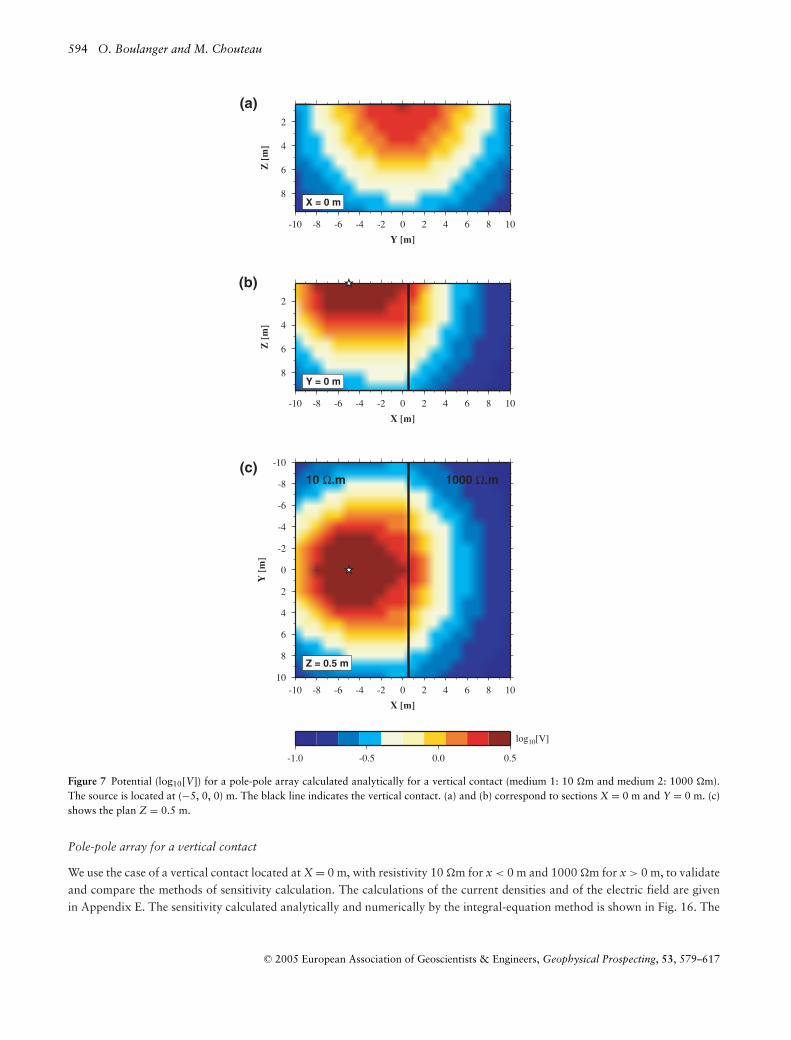
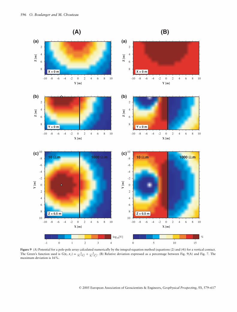
line delimits the vertical contact. Figures 7(a) and 7(b) correspond to the sections X = 0 m and Y = 0 m. Figure 7(c) representsthe plane Z = 0.5 m. The calculations of the potential and of the current density are given in Appendix E. Figures 8, 9 and 10show the potential and the relative deviation compared with Fig. 7 for the integral-equation method using the Green’s functionsG(ri , r j ) = 1
|ri −r j | , G(ri , r j ) = 1|ri −r j | + 1
|ri −r′j |and the finite-difference method, respectively. The three methods give satisfactory
results. The maximum relative deviations for Figs 8 and 9 are 56% and 16% at the vertical contact, on the source side. Aroundthe source the deviation does not exceed 5%. The maximum relative deviation for Fig. 10 is 100% at the point source, at thecontact and in the medium of 1000 m. The further one moves away from the current source, the more the amplitude of thepotential decreases and more likely the relative error is to increase.
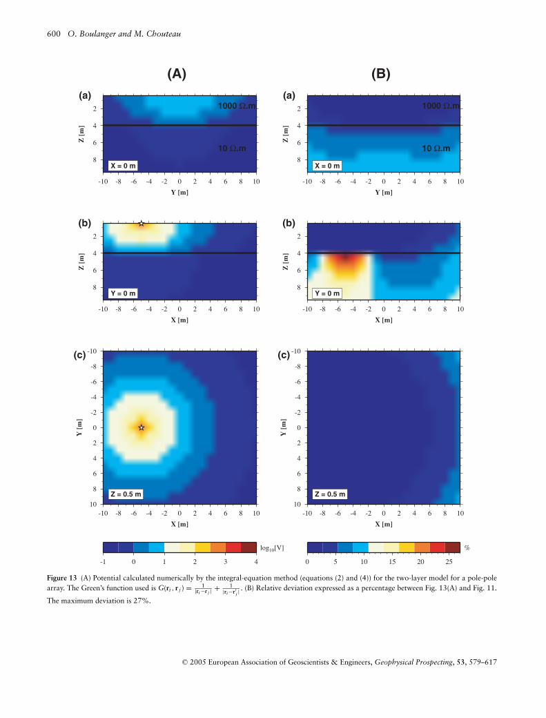
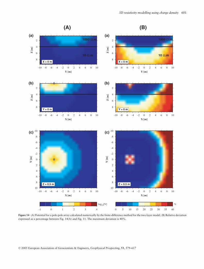
The two-layer case
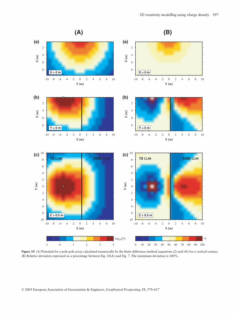
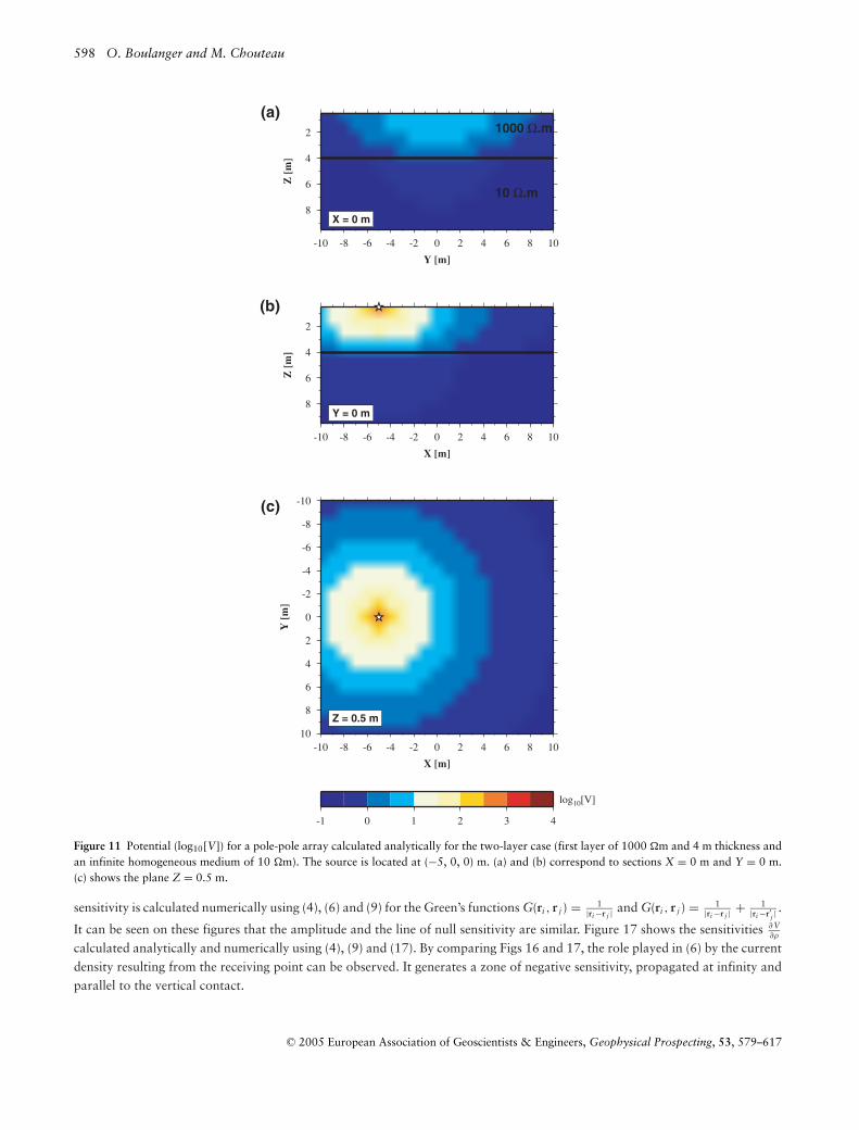
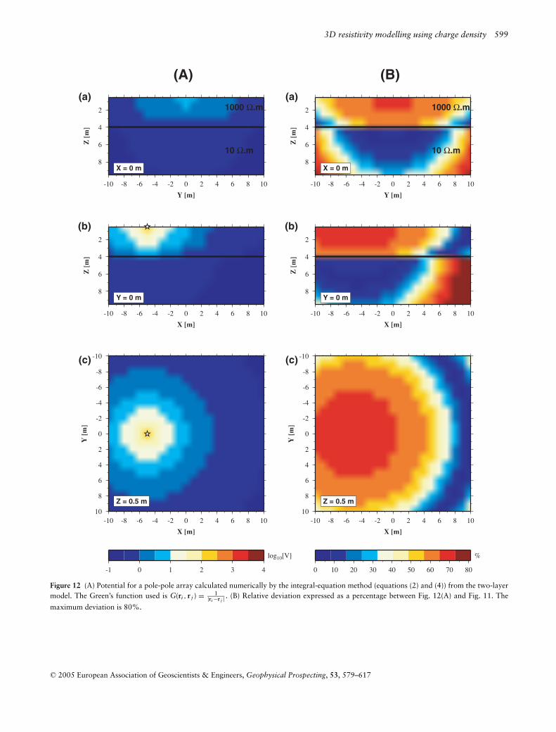
Figure 11 shows the potential as log10(V) analytically calculated for a two-layer subsurface (first layer of 1000 m with athickness of 4 m overlying an infinite homogeneous medium of 10 m) in the x-, y- and z-directions. The source is locatedat (−5, 0, 0) m. Figures 11(a) and 11(b) correspond to the sections X = 0 m and Y = 0 m. Figure 11(c) represents the planeZ = 0.5 m. The calculations of the potential and the current density are given in Appendix D. Figures 12 , 13 and 14 showthe potential and the relative deviation compared with Fig. 11 for the integral-equation method using the Green’s functionsG(ri , r j ) = 1
|ri −r j | , G(ri , r j ) = 1|ri −r j | + 1
|ri −r′j |and the finite-difference method, respectively. The maximum relative deviation for
Fig. 12 is 80% uniformly distributed around the source in the 1000 m layer. The maximum relative deviation for Fig. 13 is27% and is in the 10 m medium under the source. Around the source the deviation does not exceed 2.5%. The maximumrelative deviation for Fig. 14 is 40% at the source point and is radially symmetric about the source.
Calculation of the sensitivity
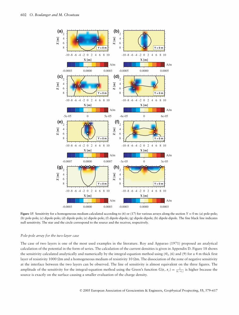
In the following figures, the transmitting current is positive. The sources and the receivers are represented by a star and a circle,respectively. The calculation of the sensitivity for a homogeneous medium using a dipole-dipole array is given in Appendix C.
Pole-pole, dipole-pole and dipole-dipole arrays for a homogeneous medium
Figure 15 shows the sensitivity calculated analytically for various arrays (pole-pole, dipole-pole and dipole-dipole) for electrodesat the ground surface and at depth. The solid black line indicates the null sensitivity associated with the polarity change. It canbe seen that sensitivity increases near the transmitting and receiving positions. Figure 15(a) shows that the negative sensitivityincludes the area located between the electrodes and extends to the surface (it is a circle on the surface). Figure 15(b) shows thatwhen the electrodes are superimposed, the zone of negative sensitivity forms a closed spherical surface. With the dipole-polearray, frequently used in electric prospecting, the sensitivity is asymmetrical (Figs 15(c,d,e)). The sensitivities for various arraysof dipoles/poles are shown in Figs 15(f,g,h).
C© 2005 European Association of Geoscientists & Engineers, Geophysical Prospecting, 53, 579–617
594 O. Boulanger and M. Chouteau
2
4
6
8
Z [
m]
-10 -8 -6 -4 -2 0 2 4 6 8 10
Y [m]
X = 0 m
(a)
2
4
6
8
Z [
m]
-10 -8 -6 -4 -2 0 2 4 6 8 10
X [m]
Y = 0 m
(b)
-10
-8
-6
-4
-2
0
2
4
6
8
10
Y [
m]
-10 -8 -6 -4 -2 0 2 4 6 8 10
X [m]
Z = 0.5 m
(c)10 Ω.m 1000 Ω.m
-1.0 -0.5 0.0 0.5
log10[V]
Figure 7 Potential (log10[V]) for a pole-pole array calculated analytically for a vertical contact (medium 1: 10 m and medium 2: 1000 m).The source is located at (−5, 0, 0) m. The black line indicates the vertical contact. (a) and (b) correspond to sections X = 0 m and Y = 0 m. (c)shows the plan Z = 0.5 m.
Pole-pole array for a vertical contact
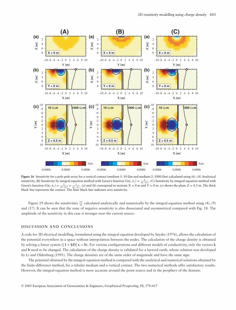
We use the case of a vertical contact located at X = 0 m, with resistivity 10 m for x < 0 m and 1000 m for x > 0 m, to validateand compare the methods of sensitivity calculation. The calculations of the current densities and of the electric field are givenin Appendix E. The sensitivity calculated analytically and numerically by the integral-equation method is shown in Fig. 16. The
C© 2005 European Association of Geoscientists & Engineers, Geophysical Prospecting, 53, 579–617
3D resistivity modelling using charge density 595
2
4
6
8
Z [
m]
-10 -8 -6 -4 -2 0 2 4 6 8 10
Y [m]
X = 0 m
(a)
(A)
2
4
6
8
Z [
m]
-10 -8 -6 -4 -2 0 2 4 6 8 10
X [m]
Y = 0 m
(b)
-10
-8
-6
-4
-2
0
2
4
6
8
10
Y [
m]
-10 -8 -6 -4 -2 0 2 4 6 8 10
X [m]
Z = 0.5 m
10 Ω.m 1000 Ω.m(c)
-1 0 1 2 3 4
log10[V]
-10
-8
-6
-4
-2
0
2
4
6
8
10
Y [
m]
-10 -8 -6 -4 -2 0 2 4 6 8 10
X [m]
Z = 0.5 m
10 Ω.m 1000 Ω.m(c)
0 10 20 30 40 50
%
2
4
6
8Z
[m
]
-10 -8 -6 -4 -2 0 2 4 6 8 10
X [m]
Y = 0 m
(b)
2
4
6
8
Z [
m]
-10 -8 -6 -4 -2 0 2 4 6 8 10
Y [m]
X = 0 m
(a)
(B)
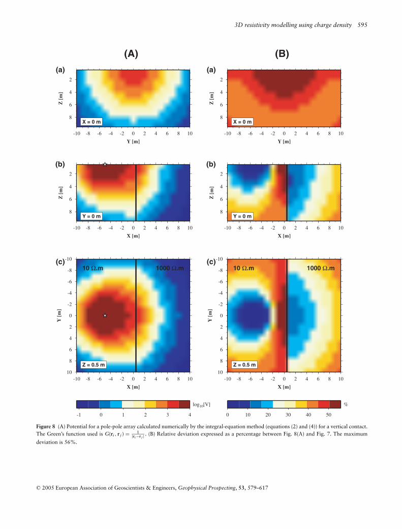
Figure 8 (A) Potential for a pole-pole array calculated numerically by the integral-equation method (equations (2) and (4)) for a vertical contact.The Green’s function used is G(ri , r j ) = 1
|ri −r j | . (B) Relative deviation expressed as a percentage between Fig. 8(A) and Fig. 7. The maximum
deviation is 56%.
C© 2005 European Association of Geoscientists & Engineers, Geophysical Prospecting, 53, 579–617
596 O. Boulanger and M. Chouteau
2
4
6
8
Z [
m]
-10 -8 -6 -4 -2 0 2 4 6 8 10
Y [m]
X = 0 m
(a)
(A)
2
4
6
8
Z [
m]
-10 -8 -6 -4 -2 0 2 4 6 8 10
X [m]
Y = 0 m
(b)
-10
-8
-6
-4
-2
0
2
4
6
8
10
Y [
m]
-10 -8 -6 -4 -2 0 2 4 6 8 10
X [m]
Z = 0.5 m
10 Ω.m 1000 Ω.m(c)
-1 0 1 2 3 4
log10[V]
-10
-8
-6
-4
-2
0
2
4
6
8
10
Y [
m]
-10 -8 -6 -4 -2 0 2 4 6 8 10
X [m]
Z = 0.5 m
10 Ω.m 1000 Ω.m(c)
0 5 10 15
%
2
4
6
8Z
[m
]
-10 -8 -6 -4 -2 0 2 4 6 8 10
X [m]
Y = 0 m
(b)
2
4
6
8
Z [
m]
-10 -8 -6 -4 -2 0 2 4 6 8 10
Y [m]
X = 0 m
(a)
(B)
Figure 9 (A) Potential for a pole-pole array calculated numerically by the integral-equation method (equations (2) and (4)) for a vertical contact.The Green’s function used is G(ri , r j ) = 1
|ri −r j | + 1|ri −r′j |
. (B) Relative deviation expressed as a percentage between Fig. 9(A) and Fig. 7. Themaximum deviation is 16%.
C© 2005 European Association of Geoscientists & Engineers, Geophysical Prospecting, 53, 579–617
3D resistivity modelling using charge density 597
2
4
6
8
Z [
m]
-10 -8 -6 -4 -2 0 2 4 6 8 10
Y [m]
X = 0 m
(a)
(A)
2
4
6
8
Z [
m]
-10 -8 -6 -4 -2 0 2 4 6 8 10
X [m]
Y = 0 m
(b)
-10
-8
-6
-4
-2
0
2
4
6
8
10
Y [
m]
-10 -8 -6 -4 -2 0 2 4 6 8 10
X [m]
Z = 0.5 m
10 Ω.m 1000 Ω.m(c)
-1 0 1 2 3 4
log10[V]
-10
-8
-6
-4
-2
0
2
4
6
8
10
Y [
m]
-10 -8 -6 -4 -2 0 2 4 6 8 10
X [m]
Z = 0.5 m
10 Ω.m 1000 Ω.m(c)
0 10 20 30 40 50 60 70 80 90 100
%
2
4
6
8Z
[m
]
-10 -8 -6 -4 -2 0 2 4 6 8 10
X [m]
Y = 0 m
(b)
2
4
6
8
Z [
m]
-10 -8 -6 -4 -2 0 2 4 6 8 10
Y [m]
X = 0 m
(a)
(B)
Figure 10 (A) Potential for a pole-pole array calculated numerically by the finite-difference method (equations (2) and (4)) for a vertical contact.(B) Relative deviation expressed as a percentage between Fig. 10(A) and Fig. 7. The maximum deviation is 100%.
C© 2005 European Association of Geoscientists & Engineers, Geophysical Prospecting, 53, 579–617
598 O. Boulanger and M. Chouteau
2
4
6
8
Z [
m]
-10 -8 -6 -4 -2 0 2 4 6 8 10
Y [m]
X = 0 m
1000 Ω.m
10 Ω.m
(a)
2
4
6
8
Z [
m]
-10 -8 -6 -4 -2 0 2 4 6 8 10
X [m]
Y = 0 m
(b)
-10
-8
-6
-4
-2
0
2
4
6
8
10
Y [
m]
-10 -8 -6 -4 -2 0 2 4 6 8 10
X [m]
Z = 0.5 m
(c)
-1 0 1 2 3 4
log10[V]
Figure 11 Potential (log10[V]) for a pole-pole array calculated analytically for the two-layer case (first layer of 1000 m and 4 m thickness andan infinite homogeneous medium of 10 m). The source is located at (−5, 0, 0) m. (a) and (b) correspond to sections X = 0 m and Y = 0 m.(c) shows the plane Z = 0.5 m.
sensitivity is calculated numerically using (4), (6) and (9) for the Green’s functions G(ri , r j ) = 1|ri −r j | and G(ri , r j ) = 1
|ri −r j | + 1|ri −r′j |
.
It can be seen on these figures that the amplitude and the line of null sensitivity are similar. Figure 17 shows the sensitivities ∂V∂ρ
calculated analytically and numerically using (4), (9) and (17). By comparing Figs 16 and 17, the role played in (6) by the currentdensity resulting from the receiving point can be observed. It generates a zone of negative sensitivity, propagated at infinity andparallel to the vertical contact.
C© 2005 European Association of Geoscientists & Engineers, Geophysical Prospecting, 53, 579–617
3D resistivity modelling using charge density 599
2
4
6
8
Z [
m]
-10 -8 -6 -4 -2 0 2 4 6 8 10
Y [m]
X = 0 m
1000 Ω.m
10 Ω.m
(a)
(A)
2
4
6
8
Z [
m]
-10 -8 -6 -4 -2 0 2 4 6 8 10
X [m]
Y = 0 m
(b)
-10
-8
-6
-4
-2
0
2
4
6
8
10
Y [
m]
-10 -8 -6 -4 -2 0 2 4 6 8 10
X [m]
Z = 0.5 m
(c)
-1 0 1 2 3 4
log10[V]
-10
-8
-6
-4
-2
0
2
4
6
8
10
Y [
m]
-10 -8 -6 -4 -2 0 2 4 6 8 10
X [m]
Z = 0.5 m
(c)
0 10 20 30 40 50 60 70 80
%
2
4
6
8Z
[m
]
-10 -8 -6 -4 -2 0 2 4 6 8 10
X [m]
Y = 0 m
(b)
2
4
6
8
Z [
m]
-10 -8 -6 -4 -2 0 2 4 6 8 10
Y [m]
X = 0 m
(a)1000 Ω.m
10 Ω.m
(B)
Figure 12 (A) Potential for a pole-pole array calculated numerically by the integral-equation method (equations (2) and (4)) from the two-layermodel. The Green’s function used is G(ri , r j ) = 1
|ri −r j | . (B) Relative deviation expressed as a percentage between Fig. 12(A) and Fig. 11. The
maximum deviation is 80%.
C© 2005 European Association of Geoscientists & Engineers, Geophysical Prospecting, 53, 579–617
600 O. Boulanger and M. Chouteau
2
4
6
8
Z [
m]
-10 -8 -6 -4 -2 0 2 4 6 8 10
Y [m]
X = 0 m
1000 Ω.m
10 Ω.m
(a)
(A)
2
4
6
8
Z [
m]
-10 -8 -6 -4 -2 0 2 4 6 8 10
X [m]
Y = 0 m
(b)
-10
-8
-6
-4
-2
0
2
4
6
8
10
Y [
m]
-10 -8 -6 -4 -2 0 2 4 6 8 10
X [m]
Z = 0.5 m
(c)
-1 0 1 2 3 4
log10[V]
-10
-8
-6
-4
-2
0
2
4
6
8
10
Y [
m]
-10 -8 -6 -4 -2 0 2 4 6 8 10
X [m]
Z = 0.5 m
(c)
0 5 10 15 20 25
%
2
4
6
8Z
[m
]
-10 -8 -6 -4 -2 0 2 4 6 8 10
X [m]
Y = 0 m
(b)
2
4
6
8
Z [
m]
-10 -8 -6 -4 -2 0 2 4 6 8 10
Y [m]
X = 0 m
(a)1000 Ω.m
10 Ω.m
(B)
Figure 13 (A) Potential calculated numerically by the integral-equation method (equations (2) and (4)) for the two-layer model for a pole-polearray. The Green’s function used is G(ri , r j ) = 1
|ri −r j | + 1|ri −r′j |
. (B) Relative deviation expressed as a percentage between Fig. 13(A) and Fig. 11.
The maximum deviation is 27%.
C© 2005 European Association of Geoscientists & Engineers, Geophysical Prospecting, 53, 579–617
3D resistivity modelling using charge density 601
2
4
6
8
Z [
m]
-10 -8 -6 -4 -2 0 2 4 6 8 10
Y [m]
X = 0 m
1000 Ω.m
10 Ω.m
(a)
(A)
2
4
6
8
Z [
m]
-10 -8 -6 -4 -2 0 2 4 6 8 10
X [m]
Y = 0 m
(b)
-10
-8
-6
-4
-2
0
2
4
6
8
10
Y [
m]
-10 -8 -6 -4 -2 0 2 4 6 8 10
X [m]
Z = 0.5 m
(c)
-1 0 1 2 3 4
log10[V]
-10
-8
-6
-4
-2
0
2
4
6
8
10
Y [
m]
-10 -8 -6 -4 -2 0 2 4 6 8 10
X [m]
Z = 0.5 m
(c)
0 5 10 15 20 25 30 35 40
%
2
4
6
8Z
[m
]
-10 -8 -6 -4 -2 0 2 4 6 8 10
X [m]
Y = 0 m
(b)
2
4
6
8
Z [
m]
-10 -8 -6 -4 -2 0 2 4 6 8 10
Y [m]
X = 0 m
(a)1000 Ω.m
10 Ω.m
(B)
Figure 14 (A) Potential for a pole-pole array calculated numerically by the finite-difference method for the two-layer model. (B) Relative deviationexpressed as a percentage between Fig. 14(A) and Fig. 11. The maximum deviation is 40%.
C© 2005 European Association of Geoscientists & Engineers, Geophysical Prospecting, 53, 579–617
602 O. Boulanger and M. Chouteau
2
4
6
8
Z [
m]
-10 -8 -6 -4 -2 0 2 4 6 8 10
X [m]
-0.0003 0.0000 0.0003
A/m
(a)
Y = 0 m
2
4
6
8
Z [
m]
-10 -8 -6 -4 -2 0 2 4 6 8 10
X [m]
-5e-05 0 5e-05
A/m
(c)
Y = 0 m
2
4
6
8
Z [
m]
-10 -8 -6 -4 -2 0 2 4 6 8 10
X [m]
-0.0007 0.0000 0.0007
A/m
(e)
Y = 0 m
2
4
6
8
Z [
m]
-10 -8 -6 -4 -2 0 2 4 6 8 10
X [m]
-0.0003 0.0000 0.0003
A/m
(g)
Y = 0 m
2
4
6
8
Z [
m]
-10 -8 -6 -4 -2 0 2 4 6 8 10
X [m]
-0.0003 0.0000 0.0003
A/m
(h)
Y = 0 m
2
4
6
8
Z [
m]
-10 -8 -6 -4 -2 0 2 4 6 8 10
X [m]
-3e-05 0 3e-05
A/m
(f)
Y = 0 m
2
4
6
8
Z [
m]
-10 -8 -6 -4 -2 0 2 4 6 8 10
X [m]
-6e-05 0 6e-05
A/m
(d)
Y = 0 m
2
4
6
8
Z [
m]
-10 -8 -6 -4 -2 0 2 4 6 8 10
X [m]
-0.0005 0.0000 0.0005
A/m
(b)
Y = 0 m
Figure 15 Sensitivity for a homogeneous medium calculated according to (6) or (17) for various arrays along the section Y = 0 m: (a) pole-pole;(b) pole-pole; (c) dipole-pole; (d) dipole-pole; (e) dipole-pole; (f) dipole-dipole; (g) dipole-dipole; (h) dipole-dipole. The fine black line indicatesnull sensitivity. The star and the circle correspond to the source and the receiver, respectively.
Pole-pole array for the two-layer case
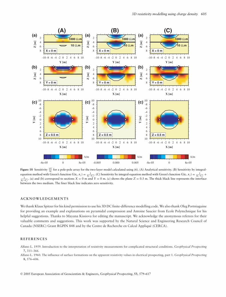
The case of two layers is one of the most used examples in the literature. Roy and Apparao (1971) proposed an analyticalcalculation of the potential in the form of series. The calculation of the current densities is given in Appendix D. Figure 18 showsthe sensitivity calculated analytically and numerically by the integral-equation method using (4), (6) and (9) for a 4 m thick firstlayer of resistivity 1000 m and a homogeneous medium of resistivity 10 m. The dissociation of the zone of negative sensitivityat the interface between the two layers can be observed. The line of sensitivity is almost equivalent on the three figures. Theamplitude of the sensitivity for the integral-equation method using the Green’s function G(ri , r j ) = 1
|ri −r j | is higher because thesource is exactly on the surface causing a smaller evaluation of the charge density.
C© 2005 European Association of Geoscientists & Engineers, Geophysical Prospecting, 53, 579–617
3D resistivity modelling using charge density 603
2
4
6
8
Z [
m]
-10 -8 -6 -4 -2 0 2 4 6 8 10
Y [m]
X = 0 m
(a)(A)
2
4
6
8
Z [
m]
-10 -8 -6 -4 -2 0 2 4 6 8 10
X [m]
Y = 0 m
(b)
-10-8-6-4-202468
10
Y [
m]
-10 -8 -6 -4 -2 0 2 4 6 8 10
X [m]
Z = 0.5 m
1000 Ω.m10 Ω.m(c)
-0.0006 0.0000 0.0006
A/m
-10-8-6-4-202468
10
Y [
m]
-10 -8 -6 -4 -2 0 2 4 6 8 10
X [m]
Z = 0.5 m
1000 Ω.m10 Ω.m(c)
-0.0006 0.0000 0.0006
A/m
2
4
6
8
Z [
m]
-10 -8 -6 -4 -2 0 2 4 6 8 10
X [m]
Y = 0 m
(b)
2
4
6
8
Z [
m]
-10 -8 -6 -4 -2 0 2 4 6 8 10
Y [m]
X = 0 m
(a)(B)
2
4
6
8
Z [
m]
-10 -8 -6 -4 -2 0 2 4 6 8 10
Y [m]
X = 0 m
(a)(C)
2
4
6
8
Z [
m]
-10 -8 -6 -4 -2 0 2 4 6 8 10
X [m]
Y = 0 m
(b)
-10-8-6-4-202468
10Y
[m
]-10 -8 -6 -4 -2 0 2 4 6 8 10
X [m]
Z = 0.5 m
1000 Ω.m10 Ω.m(c)
-0.0006 0.0000 0.0006
A/m
Figure 16 Sensitivity for a pole-pole array for a vertical contact (medium 1: 10 m and medium 2: 1000 m) calculated using (6). (A) Analyticalsensitivity. (B) Sensitivity by integral-equation method with Green’s function G(ri , r j ) = 1
|ri −r j | . (C) Sensitivity by integral-equation method withGreen’s function G(ri , r j ) = 1
|ri −r j | + 1|ri −r′j |
. (a) and (b) correspond to sections X = 0 m and Y = 0 m. (c) shows the plane Z = 0.5 m. The thickblack line represents the contact. The finer black line indicates zero sensitivity.
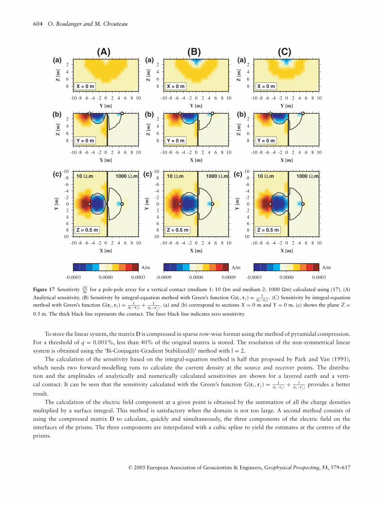
Figure 19 shows the sensitivities ∂V∂ρ
calculated analytically and numerically by the integral-equation method using (4), (9)and (17). It can be seen that the zone of negative sensitivity is also dissociated and asymmetrical compared with Fig. 18. Theamplitude of the sensitivity in this case is stronger near the current source.
D I S C U S S I O N A N D C O N C L U S I O N S
A code for 3D electrical modelling, formulated using the integral equation developed by Snyder (1976), allows the calculation ofthe potential everywhere in a space without interpolation between the nodes. The calculation of the charge density is obtainedby solving a linear system ([ I + kD] x = b). For various configurations and different models of conductivity, only the vectors kand b need to be changed. The calculation of the charge density is validated for a layered earth, whose solution was developedby Li and Oldenburg (1991). The charge densities are of the same order of magnitude and have the same sign.
The potential obtained by the integral-equation method is compared with the analytical and numerical solutions obtained bythe finite-difference method, for a tabular medium and a vertical contact. The two numerical methods offer satisfactory results.However, the integral-equation method is more accurate around the point source and in the periphery of the domain.
C© 2005 European Association of Geoscientists & Engineers, Geophysical Prospecting, 53, 579–617
604 O. Boulanger and M. Chouteau
2
4
6
8
Z [
m]
-10 -8 -6 -4 -2 0 2 4 6 8 10
Y [m]
X = 0 m
(a)(A)
2
4
6
8
Z [
m]
-10 -8 -6 -4 -2 0 2 4 6 8 10
X [m]
Y = 0 m
(b)
-10-8-6-4-202468
10
Y [
m]
-10 -8 -6 -4 -2 0 2 4 6 8 10
X [m]
Z = 0.5 m
1000 Ω.m10 Ω.m(c)
-0.0003 0.0000 0.0003
A/m
-10-8-6-4-202468
10
Y [
m]
-10 -8 -6 -4 -2 0 2 4 6 8 10
X [m]
Z = 0.5 m
1000 Ω.m10 Ω.m(c)
-0.0009 0.0000 0.0009
A/m
2
4
6
8
Z [
m]
-10 -8 -6 -4 -2 0 2 4 6 8 10
X [m]
Y = 0 m
(b)
2
4
6
8
Z [
m]
-10 -8 -6 -4 -2 0 2 4 6 8 10
Y [m]
X = 0 m
(a)(B)
2
4
6
8
Z [
m]
-10 -8 -6 -4 -2 0 2 4 6 8 10
Y [m]
X = 0 m
(a)(C)
2
4
6
8
Z [
m]
-10 -8 -6 -4 -2 0 2 4 6 8 10
X [m]
Y = 0 m
(b)
-10-8-6-4-202468
10Y
[m
]-10 -8 -6 -4 -2 0 2 4 6 8 10
X [m]
Z = 0.5 m
1000 Ω.m10 Ω.m(c)
-0.0003 0.0000 0.0003
A/m
Figure 17 Sensitivity ∂V∂ρ
for a pole-pole array for a vertical contact (medium 1: 10 m and medium 2: 1000 m) calculated using (17). (A)
Analytical sensitivity. (B) Sensitivity by integral-equation method with Green’s function G(ri , r j ) = 1|ri −r j | . (C) Sensitivity by integral-equation
method with Green’s function G(ri , r j ) = 1|ri −r j | + 1
|ri −r′j |. (a) and (b) correspond to sections X = 0 m and Y = 0 m. (c) shows the plane Z =
0.5 m. The thick black line represents the contact. The finer black line indicates zero sensitivity.
To store the linear system, the matrix D is compressed in sparse row-wise format using the method of pyramidal compression.For a threshold of q = 0.001%, less than 40% of the original matrix is stored. The resolution of the non-symmetrical linearsystem is obtained using the ‘Bi-Conjugate-Gradient Stabilized(l)’ method with l = 2.
The calculation of the sensitivity based on the integral-equation method is half that proposed by Park and Van (1991),which needs two forward-modelling runs to calculate the current density at the source and receiver points. The distribu-tion and the amplitudes of analytically and numerically calculated sensitivities are shown for a layered earth and a verti-cal contact. It can be seen that the sensitivity calculated with the Green’s function G(ri , r j ) = 1
|ri −r j | + 1|ri −r′j |
provides a better
result.The calculation of the electric field component at a given point is obtained by the summation of all the charge densities
multiplied by a surface integral. This method is satisfactory when the domain is not too large. A second method consists ofusing the compressed matrix D to calculate, quickly and simultaneously, the three components of the electric field on theinterfaces of the prisms. The three components are interpolated with a cubic spline to yield the estimates at the centres of theprisms.
C© 2005 European Association of Geoscientists & Engineers, Geophysical Prospecting, 53, 579–617
3D resistivity modelling using charge density 605
2
4
6
8
Z [
m]
-10 -8 -6 -4 -2 0 2 4 6 8 10
Y [m]
X = 0 m
1000 Ω.m
10 Ω.m
(a)(A)
2
4
6
8
Z [
m]
-10 -8 -6 -4 -2 0 2 4 6 8 10
X [m]
Y = 0 m
(b)
-10-8-6-4-202468
10
Y [
m]
-10 -8 -6 -4 -2 0 2 4 6 8 10
X [m]
Z = 0.5 m
(c)
-8e-05 0 8e-05
A/m
-10-8-6-4-202468
10
Y [
m]
-10 -8 -6 -4 -2 0 2 4 6 8 10
X [m]
Z = 0.5 m
(c)
-0.005 0.000 0.005
A/m
2
4
6
8
Z [
m]
-10 -8 -6 -4 -2 0 2 4 6 8 10
X [m]
Y = 0 m
(b)
2
4
6
8
Z [
m]
-10 -8 -6 -4 -2 0 2 4 6 8 10
Y [m]
X = 0 m
1000 Ω.m
10 Ω.m
(a)(B)
2
4
6
8
Z [
m]
-10 -8 -6 -4 -2 0 2 4 6 8 10
Y [m]
X = 0 m
1000 Ω.m
10 Ω.m
(a)(C)
2
4
6
8
Z [
m]
-10 -8 -6 -4 -2 0 2 4 6 8 10
X [m]
Y = 0 m
(b)
-10-8-6-4-202468
10Y
[m
]-10 -8 -6 -4 -2 0 2 4 6 8 10
X [m]
Z = 0.5 m
(c)
-8e-05 0 8e-05
A/m
Figure 18 Sensitivity ∂V∂ρ
for a pole-pole array for the two-layer model calculated using (6). (A) Analytical sensitivity. (B) Sensitivity by integral-
equation method with Green’s function G(ri , r j ) = 1|ri −r j | . (C) Sensitivity by integral-equation method with Green’s function G(ri , r j ) = 1
|ri −r j | +1
|ri −r′j |. (a) and (b) correspond to sections X = 0 m and Y = 0 m. (c) shows the plane Z = 0.5 m. The thick black line represents the interface
between the two medium. The finer black line indicates zero sensitivity.
A C K N O W L E D G E M E N T S
We thank Klaus Spitzer for his kind permission to use his 3D DC finite-difference modelling code. We also thank Oleg Portniaguinefor providing an example and explanations on pyramidal compression and Antoine Saucier from Ecole Polytechnique for hishelpful suggestions. Thanks to Mayana Kissiova for editing the manuscript. We acknowledge the anonymous referees for theirvaluable comments and suggestions. This work was supported by the Natural Science and Engineering Research Council ofCanada (NSERC) Grant RGPIN 848 and by the Centre de Recherche en Calcul Applique (CERCA).
R E F E R E N C E S
Alfano L. 1959. Introduction to the interpretation of resistivity measurements for complicated structural conditions. Geophysical Prospecting7, 311–366.
Alfano L. 1960. The influence of surface formations on the apparent resistivity values in electrical prospecting, part 1. Geophysical Prospecting8, 576–606.
C© 2005 European Association of Geoscientists & Engineers, Geophysical Prospecting, 53, 579–617
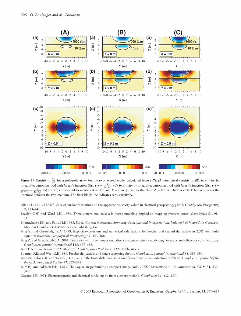
606 O. Boulanger and M. Chouteau
2
4
6
8
Z [
m]
-10 -8 -6 -4 -2 0 2 4 6 8 10
Y [m]
X = 0 m
1000 Ω.m
10 Ω.m
(a)(A)
2
4
6
8
Z [
m]
-10 -8 -6 -4 -2 0 2 4 6 8 10
X [m]
Y = 0 m
(b)
-10-8-6-4-202468
10
Y [
m]
-10 -8 -6 -4 -2 0 2 4 6 8 10
X [m]
Z = 0.5 m
(c)
-0.0003 0.0000 0.0003
A/m
-10-8-6-4-202468
10
Y [
m]
-10 -8 -6 -4 -2 0 2 4 6 8 10
X [m]
Z = 0.5 m
(c)
-0.005 0.000 0.005
A/m
2
4
6
8
Z [
m]
-10 -8 -6 -4 -2 0 2 4 6 8 10
X [m]
Y = 0 m
(b)
2
4
6
8
Z [
m]
-10 -8 -6 -4 -2 0 2 4 6 8 10
Y [m]
X = 0 m
1000 Ω.m
10 Ω.m
(a)(B)
2
4
6
8
Z [
m]
-10 -8 -6 -4 -2 0 2 4 6 8 10
Y [m]
X = 0 m
1000 Ω.m
10 Ω.m
(a)(C)
2
4
6
8
Z [
m]
-10 -8 -6 -4 -2 0 2 4 6 8 10
X [m]
Y = 0 m
(b)
-10-8-6-4-202468
10Y
[m
]-10 -8 -6 -4 -2 0 2 4 6 8 10
X [m]
Z = 0.5 m
(c)
-0.0003 0.0000 0.0003
A/m
Figure 19 Sensitivity ∂V∂ρ
for a pole-pole array for the two-layered model calculated from (17). (A) Analytical sensitivity. (B) Sensitivity by
integral-equation method with Green’s function G(ri , r j ) = 1|ri −r j | . (C) Sensitivity by integral-equation method with Green’s function G(ri , r j ) =
1|ri −r j | + 1
|ri −r′j |. (a) and (b) correspond to sections X = 0 m and Y = 0 m. (c) shows the plane Z = 0.5 m. The thick black line represents the
interface between the two medium. The finer black line indicates zero sensitivity.
Alfano L. 1961. The influence of surface formations on the apparent resistivity values in electrical prospecting, part 2. Geophysical Prospecting9, 213–241.
Beasley C.W. and Ward S.H. 1986. Three-dimensional mise-a-la-masse modeling applied to mapping fracture zones. Geophysics 51, 98–113.
Bhattacharya P.K. and Patra H.P. 1968. Direct Current Geoelectric Sounding: Principles and Interpretations. Volume 9 of Methods in Geochem-istry and Geophysics. Elsevier Science Publishing Co.
Bing Z. and Greenhalgh S.A. 1999. Explicit expressions and numerical calculations for Frechet and second derivatives in 2.5D Helmholtzequation inversion. Geophysical Prospecting 47, 443–468.
Bing Z. and Greenhalgh S.A. 2001. Finite element three-dimensional direct current resistivity modelling: accuracy and efficiency considerations.Geophysical Journal International 145, 679–688.
Bjorck A. 1996. Numerical Methods for Least Squares Problems. SIAM Publications.Boerner D.E. and West G.F. 1989. Frechet derivatives and single scattering theory. Geophysical Journal International 98, 385–390.Brewitt-Taylor C.R. and Weaver J.T. 1976. On the finite difference solution of two-dimensional induction problems. Geophysical Journal of the
Royal Astronomical Society 47, 375–396.Burt P.J. and Adelson E.H. 1983. The Laplacian pyramid as a compact image code. IEEE Transactions on Communications COM-31, 337–
345.Coggon J.H. 1971. Electromagnetic and electrical modeling by finite element method. Geophysics 36, 132–155.
C© 2005 European Association of Geoscientists & Engineers, Geophysical Prospecting, 53, 579–617

3D resistivity modelling using charge density 607
Dey A. and Morrison H.F. 1979a. Resistivity modeling for arbitrarily shaped three-dimensional structures. Geophysics 44, 753–780.Dey A. and Morrison H.F. 1979b. Resistivity modelling for arbitrarily shaped two-dimensional structures. Geophysical Prospecting 27, 106–136.Freund R. and Nachtigal N. 1991a. An implementation of the QMR method based on coupled two-term recurrences. SIAM Journal on Scientific
and Statistical Computation 15, 313–337.Freund R. and Nachtigal N. 1991b. QMR: A quasi-minimal residual method for non-Hermitian linear systems. Numerical Mathematics 60,
315–339.Geselowitz D.B. 1971. An application of electrocardiographic lead theory to impedance plethysmography. IEEE Transactions on Bio-Medical
Engineering BME-18, 38–41.Golub G.H. and Van Loan C.F. 1996. Matrix Computations, 3rd edn. Johns Hopkins University Press.Hestenes M. and Stiefel E. 1952. Methods of conjugate gradients for solving linear systems. Journal of Research of the National Bureau of
Standards 49, 409–436.Hohmann G.W. 1975. Three-dimensional induced polarization and electromagnetic modeling. Geophysics 40, 309–324.Hvozdara M. and Kaikkonen P. 1998. An integral equations solution of the forward D.C. geoelectric problem for a 3-D body of inhomogeneous
conductivity buried in a halfspace. Journal of Applied Geophysics 39, 95–107.LaBrecque D.J., Miletto M., Daily W., Ramirez A. and Owen E. 1996. The effects of noise on Occam’s inversion of resistivity tomography data.
Geophysics 61, 538–548.LaBrecque D.J., Morelli G., Daily W., Ramirez A. and Lundegard P. 1999. Occam’s inversion of 3-D electrical resistivity tomography. In:
Three-Dimensional Electromagnetics (eds M. Oristaglio and B. Spies), pp. 575–590. Society of Exploration Geophysicists, Tulsa, OK.Lanczos C. 1961. Linear Differential Operators. Van Nostrand (Dover, 1997).Lesur V., Cuer M. and Straub A. 1999. 2-D and 3-D interpretation of electrical tomography measurements, Part 1: The forward problem.
Geophysics 64, 386–395.Li Y. and Oldenburg D.W. 1991. Aspects of charge accumulation in DC resistivity experiments. Geophysical Prospecting 39, 803–826.Li Y. and Oldenburg D. 1997. Fast inversion of large scale magnetic data using wavelets. 67th SEG meeting, Dallas, USA, Expanded Abstracts,
490–493.Losano V. and Laget B. 1996. Fractional pyramids for color image segmentation. In: Proceedings of the IEEE Southwest Symposium on Image
Analysis and Interpretation, San Antonio, Texas, USA, pp. 13–17.Lowry T., Allen M.B. and Shive P.N. 1989. Singularity removal: A refinement of resistivity modeling techniques. Geophysics 54, 766–
774.McGillivray P. and Oldenburg D.W. 1990. Methods for calculating Frechet derivates and sensitivities for the non-linear inverse problem: a
comparative study. Geophysical Prospecting 38, 499–524.Mufti I. 1978. A practical approach to finite-difference resistivity modeling. Geophysics 43, 930–942.Mundry E. 1984. Geoelectrical model calculations for two-dimensional resistivity distributions. Geophysical Prospecting 32, 124–131.Murai T. and Kagawa Y. 1985. Electrical impedance computed tomography based on finite element model. IEEE Transactions on Biomedical
Engineering BME-32, 177–184.Nocedal J. and Wright S.J. 2000. Numerical Optimization. Springer-Verlag, Inc.Park S.K. and Van G.P. 1991. Inversion of pole-pole data for 3-D resistivity structure beneath arrays of electrodes. Geophysics 56, 951–960.Pissanetzky S. 1984. Sparse Matrix Technology. Academic Press, Inc.Poirmeur C. and Vasseur G. 1988. Three-dimensional modeling of a hole-to-hole electrical method: Application to the interpretation of a field
survey. Geophysics 53, 402–414.Portniaguine O. 1999. Image focusing and data compression in the solution of geophysical inverse problems. PhD thesis, University of Utah.Pratt D.A. 1972. The surface integral approach to the solution of the 3D resistivity problem. Bulletin of the Australian Society for Exploration
Geophysics 3, 33–50.Press W.H., Teukolsky S.A., Vetterling W.T. and Flannery B.P. 1992. Numerical Recipes in C: The Art of Scientific Computing, 2nd edn.
Cambridge University Press.Pridmore D.F., Hohmann G.W., Ward S.H. and Sill W.R. 1981. An investigation of finite-element modeling for electrical and electromagnetic
data in three dimensions. Geophysics 46, 1009–1024.Raiche A.P. 1974. An integral equation approach to three-dimensional modelling. Geophysical Journal of the Royal Astronomical Society 36,
363–376.Roy A. and Apparao A. 1971. Depth of investigation in direct current methods. Geophysics 36, 943–959.Sasaki Y. 1992. Resolution of resistivity tomography inferred from numerical simulation. Geophysical Prospecting 40, 453–463.Sasaki Y. 1994. 3-D resistivity inversion using the finite-element method. Geophysics 59, 1839–1848.Schulz R. 1985. The method of integral equation in direct current resistivity method and its accuracy. Journal of Geophysics 56, 192–200.Scriba H. 1981. Computation of the electric potential in three-dimensional structures. Geophysical Prospecting 29, 790–802.Seigel H.O. 1959. Mathematical formulation and type curves for induced polarization. Geophysics 24, 547–565.Sleijpen G. and Fokkema D. 1993. BICGSTAB(l) for linear equations involving unsymmetric matrices with complex spectrum. Electronic
Transactions on Numerical Analysis 1, 11–32.
C© 2005 European Association of Geoscientists & Engineers, Geophysical Prospecting, 53, 579–617
608 O. Boulanger and M. Chouteau
Snyder D.D. 1976. A method for modeling the resistivity and IP response of two-dimensional bodies. Geophysics 41, 997–1015.Sonneveld P. 1989. CGS, a fast Lanczos-type solver for nonsymmetric linear systems. SIAM Journal on Scientific and Statistical Computation
10, 36–52.Spiegel R.J., Sturdivant V.R. and Owen T.E. 1980. Modeling resistivity anomalies from localized voids under irregular terrain. Geophysics 45,
1164–1183.Spitzer K. 1995. A 3-D finite-difference algorithm for dc resistivity modelling using conjugate gradient methods. Geophysical Journal Interna-
tional 123, 903–914.Spitzer K. 1998. The three-dimensional DC sensitivity for surface and subsurface sources. Geophysical Journal International 134, 736–746.Spitzer K., Chouteau M. and Boulanger O. 1999. Grid-independent electrode positioning for 3D DC resistivity and IP forward modelling. In:
Symposium 3DEM2, Salt Lake City, Utah, pp. 189–192.Spitzer K. and Wurmstich B. 1999. Speed and accuracy in 3-D resistivity modeling. In: Three-Dimensional Electromagnetics (eds M. Oristaglio
and B. Spies), pp. 161–176. Society of Exploration Geophysicists, Tulsa, OK.Telford W.M., Geldart L.P. and Sheriff R.E. 1990. Applied Geophysics, 2nd edn. Cambridge University Press.Ting S. and Hohmann G. 1981. Integral equation modeling of three-dimensional magnetotelluric response. Geophysics 46, 182–197.van der Vorst H. 1992. Bi-CGSTAB: A fast and smoothly converging variant of Bi-CG for the solution of nonsymmetric linear systems. SIAM
Journal on Scientific and Statistical Computation 13, 631–644.Wang T. and Mezzatesta A. 2001. 3D DC resistivity modeling using the sweeping-seed conjugate gradient method. Geophysics 66, 441–447.Wannamaker P., Hohmann G. and SanFilipo W. 1984. Electromagnetic modeling of three-dimensional bodies in layered earths using integral
equations. Geophysics 49, 60–74.Wurmstich B. and Morgan F.D. 1994. Modeling of streaming potential responses caused by oil well pumping. Geophysics 59, 46–56.Xiong Z. 1989. Short note: Electromagnetic fields of electric dipoles embedded in a stratified anisotropic earth. Geophysics 54, 1643–1646.Xiong Z. 1992a. Electromagnetic modeling of 3-D structures by the method of system iteration using integral equations. Geophysics 57,
1556–1561.Xiong Z. 1992b. Short note: Symmetry properties of the scattering matrix in 3-D electromagnetic modeling using the integral equation method.
Geophysics 57, 1199–1202.Zhang J., Mackie R.L. and Madden T.R. 1995. Three-dimensional resistivity forward modeling and inversion using conjugate gradients.
Geophysics 60, 1313–1325.Zhao S. and Yedlin M.J. 1996. Some refinements on the finite-difference method for 3-D resistivity modeling. Geophysics 61, 1301–1307.Zhdanov M.S. and Keller G.V. 1994. The Geoelectrical Methods in Geophysical Exploration. Volume 31 of Methods in Geochemistry and
Geophysics. Elsevier Science Publishing Co.
A P P E N D I X A
Potential calculation with charge density
For a dipole-dipole array the sources and receivers are located at the points A and B, and M and N, respectively. IAB is thecurrent in amperes between electrodes A and B. σ A is the conductivity of the cell where the source point A is located. σ B is theconductivity of the cell where the source point B is located. The potentials VAM, VAN, VBM, VBN between the different electrodescombinations are given by
VAM = IAB
4πσAG(rM, rA) + 1
4π
nx∑n=1
ny∑p=1
nz∑q=1
[τ x−
n,p,q(rA)
ε0J
(rM, xn− 1
2
)+ τ y−
n,p,q(rA)
ε0J
(rM, yp− 1
2
)+ τ z−
n,p,q(rA)
ε0J
(rM, zq− 1
2
)]
VAN = IAB
4πσAG(rN, rA) + 1
4π
nx∑n=1
ny∑p=1
nz∑q=1
[τ x−
n,p,q(rA)
ε0J
(rN, xn− 1
2
)+ τ y−
n,p,q(rA)
ε0J
(rN, yp− 1
2
)+ τ z−
n,p,q(rA)
ε0J
(rN, zq− 1
2
)]
VBM = IAB
4πσBG(rM, rB) + 1
4π
nx∑n=1
ny∑p=1
nz∑q=1
[τ x−
n,p,q(rB)
ε0J
(rM, xn− 1
2
)+ τ y−
n,p,q(rB)
ε0J
(rM, yp− 1
2
)+ τ z−
n,p,q(rB)
ε0J
(rM, zq− 1
2
)]
VBN = IAB
4πσBG(rN, rB) + 1
4π
nx∑n=1
ny∑p=1
nz∑q=1
[τ x−
n,p,q(rB)
ε0J
(rN, xn− 1
2
)+ τ y−
n,p,q(rB)
ε0J
(rN, yp− 1
2
)+ τ z−
n,p,q(rB)
ε0J
(rN, zq− 1
2
)].
The potential V calculated for any array for four electrodes is V = (VAM − VAN) − (VBM − VBN).
C© 2005 European Association of Geoscientists & Engineers, Geophysical Prospecting, 53, 579–617
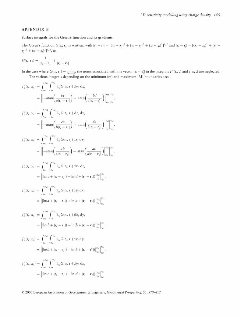
3D resistivity modelling using charge density 609
A P P E N D I X B
Surface integrals for the Green’s function and its gradients
The Green’s function G(ri, rj) is written, with |ri − rj| = [(xi − xj)2 + (yi − yj)2 + (zi − zj)2]1/2 and |ri − r′j| = [(xi − xj)2 + (yi −
yj)2 + (zi + zj)2]1/2, as
G(ri , r j ) = 1|ri − r j | + 1
|ri − r′j |
.
In the case where G(ri , r j ) = 1|ri −r j | , the terms associated with the vector |ri − r′
j| in the integrals J.a(ri, .) and J(ri, .) are neglected.
The various integrals depending on the minimum (m) and maximum (M) boundaries are:
J ax (ri , xj ) =
∫ zM
zm
∫ yM
ym
∂xi G(ri , r j ) dyj dzj
=∣∣∣∣∣∣∣∣−atan
(bc
a|ri − r j |)
+ atan(
bda|ri − r′
j |)∣∣∣∣
yM
ym
∣∣∣∣zM
zm
,
J ay (ri , yj ) =
∫ xM
xm
∫ zM
zm
∂yi G(ri , r j ) dzj dxj
=∣∣∣∣∣∣∣∣−atan
(ca
b|ri − r j |)
+ atan(
dab|ri − r′
j |)∣∣∣∣
zM
zm
∣∣∣∣xM
xm
,
J az (ri , zj ) =
∫ yM
ym
∫ xM
xm
∂zi G(ri , r j ) dxj dyj
=∣∣∣∣∣∣∣∣−atan
(ab
c|ri − r j |)
− atan(
abd|ri − r′
j |)∣∣∣∣
xM
xm
∣∣∣∣yM
ym
,
J ax (ri , yj ) =
∫ zM
zm
∫ xM
xm
∂xi G(ri , r j ) dxj dzj
=∣∣∣∣∣ln(c + |ri − r j |) − ln(d + |ri − r′
j |)∣∣xM
xm
∣∣∣zM
zm,
J ay (ri , zj ) =
∫ xM
xm
∫ yM
ym
∂yi G(ri , r j ) dyj dxj
=∣∣∣∣∣ln(a + |ri − r j |) + ln(a + |ri − r′
j |)∣∣yM
ym
∣∣∣xM
xm,
J az (ri , xj ) =
∫ yM
ym
∫ zM
zm
∂zi G(ri , r j ) dzj dyj
=∣∣∣∣∣ln(b + |ri − r j |) − ln(b + |ri − r′
j |)∣∣zM
zm
∣∣∣yM
ym,
J ax (ri , zj ) =
∫ yM
ym
∫ xM
xm
∂xi G(ri , r j ) dxj dyj
=∣∣∣∣∣ln(b + |ri − r j |) + ln(b + |ri − r′
j |)∣∣xM
xm
∣∣∣yM
ym,
J ay (ri , xj ) =
∫ zM
zm
∫ yM
ym
∂yi G(ri , r j ) dyj dzj
=∣∣∣∣∣ln(c + |ri − r j |) − ln(d + |ri − r′
j |)∣∣yM
ym
∣∣∣zM
zm,
C© 2005 European Association of Geoscientists & Engineers, Geophysical Prospecting, 53, 579–617

610 O. Boulanger and M. Chouteau
J az (ri , yj ) =
∫ xM
xm
∫ zM
zm
∂zi G(ri , r j ) dzj dxj
=∣∣∣∣∣ln(a + |ri − r j |) − ln(a + |ri − r′
j |)∣∣zM
zm
∣∣∣xM
xm,
J (ri , zj ) =∫ xM
xm
∫ yM
ym
G(ri , r j ) dyj dxj
=∣∣∣∣∣∣∣∣−c atan
(ab
c|ri − r j |)
− d atan(
abd|ri − r′
j |)
+ b ln(a + |ri − r j |) + a ln(b + |ri − r j |)
+ b ln(a + |ri − r′j |) + a ln(b + |ri − r′
j |)∣∣∣∣yM
ym
∣∣∣∣xM
xm
,
J (ri , xj ) =∫ yM
ym
∫ zM
zm
G(ri , r j ) dzj dyj
=∣∣∣∣∣∣∣∣− a atan
(bc
a|ri − r j |)
+ a atan(
bda|ri − r′
j |)
+ c ln(b + |ri − r j |) + b ln(c + |ri − r j |)
− d ln(b + |ri − r′j |) − b ln(d + |ri − r′
j |)∣∣∣∣zM
zm
∣∣∣∣yM
ym
,
J (ri , yj ) =∫ zM
zm
∫ xM
xm
G(ri , r j ) dxj dzj
=∣∣∣∣∣∣∣∣−batan
(ca
b|ri − r j |)
+ batan(
dab|ri − r′
j |)
+ a ln(c + |ri − r j |) + c ln(a + |ri − r j |)
− a ln(d + |ri − r′j |) − d ln(a + |ri − r′
j |)∣∣∣∣xM
xm
∣∣∣∣zM
zm
,
with a = xi − xj, b = yi − yj, c = zi − zj and d = zi + zj.Singular points can be observed for the preceding integrals when the point (x, y, z) approaches the origin. Singularities are
resolved analytically.
Singularity 1
Considering the integral
J (r, z) =∫ a
−a
∫ a
−a
dx dy(x2 + y2 + z2)1/2
,
for z = 0, we have
J (r, 0) =∫ a
−a
∫ a
−a
dx dy(x2 + y2)1/2
.
The change of variables x = ax and y = ay leads to
J (r, 0) = a∫ +1
−1
∫ +1
−1
dx dy(x2 + y2)1/2
= 4a∫ +1
0
∫ +1
0
dx dy(x2 + y2)1/2
C© 2005 European Association of Geoscientists & Engineers, Geophysical Prospecting, 53, 579–617
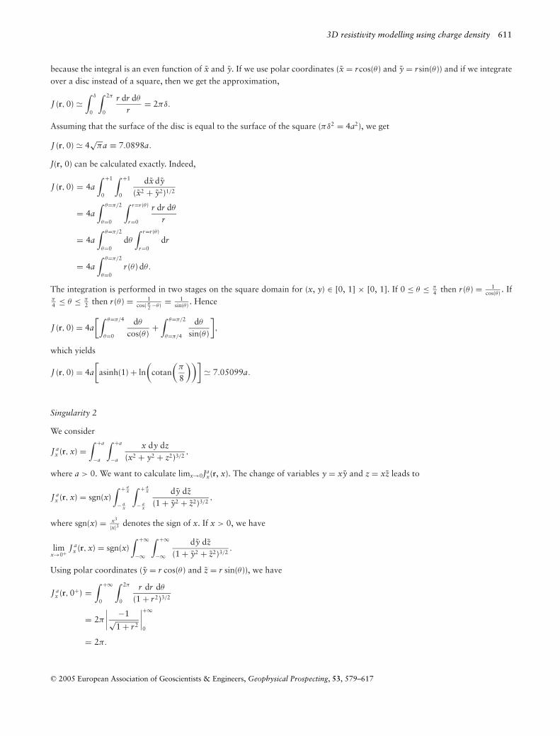
3D resistivity modelling using charge density 611
because the integral is an even function of x and y. If we use polar coordinates (x = rcos(θ ) and y = rsin(θ )) and if we integrateover a disc instead of a square, then we get the approximation,
J (r, 0) ∫ δ
0
∫ 2π
0
r dr dθ
r= 2πδ.
Assuming that the surface of the disc is equal to the surface of the square (πδ2 = 4a2), we get
J (r, 0) 4√
πa ≡ 7.0898a.
J(r, 0) can be calculated exactly. Indeed,
J (r, 0) = 4a∫ +1
0
∫ +1
0
dx dy(x2 + y2)1/2
= 4a∫ θ=π/2
θ=0
∫ r=r (θ )
r=0
r dr dθ
r
= 4a∫ θ=π/2
θ=0dθ
∫ r=r (θ )
r=0dr
= 4a∫ θ=π/2
θ=0r (θ ) dθ.
The integration is performed in two stages on the square domain for (x, y) ∈ [0, 1] × [0, 1]. If 0 ≤ θ ≤ π
4 then r (θ ) = 1cos(θ ) . If
π
4 ≤ θ ≤ π
2 then r (θ ) = 1cos( π
2 −θ ) = 1sin(θ ) . Hence
J (r, 0) = 4a[∫ θ=π/4
θ=0
dθ
cos(θ )+
∫ θ=π/2
θ=π/4
dθ
sin(θ )
],
which yields
J (r, 0) = 4a[asinh(1) + ln
(cotan
(π
8
))] 7.05099a.
Singularity 2
We consider
J ax (r, x) =
∫ +a
−a
∫ +a
−a
x dy dz(x2 + y2 + z2)3/2
,
where a > 0. We want to calculate limx→0Jax(r, x). The change of variables y = xy and z = xz leads to
J ax (r, x) = sgn(x)
∫ + ax
− ax
∫ + ax
− ax
dy dz(1 + y2 + z2)3/2
,
where sgn(x) = x3
|x|3 denotes the sign of x. If x > 0, we have
limx→0+
J ax (r, x) = sgn(x)
∫ +∞
−∞
∫ +∞
−∞
dy dz(1 + y2 + z2)3/2
.
Using polar coordinates (y = r cos(θ ) and z = r sin(θ )), we have
J ax (r, 0+) =
∫ +∞
0
∫ 2π
0
r dr dθ
(1 + r2)3/2
= 2π
∣∣∣∣ −1√1 + r2
∣∣∣∣+∞
0
= 2π.
C© 2005 European Association of Geoscientists & Engineers, Geophysical Prospecting, 53, 579–617
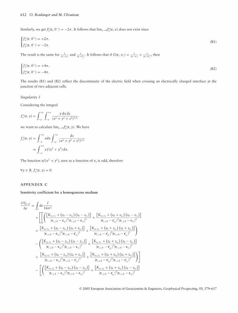
612 O. Boulanger and M. Chouteau
Similarly, we get Jax(r, 0−) = −2π . It follows that limx→0Ja
x(r, x) does not exist since
J a
x (r, 0+) = +2π,
J ax (r, 0−) = −2π.
(B1)
The result is the same for 1|ri −r j | and 1
|ri −r′j |. It follows that if G(ri , r j ) = 1
|ri −r j | + 1|ri −r′j |
, then
J a
x (r, 0+) = +4π,
J ax (r, 0−) = −4π.
(B2)
The results (B1) and (B2) reflect the discontinuity of the electric field when crossing an electrically charged interface at thejunction of two adjacent cells.
Singularity 3
Considering the integral
J ax (r, y) =
∫ +a
−a
∫ +a
−a
x dx dz(x2 + y2 + z2)3/2
,
we want to calculate limy→0Jax(r, y). We have
J ax (r, y) =
∫ +a
−axdx
∫ +a
−a
dz(x2 + y2 + z2)3/2
=∫ +a
−axf (x2 + y2) dx.
The function xf (x2 + y2), seen as a function of x, is odd, therefore
∀y ∈ R, J ax (r, y) = 0.
A P P E N D I X C
Sensitivity coefficient for a homogeneous medium
∂Vd−d
∂ρ=
∫v
dvI
16π2
×[[([
Ks1,r1 + (zk − zs1
) (zk − zr1
)]|ri, j,k − rs1 |3|ri, j,k − rr1 |3
+[Ks1,r1 + (
zk + zs1
) (zk − zr1
)]|ri, j,k − r′
s1|3|ri, j,k − rr1 |3
+[Ks1,r1 + (
zk − zs1
) (zk + zr1
)]|ri, j,k − rs1 |3|ri, j,k − r′
r1|3 +
[Ks1,r1 + (
zk + zs1
) (zk + zr1
)]|ri, j,k − r′
s1|3|ri, j,k − r′
r1|3
)
−([
Ks2,r1 + (zk − zs2
) (zk − zr1
)]|ri, j,k − rs2 |3|ri, j,k − rr1 |3
+[Ks2,r1 + (
zk + zs2
) (zk − zr1
)]|ri, j,k − r′
s2|3|ri, j,k − rr1 |3
+[Ks2,r1 + (
zk − zs2
) (zk + zr1
)]|ri, j,k − rs2 |3|ri, j,k − r′
r1|3 +
[Ks2,r1 + (
zk + zs2
) (zk + zr1
)]|ri, j,k − r′
s2|3|ri, j,k − r′
r1|3
)]
−[([
Ks1,r2 + (zk − zs1
) (zk − zr2
)]|ri, j,k − rs1 |3|ri, j,k − rr2 |3
+[Ks1,r2 + (
zk + zs1
) (zk − zr2
)]|ri, j,k − r′
s1|3|ri, j,k − rr2 |3
C© 2005 European Association of Geoscientists & Engineers, Geophysical Prospecting, 53, 579–617

3D resistivity modelling using charge density 613
h
I(x ,y ,z )s s s
ρ21ρ
air
V1,s
V2,s
z
xy
Figure 20. Two-layer model consisting of a top layer of thickness h and resistivity ρ1 overlying a half-space of infinite resistivity ρ2. The currentis transmitted at the location I(xs, ys, zs) and the potential is observed at points V1,s and V2,s.
+[Ks1,r2 + (
zk − zs1
) (zk + zr2
)]|ri, j,k − rs1 |3|ri, j,k − r′
r2|3 +
[Ks1,r2 + (
zk + zs1
) (zk + zr2
)]|ri, j,k − r′
s1|3|ri, j,k − r′
r2|3
)
−([
Ks2,r2 + (zk − zs2
) (zk − zr2
)]|ri, j,k − rs2 |3|ri, j,k − rr2 |3
+[Ks2,r2 + (
zk + zs2
) (zk − zr2
)]|ri, j,k − r′
s2|3|ri, j,k − rr2 |3
+[Ks2,r2 + (
zk − zs2
) (zk + zr2
)]|ri, j,k − rs2 |3|ri, j,k − r′
r2|3 +
[Ks2,r2 + (
zk + zs2
) (zk + zr2
)]|ri, j,k − r′
s2|3|ri, j,k − r′
r2|3
)]],
where Ksu,rw = (xi − xsu )(xi − xrw ) + (yj − ysw )(yj − yrw ), |ri,j,k − rsu | = ((xi − xsu )2 + (yj − ysu )2 + (zk − zsu )2)1/2, |ri,j,k − r′su
| =((xi − xsu )2 + (yj − ysu )2 + (zk + zsu )2)1/2, |ri,j,k − rrw | = ((xi − xrw )2 + (yj − yrw )2 + (zk − zrw )2)1/2 and |ri,j,k − r′
rw| = ((xi − xrw )2 +
(yj − yrw )2 + (zk + zrw )2)1/2. The indices u and w take values 1 (polar case) and 2 (dipolar case).
A P P E N D I X D
Sensitivity for the two-layer model (Fig. 20)
The formulation of the analytical potential for a two-layer model has been given by Bhattacharya and Patra (1968), Zhdanovand Keller (1994) and Roy and Apparao (1971). The layered medium consists of a layer of thickness h and resistivity ρ1 overlyingan infinite half-space of resistivity ρ2. The reflection coefficient is k = ρ2−ρ1
ρ2+ρ1( ρ2
ρ1= 1+k
1−k). For a source + I located on the surfaceat (xs, ys, 0), the potentials V1,s and V2,s for any point (x, y, z) are given below, where |r − rs| = [(x − xs)2 + (y − ys)2 + z2]1/2,|r − r′
s| = [(x − xs)2 + (y − ys)2 + (z + 2 nh)2]1/2 and |r − r′′s | = [(x − xs)2 + (y − ys)2 + (z − 2 nh)2]1/2. We have
V1,s = ρ1 I2π
[1
|r − rs| +∞∑
n=1
kn
|r − r′s|
+∞∑
n=1
kn
|r − r′′s |
]
for 0 ≤ z ≤ h, and
V2,s = ρ2 I(1 − k)2π
[1
|r − rs| +∞∑
n=1
kn
|r − r′s|
]
for z ≥ h. The current density due to a source located at the point (xs, ys, 0) is expressed for medium 1 (j1,s = σ 1E1,s) and medium2 (j2,s = σ 2 E2,s) as
j1,s =
j1,xs = I2π
[(x − xs)
|r − rs|3+
∞∑n=1
(x − xs)kn
|r − r′s|3
+∞∑
n=1
(x − xs)kn
|r − r′′s |3
]
j1,ys = I2π
[(y − ys)
|r − rs|3+
∞∑n=1
(y − ys)kn
|r − r′s|3
+∞∑
n=1
(y − ys)kn
|r − r′′s |3
]
j1,zs = I2π
[z
|r − rs|3+
∞∑n=1
(z + 2nh)kn
|r − r′s|3
+∞∑
n=1
(z − 2nh)kn
|r − r′′s |3
]
C© 2005 European Association of Geoscientists & Engineers, Geophysical Prospecting, 53, 579–617

614 O. Boulanger and M. Chouteau
d
ρ21ρ
airI
V1,s V2,s z
xy
Figure 21. The vertical contact model with resistivities of ρ1 and ρ2. The current is transmitted at the location I(xs, ys, zs) and the potential isobserved at points V1,s and V2,s.
for 0 ≤ z ≤ h, and
j2,s =
j2,xs = I(1 − k)2π
[(x − xs)
|r − rs|3+
∞∑n=1
(x − xs)kn
|r − r′s|3
]
j2,ys = I(1 − k)2π
[(y − ys)
|r − rs|3+
∞∑n=1
(y − ys)kn
|r − r′s|3
]
j2,zs = I(1 − k)2π
[z
|r − rs|3+
∞∑n=1
(z + 2nh)kn
|r − r′s|3
]
for z ≥ h. For a virtual source located at the point (xr, yr, zr), subscript s is replaced by subscript r.
A P P E N D I X E
Sensitivity for a vertical contact (Fig. 21)
The solution of the potential for a vertical contact has been given by Telford, Geldart and Sheriff (1990) and Zhdanov and Keller(1994). The two quarter-spaces have resistivities of ρ1 and ρ2. We write ks = ρ2−ρ1
ρ2+ρ1, |r − rs| = [(x − xs)2 + (y − ys)2 + z2]1/2 and
|r − r′s| = [(2d + xs − x)2 + (y − ys)2 + z2]1/2, where d is the distance between the point source and the vertical contact. For a
source located in medium 1 at the point (xs, ys, zs), the potentials in medium 1 and 2 are written
V1,s = ρ1 I2π
[1
|r − rs| + ks
|r − r′s|
]
and
V2,s = ρ2 I(1 − ks)2π
1|r − rs| .
The current density due to a source located in medium 1 at the point (xs, ys, zs) is expressed by
j1,s =
j1,xs = I2π
[(x − xs)
|r − rs|3− ks(2d + xs − x)
|r − r′s|3
]
j1,ys = I2π
[(y − ys)
|r − rs|3+ ks(y − ys)
|r − r′s|3
]
j1,zs = I2π
[(z − zs)
|r − rs|3+ ks(z − zs)
|r − r′s|3
]
C© 2005 European Association of Geoscientists & Engineers, Geophysical Prospecting, 53, 579–617

3D resistivity modelling using charge density 615
and
j2,s =
j2,xs = I(1 − ks)2π
(x − xs)
|r − rs|3
j2,ys = I(1 − ks)2π
(y − ys)
|r − rs|3
j2,zs = I(1 − ks)2π
(z − zs)
|r − rs|3.
For a virtual source located in medium 2 at the point (xr, yr, zr), we replace subscript s by subscript r and kr by −ks.
A P P E N D I X F
Algorithms of pyramidal compression
Algorithms 1 and 2 generate the matrices of compression Wk and WTk on level k, respectively. Algorithm 3 calculates the product
Wx on level k. Algorithm 4 calculates the product xW and WT x on level k. The level k is determined by the relationshipk = f loor [ log(n−1)
log(2) ] with n = length(xin).
Algorithm 1 Matrix of compressionW(xin, k) on the level k
n = length(xin)δ = 2k−1
for i = 1 : n doW(i, i) = 1
end forfor i = 1 + δ : 2δ : n − δ do
W(i, i − δ) = 0.5W(i, i) = −1W(i, i + δ) = 0.5
end for
Algorithm 2 Matrix of compression transposed WT(xin, k) on the level k
n = length(xin)
δ = 2k−1
for i = 1 : n do
W(i, i) = 1
end for
for i = 1 + δ : 2δ : n − δ do
W(i − δ, i) = 0.5
W(i, i) = −1
W(i + δ, i) = 0.5
end for
C© 2005 European Association of Geoscientists & Engineers, Geophysical Prospecting, 53, 579–617
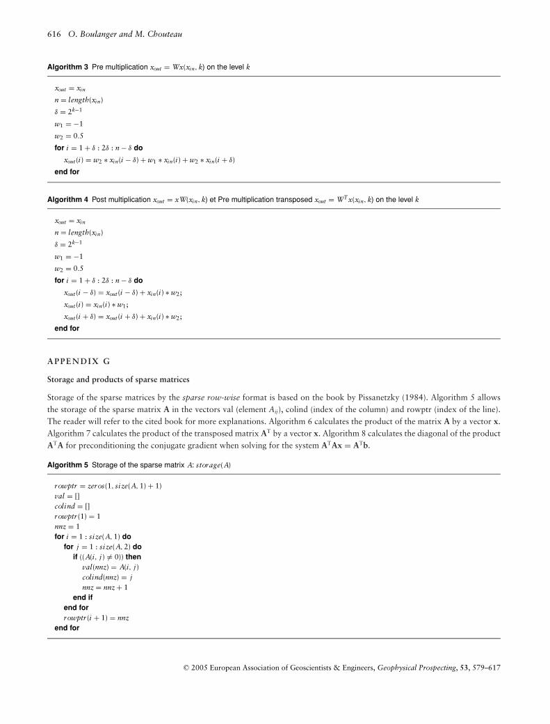
616 O. Boulanger and M. Chouteau
Algorithm 3 Pre multiplication xout = Wx(xin, k) on the level k
xout = xin
n = length(xin)
δ = 2k−1
w1 = −1
w2 = 0.5
for i = 1 + δ : 2δ : n − δ do
xout(i) = w2 ∗ xin(i − δ) + w1 ∗ xin(i) + w2 ∗ xin(i + δ)
end for
Algorithm 4 Post multiplication xout = xW(xin, k) et Pre multiplication transposed xout = WTx(xin, k) on the level k
xout = xin
n = length(xin)
δ = 2k−1
w1 = −1
w2 = 0.5
for i = 1 + δ : 2δ : n − δ do
xout(i − δ) = xout(i − δ) + xin(i) ∗ w2;
xout(i) = xin(i) ∗ w1;
xout(i + δ) = xout(i + δ) + xin(i) ∗ w2;
end for
A P P E N D I X G
Storage and products of sparse matrices
Storage of the sparse matrices by the sparse row-wise format is based on the book by Pissanetzky (1984). Algorithm 5 allowsthe storage of the sparse matrix A in the vectors val (element Aij), colind (index of the column) and rowptr (index of the line).The reader will refer to the cited book for more explanations. Algorithm 6 calculates the product of the matrix A by a vector x.Algorithm 7 calculates the product of the transposed matrix AT by a vector x. Algorithm 8 calculates the diagonal of the productATA for preconditioning the conjugate gradient when solving for the system ATAx = ATb.
Algorithm 5 Storage of the sparse matrix A: storage(A)
rowptr = zeros(1, size(A, 1) + 1)val = []colind = []rowptr (1) = 1nnz = 1for i = 1 : size(A, 1) do
for j = 1 : size(A, 2) doif ((A(i, j) = 0)) then
val(nnz) = A(i, j)colind(nnz) = jnnz = nnz + 1
end ifend forrowptr (i + 1) = nnz
end for
C© 2005 European Association of Geoscientists & Engineers, Geophysical Prospecting, 53, 579–617

3D resistivity modelling using charge density 617
Algorithm 6 Product of the sparsematrix AAA by the vector xxx (y = Axy = Axy = Ax): y = spAx(val, colind, rowptr, nnz, x, y)
for i = 1 : length(y) dotemp = 0for j = rowptr (i) : rowptr (i + 1) − 1 do
temp = temp + val(j) ∗ x(colind(j))end fory(i) = temp
end for
Algorithm 7 Product of the transposed sparse matrix ATATAT by the vector xxx (y = ATxy = ATxy = ATx): y = spAtx(val, colind, rowptr, nnz, x, y)
for i = 1 : length(y) doy(i) = 0
end forfor j = 1 : length(x) do
if (rowptr ( j + 1) − 1 ≥ rowptr ( j)) thenfor i = rowptr ( j) : rowptr ( j + 1) − 1 doy(colind(i)) = y(colind(i)) + val(i) ∗ x( j)
end forend ifend for
Algorithm 8 Diagonal of the product AT AAT AAT A: y = diagspAtA(val, colind, rowptr, y)
for i = 1 : size(A, 1) dofor j = rowptr (i) : rowptr (i + 1) − 1 do
y(colind( j)) = y(colind( j)) + val( j)2
end forend for
C© 2005 European Association of Geoscientists & Engineers, Geophysical Prospecting, 53, 579–617