JOURNAL OF RESEARCH of the National Bureau of Standards - C. Engineerin g and In strumentation

Vol. 71 C, No . 4, October~December 1967

Measurements of the Thermal Resistivity of Platinum

Conductivity and from 1 00 to 900

Electrical °C*

D. R. Flynn and M. E. O'Hagan**

Institute for Applied Technology, National Bureau of Standards, Washington, D.C, 20234

(August 17, 1967)

1. Introduction

Standards and standard refere nce mate ri als a re the basis of a consiste nt and accurate meas uring sys tem. The need for standard referen ce materials in thermal conductivity measurements is two-fold. In th e first place, such materials are required for comparative measurements in which the therm al conductivity of the material under test is de termin ed in term s of that of the standard refere nce material. Secondly , s uc h ma­te rial s are req uired in evalu ating the accuracy of apparatu s des igned for thermal con du ctivity meas ure­ments. The degree to whi ch the measured value of the thermal conductivity of the standard refere nce ma­terial agrees with the accepted value is a c hec k on the accuracy of the apparatus in which the measurements were made.

The basic requirements for any s tandard referen ce material are that it be stable, reproducible and appro­priate for the measurements at hand, and that the property in question be uniform throughout the ma­terial. In the case of standard reference mate rials for thermal conductivity other desirable requirements are that the s tandard be usable over a wide range of tem­perature, that it be c he mi cally inert so as not to be

*Thi s researc h wa s the suhjec t of a di sse r tation s ub mitt ed by M. E. O' Haga n to the Facu lt y of Th e Sc hool of E ngi nee rin g; ancl Appl ied Scie nce. The George Was h ingtun Un ivers ity. in parti al sa t isfac tion of the f ('qu ire rn{,lll s for the degree o f Doctor of Scie nce. This wo rk was support ed in part by Eng;elhard Indu s tri es. Inc .. Newark . New Je r!"cy. who suppli ed the platinum a nd fina nc ial a ss is tance in t he form of a g ra n t to th e Nationa l Bureau of S tandards. M. E. O' Hag-a n was support ed in part by C ra nt AFOSR- 102S- 66 fro m the Air Force Office of Sc ie ntific Hesta rc h and in part by the In s titut e for In dus tria l Hescan.: h a nd S tandard s. Dublin. Ire la nd .

** Present address: In stitu\(' for Industrial Hcscar{' h and Sta ndard s. Dubli .. . Ire land.

a ffec ted by or affect othe r ma terials in the syst e m and th at the therm al condu ctivit y of the refere nce ma teri al be c lose in va lu e to th at of th e ma te ri a ls whic h a re to be meas ured in te rm s of it.

The advantages of using platinum as a the rmal co n­ductivity refere nce materi al have been pointed out by Powell and Tye [1] 1 and by Slack [2]. Platinum is available in hi gh purity in pieces of s ubs tanti al size. It has a fa irl y hi gh melting point (1769 °C on the 1948 Internation a l Prac ti cal Te mperature Scale), has no known tra ns ition point s, and is re latively s tab le c he m­ically in a ir a nd other atmosphe res, with the excep­tion of hydroge n, eve n at hi gh tem peratures r3, 41. lts thermal co nductivity , although relati ve ly high for use as a reference material with nonme tals, is about the geo me tri c mean for me tal s and alloys.

Since the thermal conductivity of a pure metal is s trongly correlated with the elec tri cal condu ctivity of the me tal , it is highly desirable that the e lec tri cal con­du ctivity of a metal whi ch is inte nded for use as a thermal co ndu ctivity refere nce material be very stable under varying heat treatm ents. The s tability of the electri cal co ndu ctivity of platinum is evidenced by the fac t that the International Practical Temperature Scale is defined by a platinum resistance thermometer in the temperature range - 182.97 to + 630.5 °C [5,6]. Studies are currently underway at NBS [7] and other laboratories to investigate the possibility of extending to the gold-point (1063 °Cl the range over which a platinum resistance thermometer is used to define the temperature scale.

I Fi :.r ures. in brad.1·I ~ indi ('a t !"' tilt" lilt'ratllrt' n'h ' rt ' I H't'~ al Ih t' ('n d Iff Ihi ~ papt' '',

255

Platinum appears to be, in every way save one, an ideal material to use as a thermal conductivity refer­ence standard. The exception is that the spread among the literature values for the thermal conductivity of platinum is considerable, to say the least.

Powell, Ho , and Liley [8] show a plot of essentially all of the published thermal conductivity data for platinum through the year 1965. The spread in the data increases from about 10 percent at room tempera­ture to over 30 percent at 1000 dc. Even if many of the older data are discounted, the picture is not par­ticularly improved. O 'Hagan [9] has summarized the methods used for previous measurements of the thermal conductivity of platinum and also has sum­marized the characterizations of the various samples.

Prior to the measurements of Powell and Tye [1], all thermal conductivity values reported for platinum at temperatures above 100 °C were obtained by methods in which the temperature gradient in the specimen was produced by louie heating due to passage of an electric current directly through the specimen. While the re­sults of all but one [10] of these higher temperature investigations employing electrical methods essen­tially agree with one another, they disagree with those of later investigations [1, 11 , 12], which e mployed nonelectrical methods. This raised the question as to whether or Jlot electrical methods yield results that are intrinsically different from those of nonelectrical methods. This could mean that the theory which has been used in analyzing electrical methods is in e rror, or it could mean that heat conduction is significantly dependent on electric current density, at least in the case of platinum_

The considerations discussed above pointed to the need for a comprehensive investigation of the thermal conductivity of platinum. It was felt that both an absolute steady-state method without an electric cur­rent flowing in the specimen, and also an absolute steady-state method with a current flowing in the specimen should be employed.

. As regards the nonelectrical method, experience at NBS with guarded longitudinal heat flow methods in­dicated that such a method could be made to yield accurate results on a material having as high a thermal conductivity as platinum, provided a specimen of sufficient cross-sectional area was used. With a fairly conductive metal , there were no particular advantages in going to a radial heat flow method; furthermore, to do so would have required a much larger sample.

As regards the electrical method, an arrangement utilizing quite large current densities would be more likely to reveal deviations due to a dependence of thermal conductivity on current density_ It was also desirable to use the same method as that used by most of the previous investigators. Fortunately, these two desiderata both pointed to the necked-down sample configuration utilized for measurements on platinum by Holm and Stormer [13], by Hopkins [14], and by Cutler, et al. [15].

To give a pirect and accurate comparison between the two method s it was considered desirable to com­bine both sets of measurements in one apparatus and

on the same specimen thereby eliminating a number of uncertainties which would arise in comparing data derived from measurements in different apparatus and on different specimens. The above considerations led to an apparatus , described in section 3, in which thermal conductivity measurements can be made by both the usual longitudinal heat fl ow method and by an electrical method.

It was also felt that thermal conductivity measure­ments should be made on platinum samples of at leas t two purities_ Samples were obtained of a high purity platinum (resistance thermometer grade) and of a somewhat lower purity platinum (commercial grade). As of this writing, only the measurements on the lower purity platinum sample have been completed. The results obtained on that sample are presented in this paper and are compared with the results of other investigators.

2. Description of Sample

In order for a >lalid comparison to be made be tween the results of different investigators who measure on a particular kind of material, it is necessary that their specimens be characterized as extensively as possible so that differences in specimens may be accounted for. For this reason a number of pertinent measurements were made in an attempt to characterize the speci­men used in the present investigation. These meas­urements and the results thereof are described below.

The platinum was provided by Englehard Industries, Inc. , in the form of a solid bar 2_04 em in diameter by 31 cm long, and was classified as being of commercial purity. The fabrication and cleaning procedures used in preparing the platinum have been described by O'Hagan [9]-

The as-received bar was annealed in air for 5.5 hr at 770°C in a horizontal tubular furnace and furnace cooled at a rate of approximately 120 deg/hr. Shortly thereafter the bar was accidentally dropped causing it to deform slightly at one end. After correcting the damage the bar was reannealed for 1.5 hr at 680 °C and furnace cooled at a rate of approximately 90 deg/hr. Its thermal conductivity was then measured in the NBS Metals Apparatus [34, 35] over the temperature range - 160 to + 810 °C [32].

Following these measurements the bar was ma­chined and ground to 25.4 em long by 2.000 em diam. The density of this bar was measured (see below) and the electrical resis tance was measured at ice and liquid helium te mperatures (see below)_ The thermal conductivity specimen (18.4 em long by 2.000 em diam) was then fabricated from one end of this bar. A length of 6-4 em was cut from the other end for separate low temperature thermal conductivity measurements [33]. The remaining disk , approxi­mately 1 em long, was reserved for metallographic and spectrographic analyses.

A thin neck , approximately 0.1 em in diameter and 0.3 em long, was machined in the thermal conductivity specimen at approximately 4 c m from one end. To cleanse this necked-down region of oil and any con-

256

tamination contracted from the cutting tools, the fol­lowing cleaning procedure was follow ed_ Degreasing was effected by immersion for half an hour in tri­chlorethylene vapor- The neck was then pickled for 10 min in hot 50 percent nitri c acid . Following this the neck was washe d in distilled water, pickled for 10 min in 50 perce nt hot hydrochloric ac id, and again washed in distilled water- There was equal likelihood of the rest of the spe ci men having slight surface con­tamination as a result of machining but its effect on the bulk properties of the specimen would not be nearly as grave as the corresponding effect in the neck region. It was considered sufficien t to clean the surface of the specimen wi th toluene and carbon tetrachloride.

A general qualitative spectrographic analysis, per­formed by the NBS Spectrochemical Analysis Section on the 2-cm-diam by l -cm-Iong platinum disk men­tioned a bove, detected Ag (10- 100 ppm), P d (l0- 100 ppm), Fe « 10 ppm), and Mg « 10 ppm). O'Hagan [9] reported the results of a quantitative spectrographic analysis made on a portion of a 0.05 cm wire drawn from the same platinum ingot as th e thermal con­ductivi ty s pecimen.

Photomicrographs were also made of the platinum disk , c ut from the bar sample . They showed grain size to be of the order of 0.02 cm. No evide nce appeared of inclusions of foreign matter or of any irregularities in microstructure. Hardness measure ments were mad e on the original platinum bar, after the second anneal, using a Vi c kers Pyramidal Diamond Tester with a 10 kg load. Values ranged from 36.5 to 38.0 Vic kers hardn ess number.

The densi ty of the bar, wh en it was 25 .4 c m long, was determ ined by mass and dimen sional measure­ments to be 21.384 g/cm:! at 21 DC, acc urate to within ± 0.002 g/c m:!. This d ensity is a n average value [or the whole bar and there is no guarantee that the de ns ity was uniform to that degree throughout the bar.

The ratio of the resistance at the ice- point te mpera­ture to that at the boiling point of helium at atmospheric pressure is a me asure of the extent and condition of impurities in a material a nd of the crystallographic state of the material. This ratio was determined on the 2-cm-diam bar-

The ice-point resis tances were measured both be­fore and after the helium point measurements. The current was supplied from a regulated d-c power supply and was measured using a calibrated resistor and a precision potentiometer. The voltage drops in the specimens were measured on a high precision 6-dial pote ntiometer. In each case the resistance was measured at three or four different current levels and the value corresponding to zero current obtained by extrapolation. The ratio of the resistance of the sample at the ice-point to that at the helium-point was found to be 393. Thi s value is believed to be accurate to within 1 percent. However, it corresponds to an average value over a considerable length of the sample and the sample may not have been uniform in puri ty throughout.

A se t of knife edges of known separation was fas­tened to the 2-cm bar during the first set of ice-point resistance measureme nts. The knife edges acted as po­tential taps. Using the known se paration of the knife

edges and the cross-sectional area of the bar, the ice­point resistivity, corrected to 0 DC di mensions, was determined to be 9.84hd1 c m, accurate to within ± 0.0101L0 c m.

A length of 0.05 c m platinum wire, drawn from the same ingot as the th ermal conductivity sample, was electrically annealed in air fo r 1 hr a t about 1450 DC. The elec tromotive force of thi s wire versus the plati­num standard Pt 27 [16] was measured by th e NBS Temperature Section with the reference junctions a t o DC. The values obtained (at 100 deg in tervals) in­creased in an essentially linear man ner from 0 IL V at o DC to + 15 ILV at 1100 DC . This indicates that the sample used in the present investigation was less pure than Pt 27.

The temperature coeffic ient of resistan ce , 0' = (R IOO - Ro)/100Ro, between the ice-point and the steam-point is often used as an indication of the purity of resistance thermometer grade platinum. The limiting value of 0' for extremely pure platinum is given by Berry [17] to be 0.003928!J' The size and low resistance of the thermal conductivity s pecimen precluded a highly acc urate direct determination of 0' on the speci­me n using existing equipment. On the basis of the elec tri cal res is tivity measure ments (described later) on th e nec ked-down portion of the specimen, 0' had a value in the ra nge 0.003876 :;;: 0' :;;: 0.003916. The rela­tively large uncertainty in 0' arises from the use of platinum versus platinum- l0 percent rhodium ther­mocouples to measure the temperature near] 00 dc. Berry r1 7] gives a plot whi ch correlates 0' with the ratio of the res istance of a sample at absolut e ze ro to that at the ice-point. He also correlates the resi s tance at absolute ze ro with that a t t~ e helium-point. On the basis of Berry's correla tions, the ice-point to helium ­point resis tance ra tio for the thermal condu ctivity specimen used in the present investigation corre­sponds to 0.003907:;;: 0' :;;: 0.003916. This is not incon ­sistent with th e range of values obtained from the electrical res istivity measure me nts.

Although 0' could have been meas ured directly with high accuracy on the 0.05 c m platinum wire, thi.s was not done since the re sults would not necessanly be valid for the 2 cm bar, owing to possible differences in purity and annealing. Corruccini [18] gives an em­pirical expression, due to Wm. F . Roeser, correlating 0' wi th the electromotive force versus Pt 27 with the junction at 1200 DC and the reference junction s a t o DC. Extrapolation of the emf measurements me n­tioned above , in dicates an emf of + 16 IL V at 1200 DC, corresponding on the basis of Roeser' s expres­s ion , to 0' = 0.0039]4 for the 0.05 cm wire drawn from the same material as was used to fabricate the thermal conductivity specimen.

A cooperative project, involving NBS and several producers of thermome tric grade platinum, is cur­rently underway to stud y the properties of pure plat­inum. If as a result of this project, it appears that further characterization is indicated for the platinum used in the present investigation , such characteriza­tion will be performed on material which is being reserved for that purpose.

257

3. Method and Apparatus

3.1. Method

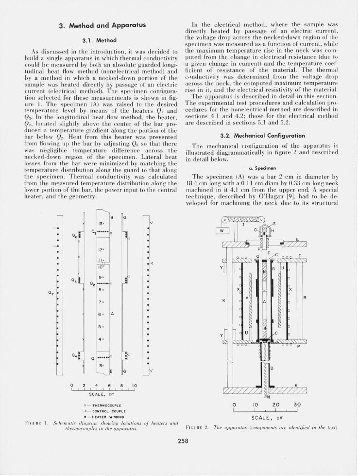
As discussed in the introduction, it was decided to build a single apparatus in which thermal conductivity could be measured by both an absolute guarded longi­tudinal heat flow method (nonelectrical method) and by a method in which a necked-down portion of the sample was heated directly by passage of an electric current (electrical method). The specimen configura­tion selected for these measurements is shown in fig­ure 1. The specimen (A) was raised to the desired temperature level by means of the heaters Ql and Q:l . In the longitudinal heat flow method, the heater, Q~ . located slightly above the center of the bar pro­duced a te rn perature gradient along the portion of the bar below Q~. Heat from this heater was prevented from flowin g up the bar by adjusting Q:l so that there was negligible temperature difference across the necked-down region of the specimen. Lateral heat losses from the bar were minimized by matching the temperature distribution along the guard to that along the specimen . Thermal conductivity was calculated from the measured temperature distribution along the lower portion of the bar, the power input to the central heater , and the geometry.

0 7

B

o~

8x

7 x

6 x A

5 x

4 x

Q'1 • · ·

G

0 1 1

2 4 6 8 1 1 1 1 1

SCALE, cm

x - THERMOCOUPLE

<J- CONTROL COUPLE

• - HEATER WINDING

v

. <J

10 1

FI(;URE 1. Schemlllic diuf(rrtm showillf( locutions of heulers and IhermoC()III,les ill the "1'liI/ruIIlS.

In the electrical method , where the sample was directly heated by passage of an electric current, the voltage drop across the necked-down region of the specimen was measured as a function of current, whil e the maximum temperature rise in the neck was com· puted from the c hange in electrical resistance (due to a given change in current) and the temperature coef­ficient of resistance of the material. The therm al c .• nductivity was determined from the voltage drop across the nec k, the computed maximum temperature rise in it, and the electrical resistivity of the material.

The apparatus is described in detail in this section . The experimental test procedures and calculation pro­cedures for the nonelectrical method are described in sections 4.1 and 4.2; those for the electrical method are described in sections 5.1 and 5.2.

3.2. Mechanical Configuration

The mechanical configuration of the apparatus is illustrated diagrammatically in figure 2 and described in detail below.

a. Specimen

The specimen (A) was a bar 2 cm in diameter by 18.4 c m long with a 0.11 cm diam by 0.33 cm long neck machined in it 4.1 cm from the upper end. A special technique, described by O'Hagan [9], had to be de­veloped for machining the neck due to its structural

o I

10 !

20 !

SCALE. em

p

p

30 !

R

FICURE 2. The aplJarallis (com lJOnents are identified in the text ).

258

weakness. Hollow molybde num extensions (B) of the same diameter as the specimen were screwed to the specimen (A) at both e nd s. The open ends were brazed to copper bloc ks (C) tha t se rved as heat sinks. The molybdenum extens ions were fill ed with high purity "coral" alumina. The lower end of the specimen as­sembly (B- A- B) was bolted to, but electrically in­sulated from, a brass fl a nge which was welded to a water-cooled brass column (D). This column was firmly bolted to plate (E) whic h served as a base for the apparatus.

One of the major problem s with the necked-down specimen was that of protec ting the neck from mec han­ical strain due to tension , co mpression, torsion , or bending. Any clamp supporting the neck would have had to be electrically insulated from the specimen and differential thermal expansion between the clamp and specimen could have introduced strain in the neck. As an alternative to a clamp it was' decided to counter­balance th e load on the neck due to the weight above it so that there would be only a s mall net force on the neck . The weight of platinum above the ce nte r of the nec k was co mputed from dim ensional meas ure ments and from the me as ured de nsity of th e specim en, and the compone nts exte nding from the uppe r e nd of the specime n were weighed before asse mbly.

The counterweight (W) was s us pe nded from a s trin g which passed over two pulleys and a ttac hed to an aluminum ha nge r (H). The pull ey wheels were mounted on low-fric ti on be arin gs having a startin g force of less th an 1 g each. A molybdenum well (F), whi ch was brazed to th e upper co pper bloc k (C), passed through a linear bearin g (L) whic h served to maintain the up­per part of the specime n in precise aline me nt with th e lower part , and presented negligible res is tan ce to th e free verti cal motion of the s pec imen resulting from thermal expan sion. This bearing was mounted on the upper plate (E) but electricall y in sulated from it. The two aluminum plates (E, E) were conn ec ted by three ti e bars (K) to form a rigid fra me work for maintaining proper specime n alinement. An auxiliary device , de­scribed by O'Hagan [9], pre ve nted the upper part of the specimen from rotatin g but still allowed free vertical motion. Current was introd uced to the specim en via a copper rod (N) at the lower end and through a hollow molybdenum elec trode (0) at the upper end. The upper electrode was braze d to a copper support (S) which was fastened to , but electrically insulated from , the upper plate (E). The molybdenum well (F) contained a liqUId metal alloy into which the electrode dipped thereby affording a flexible current co nnection. The buoyant force of the liquid metal on the electrode contributed to the load on the neck and was compensated for in the co unterweight. The electrode was fixed but the molyb­denum well move d upwards with the specimen due to thermal expansion during test ru ns. Thi s changed the buoyant force a nd conseque ntJ y put a load on the neck. The maximum change in bu oyant force was only 3 g, however, whi ch would not strain the nec k s ignifi ­cantly. The liquid metal used was a gallium -indium e utec ti c alloy c hosen primarily for its low vapor pres­s ure and its co mparative ly low freez in g te mperature of

15.7 0c. The req uirement for low vapor pressure was di c tated by a need to e vacuate th e sys tem. Preliminary tes ts were run to evaluate th e uncertainty in buoyant force du e to s urface te ns ion a nd sti c king of the gallium­indium to the molybde num s urfaces. A very definite hysteresis e ffec t wa ob erved as th e e lec trode was moved re lati ve to th e well and th e n re turned to its initial position. The largest un certainty in buoyant force was dete rmin ed to be about 4 g. Th e c hoice of molyb­de num as th e e lectrode and well mate ri al s te mmed from its co mpatab ilit y with gallium , whi ch reacts with mos t other metals, and from the fac t that molybd enum is wetted by gallium. Th e c urre nt feed-in sys te m also served as a heat s ink for the upper part of the speci­men assembly. The hollow molybde nu m el ec trode was internally cooled by circ ulating water at a te m perature hi gher than the freezing point of the gallium-indium eu tecti c alloy.

b. Furnace and Guard

The inn er core (G), or the guard as it is called, was a molybdenum tube of 5.7 c m inside diameter. Sin ce the inner co re acted as a thermal guard to prevent heat losses from the s pecim en, it was cons idered more des irable to make it fro m metal rathe r th an from ce­rami c so that the te mperature di s tribution along it could be more eas ily controll ed a nd more accurately meas ured. The bottom of th e guard was a ttached to a water-cooled brass plate (P ). A water-cooled brass ring (Q) was attached to the uppe r e nd of the guard . The ou ter furnace core (V) was an aluminum oxide tube s upported top a nd bottom by three l-c m di a m alumi ­num oxide rods (U).

Th e ex terior portion of th e furn ace co nsis ted of a water-cooled she ll (X) s upported be twee n two wate r­cooled plates (P ). At tached to th e up per plate of the furnace was a sp lit nut. Thi s nut e ngaged a lead screw mounted betwee n the plates (E, E) a nd by turning the scre w the furnace co uld be moved up or do wn. Ready access to the s pecim e n was there by afforded . The three rods (K) ac ted as guide rods for the furnace. Six linear bearings (Y) attached to the furnace plates ensured alin e ment and permitted the furnace to move up and down freely. The correc t vertical location of the guard relative to the specimen was de termined whe n a probe attached to the upper end of the guard made electrical contact with a plate attached to the mol yb­denum well at the upper end of the specime n asse m­bly. When the furn~ce had been positioned, the indi­cating probe attached to the guard was r e moved.

The space between the s peci me n and the molyb­denum guard and that between th e guard a nd the water-cooled shell were filled with fin e high-purity aluminum oxide powder of low thermal conductivity and low bulk dens ity (0.16 g/cm 3).

c. Environmental System

Th e entire apparatus was mounted inside a 24-in diam me tal bell jar to enable operation in an inert atmosphere. A 4-in oi l diffusion pump and a 5 cfm mechanical pump were used to evacuate the system prior to refilling with argon or helium. Initial evacua-

259

HELICAL HEATER ELEMENT

'JUMPERS"

SWAGED TEMPERING ELEMENT

POTENTIAL TAPS

FIGURE 3. Schematic dia.p,ram showinp, the eOllslmelioll of th.e sllee i men hea.ter.

tion was co ntroll e d to avoid disturbance of the fine powder ins ulation .

3.3. Thermal Configuration

The heater and thermocouple locations on the specimen and guard are shown in figure 1.

c. Specimen

The heaters, Ql and Q:l, used to raise the mean tem· perature of the sample were locate d in the molybde­num extensions. These heaters consisted of six series-connected helical coils of 0.02 cm diam plat­inum- thirty percent rhodium wire insulated from the surrounding metal by thin-wall aluminum oxide tubing. Platinel 2 thermocouples were attached adjacent to heaters QI and Q3 for use in controlling the tempera­tures at these locations.

The ce ntral heater , Q2, was contained in six holes drilled through the platinum bar and was constructed as shown in figure 3. Th e inne r four holes were 0.1 cm in diameter and accommodated helical elements con­tained in thin-wall aluminum oxide tubing. The ele­ments were made from 0.013 cm diam platinum-lO percen t rhodium wire, the outside diameter of the helix being 0.05 c m and the pitch 0.025 cm. The outer two holes were 0.16 c m in diameter and accommodated "swaged ele ments" having platinum- l0 percent rhodium sheaths insulated from platinum -10 percent rhodium heater wires by compacted M~O powder in­s ulatiun. The swaged elements were a snu g fit in the holes so that there was good thermal contact between the sheath and the bar, and consequently good thermal coupling between the heater and the bar. The six ele­ments were connected in series as in heaters QI and Q3. Platinum heater leads, 0.05 cm in diameter, were welded to the ends of the swaged elements. The good thermal contact in the swaged elements en­sured that the temperature at the ends of the heater

~ Platine l ha s a high the rmal e mf. apprux ima leiy that of C hromel P versus Alu me L The negative leg of the th ermocouple is 65 IWfccnl Au. 35 pe rcent Pd alloy (plat inel 5355) and tilt' posilj '.: e tel! is 5,5 IWf"{'e nt Pd. :31 pf'fCe nt PI. and 14 percent Au Wlatinel 7674).

closely approximated that of the specimen. Moreover, the current leads extended radially from the heater in an isothermal plane. The combined result was to mini­mize heat losses via the leads. Two 0.02 cm platinum-10 percent rhodium potential leads were welded to each of the current leads, one at the junction of the heater and the current lead, and the other about 1 cm back along the current lead. The two platinum-lO percent rhodium potential leads together with the intervening section of platinum current lead served as a differential thermocouple to determine the temperature gradient in the current lead . By taking potential readings with the current flowing in the forward and reverse direc­tions, the IR drop in the current leads could be ac­counted for and the temperature gradients therein determined. These data were used in computing heat flows along the leads. The potential drop across the inner taps was used in computing the power generated in the heater. The distances from the heaters to the nearest thermocouples and potentia] taps were such that perturbations in heat flow and electric current fl ow generated by the presence of the heaters decayed to an insignificant level at the position of the thermo­couples or potential taps (see appendix B of O'Hagan [9]).

Five thermocouples , spaced 2 cm apart, were lo­cated in the gradient zone of the specimen, with the lowermost one (designated 4 in fi g. 1) be ing: 2 e m from the end of the specimen. The thermocouples were fabricated from 0.020 cm diam platinum and platinum-10 percent rhodium wires which were annealed in air at about 1450 DC for 112 hr and then butt-welded together. They were pressed into 0.018 cm wide by 0.023 cm deep horizontal slits in the surface of the specimen thereby replacing the metal removed in machining the slits. By virtue of the fact that the spec i­men was fairly pure platinum with essentially the same absolute thermoelectric power as the platinum leg of the thermoco uple th e junction of eac h thermocouple was effectively at the point where the platinum- lO percent rhodium leg first made contact with the speci­men, and the temperature measured was the tempera­ture at that point. The platinum- lO percent rhodium wire emerging from its groove extended a short way around the specimen in the same isothermal plane­insulated from the specimen in broken ceramic tub­ing-so as to minimize the amount of heat conducted away from the junction. Similar thermocouples were located in the molybden um extensions, three in each, to measure the temperature distribution along them. This information was essential to the mathematical analysis of the system.

Additional thermocouples were located on either side of the neck (locations 9, 10, 11, and 12 in fi g. 1). These were fabricated from annealed 0.038 cm diam platinum and platinum- lO percent rhodium wire and pressed into slits. In addition to measuring tempera­ture, these thermocouples were wired at the selector switches so that the platinum legs could be used to measure voltage drops across the neck when an electric current was flowing through the neck. With no current flowing, the platinum- IO percent rhodium legs, in

260

--.J

conjunction with the platinum neck, could be used as a differential thermocouple to control the differential temperature across the neck in the longitudinal heat flow method of measure me nt.

b. Guard

The guard had three heaters, Q4, Q5, and Q6, at positions co rres ponding to those on the specimen assembly. All three were swaged heaters with plat­inum- l0 percent rhodium sheaths and heating ele­ments, and MgO insulation. They were pressed into grooves machined in the guard, thus giving good ther­mal contact. The end heaters (Q4 and Q6) were used to keep the guard at the desired temperature. The cen­tral heater (Q5) was used to produce a temperature gradient in the guard matching that in the specimen.

The guard was electrically grounded but the heaters were isolated. Platinel control thermocouples were peened into the guard adjacent to each of the heaters.

Twelve thermocouples were located on the guard, three in the gradie nt zone, three in the isothermal zone, and three in each of the end zones. All the thermo­couples were 0.038 em plat inum versus platinum -l0 percent rhodium with the junctions pressed into s lits machined in the guard. The th ermoco uple wires were take n one turn around the guard in broke n cera mi c tub­ing in an isotherm al plane and ce me nted to the guard with high purity alumina cement. This helped to te mper the thermocollple leads and reduce the a mou nt of heat condu cted away from the junction by the leads. Within the furnace all the thermocouples were insulated in single-bore ceramic tubes. For the r emainder of their lengths the wires were in sulated in fl exible fiber-glass sleeving. All t he thermocouples, both from the guard and the specimen assembly, went to a junction box mounted on the inside of the feedthrough ring. There they were torc h welded to identical wires which were taken through wax vacuum seals to an ice bath. All the Platinel control couples went to terminal s trips 0n the upper plate of the furnace. There they were spot­welded to Chromel P and Alumel wires coming from the temperature con trollers.

The aluminum oxide outer core (V) was provided with a heater winding (0.1 cm diam molybdenum) to bring the furnace as a whole to temperature and to reduce heat losses from the molybdenum guard and the power load on its heaters. A Platinel control thermocouple was mounted on the outer core (V).

3.4. Instrumentation

a . Temperature Control

In the longitudinal heat fl ow method of measuring thermal conductivity, the platinum- l0 percent rho­dium legs of the ou ter pair of thermocou pies in the neck region were used in conjunc tion with the necked­down portion of the specimen as a di fferent ial th ermo­couple to control the power to heater Q:3, and thus maintain essentiall y a zero te mperature differen ti al across the nec k_ The signal from this thermocouple was amplifi ed by a chopper-stabilized doc amplifier

261

and fed into a c urre nt-adjus ting-type proportional con­troller incorporating automa ti c reset control and rate control. The output of the proportional controller regu­lated the power to the heater by means of a transistor­ized c urre nt amplifier fed by a regulated doc power supply. In th e e lectri cal me thod of measuring thermal condu ctivit y, an electri c curre nt flowed through the specimen and the above system of control could not be e mployed. In thi s case the Platinel control couple adjacent to hea ter Q3 was put in series opposition with a signal from an adjustable constant voltage so urce and the res ultan t s ignal fed to the proportional con­troll er which regula ted the power to Q3. The external signal was manu ally adjus ted to give zero temperature differe ntial across the neck.

The s pecimen heate r (Q2) was fed constant voltage (± 0.01 %) from a regulated doc power supply. Power to heater Q, and to the three guard heaters (Q4, Q5 , and Qli) was supplied by variable-voltage trans­form ers, whi ch in turn were fed by voltage-regulated isolation transformers. Power to each heater was regulated by individual thermocouple-ac tuated con­troll ers. Power to the heater winding (Q7) on the alumina co re was supplied by a variable-voltage trans­form er fed by a voltage-regulated isolation transform er. The c urre nt was manually ratioed among the three heater sec tions. The total power to this heater was regulated by a single thermocouple-actuated co n­troller. All heaters were supplie<.:l by se parate isola­tion transformers or power suppli es to minimize c urrent leakage effects.

b . Temperature Measurement

The noble metal leads of the ther mocouples were brou ght to an ice bath, where they were individually join ed to copper leads. The co pper leads went in shield ed cables to a bank of double-pole selector switches of the type used in precision potentiometers. The selec tor switches were housed in a thermally insulated aluminum box with 1 e m thick walls. The copper leads were thermally grounded to (but elec­trically insula ted frol1)) the switch box to minimize heat transfer direc tly to the switches. The emfs of the specimen thermocouples were read on a calibrated six-dial high-precision potentiometer to 0.01 /.LV , using a photocell galvanometer amplifier and a secondary galvanometer as a null detector. (Due to thermal emfs in the potentiometer and circuitry, these emfs were prob ably not meaningful to better than ± 0.05 /.LV.) The emfs of all other thermocouples were read on a seco nd precision potentiometer to 0.1 /.LV using an electronic null detec tor.

c. Power Measurement

Power input to the specimen heater was measured using a potentiometer in conjunction with a high­resistance volt box to measure the drop acros s the inner set of potential taps , and a standard resistor in sen es with the heater to measure the current.

d. Resistance Measurement

All electrical resistance measurements were made by measuring the current (from a 0- 100 A regulated d-c power supply) flowing through the specimen, utilizing a calibrated 0.001 n standard resistor and by measuring the appropriate voltage drop in the ~1)eci­men, using a potentiometer.

4. Longitudinal Heat Flow Method 4.1. Experimental Procedure

a. Preliminaries

The furnace was heated to 150 °C and the system evacuated to 3 X 10- 4 torr. Initial pump-down was through a needle valve to give a sufficiently low rate so as not to disturb the very light powder insulation. When the pressure had fallen below 10- 1 torr, the dif­fusion pump was turned on, pumping initially through the needle valve, and , when the pressure was below 10- 2 torr, through the 4-in port. After pumping for 24 hr, the pumps were turned off and the system back­filled with high purity (99.99%) argon. The argon was bled in slowly through a needle valve to avoid dis­turbing the powder. The pressure was allowed to build up to almost 1 atm before the valves were shut off and the cycle of evacuating and backfilling repeated. The final argon pressure after the second backfilling was about three-quarters of an atmosphere.

The cooling-water flows to the system were adjusted to the desired levels as indicated on flow-meters. The water was pressure-regulated to maintain constant flow rate. A control thermocouple on the specimen was wired to shut all the heaters off if its temperature ex­ceeded a predetermined level. This was a safety pre· caution in the event of an interruption in the cooling­water flow.

The test procedures are described in detail below. To facilitate the discussion let us refer to figure l. The region of the specimen below the specimen heater, Q2, will be referred to as the lower part of the speci­men, and the region above Q2 as the upper part of the specimen.

b. Description of Tests

In the longitudinal heat flow method of measuring the thermal conductivity each datum point was com­puted by simultaneous solution of three tests:

1. an " isothermal" test with no power input to the specimen heater (Q2) and with the temperature distri­bution on the guard adjusted to closely match that on the specimen.

2. a "matched" gradient test with sufficient power input to the specimen heater to maintain the desired longitudinal temperature gradient in the specimen and with a matched temperature distribution on the guard.

3. an " unmatched " gradient test with the power input to the specimen heater and the temperature at the center of the meas uring span the same as in the "matched" gradient tes t, and with the temperature distribution on the guard parallel to that on the speci­men but 10 deg cooler.

Matched Gradient Test

The furnace temperature was raised by means of heater Qi. The power to the specimen heater, Q2, was adjusted to give a temperature gradient of 5 deg/cm in the lower part of the specimen. Power to Q3 was automatically controlled, using a propor­tional controller, to maintain a minimum tempera­ture drop across the neck. The Pt-l0 percent Rh legs of thermocouples 9 and 12 were used in con­junction with the necked-down portion of the speci­men as a differential thermocouple activating the proportional controller. The temperature drop across the neck never exceeded 0.1 deg. The specimen was maintained at the required mean temperature by thermostatting the power to the lower heater QI.

The temperature distribution along the guard was forced to match that along the specimen by adjusting the controllers for heaters Q4 , Qfi, and Qfi. Tempera­tures at corresponding locations on the specimen and the guard generally agreed to within 1 deg.

After allowing time for the system to come to equi­librium, readings were taken of the thermocouple emfs and the voltage and current to the specimen heater, Q2 ' Normally these data were taken three times over a period of about 2 hr. The temperatures never drifted more than a few hundredths of a degree from one set of readings to the next and the three sets of data were averaged. When the drift between the first and second sets of readings was less than 0.01 deg, the third set of readings was not taken. On completion of the last set of readings, the voltage drops between the inner and outer taps of each cur­rent lead were measured with the heater current flowing normally and then reversed.

Unmatched Gradient Test

Upon completion of the "matched" gradient test the controllers for the guard heaters Q4, Q5, and Q6 were adjusted to lower the temperatures on the guard by 10 deg while maintaining the temperature distribution parallel to that on the specimen. With the guard at the lower temperature heat losses from the specimen to the surrounding insulation were sig­nificantly increased and the heat flow in the specimen reduced. As a result, the temperature gradient in the specimen and its mean temperature were decreased. The power to heater QI was adjusted to restore the specimen to the initial mean temperature. The system was then allowed to equilibrate and the same data were taken as for the "mate hed" gradient test.

Isotherma I Test

For the "isothermal" test heater Q2 was shut off and heater QI adjusted until the specimen was approxi­mately isothermal. No adjustments had to be made to Q3 as the controller automatically adjusted to maintain TIl - T lo = O. The guard heaters were likewise adjusted until the temperature distribution on the guard once again matched that on the specimen. When the sys­tem was in equilibrium, the data mentioned above were taken, with the exception of the power to the specimen heater which was shut off.

262

At noo °C an additional "matched" gradient test was run after the three regul a r tes ts were comple ted. The extra data obtained in thi s tes t served as a check on drifts in thermocouple calibrations during the testing period.

c. Testing Sequence

All of the measure me nts described above were made a t a number of temperatures. Tes ts were fir st run in air at 100 °C, the n in argo n a t 100, 300, 500, 700, 600, 400, and 200 °C in th at order. One of the guard heaters would short out a t about 750 °C and consequently the upper limit on the first run was 700°C. After completing that run in argon the system was evacuated and backfill ed with helium (99.99% pure) to a pressure of about three·quarters of an atmos· phere. The helium , having a much higher therm al conductivity than argon, changed the e ffec tive thermal conductivity of the insulation surrounding the speci· men. T ests were run in helium at 200 and 400 °C to experimentally e valuate heat losses from the specimen to the in sulation. The syste m was then opened up and the trouble with the guard heater corrected . The fur· nace was fill ed with fresh powder insul a ti on , the pow· der bein g pac ked lightly aro und the neck to ensure that the nec ked·down region was uniformly fill ed with in sula tion. The sys tem was refilled with argon as de· scribed at the beginning of thi s sec tion a nd tes ts were run at 300, 700, 900, and noo 0C. Heater Q:l burned out while tests were being co ndu cted at noo °C by the electri cal method a nd those tests were in co mplete . The thermocouples started driftin g at noo °C and losing their calibra tion du e to co nta mina tion. Co nse­que ntly, it was decided to terminate the tes ts at th a t point.

4.2. Calculation Procedures and Uncertainties

For one-dimensiona l steady-s tate heat fl ow, the total heat flow , Q, through the specime n is give n by

where quantitI es of one tes t are distinquished from those of the other by use of pri mes. If we define the reference temperature as

T - T( dT/dz) - T' (dTldz) ' o - ( dT/ dz) - (dT/ dz ) , (4)

the second term on the right·hand side of (3) vanishes, and the thermal conductivity at the reference tempera­ture, To, is given by

A - - (Q -Q') 0 - A[(dT/dz) - (dT/dz) T (5)

The purpose of co mputin g the thermal conductivit y from data corresponding to two different powers was to correct for errors that did not depend on the power transmitted through the specimen. The most obvious errors of thi s type are thermocouple errors. In a simultaneous solution each thermocouple in effect measures a temperature difference so that errors in calibration of the thermocouples cancel out to first order. Further possible sources of error will beco me evide nt below. Determin ation of Ao involved measure­me nt of the cross-sec tio nal area of the speci men , the tota l heat fl ow in the specim e n a nd the longitudinal te mperature grad ient in the specim en for each of the two tes ts . These quantities were e valuated a t the position of the middle thermocouple in th e meas uring span.

a . Cross-Sectional Area

The effective cross-sectional area of the specimen, after correc tion of the meas ured diam eter for surface roughness, was de termined to be 3. 1331 c m2 at 21°C. The un certainty:\ in thi s area was es timated to be less than 0.02 percent. The diam eter at te mperature t (0C) was computed from th at at 25 °C using the equation

Q= _AAdT dz'

(1) D, = Dzo(0.99978 + 8.876 X 10- f; t + 1.311 X 1O- l' t 2). (6)

where A is the thermal conductivity, A is the cross­sectional area of the specimen , T is the temperature and z is the longitudinal coordinate. For moderate temperature ranges, the thermal conductivity of the specimen can be assumed to vary linearly with temperature; then (1) becomes

dT Q = - AoA {I +.8o(T- To)} dz' (2)

where Ao is the thermal conductivity of the s pecime n at a reference temperature, To, and.8o is it s correspond­ing temperature coeffi cien t. The difference between the heat flow s in two tes ts is given by

Q-Q'=- A~ [ (~~ - (~~']

- A~.8o[( T- To )(~~ -(T' - TIJ)(~~l (3)

This equation was derived from smoothed thermal ex­pansion data for platinum [19]. The cross-sectional area was then computed from the diameter.

b . Heat Flow

The total heat flow through the specimen at the position of the center thermocouple was calculated using the expression

Q = P - qa - q/i - qn-q; - q,., (7)

where P is the meas ured elec trical power input to the s pecim e n heater ;

qa and qt, are the heat losses along the two leads carrying current to the specimen heater;

q" is the heat loss across the necked-down portion of the spec imen ;

.1 Uncertainties s tated in thi s paper represent eithe r (a) s tatis tical uncert ainties based on results of calibrations or (b) limits to errors conservatively estimated by the authors.

263

DC POWER SUPPLY

HEATER

VOLT BOX

Ev

FIGURE 4. Circllit diagram for the S/Jecimen heuter.

qi is the heat loss into the insulation surrounding the specimen; and

qc is the heat loss down the thermocouple wires and ceramic tubes next to the specimen.

Each of the quantities in (7) is considered separately below.

Power Input to Specimen Heater (P): The electrical circuit for the specimen heater is illustrated diagram· matically in figure 4. The power input to the heater was computed using

where E,. is the voltage drop across the output of the volt box as measured with a potentiometer, n is the resistance ratio of the volt box, E s is the voltage drop across the standard resistor, R s , as measured with a potentiometer, R/ is the total resistance of the potential leads and R ,. is the total resistance of the volt box.

The potentiometer, voltbox, and shunt box were each calibrated to 0.01 percent or better. The emf of the standard cell was known to 0.01 percent or better. The correction terms in (8) for the voltage drop in the potential leads and for the current through the voltbox were small (a few tenths of a percent) and uncertainties in these corrections could not have introduced more than 0.01 percent additional error in P. Thus the percentage uncertainty in the measured electrical power input was less than 0.05 percent.

Heat Flow in Current Leads (qo, qb): The circuit diagram in figure 4 shows only one set of potential leads coming from the heater. In fact there were two sets as shown in figure 5, but only the inner set, i.e., the potential taps closer to the heater, was used in measuring the power input to the heater. The two sets of potential leads were required in measuring heat conduction along the current leads. The current leads were platinum and the potential leads platinum-l0 percent rhodium. Consequently, each current lead could be used along with its two potential leads as a differential thermocouple to measure the temperature drop , 6.T, between the potential taps . With current flowing to the heater the voltage drop measured be­tween 1- 2 or 3-4 was the algebraic sum of the IR drop between adjacent potential taps (where I is the current

t R I HEATER

FIGURE ;). Arrangellleni o.//JOlellliu//eor/s for the s!,ecilllell heuler.

and 1<. is the resistance of the current lead between the potential taps) and the Seebeck emf due to the temperature drop, tlT, between the potential taps. Assuming no heat losses frolll the current leads it can be shown [9, 20-26] that the heat conducted along the leads is given by

(9)

where p is the electrical resistivity of the current lead and 'A its thermal conductivity. By taking measure­ments with the current flowing forward and reversed, Rand 6.T were determined for each lead, and con­sequently q" and qu.

The heat conducted along the leads, as determined using (9), was less than 0.05 percent of the heat flowing in the specimen. These corrections were sufficiently accurate that no errors larger than 0.02 percent are believed to have been introduced into the measured thermal conductivity values by uncertainties in qa and qu. We will disc uss below the possible magnitude of heat losses from the current leads into the surround­ing powder insulation.

Heat Flow across Neck (qll): Referring to figure 1, it is seen that heat could be conducted across the necked-down region of the specimen by the neck itself and by the powder insulation surrounding it. The con­ductance of the powder was K1T"(b 2 - a 2)/2l where K is the therma1 cunductivity of the powder, b the radius of the specimen, a the radius of the neck, and 2l the length of the neck . The conductance of the specimen between thermocouple positions 10 and 11 was 'AF where 'A is the thermal conductivity of the specimen and F is a geometric factor which was determined from the corresponding equation for electrical conductance, 1 = crFV, where 1 is the current, cr the electrical con­ductivity and V is the voltage drop between the thermo­couples. These data were available from measurements by the electrical method. The heat flow across the necked-down region was given by

[ 1T(b2 - a 2) J qll= 'AF + K 2l 6.T, (10)

where it is assumed that the temperature differential across the insulation was the same as that measured between the thermocouples.

The correction for heat flow across the necked­down region of the specimen was always less than 0.05 percent of P. Errors in the temperature drop across the neck due to possible inhomogeneities in the thermocouple leads or to stray thermal emfs would, for the most part, cancel since they were common to qll and q:, (i.e., corresponding to Q and Q'). At 300 °C a series of tests were run in which the tempera· ture drop across the neck was held in turn at about - 5, 0, and + 5 deg, a range 20 times larger than that which occurred during normal measurements. The corresponding values for (qll- q;') were about + 1 percent , 0 percent, and -· 1 percent, respectively, of

264

P. The three thermal co ndu cti vity values obtained, using (10) to effect the correction [or heat flow across the neck, fell within a range of less than ± 0.02 per­cent. For norm al tes ts, in which the temperature across the necked-down region was maintained quite small, it is felt that any un certainty in the measured thermal conductivity values due to thi s source was less than 0.02 perce nt.

Heat Loss into the Insulation (qi): In order to determine qi , the heat exchange between the speci­men and the surrounding insulation , it was neces­sary to perform an extensive mathe matical analysis. If the temperature distribution along the guard exactly matched that along the specimen there would have been no radial heat exchange between the specimen and the guard. However, there would still have been an exchange of heat between the specimen and the surrounding in sulation in order to provide the longi­tudinal heat flow in the insulation adjacen t to the specimen.

The heat flow from an eleme ntal length of the surface of the spec imen was

dqi = 27raK (a8) dz, ar r = (/ (11)

where a is the radius of the s pecime n, K the thermal conductivity of the insulation, 8 the temperature in the insulation relative to an arbitrary fixed tempera· ture, r the radial coordinate, and z the longitudinal coordinate. The net heat flowing across the surface r = a between ZI and Z2 was

(12)

where K is, in general, temperature dependent. Let us define a new potential, g, that satisfies the relation

(13)

where Ko := K(O) . Integrating (13),

1 fO g=- K(8)d8, Ko 0

(14)

where we have selected the integration constant so that g = 0 when 8= O. Writing (12) in terms of g we get

(15)

where

_ IZ2 (ag) D (zl, z2)-2rra -:: dz. " a, r = (/

(16)

The factor D (Zl' Z2) was determined by analyzing the heat flow in the hollow cylind er of powder ins ula­tion bet ween the specimen and the guard , using the measure d temperature distributions along the speci-

men assembly and along the guard cylinder as bound­ary conditions. Polynomial expressions relating tem­perature to longitudinal position were used to describe these temperature distribution s in the regions between the heaters. In the intervening regions near the heaters, smoothing cubics [27] were used which provided con ti­nuity of temperature and longitudinal temperature gradients. The evaluation of D(Zl , Z2) is described more fully in appendix A.

Since the heat flow in the specimen was to be evalu­ated at the position of the center thermocouple in the gradient region, all the heat loss to the insulation from the location of the heater down to the position of the center thermocouple had to be considered. In addition, heat losses in the region between the speci­men heater and the neck had to be considered since these had to be provided by the specimen heater. The neck, in effect, could be considered as the upper end of the specimen for purposes of this analysis, since any heat exchanges between the powder and the specimen above the neck did not affect that part of the specimen below the neck as long as zero tem­perature differential was maintained across the neck. Therefore, in evaluating qi, the limits of integration for D(zl. Z2) were the position of the center thermo­couple (zd and the position of the center o[ the neck (Z2).

The correction (qi - q;') for heat exchange with the powder insulation was potentially a large source of error and considerab le effort was expended to, first. keep this correction small and, second, evaluate it accurately. Evaluation of this correction, as seen [rom (15), required a knowledge of the integral, D(zl. Z2), and of the thermal conductivity, Ko, of the insulation . • Numerous factors cou ld have advelseJy affected the

determination of D(zl. Z2)' The use of logarithmic function s to define the radial temperature distribu­tion across the ends of the hollow cylinder of insu la­tion was an approximation. However, it is eas il y shown that the potential distribution near the speci­men was not sign ificantly affected by the boundary conditions at the remote ends of the extensions.

In the mathematical analysis it was assumed that the temperatures on the inner surface of the guard were the same as the temperatures measured on the outer surface. The molybdenum guard had high thermal conductivity so that any radial temperature gradients in the guard would be small and the asso­ciated errors would tend to cancel on simultaneous solution of the gradient and isothermal tests . Angular variations in the temperature distribution on the guard could have arisen if the specimen and guard were not concentric or if the insulation between the specimen and the guard was not pac ked uniformly. Great care was taken to avoid both of these conditions. Any angular variations would have been approximately the same for two tes ts at the sa me mean temperature and so the associated errors would in large part cancel under simultaneous solutio n. Such would not be the case for errors ari sing from uncertainties in the longi­tudinal positions of the thermocouples s in ce the temperature distribution along the guard cyli nder in

265

the gradi ent test differed from that in the isothermal test. The necessary steps were taken to ensure that the longitudinal position of the guard was accurately known relative to that of the specimen, and the loca­tion of the thermocouple slits both on the guard and on the specimen assembly were measured accurately prior to installation of th e thermocouples.

The details of the actual temperature distributions in the heater r egion s where smoothing c ubics [27] were used co uld conceivably have influenced D(ZI , Z2)' Except for the regions of Q2 and Q5, such effects should have bee n about the same in the gradient and in the isothermal tests , and he nce would have canceled on simultaneous solution of these tests. Since the guard heaters were on the outside of a considerable thickness of high-condu c tivity metal, we feel that the temperature on th e insid e surface of the guard cylinder varied smoothly with position in the regions of the guard heaters. Thus , no significant errors were believed to be introduced by the use of a smoothing function in the region o[ Q:;.

R. W. Powell [28] has pointed out that a possible additional source of error, not specifically discussed by O'Hagan [9] , is heat loss into the powder insulation from the external platinum jumpers which connected the elements of heater Q2 (see sec. 3.3a and fig. 3). There were five such jumpers, each about 0.3 cm long, contained in aluminum oxide tubing to electrically insulate them from the specimen . Although the heat generated in the jumpers was only a small fraction of the total heat generation in the heater , these jum pers were heated , by conduction [rom the helical heater coils inside the specimen , to a temperature above that of the specimen. This would have resulted in a heat flow into the powder insulation surrounding the jump­ers. A portion of this heat would have flowed back into the spec imen but , at least in principle , a net por­tion of the power input to the specimen heater could have been lost from the heater jumpers with a corre­sponding error in the measured thermal conductivity values.

Since the temperature rise o[ the jumpers was de­pendent upon the power input to the specimen heater , the heat loss di sc ussed in the previous paragraph was not eliminated, or even reduced, by the simultaneous solution of a matched gradient test and an isothermal test. The use of an un matched gradient test also did not help in evaluating this source of heat loss . The s moothin g functions used were quite adequate for the isothermal tes ts but did not truly represent the temper­ature distributions in the region of Q2 for the gradient tests. In vie w of the importance of this potential source of error, heat loss from the jumpers is considered further in appendix B, where a mathematical analysis is used to approximately evaluate this source of error. This analysis indicates that errors in the measured thermal conductivity values due to heat loss from the jumpers on heater Q2 were less than 0.2 percent at 100 °C and less than 0.5 percent at 900.°C.

A calculation (see appendix I of O'Hagan [9]), based on the degree of tempering provided by the swaged elements to which the heater current leads were

attached , indicated that the current leads were only 1 to 2 deg C hotter than the adjacent specimen ma­terial. By co mparison to the discussion of heat loss from the jumpers (see appendix B), which may have been over 100 deg C hotter than the specimen, we see that any errors due to heat loss from the heater leads into the powder insulation were negligible.

In analyzing the data the "isothermal" test was combined with the " matched gradient" test and with the "unmatched gradient" test to give two equations of the form (5). Inspection of eqs (5), (7), and (15) shows that the value obtained for A.o depe nds in a linear manner on the value ass umed for Ko. The ef­fective thermal conductivity of the insulation sur­rounding the specimen depends on the density of the powder and the pressure and type of gas present , and is best determined under experimental conditions. This was done by simultaneous solution of two equa­tions of the form (5) which yielded values both [or the thermal conductivity of the specimen, A.o, and the thermal conductivity of the insulation, Ko. The thermal conductivity values obtained for the alu minum oxide insulation, in argon and in helium, were given by O'Hagan [9].

If there was a significant heat exchange between the specimen and the insulation that was not being adequately corrected for, one would expect a system­atic difference between the values obtained for the thermal conductivity of the specimen in helium and those obtained in argon , due to the large difference between the thermal conductivity of the powder in the different atmospheres. In fact , however , the values measured in helium fell within the scatter band of those measured in argon indicating that any un cor­rected heat exchanges were certainly less than 0.2 percent , th e width of the scatter band (see sec. 4.3).

For all of the tests taken the correction I a; - q/ I was less than 0.1 percent of P. It is felt that D (Z I , Z2) and Ko were each known to better than 10 percent and hence the uncertainty in (q; - q;) less than 0.02 per­cent of (P - P'). However , in view of all the factors which conceivably could have influenced this correc­tion , an un certainty of 0.1 percent is assigned to the measured thermal conductivity values due to possible errors in (q; - qi). To thi s must be added the un­certainty due to heat loss from the jumpers on heater Q2.

Heat Loss along Thermocouple Wires and Insulators (qc): The heat loss, qc, along the thermocouples and ceramic insulators next to the specimen was computed from the expression

1/ (dT) qc =;?; C; dz ' (17)

where Ci is the longitudinal thermal conductance of the ith wire and its insulator, n is the total number of wires crossing the plane where the thermal conduc­tivity was evaluated, and dT/dz is the temperature gradient at that plane. Each C; was computed from the thermal conductivities and dimensions of the wire

266

and insulator. This correction was rather large, falling from about 0.8 percent a t 100 °e to 0.3 percent at noo °e , the falloff be in g due to the rapidly decreasing thermal conduc tivity of the ce ra mi c tubing. Although the thermal conduc tivit y of th e th ermocouple wires was known fairly acc urate ly (5%) the thermal conduc· tivity of the cera mic tubin g was known only approxi­mately (15%). Furthermore, the cross·sec tional areas of the wires and tubing were not accurately known (5%). Thu s the total conducta nce of the wires and the ce ramic tubing was only known to about 25 percent. The corresponding uncertainty in the measured thermal conductivity values was 0.2 percent at 100 °e and 0.1 percent at 900 °C.

Departure from Steady-State: The ratio of heat absorbed (or released) to that conducted in the speci· men is given approximately by

wcA L (dT/dt) AA (cIT/dz)

f. (ciT/cit ) o (dT/dz)'

(18)

whe re w is de ns it y, c is s pecifi c hea t, A is a rea, L is total le ngth of spec im e n below the necked·down region , cIT/dt is time r a te of te mperature cha nge, A is thermal co ndu ctivity, dT/elz is te mpera ture gr adi ent , and D= A/WC is therm al diffu sivity. T e mperatures in the sys te m did not drift at a rate grea ter than 0.03 deg/ hr (i.e., 1O - C. deg/sec); the le ngth , t , was about 14 e m; the te mperature gradient was 5 deg/c m; and th e th ermal diffu s ivity of pl atinum in th e te mpe ra ture ra nge 0- 1100 °e is a lways greater tha n 0.2 cm 2/sec [12]. He nce th e ratio of heat a bso rbed (o r released) to that conduc ted was less th a n ± 0.02 perce nt. No correction was mad e for de parture from s teady·state conditions.

Total Uncertainty ill Heat Flow: Us ing s tand ard propagation of error formulas, the es timated uncer· tainty in (0 - 0 ') was 0.4 pe rce nt at 100 °e a nd 0.7 percent at noo 0C.

c. Temperature Gradient

Th e te mperature gr adi ent in the s pecim e n was computed from the measured temperatures at the five thermocouple pos itions in the gradient region . The separa tions between thermocouple grooves at room te mperature we re accurately measured before the thermocouples we re installed ; the separation at elevated temperature was computed using (6). Since temperature gradients in the specimen were rath er small (less than 5 deg/cm) it was esse ntial that the conversion of thermocouple e mfs to te mperature not introduce any additional uncertainti es. The equation

( t ) ( t )2 E = 15.83952 1000 - 9. 18328 1000

( t ) :; ( t \ 4 + 7.30572 1000 - 1. 92753 1000)

- 2.50480 (1.0 - ex p r - 4. 18312 ( t/ l000))) , (19)

where t .is te mperature ee) and E is emf (m V), was found to fit to within 1 f.L V the calibration data for the platinum vers us platinum -10 percent rhodium thermoco uple wire from which the specimen thermo­couples were fabricated. This equation was used for co nvertin g the thermocouple voltages to temperatures.

Th e te mperature gradient was computed by evaluat­ing the slope, at the ce nter thermocouple location, of the quadratic equation of least·squares fit to the five temperatures and th ermocouple positions. The uncer­tainty in the te mpe ra ture gr adie nt due to uncertainties in e ffec tive thermocouple positi o ns is es timated to have bee n less than 0.2 percent. Errors in r eading thermo· .couple e mfs did not introduce an uncertainty of more than 0.05 percent for the te mperature gradi ents used. Error s due to heat conduction alon g th ermocouple leads s hould have been negligible and we re certainly less than 0.05 percent (see Appendix G of O'Haga n [9]). Due to the use of a simultaneous solution of a gradie nt and an isothermal test, errors in the measured te mperature gradient due to variations between in­dividu al thermocouples are estimated to have been less th an 0.05 percent. It is es timated that the conversion of thermocouple emfs to temperatures introduced errors of less tha n 0.2 percent in the te mperature gradie nts.

The es timated o verall uncerta inty in the te mperature gradi ent is es timat ed to have bee n 0. 3 perce nt.

d . Mean Temperature

In addition to the uncertainties di sc ussed a bove in the area , heat Ro w, a nd te mpe rature gradie nt , there is an un certainty in the te mperatures to whi ch the therm al condu cti vity va lues corres pond . F or a 0.5 deg un certainty in te mpera ture, the associa ted uncertainty in therm al co ndu c tivity is less tha n 0.001 percent at 100 °e and less than 0.02 perce nt a t 900 °C.

4.3. Results

The experimental values obtained for the thermal conductivity of our platinum specime n by the longi· tudinal heat Row method are given in table 1. The

T ABLE 1. Experimental values for the thermal conductivity of platinum as measured using the longitudinal heat flolV method

The va lues gi veri are co rrec ted for the rm al expa ns ion.

-

]\'Ie an Thermal Tes t Run Atmos phe re te mpe rature conduc ti vit y

°C W/c m dcg

I I Air 99.6 0.7 15 2 I A rg(ltl 99.8 .715 3 I Argoll 30 1.0 .728 4 I Argon 501.5 .753 5 I Argon 701.2 .784 6 I Argon 601.3 .769 7 I Ar~on 400.2 .740 8 I Argon 20 1.7 .72 1 9 I Hel ium 199.6 .72 1 10 I Hel iu m 400 .6 .740 I I 2 A rgul1 300.0 .729 12 2 A rgon 70 1.3 .786 13 2 A rgon 900 .0 .822 14 2 A rgon 1100.5 (.866)"

"See l ex!.

267

TAB LE 2 . Typical set of data from measurements of the thermal conductivity of platinum by the longitudinal heat flow method

The dat a correspond to Test No.6 in table 1.

Nlatched Unmat c hed Isothcnnal gradi e nt gradient

T e mpe rature di s tribution a long the spec im en .. ............................. oC .. r, .580.4 579.0 600.7

Teo 590.9 588.9 600.6 T,; 601.3 598.8 600.3 r, 611.7 608.9 600.1 '1'", 622. 1 6 19.0 600.0

T em perature grad ie nt a t the location o f dT the rmocou ple '1'6 .. ............ deg/cm . . 5. 18 4.96 - 0.09

tlz Power generated in specime n

hea ter .. ............. W . . P 12.8 18 12.853 .0 Heat fl ow ac ross the necked·down

region .. .. .... W .. (J II 0.003 - 0.008 - .002 Hea t fl ow a long the c urre nt leads . ... W ... q" .004 .017 .002

.003 .006 .002 Heal How to the ins ulati on .. . . .... .. W ... ( / 11 .006 .542 .027 Hea t flow alo ng the thermocouple

wires and insulators .. .......... W .. . </,. .05 1 .049 - .001 _____ . ________________ L-____ -L ____ -L ____ _

thermal conductivity values given there have been corrected for thermal expansion of the specimen. A typical se t of data , including the various correction terms, is given in table 2.

A cubic equation of least-squares fit was found to fit the data (corrected for expansion) from the longi­tudinal heat flow method with the residuals having a standard deviation of 0.08 percent. This was signifi ­cantly less than the standard deviation of the residuals from a parabola. The equation, valid over the range 100 to 900 °e, is

A= 0.713+0.683 X 10 - 5 ( + 0.173 X 10 - 6(2

- 0.513 X lO - IOt \ (20)

where t is temperature in °e and A is in W fcm deg. Departures of the data points from (20) are plotted in figure 6. With the exception of the point at 1100 °e all the data points, including the two obtained in helium, fall within ± 0.1 percent of the curve. There were no significant differences between the values

I I I I

+O.sl +0.20-

+0.15

+0.10- • -

• • +0.05 c- • ;!1 • • • i 0 0 • ;:: • <I -0.05f--;; UJ • • 0 • -0.10 f-- •

-0.15f-- -

-0.20f-- -I I I I I

o 200 400 SOO 800 1000

TEMPERATURE. ·c

FIG URE 6. Percentage delwr/ures from eq (20) of the thermal con­ductivity data points obtained by the longitudinal heat flow method.

T ABLE 3. Swnmary of individual uncertainties contributing to the overall uncertainty in the thermal conductivity results obtained using the longitudinal heat flow method

U ncert aint y. % Source of un cert aint y

100 °C 900 °C

C ross-sec t jo nal a rea 0.02 0.02 Heat How

Power input to spec ime n healer .05 .05

Heat fl ow in c urre nt leads .02 .02 Heat flow ac ross nec k .02 .02 Heat loss i nl o the ins ulation .3 .6 Heat toss a long thermocou -

ple wi res and insulators .2 .1 De part u re from s tead y-s lal e .02 .02

Te mpe rature grad ie nt .3 .3 M ea n tempera ture .001 .02

Combined " 0.5 O.i

a Each combined uncertaint y was obtained by ta king the square ronl of the SlIlll of th f' squ ares of th e individual uncert a inties .

obtained on heating and cooling in the first run amI -those from the second run. At 1100 °e the thermo­couples started drifting giving rise to signific ant uncertainties in temperature measurement. After completing the "matched" gradient, "unmatched" gradient, and "isothermal" tests at 1100 °e a second "matched" gradient test was run. Two values for thf' thermal conductivity were obtained by simultaneous solution of each of the two" matched" gradient tests with the "isothermal" test. The first value (0.820) was below the value predicted by (20) and the second value (0.905) was above it. Assuming that the tempera­ture drifts were linear with time, interpolation to the time of the "isothermal" test gave a value of 0.866 for the thermal conductivity of the specimen at 1100 0c. This value is 0.6 percent above the value given by extrapolation of (20) to 1100 0c. The llOO °e point , due to the larger uncertainty associated with its value , was not used in deriving (20).

The thermal conductivity values corresponding to (20) are believed to be uncertain by not more than 1 percent over the temperature range 100 to 900 °C. The estimated uncertainties arising from the various known sources of error are summarized in table 3; these uncertainies were discussed in section 4.2.

5. Electrical Method

5.1. Experimental Procedure

Measurements of thermal conductivity by the method in which the sample was heated directly by passage of an electric current were made following each measurement by the longitudinal heat flow method. Thus the preliminary procedures and testing sequence described in section 4.1 also apply to these measurements. Power to heaters QI and Q3 was con· trolled to maintain TIO and TIl constant with ITII - Tio l less than 0.2 deg. Temperatures along the guard in the region opposite the neck were maintained at the same value as Tlo. Data were taken with currents (both normally and reversed) of approximately 10, 58, 82, and 100 A dc flowing through the specimen. These

268

c urre nt levels correspo nd app roxi mately to even increme nts of power gene ra tion. Readings were taken of thermoco uples 9, 10, 11 , a nd 12 (see fig. 1) on the s pec im e n a nd of th e guard the rmocouples be tween heaters Q5 and Q6. Th e voltage drops between the platinum legs of th ermocouples 10 a nd 11 and also between 9 and 12 were meas ured with the current being meas ured s imultaneous ly on another poten ­tiome ter.

The te mperatures ne ve r drifted more than a few hundredths of a degree d uring a tes t (ap proximately three-quarters of an hour) , and although the current showed drifts of 0.05 percent th e measured r esistances remained constant to 0.01 percent with curre nt a nd voltage being read simultaneously.

5_2_ Calculation Procedures and Uncertainties

Consider a conductor of arbitrary geometry which is perfectly insulated , both therm ally and electrically , except for the ends where electric current enters and leaves the conductor. Jo ule heat will bt' generat t'd in the condu ctor by the elec tric current. Le t T1Il bt' the maximum te mperature in the conductor. Let V be the voltage drop between two s urfaces, one on either side of the surface of maximum te mperature, which are both at some lower temperature_ To. It is s hown in appendix C , where earlier work is refert' nced . tha t th e followin g rdation holds:

V2 JTIII f "'11 - = ApdT = 'Aprl(J . 8 To n

where 8 = T - To , (J/)/ = Till - To, A JS the tht' rmaJ con­duc ti vity of the conductor, and p is the elect ri cal resistivity of the conduc tor.

Equa tion (21) s hows that th e maximum te mperature rise, (Jill, in an electrically heated cond uctor with negligible lateral heat losses and with both its . t1ds held at the same temperature is a function only of the voltage drop V across it , and of the thermal and electrical condu ctivities of the material , a nd is in­dependent of the geometry of the conductor provided the geo metry is such as to make lateral heat losses negligible. If the maximum temperature rise can be measured as a function of th e appl ied potential, 'Ap is readily determined.

The maximum temperature rise, (Jill, can be meas­ured indirectly using the specimen as its own resist­ance thermometer. This method was employed by Holm and Stormer [13] and Cutler e t a1. rI5], and requires that the temperature coeffi cient of res is tance of the material be known over th e temperature range of interest and that it be large enough to yield suffi cient sensitivity. Platinum sati sfi es both requirements very well and the res istance method of measuring the maximum te mperature rise was adopted in the prese nt experime nts.

It is shown in appendix C that the followin g relation holds for a perfectly in sulat ed condu ctor:

Ro =.J:. f 8m 'April + yo8)d(J R F 0 F '

(22)

F=-+ { r R } 1/./ A{ld(J

(I

and R is the elec trical resistance between the two surfaces, one on either side of the surface of maximum temperature, whi ch are both at the same temperature. T. T he quantiti e Ro and po are the values R and p wo uld have if the conductor were isothermal at some reference temperature, To. The quantity yo i" the coeffi c ient of linear thermal ex pansion a t To.

Assumin g that A and p can both be re presented by li neRr fun ctions of te mperature - a va lid assumption over s ro a ll tempera ture inte rvals - we can writt' :

p = po (l + ~ofl) .

A - 'An 0 + /3ofl) .

(24)

(2:;)

( 6)

whe re ao is the te mpe rature coeffi cient of resistance evaluated a t e-= 0, /3n is the temperature coefficit'n t of thermal rond ucti vity eva lua ted at fl = 0 and '17 0 = a" + /30. The ter m in ao/3oA"' in (26) has heen neglt'c ted. Substituting the abo ve expre<;s ion fo. 'Ap into (2.3) Rnrl integrMin g we gt' t

(27)

If the integration is eva luatt'rl for T = To, or 8 = O. we hRV P , froro (27) anrl (21),

, - r ('170 ) J . /2 F - 2'Aop"e/ll 1 +2 elll . (2m

and

(29)

Substituting F fro m (27) into (22) and performing tht' inrli r atecl intpgration we havt' for e = o.

(31)

T he coe ffi rients ao a nd /3n are the " true" coeffi cients in thal th e y corres pond to electrical resistivity and therm al r-onclu ctiv ity valu es whirh have been corrected for thermal expan s ion . If one considers "apparent" coeffi cif'nts a~ a nd f3~ whic h corres pond to "apparent" therroRl cond uctivity value s which have not been

269 275-2860- 67- 2

correc ted for thermal expans ion, then it is apparent tha t ao = ll'~ + Yo, f30 = f3~- Yo , 'YIo = 'YI ~, and (30) can be written as

Ro f3 !) a~ 1 -R =,+,-C arctan C,

'YIo 'YIo (32)

where, reiterating, a~, f3~, and 'YI ;)= a~+ f3~ are ap­parent coe ffi c ie nts corresponding to electrical resis­tivit y and th ermal conductivity values which have not bee n corrected for thermal ex pan sion. Thus the maximum temperature rise in the conduc tor can be computed without knowing the coeffi cient of expansion.

Equation (30) gives 0/11 implicitly in terms of known measured parameters, and its value can be determined by iteration. In practice it would generally be neces­sary to meas ure R at at leas t two different levels of heating c urrent a nd then ex trapolate to zero current to obtain Ro. Once 0111 is obtained using (30) , its value can be used in conjunction with (29) to obtain the thermal conductivity. In the present inves tigation , R and V were measured at four or fiv e differe nt current levels. The data obtained were analyzed as described below.

An adjusted voltage, V *, was defin ed as:

Vt V ,'2 = _ _ _ _

In the limit of s mall aoO/ll, (30) reduces to

R - Ro 2 --R-=-3 01l/.

ao 0

(33)

(34)

An adju sted res istan ce, R *, was defin ed for the case where aOO li1 is not s uffi ciently small for (34) to be valid:

R * = Ro(l +~ll'oOIl/)' (35)

In the limiting case of s mall ll'oOIl/' (35) reduces to (34) a nd R* to R.

Substituting (33) and (35) into (29), we obtain

V :'2 = 12A.opo R ,-- Ro aoRo

Differe ntiating (36) and rearranging, we obtain

\ _ ll'oRo dV*2 "0 - -----

12po dR * -

(36)

(37)

The thermal conductivity values in the electrical method were obtained from the slope of the V*2 vers us R'" curve , using (37). From (33) and (35) we see that

dV*t

dR *

dV2 Lim ""o", ~ o dR '

(38)

In the analysis given in appendix C and also that given just above, we ex plicitly assumed that there was no loss or gain of either electric current or heat across th e surface of the conductor. In the prese nt investi gation a necked-down sample was employed, the nec k and the specimen as a whole being sur­rounded by an insulating powder. Since thi s ins ulating powder had an electrical conductivity many orders of magnitude lower than that of the specime n material , th e assumption of no flow of e lectric c urre nt across the bou ndaries was co mple tely valid. The powder s urrounding the neck prevented hea t loss by convec­tion, and radiation through th e powder was negligible. However , the powder conducted heat away from the neck and it was necessary to analyze this heat loss and develop an appropriate correction for it. Since most of the te mperature rise betwee n thermocouple positions 10 and 11 was in the neck itself, only heat losses from the nec k were considered and other heat exchan ges were neglected. O 'Hagan [9] has shown that in the presence of small heat losses from the neck, (37) is replaced by

where

A - I ll'oRo dV *2 0 - 1 + C 12po dR * ' (39)

(40)

KO bein g th e thermal conductivity of the powder insulation at the reference temperature, To, and Ao the th ermal conductivity of the specimen at To. The geo­metri cal fac tor , n, is given b y

(41)

where 2a is the diam eter of the neck and 2l is the length of the neck, and Ko and K, are the modified Bessel functions of second kind and order zero and one, res pectively.

The calculation procedure used was as follows: At any given nominal te mperature , measurements were made at n c urrent levels. An approximate value for Ro was computed from the resista nce corresponding to the lowes t current level, for which Joule heating was minimal and the neck was nearly iso thermal. For each experim entally determin ed re­sistance a corresponding approximate value of Om was computed using (34) . Values of ll'~ were computed from the data obtained in the resistivity measure­ments (see sec. 5.3a). Using this value of Om as the firs t trial value , Newton-Raphson iteration was used to compute the value of Om which satisfied (30).4 Values for R* and V*2 were then computed from (35) and (33) respectively. Since it was impractical to hold To (i.e., the average temperature of thermo-

4 Values for {3~ comput ed from the the rmal c lJlldu <.:t ivit y valu es obta ined h y Wa tsun and Flynn [32 1 on the sa me s pec imen we re used .

270

couple locations 10 and 11) a t exactly the sa me valu e for different c urre nt se ttings, it was necessar y to adjust s lightly the V*t and R ol valu es to correspond to a co mmon refe re nce te mpe rature. A straight line of least·squares fit through th e e valu es of R* and V olt gave Ro as the ordin ate interce pt and dV*t/dR* as the s lope. Thi s value for Ro was a mor e accurate valu e than the initial value used , as it was based on an extrapolation to 1= 0. Th e calcu lation was then reo peated using thi s valu e of Ro. Thi s in turn led to improved values for Ro a nd dV*t/dR *. The iteration converged in a few passes a nd the fin al valu es for Ro and dV*t/dR* were used in (37) to co mpute the ap­parent thermal co ndu cti vity . Us ing thi s apparent value for Ao, and eqs (40) and (41) , the correction factor for heat losses from the nec k was co mputed and used in (39) to give the fin al value for the the rmal conductivity.

a. Electrical Resistivity

The e lectri ca l res is ti vit y va lu es were co mputed fro m

(42)

where P ice is th e inde pe nde ntl y meas ured ice-po int resis tivity , Ro is the res is ta nce of t he necked-down region at zero curre nt , a nd (Ro) icc is th e valu e of Ro ex trapo la ted to th e ice po in t. Th ese va lu es we re th e n co rrec ted fo r th e rm a l ex pan s ion. Th e un ce rt ainl Y in Pi ce was no t more th an 0.1 pe rcent. Th e un ce r­tainties in Ihe meas ured valu es of Ro did no t excee d 0.05 perce nt. Howeve r, an additi ona l un ce rt a int y mus t be ass igned to th e valu es of R o du e to the un cer­tainty in the t e mpe rature to wh ich th ese va lu es cor­res pond. Quil e co nservat ive ly, temperatures we re known to within 0.5 deg, corres ponding to 0.14 percent of Ro at 100 °C and 0.04 pe rce nt at 900 °C. Th e un · certainl Y in (RO) i( 'c ' whi ch was based on an ext rapo la­tion , was es timated to be less th a n 0.25 percent. At lower te m peralu res the unce rt a in ti es in Ro were correla ted with th e un cert ain ty in (RO)ice so that the un ce rtainties in R,,/ (Ro)i CC were lower than th e un­certainti es in eith e r Ro or (RO)ice at lowe r te mpe ra ­tures but not necessaril y a t higher te mperatures. Th e ove rall un certainty in elec tri cal resis tivit y was esti· mat ed to be less than 0.1 percent at 0 °C and less th a n 0.4 percent at 900 °C.

Th e thermal conductivity was compute d, using (39), from the rat io Ro/po. Since Po was ta ke n from a s moothed curve, thi s quantity was furth er un ce rtain by the scatter in the individual Ro data points aro und a smooth curve , or a bout a n additiona l 0.05 pe rce nt (see sec. 5.3a). T he ove ra ll un ce rtainty in Ro/po was probably less than 0.4 perce nt.

b. Tem perature Coefficient of Resistance

Th e un ce rtaint y in th e se nsitivity, ao, of th e s peci­me n as a res is ta nce th erniometer was esse nti a ll y the un ce rt aint y in th e sens iti vit y of the thermoco uples used p lu s a s mall un ce rt a int y in the resis tance meas­ure me nts and th e the rmoco uple e mf meas ure me nts.

That thi s is so is see n by co nside rin g that Ro was meas ured as a fun c ti on, say Ro =.f(E) , of th e thermo­co uple e mf, E. Th e n

. 1 dR"I ' c(((E) dE _ dE 0'0 = R" £IT =:((E) --;ti!; dT = g(E) dT' (43)

Th e unce rt a int y in th e se nsltJvlty, dE/dT, of th e th e rmoco upl es is es timated 10 have been less than 0.2 pe rce nt while th e un certa in l y in the resistance and vo ltage meas ureme nt s was less th an 0.05 percent. Thus 0'0 is be li e ved to have bee n known with an un­ce rtaint y of less th a n 0.2.5 pe rcent.

c. Slope of V*' Versus R* Curve

The voltage drop across the nec k a nd th e res is ta nce of the nec k were each measured with a n un certaint y of about 0.02 pe rcent. The change in the resis ta nce of the neck for the differe nt c urrent levels was s mall co mpared to the res is tance itself, so that a ny error in measuring res is tanc;e would be grea tly magnifi ed in co mputing the rate of c hange of resis tance as a fun c­ti on of the voltage drop. For a ll of th e data take n , th e de partures of th e R* valu es from the leas t-squares s tra ight line fitt ed to th e R* a nd V*2 values were less th a n 0.01 pe rce nt and for a majority of th e tes ts they we re less th an 0.005 pe rcent. However , s in ce (R - Ro) ~ R, the s mall scatter in R was hi ghly magnifi ed in cal­c u latin g dV*t/dR *. What depart ures did e xi s t te nded to be sys te mat ic rat her than ra ndom a nd te nded to indicate that the plot of R* ve rs us V*2 was ver y s li ghtly co ncave downward rather th an lin ear , as ass um ed. S uc h an effec t co uld poss ibl y have been d ue to neglec tin g higher order te rm s .in th e tempe ra ture de pe nde nce of th e th e rma l co ndu c tivit y and th e e lcc­tri cal resis t ivit y. Th e un certa int y in dV*2 /dR * I S

es timat ed to have bee n less th an] .5 pe rce nt.

d. Heat Loss Correction

The un ce rtai nty in the hea t loss correc tion, C, may have been as large as 50 pe rcent. of C. For t.he te s ts in argo n thi s corres pon ds to an un certainty in the meas­ured valu es for the therm al conductivity of the speci· me n of 0.1 percent at 100 °C and 0.6 percent at 900 °C. For th e tes ts in helium the corresponding uncertainti es were 0.5 pe rcent at 200 °C and 0.7 perce nt at 400 °C.

e . llppartures From Theory

In th e derivat ion II I the m athe mati ca l ex press ions used to co mpute the rmal, ond uc tivit y in the e lec tri ca l method , there were a nUII:1'!'> r of ex rli c it o r imp li c it ass umption s made whic h c, ' I Icad to erroneous re­s ults if these ass umptions were not valid .

It is s hown .in appe ndix C th a t the Thomso n effect cancels out to first ord e r provid ed the temperatures at the two pote ntial taps (used to measure V) are approximately the same. The requirement that the potential taps be at the same temperature is a lso necessary for the Seebec k emf and Fermi energy terms in (C- 50) to drop out. In all of the meas ure-

271

ments, the temperatures at the inner potential taps (thermocouple positions 10 and 11) agreed within 0.2 deg or better, as compared with values of 811/ (for 100 A current) ranging from 35 deg at 100°C to 100 deg at the highest temperatures. Neglecting the Seebeck term in (C-50) for IT2 -T1 1<0.2 deg corresponds to an uncertainty in the measured thermal conductivity values of less than 0.05 percent. Neglecting the Fermi energy term in (C-50) also involves an uncer· tainty of less than 0.05 percent (see O'Hagan [9, p. 127]).

It is explicitly assumed in appendix C that the con· ductor is homogeneous and isotropic; this should be a valid assumption for platinum of the purity used in the present investigation.

As stated in appendix C, the electron current is con· sidered to be the only mass current. In principle it would be possible for platinum, or any impurities which might be present , to migrate under the in· fluence of the electric potential gradient (electromigra· tion) or under the influence of the temperature gradient (Soret effect). If such mass motion existed there would be an associated entropy flow and equation (C-4) and all following equations in appendix C would have to be modified to include a term involving the mass current density and its associated entropy transport. A rigorous analysis including mass migration would be quite complex and was felt to be beyond the scope of the present investigation. However, a qualitative dis· cussion of the probable effect of such mass motion if it were to occur is given below.

In electromigration, the energy flow is proportional to the electric field. Similarly, the energy flow due to the Thomson effect is essentially proportional to the electric field. Thus if one were to introduce an electro· migration term into (C-4) and rigorously go through the analysis, the equivalent expression to (C- 31) would include an electro migration term of a form analogous to (i.e ., proportional to the electric field) the term in (C- 31) involving the Thomson coefficient. Provided this term were small compared with the first two terms in (C- 35) it would, to first order, cancel in a similar manner to the way the Thomsoll term can· celed, provided the temperature at the two potential taps were the same and the medium was homogelleous and isotropic. Physically what happens is that the energy transport due to electro migration adds to the energy transport by conduction on one side of the surface of maximum temperature and subtracts on the other side, with no net effect on the maximum temperature rise in the conductor or on the voltage drop between the potential taps, at least to first order. To reemphasize, the temperatures at the taps must be the same for this cancellation to occur and also the medium must be homogeneous and isotropic.

In the Soret effect, the energy transport is propor· tional to the te mperature gradient. Thus the ratio of energy transport due to the Soret effect to that due to heat conduction by other mechanisms is independent of the temperature gradient. The Soret effect is a dif· fusion process , similar to heat conduction. For a homo­geneous medium , therefore, the Soret effect simply

behaves as an additional mechanism for " heat conduc­tion" and thus is a legitimate augmentation (or deple­tion, depending on the sign of the heat of transport) of the thermal conductivity and should be included in the total thermal conductivity value.

For the conditions of the present experiments, there would be no errors involved due to electromigration or Soret effect provided the medium remained homo­geneous and isotropic. Both of these effects can change the distribution of impurities and vacancies in a solid. During the experiments the current was in one direc­tion through the specimen about one-half of the time and in the other direction about one-half of the time. Thus, it is doubtful if there was significant inhomo­genity introduced due to electromigration effects, even if they were occurring. The Soret effect, if large enough, could cause a redistribution of impurities in the specimen.

For platinum of the purity used, the thermal con­ductivity at high temperatures would not be expected to be significantly affected by changes in the impurity and vacancy distribution . All of the data at low tem­peratures, where impurity concentration could affect the thermal conductivity, were taken before the speci· men was heated to temperatures where significant mass migration was likely to occur. In view of the above discussion it is felt that neither electromigra­tion nor Soret effect had any adverse effect on the results.

5.3. Results

o. Electrical Resistivity

The ice-point resistivity was determined on the platinum bar before the neck was machined in it (see section 2). The value obtained was

(PO)ice=9.847±0.0l0/Lfl c m, (44)

corrected to 0 °C dimensions. In conjunction with the electrical method of meas­

uring thermal conductivity, the resistance of the necked-down region of the specimen at each tem­perature was determined at a number of current levels. The resistance, Ro, at temperature To, was evaluated by extrapolation to zero current as described in section 5.2. In the first series of tests, or the first run as it will be referred to, measurements were made in the following order: 100, 300, 500, 700, 600, 400, and 200°C in argon; and 200 and 400 °C in helium. The apparatus was then opened up for repair of the guard heater as described in section 4.1c. In the second series of tests, or the second run as it will be referred to, measurements were made at 300, 700, 900, and 1100 °C in argon, in that order.

The values for the resistance of the neck obtained during the second run were about 1.5 percent higher than the values obtained at corresponding tempera­tures in the first run. This increase in resistance was observed both for measurements at the inner potential taps (l0, 11) and for measurements at the outer poten­tial taps (9, 12), indicating that the increase in values

272

were due ei ther to contamination or to a c hange in the geo metrical factor of the nec ked-down region rather than to , for example, a short circuit which changed the effec tive posi tion of one of the potential taps. Since data taken in the first run at lower temperatures after the sample had been heated to 700 °C agreed quite closely with results ob tained before the sample was heated to 700 DC, it is felt that there was no evidence indicating that any che mical contamination of the necked-down region occurred during the first run. Furthermore, 700 °C is rather too Iowa te mpera­ture to expect any signifi cant contamin ation of plat­inum in a relatively clean e nvironme nt. Exactly what happened is not known but it is believed that the necked-down region suffered some slight geometri cal change between the first and second runs, perhaps while the guard heater was being re paired . In deter­mining the electrical resistivity, data from the first run had to be treated separately in view of this change in the geometric factor.

A quadratic equation was fitted , by the method of least squares, to the measured values of Ro from the tes ts in air, argon, and helium fro m the firs t run . The equation, ex trapolated to 0 °C and normalized to the ice-point resistivi ty, (44), gave

p = 9.847(1 + 0.3963 X 10- 2 1- 0.S389 X 10- 6 / 2 ) (4S)

as the electrical resistiv ity (correc ted for thermal expansion) of the neck fro m 0 to 700 °C, I bein g in °C a nd p in /-til c m. The standard deviation of the residual s fro m thi s equation was 0.03 percent. Depar­tures of the data points from thi s equation are plotted in fi gure 7 where the overall scatter is see n to be ± O.OS percent. All but three of the points fall within 0.025 percent of the curve and there is no signifi cant difference between the values obtained on heating and cooling.

A second quadratic equation was fitted to the data points (corrected for thermal expansion) at 300, 700,

I I I +0.20 l- • FIRST RUN

+0.15 I-~ SECOND RUN

+0.101-

+U05r- • -, 0- , • • • .... z 0 .. - ... 0 i= :'0 -0.05 >

t- -w 0

-0.10 r- ~

-0,15 t-

-0,20 t-I I I I I

0 200 400 600 800 1000

TEMPERATURE. 'c

F IGURE 7, r JercenlCJf(e departllres from eq (45) of the elect rical resist ivity data points .

The value'S (.btained durin),! Ih(' SN'tllld r un ha ve been no rmalized al 700 °C as di s('u ~s{'d in I he lexl.

and 900 °C obtained in the seco nd run . The equation , normal ized to the valu e give n by (45) at 700 DC, gave

p = 9.767(1 + O.403:~ X 10 2/ _ 0.5802 X "10 - 6( 2), (46)

t being in °C and p in /-til cm. W hile the geo me tri c factor of the neck changed between the fir t and second r uns the re is no reason to beli eve the resistivity would have c ha nged . Any strains introdu ced when the geometric fac tor c hanged would have a nnealed out at 700 °C. Thu s normalizing the data from the second run to that from the first run at 700 °C is felt to be justified. The departures of the normalized data points at 300, 700, 900, and 1100 °C from the valu e given by eq (4S) are indicated by triangles in figure 7. The 1100 °C data point was not used in deri ving (46). The th ermocouples started to drift at 1100 °C du e to con tamination so that greater uncertainty had to be assigned to data obtained at that temperature. The 1100 °C data point agrees with the extrapolated valu e give n by equation (46) to within 0.02 percent. The deviations from the quadratic equation (45) at the hi gher temperat ures as shown in fi gure 7 are in line with what one would expect. Recent measurements at BS [29] in conjunc tion with work toward ex tending platinum res is tance thermometry to the gold point showed th at the meas ured resis tan ce of a certain high purity platinum res is tance thermom eter at th e gold point (1063 DC) was about 0.07 percen t be low the valu e obtained by extrapolating the Callendar equation [51 for that thermometer from 630.5 °C to the gold point (1063 DC). Laubi tz and van der Meer [30], in measuring the elec tri cal resis ti vity of high purity (99.999% pure) platinum , found that be twee n 800 and 1200 °C thei r experime ntal res ults fell co nsiste ntly below the values extrapolated from an equ a tion similar to (45) by a n average amount of 0.10 percent.

As s ta ted in sec tion S.2a, the uncerta inty in the elec tri cal resi s tivity values is es timated to be less tha n 0.1 pe rce nt at 0 °C a nd less than 0.4 percent at 900 °C.

b . Thermal Conductivity

The experimental valu es obtained for the thermal conductivity of the platinum sample by the electrical method are given in table 4. The values for po and 0'0

used in computing th ese therm al conductivity values were computed us ing (45) in the first run and (46) in the second run . The thermal conductivity values given in table 4 have been corrected for th ermal expansion. A typical set of data is given in table 5 .

The followin g equation , obtained by the method of least squares, was found to fit the thermal conductivity data (corrected for thermal expans ion) obtain ed in air and in argon, usi ng the e lec trical method , with a standard dev iation of 0.30 percent:

A= 0.716- 0.247 X 1O - :;t + 0.182 X 1O - (;t 2

- 0.783 X I0 - I Ot 3 , (47)

where t is te mperature in °C and A is in W /cm deg.

273

TAB LE 4. Experimental values Jor the thermal conductivit y oj platinum as measured using the electrical method

The val ues given are co rrec ted for thermal expansiun.

Mtan Thermal T es t Run At mo s p here tempera ture conductivity

°C \XI /em deg

Air 99.8 0.7 19 A rgo n 99.7 .716 Argo n 299.9 .732 Argo n 500.0 .749 Argon 700.1 .779 Argon 599.6 .763 Argo n 100.3 .738 Argo n 202.0 .720

9 Helium 199.9 .722 10 H elium 400.2 .745 II Argo n 300. 1 .73 1 12 Argon fi'o)l).lJ .774 13 Argon 900.0 .804

TABLE 5. Typical set oj data from measurements oj the thermal conductivity oj platinum by the electrical method

The datu corn-' s !Jvnd to Test No.6 in table 4.

Heating c urrent IhnHl g h Il f'cked -d own region... . ..... A .. ,

Ave rage te mpe ratu re a l thermo­couple lucatio ns 10 and II ... . ,0e." Til

\ ul lage drop be twee n platinum legs of thermocouples 10 and 11. ................ . ... .. .......... mV ... I '

EI{,/-tr i('al res i ~ tatlt 'e \)('IW("(-'11 lllal . in urn le~s II I' tlu-n no('o ll pi,'''' 10 and II.. ............ mn .. 1<

C alculated te mp eraLu re ri se in nec ked·down region .. . ........ deg.. 0",

Square of adj us ted vo lt age drop.. . .(m VF, .. V*~

Adju s ted resisla ncc.. . .. , ..... mO. . I{ *

Reference tem pe rature. . . .... 0C. . Til ElectricaJ res is tivit y at rdere n<;p

temperat ure.. ..p.!l Clll.. PI! ElectricaJ resistance corresponding

to reference te mperature ... mO .. 1(u T e mperature coeffi c ie nt of

res istiv it y at re ference te m-perature. . . ..... , ... deg- I. . O'n

T e mperature coeffic ie nt of thermal condu c tivit y a t refe re nce te m· pe rature . . .. ........... deg- 1 .. PI!

Correction for heat loss.. . ... C Correct ion for therma l expan-

s ion .. . ........ pe rcent Co mputed value for thermal

condu ct ivit y of spec i-men .. . .... W /e m deg.. All

0.4 I I

• 0.3-

• 0.2 - •

~ 0 . 1 -

z 0 ~ ~ <I

> -0.1-w 0 •

-0.2- • -0.3 - • -0.4 I I

0 200 400

I 10.0 I

599.5

12.03

1.2086

0.8

145. 1.2086

I

•

•

I 600

57.6 8 1. 7

599.6 599.6

70.80 102.1 4

1.2290 1.2509

25.5 52.2

4930. 10090. 1.2292 1.25 13

•

•

599.6

3 1.1 6

1.2079

I

I

0.001032

0.000267 0.0077

0.56

0. 763

•

800

I

I 1000

TEMPERATURE, ·C

100.1

599.6

127.52

1.2734

80.2

15456. 1.2746

-

-

-

-

-

-

FI GU RE ll. Percenta!e depu/"lIlres Jrom eq (47) oj the thermal con· ductivity data points obtained by the electrical method.

This equation is valid from 100 to 900 °C. Deviations of the data points fro m eq (47) are plotted in figure 8. The scatter is random and there are no significant differences betwee n values obtained on heating and cooling or between the first run and the second run . The value obtained in helium at 200 °C agrees within 0.05 percent of the value given by (47) but the measure­ment in helium at 400 °C shows a deviation of + 0.9 percent. The measure ments in helium were made during the first run and there is a possibility that the powder insulation did not uniformly and completely fill the necked-down region. If the powder did not completely fill the space, the boundary conditions assumed in deriving the heat loss corrections would not have been met. Any errors in the heat loss correc­tion would be amplified in helium , partic ularly at the higher temperature, due to the high thermal conduc­tivity of thi s gas, In the second run the powder was carefully pac ked around the neck so that the necked­down region was completely and uniformly filled with insulation, The two data points obtained in helium were not used in deriving (47).

The thermal conductivity values corresponding to (47) are believed to be uncertain by not more than 2 percent over the temperature range 100 to 900 °C. The estimated uncertainties arising from the various known sources of error are summarized in table 6; these uncertainties were discussed in section 5.2.

TABLE 6. Summary of individual un certainties conlributing to the overall uncertainty in th.e th.ermal conductivity rewlts obtained using the electrical method

Source of uncertaint y

Geome trical fac tor (R olp H) Tempera ture coefficie nt of res is tance S lope of V*~ versus R * cur ve Hea t loss co rrec tion (tests in a rgon) See bec k e ffec t T e mpe rature coe ffi c ie nt of Fe rmi e ne rgy

ClJrnbined ·1

Uncertainl y. %

100 °C 900 °C

0.4· 0.4 .25 .25

1.5 1.5 .1 .6 .05 .05 .05 .05

1.6 1. 7

11 t:ac h co mbin ed u llcertainl y wa s o btained by taking the squa re root of the sum of the squ ares of the indi vidual uncerta inties.

6. Comparison of Results With Other Investigations

The s moothed experime ntal res ults given in sections 4.3 and 5.3 are tabulated in table 7. The electrical resistivi ty values corres pond to eq uation (45) from o to 700 °C and to (46) at 800 and 900 0C. The therm al conductivity values for the longi tudinal heat fl ow method and the electrical method correspond to eqs (20) and (47), respectively. The values for the Lore nz function , Ap/T, were computed from the smoothed values for the electrical resistivity, p , the two sets of values for thermal conductivity, A, and the absolute temperature , T_

In this section the results of other investigations on platinum are compared with the results of the present

274

inves tigation . Since many inves ti gators do not correct their thermal conductiv ity and electric al resistivity results for thermal expansion, it was necessary to convert all data to a co mm on basis in order to make valid comparisons.

TABLE 7. Smoothed experimentcd values for thermal condnctivity, electrical resistivity , ond Lorenz jllnction 0/ platinulII

All values a rc (' ur-ree l ed f tlr tlH; nn ll l ex pan s ion .

Th ermal co ndu c li vil y Lo re n z fun c li o n T e m· Electrical W /cm deg V'/del!' pe ra· resis tivit y ture JLD C Ill Longitu- El ec t r ica l Lo ngitud in a l Elec t ri c al °C dinal me th od me th"d me thod

m e thod

0 9.847 .... . ........ . ..... ...... . .. . 100 13.70 0.715 0.717 2.62 X 10- ' 2.63 x LO- s 200 17.44 .721 .722 2.66 2.66 300 21.08 .729 .729 2.68 2.68 400 24.6 1 .740 .739 2.70 2.70 500 28.03 .753 .750 2.73 2.72 600 3J. 35 .768 .763 2.76 2.74 700 34.56 .785 .776 2.79 2.76 800 37.65 .803 .790 2.82 2.77 900 40.63 .822 .804 2.85 2.78

40

E 0

~ 20

::l. ~

0

]( I

+1.0

1. ! ~ 0

W 0:: :::>

!- ! • I- 0

l. 0:: I <! a.. W 0

-1.0

0 200 400 600 800

TEMPERATURE, °c FtG URE 9. Electrical resistivity of platinum: cOlllparison of pre·

vious data with. the results 0/ the present investigat.ion.

ll'owcll and T ye I I I. Bep'"l ed p U"; I ) '"'' 99.999 peree nl for bo,h ; " "'l'fe, le; led. The I ratiu of the icc 1J~) inl tu he lium p'lin! rt.' s is l ivi l y o f their No. I :- P'-' t ' i llll'll. \,lii('h \\<I S

_ purer than th(· ir Nu. 2 i:l P CCilll t' ll . was pJ'l'vi(l ti s ly n'po rt e d b y P owell. T }c. an d WoO/dman 1II 1 to be abilul 760. The un ee rtain l it·s s hown represent p4 ,ss iblt' round 'Hff errur du t· III

n:~ u ll s olll y Iwi n;.! 1"(·1'I1 I·ted III neares l 0. 1 Jl.f1 ( ' 111 •

... Laubit z il nd va n del" \ Iet' r 1301. 'ril e I"c purh.:d pu r it y wa h 1)9.999 percent. The ra l ill uf ict' "" in l tn hel ium poi llt rt's isl ivil y was aboul I HlJO.

, [{ I,est' r 13 11. I lil' satnl,le "as pmhabl y thern\I"'H'l ri (" I-! rad(' 1, la l inlllll li av ill;.! a purit y of ahout 99.999 11(, 1"("('nl.

• \l ar tin. Si d les, and Da ni e ls on 137 1. The v"lu t's shown (' ur rCSIJOnd 10 th e i r s am ple wh ich had a repu rt ed puri t y IIf lJ9.l)lJl.) pe rct' nt and a ratio of ice po i nt to h elium !Jllint n ':o:i iSli v. it }' of 5000.

6.1 . Electrical Resistivity

Th e e lec tri ca l res ist ivity valu es re ported for plat· inum by Powe lJ and Tye r1], Laubitz and van der Meer [30], Roese r 1311, a nd Marti n, idles, a nd Danielson r37] are compared w ith the res ults of the prese nt in · vestigation in fi o-ure 9. The re ported puriti es and resi s tivity ra tios for th e diffe re nt samples are given in the fi gure cap ti on.

6 .2 . Thermal Conductivity

Th e th e rm al cond uc tivit y values re ported for plat· inu m by Powell and Tye [1 1, Laubitz a nd van de r Meer [301, and Martin , S idles, and Dani elso n [37,601 are compared with the results of the prese nt inves ti ­gatio n in figure 10. The base line in thi s figure is a weighted ave rage of the two se ts of data obtained in the prese nt investigation , the data from the lon ­gitudin al heat fl ow method being given twice the weight that was given to th e data from the electrical me thod, whi c h had a large r uncertainty. The derived c u I've of Slac k r21 is also shown in fi gure 10; this re prese nt s esse nti all y all of the th ermal co ndu c· tivit y values reporte d for platinu m prior to 1962 with the exce pt ion of the data of Kri shn an and J a in [101.

The pre viou s ly unre ported data of Watson and Flynn [32 1 shown in fi gure 10 we re made a t NBS on the bar from whi c h th e s pec im e n fo r th e present in ·

0> Q)

0 . 6 'tJ

E ~ 3=

.-< 0.7

+ 10 ~ 0

w • • • • • 0:: • :::> • • ~ I- ~

~ 0 0:: ... ... • -& . ... • t • -• • • w • • • 0 •

- 10 • • o 200 400 600 800

TEMPERATURE, °C

F I(;U RE 10. Th erlll al condll.ctivity of platinlllll: compa.rison of pre­niolls data wilh /h e reslii /s aI /h e Ilresent inves tigation.

T he l" UI"\'e in the UpPt'f dnrwing and rI,,' base lirH' i n the lo wer drawin g: ("urrctipond [ () 1:1

we i:::h ted ave ra ge of till' [ \\11 ~ l'I !:o of dat" fro m Ih e prt' s l'n t in vesti ga ti on wit h th e dat a from the lo n~il ud in al heal flu \\' llleth 4,d Iwill /!, ;.!ivc n t wic t." ti lt" we ig ht of Ih e data from the elcc­I ri ca l lIle thud.

Pre :o:i t'l1 t invesligali ll ll - Iullgil udinalll l'<tl fh,w method . I'resent in ves t i l-!irl iUIl - ciCCI ri ("a l Ill c tlwd.

, Watson and I: I} lin !321 -~anl e s a mple as Iha t used in the prese nt i nvcs t i:.,WtiulI . • The eurve Hf Slack 121. • 1'41we l l and 'f' yt· I I !. .. I.auh it z and vall der iVlen 130 1. • \l a rlin. Sidles. and Dan iel son 1371. til t.! valla 's s hown correspund l u the ir sampl e D.

275

0> 0 .80 <I> -u

E <> 0.7S F ~ -;: I- 0.76 ;;; I-g 0.74

o Z o o 07'l.

« ~ 0.70 a:: W I

\ \

\ \

\ , , , ,

" " F "

"

T ,.,

I - --- r---

o --- --- - - -- -- -

I- 0.6S -200

~ ____ ~ ______ L_ ____ ~ ____ ~ ______ L_ ____ ~ ____ _"

-100 o TE MPERATURE, °C

100 200

FI (;URE [1. Thermal conductivity of platinum: comparison between existillf!, low tem/leratllre data and those of the present investigation.

A. Present i ll \le~t jg-atioll: the cu rve shown is thut ubtaine d II )' the lungi tudinal heat fluw Ill d[wd. B. Halpe rn and Flynn 1331: measure me nt s made un a purtiun ()f the sample lI sed for the 1)I'csent invt: s tiJ,!atiiJIl. C. Wat s un and Flynn 1321: meas urement s made un a purtio ll uf the samp le lI sed fur the prese nt in\'es ti ~ation. D. Puwell and T yj> I I I. E. Bode IZ81. F. Powell. T} e. dU J W OOdll ldl1 13'-)1: me asure tll t llb IIIClde 1111 nile ul the 1>u mpll! 1> of Powell and T) e [II . C . Moure and McElruy [401: mea s ure me nt s mad e un Iinc of the sa mple s of Puwcll and T ye [II .

ve" ligalion was laler machined. Watson and Flynn made their measurements in air in a longitudinal heat flow apparatus which has been described by Watson and Robinson [34 1 and by Ginni ngs [351.

Several recent sets of thermal conductivity value" for platinum at lower temperatures are displayed in figure 11. The data of Powell and Tye [1], curve D, were also shown in figure 10. The data of Bode [38], curve E, were obtained using a longitudinal heat flow method; Bode stated thal he considered his values

3.2 X 10- 8,-------

.1.0

'" 0> <I>

2 .8 ~

to be accurate to within 0.5 iJercen t. Since the present investigation was begun , Powell, Tye , and Woodman [39J , curve F , have used a longitudinal heat flow method to make low te mperature th ermal conductivity meas­urements on one of the s amples of Powell and Tye. Also during this time, Moore and McElroy [40], curve G, have made thermal conductivity measurements on the same sample which PowelJ, Tye, and Wood­man [391 used for their investigation. In the tempera­ture range shown in fi gure 11 , the thermal conduc-

A ___ - --

--------------

-U

"-'" > ~

E

/" ---_ /,L._ __--

/' - -- :::::-:::: -:.. c 2 .6 Z

/ ~ -- - -- ---- - -- ----- -o s------

0 f=

-- -.... ---0 2.4

Z ::J u.. N 2 .2 Z W a: 0 -l 2 .0 _ l

0 500 1000 1500

TEMPERATURE. °C

FIGURE 12. Lorenz function jar piatinum: comparisun between exist ing data and those of the present investigation .

• \ , Slack 121. H. P'owd l and T }e I I I. e. Wh,. .. I<·,'1361. D. "I art in. Sidle~. and Danjd~(I 1 1 [:371: the ya i ll n ::, 110\\ II t ' orn:~ p"nd to 1heir ~allll'lt' O. E. Pr(,~t'lIt inve~1igatjoll: lhl' curvl' elwwn was , ·"mpu1t-d frotn til l' thermal ('0IllhH' 1i vit} yulue~ oh1ai n t'd b} Iltt'

IOllj.!itlLdinal hea t film Illt'th"t/.

276

tivity of platinum co uld be a ffec ted by s mall differences in purity and thi s may acco unt fo r some of the dif­feren ces shown. Howe ve r, th e meas urements of Powell , T ye, and Woodman [39 1 a nd those of Moore and McElroy [40.1 were ca rri ed out on th e same sam­ple; he nce th e diffe re nces be tween the results of these inves ti gators mus t be pres um ed to be due to . ex peri me ntal e rrors.

Additional refere nces to pre vious meas urements of the thermal conductivit y of pl atinum are given by Powe ll , Ho , and Liley [81. Ciszek [61J has recently reported some high te mperature th ermal diffu sivity meas urements for platinum.

Values obtained for the Lore nz fun c tion of plat­inum are compared with those of oth er in vestigators in figure 12. The present meas ureme nts indicate a Lore nz function in creas in g above the theo reti cal value as the te mperature increases. Laubitz and van der Meer [301 point out that s uch be hav ior of th e Lore nz fun c tion ca n be unde r stood q ualit atively if one as ­s um es a low Fermi ene rgy for pla tinum .

7. Conclusions

Th eo-ood agree me nt a mo ng th e thermal condu c­ti vity v: lues ob tain ed for platinum by two different me th ods in th e prese nt in ves ti gat ion and by a n in ­de pe nde nt meas ure me nt by Wat son and F lynn r32 1 le nd cons idera ble weight to th ese result s. Th e va lues indi cate th at th e the rmal co ndu c ti vi ty of pla tinu m inc reases with te mpera tu re as found by Laubitz and van de r Meer r301 rathe r th an being esse nti all y in­d e pe nde nt of te mpe ra ture as found by Pow ell and Tye [11. However, there rem ain s the possibi lit y that the re is a real difference between the samp les of Powe ll and T ye [11 and those of othe r inves tigators . In order to ex plore thi s possibility, measure ments s hould be made at high te mperatures in another laboratory on on e of th e actual samples of Powell and Tye. S teps are bein g take n to see if this ca n be done.

Th e res ults of the present inves ti gat ion indi cate that e lec tri cal me thod s of meas urin g thermal con· du ctiv it y can yield equivale nt res ult s to those obtained by the more co nve nti onal nonelec tr ical me thods, a t least for th e co nd itions of thi s inves tigation. Thi s can be interpre te d as indicating that the therm a l co nduc ­tivit y of pl a tinum does not d epend significantly on electric curre nt de ns iti es in the range less than 104A/cm".

Before platinum can be es tabli shed as a th ermal conductivity reference standard, add itional measure· me nts by th e same m ethod on samples of differing purity are indicated. It is int e nde d to re peat the meas ure me nts d escribe d in thi s pape r on a sample of platinum of higher purity than tha t used in the prese nt inves tigat ion.

We app rec iat e th e a dvi ce a nd assis ta nce provided by Henry C. Albe rt and A. V. Lin co ln , bo th of Engel­hard Indus tri es, Inc. We th ank He nr y E. Robinson , C hi e f, Env ironm enta l Engin eerin g Sec ti on, NBS, and

Adjunct Professor of E ngin eering, The George Was h­ington Unive rsity, for hi s advi ce a nd s upport. The intricate and diffic ult mac hinin g requ ired for thi s projec t was done by Raymond C hid es te r. Mu ch good advice in matters of fabri cation came from J ohn Hettenhouser.

8. Appendix A. Evaluation of D(Zl ' Z2)

In this appendix, the factor D(zJ, Zt) is e valuate d. This fac tor was needed to correct for heat exchange be tween the specimen and the surrounding insulation in the lon gi tudinal heat flow method.

In order to e valuate D (Z I , Zt ) one must know the temperature de pen den ce of the thermal conduc tivity of the powder in s ulation as well as the radial tempera­ture gradi ent at the s urface of th e s pec im en. Th e th e r­mal co ndu c tivity of the in s ulati on was ass umed to be a linear fun ction of temperature;

(A- I )

where Ko and 00 are evaluated at 8 = 0, 0 being the te mpe ra ture coefficient of the thermal conduc tivity of the in s ul a tion . T he n. from (14)

(A- 2)

Th e rad ia l te mperat ure gr ad ie nt at the s urface of th e s pecimen was de te rmin ed by ana lys is of the hollo w cy linder of powder in ul a ti on be tween the s pecime n a nd the guard with know n te mpe rature di s tr ibu tions at it s bound a ri es. At th e s urface of th e s pec im e n, r= a , the potent ia l d is tribution was re p­rese nted by

and at th e inner surface of the guard , r= b , the pote n­ti al di s tribution was re presented by

z Z • f),7TZ (t)r=,, = ho+ (hw - ho) -+ L 8 11 SII1 --,

W 11 = 1 W (A- 4)

where t(r, z) has the values t (a, 0) =g." t(a, w)=gw, t(b, 0) = h." t(b , w) = hw, at the ends of the regio n, z= Q and z= w, whieh correspond to th e o utermos t thermoco uples on the guard. At th ese e nds the radial te rn perature di s trib ution in the powder ins ulati on was ass um ed to be logarithmi c:

In ria (tl z=w= ,z,,, + (hw-,zw) In b/a'

(A- S)

(A- 6)

The Fourier coe ffi cie nt s All and 8 11 In (A-3) and

277

(A - 4) we re determined from the measured tempera­ture di stributions along the s pecimen assembly and t he guard cylinder- In th e gradient region of the specim en, and in the upper and lower specim e n ex­te nsions, the observed te mperatures and thermo­couple locations (corrected for thermal expan sion) were used to derive quadrati c equations givin g e versus z, where e was meas ured relative to the te m­perature at the ce nter of the gradie nt region of the specimen. In th e neck region , which was nearly iso­thermal a t all ti mes, a linear equation was used . The three quadratics in e transform ed to quarti cs in g and the linear equation in e transform ed to a quadratic in g with application of (A-2)_ In the intervening heater region s, smoothing cubics [27] were used which pro­vided co ntinuit y of t em~erature a nd lon g:itudinal te m­perature g:radients. Thus the g-distribution along: th e

s pec im e n was described by seve n smoothly joined polynomials : quartic (lower extension), smoothing cubic (lower extension heater) , quartic (gradient region of specimen), smoothing cubic (specimen heater), quad­rati c (nec k reg:ion of s pecime n), s moothin g cubic (up­per ex tension heat er), qu adratic (upper extension). Equating: thi s set of polynomials to the ri ght-hand side of (A-3) a nd makin g use of orthogonality e nabled calc u­lation of the AI/'s. A similar se t of polynomials was used to represent th e rdistribution along: the guard , from which th e BI/'s were calc ulated. -It would serve no useful purpose to explic itly dis play the expressions for AI/ or BI/ in this paper; th ey are quite le ngthy and rather complex.

With the boundary conditions (A- 3, (A-4), (A- 5), and (A-6) the potential, g, a t any point in the powder in su­lation is given by

g = [gO + (flo - go) :~ ~j: ( 1 -~) + [gw + (hw - gw) :~ ~j:] ~

+ ~ AI/Fo( mrr/w; mTb/w ) - B I/ Fo( mrr/w; n7Ta/w ) . n7TZ L... S1l1 -II ~ I Fo(n7Ta /w; n7Tb /w) w '

(A-7)

where Fo(x , y) == lo(x) Ko( Y) - Ko (x) /o(y),

I I/I = modified Bessel fun ction of firs t kind a nd order In ,

K II/ = modifi ed Bessel function of second kind and order In_

S ubstitution of (A-7) into (16) yield s D (ZI , Z2):

where FI (x, y) == II (x) Ko(y) + KI (x )/o(y) .

9. Appendix B. Evaluation of Heat Loss from Heater Jumpers

As di scussed in section 4.2b, the " jumpers" s hown in fi gure 3 were heated by co nduction from the helical heater elements to a temperature somewhat above that of the adjacent portion of the specime n. Since the smoothin g fun ct ions [27] used to represent the te m­peratu re di s tribution along the specimen did not allow for thi s local hot region , an uncorrec ted-for heat loss from the jumpers into the po wder in sul ation must have occurred. The purpose of thi s appendix is to es ti mate the poss ible magnitude of this heat loss.

We wi ll ass um e th at the five hot jumpe rs can be represented by eq uiva len t hot regions at the convex

(A-8)

surface, r = a, of the specim en. By integrating over the angular te mperature distribution near the longitudinal posi tion of the heater , we can obtain an effec tive aver­age lon gitudinal te mperature distribution which can be used to estimate the heat loss from the jumpers. We ass ume that , for a gradient tes t , the effective longi­tudinal temperature distribution was as shown in the curve labeled g' (z) , in figure 13. In our analysis, it was assumed th at the te mperature di s tribution was as shown in the curve labe led g(z) in fi gure 13. The diffe re nce between th e effec ti ve lon gitudin a l tem pera­ture di s tribution, g' (z), and the assumed tem perature distribution, g(z), is show n in the c urve labeled gil (z) in fi gure 13.

If we go through an anal ys is sim il ar to that in ap-

278

T

g'(Zl

9 (Zl

______ G~=r~~~ ___ g_"_(Z_l _

L--_____________ Z

1" IG UIlE 13. LOII{!itllriinal tClllflcmtllre distriblltion in the lI ieinity 0/ the slleeimen he{[ter.

TI ll" I l1 n·t· ditre'n'lIl ( ' u r \'t'~ <ln' ideillilit,d in 1111' 1(';..1.

pendix A, but u s in~ g'(z) ra th e r th a n fdz) to re prese nt th e lon ~itudin a l te mpera ture d is tribution a l ()n~ til e s pec im e n , we ob ta in

(B- 1)

where D'(Z" Z2) corres pond s to g'(z), D(Z" Z2) I S

give n by (A - 8), a nd

D"( ) - 2 ~ An F, (fl.7T'a/w: n7T'b/w) ( n7T'Z~ Z" z~ -- 7T'(f L.. 1/ cos--,,=, FlO (n1ra/w: n7T'b /w) w

n7T'z,) -cos~ , (B-2)

where the Fourier coeffic ients A;; are de fin ed by

a resis tance th e rm omete r. Th e jumpe rs s hown in figure 3 occupied less th a n 2.5 pe rce nt of th e pe rimet er of th e s pecimen at th e midpl a ne of th e s peci me n heater. Using this information an upper limit for C was d e termine d for eac h of the tes ts in ta bl c J. Us in ~ thi s in conjunction with th e meas ured values of K a nd th e va lue for D"(zo, z~) obtain ed above, th e max imum error due to the uncorrected·for hea t loss [rom th c jumpe rs was computed to increase from 0.2 pe rce nt at 100 °C to 0.5 pe rcent at 900 0c.

10. Appendix C. Theory of the Electrical Method

Although th e theory uf e lec tri ca l me thod s o[ nl eas ur· ing thermal conductivity ha d been developed in the lit e rature, th e re was no s ingle refere nce th a t ade· qu a te ly cove red th e s ubj ec t. In th e prese nt inves ti ga· ti on , it was found necessary til di ges t a rath e r large number of pape rs in ordc r to a rriv e a t a n IInd e rs ta nd ­in g o[ th e va lidit y of th e ex press ion s used for co mput­in g th e th e rm a l cond uct ivit y values. It is hoped th a t th e fair ly unifi ed trca tm e nt ~ive n in thi s append ix wi ll be useful to future work e rs in thi s a rea.

In the elect.rical method the s pecim e n s upports an e lec tri ca l potcntia l grad ie nt, as we ll as a te mpera­t ure gradi e nt , and t. he co rres pondin g t he rmoe lec t ri c effec ts mu s t be ana lyzed. Thi s is done mos t conven­ie nt Iy by t he me th ods of irre vers ible th e rmod yna mi cs, app lyin g th e On sager R eciproca l R e la ti o ns 1.\.4- :)-\·1. Th e app li ca ti on of the re lations to s tead y·s ta te proc­esses involves an approx im a ti on; but as Ca ll e n 144 1 point s ou t , it is an exce ll e nt a pprox im a tion and is co m pl e te l y jus ti fiabl e in this case.

W e define a se t of current de ns iti es J i :

(C- l )

" 2 JW" . n7T'Z A,,=- f!- (z) s in --dz. w 01 w

(B-3) where X j are th e "conjugate forc es," s uc h that

Let us ass u me th a t

g"(z) = C,

g"(z) = 0.

f!-"(z) can be re presen ted by

f- E<Z< f+ E] (B-4)

e lsewhe re

whe re f is the location of the cente r p lane of the heate r which has a thicknes s of 2E. S ubs titution of (B-4) into (B-3) yields, after integration ,

" 4G . n7T' f . n7T'E A,,=- sm -- Sin - -.

n7T' W W (B - 5)

Us ing (8 -5) fo r A;;, eva lu a tion of (B-2) for th e geo m­e try of o ur ap paratu s yields D"(z" z~) = 1.2G (deg c m).

An uppe r limit for th e te mperature or th e jumpe rs was provid e d by th e average te mperature of the heat er windin ~ , wh ic h was de te rmin ed us in g th e hea te r as

R(S) = 2:Ji·Xi. (C-2)

wh ere H (S) is tb e rat e of produc tion of en tropy in th e sys te m. Th e n th e Onsager Rec iprocal Th eurem 153, 54 1 s tates that

((- 3)

in th e absence o[ a magnetic fie ld . Th e rat e of e ntropy produ c tion N (S) is uniqu e ly defined by th e sys te m und e r co ns id e ration , but s in ce R(S) can be split into a s um of products in man y ways , one is left with a c hoi ce of c urre nt d e nsi ti es and conjugate forces r45 1.

W e define an e lectric- c urre nt densit y J, an e nergy c urre nt de ns ity W. and a n e ntropy current d ensity S , so that the diverge nce of each of these current de n­s iti es is the rate of change per unit volume of th e correspondin g th ermodynamic variable. With these

279

definitions for the current densities we ca n write [44, eq 121:

TS = W - ~J. ((- 4) e

where T is the absolu te te mperature, f.L is th e electro· chemical potential e is the e lectronic cha r,re and J . the electric cUIT~n t density , is equal to the electron current density tim es th e electronic charge. We are considerin g the e lectro n c urrent to be the on ly mass current. Mass tran s port and the associated entropy flows due to el ec tromigrat ion (preferential migration of ions in a so lid when a direct current is passed through the solid) and due to the Soret effec t (mass transport in a solid due to a tem pera ture grad ien t) are not considered. Th e reader is referred to [41- 43J for di sc ussion s of these two effects.

We are concerned with steady·state condi tion s for which:

V·W = o,

V · J = O,

V ·S = R(S).

From (C- 4) and (C- 7) we can write

(C- 5)

(C- 6)

(C- 7)

I« S) = J. [- ~ VG;)-~ V(~)]+W' V G}

(e- 8)

Using the identity

(C - 9 )

we can wri te the current densities 111 terms of the "conjugate forces":

J = LII [:;'2 VT- ~V(~)] + LI~ [-;2 VT}

(C- 1O)

W = LI2 [~T2 VT- ~ V(~)] + L~2 [ - ;2 VT}

(C-ll)

The electrochemi cal potential f.L is given by

f.L = (, +e1> , (C-12)

where 1> is the electrostatic potential, and (, is the che mical potential, which in the case of a metal is simply the F ermi e nergy [551. Since the Fermi energy is a fun ction of temperature only, we can write

V (~) = ~ :1(, VT + V 1>. e e ciT

(C- 13)

We now proceed to e valuat e the coefficients LII . L12 , and 1"~2.

T he e lec trical co ndu ctivity is defined under 1SO'

th ermal cond itions (i.e., VT = 0) as

(C- 14)

since for VT = 0, V(f.L/e) = V1>. From (C- lO) it 1'01· lows that

(C- 15)

The absolute thermoelectric power is defined (see [561) as

sahs = [- V(f.L/e)] VT J

(C- 16)

and from (C- lO) it follows that

f - 7' [f.L + T. SOlhS] -1 11-0" - ./, <: •

e (C- 17)

The thermal conductivit y is defined as

(C- 18)

where Q is the heat current density, since when J = O, W = Q.

From (C- I0) and (C-ll) we ge t

L22 = AT2 + U"T [~+ TsahsT (C- 19)

Substituting for LII , L12 , and L~2 in (C- lO) and (C- ll), we can write J and W in terms of the defined thermo· electri c parameters :

(C- 20)

W = [ ~ + Tsahs] J - A VT. (C- 21)

Taking the divergence of Wand using (C- 5) and (C-6),

V ' W = J· V (f.L /e + TsahS) - V· AVT = O. (C- 22)

Therefore

J. [V (f.L/e) + TVS"bS + sabsVT] - V · A VT = O. (C- 23)

280

In a homogeneo us and isot ropic med ium , th e param­e ter sa ils is a fun ction of te mpe ra ture only , and we can write

J. [V (jJ-!e) + (TasallS/a T) V T+ sahSVT] - V ' 'AVT = O. (C- 24)

The coe ffi cient TasallS/aT is defined 1441 as the Thom­son coeffic ie nt T . From (C-20) and (C- 24)

J. [- J/O'+ TVT] - V . 'AV T = O. (C- 2.5)

At this point , it is convenient to introdu ce a pseudo­pote ntial t/J such that

J =-O'Vt/J. (C-26)

and

Vt/J = V (jJ)e) + sallSVT. (C - 27)

Writi ng (C - 25) in term s of If; we get

(C - :28)

Eq uation (C - 28) can be considered as th e ge nerali zed equat ion relatin g the tem pe rature distribution and the pse udo-pot e nti a l distribu tion .in an isotropic ho­mogeneous med iu m carrying an e lec tri c current. We now proceed to so lve t hat eq uation.

The seco nd te rm in (C- 28) can be written as V · (!f;tO'V!f;) s in ce

V · (t/J(TVt/J ) = t/J V · (O' V t/J) + O'Vt/J" V1};

= O'V!f; · Vt/J , sin ce V' O' Vt/J =- '1 ' J = O (C - 29)

The third term in (C - 28) ca n a lso be writte n in the form of a diverge nce, sin ce

+ (f 7dT) V · «(TV t/J)

(C-30)

where T* is a ny arbitrary fi xed te mperature. Us ing these ide ntiti es (C - 28) can be written as

(C - 31)

lntegrati ng,

(C - 32)

where (; is any jJote ntial satisfying the Laplacian \72(;=0 and c is a vector constant. Since V . (O'V!f;) = 0 we can write

(C - 33)

wh e re t/J" is a constant wh ich must satisfy the boundary condi tions. Substituting for "1(; in (C-32), we get

'AVT + 0'( t/J - 1j;,,)V \f; + (O'V'/, ) r TdT= c_ '(C-34)

If c = 0, it can be see n from (C- 34) that 'IT and V !f; must be parallel at all points. Thi s impli es that if there is no elec tri c c urren t flow across a boundary, there can be no heat flow across that same boundary. More­over, equipote ntial surfaces are also iso thermal. More explicitly, the condition that c = 0 requires that a ll the heat generated in an e lectrically insulated con­ductor must flow out at the ends of the conductor, there bei ng no heat losses from the sides. This con­ditio n can never actually be met in practice since there is no perfect or even near-perfect thermal insulator. However, by appropriate choice of geometry, as emp loyed in the present experiments, heat losses can be made very sma ll so that we can take c = 0 as a va li d statement of th e boundary co ndition . Equation (C- 34) then reduces to

'ApV T+ (t/J-t/Jo) V~J + (V!f; ) f TdT = O, T' (C- 3.5)

where p is the e lect ri ca l res is tivity , p= I/O'. If th ere is a point in the medium whe re th e tempera­

ture has a maximum va lu e_ T",_ th e gradient 'I T is zero at that point. Furth e r , if we Je t

(C- 36)

t he firs t and third terms in (C- 35) are zero at T = T",. Sin ce th e re is a c urren t flowing, O'V t/J 01= 0 and (C-3S) is sati sfied only if !f; - !f;o = 0 at T = T",. Ln other words

t/J = t/J 0 at l' = TIIt _ (C- 37)

so that '/1o is the value of t/J at the point of maximum tem perature.

Integrating (C- 35) along a line from one isothermal surface S, (1',. !f;,) to another isothermal surface S2(Tz, t/Jz) and substitutin g 1'/1/ for r ',

f' ~T + 'Z V t/J. dr TdT = O, ."" 1 Till

(C- 38)

where I' is a pOSit IOn vector. Since "IT · dr = dT and V' ~J . dr = dt/J , we have

r~ ' 'APdT + J'!Jz (t/J- t/Jo)d!f;+J olJ' dt/J r~ TdT=O ,

) '/ 1 1/1 . WI )'111/ (C- 39)

281

F'GUHE l4. A thermally and electrically insulated conductor oj arbitrary geometry.

An arbitrary iso tropic and homogeneous conductor is represented in figure 14.

There is no electric current flow across the bound· ary C and the geometry is selected to make heat losses from C negligible so that the condition for c = 0 discussed above is satisfi ed. The iso thermal surfaces 5, and 52 are taken to be at the same temperature , To . and the surface of maximum te mperature is re pre· sented by SII/ . In the abs e nce of the Thomson effect, the s urface of maximum te mperature would bisect the redu ced resistance between 5, and 52 , the reduced resistance - a geometrical quantity - being the r e­sistance of the medium for electrical conductivity of unity. However, the Thomson effect moves the surface of maximum temperature away from the symmetrical location, this effect being referred to as the "Thomson shift" [57J. It is analyzed in detail by Davidson [571 and disc ussed by Holm r581 and Llewellyn Jones [591. It is convenient to define tjJo = 0 and co nsider th e inte­aral (C~39) from 511/ wh ere T = T'1/ and tjJ = 0 to any ~ther surface 5 wh e re tjJ = tjJ. T = T. Rearranging: we have

('" ~}(hf; = (1',,/ "-pdT + ( '" dt)i (Till TeIT. Jo Jr Jo Jr

(C~40)

It is convenient to write (C~40) in the following form:

(C~41)

where { (T li t-) F(T, Tn/) = + 2 Jr /1/ 'ApdT - (C~42)

and

(C~43)

second-ord er term (E /F)2 in (C~44) can be neglected. Then

Ij; = E± F , (C~45)

the plus and minus signs referring to the high and low potential sides of 511/ respectively.

Referring to (C~43) we see that although T is a fun c-

tion of tjJ . th e sign of ("'",,/ TeLT is independent of the Jr sign of Ij; sin ce 1',,/ is always greater than T. Conse­quently E is , to th e first order, an eve n fun ction of Ij; . having the same value at corresponding points on the high and low potential si des of 511/' At 5, we have

(C~46)

and at 52

~J2=E(To , TIII )+ F(To, 1'1/1)' (C~47)

Therefore,

(C~48)

From (C~27) and (C~13) we have

(C~49)

(C~50)

In an isotropic and homogeneous medium ~ and 5a "s

are functions of temperature only. Whe n the terminal temperatures are the same , as in the case we are con­sidering; i.e., when 1', = 1'2 = To , we can write from (C~48) and (C~50)

where V is the voltage drop between the surfaces 5, and 52. If the potential probes are not at the same temperature, a correction must be made as indicated in (C~50). Writing F explicitly we finally get from (C~51) and (C~42):

V2 f TIII 1°11/ -8 = 'ApdT = 'Apde , To 0

(C~52)

where e= T- To , e", = 1'111- To. Solving th e quadratic equation (C~41), we get We now proceed to relate the maximum temperature

rise in a conductor to the measured resistance of the Ij; = E± (E2 +P)I/2=E±F(l+ (E/F)2)I/z. conductor. This problem has been discussed by Meiss­

ner [20] and by Holm [58j. (C~44) Consider two geometrically identical conductors

differing only in that one (real) conductor has a finite The Thomson effect IS relatively small so that the temperature-dependent thermal conductivity, 'A = 'A (e),

282

while the other (hypothe ti ca l) co nduc tor has an in­finite thermal condu c tivity. Both conductors are assumed to have the sam e te mperature-dependent electrical resistivity, p = p ( () ). We assume the lateral surface of eac h co nductor to be insulated perfectly against the flow of both hea t and elec tri city. Let each end of both co ndu ctors be in thermal equilibrium with a heat sink at a te mperature () = O. If an elec­trical c urrent is passed through the real conductor, there will be an accompanyin g te mperature rise due to the heat ge nerated b y the passage of the c urrent. Thi s in turn wi ll ca u e a chan ge in th e electrical resistance of the conductor. Si nce the hypothetical conductor is ass ume d to have an infinite thermal conductivity, the temperature throughout this con­ductor will be () = 0, even in the presence of heat generation , a nd the electrical resistivity will have the constant value p = p(O) = po at all points in the hypothe­tical conductor. We wis h to consider the difference be­twee n th e e lec tri ca l r esis ta nces of these two con­du ctors du e to the fac t that one of th e m (real) is heated to a hi gher te mpe rature due to havin g only a finit e thermal condu ctivit y.

Le t , IjJ and () be th e potenti a l and the te mperature res pec tive ly in th e real conductor and le t IjJIl and ()o refe r to th e correspo ndin g variab les in th e hypoth e ti ­cal conduc tor. If th e same e lec tri ca l current is passed through th ese two condu ctors, th e te m perature a nd pote nti al di s tributions in th e two co ndu ctors will dif­fe r due to th e te mperature-depe ndence of th e proper­ti es in th e re a l condu ctor a nd also due to th e th e rm al expansion of thi s co nductor. If dljJ and d~lo a re the potential differe nces be twee n correspo ndin g equipo­te ntial s urfaces in th e two condu ctors , we can , from (C - 26), derive the relation

d1jJo _ po - l.I, - - (l + Yo()) , (,'t' P

(C - 53)

whe re yo is th e coe ffi c ient of linear th ermal ex pansion at () = O. Neglec tin g term s ari sin g from th e Thomso n effec t , we have from (C - 41),

1jJ = ± F

and from (C - 35) ,

d() Ap d1jJ = -1jJ.

Combining the last three equation s,

Integra ting,

dtjJo =+ Apo (1 + Yo() )d8 . - F

( 0", \~o = Jo

Apo (l + Yo()) de F

(C- 54)

(C - 55)

(C- 56)'

(C - 57)

Since both co ndu ctors a re assum ed to carr y the same c urre nt ,

Ro \Ilo

R Iji' (C - 58)

and we have

ApoO + yo8)d(} F ' (C-59)

where R is the e lectrical resistance between two sur­faces at temperature () = 0 in the real conductor and Ro is that be twee n these s urfaces in the hypothetical conductor havin g an infinite th e rmal co ndu ctivity.

11. References

[t I Powell , R. W. a nd Tye, R. P. , The promi se of pl a tinum as a hi gh te mpe ra ture th e rmal condu c tivit.y refe re nce mat e ri a l, Brit. J. App!. Ph ys . 14 ,662 (1963).

[2] S lac k, C. A., Pl a tinum as a the rma l conductivit.y s tandard , .J. Appl. Ph ys . 35, 339 (1964).

[3 1 I-I ill. J. S. and Albe rt , H . .I .. I~oss of we ight of pla tinum , rhod ium . a nd pa ll adium a t high te mpera tures, Engelh ard Indu s tri es, In c. Tec hni ca l Bull etin , IV , 59 (J963).

[41 Ga laga li , R . .I .. C Il<lnge uf pl a tinum res is ta nce by h ydroge n, Brit. .1 . App l. Phys . 15 ,208 (1964).

15 1 S tim son, H. F . . The int e rnatio na l te mpe ra ture sca le of 1948. .J. Res. N BS 4.2 , 209 (1949) RP 1962.

[61 tim son, H. F. , Int e rn a ti o nal prac ti ca l t.e mpe ra ture sca le of 1948. text re vis ion of 1960, J . Res. NBS 65A Wh ys . and C he m.), No. 3, 139 (1961).

PI Eva ns . .1. I>. a nd Burns, C. W., A s tud y of s tab ilit y of hi gh te rn · J.le ra ture platinum res is ta nce the rmomete rs . in T e mpe ra ture, lt s Meas ure me nt a nd Co ntro l in Sc ie nce a nd In dus tr y, 3, Part 1, p. 313 (Re inho ld . 1962).

181 Powe ll , R. W. , 1-10, C. Y. , a nd Li le y. I' . E. . Th e rm a l co nducti v· it y of se lec t.e d ma te rial s. NSRDS -NBS 8 (No v. 25, 1966).

191 O' Haga n , M. E., Measure me nts of the Th e rm a l Cund uc ti vit y a nd E lec tri ca l Res is ti vit y of Pl atinum from 3 73 to 1373 OK, Doc tora l Disse rta tiun , Th e Geo rge Was hin gto n Unive rs it y (A u ~ . 1966).

11 01 Kri s hna n, K. S . a nd J ain , S. C., De te rmin a t ion of th e rm a l co n­duc tiviti es at hi gb ' ~ mJ.le ratures, Brit. J App!. I' h ys . 5 ,426 (1954).

1]11 Powe ll . R. W. , T ye , R. P. , and Woodman , M . .I .. Th e rma l con· duc tiviti es a nd e lectri ca l res is ti viti es of t he pl a tinum metal s . Platinum Metals Rev. 6, 138 (1962).

1]21 Ma rtin, .1. J . and S idles, P. H. , The rmal difl'u s ivity of platinum from 300 to 1300 OK, Re port No. IS- tOlS , contribution No. 1614 of the Ames Laboratory of the U.S . Atomic Ene rgy Co m· miss ion (1964) .

IJ31 Holm, R . and S torme r, R. , Mess ung d e l' Warm e le itfa hi gke it e ine r I' la tinprobe e in T e mpe raturge be it 19 bis 1020 °C , Wi ss . Verofl'. S ie me ns-Werk 9, 312 (1930). (An u n pub li shed Eng· li s h tra ns lat ion for NBS was made by Juint Publi cat iuns He­sea rc h Se rvice .)

1141 Hop kins, M. R. , Th e the rm a l a nd e lec tri ca l condu c tiviti es of me La ls at hi gh (e mpe ra tures, Z. Ph ys . 147, 148 (1957).

I t 51 C utl e r, M. , Snodgrass, H. R., C he ne y, C. T. , Appe l, J., Ma ll on, C. E. , a nd Meye r . C. H .. Jr. , The rm al co nduc ti vit y of reactor mate ri a ls , Fin a l R epo rt GS- 1939 , Ce nera l Atom ic Division , Cene ra l Dynami cs Co rpora ti o n, Sa n Di ego (30 J anuary 1961).

[161 Wichers, E., Th e Hi s tory of Pt 27, in Temperature, Its Measure­me nt a nd Co nt ro l in Scie nce and Industry , 3, P a rt 1, p. 259 (Reinhold , ]962).

1171 Berr y, R . .1 ., Re lat ionsh ip be tween the real and idea l res is ti vity of platinum, Canad . .1 . Ph ys . 41,946 (1963).

[181 Corruccini , R. J , A nnealin g of platinum for the rmometry, J Res . NBS 47, 94 (1951) RP2232.

283

1191 Kirb y, R. K., NBS , priva te co mmunication (Dec . 1965). 1201 \\ Ie iss ner , W. , Thermisc he und e lekt ri sche Leitfahigkeit einiger

Metalle zwische n 20° und 373° abs. , Ann. Phys. 47, 1001 (1915).

I:2IJ \IcF("e, R .. Optimum input leads for c ryog:e ni c apparatu s. Re v. Sci. In str. 30, 9ll (JY59).

[221 Neighbor , J . E. , Leads power in ca lorime try , Rev. Sci. In s tr. 37, 497 (1966).

123 1 \\Ia llon, R. C., Optimum e lec tri ca l leads of a luminum and sod ium for c r yoge ni c appa ratu s, Rev. Sci. lns tr. 33, 564 (1962) .

[241 Sobol, H. and McNicul. .I . F. , Evaporation of He lium I due to c urren t-carrying lead s, He v. Sci. Ins tr. 33, 473 (1962).

1251 S te in, H. P., A solution uf the steady lin ea r heat-Auw eq uation wit h hea t g:ene ration a nd conduc tivity an arbitrary fun c tion uf te mperature , J. App!. Mec h. 26,685 (1959).

[261 C innin g:s , D. C. and Wes t , E. D., Heate r lead problem in ca lo­rim e try , Hev. Sci. Ins tr. 35,965 (1964).

1271 Peavy, B. A. , Determination a nd s moothing of Fourier coeffi­cient s re presenting sectionall y di scontinuou s func tions on a finit e surface, J. Res. NBS 71C (Eng:r. and I nstr.) No.2, 93 (1967).

[28J P uwe ll , H. W., Thermoph ys ica l Prope rti es Research Ce nt e r, private co mmunica ti on to D. R. Fl ynn (O ct. 1966).

[29J Evans , 1. P. , NBS, private communication (Aug. 1966). 1301 Laubitz , M . .1. and van der Meer , M. P. , The thermal conduc­

tivit y of pl atinum between 300 and 1000 OK, Canad. J. Phys. 44, 3173 (1966).

[31 1 Roeser , Wm. F. , in Ameri~an Institute of Ph ys ics Handbook , Seco nd Ed ition, p. 4- 13 (McG raw- Hill Book Co. , 1963). The va lues given in thi s re fe re nce have been adjusted to correspond to temperatures exp ressed on the Inte rnational Prac ti ca l Temperature Sca le of 1948. The original reference is to the work of W. F. Roeser as give n in Temperature, It s Measurement and Contro l in Science and Indu stry, p. 1312 (Re inhold , ]941).

1321 Watson , T. W. and Flynn , D. R. , N BS, private communication (J an. 1966).

[331 Halpern, Ca rl and Flynn, D. R .. NBS, privat e communication (A ug. 1966).

1341 Wat so n, T. W. and Robin son, H. E., The rmal co ndu ctivit y of so me co mme rc ial iro n-ni cke l a ll oys , Trans . ASME J. Heat Transfe r 83C, 403 (1961).

[35J Cinnings , D. C ., S tand ards of heat capacity and thermal con­ductivity. in Therm"ele~tricity. edit ed by Paul H. E~ li . p. 320 (Wi ley , ]960).

1361 Wheele r, M. 1. , Thermal diffusiv ity a t incandescent te mpera­tures by a modulated e lec tron beam technique, Brit. J. App!. Phys. 16, 365 (1965).

[371 Martin. J. J., Sid les, P. H. , and Danie lson, G. c., Thermal dif­fusivity of platinum, Re port No. IS- 1261 , con tribution No. 1810 of the Ames Laburatory of the U.S. Atomic Energy Commi ssion.

[381 Bode, K-H, Messung de r Warmeleitfahigkeit von rei nem P latin zwische n 0 °C und 100 °C, PTB Mitteilungen Nr. 5, 416 (1964).

[39J Powe ll , R. W., Tye, R. P. , an~ Woodman , Margaret J. , The thermal conductivit y and e lec tri ca l res istivit y of polycrys tal­lin e llI : tals of the platinum group and of s ingle crystal s of ruthenium , J. Less-Common Metals 12, ] (1967).

[401 Moore , .1. P. , and M cE lroy , D. L., Oak Ridge Nationa l Labora­tory, private co mmunica tion (Mar. 1967).

[411 Huntin gton, H. B. , and Ho, S. c., E lec tromigration in metal s, .J. Ph ys. Soc. Japan 18, Supplement 11 ,202 (1963).

[42J Ho, S. c., Hekenkamp, T . and Huntington , H. B. , AEC Doc u­me nt Code No. RPI - 1044- ] , Contract HT(3o-l) - 1044 (Apr. 1, 1964).

1431 O'Boy le. D. , Observations of e lectromigration and the Soret e f­fec t in' tungs ten, J. App !. Phys . 36, 2849 (1965).

[44J Callen , H. B. , The app li cation of Onsager's rec iprocal re lations to th e rmoelectric , the rmomagn eti c, and ga lvanomagne ti c e ffec ts , Ph ys. Re \'. 73,1349 (1948).

[45J De Groot, S. R. , Thermodynam ics of Irreve rsible Processes (lnt e rsc ience , 1951).

[461 Domenicali, C. A., Irreve rs ible thermodynamics of therm o­e lec tri c effec ts of inhom o~eneous , anisutrup ic media. Ph ys . Hev. 92,877 (1953).

[47] Dom enicali , C. A., Irrevers ible the rmodynamics of the rmo­electricity, Rev. Mod. Phys. 26, 237 (1954) .

[48] Dom enicali , C. A. Stationary tem perature di s tribution in an e lec tri ca ll y hea ted co ndu c tor . .J. App!. Ph ys. 25, 1310 (1954).

1491 Leech , J. W., Irreve rs ible the rmodynamics and kinetic theo ry in the de rivation of th e rmoelectric relations , Ca nad. 1. Phys. 37, 1044 (1959).

150 1 Ziman , .J. M., E lectro ns and Phonun s (Clarendon Press , Ox­ford , 1960).

[511 Bea um ont, C. F. A., Connec tion be tween mac roscop ic and mic rosco pic trans port phenomena in so lid conduc tors, Am . J. Phys. 33,547 (1965) .

[52J EI-Saden , M. R. , Theo ry of nonequilibrium thermodynami cs with applica!ion to th e trans port processes in a so lid , Trans. ASME,.1. Hea t Transfe r, Paper No. 65- HT- l (1965).

[53J On sager, L. , Heciproca l re lations in irreve rs ibl e prucesses, Part I, Ph ys . Rev. 37,405 (193 1).

[541 Onsager, L. , Reciprocal re lations in irreve rs ible processes, Part II , Phys . Rev. 38, 2265 (1931).

[551 Ca ll en , H. B. , Thermoelec tri c and the rmomagnetic e ffects in e lec troche mi cal constants, NBS Circular 524, 141 (1953).

[561 MacDonald , D. K. c. , Thermoelec tri c it y-An Introduc tion tu the Prin c iples (Wi ley , 1962).

1571 Davidson , P. M. , The theo ry of the Thom son e ffect in e lectri ­cal contacts, Proc . In s\. Elec. Engrs . 96, Part 1, 293 (1949).

[5llJ Holm , H. , Electri c Contac ts : Theory and Appl ica tion. 4th ed. (Sp rill~e r-V e rla~ , 1967).

[591 Lle we ll yn Jones, ~~ . , The Phys ics of Elec tri cal Contacts (U ni · vers ity Press, Oxford, 1957).

[601 Martin , .J. J. , Sidles, P. H. , and Danie lson , C. c., Thermal dif­fu sivit y of platinum from 300 to 1200 OK, J. App!. Ph ys. 38, 3075 (1967) .

[611 C isze k , T. F., Th e Thermal Diffu sivit y and Electri cal Res istiv­it y of Plat inum a t Te mperatures Above 1000 OK, Master's Thes is, Iowa State Univers it y (1966).

(Paper 71C4- 258)

284